Master's Thesis - MatheO
80
https://lib.uliege.be https://matheo.uliege.be Master's Thesis : An in-silico modelling platform for the prediction of Posterior Vault Expansion outcomes Auteur : Deliège, Lara Promoteur(s) : Geris, Liesbet Faculté : Faculté des Sciences appliquées Diplôme : Master en ingénieur civil biomédical, à finalité spécialisée Année académique : 2019-2020 URI/URL : http://hdl.handle.net/2268.2/9078 Avertissement à l'attention des usagers : Tous les documents placés en accès ouvert sur le site le site MatheO sont protégés par le droit d'auteur. Conformément aux principes énoncés par la "Budapest Open Access Initiative"(BOAI, 2002), l'utilisateur du site peut lire, télécharger, copier, transmettre, imprimer, chercher ou faire un lien vers le texte intégral de ces documents, les disséquer pour les indexer, s'en servir de données pour un logiciel, ou s'en servir à toute autre fin légale (ou prévue par la réglementation relative au droit d'auteur). Toute utilisation du document à des fins commerciales est strictement interdite. Par ailleurs, l'utilisateur s'engage à respecter les droits moraux de l'auteur, principalement le droit à l'intégrité de l'oeuvre et le droit de paternité et ce dans toute utilisation que l'utilisateur entreprend. Ainsi, à titre d'exemple, lorsqu'il reproduira un document par extrait ou dans son intégralité, l'utilisateur citera de manière complète les sources telles que mentionnées ci-dessus. Toute utilisation non explicitement autorisée ci-avant (telle que par exemple, la modification du document ou son résumé) nécessite l'autorisation préalable et expresse des auteurs ou de leurs ayants droit.
-
Upload
khangminh22 -
Category
Documents
-
view
4 -
download
0
Transcript of Master's Thesis - MatheO

https://lib.uliege.be https://matheo.uliege.be
Master's Thesis : An in-silico modelling platform for the prediction of Posterior
Vault Expansion outcomes
Auteur : Deliège, Lara
Promoteur(s) : Geris, Liesbet
Faculté : Faculté des Sciences appliquées
Diplôme : Master en ingénieur civil biomédical, à finalité spécialisée
Année académique : 2019-2020
URI/URL : http://hdl.handle.net/2268.2/9078
Avertissement à l'attention des usagers :
Tous les documents placés en accès ouvert sur le site le site MatheO sont protégés par le droit d'auteur. Conformément
aux principes énoncés par la "Budapest Open Access Initiative"(BOAI, 2002), l'utilisateur du site peut lire, télécharger,
copier, transmettre, imprimer, chercher ou faire un lien vers le texte intégral de ces documents, les disséquer pour les
indexer, s'en servir de données pour un logiciel, ou s'en servir à toute autre fin légale (ou prévue par la réglementation
relative au droit d'auteur). Toute utilisation du document à des fins commerciales est strictement interdite.
Par ailleurs, l'utilisateur s'engage à respecter les droits moraux de l'auteur, principalement le droit à l'intégrité de l'oeuvre
et le droit de paternité et ce dans toute utilisation que l'utilisateur entreprend. Ainsi, à titre d'exemple, lorsqu'il reproduira
un document par extrait ou dans son intégralité, l'utilisateur citera de manière complète les sources telles que
mentionnées ci-dessus. Toute utilisation non explicitement autorisée ci-avant (telle que par exemple, la modification du
document ou son résumé) nécessite l'autorisation préalable et expresse des auteurs ou de leurs ayants droit.
SPRING ASSISTED CRANIOPLASTY :
An in-silico modelling platform for the prediction ofPosterior Vault Expansion outcomes.
Master thesis conducted by
LARA DELIEGE
with the aim of obtaining the degree of Master in Biomedical Engineering
Under the supervision of
Dr. Liesbet GerisDr. Alessandro BorghiDr. Silvia Schievano
University of Liege - Faculty of Applied SciencesACADEMIC YEAR 2019-2020


Abstract
Posterior Vault Expansion using springs (PVE) has been adopted at Great Ormond Street Hospi-tal (GOSH) with the aim of normalizing deformed head shapes. These calvarial abnormalities arecaused by a birth defect called craniosynostosis. This condition causes the fusion of certain skullsutures before birth and can generate high intracranial pressure when the brain starts developing.The goal of surgical correction is to normalize the head shape by means of metallic distractors(springs) which expand the back portion of the skull and increase the intracranial volume. In caseof sagittal craniosynostosis correction, it has been shown that surgical outcomes can be predictednumerically using the finite element method (FEM): we hereby tested such method for the predic-tion of PVE surgical outcomes using information retrievable from Computed Tomography (CT)scans and X-ray images.
Fourteen patients who underwent PVE (age at surgery= 2.0 ± 1.7 years, range [5 months ; 5.5years]) who received preoperative CT (± 44 days before surgery) and postoperative CT (± 147days after surgery) were recruited. Seven of these patients were treated using two springs (samemodel - either S10, S12 or S14), five with four and two with six springs. Information on osteotomiesand location of spring attachments were recovered from the postoperative CTs. Springs expansionwas simulated over 10 days in Ansys Mechanical 19 R1. Simulated skull shapes were retrievedand compared with postoperative CT images. For each patient, Intracranial Volume (ICV) andCranial Index (CI) were also computed. Finally, the spring kinematics was updated using X-rayimages of a database of 50 patients. The springs dimensions were manually measured for eachof them and recorded to update the material properties in order to reflect a different expansionkinematics.
The average postoperative ICV recorded was 1.45 L ± 0.23 L and the simulated model yieldedcomparable values with an average of 1.39 L ± 0.24 L. The average postoperative CI recoveredfrom CT scans was 87.8 ± 11.1% against 84.4 ± 12.4% for the model. Comparison of the simulatedpostoperative skull with the postoperative CT skull reconstruction showed very similar extent ofexpansion. It appeared that the springs involved in a PVE open more slowly than in the caseof the sagittal procedure (67% of maximal opening reached after 21 days in opposition to 1 day,respectively).
Finite element modeling seems to be a suitable technique to predict the outcome of PVE withsprings. Further developments will expand the model by including crack propagation, which occursat the skull base in a subset of patients, therefore allowing for further improvement in modellingcapability. The final goal of this project is to be able to use this patient-specific model (usingdata from 3D medical imaging) as a tool for surgical planning for spring assisted posterior vaultexpansion and improve the current understanding of the effect of surgical correction in patientsaffected by syndromic craniosynostosis.
I

Acknowledgements
This project represents my first experience of a long term work and I probably would not havebeen able to conclude it without the assistance and support of many.
First and foremost, I would like to express my gratitude to my promoter Professor LiesbetGeris for giving me the opportunity to work on this exciting project in London and being availablewhenever I needed help or advice.
Thereafter, I would like to thank my supervisors, Prof. Alessandro Borghi and Prof. SilviaSchievano from UCL for welcoming and including me in their researches. They have always beensupportive and available to answer any of my questions. They also have been really encouragingand enthusiastic towards my work all along the way. I especially want to thank them for lettingme borrow hardware before coming back home due to the covid-19 pandemic to continue my workin the best conditions possible. They have been really helpful and responsive via online meetingsduring this unusual situation.
Moreover, I would like to express my thanks to the people working in the team that made mefeel welcome and at ease in the office. Everyone was ready to help and take time off their work toanswers any questions or issues that I might have been facing at the time.
Finally, I am deeply grateful to my family and friends who encouraged me all along the upsand downs of the experience.
II

Table of contents
Abstract I
Acknowledgements II
Introduction 1
1 Background 31.1 Anatomy . . . . . . . . . . . . . . . . . . . . . . . . . . . . . . . . . . . . . . . . . . 3
1.1.1 The Skull . . . . . . . . . . . . . . . . . . . . . . . . . . . . . . . . . . . . . 31.2 Bone Composition and Growth . . . . . . . . . . . . . . . . . . . . . . . . . . . . . 51.3 Craniosynostosis . . . . . . . . . . . . . . . . . . . . . . . . . . . . . . . . . . . . . 6
1.3.1 Non-syndromic craniosynostosis . . . . . . . . . . . . . . . . . . . . . . . . . 61.3.2 Syndromic . . . . . . . . . . . . . . . . . . . . . . . . . . . . . . . . . . . . . 71.3.3 Consequences of the Craniosynostosis . . . . . . . . . . . . . . . . . . . . . . 91.3.4 Treatment of Craniosynostosis . . . . . . . . . . . . . . . . . . . . . . . . . . 91.3.5 Timing for Surgery . . . . . . . . . . . . . . . . . . . . . . . . . . . . . . . . 11
1.4 Posterior Cranial Distraction . . . . . . . . . . . . . . . . . . . . . . . . . . . . . . . 111.5 Spring Assisted Posterior Vault Expansion (SAPVE) . . . . . . . . . . . . . . . . . 121.6 Springs Mechanics . . . . . . . . . . . . . . . . . . . . . . . . . . . . . . . . . . . . 13
1.6.1 Springs Kinematics . . . . . . . . . . . . . . . . . . . . . . . . . . . . . . . . 151.7 Prediction of SAC: Finite Element Analysis . . . . . . . . . . . . . . . . . . . . . . 16
1.7.1 Aim of Finite Element Modelling for SAC . . . . . . . . . . . . . . . . . . . 161.7.2 Segmentation From CT Scans . . . . . . . . . . . . . . . . . . . . . . . . . . 171.7.3 Importing in Ansys . . . . . . . . . . . . . . . . . . . . . . . . . . . . . . . . 171.7.4 Results of the Simulations . . . . . . . . . . . . . . . . . . . . . . . . . . . . 17
1.8 Main Aims of the Thesis . . . . . . . . . . . . . . . . . . . . . . . . . . . . . . . . . 18
2 Materials and Method 192.1 Patient Selection . . . . . . . . . . . . . . . . . . . . . . . . . . . . . . . . . . . . . 192.2 Pre-processing . . . . . . . . . . . . . . . . . . . . . . . . . . . . . . . . . . . . . . . 20
2.2.1 Segmentation . . . . . . . . . . . . . . . . . . . . . . . . . . . . . . . . . . . 202.2.2 Volume Scaling . . . . . . . . . . . . . . . . . . . . . . . . . . . . . . . . . . 212.2.3 Replication of the Surgical Cuts . . . . . . . . . . . . . . . . . . . . . . . . . 242.2.4 Importing in Ansys Workbench 19 R1 . . . . . . . . . . . . . . . . . . . . . 282.2.5 Set up in Ansys Mechanical . . . . . . . . . . . . . . . . . . . . . . . . . . 282.2.6 Choice of the Mesh: Mesh Dependency Analysis . . . . . . . . . . . . . . . . 292.2.7 Choice of Boundary Conditions . . . . . . . . . . . . . . . . . . . . . . . . . 30
III

Page IV/73
2.2.8 Material Assignment . . . . . . . . . . . . . . . . . . . . . . . . . . . . . . . 31
3 Result Analysis 333.1 Simulations . . . . . . . . . . . . . . . . . . . . . . . . . . . . . . . . . . . . . . . . 333.2 Intracranial Volumes . . . . . . . . . . . . . . . . . . . . . . . . . . . . . . . . . . . 343.3 Cranial Index . . . . . . . . . . . . . . . . . . . . . . . . . . . . . . . . . . . . . . . 37
4 Optimization : Spring Kinematics 424.1 Methods . . . . . . . . . . . . . . . . . . . . . . . . . . . . . . . . . . . . . . . . . . 42
4.1.1 Patient List . . . . . . . . . . . . . . . . . . . . . . . . . . . . . . . . . . . . 424.1.2 Data collection for Patients . . . . . . . . . . . . . . . . . . . . . . . . . . . 424.1.3 Measurements . . . . . . . . . . . . . . . . . . . . . . . . . . . . . . . . . . . 424.1.4 Measurement Methods . . . . . . . . . . . . . . . . . . . . . . . . . . . . . . 43
4.2 Data Analysis . . . . . . . . . . . . . . . . . . . . . . . . . . . . . . . . . . . . . . . 464.2.1 Classification of the data . . . . . . . . . . . . . . . . . . . . . . . . . . . . . 464.2.2 Outliers Determination . . . . . . . . . . . . . . . . . . . . . . . . . . . . . . 474.2.3 Mathematical Model . . . . . . . . . . . . . . . . . . . . . . . . . . . . . . . 474.2.4 Curve Fitting Results . . . . . . . . . . . . . . . . . . . . . . . . . . . . . . . 48
5 Effect of Kinematics Optimization 505.1 Simulations . . . . . . . . . . . . . . . . . . . . . . . . . . . . . . . . . . . . . . . . 505.2 Intracranial Volume . . . . . . . . . . . . . . . . . . . . . . . . . . . . . . . . . . . . 515.3 Cranial Index . . . . . . . . . . . . . . . . . . . . . . . . . . . . . . . . . . . . . . . 535.4 Discussion . . . . . . . . . . . . . . . . . . . . . . . . . . . . . . . . . . . . . . . . . 53
6 Future Works: Analysis of Fracture due to Springs Insertion 546.1 Basics of Fracture Mechanics . . . . . . . . . . . . . . . . . . . . . . . . . . . . . . . 546.2 Method . . . . . . . . . . . . . . . . . . . . . . . . . . . . . . . . . . . . . . . . . . 55
6.2.1 Crack Simulation Methods in Ansys Workbench 19 R1 . . . . . . . . . . . . 556.2.2 Preparation in Simpleware: Creation of a Non-Uniform Rational Basis Spline
(NURBS) Model . . . . . . . . . . . . . . . . . . . . . . . . . . . . . . . . . 566.2.3 Replication of the Osteotomy in Solidworks . . . . . . . . . . . . . . . . . . 566.2.4 Set-up in Ansys Mechanical . . . . . . . . . . . . . . . . . . . . . . . . . . 56
6.3 Results . . . . . . . . . . . . . . . . . . . . . . . . . . . . . . . . . . . . . . . . . . . 586.4 Limitations . . . . . . . . . . . . . . . . . . . . . . . . . . . . . . . . . . . . . . . . 61
Conclusion 62
Appendices 63Bibliography . . . . . . . . . . . . . . . . . . . . . . . . . . . . . . . . . . . . . . . . . . 70

Introduction
The incidence of craniosynostosis worldwide is 1 in 2,000 to 2,500 live births each year [1]. Thiscondition is defined as the deformation of skull growth associated with premature closure of oneor more skull vault sutures. The spectrum of the disorder most commonly involves the closure of asingle suture in the skull, but in case of syndromic craniosynostosis (where an underlying geneticabnormality is present) multiple sutures are affected and extra-cranial anomalies can be present.This condition, in advanced stages, presents a considerable risk for the development of the child’sbrain. Prematurely fused sutures don’t allow the skull to properly expand as the brain is growing,resulting in elevated intracranial pressure (ICP) that could have detrimental consequences on thepatient’s life and development [1].
Until recently, procedures used to treat craniosynostosis carried a mortality rate of 1.5–2%and were associated with complications such as blood loss, infection, spontaneous cerebrospinalfluid (CSF) leak, and required lengthy hospital stay as well as post-operative monitoring in anintensive care unit [2]. In 2008, the spring assisted cranioplasty (SAC) was introduced at GreatOrmond Street Hospital in London to treat patients affected by craniosynostosis. It is now the pre-ferred minimally invasive technique as it allows the treatment of craniosynostosis at an early stage.
Surgical outcomes in terms of final head shape remain partially unpredictable as the springplacement is performed according to the operating surgeon’s judgement. Therefore, the questionwe have decided to address is the following: would it be possible to predict the head shape afterthe spring cranioplasty procedure, depending on the osteotomy performed and the patient’s ownanatomical features, using an in-silico model?
This thesis is divided into six main chapters. The first one is dedicated to the definition ofthe general context of the project. The basic anatomy notions of the skull are introduced. Also,more details are given about the different types of craniosynostosis, existing syndromes and currenttreatment approaches. Afterwards, a quick introduction of the previous work is provided in orderto introduce the main aim of this master thesis.
The second chapter focuses on the method of data pre-processing: how the models were re-trieved by means of medical image segmentation and prepared for simulation as well as the set-upin Ansys mechanical.
Chapter three reports the results from the first set of simulations. Results are presented inthree different ways: visually by overlaying post-op 3D models with simulated end-of-expansionFEA models, by comparison of the intracranial volumes (ICV, measured vs simulated) and bycomparing a standard craniometric index (measured vs simulated). Method limitations are high-
1

Page 2/73
lighted for a subset of patients.
The fourth chapter will concentrate on an optimization of the spring kinematics in order totackle the aforementioned limitations.
Chapter five will then show that spring kinematics optimization improves modelling outcomesfor the previously mentioned subset of patients and makes the overall model more efficient androbust.
Finally, the last chapter highlights the possible future works that were explored regarding theonset of fracture of the skull over time. This lead was followed using some hypotheses to modelthe crack propagation in a specific patient’s skull.

Chapter 1
Background
The goal of this chapter is to provide a general context for the project. First, the basic structureand function of the skull will be described, starting from the bony tissue and then followingwith the membranous portions (cranial sutures). Then, we will review the current knowledgeabout the craniosynostosis (premature suture closure): syndromic or non-syndromic, the mostcommon syndromes, their cause and consequences, finishing with a review of the techniques usedto treat craniosynostosis. Afterwards, we will focus on the case of sagittal craniosynostosis patients.Finally, the main contributions of this master thesis are presented.
1.1 Anatomy
1.1.1 The SkullThe skull (or cranium) is the bony structure of the head. It supports the structures of the faceand forms a cavity for the brain. Like the skulls of other vertebrates, it protects the brain frominjury. Its functions also include fixing the distance between the eyes to allow stereoscopic vision,and fixing ears position to enable sound localisation in terms of direction and distance [3].
Figure 1.1: Lateral view of the skull bones
3

CHAPTER 1. BACKGROUND Page 4/73
I Skull Bones
The skull is made up of 22 bones: the cranium includes eight bones, that forms the cavity forthe brain (the occipital bone, two parietal bones, two temporal bones, the ethmoid, sphenoid andfrontal bones), depicted on Figure 1.1. The 14 other bones compose the face and include the nasalbone, the zygomas and the maxilla bone. The mandible is the only moving part of the skull, itallows the opening and closing of the mouth [4].Their macroscopic structure is common to other types of bone; they are composed of differentlayers:
• Periosteum: this is the outer surface of the bone. It contains blood vessels and nerves thathelp provide nutrients.
• Compact bone: this is the layer of bone below the periosteum. It’s a very hard, dense typeof bone tissue.
• Diploe: this is the innermost layer. It’s lightweight and its spongy structure helps absorbsudden stress.
These layers together are the optimal combination to provide maximal strength and shock absorp-tion at the same time (Figure 1.2) [5].
Figure 1.2: Structure of flat bones [5]
I Sutures
In babies, the edges of the skull bones are held together by soft tissue structures called ”sutures”,in order to form a structure that is both flexible and strong. The major sutures that will beaddressed in this project are: the sagittal suture - junction between the two parietal bones - thecoronal suture - junction between the frontal and parietal bones - the squamosal suture - junctionbetween the parietal and temporal bones - and the lambdoid suture - junction between the parietaland occipital bones depicted in Figures 1.3 to 1.5. Sutures close over time to increase skull rigidityand improve resistance to trauma [6].In newborns, the skull bones are linked by fibrous membranes called fontanelles (Figure 1.6). Theyallow the skull to be compressed during birth and then to accommodate to the growth of the brainduring early infancy. It would usually takes 2 months for the posterior fontanelle to close whilebetween 7 and 18 months for the closure of the anterior one [7] [8].

CHAPTER 1. BACKGROUND Page 5/73
Figure 1.3: Sutures : superior view [4] Figure 1.4: Sutures : posterior view [4]
Figure 1.5: Sutures : lateral view [4] Figure 1.6: Anterior and posterior fontanelles [9]
1.2 Bone Composition and GrowthAs we know, bone is composed of three major components: an organic phase (30%), an inor-ganic phase (60%) and water (10%). The organic phase is mainly composed of collagen Type 1(90%) which, organized in triple helix chains, provides tensile strength, proteoglycans and othernoncollagenous proteins. The inorganic component is mainly made of calcium hydroxyapatiteCa10(PO4)6(OH)2 under the form of mineral plates placed between the collagen fibers. This com-bination of materials makes bone, a composite material. It will benefit the elasticity and toughnessof the collagen fibers as well as the hardness and rigidity of the mineral plates [10].
Three types of cells are involved in the bone growth/remodeling; the osteoblasts, the osteocytesand the osteoclasts. Osteoblasts are bone-forming cells, osteocytes are mature bone cells andosteoclasts break down and reabsorb bone. There are two types of ossification: intramembranousand endochondral [11]. The first one consists in the substitution of connective tissue membraneswith bony tissue. This phenomenon is characteristic of flat bones on top of the skull. The futurebones begin their formation as connective tissue membranes (the fontanelles for example) then theosteoblasts migrate to the membranes and deposit bony matter around themselves. Once theyare completely enclosed, they are called osteocytes. The second type of ossification involves thereplacement of hyaline cartilage with bony tissues [11]. The first step consists in the infiltration ofcartilage with blood vessels and osteoblasts that start to convert the cartilage into a periosteum,while enclosed cartilage is disintegrating and progressively leaving behind the medullary cavity[12]. In long bones, another center of bone growth appears later and is located in the epiphysesi.e. the extremities. At the end of ossification, only two areas still contain cartilage: the articular

CHAPTER 1. BACKGROUND Page 6/73
cartilage over the epiphyses and the epiphyseal plate cartilage between the epiphysis and diaphysis(central part). The endocranium and the bones supporting the brain (the occipital, sphenoid,and ethmoid) are largely formed by endochondral ossification while frontal and parietal bones areintramembranous.[11]
Figure 1.7: Schematic of bone formation [12]
1.3 CraniosynostosisAs mentioned before, craniosynostosis describes partial or complete premature fusion of cranialsutures. Craniosynostosis can be described as involving a single suture versus multiple sutures andas either syndromic or non-syndromic.
1.3.1 Non-syndromic craniosynostosisThis type of craniosynostosis is the most commonly encountered, it typically involves a singlesuture generally being sagittal, unicoronal, bicoronal, metopic or lambdoid. Sagittal synostosisis the most common form and represents about 45% of non-syndromic cases and results in anelongated shape of the head. Unicoronal synostosis is involved in 25% of cases resulting in anunilateral flattening of the forehead on the affected side. In contrast, bicoronal fusion producesskull shortening in the anterior-posterior direction and skull lengthening in the lateral directions.The metopic synostosis also occurs in 25% of cases [13]. It results in a triangular-shaped foreheadand parietal and occipital prominence. Finally, the rarest forms of synostosis show the fusion ofone lambdoid suture. This gives the skull an appearance of obliquity when viewed from behind[14]. All these cases are illustrated in Figure 1.8.

CHAPTER 1. BACKGROUND Page 7/73
Figure 1.8: Different cases of craniosynostosis presented from the superior and inferior views. (A)unaffected individual; (B) metopic craniosynostosis; (C) bicoronal craniosynostosis (top), rightunicoronal craniosynostosis (center), left unicoronal craniosynostosis (bottom); (D) sagittal cran-iosynostosis; (E) bilateral lambdoid craniosynostosis (top), Right unilateral lambdoid craniosyn-ostosis (center), and left unilateral lambdoid craniosynostosis (bottom). [15]
1.3.2 SyndromicPatients with syndromic craniosynostosis have underlying genetic anomalies which make thesepatients much more complicated to care for. Those anomalies are well-defined and grouped inclinically recognisable syndromes. The syndromic craniosynostosis cases can demonstrate domi-nant, recessive and X-linked patterns of inheritance.
Many of the craniosynostosis syndromes are caused by mutations in the Fibroblast GrowthFactor Receptors (FGFRs). FGFR-2 is the main gene of the family which also includes FGFR-1and FGFR-3, and is involved in various syndromic craniosynostosis. However, FGFR-2 mutationsshow different clinical presentations and patients with the same mutation can exhibit diverse clin-ical manifestations. [2][16]
The most commonly identified syndromes include:
• Apert syndrome : this syndrome is generally characterized by bicoronal synostosis as well asa severe symmetrical syndactyly of fingers and toes. Syndactyly is a condition where twoor more extremities (fingers or toes) are fused together (Figure 1.11). It is mainly causedby mutations in FGFR-2 that occurs in about 1 in 100,000 births. Cranial characteristicsinclude a large anterior fontanelle, temporal widening and occipital flattening (Figure 1.10)[17][16].
• Crouzon syndrome : this condition shows 2 mains characteristics; brachycephaly (meaningthat the skull is shorter than normal) and shallow orbits due to deficient anterior calvarialgrowth and early fusion of surrounding bones. The latter leads to an ocular proptosis whichis a protrusion of the eye from its socket. It is caused by mutations in the FGFR-2 but as

CHAPTER 1. BACKGROUND Page 8/73
opposed to Apert Syndrome, it usually isn’t associated with limb abnormalities. The preva-lence is 1 in 25,000 births, making it the most common syndromic craniosynostosis. Themost usual pattern is bicoronal synostosis (brachycephaly) although scaphocephaly (elon-gated skull), trigonocephaly (triangular-shaped head) and even cloverleaf skull deformityhave been recorded (Figure 1.9) [17][16].
• Pfeiffer syndrome : this syndrome has a range of features and presentations, making itsseverity range from mild to very severe. Usually, radially deviated thumbs and/or big toes inaddition to turribrachycephaly (head elongated upwards) are observed. The majority of thecases involve mutations of FGFR-2 but also of FGFR-1. The incidence is about 1 in 100,000live births. The Pfeiffer syndrome can be classified in three clinical sub-types: Type 1 is theclassic one with the features described above, Type 2 and Type 3 are more severe ones suchas cloverleaf skull (only in Type 3) (Figure 1.12) [17][16].
• Saethre-Chotzen syndrome : this condition usually involves unilateral or bilateral coronalsynostosis. It is caused by the autosomal-dominant inheritance of mutations of TWIST-1,a transcription factor that is responsible for mesenchymal cell development of the cranium.Some characteristic features that are found in the majority of patients are a low frontalhairline, eyelid ptosis (falling of the upper eyelid), facial asymmetry, and ear deformities.The prevalence is estimated at 1 in 25,000–50,000 live births. The affected population isconsidered high-risk of developing elevated ICP even after a first operation, requiring asecond cranial expansion in the majority of cases [17][16].
Figure 1.9: Crouzon Syndrome[17] Figure 1.10: Apert Syndrome [18]
Figure 1.11: Syndactyly of fingers[18] Figure 1.12: Cloverleaf skull deformity (PfeifferSyndrome) [19]

CHAPTER 1. BACKGROUND Page 9/73
1.3.3 Consequences of the CraniosynostosisA healthy brain triples in volume during the first year of life and reaches two thirds of its adult sizebetween the ages of 6 and 10. Skull growth happens thanks to bone apposition (growth by depo-sition of layers) and the growing brain which causes the displacement of cranial bones. However,this process stops when sutures fuse. This is the most dangerous consequence of craniosynostosis:the inability of the developing skull to accommodate the volume requirements of the growing brain[17]. This leads to skull disproportion and may cause the rise of the ICP. This augmentation ofpressure grows exponentially with the number of fused sutures. Other factors are also known forcontributing to an increase of the ICP in patients with craniosynostosis: abnormal CSF in circu-lation, hydrocephalus (accumulation of CSF in the ventricles within the brain) and upper airwayobstruction [20].A delayed diagnosis of elevated ICP may result in optic nerve atrophy, blindness and developmen-tal delay [17]. Intracranial volume, however, is normal for most patients with craniosynostosis. Acorrelation between the type of craniosynostosis and the different kinds of impairment has beenshown: sagittal synostosis seems to be associated with speech and language difficulties as it mayalter the occipital and parietal brain as well as the prefrontal cortex. Indeed, those regions areknown to be associated with language development and processing of information. Similarly, pa-tients with a metopic synostosis may present some higher neurological function impairments asthe frontal lobe, responsible for motivation, planning, social behaviour, and speech production, isdistorted [14].
Another frequent consequence of craniosynostosis is the Chiari malformation: it results in thedisplacement of the cerebellar tonsils down through the foramen magnum. They can obstruct theCSF outflows and cause non-communicating hydrocephalus, leading to headaches, nausea, muscleweakness and even paralysis in the most severe cases [17].
1.3.4 Treatment of CraniosynostosisThere are different ways of treating craniosynostosis; the type and extent of recommended surgerydepend on several factors: the age of the patient, the number and location of fused sutures. Thesurgical team that will perform the procedure generally includes a craniofacial surgeon and aneurosurgeon.
I Endoscopic strip craniectomy followed by helmet therapy
This surgery is usually recommended for babies younger than 4 months with a single suture fused.During the operation, surgeons use an endoscope; a thin, lighted tube with a camera and smalltools attached. This device allows much smaller cuts made to the baby’s head and scalp comparedto open surgeries. The surgeon can make either small holes in the skull or enters the skull throughthe softer spots. After separating the skull bone from the protective layer covering the brain (thedura), the surgeon removes the fused suture on the top of the head. They also cut out two smallstrips of bone on each side of the skull near the ears (Figure 1.13). The patient will then have towear a specifically fitted helmet for several months following the surgery to mold their head to ashape allowing a normal brain growth. [21]

CHAPTER 1. BACKGROUND Page 10/73
I Total Calvarial Remodelling (TCR)
For babies older than 5 months, the reshaping by helmet therapy may be less effective. TCRconsists in opening the top of the child’s head in a zig-zag pattern (this type of incision makes surethe hair won’t part along a straight line scar in the future), removing and reshaping the affectedparts of their skull, and then fixing them back in place to create new space (Figure 1.14). [21][22]
Figure 1.13: Endoscopic strip craniectomy [23] Figure 1.14: Open remodeling surgery [24]
I Distraction for Fronto-orbital or Posterior Cranial Surgery
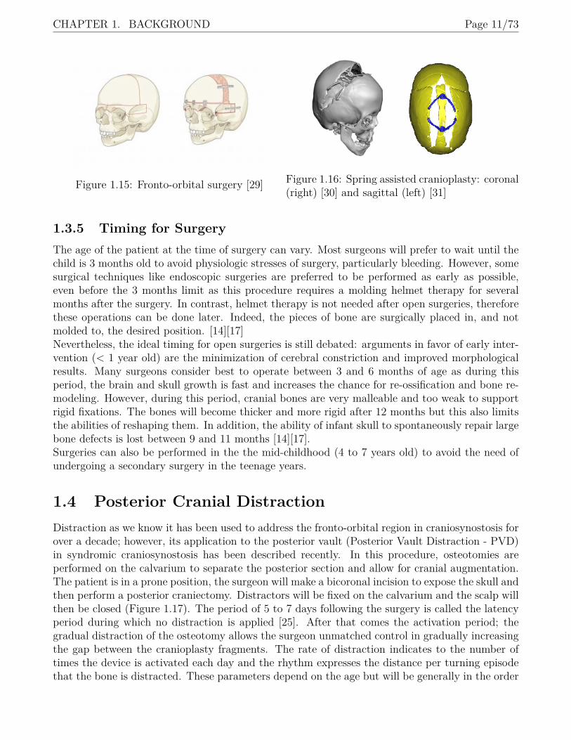
The procedure involves performing controlled cuts in the bones and using a device to graduallyseparate the bone fragments. Those fragments are then kept apart by the distractors over a periodof 1 to 3 months, allowing new bone to form. This process is called distraction osteogenesis 1.4.This type of procedure is usually recommended for babies of any age with a fused coronal suture[25]. For the fronto-orbital case, the reshaping process concentrates on the patient’s forehead andthe upper part of their eye sockets. After moving this part, creating space for the brain and eyesdevelopment, the surgeon fixes it with screws and plates that will be absorbed into the body overtime (Figure 1.15) [21]. This technique for posterior vault expansion will be further developed insection 1.4.
I Spring Assisted Cranioplasty (SAC)
More recently, craniofacial surgeons adopted elastic distractors, such as stainless steel springs,to reshape the skull. This technique is minimally invasive and appears to reduce morbidity andhospital stay [26]. However, potential drawbacks include the need for a second procedure forthe springs removal after 4 to 6 months [27] and the lack of published long-term follow-ups [28].Furthermore, the surgeon currently has very little control over the distance or rate at which bonesare separated from one another [17]. In this procedure, the patient is positioned in a sphinxposition (facing the table with a cushion to raise the upper body and the head) and dependingon the type of craniosynostosis, the surgeon will perform different surgical cuts, used to insertthe springs and allow for expansion. The springs are secured in place by means of notches at thedesired location (Figure 1.16). This technique will be further developed for the posterior vaultexpansion in section 1.5.
CHAPTER 1. BACKGROUND Page 11/73
Figure 1.15: Fronto-orbital surgery [29] Figure 1.16: Spring assisted cranioplasty: coronal(right) [30] and sagittal (left) [31]
1.3.5 Timing for SurgeryThe age of the patient at the time of surgery can vary. Most surgeons will prefer to wait until thechild is 3 months old to avoid physiologic stresses of surgery, particularly bleeding. However, somesurgical techniques like endoscopic surgeries are preferred to be performed as early as possible,even before the 3 months limit as this procedure requires a molding helmet therapy for severalmonths after the surgery. In contrast, helmet therapy is not needed after open surgeries, thereforethese operations can be done later. Indeed, the pieces of bone are surgically placed in, and notmolded to, the desired position. [14][17]Nevertheless, the ideal timing for open surgeries is still debated: arguments in favor of early inter-vention (< 1 year old) are the minimization of cerebral constriction and improved morphologicalresults. Many surgeons consider best to operate between 3 and 6 months of age as during thisperiod, the brain and skull growth is fast and increases the chance for re-ossification and bone re-modeling. However, during this period, cranial bones are very malleable and too weak to supportrigid fixations. The bones will become thicker and more rigid after 12 months but this also limitsthe abilities of reshaping them. In addition, the ability of infant skull to spontaneously repair largebone defects is lost between 9 and 11 months [14][17].Surgeries can also be performed in the the mid-childhood (4 to 7 years old) to avoid the need ofundergoing a secondary surgery in the teenage years.
1.4 Posterior Cranial DistractionDistraction as we know it has been used to address the fronto-orbital region in craniosynostosis forover a decade; however, its application to the posterior vault (Posterior Vault Distraction - PVD)in syndromic craniosynostosis has been described recently. In this procedure, osteotomies areperformed on the calvarium to separate the posterior section and allow for cranial augmentation.The patient is in a prone position, the surgeon will make a bicoronal incision to expose the skull andthen perform a posterior craniectomy. Distractors will be fixed on the calvarium and the scalp willthen be closed (Figure 1.17). The period of 5 to 7 days following the surgery is called the latencyperiod during which no distraction is applied [25]. After that comes the activation period; thegradual distraction of the osteotomy allows the surgeon unmatched control in gradually increasingthe gap between the cranioplasty fragments. The rate of distraction indicates to the number oftimes the device is activated each day and the rhythm expresses the distance per turning episodethat the bone is distracted. These parameters depend on the age but will be generally in the order

CHAPTER 1. BACKGROUND Page 12/73
Figure 1.17: Illustration of posterior vault distraction with internal distractors [29].
of half a millimeter to one millimeter by day. The duration of this activation period will thereforedepend on the distance estimated by the surgeon and the head shape desired (usually between 20to 30 days). Finally, after a consolidation period of 6 to 8 weeks with no activation, a procedureis required for the device removal. This time period will help to prevent relapse of the fragmentsback to their original positions [17]. Many types of distractors are available depending on themanufacturing company and anatomical area targeted. However, they are usually classified in twobroad categories: internal and external distractors. Internal distractors are placed beneath the skinwith only the turning mechanism sticking out. External distractors are fixed into the bone usingpins or screws, but the majority of the device is outside of the body [25]. While the first type ismore subtle, it requires a second surgery for the removal; external devices, though, are conspicuousbut can be removed in a clinical setting. For this procedure, PVD allows a significant expansionof the intracranial space and improvement in head shape. Indeed, the posterior vault distractionprovides a larger volume increase per millimeter of advancement than anterior expansion. Thistechnique also helps patients with the Chiari malformation, thanks to its decompressive effect [17].
1.5 Spring Assisted Posterior Vault Expansion (SAPVE)The first spring assisted craniofacial procedures were reported by Lauritzen et al. [32] in 1998. Thesprings were made in the operation room from stainless steel alloys available as wires of differentthicknesses. This kind of procedure was then introduced in January 2008 at GOSH after an 8months period of distractor design for use in scaphocephaly correction.In case of SAPVE, a preliminary set of CT images is performed to assess the underlying patientanatomy and perform 3D reconstruction of the patient’s skull. The timing for these preoperativeimages can vary according to patients, but usually does not exceed a year before the surgery.On the operation day, the patient will be put under general anaesthetics, his/her hair will beclipped just over the incision site and fixed out of the way. The surgeons will make an incisionfrom ear to ear, over the top of the head and expose the skull by pulling the skin downwards overthe back of the head. Next, they will perform an osteotomy behind the coronal sutures and movethe back portion of the skull backwards, leaving a small gap between both parts of the bone. Assprings are used to expand the posterior vault, they will be fixed to each side of the cut, intonotches provided for this purpose. The number of springs inserted is decided by the operatingsurgeons in order to give the best shape possible to the skull. As said before, this number usuallyvaries from 2 to 4 but can go up to 6 in some cases. After that, the skin is unfolded back over the

CHAPTER 1. BACKGROUND Page 13/73
incision and the surgeon will proceed to close it with stitches. One or two drainage tubes will beleft in place to collect any leaking fluid and will be removed a couple of days later. The patientwill be closely monitored at the hospital during around five days following the operation beforebeing able to go home if his/her recovery is on the right track [26].
Figure 1.18: Spring model used at GOSH [31].
Although this procedure is usually described as safer than others, a few risks remain. Thissurgery requires separating the skull bone from the dura, this process can cause brain injury orinternal bleeding which could lead to serious complications such as seizures or strokes. However,the overall risk of such major neurological event or death is below one per cent. Spring insertionalso carries some specific risks, such as failure or dislodgement of the springs [26].
A series of follow-up appointments will be planned, during which some additional medical im-ages could possibly be recorded. These are useful to track the kinematics of the spring openingor simply verify that they are still correctly in place. Usually, the first postoperative CT scan isdone a day or two after the surgery.
The timing of removal differs for each individual child but is usually around six months to ayear after insertion. This allows the bone to grow in between the springs, preventing the skull todeform again. Posterior vault expansion has already shown promising results for reducing increasedICP, especially in children with severe craniosynostosis. If pressure rises again later in life, theoperation can safely be repeated [26].
1.6 Springs MechanicsSprings were introduced at the Great Ormond Street Hospital in London, in 2008 for the correc-tion of scaphocephaly in sagittal craniosynostosis performed using spring devices. Those devicesare torsional springs made of stainless steel wire with a central loop and an initial opening of 60mm before implantation (Figure 1.18). These springs exist in three different models (S10, S12,S14) differing by their wire diameters (1.0, 1.2, 1.4 mm respectively) and stiffness (0.17, 0.39, 0.68N/mm respectively). They follow a Hookean behavior when compressed, meaning that the amountof compression that they underwent is directly proportional to the outwards force they exerted.A mechanical compression test was performed in order to observe the relation between force andopening distance for the different spring models at loading and unloading (Figure 1.19). The com-pressive force was applied on one tip of the springs placed vertically aiming at reducing the spacein between the 2 tips. The initial opening at resting conditions is 60 mm and they are crimped

CHAPTER 1. BACKGROUND Page 14/73
until an opening of 20 mm is reached and then back to 60 mm again. Springs are equipped withfootplates (those footplates will be placed in notches in the skull to secure the spring in place),here they are removed to test more easily (their stiffness is negligible). Thanks to those curves,it is possible to compute the spring stiffness K by measuring the slope of the linear fitting of thecurve (Example done for the S12 model on Figure 1.19) [31].
Figure 1.19: Force/opening curve for the different spring models [31].
In a previous study, a group of 60 patients who underwent spring cranioplasty for the treatmentof sagittal craniosynostosis was recruited. The surgery average age was 5.2 ± 0.9 months. Eachpatient was implanted with 2 springs for a duration of about 3 to 4 months [31].
Considering the spring combination per patient, 33 patients received two of the same springmodels implanted (S10-S10, S12-S12 or S14-S14). The remaining 27 had a combination of 2 dif-ferent spring models in the anterior and posterior positions, with no obvious trend for the positionof the stiffer spring. One could notice that patients with two S14 models were older (6.0 ± 0.7months) than those in the other groups (S10-S12: 4.8 ± 1.0 months, S12-12: 5.2 ± 1.0 monthsand S12-14: 5.2± 0.7 months), confirming that older patients generally received stiffer springs [31].
As we know, the stiffness of S10 springs is lower than the others, therefore, the force exertedat insertion and at the first follow-up is also lower than the force for S12 and S14 (same thing forS12 compared to S14). If insertion was day zero, the time of the first follow-up (FU1) was around1–2 days for 60 patients, whereas the second follow-up (FU2) happened after 6 to 59 days (mean:22 days) for 57 patients [31].The combined opening and force plots over time showed the progressive spring opening from in-sertion to removal, while spring forces decayed, with a statistical difference in opening and forcebetween each consecutive time point (Figure 1.21 and Table 1.20).

CHAPTER 1. BACKGROUND Page 15/73
Figure 1.20: Spring opening distance and force values at different time points [31].
Figure 1.21: Combined spring opening distance (left) and force (right) at insertion, FU1, FU2 andremoval [31]
1.6.1 Springs KinematicsThe spring kinematics was studied using the opening values at the 4 time points, from insertionto removal. It was assumed that the skull behaved as a viscoelastic material and that the springopening distances followed an exponential curve governed by a time constant τ [31]:
OP (t) = OPIO + (OPRO −OPIO).(1− e− tτ ) (1.1)
Where, OPIO is the opening at insertion and OPRO, the opening at removal.In an exponential rise, τ represents the time at which the analyzed data reaches (1 – 1/e) = 67%of its maximum value. Here, τ is therefore, the necessary time for the springs to reach 67% of itsmaximum opening i.e. 60 mm. The model fitting was carried out using the nonlinear least squaresmethod, implemented in Matlab (MathWorks). This time relaxation value was computed foreach patient and the normal probability distribution of the data was tested to obtain the averageand standard deviation of τ in the population [31].
To assess the timing of the springs kinematics, two properties of exponential rise have beentaken in account:
1. The exponential function reaches its plateau after 5τ
2. In a normal distribution (mean, µ and standard deviation, σ), Chebychev’s inequality statesthat 97.8% of the population is found within the interval [−∞, µ+ 2σ].

CHAPTER 1. BACKGROUND Page 16/73
Knowing that, it can be conclude that 97.8% of spring will reach the opening plateau after a time:T = 5(µτ + 2στ ).
After the model fitting for patients with sagittal craniosynostosis, the value of τ retrieved wasabout 1.16± 0.46 days meaning that the springs were extended at 67% of their maximal openingafter a little more than 1 day. Therefore, the population time T was calculated as 10 days (for98.7% of the springs to reach the opening plateau).Figure 1.22 depicts the comparison between the spring opening distance at 10 days (OPT ) and theopening distance measured on the operating table at removal (OPR), showing a good correlationand an absolute difference of 0.06%± 0.17% [31].
Figure 1.22: Bland-Altman plot of the comparison between the spring opening at removal (OPR)and the opening at 10 days (OPT ) [31].
1.7 Prediction of SAC: Finite Element Analysis
1.7.1 Aim of Finite Element Modelling for SACA number of studies have already been conducted on the correction of scaphocephaly caused bythe fusion of the sagittal suture. Like this project, those studies aim to predict the resulting headshape based on a patient-specific computational model. The final goal is to use this technique toperform prospective prediction of springs dynamics to inform surgical planning, distractor selectionand improve preoperative patient information [33].

CHAPTER 1. BACKGROUND Page 17/73
1.7.2 Segmentation From CT ScansThe preoperative CT scans retrieved for each patient were segmented in Simpleware to isolate theskull from soft tissues and to be prepared for the simulations.In the work by Breakey et al. [34], a population growth curve was created based on the bone surfaceof 24 unoperated sagittal craniosynostosis patients (age at CT scan: 4.0 ± 1.3 months). This curvewas used to rescale the CAD models in order to take the growth in between the preoperative CTand the surgery into consideration [33].The next step consists in making the osteotomies in Simpleware based on the real measurementsrecorded in theatre during surgery. In case of sagittal craniosynostosis correction, two osteotomiesare made parallel to the fused suture at a distance LAT extending from the coronal to the lambdoidsutures. Then the craniectomy of squared piece of bone is performed in order to insert the springs,one anteriorly and one posteriorly (Figure 1.23).All models are meshed identically using tetrahedral elements in Simpleware; the mesh densitywas selected depending on the convergence of the simulated spring extension and the computationtime [33].
Figure 1.23: Osteotomies and measurements recorded during surgery: A = distance between thecoronal suture and the anterior spring; P = distance between the coronal suture and the posteriorspring; LAT = dimension of the parasagittal osteotomy; OFD = occipitofrontal diameter; BPD =biparietal diameter [33]
1.7.3 Importing in AnsysThe skull geometry was then imported in Ansys Mechanical 17.2 as an external model linkedto a static structural analysis system.The base of the model was fully constrained to mimic the presence of the calvarial skull base.The springs were then inserted using the linear conditions implemented in Ansys to simulatedthe effect of implantation [33]. Data of bone and suture elastic and viscoelastic properties wereinitially retrieved from literature [35][36].
1.7.4 Results of the SimulationsIn case of sagittal craniosynostosis correction, the simulations were performed to observe thecomplete spring expansion over 10 days (Figure 1.24). Results have shown great shape matching

CHAPTER 1. BACKGROUND Page 18/73
between the simulated head shape and the CT scans. In the work of Borghi et al. [33], thecomparison was made in terms of surface distance patterns and surface error distribution. It hasbeen demonstrated that, for the population of the study, 80% of the error was below 2 mm. Themodel also managed to estimate the cranial index with a discrepancy of less than 2%.
Figure 1.24: a Preoperative model with spring inserted, b simulated expansion on-table, c atfollow-up 1, and d follow-up 2 for a representative patient [33].
1.8 Main Aims of the ThesisThe main goal of this thesis is to model the posterior vault expansion using finite element simula-tions. Those patient-specific models will be created based on preoperative computed tomographyimages. Currently, the PVE surgeries are performed according to the operating surgeon’s experi-ence and the dimension and position of osteotomies (bone cuts) are selected on-table as well as thetype, position and number of springs to be inserted. This method has led to complications andrevision rates of over 10% in GOSH centre since 2008. Therefore, the final objective is to developa three-dimensional finite element simulation platform that will be used by surgeons performingspring-assisted PVE procedures as a preoperative planning tool as well as a teaching and learningaid.

Chapter 2
Materials and Method
2.1 Patient SelectionThe population of this project was selected among the GOSH patients database who underwent aSAPVE, affected by Apert, Crouzon, Pfeiffer or Multi-sutural (no specific genetic diagnosis) syn-drome. The selection of the 14 patients was based on the availability of both pre- and postoperativeCT scans for each patient and the presence of visible springs in the postoperative reconstructions.The Table 2.1 below shows the list of patients recruited and their personal details.
Patients Agesurg. (Days)
Time(Days) Syndrome a
Preop CT-Surg Surg-Postop CTP1 193 55 162 Apert 239.1
P2 234 3 67 CranialDysraphism 157.9
P3 237 47 29 Apert 239.1P4 299 66 70 Multi-sutural 157.9P5 381 49 112 Crouzon 148.5P6 393 4 57 Apert 239.1P7 464 1 6 Pfeiffer 148.5P8 479 232 266 Multi-sutural 157.9P9 523 16 562 Crouzon 148.5P10 533 14 280 Crouzon 148.5P11 1075 32 144 Crouzon 148.5P12 1534 8 152 Multi-sutural 157.9P13 1992 10 86 Multi-sutural 157.9P14 2044 74 68 Multi-sutural 157.9
Table 2.1: Patients’ details constituting the population of this project
19

CHAPTER 2. MATERIALS AND METHOD Page 20/73
2.2 Pre-processing
2.2.1 SegmentationIn computer vision, image segmentation is the process of partitioning a digital image into multiplesegments (set of pixels). Medical image segmentation is the process of automatic or semi-automaticdetection of boundaries within a 2D or 3D image in view of assigning a label to every pixel of theimage so that pixels with the same label share certain characteristics. The goal of segmentation isto simplify and/or change the representation of an image into something that is more meaningfuland easier to analyze [37].The simplest method of image segmentation is called the thresholding method and is the one usedin this project. This method is based on a threshold value interval to turn a gray-scale image intoa binary image. The key of this method is to select those threshold values and this is what thissection will be describing [38].
Starting by importing the DICOM files, corresponding to the raw CT scan data, into SimplewareScanIP, the bone needs to be differentiated from the rest of the tissues to isolate the region ofinterest, which is the skull.At this stage, in order to get a better visual representation, a volume rendering preset can beadded to highlight a particular region. However, in our case this is not necessary as the skeletonis easily discernible from the other parts of the scan (Figure 2.1).
Figure 2.1: Raw CT-scan data viewed in Simpleware.
Then, as explained above, the soft tissues have to be removed by defining a threshold intervalin order to segment the skull away from the rest of the image.After creating a new mask, the values of the density threshold have to be determined to carryon the segmentation. To identify which range of values to use, the software offers a profile linecollaboration tool. The latter shows the density grey-scale values on a profile line on a chosenstudy slice. Once a clear slice has been selected, a line is drawn across a region that we know isbone (Figure 2.4). This will give the changes in density along that line and enable us to find thedensity interval of bone to enter in the threshold tool (Figure 2.2). This results in the isolationof all pixels contained within this interval. As can be seen on Figure 2.3, this includes the panelaround the child’s head and a part of his spine which are not needed for our application.

CHAPTER 2. MATERIALS AND METHOD Page 21/73
To clean the model and obtain only the skull part of the scan, the Flood Fill tool will be used tocreate one continuous model. By clicking on a pixel from the cranium, we are able to isolate itfrom the rest (Figures 2.5). Sometimes it can happen that the top of the spine remains after thisoperation; in this case, the Unpaint tool would be used to dissociate it from the skull and performFlood fill once again. The result for all 14 patients are depicted further in the report on the leftside of Tables 2.3 to 2.6.
Figure 2.2: Profile line resulting from the selec-tion in Figure 2.4. Figure 2.3: 3D result of threshold tool.
Figure 2.4: Selection of a bony area to determinethe threshold values.
Figure 2.5: Pixel selection to use the Flood Filltool on the blue region.
2.2.2 Volume ScalingTo compare the simulated model to the postoperative CTs, the time period and underlying growthbetween the surgery and the preoperative CTs images have to be taken into account. That is whythe model created from the preoperative CT has to be re-scaled considering this time to enable arelevant comparison.
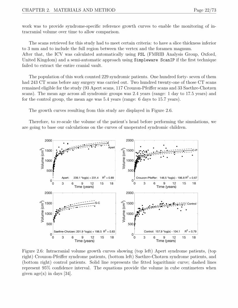
Breakey et al. published a study [34] on analyzing intracranial volume gain and tracking headcircumference growth in children with unoperated syndromic craniosynostosis. The goal of this
CHAPTER 2. MATERIALS AND METHOD Page 22/73
work was to provide syndrome-specific reference growth curves to enable the monitoring of in-tracranial volume over time to allow comparison.
The scans retrieved for this study had to meet certain criteria: to have a slice thickness inferiorto 3 mm and to include the full region between the vertex and the foramen magnum.After that, the ICV was calculated automatically using FSL (FMRIB Analysis Group, Oxford,United Kingdom) and a semi-automatic approach using Simpleware ScanIP if the first techniquefailed to extract the entire cranial vault.
The population of this work counted 229 syndromic patients. One hundred forty- seven of themhad 243 CT scans before any surgery was carried out. Two hundred twenty-one of those CT scansremained eligible for the study (93 Apert scans, 117 Crouzon-Pfeiffer scans and 33 Saethre-Chotzenscans). The mean age across all syndromic groups was 2.4 years (range: 1 day to 17.5 years) andfor the control group, the mean age was 5.4 years (range: 6 days to 15.7 years).
The growth curves resulting from this study are displayed in Figure 2.6.
Therefore, to re-scale the volume of the patient’s head before performing the simulations, weare going to base our calculations on the curves of unoperated syndromic children.
Figure 2.6: Intracranial volume growth curves showing (top left) Apert syndrome patients, (topright) Crouzon-Pfeiffer syndrome patients, (bottom left) Saethre-Chotzen syndrome patients, and(bottom right) control patients. Solid line represents the fitted logarithmic curve; dashed linesrepresent 95% confidence interval. The equations provide the volume in cube centimeters whengiven age(x) in days [34].
CHAPTER 2. MATERIALS AND METHOD Page 23/73
The Table 2.1 in Section 2.1 lists the patients details used in this project. In some cases thepre-operative CT was retrieved months before the surgery. Knowing the patient’s age on the op-eration day and the time in between surgery and the acquisition of the first CT, the age at CTcan easily be calculated. These values will be used to compute the multiplication factor which willmultiply the pre-operative volume from the first CT in order to obtain a good approximation ofthe volume on the surgery day.
The preoperative ICV values were retrieved from the previously introduced study of Breakeyet al. [34] since our patient selection is part of its population.Using the logarithmic curves from that same study, we are able to select the parameter defining thelogarithmic growth, a, according to the patient’s syndrome (Figure 2.6, Table 2.1). The equationfor ICV calculation in Apert’s patients is shown in Figure 2.6 (top left) and can be broken downas follows:
ICV = a× log(x) + b, (2.1)Where x is the age in days and b the base value for the specific syndrome.
To recalculate the ICV at the time of the surgery, b must be first adjusted to the patient specificvalue using the ICV of the pre-operative CT and the age at the CT acquisition (ageCT ):
badjusted = ICVCT − a× log(ageCT ) (2.2)The ICV on the day of the surgery (ICVsurg) is then obtained using the adjusted value badjusted,
and the age of the patient on the day the springs were inserted (agesurg). The equation 2.1 thereforebecomes:
ICVsurg = badjusted + a× log(agesurg) (2.3)Finally, the multiplication factor is obtained by:
Multiplication factor =(ICVsurgICVCT
) 13
(2.4)
The volume growths resulting from these calculation were on average in the range of [0.006; 3.5]%.All volumes and factors computed are presented in Table 2.2.
The Rescale tool in Simpleware allows to enter the percent of change in all directions, i.e. themultiplication factor.

CHAPTER 2. MATERIALS AND METHOD Page 24/73
Patient vpre (cm3) vsurg (cm3) Multiplication factor
P1 1081.82 1162.02 1.024124P2 896.07 898.11 1.000757P3 974.96 1027.81 1.017752P4 1538.92 1578.30 1.008458P5 1245.01 1265.45 1.005444P6 1583.09 1585.54 1.000515P7 1735.54 1735.86 1.000062P8 953.54 1058.12 1.035298P9 1268.56 1273.17 1.001211P10 1105.72 1109.67 1.001190P11 1264.21 1268.7 1.001182P12 1566.94 1567.77 1.000176P13 1686.13 1686.92 1.000157P14 1330.4 1336.22 1.001457
Table 2.2: Preoperative volumes on the CT and surgery days, and multiplication factor for eachpatient.
2.2.3 Replication of the Surgical CutsOnce the model was scaled, the osteotomies (surgical cuts) had to be replicated. To that purpose,a new mask was created in Simpleware by extracting the surface of the postoperative CT: thelatter had to heretofore be meticulously aligned with the preoperative scan in Meshmixer.
This alignment would allow the replication of the osteotomies on our model in concordancewith the real surgical cuts from the postoperative reconstruction. Those cuts can be of differentshapes (straight, L-shaped or more complex) depending on the final outcome desired. To be con-sistent with each model, the width of the osteotomies was fixed at a scale of 1 and the length of thenotches created at the springs locations was fixed at a scale of 5 with the same width. All theseoperations had been made using the 3D editing tool. To finalise the preparation of the model,a few more tools such as Smoothing filters, cavity fill and island removal were used to removedminor imperfections and cavities in order to simplify the surface of the model.To reduce the computation time as much as possible in the simulation part, a plane cut was madefor each model in the aim of removing complex elements that were not relevant for our analysissuch as the nose, teeth and mandible. However, the cut had to be made carefully so that the baseof the skull and the foramen magnum were preserved for the future intracranial volume evaluation.In certain cases, the fontanelles and/or bigger defects had been closed, still aiming at simplifyingthe model for the simulations.
By dragging the updated mask into the FE model tab, a new finite element model was created.The model configuration options could then be modified as desired; to generate a model dedicatedto the import in Ansys, the export type was set to Ansys workbench volume (solid/shells)(legacy).In the volume meshing tab, the coarseness of the mesh (ranging from -50 to 0 which representsa coarser to finer mesh) was chosen as well as the order of the elements; the software offered the

CHAPTER 2. MATERIALS AND METHOD Page 25/73
choice between 2 orders: linear and quadratic.A linear element or first order element will have nodes only at its corners while a second orderelement or quadratic element will have mid side nodes in addition to nodes at the corner.In the Node sets tab, the different node sets destined to apply the boundary conditions were de-termined. Two options were considered and will be developed in a further section.Once the model was setup, the full FE model was generated and exported in a .cdb files.
The results obtained after simplifications and the creation of the surgical cuts are compared tothe preoperative 3D reconstruction just after the segmentation in Tables 2.3 to 2.6.
Patient’s information Preoperative CT after segmentation Model ready for exportation
Patient 1Age at surg.: 6 monthsApert
Patient 2Age at surg.: 8 monthsCranial Dysraphism
Patient 3Age at surg.: 8 monthsApert
Table 2.3: Illustrations of the 3D models after the surgical cuts and simplifications

CHAPTER 2. MATERIALS AND METHOD Page 26/73
Patient’s information Preoperative CT after segmentation Model ready for exportation
Patient 4Age at surg.: 10 monthsMulti-sutural
Patient 5Age at surg.: 13 monthsCrouzon
Patient 6Age at surg.: 13 monthsApert
Patient 7Age at surg.: 15 monthsPfeiffer
Table 2.4: Illustrations of the 3D models after the surgical cuts and simplifications (continued)

CHAPTER 2. MATERIALS AND METHOD Page 27/73
Patient’s information Preoperative CT after segmentation Model ready for exportation
Patient 8Age at surg.: 16 monthsMulti-sutural
Patient 9Age at surg.: 17 monthsCrouzon
Patient 10Age at surg.: 18 monthsCrouzon
Patient 11Age at surg.: 2.9 yearsCrouzon
Table 2.5: Illustrations of the 3D models after the surgical cuts and simplifications (continued)

CHAPTER 2. MATERIALS AND METHOD Page 28/73
Patient’s information Preoperative CT after segmentation Model ready for exportation
Patient 12Age at surg.: 4.3 yearsMulti-sutural
Patient 13Age at surg.: 5.5 yearsMulti-sutural
Patient 14Age at surg.: 5.7 yearsMulti-sutural
Table 2.6: Illustrations of the 3D models after the surgical cuts and simplifications (continued)
2.2.4 Importing in Ansys Workbench 19 R1In Ansys workbench, a static structural analysis system was created and an external model wasadded as well. The .cdb files obtained previously was imported in this external model and theunits had to be checked to make sure the model was imported at the right scale i.e. millimeters.This external model will be used as geometry for the simulations, both systems can therefore belinked together.
2.2.5 Set up in Ansys MechanicalSince the models had already been automatically meshed in Simpleware, all that was left to dowas: define and place the springs and the boundary conditions.
For that, we began by adding Connections i.e. springs to the model. Each spring extremity(anterior and posterior) had to be defined using a Named Selection beforehand. Depending on thetype of springs needed, the stiffness and the preload i.e. free length, were defined. Three different

CHAPTER 2. MATERIALS AND METHOD Page 29/73
types of springs are used in GOSH; their mechanical properties are included in Table 2.7 andretrieved from the literature [31]. The reference and mobile body are represented by the anteriorand posterior part of the skull respectively. Therefore each side of the spring was applied by directattachment.
Spring Model Longitudinal Stiffness (N/mm) Free length (mm)S10 0.17 60.7S12 0.39 57.3S14 0.68 55.6
Table 2.7: Spring mechanical properties
In the Static Structural ribbon, the nodal displacement at the boundary conditions, defined asa named selection as well, was fixed in every directions to avoid rigid displacements.
Figure 2.7: Top and side view of the springs insertion in Patient 12
2.2.6 Choice of the Mesh: Mesh Dependency AnalysisTo determine the optimal meshing for our models, several size of elements were tested in a meshdependency analysis. For 5 patients (four of them with 2 springs and one with 4 springs), 10different meshes were analysed. Two factors were taken into account: the order and the size of theelements. As reported above, Simpleware allows the choice of the mesh coarseness in a the range-50 to 0 which represents the evolution from a coarser to finer mesh (i.e. the number of elementsincreases) and the choice between linear or quadratic elements.
Several graphs were grouped to represent the evolution of the total deformation in function ofthe number of elements and their order.
As can be observed in Figure 2.9, the cases with quadratic elements seems to converge faster,and to overall a larger deformation, than the linear ones. Simulations were solved for the 10 casesand helped in making the decision of which mesh to keep for the rest of the project, the choice wasbased on accuracy and time performance. At first glance, quadratic elements seem to be the bestchoice as the deformation doesn’t vary too much with the number of elements. However, whenthe model was simulated after spring insertion, the simulated model appeared to be deformed inan unrealistic way leading to larger deformation values (Figure 2.8). That problem did not occurwith linear elements. As a result, the following parts of the project will consider first order elements.

CHAPTER 2. MATERIALS AND METHOD Page 30/73
Figure 2.8: Comparison between simulations with linear elements (left) and quadratic elements(right) for patient 3.
Then came the choice of the appropriate coarseness. Only a few millimetres of difference wereobserved between the coarseness -30 and -10, however the finer mesh took a large amount of CPUtime to solve (10±2 hours). That’s why, to achieve a trade-off between accuracy and computationtime, the -20 coarseness was chosen and the efficiency of the model will be depicted in a furthersection.
Figure 2.9: Evolution of the total deformation in function of the number and order of the elements
2.2.7 Choice of Boundary ConditionsA set of boundary conditions had also to be determined. These conditions represent which partsof the skull were fixed in all directions during the simulations. Two possibilities were explored: the

CHAPTER 2. MATERIALS AND METHOD Page 31/73
entire skull base and the Foramen magnum only (Figures 2.11). Both had been tested by Nagasaoand al., 2011 [39].It is visible in the Figure 2.10, that the difference does not exceed 4 mm for the most extremecase (these data correspond to the deformation of linear elements of coarseness -30 and -20). Thisslight difference was considered negligible, especially for the finest mesh. Constraining the foramenmagnum was considered a better option since it allowed better consistency throughout the patientpopulation.
0 1 2 3 4 5 6
105
0
10
20
30
40
50
60
Figure 2.10: Evolution of the total deformation in function of the boundary conditions
Figure 2.11: Boundary conditions : Skull base fixed (Right) and Foramen magnum fixed (Left).
2.2.8 Material AssignmentThe mechanical properties of bone for the first batch of simulations were taken from a previouswork on FE modelling of sagittal craniosynostosis correction [35].

CHAPTER 2. MATERIALS AND METHOD Page 32/73
A new material had thus to be defined in the engineering data in Ansys: The calvarium was con-sidered as a viscoelastic material with Young’s Modulus of E = 1300 MPa and Poisson’s ratio ofn = 0.22 [35][36].
Young’s Modulus Poisson’s ratio Bulk modulus Shear modulus1300 MPa 0.22 773.81 MPa 532.79 MPa
Table 2.8: Elastic material properties of the skull
In mechanical solutions from Ansys, the viscoelastic behavior of the skull material is imple-mented through the use of Prony series. The shear modulus G, the Young’s modulus E and thePoisson’s ration ν are related by Eq.2.2.8 for isotropic and homogeneous materials:
G = E
2(1 + ν)
Instead of G being constant, it is represented by Prony series in viscoelasticity [40]:
G(t) = G0
[αG∞ +
∑αGi e
− tτi
]This equation mean that the shear modulus is represented by a decaying function of time t.
Therefore, we need to provide pairs of relative moduli αi and relaxation time τi, which representthe amount of stiffness lost at a given rate.
In our case, the material properties were first retrieved from literature [36] and optimized inthe work of Borghi et al. [33] resulting in the constants in Table 2.9.
Index i Relative moduli (i) Relaxation time (i) [s]i=1 0.73213 6720.4i=2 0.25208 40322
Table 2.9: Viscoelasticity properties.

Chapter 3
Result Analysis
3.1 SimulationsA curve fitting was done for patients with sagittal craniosynostosis [31] and the value of τ retrievedwas about 1.16 ± 0.46 days meaning that the springs were extended at 67% of their maximal open-ing after a little more than 1 day [33]. Therefore, the population time T was calculated as 10 days.A simulation over 10 days was run for the fourteen 3D models and the results of total deformationwere then exported as .stl file (Figure 3.1). These files were then aligned in Meshmixer to comparethe simulated end-of-expansion with the actual postoperative CT scan. The results of these com-parisons are depicted in Tables 3.2 to 3.5 below. However, in order to better observe the physicalexpansion, The Appendices contain a figure for each patient regrouping the comparison with thepreoperative CT as well.
Figure 3.1: a Pre-operative model with osteotomy and spring conditions, b,c,d simulated springexpansion over time for a representative patient.
From those tables, one can notice that, for the most part, the simulated model closely matchesthe postoperative CT scan. However, for a few patients (8, 9, 11, 13) it must be noted that theupper part of the occipital bone was cut during surgery to improve the final shape.The case of Patient 7 required further attention: the total simulation time was set to 6 daysinstead of 10 as the patient had his postoperative scan 6 days after the surgery and one can observethat the two reconstructions don’t match. Such observation hints that relaxation properties forthe calvarium of patients affected by syndromic craniosynostosis are different from those of thepublished population (patients affected by sagittal craniosynostosis). This result suggests that therelaxation time is longer for the considered population. For this reason, the spring kinematics willbe studied in a further section for the specific cases of patients who underwent a posterior vaultexpansion procedure.
33

CHAPTER 3. RESULT ANALYSIS Page 34/73
3.2 Intracranial VolumesThe prediction accuracy of the model was then tested in terms of ICV calculated in Meshmixer.First, the .stl files of the expanded model was exported from Ansys, it must be ensured that themodel is in true scale to have the correct expansion. This file was then imported in Meshmixer andre-scaled as Ansys usually exports files in meters. To do that, we used the Transformation tooland set the scale in every directions to 1000. Using the Selection tool, all cut and defect contourswere selected and deleted; the aim being to completely dissociate the inner and outer shells of theskull (Figure 3.2).After using the Separate Shell tool, only the inner one was kept and all the small islands remainingfrom the previous step were cleaned out. It could be noticed that the model was composed of twocolors: grey and stripped with light pink. These colors delimit the active work surface (grey) andthe inactive one (pink). At this stage, the active surface was defined as the inside of the innershell (Figure 3.2 (left)). To invert it, the entire shell was selected and we used the Flip Normaltool located in the Edit tab.Once this was done, the Fill and Bridge tools would be used to close the holes and the osteotomyof the model.Finally, the Figure 3.3 illustrates the final shape: its volume was calculated by the software withthe Stability tool in the Analysis tab. The volume obtained is basically equal to the volume of thebrain and can be compared to the ICV from the postoperative CT, computed in a previous study[30].
Figure 3.2: Outer shell of the skull once the defect contours have been removed (Left) and innershell of the skull (Right).
Figure 3.3: Front and side views of the final intracranial volume to evaluate.
The comparison of all the ICVs calculated in Meshmixer are depicted in a bar chart (Figure3.4). Once again, it is clear that the simulation of Patient 7 is not correctly estimated with avolume difference of about 479 cm3. In addition, we also noticed that the younger patients in

CHAPTER 3. RESULT ANALYSIS Page 35/73
general have greater differences; the latter could be explained by the fact that, for young patients,most of the other sutures are still opened and could therefore move differently. For our models,most of the sutures and defects were closed to simplify the meshing process and optimize thecomputation time during the simulations but it is something to keep in mind. Usually, it appearedthat with all the fontanelles and other sutures opened, the entire cranium would be slightly wider.However, these parts slowly ossify during the expansion process and therefore it was deemed anacceptable approximation to close them from the beginning.
Figure 3.4: Comparison of the ICV calculated for the simulated model and post-operative CT forthe 14 patients.
To analyse the agreement of our results, we carried out a Bland-Altman test. This is themost common method for comparing two measurements of the same variable, in our case, thepostoperative ICV and the ICV predicted by the simulation. The resulting graph is a scatter plotXY, in which the X-axis shows the mean of the two measurements, and the Y-axis, the differencebetween those measurements [41].
Figure 3.5: Bland-Altman plot of the whole population.

CHAPTER 3. RESULT ANALYSIS Page 36/73
In Figure 3.5, three horizontal lines are represented. The bias (solid line) is computed as themean of the values determined by one method minus the values determined by the other methodand equals to 17.3 cm3. Then the upper and lower limits of agreement (LOA) (dashed lines) arecalculated by using that bias and the standard deviation (SD) of the differences between the twomeasurements such that 95% of the data should lie within ±1.96 SD of the mean difference (bias).This corresponds to -315.8 and 350.4 cm3 for the lower and upper limit respectively.
This type of graph can then highlight anomalies, for example, if one method always gives toohigh results, then all points are above or below the zero line. If the points on the Bland–Altmanplot are scattered all over the graph, above and below zero, then it suggests that there is no con-sistent bias of one approach versus the other.
In our case, all data points are within the 95% confidence interval except one correspondingto Patient 7 as expected (below the lower LOA). If the differences within bias ± 1.96 SD arenot clinically important, the two methods may be used interchangeably. We’ll have to keep inmind that the simulated model ICVs were measured manually and therefore could contain smallmeasurement errors.
Figure 3.6: Correlation plot between the post-operative ICV and the simulated model ICV
Figure 3.6 shows, the correlation between measurements of the ICV from the postoperativeCT and from the simulated model. The correlation coefficient, r, measures the strength and thedirection of a linear relationship between two variables. Its value is always between -1 (no relation-ship) and +1 (perfect positive relationship). Here, r equals +0.85 meaning that the relationship isfairly strong and the positive sign indicates that when one variable increases, the other one tendsto increase as well [42].
Correlation coefficients have a probability, p-value, which shows the chances that the rela-tionship between the two variables is equal to zero (null hypotheses i.e no relationship). Strongcorrelations have low p-values because the chance that they have no relationship is very low. In thiscase, the p-value is equal to 0.0002 which confirms that the correlation is statistically significant[42].

CHAPTER 3. RESULT ANALYSIS Page 37/73
3.3 Cranial IndexThe cephalic index or cranial index is the ratio of the maximum width of the head multiplied by100 and divided by its maximum length. This ratio is the criterion used to classify the patient’shead shape.The indices are categorized in 3 main groups [43]: dolichocephalic or ’long-headed’ below 75%,mesocephalic or ’medium-headed’ between 75 and 83% and brachycephalic or ’short-headed’ above83%. This index was calculated in Meshmixer using the Units & Dimensions tool in the Analysistab. This tool provides the width, length and height of the skull. It must be noted that for arelevant comparison with the CI of the postoperative CT, the latter has to be previously alignedwith the model predicted by the simulation.
Simulated model Postoperative CTPatient Syndrome Width Length CI (%) Width Length CI (%) |Diff CI|
1 Apert 140.4 159.1 88.2 153.6 158.5 96.9 8.62 Cranial Dys. 131.5 141.9 92.7 146.9 143.7 102.2 9.63 Apert 128.7 136.8 94.1 131.3 135.2 97.1 3.04 Multi-sutural 153.4 168.2 91.2 155.8 168.9 92.2 1.05 Crouzon 130.2 158.0 82.4 140.3 161.6 86.8 4.46 Apert 141.8 170.3 83.3 146.7 166.0 88.4 5.17 Pfeiffer 156.2 164.8 94.8 155.9 138.4 112.6 18.18 Multi-sutural 125.9 156.6 80.4 131.0 157.6 83.1 2.79 Crouzon 121.1 182.0 66.5 128.4 176.1 72.9 6.410 Crouzon 136.4 150.8 90.5 135.2 156.4 86.4 4.011 Crouzon 121.5 180.1 67.5 126.9 183.0 69.3 1.812 Multi-sutural 133.4 176.2 75.7 141.1 175.0 80.6 4.913 Multi-sutural 145.1 188.4 77.0 150.3 188.8 79.6 2.614 Multi-sutural 119.8 162.4 73.8 131.0 161.4 81.2 7.4
Table 3.1: Dimensions of the skull in millimeters and cranial index computed from these measure-ments for the simulated models and postoperative CTs.
Based on the postoperative CI and the indices recovered from literature [43], the population ofthe study can be classified as 2 dolichocephalics, 4 mesocephalics and 8 brachycephalics.By looking at the last column of Table 3.1 containing the difference between the CI computed forthe postoperative CTs and the simulated models, it is possible to observe that difference betweencomputed and measured CI ranges up to 8-10 %. Through a closer inspection, it is noticeablehow the predicted length is very close to the measured one while the predicted width is around10mm lower than that measured on the post-op 3D models. This may due to the presence ofcranioplasty springs, which add width and render such measurements less reliable (Figure 3.7).The most extreme value difference is 18% corresponding to Patient 7, who had the smallest timeperiod before his follow-up CT. The next chapter will consist in trying to optimize the materialproperties to fix these differences.

CHAPTER 3. RESULT ANALYSIS Page 38/73
Figure 3.7: Cranioplasty springs viewed from the front and the back in the postoperative CTs ofPatient 14 and 9 respectively.
Patient’s information Transverse plane cut sagittal plane cut
Patient 1Time surg. - CT: 162 daysCrouzon
Patient 2Time surg. - CT: 67 daysCrouzon
Patient 3Time surg. - CT: 29 daysCrouzon
Table 3.2: Illustrations of the comparison between the simulated models (dark grey) and thepostoperative CT scan (light grey)

CHAPTER 3. RESULT ANALYSIS Page 39/73
Patient’s information Transverse plane cut sagittal plane cut
Patient 4Time surg. - CT: 70 daysMulti-sutural
Patient 5Time surg. - CT: 112 daysCrouzon
Patient 6Time surg. - CT: 57 daysCrouzon
Patient 7Time surg. - CT: 6 daysPfeiffer
Table 3.3: Illustrations of the comparison between the simulated models (dark grey) and thepostoperative CT scan (light grey) (continued)

CHAPTER 3. RESULT ANALYSIS Page 40/73
Patient’s information Transverse plane cut sagittal plane cut
Patient 8Time surg. - CT: 266 daysMulti-sutural
Patient 9Time surg. - CT: 562 daysCrouzon
Patient 10Time surg. - CT: 280 daysCrouzon
Patient 11Time surg. - CT: 144 daysCrouzon
Table 3.4: Illustrations of the comparison between the simulated models (dark grey) and thepostoperative CT scan (light grey) (continued)

CHAPTER 3. RESULT ANALYSIS Page 41/73
Patient’s information Transverse plane cut sagittal plane cut
Patient 12Time surg. - CT: 152 daysMulti-sutural
Patient 13Time surg. - CT: 86 daysCrouzon
Patient 14Time surg. - CT: 68 daysCrouzon
Table 3.5: Illustrations of the comparison between the simulated models (dark grey) and thepostoperative CT scan (light grey) (continued)

Chapter 4
Optimization : Spring Kinematics
4.1 Methods
4.1.1 Patient ListThis part of the study includes 50 patients who had received a posterior vault expansion operationat Great Ormond Street Hospital between 2008 and 2016. The surgeries were performed by thecraniofacial team under the lead clinicians Prof. David Dunaway and Mr. Owase Jeelani.The list was limited to patients with 2 springs and an ”hinged” PVE (in opposition to the ”flap”PVE where a total craniectomy of the back of the skull is done).
4.1.2 Data collection for PatientsThis part of the project required the use of a specific computer which can access the GOSHdatabase containing every patient’s available imaging and personal data.
For all 50 patients, the following information was collected:
• Patient number, depending on when they entered the study.
• Date of birth,
• Date of PVE procedure,
• Age at surgery was then calculated by subtracting the date of birth and the date of theoperation,
• Number of postoperative follow-up images
4.1.3 MeasurementsThe spring opening measurements were taken manually for all patients at each postoperative follow-up to observe their extension over time. The amount of follow-ups and on-table measurements wereunfortunately way smaller than for the previous studies on the sagittal craniosynostosis patientsand a total of 80 X-ray images were collected. Patients who received a second PVE operation wereexcluded.
42

CHAPTER 4. OPTIMIZATION : SPRING KINEMATICS Page 43/73
Figure 4.1: X-ray image of Patient 4 implanted with 2 lateral springs.
4.1.4 Measurement MethodsSince the measurements were taken from the database on two-dimensional images, we had to takeinto account the image projection and the curvature of the springs while measuring the distortedsprings. The only way of being completely accurate is taking measurements in the operating room.Those data were not recorded for the PVE patients and therefore two approaches were consideredto measure the springs opening (OP) from the available follow-up x-rays.
Method 1: Thales Theorem
Knowing that the real value of the ring diameter is 10 mm (Figure 4.2), the spring shape wasapproximated to a triangle and, by making sure to take measurements parallel to each other, weused the Thales theorem to retrieve an approximation of the real measurements of the distortedsprings. From the theorem, we obtain the equation:
DR
DF
= nRnF
(4.1)
Where DF is the real distance between the feet of the spring, DR is the real diameter of thering = 10 mm, nF and nR are the corresponding measurements on the distorted image (Figure4.2). Therefore,
DF = 10× nFnR
(4.2)
Figure 4.2: Modelisation of a distorted spring (left) and a straight one (right).

CHAPTER 4. OPTIMIZATION : SPRING KINEMATICS Page 44/73
Method 2: Phantom Measurements [44]
The second approach required a few more values and the mathematical models is presented below.First, the non-distorted angle α′ value is computed,
α′ = 2 arctan(A1
B1tan α2
)(4.3)
with α being the opening angle, A1 is the vertical length of the ring and B1, the horizontal lengthof the ring (Figure 4.3).
The second formula takes this α′ and uses the length of the spring arms L = 37 mm (obtainedthrough the Pythagorean theorem), to calculate the non-distorted spring opening OP :
OP = 2L sin(α′
2
)(4.4)
Figure 4.3: Schematic of the spring variables used in the Phantom measurements method.
Results of Both Methods
Both methods were applied to the 160 springs and all measurements were recorded in an Excelspread sheet.Before looking at the results, it can be stated that the second method was very difficult to applyto each and every spring. Staying consistent in the measurement of the angle was especially chal-lenging as some of the spring legs were bent on the image.
Now looking at Figures 4.4 and 4.5, the measurements obtained with the first method appearless dispersed and a larger portion of them belong to a realistic opening interval. Indeed, whenthe springs are placed during the procedure, their legs are crimped to an opening of about 20mm and a fully opened spring reached an opening of 60 mm. In contrast, adjusted measurementsobtained with the second method largely exceeded this interval as 11 points were above 60 mmand 22 points below 20 mm.We can conclude that errors were introduced in the measurement adjustments with the secondmethod and as a result, the first one was chosen to continue the kinematic analysis.

CHAPTER 4. OPTIMIZATION : SPRING KINEMATICS Page 45/73
Figure 4.4: Adjusted measurements of both springs for the 80 images over time with the Thalestheorem.
Figure 4.5: Adjusted measurements of both springs for the 80 images over time with the Phantommeasurements.

CHAPTER 4. OPTIMIZATION : SPRING KINEMATICS Page 46/73
4.2 Data AnalysisThe aim of this section is to create the line of best fit of Figure 4.4 in order to assess and quantifythe spring opening kinematics relative to PVE procedures.
4.2.1 Classification of the dataThe spring opening data was simplified by taking into account only the average measurement ofthe two spring for each patient. The measurements were than divided in 4 groups representing thefollow-up (FU) images at different points in time:
• FU1 = [1-2] days, mean = 1.5 ± 0.5
• FU2 = [3-30] days, mean = 20.4 ± 10.5
• FU3 = [41-73] days, mean = 52.7 ± 11.8
• FU4 = [106-308] days, mean = 206.3 ± 65.1
For each group, the average opening and standard deviation were calculated, see Table 4.1 andillustrated in Figure 4.6.
FU1 FU2 FU3 FU4Average OP [mm] 32.6 40.6 50.2 49.1
SD [mm] 4.4 9.9 4.8 5.5
Table 4.1: Average opening and standard deviation calculated over time.
Figure 4.6: Average opening and standard deviation represented by follow-up.

CHAPTER 4. OPTIMIZATION : SPRING KINEMATICS Page 47/73
4.2.2 Outliers DeterminationSome outliers were removed from the graph to try and reach the best and most realistic approxi-mation.Outliers are defined as date values that differ greatly from the majority of the data set. Theapproach used is the Interquartile Range. It is based on the first (Q1) and the third (Q3) quartileof the the measurement data. Those are easily computed with the Quartile operation in Exceland the Interquartile Range (IQR) is therefore the difference between these two calculations. Theoutliers were defined as those data points outside the range [Q1-1.5IQR, Q3+1.5IQR] [45].
In our case, the results obtained are listed in Table 4.2. In the end, two outliers were rejectedfrom the group FU1 as their values were higher than 41.86 millimeters.
FU1 FU2 FU3 FU4Q1 29.9 34.1 46.3 45.4Q3 34.7 45.6 53.1 53.1IQR 4.8 11.5 6.8 7.6Lower Limit 22.8 16.7 36.1 34.1Upper Limit 41.9 62.9 63.3 64.4
Table 4.2: Computation data for outliers determination.
4.2.3 Mathematical ModelTo create the line of best fit for our scatter plot, the curve fitting tool of Matlab was used.This fitting was performed using the equation of an exponential rise (Eq. 4.5)[31] following anon-linear least squares method and the Trust-region algorithm. The robustness was chosen asLeast Absolute Residuals (LAR); This method finds a curve that minimizes the absolute differenceof the residuals, rather than the squared differences. Therefore, extreme values have less influenceon the fit [46].
OP (t) = OP0 + (OP∞ −OP0)× (1− e−tτ ) (4.5)
Where,
• OP0 is the initial spring opening,
• OP∞ is the maximal opening which, in this case, is the opening at the last follow-up i.e. 49.1mm (Table 4.1).
• τ is the time constant of the exponential (after a time equal to τ , the exponential rise hasreached 67% of its maximum).

CHAPTER 4. OPTIMIZATION : SPRING KINEMATICS Page 48/73
4.2.4 Curve Fitting ResultsThe result of curve fitting are presented with a 95% confidence interval in Table 4.3 and illustratedin Figure 4.7.
General model OP0 [mm] τ [days]31.37 (30.84, 31.90) 21.21 (17.85, 24.58)
Table 4.3: Results for the general model.
Goodness of fit R-squared RMSE0.9749 1.574
Table 4.4: Goodness of fit.
Figure 4.7: Fitting of the spring expansion scatter plot by the exponential model.
The values in Table 4.4 express that the fitting is actually of good quality as the R-squaredvalue is very close to 1 and the Root Mean Squared Error (RMSE) is relatively small. An R-squarevalue of 0.9749 means that the fit explains 97.49% of the total data variation about the average;it is the square of the correlation between the response values and the predicted response values [47].
Previously it was said that to assess the timing of the spring kinematics, two properties ofexponential rise have been taken into account [31]:
1. The exponential function reaches its plateau after 5τ
2. In a normal distribution (mean, µ and standard deviation, σ), according the Chebychev’sinequality, 97.8% of the population is found within the interval [−∞, µ+ 2σ].

CHAPTER 4. OPTIMIZATION : SPRING KINEMATICS Page 49/73
Knowing that, it can be concluded that 97.8% of spring will reach the opening plateau after atime: T = 5(µτ + 2στ ).
However, contrary to the spring kinematics of sagittal craniosynostosis correction, this value oftime relaxation τ was not computed for each patient individually because of the lack of follow-upinformation per patient. In our case, the value of τ was computed over the whole population toexploit at best the data available.
Therefore, with a time constant of 21.21 days, we can expect the springs to be fully extendedafter about 5τ , which represents 106 days.By looking at the curve fitting results, one can deduce that over 60 days, the expansion hasalready reached over 98% of its final opening. We will thus be looking at the patients having apostoperative follow-up under 60 days to see if the optimization of our model can be validated.

Chapter 5
Effect of Kinematics Optimization
Three patients of the study had a time period between the procedure and the CT, lower than 60days: Patients 3, 6 and 7 with 29, 57 and 6 days respectively.For this new set of simulations, the constants relative to the bone, previously retrieved fromliterature [33] (see Section 2.2.8), were thus divided by 1.1 (corresponding to the time constant forthe sagittal craniosynostosis case) and multiplied by 21.21 [days] (time constant arising from thekinematics optimization). The relative moduli remained unchanged. The viscoelastic propertiesof the skull therefore became:
Index i Relative moduli (i) Relaxation time (i) [s]i=1 0.73213 1.296× 10⁵
i=2 0.25208 7.774× 10⁵
Table 5.1: Updated viscoelastic properties of the skull.
5.1 SimulationsFrom a visual inspection, it is visible from Table 5.2, that the use of the new material parametersallow for dramatic improvement in the simulation of spring expansion. The table presents a sagittaland a transverse plane cuts showing that the predictions match the postoperative CTs very closely.The mismatch observable on the top of the skull is due to surgical repositioning of the top partof the occipital bone, with the aim of further improving the overall appearance. Such manualrepositioning wasn’t taken into account in the numerical prediction.
50

CHAPTER 5. EFFECT OF KINEMATICS OPTIMIZATION Page 51/73
Patient’s information Sagittal plane Transverse plane
Patient 3Time surg. - CT: 29 daysCrouzon
Patient 6Time surg. - CT: 57 daysCrouzon
Patient 7Time surg. - CT: 6 daysPfeiffer
Table 5.2: Illustration of the comparison between the simulated models (dark grey) and the post-operative CT scans (light grey) with the optimized kinematics (green).
5.2 Intracranial VolumeFigure 5.1 shows the variation of the intracranial volume before and after the optimization com-pared to the postoperative one. One can observed that the difference between the simulated andthe postoperative model is decreased dramatically for Patient 7.For the two other cases, a small but evident improvement is present. The error compared to thepostoperative 3D image for each patient is very small and can be neglected. Indeed, Patient 3 hadan error of about 2% of the postoperative ICV, Patient 6 had an error inferior to 5% and 2% aswell for Patient 7.

CHAPTER 5. EFFECT OF KINEMATICS OPTIMIZATION Page 52/73
Figure 5.1: Bar graph illustrating the comparison between the ICV of the simulated models andpostoperative CTs.
Once again, the results were analysed using a Bland-Altman plot (Figure 5.2) and a correlationplot (Figure 5.3). The first figure shows that the 95% confidence interval has been narrowed downand the majority of the data points are close to the average line meaning that the model predictsthe volumes correctly.
Figure 5.2: Bland-Altman plot including the optimized models
The correlation plot displays an even stronger correlation between the two measurements witha correlation coefficient r = +0.92 and a p-value of 2.3× 10⁻⁶.
These results allow us to validate the model as a good prediction tool in terms of intracranialvolume.

CHAPTER 5. EFFECT OF KINEMATICS OPTIMIZATION Page 53/73
Figure 5.3: Correlation plot between the post-operative ICVs and the simulated model ICVsoptimized
5.3 Cranial IndexFinally, by looking at Table 5.3, one can see that this optimization also improves the estimation ofthe cranial index by reducing the value differences with the postoperative CTs. This means thatthe ratio between the width and the length of the patient’s head is, in fact, closer to reality.
Simulated model Postoperative CTPatient Syndrome Width Length CI [%] Width Length CI [%] | Diff CI|
3 Apert 127.7 132.9 96.1 131.3 135.2 97.1 1.06 Apert 146.6 167.9 87.3 146.7 165.9 88.4 1.97 Pfeiffer 154.4 134.5 114.8 155.9 138.4 112.6 2.2
Table 5.3: Dimensions of the skull in millimeters and cranial index computed from these measure-ments for the simulated models and postoperative CTs after optimization.
5.4 DiscussionA major limitation of this work was the use of the same Young’s modulus (1300 MPa) for thewhole population, having an age range from 5 months to 5.5 years. Our choice was based on theaverage age of 2 years. It is well known that the skull stiffness varies when the baby grows up,going from soft in the early stages to stiff after a few years. It is well-known that the skull stiffnessfor our younger patients is likely to be less than the chosen value, however this would provide amarginal improvement to the model. Furthermore, literature data on calvarial stiffness is relativeto normal subjects [48], therefore the mechanical properties of patients affected by syndromiccraniosynostosis is - to date - unknown.

Chapter 6
Future Works: Analysis of Fracture dueto Springs Insertion
It appeared that some patients’ CTs scans (Figure 6.1) exhibited some cracking at the end ofthe osteotomy, where the forces were concentrated during the expansion process. Therefore, wewondered if those cracks would affect the final volume of the head and decided to add them inour models to see if they could be reproduced in simulations as this is something interesting to beable to control. Due to limited time and resources, the simulations were performed with unreal-istic parameters but future developments will aim at ensuring simulation convergence in realisticconditions.
Figure 6.1: Parts of the cracking noticed in patients scans, hereby for Patient 13.
6.1 Basics of Fracture MechanicsThe fracture of a material involves a crack of a certain length which increases upon loading. Thestudy of fracture mechanics is about understanding when a crack becomes critical i.e. when itreaches a sufficiently long length that the crack propagation goes from being stable to unstable.The latter will occur once the stress intensity factor (SIF) K exceeds the material’s fracture tough-ness [49].We can describe fracture mechanics using the equation below:
K = Y σ√πa
54

CHAPTER 6. FUTURE WORKS: ANALYSIS OF FRACTURE DUE TO SPRINGSINSERTION Page 55/73
Where K is the Stress intensity factor [ksi√in] or [MPa
√m], Y is a geometric factor being a
function of the sample size and the size of the crack. σ is the stress applied and a, the crack length.
There are three ways of applying a force to enable a crack to propagate (Figure 6.2) [50]:
• Mode I is an opening mode where the force is perpendicular to the crack faces,
• Mode II is a sliding mode where crack faces slide on each other and the forces are parallel tothe crack faces,
• Mode III is a shearing mode that involves a shear stress sliding the crack faces in the directionperpendicular to the primary crack direction.
A crack can be loaded in one mode exclusively, or it can be loaded in some combination of modes.
Figure 6.2: The three fracture modes [50].
6.2 Method
6.2.1 Crack Simulation Methods in Ansys Workbench 19 R1For this part of the project, a recent Ansys feature was used: the Separating Morphing andAdaptative Remeshing Technology (SMART) crack growth, able to automatically remesh a 3Dmodel during a simulation according to mesh propagation.There are 2 fracture simulation methods available in the software and they rely on two differentmodels [51] :
• The Cohesive Zone Modeling (CZM), used for simulating the debonding between two surfacesattached adhesively. The delamination occurs when a force is applied but cannot grow beyondthe interface . This method will not be the first choice for simulating the crack growth inthe bulk of a material [51].
• The eXtended Finite Element Method (XFEM), used for internal crack calculations. Thismethod eliminates the need of remeshing the crack tip regions. Instead, it splits the ele-ments in the zone to create a finer mesh without remeshing. However, this process is verycomputationally expensive and slow down the whole simulation [51].
In the case of SMART crack growth and unlike XFEM, the splitting area can be scaled up tolarger projects because remeshing is limited to a small region around the crack tip at each iteration.[51]

CHAPTER 6. FUTURE WORKS: ANALYSIS OF FRACTURE DUE TO SPRINGSINSERTION Page 56/73
6.2.2 Preparation in Simpleware: Creation of a Non-Uniform RationalBasis Spline (NURBS) Model
The model without osteotomy was prepared in Simpleware, every defect was smoothed and allthe complex parts at the base of skull were be removed. Using the smoothing filters, the modelwas simplified as much as possible. The NURBS model was then created to later be importedin Solidworks. This technique was used to allow a very smooth surface and sharp cuts, whichwere not achievable with the usual method, in order to reduce the complexity and optimize thecomputation time in the simulation process. Once the full model generated, the geometry wasdivided in hopefully uniform patches. The process can be time consuming while trying to get asurface very smooth. The model was finally exported in a .igs files.
6.2.3 Replication of the Osteotomy in SolidworksThe file previously saved was imported in the software, it can then be modified by making cutssimilar to the preoperative model used in previous simulations. For each part of the osteotomy, anew plane was defined in order to try and keep the cut as perpendicular to the surface as possible.This step is very important for the set-up of the crack in Ansys. Osteotomies were recreated fromscratch and several iterations were used to ensure the bony cuts were as close to the original aspossible. It was also necessary to create a sharp notch at the extremity of the osteotomy. Thegeometry was then saved as a .SLPRDT file.
Figure 6.3: Model with osteotomy before simulation (left) and model recreated in Solidworks(right).
6.2.4 Set-up in Ansys MechanicalA static structural system was created with the imported geometry. For these simulations, it wasdeemed appropriate to use the sagittal plane of symmetry of the skull to considerably reduce thecomputation time. To achieve this, the geometry was opened in Ansys Design Modeler; up inthe Tool tab, the symmetry tool was selected and the plane YZ was defined as the symmetry plane.
In Ansys Mechanical, the notch position had to be defined and the crack direction set up. Forthat, a new coordinate system was created and placed on the front edge of the notch. One axishad to be pointing forward to indicate the crack propagation direction (x), another axis normalto the notch’s edge i.e. the crack opening direction (y) and the last one, aligned with the edge(Figure 6.4 left).

CHAPTER 6. FUTURE WORKS: ANALYSIS OF FRACTURE DUE TO SPRINGSINSERTION Page 57/73
Figure 6.4: Set-up of the crack with the position of the coordinate system and the regions selected.
For the mesh, the method selected was the Patch conforming method using tetrahedrons ele-ments of size 2 mm. Then using the Sizing tool, a sphere of influence of 6 mm of radius around thenotch edge was created and centered on the coordinate system previously defined. The elementsinside this sphere had a size of 0.08 mm (Figure 6.5).
Then, from the Command ribbon, the option for Fracture was chosen. Further options forintroducing a crack were: Arbitrary Crack; Semi-Elliptical Crack and Pre-Meshed Crack. Here aPre-meshed Crack had to be defined. To do that, three new named selections were created: crackon the edge of the notch, top on the superior face of the notch and bottom on the inferior face(Figure 6.4 right). This time the worksheet method was selected as each of these regions had tobe associated to a node set for use in the analysis. The table was filled similarly to Figure 6.6depending on the selection type.
Figure 6.5: Premeshed crack with a finer mesh delimited by the sphere of influence
Within the Pre-Meshed Crack object, the Node sets created previously were allocated to thecrack front, and the top and bottom faces. The crack coordinate system was referenced and thenumber of solution contours was then set to 4. These contours are the “loops” through the mesharound the crack tip used to evaluate the Stress Intensity Factor by integrating the crack tip regionstrain energy.

CHAPTER 6. FUTURE WORKS: ANALYSIS OF FRACTURE DUE TO SPRINGSINSERTION Page 58/73
Figure 6.6: Worksheet used to convert the named selections into mesh nodes.
Again in the Fracture menu ribbon, three methods were available to model the crack frontand its growth: Interface Delamination, Contact Debonding and SMART Crack Growth that waschosen for the rest of the simulation. The Pre-Meshed crack object was selected, the option tocarry out a Static analysis was chosen and the Critical Fracture Toughness was defined. The StressIntensity Factor method was selected in this case meaning that the crack would propagate whenthe calculated SIF, K, exceeded the fracture toughness Kc. This calculation was done along thedistributed crack front, and the distribution of the SIF would control the adapting crack frontshape.
The base of the skull and the anterior symmetry plane were defined as fixed supports and onespring is inserted in the notch provided for this purpose. The spring was defined in the same wayas in the previous simulations with a stiffness of 1N/mm.The main fracture mechanism in this model was the crack tensile opening Mode 1, which calculatesK1. Finally, a crack extension probe was added to the solution to monitor the crack growth andproduced an XY plot.
6.3 ResultsSprings were placed one by one and then both at the same time to observe the differences incrack extension. Their individual stiffness was fixed to 1N/mm and their relaxation constantswere arbitrarily chosen after trying, to no avail, the ones used in previous chapters. This failurewas suspected to be due to a lack of computing power and/or resources in Ansys.
The results obtained still provide an interesting comparison in total deformation and crackextension for each spring placement.
Figure 6.7: Total deformation of the 3 different configurations: spring on the side (left), spring onthe top (middle), both springs (right)

CHAPTER 6. FUTURE WORKS: ANALYSIS OF FRACTURE DUE TO SPRINGSINSERTION Page 59/73
The maximal deformations are depicted in Figure 6.7: 11.4 mm (left), 15.3 mm (middle) and23.6 mm (right). It appeared indeed that larger deformations happened when the force was appliedon the superior part of the skull.These numbers were obtained after 1 day and a time step of 3600 seconds as this was the maximalsimulation time that could be reached with our resources. Ideally, the simulation should have beenrun over 10 days to observe if the crack allowed a closer approach to the actual deformation of thepostoperative images.
Figure 6.8 shows the propagation of the cracks in each configuration from the inside and theoutside; the top spring gave a slightly straighter crack compared to the side spring crack whichwas more curved. It could also be noticed that the crack propagated with an angle as it followeda downward path viewed from inside and an upward path viewed from outside.It was still early in the propagation process to state confidently that the behavior was the samethan in the postoperative scan but the downward path in the inside is promising.
Figure 6.8: Inner (right) and outer (left) views for each configuration.

CHAPTER 6. FUTURE WORKS: ANALYSIS OF FRACTURE DUE TO SPRINGSINSERTION Page 60/73
Finally, the extension lines were not strongly impacted by the placement of the springs. Forall configurations, the fracture occurred at the same time and followed a similar course. It couldbe observed that when the two springs were involved, the fracture propagated quicker and furtherduring the whole simulation time. This was however not a significant difference at this early stagesince the scale was really small but it could show greater distinction after several days. Next tothat, the extensions of the simulation for the top and side spring separately are almost completelyoverlapping.
Figure 6.9: Crack propagation for each configuration
Figure 6.10: Variation of the stress intensity factor across the crack edge

CHAPTER 6. FUTURE WORKS: ANALYSIS OF FRACTURE DUE TO SPRINGSINSERTION Page 61/73
6.4 LimitationsThe longest simulation which was finalised was over a day (86400 s, CPU time = 7 hours).It was noticed that, although the software computed the first apparition of the crack in a consistentway, the rest of the crack extension is strongly affected by the time-step adopted.Furthermore, it appeared that fracture simulations in bent surfaces proved more difficult to con-verge. This is one of the reasons the fracture was only simulated over a day. In future, extracomputational power will be needed to extend the simulation and allow for validation of the re-sults. Our current achievements look - however - very promising.

Conclusion
The aim of this master thesis was to create a numerical model of spring assisted posterior vaultexpansion using finite element method based on pre- and postoperative images. Such models hadalready been created for sagittal craniosynostosis, therefore a starting point on spring kinematicswas available. The ultimate goal was to be able to predict the post-operative shape of the skullbased on surgical parameters (osteotomy location, choice of distractors) and time frame of postop-erative assessment. Such model would constitute an invaluable surgical planning tool for cliniciansbut also a learning and training aid to teach new surgeons who approach craniofacial surgery.
First, the correlation between our model and the actual postoperative CT scans was highlighted,and comparison was drawn using intracranial volume and cranial index.This first set of simulations was performed using a set of parameters retrieved from the literature,which were relative to numerical models of sagittal craniosynostosis correction in babies aged 3-8 months old. Such parameter set proved suitable to predict long term outcomes in the cohortanalysed, but it failed to predict short term reshaping for patients who had postoperative follow-upbefore 60 days from the operation.
The next step was therefore to modify and adjust the kinematics to the specific case of PVEprocedures. In order to do that, two measurement methods were explored to take the image dis-tortion into account. Once a specific method was adopted, the spring openings were recorded overtime for a total of 50 patients. This data collection resulted in a population based spring expansioncurve showing that 67% of the maximal opening was reached after 21 days for the PVE, opposedto 1 day for the sagittal, confirming our previous assumption.
In the next section, this new parameter set was tested on a subset of patients (three) whoreceived early post-op CT (under 60 days): This final set of simulations proved the validation ofthe model, displaying a far better match over time, especially in the beginning of the expansion.Correlation between the postoperative measured and simulated ICV was further improved.
Finally, the first steps of crack propagation on a skull model were laid down and assessed. Thismode of analysis proved to be promising in order to improve estimation of the skull under theeffect of cranioplasty springs. Although full validation wasn’t achieved, these results trigger newresearch questions and perspectives for future works in order to fully predict the behavior of theposterior vault expansion.
62

Appendices
The Figures 6.11 to 6.24 shows the preoperative CT (top left), the model with osteotomy beforesimulation (top right) and the combination of the post-operative CT with the simulated model(bottom left) for all patients. The sagittal and transverse plane cuts are composed of the post-operative CT (light grey), the simulated model (dark grey) and the pre-operative CT (yellow).
Figure 6.11: Patient 1
Figure 6.12: Patient 2
63

Figure 6.13: Patient 3
Figure 6.14: Patient 4
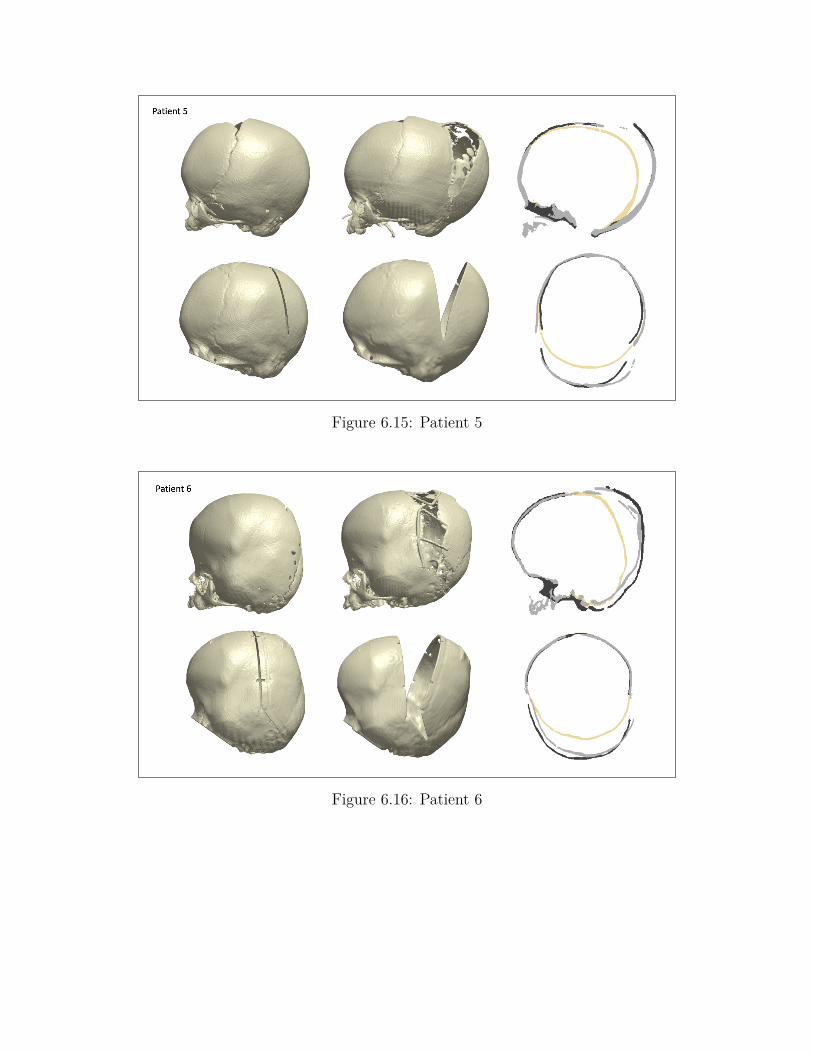
Figure 6.15: Patient 5
Figure 6.16: Patient 6

Figure 6.17: Patient 7
Figure 6.18: Patient 8

Figure 6.19: Patient 9
Figure 6.20: Patient 10

Figure 6.21: Patient 11
Figure 6.22: Patient 12

Figure 6.23: Patient 13
Figure 6.24: Patient 14

Bibliography
[1] Andrew W Hoey, Benjamin S Carson Sr, and Amir H Dorafshar. Craniosynostosis. Eplasty,12, 2012.
[2] Kshemendra Senarath-Yapa, Michael T Chung, Adrian McArdle, Victor W Wong, NatalinaQuarto, Michael T Longaker, and Derrick C Wan. Craniosynostosis: molecular pathways andfuture pharmacologic therapy. Organogenesis, 8(4):103–113, 2012.
[3] Skull. https://en.wikipedia.org/wiki/Skull. (Last accessed Feb 18 2020).
[4] The skull. https://open.oregonstate.education/aandp/chapter/7-3-the-skull/. Ore-gon State University, (Last accessed on Feb 18, 2020).
[5] Flat bone. https://en.wikipedia.org/wiki/Flat_bone. (Last accessed on May 31, 2020).
[6] Graham Lloyd-Jones. Ct brain anatomy: Skull bones and sutures. https://www.radiologymasterclass.co.uk/tutorials/ct/ct_brain_anatomy/ct_brain_anatomy_skull, 2019. (Last accessed on May 31, 2020).
[7] Basics of cranial anatomy and the nervous system. https://www.goodmancampbell.com/brain-anatomy, 2008. (Last accessed Feb 18, 2020).
[8] About the fontanelle. https://www.pregnancybirthbaby.org.au/about-the-fontanelle,2018. (Last accessed on Feb 19, 2020).
[9] Anterior fontanelle. https://www.earthslab.com/anatomy/anterior-fontanelle/. (Lastaccessed on Feb 18, 2020).
[10] Tracy Jones. Bone matrix. https://www.orthobullets.com/basic-science/9003/bone-matrix, 2016. (Last accessed on April 15, 2020).
[11] Bone development & growth. https://training.seer.cancer.gov/anatomy/skeletal/growth.html. (Last accessed on Feb 19, 2020).
[12] Growth & formation of bone. http://msgallagherlhs.weebly.com/formation--growth-of-bones.html. (Last accessed on Feb 18, 2020 ).
[13] John C Kolar. An epidemiological study of nonsyndromal craniosynostoses. Journal of Cran-iofacial Surgery, 22(1):47–49, 2011.
[14] Rohit K. Khosla Rebecca M. Garza. Nonsyndromic craniosynostosis. Semin Plast Surg,26:53–63, 2012.
70

[15] Kevin Flaherty, Nandini Singh, and Joan T Richtsmeier. Understanding craniosynostosis asa growth disorder. Wiley Interdisciplinary Reviews: Developmental Biology, 5(4):429–459,2016.
[16] Jung Min Ko. Genetic syndromes associated with craniosynostosis. J Korean Neurosurg Soc,59(3):187–191, 2016.
[17] James Seaward Christopher Derderian. Syndromic craniosynostosis. Semin Plast Surg,26(2):64–75, 2012.
[18] 115 apert syndrome. https://radiologykey.com/115-apert-syndrome/, 2015. (Last ac-cessed on April 9, 2020).
[19] Ian Bickle. From the case: Pfeiffer syndrome. https://radiopaedia.org/images/12307746,2015. (Last accessed on April 9, 2020).
[20] Jung Won Choi, So Young Lim, and Hyung-Jin Shin. Craniosynostosis in growing children:pathophysiological changes and neurosurgical problems. Journal of Korean NeurosurgicalSociety, 59(3):197, 2016.
[21] Craniosynostosis. https://www.seattlechildrens.org/conditions/craniosynostosis/#fronto-orbital. Seattle Children’s Hospital, (Last accessed on Feb 20, 2020).
[22] Julia D Sharma, Justine L O’Hara, Alessandro Borghi, Naiara Rodriguez-Florez, WilliamBreakey, Juling Ong, Nu Owase Jeelani, David J Dunaway, and Greg James. Results followingadoption of a modified melbourne technique of total scaphocephaly correction. Journal ofCraniofacial Surgery, 29(5):1117–1122, 2018.
[23] Minimally invasive surgery for craniosynostosis. https://www.mayoclinic.org/medical-professionals/neurology-neurosurgery/news/minimally-invasive-surgery-for-craniosynostosis/mac-20438762, 2018. (Lastaccessed on Feb 20, 2020).
[24] Dong Ha Park and Soo Han Yoon. Craniofacial malformation treatment: craniosynostosisand positional plagiocephaly. Journal of the Korean Medical Association, 55(9):878, August2012.
[25] Distraction osteogenesis. http://craniofacialteamtexas.com/distraction-osteogenesis/, 2015. Craniofacial Team of Texas, (Last accessed onApril 17, 2020).
[26] Posterior vault expansion. https://www.gosh.nhs.uk/medical-information/procedures-and-treatments/posterior-vault-expansion, 2019. The Craniofacialteam in collaboration with the Child and Family Information Group, (Last accessed on Feb20, 2020).
[27] Spring-assisted cranioplasty. https://www.gosh.nhs.uk/medical-information/procedures-and-treatments/spring-assisted-cranioplasty, 2019. The Craniofa-cial team in collaboration with the Child and Family Information Group, (Last accessed onApril 14, 2020).

[28] Will Rodgers, Graeme Glass, Silvia Schievano, Alessandro Borghi, Naiara Rodriguez-Florez,Arpan Tahim, Freida Angullia, William Breakey, Paul Knoops, Maik Tenhagen, JustineO’Hara, Allan Ponniah, Greg James, David Dunaway, and NUO Jeelani. Spring-assistedcranioplasty for the correction of nonsyndromic scaphocephaly: A quantitative analysis of100 consecutive cases. Plastic and Reconstructive Surgery, 140:1, 2017.
[29] Craniosynostosis surgery. https://www.chop.edu/treatments/surgical-treatment-craniosynostosis. Children’s Hospital of Philadelphia, (Lastaccessed on Feb 20, 2020).
[30] Karan Ramdat Misier, Will Breakey, Lara van de Lande, C. Caron, M. Koudstaal, SilviaSchievano, David Dunaway, Owase Jeelani, and Alessandro Borghi. Using statistical shapemodelling to assess outcomes in spring-assisted posterior vault expansion. 2019. AbstarctISPN.
[31] Alessandro Borghi, Naiara Rodriguez Florez, Federica Ruggiero, Greg James, Justine O’Hara,Juling Ong, Owase Jeelani, David Dunaway, and Silvia Schievano. Assessment of spring cranio-plasty biomechanics in sagittal craniosynostosis patients. Journal of Neurosurgery: Pediatrics,20(5):400–409, 2017.
[32] Claes Lauritzen, Yasushi Sugawara, Oya Kocabalkan, and Robert Olsson. Spring mediateddynamic craniofacial reshaping: case report. Scandinavian journal of plastic and reconstructivesurgery and hand surgery, 32(3):331–338, 1998.
[33] Alessandro Borghi, Naiara Rodriguez Florez, Federica Ruggiero, Greg James, Justine O’Hara,Juling Ong, Owase Jeelani, David Dunaway, and Silvia Schievano. A population-specificmaterial model for sagittal craniosynostosis to predict surgical shape outcomes. Biomechanicsand Modeling in Mechanobiology, pages 1–11, 2019.
[34] Richard William Francis Breakey, Paul GM Knoops, Alessandro Borghi, Naiara Rodriguez-Florez, Justine O’Hara, Gregory James, David J Dunaway, Silvia Schievano, and NU OwaseJeelani. Intracranial volume and head circumference in children with unoperated syndromiccraniosynostosis. Plastic and reconstructive surgery, 142(5):708e–717e, 2018.
[35] Jiawen Wang, Donghua Zou, Zhengdong Li, Ping Huang, Dongri Li, Yu Shao, Huijun Wang,and Yijiu Chen. Mechanical properties of cranial bones and sutures in 1–2-year-old infants.Medical science monitor: international medical journal of experimental and clinical research,20:1808, 2014.
[36] Wenyi Yan and Oscar Dwiputra Pangestu. A modified human head model for the study of im-pact head injury. Computer methods in biomechanics and biomedical engineering, 14(12):1049–1057, 2011.
[37] Ying Tan. Chapter 11 - applications. In Gpu-Based Parallel Implementation of Swarm Intel-ligence Algorithms, pages 167 – 177. 2016.
[38] R Merjulah and J Chandra. Classification of myocardial ischemia in delayed contrast en-hancement using machine learning. In Intelligent Data Analysis for Biomedical Applications,pages 209–235. 2019.

[39] Tomohisa Nagasao, Junpei Miyamoto, Hua Jiang, Tsuyoshi Kaneko, and Tamotsu Tamaki.Biomechanical analysis of the effect of intracranial pressure on the orbital distances in trigono-cephaly. The Cleft palate-craniofacial journal, 48(2):190–196, 2011.
[40] Imaoka Sheldon. Analyzing viscoelastic materials, mechanical solutions from ansys have con-venient tools for calculating deformation of materials in which stiffness changes as a functionof loading, time and temperature. ANSYS Advantage, 2(4), 2008.
[41] Giavarina Davide. Understanding bland altman analysis. Biochemia medica, 25(2):141–151,2015.
[42] Phoebe Balentyne Diana Mindrila. Scatterplots and correlation. https://www.westga.edu/academics/research/vrc/assets/docs/scatterplots_and_correlation_notes.pdf.(Last accessed on May 20, 2020).
[43] Cephalic index. https://en.wikipedia.org/wiki/Cephalic_index. (Last accessed on April17, 2020).
[44] Nikolaos Haliasos, Alessandro Borghi, Mudasir Nazir, Frank Smith, David Dunaway, andOwase Jeelani. Measuring the gosh spring: a mathematical model for the standardization ofopening measurements of a novel cranial distraction device. 2014.
[45] Nist/sematech e-handbook of statistical methods. http://www.itl.nist.gov/div898/handbook/, 2012. (Last accessed on May 26, 2020).
[46] Least absolute deviations. https://en.wikipedia.org/wiki/Least_absolute_deviations, 2020. (Last accessed on May 9, 2020).
[47] Hayes Adam. R-squared definition. https://www.investopedia.com/terms/r/r-squared.asp, 2020. (Last accessed on May 26, 2020).
[48] Susan S Margulies and Kirk L Thibault. Infant skull and suture properties: measurementsand implications for mechanisms of pediatric brain injury. J. Biomech. Eng., 122(4):364–371,2000.
[49] David Roylance. Introduction to fracture mechanics. 2001.
[50] E Oterkus, C Diyaroglu, D De Meo, and G Allegri. Fracture modes, damage tolerance andfailure mitigation in marine composites. In Marine Applications of Advanced Fibre-ReinforcedComposites, pages 79–102. 2016.
[51] Ansys, smart fracture. https://www.ansys.com/-/media/Ansys/corporate/resourcelibrary/whitepaper/smart-fracture.pdf, 2020. (Last accessed on May12, 2020).
[52] Alessandro Borghi, Naiara Rodriguez-Florez, Will Rodgers, Gregory James, Richard Hayward,David Dunaway, Owase Jeelani, and Silvia Schievano. Spring assisted cranioplasty: a patientspecific computational model. Medical engineering & physics, 53:58–65, 2018.
[53] Natario Linard Couser Srivindhya Kolluru. Craniosynostosis syndromes. https://eyewiki.aao.org/Craniosynostosis_Syndromes, 2019. (Last accessed on April 9, 2020).