Working Paper

A Set of Climate Models for Integrated Modelling of

Climate Change Impacts

Part 11: A 2.5-Dimensional Dynamical-Statistical

Climate Model (2.5-DSCM)

Vladimir K. Petoukhov Andrey V. Ganopolski

WP-94-39 May, 1994

lillASA International Institute for Applied Systems Analysis A-2361 Laxenburg Austria

b Telephone: +43 2236 715210 Telex: 079 137 iiasa a Telefax: +43 2236 71313

A Set of Climate Models for Integrated Modelling

of Climate Change Impacts

Part I1

A 2.5-Dimensional Dynamical-Statistical

Climate Model (2.5-DSCM)

Vladimir K. Petoukhov Andrey V. Ganopolski

May 1994

Worki17g Papers are interim reports on work of the International Institute for Applied Systems Analysis and have received only limited review. Views or opinions expressed herein do not necessarily represent those of the Institute, its National Member Organizations, or other organizations supporting the work.

!aIIASA International Institute for Applied Systems Analysis o A-2361 Laxenburg Austria

Am. Telephone: +43 2236 71521 Telex: 079 137 iiasa a o Telefax: +43 2236 73147

FOREWORD

The climate research component of the Forestry and Climate Change Project has had as one of the objectives to develop a series of simplified climate models which can be part of integrated models for analyses of climate change. This Working Paper describes climate simulations with a 2.5-Dimensional Dynamic-Statistical Climate Model.

Table of Contents

1. Summary

2. Introduction and overview.

3. Description of the 2.5-DSCM 3.1 Approach 3.2 Atmospheric component of the model 3.3 Oceanic component 3.4 Land component 3.5 Linkage of climate components

3.5.1 Atmosphere and ocean 3.5.2 Atmosphere and land

3.6 Present status of the model

4. Model results 4.1 Overview of results 4.2 Simulation of present climate 4.3 Equilibrium response to a doubling of CO, content in the atmosphere 4.4 Time dependent runs

5. Multilayer isopycnal ocean model 5.1 Physical background 5.2 Model description 5.3 Numerical methods 5.4 Model results

5.4.1 Description of the numerical experiments 5.4.2 Oceanic circulation 5.4.3 Thermohaline structure of the ocean 5.4.4 Heat and salt balance 5.4.5 Tracers distribution

6. Integrated Assessment of Climate Change Impacts on European Forests (ICCF): A projected application to integrated modelling of climate change impact

7. Conclusion

Appendix. The structure of the global scale coupled climate model and preliminary results

References

1. Summary

Projections of changes in climate are valuable in their own right, but they raise another, perhaps more

important set of questions: What effects might such changes have on food production, on forests, on

insect life, energy demand, and fresh water supply - on dozens of factors that directly and indirectly

affect human well-being?

To address these questions, specialists must link ecological models with climate models; to assess

policies, the climate models must in turn be driven by accounting frameworks that calculate total

emissions and concentrations of greenhouse gases, depending on policy scenarios. This chain - from

policy-oriented accounting tool to climate model to ecological impact model, with feedback, possibly

supported by a model for socioeconomic analyses - comprises an integrated assessment model or an

integrated model of climate change, as it is also called.

In terms of running time a climate model can easily play a dominant role within an integrated model

of climate change. General Circulation Models are the state of the art for studying and projecting

climate, but for integrated assessments they are impractical: they are not computer-efficient with

respect to both running time and hardware. They can take weeks, running on a super computer, to

calculate one complete scenario. Many ecologists and policy analysts, however, wish to assess a great

number of scenarios and therefore need a suitable climate model that can give results within hours,

possibly within a day, using a workstation or a PC.

In fact, the needs of impact modellers and other model users are very often antagonistic to each other,

like, e.g., their desire for both a quick turnaround time and climatic information with a high spatial

and temporal resolution. Therefore, the choice of a proper climate model is crucial for the entire

integrated model. In principle, it is the environmental impact one wishes to assess that determines

the degree of sophistication of the climate model and thus its computing time requirements. But

environmental impact modellers or assessors, on the other hand, must be prepared to answer questions

of great consequence. They might be asked, e.g., whether the environmental impact under discussion

could also be studied having less climate variables available as input information, and which spatial

and temporal resolution of these climate variables would still be acceptable.

The Working Paper summarizes the status of two climate models out of a set of four of graded

complexity that are available or under development at IIASA, and describes the envisaged position of

these climate models in the context of an integrated model of climate change. The climate models

mentioned in Part I and I1 of the Working Paper are a 2-dimensional Zonal Climate Model and a 2.5-

dimensional Dynamical-Statistical Climate Model, respectively. They offer different sets of climatic

information with different spatial and temporal resolutions and thus allow a choice depending on the

environmental impact to be studied in an integrated fashion.

The Working Paper also sheds light on a projected application to integrated modelling of climate

change impacts, which forms one of the focal points of IIASA's environmental research until 1996

and involves five collaborating research teams from Australia, Finland and Sweden. This will be an

integrated assessment of climate change impacts on European forests. A two-step approach employing

both the Zonal Climate Model and the Dynarnical-Statistical Climate Model is outlined. An important

feature of the integrated assessment is that the ecophysiology of a single plant up to that of aggregated

forest ecosystems will be considered. This provides a linkage to the climate models mentioned and

thus, in combination with a policy-oriented accounting tool for greenhouse gas emissions and

concentrations, an integrated assessment becomes feasible.

2. Introduction and overview.

Current studies in the field of climate modelling are carried out using five basic methods depending

on the scientific tool of investigation.

The first approach uses highly sophisticated climate models which simulate the general circulation of

the atmosphere and/or the ocean. These are the so-called general circulation models (GCMs) (e.g.,

Manabe et al., 1992; Hansen et al., 1983; Cubasch et al., 199 1). The thermodynamical approach is

based on simplified energy balance models (e.g., Budyko, 1969; Sellers, 1969; North, 1975; Rasool

and Schneider, 1971). Radiative-convective and radiative-turbulence models form the third type of

climate modelling (e.g., Karol and Rozanov, 1982; Humrnel and Kuhn, 1981; Ou and Liou, 1984).

Empirical-statistical models are the basis for the so-called statistical method of climate research (e.g,

Vinnikov, 1986; Polyak, 1975). The fifth type of climate modelling, finally, is represented by the

so-called statistical-dynamical (or, equivalently, dynamical-statistical) models (see, e.g., Saltzman,

1978; Adem, 1964; Petoukhov, 1976).

Three-dimensional GCMs are the state of the art for present studies of climate and climate change.

Most of them use the primitive hydrothermodynamical equations for both the atmosphere and the

ocean. These models have a high spatial and temporal resolution (in the best GCMs the latitudinal

and longitudinal resolution is up to 1 ", the temporal resolution is up to 10 minutes, and the number

of vertical levels is more than 20). The most sophisticated GCMs explore the atmospheric and oceanic

interaction. GCMs are widely used for simulating present climate in terms of its annual cycle and its

intraseasonal and interannual variability, as well as for evaluating natural and anthropogenic impacts

on climate.

However, GCMs have some shortcomings which make them inconvenient for climate change impact

studies. Due to their degree of complexity they have a relatively long turnaround time, even on the

most advanced computer systems. This fact places certain limitations on the application of GCMs in

integrated models in the cases of polyvariant analysis of climate change scenarios. Different parts of

GCMs are not equally developed (e.g., cloudiness being an important component of the climate system

is one of the relatively weak points of these models). The accuracy of simulating basic present climate

conditions (e.g., surface air temperature) at a grid-point level is not very high, especially in polar

regions. A noticeable concurrence seems to exist between the uncertainty of simulating current

temperature and the uncertainty of temperature sensitivity due to standard experiments (see Figures

2.2 and 2.3 in Part I of this Working Paper, hereafter referred to as W l ) .

The second type of climate modelling is represented by energy balance models (EBMS). They are less

sophisticated, have a sound physical bases, and are computer efficient in terms of running time.

Restrictions to applying these models in climate change impact investigations are connected with the

small number of climate output variables (see Table 2.4 in WPI), and with their relatively low spatial

resolution (they are mainly zonal; in nonzonal models of this type oceanic and atmospheric modules

are generally not separated).

Radiative-convective models (RCMs) and radiative-turbulence models(RTMs) are the best tool for

investigating the radiative effect of greenhouse gases and aerosols and for evaluating their influence

on the mean global and zonal temperatures at various pressure levels. But these models cannot be

used for regional climate responses to, for instance, anthropogenic impacts. RCMs and RTMs are

very limited also as to the number of climatic variables they deal with. For these reasons the

application of RCMs and RTMs in integrated models is restrictive.

Empirical-statistical climate models that are based on empirical climatic information are useful when

elucidating the various spatial/temporal correlations which exist between climatic variables under

present climatic conditions. At the same time, the possibility of using them for estimating correlation

trends under a changing climate is doubtful. In this sense, relatively simple statistical models derived

from GCM results seems to have a perspective. These statistical models (see, e.g., Hasselmann and

von Storch, 1992) represent what we call the top-down approach with regard to the climate module

design for an integrated model of climate change impacts (see Table 2.2 of WPl).

Dynamical-statistical climate models (DSCMs) occupy an intermediate position in the hierarchy of

climate models between GCMs and EBMs. On the one hand, DSCMs are rather sophisticated (in

comparison with EBMs), comprise the most important feedbacks, and a large number of climate output

variables. Their spatial and temporal resolution is adequate to many environmental impact problems

(see Table 2.5 in WPI). On the other hand, they are not as complicated as GCMs and can process

many model experiments in a computer-efficient mannner. This is very important for assessing the

influence of various climate change scenarios on manhiota life aspects. The weakest point of DSCMs

is basically the heuristic character of the spatial and temporal averaging procedure which is applied

to the original set of primitive hydrothermodynamical equations (for atmosphere, ocean and land) and

which results in the working equations of these models.

The DSCM includes all major components of the climate system: atmosphere, land, and ocean.

Nevertheless we envisage to use instead of original oceanic module of DSCM, more sophisticated

ocean model, namely oceanic GCM, called MILE'. The main reason for that is the recognized

importance of oceanic processes for climate changes. MILE was specially designed for long-term

climate simulation and it has rather quick turnaround time. Thus, coupling atmospherelland modules

of DSCM with MILE does not increase significantly projected computer resources.

The structure of the paper is as follows. The concept and structure (climate components) of the 2.5-

DSCM of the Institute of Atmospheric Physics (IAP, Moscow) are described in Chapter 3 . Chapter

4 reviews the results of simulations with this model of present climate, of a transient experiment

(instantaneous doubling of atmospheric CO,), and of a time-dependent climate change experiment

(increase of the atmospheric greenhouse gases content according to the 1990 IPCC scenario A,

Houghton et al., 1990). A multilayer isopycnal oceanic model (MILE) developed in the Computer

Center of the Russian Academy of Sciences (CC, Moscow) which is envisaged to be coupled with 2.5-

DSCM is described in Chapter 5. A brief description and perspective of the improved global version

of the 2.5-DSCM are given in Chapter 6 and Appendix. Possible applications of the 2.5-DSCM in

the framework of climate change impact studies, as well as the envisaged use of the DSCM in an

Integrated Assessment of Climate Change Impacts on European Forests (ICCF) are also discussed.

Chapter 7 summarizes the status of the 2.5-DSCM and its position in the context of an integrated

model of climate change inpacts.

Multilayer lsopycnal urgescale ocEan model

6

3. Description of the 2.5-DSCM

The main concept of the 2.5-DSCM described below is that the evolution of the climate system on

spatial scales 2 500-1000 km (in the atmosphere) and 2 300-500 km (in the ocean) and with a time

scale r 10 days is the result of the nonlinear interaction between a limited number of large-scale

climate-forming objects (CFOs). In accordance with this concept, the minimum CFOs are synoptic-

scale eddies and waves as well as ensembles of dry and moist (cumulus) convection, in the

atmosphere, and synoptic-scale eddies and waves as well as convective ensembles, in the ocean.

Small-scale and mesoscale eddies and waves of the atmosphere and ocean are treated in the model as

vertical and horizontal of "turbulence. "

The second important point of the concept is that the vertical structure of the main climatic variables

of the atmosphere and ocean is considered to be universal, i.e., it is supposed to have stable features

(to be represented by stable thermodynamical structural elements, TSEs) under a broad range of

climatic states, even somewhat away from present climate conditions. For example, vertical

temperature profiles in the free troposphere and stratosphere are considered to be quasi-linear, in the

mixed layer of the ocean quasi-isothermal, and so on (a more detailed description of the TSEs with

respect to the main climatic variables of the model is given below in this chapter). The number and

composition of CFOs and TSEs are also considered to be universal in the above-mentioned sense, as

well as physical mechanisms of their generation, interaction, and feedbacks between various chains

(components, modules, variables) of the climate system.

The main temperature-related feedbacks taken into account in the 2.5-DSCM are listed in Table 2.6

of WP1. In Figure 3.1 the general structure of the 2.5-DSCM is shown (Petoukhov, 1991). The

spatial and temporal resolution of the 2.5-DSCM and the number and composition of the climate

components and feedbacks, as well as of the climate output elements of the model (see Tables 2.3,

2.4, 2.6 of WP1 and Table 3.1), are anticipated to be appropriate for assessing already quite a few

climate change impacts and for incorporating the model into different integrated models (see, e.g.,

Tables 2.1, 2.4, 2.5 and 5.3 of WPI).

ATMOSPHERE

STRATOSPHERE

TROPOSPHERE

BOUNDARY LAYER

LAYER I OCEAN I t SEASONAL I THERMOCLINE

MAIN THERMOCLINE

I BOTTOM LAYER I

OCEAN

UPPER SOIL

LOWER SOIL

LAND

Figure 3.1. Structure of the 2.5 DSCM

Table 3.1 Main features of the present version of the 2.5-DSCM

Computed climate elements

Main processes

Atmosphere

Greenhouse gases

18" x 4.5" (18" on h and 4.5" on 8 ; 3 layers in atmospheric module (20 layers for radiative transfer calculations); 3 layers in oceanic module; 2 layers in land module; simplified geographical distribution of ocean and land; hemispheric').

I Seasonal (time step - 1 s 3 days).

Prognostic equations for atmospheric temperature and specific humidity; energy balance equations for land and sea ice temperatures; prognostic equation for oceanic temperature and sea ice thickness; diagnostic equations for atmospheric and oceanic large-scale long-term circulation patterns, auto- and cross-correlation functions of atmospheric and oceanic synoptic components (e.g TI2, T'q',, ql*,, etc.), soil moisture.

Optical parameters of atmospheric gases, water droplets, crystals and aerosols in solar and terrestrial radiation bands; aerosols and greenhouse gases concentrations; soil and vegetation parameters; oceanic salinity.

T, Pr, WV, R, H, E, C1, Sn, SI, TI2, qr2, u'T1, vlT', u'q',, vrq',, uf2, vI2, Prr2.

Radiation transfer; large-scale circulation and macroscale eddylwave horizontal and vertical transport of momentum; heat and moisture (MHM); MHM smalllmesoscale "turbulent diffusion"; large-scale condensation, deep and shallow convection.

Horizontal and vertical momentum and heat exchange by means of large- scale circulation, synoptic eddies, convection, and small mesoscale "diffusion".

Water vapor; snow and ice albedo; cloudiness; lapse rate; horizontal and vertical transport processes in the atmosphere and ocean; vegetatiodsoil

I Soillvegetatiodatmospher heat and moisture exchange. I I

Eight vegetatiodland-cover and soil types (with and without snow cover); open ocean; sea ice; Antarctic sheet.

None.

LW calculations: H20, CO,, CH,, 0 , . SW calculations: H,O, O,, aerosols2).

I moisture. I

Running time II

I

ca 15 minutes on a SUN SPARC 2 workstation for one model year.

1) The global version of the model with realistic geography is now under development. For the geographical distribution of ocean and land, grid spacing, and preliminary results of global versions runs see Appendix.

2) The global version of the model will also include the most radiatively active CFCs in the SW radiation scheme, using the same procedure as in the 2-D ZCM (see Chapter 3 of WPl)

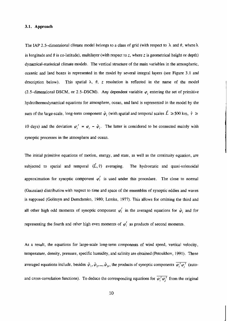
3.1. Approach

The IAP 2.5-dimensional climate model belongs to a class of grid (with respect to h and 8, whereh

is longitude and 8 is co-latitude), multilayer (with respect to z, where z is geometrical height or depth)

dynamical-statistical climate models. The vertical structure of the main variables in the atmospheric,

oceanic and land boxes is represented in the model by several integral layers (see Figure 3.1 and

description below). This spatial X, 8, z resolution is reflected in the name of the model

(2.5-dimensional DSCM, or 2.5-DSCM). Any dependent variable pi entering the set of primitive

hydrothermodynamical equations for atmosphere, ocean, and land is represented in the model by the

A

sum of the large-scale, long-term component Gi (with spatial and temporal scales L 2 500 km, 'i 2

10 days) and the deviation pi' = pi - Gi. The latter is considered to be connected mainly with

synoptic processes in the atmosphere and ocean.

The initial primitive equations of motion, energy, and state, as well as the continuity equation, are

subjected to spatial and temporal (L,?) averaging. The hydrostatic and quasi-solenoidal

approximation for synoptic component pi is used under this procedure. The close to normal

(Gaussian) distribution with respect to time and space of the ensembles of synoptic eddies and waves

is supposed (Golitsyn and Demchenko, 1980; Lernke, 1977). This allows for omitting the third and

all other high odd moments of synoptic component pi in the averaged equations for Gi and for

representing the fourth and other high even moments of pi as products of second moments.

As a result, the equations for large-scale long-term components of wind speed, vertical velocity,

temperature, density, pressure, specific humidity, and salinity are obtained (Petoukhov, 1991). These

averaged equations include, besides G,, G2, ..., G,, the products of synoptic components pip; (auto-

and cross-correlation functions). To deduce the corresponding equations for p/ p: from the original

(prirlitive) equations, one of the common methods of statistical fluid dynamics (Monin and Yaglom,

1965, 1967) is applied (Petoukhov, 1990). Namely, the set of primitive equations forp,, p2, ..., pN

is multiplied, for example, by p,' and the ( i , ?) average is used. Then the original (primitive)

equation for p, is multiplied by p,', p2', ..., p i , and again the ( i , i ) average is applied. The

ace' ap1' averaged equations, including p,' 2 and 4 - , respectively are then summarized to obtain the

a t cot

nonstationary (in the general case) equation in partial derivatives for (Petoukhov, 1990, 1991).

The same procedure is applied to p 2 ' , p ~ and any other p/(i = 1 ,2 , . . . ,M, which gives the

7- - = 1,2,..., . The above-mentioned corresponding equations for p, 9 , p36 ,...,pN 6

features of synoptic components are taken into account under this procedure and two additional

assumptions are used: (1) the synoptic component in high and middle latitudes is considered to be

quasi-geostrophic in free atmosphere; and (2) of all the nonadiabatic processes only phase transition

of water vapor and surface friction are considered to be energetically important in the synoptic

component of Q, where Q is the sum of nonadiabatic sources and links in the atmosphere and the

ocean. Let us now describe the model equations in detail.

3.2 Atmospheric component of the model

The set of basic equations of the model for the atmospheric component, resulting from the above-

mentioned ( i , ?) averaging is as follows (Petoukhov, 1991):

a a a A A ,. ,. A 1 ap + -$up + V,vup = - fpv - - - + & + F&

P~ az a sin 8 dX - -

In equations (3.2.1)-(3.2.7) F, 4,. h, P. * , P , and are temperature, specific humidity, zonal,

meridional, and vertical components of velocity vector v , pressure, and density, & = 1/F,

where A = (AA, A,, Ad (any vector); x is any scalar; Q, and Q, are heating rates per unit volume

" 6 6 6

due to radiative transfer and water vapor phase transition, Q,, Q , , F, , F, , F, , and fid describe

small-scale and mesoscale "turbulence" heating rate, water vapor influx, z and 8 components of

frictional force acting on h and i ) components of v; M is water vapor influx due to phase transition;

the other designations in equations (3.2.1) to (3.2.7) are evident. The single-underlined terms in

equations (3.2.3) and (3.2.4) are important only in the boundary layer, while the double-underlined

terms are important only in the equatorial regions (see text below). The term - - a' in equation asin8 ah

(3.2.3) is important outside the equatorial regions only.

Equations (3.2.1) to (3.2.7) contain, besides the large-scale long-term components, the auto- and

cross-correlation functions of synoptic-scale component: u' , , , , , , , , , m,

and T'Z. The set of equations for these variables using the above-mentioned method can be written

as follows (Petoukhov, 1990, 1991):

- i?TT2m = - c U T $ P v h f (3.2.8) az

- m a w = - cvT;"ve~ (3.2.9) az

- a n = - U 9. z P W - c ~ ~ P v ~ Q ~ (3.2.10)

^./Z - V qv - P W - C , P V r e g v (3.2.11) az

1 tam = - C , ~ [ T / U ' V , ~ + F T V ~ ~ ) + - T / Q ~ ; (3.2.12) az cv

In equations(3.2.8) to (3.2.16) c,, > 0 , c,, > 0, c, > 0 , c, > 0 , and c, > 0 are

dimensionless functions of 8 , A , and z (Petoukhov, 1980, 1990, 1991 ; Mokhov et al., 1992),

K pz,e = Cpw.e L;: (H,RO)' (li2 + ?)I)'" > o

at high and middle latitudes and

K~~ = K~~~~ = c ~ ~ , ~ L ; ~ , ~ ( H ~ o ~ ) ' ( f i 2 + c)'" > o

in equatorial regions, where cpw and cpwSe are ~lirnensionless functions of 8 , A , and z; Ro , Roe , LRo

and LRo,e are, respectively, Rossby number, equatorial Rossby number, Rossby deformation radius

and equatorial Rossby deformation radius (Pedlosky, 1979); H, is the scale height for the

atmospheric density; V, and V, are, A and 8 components of V vector operator; $I in equation

(3.2.16) stands for TI or q,/ (Petoukhov, 1980, 1991).

The term Q, in equation (3.2.1) comprises the upward and downward fluxes of solar $: and

- t 4 terrestrial FRT radiation. The p: fluxes are computed in the model using the method described in

Tarasova and Feigelson (1981), Veltischev et al. (1990), and Tarasova (1992). The method is based

on two-stream 6-Eddington approximation of the transport equation solution in gas-aerosol

atmosphere in spectrum ranges outside the water vapor absorption bands. In the NI region of the

solar spectrum the combined 6-Eddington method is applied taking into account the water vapor

absorption calculated by use of integral transmission function (Veltischev et al., 1990; Tarasova,

1992). Cloud droplets and crystals absorption computation was conducted using the integral

transmission function for liquid water and crystals (Tarasova, 1992). The terrestrial radiation fluxes$:

were calculated in the model by the method suggested in Mokhov and Petoukhov (1978) utilizing the

integral transmission function approximation.

The term QPH in (3.2.1) is represented in the model by two items: one of them @::) describes the

phase transition of water vapor due to large-scale condensation in stratus cloud systems; the other one(^^)

represents the processes of deep and shallow (not precipitating) moist convection. No liquid and

crystal water storage is assumed to occur in stratus and cumulus cloud systems on the above-mentioned

spatial and temporal E , i scales, so that precipitation is supposed to be equal to condensation.

The large-scale stratus cloudiness lower boundary in the model is suggested to be disposed at three

atmospheric levels: (1) at the top of atmospheric boundary layer d,; (2) at the level of maximum

value of large-scale vertical flux of water vapor & = $9, + m; (3) at the level of maximum

a value of water vapor influx due to large-scale vertical motions R~~ = - ($q, + ~ 1 9 ~ ) . az

The cloud amount fii, and liquid water content M in each layer are calculated in the model as

functions of large-scale temperature pi , relative humidity y f , = 4 Jg,,,, , and of vertical

velocity w = + (w'2) ' I2 (Dushkin et al., 1960; Petoukhov, 1991):

ii = i,(fq,,@) . (3.2.17a)

MWi = ~ ~ ~ ( F ~ , f ~ ~ , e , n ~ ) (3.2.17b)

The expression for w'2 is obtained in the model using the above-mentioned method of synoptic-scale

component description by multiplying the barical tendency equation (see, for example, Lorenz, 1967)

by w' and then using the (i, ?) average procedure (Petoukhov, 1991).

The overlap of stratus cloudiness deposited in different layers is suggested to be statistically

independent under I +S I < w,, , highly correlated under I w I > w,, , with linear dependence

of the correlation on I w I in the range w,, < 1 w I < wLSl, where w,, and w,, are functions

of minumum and maximum life cycle duration for stratus cloud systems (Petoukhov, 1991; Manuilova

et al., 1992). The term gH (equal to large-scale precipitation rate, as has already been mentioned)

in the model is the function of cloud amount fii, large-scale vertical velocity I??, and water vapor

A, content q, = QV, (Petoukhov, 1980, 1991):

LS A L S , ( i ) i = 1,293 -

The quantity q'2, in equation (3.2.18) is calculated using the formula analogous to (3.2.12) in which

7 7 7 p, m, m, v A P , v$, and T'QpHr are replaced, respectively, by q ,,, qv u , qv v ,

V and q Q . The quantities TrQp; and q,,' QPHf are calculated as (t, i) averaged products

of T' (or q,,' ) and QpH computed by (3.2.18), in which A, ~ = , 4"re replaced by n = A + n ' ,

w = ~ + w ' , a n d q v = q v + q , , ' .

The second item 6YH in Q, is represented in the model by the schemes of deep and shallow moist

convection, which are close to Betts (1986) parameterizations. The main assumptions used in these

schemes are (1) the simultaneous relaxation of temperature and moisture fields in deep and shallow

convective ensembles toward the large-scale long-term (quasi-equilibrium) hydrothermodynamical

fields of the atmosphere. (2) the closeness of the vertical structure of quasi-equilibrium fields toward

the phenomenological universal vertical profiles - quasi-linear for temperature and wind, quasi-

exponential for density, pressure, and specific humidity (Petoukhov, 1991). Under these assumptions

the simple mathematical procedure of the 8YH computation is described in Petoukhov (1991) using

the so-called parcel method, but taking into account the dry air entrainment and evaporation of

rainfall. The latter is calculated using Schlesinger et al., (1988) scheme. This procedure comprises

calculation of A, and &, - cumulus cloud amount and liquid water content. The quantities

T' Q;; and q,! Q;; are calculated using the same method as when computing the terms T'Q;;' and

q,!Q;f. Let us note that the term M in (3.2.2) is equal to Q,JL~, where Le is the latent heat of

evaporation or sublimation (under negative temperatures).

The terms Q, (in 3.2. I), Q, (in 3.2.2), p u , and pug (in 3.2.3), and p, , pfi (in 3.2.4) represent,

correspondingly, the heating rate, influx of water vapor, z and 0 components of frictional forces

applied to li and 9 components of motion due to small scale (mainly vertical) and mesoscale (mainly

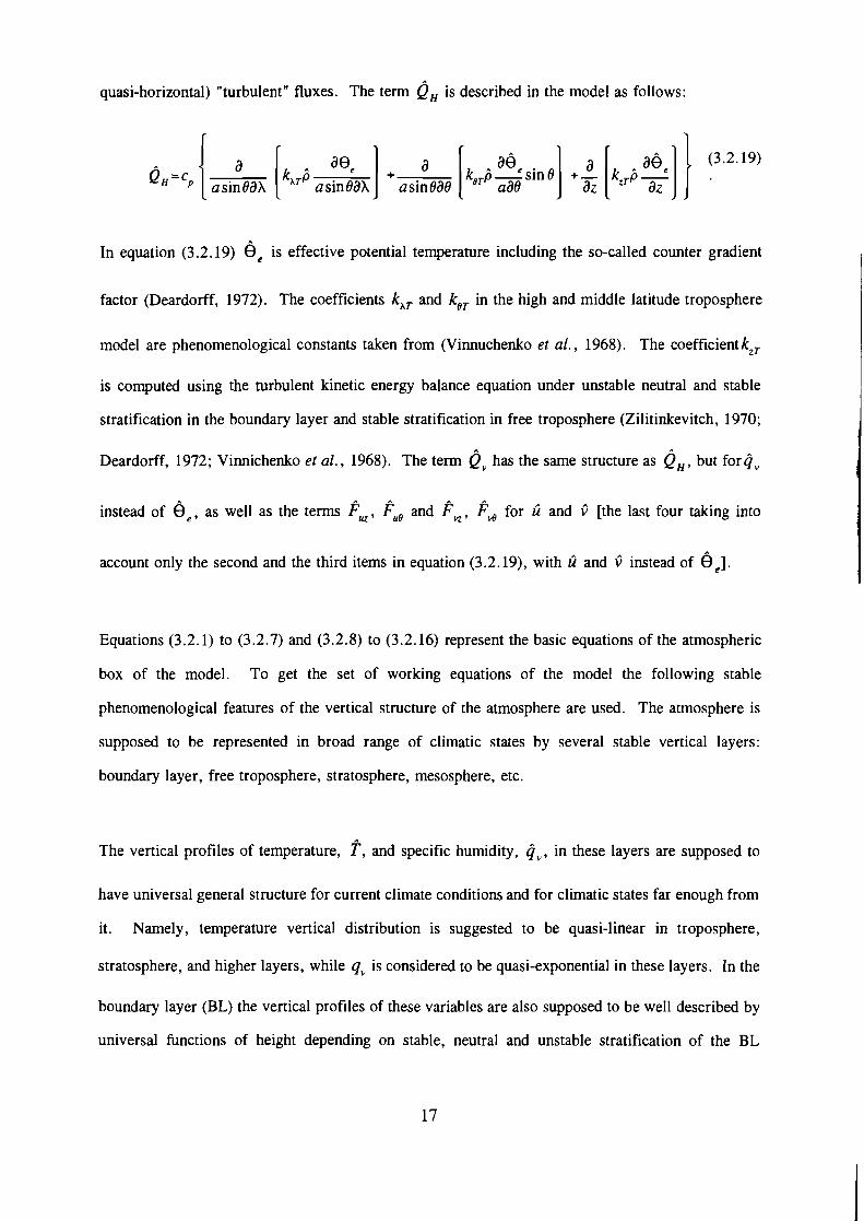
quasi-horizontal) "turbulent" fluxes. The term Q, is described in the model as follows:

In equation (3.2.19) 8, is effective potential temperature including the so-called counter gradient

factor (Deardorff, 1972). The coefficients k, and k,, in the high and middle latitude troposphere

model are phenomenological constants taken from (Vinnuchenko et al., 1968). The coefficientk,,

is computed using the turbulent kinetic energy balance equation under unstable neutral and stable

stratification in the boundary layer and stable stratification in free troposphere (Zilitinkevitch, 1970;

Deardorff, 1972; Vinnichenko et al., 1968). The term Q,, has the same structure as Q,, but for q v

instead of B e , as well as the terms %, flu, and e l , fld for 2 and P [the last four taking into

account only the second and the third items in equation (3.2.19), with P and P instead of 0 , ] ,

Equations (3.2.1) to (3.2.7) and (3.2.8) to (3.2.16) represent the basic equations of the atmospheric

box of the model. To get the set of working equations of the model the following stable

phenomenological features of the vertical structure of the atmosphere are used. The atmosphere is

supposed to be represented in broad range of climatic states by several stable vertical layers:

boundary layer, free troposphere, stratosphere, mesosphere, etc.

The vertical profiles of temperature, f, and specific humidity, Qv, in these layers are supposed to

have universal general structure for current climate conditions and for climatic states far enough from

it. Namely, temperature vertical distribution is suggested to be quasi-linear in troposphere,

stratosphere, and higher layers, while qV is considered to be quasi-exponential in these layers. In the

boundary layer (BL) the vertical profiles of these variables are also supposed to be well described by

universal functions of height depending on stable, neutral and unstable stratification of the BL

(Zilitinkevitch, 1970; Deardorff, 1972). The vertici~l profile of b is suggested to be quasi-exponential

through the whole atmosphere:

8 = i (0) exp {- ZIH,,} , (3.2.20)

where I$ = R ~ ( o ) / ~ , with only slight dependence of b(0) on h and 6.

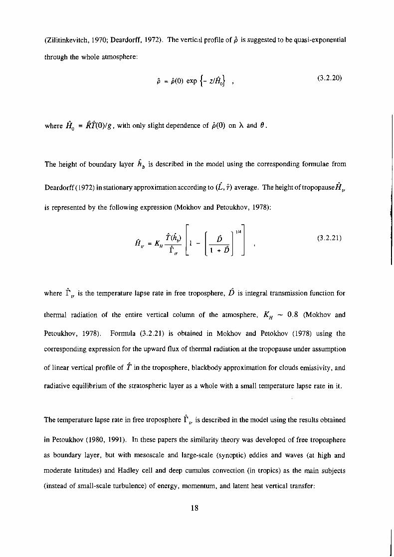
The height of boundary layer h, is described in the model using the corresponding formulae from

Deardorff (1972) in stationary approximation according to (i, i) average. The height of tropopause H,,

is represented by the following expression (Mokhov and Petoukhov, 1978):

where f , is the temperature lapse rate in free troposphere, D is integral transmission function for

thermal radiation of the entire vertical column of the atmosphere, K, - 0.8 (Mokhov and

Petoukhov, 1978). Formula (3.2.21) is obtained in Mokhov and Petokhov (1978) using the

corresponding expression for the upward flux of thermal radiation at the tropopause under assumption

of linear vertical profile of f in the troposphere, blackbody approximation for clouds emissivity, and

radiative equilibrium of the stratospheric layer as a whole with a small temperature lapse rate in it.

The temperature lapse rate in free troposphere f , is described in the model using the results obtained

in Petoukhov (1980, 1991). In these papers the similarity theory was developed of free troposphere

as boundary layer, but with mesoscale and large-scale (synoptic) eddies and waves (at high and

moderate latitudes) and Hadley cell and deep cumulus convection (in tropics) as the main subjects

(instead of small-scale turbulence) of energy, momentum, and latent heat vertical transfer:

5 k, (Ad -

where Fa , rwa are adiabatic and moist adiabatic lapse rates,

ir~u-cumulus cloud amount in free troposphere, c, > 0 - dimensionless function of X, 0 , and z

of the order of unity. In equatorial regions LRo and Ro should be replaced by LR0,, , and Roe,

correspondingly. All the variables in equation (3.2.22) [except kz,(h,)l are calculated at z = - . 2

Using the same approach, the expression for vertical profile of specific humidity in free troposphere

is obtained in Petoukhov (1980, 1991):

where

112

where Kqz = C,L;~ (P + 7) in high and middle latitudes (in equatorial regions

LRo, Ro should be replaced by LRo ,, Ro,); c, > 0-dimensionless functions of A , 0 , and z of

the order of unity; Wl is the wetness of the upper soil layer or of oceanic and sea ice surfaces (for

the ocean Wl = 1 ; cDq is the humidity transfer coefficient (see section 3.5).

Under these assumptions of the vertical structure of temperature and specific humidity, the equation

(3.2.1) is integrated in the model with respect to z from z = h, to z = atr [that gives the prognostic

equation for f (hb) ] and from z = fi, to z = IjtOp, where qOp = 35 km is the upper boundary of

the atmosphere in the model (that gives the prognostic equation for lapse rate tst in the stratosphere

or equivalently for the mean mass-weighed temperature of the stratosphere fst,m). Equation (3.2.2)

is integrated in the same limits with respect to z that gives the prognostic equations for 4,(6,) and

for the index of exponent 8, in the formula for &(z) in the stratosphere

where (z" = z - Ijtr) or equivalently for the mass-weighed specific humidity in the stratosphere

*

4~, , ,~ .

As to the equations for temperature and specific humidity in the boundary layer, the standard

procedure of scale and magnitude analysis of terms in equation (3.2.1) for the boundary layer

conditions (see, e.g., Zilitinkevitch, 1970) gives the following equation for f in this part of the

atmosphere:

where

The expression for w'T' in the boundary layer can be obtained from (3.2.16) using the common

a@ a @ - - < < - assumptions made in the investigations of BL: (1) - '@ , (2)b - ae ax az

Po[l - a,(? - T~)] where To = const , a = l o , (3) Q, = Q& = 0 (Zilitinkevitch,

1970; Deardorff, 1972).

As a result the term w/T' in equation (3.2.26) is written in the form

where

Except in the rare case of boundary layer temperature inversion on the (i, i) temporallspatial scale,

the quantity K; in (3.2.29) is less than zero due to f(k,) < f (0).

Combining (3.2.26) to (3.2.29) one can obtain

where

Using the same procedure, equation (3.2.2) in the boundary layer can be written in the form

In equation (3.2.32)

where f is relative humidity.

Under usual boundary layer temperature stratification, K: < 0 when f(hb) < f(0) [see (3.2.29)

for K;] .

Equations (3.2.30) and (3.2.32) give the standard formulation of the problem of temperature and water

vapor vertical distribution in the BL. Together with the boundary conditions for temperature and

specific humidity at the surface (or, more exactly, in the surface layer, see section 3.6), they provide

the linkage between the equations for f(h,) and Q(hb), on the one hand, and the equations for the

surface temperature of ocean or land and for soil moisture, on the other hand (see sections 3.4 and

3.5). The natural condition of continuity of temperature, specific humidity, and total vertical fluxes

of heat and moisture at z = 4 is adopted in the model. The linkage between the vertically integrated

tropospheric and stratospheric equations for temperature and specific humidity is provided by using

the condition of continuity of the same variables at z = H5,. In vertically integrated equations for

stratospheric temperature and specific humidity, heat and moisture vertical fluxes due to convection

and turbulent diffusion are equal to zero at z = HrOp. To provide continuity of vertical heat and

A

moisture fluxes at z = h, the "jump" of coefficients of vertical small-scale and mesoscale "turbulent"

heat and moisture transfer k,,, k,, is adopted in the model (Moeng and Randall, 1984; Wyngaard and

Le Mone, 1980). At z = k, these coefficients are considered to be equal to zero. Atz = &

the vertical small-scale and mesoscale "turbulent" fluxes of all substances, except water vapor, are

considered to be equal to zero.

fi,,(fi,,,, Vertically integrated equations (3.2.1) and (3.2.2) include the terms j V . PFfi dz and

H,,(H,J V . P ~ , f i dz , respectively. Corresponding formulae for P and li in these terms are obtained

ib(~,,l

in the model using equations (3.2.3) to (3.2.4) under some simplifications reflecting universal features

of li and P fields in the above-mentioned large-scale vertical layers at high and middle latitudes and

in equatorial regions. Namely, in the free atmosphere of high and middle latitudes using the standard

method of scale and magnitude analysis of terms (see, e.g., Pedlosky, 1979), one can omit the left-

hand sides as well as the two last terms on the right-hand sides of equations (3.2.3), (3.2.4).

This brings one to the so-called geostrophic balance formulae for li and D [the first and the second

terms on the right-hand sides of equations (3.2.3) and (3.2.4)], so that in this part of the atmosphereli

and P can be written in the form

av ai, - I fi,,zzzhh = cT(Afr) , az

where li, and 0, are the components of thermal wind (see, e.g. Pedlosky, 1979). As shown in

equations (3.2.35a) and (3.2.35b), the vertical profiles of li and P are linear with respect to z in free

troposphere and stratosphere.

In the boundary layer of high and middle latitudes the terms pu and gK should be added to the first

and the second terms on the right-hand sides of equations (3.2.3) and (3.2.4), respectively. This gives

the Ekman formulation of boundary layer wind speed problem, except that kzU and k,, are determined

in the model from the turbulent kinetic energy balance equation (Petoukhov, 1991). The boundary

conditions for the Ekman problem in the model are as follows:

aa ao aa ao where f -(hb), $-(hb), - I , and - 1 , are 2 and C components of wind and - , - at the top

az hb- az b- az az

of the boundary layer and 2+(hb), O+(hb) are 6 and O components of wind at the bottom of free

troposphere. So far the solution of E h a n problem includes, as the parameters, the quantities rT(hb),

oT(hb), fi+(hb), and O+(hb), the first two being the functions of temperature field at the bottom of free

atmosphere and the second two being "free" parameters of the Ekman problem. To close the system

the following expressions are used

A aa k z u p g I z d , = ' D U B I '1'lZd,

ai, k N ~ z I z . " , = c D v ~ l o ~ i , ~ z i

1

which are the lower boundary conditions for li and 9 components in the boundary layer. Here hs

is the height of the surface layer. The corresponding formula for hs used in the model is taken from

(Zilitinkevitch, 1970). The module of surface wind velocity 1 ~ 1 is described in the model as

follows:

Drag coefficients cDu and cDv in equation (3.2.37) are functions of bulk Richardson number and of

surface roughness length (see sections 3.5.1 and 3.5.2). It is supposed that cDu = cDv = cD . In the

equatorial free atmosphere the evaluation of magnitude of terms in equations (3.2.3) and (3.2.4) gives

The continuity equation (3.2.7) for this region using the analogous scale and magnitude analysis can

be written in the form

a , , v,je + - p w = 0 az

i ap In equations (3.2.39) to (3.2.41) is described by (3.2.20). The term - - in equation (3.2.40)

a ae

using equation (3.2.6) in which the second item on the right-hand side can be omitted in equatorial

regions due to small "penetrability" of the equatorial belt for the synoptic eddies (see, e.g., Pedlosky,

1979), can be written in the form (Petoukhov, 1991):

In equation (3.2.42) the following approximation for is commonly applied to convectively active

layers (equatorial free atmosphere is one of the most active convective layers):

where Ho = R T o / g .

Substituting equation (3.2.41) to (3.2.43) for equations (3.2.39) and (3.2.40) ,gives

In equations (3.2.44) and (3.2.45) the upper boundary condition l I I 0 , = 0 is used and, taking into

account equation (3.2.20) and assuming $ to be confined at the infinity, the upper limits of integratio&top

in the first items on the left-hand side of equations (3.2.44) and (3.2.45) are replaced by infinity.

Using the linear dependence of i' on z in troposphere and stratosphere and taking into account

equation (3.2.20) the solution to equation (3.2.44) and (3.2.45) in these layers can be written as

follows:

+ = + l , l ( S I ) + + 2 , 1 ( S 1 ) . Z (3.2.46)

provipling the quantities k,, , k,, and kZU, kZv (we assume k,, = k,, = k,, kZu = kZv = kZ) are

written in the form

where il,t(,t) 7 i2,,,, 9l,tO7 C2,qst) , kHl,,, , kHz,,,, , kZI,t(St), kz2,qst) are functions X and 8 , lower

indices t and st refer to troposphere and stratosphere, respectively.

Ir The boundary conditions on 8 for fi,, it,, i , , it2 at (o = f toe where co = - - 8 and pe is the

2

width of the equatorial dynamical belt (Dobryshman, 1980), are

where i, ( - , i2 1 - , it1 1 - , and 0, I - are corresponding parameters of linear (with respect to z)

expansion formulae for fi and it in middle latitudes under p +f pe [see equations (3.2.34) and

(3.2.35) and corresponding text]. The lower indices t and st are omitted in (3.2.49) for brevity.

Substituting equations (3.2.46) to (3.2.49) for equation (3.2.44) and (3.2.45) give six nonlinear

ordinary equations of the second order with respect to 8 for six functions u, , u, , v, , v2 , kHl , andk,,

in troposphere and stratosphere. The boundary conditions for kHl and kHz in both layers (troposphere

and stratosphere) are set in the model at the equator:

As to the parameters kZl,,, kzl,sr, kZ1,,,, k Z,,,, the following conditions are used in the model

27

The other two conditions applied to these four parameters are the conditions of continuity of li and$

at z = H ~ . With some minor simplifications the analytical solution to problems (3.2.44) and (3.2.45)

in equatorial troposphere and stratosphere is obtained in Petoukhov (1991), which is used in the global

version of the model. In equatorial boundary layer, applying scale and magnitude anlaysis of terms

one can reduce equations (3.2.39) and (3.2.40) to

The quantity G in equations (3.2.52) and (3.2.53) is specified in the model as follows

~ = w w , z + w 2 z 2 . (3.2.54)

This gives G = 0 at z = 0. The quantities w,, w, (which are functions of and 8 ) are

determined in the model by the conditions of continuity of large-scale vertical velocity and its

derivative with respect to z at z = h,.

Taking into account equations (3.2.54) and (3.2.42) one comes to boundary layer problems (3.2.52)

and (3.2.53) for li and O under boundary conditions (3.2.37) and li and O continuity at z = h,.

The systems (3.2.52) and (3.2.53), being added by kinetic turbulent energy balance euqation for

kZU = kZV = k, in the boundary layer [with corresponding boundary conditions of k, continuity at

z = hs and neutral stability formula for k, at z = h, (Zilitinkevitch, 1970; Deardorff, 1972)l give

the solution to u and O in the equatorial boundary layer.

Let us note that taking into account equations (3.2.15) and equation (3.2.20), equations (3.2.8) to

(3.2.11) give the so-called diffusion approximation for corresponding synoptic cross-correlation

functions. The utilization in the model of the universal vertical structure of atmopsheric temperature

and humidity allows us to simplify to a great extent the procedure of radiative a d cumulus convection

processes computation (Petoukhov, 1991). This assumption, (i, ?) averaging, and vertical integration

of the equations for temperature and specific humidity, as well as proximity of u and O to thermal

wind approximation in free atmosphere of high and middle latitudes, noticeably shorten the turnaround

time of the model due to possibility of having relatively large time steps ( = 1 t 3 days) without

violation of CFL criteria when using the explicit numerical schemes.

3.3. Oceanic component

The basic equations of the model for the long-term large-scale oceanic component deduced from the

set of primitive equations using (i, ?) average and scale and magnitude analysis are as follows

(Petoukhov, 1991):

a fo 1 afioPo a $ o f o ~ i n e a ~ ~ f ~ + + + = k A f

a2 To at a sin 0 ah a sin686 az m 0 H 0 + kZTO - az 2

aso 1 aaoso a;,30sine a ~ ~ 3 ~ a2 So + + + = k A 3 at a sine ah a sin B a B az HSO H o k ~ z

In equations (3.3.1) to (3.3.7) all designations are analogous to those of atmospheric box, but with

lower index "0." $, stands for salinity, AH is the horizontal Laplacian on the sphere with radius

TS - TS r = a , kmo = kHso = ~ H O , k, - km = km, kHu0 = kH, = kHo, k,, = k,, = k,,. The

17 equations for c, and uo vo in equations (3.3.1) to (3.3.7) using the same method as in

atmospheric module can be written in the form (Petoukhov, 1991):

In equations (3.3.8) to (3.3.10) c,, > 0 , c, > 0 , and c,, > 0 are dimensionless functions of

X, 8 , and z of the order of unity and K,,, K,, and K,, are as follows (Petuokhov, 1991):

where H O , Roo, and L: are, scale height, Rossby number, and Rossby deformation radius for the

ocean at high and middle latitudes (Pedlosky, 1979). In the equatorial belt Roo and L: are

represented by corresponding equatorial values (Pedlosky, 1979).

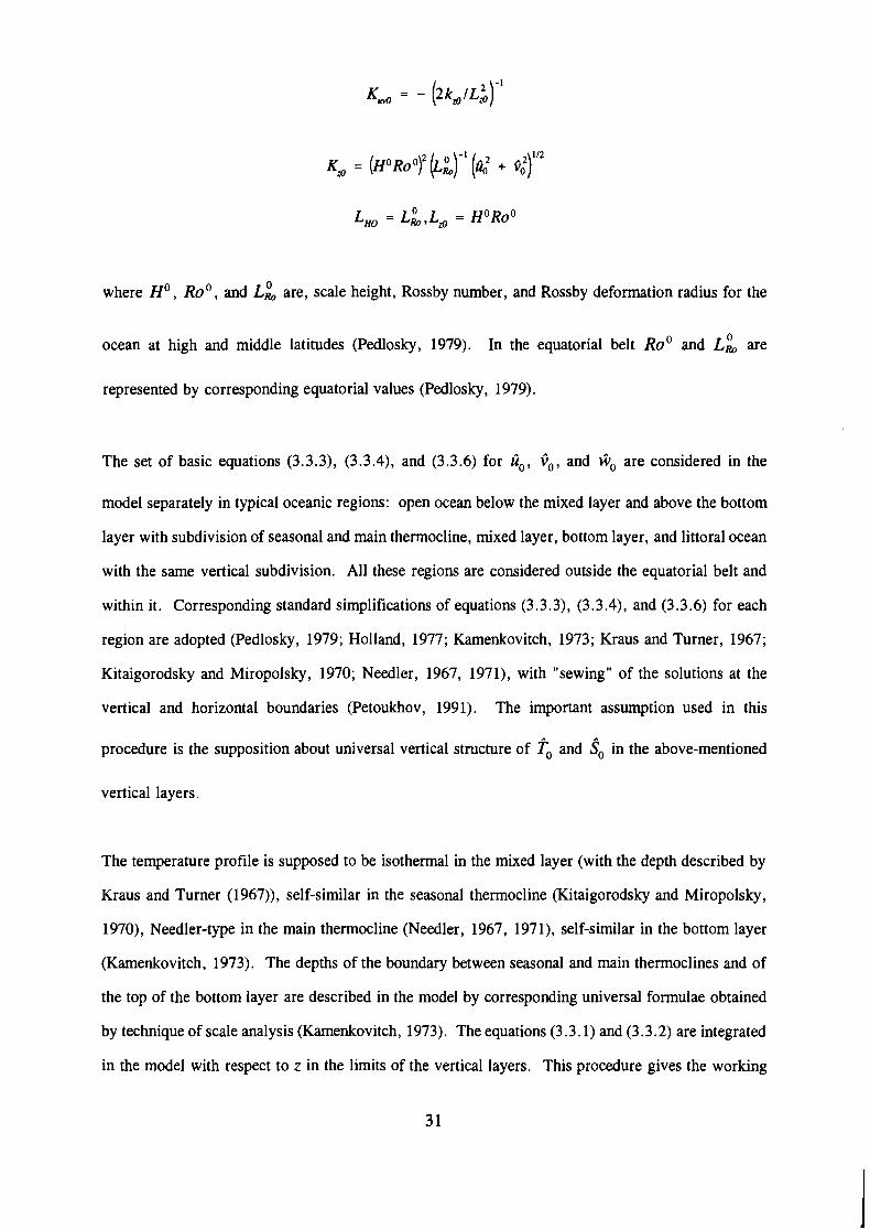
The set of basic equations (3.3.3), (3.3.4), and (3.3.6) for ho, c0, and Go are considered in the

model separately in typical oceanic regions: open ocean below the mixed layer and above the bottom

layer with subdivision of seasonal and main thermocline, mixed layer, bottom layer, and littoral ocean

with the same vertical subdivision. All these regions are considered outside the equatorial belt and

within it. Corresponding standard simplifications of equations (3.3.3), (3.3.4), and (3.3.6) for each

region are adopted (Pedlosky , 1979; Holland, 1977; Kamenkovitch, 1973; Kraus and Turner, 1967;

Kitaigorodsky and Miropolsky, 1970; Needler, 1967, 1971), with "sewing" of the solutions at the

vertical and horizontal boundaries (Petoukhov, 199 1). The important assumption used in this

procedure is the supposition about universal vertical structure of To and $ in the above-mentioned

vertical layers.

The temperature profile is supposed to be isothermal in the mixed layer (with the depth described by

Kraus and Turner (1967)), self-similar in the seasonal thermocline (Kitaigorodsky and Miropolsky,

1970), Needler-type in the main thermocline (Needler, 1967, 1971), self-similar in the bottom layer

(Kamenkovitch, 1973). The depths of the boundary between seasonal and main thermoclines and of

the top of the bottom layer are described in the model by corresponding universal formulae obtained

by technique of scale analysis (Kamenkovitch, 1973). The equations (3.3.1) and (3.3.2) are integrated

in the model with respect to z in the limits of the vertical layers. This procedure gives the working

nonstationary equations of the model for the temperature and salinity in the mixed layer and at the top

of the main thermocline fom, so,,,, f o r , and sot (Petoukhov, 1991). This vertical integration

noticeably reduces the turnaround time of the model.

The equation for the thickness of sea ice ( f ) used in the model is similar to the corresponding

equation of the Manabe and Bryan (1972) model. The single distinction is that the model under

consideration describes separately the processes of sea ice advection due to large-scale and synoptic-

scale movements and that the leads formation is parameterized in the model in terms of ice thickness

( f ) at each mesh (Petoukhov and Manuilova, 1984; Petoukhov, 1991).

3.4. Land component

The land surface temperature fl is calculated in the model using the standard equation of surface

temperature balance (see, e.g., Manabe, and Bryan, 1972). For computation of soil moisture the two-

layer model is used based on BATS scheme (Dickinson et al., 1986). Eight vegetatiodland-cover

types (VLCT) are represented in the model: desert, tundra, grass, croplmixed farming, shrub, mixed

woodland, deciduous forest and evergreen forestlrainforest. The geographical distribution of these

vegetatiodland-cover types at the model resolution follows one used in the BATS scheme. Each

model mesh was assigned a dominant type of VLCT. The fraction of bare soil were determined using

corresponding BATS parameterization. Eight soil types (STs) was taken into account. The

geographical distribution of the STs was set using the same sources of information as in the BATS

scheme, but with much more sketchy (according to model resolution) details and less subdivisions into

soil types (BATS scheme explores 18 VLCT and 12 ST classes). Sensible heat flux, evaporation,

evapotranspiration, surface run-offs and in-soil water transfer were computed using BATS

parameterizations (Dickinson et al., 1986).

3.5. Linkage of climate components

The linkage between atmospheric, oceanic, and land components is realized in the model by surface

fluxes of radiation, evaporation (evapotranspiration in vegetation-covered regions) rainfall, sensible

heat,and momentum.

3.5.1. Atmosphere and ocean

Oceanic surface is treated as a blackbody radiator in thermal range of spectrum. The ocean albedo

is a function of solar zenith angle and wind speed as specified by Cox and Munk (1956). The surface

fluxes of momentum, heat, and water vapor are computed in the model using a drag law

parameterization (Deardorff, 1967). The drag coefficient (c,), as has already been mentioned, is a

function of the drag coefficient for neutral stability (c,,) and the bulk Richardson number (Ri) for

the surface layer (Deardorff, 1968). The quantity c,, is a function of roughness length, which in turn

is a function of oceanic surface air wind speed (Garrat, 1977).

The heat and humidity transfer coefficients (c,, and c,,) are functions of c, and Ri in accordance

with Deardorff (1968) parameterization obtained from the Monin-Oboukhov similarity relations. The

roughness length of sea ice is taken from Doronin (1969).

As has already been pointed out, the module of surface air wind speed entering the drag law

parameterizations is described in the model as follows:

so that the regions with high synoptic activity (i.e., with high values of u'2 and 7) make a

pronounced contribution to ocean-atmosphere (and land-atmosphere) energy exchange.

3.5.2. Atmosphere and land

Land surface in thermal range of spectrum is black radiator. The albedo of the land surfaces is

computed in the model using BATS parameterizations for barelsnow-covered soil and vegetatiodsnow

covered soil albedos at the model resolution with the above-mentioned (see Section 3.4) land surface

subdivisions with respect to VLCTs and STs. The surface fluxes of momentum, heat, and water vapor

are computed in the model using the same drag law parameterizations as in oceanic module. The

surface roughness lengths for bare soil, and snow and vegetatiodsnow covered surfaces are taken from

BATS paper as well as the other parameters of formulae describing surface sensible heat flux,

momentum flux, evaporatiodevapotranspiration, and in-soil water transfer, (see Table 5.3 of WPl).

No orography of the land surface is taken into account in IAP 2.5-DSCM, except the Antarctic ice

sheet, for which corresponding heat and snowlice mass balance equations are used (Mokhov et al. ,

1983; Petoukhov, 1991). The main features of the 2.5-DSCM are descirbed in Table 3. 1.

3.6. Present status of the model

At present the model is able to analyze the Northern Hemisphere with strongly simplified geographical

distribution of the coastline represented by segments of parallels and meridians (see Figures 4.1-4.20).

Salinity is prescribed in the current version of the model. The vertical distribution of small-scale

turbulent coefficients of heat, humidity, and momentum transfer kZ , kZT, kZq in the atmospheric

boundary layer are approximated by analytical formulae using corresponding results of computations

of kZ, kZT, kZq for unstable, neutral, and stable stratification of BL, represented in Zilitinkevitch,

(1970). Due to its hemispheric character and relatively large spatial steps (see Table 3. l) , the current

version of the model does not allow for detailed resolution of the equatorial belt and the littoral ocean.

Taking this into account, the additional simplification have been adopted in the atmospheric and

oceanic dynamical modules of the present version. Namely, li and O components are represented by

formulae (3.2.34), (3.2.35) in the free atmosphere as a whole with the replacement off , LRo, and Ro

by f,, LR,,e, and Roe in equatorial belt (Pedlosky, 1979). In the atnospheric boundary layer the

Ekman model for the fi and C components is used but with kZ being described by the above-

mentioned analytical formulae using results of Zilitinkevitch (1970), and with f replaced by f, in the

equatorial belt. The oceanic dynamical fields fi,, C,, and Go are represented in the present version

by the sum of the barotropic (Munk, 1950) component (built on zonally averaged wind stress), the

component due to the zonally averaged overturning stream function (Petoukhov, 1991), the polar

downwelling and middlelhigh latitude upwelling (in terms of zonally averaged oceanic temperature,

salinity, wind stress), the Ekman component, and the geostrophic component with fi replaced byf,

in the equatorial belt. The Munk and overturning stream function formulae describing the

corresponding parts of 4, Co, and Go components are improved, in comparison with the usual

description, by introducing the synoptic component influence, according to equations (3.3.8) to

(3.3.10). The BATS scheme is adapted to geographical distribution and spatial resolution of the

current simplified version of the model.

At present a modified global version with realistic geography (see Figure Al . 1 of Appendix 1) and

a spatial resolution of 12" x 4.5" (for the atmospheric component) and 6" x 4.5" (for the land and

oceanic component) is under development with separate consideration of equatorial and middlelhigh

latitude regions as have been described in sections 3.2 to 3.5 and with oceanic module (MIOM, see

Appendix 2) described in terms of isopycnal coordinates (Ganopolski, 1991), including prognostic

salinity equation. The sea ice module is being improved by incorporating a more realistic scheme of

ice (and leads) formation, ice hummocking, and advection. For more details of the improvement, see

Chapter 5 and Appendices 1 and 2 of this paper.

4. Model Results

This chapter contains a description of the results obtained from the current version of the model.

4.1. Overview of results

The figures are grouped into tree parts (Table 4.1): simulation of present climate (indicated by

"lxCO,"), equilibrium response to a doubling of CO, ("2xC02), and time dependent experiment

("Scenario").

Table 4.1. Overview of model results.

Fig. 4.1 Fig. 4.2 Fig. 4.3 Fig. 4.4 Fig. 4.5 Fig. 4.6 Fig. 4.7 Fig. 4.8 Fig. 4.9 Fig. 4.10 Fig. 4.11 Fig.4.12 Fig. 4.13 Fig. 4.14 Fig. 4.15

Fig.4.16 Fig.4.17 Fig. 4.18 Fig. 4.19

Fig. 4.20

Fig. 4.21

lxC0,

Zonal mean surface air temperature. Zonal mean startospheric temperature. Zonal mean surface air specific humidity. Zonal mean evaporation. Zonal mean precipitation. Zonal mean meridional heat transport in the atmosphere. Zonal mean heat transport in the ocean. Zonal mean planetary albedo. Zonal mean flux of outgoing long-wave radiation. Zonal mean total cloud amount. Zonal mean temperature synoptic variance in the atmosphere. Zonal mean specific humidity synoptic variance. Surface air temperature. Precipitation. Ocean surface temperature.

2xc0,

2xC02 - 1xC02 zonal mean surface air temperature difference. 2xC02 - 1xC02 zonal mean startospheric temperature difference. 2xC02 - 1xC02 zonal mean precipitation difference. Geographical distribution of 2xC0, - 1 xC02 precipitation

difference.

Scenario

1990 IPCC Scenario A of C02-equivalent concentration (1985-2084). Transient responce of surface air temperature (Scenario A).

4.2. Simulation of present climate

Figure 4.1 shows the present climate latitudinal distribution of zonally averaged temperature atz = 4 (i.e., at Stephenson screen level) for February and July in the model and as derived from observational

data (Oort and Rasmusson, 1971) at p = 1000 p b . The term "present climate" refers to the past

10-year average of the model results after 100 years of integration starting from the initial state

corresponding to present climate annually and zonally averaged empirical values of climatic variables.

Figure 4.2 demonstrates the latitudinal course of present climate mass-weighed zonal temperature of

the stratosphere in the model in comparison with empirical data taken from Makhover (1983) for the

same months. In Figure 4.3 the zonal specific humidity meridional profile in the model atz = is

is given for winter and summer as well as corresponding values obtained from present climate

observations at p = 1000 pb (Oort and Rasmusson, 1971). As shown in the figures, the model

results are in satisfactory agreement with empirical data.

Zonal mean precipitation and evaporation data obtained in the model, as well as corresponding

empirical data, for February and July are depicted in Figures 4.4 and 4.5. The model results describe

rather well the equatorial and middle latitude maxima of rainfall, summer minimum of evaporation

at cp - 45' + 50°N, and subtropical minimum of precipitation. The equatorial maxima of rainfall

and evaporation in the model are deposited at the equator for both winter and summer, whereas the

real distribution of these variables exposes the periodic seasonal shift of these maxima from the

Northern Hemisphere to the Southern Hemisphere and vice versa (see, e.g., Houghton et al., 1990).

This shortcoming of the current version is connected mainly with its hemispheric character and will

be overcome in modified global version, in which the intertropical convergence zone (ICZ) will be

able to transfer from one hemisphere to another.

Figure 4.6 shows the mass-weighed zonally averaged atmospheric meridional heat flux due to a

synoptic component in the model in comparison with observational data from Oort and Rasmusson

(1971). The model results are in rather good agreement with empirical estimations.

40

30 W P:

20 4 P:

10 r: W 0 !5 . - 4 -10 c

P: 2 vl -20

-30

-40 0 10 20 30 40 50 60 70 80 90

LATITUDE

Figure 4.1. Zonal mean surface air temperature of the atmosphere ("C) for February and July in the model and as derived from observations.

-751 I I I I I I l i b 1 1 , 1 I o ib 2b 3b 4b 50 60 70 80 90

LATITUDE

Figure 4.2. Model zonal mean rnass-weighed temperature of the stratosphere ("C) for February and July in comparison with observational data.

Total oceanic meridional heat transport in the model are shown in Figure 4.7. Taking into account

the range of uncertainty of present empirical data on this variable the model results can be considered

satisfactory.

Components of the net radiation balance at the top of the atmosphere and zonal mean cloud amount

in the model are depicted in Figures 4.8,4.9, and 4.10. Except for the warm season in polar regions,

for which a discrepancy between model results and empirical data is noticeable (this is closely

connected with the polar cirrus clouds problem, see, e.g., Ou and Liou, 1984; Feigelson (ed.), 1989),

the model, even in its current simplified version, describes the seasonal and latitudinal courses of these

important climate variables with rather high accuracy.

\ = \

\ \ .-

0 10 20 30 40 50 60 70 80 90 LATITUDE

Figure 4.3. Zonal mean surface air specific humidity (glkg) for February and July in the model and corresponding empirical data from Oort and Rasmusson (1971).

LATITUDE

Figure 4.4. Zonal mean evaporation (&month) for February and July in the model in comparison with observations.

LATITUDE

Figure 4.5. Zonal mean precipitation (&day) for February and July in the model and corresponding empirical data.

0 - - July

0 10 20 30 40 50 60 70 80 90 LATITUDE

Figure 4.6. Zonally averaged mass-weighed meridional heat transport in the atmosphere (CO mlsec) due to transient eddies for February and July in the model and corresponding empirical data from Oort and Rasmusson (1971).

d LATITUDE

al., 1985)

Figure 4.7. Total meridional heat transport in the ocean. (PW) in the model (February and July) and current maximum and minimum empirical estimations (mean annual) of this quantity.

I

1 ~ 1 1 1 ' 1 1 1 1 1 1 o 10 20 30 40 50 6b 7'0 8b g b

I 1 I

LATITUDE

Figure 4.8. Zonal mean planetary albedo for February and July in the model in comparison with satellite data.

- - z 0 - July 4

1403 , , , , , , I , , I l l 1

0 10 20 30 40 50 6 70 g b LATITUDE

Figure 4.9. Zonal mean flux of long-wave outgoing radiation (w/m2) for February and July in the model and as derived from satellite data.

. - - - - July

O . Z I , I , I ~ I ~ l o l o 20 30 40 5b 6b 7b ab 9'0

I I I 1

LATITUDE

Figure 4.10. Zonal mean total cloud amount for February and July in the model in comparison with empirical data.

As has already been mentioned, one of the specific features of the dynarnical-statistical model under

consideration is the explicit description of auto- and cross-correlation functions of synoptic component.

Figures 4.11 and 4.12 give the examples of computations of two auto-correlation functions (mass-

weighed and surface air z) for February and July (zonal average) in the model and as derived

from observations (Oort and Rasmusson, 197 1).

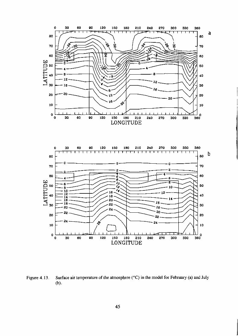
In Figures 4.13 to 4.15 the geographical distribution of some basic atmospheric and oceanic climatic

fields are represented. The results depicted in Figures 4.13 to 4.15 can be, of course, considered only

illustrative ones (due to the highly simplified geographical structure of oceanlland distribution in the

current version of the model), although some of the important features of the real climatic system are

reflected, at least qualitatively. For example, Siberian and Greenland quasi-stationary anticyclones

in surface air temperature (see Figure 4.13), and the Sahara minimum of precipitation (Figure 4.14).

. - -

40 - - July

0 10 20 30 40 50 60 70 80 90 LATITUDE

Figure 4.11. Zonally averaged mass-weighed synoptic variance of the atmospheric temperature ("CZ) for February and July [model and empirical data from Oort and Rasmusson, (1971)l.

. - - February [MODEL] July - February OORT and RASM., 1971 - - July [,",","Land RASM 1971

LATITUDE

Figure 4.12. Zonally averaged synoptic variance of surface air specific humidity for February and July in the model in comparison with empirical data from Oort and Rasmusson (1 97 1).

LONGITUDE

0 0 0 30 60 90 120 150 180 210 240 270 300 330 360

LONGITUDE

Figure 4.13. Surface air temperature of the atmosphere ("C) in the model for February (a) and July (b).

0 0 30 60 90 120 150 180 210 240 270 300 330 360

LONGITUDE

0 30 60 90 120 150 180 210 240 270 300 330 360

80 80 b

70 70

60 60

W n 50 50 3

40 40

4 30 30

20 20

10 10

0 0 0 30 60 90 120 150 180 210 240 270 300 330 360

LONGITUDE

Figure 4.14. Precipitation (mrnlday) for February (a) and July (b), model.

0 0 30 60 90 120 150 180 210 240 270 300 330 360

LONGITUDE

0 30 60 90 120 150 180 210 240 270 300 330 360

80 80 b

70 70

60 60

W C] 50 50 3 b z 40

40

4 30 30

20 20

10 10

0 0 0 30 60 90 120 150 180 210 240 270 300 330 360

LONGITUDE

Figure 4.15. Ocean surface temperature ("C) for February (a) and July (b), model.

47

4.3. Equilibrium response to a doubling of CO, contemt in the atmosphere

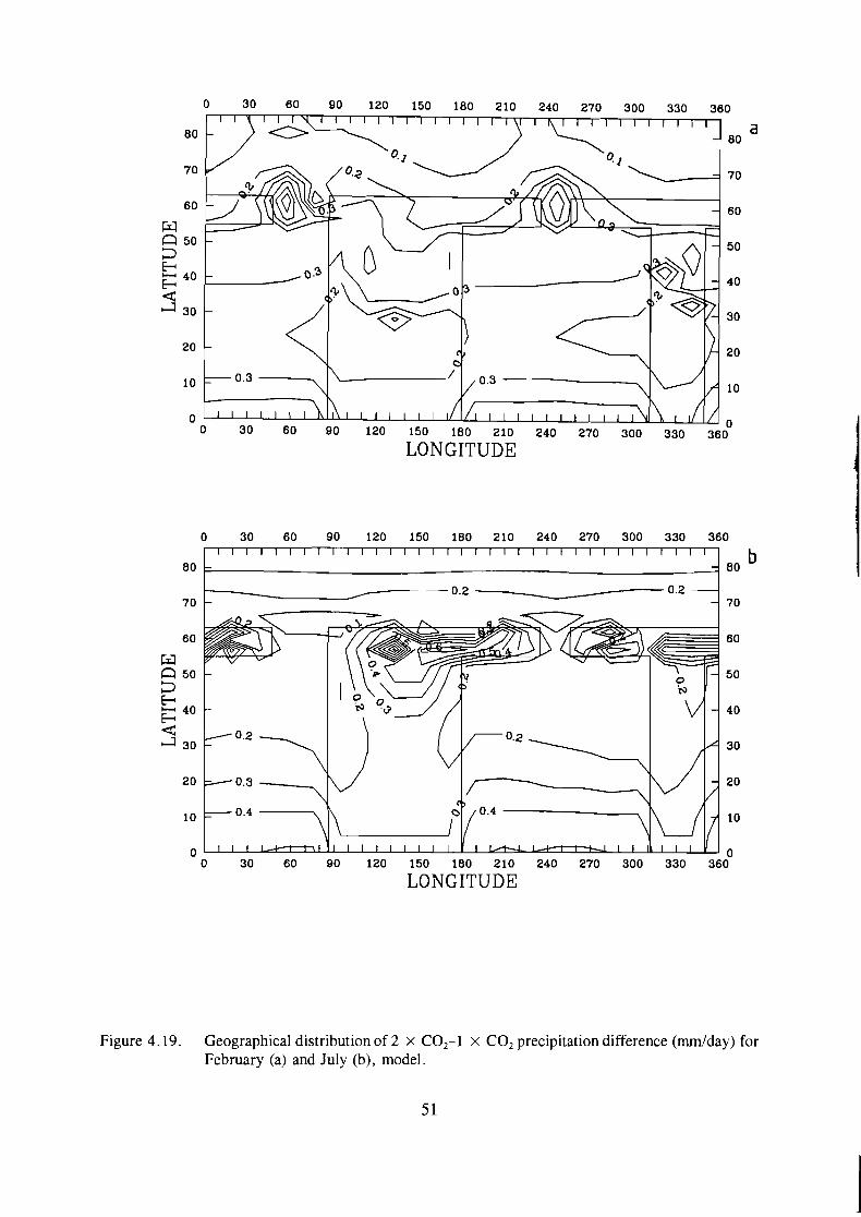
Figures 4.16 to 4.19 illustrate the results of an equilibrium climate response to an instantaneous

doubling of CO, in the atmosphere. The term "equilibrium response" refers to the past 10-year

average of the model results after 100 years of integration starting from present climate conditions.

Also given are the corresponding results of GCMs (GFDL and MPI) runs. Taking into account

noticeable a discrepancy between GCMs results, the model under consideration, as shown in Figures

4.16 to 4.19, can apparently be used as one of the appropriate (informative and computer-efficient)

tools for investigations the problem of the possible greenhouse effect.

4.4. Time dependent run

In Figure 4.20 the model result is depicted of hemispherically averaged temperature transient response

to gradual time dependent increase of greenhouse gas content in the atmosphere according to the 1990

IPCC scenario A, shown in Figure 4.21. The analogous result of the MPI run is given for

comparison. The results of the computations are in rather good agreement, except for the first three

decades; this difference seems to be connected with the problem of "cold start" in MPI GCM (see

Cubasch et al., 1991) and with the hemispherical character of the present version of 2.5-DSCM.

0 10 20 30 40 50 60 7'0 gb I I

LATITUDE

Figure 4.16. 2 x C0,-1 X CO, zonally averaged surface air temperature difference ("C) for February and July in the model and responding results of GFDL runs (Manabe et a l . , 1992).

-2.0 0 10 20 30 40 50 60 70 80 90

LATITUDE

0.0 -

Figure 4.17. 2 x C0,-1 X CO,, zonal mean mass-weighed stratospheric temperature difference ("C) for February and July, model.

- -

w - -

February July / \

U I \

z - w I \

-0.5 - w - Cr, Cr, - C1

n - w -

-1.0 - '3 - ,'- 4 - E w / - a r: - 2 -1.5 - -

-

- GFDL - MPI 2.5-D DSCM

0 10 20 30 40 50 60 '70 80 90 LATITUDE

Figure 4.18. 2 x C02-1 x CO,, mean annual zonally averaged precipitation difference (mrntday) in the model in comparison with corresponding results of GFDL runs (Manabe et al., 199 1, 1992) and MPI (Roeckner, private coinmunication).

30 60 90 120 150 180 210 240 270 300 330 36;

LONGITUDE

0 30 60 90 120 150 180 210 240 270 300 330 360

80 80 b

70 70

60 60

W n 50 50 3

40 b

40

d a 30 30

2 0 20

10 10

0 0 0 30 60 90 120 150 180 210 240 270 300 330 360

LONGITUDE

Figure 4.19. Geographical distribution of 2 X C0,-1 x CO, precipitation difference (mmlday) for February (a) and July (b), model.

Figure 4.20. CO, equivalent concentration for the 1990 IPCC Scenario A (Cubasch, et al., 1991).

200 - - -

000 - - - - -

800 - - -

- -

- - -

600 - - -

- - - -

400

TIME

200

0

Figure 4.21. Time-dependent evolution of hemispherically averaged surface air temperature, ("C) in the model for the 1990 IPCC Scenario A in comparison with the MPI results for the globally averaged temperature (Cubasch et al., 199 1).

- - -

- *

- -

- -

-

- -

- - -

I l l l l l l l l l l l l l l l l l l

1985 2000 2015 2030 2045 2060 2075 TIME

5. Multilayer Isopycnal Largescale Ocean NIodt!l

The present ocean model called MILE Multilayer lsopycnal Largescale ocEan model) is designed for

the simulations of large-scale and long-term ocean processes. The model has the same set of

prognostic variables as traditional oceanic GCMs, but it is much faster that allows to use MILE as a

part of integrated model of climate change. The model was originally developed at Computing Center

of the Russian Academy of Sciences. The previous version of this model was described in Ganopolski

(1991).

5.1 Physical background

There is a number of empirical evidences and models results suggesting that the large-scale oceanic

currents are quasi-isopycnal, i.e. oceanic water masses move practically along surfaces of constant

density, while mixing across isopycnal surface is very slow. It is one of the reasons, why isopycnal

coordinates (ICs), where density is used as a vertical coordinate instead of depth, seem to be more

appropriate for the oceanic modelling than traditional Cartesian (Z-) coordinates. The other advantage

of ICs is that this coordinates allow to describe isopycnal and diapycnal mixing separately, thus

excluding impact of lateral diffusion on diapycnal mixing as it takes place in Z-coordinates models.

In addition, ICs have the ability to adopt their spatial resolution to vertical density gradients and,

thus, one can expect that ICs should be more effective in reproducing of oceanic density structure.

At the same time, application of ICs is more complex and creates many technical problems, especially

with definition of boundary conditions. That is why before recently ICs were of limited use for

oceanic modelling. But now encouraging results in development of ICs models are obtained. Two

OGCMs, based on ICs already published, namely Miami University model ( Bleck et al., 1989, 1992)

and Hamburg OPYC model (Oberhuber 1993a,b).

The other important feature of large-scale oceanic processes is that velocity field is in close

geostrophic balance. It means that nonstationar and nonlinear terms in dynamical equations are

relatively small (they are important only for mesoscale processes and in narrow equatorial zone). This

fact allows to simplify dynamical equations and exclude the terms responsible for fast internal oceanic

5 3

gravity waves. That, in turn, allows to increase significantly time step of integration and reduce the

computational cost of model run. The use of simplify dynamical equations instead of primitive ones

leads to some limitation of the model, but for many purposes this approach is quite justified. The MPI

large-scale OGCM (Maier-Reimer et al., 1987) is the example of successful application of this type

of models for oceanographic and climatic studies.

The oceanic model MILE described below represents the first attempt to design the global scale model

of the ocean climate, based on isopycnal coordinates and quasi-geostrophic approach.

5.2 Model description

The ocean is represented in the model by a set of N vertically uniform layers with thickness h,,

potential temperature q., salinity Si, and current velocity ui (see Figure 5.1). The two upper layers

represent the active ocean layer, that is directly subjected to the seasonal variability. The layer i = 1

is the effective mixed layer (ML)2. The bottom of the second layer coincides with the maximum

during an year ML depth. Thus, the second layer occupies the region, which at a given moment lies

just below ML, but at least once per year is brought into ML. This layer we call buffer layer (BL)

for its intermediate nature. The introducion of the BL allows to overcome a problem arising when ML

directly interacts with the isopycnal layers (Oberhuber, 1993a; Bleck et. al, 1989, 1992). The BL can

disappear when ML deepening, but it immediately restores, when detrainment process (shallowing of

ML) begins. It is important, that water, detrained from ML, enters into BL and does not perturbs the

density of underlying isopycnal layers.

The layers with numbers i=3,N-2 are isopycnal ones, i.e. their potential density pi = const. In a

given gridpoint only isopycnal layers with the numbers i 2 k can exist, where k has to satisfy the

2, Effective M L depth is determined as the depth of uniform layer with heat capacity equal to the sum of the heat capacities of the M L and seasonal thermocline.

derlsity condition p, > p, (or p, > p , , if BL is absent). If this density condition is satisfied also for

the layer with the number k-1, a new layer comes into existence. To keep reasonable vertical

resolution some limitations on layer thickness and depth of the bottom surface are applied. The

thickness of any isopycnal layer cannot be less than 5m. The depth of the bottom of the lowermost i -N-2

isopycnal layer has to satisfy condition ZN, = C hi < Zm= min(H/2,2000m). i - 1

Two bottom layers (i=N-1,N) encompass the ocean water masses lying below the main thermocline

(z > 1-2 km). There are not any restrictions on the density of these layers, thus characteristics of the

deep water masses can take arbitrary values. The thickness of the lowermost layer in contrary is fixed:

hN=2/3(H-Z-). The thickness of layer N-l is determined as 2/3H - G,. Such approach allows to

have reasonable vertical resolution in deep ocean without significant increasing of the number of

isopycnal layers.

Figure 5.1 The vertical structure of the multilayer isopycnal ocean model.

5 5

The model dynamics is described on the basis of linearized stationary equations of the motion. The

horizontal component of the current velocity (which is assumed to be equal isopycnal components of

velocity in the isopycnal layers) is represented as a sum of baroclinic and barotropic components.

For determination of the barotropic components the integral stream function \k is introduced

Following by Sarkisyan (1977) the integral stream function is described by equation

1 AmV2V2\k - ev \k = -- c ~ r 1 ~ 7 ~ + (5.2.2) PO sinp ah fp,

where AM is the coefficient of horizontal viscosity, e=(0.5 If 1 kM)'I2H-', kM is the coefficient of vertical

viscosity, r the earth radius, H the ocean depth, f the Coriolis parameter, P=df/dy, po is the

averaged sea water density, 7 , the surface wind stress, and B represents the terms including the

horizontal derivations of the ocean depth. In the experiment described below, H = const and thus

B = 0. Boundary conditions for equation (5.2.2) are

where M is the number of separate land domains with the coastlines r,. In case M > 1, it is necessary

to use additional equations for determination \km(t) for m> 1. (The stream function at the boundary

of one land domain can be determined arbitrary, e.g. \k,=O). In the present version of the model we

consider two land domain (all continents except Antarctica are combined). The stream function on the

boundary of Antarctic is prescribed on the basis of empirical estimations rather than determined from

special equation. The introducing of additional equation for determination of streamfunction at the

land boundaries is envisaged to be done on the next stage of model development.

The baroclinic components of current velocity u I,= (u Ii,vfi) are described by the equation

with boundary conditions

where subscript "L" means that the space derivation are determined along a layer rather than

horizontally, p'; is the pressure anomaly, computed by vertical density profile

where p, is so-called in situ density related with in situ temperature T,, salinity and pressure by

equation of state

where T,= Ts(T,S,p), p =pgz.

The friction between i and i+ 1 layers ri (for N > i > 0) is given by

and bottom friction is given by

where CD is the bottom drug coefficient.

Evolution of the layer's characteristics is described by the following set of equations:

ah; - + V L (u,hJ = wi-, - W , 9 (5 .2 .9 )

at

a (h . T.) I I + V L ( u i h , q ) + w , - , ~ : , - wi?* = 6 e i T + V L ( A , h , V q ) , (5 .2 .10)

at

a(h.S.) ' + V L (uihiSi) + w, ,S , : , - wiSj' = 6 ~ : + V L (A,h;VS,) (5.2.11)

at

where Ti , ,.Ti are the values of temperature and salinity at the boundary between i and i+ 1 layers,

A, the coefficient of isopycnal diffusion, wi is the relative vertical velocity at the bottom of ith layer,

6Q:=qi.,T - qiT is the heat (the same for salt) uptake into layer i and q: the heat flux at the bottom

of layer i. The fluxes at the ocean surface are determined as follows

where Q, is the heat flux at the free ocean surface, Q, the heat flux through sea ice, f, the sea ice

fraction, c, the water specific heat capacity, So the surface salinity, P the precipitation, E the

evaporation, and R the runoff which is considered as a surface freshwater flux at a given gridpoint.

All horizontal fluxes in equations (5.2.9)-(5.2.11) are assumed to be zero on lateral ocean boundaries.

From the boundary condition of the "rigid lid" at the ocean surface and nonpenetration at the bottom

it directly follows that wo= w,=O. The value w, has the physical sense of entrainment

(detrainment) velocity at the ML bottom. For determination of w, and the fluxes at the bottom of

the ML a modification of Kraus-Turner integral model is used. Following Reasniansky (1976), the

equation for entrainment velocity is written in the form

where

hl h, c g v - F(-) = max(1--, 0 ) , he=- he he CCf '

V . = C ~ ~ ' ~ U , is the surface friction velocity, CD the ocean surface drug coefficient, u, the averaged

module of surface wind speed, p * , the water density below the ML layer, Bo =-g(cyqo, + 0qO2) is the

surface buoyancy flux, a = ap/aT, P =apIaS, C,, C,, C, are the model parameters. To account for

the processes caused by synoptic variability of the surface meteorological conditions, a dependence

of coefficient C, from latitude is introduced following Ganopolski (1988) as

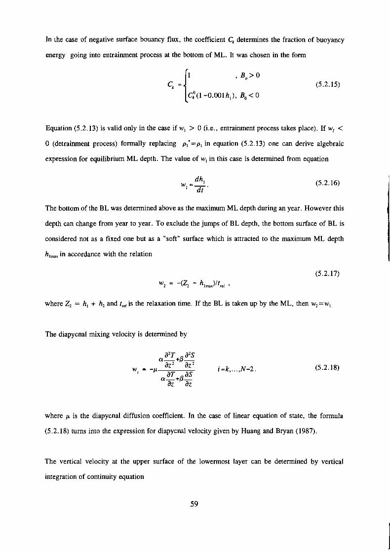
In the case of negative surface bouancy flux, the coefficient C, determines the fraction of buoyancy

energy going into entrainment process at the bottom of ML. It was chosen in the form

9 B*>O

ci(1-0.001 h,) , B, < 0

Equation (5.2.13) is valid only in the case if w, > 0 (i.e., entrainment process takes place). If w, <

0 (detrainment process) formally replacing pIo=p, in equation (5.2.13) one can derive algebraic

expression for equilibrium ML depth. The value of w, in this case is determined from equation

The bottom of the BL was determined above as the maximum ML depth during an year. However this

depth can change from year to year. To exclude the jumps of BL depth, the bottom surface of BL is

considered not as a fixed one but as a "soft" surface which is attracted to the maximum ML depth

h,,, in accordance with the relation

where Z, = h, + h, and tre, is the relaxation time. If the BL is taken up by the ML, then w2=w,

The diapycnal mixing velocity is determined by

where p is the diapycnal diffusion coefficient. In the case of linear equation of state, the formula

(5.2.18) turns into the expression for diapycnal velocity given by Huang and Bryan (1987).

The vertical velocity at the upper surface of the lowermost layer can be determined by vertical

integration of continuity equation

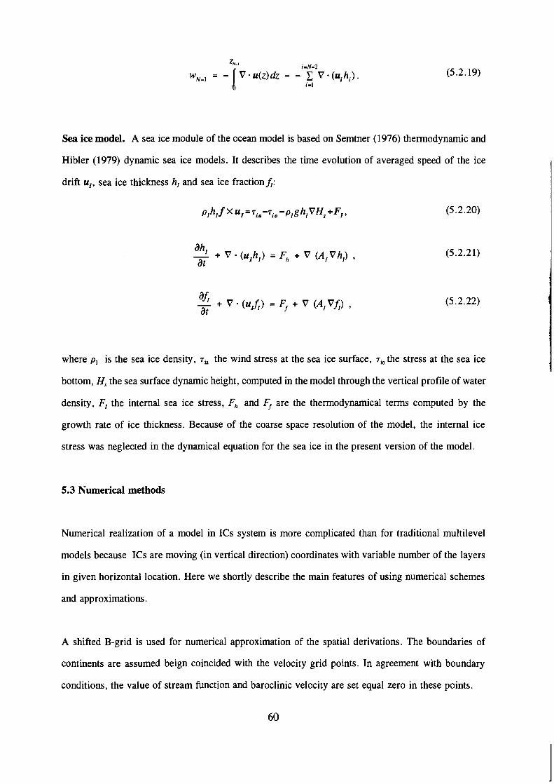
Sea ice model. A sea ice module of the ocean model is based on Semtner (1976) thermodynamic and

Hibler (1979) dynamic sea ice models. It describes the time evolution of averaged speed of the ice

drift u,, sea ice thickness h, and sea ice fractionf,:

where p, is the sea ice density, ria the wind stress at the sea ice surface, T~~ the stress at the sea ice

bottom, H, the sea surface dynamic height, computed in the model through the vertical profile of water

density, F, the internal sea ice stress, F,, and Ff are the thermodynamical terms computed by the

growth rate of ice thickness. Because of the coarse space resolution of the model, the internal ice

stress was neglected in the dynamical equation for the sea ice in the present version of the model.

5.3 Numerical methods

Numerical realization of a model in ICs system is more complicated than for traditional multilevel

models because ICs are moving (in vertical direction) coordinates with variable number of the layers

in given horizontal location. Here we shortly describe the main features of using numerical schemes

and approximations.

A shifted B-grid is used for numerical approximation of the spatial derivations. The boundaries of

continents are assumed beign coincided with the velocity grid points. In agreement with boundary

conditions, the value of stream function and baroclinic velocity are set equal zero in these points.

Equations (5.2.2) for vencally averaged stream function was solved by introducing of vertically

averaged vorticity w=A* and spliting (5.2.2) into two equations, which are solved iteratively:

1 " tg i zV2pdz, AmV2w - EW = -- ~ u r 1 ~ 7 ~ + -- + - Po sinp aX fp,

Two different methods are used for solving equation (5.2.4). One is employed for the points locating

out of equator and the other one for equatorial rows of grid points. As it was mentioned above, the

velocity field out of the narrow equatorial region is in quasi-geostrophic balance. It means that the

Coriolis term and horizontal gradient of pressure are the two major terms, while the friction terms are

relatively small, except for ML where surface wind stress is also important. It allows to solve equation

(5.2.4) iteratively in the form

where F,, F, are friction terms. The superscript "n-1" means that the value is taken from the previous

time step, "*" means the value from the previous iteration, and "**" means new value.

On the equator the Coriolis term is absent, thus pressure gradient should be compensated by the

friction. To solve equation (5.2.4), the so-called "disturbed" dynamical equations (Bryan, 1984) are -

used:

where E 4 1 is the "disturbed" parameter, that slows down the propagation of the fast equatorial

waves. This approach allows to keep time step of integration enough large, while it does not

significantly violate current velocity field.

To compute the horizontal density pressure gradient it is necessary to use horizontal density derivation

instead of along-layer ones. For this end the values of temperature and salinity are interpolated from

the layers onto appropriate horizontal levels such a way to preserve heat and salt contents in the

vertical water column.

The explicit scheme with splitting into physical processes is used for numerical solution of equations

(5.2.9)-(5.2.11). It is known that one of the main problem connected with using of ICs is the abrupt

changes of the layer's thickness. This problem is overcomed by applying for solving the advective part

of equation (5.2.9) the flux correction transport algorithm, developed by Zalesac (1978). For

numerical solution of equations (5.2. lo), (5.2.11) the upstream scheme is used with the mass fluxes

obtained in solving equation (5.2.9).

The other problem arising in ICs model is the keeping of prescribed density of isopycnal layers.

Indeed, if nonlinear equation of state is used, the diapycnal and isopycnal mixing inevitable lead to

perturbation of density along the isopycnal layers (see also discussion of this problem in Oberhuber,

1993a and Bleck et a1.,1992). Two measures are undertaken to keep reper density and at the same

time do not change significantly diapycnal mixing velocity, determined by (5.2.18). First of all, the

numerical approximation of the terms wi and 6Q, are chosen in such form to produce the minimum

distortion of the isopycnal layers density. For this end we use the constrain, that in the case of

linearized equation of state this approximation should gives exact conservation of potential density.

For elimination of small deviation of the layer density from reper value, which appear from

nonlinearity of the equation of state, additional realligment of layers structure is applied. The

characteristics of every isopycnal layer are recalculated by

hi dh, = - P ( ~ , S ; ) -pi'

Po a(T-T+,)+P(S;-S;+,) '

where dh, is the changes of layer thickness, and pi* the reper density of i-th layer. At the end of

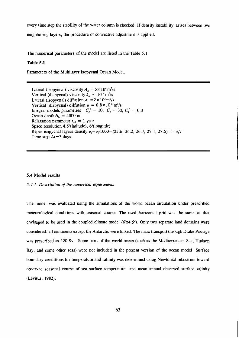
every time step the stability of the water column is checked. If density instability arises between two

neighboring layers, the procedure of convective adjustment is applied.

The numerical parameters of the model are listed in the Table 5.1.

Table 5.1

Parameters of the Multilayer Isopycnal Ocean Model.

Lateral (isopycnal) viscosity A, = 5 X lo4 m2/s Vertical (diapycnal) viscosity k, = lo3 m2/s Lateral (isopycnal) diffusion Ai =2 x 103 m2/s Vertical (diapycnal) diffusion p = 0.8 X lo4 m2/s Integral models parameters C: = 10, Ce = 30, C: = 0.3 Ocean depth Hb = 4000 m Relaxation parameter t,,, = 1 year Space resolution 4.5O(latitude), 6O(longitde) Reper isopycnal layers density ui=pi-1000=(25.6, 26.2, 26.7, 27.1, 27.5) i=3,7 Time step At = 3 days

5.4 Model results

5.4.1. Description of the numerical experiments

The model was evaluated using the simulations of the world ocean circulation under prescribed

meteorological conditions with seasonal course. The used horizontal grid was the same as that

envisaged to be used in the coupled climate model (6Ox4.5"). Only two separate land domains were

considered: all continents except the Antarctic were linked. The mass transport through Drake Passage

was prescribed as 120 Sv. Some parts of the world ocean (such as the Mediterranean Sea, Hudson

Bay, and some other seas) were not included in the present version of the ocean model. Surface

boundary conditions for temperature and salinity was determined using Newtonial relaxation toward

observed seasonal course of sea surface temperature and mean annual observed surface salinity

(Levitus, 1982).

where k is the relaxation parameter. To eliminate the time lag, caused by using of this type of

boundary conditions and to obtain correct amplitude of the seasonal variability of surface temperature,

observed fields of surface temperature and salinity were slightly modified. Seasonal course of surface

wind stress was determined by Hellerman (1982) and averaged module of surface wind from Esbensen

and Kushnir (1980). The seasonal course of sea ice distribution was prescribed on the basis of

empirical data. The heat flux through sea ice was neglected. The model was run from zonally uniform

initial conditions for 1000 years. By the end of integration the ocean achieved the state close to quasi-

stationar with global heat uptake less than 0.05 Wlm.

5.4.2 Oceanic circulation

There is still a lack of knowledge about 3-dimensional field of the oceanic currents, that complicates

the validation of oceanic GCMs. But at least two characteristics can be compared with observations,

namely, surface currents field and interhemisperic and interoceanic mass excahge. The last one is not

the result of direct measurements, but is estimated on the basis of tracers distribution patterns. The

field of the surface and undersurface oceanic currents are shown in Figure 5.2. The model reasonable

reproduces all main gyres of surface circulation, but the absolute values current velocity of western

boundary currents such as Gulfstream and Kurosio are underestimated, that is typical for all GCMs

with rough space resolution. It is interesting that the model enable even reproduces the equatorial

undercurrents (compare Figures 5.2a and 5.2b) and some other features of tropical currents. Some

shortcomings are also obvious. In particulary, the North Atlantic currents does not penetrate into

Arctic basin and Greenland current is very weak. Because of coarse resolution, all coastal upwellings

are very weak, while the intensity of equatorial upwelling is overestimated.

It is recognized now, that interoceanic mass exchange (the so-called conveyor belt) is very important

feature of present climate. The model investigations of the global scale ocean circulation (e.g. Bryan,

1986; Manabe Stouffer, 1988) show that few different stable (or metastable) patterns of conveyor belt

Figure 5.2 Mean annual ocean circulation in the upper mixed layer (a), at the depth 150 m (b), and in the bottom layer (c). Length of velocity vectors is proportional to the square root of the velocity. The vector scale is different for different maps.

0 35

LATITUDE

0 35

LATITUDE

Figure 5 . 3 The vertical structure of the overturning stream function in the Atlantic ocean (a), and Pacific ocean (b).

can exist even under similar external forcing and, that changes of this forcing can dramatically change

the oceanic circulation and, as result, global climate. In this context it is important that our model not

only qualitatively (direction) but also quantative (values of mass fluxes) reproduces zonally averaged

circulation (Fig.5.3). The intensity of deep water formation in Norther Atlantic is about 22 Sv

(lSv= lo6 m3/s) that agrees with empirical estimations on the basis of tracers propagation, and with

the results of other GCMs simulations. The mass flux on the southern boundary of the Atlantic is

about 15 Sv, and approximately the same but with opposite sign on the southern boundary of Pacific.

Figure 5.2c, where the currents field in the bottom layer (the depth about 3 km) is shown, presents

the bottom part of conveyor belt. The water masses forming in the Northern Atlantic then distribute

along western boundary of the ocean to 40 S latitude and then turn eastward and penetrate into Indian

and Pacific ocean, first along western boundaries northward, and then propagate eastward with zonal

flows. This scheme is in a good agreement with the present concept of interoceanic mass echange.

5.4.3 Thermohaline structure of the ocean

Because of Newtonial type of boundary condition using in the model for temperature and salinity,

these two characteristics at the surface are close to observed. The mean annual temperature distribution

at the 500 m depth (approximately the middle of thermocline) is shown in Figure 5.4. Comparison

of this field with empirical data of Levitus (1982) shows that the model slightly overestimates the

temperature at this horizon, especially in equatorial zone. The vertical section of zonally averaged

temperature for individual basins are shown in Figure 5.5. One can see that the model overestimates

the temperature in deep layer by 1-2°C and even more in high latitudes. The reason for Arctic basin

is clear enough: the absence of real bottom relief in Northern Atlantic leads to more intensive than

in reality mass exchange between polar and subpolar part of Atlantic. Comparison of the model

temperature field in the southern part of the ocean leads to conclusion, that the model underestimate

the intensity of deep water formation near Antarctic , and, as the result, the tongue of cold Antarctic

bottom water masses is not pronounced enough.

Figure 5.4 Annual mean potential temperature at 500 meters. (a) model, (b) Levitus (1982).

68

Figure 5.5 The vertical structure of the zonally averaged temperature in the Atlantic ocean (a), and Pacific ocean (b).

69

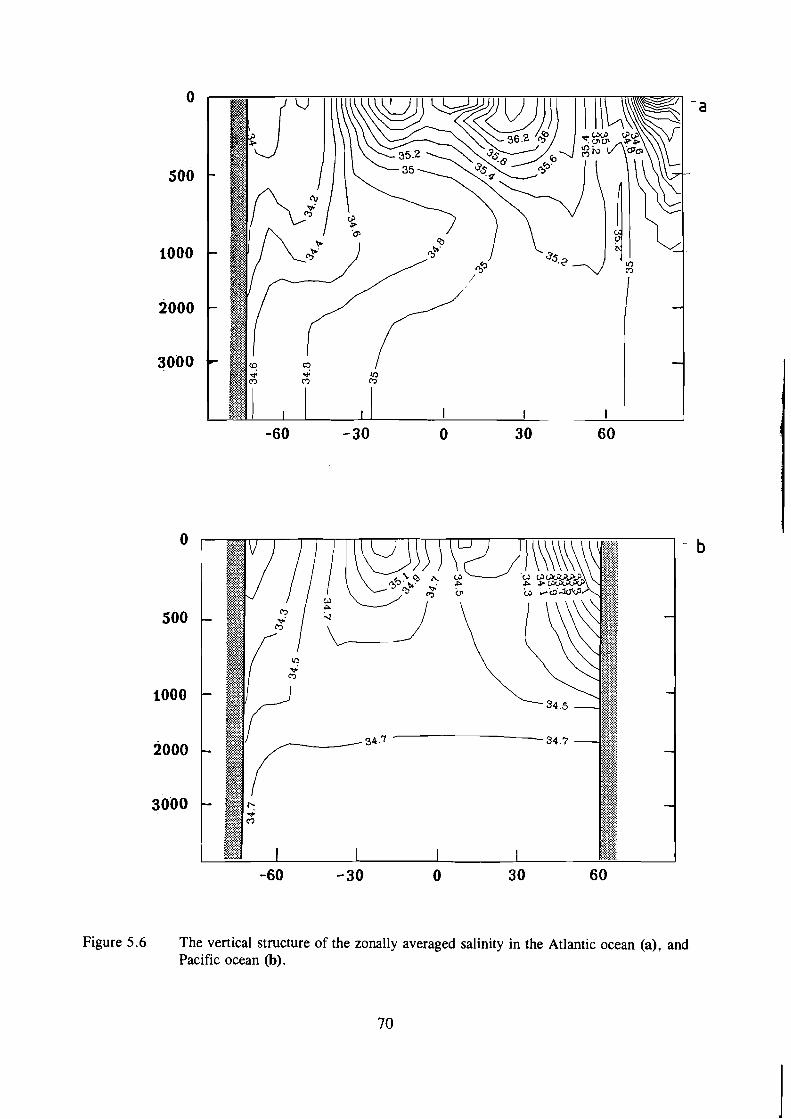
Figure 5.6 The vertical structure of the zonally averaged salinity in the Atlantic ocean (a), and Pacific ocean (b).

Vertical sections of zonally averaged salinity for Atlantic and Pacific are presented in Figure 5.6. The

model correctly reproduces the main features of salinity field. It should be emphasized the presence

of tongue of intermediate relatively fresh water masses in southern hemisphere at the depth 0.5 - 1

krn. This tongue is especially pronounced in Atlantic basin because it overcoveres much more salt

North Atlantic water masses.

5.4.4 Heat and salt balances

Ocean as a part of climate system plays extremely important role in meridional redistribution of heat.

That is why the meridional heat transport in the ocean is one of the major characteristics of the model

simulations. The problem of model validation is complicated by the fact that empirical estimations of

meridional heat transport in the ocean, obtained by different methods, gives significantly different

results. Figure 5.7 shows the results of the model in comparison with empirical estimation of Talley

(1984). The maximum heat transport in the northern hemisphere is about 1.5 PW (1PW = 1015W) and

-2.5 PW in Southern. The Atlantic ocean is characterized by positive heat transport for all latitudes

with maximum in the northern hemisphere close to 1PW and northward flux through equator is 0.4

Pw .

Space distribution of surface annual net heat fluxes is shown in Figure 5.8. The main regions of

oceanic heat release is the Gulfstream and Kurosio and northern part of Northern Atlantic. The

maximum values of heat fluxes here are 100-200 W/m2. In the southern hemisphere the distribution

of heat fluxes more zonal.

Figure 5.9 shows the zonally averaged model freshwater flux to the ocean in comparison with

empirical estimation of Baumgartner and Reichel (1976). One can see that agreement between model

results and empirical data in tropics and in the middle latitudes is quite good. In high latitudes of

southern hemisphere model freshwater flux is as twice greater than observed. The local minimum of

freshwater flux in subpolar region of the northern hemisphere coincides with the region of deep water

formation, where much stronger than observed negative freshwater flux (positive salt flux) is necessary

to support high surface salinity.

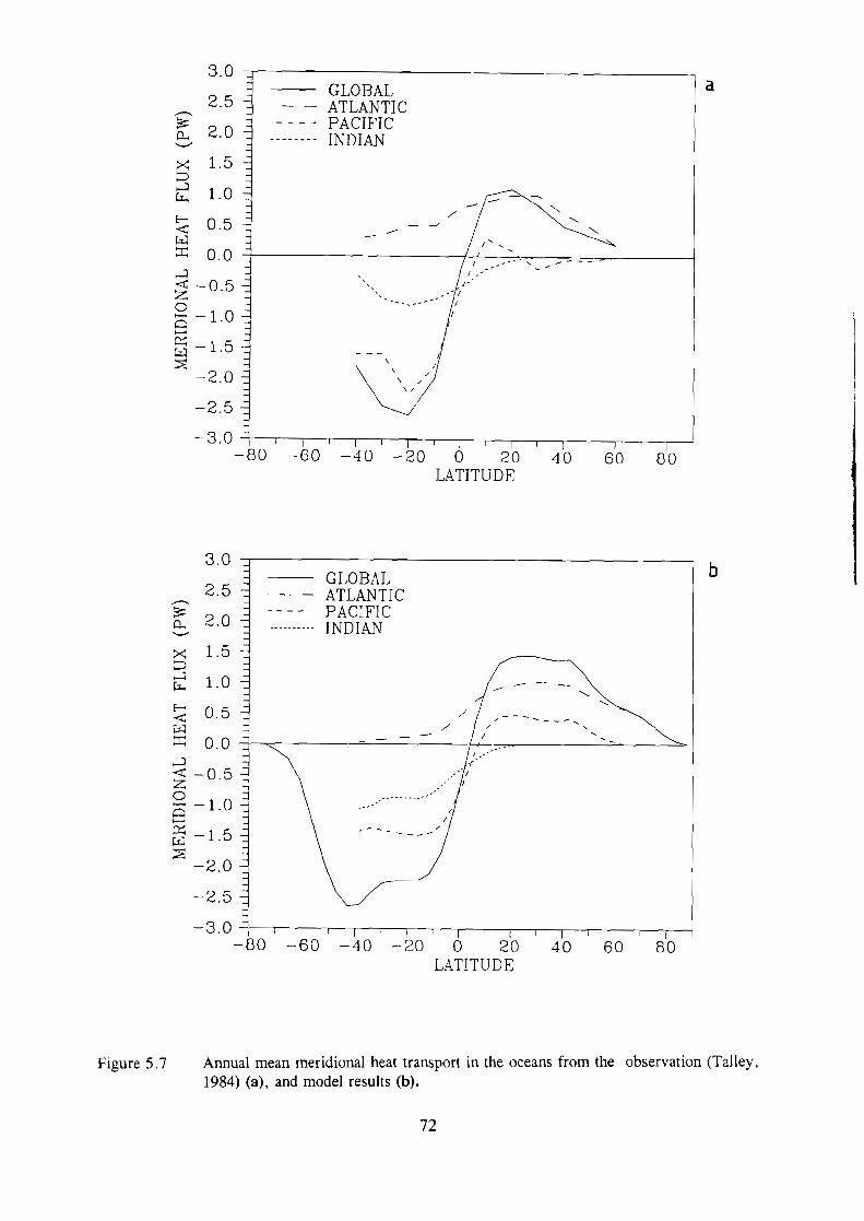
GLOBAL ATLANTIC

- - - - - ----.-----

PACIFIC INDIAN

Figure 5.7 Annual mean meridional heat transport in the oceans from the observation (Talley, 1984) (a), and model results (b).

Figure 5.8 Annual mean ocean surface heat flux (W/m2), positive downward.

Figure 5.9 Annual mean zonally averaged surface fresh water flux in the model (solid line) and Baumgartner and Reitel (1976) (dashed line).

5.4.5 Tracers distribution

One of the important elements of the model validation is the simulation of different tracers

distribution. The radioactive isotope CI4 is one of commonly used tracers. This isotope has half-life

5730 years. Because it is prouuced only in atmosphere, its relative (to C12) concentration in the ocean

shows the resident time of given water masses, that in turn allows to estimate the intensity of water

masses exrhange. In contrast, the bomb-produced radiocarbtm appeared recently (starting from 1955)

and its excess in the upper oceanic layers shows the intensity of short-periodic anomalies penetration

into the ocean.

The experiment with radiocarbon was carried out on the basis of thc . . snic inorganic carbon cycle

model directly embedded into MILE. This model is similar to that described in Maier-Raimer and

Hasselmann (1987). After reaching of climate equilibrium, the carbon cycle model was switched on

and additional run for 1500 years was made. The initial condition for CI2 and CI4 were uniform. The

surface fluxes of carbon (5') and radiocarbon (SI4) were calculated in the form

where p C 0 2 is the partial pressure of carbon dioxide in the ocean ("0") and in the atmosphere ("a"),

X = 0.05 mol m-2 a-I ppm-' is the bulk coefficient.

After reaching of equilibrium state for carbon distribution, the concentration of atmospheric CI2 and

CI4 was changed in accordance with empirical observation starting from 1800 (beginning of industrial

era). The results of radiocarbon simulations for meridional sections of Atlantic and Pacific ocean

corresponding year 1975 in comparison with GEOSECS observations are shown in Fig.5.10 and 5.11.

One can see that the model correctly describes the main features of natural radiocarbon distribution

(deep ocean) and bomb-produced radiocarbon (upper ocean) as well. For example, the minimum value

of radiocarbon in the deep Northern Pacific (the oldest water masses) is about -220 ppm, while

Figure 5.10 Latitude versus depth section of AI4C (per mil) along the western Atlantic GEOSECS track (1974): (top) GEOSECS observations and (bottom) model.

Figure 5.11 Latitude versus depth section of AI4C (per mil) along the western Pacific GEOSECS track (1974): (top) GEOSECS observations and (bottom) model.

observation shows value -240 ppm. Configuration and the depth of zero relative cor.centration isoline

in both oceans reasonable agree with observations. The carbon uptake during last decade (1980-1989)

simulated with the model is 2.5 GtC, that falls in the IPCC 1990 estimation range.

Thus tracers experiments give additional support the idea that MILE model describes the main features

of oceanic climate characteristics reasonable well and can be used as an oceanic module of a coupled

climate model.

6. Integrated Assessment of Climate Change Impacts on European Forests (ICCF):

A Projected Application to Integrated Modelling of Climate Change Impact

A study with the above title was the outcome of a 1992 Working Meeting at IIASA. As outlined in

Chapter 5 of WPl the overall objective of the study is to carry out an integrated assessment of the

impacts of climate change on the European forests for a variety of greenhouse gas emission scenarios.

The study requires a number of models from different disciplines and these models must be modified

and linked in an integrated fashion. At the Working Meeting the 2.5 DSCM was considered for

describing the climate system. It was decided that the DSCM will be used after various medium-term

improvements are introduced (see also Phase 3 of the work schedule presented in section 5.2 of WPI).

The improvements will be part of the global version of the DSCM, which reveals a spatial resolution

6" x 4.5" in the atmospheric and landtocean modules, (for details see Appendix). These

improvements are as follows:

a Introduction of the complete BATS scheme. The increased space resolution of the improved

DSCM would allow to account for all vegetation and soil types foreseen by the BATS scheme

to be taken into account. However, alternative vegetationlland covertsoil schemes (e.g.,

Sellers et al., 1986; Kowalczyk et al., 1991; DucoudrC et al., 1993) will be discussed as well.

a Introduction of a vegetation succession model. It remains to be decided how vegetation

patterns other than European forest ecosystems will be considered in the study. Appropriate

vegetation models have been published, for example, by Bogatyrev (1990, 1991), Kellomaki

et al., (1992), Venevsky (1992).

a Introduction of the magnitudes of the diurnal cycles with respect to the main atmospheric and

land surface climate variables. Among the ecophysiological and forest production models

mentioned in Table 5.2 of WP1, BIOMASS is the model with the highest temporal (daily)

resolution. It needs to be elucidated whether the above parameterization of the duirnal cycle

(following e.g. Saltzmann and Ashe, 1976) will be advantageous to the ecophysiological

modelling work of the study.

Improvement of the DSCM with realistic geography and distribution of surface types will

allow for the production of climate-related output information on surface air temperature and

specific humidity, precipitation, evaporation, solar fluxes, soil moisture, and temperature, as

well as the synoptic and (parameterized) daily variability of these quantities. This output

information may serve as input to the ecophysiological and forest production models

(BIOMASS, G'DAY, Q, SIMA, TAM; see Table 5.2 of WP1) employed by the ICCF Study.

We will make use of a similar superimposing technique as mentioned in Section 5.2 of WP1

for overlaying climate model results over more regional/local observations. The output of the

ecophysiological and forest production models, in turn, can then be used to assess the

biosphere-climate feedback in the DSCM.

As also stated in Section 5.2 of WP1, at least partly, an important question is: how to account for

regions other than Europe and for vegetation other than forests? As an additional alternative to these

in the above-mentioned Section, we see the possibility of using a Holdridge type (see, e.g., Leemans,

1990) or time-lag succession vegetation schemes (see, e.g . Bogatyrev, 1990, 199 1 ; Kellom&i et al.,

1992) combined with the large-scale soil geochemistry schemes (see, e.g., Krapivin et al., 1982;

Tarko et al., 1989). This would allow us to incorporate the parameterization of succession processes

with different characteristic time scales depending on ecosystems in the DSCM.

We see several important advantages in linking the DSCM with the hierarchy of the above-mentioned

ecophysiological and forest production models. Firstly, the detailed ecophysiological models can be

used for validating and improving the understanding of global-scale vegetation and geochemical cycles.

Secondly, being interactively linked with the DSCM, these models can help to refine the

climatetbiosphere response, at least for Europe as a whole.

In the process of developing the DSCM we are planning to pay special attention to investigating the

model's sensitivity to uncertainties of vegetation and other parameters and to the uncertainties of

climate output information on vegetation processes. The fact that the DSCM is much more computer

efficient than GCMs, permits us to produce a great number of sensitivity experiments.

Thus, not only probable, but also sustainable scenarios in respect to the evolution of European forests

or, vice versa, the collapse of forest ecosystems can be investigated. Moreover, specific clirnate-

ecosystem behaviors such as bifurcations, instabilities, and large-scale/long-term structural

reformations can also be elucidated.

7. Conclusions

The objective of Part I1 of the Working Paper is twofold: first, to summarize the present status and

improved version of the 2.5-DSCM; and, second, to describe the envisaged position of this climate

model in the context of an integrated model of climate change. The latter model aims at a holistic

approach that helps policy analysts to rapidly assess timedependent changes in regional ecology, with

feedback, resulting from various greenhouse gas emission policies.

Special attention must be paid to the climate module of an integrated model of climate change because

it can easily play a dominant role within the integrated model in terms of running time. Attempts

were made to facilitate the understanding of the needs of both environmental impact modellers or

assessors, on the one hand, and policy analysts, on the other hand. In fact, even among themselves

their requirements for an integrated model of climate change can be antagonistic to each other. For

example, ecological impact models might require a spatial resolution, which is beyond that of GCMs,

and, at the same time, uncertainty in climate model output that can only be satisfied by GCMs or less

sophisticated climate models on a coarser resolution scale, while policy experts are essentially asking

for the possibility in assessing the impact of a wide variety of emission strategies, i.e., for a quick

turnaround time of the integrated model.

For many applications this problem can be solved by creating a set of climate models of graded

complexity that are computer-efficient and suitable for a wide variety of policy and impact analyses.

As outlined in WP1 two independent approaches, the top-down approach and the bottom-up approach,

were identified in regard to the design of the climate module. In our opinion both approaches

complement each other; it would be worthwhile pursuing them in parallel. Carefully considering the

pros and cons of both approaches, especially the fact that the top-down approach requires frequent

access to a GCM, we come to the conclusion that IIASA ought to pursue the bottom-up approach,

albeit a somewhat reduced flexibility. The bottom-up approach seems to offer a more restricted choice

with respect to diversity of climatic information and its spatial and temporal resolution than the top-

down approach. However, this might be compensated for by some advantages of the bottom-up

approach, e.g., the somewhat easier implementation of new feedbacks, if appropriate parameterizations

exist or can be derived. The 2-D ZCM (described in WPl) and the 2.5-DSCM are meant for

integrated modelling of climate change impacts which makes use of the bottom-up approach. Both

climate models are at the upper level of complexity (in terms of spatial and temporal resolutions) out

of a set of four climate models that are available or under development at IIASA.

A number of model experiments have been performed which document the present status of the 2.5-

DSCM. It simulates today's zonal means of the basic climatic characteristics (temperature,

precipitation, evaporation, meridional heat transport, and others) reasonably well and realistically

reflects their geographical and seasonal distribution. For a doubling of atmospheric CO, the DSCM

reveals a climate sensitivity of about 2.5 K and an increase of the hemispherically averaged

precipitation rate of about 8 % . The climate sensitivity lies within the range estimated by the IPCC

(1.5 to 4.5 K) the ratio of precipitation increase to climate sensitivity agrees well with GCM results

(Houghton, et al., 1990).

The 100-year integration (1985'-2084) employing IPCC's 1990 (C0,-equivalent) concentration

Scenario A was made. Our results are in rather good agreement with the recently published results

of the MPI GCM.

Finally following WPl, Part I1 of the Working Paper sheds light on applying the DSCM to an

Integrated Assessment of Climate Change Impacts on European Forests (ICCF). The respective

integrated model comprises a series of models - from policy-oriented accounting tool for greenhouse

gas emissions and concentrations to climate model to sequence of dovetailing ecophysiological and

forest production models to socioeconomic tools with feedback.

An important feature of the integrated assessment using the 2.5-DSCM is that the ecophysiology of

a single plant up to that of aggregated forest ecosystems will be considered. An approach employing

the DSCM, in combination with a suitable superimposing technique aiming at bridging the spatial

resolution gap between the DSCM, on the one hand, and the ecophysiological and forest production

models, on the other hand, is considered.

The main types of infomation which the DSCM is anticipated to pass on to the ecophysiological and

forest production models are surface air temperature and specific humidity, precipitation, evaporation,

solar fluxes, soil moisture, and temperature, as well as the synoptic variability and (in terms of

parameterized amplitudes) daily cycle of these quantities. This information seems to compliment very

well the large-scale information needs of the ecophysiological and forest production models of the

ICCF study and thus help to achieve the overall objective of this study.

APPENDIX. The structure of the global-scale coupled climate model and preliminary results

The first step in application of the 2.5-DSCM for the purposes of integrated assessment is the the

extension of the model to the global scale, including of realistic geography and coupling with

multilayer isopycnal ocean model MILE, described in Chapter 5. A global-scale version of the model

has the space grid resolution of 4.5" latitude and 6" longitude (see Figure A. 1). This space grid allows

to resolve the main features of oceanlland distribution and major patterns of surface land types. This

space resolution is the same order as used in the most of climatic GCMs. For implementation of MILE

as an oceanic module of coupled climate model a few improvements are necessary. They are 1.

incorporation of bottom topography and specific description of the shelf zones and internal water

basin; 2. parameterization of the mass exchanges through passages which can not be resolved on the

space grid but nevertheless are important for heat and salt balances of the oceans.

At the first stage of model development the atmospheric and oceanic models will be linked through

the heat and momemtum fluxes. The using of fresh-water fluxes computed by atmospheric model

needs futher improvements. The most of the present GCMs use for climate investigation so-called

flux adjustment procedure to exclude climatic trends after coupling atmospheric and oceanic modules.

Since justification of implementation of such procedure is not fairly satisfactory, our ultimate objective

is to have a completely coupled system without any fluxes adjustment. The time step in the

atmospheric module as well as in the oceanic one will be 3 days and both modules will interact

synchronously. The estimated computer time requirements for the global version of the model are

approximately 1 hour of SPARC-2 station per 3 years of the model integration that is still acceptable

for the purposes of integrated assessment studies.

The results of simulation on the base of global scale oceanic GCM MILE are represented in Chapter

5. Here some of the preliminary results of present climate simulations with global scale version of 2.5-

D DSCM will be present. The seasonal course of sea surface temperature and sea ice extension were

prescribed on the basis of empirical data.

Zonally averaged distribution of surface air temperature for two seasons is shown in Figure A.2 in

comparison with empirical data (Landsberg, 1985). One can see that model results are in a reasonable

agreement with observations for both seasons and both hemispheres. Geographical distribution of

surface air temperature is shown in Figures A.3 and A.4.

Zonally averaged precipitation distribution is shown in Figure A.5. The model correctly describes the

location and absolute values of tropical maximum of precipitation and some other important features

of precipitation patterns. The most significant discrepancy between model and observation takes place

in February in high latitudes of southern hemisphere, where the model underestimates precipitation

approximately by a factor of 2. Figure A.6 shows the zonally averaged cloudiness which is close to

observed values in both seasons.

Thus, even preliminary results obtained with the global scale DSCM shows the model ability to

reproduce important features of present climate reasonably well.

Figure A. 1 Grid spacing and geographical land ocean distribution envisaged to be used in the global version of nonzonal climate model.

e Am- \ 7

- February July

d l - - I

I - 4 0 1 1 1 , , , 1 1 1 1 , 1 , , , , 1 1 , , , , , 1 , , , ,

-90 L75 -60 -45 -30 -15 0 15 30 45 60 7k E

- I LATITUDE

Figure A.2 Zonal mean surface air temperature of the atmosphere ("C) for February and July in the model and as derived from observations.

Figure A.3 Surface air temperature of the atmosphere ("C) in the model (a) and empirical data (b) for February.

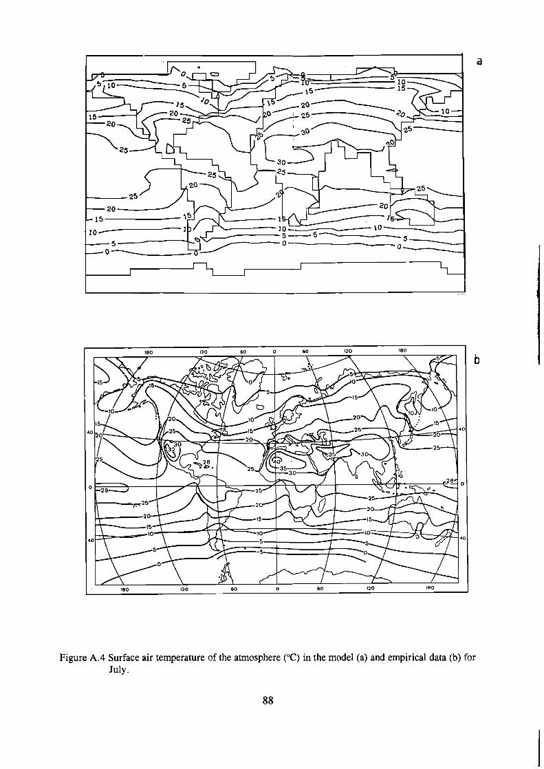
Figure A.4 Surface air temperature of the atmosphere ("C) in the model (a) and empirical data (b) for July.

- F e b r u a r y JAEGER, 1976) 0 - - July JAEGER, 1976)

h

F e b r u a r y MODEL - - July MODEL]

n

I

LATITUDE

Figure A.5 Zonal mean precipitation (mm/day) for February and July in the model and corresponding empirical data.

0.0 ' 1 , I I , , , I , , , , , -$o -?10 -50 -30 -10 10 30 50 70 90

LATITUDE

Figure A.6 Zonal mean total cloud amount for February and July in the model in comparison with empirical data.

REFERENCES

Adem, J . , 1964, On the physical basis for the numerical prediction of monthly and seasonal temperature in the troposphere-ocean-continent system, Mon. Wea. Rev., 92:91- 104.

Ardanuy, P.E., Stowe, L.L., Gruber, A., Weiss, M., and Long, C.S., 1989, Longwave cloud radiative forcing as determined from Numbus-7 observations, Journal of Climate, 2:766-799.

Baumgartner, A., and Reichel, E., 1975, The World Water Balance, Elsevier, 179 pp.

Betts, A., 1986, A new convective adjustment scheme. Part 1: Observations and theoretical basis. Part 2: Single column tests using GATE wave, BOMEX ATEX and Arctic air mass data sets, Quart. J. Roy, Meteorol. Soc. , 112:677-709.

Bleck, R., Hanson, H.P., Hu, D., and Kraus E.B., 1989, Mixed-layer-thermocline interaction in a three-dimensional isopycnic coordinate model, J. Phys. Oceanogr. , l9 : 1417-1439.

Bleck, R., Rooth, C., Hu, D., and Smith, L.T., 1992, Salinity-driven thermocline transients in a wind- and thermohaline-forced isopycnic coordinate model of the North Atlantic, J. Phys. Ocean., 22:1486-1505.

Bogatyrev, B.G., 1990, Modeling of plant communities dynamics on the tundra-taiga boundary under climate changes, in Proceedings of the International Symposium Northern forests: State, dynamics, anthropogenic influence, Moscow, v. iii, p. 12-1 8 [in Russian, English resume].

Bryan, F., 1986, High latitude salinity effects and interhemispheric thermohaline circulations. Nature, 305: 301-304.

Bryan, K., 1984, Accelerating the convergence to equilibrium of ocean-climate models, J . Phys. Oceanogr., 14: 663-673.

Budyko, M.I., 1969, The effect of solar radiation variations on the climate of the earth, Tellus, 21:611-619.

Carissimo, B.C., Oort, A.M., and Vonder Haar, T.H., 1985, Estimating the meridional energy transports in the atmosphere and the ocean, J . Phys. Oceanogr., 15: 82-91.

Cox, C., and Munk, W., 1956, Slopes of the sea surface deduced from photographs of the sun glitter, Bull. Scripps Inst. Oceanogr. , 6:401-488.

Cubasch, U., Hasselmann, K., Hock, H., Maier-Reimer, E., Mikolajewicz, U., Santer, B.D., and Sausen, R., 1991, Time-dependent Greenhouse Warming Computations with a Coupled Ocean-atmosphere Model, Max-Planck-Institut fiir Meteorologie, Hamburg, Report No. 67, ISSN 0937-1060, 18 p.

Deardorff, J .W., 1967, Empirical dependence of the eddy coefficient for heat upon stability above the lowest 50 m., J . Appl. Meteor., 6:631-643.

Deardorff, J.W., 1968, Dependence of air-sea transfer coefficients on bulk stability, J. Geophys. Res., 73: 2549-2557.

Deardorff, J.W., 1972, Parameterization of the planetary boundary layer for use in general circulation models, Mon. Wea. Rev., 100(2):93- 106.

Dickinson, R.E., Henderson-Seller, A., Kennedy, P.J., and Wilson, M.F., 1986, Biosphere-Atmosphere Transfer Scheme (BATS) for the NCAR Community Climate Model, NCARJTN-275 + STR, NCAR TECNICAL NOTE, Boulder, Colorado, 69 p.

Dobryshman, E.M., 1980, Dynamics of the equatorial atmosphere, L., Hydrometeoizdat, 287 p. [in Russian].

Doronin, Yu.P., 1969, Thermal Interaction of the Atmosphere and the Hydrosphere in the Arctic, Israel Program for Scientific Translations, Jerusalem, 1970, 244 p. [NTIS N71-156681.

DucoudrC, N.I., Laval, K., and Perrier, A., 1993, SECHIBA, a new set of pararneterizations of the hydrolic exchanges at the land-atmosphere interface within the LMD atmospheric general circulation model, Journal of Climate, 6:248-273.

Dushkin, P.K., Lomonosov, E.G., and Luinin, Yu.N., 1960, A test of numerical humidity, cloudiness and precipitation forecast method using a computer, Meteorology and Hydrology, No. 12, p. 3-12 [in Russian].

Esbensen, S.K., and Y .Kushnir, 1981, The heat budget of the global ocean: an atlas based on estimates from surface marine observations. Climate Research Institute, Oregon State University, Report N 29.

Feigelson, E.M., ed., 1989, Radiative properties of cirrus clouds, M., Nauka, 224 p. [in Russian].

Ganopolski, A.V., 1988, A role of wind synoptical variability in formation of the vertical thermal structure of the upper ocean layer, Marine Hydrophysical J . , N 6: 23-28 [in Russian].

Ganopolski, A.V., 1991, A multilayer model for the ocean seasonal variability, Oceanology, 3 1: 892- 897 [in Russian].

Garrat, J.R., 1977, Review of drag coefficients over oceans and continents, Mon. Wea. Re\,. , 105:915-928.

Golitsyn, G. S . , and Demchenko, P.F., 1980, Statistical properties of a simple energy balance climate model, Izvestia Acad. Sciences USSR, FAO, 16(12): 1235- 1242 [in Russian].

Goudriaan, J., and Ketner, P. , 1984, A simulation study for the global carbon cycle. including man's impact on the biosphere, Climate Change, 6: 167-192.

Hansen, J., Russel, G., Rind, D., Stone, P., Lacis, A., Lebedeff, S. , Ruedy, R., and Travis, L. , 1983, Efficient three-dimensional global models for climate studies: Models I and 11, Mot!. Wea. Rev. , 11 l(4): 609-662.

Hartmann, D.L., Ramanathan, V., Berrior, A., and Hunt, G.E., 186, Earth radiation budget data and climate research, Reviews of Geophysics, 24(2):439-468.

Hasselmann, K., and von Storch, H., 1992, Concept of a Global-Environment-and-Man (GEM) model, Max Planck Institut fiir Meteorologie, Second International Conference on Modelling of Global Climate Change and Variability, Abstracts, p. 29.

Hellerrnan, S. and M.Rosenstein, 1983,Normal monthly wind stress over the world ocean with error estimates, J. Phys. Oceanogr., 13: 1093- 1 104.

Hibler W.D., 1979, Dynamic thermodynamic sea ice model, J. Phys. Ocean., 17: 815-846.

Holdridge, L.R., 1967, Life zone ecology, Tropical Science Center, San Jose.

Holland, W.R., 1977, Ocean general circulation models, The Sea, 6(5):3-45.

Houghton, J.T., Jenkins, G.J., and Ephraums, J.J., eds., 1990, Climate Change. The IPCC Scientific Assessment, Cambridge University Press, 365 p.

Hsiung, J., 1985, Estimates of global oceanic meridional heat transport, J. Phys. Oceanogr. 15: 1405-1413.

Huang, R.X., and Bryan K., 1987, A multilayer model of the thermohaline and wind-driven circulation, J. Phys. Ocean., 17: 1909-1924.

Hurnmel, J.R., and Kuhn, W.R., 1981, Comparison of radiative-convective models with constant and pressure-dependent lapse rates, Tellus, 33: 254-26 1.

Jager, L., 1976, Monatskarten des Niederschlags fiir die game Erde, Bericht Deutscher Wetterdienst, 18(139):38.

Kamenkovitch, V.M., 1973, The principles of the ocean dynamics, L., Hydrometeoizdat, 240 p. [in Russian].

Karol', I.L., and Rozanov, E.V., 1982, Radiative-convective climate models, lzvestia Acad. Sciences USSR, FAO, 18(11): 1179-1 191 [in Russian].

Kellomaki et al., 1992, A simulation model for the succession of the boreal forest ecosystem, Silva Fennica, 26(1): 1-18.

Kitaigorodsky, S. A., and Miropolsky, Yu.Z., 1970, On the theory of the active layer of open ocean, lzvestia Acad. Sciences USSR, FAO, 6(2) : 178- 1 88 [in Russian].

Kowalczyk, E.A., Garratt, J.R., and Krumrnel, P.B., 1991, A soil-canopy scheme for use in a numerical model of the atmosphere - 1D stand-alone model, CSIRO, Australia, Technical Paper No. 23, CSIRO division of atmospheric research, 56 p.

Krapivin, V.F., Sviredjev, Yu.M., and Tarko, A.M., 1982, Mathematical modelling of the global biosphericprocesses, M. Nauka, pp. 272 [In Russian].

Kraus, E.B., and Turner, J.S., 1967, A one-dimensional model of the seasonal thermocline - 11. The general theory and its consequences, Tellus, 19(1):98-105.

Landsberg, H.E., (ed), 1985, World survey of climatology, V 1A: General climatology IA, Elsevier, Amsterdam - London - New York - Tokyo, 224 p.

Leemans, R., 1990, Possible change in natural vegetation patterns due to a global warming. IIASA, Laxenburg, Austria, WP-90-08.

Lernke, P., 1977, Stochastic climate models. Part 3. Application to zonally averaged models, Tellus, 29(5):387-392.

Lorenz, E.N., 1967, The nature and theory of the general circulation of the atmosphere, W0, 161p.

Maier-Reimer, E., and Hasselman, K . , 1987, Transport and storage of CO, in the ocean - an inorganic ocean-circulation carbon cycle model. Climate Dynamics, 2: 63-90.

Maier-Reimer, E., Hasselman, K . , Olbers, D., and Willebrand, J., 1987, An ocean circulation model for climate studies. Techn. Report, Max-Planck-Institut fiir Meteorologie, Hamburg.

Makhover, Z.M., 1983, Climatology of the tropopause, L., Hydrometeoizdat, 255 p. [In Russian].

Manabe, S., and Bryan, K . , 1972, Climate and ocean circulation, L., Hydrometeoizdat, 192 p. [in Russian].

Manabe, S . , Stouffer, 1988, Two stable equilibria of a coupled ocean-atmosphere model, J. Climate, 1:841-866.

Manabe, S., Stouffer, R.J., Spelman, M.J., and Bryan, K . , 1991, Transient response of a coupled ocean-atmosphere model to gradual changes of atmospheric CO,. Part I: Annual mean response, J. Climate. 4:785-818.

Manabe, S., Spelman, M.J., and Stouffer, R.J., 1992, Transient responses of a coupled ocean-atmosphere model to gradual changes of atmospheric CO,. Part 11: Seasonal response, Journal of Climate 5 : 105-126.

Manuilova, N.I., Mokhov, I.I., and Petoukhov, V . K . , 1992, Estimation of the influence of hydrological cycle characteristics on the sensitivity of global climate to anthropogenic impacts, Meteorology and Hydrology, No. 1, p. 44-5 1 [in Russian].

Matveyev, Yu.L., and Matveyev, L.T. , 1984, Physical-statistical analysis of the global cloudiness field, Izvestia Acad. Nauk USSR, FAO, 20, No. 11, 1042-1054 [In Russian].

McMurtrie, R.E. et a l . , 1992, Modifying existing forest growth models to take account of effects of elevated CO,, Aus. J. Bot., 40:657-677.

Moeng, C.-H., and Randall, D.A., 1984, Problems in simulating the stratocumulus-topped boundary layer with a third order closure model, J.A.S. , 41: 1588-1600.

Mokhov, I.I., and Petoukhov, V . K . , 1978, Parameterization of thermal radiation fluxes for climatic models, Preprint of the Institute of Atmospheric Physics of the Academy of Sciences of the USSR, Moscow, No. 3, 34 p. [in Russian].

Mokhov, I.I., Mokhov, O.I., Petoukhov, V . K . , and Khairullin, R.R., 1992, Tendencies of eddy activity trends in the atmosphere under global climate changes, Izvestia Acad. Russia, FAO, 28(1): 11-26 [in Russian].

Mokhov, I.I., Petoukhov, V . K . , and Rusin, N.N., 1983, Sensitivity of mass and heat exchange of the Antarctic sheet surface to climatic changes, Meteorology and Hydrology, No. 11, p. 53-59 [in Russian].

Monin, A.S., and Yaglom, A.M., 1965, Statistical hydrodynamics. Part I, M., Nauka, 64.0 p. [in Russian].

Monin, A.S., and Yaglom, A.M., 1967, Statistical hydrodynamics. Part 11, M., Nauka, 720 p. , [in Russian].

Munk, W .H., 1950, On the wind-driven ocean circulation, J . Meteorol., 7(2):79-93

Needler, G.T., 1967, A model for thermohaline circulation in an ocean of finite depth, J . Marine Res., 25(3):329-343.

Needler, G.T., 197 1, Thermocline models with arbitrary barotropic flow, Deep-Sea Res., 18(9):895-904.

North, G . , 1975, Theory of energy balance climate models, J . Atmos. Sci., 32:2033-2043.

Oberhuber, J . , 1993a, Simulation of the Atlantic circulation with a coupled sea ice-mixed layer- isopycnal general circulation model.Part I: Model description, J.Phys. Oceanogr., 23: 808-829.

Oberhuber, J . , 1993b, Simulation of the Atlantic circulation with a coupled sea ice-mixed layer- isopycnal general circulation model.Part I: Model experiment, J . Phys. Oceanogr., 23: 830-845

Oort, A.H., and Rasmusson, E.M., 1971, Atmospheric circulation statistics, NOAA Prof. Pap. 5 , Rockville, pp. 323.

Oort, A.H., 1983, Global atmospheric circulation statistics, 1958-1973, NOAA Prof. Pap. 14, Rockville, pp. 180.

Ou, S .-C.S., and Liou, K. -N., 1984, A two-dimensional radiation-turbulence climate model. I. Sensitivity to cirrus radiation properties, J. Atmos. Sci., 41:2289-2309.

Pedlosky , J . , 1979, Geophysical Fluid Dynamics, Springer-Verlag, New York, 6 19 p.

Petoukhov, V.K., 1976, Zonally averaged model of heat and moisture exchange in atmosphere underlying ocean layer system, Izvestia Acad. Sciences USSR, FAO, 12(11): 1130-1 142 [in Russian].

Petoukhov, V.K., 1980, Zonal climatic model of heat and moisture exchange in the atmosphere over underlying layer, in Physics of the atmosphere and the problem of climate, G.S. Golitsyn, and A.M. Yaglom, eds., M., Nauka, p. 8-41 [in Russian].

Petoukhov, V.K., 1990, Thermodynamical approach to macroturbulent heat, humidity and momentum transfer description in climatic models, in Investigations of eddy dynamics, atmospheric energetics and the problem of climate, E.G. Nikiforov and N.Ph. Romanov, eds., L., Hydrometeoizdat, p. 156-171 [in Russian].

Petoukhov, V.K., 199 1, Dynamical-statistical modelling of large-scale climatic processes, Ph. D. B. Leningrad Hydrometorological Institute, St. Petersburg, 431 p. [in Russian].

Petoukhov, V.K., and Manuilova, N.I., 1984, Estimation of some climate-forming factors in a simple thermodynamical climate model, Meteorology and Hydrology, No. 10, p. 3 1-37 [in Russian].

Polglase, P.J., and Wang, Y .P., 1992, Potential C0,-enhanced carbon storage by the terrestrial biosphere, Aus. J. Bot., 40:641-656.

Polyak, I.I., 1975, Numerical methods of observation analysis, L., Hydrometeoizdat, 2 12 p. [in Russian].

Rasool, S.I., and Schneider, S.H., 1971, Atmospheric carbon dioxide and aerosols: Effects on large increases on global climate, Science, 173: 138-141.

Resnjansky, Yu.D., 1976, Parameterization of dissipation of integral energy in the upper ocean layer, Izvestia USSR Academy, 1 1 : 726-733 [In Russian].

Saltzman, B., 1978, Statistical-dynamical models of the terrestrial climate, Adv. of Geophys., 20: 183-304.

Saltzman, B., and Ashe, S., 1976, The variance of surface termperature due to diurnal and cyclone- scale forcing, Tellus, 28(4):307-322.

Sarkisyan, A.S., 1977, Numerical analysis and forecast of sea currents, Hydrometeoizdat, 182 p. [in Russian].

Schlesinger, M.E., Oh, J.-H., and Rosenfeld, D., 1988, A parameterization of the evaporation of rainfall, Mon. Wea. Rev., 116, No. 10, 1887-1895.

Sellers, P.J., Mintz, Y ., Sudy, C., and Dalcher, A., 1986, A Simple Biosphere Model (SiB) 'for use within general circulation models, J . A . S . , 43(6):505-531.

Sellers, W.D., 1969, A climate model based on the energy balance of the earth-atmosphere system, J . Appl. Meteorol. , 8(3): 392-400.

Semtner, A.J., 1976, A model for the thermodynamic growth of sea ice in numerical investigations of climate, J. Phys. Oceanogr., 6: 409-425.

Talley, L.D., 1984, Meridional heat transports in the Pacific Ocean, J. Phys. Oceanogr. 14: 231-241.

Tarasova, T.A., 1992, Evaluation of aerosol and cirrus cloud single scattering albedo using ground- based radiation measurements, Proceedings of International Radiation Symposium, Tallinn, August 1992, p. 10-17.

Tarasova, T.A., and Feigelson, E.M., 1981, An accounting of aerosol effects in radiative heat exchange, Izvestia Acad. Sciences USSR, FAO, 17(12):1330-1333 [in Russian].

Tarko, A.M., Bogatyrev, B.G., Kirilenko, A.P., and Udalkina, M.V., 1989, Modelling of the global and regional changes of carbon circle in the biosphere, Preprint of the Computing Center USSR Acad. of Sci., Moscow, pp. 39 [In Russian].

Veltischev, N. N. , Tarasova, T.A., and Frol'kis, V.A., 1990, Practical methods of accounting of solar radiation absorption by water vapor in different radiative schemes, Preprint of the Institute of Atmospheric Physics of the Academy of Sciences of the USSR, Moscow, No. 1, 27 p. [in Russian].

Venevsky, S.V., 1992: Terrestrial vegetation in Asia as one of possible regulators in climate change. Proceedings of the 8th Conference of the International Society for Ecological Modelling, Kiel, p. 201-21 1.

Vinnichenko, N.K., Pinus, N.Z., Schmeter, S.M., and Shur, G.N., 1968, Turbulence in free atmosphere, L., Hydrometeoizdut, 336 p. [in Russian].

Vimikov, K.Ya., 1986, Sensitivity of climate, L., Hydrometeivzdut, 224 p. [in Russian].

Wyngaard, J.C., and Le Mone, M.A., 1980, Behaviour of the refractive index structure parameter in the entraining convective boundary layer, J.A.S., 37:1573-1585.

Zilitinkevitch, S.S., 1970, Dynamics of the atmospheric boundary layer, L., Hydrometeoizdat, 291 p. [in Russian].

Zalesak, S., 1979, Fully multidimensional flux-corrected transport algorithms for fluids, J. Comput. Phys., 31: 335-362.