A -4I • AD-A270 052

if. Theoretical and

AppliedMechanics 1992

edited byS.R. Bodner

J. SingerA. Solan

Z. Hashin

TD GT� .~. LEC T EflS•.EP ;3 0 1993

. proedfor ivublia

North-Holland

THEORETICAL AND APPLIED MECHANICS 1992

Accesion For

NTIS CRA&IDTIC TABUV;announcedcJustification

By DTICDist, ibution TL CTflELECTE

Availability Codes SEP 3 0 1993Avail andIor E 0

Dist Special E D

1DTIC q1JA!X'. t'rF•i

•prproved for public ree

INTERNATIONAL UNION OF THEORETICALAND APPLIED MECHANICS

Si

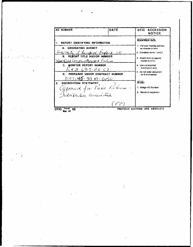
AD NUMBER DATE DTIC ACCESSIONNOTICE

REQUESTE1. REPORT IDENTIFYING INFORMATION

1. Put your mading addressA. ORIGINATING AGENCY on reverse of form.

L&'c/1• _:7 •,U, 2. Copete items I and 2,.

B. REfOR* TITLE 'AND/OR NMMBER 3 Attach form to reports

, 3 maloed to DTIC.

C. VONITOR REPORT NUMBER 4. Use unclassified/K C, ). • 9 7, ; 9 ! 1 "'° C ' ifrmation <only"D. PPEO 5. Do not order document

D. PREPARED UNDER CONTRACT NUMBER or 6 to 8 weeks.

7,.) ,0 ,44- 93 N,)-C,/i-d2. DISTRIFBTION STATEMFINT- -) DTII

1'' -- . AssnADNuer2. Return to requester

DTIC Form 50 PREVIOUS EDITIONS ARE OBSOLETEMar 91

THEORETICAL AND APPLIED MECHANICS1992

Proceedings of the XVIlIth International Congress of Theoretical and Applied Mechanics.Haifa. Israel, 22-28 August 1992

Edited by

Sol R. BODNERJosef SINGER

Alexander SOLAN

Technion - Israel Institute of Technology

Haifa, Israel

and

Zvi HASHINTel Aviv University

Tel Aviv, Israel

93-22612

1993

ELSEVIERAMSTERDAM - LONDON - NEW YORK ° TOKYO

ELSEVIER SCIENCE PUBLISHERS B.V.Sara Burgerhartstraat 25P.O. Box 211, 1000 AE Amsterdam, The Netherlands

ISBN: 0 444 88889 6

© 1993 IUTAM. All rights reserved.

No part of this publication may be reproduced, stored in a retrieval system or transmitted in any form or by any means, electronic.mechanical, photocopying, recording or otherwise, without the prior written permission of the publisher, Elsevier SciencePublishers BS., Copyright & Permissions Department, P.O, Box 52 1, 1000 AM Amsterdam, The Netherlands.

Special regulations for readers in the U.S.A. This publication has been registered with the Copyright Clearance Center Inc.(CCC), Salem, Massachusetts. Information can be obtained from the CCC about conditions under which photocopies of parts ofthis publication may be made in the U.S.A. All other copyright questions, including phototcopying outside of the U.S.A., should bereffered to the publisher, Elsevier Science Publishers B.V., unless otherwise specified.

No responsibilty is assumed by the publisher or by IUTAM for any injury and/or damage to persons or property as a matter ofproducts liability, negligence or otherwise, or from any use or operation of any methods, products, instructions or ideas containedin the material herein.

This book is printed on acid-free paper.

PREFACE

This book contains the Proceedings of the XVIIIth International Congress ofTheoretical and Applied Mechanics, held at th-b Technion, Israel Institute ofTechnology, Haifa, August 22-28, 1992. The Congress was held under the auspicesof The International Union of Theoretical and Applied Mechanics (IUTAM) byinvitation of The Israel Society for Theoretical and Applied Mechanics and Technion,Israel Institute of Technology and under the sponsorship of the Israel Academy ofSciences and Humanities.

The full text of the two General Lectures, of introductory lectures of the threeminisymposia and of sectional lectures, according to the list on pages xi, xii, areincluded in this volume. The contributed papers are listed by author and title; most ofthem will be published in appropriate scientific journals.

The publication of these Proceedings has been handled promptly and verycapably by Elsevier Science Publishers B.V. and their editors to whom we are verygra:eful.

Josef Singer Sol R. Bodner Alexander Solan Zvi Hashin

HaifaDecember 1992

Mayor A& VanL WND

. ,r e O l n .v a V v 1117O l i h t t le f t :Inger, ffa - flder, J. Lighhl

Oeing Cer'eiony

VII

H

C

4)

4)Q

I-0

U_______________________________ 0

I-

4)

EE0Q

'b:i 4)0C

U

C

4)0

Viii

H.K. Moffatt and M. Kiya

L. van Wijngaarden, Z. Hashin and M. Sayir

S= J l I I l I II l •

r

./• .• "N i

Mrs. N. Bodner, G.I. Barenblatt, S.R. Bodner

J.'F. Slti;tri (til(t "l•. l"tltstirl!i

i m m

7ýx

SPONSORING ORGANIZATIONS AND COMPANIES

The following academic, public, and industrial organizations have provided financial support:

- The Israel Academy of Sciences and Humanities- Technion, Israel Institute of Technology- Ben Gurion University of the Negev

and the Pearlstone Center for Aeronautical Engineering Studies- Tel Aviv University- Zurich Cha, ter of the Swiss Technion Society

- Israel Ministry of Defense, (MAFAT)- Israel Ministry of Science and Technology- Israel Ministry of Trade and Industry- Israel Ministry of Tourism- Haifa Municipality

- European Research Office, United States Army

- Amcrican Israeli Paper Mills, Ltd.- El-Al Israel Airlines- Israel Electric Corporation, Ltd.- I.B.M. Israel- Israel Military Industries- Klil Industries, Ltd.- Ormat Turbines (1965) Ltd.- Israel Aircraft Industries- Rafael, Israel Armament Development Authority- Oil Refineries, Ltd.- Paz Oil Co., Ltd.

Support for the

MINISYMPOSIUM ON INSTABILITIES IN SOLID AND STRUCTURAL MECHANICS

was provided by the

- European Office of Aerospace Research and Developmert, United States Air Force

CONTENTS

Preface v

.,• Sponsoring Organizations and Companies x

Congress Committees xiii

List of Participants xiv

Report on the Congress xx

OPENING AND CLOSING LECTURES

A. ROSHKO : Instability and turbuleice in shear flows I

G.I. BARENBLATT: Micromechanics of fracture 25

INTRODUCTORY LECTURES OF MINISYMPOSIA

"Instabilities in Solid and Structural Mechanics"

R. ABEYARATNE: Material instabilities and phase transitions in thermoelasticity 53

S. KYRIAKIDES : Propagating instabilities in structure:, (Summary) 79

Y. TOMITA : Computational approaches to plastic instability in solid mechanics 81

"Sea Surface Mechanics and Air-Sea Interaction"

W.K. MELVILLE: The role of wave breaking in air-sea interaction 99

O.M. PHILLIPS Extreme waves and breaking wavelets 119

P.G. SAFFMAN Effect of wind and water shear on wave instabilities 133

'Biomechanics"

S.C. COWIN : Nature's structural engineering of bone on a daily basis 145

R.D. KAMM: Liquid layer dynamics in pulmonary airways 161

R.McN. ALEXANDER: Energy-saving mechanisms in animal movement 177

xii

SECTIONAL LECTURES

H.H. BAU : Controlling chaotic convection 187

C.R. CALLADINE : Application of structural mechanics to biological systems 205

Y. COUDER: Viscous fingering as a pattern forming system (Summary) 221

G. GRIMVALL: Mechanics in sport 225T. KAMBE: Aerodynamic sound associated with vortex motions: observation 239and computation

A. LIBAI : Nonlinear membrane theory 257

M.E. McINTYRE : On the role of wave propagation and wave breaking in 281atmosphere-ocean dynamics

J.B. MARTIN • Computational aspects of integration along the path of loading 305in elastic-plastic problems

S. MURAKAMI : Constitutive modeling and analysis of creep, damage, and creep 323crack growth under neutron irradiation

Q.S. NGUYEN : Stability and bifurcation in dissipative media 339

A. PROSPERETTI : Bubble mechanics: luminescence, noise, and two-phase flow 355

M.B. SAYIR : Wave propagation in non-isotropic structures 371

K.R. SREENIVASAN and G. STOLOVITZKY : Self-similar multiplier distributions 395and multiplicative models for energy dissipation in high-Reynolds-number turbulence

A.A. VAN STEENHOVEN, J.D. JANSSEN, and D.H. VAN CAMPEN: 407Cardiovascular fluid mechanics

J. ZIEREP : Trends in transonic research 423

CONTRIBUTED PAPERS

List of Contributed Papers presented at the Congress 437

,1AID

CONGRESS COMMrITEE OF IUfAM

P. Germain* (France), ChairmanH.K. Moffatt* (UK), Secretary

J.D. Achenbach (USA) S. Kaliszky* (Hungary)A. Acrivos* (USA) Y.H. Ku (USA)L. Bevilacqua (Brazil) S, Leibovich (USA)B.A. Boley (USA) J. Lemaitre (France'C.R. Calladine (UK) M.J. Lighthill* (UK)C. Cercignani (Italy) Z. Mroz (Poland)G.G. Chernyi (Russia) E.-A. Milller (Germany)I.F. Collins (New Zealand) R. Narasimha (India)A. Crespo (Spain) F.I. Niordson (Denmark)D.C. Drucker (US A,) N. Olhoff* (Denmark)Z. Hashin (Israel) J.R. Philip (Australia)M.A. Hayes (Ireland) W. Schiehlen (Germany)N.J. Hoff (USA) B. Tabarrok (Canada)J. Hult (Sweden) L. van Wijngaarden (Netherlands)I.Imai (Japan) R. Wang (China)A. Yu. Ishlinsky (Russia) Zheng Zhemin (China)

F. Ziegler (Austria)

* Members of Executive Committee (1988-1992).

LOCAL ORGANIZING COMMITTEE

J. Singer%, ChairmanS.R. Bodner*, Co-Chairman

A. Solan*. Secretary

S. AbarbanelD. GivoliH. ElataZ. Hashin*D. ShilkrutA. SilberbergA. Yarin

* Members of Executive Committee

xiv

LIST OF PARTICIPANTS

AUSTRALIA (4 participants) Wegner J.L.Yeh K.Y.

Asokanthan S.F.Borgas M.S. CHINA (BEIJING) (8 participants)Karihaloo B.Muhlhaus H.B. Guo Z.H.

He Y.AUSTRIA (3 participants) Hwang K.C.

Wang G.T.Kluwick A. Wang R.Perktold K. Zhang R.J.Ziegler F. Zheng Z.

Zhou X.C.AZERBAUIAN (1 participant)

CHINA (TAIPEI) (6 participants)Iskenderov I.A.

Chang C.C.BELGIUM (5 participants) Chen F.

Chu C.C.Bao H. Pao Y.H.Boucher S. Su F.C.Nielens H. Wu E.Verdonck P.Verlinden 0. CZECHOSLOVAKIA (3 participants)

BRAZIL (2 participants) Brilla 1.Horacek J.

Musafir R.E. Klimes F.Zachariadis D.C.

BULGARIA (5 participants) DENMARK (9 participants)

Bontcheva N. Byskov E.Dabnichki PA. Jensen H.M.Karagiozova D. Larsen P.S.Markov K. Mikkelsen L.P.Zapryanov Z. Niordson F.I.

Olhoff N.CANADA (18 participants) Pedersen P.T.

Thomsen O.T.Bourassa P.A. Tvergaard V.Cohen H.Davies H.G. FINLAND (1 participant)Dickstein P.Dost S. Holopainen P.Dziedzic M.Floryan J.M. FRANCE (39 participants)Graham G.A.C.Haddow J.B. Berest P.Han R.P.S. Berthaud Y.Leutheusser H.J. Blanze C.Mioduchowski A. Boehler J.P.Rimrott F.P.J. Caulliez G.Smith S.H. Charru F.Szyszkowski W. Chaskalovic J.Tabarrok B, Cochelin B.

Couder Y. Pfeiffer F.Dias F. Pingel T.Djeridi H. Rozvany G.Drochon A. Schiehlen W.Etay J. Schirm W.Fressengeas C. Schumacher A.George J. Soeller C.Germain P. Stein E.Grandidier J.C. Stumpf H.Iooss G. Wierzbicki T.Jullien J.F. Zhang C.Klepaczko J.R. Zierep J.Lagarde A.Lemaitre J. GREECE (4 participants)Lespinard G.Magnaudet J. Georgantopoulos G.A.Maigre H. Kounadis A.N.Maugin G.A. Sotiropoulos D.A.Molinari A. Vardoulakis I.Nguyen Q.S.Nouailhas D. HONG KONG (I participant)Pelissier R.Potier-Ferry M. Hui W.H.Resch F.J.Reynier M. HUNGARY (2 participants)Rittel D.Roseau M. Kaliszky S.Rougee P. Tamai T.Su lem J.Thebaud F. IRELAND (1 participant)Waldura H.

Hayes M.A.GERMANY (36 participants)

ISRAEL (85 participants)Altenbach H.Altenbach J. Adan M.Buhler K. Agnon Y.Chen X.N. Altus E.De Boer R. Arcan M.Dinckelacker A. Ayzenberg M.Faciu C. Bar-On E.Furta S. Barron A.Gersten K. Baruch M.Gross D. Ben David D.Kazimierczyk P. Ben Haim Y.Koenig M. Benveniste Y.Kowalewski T.A. Bergman R.Krause E. Bershadskii A.Kuhn G. Bodner S.R.Labisch F.K. Branover H.Le K.C. Broday D.Lenz J. Burde G.I.Meyer L.W. Chiskis A.Mitra N.K. Dmitriuk W.Muller E.A. Drozdov A.D.Noack B.R. Durban D.Ohle F. Elad D.Olszok T. Elata D.

xvi

Elida D. Wiener Z.Fang D. Wygnanski 1.Frankel I. Yarin A.Galper A. Zvirin Y.Gandelsman M.L.Gershtein M.S. ITALY (I I participants)Ginzberg I.Givoli D. Amadio C.Glozman M. Bigoni D.Gringauz M. Cercignani C.Gurevich B. Franzese P.Hashin Z. Guglielmino E.Hetsroni G. Martelli F.Khain A. Nappi A.Khen R. Perego U.Kimmel E. Ruta G.C.Lanir Y. Tatone A.Lesin S. Zannetti L.Levich E.Libai A. JAPAN (22 participants)Litovsky Y.Markus S. Amari T.Mickulinsky M. Ashida F.Miloh T. Fukuyu A.Mizrahi J. Hasimoto H.Moshaiov A. Horii H.Nekhamnkina 0. Imai I.Nezlina Y. Kambe T.Nir A. Kawata K.Partes R. Kitagawa H.Perlman E. Kiya M.Partom Y. Kobayashi S.Rom J. Kondo K.Rosen A. Kumagai T.Rotem A. Murakami S.Rubin M.B. Sakao F.Ryvkin M. Sumi Y.Sabag M. Takahashi K.Salganik R.L. Tatsumi T.Shalman E. Tornita Y.Shapiro M. Uetani K.Sheinman 1. Yamamoto Y.Shemer L. Yoshida H.Shilkrut D.Shoavi E. KOREA (3 participants)Shtark A.Shtilman L. Jeong J.J.Singer J. Pak C.H.Solan A. Youm Y.Spivakovsky V.Stavsky Y. MEXICO (I participant)Stiassnie M.Tirosh J. Sabina FJ.Tsitverblit N.Vigdergauz S. NETHERLANDS (21 participants)Vilenkin B.Weinstein M. Arbocz J.Weiss M.P. Bakker P.G.

Besseling J.F. Martins J.A.C.Braat G.F.M. Trabucho L.Coene R.Dieterrnan H.A. ROMANIA (1 participant)Huyghe J.Janssen J.D. Cristescu N.D.Kouhia R.J.Leroy Y.M. RUSSIA (32 participants)Meijaard J.P.Meijers P. Barenblatt G.I.Menken C.M. Belsky V.G.Shlyapobcrsky J1. Blekhman 1.1.Sluys L. Borodich F.M.Van Beek P. Chashechkin Y.D.Van Campen D.H. Chernyi (3.C.van der Giessen E. Elkin Al.IVan Steenhoven A.A. Fabrikant A.L.van Wijngaarden L. Freidin A.Zhang G.Q. Goldenveizer A.L.

Goldstein R.NEW ZEALAND (I participant) Gregoryan S.S.

Ivanov V.Collins [.F. Kanaun S.K.

Lyubirnov G.A.NORWAY (I participant) Makarov S.0.

Manevitch L.I.Tyvand P.A. Matasov A.

Mikhailov G.K.POLAND (21 participants) Mirkin M.

Nezlin M.V.Bauer J. Nuller B.Dolinski K. Obraztsov I.F.Duszek-Perzyna M.K. Ryaboy V.M.Gawinecki J.A. Sedov L.I.Golos K. Sliukhman I.Grabacki J.K. Slepyan L.I.Gutkowski W. Smirnov B.1.Kiciber M. Stein A.A.Kurnik W. Talipova T.Mroz Z. Yanovsky Y .G.Nowak Z. Yumasheva M.A.Osinski Z.Pecherski R.B. SOUTH AFRICA (2 participants)Peradzynski Z.Perzyna P. Jekot T.Petryk H. Martin J.B.Rakowski J.Skrzypek 3.3. SWEDEN (7 participants)Szafranski W.Tylikowski A. Essen H.Zorski H. Grimmall G.

Hluh J.PORTUGAL (5 participants) Larsson P.L.

Neurneister J.M.Arantes e Oliveira E.R. Sjodin B.Camotim D.R.Z. Storakers B.Faria L.

xviii

SWITZERLAND (10 participants) UKRAINE (4 participants)

Cuche D. Guz A.N.Dual J. Levitas V.I.Hazanov S. Rassokha A.Herrmann G. Shupikov A.Juengling D.F.Meyer Matievic M. USA (107 participants)Pellegrini 0.Sayir M.B. Abeyaratne R.Spirig T.H. Achenbach i.D.Staudenmann M. Acrivos A.

Agarwal R.K.TRINIDAD (I participant) Aifantis E.C.

Akylas T.R.Ramkissoon H. Bammann D.J.

Batra R.C.TURKEY (1 particpant) Bau H.H.

Bazant Z.P.Kaykayoglu C.R. Berdichevsky V.

Berkooz G.UK (35 participants) Bert C.W.

Boley B.A.Alexander R.McN. Brenner H.Brandt R. Brock L.Calladine C.R. Brodsky N.Carpenter P.W. Budiansky B.Cowley S.J. Chaudhuri R.Crighton D.G. Cherepanov G.Dunne F.P.E. Cherkaev A.V.Earles S.W.E. Christensen R.M.Fleck N.A. Chudnovsky A.Guest S.D. Clifton R.J.Hardy S.J. Cohen B.Haughton D.M. Cowin S.C.Healey J.J. Crandall S.H.Lighthill J. Dagan Z.Lucey A.D. Drucker D.C.McIntyre M.E. Dvorak G.J.Moffatt H.K. Dvorkin J.Nagata M. Elishakoff I.Ogden R.W. Fernando H.J.Pedley T.J. Finkelstein I.Pellegrino S. Fish I.Reid S.R. Folias T.Ricca R.L. Freund L.B.Richards K.J. Gao H.Rogers T.G. Glenn L.Shi J. Goddard J.D.Slaughter W.S. Graham A.Soldatos K. Halpem D.Spence D. Hanagud S.V.Stronge W.J. Haythornthwaite R.M.Stuart J.T. Hetnarski R.B.Sutcliffe M. Hoff N.J.Ursell F. Holmes P.J.Vassiliev D. Huang T.C.Willis J.R. Hulbert G.M.

Hutchinson J.W. Rubinstein A.A.lacob A. Rumschitzki D.Jasiuk 1. Sackman I.L.Joseph D, Saffinan P.G.Kachanov M. Sen M.Kamnm R.D. Shaw S.Kapoor B. Shillor M.Keer L.M. Shtern V.Kestin J. Sreenivasan K.R.Knowles J. Steele C.R.Kohn R.V. Steif P.S.Krajcinovic D. Triantafyllou G.Kraynik A.M. Truskinovsky L.Kyriakides S. Vakakis A.F.Leibovich S. Vaynbiat D.Ling F. Voloshin A.S.Lurie K. Wei K.Mac Sithigh G.P. Weinbaumn S.Maity A.K. Weitsman Y.J.Majerus 3. Weng G.J.Mal A.K. Wnuk M.P.Markenscoff X. Yang Z.Mauri R. Yu Y.Y.Meirovitch L.Melville W.K. VIETNAM (I participant)Mendelsohn D.Metzner A.W.K. Anh N.D.Mondy L.

"Ced',YUGOSLAVIA (5 participants)Ostrach S.Phillips Q.M. Cveticanin L.Ponte-Castaneda P. Dzodzo M.B.Pi-osperetti A. Hedrih (Stevanovic) K.Reshotko E. Ruzic D.Roshko A. Vujicic V.A.

REPORT ON THE CONGRESS

Josef Singer

The decision to accept the invitation from Israel to hold the XV[Ith International Congressin Haifa was taken by the Congress Committee of IUTAM during its meeting in Grenoble inAugust 1988. It was decided that the format of the Congress would follow the one adopted forthe recent successful Congresses in Lyngby and Grenoble. The Congress would cover theentire field of mechanics with special emphasis on three selected topics to constitute the so-called minisymposia.

The Congress Committee selected the following three topics for these minisymposia:

1. Instabilities in Solid and Structural Mechanics.2. Sea Surface Mechanics and Air-Sea Interaction.3. Biomechanics.

The Congress Committee also selected two general lecturers: Professor Anatol Roshko(USA) to present the Opening Lecture and Professor G.l. Barenblatt (Russia) to present theClosing Lecture; as well as 15 Sectional Lectures. The chairmen of the Minisymposia furtherselected 9 Introductory Lectures for their symposia.

As in Lyngby and Grenoble, the contributed papers were presented in parallel sessions,either as 25 minute lectures or in poster-sessions which were scheduled separately from thelectres. There were lively e-scussions both after the lectures and in the poster-sessions, wherethe second half of the sessions were devoted to general discussions guided by the chairmen.

The Opening Session of the Congress was held in the Churchill Auditorium of theTechnion at 10 o'clock on Sunday, 23rd August, 1992. The Session was opened by ProfessorJosef Singer, Chairman of the Local Organizing Committee of ICTAM '92, with the followingwords:

"Distinguished Members of the Dais, Ladies and Gentlemen,

It gives me great pleasure to open the 18th International Congress of Theoretical andApplied Mechanics and to greet this outstanding gathering of scientists and engineers whichwill ensure the success of the Congress.

Welcome to Israel, to Haifa and to the Technion, Israel Institute of Technology.

Let me also greet you in Hebrew (welcome to participants).

I think you will understand me better if I do not continue in Hebrew. Maybe by the time wecome to the Closing Session, your Hebrew will be good enough to permit me to address youall in our language.

So let me introduce you to the Dais:

I will start at the far end of the Head Table. There are the Deans of the two TechnionFaculties which are most active in Mechanics:

Professor Blech, Acting Dean of the Faculty of Mechanical Engineering, and ProfessorShinar, Dean of the Faculty of Aerospace Engineering.

Next, the Secretary-General of IUTAM, Professor Schielen of Stuttgart University, who isentrusted with the many IUTAM Symposia and other lUTAM activities.

To his left, the President of the Israel Society for Theoretical and Applied Mechanics,Professor Hashin of the Faculty of Engineering of Tel Aviv University, an active member ofour Organizing Committee.

Next, the Secretary of the IUTAM Congress Committee, Professor Moffatt of CambridgeUniversity, whose guidance and tireless efforts have been essential to the success of thescientific program and the preparations of the Congress.

To his left, the Mayor of our beautiful city, Haifa, Mr. Gurel, who graciously supports ourmeeting and many other international activities.

Then our IUTAM President, Professor Germain, of the French Academy of Science,whom many of you also remember as the Organizer of the successful Congress in Grenoble in1988.

To his left, Professor Paul Singer, Senior Vice President of Technion, who will soon bringto you the greetings of the Technion President.

Then the IUTAM Vice President, Sir James Lighthill, the past IUTAM President andformer Vice Chancellor of University College London.

To his left, Professor Bodner of our Faculty of Mechanical Engineering, the Co-Chairmanof our Local Organizing Committee, who gave his time and knowledge untiringly and thuscontributed so much to our Congress.

Then the Treasurer of IUTAM, Professor van Wijngaarden of the University of Twente inThe Netherlands, whose importance is self-evident.

And last, but certainly not least, the wonderful Secretary of our Local OrganizingCommittee, Professor Alex Solan, Technion Vice President for Academic Affairs, with whommost of you have already corresponded and without whose outstanding and never ending workwe could not have carried out the preparations for the Congress.

ICTAM Participants, as I look around me I see many friends, the top scientists of theinternational mechanics community, the international mechanics family. I am sure that ourdeliberations will not only advance our field, but will also weave many new collaborations andfriendships.

For the benefit of the delegates who are new to ICTAM, I would like to ask some of theformer IUTAM Presidents to please rise: Professor Frithiof Niordson of Denmark, andProfessor Daniel Drucker of U.S.A.

To finish the introductions, it gives me great pleasure to see here among us, my formerteacher and good friend, Professor Nicholas Hoff of Stanford University, who taught me themeaning of theoretical and applied mechanics and much more, and whom many of you willremember as the President and Organizer of our 1968 Congress at Stanford. Please riseNicholas.

Friends, I may have taken up some time with these introductions, but I remember that atthe first ICTAM I attended in Stresa in 1960, seeing the great names in the flesh was, indeed, agreat experience!

Ladies and Gentlemen, we Israelis are honored and happy to host the 18th InternationalCongress of Theoretical and Applied Mechanics in our old-new Land.

Though the ancient Israelis are better known for their Monotheism than for theirachievements in mechanics, one finds that they tried their hand in some large scale experimentsin mechanics.

ixi

For example, in the Book of Exodus we hear that in their flight from Egypt, the Childrenof Israel (with some assistance from the Almighty) experimented with sea-air interactions, forwe read in Exodus 14/21,22:

"And Moses stretched out his hand over the sea and the Lord caused the sea to go back bya strong east wind ..... and made the sea dry land and the waters were divided".

"And the Children of Israel went into the midst of the sea upon the dry ground, and the

waters were a wall unto them on their right and on their left".

Would this not fit into our second Minisymposium?!

Or, in the Book of Joshua, we hear of an early experiment in the dynamics of soundwaves, for we read in Joshua 6/5:

"And it shall come to pass, that when they make a long blast with a ram's horn, and whenye hear the sound of the trumpet, all the people shall shout, and the wall of the city shall falldown flat".

So, there was some mechanics activity here 3,500 years ago!

In modern times, Israel has a small but very active mechanics community, whose presenceand achievements are known internationally, and whose participation in IUTAM Congressesand Symposia has been very significant

At the Technion we were fortunate to have had Professor Marcus Reiner, well known asone of the Fathers of Rheology, active here from 1947-1976. He built a thriving department ofmechanics, that later diffused into other departments.

In 1961 Professor Reiner organized an IUTAM Symposium on "Secondary Effects inElasticity, Plasticity and Fluid Dynamics", in Haifa (by the way, my wife worked with him onthe organization of that symposium) a symposium which was the occasion of the first visit toIsrael for some of you.

In 1985 Professors Bodner and Hashin organized another IUTAM Symposium on"Mechanics of Damage and Fatigue", at Technion, which was also very successful.

Hence, an ICTAM at Haifa seem to follow logically. Well, some of us in the audience haveaged a bit since the first time Israel offered to host ICTAM many years ago, but I am happythat we all made it finally!

We have, I believe, an excellent scientific program thanks to you the contributors and to theexcellent work of our International Papers Committee. As you know, the choice was difficultand the 600 papers chosen out of 1,183 submitted originated in 48 different countries.However, as we had many and continuous changes, even in the number of countries, theprogram you have could be finalized only two weeks ago.

The flags on the platform represent all the countries from which papers were accepted. Theflags indicate origins of papers, but we are all here as individuals, contributing to theoreticaland applied mechanics. Individuals whose friendship and collaboration will be reinforced bythis Congress and who will assist in bringing our nations closer and improve their relations.

Before closing. I would like to thank the IUTAM Congress Committee, and in particular itsExecutive Committee, the IUTAM Bureau, the International Papers Committee, as well as thedifferent National Committees. I will express my gratitude to my local collaborators, whoworked so hard to prepare the Congress, in more detail at the Closing Session. For now, only

sincere thanks to you, my colleagues of the Local Organizing Committee and to the devotedstaff of the Technion and Kenes teams who will also look after us in the coming days.

I would also like to thank the Israel Academy of Sciences and Humanities, the variousIsraeli government ministries, our municipality, and the Haifa Tourist Board, the universitiesand industrial companies, whose names appear on the program and, in particular, the U.S. AirForce European Office of Aerospace Research and Development, and the U.S. Army EuropeanResearch Office, for their generous support.

As you know, the Israel Academy is one of the sponsors of our Congress. Its President,Professor Joshua Jortner, who is abroad, sent us his greetings which I would like to read toyou:

"The Israel Academy recognizes the important contribution international meetings make tothe advancement and excellence of research, by providing a forum for direct contact betweenscientists and engineers engaged in high quality scientific endeavor.

I am confident that the 18th International Conference in Theoretical and Applied Mechanicswill contribute to the advancement and the enhanced cooperation in these exciting andimportant fields of scientific and technological research. The integration of science andtechnology which is so well reflected in your Conference is of prime importance for Israel andfor the international community at large.

Please convey my compliments, on behalf of the Israel Academy of Sciences and

Humanities, to all the participants.

I wish you a fruitful and stimulating meeting."

Ladies and Gentlemen, I concur with Professor Jortner, and wish us all, delegates andaccompanying persons, a fruitful and enjoyable Congress, and a very pleasant stay in Israel.Thank you."

Professor Singer then called on Professor Solan, the Secretary of the Local OrganizingCommittee, to introduce the speakers who followed.

Mayor Gurel then brought the greetings of the Municipality of Haifa to the Congressparticipants and wished them successful deliberations and a pleasant stay in Haifa and Israel.

Since the President of the Technion was abroad, the Senior Vice President, President Paul

Singer, greeted the assembly with the following words:

"Distinguished Guests and Friends,

It is my privilege and honor to welcome you, participants of the International Congress ofTheoretical and Applied Mechanics to the Technion - Israel Institute of Technology, with thetraditional Hebrew greeting - "Blessed be those who came". -This Congress is the XVIII th ina series which started in Delft, Netherlands and carries with it by now a most famoustradition. We are therefore very proud and consider it a great distinction, that for the first timethe Congress convenes in Israel, and the Technion Management is especially proud that ourscientists have been entrusted with the task of organizing and hosting this event.

But, there is another "FIRST" which I would like to point out to you. A perusal of theprevious sites shows that you are meeting for the first time at an altitude of several hundredmeters above the sea level, - I am confident this will bring to this Meeting "Scientific heights"previously unknown. You have certainly chosen a very unique location: Mount Carmel (on oneof its hills we are here) - was mentioned already a few thousand years ago. For instance, in theBook of Jeremiah one finds "To the CARMEL by the sea, - one comes". This mountain isperceived and mentioned from very, very old times as a "SAFE SHORE". The ancient

xxiv

Egyptians used to call it "The Holy Summit" and the famous Egyptian Emperor (Pharaoh)Ramses the Second, nicknamed it in the 13th Century B.C., "The Mountain of Strength".Possibly the most famous personality associazed with it is the Prophet Elijah who used toprophesize and build his favorite models and theories and indoctrinate his followers right hereon these hills. I mention this, since in the Ninth Century B.C., during the reign of King Ahabof Israel, a very famous Assembly was organized by the Prophet Elijah on Mount Carmel inthe presence of the King, possibly the precursor of the subsequent scientific conferences heldon this mountain. About 850 people attended that famous Assembly, not very different fromthe attendance of this Congress, at which some ideological differences (theories or approachesin our present language) were confronted. Well, here the parallel stops, since meetings in thosetimes could have very violent endings as happened in the Assembly convened by King Ahab.

Interestingly, the location of Prophet Elijah's home-cave is determined to be in twodifferent places, some 300 meters apart, by the Christian and Jewish faith. Given the distanceof nearly 3000 years on the time scale, this is pretty good accuracy.

Referring anew to your Congress series, I was struck by an interesting historicalcoincidence. The first ICTAM took place in DELFT in 1924, and in the very same year ourUniversity, the Technion, opened its gates for business, enrolling its first 14 students with 7Faculty members (a pretty good ratio we did not succeed in maintaining) - as the firstUniversity in modem Israel - it was followed less than a year later by the Hebrew Universityof Jerusalem. So, the date of your first Congress is also a cornerstone in the history of ModernIsraeli Culture.

Today, we have 19 Faculties and Departments, and a number of Research Institutes, inmost fields of Engineering and Sciences, as well as Architecture and Medicine. There are now'over 10,000 students at the Technion, among them nearly 3,000 postgraduate studentsresearching and studying for higher degrees. We have about 700 full-time Faculty membersand many hundreds of associated scientists and adjunct teachers. I hope you will have thechance to visit and meet some, though this is the week of our annual vacation.

As you know, Israel is a country of small size and limited natural resources. As such, weput special emphasis on Science xnd Technology, the prime component in our strive toeconomic independence and the building of an advanced society. In this context, weconsiderably value international cooperation of which scientific congresses are an importantform.

The recent political changes in the world have opened new avenues for internationalcooperation and for us in Israel they have significant implications. A sizable part of thescientific world was practically unreachable for us; this has changed completely during the lastcouple of years, - as the composition of this assembly, I believe, shows. Moreover, theenergetic pace of European unification and the related developing of special technological andscientific collaboration schemes of international impact is also of great relevance for us. As aresult, we are undergoing here a process of orientation towards a multitude of newopportunities, and I am confident that the outcome will benefit all those involved.

Maybe I should also mention that on historic scales (I already mentioned history before) thedirection of international exchanges has gone through cycles.Today, there is no doubt that theleading Mecca's for Science and Technology are mostly in Europe and the United States ofAmerica. In hi! Nobel acceptance speech in 1979, the Pakistani physicist, Abdus Salam, fromImperial College, London, described through individual examples the clear direction oftechnology transfer in the early centuries of this millennium. He mentioned the cases ofMichael the Scott and the Danish physician Henrik Harpestraeng who travelled in the 13thCentury from the underdeveloped countries of the North to the flourishing Universities of theSouth, Toledo, Cordoba. In these places the Arabic and Hebrew Scholarship was then at itspeak, and scholars were attracted to these and other Southern Universities from both thedeveloped countries of the Middle East and Middle Asia, as well as from the developingnorthern countries.

It is my wish that we here do the utmost, so that again we may confidently say "ThatScholarship will emerge from Zion". Meanwhile, on the way to this goal. I wish that yourCongress will contribute significantly to the increase of knowledge and will stimulate andinspire you in your future work. I hope you have an interesting, enjoyable, fruitful andpleasant week at the Technion in Haifa-"

Professor Zvi Hashin, President of the Israel Society for Theoretical and AppliedMechanics, then brought his greetings:

"Members of the Presidium, Ladies and Gentlemen,

I have the honor and privilege to bring you the greetings of the Israel Society forTheoretical and Applied Mechanics. Our society is one of the many national societies which arefederated into the International Union of Theoretical and Applied Mechanics (IUTAM). TheIsrael Society was founded in 1950, only two years after the establishment of the State ofIsrael in 1948, by my dear and esteemed former teacher and advisor Prof. Markus Reiner. Healso was the first President of the Society, until he passed away in 1976. It has been my greatprivilege to replace him as President of the Society from 1976 until the present. ProfessorBodner and myself are the delegates of Israel to the IUTAM General Assembly. ProfessorSinger was our member in the IUTAM Congress Committee until 1988. Since 1976 we haveconsistently extended invitations to IUTAM to hold the International Congress of Theoreticaland Applied Mechanics (ICTAM), in Israel and we are gratified and honored to have beenselected during the last ICTAM in Grenoble 1988 to host this major event in 1992. We woAidlike to believe that it is a recognition of the growth and maturity of the mechanical sciences inour country.

The Israel Society for Theoretical and Applied Mechanics is grateful to Professor JosefSinger for having accepted its invitation to chair the Local Organizing Committee, and to all themembers of the Committee. In particular, we wish to express special gratitude to Professor SolBodner, Co-Chairman, and to Professor Alexander Solan, Secretary, for the enormousamounts of time and effort they have generously contributed to create ICTAM 18.

Thank you very much and I wish all of us a very successful and pleasant Congress."

Professor Sol R. Bodner, Co-Chairman of the Local Organizing Committee, thenpresented his greetings:

"I would like to make a few remarks on this occasion.

Exactly forty years ago, as a young graduate student working with Professor NicholasHoff at the Brooklyn Polytechnic Institute, I attended the 8th International Congress ofMechanics in Istanbul. It was a wonderful affair - the scientific level of the presentations, theextraordinary hospitality of the hosts, and the marvellous sights of the city. Present there werethe famous personalities of Mechanics - Prager, who as partial host gave a brief talk inTurkish, von Mises, Courant, - I believe von Karman and G.I. Taylor were there, and manyothers. My impression from that Congress was that Mechanics was an excellent field in whichto make a career.

Now, forty years later, the Congress has returned to the Eastern Mediterranean region andwe are again gathered at its shore. I still consider Mechanics as a field that offers continuingpossibilities for creative and intellectually demanding and satisfying work. It is impossible torecreate the atmosphere of Istanbul of 1952. but we shall do our best to offer the hospitality ofthe region.

The logo of the Congress, the ship, is taken from the emblem of the port city of Haifa, thefancy sail of the ship is the Hebrew word Chai which means 18 and also "life", or moreliterally "alive".

Xxvi

I would like to add my personal welcome to all of you who came to Haifa for thisCongress."

Finally, Professor Paul Germain, President of IUTAM addressed the gathering:

"It is my privilege, as President of IUTAM, to close this uofficial opening ceremony and todeclare open our XVIII th International Congress of Th, oretical and Applied Mechanics. butbefore I do it, I intend to say a few words, to thank our hosts, to recall the objectives and theresponsibility of IUTAM and to emphasize the role and the importance of such a Congress forthe modem development of Mechanics.

We are invited today by a country and a people who. at the same time are very old and verynew. Thank you, Mayor Gurel for your presence this morning and for your welcome. Yourepresent here both of them. A country which has to face many difficult problems, which mustfight every day to solve them, which hopes to get and which has to get, full recognition by allits neighbours and then, which has to reach and to win the peace, a true peace, a peacefulpeace. A land to which so many in the world are so deeply related because they feel that, here,lie some of their deepest roots. A people who, more than 3000 years ago, has begun to givethe world an incomparable source of moral and spiritual life in which so many in the worldtoday continue to draw inspiration, stimulation and strength. A people who was dispersedduring centuries, who has too often suffered unjustly and especially during the first half of thecentury with this incomprehensible and inadmissible Shoah. A people who is today engagedwith great success in modem life and in particular the scientific life. One of the evidences isthis Technion, this very famous Institute of Technology. Our best thanks go to its Presidentwho has accepted that our Congress be held here. Many years ago, as it was recalled, ourcolleagues from the Israel Society of Mechanics asked our Congress Committee to hold one ofour international congresses in their country. Despite the high standard of their achievements inthe field of Mechanics, it was not found possible to accept their invitation on account of theinternational situation until four years ago at our last meeting in Grenoble. Many unpredictableevents happened in the world since that time. But one must recognize today that the choicewhich looked a little risky was a reasonable one. No special difficulty arose for the attendancefrom the choice of the location. With the help of Technion and of the civilian authorities, theLocal Organizing Committee under the friendly supervision of our Congress Committee wasable to do the necessary work to hold this Congress in very good conditions. Without waitingfor the closing session which is the most appropriate time to express our recognition, we mayalready express to Professor Singer and to his colleagues our gratitude.

Dear colleagues and friends, at the present time, the interactions of science and technologywith the cultural, social economical, ecological problems are very strong. As scientists we are,each one of us, concerned by such a responsibility. Our Union provides a good tool to assumethis responsibility at the international level, by its own initiatives first and second throughICSU, the International Council of Scientific Unions. As you know IUTAM is one of them.ICSU with its various specialized Committees has a role which is every day more important, inparticular, as a partner on account of its scientific expertise of the United Nations and of itsnumerous programs and organizations. The fears and the expectations of the people cannot beignored. The understanding and the appreciation of science have to be improved. I am glad totell you that IUTAM has significantly increased its involvement in the ICSU work, byencouraging the operations in which the scientific content plays the principal role and byparticipating in those when its own expertise is very high. The best example is the scientificprogram of the International Decade for Natural Disaster Reduction run by a group of experts,coming from various Unions, chaired by Sir James Lighthill, our former President, with aremarkable success. The influence of IUTAM and of its voice inside ICSU is a function of thesupport it received from the mechanicians all over the world. And one measure of this supportis the presence and the participation of many of them at the International Congress. It is onefirst reason to express to all of you my thanks on behalf of the Bureau and of the GeneralAssembly.

Xxviii

Congress Statisti

S AL AP L P L

Australia 6 2 2 1 2 4Austria 5 3 - 2 - 3Azerbaijan * * * I -

Belgium 4 1 3 1 2 - 5Brasil 10 1 2 - 2 - 2Bulgaria 28 3 6 3 1 - 5Canada 28 8 15 7 9 - 18China- Beijing 114 3 25 3 8 - 8China - Taipei 26 4 6 3 2 - 6Czechoslovakia 11 1 3 - 3 - 3Denmark 10 6 3 6 2 - 9Estonia I - I - - -

Finland I - 1 - - -France 65 25 19 22 11 2 39Germany 46 13 18 13 13 1 36Greece 5 2 2 1 1 - 4Hong Kong 1 1 - I - - IHungary 4 2 - I - 2India 8 - 3 - - -Ireland 1 - I - I -IIsrael 91 20 28 20 22 1 85Italy 18 4 7 4 3 - 11Japan 28 13 12 10 5 3 22Kenya 1 - - -Korea - - -3Latvia 3 - 2Lithuania 6 - 3Mexico I I 1 - INetherlands 16 8 7 8 7 1 21New Zealand 2 1 - I - - INorway 1 1 - I - - IPoland 37 6 14 5 10 - 21Portugal 5 3 1 2 1 5Romania 28 2 - 2 - - IRussia 304 32 58 25 12 1 32Singapore I - 1 - - -South Africa 4 - 1 - 1 1 2Sweden 10 2 2 2 1 1 7Switzerland 7 2 4 2 4 1 10Trinidad - - - - - ITurkey 10 2 1 1 - IUkraine * * 4 - 4United Kingdom 37 14 15 13 13 3 35USA 184 72 67 59 28 11 107Venezuela 1 1 - - - -Vietnam 2 - I - 1 1Yugoslavia 11 - 5 - 4 5

Total 1183 257 342 223 171 26 525

599 394420

X'xvt

But our main task, our unique task this week, concerns mechanics and its development;mechanics an old science, but a-. always young one. Those who like me attended many suchInternational Congresses can tell you how fruitful these meetings are. They give to eachparticipant as in any other scientific meeting the opportunity to communicate directly with thecolleagues working in the same area, by letting them know their new results and by learningfrom them the latest progress. But you find more in such a Congress: the possibility to devoteone week to your own on-going education, to broaden your interest to the neighbouringdisciplines, to become aware to the new discoveries, to see the evolution of ideas, the creationof new concepts, the fantastic improvements in theory and applications. Our two GeneralLectures, our invited Sectional Lectures, our three mini-symposia with their lectures ofpedagogical character meet precisely these purposes. And one discovers that the contributionsselected by the International Papers Committee represent stones which are necessary to buildthis wonderful monument of mechanics, not yet achieved, always more beautiful, moreimpressive, more useful, 300 years after Newton. Yes, may all of us, and especially theyounger ones, enjoy their participation; may they draw the greatest possible benefit of thisweek. For those who have prepared this meeting, that is their main wish; that would representthe best reward.

And now, it is time to start. I declare open the XVII/ th International Congress ofTheoretical and Applied Mechanics and leave the chair to Sir James Lighthill who, within afew minutes, after a few announcements by Professor Solan, will introduce the speaker invitedto deliver the opening General Lecturer. Thank you for your kind attention."

Sir James Lighthill then introduced Professor Anatol Roshko who presented the OpeningLecture "Instability and Turbulence in Shear Flows".

The scientific program of the Congress was presented from Sunday afternoon till Thursdayevening in 5-6 parallel sessions. The poster sessions took place in 8-9 adjoining rooms onthree mornings, at times when no other lecture sessions were in progress. This resulted ingood attendance and very lively discussions.

The detailed statistics of the Congress are presented on the following page. It is noted thatthe proportion of acceptances to submissions was almost exactly 1/2. The proportion of actualpresentations to acceptances was lower than anticipated which seems to be primarily due tocurrent difficulties in a number of countries for obtaining travel funds. As a consequence, theoverall attendance was also somewhat lower than expected but was more than adequate for avery invigorating Congress.

The meaning of the symbols used in the following listing by countries is as follows:

S - Submitted abstractsAL - Accepted as LectureAP - Accepted as Poster

L - Presented as LectureP - Presented as Poster

IL - Invited Lecture* The numbers for S, AL, AP for Azerbaijan and Ukraine and other countries of the

former Soviet Union are included in Russia.

Xxix

The Social Program included a Welcome Reception on Saturday evening, a DinnerReception on Monday evening, both at the Churchill Auditorium Plaza; the CongressExcursion on Tuesday afternoon to Rosh Hanikra and the Crusader City, Acco; a city tour ofHaifa and the Druze villages on Mount Carmel on Thursday, and other optional tours foraccompanying persons on Sunday, Monday and Wednesday as well as pre-congress and post-congress tours to other parts of Israel. The Congress Banquet was held at the Dan CarmelHotel on Thursday evening.

The Closing Session of the Congress was held in the Churchill Auditorium at 5.30 p.m. onThursday, 27 August 1992, immediately after the Closing Lecture by Professor G.l.Barenblatt on "Micromechanics of Fracture". The closing ceremony was opened by ProfessorJosef Singer, Chairman of the Local Organizing Committee, with the following words:

"Ladies and Gentlemen,

All good things must come to an end, and the 18th ICTAM is no exception. I will notrepeat in detail my thanks to the various IUTAM committees and to the different nationalcommittees for their excellent work and continuous assistance, nor to the Israeli sponsoringorganizations and others for their generous support.

But I would like to express, on behalf of the Executive Committee of the Local OrganizingCommittee (Professors Bodner, Hashin, Solan and myself), our appreciation to our localcollaborators:

To Professor Alexander Yarin and Dr. Dan Givoli for their very significant contributionsand also to the other members of the LOC for their support.

To Dabia Sarid, the administrator of the Faculty of Mechanical Engineering, and to BerniceHirsch and Edna Gal, who assisted us so ably in solving the many detailed problems and lastminute rush jobs, as well as to Mottle Fein who did much of the computer programing. Also tothe Superintendents of the Technion buildings, of the Churchill Auditorium and especially ofthe Lady Davis Complex, to the Technion electricians and to the staff of the Techniondormitories. To all of them, for their help to make Technion facilities available to us during theannual vacation week, when Technion is usually closed.

Our thanks also to the efficient Kenes staff for their excellent professional operation duringthe Congress that provided us with the daily technical support for our deliberations and otheractivities.

Ladies and Gentlemen,

We have had a very successful Congress, and this is primarily due to you, the lecturers,contributors, chairmen and participants.

As you know, clouds of uncertainties hung over our preparations caused by the difficulteconomic situation of the countries in Eastern Europe. The IUTAM Bureau and ExecutiveCommittee of Congress Committee made available special funds for partial support toparticipants and this helped to disperse some of those clouds. The attendance from thesecountries was significantly augmented, and we have nearly the same number of participantsfrom Eastern Europe as attended in Grenoble and even more from the countries of the formerSoviet Union.

Friends,

We were honored and happy to be host to the 18th Congress. We hope that you not onlyenjoyed the Congress, but that you will take with you fond memories of Israel and its people.

xxx

Here are a few more words for your Hebrew vocabulary: toda raba, which means thank youvery much, shalom, which you know, and lehitraot, which means au revoir."

Professor Sol R. Bodner, Co-Chairman of the Local Organizing Committee, thenremarked:

"As one of the group that worked very hard the past few months arranging the details ofthe Congress, I am very happy that the Closing Ceremony has come about. I have theimpression that the Congress events proceeded fairly smoothly and properly. From what I sawin the various halls, the lecture and poster sessions were well attended with some veryintensive discussions.

For most of you, the participants, this Congress was probably the occasion for your firstvisit to Israel. To all of you, we wish to invite you to come again whenever you can to visitthe various universities and the many sights of interest. We greatly value and appreciate thecontinuous cooperation of the international Mechanics community and have been honored to beyour hosts on this occasion. The word in Hebrew is lehitraot - meaning, see you again."

Then Professor H. Keith Moffatt, Secretary of the Congress Committee, presented hisreport:

"Mr President, Dear Colleagues,

I think you will agree that there is something quite unique about the International Congressof Theoretical and Appiied Mechanics, or ICTAM as it is affectionately known. It is not justanother Conference or Symposium to add to the many that are held annually; either nationallyor internationally. Its uniqueness lies in the great historical tradition that goes back to the firstCongress of Delft in 1924, and that has been maintained and strengthened through thesucceeding decades. On your behalf, the Congress Committee strives to maintain the standardof excellence established in earlier years, and I believe that this XVIIIth Congress in Haifa hasbeen quite exceptional in the quality and diversity of the lectures delivered and the postersdisplayed and defended. Our Opening and Closing Lecturers and our invited SectionalLecturers have given us a brilliant survey of work in the fields of fluid and solid mechanics,and I wish to thank them collectively for the great effort they have devoted in preparing theirlectures and delivering them here in Haifa.

The three mini-symposia have been equally successful and the introductory lectures havebeen extraordinarily stimulating and instructive. I wish to thank the Chairmen and Co-Chairmen of these mini-symposia for their efforts in constructing these programs, and theLecturers for their willing cooperation.

I wish to say a particular word about the Poster-Discussion Sessions. The CongressCommittee has always maintained that papers accepted for these Sessions must be at least equalin quality to the standard that we set for contributed lectures. The high standard of Posters atthis Congress and the lively discussions that they have provoked testify to the success of thispolicy. The poster-discussion sessions promote the development of informal contacts that canlead to future research collaboration, and I believe that they form an important, integral andindispensable part of our Congress structure. Participants enjoy poster-discussion sessionsprecisely because of their participatory character, and time is available for discussion ofcontroversial issues, in a way that is generally not possible within the strict time constraints ofconventional lecture sessions.

The number of participants at this Congress has been low, although what we have lackedin quantity we have made up in quality. Nevertheless, the decline in numbers is a matter ofgreat concern to the Congress Committee, and we believe that this trend can be reversed onlyby a vigorous campaign in all the 40 countries of the Union to raise awareness of theimportance of the Congress, and to raise funds at National level to support increasedparticipation. I invite you all to advertise the Congress to your colleagues and your graduate

'xXI

students, so that they may already set their sights on participation in the XlXth Congress inAugust 1996, in a location that will soon be announced by the President.

The Congress Committee is eager to be responsive to any constructive criticisms orsuggestions that participants may wish to make, which may influence the planning of futureCongresses. If you have any suggestions, please write to me and I shall make sure that thesuggestions receive careful consideration.

Now I have to report the impending retirement of nine members of the CongressCommittee and the election of nine new members. The retiring members are:

Professors Bevilacqua, Collins, Drucker, Hult, Imai, Ishlinsky, Lighthill, Miller andNiordson.

I wish to thank all for their cooperation in the work of the Committee, and particularlyProfessor Dan Drucker, Sir James Lighthill and Professor Frithiof Niordson who, as pastPresidents of IUTAM, have served also with great distinction as Presidents of the CongressCommittee.

The new members, elected by the General Assembly are, in alphabetical order:

Professors Aref (USA), Bodner (Israel), Engelbrecht (Estonia), Hutchinson (USA),Lundberg (Sweden), Gert Meier (Germany), Pedley (UK), Sayir (Switzerland) andTatsumi (Japan).

I wish to welcome these new members whose election to the Committee takes effect on 1November 1992

The new Executive Committee was appointed by the Congress Committee this morning and isas follows:

Professor van Wijngaarden - PresidentProfessor Olhoff - SecretaryProfessor Acrivos, Professor Kaliszky, Professor Moffatt, Professor Bodner.

The Congress Committee is honoured to have two members who have served for manyyears and who now serve without limit of tenure. These are Professor Nicholas Hoff, whowas President of the Stanford Congress in 1968 and who we have been very happy to see sowell and active here in Haifa throughout the week of the Congress; and Professor Y.H. Ku,formerly of the National Chengchi University, Nanking, China, now Emeritus Professor at theUniversity of Pennsylvania, USA. Professor Ku celebrated his 90th birthday last year, and hiscollected scientific papers of the last twenty years have just been published by the ShanghaiJiaotong University Press. I am sure you would wish to join me in congratulating him, andwishing him well for the future.

Finally, President, I wish to thank Josef Singer and the Local Organising Committee andparticularly its Secretary, Alex Solan, for their devoted efforts in making this Congress run sosmoothly; it is a Congress from which we have all gained intellectual stimulus andenlightenment, and on which we will all look back with great warmth and affection."

The President of IUTAM, Professor Paul Germain then said:

"Dear Colleagues and friends,

You have heard the report of the Secretary of the Congress Committee, Professor Moffatt.I strongly approve his statements: from the scientific point of view, the XVlIlth ICTAM was avery good Congress. I am sure that all of you agree with me when I express our best thanks tothe Congress Committee and in particular to Keith Moffatt, to the International Papers

xxxii

Committee which had to select the papers to be presented, a very difficult task and a greatresponsibility indeed, to the Local Organizing Committee, in particular Professor Solan andProfessor Bodner, who had the duty to organize the programme taking into account all theconstraints and requirements, and, last but not least, to the contributors who have deliveredtheir best results and made us discover new problems, new methods and new points of view.

The facilities, very well managed by the Local Organizing Committee, were also of highstandard. The outside temperature was pretty high. But the air-conditioning was running sowell that the poor Europeans who are not used to such an equipment were somewhat freezingand they found very nice to go outside from time to time in order to get some warm air. Onlyone disappointment: we were expecting a more numerous attendance.

I have now the very pleasant duty to conclude the present Congress by announcing whoreceives the two LUTAM Bureau prizes. I remind you that such a prize is offered to a youngscientist for an outstanding presentation of a good paper. Two prizes are distributed, one influid mechanics and one in solid mechanics. The fluid mechanics prize is given to Dr. ChenXie Nung for an outstanding poster presentation of a paper, co-authored by Dr. Sharma,entitled "Slender Ship Moving at Near-Crdtical Speed in a Shallow Channel". It is shown by atheoretical and a numerical analysis how the steady motion of the ship produces the unsteadygeneration of a train of solitary waves in front of it. The Solid Mechanics prize is given to Mr.S.D. Guest, a graduate student of the University of Cambridge for the very clear presentationof the paper "Propagation of Destabilizing Waves in the Folding of Faceted Tubes", co-authored by Dr. S. Pellegrino. The lecture was of high quality. The non linear complexproblem dealing with wave propagation and the motion of bifurcations was clearly outlined andexcellently illustrated by two very well chosen models.

We have now to look at the future. I have the pleasure to announce that the CongressCommittee after many discussions held during two meetings has decided that the XIXthICTAM will take place in Kyoto. The Local Organizing Committee will be chaired byProfessor Tatsumi. We are all confident that this first ICTAM in Asia will be the occasion of adeep renewal of IUTAM. We expect a numerous attendance from Far East Asia. ProfessorMoffatt did not want to continue to be Secretary General after 8 years of very hard and veryefficient work devoted to ICTAM. Our thanks again to Keith Moffatt. Professor Olhoff will behis successor. He is well prepared to the job with the organization of the XVIth ICTAM in1984 and his experience of the International Papers Committee in 1988 and 1992.

The General Assembly has chosen 19 symposia which will be held in 1994 and 1995, andhas elected the new Bureau. Professor Leen van Wijngaarden will be our next President,Bruno Boley the Treasurer, Franz Ziegler the General Secretary. The other members will beProfessors Chernyi, Moffatt, Schiehlen and Tatsumi. I want to express my deep gratitude afterthese 4 years during which I had the great honour to be the President of IUTAM. Needless tosay that I will always keep the best recollection of these 4 years I have spent with colleaguesand friends, all devoted like me to the promotion and to the development of Mechanics, all overthe world.

Thank you all of you for your dynamic participation. Good luck to everybody. I hope thatall of us will be in Kyoto in 1966."

Professor Germain then closed the I Rth International Congress of Theoretical and AppliedMechanics.

Theoretical and Applied Mechanics 1992S.R. Bodner, J. Singer, A. Solan & Z. Hashin (Editors)Elsevier Science Publishers B.V.© 1993 IUTAM. All rights reserved.

INSTABILITY AND TURBULENCE IN SHEAR FLOWS

A. Roshko

California Institute of Technology, MS 105-50, Pasadena, California 91125, U.S.A.

Abstract

Increasing attention is being paid to the large scale structure of turbulence and to the so-

called "coherent" vortical structures which have been disclosed and studied for a number of

turbulent shear flows in laboratory experiments and in numerical simulations. The coherent

structures develop from the instability waves which create the flow; they portray the genesis of

the turbulence in the primary instability of the global vorticity distribution. This is not in the

sense of classical laminar instability, which initiates transition to turbulence, but as the drivinginstability in the fully developed turbulence. That instability provides the link to the amplitude

of the turbulent motion, which in classical turbulent modelling must be calibrated empiricallyas a fundamental step or steps in the closure of the Reynolds averaged equations of motion.

It also rationalizes the dependence on various parameters, such as compressibility, clarifiesresponse to external disturbances, and suggests the possibility of "turbulence control". The

global instability is being incorporated into new models of turbulent shear flow development

and the coherent structures form the basis for new, Lagrangian models of chemical mixing andreaction in these flows.

1. INTRODUCTION

Our knowledge of turbulent flow is still mainly empirical. Feynman has called turbulence"the greatest puzzle in classical physics". It has been a prominent topic at these Congresses

of Theoretical and Applied Mechanics. That it continues to attract the attention and energy ofimpressively large numbers of researchers attests to its technological importance and, just as

importantly, to its intellectual challenge.Since the recognition over a century ago of its importance in engineering, the problem of

turbulence has developed in many directions and presents different points of view and different

goals for various schools of research. Still the ultimate objective for applied mechanics is the

original one, to model and "predict" turbulent fluxes of momentum and of passive scalars such

as heat. These fluxes are at the heart of practical technological problems such as the needto predict aerodynamic drag or to compute mixing rates in propulsive devices, in chemical

engineering processes and in tike upper atmosphere, to name just a few examples. Equally

important as the urgent technological motivation has been an intense, continuing interest tounderstand turbulence in a fundamental, scientific way; and each has benefitted from the other.The pursuit of these two aspirations has been largely within the context of two dominant

approaches to the turbulence problem, namely Reynolds-equation modelling and the statistical

theory of turbulence.The equations obtained by Reynolds in 1895 may be written in their simplest form for flow

which is incompressible (density p = const) and in which the mean values, denoted by an

overbar, ( ), are steady. Derived in an Eulerian frame, the equations are

Continuity a- = 0 (1)axj

Momentum pa-j =Xj - Oz, + -(nj + T,) (2)

The crucial result of "Reynolds averaging" is to introduce into these mean-flow equations theterm T =_ -pui'tu, which denotes mean momentum flux resulting from correlated fluctuationof momentum pu' and velocity ,t at a point in the flow. From its juxtaposition with the viscous

stress i,5 in the momentum equation, Tij is called the "Reynolds stress". For a Newtonian fluid,

the viscous stress is related to the velocity field by a linear relation, fij = + 24 + 1

where pt is the coefficient of viscosity, For a turbulent flow, to relate the Reynolds stress to thevelocity field is the great problem of "closure" for the Reynolds equations.

Other equations of this type include one for turbulent transport of a passive scalar c:

-0ý 0Pfij O- - (1j + Qj)

Ocwhere qi = -D O and Qi =_ c'i4. Still others have been developed over the years. For

example it is possible to write an equation for the turbulent kinetic energy, k' -p tkt k, inthe form

pfi l TIJ + (RDT) -"Orj ~~ (3)0k' )IXj Oxj On,'

The first term on the right hand side denotes the rate of production of turbulent energy by

the Reynolds stress while the last one is the rate of viscous dissipation. The redistributionterms (RDT) contain new correlations such as p'.7 and k'... It is also possible to write acorresponding equation for the Reynolds stress itself.

ij --- ,, + (D- ' 2 .P171 + , h (11,1T) - 2/ OIL' - (4)

ax,. ?X,,) ox", 03.,

with additional new correlations, e.g. pit,' . appearing in the RDT. Thus, introducing such

higher order equations escalates the number of correlations which have to be "modelled" for

closure, but this may still be advantageous because now the fundamental quantity 7',j is not

modelled; its evolution is coaupui%,d from Eq. (4) in coiajunction with Eqs. (1) and (2) (Launder,

1990). We shall refer to the hierarchy of such equations as the "Reynolds-averaged equations"

or, symbolically, "'7Fh equations" and, correspondingly, to "Ne modelling".

The statistical theory of turbulence, introduced by Taylor in 1935 and developed by Batch-

elor and others, is for homogeneous fields, thus does not address the turbulent fluxes and the

all important question of the turbulence production. Instead it sets out to develop a rationaldescription and theory of a simpler turbulent problem, through equations for two-point correla-

tion functions. For example, f(r) =' (:' (x + r)/ correlates the fluctuating

velocity component it (t) at two points separated by a distance r. This approach has produced

a very useful language and framework for developing ideas and concepts in turbulence and has

led to important results, for example Kolmogorov's theory of an inertial sub-range of turbulence

dynamics.In Re modelling as well as in the statistical theory, scaling methods have played a very

important role. One might even say that they have given us most of our insights into turbulence

and have provided the best vehicle for organizing our empirical knowledge of it. At its simplestlevel, scaling makes use of dimensional analysis and similarity concepts to make predictions

about the scaling parameters in particular canonical flows.

An instructive illustration of this is the turbulent jet, an example of which is shown inFigure 1. It is a photo of a rocket exhaust plume on a test stand. The thrust F of the rocket is

quoted as "3 million pounds". With that we can infer that the jet Reynolds number in the far

field, Re _= V/p./, is 2 x 109. At this value of Reynolds number the magnitude of the mean

viscous stress I -,)I in Eq. (2) is only about I1I- 7 compared to the Reynolds stress and cannot

directly affect the development of the mean flow. Thus it is assumed that the viscosity 11. drops

out of the group of governing parameters. This assumption that, at high values of Rc, turbulent

free-shear flow fields do not depend on the viscosity has support from various experimental

evidence. It implies that Tj is independent of R/ and that, in Eq. 4, the dissipation term is also

independent of R'; i.e. the velocity gradients adjust themselves, with changing /1', to balance

the dissipation required by the Rc -independent production term. (In wallflows, the viscous

terms cannot be omitted even in Eq. 2, because near smooth walls they become dominant.) It

also follows that sufficiently far from the origin of the jet, in the "far field" where the initial

geometrical details should no longer be important, the jet development depends only on the

distance xr from its origin and on global parameters, namely the thrust F and the ambient density

p. Dimensional analysis then tells us that the jet thickness 6(x) must be proportional to X and

the jet grows at a constant rate db//dr which must be the same for all free jets. Thus laboratorymeasurements at Re --- 1(4, where 10)-2fT 1 j, "predict" that for all higher Reynolds

4

Fig. 1. Turbulent jet from a rocket on a test stand. (From Los Angeles, LaneMagazine and Book Co., Menlo Park, California.

numbers the turbulent jet cone, made visible by some marker as in Fig. 1, will have an angle ofabout 23*. An important property of the jet is the rate at which it entrains surrounding fluid.It literally sucks or induces fluid into itself, so that its mass flow rate increases continually

along its axis: the entrained mass flow rate is rhe(x). Again from dimensional analysis, thisentrainment rate can be related to the thrust and the surrounding fluid density by the formuladrhe/dx = const. Vip'F. From an experiment by Ricou and Spalding (1961) at Re up to 105,the value of const. is known to be 0.28. With this we can "predict" that at 3 million poundsof thrust the jet in Fig. 1 was entraining air at the rate 1100Kg/sec/meter. (This result will bemodified in early parts of the jet, where the gases are still hot and the density p is not uniform,

and near the top of the jet, where buoyancy may play a role.) Such entraining capability is thebasis for jet pumps, ejectors and thrust augmentors.

Similar and more sophisticated applications of dimensional and similarity arguments(c.f. Monin and Yaglom, 1971; Tennekes and Lumley, 1972; Barenblatt, 1979) have led toa large number of useful results and insights into various turbulent flows. Indeed, the use of"-eddy viscosity" and "mixing length" formalisms in self-similar turbulent flows can perhapsbe better justified as examples of scaling rather than "gradient-diffusion" methods. A notable

result from this approach is von Karman's use of "mixing length theory" to derive the log law

for turbulent boundary layers and to introduce his famous constant K.

One impact of ReW averaging and of the statistical theory was to tend to encourage a view

of "fully turbulent" flow as too complicated and disorganized to contain structural features thatcould be usefully incorporated into any model. By design, Re modelling and the classicalstatistical theories deal only with mean quantities; the effects of turbulent motion appear inthe statistical correlations. In the Re equations these are correlations at a point, containing

no information about spatial or temporal structure of the turbulence. In the statistical theory,spatial correlation functions (and space-time correlations) do provide some information about

turbulent structure. Such spatial correlation functions can, in principle, also be introduced intothe Re equations (Batchelor, 1953; Lesieur, 1986). In recent work (e.g. Lundgren, 1982; Pullin

and Saffman, 1993), efforts are being made to design mathematical models of physical vorticalturbulent structure for special regimes such as Kolmogorov's universal equilibrium regime.

Generally however, with a few such exceptions, arguments in turbulence modelling and theorymake much use of imagery - "eddies"; "transfer of energy between eddies"; "interfaces";"large and small structure", etc. - without the force of true, physically appropriate models.There is continuing need for such models, either for helping guide classical modelling or for

discovering new approaches.

2. ORGANIZED STRUCTURE IN TURBULENCE

The preceding outline of the two dominant approaches to turbulence provides background

for discussing in the main part of this talk another trend, possibly going back to Leonardo, inwhich it is recognized that patterns of organized structure exist in in turbuient shear flows.

After about 1940 experimental work on turbulent flow was largely steered in the two maindirections of Re-modelling and statistical theory. The hot-wire anemometer which had been

perfected was able to obtain accurate time histories of velocity fluctuations a'(t) and thus to

provide the various correlations needed to model the Re equations as well as the correlation

functions and spectra needed in the statistical theory. Highly successful in these tasks, the hot

wire did not at first reveal anything that could be called organized structure. For one thing,

there was little incentive to examine or analyze the velocity data for anything but the mean

quantities and, in any case, even if examined in detail the fluctuation history at a single point

in any turbulent flow is not revealing, nor are the single-point correlations used in the /Fu

equations. But two point correlations of the fluctuation histories at two different points do give

6

a start on defining spatial structure. [hey were first used by Townsend (1956) and his school,

e.g. Grant (1958), to find evidence of organized vortical structure in far wakes and boundary

layers. Space-time correlations, introduced by Favre, Gaviglio and Dumas (1958), revealed

moving patterns with defineable celerities, scales and lifetimes in boundary layers and in free

shear layers (Fisher and Davies, 1964). All these were the first intimations of "organized" or"coherent" structure to be extracted from hot wire measurements in fully developed turbulent

flows.

Actually, examples of coherent structure in flows with turbulence but with a deterministic

scale were abundant. Most prominent is the example of vortex shedding from bluff bodiesand the corresponding Karman "vortex street". For a circular cylinder, vortex "shedding"

occurs from Re - 50 to the highest val1es observed in the laboratory (Re- 107), and to still

higher values in (less well controlled) geophysical flows. Turbulent motion, superimposed onthe organized, periodic motion, appears already at Re - 102. But the periodic creation and

shedding of vortical structures is dominant, at a well defined frequency fs that is related to thebody dimension and the velocity of the cylinder, expressed non dimensionally in the Strouhalnumber, S _= fsd/U,. Therefore this was not usually considered to be a "fully turbulent flow",

which by implication is (statistically) featureless. The power spectrum of velocity fluctuation

in the near wake of a bluff body has a sharp peak at the Strouhal frequency, superimposed on a

broad backgiound, in contrast with the featureless spectra of homogeneous turbulence.Far downstream of the position of the cylinder, in the "far wake", the sharp spectral peak at

fs disappears. It was in that region of "fully developed turbulence" that Townsend and Grantfound evidence of defineable structure. Taneda (1959), using flow visualization, found that the

original vortex street breaks down at some distance downstream, to be replaced by one with

larger scale but similar in its side view appearance. Quoting him, "After this, however, the

wake shows a strong tendency to rearrange itself again into the configuration of the Kdrminvortex street. In this way the formation and the breakdown of the regular vortex street occur

alternately as the distance from the obstacle is increased, the wave length becoming larger

and larger with every transition from one vortex street to the next. Even when the regular

vortex street is not formed, the dimension of the predominant discrete vortices which appearin the wake always increases as the distance from the body increases." The Reynolds numbers

in Taneda's experiments were so low (< 300) that they were probably not seen as examples

of turbulent flow but later experiments by Cimbala (1984) at higher values of Re (,--, 5000),

using flow visualization and hot-wire measurements, showed similar structure appearing far

downstream where there was no Strouhal spectral peak in the spectrum. Indeed, the wake

shown in Fig. 2 was downstream of a porous flat plate (a strip of screen placed normal to

the stream) which did not shed vortices at all. At xr/d = 10 the wake contains only smallscale turbulence in fluid which has gone through the screen. Between x/d = 50 and 70 there

is a burst of organized structure, quite similar to those observed by Taneda. While in this

edge view it looks like a Karman "street", views normal to the plane of the wake show it to

x1dO 10 20 30 40 50 60 70 80

Fig. 2. Wake of porous flat plate with solidity 47%. Rc = 6000. Visualized by asmoke wire placed at x/d = 0 and x/d = 44, resp. (Cimbala, 1984)

be three dimensional, suggestive of the mean, correIation structure inferred by Townsend and

Grant. At other times, at the same location, the wake may be more disorganized, or containa burst of coherent structure with a different scale. Thus, no fixed frequency shows up in

spectral measurements of velocity at a fixed position but, rather, a broad spectrum with a well

defined maximum peak which shifts continuously, to lower frequency with increasing distancedownstream, i.e. with increasing wake scale.

These trends in Taneda's and Cimbala's experiments illustrate general features of coherentstructure in fully developed turbulent flow that had also emerged from experiments on free

shear layers (also called "mixing layers"). In particular it was pictures like the one in Fig. 3,

Fig. 3. Shadowgraphs of mixing layer with velocity ratio U2/U1 = 0.38. Densityuniform. (U1 - U2 )6•/v - 5 X 10)4 , based on scale of largest structures.Simultaneous edge and (partial) plan views. (Konrad, 1976).

showing vortical structures in a matrix of small scale turbulence, that helped confirm various

earlier indications (Liepmann, 1952) that organized structures exist in "fully developed turbulent

flows" and encouraged efforts to understand their significance and possible uses.The following is a brief account of some of the developments from those efforts, with

emphasis on the theme of this paper that the coherent structures in turbulent shear flow result

from and exhibit the instability of the underlying, global mean flow. We discuss mainly jets,wakes and mixing layers, which are examples of free shear flows, contrasted with wall-bounded

flows such as pipe flows and boundary layers, in which manifestations of coherent structure

are also found (Kline et al., 1967, Robinson, 1991). The wall bounded flows are considerablymore complicated than the free shear flows and identification of the coherent structures in them

is more difficult. Wall flows have a two-scale structure while free shear flows have single-scale

structure, characterized by some measure of tle local thickness 6(x). At sufficiently highReynolds number the development of free shear flows may be independent of viscosity, as

indicated above. In wall flows, on the other hand, the no-slip condition at the wall ensures

that viscosity is always "in the picture", creating a two-scale structure. The fundamentaldifference is also reflected in the stabilities of the underlying mean flow profiles. Free shear

flows are variously described as having "inviscid", "dynamic", "inflectional-point" or "fast"

instability; wall bounded flows are "inviscidly stable" or, at best, have "slow" instability.

The no-slip condition, the two-layer structure and the slow instability in wall flows results in

coherent structure which is quite different and more difficult to understand than that in the

free-shear-layer class. In this paper only the latter is addressed.

In earlier paragraphs and in the following, reference is made to "fully turbulent flow". This

is a term that has been used, usually in connection with the self-similar canonical shear flows

(jets, wakes, mixing layers, boundary layers), to characterize the flow state at high Reynolds

number and sufficiently far downstream to have "forgotten" the details of the initial conditions.It has also tended to suggest the loss of defineable structural features. To put this in perspective,

it is important to make a distinction between the "near field" and the "far field", e.g. the near

wake and far wake of a bluff cylinder. The near field depends on initial conditions and scales

with the initial parameters, e.g. the vortex shedding frequency is locked in to the cylinder

diameter. In contrast, the far field has forgotten the details of the initial conditions, depends

only on global parameters such as the drag force, and scales with local parameters, such as the

local thickness 6(x), which are evolving. These distinctions between near and far fields carry

over to coherent structures. In both cases the structures have their genesis in the local instabilityof the flow, but they are more easily recognizeable in the near field because of fixed scales. In

the near field the spectrum of coherent structure is sharp because the scales are sharply defined;

in the far field the scales of coherent structures passing a given point are broadly distributed.

9

3. STRUCTURE IN FREE SHEAR LAYERS

A good introduction to the relation of instability to coherent structure in free shear layers is apicture, Fig. 4, obtained by Freymuth (1966), of the initial instability development in a laminarfree shear layer. The initial part of this picture displays the expected Kelvin-Helmholtz (K-H)two dimensional "laminar" instability, whose beginnings are accurately predicted by Rayleigh'slinear stability equation for inviscid flow. The exponential growth of the velocity and voilicityperturbations causes thickening of the mean shear layer, which eventually closes the instabilitywindow and cuts off the wave development, by which time the wave has steepened into avortical structure; we call it a "coherent" structure. Its scale is related to the thickness of theinitial laminar layer. The fluctuating velocity has a characteristic frequency, connected to theinitial thickness and the initial velocity. These are near-field features.

Fig. 4. Kelvin Helmholtz instability, vortex formation and pairing in a free shearlayer. (Freymuth, 1966).

The right hand side of the picture shows a remarkable phenomenon, the "pairing" of thevortices which form at the end of the first instability. This depicts a subharmonic response(Browand, 1966; Ho and Huang, 1982) of the thickened layer to available disturbances; theK-H instability in the thicker layer that has emerged from the initial instability is repeated ata lower wave number. That is, the K-H instability results in velocity fluctuations 1'(t) andv'(t) which cause the layer to grow through the action of the Reynolds stress, u'v,, that isdeveloped. When the mean thickness has grown to approximately twice the initial thicknessthe "window" of instability for the initial wave number ends and the layer becomes receptiveto a lower wave number. The second instability may be viewed either as the active interactionof two vortices from the first instability, resulting in "pairing", or as the "roll up" of (nearlypassive) vortices by the subharmonic wave. This process is repeated and the growth of theshear layer is associated with repeated "pairing" (Winant and Browand, 1974) or amalgamationof the coherent structures into larger ones. After the second pairing the shear layer has largelylost memory of the initial conditions and is approaching a far-field, self-similar development,with scales independent of initial conditions.

10

More of the far field is shown in the picture in Fig. 3 obtained by Konrad (1976). Here

the total length of shear layer is 50 A0, where A0 in the initial K-H wave length, and about5 pairings or amalgamations have occurred, while Freymuth's picture spans 9 A0 and only Ipairing has occurred. Most of Freymuth's picture is in the near field, while in Konrad's picturethe near field is to the left of the "mixing transition" (Breidenthal, 1980) marked -mt".

It is striking that the flow in the far field contains coherent structures that are similar tothose in the near field. But there are fundamental differences. One of the most important is

that, consistent with the far-field hypothesis, there is nofixed, external reference scale; the localmean scale of coherent structures, i.e. the vortex spacing or wave length is related to the local,

evolving scale, i.e. the thickness ,(x). Since the mean thickness 6(x) increases smoothly, theimplication is that the spectrum of scales (and corresponding frequencies) at given x cannot

be sharp, since there is nothing special about any value of x. Indeed, measurements of the

spacing A(x) (Bernal, 1981, 1988) or of frequency f(x) (Winant and Browand, 1974) showa broad distribution about a maximum value. The implication (and observation) is that, at a

given position, there are intervals of coherent wave trains, each with different instantaneous

scale, interspersed with intervals of disorganized motion.

2

0 2

XI

Fig. 5. Distribution of spacings of coherent structures in a turbulent free shear layer.A(x) is the mean spacing at x. Vertical bars are from measurement. Curveis a log normal distribution. (Bernal, 1981, 1988).

I I

How do the properties of these wave trains compare with those of classical K-H wave

properties? First, as already mentioned, the spectrum of wave lengths or spacings A of vortices

passing a given position x are broadly distributed around a mean vlaue A (x) - 3.5 6,,(x),

where 6,•(x) is the evolving "vorticity thickness". That is, although the large structure is

coherent it is not deterministic. The distribution (Fig. 5) has been measured by Bernal (1981,

1988), who constructed a statistical model, following the lead of Takaki and Kovasznay (1978),

and found it to have a log normal distribution, which is characteristic of a fractionization process

or its opposite, an amalgamation process.

Second, it is found that the most probable wave length in this distribution corresponds

to the neutral point in the window of K-H amplification rates, when this is scaled with local

parameters. Correspondingly, the frequency power spectrum, just as in the measurements of

Cimbala in the wake, has a (broad) peak at the neutral point. The explanation of why these

maxima appear at the local neutral frequency, rather than at the frequency corresponding to

the peak in the amplification curve, is as follows (Ho and Huerre, 1984; Marasli, Champagne

and Wygnanski, 1991). A wave in a spatially growing layer develops at fixed frequency. Its

amplification rate depends on the local dimensionless frequency f - fb(x)/U,; the convective

wave speed U, is nearly constant but the thickness 6(x) is increasing. Thus 1(:r) is decreasing

and the wave eventually reaches a position x where i is at the neutral value and the wave

cannot grow further. It is now at its maximum amplitude and has developed into a "coherent"

vortical structure. The corresponding frequency and the wave length, or vortex spacing, is

the most probable one for that position. That is, the most probable vortex spacing at given :r

corresponds to the frequency with the greatest opportunity for amplification up to that point.

By that time the linear theory is no longer accurate. Gaster, Kit and Wygnanski (1985)

made measurements of the velocity fluctuations in a mixing layer with local Re " 104 , using

small forcing to provide a phase reference. They measured profiles across the shear layer of

the velocity fluctuation amplitude, in effect the eigenfunction of the instability, and found that

in the initial stages of amplification it agrees well with the theoretical shape, showing a single

maximum and two side lobes. In the linear theory these lobes grow and become dominant at

the neutral point; in the experiment the tendency is the same but quantitative correspondence

is not as good as in the earlier stages. However their profiles of the phase distribution across

the layer corresponds well with the theoretical ones up to the neutral point.

Similar measurements were made by Marasli et al (1991) in the plane wake of a flat plate

at x/4o up to 1400 and local Re -,-• 103 . "For the unforced flow, the peak in the measured

spectrum of the cross-stream (turbulent) velocity fluctuations at any downstream location (in

the far wake) corresponds to the local neutral frequency from linear, spatial stability theory for

inviscid, parallel flow." That is, the trends were similar to those in the mixing layer and to

those observed by Cimbala.

Another difference between the near and far fields of a free shear layer is that the layer

emerges into the far field, after the mixing transition, with three dimensional structure. In

12

particular, a secondary, spanwise instability leads to the development of streamwise vornicity

which organizes itself into a lacework of "ribs" between the primary rollers (Bernal, 1981;

Hussain, 1984; Rogers and Moser, 1992).Three dimensional rib structure has also been observedin wakes in laboratory experiments and numerical simulations (Meiburg and Lasheras, 1990).

It may seem surprising that, in the presence of three dimensionality, the agreement with

theoretical instability calculations for two dimensional layers and wakes could be as good

as it is in the comparisons described above but, as noted, the agreement is best in the early,low-amplitude stages of the instability, where linear theory still applies. There the spanwiseinstability is still uncoupled from the primary instability. In the mixing layer, the spanwiseinstability is slower than the primary, thus the latter dominates and results in quasi two-

dimensional rollers. In the wake, the spanwise instability may develop as fast as the primary(Robinson and Saffman, 1982), resulting in structures that are fully three dimensional (wavy

or loopy); but in edge views the wake still looks like a "Karman-street" (Breidenthal, 1980;

Cimbala, 1984).With increasing distance downstream, the primary instability and the secondary instability

both rescale themselves as may be seen in the edge and plan views in Fig. 3. In the mixing

layer, rescaling of the secondary instability lags the primary; in the wake they appear toproceed together. This continuously rescaled large structure dominates the smaller structures

which evolve from convectively developing chaos and from higher-order instabilities.

4. IMPLICATIONS AND APPLICATIONS OF COHERENT STRUCTURE

The developing knowledge of coherent structure has been useful in various aspects ofturbulent shear flow, in ways that were usually not accessible within the context of traditional

modelling. As indicated above, they have given qualitative and quantitative insights into

traditional, measured correlations and spectra. Other phenoniena, such as intermittency at the

"turbulent interface" and the mechanics of entrainment have also been illuminated. In the

following sections, we briefly discuss other developments, in particular the appearance of newdirections in modelling.

4.1 Parametric Effects on Growth Rates.The interpretation of coherent structure as a manifestation of the underlying primary insta-

bility suggested a connection between growth rates d6/dx and instability amplification rates

based on the mean velocity profile. A model of the direct connection took some time to workout (see section 4.4) but even earlier the effects of various parameters could be described. It

was noted for example that density difference between the two streams of a mixing layer has an

effect on the growth rate, dS/dx, which is qualitatively the same as the effect on amplificationrate in linear stability theory; that is, lower density on the high speed side increases amplifi-

13

cation rate and growth rate, respectively; and vice verse. Using results from linear stability

theory, Brown (1974) and Dimotakis (1986), obtained quantitative formulas for the effect.

Similarly, a connection with stability theory was made for the effect of compressibility

on mixing layers between high speed flows of gases. The strong effect of compressibility,

to decrease growth rate, correlates with a corresponding effect on amplification rate given bylinear stability theory (Papamoschou, 1986). When the Mach number is defined in a frame

which is convecting with the wave or, equivalently, with the coherent structure (Bogdanoff,1982), it provides the proper reference for evaluating compressibility effects . The effects ofthis "convective Mach number" on the growth rates of mixing layers for a variety of parametric

combinations of velocities (U2 , U1) and gas properties (p, pl, a2, aj) is shown in Fig. 6.

. Experimental data for shear layer In channel"Stability theory for unbounded shear layer

* Stability theory for shear layer in channel

(-ad)o

0.5

(dSIdx),

0 1 2Convective Mach Number Mc

Fig. 6. Effect of compressibility on turbulent free shear layers. All data normalizedat M, = 0. Growth rates from experiment. Amplification rates from linearstability theory. (Papamoschou, 1986; Zhuang et al, 1990).

4.2 Tlurbulence Control and Sensitivity.The existence of coherent structures suggested that they could be manipulated and the

mean flow development thus modified, i.e. "controlled" in the current idiom. An example isthe substantial reduction of the drag of a bluff cylinder that can be achieved by simply placinga splitter plate in its wake to interfere with the formation and shedding of vortices (Roshko,1955). But the possibility for accomplishing such control in the far-field of a turbulent shearlayer is a little more subtle because there is no fixed scale, as discussed earlier, and because

14

of possible difference in the nature of the underlying instability, "absolute" cf. "convective"(Huerre and Monkewitz, 1985).

Actually, control can be exercised in several ways. One is to change the stability scenario,as with the splitter plate in the near wake. Another is to change the external environment, i.e. to"change" the excitation or "forcing" to which the flow may be receptive. Such "active control"

of a turbulent jet was demonstrated in the experiment by Crow and Champagne (1971) in whichacoustic excitation ai J.he jet origin enhanced growth rates when suitable freq'tL,,.ic•;, related

to the "jet-mode" instability frequency, were used. The latter is analogous to the "Strouhal"frequency of vortex shedding from a bluff body.

For the far field of the mixing layer, where there is no fixed scale, Oster and Wygnanski

(1982) showed that, by introducing a small, periodic oscillation at the trailing edge of the splitterplate, they could produce a strong effect on the growth rate, dl/dx. In a later experiment,Roberts (1985) produced similar effects by adding to the velocity of one stream a periodic

variation of about 1%. Roughly, the effect is to increase the growth rate in the early partof the shear layer and then to stop it further downstream, at a value of x which increaseswith decreasing forcing frequency. After an interval of inhibited growth, the layer resumes

its far-field growth rate. These effects and their relation to the shear layer parameters canbe understood as the instability response of the developing shear layer to periodic excitation(Browand and Ho, 1983; Ho and Huerre, 1984) at an amplitude which, though small, takes

control away from the broad band of other, available disturbances. The periodic disturbanceforces the appropriate wave to emerge and grow until 6(x) reaches a cut-off value, after which

the forcing tends to lock in the wave. Corresponding effects on Reynolds stress and mixingrate are quite spectacular.

This sensitivity to relatively small, imposed disturbances raises fundamental questions abouthow the turbulent mixing layer sustains itself, whether by self excitation or by external forcingfrom its environment. The ordinarily smooth, linear mean growth rate indicates that the shear

layer is responding to a broad band of excitation. That excitation could come from disturbances

in the free stream (which ordinarily have broad spectrum) or by Biot-Savart feedback to theorigin from the developing turbulent layer itself. It is at the splitter-plate trailing edge, the origin

of the shear layer, that the shear layer instability is most receptive to excitation. The presenceof such feedback was noted by Dimotakis and Brown (1976); its possible role in establishing

self excitation was studied by Kaul (1988). It has also been noted in connection with effects of"outflow boundary conditions" in numerical simulations. Also relevant to the question of how

the turbulence sustains itself is the nature of the underlying instability, whether "convective"

or "absolute".

4.3 Necessity for Lagrangian Viewpoints.

An important property of coherent structures, implicit in the name, is their coherence oversignificant lifetimes. This naturally makes for a Lagrangian view of them. Such a view

15

is indispensable in situations where unsteady data and their corrc!ations are needed, as in

meteorology. But even for problems in which only the mean fluxes of a stationary flow arerequired, as for the classical shear flows discussed above, it is sometimes advantageous oi

even crucial to first describe structures in a Lagrangian frame in order to correctly describe theprocesses leading to the final, mean values.

Such a case is the problem of determining the rate of production of chemical reactionproducts in turbulent mixing of reactant fluids, in mixing layers and jets. To account for

some puzzling effects in such flows, and cognizant of the observed large, vortical entrainingmotions associated with the coherent structures, Broadwell and Breidenthal (1982) proposed aLagrangian model of turbulent mixing in which the coherent structures are viewed as "reactors"into which the two fluids are entrained by the large scale motions, then stirred down to smaller

scales and, finally, molecularly and chemically mixed. This approach makes it possible torationally incorporate aspects of chemistry that are sensitive to how the reactants are broughttogether. In the final result, mean values of product fluxes are obtained, but in the Lagrangian

approach some of the modelling is done before averaging. A review of the method and ofsome of its developments (Kerstein, 1992) and applications may be found in a recent paper byBroadwell and Mungal (1991).

Even in the basic problem of modelling the Reynolds stresses and the development of themean flow, the limitations of the Eulerian reference frame are hidden when the shear flow is

an equilibrium flow. In non equilibrium flows, e.g. relaxation from one equilibrium to another(Narasimha and Prabhu, 1972), the "memory" implicit in the lifetime of coherent structure may

be important in the mechanics and for modelling.

4.4 New Directions in Modelling.As stressed in the Introduction, a principal objective for a theory of turbulence, certainly for

applied mechanics, are models which predict the turbulent fluxes in shear flows, in particular

the turbulent stresses. At one extreme of possible approaches are the Re models, which aredesigned for broad applicability but contain empirical closure constants. At the other extremeis direct numerical simulation (DNS), i.e. the solution by numerical computation of the exact,

unsteady Navier-Stokes equations. Such realization of turbulent flow in time-evolving detailin a computer is not really a "model" but rather an alternative to experimental realization in thelaboratory, an alternative which has many attractive and useful features. It is limited at presentin the values of Reynolds number (- 103) for which accurate simulation can be achieved. Buteven when and if it becomes possible to numerically simulate turbulent flows at will, therewill still be a practical need and an intellectual incentive to seek the simplification and insightprovided by models.

Between the extremes of Re modelling and DNS is the possibility for models which insome way incorporate the underlying, driving instability. Indeed, efforts to base turbulencemodels on hydrodynamic instability existed even before impetus was given to such efforts by

16

the observations of coherent structure. Examples include the marginal instability theories of

Malkus (1956) for turbulent boundary layers and Lessen (1974, 1976) for free shear flows;

and the wave-guide theory of Landhal (1967) for turbulent boundary layers. Theories which

more explicitly sought to derive the production of Reynolds stress from the instability includethose of Tam and Chen (1979); Zhang and Lilly (1981); and Liu (1988). Insights have also

been obtained from related efforts to model acoustic noise radiation from turbulent jets, by

associating the source of the radiation with the instability waves in the jet free shear layers(Mollo-Christensen, 1967; Liu, 1974; Ffowcs Williams and Kempton, 1978; Tam and Morris,

1980; Tam and Burton, 1984).The present status of these modelling approaches is well represented in the recent papers

of Morris, Giridhavan and Lilley (1990) and Liou and Morris (1992), who have constructed

models, without empirical constants, for the tvirbulent development of free shear layers. Explicit

use is made of the Rayleigh stability equations, which are for inviscid flow,

0 = A(x) RI 0(y) cxp [i(ax + Oz - wt)] (5a)

(dY2- a/w) _ (a2 +/82) d2 ii ¢=0 (5b)

for the eigenfunction ¢ uf velocity fluctuations. The distribution and evolution of it', v' and

thus of the Reynolds stress are computed, in coupled interaction with the developing mean flow

equations (1)-(3), described earlier. In Eq. (5), a and/3 are streamwise and spanwise complex

wave numbers, respectively, w is the complex frequency and fi(y) is the mean velocity profile.

(Basically, the distribution of the mean vorticity dfi/dy determines the instability.) Morris et

al. explore several methods for coupling the equations. The simplest of these is an integralmethod, in which a shape function is assumed for ii(y). A set of coupled equations is obtained

for the shear layer thickness 6(x) and the fluctuation amplitude A(x). For each wave mode

A(w, /3), the equations have the form

1 dA 2 1 d62 dx -2(-i) + d- (6)

1 d65I d6 = C(-ai) A2 (7)

where (-as), the imaginary part of a, is the amplification factor and C is a constant that

depends, for each shear layer, on the velocity ratio U2/U 1 and on the shape fuprtion assumed

for ft(y). If the shear layer contains more than one wave mode the right hand side of Eq. (7)

becomes a summation, or integration, over the spectrum of wave numbers. The computation

of the flow development is initiated at x = 0 (the "trailing edge") with an initial spectrumA(0; w, [) of small amplitude, 0.01. Results for broad band as well as discrete spectra are

obtained by Morris et al.

Equation (6) is derived from the energy equation (3) for the turbulent energy production, thatis the wave energy production. At this point, modelling assumptions are introduced. The directviscous dissipation and the energy transfer terms, except p'u', are omitted. The justifications,in particular for the treatment of the energy transfer from large to small scales, are based on

insights from experiment (e.g. Ho and Huang, 1982) and on the earlier models. The result is amodel with no empirical constants.

The values for growth rate d5,/dx computed from the model agree well with experimentaldaia (Fig. 7). RLsults from a more genermi ,,-'ion of the model than that outlined above, whichallows for effects of density ratio or of compressibility, are also obtained. Comparison with

available experimental data for the effect of compressibility is also good. For example, it isfound that spanwise instability, represented by wave numbers fi, begins to play a significantrole only at higher values of convective Mach number (- 0.5), as had been found by Sandhamand Reynolds (1990) in direct numerical simulations.

S~xA

0.2c00 .ýI rL

1,

Zx

0 ----

0 0.4 0.8

velocity ratio parameter (UI - U2)/ (U[ + U2)

Fig. 7. Growth rate of free shear layer; dependence on velocity difference.G model of Morris et al (1990); 0 A V x experimental points com-piled by Brown and Roshko (1972).

5. SUMMARY AND CONCLUDING REMARKS

The evidence that turbulent shear flows contain organized structure, and the idea that theyare related to hydrodynamic instability in the mean turbulent flow, have been around for along time, cf. the reviews by Liepmann (1952, 1962). Only recently have they fully come

18

together in the view that the primary instability due to the mean global vorticity distribution is

the driving mechanism for the developing turbulent flow. The genesis of the turbulence is inthat instability. Insightful theories should include that fundamental mechanism as the one from

which other aspects of the turbulence derive and to which they relate: the indeterminancy and

statistical nature of the coherent structures; the development of smaller and larger structure;

and so on. Inputs from the theories of dynamical systems, chaos and fractals should be useful

in illuminating various aspects of such theories for turbulent shear flow.The evidence fcr the views presented is most obvious in the free shear layer, where the

primary instability creates, basically, a row of vortex structures all of one sign, and it is not

surprising that a successful model has been worked out first for that case. In plane wakes the

basic configuration is two rows of structures of opposite sign, and the same is true for plane jets,

which have not been explored as extensively. For axisymmetric wakes and jets, the coherentstructure is more difficult to discern in the far field, because probablv the primary instabilities

are helical. The existence of large structure is not apparent in the far-field picture in Fig. I but

it has been educed for similar large jets from computer enhanced video movies (Mungal et al,1989, 1992). Morris has applied his model to the near field of round jets, i.e. to the annular free

shear layer (Viswanathan and Morris, 1992). The far field is still to be addressed but, in time,

the joining of instability theory with the mean flow equations will no doubt be extended to thisand other, canonical shear flows. All these developments are still in the exploratory stage.

I wish to acknowledge the Office of Naval Research, United States Navy for support of

research over many years. Ideas and points of view described here have developed from theresearch of students and colleagues at GALCIT and elsewhere and from discussions with them.

The list of references from which I have benefited is many times longer than the one which is

appended here.

6. SELECTED REFERENCESReviews, overviews and expositions shown in bold-face type

Barenblatt, G.I. 1979 Similarity, Self-Similarity, and Intermediate Asymptotics. Consul-tants Bureau, Plenum Publishers, 161-198.

Batchelor, G.K. 1953 The Theory of Homogeneous Turbulence. Cambridge UniversityPress.

Bernal, L.P. 1981 The coherent structure of turbulent mixing layers. I. Similarity of the primaryvortex structure, II. Secondary streamwise vortex structure, Ph. D. Thesis, California Instituteof Technology. Also Bernal, L.P. and Roshko, A. 1986 J. Fluid Mech. 170, 499-525.

Bernal, L.P. 1988 The statistics of the organized structures in a turbulent mixing layer. Phys.

1 9

Fluids 31, 2533-2543.

Bogdanoff, D.W. 1983 Compressibility effects in turbulent shear layers. AIAA J. 21(6), 926-927.

Breidenthal, R. 1980 Response of plane shear layers and wakes to strong three dimensionaldisturbances. Phys. Fluids 23, 1929-34.

Breidenthal, R. 1981 Structure in turbulent mixing layers and wakes using a chemical reaction.J. Fluid Mech 109, 1-24.

Broadwell, J.E. and Breidenthal, R.E. 1982 A simple model of mixing and chemical reactionin a turbulent shear layer. J. Fluid Mech. 125, 397-410.

Broadwell, J.E. and Mungal, M.G. 1991 Large-scale structures and molecular mixing. Phys.Fluids A3, 1193-1206.

Browand, F.K. 1966 An experimental investigation of the instability of an incompressible,separated shear layer. J. Fluid Mech. 26, 281-307.

Browand, F.K. and Ho, C-M. 1983 The mixing layer: An example of quasi two-dimensionalturbulence. J. de Micanique Thiorique et Appliqui, Numero Special, 99-120.

Brown, G.L. 1974 The entrainment and large structure in turbulent mixing layers. Fifth Aus-tralasian Conference on Hydraulics and Fluid Mechanics, 352-359.

Brown, G.L. and Roshko, A. 1974 On density effects and large structure in turbulent mixinglayers. J. Fluid Mech. 64, 775-816.

Cantwell, J.B. 1981 Organized motion in turbulent flow. Ann. Rev. Fluid Mech., 13,457-515.

Cantwell, J.B. 1990 Future directions in turbulence research and the role of organizedmotion. loc. cit. Lumley, J.L 1990.

Cimbala, J 1. 1984 Large structure in the far wakes of two-dimensional bluff bodies. Ph. D.Thesis, California Institute of Technology. Also Cimbala, J.M., Nagib, H.M. and Roshko, A.1988 J. Fluid Mech. 190, 265-298.

Cohen, J. and Wygnanski, 1. 1987 The evolution of instabilities in the axisymmetricjet. J. FluidMech. 176, 191-235.

Coles, D. 1985 Dryden Lecture: The uses of coherent structure. AIAA-85-0506.

Corcos, G.M. and Sherman, F.S. 1976 Vorticity concentration and the dynamics of unstablefree shear layers. J. Fluid Mech. 73, 241-264. Also 1984, 139, 29-65.

Crighton, D.G. and Gaster, M. 1976 Stability of slowly diverging jet flow. J Fluid Mech. 77,397-413.

Crow, S.C. and Champagne, F.H. 1971 Orderly structure in jet turbulence. J. Fluid Mech. 48,547-591.

20

Dimotakis, P.E. 1986 Two-dimensional shear-layer entrainment. AIAA J. 24(11), 1791-1796.

Dimotakis, P.E. and Brown, G.L. 1976 The mixing layer at high Reynolds number: large-structure dynamics and entrainment. J. Fluid Mech. 78, 535-560.

Dimotakis, P.E., Miake-Lye, R.C., and Papantoniou, D.A. 1983 Structure and dynamics ofround turbulent jets. Phys. Fluids 26, 3185-3192.

Favre, A.J., Gaviglio, J.J., and Dumas, R.J. 1958 Further space-time correlations of velocityin a turbulent boundary layer. J. Fluid Mech. 3, 344-356.

Ferziger, J.H. 1977 Large eddy numerical simulations of turbulent flows. AJAA J. 15,1261-1267.

Ffowcs Williams, J.E. and Kempton, A.J. 1978 The noise from the large-scale structure of ajet. J. Fluid Mech. 84, 673-694.

Fiedler, H.E. 1988 Coherent structure in turbulent flows. Prog. Aerospace Sci. 25, 231.

Fiedler, H.E. and Fernholz, H.H. 1990 On management and control of turbulent shearflows. Prog. Aerospace Sci. 27, 305-387.

Fisher, M.J. and Davies, P.O.A.L. 1964 Correlation measurements in a non-frozen pattern ofturbulence. J. Fluid Mech. 18, 97-116,

Freymuth, P. 1966 On transition in a separated laminar boundary layer. J. Fluid Mech. 25,683-704.

Gaster, M., Kit, E., and Wygnanski, 1. 1985 Large-scale structures in a forced turbulent mixinglayer. J. Fluid Mech. 150, 23-39.

Grant, H.L. 1958 The large eddies of turbulent motion. J. Fluid Mech. 4, 149-190.

Gutmark, E. and Ho, C.M. 1983b Preferred modes and the spreading rates of jets. Phys.Fluids 26, 2932-2938.

Ho, C.-M. and Huang, L.-S. 1982 Subharmonics and vortex merging in mixing layers. J.Fluid Mech. 119, 443-473.

Ho, C.-M. and Huerre, P. 1984 Perturbed free shear layers. Ann. Rev. Fluid Mech. 16,365-424.

Huerre, P. and Monkewitz, P.A. 1985 Absolute and convective instabilities in free shear layers.J. Fluid Mech. 159, 151-168.

Huerre, P.andMonkewitz, P.A. 1990 Local and global instabilities in spatially developii~gflows. Ann. Rev. Fluid Mech. 22,473-537.

Hussain, A.K.M.F. 1984 Coherent structures and incoherent turbulence. In: Turbulence andChaotic Phenomena in Fluids (T. Tatsuini, ed.), 453-460, North Holland.

Hussain, A.K.M.F. 1986 Coherent structures and turbulence. J. Fluid Mech. 173,303.

21

Jimenez, J. ed. 1981 The Role of Coherent Structures in Modelling Turbulence and Mixing.Lecture Notes in Physics No. 136, Springer Verlag.

Jimenez, J. ed. 1991 The Global Geometry of Turbulence, Plenum Press.

Kaul, U.K. 1988 Do large structures control their own growth in a mixing layer? An assess-ment. J. Fluid Mech. 190, 427-450%

Kerstein, A.R. 1992 Linear-eddy modelling of turbulent transport. Part 7: Finite-rate chem-istry and multi-stream mixing. J. Fluid Mech. 240, 289-313.

Kline, S.J., Reynolds, W.C., Schraub, EA., and Runstadler, P.W. 1967 The structure of turbu-lent boundary layers. J. Fluid Mech. 30, 741--773.

Konrad, J.H. 1976 An experimental investigation of mixing in two-dimensional turbulentshear flows with applications to diffusion-limited chemical reactions, Ph. D. thesis, CaliforniaInstitute of Technology.

Laufer, J. 1981 Instability and turbulence in jets. loc.cit. R.E. Meyer, ed..

Launder, B.E. 1990 Phenomenonological modelling: Present and future. loc. cit. Lum-ley, J.L 1990.

Lepicovsky, J., Ahuja, K.K., Brown, W.H., and Burrin. R.H. 1987 Coherent large-scalestructures in high Reynolds number supersonic jets. AIAA J. 25, 1419.

Lesieur, M. 1989 (2nd ed. 1991) Turbulence in Fluids, Klewer Academic Publishers.

Lessen, M. and Singh, J. 1974 Stability of turbulent jets and wakes. Phys. Fluids 17(6), 1329.

Lessen, M. and Paillet, F.L. 1976 Marginal instability of turbulent shearing layers and thebreak point of a jet. Phys. Fluids 19(7), 942.

Liepmann, H.W. 1952 Aspects of the turbulence problem. Z. Angew. Math. Phys. 3,321-342, 407-426.

Liepmann, H.W. 1962 Free turbulent flows. In: Micanique de la Turbulence, A. Favre,ed. C.N.R.S., Paris, 211-227.

Liepmann, H.W. 1979 The rise and fall of ideas in turbulence. Amerikan Scientist 67,221-228.

Liou, W.W. and Morris, P.G. 1992 Weakly nonlinear models for turbulent mixing in a planemixing layer. Phys. Fluids A 4(12), 2798-2808.

Liu, J.T.C. 1974 Developing large-scale wavelike eddies and the near jet noise field J. FluidMech. 62, 437-464.

Liu, J.T.C. 1988 Contributions to the understanding of large-scale coherent structuresin developing turbulent free turbulent shear flows. Adv. App. Mech. 26, 183--309.

Liu, J.T.C. 1989 Coherent structures in transitional and turbulent free shear flows Ann.

22

Rev. Fluid Mech. 21, 285-315.

Lumley, J.L. (ed.) 1.990 Lecture Notes in Physics: Whither Turbulence? Turbulence at theCrossroads. Springer-Verlag, Berlin.

Lundgren, T.S. 1982 Strained spiral vortex model for turbulent fine structure. Phys. Fluids25, 2193.

Malkus, W.V.R. 1956 Outline of a theory of turbulent shear flow. J. Fluid Mech. 1, 521.

Marasali, B., Champagne, F.H. and Wygnanski, li.J. 1991 On linear evolution of unstabledisturbances in a plane turbulent wake. Phys. Fluids A 3, 665-674. Also J. Fluid Mech. 198,255-273.

Meiburg, E. and Lasheras, J.C. 1988 Experimental and numerical investigation of the three-dimensional transition in plane wakes. . Fluid Mech. 190, 1-37.

Mankbadi, R.R. 1992 Dynamics and control of coherent structures in turbulent jets.Appl. Mech. Rev. 45(6), 219-244.

Meyer, R.E. (ed.) 1981 Transition and Turbulence. Academic Press.

Michalke, A. 1965 Vortex formation in a free boundary la' -r according to s.. Ility theory. I.Fluid Mech. 23, 371-383.

Michalke, A. 1984 Survey on jet instability theory. Prog. Aerospace Sc. 21, 159-199.

Mollo-Christensen, E. 1967 Jet noise and shear flow instability seen from an experimenter'sviewpoint. A.S.M.E. J. Appl. Mech. E89, 1-7.

Monin, A.S. and Yaglom, A.M. 1971 Statisticalfluid mechanics (transl. from Russian ed.1965). M.I.T. Press: Cambridge, Mass.

Monkewitz, P.A. 1990 The role of absolute and convective instability in predicting thebehavior of fluid systems. Eur. J. Mech., B/Fluids 9(5), 395-413.

Morris, P.J., Giridharan, M.G. and Lilley, G.M. 1990 On the turbulent mixing of a compress-ible free shear layer. Proc. Roy. Soc. A 431, 219-243.

Mungal, M.G. and Hollingsworth, D.K. 1989 Organized motion in a very high Reynoldsnumber jet. Phys Fluids Al, 1615-1623.

Mungal, M.G., Lozano, A., and van Cruyningen, 1. 1992 Large-scale dynamics in highReynolds number jets and jet flames. Exp. in Fluids 12, 141-150.

Narasimha, R. 1990 The utility and drawbacks of traditional approaches loc. cit. Lumley,J.L., (ed.) 1990.

Narasimha, R. and Prabhu, A. 1972 Equilibrium and relaxation in turbulent wakes. J. FluidMech. 54, 1-17.

Oster, D. and Wygnanski, 1. 1982 The forced mixing layer between parallel streams. J. Fluid

23

Mech. 123, 91-130.

Papamoschou, D. 1986 Experimental investigation of heterogeneous compressible shear lay-ers. Ph. D. thesis, California Institute of Technology. Also Papamoschou, D. and Roshko, A.1988 J. Fluid Mech. 197, 453-477.

Pierrehumbert, R.T. and Widnall, S.E. 1982 The two- and three-dimensional instabilities of aspatially periodic shear layer. J. Fluid Mech. 114, 59-82.

Pullin, D.i. and Saffman, P.G. 1993 On the Lundgren-Townsend model of turbulent fine scales.Phys. Fluids A 5(1), 126-145.

Reynolds, W. C. 1990 The potential and limitations of direct and large eddy simulationsloc. cit. J.L. Lumley, ed. 1990.

Ricou, F.P. and Spalding, D.B. 1961 Measurements of entrainment by axisymmetrical turbu-lent jets. J. Fluid Mech. 11, 21-32.

Roberts, F.A. 1985 Effects of a periodic disturbance on structure and mixing in turbulent shearlayers and wakes. Ph. D. thesis, California Institute of Technology.

Robinson, A.C. and Saffman, P.G. 1982 Three-dimensional stability of vortex arrays. J. FluidMech. 125, 411-427.

Robinson, S.K. 1991 Coherent motions in the turbulent boundary layer. Ann. Rev. FluidMech. 23, 601-639.

Rogers, M.M. and Moser, R.D. 1992 The three-dimensional evolution of a plane mixing layer:the Kelvin- Helmholtz rollup. J. Fluid Mech. 243, 183-226.

Roshko, A. 1955 On the drag and shedding frequency of bluff bodies. J. Aero. Sciences 22,

124-132.

Roshko, A. 1976 Structure of turbulent shear flows: A new look, AIAA J. 14, 1349-1357.

Saffman, P.G. 1978 Problems and progress in the theory of turbulence, 101. In: Structureand Mechanisms of Turbulence II, H. Fiedler (ed.), Springer-Verlag.

Saffman, P.G. 1981 Vortex interactions and coherent structures in turbulence. loc. cit.R.E. Meyer, ed. 1981.

Sandham, N. and Reynolds, W.C. 1990 Compressible mixing layer: Linear theory and directsimulation. AIAA J. 28, 618-624.

Stuart, J.T. 1971 Nonlinear stability theory. Ann. Rev. Fluid Mech. 3, 347-370.

Takaki, R. and Kovasznay, L.S.G. 1978 Statistical theory of vortex merger in the two-dimensional mixing layer. Phys. Fluids 21, 153-156.

Tam, C.K.W. and Chen, K.C. 1979 A statistical model of turbulence in two-dimensionalmixing layers. J. Fluid Meclh. 92, 303-326.

24

Tam, C.K.W. and Burton, D.E. 1984 Sound generated by instability waves of supersonic flows.J. Fluid Mech. 138, 249-271.

Taneda, S. 1959 Downstream development of the wakes behind cylinders. J. Phys. Soc.Japan, 14, 843-848.

Tennekes, H. and Lumley, J.L. 1972 A First Course in Turbulence, M.I.T. Press, Cam-

bridge, Massachusetts.

Thomas, F.O. 1991 Structure of mixing layers and jets. AppL Mech. Rev. 44, 119-153.

Townsend, A.A. 1976 The Structure of Turbulent Shear Flow, 2nd edn. (1956, 1st edn.)Cambridge University Press.

Viswanathan, K. and Morris, P.J. 1992 Predictions of turbulent mixing in axisymmetric com-pressible shear layers. AIAA J. 30(6), 1529-1536.

Winant, C.D. and Browand, F.K. 1974 Vortex pairing: the mechanism of turbulent mixinglayer growth at moderate Reynolds numbers. J. Fluid Mech. 63, 237-255.

Wygnanski, I. and Petersen, R.A. 1987 Coherent motion in excited free shear flows.AIAA J. 25, 201-213.

Yoda, M., Hesselink, L., and Mungal, M.G. 1992 The evolution and nature of large-scalestructures in the turbulent jet. Phys. Fluids A 4, 803-811.

Zhang, S. and Lilley, G.M. 1981 A theoretical model of the coherent structure of the turbulentboundary layer in zero pressure gradient. In Proc. 3rd Int. Symp. on Turbulent Shear Flows.Springer-Verlag, Berlin.

Zhuang, M., Kubota, T. and Dimotakis, P.E. 1990 Instability of inviscid, compressible freeshear layers. A.LA.A. . 28,1728-1733.

Zhuang, M., Dimotakis, PE. and Kubota, T. 1990 The effect of walls on a spatially growingsupersonic shear layer. Phys. Fluids A 2(4), 599-604.

Theoretical and Applied Mechanics 1992S.R. Bodner, J. Singer, A. Solan & Z. Hashin (Editors)Elsevier Science Publishers B.V. 251993 RUTAM.

Micromechanics of fracture

G.I. Barenblatt

Theoretical Department, P.P. Shirshov Institute of Oceanology, RussianAcademy of Sciences, Moscow, Russia*

Abstract

The characteristic property of the phenomena studied bymicromechanics is the governing influence of the variations of thematerial microstructure on the macroscopic behavior of bodies. In themathematical models of such phenomena, the macroscopic equations ofmechanics and the kinetic eqi-ations of the microstructuraltransformations form a unified set that should be solved simultaneously.

Fracture occurs in the zones of high stress concentration where thephenomenon is often complicated by phase transformations, chemicaltransformations, and heat generation. This makes the application of themicromechanical approach to fracture phenomenon very natural.

At the beginning of the present lecture, a concise general outline ofmicromechanics is given. Applications of scaling, intermediateasymptotics, and renormalization groups to the micromechanics offracture are discussed. Subsequently, an example of the application ofthe micromechanical approach to the study of damage accumulation isconsidered.

1. INTRODUCTION

Monsieur le President, Ladies and Gentlemen: First of all I want tothank the Organizers of the Congress collectively and individually for thehonour rendered to me by the invitation to present this lecture.

The construction of continuum mechanics, - the general mathematicalmodel of motions and/or equilibrium of real deformable bodies usuallyproceeds in the following way. After proper definition of the basicconcepts such as the observer, continuous medium, etc., the generalcovariance principle and conservation laws are introduced. According tothe covariance principle, the laws of motion of the continuous media

*Present address: DAMTP, University of Cambridge, Silver Street,

Cambridge CB3 9EW, U.K.

26

should be expressed via the equations equally valid for all observers. Thisprinciple of equality of all observers claims the invariant nature of themedium and its motions and therefore greatly simplifies the analysis.Conservation laws express the general fact that matter, momentum,angular momentum, energy, etc., do not arise spontaneously and do notdisappear by themselves. In combination with the covariance principle,the conservation laws lead to such concepts as flux vector, stress tensor,energy flux, couple stresses, etc.

Conservation laws and the covariance principle taken alone areinsufficient for designing the mathematical models of the motions of realbodies. To achieve this goal, it is necessary to provide the continuum withphysical properties. This means that a certain apriori model of thecontinuum is proposed which is adequate for the class of motions andbodies under consideration, but is generally valid only for restrictedclasses of the motions of real bodies. Such models, the so-calledconstitutive equations, are represented by certain relations between theproperties of the motion (or the state) of the continuous medium and theactive internal forces.

Simplest examples are the classical models of continuous media suchas Hooke's elastic solid. This model for an ideally linear isotropic elasticbody is characterized by three constants: density p, and two elasticconstants, e.g. Young modulus E and Poisson's ratio v. For obtaining themathematical model for the brittle fracture phenomenon, Hooke's modelshould be extended since fracture phenomena do not exist in theclassical linear elasticity problem statement. Extension of the model of anideal 'elastic solid for bodies with cracks assumes that the body isperfectly linearly elastic outside infinitely thin cracks. However, cohesiveforces are acting on the crack surfaces near the edges of the cracks. Thedistribution of the cohesive forces over the crack surface in the mobileequilibrium state is autonomous, i.e. independent of the form andposition of the outside edge regions of the cracks. In this extendedmodel, an additional constant appears: fracture toughness or cohesivemodulus KO, which is an integral characteristic of the cohesive forces.

It as assumed in using classical models that the constants entering theconstitutive equations are universal ones. This means that theseconstants, being determined from some special experiments, preservetheir values for arbitrary motions described by the considered model.

An approach similar to the classical encounters essential difficultieswhen applied to many new materials entering modern research and hightechnology, or even traditional structural materials under extremeconditions characteristic of fracture regions. Researchers attempted atfirst to use modified classical models, especially for new materials. So,three, four, and even eight model constants appeared. This procedure.however, is unreliable. It is not only the growing complexity of thedetermination of new constants that arises, nor even the loss of a clearphysical sense of these constants. Much worse is that these constants, so-to-say. "cease to be constants", i.e. the range of universality where theconstants of the model can be considered as genuinely universal onesbecomes so narrow that the models lose their predictive capability.

The reason for that is well known. Every material has its ownrelaxation time c, i.e. a characteristic time when the shear stresses are

17

preserved under imposed fixed shear strain. In turn, every processintroduces its own characteristic time r. Therefore, for each process ineach material a governing dimensionless parameter appears, the so-called Deborah number,

De=r/T (I.

For "fluid-like" behavior of a material in a process, De should be De<< 1.while for "solid-like" behavior, De>>1.

We now note that the normal duration of a human experimentencompasses about 18 decimal orders of magnitude: from Ins = 10"9s, to10 9 s - 30 years, so that 10 9 s<T<10 9 s is the range of the usual humanexperiments. For water at normal conditions, ~- 10"12 s, while for steel atnormal temperatures and not too large stresses, C-10 12 s. Thus for the fullrange of human experiments at normal conditions, De<<1 for water, andDe>>l for steel. But that does not apply to steel near the edge of anextending crack where, due to the stress concentration and/or heatgeneration, z is strongly reduced. It also does not apply for well knownsynthetic materials such as silly putty, for which r-Is under normalconditions. That material demonstrates all types of behavior ranging fromperfectly elastic and brittle when it is struck or torn quickly, to perfectlyviscous when it takes the form of a cup where it is placed for a period ofless than an hour.

For describing such mixed behavior, an approach was advanced whichseemed at first glance attractive: spatial and temporal non-locality wasintroduced to the models. It meant practically that functionals wereintroduced into the constitutive equations, For instance, for the so-called"simple body",

a = u(F(0)) (1.2)

(Here a is the stress in a given particle. F(0) the strain gradient. u the

constitutive functional, and 0 is the time over the whole range from thebeginning of deformation to the actual current time t: -<O<0<t).

Without going into details, it is noted that the appearance offunctionals in constitutive equations always means that the approach isinsufficient. To demonstrate, let us consider the simplest example: gasflow in a tube with heat conducting walls. Imagine an obviouslynonsensical case: we do not wish to introduce temperature as aconsideration. Evidently the density of a certain particle will become afunctional of pressure. It is not necessary to explain that in gas dynamicssince another way is used (although not in the mechanics of polymers).The temperature is introduced into consideration and an energy equationis added to the mathematical model. The temperature, however, isnothing but the mean energy of microscopic molecular motion, and theenergy equation can be interpreted as a kinetic equation for this directlyobservable characteristic of the microstructure. Introduction of thetemperature simplifies everything since at least the functionals disappearfrom consideration.

28

2. MiCROMECHANCS

In the last decades, and most intensively in recent years, analternative approach has appeared more and more frequently in researchpractice. According to this approach, the properties of the materialmicrostructure, directly or indirectly observable, are explicitlyintroduced into consideration. The equations of macroscopic motions andthose of the kinetics of microstructural transformation are consideredsimultaneously.

In our opinion this is the very subject of micromechanics. Thus, in ourunderstanding, micromechanics is the branch of mechanics studying thephenomena for which the variations of microstructure are of governinginfluence for the macroscopic behavior of bodies.

If the time scales of the processes under consideration are such thatthe variations of the microstructure can be considered either asinstantaneous or as negligible, a classical approach neglectingmicrostructural variations and using finite constitutive equations -integrals of the kinetic equations - can be applied.

Concerning the very term "micromechanics", often, and in particularin the works of Professor J. Achenbach, Professor Z. Hashin, Professor V.Entov and other scientists, this term is used in a more narrow sensedenoting the technique for determining macroscopic properties ofbodies on the basis of certain models of their microstructure. From ourviewpoint, this is only a certain part of the subject of micromechanicsand we prefer the wider definition given above.

We do not have time and place here for including a comprehensivehistorical analysis of the origin and formation of micromechanics. Itseems necessary, however, to mention several milestone works which aredoubtless related to micromechanics in the sense just mentioned. At thesame time, they belong to researchers whose reputation in mechanics isundisputable - they are generally accepted as outstanding representativesof the mechanical community. The last point is specially important: themechanical community is rather conservative - in the good sense of theword - in matters that concern the subject of mechanical research.Therefore, the example offered by outstanding people within themechanical community is Important: to be modern in mechanics, theresearchers should know micromechanics. The first to be mentioned isTh. von Krmn., one of the great founders of IUTAM and ICTAM's. Il aseries of papers, summarized to some extent in his Maryland lectureentitled "Aerothermochemistry" [11, Th. von KArmAn formulated thegeneral problem of aerothermochemistry as the problem of fluiddynamics with chemical transformations accompanied by heat generation.For the transformation rate W of an active component of the mixture, heused semi-empirical formulae of the Arrhenius type:

W-( i-a)Pexp(-U/kT) (2.1)

Here a is the mass concentration of an active component underconsideration, U - a constant called the activation energy, k - theBoltzmann constant, p - "reaction order", - another constant. The heatgeneration rate is assumed to be proportional to the reaction rate.

29

It is instructive that Th. von Karman did not intend to invent a newbranch of science motivated only by the internal needs of science. Justthe opposite: he was one of the first who understood, for example, thatthe problem of space vehicle reentry to the Earth's atmosphere cannot besolved without proper consideration of the chemical transformation anddissociation of air. Even clearer for him was the necessity to create thisnew branch of mechanical science in his attempts to design a rationaltheory of liquid fuel combustion in Jet engines.

In the general lecture on the XIV ICTAM 121 devoted to"Microhydrodynamics", G.K. Batchelor summarized a series of worksconcerning micromotions of small bodies in fluids. Subsequent papers ofG.K. Batchelor and his students, especially E.J. Hlinch, applied the resultsand approaches of microhydrodynamical studies to create the modernhydrodynamics of suspensions.

In his papers [3,41 entitled "Micromechanics", B. Budianskyemphasized the growing attention of the mechanical community to "themechanics of very small things". He considered several problems,seemingly special but in fact very important from the general viewpoint ofthe micromechanics of solids, such as transformation - toughening due tophase changes and particulate toughening.

It is instructive to look at the photographs of microstructural picturesfrom the mentioned papers by G.K. Batchelor 121 and by B. Budiansky [31to better represent the objects which have recently entered the fields ofinterest of the mechanical community.

B. Budiansky writes [41: "Micromechanics is the currently fashionabledesignation of what is really an old subject, but one that is receivingincreasing attention from theoreticians in applied mechanics. Armedwith their repertoire of analytical tools, they try to relate the overalldeformation and strength properties of the materials to the behaviors andinteractions of their microscopic constituents". Try to relate does notalways mean the use of finite equations: they can be related by differentialequations. and that is exactly the definition used here. A natural questionarises: whether the coining of a new term is important and justified,thereby legitimizing a new branch of continuum mechanics and giving it astatus of certain independence?

I suppose, yet, it is. The examples of the theory of oscillations whichconsiders oscillations in a way irrelevant to their physical nature,functional analysis, cybernetics, and to a lesser extent cynergetics,confirm it. A general approach as well as a unified style of the analysis ofnew phenomena appears, which, to a certain extent, leads to a newgeneral ideology. Seemingly uncoordinated results appear in unified form.The transter of results from one subject to another becomes possible aswell as the prediction of results based on the previous experience.Therefore the legitimization of micromechanics as a unified new branchof continuum mechanics seems to be well deserved and expedient.

For a more or less detailed further presentation, I had to make achoice. So, I selected the application of similarity, more exactly scaling(renormalization group) methods, in the micromechanics of fracture andthe micromechanical analysis of damage accumulation.

30

3. APPLICATION OF SIMILARITY METHODS IN MICROMECHANICSOF FRACTURE

A. The systems of equations of micromechanical models are usuallycomplicated, and analytical solutions of such sets may be obtained only asrare exceptions. Even obtaining numerical solutions involves seriousproblems. Therefore, the asymptotic methods and, in particular, simi-larity methods play an important role in the nilcromechanics of fracture.

The application of similarity methods in fracture mechanics has along-time established tradition. Here we will speak about scaling (orsimilarity laws of the second type) which are closely connected with therenormalization group: a concept, very fashionable now in theoreticalphysics. We illustrate it firstly on a simple geometrical example. Considertwo continuous curves of diameter D. One of them is a normal circle. Weinscribe a regular n-gon with side length il in it. For the length of theperimeter of the polygon, L, dimensional analysis gives

Ln = D(D(TI/D) (3.1)

For sufficiently small ri/D, the function c) is arbitrarily close to its limit 7r,so asymptotically L,=xD. It is trivial that this asymptotic is invariant withrespect to a transformation group

I

L9 = Ln, D'= D, i' = XTI (3.2)

(X<lis a group parameter). We refer to this case as the similarity of thefirst type, or complete similarity.

The second curve is a Mandelbrot fractal, for instance von Koch curve[5,61. (It was B. Mandelbrot who coined the very term "fractal" and wasable in his excellent monographs-essays 15,61 to show systematically theimportance of such objects which entered mathematics and physics earlyin this century for modern natural philosophy in the whole.) Then, theasymptotic of the function cP in (3.1) at small iI/D is O-~C(7l/D)-a, wherecc=Const, O<a<l, so

Lt= Const(Dl +a/.qa) (3.3)

It is clear, that at TI/D-ýO there is no finite limit, L11-o-o. MeanwhileLT(l' tends to a finite limit, and the asymptotic (3.3) is invariant withrespect to the transformation group

tLn= .- ILn, D' = D, 1' = X11 (3.4)

- the simplest example of the renormalization group mentioned above.The number m=l+a is called the fractal dimension of the curve underconsideration. We refer to such a case as scaling, similarity of the secondtype, or incomplete similarity.

31

The natural step in micromechanics of fracture proposed by B.Mandelbrot and his colleagues 171 was to investigate the fracture surfaceof metals - whether the fracture surface is fractal and, if so, whatinformation can be extracted from its fractal dimensions?

An excellent result of the perfect fractality of fracture surfaces wasobtained by V.K. Horvath and H.J. Herrmann [81 for stress-corrosioncracks (Fig. 1). More typical and natural are the results demonstrated byR.H. Danskardt. F. Haubensack and R.O. Ritchie 19]: there exist severalintervals of fractality between the natural material length scales. The non-trivial question is how the fractal dimension of the fracture surface iscorrelated to fracture toughness of the material or, in other words, howto use these results for quantitative strength calculations? Although thisquestion has no definite answer yet, it is a good problem.

The application of the similarity approach combined withmicromechanical analysis to fatigue crack studies is instructive. Theclassical result in fatigue fracture is the scaling law by Paris and Erdogan[101 for crack propagation under multi-cycle fatigue:

de/dn = A(AK)m (3.5)

Here dt/dn is the fatigue crack velocity per cycle averaged over thecycle and AK is the stress-intensity factor amplitude. An example of sucha "kinetic diagram" is presented in Fig. 2.

Let us consider 111-131 the kinetic diagram (3.5) from the viewpointof the similarity approach. The average velocity dt/dn can depend on thefollowing quantities: AK, R=Kmin/Kmax - the asymmetry of loading, h - thecharacteristic specimen size, f - frequency, KIC - standard fracturetoughntps, t - yield streýs, t - time. Dimensional analysis gives

dt/dn =(AK/ay )2 0(AK/KIc,R,z,ft) (3.6)wherez = a y -'/KIc (3.7)

is the basic similarity parameter. An asymptotic stage is consideredwhere the influence of the argument ft disappears. The intermediate-asymptotic character of fatigue crack propagation is clearly confirmed byanalysis of the fracture surface: a regular system of striations appears atthis stage. Moreover, the parameter AK/KIc is small. Then. twopossibilities appear: complete similarity when the limit of 4 at AK/Kic-+Ois finite or not. If it is finite, we would obtain the power law (3.5) withm=2 which is practically never the case. Let us assume, however, that theincomplete similarity (similarity of the second kind 114,151) takes placeat the intermediate asymptotic stage of fatigue crack extension, when

S= (AK/KcIca4Di(R,z) (3.8)

and ax, in principle, should also depend on the similarity parameter z.

32

12-

100

8-

7---

0- 1•" ",

Figure 1. The straight line on the log-log plot of the number of "filled"boxes of the net: covering the section of the cracked body against the boxsize demonstrates the fractal character of the stress corrosion cracks inInconel 600 in high temperature water (after 181). (The circles andcrosses denote various methods of data processing).

33

10 -, y/

/10

T/

10 L

-7 •./

0 /0 /0 40 5

/ /

/

//

1.0t

_ , I1 I ,

±0 20 30) 40] 50

Figure 2. Kinetic diagram for fatigue crack growth in the aluminium alloyBT-3-1 [131.

34

Substituting (3.8) to (3.6) we obtain exactly the scaling law (3.5) with theresult that m depends on z, i.e. the specimen size! Experiments (seeFig. 3) have shown that this dependence is often very strong, so thedesigners should be careful in using the results of the experiments withsmall specimens in predicting the life-time of large structures.

Two important notes should be added here. In fact, in the middle ofthe kinetic diagram the mechanism of fracture starts to change; traces ofstatic fracture modes such as dimples appear on the fracture surface. It isconnected quantitatively with reaching some critical stress intensityfactor KGy equal in order of magnitude to a 'yd, where d is themicrostructural length-size. e.g. the grain-size. Therefore, the Paris-Erdogan kinetic curve apparently consists of two sections correspondingto AK>>KGy and AK<<KGy.This was not properly identified apparentlybecause the values of m corresponding to the two branches of thediagram were sufficiently close.

The second note is that sometimes (it was n( ticed with the aluminiumalloys and required careful investigation with good statistics) the kineticdiagrams are not single-valued curves (Fig. 4), and there exists a ratherlarge overlapping range (see 1131). Fracture surface analysis shows thatthe upper and lower branches of this non-single-valued kinetic curvecorrespond to different fracture mechanisms. Apparently these curvesexplain the remarkable effect noticed by Forsyth 1161 - the alternating ofsmooth and rough regions at the surface of fatigue cracks.

B. The modern tendency of using high strength materials hasadvanced the problems of multiple fracture. The statistical approachcannot be avoided here, although it is not phenomenological statistics tnthe Weibull spirit of the late thirties. A combination of the statisticalapproach with modem fracture mechanics is needed here.

In some conceptual aspect, an analogy with developed turbulence wasfound to be fruitful. In the turbulence phenomenon we have the fluidinstead of the deformable solid, the vortices instead of cracks anddefects. The turbulent flow contains a cascade of interacting vortices ofvarious length scaleE The motion of a certain small number of vortices inthe fluid can be studied more or less effectively as well as the evolution ofa small number of cracks or defects in a solid under varying load orstrain. Nothing can be performed effectively if there are multiple vorticesin a fluid flow or multiple defects or cracks in a deformable solid. So.everything really achieved in turbulence, and the famous Kolmogorov-Obukhov theory first and foremost, is based on the statistical approachand similarity principles for the vortex cascade. In the studies of multiplefracture this approach is also followed.

We assume, therefore, the physical scheme of multiple fracture in thefollowing way. There exists in a deformable solid a cascade of crack-likedefects, pores, vacancies, dislocations, etc. which are interacting. Theinteraction of the defects could be, in principle, of two kinds: defects caneither strengthen of weaken each other. Furthermore, the stressconcentration near the tips of large defects stimulates the generation ofnew small defects. On the other side, small defects stimulate theextension and coalescence of large ones.

-35

0

15

4

3 .X

22 , I1 2 34

Figure 3. The dependence of the exponent in the Paris-Erdogan law (3.5)on the similarity parameter z for the steel 4340 for specimens of variousorientation {A,L,T) with respect to the rolling direction: A(O), L(*). T(x)(1111 on the basis of data 1151).

36

10-s

00

0

0 00

0

0000

0

0

t5 1o 20 JO 50

Figure 4. Kinetic diagram of fatigue fracture of Aluminium alloy B95 T1for notched specimens. Two branches of the diagram with a largeoverlapping region are clearly seen (1131).

The basic hypothesis of our approach, the similarity principle 1181 isthat in multiple fracture the process of the development of the cascade ofdefects is statistically self-similar. This principle means that in thedevelopment of the multiple fracture process, only the dimefnsionalparameters vary with a statistically averaged defect size Isc and meandistance between the defects Lsc. The dimensionless statisticalproperties of the cascade remain invariable.

In particular, the distribution curve of the defects size exists for acascade. Self-similarity means that when damage accumulation isproceeding, the form of this curve remains fixed and only the maximumfrequency NSC and the corresponding mean defect size Isc are varying.Therefore the size distribution can be represented in the followinguniversal form:

N/Nsc = O(I/tSC) (3.9)

Three basic questions appear in connection with this similarityprinciple:

I. Does self-similarity of the defects cascade evolution exist for thewhole damage accumulation process or at least for a certain part of it?

II. If self-similarity is only observed on certain stages of the multiplefracture process, what is the reason of its loss and of the transition fromone self-similar stage to the next one?

11. In general, does self-similarity of the cascade evolution have somepractical and/or theoretical interest?

Let us answer these questions successively.I. The data processing of the defects cascade evolution in damage

accumulation has shown that the similarity principle does not contradictat least some parts of the fracture process in creep, fatigue, and statictension for materials of various classes. So, the pore size distribution foriron at various strain levels coincides upon being plotted in universalcoordinates (Fig. 5).

Thereby, the pore size distributions at various stages of the damageaccumulation process can be obtained, one from another, by a similaritytransformation. Only the parameters Nsc, tsc are found to be time-dependent. Moreover, the universal size distribution curves of the defectsobtained in the same way for different materials tested in creep, fatigue,or static tension turn out to be rather close in spite of the differences inmaterial properties, as well as in the loading conditions, and especially inthe length scales - from the atomic level to blocks of rocks the size oftens of miles (Fig. 6). This apparently means that there exists a certainuniversality in the damage accumulation process, at least for a sufficientlywide class of materials.

II. The multiple fracture process is multistage and multiscale.Apparently, transitions occur from one self-similar stage to the next one.The loss of self-similarity seems to be related to the loss of stability ofcascade evolution at a certain critical value of the length size t sc. On thebackground of smaller defects, a new cascade appears with its ownevolution laws and new self-similar stage.

38

66C 6C (a)/00

50

0

00

0.1/

.05 - X

0020.2 /V

6C

Figure 5. Pore size distributions in natural (a) [191. and universal (b)coordinates for crystalline iron specimens (0.006%C) tested In creepunder 9.3 MPa tensile stress and 700*C temperature. 1: E=2.1%, t=23hours; 2: e=6.2%. t=142 hours, 3: c=9.3%, t=262 hours. NSC: maximumfrequency, ISC: corresponding pore size (after 1131).

39

V Z

U.+

, X0 0 0

0%LA

0

6C x

+0

0o f f

tAA 2

Ox.o 3

mO~o 5

0

0, 1, 0fOGeO $

5/ C

Figure 6: Defect size 'Iistribution for various materials under various typesof loading. 1 - polycrystalline copper, fatigue; 2 - brass, static tension:3 - iron, creep; 4 - steel 347, creep- 5 - steel 304, creep- 6 - rocks (after1131).

40

III. For a symmetric isolated crack of the length 1, the condition forthe critical value of the stress intensity factor K at the tip of the crackK=K 0/4ni2 (3.10)

gives, as is well known, a finite relation between the crack length andapplied load. If there are multiple cracks in a body, then a set of 2n finiteequations (n -the number of cracks) can be obtained by application ofcondition (3.10) at each crack tip. This set, however, becomes non-constructive with growing n, while for a rather small number liken=10-20 obtaining the solution becomes impossible even using modemcomputers. The statistical self-similarity of the cascade of defects returnsus to the simplest case analogous to that of an isolated symmetric crack.Indeed, the finite relation exists between the average crack size in thecascade Isc and the applied load. Moreover, the principal possibilityappears to be to estimate the loading capacity as well as the life-time of astructure using the parameter tSC and material properties.

The Paris-Erdogan scaling law (3.5). considered above in some detail,also follows ultimately from the self-similarity of the cascade of defects inthe vicinity of the crack head. Moreover, from the self-similarityhypothesis of the cascade of defects, the Coffin-Manson equation for low-cycle fatigue, which is well known to experimentalists,

nf[Ael(AE)a = Const (3.11)

can be obtained by a simple analysis [121. Here nf[AE] is the number ofcycles to failure at a given strain amplitude Ae, a - a material constant.It isinteresting that the well-known Palmer-Minor damage accumulation ruleat variable strain amplitudes:

nJ dn/nf[Ac(n)]=1 (3.12)

0

also follows rigorously from the self-similarity hypothesis formulatedabove.

It is also noted that the principle of statistical self-similarity of thecascade of defects could be a distinctive bridge betweenphenomenological strength studies and the microscopic studies ofdislocations, vacancies, etc. which as yet have no constructive outcome topractical strength analysis. Remember again the analogy with turbulence.In the theory of turbulence, the methods of practical computation ofturbulent flows are always based on the idea of the vortex cascade self-similarity (including various subgrid simulations in numerical models)which allows one to reduce the calculations to solving a rather reasonablesystem of the equations for turbulent energy density, average vortex size(or some related quantity), etc. A similar approach seems to be possible,in principle, in multiple fracture studies.

41

4. DAMAGE ACCUMULATION

The study of damage accumulation in a cylindrical specimen undertension, influenced by microstructural effects, is apparently one of thecharacteristic examples of the micromechanical approach to fracturestudies. Here we will discuss a tentative mathematical model of thisphenomenon.

The concept of damage was introduced to fracture mechanics by L.M.Kachanov 119,201, F.K.G. Odqvist and J. Hult 121,221. According to thisapproach the damage factor o is introduced, or, equivalently, thecontinuity factor f=l-0). In the virgin material =o=0 1 '=1 and fracturecorresponds to .o=1, -#=O.

A physical interpretation of damage at a point is the properly averagedrelative amount of broken bonds between microstructural elements of thebody. Under the natural assumption that every broken bond excludes afixed volume of the material from carrying capacity, the simplestinterpretation of damage is obtained as:

(0 = (s-s)/S (4.1)

where S is the specimen cross-section area and Sr is the area of the part

of the cross-section where the elements are able to carry the tensile load.A kinetic law of damage accumulation is assumed according to 119-221which can be represented in the form

atto = (l/r) q(),(Y,T) (4.2)

Here t is the time, c - a certain constant characteristic time of thedamage accumulation process, a - the actual stress in the load-carryingpart of the specimen cross-section which is related to the bulk tensilestress ao and damage (o for the case of the simplest damageinterpretation (4.1) by an equation,

o = (To/(1-W) , (4.3)

and T is the temperature. The dimensionless function q is assumed to bespecified for the given material. We emphasize that stress andtemperature dependence of damage accumulation rate is much strongerthan the direct dependence on the current damage. As an example, theoften used Arrhenius-type kinetic law with stress-dependent activationenergy can be considered,

q=( 1 -o)Pexp[-U-ya)/kTl (4.4)

Here k is the Boltzmann constant, U - the zero-stress activation energy, p- a constant, "reaction order", y - the other kinetic constant. Thequantities U/kT, 'yo/kT are large, of the order of ten or even more, sothe stress and temperature dependence of the damage accumulation rateis strong. Power-type kinetic laws are also in use.

42

q=( 1-to)PIGT/ao)n (4.5)

where p, n are dimensionless constants and n is assumed to be large.For fixed constant temperature, the relation (4.2) can be considered

as an ordinary differential equation for the damage a) as a function of time.An important point is that its solution exists only for a finite time. Whenthe value (o becomes equal to one, the solution of the ordinary equation(4.2) ceases to exist which defines the specimen life-time, to. It is notedthat due to initial damage inhomogeneity. the current damagedistribution can be nonuniform over the specimen length. According tothe approach formulated above, damage accumulation would proceedindependently in each cross-section over the specimen length. Thusrupture and life-time of a specimen will be determined by the ultimatedamage value to=1 being reached In the inltiplly most damaged cross-section without any influence from the neighbouring cross-sections.

We will see that the influence of the material microstructure candrastically change the statement of this problem. Namely, a specific non-linear diffusion-type mechanism for damage transfer appears. Therefore,the ordinary differential equation (4.2) is replaced by a non-linearparabolic partial differential equation with a diffusion coefficient that isstrongly stress dependent.

Indeed, real materials: metallic alloys, ceramics, composites, rocks,etc. always possess a particular microstructure. In polycrystalline metals,the microstructure Is formed by the grains and intercrystalllne matter,while a supramolecular structure of various orders exists in polymers, etc.This microstructure is microinhomogeneous; we have, so-to-say,"microstiffeners" and "microweakeners" distributed over the material.Damage accumulation consists in breaking bonds between the elementsof microstructure and/or inside these elements and subsequentformation and coalescence of defects. An instructive example is thecavitation and the formation of micro-cracks at the grain boundary facetsstudied by V. Tvergaard 123,24]. Due to microinhomogeneity of themicrostructure (different grain sizes, and grain properties), this damageaccumulation process becomes microinhomogeneous. Moreover, thebreakthrough of cracks at the grain boundary facets increases the localstresses arising under the action of the bulk tensile stress. At the sametime there is a reduction of the local damage accumulation rate instronger places (a compressive stress due to local "microstiffening").Thus, in addition to the acting bulk tensile stress, a system of self-balanced microstresses appears.Therefore the stresses in an idealizedmicroscopically homogeneous material differ from those reallyinfluencing the local damage accumulation rate.

Thus, consider a prismatic bar under static tension ao and isothermalconditions. Microscopic damage distribution and microstress fields arestochastic. Both fields are considered as statistically homogeneous overthe cross sections, although in general, non-homogeneous over the barlength and time-varying.

By averaging relation (4.2) which is valid for ideally homogeneousconditions over the cross-section, we obtain

43

at<(o>=( 1/,r[( 1/S) I q(,o).,TldS)] (4.6)

S

where the brackets <>, which we will further omit, denote averaging ofthe ensemble. (Due to the ergodicity hypothesis which is natural here, wecan replace averaging over the cross-section by ensemble averaging).However, the right-hand side cannot be replaced by the damageaccumulation rate corresponding to the average stress ao/(I-co) as it

should be in the microhomogeneous case; there exists a certainadditional microstress field and the stress dependence of the damageaccumulation rate is strong.

To calculate the right-hand side of (4.6), we will use the approachoften used after Khinchin and Kolmogorov in the theory of stochasticprocesses. Indeed, the right-hand side of (4.6) will be replaced by anintegral over the bar length by introducing a cerfai, '_. weight function

00

(1/S) q((oacY,T)dS= j q(co,a(ý),T)p(x-ý)d4 (4.7)

S -00

Here the weight function p(x-ý) determines the relative amount ofelements of the cross-section area where the damage accumulation ratecorresponds to the actual average stress in a neighbouring cross-sectionhaving a certain displaced coordinate 4; this always can be done. We usedhere essentially the fact that the average damage (o and con'sequently theaverage actual stress are the fields continuously varying over the barlength so that the actual stress at a certain point of the cross-section,increased or reduced by micro-stresses or microinhomogeneity,corresponds to the average stress in a certain neighbouring cross-section.Furthermore, under the assumption that the damage accumulation rate isstrongly stress dependent, the weight function p(x-ý) is rapidlydecreasing with growing modulus of its argument. Therefore, the limitsin the right-hand side integral of (4.7) can be taken to be infinite.

Obviously, the weight function p(x-ý) satisfies the relation

00

f p(x-•}d•=l , (4.8)

by consideration of an ideally microhomogeneous case. For the sake ofsome simplification, we also assume that the weight function issymmetric, so that

00

I (x-0 ) p(x-)d4=0 .(4.9)

44

Furthermore, we introduce the microstructural length-scale X by therelation

00

X2 =(1/2) j (x-_) 2 p(x-4)dx (4.10)-00

It is noted that we neglected the dependence of the weight function onthe current damage for simplicity sake since otherwise X would be afunction of the current darhage.

Now we expand the function qo,o(o),T) under the integral sign in theright-hand side of (4.7) into the Taylor series near the point 4=x:

q(wo,(,(),T) = q(co,c,(x,t).T) + (4-x)(0q)ý=x +

(x 22+ 2 q)2=X + "" (4 11)

Neglecting the remaining terms which can be properly justified andsubstituting the expansion (4.11) to (4.7), using the relations (4.8)-(4. 10),and substituting the result in (4.6). we come to the partial differentialequation,

= (I/t)q(o,a(x,t),T) + -t q1xs] (4.12)

Obviously damage under ordinary conditions cannot heal, so that equation(4.12) is valid only if its right-hand side is not negative; otherwise it isreplaced by

at(o = 0 (4.13)

Using the relation (4.3) between the average actual stress and theaverage damage, we obtain from (4.12) an evolution equation for thedamage o:

1Ya~q ax(0l (4.14)•ta =(I/¶)q(wO,ao/(1-to),T)+1x(¢ %oa(q) 1

Thus, instead of the ordinary differential equation (4.2), a non-lineardiffusion-type equation is obtained for the damage (o, where the diffusioncoefficient is strongly stress dependent. The resultant mathematicalproblem is currently fashionable among the constellation ofmathematicians concerned with blow-up and quenching problems of non-linear partial differential equations (see the recent publications [25-281).(Blow-up and quenching correspond to fracture; in fracture problems,however, an additional non-linearity related to condition (4.13) is added.)

45

In the simplest case of the Arrhenius-type damage kinetics of zeroorder, equation (4.14) assumes the dimensionless form

2

Dow = V 2 eN' + k-V2 a 'eW = I(N) (4.15)

if I1Ž0, and ae'V =0 if 1<0. Here

0=(t/-r~exp{-U/kT), =/1o. 4---yao/kT

t=x/L, k=- 2 /L 2 (4.16)

where L is the characteristic length-size of the initial damage distributionover the bar length.

The initial condition takes the form

V(ý,0) = M/(1-oo{()) (4.17)

where cooo() is the initial damage distribution over the specimen length.The boundary conditions are taken in the form of vanishing damage fluxat the boundaries:

D)•(0, 0)=0, ij•{1,)=0 (4.18)

which corresponds to a periodic damage distribution of wavelength L orstrongly reinforced specimen grips. The solution should be obtained inthe region

0<!41, 0<00o0 (4.19)

Here 00 corresponds to the blow-up (fracture) time where the solution V€at a point becomes infinite. The specimen life-time is determined by theequation

to=0o0 eU /kT (4.20)

It is interesting to consider for demonstration purposes the results ofthe numerical integration of the problem (4.15), (4.17) (4.18)*,presented in Figs. 7,8.

In Fig. 7a, the process of damage accumulation for extremely lowk=10-5 is presented. As we see, no damage diffusion-extension of thedamaged region is observed. In Fig.7b (k=10"3 ). the extension of thedamage region is clearly observed, and it is seen that damageaccumulation in the initially most damaged cross-section commencesonly after noticeable extension of the damaged region which occurs at atime which is one order of magnitude larger than the life-time without

*Numerical calculations were performed by Dr. V.M. Prostokishin.

46

45-

50

25- '.3

20-

1010.00 0. 25 0. so 0. 75 1.00

Figure 7a. Damage evolution at various values of dimensionless diffusion

parameter k. J[i=yao/kT=10,0o =4.7.10-2 - dimensionless life-time at'0

k=0.1; k=10-5, (0)-O=O (1)M-0/0*=0.55; (2)-0/e*=1.05; (3)-O/0* =1.29;0 0 0

(4)-0/0* = 131..0

47

70-..

60

555

50

45

40-

35-

30 4

25 " .3

20- 2

15 a

1010. 00 O. Z5 0. 50 0. 75 1. 00

Figure 7b. Damage evolution at various values of dimensionless diffusion

parameter k. [t=, 0o/kT=10, 0 o=4.7.10- 2 - dimensionless life-time at

k=0.1; k=10-3 , (0)-e=0; (1)-O/0*=4.0: (2)-;/& =16.0; (3)-0/ =24.32;0 0/ .

(4) .e/O* =24.33; (5)0/0* =24.34.0 0

48

50

45

40

35

30

25 7

255

20 5

152 3

0.00 0. 25 0. 50 0 75 1. 00

Figure 7c. Damage evolution at various values of dimensionless diffusion

parameter k, [i=yo/kT=1O0o4.7.102 dimensionless life-time at

k=0.1: k=10-1. (0)-0=O (1)-0/0*=1.O; (2)-O/6*=6.0: {31-0/0o=11.0;o 0 0

(4)-0/0*=16.0; (5)-e/0* =21.0; (6)-0/0o* =28.0;o 0 0

(7)-0/0o*=29.25: (8)-e/o*=29.26; O/E*o=29.270 0 0

30.

4043

2220 /

10

10 " 0 04 1'05 loll "

Figure 8. Graph of the function 0*/0o=F(k). dimensionless life-time ratio

for positive k, and k=O. Existence of a critical value of k separating tworegimes is seen. Curve (1) corresponds to p=I, t±=yo0 /k'F=10: curve (2)

corresponds to p=O, ,i=10: curve (3) corresponds to ýt=20. p=0 and p=1(the curves for both valises practically coincide).

50

damage diffusion. Figure 7c (k=10-1) is instructive: initially, damageuniformly covers the specimen, and then damage accumulation proceedsuniformly over the specimen. Note the damage wave propagation (curves2-4). Figure 8 demonstrates the increase of the specimen life-time withincreasing dimensionless diffusion factor k.

It is plausible that for large stress dependence of the accumulationrate there exists a critical value of the diffusion parameter kcr. For k<kcr,damage accumulation proceeds non-uniformly and rupture occurs in thecross-section that has the largest initial damage. For k>kcr damageaccumulation proceeds in the following way: initially damage becomesuniformly distributed over the specimen and this process takes the majorpart of the specimen life-time. Upon reaching uniform damagedistribution, damage accumulation continues uniformly over thespecimen length subsequently leading to fracture.

The tentative model of damage accumulation was considered heremainly to demonstrate the approach and to discuss an apparently newphenomenon - stress-influenced damage diffusion. I would like to repeathere a sentence from a very comprehensive recent review by A.Needleman and V. Tvergaard [291 devoted to plastic flow localization inmetals: "Now everybody loves a localization problem!" Localization ofplastic deformation into shear bands in ductile metals is, indeed, afascinating problem.The remarkable plenary lecture by J. Rice [301 at XIVICTAM, the book of J. Hutchinson 1311. the papers of the author of thisreview as well as those of other colleagues referenced here form reallyfascinating contributions. The approach, however, is based entirely on theconstitutive equations. In principle, this problem is close to the problemof damage accumulation, and I sincerely hope that the love of localizationproblems will materialize also in considering them by the approachoutlined above.

Ladies and Gentlemen, I come to the conclusion. You could have heardin recent years the opinion that fracture mechanics, while being sofashionable in former times, is now exhausted, that there is a crisis infracture mechanics, that it is unable to answer important questions ofengineers, etc.

I do not think so. Like a beautiful lady in her Balzac age, fracturemechanics has her past deserving to be remembered and her promisingfuture. She attracts both young and mature people, and of course hasproblems of development. I think that the micromechanical approachwhich is now in development by many research groups throughout theworld will help to answer the existing questions and will propose newfascinating challenges. Moreover. there is in this field some flavor of closediscoveries, - discoveries important not only for science and technologybut for everyday life of everybody.

REFERENCES

1 Th. von KArman, From Low Speed Aerodynamics to Astronautics,Pergamon Press. Oxford, 1963. pp. 29-46.

2 G.K. Batchelor, Development in Microhydromechanics, inTheoretical and Applied Mechanics, W.T. Koiter (ed.), North-Holland, The Netherlands, 1976, pp. 33-55.

3 B. Budiansky, Micromechanics, Computers and Structures, 16, No I-4 (1981) pp, 3-12.

4 B. Budiansky. Micromechanics, II. Proceedings of the 10th USNational Congress of Applied Mechanics, Austin, TX, (1986) pp. 1-8.

5 B. Mandelbrot, Fractals: Form, dihance. and Dimension, W.H.Freemanand Company, San Francisco, 1977.

6 B. Mandelbrot, The Fractal Geometry of Nature, W.H. Freeman andCompany, San Francisco. 1982.

7 B. Mandelbrot, D.E. Passoja, and A.J. Paullay, Fractal character offracture surfaces of metals, Nature, 308 (1984) pp. 72!-722.

8 V.K. Horvath, H.J. Herrmann, The fractal dimension of stresscorrosion cracks. Chaos. Solitons and Fractals. 1, No. 5 (1991) pp.395-400.

9 R.H. Dauskardt, F. Haubensack, R.O. Ritchie, On the interpretation ofthe fractal character of fracture surfaces, Acta Metall. Mater. 38, No.2 (1990) pp. 143-159.

10 P.C. Paris, F. Erdogan. A critical analysis of crack propagation laws, J.Basic Engineering, Trans. Am. Soc. Mech. Engrs. Ser. D, 85 (1963)pp. 528-534.

11 G.I. Barenblatt, L.R. Botvina, Incomplete self-similarity of fatigue inthe linear range of crack growth, Fatigue of Engineering Materialsand Structures, 3 (1981) pp. 193-212.

12 G.I. Barenblatt. L.R. Botvina. Application of the similarity method todamage cumulation and fatigue crack growth studies. In Defects andFracture. Proc. Intern. Symposium of Defects and Fracture. Tuozno.

',., Sih, C. and Zorski, H. (Eds.), Nijhoff, Boston, 1982, pp. 71-79.13 L.R. Botvina, The kinetics of fracture of structural materials, Nauka,

Moscow, 1989 (in Russian).14 G.I. Barenblatt, Similarity, Self-Similarity, and Intermediate

Asymptotics., Consultants Bureau, New York, London, 1979.15 G.I. Barenblatt, Dimensional Analtysis, Gordon and Beach, New York.

London, 1987.16 F.A. Heiser. W. Mortimer, Effects of thickness and orientation on

fatigue crack growth rate in 4340 steel. Met. Trans. 3 (1972) pp.2119-2123.

17 P.J.E. Forsyth, Some observations and measurements on mixedfatigue-tensile crack growth in aluminium alloys. Scr. Met. 10, No. 6(1976) pp. 383-386.

,18 G.I. Barenblatt. L.R. Botvina. Self-sinilarity of the fatigue fracture:the damage accumulation. Bull. USSR Ac, Se., Mechanics of Solids.No. 2 (1983) pp. 88-92.

52

19 B.J. Cane, G.W. Greenwood, The nucleation and growth of cavities iniron during deformation at elevated temperatures, Metal Sci., 9, No.2 (1975) pp. 55-60.

20 L.M. Kachanov, On the life-time under creep conditions, Bull. USSRAc. Sci., Division of Technical Sciences. No. 8 (1958) pp. 26-31.

21 L.M. Kachanov, Rupture time under creep conditions, In: Problemsof Continuum Mechanics, J.R.M. Radok, (Ed.), SIAM, Philadelphia.1961, pp. 202-218.

22 F.K.G. Odqvist, J. Hult, Some aspects of creep rupture, Arkiv forFysik, 19, No. 26 (1961) pp. 379-382.

23 F.K.G. Odqvist, Mathematical Theory of Creep and Creep Runture,Clarendon Press, Oxford, 1966.

24 V. Tvergaard, Micromechanical modelling of creep rupture, Z.Angew. Math. Mech. 70, No. 4 (1991) T23-T32.

25 E. van der Glessen, V. Tvergaard, A creep rupture model accountingfor cavitation at sliding grain boundaries, Int. J. of Fracture, 48(1991) pp. 153-178.

26 A.A. Samarksy, V.A. Galaktionov, S.P. Kurdyumov, A.P. Mikhailov,Blow-up regime in problems for quasillnear parabolic equations,Nauka, Moscow, 1987, (in Russian).

27 H. Brezis, F. Merle, Uniform estimates and blow-up behavior forsolutions of -Au=V(x)eu in two dimensions, Publication du Laboratoired'Analyse Numerique, Universit6 Pierre et Marie Curie, Paris, 1991.

28 Y. Giga, R.V. Kohn. Nondegeneracy of Blow-Up for Semilinear HeatEquations, Communications on Pure and Applied Mathematics, XLII,(1989). pp. 845-884.

29 H.A. Levine, Quenching, non-quenching, and beyond quenching forsolutions of some parabolic equations, Annali di Matematica Pura edApplicata (IV), CLV, (1989), pp. 243-260.

30 A. Needleman, V. Tvergaard, Analysis of plastic flow localization inmetals, Applied Mechanics Reviews, 45, S3-S18, 1992.

31 J.R. Rice, The localization of plastic deformation, In: Theoretical andApplied Mechanics, Koiter, W.T. (Ed.), North-Holland, TheNetherlands, 1976, pp. 207-220.

32. J.W. Hutchinson, Micromechanics of damage in deformation andfracture, Published by the Technical University of Denmark. Lyngby,1987. Ch. 6, pp. 51-64.

Theoretical and Applied Mechanics 1992S.R. Bodner, J. Singer, A. Solan & Z. Hashin (Editors)Elsevier Science Publishers B.V. 53@ 1993 IUTAM. All rights reserved.

Material Instabilities and phase transitions in thermoelasticityRohan Abeyaratne

Department of Mechanical Engineering, Massachusetts Institute of Technology, Cam-bridge, Massachusetts 02139, USA.

AbstractThis paper reviews recent joint work with J. K. Knowles on the propagation of phaseboundaries in a two-phase thermoelastic solid. We address some general thermo-mechanicalissues, present an explicit model, compare the predictions of the model with experimen-tal observations, consider the influence of inertia, and describe the role of viscous andstrain-gradient effects. This paper is based on the work described in 12,3,4,7].

1. INTRODUCTIONCertain alloys can exist in more than one solid phase, each phase being associated witha distinct crystal structure. Typically, one phase is preferred under certain conditionsof stress and temperature, while another is favored uiider different conditions. As thestress or temperature vary, the material may therefore transform from one phase toanother, leading to a discontinuous change in the properties of the body. Examples ofsuch materials include the shape-memory alloy NiTi, the ferroelectric alloy BaTiO3 ,the ferromagnetic alloy FeNi and the high-temperature superconducting ceramic alloyErRit 4B4. In each of these examples, the transition from one phase to another occurswithout diffusion and one speaks of the transformation as being displacive.

Consider for instance the class of Cu-Al-Ni alloys described by Otsuka and Shimizu[361. These alloys exist in a cubic phase (aust.enite) and an orthorhombic phase (marten-site). Under stress-free conditions, the cubic phase is stable at temperatures above thetransformation temperature OT, the orthorhombic phase is stable below it. When astress-free specimen of austenite is cooled from above the transformation tcrnperature,the martensite phase is nucleated at the "martensite start temperature" M, (< OT). Thespecimen now consists of a mixture of both austenite and martensite, and the phases areseparated from each other by one or more interfaces - phase boundaries; one speaks of thephase boundaries as being coherent, implying that the deformation is continuous acrossthem even though the deformation gradient is not. The phase boundaries that have nu-cleated now propagate, transforming particles from austenite to martensite as they passthrough, eventually converting the entire specimen into inartensite. If the specimen isnow heated, the whole process is reversed, with the. Martensite to austenite transforma-tion being initiated at the "austenite start temperature:' A, (> Or). This is a rretrsible

54

or thermoelastic phase transition. The values of the transformation temperature OT andthe nucleation temperatures M, and A, depend critically on the alloy composition andthe heat treatment; they also vary with the application of stress, e.g. see Figure 10 in[36].

In die case of Cu-Al-Ni, there are in fact a number of different types of martensite,distinguished from each other by a difference in stacking order, see Figure 15 in [36].Consider for example the two martensites -y' and #l'. The transformation from austenite-* y' martensite occurs under either stress-free conditions or at small values of appliedstress, while the austenite --+ 03' martensite transformation occurs only at sufficientlylarge values of stress. More importantly, a phase boundary in the tormer case typicallypropagates slowly, while a phase boundary between austenite and /30 martensite propa-gates rapidly at speeds which are of the order of the shear wave speed. Thus both slowand fast-moving phase boundaries occur, and both are of interest; see also Grujicic et al.[22] and Nishiyama [34].

Various continuum-level issues related to reversible phase transformations in crys-talline solids have been successfully studied using the theory of finite thermoelasticity,e.g. Ericksen [17,18], James [25] and Pitteri [39). For a thermoelastic material, theHelmholtz free-energy function '0 depends on the deformation gradient tensor F and thetemperature 0: 0 = 4(F,O); since the occurrence of diffusion is not envisaged here, it isnot necessary to explicitly account for the dependency on alloy composition. If the stress-free material can exist in two phases, then the energy function ý' must have two disjointenergy-wells, each well corresponding to one phase. At 0 = 0 T, the two minima have thesame height; for 0 > 0 T the austenite minimum is smaller, while for 0 < OT, the marten-site minimum is smaller. In the presence of stress S, the situation may be described insimilar terms except that now one must consider the energy-wells of the potential energyfunction G(F; S,0) where S denotes the first Piola-Kirchhoff stress tensor.

Much recent activity in continuum mechanical studies on thermoelastic phase tran-sitions has been focussed on two basic issues: the first concerns energy minimizing de-formations corresponding to the stable configurations of a body; the second is relatedto the non-equilibrium evolution of a body towards such stable configurations throughintermediate states of metastability.

Ericksen 116] studied energy minimizing deformations for a two-phase material withinthe one-dimensional mechanical setting of a tensile bar. He showed, in particular, that forcertain values of prescribed displacement, the stable equilibrium configurations of the barinvolve co-existent phases. The analogous issue in higher dimensions is more complicated:typically, deformation gradient tensors F, and F, corresponding to the austenite andmartensite energy minima are not kinematically compatible with each other, i.e. F. -Fmis not a rank-one tensor. Therefore an energy minimizing deformation cannot correspondto homogeneously deformied states of austenite and rnartensite separated by a phaseboundary. In fact, an energy minimizer usually does not even exist, and one mustcontend instead with minimizing sequences. The deforniation pat tern associated with

such a sequence characterizes tihe underlying microstructure of the material; ill Ciu-Al-Nifor example, an austenite-martensite phase boundary separates a homogeneous state ofaustenite from a fine mixture of twinned martensite. These ideas were put forward byKhachaturyan and Shatalov [271 and Roitburd [411 using a geometrically linear theory,and by Ball and James [8] for the finite deformation theory; see Hhattacharya [10] fora comparison of these two theories. Ball and James [8] studied an austenite/twinnedmartensite interface in detail, and showed that the consequences of their theory are inagreement with the crystallographic theory of martensite which is a classical theory thatis not based on the idea of energy minimization. Needle-like microstructures and self-accommodating microstructures have been explored by Bhattacharya [9] using similarideas. The fineness of the microstructure is controlled by surface energy, though theeffects of surface energy may be more subtle than this; e.g. see Curtin and Struthers [21]and Kohn and Mfiller [29].

The usual continuum theory of thermoelasticity,though adequate for characterizingtwo-phase energy minimizers, does not, by itself, characterize quasi-static or dynamicprocesses of a body involving transitions from one phase to another. This is illustrated ina striking manner by the tremendous lack of uniqueness of solution to particular initial-boundary-value problems formulated on the basis of the usual theory; see Abeyaratneand Knowles [1,3].

Quasi-static or dynamic processes generally involve states that are merely metastableand so fall under the category of "non-equilibrium thermodynamic processes." Consider-ations pertaining to the rate of entropy production during such a process leads naturallyto the notion of the driving force (or Eshelby force) f acting on a phase boundary, Abe-yaratne and Knowles [2] and Heidug and Lehner [24]; see also Eshelby [19]. Knowles [28],Rice [40]. The theory of non-equilibrium processes can then be used to argue for theneed for a constitutive equation - a kinetic law - relating the propagation speed V,, ofthe phase boundary to the driving force f and temperature 0: V, = V(f, 0). The kineticlaw controls the rate of progress of the phase transition, as has long been recognized inthe materials science literature, see e.g. Christian [13]; in fact, some, though not all,micro-mechanical models of kinetics lead to kinetic laws of the form V - V(f, 0).

The kinetic relation controls the progress of the phase transition once it has com-menced. A separate nucleation criterion is required to signal the initiation of a transition.(This is analogous to the roles played by a flow rule and a yield criterion in continuumplasticity theory.) Explicit models of nucleation are more complicated to establish. Ageneral discussion of nucleation theory in phase transitions, from a materials sciencepoint of view, may be found in Christian [13].

Thus a complete constitutive theory which is capable of modeling processes involvingthermoelastic phase transitions consists of three ingredients: a Ilhlmholtz free-energyfunction, a kinetic relation, and a nucleation criterion. The particular initial boundary-value problems referred to pieviously, which were i!l-posed ;1l the usual setting, wereshown in Abeyaratne and Knowles 11,3] to be well-posed and to have unique solutionswithin this broadened setting.

56

A number of studies have been concerned with developing explicit constitutive mod-els. For example, Ericksen [181 and Silling [451 have constructed three-dimensionalHelmholtz free-energy functions for modeling certain crystals; Falk [201 has studied aone-dimensional polynomial free-energy function, see also Jiang [261. Models of kineticrelations have been constructed, for example, by Mfiller and Wilmansky [321 using certainstatistical considerations, and by Otsuka et a., [35) by assuming phase-boundary motionto be similar to dislocation motion.

In [7], we constructed a complete, explicit one-dimensional model for describing ther-moelastic phase transformations. In constructing our model, we were motivated by adesire to maintain great simplicity, and to construct an analytically amenable modelthat could be used to gain helpful insights, especially for fast transformations, before un-dertaking computations based on more realistic assumptions. Our Hlelmholtz free-energyfunction has two energy-wells, corresponding to an austenitic phase and a single variantof martensite. Both phases are modeled as having the same constant elastic moduli,coefficients of thermal expansion and specific heats at constant strain; the phases aredistinguished from each other by the presence of a transformation strain and a latentheat. We also constructed an explicit example of a kinetic relation based on the notionof thermal activation. Finally, the nucleation criterion considered assumes nucleationto occur at critical values of driving force, one value signalling the initiation of theausten.te --- martensite transition, and another, the reverse transition; this nucleationcriterion can be stated equivalentlyjin terms of temperature-dependent stress-levels (orstress-dependent temperature-levels). The quasi-static response of this model to vari-ous thermo-mechanical loadings was also studied in 171 and the results were compared

qualitatively with some experimental observations as described in Section 4 below.

There is a considerable mathematical literature concerned with the issue of identifyingmeaningful solutions to a system of quasi-linear partial differential equations; e.g. see thereview article by Dafermos [151. In the one-dimensional purely mechanical setting of atensile bar, the differential equations of interest stem from linear momentum balance and

kinematic compatibility. A typical motion of the bar involves moving strain discontinu-ities corresponding to shock waves, and possibly phase boundaries, and each discontinuityis subject to a pair of jump conditions arising from the aforementioned physical consid-erations, as well as to the entropy inequality fV,, > 0 arising from the second law ofthermodynamics. If the stress-strain relation is monotonically increasing, and in addi-tion is either strictly convex or strictly concave, phase transformations cannot occur, andall strain discontinuities are shock waves; as in gas dynamics, the entropy inequality thenserves to single out unique solutions to the Cauchy problem. The stress-strain curve

associated with a two-well energy function is not monotonic (it consists of two risingbranches that are connected by an intermediate declining branch), and the entropy in-equality is no longer sufficient to deliver uniqueness. The standard approach to resolvingthis difficulty has been to replace the entropy inequality by a stronger "solution-selectingmechanism" or admissibility criterion. Among these, the most common in the setting ofphase transformations are perhaps the viscosity-strain gradient criterion (Shearer [43],Slemrod [461, Truskinovsky [491), the entropy-rate shock criterion (Dafermos [15], llat-

57

tori [231), and the chord criterion (Shearer (42], Pego [37]). A, alternative approach forattempting to achieving uniqueness is to supplement the entropy inequality (which musthold at all discontinuities) with a kinetic relation (at subsonic phase boundaries) anda nucleation criterion. We have shown in [3] that within the context of the Riemannproblem for a special material, the lack of uniqueness remaining after imposition of theentropy inequality is precisely that needed to accommodate these supplementary ingredi-ents; see also LeFloch [31]. In addition, we have also shown that the three aforementionedadmissibility criteria correspond precisely to three particular kinetic relations of the formV. -= V(f), [4,5,6].

The solution to most multi-dimensional problems involving phase transitions must beobtained numerically. Collins and Luskin [14] and Silling [44] have studied energy mini-mizers using, respectively, finite element and finite difference based methods. Moleculardynamics simulations have also been carried out, e.g. Yu and Clapp [50].

The present paper reviews some of the aforementioned results concerning phaseboundary propagation. In Section 2 we describe a general three-dimensional thermo-mechanical framework which includes the effects of inertia; this leads naturally to thethermodynamic notions of driving force acting on a phase boundary and a kinetic lawcontrolling its propagation. We also describe some characteristics of the potential energyfunction associated with a two-phase material. From there on we restrict attention to aone-dimensional setting: In Section 3 we describe an explicit constitutive model. Thenin Section 4 we describe the quasi-static response of this model in a number of thermo-mechanical loading programs, including one that displays the shape-memory effect. Thepredictions of the model are compared qualitatively with experimental observations. InSection 5 we consider the effects of inertia in the absence of thermal influences, and elu-cidate the precise roles of the entropy inequality, the kinetic relation, and the nucleationcriterion in the context of a Riemann problem. Finally, in Section 6 we consider theeffects of viscosity and strain-gradients; by considering a phase boundary to be a suitablelimit of a travelling wave, we show that the presence of these effects leads, in a naturalway, to a specific kinetic relation. A more detailed discussion of the material in the firstpart of Section 2, and all of Sections 3 and 4, may be found in [2,7]; other than for aslight difference in the underlying constitutive model, Sections 5 and 6 are based on [3,4].

2. SOME GENERAL CONSIDERATIONSConsider a body which occupies a region R? in a reference configuration and consider amotion of this body on some time interval. Let St be a propagating surface in 7Z acrosswhich the deformation is continuous but the deformation gradient tensor F suffers ajump discontinuity; suppose that F varies smoothly on either side of St. In the presentsetting, such a surface may represent either a shock wave or an interface that separatestwo distinct phases of the material. Note that S, is a non-material surface, i.e. differentparticles of the body are located on S, at different times.

Let n denote a unit normal vector and V, the normal velocity of a point x on St. Weshall speak of the side into which n points as the positive side of St. If p(x, t) is a generic

58

field quantity that varies smoothly away from St and suffers a jump discontinuity aci oss+

Si, we let P(x, t) and P(x, t) denote the limiting values of p at a point x on St and write

[[p(x, t)] = p(x, t) - P(x, t).

Propagation: We now list the various jump conditions that must hold on Si, usinga Lagrangian description throughout. Continuity of the deformation across S, impliesthat

[[vii + V.[[FJin = 0 on St, (2.1)

where v(x,t) denotes particle velocity. If p(x) is the mass density of the body in thereference configuration and S(x, t) is the first Piola-Kirchhoff stress tensor, the balanceof linear momentum leads to

[[SnlJ + [[pvo]V. = 0 on St. (2.2)

Next, let q(x, t) represent the nominal heat flux vector and e(x, t) the internal energyper unit mass; then the first law of thermodynamics requires that

[[Sn. vJ] + [[pe + pv v/2]]V,, + [[q n]] = 0 on St. (2.3)

Finally, the second law of thermodynamics leads to

[[p]]V,, + [[q. ni]/0 < 0 on St, (2.4)

where 0 is absolute temperature and 17 is entropy per unit mass. The various physicalquantities just introduced are assumed to vary smoothly away from S,, and with theexception of 0, are permitted to suffer jump discontinuities across Si. The temperature0 is required to be continuous. (In the event that heat conduction is neglected and theprocess is modeled as being adiabatic, one must relinquish this assumption on temper-ature and permit 0 to jump across St, as in the classical theory of shock waves in gasdynamics.)

The jump conditions (2.1)-(2.4) impose restrictions on the field quantities on the twosides of the surface of discontinuity St. When this surface corresponds to a shock wave,there are no further conditions to be imposed on St. On the other hand if Si describes aphase boundary, particles transform from one phase to another as they cross this movingsurface and it is necessary to account for the process (i.e. kinetics) of this transition ina suitable manner; in order to do this within the continuum theory, one must supplyfurther information on St, in addition to (2.1)-(2.4). The need for such supplementaryinformation can be made clear by considering the physics of phase transitions as descrilbed

59

in the materials science literature, e.g. [13]; or, by solving particular initial-boundary-value problems, and thereby demonstrating the tremendous lack of uniqueness of solution

that exists in the absence of such information, [1,3]; or, by the constitutive fornialisill

associated with non-equilibrium thermodynamic processes as outlined below.

Suppose for the remainder of this section that St represents a phase boundary. Con-sider a sub-region V of 7Z and let F(t; D) be the rate of entropy production at time t

associated with the particles in V. By using the basic field equations and jump condi-

tions, one can express r in the form

r(t;V)=) f dV + q.GradO dV+ fVndA (2.5)-0 v 02 + 0nD V

Here 6(x,t) is the internal dissipation defined by 6 = 0t + S F /p - e (see [47]), and

f(x, t), defined by

I+ +f = [p4]] - 2S+ S)-[FH on St, (2.6)

is known as the driving force acting on the surface Si. In writing (2.6) we have introduced

the Helmholtz free-energy per unit mass 4' = E - r7. In the case of quasi-static processes,

one can provide a purely mechanical interpretation for fn as a force per unit area exerted

pointwise on St by the body; this suggests the alternative name driving traction for f.

The representation (2.5) for r decomposes the total rate of entropy production intothe sum of three parts: the first arises from local dissipation in the bulk material away

from S,, the second is the contribution due to heat conduction, and the third representsthe entropy production rate arising from the moving phase boundary Si. Suppose from

hereon that the material is thermnoelastic, i.e. that it is characterized by a llelmholtzfree-energy potential k(F, 0) such that

?k(x, t) = 4(F(x,t),O(x,t)), S = P4'F, r/ = -77 '9. (2.7)

Then the internal dissipation 6, and therefore the associated entropy production rate,

both vanish. If the body is in thermal equilibrium, O(x,t) = constant, the entropyproduction rate due to heat conduction vanishes; if the body is in phase equilibrium,by which we mean the driving force f(x, t) vanishes, the entropy production rate due to

the moving phase boundary vanishes. Thus, the temperature gradient Grad O and the

driving force f are the "agents of entropy production" when a thermoelastic body is not

in thermal and phase equilibrium; one speaks of (Grad 0)/02 and f/0 as thermodynamic"affinities" and the conjugate quantities q and V, in the entropy production rate (2.5) as

the corresponding "fluxes", e.g. Callen [121, Truesdell [471. Note that while q represents

heat flux, pV,, represents the flux of mass crossing the propagating phase boundary.

60

The presence of non-vanishing affinities (Grad 0)/02 and f/O indicates a lack of ther-mal and phase equilibrium; according to the theory of non-equilibrium processes as de-scribed in the aforementioned references, the evolution towards a state of equilibriumis controlled by constitutive laws which relate each flux to its conjugate affinity, andpossibly to other variables as well. In the present case, this suggests the need for twoconstitutive relations: q = Q(GradO, F, 0) in the bulk material and

V, = V(f, O) on St, (2.8)

representing a heat conduction law and a kinetic law respectively. The entropy inequality(2.4) can be written equivalently as

fV,. > 0 on St, (2.9)

and so the constitutive function V must be such that

V(f,O)f > 0. (2.10)

If V is continuous, this implies that V(O, 0) = 0, indicating that the flux V,, also vanisheswhen the body is in phase equilibrium.

The basic principles of the continuum theory do not impose any further restrictionson, or provide examples of, the kinetic response function V. These must be supplied byappropriate constitutive modeling, two examples of which are given in Sections 3 and 6.In the special case of processes taking place close to phase equilibrium, it is natural toreplace the relation (2.8) by its linear counterpart V, = v(O)f with v positive.

Energy-wells: In general, a propagating surface Si could be either a phase boundaryor a shock wave. Shock waves are intimately connected with inertia and do not exist inthe absence of such effects. In order to focus attention on features that ale unique tophase boundaries, it is therefore useful to consider a quasi-static setting. We close thissection with some discussion on the characteristics of the potential energy function G,

G(F;S,0) = p4(F,0) - S -F, (2.11)

associated with a two-phase material. It should be noted that while the Gibbs free-energy

g(F, 0) = p4P(F, 0) - pOF(F, 0) -F is distinct from the potential energy function G, theirvalues coincide at extrema of G(- ; S, 0).

Let St represent a quasi-statically propagating phase boundary, and consider, andfix, an instant t and a point x on St. At this (x, t), let n be a unit vector normal to

St, let 0 be the temperature, and let F and S be the limiting values of the deformation

61

gradient tensor and the first Piola-Kirchhoff stress tensor respectively. Continuity of the

deformation requires that F=F +b ® n for a suitable vector b; continuity of traction

requires that S n =S n. In addition, suppose that the phases on the two sides of Si are

metastable in the sense that the free-energy 4,(F, 0) is strongly elliptic at F =F; see [48] fora discussion relating strong ellipticity to infinitesimal stability. Finally, the formula (2.6)

for the driving force simplifies, in the present quasi-static setting, to f = p[[zfl - A [[F]].

We now consider the potential energy function G(F; S, 0) and examine some of its fea-

tures. Similar results hold for G(F; S, 0). Consider the set A = A(, n) of all nonsingular+

tensors which are kinematically compatible with F:+

A= {FIF=F+a®n for all vectors a}, (2.12)

+and consider the restriction of the function G(. ; S,0) to the set A. On making use of

the traction continuity condition and the constitutive relations S= p,'F(F,9), one finds

that G, as a function of a, has extrema at a = 0 and a = b (corresponding to F =F

and F =F). Moreover, the requirement of strong ellipticity can be used to show that

these extrema are local minima. Figure 1 shows a schematic graph of G(F; S, 0) versus

F showing two local minima ("energy-wells") at F =F.

'G(F;0,e)

-------------------- -

F ~ F F

Figure 1. Schematic graph of potential energy function G versus deformation gradient tonsorF.

62

Finally, one sees that the difference between the values of G at the two mininma P =F

is equal to the driving force: f =G - G=9 - g. Suppose that the minimum at F =F is

less than the minimum at F =F as is the case depicted in Figure 1; then f is positive,so that by the entropy inequality fV,, > 0, one has V,, > 0. The phase boundary S,therefore moves into its positive side, creating more material in the low-minimum phaseat the expense of material in the high-minimum phase. Thus the phase correspondingto the lesser minimum of G is preferred. The same is true when f is negative. Thus wemay speak of the phase associated with the lesser minimum of G as being stable (or atleast as being more stable than the phase associated with the higher minimum).

3. A CONSTITUTIVE MODELFrom here on we restrict attention to a purely one-dimensional setting for a uniaxial bar.In the present section we describe a simple explicit constitutive model, consisting of aHelmholtz free-energy function, kinetic relation and nucleation criterion. Its implicationswill be discussed in the sections to follow.

Helmholtz free-energy function: Let 0, be the critical temperature: when 0 > 0,the material exists in only a single phase, no matter what the stress-level. On the otherhand for 0 < 0 < 0,, we assume that two metastable phases exist if the stress cr lies in asuitable range (0) < a < aM(O), and that only one phase exists otherwise.

The potential energy function G(y; a, 0) = p4(-, 0) - a-y that characterizes the ma-terial must therefore be such that G(.;a,, ) has two local minima when 0 < 0 < 0,am(O) < o, < aM(O), and a single minimum otherwise.

This implies that the stress-strain-temperature relation a = 6 (-Y, 0) = p4(y, 0) musthave the following properties: for 0 > 0,, & must be a monotonically increasing functionof -y. For 0 < 0 < 0,, & must first increase with -y on a range -1 < -y < -/'Mf(0), thendecrease over an intermediate range -yM(O) < -1 < -1,,(0), and finally increase again for-y > ',m(9). We shall assume that " has the trilinear form shown in Figure 2:

W.Y - Ya( OT-o), -1 < -j < IrM(0), 0 < 0 < 0",•r =•(7,) =(3.1)

P('ý - -IT) -PO(0 - OT), -Y > 71m (0), 0 < 0 < 0,,

where we have omitted displaying the equation of the declining branch. Though thefigure has been drawn with am(O) negative, this need not be the case. The restriction 3Y >-1 arises from the requirement that the deformation be one-to-one. The relationshipsbetween aM(O), am(0) and -yM(O), -'m(0) may be read from Figure 2. We take IM(O) and-y,,(O) to be linear functions of 0 that coincide at 0 = 0,.

The two rising branches of the stress-strain curve are associated with distinct phasesof the material which we refer to as the low-strain phase and the high-s.rain phasf. In thesimple model here, both phases have the same constant elastic moduli ji and ericlinctits

of thermal expansion a. The constant -yT(> 0), representing the horizontal (listaicebetween the two rising branches of the str(ess-strain curve, is the transforinaion t straiil.We require OT to be the transformation tempuraluit, so that both phases exist an(d bothare stable when 0 = OT, a = 0; this means that G(. ; 0, O0,) is to have two local Kiniimna,and that the values of G at these minima are to coincide.

I I

Figure 2. The trilinear stress-strain curve at a fixed temperature 0.

By integrating the relation pC-r,0) = 5 (-,0) with respect to 7, and enforcing therequirements that (i) 4(-y,0) be continuously differentiable for -y > -1, 0 < 0 < 0,, (ii)that both phases have the same constant specific heat at constant strain c = -0'e000(', 0),and (iii) that OT be the transformation temperature, one finds

{ a2 -- Y(O - OT) - pcO log(O/OT), (3.2)

(Y - -tT)' - ua(- - "tT)(O - OT) -- pCO 1g(O/OT) + Ll (9 - OT),

where (3.2), holds for the low-strain phase, (3.2)2 for the high-strain phase. The constantAT can be shown to represent the latent heat of the transition at the transformationtemperature 0 T. In view of the particularly simple manner in which the temperature 0enters into the present model, one would not expect it to be realistic when 0 is far fromthe transformation temperature OT.

The stress-level ao,(O), defined by

a.(O) = (PAT/-YTOT)(O - OT), (3.3)

64

is known as the Maxwell stress and has the geoiuetric significance shown in Figuic 2where the two shaded areas are equal. One can readily verify that when. a < a(jo), thelow-strain minimum of the potential energy function 1(.; a, 0) is smaller than the high-strain minimurn, while the converse is true for a > a((0). Thus the low-strain pLase isstable when a < ao(O), the high-strain phase is stable when a > aL.(O), and both phii.sesare stable when a = ao(0). Observe from this and (3.3), that if the latent heat A-, > 0,the low-strain phase is stabie at high temperatures, while the high-strain phase is stableat low temperatures; thus AT would be positive when the low-strain phase is au."tf niteand the high-strain phase is martensite. If the converse is true, then AT < 0.

V.

Figure 3. Phase boundary velocity as a function of driving force at various temperatures.

Kinetic relation: Let x = s(t) denote the location of a phase boundary during aquasi-static process, and suppose that the particle at x = s- is in the high-strain phaseand the particle at x = s+ is in tie low-strain phase. The driving force f on this phaseboundary can be calculated by substituting (3.1) and (3.2) into f [=pV'j - alL,]], th,,s

leading to

f = f(a, 0)= =yT[C -ao(O)]. (3.4)

Since the bar is in a two-phase state, the potential energy function G(. ;a,0) has+two local minima, one at -y =•, the other at -y =it, and they are separatedl by a local

maxinirmn; this is analogous to the a'ase jH,(Iclht d schhilliatrcallv in ligrire I. As thhe

phase boundary moves through tilt bar, the particle rmnic d at cly ahlead of it "julli'"

from one local uti ninium of (G to the other, aid the underlyi rig kinetic relation can be

constructed by viewing thi.- jumping process at tlt- atomic scale. Ili partir icular, if tilis

process is "thernalv-actiwvted", classical argu iietits based on tIhe idea t hat atollis j11111p

from one local mininium to the olher when thiey possess so fit-rent elnlergy to cro•ss over

the intermediate energy barrier, leads to theI following kiti(et ic relat ion:

s~ I~~0 ?{x 27AO ~a,%(0) - m(Y0)j I ~ 2rkV 7% l tU'WC ,r(0) 1where R and r are positive( material constants, k is holtzinarm's 5colmstan. aidl ( f[)

and t(7,fO) have the meaning show ii iii Figure 2. One can ris(e (3,1) Io express (3.5) in I ie(

alternate form S' V(f,O). Graphs of V' = V/1 versus f' - flit, at different values

of temperature 0' (0-0y,)/Oj, are shown in Figure 3. One can show that I (f,O)f > 0

as required by (2.10), and also that V is ar inncreasing firnction of f at fixed 0. The

variation of V with temperature 0 at fixed f is more cOliiplicated: sce [7].

Nucleation criterion: Consider a proc('ss in which the entire. bar is in a single-phase

configuration for an initial interval of time and in two-phase states for subl)sequent tilines.

The instant of time and the point in the bar at which the transition from the single-phise

to the two-phase configuration is initiated are dletermined by a nucleation criterion.

Addressing first the question of location, in reality, the nucleation site is stronglyinfluenced by inhomogeneities. Since our bar is uniform, titl location of the nucleation

site is rather arbitrary. In the case of a bar rendered inhomogereous by nieans of a slight

uniform taper with the small end at x = 0, tie low strain phlase to high-strain phase

transition would necessarily commence at x = 0 and the reverse transit ion at x = L. We

shall arbitrarily assume that this is the case inn our uniforin har as well.

Turning next to the conditions ,under which nucleation occurs, we assume that each

transition is initiated at a critical value of driving force, a value f.( > 0) for tie low-strain

phase to high-strain phase transition and a value f..(< 0) for the reverse transition. By

making use of (3.4), one can restate this, for quasi-static processes, ii terms of critical

values of stress and temperature: the low-strain phase to high-strain phase transition

is initiated when a = a1,.jj(O) while the reverse transition is initiated at, a = all-tJO)

where

aL-II(O) =_ (pA7/Y )(O - 0.), alI(O)) -0..): (3.6)

0. and 0.. denote material constants which may be readily related to the critical til-cleation values f. and f.. of driving force. Observe that when thie stress vanishes, this

nucleation criterion states that the low-strain plhrase to high-strain phase transition is

initiated at 0 = 0., the reverse transition at 0 = 0... 'lus when A-, > 0, corresponding

66

to the case where the low-strain phase is austenite and the high-strain phase is ,iiarten-site, 0. and 0.. represent the "rnartensite start temperature" anrd the "austenite starttemperature" respectively: 0. = M,, 0.. = A,. The converse is true if Ar < 0.

4. THERMO-MECHANICAL RESPONSEConsider a bar composed of the material described in the preceding section. l'et Lbe its length in the reference configuration and 6 its elongation from this state. Weconsider quasi-static processes during which the bar is always at a uniform stress a(t)and temperature 0(t). Suppose that the temperature 0(t) and one of the two mechanicalquantities S(t) and a,(t) are prescribed and that we wish to determine the remainingmechanical variable.

Suppose that initially, for 0 < t < t., the entire bar is in the low-strain phase; by(3.1), the elongation, stress and temperature are then related by 6/L = a/lp + o(0 - 0o).At the instant t., the high-strain phase is nucleated at the left end of the bar so that by(3.6)1,

Cr(t.) = (PATr/"T0T)[O(t.) - 0.1. (4. I)

For some time thereafter, the bar is in a two-phase configuration with the high-strainphase on 0 < x < s(t), the low-strain phase on s(t) < x < L; by (3.1), one now findsthat 61/L = 7-s/ L + ac/ + a(O - 0,). Differentiating this with respect to time and usingthe kinetic relation (3.5) to eliminate . leads to

6/L -61 - aO = ('YT/L)v(o,0) (4.2)

with v(a,O) given by (3.5). The response of the bar during this second stage is governedby the initial-value problem consisting of (4.2), (4.1). If at some subsequent time thephase boundary reaches one end of the bar, then the bar is again in a single-phasestate, and its response can be determined directly from (3.1). If the bar is entirelyin the high-strain phase, and the high-strain phase to low-strain phase transition isnucleated at some instant t.., the initial condition (4.1) must be replaced by a(t..) =

(pAT/YTOT)[O(t..) - 0j.]

In order to study the response of the model in such processes, we carried out somesimple numerical computations for three types of loading. In all cases the bar was initiallyin the low-strain phase. The specific values of the various material parameters used maybe found in [7]; in particular, we took AT > 0 corresponding to the low-strain phase beingaustenite and the high-strain phase being martensite. The non-dimensional quantitiesreferred to in the results shown in Figures 4-7 are the stress a' = a/011T, temperature

0' = (0 - OT)/OT, elongation A' = A/LyT where A is the elongation from the initialconfiguration (rather than from the reference configuration), and the elongation-rate

1= /R7,-. Consider the following three loading programs:

00

(d Rb 0 8

0

Figure 4. Mechanical cycling at various temperatures, all at the same elongation rate.

0' 0

0 0

(a) q'-0.25 (b) q'- 0.75

(C) q= 1,25 (d) q'-0.75

Figure 5. Mechanical cycling at various elongation rates, all at the same temperature.

68

(i) The initially stress-free bar is loaded isothermally at a constant eloingatioI-rate6 > 0. At some subsequent time, loading is replaced by unloading at the rate -, stillat the same temperature, until the stress returns to zero. Figure 4 shows the result-ing response for different values of 0 at the same value of i. Observe that permanentdeformation occurs at sufficiently low temperatures, but does not occur at sufficientlyhigh temperatures. Note also that the principal effect of raising temperature is to shiftthe hysteresis loop in the direction of increasing stress, without significantly altering itsvertical thickness. Figure 5 shows the effect of different elongation-rates 6 at the Samrevalue of 0. Observe that at sufficiently slow elongation-rates, the force decreases immedi-ately after nucleation, whereas at higher rates the force increases. In Figures 5(a),(b),(c),unloading commenced before the entire bar transformed to the high-strain phase, whilein Figure 5(d) unloading started after the low-strain to high-strain transition was com-plete. These observations are qualitatively sinilar to experimental observations on someshape-memory alloys, e.g. AgCd ([30]), NiTi ([36]), CuZnSi ([38]) and CuAINi (Q331).

(ii) The bar is loaded thermally at constant stress a by initially cooling it at a constanttemperature-rate 6 < 0 and later heating it at a rate -0. Figure 6 shows the resultingresponse at different values of stress and the same cooling/heating rate 101. Observethat the effect of increasing the stress-level is to shift the hysteresis loop in the directionof increasing temperature without significant change in its thickness. This feature hasbeen observed in InTl by Burkart and Read [11] in experiments conducted at compirssivestress.

A A AC) 0,-10

(a) C=Q 0b) a' - 0.5

0 0 0

Figure 6. Thermal cycling at various stresses, all at the same cooling rate.

(iii) Consider a stress-free bar at the transformation temperature; thus initially, a =

0,0 = OT,b = 0. The bar is now subjected to a four-stage thermo-mechanical loadingprocess: first, it is stretched isothermally at a constant elongation-rate ý > 0 (leadingto the curve OAB in Figure 7). After the bar has fully transformed to the high-strainphase, it is then mechanically unloaded back to zero stress, still at 9 = OT, (curve 13C).The bar is now at a = 0, 0 = 0 T, but it is permanently deformed 6 > 0. From hereon thestress in the bar is maintained at zero. In stage three, the bar is heated at a constantrate 9 > 0 until it is fully transformed to the low-strain phase (curve CDE). Finally it

6'9

is cooled back to the initial temperature 0 = O, (curve EO). This returns the bar to itsoriginal state a 0, 0 OT, 6 = 0, demonstrating the so-called slhapf-mcirory (fftcl.

0

E

O1

Figure 7. The shape memory effect.

5. INERTIAL EFFECTSWe now consider the effects of inertia, and for simplicity, make the unrealistic assumptionthat the processes of interest take place isothermally, O(x, t) = constant (< 0,). Allthermal variables can now be suppressed, the energy field equation and jump conditionbeing satisfied a posteriori by applying a suitable distribution of heat sources. Thepresence of inertial effects permit a discontinuity to be either a shock wave or a phase

boundary: the strains "7 and " on either side of a shock wave both belong to the samephase of the material, and so are associated with the same branch of the stress-straincurve; in contrast, a phase boundary is associated with two different phases, and thereforewith two different branches of the stress-strain curve.

Consider a bar of uniform cross-sectional area whose stress-strain relation is a = 6(Y)

with & having the trilinear form shown in Figure 2. Let x = s(t) denote the location ofa strain discontinuity during a motion of the bar. The one-dimensional counterparts Uf(2.1), (2.2), (2.6) and (2.9) must hold at each such discontinuity. By combining the firsttwo of these, one finds

o = > 0. (5.1)

From (5.1) and (3.1) one sees that shock waves in both the high-strain and low-strainphases have the same constant propagation speed c = (p/p)½. In addition, the linearity

70

of the stress response function 6(-1) between the two strains 1 and "Y allows one to inferthat the driving force f on a shock wave vanishes. Thus, in particular, the entropyinequality f. > 0 is automatically satisfied at all shock waves in this trilinear material.

Turning next to phase boundaries, it is readily seen from Figure 2 and (5.1) that thepropagation speed I.1 of a phase boundary cannot exceed the shock wave speed c; thusphase boundaries in this material are necessarily subsonic. (This would not be true ifthe two phases had different elastic rnoduli, say PH and ptL with pt, - P'L; such a caseis discussed in [3], demonstrating that subsonic and supersonic phase boundaries behavequite differently.) The kinetic relation is to hold at all phase boundaries. The resultsthat follow hold for any kinetic relation of the form S' = V(f) with V(f)f >_ 0 and Vmonotonically increasing (and are not restricted to the particular form (3.5), (3.4), whichin any case was constructed by assuming the process to be quasi-static).

In order to elucidate the distinct roles played by the entropy inequality, the kineticrelation and the nucleation criterion, we now discuss a particular initial-value problem.We consider an infinite bar and seek solutions of the fields equations r'(y)-• - pvt = 0and -t - v. = 0, subject to the corresponding jump conditions, the entropy inequality,the kinetic relation, the nucleation criterion and the (Riemann) initial conditions

-/(x,0+) = 7{LL -- 0<x<0, v(x0+)= VL' -00<x<0< (5.2)1 RI O< X<o0, IVR, 0< X< 00.

The initial strains and velocities 7L, U, vL and vR are given constants and we restrictattention to the case where -yL and _YR are both in the low-strain phase. Finally, it willbe convenient to introduce a parameter h, having the dimension of stress, that dependsonly on the given data:

h = (y/2) [7L + -YR + (vR - VL)/CI. (5.3)

We seek solutions that are piecewise smooth and invariant under the scale changex --_ kx, t -+ kt, where k is a constant. Such solutions must have the piecewise constantform shown in Figure 8 where -tj and vj are the constant values of the strain -"(x,t)and the particle velocity v(x, t) in the jth-wedge of the (x, t)-plane. This solution forminvolves N strain discontinuities on lines x = .jt which may be shock waves or phaseboundaries. For the trilinear material, fans cannot occur. Since the strain and velocityfields corresponding to Figure 8 are piecewise constant, the governing field equations aresatisfied automatically. The one-dimensional versions of the jump conditions (2 1), (2.2)and the entropy inequality fi > 0 must be enforced at each of the N discontinuities. Wemomentarily postpone consideration of the kinetic relation and the nucleation criterion.

Entropy inequality: The jump conditions and entropy inequality can be invokedto show that any solution of the form shown in Figure 8 must necessarily take one of thetwo simpler forms shown in Figure 9: when the initial data are such that h > ao, where

71

= 92t 1 x = 1

X SN,1

Y=YT Y=N.I V=V=

Y==YNo

V V -

-.------- ~~----------0--- ___--_____Y=Yt' V=V L Y=YF . v=VR

Figure 8. Assumed form of solutions to the Riemann problem.19V=VI

x -Ct x =ctLOW-STRAIIN PHASE

vvL LOW-STRAIN LOW-STRAI =SPHASE PHASE v--

0 x

(a) NO PHASE BOUNDARIES

x=t f

HIGH STRAIN 3

LOW-STRAIN HASE LOW-STRAIN

-ct PHASE PHASE P xE

V=V PH 2 V1SLOW-STRAIN PHASE LOW-STRAIN PHASE

(b) TWO PHASE BOUNDARIES

Figure 9. Form of solutions to Pdemann problem permitted by entropy inequality.

72

Oo is the Maxwell stress given by (3.3), there is a two-paramtri hr fari~ly of solut io•sl ofthe form shown in Figure 9(b); the two parameters are the velocities . and 'i. of the twophase boundaries. On the other hand, when -p < h < -,ýj, there is a solution of theform shown in Figure 9(a) involving no phase boundaries. For initial data in the comiion

interval ao < h < aM, both types of solutions exist.

This reveals two distinct types of non-uniqueness. First, there is the lack of uniquenoessarising because of the undetermined velocities of the moving phase boundaries; this isexemplified in the first case. Second, for initial data such that or < h < t Iwo typesof solutions can occur, one in which the bar ultimately changes pha-se, the other inI whichit does not.

Kinetics, nucleation and uniqueness: We now indicate how the nucleation crite-rion and the kinetic relation resolve this lack of uniqueness. Within the class of solutionsfor which the bar changes phase (Figure 9(b)), it is possible to show that the kinleticrelation .S = V(f), with V monotonically increasing, serves to determine the velocities ofthe two phase boundaries, so that the Riemann problem, when augmented by the kineticrelation, has a unique solution. The only remaining issue arises for values of h in theintermediate range (ao , oM]; in this case, it is required to choose between precisely twosolutions, in one of which the bar changes phase (Figure 9(b)), while in the other it doesnot (Figure 9(a)). In order to make this choice, one appeals to the nucleation criterion,according to which a phase transition from the low-strain phase to the high-strain phaseis initiated at a critical level f = f. of driving force. It is possible to show by invokingthis criterion that the change-of-phase solution is selected for initial data in the rangeoL-H !5 h < aM, while for ao < h < aL-H the criterion picks the solution with no phasechange; here oL-HU is the nucleation stress-level defined in (3.6).

6. EFFECT OF VISCOSITY AND STRAIN-GRADIENTBy modeling the material as being thermoelastic, we neglect, in particular, the effects ofviscosity and strain-gradients. Such effects could have important local consequences inthe vicinity of a phase boundary, even if it is appropriate to neglect them when describingthe bulk behavior of the material elsewhere in the body. In this section we describe theinfluence of such effects in a one-dimensional isothermal setting.

Suppose that the effect of viscosity and strain-gradient on the constitutive relation isto replace the elastic stress-strain law a = &(,y) by

a = &(-y) + Pv-t - p , (6.1)

where the constants v, > 0 and A > 0 are the viscosity and the strain-gradient coefficientrespectively, and & is the trilinear function shown in Figure 2. A propagating phase

boundary in the elastic bar, associated with the states (Y, v) and (v, +), corresponds, inthis augmented theory, to a travelling wave that smoothly connects these two states:

-f0 v= V(0) ~= - ýt, (6.2)

-0+ t=

where . is a constant. The functions -Y((), v(, ) are to be twice continuously different iableon (-cc, oo) and must satisfy the field equations (7, -pv, = 0, y -?,,. = 0 and (6.1),and the boundary conditions (6.3). The trilinearity of ýy allows oie to deterrinne •(()and v(ý) explicitly, though we shall not display the result here.

Such travelling waves y(s), v(ý) have a limit as the viscosity v anrd the strain-gradiuiitcoefficient A tend to zero, with the dimensionless parameter u =7 2A'2/v and the d(ata

1, ,7, +, held fixed; indeed, 7(ý), v(ý) tend to 1, , for ý < 0, and to t+ fer ý > 0 in thislimit. The limiting functions (ý), t,() satisfy all (if the differential equations and jumpconditions of the elastic theory; in addition, one finds that the limiting discontinlu: ysatisfies a particular kinetic relation .ý = '(f; w). This kinetic relation characterizes theinfluence of viscosity and strain-gradient on a phase boundary even whl'n these effectsare negligible in the bulk material.

4f, f -

I,

- *

Figure 10. The kinetic relation induced by viscosity and strain-gradient effects.

The kinetic relation inherited in this way may be fully and explicitly deterinniled,though its representation is too complicated to display here. Figure 10 describes it byplotting f/If vs. ./c where f, = 'ptT(-•m + -W). One finds that f/f, depends onlyor the three material parameters C7M/a7, tM/'ym and( ,; the figiire is plotted for fixedvalues of the first two of these and for various values of w. The kinetic response funct ionV increases mn'notonically with f for the values of the paranieters considered. It can be

74

shown that V satisfies t-e requirement V(f; -')f > 0 inposed on every kinetic responsefunction by the entropy inequality.

The effect of viscosity and strain-gradients (c: capillarity) on shock waves ii, gasdynamics is well-known. Here too, the (discontinuitjies are smoothed-out and replaced bynarrow zones in which the fields vary continuously but rapidly. In the limit of vanishingviscosity and capillarity, one recovers the particular shock wave that is associated with the

states (Y, v), (Y, v) and all traces of viscosity and capillarity disappear in this limit, Incontrast for phase boundaries, the limit of vanishing viscasity and strain-gradient effects

leads to a particular discontinuous solution from among the many that can be associated- _ + +

with the states (-I, V), ('Y, V), the particular phase boundary selected by this limitingprocedure being the one that obeys the aforementioned kinetic relation. Thus the effectsof viscosity and strain-gradient persist (in the form of a kinetic relation S' = V(f; ')even in the limit v, A -- 0, through the presenice of the paraneter 6,;.

Acknowledgements

We have had the benefit of questions and comments from Kaushik Bhattacharya,Richard Jame- Kazuhiiro Otsuka, Phoebus l(osakis, James Rice and Lev Truskinovsky,to whom -"e express our thanks.The results described here were obtained in the courseof investigations supported by the U.S. Office of Naval Research and the U.S. ArmyResearch Office.

7. REFERENCES

1. R. Abeyaratne and J. K. Knowles, On the dissipative response due to discontinuousstrains in bars of unstable elastic material, Int. J. Solids Struct. 24(1988), 1021-1044.

2. R. Abeyaratne and J. K. Knowles, On the driving traction acting on a surface ofstrain discontinuity in a continuum, J. Mech. Phys. Solids, 38(1990), 345-360.

3. R. Abeyaratne and J. K. Knowles, Kinetic relations and the propagation of phaseboundaries in solids, Archs ration. 11cch. Analysis,114(1991),119-154.

4. R. Abeyaratne and J. K. Knowles, Implications of viscosity and strain gradienteffects for the kinetics of propagating phase boundaries in solids, SIAM J. Appl.Math. 51(1991),1205-1221.

5. R. Abeyaratne and J. K. Knowles, On the propagation of maximally dissipativephase boundaries in solids, Quart. Appl. Math. 50(1992) , 149-172.

6. R. Abeyaratne and J. K. Knowles, Nucleation, kinetics and admissibility criteria forpropagating phase boundaries, in Shock Induced Transitions and Phase Strucluresin General Media, (Editors - R. Fosdick, E. Dunn and M. Slemrod), IMA Volumesin Mathematics and Its Applications, Vol. 52, Springer-Verlag, 1992.

7. R. Abeyaratne and J. K. Knowles, A continuum model of a thermoelastic solidcapable of undergoing phase transitions, to appear in the Journal of the Mechanicsand Physics of Solids.

8. J. M. Ball and R. D. Jamcs, Pine phase mixtures as minimizers of energy,,Archsration. Mech. Analusis.100(1987).15-52.

9. K. Bhattacharya, Wedge-like microstructure in martensite, Acta .Mtetal, Matttata,39(1991), 2431-2444. Self-accommodation in martensite, (1992), to appear in theArchs ration. Mech. Analysis.

10. K. Bhattacharya, Linear and nonlinear therinoelasticity theory for crystalline solids,in Recent Advances in Elasticity, AMD) Volume 124, Proceexdings of the ASMEWinter Annual Meeting, Atlanta, (1991b).

11. M. W. Burkart and T. A. Read, Diffusiontless phase change in the indiuti-thalliumsystem, Trans. 4IME: J. Metals, 197(1953), 1516-1524.

12. H. B. Callen, Thermodynamics and art Introduction to The;rwrostatistics.,1985, Wi-ley, New York.

13. J. W. Christian,The Theory of Transformations in Metals and Alloys, Part 1,1975.Oxford: Pergamon Press.

14. C. Collins and NM. Luskin, The computation of the austeritic-martensitic phasetransition, in Partial Diffe'rential Equations and Continuunt Models of Phase Tran-sitions, (Editors - M. Rascle, D. Serre, and M. Slemrod), Lecture Notes in Physics344,1989, Springer-Verlag, 34-50.

15. C. M. Dafermos, Htyperbolic systems of conservation laws, in Systems of nonlinearpartial differential equations, (Editor - J. M. Ball), 198:3, 25-70, 1). Riedel, Dor-drecht.

16. J. L. Ericksen, Equilibrium of bars, J. Ela.ticity, 5(1975), 191-201.17. J. L. Ericksen, Some phase transitions in crystals, Archs ration Micch. Analysis,

73(1980), 99-124.18. J. L. Ericksen, Constitutive theory for some constrained elastic crystals, Int. J.

Solids Struct. 22(1986), 951.964.19. J. D. Eshelby, Continuum theory of lattice defects, in Solid State Physics, (Editors

- F. Seitz and 1). Turnbull), 19.56, Academic Press, New York. 3. 79-144.20. F. Falk, Model free energy, mechanics and thermodynamics of shape memory alloys,

Acta Metal., 28(1980), 1773-1780.21. M.E. Gurtin and A. Struthers, Multi-phase thermomechanics and interfacial struc-

ture 3. Evolving phase boundaries in) the presence of bulk deformation, Archsration. Mech. Analysis, 112(1990), 97-160.

22. M. Grujicic, G.B. Olson and W.S. Owen, Mobility of the 3 -1 rtiartensitic interfacein Cu-Al-Ni: Part L. Experimental ineasurerients.Mett. Trans A, 16A(1985), 1723-1734.

23. 11. Hattori, The Riemann problem for a van der Waals fluid with entropy rateadmissibility criterion. Isothermal case. Archs ration. Mcch. Analysis, 92(1986),247-263.

24. W. IWeidug and F.K. Lehner, Thermodynamics of coherent phase transformationsin nonhydrostatically stressed solids, Pure Appl. Geophys. 123(1985), 91-98.

25. It. D. James, Displacive phase transformations in solids, J. Mcch. Phys. Solids,34(1986), 359-394.

26. Q. Jiang, A continuum model for phase transformations in therinoclastic solids, toappear in J. Elasticity.

76

27. A.G. Khachaturyan and G.A. Shatalov, Theory of macroscopic periodicity for aphase transition in fht solid state, Soviet Physics JETP, 29(1969), 557-561.

28. J. K. Knowles, On the dissipation associated with equilibrium shocks in finite elas-ticity, J. Elasticity, 9(1979), 131-158.

29. R. V. Kohn and S. Maller, Branching of twins near an austenite-twinned martensiteinterface, Phil. Mag. (Part A), 1991, to appear.

30. R. V. Krishnan and L. C. Brown, Pseudo-elasticity and the strain-memory effectin an Ag-45 at. pct. Cd alloy, Met. Trans., 4(1973), 423-429.

31. P. Le Floch, Propagating phase boundaries: formulation of the problem and exis-tence via Glimm's scheme, Archs ration. Mech. Analysis,1992,to appear.

32. I. Mfiller and K. Wilmansky, Memory alloys - phenomenology and ersatzmodel, inContinuum Models of Discrete Systems, (Editors - 0. Brulin and R.K.T. Ilsich),1981 North Holland, Amsterdam, pp.495- 50 9.

33. I. Mfiller and H. Xu, On the pseudo-elastic hysteresis, Acta Met. Materialia,39(1991), 263-271.

34. Z. Nishiyama,Martensitic Transformation,1978, Academic Press, New York.

35. K. Otsuka, C. M. Wayman, K. Nakai, H. Sakamoto, and K. Shimizu, Superelasticityeffects and stress-induced martensitic transformations in Cu-Al-Ni alloys, Acta Met.24(1976), 207-226.

36. K. Otsuka and K. Shimizu, Pseudoelasticity and shape memory effects in alloys,Int. Metals Reviews, 31(1986), 93-114.

37. R. Pego, Phase transitions in one-dimensional nonlinear viscoelasticity: admissibil-ity and stability, Archs ration. Mech. Analysis, 97(1986), 353-394.

38. H. Pops, Stress-induced pseudo-elasticity in ternary Cu-Zn-based beta prime phasealloys, Met. Trans., 1(1970), 251-258.

39. M. Pitteri,Reconciliation of the local and global symmetries of crystals, J. Elastic-ity, 14(1984), 175-190.

40. J. R. Rice, Continuum mechanics and thermodynamics of plasticity in relation tomicroscale deformation mechanisms, in Constitutive Equations in Plasticity (Editor- A. S. Argon), 1975, MIT Press, 1975, pp. 23-7(,.

41. A. L. Roitburd, Martensitic transformation as a typical phase transformation insolids, Solid State Phys. 33(1978), 317-390.

12. M. Shearer, The Riemann problem for a class of conservation laws of mixed type,J. Diff. Eqns. 46(1982), 426-443.

43. M. Shearer, Nonuniqueness of admissible solutions of Riemann initial value prob-lems for a system of conservation laws of mixed type, Archs ration. Mech. Analysis,93(1986), 45-59.

44. S. A. Silling, Numerical studies of loss of ellipticity near singularities in an elasticmaterial, J. Elasticity, 19(1988), 21P 19,

45. S. A. Silling, Phase changes induced by deformation in isothermal elastic crystals,J. Mech. Phys. Solids, 37(1989), 293-316.

46. M. Slemrod, Admissibility criteria for propagating phase boundaries in a van derWaals fluid, Archs ration. Mech. Analysis, 81(1927), 301-315.

77

47. C. Truesdell, Rational -,•erinodynamies, 1969, Springer-Verlag, New York.48. C. Truesdell and W. Noll, The nonlinear field theories of mechanics, Ilandbuch der

Physik, 111/3, (Editor-S.Flfigge), 1965, Springer, Berlin.49. L. Truskinovsky, Structure of an isothermal phase discontinuity, Soviet Phys. Dok.

30(1985), 945-948.50. Z. Z. Yu and P. C. Clapp, Growth dynamics study of the martensitic transformation

in Fe-30alloys: Part II. Computer simulation of martensitic growth, Met. Trans.A, 20(1989), 1617-1629.

Theoretical and Applied Mechanics 1992S.R. Bodner I Singer, A. Solan & Z. Hashin (Editors)Elsevier Science Publishers B.V. 71993 IUTAM.

Propagating instabilities in structurs

Stelios Kyriakides

Department of Aerospace Engineering and Engineering Mechanics, TheUniversity of Texas at Austin, Austin, Texas 78712, USA

SUMMARY

Instability is one of the factors which limit the extent to which structurescan be loaded or defbrmed and plays a pivotal role in the design of structuresloaded in compression but also in tension. The major issue of practicalconcern is the establishment of the critical buckling load and deformation, thatis, the lowest load or smallest deformation at which alternate equilibriabecome possible. This is usually established through linearized bifurcationanalyses. In practice, the critical condition can be affected by imperfections,material nonlinearities and other factors. Incorporating these in the problemusually requires solution of the more complete nonlinear problems.

This classical approach, that is, concern about the onset of instability, issufficient for the design of most structures. In the past fifteen years, a class ofstructural instabilities have been identified in which the classical approach isnot sufficient. In general, these affect structures of larger size in which,following the onset of instability, collapse is confined to a relatively small partof the structure, that is, it localizes. However, under prevailing conditions, theinitially local collapse can propagate, or spread, often in a dynamic fashion,over the rest of the structure. The load required to propagate such instabilitiesis often substantially lower than that required to initiate them in the originalstructure.

In practice, propagating instabilities are initiated from local imperfectionswhich locally weaken the structure and cause local changes in its geometry(collapse). Very much like a set of dominoes once the geometric integrity ofsuch structures is compromised locally, the instability has the potential ofspreading over the whole structure.

The aim of this lecture is to demonstrate the breadth of relevance of thephenomenon by pulling together results from studies of four structuralexamples which exhibit this behavior. Although the practical relevance of theexamples varies from insignificant to very significant, each demonstratesdifferent aspects of this behavior.

The first problem is that of finite inflation of an elastic tube. This problemdemonstrates the complexity of localization-type instabilities, which in thiscase takes the form of a bulge, and the subsequent propagation or spreading ofthe bulge. The problem, once understood, can be solved quite adequately withrelative ease using finite-deformation membrane theory. Thus, it provides amodel problem for introducing some of the features of this type of structuralbehavior.

80

The second problem is that of propagating buckles in offshore pipelinesused for transporting oil and gas. Under some circumstances, a localdisturbance can initiate a collapse which can propagate dynamically along thelength of the line and totally destroy it. In this case the problem is governed byinteraction between geometric nonlinearities with inelastic characteristics ofthe pipe material. The understanding of many aspects of this problem hasover the last fifteen years reached a certain degree of maturity and theprogress achieved to date will be reviewed.

The third problem is that of localized collapse and the subsequentspreading of this collapse in shells lining stiffer cylinders. This problem hasthe additional nonlinearity of contact. It can occur for linearly elastic as wellas elastic-plastic shells. The fourth problem involves a long panel with anarch cross section, loaded by uniform pressure. It will be demonstrated thatfollowing the classical onset of instability the panel can develop a localizedbuckle which then can propagate at a relatively low pressure and collapse thewhole structure.

It will be shown that the underlying common characteristic of structuresexhibiting this class of instabilities is a nonlinear, local load-deformationresponse with two branches with positive slope joined by an intermediate onewith negative slope, as shown in Fig. 1. Thus, for some range of loads, suchstructures have three possible equilibria for each value of load. The one on thefirst ascending branch will represent prebuckling deformations. The one onthe second ascending branch will represent buckled configurations. Undersome conditions, the two states can co-exist in the same structure.

Details of each problem including experimental and analyticallnumericalsimulations as well as a comprehensive literature review can be found in thereview article in the reference.

00.J

Deformation

Figure 1. Local "load-deformation" response characteristic of this class ofproblems

REFERNCE

S. Kyriakides, Propagating Instabilities in Structures. In, Advances ofApplied Mechanics, T.Y. Wu and J.W. Hutchinson (eds.), Vol. 30, AcademicPress, Boston, Massachusetts, 1993.

Theoretical and Applied Mechanics 1992S.R. Bodner, J. Singer, A. Solan & Z. Hashin (Editors)Elsevier Science Publishers B.V. 811993 IUTAM.

COMPUTATIONAL APPROACHES TO PLASTIC INSTABILITY

IN SOLID MECHANICS

Yoshihiro TOMITA

Department of Mechanical Engineering, Faculty of Engineering,Kobe University, Nada, Kobe 657, Japan

AbstractThe paper presents computational approaches to predict the onset and growth of such plastic

instability phenomena as buckling, necking and flow localization. The regularization schemesto remedy the problems associated with spurious mesh sensitivity and incorrect convergencein finite element prediction of flow localization are discussed. The instability of thick circulartubes deformed under pressure and combined loading, neck and bulge propagation in poly-meric materials, wrinkling of plates and shells under forming processes, flow localization ofthermo-elasto-viscoplastic materials under various deformation rates, and flow localization ofmono- and polycrystalline solids are briefly reviewed.

1. INTRODUCTION

Instability phenomena in plastic solids under deformation present themselves in variousways. The decrease in the stiffness due to the geometrical change and/or material softeningcaused by the deformation is responsible for the occurrence of such instability phenomena asbuckling, necking and shear banding. Because the formation of these instabilities is an impor-tant precursor to collapse or failure, the computational prediction of the onset and growth ofthese instabilities is indispensable to understanding the final strength of the structures andmaterials.

The purpose of the present paper is to provide an introduction to computational predictionsrelating to plastic instability in solid mechanics. The basic equations, including the virtualwork principle and the weak form of the energy balance equation, and constitutive equationscovering various aspects of material response are first outlined. To clarify the instabilitiesassociated with the bifurcation which governs the load-carrying capability, and the forminglimit of the thin-walled bodies, the specializations and extensions of Hill's theory of unique-ness and bifurcation [11 to cover these specific problems will be discussed. The computationalstrategies for the prediction of deformation behavior deep in the postbifurcation range aregiven.

With regard to shear-band-type localization, since the deformation process manifests itselfas autocatalytic, and the problem likely becomes an ill-posed one, the computational resultsexhibit an inherent mesh dependence. Several adaptive remeshing schemes to resolve thesharp strain gradients, and regularization procedures proposed to remedy the mesh-dependentfeatures of the computational results are briefly reviewed.As illustrative examples, instability behaviors associated with the thick circular tubes under

pressure and combined loading, instability propagation in polymeric materials, and wrinklingbehavior of plates and shells under different forming processes are briefly reviewed. Subse-quently, the flow localization behavior of thermo-elasto-viscoplastic material under variousdeformation rates will be presented. We close with direct physical approaches to flowlocalization of mono- and polycrystalline solids which strongly depend on the evolution ofmicrostructure, and their interaction.

82

2. BASIC EQUATIONS

2.1 Governing EquationsConsider an equilibrium state fbr a body with volume V and surface S subjected to a veloci-

ty constraint on S and traction on S . An updated Lagrangian formulation is employed whereeach material particle is labeled by a set of curvilinear coordinates x' with metric tensor G.,which are embedded in the body in the current state. The weak lorm of the equation govern-ing the rate of stress and traction yields the virtual work principle [1,21,

J(SiJ+ o iVi) 6V1jdV= f P1 6VidS, (2.1)V •St

where 6V. is the virtual velocity satisfying the homogeneous boundary condition over sur-face S,,. Here, SU is the Kirchhoff stress, which is identical to Cauchy stress cPi in the cur-rent configuration. An overdot denotes a material time derivative and ( ), denotes the covar-iant derivative with respect to current coordinates. Generally the confiuration-dependentpart of traction rate P. is a homogeneous function of degree one in the velocity V, and veloci-ty gradient V, [31 which has a potential for a specific case. We can generalize this equation toa dynamic case and a case with residual non equilibrium force at the previous step.

Meanwhile, the weak form of the energy balance equation for the same body subjected toheat flux q=-niq1=Q on S with the surface unit normal ni and temperature constraint on ST is

6TpcfdV + bT O i 1 3TdV= 6 TcwPdVj 6T~dS, (2.2)V V V JS

where p , c and 0'J are the mass density, specific heat and thermal conductivity tensor,respectively. Here, 6T is the variation of the temperature which satisfies the homogeneousboundary condition on ST* The fraction of irreversible work, wP, which is converted to heat isat, where a is in the range of 0.85 to 0.95 for many metals. The specific form of heat flux Qdepends on the respective boundary conditions.

2.2 Constitutive EquationsSince instability predictions strongly depend on the assumed material response, here consti-

tutive equations which have been employed in instability analysis are briefly summarized. Inelastic-plastic material response, the plastic part, DP k, of the strain rate, D =(VkJ +V 1k)/2, isspecified through various kinds of constitutive equations. Elastic material response taCes theform of a linear relationship between the elastic strain rate, De=D. -DP.., and a suitableobjective stress rate, Ski. Then the elastic-plastic constitutive equation can be Zxpressed by

§ij=LJk1Dk, (2.3)

where Lij01 is the constitutive tensor and depends on the current stress and the deformationhistories.

Within the rate-independent response, for the rather wide class of materials which obey theflow rule, DP.. can be expressed by

DPij=n m S"m ii/h, (2.4)

where nm , mi, and h are the normal to the yield surface, direction of plastic strain rate andhardening m8dulus, respectively. The constitutive equations due to I flow [1,4,51 andkinematic hardening [61 theories and to many anisotropic theories (see refs.7,8) fall into thespecial case of Eq.(2.4) with n =m.. In Rudnicki and Rice 191, for material where n..m.. andgmn is replaced by 6 an, the sp~cifiý form of ni, and mi,, for example, can be determiaed 6y the

I i

Gurson-type yield function [10,111. several extended versions accounting for the kinematichardening [12], the change in elasticity modulus due to void volume fraction 1131 and theinteraction of voids [14] were also suggested.The deformation-type constitutive equation by Budiansky 115J was lixcuscd on as the sim-

plest model which permits the development of a corner on the yield surface. It has beengeneralized to account for the finite strain 116-181 and anisotropy 1191, and extensivelyemployed for buckling- and shear-band-type instability analyses. The plastic strain rate is

DP, j=n Smnnii/h+(S'ij-n•Smnjj)/h., (2.5)

where h. is a new hardening modulus. This constitutive equation is validated fur the dclorma-tion satisfying the total loading condition [151. For the strongly nonproportional stress histo-ries, Christoffersen and Hutchinson [201 proposed the comer theory in which angular meas-ure, 0 , of the stress rate direction with respect to corner direction of the yield surface is de-fined. The plastic strain rate can be expressed by

2EPC 1DP.. = asi ~lS W, EP, 2--f(0))Cijkl ,Sljs , (2.6)

where C, ki is a plastic compliance tensor of Eq.(2.5). The transition function f(0) is unit ythroughout the total loading range 0:50_50 and zero for 0 _< st. Hcre, f(O) decreases fromunity to zero as 0 increases from 0 to f" effect 12have been introduced in Eq.(2.6).

Constitutive descriptions of single-crystal plasticity in terms of crystallographic shearing onspecific slip systems have been given by Asaro and Rice 1231, and Asaro [241. In the currentconfiguration, the plastic strain rate is described byDP=1 p(a)tj .a), 2pa) =se)).eame(a)+me(a)Isea) , (2.7)

where (a) designates the crystal-structure-dependent (a)th slip system with the slip directionse*•. and normal m('). in the current state. Here, .'j.) is the shear rate on slip system (a), and thesummation in Eq.(2.4 ) extends over the active slip systems. The constitutive equation for thesingle crystal can be established by Eq.(2.7) and the evolutional equation for the flow stresson slip system (a). In the description of the hardening moduli, self-hardening and latenthardening are introduced to duplicate the experimental observations [241. Recently, moreelaborate descriptions of latent hardening have been proposed [25}.

The materials generally possess strain rate and temperature sensitivities to some extent, andthey have an important effect on instability behavior. Generalized versions of the above-mentioned constitutive equations accounting for the thermo-elasto-viscoplastic response ofthe materials have been established 126,27] and employed in thermocoupled instability analy-ses.

In the meantime, in order to avoid numerical instability and maintain the required accuracy,suitable integration schemes of constitutive equations are employed [28-30]. Iterative meth-ods, however, which can achieve numerically stable computational processes with largeincrement, may have the drawback of creating problems associated with the exact account ofthe deformation history.

3. BIFURCATION AND POSTRIFURCATION ANALYSIS

3.1 Bifurcation AnalysisThe bifurcation criterion employed is Hill's theory of uniqueness and bifurcation [ 1] for

elastic-plastic solids. This theory states that the solution is not unique when a nontrivial solu-tion can be found for the eigenvalue problem given by the following variational equation:

84

6 1=0, I= J (Lik'D' D' + o'jV"i )V° dV- IP'V*dS. (3.1)

Here, () denotes the difference between the fundamental solution and the second one. Thesurface integral of Eq.(3.1) arises from the configuration dependence of loading and ULks isassumed to be a constitutive tensor for a linear comparison solid. When plastic loading con-tinues throughout the plastic zone in the fundamental solution, tWe bifurcation point for under-lying materials is also given by Eq.(3. 1).Now, when the bifurcation functional in Eq.(3.1) is approximated by the finite element

method, we can arrive at the following homogeneous algebraic equation:

[K]{ }=0, (3.2)

where { 6*} denotes the values of V, at the nodal points. When this homogeneous equationhas a nontrivial solution, bifurcation may occur. The bifurcation condition becomes

det[K]=O, (3.3)

and the corresponding mode is obtained as the eigenmode of Eq.(3.2). At every computation-al step of fundamental analysis, the change of the sign of det[K] is checked and then an itera-tive method is used to determine the vanishing point of det[K].

In the course of the deformation analysis of the block and bar, Kitagawa et al. [31,321 foundthat the sign of the determinant of the stiffness matrix for the finite element model, which hasthe capability of expressing bifurcation mode, changes at the bifurcation points on thefundamental path, and the associated eigenmode is the corresponding bifurcation mode. Thishas been successfully applied to various kinds of bifurcation problems. A similar and extend-ed discussion can be seen in refs. 33-35.Next, we consider an axisymmetric body subjected to axis Ymmetric deformation. Here, x1

and x2 are curvilinear coordinates in a meridian plane and x is circumferential. Nonaxisym-metric admissible velocities V% are considered in the forms

V~m=V mICos mx3 , V*gm2 =Vm 2sin mx3 , Vm 3 -=V m3COS mx3, (3.4)

where m is the mode number, and V is the function of x' and x2 and independent of x3.Substituting these into Eq.(3. 1), we arrive at the bifurcation functional for mode m by

I, f(LaO D.f rk,+ ,V )rdA, ,rdS, (3.5)

where D .. and V . can be described by V and its derivatives with respect to x' and x2,and mode number m, and so on. Here, r is tIe radial distance of a generic point in the axi-symmetric body. A and S are the cross-sectional area of the body and its boundary,respectively.The finite element approximation is then employed to describe V over an element, and

the corresponding bifurcation condition in Eq.(3. 1) becomes

det[Km]=0 (m=1,2,3...). (3.6)

The first bifurcation point is referred to as the critical bifurcation point, and the correspondingmode is the critical bifurcation mode.

When the materials follow the nonassociative flow law, the bifurcation condition in Eq.(3. 1)becomes invalid because of the nonsymmetry of tensor Lij0 in Eq.(2.3). Raniecki and Brunhs

85

[36] introduced two comparison solids, through which the search for the genuine bifurcationstate is replaced by a search for upper and lower bounds. Investigation concerning the im-provement of the lower bounds can be seen in [371. Furthermore, for materials obeying thenonlinear constitutive equation, Tvergaard 1381 and Triantafyllidis 1391 proposed methods todetermine the upper and lower bounds, respectively, for the first bifurcation. See also therecent paper [401.

3.2 Wrinkling Analysis of Thin-Walled BodiesConsider a bifurcation into a more complicated membrane and bending type of deformation

from membrane deformation. Any general point on a thin-walled body can be identified by(yl,y 3)(I=1,2) where (yl,y2) are curvilinear coordinates on the middle plane, and the y3 axis isperpendicular to the plane. Now, let v. and V. be the velocities of the body at (y',O) and(y',y 3), respectively. According to Naghdi's th'n-shell theory 1411, velocity V. can be ex-pressed as

V'=vl+y3 b1 , V 3=v 3+y 3 63, (.3.7)

where y36. describes the director or relative velocity at a point (y',y 3 ) relative to the velocity atpoint (yld). Specifically, the Kirchhoff-loAve hypothesis for thin shells provides the follow-ing relationship:

6 1 =-(V3.1+bLIvI), 63=0, (3.8)

where bJ is the curvature tensor of the middle plane and vanishes for flat plates. WhenEq.(3.7) and the corresponding velocity gradient and strain rate are substituted into Eq.(3.I)with P*'=0, the bifurcation functional for this problem becomes

I=I fItM'EU*Md 1 d*MN+4"LI3N3d' 13d+. N3+ *I. M Vi+V* 3 MV)

+t3/12JLIJMN K*u K*MN + 4 -L13N3 K 13 K * N3 + 0 MJ( WM W * 3M W •3)} JdA. (3.9)

The details of the notations are explained in Tomita and Shindo 142]. Tensor Lik1 is the plane

stress (o 33=0) constitutive tensor, where

.'Jk =LiJk --Lij33L k33iL 3333, (3.10)

which is uniform throughout the thickness because of the assumption of a membrane stateprior to bifurcation. Adopting the Kirchhoff-LAove hypothesis in Eq.(3.8) for the bifurcationfunctionals in Eq.(3.9), we can get the simplified functional of

I k=f -CLMN d*d *MN + 0 I VL *l. * o i+* M3V JLk=*~1t{LudMN (~v'Mv U+v M3vJ3)}

+t3/12T IJMNK*U K. MN+ o MJ( ) 'M (. Ij,+ wo 3 M W. .u)} ]dA. (3.1I)

Since the in- and out-of-plane deformation modes arc coupled with each other, the neckingtype of mode is affected by the bending type of mode and vice versa. On the other hand, lor aplate, we should recall that bu=0, and we can arri',t at the decoupled bifurcation functionals1421.

Due to the complexity of constructing a finite element which satisfies the C' continuityrequirement for a general shell, the functional in Eq.(3.9) is recommended for use in suchproblems. One exceptional case is the problem of an axisymmctric shell which has been

86

discussed [42j. The search for the bifurcation point is the same as that explained before.

3.3 Postbifurcation AnalysisThe solution of the boundary value problem at the bifurcation point can be expressed by the

sum of the fundamental solution at the bifurcation point and a suitably normalized bifurcationmode. As discussed by Hutchinson [431, the specific amplitude of the bifurcation mode isdetermined such that loading occurs everywhere in the current plastic zone, except at onepoint where neutral loading takes place. The highly nonlinear nature of the postbifurcationbehavior can be clarified by employing the virtual work principle with the finite elementapproximation. When the bifurcation point obtained from Eq.(3. 1) is not the real bifurcationpoint, the postbifurcation behavior must be traced by the specially developed method 1401 orcalculated approximately using bodies with initial imperfections through, again, the virtualwork principle. The proper magnitude of imperfection, which depends on the problems andthe number of significant figures of the employed computational facility, and of theincremental step must be introduced to suitably predict bifurcation and postbifurcationbehavior 131,32,44].

4. FLOW LOCALIZATION ANALYSIS

4.1 Problems Associated with Flow Localization AnalysisOnce the flow localization into narrow bands of intense straining starts, problems associated

with the incompressibility of the materials, and an excessive distortion of the element due tohigh deformation gradients appear. Furthermore, due to the ill-posedness of the problem, thenumerical solution of localization problems for a rate-independent solid exhibits an inherentmesh dependence [45 1.

The problem associated with the incompressibility of the materials was comprehensivelydiscussed by Nagtegaarl et al. 1461, who proposed the well-known crossed triangular element.Subsequently, many elements with reduced or selective reduced integrations 1471 and withhourglass control 1481 have been developed. The aspect ratio of the quadrilaterals (crossedtriangular elements) is chosen so that they deform by alignment with the most critical shearband direction 149]. By contrast, in the conventional quadrilateral elements, suitable hourglasscontrol must be introduced to capture a sharp shear band [291.

Regardless of the elements employed, the elements in the localized zone are excessivelydistorted and the performance of the approximation of the velocity distribution becomes poor.For this problem, Ortiz and Quigley [501 proposed the adaptive h-method in which the re-finement of the mesh is performed in specific regions such that the variation of the solution iswithin a prescribed tolerance over the element in the mesh. An adaptive remeshing algorithmto produce constant error finite elements was also proposed [511. In the adaptive method, aproper transfer operator must be defined to correctly redistribute the variables for the newmesh [501. However, the problem associated with mesh dependence still remains an openquestion. This will be discussed next.

4.2 Localization Analysis with RegularizationThe problem associated with the ill-posedness can be resolved by introducing a suitable

length scale. The viscoplastic regularization is aimed at introducing the length scale by thestrain rate sensitivity of the material to make the original problem into a well-posed one145,52,531. Without regularization, the widths of the computed shear bands are set by themesh spacings, as observed in many localization analyses. However, for mesh sizes whichappropriately resolve the localization with suitable regularization, convergence occurs withthe refinements f53]. Thus viscosity can be a regularization parameter from a computationalpoint of view or a micromechanical parameter to be determined from observed shear-bandwidth from a physical point of view 1531. The possibility of the existence of a stable stationaryshear band of a finite thickness has been shown 1351. Nevertheless, when a flow localizationdevelopes sufficiently, the localization zones again exhibit mesh dependency 135,54,551.

The length scale can be naturally introduced by employing the nonlocal continuum. Whenthe magnitude of inelastic strain rate DP at location x is defined by spatial averaging while theelastic behavior is treated as local [541, the elastic-plastic constitutive equation can be ex-pressed by Eq.(2.3). Then the same finitf element model can be used 1561. For damagingmaterials, Bazant and Cabot 1561 defined the nonlocal damage parameter expressed by spatialaveraging as in the plastic strain rate DI and succeeded in the substantial reduction of themesh sensitivity of the flow localizations.

Aifantis [571 introduced higher strain gradient terms in the flow stress to represent themicrostructural dependent nature of the material response. This provides a natural length scaleto the problem and makes it possible to investigate the structure of shear bands 158,591. Usingstrain-gradient-dependent flow stress for the thermal softening material

= , ,T) - cV"E", (4.1)

Tomita and Nakao [60,61] showed that the finite element predictions of the evolution of shearband thickness and strain distribution can duplicate the analytical results [591 without meshsensitivity. Figure 4.1 shows the finite element mesh-size-independent prediction of shearlocalization and the specimen-size-independent nature of shear banding 160,611. It has beenproven numerically that the incorporation of the length scale in a different manner equallyeliminates the mesh sensitivity of the flow localization process when the length scales aresuitably estimated [621.

U l •- 2L j

-7 Mesh Division,"F=2W65IL/W=3. ,u=Li A:16X48,B:24x72,C:32X96

.......... -- .......................... Specim en Size

(a) I:W=Wo.II:W-1.5Wo, li:W=2w,

.5 .5 1,. .55

.4 .44 A4AA AAIK.3 ,.3

.3 1. 12 1M 1.2,

, -0, 0=0.125 .1 C-0,005. U-0. 15 C=0.005,U=0.125C Co0, o 0"125 C/Wo,, i i

0 .5 1.0 0 5 1.0 0 .5 1.0 1,5 2.0 0 .5 L.0 1.5 2.0S/WO (b) I ' /,o () IiWo

Figure 4. 1 Representative strain distribution in the shear band. (a) Computational model, (b)Effect of mesh division with specimen size I, (c) Effect of specimen size with mesh division C,c: positive parameter in Eq.(4.1). (from 1601).

Numerical simulations using a Cosserat continuum 1631 and a constitutive equation of dipo-lar materials 1641 clarified that the strain profile over the localization zone and the magnitudeof energy required for deformation converge to certain unique values for static as well as fortransient loading.

It is noted that a more rigorous investigation concerning the introduction of the higher-ordcrgradient term is necessary [651. Furthermore, the problem associated with the identification oflength scales is still open. It would be natural to relate them to the size of thc real localizationzone.

88

To resolve the sharp strain gradients, it has been proposed to add a highcr-order deformationmode to the conventional finite element [66,671. In the element, velocity fields containing ashear band/ plane can be expressed by

v.= I N via + Z Mi Yb' (4.2)1 a l

where the first term is a C0 finite element interpolation and the second stands for the incom-patible term expressed by the localized mode amplitude j', and the shape function M.,. Thedirection of the shear band/plane is estimretcd at the Gauss integration points by the shear bandanalysis 1681 and the linear perturbation analysis 1691 for strain-rate-independent and-dependent materials, respectively.When the thickness of the shear band i- smaller than the size of the elemnt, an embedded

formulation where the bandwidth or the -)rofile of the strain fields is assumed to be known apriori [70) restores the well-posedness of the problem for strain-rate-independent materials.For strain rate-dependent materials, since the problem is wcllposcd, the enriched formulation[711 with a spectral interpolation is used to approximate the localized strain fields. Then themesh dependence is substantially reduced in the embedded element and when used for acoarse mesh, it predicts the effective strain much better than the standard element. Recently,the ability of different finite element enhancements to capture localization was discussed 172].

5. PLASTIC INSTABILITIES IN SPECIFIC PROBLEMS

5.1 Instability Behavior of Circular TubesThe problem of instabilities in elastic-plastic tubes has been invesligated by a number of

authors. The instability at the maximum pressure point is overcome by volume loading [73].The bifurcation points for internal pressure [74,75i and external pressure[761 under axiallyplane strain conditions, and for combined loading of internal pressure and axial force 144,77]have been obtained by employing Eq.(3,5).

The initial-to-medium postbifrrcation behavior 175,761 and localization of the deformationaccompanied by shear bands 1781 have been clarified under axially plane strain conditions.Tomita et al. 122,441 investigated the loading-path-dependent bifurcation and postbifurcationbehavior of tubes subjected to axial tension and internal/external pressure. The influence ofaxial loads, the Bauschinger effect and corner structure on the yield surface on the onset andgrowth of surface instability and shears band were investigated. In these analyses, to avoidinstability in the numerical analysis in the vicinity of the maximum pressure point, computa-tions were performed under displacement control 1791. Quite recently, Tvcrgaard 1801 predict-ed the nonaxisymmetric modes leading to localized necking and the subsequent shear fractureon one side of the tube 1781 in connection with secondary bifurcation points after thedevelopment of an axisymmetric localized bulge.

When an elastic-plastic circular tube is drawn axisymmetrically through a frictionless die,bifurcation with short circumferential wavelength over the traction-free inner surface, asurface-type bifurcation 181,821, or long wavelength mode, becomes possible 1831. As thetube deforms further beyond the bifurcation point, the surface wave will grow into a consider-able surface undulation and ultimately may lead to the development of a shear band connect-ing the highly strained regions beneath the traction-free surfacc in a zigzag fashion 1841. Inthe composite tube [851, besides the surface-type bifurcation, the boundary-type bifurcationwith large mode amplitude at the boundary plane of two materials appears. Figure 5.1 clari-fies that the boundary-type bifurcation may cause strong strain localization which starts nearthe plane and extends on either side of the plane.

5.2 Instability Propagations in Polymeric MaterialThe mechanical aspects of instability propagation in polymeric material have recently re-

ceived much attention. lutchinson and Neale 1861 and Chater and Hutchinson 1871 clarifiedthe characteristic feature of the propagations of necking in tension blocks, bulging in balloons

and buckling in tubes under lateral pressure in tcrt,is of simplified analyses. In 1furtherstudies, full finite element analvses for solid circular bars 188), plane strain 'blocks 1891 andtubes ['001 have been conducted. Figure 5.2 shows cluasi-staic necck anid bulge propagationswith respect to eircumfkrcntial and axial directions, respectively, in cylinders under planestrain and axisymmetric deformation conditions, respectively, with internal pressure. It I snoted that the thickness nonuniformi~tv induced by neck propagation aluiig the circumfcrt-ntaldirection diministies when IhL propagation of axisymrnetric necking~ and bulging bevins. Forfurther discussion concerning buckle propagation, see Kyriakides 191 1.

I iJ -- 0----axisvmmetric

Is- -nonaxLsymmetric

3 4

\22

E2 ~20-.8 0304 -03911 /4

2f-

* -,28 -0.28 -0..0 -032

Figure 5.31 Reprmoeaseto-ivescopaindstricbekprpgtionFgr. (a Neck proiulge, (b)Teperature o

fon adsubequent study, the deforection.tr rate la ses tivity undter itemprnaturesre d pendE haerag~e lsto-vinscfoplatic nekpoagto leavtior Atrai (lowt ranite ofdelrmenton igstabi

lizaion ffets b uptrnsin te unaxil stedsstrainbeltions overome thedetail)aio

90

effect due to thermal softening, and neck propagation with a heat sourcc can be observed. Thedeformation-induced heating and its conduction strongly affect the neck propagation behaviorfor a relatively low rate of deformation; predictions with adiabatic assumptions do not provideproper results.

Due to the nonuniform and three-dimensional nature of the detormation behavior of poly-meric material, identification of the constitutive response from the load elongation curve isquite difficult [951 and requires both precise experiments and computational simulations [941.Furthermore, anisotropy caused by the microscopic mechanisms of the molecular chains andto the distribution of their orientations due to the plastic deformation is quite important andcan be characterized by the molecular orientation developing with plastic straining 196j.

5.3 Wrinkling Formation During Forming ProcessesIn connection with deep drawing of circular cylinders, the nonaxisymmctric wrinkling behavior

of a flat flange was first investigated by employing the simplified bifurcation functional (3.11)with b,=O in conjunction with admissible velocities v, (3.4) 197). Subsequently, it extended tothe wrinkling behavior of general axisymmetric shells 1981. The same or similar procedureshave been employed to clarify the effect of material characteristics and the restraining effect ofthe blank-holding force 197,99,1001, die angles [97], normal anisotropy and details of diegeometry [981 on the onset of wrinkling during the deep drawing processes. Figure 5.4 showsnosing ratios X,, and X, at the wrinkling and critical wrinkling points, respectively, versusthe initial thickness to mean radius ratio (t)/Ro), and the number of wrinkles m for differentdie semi-angles cE. The typical wrinkle modes are illustrated in the figure.

043

020

F u00 00,o-o,. -0000

Figure 5.4 Nonaxisymmetric wrinkling of circular £

tubes subjected to nosing operation. 40oIo X,,, :wrinkling and critical wrinkling points

m 981). 30w y 4 8 32

c040 20 30 b s0 20 40 10 63 80

(b) (c)Figure 5.5 Wrinkling behavior of square sheet under diagonal tension. (a) Computationalmodel, X, Y: orthotropic axes, (b) Wrinkling modes, wo, 6 , 6* deflectional velocity, rota-tional velocities around y and x axes, respectively, (c) Effect of work hardening exponent n,yield stress o , normal anisotropy 7 and tensile direction T in (a) on wrinkle height h ate=0.02 (from [21 1).

In stretch forming with a draw bead, the fundamental dclormation path includes the strongdeviation from the proportional loading path or unloading, and the bifurcation analysis men-tioned in section 3.1 with corner theory 1201 is pcrt'Ormcd 391. Thc strong deviations fromproportional loading have an important stiffening effect in the material, and thus the onset of'wrinkling is considerably delayed as compared with that predicted by the deformation theoryt391. Furthermore, the results clarified that the draw bead restrains puckering and promotesthe onset of localized necking, which shows good agreement with those of cxpcriments[1011.Stretching a square sheet along one of its diagonals (see Fig.5.5), which has been developed

to simulate the wrinkling behavior in press forming of auto body panels, has been investigated[19,21] by employing the simplified bifurcation functional in Eqt(3.9) with bh=0 in conjunc-tion with corn,-r theory 1201 with Hill's ortho-rpic yield function 11021. A substantial delay

of wrinkling is observed when the plate is stretched to the minimum r value direction. Theeffect of the orthotropy of a material on wrinkling behavior is suppressed as compared withthat predicted with !he Jow theory type of constitutive equation I 191.To investigate the growth rate of wrinkles and the residual height of wrinkles, three-

dimensional shell analysis with a slight initial imperfection which has a similar shape to (hatof the wrinkling mode shown in Fig.5.5(h) has been performed. Figure (c) shows dependencyof wrinkle height h on material parameters and tensile direction. The same tendency is ob-served for residual wrinkle height. The same problems have been recently traced 1103].

750. r (? %ý,~~~40F SthZltC 3 ' 0 ' F4. DD/-5

10. A'A-- - - 1- OS20.•=10 . _A'.. .... i 0 5oo - - _ .,,_ .+._ = _.:

0. A L. A B C D E F

100. 200. 300. (b)" ,,/MPa

(a)Figure 5.6 Wrinkling behavior of rolled thin sheet metal. Wrinkling points (left) and Wrin-kling modes (right) (from 1104)).

The same procedure may be applied to the wrinkling behavior in sheet metal rolling inFig.5.6. Wrinkles at 45 degrees and 0 degree with respect to the rolling direction are calledcross and vertical buckles, respectively. Figure 5.6 shows that the compressive force due tofriction or shear force induced by the slight inclination of the work roll acting at both ends ofthe sheet is responsible for the formation of these wrinkles 1 1041. A different type of wrin-kling is caused by nonuniform tension due to rolling with a crown roll [1041.

As discussed in section 3.2, since the interaction between the wrinkling- and necking-typebifurcations may be automatically introduced for sheets with curvature, the effect of sheetgeometry and material properties on the critical stress states for wrinkling and necking can beclarified. Furthermore, when the wrinkling is confined to a local region of the sheet metal andsuch a region can be isolated from the remainder of the sheet metal, the curvature and thethickness-dependent forming limit diagram (FLD) 1105] and wrinkling limit diagram (WLD)[106,1071 may be established. WLD, FLD and information from the sheet forming codesbased on the membrane theory will provide information concerning the onset of wrinklingand necking.

92

Most of the problems associated with sheet metal forming with a tool fall into the categoryof unilateral contact [108,1091, which is not discussed here.

5.4 Flow Localization of Thermo-Elasto-Viscoplastic SolidsReal strain-rate-dependent flow localization manifests itself as different features depending

on the rate of deformation, whereas it is essentially the same under the isothermal condition[110,1111, meaning that thermocoupled analysis is inevitable. Plane strain tension[29,30,55,60,61,1121, compression [261, and plane strain compression near a stress-freesurface [271 have been analyzed without the inertial effect by assuming an adiabatic processwhich represents the upper bound of the temperature 129,1121, and by accounting for heatconduction [26,27,55,60,61]. Plane strain quadrilateral elements with hourglass control[29,1131 and crossed triangular elements 126,27,55,60,611 are employed. An intensification ofshear localization has been observed for larger specimens, and the adiabatic assumption mayprovide suitable information only in the specific order of the strain rate which increases as thespecimen size decreases. Localization of the deformation is delayed by the strain rate effectand strain gradient dependence of the yield stress, as seen in Eq.(4.1), while increase in thecurvature of the flow potential surface, heat generation and noncoaxiality of the strain rate todeviatoric stress have the opposite effect. The results also illustrate that the effect of the inter-action of material properties and thermal softening and growth of voids arc two competingand interacting softening mechanisms in porous material.

[ YShear free (l•CO 1=12 D(a) (dr)

(b) 6=10 2AD "0.10 U Oi (C) U)=10 4

Z. X (d)~ ~ / /0- (b)

I e let*jj A De/

0.05 F(~i( 0~

CO: Conductive (f)

AD: Adiabatic "CS. "(f) (I=106 AD

0 0.05 0.10 0.15 0.20 0.25E'= -In(l+ u / Id)

Figure 5.7 Growth of surface undulation (left) and representative viscoplastic strain distribu-tion (right) for dynamic compression of blocks near stress free surface (from 11161).

Needleman [1141 has performed dynamic flow localization analyses for plane strain com-pression with the strain softening constitutive equation as a simple model for a thermallysoftening solid. This equation phenomenologically describes the various microscopic soften-ing mechanisms including damage due to voids and mnicrocrack development, and texturesoftening. As a result, the problem can be treated from a purely mechanical point of view.Except for a significant delay of shear band development due to the inertiai cffect, the mainfeatures of shear band development are the same as under quasi-static loading conditions.Batra and Liu [1151 investigated a similar problem by introducing a temperature bump at thecenter of the block showing thermally softening viscoplastic response.

Figure 5.7 shows the compression of the block near the stress-free surface [ 1161. Deforma-tion process with heat conduction (CO) and locally an adiabatic condition (AD) have beenassumed. A competing effect of thermal softening and inertia is observed in the evolution ofundulation and representative strain. According to the experimental observation, flow stressincreases with abrupt increase in strain rate [117,118]. The effect of this material strain ratehistory dependence on flow localization behavior has been investigated 11161. Figure 5.8

depicts the results of dynamic compression of plane strain blocks. Dilerncrccs observed inrepresentative strain distribution (c) for 11 and III are attributed to the strain rate historydependence of the material, which certainly stabilizes the deformation. Furthermore, thecomparison between two results for I and 11 clarifies that the dynamic deformationsubsequently applied to the quasi-static deformation stabilizes the deformation, Meanwhile,the effect of strain rate sensitivity exponent m on the flow localization behavior is quitesubstantial 129,1161. In Ncmat-Nasser et al. 1291, mr was switched to units at a certain strainrate so that the bands were broader and tended to disappear at very high strain rate. Fordipolar materials, the localization of deformation is significantly dclaycd, and localizeddeformation zones are wider as compared with those for nonpolar materials I1191.The three-dimensional aspects of localized deformation without incrtial effect I1201 and with

inertial effect 169,1131 have been investigated. Zbib and Jubran 11131 clarified the smoothtransition of plane stress to plane strain deformation by employing very thin to thick speci-mens. The orientations of the shear band are 35.25 and 45 degtrccs, and they are consistcntwith theoretical predictions. Again, a softening mechanism and an initial imperfection arc themain causes of shear banding. The multiaxial effect stabilizes the deformation and causesdelay of the localization 1113,1201.

Y -t - U(t

•T•Shear A

•L [.~~free • ,

- ~x-

r•-- O Ti Ti+T i

(a) (b)

- ,,• K,. . .- ' i.,-

0. 2- • 2,.o., - -• :

0 .1- 0" . I-

001 011

(c)

Figure 5.8 Dynamic compression of blocks under plane strain condition. (a) Computationalmodel, W/L=I, (b) Boundary condition applied at both ends, 6 /L=0.002/s, 6i/L=10 4/s,Ti= 107s, 1: constant displacement rate (5=t ) 11: displacement rate jump (u=-u to u=-u att=-T4, corresponding end displacement u/L=0.15) without strain rate history dependence, 11f 11with strain rate history dependence, (c) Representative strain distribution at u/L=O. 125 (from[1161).

5.5 Flow Localization of Mono- and Polycrystalline SolidsPhysically observed features of flow localizations induced by the evolution of microstructurc

and their interaction are quite complicated, and hcnce the limitations of the phcnomcnologi-cal approaches may be undeniable. In such a situation, an essential procedure is the directphysical approach.

In the crystalline model, constitutive equations originated by Asaro and Rice 1231 and Asaro1241 have been extensively employed. Peirce ct al. 11211 carried out a fir.te clement analysisof macroscopically localized deformation in single crystals deformcd by tension by employ-ing the two-dimensional double-slip model of lAsaro 1241. The results clarified the geometrical

94

softening due to lattice rotation, and the effect of self- and latent hardening on shearlocalization, which are in close agreement with experiments. When the single crystals deformunder a high strain rate, thermal softening coupling with geometrical softening causessubstantial acceleration in shear band initiation [1221. Kitagawa and Matsushita 1123,1241clarified that when the number of slipdirections increases, the shear banding behaviorbecomes close to that for J2 deformation theory.Figure 5.9(a) shows mode I crack tip displacement in a silicon iron plate deformed under

plane strain conditions observed experimentally 1125 1, and (b),(c) depict the displacementvector and contour of representative strain calculated using a single-crystalline model, res-pectively [1261. Although the material properties, crack shape and loading conditions are notalways the same, good correspondence can be found concerning the formation of the sharpcorner at the crack tip ind the mnannc, of spread of the deformation field, which is limited to anarrow band emanating from the tip in a radial direction.

1W,

(b) (c)v

tive stranStrongly distorted region [ 1-, I I L t

In order to understand the role of grain boundaries on the localization, L/ monds et al. 1127]investigated bicrystals which have the same geometry but have different levels of latenthardening and grain boundaries across which crystallographic misorientation exists. It wasfound that the boundaries cause a nonuniform deformation from the onset of plastic flow, andthe formation of shear bands is strongly affected by the initial misorientation across theboundary and by the difference in latent hardening.The primitive polycrystalline model has been constructed as a heterogeneous aggregation of

the single crystal with different slip systems 1123,1241. To account for the inhomogeneousdeformation within the single-crystal grain, the grain is divided into several finite elementswhose constitutive response is expressed by a single-crystal model such as Asaro's model[241 with the same slip direction. The grain boundaries arc the same in bicrystals. The com-patibility of the deformation and equilibrium are satisfied. The model provides insight as tohow the flow localization depends on the grain size, grain profile and the orientation of theslip system. The evolution of representative plastic strain in Fig.5. 10 captures thecharacteristic feature of the flow localization in tension blocks. That is, microscopically, aheterogeneous structure of the material microscopically produces an inhomogencousdeformation field, and then surface roughness increases steadily with increase of macroscopicstrain. Irregularity of deformation develops more rapidly near the frec surface and the centralpart of the body. These deformation fields cause the macroscopic shear bands seen in the

figure. As the number of grains along the thickness decreases, the deformation behaviorbecomes more dependent on such initial grain characteristics as the shape, size and orientationof the slip plane 11281.Harren and Asaro [1291 investigated nonuniform deformation behaviors in polycrystals

using similar but more elaborate models than these mentioned above. Two-dimensionalpolycrystals are the aggregate of hexagonal single crystals with three slip directions. A patchynonuniform deformation mode associated with the substantial jumps in current latticeorientation, i.e., the subgrain boundary, occurred. It was also clarified, for example, that thegrain boundaries act as an impedance to the slip activity, while the triple points act asinitiators of nonuniform deformation modes. How shear bands cross the grain boundary waselucidated, and the validity of Taylor's model was also precisely examined. However, again,proper modeling of the grain boundary and high resolution is required for the prediction ofinitial grain levei ,hear banding [129].

0 1 2 F/(B tr) 3 4

o-. 1 1 2

0.10- 4

Figure 5.10 Load vs elongation and evolution of representative plastic strain in polycrystallineblock under tension (from [123, 1241).

Solution of these problems can be expected with the recent development of mechanicalanalysis employing molecular dynamic (MD) simulation, which is the most elementalmethod and has potential for treatment of the dynamics of the crystal defect, such as vacancy,dislocation and twinning. Although the large discrepancy in time and space in the continuumanalysis and MD analysis is inevitable, further development is expected, and indeed, quiteintensive studies are now under way to bridge the micro- and macroscopic deformatiunbehaviors [130].

6. CONCLUDING REMARKS

An introduction has been given to the computational prediction of plastic instabilities. Thecomputational strategies to predict the onset of bifurcation for general solids and thin-walledbodies, and to mesh independent predictions of flow localization behavior were discussed.Several topics, mainly selected from the contributions during the last decade, includinginstability behaviors of thick circular tubes under various kinds of loading, instabilitypropagation in thermo-elasto-viscoplastic polymeric materials, wrinkling of thin walledbodies under different type of metal forming processes, dynamic flow localization of thermo-elasto-viscoplastic blocks and flow localization of mono- and polycrystalline solids werereviewed.

Thus, computational studies can play an important role in understanding and modeling thewide range of instability behavior. The prcblem, however, associated with flow localizationstill to be solved is the precise prediction of the chain of events observed in deforming

96

material, that is, the initial stage of deformation which includes the microscopicallyinhomogeneous deformation leading to instability to tl.e final stage of macroscopic failure.To clarify the continuous transition from micro- to macc,)scopic deformation behavior, thedevelopment of direct physical approaches for each class ai•d bridging of the substantial gapin size and time between the different classes are essential. The suggestive report related tothis is given in ref. 131.

ACKNOWLEDGMENTS

Partial support for my work reviewed here from the Ministry of Education, Science andCulture of Japan (MESCJ), from Kobe University through KURNS, and from AmadaFoundation for Metal Work Technology, is gratefully acknowledged. I also appreciate thesupport provided by MESCJ for presentation of this paper.

REFERENCES

1 R.Hill, J. Mech. Phys. Solids, 8 (1958) 236.2 Y.Seguchi, H.Kitagawa, Y.Tomita and A.Shindo, Memo. Fac. Engng. Kobe Univ. 17

(1971) 51.3 M.J.Sewell, Arch. Ratl. Mech. Anal., 23 (1967) 327.4 H.Kitagawa and YTomita, Proc. 21st Japan Natl. Congr Appl. Mech., (1971) in: Theoretical

and Applied Mechanics, 21 (1973) 243, University of Tokyo Press.5 J.W.Hutchinson, in: R.F.Hartung (ed.), Numerical Solution of Nonlinear Structural

Problems, ASME (1973) 17.6 V.Tvergaard, Int. J. Mech. Sci., 20 (1978) 651.7 K.W.Neale, SM Arch., 6 (1980) 79.8 YTomita, Computational Elasto-Plasticity (1990) Yokendo.9 J.W.Rudnicki and J.R.Rice, J. Mech. Phys. Solids, 23 (1975) 371.10 A.L.Gurson, Trans ASME, J. Eng. Mater. Tech., 99 (1977) 2.11 V.Tvergaard, Int. J. Fract., 17 (1981) 389.12 M.E.Mear and J.W.Hutchinson, Mech. Mater., 4 (1985) 395.13 YTomita, A.Shindo and K.Tohne, Trans JSME., 54A (1988) 578.14 N.A.Fleck, T.Kuhn and R.M.McMeeking, J. Mech. Phys. Solids, 40 (1992) 1139.15 B.Budiansky, Trans ASME., J. Appl. Mech., 26 (1959) 259.16 S.Storen and J.R.Rice, J. Mech. Phys. Solids, 23 (1975) 421.17 A.Needleman and V.Tvergaard, ditto., 25 (1977) 159.18 J.W.Hutchinson and K.W.Neale, in: D.P.Koistinen and N-M.Wang (ed.), Mechanics of

Sheet Metal Forming, (1978), 127, Plenum Press.19 Y.Tomita and A.Shindo, in: J.Salencon (ed.), Plastic Instability, (1985) 203, Press Pont et

Chaussees.20 J.Christoffersen and J.W.Hutchinson, J. Mech. Phys. Solids, 27 (1979) 465.21 YTomita and A.Shindo, Int. J. Mech. Sci., 30 (1988) 921.22 Y.Tomita, A.Shindo, Y.S.Kim and K.Michiura, ditto., 28 (1986) 263.23 R.J.Asaro and J.R.Rice, J. Mech. Phys. Solids, 25 (1977) 309.24 R.J.Asaro, Acta Metall., 27 (1979) 445.25 Y.Zhou, K.W.Neale and L.S.Toth, in: M.Jono and T.Inoue (eds.), Mechanical Behaviour

of Materials, (1991) 135, Pergamon Press.26 J.Lemonds and A.Needleman, Mech. Materials, 5 (1986) 339.27 Y.Tomita, S.Asada and A.Shindo., Trans JSME., 55A (1989) 1865.28 D.Peirce, C.F.Shih and A.Needleman, Computers & Struct., 18 (1984) 875.29 S.Nemat-Nasser, D.-T. Chung and L.M.Taylor, Mech. Materials, 7 (1989) 319.30 A.Zavaliangos and L. Anand, Int. J. Num. Meth. Engng., 33 (1992) 595.31 H.Kitagawa, J.Tanabe, K.Shykuri and M.Hamada, Trans JSME., 46A (1980) 486.32 H.Kitagawa, J.Tanabc, M.Hamada and Y.Tomita, ditto., 48A (1982) 141.33 R.de Borst, Ing. Arch., 59 (1989) 160.

Lr7

34 P.Bardet, Computers & Strucm, 36 (1990) 993.35 Y.M.Leroy and O.Chapuis, Comp. Meth. Appi. Mech. Engng., 90 (1991) 969,36 B.Raniecki and O.Brunhs, I. Mech. Phys. Solids, 29 (1981) 153.37 Y.Tomita, A.Shindo and A.Fatnassi, Int. I. Plasticity, 4 (1988) 25 1.38 V.Tvergaard, D.C.A.A.M. Report 4, No.250 (1982)39 N.Triantafvflidis, I. Mech. Phys. Solids, 33 (1985) 117.40 H.Petryk and K.Thermann, Int. J. Solids Struct., 29 (1992) 745.41 P.M.Naghdi, Handbuch der Physik, VI, (1972) Springer-Verlag Berlin.42 Y.Tomita and A.Shindo, in: T.Inoue et al. (eds.), Computational Plasticity. (1990) 165,

Elsevier.43 J.W.Hutchinson, J1. Mech. Phys. Solids, 21 (1973) 163.44 Y.Tomita , A.Shindo and M.Nagai, Int. J. Mech. Sci., 26 (1984) 437.45 A.Needleman, Comp. M'1:h. Appi. Mech. Engng., 67 (1988) 69.46 J.C.Nagtegaarl, D.M.Parks and J.R.Ricc, Comp. Meth. AppI. Mech. Engng., 4 (1974) 177.47 O.C.Zienkiewicz, The Finite Element Method (3rd edn). (1977) McGraw-Hill.48 W.K.Liu, H.Hang, S.Chen and T.Belyscheko, Comp. Meth. Appi. Mech. Engng., 53

(1985) 13.49 V.Tvergaard, A.Needlemen and K.K.Lo, J. Mech. Phys. Solids, 29 (1981) 115.50 M.Ortiz and J.J.Qurgley, Comp. Meth. Appi. Mech. Engng., 90 (1991) 781.51 M.Pastor, I. Peraire and O.C.Zienkiewicz, Arch. Mech., 61 (1991) 30.52 B.Loret and J.H.Prevost, Comp. Meth. Appl. Mech. Engng., 83 (1990) 247.53 J.H.Prevost and B.Loret, ditto., 83 (1990) 275.54 Z.P.Bazant and F.P.Lin, Int. JI Nunm. Meth. Engng., 26 (1988) 1805.55 Y.Tomita, A.Shindo and T.Sasayama, Int. I. Mech. Sci., 32 (1990) 613.56 Z.P.Bazant and G.P.Cabot, Trans ASME., J. Appl. Mech., 55 (1988) 287.57 E.C.Aifanhis, Int. I. Plasticity, 3 (1987) 211.58 H.M.Zbib and E.C.Aifantis, Res. Mechanica, 23 (1988) 261.59 H.M.Zbib and E.C.Aifantis, ditto., 23 (1988) 279.60 Y.Tomita and T.Nakao, in: M.Jono and T.Inoue (eds.), Mechanical Behaviour of Materiais,

(1991) 197, Pergamon Press.61 Y.Tomita and N.Nakao, in: D.Besdo and E.Stein (eds.), Finite Inelastic Deformations,

Theory and Applications, (1992) in press.62 Y.Tomita and Maruhashi, Proc JSME., 920 (1992) in press.63 R.de Borst and L.J.Sluys, Comp. Meth. Appi. Mech. Engng., 90 (1991) 805.64 R.C.Batra, Int. J. Plasticity, 3 (1987) 75.65 H.Muhlhaus and E.C.Affantis, MME. Report No. 17 (1989).66 M.Ortiz, Y.Leroy and A.Needleman, Comp. Meth. AppI. Mech. Engng., 61 (1987) 189.67 A.Nacar, A.Needleman and M.Ortiz, ditto., 73 (1989) 235.68 J.R.Rice, W.Koiter(ed.), Proc. 14th IUTAM Congress, Delft (1976) 207, North-Hol land.69 YLeroy and M.Ortiz, Int. J. Num. Anal. Meth. Geomech., 14 (1990) 93.70 J.Fish and T.Belytschko, Computers & Struct., 35 (1990) 309.71 J.Fish and T.Belytschko, Comp. Meth. Appi. Mech. Engng., 78 (1990) 181.72 P.Steinmann and K.Willam, Arch Mech., 61 (1991) 259.73 A.Needleman, I. Mech. Phys. Solids, 23 (1975) 357.74 C.C.Chu, Trans ASME., J. AppI. Mech., 46 (1979) 889.75 Y.Tomita , A.Shindo and H.Kitagawa, InL J. Mcch. Sci., 23 (1981) 723.76 Y.Tomita and A.Shindo, Comp. Meth. Appi. Mech. Engng, 35 (1982) 207.77 H.Kitagawa, R.Yokoyama znd M.Hamada, Trans JSME., 50A (1984) 20978 M.Larrson, A.Needleman, V.Tvergaard and B.Storakers, J.Mcch. Phys. Solids, 30 (1982)

121.79 V.Tvergaard, ditto., 24 (1976) 291.80 V.Tvergaard, Eur. J. Mech., A/So Iids, 9 (1990) 2 1.81 R.Hill and J.W.Hutchinson, JI Mech. Phys. Solids, 23 (1975) 236.82 .1.W.Hutchinson and V.Tvergaard, Int. J. Mech. Sci., 26 (1980) 339.83 Y.Tomita, A.Shindo and Y.S.Kim, Trans JSME., 51A (1985) 1872.84 Y.S.Kim, YTomita and A.Shindo, Computational Mechanics, 4 (1989) 211.85 Y.Tomita, A.Shindo and T.Umakoshi., Trans JSME.. 55A (1989) 765.

98

86 J.W.Hutchinson and K.W.Neale, J. Mech. Phys. Solids, 31 (1983) 405.87 E.Chater and J.W.Hutchinson,Trans ASME.. J. AppI. Mech., SI1 (1984) 269.88 K.W.Neale and P. Tugcu, J. Mech. Phys. Solids, 33 (1985) 323.89 L.O.Fager and .LL.Bassani, Int. J. Solids. Struct., 22 (1986) 1243.90 Y.Tomita, T.Takahashi and A.Shindo, Int. J. Mech. Sci., 32 (1990) 335.91 S.Kyriakides (1992) in this volume.92 P.Tugcu and K.W.Neale, Int. J. Solids Struct., 23 (1987) 1063.93 P.Tugcu and K.W.Neale, Int. J. Mech. Sci., 32 (1990) 405.94 YTomita and K.Hayashi, in: J.P.Boehler and A.S.Khan (eds.), Anisotropy and

IA o:afization of Plastic Defoination, (1991) 524, Elsevier.95 C.U'Sell and J.J.Jonas, J. Mater. Sci., 14 (1979) 583.96 M.C.Boyce, D.M.Parks and A.S.Argon, Mech. Mater., 7 (1988) 15.97 YTomita, A.Shindo and K.ltoh, Proc. 32n'd Japan NatI. Congr. Appl.Mech.,

(l982)in:Theoretical and Applied Mechanics, 32 (1984) 367, Univ. of Tokyo Press.98 A.Fatnassi, Y.Tomita and A.Shindo, Int. J. Mech. Sci., 27 (1985) 643.99 K.Naruse and H.Takeyama, Trans JSTP., 20 (1979) 386.100 N.Triantafyllidis and A.Needleman, Trans ASME., J.Engng. Mater.Tech., 102 (1980)

241.101 T.Yoshida, K.Itoh, and T.Sagawa, Trans JSTP., 32 (1991) 1286.102 R.Hill, Mathematical Theory of Plasticity, (1950) Oxford.103 X.Wang and L.H.N.Lee, in: J.P.Boehler and A.S.Khan (eds.), Anisotropy and

Localization of Plastic Defomation, (1991) 676, Elsevier.104 Y.Tomita and H.Shao, Proc. AEPA 92, (1922) in press.105 N.Triantafyllidis, in: J.Salencon (ed.), Plastic Instability, (1985) 115, Press Pont et

Chaussees.106 J.W.llutchinson and K.W.Neale, ditto., (1985) 71.107 K.W.Neale and Tugcu, Int. J. Num. Meth. Engng., 30 (1990) 1595.108 K.Itoh, H.Ohki and H.Takcyama, Trans JSTP., 24 (1983) 920.109 X.Chateau and Q.S.Nguyen, Eur. J. Mech., A/Solids, 10 (1991) 7 1.110 K.Chung and R.Wagoner, Metall. Trans., A17 (1986) 1632.111 YTomita, A.Shindo, S.Asada and H.Gotoh, Trans JSME., 54 (1988) 1124.112 H.M.Zbib, MME Report No.91-01 (1991).113 H.M.Zbib and J.S.Jubran, ditto., No.91-01 (1991)114 A.Needleman, Trans ASME., J. Appl. Mech., 56 (1989) 1.115 R.C.Batra and De-Shin Liu, ditto., 56 (1989) 527.116 YTomita and K.Mimura, Proc. AEPA 92, (1992) in press.117 J.D.Campbell,A.M.Eleiche and M.C.C.Tsao, Fundamental Aspect of Structural Alloy

Design, (1977) 545, Plenum PubI.118 K.Mimura and Y.Tomita, Journal de Physique IV, DYMAT 91, Les editions de Physique,

France (1991) 813.119 R.C.Batra and C.H.Kim, Int. J. Plastaicity, 6 (1990) 127.120 M.Chu, Y.Tomita and A.Shindo, Trans JSME., 55A (1989) 1872.121 D.Peirce, R.J.Asaro and A.Ncedleman, Acta. Metall., 30 (1982) 1087.122 M.A.Zikry and S.Nemat-Nasser, Mech. Mater., 10 (1990) 215.123 H.Kitagawa and H.Matsushita, Trans JSME., 51A (1984) 2120.124 H.Kitagawa and H.Matsushita, Int. J. Solids Struct., 23 (1987) 351.125 M.Kikukawa, M.Jono, M.lwahashi, M.Ichikawa and N.Uesugi, J. Soc. Mater. Sci. Japan,

31 (1982) 669.126 H.Kitagawa, in: T.lnoue et al. (eds.), Computational Plasticity, (1990) 165, Elsevier.127 J.Lemonds, R.J.Asaro and A.Needleman, Mech. Materials, 4 (1985) 417.128 YTomita, K.Mimura and T.Sasayama, Trans JSME., 57A (1991) 3036.129 S. VHarren and R.J.Asaro, J. Mech. Phys. Solids, 37 (1989) 3036.130 H.Kitagawa and Nakatani, in: M.Jono and T.Inouc (eds.), Mechanical Behaviour of

Materials, (1991) 111, Pergamon Press.131 L.Anand, O.Dillon, T.A.Place and B.F.von Turkovich, Int. J. Plasticity, 6 (1990) 1.

Theoretical and Applied Mechanics 1992S.R. Bodner, J. Singer, A. Solan & Z. Hashin (Editors)Elsevier Science Publishers B.V.© 1993 IUTAM. All rights reserved.

The Role of Wave Breaking in Air-Sea InteractionW. K. Melville'

"Scripps Institution of Oceanography, University of California, San Diego, La Jolla, CA

92093-0213.

AbstractSome of the roles of breaking in air-sea interaction are reviewed. At present we have

no rational way of theoretically predicting the evolution of an air-water interface beyondbreaking, so progress depends to a great extent on experimental measurements in boththe laboratory and the field. Even the task of identifying breaking in a random wave fieldis not simple and much effort has been expended in determining rational breaking criteriaand their measurement. As a consequence of breaking, much of the local momentum fluxtransmitted from the atmosphere to the ocean via the wave field is rapidly transferredto currents. Breaking is the primary dissipative mechanism for the surface wave field,making energy available for mixing the surface layers. Local equilibrium wave models, inwhich wind input, nonlinear transfers, and dissipation due to breaking are in balance, leadto predictions of the wave spectrum and to estimates of the dissipation. It is shown thatrecent field measurements of enhanced dissipation in the surface layers are consistent withequilibrium modelling and laboratory measurements of dissipation and mixing. Enhancedlevels of surface turbulence and bubble mediated gas transfer can lead to significant in-creases in gas transfer across the surface with the onset of breaking. Breaking is one ofthe major sources of ambient sound in the ocean. Recent results on the use of ambientsound to identify and quantify breaking are presented.

1. Introduction

The study of surface waves has a long tradition in theoretical and applied mechanics,but even before the formal investigation of the subject it must have been of interest for aslong as man has been involved in maritime exploration and trade. The dangers presentedto early explorers by wind and waves are readily apparent when it is observed that manywere putting to sea in ships which were barely longer than many of today's cruisingyachts. Even today, fishing vessels capsize and are lost in steep and breaking seas. Whilesteep and breaking seas provide the extreme environments that are encountered, it is stillsurprisingly the case that most descriptions of the ocean surface, whether for engineeringor oceanographic purposes, are based on linear theory. The foundations of linear wavetheory were laid by many of the founders of theoretical hydrodynamics in the nineteenthcentury. In 1847 Stokes published his investigation of weak nonlinear effects on surfacewaves, but it took more than a century for the subject to extend to an investigationof nonlinear interactions between surface waves (Phillips, 1960) and subsequently thestability of weakly nonlinear waves (Benjamin &,: Feir, 1967).

100

Convenient measures of the nonlinearity are the wave steepness ak. where a is the waveamplitude and k is the wave number, or equivalently, u/c where u is a measure of thehorizontal fluid velocity at the surface and c is the phase speed. In breaking waves u/cmay exceed unity while ak is 0(l), and so breaking waves are strongly nonlinear. Rigoroustheoretical investigations of breaking have been confined to describing local features ofthe flow (Longuet-Higgins, 1988). Numerical codes are available to describe the evolutionof two-dimensional surface waves up to breaking, but they are unable to continue beyondthe point at which the surface impacts on itself (Dommermuth et al., 1987). Thus thestudy of wave breaking is based in large part on experiments in both the laboratory andthe field.

The most common expression of breaking at the sea surface is a whitecap due to theentrained air.' Whitecaps become obvious at scales of O(lm) extending up to O(007m),but breaking may occur without significant air entrainment down to scales of centimeters.This lack of a universal visual feature identifying breaking and the difficulty of measuringvariables in a two-phase free-surface turbulent flow have made progress difficult, especiallyin the field. However, this difficulty is justified by the importance of breaking to theprocesses occurring at the air-sea interface. Breaking plays a number of related roles inair-sea interaction. These include:

a. Limiting the height (slope) of surface waves.

b. Being a source of vorticity and turbulence.

c. Dissipating surface wave energy, some of which is available for turbulent mix-ing.

d. Generating ocean currents by transferring momentum from the wave field.

e. Enhancing gas transfer due to surface turbulence and bubble entrainment.

f. Generating sound at the ocean surface which may be used as a diagnostic toolfor air-sea interaction studies (Acoustical Oceanography).

g. Providing passive and active microwave signatures which may prove useful inremote sensing of the ocean.

It may seem surprising that a process which is intermittent in space and time, andwhich, at least at the larger scales, is only occurring over a small fraction of the oceansurface at any time, may be significant. We shall see below that the direct effects ofbreaking are typically felt to a depth of the order of the wave height. In relatively benignconditions this may be to depths of the order of metres, but in stormy seas this may bedepths of O(10m). The sensitivity of the atmosphere-ocean system to the conditions inthe first ten metres of the ocean are graphically presented by Gill(1982):

a. Of the solar radiation incident on the atmosphere 40% is absorbed in the first10mn of the ocean; more in coastal waters.

'For the proceedings of a recent conference on the subject of whitecaps, see Monahan & McNiocaill, 1986.

101

b. The first 0in of the water column has the same weight as all the atniosphereabove.( This has important implications for gas transfer by bubbles.)

c. The first 2.5m of the water column has the same heat capacity as all theatmosphere above.

Now breaking is observed to begin at a wind speed of approximately 3m/s. This, togetherwith the fact that the momentum and mechanical energy fluxes across the air-sea interfacetypically scale as the square and cube of the wind speed, respectively, implies that evenrelatively short periods of high winds and waves may contribute significant fractions ofthe total fluxes across the air-sea interface, with breaking absent only under the mostbenign conditions.

In this paper we shall review some of the recent contributions to our knowledge ofbreaking and its role in air-sea interaction. This is not meant to be an exhaustive reviewof the subject, a task which would expand well beyond the format of these proceedings.However, it is hoped that the reader will achieve an appreciation for the wide range oftechniques, both theoretical and experimental, that are being used to investigate thisimportant phenomenon.

2. Breaking Criteria and Detection

Historically, the first "breaking" flow to be identified was Stokes' 1200 corner flow at thecrest of a periodic wave of limiting slope (ak = 0.443). In a frame of reference travellingat the phatse speed the fluid at the crest is at rest, and so in the laboratory frame it ismoving at the phase speed of the wave. This then satisfies the kinematic criterion thatthe fluid velocity matches or exceeds the phase velocity. However, it is most unlikelythat such a flow can ever be realized, since uniform wave fields of much smaller slope aresubject to intrinsic instabilities which may lead to breaking. Melville (1982) has shownexperimentally that for wave slopes below approximately 0.3 two-dimensional waves are

unstable to two-dimensional Benjamin-Feir instabilities which lead to breaking, while atlarger slopes three-dimensional instabilities dominate ( See also Su et al., 1982; McLeanet al., 1981). Numerical solutions havw shown that uniform wave trains with slopes assmall as 0.1 may evolve to breaking following instability (Dold & Peregrine, 1986).

Stokes' limiting form gives an expression for the wave height,H, in terms of the wave

period,T, and the gravitational acceleration, g:

H = 0.027gT2 . (1)

Laboratory experiments by a number of authors ( Figure 1) have shown that breakingoccurs for average values of the numerical factor in the range 0.016-0.022, or at slopesbased on the wave height and length of approximately two-thirds that of the limitingslope ( Coincidentally, this is close to the slope of 0.3 at which fast three-dimensionalinstabilities begin.) However, as Figure 1 shows, the scatter in the data is considerable.

Field observations of breaking have been based on a so-called "jump meter" which usesthe time derivative of the surface displacement measured by a wave gauge along withthe characteristic phase speed of the wave to determine spatial gradients in the surfacedisplacement (Longuet-Higgins & Smith, 1983; Thorpe & Humphries, 1980). Gradients

102

24- -

Si .oeS' Im m Mt in

S). wave height' 0.6-

16 0.4-

12 0 0

t.8. AA I -0if i i L .8 * 02 -

0 200 400 600 800 1000 1200 0 0.5 (21t) LO (4ntPeriod parameter, gT: (cm) time (s), (ar0 t (rad))

Figure 1. Laboratory measure- Figure 2. Laboratory measurements of nor-ments of wave heights and periods at malised surface displacement and horizon-breaking compared with Stokes lir- tal fluid velocity in breaking and unbroken

iting form (Bonmarin, 1989). waves (Melville & Rapp, 1988).

which exceed an arbitrary threshold are considered to be breaking. Weissman et al.(1984)

have used high-passed wave gauge records to detect breaking in lake experiments. Sincelarge temporal gradients are reFolved by high frequency Fourier components, the jump-meter and high-frequency approaches are related. Helthuijsen & Herbers(1986) visuallyobserved whitecaps at the location of a wave measuring buoy and analysed their data interms of the joint height-period probability distributions of both •he broken a-,d unbrokenwaves passing the buoy. These distributions showed considerable overlap and no clearthreshold for breaking based on the combined wave height and period. This contrastswith the laboratory measurements described above. However, the difficulty with pointmeasurements, whether in the laboratory or field, is that in a random breaking wavefield they may catch the wi:ve at ary stage in the breaxing process, and since the waveparameters may change during that time they are not necessarily the same as those atthe instant of the onset of breaking.

This point was made very clear by a laboratory study by Melville & Rapp(1988) whoused a laser anemometer to measure the horizontal velocity of the fluid at the surfaceto detect breaking. Figure 3 shows an example of a small section of coincident surface

displacement and velocity time series. Of the two waves in the frame the smaller less steepwave is breaking while the larger steeper wave is not. The wave began breaking near thepeak of the wave envelope but decrised in amplitude and slope as it continued to break.

This example displays the danger of using observations of breaking at any stage in itsevolution to infer breaking criteria. It also points to the difficulties inherent in using the

1(1U3

surface displacement or its first derivative in time as an indicator of breaking.In recent years other non-hydrodynamic methods of detecting breaking have been in-

vestigated and exploited. These include acoustic methods (about which we will havemore to say below), and microwave methods. The use of active microwave methods todetect and quantify breaking has been investigated by a numler of authors. Keller etat. (1986) presented an illustrative summary of the use of coherent mlicrowave systeillsin measuring breaking waves. They pointed out that both specular, Bragg and volumescattering may contribute to the scattered components. Banner & Fooks( 1985) associatedenhanced scattering by a quasi-steady spilling wave with the Bragg components in thesmaller-scale waves and surface disturbances that accompany the turbulence. The authorand his co-workers (Melville et al., 1988; Jessup et al, 1990, 1991a,b; Loewen & Melville,1991) have attempted to quantify the scattering by breaking waves and correlate it withthe dynamics of the breaking waves. In laboratory studies we have found that the scat-tering correlates with the dissipation due to breaking, although the detailed reason forthis result remains to be inve.tigated. In the field we have found that the lower ordermoments of the microwave Doppler spectrum taken together provide a good indicatorof breaking and that the contribution of the breaking waves to the radar cross sectionat moderate incidence angles is significant and increases approximately as the cabe ofthe friction velocity of the wind. Notwithstanding these successes, the fact remains thatsteep but unbroken waves may have similar microwave signatures to breaking waves, andresolving the differences may prove difficult.

In summary, the only reliable methods for identifying breaking at all scales includemeasurements of both the surface geometry and the surface velocity field. Such methodsare confined to the laboratory at present. The problem of detection and quantificationof the parameters describing breaking waves remains an imp.ediment to field studies ofbreaking.

3. Momentum Flux across the Aic-Sea Interface

The wind generates waves! The wind generates currents! Even to the lay observerthese statements are obviously true. Now waves can transport momentum withi a meanmomentum flux that is proportional to the square of the wave height. What is not soobvious is the partitioning of the fluxes across the air-sea interface between waves andcurrents. If the waves were to continuously receive momentum from the wind they wouldcontinue to grow arid the momentum flux they carry would continue to increase. Thegrowth of the waves is arrested by breaking and in breaking the wave field gives up partof its momentum flux to currents. Thus breaking is an important process in thc generationof ocean currents.

These issues were addressed by Mitsuyasu (1985). The essentials may be discussed byconsidering a locally uniform two-dimensional wave field which has spatial gradients on ascale much larger than the wave length. The wave momentum flux, Sil, is given by

.511 = I E, (2)

2where E = lP,,y9 is the wave energy density. The momentum tiux from the air to tilewater TO is given by r( = 7, + rT, where 7,, is the flux directly into the waves, and T, is

104

44

* 4 4 '

o''I

S L

-20 -10 0 10 )0 34

U,( -XD

Figure 3. Laboratory measurements of normalized variance of the free surface dis-placement of a wave packet as a function of downstream position. Note the de-crease across the breaking region. Symbols refer to values of a slope parameter a0 ko

+,0.26; A,0.30; 0,0.39. (Melville & Rapp, 1986).

the remaining turbulent flux which is not coherent with the wave field. Now r,,, can berelated to the gradient in the momentum flux,

dSI _ E (3)dx c

where /3 = E is the energy density growth rate, and c and c. are the phase and groupvelocities, respectively. From laboratory experiments in the absence of breaking Mitsuyasufound that rw = 22(ak) 2 r0 , giving significant values of 7w for representative values of thewave slope ak. This estimate of the momentum flux directly into the wave field wassupported by laboratory and field measurements giving ratios of -' in the range 0.4 - 0.6(Hsu et al., 1981, 1982; Snyder et al., 1981). However, field measurements of the secularwave growth showed that -= 0 .0 5 mr; that is, only 5% of the momentum flux from thedr

atmosphere is carried by waves propagating out of the generation region. This is only10% of the measured momentum flux from the wind to the waves. Mitsuyasu conjecturedthat the remainder of rT is lost from the wave field by breaking in the generation region.

This argument was supported by laboratory experiments on unsteady breaking byMelville & Rapp(1986). Using the dispersive properties of deep-water waves to focusa wave packet in a laboratory channel, and by measuring the wave field upstream anddownstream of the break, we were able to measure the excess momentum flux lost fromthe wave field (Fig. 3). Using field measurenients of the incidence of breaking by Thorpe& Humphries (1980), we were able to show that Mitsuyasu's conjecture was supportedby the combined laboratory and field data. The laboratory studies were considerablyextended by Rapp & Melville(1990).

We can conclude from this work that while a significant fraction of the momentum fluxfrom the atmosphere (50% or so) may pass through the wave field; most of it is lost tocurrents by breaking in the generation region.

4. Wind-Wave Modelling

4.1. The radiative transfer equationWhile a rigorous theoretical foundation for prediction of wind-wave generation evolution

and decay does not yet exist, a sufficient number of the important pieces of the puzzlecan be assembled to formulate the problem in terms of the radiative transfer equation(Phillips, 1977)

dN dN

dt t- + (,F + 1J).VN = -Vk.'(k)+ S,,- 1), (4)

where N(k) = /F(k) = (y/k)'/ 2F(k) is the wave action spectral density; 1(k) is theaction spectral flux due to wave-wave interactions: *5', is the wind input, and D represents

the dissipation which is thought to be due primarily to breaking. I = -V.T(k) is the"collision integral" representing the nonlinear wave-wave interactions as formulated byHasselmann (1962). In operational wave models I is computed numerically. The windinput term is based on Miles theory (1957, 1962), and empirical input (Snyder et al.,1981; Plant, 1982) leading to an expression of the form

S, = "cos2P9O(a./c)2N(-) (5)

(Phillips, 1985), where rn and p are empirical constants an( u., is the friction velocity inthe air. The dissipation term is the least well understood. Itasselnann (1974) has madeheuristic arguments subsequently modified by Komen et al.(1984) leading to an expressionof the form

D oc &(a/&) 2(6iaPom)2 N(-) (6)

where 6 is a slope parameter and the subscript 'PM' refers to a value representative ofthe Pierson-Moskowitz spectrum . Figure 4 shows an examtp!e of the spectrum and thecontributions from the various terms as computed by Komen et al (1984). According tothis model the wind input and dissipation predominate at frequencies greater than thespectral peak, while the effect of the nonlinear interactions is to add energy at the lowerfrequencies while subtracting it from the higher frequencies. Clearly, if this class of modelsis representative of the physics, then the dissipation due to breaking is comparable to thewind input and must have a profound effect on the details of the spectral evolution.

4.2. Equilibrium Models and Spectral SlopesWith the example of the success of Kohnogorov's universal equilibrium and inertial

subrange in describing turbulence spectra , it is not surprising that similar approacheshave been made in an attempt to explain the essential characteristics of the surface waveenergy spectrum. The motivation for this work has expanded in recent years with theneed to understand active microwave remote sensing systems which are directly affectedby the small scale waves having wavelengths of O(l m) or less.

106

Phillips (1958) speculated that at high frequencies and wavenumbers saturation dueto breaking would occur, and that the form of the spectrum could only depend on thefrequency a and gravity g. This led to a frequency spectrum of the form F(a) = ag a-with a becoming known as 'Phillips constant'. The deep-water dispersion relationship,a 2 - gk, then gives a wavenumber spectrum F(k) oc k-4 . During the 1970's, as moremeasurements of wave spectra became available, it became apparent that a was notconstant. On the hasis of laboratory mea-irements and diiLaLiunal analysis Toba (191'3)proposed that F should also depend on the ratio u.,/c (where u., is the friction velocityin the air) giving

F(a) ox (u.a/c)g2 a"- = U.ag-. (7)

This result was supported by subsequent laboratory and field data (Kawai et al., 1977;Forristall, 1981; Donelan et al., 1985) and the parameter c/u.a has become known asthe "wave age". Kitaigorodskii (1983) followed Kolmogorov's inertial subrange idea moreexplicitly considering an equilibrium region in which I = S,, = D = 0. As a consequenceof this hypothesis he found that

F(k) _ e. 3 g'1/2k-7/2 (8)F (a) ;z 01o/3 90ý-4; (9)

this frequency spectrum agreeing with the more recent observations. Kitaigorodskii'smodel was quickly followed by an equilibrium model from Phillips (1985). The basisof Phillips' modelling was that the right hand side of Equation 4 was zero through anequilibrium in which all terms were significant:

I+S,+D = 0 (10)

I ocS, cx D. (11)

This work provides the most readable and rational account of this class of wave modelling.Phillips found that the energy spectrum was given by

F(k) = 0(cos O)Pu.g-" 2 k- 2 (12)

and the spectral rate of energy loss was given by

e(k) = y)3"(cos0)'Puk-. (13)

It may at first seem surprising that the very different hypotheses of Kitaigorodskii andPhillips should give the same spectral slope of -7/2; however, as pointed out by Phillips,the form of I, which is the same in both cases, the assumption of proportionality betweenthe three terms, and dimensional constraints, determine the slope. (This work also pro-vides a general more reminder that the prediction of a spectral slope may be a necessarybut not sufficient test of a theory.)

Most recently, Banner (1990) has synthesized a spectral model based on observations.Writing the wavenumber directional spectrum in the form

F(k,O) = F(k, Omax)D(O; k) (14)

1 07

where F(k, O,,) oc k- 4 andD(O; k) are based on observations; he calculates a frequencyspectrum proportional to u.,a0 -'.

We summarize by noting that our inability to directly measure the spectral distributionof dissipation due to wavebreaking is the greatest impediment to the further developmentof the current generation of wind-wave models. In the absence of these measurements, the

local equilibrium hypothesis provides a rational way of estimating the dissipation basedon our better knowledge of wind input and weak nonlinear transfers. It is also consistentwith a multiple-scale approach in which on short length and time scales the spectrum isin equilibrium, while on longer scales secular changes can occur.

x 105_ 103F d l I I I I I 1 I I I I 'Or TT ITiT• Il lil l~~

3

2104

00

So *

0e

0 1 2 3 + ÷ 00

f . .f +- - IUs £ = ,

+

0-40"4 + +÷

0-2 .10,i k06+ ,+

0 A

-0-2 ... '" ~~~~~~~107; F " " , .... ..

.-0"4 , "10-1 100 101 102S I I p j I i I I

0 1 2 3 Z/U3f/fm

Figure 4. Model wave spectrum and con- Figure 5. Field measurements of enhancedtributions of the wind input, -. -, nonlin- dissipation in the surface layer (Agrawal et

ear transfer, ..., and dissipation,- - -, in al., 1992).the wind direction (Komen et al., 1984).

108

5. Dissipation due to breaking

In the absence of a direct method for testing the available models of spectral dissipation,we can at least determine whether they are consistent with the available observations. Weconsider Phillips'(1985) equilibrium model as the basis for such a comparison. Phillips'integrated spectral dissipation rate (over the equilibrium range) , f(k), gives a total rateof energy dissipation, co, whereCo -- ( 2-13'(3P) P•)p~u2.a ln(rCo'). (1 5)

PaThere are a number of empirically based parameters included in this expression whichPhillips estimated to be given by the following approximate values: a - 6 - 11.10-2;'yf33l(3p) > 4.10', and r : 0.4 - 0.7. The drag coefficient, CD is taken to be equal to

1.2 x 10-3. With these estimates we find that

E0 > 5.P•au.. (16)

Now, laboratory experiments on unsteady breaking by Rapp & Melville(1990) haveshown that more than 90% of the energy lost from the wave field is dissipated in the watercolumn within four wave periods of the onset of breaking; the active breaking itself lastingfor a time comparable to the wave period. This very rapid rate of dissipation was difficultto reconcile with preconceptions until our recent work (Lamarre & Melville, 1991) showedthat up to 50% of the energy lost from the wave field is initially expended in overcomingthe buoyancy forces acting on the entrained air. (See below). As the air returns to thesurface it acts as a buoyant source of kinetic energy, but also enhances dissipation due tothe shear in the bubble boundary layers. The experiments of Rapp & Melville (1990) alsoshowed that the turbulent region generated by the breaking wave advected and mixeddown to a dimensionless depth kD - 0.5 - 1, where k is the characteristic wavenumberof the breaking waves. This suggests that the bulk of the dissipation in the water columndue to breaking will take place in a layer which is much less than the wave length , and ifbreaking occurs for ak - 0.3 (c.f. Figure 1), then the thickness of this highly dissipativelayer would be in the range 1 - 11 wave heights.

We can be a little more specific with these ideas by assuming that the total energy isdissipated over a depth D at a volumetric rate (W,

fo= p,,,dz (17)

= C,, (18)

which defines the mean dissipation C, over the depth D.In a logarithmic boundary layer the dissipation rate is typically scaled with u2/Kz

where K is von Karman's constant (0.4). This scaling gives a dimensionless dissipationrate of unity. It is of interest to determine whether the estimated dissipation rate in thewater column under breaking waves based on the modelling of Phillips (1985) and the

measurements of Rapp & Melville (1990) gives values significantly different from those inthe classical wall layer. If we use the mean values of ( and D to scale z, we have that

fCwKZ ____ 5KPaUý,,• O( )> (19)

U 3 W PwU w Pwu 3 w

109

It remains to determine tile friction velocity in tile air, a.,, in terms of the frictionvelocity in the water, u.,,,. We can investigate this relationship by considering the dispo-sitioji of the momentum flux lost from the wave field by breaking. This momentuml fluxis transferred to currents. Given the intense mixing due to breaking we anticipate thatthere will a distinct surface current within a depth of the order of one wave height fromthe surface. Since we are assuming that the wave field is in approximate local equilibrium,to be consistent we must also assume that the horizontal gradients in the current are notlarge, and in consequence are changing on the same slow spatial scales as the wave vari-ables. This implies that if such a surface current exists then the momentum flux throughits upper boundary (the surface) is almost matched by that passing through its lowersurface at a depth comparable to the wave height. Thus we expect that pau! ;.• PpwU2w,whence, a _ (11-)10, and (wKzu > 60 = (10 - 102), say.

These estimates were motivated by recent measurements of Agrawal et al.(1992). Work-ing from a platform in Lake Ontario they used optical, acoustical and electro-mechanicalinstruments to measure the dissipation near the surface. Their principal results are pre-sented in Figure 5, which shows the measured dissipation scaled in wall variables, as afunction of depth scaled by u!.w/g. The figure may be summarized by the observationthat for i = gz/u,,, > 10' the law of the wall scaling appears to hold, whereas for , < 10'the dissipation rate is up to two orders of magnitude greater. How does a value of . = 10'compare with the wave height? Agrawal et al.(1992) did not give complete informationon the supporting data for their measurements; however, they did indicate that the fetchlimited waves were of the order of 30cm significant wave height (H•,), and the winds weregreater than 8ms-'. Taking these values and assuming a value of the drag coefficient inthe air of CD = 1.2 x 10', the scaled significant wave height, Hi,, = 0.4 x 10-s. Thusthe characteristics of the measured enhanced dissipation layer are in agreement with theestimates based on Phillips (1985) modelling and our laboratory measurements of un-steady breaking (Rapp & Melville, 1990). While Agrawal et al.(1992) speculated that thesource of the high digsipation events was breaking waves, they stated that independent(unpublished) estimates of energy fluxes to steep waves at frequencies greater than thepeak of the spectrum were consistent with the enhanced kinetic energy dissipation theyhad measured. As shown above, enhanced dissipation also requires that the energy bedissipated over a sufficiently small depth. The estimates presented here, which are basedon both measurements and modelling, provide support for the conclusion that the sourceof the enhanced dissipation is breaking.

6. Gas Transfer

Public debate has heightened awareness of the importance of the oceans in modulatingsecular changes in climate. Perhaps nothing has attracted as much attention as the influ-ence of the increase in greenhouse gases on global warming. Quantitative estimates of therole of the oceans in taking up increases in CO 2 are based in part on global budgets whichinvolve considerable uncertainty. As Baggeroer & Munk (1992) have recently observed intheir status report on acoustic monitoring of ocean warming, "... all we know for sure isthat the oceans are an important sink of heat, and C0 2, and of ignorance."

For moderately soluble gases such as CO 2 arid 02 the transfer across the air-sea in-

110

6 a

E 4 ', i:•

I

.!'m' b8E 0.4 4,

.2

EvU

I02

100. LU A10:90

t 120. d101

10

10 2 0 020 11 2 0 011

Nov Dec Jan Feb Mar

Figure 6. Field measurements of dissolved oxygen and other environmental variables,including wave height, wave orbital velocity and wind speed. Note the rapid increase inthe dissolved gas with storm events indicated in the wave orbital velocity time series, andthe slower relaxation back to lower levels (Wallace & Wirick, 1991).

- I --- -

III

terface is believed to be controlled by the aqueous boundary layer (Jaehne, 1990) and isparameterised in terms of a gas transfer velocity k where the molar flux of gas across thcinterface, j = kAc, and Ac is the difference between the saturation and bulk concentra-tion of the dissiolved gas. For low wind speeds, wind-wave tunnel studies have shownthat

k P 0.15Sc- 0 5ut, (20)

(Jaehne, 1990; Khoo & Sonin, 1992), where Sc = v/1 is the Schmidt number, the ratioof the kinematic viscosity of the fluid to the diffusion coefficient of the dissolved gas. Athigher wind speeds, above 8- lOms-', there is a break point in the linear rise, with higherwind speeds giving a correspondingly higher transfer velocity. This increase in the transfervelocity has been attributed to the onset of breaking and bubble entrainment, but recentexperiments by Khoo & Sonin (1992) in which the turbulence is induced by agitationfrom below with no breaking nor air entrainment show a similar break and enhancementof the gas transfer. Notwithstanding this uncertainty regarding the mechanism leading toenhanced gas transfer at higher wind speeds, Jaehne (1990) has demonstrated that theaddition of a mechanically generated breaking wave to a wind-generated wave field in thelaboratory can enhance the gas transfer by a factor of two.

The opportunites for field studies of gas transfer have improved recently with the avail-ability of relatively rapid- response dissolved gas sensors which can be deployed on longterm moorings. In a recent field experiment in the Middle Atlantic Bight, Wallace &Wirick (1992) deployed a pair of dissolved oxygen sensors at two depths (19m and 34m)for a period of four months. They found that the time series of dissolved oxygen weredistinguished by sudden large increases associated with surface wave activity, followedby longer periods of degassing between storms (Figure 6). They compared their mea-surements with semi-empirical models due to Thorpe (1984) and Spitzer & Jenkins(1989)(each including bubble transport) and a thin-film model (excluding bubble transport). 2

They concluded that Thorpe's model gave the best agreement with the measurements,but by being forced by wind rather than waves it led to some discrepancies. One of theprimary causes of the enhanced gas transfer due to bubbles is the increase in diffusionof gas across the bubble surface due to the increase in hydrostatic pressure with depth.As noted in the introduction, the hydrostatic pressure at 10m depth is twice that at the

surface. Significant bubble populations are commonly observed at 10m depth, especiallyin storms. Impediments to improved modelling of bubble transport include uncertaintiesabout initial distibutions of bubble sizes and subsequent breakup, turbulent transportand surface chemistry and contamination. A more detailed review of this important andfascinating subject is beyond the scope of this review, but the reader is referred to Thorpe(1992) for a current assessment.

It is believed that enhancement of gas transfer by breaking is due to both the local in-crease in turbulent intensity and the entrainment and dissolution of bubbles. Kitaigorod-skii (1984) has modelled the influence of patches of enhanced turbulence due to breaking.He finds that the transfer velocity k is proportional to Sc-1/2[v(,(0)]1/4, where E,(0) isthe dissipation of turbulent energy near the surface. ' While noting the similarity of the2 Note that thee three model results are denoted by 1,2, 3, respectively, in Figure 6.3 Note that Kitaigorodskii used the Prandtl number to denote the ratio of the diffusion of momentum to

112

scaling of the velocity to Kolmogorov scaling, Kitaigorodskii asserted that the argumentsleading to this result are independent. It is of interest to determine the effects of the en-hanced dissipation discussed in the previous section in the light of Kitaigorodskii's result.From our estimates of Section 5 we would expect an enhancement of the dissipation bya factor of at least 60. According to Kitaigorodskii this would lead to an increase in thetransfer velocity by at least a factor of three.

7. The Acoustics of Breaking Waves

Until recently, ambient sound in the audio range (20Hz - 20kHz) in the ocean wasbroadly classified as being due to ocean turbulence (< 100Hz), shipping traffic (< IkHz),and "wind" noise (100Hz - 20kHz), and was represented by smooth empirical spectra(Wenz, 1962). While it was recognized that much of the wind noise was in fact dueto breaking, it is only in the last ten years that attention has focussed more directly,and in a quantitative fashion, on the relationship between ambient noise at the oceansurface and surface wave breaking. The beginnings of much of this work are summarizedin the proceedings of a wonderful conference which brought together acousticians andhydrodynamicists in Lerici in 1987 (Kerman, 1988). By that time field measurements hadshown that discrete acoustic events could be identified with breaking (Farmer & Vagle,1988) and there was considerable speculation about the source of the sound. Sources ofsound associated with the entrainment of air are almost certainly the dominant sourceof sea-surface sound. After entrainment the volume of air is broken up into smaller andsmaller bubbles. At the time of its generation a bubble is not in its equilibrium shape andas it relaxes to this spherical shape it oscillates in its axisymmetric ("breathing") mode.This volume mode of oscillation is the most efficient for the radiation of sound and has acharacteristic frequency

W = 3-tP/pr2 , (21)

where -t is the ratio of the specific heats of the gas, P is the equilibrium pressure, p isthe density of the liquid and r is the equilibrium bubble radius. For a bubble of radiuslmm in water at atmospheric pressure, the resonant frequency is approximately 3.26kHz. Banner & Cato(1988) presented a video recording of the sound generated in thisfashion by bubbles pinching off in a quasisteady spilling breaker. In a series of laboratoryexperiments, Medwin and his colleagues (Medwin & Beaky, 1989; Medwin & Daniel,1990) have shown that this is the dominant source of sound at frequencies greater thanapproximately 400-500Hz.

We were concerned to determine whether the sound generated by breaking could be usedto do more than just identify breaking events. Preliminary experiments were undertakenwhich showed that for frequencies greater than 500Hz the sound radiated by breakingwaves in the laboratory correlated with the energy dissipated (Melville et al., 1988). Now ifthe causes of this correlation could be understood, and if the result also applied to the field,then this would offer an efficient way of monitoring surface wave dissipation, a difficultmeasurement to make directly (See above.) These preliminary results were confirmedin more extensive measurements (Loewen & Melville, 1991a) which showed that of the

mass, This is usually reserved for heat transfer.

113

15-100 8 12 *o °o2

310 00

*0001 AA 6-0a 000'

3-

001 00ý0 0.5 1'0 1 5 0.0 05 10 15

100.0 1000

AN 10 0- .00.1000

1000

0.11 a0 101 1.0 0.0 05 10 1.5

(t-t 0)/ T

Figure 7. Moments of the void fraction field measured under unsteady breaking wavesin the laboratory. VIVo: normalized total volume of air; Ab/Vo: normalized area of thebubble cloud, where b is the breadth of the channel; 6: mean void fraction by percent;Lb/Ed: ratio of the potential energy of the bubble cloud to the total energy dissipated inbreaking. (Lamarre & Melville, 1991a).

200

0 S=0.54U S=0.4481.4A S=0.384

150o 0 =0.70C1 G=0.55A G=0.40

f0 b (Hz)100

50

00 50 100 150 200

fR (Hz)

Figure 8. Comparison of measured frequency of collective oscillations under unsteadybreaking waves anid computed frequency based on void fraction measurements (Loewen&-Melville, 1992).

114

order of 10-i of the mechanical energy dissipated was radiated as sound. Simple semi-empirical modelling (Loewen & Melville, 1991b) showed that for gently spilling waves thesound radiated above approximately 400Hz (Medwin & Beaky, 1989; Medwin & Daniel,1990) could be reproduced with a simple dipole model of bubbles entrained at the surface.Inplicit in this result is the fact that the sound radiated is proportional to the volume ofair entrained.

Whiie these results were encouraging for gently spilling waves they did not account forthe air entrainment and acoustics of more energetically breaking waves in which largevolumes of air are entrained. In these cases it more useful to consider the whitecap asa continuum described by its geometry and void fraction field, rather than a collectionof discrete bubbles. By using the electrical conductivity of the air-water mixture in thewhitecap we were able to measure the void fraction field and hence the evolution ofthe bubble cloud in unsteady breaking waves (Lammare & Melville, 1991a) . It wasfound that all of the lower order moments of the void-fraction field evolved as simpleexponential or power law functions in time (Fig. 7). But the most important result ofthis work was to show that the energy expended in entraining the air against buoyancyforces could account for up to 50% of the total mechanical wave energy dissipated. Thisresult serves to support the earlier empirical correlation between energy dissipation andsound radiation. Subsequent field work using similar conductivity probes showed that thelarge void fractions measured in the laboratory (0(10%)) were also to be found in thefield (Lamarre & Melville, 1991b).

Bubble clouds may also oscillate as a whole in what are called "collective oscillations".The possibility that such oscillations could occur in bubble clouds entrained by breakingwaves had been considered by Prosperetti (1988) and by Carey and Browning (1988) asa source of low frequency sound (< 500Hz) at the ocean surface. The lowest mode ofoscillation of a spherical bubble cloud has a frequency

( 3 )i/2 ~'0 , (22)

where R is the radius of the cloud, -y is the ratio of the specific heats, PO is the equilibriumpressure inside the individual bubbles comprising the cloud, and a is the mean voidfraction. If isothermal conditions apply -1 = 1. For example, if R0 = 0.3m, & = 0.1,and Po = lOlkPa then Q ý= 30 x 21rrads- 1 . Confirmation of the essential characteristicsof collective oscillations in laboratory models have been obtained by Yoon et al. (1991)who generated a vertical bubble column above a bubble generator, and by Kolaini etal.,( 1991) who dropped volumes of water onto still water surfaces. However, Hollet(1989) and Farmer & Vagle (1988) had earlier shown in the field that low frequency soundaccompanies wave breaking. Evidence that collective oscillations may be the source of lowfrequency sound in breaking waves was provided in two complementary sets of laboratorymeasurements. In both two- and three-dimensional breaking waves Lamarre & Melville(1992) measured the void fraction. Following Lu et al. (1990) these data were thenused to predict the eigenfrequencies of the collective oscillations of the bubble clouds andcompared with low frequency sound measurements by Loewen & Melville(1992). It wasfound that for spilling breaking the sound radiated below approximately 500Hz did notvary with the strength of the break; however, on tile transition to plunging breaking the

low frequency sound was clearly a function of the strength of the break, and that spectralpeaks could be identified. The results of this comparison between measured and predictedcollective oscillation are shown in Figure 8.

The success of these relatively simple acoustic models in predicting parameters describ-ing the sound radiated by breaking waves is reason for confidence that ambient soundmay be a useful tool for learning more about surface fluxes. For example, acoustic char-acterization of collective oscillations may lead to estimates of the volume of air entrainedby breaking waves. This is important initial data for models of gas transfer.

8. ACKNOWLEDGEMENTS

Many of the results reviewed here were obtained in joint work with my students atMassachusetts Institute of Technology and Scripps Institution of Oceanography. My workin the area of surface waves has been generously supported by grants from the NationalScience Foundation, the National Aeronautics and Space Administration, and the Officeof Naval Research.

9. REFERENCES

Agrawal, Y.C., Terray, E.A., Donelan, M.A., Hwang, P.A., Williams, A.J. III, Drennan,W.M., Kahma, K.K. & Kitaigorodskii, S.A., Nature, in press (1992).Baggeroer, A. & Munk, W., Physics Today, 45 (1992) 22.Banner, M.L., J. Phys. Ocean., 20 (1990) 966.Banner, M.L. & Cato, D.H., in Sea Surface Sound - Natural Mechanisms of Surface gen-erated Noise in the Ocean, Ed. B.R. Kerman, 429 Kluwer, Dordrecht, 1988.Banner, M.L. & Fooks, E.H., Proc. Roy. Soc. Lond. A 399 (1985) 93.Benjamin, T.B. & Feir, J.E., J. Fluid Mech., 27 (1967) 417.Bonmarin, P. J. Fluid Mech., 209 (1989) 405.Carey, W.M., & Browning, D.G., in Sea Surface Sound - Natural Mechanisms of Surfacegenerated Noise in the Ocean, Ed. B.R. Kerman, Kluwer, Dordrecht, 1988.Coles, K.A. Heavy Weather Sailing. John de Graff Inc., Clinton Corners, N.Y., 1978.Dold, J.W. & Peregrine, D.H., Proc. 20th Conf. Coastal Eng., Taipei, A.S.C.E., 1 (1986)163.Dommermuth, D.G., Yue, D.K.P., Rapp, R.J., Chan, E.-S. & Melville, W.K., J. FluidMech., 89 (1987) 432.Donelan, M.A., Hamilton, J. & Hui, W.H., Phil. Trans. Roy. Soc. Lond. A 315 (1985)509.Farmer. D.M. & Vagle, S., J. Geophys. Res., 93 (1988) 351 91.Forristall, G.Z., J. Geophys. Res., 86 (1981 8075.Gill, A.E., Atmosphere-Ocean Dynamics, Academic, London, 1982.Hasselmann, K., J. Fluid Mech., 12 (1962) 481.Hasselmann, K., Boundary- Layer Met., 6 (1974) 107.Hollet, R., J. Acous. Soc. Am., 85(S1) (1989) S145.Holthuijsen, L.H. & Herbers, T.H.C., J. Phys. Ocean., 16 (1986) 290.Hsu, C.T., Hsu, E.Y. & Street, R.L., J. Fluid Mech., 105 (1981) 87.

116

Hsu, C.T., Wu. H.W., Hsu, E.Y. & street, R.L., J. Phys. Ocean., i2 (1982) 929.Jaehne, B., In Proc. Air- Water Mess Transfer: Second Int. Symp., Minneapolis, ASCE,1990Jessup, A.T., Keller, W.C. & Melville, W.K., J. Geophys. Res., 95 (1990) 9679.Jessup, A.T., Melville, W.K. & Keller, W.C., J. Geophys. Res., 96 (1991a) 20547.Jessup, A.T., Melville, W.K. & Keller, W.C., J. Geophys. Res., 96 (1991b) 20561.Kawai, S, Okada, K. & Toba, Y., J. Ocean. Soc. Japan, 33 (1977) 137.Keller, W.C., Plant, W.J. & Valenzuela, G.R., In Wave Dynamics and Radio Probing ofthe Sea Surface, Eds O.M. Phillips & K. Hasselmann. 295 Plenum, New York, 1986.Kerman, B.R., Ed., Sea Surfac- Sound - Natural mechanisms of Surface Generated Noisein the Ocean, Kluwer, Dordrecht, 1988.Khoo, B.C. & Sonin, A.A., J. Geophys. Res., 97 (1992) 14413.Kitaigorodskii, S.A., J. Phys. Ocean., 13 (1983) 816.Kitaigorodskii, S.A., J. Phys. Ocean., 14 (1L'S4) 960.Kolaini, A., Roy, R.A., Crum, L.A., J. Acous. Soc. Am., 89 (1991) 2452.Komen, G.J., Hasselmann, S. & Hasselmann, K., J. Phys. Ocean., 14 (1984) 1271.Lamarre, E. & Melville, W.K., Nature 351 (1991a) 469.Lamarre, E. & Melville, W.K., IEEE J. Ocean. Eng., 17 (1991b) 204.Lamarre, E. & Melville, W.K., J. Acous. Soc. Am., sub judice (1992).Loewen, M.R. & Melville, W.K., J. Fluid Mech., 224 (1991a) 601.Loewen, M.R. & Melville, W.K., J. Acous. Soc. Am., 90 (1991b) 2075.Loewen, M.R. & Melville, W.K., J. Acous. Soc. Am., sub judice (1992).Longuet-Higgins, M.S., in Sea Surface Sound - Natural Mechanisms of Surface GeneratedNoise in the Ocean B.R. Kerman, Ed., Kluwer, Dordrecht, 1988.Longuet-Higgins, M.S. & Smith, N.D., J. Geophys. Res., 88 (1983) 9823.Lu, N.Q., Prosperetti, A. & Yoon, S.W., IEEE J. Ocean. Eng., 15 (1991) 275.Mc Lean, J.W., J. Fluid Mech., 114 (1982) 315.Medv.,in, H. & Beaky, M.M., J. Acous. Soc. Am., 86 (1989) 1124.Med.' in, H. & Daniel, A.C., J. Acous. Soc. Am., 88 (1990) 408.Melville, W.K., J. Fluid Mech., 115 (1982) 163.Melville, W.K., J. Fluid Mech., 128 (1983) 489.Melville, W.K. & Rapp, R.J., Nature 317 (1986) 514.Melville, W.K. & Rapp, R.J., J. Fluid Mech., 189 (1988) 1.Melville, W.K., Loewen, M.R., Felizardo, F.C., Jessup, A.T. & Buckingham, M.J., Nature336 (1998) 54.Miles, J.W., J. Fluid Mech., 3 (1957) 185.Miles, J.W., J. Fluid Mech., 13 (1962) 433.Mitsuyasu, H., J. Geophys. Res., 90 (1985) 3343.Monahan, E.C. & Mc Niocaill, G., Eds, Ocea,, Whitecaps and their Role in Air-Stu Ex-

change Processes. Reidel, Dordrecht, 1986.Phillips, O.M., J. Fluid Mech., 4 (1958) 426.Phillips, O.M., J. Fluid Mech., 9 (1960) 193.Phillips, O.M., The Dynamics of the Upper Ocean. 2nd ed., Cambridge, 1977.Phillips, O.M., J. Fluid Mech., 156 (1985) 505.Prosperetti, A., J. Acous. Soc. Am., 84 (1988) 1042.

117

Plant, W..J., J. Geophys. Res., 87 (1982) 1961.Rapp, R.J. & Melville, W.K., Phil. Trans Roy. Soc. Lond. A 3:31 (1990) 735.Snyder, R.L., Dobson, F.W., Elliott, J.A. & Long, R.B., J. Fluid Mech., 102 (1981) 1.Spitzer, W.S. & Jenkins. W.J., J. Marine Res., 47 (1989) 169.Su, M.-Y., Bergin, M., Marlev, P. &- Myrick, R., J. Fluid Mech., 124 (1982) 45.Thorpe, S.A., Ann. Geophys., 2 (1984) 53.Thorpe, S.A., Q. J. Roy. Met. Soc., 118 (1992) 1.Thorpe, S.A. & Humphries, P.N., Nature 283 (1980) 463.Weissman, M.A., Katsaros, K.B., Atakturk, S.S., J. Phys. Ocean., 14 (1984) 1608.Wallace, D.W.R. & Wirick, C.D., Nature 356 (1992) 694.Yoon, S.W., Crum, L.A., Prosperet',i, A. & Lu, N.Q., J. Acous. Soc. Am.. 89 (1991) 700.Wenz, G.M., J. Acous. Soc. Am., 34 (1962) 1936.

Theoretical and Applied Mechanics 1992S.R. Bodner, J. Singer, A. Solan & Z. liashin (Editors)Elsevier Science Publishers B.V. ; !90 1993 IUTAM. All rights reserved.

Extreme Waves and Breaking Wavelets

O.M. Phillips

Dept. of Earth & Planetary SciencesThe Johns Hopkins UniversityBaltimore, MD 21218, USA

Abstract

This review summarises some recent findings about ocean surfacewaves at the two extremes of scale - the expected configurations ofextreme wave groups (giant waves) on the one hand and on the other,the processes whereby short wind-generated gravity waves are sup-pressed by their interaction with longer waves. A simple approxi-mate theory expresses the space-time configuration of extreme wavesin terms of the autocorrelation function of the wave field as awhole, and this is tested by buoy and Surface Contour Radar measure-ments made in the field during the SWADE experiment. The interac-tions between (not so extreme) long wave groups and shorterwind-generated gravity waves have been explored in the laboratory inthe NASA-Wallops Wind Wave facility. The short waves are suppressedby breaking during the passage of the group, their significant slopeat the long wave crests remaining constant as the amplitude andwavelength both dec.rease. The gradual regeneration of these wavesby the wind is interrupted in the tank by a wave energy front origi-nating from the upwind end.

Introduction

People who look at waves on the surface of the sea must havenoticed both their randomness and their quasi-regularity. Theirdetailed configuration changes constantly, yet the dominant wavegroups usually have a comforting regularity. Occasionally, anextremely high crest or deep trough 'appears from nowhere' (as eye-witnesses have claimed) sometimes causing damage or loss of life.In a moderate wind, the surface may be covered by distinct wavegroups or trains a meter or two in length, but under high winds withmuch longer big waves, the surface, streaked with spume and rippledwith very short capillary waves, often seems to have largely lostthese intermediate scale gravity waves. In a hard driven wind seawhen the longest dominant waves are breaking, the breaking zoneserase shorter slower waves leaving a smoother surface behind. Whenthe longest waves themselves are not breaking, any shorter wavespresent do tend to break, intermittently and sporadically, near thecrests of the largest waves. The dynamics of the breaking processhave been elucidated greatly by the fine experiments of Duncan(1981), Melville and Rapp (1985) and others.

120

There is clearly a melange of processes occurring, and I wouldlike to concentrate on just two of these. The work that I review ispartly theoretical; the measurements have been made both in the lab-oratory and in the field, and a number of people have contributedsubstantially. Daifang Gu was involved with the theory and did thedata analysis of extreme waves- Mark Donelan and Edward Walsh gener-ously provided, and allowed our use of, hard-won data from the Sur-face Wave Dynamics Experiment (SWADE) in the western Atlantic Oceanoff Virginia; Jacob Chu and Steven R. Long conducted theNASA-Wallops experiments and the extensive data analysis. To themall, my sincere thanks.

Extreme Wave Form

Extreme wave events, giant waves or rogue waves, have beenresponsible for many marine accidents, some involving loss of life.They occur under storm conditions when the waves are already high,perhaps amplified further by refraction in currents such as theAgulhas current off eastern South Africa or the Gulf Stream. Thevery highest individual waves, the rogue waves, seem to appear withlittle warning and may be regarded as the statistical extremes in analready rough random sea, occurring sporadically in space and time.Although the occurrence of these events may be random, it is ofinterest to inquire whether in the vicinity of extreme wave crests,there is any predictable, expected configuration of the sea surface,any 'organized structure' of the surface in space and time withwhich a mariner and his ship must cope.

Any such 'organized structure' in a random sea (or random func-tion in general) is not of course deterministic in the ýsual sense,but the selection of regions surrounding extreme maxima does extracta regularity from the randomness of the field as a whole. Suppose,for example, we have an extensive record t(x.() of surface displace-ment in a random wind-generated wave field as a function of positionand time. From this record, let us pick out the high wave crests -extract instances of wave maxima lying between t. and •.+ dt, wheret is a large multiple of the r.m.s. wave height, and consider thenature of the surface displacements surroundiný these maxima. Atthe maxima, the surface displacements are all in essence the same,t,. Close to the maxima, the surface displacements t < ,. Theexpected or mean surface displacement is somewhat less than t whilestill being very large, and the variance about this mean is small.As the distance in space or time from the maxima increases, theexpected value of ? decreases and the variance among different real-izations increases until ultimately, far from the extreme events,the order is lost, the expected position of the free surface issimply the mean water level, t-O and the variance is that of theoverall wave field. This paper is concerned with the question:Given the existence of an extreme wave crest, what is the expectedsurface configuration surrounding this -rest or, equivalently, themean over many realizations of extreme events, and what is the dis-tribution of variance about this mean? This question seems to havebeen asked first by Boccotti (1981-1989) of the UniversitA di ReggioCalabria in Italy. In a random sea, one cannot predict where orwhen extreme crests or troughs will appear, but one can predict whattheir expected configuration will be when they do occur.

The direct calculation of the expected surface displacementý(x.t), given that at the origin, say, • has an instantaneous maximumwhose value t is a substantial multiple of the r.m.s. value

a-(-), is extremely cumbersome and has not been done. The defi-

nition of a maximum requires that the surface slope Vk be zero, thecurvature be negative, t be zero and the vertical accelerationnegative and conditional probabilities with all these restrictionsmake for impossibly tedious algebra. Let us ask the question in adifferent way.

Rather than seeking the precise points where realizations of

k(x,t) attain maxima, let us consider those regions where

t ! V(•)I- yo, where y is (formally) a number large compared withunity. For a given N, at any instant these regions consist of iso-lated islands each containing at least one maximum and as yincreases, the islands shrink, converging towards the maxima andthen disappearing. Our interest is in large values of y, wherethere are rare, small, isolated islands in which kŽyo and let uspose the question thus: Given that at x,1, say, t > y where y is

large, what is the expected distribution of t in the vicinity andwhat is the standard deviation about this expected value? Theexpected distribution in space and time describes the configurationand evolution of the extreme wave events and the standard deviationis the random uncertainty. This formulation allows a very much sim-pler calculation.

Accordingly, let t3 -•(x.t), •-"(x+r.1+t), e=o2 and

p(r.t)-tz/e2, the autocorrelation function for the surface dis-placement. From the theorem of conditional probability, the distri-bution of U2 given that ,• 7yo is, in the usual notation,

p(R2 R1k Žya) - pQý 2-ki2ŽYe)/P(?!Žye).

and, for a Gaussian process, the righthand side is easy to calculate(Phillips, Gu and Donelan, 1992). After some calculation, it isfound that the expected value of ý2 given that tj is > ye is then

f f2P2 1(.a 1 Žya)dt2

-yop[f(y)]-' (2.6)

where 1(y) is an integral expression whose asymptotic form is

1(y) _ I _ y-2 + 3y-4 - ... for y>>». (2.4)

In particular, when r-0.,-O. the autocorrelation function p-I sothat the average height of those waves higher than ya is yo[l(y)]Y sothat

V(x+r, t•)__ = p(r.).

The simplicity of this result is a surprise. It is an approximationin two senses - in the use of a Gaussian distribution and in averag-ing over points in islands surrounding maxima rather than averagingrelative to the maxima themselves. Let us see how well this simpleapproximation works.

122

When r -0, we are concerned with waves measured in time at asingle point by a wave staff or buoy. In this simple case, thedirect calculation of the expected history of surface displacementsurrounding a high maximum is manageable with a narrow spectrumapproximation (Phillips, Gu and Donelan, 1992). Though more cumber-some than the calculation leading to the result above, it does pro-vide a theoretical check on the latter. Time series data obtainedin SWADE by a buoy at 38.37°N, 73.65°W during a storm on 26 October,1990 appeared to be closely Gaussian, and the autocorrelation func-tions p(t) were calculated for each of four data segments. Therecords were then searched for maxima larger than a chosen multipleof a. The time of occurrence of a high wave is denoted by tm and theaverage surface displacement in the vicinity, t(t.+r) was found as afraction of k(C.) by averaging over the ensemble of maxima, A sampleof this is given in Figure 1, the solid line showing the expectedconfiguration using the direct calculation and the narrow spectrum

1.0• 1.0 . .. .wwavedni1.dai wavedn2.doi

0.5 0.5

0.0 0.0

-0.5 -0.5

-1.0 ..-..-. . -1.0•0 10 20 30 40 50 0 10 20 30 40 50

r (s) r (s)

1.0 wovednl."""0---ta

0.5- 0.5

0.0'" 0.0

-0.5 -0.5

-1.0__ -1.010 10 20 30 40 50 0 10 20 30 40 50

-r (s) r (s)

Figure 1. Averaged time histories of t(t) in buoy data surroundinghigh maxima with y- 2 (top) and 2.5 (bottom) compared with theexpected configuration (solid line) calculated'for a narrowspectrum. For y-2.5 the sample size is of course smaller.

approximation, while the dotted and dot-dash lines show the means ofthe displacements following and preceding the maximum. Figure 2shows a comparison between the approximate theory (solid line) andthe measured averaged time histories surrounding maxima. The directcalculation and the approximate theory are virtually indistinguish-able in this case (which is typical of others examined); near themaximum the measured average displacements are very close to thetheory but develop more random variations as the time interval

123

increases and correlation is lost. Far from the maxima of course,the expected surface displacement is zero with a standard deviationof a, that of the wave field as a whole.

A much more interesting case, and a much more demanding test ofthe result above, concerns the expected spatial configuration of thesurface surrounding high maxima. No direct calculation is availablefor this, but according to the approximate theory, the expectedinstantaneous configuration surrounding high crests should be givenby the spatial autocorrelation function, with t-0. This functionis of course the Fourier Transform of the two-dimensional wave spec-trum and its form will depend on the directional characteristics ofthis spectrum as well as its scalar wave-number dependence.

Extensive data on the spatial configuration of the sea surfaceunder various wave conditions have been obtained by Dr. EdwardWalsh's group during SWADE using their surface contour radar.

0.00" ---- wavednl.doa 1.0 wovedn2.dao

-0.5 -0.5

-1.0 - 1.0.50 10 20 30 40 50 0 10 20 30 40 50

T (S) T (s)

wavednl.dof 1.0 wavedn2.dat

0.5 0.5

-0.0 0.0

0 10 20 30 40 50 0 10 20 30 40 50r (s) -r (S)

Figure 2. As in figure 1, but now compared with the temporal auto-correlation function p(e).

Briefly stated, the surface contour radar is an aircraft-mountedradar altimeter whose beam sweeps to and fro transverse to theflight path; the distance from aircraft to the water surface beingmeasured by the return time of the individual radar pulses. Thetransverse sweeps mark out a swath along the flight track whosewidth is proportional to the aircraft altitude and the measurementsprovide a nearly instantaneous 'map' of the wave pattern in theswath below. From the digitized data, the spatial autocorrelation

124

function p(r) can readily be found; as before, the data are thensearched for high maxima (or low minima) and the ensemble of surfaceconfigurations around these points is averaged to define •(t)/m.

This is to be compared with p(r)-.

As examples, consider two contrastine wave conditions encoun-tered on 4 and 5 March 1991. For a coupe of days prior to the 4th,the wind was fairly steady from the south, and the wave field at themeasurement region (south and east of the Gulf Stream) was uni-modal, with dominant waves moving north, having a narrow directionalspread. The significant wave height was about 5 m. The spatialautocorrection function of waves in the entire swath, shown in Fig-

1.0- cb)

•0 ~~60060

(C)08

Figure 3. (a) Spatial autocorrelation function p(r) in a uni-modalwind sea. (b, c, d), the mean surface configurations of the seasurface surrounding high maxima with y- 2, 2.5 and 3.5 respec-tively.

ure 3 a, is consistent with a field of rather lon*-crested waves,with a dominant wavelength of about 250 m travelling slightly to theright of the flight path. Maxima for k> ya were then identified forvalues of y-2, 2.5 and 3.5 and the ensemble averaged surface con-figurations in the vicinities of the maxima calculated. The resultsare shown in Figures (3b, c, d). For y-2 the average configuration

125

is remarkably close to p(r); as y increases, the theory should getbetter but the statistics deteriorate (fewer realizations) so thatthe 'noise' increases. The dominant characteristics, however, per-sist.

During the following night there was a cold air outbreak, withstrong winds from the North-West and on 5 March, further measure-ments were taken a little to the south of the previous site. Thecombination of wind sea, originally travelling to the south east,but refracted and scattered by passage through the Gulf Stream, aresidual 10-second swell travelling north produced a sea state witha very wide directional spread in its dominant waves. The autocor-

I /

0-0

0- k-

-15 400 -ITO

Figure 4. (a) Spatial autocorrelation function p(r) in a wave fieldwith a wide directional spread of the dominant frequencies. (b,c, d) mean instantaneous surface configurations surrounding highmaxima with y-2.2.5ancI3 respectively.

relation function p(r) had the rather remarkable form shown in Figure(4a) and the mean instantaneous configurations surrounding highmaxima are illustrated in Figures (4b, c, d) for increasing valuesof y (remember that the vertical scale is exaggerated). The wavesare evidently very short crested as is consistent with their widedirectional spread, having more the nature of a transient standing

126

wave formed from wave groups travelling in almost opposite direc-tions. The average configuration surrounding minima with y,2 isshown in figure 5 - to a helmsman, the trough would look like a'black hole'. Eyewitness reports of giant waves frequentlydescribed them as "coming out of nowhere". It is interesting tonote that this location is near "the north wall of the Gulf Stream",a region infamous for erratic and extreme waves.

-I

6000((p)

0

Figure 5. Mean configuration surrounding extreme troughs in thesame data set as for figure 4, y-2. The bottom of the trough(out of sight) extends to -1.

Short Wave Suppression

At the other end of the spectrum, we have the short gravity andcapillary waves. Mitsuyasu (1966) discovered that in the presenceof swell, short gravity wave components of a wind-wave field wereconsiderably smaller than they were without the swell, all otherconditions being the same. The effect was also observed by Phillipsand Banner (1974) and Donelan (1987) in wind-generated waves super-imposed on continuous trains of swell. Although the phenomenon iswell known, t:r' • ' consensus ahu-.- the mechanisms involved.Phillips and Banner ascribe it to enhanced breaking of the windwaves at the swell crests, while Donelan pointed out that the oscil-latory straining of the short waves by the swell can disrupt theenergy transfer to them from longer waves by resonant waveinteractions. It occurred to us that the nature of the mechanismmight be clarified if the wind waves were subjected to the passageof a group of longer waves rather than a continuous train of them.Enhanced wave breaking provides a rapid energy loss and if this isthe process responsible, the reduction in energy density should alsobe found after a long wave group had passed. On the other hand,wave-wave intereactions have time scales very much longer than thewave period so the disruption of them as the group passes shouldhave little net effect.

127

15

b '9

10/

0 10 20 30 40 50 60Time (sec)

Figure 6. An x-t diagram of the wind-wave, swell group interactionexperiment.

4.0 14.0 _ _ _ _ _

_ .0 0.0

.3 -4.0 -4.0L15 15 20

> 4.0 __ _ _ _ _ 4.0 _ _ _ _ _

0' vI! 11-4.0 -4.0 V V-40 10 1 15 -40 L2 0 2 :5 3 0

Time (s)

Figure 7. Ensemble means of the surface displacement specify thepropagation of wave groups past the measurement stations. Leftcolumn, fetches of 5.2, 5.9m; right, 9.5, 14.4m.

128

The experiments that I will describe now, then, involve a pre-existing statistically steady wind wave field in a laboratory windwave facility into which, at the upstream end, groups of longer,mechanically generated waves are injected, the time histories of thewave fields being measured at various points down the tank before,during and after the passage of the groups. Because of the random-ness of the wind-generated waves and the absence of stationarity, it

0.04

0.0

0.04

0 .0 N •..., , •

0.10

0.0

0 50 0 50

Time (s) Time (s)

Figure 8. Time histories of e for the wind waves at u. - lScm/s(left column) and 27 cm/s (right) at fetches 5.1, (top row),5.9m, 9.5m and 14.4m (bottom row).

129

was necessary to repeat each experiment a large number of times(100), recording the data digitally in order to obtain ensembleaverages. Although initially motivated by the questions describedabove, the experiment revealed a number of different phenomena andseveral surprises, and to put them into context, consider the x-tdiagram of Figure 6 which provides a 'road-map', of the experiment,with fetch down the tank plotted vertically and elapsed time hori-zontally. Initially, there is a statistically steady field of windwaves growing with fetch; the stationary observation points areindicated by the horizontal lines. A group of longer waves is thengenerated at zero fetch and passes down the tank, moving with itsgroup velocity, catching up and overtaking the wind waves whose

roup velocity is less. For each set of conditions, the experiments repeated 100 times with identical input pulses of the wavemaker.

The ensemble average of the surface displacement is just the (deter-ministic) long wave group (Figure 7); when this is subtracted fromeach realization, the residual is the distribution of shortwind-generated waves (as a function of time at each measurement sta-tion) as modified by interaction with the long wave groups. Carehad to be exercised in extracting short wave informationparticularly during the interaction, and details are given by Chu,Long and Phillips (1992).

04

0.2o

00

-0.2 -0 1t I I I I I I I

S0.1 0.2

o ,

troughs -0.2 crests

Figure 9. Apparent frequencies of wind waves at crests and troughsof the swell, with slope (ak) and frequency n. The solid lineis calculated from the kinematic conservation equation.

Figure 8 represents the time histories at fixed points of themean square surface displacement of the short waves in a representa-tive sample of the experiments, each being averaged over the 100realizations. It is clear that in each case, the wind waves aresuppressed immediately during the passage of the long wave group,the event being marked by large spikes on the left of the figuresresulting from 'phase jitter' of the long waves among the differentrealizations. This suggests that in these experiments, enhancedbreaking of the wind-generated waves is indeed the process responsi-ble for suppression, since it provides a rapid energy loss mecha-nism. This sugggestion is reinforced by measurements of the shortwaves during the passage of the group. A short wave energy packetis stretched and compressed by the orbital velocities of the longerwaves, the magnitude increasing in the first half of the overtaking

130

long wave group as successive wave crests are higher and higher.Its apparent frequency thus oscillates with increasing amplitude andFigure 9 shows the (scaled) measured frequency variation as a func-tion of long wave slope. The line shows what one would expect fromwave kinematics; the observed frequency is a little higher than theline for high crests, possibly because of amplified wind drift whichis neglected in the calculation.

The mean square surface displacement of the wind waves at theswell crests, relative to that before the arrival of the swellgroup, is shown in Figure 10. In the absence of wave breaking, thiswould increase with ak because of the convergence of flow at thecrests of the long waves combined with the decrease in local appar-ent gravity. Clearly, in the experiments e decreases as successivewave crests become higher. Interestingly, though, the 'significantslope' (t) 1/

2 /Kd, where Xd is the dominant wavelength, remains sensi-bly constant as Figure 11 shows - the wavelength at the crest of theswell varies as (1 - ak) - indicating that as they are deformed bythe swell, the short waves retain a level of geometrical similarity,as one might expect of intermittently breaking waves.

10 IQ 0 .'"3

"" 2t 0

05

0 0.1 02 0.3 0 01 02 03ok Ok

Figure 10. (left) Mean square surface displacement of the windwaves at the swell crests (referred to undisturbed values) as afunction of swell slope ak.

Figure 11. (right) The corresponding significant slopes.

After the highest swell crest has swept through the short waves,breaking appears largely to cease on the successively smaller creststhat follow. When the group has gone by, the water surface appearsmuch smoother than before even to the eye. This is evident also inmeasurements of the mean square slope shown in Figure 12. At thehigher slopes of the swell, the wind wave slope is reduced enor-mously; the smaller scales in the wind wave field which contributesignificantly to the slope seem to have in effect disappeared.

Following the suppression, the wind waves gradually regenerate,though at a rate t' apparently slower than that indicated by Plant'sformula I =,04(u,/c) 2. The best-fit coefficient from these experi-

131

S0.015 0.015

a " 0 .0 •,0 .0 1_ _ _

00.030

0.00.

0 50

Time (s)

Figure 12. Mean square slope at a fetch of 5.9m as a function oftime, measured using two probes 1 cm apart. left panel:u.- 15cms-', ak - 0.1; right: u.- 15cms', ak - 0.26; bottom:u.=27cms', ak - 0.26,

0.05'

I5Cmn S I

/4

I

3 6- 7 9

'Vu Hz

Figure 13. Local spectra at diiferent phases of zhe interaction.(1) initially undisturbed, (2) after passage of the long wavegroup, (3) in the wave energy front and (4) after the recoveryphase.

132

ments is 5.2x 10-", being smaller possibly because of the localsmoothness of the water surface under these conditions.

This recovery is interrupted, particularly at small fetches, bythe sudden arrival of a front of waves longer and higher than theoriginal undisturbed wind waves. As Figure 7 shows, this is a con-sistent and reproducible occurrence. Figure 13 shows Local spectraat various points in the interaction - one is the initial field, twothe waves after suppression (note that the dominant frequency is thesame but the spectral density is reduced over the whole range),three is the spectrum in the wave energy front with a higher energydensity and lower frequency than the initial field, four is thespectrum at the end of the window, when the waves have apparentlyreturned to their initial state. When we calculate the significantslope of the waves in the energy front, we find that this again isthe same as in the undisturbed field - they are higher because theyare longer. We do not altogether understand yet the da-ailed dyna-mics of this wave energy front. They are clearly very differentfrom the sharp front in the frequency spectrum of wind waves. Thewave frequency is found to gradually decrease as the front propa-gates down the tank, and I think its evolution involves leakage oflow frequency components ahead of the front by dispersion, which arethen amplified by the wind until they reach saturation.

Now that I have come to things that I do not understand, I thinkI should stop. I am happy to acknowledge the support of the U.S.Office of Naval Research for these projects and the grants N00014-90-J-1623 and 1482.

References

1. Boccotti, P. 1981 On the highest waves in a stationary Gaussianprocess. Att Acc. Lig., 38.

2. Boccotti, P. 1989 On mechanics of irregular gravity waves. AttiAcc. Naz. Tincel, Mem 19, 109-170.

3. Chu, J.S., Long, S.R. and Phillips, O.M. 1992 Measurements onthe interaction of wave groups with shorter wind-generatedwaves. J. Fluid Mech., in press).

4. Donelan, M.A. 1987 The effect of swell on the growth of windwaves. Johns Hopkins AFL: Technical Digest 8, 18-23.

5. Duncan, J.H. 1981 An experimental investigation of breakingwaves produced by a towed hydrofoil. Proc. R. Soc. London A377, 331-348.

6. Melville, W.K. and Rapp, R.J. 1985 Momentum flux in breakingwaves. Nature 336, 54-59.

7. Mitsuyasu, H. 1966 Interaction between water waves and wind IRep. Res. Inst. Appl. Mech., Kyushu Univ. 14, 57-88.

8. Phillips, O.M. and Banner, M.L. 1974 Wave breaking in the pres-ence of wind drift and swell. J. Fluid Mech., 66, 625-640.

9. Phillips, O.M., Gu, D. and Donelan, M. 1992 On the expectedstructure of extreme waves in a Gaussian sea. I. Theory andSWADE buoy measurei-nnts. J. Phys. Oceanogr. (in press).

10. Phillips, O.M., Gu, D. and Walsh, E. 1992 On the expectedstructure of extreme waves in a Gaussian sea. II. SWADE surfacecontour radar measurements. J. Phys. Oceanogr. (submitted).

Theoretical and Applied Mechanics 1992S.R. Bodner, J. Singer, A. Solan & Z. Hashin (Editors)Elsevier Science Publishers B.V. 133© 1993 IUTAM. All rights reserved.

Effect of wind and water shear on wave instabilities

P. G. Saffman

Caltech, Pasadena, CA 91125

AbstractThe effect of vorticity or shear on the inviscid evolution and instability of surface

waves is discussed. The instability of a flat surface is considered in detail. For thecase of shear in the water, the instability is examined by means of Howard's semi-circletheorem, which is shown to elucidate the qualitative nature of the instability domain.This can then be determined numerically without recourse to analysis of the criticallayer. The dependence of growth rate on the air profile for the case of wind blowingover water at rest is similarly considered. For bounded laminar profiles, the results arefound to be sensitive to the profile shape, and Miles's approximate formula is foundto be inaccurate. On the other hand, for unbounded logarithmic profiles, the growthrates are. relatively insensitive to the profile shape. However, there is still disagreementbetween numerical calculations and Miles's formula, which overestimates the growthrate by a factor of two. A simple model is presented for the case of shear in both waterand air.

1. INTRODUCTION

There are tw3 problem areas in which wind and water shear, or equivalently vorticityin the air and the water, affect the instabilities of surface waves at an air-water interface.First, there is the question of the instability of existing waves, generated mechanically forexample, or by earlier winds. In this situation, the dynamics of the air is unimportantand the hydrodynamics of the water motion is tl-e question. There are then threecategories of wave instability, as follows.

(i) Two- and three-dimensional long wave envelope modulations or side band insta-bilities:These go generally under the name of the Benjamin and Feir [1] instability. Instabil-ities of this kind are also described by Lighthill [2] (who used Whitham's variationalprinciple), Zakharov [3], j4] and others. These instabilities have non-water wave inter-est, because they exhibit the phenomenon of recurrence, and also because the envelopemodulation while weakly nonlinear is described by the cubic Schrbdinger equation.

134

(ii) Resonant interactions, Phillips [5]:This describes the transfer of energy between wave trains containing waves of wavenunn-bers ki and frequencies wi when E k, = 0 and F >, = 0.

(iii) Two- and three-dimensional, sub- and super-harmonic instabilities of finite amn-plitude waves of permanent form:The two-dimension case was studied by Longuet-Higgins [6], [71. Saffman [8] andMacKay and Saffman [91 applied Haamiltonian methods and the concept of signatureto explain qualitative ly some of the results, such as the change of stability when thewave energy as a furction of wave height is stationary or modes collide. The three-dimensional case was studied by McLean, Ma, Martin, Saffman and Yuen [10], see alsoMcLean [11], We shall refer to this as the MMMSY instability.

The phenomena in (i) and (iii) can, of course, be interpreted in terms of resonantinteractions, but it is useful to categorize them separately since small disturbances growat exponential rates rather than the linear rate associated with the resonances of (ii).

The resonances and envelope modulations are basically slowly varying, weakly nonlin-ear phenomena, and the modifications due to shear will arise primarily through changesin the dispersion equations and the speed of weakly nonlinear, uniform wave trains(Stokes waves). For example, Li, Hui and Donelan [12] have calculated the effect ofconstant water shear on the side-band instability for the case of infinite depth, andfound that small shear tends to enhance instability whereas large shear tends to sup-press it.

The effect of shear on the MMMSY, basically short wave instabilities, is a moredifficult problem and will require massive computations in general, as potential theorycannot be used to relate perturbations of the flow to perturbations of the surface.Also, there is no scalar stream-function for three-dimensional long wave disturbances.However, Benney and Chow [13] have used perturbation methods for weakly nonlinearwaves and found that weak shear generates relatively strong three-dimensional longwave instabilities. The properties of the instability are significantly different from thoseof the Benjamin and Feir type. For finite ampliftude waves and zero surface tension,Okamura and Oikawa [14] have calculated the three-dimensional instability of wavesof permanent form which were calculated by Teles da Silva and Peregrine [15]. Thedisturbance 7r'(x, z, t) of the free surface has the form

ft 27r' 27rinx7 oc e 2"p+qz) eo-t E e7• . (e)

They recover the finite depth MMMSY results (McLean [16]) for class I (which includesthe Benjamin and Feir instability as the subharmonic wave number p tends to zero) andclass II (principally period doubling) disturbances, as the shear tends to zero. Theyalso see the Benney-Chow long oblique waves, which are absent when there is no shear.

The second problem area is concerned with wave generation by wind or current. Inparticular, we can consider the generation of waves as a problem of the hydrodynamicinstability of a uniform state. For this phenomena, there are three main categories.

135

(i) Kelvin-Helmholtz (KH) instability:T1,is is the classic instability of a vortex sheet nwodified by a density difference bet weenthe fluids on the two sides of the sheet.

(ii) Miles [17] instability:This is the instability of a shear flow in the air over water initially at rest which callinput energy into waves whose phase speed lies between the minimum and maxirIurnof the wind velocity.

(iii) Drift layer instability:This is the hydrodynamic instability of a current with shear in the water, which couldbe produced, for example, by the drag of the air over the water or mechanically byrunning a stream over the surface, as for example in an estuary. It was investigatedby Esch [181 for gravity waves on piecewise linear profiles, by Stern and Adam [19] forcapillary-gravity waves on piecewise linear profiles and by Morland, Saffman and Yuen[20] for capillary-gravity waves on smooth profiles.

This review will concentrate on these three mechanisms of wave generation. Notethat the discussion is limited to inviscid instability mechanisms, and the direct effectof viscosity on the wave evolution is neglected. (Viscosity may, of course, play animportant role in the generation of the shear profiles, but this is assumed to be on amuch longer time scale than that of the instability.) Viscosity is sometimes employedto circumvent analytical difficulties associated with a critical layer; this introduces theOrr-Sommerfeld equation (e.g. Valenzuela [21] and subsequent studies of coupled air-water shear flows). But a consistent purely inviscid treatment is possible and the criticallayer can be ignored except that it has an indirect effect in requiring fine resolution inthe numerical integrations when the growth rate is small.

The further mechanism (Phillips [22]), in which waves are generated by random pres-sure fluctuations due to a turbulent wind and the main effect of shear is the modificationof the dispersion relation, will not be considered here.

2. GENERATION OF WAVES BY WATER SHEAR

We consider the instability of an incompressible, infinitely deep, steady uniform flow

u(x,y,t) = U(y), v(x,y,t) = 0. Here, x is the horizontal axis in the direction of theflow, y is the vertical coordinate (increasing upwards), and u and v are the velocity com-ponents. The undisturbed free surface is taken as y = 0. The air motion is neglected. Itis sufficient to consider two-dimensional motion, as the inviscid form of Squire's theoremholds. That is, for every unstable three-dimensional disturbance there is a correspondingtwo-dimensional disturbance with larger growth rate (Yih (23]). Introducing a streamfunction, we consider disturbances of the form

u'(x, y, t) = i~y(y)/k eCk-t), v'(x, y,t) = (y) eik(x-t) (2)

It follows from the Euler equations, and the boundary conditions that the pressureis constant on the free surface and the disturbance vanishes at infinite depth, that ¢

136

satisfies

- U¢ = 0, (3)

with boundary conditions

(U - c)2 0¢ - (U,(U - c) + g + TO2 ) = 0 on y = 0, (4)

and

--*0 asy--oo. (5)

Here, g is gravity, T is surface tension and k is the wavenumber of the disturbance.This is an eigenvalue problem for the (possibly complex) disturbance wave speed c. Ifci = !c 5 0, then the disturbance grows at an exponential rate and the flow is unstable.(The roots come in complex conjugate pairs so it is sufficient to find a non-zero c'.) Fora given shear profile, with Ud = U(O) giving a characteristic speed, and

A =2- f U (y) dy (6)

a characteristic thickness of the drift layer, it follows that

c = fn (Ud, A, g, T, k). (7)

The mathematical task is to determine the values of the parameters which make Ccomplex.

We know that there are two kinds of eigenfunction and eigenvalue. There are theproper ones, which are associated with a discrete spectrum. The eigenvalues are isolated,and the eigenfunctions are non-singular. In the pesent case, the proper or discretespectrum contains values of c which are either complex, or real with c < 0 or c > Ud. Theimproper eigenvalues are values of c for which the Rayleigh equation is singular. Thesehave cq = 0 and 0 < c < Ud. The spectrum is continuous and and the eigenfunctions aresingular. The continuous spectrum is needed for the initial value problem or analysisof the Rayleigh equation, regarded as the small viscosity limit of the Orr-Sommerfeldequation, when the proper spectrum is not complete. This is the case here, where thereare only two proper eigenvalues. But the continuous spectrum usually contributes adisturbance which decays algebraically, and is not needed for considerations of stability.(An exception is a vortex flow studied by Smith and Rosenbluth [24] for which thecontinuous spectrum grows algebraically.) We therefore restrict attention to the discretespectrum.

Rayleigh's criterion (see, e.g. Drazin and Reid [25] asserts that a necessary conditionfor instability is the existence of a point of inflection in the velocity profile, i.e. thereexists y, in -oo < y, < 0 such that Uy,(y,) = 0. However, on repeating the details ofthe argument, it is found that Rayleigh's criterion does riot apply to this problem owingto the different boundary condition at the free surface.

I1

A more powerful result for qualitative analysis of the proper eigelnvalues is I loward's[26] semi-circle theorem, which was shown by Yih [23] to be still valid for the I)resentproblem. According to this result, the unstable proper roots of the eigenvalule problemlie in a semi-circle in the c, - ci plane whose diameter lies on the real axis froom 0 to (ij.We can now describe the behaviour of the eigenvalues as A 2=r/k varies from 'X" to 0.

When Ud = 0 and there is no shear in the water, the dispersion relation is c ± ±<,where

A Aj,1CO(~ = 2A- (8)

Here A,, = 27r(T/g)1/2 and cm = (4IgT) / are the wavelength and phase sp(xx( of theslowest capillary-gravity wave.

Now introduce shear and vary A keeping all other parameters constant. When A isvery large, the effect of shear is negligible, being confined to a relatively thin layer, andthe speeds arc given by (8). There arc thus two modes, one co-flowing (i.e. with velocityin the direction of the shear current), and the other counter-flowing. As the wavelengthdecreases, the magnitudes of the speeds (decrease.

Consider first the co-flowing wave. Clearly its speed c will be greater than Ud, asshear convects the wave. Also, as A - 0, the speed goes to infinity as the effect ofcapillarity becomes dominant. Therefore there must be a value of A such that, the speedis a minimum, and this mininmum speed is greater than Ud. Hence, the co-flowing wavenever enters the Howard semi-circle, and this mode is stable. As the Rayleigh equationnever becomes singular, the mode is unique and there are no other members of thediscrete spectrum with c > Ud.

The situation for the counter-flowing wave is fundamentally different. The entrain-ment effect of the shear now increases the wave speed, measured algebraically. But whenA is small, the wave speed goes back to -oo, and hence there is a value of A, A,. say, forwhich the wave speed is a maximum, denoted by V, say. There are now two possibilities.First, the entrainment of the shear is smaller than cm. Then V < 0 and c is alwaysreal and negative, and the mode is stable. Second, the entrainment is sufficiently largethat V > 0. Then the semi-circle is entered and complex roots appear. However, asA continues to decrease, the capillary effect eventually dominates the entrainmient andthe semi-circle is exited, the mode changing back from unstable to stable. Thus, therewill be a range of wavelengths which are unstable, the limiting values being neutrallystable as the semi-circle is entered and left. at c = 0. The deciding factors are the valuesof the ratios Ud/c.m and A/A,,,.

We now give arguments to show that. Ud,/c,,, is a necessary condition for instability,i.e. the waves are always stable when this condition is violated. Further, when thiscondition is not satisfied, unstable mnodes exist only when A exceeds a critical valuewhich depends oi Un)/c,,.

The transition wave numbers A or which the counter-flowing wave speed enters orleaves the semi-circle are the cigeivalies k of tlhc equation

e',,,:, + = ' ,< 0,j )

138

with boundary conditions

Ud• y - (UdUd,,y + g + k2T)= 0 on y=0 (10)

and (5). These are obtained by putting c = 0 in the Rayleigh equation (3) and itsboundary condition (4). By inspection, (9) and (10) can be scaled for a given profilein terms of c0/Ud and A/A. Then in a A/A - co/Ud plane, the curve on which c = 0separates the plane into an upper stable region, in which c, < 0 and ca = 0, and a lowerunstable region in which 0 < c, < Ud and c, 4 0. The separating curve passes throughthe point co/Ud = 1 when A/A = 0. Now c0 and A are not independent, being coupledby the dispersion equation (8), which is fixed when c"`iUd and Am/A are known andcan be written

C0 cm ý.A A A A,,,d =Ud 2A-, A 2A

If cm/Ud < 1 , the dispersion relation intersects the stability boundary when A issufficiently large, because the minimum of the scaled dispersion relation (11) moves tothe left as A increases.

For the case of an exponential profile, U(y) = Ud e the c = 0 neutral curve canbe determined analytically, and is

A )2) (12).

To obtain growth rates, numerical methods must be resorted to in general. However,this is fairly straightforward and care is required only when cj is very small. For instance,the Rayleigh equation (3) can be regarded as an equation for complex k as a functionof c. The value of c, is fixed and ci is varied until the solution of a centred finitedifference approximation to the differential equation and boundary conditions gives kreal. Continuation methods can be employed to find further solutions. The critical layeris unimportant in the calculation, except for the need to employ a fine mesh near thevalue of y for which U(y) = c, when c, is particularly small.

When T = 0, the locus in the semi-circle is qualitatively different. In this case, theco-flowing waves are again always stable, but their speed tends to Ud as A -- 0.Thecounter-flowing waves are stable until their wavelength decreases to a value A, at whichthey are stationary. For A < A•, the entrainment by the shear makes the speed positive,and the waves are unstable until A = 0, when c, has reached the value Ud. For theexponential profile,

_\ 2 r2U~ 4 gA\ -13

A2 -Ag" (%I U + (13

The mechanism for the generation of waves by drift layer instability is qualitativelyattractive. It provides a delay mechanism for the wave generation after a wind startsblowing, because the instability mechanism will not work until the layer thickness A

139

reaches a critical value. But quantitative predictions are very poor. The necessarycondition Ud > cm is not satisfied by the wind drift layer, and the predicted phase,speeds are of order - c, which is much too fast. On the other hand, the theo-ry may beapplicable to estuary discharge (J. Jimenez, private communication) or tidal flow (1).W.Moore, private communication) in the presence of wind. An onshore wind, for example,would tend to amplify counter flowing waves on an estuary current or ebbing tide whichwould be unstable and produce choppiness, whereas waves would not be supported withan onshore wind and a rising tide and the surface would remain relatively smooth.

An interesting question, currently under study, is the behaviour of the instability inthe presence of a stable long wave. This is the MMMSY problem, for the case in whicha superharmonic disturbance is unstable. For capillary gravity waves, it is possible thatthere might be enhanced instability because water shear causes extra corrugation of theinterfaces (Milinazzo and Saffman [271).

3. EFFECT OF WIND SHEAR ON WAVE GENERATION

We now consider the case of shear in the air and not in the water. We neglectsurface tension, and again suppose the flow is laminar and inviscid. In this case, theeigenfunction 0(y) for two-dimensional waves of wavenumber k satisfies the Rayleighequation (3) for 0 < y < oo, where U(y) now denotes the shear profile in the air. In thewater, -oc < y < 0, the Rayleigh equation reduces to

0,_ - k20 = 0. (14)

Further, 0 -+ 0 as y - ±oo, and at the interface y = 0,

[p{(U - c)2 _ (U• (U - C) + g) 011air - (15)

These e-uations again constitute an eigenvalue problem for the wave speed c.Miles [17J and Lighthill [281 demonstrate the existence of growth by a quasi-steady

analysis of the critical layer for waves whose wavenurnber is such that 0 < c, < U"",where c.. V/l. they give the formulae

rf3 wc e-w2 d) (16)

where r IP/P., { = ky, w = U(y) - cw, and a prime denotes differentiation withrespect to ý. A subscript c indicates evaluation at the critical layer { = kyc, which isdefined by U(yc) = c,. If c,, does not lie between the maximum and minimum valuesof U(y), then 13 is defined to be zero. We shall refer to (16) as the Miles formula. Inthe case of exponential profiles in the air,

U = U, (1 - -/A), (17)

the expression for 13 can be evaluated in closed form to yield

167rrk 2 AU,, 2 kA (1

-c•,,(2 + kA) 2(4 + kA) 2 \. - -- "

140

It can be shown that Squire's theorem still holds (see Morland and Saffman 1291), andit is therefore sufficient to consider two-dimensional disturbances.

As for the case of shear in the water, Howard's semi-circle theorem still holds andcombined with straightforward numerical methods eliminates the need for a criticallayer analysis. For a bounded flow (i.e. Uo• < oc) such as the exponential profile(17), or an error function profile U = U, erf (2y/VJrA), there are two modes for infinitewavelength. As A decreases, the speed of the co-flowing wave decreases until at a criticalwavelength Xk, the wave enters the semi-circle at c, = U,. As A now tends to zero, thelocus is inside the semi-circle and the co-flowing wave is unstable for 0 < A < A,. Onthe other hand, the speed of the counter-flowing wave is always negative and approacheszero as A -- 0. These waves are therefore 'always stable. Outside the semi-circle, thephase speed is given approximately by c, = ±c,(A,) ; U, ; which is to be expected asthe air is just a small perturbation of the water motion.

The details of the complex wave speeds in the semi-circle depend on the values of r( 10-3 for the air-water interface) and Ag/U, , and on the profile. If Ag/Uk > r,then c,r i c,,(,) inside the semi-circle. For Ag/U2 = 0.1, kc_ - 5 x 10-3g/U. For

Ag/U, = 0.01, kci - 0.2g/U,. The growth rates for these cases given by the Milesformula (16) are different by a factor about 2 or 1/2 depending on the profile.

If A = 0, the shear in the air condenses to a vortex sheet, and the instability mech-anism is the classic KH instability (see Lamb [30]). The condition for the instability ofthe smooth profile to be of this class is Ag/Uk <« 21rr. The complex wave speed forthe KH instability is

c = rU± ± VAg/27r - rU:. (19)

These values are retrieved by the numerical computations when Ag/U,2 -- 0 withA > A. In this limit, the approximation c,-, c. becomes invalid for the unstablemodes since from (19) their phase velocity is approximately constant with value rU".The KH instability becomes significant for smooth profiles when A is small enough thatwaves long compared to A are KU unstable.

Unbounded profiles, e.g. lin-log profiles in which U ox y for y < y. and U oc log yfor y > y., where y. is the width of the viscous sub-layer, are of interest as modelsof turbulent flow. In this case, the semi-circle occupies the whole positive c, axis,and all wavelengths are unstable. However, the numerics is still straightforward. Itis found that the numerical results agree qualitatively with those calculated from theMiles formula (16) provided A > u2/g, where u. is the friction velocity. This conditionensures that the critical layer lies outside the viscous sublayer so that the Miles formulais applicable. For further details, see Morland and Saffman [28]. However, there isa significant quantitative difference, with the Miles formula (16) overestimating thegrowth rate obtained from numerical solution by a factor of two.

When there is shear in both Aind and water, the problem becomes more difficult. Apreliminary analysis using a piecewise linear profile indicates that new phenomena maybe present. The advantage of such a profile is that the dispersion relation is obtainedfrom solving a quartic, and the dependence on the various parameters is more easilyexamined than is the case for smooth profiles. But there is still the difficulty of makingsense of the results when there are many parameters in the problem. The profile used

141

is

0 if y < -A, ;V. + V•,y/A" if --A.. <: y < 0; (0U(y)= W (20)

VW + V±Vy/Aa if0<y<A ;VW,+V. ify > A,.

The main conclusion from an initial study is that water shear tends to stabilize theMiles type instability, and extends the boundary of the region where KH instability isseen. Also, there is a range of windspeeds for which waves with a wavelength in a rangedo not grow, i.e. different wave components behave differently under a given wind inthe presence of water shear. For further details, see Caponi et al [31].

4. REFERENCES

I T.B. Benjamin and J.E. Feir, J. Fluid Mech., 27 (1970) 417.2 M.J. Lighthill, J. Inst. Math. Appl., 1 (1965) 269.3 V.E. Zakharov, Soy. Phys. J.E.T.P., 51 (1966) 1107.4 V.E. Zakharov, J. Appl. Mech. Tech. Phys., 2 (1968) 190.5 O.M. Phillips, J. Fluid Mech., 9 (1960) 193.6 M.S. Longuet-Higgins, Proc. Roy. Soc., A360 (1978) 471.7 M.S. Longuet-Higgins, Proc. Roy. Soc., A360 (1978) 489.8 P.G. Saffman, J. Fluid Mech., 159 (1985) 169.9 R.S. MacKay and P.G. Saffman, Proc. Roy. Soc., A406 (1986) 115.10 J.W. McLean, Y.C. Ma, D.U. Martin, P.G. Saffman and H.C. Yuen, 1981 Phys. Rev.

Lett., 46 (1981) 817.11 J.W. McLean, J. Fluid Mech., 114 (1982) 315.12 J.C. Li, W.H. Hui and M.A. Donelan, M.A., Nonlinear water waves ( Eds K. Horikawa

and H. Maruo) Springer-Verlag, 1988.13 D.J. Benney and K. Chow, Stud. App. Math., 74 (1986) 227.14 M. Okamura and M. Oikawa, J. Phys. Soc. Japan, 58 (1989) 2386.15 A.F. Teles da Silva and D.H. Peregrine, J. Fluid Mech., 195 (1988) 381.16 J.W. McLean, J. Fluid Mech., 114 (1982) 331.17 J.W. Miles, J. Fluid Mech., 3 (1957) 185.18 R.E. Esch, J. Fluid Mech., 12 (1962) 192.19 M.E. Stern and Y.A. Adam, Mem. Soc. Roy. Sci. Liege. Ser 6, 6 (1973) 179.20 L.C. Morland, P.G. Saffman and H.C. Yuen, Proc. Roy. Soc., A433 (1990) 441-450.21 G.R. Valenzuela, J. Fluid Mech., 76 (1976) 229.22 O.M. Phillips, J. Fluid Mech., 2 (1957) 417.23 C.S. Yih, J. Fluid Mech., 51 (1972) 209.24 R.A. Smith and M.N. Rosenbluth, Phys. Rev. Lett., 64 (1990) 649.25 P.G. Drazin and W.H. Reid, Hydrodynamic Stability, Cambridge Univ. Press, 1981.26 L.N. Howard, J. Fluid. Mech., 10 (1961) 509.27 F.A. Milinazzo and P.G. Saffman, J. Fluid Mech. 216 (1990) 93.28 M.J. Lighthill, J. Fluid Mech., 14 (1962) 385.29 L.C. Morland and P.G. Saffman, submitted J. Fluid Mech.

142

30 H. Lamb, Hydrodynamics (6th ed.), Cambridge Univ. Press.31 E.A. Caponi, M.Z. Caponi, P. G. Saffman and iI.C. Yuen, Proc. Roy. Soc. A438

(1992) 95.

Acknowledgment

I wish to acknowledge support by the Office of Naval Research, Grant No. N00014-92-J-1435. My work was carried out in collaboration with Dr. E. Caponi, Dr. M.Caponi, Dr. L. Morland and Dr. H. Yuen.

143

C'

0 U-

Asmall Alarge

Figure 1. Howard semi-circle for drift wave instability

Co

Ud

C2~n

unstable

A A

Figure 2. Stability boundary for drift wave instability

Theoretical and Applied Mechanics 1992S.R. Bodner, J. Singer, A. Solan & Z. Hashin (Editors)Elsevier Science Publishers B.V. 1451993 IUTAM.

Nature's Structural Engineering of Bone on a Daily Basis

Stephen C. Cowin

Department of Mecbhnical Engineering, The School of Engineering of The CityCollege and The Graduate School of The City University of New York, NewYork, N. Y. 10031

AbstractLiving tissue adapts to its environmental mechanical loading on a daily

basis. The adaptation begins within seconds of a significant loading changeand, while the change can take months in bone, it can happen in weeks in softtissues. Wolff s law is one of the observations of functional adaptation of livingtissue to mechanical loading. It is the observation that the axes of theindividual bony struts in the cancellate (spongy or porous) bone coincide withthe principal axes of stress induced by the external loads applied to the wholebone. After a brief historical introduction to the subject, two topics of currentresearch concerning Wolff s law are described. The first topic is aphenomenological continuum model whose objective is to describe the temporalevolution of both the density changes and the reorientation of the anisotropicmicroarchitecture when the stress state applied to a bone is changed. Thesecond topic is the modeling of a possible cellular mechanosensorytransduction mechanism by which communicating bone cells (osteocytes)sense the very small in vivo strains in the bone and signal other bone cells tobuild bone (osteoblasts) or to remove bone (osteoclasts).

1. HISTORICAL BACKGROUND

The history of development of what is today called Wolff's law begins at ameeting of a Natural Science Society in Zurich held exactly 126 years ago, inAugust of 1866. In attendance were Professor H. Meyer, an anatomist, andProfessor K. Culmann who was Professor of Engineering Science at the newlycreated Swiss Federal Technical Institute (ETH) in Zurich. Professor Culmannwas a leading structural engineer and his book [11 on graphical statics, thethen-current standard procedure for structural stress analysis, appeared thatyear. He is credited with the creation of what we now call the two-dimensionalMohr's circle (i.e., Mohr extended the Culmann circle to three dimensions). Atthe meeting Meyer made a presentation in which he displayed preparationsand drawings of the trabecular architecture seen in a frontal section of thepelvic end of the human thigh bone as shown in Figure 1. Note that a strut ofthe cancellate (spongy or porous) bone is called a trabecula, from the Latin for"little beam." Culmann observed that the form of the trabeculae in the pelvicend of the thigh bone closely resembled the form of the stress flow lines (i.e.,stress trajectories) in an object of the same shape as the bone and loaded in thesame way. He made that observation based on his experience with a cranedesign that was similar in shape to the frontal section of a human

146

-//

e Di ....' --;

o I-- • •/'" I- -I/ i

Figure 1. On the left is Culmann's crane with the pri ncipal stress trajectories indicated. Onthe right is von Meyeres sketch of the trabecular architecture in a section through the proximalend of the human femur. Both the femur and Culmann's crane are loaded transversely at theircantilevered ends as illustrated on the little insert at the lower far right. Taken from Wolff [2].

thigh. Figure 1, taken from an 1870 paper [2] of Wolff s, illustrates therelationship between trabecular architecture and the stress flow lines ofCulmann's crane. The coincidence of trabecular directions with the directionsof the stress flow lines is called Wolffs law. The interaction between Meyer andCulmann is considered by many to be the origin of what is perceived to beWolff s law. The name of Julius Wolff, an anatomist and a contemporary ofMeyer and Culmann, is associated with the observation because Wolff wrotevoluminously about it, Wolff [3, 4]. The meeting of Meyer, the anatomist, andCulmann, the engineer, was an important historical event, the apparentgenesis of the important biological concept of structural adaptation. Culmann'sinvolvement with the ideas of structural adaptation in bone was a minorincident in a highly successful professional engineering career. Culmann didnot publish any material on this topic, although he published a great deal ongraphical statics and a very influential 1851 article on the la~est advances inbridge, railway and river-boat construction in England and the United States,Charlton [5].

With the observation of Culmann as his basis, Wolff [2] in 1870 statedthat, when the environmental loads on a bone are changed by trauma,pathology or change in life pattern, functional remodeling reorients thetrabeculae so that they align with the new principal stress trajectories. Wolffnever attempted to prove this assertion. In 1885, Roux [6], who broadly

generalized the concept of functional adaptation, produced an analysis of the

147

AN7'.. , 2>.. 1 /. . '\, Q :

------ '•-. ,,-.-g-•7 ,- 0 ,- -- ': , ,. :

Figure 2. Left: Pauwels' [12] sketch of the cancellous architecture in the ankylosed knee heconsidered. Right: Pauwels' sketch of the principal stress trajectories in the photoelastic modelhe constructed. The two transverse dotted lines in the photoelastic model are the boundaries ofthe anatomically correct model of the knee.

structure of the cancellous tissue of an ankylosed knee as a proof of Wolff s law.The development of the theory of the trajectorial architecture of cancellous boneappears to have slowed after the 1885 book of Roux because the theory haddeveloped as far as it could with the then current techniques for stressanalysis.

In 1954 Pauwels [7] examined another ankylosed knee using two-dimensional photoelastic models to estimate the principal stress trajectories inthe knee. Figure 2(a) shows Pauwels' sketch of the cancellous architecture ofthe ankylosed knee and Figure 2(b) shows the stress trajectories in hisphotoelastic model of the situation. Pauwels indicates that this analysis is aproof of Wolff s hypothesis.

An increased research interest in the trajectorial theory of bonearchitecture has occurred in recent yeavs. This increased research interest isdriven by two synergistic factors. First, there is the clinical need to understandthe mechanical and remodeling behavior of bone tissue because the use ofimplanted bone prostheses has increased very greatly. Prostheses transfer jointforces to the bone cortex via the trabecular network. Second, scientific andengineering experimental techniques developed in the physical and biologicalsciences and in engineering in the last thirty years now supply the technologythat blocked further development in the 1880's. For example, Hayes and Snyder[8] employed quantitative stereology techniques and a two-dimensional finiteelement mesh to study the trabecular architecture of the patella and concludedthat the trabecular structure aligns itself with principal stress trajectories.Little et al. [9] reported a three-dimensional finite element analysis of the uppertibia and made drawings of the stress trajectory patterns. They concluded thatthese patterns are very similar to the orientations of the trabeculae in thesection views of actual tibiae.

The uaiderlying idea of the studies of Little et al. [9] and Hayes andSnyder [81 is the same as that that underlay the analysis of Roux and ofPauwels, namely, the verification of Wolff s trajectorial architecture hypothesisby comparison of the stress trajectories predicted by elastic stress analysis withthe actual trabecular trajectories. Roux used rubber models in the shape of theankylosed knee and noted the deformation patterns of inscribed lines on thesurface of the rubber when it is loaded as a knee is loaded. Pauwels used the

148

photoelastic stress analysis. Unlike the experimental models of Roux andPauwels, the finite element technique can be applied to the stress analysis ofobjects of any shape and of any degree of anisotropy and inhomogeneity, thuspermitting cortical bone to be distinguished from cancellous bone, andcancellous bone tissue of different densities and different elastic constants to bedistinguished in the model.

2. THE PIHENOMENOLOGICAL CONTINUUM AND MECHANOSENSORYTRANSDUCTION MECHANISM MODELS

A phenomenological continuum model for the temporal evolution of boththe density changes and the anisotropic microstructure of cancellous bone isdescribed in the next three sections. In this model a quantitative stereologicalmeasure of the mic-ostructural arrangement of trabeculae and pores ofcancellous bone, called the fabric tensor, is related to the elastic constants of thetissue. This formulation of the elastic constitutive equation in terms of thefabric tensor leads to a mathematical statement of Wolff s law at remodelingequilibrium. The fabric tensor and its experimental determination arediscussed in the following section. The relationship between the elasticconstants and the fabric tensor in a local region of cancellous bone is describedin a subsequent section. A mathematical formulation of Wolffs law oftrabecular architecture at remodeling equilibrium is sketched in the fifthsection.

The remainder of this paper concerns a cellular level mechanosensorytransduction mechanism for Wolffs law. A new hypothesis is advanced for thecellular level feedback mechanism associated with Wolff s law. The hypothesisconcerns the mechanism by which the osteocytes housed in the lacunae ofmechanically loaded bone sense the mechanical load applied to the bone by thedetection of cyclic dynamic strains. The model incorporating this hypothesisemploys a hierarchical model of bone tissue structure as the medium for theconversion of cyclic mechanical loading applipd to the whole bone to the fluidshear stress at the surface of the osteocytic cell process. The proposedmechanosensory model is described in section six and the hierarchicalanatomical and permeability model levels are detailed in the next two sections.In the final section the predictions of the mechanosensory model and theirsignificance are described.

3. FABRIC

It is recognized that porosity or solid volume fraction is the primarymeasure of local material structure in a porous material. Porosity does not,however, reflect any directionality of the specimen's microstructure. The faurictensor is constructed to represent the orientation of the local materialmicrostructure in many porous materials, [10-16]. The term fabric tensor isused here to indicate any positive definite second-rank tensor in threedimensions that characterizes the local anisotropy of the material'smicrostructure. The fabric tensor is a point property (even though itsmeasurement requires a finite test volume) and is therefore considered to be acontinuous function of position in the material model. Methods exist tomeasure fabric ellipsoius in cellular materials, cancellous bone, rocks andgranular materials and are described in [10-161.

One rather general way to -onstruct a fabric tensor for a material is froma set of N measurements of material microstructural features, eachmeasurement characterized by a scalar mn and a unit vector cn (c".c"= 1),

where n = 1, 2,...N. The normahized fabric tensor II is defined in terms of the Nobservai' ons as,

N NIi Y, mn= 1: mnen~ftn'

n=l n=1

where the encircled cruciform indicates the open or tensor product of c" withitself. Due to the normalization, trH = 1, since C,-cn = I for all N.

The experimental procedure for the measurement of cancellous bonefabric is described by Whitehouse [15], [16), Harrigan and Mann [121 andTurner et al. [13]. It consists of determining the mean distance, mn, betweenthe change of phases, bone to void and vice versa, along each test direction c",The work of these authors has shown that the fabric tensor is a good measureof the structural anisotropy in cancellous bone tissue. The methodology ofmaking measurements is easily adapted to an automated computationalsystem as shown by Harrigan and Mann [12], Turner et al. [131 andHodgskinson and Currey [14]. The determination of H for the cancellous bonefrom a horse is illustrated in Figure 3, which is taken from [14].

4. WOLFF'S LAW AT REMODELING EQUILIBRIUM

A continuum formulation of Woltffs law at remodeling equilibrium (RE)was suggested by Cowin [17]. This formulation is based on an elasticconstitutive relation for cancellous bone in which the elastic coefficients dependon the solid volcme fraction of bone as well as the fabric tensor. The constitutiveequation for this continuum formulation is

T = C(H, v)[E] , or Tj = Ciji.m(H, v)Ekm , (2)

where T, H, E are the stress, fabric and strain tensors whose Cartesiancomponents are Tij, Hij and Eij, respectively, C(H, v) is the fourth rank

elasticity tensor whose components are Cijkm, and v is the solid volumefraction of the trabecular tissue. The quantity C[E] is the second rank tensorwith components CijkmEkm. It is assumed that all the structural anisotropy ofthe material is characterized by the fabric tensor H; this assumption can beshown to require that the material have crthotropic symmetry, [19). Theabsence of bone remodeling is remodeling equilibrium. Specifically,remodeling equilibrium (RE) is the set of conditions under which there is norealignment of trabecular architecture and no net deposition or resorption ofcancellous bone tissue. RE is thus characterized by a particular equilibriumarchitecture, denoted by v* and H*, and a particular stress and strain state,denoted by T* and E*, respectively. The RE stress T* and strain E* mayactually be ranges of stress and strain, or some special measures of stress andstrain history. This matter is discussed by Cowin [201. It is reasonable to thinkof T* and E* as long time averages of the environmental stress and strain,although they may be other functions of the stress and strain history of the hone

150

Figure 3. The fabric ellipses for cancellous bone; faces of two cubes of cancellous horse bone.

tissue.Wolff s law of trabecular architecture is the observation that the

principal stress axes coincide with the principal trabecular directions incancellous bone in RE. This means that, in RE, the principal axes of stress T*must coincide with the principal axes of fabric H*. This coincidence ofprincipal axes is assured if the matrix multiplication of T* and H* iscommutative, i.e., if

T*H* = H*T*. (3)

This equation, which is a simple statement of the commutability of the matrixmultiplication T* and H*, can be viewed as an algebraic statement of thephenomenological Wolff s law. If the principal axes of T* and H* arecoincident, it is shown in [17] that the principal axes of E* are also coincidentwith those of T* and H*, thus

T*H* = H*T*, E*H* = H*E*, T*E* = E*T*, (4)

the principal axes of T, E and H are all coincident or they are all distinct. Sincethe eigenvectors of H are the axes of material symmetry for orthotropy, thiscoincidence of the principal axes of T, E and H is equivalent to the observationthat the principal axes of T and E coincide in an orthotropic material only whenthe axes of T and E are coincident with the axes of material symmetry.

151

To

Figure 4. An illustration of the formulation of the evolutionary fabric problem considered. a.)

The remodeling equilibrium situation associated with a stress state T' that exists for t < 0. b.)

The situation at t = 0+ when a new stress state T* is applied and held constant for all subsequenttime.

5. AN EVOLUTIONARY WOLFF'S LAW

A constitutive hypothesis to describe the temporal evolution of trabeculararchitecture, an extension of the formulation of Wolff s law at remodelingequilibrium described above, was put forward by Cowin et al. [21]. Thatconstitutive hypothesis will be described here, without equations. This isaccomplished by describing what the theory will predict in a particular,spatially homogeneous evolutionary fabric problem.

The evolutionary fabric problem considered is a situation in which aspatially homogeneous trabecular architecture, characterized by the fabric H'and a solid volume fraction vo, is in RE under the stress T' and the strain E' for

a long time (-oo < t < 0). At time t = 0' the stress is changed to a new stress T*

and held at the new stress for all time (0 < t <o-). As time becomes very large a

new RE state denoted by T*, H*, E* and v* is achieved. The two RE states of theproblem are thus characterized as follows: the one that exists before t = 0 is

characterized by T', E', H' and vo; and the one that exists as time becomes verylarge, is characterized by T*, E*, H* and v*. These two stress states areillustrated in Figure 4.

The fabric and strain tensors as they evolve in time between these two REstates are denoted by H(t) and E(t). The various coordinate systems employedare illustrated in Figure 5. Figure 5 is a sequence of four illustrations showingthe temporal evolution of the trabecular architecture from an RE situationcharacterized by states of stress, strain and fabric denoted as T', E' and H',respectively, to an RE situation characterized by states of stress, strain andfabric denoted as T*, E* and H*, respectively. Figure 5a illustrates theremodeling equilibrium situation that exists for t < 0. The principal axes of T°,E' and H° are coincident. Figure 5b illustrates the situation when remodelingis initiated at t = 0'. The applied stress is now represented by the temporally

152

ITo TO

EO E

EOHOTo° (a) H&" To (b)

TO To

T H

(d) E o c

Figure 5. This sequence of four illustrations shows the evolution of the trabecular architecturefrom an RE situation characterized by states of stress, strain and fabric denoted as To, E' andH', respectively, to an RE situation characterized by states of stress, strain and fabric denotedas T*, E* aihd H*, respectively. The clockwise sequence starting from the upper left handcorner, (a), (b), (c) and (d) is described in the text.

constant stress tensor T*, whose principal axes make an angle t with theprincipal axes of the previously applied stress tensor T'. Furthermore, thetemporally varying strain tensor E(t) has instantaneously assumed a newvalue while the fabric tensor H' remains at its t < 0 value. Figure 5c illustratesthe situation at a typical time t as remodeling is proceeding. The angles thatthe principal axes of strain and fabric make with the horizontal axes aredenoted by e(t) and ic(t), respectively. As time increases, the principal axes ofstrain and fabric move into coincidence with the principal axes of the appliedstress. Figure 5d illustrates the new remodeling equilibrium situation which isachieved as t tends to infinity. A new RE situation has been established; it ischaracterized by states of stress, strain and fabric with coincident principal

axes denoted as T*, E* and H*, respectively, and by a solid volumni fraction v*.The model just described is necessarily non-linear. This nun-linearity is

fundamental in that it stems from the fact that, during remodeling, therelationship between stress and strain is changing as the stress and strainvariables themselves are changing. In order to preserve the remodelingproperty of the model, terms that are of the order strain times the changes indensity and/or microstructural properties must be retained. If these termswere dropped, there would be no feedback mechanism for architecturaladaptation and no adaptation of the trabecular architecture. There is,therefore, no linearized version of this model of the temporal evolution of

153

trabecular architecture. A significant limitation of the proposed continuummodel is the length scale below which it cannot be applied, about 5mm, becauseof the inhomogeneity of the porous structure. This precludes application of themodel at a bone-implant interface.

6. MECHANOSENSORY MECHANISM

The continuum model considered above is described as"phenomenological" because it has as its objective a description of the observedphenomena, without addressing the mechanism that controls the phenomena.The remainder of this paper addresses this shortc3ming by describing a modelfor a cellular level mechanosensory transduction mechanism for Wolffs law.This is a new hypothesis for the cellular level feedback mechanism, recentlyadvanced by Weinbaum et al. [22]. The hypothesis is that the mechanical loadsapplied to a whole bone cause the movement of bone water which, in turn,causes shear stresses on the bone cells encased in the whole bone; the bonecells sense these stresses and communicate with other bone cells to deposit orresorb bone tissue. The bone cells that sense the fluid movement are theosteocytes housed in the lacunae. The strains that are detected are cyclicdynamic strains. The model incorporating this hypothesis employs ahierarchical model of bone tissue structure as the medium for the conversion ofcyclic mechanical loading applied to the whole bone to the fluid shear stress atthe surface of the osteocytic cell process.

There are three levels of scale in this model. The smallest scale level isthe spacing A (approximately 7nm) between the proteoglycan fibers on themembrane surface of the osteocytic process. The middle scale level is the gap(approximately 0.1 gm) between the wall of a canaliculus and the surface of thecell process in the canaliculus. The largest scale level is a unit cell(approximately a cubic voiume 40 gim on each edge) containing a lacuna andhalf the length of all the canaliculi associated with the lacuna. Using viscousfluid theory, the Brinkman approximation for fluid flow through porous mediaand the Biot theory - the theory of stress-induced flow of interstitial fluid inporous solids - we relate the fluid shear stress at the osteocytic surface to themechanical load applied to the bone.

7. HIERARCHICAL MICROANATOMICAL MODEL LEVELS

The purpose of this section is to describe the three hierarchicalanatomical levels of the model. An anatomical illustration of a lacuna housedosteocyte and its cytoplasmic processes, taken from page 225 of Krstic [231, isshown in Figure 6. A schematic model of the lacunar-canalicular porosityassociated with the fluid space surrounding the osteocytes in a trabecula isillustrated in Figure 7. An idealized model of the cross section of a canaliculusis shown in Figure 8. This figure illustrates the details of the fluid annulus ofthe canaliculus with its cell process and fiber matrix structure. While Figure 7is on the length scale L (approximately 40ptm) of the lacunar spacing, the fieldshown in Figure 7 is 5L by 5L (200pm by 2004m); both panels of Figure 8 are ona scale of about 1/500 that of Figure 7, approximately 0.4 tm by 0.4gm. The top ofFigure 8 shows the annular shape of the transverse cross section and thebottom shows a longitudinal cross section. The annular region exists between

154

2',

Figure 6. Diagram of two osteocytes (1) in the } ilamellar bone of calcified bone matrix (3).Two neighboring lamellae (2) with differentcollagen orientations (7) are visible. The 2osteocytic cell bodies are located in lacunaeand are surrounded by a thin layer ofuncalcified matrix (4). Their cell processes(5) are housed in canaliculi (6). Some of thegap junctions between the cell processes areindicated (arrows).

the surface of the osteocytic cell membrane and the surface of the canalicularwall. Figure 8 shows an idealization of the cross-bridging fibers and the opengap A between the fibers. The cross-bridging fibers, which traverse the annularregion, represent the cross linking proteoglycans of the surface glycocalyxstructure. It is important to note that the canaliculus shown in Figure 8 is oneof the many canaliculi indicated on the much larger scale idealization shownin Figure 7. Figure 9 gives an enlarged view of the cross linking proteoglycannet in a small central section of a typical canaliculus, such as the one labeled[1] in Figure 7. Figure 9 is another idealized model of the cross linkingproteoglycan net in the annular region between the osteocytic cell membraneand the surface of the canalicular wall. Figure 9 is on a scale of about 1/4 thescale of Figure 8 and 1/2000 the scale of Figure 7. Although the model of thecross linking proteoglycan net used in the analysis of [22], shown in Figure 8,does not mimic the detail of the representation of the cross linking proteoglycannet shown in Figure 9, the work of Weinbaum et al. [251 shows that the effectivefluid resistance is roughly the same for both periodic and random matrixstructures with the same average fiber spacing.

The four fundamental lengths that characterize the local fluid behaviorare shown in these figures. One is the center to center distance between twolacunae L illustrated in Figure 7 and a second is the radius of curvature of theannulus b as shown in Figure 8. The other two fundamental lengths are shownin Figures 7 and 8: the gap height of the annulus, (b - a), and the matrix fiberspacing A.

8. HIERARCHICAL PERMEABHILT MODEL LEVELS

The purpose of this section is to describe the three permeability constantsassociated with the three hierarchical length scales A , (b - a) and L. These

155

Figure 7. An idealized model of a trabecular cross section illustrating the lacunar-canalicularporosity associated with the fluid space surrounding the osteocytes in a trabecula. The number[11 indicates one of the numerous canaliculi that connect lacunae 121. The number [1] alsoindicates the region of this Figure that is enlarged many times in Figure 8. Each lacuna 121

houses an osteocyte

"(not shown), and"osteocytic processes"(not shown) run fromeach osteocyte abouthalf way down each

canaliculus toconnect, with a gapjunction (not shown),

[4] to the osteocyticprocesses from the

osteocyte housed inthe adjacent lacuna.The number [31

L indicates the unitcell used in ourcalculation of them~~m mlarge scalepermeability

L constant k, [41

indicates bone cells

it -on the surface of thetrabecula. Thelinear stressS• 131 L= :=:: distribution that the

cossection issubjected to at oneDu extreme of the cyclicloading is indicatedby [51 and at the otherextreme by [61. Thislinear stressdistributionrepresents a periodic,

combined axial andbending loading.The length L is the

- .- center to center[61 51 distance between two

- •lacunae.

levels correspond to the three hierarchical levels of the model described in theprevious section. The three permeability constants are denoted by kp, kp,eff andk, respectively, and each has the units of area. The local or small scalepermeability constant kp represents the permeability of the bone fluid throughthe cell membrane glycocalyx of cross-bridging fibers of theglycosaminoglycans (GAGS) of the proteoglycans, without consideration of theboundaries of flow, namely the surface of the cell process and the wall of thecanaliculus. In order to account for the boundary layer effects at theseboundaries of the por- space, the effective permeability kp,eff constant isintroduced. It represents an averaging of the small scale permeability kp over

156

Figure 8. An idealized model of the crosssection of a canaliculus: (top) transversecross section showing the annular shape of theregion, (bottom) the longitudinal crosssection. This Figure is on a scale of about

bp 1/500 times the scale of Figure 7. This Figurea,/ gives an enlarged view of a small central

- -section of a typical canaliculus, such as the. . / - ' one labeled [1] in Figure 7. The number [11 of

/ this Figure indicates the surface of theosteocytic cell membrane, [2] the gap junctionbetween two connecting osteocytic cell

[3 1 _1 processes, [3] the surface of the canalicularwall, [4] a typical fiber traversing the annular

\ \\ region and representing the cross linkingproteoglycans. The dotted lines [5] representthe outer edge of the viscous boundary

(a) layer.The velocity distribution varies from aradially distorted parabola [61, to a plug flow

[7] as the effective viscous boundary layer diminishes due to an increase in the fiber density.Three of the four fundamental lengths that characterize the local fluid behavior are shown: the

radius of[3) curvature of

the annulusb, the gap

7]] height of the4- [5 annulus,

--[6, (b- a), andthe open gap Abetween the

------- .. -fibers. TheOstocytic Process Connecting Osteocytic Process fourth

(2)fun damientallength is thecenter tocenterdistance

- length L

between two

(b) lacunaeshown inFigure 7.

the annular pore space of the canaliculus. The large scale permeabilityconstant k represents the permeability of the entire canalicular system of alacuna, a system consisting of all the canaliculi associated with one lacuna.The following items are discussed below in the order indicated: the largestscale constant k; then the smallest scale constant kp; formulas for kp,eff and k;and the relationship of kp to D.

The large scale permeability constant k is introduced as part of Darcy's

law. If u represents the fluid velocity vector and Vp the gradient of the porefluid pressure p, then Darcy's law is

U = -KVp, (5)

157

[21 [31

00

I !

Figure 9. An idealized model of the cross linking proteoglycan net in the annular regionbetween the osteocytic cell membrane and the surface of the canalicular wall. This Figure is ona scale of about 1/4 the scale of Figure 8 and 1/2000 the scale of Figure 7. This Figure gives anenlarged view of the cross linking proteoglycan net in a small central section of a typicalcanaliculus, such as the one labeled [1] in Figure 7. The number [1] of this Figure indicates theosteocytic cell membrane, [2] the surface of the canalicular wall, and [3] the darkened ellipsesrepresent albumin molecules.

where the coefficient of permeability, K = k/g, is a ratio of the permeability

constant to the fluid viscosity g.The local or small scale permeability constant kp for the fluid filled

matrix is introduced as part of Brinkman's [26] equation. The theory in Tsayand Weinbaum [271 has shown that Brinkman's equation provides a highlyaccurate approximation for bounded flow in a channel with cross-bridgingfibers provided the aspect ratio of the fibers is greater than five. This criterionfor the aspect ratio is easily satisfied for long slender proteoglycan fibers. Wethus describe the fluid annulus surrounding the osteocytic process by aBrinkman equation for a fiber filled medium,

Vp =g •u + 4.V2 u. (6)

Brinkman's equation (6) reduces to Darcy's law (5) in the dense fiber limit

when kp is small and to the standard Stokes equation (i.e.,Vp = ýiV 2u) in thelimit where the fibers are dilute and kp is large. The Brinkman equation (2)shows that the thickness of the fiber induced boundary layer is of the order 'kp.

The average velocity of flow through a canalicular pore annuluscontaining the fiber matrix is obtained by dividing the volume flow rate Q

158

through the canaliculus by the annular area 7r(b 2 - a2 ). The effectivepermeability kp,eff is determined from the average velocity Q/n(b 2 - a2), where Qis calculated from the velocity profiles in the annulus obtained from theBrinkman equation (6), the fluid viscosity g, and the pressure gradient in the

axial direction of a canaliculus, [Vp, thus

kp, eff ` Q V-1(7)cr(b2 - a2)

The large scale permeability constant k can then be determined by firstcalculating the large scale volume flow rate by multiplying the volume flowrate Q through one canaliculus by n/L2 - the number of canaliculi n per unitarea L2 crossing the face of a unit cell. The quantity nQ/L2 is equal to theaverage velocity u in the axial direction of a canaliculus. Darcy's law (1) canthen be ih~verted to obtain an expression for the large scale permeabilityconstant k,

k = JnQ' JVpj'.()

This is the large scale permeability constant k for the unit cell illustrated inFigure 7. The cell is assumed to have n canaliculi per unit area in each of itsthree principal directions.

The value of the small scale permeability constant kP for an infinitemedium can be related to the fiber spacing parameter A. A relationship of thistype can be obtained from the rigorous solution for the flow perpendicular to atwo-dimensional square array of fibers. This solution, however, is acomplicated function of the fiber volume fraction for this geometry and Tsayand Weinbaum [271 show that the following simple approximate formula for kpas a function of A is accurate to within ten percent for all volume fractions lessthan 0.7:

A 2.377kp = 0.0572aQ(i-) (9)

a0

where a, is the fiber radius. A rough approximation to equation (9) is that kp isapproximately equal to the square of A; thus, since the Brinkman equationshows that the thickness of the fiber-induced boundary layer is of the order (]7,it follows that the boundary layer thickness is approximately equal to the fiberspacing parameter A.

9. MODEL PREDICTIONS

The model described above, in conjunction with the theory of stress-induced flow of interstitial fluid in porous solids (Biot theory), is used to relatethe externally applied cyclic mechanical loading applied to the whole bone tothe fluid shear stress experienced by the osteocytic cell process in a bonecanaliculus. The first step is to employ the Brinkman equation (6) to find the

fluid velocity in a canaliculus through the fiber net representing the cellmembrane glycocalyx of cross-bridging proteoglycan fibers. This velocity canthen be used to relate the fluid shear stress on the cell process to the pressuregradient in the canaliculus. The pressure gradient in the canaliculus isrelated to the applied mechanical loading by the Biot theory [281. Biot theory hastwo basic assumptions: (i) Darcy's law (5) governs the flow of the interstitialfluid; (ii), the matrix material of the porous medium follows Hooke's law. Thepermeability k is employed in the Biot theory. It is calculated, as is kp,eff, fromthe fluid velocity in a canaliculus determined above. The velocity is integratedover the cross section to obtain the total flux Q which, in turn, is used in theformulas (7) and (8) for kp,eff and k, respectively.

Biot theory is then used to calculate the pore fluid pressure relaxationtime from the expression for the large scale permeability k and known data onthe elastic constants of bone. This relaxation time has been measuredexperimentally and shown to be approximately 2 sec. However, for the typicalvalues of a and b of the inner and outer radii of the canaliculus, 0.087 and 0.20gim, the model predicts a fluid pressure relaxation time of the order 10-2 sec.,much less than the experimentally measured 2 sec., if the proteoglycan matrixwere not present in the fluid annulus. However, when the annulus is filledwith a matrix whose principal component is the GAG side chains of theproteoglycans, fibers with a typical radius of typical radius of a, = 0.6nm, onefinds for the same values of b and a that a pore relaxation time of 2 sec. can beachieved when the fiber spacing A in (9) is 7 nm. This predicted spacingcorresponds nearly exactly with the size selective matrix structures that havebeen observed at the membrane surface of endothelial cells in many tissueswhere this structure serves as a capillary filter for plasma proteins, Michel[29]. It is of particular significance that bone pore fluid is a plasma derivativethat is rich in albumin. This molecule has been hypothesized to order the sidechains of the proteoglycans, as shown in Figure 9, and thus determine thecharacteristic dimension of the molecular sieve, for virtually all capillarytissues.

The second important prediction of the model is the shear stress actingon the membranes of the osteocytic processes. It is important to note that thetheory predicts that no fluid movement will occur, and thus no shear stress,when the loads applied to the bone are steady. The results we report are for thecyclic loading conditions at 1 Hz. For a matrix with the above fiber spacing onefinds that for whole bone subject to physiological strains, a peak shear stress ofbetween 10 and 20 dyne/cm 2 will be obtained, the maximum value depending onthe ratio of the applied bending to axial load. These shear stresses are preciselyin the same range as the fluid shear stresses acting on endothelial cells wherean adaptive remodeling of the vasculature has been observed. From geometricconsiderations the portions of the membranes of the osteocytes that lie withinthe lacunae would experience considerably lower shear stress levels. Althoughthe strain is mechanically sensed by the osteocytes, it can be communicated tothe osteoblasts and bone lining cells at the surface of the trabeculae by changesin ion currents through cell to cell membrane ion channels in the gapjunctions at the apical ends of the osteocytic process, as shown in Figure 8b.

These theoretical predictions have important implications for thepossible nature of the excitation process that control stress-related resorptionand deposition of bone tissue. The results suggest that the same fiber matrix

160

microstructure characteristic of other filtration tissues exists in the fluidsheath surrounding the osteocytic processes. Theoretical predictions for thefluid shear stress on the membranes of the osteocytic processes correspondclosely to the experimentally measured range of stresses where Ca++ has beenobserved to be released from intracellular stores in shear stress-activatedendothelial cells. The presence of Ca÷÷ is known to control the opening andclosing of the ion channels in the gap junctions, thereby changing the potentialdifference between cells. Weinbaum et al.[22] propose that the resulting changein potential through the intracellular pathway is the electrical stimulus for theactivation of the osteoblasts.

ACKNOWLEDGMENT

This investigation was supported by NSF Grant No. BSC-9103236 and by grant number 662319from the PSC-CUNY Research Award Program of the City University of New York. The authorthanks T. J. Pedley and S. Weinbaum for constructive comments on an earlier draft.

REFERENCES

1. K. Culmann, Die Graphische Statik. (Meyer & Zeller, Zurich, 1866).2. J. Wolff, Arch. path. Anat. Physio. Med., Virchovs Arch. 50 (1870) 389.3. J. Wolff, Das Gesetz der Transformation der Knochen. (Hirschwald, Berlin, 1892).4. J. Wolff, The Law of Bone Remodelling, (Springer, Berlin, 1986).5. T. M. Chariton, A History of the Theory of Structures in the Nineteenth Century, (Cambridge

University Press, Cambridge, 1982).6. W. Roux, Gesammelte Abhandlungen uber die Entwicklungsmechanik der Organi.men,

(W. Englemann, Leipzig, 1885).7. F. Pauwels, Biomechanics of the Locomotor Apparatus, (Springer, Berlin, 1980).8. W. C. Hayes and B. Synder, in Mechanical Properties of Bone, edited by S. C. Cowin

(American Society of Mechanical Engineers, New York, 1981).9. R. B. Little, H. W. Wevers, D. Siu, and T. D. V. Cooke, J. Biomech. Eng. 108 (1986) 111.10. M. Oda, Soils Found. 12 (1972) 17.11. M. Oda, J. Konishi, S. Nemat-Nasser, Geotechnique 30 (1980) 497.12. T. P. Harrigan, R. W. Mann, J. Mater. Sci. 19 (1984) 761.13. C. H. Turner, S. C. Cowin, J. Y. Rho, R. B. Ashman, J. C Rice, J. Biomech. 23 (1990) 549.14. R. Hodgskinson and J. D. Currey, Proc. Instn. Mech. Engrs. 204 (1990) 101.15. W. J. Whitehouse, J. Microscopy 101 (1974) 153.16. W. J. Whitehouse, E. D. Dyson, J. Anatomy 118 (1974) 417.17. S. C. Cowin, J. Biomech. Eng. 108 (1986) 83.18. S. C. Cowin, Bull. Hosp. Joint Dis, Orthop. Inst. 49 (1989) 206.19. S. C. Cowin, Mech. Mater. 4 (1985) 137.20. S. C. Cowin, Cal. Tissue Int. 36 (1984) S99.21. S. C. Cowin, A. M. Sadegh, and G. M. Luo, J. Biomech. Eng. 114 (1992) 129.22. S. Weinbaum, S. C. Cowin and Yu Zeng, submitted to J. Biomech.23. Krstic, R.V. . Die Gewebe des Menschen und der Saugetiere. (Springer Verlag, Berlin,

1978).24. S. C. Cowin, L. Moss-Salentijn and M.L. Moss, J. Biomech. Eng. 113(1991) 191.25. S. Weinbaum, R. Tsay and F. E. Curry, Microvasc. Res. 44(1992)85.26. H. C. Brinkman, Physica. 13(1947) 447-27. R.-Y. Tsay and S. Weinbaum, J. Fluid Mech. 226(1991)125.28. M.A. Biot, J. Appl. Phys. 12(1941)155.29. C. C. Michel, J. Physiol. 404(1988) 1.

Theoretical and Applied Mechanics 1992S.R. Booner, J. Singer, A. Solan & Z. H, ,iin (Editors)Elsevier Science Publishers B.V. 161© 1993 IUTAM. All rights reserved.

LIQUID LAYER DYNAMICS IN PULMONARY AIRWAYS

R.D: Kamm

Massachusetts Institute of Technology, Department of Mechanical En-ineering, FluidMechanics Laboratory, Cambridge, Massachusetts 02139, USA

AbstractThe pulmonary airways are lined with a surfactant-tich liquid layer which thickens

markedly with respiratory disease. The dynamics of this liquid layer have been investigated,primarily through numerical simulation. Two specific cases were examined: (i) When the 1z-yeris sufficiently thick, a fluid dynamic instability may occur, causing the liquid layer to form ameniscus that obstructs the airway lumen. The numerical results indicate that this occurs duringdeflation at approximately 25% maximal lung volume for a liquid layer initially 10 p.m thick a! ..that the presence of surfactant can delay or even prevent this process. (ii) When a boluscontaining exogenous surfactant is instilled * +he lung, it spreads due to Marangoni convection.The influence on spreading rate of the charactenstics of the instilled bolus and of the residentliquid layer have been examined.

1. INTRf"DUCTION

When you exhale as far as possible, a volume of gas remains in the lung -- usually about25% of the Total Lung Capacity (TLC) -- that cannot be eliminated no matter how much effort isexpended. While several factors contribute to this observation, the reason in many subjects,especially those with various forms of respiratory disease, is that there is a thin liquid layer thatlines the airways of the lung from the gas exchange region in the periphery (the "alveolar zone")all the way to ti t trachea. The liquid layer, if sufficiently thick relative to the airway radius, canundergo a fluid dynamic instability akin to the Rayleigh instability of a liquid jet; a smallperturbation in film thickness grows for wavelengths greater than 27ta where a is theundisturbed inner radius of the film [11. Moreover, if the liquid layer is thin relative to theairway radius, this instability ultimately leads to the formation of an unduloid or portions of anunduloid separated by dry regions f2l. For thicker films, as might be expected in respiratorydisease or at lower lung volumes, the instability leads instead to the formation of a meniscus thatblocks the lumen of the airway producing what is termed "airway closure" [3]. Thisphenomenon is thought to be responsible for the observation that lungs trap gas at low volumeand may also be the cause of an increase in minimal lung volume in diseases which areassociated with excess airway liquid. In such diseases, airway closure, if it persists, can iead togas absorption peripheral to the meniscus ("atelectasis"), with a concomitant impairment in gasexchange capability.

The thickness of the pulmonary liquid layer varies from about 0.1 pm in the smallestairspaces, the alveoli, to about 10 ltm in the trachea in a normal, healthy lung 141, and canincrease many-fold in respiratory disease. What regulates its thickness remains largelyunknown although the epithelial cells, especially those in the alveolar zone, have the capabilityof pumping sodium ion out of the airway liquid, thus setting up an osmotic gradient that drawswater out of the airway lumen and into the surrounding tissue space, the interstitium 151. Indisease, water originating in the pulmonary capillaries enters the interstitial space causingpulmonary edema, and often leaks through the alveolar epithelium into the alveolar airspace.

162

The liquid layer has many functions, among which are the transport of airborne impuritiestoward the mouth, the protection of the thin layer of epithelial cells that line the airways, and thehumidification of the air that you breathe in. Although largely comprised of water, theproperties of this fluid are complicated by the presence of a potent surfactant produced byepithelial cells in the alveolar zone, of mucus, a highly viscous, non-Newtonian substance,introduced by goblet cells contained in the lining of the airway walls, and of proteins, some ofwhich are needed for normal surfactant function and others, such as those originating from theblood plasma, which act to impair normal function of surfactant. Far from static, this layer is inconstant motion due in part to the action of ciliated cells along the airway that continually drivethe liquid toward the trachea. Additional factors that can affect the motion and distribution ofthe airway liquid include coughing, transport across the airway epithelium, gravity, changes inlung volume, and interfacial shear due to normal breathing.

One of the more fascinating yet little-studied characteristics of this liquid layer is thepotential for flows generated by surface-tension gradients (the Marangoni effect). In the normallung, there exists a standing gradient with surface tension low in the alveolar zone and high inthe central airways [6,71. This gradient, in combination with the cxistence of a contiguousliquid layer, must tend to generate a steady flow of liquid toward the mouth totally apart fromflows generated by the cilia. Such naturally-occurring Marangoni flows are an aspect of liquidtransport in the lung that has never been subjected to systematic, quantitative analysis.

The role of pulmonary surfactant in disease is widely recognized. For example, in neonatalrespiratory distress syndrome (RDS) the primary pathology is a lack of normal surfactantproduction. The currently accepted and generally successful treatment for infants sufferingfrom RDS is direct instillation of an exogenous surfactant, known as surfactant replacementtherapy (SRT) [8]. In a small but significant subgroup, however, SRT fails for reasons that arenot yet fully understood, but may be due to factors that influence the transport of exogenoussurfactant to the lung periphery. These issues have led to the recent interest in transientMarangoni flows in thin films [9,10,11]. The observation that surfactant is efficiently andrapidly distributed throughout the lung has also led to the notion that surfactants might be usedas vehicles for drug delivery [ 12], either by direct instillation of a bolus or via an aerosol.

In this paper, we discuss two topics related to the dynamics of the pulmonary liquid layer.The first is airway closure which we simulate for the smallest non-alveolated airways (theterminal bronchioles) found in the lung, including the effects on closure of endogenoussurfactant. The second is the transient distribution of a bolus of exogenous surfactant, placed inan axi-symmetric distribution on the walls of a tube of constant diameter. In addition, somequalitative experimental results are presented for airway closure in a large-scale model.

2. METHOD OF ANALYSIS

The purpose of this modeling study is (i) to elucidate the time-scales for airway closure andthe lung volumes at which closure occurs for a given liquid layer thickness, and (ii) to identifythe rate of spread of an instilled surfactant monolayer. For the analysis of these problems in athin liquid layer lining the inside of a tube of cylindrical cross-section (Fig. 1),we employ anumerical method solving the coupled continuity, surfactant conservation and axial momentumequations. We assume that (i) the surfactant monolayer is insoluble in the aqueous sub-phase,(ii) that, for cases simulating expiration, the model airway retains a fixed geometry as itsdimensions decrease, (iii) the aqueous sub-phase behaves as a Newtonian fluid, (iv) surfaceviscosity can be neglected, and (v) the lining is thin and disturbances are of long wavelength.For a more detailed derivation of the following equations see [ 131.

Consistent with these assumptions, the continuity equation can be expressed as:

S+ d =0 (1)dt dZ

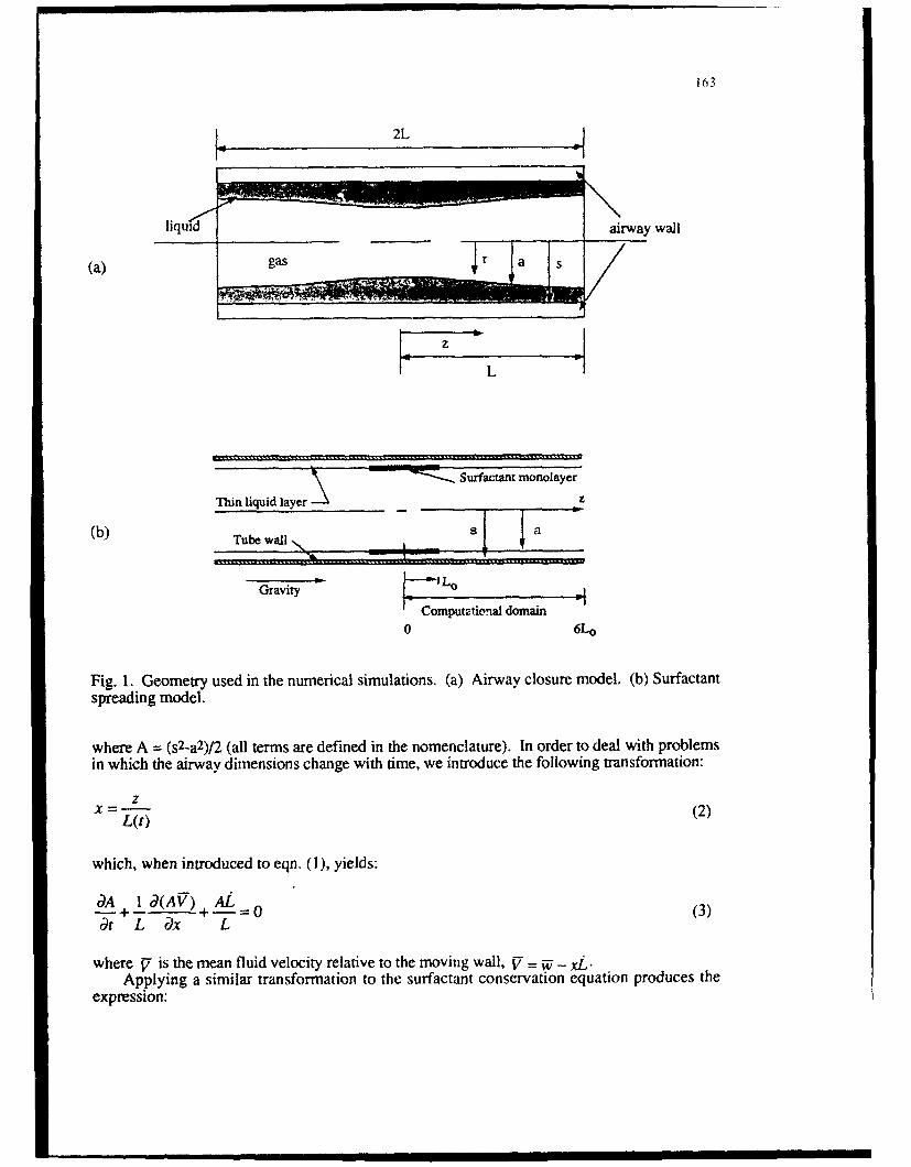
163

2L

liquid airway wall

(a) gsr a S

L

Thinliqid lyerSurfactant monolayerThin liquid layer --•z

(b) Tube wal. . a

Gravity Lo

F Computational domain0 6Lo

Fig. 1. Geometry used in the numerical simulations. (a) Airway closure model. (b) Surfactantspreading model.

where A = (s2-a2)/2 (all terms are defined in the nomenclature). In order to deal with problemsin which the airway dimensions change with time, we introduce the following transformation:

z x = •(2)L(t)

which, when introduced to eqn. (1), yields:

oA 1 d(AV) ALT+ - + = 0 (3)td L dx L

where f is the mean fluid velocity relative to the moving wall, f = WApplying a similar transformation to the surfactant conservation equation produces the

expression:

164

d l)+Id (arVa t I df or) 0

tT 7 t L Lj 7,•Ly FLTx dx4

where

[1 + da 4Y V'2 (5)

The axial momentum equation, with gravity oriented parallel to the tube axis is written

p- -- w- t= a r--rtE +r -- j +pg (6)P~dtd+Urd+ z } r dr dr}

the solutions of which must satisfy boundary conditions on the radial velocity:

ds ds da daus-= +W -,I U. =-a +W,2 (7)

axial velocity at the wall

w, =xL (8)

and the velocity gradient at the interface

,(dw)i da (9UI - = -"-z (9)Tr .dr dz

which is what gives rise to the Marangoni effect. For all cases discussed below we assumesymmetry about z = 0 and impose the condition of zero axial velocity at z = L.

The radial momentum equation is not needed since, in the long-wavelength approximation,the radial pressure gradient can be neglected compared with its longitudinal variation.Therefore, pressure in the liquid film is determined by Laplace's law applied across the gas-liquid interface, used in the form:

p(z,t) = -Y+ d(r })+ pg,. (10)

where gas pressure, Pgas, is assumed constant. Combining eqns. (6)-(9) and integrating themomentum equation across the liquid layer in the manner of Johnson et al.[31, we obtain

161

a dna da din.a__

V"l 2pLdx A

SL -L ox A- a-A -~ A2 I - n a)

This system of equations is solved numerically using a third-order Adams-Bashforth techniquefor time-derivatives and central differences for spatial derivatives. In some of the followingcalculations, the effects of axial inertia were negligible, resulting in a somewhat simpler form ofthe equations. In addition, although surface diffusion is included in some of the foIlowingresults, it was found to be negligible in all cases when realistic numerical values are used.

For simulation of the lung during expiration, all linear dimensions are taken to vary as thecube root of lung volume [ 141, which is assumed to decrease linearly with time:

11J3

L(t) = I I SW= L(t) (12)L~~t). =Icl- st) 3

3. EXPERIMENTS ON AIRWAY CLOSURE

To provide a qualitative illustration of airway closure, experiments were conducted in alarge-scale model of a segment of the airway tree, manufactured by a computer-aided millingprocess by Hammersly and Olson [15]. Two immiscible liquids were used, silicone oil (gI =9.7 dyne s/cm2 , p = 0.97 g/cm3) and a water-ethanol mixture (88.4% water, 11.6% ethanol byweight) that was density-matched to minimize buoyancy effects. The water-alcohol mixturewas used to simulate the relatively inviscid air and was dyed to distinguish it from the clearsilicone oil that simulated the liquid lining in the lung.

The system was prepared for an experiment by first filling the entire network with siliconeoil, then slowly adding the water-alcohol mixture, leaving a thin, nearly uniform layer ofsilicone oil on the walls of the network. The initial thickness of the liquid layer wasapproximately proportional to the airway diameter for each generation (h0/s = 0.30--0.02) exceptfor regions of near zero thickness near the flow divider (carina) of each bifurcation. When theentire network had been purged, the flow was stopped and a sequence of photographs weretaken during the time it took for all of the branches to become occluded by a meniscus. Aselected set of these photographs is shown in Fig. 2a-d.

Following the stoppage of flow, the uniform annular film in each airway initially grewtoward an unduloid-like shape and then finally to complete closure by a meniscus. The processbegan slowly, then proceeded more and more rapidly as the amplitude of the disturbance grew,taking a total of from about 15 to 25 minutes. The final stages in the joining of the opposinginterfaces occurred on a time scale of seconds whereas the process leading up to this event tookmany minutes. By 25 minutes, all branches were occluded, producing a collection of "dog-bone-shaped" dark regions.

Despite the tendency for the menisci to be slightly nearer the larger neighboring branch(parent airway) in each instance, there was little evidence to suggest that a significant quantity ofliquid was exchanged between branches on the time scale of film collapse; each meniscusoccupied roughly the same fractional volume of the branch at the end of the experiment. Thismay have been at least partly a result of the tendency for wall liquid to be drawn from the bifur-

166

Fig. 2. Sequence of photographs showing the progression of a viscous liquid film lining theinside walls of a plexiglas model from a layer with h0ts nearly uniform at 0.23 to a final statewith all airways occluded by a meniscus. Photos correspond to the following times, referencedto the time that the airway shown in (a)-(c) is first purged: (a) t = 3:45 min. (b) t = 22:35 min.(c) t = 23:05 min. (d) t = 30:45 min..

cation zones toward the center of the branch as the instability grew, leaving behind a narrowedlayer where exchange would have to take place. In every instance, the wavelength of theinstability that ultimately led to closure was comparable to the length of the branch itself.

4. PREDICTIONS OF AIRWAY CLOSURE

Airway closure was modeled for a lung during expiration using the full form of eqns. (3),(4), (8) - (12). A single airway was considered, having the idealized geometry depicted in Fig.la. The airway size and liquid layer thickness at maximal lung volume were selected torepresent typical values for a terminal bronchiole (see caption for Fig. 4). It is assumed that theairway remains geometrically similar and that no liquid escapes from the ends at x = 1,-1. Inaddition, the equation of state relating surfactant concentration to surface tension is given in Fig.3, taken from the measurements of Schurch [161.

A typical result is shown in Fig. 4. In Fig. 4a, the thickness of the liquid layer is shown asa function of time, demonstrating the transition from an initially uniform layer (perturbation

35

30

25

0, 20dynes/cm 15

50 ,

0.75 1.00 1.25 1.50 1.75 2.00

Fig. 3 Surfactant equation of state for lung surfactant [16] used in the calculations of airwayclosure. Minimum surface tension is taken to be 1 dyne/cm. Surfactant concentration is shownhere normalized to the value at a = 30 dyne/cm which corresponds to 2.3x 10's molecules/m 2,

amplitude 0.001lo0) at t = 0, through the growth of the instability and ultimate closure. Fortimes less than about 400 msec the layer remains fairly uniform, but thickens due to theredvction in airway size. For t > 400 msec, the instability rapidly grows and liquid is drawnfrom the ends of the tube toward the center until at t = 436 msec, the protrusion at x = 0 reachesthe centerline and closure occurs. It shotid be noted that, in all these simulations, theapproximations made in the analysis break down in the final stage of closure, but this stagepasses so quickly that it has relatively little influence on the predicted closure times 13].

For the case shown, the liquid film is at first stable to small perturbations and the initialdisturbance begins to relax toward a cylindrical surface. By the time lung volume falls to0.89TLC, however, the film has thickened to the point that the mean inner film radius is lessthan L/It and the Rayleigh instability takes over, reversing the initial tendency toward a uniformfilm and generating a flow from the ends toward a growing "bulge" near the center. Givensufficient time at a given lung volume, this instability would proceed to a new equilibriumconfiguration (an unduloid) without airway closure. However, as lung volume continues tofall, the ratio of liquid volume to tube volume increases above a critical value of 0.297 (at a lungvolume of 0.26TLC) and, rather than forming an unduloid, a closed meniscus is the stable,minimum surface energy state. For different geometries and/or different liquid volumes, thissequence can be altered and the critical volume condition might be met before the Rayleighinstability causes the film to become unstable; in that case it is never possible to obtain a stableunduloid. These events are illustrated in the stability map of Fig. 5 where a reduction in lungvolume can be viewed as moving downward along a line of fixed L/ns. For case 1, the filmbegins as a stable, uniform-thickness layer, passes through a region in which the stableconfiguration is an unduloid, and ends up forming a liquid bridge as a/s falls below a value ofabout 0.8. Case 2 is one in which the only instability ultimately leads to a liquid bridge, by-passing the unduloid state entirely.

The pressure distributions shown in Fig. 4b correspond to the same times and lungvolumes as shown in 4a. The interesting feature here is that the minimum pressure at the wall isobserved at maximal lung volume when the radius of curvature is largest. This counter-intuitiveresult is due to the presence of surfactant at concentrations typical of those found in the lung.

t68

I 0

0.9 - - - - -- -- - - -- - - - - -- -200

0.8 -400 -(b)

0.7 pre~sure. .6001=28 dynes/cm~

0.6 - - - - - - 1= o 8 0

0.5 -- I28 -1MX-- t=390

OA ) - --435 -12000.3 -1-1400

-1 -0.6 -012 0.2 0.6 1 -1 -0 .ý -0.2 0.2 0.6x X

14

12(C

10

r6

4

-0.6 -0.2 0.2 0.6 1

Fig. 4. Airway closure in a contracting airway with variable surface tension. At TLC, L0.075 cm, s = 0.025 cm, a =0.024 cm. Fluid properties: g. = 0.01 dyne-se/cm2, p = lg/cm 2-Expiration rate = 200% TLC/sec. (a) Film thickness at four times (in msec), (b) pressure inliquid layer at name times, (c) surfactant concentration at same times. Closure occurs at 435msec.

.0- . . .

0.6

0.4-

00.2 0 0.6 08 1 0 1.2

Fig. 5 Stability map for the formnation of an unduloid and liquid bridge.

As the interface contracts during expiration, the surfactant concentration rises (see Fig. 4c) andthe surface tension consequently falls. With sufficient surfactant present, it falls so rapidly thata/a actually decreases as the airway contracts. The magnitude of the liquid pressure falls froman initial value of about 1250 dynes/cm 2 to about 100 dynes/cm 2 and remains low for theduration of expiration. The gradients in surfactant concentration remain relatively small until thefinal stages of closure, but are, in fact, large enough to effectively "freeze" the interface due tothe Marangoni effect. Thus, closure is delayed by pulmonary surfactant as a result of twomechanisms. First, the reduction in surface tension as the gas-liquid interface becomesincrcasingly compressed during expiration brings about a consequent reduction in the pressuregradient driving the instability for a given displacement amplitude. This driving force scaleswith the surface tension and its reduction due to airway contraction is, in most cases, thedominant influence. Second, the presence of a surface tension gradient produces a shear stressat the interface (see eqn. (9)) that effectively reduces the interfacial velocity to near zero values.By itself, this slows the instability by a factor of about four -- for a given pressure gradient andfim thickness, the flow rate between two stationary surfaces is lower by a factor of four thanthat between one stationary and one free surface. As long as the surface tension remains non-zero, neither mechanism causes an unstable condition to become stable; they only affect the razeat which the instability proceeds and, therefore, can influence the lung volume at which closureoccurs for a given rate of expiration.

Fig. 6 shows the results from many calculations of the type just described, both with andwithout surfactant and with different values of surface tension. The two limiting cases (highand low values of the expiration rate) can be understood as follows. In the quasi-static limit (farto the left in the figure) closure occurs as soon as both conditions (L > ita and Viiq/s 3 > 5.6) arefirst satisfied and is independent of the rate of expiration. In the limit at the right, the airwaycontracts so rapidly that the instability has no time to develop and closure occurs essentiallywhen the volume of liquid equals the airway volume. In between these limits, a competitionexists between the growth of the instability and the reduction in airway volume. Interestingly,the case which is thought to be most representative of the real lung (labeled case IV forexpiration rates of about 20%TLC/s) fall into this transition range, suggesting that surfactantdoes indeed function to reduce the closing volume of the lung under normal conditions. Note

30

25•-'•--- - - - -- - - -suff

esufficient liquidcase I, ., .threshold

Closing 20volue, " I. case III,

volume, cs 1,a3ca e I, "I,%TLC 15 _20

5 "entire airway5full of liquid

100 1000 104

Expiration rate, %TL.C/scc

Fig. 6 Closing volume for different rates of expiration. For the three curves labled Case Ill,the surface tension is held constant at 1, 20 or 30 dynes/cm. Horizonatal lines show limits forslow (upper) and fast (lower) expirations.

170

that closing volume in a normal lung usually occurs at a lung volume of about 30%TLC,roughly consistent with these predictions. Also consistent with these predictions, lungs withinsufficient surfactant (as in respiratory distress syndrome) exhibit gas trapping and atelectasisat higher than normal lung volumes and often require mechanical ventilation with high airwaypressures to maintain patent airways.

Other factors, not accounted for in this model, may also be important. The airways arecompliant vessels, the stiffness of which is largely determined by the tethering forces exerted ontheir external surface by the surrounding lung tissue (parenchyma). This tethering force scaleswith the inflating pressure of the lung and approaches zero for lung volumes in the range of15%TLC [171. Although the precise influence of airway compliance in the real lung is notknown, the effects of compliance nave been incorporated into a model of airway closure [181and demonstrate that compliance hastens the closure process and would thus cause it to occur atsomewhat greater lung volumes.

5. SPREADING OF AN EXOGENOUS SURFACTANT

The geometry used to study the axial dispersion of an instilled bolus of exogenoussurfactant is shown in Fig. lb. In this model, a linear equation of state of the form, 0 = 0.ax-off, is employed, where amax is the maximum value of surface tension. The surfactant isdeposited in an axi-symmetric distribution between x = 0 and 1 at time t = 0. This introduces agradient in surface tension which draws the interface to the right, dragging with it fluid in thesub-phase. As shown in Fig. 7, liquid in the vicinity of the deposited surfactant moves outwardin the form of a propagating, shock-like disturbance of nearly constant amplitude. Over most ofthe domain, flow is generated by the (nearly linear) surface tension gradient (Marangoniconvection) with capillarity associated with surface curvature playing an insignificant role. Atthe leading edge of the advancing front, however, the steep gradient in film thickness gives riseto large interfacial curvatures and capillarity becomes the dominant factor leading to pressuregradients in the film that generate the observed flow. Surface curvature and capillarity also playa role in the trailing region near the site of surfactant deposition, although to a somewhat lesserextent. A simple scaling analysis, confirmed by more extensive numerical simulations [111,demonstrates that the height of the surface film will approach twice the initial thickness of theliquid layer and that its leading edge will propagate at a speed that scales as (aMh0gt-lt- 2)1/3.

2 1

h__1 ,•r 0.6-

ho 1: 0.4

0.2

z/Lo z/Lo

Fig. 7 Dimensionless liquid layer thickness (a) and surfactant concentration (normalized byconcentration at z/L0 =0) (b) for the spreading of a surfactant from an initial deposition betweenz/Lo = 0 and 1. Parameter values: h0/Lo = 0.01, ho/s = 0.01, Hbol = 0.0, Bo = 0.0. Curvesare for dimensionless times tOmaxh/(11L0 2) = 0, 2, 10, and 16.

!~ ~~~ -I I I

A refined discretization from 60 to 240 nodes dampens the waves at the trailing edge of thepropagating disturbance, but has little effect on those at the leading edge. Further refinement, to480 nodes, produces no further change leading us to conclude that while the wave structure atthe back is a numerical artifact, the precursor wave structure is real and is presumably associatedwith the dispersive character of the equation set. Subsequent results were obtained using thecoarser grid since this resolution seems adequate to capture the primary spreading behavior.

The parameters of this problem include the ratio of initial film height to airway radius(h0/s), the ratio of initial film height to the axial extent of the region of deposited surfactant(ho/L 0), the initial surface tension difference, the Bond number representing the ratio ofgravitational to surface tension effects, and the amount of bulk liquid deposited on the film in abolus along with the surfactant, characterized by the parameter Hi,0 as defined by the followingexpression for the initial film thickness distribution:

h 717s+ - (13)

for -1 < z/Lo < 1 and h/ho = 1 elsewhere. Each of these was varied independently in order toascertain their effect on spreading behavior.

Simulations in which ho/s was varied between 0.001 and 0.04 (the range of valuesanticipated in the lung) showed no significant differences from the behavior depicted in Fig. 7.Airway curvature therefore plays essentially no role in surfactant spreading. Consequently,models in which the effects of airway curvature are neglected would seem perfectly appropriatefor most cases.

Variations in hO/LO proved to be somewhat more significant as shown in Fig. 8. Whenexpressed in this non-dimensional format, the main influence of h0/Lo is on the shape of thepropagating disturbance rather than its speed of propagation with larger values giving rise to agenerally more rounded appearance and a broader, less well-defined shock zone. Indimensional terms, since time is normalized by tLL0 2/(,maxhO) the rate at which the wavepropagates is proportional to hoVLo2; thinner films or larger regions of surfactant coverage tendto reduce the rate of spread.

2 1-------- - _ _

h+ /A-"-

h.- ( (b-0.4

0.5 - 0.2

0 4 60 2 4 6 0 2

z/L(,, /

Fig. 8 Dimensionless liquid layer thickness (a) and surfactant concentration (b) showing theeffect of changing ho/LO. Parameter values: are the same as in Fig. 7 except ho/Lo = 0.01.Curves are for dimensionless times tamajh](tVL(t 2) = 0, 2, 10, 3nd 16.

Given this dependence of propagation speed on film thickness, it seemed reasonable toattempt to augrrent the rate of transport by introducing the surfactant in a liquid volumesufficient to significantly increase the underlying film thickness. However, when bolusvolumes were increased (Fig. 9), we found that the rate of propagation was virtually unaffected.

172

1.5 / (b)

h I -/ 0.6

0.1

- - 6- "-4 60 4zlL0 ,,/L ,

Fig.9 Dimensionless liquid layer thickness (a) and surfactant concentration (b) showing theeffects of changing bolus volume. Parameter values are the same as in Fig. 7 except Hioi 1.0.Curves are for dimensionless times tom ~h0/(I.o2) = 0, 2, 10, and 16.

2 ,I1.5 '1

0.8- (b')

hh._ r 0.6-

ho 0.4-

-.50 0.20 5o 1 -5 5o 1-5 0 5z/Lo z/L,

Fig. 10 Dimensionless liquid layer thickness (a) and surfactant concentration (b) showing theeffects of changing bolus volume. Parameter values are the same as in Fig. 7 except for Bo =0.1. Curves are for dimensionless times t;maxho/(gL02) = 0, 2, 10, and 16.

Moreover, the additional instilled volume appears to have remained in a central pool at the site ofdeposition which was proportionately of greater depth than the original case (compare Figs. 7and 9).

Gravity was also considered by choosing values of the Bond number (Bo = 0.001 to 0.1)corresponding to a vertically oriented airway ranging in size from a terminal bronchiole to thetrachea. Only in the tracheal simulation (Bo = 0.1) did gravity exert a significant influence,causing the spread to be noticeably asymmetric as shown in Fig. 10. Even in this extreme case.the rate of spread of the surfactant was only slightly increased, suggesting that, at least forrelatively small volumes of deposited surfactant, gravity plays a minor role. This is clearly notthe case, however, in experiments that have been reported in which the volume of the instilledbolus is comparable to that of the entire central airway system 1191 in which case other factors,not represented in these simulations, take precedence.

Lastly, we investigated the perhaps more realistic situation of placing an exogenoussurfactant on a thin film containing an endogenous surfactant layer (Fig. 11). In this case. the

propagating wave compresses the interface ahead of it, producing a secondary gradient insurface tension due to increased concentration of the endten.,us surfttctant. This generatesflow away from the deposition site and toward more remote locations. By this mechanism, theeffect of the instilled surfactant spreads much more rapidly (compare Figs. 7 and 11).However, because the height of the disturbance is correspondingly reduced, the amount of wallliquid transported away from the deposition site is actually less than when there is noendogenous surfactant. This finding is also true in cases when the volume of the bolus isincreased with endogenous surfactant present (results not shown).

0.5 2

0

Fig. 1I. Dimensionless liquid layer thickness (a) and surfactant concentration (b) showing theeffects of changing bolus volume. Parameter values are the same as in Fig. 7 except for thepresence of surfactant on the initial interface. Curves are for dimensionless timestomaxh0/(IILo0) = 0, 1, 2 and 3.

These results can be used to predict the rate of spread of a boius of surfactant deposited inthe trachea of a newborn infant. In the absence of endogenous surfactant, and using theparameter values given in the caption, surfactant would naverse the entire length of the trachea(1.5 cm) in just 0.2 seconds. If we neglect the influence of bifurcations, the action of othermechanisms such as the beating of the cilia in propelling liquid toward the mouth, and the rapidincrease in surface area per unit length of airway with distance toward the periphery, wecalculate that this front would reach the alveolar zone in about 7 seconds. Such transport rateshelp to explain why surfactants instilled in the trachea of infants produce so favorable an effect,and also argues for the use of surfactants in the delivery of other medications that need to bedrawn into the lung.

6. CONCLUSION

In this paper we have examined two problems pertaining to the stability and mobility of theairway liquid lining as a means of raising a variety of intriguing and significant fluid dynamicquestions. As the lung and airway network expand and contract during normal breathing thethickness of the liquid layer varies and can, if sufficiently thick, become unstable at low lungvolumes by a mechanism analogous to the Rayleigh instability of a liquid jet and form ameniscus that blocks the airway. If this blockage persists, gas absorption peripheral to themeniscus produces regional atelectasis and a loss of gas exchange capability. Since excessairway liquid and atelectasis are common manifestations of respiratory disease, thisphenomenon may be critical. If atelectasis is to be avoided, the airways, if closed, must reopenon inspiration. This raises questions concerning the movement and eventual elimination of theliquid meniscus.

174

A related set of fluid dynamic issues is raised by the presence of pulmonary surfactantwhich is produced in the gas exchange region of the lung but found in varying amountsthroughout the airway tree. In lungs with normal surfactant production, a surface tensiongradient exists that has the capability of drawing liquid from the periphery toward the mouth bythe action of surface tension gradients. The importance of pulmonary surfactant is underscoredby the prevalence of pulmonary diseases in which surfactant production is imp-iired such asneonatal or adult respiratory distress syndrome (RDS). Instillation of exogenous surfactant isnow the accepted treatment for neonatal RDS with generally excellent results. For a small butsignificant subgroup, however, this therapy is ineffective. Since the efficacy of this methodmay depend on how effectively surfactant is transported to the lung periphery, studies are nowunderway to determine how an exogenous surfactant spreads in the lung. The spreading iseffected by Marangoni flows, raising the exciting prospect of using surfactants as a vehicle fortransporting other medications to the periphery where they can be readily absorbed.

The solutions presented here address but a few of the intriguing fluid dynamic problemsrelating to the dynamics of the pulmonary liquid lining layer. Studies relating to the formation,movement, and reopening of liquid menisci are essential to further our understanding of thesephenomena in healthy and diseased lungs. Important questions remain concerning the factorsthat regulate the distribution of liquid between the vascular, interstitial and airwaycompartments. The movement of airway liquid through a multiple-generation network due tosurface tension gradients, either due to endogenous or exogenous surfactant needs further study.In particular, the potential role of instilled surfactant as a vehicle for drug delivery warrantsinvestigation.

AcknowledgementsMany individuals have made significant contributions to the work presented in this paper.

They include M. Johnson, J. Haid, F. Espinosa, T.J. Pedley, J.J. Fredberg, A.H. Shapiro,D.R. Otis. This work was supported by grants from the National Heart, Lung, and BloodInstitute, HL33009 and HL45679.

NOMENCLATURE

a = radius to free surface, cmA = (S2- a2)/2, cm 3

Bo = Bond number, pgh0Lo/aD, = surfactant surface diffusion coefficient, cm 2/sg = accele.ration due to gravity, cm/s2

h = liquid layer thickness, (s-a), cmL0 = initial monolayer half length, cmL = airway half-length, cmM = mass of surfactant per unit circumference, g/cmp = pressure in liquid film, dyne/cm 2

Pgas = gas pressure in airway, dyne/cm2

s = radius to airway wall, cmt = time, su = radial velocity of liquid layer, cm/sTLC = total lung capacityTexp = time in which the lung is emptied from TLC, sVa = wa - xL = surface axial flow velocity relative to airway wall, cm/sV = "if- xL = mean axial flow velocity relative to airway wall, cm/sw = axial velocity of airway film, cm/sW = mean axial velocity of airway film, cm/sx = Z/L

d i II i"

z = axial coordinate in airway, cm

Cc = slope of the linear equation-of-state for a vs. r, cm 2/s 2

7/ = [I + ((I/L)aa/ax) 2]-1/ 2

r = dimensionles, surfactant concentrationA. = viscosity of atiway liquid, dyne.s/cm 2

p = density of airway liquid, g/cm 3

a = surface tension, dynes/cmamax = maximum value for o

Subscripts

a -(r-a)s -(r=s)

REFERENCES

1 L. Rayleigh, London Math Soc. Proc. 10 (1879) 4.2 P.S. Hammond, J. Fluid Mech., 137 (1983) 363.3 M. A. Johnson, R. D. Kamm, L. W. Ho, A. H. Shapiro and T. J. Pedley, J. Fluid Mech.,

233 (1991) 141.4 W. C. Hulbert, B. B. Forster, W. Laird, C. E. Phil and D. C. Walker, Lab. Invest., 47

(1982) 354.5 J. A. Nadel, J. H. Widdicombe and A. C. Peatfield, Vol. 1 Handbook of Physiology,

Respiratory System, Chapt. 13, Waverly Press, Inc., (1986) 419.6 S. Schurch, Resp. Phys., 48 (1982) 339.7 P. Gebr, S. Schurch, Y. Berthiaume, V. Im Hof and M. Gerser, J. Aero. Med., 3(l),

(1991) 27.8 A. Jobe and M. Ikegami, Am. Rev. Respir. Dis., 136 (1987) 1256.9 D. P. Gaver and J. Grotberg, J. Fluid Mech., 213 (1990) 127.10 D. P. Gaver and J. Grotberg, J. Fluid Mech., 235 (1992) 399.11 F. F. Espinosa, A. H. Shapiro, J. J. Fredberg and R. D. Kamm, J. Appl. Physiol.

Submitted for publication.12 V. S. Kharasch, T. D. Sweeney, J. J. Fredberg, J. Lehr, A. I. Damokosh, M. E. Avery

and J. D. Brain, Am. Rev. Respir. Dis., 144 (1991) 909.13 D. R. Otis, M. Johnson, T. J. Pedley and R. D. Kamm, J. Appl. Physiol. Submitted for

publication.14 J. M. B. Hughes, F. G. Hoppin and J. Mead, J. Appl. Physiol., 32 (1972) 25.15 J. R. Hammersley, B. Snyder and D. E. Olson, Ad. Bioeng: ASME (1986) 66.16 S. Schurch, H. Bachofen, J. Goerke and F. Possmayer, J. Appl. Physiol., 67(6) (1989)

2389.17 F. G. Hoppin, J. C. Stothert, Jr., I. A. Greaves, Y.-L. Lai and J. Hildebrandt, Vol. 3

Handbook of Physiology. The Respiratory System, Chapt. 13 (1986) 195.18 D. Halpern, J. B. Grotberg, J. Fluid Mech., (1992). In press.19 N. Gilliard, P. M. Richman, T. A. Merritt and R. G. Spragg, Am. Rev. Respir. Dis., 141

(1990) 743.

Theoretical and Applied Mechanics 1992S.R. Bodner, J. Singer, A. Solan & Z. Hashin (Editors)F! icr Science Publishers B.V. 177Q ý3 IUTAM. All rights reserved.

£NERGY-SAVING MECHANISMS IN ANIMAL MOVEMENT

R. McN. Alexander

Department of Pure and Applied Biology, University of Leeds,Leeds LS2 9JT, U.K.

AbstractAnimals use legs and flapping wings instead of the wheels

and rotors of man-made vehicles. Some largely avoid theenergetic penalties of using reciprocating instead of rotarymotion by means of springs which store the kinetic energy thatis lost, as the body or a limb decelerates, and return it in anelastic recoil. Pendulum mechanisms involving exchange ofkinetic energy with gravitational potential energy providealternative means of saving energy at low speeds.

1. INTRODUCTION

Energy saving is important to animals, in many ways. Ananimal may be unable to obtain more than a limited amount offood (and so energy) each day. Alternatively, more food may beavailable only at the cost of taking risks, or of having lesstime available for other activities such as reproduction. Ananimal that moves economically may be able to run faster orfurther for the same energy cost, so may be better at catchingprey or escaping from enemies. The structures and patterns ofmovement on which economy of energy depends are largelyinherited, so can be modified by evolution - other things beingequal, animals that are more economical of energy are morelikely to survive and have offspring. This paper shows some ofthe many energy-saving devices that have evolved in animals.

Unfortunately, we have to start with an awkwardcomplication. It is often relatively easy to predict fromengineering mechanics how a change in structure or pattern ofmovement will affect the mechanical power needed for locomotion.However, the costs that drive evolution are not work, but fuel(food) consumption. We want to know the effects of changes noton mechanical power but on metabolic power, the rate at whichfood energy (measured as heat of combustion) is used.

We might hope to be able to calculate metabolic frommechanical power by dividing by some constant efficiency, butthat approach would lead, in some cases, to serious errors.Metabolic energy must of course be used when muscles do work(conservation of energy requires it) but it is also used whena muscle exerts tension while maintaining constant length andso doing no work. Muscle consists of an array of inter-

178

digitating protein filaments that can slide past each other,allowing it to lengthen and shorten like a telescope. It ismade to shorten by crossbridges between the filaments whichattach, pull and detach like a team of men pulling in a ropehand-over-hand. These cycles of attachment and detachmentcontinue as long as tension is being exerted, whether the muscleis shortening or not, and each cycle costs energy.

The relationship between mechanical performance andmetabolic energy cost is imperfectly understood (Ma & Zahalak,1991; Alexander, 1991), but to a first approximation we canthink of metabolic cost as the sum of two components:(i) the cost of work, proportional to the work performed; and(ii) the cost of force, proportional to the number of activecrossbridges multiplied by the number of cycles made by each ofthem. The number of crossbridges is proportional to the volumeof muscle that has to be activated to exert the force, and therate at which they cycle is higher in muscles that can shortenfast than in muscles that can contract only slowly. Thusevolution can be expected to favour changes that reduce the workthat muscles have to do, that reduce the volume of muscleinvolved, or that enable the animal to use slower, moreeconomical muscles.

2. RUNNING

The energy cost of running is particularly interesting forthe paradoxical reason that very little net work is needed, torun at constant speed over level ground. Work is of courserequired to overcome aerodynamic drag, and friction in thejoints, but the quantities are only tiny fractions of themetabolic energy requirement (Alexander, 1977). Additionalenergy costs arise because animals travel on legs rather thanwheels. It is difficult to imagine how wheels could haveevolved but La Barbera (1983) has argued that legs are in anycase preferable largely because of their capability of travelover irreqular terrain.

To understand the additional costs of travel on legs wemust take account not only of the positive work that muscles dowhen they shorten while exerting force, but also of the negativework done when they are forcibly lengthened, degradingmechanical energy to heat. One muscle in a leg may do positivework while another does negative work. Alternatively, musclesmay do positive work at one stage of the stride and negativework at another. In either case, the sum of all the quantitiesof positive work performed in a journey may greatly exceed thenet work requirement. Similarly, the fuel consumption of yourcar is increased if you drive with the brakes on.

The most obvious additional cost of travel on legs arisesbecause wheels rotate but legs reciprocate. The kinetic energyof an animal (or of any other system of masses) can be thoughtof as the sum of external kinetic energy associated with the

ML l i i i

movement of the centre of mass and internal kinetic energyassociated with movement of parts relative to the centre of mass(see, for example, Alexander, 1988). The internal kineticenergy of a wheeled vehicle may be constant, when it travels atconstant speed, but that of a legged animal rises and falls asits legs swing backward and forward. Positive work must be doneon each leg twice in each stride, and negative work must be donetwice, to keep it swinging. The quantities involved can bereduced by reducing the moment of inertia of the limb about itsproximal end. Specialised running animals such as horses andantelopes have large muscles in the upper parts of their legs,where their mass contributes little to the moment of inertia,while their feet are slender and correspondingly light.

A pendulum can be kept swinging with very little energyinput, because potential energy changes compensate for thefluctuations of kinetic energy. Legs may swing forwardpassively in walking (Mochon & McMahon, 1980; McGeer, 1992) butat higher speeds they have to be driven well above theirpendulum frequency. We will examine later the possibility thatlegs may be spring-mounted, so as to vibrate at the appropriatefrequency, but it will be convenient to leave that until afterdiscussing other, more firmly established, elastic mechanisms.

We have been discussing energy costs that arise becauselegs have mass and make reciprocating movements. We turn nowto other energy costs. Fig. 1 shows some simple wolking deviceswhich will be assumed in the discussion that follows, to havelegs of zero mass.

In Fig. l(a) each leg has two joints, powered byappropriate actuators : a hinge joint at the proximal end, whichenables the leg to be pointed in any required direction withina plane, and a sliding joint which allows changes of leg length.It might have seemed more realistic to have drawn a leg with twohinges (a "hip" and "knee") but the arrangement shown allowsthe same number of degrees of freedom of movement. Supposethat this device walks over level ground keeping the forces onits feet vertical and equal to body weight. Suppose also thatthe moment of inertia of its body is so high that the amplitudeof pitching movements is negligible. In that case, kinetic andpotential energy will remain constant throughout the stride andno net work will be required at any stage, except to replacefrictional losses. However, at the stage shown in Fig. l(a)(i)the hinge actuator is doing positive work and the sliding jointactuator negative work; while at the stage shown in Fig.l(a)(ii) the reverse is the case. Similarly, if a leg with hipand knee joints walked in this way, the actuator of one jointwould have to do work against the actuator of the other, duringmuch of the stride.

This wastage of energy could be avoided by having legs withtwo sliding joints as shown in Fig. l(b), or by more complicatedpantograph mechanisms such as have been used in some leggedrobots (Waldon et al., 1984), but I know no cases of animalssaving energy in this way.

180

i ii ii

a b

i ii

Fig. 1 Diagrams of simple walking devices

Another walking style that avoids having actuators workingagainst each other is shown in Fig. 1(c). The torque actuatorat the proximal end of the limb remains inactive, so the groundforce is aligned with the leg. The sliding joint actuator doesnegative work at the stage of the stride shown in Fig. 1(c)(i),reducing the kinetic energy of the body; and positive work atthe stage shown in Fig. l(c)(ii), restoring the kinetic energy.Thus positive work done at one stage is counteracted by negativework done at another, but it is easily shown that thequantities of work are less than in the style of walking shownin Fig. l(a), for all reasonable step lengths. Alexander (1951)shows similarly for a leg with two hinge joints, that positiveand negative work requirements can be minimized by aligning theground force with the proximal joint. The forces exerted on theground in walking and running by dogs, sheep and othervertebrates tend to be aligned with the proximal limb joints,or with points above them (Jayes & Alexander, 1978).

Even this reduced work requirement can be eliminated(leaving only the work needed to replace frictional losses) ifthe actuator of the sliding joint is replaced by a spring : thetheory is presented by McMahon & Cheng (1990). A vehiclebouncing along on sprung legs must rise and fall, accelerate anddecelerate, but the fluctuations of kinetic energy plusgravitational potential energy are balanced by fluctuations ofelastic strain energy.

Some of the muscles in the legs of mammals have longtendons in series with them. These serve as springs, and have

excellent elastic properties : Bennett et al., (1986) show thatwhen tendons are stretched to physiologically relevant stresses,and allowed to recoil, percentage energy dissipation is no morethan about 7%. The forces on leg tendons and the extent towhich they stretch in running, have been calculated for manymammals (Alexander, 1988) but the most thorough studies are ofkangaroos, most recently by Griffiths (1989). He measured theforce exerted by the gastrocnemius (calf) muscle and its changesin length, as the animal hopped. He showed that it stretchedby about 12 mm as the force increased and shortened as the forcefell, as if it were a passive spring. He also measured theelastic compliance of its tendon and showed that 41% of theneqative and positive work was attributable to passivestretching and recoil of the tendon, leaving only 59% of thework to be done by the muscle fibres.

4.7 kM 6.4 kN

tendon

Fig. 2 The force on the foot Fig. 3 At this stageof a human runner, calculated of a galloping stride,from force plate records. all four legs change

their direction ofmovement and energycan be saved byelastic extension andrecoil of a sheet oftendon in the back.

The ligaments in the arch of the human foot form anadditional spring. Fig. 2 shows a foot at the stage of arunning stride at which the forces are greatest. The groundforce and its point of application (on the ball of the foot) areknown from force plate records. The force in the Achillestendon and the reaction at the ankle joint have been calculated.These three forces flatten the arch, storing strain energy inthe ligaments. Experiments with amputated feet (Ker et al.,1987) show that the arch is a reasonably good spring, withabout 20% energy dissipation, and enable us to calculate thestrain energy stored in it. It seems that of the (kinetic pluspotential) energy lost and regained in each step, about 35% is

182

stored as elastic strain energy in the Achilles tendon and about17% in the arch of the foot. Thus half of the negative andpositive work requirement is accommodated by deformation andrecoil of springs, leaving only half to be supplied (atmetabolic energy cost) by muscles. The muscles that attach tothe human Achilles tendon have fibres about 50 mm long, butmuscles associated with tendon springs in more specializedrunning mammals have much shorter fibres. For example one ofthe digital flexor muscles in the fore leg of tne horse hasmuscle fibres only about 3 mm long attached to a 700 mm tendon.Analysis of films of galloping horses shows that this muscle-plus-tendon lengthens and shortens by about 50 mm in eachstride (Dimery, Alexander & Ker, 1986). The vestigial musclefibres can coutribute very little to this length change, whichmust be almost entirely due to passive stretching and recoil ofthe tendon. The advantage of the reduced size of the musclefibres is presumably that very little metabolic energy is neededto develop tension in them.

An alternative means of saving energy is to balancekinetic energy fluctuations against gravitational potentialenergy fluctuations. In Fig. 1(d) the length of the leg is keptconstant and the ground force is kept aligned with the leg. Atthe illustrated stages of the stride, kinetic and potentialenergy changes art balanced and no work is required of eitheractuator. 1iowever, work is required when one foot is lifted andthe other set down (McGeer, 1992). Alexander (1993) has shownthat gaits involving exchange of kinetic with gravitationalpotential energy can be economical at low speeds, and that- h'aianwalking is close to making the best possible use of thisprinciple.

I return now to the kinetic energy changes associated withforward and backward swinging of the legs. When quaarupedstrot, each fore leg moves in synchrony with the diagonallyopposite hind leg. At higher speeds mammals gallop, swingingthe fore legs back while the hind legs swing forward and viceversa. Fig. 3 shows a stage of the strike at which all fourlegs change their directions of movement and internal kineticenergy passes ti-rough a minimum. Alexander, Dimery & Ker (1985)have shown that much of the lost kinetic energy may be storedas elastic strain energy in a sheet of tendon in the back,saving metabolic energy. There is another stage of the strideat which the legs are at the opposite extremes of their rangesof movement, at which it would again be useful to store kineticenergy taken from them, as elastic strain energy. Bennett(1989) has identified a sheet of tendon in the thigh as apossible store for some of this energy.

3. FLIGHT

When insects, small birds and bats hover they beat theirwings back and forward in a near-horizontal plane, driving airdownwards in the manner of a helicopter rotor. When they fly

fast they beat their wings up and down, adjusting their angleof attack in such a way as to supply not only the upward forceneeded to counteract the body's weight but also the thrustneeded to overcome drag. In either case, we have areciprocating motion : kinetic energy must be supplied to thewings twice in each wing beat cycle, and removed twice. Thismay add little or nothing to the work required of the muscles,if the inertial work required to accelerate the wings is smallcompared to the aerodynamic work required for flight. Work doneto accelerate the wing at the beginning of a stroke may berecovered as useful work done against the aerodynamic forcesthat decelerate it at the end of the stroke. However, if theinertial work requirement is large, some of it may have to bedissipated by muscles doing negative work at the end of thestroke.

The inertial work is relatively large in slow and hoveringflight. Ellington (1984) calculated for hovering by variousinsects that the ratio of inertial to aerodynamic work laybetween 0.7 and 3. In such cases, worthwhile energy savings canbe made by elastic mechanisms. This could be done by placingsprings of appropriate stiffness either in parallel or in serieswith the muscles. Springs in parallel would reduce the forcesrequired of the muscles without affecting their length changeswhile springs in series would do the reverse. Bennett, Ker &Alexander (1987) show that the two cases require springs ofdifferent stiffness. Weis-Fogh (1960) described parallelsprings in the wing hinges of locusts and a series spring on asmdi.L muscle in dragonflies. However, in advanced insects(bees, flies, bugs, beetles etc.) the muscles themselves serveas springs. This was demonstrated by Machin & Pringle (1959),who showed that muscles from such insects, mounted in apparatusthat simulated the loads that would act on them in flight, couldbe made to behave like springs with negative hysteresis :instead of dissipating energy in each cycle of extension andshortening, they did work in each cycle.

The cross-bridges seem to be the springs in these insectmuscles. In Machin & Pringle's (1959) experiments the musclefibres were made to lengthen and shorten by about 5% (peak topeak). Such small length changes might be accommodated bystretching of cross-bridges, without detachment : when a cross-bridge detaches any strain energy stored in it is lost. Themuscles are believed to work over similarly small length rangesin the intact flying insect. Because the range is small, alarge volume o. muscle has to be activated to supply the workfor each wing beat, so it may seem doubtful whether metabolicenergy is saved in comparison with possible alternativearrangements that would not exploit muscle elasticity.

The wing muscles of birds are arranged differently fromthose of the insects we have been discussing, with much largevelocity ratios. Consequently, they have to make length changesof about 20% peak to peak (Cutts, 1986) and there is littlescope for exploiting the elastic properties of cross bridges.Pennycuick & Lock (1976) suggested that useful energy savings

184

might be made by storage of strain energy in bent feathers, butAlexander (1988) argued that the mechanism could not work whenit would be most useful, in hovering. Jenkins, Dial & Goslow(1988) Look X-ray cine film of a starling flying in a windtunnel and showed that the width between the shoulders increasesand decreases in each wing beat cycle. They remarked that thefurcula (wishbone) was behaving like a spring, but it is easyto show from data in their paper that the strain energy storedin it is only about 5% of the inertial work required toaccelerate the wings. So far, no spring has been identifiedthat could have an important energy-saving role in bird flight.

4. SWIMMING

Fishes swim by beating their tails from side to side, andwhales beat their tail flukes up and down. Inertial work mustbe done at the beginning of each stroke, and there may be scopefor energy saving by elastic storage. Bennett, Ker & Alexander(1987) thought that the long tendons in the tails of dolphinsmight serve as in-series springs, but their (admittedly veryrough) calculations indicated that they were too compliant tosave energy. Wainwright, Vosburgh & Hebrank (1978) suggestedthat the mesh of helically-wound collagen fibres in fish skinmight be a useful spring, but its geometry makes it difficultto estimate how much strain energy is stored (Alexander, 1987)and the possibility remains open.

REFERENCES

Alexander, R.McN. (1977) Terrestrial locomotion. In R.McN.Alexander & G. Goldspink (edit.) Mechanics and Energeticsof Terrestrial Locomotion. 168-203.

Alexander, R.McN. (1987) Bending of cylindrical animals withhelical fibres in their skin or cuticle. Journal ofTheoretical Biology. 124, 97-110.

Alexander, R.McN. (1988) Elastic Mechanisms in AnimalMovement. Cambridge : Cambridge University Press.

Alexander, R.McN. (1991) Energy-saving mechani..'sms in walkingand running. Journal of Experimental Biology. 160, 55-69.

Alexander, R.McN. (1992) A model of bipedal locomotion oncompliant legs. Philosophical Transactions of the RoyalSociety B (in press).

Alexander, R.McN., Dimery, N.J. & Ker, R.F. (1985) Elasticstructures in the back and their role in galloping in somemammals. Journal of Zoology. A 207, 467-482.

Bennett, M.B. (1989) A possible energy-saving role for themajor fascia of the thigh in running quadrupedal mammals.Journal of Zoology. 219, 221-230.

Bennett, M.B., Ker, R.F. & Alexander, R.McN. (1987) Elasticproperties of structures in the tails of cetaceans(Phocaena and Lagenorhynchus) and their effect on theenergy cost of swimming. Journal of Zoology 211, 177-192.

Bennett, M.B., Ker, R.F., Dimery, N.J. & Alexander, R.McN.(1986) Mechanical properties of various mammaliantendons. Journal of Zoology A 209, 537-548.

Cutts, A. (1986) Sarcomere length changes in the wing musclesduring the wing beat cycle of two bird species. Journalof Zoology A 209, 183-185.

Dimery, N.J., Alexander, R.McN. & Ker, R.F. (1986) Elasticextension of leg tendons in the locomotion of horses(Equus caballus). Journal of Zoology A 210, 415-425.

Ellington, C.P. (1984) The aerodynamics of hovering insectflight. VI. Lift and power requirement. PhilosophicalTransactions of the Royal Society B 305, 145-181.

Griffiths, R.I. (1989) The mechanics of the medialgastrocnemius muscle in the freely hopping wallaby(Thylogale billardierii). Journal of ExperimentalBiology. 147, 439-456.

Jayes, A.S. & Alexander, R.McN. (1978) Mechanics of locomotionof dogs (Canis familiaris) and sheep (Ovis aries).Journal of Zoology. 185, 289-308.

Jenkins, F.A., Dial, K.P. & Goslow, G.E. (1988) Acineradiagraphic analysis of bird flight : the wishbone instarlings is a spring. Science 241, 1495-1498.

Ker, R.F., Bennet, M.B., Bibby, S.R., Kester, R.C. & Alexander,R.McN. (1987) The spring in the arch of the human foot.Nature. 325, 147-149.

La Barbera, M. (1983) Why the wheels won't go. AmericanNaturalist. 121, 395-408.

Ma, S. & Zahalak, G.I. (1991) A distribution-moment model ofenergetics in skeletal muscle. Journal of Biomechanics.24, 21-35.

Machin, K.E. & Pringle, J.W.S. (1959) The physiology of insectfibrillar muscle. II. Mechanical properties of a beetleflight muscle. Proceedings of the Royal Society. B 151,204-225.

1McGeer, T. (1992) Principles of walking and running. In RMcN.Alexander (editor) Mechanics of Animal Locomotion. 113-139, Berlin, Springer.

McMahon, T.A. & Cheng, G.C. (1990) The mechanics of runninghow does stiffness couple with speed? Journal ofBiomechanics. 23, suppl. 1, 65-78.

Mochon, S. & McMahon, T.A. (1980) Ballistic walking : animproved model. Mathematical Biosciences. 52, 241-260.

Pennycuick, C.J. & Lock, A. (1976) Elastic energy storage inprimary feather shafts. Journal of Experimental Biology.64, 677-689.

Wainwright, S.A., Vosburgh, F. & Hebrank, J.H. (1978) Sharkskin : function in locomotion. Science. 202, 747-749.

186

IWaldron, K.V., Vohnout, V.J., Pery, A. & McGhee, R.B. (1984)Configuration design of the Adaptive Suspension Vehicle.International Journal of Robotics Research. 3, 37-48.

Weis-Fogh, T. (1960) A rubber-like protein in insect cuticle.Journal of Experimental Biology. 37, 889-906.

Theoretical and Applied Mechanics 1992S.R. Bodner, J. Singer, A. Solan & Z. Hashin (Editors)Elsevier Science Publishers B.V. 18 7© 1993 IUTAM. All rights reserved.

CONTROLLING CHAOTIC CONVECTIONHaim H. Bau

Department of Mechanical Engineering and Applied Mechanics, University ofPennsylvania, Philadelphia, PA 19104-6315, USAE-mail: bau@eniac.seas.upenn.edu

AbstractThrough the use of a feedback control strategy, one can profoundly alter the

bifurcation structure of convective flows. For instance, with the use of a feedbackcontroller, one can maintain the no-motion state in fluid layers heated from belowand cooled from above at significantly higher temperature differences than thecritical one corresponding to the onset of convection in an uncontrolled system.Likewise, one can maintain steady, time-independent flow under conditions inwhich the flow would otherwise be chaotic. Similarly, one can stabilize periodicnon-stable orbits which exist in the chaotic regime of the uncontrolled system.Finally, the controller also can be used to destabilize otherwise stable flows andthus induce chaos in laminar, non-chaotic flow. In this paper, I will discuss theprogress that has been made in achieving the foregoing in the convective loop andthe saturated porous layer paradigms.

1. INTRODUCTION

In recent years, active control strategies have been successfully used for,among other things, noise reduction and vibration suppression. The area of activecontrol of fluid flow is no less important from a technological point of view; for inmany situations, it may be desirable to maintain flow conditions other than thenaturally occurring ones. Below, I mention a few examples.

In some situations, convection suppression may be desirable. For instance,when a crystal is pulled from a liquid melt heated from below, it may be desirable tooperate at Rayleigh numbers higher than the critical one at which convectionnormally begins and yet have no convection so as to minimize transport ofcontaminants from the crucible walls to the crystal.

In other situations, suppression (laminarization) of chaotic or turbulentmotion and maintenance of a steady, time-independent flow may be desirable inorder to minimize flow unpredictability, remove temperature oscillations which mayexceed safe operational conditions, and/or reduce drag. For instance, stabilizingthe Blasius profile and delaying the laminar-turbulent transition in the boundarylayer flow may provide a means for reducing aircraft drag and thus obtainingsignificant savings in fuel cost. Likewise, suppressing oscillatory convection incrystal growth processes may lead to an improvement in crystal quality.

In yet other situations, it may be desirable to stabilize one of the time-periodic orbits embedded in the turbulent attractor in order to achieve a desired

188

flow behavior. Indeed, from the purely scientific point of view, the ability to stabilizeand observe various non-stable, periodic orbits embedded within the chaoticattractor may help enhance our understanding of the chaotic dynamics and assistus in describing various important properties of the chaotic attractor.

In still other situations, it may be advantageous to induce chaos, underconditions in which it would not normally occur, so as to enhance mixing, heattransport or chemical reactions in combustion chambers or chemical reactors.

Surprisingly given all the foregoing, the idea of altering the bifurcationstructure of flows through the use of active control has received relatively littleattention. Most studies to date have focused on passive control methods.

Passive control strategies do not require a direct investment of energy andthey are usually accomplished by changing the geometry of the solid boundaries.For example, mixing can be enhanced through the use of pipes with sinusoidallymodulated walls rather than straight pipes or by introducing spoilers in the flow.Boundary layer transition to turbulence can be delayed by using perforated solidwalls to facilitate suction (Bushnell and McGinley, 1989); and thermal convectioncan be suppressed by introducing buffers in cavities. Passive devices may haveindirect energy effects as their presence may affect the amount of energy needed topropel the fluid or to propel an object submerged in the fluid.

In contrast, active control strategies require a direct investment of energy foractuation purposes. Examples of active control include inducement of periodicmotion of the solid boundaries, suction and/or blowing, induction of acousticpressure waves, and heating and cooling of the fluid to affect its viscosity. See, forexample, Liepman et. al. (1982) and Liepmann and Nosenchuck (1982) whoadvocated the use of thermal actuation to suppress or enhance Tollmien-Schlichting waves in laminar boundary layer flow. Active control strategies can befurther sub-classified into predetermined and feedback.

Predetermined control consists of pre-programmed actuation designed toaccomplish a desired outcome. The actuation, however, is not sensitive to thefluid's behavior. For example, one may periodically modulate the motion of acavity's boundary to induce chaotic advection and enhance mixing (Ottino, 1991).Another instance of predetermined control is the utilization of magnetic fields ortime-periodic modulation of wall temperature to suppress convective processes.

In contrast, a feedback controller reacts to events occurring in the fluid so asto suppress or enhance naturally occurring instabilities. To make the concept offeedback control more concrete, let's consider the Rayleigh-Benard problem of ahorizontal fluid layer heated from below and cooled from above (Fig. 1). In theclassical problem, as the temperature difference between bottom and top(expressed in non-dimensional form as the Rayleigh number) increases, the stateof the system changes from no-motion to time-independent motion to time-dependent, possibly chaotic, motion. These transitions occur because once theRayleigh number exceeds certain critical values, conditions are ripe for instabilitiesto manifest themselves. The objective of the feedback controller is to enhance thedissipating mechanisms so as to suppress the naturally occurring instabilities. Forexample, Fig. 1 describes the control strategy (dealt with more fully later in thepaper) we used to delay the transition from the no-motion to the time-independentmotion state. In this example, a sensor measures the fluid's temperature at mid-height and the bottom temperature is slightly modified in proportion to the deviationof the sensed temperature from its desired (no-motion) value. At locations where

flow behavior. Indeed, from the purely scientific point of view, the ability to stabilizeand observe various non-stable, periodic orbits embedded within the chaoticattractor may help enhance our understanding of the chaotic dynamics and assistus in describing various important properties of the chaotic attractor.

In still other situations, it may be advantageous to induce chaos, underconditions in which it would not normally occur, so as to enhance mixing, heattransport or chemical reactions in combustion chambers or chemical reactors.

Surprisingly given all the foregoing, the idea of altering the bifurcationstructure of flows through the use of active control has received relatively littleattention. Most studies to date have focused on passive control methods.

Passive control strategies do not require a direct investment of energy andthey are usually accomplished by changing the geometry of the solid boundaries.For example, mixing can be enhanced through the use of pipes with sinusoidallymodulated walls rather than straight pipes or by introducing spoilers in the flow.Boundary layer transition to turbulence can be delayed by using perforated solidwalls to facilitate suction (Bushnell and McGinley, 1989); and thermal convectioncan be suppressed by introducing buffers in cavities. Passive devices may haveindirect energy effects as their presence may affect the amount of energy needed topropel the fluid or to propel an object submerged in the fluid.

In contrast, active control strategies require a direct investment of energy foractuation purposes. Examples of active control include inducement of periodicmotion of the solid boundaries, suction and/or blowing, induction of acousticpressure waves, and heating and cooling of the fluid to affect its viscosity. See, forexample, Liepman et. al. (1982) and Liepmann and Nosenchuck (1982) whoadvocated the use of thermal actuation to suppress or enhance Tollmien-Schlichting waves in laminar boundary layer flow. Active control strategies can befurther sub-classified into predetermined and feedback.

Predetermined control consists of pre-programmed actuation designed toaccomplish a desired outcome. The actuation, however, is not sensitive to thefluid's behavior. For example, one may periodically modulate the motion of acavity's boundary to induce chaotic advection and enhance mixing (Ottino, 1991).Another instance of predetermined control is the utilization of magnetic fields ortime-periodic modulation of wall temperature to suppress convective processes.

In contrast, a feedback controller reacts to events occurring in the fluid so asto suppress or enhance naturally occurring instabilities. To make the concept offeedback control more concrete, let's consider the Rayleigh-Benard problem of ahorizontal fluid layer heated from below and cooled from above (Fig. 1). In theclassical problem, as the temperature difference between bottom and top(expressed in non-dimensional form as the Rayleigh number) increases, the stateof the system changes from no-motion to time-independent motion to time-dependent , possibly chaotic, motion. These transitions occur because once theRayleigh number exceeds certain critical values, conditions are ripe for instabilitiesto manifest themselves. The objective of the feedback controller is to enhance thedissipating mechanisms so as to suppress the naturally occurring instabilities. Forexample, Fig. 1 describes the control strategy (dealt with more fully later in thepaper) we used to delay the transition from the no-motion to the time-independentmotion state. In this example, a sensor measures the fluid's temperature at mid-height and the bottom temperature is slightly modified in proportion to the deviationof the sensed temperature from its desired (no-motion) value. At locations where

190

the flow is hotter than usual and the fluid tends to ascend, the boundarytemperature is reduced to assist in dissipating the excess heat. The reverse occursat locations where the fluid descends. This strategy can be used to significantlyincrease the magnitude of the critical Rayleigh number for the onset of convection.

a805)X

6 xj,y,0,) I - K( t(x~y,0.S5,r) - 0 5)

Fig. 1 A schematic description of the use of feedback control to stabilize the no-motion state in the Rayleigh-Benard problem. 0 is the non-dimensionaltemperature; x and y are coordinates in the horizontal platform; z is a verticalcoordinate; t is time; and K is the controller's gain.

For the remainder of this paper, I will focus on the use of active feedbackcontrol strategies to modify the nature of convective flows.

2. GENERAL CONCEPTS

In this section, I will present the general concepts underlying feedbackcontrol utilizing mathematical notation. First, let's consider the dynamic system(i.e., the Navier-Stokes equations),

F F(B;R) (1)

where Z'- is a vector of dependent variables (i.e., velocity components, temperature,and density); superscript dot denotes the time (t) derivative; R is the parameters'vector (i.e., the Reynolds and/or Rayleigh number); and F is a non-linear (possiblydifferential) operator with the appropriate boundary conditions. Let -=E0 denotean equilibrium, non-transient (i.e., time-independent, time-periodic or quasi-periodic) solution of (1). For example, E0 may be one of the non-stable periodicorbits embedded in the chaotic attractor. As R is varied, equilibrium states maylose stability at bifurcation points and give rise to new, non-transient, stablesolutions. Often several successive bifurcations will eventually result in chaoticbehavior. EO may be either a stable solution for a limited range of the parameters'R (say, for RI <R<R2) or a non-stable solution for all R values. Let us assume that

for a particular process, a selected E0 has better properties than the normallyoccurring flow structure. For example, in Rayleigh-Benard convection, _E0 mayrepresent the no-motion state which we wish to maintain under conditions in which

convection would normally occur. In turbulent boundary layer flow, EO may

I I d i I a i

represent either the laminar, time-independent state or one of the time-periodicorbits embedded in the turbulent attractor. Our objective is to render E0 stable inregions of the parameter space (R) in which it would normally be non-stable.

2.1 DIRECT APPLICATION OF FEEDBACK CONTROL

Feedback control is implemented by augmenting the system (1) with thecontroller C(.):

=G(-; R, K) = F(H; R) + C(Q -Eo;R. K), (2)

where C(.), the controller's output, is either a linear or a non-linear operator withC(O; R, K)=O for all R and K values; K is the controller's gain vector; (:----E0) is thedeviation of the measured variables from their desired values; and E-0 is anequilibrium solution which may be stable for some range of the parameters R ornon-stable for all R values. In the former case, the controller may be used to movebifurcation points in parameter space (i.e., delay the bifurcation to higher values ofR), thus delaying the appearance of chaos. In the latter case, the controller can beused to stabilize states which otherwise would be non-stable for all values of theparameter R such as non-stable periodic orbits embedded in a chaotic attractor.

Note that E-=-E, is a solution of both the original system (1) and theaugmented system (2). That is, the controller preserves the system's equilibria. Inother words, the controller attempts to preserve the stability of EO in regions ofparameter space in which EEO would normally be non-stable. The proposedmethod of control is not the only possible one. Alternatively, one might attempt toachieve the desired flow behavior by generating a new flow structure (_EN) which isan equilibrium state of (2) but not of (1), i.e., C(-EN; R,K)*O. Such a controlstrategy might conceivably be necessary if none of the equilibrium states (HE-) of (1)has the desired behavior. However, an attempt to induce a flow structure (EN)which is not an equilibrium solution of (1) may require a fair amount of powerinvestment. In contrast, the stabilization of E-0 in a noise-free environment requiresan infinitesimal amount of power. Here, we discuss only the stabilization ofequilibrium solutions.

In practice, the controller C(.) can be implemented by manipulating thesystem's boundary conditions. For example, one can equip some of the system'ssurfaces with sensors and actuators.

In relatively simple cases, the analysis of the controlled system (2) can becarried out using tools of stability theory to establish the effects of controller gainson the bifurcation structure of the system. In more difficult cases, one might utilize a"black box" approach and implement the control without knowing either thebifurcation structure of the system (1) or the mathematical model F(.). One doesneed, however, to have an estimate for E0.

192

2.2 TRAJECTORY DIRECTING

A somewhat different, but related, control strategy based on analyzing thebehavior of a system's trajectories in phase space has been advanced by Ott et. al.(1990a and b). The major advantage of this technique is that it provides aprocedure to implement control when the mathematical model for the system is notknown or is too complex to analyze. The method has been used thus far only inlow-dimensional systems. The procedure requires the identification of the non-stable periodic orbit (P), which one wishes to stabilize and which is embedded inthe chaotic attractor, and its linearly stable (ESp) and unstable (EUp) manifolds.This can be done by using embedding to reconstruct the phase space of theattractor from a time series of one of the system's variables obtained by numericalor physical experiments. Subsequently, one can construct a return map to aselected (Poincare) cross-section obtained by stroboscopically sampling the dataat the period of the orbit one wishes to stabilize. This periodic orbit is a fixed pointon the map. The controller is applied in such a way as to force the system'strajectories to approach the stable manifold (ESp) of the periodic orbit (P). Ott et.al. (1990) have successfully stabilized some periodic orbits of the Henon attractorby applying the controller once within each period. The same technique has beenimplemented experimentally by Ditto et. al. (1990) to stabilize two otherwise non-stable, periodic orbits embedded in the chaotic vibrations of a magnetostrictiveribbon.

2.3 OPTIMAL CONTROL

Optimal control involves the minimization of an appropriately defined costfunction (Lions, 1971). For example, when one is applying heating and cooling fordrag reduction in boundary layer flow, the cost function may be defined as:

1T2O(q) = -f dt(Jf w q(x,y,t) dxdy + D) (3)

0 s

where q(x,y) is the distribution of heating/cooling fluxes along the surface; theintegration is carried out over the entire surface over time interval T; D is the drag;and w is a weight which represents the control's cost. In the case of convectionsuppression in the Rayleigh-Benard problem, D may represent the absolute valueof the vertical velocity component integrated along a horizontal cross-section or theNusselt number. The objective is to obtain the distribution q which minimizes thecost function O(q) subject to various constraints. Thus, the optimal control problembecomes a problem of the calculus of variations.

Depending on the system's constraints, the resulting flow structure of thecontrolled system may or may not be an equilibrium solution (Bo) of the system (1).The problem can be formulated, however, as a feedback control problem in whichq=q(=.-=_0) with q(O)=0.

The advantage of the "optimal control" technique is that it provides asystematic algorithm to obtain a desired state of the system and to optimize thecontrol strategy. Unlike the method described in section 2.1, one need not select apre-specified functional form for the operator C(-). The disadvantage is that the

method is computationally intensive and the minimization of the cost functionrequires that the system (1) be solved repetitively. This may be beyond presentcomputational capabilities in situations in which the system (1) consists of theNavier-Stokes equations. To alleviate this problem, Choi et. al. (1992) havedesigned a simplified procedure which they have entitled "suboptimal control" andhave applied it to the stochastic Burgers equation.

3. EXAMPLES OF THE IMPLEMENTATION OF FEEDBACK CONTROLSTRATEGIES

In this section, I describe some of the work that has been done at theUniversity of Pennsylvania on feedback control of convective flows in a thermalconvection loop (Singer et. al. 1991, Singer and Bau, 1991, Wang et. al., 1991)and in a saturated porous layer heated from below and cooled from above (Tangand Bau, 1992a and b). To date, we have been able to demonstrate boththeoretically and experimentally in the case of the thermal convection loop that afeedback controller, such as the one described in section 2.1, can successfully andprofoundly alter the bifurcation structure of convective motions by effecting smallperturbations in the boundary conditions. Currently, we are verifying that similarresults can be achieved in a fluid layer heated from below and cooled from above.

Iaocmsvph. Uinacble Hopforbt t 4i cycke bd ,canon

Cco~krg gdJoC°lnket • "- " " '

Wc Ra R•,_,-7.378 RaA-15.984

RaFtll6.0I Traniei; chaes ! Chaos

steady

.state T.o steady svacrs

Fig. 3: An unscaled bifurcationdiagram depicting various possiblesolutions as Ra is increased (P=4).

Fig. 2 Schematic description of the Stable/non-stable solutions areexperimental apparatus, denoted by solid/dashed lines. The

dark region represents theappearance of the strangeattractor which exists for Ra>RaA.

194

3.1 THE THERMAL CONVECTION LOOP

Consider a thermal convection loop constructed from a pipe bent into a torusand standing in the vertical plane as depicted in Fig. 2. The diameter of the pipe isd; and the diameter of the torus is D. q is the angular location of a point on thetorus. The time-independent wall temperature of the pipe Tw(q), which may varywith the angular location q, is symmetric with respect to the torus axis that isparallel to the gravity vector. Variations in the wall temperature may cause aspatial temperature distribution inside the fluid which, under appropriateconditions, may induce fluid motion in the loop. The convection in such loops hasbeen investigated by, among others, Creveling et. al. (1975) and Gorman et. al.(1984, 1986).

The motion in the loop can be described within the framework ofBoussinesq's approximation by using a one-dimensional model consisting ofmass, momentum and energy balances (Bau and Wang, 1991):

U = u(t), (4)

u -Ra PT cos(O)dO - Pu, and•r (5)

u d + (0)- T].T=-uo-+ Bd 02 (6)

The fluid is assumed to be incompressible and Newtonian. In the above, allquantities are non-dimensional. The length scale is the torus' radius D/2;

Ra = gflAT91 is the loop's Rayleigh number; P3 is the thermal expansion coefficient;DP

g is the gravitational acceleration; and AT is the averaged wall temperaturedifference between the loop's bottom and top. The time scale is -T= poCpd/(4h),

where Po is the fluid's average density, Cp is the thermal capacity, and h (which weassume to be constant) is the heat transfer coefficient between the fluid and thepipe's wall. P=32v t/d 2 =8 Pr/Nu is the loop's Prandtl number, where v is the

kinematic viscosity. Pr=v/o. and Nu=hd/k are the conventional Prandtl and Nusseltnumbers, respectively. a and k are the fluid's thermal diffusivity and conductivity.B=(d/D) 2 /Nu is the Biot number.

The system (4-6) exhibits multiple, non-transient states {uo(t), To(0,t)} whichmay exist only for certain Ra values and whose stability characteristics may vary inaccordance with the magnitude of the Rayleigh number. Our objective is tostabilize and destabilize some of these equilibrium states through the use offeedback control. Our control strategy is to measure the deviation of the actualtemperature from its desired value at various locations around the loop and modifythe wall temperature accordingly. For example, a convenient input signal to thecontroller is AT3-9(t)-AT3.9,0(t), where AT3-9(t) and AT3-9,0(t) denote,respectively, the actual and the desired temperature differences between positions

195

3 and 9 o'clock around the loop. The wall temperature is modified in proportion tothe above deviation, i.e.,

T(O,t)=Tnominai(O)+C[AT3 .9 (t)-AT 3 -9,0 (t)], (7)

where the controller C(.) is typically chosen to be a linear function of its argument.To facilitate the analysis, the temperature distribution in the fluid and the wall

is expanded into a Fourier series in terms of 0 (Malkus, 1977).

T,.(0,t) = WO(t)+W,,(t) sin(nO), andn=1 (8)

T(O, t) = So(t) sin(nO) + C. (t) cos(ne).,=o (9)

Expansions (8-9) are substituted into equations (4-6). By requiring that theequations be satisfied in the sense of weighted rosiduals, the infinite dimensionalsystem (4-6) is transformed into an infinite set of ordinary differential equations.Three of these equations, similar in nature to the Lorenz (1967) equations,decouple from the rest of the set and can be solved independently with exactclosure. In other words, the entire dynamics of the system can be captured by threeordinary differential equations:

Uw-=c-U,

P (10)c_-Us-c (l )

s =uc-s +RaW, (12)

In the above, the dependence on the Biot number, B, was removed via thesimple, algebraic transformation {u, c, s, Ra, P, t) <- 1/(1+B) (u, Ra C1, Ra S1,Ral(1+B), P, t(l+B)2 ). The quantities c and s, respectively, -;:esent thetemperature differences in the fluid between positions 3 and 9 and 6 and 12 o'clockaround the loop. Wi represents the difference in the wall temperature betweenpositions 6 and 12 o'clock. For the uncontrolled case, without loss of generality, weset W1 =-1.

The three ODEs (10-12) possess a number of equilibrium, non-transientsolutions, some of which are listed below:

(A) no motion state (u=O);(B) time-independent motion, either in the clockwise 'denoted B-) or

counterclockwise (denoted B+) direction (u=+±-17- 1);(C) chaotic motion; and(D) periodic motions of various periodicities (i.e., for certain values of theRayleigh number, one observes stable periodic solutions. Also, non-stableperiodic orbits are embedded in the chaotic attractor).

196

Some of the above solutions and their stability characteristics are depictedschematically in Fig. 3 for a loop Prandtl number P=4 which we estimate toapproximate the loop Prandtl number of our experimental apparatus (Singer,1991). In Fig. 3, we denote stable and non-stable solutions by solid and dashedlines, respectively.

Briefly, if one were to follow the chain of events in the uncontrolled system asthe Rayleigh number (Ra) increases, one would observe no net motion in the loopfor Ra<l. At Ra=l, the no-motion solution loses its stability through a supercrticalpitchfork bifurcation and is replaced by time-independent motion. Depending onrandom disturbances, this motion will be either in the clockwise (B-) orcounterclockwise (B+) direction. The motion solution is stable for 1<Ra<16. AtRa=16, the steady solution loses stability through a subcritical Hopf bifurcation.The resulting limit cycle is non-stable and its period increases to infinity as theRayleigh number decreases to Rahom- 7 .3 7 8, where the periodic orbit becomesan homoclinic orbit and passes through the no-motion state (A). At Ra=Rahom,there is a bifurcation (the homoclinic explosion) which results in an assortment ofnon-stable periodic and non-periodic orbits known collectively as the non-wandering set which is initially non-attracting. As the Rayleigh number is furtherincreased beyond RaA-15.984<RaH, the non-wandering set becomes a strange(the Lorenz) attractor. The chaotic regime exists for Ra>RaA with occasionalwindows of periodic behavior. Non-stable periodic orbits of various periodicitiesare embedded in the chaotic attractor. In the chaotic regime, the motion in the loopconsists of irregular oscillations with occasional reversals in the direction of theflow as shown, for example, in Fig. 3 for Ra=3RaH(4)=48. In Fig. 4, theexperimentally observed temperature difference between positions 3 and 9 o'clockare depicted as functions of time. Qualitatively similar behavior is exhibited by thevariable c when the equations (10-12) are integrated numerically. The positive andnegative values of c in Fig. 4 correspond to flow in the counterclockwise andclockwise directions, respectively.

For example, the control (7) for suopressing chaotic motion is incorporatedinto the mathematical model by setting,

W = -I - -L-(COt)- C)Ra (13)

where for demonstration purposes, proportional control is employed. In the above,c(t) and co denote, respectively, the actual and the desired temperature differencesbetween positions 3 and 9 o'clock.

With the use of similar control strategies, we can alter the bifurcationstructure depicted in Fig. 3. More specifically, we can:

(i) maintain the no-motion state at significantly higher temperature differencesbetween the heated and the cooled portions of the loop than the critical onecorresponding to the onset of convection in the uncontrolled system (verifiedthus far by theoretical calculations only, Singer and Bau, 1991);(ii) maintain steady, time-independent flow under conditions in which the flowwould otherwise be chaotic (verified by experiments and theory, Singer et. al.,1991, and Wang et. al., 1992).

197

(iii) stabilize periodic non-stable orbits which exist in the chaotic regime of theuncontrolled system (verified thus far by theoretical calculations only, Singerand Bau, 1991); and(iv) induce chaos in otherwise laminar (fully predictable), non-chaotic flow(verified by theory and experiments, Wang et. al., 1992).

V323A0 3

-'a' I fC2 0

7ý e (.--_ __ -es).3 -2 - : 0 7 2 4.t

K

Fig, 4: The experimentally measured Fig. 5: Stability characteristics of thetemperature differences AT3-9 depicted counterclockwise motion solution underas functions of time. proportional control. The critical

Rayleigh number is depicted as afunction of the controller's gain (K).

16 20

C I5

0~0'

-8 c

-1 2

-20 -25 7 B

00 0.5 1.0 1.5 2ý0 2.5 3 0 1,5 4.0 0 a - 2z- 22. t• t 5 '' "2

Fig. 6: The temperature difference Fig. 7: The experimentally measuredbetween positions 3 and 9 o'clock is temperature difference AT3-9 isdepicted for Ra=50 and P=4 as a depicted as a function of time for similarfunction of time for the controlled (K=- conditions to those in Fig. 6. The35, solid line) and the uncontrolled controller was activated 33 minutes into(K=O, dashed line) systems. the run.

For example, we stabilized the time-independent motion (B+), by employing

the control strategy described by equation (13) with cq(t) = -IR-T1. Fig. 5 depictsour theoretical results pertaining to the effect of the controller's gain on the locationof the Hopf's bifurcation point RaH. Clearly, negative (positive) values of K serve to

198

stabilize (destabilize) the counterclockwise motion solution. As the magnitude ofthe controller's gain decreases, the magnitude of the Rayleigh number at the Hopfbifurcation point increases and the onset of chaos is delayed.

Another interesting phenomenon exhibited in Fig. 5 is that for sufficientlyhigh values of the controller's gain (i.e., K>1.63), the Hopf bifurcation becomessupercritical. For example, in an experiment (Fig. 5) in which we set K=i.7 andgradually increased the Rayleigh number, we observed bifurcation from time-independent to stable, time-periodic flow.

Figures 6 and 7 illustrate the impact of the feedback control on the system.In Fig. 6, the theoretically obtained temperature difference between positions 3 and9 o'clock is depicted as a function of time for the controlled (solid line) anduncontrolled (dashed line) systems for the same nominal operating conditions(Ra=50-3RaH). The uncontrolled system exhibits chaotic oscillations while thecontrolled system exhibits laminar behavior. Similar behavior is observed inexperiments. Fig. 7 depicts the experimentally obtained temperature differencebetween positions 3 and 9 o'clock as a function of time for the same nominaloperating conditions as in Fig. 6. To illuminate the impact of the feedback control,the behavior of the uncontrolled system is depicted for about 33 minutes prior to theapplication of the controller. Witness that once the controller has been engaged,the seemingly random, violent oscillations disappear and the flow is "laminarized".The relatively low amplitude oscillations seen in the system after the application ofthe controller are attributable to the fact that our experimental system is relativelynoisy and sensitive to changes in the environment.

is

to AT3-9 (OC)

5-

10

-10 1 - = .

-20-21 -2J -5 - -5 C 5 2C 5 2

time csN,

Fig. 8: The controller is being used to Fig. 9: Stabilization of an otherwiseinduce chaos at Ra=0.6RaH with non-stable periodic orbit embedded inK=35W/C. The figure depicts the the chaotic attractor for Ra=50.temperature difference betweenpositions 3 and 9 o'clock as a functionof time.

We can also induce chaos under circumstances in which chaos will notnormally occur by using positive feedback (K>O) in (13). In this case, though, wewill need to destabilize simultaneously both the counterclockwise (B+) and theclockwise (B-) time-independent motion states. This we accomplish by employing

I w)

the control strategy W, =-l---[Sgn(c)c(t)-c0 ). The experimental results of thisRa

strategy are depicted in Fig. 8, where we show c(t) as a function of time forsubcritical Rayleigh numbers Ra-0.6 RaH=10. To illustrate the difference betweenthe uncontrolled and the controlled systems, we initially depict the uncontrolledbehavior for t<10nq. Witness the relatively time-independent, counterclockwisemotion. The controller was activated at t=1800s. It caused flow instabilities toamplify, as is evident in Fig. 8, until eventually chaotic flow developed.

Finally, we can use the controller to stabilize one of the otherwise non-stable, periodic orbits embedded in the chaotic attractor. We do this by employinga control strategy similar to the one described by equation (13), with co(t) nowrepresenting the periodic orbit we desire to stabilize. The periodic orbit wasidentified by examining a return map. Alternatively, one can employ one of thetechniques described in Mindlin and Gilmore (1992). The controller can beemployed either continuously in time or at discrete time intervals such as onceevery period (i.e., K=K05(t-nt), where 8(-) is the Dirac delta function, 1 is theperiod of the orbit we wish to stabilize, and n is an integer) or when the orbit passesin close vicinity to a point on the periodic orbit we wish to stabilize. Fig. 9 depicts arepresentative result of the "cs"-plane projection of a stabilized periodic orbit underconditions in which, in the absence of the controller, the flow would be chaotic(Ra=50).

As we have seen, the thermal convection loop paradigm exhibitscomplicated temporal behavior. Next, I describe a strategy for controllingconvection in a system which is not only temporally but also spatially complex.

3.2 THE LAPWOOD PROBLEM

Let us consider thermal convection in a saturated porous layer confined inan upright box, heated from below and cooled from above. The side walls of thebox are insulated. As in the case of the thermal convection loop paradigm, as thetemperature difference between the bottom and top (or the Rayleigh number)increases, the equilibrium state of the system undergoes a sequence ofbifurcations from no-motion to time-independent, cellular motion to oscillatory,chaotic flow. Our objective is to shift the bifurcation points with the aid of afeedback controller. I describe below only the stabilization of the no-motion state(Tang and Bau, 1992 a and b).

I use, respectively, the height of the box (H), the thermal diffusion time H/a

(where a is the equivalent thermal diffusivity of the porous medium), and the

nominal temperature difference (AT*) between the bottom and top of the box as thelength, time and temperature scales. In the uncontrolled system, the non-dimensional bottom and top temperatures are assigned the values one and zero,respectively. The non-dimensional, horizontal dimensions of the box are Lx andLy. The motion of the fluid is described by the Darcy-Oberbeck-Boussinesq (DOB)equations (i.e., Joseph, 1976):

200

Lu= B-(-u-Vp+RO)

b =X-'(U, -u.VO+V O)' (14)

where uT={ux,uy,uz} is the divergent free (V.u = 0), non-dimensional velocity vectorwhich satisfies the impermeability boundary conditions on all solid surfaces; x and

y are horizontal, Cartesian coordinates; z is the vertical coordinate; 0=T-(I-z) is thedeviation of the non-dimensional temperature from the linear (conduction) profile;

R = gA3HAT" is the Darcy-Rayleigh number- g is the gravitational acceleration; X isva

the medium's permeability; [5 and v are, respectively, the thermal expansioncoefficient and the kinematic viscosity of the saturating fluid; p is the pressure

deviation from its hydrostatic value; B = A (usually, B<l); c is the porosity;

and X = (PoCp)eq is the ratio between the equivalent thermal capacity of the(Pocp)f

medium and that of the saturating fluid.The DOB equations admit the no-motion solution {u, 0)=0, which for R<Rc is

globally stable. The magnitude of Rc depends on the aspect ratios Lx and Ly. Forexample, for an unconfined fluid layer with rigid bottom and top boundaries,Rc,=4R2 (i.e., Lapwood, 1948). At R=Rc, the no-motion state loses stability througha supercritical bifurcation into time-independent, cellular motion. The linearizedproblem of stability is self-adjoint, thus the growth rate at the onset of instability isreal. In other words, the bifurcation occurs through a real eigenvalue, and the"principle of exchange of stability" is valid.

To extend the range of stability of the no-motion solution to higher values ofthe Rayleigh number, we modify the bottom temperature in proportion to thedeviation of some interior temperatures from their (no-motion) conduction value.We will assume that the temperature distribution is measured at some horizontalcross-section, i.e., at z=0.5, as a function of the horizontal co-ordinates (x, y). Thecontroller will sense the deviation 00.5=0(x,y,0.5,t) of the actual temperature from

its desired value (0=0) in the plane z=0.5. (For R>Rc, in the absence of the

controller, 00.5 * 0). It will, then, modify sliqhtly the spatial distribution of the base'stemperature in proportion to the measured deviation and its time derivative, i.e.,

0(0,x,y) = C(Q0 .5) = -KpOo. 5 - Kd 0 5 (15)dt

where Kp and KD represent, respectively, the gains of the proportional and thedifferential controllers. Note that boundary condition (15) replaces the boundary

,, I ' I

condition 0(x,y,0,t)=0 in the uncontrolled problem. This can be accomplished inpractice, for example, by embedding a network of computer-controlled heaters inthe base plate and varying their heat input in an appropriate manner.

Next, we investigate the linear stability of the controlled system in thepresence of the controller. The analysis is somewhat more complicated than in theuncontrolled case since the system (14-15) is no longer self-adinint and onecannot ignore the possibility of the no-motion state undergoing a Hupf bifurcationresulting in time-periodic motion. As in the classical case, the disturbances can bedecomposed into even and odd modes with respect to the mid plane (z=0.5). Theodd modes, which lose stability at R=167E2 (r=4), have a node at z=0.5. Thus, thecontrol strategy employed here (equation 15) will affect only the stabilitycharacteristics of the even modes. The results of the analysis are summarized inFig. 10, where we depict the ratio between the Rayleigh numbers of the controlledand uncontrolled systems at marginal stability (r=R/4it 2 ) as a function of theproportional controller's gain (Kp) for various gains of the differential controller(KD=0., 0.02, and 0.06) for a box with aspect ratios Lx=Ly=l. The various symbolsin Fig. 10 represent the "most dangerous" modes (n,m). The first number (n)represents the number of cells in one direction and the second number (m)represents the number of cells in the other direction. For example, the modes (1,0)and (1,1) correspond, respectively, to unicellular two and three-dimensionalconvection. The solid and dashed lines represent, respectively, bifurcationsthrough real and complex eigenvalues. The figure demonstrates that through theaction of the controller, the critical Rayleigh number at the onset of convection canbe increased by as much as a factor of 4. Through optimization, a further increasein the critical Rayleigh number may be attainable.

We have also successfully applied similar techniques to stabilize the no-motion state in the Rayleigh-Benard problem (Tang and Bau, 1992c).

n, rn)S 1, !W

A K,.D-06O.O,

- Time-independentS-- Osi11atory

D )V DOOEOS -6A

4l2

Kp

Fig. 10: The critical normalized Rayleigh number (r) at the onset of convection isdepicted as a function of the controller gain Kp for KD=0.0, 0.02, and 0.06. Thesymbols represent the various modes (n,m). The solid and dashed-dot linescorrespond, respectively, to bifurcations into time-independent and time-periodicconvection.

202

4. CONCLUSION

As the simple examples described here indicate, the bifurcation structure ofconvective flows can be modified in a significant way through the use of feedbackcontrol. In the future, similar techniques may profoundly impact diversetechnological processes, enabling us, for instance, to substantially reduce drag inturbulent flows and significantly modify convection in crystal growth and materialprocessing industries.

ACKNOWLEDGMENT

This work was supported, in part, by the Department of Energy, Office ofBasic Energy Sciences, through Grant DE-FG02-92ER14271. A travel grant fromthe US National Committee on Theoretical & Applied Mechanics is also gratefullyacknowledged.

REFERENCES

Bau H.H. and Wang Y-Z, 1991, Chaos: a Heat Transfer Perspective, to bepublished in Annual Reviews in Heat Transfer. IV, 1-50, (C.L. Tien, editor),Hemisphere.

Bushnell, D.M., and McGinley, C.B., 1989, Turbulence Control in Wall Flows, inAnnual Reviews Fluid Mechanics. 21, 1-20.

Choi, H., Temam, R., Moin, P., and Kim, J., 1992, Feedback Control for UnsteadyFlow and its Application to Burgers Equation, Center For Turbulence Research,CTR MS 131.

Creveling H.F., De Paz J.F., Baladi J.Y., and Schoenhals R.J., 1975, Stabilitycharacteristics of a single phase thermal convection loop, J. Fluid Mechanics. 67,65-84.

Ditto W.L., Rauseo S.N., and Spano M.L., 1991, Experimental Control of Chaos,Physical Review Letters. 65, 3211-3214.

Gorman M., Widmann P.J., and Robins K.A., 1984, Chaotic Flow Regimes in aConvection Loop, Physical review Letters, 52, 2241-2244.

Gorman M., Widmann P.J., and Robins K.A., 1986, Nonlinear Dynamics of aConvection Loop: a quantitative comparison of experiment with theory, Physica19D. 255-267.Joseph D.D., 1976, Stability of Fluid Motions II., Springer-Verlag.

Lapwood, E.R., 1948, Convection of Fluid in a Porous Medium, ProceedingCambridge Phil. Soc.. 44, 508-521.

Liepmann, H.W., Brown, G.L., and Nosenchuck, D.M., 1982, Control of Laminar-instability waves using a new technique, J. Fluid Mechanics 118, 187-200.

Liepmann, H.W., and Nosenchuck, D.M., 1982, Active Control of Laminar-TurbulentTransition, J. Fluid Mechanics 118, 201-204.

Lions, J.L., 1971, Optimal control of Systems Governed by Partial Differentialuations, Springer-Verlag.

Lorenz E.N., 1963, Deterministic Nonpeniodic Flow, J. of the Atmospheric Sciences.20, 130-141.

Malkus W.V.R, 1972, Non-periodic convection at high and low Prandtl number,Mem. Societe Royale dps Sciences de Liege. 6esene, tome IV, 125-128.

Mindlin, G.S., and Gilmore R., 1992, Topological Analysis and Synthesis of ChaoticTime Series, to appear in Physica D.

Ott E., Grebogi C, and Yorke J.A., 1990a, "Controlling Chaos" ,Physical ReviewLtes64, 1196-1199.

Ott E., Grebogi C, and Yorke J.A., 1990b, "Controlling Chaotic Dynamical Systems",in CHAOS: Soviet-American Perspectives on Non-linear Science. (D.K. Campbell,editor), American Inst. of Physics, New York, pp. 153-172.

Singer, J., Wang, Y-Z, and Bau, Haim H., Controlling a Chaotic System, PhysicalReview Lefttrs, 66, March 4, 1991, 1123-1125.

Singer, J., and Bau, Haim H., 1991, Active Control of Convection, Physics of FluidsA. 3, 2859-2865.

Tang, J., and Bau, Haim H., 1992a, Stabilization of the No-motion State of aHorizontal, Saturated, Porous Layer Heated From Below, to appear in ASMEProceeding. of the 1992 Winter Annual Meeting.

Tang, J., and Bau, Haim H., 1992b, Feedback Control Stabilization of the No-Motion State of a Fluid Confined in a Horizontal, Porous Layer Heated from Below,submitted for consideration for publication.

Tang, J., and Bau, Haim H., 1992c, Stabilization of the No-motion State of theRayleigh-Benard Problem through Feedback Control, submitted for considerationfor publication.

Wang, Y-Z, Singer J., and Bau, Haim H., 1992, Controlling Chaos in a Thermalconvection Loop, J. Fluid Mechanics 237. 479-498.

Theoretical and Applied Mechanics 1992S.R. Bodner, J. Singer, A. Solan & Z. Hashin (Editors)Elsevier Science Publishers B.V. 205© 1993 IUTAM. All rights reserved.

Application of Structural Mechanics to BiologicalSystemsC.R. Calladine

Department of Engineering, University of Cambridge, Trumpington Street, CambridgeCB2 IPZ, United Kingdom

AbstractI describe two examples of the application of mechanics to biological rod-like structures

at the molecular level.The first is the filament of a bacterial flagellum. This is a slender but rigid corkscrew-

like structure by which a bacterium propels itself through the water. The filament, of diameter20 nm, is built from identical subunits in a definite cylindrical lattice. The fact that thefilament is curved rather than straight poses a paradox, which can be resolved by mechanics.

The second example is DNA, the material of heredity. This molecule is a rod ofdiameter 2 nm, with a double-helical structure. Mechanical properties, such as intrinsiccurvature and flexibility, are a function of the sequence of bases along the molecule; and theyare used in the recognition of particular sequences of DNA by protein molecules. Again,mechanics enables us to understand the behaviour.

I also make some general remarks about some hazards which are likely to emerge whenwe try to apply mechanics to problems in molecular biology.

1. INTRODUCTION

In this talk I intend to discuss two specific examples of the application of mechanics - aswe understand that term here in IUTAM - to the solution of structural problems in molecularbiology. The first example is a slender, rigid, corkscrew-like filament, the bacterialflagellum,which is part of the machinery for propelling bacteria through water: it is a filament ofdiameter 20 nm, and is made from a single type of "building block", which is a molecule ofthe protein flagellin. The problem is to understand the principles of construction of thefilament. The second example is the double-helical DNA molecule, a thread of diameter 2 nm,which carries the complete genetic information in every cell of a living organism. Here theproblem is to understand the mechanical properties of the thread - such as its intrinsiccurvature and flexibility - in terms of its base sequence, and how these play a role in the waysby which DNA works within the cell.

I thought it would be more interesting to present here two examples of this genre ratherthan one, in spite of the obvious difficulty inherent in such a plan over the time available fornecessary detail. My main aim will be to try to convince you that mechanics has someinteresting applications in the field of molecular biology - even if you are quite unfamiliar withbiology as a discipline.

Let me begin by making some general remarks about collaboration between mechanicspeople and biologists. Both groups work, of course, within the same general framework of"scientific method"; but in practice there is usually a high barrier between the two sets ofpeople. One element of this barrier is jargon: each side coins words and expressions whichwill be convenient for the communication of ideas and thoughts. However, as most of us are

206

aware, jargon within any field can actually inhibit clear, productive thought. Thus, someonefrom outside a given field often has a double task in penetrating the jargon to the core ideas ofthe subject. I shall try, of course, to keep this talk relatively free from jargon.

In trying to overcome barriers between ourselves and biologists, it is necessary for us totalk with biologists; and even more important for us to listen to them. For a tremendo..swealth of experimental observation is available in biology; and a mechanician must hope thatsomewhere among the data a suitable problem may be found. We are definitely not in thebusiness of having a solution and looking for a suitable problem to which it may be applied.Rather, we are looking for tractable problems among a veritable haystack of empirical data.This is an area of work where, if one can but state the problem, one has already come a longway towards its solution.

A special difficulty which mechanics people will experience in this field is that biologiststalk and think a great deal about "structure" at many different levels. Most biologists have"hands-on" experience with three-dimensional chemical model structures of the ball-and-spokevariety; and many are also competent crystallographers. When they discuss possiblealternative structural conformations for a molecule - whether large or small - they find itnatural to think in terms of "minimum energy" configurations. Very few biologists have everencountered what we call the concept of stress; which is, of course, absolutely central in all ofour applied-mechanics approach to engineering structures. This difference in outlook can be abig stumbling-block to cooperation.

As I have intimated, this lecture will be rather scanty on details. Those who seek a morecomplete description of the work will get help from the bibliography.

2. CONSTRUCTION OF THE BACTERIAL FLAGELLUM [1-41

I was fortunate to have been given this problem by my friend Aaron Klug. His maininterest is the structural organisation in biological systems; and he detected in the bacterialflagellum a paradox which seemed to be beyond the range of crystallography or chemistry orthermodynamics; but which he thought might be susceptible to an attack from the standpointof structural mechanics [5].

The main dimensions of a bacterial flagellar filament are as shown in the sketch ofFigure 1. The filament is of length a few microns (gam) and diameter 20 nm. It has the form

0.021pm =20 nm

2p~m 70.2gim______

(a) (b)

Figure 1 (left). Sketch of Salmonella bacterium "at rest", showing the cell ("body"), rotarymotors and "normal" flagellar filaments.

Figure 2 (right). The surface lattice for a "straight" flagellar filament, to a mnach larger scale:this is an "unrolled" sheet which was formerly wrapped around a short piece of filament. Theposition of each subunit is marked by a spot; and the two sides join at the open spots.

207

of a "rigid" and uniform helix, typically with radius 0.2 r.tm (= 200 nm) and pitch 2 ýin. Thefilament is built from a single kind of protein building block or subunit, and the simplecylindrical surface lattice of the filament contains near-longitudinal 11 -start helices, as shownin Figure 2. This and other information about the packing-pattern of the flagellin moleculescomes from electron microscopy by image-reconstruction techniques [61; while data on theoverall helical shape comes from both electron- and light-microscopes [7,81.

The paradox perceived by Klug is this. If all the building blocks in the cylindrical latticewere in a strictly equivalent relationship with their neighbours, then the rod would be straight.But the rod is actually curved into a helical shape. How, then, is the construction arranged?

Our early thinking about this problem suggested that the solution might lie in the idea ofsome sort of "bistable switch" between two states [9], either within the subunit or at aninterface or connection-point between neighbouring subunits. (In terms of the mechanics ofthe complete assembly, there can hardly be a difference between these two situations.) At themolecular level, a bistable feature of this kind had already been found within the four parts ofthe haemoglobin molecule [10].

On the whole, progress was slow until we took into account data which increasinglybecame available on a range of different helical forms which a flagellar filament can adopt in avariety of different circumstances: the filament is polymorphic. Briefly, there are (i) differentnatural helical shapes in different mutants of salmonella and E. coli. bacteria [71; (ii) differentshapes under different environments - such as different acidity and salt content of thesurrounding water [11]; (iii) different forms when flagellin monomers from different strainsare mixed and co-polymerised into artificial helical filaments [7]; and (iv) changes in helicalshape when a filament is subjected to torsional stress [12], and particularly when its rotarymotor reverses direction, as sketched in Figure 3 [13,14]. Furthermore, it turned out that the"family" of distinct helical waveforms which can be built under all of these differentcircumstances had a limited number of members, as shown in Figure 4: the same helicalforms appeared over and over again in the different assays.

(a) (b)

Figure 3 (left). (a) In smooth swimming, the various filaments (cf. Figure 1) associate toform a single bundle. (b) Occasionally the rotary motors go into reverse, and a newwaveform is seen at the distal end. These sketches were taken from light-microscope assays[141.

Figure 4 (right). Sketch of the family of discrete helical waveforms of flagellar filamentswhich are made by copolymerisation of protein monomer subunits from two strains ofbacteria [1], and which appear also in other assays.

208

Now to a structural engineer investigating the building of a helical rod in a curious way,it seemed obvious that one should map the available data on radius and pitch of the variouspolymorphic helices into a space of (uniform) curvature ic and twist r. When we did this andtook account of the helical handedness of the discrete forms (right-handed (+) or left-handed(-)) [8] we found that the points corresponding to the family of discrete forms lay on a singlearc [2-4]; and indeed that they lay close to an array of 12 points equally spaced on a sinusoidalcurve, as shown in Figure 5.

At this stage it became not difficult to envisage a situation in which the subunits - whichare represented, conventionally, by featureless spots in Figure 2 - were rectangular in shape,and connected at their comers in a chess-board fashion, with one type of corner-connectionhaving a bi-stable feature, as shown in Figure 6(a) [2,3]. The different helical forms couldthen correspond to a number (from 0 to 11) of entire longitudinal strands of connections beingone configuration rather than the other, as shown in Figure 6(b). If we then arranged that thechain of "I" (or B) connections was slightly longer than the corresponding chain of "0" (or A)connections, then the different numbers of "1" connections would produce different amountsof curvature in the filament; and indeed, provided that the strands of "1" connections were allbunched together in one portion of the circumference of the rod, as shown in the examples ofFigure 6(b), the points in the K, t plot all lay on a single, sinusoidal arc as shown inFigure 6(c). The points are equally spaced in the t direction because each additional strand of"1" connections introduces an equal extra twist to the filament overall, as explained in thecaption of Figure 6(b).

The way in which the strands of "1" connections produce curvature may be seen from asimplified "lion's cage" model [21, shown in Figure 7, in which two rigid discs are separatedby II parallel elastic bars, some of which (in the "1" state) are slightly longer than the others("0" state) when they are relaxed. It is an elementary matter to show that the angle of tiltbetween the discs - which corresponds, of course, to curvature in the filament - isproportional to sin(nt/1 1), where n is the number of bars in the longer, "1" configuration.The complete range of 12 possible states includes two straight forms (n = 0, n = 11): one ofthese has left-handed twist and the other right-handed twist.

6 [3 4 145

o2I .x

-2 0 2 4 6 8

twist 0

Figure 5. Twist-curvature plot of helical forms observed in homopolymers from differentstrains or mutants of bacteria (e) and copolymers of subunits from two different strains (cf.Figure 4) (o). Arbitrary units for curvature and twist. Point X on the right corresponds to amutant with straight flagellar filaments having right-handed twist, as in Figure 2 [6]; and pointX on the left corresponds to another "straight" mutant, discovered later, with filaments havingleft-handed twist.

2'09

D E:EUIEE ~ ~ -BC fo f4

(a) (b) f2 f6

' ((p

3

0 0o

I II Ii I 0m

-6 -4 -2 0 2 4 6 8 10 12 14

(c) f- f2 f4 f6 twist. tC ([Im -l

Figure 6. (a) Proposed near-rectangular subunit, showing inter-connections with identicalneighbours. The rule of connection is that C joins to E, and D joins either to A or theneighbouring point B. (b) Four possible packing arrangements in the surface lattice (cf.Figure 2), in which the subscript indicates the number of near-longitudinal (vertical) strands ofconnections in the longer "1" configuration, corresponding to connections B in (a). Thehorizontal lines are circumferential. Note how the inclination of the near-longitudinal columnsof subunits with respect to the circumference changes as the number of "1" strands increases,as a direct consequence of the geometry of packing; so that the overall twist of the filamentchanges in proportion to the number of "I" strands. (c) Curvature (K), twist (') plot for thetwelve theoretical packing states (of which four are shown in (b)) together with the helicalshape (for a given contour length) of the corresponding waveforms. The geometricalparameters of the model have been chosen to fit the experimental observations from Figure 5and from other sources, which are marked by open symbols.

210

In principle, of course, there could be several different configurations with, say, n = 9sets of longitudinal strands in the "I" configuration and two sets in the "0" configuration.Why, then, have we chosen only one, as shown in Figures 6(b) and 7, in which these two arebunched together on one side of the filament? It is clear that such a "bunching" feature willmake the range of distinct states lie on the single arc as in Figure 6: but can we adduce anyphysical reason for this restriction?

A plausible answer is that if the two slightly shorter rods in the model of Figure 7 werenot adjacent to each other in a single group, then the elastic strain energy would be greater. Itis straightforward to obtain this result; and indeed a similar result holds for all values of n [2].

Let us now look more closely at the "chess-board" model of the arrangement ofsubunits. The essential feature of the chess-board scheme is that it provides a way ofdisposing subunits on the known surface lattice while providing for longitudinal strands ofconnection which can give the short/long "0/1" feature that is needed for curvature. It iscrucial, of course, to the model that the "0/1" pattern should propagate unchanged along theentire length of a filament; and again an elastic calculation - though admittedly on a plane gridof elastic units - shows that the "0/1" switch will not propagate in any direction of the surfacelattice (Figure 2) other than the near-longitudinal 11-start direction [3].

Some features of the structural model are critical, while others are not. Thus, thegeneral layout, with a single "0/1" bistable feature for each subunit, and an otherwise simpleelasticity, are all crucial. But it is probably not essential to have the subunits planar, forexample. We have also assumed tacitly that inter-unit contacts are of the "frictionless sphericaljoint" variety. This is not unreasonable as a picture of connections between adjacent proteinmolecules; but, again, it is not an essential feature.

Some may object, of course, that our flat subunits do not look at all like proteinmolecules. The key point here is that our unit is, strictly, a model for the proper spatialconnection between the four points at which the molecule connects to its neighbours.

We were led to use the scheme of four connecting points for each sub-unit by thefollowing reasoning; which turned out to be incorrect, as we shall see. (There must, ofcourse, be an even number of connecting points per subunit if two units connect at each joint.)

C

10B

A

E

Figure 7 (left). "Lion's cage" model to explain how curvature of the filament depends on thenumber of longitudinal strands of connections in the "I" (long) and "0" (short) configurations.Here the strands are represented by rods which are bistable in their relaxed form - as shown -but are otherwise linear-elastic. When the two short rods are connected up to the discs, thediscs tilt relative to each other, corresponding to curvature in the filament.

Figure 8 (right). Six-connected version of the model subunit, in which the four-connected"surface" unit of Figure 6(a) is equipped with an inward-facing extension which, inter alia,ensures that the subunits pack in a unique surface lattice.

211

Thus, if one rigid block is fixed, and another rigid block is then connected to it by means of aspherical joint, the act of coupling removes three degrees of freedom from the second block:for, whereas it originally had 6 independent degrees of freedom in 3-space, it now has only 3,in the form of 3 components of rotation. Hence we may say that a spherical joint removes 1.5degrees of freedom per connecting block. Therefore a block withfour connecting points losesa total of 6 degrees of freedom when it is connected up; and so it becomes fixed in space, andpart of a rigid structure.

This argument is almost entirely satisfactory provided the blocks are built into the correctsurface lattice. But in fact the four-connected subunits of the type which we are discussingcan clearly be builk i, i,,6 an arbitrary cylindrical surface lattice, and not only the specific latticeof Figure 2 in which we are interested. So what determines a specific surface lattice? fheonly acceptable answer to this question is the subunits themselves. The details of the surfacelattice must be a consequence, somehow, of the geometrical design of the cubunit: and thesubunits can then self-assemble into the correct packing pattern.

The extra geometrical constraints that produce the proper global packing pattern can beprovided by the addition of two further points of connection with neighbouring units. Apossible arrangement is shown in Figure 8 [4]. It is clear that the total number of unitsaround the circumference of the cylinder will be determined by the geometrical layout of theinward-projection; and indeed the overall twist of the assembly to ensure correct closure isalso fixed by the additional geometrical constraints.

The scheme which I have outlined here enables us to see, in principle, how a single kindof subunit can build only into one particular surface lattice with, indeed, a specific number oflongitudinal strands of connections in the "1" configuration: the assembly simply will not fittogether in any other way. And a very small change in the geometry of the subunit wouldmake the units assemble only into another, specific member of the discrete family ofwaveforms.

There is not much point in pursuing a detailed analysis of the small changes in geometryof the subunit which would effect changes between particular helical forms within the discreterange of available states. The crucial point is that the changes are small; and moreover they areof the kind which would be produced in the actual protein by a variety of means, such as achange of hydrogen activity, or a mechanical torque. And it is not difficult to see that acopolymerisation of two different monomers, each of which by itself would construct aparticular member of the family of distinct helical waveforms, could construct, between them,an intermediate member of that family.

In summary, we have here a "mechanical" model which produces all of the main aspectsof the known behaviour of the bacterial flagellar filament. The essential features of the designare clear, but much of the detailed geometry of the subunit is still uncertain. The data nowavailable on the detailed shape of a subunit [ 15-17] are much better than they were in the mid1970s, when the work which I have described was done; but they are still insufficient for theconstruction of a physically accurate model. It seems likely that new experimental techniqueswill enable some progress to be made on this problem within the next few years. Aparticularly interesting recent result is that the part of the flagellin molecule which isresponsible for the special scheme of construction of the filament occupies only a smallfraction of the molecule, at the two ends of the protein chain [ 18].

3. STRUCTURAL MECHANICS OF DNA [19-231

It has been well known for nearly 40 years that DNA, the molecule within every cell ofour bodies, that stores our individual genetic "design blueprint", has a double-helicalstructure, as shown schematically in Figure 9. Attached to each of the helical "backbones" orstrands are chemical bases of four different kinds - A, T, G, C - which carry the geneticinformation in three-letter code-words. The bases form pairs in a cross-chain sense; and sincethings are so arranged that A always pairs with T and G with C, as in Figure 9, the second

212

strand carries the complement of the code-message of the first. The helical strands are madefrom sugar-phosphate units, and their degrec 9f intertwining is such that there are about 10base-pairs in one double-helical turn of DNA.

When a cell is about to divide into two cells - this being the basic scheme for growth orconstruction in all living organisms - the DNA has to be duplicated, so that a complete andaccurate copy of it can be incorporated in each daughter-cell. This is achieved in the cell byfirst separating the two strands from each other and then assembling onto each, from availabl,,"spare parts", the missing complementary strand.

All of this is well-known, high-school science. What is perhaps not so well-known isthat the DNA thread in any "chromosome" or packaging unit in the cell is extremely long incomparison with ius width: its aspect ratio is typically about 2 x 10". Thus, if we were toenlarge a piece of DNA by a linear factor of 106, it would be like a piece of string 2 mm indiameter and about 40 km long. On the same scale, the diameter of a single cell would beabout 10 m. We have to conclude that there is a colossal packaging problem, to get the DNAthread bundled up into the available space, and without tangling.

Nature uses a hierarchy of packing procedures to achieve this massive degree ofcompaction. The details are rather complicated; but for present purposes it suffices to say thatthe DNA thread in the cell is wrapped round a series of "bobbins" made from special proteinscalled histones. The DNA wraps twice round each "histone spool" in a left-handedsuperhelical sense, as shown schematically in Figure 10. There are about 80 base-pairs ineach turn of DNA around the spool. The picture of Figure 10 is not drawn to scale: in fact,the total volume of DNA in the arrangement is approximately equal to the total volume ofhistones.

Figure 9. Double-helical structure of DNA: a schematic view showing the "anti-parallel"directions of the two chains, and bases, base-pairs and base-pair steps.

protin spool two loops

Figure 10. DNA wrapped around histone spools.

213

I have used the word "superhelical" here to describe this wrapping of DNA around aspool to distinguish the path of the DNA thread from the right-handed helical twisting of thetwo strands about each other, on a much smaller scale, within the DNA thread itself.

Before we can proceed further, I must explain some simple labelling conventions. Eachof the sugar-phosphate chains has a distinct sense of direction, which can be seen directlyfrom the atoms in "all-atom" pictures (cf. Figure 12, below) but which has to be shown by anarrow in a schematic drawing like that of Figure 9. The sequence of DNA is described bygiving a letter-by-letter description of the bases along one strand, in the conventional direction.Later on we shall discuss double-helical DNA as an assembly of base-pair steps ("dinucleotidesteps"). For example, base-pair steps TC (o), CG (o), AA (A) and AC (A) may be seen onthe ;r"nd which runs from left to right in Figure 9. These same four steps would be read - inthe opposite order - as GT (A), TTI (A), CG (e) and GA (o) with reference to the otherstrand. Thus the step TC (o) may be described alternately as TC or GA, while the step A maybe described alternatively as and TT or AA; but step CG (e) reads the same with respect toeither strand. Altogether, there are 10 different kinds of base-pair step, according tosequence.

Two further points need to be made here. The first is that A and G bases ("purines") arelarger than T and C bases ("pyrimidines"). I nis difference will play a part in the structuralmechanics of DNA, as we shall see. The second is that modem analytical technology makes ita relatively straightforward matter to determine the precise sequence of a given piece of DNA afew hundred base-pairs long.

3.1. Some questions about DNAI propose now to discuss some questions about DNA for which applied mechanics can

help to provide some answers. I shall necessarily be brief; but I hope to be able to givesufficient detail for the discussion to be comprehensible. Full details may be found in thebook which my collaboratot Horace Drew and I have written recently [231.

3.2. Why is DNA double-helical?If DNA were stretched out to make a plane "ladder", there would be gaps between

successive base-pairs, because the bases are 3.3 A thick (1 A = 10-10 m = 0.1 nm) whereasthe standard length of the segments of connecting chain is about 6 A. One step of such anartificially straight ladder is shown schematically in Figure 11 (a).

The DNA molecule is surrounded by water in the cell. Now the bases are hydrophobic;and thus they hate to have water sandwiched between them. The twisting of the plane ladderinto a double-helix - shown for one step in Figure 11 (b) - thus allows the bases to stackdirectly onto each other, while the 6 A chain-lengths adopt a spiral shape so that they climb byonly 3.3 A per step. A simple geometrical calculation, based on the dimensions shown inFigure 1 l(a), indicates an angle of helical twist in (b) of about 34%, which is typical of actual

helical

6 A;

(a ) ". . .. . . 18 . . . . . ... (b )

Figure 11. (a) A base-pair step of an artificially straightened "ladder" of DNA. (b) Thesame, but with the base-pairs arranged with helical twist, so that they can stack directly ontoeach other.

214

DNA. (Such a calculation is, however, too crude to predict whether the double helix will beleft- or right-handed.)

This picture of the double-helical structure of DNA leads to an important point. Thesugar-phosphate chains are often described as "backbones" in textbooks, as if they wereproviding some rigid support to the base-pairs - as if to the treads of a spiral staircase. Infact, the structure is controlled by the base-stacking arrangements; and the flexible chains haveto adjust their positions accordingly. These chain-links provide some constraint, of course, tothe relative positions which can be adopted by the stacking bases; but they are not inthemselves the primary structural element of the double-helix.

3.3. Why is DNA wrapped around the histone spools in a left-handedfash! on?

When the coded message of DNA is being read by the machinery within the cell, it isnecessary for the two sugar-phosphate strands to come apart, so that the special "reading-enzymes" can gain access to the individual bases on one particular strand of the DNA.

Left-handed wrapping of the DNA around the spools is helpful in this respect. Thus, ifwe remove a spool and pull the now naked segment of DNA out straight, the DNA becomesstrongly untwisted if the wrapping around the spool was in a left-handed sense. You caneasily demonstrate this effect yourself, by wrapping some electric power cord around a beercan, removing the beer can, and pulling the cord out straight [24,25,231.

Thus Nature provides a neat and simple way of untwisting DNA when this is needed,as the first stage in the process of separating the two strands. In general, of course, it is notan easy matter to untwist a piece of string: there is a difficult problem in gripping the filamentstrongly enough. The arrangement in which the DNA goes in a left-handed sense round the

B A B A

Figure 12 (left). All-atom representations of DNA in the classical "B" and "A" forms,showing two double-helical turns.

Figure 13 (right). Rigid-block representations of the base-pairs of DNA in the classical "B"and "A" forms. The sugar-phosphate chains are not shown, in order to display the geometryof the base-pair steps; and only one Lelical turn is shown. (The scale is different from that ofFigure 12.)

215

removable histone spools provides a way of gripping and untwisting the DNA - in addition,of course, to achieving an overall compaction in length of the DNA,

3.4. How does DNA change from the "B" to the "A" form?For this third question we must go back almost forty years, to the time when

Rosalind Franklin obtained the first x-ray diffraction pictures, from samples of random-sequence DNA which had been prepared by pulling a tangled mass of DNA threads out intofibres: this procedure aligned the individual pieces of DNA with respect to each other, andallowed the x-ray method to reveal the mean or average configuration of the DNA molecule[261.

This exercise produced two distinct diffraction patterns: "A" when the fibre was dry,and "B" when it was wet. When these diffraction patterns had been analysed properly, so thatthe detailed structure could be discerned, the two corresponding kinds of DNA were bothright-handed double helices: but there were some clear differences between them, as may beseen from Figure 12. Thus, relative to the "B"-form, a piece of "A"-form DNA having thesame number of base pairs: (i) is shorter, (ii) is fatter, (iii) has its bases tilted with respect tothe overall axis, and (iv) has about 10% less helical twist per base pair [271. The first three ofthese features can be seen clearly in Figure 12.

For many years it was not at all clear what mediated the "B"-to-"A" transition when thewater-activity was reduced. Usually the "backbone" was adduced as being somehowresponsible - even though it could hardly explain the well-established fact that DNA havingspecific base sequences switched more readily to the "B" form with increasing water activitythan DNA having other sequences.

As soon as we accept the idea that the double-helical structure of DNA is driven by thearrangements for stacking the bases on top of each other, we can begin to see how thetransition between the two forms comes about. What we need is an interpretation of the twopictures in Figure 12 from the point of view of the stacking arrangements within a typical base

roll

slide

Figure 14. Definition of the "roll" and "slide" relative motions at a base-pairs step: "helicaltwist" is shown in Figure 11 (b).

Figure 15. Propeller-twist in two base-pairs. The bases are shown here as if they were all ofthe same size.

216

step. This is shown in Figure 13, where the base pairs have been drawn as rigid blocks, andthe sugai _:'bosphate chains have been omitted entirely [191. At this point we need to introducea technical definition. The so-called "minor-groove side" of the DNA has been marked inFigure 13 by marking the edges of the blocks in black. (See also the shading in Figure 11,which serves the same purpose.) This feature can also be seen in Figure 12: the "groove" isthe space between the sugar-phosphate chains.

To go from the characteristic "B" step to the characteristic "A" step we need simply toapply both the "roll" and "slide" internal motions, as defined in Figure 14. These are in facttwo of the six degrees of freedom which one rigid block has, in general, with respect to itsneighbour; and of the six these two are the least constrained by the combined effects of thestacking arrangements and the sugar-phosphate links. A third degree of freedom, helicaltwist, is what we have already seen in Figure 11 (b). The transition from the "B" to the "A"form requires, on average, a change in roll angle of 12% and a change in slide of about 3 A.

In recent years it has become possible to examine the stacking arrangements within thebase-pair steps of DNA to atomic resolution by means of x-ray analysis of single crystals thathave been made from very pure samples of short pieces of DNA having identical sequences.Such structures are almost always rather irregular, with strikingly different geometries inindividual base-pair steps, although the double-helical structure appears to be uniform to first-order [28,291. An almost-universal feature which emerges from such studies is that the base-pairs are not actually planar, but have "propeller twist" [28,301. This is sketched inFigure 15. It can be seen from Figure 16 that if two propeller-twisted base-pairs are stackedonto each other, then geometry requires that the "slide" motion will be directly linked to the"roll" motion. And this is precisely the arrangement which we have already described asbeing characteristic of the "B"-to-"A" transition.

What, then, "drives" the transition? The explanation is, broadly, that in "wet"conditions, the hydrophobic forces make the base-pairs "cover" each other as well as possible,thereby giving low "slide", as in Figure 16(a). But in "dry" conditions the hydrophobic effectis weaker, and other stacking-forces push the base-pairs into an "offset" or high-slideposition, as in Figure 16(b). (Unfortunately, these pictures are too crude to show this effectconvincingly.)

It is not obvious from what I have said so far that the "A"-to-"B" transition will takeplace as a clear "switch" - as it does in practice, when the water activity is steadily reduced -rather than in a "smooth" fashion. The key to the situation is that in double-helical structureswhich have been studied by single-crystal x-ray methods, certain kinds of base-pair step,particularly of the kind Pyr-Pur (Pyr = pyrimidine, i.e. A or G; Pur = purine, i.e. T or C)

(3Y) so slide = I A (5Y) (3') slide =2A W 5)

S .i .. ... ........ "-...

(5') roll= 0 (3') (5') roll = 20" (3')

Figure 16. Two distinct stacking-arrangements of a base-pair step, showing the couplingbetween roll and slide on account of propeller-twist. The sugar-phosphate chains run in the"5' -4 3'" direction (cf. Figure 9), so the smaller (Pyrimidine) h,(- precedes the larger(Purine) base on each chain.

adopt either a high-slide, high-roll or a low-slide, low-roll configuration; but not anintermediate form. This is the situation shown in Figure 16. It seems that it is base-pair stepsof this kind which produce the "switch" feature of the transition in a tract of DNA. Othertypes of step prefer a fixed configuration: for example, AA steps always have a low-roll, low-slide shape; and thus they are reluctant to move over into the "A"-form.

3.5. How does DNA curve around a histone spool?The bending of DNA is more complicated than the bending of an ordinary elastic rod for

two main reasons, First, it is clear that the helical structure of the DNA will play an importantpart in bending. Second, the relative rotations at base-pair step level which are necessary forchanges in curvature in DNA can occur most easily by means of "roll" within the individualbase-pair steps.

Figure 17(a) shows schematically a piece of DNA which has been bent into a curve ofabout 4.5" per step, on average [20]. (This is precisely the degree of curvature required forbending DNA around a histone spool: 360* in 80 steps.) The curvature is produced bypositive roll in some base-pair steps, but negative roll in others which are half-a-turn of helicaltwist away. Simple geometry shows that curvature requires a periodic variation of roll, at aperiod equal to the helical repeat of the DNA. In Figure 17(a) the roll angles varysinusoidally with position along the molecule. A different way of achieving the same overallcurvature is to have alternating patches of "B"-form and "A"-form DNA (as in Figure 13),with the pattern

50t--AA=ITT e

N?.)

20

L -1 Ld "0

________________0 10 20 40 iA) 50 f 0

20o- GC•_ _N 2 G centre

S M0 20 10 40 50 6,0 '()

location of base pair step on histone spool

Figure 17 (left). Two double-helical turns bent through a 90" curve (a) by a smooth variationof roll angles and (b) by step-wise variation of roll.

Figure 18 (right). Total number N of (a) AA = TIT and (b) GC base-pair steps in (many piecesof) curved chicken DNA, plotted against location on the histone spool (cf. Figure 10). Theoverall length of the DNA is 145 base-pairs, but the data were symmetric, and so could beplotted, as shown, from end to centre.

218

repeating every 10 base pairs, as in Figure 17(b). Plainly, there is no unique way ofimparting a given curvature to DNA.

Now if a piece of ordinarily-straight DNA is to be curved tightly around a histone spool,it is necessary for changes of roll to occur at some of the base-pair steps along the mo' ',cule.It should be clear from previous remarks that some specific types of base-pair steps prefer alow-roll position, while others prefer a high-roll position; and that others readily adopt either alow-roll or a high-roll configuration.

Figure 18 shows the results of sequencing pieces of DNA from chicken blood cellswhich are known to have been wrapped twice round histone cores [311. More than onehundred distinct 145-base-pair lengths of DNA of this kind were sequenced, and statisticalanalyses were performed on the positional preferences for various kinds of base-pair step.Without going into much detail, we can see immediately that the frequency of occurrence ofsteps AA and steps GC at different positions around the circumference of the spool variesperiodically with position. In both cases the periodicity is about 10 base pairs; i.e. itcorresponds to the helical repeat of the DNA. But closer examination shows that AA stepsprefer to occupy "low-roll" positions - where the minor-groove side of the DNA facesinwards - while GC steps prefer "high-roll" positions.

Time does not permit me to go through the details of this substantial assay; but I mayremark that the positional preferences of this kind that are shown by particular dinucleotidesteps are in general accord with configurations that are found in single-crystal assays on thesame types of step.

3.6. How do proteins recognise particular sequences of DNA?There are many biological processes in which a particular protein has to search, and

find, and attach itself to a specific sequence - such as ACAATATATATTGT - in a very longpiece of DNA. Such a sequence, for example, might mark the start of a gene.

Recognition processes, whether between protein and protein or protein and DNA, havea strong geometrical component. Thus, for strong oinding or attachment of one to the otherthere must be not only a good geometric fit but also an arrangement of atoms within the matingsurfaces which allow the formation of a sufficient number of specific hydrogen bonds. In thisway, particular proteins can find and bind to specific sequences of DNA by what is usuallycalled a "direct reading" process.

But there is also a second, different element in the recognition process, which has onlyrecently been elucidated. The binding of "434 repressor" to the 14 base, pair DNA sequenceACAATXXXXATTGT provides a good example [321: here X denotes a variable base.

For binding to take place, the two 5-letter end-sequences of the DNA must be exactlyas given above. But it turns out that a rather wide variation of sequence is tolerable within the

Figure 19. Schematic view of the binding of 434 repressor protein to DNA, showing a central"bend" of about four base-pairs which are not in direct contact with the protein.

219

central four-base region. And indeed the strength of binding depends significantly on theDNA sequence of this somewhat variable portion.

Figure 19 shows a sketch of the binding arrangement. The two end regions of theDNA are tightly bound to the protein by "direct reading" recognition. Notice that the shape ofthe protein is such that the central portion of DNA has to bend through about 20" in order tofit. Now we have seen above that different dinucleotide steps have different positionalpreferences in DNA that is curved; and it turns out that there is an excellent correlationbetween the strength of binding on the one hand and the position preferences - as determinedfrom the chicken blood cell DNA wrapped around histone spools (cf. Figure 18) -corresponding to the sequence of the central region in the 434 recognition sequence.

4. CONCLUSION

In this lecture it has been appropriate to present the various thoughts and ideas by meansof words and pictures. In particular, I have not employed any mathematical symbolism,although in a full account (e.g. [231), there would be plenty of mathematics. (For example, afull treatment of base-pair stacking in a piece of DNA clearly requires careful computation offinite angular rotations.)

In fact, the main task in each of the two problems which I have described has been to setup a suitable conceptual reference-frame for thinking about the structural mechanics of thesituation. As I have tried to demonstrate, the resulting models enahbe us to explain, within theframework of structural mechanics, a rather wide - nge of physical : ýcnomena.

The thought-processes which lead to these appropriate models have involved structuralmechanics at a most elementary level. Thus, for example, in each of the two problems wehave used, in different ways, the primitive observation that a rigid body has six degrees offreedom in three-dimensional Euclidean space. It is perhaps rare nowadays to find problemswhere the key to the solution lies in such a simple and elementary idea. But we have, ofcourse, also employed other considerations than those of elementary kinematics. For the mostpart these have involved, explicitly or implicitly, some linearisation of the various equationsand an invocation of elementary elasticity, coupled with some simple ideas of mechanicalbistability. The fact that the various models produce satisfactory results in spite of amplelinearisations suggests that the underlying ideas are both robust and appropriate to theproblems under investigation. And indeed, we may perhaps put both of our problems into thecategory of those that are solved in the first instance by a judicious amount ofoversin'plification. It remains to be seen, of course, whether there are many more problems inmolecular biology which will yield to the same mode of attack.

5. REFERENCES

1. Calladine, C.R. (1975) Ncture 255, 121.2. Calladine, C.R. (1976) J. theor. Biol. 57, 469.3. Calladine, C.R. (1978) J. molec. Biol. 118, 457.4. Calladine, C.R. (1983) Sci. Prog., Oxf., 365.5. Klug, A. (1967) Symposium of the International Society for Cell Biology, Vol. 6 (ed.

by J.F. Danielli) pp. 1-18. Academic Press, New York.6. OCBrien, E.J. & Bennett, P.M. (1972) J. molec. Biol. 70, 133.7. Asakura, S. & lino, T. (1972) J. molec. Biol. 64, 251.8. Shimada, K., Kamiya, R. & Asakura, S. (1975) Nature 254, 332.9. Wakabayashi, K. & Mitsui, T. (1972) J. Phys. Soc. Japan 33, 175.10. Perutz, M.F. (1970) Nature 228, 726.11. Kamiya, R. & Asakura, S. (1977) J. molec. Biol. 108, 513.12. Hotani, H. (1982) J. molec, Biol. 156, 791.

220

13. Macnab, R.M. & Koshland, D.E. (1974) J. molec. Biol. 84, 399.14. Macnab, R.M. & Ornston, M.K. (1977) J. molec. Biol. 112, 1.15. Shirakihara, Y & Wakabayashi, T. (1979) J. molec. Biol. 131, 485.16. Namba, K., Yamashita, I. & Vonderviszt, F. (1989) Nature 342, 698.17. Trachtenberg, S. & DeRosier, D.J. (1991) J. molec. Biol. 220, 67.18. Vonderviszt, F., Aizawa, S.-I. & Namba, K. (1991) J. molec. Biol. 221, 1461,19. Calladine, C.R. & Drew, H.R. (1984) J. molec. Biol. 178, 773.20. Calladine, C.R. & Drew, H.R. (1986) J. molec. Biol. 192, 907.21. Calladine, C.R., Drew, H.R., & McCall, M.J. (1988) J. molec. Biol. 201, 127.22. Drew, H.R., McCall, M.J. & Calladine, C.R. (1990) DNA topology and its biological

effects (ed. by N.R. Cozzarelli & J.C. Wang) Chapter 1, pp. 1-56. Cold SpringHarbour Laboratory Press.

23. Calladine, C.R. & Drew, H.R. (1992) Understanding DNA: the molecule and how itworks. Academic Press, London.

24. Cozzarelli, N.R., Boles, T.C. & White, J.H. (1990) DNA topology and its biologicaleffects (ed. by N.R. Cozzarelli & J.C. Wang) Chapter 4, pp. 139-184. Cold SpringHarbour Laboratory Press.

25. Fuller, F.B. (1971) Proc. Nat. Acad. Sci. USA 68, 815.26. Judson, H.F. (1979) The eighth day of creation. Simon & Schuster, New York.27. Alden, C.J. & Kim, S.-H. (1979) J. molec. Biol. 152, 723.28. Wing, R.M., Drew, H.R., Takano, T., Broka, C., Tanaka, S., Itakura, K. &

Dickerson, R.E. (1980) Nature 287, 755.29. Kennard, 0. & Hunter, W.N. (1989) Quart. Rev. Biophys. 22, 327.30. Nelson, H.C.M., Finch, J.T., Luisi, B.F. & Klug, A. (1987) Nature 330, 221.31. Satchwell, S.C., Drew, H.R. & Travers, A.A. (1986) J. molec. Biol. 191, 659.32. Koudelka, G.B., Harrison, S.C. & Ptashne, M. (1987) Nature 326, 886.

Theoretical and Applied Mechanics 1992S.R. Bodner, J. Singer, A. Solan & Z. Hashin (Editors)Elsevier Science Publishers B.V. 221@ 1993 IUTAM. All rights reserved.

Viscous fingering as a pattern forming system

Y. Couder

Laboratoire de Physique Statistique de P'Ecole Normale Sup~rieure24 rue Lhomond, 75231 Paris Cedex 05. France

The conference I gave in Haifa corresponded very closely to a review articlethat I had written earlier(1 ). In order to avoid repetition I will only give here a briefsummary. The interested reader can find more complete information in the above-mentionned article and in the references therein.

Saffman Taylor viscous fingering is the process which occurs in a Hele Shawcell when a fluid of small viscosity forces a fluid of large viscosity to recede. In such asituation the pressure field in the whole cell is Laplacian and the interface, whichmoves with a velocity proportional to the local pressure gradient, is unstable. Asthe interface is stabilizedat small scales by surface tension, the instability has acharacteristic length-scale called the capillary length I which can be found by thelinear stability analysis of a plane front. Experimentally the viscous fingering is anunbounded instability and creates typical patterns, the problem being to understandtheir formation.

Amongst the large variety of morphogenetic instabilities, two are of aparticular interest for comparison with Saffman Taylor viscous fingering: thedendritic crystal growth and the diffusion-limited aggregation (DLA).

Dendrites are formed during the growth of a monocrystal in a melt or in asolution in conditions far from equilibrium. Here, due to the growth of the solid itssurface moves with a velocity which is proportionnal to the gradient of either thetemperature or the impurity concentration. Both these quantities have a diffusivefield, comparable to a Laplacian field in the limit where the diffusion length is verylarge. The front is stabilized by surface tension through the Gibbs-Thomson effect sothat there is also a typical length scale 1s to this instability. The dendrites formneedles with a parabolic tip, the direction of their growth corresponding to one ofthe main cristallographic directions of the cristal.

Diffusion limited aggregation is a model system introduced by Witten andSander in which random walkers moving on a lattice are emitted far away from acentral seed. If a walker visits any of the sites neighbouring this seed it remainsthere. The process is repeated, each walker stopping whenever it visits a siteneighbouring an already occupied point. It was shown that the probability of visit ofa given site by the walker obeys a Laplacian law and that a region of the aggregategrows with a velocity proportionnal to the local gradient of this probability. Thetypical scale Iu of this system is simply the mesh size of the computing grid.

In very general terms the growth morphologies obtained in Saffman Taylorfingering and their comparison with those of the two other systems show that three

222

factors are determinant.- The geometry: for Laplacian systems the geometry of the fixed boundaries definefamilies of possible analytic solutions for the possible shapes of the interface as wellas the selection amongst them.- The isotropy or anisotropy of the system- The length scales involved in the growth. These are usually the instability lengthscale 1. and the total width of the moving front. If these length scales are ofcomparable order of magnitude stable curved fronts can be obtained. If they are veryfar apart, fractal growth will occur in the intermediate range separating them.

The geometry.The simplest problem in viscous fingering is the growth in a linear channel. If

the width is of the order of a few I a single finger moving steadily along the cell isobtained occupying half of the cel%'s width. This is one of the archetypes of stablecurved fronts and its investigation has a long history. A family of solutions wasfound in the initial work of Saffman and Taylor if surface tension was neglected.However it is only much later that the selection of the actually observed fingers wasunderstood as resulting from the effect of isotropic surface tension. The only othergeometries in which the understanding of the stable fronts has reached the samelevel is that of the recently introduced sector-shaped cells. In these geometries theobserved fingers als• occupy a fraction of the cells' angular width. This fraction is anincreasing function of the cell's angle.

The isotropy or anisotropy of the system.If either a local disturbance of the tip or anisotropy is imposed to a Saffman-

Taylor finger growing in a channel, the finger becomes narrower and more stable. Inthe limit of a wide channel it becomes obvious that the finger's tip is parabolic, isfollowed by lateral side branching and has the general aspect of a cristalline dendrite.The introduction of these disturbances thus lifts the specific selection due toisotropic surface tension. The new finger is no longer selected by its width but by theradius of curvature at its tip which is proportionnal to 1c* The striking aspect of thisresult is that this is precisely, due to their anisotropy, the type of selection of thedendrites. The isotropy or anisotropy of a system is thus an essential ingredient in itsgrowth morphology because it changes the selection mechanism. In general termsthe isotropic fronts undergo a selection related to the large scale of the system whilethe anisotropic ones are selected by the small scale of the system.

The length scales.Within the limit of infinite viscosity contrast and very rigid glass plates, it is

possible to obtain fractal growth in viscous fingering. This occurs whenever thelength scale of the front width is very large compared to Ic and was mostly observedin radial geometries. The resulting fractal dimension is similar to that of diffusionlimited aggregation.

Recent experiments on very unstable Saffman fingering were done in thosegeometries in which the stable curved fronts are well known, i.e. the linear channeland the sector shape cells. For each of these experiments a large number of identicalruns were performed so as to obtain a statistical analysis of the occupancy of the cellby the patterns. The result is that the region of the cell with a mean occupancy larger

than average has the shape and width of the stable curved front in this geometry. itthus appears that the selection mechanism has survived the finger instability.Diffusion limited aggregation numerical experiments were done in the samegeometries. They form patterns that are fractal in a much larger range because thescales are further apart from each other. However their averaging produces the sameresults. We can note that this averaging method works both for isotropic oranisotropic fractal growth, the average isotropic fractal pattern being selected by itslarge scale and the average anisotropic patterns on its small scale. A theoreticalinterpretation of these results in terms of a modified mean field theory has beengiven recently.

(1) Y. Couder, Growth Patterns: from stable fronts to fractal structures in Chaos,Order and Patterns , Edited by R. Artuso, P. Cvitanovic and G. Cassati, Plenum NewYork 1991

Theoretical and Applied Mechanics 1992S.R. Bodner, J. Singer, A. Solan & Z. Hashin (Editors)Elsevier Science Publishers B.V. 225© 1993 IUTAM. All rights reserved.

Mechanics in sport

G. Grimvall

Department of Theoretical Physics, Royal Institute of Technology,S-100 44 Stockholm, Sweden

AbstractSports offer many examples that illustrate both simple and complex aspects of

mechanics. This paper considers examples that require only an introductory under-raduate course in mechanics, but often show surprising or thoughtprovoking results.everal of them will deal with official rules for track and field events, and the

implication of those rules on the recorded result. Other examples deal with theprecision by which some movements must be executed, and the surprising ability of thehuman brain to cope with this. One aim of the paper is to provide the unversityteacher with material that can be used to illustrate some principles of mechanics.

1. INTRODUCTION

There is a rich but scattered literature on various aspects of the mechanics of sport.Frohlich [1] has written a "resource letter" on the physics of sports, with references togeneral books and also to 90 specialised articles on particular sports, ranging fromarchery and athletics to cycling and karate. There is also a selection of reprints on thephysics of sports [2). In the general field covered by the present article, two booksstand out as exceptionally good. One is "The physics of ball games" by Daish [3]. It isdivided into two parts The first part contains a general treatment of various ballgames, and the second part gives a mathematical treatment at the level of under-graduate courses. The other book is "Dyson's mechanics of athletics", originallywritten by Dyson and with its latest edition revised by Woods and Travers [4]. It givesa detailed description of the mechanics of track and field events, with a large numberof illustrative drawings, but with a minimum of algebra.

Much of what is published on the mechanics and physics of sports deals with sportsthat are strong in the US, e.g., baseball and golf. In addition to references given byFrohlich [1], one ma, mention books by Watts and Bahill [5], Adair [6], Schrier andAllman [7], Brody [81, Cochran and Stobbs [9], Brancazio [10] and de Mestre [11], andrecent papers on the aerodynamics of sports balls (baseball, golf, cricket) [121 and onfeatures of a baseball bat [13]. Below we shall discuss how an athlete's result maydepend on parameters that are restricted, by the rules of the sport, to have certainvalues. In major league baseball, the coefficient of restitution of the ball is required tobe 0.546*0.032. Kagan [14] has considered the mechanical implications of such avariation.

The classic book "Bicycling science" by Whitt and Wilson is out in a new andrevised edition [15]. It contains many data on the energy required in transport, withemphasis on bicycles.

226

Biomechanics is not treated in the present paper. This broad field covers subjectsranging from how runners save energy by bouncing on their tendons and ligaments andon their running shoes [161 to how a videofilm of athlete's motions can be digitalised toguide improvements in the performance in sports [171. The book by Hay [18] is astandard reference on biomechanics and sport.

2. EFFECT OF INCLINED TRACKS AND FIELDS

The international rules for the athletic throwing events (shot, discus, hammer,javelin) say that "the overall downward inclination of the landing sector, in thethrowing direction, shall not exceed 1:1000". (In this paper, exact quotes from theInternational Amateur Athletic Federation Handbook 1992-93 [19] are withinquotation marks.) Similarly, the overall inclination of the tracks in the runningdirection shall not exceed 1:1000. What is the advantage of a maximum allowedinclination in throwing and in 100 m sprint?

2.1. Throwing eventsLet the implement strike the field at a distance L from the athlete. With a

maximum allowed inclination, that point lies L/1000 below the true horizontal plane.If the trajectory of the landing implement makes an angle ý to the horizontal plane, itwill move an additional distance L/(1000 tanV) before it strikes the field. 1. in hammerthrowing the trajectory follows fairly well an ideal parabola, with p ~ 450. Then tanpz 1 and we get the simple rule that the recorded length is as much longer as thelanding point lies below the ideally horizontal field, see Figure 1. The world record is

450 450

H

.........................

Figure 1. A throw following the parabola of maximum range will come as muchfarther as the landing point lies below the ideally horizontal plane.

227

presently 86.74 m, so the advantage of a maximum allowed inclination is about 9 em.We remark that in hammer throwing (and also in discus and javelin) the recordedlength is given to the nearest even centimeter below the measured length, or themeasured length if that is obtained as a whole even centimeter. In shot putting, therecorded length is given in whole centimeters.

In javelin throwing the measurement is made at the point where the metal headfirst strikes the ground, even if the javelin afterwards falls flat. The javelin may oftenseem to land at a small angle o to the horizontal plane, but this is largely an illusion.Even if the javelin axis is almost horizontal, the trajectory of the center of gravity (andhence also of the metal head) approaches the ground more steeply. For an estimate wecan take tany - 1, as for hammer throwing. The present world record is 94.74 m, soalso in javelin throwing does the maximum allowed inclination of the field give anadvantage of about 9 cm.

In shot putting the world record is 22.47 m, and hence the advantage of an inclinedfield is at most about 2 cm. Shot puts that under ideal measurements differ by 0.9 cmmay sometimes be recorded as being of equal length, according to the rule cited above.

2.2. 100 m sprintThe throwing events allowed a satisfactory treatment based on elementary

mechanics. The sprint events are considerably more difficult to discuss. For illustrativepurposes we shall treat them under some elementary, although possibly dubious,assumptions.

As a rule of thumb, a reasonably well trained person walking in mountain areas canclimb 300 m in a hour. The famous Baedeker tourist guide suggests 320 m/h forvertical ascent, while the instruction of the Austrian army says 300 m/h when carryinga load. These numbers correspond to a power of about 80 W, for the increase inpotential energy alone. When the climb is of more limited duration, man can produce amuch higher power. For instance, the 1987 record for running up the stairs in theEmpire State Building in New York (320 m vertically) is 10 min 59 s, corresponding toa power of somewhat more than 300 W for the change in potential energy. All theprevious excercises require the burning of oxygen. In sprint, the athlete makes directuse of chemical energy stored in the muscles. To get a crude estimate we assume thathe can develop 1.5 l. W.

Now consider 100 m sprilit, and let there be an upward inclination of 1:1000, i.e. atotA of 0.1 m. Suppose that the athlete needs an extra time t', so that the energy Pt'corresponds to the increase in potential energy due to the slope. With a power P = 1.5kW, t' will be about 0.05 s. For all races up to and including 10 000 in, times arerecorded to within 0.01 s.

If there is a downward slope along the running direction, it is not obvious how thegain in potential energy can be used to increase the speed. However, between twoconsecutive steps the body follows a trajectory that is similar to that described by theimplements in throwing events, although with a much smaller angle ýo. If the characterof the leg motion is not changed due to the inclined track, each step in free flight willbe longer by a factor [I + 1/[(1000 tanyp)]. Therefore, with an inclined track the stepsneed not be taken so often and the muscles may provide more energy per step, leadingto an increased running speed. With tang2 = 1 and a power consideration as above weagain get about 0.05 s advantage. With a realistic and much smaller tanv, the advan-tage would be quite significant. However, it is not clear that the power can be used aswe have assumed, and it is not clear that the inclined track will not slightly butdetrimentally affect the leg motion.

As a final illustrating calculation we again assume that the athlete can directlybenefit from the gain in potential energy. McFarland [20] considered the effect of thereduced air pressure in Mexico City and assumed that the reduced energy waste on air

228

resistance, compared to the sea level, could be used directly to increase speed. From hisdata we find that a gain in energy by about 1 kJ during the 100 m race results in atime that is shorter by 0.09 s. In our case an athlete of mass 75 kg gains 73 J inpotential energy on a track with maximum allowed inclination, corresponding to anadvantage of 0.007 s, i.e., a negligible amount.

3. RULES ON THE EQUIPMENT

3.1. The hammerA hammer consists of a metal head, a wire and a grip. "The head shall be of solid

iron or other metal not softer than brass or a shell of such metal, filled with lead orother solid material with a minimum diameter of 110 mm. It must be completelyspherical in shape." Further, its "centre of gravity shall be not more than 6 mm fromthe centre of the sphere". The centre of gravity is normally not at the centre of thesphere, in spite of the requirement that the head shall be "completely spherical inshape", because the head must have some kind of attachment to the string. The rulessuggest an ingenious way to test whether the head satisfies the requirement on thecentre of gravity. "it must be possible to balance the head, less handle and grip, on ahorizontal sharpedged circular orifice 12 mm in diameter", cf. Figure 2. Of coursc it isthen understood that the head must balance for all of its orientations.

Or l2mmC.

SALANQ0

ROM 10G1 Rim

Suggested apparatus for testing centre ofgravity of Hammer head

Figure 2. Illustration in the International Amateur Athletic Federation Handbook [191.

3.2. The hammer cage"All hammer throws shall be made from an enclosure or cage to ensure the safety of

spectators, officials and competitors. The cage should be designed, manufactured andmaintained so as to be capable of stopping a 7.26 kg hammer head moving at a speedof up to 29 metres per second." One may wonder, why 29 m/s?

The well known expression for the length s of a throw over a horisontal plane, withan elevation angle a to that plane and with the neglect of air resistance, is

s = v sin(2e) (1)g

229

The maximum range is v2/g, for a = 450. The present world record in hammerthrowing is 86.74 m. Therefore a lower limit to the velocity v is 29.2 m/s, neglectingthe small correction related to the fact that the launch is not exactly from where thedistance is measured. Since air resistance is not entirely negligible (cf. Section 4.1) theactual speed at which it might hit the cage in a world record throw must be somewhatlarger than 29 m/s, although not as much as 30 m/s. Obviously the rules do not allowfor a safety factor.

When throwing the discus one may either use a (slightly modified) cage for hammerthrowing or a specially designed cage. The latter should be "capable of stopping a 2 kgdiscus moving at a speed of Lp to 25 metres per second". The present world record is74.08 m. Arguing as above for the hammer, the discus record corresponds to a releasespeed of at least 26.9 m/s, i.e., significantly higher than the design value of 25 m/s forthe cage. The apparent inconsistency is resolved if we note that a discus "rides" on theair and therefore may travel farther in a normal atmosphere than in vacuum. Actually,a head wind will often increase the length of a discus throw [4,211.

3-3. Geometrical specifications on the implementsThe hammer is specified geometrically by the diameter of the head (110 - 130 mm),

by the entire length of the hammer measured from inside the grip (1175 - 1215 mm)and by the position of the centre of gravity (±6 mm). All three parameters affect thedistance D from the grip to the centre of gravity, which thus may vary from 1175 - 65 -6 = 1104 mm to 1215 - 55 + 6 = 1166 mm. To this we should add a distance of almost1 m, corresponding to the length of the arms. However, it is difficult to analyse how D(with arm length added) affects the length of throw. The release velocity depends onboth D and on the angular velocity w of the string at the moment of release. Anincrease in D is likeiy to decrease w. In fact, if w had been independent of D, the largestand the §mallest D allowed by the rules would result in throws that differ in length by12 %, i.e., about 10 m for a world class result. Obviously an argument based on aconstant w is useless. In this context it can also be remarked that the rotational motionof the hammer does not have the athlete as its centre. If that were the case, theborizont&! o'.ntripetal force would be up to 3 times the weight of the athlete and thatcan not be achieved with any reasonable frictional force between the athlete and theground. The motion is more like that of the Earth and the Moon, rotating about acommon centre of gravity.

In discus and javelin throwing, the air affects the trajectory of the implement. Thisis reflected in the precise specifications on the implement geometry. The discusgeometry is specified by 5 lengths, and the javelin by 5 lengths along its axis and 10values referring to various diameters. In 1984 new rules were introduced for the javelin,moving the centre of gravity to the rear by 4 cm and making the rear end somewhatthinner. That reduced the world record by about 15 m. In hammer throwing the effectof the air is difficult to estimate more precisely, because of the string and grip attachedto the head. In Section 4.1 we crudely estimate it to reduce the length of a throw byabout 2 m. In major events the hammers are provided by the organisors. Since thediameter of the head, according to the rules, should lie between 110 mm and 130 mm,two acceptable hammers may differ in the area of the head by 40 %, while still havingthe same mass. Air resistance is proportional to the cross sectional area, so the twohammers may be expected to give recorded lengths that differ by more than a meter(cf. Section 4.1).

Continuing on an analogous theme, we note that in discus throwing the range ofsupply of equipment for competition must be in the range 2.005 kg to 2.025 kg,according to the rules. It is difficult to calculate what a difference by 0.020 kg in massdoes to the length of a throw because the ability to exert muscular force on theimplement is not independent of its opposing inertial force. However, we are somewhat

230

helped by the fact that the discus for women has a mass of 1 kg, and the world record(76.80 m) is longer than that for men (74.08 m). In view of known differences betweenmen and women in other sports requiring strength, it seems likely that the massdifference of 1 kg affects the length of a throw by, say, 20 m. A mass difference of 0.020kg would then correspond to almost half a meter in the recorded result, if we canextrapolate linearly from the 1 kg through the 2 kg discus.

4. AIR RESISTANCE AND WIND VELOCITY

Air resistance affects the results not only in the throwing events but in many othersports as well. One may think of the world record by Beamon in the long jump at theOlympic games in 1968 in Mexcico City, that is often given as an example although weshall see below that the effect was quite small. In golf there is not only a retarding airresistance. The Magnus effect on a spinning ball may help to carry the ball typically 75m farther than in an air and 50 m farther than in vacuum [9]. In this Section we shallcompare a dimensionless "figure-of-merit" for the ordinary air resistance on variousballs and then discuss wind speed versus air pressure for some sports.

4.1. A figure-of-merit for air resistanceThe standard expression for the air resistance F acting on a body with a smooth

surface moving with a speed v in air of density p is

F = 1 CdApv 2 (2)2

Here A is the cross sectional area and Cd(Re) is a drag coefficient that varies with theReynolds number Re. For a sphere with radius r,

Re = 2 rv 13)Vk

where v is the kinematic viscosity of air. For a sphere, in air at normal pressure andtemperature, Re = 12.8. 104rv, if v is expressed in m/s and r in m. For 103 < Re < Recz 2. 105, and for a sphere, we may take Cd = 0.5. When Re > Rec, Cd(Re) decreasessignificantly, i.e., the air resistance is lowered.

In a uniformly retarded linear motion, the distances covered in a time t, with initialvelocity vo and retardation a, is

s = vot - at 2 (4)

If a is small it is useful to introduce a dimensionless quantity ý that measures how theretardation affects s. We define

at2 at (5)S2-ot - 2v,--5

which yields

s = vot(1 - ) (6)

231

Similarly, the velocity v after a time t is

v = Vo- at = vo(1 - 24) (7)

Let m be the mass of the moving body, and take a = F/m, with F from Eq. (2).Further, let t = to be the time of interest (e.g., the time to complete the trajectory of aball). Since to is usually not directly available, we replace it by io/v. where [o is acharacteristic length, e.g., the length of a throw. Then

1 CdApv (11) ( =I (CApfa)o M2vom 4 ~~Cm (8)

In Table 1 are summarised characteristic parameters and the resulting C for somesports. For all cases we have taken Cd = 0.5. When the trajectory of the object is notstraight, the relation between to, vo and to is complex. We have taken vo to be thespeed of release etc., without resolving it into vector components. The distance to ischosen to be the straight distance between the end points of the trajectory of interest.Variations in 4 by 50 % are not significant.

Table 1

Parameters governing the air resistance

Sport Area Mass Speed Length 4 Re

A (cm 2) m (kg) Vo (m/s) to (m)

Shot 95 7.26 15 22 0.005 100 000Hammer 95 7.26 29 90 0.02 200 000Golf 14 0.046 70 200 1 190 000Tennis 32 0.058 60 20 0.2 240 000Table tennis 11 0.0025 25 7 0.5 60 000Soccer 380 0.43 30 30 0.5 420 000Long jump 5000 70 10 8 0.01 500000

The values in Table 1 for the ball games do not include any effect of a spinning ball.The density of air is taken to be that at sea level. The velocities are those at the startof the trajectory, for world class performances.

We see that for soccer Re > Re, so Cd is significantly smaller than the value 0.5assumed in Table 1. This rectaces 4 to about 0.3. A kick that would carry the soccerball about 40 m if the standard value Cd = 0.5 is used, actually travels about 60 m [3].In golf Re < Rec according to Table 1, but our estimate of Rec refers to a smoothsurface of the ball. Golf balls have dimpled surfaces which considerably reduces the airresistance. For long jump, Re estimated from a sphere may be less relevant.

The approach in the beginning of this Section assumed that << 1. It is obviousthat the ball games cannot be treated by considering air resistance as a smallperturbation.

4.2. Wind speed versus air pressureThe expression (2) for the air resistance contains a velocity v which of course is to

be taken relative to the air. A tail wind with a speed v' would reduce the retarding

232

force F. This is insignificant when << 1. In fact, ý does not contain v - v' becausethe tail wind gives a second-order effect when ý << 1.

In the track and field events long jump, triple jump and running up to and including200 m, the international rules state that "if the wind velocity measured in the directionof jumping" (etc.) "averages more than 2 metres per second, the record will not beaccepted". The wind speed is measured and averaged automatically, during a certaintime that varies with the event.

The air resistance depends not only on the speed through the air but also on the airdensity, i.e., indirectly on the altitude. The air pressure at sea level is about 1010 hPa.In Mexico City, located at an altitude of 2200 m, the pressure is about 780 hPa. Fromthe gas law, pV = RT, we get that the density p is proportional to the pressure p, atequal temperatures T. Hence p is 23 % lower in Mexico City than in, e.g., Rome. Nowcompare an event in still air in Mexico City with an event with a tail wind in Rome.The air resistance in the two cases is the same if there is a tail wind v' in Rome so that(v-v') 2/v? = 780/1010. When v ; 11 m/s, as is approximately the case in 100 m sprint,v' = 1.3 m/s. McFarland [20] has considered how much the lower air resistance inMexico City affects the time for 100 m sprint. He allows for the varying speed duringthe run, and assumes that the kinetic energy (i.e., the speed) increase corresponds tothe lower energy loss due to air resistance at low pressure. This model calculationsuggests that running in Mexico City ,ather than at sea level, and in both cases in stillair, gives an advantage of about 0.09 s. Based on this result we would expect that amaximum tail wind of 2 m/s gives an advantage of about 0.13 s.

The combined effect of the low air density in Mexico City and a maximum allowedtail wind of 2.0 m/s there, would be equivalent to competing at a place where the airpressure is reduced to 52 % of that at sea level. This combined effect may lower thetime by 0.2 s in 100 spcint.

We finally note that a change in temperature affects the air density. An increase by20 oC, which is not unreasonable if we compare, e.g., Stockholm and Rome, corre-sponds to a difference in p by 6 % when the pressure is held constant. That means anadvantage by 0.02 s in 100 m sprint, but only about 1 cm in long jump. In hammerthrowing its effect is larger than about 10 cm, i.e., larger than the effect of a maximumallowed inclination of the field.

5. RECORDS AND GRAVITATION

The acceleration of gravity, g, varies from place to place. One might first think thathigh altitudes would reduce g significantly, but that is a small effect compared to thevariation of g with the latitude ýo. It is a good approximation to take

g = 9.832 - 0.052 cos 2p (m/s 2) (9)

The dependence on W has two causes, one being a "direct" centrifugal effect due to therotation of the earth and the other coming indirectly from the fact that the rotationalso changes the shape of the earth to a somewhat flattened sphere. The actualacceleration of gravity may differ slightly from the result of Eq. (9) due t(. localvariations in the mass distribution on the Earth, but for our purposes Eq. (9) issufficient. From it we get the results of -'able 2.

233

Table 2The acceleration of gravity, g (m/s 2), in some cities.

Stockholm 9.818 Rio de Janeiro 9.788Berlin 9.813 SPo Paulo 9.789Mexico City 9.780 Melbourne 9.800

Now consider a standard parabolic trajectory, for which s = v2sin(2a)/g. With agiven launch speed v and elevation angle a, a change in g changes the distance s by As.From Eq. (9) we can write

As/s = JAg/g[ = 0.0053 cos 2 p (10)

One of the classic world records is that of the Japanese Tajima, whose 16.00 il intriple jump at the Olympic games in Berlin in 1936 was not matched until 1950, whenFerreira da Silva from Brazil also reached 16.00 m, in Sao Paulo. The following year hejumped 16.01 m in Rio de Janeiro. However, we see from Table 2 that the loweracceleration of gravity in StLo Paulo and Rio de Janeiro, compared to Berlin.corresponds to an advantage of about 4 cm for Ferreira da Silva. This fact started apublic discussion at the time, whether not Tajima's result was still the best. The sameargument, when applied to hammer throwing, gives an advantage to competitors inMexico City, over those in say Stockholm, by 34 cm. This is from the differen.o ingravity alone. About an equally large advantage may come from the lower air pressure,and hence reduced air resistance on the hammer, in Mexico City, cf. Section 4.2.

McFarland [201 has simulated numerically a long jump, a triple jump and a highjump in Mexico City and in Moscow, allowing for variations both in gravity and in airresistance. He concludes that the famous world record by Beamon got an extra lengthby about 2 cm from the decreased gravity, 3 cm from the reduced air pressure andanother 3 cm from the fact that there was a maximum allowed tail wind of 2 m/s.These results of his detailed calculations are in all essentials in agreement with theresults we arrive at using the simplified arguments in this paper.

A word of caution is appropriate when one discusses the effect of reduced gravity onsports records. In some textbooks one is asked to estimate the world record in highjump, if competitions could be held on the Moon where the gravity is only 1/6 of thevalue on the Earth. Obviously the record would not be 6 times higher on the Moonthan on the Earth, because what matters is how much the centre of gravity is raised inthe jump. For a world class male athlete on the Earth, it is raised from about 1.1 m toabout 2.4 m when the bar is passed. About 8 or 9 meters would then be a reasonableanswer to the Moon problem. However the altered gravitý certainly also affects theathlete's approach and take-oh". !`at will be less forceful on the Moon.

We now return to throwing events. The inertial forces are much more importantthan gravity forces during the athlete's throw. Cor;ider, as an illustration, shotputting. For our purpoue a crude model is sufficient. We assume that during the finalstage of the put, the launch velocity v is reached in a uniformly accelerated motionover a distance h. That acceleration requires a force Fj = mv2/(2h), or Fi = 400 N if il= 7 kg, h = 2 m and v = 15 m/s. During the throw the athlete also raises the shot andso has to overcome the gravity force. The difference in g between Stockholm andMexico City corresponds to a change in the gravity force on the shot by 0.2 N, or1/2000 of Fi. The arm and other parts of the athlete's body must also be acceleratedand raised in the gravity field, but that will lead to approximately the same ratiobetween altered gravity force and inertial forces. If the total force applied by theathlete is constant (i.e., iodependent of the small gravity changes) the launch velocity

234

would increase by 1/4000 and the length of the throw by 1/2000 in our example. Thatmeans 1 cm in a 20 m shot put, to be compared with about 6 cm from the effect of thereduced gravity force during the free flight of the implement.

6. THROWING AT A TARGET - THE PRECISION OF RELEASE

In some sports an implement is released towards a mark or another implement atsome distance, and the aim is to come as close as possible to the target. Here we shallfirst consider sports akin to boule, and then curling. Finally, references are given towork on tennis, golf and basketball.

6.1. Varpa, boule and related sportsA vertical stick is placed 20 m from the competitors, who are throwing flat stones

(real stones, or cast metal discs) trying to land as near the stick as possible. Thisparticular version of a universally spread game is called varpa and has its roots on theisland of Gotland, in the Baltic Sea. Boule is a similar game, with metal balls thrownat another ball at a distance of about 15 m. In one version of the varpa one measuresthe distance between the stick and the nearest part of the stone. A champion has anaccumulated distance to the stick of about 400 cm after a completed competition of 36throws, i.e., about 10 cm per throw.

In order to come close to the target, the direction sideways has to be correct. Weshall neglect that and focus on the problem of landing the stone at the correct distancefrom the launch point. Suppose that a pointlike mass is thrown so as to land within thedistances d ± b. We neglect air resistance and use the result for the parabolictrajectory, i.e., we require that

v 2

d-b< 1-sin(2a)<d~ b (11)

When d = 20 m and b = 10 cm, the inequality is fulfilled for all elevation angles a andlaunch speeds v that lie within the shaded area in Figure 3. The allowed interval inlaunch speed, for an angle a = 450, is (14.00±0.04) m/s. It is remarkable how well thehuman brain is able to achieve such a fantastic precision. But it is not necessary toexemplify with a champion. Even an unexperienced person can come within 1 m of thestick 20 m away, after a short practice. That requires a launch velocity (14.00±0.35)m/s, i.e., a variation by less than 2.5 %. For completeness it should be noted that thedistance to the stick is measured from the closest part of the stone. Since the stone hasa certain size the requirements on v and a are somewhat less stringent than obtainedin our model of a pointlike particle.

6.2. CurlingIn curling a stone slides over the ice towards a target about 36 m away. We analyse

this in an idealised model where a mass m moves over a horisontal surface with aconstant coefficent of friction f. The speed of delivery is v. After a time t the massstops, at a distance s. Thus

v -at - 0 (12)

s = vt - at2/2 (13)

235

v(m/s)

14,5-

14,0 1 ..

30 35 40 45 50 55 0()

Figure 3. The "window of acceptance" for the launch velocity v and the elevattionangle a• in the sport varpa, where a flat stone is thrown towards a stick at a distance of20 m and the center of the stone lands within 10 cm of the stick.

The retardation is a = gf, where g is the acceleration of gravity. Hence

f = 2s/(gt 2) (14)

The typical time for the stone to slide to the target is t = 22 s. With s = 36 m, Eq.(14) gives f = 0.015. The coefficient of friction between the curling stone and the ice isvery low!

In analogy to the discussion above for varpa we now ask what is the allowed intervalfor the velocity of delivery if the stone is to stop within a certain distance interval.Eliminating t in the equations above gives

v = V2g--g-- (15)

With, say, s = (36M0.5) m and f = 0.015 one has v = (3.25d0.03) m/s. Several factorscomplicate the situation in the real world of curling. The ice is not flat but has bubblesfrom being sprinkled with water. The underside of the stone is not flat, and it is incontact with the ice only along its rim. Further, the stone is given a slight rotation,that leads to a curl in the path and to complicated frictional forces. During acompetition the coefficient of friction may change, and different rinks can havefrictions that vary by 20 % or more. On the other hand the rules allow the sweeping ofthe ice with brooms, in front of the stone while it slides forward. That may affect thesliding distance by several meters. However, we should note that an increase in s by 3m, in our model example only requires that v increases from 3.25 m/s to 3.39 m/s, so vstill has to be controlled within a few per cent.

236

6.3. Other sports - tennis, golf and basketballWe end by giving references to some works on the required precision in other sports.

With computer techniques one may realistically calculate the trajectory of a tennis ballor a golf ball, even when it is spinning in air. In tennis one can define an "acceptancewindow" in speed and velocity of a returned ball, so that it clears the net and hitsinside the court. An advanced popular book has been written by Brody (8]. He has alsowritten some more technical articles on tennis [22,23). Similar work, but relating togolf, has been published in a popular and lavishly illustrated book by Cochran andStobbs [9j. Holmes [241 has modelled golf putting.

Shots in basketball are particularly complex when performed while the athlete is inthe air, since the launch velocity is affected by the translational and rotational motionof the body, as discussed by Brancazio [10,25]. Townend [26] has considered the free(ie., penalty) shot in basketball, with particular emphasis on the launch angle, thespeed and the height of the launch point.

7. CONCLUDING REMARKS

In the first part of this paper we considered various factors that the athlete has nocontrol over, but which will affect the recorded result. Table 3 summarises some of thefindings. The columns refer to (i) the efffect of a maximum slope of 1:1000 of the fieldor track; (ii) variations in the acceleration of gravity between a place close to theequator (e.g., Mexico City, Sao Paulo) and a place further to the poles (e.g.,Stockholm); (iii) reduced air pressure at high altitudes (e.g., Mexico City) compared tosea level; and (iv) maximum allowed tail wind of 2 m/s. The numbers given are ofcourse only approximate and of varying uncertainty, as discussed above. Each entryrefers to the size of the possible improvement due to the factor under consideration.The units in Table 3 are meter (hammer, long jump) and second (100 m sprint). It isseen that the combined effect of the most favourable inclination, gravity, air pressureand tail wind implies a total advantage of about 1 % of the recorded result in hammerthrowing and long jump and about 2 % in 100 m sprint.

Table 3Summary of advantages related to various factors, given in meters (hammer, longjump) and in seconds (100 m sprint)

Sport Slope Gravity Air Wind

Hammer 0.1 0.3 0.5 0.2Long jump 0.01 0.02 0.03 0.03100 m sprint <0.02? <0.01 0.09 0.13

In the last part of this paper we considered the precision by which an athlete has torelease an implement in order to succesfully reach a certain target. Often the speedgiven to the implement must be controlled to within I %, which is an impressive*ndication of how well the human brain can coordinate movements.

237

8. REFERENCES

1 C. Frohlich, Am. J. Phys., 54 (1985) 590.2 C Frohlich (ed.), Physics of sports; Selected reprints, American Association of

Physics Teachers, College Park, MD, 1986.3 C.B. Daish, The physics of ball games, Hodder and Stoughton, London, 1972.4 B.D. Woods and P.E. Travers, Dyson's mechanic 0 of athkieLiu, HIodder and

Stoughton, London, 1986.5 R.G. Watts and A.T. Bahill, Keep your eye on the ball: The science and folklore of

baseball, Freeman, New York, 1990.6 R.K. Adair, The physics of baseball, Harper and Row, New York, 1990.7 E.W. Schrier and W.F. Allman (eds.), Newton at the bat: The science in sports,

Scribner's, New York, 1987.8 H. Brody, Tennis science for tennis players, Univ. Pennsylvania Press,

Philadelphia, PA, 1987.9 A. Cochran and J. Stobbs, The search for the perfect swing, Lippincott,

Philadelphia, 1976.10 P.J. Brancazio, Physical laws and optimum performance, Simon and Shuster, New

York, 1984.11 N. de Mestre, The mathematics of projectiles in sport, Cambridge Univ. Press,

Cambridge, 1990.12 R.D. Mehta, Ann. Rev. Fluid Mech., 17 (1985) 151.13 T. Bahill and W. Karnavas, New Scientist, 130 (1991) No. 1763, p. 26.14 D.T. Kagan, Am. J. Phys., 58 (1990) 151.15 F.R. Whitt and D.G. Wilson, Bicycling Science, MIT, Cambridge MA, (1982).16 R. McNeill Alexander, New Scientist, 114 (1987) No. 1538, p. 42.17 A. Turnbull, New Scientist, 135 (1992) No. 1831, p. 23.18 J.G. Hay, The biomechanics of sports techniques, Prentice-Hall, Englewood Cliffs,

NJ, 1985.19 International Amateur Athletic Federation Handbook 1992-1993, London, 1992.20 E. McFarland, Am. J. Phys., 54 (1986) 513.21 C. Frohlich, Am. J. Phys., 49 (1981) 1125.22 H. Brody, Am. J. Phys., 47 (1979) 482.23 H. Brody, Am. J. Phys., 49 (1981) 816.24 B.W. Holmes, Am. J. Phys., 59 (1991) 129.25 P.J. Brancazio, Am. J. Phys. 49 (1981) 356, Erratum: 49 (1981) 356.26 S. Townend, in Mathematical modelling: A source book of case studies, edited by

I.D. Huntley and D.J.G. James, Oxford Univ. Press, Oxford, p. 97, 1990.

Theorctical and Applied Mechanics 1992S.R. Bodner, J. Singer, A. Solan & Z. Hashin (Editors)Elsevier Science Publishers B.V. 239@ 1993 lUTAM. All rights reserved.

Aerodynamic sound associated with vortex motions:

observation and computation

T. Kambe

Department of Physics, University of TokyoHongo, Bunkyo-ku, Tokyo 113, Japan

AbstractTheory of vortex sound in the aeroacoustics can describe characteristic features of

the waves radiated by localized vortex motions at low Mach numbers. Some evidencesand illustrative examples are presented from our studies to show remarkable agreementbetween observed and computed wave profiles emitted by the vortex motions with orwithout presence of solid body. Among the cases to be discussed here are (i) head.on collision or oblique collision of two vortex rings, (ii) vortez-cylinder interaction, (iii)vortez-edge interaction. Corresponding to each of the three cases, the radiation patternsare characterized by the quadrupole, dipole and cardioid type, respectively. Monopolar(isotropic) component detected in the experiment is likely due to the viscous dissipationof kinetic-energy. In the oblique collision of two vortex rings, reconnection of vortex-lines occurs, and causes a violent motion of the vorticity, resulting in excitation of acharacteristic type of acoustic wave.

1. INTRODUCTION

In the theory of vortex sound at low Mach number and high Reynolds number [1-8],the source flow is characterized by a localized vortex motion scaled on a length 1 whichis regarded as the vortex size too. This flow field is surrounded by outer wave fieldscaled on the length \ ýý cr = O(l/M), where r = 1/u, u being a typical velocity ofthe flow field. The sound speed and density in the undisturbed uniform medium aredenoted by c and p0, respectively. Typical Mach number M is assumed to be muchless than unity: M = u/c < 1. This enables separate analysis of the two fields: innerflow and outer wave regions, because of the compaciness of the source flow, I < A. Thetheory of vortex sound is one of the most successful parts in the theory of aerodynamicsound [9-12].

In our investigation of the vortex sound in the past decade, evidences showing the va-lidity of the theory are accumulating. Our experimental and theoretical studies includethree typical cases. The first one is the sound generated by two interacting vortices infree space in the absence of external body: i.e. (i) head-on collision and (ii) obliquecollision of two vortex rings. In the first stage of the collision, the vortex interaction isalmost inviscid. This is followed by the second viscous stage : cancellation of oppositesigns of vorticity at the time of collision, reconnection of vortex-lines, or turbulent dis-integration. Acoustic waves generated by these motions were detected experimentallyand investigated in detail. The second case is the sound wave generated by a vortex

240

interacting with a solid body of length scale 1. Presence of an external body in thevicinity of an eddy causes emission of waves of the dipole type [13], whereas the wavesin the former case are characterized as the quadrupole. The third case considered belowis the wave generation by a vortex ring moving near an edge plate whose size is largerthan the scale A. Remarkable feature of the wave field are the effects of the edge andnon-compactness of the plate, giving rise to the scattering of waves by the edge plate.Here the temporal wave profile depends on the time history of the vortex motion [291.

In the present paper, asymptotic representation of the velocity potential of the innerflow is sought first, and then the solution of the outer wave equation is determined soas to be matched to the inner solution. This method is especially successful to the firstcase of the vortex sound in free space, and also applicable to the second case of compactbody. The third case must be treated differently because of the effect of scattering. Maininterest here is comparison of the wave profiles thus determined computationally withthe corresponding profiles detemined experimentally. The vortex motions consideredare three dimensional. Although two dimensional problems of sound generation byrectilinear vortices were studied in the early times of development ([2], see [10] forreviews), experimental observations and validation are rare.

2. MATHEMATICAL FORMULATION

Basic equation of the aerodynamic sound is given by the Lighthill's equation [9]:

02

Pt- C2V 2p = (1)

where Tj pvv 1j + (p - c2p)6&j -- ,jp is the pressure, p the density, vi the i-th component of velocity and -'ij the viscousstress tensor. Summation convention is assumed on the right hand side (rhs) of (1) andhenceforth.

In the inner region scaled by the length 1 and time r, the ratio of the two termson the left hand side is estimated as LpoI/Ic 2V2p = 0(t2/c r 2) = O(M 2 ). In the firstapproximation neglecting terms of O(M 2 ) and hence the term ptt, the equation (1)reduces to the Navier-Stokes equation for an incompressible fluid, governing solenoidalvortex motion treated as a source flow.

The solenoidal velocity field v(x, t) can be represented in terms of a vector potentialA(2,t): v = V x A. Given the vorticity w(x,t), the vector potential is expressed as

A(x,t) = - f W(y't) d~y (2)

(e.g. see [14]). At a large distance r = fxj away from the localized vorticity region havingeither a compact support of w(y,t) or such a property that Iw, decays expoentially asr - co, the factor 1/1z - yj can be expanded in a Taylor series which is convergent for

lylix/i < 1, and the velocity field v(x,t) tends to be represented asymptotically by avelocity potential t. Asymptotic expansion of the potential -t(xt) which is obtainedafter some nontrivial calculation for r/l -- oo is given in the form [15],

'1(z, t) = -Do(X, t) + Q, o,1 + Qa, 0a,- + Qj 0 0 jk I + 0(r) , (3)r r r

241

where 8i = 8/Oxi, and

Q,(t) = J x w)1 d~y , (4)

Qij(t) = (Y- (yx w× i d~y ' (5)

2--- (y ×x y) y.k d3 Y ' (6)

The vector x = (xi) is used for the point of observation and y - (y') for the point of

integration (the souce point). It is almost trivial to show the following properties,

Qi,(t) = 0 , Qik(t) = 0 , Qii,(t) = 0 (7)

by the orthogonality of the two vectors y and y x wo. The resultant impulse of the vortexsystem is defined by 47rQi, which is an invariant of motion for unbounded fluid wihtoutexternal body.

The first term I0(x,t) represents the effects which cannot be represented by theexpression (2) (e.g. fluid compressibility or presence of a solid body in the inner region).The compressibility of the source flow ( Idiv v) being O(M 2 )) is assumed to be localized,apart from the generated acoustic wave which is of larger scale A > I and treated inthe next stage. From the theory of irrotational motion with localized rate of expansionA = div v, the first term bo is given by the following asymptotic expansion [14],

1 1 1 1-)Ro= °(t)- + 1?.(t) O' + R4j(t) 613- + Rijk(t) 8 t 3 Ok- + O(r (8)

r 7 r r

where R 0 , &R, - -.. are all functions of time t and determined by the distribution ofA(z, t). Presence of a solid body in the vicinity of the vortex motion can be representedby an additional velocity potential whose asymptotic expansion is again of the form (8)[141. In the case of solid body, the first monopole term must vanish by the condition ofno net outflow over the body surface. Thus both effects of compressibility and presenceof solid body are represented by the expansion (8).

Corresponding pressure field at large distances from the vortex motion is given bythe linear approximation, p(l)(m, t) = -pott, namely

Wp(Z'a t) - OP .1 - b1-I+0r

-poPo - - poP' 6,- a pi P e900l- - pPj O, O9jOk ± + O(r-) (9)r 7"r r

where the over-dot denotes a time differentiation, and Po(t) = Ro, PJ(t) = Q, +Ri, P1j(t) = Q1j + RP., Pijk(t) = Q3,j + Rip, ..

In the outer region, the rhs of (1) becomes vanishingly small and the pressure is gov-erned by the wave equation: ptt-c 2V 2p = 0, because of the (assumed) adiabatic relationdp c'dp. The wave pressure p(W) matching to the inner solution (9) asymptotically as

x /A --* 0 is given by the multi-pole expansion,

p(M)(Zt) = PO(4) Io 0- -8 o [0010 P I + ,.. (10)

where t. = t - r/c is the retarded time. This is verified as follows.

242

Obviously, each term of (10) satisfies the wave equation. Matching of the two solu-tions p(') and p(W) is carried out in an intermediate region. In terms of the inner variabledefined by the normalization i --- x/1 (and f r/l), the outer variable i- zi/A andintermediate variable t. are given by

: = Mi = M= (M (11)

where a is a parameter in the range 0 < a < 1. Normalized retarded time is f, = t,/r --• f= f - M'-, where 1 = t/%, f = r/A, ý = M"-I' = M=f. Using ý, we have

f = M-`4 and f = Ml-ý. Thus in the limit M --+ 0 with keeping t and Ci fixed (theintermediate limit), we obtain F --+ oo and f -- 0. As an example we consider matchingof the second order term. The third term of the inner pressure (9) is written as

_p•• Ij M~a .(,, 02 1

-'p0 Pj(j) asaj = -P 81. 1i

whereas the third term of the outer wave pressure (10) is

P0 M13 Ot (;(E =-P0 t OG +1 ' [ -4 (12)

where the superscripts (i) and (w) are used to distinguish the functions in the tworegions. It is found that both expressions have the same order of magnitude M' andwe have P( = in the intermediate limit as M --+ 0. Crow [4] shows that thesecond term of the order O(M,2+2 ) in the parenthesis [] on the rhs of (12) can bematched to the term in the next approximation (effect of compressibility, e.g. the termPtt) of the inner expansion. Precisely speaking, an arbitrary term C(-)6bi can be addedto P(7)(i) in the leading order matching. If so, in the next order O(MaM2 (1a-)) =O(Ma+ 2 ), the second term in [] of rhs of (12) will ,nclIde the additional term of the form(ýV2(ý/2) = 0/c. This arbitrariness drops out when we introduce a monopole term ofthe form P -")= -(M2/12)6(1) by the consistency argument. Then the combined outersolution -C(f - )/ + V2[C(f - f)/i] vanishes identically [4]. Matchings of the otherterms are verified similarly. In particular, in the matching of the fourth terms, anotherarbitrariness in the dipole term comes in, but can be dropped out by the same reasoning.

The origin of the first monopole term of (10) is considered by Kambe [16] (see also[17, 181). It is shown from the dynamical equation of motion (Navier-Stokes equation)that

Po(t) = _5 -3 /1(t), K(t) = 2(yt)d'y (13)127r c2 2

where K is the total kinetic energy and 7 the ratio of specific heats (-Y = 7/5 forthe air). We assume that significant effect of the compressibility of the vortex motionappears only in this isotropic term due to the assumption of the compact source flow andM < 1, mentioned in the beginning. The rest factors Pi, Pi, Pjk ,' •. of the multipolecomponents of p(') are given by Qj, Qij, Q1ik ,... associated with the vorticity w andRA, , A, P-ii. , ... representing the influence of a solid body. The functions Q1 , Q, ,.-.are integrals of the moments of the vorticity w(y, t) as given in (4)-(6). Thus themultipole components of the generated wave p(w) are expressed in terms of the vorticityof the source flow. This is called as vortez sound. The the second term of (10) representsdipole emission due to change of the total impulse 47rQi and/or presence of a solid body.

243

3. COLLISION OF TWO VORTEX RINGS

We first consider the vortex sound in an unbounded fluid with no solid body, gener-ated by collisions of two vortex rings. In this situation, the impulse 4rQi is conserved,and hence the dipole term disappears. In fact, the dipole emission (considered in thenext section) is related to the rate of change of the resultant external force Fi(t) exertedon the fluid [13] which is absent by the assumption. Therefore Pij and Pip, are givenonly by Qi, and Qijk respectively. The pressure in the acoustic far-field (j -4 oC,much simplified in its form because the space derivatives applied to r-1 in (10) becou.•:•higher order of smallness than those applied to the functions of t, as (ý --+ oo). Thusthe pressure observed at a point X = (zX,X 2 , X3 ) in the acoustic far-field is given as

(Po P0 )(t+).!.. Po (4) XiXjzk + (14)PM (X, t) P0 " C2 3 1 Q r

where superscript (n) denotes the n-th time derivative. The second quadrupole term(M6hring's quadrupole [6]) can be shown to derive from the non-isotropic part of theReynolds stress poviv3 [16]. The conservation of the resultant moment of impulse (an-gular impulse) leads to the symmetry property Qj = Qj (and Q$) = 0, etc. by (7)).The first isotropic (monopole) term arises when the total knetic energy K of the sys-tem changes, but vanishes identically in an inviscid fluid. ilere we have written theformula up to the third order terms. An experimental observation (described in § 3.2.)is showing existence of this order.

Using the length scale 1, the vorticity scale w = u/1 and the time scale r = 1/u, thescaling law of the wave pressure of the quadrupole sound is deduced as follows. Thetensor Qii is normalized by 14u and hence Q(ý) by 14 u/-r = 1u4 (the first monopole termgives the same by (13) ). Thus we find the scaling law for the quadrupole sound as

-Po? 1u po4PQ ~ OJU -• PU 4 1

2 r C2

r7

The sound intensity Iq is given by p2/poc. Hence we obtain the well-known intensitylaw [9]: IQ - (pou./c')(1/r)2 c us.

3.1. Head-on collisionAxisymmetric collision of two vortex rings [17] is a particularly simple example of

the vortex sound. In an inviscid fluid, the first term of the formula (14) vanishes andthe second quadrupole term reduces to

9ldz

2 0S$... .. ~ __-

2R,-'

Figure 1. Directivity of the acoustic Figure 2. Head-on collision of two vortexpressure: I - 3 cos2

2. rings (definition sketch).

244

PO Q(3)(t') (I -3c s21(5

12C2 r1

where the vorticity is assumed to have only azimuthal O-component W(s, z) in the cylin-drical coordinate system (z, *, 0), leading to

Q(t) f fW(u,,Z) a 2 Z dodz ,(6

with z = z3 and or = z + zX and 9 = arccos(z/r). In this case the temporal behavior

of the pressure is described by the single scalar function of 3rd-order derivative Q(3)(t),and spatial distribution is given by the axisymmetric four-lobe directivity (Figure 1).

(a) ComputationSuppose that we have two vortex rings having a common symmetry axis z with one

vortex being a mirror image of the other with respect to the plane z = 0 (Figure 2), andthat they approach each other according to the equation of motion. When the vortex ischaracterized by its strength -r, ring radius R(t) (core radius 6) and the distance Z(t)from the symmetry plane z = 0, the interacting motion of two vortex rings of very thincores is described by a system of first-order ordinary differential equations [19] originallyderived by Dyson [201. Then the profile function Q(t) is expressed by -2FR 2 (t)Z(t).The wave pressure form is given by Q(M)(t), which is calculated numerically by solvingthis system of differential equations and shown by the curve I in Figure 3, together withthe observed one E (see (b) ). When the two vortices come close to each other, forwardspeed IZ(t)I decreases, but the ring radius R(t) grows rapidly, and the cores of the twovortices get closer to come into contact [191. The first peak of the profile correspondsto the initial inviscid stage of the colliding motion.

Effect of finite core-size and core deformation on the wave profile is studied in detailby the contour dynamics [21]. This analysis suggests that the dip observed in thecurve _Q(3)(t) is due to core deformation, although the core size used in the numericalsimulation seems to be larger than in the experiment and the fluid is inviscid.

A numerical simulation of axi-symmetric viscous vortex collision -was carried out to estimate theprofile function Q(3)(t), shown by Q(3)(t) / Ithe curve V in Figure 3, at the 8. RoU4/Reynolds number Re _ 1.3 x 103, / ;,based on the initial translation E,velocity U = [1(0)1 and ring dia- 4. /meter 2R0 = 2R(0) [31). . t

(b) Observation 0 2 58Experimental observations of 58#

the corresponding acoustic waves -4 Vdue to the vortex collision are .reported in [17] and [221. In the -8,latter study, the waves wereobserved in all directions at0 = 10' to 3500 with 100 interval Figure 3. Temporal profiles -Q( 3 )(t) (normalized):in a meridional plane including I, inviscid; E, experimental; V, viscous simulation.

245

the symmetry axis X3.The observed pressures at 35 stations are represented in the truncated Fourier series:

p(O, t) = ao(t) + al(t) cos 0 +bi(t) sin0 + a2(t) cos 20 + b2 (t) sin 20. The two terms ao(t)and a2 (t) cos 20 are found to be dominant and rewritten as

Pmq(O, t) = pm(t) + pq(t)(1 - 3 coS2 0)

where Pm and Pq represent the monopolar and quadrupolar components respectively.Significant amplitudes of p..(t) and pq(t) are detected (Figure 4). This experimentalstudy suggests that there exists monopole component associated with dissipation ofthe kinetic energy (13). The Reynolds number Re is of the order 10" or larger inthis experiment. A general feature of the observed curve pm implies, helped by (13) and(10), that the kinetic energy K decreases like a step function (or rather like the function- tanh) at the time around t -z 2000(ps).

An experimental visualization in color was made recently in water at lower Reynoldsnumber of the order 10' [23]. This clearly shows, when the two vortex rings are close toone another, reconnection of vortex lines and formation of smaller rings by instability.At higher Reynolds number, turbulent disintegration is observed.

1200 1600 2000 2400 (ps)

0.04-P•"~~~~~~~ .' In g••,,. ... e /L.L_ .' ),.L-,*A t

-0.04M

(U 33.4m/s, Ro = 4.7mm)

Figure 4. Observed temporal profiles of p,(t) and pq(t).

3.2. Oblique collisionOblique collision of two vortex rings at right angles is studied experimentally and

computationally [15]. Evidently this oblique collision (Figure 5) has no axisymmetrylike that in the previous case of head-on collision. This requires an increased amountof data for the analysis. At the oblique collision, opposite senses of vortex lines areforced to come in contact at the inner part. This event is followed by violent mo-tion of vorticity and excitation of acoustic waves. Analysis of the wave data providessome information of the complex vortex motion associated with vurtexhne reconnection,sometimes turbulent.

Consider a problem that the initial state is given in such a way that two vortex ringsare set to move along the paths intersecting at right angles at the origin and collide withone another. The bisecting straight line between the two paths of the vortex center istaken as the polar axis 0 = 0 (along the x3 axis) of the spherical coordinate system. Theplane perpendicular to the X3 axis is the (zX, X2) plane on which 0 = ir/2. There aretwo symmetry planes including the x: axis: one includes the trajectories of the vortexcenters which is defined as (X 2,X3) plane and the plane (xi, z3) perpendicular to it isalso a symmetry plane which bisects the two trajectories. The plane 4 = 0 is takenalong the positive x, axis. Thus the two vortex rings (centers) move toward the originalong the direction of the angles (0,q') (7r/4,7r/2) and (7r/4, 37r/2) before colliding

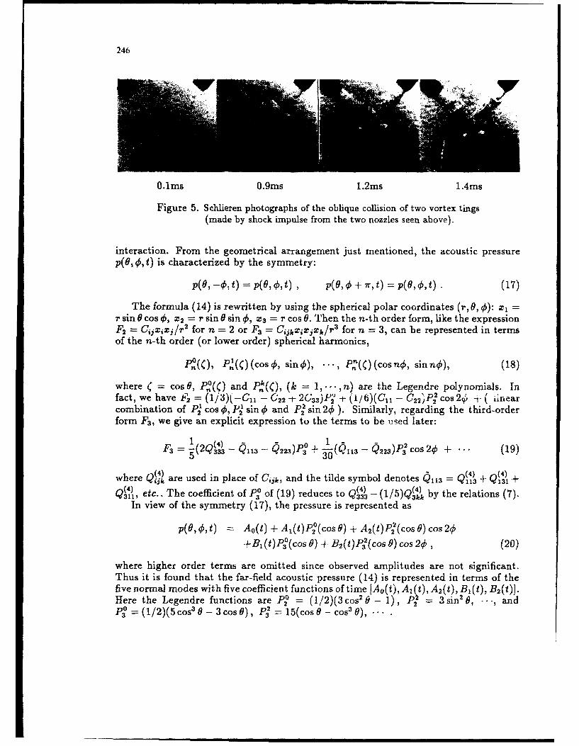
246

0.lms 0.9ms 1.2ms 1.4ms

Figure 5. Schlieren photographs of the oblique collision of two vortex tings(made by shock impulse from the two nozzles seen above).

interaction. From the geometrical arrangement just mentioned, the acoustic pressure

p(g, 0, t) is characterized by the symmetry:

p(0,-01,t) = p(0, 0,t) , p(O, + -7r,t) = p(,0,,t) . (17)

The formula (14) is rewritten by using the spherical polar coordinates (r',9, 0): X, =r sin 0 COS 0, M2 = r sin 0 sin 0, X3 = r cos 0. Then the n-th order form, like the expressionF 2 = CGijx1/r 2 for n = 2 or F3 = Cijk iXjXk/Tr for n = 3, can be represented in termsof the n-th order (or lower order) spherical harmonics,

Pock), Pn1W C)Cos , sine0), ... , PC)(CcS os , sin nO), (18)

where C = cos9, Po(C) and P,(C), (k = 1,---,n) are the Legendre polynomials. Infact, we have F = (1/3)(-Cll - C22 I- 2' 33 )JP' 1 (i/6)(Cll - C 22 )P2 cos 2i '+ ( iinearcombination of P2' cos 4, P2 sin 4 and P2 sin 20 ). Similarly, regarding the third-orderform F3 , we give an explicit expression to the terms to be uJsed later:

F33 0+ •223)P3 cos 20 + (19)

where Q(4) are used in place of Ctjk, and the tilde symbol denotes 1 = (4) + Q +4)

Q(4) etc.. The coefficient of P3 of (19) reduces to Q) (115)Q( by the relations (7).In view of the symmetry (17), the pressure is represented as

p(8,4,t) = Ao(t) + A1(t)P°(cos 0) + A 2(t)P2(cos ) cos 24

+Bi(t)P3'(cos9)+B 2(t)P32(cos9)cos24 , (20)

where higher order terms are omitted since observed amplitudes are not significant.Thus it is found that the far-field acoustic pressure (14) is represented in terms of thefive normal modes with five coefficient functions of time [Ao(t),Al(t),A 2(t),Bl(t),B 2(t)].Here the Legendre functions are P2 = (1/2)(3cosS2 - 1), p2 = 3sin2 , .-- , andP3 = (1/2)(5cos 3 0 - 3cos0), P3 = 15(cos0 - cos'9), .

247

(a) ObservationThe acousttic waves emitted by the 900 collision were detected at 102 different

angular positions on the three great circles of radius r = 620mm on the three orthogonalpianes: (1) 0 = 7r/2,31r/2; (2) q0 = 0,7r; (3) 0 = r/2 . The trajectories of the vortexcores in the (z 2, X3) plane observed by a photosensor are shown in Figure 6, where thering radius Ro= R(O) of the single (unperturbed) vortex is 4.7mm. ( U 27m/s)

vortex ring X3 vortex ring 0 .

-0.02q

0.02'A,

0 0 -0 A2. .-.0002 2

a b B20t

Figure 6. Observed core trajectories oftwo colliding vortices in the (z 2, z3 ) a•,plane including the vortex center..-..- .. .The marked positions a and b 4,7 5.1 5.5correspond to the times of Figure 7 t (ms)(broken lines).

Figure 7. Main mode amplitudes ofobserved waves.

The symmetry relation (17) is found to be consistent with the observed data, Infact, the acoustic pressure detected in the plane 0 = 7r/2 can be expanded into Fourierseries with respect to the angle 4, and it is found that the Fourier coefficients of sinm4(m = 1 -- 4) and cos m'o (m' = 1,3, 4, 5) are negligible.

Three sets of profile functions of [Ao, A,,A 2,B 1, B 2] can be determined from theobserved data. It is found that they coincide almost with each other. These profiles areshown in Figure 7.

(b ) ComputationNumerical simulation of the vortex collision at right angles, which corresponds to the

experiment, was carried out by M. Takaoka in order to estimate the acoustic emission,using the method of [24]. The incompressible Navier-Stokes equation is solved numeri-cally, together with the continuity equation, by the spectral method on 64' grid points.Imposed boundary conditions are 27r periodicity in the three coordinate directions.

The isotropic component is proportional to the second time derivative of the kineticenergy, and the auadrupole components and higher modes are related to the change ofmoments of vorticity distribution. Using the data from the simulation, we can calculatethe tensors Qii(t) and Qi 1 k(t) of (5) and (6). Thus we readily obtain the main mode

248

coefficients {A0 , An, A2 , 1 ,/3 2 1. The main mode amplitudes of the computation andthe observation are qualitatively similar, but quantitatively different, probably becauseof the difference of the values of the Reynolds number. Unfortunately, the Reynoldsnumber of the computer simulation is smaller by two orders of magnitude than that ofthe experiment.

(c) Implication of dominant wave componentsObserved amplitudes A, and A2 of the two quadrupoles P. and P2 cos 244 in (20)

are significantly large. The amplitudes Al(t) and A2 (t) are considered as consisting ofthree longitudinal quadrupoles Q11, Q22, Q33 (to the directions X , X 2 , X3), as understoodfrom the form of the coefficients of F2 . It is probable that there exists non-negligibleamplitude in the monopole.

Out of the two third-order components, the amplitude B2 of P3 cos 2q0 is negligiblysmall, but the appearance of the mode P3 is substantial. To see the significance of this

mode P3, we examine its coefficient B, which is given by Q(, ft) - Q (t), where

Q3 =3- (y x w) 3)3 y d'y, Q3k - (Y X w) 3 y' d'y

P3 -= (Y X W)3 = y YW -- y2WI = Y. X. ,

the vectors y. = (Yl,y2) and w. = (w1 ,w2 ) Lcing projection of y and w to the plane(z-, 2 ). Restricting our attention to the location of vortexline reconnection at the innerpart of the collision and reminding the geometry of the vortex"'nes, it is expected thatthe variable p3 (near y. = 0) changes its sign before and after the reconnection, and

that its rapid change will give substantial contribution to the terms Q(34(t) and Q(4)(t).Thus it is suggested that the significant amplitude B,(t) observed in the cxperiment(see Figure 7) is representing an acoustic signal of a local violent motion a t the innerpart of the collision. The observed acoustic pressure shows a characteristic, asymmetricdirectivity at the tiD,2s when the B 1 mode is substantial (see Figure 8). As a testobservation, we took a shadowgraph (Figure 9) of the waves generated by the corecollision with the vortex speed much higher than Lhat of the acoustic measurement. Itis supposed that the wave generation corresponds to the phase a of Figure 8.

00

900'i -. 90 . ..:

180°1808

Figure 8. The asymmetric directivityof the acoustic pressure at the times Figure 9. Waves generated by the c,,rea and 3 marked in Figure 7 collision at a higher vortex speedpositive (o), negative(e). (taken by T. Minota)

249

4. INTERACTION OF A VORTEX RING WITH A BODY

Presence of a solid body in a flow causes a considerable increase in the intensityof generated sound. The degree of increase depends on the boundary conditions. Ifthe body is finite with its dimension being small compared with a typical wavelength,then the sound wave generated by nearby iis charactcrized by a dipole emissiowhose intensity is proportional to the sixth power of the typical velocity u. On theother hand, the intensity of sound generated by eddies in the vicinity of a sharp edgeof a flat semi-infinite plate (considered in the next section) is proportional to the fifthpower of u and the wave field takes a cardioid directivity pattern. [ see 171 for generalformulation; [25] for a circular cylinder; (261 for a sphere ; (271 for a wedge.]

Solenoidal vortex motion in the neiborhood of a solid body at rest is dominated by adipole field. This is interpreted as follows. The first and second terms of (8) disappearby the conditions of vanishing net outflux across the body surface and no translationalmotion of the body (14], respectively. However, the impulse 47rQ1 (the coefficient of thesecond term of (3) ) changes according to the momentum exchange between the bodyand the surrounding fluid. The rate of change of 47rQi(t) is given by the resultant forceF(t) exerted on the fluid by the relation, 4rQi = F1 (see (191).

It is shown [7] that the temporal wave profile is determined by the following integralwhich is a function of time t:

H1(t) f w(yt) 'I1(y)d3y (21)

where w is the vorticity of the source flow and the function 'I'(y) (i = 1,2, 3) is a vectorpotential (with div 'Q = 0) for the velocity of an imaginary potential flow (around thebody) of a unit velocity at infinity in the i-th direction. The function 4iP(y) representsthe presence of the body in the vicinity of the vortex motion.

4.1 General formulaIf the eddy and the body without sharp edge are both compact relative to the

acoustic wavelength, the acoustic pressure obtained by Curle [131 is expressed as

p(Xt) = 1 Xi F )(t - r (22)pý, ) 4rc _r2 c

in the far-field where -Fi(t) is the force exerted on the body by the surrounding fluid,represented by an integral of the stress over the body surface. The expression (22) isclearly a dipole wave with its axis in the direction of Fi(t)

A different expression of the acoustic pressure is obtained by Obermeier 1281 andKambe 171 for the same problem. The pressure generated by the interaction of a solidbody and a closed-loop vortex (a) as

p(X,,t) --_ Po x, fii,( _, r) (23)47rp r2 c

where the function [1i(t) of (21) reduces to

11'(1) r ' ', .ds -r I' f( , ,) dS = I'J,(t). (2,1)

The constant I' is the strength of the vortex, the infinitesimal variables ds and dS area line element of the closed loop a and an elernnt of the open surface S bounded by

250

1r, respectively, and n is a unit normal to the surface S. The function J1(t) denotes thevolume flux of the potential flow %Yj passing through the loop a'.

To obtain the scaling law of the dipole emission, we note that 11i is normalized byul3 since r -' ul and IV x jI4 being of order unity away from the body. Thus the scalinglaw is po uPIs pou 3 1

PO UP1 OUIPD ý -_ - -

c T2 r c r

The sound intensity is ID - (pou 6/C3)(1/r)2 cK uO.

4.2 A vortex passing nearby a circular cylinder

(a) ComputationConsider a circular vortex ring of radius R (core radius 6) passing by the side of an

infinite straight circular cylinder of radius a (Figure 10). The x3 axis is taken alongthe cylinder axis. (In this case, %P3 denotes a uniform flow to the cylinder axis.) Ifthe vortex is sufficiently distant from the cylinder, the vortex path can be regarded asrectilinear. It is assumed that the vortex ring keeps its circular form (approximately)and the ring center moves within the plane (x1 , x.2), which means that the normal tothe ring plane lies within the (xi, x2 ) plane. The above expression (23) reduces to

1800

(0o) ••.t = 1695(ps)

+ _ rcylinder

// / 900 vortex

flowF //2 0.

,,/ / b 1c

W cm

44 190

i iIZ1

2100

R vortex ring InlP

Figure 10. Schematic diagram of Figure 11. Dipole character of the far-fieldthe problem and the flow F acoustic pressure p(0, t) and correspondingto the observation direction. vortex position relative to the circular

cylinder at three times, where U =27m./s,R :: 4.7mm and a -,4.5mm

251

p(, )= tsi + (t'cosJ+ j2 (t)sin¢] (25)c 47rc r

_ Po r sin 1(t) cos(o - O(t)) (26)47rc r

where J2 = j2 + j2 and tanO = j 2/J1 , since j 3 is taken to be zero and qP, (i = 1,2)has only the X3• component: (0, 0, Ti). The angle 0 denotes the azimuthal angle of theprojection of the position vector x on the (zl, x2) plane, measured from the r, axis. Theangle 9 is the polar angle of the direction x from the x3 axis. Evidently the directivityof the acoustic emission (26) is of dipole character with its axis in the direction O(t)determined by j, and J2. The coefficient J(t) is the second time derivative of thevolume flux J(t) passing through the vortex ring of the flow F around the cylinderto the direction of observation 0 ((251, Figure 10). Note that the wave pressure (26)vanishes toward the cylinder axis 9 = 0 and ir. Thus the non-compactness of the bodyto the direction of the cylinder axis does not "nfluence the characteristic feature of thewave field.

(b) ObservationCorresponding acoustic waves were detected at various angles 0 in the plane 0 = 900

and various angles 0 in the plane 4 = 00 and 1800. Average wave observed at every 100position (in the plane 0 = 900) is expanded into Fourier series with respect to 0. It isfound that the main component is given in the form,

Pob,(O, t) = -a(t) sin 0 + b(t) cos 4,

in accordance with the expression (25), and the dipole character is clearly seen in Figure11. The solid curves a, b in figure 12 are the observed profiles. The broken curves showcomputed (normalized) amplitudes a = -J 2 and b = Ji for the vortex ring moving alonga straight line parallel to the x2 axis but with observed variable speed (the velocitydecays gradually). Agreement in absolute values between the observed and predictedprofiles are fairly good.

-0.04-

1.0 1.4 1L8 2.2 2.6 3.0

t (ma)

Figure 12. Comparison of the coefficients a(t) and b(t): observation (solid) andcomputation with 6/R =0.15 (thick broken) and 0.1 (thin broken).

252

5. INTERACTION OF A VORTEX RING WITH AN EDGE OFA FLAT PLATE

Presence of a flat plate with a sharp edge in the vicinity of a vortex alters the wavefield significantly, as well as the inner field bounded by the plate. When the edge plateis non-compact, the temporal wave profile depends on the history of the vortex motion,which is the scattering effect of the edge. This effect is taken into account by usingthe low-frequency Green's function [5], and the formulation is made differently from theprevious ones ([291, [30], [10]).

In the present case of a vortex ring moving near the edge of the plate (Figure 13, theedge being taken as the z3-axis, the polar axis), the plate is placed at Y2 = 0 (Y1 < 0)or ±= 180'. The wave pressure generated by this interaction is obtained [7, 291 as

Po sin 0 (sinO)1/2 r (27)P(X, t) =2 (27I(2)11 f(t - .)

where f(t)=fiJj (t - d (t):r = (28)

the latter expression is obtained from (21) like (24) with *'i = 'i' = (0,0,ik(y)). Thestreamfunction 0(y) is defined by _y1/ 2 cos 10, representiong a hypothetical potentialflow around the edge from below to above the plate, where Y = (yj + 2/)'/2. Notethat the velocity V x @ of the hypothetical flow is scaled as L-1/ 2 (L being the nearestdistance to the edge), and that the time scale for the flux change should be given by"rL = L/u. Using the argument which is similar to the case of dipole, we obtain thescaling law of the wave pressure for the edge sound as

po ulL' /212 1 _pOU5 /2 lI\)2 1

PE c 12 1 2 1 C'--

The acoustic intensity IE defined by p2E/poc is now proportional to u5-L -'. The angulardependence of the wave pressure (27) is given by the function F(O, ) sin 4 (sin 0)2

2 \(t) tr2.0 1.5 11(t)

f W)

\ ,1.0 0.75fi(t)

half-plane/o'e

0

rinUMIL

.............................

Figure 13. Trajectory of the vortex -4 -2 0 2 4

ring moving near the edge and the Figure 14. Three functions, f(t), 11(t), 11(t)streamlines given by -0 =const, for the angle of trajectory a = -17r.

253

12, P.(0, 0)°

0.W

plate 14*plt

a _Vw/2 L = 9.6mnr

U90=U30.4m/s R =4.7MM-90*

Figure 15. Polar plot of the acoustic pressure Figure 16. Perspective profile ofobserved at a fixed time to with 9 = 7r/2. the observed wave:The solid curve is j,,p(to) sin ½€. p.(0, t) = frp (t) sinI

(Figure 15). In the plane perpendicular to the x3 axis (8 = 7r/2), the directivity of theacoustic intensity is the cardioid, ', - sin 2 '0 on a fixed circle r =const and 0 =const.

(a) ComputationThe temporal wave profile of the pressure is represented by f(t) of (28)

I

f(t) = J(.--w)2IIF(w)exp[--iwtldw = ( 11(t) (29)

[26], where H(t)/r is the volume flux of the flow -0 passing through the vortex ring

of radius R (core radius 6), and IIF(w) is the Fourier transform of lt(t). The vor-tex trajectory is a straight line with the angle a to the y, axis. The three functionsf(t), fI(t), ft(t) are shown in Figure 14 for a = -7r/2. It is observed that the curvesf(t) are intermediate between I1(t) and JI(t). This intermediate behavior exhibited by

the half-integer differential operation (d/dt)½ is related to the scattering of the wave by

the non-compact edge plate. It is interesting to compare this with 11(t) of (23) for thecompact case.

(b) ObservationThe sound emission f.ii a vortex ring travelling near the edge of a flat plate along

a nearly straight path was investigated in a laboratory experiment [29]. Both of thespatial profile F(O, 0) and temporal profile f(t) were found to agree with the predictedones described above.

The pressure p(4, t) observed in the plane 0 = 90' is expressed by a truncated Fourierseries. It is found that the main component is of the form p.(O, t) = f,(t) sin 10 inaccordance with (27). Experimental study was done mainly for the vortex path ofa = -- 7r/2. Figure 15 is a polar plot of the pressure p.(q, t) at a fixed time to: p.(4, to).A perspective plot of the pressure profile p.(0,t) is illustrated in figure 16. The half-plane lies at 0 = ±180', on both sides the pressure takes opposite signs. The vortexmoved from the positive to negative y2 -axis with the translation velocity U = 30.4m/s,R = 4.7mm and L = 9.6mm.

Figure 17 shows comparison between the observed curve and computed curves on

254

0,4'

0.4 -

-0.1 7

-0.2,

0 400 800 1200 1600 2000

t (As) V , FQ 7U (m/s)

Figure 17. Comparison of fep(t) and Figure 18. Observed power lawscorresponding computed curves, of Ap (Pa) vs. U (m/s).

the absolute scales. The solid curve is the experimentally determined profile feb(t) andthe broken curves are the computed ones of p/F(0,9 = 90') obtained by using (27, 28)for the relative core size 5/R = 0.2 (thin broken) and 0.3 (thick broken). Agreement ofthe two curves is remarkable.

6. CONCLUSION

Concerning the problem of the vortex sound, a new formulation is developed for acompact source flow of localized vorticity distribution, based on asymptotic expansionof the velocity potential of the inner flow. This is successfully applied not only tothe sound generation by two interacting vortices in free space, but also to the caseof wave generation by a vortex interacting with a compact external body. The thirdcase of the wave generated by a vortex moving near a non-compact edge plate must betreated differently, taking account of the scattering effect. In each of the three cases, thecomputed wave profiles show remarkable agreement with the observed ones, implyingvalidity of the theory of vortex sound. Figure 18 is a summary of our experiment,illustrating observed power laws (in the log-log plot) of the acoustic pressure (peak)amplitude Ap versus the translation velocity U of a single vortex (in isolated state).

In the section 3.1 of head-on collision of two vortex rings, a consistent account isgiven by relating the phases of the vortex collision with those of the wave profiles. Anew feature is noticed concerning asymmetric wave emission in the oblique collision inthe section 3.2.

Finally, some remarks are to be made about other successful comparisons betweenobservation and computation, which are out of scope of the present article. Acousticnoise of dipole-type is investigated recently, based on the computer simulation of auniform flow around an aerofoil, and compared with correspoiiding experiment at MA =0.23 and Re = 3 x 10i (with reference to the chord and the freestream velocity) [32].Fair agreement is found between the two noise spectra obtained from the computersimulation and the experiment. The computed data shows structure of the surfacedipole over the wing surface. Another study [33) of a shock wave interacting with avortex filament also revealed reasonable agreement between the observation and thecalculation.

255

Acknowledgement

The author wishes to thank Dr. Toyoko Minota for collaborative work on the presentsubject and Dr. Masanori Takaoka on the computational aspect of the oblique vortexcollision.

REFERENCES

1 A. Powell, J. acoust. Soc. Am., 36 (1964) 177.2 F. Obermeier, Acustica, 18 (1967) 238.3 V.R. Lauvstad, J. Sound Vib., 7 (1968) 90.4 S.C. Crow, Stud. appI. Math., 49 (1970) 21.5 M.S. Howe, J. Fluid Mech. 71 (1975) 625.6 W. M6hring, J. Fluid Mech. 85 (1978) 685.7 T. Kambe, J. Fluid Mech. 173 (1986) 643.8 E.-A. Muller and F. Obermeier, Fluid Dyn. Res. 3 (1988) 43.9 M.J. Lighthill, Proc. R. Soc. Lond., A211 (1952) 564.

10 D.C. Crighton, Prog. Aerospace Sci. 16 (1975) 31.11 M.E. Goldstein, Aeroacoustici, McGraw-Hill, 1976.12 A.P. Dowling and J.E. Ffowcs Williams, Sound and Sources of Sound, Ellis

Horwood Ltd., 1983.13 N. Curle, Proc. R. Soc. Lond. A231 (1955) 505.14 G.K. Batchelor, An Introduction to Fluid Dynamics, Chap. 2 & 6, Cambridge

University Press, 1967.15 T. Kambe, T. Minota, T. Murakami and M. Takaoka, in Topological Fluid

Mechanics (eds.: H.K. Moffatt & A. Tsinober), 515-521 (1990).16 T. Kambe, J. Sound Vib. 95 (1984) 351.17 T. Kaxnbe and T. Minota, Proc. R. Soc. Lond., A386 (1983) 277.18 F. Obermeier, J. Sound Vib. 99 (1985) 111.19 T. Kambe and T. Minota, J. Sound Vib. 74 (1981) 61.20 F.W. Dyson, Phil. Trans. R. Soc. Lond. A184 (1893) 1041.21 K. Shariff, A. Leonard and J.H. Ferziger, NASA Tech. Mem. 102257 (1989).22 T. Minota and T. Kambe, J. Sound Vib. 111 (1986) 51.23 T.T. Lim and T.B. Nickels, Nature 357 (1992, May 21).24 S. Kida, M. Takaoka and F. Hussain, Phys. Fluids Al (1989) 630;

and J. Fluid Mech. 230 (1991) 583.25 T. Minota and T. Kambe, J. Sound Vib. 119 (1987) 509.26 T. Minota, T. Kambe and T. Murakami, Fluid Dyn. Res. 3 (1988) 357.27 T. Minota, T. Murakami and T. Kambe, Fluid Dyn. Res. 4 (1988) 57.28 F. Obermeier, J. Sound Vib. 72 (1980) 39.29 T. Kamnbe, T. Minota and Y. Ikushima, J. Fluid Mech. 155 (1985) 77.30 J.E. Ffowcs Williams and L.H. Hall, J. Fluid Mech. 40 (1970) 657.31 T. Kambe and U Mya Oo, J. Phys. Soc. Jpn. 53 (1984) 2263.32 S. Adachi, K. Ishii, S. Akishita and K. Kuwahara, DGLR/AIAA-92-02-157

(DGLR/AIAA-14th Aeroacoustics Conference, Aachen, May 1992).33 T.M. Weeks and D.S. Dosanjh, AIAA Journal, 5(4) (1967) 660.

* • I |mom

Theoretical and Applied Mechanics 1992S.R. Bodner, J. Singer, A. Solan & Z. Hashin (Editors)Elsevier Science Publishers B.V. 2571993 IUTAM.

Nonlinear Membrane TheoryA. Libai

Faculty of Aerospace Engineering, Technion, Haifa 32000, Israel

AbstractNonlinear membrane theory can be regarded as an approximation to the nonlinear

behavior of shells of finite thickness under suitable conditions, or else studied as amathematical model, complete in itself, for shells which are formally assumed to be in-capable of carrying moments. Selected topics of interest in the statics of nonlinearelastic membranes will be discussed. These include: the basic equations, the behavior ofa membrane adjacent to a stressed initial state, the undeformed membrane, boundary con-ditions, membrane edge effect, lines of rotational discontinuity, axisymmetric mem-branes, cylindrical membranes, wrinkle fields and others. The intrinsic form of theshell equations will be adopted in most of the discussions. Cases with small-strain geo-metric nonlinearities as well as some finite strain problems will be considered.Emphasis will be put more on general and formulative issues rather than on specificsolutions, but the analysis of a specific case will be outlined.

1. INTRODUCTION

Membrane theory is commonly regarded as an approximation to the shell problem,obtained by formally suppressing the stress couples and transverse shears in the shellequations, compared with the tangential force resultants ("membrane forces"). Thesuppression takes place in the force equilibrium equations, force boundary conditions,energy, and moment equilibrium around the normal to the shell. There is ample experi-mental and theoretical evidence to the effect that membrane theory is a valid "interior"approximation to the shell equations, which dominates the behavior far from boundariesand discontinuities (either in the geometry or the loading), for deformation processeswith a typical length measure 'r' of the reference surface, and provided that thereexists adequate support at the shell boundaries. Processes with length measure vrT-t,where t is the shell thickness (such as buckling, short-wavelength vibrations, edgeeffects), and also those involving substantial inextensional deformations, are to betreated by the more general bending theory. Also, bending corrections- to the membranesolution which are based on its deformation patterns can be calculated. These can beused to estimate the accuracy of the membrane approximation and to correct the stresslevels (which are of a lower order in t/r). Chapters on membrane theory can be found inmany standard books on shell theory [1-13]. Some consider nonlinear behavior speci-fically [7-14].

Another approach to membrane theory regards membranes as two-dimensional deformablesheets, plane or curved, which are formally incapable of carrying any stress couples ortransverse shears, and can sustain tangential force resultants only. These are the"ideal" or "true" membranes (the term "ideal" membranes will be used to distinguish themfrom "shell membranes" which can carry stress couples, as previously discussed). Thetheory of ideal membranes can be formally modelled as a complete entity in itself.

Several important characteristics distinguish the behavior of ideal membranes fromshell membranes. To name a few:

258

(1) Ideal membranes cannot sustain compressive stresses, whereas shell membranes cancarry compressive stresses until buckling takes place.

(2) Ideal membranes exhibit "wrinkle fields" or "tension fields" to compensate for thenonexistence of compressive stresses. In shell membranes, postbuckling behavior isout of the scope of the model, but the approximation of an "incomplete tensionfield" can be sometimes used to investigate the transition from postbuckling towrinkle-fields [15].

(3) Ideal membranes can accept lines of angular discontinuity in the deformationpattern on the boundary or in the interior. In shell-membranes, angular continuityis preserved.

(4) In the same vein: existing lines of angular discontinuity in an ideal membrane canbe smoothed out under suitable conditions. In shell-membranes, the theory breaksdown near such lines.

(5) Large inextensional deformations can be sustained in an ideal membrane, but not ina shell membrane.

(6) A large variety of kinematic and force boundary conditions can be imposed on anideal membrane within the scope of the model (with obvious exceptions - such asimposed stress couples or transverse shears). Exact edge conditions can rarely bespecified for a shell-membrane. Bending or 3D theories are used for edge effectanalysis, with component 3D, bending and nonlinear membrane effects.

(7) The "undeformed *ape" of an ideal membrane needs only a metric specified in a 2D(curved) space u (a=1,2) plus a specified closed line in this space. It can be"packed in a box". A shell membrane starts from a 3D thin walled body which con-stitutes its undeformed shape. Not all the geometrical properties of this shapeappear in the equations, but they are necessary for the analysis of itslimitations.

The question as to whether ideal membranes do actually exist as physical entitiesneed not be answered: the analyses of mechanics problems involve some degree of ideal-ization and modelling of the behavior of the physical world, and the success of a modelshould be measured by its ability to predict this behavior in some approximate sense.With this in mind, several classes of shell problems can be modelled as ideal membranes.Among those, the most important is the asymptotic behavior of thin shells as (t/r)approaches zero. In fact, ideal membrane behavior can be arrived at solely by thislimiting process. Other classes of problems which can be modelled as ideal membranesinclude shells made from special materials (biological membranes, cloth and other thinfilms, inflatables), problems involving large loads of the pressure variety, many largestrain problems, etc.

In what follows, no direct distinction between the two types of membranes will bemade. The typing, if needed, should be based on the problem at hand. For example, com-pressive stresses will be included in the analysis, but problems related to wrinklefields will also be discussed. Boundary conditions for an ideal membrane will be lookedat, with the understanding that in a shell membrane this may be just a component of amore complex edge effect problem.

A "real" shell is, of course, a thin 3D continuum. Shell theory is an approximationto 3D behavior. Membrane Theory is an approximation to shell theory and, putting asidespecial cases, the behavior of ideal membranes is a subset of Membrane Theory. However,if the parameters and objectives are right, the latter can give very good predictions ofthe behavior of this 3D body under conditions involving strong nonlinearities which,otherwise, would have been extremely difficult to treat.

25

2. NONLINEARITIES IN MEMBRANE THEORY

These follow the usual classification into geometrical and material nonlinearities.Small strain theory with nonlinearities due to the inextensional component of the defor-mation and to local strain gradients is the more common case. Tension field theory canbe included within this class since the wrinkling process involves mostly geometricalchanges. A special subclass of the above is "rigid-inextensional" theory which assumesthat the strains are zero and that deformation can take place through inextensionaland/or wrinkle fields only.

The relative simplicity of the application of two-dimensional hyperelastic consti-tutive relations to ideal membranes has led to the development of the materially non-linear large strain membrane theory which, in addition to many practical uses, can beapplied to problems involving the loss of stability in tension due to combined materialand geometrical effects.

The main feature that nonlinearity adds to membrane theory is shape-adaptability:both geometry and membrane forces participate simultaneously in taking on the appliedloads. This is facilitated by considering equilibrium with respect to the deformed con-figuration. The process gives rise to a sixth order partial differential system whichcan accommodate, in most case, three boundary conditions. This should be contrasted withlinear membrane theory which is taken with respect to an undeformed geometry and canaccommodate, in principle, only two boundary conditions. In some cases of well supportedmembranes (such that the boundary conditions prevent inextensional deformations), linearmembrane theory yields good predictions away from the boundary. In such cases, the corr-esponding small strain noninear theory predicts the formation of boundary layers ofthickness rvr at the edges, where E is a typical strain measure of the membrane.

A well studied group of problems which belong to this class is the axisymmetric de-formation of membranes of revolution. However, as the strain increase, the boundarylayers are obliterated and boundary effects extend over a large part of (he membrane.See section 5 for more details.

At the other extreme lie cases where almost all of the deformation is inextensionaland the contribution of the strains is minor. For a trivial but illuminating example,consider a rectangular ideal membrane sheet in the xy plane, clamped along its edge x=0and loaded along its edge x=a by a uniform line load P in the z direction. In its de-zformed shape, the sheet rotates through 90' and a line of angular discontinuity formsalong x=O. The addition of normal pressure causes the deformed shape to be curved but!he essential feature of almost inextensional deformation is preserved.

The "spherical barrel" example of section 7 serves to demonstrate some of thesecases. This is a truncated ideal spherical membrane attached to rigid rings which arepulled apart by forces P. The membrane collapses in to form a cylindrical wrinkle field.For small P, "rigid-inextensional" theory holds with the wrinkles extending clear to therings. For larger P, a narrow unwrinkled axisymmetric boundary layer is formed adjacentto the rings. For larger P, the boundary layer no longer exists. The unwrinkledstretched membrane which covers a large part of the surface is analyzed by axisymmetriclarge strain theory.

3. A REVIEW OF THE MEMBRANE EQUATIONS

(a) NotationsTensorial component notation is adopted in the general discussion. Physical

components are used in examples. Vector notation is used as needed, referred to a fixedCartesian coordinate system x,y,z. The membrane is to be analyzed in three possiblestates: Current state (denoted with an upper bar), undeforined state (without bars), and

260

reference state (denoted with a subscript or superscript (o)). The latter is a knowndeformed state with respect to which incremental solutions are sought.

In the sequel, a comma, a double vertical bar, and a single vertical bar, denotepartial and covariant differentiations with respect to the current and reference states,respectively. Upper case letters denote full quantities and lower case letters denoteincremental quantities (from the reference state). A membrane is identified either by

the position vector R(u a) of material points on its deforming reference surface, or by

its current metric and curvature tensors Aq and Bap, respectively, which satisfy the

three continuity equations of Codazzi-Mainardi and Gauss [16,17]. Associated quantities

are A=det(Aot3), permutation tensor £e3' unit normal N and Christoffel symbols f:•y, given-( 1ak~

by f -IA (A), +Ax1 3 -A X). The corresponding quantities in the undeformed and

reference states are R, A p etc. and R(o), A(Op) etc., respectively.

The boundary of a membrane is a curve r with arclength parameter s:F: ua = (s),

where ds 2 Ao du aduI3.

Unit vectors along the curve are -, v-, N where X I=u, and V a XC 3

The normal (K n) and geodesic (K g) curvatures along the curve are:

n

The symmetric force resultant tensor Rap acts on elements of the current membrane, incurrent directions and is measured in terms of the current metric. Kirchhoff("engineering") resultants act in the same directions but use the undeformed metric.

They are given by /A-N = A'Nct13.

The loading vector per unit deformed/undeformed area is p=p R,o•+pN/p=p°tR,C+pN.

Components with respect to undeformed directions (fot) or to cartesian directions

(feei) are occasionally used.

Two-point tensors and vectors associated with the geometry of the deformation are theGreen Strain Tensor Eot3, change of curvature tensor Kot3 and displacement vector V. These

are given by 2E -A A K -B xB ; V=R-R=v R,o +wN=v e..

(b) A Review ot the Basic EquationsThe important issues are the choice of variables and choice of directions. The

intrinsic form utilizes A Ic and B(XP as geometric field variables and relates the

equations to the current directions. The displacement form utilizes the displacements

(v ,w) as field variables and relates the equations to the undeformed directions. Othervariants are possible too. The equations are occasionally related to extrinsicdirections such as the axial and radial directions in membranes of revolution orCartesian directions. The intrinsic form is preferred in the sequel.

261

(b.1) Equilibrium

The fundamental form is the vector equation of equilibrium (V/'T C),ao+i/ p=0 where

Ta='-R ,p is the stress resultant vector.

Alternate component forms with respect io the current directions are: N&al3 epa=0;

N ~~+5=0 or A (/ Na1 3 3, +TPNU^t+pP=0, N +p=O.

Component forms with respect to the undeformed directions utilize the "displacement

gradients" and "rotations" defined by S =vaf I A-B aw; (ot=-(w,a+BrvP). The equations

are [18]:

[ Ap+ S Y)NpIIa+ B (P13 Nap + f = 0

[Ayp + S.~ ByNa13 - (q,3N a') I + f = 0

(b.2) Kinematics and Compatibility

The A a and Bap must satisfy the continuity (compatibility) equations of surface

theory. These are [16]:

(94y- rFB p3, = 0 Codazzi equations

+A8 Aap',Y8 + AýkaF•IP J = 0 Gauss equation.

In the case of small strains, simplified equations are available, which are linear inthe strains and their first order derivatives [19,20,14]. See section 4(a).

For the displacement formulation, the strain-displacement equations are [18]:

=p 71(Sao +s + Sa~Sp +

(U.3) Constitutive Relations:Only hyperelastic materials are considered. Let 4) (Eaxp) be the strain energy density

per unit undeformed area. Then N =2 - +- -. ti-• . Methods for obtaining t, have been

discussed elsewhere. See, for example Green and Adkins [10], Wu [21], Libai and Simmonds[13]. Approximate strain energy functions for many biological membranes have beenobtained, although these apply under restricted conditions only [22,23].

"Rigid-inextensional" behavior where all the Eap are set to zero (except for

wrinkling) is also a constitutive relation.While the assumption of dependence on the Ep only appears to be valid for ideal

membranes, this is not necessarily true in "shell membranes", where, in the most general

262

case, dependence on the K ao might be expected too. However, to conform with commonusage, the possible dependence on the Kap will be ignored in the sequel.

(b.4) Boundary ConditionsThese come out of the virtual work identity for the deformed membrane

JT*Sivd-S + JJ.S-Vd~a = JfJT-a.8V ,d-a

F a a

where T* is the applied force per unit length and 5V is the virtual displacement.Integration by parts yields the work form of the equilibrium equations and also theboundary conditions (T*-Tav ).sV=O.

The natural conditions in component form are T* T*'X - NlaVa ; T*- VS a V

and T*-N=IT*Jcos(T*,N)=O. The first two conditions equate the applied shearing andnormal forces m the tangent plane to the corresponding stress resultants. The third isa condition on the field variable N itself (since the direction of T* is known). It isan equilibrium condition, but it sets up a kinematic requirement on the direction. At afree edge, t*=O and only two conditions can be applied. This agrees with the nature ofthe membrane equations, as will be seen later. The vector form of the boundaryconditions can also be related to undeformed directions, leading to natural conditionsin the displacement formulation [18]:

10 + S.0] N°Dva = T*.R,-

-0PNapV, = T*.N .

Again, if T*=O, then, from the first equation N°ov,,=O and the second equation isidentically satisfied, so that no condition on pp can be set

The kinematic conditions emerge from 8V=a In the displacement formulation theyrequire the specification of the displacements v ,w from the undeformed configuration.Taken with respect to the current state, the conditions 6yct=0 , 5w=O may be used inproblems with evolving kinematic conditions. More commonly, they are translated intoconditions on the intrinsic quantities on the boundary: the extensional strain 6 s, the

normal curvature Kn and the geodesic curvature K g. For example, if the boundary does notdeform, then es=0, Kg=Kg, Kn=K . In many engineering applications, the curvatures and

strain are the obvious data.A more general approach relates the natural and kinematic conditions to the behavior

of a surrounding "boundary beam", where the ordinary differential equations of the beambecome the boundary conditions of the membrane (24]. It is also possible to utilize var-iational formulations for a direct derivation of the boundary conditions in intrinsicform. As a word of caution, it must be emphasized that the boundary conditions strictlyapply to ideal membranes only. In shell-membranes the bending component of the boundaryconditions is always present to some degree. Also, compressive boundary loads may causewrinkling in ideal membranes.

,(3

(c) Angular DiscontinuitiesConditions of kinematic and static continuities exist across internal lines in the

membrane: The deformed position and stress resultant vectors must be continuous, and,

unless the normal force across the line vanishes, the unit normals N" must coincide. Thelatter can also be obtained from the elementary observation that membrane equilibriumcannot be locally maintained in the presence of an angular discontinuity with a noi.-zerotensile force (see Fig. 1). This leads to two conclusions: (a) preexisting lines of

Z A. Not in equilibrum

B. Shell Membrane

of //C. Ideal Membrane

Figure 1. Angular discontinuity with tensile force.

angular discontinuity are smoothed out by a nonzero tensile force. (b) If the forcevanishes, then a line of angular discontinuity is permitted (even if it did not pre-exist). As before, the above is strictly valid for ideal membranes under tension only.In shell membranes the membrane state breaks down near the line and bending effects in-termix. Hence, the immediate region near the fold should be taken out of the analysis.Yet, the procedure of disregarding very local bending zones is common in the analysis ofsufficiently thin highly loaded shell membranes. They can be thus analyzed as idealmembranes.

4. THE NATURE OF THE MEMBRANE PROBLEM

(a) Behavior of the EquationsThe membrane field equations form a sixth order nonlinear partial differential

system. Compared with linear theory, the nonlinear terms raise the order from four tosix. They occur in the highest derivatives and involve the current state of stress ofthe membrane. Consequently, the membrane may behave in radically different ways,depending on the nature of the state of stress and deformation in the neighborhood ofdifferent solutions. A helpful and convenient method for the study of'the system in aspecific region of its variable-space is to expand it around a solution point("reference state") in the region, and consider the perturbation series from this point.

264

Properties near this state can me gleaned from the linear terms in the expansion in thesense of "small deformations superposed on large" which has many applications inNonlinear Mechanics [9,25]. In membranes it has been used to investigate stability andvibrations [18,26-29] but has additional practical applications in cases where asolution is sought which is "not far" in some sense from a known state [18.24,14,30].

e -• •( o) , -fi -B( ° -• a •-( -~ .a(°)Let (o) denote the reference state. Let: e -E r E(0) -- B(O) y( X -i -r=1" O)

a UP~ be the , k X= p y 0-fna1P=N(XP-NO)P Ap , Ap be the increments from the reference state. Restrictions are(0) arimposed that the e(0O and __, be sufficiently small such that lineari:ation can be per-

formed in these variables, and that no wrinkling takes place. Substitution into thefield equations yields the following set of incremental equations:

(o)Icy + =

n(XB (0) + NaP k + no'Pk +A_ (o)ap _ _

e137(k -31 B .1)3ý =0

Bak +~4 +a I ~k KeaX(o) ap IU (4 2p K~ oe X

naO = CaP YSe = [4,E ap.Eyj] (O)e. 8

where K is the Gaussian curvature of the reference state (o), and all tensorial opera-

tions are performed in this state. For quadratic strain energy densities, the Cafts isthe linear elastic tensor. Since the ko are not assumed to be small, nonlinear (under-

lined) terms are retained (in fact, were the (o) system chosen as the undeformed state,then a small-strain-finite-rotation membrane theory would have resulted!). In the above,

the cofactor tensor is defined by fsaost1= ps3f and the incremental Christoffel tensor

is given by its linearized form:

For a complete linearization, the underlined terms should be dropped. Henceforth, Apa=_-Ois assumed for simplicity. To facilitate further study, a D.M.V.-type approximation ismade by replacing tangential equilibrium and compatibility with a stress function F andcurvature function G:

n kXP = G aJ3 + Rk

where the Ri are lower order remainder terms. This approximation has a wide range of

applicability in shell theory. For the present study it suffices to note that it is alsouseful for a qualitative evaluation since it preserves the highest derivatives of thesystem (however, more exact substitutions are available, as will be seen later).Furthermore, the incremental constitutive relations are assumed to be isotropic witheffective moduli Et and V (this is exact for quadratic strain energies). Substitution

and rearrangement yield:

Lb(F) + Ln(G) + Ap = RN (normal equilibrium)

1 V4 (F) + Lb(G) = RB (compatibility)

Here, Ri are remainder terms involving lower order derivatives and the differential

operators Lb, Ln and V4 are

Bo , = "curvature operator"Lb(f) =-- 0

Ln(f) = Na• f o = "stress operator"

V4 (f) = f• = "biharmonic operator"

Further elimination yields the nonlinear membrane equation:

I LnV4(F) - LbLb(F) - Lb(Vp) = RF

For the corresponding displacement formulation, see Budiansky [18].

Discussion:(1) The system is always twice elliptic, but the third operator depends on the

reference state of stress. This influences the boundary conditions which can beassigned. At a free edge, for example, the stress operator is parabolic and only twoconditions can be assigned (see previous discussion).

(2) The operator I Ln is of the order of the strains c of the reference state. If

it is small compared with rLb then a boundary-layer type solution is to be expected of

size rWo. This breaks down if Fo=0(l) or if Lb(F)=0 (in the latter case are included00

problems of linear membrane theory where the boundary conditions are inappropriate for

Lb [21).

(3) The number and arrangement of boundary conditions does not depend on LbW in

contrast to linear theory, where it controls the behavior. However, for small strainsand appropriate boundary conditions, Lb is dominant away from the edges.

(4) If an unloaded state is chosen as reference, then Nap)=0 so that L =0. The(o) nequations uncouple and reduce to the fourth order linear membrane system which canaccommodate only 2 boundary conditions and depends heavily on Lb. Singular perturbation

techniques may be needed to start a nonlinear problem from this state.

Choice of reference state:(1) A convenient reference state is one which has a simple geometry and can be easily

analyzed. It need not even have the same boundary data as either the undeformed or finalstates. For example, a pressurized circular membrane is a good cheice for problemsinvolving oval or incomplete cylinders.

266

(2) In cases with sufficiently rigid boundaries and small strains, the Not. of the(o)linear membrane solution plus the B1(o) of the undeformed state can be used for

approximate analysis. In shell-membranes this has the advantage of easy merging withbending effects where appropriate.

(3) Obviously, the chosen state should be sufficiently "close" to the final solutionin order to ensure meaningful results (easier said then done).

(b) Dependence on the initial shapeA study of the intrinsic form of the equations shows that the only initial data which

is formally needed is the metric Acxp (which appears in the constitutive relations) and

the definition of the boundary F:uq=ua(S). All other properties of R, including theundeformed curvatures B (3 do not appear -i the equations. The boundary data and loading

are usually related to the final form (e.g. pressure) or to extrinsic directions (e.g.axial loads in a shell of revolution), but rarely to the initial shape. It follows thatall membranes having the same AP and I" should have the same final state. This includes

the class of surfaces which are isometric to the initial surface, including those withany number of angular discontinuities (folds). For all practical purposes, the membranecan be, initially, even "packed in a box".

The displacement formulation requires an initial surface to measure the displacementsfrom. There is some arbitrariness in the choice since any surface from the isometric setcan be chosen. If the initial metric plus kinematic boundary data ensure the existenceof a unique B ap in the class of smooth functions, then the resulting surface is commonly

chosen for R. It should be, however, noted that this is an artifice, since the boundarydata is provided for the final state only, and a deformation of the boundary between theinitial and final states is possible. To cite an example: the shapes of the ends of aclosed pressurized cylindrical membrane are assigned to be plane ellipses. Yet, theinitial shapes can be circular, with specified edge displacements as kinematic boundaryconditions. This choice of initial shape might be easier to solve than the choice of aninitial elliptical shape.

A shell-membrane does have a unique undeformed body to start from. The need for itarises whenever an interaction with bending theory is required. However, it is not apart of the formal membrane data, unless it is chosen as the initial state.

(c) Wrinkling and Tension FieldsVery thin shells and other shells having low bending rigidities can support little

compressive stress before they buckle. If such shells are pulled in one direction andcompressed in the other (such as when subjected to shear), a large number ofhigh-aspect-ratio buckles forms with creases oriented in the tension direction. As thebending rigidity goes down, so do the buckling stress and the distance between creaselines. In ideal membranes, the instability stress approaches zero and the number ofbuckles becomes very large, thus forming a typical "tension field", which is not anuncommon sight in very thin, flexible membranes. The assumed inability to carrycompressive stresses is common to all ideal membranes. It has been initially used byWagner [31] to examine the postbuckling behavior of thin plates in shear, and was shownby Steigmann [321 to be exact. Several investigators undertook the study of tensionfields in plane membranes [33-38]. Wrinkled biological membranes, were studied byDanielson et al. [39]. Curved wrinkled membranes, which are of more interest in thisreview, were studied by Kondo [40,41], Wu [42,43], Zak [44] and others. A more extensivestudy of the foundations of plane and curved tension field theory was initiated byPipkin [451, Stclrgmnn [46] and in collaboration [47,48]. A numerical approach was

developed by Roddenian et al. [491. The instability due to Arinkling of bent piessurizedcylindrical membranes was investigated by Coner and Levy [501. Koga 1271 and !LukasieicN&1et al. [511. The ponding instability of partly wrinkled spherical membranes was analyedby Glockner and his associates [52-561, Croll [571 has studied the formation of wrinklesin transversely loaded plates and Libai analyzed boundary layers adjacent to ,rinkles[581. The list is not exhaustive and will, in all probability expand in the near futureas partial wrinkle fields will be routinely incorporated into nonlinear membraneanalysis. Also, more effort should be put into "incomplete tension fields" whichdescribe the transition front shell to wrinkled membrane, and into the wrinkling ofbiological membranes.

The underlying idea of tension field theory is to replace the complex wrinkledsurface (with its random form of detailed wrinkles) with a smoothed out "pseudo surface"[431 or "wrinkle surface" which could be imagined as a continuous distribution ofwrinkles or fibers, and constitutes a regular surface in space. This is equivalent tothe concept of a generalized curve or surface in the calculus of variations [591. Thepseudo-surface should satisfy the equilibrium equations, with one of its principalstress resultants being positive and the other set to zero. [or convenience, anon-material orthogonal coordinate system which coincides with the principal stressdirections is employed. Nontensorial notation is used, where N1 is the nonvanishing

principal resultant, e are unit vectors in the principal directions and Ao=7 A . Then:

- - = __ -I - _, Nlel' T•2=0 ell - A A e2 + --A N, p=p() + pN.t 11P=1') 2e1

A2 rI

The vector and component equations of equilibrium become, respectively:

(NIA 2 el), 1 + AIA 2 P = 0

(2 N),1 + AIA 2 P(I) = 0

1,2 N I+ AIA 2 P( 2) = 0

where both NI! and the geometry (A 1,A2 ,r') are unknowns. The nature of the loading

determines the properties of the stress trajectories:

(1) If P( 2 )=0, then e,,I is parallel to N and the trajectories are geodesics.

(2) If p=O, then -- 0 and the lines are asymptotic (with K,<).

(3) If both are zero, then e 1,=0. The lines are straight, and the surface is ruled.

(4) If p(l)=0, then the force-per-element (NIA 2 ) is constant. Thi s is analogous toflow lines in fluid flow.

The geometric variables (Ai,A 2 ,r ,r2,r 2 ) are connected through the continuity

268

equations of Codazzi and Gauss.To tie the solution to the rest of the membrane and to the initial metric, consti-

tutive relations are needed. Only isotropic membranes will be considered at this stage(non-isotropic membranes were studied by Mansfield [60] and Roddeman [49]). Here, theprincipal directions of stress and strain coincide. The condition N 2=0 can be used to

eliminate the true principal strain E2 2 from the constitutive relations, which leaves

NI=f(E1 ). The difference between the apparent strain E22 of the pseudo-surface and the

true strain is the "pseudo strain" E 2 E2 2* -E 2 2 . It was introduced by Wu [43] and is used

as an extra variable in lieu of the extra equation N2 =0 which was imposed on the field

equations. The constitutive relation does not add an additional variable, but should beused to relate the tension field to the material system. If there are no additionalsymmetries, the problem may be complex [46].

Other methods for constitutive modification where employed by Reissner [33] who useda special orthotropic material law and Stein et al. [34] who introduced a variablePoisson ratio. More recently, Pipkin [45] introduced a "relaxed" energy density toaccount automatically for the modified constitutive relations.

The boundary conditions with the unwrinkled portions of the membrane are obtainedfrom continuity requirements:

(1) The resultant NI>0 is continuous across the boundary.

(2) N2 =0 as the boundary is approached from the unwrinkled side.

(3) If N1 *0, then angular continuity is preserved.

(4) Positional continuity is maintained, thus implying E*2 =0.Examples: See section 5 for the axisymmetric case. See section 7 for the edge zone

near a wrinkle field. Further investigations and details may be found in the literaturecited above.

5. AXIMEMBRANES

These are membranes whose undeformed shapes are surfaces of revolution and are axi-symmetrically deformed. Because of their relative "simplicity" they have been studiedextensively in literature and solutions to many nonlinear problems exist. Hence, theirdiscussion here will be limited in scope. More information and details can be found inthe literature and some have been gathered in chapters in books. Examples are Green andAdkins [10] who discuss constitutive relations and some finite strain problems, andLibai and Simmonds [13, chapter 5] who made a more extensive survey with examples.

The reference surface of the undeformed membrane is defined in a fixed cylindricalcoordinate system (r,0,z) by its meridional position vector R=r(s)er+z(s)ez where s is

arclength. The angle a between R,s and er satisfies r,s=coscx; Z,s=sincx. The

corresponding quantities in the deformed meridian are r, z, a. A nontensorial approach

is adopted. Meridional and circumferential stretches are defined by Xs=d- and X -r

respectively. Stress resultants are Ns and No (or Ns and N. per unit undeformed length).

The loading vector is p=pHer+pvez and may depend on the field variables. The equilibrium

equations are

(rNs sin),s + rpv = 0 (rN Scosa),s = N0 -

In the case of uniform pressure p one may also use the parily integrated form:

rNssinz = 2 p r - cI (rN s,,s = N 0cosa

To these are added the equations of geometry and constitution:

r,, = (rx0 ),s = ,Cosa z,s = X sSina

Ns = O'ks NON = 0'4)0

where (,(Xs•,X) is the strain energy density. For boundary conditions, the position or

stress resultant vectors should be specified, subject to overall equilibrium. The systemis 4th order (but can be usually reduced to second order plus two quadratures). It is atwo-point b.v.p. which requires appropriate numerical procedures (e.g. Runge Kutta plusshooting) or approximate techniques for solution.

Pressurized wrinkled aximembranes with meridional tension fields: Here N0 =0. Further

integration yields rNs=r Ns=c2 - The meridian of the pseudo-surface can be expressed

explicitly in terms of the Jacobi elliptic function dn with modulus k:

-=2 pc.( -_ where k2 -2(1+ / -

To relate the result to the undeformed surface, the equations N0 =0 and Nsr(s)=c 2 are

used in the constitutive relations to eliminate 1-0 and express X s in terms of s. Thisestablishes s(s)=J'k ds. If stretching is neglected (X2=1) then s= s. The constants ci

s 1are obtained from the edge conditions of the wrinkled zone.

Aximembranes cannot deform inextensionally: any radial displacement and any nonuni-form axial displacement produce straining (an exception is near the apex where a localsemi-inextensional deformation is possible). However, if wrinkles are permitted, theninextensional deformation become possible and even common [13,42,52-561. Barringwrinkles, it follows from small strain moderate rotation theory that linear theory isvalid interior solution for many aximembranes, with narrow boundary layers of size rV.added to account for support conditions. Many studies of this phenomenon exist [61-65].The use of nonlinear correction for internal continuity finds its use in toroidalmembranes [66,671. In problems involving large strains, boundary layers usually do notexist, and problems associated with inflation and stability are the more importanttopics. Constitutive relations assume a major role and combine with the evolvinggeometry to produce limit point [10,68] or bifurcation type [69-72] instabilities.

Aximembranes can be classified by their undeformed shapes. Within each class thesmall-strain problem is studied separately. Some cases will be briefly reviewed:

Plane Circular Membranes: The small strain moderate relation theory is due to Fdppl[73]. A less restrictive theory is due to Reissner [74]. Many solutions for pressureand/or end loaded circular and annular membranes are found in the literature. Some weresummarized by Libai and Simmonds [13]. More have recently appeared [75-79]. In the caseof large strains, inflation [10,80-83] and deformation under concentrated loads [84-861

270

are some of the studies of interest. The inverse problem of deformation into apredetermined inflated shape has also been considered [81,82,87,881.

Spherical Membranes: Small strain problems lead to the study of edge effects. Shallowspherical membranes were treated by Dickey [76]. The common large strain problem is thatof the inflation of spherical balloons. Of special interest is the possible existence ofa maximum pressure. In volume-controlled problems, a further increase; in volume wouldlead to a decrease in the pressure. this trend may reverse itself at higher volumes, andis strongly material dependent [10,69]. The bifurcation of a spherical balloon into anonspherical shape has also been studied [69-72].

Circular Cylindrical Membranes: In the small strain range the main issue is the edgeeffect due to kinematic constraints or nonaxial end loads. Also if the end load isradial, a small part of the cylinder deforms into an annulus, while the rest remainscylindrical. At the line of angular discontinuity, Ns=0 [13,62]. The large strain

problem has the first integral [89] D-Xs ,X =C, where C is a constant of integration.s

This has been used to reduce the large strain problem of pressurized cylindricalmembranes to quadratures [13,90,911. The stretching of a cylindrical membrane attachedto rigid end rings has also been studied [82,90]. Finally, as in spherical membranes,the possibility of a maximum pressure exists here too [92,68].

Toroidal Membranes: The important issue in the small strain theory for circulartoroidal membranes is adjustment of the apparent discontinuity at the apex. This wasaccomplished by Jordan [66] and by Sanders and Liepin [67]. Problems involving largestrains were treated by Kydoniefs and Spencer [93]. The major difficulty in nonsymmerricpressurized toroidal ideal membranes (where r(a=0)•r(a=nr)) lies in the fact that a

necessary condition for equilibrium is r(a-=0)=r(a-=n). This must hold regardless of themagnitude of the pressure. Slight asymmetries can be taken care of by local nonlinearrotations which, as pointed out by Kuznetsov [941, are nearly inextensional at a=0,tr.However, if the asymmetry is substantial, then large strains are required to take placeeven if the pressure is very small. This "toroidal paradox" was used by Goldenveizer [21in discussion of the existence of membrane solutions, however, if wrinkling is accepted, a part of the deformation process, then a solution might be possible, and should betried. To account for axial equilibrium, the tension field must be meridional (N0 =0)

wherever it occurs. In addition, wherever Ns=0, a circumferential line of angular

discontinuity is permitted. The membrane is unstable at its undeformed form, so thatlarge scale wrinkling takes place even at low pressures.

For the shape of the membrane in unwrinkled regions, the general equations should beused, but if the pressure is low, the extensional strains can be neglected and theforces calculated by linear membrane theory. In the wrinkled regions, the theory forwrinkled axisymmetric membranes [43,47] applies, and the shape can be calculated withoutdifficulty, as was seen earlier in this section.

Large Strain Asymptotic Behavior: In the case of very large strains a simplifiedasymptotic analysis can be made. Of some interest is the possible tendency of closedinflated aximembranes to assume a spherical shape as the pressure and stretches becomevery large. This was shown for a class of materials of the Mooney type by Isaacson [95],Wu [21] and Sagiv [96]. Antman and Calderer [97] investigated the restrictions that mustbe put on the energy density of a spheroidal shell is to approach a spherical shape. Thebehavior of Neo-Hookean membranes with very large meridional strains was studied byFoster [98].

271

6. CYLINDRICAL MEMBRANES

In this section, some problems related to pressurized and stretched noncircularcylindrical membranes are discussed. Included are cases where the boundary has a non-circular (oval) form, or where processes cause an initially circular membrane to becomenon-circular in its deformed state. The general procedure is that of an incrementalanalysis, with the pressurized and stretched unbounded circular cylindrical membranetaken as the "reference state" (section 4a). This is a point in the solution domain. forall cylindrical membranes. It has a simple unvarying geometry to which all homogeneouspressurized oval membranes tend, far enough from their ends. The main restriction isthat the i'mal deformed state should be sufficiently "close" to the reference state soas to make an incremental analysis (including linearization in the metric and its firstorder derivatives) valid in some approximate sense.

Let x and s denote longitudinal (generator) and circumferential (hoop) arclengthcoordinates in the reference state. The membrane material is assumed to be nonlinearlyhomogeneous and orthotropic, such that a circular cylindrical membrane of length L and

radius r is transformed by pressure p and total tension T into a circular cylinder of

length L and radius rr. Let No-x - rx--- and )= Ps=Pr be the physical Cauchy stress

resultants in this reference state. Let nx, n., , nE, •t s K , K I t be the incre-

mental stress resultants, strains and curvatures, all measured with respect to theCartesian metric (x,s). Then, using (4a), the following field equations result:

(nx - Pses + Pxex),x + (nt + 2P•et),s = 0

(n s - Pxx + Pses),s + (nt + 2Pxet),x = 0

PK + PK+In + n K + 2nt)= 0Px ss T -s nxx ss tt

0

1 2 (Kt _ 2 t),x

_I =0(K5 - £E), - I(s r x t,s

-K + + +KE - 01 trx _______

Sx x,ss s,xx t,xs x s t

= fn -f n

Es f fsn s f xsn x

2 = ftnt

where the fi are constitutive coefficients obtained by inverting the incremental consti-

tutive relations of the reference state in terms of Cauchy resultants. For quadraticenergy densities, these are the elastic constants, in which case the equations should besimilar to those of Libai [30] and Danielson and Simmonds [99]).

272

Following section (4a), but without making the approximations therein, stress andcurvature functions are defined by putting nt=-F, xs and Kt=G, xs Substitution yields:

nx = (I + ax)F, s F ; ns = (I + s)F,xx + asF,

E = fx( + P3x)F, ss - s(I + XS)F xx

FES = fs(I + s )F, xx- fxs(I + 03sx)F, ss; 2Et =-ftF xs

s = Gss + I- C x=Gxx =--(+ x - 2ftF,)xx0 0

where the oti and are constants having the order of magnitude of the strains at the

reference state, and are easily calculated [100]. Introduction into the remaining twoequations leads to one 4th order and one 2nd order equation in F and G. These are non-linear due to the (FG) and (GG) terms - as is common in similar formulations.

In many practical applications all the nonlinear terms in the increments may besuppressed (at least as a first approximation). If, in addition, the strains at thereference state are small, the equations simplify to

I G, + V 4 F + [fxF,s + (2f - fs)F,]= 0r xx 1 '1xss t xs xx

0 _2

PxG, + PsG, + I F 2 2 Psf F, = 0x xx soss r40 xx rd0 sxs ss

where the modified biharmonic operator Vi is defined by

V 4 F= fF, + fRx + 2(f - f )Fxxs

Further elimination yields the 6th order equation

r2oV4(PxF, + PsF,s) - F, = (Pxf + Psfx- 2Pf)F, - PsfxFssss

In the DMV approximation, the right hand side of the equation is set to zero. For

quadratic energy densities of isotropic membranes, set: fx=fs=Et, f vI, f +v

V14F-V 4 F. As a practical application, consider the problem of an oval cylindrical

membrane subjected to uniform pressure p and an equally distributed tensile force Px=T/S

on its boundaries x=0,L. Diaphragm-type supports maintain the oval shape r. Small straintheory is assumed. The reference surface is chosen to be a circular cylinder with radiusr and length L0 which are obtained by applying the loads to the isoperimetric cylinder

with radius ra=S/2r and length L. The approach consists of applying to the incrementalr -r I n = 0.

problem the boundary conditions Es=r K (s)__ - xa oOf the three conditions, that of es leads to an edge-effect correction, which is

strongly affected by Px , while that of K s affects large parts of the membrane ("slow

decay"), which is of more interest. A similar situation exists in the semi-renibrane

analysis of tubes [101] where the effects of c s tend to be suppressed,

Solutions to the case of lateral pressure (Px=O) were studied by libai 124] who also

suppressed the boundary conditions on E Is and used a Fourier expansion in the s

direction. The solutions possess important features which compare favorably with thoseof the more common linear membrane analysis of an oval. The latter has sone seriousdeficiencies which render it unacceptable in many applications: (a) It requires thecontinuity of r(s) and its derivatives (up to the 4th !). (b) It does not tend to thecircular form far from the edges. In fact, it diverges as L---o. (c) It has no decaymechanism for boundary disturbances. (d) It cannot accommodate boundary conditions alongits generators (important for cylindrical panels).

The behavior of the incremental solution relates to the parameter y ....- E s ( •

a(a) It yields smooth solutions even if the slope or curvature cf the initial form havediscontinuities. (b) It approaches the circular shape as y increases. (c) The typicaldecay length 0 for end disturbances with harmonic index n is

Ox=rn 3 /2 C - 1 4=- 3/ 27 1 /4 . (d) It can accept "flexible" boundary conditions along the

generators [30]. (e) It approaches the linear membrane solution for y<<I, and the oni-

ginal shape as p-0). (f) For large n, it approaches th, solutions of the biharmonicequation of plane elasticity. The method is being applied to other problems [100]including those of cracks in cylindrical membranes.

An akin problem is that of nonlinear effects in beam-bending of tubes (BrazierProblem). Here, circumferential shell bending is commonly assumed to resist theovalization which accompanies the beam bending of circular cylindrical tubes. However,if the tube is thin and not very long, membrane resistance to ovalization which comesout of the supports provides the dominant mechanism. Pressurization enhances the effect.

7. EXAMPLE: EDGE EFFECT IN A PARTLY WRINKLED AXIMEMBRANE

Consider a truncated ideal spherical membrane of radius R, connected to rigid ringsof radius rc along its boundaries ,=xczc, 0a=l-a c (Fig. 2). If the rings are pulled apart

by forces P, the spherical membrane collapses inward, and a meridional tension field inthe form of a pseudocylinder is created. It extends almost to the supports, but a verynarrow wrinkled region forms near the rings [471. The equations in the unwrinkled region

are those of aximembranes (section 5). Axial equilibrium yields 2nrrN rsin(x=P. The other

equations can be reduced to a second order equation in y=cot0x as function ol ox=s/R. The

boundary conditions at ac is r c=rc (or X0 = 1). At the boundary of the wrinkled region

=(X~B. the conditions are those of continuity: ccB=ir/ 2 and N0 =0. These can be converted

into y=y,cc=0. Note that aoB is also unknown, so that three conditions are needed for the

differential equation and a 1.

The availability of two conditions at a B facilitates the soluhion of the equ-tion as

274

z

I i *

r

................. ...... ... 3..(a) (b) (c)

Figure 2. Partly wrinkled truncated spherical membrane.(a) Original (b) Wrinkled (c) Wrinkled with edge zone

an initial value problem starting fron, a B by either a power series or numerical

integration [58]. The condition X 0 =1 determines ac and consequently (B" In small straintheory, the equations are:

(sinaoy,(), - (csca)y = ( -cosa]

(sina)yo w at a = c P= 1 aty o• c 27 =-fR-Et

Construction of a formal power series solution yields the 1st order solution:

B ac = Sa + 0(c) (a 4 ir/2).c

Near zc=7r/2 this solution breaks down and an additional term is needed, yielding

a B - ac = 2v + 0(3 /2 ) (a c - 7r/2)

Large-strain results for a Neo-Hookean material were obtained by numerical integration.These indicate the breakdown of the edge effect for large strains, as expected. All theother relevant parameters of the problem were also calculated [58].

Boundary layers 0(c) are unusual in shell theory. In small strain theory they couldbe virtually ignored if not for the large rotations within the layer which indicate thepossibility of strong interaction with bending effects in thin shell-membranes. They arenot easily "captured" by pure numerical methods, unless looked for.

8. REFERENCES

I S.P. Timoshenko and S. Woinowsky-Krieger, Theory of Plates and Shells, 2nd ed.,McGraw Hill, 1959.

2 A.L. Goldenveizer, Theory of Elastic Thin Shells, Pergamon Press, 1961.3 H. Kraus, Thin Elastic Shells, Wiley, 1967.4 V.V. Novozhilov, Thin Shell Theory, 2nd ed., Wolters-Nordhoff, The Netherlands.

1970.5 W. Fliigge, Stresses in Shells, 2nd Ed., Springer Verlag, 1973.6 C.R. Calladine, Theory of Shell Structures, Cambridge University Press, 1983.7 P.L. Gould, Analysis of Shells and Plates. Springer Verlag, 1987.8 K.M. Mushtari and K.Z. Galimov, Nonlinear Theory of Thin Elastic Shells, Israel

Program for Scientific Translations, Jerusalem, 1961 (NASA- 1'*-l-62).9 A.E. Green and W. Zerna, Theoretical Elasticity. 2nd Ed., Clarendon Press, Oxford.

1968.10 A.E. Green and J.E. Adkins, Large Elastic Deformations, 2nd Ed., Clarendon Press,

Oxford, 1970.11 F.I. Niordson, Shell Theory, North Holland, 1985.12 J.W. Leonard, Tension Structures, McGraw Hill, 1988.13 A. Libai and J.G. Simmonds, The Nonlinear Theory of Elastic Shells, Academic Press,

San Diego, 1988.14 A. Libai and J.G. Simmonds, Nonlinear Elastic Shell Theory, in Advances in Applied

Mechanics (Hutchinson and Wu, eds.), 23, 1983, 271-371.15 P. Kuhn, Stresses in Aircraft and Shell Structures, McGraw Hill, New York, 1956.16 L.P. Eisenhart, An Introduction to Differential Geometry, with Use of the Tensor

Calculus, 1947.17 D.J. Struik, Lectures on Classical Differential Geometry, Addison-Wesley, 1950.18 B. Budiansky, Notes on Nonlinear Shell Theory, ASME J. Appl. Mech., 35 (1968)

393.19 W.T. Koiter, On the Nonlinear Theory of Thin Elastic Shells, I-Ill, Proc. Kon. Ned.

Ak. Wet., B69, 1966, 1-54.20 D.A. Danielson, Simplified Intrinsic Equations for Arbitrary Elastic Shells, Int. J.

Eng. Sci., 8 (1970) 251.21 C.H. Wu, Large Finite Strain Membrane Problems, Q. Appl. Math., 36 (1979) 347.22 Y.C. Fung, On Pseudoelasticity of Living Tissue, Mechanics Today, 5 (1980) 49.23 A.E. Evans and R. Skalak, Mechanics and Thermodynamics of Biomembranes, CRC Press,

Boca Raton, Florida, 1980.24 A. Libai, The Nonlinear Membrane Shell with Application to Noncir,-'lar Cylinders,

Int. J. Solids Struct., 8 (1972) 923.25 A.E. Green, R.S. Rivlin and R.T. Shield, General Theory of Small Elastic

Deformations Superposed on Finite Elastic Deformations, Proc. R. Soc. London, A2 11(1952) 123.

26 A.H. Corneliussen and R.T. Shield, Finite Deformation of Elastic Membranes withApplication to the Stability of an Inflated and Extended Tube, 'Arch Rat. Mech.Anal., 7 (1961) 273.

27 T. Koga, Bending Rigidity of an Inflated Circular Cylindrical Membrane of RubberyMaterial, AIAA J., 10 (1972) 1485.

28 R.T. Shield, On the Stability of Finitely Deformed Elastic Membranes, ZAMP, 23(1972) 16.

29 A. Needleman, Necking of Pressurized Spherical Membranes, J. Mech. Phys. Solids, 24(1976) 339.

30 A. Libai, Pressurized Cylindrical Membranes with Flexible Supports, lASS Int. Symp.on Pneumatic Structures, Delft, 1972.

276

31 H. Wagner, Ebene blechwantrAger mit sehr diinnem stegblech, Z. Flugtech.Motorluftschiffart, 20 (1929) 200 (translated as NASA TM 604-606).

32 D.J. Steigmann, Proof of a Conjecture in Elastic Membrane Theory, J. Appl. Mech. 53(1986) 955.

33 E. Reissner, On Tension Field Theory, Proc. 5th Int. Cong. Appl. Mech., 1938,359-361.

34 M. Stein and J.M. Hedgepeth, Analysis of Partly Wrinkled Membranes, NASA TN D-813,1961.

35 G.P. Cherpanov, On the Buckling Under Tension of a Membrane Containing Holes, PMM,27 (1963) 275.

36 E.H. Mansfield, Tension Field Theory, Proc. 12th Inst. Cong. Appl. Mech., SpringerVerlag, Berlin, 1969, 305-320.

37 E.H. Mansfield, Load Transfer via a Wrinkled Membrane, Proc. R. Soc. London, A316(1970) 269.

38 C.H. Wu and T.R. Canfield, Wrinling in Finite Plane-Stress Theory, Q. Appl. Math. 39(1981) 179.

39 D.A. Danielson and S. Natarajan, Tension Field Theory and the Stress in StretchedSkin, J. Biomechanics, 8 (1975) 135.

40 K. Kondo, On the General Theory of the Curved Tension Field, J. Soc. Aero. Sci.Nippon, 10 (1943).

41 K. Kondo, I. Takeshi, S. Moriguti and T. Murasaki, Tension Field Theory, Memoirs ofthe Unifying Study of the Basic Problems in Engineering Science by Means ofGeometry, Vol. 1 Division C, 1955, 417-441.

42 C.H. Wu, The Wrinkled Axisymmetric Air Bags Made of Inextensible Membranes, J. Appl.Mech., 41 (1974) 963.

43 C.H. Wu, Nonlinear Wrinkling of Nonlinear Membranes of Revolution, J. Appl. Mech..45 (1978) 533.

44 M. Zak, Statics of Wrinkling Films, J. Elast. 12 (1982) 51.45 A.C. Pipkin, The Relaxed Energy Density for Isotropic Elastic Membranes, IMA J. of

Appl. Math., 36 (1986) 85.46 D.J. Steigmann, Tension Field Theory, Proc. R. Soc. London, A429 (1990) 141.47 D.J. Steigmann and A.C. Pipkin, Axisymmetric Tension Fields, Z. Angew. Math. Phys.,

40 (1989) 526.48 D.J. Steigmann and A.C. Pipkin, Wrinkling of Pressurized Membranes, ASME J. Appl.

Mech., 56 (1989) 624.49 D.J. Roddeman, J. Drukker, C.W.J. Oomens and J.D. Janssen, The Wrinkling of Thin

Membranes, Part I - Theory, Part II - Numerical Analysis, J. Appl. Mech., 54 (1987)884.

50 R.L. Comer and S. Levy, Deflection of an Inflated Circular Cylinder Cantilever Beam,AIAA J., 1 (1963) 1652.

51 S.A. Lukasiewicz and P.G. Glockner, Stability of Lofty Air Supported CylindricalMembranes, J. Struct. Mech. 12 (1985) 543.

52 D.J. Malcolm and P.G. Glockner, Collapse by Ponding of Air-Supported Spherical Caps,Proc. ASCE, 107 (1981) 1731.

53 G. Ahmadi and P.G. Glockner, Collapse by Ponding of Pneumatic Spherical Caps UnderDistributed Loads, Can. J. Civ. Engr., 40 (1983) 740.

54 S.A. Lukasiewicz and P.G. Glockner, Collapse by Ponding of Shells, Int. J. SolidsStruct., 19 (1983) 251.

55 W. Szyskowski and P.G. Glockner, Finite Deformation and Stability Behaviour ofSpherical Inflatables Under Axisymmetric Concentrated Loads. Int. J. Non-Lin. Mech.,19 (1984) 489.

56 W. Szyskowski and P.G. Glockner, Finite Deformatic- and Stability Behavior ofSpherical Inflatables Subjected to Axisymmetric Hydrostatic Loading, Int. J. SolidsStruct., 20 (1984) 1021.

57 J.G.A. Croll, A Tension Field Solution for Nonlinear Circular Plates, in Aspects ofthe Analysis of Plate Structures, Dav al., Eds., Clarendon Press, Oxford, 1985,309-323.

58 A. Libai, The Transition Zone Near VNrinkles in Pulled Spherical Membranes, Int. J.Solids Struct. 26 (1990) 927.

59 L.C. Young, Lectures on the Calculus of Variations and Optimal Control Theory, W.B.Saunders, Philadelphia. 1969.

60 E.H. Mansfield, Analysis of Wrinkled Membranes with Anisotropic and NonlinearElastic Properties, Proc. R. Soc. London, A.353 (1977) 475.

61 E. Bromberg and J.J. Stoker, Non-Linear Theory of Curved Elastic Sheets, Quat. Appl.Math., 3 (1945) 246.

62 W. FlUgge and P.M. Riplog, A Large Deformation Theory of Shell Membranes, Tech. Rep.No. 102, Div. Eng. Mech. Stanford Univ., 1956.

63 E. Reissner, The Edge Effect in Symmetric Bending of Shallow Shells of Revolution.Comm. Pure Appl. Math., 12 (1959) 385.

64 A.E. Clark and O.S. Narayanaswamy, Nonlinear Membrane Problems for Elastic Shells ofRevolution, Proc. Symp. on the Theory of Shells, D. Muster, Ed.. 1967, University ofHouston Press, 83.

65 F.Y.M. Wan and H.J. Weinitschke, Boundary Layer Solutions for Some Nonlinear ElasticMembrane Problems, ZAMP, 38 (1987) 79.

66 P.E. Jordan, Stresses and Deformations of the Thin Walled Pressurized Torus, J.Aerospace Sci., 29 (1962) 213.

67 J.L. Sanders, Jr. and A.A. Liepins, Toroidal Membrane Under Internal Pressure, AIAAJ., 1 (1963) 2105.

68 R. Benedict, A. Wineman and W.H. Wang, The Determination of Limiting Pressure inSimultaneous Elongation and Inflation of Nonlinear Elastic Tubes, Int. J. solidsStruct., 15 (1979) 241.

69 A. Needlman, Necking of Pressurized Spherical Membranes, J. Mech. Phys. Solids, 24(1976) 339.

70 V.I. Feodosev, On Equilibrium Modes of a Rubber Spherical Shell Under InternalPressure, PMM, 32 (1968) 335.

71 A. Needleman, Inflation of Spherical Rubber Balloons, Int. J. Solids Struct., 13(1977) 409.

72 R.T. Shield, On the Stability of Finitely Deformed Elastic Membranes, ZAMP, 23(1972) 16.

73 A. Fbppl, Vorlesungen Uber Technische Mchanik, Vol. III, Teubner, Leipzig, 1907.74 E. Reissner, On Finite Deflections of Circular Plates, Proc. Symp. Appl. Math. I AMS

Providencee (1949) 213.75 R.W. Dickey, The Nonlinear Circular Membrane Under a Vertical Force, Q. Appl. Math.,

41, (1983) 331.76 R.W. Dickey, Membrane Caps, Q. Appl. Math., 45 (1987) 697.77 H.J. Weinitschke, On Finite Displacements of Circular Elastic Membranes, Math. Meth.

in the Appl. Scd., 9 (1987) 76.78 H.J. Weinitschke, Stable and Unstable Axisymmetric Solutions for Membranes of

Revolution, Appl. Mech. Rev. 42, part 2, (1989) 289.79 S.P. Joshi and L.M. Morphy, Large Axisymmetric Deformation of a Laminated Composite

Membrane, ASME J. Appl. Mech., 57 (1990) 150.80 W.W. Klingbeil and R.T. Shield, Some Numerical Investigations on Empirical Strain

Energy Functions in the Large Axisymmetric Extensions of Rubber Membranes, ZAMP, 15(1964) 609.

81 L.J. Hart-Smith and J.D.C. Crisp, Large Elastic Deformations of Thin RubberMembranes, Int. J. Eng. Sci., 5 (1967) 1.

82 W.H. Yang and W.W. Fang, On Axisymmetrical Deformations of Nonlinear Membranes,ASME J. Appl. Mech., 37 (1970) 1002.

278

83 P. Pujara and T.J. Lardner, Deformations of Elastic Membranes: Effects of DifferentConstitutive Relations, ZAMP, 29 (1978) 315.

84 E. Schwerin, Uber Spannungen und Formanderungen Kreisringforminger Membrananen,Zeit. f. Tech. Physik, 12 (1929) 651.

85 J.P. Fulton and J.G. Simmonds, Large Deformations Under Vertical Edge Loads ofAnnular Membranes with Various Strain Energy Densities, Int. J. Nonlinear Mech., 21(1986) 257.

86 J.G. Simmonds and M.A. Horn, Asymptotic Analysis of the Nonlinear Equations for anInfinite Rubber-Like Slab Under an Equilibrated Vertical Line Load, J. Elasticity,24 (1990) 105.

87 C.H. Wu, Tube to Annulus - an Exact Nonlinear Membrane Solution, Q. Appl. Math., 27(1970) 489.

88 H. Vaughan, Pressurizing a Prestressed Membrane to Form a Paraboloid, lnt. J. Eng.Sci., 18 (1980) 99.

89 A.D. Pipkin, Integration of an Equation in Membrane Theory, ZAMP, 19 (1968)818.

90 C.H. Wu, On Certain Integrable Nonlinear Membrane Solutions, Q. Appl. Math., 28(1970) 81.

91 W.L. Yin, Nonuniform Inflation of a Cylindrical Elastic Membrane and DirectDetermination of the Strain Energy Function, J. Elasticity, 7 (1977) 265.

92 A.D. Kydoniefs and A.J.M. Spencer, Finite Axisymmetric Deformation of an InitiallyCylindrical Elastic Membrane, Q. J. Mech. Appl. Math., 22 (1969) 87.

93 A.D. Kydoniefs and A.J.M. Spencer, The Finite Inflation of an Elastic ToroidalMembrane of Circular Cross Section, Int. J. Engng. Sci., 5 (1967) 367.

94 E.N. Kuznetsov, The Membrane Shell as an Underconstrained Structural System, ASME J.Appl. Mech., 56 (1989) 387.

95 E. Isaacson, The Shape of a Balloon, Comm. Pure Appl. Math., 18 (1965) 163.96 A. Sagiv, Inflation of an Axisymmetric Membrane: Stress Analysis, ASME J. Appi.

Mech., 57 (1990) 682.97 S.S. Antman and M.C. Calderer, Asymptotic Shapes of Inflated Spheroidal Nonlinearly

Elastic Shells, Math. Proc. Camb. Phil. Soc., 97 (1985) 541.98 H.O. Foster, Very Large Deformations of Axially Symmetrical Membranes Made of

Neo-Hookean Materials, Int. J. Eng. Sci., 5 (1987) 95.99 D.A. Danielson and J.G. Simmonds, Accurate Buckling Equations for Arbitrary and

Cylindrical Elastic Shells, Int. J. Eng. Sci., 7 (1969) 459.100 A. Libai, The State of Stress Near a Longitudinal Slit in a Membrne Tube-Formulation

of the Problem, Report to the Fund for the Promotion of Research at the Technion.101 E.L. Axelrad, Theory of Flexible Shells, North Holland, 1987.

APPENDIX: SOME TOPICS IN CYLINDRICAL SHELL-MEMBRANES

(a) Nonlinear Bending of Finite Length Membrane Tubes

A circular cylindrical tube subjected to a beam bending moment M(x) deformsnonlinearly due to the "ovalization" of its cross sections, until it collapses orbuckles locally. In very long tubes, ovalization is resisted by circumferential shellstress-couples, and is known as the Brazier effect. However, in finite-length tubes,membranes resultants which stem from the supports participate in this resistance andeven dominate it for appropriate geometries.

The membrane tube problem can be stated in terms of a simplified mixed variationalequation 5U*(F,G)=0, where:

L

= N/(2E~t) - N',/(2E, t)]dA - L (ETd0

8

with: 0 = s/r; q = 0 + G,s y =f cosqds

0

Nx =-[(Fqq + F)q,s],s Nxs = r(F,qq + F)qs]x

I = r3 t ; = fty2 ds: cross-sectional moments of inertia.

Solutions can be obtained by expanding F and G as truncated Fourier series in 0,starting with m=2. The strongest nonlinearity is due to T, and in most cases q may bereplaced by 0 in Nx and N xs. It has been demonstrated before that the dominant Fouriercomponent of the ovalization is m=2. Putting

F = r2 f(x)sin(20) ; G = - rg(x)cos(20)

into the reduced functional and performing 8U* = 0, differential equations and boundaryconditions are obtained:(r2/Ext)fxx + (rM,/2Exl) 2(I/T),g = 0

f/Ext - r2(f/4E xst - g/1 8),xx = 0

(2g - 9f/Exst),xf = ; g8fx = 0

2 3 4T = I(1 - 2g - 8/9 g + 28/9 g + 32/75 g .....

Traction boundary conditions are the specification of f and fx(Nx and Nxs). Thekinematic conditions are the vanishing of their coefficients: the geodesic (warping) andnormal curvature changes.

Equilibrium paths (up to collapse) and local buckling curves for finite length tubessubjected to a constant bending moment and with diaphragm and clamped support conditionswere presented by Libai and Bert in ICIAM '92. Good correlation with previous numericalwork on local buckling was observed for membranes with (L/r)(t/r)l/2<l.2. Beyond this,circumferential shell bending effects became significant.

(b) The Decay of Edge Disturbances in Loaded Cylindrical Shells and Membranes

The addition of a bending term -DV 8F to the DMV form of the cylindrical membraneequation converts it to a DMV cylindrical shell equation which is suitable for thequalitative analysis of edge effects and their decay into the shell. To study decay fromthe curved edge, a solution F=Cexp(-x/d)cos(ms/r) is put into the equation. Here, d is acharacteristic decay length and m is the harmonic index. This yields a characteristicequation in d:

280

1m2 2 xe m2s D 1 m2 4 0

Here, the first term is the nonlinear membrane effect (with initial strains Ex=Px/Et,

£s=P/Et), the second is the bending effect, and the third is the linear membrane

effect. Decay lengths are given below for some important special cases:

i l) Axisymmetric linear bending (m=0, ex=O): d/r=O[(t/r) /2.

(2) Axisymmetric nonlinear membrane (m=0, D=0): d/r=-0(Exl/2).

(3) Slow decay, linear bending (F x=Es=0): d/r=-O[(r/t) /2m-2.

(4) Slow decay, nonlinear membrane (D=O): d/r=-O(Es 1/4 m' 3/2

(5) Slow decay, nonlinear membrane (D=O, cs=0): d/r=_0( x 1/2rm- I

(6) Plane sheet (l/r=O, m=O): d/t=0(Ex 1/2)

Cases (l)-(2) typify rapidly decaying edge disturbances due, for example, to radial androtational continuity requirement. Cases (3)-(5) represent the slow decay ofcircumferentially varying edge input. As is well known, linear membrane theory cannothandle the diffusion or decay of nonuniform input. For example, nonuniform loads Nxapplied to the edges, retain the same nonuniformity through the membrane, even for verylong shells, contrary to St. Venant's principle. Linear bending (case 3) or nonlinearmembrane theories (case 4) provide weak mechanisms with long decay lengths. Thisjustifies the approximation F,s>>F,x made in these cases. Note that for thin, highly

stressed shells, the membrane decay length may be considerably shorter than the linearbending length and be the dominant effect.

Case (6) represents the decay of a bending-membrane edge disturbance from a long

stretched sheet. As d--)O the ideal membrane case is approached. This occurs as (t3 /2 , E,

P- l/2)--_., and demonstrates the three main reasons for asymptotic ideal membranebehavior: thickness--)O, rigidity--4O, loads->oo.

The characteristic equation is also useful for the evaluation of the relative

importance of nonlinear membrane effects (e x, ,x) vs bending effects (t2/12r 2 ) in

shells. In many practical cases, the first may be large compared with the second. Forexample, if ex=0.01 and r/t=100, then the nonlinear membrane term would be a thousand

times larger than the bending term. This simple example should explain why nonlinearmembrane theory is important.

Theoretical and Applied Mechanics 1992S.R. Bodner, 1. Singer, A. Solan & Z. Hashin (Editors)Elsevier Science Publishers B.V. 281© 1993 IUTAM. All rights reserved.

On the role of wave propagation and wave breaking

in atmosphere-ocean dynamics

M. E. McIntyre

Department of Applied Mathematics a,.nd Theoretical Physics, University of Cambridge.Silver Street, Cambridge CB3 9EW, I:K Ilen2•,phx.can.ac.uk)

Abstract

Wave propagation, wave breaking, and the concoumi taut wave-mdindiced nloentllunltransport are ubiquitous processes in the Earth's atmnosphere and oceans, a classic ex-ample being the surface gravity waves from storms in the Southern Ocean that drivemean longshore currents on California beaches. Such processes are not only interestingin themselves, but are also fundamental to making sense of the various 'wave-turulIencejigsaw puzzles' with which the atmosphere and ocean. separately and ill conibination.confront us. For instance, what used to be regarded as an enigmatic 'negative viscos-ity' of the subtropical atmosphere is now straightforwardly comprehensible in ternisof Rossby wave propagation and breaking. Other examples include understanding (a)why the mean east --west winds in the equatorial lower stratosphere reverse every 14 1Imonths, throughout a belt encircling the globe, (b) why the lowest temperatures onearti (as low as 110K, or -163'C) are found not in the winter helnisphere but nearthe summer pole, at altitudes between 80 and 90 km, (c) why the c-folding atmosphericlifetimes of certain man-made chlorofluorocarbons are of the order of a century, and (d)why the greatest concentrations of stratospheric ozone are found where photochemicalozone production rates are least.

This lecture will discuss some of the theoretical-mechanical concepts relevant to un-derstanding these phenomena, including the concepts of wave 'momentum' and wave'breaking'. There emerge, somewhat unexpectedly, what might prove to be some usefulnew ideas about the problem of water-wave generation by wind. The nmin point isthat the water waves can be systematically amplified by certain irreversible, ratchet-like, non-superposable effects that depend on spatio-temporal inhomogeneities, such aswind gustiness and wave 'groupiness'. These include the effects of what might be called'Rossby lee waves' in the airflow downstream of water-wave groups. The resulting wavedrag can amplify non-breaking water waves and might, for instance, help to explain thegrowth of the 'energy front' reported by 0. M. Phillips in this Proceedings.

1. INTRODUCTION

I want to widen the context of this Minisymposiun and talk about soine phenonwiiaand concepts that appear fundamental to a whole range of problems in atmosphereocean dynamics. I also want to say something about that old but still problematictopic, the generation of water waves by wind. I cannot claim to be an expert on thatproblem, let alone on air-sea interaction in general, but it is possible that a fresh lookfrom another perspective might help to advance our nunderstandling.

282

The atmosphere and oceans used to be thought of simply as 'turbulent' fluids on avast scale, and early attempts to understand them often involved Reynolds averagingtogether with the hope that the resulting eddy-flux terms might be able to be charac-terized, at least roughly, in terms of the notion of ýeddy diffusivity'. It was therefore asurprise when even the signs of these fluxes sometimes turned out contrary to expec-

tation. This was found, for example, from global-scale atmospheric 'general circulationstatistics' (e.g. Lorenz 1967); and for a time the phenomenon was thought, of as a kind ofmysterious 'negative eddy viscosity' (Starr 1968). This meant of course that no-one un-derstood what was going on. Eastward momentum was seen to be transported polewardby large-scale eddies, against the local mean horizontal shear in subtropical latitudes.The eddy viscosity became infinite a little further poleward. Many other such exam-ples are now known, one of the most conspicuous being the celebrated 'quasi-biennialoscillation' (QBO) of the equatorial lower stratosphere, to be described in §4.

The mystery was gradually solved as it was recognized how important for this pur-pose, as well as ubiquitous, are the various wave propagation mnechanisms that operatein the atmosphere and oceans, such as internal gravity wave and Rossby wave* propaga-tion. Among the important pioneering contributions were those of Charney and Drazin(1961), Eady (unpublished, but see Green 1970), Booker and Bretherton (1967), Wallaceand Holton (1968), Lindzen and Holton (1968), Dickinson (1969), and Rhines (1975),Today we have a relatively clear view of these problems, both through data from cleverterrestrial and space-based observing techniques, and through a better understandingof the basic theoretical principles and of how to applv both numerical and idealizedtheoretical-mechanical modelling. Such modceiitng i:, used not only in hypothesis-testingthought-experiments, but also as pointing toward better ways to make observationaldata tell us, in a dynamically intelligible way, more about what is going on in the realatmosphere and oceans (e.g. Thorncroft et al. 1993, & refs.). Better understandingincludes seeing what is robust about an idealized model, hence which aspects of it arelikely to carry over to more realistic situations. This lecture will mention a few suchmodels and their contribution to our present-day understanding. Also touched on willbe the intimate relation between wave propagation mechanisms and shear instabilitymechanisms, and the concept of 'wave breaking' and its frequent relevance -- whenappropriately defined - to phenomena involving wave-induced momentum transport.

It is interesting to view the wind-wave problem from the conceptual vantage pointthus arrived at. There emerge what may turn out to be some new ideas about wavegeneration mechanisms, to be discussed briefly at the end of -.he lecture. Besides being ofgeneral significance for our understanding of ocean waves and air-sea interaction, theseideas might help to explain, for instance, the growth of the 'short wave energy front'seen in the experiments described in Professor Phillips' Minisymposium Lecture in thisProceedings and in Chu et al. (1992). The key is to recognize all the wave propagationand wave breaking mechanisms that come into play, in the air as well as in the water.

2. THE MIDDLE ATMOSPHERE: SOME OBSERVED FACTS

The phenomena to be discussed, including the phenomenon of 'negative viscosity'.are seen very clearly in what is now usually called the 'middle' atmosphere (but still.occasionally, the 'upper' atmosphere). It comprises the stratosphere, extending to about50 km altitude, and the mesosphere above it, extending to somewhere between 80 and

*Rossby waves (historically, 'Kelvin -Kirchhoff-Rayleigh--Rossby waves') may also be called 'vorticity

waves' or, more generally, 'potential-vorticity waves' (§6 below). 1 am following today's establishedusage.

281

100 kin. Figure 1 includes the bulk of the minddle at iiiospliere: it shows a typical Illearl.Januiar-vtemiperaturie distrtibutionas a ifunttl(t(ionof altitude ai' I la(1titudel(. Thel unitsonifright-hand scale are e-folding pre'ssulre scale heights, roughly 7 km.i st) that t he altituderantigeis from s~ea level to rouighly -85 kmi. (oehr bv hsattd.tu tuerise steeply into what is called the thermosphere, where simple thermiodynianjics andcontinuum mechanics break down andl plasmna physics liecoines Impllortanit, ) This See-tioni and1 §§4.8 sketch b~riefly somei( of what is ktiowrnl andl unxderstoodI abliot the miiddleatmosphere: a More eXtenlsive discussion and bibliography can be foundl ill a reccitt eview of mnine (1992) written for a nion-specialist audience of physicists, and Iii other,more specialized review maite rial cited thlerelin' see for Instance the book by Andrews.Holton and Leovy (1987).

0. 0~ 1 ***.. 7 .c; -

220 0 Meso-0. CI sphere

240

250

2 40

:.> 4 sonere

23'.3

2W2

2~0 ~ I Tropo-

SOS 70S 60S 50S 40S 30S 20S IOS 0 '10k 20H 3014 4014 5014 60M4 7014 SON

Figure 1 Tciiiperatures '1 between sea level and about 85 kill for typ~ical Januiary conditions (degreesKelvin, longitude and time averaged). Northward is t~oward thle right, and the right-hand altitude scaleis in C-folding pressure scale heights. roughly T kil. Fronm satellite and (it her observations anlalvzed ibyBarneitt and Corriey (1985).

The light shading in Figure 1 shows the warmest regions., andl the (lark shading thecoldest, in January. Some of these features can be undlerstood largely fromn considera-tions of radiative heat transp~ort. For instance thr- high templeratulres T Z 260 K near7scale heights or 50 kin, defining the 'stratopause*. are largely dute to heating by absorp-tion of solar ultraviolet radiation by ozone, balanced by infrared c7ooling to space. Tincreases southwardl at the st ratopause mainly because the diurnally averaged normalsolar irradiance has anl absolute riaxirnutm at the south pole at the Decemnber solstice.an(1 throughout a substantial part of December andl January. The south pole is then.so to speak, the sunniest place onl earth.*

A nmbmler of other fe'atures are not so simplly explained. One exairijle Is the verycold region at the to1) left of the p~ic~ture, where thie lowest mevan temperature plotted 'isT 150 K. In fact. indlividu1.al rocket. soundings have shown temperatures as low as 110 1K

*For solar declination (a relative to a spherical, rotat ing earth, the fractional lenigthI of day A( @1 atlatitude 6 is r- arccos[mnaxf{- I, niri( . -. tan (1tarl 6)}] . and the diurnally averaged vertical rouillonenltof solar irradliance is the fill solar irradiancernultiplied by A(6) sin nsin6+ ±7-,-l sill irA() 0)1 cos (I Cos(,;.This has an absolute InaxirriunIl at, tle southl pole when (a is withiln 2.80 of its min itnum value -2..

284

on occasion. At these altitudes, the sunniest place on earth is also the cold-st placeon earth. Until about a decade ago, this was regarded as one of the great enigmas ofatmospheric science, the enigma of the 'cold summer mesopause'. There is no doubt thatthe observed temperatures are far below what they should be on the basis of radiativeheat transport and photochemistry alone. Temperatures substantially higher than theirradiative values also occur. They occur, for instance, throughouM most of the depth ofthe north-polar region on the right of Figure 1.

Let us note one other observed fact, at first sight having little to do with the observedpattern of temperature anomalies, but actually closely connected. This is the now-notorious fact (with its potentially serious implications for the stratospheric ozone lay(.er)that the man-made chlorofluorocarbons known as CFC-11 and CFC-12 have very longatmospheric lifetimes, of the order of a century. These are c-folding times. Even if allleakage of these CFCs into the atmosphere could be stopped tomorrow, it would takeseveral centuries for their concentrations to decrease to, say, 1% of present values.

How are these facts connected? The connecting link is indicated in Figure 2. whichshows an estimate of the mean circulation of the stratosphere and mnesosphere. Itis the mean in a sense very roughly equivalent to a Lagrangian mean with suitablere-initialization of particle ensembles (see the caveats in my 1992 review and its bib-liography). This mean circulation gives us a roughly correct explanation both of thetemperature anomalies and of the observed lifetimes of CFCs. and the lifetimes of cer-tain other long-lived chemical tracers. The temperature anomalies are accounted for byadiabatic expansion in the rising branches of the circulation, and adiabatic compres-sion in thc descending branches, pulling temperatures away from the radiative valuestoward which they would otherwise tend to relax. The rising branches carry chemicaltracers upward, for example CFCs and other tropospheric tracers through the tropicalstratosphere. The rate at which they are carried upward governs the rate at which theyare exposed to sufficiently energetic solar ultraviolet radiation, and hence destroyedphotochemically. This is the main way in which CFCs are destroyed, removal rates atsea level being relatively small. The typical strength of the mean circulation requiredto account for the observed temperature anomalies also gives a CFC destruction rateconsistent with the observed lifetimes.

Again, the rising branch of the circulation at higher altitudes, shown schematicallyby the heavy dashed curve at the top left of Figure 2, explains the extraordinarily lowsummer mesopause temperatures. The circulation also carries small amounts of wa-ter vapour upward to the mesopause. A phenomenon observed at these altitudes, thesporadic formation of 'noctilucent' and 'polar mesospheric' clouds, requires a supply ofwater vapour as well as exceptionally low temperatures.* Water vapour is photochemi-cally destroyed near the mesopause, where ultraviolet photons are even more energeticthan in the stratosphere. Considerations like these, and other observational evidence,give confidence in the picture suggested by Figure 2.

The mean circulation is also part of what controls the distribution of ozone, and therate of replenishment of the ozone layer. The photochemnistry of ozone is complicated andcan interact more subtly with the fluid dynamics than, for instance, CFC destruction,which depends mainly on total exposure to ultraviolet photons. Ozone can be expectedto be more sensitive to processes hidden by the averaging in Figure 2; we return brieflyto this point in §8.

*See for instance Thomas et a]. (1989, & refs.). These incidentally are the world's highest clouds, byfar, occurring at altitudes around 83-85 km. Anyone who lives between about 50' and 60' latitude canobserve them a.s an electric blue glow above the poleward horizon, sometimes intricately patterned, ona few clear nights after midnight in the two months following midsummer.

285

Sense of mesosphericcirculation (schematic)

X January, 1979

50

S40(-a

20I 1 i-80 -60 -40 -20 0 20 40 60 80

Latitude

Figure 2. Light curves: mass transport streamlines of the longitude and time averaged global-scalecirculation in an altitude range between about 3 and 9 pressure scale heights (cf. right-hand scalein Figure 1), estimated from satellite data for January 1979 by Solomon et al. (1986). The pressurealtitude is in nominal kilometres, defined as 1/7 of a scale height. The circulation is defined in a quasi-Lagrangian sense giving a simplified, but roughly correct, indication of the vertical advective transportof chemical tracers (and is broadly consistent with direct observations of such tracers). The lime fora notional fluid element to rise from the tropical tropopause to, say. 40 km is typically of the order oftwo years. Heavy dashed curve: qualitative indication of the extension of the circulation into the uppermesosphere and lower thermosphere.

How is the mean circulation driven? This again forces us to consider processes hiddenby the averaging. The key point is that the Earth is a rapidly rotating planet. It israpidly rotating in the sense that the distribution of angular momentum M per unitn massin the atmosphere is dominated by the Earth's rotation, and only weakly affected by airmotion relative to the Earth. In the extratropics there is a strong latitudinal gradientof M. So a circulation like that shown in Figure 2 cannot persist unless somethingexerts a persistent torque on the extratropical atmosphere, in an appropriate sense (infact, against the Earth's rotation everywhere except in the summer mesosphere, whereit must be with the rotation). In a thought-experiment in which this torque is switchedoff, the circulation begins to die down, and temperatures to relax toward their radiativevalues (e.g. Haynes et a]. 1991, & refs.).

It is now believed on good evidence that in the real middle atmosphere this torquearises from wave-induced angular momentum transport, in fact mostly from Rossbywaves and internal gravity waves generated in the troposphere. The Rossby wavesaccount for most of the lower part of circulation shown in Figure 2, and the gravitywaves account for the upper mesospheric branch. The sense of the angular monteutmttransport is related to the phase speeds of the waves and to the dtifferent places wherrethey are generated and dissipated, and not locally to such things as the sign of themean shear. It is no wonder, then, that attempts to apply ideas like 'eddy viscosity,can produce incongruous results, such as negative or infinite eddy viscosities.

286

3. WAVE-INDUCED MOMENTUM TRANSPORT

The fact that wave propagation and diffrz 'tion are generally accomt,aiied by a sys-tematic flux or transport of momentum is a well-known rule in theoretical physics.applying to waves in fluids as well as to the more obvious case of wavevs m ;vacuum.

such as photons. The key phenomenon i, that, if progressive waves are gentnrated Il oneplace A and dissipated in another B, this is accompanied by an irreversible. cuemulativetransport of momentum from A to B. The sense and rate of this transport is usuallygiven, to some useful approximation. by what might be called the phot on analogy, or.quasimomentum rule' (§5).

The physical reality of such wave-induced momentum transport is easy to demon-strate in the laboratory. For instance, it manifests itself in the phenomenon known asthe 'sonic wind' or 'quartz wind' (e.g. Lighthill 1978a.b), in which a piezoelectric trans-ducer emits a beam of ultrasound that transports nomenituin from the transduccr tolocations where the waves dissipate. The resulting mean force on the fluid often gene r-ates a turbulent jet. One can demonstrate what is fllndamentallV the same thing Withhotany special apparatus at all, using capillary-gravity waves at frequencies of or(der 5 Hz.This was done during the lecture using a small cylindrical wavenmaker (Figure 3a) ani Ia glass dish containing water with chalk dust on the surface. Making the wavemakeroscillate vertically shows that the observed mean flow (arrowed curves) is predominant l1vwave-induced, and not Rayleigh---Schlichting boundary-layer streaming from the surfaceof the wavemaker. The latter has the opposite sense (e.g. Lighthill 1978a, p.3 4 8: VanDyke 1982, Fig. 31). Carefully stopping the wavemaker and observing the persistentceof the mean flow shows that it is more than a *Stokes drift': irreversible. cumulativemomentum transport has indeed taken place. With a larger area of water. one Can usea curved wavemaker to focus the waves on a more distant spot (Figure 3b). illustratingthe fact that the wave generation and dissipation sites can be well separated spatially.

/ '

(a) Wavemaker (h)

Figure 3. Simple demonstrations of momentum transport by 5 liz surface (-apilary-gravity wav•,s (svee

text). Configuration (a) works well with a wavemaker whose diameler - 3 to 4 cn, and coonfiguration(b) with a waveriaker whose radius of curvature > 50(cm, Fromi Mlclntyvre and Norlon ( 1990).

This last point is underlined by the classic work of Munk ct al. (1963) in which,following earlier work by Barber and Ursell, they demonstrated that surface gravitywaves generated by storms in the Southern Ocean cart, and often do. propagate ;1ro1ssthe Pacific all the way to beaches in California, where they break and generate lohmshlrc,mean currents (see also Snodgrass et al. 1966). This is a clear case of irreversible wave-induced momentum transport over many thousands of kilonietres! The internal gravitywaves that sustain the miesospheric circulation of Figure 2 also, dissipate mostly b'Vbreaking. They have sources mostly in the denser layers of the atmosphere far below.so that horizontal momentum is transported over vertical (list ances not of thIusajds.but certainly many tens, of kilomietres (e.g. Fritts 1984, 1993).

Essentially the same things happen with Rossby wawvs. ,exce~pt that Rosshy wavedynamnics has a peculiar ýone-signedness' that call c, mstraiii tih sense of the 1oeliotlietill

transport in a ratchet-like, way. As we!l its b~eing itrsngfor this reason, 1.theca ofR~ossby waves is argutablyl the sinioTlest to understand from first pruinip"-~. Tlii~wll %ý1 In'seen in §7. First, however. I want t~o aitention an exiiiiipe In lig ine nalilvtother kinds of waves, in which the wave-induitced nioninatuim tratisport initeracts Wit Iiwave refraction to produce an interesting feedb(Ilack oscillation of the mean Plox thathas been observ.ed bo0th inl the lab~oratory andl in thie real at mosplierc the recllrai ti'quasi-biennmal uscillationý or *Q2B() and then I wanit to touch) briefly oni tlie 1)hiotolianalogy and on what Is sonietiflis called wave .tuonlciet innl'

4. THE QBO AND ITS LABORATORY ANALOGUE

The 'laboratory QBO' was demonolitratedl in it famlous" experinlic nt by Plumb11 witMcEwan (1978). The system used was a salt ~tratified fhilid conitalined ill a largeIt'La);ratorv annulus. of depth 50 cmi and gap widthi 12 cnil. Internial gravity waves are eXcited(by making a flexible lower boundary oscillate lin at .tandioli" w~ave. eCuiv~th 'ut to equia~lamuplitudles of clockwise and anticlockwise p~rogressiVe waves. Thec response of t lie fluidbreaks this svimietri (the( auniiiuus is at rest relative to tit(e laboratory. andtI li Eardtl srotation can be neglected): and a wav-e-induced mean flow arises. hiorizontally aroiit lcIthe annuluis. Soon a regimec Is estalblislieti displaying a cliaracto rjst ic spacet ilie signla.tire, iii which tlhe mecan flow reverses periodically at at giveni altit tide, and dt es s-o earlier,at higher altitudes. Tlis, was ilbist ratetl by a movie of the original experliment ;liownlin the lecture,

The two miechaniismns involved are first thie wvave'-induic-d ingular nliomnentutm t ramsport. runitila tively chianging the me1anl velocity profile as the( wae ijssip~ate' (%viscouslytin this case). and seCOlilh rlme effec(t of ri(,tean shear. iii Doppler shift ing antd refractinigtile waves (somlewhiat like the selective surface-wave refraction that canl make at bathiti:bvortex appear. at first glance. to be rot ating, t lie wronp, way '), in thie Plumb %[(-Ewaltexperiment the wave (lissilpation rate is least, and the Vertical grouip velocity greatest,when the waves propagate agatinst thle mnean flow. Suich waves thierefore jwlenet ate hilgh-est. They transport aniguilar nioniet itnn in thit' saime senise it., thei(r intrinsic aitgulai

phase speed anld canl thlerefore reverse the mean muotion where they dlissiita te. first athigher and then at lower and lower alt itud(es Iin the aiutilus. -Matliheniat':cal mlodels thatexpress these ideas tend to beh1ave nion -chatot ical'y. and to produce the spacet ilnec sigina-tuire very robustly (ei. odeni anld Holtoni 1988: Hlaynies et al. 1993). as lonig asý wavesof sutflicient anmplitutde are excited iillO Iotlsnss clockwise aitd antl iclockwise'.

Thesam sa ct inesiga Uii ( lb -l ot ealyperi( lie~) is consit l~( H slyt w"N.peseut t inlthe mimeari east West wimiolso~f the tropical lower stra tosphlei e. t hiroughiolut a belt ericire~li ugthe glol)(. at a Itittildes b~etweeni ab~out 16 and 35 kin ain( lat itutdes 1 etw'-ee abhout it 15.Whereas iii tlie( labl oratory it typically takes about hialf anl lio'ir for the ineami flw treverse. In thie real st ratospht're it takes about 14 ±ý 3 niont his. Thec wintirvrsl ar(eclea rly sceen Iin tlie tropical -a diosonide dLata. that bi )ca inc routit el v av'lilab1 d from Ti.tlieearly 1 950s ontwardls, alid tlhere is indirect evideumee for thieir exist('Iice miall" de1Ca tlcslw)ftome theni (HFainlilton andI Garcia 1984: Teitelbauiln et al. I93). Although our detailedIumidterst amiding Is mu olimplete. it see inls overx\ helmi nglv hilei V t hat t lie rt'seii lbl ;ice tothe labora tory experimniit anld to utia t li('n1iat a-al tno0det<. Of it IS' lit it cHcit lent a alitthlat h~e 111 lean flow chanlges are wave I rix * -uii tnt iuci tlie( sat ut way. iidt 't N, 1 ci*-1 in

wave thrivinig was t boughit of at all Iin t his conitext t lie observecd (2130) ui> - to 1eaniotlher great enig-ma of atmii(sph~ieric scit 'itee a stronig case' had alt-eat ly 1 e 'li miad efor the existeimee of sonite ,,tra jige kind of eddy or- fluiet iat ioll m1di ieed anlgular un nulelltu intraii15)( rt . again entailing 'ti#'ga t ive eddy vi-w-(osit v, 'itlhot it 'ome vsItl ici 'Add. tlra sjit rtý

it sienelyd impossible to make dyntam ical scu'se ( if tile 0lbse rvt't I i tati flow chi;1tiges. tin

288

the. basis of careful physical arguments and nume11rical experliments, \\allace anld 11?lto~i1968). It wais ouR- after this that the realization caine ( Liudze-. and Holt on 196, ) thatwave- inrduced angular mnomentiiii transp~ort couldi bellav( inl Just the required niantier.

W~e do not vet have a convincing qItiantitartive nio)del of tlhe real Q13. lincludilng, forinstance. the effect C the inear, upxvelliiig illustrated inl Figure 2. This alvect-s taigii-lar momentum upward on a comiparable tiniescale. andl we lack sufficietit qu1anltitatiVeknowledge of its strength and seasonal variation. There isalso uncertailtitv over exact Ivwhich wave types are significant in the tropical strzitoslihere. It usedl to be assuillc.: thatthe princip,,l such wave types are the e(quatorially trap~ped Nelvin and] Rosshy gravitywaves (e.g. Andrews et al. 1987. Gill 1982). There is ob~servationial support for thisin the case of the Kelvin wave. whose observecl ainijlituile is not far fromi having anlapp~ropriate order of magnitude. But. it has seemned miore and mnore likely, for instance.thait planetary- scale Rossby waves originating in t he extratropical troposphere are inor('significant than eqjuatorial Rossby gravity waves mieaning locally significant 'in thetropics (e.g. Dickinson 1968: Liindzeni and Tsay 1973: Andrews aind McIntyre 1976:Dunkerton 1983, Takahashi and Boville 1992: O'Sullivan and Hitchmian 1992. seeýý

below) as well as kidirectly significant through the strength of the mnean upwellinlg.W~e have even less knowledge, either observational or theoretical, of possible wvave

generation mechanisms. The real QBO seemls to ivlehighly colilpli('ated. chiaotiC.nnierwave ger. -aionrocesses rlanyilth roposphevre, both tropicall and ex-

tratropi.:al) to which there is a robustly noni-chaotic response in thetrpclsaophewith, it might be added, p~otentially import ant consequences, for- long-range weather

forecasting, suc'h as a feedback ox, the dlepth of cumulionimibus convection and( heirceon tropical cyclone intensities and El iNifio timnings (Gray et al. 1992). These aispectsremain a challenge and opp~ortunity for the future.

5. LONG-DISTANCE TRANSPORT AND THE PHOTON ANALOGY

The'photon analogy' or 'quasimionlentumn rule' says that the rate at. which mnomentumilis transported fromn location A to location B, when a wave packet is generated zi A anlddissipated at B. is the same as if

(a) the fluid were absent. and(b) the wave packet had_ a certain amount, of nionientumi q that it

carries around with it, like, a photon in a. vacuumil.The quantity q is not actually a momentumi. It is a property of the Wave 1)ackli tha mnayinore aptly be called its quasirnorentuxn or pseunlomo~melitum. inl order to dlist inguishi itfrom momentum. Momentum, in the presenice of a. material mnediumii, Is ai fandainvietllvdhifferenit quantity.* Hence the alternative termn 'qua,.inliomientumi ride'. Indeed a better.more precise statement is that "thie rate... is the samne as if

(a) the fluid were absent, and(b) the wave packet hiad miomentumi equial to its, quasinionientlunil.

The 'luasiniomlentuni is a waIve property in the Sense that it canl be eva1lua(ted froni liii-earized wave theory alone. InI thie sinplje(,t theoretical approxilnat ionls (slow ilodlillat ~io

*This is because its conservation co~rresponds to a dlifferent. t ranslat jonal syimnlet ry {(f di. propagatinginedium rather than of the total phyvsics). rilier is no widelyI agre-ed name for q. Other n aies iewith diffecrenit. kinds of waves include 'wave- vect.or', 'Poyntitngs nionijenttn' Aim Iiiiko wski niioniifit iiin..,radiation niornerittni'. 'acouistic 1imoirientitlni, 'crystal iitotiiettuiri, -plimottoitnoeinitin'i 'IItensor nmo-nientitun' 'field momneritum, 'canonical inomentitni. 'wave nionoie'it Iim'. antd nioluentutnt'. Ihis, hiasled to somne ron fusion. F'or the basirs plus somne hist ory goinug bac'ý to t he t titne of Ralvicgli. I '(witInig.Abraham, an(] Minkowskj, and for keys to the literature. the readr 'r ay consult moy 191 essaN and itsbibliography, also Loudon and P'aige (199)1, p. 236), IPemerls (1991 §~j !4 t ,ai ISeed(10. V0,)

as vwell as snilall ail)Iit itlde ). wec iimv t aoe (I TA when' i> lii.t I ttliC WW'(' 1111, i2'&ill tilt setist' discuissed e~g. hy [Ircrli,'roi tm; Gt11 it l¶i- t, k I- rlie \\'a'Vt'tilhtV %4e1

tor, and Z', Iis the intrinsic frequency,(1 .orfr-4ijeticy ()opph'r *"hiftd I') t it 1cthcic ffi ~;tnmmoving with the local inean flow. Like E, q 1, U! tr %Vin wa;emtiphittitle' o.

The analogy SillIn lia ri ze. a body of sýp'ciai a11A en'-clill rt"lult " froml t1f~ bet tsIn whtich(a is Cons1idered smnall and in win1ch wave indut'(til mnit ltnii 'm 11railsj I~t . ;11( ;111 111 it,sOciated njt'aneffects, -irc self- conl~isit itly dtI'-cri I ed co-rn 't It) Oi -)I A,, j', ýcl knoiitwn

thet ~t'reica clcuatons~'iibe('vlalor~i e ate Itricky.eqilat trial oh~b raxir v %N*;1%"Cbeing a case inI poinit ( Andrew, and Miehitvie I 978; ý9. k-r's Such d icorit'> airo' oftcii

quialitative'ly applicable. anld mlay also) be tj1atiaittat ivt'l applicabh' to) impor-tant pirt>of the problem. such aus the part co)ncetijet withi wa-;ve jut Iaited niolMnem,11? urn railý-por he

tenthe sites of wave Ireiierat ion and lisp tiiAmp tlit cý wIt-in the Mit'evem iint. Watvfield canl inl somei cases lhe t ruly stinal II tin l relt 'an! t 'S"I '. 1ineasu1rc byI wavesojc~

as for instance inI lie (-as( of Surface gra vitv %vav'esc s; gt1j;~jleSi ';of the theory and the photoin anailogy c~ext cl to tiuhite a' pnqitutde a, well (Audr'vý 'w> an:\Jchiitv-rt l9,Sa~b ). The atnalogx- has relecvanice to all lhe sIit atl ios ;Iiuel all1 the wvty~pes unetit ;oiied in this lec'rure. inchIteliiw, tlie eqtia t (ra I IKelvil andl -~It gai

waves that are thought to cointribute to the( real Q13().But wvait. I hecar someone say, '''llv all this harslt iu 1bout all ;nlg h

the 'ats if' and the -quasi .tot say miotlhtijig of tlie -pcildo- 7 Isn't this C(inplica;tinI(-thinigs unne~lcessarily'! Surel wave packets- illit fluid rca llv tlh) have n1(iiout 'i uilm q. which~lthey really do carry around with tiiithei. juist likc pli oiisv IIIa a' itmn VC111.is It ult t wellknown that dissipatlingta), Wa exciaig Vthe I'llntz Iini t natigqwthI the uileanI

flow? How could they do such a t hing if they didn't relyhave mt anen(,It 1111 q to('X('lIkTgv" Besides. hlow else, could those wvaxes that p)ropaiga te aross" tlie Paicifiv. aftergeneration by stornis inl the far i 50itil. drti ve l( tiislore (u'1 Virrtms onut northbern I ac'tlit's?InI that situnat ion we(1 nor have a st eady waveim tak-er. ;1nt( Iwe d( xot Iiavc a stetadyv.radiation stress* spannitng t he whol1e oceat ftr w weeks omi end. So sun 'ly wave pa'kct"'[.and finite wavetrains . mnust just carry tllile ncti mi With tiheuii A iid wthat about tlitniiesospheric c'irculation anid the noctiluct'c t iit c Ins? 13('al int eriia gra'i t v waves, arthighly intermittent. anid isolat''d wave packets are aigaini. arguably, a m1oms' rele~vant

ida~lization than steady' waves spatinitlig the Whole dept hi 4 tlie miiddle at imiosphit're.

Well. what really happens is intecresting, and worthI a brief (digre'ssio~n. Take for IIIstance anl idlealizedI version of the situnation lit mnid-Pacifit'. Figiirt -4. from my1,, 1981 essay.vshows an isolated, nion-dissipating. two-dimemisiotial packet of surface gravity wvaves. ondeep water. More pirecisely. it shows s(misheitialthe leading-ourdtr theoretciclsolution describing the dlist uirlanct' and it -1c~u~)ivn O 2 ) eoiyfed1l'ia)(

from th(e work of Loiigui(t -Higginis aniý, Ste(wart (1962), That soitlution can 1c iv~ t sdocomphute the total momient urn of the propaga Iii ls r ic.I r c o th I' ha t~i

idlea to b~e li terally trute. in t it iiiailint'i Just t'xixisaged. it would be necessary fr t liaImoilentumli to be well definled and equal to q. It turnvs ouit that Iit this eas-e th lie oie'liitumn Is indleed well defined. Bilt a care'ful comut ittat io n slut Axs x''at Longute -Hi~giuis andStewart also found, niamiely that thme Iloliomneituln is n1ot t'tjtial to (I (scet figure caption')To leading order, it is ze'ro!

This is not a paradox. Rat her, it Is oil(' of manyu cutetl mt re'xamplehs Shoewinig that . fluwaves in material miedia, the photon idea caim ad 1m~'taken it 1t'rallv as a genleral priuuciple.Ini order for tie' photon Idea to miake sense lit ti.eneral InI fact to ii ahke st'iis' t )iitsidla very linlited st't of cirvt'iminstances, it Is ite Iced cruciald to regard. it asý anl anlab ig.ixe.,, to retain the wvords 'as IF' lrecedli i itt'iis ((11) amid (b)t aliovXe. atI dt o i outitemi'l torecognize thet dlistinct ion la'ween tmie uit'iit andIrusui )mtitii Thust, ,t atet. tlimanialt igy is hoth Iiisefiil. anld cap ablt' ()f genit ral Insu'et ice 1 j~ stlfica toi in ( hit' approtachi IS'

290

to use 'generalized Lagrangian means' in conjunction with Kelvin'. circulation tieoeici(Andrews and McIntyre 1978a); the importance of the circtilatioi tlhorenfi in thi kind ofproblem was recognized by Rayleigh (1896), and its connection with the photon analogywas, I think, first recognized by Bretherton (1971). Additional consideratiols that haveimproved our general understanding, but have yet to be fully work(d out, ca- hIe foundin my paper with Norton (1990). But, to return to the idealized *Pacific* problevi., howthen does the whole thing work fluid-mechanically?

The main point is this. As a wave packet propagates past any given fluild eleilmentbetween its generation and dissipation sites, it gives rise to an 0(a") 4 11jiar forcingwhose time integral is zero for that fluid element. Details are, complicated but the mostsignificant aspect of this forcing can be thought of, for present Jturposes, as coming fromthe divergence of a radiation stress spanning the region occu pied by the wave packet(and satisfying Newton's third law of 'action and reaction'). This causes the given fluidelement first to feel a mean push. and then a mean pull, against other fluid elem(ents inthe region. Consequently, the time-integrated force on the given fluid element is zero.Corresponding statements are true of the other aspects of the O(a2) mean forcing. suchas apparent mass sources and sinks (e.g. Andrews and McIntyre 1978a).

Computing the O(a 2 ) response to a given O(a'2 ) mican forcing is a linear problerm.Therefore, during a time interval in which one or more wave packets propagate from Ato B, one can regard the O(a 2 ) mean forcing as the sumn of two contributions: first asteady forcing, corresponding to a steady wavetrain and its radiation stress spanning theentire region between A and B - and conforming to the photon analogy and secondan oscillatory forcing in the same region whose time integral vanishes everywhere.

It is only the first of these two contributions that is interesting from the presentviewpoint, i.e. that corresponds to the notion of a cumulative., irreversible wave-inducedtransport of momentum from A to B. The second, oscillatory contribution evokes aresponse that is non-cumulative, because of the vanishing of its time integral. It tendsmoreover to be strongly dependent on circumstances such as conditions at remoteboundaries, and how the waves were generated. Its details can be complicated. Forinstance if one were to include stable stratification and Coriolis effects in a less idealizedmodel of the Pacific ocean, then the O(a2) response to the passage of a non-dissipatingwave packet would be quite different from that shown in Figure 4. It would involve theexcitation of very weak O(a 2 ) internal Corioiis-gravity (inertio -gravity) waves over alarge area of ocean. In fact something similar happens even in the special case of Fig-ure 4 (see my 1981 essay for further discussion) since in general there are very distant.very weak, fast-propagating, ultra-long O(a 2) surface gravity waves, which I have notattempted to depict in the figure but which embody significant amiounts of momentunm,and which depend on how the wave packet was generated.

In summarn, then, what is complicated, and circumstance-dependent, is the detailed.unsteady O(a ) mean response of the fluid medium to the generation, propagation anddissipation of a wave packet, or of many wave packets. What is simple, and general.is the fact that the time integral of this O(a2) response is zero apart from the cu-mulative contribution given by the photon analogy. This is true, in a wide range ofproblems of this kind, whether or not any well-determined, well-localized (a2') meianmomentum appears ternorarily within the fluid as wave packets propagate past, orwhether for instance O(a ) mean momentum is temporarily taken up by distant bound-aries, aýs is sometimes signalled by divergent momentum integrals in idealized versionsof the problem --- or whether O(a 2 ) mean momentum is taken up by distant long-wavedisturbances, as in the problem of Figure 4 and its variants.

Another thought-experiment of fundamental interest in this comiection is to scatterthe wave packet of Figure 4 from an imnnmiersed obstacle, and ask what the nman recoil

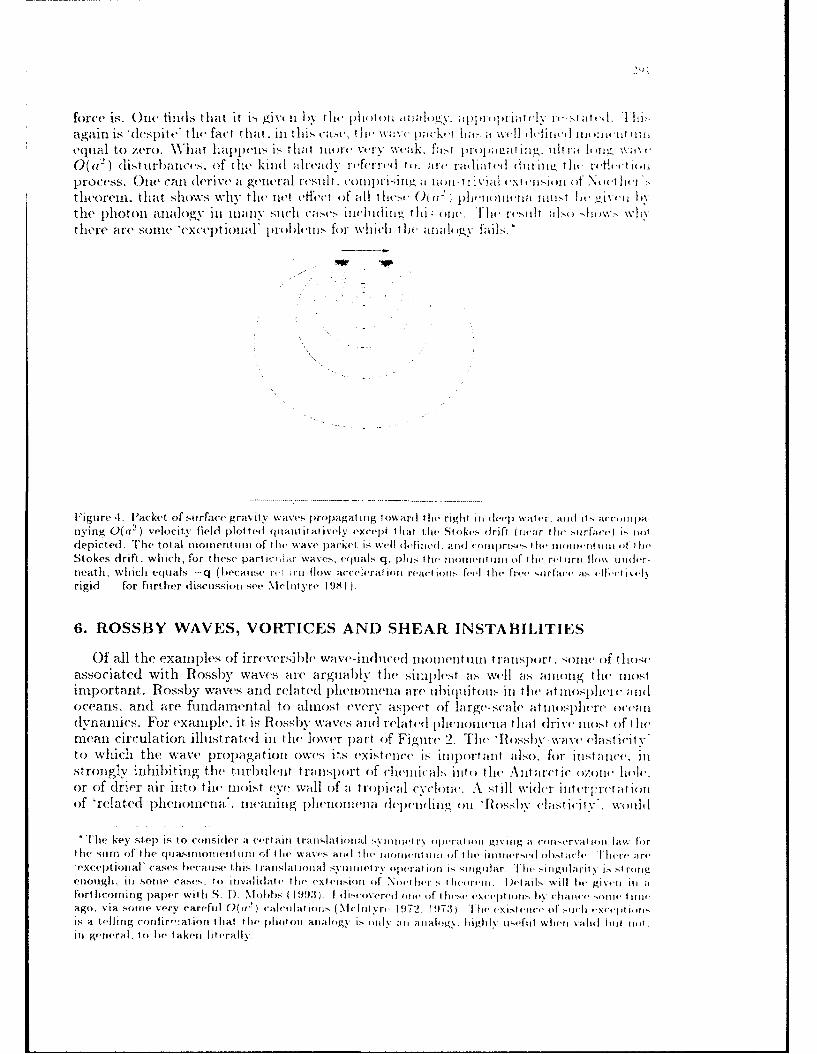
force is. Onet( hill(s that it I" gir't ii hy ill(-)10 (i prhialll i!V ;Iiipl(y6II lIy tir es t- iI la gai ii is *despite, the fact that. III This ca-c.% liii wavel p~lt-rkt Irs;r, well ileicIl 1lit t14 11u11rnequal to Zero. \V'lilt hiappeils is h it ha t re1ly4 VCNWI I, f~i:,t pr pini;ti liog , lnit bI a t tý i\;1

0(a2) (list urlbancies. of the kind( atlready re fern s 0l to- ran I-;I(I t (.1 dii iiiIll,- Ici t io*rt ii (I

process. Oil( (-ail detrivet it general resuilt . coIllIWi'-'IIIg ;Iii u 111 ia )1 I 'I*~tx IcIt , I it a

theoreml. that shlows whyr thec ijet effect ou all t h i'(lh tr phit'umticia' llteit I'e l-iveui h1

the 1)hotoil atialogy illnai stt~l hi S 15C'5cac- iiicIltttiii, thijAý oic IJIC',llt \01Vh ls hiw wthere' are someW Cxcepl~toiliil probut'lems foIr whilch till(-at 1lt hgy fa-ils.

Figure .1 V acket of strface gravitv waves, propuagatitng towýard t lle right In deepl waOter antI Itl ;ifttOMiIM~

nying 0(ia 2 ) ve~l.C I ty field p~loitl te ilarit it atvely except thlat thle Stokes drift (rivar t li, wufc) iotdepicted. The total mlotnefrit in of thre wave packet is we~ll defitiet rd, ;t rilt]cnlrst, ilie mtttttimeis tit t I))ie

Stokes dIrift. which, for these part ic i~trl Wav'.etjiLs q. phi, i lit. mtouttivnitl of ilth rettirit flov. uitoerneath, which equals -q (because' 1'c! r-flow acceleralt ill react iota feel t lit' fret, sirfiace a tibt ,erigid -for further dliscussioni ee McIntyrre 1 98 1).

6. ROSSBY WAVES, VORTICES AND SHEAR INSTABILITIES

Of all the examtnjhle of irreversib~le V~ave-Iii(liit''( ilt utieritin 1-tIatlspotrt . soit it of lthom,associated with ilossiw waves are argtilahbl thle simplest ais well ais anitintg the mo1(stimportant. P o55hy waives and rela ited plileuoflica ate- tiblyiji toils Ill t lie attiit 15)1 ire it 0(o),(Ceanls, anld are fundatriental to ahlmo(st every aspect of large- scale atmostphe) ire ''ai

dynamiics. For e'xamplle. it is Rosshy waves mid related plixilotneita that dirivte llt st of I t('Mean circulation illulstrate'd Iin the lower par't (If Figure 2. Te'Ra Itsslw -wave t'lasticjtyto which the wave propala t loll o)wes its t'XIstelive Is 11111)1 rt alit allst I for itist a rice. III

-strongly inhibititng the tiirhtleiit t r;Iispt rt of chilexijeals jutt I thlt Antarctlttit'oom h101 1'iIc.

or of drier air intott tlt nmtoist eye wall If at t ropical cyclt lut. A ,,till widter jit er; 'retat i~llof 'relatedl plieilriotiaei '. . meaning 1)1(0lifnlella (It pt't ii ig t)IlPtlh urosb t'listicit iv'.wt1111

*lie key step is to colllitet' a e(rt am tt'arslat iotal AN Inficit r~v operlat lori gIving aI tutu,(rv;t Iott law" fortheI( stun of thbe qtiasirniomui'tt alt oft t(re wave abdai lit' tiometitti n of t lie Immersed~'t ob~t acitt Hcrt' art-,exceptional, vases llecatist' this I ratislt loii al sirttr op-ratiott is singular. [Ie siingiilarit , i, st rorigenoulgh, iii1 somie cases, to inlvalitjlate th Ia txt tl'nioti of Nuot hersli'ý holIr'tt. I et ad- will be girt-ti Itt afort. ic-orrririg papter wit i S. 1). Niolits ( I 1993). 1 tli' tvt'ret onle of tIhv'sv t'Xtt'pt otis hrtchancte sortit' t 11r1'

ago, via some very careful 9(a,') calrillatiotis I Nchit vrt 1972. I 1973 lhe t'Xi.tt'rito'suc td~I- nxr.'j III" ott

is a tellirig corifir-':atiort t hrat the pbotonl atralov I!, otll'. ;il aialog\. highklyitsiefrt wilvti vallkill but ot.Iii getteral. to) be taken lite'rally.

292

include many important types of shear lustatilitiCS. all th. way fr,,oi ordinary .,mall.scale shear instabilities to the large-scale. buioyancy-p)owee(Td "baro(-cinic instalbilitis"that can lead to the formation of common types of atmospheric and oceanic eddies andvortices, including extratropical weather cyclones (Hoskins et al. 1985. & refs.).

Rossby waves and related phenomena occur in dynamical systeiis of the gencric formDQ/Dt = 0, U = I(Q) , (6.A~iJ,

where DiDt = Ot + u - V = O0 + tO, + v'v. the two- dimensional material derivative.and where I(.) is a time-independent functional of the ,haterially conserved scalar fieldQ. The simplest case is the familiar case of two-dimensional iinviscid. incomprlessiblevortex dynamics, for which

I(Q) = (-0, af)V- 2 Q, (6.2)

where Qr = Q = V• - 71Y, the ordinary vorticity and. to make the inverse Laplaciaxiunambiguous, suitable boundary conditions are unlderstood such as evanescence of lulat infinity. Note that (6.2) implies V. u = it, + Y Z 0. The next simpl-st case is ,hesame thing on a rotating earth whose vertical component of absolute vorticit:, is Q,.say, a prescribed function of horizontal position but not of time. Then, retaining thenotation u = (i. v) for the relative velocity anid Q, = t,, - i,, fok the relative vorticity.we may take Q Qe + Qr in (6.1) anrd retain (6.2) unchanged, remembering that Q,. isprescribed. The notation in (6.1) has been chosen tý, emphasize the fact that the singlescalar field Q contains all the dynamical inlfo:mation. At every instant, the Q field canbe 'inverted' to recover the velocity field u. One may call I(.) the "inversion ftlnctional'.

In more realistic models of the rotating, stratification-constrained. vortical flows thatoccur in the real atmosphere and oceans, the saie generic mathematical structure (6.1)applies, in many a'ases to remarkable accuracy. This is why simple two-dimensionalvortex dynamics has always been such an important idealization in the context ofatmosphere-ocean dynamics. The coordinates x and y now measure horizontally-projected distances along the (approximately horizontal) stratification surfaces. DiDtand d = (u, v, 0) are still two-dimensional on each such surface, and mi, + r'y is stillzero' to some useful approximation (more precisely. has typical magnitudes K< typi-

cal magnitudes of v, - u_). What is new is that the inversion functional I(.) is nowthree-dimensional. Away from the equator, it still has the qualitative character of (6.2)but with V 2 more like a three-dimensional inverse Laplacian. in coordinates verti-cally stretched by Prandtl's ratio, the ratio of the buoyancy to Coriolis frecquenciCs.Distortions of the stratification surfaces are also determined as part of the inversionoperation. One may generally characterize such stratified, rotating flows as approxi-mately 'layerwise two-dimensional'. In the most accurate models, which include modelswhose validity extends into the tropics, Q is the Rossby -Ertel potential vorticity. andinversion is no longer a linear operation (e.g. Hoskins et al. 1985, & refs: Thorpe 1985:Davis 1992; Raymond 1992).

One has here, incidentally, a framework for the general characterization of coher-ent structures such as vortices and vortex pairs. in atmosphere ocean dyn(lamnicsamounting to variations on a theme from Professoi Rosh.bko's Opening Lecture in thisProceedings. For instance a 'vortex', in any dynamical system of the form (6.1). isthe coherent structure represented by a strong, isolated anomaly in the Q field togetherwith the induced velocity and any other relevant fields in and around it. where induced"means given by whatever inversion operator I(.) characterizes that dynamfical system.Atmospheric cyclones and anticyclones, and oceanic Gulf Stream rings and 'Meddles"(e.g. Armi et al. 1988), are all cases in point. Figure 5 illustrates one such structure in amodel atmosphere, somewhat idealized but instantly recognizable to any meteorologist

N93

familiar with large-scale atniosplihric behaviour. It is a cyclo iiB' carthI co-rot iltt bigt~ratrolpical vortex indtuced by it strong. c'ompa~ict antonirial inl thelit Rssby Erte]l)O Iiilt ialvorticity field near the tropopause. Coherent strirelt urs such] it,, thiest' are o fitctliI()tanit for weather dlevelopmients, in which falst atlvectioii of potenit nal-vorticity ajiilenear the tropopause is an impiortanit asp~ect of the (ylilai~lics. alplroxilltiatel% ýsattsfyjiiiieq. (6.1a.) over tiniescales of several (lays.

50

Figure 5. Section across the axisymnmetric structure induc ed hy an isolated, axisyninietric, cyclonicpotential-vorticity anomaly (stippled region) near a model troj)opaluse (heavy cuirve) across whlich theRossby--Ertel potential vorticity has, a strong discontinuity, by a factor of 6. Thie famirly of thinl curessome of which are closed are isopleths of tangential velocity, at :3 rns-'intervals the greatest velocities> 21 mns- being at the tropopause -- and the other family of thin curves, mnore nearly horizontal, arethe stratification surfaces. These are isopleths of potential temperature 0 defined to Coincide withactual temperature at pressure 1000mnb or 1000 hPa, plotted at 5K intervals. Anontualy' mneanis apotent ial-vort iciity contrast on a 0 surface (Hoskins et a]. 1995, eq. 29)- The induced surface-pressureminimum is 41 hPa below ambient. The structure is typical for middle larit odes; the Coriolis paramneteris 10' s- (as at latitude 43.3'N). The dlorriain shown has a radius of 2500kin. Fromn the work of Thorpe(1985)y

Now to 'Rossby-wave elasticity'. The simplest example occurs inl the strictly two-dimensional dynamical system specified by (6.2) with Qr Q - Q, i'r, - ay, anld Q,.a linear function of y so that when u = 0 we have

OQ/Oy = OQe/Oy =/3 =constant . (6.3)

This is Rossby's famous 7/3-plane' or 'nearly flat earth' model, with ('?. Y) ta~kenl to beCartesian. Thien (6.1) is satisfied in this case without linearization, ats it happens

by expressions of the form u = (-O , -),',(x~y,t) ( Qr V2 C.,) W ith1 " y( x. !, t ) -,Cos ly Cos I{k(x - ct)}1, provided that the phaseI speed C anld the WilVellilrnber componentsk, I satisfy the dispersion relation

The one-signedness p~reviously referred to shows up here: (6.4) is a foriniula for c. an1dnot c 2as in classical smiall-vibration p~rolblenms in lion-rotating reference franiies,. X\' canlsee tije reasons for the one-signedness and appreciate its robuistness its follows.

By (6.1), the contours of constant Q are also) material contours. If a distuirbancemakes these contours u ndlulate ats suggested inl Figuire 6, then Q, iln (6.2) wvill be al-ternately positive arid negative as indicated by the phlis and minuiis signs in Figure 6.Then sinlce( 4'ý V 'Q, the contours of ]j', canl be p)ictulredl as the cquipotcniials of theelectrostatic field dine to a pattern of alternating positive aito negattive, charges (withI the

294

sign changed), or as the topographical co(itolirs giving th (l displaceitiint of a stretchedelastic membrane that is pulled up ( -) and pushed down (-f ) altertiately III thle samiepattern. Hence Q, will have hills and valleys ceintr(ld respectively on the 1in1us and theplus signs, imiplying that the strongest north-south velocities (at right angles to theelectric field in the electrostatic analogy) will occur at intermediate positions, a qu1arterwavelength out of phase with the displacement, and in thle sense shown by the he•avy.dashed arrows in Figure 6. If one now makes a moving picture in one's inind's eve ofwhat this induced velocity field will do to the material contours. one can sce at onc(,that the behaviour must be oscillatory, and also such that the undulations propagatefrom right to left only.

The same physical picture exhibiting one-way propagation applies wheCn Q,. = 0 butQ has a background gradient OQoiOy due to a mnean shear flow u ti (y) , 0})

OoI y = - 2 uo0 I y2 = -u 0,.,, (6.5

so that Q = Qo(y) + Q'(x. y. t) and iý, = - ifu,)(y)d) + -"(x. y. ) and. for smalldisturbances,

(at + uoar)Q' - u0Yuw'? = 0 , /,' = -'2 Q' (6.6)

essentially the Rayleigh equation. It is no surprise, therefore. to find that the simplestclassical shear instabilities, such as the instability of the u() = tanh y shear layer, orits Rayleigh (piecewise linear) counterpart, can be understood (consistently with theRayleigh, Fjortoft and Arnol'd stability theorems) in terms of a coupled pair of Rossbvwaves, in a certain frame of reference, each of which propagates against the local meanflow and phase-locks with the other in such a way as to bring it to rest. Furthermore.each Rossby wave makes the other grow exponentially, via a reduced phase shift betweendisturbance velocities v' and the sideways displacements r/' of the Q contours (Lighthill1963, Bretherton 1966, Hoskins et al. 1985 §6b). The Miles (1957) wind-wave instabilityis in some ways fundamentally similar, except that one of the Rossby waves is replacedby the surface gravity wave, and there is a mismatch between the strengths of the gravityand Rossby elasticities leading among other things to relatively slow growth.

7. ROSSBY-WAVE BREAKING: A DEFINITIVE EXAMPLE

In Figure 6 the Q (material) contours are depicted as undulating reversibly. thesituation described by linearized, dissipationless wave theory. Indeed, for linearizedtheory to be self-consistently and generally applicable, along with associated ,'onrept ssuch as the principle of superposition, the undulations must also be gentle. Strictlyspeaking, the sideways slopes (ay/Ox)Q must be infinitesimal. The opposite extreme.that of infinite sideways slopes followed by sideways overturning, and rapid. irreversibledeformation, lengthening and folding of the Q contours, is a comnnonplace occurrenceand can be recognized as a Rossby-wave version of 'wave breaking'. An idealized exampleis shown in Figure 7; see also Figure 9 below. This phenomenon. in a variety of forms.is ubiquitous in the real atmosphere and oceans and plays an important role in theirreversible transport of momentum and angular inomeinturn by Rossby waves.

The case of Figure 7, known as the Stewartson Warn-Warn (SVWW) Rossbv-wavecritical-layer solution, is now described in more detail. It is important out of all propor-tion to the restrictive idealizations used because it is an unequivocal example, describedby an analytical solution, of irreversible wave-induced angular momentum transport duesolely to wave breaking, with no other wave (dissipation mechanisms involved.

We return to the dynamical system described by (6.1)- (6.3), but now introduce anundisturbed flow uo( y) having constant shear uy. say. Again the Q contours are malde to

29

£ Q =constant

Figure 6. Sketch of the Q contours and the Q-anomaly (Q') pattern, and the induced velocity fieldgiving rise to the sideways 'Rossbv elasticity' in a simple, non-breaking Rossby wave.

undulatc, this time by introducing a gently undulating boundary near some value Y5' of y,exciting Rossby waves of constant phase speed c and y-lengthscale uO, 13. The boundarydisplacement amplitude is of order e uoy/f3 where E. is a small dimensionless parameter.The x-wavelength 27r/k of the undulation is assumed long enough, >> 27r uoq/ii, forthe inverse Laplacian V- 2 in (6.2) to be approximated by (O/Oy)- 2 , simplifying themathematics. (The lengthscale uoy!/O then corresponds to the lengthscale I` in (6.4)when c : I-1 uOy.) Under these restrictions and with suitable choices of Yo, this problemcan be solved analytically (Stewartson 1978, Warn and Warn 1978). The Q contoursbehave in an approximately undular manner except in a narrow region surrounding thecritical line, or y-location where uo(y) = c. This narrow region, the 'critical layer', isseparated from the undulating boundary by a distance Z uov/fl and has width of order

b = I/2 Uo ,// 3 . (7.1)

The 'inner problem' for this region is mathematically the same as the nonlinear pen-dulum problem, incompressible fluid flow replacing incompressible phase-space flow. Itis analytically soluble in terms of elliptic functions, and the solution confirms that theregion is, indeed, a region of Rossby wave breaking in the sense envisaged. Figure 7shows the solution at four successive times. Q contours are overturning sideways, anddeforming in a manifestly irreversible way.

Let us suppose that the resulting rearrangement of the Q field has, in a coarse-grain view, something of the character of a mixing layer as shown in idealized form inFigure 8a. Then it is a trivial matter to see that there must be an associated irreversibletransport of momentum. Let 6Q(y) be the change in Q represented by the differencebetween the solid and dashed lines in Figure 8a, and bi(y) the corresponding change inu. Application of the inversion operator (6.2) gives (since 6Q = Q = -6bft here) theparabolic profile

bfY½ 0(9(yý2 4 2 2b (y7.2bmS0bm) (y < 1b, or y> ibm) (7.2)

where bn is the breadth of the mixing layer. Negative momentum

6M 0C 6bi(y)dy =-Obm 3 (7.3)

has been transported irreversibly into the region where Q has been rearranged. Thisphenomenon is robust: any change ýQ(y) qualitatively like that in Figure Sa will beassociated with a momentum change of the order of magnitude, and sign, indicated by(7.3). For instance the SWW solution has a limiting value of 6M as t -4 00, whichcan be expressed in the form (7.3) with the value of bm shown by the bar at the centre

296

of Figure 7d. This value of f).. may be thought of as an 'eflecttive ,nixiang width, folthe SWW solution. In this case the inonent uri (7.3) has come fromu the w;:vt, s lmrcecomprising the undulating boundary at large 1'. Whein 3. or more gtenerall" rw h, itialgradient O(Q, + Qo)/ 8 y, is positive, this monwntum is necessarily negative amothermanifestation of the one-signedness of Rossby dynamics.

The SWW solution provides us, incidentally, with a definitive couiterexainple toarguments saying that Q-mixing scenarios like that of Figure 8a are imIpossible becausethey violate momentum conservation. These arguniints overlook thle possibility of waveinduced momentum transport from outside the region. Further historical remarks andreferences, going back to various issues surroundfing. for instance. G.I. Taylor's 'vortiitvtransfer theory', and its recent developments including links with the photon anialogy.can be found in my 1992 review and in the paper with Nortoii (1990).

Another interesting point about Figure 7 is that the predicted Q configuration be-comes shear-unstable after the contours first overturn. So if any noise is present initially.the actual evolution is quite different in detail. In typical cases the result is an appar-ently chaotic form of Rossby wave breaking, arid an increase in the effective mixingwidth bm by a modest factor such that &M (cx brn3 ) increases in magnitude by a fac-tor 2 or 3. Figures 8b,c, from the definitive study by Haynes (1989), show the Q and6ii profiles, defined as Eulerian x-averages, in one such case. The 6i- profile has theapproximately parabolic form suggested by the idealization (7.2).

The foregoing examples are conceptually important in another way, already hi.1tedat. The inviscid, two-dimensional fluid-dynamical system under consideration is knownto have mathematically regular behaviour, over arbitrarily long time intervals. Theexamples are therefore cases of wave dissipation and irreversible momentumn transportthat do not depend on overtly dissipative processes like viscosity. The irreversibilityinvolved is a purely fluid-dynamical irreversibility, precisely that associated with thepersistent lengthening of the Q contours as time goes on, and familiar from other fluid-dynamical paradigms such as 'random straining' and 'turbulence' (e.g Batchelor 1952).

8. THE DEFINING PROPERTY OF WAVE BREAKING, THE STRATO-SPHERIC 'SURF ZONE', AND OZONE CHEMISTRY

What should one mean by wave breaking for general, non-acoustic* waves in fluids?Even in the most familiar case, ordinary surface gravity waves, the phenomenon usuallyrecognized as breaking has an extensive 'zoology' of shapes and time-evolutions. Thesame is true of internal gravity and Rossby waves. The question does not seem to haveany natural answer from a 'zoological' or morphological viewpoint. However. a naturalanswer does suggest itself if one wants the concept of 'wave breaking' to be relevant tothe general question of wave-induced momentum transport, or, more precisely, to thequestion of when wave-induced momentum transport becomes irreversible.

One can then use the rapid, irreversible material-contour deformation illustratedabove as the defining property of wave breaking. 'Rapid' means that deformation ratesare comparable, at least, to the local intrinsic wave frequency. Such a definition is en-tirely compatible with the accepted phenomenology, and relevance, of wave breakingin the case of surface gravity ,vaves and longshore ocean-beach currents. The case forsuch a generalization is carefully argued in three papers with T. N. Palmer (19835).It avoids 'zoological' definitions, and requirements to decide whether 'turbulence' is in-volved, but does take account of the relevant general theorems, particularly Kelvin's

*Shock formation in acoustic waves seems best kept conceptually separate, if only because its essential

dependence on the existence of overtly dissipative processes (microscopic irreversibility).

5

0i-y~J72 ~ ~

-5

Figure 7. ('ontour-s of constant Q for lthe SWv X soht ii on, a special bu13t cle'ar-cuit. examplpe of lhussry -wave breaking (cont rast the purely uiidular. noir-lreakirig iPossby wave in Figure 6). and] thle coinsequientirreversible wave- ind uced miomenturm transport. See also Figure!). Iliey?-scal(' [iits beeni exp~and~ed Ir;isngthe re-scaled coordinrate Y = y/b wit~h b =(1l/2 ur)y /AI the range -5 < V < 5 is plot ted. Four successivestages in the evolution are shown, at timies 1, 1.51 2, 3t jil niits of 211/2 (k b ury )- 1 . where A- is tIhe x'-wavenurinher. The vertical bar in paniel (d ) gives the effective mnixinrg scale b,,- b; cf. (7.2), (7.3t) and]Figure 8a. Front Killworth and McIntyre (1985), after St~ewartsoi (1978) arnd Warn and( Warn ( 1978),

(a) Y bi y(,

bm ________ 021Y) i(

Figu~re 8. 9-mrixing scenarios and assoclat.(d nironient ur change; see (7.2), (7.3): (a) thre simiiplist ic,but qualitatively relevant, idlealizat ion t hat. assirnrres p~erfect 9-minixinrg over width brr ( b) art act ial

Etilrianmea Q~y proilefronta accurate, quasi-chaotic Rossln-wave crit ical-laver ono P.IHlaynes, personal comnmunicationr); and (c) the approximoately parabl ric p~ r()rr lie corresponidinig to(b), showing the rn1oinentiJni change dire to thre Hlosshv wave breaking (firsi oIf (7.2) and (if (7.3)). Asin Figure 7, tie re-scaledl coordinate Y =y/b is rused, over tOw sarire range -5 to1 5(I ur,/ .

circulation theorem arnd the Way it mnanifests it sclf InI exact., formally comp1 le'teC IHim-ries of wave nmean interaction. The relevanlt mate(rial (contouirs are dlefl~ined to be throsethat would otherwise tilundla te reversib~ly undI~er the genleralizedI elasticityV. or restoringmechaniism, that gives rise to the wave propagationl.

Figure 9. of which anl anilmated versionl wils SeenCI ill tlie lectire, Show-, a less, Idealizedexarnlple of Ro(ssby wave lbreakiiig anud its effects, takeni front thre work of Norton (1993).The parameter conditions are far closer to t hose III thme real stra tosp~here than tho seaJsslumeId by critical-layer theory. Here t lle dvmliariiical systvitl co~mpmrises the( siraib nw

298

water equations on a sphere, solved numerically by a high-resolution pseudospctralmethod. The projection is polar stereographic, and the winter northern hemisphereis shown. An axisymmetric initial state is disturbed by smoothly distorting the lowerboundary in a large-scale pattern so as to imitate the effect, on the real stratosphere, ofplanetary-scale Rossby waves propagating up from the much denser troposphere below(Charney and Drazin 1961). The result looks remarkably similar to what is seen in thereal winter stratosphere at altitudes of the order of 25 to 50 kin.

The left panel of Figure 9 shows Q, now the shallow-water potential vorticity, definedas absolute vorticity over local layer depth. The model problem still has the generic form(6.1) to excellent approximation, but with a shorter-range potential-vorticity inversionoperator* I(.). The central region is the model's 'stratospheric polar vortex', where therelevant material contours, which in this experiment lie initially along latitude circles,are almost coincident with the Q contours and undulate nearly reversibly. In this regionthere is little Rossby-wave breaking. This is illustrated by comparison with the rightpanel, which shows the behaviour of some material contours computed very accuratelyusing a high-precision 'contour advection' technique adapted from the work of Dritschel(1988). Outside the polar vortex, in middle latitudes, is a region in which the wavesare breaking vigorously. There, the initially-latitudinal material contours are deformedrapidly and irreversibly, and mixed into a broad, 2D-turbulent 'Rossby-wave surf zone*;e-folding times for contour lengthening were estimated to be about 4 days (Norton, op.cit.). This 'surf zone' is the real-stratospheric counterpart of the idealized Rossby-wavecritical layer. It is far broader, and very different in detail, but it illustrates equallywell the robustness and one-signedness of the angular momentum transport associatedwith irreversible Q-rearrangement. As already suggested, such Rossby-wave breakingis an important part of how the mean circulation illustrated in Figure 2 is driven.Furthermore, its recognition in models of the global-scale stratospheric transport oftrace chemicals like CFCs is beginning to lead to improved realism in the predictionsof such models, both via a more realistic mean circulation, and also via a more realisticrepresentation of the quasi-horizontal turbulent transport (Garcia et a]. 1992).

This latter aspect may be especially important for ozone photochemistry (and rele-vant to some current controversies about ozone depletion - see §10 of my 1992 review).This is because ozone photochemistry by its nature could be more sensitive than, forinstance. CFC photochemistry, to the timing of a typical molecule's excursions acrossthe 'surf zone'. Timescales for such excursions are comparable, at certain altitudes, tophotochemical timescales. Together with the mean circulation itself, these complicatedfluid motions control the rate at which ozone is produced photochemically, mainly inthe high tropical stratosphere, and carried thence to the extratropical lower strato-sphere where it accumulates (unless destroyed by 'ozone-hole chemistry') in far greaterconcentrations than can be produced by tropical photochemistry alone.

Model simulations like that of Figure 9 are also relevant to understanding the Antarc-tic ozone hole. The contours in the right-hand panel of Figure 9 can be regarded as iso-pleths of an advected passive tracer, the advection being very accurately simulated, withno artificial diffusion. The simulation shows that, at least in the model, chemical sub-stances in the surf zone do not penetrate past the region of strong Rossby elasticity con-centrated in the steep Q gradient near the vortex edge. This is believed to be important

*To rough approximation, this I(-) is given by (6.2) with V- 2 replaced by (V 2 - K2 ) -, correspondingto an elastic membrane tethered by local springs, somewhat like a spring mattress, with a latitude-dependent e-folding scale i-' (the 'Rossby radiuis') of about 1400 kin at the pole. 2000km at 450N,and 3000 km in the tropics. McIntyre and Norton (1990, 1993) give examples of much more accurate(but much more elaborate) potential-vorticity inversion operators I(-) for shallow-water models.

Qý\ r

/ N\N~jL

Figure 9. W inter hemnisphere in a high-resolution, sliallow-.wah r numek(rical niodeI of' the st ratosphiere.from Norton (1993). The mean depthI is 4 kin, arid the( numerical resolution (t rianigular I ruiicai~ionat total wavenumber 127) corresponds to a mesh size roughly I' latitude. Left, panel: potentit al x'or-ticity Q, contour interval 4 x 1O-ý in -' zero contour dotted. (Negative Q values would, in athree-dimensional nmodel, signal the thtree-di mensional mnode of' lossby-wave breaking pointedI out byO'Sullivan and Hitchman 1992.) Right panel: isopleths of' an advected tracer field, initially axi~syni-metric and coincident with the Q contours, showing the flufid-dynamical irreversibility characteristic ofRossby-wave breaking and two-dimensional 'tujrbulence'. This was computed with iiear-perfe~ct. accul-racy using a high-precision 'contour advection' techique. introduced ind(epenidently by Norton (1993)and by Waugh and Plumb (1993) using an algorithm developed in another cont~ext. by IDritsclici ( 19881).

for ozone-hole chemistry. The same phenonmenon has b)een (denmonstrated in thec labora-tory by Sommeria. et al. (1989, 1991). The contour-ad vertion technique. co~lccieifd of asa benchmiark numerical tracer ad~VectionI algorithmn, was introduced independlentlJy IwNorton (op. cit.) and by Waugh and Plumb (1993).

Recentlyl O'Sullivan and Hitchia~n (1992) have shown that anl entirely different inodeof Rossby-wave breaking is possible near the equator. where time pot~ential vorticityitself changes sign. It conforms to the general wave-breaking dlefinition, with three-dimensional rather than layer wise- two- (11inem nsion al material contour (lefo rmnations', aris -ing from an asymmetric inertia~l (quasi-centrifugal) inistability. Among other tihings, thismay have new implications for the quantitative modelling of the QBO.

9. WIND-GENERATED WATER WAVES: TWO NEW MECHANISMS?

What does this old but, elusive problemi look like from the foregoing p)(rslpe(tivc(' Thefirst point is that Bossby-wave (lymlaiics is invoilved,. albeit on mmnuii faster timmiescali'sthan before. The velocity p~rofile in the air, whether or not alplroximtlately logarithmlic.will uisually have a strong curvature t,, near time water stirface (! .-vertical). Thevreforethere is a vertical gradient of spanwise vorticity and1( hence, III thie pr('s('It hi nguagcý aRossby elasticity, in the airflow just above the water waves; recall (6.5) awid Figure 6.That is why the miles inviscid winld wave instability, for instance, can b)e regardled asa. coupled -Rosshy-wave. gravity-wave' instability. One (-ani think Ill. termis of a pair ofpha~se-locked, coutnterjproJpagat ing waves, a lbackwar( -pjropaigat jug fl 0551 y wave Iin theair coup~led to a, forward-propagating gravity wave Ili thie w0ter. (Othecr e'xaimpIles ofRossby-wa~ve, gravity-wave instabilities go back to 0. 1. Taylor's work ini thev 1930s onl

300

the 'Taylor--Goldstein equation'; see also, e.g., Griffiths et al. (1982), Hayashi and Young(1987), and Sakai (1989).) In the Miles instability, the Rossby elasticity is relativelyweak. This implies not only that the water wave largely determines the phase speed c,but also that the growth rate is slow and that the most significant Rossby effects occurnear the critical line uo(y) = c, where intrinsic phase speeds are slow. The matheimaticalunderpinning for these statements is well known and is given in detail by Miles (1957)and Lighthill (1962).

Now the self-consistency of the linearized instability theory requires that conditionsnear the critical line resemble those in Figure 7a. In the present language. the Rossbywave is not only weak and slow, but is also in the earliest stages of wave breaking.in the generalized sense already referred to. The later stages can be expected to lookmore like those of Figure 7b-7d and beyond, with a small value of the effective mixingscale bin, viewed in a suitably undulating coordinate system. This suggests that theidealized scenario represented by the inviscid Miles mechanism lacks robustness, whentaken literally. The delicate phase-locking and synchronization of the normal mode'sdisplacement fields will be disrupted by Rossby wave breaking before much verticalrearrangement of spanwise vorticity can take place (and long before the water wavesbreak). The outcome will be net vorticity rearrangement, in the airflow, over only a smalleffective mixing depth bin, of the same order as the scale b given by (7.1) except thatthe lengthscale u 0oy/3 is replaced by a typical value of -Uoy/uovy near the critical line.There is a correspondingly small net wave-coherent momentum transport 6M a bm3from air to water, having the order of magnitude implied by (7.3) with ;I again replacedby a typical value of -u 0 yy near the critical line.

However, there is one important feature of this idealized scenario that does, on theother hand, look robust. This is the sign of the net wave-coherent momentum transport,which tends to be such that the water waves are amplified when travelling in the samedirection as the wind. More precisely, the sign is determined by the sign of -UOYY andthe one-signedness of the associated Rossby-wave dynamics --.- the same one-signednessthat so strongly controls the sense of the mean circulation throughout most of Figure 2.In the wind-wave problem the sign is determined quite independently of whether or notwe have strictly x-periodic waves and delicately synchronized exponential, normal-modegrowth.

This sign-robustness must imply a kind of 'ratchet effect'. Almost any spatio-temporal intermittency - whether it be any tendency of the water waves to arrangethemselves in groups through, for instance, subharmonic instabilities, or any gustinessof the wind that might be modelled as an intermittency in quantities like -uOY ..will tend to favour intermittent wave-coherent momentum transport whose effects arecumulative. They may possibly also be such as to reinforce the intermittency. There isno longer any reason, moreover, why the effective depths b, associated with any Rossbywave breaking should be especially small.

More generally, the sign-robustness points to the likely effectiveness of any process inwhich wave-coherent undulation of the airflow over the water waves causes Rossby waveactivity in the air to increase in total amount, or to dissipate, or both. The relevantmeasure of 'activity' for this purpose is a suitably defined quasimomentumn (Killworthand McIntyre 1985; Shepherd 1990, & refs.), since the photon analogy can be shownto apply here, in the required sense. Any such process will result in wave-coherentmomentum transport in such a sense as to amplify the water waves. This could well beimportant for the real wind-.wave problem, despite the added complexities of turbulenceand other three-dimensional effects. There appear, in part'ticular, to be two distinguish-able mechanisms whose possible role deserves closer attention, both theoretically andexperimentally.

10'1

One is simply local Rossby wave b~reakinlg characterized by ielatively hiirgc effect IVedepthis b1,, .If. for Instance, a gus-t protluces anl effectiVC that tlieiil (i1('ot lilt( crSa wave group,. leadling to rapid vertical rearranigemlent of spaiiwise vorticity ( redulilci- u0 ), then the water waves will lbe corresponling-lv amiplified for a short tuiei. 'Flietransient nature of such phenomena would add to the well-known difficuilties of observilfnathe associated pressure ph,-se shift experiment ally. The ot her imechanlisii, wl tich IIIreality might tend to occur at the same timle, Is the formation of Rossbv, lee waves IIIthe airflow. This will give rise to 'wave resistance, InI the usual way. not d(I '~edIIg oilwave breaking of any 'kind. Indeed the lee-wave mlechianismi should be at its mlost. efrejenitwhen both Rossby wave breaking- and water wave breaking are( unimportant. Thent orishould get unseparated flow oV%( r the water waves (e.g. BamR ~r 1990. k- refs.) and~.for at least some -uio', profiles, anl efficienit shledd~ing of Rossby-wave quasimniomnenitiunlinto t~he downstream airflow. It seems possible that the amnplifyinig wave group ill theexperiments of Chu et a]. reported by Professor Phillips, which they call the -short wave*(energy front", might depend onl the Rossby lee,-wave miechianism andi the experiment~smight offer a chance to study it under controlled conditions.

These ideas might also help resolve somie longstanding questions about the effectsof three-dimensional turbulence onl different t~imescales, fromn the relatively lonig, *dis-sipative' tmniescales required torstr uOJi profiles. tethe relatively shot eaictiniescales onf which rapid- distortion theory might be app~ropriate. mierely muodifyi ngthe Rossby elasticity in the air --- as with internal gravity waves inl the Importantobservational study by Finnigan an'1 Einaundi (1981), in which elddv-viscosity or othersteady-state dissipative turbulent modelling was shownm to be wrong b~y -all order of mnag-nitude'. In some wind--wave modlels, turbulent processes are modelled semi-emlpiricallyfor instance by adding something like anl eddy vizscosity to the Miles theory. Such de-vice-, (drastically modifying the type of behaviour suggestedl by Figure 7) would seemunavoidable in models that insist on .r-periodicity, or on horizontal statistical stationi-arity and linear superposability of wave- coherenit processes. But a physically correctturbulence model might necd to bring lin a wider range Of tinw"scales. This suggeststhat it could be fruitful to try to mnodel the spatio- termporal interinittenicy of the, waterwvaves and the airflow explicitly.

Acknowledgemnents: Early versions of the ideas developed here were part, of an essay that shared the1981 Adamns Prize in the Universityv of Canibridge. Their development has been influenced by manycolleagues going back to early ideas fromn I. P'. Bretherton, D. 0. Gough , T Matsuno, P.. E. Peierls,E. A. Spiegel. and most recently P. 1., Haynes, W . A. Norton, and other co-authors with whom 'it.has beern a pleasure to work. The experimental dlemonstrations in F'igure 3 were stimulated by oneof M. S- Ionguet-Higgins' beautiful wave-tank demionstrations, and G. 1. Baretablat t stimulated nue tothinl- harder abo,,j real turbulent, airflow over water. Support fromn the Natural Environment Res. archC7ouncil (through the UK Universities' Global Atmospheric Modelling P~roject and through the Brit ishAntarctic Survey), the Science and Engineering Rese;-rch Council, the UK Meteorological Ottice, andthe US Office of Naval Research is grat~efuilly acknowledged.

REFERENCES

Andrews, D)- G., [Holton, J . R. , Leovy, c. B3., 197: M1iddle Atmosphere Dhiainics. Aademiuc P ress,'189 pp.

Andrews, D. G., McIntyre, MI. . 1976: P~lanetary waves in) horizontal atr( vertical shjear: t he getier-alized Eliassen Palm relation and] thne mean zonial acceleratijon. Jt Innos. Sci.. 33, 2031 2014M. [Sýevpp. 2043 5]

Andrew.,, 1D. G_. McIntyre, NI- E., 197 8 a: Ani exact theory of nionlinear waves oni a L~agranngian-nicallflow. .1. Fluid Mech., 89, 609-0(46. [Note the cav-atOs about. L~agranngiai uneanis in § It (re~gardingcases like that of' Figure 7 above), and(, in McIntyre I 980.1

And rews, I). G!McIntyre. MI. E-,* 1978b,: OnI wave-act ioni anid its relatives .1. Fluid Med-c., 89. 6417 661( orrigendrn~l~r 95, 7.96).

302

Armii, L.. Hfebert, D_. Oakey. N_, Price, J. kicilaNdon. 1'. 1. lo~shy. 'I , iii ick, B. 1%9xs: 'I liehistory and decay of a Medite' raneani salt lens. Nat nre. 333. 649 65 1

Banner, MI. L., 1990: The iniflu ence of wave breakin g on it surrface pressure listri-6tim iti ii winld waveint eractions. J. Fl, id Meet)., 211, 463 -195,

Barnett., J. J.. Corniev, MI., 19F5: Middle atmospliere reference nirodel derived from satellite dat a. linHandbook for MIAP, voL 16. ed. K. Labitzke. J. .1 Barnett, B. E-Idwards, pp.47 1 13. Available fromSCOSTEFP seoretariat, Uniive'rsity of Illinois. 1406 W. Greeni St. U -rbana. 11l- 61141 1O ' .S.A.

Batchelor, G. K.. 1952: The effect of lioniogeticous t urbulenice onl material lines arid su rface4s. Proc.Roy. Soc. A 213, 349-366.

Booker, J. H4., Brethertori, F . P., 1967: T he critical layer for inrterna, gravity waves ini a shear flow. J.Fluid Mechl., 27, 513 539,

Bretherton, F. P., 1966: Barocliziic inistahility anid the( short wavelength (,it.-ofl i, lernis of pot entialvorticitv. Q. J. Roy. Met corol. Soc., 92, 335 3,15.

Bretherton. F. P., 1971: The general linearised theory of wave propagation, Artier. Math -Soc. 1eci uresin Applied Mathematics. 13, 61 102. [See §6]1

Bretherton, F. P., Garrett, C. J. Ri., 1968: Wavetrairis iii inhoinogericous inoving rinedia. Proc. Roy'.Soc. Lond., A 302, 529-554.

Brillouin, L., 192t5: Onl radiation stresses. Annales, deIC Pysique. 4, 52A 5W6 (In French.)Charricy, J. G., Drazin, P. G., 1961: Propagation o1 planetary-scale dist urbrances fromt the lower into

the uipper atmosphere. J. Geophys. Iles.. 66. 83- 109.Chu, J. S., Long, S. R., Phillips, 0. W,. 1992: Measurements on thle interaction of wave groups 'A ith

short~er wind-generat,-d waves. J. Fluid Mcecli., 245. 191 210D)avis. C. A., 1992: Piecewise potential vorticity inversion. J, Atmios. Sci.. 49. 1397 1-111.Dickinson. R. E., 1968: Planetary Rossby waves propagating vertically through weak westerly wind

waveguides. J. Atmos. Sei.. 25. 984 -1002. [See p. 1001 for tile suggestion about thle QBO.]Dickinson, R.. E-1 1969: Theory of planetary wave-zorial flow interaction. .1. Atrnos. S'ri.. 26, 7:3--81.Dritschel, D. G., 1988: Contour surgery: a topological reconnection schemne for extended integrations

using contour dynamics. J. Coinput. Phys.. 77. 240- 26G.Dunikerton, T. J., 1983: Laterallty-propagati ng, Rossby waves ini the easterly acceleration phase of the

quasi-biennial oscillation. Atmos.- Ocean. 21, 5,5 68.Finnilgan. J. J., Einaudi, F., 1981: The interaction between ant internal gravity waves and the planetary

boundary layer. Part It: effect of the wave on the turbulence structure. Q. J. Roy. Mfeteorol. Soc..107, q07-832-

Fritts, D. C., 1984: Gravity wave saturation in the middle atmosphere: a review of theory and obser-vations. Revs. Geophys. Space Phys. 22. 275 308.

Fritts, D. C.. 1993: Gravity wave sources. source variability and lower and miiddle atmospheric efrects.fit: Coupling Processes in thle Lower and Middle Atmosphere, ed. E. V. Thrane, T. A. Blix, D. C.Fritts; Dordrecht, Kluwer. 191-208.

Garcia, R. R., Stordal, F., Solomon, S., Kiehil, 31. T.. 1992: A new numerical model of the middleatrnoslphcre. 1. Dynamics anid transport of tropospheric trace source gases. .1. Geophys. Iles., 97,12967--1299t.

Garrett, C., Smith. J., 1976: Onl thle interaction between long arid short. surface waves. .1. Phys.Oceanography, 6, 925-930.

Gill, A. E.. 1982: Atinosphere-Ocean 1)'ynarnics. Academnic Pi~ess. 6 62 pp.Gray, W. M., Sheafl'er. 3. D., Knaff, J. A., 1992: rInfluenceof the stratospheric QHO on IKNS() variability.

J. Meteorol. Soc. Jlapan, 70, 975 99-5.Green, I. S, A.. 1970: Transfer properties of the large-scale eddies and thre gen, ral circulation of the(

atmosphere. Q. J. Roy. Meteorol. Soc., 96. 157- 185.Griffiths. R.. Wv., Killwor,.h, P. D_. Stern. M. E., 1982: Ageostrophic inst ability of oceanl currents, .J.

Fluid Mech.. 117. 343- 377.Hlamiltron, K., Garcia, R. RI., 1984: ILong-period variations ini tii(, solar sernidirirnai ainiospheric tide.

J. Geophys. Res., 89, 11705-11710).Hfayashi, 'r .-Y., Young, WV. R,., 1987: SU. ble arid un~stable. ,,hear miodes of rot at ing parallel flows in

shallow water. ). Fluid Mech., 184, 477 504.Hlaynes, P. I., 1989: '[le effect of harotropic instability oil the nonlinear evoluttion of a Hosslw wave

critical layer. J. Fluid Mechl., 207, 231 266.Hlaynies. P. iI., Marks, C. ., Mcintyre, M,. E., Shepherd. T, (;., Shin e, Kx. P_. 1991: ()ii tike "downward

303

control" of extratropical diabatic circulations by eddy- induced mean zoiial forcus J. Ait mo. Sci., 48.651-678.

Haynes, P. H., et aL., 1993: Notes on thie U K National Sutninier School in Geophysical and EnvIroirnrIentalFluid Dynamics. In preparation.

Hoskins, B. J., McIntyre, M. E., Robertson, A. W_. 1985: On the use and significance of isentropicpotential-vorticity maps. Q. J. Roy. Meteorol. Soc., 111. 877 946. Also 113, 402 40l.

Killworth, P. D., McIntyre, M. E., 1985: lDo Rossby-wave critical layers absorb, reflect or over-reflect.J, Fluid Mech., 161, 449-492.

Lighthill, M. J., 1962: Physical interpretation of the mathematical theory of wave generation by wind.J. Fluid Mech., 14, 385--398,

Lighthill. M. J., 1963: Boundary layer theory. In: Laminar Boundary Layers, ed. L. Rosenhead; OxfordUniversity Press, 46-113. [See p.93.]

Lighthill, M. J., 1978a: Waves in Fluids. Cambridge University Press, 504 pp.Lighthill, M. J., 1978b: Acoustic streaming. J. Sound Vib.. 61, 391-418.Lindzen, R. S., Holton, J. R., 1968: A theory of the quasi-biennial oscillation. J. Atmnos. Sci., 25.

1095-1107Lindzen, R. S., Tsay, C. Y., 1975: Wave structure of the tropical stratosphere over the Marshall Islands

area during 1 April - 1 July 1958. J. Atmnos. Sci.. 32, 2008.2021.Longuet-Higgins, M. S., 1969: Action of a variable stress at the surface of water waves. Phys, Fluids.

12, 737--740.Longuet-Higgins, M. S., Stewart, R. W., 1962: Radiation stress and mass transport in gravity waves.

with application to 'surf beats'. J. Fluid Mech., 13, 481-504.Lorenz, E. N., 1967: The Nature and Theory of the General Circulation of the Atmosphere. Geneva,

World Meteor. Org., 161 pp. [See especially pp.85,150.]Loudon, R., Paige, E. G. S., 1991: Alan Frank Gibson. Biogr. Mern. F. Roy. Soc. London. 37, 221-244.McIntyre. M. E., 1972: On Long's hypothesis of no upstream influence in uniformly stratified or rotating

flow J. Fluid Mech., 52, 209-243.McIntyre, M. E., 1973: Mean motions and impulse of a guided internal gravity wave packet. J. Fluid

Mech., 60, 801-811.McIntyre, M. E., 1980: Towards a Lagrangian-mean description of stratospheric circulations and chem-

ical transports. Phil. Trans. Roy. Soc. Lcnd., A 296, 129-148.McIntyre, M. E._ 1981: On the 'wave momentum' myth. J. Fluid Mech., 106, 331-347.*McIntyre, M. E., 1992: Atmospheric dynamics: some fundamentals, with observational implications. In:

Proc. Internat. School Phys. "Enrico Fermi", CXV Course, ed. J. C. Gille, G. Visconti; Amsterdam,Oxford, New York, Toronto, North-Holland, pp. 313-386. [A list of bibliographical updates and minorcorrections is available from the author, on paper or by email (mem24phx.cam.ac.uk). For caveatsabout Lagrangian means, see also the 1980 paper cited above.]

McIntyre, M. E., Mobbs, S. D., 1993: On the 'quasimomentum rule' for wave-induced mean forces onobstacles immersed in a fluid medium. To be submitted to Proc. Roy. Soc. Lond. [See McIntyre 1973for an exception to the rule.]

McIntyre, M. E., Norton, W. A., 1990: Dissipative wave-mean interactions and the transport of vorticityor potential vorticity. J. Fluid Mech., 212, 403--435 (G. K. Batchelor Festschrift issue.); Corrigendum220, 693.

McIntyre, M. E., Norton, W. A., 1993: Potential-vorticity inversion on a hemisphere. J. Atmos. Sci.,to appear.

McIntyre, M. E., Palmer, T. N., 1983: Breaking planetary waves in the stratosphere. Nature, 305,593-600.

McIntyre, M. E., Palmer, T. N., 1984: The "surf zone" in the stratosphere. J. Atm. Terr. Phys.. 46.825-849.

McIntyre, M. E., Palmer, T. N., 1985: A note on the general concept of wave breaking for Rossby andgravity waves. Pure Appl. Geophys., 123, 964-975.

Miles, J. W., 1957: On the generation of surface waves by shear flows. J. Fluid Mech., 3, 185-204.Munk, W. H., Miller, G. R., Snodgrass, F. E., Barber, N, F., 1963: Directional recording of swell from

*There is a slip on p. 339, sixth line from bottom: 'length of the wavet rain' should read 'wavelength'.Also, I now think that the statement on p. 338 about, a horizontal distance of order II >> cr (withc = (gl) /0, tenth line from bottom) is wrong. The main points are unaffected.

304

distant storms. Phil. Trans. Roy. Soc. Loud., A 255, 505 584.,Norton, W. A., 1993: Breaking Rlossby waves in a inodel stratosphere diagnosed by a vortnx-followifg

coordinate system and a contour advection technique. J. Atinos. Scl., submitted.Okuda, K., 1982: Internal flow structure of short wind waves. Part 2. The streamline pattern. J_

Oceanog. Soc. Japan, 38, 313-322.O'Sullivan, D. J., Hitchnian, M. H., 1992: Inertial instability and Rossby wave breaking in a numerical

model. J. Atmos. Sci., 49, 991-1002.Peierls, R., 1991: More Surprises in Theoretical Physics. Princeton, 106 pp.Phillips, 0. M., 1977: The Dynamics of the Upper Ocean, 2nd edition Cambridge _'Lniversit) Press,

336 pp.Plumb, R. A., McEwan, A. D., 1978: The instability of a forced standing wave in a viscous stratified

fluid: a laboratory analogue of the quasi-biennial oscillation. J. Atrmos. Sci., 35, 1827-1839.Rayleigh, Lord, 1896: The theory of sound, volume 2. New York, Dover (reprinted 1945), 504 pp. [See

§352.1Raymond, D. J., 1992: Nonlinear balance and potential-vorticity thinking at large Rossby number Q

J. Roy. Meteorol. Soc., 118, 987-1015.Rhines, P. B., 1975: Waves and turbulence on a beta-plane. J. Fluid Mechi, 69, 4117 4-13.Sakai, S., 1989: Rossby-Kelvin instability: a new type of ageostrophic instability caused by a resonance

between Rossby waves and gravity waves. J. Fluid Mech., 202, 149 176. [See also Griffiths et a].1982, Hayashi and Young 1987.]

Saravanan, R., 1993: Idealized modelling of tropospheric processes in the mechanism of the quasi-biennial oscillation. Manuscript in preparation. (The author may be contacted at the NationalCenter for Atmospheric Research, Boulder, CO., U. S. A.)

Shepherd, T. G., 1990: Symmetries, conservation laws, and Hamiltonian structure in geophysical fluiddynamics. Adv. Geophys., 32, 287-338.

Snodgrass, F. E., Groves, G. W., Hasselmann, K. F., Miller, G. R., Munk, W. H_. Powers, W. IH., 1966:Propagation of ocean swell across the Pacific. Phil Trans. Roy. Soc. Lond.. A 259, 431--497. [Allthe way to Alaska, via several recording stations including New Zealand.]

Solomon, S., Kiehl, J. T., Garcia, R, R., Grose, W., 1986: Tracer transport by the diabatic circulationdeduced from satellite observations. J. Atmos. Sci., 43, 1603-1617.

Sommeria, J., Meyers, S. D., Swinney, H. L., 1989: Laboratory model of a planetary eastward jet.Nature, 337, 58-61.

Sommeria, J., Meyers, S. D., Swinney, H. L., 1991: Experiments on vortices and Rossby waves ineastward and westward jets. In: Nonlinear Topics in Ocean Physics, ed. A. R. Osborne; Amsterdam,North-Holland, 227-269.

Starr, V. P., 1968: Physics of negative viscosity phenomena. McGraw-Hill, 256 pp.Stewartson, K., 1978. The evolution of the critical layer of a Rossby wave. Geophys. Astrophys. Fluid

Dyn., 9, 185-200.Takahashi, M., Boville, B. A., 1992: A three-dimensional simulation of the equatorial quasi-biennial

oscillation. J. Atmos. Sci., 49, 1020-1035.Teitc: )aum, H., Vial, F., Bauer, P., 1993: The stratospheric quasi-biennal oscillation observed in the

semidiurnal ground pressure data. J. Climate, submitted.Thomas, G. E., Olivero, J. J., Jensen, E. J., Schrider, W., Toon, 0. B., 1989: Relation between

increasing methane and the presence of ice clouds at the mesopause. Nature, 338, 490-492.Thorncroft, C. D., Hoskins, B. J., McIntyre, M. E., 1993: Two paradigms of baroclinic-wave life-cycle

behaviour. Q. J. Roy. Meteorol. Soc., 119, 17--55.Thorpe, A. J., 1985: Diagnosis of balanced vortex structure using potential vorticity. J. Atmos. Sci.,

42, 397-406.Wallace, J. M., Holton, J. R., 1968: A diagnostic numerical model of the quasi-biennial oscillation. J.

Atmos. Sci., 25, 280-292.Van Dyke, M., 1982: An Album of Fluid Motion. Stanford, Parabolic Press.Warn, T. and Warn, H., 1978. The evolution of a nonlinear critical level. Stud. Appl. Math., 33,

2021-2024.Waugh, D. W., Plumb, R. A., 1993: Contour advection with surgery: a technique for investigating fine

scale structure in tracer transport. J. Atmos. Sci., submitted.Yoden, S., Holton, J. R., 1988: A new look at equatorial quasi-biennial oscillation models. .. Atmos.

Sci , 45, 2703-2717.

Theoretical and Applied Mechanics 1992S.R. Bodner, J. Singer, A. Solan & Z. Hashin (Editors)Elsevier Science Publishers B.V. 305© 1993 IUTAM. All rights reserved.

COMPUTATIONAL ASPECTS OF INTEGRATIONALONG THE PATH OF LOADING IN ELASTIC-PLASTIC PROBLEMS

J B Martin

FRD/UCT Centre for Research in Computational and Applied Mechanics, University ofCape Town, 7700 Rondebosch, South Africa

Abstract

The determination of the mechanical response of a body subjected to sonic prescribedhistory of loading is the classical problem in the analysis of elastic-plastic bodies. Closedform solutions are not possible, except in a very limited number of problems, and numer-ical methods must be adopted. Spatial discretisation is most commonly carried out bythe finite element method, and the process is well understood. Time discretisation, andthe associated algorithms to advance from one time step to the next, however, have beenthe subject of considerable discussion in recent years.

Work contributing towards this problem has been carried out in the Centre for Researchin Computational and Applied Mechanics at the University of Cape Town, resulting ina coherent overall framework. This paper is intended to summarise and consolidate themajor features of this framework.

The process begins with the time discretisation of the continuous problem. The backward

difference algorithm is adopted because of its relevance in plasticity: this step is equivalentto replacing the elastic-plastic material by a nonlinear elastic material for the time step.The minimisation of the potential energy of this nonlinear elastic problem leads to anonlinear programming problem. If the elastic-plastic material is stable, the nonlinearprogramming problem will be convex.

The minimisation of the programming problem can be carried out by a two step iterativeprocess which can be identified with the conventional Newton-Raphson algorithm. In thefirst (predictor) step, the nonlinear functional is approximated by a quadratic functionalwhose minirnisation is a linear problem. The choice of quadratic functional affects the

convergence of the problem; several choices are possible. The second (corrector) stepinvolves the calculation of the properties of the nonlinear functional for the state predictedby means of the approximation; this requires a local calculation and can be identified with

the return algorithm.

The spatial discretisation is now introduced into the predictor step - this is essentially the

306

discretisation of a linear problem. The final finite element formulation is thus achivved.Several other questions are amenable to analysis in this approach, and generalisatioll totrapezoidal and midpoint rules is possible. These issues will be discussed briefly.

1 Introduction

Our purpose in this paper is to sumnarise and review work carried out at tho, Centrefor Research in Computational and Applied Mechanics at the University of Cape Townin recent years [1 - 21] on the topic of the time integration of the classical problemin plasticity. What is sought is insight into the mechanics of the integration process, asopposed to a purely mathematical approach to the integration of the differential equations.

The work referred to in [1-21] is framed largely in terms of an internal variable theory ofplasticity: this theory has provided several insights which are not immediately clear inthe conventional formulation. In this paper, however, we will present the concepts in aconventional formulation.

We shall consider an elastic-plastic body subject to some quasi-static loading history.We shall assume that the displacements are small, and that the material is stable. Thebasic incremental equations will be formulated, and time discretisation will be achievedby using the backward difference scheme. On this basis we will show that the incrementalelastic-plastic problem reduces to a nonlinear elastic or holonomic problem, with which aconvex nonlinear programming problem can be associated.

We will then discuss a two step iterative algorithm for the minimisation of the program-ming problem; this can be identified with the conventional Newton-Raphson method.Issues of convergence can ,Aso be clearly understood. Finally, the backward differenceapproximation can be relax -d, giving an equivalent trapezoidal and midpoint rule.

2 , Formulation of the incremental problem

We consider a body of volume V and surface S. The coordinates of a point in the bodyare denoted by xi, i = 1,2,3, and time is denoted by t. The strain - displacementrelations are

l (tOui Oui (2, = a \xj ÷ x,, )(1

where u,(xi, t) is the displacement field and qj(x,, t) is the strain tensor.

The equilibrium equations are

O(---- + Fi = 0 on V, (2)

307

where Fi(xi, t) are body forces and aj(xi, t) is the stress tensor. In addition

aij v.; = pi on S, (3)

where pi(xi, t) are surface tractions, and vi is the outward normal to the surface.

The loading history comprises specified body forces Fi(xi, t) on V, surface tractionspi(xi, t) on part of the surface Sp, and prescribed displacements ui(xi, t) on the remainder

of the surface S,,. For simplicity we shall assume that u,(x,, t) = ) on .

The governing equations are completed by the constituitive relations. We assume that

the strain cij can be divided into elastic and plastic components, cf, c':

S= + e. (4)

The elastic strain is given by

Kj = Dijkl (ki, (5)

where Dijk, is the compliance tensor. We define a yield function

€ = 0(aij, Hý,) (6)

where H., are internal variables which control hardening. Then

0 ' A (7)

with

A=0 if €<0 (8)

or = and O-i•<0. (9)

These are the cases of elastic behaviour and unloading from a plastic state. For the c,,eof plastic loading,

A >0 for 4=0 and -dŽijO. (10)

We note that during plastic deformation

308

* =0 .+ H0. (11)

Depending on the specific form of Ha, and ensuring that equation (11) is satisfied, wemay show that

A=G ý k, G>0. (12)

In addition, we must specify evolution equations for the internal variables II". XVe notethat Hl =0 for 0 < 0 or = 0 and (D9/0)oajo',j > 0.

The constitutive equations are invertible, and may be written in the form

dij = Bq1k f,, (13)

where Bijk1 = BjkI(E6.j, Ha). For stability, we require that 'j cij _ 0, and hence that B1 jkiis positive semi-definite. Equation (13) can be integrated with respect to time along anygiven strain path in order to determine the stress response.

3 Discretisation in time

We now introduce a time discretisation. We suppose that we know the solution at timet,-,1 and we denote the fields by Fi'-l,pn- , 0- 0- ,n-1 At a subsequent instant t,-we know F", p!' on Sp, u• on Su, and we must find u! on V and Sp, f-n, crn.

Let

AU' -= U, _U-,, Afn = _ n-I (14)

The kinematic equations (1) are linear, and hence we can write for time tn:

o'j +Fn=O on V, (15)

Ox3

,inj V4 = Pi on S, (16)

= "2 + , (17)

To these equations we must add a set of discrete constitutive equations relating A(' andaor' in order to complete the governing equations for time t,,.

309

4 Discrete constitutive relations

As a result of the time discretisation, we must introduce an additional assumption in orderto be able to integrate the constitutive equations (13) over the interval t,,-, ,I,. Physically,this can be interpreted as choosing a path in strain space along which the strain changesfrom the previous value c'- to the new value , as shown, diagrammatically in Figure 1

'Il

Figure 1: Assumed path in strain space

"T here are a variety of possible choices, but one which has particularly desirable propertiesi-, the minimum work path [22,12]. The minimum work path is defined as a path in strainspace for which the integral

W4/ = F[" %Edj~t (IS)

takes its least value W,2 for givenyo '- and arbitrary ('. The integral It', is evaluatedby integrating the constitutive equation (13) along the path. The ninimmum work path isnot unique, in the sense that there may exist a family of paths for which the work is theleast value WO,.

The function W,• has several important properties. If the elastic-plastic material is stal)le,WnO°{ CI HJ..(t,-_ ) } =W/',{IA( !-' /I (t,1_ )) will be a convex function of A("

Further, it is a potential function which provides the stress associated with c" at, the endof the path. Thus

310

_ n aw, (1a)

For conventional plastic materials, the minimum work path [23] is characterised by astraight line path in internal variable space. Alternatively, it is a path such that theplastic strain direction is fixed. This implies that, for a stress change from 0,' tothe path in stress space , as shown in Figure 2, is divided into two parts: first an elasticsegment, with the stress path remaining inside the yield surface, and second, a segmentin which the stress remains constant at yield (for an elastic, perfectly plastic material) ormoves out along a normal to the yield surface for a hardening material. Integration ofthe constitutive equations along this path is generally fairly straightforward, and in mostcases equation (18) can be evaluated explicitly.

, /,

Figure 2: Minimum work path for an elastic, perfectly plastic material

In the case of an elastic, perfectly plastic material the path in stress space is particularlystraightforward (see Figure 2): a stress change occurs first, accompanied by elastic strainchanges, and the the stress remains constant while plastic strain changes take place. It isevident from Figure 2, for an elastic, perfectly plastic material, that if the yield surfaceis convex, "e may write

(o ~ >Jf 0. (20)

This may be recognised as an incremental form of the principle of maximum plastic work;it is the existence of this inequality, and its appropriate generalisation for hardeningmaterials, which leads to the convexity of WV.

311

The minimum work path assumption in fact corresponds to a backward difference assump-tion for plastic strain rates: if we were to put

3= {(1 - a~ + aq 1, (21)

and to integrate the constitutive equation (13) over the interval t, -, t,, we would recoverthe minimum work path with a = 1.

5 The incremental problem

The incremental problem is now defined in terms of the field equations (15-17) and theconstitutive equation (19). We may recognise that the constitutive equation is essentiallya stress-strain relation for a nonlinear elastic or holonomic material, with Wn' playingthe role of a strain energy function. Thus, as a result of the minimum work path orbackward difference assumption, the incremental problem in plasticity is transformed

into an incremental holonomic or nonlinear elastic problem.

The problem may be equivalently stated in the form of a programming problem, in whichwe are required to minimise the potential energy of the holonomic problem. The solutionto the incremental problem is given by the fields AOu, AOi, which give the least value of

the functional

j'` W.`(Ac,)dV - Fj-AujndV - jp'AuidS. (2

The functional U° is convex if W,° is convex. When the incremental solution is obtained,equation (22) is updated, with (n + 1) replacing n.

6 Solution algorithm

We now consider an appropriate algorithm for finding the least value of the functionalU°. The simplest and most direct algorithm is a two step algorithm. In the first step,which we shall refer to as the predictor step, we approximate the nonlinear functional

U,° by a quadratic functional: the minimisation of this quadratic approximation is then alinear problem, and leads to improved estimates of the kinematic variables. In the secondstep, which will be referred to as the corrector step, we recompute those properties of the

functional U, which are needed to proceed with the next iteration.

We shall consider each of these steps in turn for the (i + 1)th iteration: we have estimates

Au•", A 0, and we seek improved estimates Au4('+l), AA (+'). We put

=Au!,(i+) - Au"S, Ai I = ) z (23)

312

The functional U, is then written as

ft+ Li1)dV - J JQ(Aui" + Aai)dV - -'+AiU.- W,*(q +~~S (24) - , ,

6.1 The predictor step

In the predictor step we simplify the nonlinear problem by introducing a quadratic ap-proximation to the function W,. Some flexibility is permissible in the choice of theapproximation: we write

W j + A~ij) = W,(AE A+jj 1 :3 Akt

W,(AEf 1 ) + aA'L\,j + • C'jk A~iA , (25)

Substituting IW, in equation(25) for WO, in equation (24) we may define a new functionalU,' given by

sl = U",(Au",, i ) + U,, (26)

where

U10 j i Ck A' 23A&kdV- F-{ AfJidV+f p-AitidS-fc ai'A~ijdV}. (27)

The least value of (,, gives values AfLi, ALij and hence improved estimates Az(i++),

A0((+') from equation (19). What is significant is that 0,0- is a quadratic function, andhence the problem of finding its least value is a linear problem. A variety of choices of C"'ij,

can be made: these will be discussed in detail when we refer to the rate of convergenceof the algorithm.

6.2 The corrector step

We note that in the expression for (U, given in equation (27), we need to know F>, pj',which are part of the data, and a", which is not given. Thus before advancing to the

next iteration we must compute &7I+,) this is the corrector step.The stress +1 depends on the strain at the end of the n-th time sthp, an(] the strain

at the end of the (i + 1)-th iteration for the (n + 1)-th time step, or the total accumulatedincrement Ae.(i+1). The accumulated increment is assumed to take place along the path

313

designated in Section 4, and the constitutive equations are integrated along this path. WeVnote thus that the computation of r.+I) is a local calculation at each point in the body.tj

If the backward difference assumption is adopted, integration of the constitutive equationsreduces to the problem of determining A since we can put

np.i(-(n+,),Af(I1)-(28)0,0+,) = + I,) jk,(A•.n(i+1) _ pni ),

where Cjk1 = D-11 are the elastic constants.

It is convenient to define an elastically predicted stress a' E(i+), defined by

nE(i+1) (n-i) (?AU (i+1)a = r + Cijklf-i(kl •

Then, if Hnj are internal variables associated with the i - th iteration, we note that

0,7 i+i) = OrnE(i+i), A '( + ) --0, if O(OrnE(i+1), H• ) 0 (30)0*1 r~~+) nEtj l -j o, C - 0. (30)

If (E( H,) > 0, then A + 0. The computation of a is then generallyrepresented graphically, and is referred to as the return algorithm. The simplest case, thatof an elastic, perfectly plastic material, is shown in Figure 3. The minimum work path,(-) n~i+1)

as described earlier, is made up of an elastic change from or}-l) to ani , followed byplastic strain changes at constant stress if or-i('+i) lies on the yield surface. In Figure 3,

for the case where Ac6 'i+1) $ 0, we show the vectors (0 1(i+1) - i)) and CijkA AE(i+l),

which make up o-2) It can clearly be seen that if oYENi+1) is given, we can drop a,2) 2Smia,3lghl m rperpendicular back onto the yield surface in order to find Similar, slightly more

elaborate rules of the same type can be constructed for hardening materials, for bothcontinuously differentiable and piecewise continuously differentiable yield surfaces.

FetefE(i+ l)

Figure 3: Returni algorithmr for an elastic perfectly plastic material

3!4

We emphasise, however, that the return algorithm is not a heuristic choice, but can beset up rigorously for any elastic-plastic material in terms of the minimum work path.Alternatively, in the internal variable formulation the return algorithm corresponds toa local minimum principle [201. Piecewise linear yield surfaces are included in theseformulations.

7 Convergence

The steps of the iterative algorithm are shown diagrammatically in Figure 4. The sketchshows the function U° we set out to minimise, together with the i - th estimate of thesolution. The approximating quadratic function U.01 is also shown, leading to the (i+1)--thestimate. The corrector step permits us to re-establish the new estimate on the originalfunctional U2,.

Un: quadratic approximatiou Un

predictor

corrector [

Figure 4: Steps in the iterative algorithm

Thus at the end of the two steps of the iteration we can compute Uv(Au!'(+ 1), Ac(i+l)).

A comparison of UO,(Aui , At) and U•(Au'(t+I), A•('+ 1 )) provides us with informationon the convergence of the algorithm: it is clear that a sufficient condition for monotonicconvergence is that

U,o(LAUn(i+i), Atn (i1l) :5 U'ý'(AU~i Aen ). (1Frhr s) (31)

Further, since by the definition of the process,

_ni4N~~~) Af.i%) : nAniAo), (32)

315

it follows that the sufficient condition for monotonic convergence 's tiiet if

A~ý(+1 An(+1): o A~ _<,+ , A .n3i+))

In geometric,, terms, this implies that sufficient conditions for monotonic convergencecan be met if the least value of the functional U"o lies within the lunctional U,°. Whetheror not this occurs depends on the choice of the predictor modulus C .

It can be shown that this condition is met if Cijk, is chosen as the elastic constants C,,kj[13,16]. However, the disadvantage of this choice is that the rate of convergence is veryslow. Improvements can be made by choosing the secant modulus [13] or a softened elaticmodulus -' (7•ij, where 0.5 < -' _< 1 [24. The improvements, however, are not substantial,and the rate of convergence remains slow.

The rate of convergence can be increased substantially if the consistent tangent predictor

[25] is chosen: here we put

CT o i (34)

We note that if AeF = 0,

,q02 Wno -Cikt, (35)OA% jOAC-kt lc

i.e. the consistent tangent predictol simply the elastic modulus. It is also importantto note that in the first iteration in a load increment Ac71 7= 0 at all points in the body,and hence the elastic moduli are chosen as the elastic predictor for this iteration. Thisensures convergence in the first step even when the load increment represents unloading.

in general, however, the consistent tangent predictor does not meet the sufficient conditionfor monotonic convergence of equation (33). This follows because the least value of thefunctional U,, does not necessarily lie within the functional U,, and therefore constraint(33) is not met in all circumstances.

8 Line search algorithm

Convergence of lk- algorithm with the consistent tangent predictor can be assured if aline search algorithm [25,26] is adopted. In our present context, this can be demonstratedby simple geometric arguments.

In the line search algorithm we compute Atj, A{j as before, but we consider improvedestimates

316

. ... + a.A flC+ zjA + a(A• (.(;)

where a > 0 is a scalar multiplier.

Consider first the approximating quadratic function U,"' given in equations (26) and (27).We may put

U' (Au" + aAfii, AOc.' + aAij\) -=

gl(AUni, Afni) + a2 I 2ivkIA L\.[kj dVn ,"U ' Aei ) 5 -CijkAAij•(k d

p- oi F dV+ . (37)

U;- , (Aj

As expected, this function has its least value for a 1; note also that U,'(Aui +aAift,, Ai + aAiij) = U-(AQ, Ai ) for a = 0 and a = The function is showndiagrammatically in Figure 5.

t

Ta)0 2

Figure 5: Convergence of the line search algorithm

Now consider the nonlinear ,unctiopal U°(Au"4 + aAtl, A irst, we nctethat

0,6(a = 0) = U,'(a = 0). (38)

Further, we see that

317

dU°- d 11U0'• =

dWa da

The function U°(a) is also plotted diagrammatically in Figure 5. The geometry of thisfunction permits us to reach two conclusions. First, the least value of U' will occur fora > 0, and will be less than U.(AO, s' following fromn equations (38) and (39).Second, UtT(a = 1) may be less than or greater than U,(a =0). Thus, if the line searchalgorithm is not routinely used, the iteration may or may not provide an improved estimatein the sense of an improved value of U". However, if U,/(a = 1) >Ž U,(a = 0). it is clearthat there exists a value a', 0 < a' < 1, for which UJ(a = a') < U,(a = 0).

In general, the application of the line search algorithm involves finding, at least approxi-mately, the value of a which provides the least value of T,',(a). This may occur for a < 1, orfor a > 1: in either case monotonic convergence is assured and the opt ilnumn imll)rovCilnent%r the iteration is found.

9 Spatial discretisation

With the framework described above in place, we may now consider the implementationof the finite element discretisation. This is applied to the weak form of equations (26)and (27), i.e. the mninimisation of U0,1 or U,. This is a quadratic form, and standard finiteelement discretisation procedures may be applied. The discrete form of equation (27) willb)e

UT -AL'< 1\i - Ait"'R, ('10)

where Ait is the vector of improvements in the nodal displacements, K' is the consistenttangent matrix and R' is the residual. The tangent matrix K' will be symmetric if C'ijki

is symmetric, as is the case with the choices of C: jk' which have been discussed. It may benoted that the magnitude of the residual depends on the difference between the externalnodal forces associated with E7". pn and the internal nodal forces associated with a'!.When the external and internal nodal forces are in equilibrium, R' = 0 and equation (10)gives Aii = 0, indicating that the iteration is complete.

10 Generalised trapezoidal rule

The development of the solution algorithm has been presented in terms of the adoptionof the minimum work path as the strain path for the increment. This is equivalent to abackward difference assumption in the approximation of the plastic strain over the interval(see equation 21).

Experience has shown that the backward difference assumption is robust an(] (tf(,ctive

(27]. It also has the advantage of providing a symmetric consistent tangent iti ffness mnatrix

318

and unconditional B - stability. Nevertheless, the backward diffleretIC approximatioii isassociated with linear rather thani quadratic convergence. First attempts to forimulatc- atrapezoidal rule led to non-svmin etric operators.

Ortiz and Popov [28] proposed a general class of integration algorithms, including bhotha generalised mid- point rule and a generalised trapezoidal rule, These rules do nutprovide symmetric operators, except for the special case of the backward difference r'ul,in each case; this is a major disadvantage. Sinio and Govindjee [29] have shown thata midpoint rule can be formulated which provides both quadratic convergence and asymmetric operator. It can be shown simply that this is eqIuivalent to a generalisedtrapezoidal rule with a symmetric operator.

Full details of the development have been given by Rencontre. Caddeni and Martin IN1!and Cadderni [21]. The assumed strain path over the interval remniulls the saille: the

initial stress is aj , and the final stress is cr. The strain path is niad. utp of two parts.and elastic part and a part where plastic strain takes place with a fixed d irect ion in si rai nspace. In computing the strain increment, however, we include a part of the plastic s; rain)at the end of the previous increment and a part of the plastic strain at end of the currientincrement. Thus, we put

"-A0. Dijk1 ia( .0 (7)) + (I - a)A P(n-I) + 7(=1 - o• + •,.q .1

where 0 < 1.

When a = 1, we recover the backward difference formulation. The rule is shown diagramn-matically in Figure 6 for a perfectly plastic material. Note that (1 - is knlownfrom the previous increment; if i,- lies inside the yield surface A(,) will of coursebe zero. This is the essential difference from the trapezoidal rule of Ortiz and Popov [28],where the direction of the plastic strain associated with ai, was assmned known. butnot its magnitude.

We note also that Af" will be zero if (T"J lies within the yield surface. In the case of

unloading, where - I) is not zero, we see that Ac" may thus involve plastic strainprojected from the previous increment. This suggests that the generalised trapezoidalrule may not be optimally accurate for unloading steps, where the backward differenceassumption is more effective.

The operator for the generalised trapezoidal rule so defined is symmetric, is incondi ion-ally1 B - stable for a > 1, and provides second order accuracy for a = 1; it is indeeddirectly equivalent to the generalised midpoint rule of Sino and (;ovivdjee.

319/

Figure 6: Generalised trapezoidal rule for an elastic perfectly plastic material

11 Conclusions

A coherent overall framework for the iterative solution of the incremental elastic-plasticproblem which is based on the physical concepts of extremal paths and piecewise holo-nomic materials has been presented.

The underlying physical concepts allow several insights which are not accessible in a purelymathematical treatment, and work is continuing to attempt to exploit these insights.

Acknowledgement

The work reported in this paper has been supported by Foundation for Research Devel-

opment. The author is indebted to Professor B D Reddy for his comment and criticism.

References

[1] .J B Marti n, 'A complementary work bou nding principle for forward integration alongthe path of loading', ,J Appl Mech, 54, 341 - 345, 1987.

320

[2] J B Martin, B D Reddy, T B Griffin and W W Bird, 'Applications of inatheuiaticalprogramming concepts to incremental elastic-plastic analysis', Engineering Struc-tures, 9, 171 - 176, 1987.

[3] B D Reddy, J B Martin and T B Griffin, 'Extrernal paths and holononic constitutivelaws in elastoplasticity', Quart App Math, 45, 487 - 502, 1987.

[4] J B Martin and B D Reddy, 'Variational principles and solution algorithms for inter-nal variable formulations of problems in plasticity', in Ornaggio a Giulio Ccradini,U Andreas et al (editors), Dipartiinento di Ingegneria Strutturale e Geotecnica, Uni-versita di Roma La Sapienza", 465 - 478, 1988.

[5] T B Griffin, B D Reddy and J B Martin, 'A numerical study of holonomnic approxi-mations to problems in plasticity', Int J Nam Meth Engg,26, 14-9 1466, 1988.

[61 J B Martin, 'Convergence and shakedown for discrete load steps is statically loadedelastic-plastic bodies', Mech Struct and Mach, 16, 1 - 16, 1988.

[7] J B Martin and W W Bird. 'Integration along the path of loading in elastic-plasticproblems', Engineering Computations, 5, 217 - 223, 1988.

[8] U Perego, 'Explicit backward difference operators and consistent predictors for linearhardening elastic-plastic constitutive laws', Solid Mech Arch, 13,65 - 102, 1988.

[9] B D Reddy and T B Griffin, 'Variational principles and convergence of finite elemnentapproximations of a holonomic elastic-plastic problem', Num Math, 52, 101 - 117.1988.

[10] R A Eve and B D Reddy, ' Variational principles and finite element approximationsto problems in finite-strain plasticity', in Computational Plasthcity: Models, Softwareand Applications, D R J Owen, E Hinton and E Ofiate (editors), Pineridge Press,Volume 1, 71 - 84, 1989.

[11] G Maier and A Nappi, 'Backward difference time integration, nonlinear programmingand extremum theorems in elastoplastic analysis', Solid Mech Arch. 14, 17 -36. 1989.

[12] M Ortiz and J B Martin, ' Symmetry-preserving return mapping algorithms andincrementally extremal paths', Int J Num Meth Engg, 28. 1839 -- 1853, 1989.

[13] W W Bird and J B Martin, ' Consistent predictors and the solution of the piecewiseholonomic incremental problem in elasto-plasticity', Engineering Structures. 12. 914, 1J,0.

[14] J B Martin and A Nappi, 'An internal variable formulation for perfectly plastic andlinear hardenting relations in plasticity', Eur JI Mech A:Solids, 9. 107 13 1, 1990.

[15] R A Eve, 13 ) Reddy and [R T Uockafellar, *An interna.sl variable theory of plasticitybased on the maximum plastic work inequality', Quart App Math. 48. 59 - 8.1. 1990.

321

[161 S Cadderni and J B Martin, 'Convergence of the Newton-llaplhson algrihlim inelastic-plastic incremental analysis', hnt J Numi Meth Engg, 31, 177 191, 1991.

[17] J B Martin and S Caddemi, ' Sufficient conditions for convergence of the Newton-Raphson algorithm in elastic-plastic analysis', Eur J Mech A:Solids, to appear.

[18] B D Reddy and J B Martin. 'Finite element approximations and return i)apping

algorithms algorithms for internal variable formulations of problems in plasticity',Comp Meth AppI Mech Engg, 93, 253 273, 1991.

[191 L J Rencontre, S Caddemi and J B Martin, 'The relationship between the generalisedmidpoint and trapezoidal rules in incremental elasto- plasticity', Cornp Meth in ApplMech Engg, 96, 201-212, 1992.

[20] L J Rencontre, J B Martin and W W Bird, 'Internal variable formulation of a back-ward difference corrector algorithm for piecewise linear yield surfaces', Mecca nica.27, 13-24, 1992.

[21] S Caddemi, ' Computational aspects of the integration of the von Mises hardeningconstitutive laws', Int J Plasticity, to appear.

[22] A R S Ponter and J B Martin, 'Some extremal properties and energy theorems forinelastic materials and their relationship to the deformation theory of plasticity', JMech Phys Sol, 20, 281 - 300, 1972.

[23] P Carter and J B Martin, 'Work bounding functions for plastic materials', *J ApplMech, 43, 434 - 438, 1976.

[24] C Comi and G Maier, ' On the convergence of a backward difference iterative proce-dure in elastoplasticity with nonlinear kinematic and isotropic hardening', in Com-

putational Plasticity: Models, Software and Applications, 1) R J Owen, E Hlinton and

E Ofiate (editors), Pineridge Press, Volume 1, 323 - 334, 1989.

[251 J C Simo and R S Taylor, 'Consistent tangent operators for rate-independent elasto-plastcity', Comp Meth Appl Mech Engg, 48, 101 1- 18, 1985.

[26] M A Crisfield, 'Accelerating and damping the modified Netwon-Rat)hson method',Comp Struct, 18, 395 - 407, 1984.

[27] R D Krieg and D B Krieg, ' Accuracies of numerical solution methods for thie elas ic-perfectly plstic model', .J Press Vessel Tech, ASME, 99, 510 - 515, 1977.

[28] M Ortiz and E P Popov, ' Accuracy and stability of integration algorithms for elasto-plastic constitutive relations', lnt .J Num Met h Engg, 21. 1561 - 1576, 1985.

[29] J C Simo and S Govindj ce, ' Nonlinear 13- stabilitv and sym13(l't ry preserving re1turn

mapping algorithirms for plasticity and viscoplasticity, [fit.J Nuim NMet i Iiigg. 31, 151

- 176, 1991.

Theoretical and Applied Mechanics 1992S.R. Bodner, J. Singer, A. Solan & Z. Hashin (Editors)Elsevier Science Publishers B.V. 323D 1993 IUTAM. All rights reserved.

CONSTITUTIVE MODELING AND ANALYSIS OF CREEP, DAMAGE

AND CREEP CRACK GROWTH UNDER NEUTRON IRRADIATION

S. Murakami

Department of Mechanical Engineering, Nagoya University

Furo-cho, Chikusa-ku, Nagoya, 464-01, Japan

AbstractNuclear fusion technology is currently making remarkable progress, and the structural design of

the experimental reactors is becoming one of the most crucial problems in this technology. Thepresent paper is concerned with the constitutive modeling of inelastic behavior and damageevolution of materials under thermal and neutron-irradiation conditions applicable to the rationalstructural analysis of nuclear reactor components. After discussing the mechanisms and thephysical theories of neutron irradiation reported so far, a constitutive model of creep, swelling anddamage under irradiation was developed. It was assumed that the creep under irradiation can bedecomposed into irradiation-induced creep and irradiation-affected thermal creep. The applicabilityof the pToposed constitutive equations was demonstrated by analyzing the creep, swelling and creepdamage of type 316 stainless steel under various conditions of irradiation. As an application of theproposed equations, creep crack growth under neutron irradiation was also analyzed.

1. INTRODUCTION

Polycrystalline metals exposed to the irradiation of fast neutron at elevated temperatures notonly show salient intrinsic phenomerq -f irradiation growth, swelling, irradiation creep,irradiation damage, etc., but also are subjected to significant influence on their mechanicalbehaviors of deformation and fracture under stresses [1-4]. Fuel cladding tubes of FBR(Fast

Breeder Reactors) f5-7], for example, are irradiated by fast neutron flux of the energy

E>O.1MeV at the temperatures of 400-700"C, and their mechanical behaviors have been

investigated extensively.Another and more important objective of irradiation effects is the plasma facing components

of fusion reactors. Hitherto, the central problem of the nuclear fusion has been concentrated tothe realization of the fusion reaction. However, a plasma-burn experiment due to D-

T(Deuterium-Tritium) fusion reaction was demonstrated in the JET(Joint European Torus) inNovember 1991 for the first time in the history, and the success of this experiment has

confirmed the feasibility of the controllable nuclear fusion reaction. This success implies that

the problems of nuclear fusion arc coming to the engineering stage, and the intensive

324

international collaborations for the conceptual and engineering design of the experimental fusionreactors have been already effected.

The Tokamak type fusion reactor of ITER(Intemational Thermonuclear Experimental

Reactor) project, in particular, is supposed to have the burn time of 1000 sec and burn cycles of

105, and the neutron energy and the neutron wall loading are 14.1MeV and 1MW/m 2,

respectively. If Type 316 stainless steel is employed as the first wall material, it will be subject

to the maximum temperature of 400'C and the displacement damage of 31.4 dpa during thewhole life; the material will undergo swelling, irradiation creep, irradiation damage under

considerable cyclic thermal stresses.

The recent development of the nuclear fusion technology is making the struýiural design of

the experimental fusion reactors one of the most essential problems in that technology. Though

a number of investigation have been performed on the creep and damage under neutron

irradiation, they are mainly concerned either with the kinetics of the interstitial atoms, vacancies

and dislocations, or with crystal physics and metallurgy, and thus continuum mechanics

theories on the constitutive behavior of material under irradiation have been still undeveloped.

The present paper is concerned with the mechanical modeling of creep, swelling and

damage of polycrystalline metals under thermal and neutron irradiation conditions applicable to

the structural analyses of nuclear reactor components under multiaxial states of stress. A

constitutive equation of creep, swelling and damage under irradiation will be formulated in the

framework of continuum mechanics, and by taking account of physical mechanisms of neutron

irradiation. Continuum damage mechanics will be employed to describe the irradiation damage

and final fracture of materials. It will be assumed that the creep under irradiation is

decomposed into irradiation-induced creep and irradiation-affected thermal creep. The

proposed constitutive equation was applied to analyze the creep and damage of type 316

stainless steel under various conditions of irradiation. Finally, the utility of the proposed

equations was demonstrated by analyzing the creep crack growth by means of local approach of

fracture based on finite element method.

Since the irradiation-induced creep is weakly dependent on temperature 12, 8], the effect of

temperature variation will be disregarded in this paper. Though the bubble formation at grain

boundaries, driven by helium generation, may affect the mechanical behavior of austenitic

stainless steels at high temperatures [3, 8], it will not be taken into account because of the lack

of experimental data.

2. MECHANISMS AND PHYSICAL THEORIES OF IRRADIATION-RELATED

CREEP

Preceding to the continuum mechanics modeling of creep and damage subject to the

irradiation effects, let us first review the current understanding of the physical mechanisms and

mechanical aspects of the relevant phenomena.

325

2.1. Mechanisms of irradiation related creepWhen a fast neutron collides with an atom in a crystal, the atom is knocked on from the

lattice cite, and gives a pair of an interstitial atom and a vacancy (Frenkel pair). If the primaryknock-on atom has sufficiently high energy, the atom will hit another atom, initiates a sequenceof collision and knocking-on of the constituent atoms, and thus induces a collision cascade inthe crystal [1, 31. Then, a part of the resulting interstitial atoms and vacancies may annihilateby recombining with each other or by clustering, or may be absorbed by sinks such as voids,dislocations and grain boundaries [1-41.

Interstitial atoms have larger mobility than vacancies. A part of interstitial atoms coalesce toform dislocation loops, or are absorbed by existing dislocations to facilitate their climb. Theannihilation or absorption of interstitial atoms increases the number of lattice sites, and bringsabout dilatation (swelling). The excess vacancies, on the other hand, aggregate to form voids,and contribute to void swelling. Thus when polycrystalline metals are subjected to irradiation atelevated temperatures, in addition to the ordinary thermal creep, the coalescence and theabsorption of interstitial atoms together with the aggregation of vacancies give rise toirradiation-induced creep and swelling.

Though the motion of dislocations under stress may be accelerated by their facilitated climbdue to the absorption of interstitials, they may be decelerated at the same time by the formationof dislocation loops, dislocation networks, vacancies, clusters and precipitates brought aboutby the irradiation. The ordinary thermal creep caused by stress-controlled dislocation motion,therefore, is significantly affected by the neutron irradiation. Thus, the creep under irradiationmay be divided into irradiation-induced creep and irradiation-affected thermal creep. Thedilatational part of the irradiation-induced creep is identified asswelling. The term irradiationcreep will represent the creep which is obtained by subtracting the stress-free swelling from theirradiation-induced creep.

2.2. Physical models of irradiation-induced creepThough a number of physical models have been proposed so far to describe the creep under

irradiation, they have been focused mainly on irradiation-induced creep, or irradiation creep andswelling [1-3]. One of the most successful models to describe the irradiation-induced creep isthe Climb-Enhanced Glide (CEG) mechanism, originally due to Ansell and Weertman [9].Absorpt.on of interstitial atoms brought abouf b. ,- facilitates the e1:rnb and glide of

dislocations. By postulating the operation of the Frank-Read dislocation source and assumingthat the creep rate is proportional to the climb velocity, we have the creep rate as follows 12,31:

ik(g 2 /G 2 )S I

where () is the time derivative, and k, uy and S stands for a material constant, modulus ofrigidity and the swelling rate. This mechanism postulates the flow of excess interstitials intodislocations, and the creep rate is proportional to the rate of point defect nucleation, and henceto the swelling rate S. By assuming that the climbed dislocation segment can bow and glide

326

according to the Mott-Friedel equation for dislocation-bowing, Gittus 110, 11], furthermore,developed the following equations:

k = k(/G)S (2)

Dj = klq9og,, (3)

where iii O.,Di and WD are the strain rate tensor, deviatoric stress tensor and the dislocation

flux, respectively.

Heald and Speight [12], on the other hand, by taking account of the elastic interaction of apoint defect with the strain field around an edge dislocation, proposed Stress-Induced

Preferential Absorption (SIPA) mechanism. Namely, the magnitude of the long range forcebetween an edge dislocation and an interstitial atom depends on the relative orientation betweenthe directions of applied stress and the Burgers vector, and the dislocations of different Burgersvectors have different rates of interstitial flux. Therefore, dislocations of the preferentialodientation may easily absorb interstitials, easily climb and give rise to the macroscopic creeprate in the corresponding direction. Since the anisotropic rate of dislocation climb isproportional to the rate of nucleation of point defects Ki,the creep rate is finally given as follow

[1, 2, 12]:

kYk.,- (4)

The SIPA mechanism has been ascertained to explain a number of important features of creepunder irradiation, especially when the swelling is not significant. Since the CEG and SIPAmechanisms are not mutually exclusive but may operate concurrently, the total creep rate can begiven by the combination of these two mechanisms [13]:

r - kj-gS + k~Kjo (5)

Finally the nucleation of irradiation-induced interstitial loops also depends on the directionof the applied stress; they nucleate preferentially on crystallographic planes nearly perpendicularto the applied stress. Brailsford and Bullough [14], for example, assuming this SIPN (Stress-Induced Loop Nucleation) mechanism, derived the following equation:

- -kb2p,° (6)

where b and PD are the Burgers vector and the dislocation density of the interstitial loops. The

SIPN mechanism is valid for low dislocation density, but has a serious restriction. Namely,according to this model, once a prefered loop orientation is nucleated, the strain rate will becontrolled by the irradiation dose rate, but is not affected further by the applied stress.

The swelling rates S in eqs. (1), (2), (5) and (6) have been given by the rate theory basedon the diffusion rates and density of interstitials and vacancies [1, 3, 13], or by the empiricalequations expressed in terms of stress, flux of irradiation and temperature [2, 7, 15].

327

3. MECHANICAL MODELING OF CREEP, SWELLING AND DAMAGEUNDER IRRADIATION

In nuclear reactor components operating at elevated temperatures, besides the irradiation-induced creep discussed above, the stress-controlled thermal creep under irradiation is alsopredominant. Thus for the engineering design of the reactor components, we need not only to

reformulate the above irradiation-induced creep in terms of mechanics, but also to develop arational constitutive equation which unifies the irradiation creep, swelling, thermal creep and

damage and can be easily incorporated into the computer algorithms.

For this purpose, we will note that the creep under irradiation e' can be divided into the

irradiation-induced creep E and the irradiation-affected thermal creep er , the former is

caused exclusively by the irradiation and may occur even under vanishing stress, while the

latter is the ordinary thermal creep but accelerated or decelerated by irradiation.

3.1. Mechanical modeling of irradiation-induced creep [16-181For the mechanical modeling of irradiation-induced creep EJVC let us first postulate two

important mechanisms of CEG and SIPA. According to these mechanisms, as described in thepreceding sections, the rate of irradiation-induced creep i tc will be specified by the current

state of stress a,, and the current rates of nucleation of interstitial atoms and vacancies, with

respect to the current state of internal structure of the material developed by the irradiation. The

rates of nucleation of interstitial atoms and vacancies will be proportional to the neutron flux 0,

and the state of the internal structure of the material will be identified by the densities and

configurations of interstitial atoms, vacancies and dislocations brought about by the irradiation.

Since the dislocation density, above all, is identified by the neutron fluence 4D = f 0 dt [2, 20],

we will assume that the internal state of material can be described by 4I. The rate of irradiation-".1Cinduced creep c 1 may be represented as follows:

iiC =Faj (Cl , 101) (7)

In contrast to the dislocation-controlled thermal creep, the distribution of dislocations and

the internal structure of the material caused in the irradiation-induced creep will have not

significant anisotropy. Thus, in view of the linear stress dependence of CEG and SIPA

described by eqs. (2) and (4), the general form of eq. (7) may be expressed as an isotropic

tensor function of stress cria of the order one and zero.IC

Y~ -7(9PP4'5 1 + 4,4')a~A*I+ i40(, 4D)ar, (8)

where symbols r7, ý, and care material functions of 0 and 4D, and 6bj denotes the Kronecker

delta. If we decompose the stress and strain into isotropic and deviatoric parts, eq. (8) leads to

Pic . i(1/3 +E .C-=(k/3)ik+) E Dij (9a)

328

•ck 3= 3r+ (3,. + •')at,*, (9b)Jic "(9c)

where o and UoD. are the deviatoric parts of P' and or,, respectively.•IIC

The symbol 6 kk of eq. (9) stands for the volumetric strain rate, and hence correspondsexactly to the swelling rate S. Therefore, in view of the incubation period of swelling [2, 7,21) and the linear dependence of creep and swelling on the neutron fluence 4) [2, 211], andemploying the transient expression of Bates and Korenk [7], we finally have the constitutiveequation of irradiation-induced creep and swelling [ 16, 18]:E Dc =- (1 / 3),60 + (3/ 1)rP1aD8 ~ (10a)

D~ii ) Oj 1a

S= C[1 - eR(x" ) /{1 + eR(X-0)}] (1 + Qrt) * (lOb)

where C, P, Q and R are material functions of 0 and (D, and X stands for the incubation fluencefor swelling. Where symbol ( ) , furthermore, represents the Macauley bracket.

3.2. Mechanical modeling of irradiation-affected thermal creep [16, 18]Irradiation-affected thermal creep is brought about by the ordinary thermal creep affected by

the irradiation effects. The thermal creep of polycrystalline metals at elevated temperatures, onthe other hand, is induced by the diffusion controlled dislocation motion activated by stress,and is usually accompanied by creep damage; the creep damage occurs as a result of thenucleation and growth of grain boundary cavities brought about mainly by the grain boundarysliding [22].

By examining the results of creep tests under irradiation [2, 6, 23], and by comparing theresults with those of the ordinary unirradiated tests, the effects of the concurrent neutronirradiation on creep may be

1) acceleration and deceleration of dislocation motion as a result of the nucleation of pointdefects, void clusters, dislocation networks and the precipitation of inclusions.

2) deceleration of nucleation and growth of grain boundary voids and the delay of the onsetof the tertiary creep [6], probably due to the supply of interstitial atoms from rich source ofpoint defects.These features imply that the mechanisms of thermal creep and creep damage per se are notchanged by the irradiation, and the rates of creep and damage will be subject to quantitativechange depending on the neutron flux 0 and the neutron fluence 4).

Thus, if we postulate the Kachanov-Rabotnov creep-damage theory 1241 together with thestrain-hardening hypothesis of McVetty type creep law [251, and assume that the effects ofirradiation on the constitutive and the evolution equations can be described through the changeof their material constants, we have [16, 181

•rc -(3/2)A" "a'" "aDi +(3/2)A(O,o)[urEQ/(1-OD)l"•"')YDr 1/(1 -D) (Ila)B- 0, )r)/(1- D)l k(#A) (11 lb)

329

where &o) and U7,,,are the maximum principal stress and the equivalent stress. The symbols .4,

B, it and k are material functions of 0 and 4P, while.4 *, o* and n* arc material constants for thetransient creep law [25]. The symbol D in eq.(1 1), furthermore, is an internal state variable

describing damage state (damage variable), and defined as follows:

D = 0, at t = 0 (initial undamaged state)D = 1, at t = tR (final ruptured state) (12)

According to Gilbert and Chin's experimental data for 20% cold worked type 316 stainless

steel at 650TC [5] (see Fig. 3 below), no significant difference is observed in the stress-

dependence of rupture times among unirradiated creep, creep under irradiation and post-irradiation creep; this implies

k (0•, () = ko (13a)

As regards the creep exponent, the results observed in Reference [2] allows us to assume

n1(0,0) = nto (13b)

Since the material functionA (0, (D) is related to the creep rate, it depends on the behavior of

irradiation-induced internal defects. The effects of fluence () on the microstructure of thematerial is cumulative, and develops dislocation structures. The dislocation density and

configuration will tend to an asymptotic state as (I) increases [2, 20]. The effect of , on the

other hand, is brought about by the interaction of the irradiation-induced defects with the

existing defects 126]. Namely such interaction is governed by the rate of increase of pointdefects induced by the irradiation together with the rate of their annihilation due to their

absorption by the existing sinks, such as point defect clusters, dislocation networks, etc. Thus,

sufficiently large value of 0 again leads to a stationary defect structures 1261.

Furthermore, the function B('O, 4)) is related to the rate of creep damage. The creep

damage in polycrystalline metals is brought about by the formation and the development ofmicrocavities on the grain boundaries, which are governed mainly by the local diffusion of

atoms and the matrix creep [22]. The effect of () on the material is embrittlement due to the

formation of point defect clusters and the sessile dislocation networks. The effect of 0, on the

other hand, supplies interstitial atoms, which in turn decelerate the formation of grain boundary

cavities and retards the material damage. Increase in both of 0 and 4), therefore, will lead to an

asymptotic state of damage rates. In view of these microstructural mechanisms, we will

assume the following functions forA and B:

A(O,(P) = ,40[1 + a,(1 - e-G:*)][ 1 + a 3 (1- e -4 a)1 (1 3c)

B(O, (P) = B0[1 + b1 (1 - e-b10)][1 +b3(1 -e-' )1 (13d)

where a,, a2, a3, by, b2, b3 and b, are constants that can be identified by comparing the creep

curves of unirradiated creep, creep under irradiation and of post-irradiation creep under constant

stress.

330

3.3. Constitutive equation of creep, swelling and damage under irradiationSummarizing the results of the preceding discussions, the constitutive equations of

irradiation creep and swellinzg are given by eqs. (10), (11) and (13) as follows [ 16, 18]:

ic r* fir +E Ei/c-a **n n-1

-(3/2)A o e aEQ OD# (14a)

+ (3/2)A0 11 +a,(1-e-a,")][1 +a3 (1 -ea4)][a /(1- D)°"[xe, 1:/(1 - D)j

D= B011 + bj(1 - e-bzl )]1[+ b3(1 - e-b'4)][o(1)/(1 - D)] (14b)

S =C[1 -eR( e )/(I + eR(x-0'O)] (1 + QcrM ) 0 (14c)

By taking • = 411 0, eq. (14) is reduced to the thermal creep under unirradiated condition,

while the cases of 0 , 0, 4) -fodt and 0 - 0, '1 e 0 account for the creep under irradiation and

the post-irradiation creep, respectively. Thus eq. (14) furnishes a unified constitutive equationfor unirradiated creep, creep under irradiation and for post-irradiation creep.

3.4. Analysis of creep under irradiation of 20% cold-worked type 316 stainless steetI

To evaluate the validity and the applicability of eq. (14), we will now perform the followinganalyses for 20% cold worked type 316 stainless steel at 650"C.

Material constants in eq. (14) can be identified by the procedure discussed in the precedingpapers [17, 181, and can be determined by use of the experimental results of References 15, 6,20, 21, 23]. The material constants of eq. (14) thus determined are as follow:

Ao - 3.20 x 10-' 3MPa-no • hr-', n - 3.50, B0 - 6.00 x 10-`0MPa-k. • hr-', k0 - 2.80

A* - 1.30 xl0-7MPa-'", a' - 8.50 x 10"3 hr-', n* = 2.00

x = 5.00 x 1022n .cm -2, C - 4.00 x 10-2(n "cm --. hr)-' -hr',Q - 4.75 x 10-3 MPa-', R - 1.25 x 10-'(n cm-2)-' (5b)

a , = 5.00 x 10-2, a2 - 2.60 x 10 -9(n.cm-2 hr)-', b, - -0.95,

b2 = 4.5 x 10-' 9(n• cm- 2 •hr)-', P = 2.50 x 10-(MPa• n cm-2 " hr)-' (1c)

a 3 - -9.00 x 10- 2, a4 - 2.60 x 10-2 1(n cm-2)-',b3 - 1.30, b4 -2.60 x 10-2'(n .cm -)-I (15d)

where the material constants of eqs. (15a) through (15d) were identified by the test results of

unirradiated creep, swelling, creep under irradiation and postirradiation creep, respectively.

Fig. 1 shows the results of prediction of swelling for 20% cold worked type 316 stain!esssteel at 400"C. The solid lines and the symbols are the predictions of eq. (14) and the

corresponding experimental results of Porter, Takata and Wood [21 1. The calculations were

performed by use of material constants related to stainless steel at 650'C, and the materialconstants of eq.(15) were modified by use of temperaturc dependence of swelling identified by

the experiments 151.

331

Experim ental [211 2 Unirradlated Experim ental [5]

+ ~ •Post-

[] Post-irradiation+ '=,M•aA U n irrad iated

2- 103 MPa 17 Irradiation 0 Under-irradiation20% 138 . Pa (Y 172 MPa 1.5 , = 5-10"0 172 MPa .nc. 7 Calculated

Fen/ce 1mn/m'1

6 sanlete eatq.(1 4) irrdUnder-irradiation

30 0 i , n/(cm' .hr).....

I _ I

0'9 •

•

Type 316

n n,

2 (m6.hr)

Do \ ~ .:r Caculate

=un 100 0 0/\T\1

316 stanless seel at 00\C\ ira diaio adunder-irradiationcre

fo

T0 0.5-

Type 316

.sss

20%m'hr 20%. c frT 650C'C

.lolaTime

t, r pert

a hr

~~~Fig. I Strllss ruptucolwrked properti2 repcres of unirradiated, post-irdaonue-

irrada'oncree for 20% cold worked type 316 stainless steel

[1-- Post- irradiation300 -

(V• = 5x 10"\ x \ -6 Un lrradlated

200 • " \\D -0 Under- IrradiationSE 3 • ]

_7 ' r C a l c u la t e d

S1 0 Type 316 s~s. , r. Un e \ ra lai20% c.w.

• \ • ' ,

T =650 'C/ ", \\50

Post-irra diation10 10, 10, l 0, 10,

Time to rupture t., hrFig. 3 Stress rupture properties of unirradiated, post-irradiation under-irradia',on creep for 20% cold worked type 316 stainless steel

332

As shown in Fig.1, eq. (14) represents the continuous transition from the incubation to thesteady-state period without changing the characteristic of incubation and steady-state periods.Fig.1 suggests the validity of eq. (14).

Figs. 2 and 3 show the comparison between the experimental results [5] for unirradiatedcreep, post-irradiation creep and creep under irradiation, and the corresponding predictions ofcq. (14). The symbols in the figures stand for the results of experiment, and the temperature,stress and irradiation conditions are entered in the figures.

Fig. 2, to begin with, represents the creep curves for different conditions of irradiation. Itwill be observed that the constitutive equation (14) describes accurately the essential features ofirradiation creep; i.e., creep curves under irradiation including transient creep stage,embrittlement due to prior irradiation, and the retardation of the start of the tertiary creep andincrease of tensile ductility due to neutron flux. Fig. 3, on the other hand, shows the stress-rupture time relations for unirradiated, post-irradiation and under-irradiation creep, predicted byeq. (14). It will be observed from Fig.3 that eq. (14) describes the dependence of rupture timeson the irradiation conditions observed in the corresponding experiments.

4. ELABORATION OF CONSTITUTIVE EQUATIONS FOR CONSIDERABLEVARIATION OF STRESS STATES

4.1 Elaboration based on creep-hardening surface model of variable stress creep [191Components of nuclear structures are often subject to large change of stress states, not only

in their magnitude but also in their direction. The first wall of fusion reactors, for example, issubject to reversed thermal stress due to the intermittent burn of plasma. This change in stressinduces significant transient increase of creep rates, and has a large influence on the initiationand the growth of creep cracks in the materials. The irradiation-affected thermal creep ofeq.(11) is based on the strain-hardening theory of creep, and cannot be applied adequately tothe problems of large stress variation [25]. Thus we will extend the creep-hardening surfacemodel of variable stress creep [27] to include the effects of irradiation and material damage.

In the case of the classical strain-hardening theory, in particular, the thermal creep rate ji2CTcis expressed as a function of stress and the history of creep strain rTc as follows [27]:

i-r . (3/2)f(la; qXa / aT), 4- (2/3)1Y2(i•)i/c)/2 (16a,b)

where crEQ and o'rD denote the equivalent stress and the deviatoric stress, respectively. The

symbol q in eq.(16a), furthermore, is a creep-hardening variable (i.e. an internal state variable)representing the state of creep-hardening of the material.

The conventional theory represented by eqs.(16a,b), however, cannot describe the transientincrease of creep rate which is observed after stress reversals or change in stress direction [27],because the creep-hardening variable q cannot adequately describe the recovery of materialhardening after the stress change. In order to overcome this difficulty, Murakami and Ohno[27] introduced a hyper-sphere (creep-hardening surface) in a creep strain space as follows:

333

(2/3)(e-c-a,)(.,aJc - a,)- P2 0 (17a)

where al and p denote center and radius of the hyper-sphere, respectively. The evolution

equations of these variables arc given as follows:(1-A)innn, g -=0 and (dg/de")' >0

0 g<0 or (dg / qw)t';7 O (17b)

=.(2/3)"yAi,'Cni g-=0 and (dg/ C)O >0g<O or (dg/derc)ir sO (I7c)

nW . (,-7r - a,)/[(,c T - ad X(rd - a,), 12(ld

where A is a material constant specifying the rate of development of p. Thus, the creep-

hardening variable q representing the state of creep hardening under a given deformation history

is specified by use of a,, and p in eq.(17) as follows:

q -, [1/(2,k)][p + (,Tc - aj oa)Gj/loE)1 (18)

If we employ the Bailey-Norton creep equation of constant uniaxial stress

C TC A t'"i" (19a)

and postulate the strain-hardening hypothesis, we have the following equation of multiaxial

creep [27]:STC li/or" If/ on 1/m

4 - (3/2)mA EQ q (or.,m /ao) .- (3/2)f(arw; q)(cr //or.) (19b)

where A, n and m denote material constants.In view of the concept of continuum damage mechanics, the damage state of material under

creep can be expressed by a damage variable D. If we employ the creep damage theory of

Kachanov-Rabotnov, eq. (19b) can be extended to incorporate the effects of creep damage as

follows:

, (3[ -D)]3 /, 1(1/ D)] q =Bfa" 1 (1-DD)]/( (20a,b)

where a(') denotes the largest principal stress, and B and k are material constants. The

hardening parameter in eq. (20a) can be given by eqs. (17) and (18).Since the essential mechanisms of irradiation-affected thermal creep are unchanged from

those of the creep and damage under unirradiated condition, the constitutive equation of

irradiation-affected thermal creep _qrC and the related evolution equation of creep damage can

be provided from eqs. (17),(18),(20) by replacing the coefficientsA, m, it B, k and A with the

corresponding material function of 0 and (D.

To recapitulate eqs. (14), (17)-(19) and the above argument, the constitutive equations ofcreep, swelling and damage under irradiation under multiaxial and variable states of stress are

expressed as follows:

334

•C - PIC fluE -.. +Ces

= (1/3)S•5 + (3/2)P(TuDj

+ (3 / 2 )m 0A ( 4 ). O) *' ° q ( ,/0- / ,. 0 1(. - D ) -N [OI D , ( 1( I - D ) ] (2 1 a )

q = [1/(2Ao0)][p +(ec - a)(o /oEQ)I (21b)

• -i)€tn g - 0 and (dg/ld T C) L> 0a.j 0 g<0 or (Qg/ltrc)ic50 (21c)

/3g -0 and (dg/dgIc) yc >0

{( 2 /3 ) l I2 A O i " t ?; i 4< r ( d / ) J t ( 2 1 d )0 ~~ 9<0 or (dg / drc)i ,rc !<0

(= c (j - a i)/(ek',c a,)(eTC _k) (21e)

D = B(0,,I)[acr(/(1- D)] (21f)ý = C[1 - eR(x -4) /(1 + e'(x- A) (1 + Q(Y ) (21 g)

where A(O,b) and B(,, 4) are again given by eqs. (13c) and (13d).

4.2. Analysis of creep under irradiation subject to variable states of stressThe material constants of eqs. (21) can be determined by the procedures similar to that of

Section 3.4 and Reference [27]. The material constants were identified for the 20% coldworked type 316 stainless steel at 650TC and were given in Reference t191.

2.0 oal MPG Type 316 s.$.70 20% c.w.

1.-0 f7T =650-C

. .. 70 t hr

- 1.2 1000 2000 3000Under-

Post- Unirradlated Irradiation0.8 . Irradiation = 1xO19

2 n/(cm2 hr)n/cm

0.0 -0.4 •,U

0.0

0 2 4 6 8Time t, hr x10 3

0 24 6 8

Fluence V, n/cm2 .1022

Fig. 4 Creep strain Oc, under uniaxial stress reversals between Y, = 70 MPa and

-70MPa with an interval of 1000 hours

335

Figure 4 shows the predictions of cq.(21) for the creep subjected to uniaxial stress reversals

under three different conditions of irradiation. Thc stress changes between (Y7 ;=70MPa and-70MPa with the intervals of 1000 hours as shown in the figure. It will bc observed that eq.(21) describes well the transient increase of creep rate after stress reversals under eachirradiation condition. Conventional strain-hardening theory expressed in eq. (16), in general,cannot describe this increase in creep rate, and accordingly underestimates the relaxation ofstress. It means that conventional strain-hardening theory predicts smaller redistribution ofstress in the materials.

Rupture time under stress reversal conditions in Fig.4, however, becomes about twice aslong as the rupture time under the constant stress conditions of Fig.1. It is because themaximum principal stress, which governs the process of creep damage [see evolution 'equationof creep damage (210] is zero when stress is negative or,1 -- 70MPa. Noting the behavior ofcreep under irradiation, the absolute value of the creep rate under positive stress a1 1=70MPa is

found to be larger than that under negative stress (711 =-70MPa for neutron fluence larger than-= 5 x 1022 n cm -2, and this can be accounted for by the swelling at a constant rate after the

incubation period. Thus, creep under irradiation is found to increase with stress cycles incontrast to the creep under other irradiation conditions.

(a) 2.0 (b) 2.0(20 Mpa Type 316 s.S. ( . 0MP Type 316 8.s.-- 20% c.w. - 20% c.w.

1.6 ... 1 T=6500C a 1.6 0 T=650°C

t0 hr - -60. fir- -60 - 10 0oo0 2000 3000

1001.2 200 Under- u" 1.2 4012 MPg- 3'12 MPI Irradiation n

-- 35 2 1 lx01... .. '- t hrt Under-

0 000 t hr n/(Cm2. hr) 11 0.1 0 1000 2000 3000 IrradiationC. Post- Unirradlated € =lx10

UnI.Oadiated Irradiation r a.(cfl',, hr)0.4- t.4 q5.1022 xCrn 2

510 0.0-

0 80 2 4 6 aTime 1, hr X103 Time t, hr X103

0 2 4 8 2 4 6

Fluence 4>, n/CM2 X1022 Fluence 0, n/cm2 .lO22

Fig. 5 Creep strain under change of stress lirection between 0' and 150* at the interval of 1000 hours.(a) Axial creep strain e',. (b) Shear creep strain 2c' /(3)•.2

Finally, Figs. 5 (a), (b) show the axial and shear creep strain predicted by eq. (21) underdifferent irradiation conditions brought about by the multiaxial and non-proportional loading.

The alternative stress change between 0 and 150° in y, -(3) 2 Yr2 stress plane under constantequivalent stress of 70MPa at intervals of 1000 hours are shown in the figure. Unfortunately,

336

there are no experimental data corresponding to Figs.4 and 5 under post-irradiation andirradiation conditions to confirm the validity of eq. (21).

5. ANALYSIS OF CREEP CRACK GROWTH UNDER NEUrRON IRRADIATION

As an application of the constitutive equations developed so far, we will elucidate the effectsof neutron irradiation on creep crack growth observed in nuclear reactor components. For thispurpose, the constitutive equation (14) was incorporated into a computer code of finite elementanalysis (FEM), and the creep crack growth in a plate of 20% cold worked stainless steel at650"C under unirradiation, post-irradiation and irradiation conditions was analyzed t28] by alocal approach to fracture in continuum damage mechanics. The material was assumed to showelastic-creep behavior. When the damage variable D of an element calculated from eq. (14b) hasattained to a critical value, the element is assumed to be ruptured. The aggregation of theseruptured elements is identified as a macroscopic crack.

The mesh division by simplex elements employed in the analysis is shown in Fig. 6. Theplate is subject to the constant distributed stress co in the direction perpendicular to the initialcrack, and was assumed to be in a state of plane stress. Number of elements and nodes in Fig.6 are 485 and 286, respectively. The material constants of eq.(15) together with the followingvalue of the modulus of rigidity were employed:

G=54.8GPa (22)

o,,

IfI

4W x

a, 25 ~~2

1=75

Fig. 6 Finite element discretization of a cracked plate subject to uniform tensionunder neutron irradiation

337

Fig.7 shows the relation between the incipient creep crack growth rate v and the tensile

stress ao under different conditions of irradiation entered in the figure. The conditions of

irradiation correspond to a fuel cladding of fast breeder reactors. The corresponding results of a

simplified analysis by a double cantilever beam (DCB) model 129] were also entered in the

figure by dashed lines. As observed in the results of FEM analysis, the crack growth rate under

neutron irradiation is about 1/20 of that of unirradiated condition. The crack growth rate of the

post-irradiated material, on the other hand, is 5 times as large as the unirradiated condition. It

should be noted that though the creep crack rate is suppressed by the irradiation and the crack

growth under irradiation looks more stable, it will be accelerated by about 100 times once the

neutron flux vanishes. The creep crack growth rates predicted by DCB model is 2-4 times

larger than those of FEM analysis, but shows similar results.

Type 316 s.s. Post-Irradiation10-1 20% c.w. Neutron fluence

T = 650 TC I)=5x10 22 n/cm2

a0 =25 mm, Aa = 5 mm ,,,S10-2 h= 50 m m, I= 75 mm

2X 0.5 mm•- ,

- FEM 7 •"

S10-3 DCB 7• - -'- - Un-

0- Irradiated

1 5 -0. •'1• 10-s,

C.-) , Under-Irradiation/ Neutron flux

10-6 - !! ! =lxlO1

n/(cin2 hr)

25 50 100 200

Distributed stress Go MPa

Fig. 7 Relation between tensile stress and crack growth velocity underdifferent conditions of irradiation

6. CONCLUSIONS AND REMARKS

To facilitate engineering design of nuclear reactor components under intensive irradiation,

especially of future fusion reactors, constitutive models unifying irradiation creep, swelling and

thermal creep should be developed on the sound bases of physics and continuum mechanics. In

the present paper, a constitutive equation for this purpose was developed by dividing the creep

338

rate into irradiation-induced creep and irradiation-affected thermal creep, with special emphasis

on austenitic stainless steels. The resulting constitutive equation was applied to analyze the

creep crack growth under neutron irradiation to elucidate the effects of concurrent and prior

irradiation on creep crack growth rates.Though a great deal of results have been accumulated so far in the phiysical and metallurgical

investigation on the mechanical behavior of materials under neutron irradiation, they hardly

have a relation with the current development of the theories of plasticity, viscoplasticity and

damage. To narrow the gap between the present knowledge of irradiation creep and the currentstate of design technology developed so far for fusion reactors, the collaboration of continuum

mechanics and metallurgical physics will be able to do a significant contribution.

7. REFERENCES

1. 3. Gittus, irradiation Effects !n Crystalline Solids, Applied Science Publishers, London, 1978.2. K. Ehrlich, 3. NucI. Mater., 100(1981)149.3. J. R. Matthews and M. W. Finnis, J. Nucl. Mater., 159(1988)257.4. F. A. Gamner and D. S. Gelles, 3. Nuel. Mater., 159(1988)286.5. E. R. Gilbert and B. A. Chin, Nuci. Technol., 52(1981)273.6. E. R. Gilbert, B. A. Chin and D. R. Duncan, Metall. Trans. A, 18A(1987)79.7. 3. Bates and M. K. Korenko, Nucl. Technol., 48(1980)303.8. M. L. Grossbeck, K. Ehrlich and C. Wassilew, 1. NucI. Mater., 174(1990)264.9. G. S. Aiisei| aad 3. Weertman, Trans. AIME, 215(1959)838.10. J. H. Gittus, Philos. Mag., 25(1972)345.11. J. H. Gittus, Philos. Mag., 28(1973)261.12. P. T. Heaid and M. V. Speight, Philos. Mag., 29(1974)1075.13. P. T. Heald and 3. E. Harbottle, 3. Nucl. Mater., 67(1977)229.14. A. D. Braiisford and R. Builough, Philos. Mag., 27(1973)49.15. A. Boltax, .,. P. Foster, R. A. Weiner and A. Biancheria, J. Nuci. Mater., 65(1977)174.16. S. Murakami and M. Mizuno, Creep in Structures, Proc. IUTAM Symposium on Creep in

Structures(ed. by M. Zyczkowski), Springer-Verlag Berlin (1991)237.17. S. Murakami, M. Mizuno and T. Okamoto, Nucl. Engng Design, 131(1991)147.18. S. Murakami and M. Mizuno, Nucl. Technol., 95(1991)219.19. S. Murakami and M. Mizuno, tnt. J. Solids Struct., 29(1992)23 19.20. W. G. Wolfer, J1. Nucl. Mater., 90(1980)175.21. D. L. Porter, M. L. Takata and E. L. Wood, 3. Nucl. Mater., 116(1983)272.22. H. E. Evans, Mechanisms of Creep Fracture, Elsevier Applied Science Publishers, London, 1984.23. E. E. Bloom and 3. R. Weir, 3. Nucl. Techol., 66(1972)45.24. F. A. Leckie and D. R. Hayhurst, Acta Metall., 25(1977)1059.25. H. Kraus, Creep Analysis, John-Wiley, New York, 1980.26. M. Kiritani, J1. Nucl. Mater., 169(1989)89.27. S. Murakami and N. Ohno, Tnt. 3. Solids Struct., 18(1982)597.28. S. Murakami and M. Mizuno, Mechanical Behaviour of Materials-Vl, Proc. the 6th Tnt. Conf.

Mech. Behaviour of Mater., Vol.3, ed. by M. Jono and T. Inoue, Pergamon Press, Oxford, 1991,853.

29. S. Murakami, K. Hayakawa and M. Mizuno, Eur. I. Mech., A/Solid, 11(1992) (in press).

Theoretical and Applied Mechanics 1992S.R. Bodner, J. Singer, A. Solan & Z. Hashin (Editors)Elsevier Science Publishers B.V. 339@ 1993 IUTAM. All rights reserved.

STABILITY AND BIFURCATION IN DISSIPATIVE MEDIA

Nguyen Quoc Son

Laboratoire de Mecanique des Solides, Centre commun X - Mines - Ponts - CNRSEcole Polytechnique, 91128 - Palaiseau, France

AbstractThis lecture addresses energy-related aspects of anelasticity. Anelasticity also means irreversi-

bility and dissipation. To study the behaviour of irreversible media (anelastic materials andstructures), an interesting and important direction is to consider their description in the generalframework of thermodynamics. Considerable progress has been achieved and various approachesare proposed in this direction. The most usual one is based on a systematic description of irre-versible systems via the expressions of two potentials : the free energy and the dissipativepotential. This approach is associated with the work of several authors in different domainssuch as metal plasticty, friction, fracture and damage mechanics. Our objective is to present thisdescription in relation with common and practical models of anelasticity. Some general resultsof the literature concerning the quasi-static response of irreversible systems are presented. Inparticular, when the behaviour is time-independent (e.g. plasticity, contact with dry friction,brittle fracture or brittle damage), general results concerning stability and bifurcation analysiscan be expressed in an unified framework. This framework will be presented and illustrated byrecent examples.

1. INTRODUCTION

Thermodynamics provide the largest framework for the description of the irreversible behavi-our of anelastic media (materials or structures). In this direction, considerable progress has beenachieved and various approaches have been proposed. For example, the functional approachfound in Coleman & Gurtin's work has been successfully applied to visco-elasticity in the fif-ties. In the last two decades, significant results have been however obtained within the so-calledinternal variable theory. In particular, the introduction of internal state variables can be com-plemented by a systematic description of the material behaviour via the expressions of twopotentials : the free energy and the dissipation potential (cf. [1-3] for example). This approachis associated with the works of several authors, in particular Biot, Mandel [4-5] in visco-elasti-city, Moreau, Mandel, Rice, Halphen & Nguyen .. [6-91 in plasticity and visco-plasticity, Lem-aitre & Chaboche [101 in damage mechanics. ..etc. It provides a systematic and general frame-work for the description of usual laws and for the mechanical modeling of new phenomena. Itis now widely accepted and becomes more and more popular for the description of anelasticity.

Our objective is to present this approach and to underline some general results concerning thequasi-static evolution of irreversible systems. In particular, when the behaviour is time-inde-pendent as it is in the context of plasticity, contact with dry friction, brittle fracture and brittledamage, general results concerning stability and bifurcation analysis can be expressed in an uni-fied framework. These results are, illustrated by some recent examples borrowed from the litera-ture.

340

2. THERMODYNAMIC FRAMEWORK

The notions of state variables, state equations, free energy, complementary laws and dissipa-tion potential D are here assumed for all dissipative systems. This approach leads to the defini-tion of specific models of materials and structures denoted as standard materials and standardsystems.

2.1. Standard materialsA material can be described by states variables q = (e,a) where e is a deformation and a den-

otes internal parameters . By unit reference volume, the associated free energy is W(c,a). Thedissipation is

d = a.i - (1)

where a denote the dual stress associated to c. Dissipation represents a product of fluxes andforces :

d = (a-aR).i + A.A (2)

where aR and A denote the associated forces

aR = W,c , A =- W,a (3)

To simplify the presentation, it will be accepted here that the deformation is not a dissipativemechanism, all dissipative mechanisms are taken into account by a. It follows then from (2)that :

a = aR (4)

To complete the constitutive equations, complementary relations between forces and fluxesmust be introduced. These complementary laws of evolution can be conveniently expressedunder the form

A -- D,- (5)or under the dual form

a6 'A (6)

where D (&,q) denotes the dissipation potential , a function of & depending eventually on thepresent state q, D* is obtained from D by Legendre transform. If the dissipation potential isassumed to be convex, the notion of differentiation in (5) can be understood in the sense ofsub-gradients, cf. Moreau [6], and this enables us to include in the same framework the impor-tant case of non-differentiable dissipation potentials associated with time-independent dissipa-tive processes.

Finally, the constitutive equations of a standard material are described by the expressions of

two potentials W and D.

This description is sufficiently large to include most models of anelasticity

For example, in Maxwell's model of linear visco-elasticity, state variables are (,cv ), free

energy W(E,cv ) = (c-c ).L.(c-tv ) and D = i.N.iv

341

If ev is replaced by EP and D = k lip I while w is unchanged, relation (5) gives

0= k p if 0# and IJl < k if p =0

The obtained model is the elastic-perfectly plastic material with Mises criterion and normality

law:

f(o)=Io'I-k: 0 , P = f, with p>_0, f<_0 ,uf=0.

In the same spirit, the model can be extended into finite strain with the decomposition F = Vu=E.P (cf. [7, 11]):Mandel's model of perfect plasticity consists in choosing e = F and a = P , W = W(E) =W(F.P-') . In this case, a = W,F is the unsymmetric Piola-Kirchoff stress tensor and A = -W,p= a.E . The plastic criterion is f(O) < 0 , 0 denotes the stress tensor •' = detP P.A and theflow rule is P = f,A with f= f( detP P.A).

Standard models of plasticity have been much discussed at small strain. Most models withassociated flow rules are standard models. For example, Chaboche's model of cyclic plasticity[10) is an extension of Ziegler-Prager or Mroz's model of combined isotropic and kinematichardening [12]. Camclay model is a popular standard model in soil mechanics. The notion ofvisco-plastic potential D*(a) has been discussed in particular by Rice [81. Standard models ofdamage mechanics are considered in [10] etc....

It is important to underline that the description of standard models is stable with respect tothe choice of state variables and with the expression of forces and fluxes.

For example, if an arbitrary regular change of variable 6 = fl(a) is introduced, the new asso-ciated force is B = - w,p = A . o,# while = #,, . &. It is clear that A.& = B.f and allthe principal ingredients of the model (free energy, forces, dissipative potential, convexity)remain available.

Forces A and rates & can also be transported by convection to a different configuration tonew forces B = L(q).A and new fluxes b = L(q)T -1 .& where L(q) denotes a state-dependentlinear operator. The dissipation potential D can be then written in terms of new fluxes as it hasbeen proposed in different models of plasticity at finite strain.

If c = A(t) is a given function of time, the following equations are obtained

A = - W,, (A,a) = D,- (&,A,c). (7)

Thus the evolution of internal parameters oz(t) satisfies a differential equation with initial condi-tion

W,, + D,a = 0 , a(0)=a 0 (8)

which can also be expressed in an equivalent way as

A = - W,• (40(t),0)& = 'A (A,A(t),a) (9)(0) = ao

342

2.2. Standard systemsEquations (8) also describes the quasi-static evolution of discrete or continuous structures, cf.

Biot [4].

For a system defined by parameters q - (u,*) where u are reversible parameters, a irreversi-ble parameters, and A(t) are (displacement or force) control parameters, let W(q,A) be the wholefree energy of the system. This energy results from the contribution of reversible energy storedby all different elements.

If the system is dissipative, let us introduce as in the previous section the dissipation potentialD(&,q) in the sense that:

d = A .de with A = D,- (10)

The equation describing the dynamic evolution of the system has then the general form

W, + D,4 + F(q,A) + J =0 (I0)

q(O) =Qo, 4q(0) = po

where F denotes external forces and J inertia forces.

If the external forces F are conservative, by definition F - ,q where 41(q,A) denotesthe force potential. It is convenient to include the force potential 4I, in the expression of W(which represents then the total free energy of the system) to write the quasi-static equationof evolution in the previous form (8)

W9 + O, o = 0 (12)

3. TIME-INDEPENDENT PROCESSES

3.1. Quasi-static evolution of time-independent processesWe are interested principally in the particular case of time-independent processes. This is an

important case since it includes all usual descriptions of dry friction, plasticity, fracture anddamage.

Such phenomena are associated with positive homogenous dissipation potential of degree one

D(m4,q) = m D(4,q) if m > 0 . (13)

This function is not differentiable when q - 0, the set C of sub-gradients at this point is aconvex set in the force space A and represents the domain of admissible forces. This domain isstate-dependent C = C(q) when D depends on the present state q. It can be convenient to rep-resent this domain C by inequalities f(A,q) •5 0 .

Conversely, D is recovered from C by Hill's principle of maximum dissipation

D(4,q) = Max A * i (14)A*G C

In the spirit of the previous examples of plasticity, equations (14) can also be written follow-ing (11) or (13) as :

343

W,u --0 , (5A - W,a (15)1 =Nc(qj (A),

4 (0) = q

where NC denotes the operator of normality, NC (A) is a normal to convex C at point A.

In (15), the first group of equations W,u = 0 gives the possibility to eliminate completelythe reversible variables u as u = u(aA) when W,uu is not singular. This yields a more com-pact equation of evolution for a

A =- W'* 9

dr = Nc(,(A ) (16)a(O) = ae

where W = W(a,A) = W(u(aA),a,A) is the reduced expression of energy.

3.2. Incremental responseIt is well-known that normality law represents an incremental law

For example, in plasticity, iP = p f,, with AL >_ 0, f < 0 and pf = 0. Plastic multiplier p is anadditional unknown but equality p f = 0 provides an additional equation. If r.h.s. derivabilityis assumed, it follows that jA f + p f = 0 . Thus if the plastic criterion is satisfied, i.e. f = 0,the plastic multiplier A is then given by equations A Ž_ 0, f _• 0 , p i 0 . This is the usual wayto address elastic-plastic response.

However, it is also possible to express the same result directly from the dissipation potential.The following equivalent equations are derived from normality law and from r.h.s. derivability[13] :

- k.& + q.D,q (0,A) = 0 (17)- Ai.•a + 4 . D,q (Sa,q) > 0 (18)

V 6q = (SuSa) such that 6a is an admissible rate i.e. a vector of the normal cone 6a E Nc(A).

If the admissible domain C does not depend on the present state q, equation (17) gives theorthogonal condition A.& = 0 which is for example the well-known relation r •P = 0 of perfectplasticity at small strains.

When A is computed from A = - W,, , equations (17) and (18) lead directly to the follow-ing characterization of the rate response :

The rate 4 = (fi,&) is a solution of the variational inequality

(W,U".I+ W,'u .&+ W,UA.,).6u = 0(19)

(W,,,,.6 + Waa.dt + W,,.) ).( d+

( D,q (6ck,q) - D,q (6,q)) . 0

for all admissible rates bq = (Su, 5a).

344

3.3. Some general results on the incremental responseThe incremental response has been studied in the context of plasticity [14-17]... or for contact

problems with dry friction [18-19]. Variational inequality (19) can be studied by standard meth-ods of convex analysis [201. The following remarks are straightforward :

- This variational inequality is not symmetric when D uepends on u. If D depends on a, it issymmetric if and only if the term Sa . D,, (&,cc) is symmetric. The dependence of the dissipa-tion potential on the present state is thus a source of mathematical difficulty. It is useful torecall that a non-symmetric variational inequality admits no associated extremum principle.

- Existence of a rate response i associated with an arbitrary implied control rate A is ensuredby the following positivity condition :

Sq . W,qq . 6q + 6q . D,q (So , q) > 0 (20)

for all admissible rates 6q = (Su,Sa) .

- Uniqueness of the rate response is ensured if the foltowing inequality is satisfied for anycouple of .,dmissible rates 6q1 * 6q2 :

(Sql-6ql) . Wqq . (6ql-6ql) + (Sq 1 -_q 2 ) . (D(6got,q) - D(Saltq)) > 0 (21)

- Variational inequality (19) is a mixed formulation in which the principal unknown is 6 =(ui). It may be more convenient in some situations to eliminate fi or a and to retain only eor 6 as principal unknown :

In plasticity for example, in the case of simple plastic potential, the plastic strain rate can beeliminated. The resulting rate displacement problem with unknown 6 has been discussed indetail [14-171 in small and finite strains. The associated expressions of (20) and (21) for an elas-tic-plastic solid is, [15] :

J 6a .VWudV + Su . ,uu * Su >0 (22)

f (SC1-ar 2).(VSu 1-V6u 2) dV + (/u1-_u2). ' 6,uu-(5ul -Wu1 ) > 0 (23)V

for all admissible rates of displacement.

However, in the case of multiple plastic potential, the plastic criterion is represented by sev-eral inequalities and such elimination is not possible. It is thus necessary to retain as principalunknown the couple q = (u,a).

Another possibility is to eliminate u and keep a as principal unknown following the reducedformulation (16). Such formulation has been discussed by Maier [21] in plasticity for the studyof the quasi-static evolution and of the asymptotic behaviour of elastic-plastic structures suchas elastic or plastic shake-down. In fracture mechanics, a represents the crack surfaces or cracklengths, the elimination of displacement u is also necessary. The expressions of (20) or (21)associated with the reduced formulation (16) are

So. W ,,,. Sn + ba . D,. (Sa,aoA) > 0 (24)

(Wal-Wa) . W,. . (Sal-S6al) + (25)

345

(6al-baZ) . ( D,a (6,a,^) - D,a (6a 2 ,aA)) > 0

3.4. Bifurcation and stability analysisIt has been established by Hill [15] that positivity condition (23) is a sufficient condition of

non-bifurcation. Bifurcation analysis in plasticity has been extensively studied [22-241 and mostanalyses are based on Hill's result. It is relatively clear that if two different rates exist thenbifurcation occurs eventually. However the possibility of smooth bifurcation, i.e. two responseswith same tangent but different curvatures for example, can also be i'3cussed in the light ofHill's criterion (23) by considering higher order terms.

In this spirit, conditions (21) or (23) or (25) represent the same criterion of non-bifurcation.

Condition (22) has been proposed by Hill [15] as a sufficient condition of stability of the pre-sent equilibrium of an elastic-plastic system. It appears as a direct generalization of the well-known criterion of second variat;i- in elastic buckling. Much discussions have been devoted fora full justification of Hill's result, cf. [13, 25, 261 in connection with the notion of dynamicstability i.e. stability in the sense of Lyapunov.

An equilibrium is stable if small perturbations of the system imply only small perturbedmotion near equilibrium. The energy Ep injected into the system by perturbation forces duringtime interval [0,t] is :

Ep Pt) = K(t) + -O(t) - 4D(O) with

(26)

t

4D(t) = W(q,A) 4 Jto D(&,q) dt

where K(t) > 0 denotes the kinetic energy and 4)(t) the total energy which is the sum of totalfree energy and dissipated energy of the system at time t. In general, the total energy is a path-dependent functional.

It has been established that [26]

4o(t) - 4ý(0) = 624D L + higher order terms... (27)

with 624 = f OVudV + u.ii', 1 u . d

Thus, if (22) is satisfied then it will be necessary to inject energy to remove the system fromequilibrium. The system will have no natural tendency to change itself without external actions.The considered equilibrium satisfies certain notions of stability qualified as static stability ordirectional stability [13, 19, 26].

To obtain a complete justification of dynamic stability, iL is necessary to derive further esti-mates on the perturbed motions. References [13, 25] provide ,ume discussions on this difficultsubject. In particular, when dissipation potential D is state-dependent, the loss of symmetry inthe rate response is an important difficulty and the problem is still open to further invc tiga-tions, However, if D is state-i ndependent, then dynamic stability is also ensured, at least fordiscrete systems.

In the same spirit, conditions (20) or (22) or (24) give the same criterion of (static ordirectional) stability. When D is state-independent, the considered equilibrium is also dynami-

346

cally stable, at least for discrete systems. Stability criterion (20) or (24) has been discussed for

various problems of plasticity, friction, damage, fracture [27, 28].

Note that if D is state-independent, then stability criterion (24) is

SA. 6ar > 0 V 68a admissible, where 6A = W, . 6U. (28)

It is important to underline that bifurcation does not mean exchange of stability as in theclassical context of elasticity, cf. [29, 30]. This result is well understood after Shanley's discus-sion on the buckling of elastic-plastic columns (Fig. 1) [13, 28]. Condition (20) for example isless restrictive then (21).

4. ILLUSTRATIONS

4.1 System of in:eracting linear cracksThe study of crack propagation and stability is a classical problem in Fracture Mechanics. In

brittle fracture, when Griffith's criterion for c sck propagation is assumed, a large body ofresearch work has been dedicated to the two-dimensional problem of one linear crack in planestrain, plane stress or antiplane shear. Its generalization to a system of interacting linear cracksor a plane crack of arbitrary shape has been also discussed.

An elastic solid with Griffith cracks is a system undergoing irreversible transformation subse-quent to crack propagation. Its quasi-static evolution fits perfectly in the framework of time-independent standard dissipative systems. For example, the quasi-static behaviour of a systemof interacting linear cracks can be compared to the quasi-static behaviour of a descrete elasticplastic structure. The equations of evolution of these systems are of the same mathematica!nature.

Consider the following crack propagation problem in brittle fracture, [28, 32-34]. An elasticsolid V with m linear cracks of lengths ti is subjected to a loading path defined by load param-e'cis V. The quasi-static response t(t) associated with a given loading path )(t) from a giveninitial configuration to is discussed. The cracks are assumed to propagate in their direction (nocrack kinking). The response of the solid is reversible if there is no crack propagation. Thecrack lengths t(t) represent clearly a system of geometric parameters describing the irreversibleevolution of this system. It is thus natural to take t as parameters a.

Total free energy of the system is :

W(u,tli) = f w((u)) dV - f Td u dS

Displacement at equilibrium u = u(t,A) can be eliminated and leads to the definition of totalfree energy at equilibrium W(t,A) = W(u(t,A),t,A).

Generalized torce A,= - represents the energy release rate G, associated to the i-th

crack length.

In brittle fracture, the Griffith criterion consists in adopting the following crack propagationlaw

If ; < G, then 4 0 (no propagation)If ;•, = G, then % > 0 (possible propagation)

347

where G, denotes a critical surface energy. Most often, Gc is a constant of the considered mat-erial. In some applications however, G, may also be considered as a function of the effectivelength of propagation Aý4 = 1i - ý-° in order to take into account the stabilizing effect due tothe near-tip plastic strain. The associated dissipation potential is

D(=,t) G= (Atie) if 4Ž0 , =+oo otherwise

where I denotes the set of possible propagating cracks i.e. such that Ai = G, (Ai.

The rate problem is now described by variational inequality

4Ž0 , iE I and satisfy:(29)

S+w,i.) 5 f + 0

where 4ý,jj = W,ij + G', bii

The present state (f,A) is stable in the dynamic sense if the following condition is satisfied

8g. I .,.j . 61j > 0 V U * 0 ,6I i_ 0 ,iE_ (30)

The present state (t,A) is not an angular bifurcation state if

Matrix O,ij , (ij E I) is positive-definite. (31)

If GC is a constant, the stability criterion is

- 6G. 61 > 0 for any•Ut # O, 64Ž :O , ie 1 (32)

where SG = - W, .6St.

For example, Fig. 2 represents an elementary system of two cracks simulating the delamina-tion of laminated composite [35-381. The analytical solution can be constructed and compared toexperimental results [351. It may be interesting to compare also this system to previous Shanley'smodel of elastic-plastic column of Fig. I .

4.2 Propagation of a plane crack or a damaged zoneThe propagation of a plane crack of arbitrary shape f) in a three-dimensional solid is an

important problem in fracture mechanics. The study of interface cracks in thin films or lami-nate composites provide in the same spirit similar examples of plane cracks of arbitrary shape,[35-401. In damage mechanics, some models of brittle damage also lead to the extension of adamaged zone, [41-461.

These examples are here considered in order to illustrate general results when the irreversibleparameter c is a plane surface fI of boundary S , cf. Fig. 3. The solid is assumed to be elastic.the potential energy at equilibrium is W(fl),) = W(u(f,A),fl,A) with

W(uOA) = JV W(Ou)) dV - ,fS T(A).u ds

To follow the general description, it is necessary to make the derivation W,O and W,fln b\techniques of derivation with respect to a domain. It is established that

348

W,6 = - G 6fl ds (33)

where G denotes the energy release rate at a point of the moving surface S and represents thelocal value of generalized force A associated with the motion of fl.

For a plane crack in a three-dimensional solid, G is the limiting value of local Rice-Eshelbyintegrals

G = JO with JO = Lim J(Wni- n.oau,n )dF (34)

For a damage zone, the expression of G is

G = [W - n.a.u,n ] (351

For a delamination crack in a composite plate or a thin film

G = [W - n.N.u,n - n.M.VVw.n] (36)

The second derivative of energy is

6fl. W,nn . 6ul = - 6G + SO.6f1 ds (37)

where SG denotes the variation of G following the motion 6fl of fl and R is the curvature of S.A symmetric expression of the second derivative can be obtained from the expression of SG interms of Su(6fn), cf. 113]. The boundary perturbation problem to obtain 6u(6f0) is a familiarproblem of shape optimization.

The propagation law :

If G(s) 5 GC then tils) = 0 (no propagation) (38)If G(s) = GC then f(s) _ 0 (possible propagation)

is a&sociated with dissipation potential :

D(6l,fl) = fS G, f}s) ds for f(s) > 0 (39)

When GC is a constant, the total energy depends only on the present state

O(OA) = W(f1,A) + GC J' dV (40)

The rate problem of propagation of the damaged zone fl is given by variational inequality(19) which can be now written as :

S(s) _ 0 on S, and satisfies V 6fls) 0 0 onS,(41)

(6fl- ).( ,n 0 wn+ . ) > C

where SC denotes the portion of S such that G(s) = G,

349

Stability and bifurcation again can be discussed as in previous chapters. For example, the fol-lowing proposition is obtained :

The present equilibrium is stable in the dynamic sense if the quadratic form 60 . O,nn . 601is positive definite on the set of admissible rates 6(s) _> 0 on S,

The stability criterion can also be written as

J - 6G. 60 ds > G for any 6flS Osuch that6ft(s) Ž0 on S . (42)

As an illustration, consider the torsion of a brittle elastic cylinder (461 Fig. 4. If t is the lengthof the cylinder and At the torsion angle between the two extreme sections, the displacement u isgiven by :

u"=-A yz ,u9 =, xz,u =,"rt(x,y)

where tl(x,y) denotes the warping function. The expression of energy is

W(,i,flAj) = A2 "I g [(17,x - y)2 + (11'y + x)2 I dV

Equilibrium equation W,,, = 0 leads to :

A??=0in V-f0, -= n. y -n xonS

For example, for a cylinder of circular section, these equations give the trivial equilibrium ) =0.

The dependence di?(dO) can be obtained directly from the derivation of the previous equationswith respect to fl. The following equations are obtained for a circular section

A(dy?)=0in V-41, a(df)n = R dl,,

00

Let df6() = dao + > (daj cosjO+ dbj sin jO)

j=lbe the Fourier expansion of dft. The following result is obtained

O0

d -l ,nn . dn = 2 A2 lue 2rR2 da02

- - [ daj2 + dbj2j=l

This form is not positive definite on the set ( daj , j = 0,1,.. ) such that the rate dft(O) is non-negative. Thus, trivial equilibrium is not stable.

350

Bifurcated branches

Y

)r. ./'/ with imperfectionsT

A /

E 0 F

TT

Figure 1. Plastic buckling XT/

of Shanley's column (a). .Bifurcation diagrams are givenby force-displacement curves (b) -,

or by plastic strain curves (c).

Figure 2. An elementary system simulatingdelamination of composites.

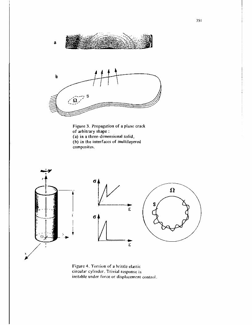
351

a 1

Figure 3. Propagation of a plane crackof arbitrary shape :(a) in a three-dimensional solid,(b) in the interfaces of multilayeredcomposites.

Figure 4. Torsion of a brittle elasticcircular cylinder. Trivial response isinstable under force or displacement control.

352

5- REFERENCES

I Germain P., Mecanique des Milieux Continus.Masson, Paris, 1973.

2 Gyarmati I. , Non equilibrium thermodynamics.Springer Verlag, 1970.

3 Maugin G. , The thermomechanics of Plasticity and Fracture,Cambridge University Press, 1992.

4 Biot M.A., Mechanics of incremental deformationsWiley, 1965.

5 Mandel J. Plasticite classique et Viscoplasticite.CISM course, 1971.

6 Moreau J.J., On unilateral constraints, friction and plasticity.CIME Course, Bressanone 1973.

7 Mandel J. Cours de Mecanique des Milieux Continus.Gauthier-Villars, 1961.

8 Rice J.R., Inelastic constitutive relations for solids : an internal variable theoryand its application in metal plasticity. J. Mech. Phys. Solids,19 (1971).

9 Halphen B. & Nguyen Q.S., Sur les materiaux standards generalises.J. de Mecanique, vol 1 (1975).

10 Lemaitre J. & Chaboche J.L., Mecanique des Materiaux solides.Dunod, Paris, 1985.

11 Lee E.H. Elastic-plastic deformation at finite strainJ. Applied Mech., 36 (1969).

12 Mroz Z. A description of work-hardening of metals with application tovariable loading. Foundations of plasticity, Varzawa, 1972.

13 Nguyen Q.S., Stability and bifurcation of standard dissipative systems.CISM Course, Udine, 1991.

14 Halphen B. , Sur le champ des vitesses en thermoplasticite finie.Int. J. Solids & Structures,] 1 (1975).

15 Hill R., A general theory of uniqueness and stability in elastic-plastic solids.J. Mech. Phys. Solids, (1958) 236.

16 Martin J.B. , Plasticity : fundamentals and general results.MIT Press, 1975.

17 Stolz C. , Anelasticity and Stability.Doctorat thesis, Paris 1987.

18 Klarbring A. Derivation and analysis of rate boundary value problemsof frictional contact. Eur. J. Mech. A, 9 (1990).

19 Chateau X. & Nguyen Q.S. Buckling of elastic structuresin unilateral contact with or without friction.Eur. J. Mech., A, 10 (1991).

20 Duvaut G. & Lions J.L., Les inequations en mecanique et en physique.Dunod, Paris, 1972.

21 Maier G. , A shake-down matrix theory allowing for workhardeningand second order geometric effect.Symposium "Foundations of Plasticity", Varsovie, 1972.

22 Hutchinson J.W., Plastic buckling.Advances in Applied Mechanics, (1973).

23 Sewell M.A. , A survey of plastic buckling.Stability, Waterloo Press, 1972.

24 Triantafyllidis N., On the bifurcation and post-bifurcation analysisof elastic plastic solids under general pre-bifurcation conditions.J. Mech. Phys. Solids, 31 (1983).

25 Nguyen Q.S. & Radenkovic D., Stability of an equilibrium

353

in elastic plastic solids. TUTAM Symposium, Marseille, 1975.26 Petryk H. , On energy criteria of plastic instability, Plastic buckling,

Proc. Considere Memorial, ENPC, Paris 1985.27 Nguyen Q.S., Bifurcation et stabilite des systemes irreversibles

obeissant au principe de dissipation maximale. J. de Mecanique, Paris (1984).28 Bazant Z.P. , Cedolin L., Stability of structures.

Elastic, inelastic, fracture and damage theories.Oxford University Press, 1991.

29 Koiter W.T., On the stability of elastic equilibrium.Ph.D. thesis, Delft, 1945.

30 Budiansky B., Elastic buckling.Advances in Applied Mechanics, vol. 14, 1974.

31 Potier-Ferry M., Towards a catastrophe theory for the mechanicsof plasticity and fracture. Int. J. Engng & Sc. (1985).

32 Bazant Z.P., Ohtsubo H., Stability conditions for propagationof a system of cracks in brittle solids.Adv. Civil Engng, (1977).

33 Nemat-Nasser, Sumi Y. & Keer L.M., Unstable growth of tensile cracksin Brittle Solids. Int. J. Solids & Structures, (1980).

34 Nguyen Q.S., Stolz C., Energy methods in fracture mechanics.IUTAM Symposium, Masson, Paris (1987).

35 Pradeilles R. Delaminage des composites.Doctorat thesis, 1992

36 Storakers B., Non linear aspects of delamination in structural members.Theoretical and Applied Mechanics, ICTAM, Grenoble 1988.

37 Destuynder P. & Nevers T., Un modete de calcul des forces de d~laminagedans les plaques minces multicouches, J.M.T.A.,6 (1987).

38 Cochelin B , Flambage et delaminage dans les plaques composites stratifiees.Doctorat thesis, Metz 1989.

39 Hutchinson J.W., Thouless M.D., & Liniger E.G. Growth andconfigurational stability of circular buckling driven film delamination.Acta Metall. Mater. 40 (1992).

40 Jensen H.M., Thouless M.D. Effect of residual stresses in the blister test.Report 439, The Technical University of Denmark, 1992.

41 Berest P. , Problemes de M~canique associes au stockage souterrain.Doctorat thesis, Paris, 1989.

42 Bui H.D. & Ehrlacher A., Propagation dynamique d'une zone endommagee.C.R. Acad. Sciences, t290, 1980.

43 Dems K. & Mroz Z., Stability conditions for brittle plastic structureswith propagating damage surfaces.J. Struc. Mech., Vol 13, (1985) 95.

44 Ehrlacher A., Contribution a i'etude thermodynamique de laprogression de fissure et a la mecanique de I'endommagement brutal. Doctorat thesis,Paris, 1985.

45 Marigo J.J., Modelisation et analyse qualitative de l'endommagementdes materiaux et des structures. Cours EDF-INRIA-CEA. Paris, 1990.

46 Fedelich B. & Berest P., Torsion d'un cylindre elasto-fragile,Arch. Mech. Stos., Vol 40, 5-6, (1988).

Theoretical and Applied Mechanics 1992S.R. Bodner, J. Singer, A. Solan & Z. Hashin (Editors)Elsevier Science Publishers B.V. 3550 1993 lUTAM. All rights reserved.

Bubble mechanics: luminescence, noise, and two-phase flow

Andrea Prosperetti

Department of Mechanical Engineering, 122 Latrobe Hall, The Johns Hopkins University,Baltimore MD 21218

AbstractA descriptive treatment of light emission from pulsating bubbles (sonoluminescence),

sound generation by rain falling on water and breaking waves, and the propagation ofshock waves in bubbly liquids is presented. The first section contains a brief survey ofsome occurrences of bubbles in literature and in the figurative arts. Considerations onthe etymology of the word are presented in the appendix.

1. INTRODUCTION

1Hopo6Avý o 6uOpomro' - Man is a bubble - is an ancient Greek proverb that enjoyed asingular favor in the western culture as an expression of the caducity and impermanenceof human life. It is used by a number of Latin and Greek authors such as Varro who,apologizing in the Preface to his De Re Rustica (36 b.c.) that the work is not as polishedas he would like, says that nevertheless, being 80 years old, he should go ahead with itspublication since, "ut dicitur, si est homo bulla, eo magis senex" ("if, as they say, manis a bubble, all the more so is an old man"). Petronius (1st century a.d.), in a mockingpassage of the Satyricon in which he compares man to inflated walking bags and flies, alsosays "nos non pluris sumus quam bullis" ("we are no more than bubbles," 42, 4). Lucian(117-180) elaborates: "I've thought of a simile to describe human life as a whole ... Youknow the bubbles that rise to the surface below a waterfall - those little pockets of airthat combine to produce foam? ... Well, that's what human beings are like. They'remore or less inflated pockets of air ... but sooner or later they're all bound to go pop"(Charon 19).

The advent of Christianity, with its message of hope and salvation, rendered the idealess relevant and probably the only pre-Renaissance textual reference to it is in the Lexiconby the 10th-I lth century Byzantine scholar Suida ("as a bubble immediately disappearswhen it is broken, so does the memory of the splendid and powerful upon their death").

However, in the northern post-reformation cultural climate of the 16th and 17th cen-tury, the metaphor regained its appeal. Most succint - and first - is Erasmus: "Hlomobulla" [man (is a) bubble, Adagia, 1508, 11. 1990]. Taverner, in his Proverbs or ada-gies ... gathered out of the Chiliades of Erasmus (1539) echoes the concept, and so doessir Thomas Elyot (1545), Golding ("When man seemeth to bee at his best, he is a]-

356

Figure 1: Engraving after a 1575 painting by Cornelis Ketel illustrating the Greek proverb"Man is a buLble." (Reproduced from Ref. 2)

togither nothing else but a bubble blowen togither of vanitie" Psalms xxxix 6, II 155,1571), Samuell Rowlands ("Poore mortals in my hands are brittle ware, Like Vapor, Bub-ble, Flower, wither'd Hay," A Terrible Battell betweene the two consumers of the wholeWorld: Time, and Death, p. 23, 1606) Sir William Browne ("What's he ... whose life's

a bubble, and in length a span; ... ? 'Tis a man," Britannia's Pastorals, Bk. i, song 2, 1.192, 1613), Simon Wastell (circa 1628), Jeremy Taylor (1651), and several others.

Sir Francis Bacon, in his The World (1629) expresses a more radical point of view:"The world's a bubble," which Francis Quarles quickly echoes "My soul, what's lighterthan a feather? ... This bubble world. What then this bubble? Nought" (Emblems, Bk.i, No. 4, published in 1635), and also "The pleasure, honour, wealth of sea and land /Bring but trouble; / The world itself, and all the world's command / Is but a bubble"(ibid., Bk. i, No. 6).

Of the 9 times the word "bubble" recurs in Shakespeare's theatre (it is never usedin his poetry), 3 times it similarly suggests volatility and insubstantiality such as "thebubble of reputation" (As You Like It II, vii, 139), or "A dream of what thou wast ... abreath, a bubble" (Richard III IV, iv, 83).

The same notion accompanies the word throughout the subsequent English languageliterature. William Cowper (The Task, published in 1785, Bk. 111, 1. 175) admonishes:"Eternity for bubbles proves, at last, / A senseless bargain." Samuel Johnson, in an ironicpassage thus commiserates the fashion-conscious: "Hard is his lot, that here by fortuneplac'd / must ... chase the new-blown bubbles of the day." Alexander Pope is mostimpartial: "Who sees with equal eye, as God of all, / a hero perish, or a sparrow fall,/ atoms or systems into ruin hurled, / and now a bubble burst, and now a world" (AnEssay on Man, 1734, Epis. i, 1. 87) and also: "Like bubbles on the sea of matter borne,/They rise, they break, and to the sea return" (ibid. Epis. iii, 1. 19). Coleridge thus usesthe metaphor to express a lover's disappointment "I listen for thy voice / Beloved! 't isnot thyne; thou are not here! Then melts the bubble into idle air,/ and wishing withouthope I restlessly despair" (Blossoming of thc Solitary Datc-Tree, st. 4). Ilis contemporarySir Walter Scott joins in the lover's desperation: "Like the dew on the mountain,/ Like

357

the foam on the river,/ Like the bubble oln the fountain, / Thou art gone, and for ever!"

(The Lady of the Lake, Canto iii, st. 16, 1810). The idea can be followed in Lord Byron:"The eternal surge of time and tide rolls on, and bears afar our bubbles" (Don Juan,1824, canto xv, st. 99), and all the way down practically to modern times.

It does not seem that English language poets ever found any word other than troubleto rhyme with bubble. An early example by Quarles was cited before. Shakespeare's isprobably the most well known one: "Double, double toil and trouble, / fire burn andcauldron bubble" (Macbeth IV, i, 10). One can also add Dryden: "War, he sung, is toiland trouble;/ honor but an empty bubble" (Alexander's Feast, or the Power of Music1. 97), the Australian poet Adam L. Gordon: "Life is mostly froth and bubble; / Twothings stand like stone: / Kindness in another's trouble, / Courage in your own" ( YeWeary Wayfarer, f"ytte viii), and even the peripheral Nathaniel Ward, who combines itwith a blatant expression of anti-feminism: "The world is full of care, and much like untoa bubble;/ Women and care and care and women, and women and care and trouble" ( TheSimple Cobbler of Aggawam, p. 25).

While the metaphor of bubble as volatility is present in other more or less unrelatedtraditions, such as in the 12th-13th century Japanese writer Kamo no Chomei ("The flowof the river is ceaseless and its water never the samne. The bubbles that float in the pools,now vanishing, now forming, are not of long duration: so in the world are man and hisdwellings" tfojoki -- An Account of my Hui, 1212), or the I 1th century Persian poet OmarKhayyam ("A deathless Saki draws Khayyams in thousands/ like wine bubbles out ofCreator's bowl," 77te JRubaiyyat st. 49, transl. Graves), it is curiously absent from othermajor literatures. The closest the Bible gets to the idea is in Provcrbs, 21: 6 with thewords hevel niddaf - literally "driven vapor." The New American Bible translates: "liewho makes a fortune by a lying tongue is chasing a bubble over deadly snares," but mostother English versions use different constructs. For example, the King J.ames Bible says:"The getting of treasures by a lying tongue is a vanity tossed to and fro of them that seekdeath." The Septuagint translation is far from literal, with the words 0OTrYvpiaLupaTop6-atar, "vain possessions."

Dante's Divina Commcdia abounds with literal bubbles. The violent rulers are pun-ished by boiling in blood: "lungo la proda del bollor vermiglio, / (love i bolliti facieno altestrida" [along the brink of the vermilion boiling, / wherein the, boiled were uttering loudlaments (trad. Longfellow), Inferito xii, 1. 101] andi the barrators (i.e., corrupt officials) byboiling in pitch: "bollia li. giuso una pegola spessa, / (ie 'nviscava la ripa (l'ogni parte./P' vedea lei, ma non vedea in essa / mai ite le bolle che 'I bollor levava, / e gonfiarsi tuttae risieder comnpressa." (was boiling down below there a dense pitch / which upon everyside the bank belirned. / I saw it, but I did riot see within it / aught but the bubbles thatthe boiling raised, / aid all swll up aul resubside compressed, Inferno xxi, 1. 17), butthe Ilorne bulla id ea is absent. Similarly, I have been unable to fillid any rcference to thisnotion in other Italian poets or in the Prench or Spanish literature.

Art interesting and direct offshoot of Erasmus's exhumation of the (Greek proverb canhowever be found inr the Netherlands. The Remonstrant minister lUytenbogaert admon-ished the Stadholder's court in the by now fa riliar terms: "Man is nothing other than abubble that children blow in a mussel shell, that glistens in the round ... but which inan instant (disappears and is gone." Renibrandt painted a portrait of l Jytentogaert (sold

358

in July 1992 at Sotheby's for 3.8x106 pounds), and one of Rembrandt's better pupils,Gerrit Dou, contributed to the tremendously successful iconography of a child blowing asoap bubble, "an image that reflected both levity and gravity, that floated like childishreveries and popped as childhood itself had to end" [1]. Many other Dutch painters, suchas Cornelis Ketel (perhaps the earliest one, on the back of a 1575 portrait, see Fig. 1 [2]),Hendrik Goltzius, Jacques de Gheyn, Jan Miense Molenaer, and Frans Hals have left usa number of images of children blowing bubbles. It is interesting that, while the ancientauthors had in mind the bubbles briefly floating on water surfaces, from Ketel onwardthe reference is always to soap bubbles. This fact is probably also due to the dramaticimprovements in the soap technology intervened since antiquity.

In the mid 1730's, the French painter Jean-Baptiste Simeon Chardin used his five-yearold son as a model for several pictures of a child blowing bubbles and later again anolder boy. By this time, however, the original Calvinist moral embodied in the Vanitasgenre had faded into the background leaving its place to the painter's delight with hissubject and his own ability as we find in several others artists all the way down to thepre-Raffaellite Sir John Everett Millais, whose painting "Bubbles" was used in some ofthe Lever Brothers' commercial advertising for Pear's Soap [1].

Other than its career as a lofty metaphor, the word bubble has also enjoyed another -and disreputable - one. With reference to the bulla, a spherical gold ornament worn bythe noble Roman children after an Etruscan custom, Juvenal uses the word to fashion aninsult: "senior, bulla dignissime" ("Old man, worthy of a bubble," Satirae 13, 1. 33), andin old Italian bolla acquaiola ("water bubble") was a disparaging designation. In Latin,animam ebullire ("to gurgle one's life out," similar to the bubbles that gurgle in the neckof a flask when the liquid is poured out) was a vulgar expres.'on for "to die" used, amongothers, by Seneca and Persius.

In Shakespeare's All's Well That Ends Well the Second Lord Durnaine qualifies Parolesas "On my life, my lord, a bubble" (III, vi, 6) and goes on to explain: "He's a most notablecoward, an infinite and endless liar, an hourly promise-breaker, the owner of no one goodquality worthy of your lordship's entertainment" (ibid., 10-12). Later, in 17th and 18thcentury English, a bubble denoted a "dupe" or gullible person. In the underworld's slang,"to betray" was indicated as to bubble, with bubble also standing for a piece of information.Bubble duster was used for "handkerchief" (presumably after the Scottish usage of bubblefor "mucus," whence also bubbly for "snotty, dirty"), and we have the plethora of Americanslang expressions bubble brain, bubble head, bubble gummer (for "teen-ager"), bubble dancer(for "dish washer," in addition to the original reference to a night-club performer), andothers. As a symbol for financial bust. one does not have to wait until the recent crash ofthe TIokyo stock exchange to encounter the word. The South Seas Bubble was a schemedevised in England in 1711 to eliminate the national debt - at the expense of the usual"bubbles" - and the French were quick to catch on with their similar 1717 MississippiBubble.

In French faire des bulles signifies something like "to make a fuss" and coincer la bulttor buller is a popular expression for "doing nothing." In Dutch, blaasjcs verkopon andthe corresponding Engli.d, to blow bubbl(;s similarly stand for "to devise baseless theories,to amuse oneself in a childish manner," and bolla di vento ("wind bubble") recurs in18th-century Italian ini a siniflar swnse.

359

It will be my task in the rest of this paper to try to convince the reader that, in spiteof all of the above, bubbles are "investigatione dignissimae" - most worthy of seriousscientific study.

It should be stressed at the outset that the type of bubbles that will form the object ofthis paper differ in a major way from those featured in the previous quotations. Althoughthe bursting of floating bubbles and the related problem of the stability of foams is amajor scientific and technical problem, here I shall confine myself to gas bubbles moredeeply submerged in a liquid.

The breadth of the subject prevents me from any attempt at exhaustiveness. I willlimit myself to a few recent developments that, hopefully, will give an idea of the vastrange and far-reaching implications of bubble phenomena.

2. SONOLUMINESCENCE

From the mathematical point of view, the richness exhibited by bubble phenomenamay be considered as a direct consequence of the 1/r singularity of the fundamentalsolution of Laplace's equation in three-dimensional space. Since bubble dimensions areoften "small" (with respect to other, problem-dependent lengths), this singular behaviorhas the opportunity to manifest itself very strongly. With bubbles, one's life is enrichedby the proximity to this singularity.

A very striking phenomenon due precisely to this fact is sonoluminescence, the lightemitted by a sound-irradiated liquid. In an acoustic wave the energy density is of theorder of E = p'2 /pc2 , where p' is the pressure amplitude, p the fluid density, and c thespeed of sound. Since tC- mole density per unit volume is p/M, where M is the molecularmass, the corresponding energy per molecule is (M/p)E/NA, where NA is Avogadro'snumber. For a fairly intense pressure wave in water water, with p' , 1 bar, this amountsto approximately 10' eV per molecule, which is of the order of 10'- times smaller thanthe energy of low-cV radiation. The appearance of such radiation therefore implies thata mechanism exists to amplify the energy density by a factor of 109.

First discovered in the late 20's, the effect prompted a number of more or less fancifulspeculations as to its origin which subsequent research has put to rest - to some extent[3]. The current understanding is that sonoluminexcence is due to the dissociation andrecombination of gaseous molecules contained in bubbles that pulsate in a strongly non-linear fashion under the action of the sound field. It is the 1/r singularity of the potentialfor the associated radial motion of the liquid that is responsible for the effect.

A theory of radial bubble pulsations and sonoluminescence is given elsewhere [4]. Forpurposes of illustration I reproduce here in Fig. 2 a graph of the internal pressure (solidline) and center temperature (dashed line) for an argon bubble in water subject to a 0.93bar sound field. The bubble radius is 26 prm and the sound frequency 21 kllz. Since theradius of a resonant bubble at this frequency would be 150 um, the bubble is driven atabout one fifth of its resonance frequency. A parallel chemical kinetics calculation [4],the results of which are shown in Fig. 3, indicates that a substantial number of hydroxylradicals are produced in these conditions by collisional dissociation of the vapor molecules.This prediction is in agreeme'nlt with the experimental fact that liquids saturated with

360

.1058 ;13 t 6

SI . I~ u 0

I . -- It•" .J

Figure 2: Pressure (dashed line) and center temperature (solid line) during steady oscil-lations of a 26 tum-radius argo, bubble driven at 21 kHz and 0.93 bar acoustic pressureamplitude

Figure 3: Number of hydroxyl radicals as a function of time during the steady oscillationsof the argon bubble of the previous figure (s(-* I line), and an equal one containing neon(dashed line).

noble gases emit a strong 310 nm-line corresponding to a transition of the excited OHradical to its ground state [5]. Heat transport inside the bubble has a strong effect on thisprocess. Neon ! as a thermal conductivity 3-4 times that of argon, and the correspondingOH number, shown in Fig. 3 by the dashed line, is much smaller than for the argoncase. It should be realized that, during the period of peak temperature, the temperaturegradient inside the bubble is of the order of 10' K/mm. Clearly, this is only possible dueto the very short duration of the peak temperature, for this example of the order of 300nsec.

However short, this time interval is many orders of magnitude longer than the durationof the sonoluminescence light flashes, which is currently estimated below 50 psec [6]. Thisextremely brief duration is perhaps the most baffling aspect of sonoluminescence. Apossible explanation could be the following. It is well known since Wood's experimentsin 1904 that gases are very opaque to radiation corresponding to their emission bands. Itis for this reason, for example, that we can only observe the outermost layer of the sunas the light emitted by the inner regions is absorbed by the surrounding layers. As thebubble compresses, the temperature is highest at the center and, when a certain thresholdis exceeded, H120 molecules begin to dissociate there. A fraction of their is excited andradiates upon decaying to the ground level. Very soon afterward, the temperature inthe next layer of gas exceeds the Oil-production threshold, and these radicals are nowavailable to absorb the radiation still coming from the center of the bubble. For thecase considered previously our computations indicate that it takes about 100 psec for thetemperature "wave" to travel to a distance of 0.01 radii from the origin center.

To explain why no light is emitted from the outer layer, one may note that, by symn-metry, the temperature gradient must vanish at the bubble center (another consequenceof the presence of a singularity !). Hlence, the temperature in the central region of thebubble is riuch more homogeneotus than in the surrounding layers. In particular, in the

1. '. D t-2.40 t-,2.60 t3.0 i

..Q K Y...... .. .. 0.... Q ..._ _ _

_ _ _ _ _ _- . .. ......... ....... ........ . ....... . ........... . j0=7. 00 _,7.4 -760 _-7.80

Figure 4: Successive shapes of a 20 ILm gas bubble driven at 20 kIlz by a 1 bar-amplitudesound field switched on at t = 0. The time unit is 10.5 usec. Initially the bubble is located1/4 wavelength above the antinode of the sound field.

outermost layer where the temperature barely exceeds the threshold, virtually all theOH's are produced in the ground state and therefore can absorb, but not emit, radiation.Clearly, radiationless transitions to the ground state must also occur, and these are ren-dered probable by the high number density of the molecules (of the order of 10' 8 /cm 3 for

the example of Figs. 2 and 3).With numbers of this order of magnitude involved, one might wonder whether one

could get "cold fusion" to occur in a liquid subjected to a sufficiently intense sound fieldand, indeed, the idea for such a reactor has been patented [7]. Unfortunately, there is asnag: the spherical shape of an oscillating bubble has a strong tendency to instability,so that any attempt to drive the bubble too strongly will lead to its shattering ratherthan to increased temperatures and pressures. This instability is similar to the well-known Rayleigh-Taylor one as, when the pressure in the bubble rises, the liquid is beingaccelerated upon by a lighter fluid, the gas.

We present the results of a calculation that illustrates this instability in Fig. 4. Thebubble here has a radius of 20 pm and is forced by a 1-bar, 20-kllz plane standing acousticwave. In spite of the fact that the wavelength is nearly 4,000 times larger than the bub-ble radius, the non-zero pressure gradient at the bubble location (1/4 wavelength abovethe antinode) induces a perturbation that, as can be seen, is strongly amplified duringthe compression phase of the oscillations. This calculation ignores various dissipativeprocesses and therefore it probably overestimates somewhat the magnitude of the effect.

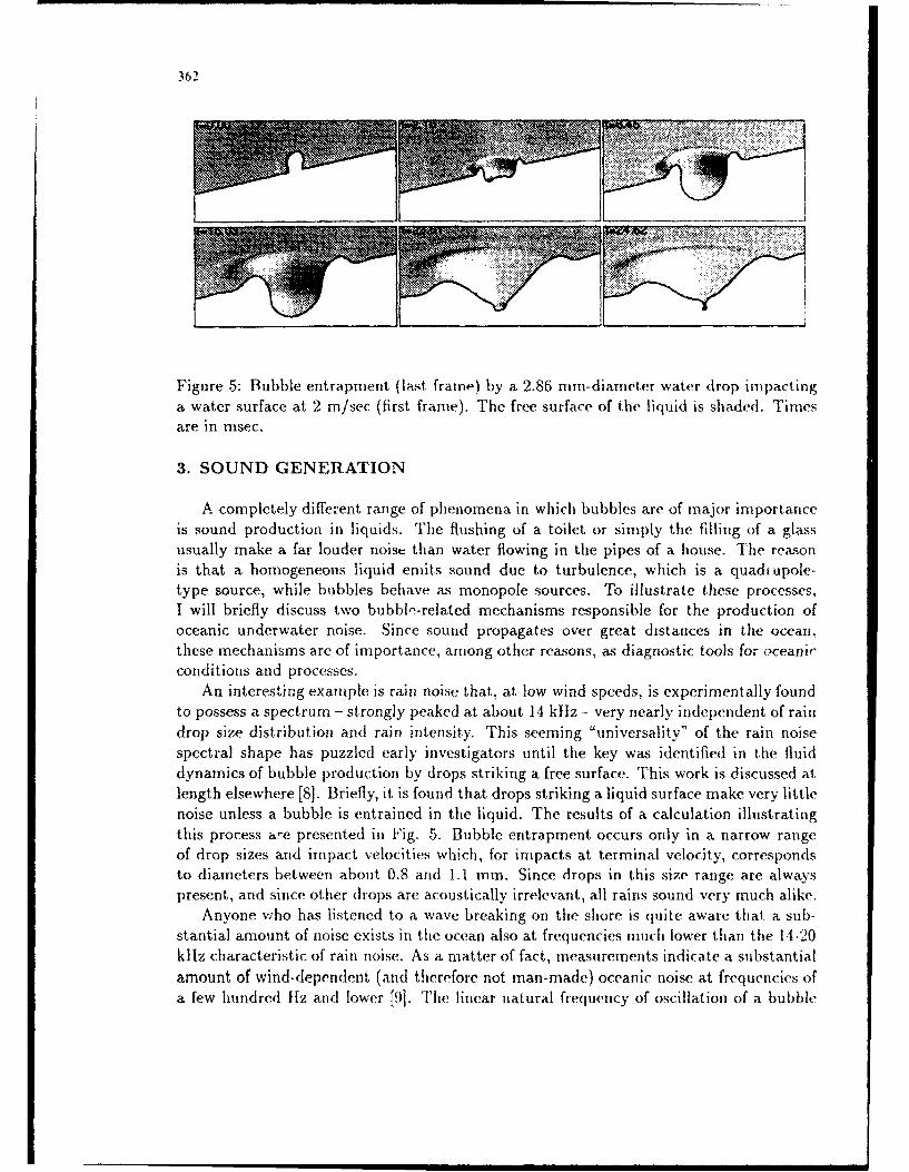
362

Figure 5: Bubble entrapment (last. frame) by a 2.86 mam-diameter water drop impactinga water surface at 2 m/sec (first frame). The free surface of the liquid is shaded. Timesare in msec.

3. SOUND GENERATION

A completely different range of phenomena in which bubbles are of major importanceis sound production in liquids. The flushing of a toilet or simply the filling of a gla-ssusually make a far louder noise than water flowing in the pipes of a house. The reasonis that a homogeneous liquid emits sound due to turbulence, which is a quadidpole-type source, while bubbles behave as monopole sources. To illustrate these processes,I will briefly discuss two bubblV-related mechanisms responsible for the production ofoceanic underwater noise. Since sound propagates over great distances in the ocean,these mechanisms are of importance, among other reasons, as diagnostic tools for oceaniaconditions and processes.

An interesting example is rain noise that, at low wind speeds, is experimentally foundto possess a spectrum - strongly peaked at about 14 kllz - very nearly independent of raindrop size distribution and rain intensity. This seeming "universality" of the rain noisespectral shape has puzzled early investigators until the key was identified in the fluiddynamics of bubble production by drops striking a free surface. This work is discussed atlength elsewhere [8]. Briefly, it is found that drops striking a liquid surface make very littlenoise unless a bubble is entrained in the liquid. The results of a calculation illustratingthis process are presented in Fig. 5. Bubble entrapment occurs only in a narrow rangeof drop sizes and impact velocities which, for impacts at terminal velocity, correspondsto diameters between about 0.8 and 1.1 mim. Since drops in this size range are alwayspresent, and since other drops are acoustically irrelevant, all rains sound very much alike.

Anyone who has listened to a wave breaking on the shore is quite aware that a sub-stantial amount of noise exists in the ocean also at frequencies much lower than the 14-20kllz characteristic of rain noise. As a matter of fact, measurements indicate a substantialamount of wind-dependent (and therefore not man-made) oceanic noise at frequencies ofa few hundred lIz and lower [9]. The linear natural frequency of oscillation of a bubble

having an equilibrium radius a is, approximately [101,

I= ý3xpo(1

where po is the equilibrium internal pressure in the bubble and I < K < "r, with "t the ratioof the specific heats, is a polytropic index dependent in a complex way on the frequency.According to this formula, for a bubble to pulsate at 100 llz, the diameter should be6-7 cm. It is very unlikely that such large bubbles are produced in substantial numbersby waves that, in the open ocean, break in a spilling rather than the plunging modecharacteristic of near-shore breaking. Instead, there are substantial reasons to believethat this low-frequency noise is originated by the collcclivw oscillations of the bubblhclouds produced by breaking waves [11,12]. A simple argument can be p)resented in thefollowing terms. At low frequencies, the speed of sound c, in a liquid containing gasbubbles is given approximately by

2 •:P0- Kpo (2)

where 3i = V/G/V is the fraction of the mixture volume V occupied by the gas. Thesimplest way to derive this expression is to note tL10t, if the liquid cornmpressibility isneglected, a change in the mixture density p., can only be due to a change in the volumeVG occupied by the gas sc that PSm/,P,= -6•VG/V. On the other hand, if the bubblescompress polytropically, • 1 G/IV = -Kbp/po and (2) readily follows upon identifying c',2with ,p/ 6 p,. I

The striking fact is that already at very small volume fractions C,, is much lower thanc. For instance, for /3 = 1%, and atmospheric pressure, one finds cm • 100 m/sec to becompared with c = 1500 ni/scc in pure water. Thus, in view of the great disparity betweenc and c,m a bubble cloud can, to a first approximation, be regarded as a compressiblemedium in a rigid enclosure. The lowest normal mode of oscillation of the cloud hastherefore a frequency wmzn of the order of c,/L, where L is the linear scale of the cloud,so that, from (1) and (2), one finds

•amin 1 (3)WO, f/6N/3 '

where N is the number of bubbles in the cloud. This result shows that 1,000 1-rambubbles - which individually have a natural frequency of about 3 kliz- would give rise toa cloud oscillating at, about 300 Ilz. Since the liquid surrounding the cloud is not actuallyincompressible, the cloud eigenmodes' energy leaks out and is radiated to great distances.

An indirect quantitative confirmation of this process has been obtained by using an"artificial" cloud in the laboratory [l13]. If air is bled out of a disk-shaped bank of needlesat the bottom of a tank, a hydrophone picks up a signal similar to that shown in Fig. 6.The peaks correspond to eigenfrequencies of the system and can be calculated as a checkof the theory. Some results of this comparison are shown in Fig. 7.

'The result (2) fails to converge to the correct limit as,3 -- 0 since the liquid compressibilityhas been neglected. It canlbe shown that this is justified at. gas volume fractions above about10-%.

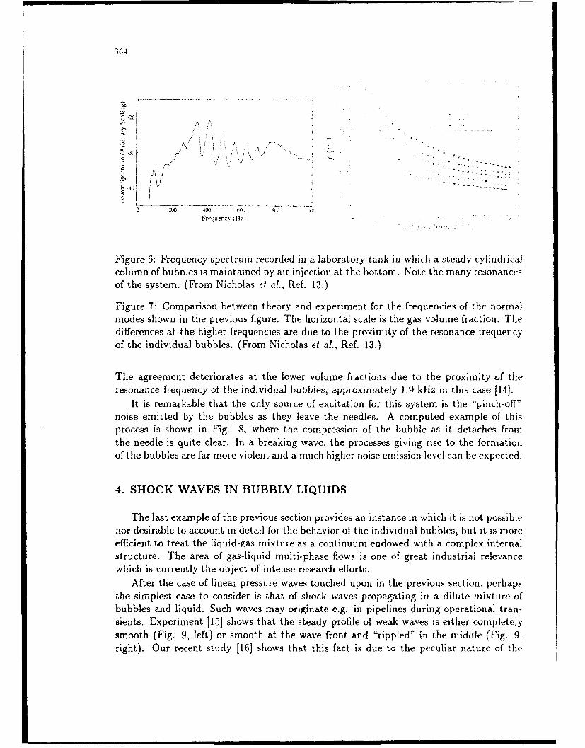
364

-30 V V

I -<:

0 40) q1 (I

Frequenct I-Hz)

Figure 6: Frequency spectrum recorded in a laboratory tank in which a steady cylindricalcolumn of bubbles is maintained by air injection at the bottom. Note the many resonancesof the system. (From Nicholas et at., Ref. 13.)

Figure 7: Comparison between theory and experiment for the frequencies of the normalmodes shown in the previous figure. The horizontal scale is the gas volume fraction. Thedifferences at the higher frequencies are due to the proximity of the resonance frequencyof the individual bubbles. (From Nicholas et al., Ref. 13.)

The agreement deteriorates at the lower volume fractions due to the proximity of theresonance frequency of the individual bubbles, approximately 1.9 kIiz in this case [14].

It is remarkable that the only source of excitation for this system is the "pinch-off"noise emitted by the bubbles as they leave the needles. A computed example of thisprocess is shown in Fig. 8, where the compression of the bubble as it detaches fromthe needle is quite clear. In a breaking wave, the processes giving rise to the formationof the bubbles are far more violent and a much higher noise emission level can be expected.

4. SHOCK WAVES IN BUBBLY LIQUIDS

The last example of the previous section provides an instance in which it is not possiblenor desirable to account in detail for the behavior of the individual bubbles, but it is moreefficient to treat the liquid-gas mixture as a continuum endowed with a complex internalstructure. The area of gas-liquid multi-phase flows is one of great industrial relevancewhich is currently the object of intense research efforts.

After the case of linear pressure waves touched upon in the previous section, perhapsthe simplest case to consider is that of shock waves propagating in a dilute mixture ofbubbles and liquid. Such waves may originate e.g. in pipelines during operational tran-sients. Experiment [15] shows that the steady profile of weak waves is either completelysmooth (Fig. 9, left) or smooth at the wave front and "rippled" in the middle (Fig. 9,right). Our recent study [16] shows that this fact is due to the peculiar nature of the

365

Figure 8: Successive shapes of a bubble blown out of a I mm-diameter needle.

1 14-

10 2

d i 08 1.3 V

1.2 2_:

.0 I- 4.-

1 02 ",. .

. f. II OOL .- '--~~- 1.0 1 OL

0 I0 20 30 40 5ý) 60 70 3 4 6

firne f~

Figure 9: Examples of pressure profiles in steady shock waves in a bubbly liquid. Atleft is a completely smooth waveform, at right an oscillating one. The dashed line is theeffective polytropic index along the wave. (From Ref. 16).

366

dispersion relation for pressure waves in a bubbly liquid. (,lonsider first linear waves atvery low frequency. As the bubbles are compressed, the gas temperature has time toequilibrate with that of the surrounding liquid, the process is isothermal and, in Eq. (2).

S= 1. As the frequency increases, complete temperature equilibration is not possible and* becomes greater than I so that the speed of sound increases. At still higher frequenciesthe natural frequency of the bubbles is approached, it is easier and easier to compressthem, and physical processes not accounted for in Eq. (2) greatly decrease the speed ofsound. The phase velocity of the waves possesses therefore a mild maximum nbelow theresonance frequency of the bubbles. This feature is clear in Fig. 10 where the solid linesshow the dispersion relations corresponding to the region near the front and the back ofthe waves of Figs. 9. The d(lshed lines are the group velocity. The speed U of the shockitself, shown by the horizontal dash-and-dot lines, is given by

U2 i± - (4)U P2 P P.l

where the subscripts a and b refer to conditions ahead and behind the wave respectively.The two panels of Fig. 10 exhibit a major quUlitative differenre. In the case of the s,,,' t,shock, there is a substantial range of frequencies where monochromatic waves near thefront and the back propagate faster than the shock itself: any perturbation falling in thesefrequency ranges will therefore propagate away from the shock. The shock is only fasterthan very low-frequency, long-wavelength perturbations -- which exceed the scale of the-hock and therefore are not generated -- or than high-frequency, highly damped ones. Inthis situation the integrity of the shock can only be maintained by nonlinear effects andthe profile is smooth. In the case of the oscillating shock, however, the shock speed isfaster than that of any, wave near its front, which is therefore steep and smooth. In theintermediate shock region, however, waves having a speed comparable with that of theshock are possible, and it is these waves that remain "trapped" in the shock and conferto it the oscillatory nature seen in the Fig. 10.

5. CONCLUSIONS

Reasons of space have only allowed me to give the briefest indication of some cur-rent problems in the mechanics of bubbles and bubbly liquids. It has not been possibleto even mention many important topics such as cavitation - both flow and acoustic -bubble nucleation, break-up, and coalescence, air entrainment in flowing liquids, biomed-ical applications, micro-gravity manufacturing, boiling heat transfer, and many others.Gas-liquid multiphase flows are of great relevance e.g. in the power generation and oilindustries and very poorly understood. One can expect theoretical as well as experimentalchallanges in these areas for many years to come.

In conclusion I would like to return for a moment to the single pulsating bubble withan idea that is perhaps far-fetched but nevertheless intriguing, It is possible that here weshall find a "power plant" for the niicro-robots of the future. It is not inconceivable thatsuch machines could be used e.g. inside the human body where power from any sourceother than acoustic would be impractical.

• Ca- -

Figure 10: Dispersion relations for the two shock waves of Fig. 9.The horizontal line is thewave velocity, the solid lines the phase velocity and the dashed line, the group velocity.The upper pair of curves is for conditions at the back of the wave, and the lower pair forconditions near the front of the wave. (From Ref. 16.)

ACKNOWLEDGMENTS

The author wishes to express his gratitude to several persons who have contributedto the present paper: H.N. Oguz, M. Nicholas, R.A. Roy, L.A. Crum, L.H. Prosperetti,X. Cheng, and M. Watanabe.

The work described here has been supported by the National Science Foundation(grant no. CBT-8918144), the Department of Energy (grant no. DE-FG02-89ER14043),and the Ocean Acoustics Program of the Office of Naval Research.

APPENDIX - AN ETYMOLOGICAL NOTE

According to Ref. [17], the Greek word for bubble, iroy¢6Avý, is related through anintermediate variant 7ro/y06 to 2rgipLot which has the basic meaning of "something thatis created by inflating or blowing." Interestingly one of the etymologies offered for theLatin bulla is from the root 00A- (whence e.g. phallus), indicating "any object swellingup" t181. However, there does not seem to be any consensus on this point as other authorsindicate a derivation from the sanskrit belih, which denotes the external female genitals[19]. Here the connection might be through the idea of "rotundity." Another Greek wordsometimes juxtaposed might be floA/36, "bulb" [17].

Be that as it may, it seems very likely that onomatopoeic elements have also shapedthe word, as we find the basic sound in unrelated languages such as Sumerian (bubul),Accadian (bubutu), Hlindi (bud-bud, bull-bula), Bengali (bud-bud), Cebuano-Visayan (buld),ard others.

As for the English bubble and its ancestors boble, bobel, bubbul, the onomatopeic ele-ment is probably dominant as also indicated by the closeness with burble [20]. Parallel

368

substantives it other Teuitoini( laiganuages a(re e'g. the Sw(edish b tbla, the Daliish bob/bt,

and the dialectal (Geriman words bobbel, bubbtl. The current German word for "bubble" is

blase, similar to the D)utch blaas, "bladder,"All the modern Roomance languages have a word deriving from the Latin bulla, al-

though sometimes the meaning of "bubble" has beeni lost, An example is Spanish wherethe word bula now primarily denotes the seal apposed to Papal documents, but was inthe past used for burbuja, that is the modern word for "bubble."

REFERENCES

1. S. Schama, The tm'Mbarvassmcnt of Richlis, Kotopf, New York, 1987, pp. 512-516.

2. XV. Stechov, 7'Ihc Art lullt/in 20, 227-228 (1938).

3. R.E. Verral and ('.M. Seligal, in K.S. Suslick (ed.), Ultrasound: its C(hemical, Phys-ical, and Biological L'ffccts, VClI Publishers, New York, 1988, pp. 227-286.

4. V. larnath, A. Prosperetti, and F. Egolfopoulos, J. Acoust. Soc. Am., in press.

5. C. Sehgal, R.G. Sutherland, and R.E. Verrall, J. Phys. Ciem. 84, 388-395 (1980).

6. B.P. Barber and S.J. Putterman, Nature 352, 318-319 (1991); B.P. Barber, R. Hiller,K. Arisaka, 11. V-tterman, arid S.J. Putterman, J. Acoust. Soc. Am. 91, 3061-3063(1992).

7. H.G. Flynn, Method of generating energy by acoustically induced cavitation fusionand reactor, U.S. Patent No. 4,333,796 (1982).

8. A. Prosperetti, L.A. Crum, and II.C. Pumphrey, J. Geophys. Res. 94, 3255-3259

(1989); uI.N. Oguz and A. Prosperetti, J. Fluid Mech. 219, 143-179 (1990); I.N.Oguz and A. Prosperetti, J. Fluid Mech. 228, 417-442 (1991); ul.N. Oguz and A.I'rosperetti, Ann. Rev. Fluid Mech., in press.

9. see e.g. 13.11. Kerman, J. Acoust. Soc. Am. 75, 149-165 (1984); P.C. Wille and D.Geyer, J. Acoust. Soc. Am. 75, 173-185 (1984); D.J. Kewley, D.G. Browning, andW.M. Carey, J. Acou.st. Soc. Am. 88, 1894-1902 (1990).

10. M.S. Plesset and A. Prosperetti, Ann. Rev. Fluid Mech. 9, 145-185 ',1977).

11. W.M. Carey, J. Acoust. Soc. Am. 78, S1-S2 (1985); W.M. Carey and D. Brow:ling,in B.R. Kerman (ed.), Sea Surface Sound, Kluwer, Boston, 1988, pp. 361-376; W.M.

Carey, J.W. Fitzgerald, and D.G. Browning, in B.R. Kerman (ed.), Natural Sourcesof Underwater Sound, Klhwer, Boston, in press.

12. A. Prosperetti, J. Acoust. Soc. Am. 78, S2 (1985); J. Acoust. Soc. Am. 84,1042-1054 (1988); A. Prosperetti, N.Q. LIt, and HI.S. Kim, J. Acoust. Soc. Am., inpress.

369

13. N.Q. Lu, A. Prosperetti, and S.W. Yooio, IEEE .1. Ocean Eng. 15, 275-281 (1990);S.W. Yoon, L.A. Crum, A. Prosperetti, and N.Q. Lu, J. Acoust. Soc. Am. 89,700-706 (1991); M. Nicholas, L.A. Crurn, R.A. Roy, It.N. Oguz, and A. Prosperetti,J. Acoust. Soc. Am., submitted.

14. K.W. Commander and A. Prosperetti, J. Acoust. Soc. Am. 85, 732-746 (1989).

15. L. Noordzij and L. van Wijngaarden, J. Fluid Mech. 66, 115-143 (1974).

16. M. Watanabe and A. Prosperetti, J. Fluid Mech., submitted.

17. P. Chantraine, Dictionnaire Etymologique de la Langue Grecque, Klincksieck, Paris,1968.

18. C.T. Lewis and C. Short, A Latin Dictionary, Clarendon, Oxford, 1975 (first edition1879).

19. A. Ernout and A. Meillet, Dictionnaire Etyrnologique de la Langue Latine, Klinck-sieck, Paris, 1959.

20. J.A. Simpson and E.S.C. Weiner eds., Oxford English Dictionary, Clarendon, Ox-ford, 1989.

Theoretical and Applied Mechanics 1992S.R. Bodner, J. Singer, A. Solan & Z. Hashin (Editors)Elsevier Science Publishers B.V. 3711993 IUTAM.

Wave propagation in non-isotropic structures

Mahir Behar Sayir

Institute of Mechanics, ETH, Zurich, Switzerland

AbstractIn structural wave propagation the characteristic wavelengths of the propagating pulse

are chosen to be sufficiently large with respect to the thickness of the structure. Narrow-band transient structural waves are particularly well-suited for example to study andquantitatively evaluate global ("homogenized") dynamical properties of sandwich or fiber-reinforced composite structures such as laminates, tubes etc. The waves are generated invarious membrane or flexural modes by piezo-electric transducers excited at narrow fre-quency bands well below their resonant frequencies to avoid coupling and thus allow per-fect control of the pulse shape. The theoretical models used to interpret and evaluate theexperimental results obtained in sandwich and composite structures must be carefully de-veloped in order to predict accurately the features following from the interaction of thevarious geometric, dynamic and material scales. A few experimental results obtained inrecent years in our laboratory are discussed in conjunction with the corresponding theoret-ical models. Part of these results are also used to interpret dynamical phenomena ob-served during the propagation of fast-running cracks in cross-ply laminates.

1. TERMINOLOGY AND MOTIVATION

Consider a transient wave in the amplitude range of linear elasticity in a thin structuresuch as a beam, plate or shell . The time function is supposed to be of narrow-band typeand can be generated by applying a suitable window (for example a translated cosine-window of relatively large duration) on a sine- or cosine-function of a given frequency. Inthe amplitude-frequency spectrum of this function the non-vanishing amplitudes will lie forall practical purposes between two frequency limits. The higher limit fnax will correspondin the structure to a wavelength X. which we call the characteristic wavelength of thetravelling pu!se. In a structural wave the ratio of the largest thickness H of the structure tothe characteristic wavelength of the propagating pulse (called "dynamic parameter") issupposed to be sufficiently small, i.e.

H/L <<I

372

The stress- and strain-distributions generated by such a wave across the thickness of thestructure are stationary and usually quite simple mathematical functions of the thicknesscoordinate. The wave travels then in membrane, torsional orflexural modes, with possiblecoupliz7 between them. Furthermore, in fiber-reinforced composite structures, due to themuch !,,wer scale of the fiber diameter or of the ply thickness, most of the important fea-tur.,, of structural wave propagation can be interpreted by assuming homogeneous mate-Alal behaviour,

Per definition in anisotropic materials with orthotropic symmetry three mutually per-pendicular principal axes of material symmetry can be associated with each material point.With respect to structural waves structures may behave orthotropically either becausethe material itself is orthotropic or because a combination of geometric features and mate-rial distribution through the corss-section of the structure generate "globally" non-isotro-pic structural behaviour in spite of the fact that the material itself is isotropic. An interest-ing case of such "structural non-isotropy" has been studied in f 11, where a flexural wavein an aluminum beam with nearly perfect circular cross-section (measured deviations froma circular boundary less then 0.05 %) "rotated" most probably because of an extremelyslight inhomogeneity in the distribution of the axial modulus of elasticity E through thecross-section (largest difference in the weighted average of the modulus in two perpendi-cular directions of the order of 1 %). The material itself was shown to behave istoropicallywithin the accuracy of the measurements.

In isotropic materials the ratio of the shear modulus G to the tensile modulus F

EM :=G/E

which will be called "material parameter" in the following has to be larger than 0.33.forreasons of material stability. Of course in anisotropic structures such as fiber-reinforcedlaminates or filament-wound tubes this material parameter may reach much lower values(for example 0.01). Also in sandwich structures with a soft isotropic core and stiffisotropic facings this parameter (determined from equivalent stiffness values) is usuallyquite low. In our laboratory sandwich beams and plates with cM as low as 0.0004 havebeen tested [2]. Thus from the point of view of effects associated with low values of thematerial parameter EM (for example transverse shear coupling) sandwich structures maybehave non-isotropically even though the material of the components is isotropic.

'Our experimental research activity on wave propagation in non-isotropic structureswhich started about 15 years ago was first motivated by the need to reach a better under-standing of coupling phenomena which are characteristic of non-isotropic behaviour. Thusto study mode-coupling in non-principal directions we investigated flexural waves in unidi-rectionally reinforced plates [31 or in-plane waves in cross-ply laminates 14, 171. To studycoupling phenomena related to low values of EM we generated flexural waves in unidirec-tionally reinforced beams [5], in sandwich-plates with extremely soft cores [21 or axisym-metric waves in filament-wound tubes 16, 4]. These experimental investigations wereinterpreted by developing for each case approfriate theoretical models based on a carefulasymptotic analysis of the basic relations of three-dimensional linear elasticity. Approxi-mations based on a priori assumptions were avoided since in all cases the presence of atleast two competing small parameters, namely EX, EM and of some other small geometricratios (as in sandwich plates or filament-wound tubes) rendered the choice of physicallyjustified simplifying assumptions without a straightforward ordering scheme rather diffi-cult. With a more thorough knowledge of the above-mentioned coupling phenomena wewere also able to determine structural properties such as flexural stiffnesses and various

moduli of elasticity with quite high degrees of accuracy 171. Our experimental and theoreti-cal methods of analysis can also be used to detect flaws or structural errors which affectlocal stiffness values to some extent, even though the characteristic wavelengihs of thegenerated pulses may be much larger than the size of the flaws. Especially flexural waveswhich by nature are particularly sensitive to changes in thickness are well suited to detectflaws such as delaminations or to check for possible errors in ply combinations, filament-wounding etc. Details related to current research on applications to non destructivedetection will be reported elsewhere. In the following I will present a review of the mainfeatures related to the experimental and theoretical work briefly mentioned above,together with some unpublished recent results.

2. SHEAR COUPLING IN FLEXURAL WAVES

2.1 Unidirectionally reinforced beamsIn 181 a theory for flexural waves with large wavelengths in unidirectionally reinforced

beams was elaborated. According to this theory which was derived by asymptoticanalysis of the three-dimensional equations of linear elasticity, the order of magnitude ofthe parameter

II := 1 `A(2.1)

determines decisively the propagation characteristics of transverse structural waves inbeams. The following table summarizes the role of the parameter p:

Order of magnitude Degree of anisotropy Nature of the shear coupling

p << I Isotropy, Weak: Be-comes active at theWeak or moderate anisotropy second step of approximation

p = (i) "Quasi-strong" anisotropy Strong: Becomes active at the(transitional case) first step of approximation

p >> I Strong anisotropy Sandwich-behaviour

In the transitional case of "quasi-strong" anisotropy with p = 0 (M) the usual assunmp-tion that cross-sections remain plane after deformation does not hold since the transverseshear strains become so large that they reach the magnitude of the axial strains due tobending. Because of this strong shear coupling, the variations of the axial displacementsalong the axis of the beam are connected with their variations through the cross section.The axial strains and stresses are then in general nonlinearly distributed through thecross-section. For sinusoidal waves of a given amplitude of transverse displacement theamplitudes of distributions of axial strain and stress are illustrated in Fig. I for a rcCtan-

374

gular cross-section. In [81 distributions for a circular cross-section were also given. As ptakes larger values, the nonlinearity of the strain and stress distribution becomes alsomore pronounced. As one reaches values of p much larger than 1, axial strains andstresses concentrate on the parts of the cross-section which are near the lateral surfacesof the beam. A core of finite thickness frees itself almost completely of axial stresses andcarries only a constantly distributed shear stress (fig. 2). Thus thu unidirectionally rein-forced beam behaves like a "natural" ideal sandwich structure.

In [8] the dispersion relation

C := (11/2 G (2.21)

(c: phase velocity of flexural waves, p: specific mass per unit volume) was derived for thetransitional case of "quasi-strong" anisotropy in a beam with rectangular cross-section.Since this case corresponds to a "distinguished limit" in the asymptotic sense, it can alsobe used in the case of moderate anistropy by expanding for small p. One obtainseventually

c:=-P (I+ 2 2p)1/2 =fs--J -E fs= l+k -E (2.3)

10 G

p= 1 3 5 p =20

-6 -4 -2 2-20 -10 2M

... 2M

.......-H /2 .-..

Fig. 1: Distribution of normal and shear Fig. 2: Sandwich behaviour for strongstress through the cross-section for p = 0 (1) anisotropy with p >> 1

(k = 2 •r / ?• "wave number"). This relation has also been derived directly in 171 for aplane bending wave travelling in one of the principal directions of structural symmetry inan orthotropic plate. It includes with the factor fs the correction for shear deformation butexcludes the effect of rotary inertia which for large ratios E/G (for example larger than 10

- • . . m0 7 1I I

as in most applications to fiber-reinforced structures) becomes indeed negligible. In 171we showed how this relation could be conveniently used to measure "global" values of Fand G in the principal directions of an onhotropic plate in bending mode (see also Section4 of the present paper).

Experimental work to check the dispersion relations for phase velocities as a functionof frequency or wave number calculated in [81 was performed by Kolsky and Mosquera 191who used beams with a rubber matrix reinforced by steel wires. They cover.::! the range ofstrong anisotropy, changed the value of the parameter p by varying the fretqucncy and ob-tained excellent agreement with the theoretical predictions. Experimental work was alsoperformed by Goodbread and myself in our laboratory using beams with an Araldite matrixreinforced by Kevlar 49 fibers at 60 volume %. Results were briefly presented at ICTAM,Toronto in 1980 and published much later in [51. To vary the parameter p we investigatednot only various frequencies but tried also to change the material parameter EM by heatingthe beam in a constant temperature oven. Comparing the phase spectra of the measuredtransient pulses at two different locations we obtained the flexural phase velocities bothas a function of temperature and frequency.and compared them with theoretical predictionsusing values of tensile and shear moduli determined in independent resonance experi-ments. The results given in some detail in [51 showed excellent agreement between the-ory and experiment.

2.2 Sandwich platesTo study strong shear coupling further M. Koller built in our laboratory a sandwich

plate exhibiting ideal sandwich structural behaviour in flexure. In this case only the facingsshould contribute to the bending moment and only the core should carry the shear force.Such behaviour is assumed a priori in most of the theoretical work on sandwich structures(see for example [ 10, 111). Our study [21 was aimed at determining the limits of applica-bility of the idealized theoretical models. Aluminum or glass facings of thickness h = 0.5mm were combined with a polyurethan or polyethylen core of thickness 2H = 3 mm to ob-tain a sandwich plate with the desired characteristics. The ratio of the shear modulus ofthe core Gc to the tensile modulus Ef of the facings was in the range 0.26 - 1.3 103. Kollerused the plates with glass facings to study impact by steel balls of various sizes (radiusvarying from I to 10 mm) in the elastic range [121. The peculiarities of sandwich behaviouras compared to an isotropic structure can also be demonstrated under static loading. Fig.3 illustrates two examples of the differences in static response of sandwich beams ascompared to the isotropic counterparts. The original photographs of the actual experimentsare published in 121. Koller showed in his impact experiments that whereas in a thin iso-tropic plate the cross-sections in the impact zone are translated rapidly and remain sta-tionary until waves are reflected from the edges of the plate, in a sandwich plate, due tothe shear compliance of the core which acts like a spring, the cross-sections bounce backafter reaching a maximum displacement value and remain stationary at a lower amplitude[121.

The theoretical part of olr study in 131 was developed by asymptotic analysis of thethree dimensional basic rela. is of linear elasticity for isotropic behaviour of both facingsand core. Four competing small dimensionless parameters

C._Pc GCX ._ H + hb , Eh := -b-_ E O := Pc , FM = G

S~H ' -P- ':Ef

376

sandwich:

Fig. 3: Differences in the static behaviour of a sandwich beam and of its isotropiccounterpart

and their relation to each other had to be considered (Pc, pf : specific mass of the core orfacings). Provided that £M is sufficiently small with respect to (Eh) 3 , three wavelengths ofdecreasing orders of magnitude in the range of structural wavelengths (large compared tothe total thickness 2H + 2h of the plate) can be defined. The role of these wavelengthswith respect to the characteristic wavelength of the propagating pulse is characterized inthe table below.

Characteristic wavelength Main dynamic contribution Main dynamic contributionX comparable with of the facings besides inertia of the core besides inertia

= 2 n H •Ef h in-planeforces throughX, =2rH - kIn-pan dfomaio Transverse shear forceAG H in-plane deformation

•.z : 2 r H VE,ý h- 2X2 : H ofHq2 Only second order values Transverse shear force

G, H22

2H Ef h3 Bending moments through

X,3 := 2 nH ,,Transverse shear forceGC H 3 flexural deformation

For wavelengths comparable with X, the dispersion behaviour (phase velocity as afunction of frequency or reciprocal wavelength) is similar to the corresponding behaviour ofa fully isotropic homogeneous plate but is strongly influenced by shear deformation evenat relatively low frequencies. For wavelengths comparable with X2 the phase velocitytakes values in the vicinity of the shear wave velocity of the core corrected by the inertiaof the facings. If the wavelength is comparable with ?.3 (which for EM sufficiently large

with respect to (eh) 3 is still larger than the total thickness of the plate) the flexural be-haviour of the sandwich plate is dictated by the flexural properties of the facings which be-have like thin plates on an elastic foundation with appreciable shear stiffness and negligi-ble compressive or tensile stiffness. As reported in [3] the theoretically predicted disper-sion curve in the latter range of wavelengths comparable with X3 has been checked exper-imentally for sandwich plates designed to fulfill the requirements on the four small param-eters mentioned above. Radially propagating flexural waves were generated with the helpof a piezoelectric transducer glued on one of the facing surfaces.sufficiently far from theedges to avoid interferences with reflections during the recording of the transient pulse.The phase velocity was obtained as a function of frequency by comparing the phase spec-tra of the displacements at two or more radial locations on the plate. The transient signalswere measured with laser-interferometry, fed into a transient recorder and Fourier-ana-lyzed subsequently. The fit between theoretical and experimental results was remarkable.since all parameters used in the theoretical predictions (Ef, Go, etc) were measured in in-dependent experiments. The results are illustrated in Fig. 4. A less spectacular but stillsatisfactory agreement between theory and experiment was obtained in the elastic impactstudy carried out by Koller [121.

250 Phase velocity h[mn/sf . h mm, glass

2H = 8 mm, 950 Adiprene200 . . . .. h = m m, glass ..............

G= 9.0 107 N/m 2 at 4.5 kHz

100 .- .............. .............. ...............-....... .......... .......... T heory, 2nd approxim ation

o o : Experiments

50 --- _X3 ----------

00.05 0.10

(1.3) (3.4) (frequency [kHz])

Fig. 4: Theoretical and experimental dispersion curves for sandwich plates

Current research work still in progress concentrates on certain aspects of damagecaused on plates with both isotropic and fiber-reinforced facings. In another currentresearch project possibilities of non-destructive detection of damage in sandwich platesare being investigated.

378

3. FLEXURAL WAVES IN UNIDIRECTIONALLY REINFORCED PLATES

In the sandwich plates mentioned in the previous section, since both the facings andthe core were isotropic, the sinusoidal "components" of the flexural waves propagated inthe radial direction generating phase cylinders of circular shape (phase cylinder. cylindricalsurface of constant phase, its axis is perpendicular to the plate and its intersection withthe plate surface is a phase curve). Thus the phase velocities were independent of the ra-dial direction along which they were measured. In a unidirectionally fiber-reinforced com-posite plate loaded in the same manner with the help of a transducer mounted on one of itstwo outer surfaces the phase of a sinusoidal component is also expected to be constantalong cylindrical surfaces but of course these have no circular symmetry (Fig. 5).

H t.7 mm

Fig. 5: Flexural waves generated by a transducer in a unidirectionally fiber-reinforcedplate

The main purpose of the study described in [3] and [131 was to investigate the shapeof the phase curves and to determine the dependence of the radial phase velocity on theangle (p with respect to the fiber direction x1. A unidirectionally reinforced laminate madeout of 5 plies of 0.14 mm thickness of carbon-reinforced epoxy was subjected to transverseloading with the help of a piezoelectric transducer. The transient signal was recorded atvarious radial directions and distances from the transducer. From the difference of thephase spectra of the measured signal at two radial locations with the same angle with re-spect to the fiber direction the wavelength and hence the radial phase velocity was de-termined as a function of frequency and angle of propagation. My former doctoral studentA. Kreis who performed the experiments concentrated on the frequency value f = 29.3 kHzand measured for example in the fiber direction the wavelength X, = 20.3 mm and in the di-rection perpendicular to the fibers )12 = 10.7 mm. Since X, was about 30 times and k2about 15 times larger than the total thickness H = 0.71 mm of the plate, shear deformationeffects were judged to be too small to affect the behaviour at the mentioned frequency anda simple first order theory was used to derive the governing differential equation for the

3179

transverse displacement w (t, x1, x2). The following equation was derived by asymploicanalysis of the three dimensional basic equations (derivatives are indicated as usual witha comma, the symbols for the various moduli of elasticity are self-explanatory):

E1 w,111 + 2 Nv12 E2 + 2 G 12 ) W,112 2 + E2 W,2222 + 12 w,tt = 0H 2

For sinusoidal time functions of circular frequency w and with the coordinate transforma-tions

x := X 12E pH •11/4" ' Y := X2 [ j1/4

1El H2 IE 2 H 2

the differential equation above was simplified to obtain

W,xxxx + W,yyyy + 2 5 •7,xxyy = W (3.1)

for the amplitude function w (x,y) where

E: E2 v 12 + 2 G12

S-E1 E2

is supposed to be small and was evaluated a posteriori on the basis of the experimentalresults as 0.29.

Kreis tried to solve (3.1) for the case of concentrated load by Fourier-transform andcontour-integration to perform the inverse transform. Some of the integrals resulting fromthis approach had to be evaluated numerically. The solution of (3.1) contains not only thecylindrical wave (without circular symmetry) generated by the transducer but also the sta-tionary motion whose amplitude decays strongly with increasing distance from the trans-ducer and whose role is to supply to the travelling wave the appropriate rhythm of ex-change of potential and kinetic energy, thus allowing propagation of the energy introducedby the concentrated load. Since all measurements were performed at a sufficient distancefrom the transducer where for all practical purposes the stationary motion had fully de-cayed, only the part of the solution which describes the propagating wave is really of inter-est in the evaluation of the experimental data. To obtain this part A. Kreis used the me-thod of stationary phase on the expressions for the inverse Fourier-transform t31. In a dif-ferent approach I tried recently to obtain a physically meaningful approximate solution forthe differential equation (3.1) by direct asymptotic analysis, assuming that the coordi-nates x, y correspond to "large" radial distances from the transducer (distances more thanthree times larger than the diameter of the transducer). The following procedure proved tobe quite efficient:

Set

w (x,y)= exp fu (x,y)l

in the differential equation (3.1) and obtain a differential equation of the form

D, lul + D2 Mu] + D3 [u) + D4 1u] = 1 (3.2)

380

where Dk [.] are nonlinear differential operators involving derivatives of order k = 1, 2, 3or 4. It can be shown that for large distances from the origin (0,0), in a first step of appro-ximation, the terms with the higher order differential operators can be neglected and thedifferential equation is reduced to

D1 [ul := (U,x) 4 + (U,y) 4 + 2 8 (U,x) 2 (U,y) 2 1

For 8 = 0 its exact solution corresponding to our problem is

uO (x,y) = - i fo (x,y) =- i [x4/3 + y4 31314

For small 8 > 0 the approximate solution

U (x,y)=-if (x,y)=-i 1(1 +282) (x4r3 + y/3)- 2-8 x-2 /3 y2;3P3 14 + 0 (63) (3.3)9 3

can easily be derived by regular asymptotic expansion in terms of 8. Thus the phasecurves of the propagating wave are given by f (x,y) = constant. The next steps of approx-imation in the asymptotic approach to (3.2) involve increasing orders of the operatorsDk [.J. Eventually one obtains a solution of the form

• (xy)--g (y/x)w ( , z ,F 2 + y exp I[- if (X,y )] (3.4)

The factor (x2 + y 2 )- 112 is obtained by considering the operator D2 [u) in (3.2). Thefunction g (y/x) which determines the dependence of the amplitude from the angle ofpropagation for large distances from the transducer follows by considering the operatorD3 [u]1 in (3.2).

The asymptotic expansion (3.3) in terms of 8 becomes singular near the axes. Theword "near" means in this case either y/x = 0 (63/2) ("near" the x-axis) or x/y = 0 (83/2)("near" the y-axis). Performing the usual singular perturbation analysis with the appropri-ate boundary layer variable one obtains for example near the x-axis a solution of the type(3.4) with

f (X, y) = X1+ _ (Y)2 + O (Y)4]} (3.5)

Evaluating (3.5) to obtain the radial phase velocity at small angles with respect to thefiber direction in a unidirectionally reinforced plate, one can show that its value is quitesensitive to small changes in this angle. In the particular plate which was tested in ourlaboratory, the radial phase velocity at an angle of 70 was 10 % lower with respect to itsvalue along the fiber direction. Thus to obtain accurate values of the tensile n,.,dulus nearthe fiber direction by measuring the corresponding phase velocity, particular care must betaken to remain in the proper radial direction while choosing the locations where the dis-placement is measured.

3I381

880 850 800 700 600 45(3C2 30')i: i " ... "o o Experiments '-'

2001 0 203171)10 9 N4rr 2 2// E2z 13.5 RC9 N,r2

F ps (least square fin)

100~:/G 12 5 10O) N/rn2 , V 12 =0.28, 6 -0.29-----

J/.f29. 3kHz, H =0.71 mm, p 1 I900 Kg/rn 3 ..

100 200 3WX 400 5WX (X)

Fig. 6: Theoretical phase curve fitvd to experimental results by choosing El, E,

Fig. 6 shows phase velocities obtained from wavelengths measured in various radialdirections. The theoretical phase curve corresponding to the developments describedabove has been fitted to the experimental results by proper choice of two pajamctern., i.e.the two tensile moduli El and E2 corresponding to the fiber direction and the direction per-pendicular to it respectively. The dimensionless parameter 8 which includes bothPoisson's ratio v12 and the shear modulus G12 was calculated using values of these twomaterial constants determined independently. Since 2x13 experimental values have beenfitted with only 2 parameters, the obtained results confirm quite successfully (within 5.5m/s variance with respect to measured phase velocities) both the experimental investiga-tion and the theoretical development.

4. EVALUATION OF FLEXURAL MODULI IN ORTHOTROPIC LAMINATES

The experimental methods developed to study th. propagation flexural waves with(non circular) cylindrical phase surfaces in unidirectionally reinforced laminates have beensubsequently refined to allow the systematic experimental evaluation of global flexuralmoduli in orthotropic laminates with arbitrary symmetric lay-up. In spite of the apparentsuccess illustrated in Fig. 6 where, by appropriately choosing values of E, and E2, an ex-cellent fit with measured phase velocity values alorg different radial directions was ob-tained, the method described in Section 3 has mainly three weaknesses:

382

a) Although the wavelength of X1 = 20.3 mm measured in the fiber direction x1 wasabout 30 times larger than the total plate thickness H = 0.71, the assumption that sheardeformation effects can be neglected is not quite justified. This is immediately shown byevaluating the factor fs in (2.3) with the values k1H = 27tH/Xl = 0.220 and E1/G1 3 = 342.One obtains fs = 0.926. This is quite different from the ideal value of I for which shear de-formation would be vanishingly small. In fact a more accurate analysis including shear de-formation effects according to (2.3) reveals that the experimental data leads to a value ofEl along the fibers of about 200 109 N/m2 which is 17 % higher than the value obtained inSection 3.

b) Curve fitting with the phase curve delivers for all practical purposes only E, and E2 .The other moduli such as G12, G1 3, G23 and v 12 needed for an accurate fitting have to bedetermined from additional independent experiments.

c) To obtain the phase curve experimentally a series of 2n, preferably 3n measure-ments must be performed where n is the number of different radial directions along whichthe phase velocity has to be determined. To measure along different radial directions re-quires a certain preparation which costs time.

Olivetti PC Digital Storage Analog FilterI/•---• DOscilloscope Krohn-HiteII II tLe Croy 9400 }H [KH 3550

, [ I , Trigger constrolDigital Function[ enerator 'i/

[Amplifier Krohn- i [- .......... !" Deno uaoSHite KH 75000 Piezoelctric'•1'

Trransducer Structure

Fig. 7: Experimental set-up for a systematic evaluation of laminate stiffneses

More satisfactory results were obtained by measuring phase velocities only along thetwo principal axes of orthotropy (n = 2). To ensure that in spite of the various experimen-tal inaccuracies to be usually expected in such a reduced programme, the accuracy of theglobal moduli resulting from the analysis remained sufficiently high, the phase velocitywas measured as a function of frequency by comparing the phase spectra at two or morepoints along each of the two principal directions. Thus for each pair of measured signals alarge number of phase velocity values for different frequencies were produced in the sub-sequent computer analysis and compared with theoretical predictions based on linear-elastic homogeneous behaviour including shear deformation effects. Theoretical resultsand experimental values were fitted (least squares) by appropriate choice of the globalflexural tensile moduli El, E2 and global transverse shear moduli G13, G2 3 along the prin-cipal directions. However, for orthotropic laminates with arbitrary symmetric lay-up, one

3ý3

has to bear in mind that the global moduli obtained from flexural modes are generally ex-pected to be different from the ones which can be determined in membrane modes (seeSection 6).

The set-up il our Laboratory corresponding to the systematic experimental evaluationmentioned above and main results for particular laminates which we produced at theLaboratory of Composite Design in our University thanks to the courtesy of Prof. M.Flemming have been described in some detail in [71. Fig. 7 shows the main features of ourexperimental set-up. Narrow band flexural pulses with well-defined functions are intro-duced through a computer and transferred with the help of a function generator to a piezo-electric transducer properly glued at some central location of the surface of a laminatewhose stiffnesses are to be determined. The flexural displacement of the plate is mea-sured at two or more locations in the radial direction at some distance from the transducerby properly positioning (the position is computer-controlled) a heterodyne laser interfer-ometer measuring displacements in the direction of the laser beam according to theDoppler-effect. The details of the interferometer which was originally built and further de-veloped at our Laboratory by J. Goodbread have been described in [14]. The demodulatedinterferometer signal is fed into a digital storage transient recorder and subsequentlytransferred to the computer to be Fourier-analyzed and further processed. The main rulesto be observed in such experiments have been listed in some detail in 141. Here threeessential features will be briefly mentioned:

Phase velocity[mIs]

1000Q [ :Experiments

El=8 1. 810 9 N/M2

G I 1 3 =3.410 9 N/m 2

60 i...... (least squares)400......I�- ...... H 1.4 mm, p 1l48 10-3 kg/m3

2 0 0 .. . .. . ................ .. . . . .. .. .. ............... . .. . . . . ........... ............... ... --200 I k =2nt /k

200 400 600 Il/mI

(17.2) (58.0) (96.5) (frequency, kHz)

Fig. 8: Obtaining El and G13 in a cross-ply laminate from data on phase velocities inflexure

(1) The frequency band of the signal should be chosen to lie well below the lowestresonance frequency of the transducer to avoid elastic coupling between the wave genera-tor and the responding structure.

384

(2) The time duration of the signal and the frequency band of the signal should be co-ordinated with the location of the transducer to avoid reflections from the edges of theplate which could interfere with the measurements.

(3) Since the time function of the signal is well-defined, the same wave is generated afew hundred times at time intervals allowing waves generated by one signal to decay be-fore the next signal is sent. By taking a simple additive average of the hundreds of re-sponses measured at the same location (and generated with the same time function at thesource) the noise to signal ratio is decreased considerably, since thanks to averagingstochastic noise due to various mechanic or electronic sources is either cancelled or re-duced below levels of relevance.

M. Veidt measured at our Laboratory ph:':e velocities as a function of frequency incarbon-fiber reinforced cross-ply laminates which were subsequently needed to study dy-namic fracture phenomena (see Section 7). Since cylindrical flexural waves travel at somedistance from the transducer along the principal directions of an orthotropic plate essen-tially like corresponding plane waves (see Section 3) and since in cross-ply laminates v 12(corresponding to in-plane lateral contraction resilience) is very low (about 0.04) the re-sult (2.2) for phase velocities can be directly used to analyze experimental data on phasevelocities along the principal directions of orthotropy (in [7] the expanded form (2.3) wasused). Fig 8 shows an example of fitting theoretical predictions to experimental data forvarious frequencies to obtain both the global tensile modu-..s E1 and the transverse shearmodulus G13 in flexural mode of a cross-ply laminate with a symmetric lay-up [0, 90, 0, 90,01s.

15 layers

]

across tIle~

-thickn 3 Shear or axialtransducers

Row of 8 ' R x2 : axial coordinatepiezoelectriG ------- ---- i --transducers H

Fig. 9: Filament-wound tube axisymmetrically loaded at one end by piezoelectrictransducers

5. AXISYMMETRIC WAVES IN FILAMENT-WOUND TUBES

Axisymmetric waves in isotropic tubes have been studied in great detail both experi-mentally and theoretically by a number of scientists (see for example 115]). In contrast,data on composite tubes are rather scarce. Thus, as part of his PhD work [61 J. Dual per-formed a series of systematic experiments on carbon-reinforced tubes produced by fila-

ment winding on a total length of 2 m with 12 000 filaments per roving and a total numberof 15 layers (fig. 9). He considered 5 cases with winding angles 03, 22.5'ý, 45(, 67.5() and820. The main purpose of the experiments was to measure the dispersion behaviour and toobtain the relevant moduli of the tube. The study should also serve as a basis for furtherinvestigations regarding non-destructive detection of possible flaws and structural errors.Dual used in his di sertation a theoretical framework based on numerical evaluations ofpower-series expansions of the full three-dimensional equations for homogeneous,orthotropic behaviour. Particularly efficient and accurate analytical expressions based oilan asymptotic analysis of the three-dimensional equations for the range of structuralwavelengths covered by the experiments have since been developed and will be publishedin [16]. The asymptotic analysis has also the merit of providing an extremely useful phys-ical insight into the various patterns of deformation in the various ranges of wavelengthsand into the corresponding propagation characteristics. A short report on main results ofthis analysis and of its confrontation with experimental data produced by Dual has beenpublished in [4]. In the following a summary of the salient features will be presented.

The asymptotic analysis mentioned above is based on a careful exploitation of thethree small parameters

CR:=H- , E :=H , CM:-G 1 2

R E2

which are inherent to the problem of axisymmetric structural waves in a thin orthotropictube. In the tubes tested the value of the geometric parameter CR was about 0.1. For thetubes with 00, 22.50 and 450 it was found a posteriori that CM = 0.04, 0.06 and 0.2 respec-tively. For the remaining two angles of winding the axial modulus E2 in CM has to be re-placed by the hoop modulus E3. Thus in all tubes CM = 0 (ER) could be assumed. This isthe case which has been called in [81 "moderately strong anisotropy". Depending on therelation of E. to ER the following three different ranges of wavelengths can be defined:

1) Wavelengths comparable with the perimeter of the tube, EX = 0 (ER)The waves propagate in a "membrane mode" with both radial (ul) and axial (u2) com-

ponents of the displacement uniformly distributed across the thickness of the tube wall.The following explicit analytical expression for the phase velocity c as a function of fre-quency f follows from the simplified differential equations of the asymptotic analysis (vV23):

C2 1-_2 , c Q := 2AJR-f , e:= - (5,1)I _- 2 (2 -ev 2) 'E2 P E_3 /p / (.E2

For values of Q << I corresponding to very large wavelengths (exceeding consider-

ably the perimeter of the tube) the waves propagate nondispersively (c = "€E2/p5. indepen-dently of the frequency as long as Q << 1) under uniaxial stress conditions. The maindisplacement component is u2, radial displacements ul can be neglected. For increasingvalues of Q, as long as Q <1, the influence of the radial displacement component ul be-comes stronger anid causes more and more energy to be canalized to radial motion ratherthan axial wave propagation. Thus the value of phase velocity drops. For values or Q near1 the radial motion becomes so strong that energy transport in the axial direction becomes

386

almost impossible in the membrane mode ("radial resonance"). For increasing valuesS> 1, the radial motion decreases and again axial displacements become more important.

Since in this case the wavelengths are smaller than the perimeter (but still large with re-spect to the wall thickness H), the curvature of the tube ceases to be effective and thewaves tend to propagate in a longitudinal nondispersive "plate mode" with negligible hoopstrains and c = "fE2/p(l-ev2), Of course this discussion follows very closely argumentswell-known from isotropic theory (see for example [9]).

2) Wavelengths comparable with the geometric average of radius and thickness,ER = 0 [(E?)2]

Anisotropic behaviour shows in this case a feature which is essentially different fromthe isotropic case: Transverse shear deformation coupled with flexural stiffness in the ax-ial direction becomes so important that simplifying a priori assumptions on the distributionof strains and stress across the thickness (for example linear or cubic) can no longer bejustified even in a first step of approximation. The proper distribution must be determinedfrom partial differential equations containing derivatives both with respect to x2 and to thethickness coordinate x, by considering the boundary conditions on the stress-free surfacesof the tube wall. An exact analytic solution of the equations and of the boundary problemcorresponding to the first asymptotic step of approximation can eventually be found, fol-lowing ideas similar to the ones developed in [81 for beams Details of the analysis will begiven in [161. The phase velocity as a function of frequency or wavelength follows from theimplicit dispersion relations

+' Th (a H / 2)] a7 ) 2: Ite aH/2 ' E -/(I-ev2)

c=X'f=--- -- V2R(5.2)

2 n R P

3) Transition regime near frequencies 0 = 1Both solutions given above for moderately large and moderately short wavelengths

and the corresponding dispersion relations (5.1) and (5.2) fail for values of 0) approaching1 from the left side (membrane solution fails) or from the right side (flexural solutionfails). This is a typical problem of singular perturbation schemes. It can be solved forsinusoidal waves by careful analysis leading to a simple differential equation of 6. order.The corresponding dispersion relation in terms of frequency and wavelength can beexplicitly expressed as

2= 1- e2 v2(--- )2 + 1 (2 7t R H)2 (5.3)"2xiR '12e(I-ev 2) X4

Fig. 10 shows for the case of winding angles of ± 22.50 experimentally determinedphase velocities and the corresponding theoretical values based on (5.1), (5.2) and (5.3).To obtain the values of the moduli E2, E3 and v needed in (5.1), the theoretical phase ve-locities were fitted (least squares) to 135 pairs of experimental values for various fre-quencies in the range of long and moderately long wavelengths corresponding to the mem-

brane behaviour both for Q < I and 0 > 1. A relative variance as low as 0.8 could hereached. With such a high degree of c.,ucracy one can safely assume that the fitting notonly delivers the proper values of the i-ioduli (in the case at hand E2 = 75.2 10"N/-. 1-.11.55 109 N/mr2 and V = V23 = 1.275) but also a meaningful confirmation of the quality otthe experiments and of the tdeqUacy of the asymptotic theory leading to the simple rela-tion 05.1). Once the moduli E2, E3 and v were determined, the theoreticai prediction>based on (5.2) and (5.3) were fitted to the experimental phase velocities in the range ofmoderately short wavelengths (involving flexure of the tube wall and transverse shear) hKproper choice of the transverse shear modulus G12. Using a set of 153 pairs of experimental values for the tube with ±22.5) winding angle the value GI 2 = 4.3 10' N/1i 2 could bedetermined with 0.9 % relative variance. If one excludes the first 3 of the 153 experimentalpairs of values where measurements are quite difficult since they occur in the transitionalrange corresponding to the vicinity of the critical value K =1. the variance drops cven toless than 0.2 %. Again this remarkable fit with just one parameter may be considered as abrilliant confirmation of both the experimental work of Dual and of the efficiency of theasymptotic approach used in the theoretical modelling leading to (5.2).

] Phasevelocity ul 3

2.00 : theoretical curve1.75 experiments c -

'1.5125 (5.1): Membrane-plate

1.00 (5. 1): Membrane-rod

0.75 Win11dinga angle + -

0.50 (5.3) : Transition

0.25 (5.2): Flexure-hoop force Frequencv- R

1 2 3 4 5 6 7

Fig. 10: Obtaining E2 , E3, v 23 and G12 in a filament-wound tube from data on phasevelocities

6. IN-PLANE WAVES IN A CROSS-PLY LAMINATE

Cross-ply laminates which were studied in flexural wave propagation modes accordingto the program described in Section 4 were also subjected to transient loading by torsionalpiezo-electric transducers generating in-plane waves (Fig. 1I). A short account of the cxperimental and theoretical results has been given in 141. A more detailed treatmlle will he

388

presented in [17]. In the following the main ideas leading to the theoretical prediction ofthe phase curves will be briefly reviewed. These theoretical phase curves have been com-pared with experimental data produced by A.Eisenhut at our Laboratory on a particularlaminate produced out of 9 carbon-fiber-reinforced laminae arranged symmetrically as (0,90, 0, 0, 90, 0, 0, 90, 0)-plies with respect to the xl-axis.

ADistance 26

from 601transducer mm 1 0

100 mmCross-plyrr structure

-A 8,mrnTorsional transducer

6 V(t)9.8

I F I I I I I I

40 120 200 280 360 1.. . .Time in Rts

Fig. 11: In-plane waves in a cross-ply laminate generated by a torsional transducer

With xac as coordinates along the principal directions of orthotropy 0a = 1, 2 the basicequations of linear elastodynamics lead in the case of in-plane waves in an orthotropicplate to the differential equations

U1,ll + 82 U2,12 + -2 U1,22 = (Cl)- 2 Ui,tt(6.1)

C2 U2 ,1 1 + 82 U1 ,2 1 + e 2 U2 ,22 = (C1 )- 2 U2,tt

vhere

e2 E2 e2 .G 1 2 [1-(evtP2 l2 , l2:=. •

S:=_ , C:+eV2 :, (c) 2 ElEl El p [1 - (evl2)2 1

In a cross-ply laminate El, E2 and v 12 are global in-plane moduli of elasticity correspond-ing to the moduli of the equivalent homogeneous orthotropic plate. Whereas e2 can be ex-pected to take a value of about 0.5 in the laminate mentioned above with twice as many

0 0-plies than 900 -plies, E2 should be an order of magnitude smaller (for example 0.05)since the cross-ply laminate is quite soft in shear. Also the global coefficient of lateral con-traction v 12 should be small (about 0.04), so that the value of 62 is not expected to exceed0.07. To derive the shape of the phase curve at distances from the transducer where tfr allpractical purposes a sinusoidal mode of propagation can be assumed (distances largerthan 1 wavelength) set

ua =Aa exp i ot-if(x, y)! , (cc= 1, 2) , (x, y):= -X (xI, x2) (6.2)C I

in (6.1) to obtain a set of two linear homogeneous equations for AI and A2 which onlyadmit non-trivial solutions if the determinant of the coefficients of A1 and A2 vanishes.This leads to a differential equation for f (x, y) of the form

di If] + i d2 [fj + d3 Iff = 0 (6.3)

where d2 1.1 is a nonlinear differential operator involving products of first and secondderivatives of f (x, y) and d3 1.1 is a nonlinear differential operator containing only secondderivatives of f (x, y). The explicit expression for the first differential operator is

d1 If] := I(f,x) 2 + £2 (fy)2 -1 [e 2 (fX) 2 +e 2 (fy)2 -1I - 84 (f,X fy) 2 . (6.4)

Since at large distances (larger than at least one wavelength) from the transducer cen-tered at the origin (0, 0) the terms d 2 [f] and d3 ff1 with the derivatives of second ordercan be neglected (see 1171 for details, the arguments are similar to those used in connec-tion with '(3.2)), the expression for the phase curve can be obtained by setting d, if] = 0according to (6.3). Using further that 84 in the expression (6.4) is a small quantity (lessthan 0.005) one obtains the following two possible expressions for f (x,y):

f(1)[=x2(I + -) +Y L11/2+O(8 8 ) , f(2) 2 +n(I + )1 +O(8 8 ) (6.5)e2 E 2 e2

Whereas in isotropic structures two solutions corresponding to rotational (with dis-placements in the hoop direction) and dilatational (with displacements in the radial direc-tion) motion and circular phase curves are expected, in the cross-ply laminate at hand thetwo possible phase curve shapes are obviously elliptic with large excentricities. One canfurther show that in a first step of approximation fIl) is associated only with the displace-ment component ul along the first principal direction of orthotropy and f(2) with the dis-placement component u2 along the second principal direction of orthotropy. The low shearstiffness (G12 << El, E2) is responsible for this decoupling phenomenon with respect tothe principal directions. Thus along the xl-axis f0) corresponds to pure dilatational motionand along the x2-axis to pure shear motion. Conversely f(2) corresponds to pure shear mo-tion along the xl-axis and to pure dilatational motion along the x2-axis. Furthermore, thecylindrical waves with elliptic phase curves propagate obviously without dispersion, sincethe radial phase velocities do not depend on the frequency, only on the angle with respectto the first principal direction xi.

In experimental work leading to his diploma thesis A. Eisenhut studied at ourLaboratory in-plane waves produced by a torsional transducer and measured the arrivaltimes of both waves carrying displacements ul and u2 respectively at various radial loca-

390

tions as a function of the angle p with respect to xj. Thus he obtained the radial velocitiesCr1 ((p) and Cr2 ((P) for both waves. For each value of (p two pairs of measured radial ve-locities were available. I fitted (least squares) the experimental results to the theoreticalpredictions by properly choosing the values of the moduli of elasticity Ej, E2 and Gl 2 (theinfluence of V12 with expected values less than 0.05 is negligible) and obtained the resultsdepicted in Fig. 12 which exhibit some problems in the dilatational modes with large ve-locities near the principal axes of orthotropy where the difference of the arrival times be-tween two locations were too short (7-10 pts) to allow accurate measurements. Neverthe-less, in the shear modes with low velocities near the principal axes and at larger angleswith respect to those axes the accuracy of the fit is quite satisfactory (less than 3 %relative variance) and confirms both the quality of the experimental study and the validityof the corresponding theoretical development.

2 850 800 7009j0 890609 1 o i ... . .. ..... ........ ....

.5006000-

rn/s • .. /.112 .40200,10"

500

-150

8Fig1 : Phasecurves.-.. of 2000 cy.ind.ical4000 i n/s 6000 inate

Fig. 12: Phase curves of cylindrical in-plane waves in a cross-ply laminate

391

It is interesting to compare results for the moduli obtained from in-plane waves asdiscussed in the present section with those generated by M. Veidt on the same laminatein the context of his doctoral work by using flexural modes as described in Section 4 (see[71 for more details).

Moduli: 109 N/m 2 E . E2 G12 G13 G23

From in-plane waves 93 47 4.8 - -

From flexural waves 92 42 - 4.2 3.0

The appreciable difference in the values of E2 for the two modes is most probably dueto the fact that in the flexural mode the central 900-ply with its fibers parallel to the x2-di-rection contributes almost nothing to the global value of E2 whereas in the membrane (in-plane) mode it is as effective as the other two 900 -plies of the laminate with its (0, 90, 0,0, 90, 0, 0, 90, 0) lay-up. Thus E2 (membrane) > E2 (flexural). Besides, since there aretwice as many 00-plies as 90 0-plies, the value of E1 in the membrane mode is roughlytwice as large as E2.

7. APPLICATIONS TO FAST FRACTURE IN CROSS-PLY LAMINATES

In the context of experimental work leading to his doctoral thesis [181 E. Moorshowed in our Laboratory that in thin carbon-fiber reinforced laminates submitted to ten-sile loading and conveniently notched as in classical tests of fracture mechanics, a crackperpendicular to the direction of the load propagates from the tip of the notch towards theother edge of the plate with an almost constant velocity reaching values in the range of500 -1200 m/s for the various lay-ups tested. Moor used shadow-optical methods [19, 201to provide experimental data on the stress field first near the tip of the crack both beforeand after it started running. Preliminary calculations by M. Veidt [211 showed that the re-sults could be interpreted by assuming that the laminate behaved as a homogeneousorthotropic structure, provided that the global shear modulus near the crack tip was ad-justed to account for the fact that damage near the crack tip substantially decreases lo-cally the global shear stiffness characteristics of the structure.

To calculate the stress and strain field near the tip of a crack running with constantvelocity v along one of the principal directions of orthotropy x, of a thin orthotropic platewe may use relations (6.1) and look for a stationary solution by assuming that the stressand strain fields remain stationary with respect to a frame moving with the crack tip (thisis of course acceptable only as long as reflections from the edges of the structure can beneglected). Thus we set

X :=X 1 - V t

and look for a solution of (6.1) of the form ua (x, x2). The transformed relations (6.1) are

(1 - y2) U1,xx + 82 U2,x2 + F2 u1 ,2 2 = 0

(7.1)(W2

- y2 ) U2,xx + 82 ui,2x + e2 u2 ,22 = 0

392

where y v / c1 . For the carbon-fiber cross-ply laminates tested in our laboratory thevalue of y was in the range 0.10- 0.15, so that y< e.

We now look for a particular solution of (7.1) which is derivable from a potential ac-cording to

UI=D,x , U2 =q4D,2 ,(7.2)

where q is a constant factor which can be adjusted to fulfill both equations (7. 1) with thesingle function •D (x, x2). From (7.1) and (7.2) after integrating the first equation with re-spect to x and the second with respect to x2 one obtains

(1y2) (D,xx +(q 82+ C2) 0,22= 0 ,

(7.3)[q (F2-y2)+81]Oxx+qe2 ,22 =0,

iD (x, x2) is a solution of both equations if these are identical, i.e. if the coefficients of O',xxand 0,22 in the first and second equation are proportional. This leads to the following twovalues for the parameter q:

qI, q2 = +/[ "4 (F_2 _,y2) 84 E2.,•:=( y2) e2.-84 - (C 2 -_y2) F2 (7.4)

2 (p2 _y2) 52

Thus the general solution for (7.1) can be written as a sum of two particular solutions

Ul = cI,x + 02,x , U2 = q 1'D, 2 + q2 ( 2 ,2 , (7.5)

where according to (7.3) the functions 01 (x, x2) and 02 (x, x2) satisfy the uncoupled dif-ferential equations

(1 - y2 ) (i 1 ,xx + (ql 82 + 02) (1,22 = 0

(7.6)(1 - 72) 2,xx +(q2 82 + £2) 02,22 = 0

which can easily be expressed as Laplace differential equations by transforming x2 in eachequation and solved by classical methods of potential theory.

The shadow-optical data gathered by E. Moor near the tip of cracks in cross-ply lami-nates fall mainly into the two patterns (a) and (b) illustrated in Fig. 13. The pattern (aoccurs at the tip of the notch before the crack starts running, actually at loads well belom(less than 20 %) the fracture load. Pattern (b) has been observed at the tip of a runninicrack. These patterns can be interpreted and simulated on the basis of the theoreticalbackground presented above which allows the prediction of the displacement, strain andstress fields near the tip of a crack running at constant velocity, provided that reflecionsfrom the edges of the structure can be neglected. M. Veidt has shown that the main differ-ences in the shapes (a) for a cross-ply laminate and (c) for an isotropic structure is due tothe much lower ratio FM (shear modulus / tensile modulus) in the former case. The shape(b) can be theoretically simulated by assuming that the shear modulus is much lower (by

393

a factor of about 3) than the one measured in the undamaged cross-ply laminate. Thesefindings could also be substantiated by E. Moor with the help of direct strain measure-ments with strain gauges conveniently placed in the vicinity of the running crack. The de-tails of these experimental studies and of the theoretical developments required for theirinterpretation and evaluation will be published elsewhere.

xl F

F ~v~dmXi

(a) Low load, stationary (b) Fracture load, running (c) Isotropic structurecrack, cross-ply structure crack, cross-ply structure

Fig. 13: Measured patterns of shadows at the crack tips of cross-ply and isotropicstructures

8. DEDICATION

Both this paper and the corresponding lecture presented at ICTAM 18 in Haifa arededicated to the memory of Professor Harry Kolsky who motivated most of us so stronglyin our research activities towards reaching a better understanding of the physical aspectsof wave propagation and dynamic fracture.

9. REFERENCES

I[ M. Staudenmann and M.B. Sayir, Apparent Rotation of a Flexural Wave in anIsotropic Beam with Circular Cross Section (to be published)

[21 M.B.Sayir and M.G. Koller, Dynamic Behaviour of Sandwich Plates, ZAMP, 37(1986) 78-103

[3] A. Kreis and M.B. Sayir, Propagation of Flexural Waves in a Thin Trnsversely Iso-tropic Plate, ZAMP, 34 (1983) 816-831

394

[41 M.B. Sayir, Wave Propagation in Composite Structures: Experimental and Theoreti-cal Studies, Acta Mechanica, 3 (1992) 7-21

[5) M.B. Sayir, Theoretical and Experimental Results on the Dynamic Behaviour ofComposite Beams, Plates and Shells, "Refined Dynamical Theories of Beams, Platesand Shells and their Applications", 72-88, Springer 1987

[6] J. Dual, Experimental Methods in Wave Propagation in Solids and Dynamic Visco-menry, Diss. ETH 8659, Zurich 1989

[71 M. Veidt and M.B. Sayir, Experimental Evaluation of Global Composite LaminateStiffnesses by Structural Wave Propagation, J. Composite. Materials 24 (1990) 688-706

[8) M.B. Sayir, Flexural Vibrations of Strongly Anisotropic Beams, Ingenieur Archiv, 49(1980) 309-323

[9] H. Kolsky andJ.M. Mosquera, Dynamic Loading of Fiber-reinforced Beams, Mecha-nics of Mat. Behaviour, 201-218, Elsevier 1984

[10] E. Reissner, On Bending of Elastic Plates, Q. Appl. Math., 5 (1947) 55-68[11] N.J. Hoff, Bending and Buckling of Rectangular Sandwich Plates, NACA TN 2225,

Nov. 1950[12] M.G. Koller, Elastic Impact of Spheres on Sandwich Plates, ZAMP 37 (1986) 256-

269[13] A. Kreis and M.B. Sayir, On Wave Propagation and Energy Flux in Thin Transver-

sely Isotropic Plates, ZAMP 36 (1985) 549-567[14] J.H. Goodbread, Mechanical Properties of Spongy Bone at Low Ultrasonic Frequen-

cies, Diss. ETH 5856, Zurich 1976[151 J. H. Heimann and H. Kolsky, The Propagation of Elastic Waves in Thin Cylindrical

Shells, J. Mech. Phys. Solids, 14 (1966) 121-1301161 M.B. Sayir, J. Dual and B. Gasser, Structural Axisymmetric Waves in Anisotropic

Cylindrical Shells: Asymptotic Theory and Experiments (to be published)[17] M.B. Sayir, M.Veidt and A.Eisenhut, Centrally Induced In-Plane Structural Waves

in Cross-Ply Laminates: Asymptoticd Theory and Experiments (to be published)[18] E. Moor, Anwendung der Methode der Schattenoptik zur Untersuchung der Rissaus-

breitung in faserverstirkten Kunststoffen, Diss. ETH , Zurich 1992[19] P. Mannogg, Anwendungen der Schattenoptik zur Untersuchung des Zerreissvorgangs

von Platten, Diss. Albert-Ludwigs-Universitit zu Freiburg i. Br. 1964[20] J.F. Kalthoff, Shadow Optical Method of Caustic.ý iandbook on Experimental

Mechanics, 430-500 Prentice-Hall, 1987[21] M. Veidt, Studien zum bruchmechanischen und strukturdynamischen Verhalten von

Faserverbundplatten, Diss. ETH 9424, Zurich 1991

Theoretical and Applied Mechanics 1992S.R. Bodner, J. Singer, A. Solan & Z. Hashin (Editors)Elsevier Science Publishers B.V. 3tp,© 1993 JUTAM. All righLt reserved.

Self-similar multiplier distributions and multiplicative models for

energy dissipation in high-Reynolds-number turbulence

K.R. Sreenivasan and G. Stolovitzky

Mason Laboratory, Yale UniversityNew Haven, CT 06520-2159, USA

AbstractWe begin with a brief description of the multiplier distribution for Er,

the average over a linear interval r of the energy dissipation rate, E.Using measured multiplier distributions obtained for atmosphericsurface layer data on F, we show that quasi-deterministic multiplicativemodels for bases 2 and 3 (that is, binary and tertiary breakdownprocesses) can be developed on a rational basis. For r in the inertialrange, moments computed up to a fairly high order from these modelsare found to be in good agreement with experimental values. For baseslarger than three, such quasi-deterministic approximations formultiplier distributions are not possible. Some applications of multiplierdistributions are presented.

1. INTRODUCTION

A Gaussian process is completely described in a statistical sense by itsmean and standard deviation. It is conceivable that a nearly Gaussianprocess can be described well by its first few moments - at least wellenough for many purposes. This is the situation with respect to velocityor temperature traces obtained in high-Reynolds-number fullyturbulent flows not too close to the wall. On the other hand, thesituation is quite different for quantities such as the energy dissipationrate, E, in high-Reynolds-number turbulence. Figure 1 is (effectively) aone-dimensional section through the field of E in the atmosphericsurface layer a few meters over land. In contrast to Gaussian or nearlyGaussian processes, information about the first few low-order momentsdoes not describe the signal in any detail. Peaks which are hundreds oftimes the mean are not uncommon, and the signal is at other times ofvery low amplitude; this strongly intermittent character is a generic

396

150 ... -

100

A

V

50

0 200 400 600 800 1000

tirme [arbitrary units]

Figure 1: A typical signal of a representative component of E, namely &'= (du/dx) 2 -(du/dt) 2, normalized by its mean. Here, u is the velocityfluctuation in the direction x of the mean velocity U. In writing the laststep of the above approximation, it has been assumed that Taylor'sfrozen flow hypothesis, namely that the spatial derivative can beapproximated by the temporal derivative, holds. The velocityfluctuation u was obtained by a hot-wire mounted on a pole 6 m abovethe ground level over a wheat canopy. The microscale Reynolds numberis of the order 2500.

property of e in high-Reynolds-number turbulence. Its understandingand modeling is important to any practical scheme for computingturbulent flows. The intermittency has important implications also incontexts such as the structure of turbulent flames.

In the last few years, '.uch work based on multifractals has occurredon the description and modeling of the intermittent character of energydissipation rate (and other similar characteristics). For a summary, see[1]. In Refs. [2-41, several simple quasi-deterministic multifractalmodels were shown to describe the statistical properties of the energydissipation rate quite accurately. Here, we provide an organized basisfor developing such simplified intermittency models.

The energy dissipation rate is a positive definite quantity which isadditive (in the sense that e over two non-overlapping intervals equalsthe sum of E values distributed over the sum of the two intervals). Inthis sense, it is convenient to think of e as a measure distributed on aninterval.

2. MULTIPLIER DISTRIBUTIONS

Consider a long data string of e distributed over an interval which is Nintegral scales in extent, N being some large integer. Divide the intervalinto 'a' equal-sized sub-intervals, and obtain the ratios of the measuresin each of the sub-intervals to that in the entire interval. These ratios,to be called multipliers, are clearly positive and lie between zero andunity. Subdivide each sub-intervals into 'a' pieces as before, and repeatthe procedure. When we reach sub-intervals of the size of the integralscale of turbulence, L, there will be sufficiently large population of theratios Mi(L), l_<i<N, and one can obtain a converged histogram of themultipliers Mi(L). Proceed with further subdivisions. At the n-thsubsequent level, where each sub-interval is of size r/L = a-n, there areN.an multipliers Mi(r). Construct the histogram of the multipliers at eachlevel. Repeat the procedure until the smallest sub-interval reached is ofthe order of the Kolmogorov scale.

The thought behind this hierarchical construction is that the nonlinearprocesses occurring in the inertial range of scales may be abstracted bya breakdown process in which each eddy subdivides into 'a' pieces, withthe energy flux redistributed in some unequal fashion without lossamong the sub-eddies; since the energy flux, as it cascades down tosmaller scales, is ultimately converted into energy dissipation, the twoquantities are equal on the average. It is further thought that thisunequal distribution among sub-eddies is the heart of the observedintermittency. The reality is, of course, more complex. For instance, it is

398

not obvious what the appropriate value of 'a' (that is, the base for thecascade process) must be, or whether it remains the same from one stepof the cascade to another. In spite of this ambiguity, it is clear that ifthere is a scale-similar breakdown occurring in the cascade process, thehistogramis of the multipliers should be identical -it each step of thesubdivision or cascade.

The probability density P(M) of the multipliers M - here andsubsequently, we omit the indices on the Mi(r) and denote them simplyby M - have been obtained for different stages of subdivision of theinterval. Since the value of 'a' is not known a priori, Chhabra &Sreenivasan [41 obtained P(M) for various bases. Figure 2 shows theresults for 'a' = 2, 3 and 5. The shape of each of the distributions isinvariant over a certain range of scales, suggesting that some type ofself-similarity occurs in this scale range, whatever the assumed base.This range of scales over which P(M) is self-similar agrees quite wellwith the inertial range of scales determined by the scaling range inspectra and structure functions. The larger symbols show an averageover steps involving comparisons betveen boxes of size 'm' and those ofsize 'm*a', where m ranged from 50 to 1000 in units of samplingintervals. (For the very smallest scales, the distributions have a concaveshape. This concavity is related to the divergence of moments [5] andwill be discussed elsewhere. For very large box-sizes, multiplierdistributions approach a delta function centered around 0.5, as wouldbe the case for random measures.)

The scale-invariant multiplier distributions obtained in figure 2 arefundamental to the understanding of the observed multifractal scaling[2]. One can compute [4] from them not only the asymptotic scalingproperties such as the multifractal spectrum (or the f(a) curve [61) of ameasure, but also finite-size fluctuations of scaling properties [4]. Inaddition, even in instances where high-order moments diverge, P(M)remains well-defined. Finally, the f(ca) function may extend over (-.,oo)whereas P(M) is a compact function defined on M r [0,11.

A disadvantage of P(M) is that it is base-dependent. However, if thecascades giving rise to the observed intermittency are randomlymultiplicative, then the multiplier distributions correspondirg todifferent bases are related by convolution, and one can scale out thisbase-dependency [41. If the multiplicative process is random (i.e.,successive multipliers are uncorrelated) several base-independentfunctions can be constructed from these multiplier distributions. Inparticular, for any two bases 'a' and 'b', we have

log<(Ma)q>/log(a) = log<(Mb)q>/log(b) = -[r(q) + Do] (1)

399

'-N-

2

00.0 0.5 1.0

M

Figure 2: Multiplier distributions P(M) for bases (from right to left) 'a' =2, 3 and 5. The larger symbols show averaged multiplier distribution,which are the mean of multiplier distributions obtained by comparingmeasure in boxes of size 'i' to those of 'm*a' , where m ranged from 50to 1000 in units corresponding roughly to the Kolmogorov scale. Thesmaller symbols show the distributions obtained for m = 50, 80, 150,200, 400 and 1000. The solid line is the triangular approximation to thebinary case. The figure is adapted from [4].

400

where t(q) = (q-1)Dq, Dq being the so-called generalized dimensions 171of q-th order, and Do = Dqo is the fractal dimension of the support ofthe measure. The f(at) function can also be easily derived from themultiplier distribution. In Ref. [41, it was show-• that the f(a) functionscomputed from these different distributions were in good agreementwith each other as well as with those obtained from direct methodssuch as box-counting. This agreement indicates the existence of aprobablistic cascade where no single base is preferred.

Incidentally, a good approximation for P(M) in the binary case is thetriangular distribution shown in figure 2. In Ref. [4] it was shown thatthe f(ax) function for this model is in excellent agreement with thatobtained directly [3]. Further, the triangular model displays the correctbehavior with respect to sample-to-sample fluctuations in f(a). It alsoreproduces the stretched exponential tails, P(E) - exp(-P(e) 1l/2 ), observedin Refs. [3,8] for the probability distribution of F.

3. SIMPLE MODELS

The multiplier distributions shown in figure 2 are extracted directlyfrom the experiment and their analytical forms are yet to be foundfrom the theory. The question meanwhile is a simple representation ofthese distributions in a way that permits one to evaluate most of themeasured properties quite accurately. The goal is to seek models thatare simple enough to be tractable mathematically and realistic enoughto represent the spirit of the underlying physics. We already mentionedthe triangular distribution as a good approximation. An even simplerpossibility is the p-model [2], which is a model for a binary cascade('a'=2). We first discuss the p-model and show how it can be obtained asa rational approximation to the measured multiplier distribution for thebinary case. We will then discuss how models in the same spirit can beobtained for the tertiary case ('a'=3). The limitations of the procedurefor high order subdivisions ('a'>3) will be highlighted.

From a physical point of view, the cascading process with 'a'=2 can bethought of as the break-up of a structure (the parent structure or eddy)into two sub-structures. For the one-dimensional case corresponding tofigure 1, a pertinent question is the following: is there any differencebetween the left and right offsprings in terms of the energy flux theyreceive from the parent structure? One can determine experimentallythat left and right are statistically indistinguishable. (This is not true forthe velocity signal itself, as can be concluded from Kolmogorov's 4/5law [91). Now, for the sake of simplicity and modeling, let us assumethat one of the two sub-eddies always receives a fixed fraction p of the

I II I I I II

401

o experinrmntal data

+ triangular distributionA6 ,

w • tertiary p-trmdel

V /CV 0 binary p-rmdel

•0 t

//U

41-- 41 theory a

2

0 L0 2 4 6 8

order of the rrmrr nt q

Figure 3: A comparison between moments computed from the measuredmultiplier distributions and those computed for the different modelsconsidered in the text. Experimental data were obtained from a recordlength of 810,000 data points. The convergence of moments wasreasonable; for example, in the last half decade of the record length, thevariations observed were smaller (in the log scale) than the symbol size.

402

energy contained in the parent eddy; naturally, the other will receive 1-p. In this sense, this model has some determinism. However, it is onlyquasi-deterministic in the sense that either one of the two eddies couldreceive the fraction p; because of the left-right symmetry mentionedabove, a given piece will receive p as often as l-p. Then, the multiplierdistribution for the p-model becomes

-(M-p) + ((M-(l-p))P'a'= 2(M) 2 (2)

If p=l1/ 2 , there is no intermittency and the physical situationcorresponds to Kolmogorov's 1941 theory [101. To obtain intermittency,we should have a value of p different from 1/2.

How can we choose p? A natural way is to match the moments ofp'a'=2(M) with those of the real p(M). For both distributions, the zero-order moment (normalization) and the first-order moment (mean value)coincide, and are I and 1/2, respectively. The first non-trivial conditionis to match the second order moment. When this is done, we obtain thevalue p=0.697, or 1-p=0.303, which can be rounded off to excellentaccuracy by 0.7 and 0.3, respectively. This is the p-model of Ref. [2]. Itturns out, purely by luck, that high-order moments computed for the p-model also agree with those computed for the real data (see figure 3). Ithad been shown in [2] that the f(c) spectrum for the binary p-modelwith p = 0.7 fit the experimental data quite accurately.

We now discuss a general scheme for developing for all 'a'*2 quasi-deterministic models of the sort developed above for the p-model.Again, we attempt to do this by matching moments. The generalmultiplier distribution for any 'a' in the p-model scheme is

i i (M-pi)

P'a'(M) = a (3)

where

•-Pi = 1, (Opi_<l) (4)

We may now equate the moments of Pa.(M) to the moments of the realmultiplier distributions. Since multiplier distributions for any base yield

403

1.0

Q)

q.4o.5 k

kk

0

0.01 I I I2 3 4

order of the cascade

Figure 4. Values of the multipliers for the binary (diamonds) andtertiary (circles) p-models. The letter K indicates the location of themultipliers if there were no intermittency, consistent with Kolmogorov's1941 theory [10].

404

the same results, we may take the distribution corresponding to thebinary cascade of figure 2. Computing the moments <Mq> from it, we areled to the equations

a

p! = a <Mq>Iog(a)/Iog( 2 ) q=1, 2, ... , a. (5)i=lI

This is a system of 'a' equations with 'a' number of pi's to be

determined. Using Girard's rule [11], it is easy to find a polynomial ofdegree 'a' whose roots are the desired Pi'S. The problem thus reduces to

the determination of the roots of the polynomial. It turns out aposteriori that this problem has physical solutions only for 'a'=2 and'a'=3: for larger values of 'a', some of the roots turn out to be complex,and have no physical meaning. The values of Pi for the tertiary cascade

('a'=3) are p1=0.1 5 5 , p 2=0.2 8 3 and p3=0.562. We designate this as thetertiary p-model. In this scheme, the classical Kolmogorov theory wouldyield p1= p2 = p3 = 1/3.

The values of pi for the binary and tertiary cascade are shown infigure 4; also marked by K are the classical non-intermittent valuesapplicable to Kolmogorov's 1941 theory. Although the binary andtertiary p-models, respectively, are generated to possess the first threeand four moments correctly, it is remarkable that the binary andtertiary p-models and the measured distributions have approximatelythe same high order moments up to, say, about 7 (see figure 3).

Other models have also been proposed. For example, Novikov [121proposed a uniform distribution for P(M). At that time, however, themultiplier distribution had not been obtained experimentally. It is nowclear, however, that a uniform distribution is not a good model for anyof the curves in figure 2. For example, a good approximation to thebinary cascade is the triangular distribution shown by a solid line infigure 2.

4. CONCLUSIONS

The multiplier distributions are a basic tool for understanding many ofthe scale-similar properties of energy dissipation in turbulence. In theabsence of an ab initio theory that yields these distributions in adeductive way, analytical progress can be made only by modeling themwith reasonable schemes. Here, we have summarized the attempts

4•5

made in the last few years. Below, we mention some applications of thiswork.

The first application is in the calculation of Er, the energy dissipationover an interval of size r; Er = rEr. According to the definition of themultipliers,

Er= EL mi, (6)

where n(r)=Ioga(r/L), and L is the large-eddy (integral) scale. Withinthe p-model scheme for a binary cascade, the probability densityfunction (PDF) for the ratio x = ErIEL is

A r F(log2(r/L)+1)x L r(k(x)+l) F(log 2 (r/L) - k(x)+1) (7)

where A is a normalization constant, r is the gamma function and

log(x (r/L)log2(1-P))

k(x) = log(p/( -p)) (8)

A second application is in computing the exponents 4q, defined as

<Erq> - (r/L)kq. (9)

The result for the triangular distribution is

1 09 4(1 1 1•q =-log2{ i 4 (- q-•-+- (q+l)(q+2) (10)

Corresponding results for the p-model are given in [2]. The PDFs of thevelocity increments can also be computed. On using the second refinedsimilarity hypothesis [13], the velocity increments can be written as

Au(r) = V Er"/ 3 . (11)

In Ref. [14], we obtained the probability density of V. The PDF of Au canbe computed if some model is assumed for ET. In Ref. [81, those PDFswere computed using the binary p-model.

406

The tertiary p-model has been used to generate a signal that sharesmany features of a real turbulent velocity trace. This issue will beaddressed elsewhere.

5. REFERENCES

[1] K.R. Sreenivasan, Annu. Rev. Fluid Mech. 23, 539 (1992)[21 C. Meneveau & K.R. Sreenivasan, Phys. Rev. Lett. 59, 1424 (1987)[3] C. Meneveau & K.R. Sreenivasan, J. Fluid Mech. 224, 429 (1991)[41 A.B. Chhabra & K.R. Sreenivasan, Phys. Rev. Lett. 62, 1327 (1992)[5] B.B. Mandelbrot, J. Fluid Mech. 62, 331 (1974)[6] U. Frisch & G. Parisi, in Turbulence and predictability in geophysical

fluid dynamics and climate dynamics, eds. M. Ghil, R. Benzi, G.Parisi, pp. 84-88, North-Holland; T.C. Halsey, M.H. Jensen, L.P.Kadanoff, 1. Procaccia & B.I. Shraiman, Phys. Rev. A 33, 1141 (1986)

[7] H.G.E. Hentchel & I. Procaccia, Physica D, 8, 435 (1983)[8] P. Kailasnath, K.R. Sreenivasan & G. Stolovitzky, Phys. Rev. Lett. 68,

2766 (1992)[9] A.N. Kolmogorov, Doki. Akad. Nauk. SSSR 30, 301 (1941)[101 A.N. Kolmogorov, Dokl. Akad. Nauk SSSR 32, 16 (1941)[11] J. Rey Pastor, P. Pi Calleja & C. Trejo, Analisis Matematico (Kapelusz,

Buenos Aires, 1957), vol I[12] E.A. Novikov, Prikl. Mat. Mekh. 35, 266 (1971)[131 A.N. Kolmogorov, J. Fluid Mech. 13, 82 (1962)[14] G. Stolovitzky, P. Kailasnath & K.R. Sreenivasan, Phys. Rev. Lett. 69,

1178 (1992)

Theoretical and Applied Mechanics 1992S.R. Bodner, J. Singer, A. Solan & Z. Hashin (Editors)Elsevier Science Publishers B.V. 407(D 1993 IUTAM. All rights reserved.

Cardiovascular Fluid Mechanics

A.A. van Steenhoven, J.D. Janssen and D.H. van Campen

Department of Mechanical Engineering, Eindhoven University of TechnologyP.O. Box 513, 5600 MB Eindhoven,The Netherlands

AbstractFluid flow in the larger arteries is essentially unsteady; under normal physiological

circumstances it may be regarded as laminar. To obtain more insight in the complex blood flow

patterns in the carotid artery bifurcation and around the aortic valve, finite element calculations

have been carried out, validated by flow visualization studies and laser-Doppler velocity

measurements. In the numerical models, the arterial wall motion and leaflet-fluid interaction are

taken into account, using a quasi 1-D linear wave propagation model and a fully couplediterative method, respectively.

IntroductionThe analysis of blood flow around heart valves and in bifurcations is a major research topic in

biomechanics. Due to the highly complicated geometry of the arterial system, the unsteadiness

of the flow, the large displacements of the valve leaflets, the deformability of the vessel walland the non-Newtonian behaviour of blood, the subject is a challenge for the engineeringdisciplines. The recent progress in this field [1 is mainly due to the fact that the experimentaltools and computational methods are so advanced now that unsteady three-dimensional flow

analyses in complex geometries have become common practice. Besides, the software and

hardware in detection apparatus (like ultrasound and MRI) are so improved that non-invasive

real-time blood flow analyses can be performed clinically in the near future and, hence, detailed

fluid mechanical information is needed to interpret the clinical data [2). The present state ofresearch [I] is that in various bifurcations a similar steady flow behaviour is found, comprising

flow separation, secondary flow and skewing of axial velocity profiles. Differences observed

are mainly due to different geometries and Reynolds numbers. However, the influences of flow

unsteadiness, wall distensibility, non-Newtonian effects and stenoses are not completely clear

yet.

408

As examples of the interesting flow phenomena in the cardiovascular system and the tools

available, we will focus in this paper on the physical-mathematical methods used to analyse the

entrance flow in a rigid-walled curved tube, the fluid flow in a distensible model of the carotid

artery bifurcation and the interaction between fluid flow and leaflet motion during the opening

and closing of the aortic valve. The geometry of the carotid artery bifurcation is shown in figure

1. It consists of a main branch,the common carotid artery,which asymmetrically divides into

two branches,the internal and external arteries. A characteristic feature of the carotid artery

bifurcation is the widening in the proximal part of the internal carotid artery, the carotid sinus.

As a second example the aortic valve is shown in the same figure. It is one of the four valves

controling the blood flow through the heart and is situated between the aorta and the left

ventricle. It consists of three flexible leaflets and behind each leaflet a cavity in the aorta wall is

present; the so-called sinus of Valsalva.

Aorta

4.S,

I highCWVtrW& I84-Y wag

rilet sinus

raasas depth

Figure 1. Sketches of the carotid artery bifurcation and the aortic valve.

Under normal conditions the human heart contracts and relaxes about once a second. The

arterial volume flow curve consists of a period of relaxation (diastole) followed by a period of

contraction (systole), see figure 6. Due to the contraction of the heart, blood flow is essentially

unsteady. The Strouhal and Reynolds numbers are defined as:

Sr- a Re=-pD eq.1

Here ii is the mean velocity at the inlet of the artery, D is the diameter of the artery and co is

the angular frequency of flow variation. For the density p and viscosity pt of blood the constant

values of 1050 kg/m3 and 3-4 mNs/m2 are commonly used, although in regions with flow

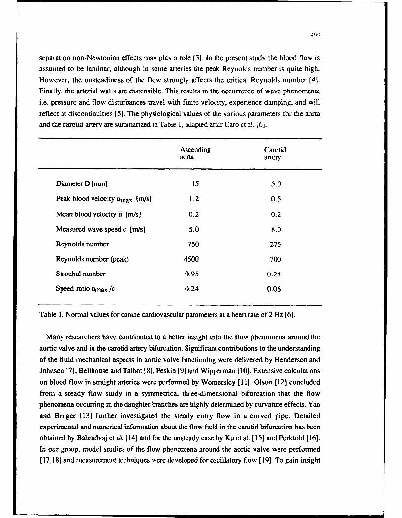
separation non-Newtonian effects may play a role [31. In the present study the blood flow is

assumed to be laminar, although in some arteries the peak Reynolds number is quite high.

However, the unsteadiness of the flow strongly affects the critical Reynolds number [4].

Finally, the arterial walls are distensible. This results in the occurrence of wave phenomena;

i.e. pressure and flow disturbances travel with finite velocity, experience damping, and will

reflect at discontinuities (51. The physiological values of the various parameters for the aorta

and the carotin artery are summarized in Table 1, adapted aftc~r Caro ct a. i6.

Ascending Carotidaorta artery

Diameter D [mm] 15 5.0

Peak blood velocity umax [n/s] 1.2 0.5

Mean blood velocity 5 [m/s] 0.2 0.2

Measured wave speed c [m/s] 5.0 8.0

Reynolds number 750 275

Reynolds number (peak) 4500 700

Strouhal number 0.95 0.28

Speed-ratio umax /c 0.24 0.06

Table 1. Normal values for canine cardiovascular parameters at a heart rate of 2 Hz [6].

Many researchers have contributed to a better insight into the flow phenomena around the

aortic valve and in the carotid artery bifurcation. Significant contributions to the understanding

of the fluid mechanical aspects in aortic valve functioning were delivered by Henderson and

Johnson (7], Bellhouse and Talbot [8], Peskin [91 and Wipperman [101. Extensive calculations

on blood flow in straight arteries were performed by Womersley [11]. Olson [12] concluded

from a steady flow study in a symmetrical three-dimensional bifurcation that the flow

phenomena occurring in the daughter branches are highly determined by curvature effects. Yao

and Berger [131 further investigated the steady entry flow in a curved pipe. Detailed

experimental and numerical information about the flow field in the carotid bifurcation has been

obtained by Bahradvaj et a]. [14] and for the unsteady case by Ku et al. [15] and Perktold [16].

In our group, model studies of the flow phenomena around the aortic valve were performed

[ 17,181 and measurement techniques were developed for oscillatory flow [ 19]. To gain insight

410

into secondary flow patterns, entrance flow in a 90-degree bend was studied [20-221. Next,

steady and unsteady flow in models of the carotid artery bifurcation were analysed [23-26].

Here, we will briefly describe the methods used and pre:,nt some characteristic results.

Experimental validation of the methods used is reported elsewhere [27-301. Finally, some

future research directions will be pointed out.

Entrance flow in a 90-degree curved tubeThe flow of an incompressible isothermal Newtonian fluid is described by the Navier-Stokes

and continuity equations. To solve these equations they are discretized using a standard

Galerkin finite element method which is implemented in the finite element package SEPRAN

[311. The spatial discretization results in the following set of non-linear first-order differential

equations [32]:

MNi +[S + N (II)] a + LT2 = f+ b eq.2a

Lu = 0 eq.2b

where Mui represents the local acceleration term, Su the viscous term, N(U1)j. the convective

acceleration term, LTR the pressure gradient term and LII the velocity divergence term. The

body and boundary forces are represented by f and b2 respectively, while U contains the velocity

and p- the pressure unknowns in the nodal points. The local time derivative in eq.2a is

approximated by :

,kn+e = un+l "un eq.3At

in which u is an abbreviation for u(nAt) with At the time step. The non-linear convective term

is linearized using one step of a Newton-Raphson iteration scheme. In order to reduce the

number of unknowns, a penalty function method is applied [33]. For the solution of the matrix

equation a direct technique was used.

The elements used belong to the group of so-called modified Crouzeix-Raviart elements. For

2D situations, like the aortic valve model, a 7-noded element with 3 pressure and 14 velocity

unknowns is used. 3D situations, like the curved tube and the carotid artery bifurcation, require

the application of a 27-noded element with 4 pressure and 81 velocity unknowns. (See figure

2). The accuracy is 0(Ax 3) for the velocity and 0(Ax 2 ) for the pressure with Ax being a

characteristic dimension of the spatial discretization. The resolution in time, using 0 = 1/2, is

shown to be 0(At2).

411

X ptessure00 velochty

Figure 2. The 7-noded and 27-noded elements used in solving the 2D and 3D fluid motion

equations, respectively.

The flow at the inlet is supposed to be fully developed. The velocities at the wall arepresumed to be zero. At the outlet the normal and both tangential stresses are set to zero, while

in the plane of symmetry both tangential stresses and the normal velocity component are put to

zero.

As an example some results of unsteady entrance flow in a 90-degree curved tube will beshown. The flow rate consisted of a sinusoidally varying unsteady flow componentsuperimposed on a steady flow component. With a curvature ratio of 8 = 1/6, the Dean number

(_ 1-8 Re) varied between 82 and 327 The Strouhal number was 0.46. In figure 3 the results of

axial and secondary flow at 0 = 22.5' from the straight inlet tube are shown. Axial flow is

presented by axial isovelocity lines and secondary flow is visualized by means of velocityvectors. Contour level 0 corresponds to zero axial velocity. As a consequence of centrifugalforces, the secondary velocities near the plane of symmetry are directed towards the outer bend

(0), whereas near the side wall of the curved tube these secondary velocities are directedtowards the inner bend (I), resulting in a Dean-type secondary flow field. For the total period

of time the center of this secondary vortex is situated near the center line of the cross-sectionalplane. The secondary velocities at t=1/4T and 1/2T are about equal, as well as the secondaryvelocities at t=3/4T and t=0. At minimal flow rate a region with low secondary velocities isfound near the inner bend. As a consequence of secondary flow a shift of the maximum of axialvelocity towards the outer bend is observed for the whole period of time. This shift is maximal

at minimal flow rate (t=3/4T). At this time interval a region with negative axial velocities isobserved at the inner bend. Similar results were obtained at other axial positions [22]. There it

also appeared that axial flow is highly determined by secondary flow. The influence of the

frequency parameter and the flow wave form appeared to be of minor importance.

412

Re

800- X

500A '

200-

0 -LT L time

S E) 22,

001

4? 6

t=3/4T ---- /

,2 Umnn

Figure 3. Axial and secondary unsteady entrance flow in a 90-degree curved tube [281.

413

Fluid flow in a distensible model of the carotid artery bifurcationIn the numerical analysis of the flow phenomena in distensible geometries not only the fluid

motion equations but also the equations governing wall motion should be taken into account.Motivated by the small ratio of fluid velocity over wave velocity (- 0.06 for the carotid artery)

an uncoupled approach is followed. First, the time dependent pressure distribution due to wavepropagation is determined. Next, the wall motion due to this time dependent pressure

distribution is calculated. Finally, the wall motion is prescribed as a boundary condition for thesolution of th. fluid notinn. We will briefly describe the three steps in this procedure andfinally an illustrative result will be given.

The time dependent pressure distribution is calculated using a quasi-ID linear model

describing wave propagation. The linearized one-dimensional mass and momentum equationsfor unsteady viscous flow through a visco-elastic tube are used, which read [341:

aA au au ap-+A -=0 ; p- -=-- fu• eq.4a,bat ax & ax

In these equations A = nR2 is the cross-sectional area of the tube, AO is the cross-sectional area

in the reference state, u(x,t) and p(x,t) are the axial velocity and transmural pressure, both

averaged over the cross-sectional area, and f is the so-called friction function. The assumptionof one-dimensionality holds if the wave length is large compared to the diameter of the tube;upto the fifteenth harmonic in the carotid artery tnis ratio is larger than 40. Due to the assumed

linearity the equations can easily be solved using harmonic functions. To that end, two

additional assumptions have to be made; one for the friction function and the other for theconstitutive relationship between A and p. For the friction term a frequency dependentexpression is used, derived from the two-dimensional theory of unsteady fully-developed flowin uniform visco-elastic tubes [11]. Visco-elastic wall behaviour is taken into account by an

experimentally determined constitutive relationship between the complex amplitudes of pressure

and cross-sectional area variations. The influence of wave reflections is incorporated in themodel by treating the carotid artery bifurcation as a bifurcation of uniform tubes. Due to thevery large wave length/diameter-ratio the contribution of local inhomogeneities, like the carotid

sinus, to the reflection and transmission coefficients appeared to be negligible. Reflections from

the outflow ends of the internal and external arteries were incorporated in a standard manner

[291.Next, the wall motion of the carotid bifurcation due to the propagating pressure pulse is

analysed. Because of the magnitude of the deformation (relative diameter changes up to 10 %are found) the system to be analysed is geometrically non-linear. For practical reasons the

mechanical behaviour of the vessel wall is described with a Hookean constitutive relation, The

414

materai parameters are selected in such a way that diameter changes similar to the cncs

observed in vivo are obtained. Visco-elastic and inertia effects are neglected, reducing theproblem to a quasi-static one. Although the wall of the artery has a thickness which is about 20

times smaller than its diameter, experiments show that its bending stiffness is considerable

[35]. These considerations lead to the use of shell elements; compared with the application of

three-dimensional brick elements this results in a considerably smaller system of equations. The

finite element package MARC is used with an 8-noded thick shell element with global

displacements and rotations as degrees of freedom and four integration points [361. Boundary

conditions for the wall motion are applied in a rather pragmatical way [29].

The final step in the numerical approach is the solution of the fluid motion equations using thefinite element method described before. However, in this case for each time step the mesh is

adapted to account for the wall motion. As inflow condition the fully developed axial and radial

velocity profiles as given by Womersley [111] were prescribed. The boundary conditions at the

wall were obtained by taking the time derivative of the wall displacement. At both outflow ends

boundary conditions of the stress-type On = -p and at = 0 were prescribed. The pressures

needed for this purpose were calculated using the quasi-ID model for wave propagation. To

investigate the effect of the wall motion, the flow fieid calculated for the distensible carotid

artery bifurcation model was compared with the flow field calculated for a corresponding rigidmodel. The geometry of the rigid model was chosen to be equal to the end-diastolic geometry

of the distensible model. In both cases an identical flow rate at the entrance was prescribed.

In figure 4 the flow rates at the outflow of the rigid model are compared with those in the

distensible model. Due to the increase in its volume, part of the volume flow entering the

distensible model is accumulated during acceleration. During deceleration this part is released.

This effect accounts for the difference between the outflow rates in the rigid and the distensible

model. As an illustration of the results, the axial flow field in the internal carotid artery at

minimal flow rate (end-systole) is shown in the same figure. Here, contour level 1 corresponds

to zero axial velocity; a reversed flow area is observed at the non-divider wall (N). At the

entrance of the internal carotid artery (10) and halfway the sinus (11) the reversed flow area

occupies about 40 % of the local cross-sectional area. For the distensible case both the size of

the reversed flow area and the magnitude of the negative velocities are found to be smaller. In

both cases Dean-type secondary vortices are observed resulting in C-shaped curvatures of the

corresponding axial isovelocity profiles. In the rigid model the curvature is more pronounced.

Most likely, the release of "flow accumulated during acceleration" in the distensible model is

the dominant factor causing the differences with the flow field observed in the rigid model [29].The above described flow field in the carotid artery changes cu: :erably as a function of

time. The recirculation area is found to develop during deceleration and to disappear during

acceleration. Also the secondary flow field and the curvature of the axial isovelocity lines are

415

12 -..... distensible

Ih 10_____ rigId

2 Intext

0.00 0.25 0-50EStime (S)

10 I1 12

distensible rigid

Figure 4. Comparison between axial velocity profiles in the symmetry plane and at three-

cross-sections in the internal carotid artery at end-systole (ES), calculated for the

distensible and rigid models [291.

416

strongly time-dependent. In general, the distensibility of the wall is found to reduce some ofthese effects, although the global structure of the flow field remains unchanged [291. However,

this conclusion should be handled with care as no comparison has been made between the 3D

pressure field with the pressure distribution calculated using the quasi-lD model for wavepropagation. Since the latter was applied to calculate the wall motion, it should not deviate too

much from the 3D pressure field if a consistent solution of the fluid motion is to be obtained.

This will be a future research topic.

Fluid-leaflet interaction in the aortic valveDue to the strong interaction between structure motion and fluid flow, in the numerical model

for the dynamic behaviour of the aortic valve fluid and structure are iteratively coupled. The

equations of motion of the subsystems are evaluated separately and an iteration is performeduntil convergence is achieved. Because of computational reasons, the fluid flow and the

structure are restricted to be two-dimensional. For the fluid the full unsteady two-dimensionalincompressible Navier-Stokes equations are solved by means of the standard Galerkin finite

element method described before. For stability reasons, the time integration is performed with acomplete Euler implicit scheme (0=1 in eq.3). As initial condition, the steady state solution for

a fully opened valve is taken. As a boundary condition at the entrance, a time-varying parabolicaxial velocity profile is prescribed and the radial dow is set to zero. The entrance channel is

chosen to be long enough to guarantee a full development of the unsteady velocity profile. Due

to the lack of experimental data this fully developed entrance condition is used, although itcertainly does not correspond to the physiological one. As contact condition on the valve, the

fluid velocity is set equal to the local valve velocity, determined from the actual valve position

and the valve position at the previous time level. At the outlet a stress-free flow condition is

prescribed. At the channel walls a no-slip condition is used.To incorporate the moving structure a segmented valve is considered, consisting of several

rigid segments connected to each other. The physiological relevance of this model valve is that

with an increasing number (n) of links, the segmented valve will behave more and more like a

fully flexible valve. In the special case when n=l, the valve reduces to the so-called rigid valve[371. In figure 5 some segment quantities are defined. Each segment has one degree offreedom: its angle of rotation "i. The inertia of the valve is neglected. At each point of time a

segment must satisfy the equilibrium conditions:

Ph, I + fihx2 + fx = 0 ; fnyl + ihy2 + Ify = 0 eq.5a,b

Phx2 li sin(Pi + fhy2 lt COS(Pi + ml = 0 eq.5c

"LIIIII

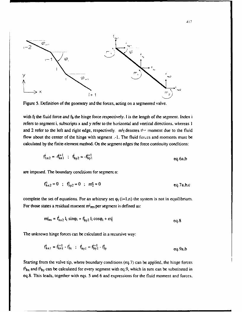
417

>X i+~w

Figure 5. Definition of the geometry and the forces, acting on a segmented valve.

with ff the fluid force and fh the hinge force respectively. I is the length of the segment. Index i

refers to segment i, subscripts x and y refer to the horizontal and vertical directions, whereas 1

and 2 refer to the left and right edge, respectively mif denotes th, moment due to the fluid

flow about the center of the hinge with segment -1. The fluid forces and moments must becalculated by the finite element method. On the segment edges the force continuity conditions:

Vhx2=-1h+ll ; Ohy2= P•II eq.6a,b

are imposed. The boundary conditions for segment n:

nhX2=0 ; fhy2=0 ; mf=0 eq.7a,b,c

complete the set of equations. For an arbitrary set pN (i=l,n) the system is not in equilibrium.

For those states a residual moment mires per segment is defined as:

mi~s = Phx2 ii sin(pj * hy2 li COSi + m eq.8

The unknown hinge forces can be calculated in a recursive way:

ph., = th I" ft. ; thyl I= fh+ylI fiy eq.9a,b

Starting from the valve tip, where boundary conditions (eq.7) can be applied, the hinge forces

fPh_ and fihy can be calculated for every segment with eq.9, which in turn can be substituted ineq.8. This leads, together with eqs. 5 and 6 and expressions for the fluid moment and forces,

418

to n equations with unknowns (pi (i=l,n). This set of equations is solved by reformulating the

problem as a non-linear least squares problem. To this end a residual moment is defined:

r( = mi eq. 10

where r is the total residual moment to be minimized and mi the moment acting on segment i,

which is a function of a position set p. Once a minimum of r is found which equals zero, (p

contains the equilibrium position of the valve segments and therefore of the valve itself. The

segment moments mi depend on all To ...... (Pn. In general no explicit relation for this

dependence can be given, especially not when the finite element fluid model is used. A

consequence is that derivatives cannot be calculated. Therefore, a method must be used which

does not require the evaluation of derivatives. A very suitable non-linear least squares method

for this study is Powelrs hybrid method [381. It combines a robust convergence far from the

equilibrium position, with a fast, superlinear convergence close to it. Notwithstanding the

robustness of Powell's method, it occasionally fails to find the equilibrium position. In these

cases, a new initial estimate is generated and the iteration process is restarted. Using this

method, both the numbers of segments (n=l and n=4) and the physical parameters, like the

Strouhal and Reynolds numbers, are varied.

In the numerical calculations a pulsatile flow rate is used. Since the flow rate decleration time

is an important parameter in the valve closure mechanism [171 ,this time is chosen as the

characteristic time z. Figure 6 shows the velocity field for n=l, Re=313 and Sr=3.60. At t=0.0

the velocities are small and a vortex is present in the sinus. At t= 1.0 the fluid is accelerated and

the valve starts to open. At t-l-.5 the valve has reached its maximum velocity and pushes out

the contents of the sinus. On t=2.0 the flow rate is maximal, the valve is slowing down but still

moving towards the fully opened position. Just at t=2.5, when the flow has its maximum

deceleration, the valve reaches its maximum position and its velocity becomes zero. At t=2.75

the valve is moving towards the closed position. A vortex in the sinus is being formed. At

t=3.0, when the flow rate is nearly zero, the valve has its maximal closing velocity. At t=4.0

the valve has nearly reached its pseudo-equilibrium position and its velocity becomes zero. It is

interesting to note that the valve moves already towards its closed position during flow

deceleration, just like the natural aortic valve does. This observation is consistent with quasi-ID

model predictions [171.

For lower Strouhal numbers the motion of the valve is found to be nearly in phase with the

flow rate and its amplitude is larger 1301. The influence of a variation of the Reynolds number

between 300 and 1100 appeared to be only marginal. Higher Reynolds number values could

not be reached as the fluid solver does not allow computations for Re >1100. Also, similar

419

.. . ..0.U.

0.05 uC _ _ _ _ __ _ _ _ _ _

0 2 3 A 7

Tim ItJr)

t - IAO

t *2.75

Figur 6. Vlociy fied arond amovin valv in pulstile low t seealtmelves03]

420

results were obtained for a segmented valve with n--4; the curvature changes of the leaflet are

only modest. Only at a much higher Strouhal number or when a harmonically varying flow rate

was used, large deformations of the valve leaflet were observed. Finally, it need to be

mentioned that if the simulation of a full physiological flow cycle is required, including back

flow and full valve closure, the model must be extended with a closure algorithm, which is not

included in the present model. This and the extension to the three-dimensional case will be a

future research topic.

Concluding discussionFrom the present study it is concluded that the finite element method can be used for detailed

analyses of unsteady blood flow in complex three-dimensional geometries. The local geometry

of the bifurcation highly affects the axial and secondary flow fields, but the wall distensibility

has only a marginal influence. During flow acceleration and deceleration the valve leaflet shows

large displacements, which induce vortex like velocity patterns in the cavity behind the leaflet.

As presented elsewhere, a good agreement is found between the numerical and experimental

results [27-.0].

Some future research topics in the analysis of fluid flow in large blood vessels are [11:--- Improvements are needed of the models for fluid-structure interaction. In case of the

analysis of the influence of wall distensibility on fluid flow, the improvements need to

include a proper account for the effects of reflections originating from the peripheral

vascular bed, the application of physiologically relevant boundary conditions in the

calculation of wall motion, the use of a model describing the complex mechanical

behaviour of the wall and an experimental validation of the uncoupled approach to

calculate the flow field in such a distensible geometry. For a complete analysis of the

dynamic heart valve behaviour, a three-dimensional fluid model must be applied and in

some cases valve inertia or visco-elasticity of the leaflet material has to be incorporated.

Furthermore, attention should be given to incorporate the possibility of full valve closure.

Then the models can be used to improve the design of existing or newly developed one-

or bi-leaflet disc type or flexible leaflet type heart valve prostheses.

The influences of non-Newtonian effects and minor stenoses on the local flow field are

not completely clear yet. Especially, the visco- elastic properties of the blood may require

a considerable effort. For the analysis of the influence of minor stenoses on the flow field

spectral element methods and PIV-methods may be favourable, as detailed analyses have

to be performed of eddy generation. Besides, the influence of biological variabilities (like

bifurcation angle and divider geometry in case of a bifurcation) need research attention.

Atherosclerotic plaque formation is found at positions where low wall shear rates occur

[39]. Here focal regions of elevated permeability to macromolecules, temporary gaps and

421

a thin endothelial glycocalyx are found. Modelling of the arterial wall is worthwhile,

focussing on maximal stress concentration in the intima and the mass transport of

atherogenic proteins between plasma and vessel wall 140]. Then probably animprovement can be reached with regard to the understanding of the fluid mechanicalcontribution to the process of atherogenesis.

Acknowledgements"The work presented here is mainly based on the PhD-theses of F.N. van de Vosse, C.C.M.

Rindt, P.J. Reuderink and J.B.A.M. Horsten. The research was supported by the DutchOrganization for Scientific Research and the Dutch Technology Foundation.

References[1] AA van Steenhoven, APG Hoeks, JD Janssen and RS Reneman (eds), Three-dimensional

blood flow in bifurcations, Abstractbook Euromech 286, Eindhoven, 1991.[2] RS Reneman, T van Merode and APG Hoeks, News in Physiolog. Sciences, 4 (1989) 185

[31 D Liepsch and S Moravec, Biorheology, 21 (1984) 571

(4] TJ Pedley, The fluid mechanics of large blood vessels, Cambridge, Cambridge, 1980[5] MJ Lighthill, Waves in fluids, Cambridge, Cambrige, 1978[61 CG Caro, TJ Pedley, RC Schroter and WA Seed, The mechanics of the circulation,

Oxford, Oxford, 1978.[7] Y Henderson and FE Johnson, Heart, 4 (1912) 69[8] BJ Bellhouse and L Talbot, J. Fluid Mech., 35 (1969) 721

[9] CS Peskin, Annu. Rev. Fluid Mech., 14 (1982) 235[10] FK Wipperman, J. Fluid Mech., 159 (1985) 487.

[11] JR Womersley, J. Physiol., 127 (1955) 553[12] DE Olson, Fluid Mechanics relevant to respiration, PhD-thesis, University of London,

1971

[13] LS Yao and SA Berger, J. Fluid Mech., 67 (1975) 177

[14] BK Bharadvaj, RF Mabon and DP Giddens, J. Biomech., 15 (1982) 349[15] DN Ku, DP Giddens, CK Zarins and S Glagov, Atherosclerosis, 5 (1985) 293[16] K Perktold, M Resch and OP Reinfried, J. Biomech., 24 (1991) 409[ 17] AA van Steenhoven and MEH van Dongen, J. Fluid Mech., 90 (1979) 21[18] AA van Steenhoven and MEH van Dongen, J. Fluid Mech., 166 (1986) 93.19] AA van Steenhoven and FJHM van de Beucken, J. Fluid Mech., 231 (1991) 599[201 PH Bovendeerd, AA van Steenhoven, FN van de Vosse and G Vossers, J. Fluid Mech.,

177 (1987) 233

422

[211 FN van de Vosse, AA van Steenhoven, A Segal and JD Janssen, Int. J. Num. Meth.

Fluids, 9 (1989) 27[22] CCM Rindt, AA van Steenhoven, JD Janssen and G Vossers, J. Fluid Mech.,

226 (1991) 445[231 CCM Rindt, FN van de Vosse, AA van Steenhoven, ID Janssen and RS Reneman,

J. Biomech., 20 (1981) 499[24] FN van de Vosse, AA van Steenhoven, JD Janssen and RS Reneman, Biorheology,

27 (1990) 163[25] CCM Rindt, AA van Steenhoven and RS Reneman, J. Biomech., 21 (1988) 985[261 CCM Rindt, AA van Steenhoven, JD Janssen, RS Reneman and A Segal, J. Biomech.,

23 (1990) 461[27] FN van de Vosse, Nummerical analysis of carotid artery flow, PhD-thesis, Eindhoven

University of Technology, 1987[28] CCM Rindt, Analysis of the 3D flow field in the carotid artery bifurcation, PhD-thesis,

Eindhoven University of Technology, 1989

[29] PJ Reuderink, Analysis of the flow in a 3D distensible model of the carotid artery

bifurcation, PhD-thesis, Eindhoven University of Technology, 1991

[301 JBAM Horsten, On the analysis of moving heart valves, PhD-thesis, Eindhoven

University of Technology. 1990[31] A Segal, Sepran Manual, Sepra, Delft, 1984[321 FN van de Vosse, A Segal, AA van Steenhoven and JD Janssen, Int. J. Num. Meth.

Fluids, 6 (1986) 427

[33] C Cuvelier, A Segal and AA van Steenhoven, Finite element methods and Navier-Stokes

equations, Reidel, Dordrecht, 1986

1341 JBAM Horsten, AA van Steenhoven and MEH van Dongen, J. Biomech., 22 (1989) 477[351 WR Milnor, Hemodynamics, Williams and Wilkins, Baltimore, 1989

[36] Marc K.3, Manuals A-E, Marc Analysis, Palo Alto, 1988

[37] JBAM Horsten, AA van Steenhoven and DH van Campen, in: P. Wesseling (ed), Notes

on Numerical Fluid Mechanics 29, Vieweg, Braunschweig, 1990

[38] MJD Powell, in: P Rabinowitz (ed), Numerical methods for algebraic equations, Gordonand Breach, London, 1970

[391 CK Zarins, DP Giddens, BK Bharadvaj, VS Sorriurai, RF Mabon and S Glagov,

Circulation Res., 53 (1983) 502[40] TJ Pedley, IUTAM Proceedings, 15 (1980) 151

Theoretical and Applied Mechanics 1992S.R. Bodner, J. Singer. A. Solan & Z. Hashin (Editors)Elsevier Science Publishers B.V. 423© 1993 [UTAM. All rights reserved.

Trends in transonic research

Jdrgen Zierep

Institut fOr Stromungslehre und Str6mungsmaschinen, Universitat (TH) Karlsruhe,Kaiserstrasse 12, D-W7500 Karlsruhe 1, FRG

AbstractTransonic flows are now as before fascinating and very important in respect to

theory, experiment and applications. In the early days analytical methods prevailed thatled to fundamental results. Now a days due to increasing power of computers numericalmethods dominate. Validation problems of Euler- and Navier-Stokes Codes are ofprimary interest. This led to simple but fundamental experiments (DFVLR-F5 wing,vortex flow, shock boundary layer interaction, condensation phenomena, ... ) and theccmparison with theory. The status quo of validation is today not sufficient in all respects.There are complex dependences on the block structures, the meshes, the laminar-turbulent transition and the turbulence models. Some future trends: Search for reliablecodes for 3D-boundary value problems to develop airfoils of low drag - especially laminartransonic airfoils; study of diabatic flows of phase changing media with several applications(lift and drag of airfoils, steam turbines, cryogenic tunnel, Organic Rankine Cycle,...);transonic flows in retrograde media (e.g. BZT fluids).

1. INTRODUCTION: WHAT IS A TRANSONIC FLOW?

In transonic flows the magnitude of the fluid velocity is comparable with the sonicspeed (= signal velocity). The body moves nearly with the same velocity with whichdisturbances propagate. The theoretical and experimental investigation of these flows isnow and as has been before, of great interest and has become of considerable technicalsignificance. Now a days there are many applications in aerodynamics of transonic flightfor instance in the field of civil aviation and thermal fluid machinery which underline eventhe economical importance of these investigations. The declared aim is: reliability, highcapacity, less drag, less noise, less pollution.

The typical qualities of these flow fields, especially the mathematical and physicalproblems involved, can already be understood by studying slender body flows (Fig. 1).In transonic slightly subsonic flow M < 1 a local supersonic region develops in theneighbourhood of maximum thickness which as a rule is limited downstream by a normalshock (Fig. 2). The local Mach number distribution on the airfoil explains the flow. In frontof the body the flow decelerates, behind the stagnation point acceleration to supersonic

424

SoniclineMachline, Shock

M : I

~-0 0Sonicline .

MoRearshockM,,- 1

®N

0 .00 Shock "

Sonicline

limit MachlinesMim MFigure 2. Schlieren picture. Rough surface.

© ,Mach lines and shock. Supersonic region.M

_ _Figure 1. Fluid fields and Mach numberdistributions on the profiles.

0o a) M _ 1, b) M -- 1, c) M > 1.

velocity exists. In the shock the velocity jumps to subsonic velocity with followingpostexpansion (Figs. 3,4). After this deceleration to backward stagnation point withfollowing approach to conditions at infinity. In transonic slightly supersonic flow M ? 1the shock-wave detaches as a rule. Between shock and body a local subsonic regionbuilds up. The displacement effect of the body leads to an acceleration to supersonic

t02 0,94 C.64

/,1 Mt MMO

| M.

Figure 3. Black-white Mach-Zehnderinterferogram of transonic flowat acurved Figure 4. Shock boundary layersurface. M = local Mach number. interaction at an airfoil.

425

velocity till the trailing edge shock is reached. The limit Machline is the last characteristicfrom the airfoil that reaches the subsonic region, while the last characteristic runningdown from the subsonic domain limits the range of influence downstream. M-4 1 leadsto the limiting case of sonic velocity at infinity. The sonic line extends to infinity. At the bodythe flow accelerates until the rear shock is reached. Comparing the Mach numberdistributions on the airfoil we see, that only slight changements exist; the flow freezes.A simple explanation is as follows: if M is only slightly above onethe shock wave standsfar upstream with Mach number behind the shock M5 1. That means the profile don'trealize whether is stands in a transonic supersonic or subsonic flow. With other wordsthe local dates at the profile change from M-< 1 to M_ > 1 only slightly.

The mathematical description leads even for slender bodies with small disturbancetheory to quasilinear partial differential equations. On the sonic line (sonic surface) thetype changes, across the shock curve (shock surface) the shock relations have to befulfilled. Both curves (surfaces) are not known a priori and have to be determined with thesolution.

2. TRENDS IN THE PAST

The great technical importance of transonic flows on the one hand and theinteresting mathematical-physical problems on the other hand had led to an extensivetheoretical and experimental treatment of relevant problems in the past 50 years. TheProceedings of IUTAM Symposium Transsonicum 11962 (Aachen) [11, If 1975 (G6ttingen)[2], 1II 1988 (G~ttingen) [3] give an interesting, unique survey of the worldwide efforts untiltoday. Concerning theory, 1962 the analytical methods prevailed. Among others we havethe hodograph method, the parabolic (local linearization) method, the characteristicsmethod and the integral equation method. A lot of general results came out like similaritylaws, equivalence rule, area rule, asymptotic expansions, ... Beside this some exactsolutions for special profiles had been discovered. The small power of computers at thattime didn't allow the numerical treatment of the direct problem. Already 1975 the interestchanged remarkable to Computational Fluid Dynamics (CFD). The increasing power ofcomputers allowed for the first time the direct numerical treatment of the nonlineardifferential equations in the fluidfield. Questions of stability, convergence and estimationof errors were more or less open this time. This changes drastically in the following years.

3. TRENDS TODAY ILLUSTRATED BY DIFFERENT CODE VALIDATIONS

The Proceedings of the Symposium Transsonicum III [3] describe this development.The concluding remarks by Hornung give a (subjective) pointed description worthreading of the status quo with the progress achieved but with open questions too.Concerning the CFD-methods the validation of Euler- and Navier-Stokes Codes are ofprimary interest. This led to some simple but fundamental experiments, e.g. the DFVLR-F5 wing experiment (Fig. 5) and the vortex flow experiment (Fig. 6) and the comparison

426

primary vortex

, econdar .. vortex

- - - .-- -----

Figure 6. Streamlines of the primary and

Figure 5. Test airfoil DFVLR-F5 in secondary vortex (M= 0.85,(x=100).

the transonic 1 m x 1m test sectionin G6ttingen.

with numerical calculations for these cases. Some other experiments and validations willbe discussed later on.

In principle there are two concepts for the numerical calculation of the viscous flowaround wings. By using the zonal numerical approach in different domains of the flowfield different differential equations according to the physical effects will be used (Fig. 7).Outside the boundary layer in front of the shock we use the potential equation, behindthe shock the Euler equations, near the body the boundary layer equations, near theiai~ing Adge and in the wake region the Navier-Stokes equations. The shock-boundarylayer interference is given by a separate local solution which has to be integratediteratively in the global flow field. The second method solves the full Navier-Stokesequations in the total flow field. The main point is to choose a suitable block-structuredgrid which secures a high resolution in the viscous interaction region and at the shock andthe trailing edge. Within the inviscid flow field zones a reduced resolution is possible. Thisconcept needs an optimization in the choise of computational grids and blocks.

• "' ~EULER .t

NAVIR STOKES Figure 7. Phenomena and zonal

POTENTIAL model equations for transonic flowBOUNDARY LAYER at an airfoil.

427

3.1A workshop was organized by Kordulla and Sobieczky [4] before the Symposium

Transsonicum Ill. A well-defined boundary value problem, the flow over a wing (DFVLR-F5) in a wind tunnel was formulated (Figs. 8, 9). Boundary conditions were given at thewalls and in the entrance and exit area. All groups and institutions that had developedsuitable Navier-Stokes programs, were invited to participate in solving this flow problem,iumerically. Active participants came from: NASA Ames, NASA Langley, NAL Japan,FFA Sweden, MBB Munich, DFVLR G6ttingen. All theoretical results were collected,compared with each other and with the experiments performed in G6ttingen. This seemsto be a milestone and should be continued in future.

A •1A DIMENSION Wm

-0.22

004 :2 o0 0.6

A- A Figure 8. 3D - test airfoil [4].

WING DFVLR-F5 I !

INLET PLANE -I EXIT PLANE

I PATE

Figure 9. Wing-plateconfiguration in lm

SUCTIO FLAP

SUCTION ' ' ,'x lm transonic windtunnel [4].

428

SEC:1 SEC: 7

10L

I I ", !

I SEC:4 SEC: 9

I . . . ..

Figure 10. Chordwise c- distributions on the wing surface in different sections (1 ,4,7,9).Experimental data given by symbols, solid lines theoretical results(Schwamborn). Flowconditions: Free-stream Mach number M= 0.82, a= 20, Re/m = 107 [4].

jryr

Figure 11. Comparison of predictedskin friction line patterns for the

wind tunnel test. (x= 20. Left: lowerwing surface. Right: upper wing"surface. [4].

421)

"" i0301A A"

CL CL.

S U

A A

(.t Chodelrjian

0.1 0.1 F'e LrndoberIg Ot WAr Oboyash, t *I

S SchmalzCotes \V Schwombon

a A. v. V Wtnd Tunn. CowA

0 0 0+05 0.5 00750 C.C 68 0Q1

Figure 12. Lift and drag coefficients of the DFVLR-F5 Navier-Stokes solutions [4].

The pressure distributions on the wing and in the field agree quite well among theparticipants and with the experiment (approximately 10%). The results are not verysensitive (Fig. 10). The skin friction lines, especially if separation exists, are much moresensitive (Fig. 11). Disappointing is the scatter of the lift (cL) and the drag coefficients(CD) (Fig. 12). There is a remarkable and complex dependence on the nature of the usedmeshes and block structures in streamwise and chordwise direction (C-0, C-H, 0-0, H-H-type) and the discretization (FVM, FDM). Beyond this the laminar-turbulent transition(switch on) and the used turbulence model (Baldwin-Lomax) may be of considerableinfluence. This is doubtless a disillusion and not recognized with pleasure but it isimportant for all further investigations in that field. Without strict validation of thenumerical codes no reliability can be guaranted!

3.2The next validation complex is experiment and computation of transonic viscous

channel flow with ventilation. Many efforts at different places had been done [5, 6, 7]. Thepractical idea is the reduction of shock strength by passive control in the domain ofturbulent shock-boundary layer interaction. Figure 13 describes on the one hand thescheme of the test section in a laboratory and on the other hand the different zonalmethodsforthe numerical approach. Outsidethe boundary layerwe have the nonviscousflow part. We solve the potential equation after suitable grid generation by well knowndifference methods. At the wall we start with laminar boundary layer, after transition wecontinue with turbulent boundary layer. In the shock boundary interaction area we fit inan analytical model [8]. In the cavity closed with a punched sheet we prescribe a constantpressure and fulfil the conservation of mass. Downstream we have a turbulent boundarylayer with oi without separation. An inverse integral method has to be applied [9]. The

430

Transonic Wind Tunnel

(analyical m delcbie

(nuwitca aouto ofer~ metod

(conservation ofmass)

laminar boundary layer turbulent boundary layer in front of the interference area turbulent boundary layer behind the interference afra(direct integral method) (direct integral method) (inverse integral methodi)

Figure 13. Zonal Methods for computation of transonic viscous channel flow withye nti latio n.

M mach number contours X

0.8- e experiment

2.5-2-10 theory

1.5 0 experiment

0 too 200 300 1.00 500 IMdisplacement and momentum thickness

C,

o .00-. theory0.o004. experiment0.003. 00,002

0.0-- --- -- -- - -- -- - - Figure 14. Comparison of theory-00------------------------------------n.I 100 20 360 104 00 x~nmil Porosity ==8.2%, cavity length~

friction coefficient50mm Th masfu

porosity =8.2 ITresod t M,,,=1.2 in thecavity length =50 m case without ventilation 16).

411

1.3 rBow shock

o vitholut cavity

14 4 with cavity

0 .9 - . L .. .... . . . -.-10 10 30 50 70 90 -Bow shock

s [mm]

Chamber

Figure 15. Interferogram without and with Figure 16. Cascade in supersonicflow.ventilation and the corresponding Mach Top: Reflexion of bow shock wave atnumber at the wall [7]. the profile. Bottom: Bow shock wave

closes the supersonic region.

calculation and the measurements for Mach number and skin friction atthe lower wall andthe displacement - and momentum thickness agree well (Fig. 14). The comparison withthe nonventilated case is convincing. The shock strength is considerably reduced (Fig.15). For a single profile the wave resistance decreases - until 50% - and the shockposition is fixed. It is remarkable that the effect of passive control is already reached witha perforation of about 8%. Further on the inclination of the perforation-channels is ofconsiderable influence (oblique perforation).

The method described here may be of interest for several applications. Forcompressor cascades in supersonic flow for instance it is possible to reduce the loss bypassive control on the suction side of the blades (Fig. 16). Experiments in a cascadetunnel [101 and in channel test section obviously show this effect. Calculation with zonalmethods are possible in a way we have described above.

In the last time another idea of passive control has been propagated [11 ]. The cavityis closed by an elastic membrane. Depending upon the elasticity and the inner pressurethe membrane builds up some kind of adaptive wall that may have a favourable influenceon the shock-boundary layer interaction.

432

3.3A very interesting new experiment for validation of modern transonic numerical

methods is the condensation, or more general the study of flows with phase transition,in Laval nozzles and around profiles. This is important for several reasons. On the onehand this is adiabatic flow with interesting new physical effects on a microscopic and amacroscopic scale (nucleation theory, droplet growth), on the other hand there areseveral actual applications in steam turbines and in cryogenic tunnels, not to forget theII

iiFigure 17ab. Schlierenpictures and calculated iso Mach lines. Left: t•o= 29%, subcriticalheat addition; Right: •o = 60%, supercritical heat addition.

/IM¢ = 0.02 "• •:• •,••)o = t,9.3 % •';A\•X'•'|'•' !i'. i .....

To1 297.1 K "•/'/• ']rIi/i':Ft i '•': !i "i i i i r '

M,=P/Pro

tog•oJ 0.7- • Experiment[m'3*s4 ] -- Theory

35 - 0.6g/g,•x

30- !.0q

25- 0.812o- o.6-t •tk:

15- 0.z, -I Figure 18. Diabatic flow in a hyperbolaSadiabatic

10- 0.2q nozzle. On the axis: Nucleation rate J,Sx [cm] Condensing mass g/gm•,, Pressure ratio

5 0.0J 5 lO 15 plPo•-

433

x [g/kgl0 2 4 6 8 10

-NANACA-02.1, 0 0.-CA0.i Mf-0 1 0

40-

20

Ac 0 O

[%] ..... ..... Figure 19a,b. Changement of the pressure

02

drag for circular arc profile (CA-0.1)-20 chordlength c = 80mm and NACA-01 2

• -D-Q_ - • profile (c = 100 mm) by heat addition due0 20 30 40.. 6070 80 to homogeneous condensation, without

•o [%] incidence (12].

ftigh of an aircraft in humid air. Condensation gives rise to heat release that influencesthe pressure distribution considerably. Strong changements of lift and wave dragcoefficients are possible in moist atmospheric air (12]. The numerical method solves theunsteady 2D-Euler equations. Iteration is finished if the stationary final solution isobtained. All equations are used in conservation form and the condensation is modelledby two successive processes. For homogeneous condensation we start with thenucleation theory by Volmer [13] and continue with the droplet growth theory accordingto the Hertz-Knudsen model. The calculation uses a finite-volume method that generalizesa corresponding procedure for adiabatic flows [14]. Depending upon the stagnationhumidity 4o we find different structures of condensation phenomena in the supersonicpart of a nozzle - subcritical and supercritical heat addition (Fig. 17a,b) [15]. The

434

Figure 20. Non-q O I T°, < 0.1 NACA-0012 equilibrium, adiabatic

A . 0.8 and equilibrium flow for// - .25. NACA-0012 profile, a=

1.250 , Mt=0.8, AMf="iii' ,//// 0.015 [16].

Iosqili~um i EquHilirum

AC7 -30% AC, 30%

comparison between calculation and measurements is convincing. This is valid inrespect to the Schlierenpictures with iso-Machlines and in respect to the static pressuremeasurements along the axis. Figure 18 gives as microscopic quantity the nucleationrate J and as macroscopic values the condensed mass g/gma, and the static pressureP/P0 l. Concerning profile flow figure 19 shows for circular arc (CA-0. 10) and NACA-001 2profile the results. Depending upon the stagnation humidity 00 the pressure drag maybe considerably reduced (CA-0. 10) or increased(NACA-00 12) [121. A simple explanationis as follows: For circular arc profile and adiabatic flow the shock position is in theneighbourhood of the rear, for M,.= 0.87. Condensation will not move this shock. Thechangement of the pressure due to heat addition leads to decreasing drag withincreasing humidity. For NACA profile on the contrary the shock position in adiabatic flowis in the middle of the profile, for Mf-- 0.8. Here due to condensation the shock moves.The changement of the pressure due to heat addition leads to an increasing drag withincreasing humidity. Remarkable is the typical double shock structure for high humidity!The first is due to super-critical heat addition, the second is the usual gasdynamic shock.If unsymmetric flows with incidence are considered things change once more [121. Nowfor NACA profile the shock is foradiabatic flow in the neighbourhood of the rear and dragand lift decrease with increasing humidity. Figure 20 shows the different effects betweennon-equilibrium condensation and equilibrium condensation on the one hand andadiabatic flow on the other hand. The case of equilibrium condensation corresponds toatmospheric flight conditions with chordlength c = 1500 mm. A drastic increase of thedrag is the consequence.

435

4. FUTURE TRENDS

The last examples lead already to efforts in future. In the field of CFD-methods nowas before reliable Euler- and Navier-Stokes codes for actual problems of modernaerodynamics are wanted. Validation is necessary ir any case. Of special interest areairfoils of low drag. This aim may be reached by design of shockless profiles (171 or byactive or passive control of the shock boundary layer interaction.

The transonic laminar airfoil is simply the optimum. If it is possible to suppress theinstabilities in the boundary layer and keep it laminar over the main part of the airfoil thiswould be a great success.

Phase transition effects are of increasing importance as we have seen. Thesituation in cryogenic tunnels belongs to these subjects and the study of condensationof N2 is of great interest [18,19]. A possible application of phase changing fluid flow liesin a new type of fluid flow machines, using a so called Organic Rankine Cycle (ORC).Some new investigations show that remarkable features exist which lead to largeefficiencies of these systems 120].

Last not least the transonic flow in retrograde (dense) fluids is in many respectssurprising [2 i]. Sorm e well known classical gasdynamic effects invert [22,23,24]. Forinstance, expansion shocks may be possible with a favourable influence on boundarylayer separation; isentropic compression of these media may lead to condensation andso on.

At Symposium Transsonicum III Earl Murman gave a delightful comment: "What weare doing is fun, it might even be important". After working in the fascinating field oftransonic flow for over 35 years I am convinced that it is important.

5. REFERENCES

1 Proceedings IUTAM Symposium Transsonicum I, ed: Oswatitscn, K., Springer-Verlag, 490 pages, 1964

2 Proceedings IUTAM Symposium Transsonicum II, eds: Oswatitsch, K. and Rues,D., Springer-Verlag, 574 pages, 1976

3 Proceedings IUTAM Symposium Transsonicum III, eds: Zierep, J. and Oertel, H.,Springer-Verlag, 504 pages, 1989

4 Numerical Simulation of the Transonic DFVLR-F5 Wing Experiment. Ed: Kordulla,W., Notes on numerical fluid mechanics, Vol. 22, Vieweg, 305 pages, 1988

5 Ddlery, J.: Recent Basic Studies in Transonic Shock-Wave/Turbulent Boundary-Layer-interactions. See [3], pp 357-377

6 Breitling, Th.: Berechnung transsonischer, reibungsbehafteter Kanal- und Profil-str~mungen mit passiver Beeinflussung. Dissertation Universittt Karlsruhe 1989,90 pages

7 Braun, W.: Experimentelle Untersuchung der turbulenten Stol3 - Grenzschicht-Wechselwirkung mit passiver Beeinflussung. Dissertation Universitat Karlsruhe1990, 98 pages

436

8 Bohning, R. und Zierep, J.: Der senkrechte Verdichtungsstol3 an der gekrnmmtenWand unter Einflul3 der Reibung. ZAMP 27, 225-240 (1976)

9 Bohning, R. and Jungbluth, H.: Turbulent Shock-Boundary-Layer Interaction withControl. Theory and Experiment. See [3], 389-398.

10 Yu, Shen; Li, Jianyi; Yu, Bin and Fan, Chungfu: Some preliminary experimentalresults on passive control of shock wave boundary layer interaction in compressorcascades. In: Proceedings of the 1st International Symposium 'Experimental andComputational Aerothermodynamics of Internal Flows', Beijing 1990, WorldPublishing Corporation, pp. 217-219

11 Breitling, R. and Zierep, J.: Computation of transonic viscous flow over airfoils withcontrol by an elastic membrane and comparison with control by passive ventilation.Acta Mechanica 87, 23-36 (1991)

12 Schnerr, G.H. and Dohrmann, U.: Drag and Lift in Nonadiabatic Transonic Flow.AIAA 91-1716, AIAA 22nd Fluid Dynamics, Plasma Dynamics and Lasers Con-ference, June 24-26, 1991, Honolulu

13 Volmer, M.: Kinetik der Phasenbildung. Steinkopf, Leipzig, 193914 Eberle, A.: A new flux extrapolation scheme solving the Euler equations for

arbitrary 3-D geometry and speed. MBB/LKE 122/PUB/1 40, 198415 Delale, C.F.; Schnerr, G.H. and Zierep, J.: The Mathematical Theory of Thermal

Choking in Nozzle Flows. J. Fluid Mech., submitted for publication (1992)16 Schnerr, G.H.: Transonic Aerodynamics including strong Effects from Heat Addi-

tion. 4th Int. Symposium on Compressible Fluid Dynamics, University of Davis,California. Computers & Fluids (1992)

17 Sobieczky, H.: Verfahren fOr die Entwurfsaerodynamik moderner Transportflug-zeuge. DFVLR-FB 85-05 (1985)

18 Wegener, P.P.: Cryogenic Wind tunnels and the Condensation of Nitrogen. Exp.in Fluids 11, 333-338 (1989)

19 Schnerr, G.H.: Gasdynamische Effekte in transsonischen Str6mungen durchEnergiezu- und -abfuhr nach partiellem Phasenwechsel des Fluids. ZAMM 71, T401-408 (1991)

20 Zfrner, W. and Blumenberg, J.: The Organic Rankine Cycle for solar-dynamicspace power generation. Zeitschr. f. Flugwiss. und Weltraumforschung 13, 260-270 (1989)

21 Cramer, M.S.: Transonic Flows of BZT fluids. Proceedings of 13th IMACSCongress on Appll. Math. and Scientific Computations, Dublin 1991

22 Thompson, P.A.: A Fundamental Derivative in Gasdynamics. Physics of Fluids 14,1843-1849 (1971)

23 Cramer, M.S.: Nonclassical Dynamics of Classical Gases. In: Waves in Real Fluids(ed. Kluwick, A.), Springer-Verlag, Heidelberg, New York, Tokyo, in press

24 Cramer, M.S. and Kluwick,A.: On the Propagation of Waves Exhibiting Positive andNegative Nonlinearity. J. Fluid Mech. 142, 9-37 (1984).

437

LIST OF CONTRIBUFED PAPERS

PRESENTED AT THE CONGRESS

Abbott, J.R., Graham, A.L., Mondy, Ait el Ferrane, M.I., Bremand, F.,L.A., Brenner, H. Lagarde, A.DISPERSION ACCOMPANYING THE NONLINEAR VISCOELASTIC ANDSETTLING OF A BALL THROUGH A PHOTOVISCOELASTIC CONSTITUTIVECONCENTRATED NEUTRALLY BUOYANT LAWS FOR POLYCARBONATE MATERIALSUSPENSION IN QUASISTATIC LOAD

Abeyaratne, R., Knowles, J.K. Akylas, T.R., Grimshaw, R.H.J.REFLECTION AND TRANSMISSION OF SOLITARY INTERNAL WAVES WITHWAVES FROM AN INTERFACE WITH A OSCILLATORY TAILSPHASE-TRANSFORMING SOLID

Altenbach, H., Zolochevsky, A.Acrivos, A., Fan, X., Mauri, R., Nir, A UNIFIED MODEL OF ISOTROPICA. MATERIALS INCLUDING SECOND-ORDER-VISCOUS RESUSPENSION IN COUETTE EFFECTSFLOWS

Altus, E.: See Adan, M.Acrivos, A.: See Kapoor, B. Amadio, C., Rajgelj, S., Nappi, A.Acrivos, A.: See Wu, W.-Y. AN EXTENDED VARIATIONAL FORMU-

LATION APPLIED TO THE ANALYSIS OFAdan, M., Sheinman, I., Altus, E. CREEP PROBLEMSPOST-BUCKLING BEHAVIOR OF BEAMSUNDER CONTACT CONSTRAINTS Amari, T., Asakura, T.

CREEP BEHAVIOR OF MAGNETICAdziev, T., Wnuk, M.P. SUSPENSION AT THE STRESS LEVEL OFINFLUENCE OF PRESTRAINING AND YIELD VALUERESIDUAL STRESSES ON MATERIALRESISTANCE TO CRACK PROPAGATION Anh, N.D.

AN APPROXIMATE TECHNIQUE FORAfeti, G.M., Resch, F.J. STATIONARY RANDOM VIBRATIONSFROM BREAKING WAVES TO BREAKINGBUBBLES: PRODUCTION CHARACTERIS- Anselmet, F., Djeridi, H., Fulachier, L.TICS OF THE MARINE DROPLET PASSIVE SCALAR DISSIPATION IN FULLYAEROSOL TURBULENT FLOWS

Agarwal, R.K. Arbocz, J., de Vries, J., Rebel, G.A CFD-BASED APPROACH FOR THE KOITER'S STABILITY THEORY EXTENDEDSOLUTION OF AEROACOUSTICS, TO THE BUCKLING OF ANISOTROPICMAXWELL, SCHROEDINGER, AND SHELLS WITH (NEARLY) SIMULTANEOUSBOLTZMANN EQUATIONS BUCKLING MODES

Agnon, Y., Glozman, M., Stiassnie, M. Arbocz, J.: See Guo, Q.Z.HIGH-ORDER HAMILTONIAN AND CHAOSIN SURFACE WAVES Arcisz, M., Kosinski, W.

HEAT CONDUCTION LAWS ANDAifantis, E.C. HUGONIOT RELATIONS IN FINITEPATTERN-FORMING INSTABILITIES ELASTICITYDURING PLASTIC FLOW AND FRACTURE Ariaratnam, S.T.: See Asokanthan, S.F.

438

Arts, T.: See Janssen, J.D. Belsky, V.G.A SOLUTION SCHEME FOR CONTACT

Asakura, T.: See Amari, T. PROBLEMS AND THE ANALYSIS OFBODIES WITH CRACKS USING MULTI-

Ashida, F., Tauchert, T.R., Noda, N. GRID APPROACHA GENERAL SOLUTION TECHNIQUE FORTHREE-DIMENSIONAL PROBLEMS OF Ben-David, D.: See Tirosh, J.PIEZOTHERMOELASTICITY INHEXAGONAL SOLIDS OF CLASS 6MM Ben-Haim, Y.

CONVEX MODELS FOR UNCERTAINTY INAshlani, F.: See Hanagud, S. RADIAL PULSE BUCKLING OF SHELLS

Asokanthan, S.F., Ariaratnam, S.T. Benallal, A.DYNAMIC STABILITY OF AXIALLY ILL-POSEDNESS AND LOCALIZATION INMOVING BANDS UNDER RANDOM SOLIDS AND STRUCTURAL MECHANICSTENSION FLUCTUATIONS

Benveniste, Y.Austermann, R., Kurnik, W., Popp, K. UNIVERSAL RELATIONS IN PIEZO-CROSS FLOW-INDUCED INSTABILITIES IN ELECTRIC COMPOSITES WITH EIGEN-A TUBE ARRAY - EXPERIMENTS, STRESS AND POLARIZATION FIELDSMODELLING, ANALYSIS

Eerdichevsky, V., Fridlyand, A.Aydin, E.M.: See Leutheusser, H.J. VARIATIONAL APPROACH TO FLUID

DYNAMICSBai, Y.L., Lu, C.S., Ling, Z., Xia,M.F., Ke, F.J. Berest, P.COALESCENCE OF MICROCRACKS AS A STABILITY OF AN IRREVERSIBLECASCADE TO CRITICAL FAILURE SYSTEM: DETACHMENT OF A

MEMBRANEBaker, G.R.: See Cowley, S.J.

Berkooz, G., Elezgaray, J, Holmes, P.Bakker, P.G. THE LOCAL NATURE OF COHERENTA MATHEMATICAL MODEL FOR 'OPEN' STRUCTURE INTERACTIONSEPARATION

Bershadskii, A.: See Branover, H.Bammann, D.J.MODELING THE FINITE INELASTIC Bert, C.W.:See Libai, A.DEFORMATION AND FAILURE OFMETALS Berthaud, Y., Billardon, R., Comi, C.

IDENTIFICATION OF DAMAGEABLEBar-Cohen, Y.: See Mal, A.K. ELASTIC-PLASTIC MATERIALS FROM

LOCALIZATION MEASUREMENTSBarthes-Biesel, D.: See Drochon, A.

Beylinson, Ya.Z., Goldberg, A.Z.,Batra, R.C., Zhu, Z.G., Wang, Y. Goldberg Z.A.CONSIDERATION OF PHASE TRANS- NONLINEAR WAVES AND FERMI-PASTA-FORMATIONS AND KINEMATIC ULAM PROBLEMHARDENING IN THE STUDY OF SHEARBANDS IN A DYNAMICALLY LOADED Bigoni, D., Zaccaria, D.STEEL BLOCK ON FLUTTER INSTABILITY IN

CONTINUUM ELASTOPLASTICITYBauer, J.: See Gutkowski, W.

Billardon, R.: See Berthaud, Y.Bazant, Z.P., Cedolin, L., Ozbolt, J.INSTABILITIES AND BIFURCATIONS DUE Birker, T.: See Zhou, M.TO CRACK INTERACTIONS AND DAMAGE

Blajer, W., Schiehlen, W., Schirm, W.Bazhlekov, I.: See Zapryanov, Z. SOME NEW DEVELOPMENTS IN THE

COORDINATE PARTITIONING METHOD

439

Blanze, C., Danwe, R., Ladeveze, P., Braat, G.F.M.Maurel, Ph. MECHANICS OF CONTACT BETWEENA NEW SIMPL.FIED METHOD FOR THE TWO ROLLERS COATED WITH MULTI-ANALYSIS OF MASSIVE-BODY LAYERED, VISCOELASTIC RUBBERSTRUCTURES

Brady, J.F.: See Kraynik, A.M.Blau, M., Moshaiov, A.THREE DIMENSIONAL MODELING AND Brandt, R.ANALYSIS OF A SINGLE LAP JOINT RELAMINARISED BOUNDARY LAYERS IN

ADVERSE PRESSURE GRADIENTSBlekhman, 1.1.THE VIBRATIONAL MECHANICS AND Branover, H., Bershadskii, A.,VIBRATIONAL RHEOLOGY: MAIN Eidelman, A., Nagorny, M.THEOREMS, BODY OF MATHEMATICS, THE LABORATORY SIMULATION OFNONLINEAR EFFECTS, APPLICATIONS TRANSFER PROCESSES AND FRACTAL

VARIABILITY OF STRATOSPHERICBleuler, H., Bl6chlinger, M., Dual, J., TURBULENCEGahler, C.MEASUREMENT OF MATERIAL DAMPING Bratukhin, Y.K., Makarov, S.O.IN FERROMAGNETIC METALS USING ON THE THERMOCAPILLARY MOVE-ACTIVE MAGNETIC BEARINGS MENTS OF THE SOLITONIC TYPE

Bl6chlinger, M.: See Bleuler, H. Bremand, F.: See Ait-el-Ferrane, M.I.

Bodner, S.R.: See Ravid, M. Brenner, H.: See Abbott, J.R.

Boehler, J.-P.: See Millien, A. Brenner, H.: See Frankel, I.

Bonnecaze, R.T.: See Kraynik, A.M. Brenner, H.: See Mauri, R.

Bontcheva, N. Brewer, D.: See Calomino, A.PLASTIC LOCALIZATION INANISOTROPICALLY HARDENING Brock, L.M.DAMAGED MATERIALS THERMAL EFFECTS IN TRANSIENT

MODELS OF DYNAMIC BRITTLEBorgas, M.S. FRACTURESTOCHASTIC MODELS OF LAGRANGIANSTATISTICS IN TURBULENT FLOW Broday, D., Kimmel, E.

ANALYSIS OF THE ENHANCED AXIALBorodich, F.M. DISPERSION IN A VIBRATING TUBESELF-SIMILARITY PROPERTIES OFSTATIC AND DYNAMIC CONTACT Brodsky, N.S., Fossum, A.F, Chan,BETWEEN A PUNCH AND ANISOTROPIC K.S., Munson, D.E.MEDIA EXPERIMENTAL EVALUATION OF A

CONSTITUTIVE MODEL FOR INELASTICBoucher, S.: See Verlinden, 0. FLOW AND DAMAGE EVOLUTION IN

SOLIDS SUBJECTED TO TRIAXIALBoulahbal, D.: See Crandall, S.H. COMPRESSION LOADING

Boulanger, Ph., Hayes, M. Browne, L.W.B.: See Dinckelacker, A.SHEAR, SHEAR STRESS AND SHEARING

Budiansky, B., Fleck, N.A.Bourassa, P. COMPRESSIVE FAILURE OF FIBREDYNAMICS OF A MULTIBODY SYSTEM COMPOSITESWITH CONTROLS APPLICATION TOBIOMECHANICS MOTION B~ihler, K.

VORTEX BREAKDOWN PHENOMENA INBovendeerd, P.H.M.: See Ianssen, J.D. ROTATING FLUIDS

440

Bui, H.D.: See Rittel, D. Chaskalovic, J.A NEW MATHEMATICAL MODEL FOR THE

Burde, G.1. TORNADOES GENESIS BY BIFURCATIONSOME EXACT NON-SIMILARITY OF THE SOLUTIONS OF NAVIER-STOKESSOLUTIONS OF THE BOUNDARY LAYER EQUATIONSEQUATIONS Chau, L.-K.: See Stumpf, H.Byskov, E.FINITE ELEMENT PRINCIPLES, Chaudhuri, R.A., Garala, H.J.ASYMPTOTIC POSTBUCKLING PROBLEMS ON DEFORMATION AND FAILUREAND NONLINEAR MEMBRANE LOCKING BEHAVIOR OF THICK ADVANCED

COMPOSITES UNDER COMPRESSIONCalomino, A., Brewer, D., Chudnovsky,A. Chen, C., Han, M., Liu, Z., Su, X.,SUBCRITICAL AND CRITICAL CRACK Wang, R.GROWTH IN NC-132 MONOLITHIC SILICON STRESS WAVE EFFECT ON THE DYNAMICNITRIDE PLASTIC BUCKLING OF CYLINDRICAL

SHELL UNDER AXIAL IMPACTCarnotim, D., Roorda, J.PLASTIC BUCKLING WITH RESIDUAL Chen, C.-T.: See Su, F.-C.STRESSES - IMPERFECTION SENSITIVITY

Chen, F., Chang, M.H.Carpenter, P.W.: See Lucey, A.D. STABILITY OF TAYLOR-DEAN FLOW IN A

SMALL GAP BETWEEN ROTATINGCaulliez, G.: See Ricci, N. CYLINDERS

Cederbaum, G., Mond, M., Kahn, P.B., Chen, X.-N., Sharma, S.D.Zarmi, Y. SLENDER SHIP MOVING AT NEAR-STABILITY ANALYSIS OF THE NON- CRITICAL SPEED IN SHALLOW CHANNELLINEAR MATHIEU EQUATION Chen,. X-N., Wei, R-1.Cedolin, L.: See Bazant, Z. DYNAMICAL BEHAVIOUR OF A

NONPROPAGATING SOLITON UNDER ACercignani, C. PERIODICALLY MODULATEDON THE INVERTED TEMPERATURE OSCILLATIONGRADIENT IN A VAPOR Cherepanov, G.P.Chan, K.S.: See Brodsky, N.S. DYNAMICS OF AN ELEMENTARY ACT OF

A CRACK GROWTH AND DISLOCATIONChang, C.-C. EMISSION AT THE INSTABILITY POINT

ON THE SOURCES OF AERODYNAMICFORCES Cherkaev, A.A VARIATIONAL METHOD FOR

Chang, M.H.: See Chen, F. ESTIMATING EFFECTIVE PROPERTIES OFCOMPOSITES WITH ARBITRARY

Chapuliot, S., Combescure, A. MICROSTRUCTURESPLASTIC BUCKLING ANALYSIS OF Chien, N.: See Honein, T.AXIALLY STIFFENED SHELLS

Charru, F. Chinilov, A. Y.BIFURCATION ANALYSIS OF INTER- ON A BOUNDARY VALUE PROBLEM INFACIAL WAVES IN A TWO-LAYER THE STABILITY THEORY OF A SHOCKCOUETrE-POISEUILLE FLOW WAVE

Chashechkin, J.D. Chiskis, A.: See Freidin, A.INTERNAL WAVES AND VORTICES IN THEWAKES IN A CONTINUOUSLY STRATIFIED Chiu, C.-H.: See Gao, H.LIQUID

441

Christensen, R.M., DeTeresa, S.J. Combescure, A.: See Chapuliot, S.ELIMINATION/MlNIMIZATION OF EDGE-INDUCED STRESS SINGULARITIES IN Comi, C.: See Berthaud, Y.FIBER COMPOSITE LAMINATES

Chu, C.-C., Wang, C.-T., Hsieh, C.-S. Conti, C.: See Verlinden, 0.

AN EXPERIMENTAL INVESTIGATION OF Cowley, S.J., Baker, G.R., Tanveer, S.,VORTEX MOTIONS NEAR SURFACES Page, M.Chudnova, R.S.: See Smimov, B.I. SINGULARITY FORMATION AND ROLL-UP

ON VORTEX SHEETS

Chudnovsky, A.: See Calomino, A. Crandall, S.H., Boulahbal, D.DYNAMIC INSTABILITIES OF ROTATING

Chudnovsky, A.: See Kunin, B. DISK INFORMATION STORAGE DEVICES

Chudnovsky, A.: See Wu, S. Crisfield, M.: See Shi, J.

Chung, J.: See Hulbert, G.M. Cristescu, N.A PROCEDURE TO DETERMINE

Churilov, S.M., Shukhman, I.G. NONASSOCIATED CONSTITUTIVEON A WEAKLY-NONLINEAR INTER- EQUATIONS FOR GEOMATERIALSPRETATION OF MODE ALTERNATION IN ACIRCULAR SHEAR FLOW Crocombe, A.D.: See Dabnichki, P.

Churilov, S.M., Shukhman, I.G. Cuche, D.: See Mayer, M.CRITICAL LAYER AND NONLINEAREVOLUTION OF DISTURBANCES IN Curry, F.-R.: See Tsay, R.-V.WEAKLY SUPERCRITICAL SHEAR FLOWS

Clifton, R.J., Prakash, V. Cveticanin, L.THE INFLUENCE OF THE REACTIVETIME-RESOLVED FRICTION IN PRESSURE- FORCE ON THE VIBRATION PROPERTIES

SHEAR IMPACT OF THE ROTOR WITH TIME VARIABLEMASS

Cochelin, B., Damil, N., Potier-Ferry,M. Dabnichki, P., Crocombe, A.D.ASYMPTOTIC-NUMERICAL METHODS MODELLING AND FINITE ELEMENTFOR NONLINEAR STRUCTURAL ANALYSES OF BUTTOCK-CUSHIONMECHANICS INTERACTION

Coene, R. Damil, N.: See Cochelin, B.THE DRIFT PAST AN AIRFOIL WITHCIRCULATION Danwe, R.: See Blanze, C.

Cohen, B., Lai, W.M., Mow, V.C. Davies, H.G., Pan, R.THE ANISOTROPY INDUCED NON- PERIODIC MOTION THROUGH ALINEARITY OF THE GROWTH PLATE BIFURCATIONBEHAVIOR - A FINITE DEFORMATIONANALYSIS de Boer, R.

COMPRESSIBLE POROUS MEDIA -Cohen, H., Mac Sithigh, R.G. TOWARDS A GENERAL THEORYON THE STABILITY OF SPINNING ELASTICPSEUDO-RIGID BODIES de Borst, R.: See Muilhaus, H.-B.

Cohen, H., Mac Sithigh, G.P. de Borst, R.: See Sluys, L.J.THE PSEUDO-RIGID MODEL;APPLICATIONS TO IMPACT PROBLEMS DeBotton, G., Ponte Castaneda, P.

THE ELASTIC/PLASTIC BEHAVIOR OFCollins, I.F. FIBER COMPOSITESINSTABILITIES IN CRITICAL STATE SOILMECHANICS de Bremaecker, J.C.: See Wei, K.

442

de Kraker, A.: See Van Campen, D.H. Dual, J.: See Bleuler, H.

Dehombreux, P.: See Verlinden, 0. Dundurs, J.: See Markenscoff, X.

Demetriades, A.: See Liang, F.P. Dunne, F.P.E., Hayhurst, D.R.VISCOPLASTIC DAMAGE CONSTITUTIVE

De Teresa, S.J.: See Christensen, R.M. EQUATIONS FOR CREEP AND CYCLICPLASTICITY

de Vries, J.: See Arbocz, J. Dupre, J.C., Lagarde, A.

De-Wachter, D.: See Verdonck, P. OPTICAL METHOD OF THEMEASUREMENT AT DISTANCE OF LOCAL

Dias, F., looss, G. STRAINS

CAPILLARY-GRAVITY SOLITARY WAVES Durban, D., Stronge, W.J.WITH DAMPED OSCILLATIONS DIFFUSION OF INSTANTANEOUS LOADS

Dickstein, P.A., Ward, C.A. IN PRESTRAINED BARS

PREDICTION OF THE SHAPE OF Duszek-Perzyna, M.K.ROTATING DROPLETS IN TERMS OF DIABATI a M.K.EXPEIMENALL CONROLLBLE ADIABATIC SHEAR BAND LOC.ALIZATIONEXPERIMENTALLY CONTROLLABLE IN DYNAMIC LOADING PROCESSES OFVARIABLES ELASTIC-PLASTIC CRYSTALS

Dimas, A.A., Triantafyllou, G.G. Dvorak, G.J.NON-LINEAR INTERACTION OF SHEAR DvORak, FD A IFLOWWITHA FRE SUFACETRANSFORMATION FIELD ANALYSIS OFFLOW WITH A FREE SURFACE INELASTIC COMPOSITE MATERIALS

Dinkelacker, A., Kowalski, T., Browne, Dvorkin, J., Mavko, G., Nur, A.L.W.B.ONW.. TITHE THEORY OF CEMENTED GRANULARON THE CORRELATION BETWEEN MATERIALSTURBULENT VELOCITY AND WALLPRESSURE FLUCTUATIONS Dziedzic, M., Leutheusser, H.J.

Djeridi, H.: See A.i~eimet, F. EVOLUTION OF VORTEX RINGSGENERATED AT AN ORIFICE

Dolinski, K. Dzodzo, M.B.ON STOCHASTIC MODELING OF FATIGUE Dzodzo, M.B.CRACK ROWTHLAMINAR NATURAL CONVECTION INCRACK GROWTH ROMB SHAPED ENCLOSURES

Dost, S., Erbay, S., Erbay, H.A. Earles, S.W.E.: See Seneviratne, UD.EFFECT OF GRAVITY ON THEDISSOLUTION AND LIQUID PHASE Eckelmann, H.: See K6nig, M.EPITAXIAL GROWTH PROCESS OFSILICON IN A HORIZONTAL SANDWICHSYSTEM Eckelmann, H.: See Noack, B.R.

Drochon, A., Leyrat-Maurin, A., Eckelmann, H.: See Ohle, F.Barthes-Biesel, D.MOTION OF A CAPSULE THROUGH A Eidelman, A.: See Branover, H.CONSTRICTION: A MODEL FOR REDBLOOD CELL FILTRATION Einav, S.: See Ginzberg, I.

Drozdov, A.D., Kolmanovskii, V.B. Elad, D.: See Ginzberg, I.STABILITY OF NONHOMOGENEOUSAGING ELASTIC AND VISCOELASTIC Eiezgaray, J.: See Berkooz, G.BODIES

Drucker, D.C., Li, M. Elishakoff, I.OPTIMIZATION AND ANTI-OPTIMIZATION

EXPLORING INSTABILITY RESULTING OF STRUCTURES DUE TO UNCERTAINTY:FROM A NON-ASSOCIATED FLOW RULE PROBABILITY OR CONVEXITY OR BOTH?

443

Erbay, H.A.: See Dost, S. Fey, R.H.B.: See Van Campen, D.H.

Erbay, S.: See Dost, S. Fiebig, M.: See Guntermann, T.

Eschenauer, H.A., Kobelev, V.V., Fish, J.Schumacher, A. MICROMECHANICAL STUDIES OFBUBBLE METHOD OF TOPOLOGY COMPOSITE MATERIALS WITH THE S-STRUCTURAL OPTIMIZATION VERSION OF THE FINITE ELEMENT

METHODEsstn, H.PROJECTING NEWTON'S EQUATIONS Fiszdon, W.: See Staumm, G.ONTO NON-COORDINATE TANGENTVECTORS OF THE CONFIGURATION Fleck, N.A.: See Budiansky, B.SPACE; A NEW LOOK AT LAGRANGE'SEQUATIONS IN TERMS OF QUASI- Fleck, N.A.: See Sutcliffe, M.P.F.COORDINATES

Floryan, J.M., Inculet, I.I.Etay, J. INDUCED POLARIZATION EFFECTS INSTABILISATION OF A SURFACE GRAVITY LIQUID DROPLETSWAVE BY A VERTICAL UNIFORMMAGNETIC FIELD: ANALYSIS AND Foerster, A.: See Kuhn, G.EXPERIMENTS

Etay, J., Fautrelle, Y. Fossum, A.B.: See Brodsky, N.S.

DANCE OF SPHERES Frankel, I., Brenner, H.

Fabrikant, A.L., Stepanyants, Y..A. TRANSPORT OF ORIENTABLE BROWNIANPARTICLES IN HOMOGENEOUS SHEARRADIATIVE FORCES ACTING ON MOVING FLOWS - A NEGATIVE DISPERSION?SOURCES IN ANTSOTROPIC MEDIA

Faciu, C. Franzese, P.: See Zannetti, L.

INITIATION AND GROWTH OF STRAIN Freidin, A., Chiskis, A.BANDS IN RATE-TYPE VISCOELASTIC THE PHASE TRANSITION ZONE INMATERIALS NONLINEAR ELASTIC ISOTROPIC MEDIA

Falkovich. A.I.: See Khain, A.P. Freidin, A., Vaynbiat, D.HETEROGENEOUS DEFORMATION OF

Fan, X.: See Acrivos, A. SOLIDS DUE TO APPEARANCE OF NEW

Faria, L.O.: See Martins, J.A.C. PHASE NUCLEI AND LAYERS

Fautrelle, Y.: See Etay, JFressengeas, C.: See Jeanclaude, V.

Fenner, D.N.: See Seneviratne, L.P. Fridlyand, A.: See Berdichevsky, V.

Frolov, I.V., Vakulenko, A.A.Fernando, H.J.S, McGrath, J., Perera, ON THE CONNECTION BETWEEN MICRO-M.A.P. AND MACRO-PROPERTIES IN THETURBULENT MIXING ACROSS DENSITY ELASTO-PLASTIC MEDIAINTERFACES: SOME NEW CONCEPTSAND RESULTS Fukuyu, A., Ruzi, T.

THE RESPONSE OF HILL'S VORTEX TO AFerron, G., Gardin, C., Grandidier, J- THREE-DIMENSIONAL DISTURBANCEC., Potier-Ferry, M.COMPRESSIVE BEHAVIOR OF Fulachier, L.: See Anselmet, F.COMPOSITE MATERIALS: ATHEORETICAL AND EXPERIMENTAL Furta, S.D.: See Kozlov, V.V.STUDY

444

Gahler, C.: See Bleuler, H. Ginzburg, V.V. See Gendelman, ON,

Galper, A., Miloh, T. Givoli, D., Rivkin, L., Keller, J.8.HYDRODYNAMICAL SELF-PROPULSION A NEW FINITE ELEMENT METHOD FOROF OSCILLATING DEFORMABLE SMOOTH FRACTURE PROBLEMSSURFACE

Glenn, L.A.Gandelsman, M.I. ENERGY-DENSITY EFFECTS ON SEISMICREFLECTION OF PLANE ELASTIC WAVE DECOUPLINGFROM THE BOUNDARY OF FIBER-REINFORCED COMPOSITE MATERIAL Glozman, M.: See Agnon, Y.

Gao, H., Chiu, C.H. Goddard, J.D.STRESS DRIVEN INTERFACIAL NEW THEORETICAL METHODS FORINSTABILITIES REYNOLDS DILATANCY IN GRANULAR

MATERIALSGao, Q.: See Zeng, P.

Goldberg, A.Z. See Beylinson. Ya.Z.Garala, H.J.: See Chaudhuri, R.A.

Goldberg, Z.A.: See Beylinson, Ya.Z.Gardin, C.: See Fer'on, G.

Golden, J.M., Graham, G.A.C.Gawinecki, J.A. THE BEHAVIOUR OF CRACKS INGLOBAL SOLUTIONS TO THE INITIAL VISCOELASTIC MEDIA SUBJECT TO AVALUE PROBLEMS IN NONLINEAR BENDING MOMENTHYPERBOLIC THERMOELASTICITY

Goldenveizer, A.L., Kaplunov, J.D.,Geller, A.S.: See Mondy, L.A. Nolde, E.V.

ASYMPTOTIC ANALYSIS OF SHEARGendelman, O.V., Ginzburg, V.V., DEFORMATION SHELL THEORIESManevitch, L.I.INSTABILITIES CAUSED BY THE Goldshtein, A., Shapimn, M.PRESENCE OF STRUCTURAL DEFECTS IN A MODEL FOR COLLISIONAL MOTION OFGLASSES AND POLYMER CRYSTALS GRANULAR MATERIALS

Georgantopoulos, G.A.: See Lekas, T.I. Goldshtik, M., Husain, H.S., Hussain.F.

George, J., Grisenti, M., Mind, F. PARADOXICAL SPECIES SEPARATIONINTERFACIAL AGITATION PARAMETERS PHENOMENONINFLUENCING G I-IQUID MASSTRANSFER Goldstein, R., Jimnikov, J., Spector, A.

EVOLUTION PROBLEMS OF CONTACTGeorgiou, E., Papageorgiou, D., INTERACTION MECHANICS WITHMaldarelli, C., Rumschitzki, D. FRICTIONTHE ASYMPTOTIC LINEAR ANDNONLINEAR STABILITY OF CORE- Golos, K., Osinski, Z.ANNULAR FILM FLOWS IN THE THIN FATIGUE CRACK GROWTH RATE MODELANNULAR LIMIT IN TERMS OF ENERGY

Gershtein, M. Golovan. A.A., Matasov. AT.NONLINEAR DYNAMICS OF MULTI- THE LEAST-SQUARES METHOD FORLAYERED SHELLS GUARANTEED ESTIMATION IN

MECHANICAL SYSTEMSGiat, Y.: See Mizrachi, J.

Gorelik, M.: See Kunin, B.(inis, I.D.: See Khain, A.P.

Grabacki, J.Ginzberg, I., Elad, D., Einav, S. CONSTITUTIVE EQUATIONS FOR SOMEANALOG MODEL OF THE BRONCHIAL, DAMAGING MATERIALSTREE

44i

Graham, A.L.: See Abbott. J.R. Gutkowski, W., Bauer, J.STRUCTURAL OPTIMIZATION WITH

Graham, G.A.C.: See Golden, J.M. SENSITIVITY CONSTRAINTS

Grandidier, J.C.: See Ferron, G. Guz, A.N.ELASTIC WAVES IN COMPRESSIBLE

Greenberg, J.B., Stavsky, Y., Sabag, M. MATERIALS WrTH INITIAL STRESSESBUCKLING OF EDGE-DAMAGED AND NON-DESTRUCTIVE ULTRASONICCOMPOSITE CYLINDRICAL SHELLS METHOD OF DETERMINATION OF TWO-

SUBJECTED TO RADIAL PRESSURE AXIAL RESIDUAL STRESSES

Grimshaw, R.H.J.: See Akylas, T.R. Haddow, J.B., Janele, P.,Mioduchowski, A.

Gringauz, M. SOLUTION OF SOME NONLINEARTHE FRICTION CONTACT PROBLEMS OF ELASTODYNAMiC PROBLEMSFRACTURE MECHANICS Hadouaj, H.: See Maugin, G.A.

Grisenti, M.: See George, J. Hagedorn, P., Kazimierczyk, P.

Gross, D., Zhang, C. ON THE OPTIMAL PLACEMENT OFA COHESIVE DAMAGE ZONE MODEL FOR SPACERS IN BUNDLED CONDUCTORSSTABLE CRACK GROWTH IN DUCTILEMATERIALS Hagedorn, R: See Meirovitch, L.

Gross, T.S.: See Mendelsohn, D.A. Ha., M.: See Chen, C.

Guest, S.D., Pellegrino, S. Han, R.P.S.: See Luo, C.PROPAGATION OF DESTABILISINGWAVES IN THE FOLDING OF FACETED Hanagud, S., Ashlani, F.TUBES ROUTES TO CHAOS IN STRUCTURAL

DYNAMIC SYSTEMS

Guimaraes, J.: See Martins. J.A.C. Handler, R.A., Levich, E. Sirovich. L.Gulic, L, Ostrach, S., Kamotani, Y. DRAG REDUCTION IN TURBULENT

GulcI. Otrch S. Kmoan, ~'CHANNEL FLOW BY PHASETHERMAL CONVECTION IN A SHALLOW RANDOMIZATION

ROTATING ANNULUS

Guintermann, T., Fiebig, M., Mitra, Hansson, T.: See Neumeister, J.M.

N.K. Hardy, S.J., Malik, N.H.OSCILLATING LONGITUDINAL VORTEX MODEL STUDIES OF NUMERICALGENERATION IN LAMINAR CHANNEL DERIVATIVES FOR GRADIENT-BASEDFLOW OPTIMIZATION TECHNIQUES

Guo, Q.Z., Arbocz, J. Hashin, Z.BUCKLING OF ANISOTROPIC CONICAL EFFECT OF MATRIX NON-LINEARITY ANDSHELLS IMPERFECT INTERFACE ON

COMPRESSIVE STRENGTH OF FIBERGuo, Z-H. COMPOSITESx-METHOD IN FINITE DEFORMATIONS

Hasimoto, H.Gurevich, B., Lopatnikov, S.L._ CREEPING SHEAR FLOW ALONG A HOLESadovnichaja, A.P. IN A WALLELASTIC WAVES IN NON-HOMOGENEOUSPOROUS MATERIALS THEORY AND Haughton, D.M.NUMERICAL EXPERIMENTS CIRCULAR SHEARING OF COMPRESSIBLE

GUtru, R.: See Perktold, K. ELASTIC CYLINDERS

Haung, W.: See Wu, S.

446

Hayes, M.: See Boulanger, Ph. Hulbert, G.M., Chung, J.A TIME INTEGRATION ALGORITHM FOR

Hayhurst, D.R.: See Dunne, F.P.E. STRUCTURAL DYNAMICS WITHIMPROVED NUMERICAL DISSIPATION:

Haythornthwaite, R.M. THE GENERALIZED-CI METHODISOTROPIC HARDENING BASED eNSIMPLE SHEAR Husain, H.S.: See (ooldshtik, M.

Hazanov, S. Hussain, F.: See Goldshtik, M.NEW MINIMUM THEOREMS FORHEREDITARY ELASTICITY Hussain, F.: See Shtem, V.

Healey, J.J. Huyghe, J.M., van Gemert, R., Janssen,NONLINEARITY IN BOUNDARY LAYER J.D.TRANSITION VISCOELASTIC REMODELLING OF

PASSIVE MYOCARDIAL TISSUE: AHedrih-Stefanovic, K. REAPPRAISAL OF ISOTROPYON SOME INTERPRETATIONS OF THERIGID BODIES KINETIC PARAMETERS Huyghe, J.M.: See Janssen, J.D.

Herrmnann, G.: See Honein, T. Hwang, K-Ch., Zhang, L.HIGHER-ORDER ASYMPTOTIC SOLUTION

Herve, E.: See Thebaud, F. FOR MODE-I CRACK GROWING INELASTIC PERFECTLY-PLASTIC

Hetnarski, R.B.: See Tylikowski, A. MATERIAL

Hiller, W.J.: See Kowalewski, T.A. Ido, Y.: See Kiya, M.

Hishinuma, E.: See Kondo, K. Inculet, 1.1: See Floryan, J.M.

Holcman, I.: Sec Ravid, M. Ingber, M.S.: See Mondy, L.A.

Holmes, P., Swart, P. looss, G.: See Dias, F.THE DYNAMICS OF PHASE TRANS-FORMATION IN AN ANTI-PLANE SHARE Iskenderov, I.A.PROBLEM CIRCULAR LAW OF FULL MECHANICAL

ENERGY CONSERVATIONHolmes, P.: See Berkooz, G. Ivanov, V.V., Lopatnikov, S.L., Rok,Honein, T., Chien, N., Herrmann, G. V.E.A NOVEL METHOD TO ESTABLISH ON POSSIBLE USE OF HYDROACOUSTICCONSERVATION LAWS FOR DISSIPATIVE FIELD FROM AN UNDERWATERSYSTEMS EARTHQUAKE FOR TSUNAMI WARNING

Hong, J.: See Liu, Y. lvanov, V.KORTEWEG-DE VRIES EQUATION AND

Horacek, J. INTERNAL WAVES IN THEANNULAR-FLOW-INDUCED INSTABILITY MEDITERRANEAN SEAOF CYLINDRICAL SHELLS Janele, P.: See Haddow, J.B.

Horii, H., Okui, Y.A MICROMECHANICS-BASED CON- Janssen, J.D., van Campen, D.H.,TINUUM THEORY FOR LOCALIZATION Bovendeerd, P.H.M., Arts, T., Huyghe.PHENOMENA J.M.

THE INFLUENCE OF MUSCLE FIBERHsieh, C.-S.: See Chung, C.-C. ORIENTATION ON LOCAL LEFT

VENTRICULAR WALL MECHANICSHui, W.H., Lepage, C.Y.DISCONTINUITY-ADAPTIVE GODUNOV Janssen, JD.: See Huyghe, 1.M.SCHEME

447

Jasiuk, I.: See Jun, S. Karagiozov, V., Karagiozova, D.,Manoach, E.

Jeanclaude, V., Fressengeas, C. CHAOS-LIKE PHENOMENA IN THESPATIAL ORGANIZATION IN THE DYNAMIC STABILITY OF ELASTIC-PORTEVIN-LE CHATELIER RELAXATION PLASTIC BEAMS UNDER PULSE LOADINGOSCILLATIONS

Karagiozova, D.: See Karagiozov, V.Jekot, T.THE ANISOTROPIC NONLINEAR Kaya, M.O.: See Kaykayoglu, C.R.THERMOELASTIC MODEL OF SI-SIOSTRUCTURE Kaykayoglu, C.R., Kaya, M.O.

SIMULATION OF SECONDARY VORTEXJensen, H.M. FORMATION DURING KARMAN VORTEXDELAMINATION SHAPE INSTABILITIES IN STREET-LEADING EDGE INTERACTION:COATED MATERIALS ASSESSMENT OF THE LEADING EDGE

KUT'A CONDITIONJeong, J.-T.: See Moffatt, H.K. Kazimierczyk, P.: See Hagedorn. P.Jitnikov, J.: See Goldstein, R.

Ke, F.J.: See Bai, Y.L.Jullien, J.-F., Limam, A., Sanchez-Sanchez, H. Keer, LM.: See Yu, M.TOWARDS A BEITTER ESTIMATE OFINSTABILITY OF CYLINDRICAL SHELL Keller, J.B.: See Givoli, D.STRUCTURES UNDER A COMPLEXLOADING Khain, A.P., Falkovich, A.I., Ginis,

I.D.Jun, S., Jasiuk, I. NUMERICAL MODELING OF THEELASTIC MODULI OF 2-D COMPOSITES INFLUENCE OF AIR-SEA INTERACTIONWITH SLIDING INCLUSIONS - A CRITICAL ON THE DEVELOPMENT AND MOTION OFEVALUATION OF THE EFFECTIVE TROPICAL CYCLONESMEDIUM THEORIES

Kachanov, M. Kimmel, E.: See Broday, D.

SOLIDS WITH MANY CRACKS: Kit, E.: See Tsirverblit, N.STATISTICAL STABILITY OF EFFECTIVEMODULI AND INSTABILITY OF Kitagawa, H., Nakatani, A.FRACTURE-RELATED PARAMETERS CRACK TIP FIELD IN CRYSTALLINEKahe, P.B.: See Cederbaurn, G. MATERIAL-COUNTERPART IN ATOMISTIC

SIMULATION OF SINGULARITY OBTAINED

Kalamkarov, A.L., Kudryavtsev, B.A., BY CRYSTAL PLASTICITY MODEL

Laurent-Gengoux, P. Kiya, M., Mochizuki, 0., Shimizu, M.,GENERALIZED INTEGRAL TRANSFORMS Ogura, Y., Ido, Y.IN MECHANICS OF PERIODIC ACTIVE CONTROL OF A TURBULENTCOMPOSITES SEPARATED FLOW ZONE

Kamotani, Y.: See Gulic, I. Klarbnng, A.: See Sj6din, B.

Kanaun, S.K., Kudrjavtseva, L.T., Kleiber, M., Kowalczyk, P.L-vin, V.M. STRESSES IN HUMAN LUNGEFFECTIVE FIELD METHOD IN ACCOUNTING FOR TISSUE-GASMECHANICS OF COMPOSITE MATERIALS INTERACTION: MODELING AND

Kaplunov, J.D.: See Goldenveizer, A.L. NUMERICAL SIMULATION

Kapoor, B., Acnivos, A. Klepaczko, J.R.ADIABATIC SHEAR BANDS - NEW

FLOW OF A SEDIMENT LAYER ON AN EXPERIMENTAL TECHNIQUES ANDINCLINED PLANE RESULTS

448

Klimes, F., Korenar, J., Metelka, T. Kowalewski, T.A., Hiller, W.J.LDA MEASUREMENTS OF PULSATILE TRANSIENT EFFECTS BY EVAPORATIONVELOCITY FIELD BEHIND PROSTHETIC FROM OSCILLATING DROPSHEART VALVE

Kozlov, V.V., Furta, S.D.Klimov, D.M. ON ASYMPTOTIC SOLUTIONS OFLIE GROUPS AND COMPUTER ALGEBRA EQUATIONS OF MOTION IN MECHANICALIN PROBLEMS OF MECHANICS SYSTEMS

Kluwick, A. Krajcinovic, D. , Mallick, K.TRANSONIC NOZZLE FLOW OF DENSE MATERIAL INSTABILITIES DURING PHASEGASES TRANSITION IN THERMOSETS

Knauss, W.G., Minahen, T.M. Krasovskij, V.: See Manevich, A.TIME DEPENDENT BUCKLING OFVISCOELASTIC STRUCTURES Kraynik, A.M., Bonnecaze, R.T.,

Brady, J.F.Knowles, J.K.: See Abeyaratne, R. THE EFFECT OF SUSPENSION

STRUCTURE ON THE STRESS INKobayashi, S., Shizawa, K., Takahashi, ELECTRORHEOLOGICAL FLUIDSK.CONTINUUM MECHANICS UNDER Kudrjavtseva, L.T.: See Kanaun, S.K.NONEQUILIBRIUM PROCESSES BASED ONA CONCEPT OF "THERMOPOLAR Kudryavtsev, B.A.: See Kalamkarov,MATERIALS" A.L.

Kobelev, V.V.: See Eschenauer, H.A. Kuhn, G. Foerster, A.A BOUNDARY-ELEMENT FORMULATION

Kocks, U.F. FOR FINITE STRAIN ELASTO-PLASTICITYKINETIC PLASTIC INSTABILITIES

Kumagai, T., Muraoko, M.Kohn, R.V. NEWLY-RECOGNIZED MOTIONS OFTHE INFLUENCE OF SURFACE ENERGY SEVERAL NUMBERS OF EQUAL SPHERESON THE MICROSTRUCTURE OF AN IN FLUID AT LOW REYNOLDS NUMBERSEXTREMAL ELASTIC COMPOSITE

Kunin, B., Gorelik M., Chudnovsky, A.Kolmanovskii, V.B.: See Drozdov, A.D. STATISTICAL ORIGIN OF THE

DIFFERENCE BETWEEN GRIFFITHKondo, K., Hishinuma, E. ENERGIES OF CRACK INITIATION ANDTRAVELLING HINGE SOLUTION FOR ARRESTLARGE DEFORMATIONS OF RIGID-PLASTIC CIRCULAR ARCHES Kumik, W.: See Austermann, R.

K6nig, M., Eckelmann, H. Labisch, F.K.AN EXPERIMENTAL STUDY OF THE ON SHEARABLE NONLINEARLY ELASTICTHREE-DIMENSIONAL STRUCTURE OF RINGSTHE WAKE OF WALL-BOUNDEDCIRCULAR CYLINDERS Ladeveze, P., Reynier, M.

CONTROL OF COMPLEX STRUCTUREKoras, A.: See Lekas, T.I. MODELS USING VIBRATION TESTS

Korenar, J.: See Klimes, F. Ladeveze, P.: See Blanze, C.

Kosinski, W.: See Arcisz, M. Lagarde, A.L: See Ait-el-Ferrane, M.I.

Kouhia, R.J.: See Menken, C.M. Lagarde, A.: See Dupre, J.C.

Kowalczyk, P.: See Kleiber, M. Lai, W.M.: See Cohen, B.

449

Lanir, Y.: See Nevo, E. Liang, F.-P., Reshotko, E-,Demeniades, A.

Laptev, A., Vassiliev, D. STABILITY OF DEVELOPING FREE SHEARMAGNETOELASTICITY OF THIN FLOWS FORMED BY TWO SUPERSONICSUPERCONDUCTING SHELLS LAMINAR STREAMS

Larsen, ?.S.: See Nielsen, N.F. Libai, A., Bert, C.W.AN INTRINSIC VARIATIONAL

Laurent-Gengoux, P.: See Kalamkarov, FORMULATION OF NONLINEAR SHELLA.L. THEORY AND APPLICATION TO THE

BEAM BENDING PROBLEM OF

Le Baron, L., Pedley, T.J. ORTHOTROPIC TJBES

BI-FLAGELLATE LOCOMOTION IN A Lighthill, J., SirSHEAR FLOW NONLINEAR EDGE WAVES

Lekas, T.I., Koras, A., Limam, A.: See Jullien, J.-F.Georgantopoulos, G.A.HYDROMAGNETIC FLOW THROUGH A Ling, F.H.THREE-DIMENSIONAL DUCT MIXING WINDOWS IN CAVITY FLOWS

Lenz, J.: See Thies, M. FOUND BY BIFURCATION ANALYSIS

Lepage, C.Y.: See Hui, W.H. Ling, Z.: See Bai, Y.L.

Leroy, Y.M., Molinari, A. Litovsky, E., Shapiro, M.RELATIONSHIP BETWEEN MECHANICAL

SPATIAL PATTERNING IN SHEAR BANDS AND THERMOPHYSICAL PROPERTIES OF

Leutheusser, H.J., Aydin, E.M., POROUSCERAMICMATERIALS

McLaren, D.G. Liu, Y., Hong, J.EXPERIMENTS ON COUETTE FLOW MATHEMATICAL SIMULATION ANDBETWEEN ROUGH SURFACES EXPLANATION OF THE MOTION OF THE

Leutheusser, H.J.: See Dziedzic, M. HUMANBODY

Levich, E.: See Handler, R.A. Liu, Z.: See Chen, C.

Levich, E.: See Tur, ANV. Lopatnikov, S.L.: See Gurevich, B.

Levin, V.M.: See Kanaun, S.K. Lopatnikov, S.L.: See Ivanov, V.V.

Lu, C.S.: See Bai, Y.L.Levitas, V.I.THE POSTULATE OF REALIZABILITY: Lucey, A.D., Carpenter, P.W.FORMULATION AND APPLICATION TO THE DYNAMICS OF AN EXCITEDTHERMOMECHANICAL SYSTEMS FLEXIBLE PLATE IN THE PRESENCE OF A

Levy, M.: See Mizrahi, J. FLUID FLOWLund, E.: See Olboff, N.

Leyrat-Maurin, A.: See Drochon, A.

Li, M.: See Drucker, D. Lundberg, R.: See Neumeister, I.M.

Luo, C. and Han, R.P.S.Li, Y.N. DYNAMIC STABILITY ANALYSIS OF ANON A STABILITY THEORY OF FRACTURE IRRATIONALLY NONLINEAR RODMECHANICS

450

Luo, Z. Markov, K.Z., Zvyatkov, KD.ARCHITECTURE AND DENSITY FUNCTIONAL SERIES AND HASHIN-DISTRIBUTION OF CANCELLOUS BONE SHTRIKMAN'S TYPE BOUNDS ON THESTUDIED BY OPTIMIZATION METHOD EFFECTIVE PROPERTIES OF RANDOM

MEDIALurie, K.A.ON A GENERAL CONCEPT IN OPTIMAL Markus, S., Stavsky, Y.MATERIAL LAYOUT ONE-DIMENSIONAL COUPLED THERMAL

SHOCK PROBLEMLyubimov, G.A.THE CHOICE OF THE MODEL TO Martins, J.A.C., Faria, L.O.,DESCRIBE THE ELASTIC PROPERTIES Guimaraes, J.OF HUMAN LUNG FRICTION-INDUCED SURFACE FLUTTER

INSTABILITIES IN LINEAR ELASTICITYMac Sithigh, G.P.: See Cohen, H.

Mataga, P.A., Ponte-Castaneda, P.Mac Sithigh, R.G.: See Cohen, H. ELASTIC-PLASTIC INTERFACIAL CRACK

GROWTHMace, B.R.: See Shoavi, E.

Matasov, A.I.: See Golovan, A.A.Magnaudet, 1.: See Thais, L. Maugin, G.A., Hadouaj, H., Malomed,Maier, G., Perego, U. B.A.ON ELASTIC-PLASTIC DYNAMIC SURFACE ELASTIC WAVES OF THEANALYSIS IN THE PRESENCES OF ENVELOPE SOLITON TYPESOFTENING

Maugin, G.A., Trimarco, C.Maigre, H.: See Rittel, D. THE ROLE OF FULLY MATERIAL

BALANCE LAWS IN CONTINUUMMalty, A.K.: See Samanta, S.K. MECHANICS

Makarov, S,O.: See Bratukhin, Y.K. Maurel, P.: See Blanze, C.

Mal, A.K., Bar-Cohen, Y. Mauri, R., Brenner, H.A THEORETICAL AND EXPERIMENTAL RHEOLOGICAL PROPERTIES OFSTUDY OF WAVE PROPAGATION IN NEUTRALLY BUOYANT SUSPENSIONSCOMPOSITE LAMINATES DETERMINED BY MOMENTUM TRACERMETHODS

Maldarelli, C.: See Georgiou, E. Maun, R: See Acnvos, A.

Malik, N.H.: See Hardy, S.J. Mavko, G.: See Dvorkin, 1.

Mallick, K.: See Krajcinovic, D. Meijad, J.P.

Malomed, B.A.: See Maugin, G.A. MECHANICAL DYNAMICAL SYSTEMSWITH DISCONTINUITIES

Manevich, A., Krasovskij, V. McGrath, J.: See Fernando, H.J.S.AN EXPERIMENTAL TESTING OFCOUPLING BUCKLING THEORY OF McLaren, D.G.: See Leutheusser, H.J.STIFFENED CYLINDRICAL SHELLS

Manevitch, L.I.: See Gendelman, O.V. Meier, G.: See Wenskus, R.

Manoach, E.: See Karagiozov, V. Meirovitch, L., Hagedorn, P.A NEW APPROACH TO THE MODELING OF

Markenscoff, X., Dundurs, J. DISTRIBUTED NON-SELF-ADJOINTELASTIC SINGULARITIES AT INTERFACES SYSTEMS

451

Mendelsohn, D.A., Gross, T.S., Young, Mizrahi, J., Giat, Y., Levy, M.L.-J.J. A DYNAMICALLY DETERMINATE MODELFRACTURE SURFACE INTERFERENCE IN OF FATIGUE AND RECOVERY OFSHEAR OR MIXED-MODE PLANE STRAIN ELECTRICALLY STIMULATEDLOADING PARALYSED MUSCLES

Menken, C.M., Kouhia, R.J. Mochel, AN., Salganik, R.L.USING THE ASYMPTOTIC APPROACH MECHANICAL-MATHEMATICAL MODELSCORRECTLY AS A PREDICTOR TO THE OF MATERIALS BEHAVIOR ACCOUNTINGPOST-BUCKLING ANALYSIS FOR DAMAGE ACCUMULATION

Mersov, G.A., Nezlina, Y.M., Moiseev, Mochizuki, 0.: See Kiya, M.S.S.THE INVESTIGATION METHOD OF Moffatt, H.K., Jeong, J.-T.EVOLUTION OF THE NONLINEAR SYSTEM FREE SURFACE CUSPS IN FLOWS ATDISTURBED BY MULTIPLICATIVE NOISE LOW REYNOLDS NUMBERS

Metelka, T.: See Klimes, F. Moiseev, S.S.: See Mersov, G.A.

Meyer, L.W. Molinari, A.: See Leroy, Y.M.ADIABATIC SHEAR FAILURE UNDERBIAXIAL DYNAMIC COMPRESSION/ Mond, M.: See Cederbaum, G.SHEAR LOADING

Mondy, L.A., Geller, A.S., Rader, D.J.,Meyer, M., Cuche, D. Ingber, M.S.THE ELASTO-PLASTIC PLATE WITH A APPLICATION OF BOUNDARY ELEMENTHOLE: COMPARISON OF AN ANALYTICAL TECHNIQUES TO THE MOTION OFMODEL WITH HOLOGRAPHIC NONSPHERICAL PARTICLES IN STOKESMEASUREMENTS FLOW

Middendorf, P.: See Wenskus, R. Mondy, L.A.: See Abbott, J.R.

Miehe, C.: See Stein, E. Moran, B.: See Yu, M.

Mikkelsen, L. Moshaiov, A.: See Blau, M.ON THE ANALYSIS OF VISCOPLASTICBUCKLING Mountian, I. Nielens, H., Raucent, B.,

Samin J.CI., Willems, P. Willems, P.Y.Millien, A., Boehler, J.-P. IDENTIFICATION MODEL FOR NORMALANALYSIS OF SHEAR BANDS IN AND PATHOLOGICAL GAIT ANALYSISANISOTROPIC ROCKS

Mow, V.C.: See Cohen, 13.

WAVE PATTERNS EXERTED BY A SHIP Mroz, Z.MOVING IN HEAVY STRATIFIED SEAS SENSITIVITY OF NON-LINEAR

STRUCTURES IN REGULAR ANDMiloh, T.: See Galper, A. CRITICAL STATES TO DESIGN AND LOAD

VARIATIONSMinahen, T.M.: See Knauss, W.G.

Mijlhaus, H.-B., de Borst, R., Sluys,Minel, F.: See George, J. L.J.

THE ROLE OF HIGHER ORDERMioduchowski, A.: See Haddow, J.B. GRADIENTS IN STRAIN SOFTENING

MATERIALS: STATIC AND DYNAMICMirkin, M.A., Vakulenko, A.A., ANALYSESZhuravlev, V.P., Zimin, V.A.THE DIFFUSION FRACTURE MECHANISM MUilhaus, H.-B: See Vardoulakis, 1.IN THE HIGH-MOLECULAR SOLID BODIES

Munson, D.E.: See Brodsky, N.S.Mitra, N.K.: See Giintermann, T.

452

Muraoka, M.: See Kumagai, T. Nouailhas, D.CYCLIC BEHAVIOR OF SINGLE-CRYSTAL

Musafir, R.E. SUPERALLOYS: EXPERIMENTS ANDON THE RELATIONSHIP BETWEEN THE MODELINGSOUND AND FLOW FIELDS OFCOHERENT STRUCTURES IN JET FLOWS Nowak, Z.

MODELLING OF THERMAL, VISCO-Nagorny, M.: See Branover, H. PLASTIC RESPONSE IN PLATE IMPACT

EXPERIMENTSNakatani, A.: See Kitagawa, H. Nuller, B.: See Ryvkin, M.

Nappi, A.: See Amadio, C. Nut, A.: See Dvorkin, J.

Needleman, A., Ortiz, M.STABILITY AND FAILURE AT Obermeier, F.: See Wenskus, R.INTERFACES

Ogden, R.W., Roxburgh, D.G.Neumeister, J.M., Hansson, T., STABILITY AND VIBRATION OF PRE-Lundberg, R. STRESSED ELASTIC BLOCKSMECHANISMS OF FAILURE INCONTINUOUS FIBER REINFORCED Ogura, Y.: See Kiya, M.BRITTLE MATRIX COMPOSITES

Ohle, F., Eckelmann, H.Nevo, E., Lanir, Y. LOW-DIMENSIONAL MODELING OFRESIDUAL STRAIN AND LV DIASTOLIC HYDRODYNAMICAL SYSTEMSPERFORMANCE - A MORPHOLOGICALLYBASED STRUCTURAL ANALYSIS Okui, Y.: See Horii, H.

Nevo, E., Lanir, Y. Olhoff, N., Rasmussen, J., Lund, E.COMPARISON OF STRUCTURAL AND METHOD OF ERROR ELIMINATION INPHENOMENOLOGICAL FINITE ELEMENT BASED SEMI-CHARACTERIZATION ANALYTICAL SHAPE SENSITIVITY

ANALYSESNezlin, M.V.COMMON MECHANISM FOR VORTEX Olszok, T.: See Stamm, G.STRUCTURE DRIVE IN PLANETARYATMOSPHERES AND GALAXIES Ortiz, M.: See Needleman, A.

Nezlina, Y.M.: See Mersov, G.A. Osinski, Z.: See Golos, K.

Nielens, H.: See Mountian, I. Ostrach, S.: See Gulic, I.

Nielsen, N.F., Larsen, P.S. Ozbolt, J.: See Bazant, Z.MODELS OF THE MUSSEL GILL PUMPCOMPARED TO IN-VITRO EXPERIMENTS Page, M.: See Cowley, S.J.

Nikolaev, V.I.: See Smirnov, B.I. Pan, R.: See Davies, H.G.

Nir, A.: See Acrivos, A. Papageorgiou, D.: See Georgiou, E.

Noack, B.R., Eckelmann, H. Papamichos, E.: See Vardoulakis, 1.THEORETICAL INVESTIGATION OF THECYLINDER WAKE WITH A GALERKIN Pecherski, R.B.METHOD ON THE EFFECTS OF MICRO-SHEAR

Noda, N.: See Ashida, F. BANDS ON YIELD SURFACE VERTICESAND PLASTIC FLOW INSTABILITY

Nolde, E.V.: See Goldenveizer, A.L. Pedersen, P.T.

Nolte, L.P.: See Pingel, T.H. SHIP COLLISION DYNAMICS

453

Pedley, T.J.: See Le Baron, L. Popp, K.: See Austerman, R.

Pellegrini, 0. Potier-Ferry, M.: See Cochelin, B.EXPERIMENTAL STUDIES ON THEINFLUENCE OF MICROCRACKS ON Potier-Ferry, M.: See Ferron, G.MATERIAL PROPERTIES

Pellegrino, S.: See Guest, S.D. Prakash, V.: See Clifton, R.J.

Peng, C.: See Reid, S.R. Rader, Di.: See Mondy, L.A.

Peradzynski, Z. Rajgelj, S.: See Amadio, C.

ON THE INITIAL VALUE PROBLEM FOR Rasmussen, J.: See Olhoff, N.HVBK EQUATIONS OF SUPERFLUID He4

Rassokha, A.Perego, U.: See Maier, G. SOLITON LOCALIZATION OF PLASTIC

DEFORMATIONPerera, M.A.P. See Fernando, H.J.S.

Raucent, B.: See Mountian, I.Perktold, K., Peter, R.O., Garti, R.COMPUTER SIMULATION OF PULSATILE Ravid, M., Bodner, S.R., Holcman, I.NON-NEWTONIAN THREE-DIMENSIONAL A TWO-DIMENSIONAL ANALYSIS OFFLOW CHARACTERISTICS IN COMPLIANT PENETRATION BY AN ERODINGCAROTID ARTERY BIFURCATION PROJECTILEMODELS

Rebel, G.: See Arbocz, J.Perzyna, P.INSTABILITY PHENOMENA AND Reid, S.R., Peng, C.ADIABATIC SHEAR BAND LOCALIZATION DYNAMIC ENHANCEMENT OF THEIN THERMOPLASTIC FLOW PROCESSES CRUSHING STRENGTH OF WOOD

Peter, R.O.: See Perktold, K. Resch, F.J.: See Afeti, G.M.

Perryk, H. Reshotko, E.: See Liang, F.-P.INSTABILITY AND BIFURCATIONS ININCREMENTALLY NONLINEAR SOLIDS Reynier, M.: See Ladeveze, P.

Pfeiffer, F. Ricca, R.L.SOME FUNDAMENTAL PROBLEMS IN LOCAL DYNAMICS OF A TWISTEDSTICK-SLIP VIBRATIONS VORTEX FILAMENT

Piechna, I.: See Stamm, G. Ricci, N., Caulliez, G.

Pierre, C.: See Shaw, S.W. GROWTH STAGES AND PROPERTIES OFTHE INITIAL GRAVITY-CAPILLARY WIND-

Pingel, T.H., Nolte, L.P., Stumpf, H. WAVES

CONTRIBUTION TO THE DERIVATION AND Rimrott, F.P.J.: See Yeh, K.Y.NUMERICAL REALIZATION OF AMATHEMATICAL MODEL FOR THE Rittel, D., Maigre, H., Bui, H.D.HUMAN SPINE EXPERIMENTAL EVALUATION OF THE

DYNAMIC STRESS INTENSITY FACTORS:Ponte Castaneda, P., Zaidman, M. A RECENT DEVELOPMENTTHE EFFECT OF TEXTUREDEVELOPMENT ON THE LOCALIZATION Rivkin, L.: See Givoli, D.OF POROUS METALS

Ponte Castaneda, P.: See DeBotton, G. Rizzi, N., Ruta, G., Tatone, A.THE INFLUENCE OF WARPING ON THEPOSTBUCKLING BEHAVIOR OF THIN-

Ponte Castaneda, P.: See Mataga, P.A. WALLED BEAMS WITH OPEN CROSS-SECTION

454

Rogers, T.G.: See Watson, P. Sabina, FT., Willis, J.R.SELF-CONSISTENT ANALYSIS OF WAVES

Rok, V.E.: See Ivanov, V.V. IN A POLYCRYSTALLINE MEDIUM

Rong, T.-Y. Sadovnichaja, A.P.: See Gurevich, B.THEORY AND METHOD OF STRUCTURALVARIATIONS OF FINITE ELEMENT Sakao, F., Sato, H.SYSTEMS IN SOLID MECHANICS COMPOSITION AND CALIBRATION OF

NEW-TYPE LUNG-SOUND SENSORSRoorda, J.: See Camotim, D. BASED ON MICROPHONES

Rotem, A. Salganik, R.L.: See Mochel, A.N.EFFECT OF THE FREQUENCY OF THEALTERNATING LOAD ON FATIGUE Samanta, S.K., Malty, A.K.DELAMINATION OF LAMINATES A YIELD CRITERION AND AN

ASSOCIATED FLOW RULE FORRougee, P. CAVITATED TWO-PHASE MATERIALSTHE MANIFOLD OF LOCAL METRICSTATES OF CONTINUUM Samin, J.Cl.: See Mountian, 1.

Roxburgh, R.G.: See Ogden, R.W. Sanchez Sanchez, H.: See Jullien, 1.-F.

Rozvany, G.I.N.: See Zhou, M. Sato, H.: See Sakao, F.

Rubin, M.B. Sawyers, D.R., Sen, M., Chang, H.-C.AN ALTERNATIVE FORMULATION OF CHAOTIC MIXING WITH CHEMICALCONSTITUTIVE EQUATIONS FOR AN REACTIONELASTICALLY ISOTROPIC ELASTIC-PLASTIC MATERIAL Sayir, M.: See Spirig, T.H.

Rubinstein, A.A. Sayir, M.: See Staudenmann, M.STRENGTH AND TOUGHNESS ANALYSISOF THE FIBER REINFORCED BRITTLE Schiehlen, W.: See Blajer, W.MATRIX COMPOSITE

Rumschitzki, D.: See Georgiou, E. Schirm, W: See Blajer, W.

Rumyantsev, V.V. Schumacher, A.: See Eschenaner, H.A.STABILITY OF STEADY MOTIONS OF Sen, M.: See Sawyers, D.R.RIGID BODIES WITH CAVITIESCONTAINING LIQUID Seneviratne, L.D., Earles, S.W.E.,

Ruta, G.: See Rizzi, N. Fenner, D.N.ANALYSIS OF MECHANISMS WITH

Ruzi, T.: See Fukuyu, A. CLEARANCE JOINTS USING FINITEELEMENT RESULTS

Ryaboy, V.M. Sepe, V., Sinopoli, A.LIMITING PERFORMANCE OF COUPLED MOTION IN THE DYNAMICCONTROLLED AND NON-CONTROLLED ANALYSIS OF A THREE-BLOCKMULTI-BODY VIBRATION ISOLATING STRUCTURESYSTEMS

Ryvkin, M., Nuller, B. Shapiro, M.: See Goldshtein, A.CUTTING OF A CELLULAR ELASTICMATERIAL BY A RIGID TRIANGULAR Shapiro, M.: See Litovsky, E.

Sharf, L., Tabarrok, B.Sabag, M.: See Greenberg, J.B. NONLINEAR STIFFNESS TENSOR OF A

BEAM ELEMENT FOR DYNAMICSSIMULATION OF MULTIBODY SYSTEMS

455

Sharma, S.D.: See Chen, X.N. Sirovich, L.: See Handler, R.A.

Shaw, S.W., Pierre, C. Sjbdin, B., Klarbring, A.MODAL ANALYSIS FOR NONLINEAR NUMERICAL METHODS FOR ELASTO-DYNAMICAL SYSTEMS PLASTIC MATERIALS AT FINITE STRAINS

Sheinman, I.: See Adan, M. Skoczen, B., Skrzypek, J., Zyczkowski,M.

Sheludko, G.A., Shupikov, A.N., INSTABILITY AND OPTIMAL DESIGN OFSotrichin, S.Y. BELLOWS AGAINST BUCKLING BASEDNON-STATIONARY VIBRATIONS OF UPON THE EQUIVALENT COLUMNMULTILAYER PLATES UNDER INTEN-SIVE CONCEPTACTION OF SHORT DURATION ANDTHEIR OPTIMIZATION. THEORY AND Skrzypek, J.: See Skoczen, B.EXPERIMENT

Slepyan, L.I.Shesterikov, S.A., Yumasheva, M.A., MICROMECHANICAL ASPECTS OFYumashev, M.W. CRACK DYNAMICS AND ENERGYINSTABILITY OF THERMOFRACTURE AT CRITERIARESTRICTED DEFORMATION

Sluys, L.J., de Borst, R.Shi, J., Crisfield, M. COMPUTATIONAL MODELLING OF SHEARA SIMPLE INDICATOR AND BRANCH BANDING IN AN IMPACT BIAXIAL TESTSWITCHING TECHNIQUE FOR HIDDENUNSTABLE EQUILIBRIUM PATHS Sluys, L.J.: See Muihaus, H.-B.

Shilicrut, D. Smirnov, B.I., Chudnova, V.I.,STABILITY OF EQUILIBRIUM STATES OF Nikolaev, V.I., Shpeizman, V.V.NONLINEAR STRUCTURES AND CHAOS PLASTIC INSTABILITY IN CRYSTALSPHENOMENON. CHAOS IN STATICS? UNDER CONSTANT STRESS AT

ELEVATED TEMPERATURESShillor, M.ON THERMOELASTIC CONTACT Smith, S.H.

THE DEVELOPMENT OF SOURCE-SINKShimizu, M.: See Kiya, M. FLOW IN A ROTATING FLUID

Shizawa, K.: See Kobayashi, S. Soldatos, K.P.A GENERAL LAMINATED PLATE THEORY

Shoavi, E., Mace, B.R. ACCOUNTING FOR INTERLAMINARVIBRATION ISOLATION BY PASSIVE STRESS CONTINUITYDESTRUCTIVE INTERFERENCE

S6ller, C.: See Wenskus, R.Shopov, P.: See Zapryanov, Z. Song, W.P.: See Yeh, K.Y.

Shpeizman, V.V.: See Smimov, B.I.Sotiropoulos, D.A.

Shtern, V,, Hussain, F. INSTABILITIES OF ELASTIC WAVES ININERTIAL INSTABILITY OF DIVERGENT PERIODIC STRUCTIURESFLOWS

Sotrichin, S.Y.: See Sheludko, G.A.Shtilman, L., Spector, M., Tsinober, A.ALIGNMENTS IN HOMOGENEOUS Spector, A.: See Goldstein, R.TURBULENCE - KINEMATICS VERSUSDYNAMICS Spector, A.: See Shtilman, L.

Shukhman, I.G.: See Churilov, S.M. Spence, D.A.BUOYANCY-DRIVEN CRACK

Shupikov, A.N.: See Sheludko, G.A. PROPAGATION: A NEW CLASS OFSTEADY SOLUTIONS

Sinopoli, A.: See Sepe, V.

456

Spencer, A.I.M.: See Watson, P. Su, F.-C., Chen, C.-T.A MATHEMATICAL MODEL OF BOTH

Spirig, T.H., Sayir, M.B. TIBIOFERMORAL AND PATELLO-CRACK PROPAGATION INSTABILITIES IN FERMORAL JOINTSA BRITTLE PIPE

Su, X.: See Chen, C.Stamm, G., Fiszdon, W., Olszok, T.Piechna, J. Sulem, J.: See Vardoulakis, I.CYLINDRICAL CONVERGING MODERATEAMPLITUDE SECOND-SOUND WAVES IN Sumi, Y.SUPERFLUID HELIUM A SECOND ORDER PERTURBATION

METHOD FOR THE STRESS ANALYSIS OFStaudenmann, M., Sayir, M.B. SOLIDS WITH SLIGHTLY WAVY ORFLEXURAL WAVE PULSES IN A ROD IRREGULAR SURFACESWITH SLIGHTLY DIFFERENTSTIFFNESSES IN THE PRINCIPAL Sun, X.-F.: See Zeng, P.DIRECTIONS

Stavsky, Y.: See Greenberg, J.B. Suquet, P.: See Thebaud, F.

Sutcliffe, M.P.F., Fleck, N.A.Stavsky, Y.: See Markus, S. EFFECT OF GEOMETRY ON

COMPRESSIVE FAILURE OF NOTCHEDSteele, C.R. COMPOSITESINSTABILITIES IN BIOLOGICAL TISSUE: (1)ENHANCEMENT OF ELECTRO-MOTILITY Swart, P.: See Holmes, P.IN COCHLEAR RECEPTOR CELLS AND (2)MORPHOGENESIS OF PLANTS Szyszkowski, W.

CONTROLLING STRUCTURALSteif, P.S. INSTABILITIES VIA EIGENVALUESEFFECT OF INTERFACE PROPERTIES ON OPTIMIZATION IN BUCKLING ANALYSISTHE STRENGTH OF FIBER-REINFORCEDCERAMICS Tabarrok, B., Tong, L., Tezer, C.

DUALITY IN MINIMAL SURFACESStein, A.A.MECHANICAL ASPECTS OF BIOLOGICAL Tabarrok, B.: See Sharf, I.MORPHOGENESIS

Takahashi, K.: See Kobayashi, S.Stein, E., Miehe, C.

A MODEL OF FINITE STRAIN Tanveer, S.: See Cowley, S.J.THERMOVISCOPLASTICITY: ASPECTS OFTHE FORMULATION AND NUMERICAL Tarnai, T.TIME INTEGRATION APPLICATION OF MECHANICS TO DESIGN

OF STRUCTURES OF MOLECULARStepanyants, Y.A.: See Fabrikant, A.L. BIOLOGY: VIRUSES AND COATED

Stiassnie, M.: See Agnon, Y. VESICLES

Tatone, A.: See Rizzi, N.Stronge, W.J.NONLINEAR DYNAMICS OF SWERVE IN Tatsumi, T., Yoshivnura, T.FRICTIONAL COLLISIONS NONLINEAR INSTABILITY OF THE

LAMINAR FLOW IN A RECTANGULARStronge, W.J.: See Durban, D. DUCT AND GENERATION OF THE

"TURBULENT SECONDARY FLOW"Stumpf, H., Chau, L.-K.NONLINEAR CRACK PROBLEM: Tauchert, T.R.: See Ashida, F.CLASSIFICATION OF SINGULARITIES FORRUBBERLIKE MATERIALS Tezer, C.: See Tabarrok, B.

Stumpf, H.: See Pingel, T.H.

457

Thais, L., Magnaudet, J. Tvergaard, V.INTERACTIONS OF WIND WAVES WITH EFFECT OF DUCTILE PARTICLETURBULENCE: AN ATTEMPT TO DEBONDING DURING CRACK-BRIDGINGCONNECT THEORY AND EXPERIMENT IN CERAMICS

Th~baud, F., Hervi, E., Suquet, P., Tylikowski, A., Hemarski, R.B.Zaoui, A. THERMALLY INDUCED DYNAMICMODELLING NONLINEAR BEHAVIOR OF INSTABILITY OF BEAMS AND PLATESCOMPOSITES WITH IMPERFECTINTERFACES Tyvand, P.A.

A FLOW MODEL FOR WOOD FIBL.RS:Thies, M., Lenz, J. SLENDER-BODY THEORYTRANSIENT AND RESIDUAL THERMALSTRESSES IN CERAMO-METALLIC Uetani, K.CROWNS SYMMETRY LIMIT THEORY AND

INELASTIC BIFURCATION THEORY (ONThomas, P.: See Wierzbicki, T. THE CRITICAL BEHAVIOR OF SIMPLY-

SUPPORTED BEAM-COLUMNSThomsen, O.T. SUBJECTED TO CYCLIC CENTRALANALYSIS OF LOCAL BENDING EFFECTS DEFLECTION)IN FRP-SANDWICH PANELS BY USE OF ATWO-PARAMETER ELASTIC FOUNDATION Ursell, F.MODEL TRAPPED MODES IN THE LINEAR

THEORY OF WATER WAVES AND SOUNDTirosh, J., Ben-David, D. WAVESFLUID-PRESSURE-ASSISTED DEEP-DRAWING OF HARDENING AND RATE- Vakuienko, A.A.: See Frolov, IV.

NSITIVE MATERIALS AT HIGH SPEEDS Vakulenko, A.A.: See Mirkin, MA.

Tong, L.: See Tabarrok, B.van Beek, P.

Trabucho, L. A SOLUTION FOR THE TWO-SPHERESOME RESULTS FOR A CLASS ON PROBLEM IN POTENTIAL FLOW INTERMSCONTACT PROBLEMS WITH FRICTION IN OFCHEBYSHEV POLYNOMIALSELASTODYNAMICS

van Campen, D.H., Fey, R.H.B.,Triantafyllou, G.G.: See Dimas, A.A. de Kraker, A.

LONG TERM STRUCTURAL DYNAMICSTrimarco, C.: See Maugin, G.A. OF MECHANICAL SYSTEMS WITH LOCAL

NONLINEARITIESTruskinovsky, L.KINKS VERSUS SHOCKS van Campen, D.H.: See Janssen, J.D.

Tsay, R.-Y., Weinbaum, S., van der Giessen, E.Curry, F.-R. INTERACTION EFFECTS DURING GRAINA COMBINED JUNCTION-PORE-FIBER BOUNDARY CAVITATION ANDENTRANCE LAYER MODEL FOR MICROCRACKING IN CREEPINGCAPILLARY PERMEABILITY POLYCRYSTALS

Tsinober, A.: See Shtilman, L. van Gemert, R.: See Huyghe, J.M.

Tsitverblit, N., Kit, E. van Wijngaarden, L.A NUMERICAL BIFURCATION STUDY OF HYDRODYNAMIC NOISE FROMDOUBLE-DIFFUSIVE CONVECTION IN A CAVITATION AND OTHER BUBBLY FLOWSRECTANGULAR ENCLOSURE

Vakakis, A.F.Tur, A.V., Levich, E., Yanovsky, V. NONLINEAR INTERACTION OFON FLUID MOTION IN PRESENCE OF STRUCTURAL WAVES AND ELASTICDILUTE POLYMER ADDITIVES JOINTS

458

Vardoulakis, 1., Paparnichos, E. Wegner, JIL.SURFACE SPALLING IN BRITTLE ROCK ON THE PROPAGATION OF WAVES FROMUNDER COMPRESSION A SPHERICAL CAVITY IN AN

UNBOUNDED LINEAR VISCOELASTICVardoulakis, I., Sulem, J., SOLIDMiilhaus, H.-B.INTERNAL BUCKLING INSTABILITIES IN A Wei, K. and De Bremaecker, J.-C.FLUID SATURATED LAYERED ROCK THE DIRECTION OF FRACTURE

Vassiliev, D.: See Laptev, A. Wei, R.-J.: Sec Chen, X.-N.

Vaynblat, D.: See Freidin, A. Weinbaum, S.: Sce Tsay, R.-Y.

Verdonck, P., De Wachter, D., Weinbaum, S.: See Wu, W.-Y.Verhoeven, R.HEMODYNAMICAL ANALYSIS OF Weitsman, Y. and Zhu, H.ARTIFICIALORGANS MULTI-FRACTURE OF CERAMIC

COMPOSITESVerhoeven, R.: See Verdonck, P.

Weng, G.J.Verlinden, 0., Dehombreux, P., Conti, SELF-CONSISTENT DETERMINATION OFC., Boucher, S. THE TIME-DEPENDENT CREEP OFA NEW FORMULATION FOR THE DIRECT POLYCRYSTALSDYNAMIC SIMULATION OF FLEXIBLEMECHANISMS BASED ON THE NEWTON- Wenskus, R., S61ler, C., Middendorf,EULER INVERSE METHOD P., Meier, G.E.A., Obermeier, F.

TOMOGRAPHIC RECONSTRUCTION OFVigdergauz, S. THREE-DIMENSIONAL DENSITY FIELDSTWO-DIMENSIONAL GRAINED COMPO- FROM INTERFEROMETRIC DATASITES OF EXTREMAL RIGIDITY

Wiener, Z.Voloshin, A.S. INSTABILITY OF DEGENERATEEXPERIMENTAL INVESTIGATION OF THE EQUILIBRIUMSTRESS SINGULARITIES BY ENHANCEDMOIRE INTERFEROMETRY Wierzbicki, T., Thomas, P.

CLOSED-FORM SOLUTION FOR WEDGEVujicic, V.A. CUTTING FORCE THROUGH A THINA GENERAL THEOREM OF OPTIMAL METAL SHEETCONTROL OF MOTION OF MECHANICALNON-AUTONOMOUS SYSTEMS Willems, P.: See Mountian, I.

Wang, C.-T.: See Chu, C.-C. Willems, P.Y.: See Mountian, I.

Wang, G.T. Willis, J.R.DYNAMIC PLASTIC BUCKLING OF ASYMPTOTIC AN,%ILYSIS F CRACKCYLINDRICAL SHELL UNDER AXIAL BRIDGING BY DUCTILE FIBPIMPACT - AN EXPERIMENTAL STUDY

Willis, J.R.: See Sabina, F.J.Wang, R.: See Batra, R.C.

Wnuk, M,: See Adziev, T.Wang, C.A.: See Dickstein, P.A.

Wu, E., Yen, C.-S.Watson, P., Rogers, T.G., Spencer, DETECTION OF IMPACT FORCE HISTORYA.J.M. AND LOCATION ON A LAMINATED PLATEEXACT THREE DIMENSIONALELASTICITY SOLUTIONS FOR BENDING Wu, S., Haung, W., Chudnovsky, A.OF MODERATELY THICK ENERGY ANALYSIS OF PROCESS ZONEINHOMOGENEOUS AND LAMINATED EVOLUTIONSTRIPS UNDER NORMAL PRESSURE

Wu, W.-Y., Yan, Z.-Y., Acrivos, A., Zachariadis, D.C.Weinbaum, S. OIL WHIP LIKE INSTABILITY OF ROTORS

FLUID SKIMMING AND PARTICLE ON SYMMETRIC LINEAR BEARINGS

SCREENING AT MICROVASCULAR Zaidman, M.: See Ponte Castaneda, P.

BiFURCATONSZannetti, L., Franzese, P.

Xia, M.F.: See Bai, Y.L. ADVECTION BY A POINT VORTEX INCLOSED DOMAINS

Yan, Z.-Y.: See Wu, W.-Y.Zaoui, A.: See Thebaud, A.

Yang, Z.ON THE LINEAR STABILITY OF A Zapryanov, Z., Bazhlekov, I.,TRAILING LINE VORTEX Shopov, P.

THE TIME-DEPENDENT DEFORMATION OF

Yanovsky, V.: See Tur, A.V. COMPOUND MULTIPHASE DROPS ATMODERATE REYNOLDS NUMBERS

Yarin, A.L,STRONG FLOWS OF POLYMERIC LIQUIDS Zarmni, Y.: See Cederbaum, G.

IN JETS AND FILMS: RHEOLOGY ANDHYDRODYNAMICS Zeng, P., Sun, X.-F., Gao, Q.

COMPUTATION DAMAGE MECHANICS:Yeh, K.Y., Song, W.P., Rimrott, CONCEPT AND PRINCIPLE

F.P.1J.ON THE INSTABILITIES OF TRANS- Zhang, C.: See Gross, D.

VERSELY LOADiED CORRUGATEDCIRCULAR DIAPHRAGMS Zhang, L.: See Hwang, K.-Ch.

Yen, C.-S. See Wu, E. Zhang, R.J., Zhang, W.BENDING THEORY OF TOROIDAL SHELLS

Yoshida, H. UNDER ARBITRARY LOADINGSIMPACT PERFORATION OF URETHANE-FOAM SPONGE Zhang, W.: See Zhang, R.J.

Yoshimura, T.: See Tatsumi, T. Zhou, M., Rozvany, G.I.N., Birker, T.TOPOLOGY OPTIMIZATION FOR

Young, L.J.: See Mendelsohn, D.A. ALTERNATIVE LOAD CONDITIONS AND

MULTIPLE DESIGN CONSTRAINTSYu, M., Moran, B., Keer, L.M.A DIRECT ANALYSIS OF SHAKEDOWN IN Zhou, X., Cui, H.ELASTIC-PLASTIC THREE-DIMENSIONAL NON-PROPAGATING SOLITARY WAVESROLLING CONTACT AND SURFACE TENSION

Yu, Yi.-Y. Zhu, H.: See Weitsman, Y.

EQUATIONS FOR LARGE DEFLECTIONSOF ELASTIC AND PIEZOELECTRIC Zhu, Z.G.: See Batra, R.C,

PLATES AND SHELLS, INCLUDING Zhuravlev, V.P.: See Mirkin, M.A.SANDWICHES AND LAMINATEDCOMPOSITES, WITH APPLICATIONS TO Zilman, G.: See Miloh, T.VIBRATIONS, CHAOS AND ACOUSTIC Zimin, V.A.: See Mirkin, M.A.RADIATION

Yumashev, M.W.: See Shesterikov, S.A. Zolochevsky, A.: See Ahenbach, H.

Yumasheva, M.A.: See Shesterikov, Zvyatkov, K.D.: See Markov, K.Z.

S.A. Zyczkowski, M.: See Skoczen, B.

Zaccaria, D.: See Bigoni, D.