Eu. - DTIC

AOG 517 INSTITUTE FOR DEFENSE ANALYSES ARLINGTON VA PROGRAM -ETC F/B 15/3DEVELOPMENT OF CIVIL DEFENSE DAMAGE ASSESSMENT PROGRAMS.(U)NOV 80 L A SCHMIDT DCPA01-77-C-0215

CLASSIFIED IDA-P-1526 IDA/HQ-O-22838ED2ii

____ ___

-- Eu.---- Eu..---- Eu---I

,' -

7,

Copy o 'of 172 copies

IDA PAPER P-1526

DEVELOPMENT OF CIVIL DEFENSEDAMAGE ASSESSMENT PROGRAMS

Leo A. Schmidt

November 1980

Prepared for

CD Federal Emergency Management Agency

LU

Appicvsd for public releow',Distribution Unitmllrid

INSTITUT FOR DEFENSE ANALYSESI ~ PROGRAM ANALYSIS DIVISION

I DA Log No. HQB80-22811

. ...

The work reported in this document was conducted under Contract No.DCPAO1-77-C-0215 for the Federal Emergency Management Agency. Thepublication of this IDA Paper does not Indicate endorsement by the FederalEmergency Management Agency nor should the contents be construed asreflecting the official position of that agency.

Approved for public release; distribution unlimited

UNCLASSIFIED

REPORT DOCUMENTATION PAGE 13FRCcIt-IICpn

Development of Civil Defense Damage Assessment Final ___________

Programs 6 epoiGO* ios ."a/ IDA Paver P-1526

Leo A. ScmIrdt DCPA-77-C-0215 j-

S. 't3'0410bG 0361tGNZATIQI, 18AC A00 A000933 10. POOGAAAN C6909M . r0JEC7 rhAMInstitute for Defense Analyses (NC &r Unit Y411

144oo Army-Nqavy DriveWokUi41GArlington, VA 22202

cal "0.1mr Opffic lAme &"a A0011141 1Z- 49303 ZQAF1

Federal Emergency Management Agency {November 1980/Washington, DC 201472 r3 "Udno A9

1*. dwIanoOIn A44xCy Po434 a 0*1, di11Mft )AN cftwenJlog om.,o I. 1CUS"t 01.31. (of #004 *O

UCLASSEIS OC6AhSIN'CAVI? Orn0*O.

' )SCOUt.19 NIA14. USOaIU1 106 ST31134,.?(.8 aM1 Zoom1

Approved for public release; distribution unlimited.

17. 01YMUl 0 usul Aw 57h EiNt (01 (00 0660"I 0010"d imQA 20-. zOf 0110o all mU NO~

IS. supW~tama1MY4tv "*TIE

it. Key w0305 (CdeIII weP.o 8Dm,4 0 3 1ft19" W O i de& ANVO

Civil defense, damage asesmn, computer program documentation,fallout, fallout calculations, road network, nuclear weapon effects.

20 ASTX*C1' lCmd"#mW0 F00WO "Si 11 *40"eV OW 'Ii.i &V .1mi WAN~

T~his study documents efforts leading towards the development of a nationaldamage assessment system to analyze damage resulting from a nuclear attack.It describes conversion of a number of programs from the IDA computer tothat currently used at the FEMA Olney Computer Center. It documents

* computer programs developed for road network data base management arnd fornationwide fallout dose calculations. A narrative description of studyactivities and conclusions concerning requirements for damage assessmentsystems are presented. I

00)'O" 1473 0 ?N Iwy. ~o.1 UNCLASSIFIED

J-.----

UNCLASSIFIEDISrC;JXS,? CI.A.UMICATIOM Of TInS VAGK(Wftuw'01 .a &y.,e

saC:.0m? Ci.ASSM ,CATION OF -WIS ID441WtSU a"@. CAMPeI

IDA PAPER P-1526

DEVELOPMENT OF CIVIL DEFENSEDAMAGE ASSESSMENT PROGRAMS

Leo A. Schmidt

November 1980

IDAINSTITUTE FOR DEFENSE ANALYSES

PROGRAM ANALYSIS DIVISION

400 Army-Navy Drive, Arlington, Virginia 22202Contract DCPA01-77-C.0215

Work Unit 4114G

ACKNOWLEDGMENTS

The project monitor for this study is Mr. James Jacobs

of the Federal Emergency Management Agency. The author is

indebted to Mr. Jacobs for his guidance, assistance and many

helpful suggestions, which contributed substantially to the

results of this study.

t!

RE: Classified References, Distribution Un-limited-No change per Mrs. Margaret Garner, FE'A/Litigation & Research

iii

ABSTRACT

This study documents efforts leading towards the

development of a national damage assessment system to

analyze damage resulting from a nuclear attack. It describes

conversion of a number of programs from the IDA computer to

that currently used at the FEMA Olney Computer Center. It

documents computer programs developed for road network data

base management and for nationwide fallout dose calculations.

A narrative description of study activities and conclusions

concerning requirements for damage assessment systems are

presented.

v

pBUIDO iA&E BAkK-OT F D

SUMMARY

This is the final report of work performed by the Institute

for Defense Analyses for the Federal Emergency Management Agency

:n Cntract DCPA01-77C-0215. It describes efforts in the con-

version of damage assessment models previously developed at IDA.

for use in the DCPA computer facility, and the extension of

these models for an enhanced damage assessment capability. An

additional effort--an analysis of existing civil resource data

bases--is described in a separate report [Ref. 1].

The models were developed at IDA to run in a batch environ-

ment on a Control Data Corporation computer and were written in

FDRTRAJ language. They were converted to run in an interactive

environment on a Sperry Univac computer. Although the changes

in coding due to syntax differences were relatively minor, the

changes necessary to take advantage of the interactive environ-

ment were found to be rather extensive. One program, ADAGIO,

required extensive data packing to fit the memory limitations

of the CDC equipment. Due to the differences in memory word

size between the two machines, an extensive rearrangement of the

pa ckinz structure was necessary.

As a result of thIs study effort, a number of general prin-

cioles of rood data processing were judged to be of particular

applicability to damage assessment systems. These principles

are:

Flexibility--the capability of the code of a damage assess-ment system to be modified to meet the needs of a parti!ularstudy;

ce cilitv--amilarity of the -r, <rammers at -he..... ;sessment fa2ility with the daae assessment -.

S-1

-- II

Understandability--documentation of the essential algor-ithms in simple technical writing language, not computerj argon;

Data Documentation--adequate documentation of the sourcesof data files;

Ease of Model Use--the ability to explore parametric vari-ations without excessive input file preparation or use ofcomputer time;

Usable Output--the ability to control the types and extentof output to meet particular needs;

Verifiability--(in summary of the above features) the abil-ity to ensure that valid implementation of proper algorithmsis used to solve the proper problem with the correct data.

In order to study the amounts of time required to complete

an evacuation, the development of a road network data base was

undertaken. The data base is described and a set of data base

maintenance programs are documented.

A stochastic fallout model developed by Carl Miller was

converted to the Univac machine and extended to allow extensive

testing. This fallout assessment program is documented. Fall-

out patterns presented illustrate the large variations in fall-

out deposition patterns which the model produces due to random

features.

A new fallout calculating program was developed and is

documented which uses the WSEG-1O fallout model, the "cluster"

fallout model [Ref. ], and a combination of the two. A number

of alternative procedures are available in the model for handling

maE variations and wind conditions.

A new fallout calculation procedure was developed and is

documented. This procedure considers one weapon at a time and

deposits all the fallout from this weapon upon mesh points of

an equal area grid covering the United States. Because of the

inverted nature of the calculations (compared to the usual pro-

cedures), very substantial reJuctions in computer running time

have been found when using this program to evaluate the effects

of a nationwide attack .S-qn

CONTENTS

ACKNOWLEDGMENTS.................... . . .. . .. .. . . .....

I. INTRODUCTION.................. . . .. .. .. .. .... 1

II. NARRATIVE OF PROJECT ACTIVITIES ............. 5

A. P2. ADAGIO............................6

B. P4. ALLEGRO...........................8

C. P5. Road Network Programs .............. 8

D. P6. RUBATO....................12

E. P7. FIRE PROGRAMS.................15

F. P8. EDITING .................... 15

0.Additional Programs.................16

H. P9. MILLER-S. ................... 17

I. P11. GRDFAL .................... 18

J. P12. GUISTO .................... 19

III. GENERAL CONCLUSIONS .................. 21

A. Desirable Features of Damage Assessment System 21

1. Flexibility..................21

2. Accessibility.................22

3. Understandability................23

±*Data Documentation ................ 25

5. Ease of Model Use................26

6. Usable Output.................26

7. Verifiability.................27

B. Specific Conclusions ................. 27

1. ADAGIO .. ................... 27

2. ALEG'RO.............. . . .. .. .. .. ..... 2

3. Road Networks....... ... . . .. .. .. .... 2

vii

4. RUBATO. ................... 28

5. Fire Programs................29

6. MILLER-S. .................. 29

7. GRDFAL. ................... 30S. GUISTO ...... ................ 30

C. Further Comment.................30

IV. STANDARDIZED PROGRAM FORMATS .. ........... 31

V. PROGRAM AREA P5. , ROAD NETWORK DEVELOPMENT . . . . ?

A. Introduction. .................. 35

1. General Area Covered .. ........... 352. Major Program Areas. ............ 36

B. Program Descriptions ................ 37

1. Program SELECT ................. 372. Program LINKLOC................39

3. Program OUTSTE ................. 39

4. Program NODROD. ................ 40

5. Program ONEROD ................. 41

6. Program TRBOTH ................. 42

C. Special Files .................. 45

1. Input Data .................. 45

2. Processed Node and Link Files. ........ 45

VI. PROGRAM AREA P9., MILLER-S FALLOUT MODEL. .. .... 49

A. Introduction. ................... 49

1. General Area Covered .. ........... 49

2. Summary of Major Program Areas. ........ 50

B. Program Descriptions ................ 511. Program MILLGD ................. 51

2. Program MILINT ................. 58

3. Program HEXGON ................. 59

C. Special Files .................. 61

1. Block Common Procedures. .......... 61

2. Plotting Programs for the Hewlitt-PackardPlotter ................... 61

3. Wind Processing Programs. .......... 62

viii

D. Examples of Program Use. ............. 62

E. Modifications to Original Code for MILLER-SModel.......................106

VII. PROGRAM AREA P11., DETERMINISTIC FALLOUTCALCULATIONS .................... 113

A. Introduction..................113

1. General Area Covered ............ 1132. Summary of Major Program Areas ........ 114

B. Program Descriptions...............114

1. Program GRDFAL................114

2. Program LEVGRD................128

VIII. PROGRAM AREA P12., WEAPON ORIENTED FALLOUTCALCULATIONS--PROGRAM GUISTO. ........... 129

A. Introduction..................129

B. Program Descriptions...............131

1. Program GUISTO................131

2. ,irogram MINGRD................143

3. Program RAWGRD................145

REFERENCES.........................149

ix

FIGURES

1 Histogram of Sum of Suboloud Activity :.ultipliersfor MILLER-S Model . . . . . . . . . . . . . . . . . 57

2 H+1 Dose Rate for 3.4 MT Weapon for User M.anualWinds on 5 Mil 'rid with Standard Seed ....... .. 68

3 H+1 Dose Rate ior 3.4 MT Weapon for User ManualWinds on 10 Mile Grid with Standard Seed ........ .. 69

4 H+1 Dose Rate for 3.4 MT Weapon for User ManualWinds on 1 Mile Grid with Standard Seed ....... .. 70

5 Biological Dose for 3.4 MT Weapon for User ManualWinds on 5 Mile Grid with Standard Seed ....... .. 71

6 H+1 Dose Rate for 3.4 MT Weapon for User ManualWinds on 5 Mile Grid with Random Seed ........ .. 72

7 H+1 Dose Rate for 3.4 MT Weapon for User ManualWinds on 5 Mile Grid with Random Seed ........ .73

8 H+1 Dose Rate for 3.4 MT Weapon for User ManualWinds on 5 Mile Grid with Random Seed ........ .74

9 H+1 Dose Rate for 3.4 MT Weapon for User ManualWinds on 5 Mile Grid with Random Seed ........ .. 75

10 H+1 Dose Rate for 3.4 MT Weapon for User ManualWinds on 5 Mile GrId with Random Seed ........ .. 76

11 Dose Rate for 3.4 MT Weapon for User Manual Windson 5 Mile Grid with Midrange Distribution Values. 77

12 H+1 Dose Rate for 1 MT Weapon for Constant 15 MPHWinds on 5 Mile Grid with Standard Seed ....... .. 78

13 H+1 Dose Rate for 1 MT Weapon for Constant 15 MPHWind on 5 Mile Grid with Random Seed .......... . 79




x

Zrl


18 H+l Dose Rate for 1 MT Weapon for Constant 15 MPHWind on 5 Mile Grid with Random Seed .......... . 84

19 H+l Dose Rate for 1 MT Weapon for Constant 15 MPHWind on 5 Mile Grid with Midrange DistributionValues ......... ....................... . 85

20 H+I Dose Rate for 1 MT Weapon with 15 MPH WindSlewed at 20 Kilofeet on 5 Mile Grid with StandardSeed ......... ........................ . 86

21 H+1 Dose Rate for 1 MT Weapon with 15 MPH WindSlewed at 20 and 40 Kilofeet on 5 Mile Grid withStandard Seed ....... ................... 87

22 H+l Dose Rate for 1 MT Weapon with 15 MPH Wind withGround Wind Slewed on 5 Mile Grid with StandardSeed ......... ........................ . 88

23 H+l Dose Rate for 1 MT Weapon with 15 MPH Wind with40 Kilofoot Wind North of 20 Kilofoot Wind on 5 MileGrid with Standard Seed ..... .............. 89

24 H+l Dose Rate for 1 MT Weapon with 15 MPH Wind with20 Kilofoot Wind North of 40 Kilofoot Wind on 5 MileGrid with Standard Seed ..... .............. 90

25 H+1 Dose Rate for 1 MT Weapon with 15 MPH Wind with20 Kilofoot Wind North of 40 Kilofoot Wind on 5 MileGrid with Random Seed ..... ............... . 91

26 H+l Dose Rate for 1 MT Weapon with 15 MPH Wind with20 Kilofoot Wind North of 40 Kilofoot Wind on 5 MileGrid with Random Seed ..... ............... . 92

27 H+l Dose Rate for 1 MT Weapon with 15 MPH Wind with20 Kilofoot Wind North of 40 Kilofoot Wind on 5 MileGrid with Random Seed ..... ............... . 93

28 H+I Dose Rate for 1 MT Weapon with Washington, D.C.October Wind on 5 Mile Grid with Standard Seed. . 94

29 H+I Dose Rate for 1 MT Weapon with Washington, D.C.October Wind on 10 Mile Grid with Standard Seed . 95

30 H+1 Dose Rate for 1 MT Weapon with Washington, D.C.October Wind on 5 Mile Grid with Random Seed. . .. 96

31 H+1 Dose Rate for 1 MT Weapon with Washington, D.C.October Wind on 5 Mile Grid with Random Seed. . .. 97

32 H+l Dose Rate for 1 MT Weapon with Stockton, Calif.,October Wind on 5 Mile Grid with Standard Seed. . . 98

xi

33 H+l Dose Rate for 1 MT Weapon with Stockton, Calif.,October Wind on 5 Mile Grid with Ramdom Seed. . . . 99

34 H+l Dose Rate for 1 MT Weapon with Stockton, Calif.,October Wind on 5 Mile Grid with Random Seed. . . . 100

35 H+l Dose Rate for Seven 1 MT Weapons in 20 MileHexagon with 15 MPH Constant Wind on 5 Mile Gridwith Standard Seed ...... ................. . 101

36 H+1 Dose Rate for Seven 1 MT Weapons in 40 MileHexagon with Washington, D.C. October Winds on5 Mile Grid with Standard Seed ... ........... ... 102

37 H+l Dose Rate for Seven 1 MT Weapons in 40 MileHexagon with Stockton, Calif. Winds on 5 MileGrid with Standard Seed ..... .............. 103

38 H+1 Dose Rate for Average of 50 Collocated Weaponswith Washington, D.C. October Winds on 5 Mile Gridwith Random Seed ........... ............ 104

39 H+l Dose Rate from Average of 50 Collocated Weaponswith Stockton, Calif. Winds on 5 Mile Grid withRandom Seed ........ ........... ......... 105

40 Albers Grid on a United States Map ........... ... 138

xii

Chapter I

INTRODUCTION

This is the final report in response to Federal Emergency

Management Agency Contract No. DCPA01-77C-0215, initiated

3/13/77.

The original statement of work was to begin development

of a national damage assessment model based on various

submodels previously developed for various analytic purposes.

More specifically the contract stated:

B. Specific Work and Services - The work undertakenshall include but not be limited to the following:

(1) Using existing damage assessment programs, performsensitivity analyses to determine which programs can bemost efficiently adapted to the Defense Civil PreparednessAgency's new Sperry Univac 1100 computer.

(2) Undertake such redesign and reprogramming as isnecessary to provide the Government with an efficientnational damage assessment model to give relativelycompatible answers with the Test and Evaluation of LocalOperating Systems (TELOS) model at fairly low aggregations,at least down to the State level.

On 4/19/79 the contract was amended to proceed towards

the goal of a final damage assessment capability model by

providing the following additional efforts:

(1) The initial capability envisioned would have onlya single method of blast damage and fallout damageassessment. The addition of several alternative typesof models of damage assessment along with a selectionprocedure among these models is now proposed.

(2) A more extended initial input-output capabilityis proposed which will better take advantage of the

Sperry Univac 1100 computer capabilities. This willbe built using the interactive version of the ADAGIOcomputer program as a starting point.

(3) Efforts will be initiated to develop a dynamicdamage assessment capability. Preliminary models willbe developed to describe the vulnerability of thepopulation during various phases of a strategic crisis,according to postulated scenarios of the steps in thecrisis.

(4) The data base effort will be expanded to includea preliminary description of items, primarily thehighway and railway networks, which will be neededin the development of the dynamic vulnerabilitymodels.

This report describes the work accomplished on these

efforts. On 19 March 1979 the contract was further amended

to "...perform a sensitivity analysis and evaluation of the

adequacy of existing civil resources data bases .... " The

results of this effort are described in IDA Paper P-1483

[Ref. 1].

It was found desirable to separate the damage assessment

activities into a number of specific program areas. This

report will generally follow this program area division as a

natural means of catagorization.

Chapter II is a narrative description of the project

activities; it describes the objectives in each program

area and the activities pursued to achieve these objectives.

Chapter III contains general and specific conclusions gleaned

from the efforts on this study. In particular it contains

a discussion of the means by which damage assessment models

may be effectively utilized by FEMA and the implications for

future large model development. Chapter III concludes the

general discussion of damage assessment models and their

utility. Chapters IV through VIII are more detailed and

are presented for the reader who wishes to become more

familiar with model operation and documentation; general

familiarity with computer programming is assumed.

2

Chapter IV describes the specific conventions used in

this series of programs as adapted to the Sperry Univac com-

puter and general methods of operations of these programs.

Chapters V through VIII contain computer program documentation

in specific program areas and examples of program use. Since

a number of program areas contain programs developed earlier

and documented in IDA papers, those descriptions will not be

repeated here. The earlier documentation is as follows:

" An overall documentation of IDA programs is given in

[Ref. 4].

" Program Area P2., ADAGIO, is described in [Ref. 5].

0 Area P4., ALLEGRO, is described in [Ref. 6].

* P6., RUBATO, is described in [Ref. 7].

0 P7., FIRE PROGRAMS, is described in [Refs. 3, 8].

e PS., EDITING PROGRAMS, is described in [Ref. 4].

rlil IN ll I 1|11 "3

Chapter II

NARRATIVE OF PROJECT ACTIVITIES

During the course of this study, extensive use was

made of the Sperry Univac 1100 computer with a variety of

models and programs. A formal program documentation does

not adequately describe many of the study's activities and

the rationale underlying many of the choices; therefore this

narrative description is presented in a less formal format

to facilitate a clearer understanding of the lessons learned

in this study.

The initial effort in this study was to transmit those

computer programs and subroutines described in [Ref. 4]

which appeared to have potential usefulness to the FEMA

computer facility at Olney, Maryland, and to enter these

items into this computer system. All these programs were

operating on a Control Data 6400 computer and written in

CDC FORTRAN, Version 3.0. The first effort was to compile

this with the Sperry Univac 1100 computer in ASCII FORTRAN

and to make those changes necessary so that all syntax was

correct. With two exceptions, the syntax of the two languages

was sufficiently similar; only minor difficulty was experienced

in conversion. Both exceptions had to do with character

constants. The acceptable delimiter of a character constant

CDC FORTRAN is a star, and in ASCII FORTRAN, an apostrophe.

All the WRITE statements with these delimeters (which was

the majority of the WRITE statements) had to be changed.

In Univac ASCII FORTRAN, the CHARACTER declaration statement

must be used to define the length of a character string,

p =G1 . . IpAG. .. ....

where in CDC FORTRAM there is no such statement. Fortunately

the text editing capability of the Univac system allowed

these changes to be readily made.

Following the initial conversion two problems remained--

(1) adapting the program to run effectively in the new

environment, and (2) ensuring that the program was still

correct. The first problem arose because the CDC-oriented

programs were designed to run in a strict batch environment

where data storage was either on IB. cards or magnetic tapes,

and where printer output was directly available. On the

Univac machine, either interactive or batch environments

were available and files could be readily stored on mass

storage devices; output was often through a terminal with

limited data transmission rates. Thus, fD-' effective use,

the computational strategy for implemcnting a group of

algorithrrs often changed and the input/output structure

revised.

As with any program conversion, it is necessary to

ensure that program algorithms are not inadvertantly changed.

Since this is an appreciable effort, it was decided to divide

the available routines into program areas and consider each

program area separately.

A. P2. ADAGIO

The first program area chosen was P2., program ADAGIO,

which studies evacuation requirements. ADAGIO was chosen

since an interactive version of this program was developed

on the Control Data KRONOS time sharing system [Ref. 5].

The first objectimTe was to reproduce the results of the

KRONOS version, in particular to reproduce the illustrative

calculations in [Ref. 5]. This was achieved, but with

some difficulty; owing to memory constraints, the program as

implemented on the Control Data machine required extensive

rnoc.-:n: of arra, variables into sin:le words. The smaller

word size of the Sperry Univac computer required redoingthe entire packing structure. The Control Data program was

written with transportability in mind. Fortunately the great

majority of the packing and unpacking operations wereconcentrated in two subroutines, PACK and UNPACK, which

utilized features unique to the Control Data FORTRAN and which

were rewritten utilizing unique Univac ASCII FORTRAN features,

'vcrteless, there were problems in introducing new :50/ed var-a needed because of the smaller word size on the Univac

machine, and ensuring that these variables were properly

defined and available in those parts of the code which utilized

them.

The original interactive ADAGIO was designed to be asflexible as possible in terminal operation. To achieve

this, the overall structure was divided into nine separately

executable elements acting upon five separate files. This

structure is preserved in the Univac version. It is muchmore convenient, in both versions, to have this independent

file and program structure, not only for flexibility but also

to allow ready exploration of parameter variations and forcomparing one type of result with another. As will be seen,

some shorter programs were better constructed as a single

element.

.An empirical rule for damage assessment programs seems to

be that no single program should be more than 2000 to 30J0e: lon . Dividing programs into short elements does :nron

dice operating complexity, however, this additional complex-

t is usually more apparent than real since, with a .in/helong program, the necessary control must be obtained throuzo.anicuiation of a variety of input parameters which o: i - -yen /reater Jemuns on th- user t- obtain th,

n A; r -7

B. P4. ALLEGRO

In the next program area, P4., the program ALLEGRO was

converted [Ref. 3]. This program is a rapid running attack

generator and blast damage assessor. It assesses urban

target area vulnerabilities through the use of the square

root damage law. Targets can be defended by area or terminal

ballistic missile defense. This type of calculation enables

a very rapid nationwide attack optimization and damage assess-

ment--in the order of a few minutes. In the original ver-

sion, the program could optimize attacks against either

population or economic value. The economic data, however,

dated back to 1963; due to their vintage, these economic data

were not transferred and only the attack generation against

population was implemented. The implementation of this

program was direct, with no serious problems encountered.

One application of this program was to assess the

effects of an attack optimized against relocated population

at various levels of evacuation and sheltering [Ref. 12].

The ALLEGRO program was modified to correct input populations

for evacuation based on nationwide population packing factors

obtained from FEMA. Here the ALLEGRO outputs contributed

to a manual optimization of the attack between urban

and rural population.

C. P5. ROAD NETWORK PROGRAMS

The next set of programs developed, program area P5.,

were new programs written as maintenance programs for a

nationwide road network data base. This data base includes

all interstate highways, all major federal and state

numbered highways, and secondary roads to the point where

at least one road junction is located in each county. This

data base is being developed to assist in the analysis of

population vulnerability durinc a strategic evacuation by

allowin7 for calculations :-iven the r2te o" evacuation traffic

flow. It consists of a set of nodes representin- population

centers or major road junctions outside of population centers.

Associated with each node is the county code, a counter

giving the number of the node in the county, a name and a

node location. These nodes are connected by links which

represent roads. Associated with each link are identifiers

of the two end nodes, the type of road (interstate highway,

US federally funded highway, or state highway), the route

number, and a road quality indicator.

To simplify processing, the data base was developed one

state at a time. The locations of roads and nodes were

taken from standard highway road maps. One requirement

imposed was that there be at least one node in each county.

One node (in each county) was selected as a principal node,

additional nodes (in each county) were selected as needed,

and finally the links joining nodes were drawn. As the

nodes and links were selected, they were marked on the source

map and the appropriate entrees made on data forms. The

principal source of trouble in this procedure was obtaining

geographic coordinates for the nodes. Since there was a

separate road map for each state and the projections and

scales of these maps were unknown (the scales could be

roughly obtained from distance scale on the map), it was

deemed impractical to obtain locations from map measurements

which both preserved local directions and directions between

nodes in adjacent states. The only known source of geographic

locations at the level of detail needed was the 1970

Census Bureau MEDLIST file which had processed the data

into urban areas, towns and rural population by county.

This file was used to give an initial location to the

principle node in each county. Where MEDLIST had a town or

city in the county, and its dimensions were not too large,

9

it was use to -ive the ri: A node location. Otherwise

the nearest available town or estimates of the location

of the rural population centroid was used. Other nodes in

a county were located in terms of their displacement from

the central node.

Several programs were developed to assist in analysis

of these data. Program SELECT was developed to take nodes

and links for a particular state from the network data file

and place them in two individual state files in the proper

format. Program LINKLOC was developed to add geographic

coordinates to each end of the links in the link file by

using the node descriptors with each link to find the

geographic coordinates of the two nodes at the ends of the

link and adding them to the link file.

The next problem encountered was that of checking the

accuracy of the data; two aids to this procedure were

developed. Program NODROD was written which lists all the

links connected to a certain node. Using this output, all

the nodes can be located on a road map, and the links

associated with each node can be readily compared to those

on the map. This procedure was an effective means of

checking for gross errors such as links missing or incorrect

nodes associated with a link.

A plotting program was developed to plot the locations

of nodes and links. This program used a Hewlett Packard

ll"xl4" plotter driven by a Hewlett Packard 9830 calculator

which could also be used as a terminal connected with the

Univac 1100. (The FEMA computer facility has a large flat

bed plotter, but this procedure was adapted to give rapid

turnaround time.) The operating procedure was to use a

Univac program TRSBOTH to generate a data file in the format

of the BASIC language, which was then transmitted to the

Hewlett Packard calculator. The calculator then executed

10

Ih. . . .. . llb I II . . .

-I' r: nim which Jrove the rlotter. The orocedure was

_1,v &""eicient, although sometimes frustratin,7 to the

... ho had to constantly remember whether he

using the Univac computer, the H.P. calculator, the plotter,or some combination of them; and which language he was using--

Unlvac FORTRAN, Univac control, H.P. BASIC, or H.P. control.

It was found that node locations were generally accurate

to several miles, although occasional gross errors occurred

either due to MEDLIST data errors or to errors in measuring

or transcribing. While a "few miles" error would be acceptable

for the purposes for which the data were intended, it

unfortunately often made plotted maps appear distorted,

especially when a straight road would connect several nodes

in a row where errors in the direction transverse to the road

are very noticeable. To obtain better maps, corrections

were made to the node locations by amounts which would

preserve the local directions between adjacent nodes. When

the plotting was repeated, much better maps were obtained,

although occasionally a second set of location corrections

was needed to obtain consistent plots.

In a Stanford Research Institute study of the feasibility

of the evacuation of New York City, a set of 15 automotive

evacuation routes in New York State were selected. This

selection was done on the basis of a survey of available

roads and in consultation with local officials. As a test

of usefulness, the data base road network for New York State

was compared to the set of SRI selected routes. For the most

part, the road network did contain the routes selected by SRI.

Use of the road network alone as a selection basis would have

given a set of evacuation routes rather close to those

obtained by SRI.

The major difference between the SRI routes and the

data base were in the roads just upstate from 'Jew York City.

1i

The location of New York City at the southern-most tip of

the state, the constraint that all routes had to be in New

York State (or, in a few cases, just over the border), and

the mountainous topography of the section northwest of

New York City, made this area the main bottleneck for

evacuation. In an attempt to alleviate the problem, SRI

chose a number of secondary roads as part of the evacuation

routes. The feasibility of these routes would not have been

clear just from perusing road maps; it required local knowledge.

This suggests that other urban areas might have available

simil-ir additional secondary roads to support additional

traffic flow, but that local resources are needed to locate

such routes.

A final observation to be made concerning the development

of the road network is that, in different sections of the

country, the road networks look much different. The East,

the Midwest and the West all have characteristic features to

their networks, and subregions within each of these can be

distinguished which themselves have recognizably different

features.

D. P6. RUBATO

In the next program area, program RUBATO was converted

to the Univac 1100 syntax, made operational, and tested.

This program computes distributions of fallout doses on a

set of nationwide monitor points through a Monte Carlo

selection of sample winds from climatological wind distributions

and evaluation of fallout doses for each sample wind at

each monitor point. The conversion of this program was

quite direct. One problem, however, presented difficulties

for testing--the random number generators for the CDC and

Univac machines generated different strings of psuedo-random

numbers even with the same seed used to start the string

12

o: numbers. Thus it was not possible to set exact agreement

between the two machines, but only statistical agrreement.l

Nevertheless, the program implementation appears to be the

same on both machines.

At the time of RUBATO implementation on the Univac

machine, it was necessary to perform fallout calculations for

a specific wind. Since the RUBATO program had both the

original WSEG-10 fallout model and the cluster version of

the WSE9-l0 fallout model implemented, it could be used for

deterministic calculations by simply choosing a ample size

of one. The results were not satisfactory because, in

the original stochastic calculations, it was felt adequate

to use the wind occurring at the nearest wind grid point.

For calculations with a single wind, however, drastic

changes in the wind would suddenly appear in going from one

grid square to another. This would give strange appearing

dose patterns at places. An option was introduced into the

RUBATO program to allow linear interpolation between wind

points.

Since the calculations were presumably for a single wind,

it was natural to want a real wind on a single day rather

than some sample drawn from climatological data, either

randomly or by some arbitrary rule. Accordingly, the program

was again modified to accept real wind data on a grid.

Programs were written to accept data in the format of winds

supplied from Global Weather Central. A set of 12 "most

probable winds" (a set of real winds from actual days

developed by R. Mason of the Command and Control Technical

Center) were used as input wind data. The program to produce

10f course the random numbers from one machine could have been saved andused to simulate a random number generator on the other machine,but then the program would have to be operable on both machines.It was not felt necessary to reinstate the program on the CDC 6400.

13

the wind grid data would accept either raw wind data at

five different pressure levels, or processed effective

fallout winds. In the prior case, the data had to be

averaged through all wind levels to obtain effective fallout

winds. The original RUBATO program used a set of some 3000

monitor points which were the centers of county population.

It also was deemed desired to be able to perform fallout

calculations for a 10 minute spacing grid covering the

United States (which was developed by FEMA), containing some

30,000 monitor points. A modification was introduced which

allowed either type of input.

The original RUBATO program associated winds with the

w:nd at the weapon location. If the wind streamlines are

significantly curved (as is often the case), then the

computed fallout patterns are significantly different than

those which would have really occurred, since fallout

follows the wind streamlines. Accordingly, subroutine CURVW

was developed which allowed integrating along the wind

streamlines to obtain downwind and crosswind distances to

use in the fallout calculation model. Much more realistic

appearing patterns were obtained using this new routine.

At this point, the RUBATO program combined several

features of the original research program and the production

program to compute fallout on a -rid. The program had

expanded well beyond the original research program without

adequate regrouping of variables and routines or documentation.

As a result the program became successively more unwieldly

to modify and use, or to understand. It was felt that a

significant effort was needed to clean up the program,

which eventually led to the GRDFAL program in program area P11.

14

E. P7. FIRE PROGRAMS

The next set of programs addressed were the urban

FIRE PROGRAMS, program area P7. [Ref. 8, 3]. The programs

were named FIRETST, POPPOP and FIRESM. Efforts were restricted

to conversion of program syntax and checking results against

CDC 6400 runs. Since the last two programs were Monte Carlo

simulations, the same type of checking problems were

encountered as those encountered for program RUBATO.

'lo effort was made to modify the programs since it was felt

that substantial additions would be desirable before they

were extensively used in urban mass fire damage assessment.

F. P8. EDITING

A set of data base management programs was developed

in an IDA contract with DCPA (documented in Ref. 4). These

programs combined population, economic and geographic data

into files appropriate for input to the ADAGIO and ALLEGRO

programs. The programs were developed for use on the Control

Data 6400 in a batch environment. Many of the features of

these programs were unique to the particular nature of the

data bases involved, but many others could be more readily

handled by system features of the Univac system. Accordingly,

this group of programs was placed on the Univac system in

program area PS., but no conversion efforts were made until

specific needs occurred.

Another group of programs provided a plotting capability

for the 6400 computer. These programs implemented a set of

data averaging procedures and a multipage plotting capability.

Those programs were also placed on the Univac system in

program area P8., but were not converted until a specific

use was foreseen.

15

G. ADDITIONAL PROGRAMS

This completes the list of IDA CDC programs converted

and made operable on the Univac system. Several programs

are described in [Ref. 4] which were not put into specific

program areas. The programs are as follows: (1) The program

ANDANTE was converted by J. Backman of the FEMA Olney

Computer Center and used for a number of production runs;

there was no need to repeat this effort. (2) A version of

the programs AIP/AI1CET was implemented at the FEMA Computer

Center; since the basic algorithms were the same in the IDA

and the FEMA versions, there was no need to convert.

(3) The program MARATHON was developed to study optimized

attacks against optimized mixtures of blast shelter and

anti-ballistic missile defense [Ref. 11]; since there

seemed to be no immediate need to analyze such defense mixes,

this program was not converted. (4) The program GEM/PADECON

was developed to study post-attack economic recovery [Ref. 6].

This program is the result of an extensive economic modeling

effort; the model includes demand predictions, supply

calculations, production functions, capital secretion,

inventory and bottleneck calculations. A large economic

data base is needed to run this model. An appreciable effort

would be needed for program conversion and a major effort

would be required to understand and update the data base

(which is at least ten years old) and the original compilers

of the data base are not available. Therefore, while it is

felt that this approach to modeling economic post-attack

recovery is valuable, the resources needed to update the

data base are beyond those available. (The economic data base

of [Ref. 1] is of a different type. It is concerned with

individual facility data for damage assessment, while GEM

uses nationwide averaged data of many different tynes.)

(5) A number of small special purpose programs were listed

in [Ref. 4]. If the need arises to use such programs, it

would be as efficient to rewrite the programs as to attempt

program conversion.

H. P9. MILLER-S

The MILLER-S fallout model is a unique approach to

fallout prediction which assumes that a number of features

of fallout deposition result from uncontrollable variations

of nuclear weapon explosions, and which calculates fallout

patterns for a weapon by randomly selecting values from

probability distributions [Ref. 9]. This model was implemented

on the DCPA Control Data 3600 computer in an experimental

version. In the next program area, P9., this model was

converted to the Univac 1100 computer. Reference 9

contains results of a sample run, but since the model used

strings of random numbers, the CDC 3600 results could only

be reproduced in a stochastic fashion, as with the RUBATO

program. In this case, confidence in the program results

could only be obtained by carefully checking the coding

against the model definition in [Ref. 9]. In the course of

this process, several coding errors in the original

implementation were discovered and corrected.

The original program was designed to accept a limited

set of monitor points as input and calculate fallout doses

for these points. In order to make the model suitable for

more conventional damage assessment calculations, a rather

extensive restructuring of the basic code was performed. The

calculations which varied from monitor point to monitor point

were isolated, and subroutines were developed which separated

the common calculations for all monitor points from those

varying with each monitor point. The flow of calculation

was restructured to minimize the nunmer of calculations in

the latter category. New input and output routines, as

well as a capability to plot the output doses, were written.

17

Reference 10 contains several addition3l modfIcat!ons

to the code which were also incorporated in the model. The

model was extended to allow computation of biological dose

in addition to the H+1 hour dose rate, and a method of

controlling the total radioactivity deposited, the "k-factor."

Testing the model under conditions of low wind shear gave

physically unrealistic upwind and crosswind fallout depositions.

Changes were made to correct this.

The model was examined under a number of different

wind conditions. A program was developed to obtain winds

for use in the MILLER-S model from daily raw wind reports.

These winds were used to illustrate types of patterns

obtained under various types of wind conditions. In low

shear/high wind conditions, patterns similar in general

appearance to WSEG-10 patterns were obtained, but even in

these conditions the pattern details were often dominated

by the random appearance of local "hot spots."

The MILLER-S model requires the storage of about 250

variables for each weapon processed, which effectively

limits the MILLER-S assessment to about one or two hundred

weapons at a time. In order to obtain an efficient nationwide

damage assessment program, a different method of procedure

is required. The requirement gave rise to the program

GUISTO, described in program area P12.

I. P11. GRDFAL

Program area P11. was developed with the intent to

strip the RUBATO program of everything that was not needed

for a calculation of fallout doses from a single wind.

The resulting program for the single wind assessment, GRDFAL,

is an almost complete rewrite of those portions of RUBATO

saved. In addition, the number of options for assessment

conditions were expanded. In particular and for completeness,

13

the option for calculating distances and angles on the

assumption of a spherical earth were implemented, although

this required considerably longer running time. The program

has the options of computing fallout doses by using individual

weapons with the WSEG-10 model, only using weapon clusters

with the simplified cluster modification of the WSEG-10

model, or for a combination of clusters when the weapons

are distant, and individual weapons when they are close.

J. P12. GUISTO

The final program area, P12., was begun as an experi-

mental program looking towards a method of implementing a

nationwide MILLER-S deposition model. The procedure was to

deposit all fallout from each weapon at intersections on a

grid. Since the grid was to cover the entire United States,

a flat earth assumption was unacceptable; a grid tied to

lines of constant latitude and longitude would exhibit

biases due to the converging of the lines of constant

longitude. Rather than attempt to correct for biases due

to this converging, a grid where each grid square has an

equal area was attempted. This led naturally to taking an

equal area map projection, and the Albers equal area

projection was selected. This usual projection has standard

parallels at 29-1/20 and 45-1/20 when used for the United

States (which was adopted here). This is a conical projection

with straight lines for lines of constant longitude and

circles for lines of constant latitude. The maximum scale

error for the United States is l-l/4 percent. Local

directions are distorted by the cone angle, which covers 360

for the United States. However, by correcting local wind

direction by the local cone angle, winds will blow in the

projected plane in the correct direction.

The test program GUISTO was written using the WSEG-10

model as a test bed. For each weapon, ten mile steps (the

19

same spacing as on the Albers grid) were taken in the

upwind and downwind directions until the hot line dose was

small enough. At each of these downwind locations, ten

mile steps were taken in the crosswind direction, again

until doses were small enough. For each of these points,

the fallout dose was computed and then distributed to the

adjacent grid corners.

When the program was tested, it was found that a

nationwide fallout calculation with this program took about

1/10 the time of a normal calculation, e.g., with the program

GRDFAL. Upon reflection, two reasons for this surprising

speed became apparent: (1) the normal screening operation,

where at each monitor point each weapon must be tested to

see if it contributes fallout doses, was not needed; and

(2) full advantage could be taken of the separability of

the WSEG-10 model into yield-sensitive, wind-sensitive,

downwind distance-sensitive, and crosswind distance-sensitive

components. The program GUISTO was then documented and made

ready for production use. To take advantage of the program

capabilities, a terminal plotting capability was developed

to graphically exhibit fallout dose values under various

conditions.

20

Chapter III

GENERAL CONCLUSIONS

Section A discusses some general conclusions concerning

features of optimal damage assessment systems. Section B

offers conclusions concerning the specific program areas

studied.

A. DESIRABLE FEATURES OF DAMAGE ASSESSMENT SYSTEMS

In the course of this study, some conclusions were

drawn concerning the desirable features of a computerized

damage assessment capabilityl. These conclusions are

really qualitative judgments and thus the presentation will

attempt to include a rationale for such judgments, supported,

%here possible, with examples. Although many are simply

good principles of data processing, those qualities judged

to be of most interest to FEMA are presented.

1. Flexibility

It is not really feasible during the development of a

damage assessment system to anticipate all the variations

in assumptions which the system will have to handle. Each

individual study which uses a damage assessment system

will have its own requirements for population locations,

sheltering assumptions, attack scenarios, data bases, methods

IThe word capability is used here to represent the ability of a computerfacility to perform damage assessment calculations on request. In sodoing they may use a number of programs organized into a damage assessmentsystem.

21

of teatin7 statistical rarameters, valume of calculations

and time available to accomplish the calculations. Moreover,

each study will generate its own requirementz, for the type

and format of results to be generated. An optimal damage

assessment capability would be able to adapt itself to

individual study requirements rather than forcing the study

to scale down its requirements to meet existing capabilities.

A corollary is that it is unprofitable for the Jeveloner

of a damage assessment system to attempt to develop programs

which will handle all options, and then hand it over to a

user in expectation that, by simply changing input parameters,

the programs could handle all possible contingencies.

Examples where extensive flexibility Aas tested are the

BRISK-FRISK system, originally developed at IDA and

converted into a large, documented system at LAMDA Corporation;

the ANCET program developed at Research Triangle Institute;

the NEVUNS system, using ANCET as a central point, developed

at IDA; and the final implementation of the DASH system by

Systems Sciences, Inc. In each case, the operational flexi-

bility inserted by the program developer was not used, once

the program was handed to the user. What did happen was,

rather than try to use the complex input structure, the

system users would make modifications to the programs to

fit the needs of individual studies. In fact it appears

that, the more complex the input structure, the more

difficult it is to effectively use the system.

2. Accessibility

A prime requirement of a damage assessment capability

is the availability of programmers at the installation who

understand the damage assessment systems to be used and who

have the capability to modify these systems to fit specific

situations. A damage assessment capability cannot be

22

-M

r used anl stored in a magnetic tape file until needeJ;

it requires continuous attention.

The introduction of modern computer systems with extensive

file handling capability and interactive control of data

processing implies that an optimal system should complete

its calculations by states rather than in one large

calculation. Thus, separate calculations might be made for

population locations, sheltering availability, blast damage,

fallout doses, etc., with the output of one sub-effort

affording the input to the next. In this process, the

required flexibility and control are provided by personnel at

the computer facility who are familiar with the system and

can readily modify it. An example of this is the TENOS

system currently implemented at FEMA. A second example,

responsive to somewhat different requirements, is the SIDAC

system implemented by the Command and Control Technical

Center of DCA. Here the basic methods of calculation are

fixed by the requirement to use the vulnerability number

procedure of the Defense Intelligence Agency. The required

flexibility is achieved by separating input data bases

into those elements needed and processed by SIDAC, and

other elements of interest to the user not processed by

SIDAC but merged with the output files after SIDAC processing;

by having specific points in the program where the user

can add to or substitute for the basic capability; and

finally by having the people who developed and who maintain

the system accessible for advice ani assistance for specific

studies.

3. Understandability

Another prime requirement of a damage assessment system

is that it have no mysterious black boxes. Every portion of

the system should be well enough unjerstood so that a

23

judgment can be made as to whether a particular part is

aprrcpriate in a particular calculation, or can be changed

if necessary.

It is a further requirement that the model implemented

be described according to the normal. procedures of technical

report writing, free from computer jargon. The descriptive

material must be understandable to someone unfamiliar with

the system's computer language. If such descriptions are

not in already published technical reports, then they should

be prepared by someone familiar with the basic physics,

and not just the computer implementation per se. Without

an understanding of the physical and mathematical bases of

a damage assessment system, no judgment concerning its

acceptability is possible. The following three items also

contribute to understandability.

a. Style

The program must be written with good programming

style; this includes adequate numbers of comments in the

program and a direct (not convoluted) writing of the lines

of code. Certain types of programmers attempt to display

their competence by writing codes that obfuscate the

algorithms by such complexity that they are almost impossible

to understand, rather than by writing code which is clear

even to the casual reader. Several portions of damage

assessment codes used by FEMA are written in such poor

style that a major effort is required simply to understand

what the code does, much less attempt modifications.

b. Modularity

A prime aid to understandability is a high degree of

modularity. Programs should be divided into subroutines,

and variables communicating between subroutines should be

24

oe through the use of block commons. creover the

modularizing should not be arbitrary, but should be based

upon natural subdivisions of the program logic. It should

be possible for a reader of the code to understand the

workings of any particular subelement at a single reading.

c. Program Documentation

Good program documentation aids understandability.

It is not true that the value of program documentation is

directly proportional to its length. Excessively detailed

documentation is often as unenlightening as poorly written

code, and a combination of poorly written code and detailed

documentation written without understanding is overwhelming.

Good documentation should provide an overview of the system,

a description of its parts, their interrelationships, and

a description of the input required to use the system. If

the code itself is clearly written, then the documentation

limited to descriptions of the subprogram structure, input,

and common variables should be adequate for someone

reasonably familiar with the system to both operate and

maintain it.

4. Data Documentation

A most often neglocted feature of damage assessment

calculations is adequate documentation of the preparation

of input data files. Such documentation should include

file format, definitions of file variables when such are

not obvious, basic sources of the data, and processing of

the basic sources to obtain the file. The documentation

should be sufficiently complete so that someone could inde-

pendently duplicate the file if necessary. Vol. III of

[Ref. 4] is an example of file documentation for damage

0ssessment data files which attempts to ochievm file i'c ion.

25

Most often, the developer of a particular data file

can informally describe the process to create the file and

can recreate the file if necessary. However, this capability

typically seems to decay exponentially with a time constant

of about five months. Since it often takes considerably

longer for inquiries concerning a data file to develop

(either in response to the calculations of a particular

study or for possible uses of the file in future studies),

these inquiries often can only receive an inadequate answer.

Some form of documentation for data files is necessary to

alleviate this loss of capability. At least part of the

documentation should be relatively formal and standardized

for all those at a particular facility working with damage

assessment calculations. A well designed system need not be

onerous to use.

5. Ease of Model Use

A damage assessment system should be sufficiently easy

to use so that an adequate number of parameter variations

can be tried in a particular study. This implies that the

preparation of input data is relatively simple and straight-

forward, and that the computer resources required for the

calculations not be oppressive. Besides efficient algorithms,

segmenting calculations into smaller size steps to eliminate

unnecessary repetition of parts of calculations often aids

in reducing the total amount of calculation necessary.

6. Usable Output

The output from a set of damage assessment calculations

should be available at various levels of summarization and

should present various types of information upon request.

The output should not only present the final values' specific

numbers, but also should assist in understanding why the

26

numbers hal those specific values. Well desi-ned formats,

options for selecting type cf presentations, and rraphical

presentations, ;here applicable, all should be available.

7. Verifiability

Several of the previous features can be combined into

this final feature. It should be possible to ensure that

the answers produced are in fact valid implementations of

the proper algorithms to solve the proper problem with

correct data. This verifiability should be available

at various levels of inquiry, from quite broad to most

specific and detailed. Most often this question arises

when the results of a particular study are compared to some

other study and someone wants to know why the results

are different. Each of the studies should be sufficiently

verifiable so that this valid and proper question can be

answered.

B. SPECIFIC CONCLUSIONS

This section presents conclusions related to specific

program areas. These conclusions are based on data processing

possibilities, and are not intended to be predictions of

specific FEMA requirements.

1. ADAGIO

The ADAGIO program was originally a program to allocate

people from risk areas to evacuation areas in a fashion so as

to minimize average travel distances subject to a set of

constraints. To this was added capabilities to adjust

initial allocations based on these requirements and manage

the resultant data files. The program is highly developed

and no further development is necessary unless specific

calculations not covered by current capabilities are required.

27

One possible future use of this program is in conjunction with

the road network data base in determining evacuation routes and

rates.

2. ALLERGO

This program is a rapid attack generator and damage assess-

ment procedure operating on urban complexes. It can allocate

on the basis of population value or economic value. The current

economic data base is quite old. New economic data bases should

be constructed, possibly starting from data in the city-county

data base. The program can readily operate with other kinds of

values, for example, militarily significant targets. The pos-

sibility of adding such targets to a data base and extending

the program might be considered.

This program determines the number of weapons to be al-

located to a single urban area but does not generate specific

weapon locations. The possibility of combining this program

with another program which does weapon location within one area

to do overall attack optimization should be considered.

3. Road Networks

The road network data base should be used as part of the

development of a dynamic damage assessment system. Further

development of the data base should wait until the dynamic

damage assessment systems are further developed and any possible

specific requirements of the data base become apparent. It is

anticipated that portions of the data base maintenance programs

will be used in a new model. Again changes should await further

model development.

4. RUBATO

The RUBATO fallout risk assessment program currently has

a number of modifications to allow fallout assessment with

28

s-, ecIfic wind ratterns. At least on- versicn of the originalprogram should be created without these modifications. A

possible extension of the program is to combine stochastic wind

distributions with stochastic shelter distributions to obtain

distributions of fallout fatalities.

5. Fire Programs

The fire programs currently available provide a good

starting point for the development of a more complete fire

spread model. This model would consider fire spread in and

between tracts. For purposes of fire evaluation, tract bound-

aries should conform to natural firebreaks. However, for data

gathering, other tract definitions (e.g. census tracts) may be

needed. Depending upon the availability of data, the fire

spread mechanisms in the current models may be found to be

either too detailed or not sufficiently detailed. In developing

such a model, a city should be used as a test bed to determine

data availability. The models should be extended to consider

blast damage in determining fire susceptibility and to include

most fire effects in influencing fire spread.

6. MILLER-S

Currently available fallout models can be classified into

three categories of use: (1) as a research tool--the DELFIC

mouiel; (2) for use in damage assessment systems--the 'SEG-10

model; (3) for fallout patterns best reproducing actual fall-

Dut patterns--the 'ILLER-S model (owing to the random hot spots

which are produced by this model). Further experience should

be gained in the use of MILLER-S, and its possible use for

nationwide damage calculations explored.

29

7. GRDFAL

This program was developed to obtain fallout doses in

production calculations using the WSEG-10 model. Where details

of the dose rate as a function of time are desired, this pro-

gram should be used for fallout calculations.

8. GUISTO

This computer program can rapidly calculate fallout doses

from winds on a specific day with the WSEG-1O model. It should

be used for damage assessment system calculations when computer

time is a significant consideration.

C. FURTHER COMMENT

The remainder of this report, Chapters IV through VIII,

documents the program formats and specific program areas of

damage assessment systems. It is presented in greater detail

for the reader who is interested in model operation. A general

familiarity with computer programming is assumed.

30

C

Chapter IV

STANDARDIZED PROGRAM FORMATS

In order to simplify the development and use of the series

of programs in this study, a set of conventions has been adopted

for naming the various elements of a program file; this set

of conventions is described here. In this description the

terminology of the Univac system will be used, but the operation

details of the system will be suppressed as far as possible.

To those familiar with the Univac operating system, the suppressed

details will be obvious.

In the Univac system, a number of programs, subprograms,

data files, etc can all be stored together as elements of a

single file called a program file. In Univac usage, a file or

element name can be defined by up to 12 characters. However,

a more restricted usage is specified here. in this standard

usage, a program file is denoted by the letter P followed by a

number. The element name of a file is "P3" written as *P3.

NAME.1

A computer program generally consists of a main program

and several subprograms. In normal FORTRAN usage, the program

and subprogram names are restricted to 6 or less alphanumeric

IThis format is acceptable to the Univac system. In the Univac systema qualifier, which is a string of up to 12 characters, is used to distinguishbetwcen two files with the same name. The qualifier may be associated witha run, in which case the above description is adequate. If a differentqualifier is associated with a run, then a file element is lescribed byLASH*P9.MAy7. In this string of symbols, the asterisk and period arenecessar-j in the Univac system.

31

r c r n .qm- s , s .

d

1 2 r:ro as 7r-:tcia element

_rram fiIe as an element with he, let"er" as a trefix

program or subprogram name. Thus the source code for the Qub-

routine CALON of the program COMPLX would be stored as an ele-

ment called NCALCN, and the main program as the element '>. LX

From original source code for each crogram or subprogra,,.,

the FORTRAN compiler produces a set of instructions in machine

language. Since locations are given only relative to the start

of the subprogram, the compiler output is called a "relocatable

element." A separate process, mapping, links together the relo-

catable elements and produces a single linked code which can be

executed. Since all addresses are now given relative to the start

of the computer memory, this is called an "absolute element."

The relocatable elements produced by compilation are named by

adding the letter R as a prefix to the program or subprogram

name. The absolute element produced by "mapping," which is an

executable program, is denoted by a prefix S added to the program

name. Thus the relocatable compiled subroutine CALCN would be

stored as RCALCN, the relocatable main program as RCOMPLX, and

the ready-to-run program with all subprograms linked as SCOMPLX.

In the Univac system a set of activities can be executed

by adding a program element to the run stream of tasks yet

to be performed by the operating system. To add the element

XBUSY of the file LASH*P3. (here, F3. is the file name, the pre-

fix LASH* is called a qualifier in Univac terminology and is used

as a prefix for all files considered in this study), one would

transmit to the computer the string 2ADD LASH*P3.XBUSY. The

mapping process is accomplished by elements named by adding the

prefix V, thus the element VCOMPLX, in file P3., say, would

accomplish the mapping process by transmitting @ADD LASH*P4.

VCOMPLX. Unless a user wishes to change a program element, he

'Li the Univac ASCII FORTRPN a main program, nare is not used. Nevertheless

it is assumel here that each main rrcgam does have a namre for 6 or lessalphanumeric characters which is used to ,enerate file nares.

32

need not be concerned with any program elements initiated by

the prefixes N, R, V or S.

In order to execute a program, typically a set of files

(for input data, input control, etc.) must be associated with

the program and execution initiated. This is accomplished

here by adding elements to the run stream consisting of the

program names with the prefix Q added. Thus to execute the

program COMPLX, the string @ADD LASH*P4.QCOMPLX would be

transmitted by the user. In some programs all input data are

input at a terminal in response to prompting from the program.

In most, however, a set of input parameters are stored in an

element of a program file named INPPAR.

After a program execution, certain cleanup tasks such as

saving temporary files or closing files are accomplished by

adding to the run stream a set of instructions contained as an

element called by the program name with the prefix P added.

This addition is accomplished automatically by the executing

program and need not concern the user unless he wishes to change

the destination of the output data.

In certain applications it may be desirable to have a

second version of a program with the same program and subprogram

names (e.g. one version may have output of up to 120 characters

per line, for listing on a printer, while another may allow only

70 characters for listing on a terminal); to allow for this, a

second set of standard prefix letters have been defined as follows:

H replaces N

G replaces R

J replaces S

K replaces V

L replaces Q

A replaces P.

For use in a batch run environment (i.e. in a situation where a

run proceeds independently of any terminal operation), certain

other changes may be desired. The following set of standard

33

e xes r de"in d

replaces N

F replaces R

M replaces S

D replaces V

B replaces Q

C replaces P.

Common blocks (collections of variables which communicate

between subprograms) may appear in a number of subprograms. A

Univac system program, called the Procedure Definition Processor,

is available to assist in changing common block structure.

This is done by changing variables in an element which is input

to this processor, and placing in each subprogram using a common

block an INCLUDE statement which ensures the common block will

be included. The element which contains the input to the pro-

cedure is called INCOMM. The procedures defined for use in a

subprogram by the INCLUDE statement are named by adding the

prefix B to the common block name.

34

Chapter V

PROGRAM AREA P5., ROAD NETWORK DEVELOPMENT

A. INTRODUCTION

1. General Area Covered

This group of programs is designed to assist in the

development of a data base representing those major roads in

the United States that might be used in a national evacuation.

The road network consists of a set of nodes (representing

cities, towns, or road junctions) and links which are roads

connecting the nodes. Since a county is a basic political

unit in defining reception centers, it is a requirement of the

network that each of the 3,100 counties in the United States

contain at least one node. Other nodes are added as needed to

describe major population centers or necessary road junctions

to adequately represent the road system. A nationwide total

of some 5,000 to 6,000 nodes is anticipated for the data base.

The links are defined by two nodes and additionally described

by interstate, federal, or state routes, route numbers, and a

quality index as follows:

1 = More than four lane interstate quality

2 = Four lane interstate

3 = Four lane limited access

4 = Four lane unlimited access

5 = Major two lane highways

6 = Intermediate two lane highways

7 = Minor two lane highways.

35

The links include '11 interstate and federal highways

rlus major state routes. In addition, each node must be

connected to at least one and preferatly two links. It is

anticipated that about 15,000 to 20,000 links will be in the

complete network.

The computer programs serve the purpose of connecting

roads and links and presenting parts of the network in an

orderly fashion to assist in error detection.

2. Major Program Areas

The basic node and link definitions are placed in a single

file, DATABASEl, with nodes first and links following. The sub-

files for each state are ordered sequentially by a slate FIPS

code but are randomly ordered within a state. Links connecting

nodes in two states are randomly input after the last state.

For a state with state code YY, the program SELECT places all

the nodes for a state and links with at least one node in the

state in the file elements P5.NODEYY and P5.LINKYY (for states

in the Northeast corridor, the file elements have the letter G

inserted before the state code). The program LINKLOC adds

location coordinates to the ends of the links in a state and

places the result in an element P5.LINKLYY (P5.LINKMYY for the

Northeast corridor). The program OUTSTE adds location coor-

dinates for the links which have nodes in an adjacent state.

The program TRBOTH transforms node and link data into a format

where the plotter with a Hewlett Packard 9830 terminal cal-

culator can use it to prepare outline maps of the road network.

The programs NODROD and ONEROD print lists of the links asso-

ciated with each road as an aid to detecting data errors.

The standard conventions for naming source programs, run

elements, etc., are used for these programs. The programs are

all designed for demand node terminal operation.

36

B. PROGRAM DESCRIPTIONS

1. Program SELECT

a. Elements in Program

-e ro-ram consists of the main program elements with no

sut o.-rams.

b. Operating Procedures

Uerr.y addins the run e

" :e ~ra - e . Sr -. bie data files " '-......

.. is node lc a-' s) are al.ays used, r.s =cdificatfn

- , rhe run element is necessary.

After execution is initiated, the program requests "input

state code." The two-digit FIPS code for the state is

entered. The program then requests "input center lat lon

S.' ,,. lat lon." Four floating point numbers separated by

commas are input. The first two are the approximate latitude

and longitude (in degrees) of the center of the state.

Geographic coordinates are transformed to flat earth rectangular

coordinates using the input latitude for the conversion.

A bias is added to the coordinate system so that the next

input latitude and longitude form the center of the coordinate

system. This point should be south and west of any part of

the state considered so that the resulting rectangular coordinate

system used for the nodes is everywhere positive.

The element P5SELE CT should be modified sc that che

output is stored in the desired elements. This is accomplished

by modifying line 1 to

2COFY,I OVTFTLE. ,P5.N0DEYY

to store the node data and modifying line 2 to

7 I TyA . , F5. ..,LYY.

to store the link data, where YY is the state.

17

c. Algorithms Implemented

:ie =r am.r~ r-_-as 7%rr' or. thj

node file with state code, state center latitude and lonritude,

an:i offset distane, from a 7oint southwest of any point in the

state.

_r oro-ram then sear-hes the file *B 4. until the oroper

state code is reached. Seauential records within that state

r for county FIPS code, county name (only the first

eIt characters of the county name are used) and the latitude

-nd longitude of the center of the county rural population.

Those are stored internally in arrays. The latitudes and

longitudes are also converted into northings and eastings by

multiplying the longitude differences for the county and state

centers by 69.2, and the latitude differences by 69.2 times

the cosine of the center of the state latitude.

The following data are then read for each node: state

code, county code, node number in the county, a northing

increment, an easting increment, an urbanized area indicator

for the node, and a node name of up to 24 characters. A node

number of 0 indicates the central node in a county. Here the

increment distances are added to the northing and easting of

the county center, as obtained from *DB4. to give a node north-

ing and easting. If the node number is not zero, then the

northing and easting in the record is added to the northin c

and easting of the 0 numbered node. (This requires having zero

numbered nodes for that county.) The resultant node northing

and easting are then placed on the node output file.

After all nodes for a state are found, the links for that

state are copied from DATABASEl. to link output file. The end

section of DATABASEI. is searched and all links with either

node in the appropriate state are selected.

3

2. Program L IN KLOC


The program consists of the -ain program element with no

subpro grams.


The -rosram is initiated by acdinm the run element ;

to the ruo stream. To ensure the prorer outrut file, if ther .i for . Y ,

±ADL , D *%S.>;EYY and line 11 s:-.uld he AD,D *p5. O .

iorut data are read from the terminal. Line 1 of the eemen:

PLI "KLO' should be ' CDPYI *Y'.TF *P5


The node file element for the state is read and the county

code, county node number, and northings and eastings for each

node are stored. Following this, each link from the link file

element is read. A search is made for the node associated with

each end of the link if the state code is the same as the state

being considered. If a match is found, the northing and east-

ing of the node is given to that end of the link. If no match

is found, O's are inserted for the northings and eastings and

an error message is written on the standard output. The link

data are then wiritten on an output file element and the process

continued until all links have been read.

3. Program OUTSTE


The program consists of the main program element with no

subprograms.

b. OperatiilqProcedures

to the run str-a-. -c ensure the roner, input if the irozram

Is being run for state "YY to add locations to links ending in

'7, he - LT huld r hcad i--. ,D * 5. , i. .

a-u 'ine 11 1,1-,u.d ro. a,3 D*5.~ ~ There i's no enDlnr :. ine i c el r::!,t F,? kE'T hould read ,-OY,I * U F L .


The algorithm for this program is similar to that for

nrogram LIT'KLOC except that the input node file element is for

the specified adjacent state rather than primary state. Thus

the only locations added are for the adjacent state.

4. Program NODROD


The program consists of the main program with no sub-programs.


The progrom is initiated by adding the element QNODROD to

the run stream. If the program is run for state YY, then line

of 2.ODROD should read z'ADD,D *P5.LINKYY. In reaponse to the

terminal inquiry "-input min max no min max es" the minimum and

max~mum northing and eastings of interost should be input as

fixed point numbers separated by commas. Thus listings for

only part of a state may be produced. If inputs for the entire

state are desired, then the input -9999,9999,-9999,9999 will

ensure the entire state area will be included. The output is

a listing appearing on the standard output medium.

40


::he ia for all nodes in a state are read into core stor-

a.e followed by that for all links. Mew nodes in ascending

numerical orde' for county code and node number are selected.

For each node, the link list is searched for all links asso-

ciated with that node. The name, code and location are written

on the standard output medium followed by a list of all links

associated with that node. With each link the type of link,

link quality, and route number are listed as well as the code

and coordinates of the other end of the link.

5. Program ONEROD


The program consists of the main program with no sub-

programs.


The program is initiated by adding the element QONEROD

to the run stream. The lines to be changed in QONEROD and the

terminal input are the same as for program QNODROD.


The algorithms implemented are the same as for program

IODROD except that as each link is listed for the first time,

it is recorded in an array. For each link listed in the array,

further printing on the output medium is suppressed. Thus in

the program NODROD each link is listed twice, once with the

node at each end. In the program ONEROD each link is listed

only once, with the node which has the lowest county code.

41

OMW

6. Program TRBOTH


The proram consists of the : ., In t -

rograms.


The .rogram is initiated b: 3djd i e... nZTBIC-

-1., stream. If - . I'Sa V7-

-. element QTRBOTH should rInd Ifi2,D * ana _1>.-

sh:uld read @ADD,D *P5.LPJKYY.

If this is the x'th section of stt-e YY to be consiJered,

then line 1 of the element PTRBOTH should read 2COPYI *:*P5.TRNIYYX, and line 3 should read @COPY,I *OTJTFILE., *5.T /V 'y

When the program begins executing, the terminal prompts

"input min, max no, min max east". Nodes will be selected onl,

within the box specified by these limits. Four fixed point

numbers separated by commas should be input.

The terminal next prompts "input bo-der, margin, route

switch, print switch." Four fixed points (variables NBORD,

ISCLE,JRTNSW,IPRT) separated by commas should be input. The

border value, NBORD, allows links to be selected where one

terminus is within the node box just defined, and the other

terminus is within a box increased in each dimension by NBORD

(if NBORD is less then zero, a special read statement allows

input of different border sizes along each boundry). A larze

value of NBORD will allow selection of all links connected with

nodes in the basic box. The variable ISCLE allows the size of

box used in plotting to be larger around each edge than the

basic box by the amount ISCLE, in effect defining a border in

the plotting area. It has no effect on the selection of han-

dling of links, or their description in the output files. If

the route number switch is one, in aidition to the basic link

"2

AL

file, an additional link file giving quality indicator ano

route numbers is written. If the print switch PRT is one, the

nodes and links output are also listed on the standard output

medium.

The terminal next prompts "input road quality, type selec-

tor and route selector." Three fixed point variables (TQLLZ,

IRT) separated by commas are input. If IQL is one, only links

of designated quality specifications (more than four lane

interstate, etc.) are selected. If the quality index is one,

seven fixed point numbers separated by commas are input in

response to a prompt; 1 indicates selecting a road of that

quality, 0 indicates do not select one. If ITP is one, only

roads of a certain type are used. In response to a terminal

prompt three fixed point numbers separated by commas are input:

the first selects interstate roads by inputting a 1, the second

US federal highways, and the third, state routes. If IRT is 1,

then only links in certain evacuation routes are selected, and

if IRT is one, then the evacuation route numbers are read, five

at a time, as fixed point numbers separated by commas; they are

read into the array KRTRD. The reading is terminated by a zero.

In addition, the file element P5SRIRTS, which defines the

evacuation routes, is read.

Each entry has three data elements, the first is the

evacuation route number, the second the position entry in the

particular evacuation route, and the third the number of the

link being considered in the input file element P5.LINKYY.


The program begins by initializing certain variables and

reading input data. The node file for the state is then read.

Only nodes lying within the box defined by the input variable

MINNO, MAXNO, MINES and MAXES are kept. In these nodes, the

node code, northing and easting are written on one output file,

43

V=Mimi

and the node number on another. These output files are gen-

erated in the format of a DATA statement in the BASIC computer

language so that they can later be read into a Hewlett-Packard

calculator for plotting. A simple change in two output format

statements would allow these files to be written in another

form.

The link file is then read. As each link is read, several

tests are made. The first is that at least one terminus is

within the box defined by MINNO, MAXNO, MINES, MAXES. The

second is that both link terminii must be within the extended

box defined through the variable NBORD. If the road quality

switch, road type switch or route number switch is one, the

appropriate tests are made for retaining the link.

If one end of the link extends outside the border of the

node box, that link is truncated at the point where it inter-

sects the boundry of the node box. This is done through a

series of tests which first determines which side of the box is

intersected by the link, and then computes the intersection

point of these two lines. This intersection point is then used

at the link terminus. The link terminii are then written to

output file MW in the form of a BASIC DATA statement. If route

numbers are to be added., link characteristics are stored in

data arrays. The process is continued until all links for the

state are read.

If route numbers are to be written, the output information

contains the center point for the link, direction cosines of

the link, and link quality, type and route number. Since more

than a single road may run between two nodes, it is necessary

to provide special output so that route numbers are not over-

written. This is accomplished by searching through all sub-

sequent links when a particular link route number is written

to find any other links with the same node numbers for end

points. If any are found, these route numbers are also output

44

wih an indicator to s'ow they are additional rotds etweenthe same two nodes. Aflat- is set so thes-e links will not he

used later.

C. SPECIAL FILES

1. Input data

The basic node and link data for all states are in the

file DATABASEl. The data for nodes are stored by state in

increasing state number. The digit 96 in columns one and two

is used as a separator for state node data. This is the first

entry in the file and after each link. The digit 99 in columns

1 and 2 appears next as a separator between node and link data.

The link data are grouped by states ordered by state number.

The separator 97 appears as the first entry in the link portion

of the file, after the link portion of the file, and then after

the links for each state. Following this the separator 98 is

entered, along with link data for links where the origin is in

one state and the end in another.

The node file entries are state FIPS code (A2), county

FIPS code (A3), (3X), node number in county (12), node county

northing, miles (15), node county easting, miles (15), node

urbanized area indicator, 1 if urbanized area (12), node name

(A24).

"he link file entries are state FIPS code for link origin

(R2), county FIPS code for link origin (A3), (2X), county node

number for link origin (12), (lX), state FIPS code for link

end (A2), county FIPS code for link end (A3), (2X), county node

number for link end (12), (9X), quality index (12), type Index

(II), route number (15).

2. Processed Node and Link Files

The node files for a state are created by the program

2E77C7. The first line is a header in the following form:

45

..t.e FIPS code (A2) , latitude for cent- . of sza-e, 1-res

(P). ), longitude of center of state (F. ) , a latitu:I south-

west of any point in the state (offset point) (Fa'.), a

longitude southwest of any point in the state (F9.4), northing

from offset to center point, miles (F9.4), casting from offset

to center point, miles (F9.4), scale north, miles/degirees

(=69.2 here) (F'8.4), scale east, mile/degrees (=69.2 cos

(center latitude)) (F8.4).

The set of node entries are of the format: state FIPS

code (A2), county FIPS code (A3), (3X) county node number (2),

state node northing, miles (15), state node easting (I5), node

urbanized area indicator (12), node name (A24), node latitude

(F9.4), node longitude (F9.4), first part of county name (A8).

Note that node name entries have the same format as the basic

input data file.

The node file is terminated by an entry with the digits99 for the state FIPS code.

The link file elements output from program SELECT has no

header and link entries are in exactly the same format as in

the input file DATABASE1. The links with both ends in a state

come first, the separator 98 is used in columns 1 and 2 and

the links with only one end in a state follow, terminated by a

99 is columns 1 or 2. For state YY these file elements are

denoted by P5.LINKYY or P5.LINKGYY.

Links with end locations attached are output from programs

LINKLOC and OUTSTE, and for state YY are denoted by P5.LINKLYY

or PS.LINKMYY. They have no header. The format is: state

FIPS code for link origin (A2), county FIPS code for link

origin (A3), (lX), county node number for link origin (12),

number of link in the state if node is in the state for the

node origin (14), state northing for link origin (I5), state

easting for link origin (I5), (lX), state FIPS code for link

end (A2), county FIPS code for link end (A3), (lX), count,, node

46

number for link end (12), number of link in state if link end

is in state (14), state northing for link end (15), state east-

ing for link end (I5), (10X), link quality index (12), link

type index (Il), link route number (14). Again the separator

98 is used after all link entries with both ends in the state,

and 99 at the end of all entries.

47

Chapter VI

PROGRAM AREA P9., MILLER-S FALLOUT MODEL

A. INTRODUCTION


This series of programs implements the MILLER-S fallout

pattern prediction model on the Sperry Univac 1100 computer.

This model was developed by Dr. Carl Miller based on a

detailed and extensive analysis of fallout pattern data. It

is unique among fallout models because several of the

parameters determining fallout pattern shapt can be stochas-

tically selected. The fallout pattern is obtained as a sum

of ten subpatterns, and parameters describing these subpatterns

may be randomly obtained. Thus, successive runs with the model

under identical input conditions can produce quite different

fallout patterns.

The model uses a set of wind speeds and directions

input for up to 50 different altitudes. These winds may be

input up to 10 different times. Input variables are also

used to describe weapon parameters such as yield and fission

fraction.

The model is described and defined in [Ref. 9]. It is

assumed here that the reader is familiar with this Reference.

The documentation does not repeat this material in this

Reference.

A computer program to implement the fallout model as

defined in the earlier reports was written, under the model

development contract, for the CDC 3600 computer and stored

49

FBRiD1IO PAGE BLAWO-io FIlkAh

at t-,T omputer Center. In this effort, this sro:Kram

sccnverted to the Sperry Univac 1100 machine, adapted

to terminal operations, updated to include the changes

indicated in the Fallout Modifications Report, and checked

against hiand calculations in this report. Several errors

in the original program were found; thus this program as

stored was not a correct imolementation of the original

model. In addition, the adaptation of the original program

was restructured and divided into several subroutines. Besides

a general separation of various activities, this restructuring

separated those calculations which were made for a particular

weapon and set of wind conditions and those calculations which

were unique to each individual monitoi.ing point. This restruc-

turing was necessary to allow adequate flexibility in the

control of the calculations flow. Those sections where the

calculations differed from the original model are indicated in

the code, but the structural changes are not flagged in the

code since their nature is evident and they do not influence

the numerical values of the model predictions.

2. Summary of Major Program Areas

Three separate variations of the implementation of the

MILLER-S model are presented here. The first, MILLGD, allows

calculations of fallout doses on a grid from a single weapon.

In this implementation, the input data form an element in the

file P9. Changes in input parameters can be readily accom-

plished through the text editor. The second version, MILI'iT,

is developed for interactive input of control parameters

through a terminal. The third version, HEXGON, allows cal-

culations of fallout on a grid with an input of up to 50

weapons. An auxiliary program, LEVGRD, is available to con-

vert wind data from a global polyconic grid for specific data

to wind data on a 20 grid covering the United States in a form

50

u by The t- model. noTher set of r a~o;;s

lcttin. of wind rid resu 1 's on He.iett-?ac.ari -7:,-r.


1. Program MILLGD


The program consists of the main program MILLGD and the

following subroutines:

MILSIH - To input run parameters and winds

SUBCLD - To calculate those parameters associatedwith a particular weapon and set of winds

XYDOSE - To calculate the dose at a single point

GE,JRNO - To generate a set of random numbers in auniform distribution in a specified interval

RANCL - To drive the Univac random number generator.

The following common blocks are used for communication

between subprograms:

/SUBPAT/ - For those parameter values which arecomputed for each weapon

/MILLPT/ - For those parameters unique to eachmonitoring point

/MILLIN/ - For input parameters.

The usual convention is adopted for various types of

elements. A source element is indicated by an M prefixing

the subprogram; a relocatable element by the prefix R. The

run stream to produce an absolute executable element is VMILLGD

and the absolute element is denoted by SMILLGD. The run stream

to execute the program is QMILLGD, and the post processing run

stream is PMILLGD. Since each of the common variables is

described either in the published program documentation, or

in the list of input parameters described below, these will

not be repeated here.

51


(1) General

The standard method of element prefixing is used in these

programs. However, a set of standard runs is contained in

elements of P9. called PROBLEM A through PROBLEM I. 'Jo user

resoonse is needed once the input element is defined. Output

is stored on an output file element defined by element PMiLLGD.

The current name is *P9.DOSFILE.

(2) Input Elements

Line 1 - Grid Definitions

Variables :TGDX, :IGDY, XMIT, YMI, DELGX, DELGY

Format (2110, 4F10.0)

This line defines the grid of monitor points with NIGDX,

NGDY, the number of intervals in the X and Y directions, XMIN

and YMIU the minumum values assumed on the grid in the X and Y

direction, and DELGX, DELGY the grid spacing in the X and Y

direction. The weapon is assumed to be at the grid origin.

The grid directions define the wind direction when the direction

from which the wind blows is given in degrees counterclockwise

from the positive Y axis. Thus, for a wind direction of 270

degrees, the wind blows from the neg'ative X direction to the

positive X direction. On normal geographic applications, the

positive X direction is east and positive Y direction is north

so the wind is given as degrees counterclockwise from the north.

Line 2 - Print and Random Number Seed Control

Variable ISEED, IPRNTA, IPRNTB, IPRNTC, IPRNTD, IPRNTE

Format (615)

ISEED = 1 randomly obtains a random number seed for each

run so the string of random numbers for each run is different

and non-repeatable; ISEED=0 uses a value of random number

52

Seei ixe1 in thd _,11e. Since -he rnncr nunbers are

used before calcul-tions for any *"rid roints are starte,

ISEED=O allows several runs with different -rids but the same

weapon parameters.

IPRXTA = 1 prints input data values on the standardoutput medium

!PRNTB = 1 prints a large amount of intermediate sub-cloud descriptive data on the standard outputmedium

!PRNTC = 1 prints final grid results on the standardoutput medium

IPRNTD = 1 writes final grid results on a output filewhich is saved

IPRNTE = 1 prints doses for each subcloud at each gridpoint.

Line 3 - MILLER-S 2 Model Parameters

Variables W, B, HZERO, FM, -,ROUND, DELZ, KID, KFACSW'

Format (6F10.2,211)

W = weapon yield (kilotons)

B = weapon fission fraction

HZERO = height of burst (kilofeet)

FM = effective target weapon weight (kilotons). Thisvariable gives the mass of material, exclusiveof the ground, which becomes entrained in thecloud to effect fallout formation.

GROUID = surface altitude (kilofeet)

DELZ = nominal thickness of an air layer (kilofeet).The variable is the integration interval ininte ratinF subclouds' downwind paths throughthe various wind values as a function of altitude.

KIND = uses randomly selected values for generatingsubcloud parameters, if 1 selects "50th percen--tile." Specifies values for subcloud parametersand suppresses stochastic effects.

53

ZI FC S'1 = selects ,,il -3f vea:-cn '.-'actor Selection,0 use k-actor, as in teori'inai model1 sec k1-factocr ai .iav/s to a value of' 19301 B/Ibr!

KT/m,'-2 set averagce k-factor value to 1930 R/hr/KT/mi2(See section below for discussion of k-factorselection).

Line 4 -Type of Wind Input

Variable WKEY

Format (Al )

WKY= if equal C use constant winds, if equal V use windsvariable with time and altitude.

Line 5 - (if WKEY=O)

Variable TIME(2), TIME(l)

Format (2P10,O)

TTMU(2) = wind speed in miles/hr

TIU(l) = direction wind blows from in degrees counter-clockwise from positive Y axis (north).

Line 5a - (if WKOY=V - Number of Times for Variable Wind

In put

Variable MTIMS

Format (15)

MTIMS =number of times for variable wind input.

Line 6 -Time for Variable Wind Input

Variable (7IME(J), J1l MTIMES)

F-ormat (7F10.0).

Line 7 - Number of Al ti tudes for Variable Wind Input

Variable NALTS

Format (1%)

:;ALTS =number o' altitudes for wind inz:-ut.

5L4

Line 8- Altitude for Variable Wind Input

7ariable (AT(J), J = I,2ALTZ)

Format (7FI.0)

ALT(J) = altitude of Jth wind input (kilofeet).

Line 9 to 9+ MTIMES NALTS Variable Wind Input

Variables for J = 1 to MTITES

(WIM D(J,K,3),WD(JKI)K = 1,FALTS)

Format (2F10.0).

Input wind speed and direction by pairs for increasing

altitudes and a constant time, and then for increasing time:

WIND(J,K,2) = wind speed miles/hr.

WIND(J,K,l) = wind direction in degrees counter-clockwise from positive Y axis (north).

(3) Selection of Overall Weapon Fission Output

The overall amount of fission deposited by the MILLER-S

model is the sum of fission deposited from each of ten sub-

clouds. The logarithm of the fission output multiplier for

each subcloud is selected from a uniform distribution with the iend points of the interval different from each subcloud. The

fission for each subcloud is the product of the fission product

multiplier for each subcloud times a value J T (k-factor) which

is a function of height of burst and entrained material in the

cloud. The sum of fission product multipliers, S could vary

from 0.075? -o 2.4 with different random number draws. If thesum is over 1, the subcloud multipliers are decreased propor-

tionately to make the sum 1.ro

The value -f JT is a value determined directly from fall-

out pattern observations includin7 surface roughness and in-

strument calibration effects. The value adonted Is felt to

o )eresent the maximum value J could achieve, with mcst weapon

55

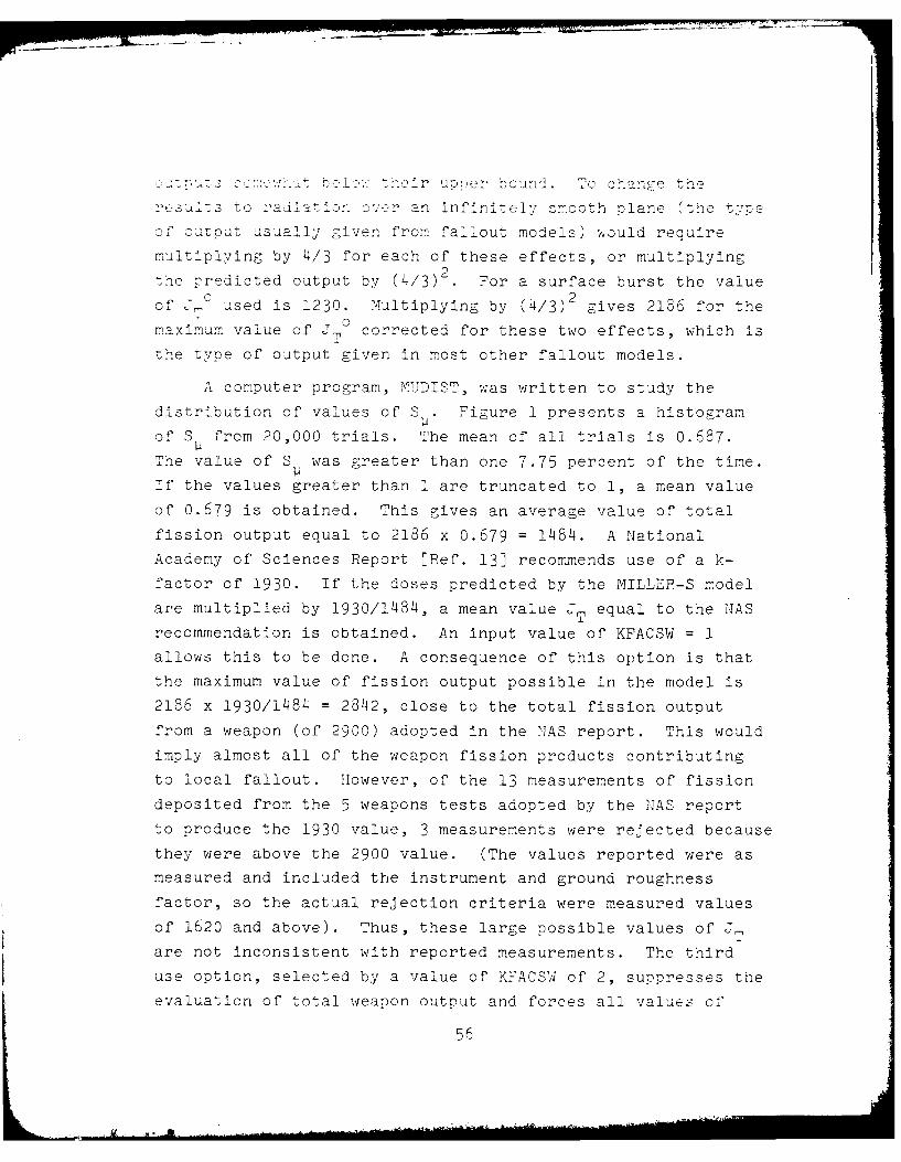
* '., .t ... . - . - - ., .:- . . . . . -.... LI 5 - : = ' '

ne u IC) -,r bc un. To chan-e the

esa 1s To V 'adia1an o': r an infinitel>, smooth plane (the t....e

of output usually given from fallout models) would require

multiplying by 4/3 for each of these effects, or multiplying2the predicted output by (4/3) For a surface burst the value

2.of J_- used is 1230. Multiplying by (4/3) gives 2186 for the

maximum value of J, corrected for these two effects, which is

the type of output given in most other fallout models.

A computer prog-ram, MDIST, was written to study the

distribution of values of S . Figure 1 presents a histogram

of S from 20,000 trials. The mean of all trials is 0.687.

The value of S was greater than one 7.75 percent of the time.

If the values greater than 1 are truncated to 1, a mean value

of 0.679 is obtained. This gives an average value of total

fission output equal to 2186 x 0.679 = 1484. A National

Academy of Sciences Report [Ref. 13] recommends use of a k-

factor of 1930. If the doses predicted by the MILLER-S model

are multiplied by 1930/1484, a mean value JT equal to the HAS

recommendation is obtained. An input value of KFACSW = 1

allows this to be done. A consequence of this option is that

the maximum value of fission output possible in the model is

2186 x 1930/1484 = 2842, close to the total fission output

from a weapon (of 2900) adopted in the HAS report. This would

imply almost all of the weapon fission products contributing

to local fallout. However, of the 13 measurements of fission

deposited from the 5 weapons tests adopted by the HAS report

to produce the 1930 value, 3 measurements were rejected because

they were above the 2900 value. (The values reported were as

measured and included the instrument and ground roughness

factor, so the actual rejection criteria were measured values

of 1620 and above). Thus, these large possible values of JT

are not inconsistent with reported measurements. The third

use option, selected by a value of KFACSW of 2, suppresses the

evaluation of total weapon output and forces all values of

56

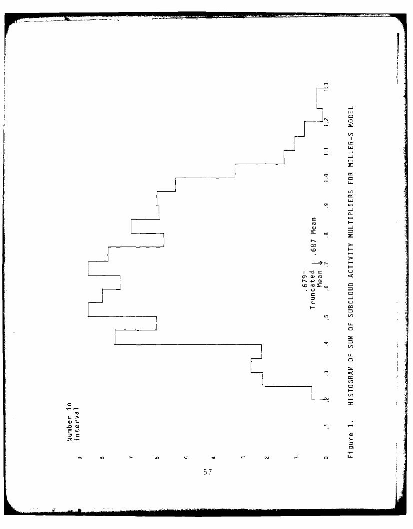
-JClU

C)

-J

* C)LL.

Ln

-AJ

00~

SI-

L)

C

S- >

sI-

co cCA

C5

.,:l eapon ouzp. t to 13 . util n each subcloud_

:ission product mui-ipiier by 1930/2 u . Thus, a variation

bt'ween subclouds is allowed while the total weapon fission

output is at the standard value. A selection by the user of

one of these three options should depend partly upon the users

viewpoint of an appropriate value of a k-factor and partly upon

the context within which the model will be used.


The summary of Volume II of [ ef. 9] defines the model

through a description of the 40 steps into which the calculation

is divided and forms the basic documentation of the model.

The algorithms in the computer program are a straightforward

implementation of these steps, except for Step 12 which per-

forms a numerical integration through the specified wind yield

to find the locations of the center of each subcloud. The

integration is achieved by using the wind speed and direction

at the start of each altitude step, specified by the height

increment DELZ, and the time spent in this altitude increment,

computed in step 11, to find the travel in the X and Y direc-

tion in this altitude step. The total travel is obtained by

simply summing the increments. The wind speeds and direction

at each altitude are obtained by linear interpolation, in both

time and altitude, from the nearest values available from the

input data. Modifications made to the original program are

described in Section E of this chapter.

2. Program MILINT


This program is the same as program MILLGD except that

the parameters are input interactively from a terminal in

response to prompting from the program. The elements are the

same as for program MILLOD except for the input subroutine

58

v;hirh is called 'ILIT. The usual convention is adopted for

the various types of program and run elements.


Program operation is initiated by adding the element

P9.QMILINT to the run stream. Since all input is interactive,

no input data file is needed. The series of prompts are

self-explanatory to allow effective program operations. Output

is saved in the file element *Pq.DOSFILE.

c. Algorithms

The same algorithms as in program MILLGD are used.

3. Program HEXGON


This program is the same as program MILLGD except that

a number of weapons at different locations may be input.

Although it is not an essential limitation, the program is

currently restricted so that all weapons are described by the

same parameters and all winds are the same. The subcloud

parameters for each weapon, however, are different and are

obtained by a different string of random numbers.

The parameters defining output of each weapon are stored

in the main program. For each weapon there are 305 values

stored. The maximum number of weapons is currently limited

to 50, thus 15,250 storage locations are allocated for this

purpose and represent a storage requirement in addition to

that needed for program MILLGD. Since the input of weapon

locations is in the main program, all subprograms and all

block common is exactly as in program MILLGD.

59


The operating procedures are exactly the same as for

program MILLGD except that a set of input lines describing

weapon locations are inserted before any other input. These

lines are as follows:

Line I - Number of Weapons

Variable NWPN

Format (15)

The number of weapons is limited to 50 or less. If the

value of NWPN is input as 9999, then 50 weapons all located

at the origin are assumed and the fission fraction of each

weapon is divided by 50. In this case no further weapon input

is needed. This gives an approximation to the expected dose

from a weapon.

Line 2 - To NWPN + 1 Weapon Location (1 . NWPN . 50)

Variable XWPN (I), YWPN,(I) I = 1,50

Format (2F10.0)

The weapon location is in relation to the origin of the

coordinate system. The same conventions for the grid and

weapons as described for program MILLGD apply.


The algorithms implemented are the same as for program

MILLGD with the exception of the following additions to the

main program:

(1) The subroutine SUBCLD is called for each weapon andthe parameters describing the weapons are stored.

(2) For each grid point, the X and Y distances for eachweapon are computed. For each weapon stored,parameters are placed in the common block /SUBPAT/,and the subroutine XYDOSE is called. The doses forall weapons are summed and reported as the dose atthat grid point.

60

C. SPECIAL FILES

1. Block Common Procedures

The common blocks for the >ILLER-S programs are entered

by the Univac FORTRAN INCLUDE statement. Those blocks are

in the element P9.INCOMM made available to the MILLER-S pro-

grams by the System PDP processor.

2. Plotting Programs for the Hewlitt-Packard Plotter

Several programs have been developed to allow plot~ing

fallout patterns on the Hewlitt-Packard 9862 plotter used in

conjunction with the Hewlitt-Packard 9830 terminal. The

Univac program TRSGDS transforms fallout grid data into a

format usable by the H.P. calculators. The input file element

*P9.DOSFILE is transformed to an output file element *P9.HPDOSP

which is later transmitted to the H.P. calculator.

All grid points with a dose less than a specified value,

currently 1 R/hr. at H+l hours, are deleted in the transfor-

mation. The element P9.TRSGDS includes control lines for file

assignments, FORTRAN compilation and mapping. The element

P9.QTRSGDS does file assignments but uses the absolute element

P9.STRSGDS for execution, by-passing compilation and mapping.

The plotting is accomplished through the execution of a

BASIC program on the H.P. calculator. This program is stored

in the element P9.HPDSPT. To accomplish a plot, the BASIC

program HPDSPT and the grid plots HPDOSP (these data are in

the format of BASIC data statements) are transmitted from the

Univac 1100 to the H.P. calculator, compiled and executed on

the calculator.1

'A simple way of effecting the transmission is to enter the Univac texteditor with the element P9.HPDSPT and P9.HPDOSP. The corand 7! is givento the text editor by depressing the fQ key on the HP calculator and againdepressing the same key after transmission. The instructions ?OiTand R9UNexecuted on the calculator will then acconolish the plotti i n order toachieve a plot without distortion the ratio of total dislistance I rervaIto total Y distance interval on the plotter bed should equal the ratio ofthe rariable NGDX/:NGDY in the program. MLLIGD.

61

3. Wind Processing Programs

Daily wind reports are available from Global Weather

Control (GWC) on a grid of 1840 points covering the :orthern

Hemisphere. Wind speed or direction are reported at 700, 500,

300, 200 and 100 millibars for each point in the grid. A set

of 12 historical winds, one for one day of each month, have

been selected by R. Mason of Command and Control Technical

Center and collected into a set called "most probable winds."

These winds are stored on the 1100 in a file called

LASH*. :ASO N-WINDS.

The program P9.LEVGRD selects the winds for a specific

month, interpolates from the GWC grid to a 2 degree grid

covering the United States, and writes the resulting winds at

each level on an output file element. The file element is

defined by the element P9.PLEVGRD. These output winds may be

listed to select appropriate real winds for input into the

MILLER-S model. The grid conversion and interpolation routines

are the same as described for the element P12.RAWGRD.

D. EXAMPLES OF PROGRAM USE

This section presents the results of several executions

of the MILLER-S model over a 28x20 point grid. The H+l dose

rate in R/hr. is presented at the grid points using the

following scale:

Blank less than 1

1-10A 10-20B 20-40C 40-60D 60-80E 80-100F 100-150G 150-200H 200-300I 300-400J 400-500

62

1,000-10,000

Figure 2 pr esents the results of a run of the MILLER-S model

on a five mile grid using the program MILLGD for a set of weapon

parameters and wind data which are given in the users manual

of the model description. The weapon yield is 3.4 MT and the

fission factor = 0.217. The weapon is surface burst at ground

level. Wind data are input 7 times, from -4 to 21 hours, and

at 35 altitudes, from 0 to 99,000 feet. The following table

shows the winds at time 0 at 10,000 ft. intervals.

Alt. (Kft.) Wind Speed (mph) Direction (deg.)

0 22 50

10 23 100

20 12 140

30 14 170

40 46 220

50 29 240

60 17 80

70 30 90

80 48 100

90 48 100

As can be seen the wind at ground level is blowing to the

southwest and gradually swings clockwise with increasing al-

titudes until at 50,000 ft. altitude it is blowing almost due

east. It then suddenly shifts and blows almost due west.

Recalling that the positive X axis on the grid is to the east,

and the positive Y axis is to the north, one would expect fall-

out to be deposited in the two quadrants above the axis. Figure

2 shows the deposition with a five mile grid spacing when the

model is run with a standard seed. In these runs, the original

method of measuring J 0 is used. The total weapon fission out-

out is 1350 R/hr./Kt/miles which is 0.6275 times the maximum

63

of 21'. in .isure ' the same -iaTon is -resente; 'n ra ten

mile grid to illustrate the total extent of the ienssition of

doses above I R/hr at H+1 hours. In Figure 4 the same wea:on

is presented on a one mile grid to illustrate in more detail

the region near ground zero. in Figure 5 the WSEG-10 biological

dose is shown on a five mile grid. The letters indicate dose

in Roentgens, rather than Roent-ens/hour, but for the same

numerical ranoes.

The fallout patterns in the .,ILLER-S are obtained by sum-

marizing the doses from each of ten subclouds. The following

table gives the total fission activity in each subcloud and

the X,Y coordinates of the center of its subcloud. (Since the

subcloud may be assymetrical, the center is not the geometric

pattern center but the center of the subcloud coordinate system.)

Subcloud Activity Subcloud X Coordinate of Y Coordinate ofNumber R/w r/Ktfile 2 Center (Miles) Center (Miles)

1 10 -0.8 0.22 20 -3.3 o.43 165 -7.7 0.24 64 -54.8 22.15 661 -4.5 48.06 212 -7.7 63.17 74 -12.3 65.68 37 -153 65.59 39 65 142.3

10 68 -207 56.0

Figures 6 through 10 present other runs with different

strings of random numbers where the subcloud parameters are

different. In the runs the total weapon fission output is

1527,1814,1435,1360 and 678 R/hr/Kt/miles 2 , respectively.

Figure 11 is a run for the same conditions except that the mid-

range values of the various distributions are selected.

A set of runs was made with a wind of 15 mph constant in

both altitude and time blowing from west to east. A surface

burst 1 "T weapon with a fission fraction of 0.5 was chosen to

64

.!ven in the Fallout 7iodification 1erort. Fi-ure 12 cresents

the pattern on a ten mile grid. Figures 13 through 1_ present

a set of another six patterns generated under the same condi-

tiors as the "observed dose." In these runs, the k-factor was

1916,1122,1112,1327,1124,1373. Figure 19 presents a pattern

under the same conditions as those just presented but usino

the 50th percentile value in a non-stochastic run of the model.

A set of' Fi-ures is presented next to illustrate the

effects of increasing wind shear. Figure 20 presents the

observed dose patterns for a 1 MT weapon with a standard seed,

as in Figure 12, but with 15 mph winds which at 0,40,60,80 and

100 kilofeet is 270 degrees, and at 20 kilofeet is 240 degrees.

Figure 21 has the wind at 270 degrees at 0,60,80, and 100 kilo-

feet but at 240 degrees at 20 and 40 kilofeet. As is seen,

these patterns are not too different in gross shape from those

of Figure 12, but are inclined at about 30 degrees once the

pattern is about 50 miles downwind. In Figure 22 the ground

wind is shifted to southeast and the wind at 60,000 feet and

above to north. The angles are 300 at OKft, 2400 at 20Kft, 2400

at 40Kft, 1800 at 60Kft, 1800 at 80Kft, 1800 at iOKft. Although

the effect of the ground wind shift is evident for small down-

wind distances, the pattern remains surprisingly like Figure

21. In Figure 23 a significant change in direction between 20

and 40 kilofeet is introduced and the pattern is markedly0 0

affected. iere the wind directions are 300 at OKft, 270 at

20Kft, 2100 at 40Kft, 1800 at 60Kft, 1800 at 8OKft, and 1S00

at 10OKft. In Fivure 24 the winds of Figure 23 are repcated

except hat the wind values at 20 and 40Kft are interchanged.

The pattern switches from concave to convex in overall shape

with this change in winds. It should be remembered that this

progression of wind direction effects is for a single set of

weapon parameters and strinr of random numbers where, for

example, the subclcuds are oricrinated at the same altitude in

65

e c<o these calcu iti ns. To iII;Ztr te the Iif'erences

which miht occur from a Iiferent draw of random numbers,

Figure 25 repeats the wind conditions of Figure 23 but with a

different set of random numbers.

Daily meteorlogical data on a grid are available at 700,

500,300,200, and 100 millibars which can be equated to 10,20,30,40, and 60 kilofeet measurements. The MILLER-S model was

used with wind input at these levels plus a wind at C Kft.

equal to the wind at 10 Kft. and the wind at 100 Kft. equal

to the wind at 60 Kft. added. Winds selected from the set of

most probable winds of R. Mason for the month of October were

used to try the MILLER-S model with representative real winds

available from gridded meteorological reports. Figure 28 pre-

sents patterns from an October wind over Washington D.C., which

was selected as typical of the many locations where the wind

direction was quite constant.

The winds as a function of altitude were:

Altitude (Kft) Speed (mph) Direction (degrees)

10 33.0 249.1

20 71.2 241.2

30 117.9 247.1

40 124.1 249.6

60 69.3 245.5

The wind reported was in knts but was used as miles/hr; thus

the actual winds were even a little higher than those used.

In order to present more of the pattern, Figure 29 repeats the

calculation on a ten mile grid. As can be seen, with this high

wind the value of ten R/hr at H+1 hours extends as far as 300

miles downwind. Figure 30 presents the same condition for a

different st_ ing of random numbers.

The winds at Stockton, California for October were

selected as representative of a different extreme, low wind

66

1zet and S1-ni i ' nt ch n-'s f :inl direction w t ,

The winds in this case are c-iven in the foilowin7 ta'!e.

Altitude (-ft) Speed (mph) Direction (erees)

10 5. S 192.20 4.3 125.930 1.1 295.540 15.3 247.660 9.3 273.0

The resulting pattern is shown on a ten mile grid in Figure 32,

and for two other sets of random numbers in Figures 33 and 4.

As can be seen, a degree of variability comparable to the

patterns in Figures 2 to 8 is obtained.

A series of calculations was made for seven 1 MT weapons

with a fission fraction of 0.5 in a hexagonal pattern. Figure

35 shows the patterns obtained with a 15 mph constant wind with

the distance across the hexagon equal 20 miles. Local regions

of higher dose are still evident here. In Figure 36 the seven

weapons are in a larger hexagon, with the distance across the

hexagon 40 miles, and for Washington, D.C. winds. Figure 37

shows the same pattern for Stockton, California winds. It

should be mentioned here that if the stochastic features of

the MILLER-S model do in fact represent actual variation between

weapons, then these figures present a view of the fallout

patterns downwind of multiple bursts which have not been

previously seen, either analytically or experimentally.

In Figures 33 and 39 the patterns represent the results

from 50 collocated 1 MT weapons with a fission fraction of

1/50th of 0.5. They are for Washington D.C. and Stockton

California winds. These patterns approximate the expected dose

for these wind patterns. However, with the large weapon to

weapon variation, the meaning of these expected doses must be

carefully interpreted.

67

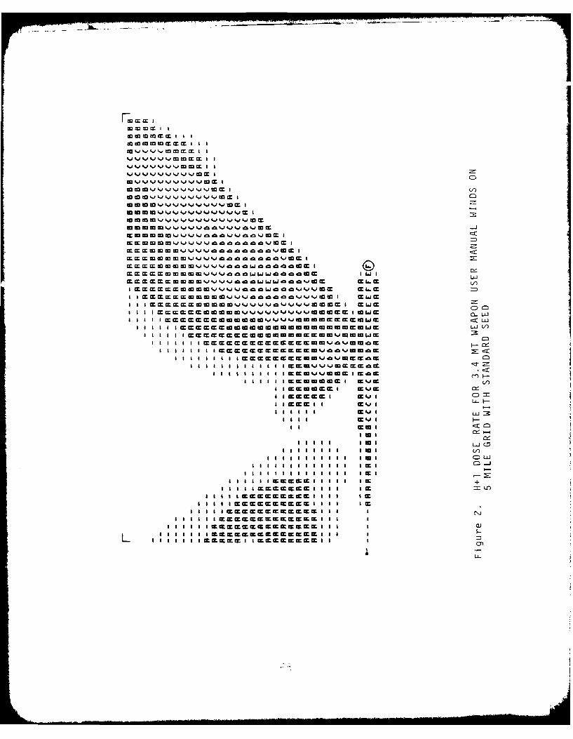
0m to cc m I I(

0 3mtmm' ~ I , = I I

E~ mmm ~ ~JI IE m m m m ~ J~I

E~mmm ~ a~' JmC)

amIE mmmM Mw k 4 * onavvv ccI. ~ Ew ca~~~~~ aaa E mm m m m a mwE

am~ ~ ~ ~ ~ ~ ~~: acmE~mmm.~JmmE~LJ ua a a aaEEEE~mmmmmmmmmmmmm~l0J WLL

a a a a a a ama M M~ i cfj cLa a a cc ccE M cCcI cc V c

a IsEmEEcI ccs IC

aaCaa LJ

Ia IEmcccc accIaII II I xmcmcccc iI I a W a

malammm m mm'aaaaaaa wlctwm .T ,a

......

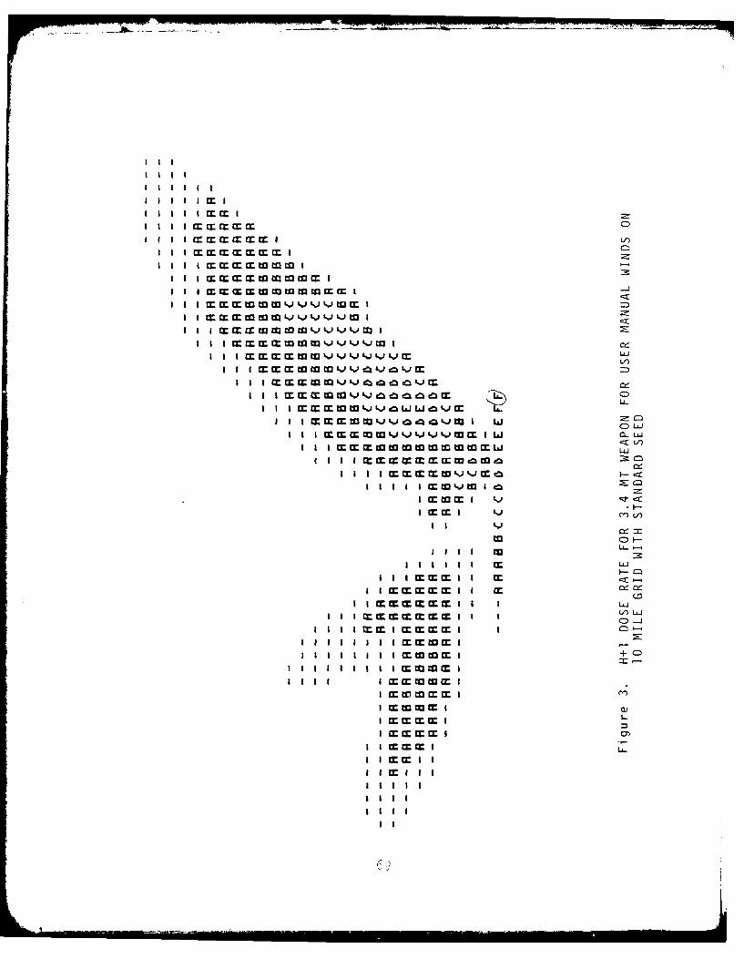
I ICD

I I

I I CC-I

I I LU

LL.

I IL C)LL

I I m m o M4 --

I~ ~ I m I JV'." J

LL.

II toI

mIIL0-

I I I ccII I z

I I ccc mIII I LUJ

l I I m lImmm l I )-i

IIII I~ ~ I U-t

I I I I t om I+C

I I III 3

I I I=M I

I I m

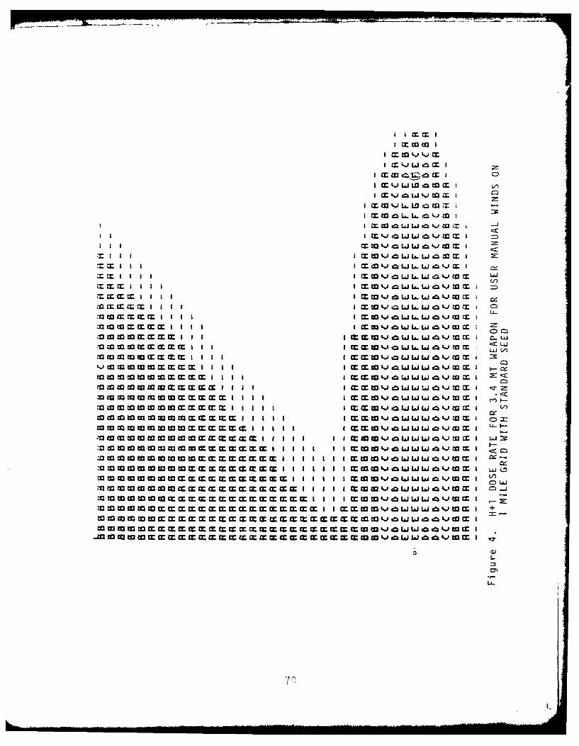
I X.jLJ z (Z

M L.) jLO cm O cti

I X . ZLJ , tOM

M I A LAtW 3% -

w 09 i-wc I M

(J

~~~ M M k.)~ L J~~

~lL~rI MI w S.0

x ccMmI I f w L. cznI WL- 4Li m i C

tmI I I L. in W 6 tA J W MtjW M i

SI M M W W Wcit. -LUm Ajc I I& I gm L.JL J J MM cc

~L I I)

II I. cm IW ~ ~ W z&.

I tjc I W W Iz LL.~' J M

mm m m mm m m I I I I : C

~ I I II ~ ~ taJ ~ 1~ I LL

~~W~~E~~cI I= I. ~

mm mmm~mmm r.EI m iI I I I I w~4w wcLw w-i

m m m m m Imm m m m m I I I M m 4% go ww l5 J I - X:mm m m m m m m m m m i I M~wjcww cj w I-+

-MMMMMMEMMMMMMMtaJmmw'.Jsmw~iz I

LL.

70

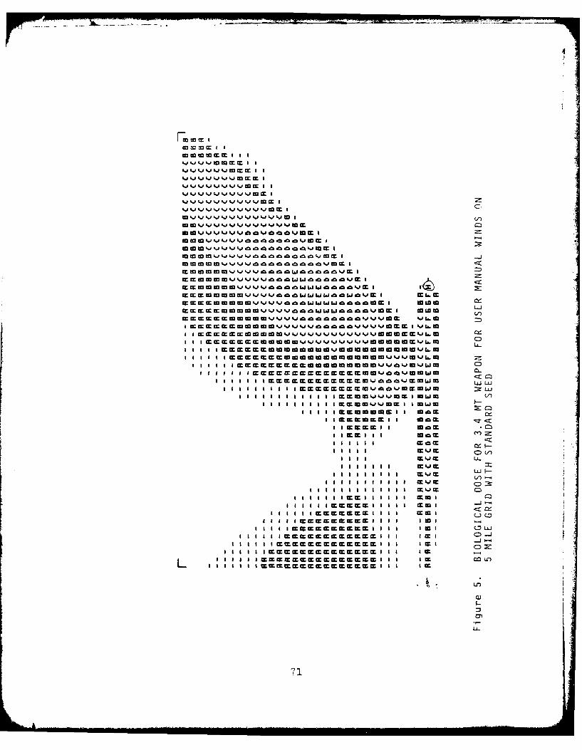
to w 03 c I I

VLJ V JL iM

CA ddo Ao v E I

v~ m m w U 4- v .IV A AA Aa w

I' nA vE mnn J i I U.ZM

m mwwwW I t0%PvC a aA j0mI am IEEi innnnnnnnnnnnn iUL Q

a~ ~ mm cc IIIIII I E E UWW : rL

I I I II 1 1I IEExwwVJEI IL.J*WI

asM MIC IaEiiii~ I wAc

Icccc I I a A EUJET

cc=11 I I A mJ

11111~c EE E EI I m

II I E E E EI IaI I I 4 C

IIIIIIIEI IEE iEEEEEEEiI iI I tz

Lc = cM M I: I: IEE IE IW W In I

I II tc mmcmccmI iI I( LU

71C

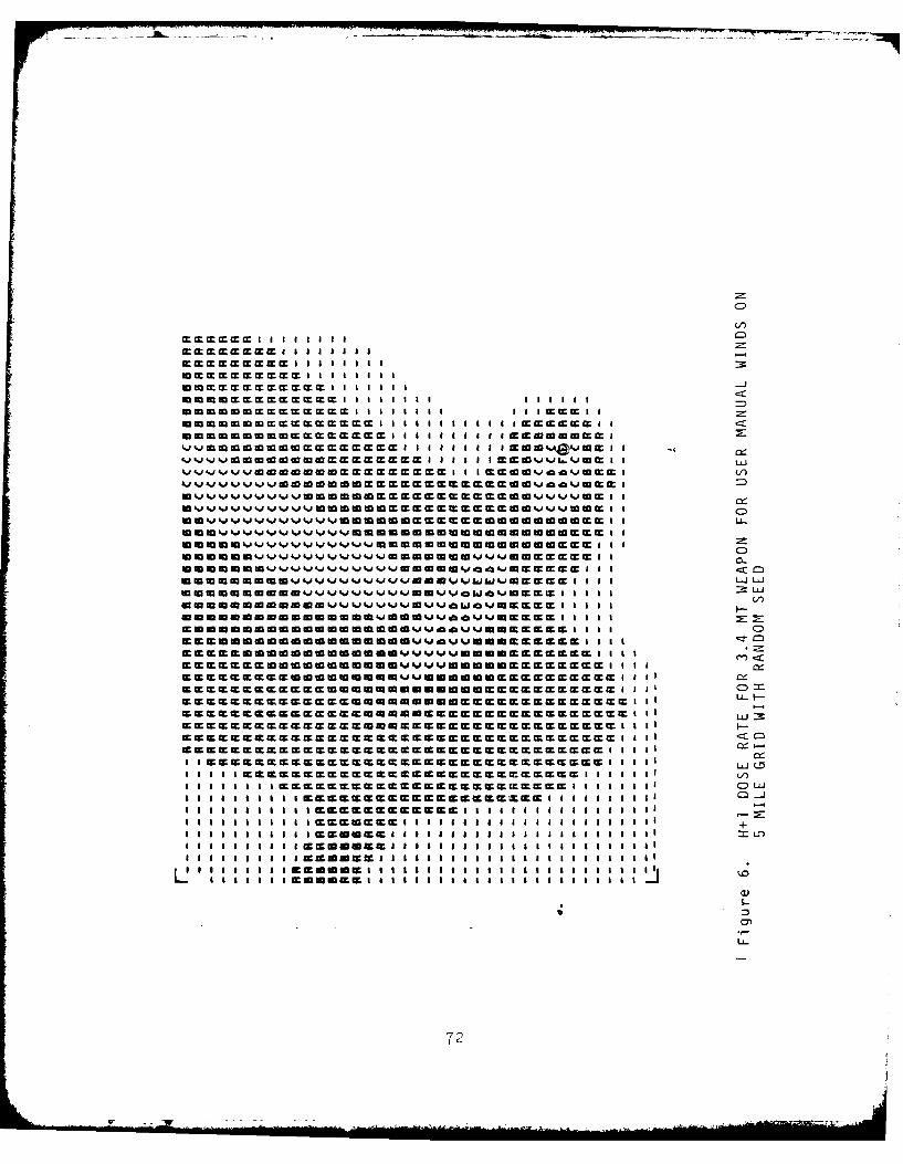
EE EE EI I I 5 £ £ I I Z-

mom= MMM=MMaMaaa ma &&%j mEa

*mmmm E~aa aaaai aaaE E~Ca*mm..m~~~~ai a aaaa-mn~

WOW 00 MWWUV4 EEW a aI a IEELJJh.'wLaminmmwm~ E~a a

~~V)~ aCa

*winm EEE~~ inJ~ '.,m ~ af

I mmmm ~E a .LL M IIIIII a Im I II II I I 'J.ICWM M I I5 J J~~ a I a I a

I II II II m mOW. m. a a a a aI I mImI I I I I I IJs.,mEcEca a a IEmmm mmi mm mm m mm m EE a as IIIIIIIImm mm .mmam mm m .D UU E EE. a a 1 a

~mmm mmmm mmmm ummm m~ aa a

Emmmm mmmmm mmum ~ EE aa a

E~E~ in~ mU U~i~ in mmE E~E a 7a2

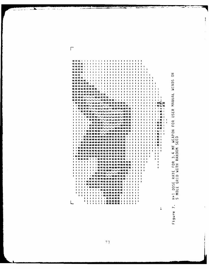
Em~ CC 11 £cI III II1 ill 1 1le111

m cr I I I I I Ia I I I I a I I I I i I I I I I I I i

4c~~ ~ ~ ~ c ccI cc I I I I I II I I i I I I I I I I I I I I I I I L/te c m m c m I I I I I I I I I I I I I I I I I I I I i I I

9 = c m J 1 0. J ' . Ji J m E E E Iai a t c c I Ic c I I I I I I I i I I I i

I Ic m to 02 J v dommminElaivi io i m i m i m~ Ia

I I IEE ccJW JIEm mwkvtowww .cVtoccc II I I I I I I I I amI

IiIiE .J a . ~ % m IiI I I I I I I I m ccI I I I IE I~~~.LJ.~.m~ Ii I cc I CD in

I I IEE IiiI~n~ I I =cc I L.I i I I iiin ~ Ii i I do mEm I

Iam c mc Mt i iEkii v M0M c .m cI I I I I I I I I EEI I

i i i m iEE totow t Mw c c c =In0 I I I I I I I I I I ccI cI a I I cc ~ n . '. W E~ ic io io i ic M i am =8 IIIIIC L

Ia Kct I I *c EEEEEmcc I I I I I I I lIi I E I I E I EEEEEEEEIccmI I lII I I Il~I IE E IE E EE E E ill I I I cctim cc w ic I I I I i I C

i I EEEEEEEEEEEEEI i i I I I I I I L

lEE EE E E EE i In i a I I S I

liiiv mcmi II I iE E E E E I lI I I:ii IllI wmEEMw n McW.W E il m ccI IIl Ii I =C=MCMCICCCc I t E U I .J EI I I I I Ia I aIo .c cmC cc ix m i IEWn',J . mW.I IE IA I I I)

i I cc Cc cc W. cc ccEccc I I I I iIiiic c cc W.EE UEccWE I I I lII III I cc ccEEEEE ccEIEIE Ii I I I +A

i iI I I I I I ccEcEcEE W I I I I I I II ~ ~ ~ ~ W I, WW I i i E EIC I I I

S.-

73

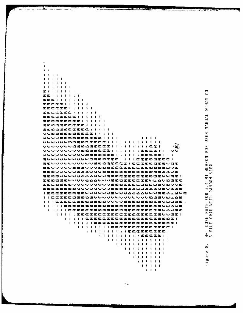
crI I I I I II I I I I I I I IC

MM1111111 V

m m cm I I I I I I

Mtmert ill il

mmmmmmmml II I I I I~x

mm m mm mliii 2

&.V W W M MM I I Ii

Im ~ mmmImI a am L~~~~~~:r (m I I I I

m w v &j vc m9 0vvw wwmm mmmm cm I t.) m Wi .I

m w dAvvvwww mwVLL m i wm C

II I I i EEmwmwwwmmmmmmEEmvd'JEW

a Ii lEE EmmWmmmmWWEEEEEwvt.%JMI

I I I I IEEEEEEEEEEEEEEEEEEE '.JWE

CD -

II I I I I I I c Ec E W E EItc

I I I I I I I I I lEE EEEEEEilO

S.-

714

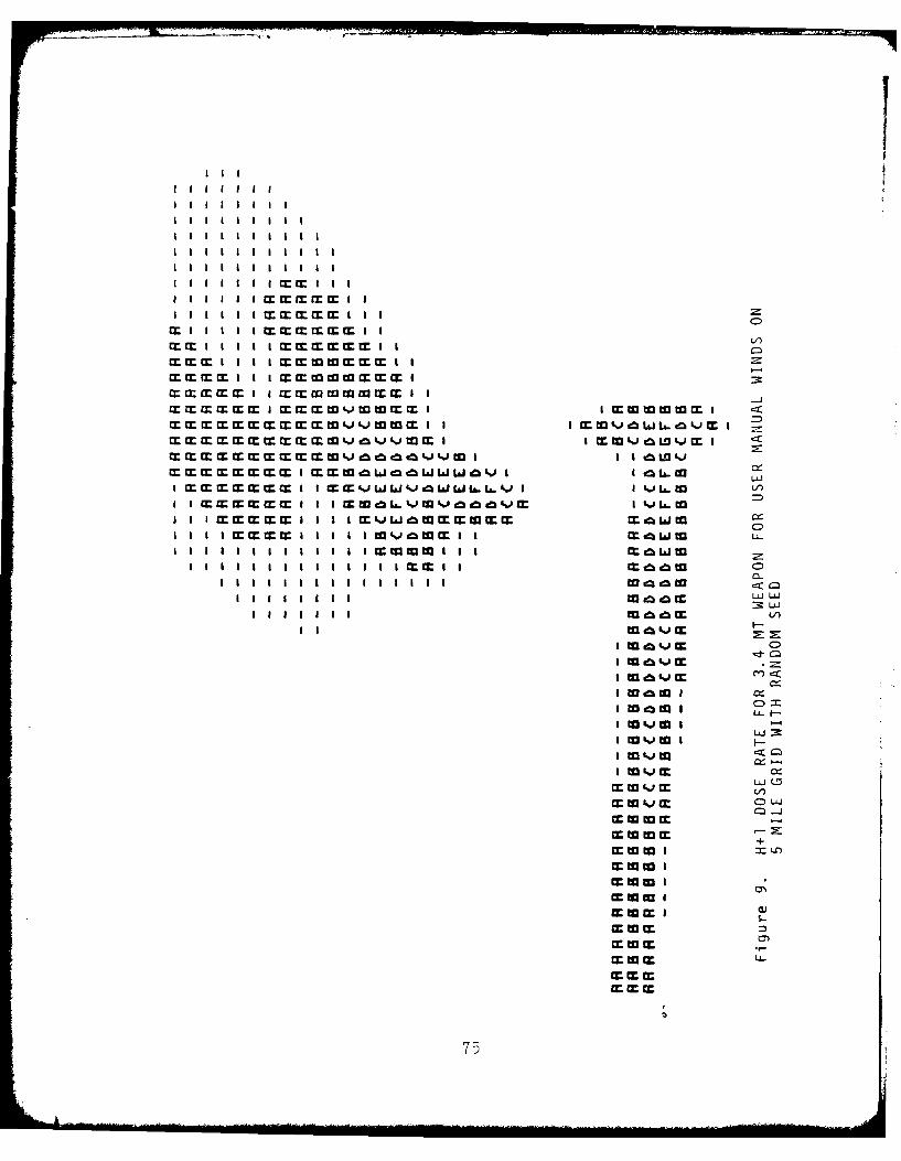
Milt11111mm i

I I I I I I I m m I m I I

IcI I I I I I ImwwEmI I I

mm m m m mw~ m I I M kWzw,-~v

SI I cMW 40

I mm m m I I ==j AjaLwit&I&tj I I ki L.

I Ilm mmmI I I m wz m w m e 1i0

I I E ~ E I I I I 34 zLJU

II I I ~ E I I I I I' mJmWI I cci, -U3C

03 m ImJ 0(

Ucmtil a t(

Lu-M

I %j

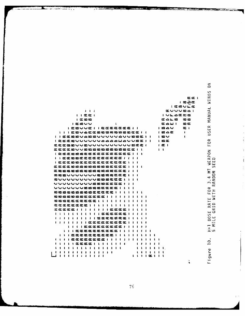
m Li t) tp Il cz

I ~~~~ ~ i c !Xok -c mwI t

M I W 1% . j4 . ~ oj Mg MAj1. I I I U3 MI i ~ m w I IW'.

li 4% IV4)ljw l I I I C

I r r m c I I I I VI II W rmt crm I I I I

mmmmmmc a a a

I ccmcc cm t a Il I II I +

1I 111111 IIMIX I I I I I I IL

(5)

~U-~

76+

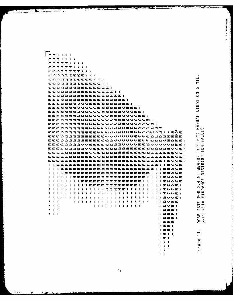
= tr a arcE I IIIII

mmmmmi aWII MM M M l a a

MIIM I MI MaM l

MMIMMIMIwIXMMM aO

mm m m tjj.M M w W M Iac

~w m " ~ 'ctm mwmmIl l 1)%)vvtovvvvm 09' k m a9

~W~aJCI rw w m wIllm kav v 0% v vv cma g v wm V

~L aMI a l ivv1, vvga mw4 l l _

V)C:

C: co

~ a Ia ~ a:'.")

I a a Ii aM M M crr m a I~~E a a a a m t) m oa a i a a a a a a a a ~ a a a a a a~'~''.'CC

a~~~~~~~~~~~ a to ii a aI '.'' LL

Ia Iaa a a a a a a a to 113 LLIa Iia aa a a I aII 103vW I

a to W 1:13aaa3 :1 a m IaL

I o om I aa~CD

I c MaI MIXI mcc

U-

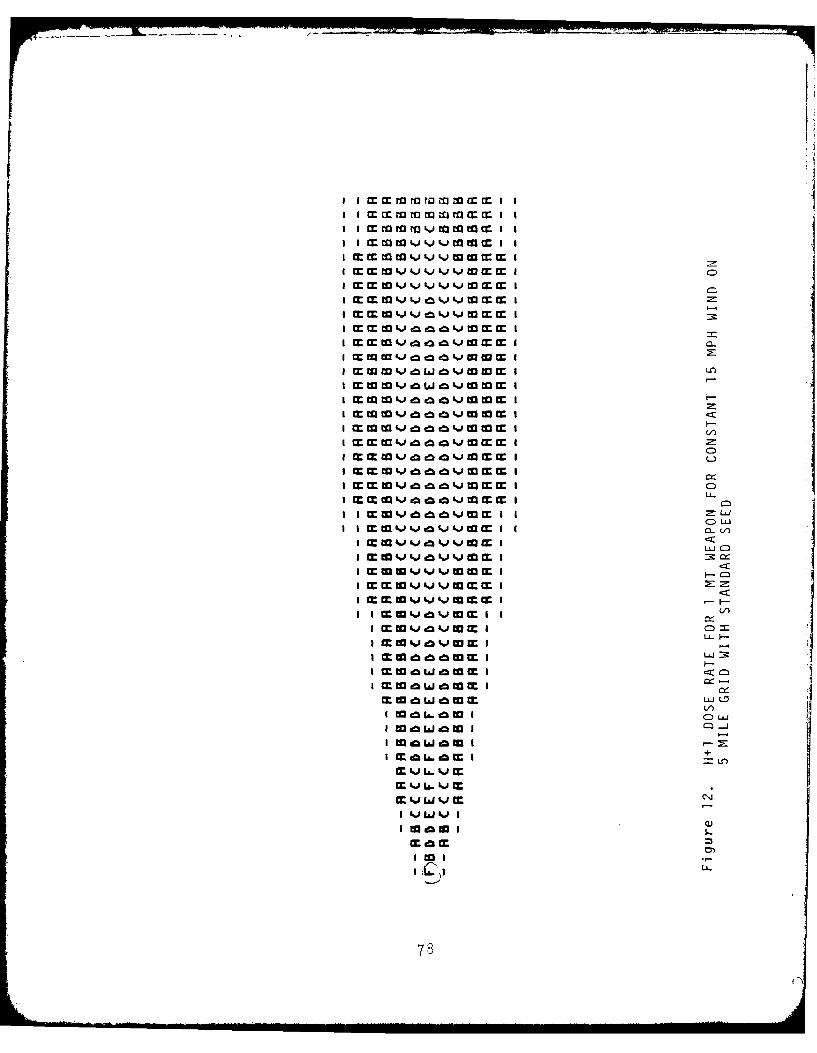
I m rrrrirrc m a. zI t ~

I LnI

m w Ick 95 LJ W w

I m if n mt I C)m m w * mc molimmm IL-c

TI w v t4 Lw~~JmCD m 'LJ

I m I

aw m I~~

l-~wI

aC L LJ

78

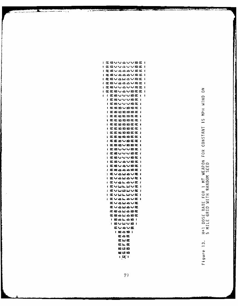
I m w zL)

I mwvoczovm II m . mw zt II e~ cm v w m I zI czLj&. I

I m m w . Q .)w I C)

I m Lt j w I

I m w ) %)Q I

I W i92F4w I

I m w 10so m wm IC

LL V

IF C IMV L.1 v I

I MVI.V I :

I~~~< cmJJ

I W t I -O

I LU~W I O

79'%w.J

M : LLrar Z TV fr.

I I m W to tamI~ I

I I Ifl m m I

I trmm I

I mmm II mm I II mm m I LO

mm m I 0n

I ccw WtoE I CI m~W w

I

I a-

I mmizw I

I mm m I

I mw~w II mm m I C

I m

I m &a fm

I. V L 9. ccEI

V-)CC to j a ccuj

S-

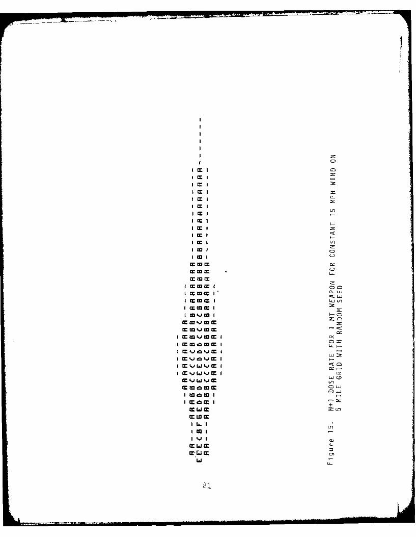
I m I

I CE

BEccB

IB

I U31

IEBoIWI03 0LIW0BcE w MC)c

BEWEI L(/

I W4j W I 1-0

B Ew j wE ccI E;m E w giwccIC

LL1

w m I 'JE;I m;L~E B% t

I to lz W.iE I

I;JE LA.

BILO1W 0-

Lfii

I m r rx mI I II I mrt rr r I II

I I t. m m fI I

llrrmcrr~l

I mmm I

I mmm I

I m m I CL

I ~WWLOmmmmc I

I EmmmW I II mmmI

i MWJW I C)a mw'imm I L

I LJ L

IF C)Iw

w w t%) w

I-0

I W vB oIL)L

I W k.i w 'jm toI

cr & 1 j' m ~-

cr ka c

I L13 IJL'J"J-

I cr. I I

I I cr rr_ II

I I mccmI I

I Im FrA II

mImr I~~ftI -

I trmrar I

I m rramc II m ti to m I-

I V)

I IW QaJ&mJ I Q- CL

I L::JWILL-

I m c wcmw I

I m~ w -~ o .

~LfL

"3

AO-AO* 517 INSTITUTE FOR DEFENSE ANALYSES ARLINGTON VA PROGRAM -ETC F/6 15/3oEVELOPM NT OF CIVIL DEFENSE DAMAGE ASSESSMENT PROGRAMS.(U)NOV 80 L A SCHMIDT DCPAOI-77-C-0215

UNCLASSIFIED IOA-P-1526 IDA/HG-80-2283 NL

I __-2 -E- u.

u N T

w 4% at jw j ~ t

I Mt~~t3 II mmgm 1

I M r 3 Er M II

I m E o mI I L

I m to t t mI II CC totaocI Ir o o t mI Ia

I m t t t mI I V

I m o o o CI II mIt t 0 mI I

I m toki o mIa a~w~mLa.

I m ov ocr

I cr a aC a La:: L i

I cmr w aok om L /I w ' act 3m I-rMI cc W 41t mICI cr a t ta M 3 V0 IIw.m M-OV0I~~ CCtV0-MIC

a LL.I tOw a o

I LbJ t. I -L UI L6v I D L+a~~C '-iwj

I iLO V

I w I

LO

514

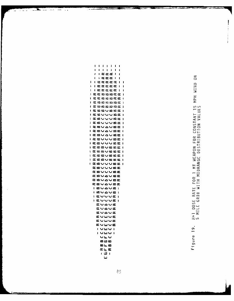
IlIllm I I

I IcmmI II

I mrmwm II

I M 3MWMC I -

I m I cc-

mmtL~nvm I :

I m w&' VLaM I

IL L I

I W&,immm II .;jtIjm I

IF < C

=LfL

Lv cch CC V

CL J

m v M

'-'+

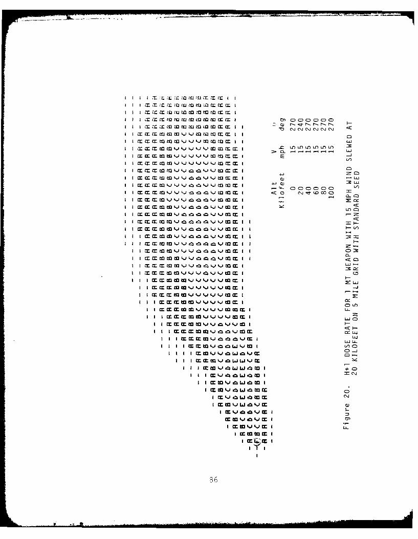
I I I I -T L- W M m M

II I X CE CUM JW3 M Mrl3(I Mi

-o J~ ~i(iC\JC\ CNJ

I x M C I- I~

~ L

II MIr f- t C3L t. I)Jl . ld to M MI -4-'

I m M -IJc m ' . L

M~ m~ Q 4 LJ, IzciLjL) M 14)c 3

I M m k.) . L) z-., QQ mMI i :-0 Ci-j . 0C

I I cr I oL) ckt= f ~ I

SI m Ccrt mkj &0JJcz Q .) j mm F- V

m mIc c 9 L) 1) m I

MI W Q4 Zdi 3MII

I M c IMtoVj %) z z JSo mI 83

I I ZC a0 JL ~ Zc , I I < cLUII I T aI L jt r

I C 3 J 4dL.Ik I I f L..,ki O M I

v 414Ik I ma:a~JI I +0 al .

I Im mWI Ij1. i V W m I u

I I~~~L~iLW

L U-

I~ IIma~zc61 0 nCI~c:) EA

I Im 3 i i L IIIL)

86%),W V

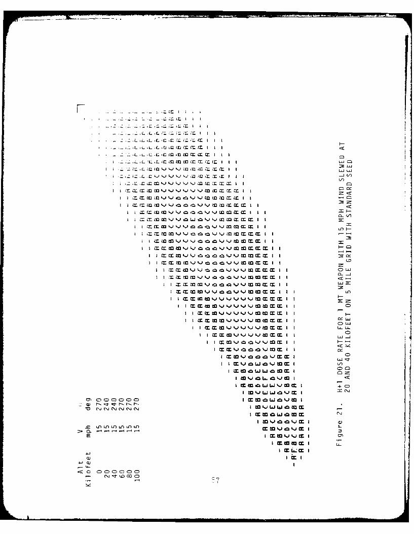
L. L .

F-L - a ElQ L Mrr M I I I

C - Cin ~ cc-XC I I I

-L L;i m f m fc- lr l I I Ic ;cIc ~ Jk);l.zi T I i W LJJ

k~j j k, Z do t ' ix I I I jVVI)

- V

4'. tt MJ O M I Im: =I I

n -

i= w tJ'.J acz9 9 dL' mm I cI I

I m L. LI-zC zc -1Wmmm IIMc

v 41-: Qt. &j mm I x

I L&J L.

-~~~~~C w -- r~r-r-m c'* m' c*.j k.0 (NJ k(NJ mm m I -

u -j

Io <

'+-c

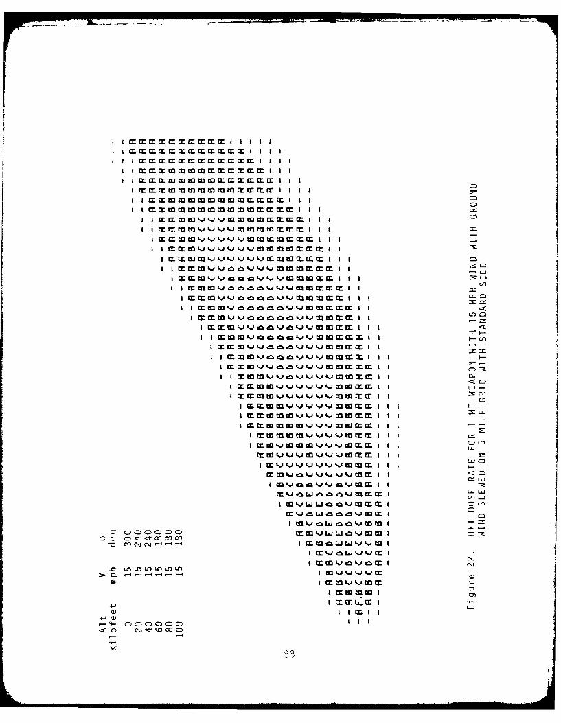
~ I I I~ I IM

I I W wW %% W n m 1kJk %jmw I I Q

I k . 4 g~m aL, go co t=

m it)t04jL)t I I

=-

a 4 % I ~ j m J%JW k) m I I I-

I a m IiVL 1 ~ t.1.0 v m w III

m jt 104. ~ % I I ctL7

V)-j

I~~~~~~~~ toL i aI IiWmmICm t. gma 5g ~mtj0

I a Ia c Jk

I m.Otoel ek I i

C U) IL LO~ LO Lf LO

E I m I a nmS

I m mWc I

4-)-ci I I I I

4- IWiL- ) C COCC

C~j <r o 003C

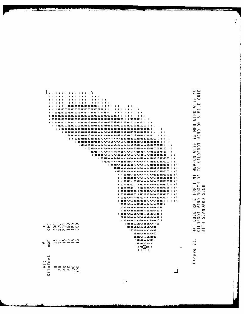
I III IIMIIM M MM IIII f LO

I1 t IIIIMM M I m IXIftIM M MII =

LC)

mw dam vv O w oIlc I I

I-IU

i IEW~~ mmmmJ%,I IJLwtmlw~mm EE wa I II JZJXmIZ I I Emi tli il m I tLIt m J' mom mI maktJmmE I I ICDa L

I ~ m ~ m E E ~ t t LL <

IQ CD ft

I M McJ'-jmWdmE ft I DI=I~ ~ CD~WW E f LLO

ft CD r-EE ft1

000 0 -61ot ni .it

I W. 'JJV.0 a JWaEmfI

I 1EEI m oJmw E It

IEWWW I Il I

EJ& ::t kD CftC-

iTI-

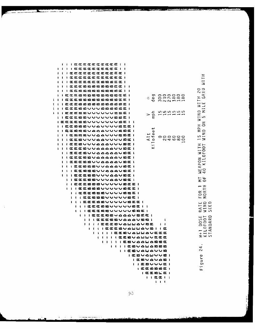
I I I I C E C CE C M C II

I I j

I am ocmmmm rmma V-C )C)C )C

I I I

I I m mmNJtj ot~ i jm I EL

I I m mm .) t O j i I I

I I m m 0k mL)tw j&JwmmICI I ji mIc ~ %

1 (VI~~~~~~~~~~~~~~~ I~ I4 mt m w -iIjc c ~ jww )C )C DC

I I mmmwvtwe m9 t mt m I .Jm mL-I I m mO m wk c n mtzdk im

I I I w m 4 aI I I m iIta mvwmI-JCD

Im w v kj 4 o I MJ:JC

I

I I lm m wj tj~ m lU

I I m m t tt vt w m ILICIIIM M Mi.V V I I M L

I Iiimm vjv v m l :v

1 1 1 W Wmm jmq ~ mm LA -

I I I I *E I tovI a 50 3t

I I I I M

I I I I

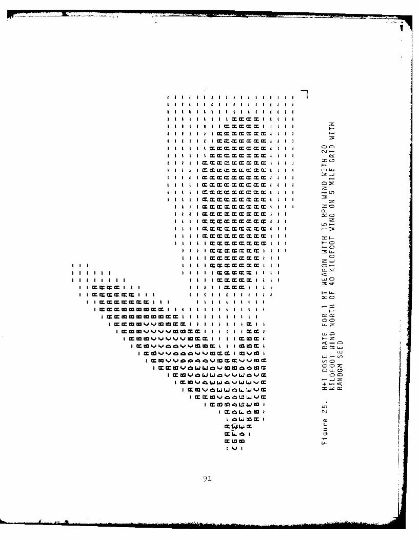
I, I-- - - - - ~ , I I IIELII I I II

I IBI BI I Ii 1 m t~ m I I II

I~j-1111BIMMIXIIXIMBX B -

=CO

I I I I I mm m m m I I I I -L

BlIll=MMM MMMBBB

II JM M IIMMX I I= :

B B B ~i B

IBBI IBI IBBm mm. m IB II C

BI I B I B I B B B I Bcm m I I I I :I BI I .I I I I II IBBI BIBB I I IB :

Bim mmi Wl BIBBBBB IMBBBBB

I IWMXIMM I I IE I I B B B B I~ I II I .B'.~~W~~E~M B BBBE B J

Biw 'smJ mmB B II II II

IMM ISIMMISI IX IBI B BII WI

IM MIIMIXMISI MIX I IIII ILUCD CD~

B LU

BC LL. C).J

CD11

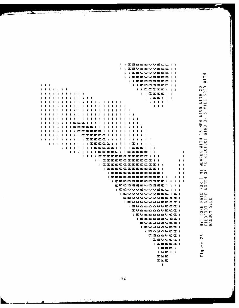
a~ I~ m m m m I I

I~~ ~ I I I~~f~~ I

I I I I I mm m I I I I I I II I IL

IIBI I I IIMMMIBBBBII BBIl =-F- C

B B IBI I BB M MI!IBI 1 1 3:LL

11 1 1 111111111111rA11111 IX I=-

111111 B MZIMBIMIIXII I I I C1 11 1 11 1111ZM MM IIM~ BIB ::B

Im m m m m m I I 1 B3 B II

1111111IMIIM IX B I I III ILL.I

11 11 1 IIMXIIMBSB M B1M:

I E XMMXI IT; Bi Bil I BDC:

I~ W~ ~ I B I C-U

I~ ~ BL - /

BWJSJIE I B)C:

B ~ ~I LL. C

B 9fjotLiLL mva I +UI

B mt~tm I

Cc L toLA

M 6. mE~

92

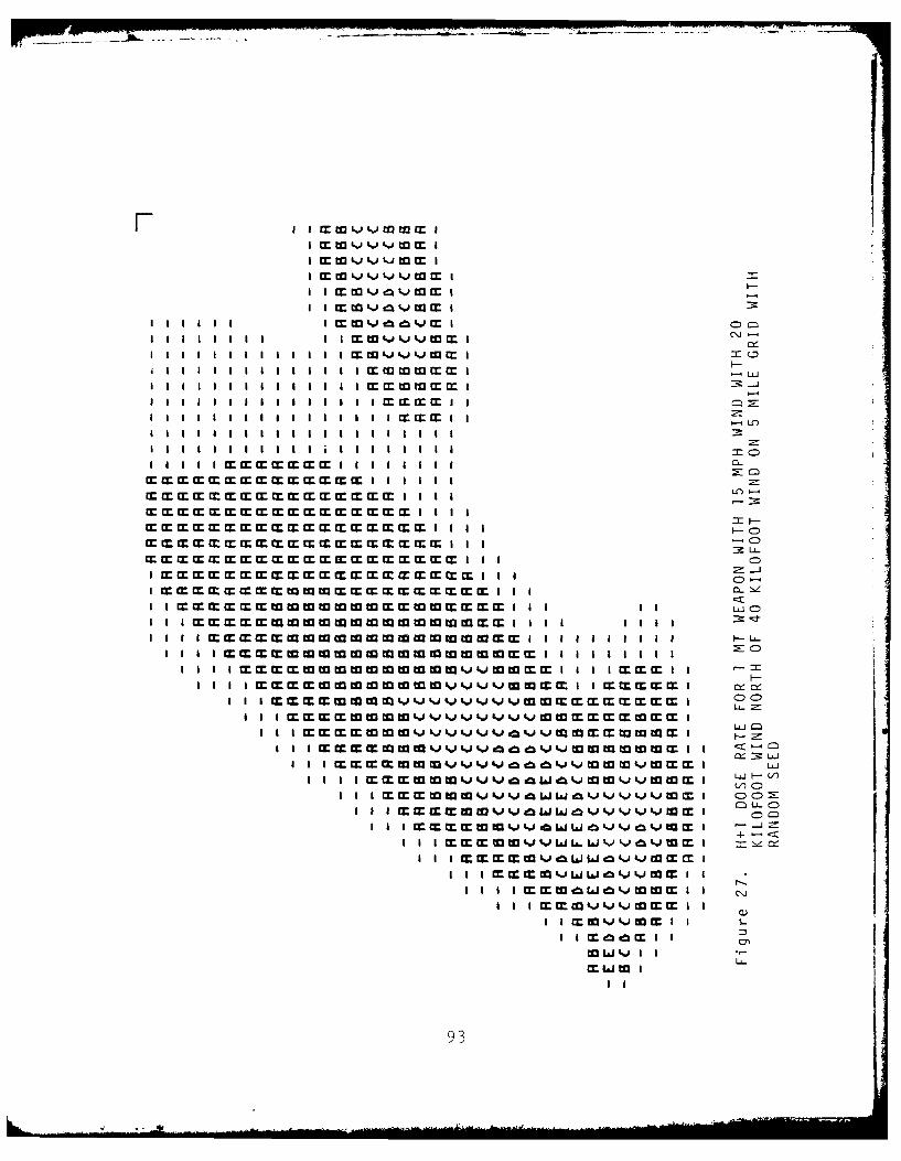
I m %)k)t JJw I

I m % a fmtrm )i

IIII I I CrW J W J I L

liiI I II IlIl I limmmI I

1 m I I I LO

i r r cc rm III I W ~ I I I I C

aua mmm mmmmm mmmi ala a ammmmmmmmmmmml l .mma l

a a ammmmmmmmma -CD

a a amm mmm mm mmmmmmla

a a ammm wwm mmmmmJmmmmElIa

I I i1 1m m -- LL

+ -

I aD atD M:

+ <

I I I l & g tjlt3 I I

I h wkj I

I I

93

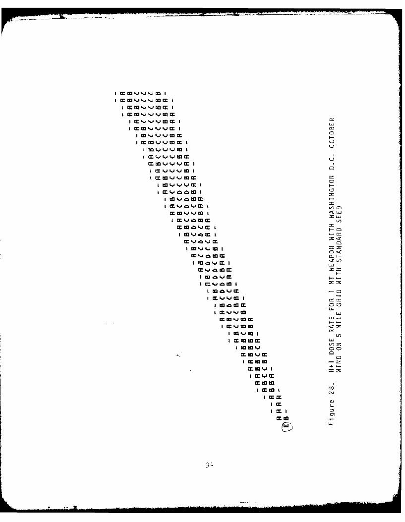
m L'J.) a I

JLA~JI 6 I

ki m m I

I m . w 4.

I M~'%W LL44UiI m wI-Ij j w

J'~J~CDIa*j w L i .

I to IJ.J 9 t

I m 1 f .. I )i

I M Lic omV

I to -% eit

I to 1% Iam IZ

I toatic

I cc Iw Jt

I mgtmC)C1

1 Mv~jtoLLu~j

m tok.)to

I to U ki CLC)

I~' M00J

m to t0

L.

I mto I

I m to Ir

1 cr

I M 3

CD,I crWmF

I =to I

I m ot

I M tO Cr C

I M 9d 0 1 -~

I mtom

I m U

I mIJ~ 03tIcrV L

10 Li M I :: In

I U3 cM

LLU

I~~ t~

0LJ

F- a

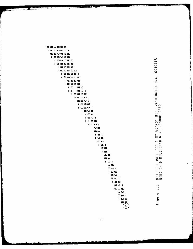
I m ~ ~I tot~j o cr (xLU

I M 3 O t c

I m M o

I ~wmtooI mtoto I

I cc mt

c0

I ccc upIV

I cc .tot

LUJ

I M . . F V

Ic. 4% 4-

II LU t

I--

I WJ I LfL

+J -

Im m

I Lai LO4%j o L

9V)

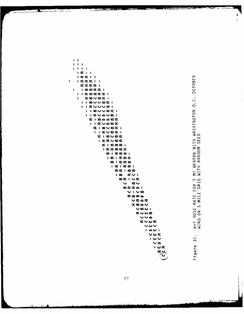
II

I tI I

I II I

t II I

I ioI

II II

m ok I vi

I I cc t 0 mI CM

I I otot

II-cdI

I C

-Z

I 3 I m U-7

IIU-I

a--

IIn

IW II U-

1 cmLa

S -

97

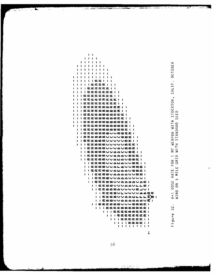
I I1 m cr I I I

I I r I I I L-J

III Immmmi

a a a mmwmm laI I lm mm wwwmm I I:I i mmwwwmmmi F-L

faia a wwwwwmaa ammmwwmwwmmli

I~~C ICZWW W~* M WW JVVJWWMI I C.FI I mmww vv v'jm l -::

I mm m~ vm cv w

I I mw vow vv m I C)(Im w vm" %V M I W J 'J WJ

I m w vmw d w I LU__

W~~ %JI LI~I 0

a a ammmwma C\J

1 c I I

95

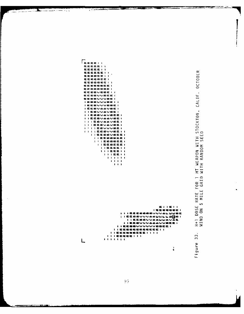
mcEEEEEBc I Ic

mmmmmE I I

mEmmmm I C>I

mmmmmmml Lmmmmmomm Ca

MMMMJWWMI Im mw 4. wm~ a L

IImw41a a w' m I

I a I w v J % w E a CI a I m cc wk .0 IIV)c

I I EWIJm.,IUJE a L

I I I w.wwwwwi V)

I I EEUEEII

I I I EE Ia

I a I =ccI I a

0-<

U-

Lu

a ~ ~ ~ c aic IEiU'a.a JI w

a I E E U E a aI

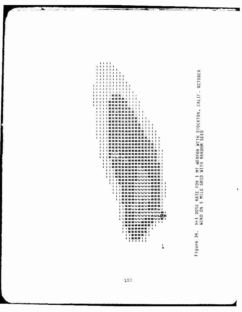
-lee,

I I I I I I I

I I I I11 M11 II

I11I I M mI ml CL I

I11I I m MM MI I I I FBI I I C C Mc c cI I I I

I I I I M MM M M II I I

I II I = Ztm t c MW.MI IIIC

I-* . M MW M M I I SE * E E I I C

mmmmmoEmmmE m I I I I IL

I I SEE *mom mEEEEil :3

mIE=M m mmmmmEEwm aIL

SI IE wEvin kJI mJS0*E I

SIfa oc I IW* . D* E

I I S ~ E*WMI'. % E I c

I I I EWE ~ J'.i~I ~LAJ.

1 E00'JIJEE -

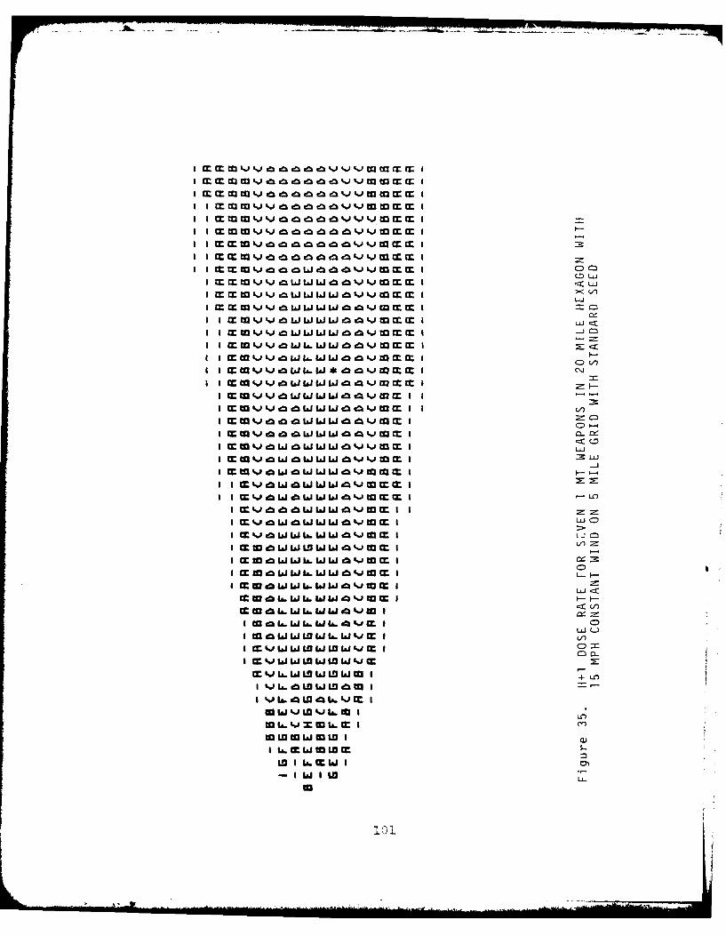
I I m w wL ,)g c nt i w eJm m I

I I m 3k c mt)&jt II I mm 3C- ckinc i m .) i mm

CLu

I I m w %.1% : wgma jm I ct

I I mWV DWA W&W ato m'.J I M: - -

I~~~C Lan.I.m

Z-1

I I w iJg 2cmwwwa4vw I t-L-

mI ii WaJI*.w w91Ito w m I LJ

I Mk toa &W w wCM.0 w I IZ

I Mki w&WwwI w ~m~ I LL C

I M % 2WW6WWLa %J W M I

a &WL wa w& ' a aaI W LW Lb.W 91.I&4 akJMIC

I~~L WW WLJ.JIa ww w -w i=IL

Sj L.. aW LLJ U WiaW I + LO

I tj I1 nL3WL m0

03W J .W .J La.W I

CO a.%J xW LA. I -)

I L6 M ai WW L1-

La I U. Cc w IIliw L

to

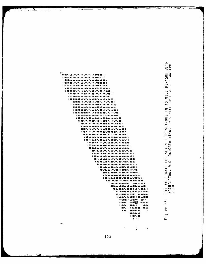
E~~~~~~F C:) J~ . .'am

I m m ki ki -.0 ki -. LU-

EJLJ%,W ~ iE I J

I~L ZUUo~JEmU~UJ ,%,'C,

I ~ ~ *%JJc*I~~~V C-)J% c JEL

~jij~m a

CC %w w i J vmm V.0I

W.v ftw b 0%. 0d vJccCI1 U~ *. J U-. ~

IE*~*W J'J~'J QI U~U'. ~ JI.C)

WWUUW U I Iwo

I ifti .0 MA*% I d

WwUJUww'o"I I-

I~~~ WOW.J0J*

=UWUUO UUWEO

*W*~~'.DE* I 0lJ* Lk

102UW .J.h

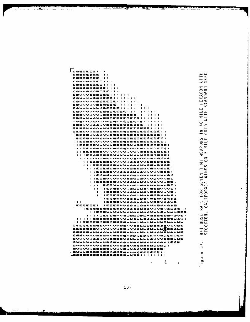
toII to t M I MI I II

W~:~ ::actM aICI.WWWMMM~ a LL

ummm ~~ a aWm cW M t IaaIto mm m~ C1 W ct Mt MII

to a aoWutgt rt iIIICWW~kj toW M a I I I m

0 o iv om ~ a a M W a Iag II-:0~~~~ ~ ~ ~ W a. tj k. W m a IIII>

m vt0vm *m E E E a a M a. a a I -IIII--Iuj

0 W 4 i av WMM MII a a a a

Em, ~ mEEEEEEa a aWm WE E EE~ a a a ab aovL

E~ u to 4 M ki 4%j v a a a -

E~mmmmWUEEEEEEI

a Im mm~ m E~ mE a WC)

a a a EWXmCJ WM I I I

a c cciw t~~ WO L fdlt C o I V)E C)JJ. u

a a W EU*' 0WW 0 Jm%0vAvv . 0 t . a w 6.WwU .6~mc .I :

a a~ a a 160 vWta .a 0 Va a.Iws.UUs.i. wW0%0a ai

=4 vv O~~ Sia 0m a w umm . Ww ' 40 0m aww

aEEEEEI mo

a EEmmmm~mu~J'Jm.JOWE a

~ 0

-

103

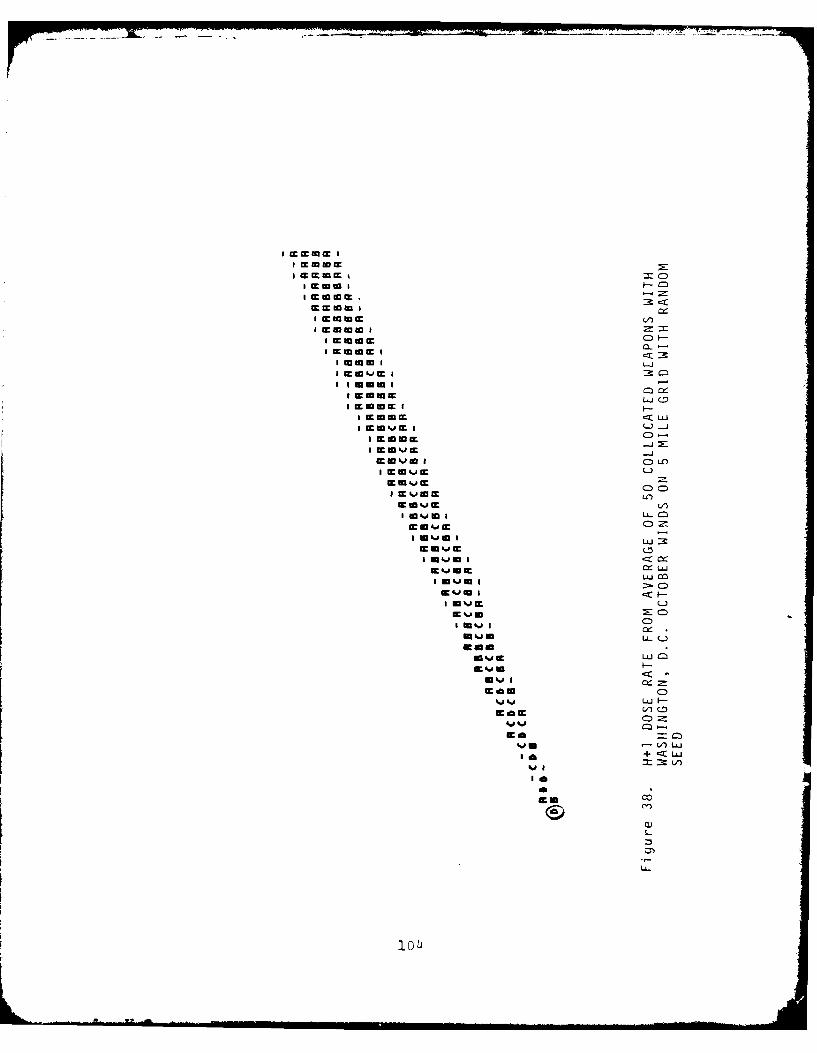
I ccccamc I

I CC W cc03I

I ccmw

ILSUE

55mmw I==I cctw c CI)

I to W wI LI CinC 02 O1-

I aW'.JE

I cc mWitcIf -

I EUcJE a

I CCUMJ c

I 5* kJE I L- c

EU 4.o' CDC

M%JUSC:

W* U tow.E'mJUC

.D a -C

v* 0jLuF

mac6. vi-C

%0%0 CD

4.44.4 L=

+ c. W=m-ta

'.1

0

S-

104

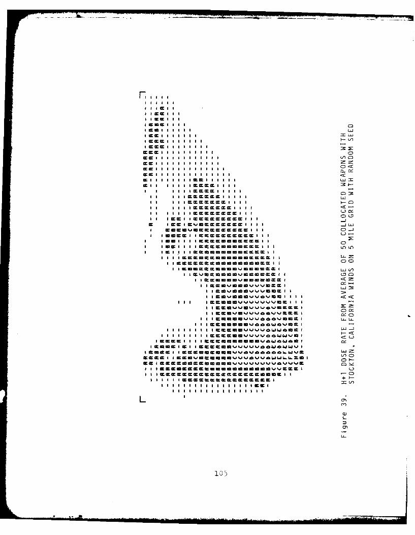
I I =cc I II c EES I IIm

IEccUaI I III LI it=I I11II1 I1A

ccEEc E I II I I S=S

EK I I I I I I mc I I I1l

I6 III IE KEc W c I I I I II mIm mccI = c cE I I II

II I I mmimEEE I I II :

II I I W.EEEECCCCCl I IC-

w m = = = = IS SI IEK E S I I

II I ISI I EEEEEEEIIIw I

OE IE~ I II EEKEEKIwwcm I I I LI .I IE KEEKEEKESwccc~ II I

I m1mWct w w wcm c II I EE EIS

I I E I Inw wwwcc I I CD CWW EE

I I Z lm lwfw w mcc I IEE W E W E E E ID

I= C

IWIXI III I KEWEGIIQ W J OJ'.JJWEI I

I c micI I 1 SKEW f*1mV 'JCv %,*Ea EEjI

I Ioci I I

mmwc I Ic SWSw UU.CCWID.JZ II -:

I I I I S*lUf UUccc L~jIO6.j~ 4 JI Q+

a UI ElC I

C-

EEIEEEmEEmmm~.105J

E. MODIFICATIONS TO ORIGINAL CODE FOR MILLER-S MODEL

This section describes modifications made to the original

MILLER-S computer program. The model was developed by Dr. Carl

Miller under DCPA contract DAHC20-71-C-0273 (Work Unit 3119F)

to the Dikewood Corporation. It is documented in a series of

volumes--"The Analysis and Correlation of Fallout Pattern Data"

[Ref. 9]. Part III is the "Computer Program Users Instructions."

It contains a listing of the computer program, a sample problem,

and output from this problem. References here to equations a-d

algorithms defining the model will refer to Part II, "Deriva-

tion of Statistical Fallout System." In this report the total

algorithm is divided into a series of 40 steps which are sequen-

tially performed. This description of modifications will refer

to sections and steps in this report.

The FEMA Computer Center had a copy of the program which

was written for the CDC 3600 computer. The first step was to

put the program on the Univac 1100/10 system and to convert

the program to be syntactically compatible with the Univac sys-

tem. Fortunately this conversion involved no changes which were

directly related to the computation schemes except to change the

nature of the calls to the random number generating routine. It

was impossible to compare the calculational results with those

in Part III of the Miller report since the change in the random

number generating routine resulted in a different set of random

numbers being generated even though the same seed was used and,

therefore, in a different set of answers.

On the code listing received at the DCPA Computer Center,

two corrections were written in by hand. The first, in step 1,

sets the value of Q(I)=l if the absolute value of shear angle a

is less than 0.001. The second, in step 34, changes its origi-

nal calculation of k34 from

106

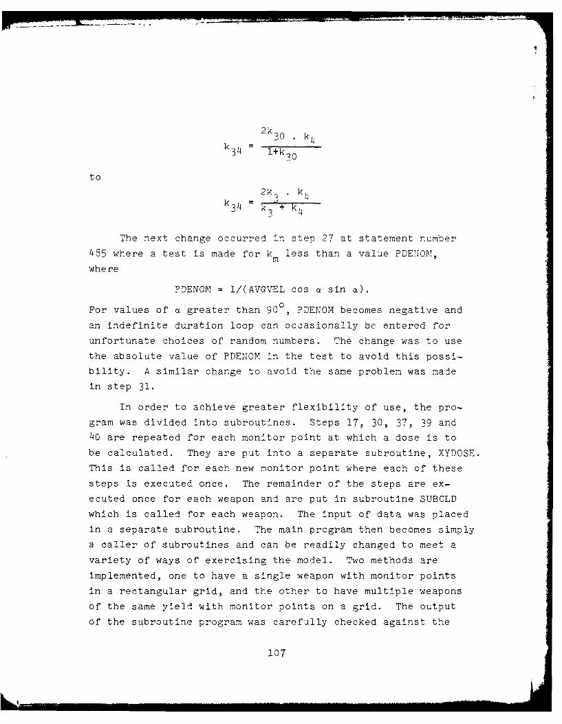
2k30

34= l+k30

to

k3~=2kv k 4k34 k k3+ k4k3 4

The next change occurred in step 27 at statement number

485 where a test is made for km less than a value PDENOM,

where

PDENOM = 1/(AVGVEL cos a sin a).

For values of a greater than 900, PDENOM becomes negative and

an indefinite duration loop can occasionally be entered for

unfortunate choices of random numbers. The change was to use

the absolute value of PDENOM in the test to avoid this possi-

bility. A similar change to avoid the same problem was made

in step 31.

In order to achieve greater flexibility of use, the pro-

gram was divided into subroutines. Steps 17, 30, 37, 39 and40 are repeated for each monitor point at which a dose is to

be calculated. They are put into a separate subroutine, XYDOSE.

This is called for each new monitor point where each of these

steps is executed once. The remainder of the steps are ex-

ecuted once for each weapon and are put in subroutine SUBCLD

which is called for each weapon. The input of data was placed

in a separate subroutine. The main program then becomes simply

a caller of subroutines and can be readily changed to meet a

variety of ways of exercising the model. Two methods are

implemented, one to have a single weapon with monitor points

in a rectangular grid, and the other to have multiple weapons

of the same yield with monitor points on a grid. The output

of the subroutine program was carefully checked against the

107

2; '; 2 no beore iv ~ -nInto Subrout ines to ensure th-e

a 1~ 1oISc-1 3 e me ane.ca results wereainei fron te t.%go co-as

Th e re.nort FaZ Zout .UdOiaiu'sDe to 'uocaaZ Rzurst

:oxx Ian i 11r, ?-CI-'A ork Unit 32231, -ecember 15,

174 Fof 131l, contains several modifLications to the origEinal

§eD Te first modificatilon is in step 3.In both cases -"or

I > v. is computed by

v v exn(1-c.002)

After thiis calculation the following is InSertedi:

If W < 78) bynass T hiz insert.

otherwise

If mnidrang-e values are _ise- -D ',D ",-I ------_r-

otherw is3e compute v <

maxend o f thLis is er t, ot h e r -. I r ne;' ian m a n; ~

the teoinniiz- of thisine

'-he next nodifoca!tioon I- I ten, 23 in th!-e method! of

con Kig is n; dby

R ,

~na ,thne new,, vais fDr the minimum, maximum and mid-

ran:'-- Df Th LIn th r:etwere rlaceJ in the nro,:-ram.

A new method for the coal - io of t dose a nt

in step 36 is -iven in this ee pt. -'I etod was c ode-1 ant

rlaced in the code. The r:ort has sm -an- calculations for

dose at a few different distances for a 1 :I- wea!on wi a

constant 15 mh win, . The results from the computer code were

close enouch to the hand calculation to verify the -lorit.hm

used.

In the orocess of comoaring results, an error in coor nate

transformations ,,-s discovr - . in te ) program. The coJdn for

C .PX was CAPX(i) = (Y-yCZEC(1)).cos -P(:) - (X-xczERO(1)).

sin DPH(I). The minus sicsn between the two terms in this

equation was changed to a plus sion.

The next change increase, the model outout by a factor

of (4/3) to account for Zroun! rc- u7rness and instrument

calibration factors. The original Jredicted dose would be

comparable to "as measured" dcse-s w le the corrected dose is

comparable to the doses ivenb the fallout prediction models.

The next modification introduced two additional means

for handling the "k-factor" in the model. In the original

model, the k-factor could vary from a minimum of 166 to maximum

of 2186, with a mean value of 1434. A new input variable

TKPACSW was defined. If this variable has a value of 0, the

original model calculation is used. A :AS report recommends

a k-factor value of 1930. if is 1, the originally

selected activity in each subcloud is changed -,o that their

ratios are the same, but the weaon k:-factor is always 1930.

If KFACSW is 2 the activity in e'i h subcloud is increased by

its ratio 1)30/1434 so that athe - weaon k-facto-r is

1930.

An option was introduced to -'-U-,u- the biolosical dose

if the new input parameter KBI1 -a . The first step in

computing the biological dose is in .- , 12, to save the time

of arrival on the zround o" t rarticles from each subcloud.10 9

7 1 ~ ~ ~ ~ 2 ,1 ed~-~hj> rr~ : D~ eCh

documentation, a cloud stabilization time is computed by

t = 0.17W ' hrs

For I = l,4 the cloud rise time is based on a formula

from the MILLER II model in Computer Implementation of the

OCD Fallout 1odel, ARS Report 66-44, OCD Task 3117C, 6/30/67,

na.-e I :

t, = ln(Cl/(C 2-hi)

where C = 18.W"lE

C2 = 21.56/W"I16

h = is the initial selected height ofthe ith subcloud

We then take tr = min(tr,t s).

For I = 5 to 10 we set

t =tr s

t is added to the time of fall, tf, to the earliest time

of arrival, te, of the fallout, i.e:

t =t + te f r

A radius of earliest arrival, re, is computed by

re = log (10/I)/KRL,

and downwind distance by

Xe = log (10/I)/IRL.

In these two equations the logarithm (10/I) is set equal to 3.

For each monitor point, a step 40 1/2 is added to the

subroutine XYDOSE which computes the biological dose. This

is done by assuming a linear arrival of fallout between fall-

out arrival and cessation and integrating the fallout arrival

110

iMS 'I t a~s: rte. To this IS added3 the bioloc-lca

"'o c aI c eosition cessat ion us in, aS'D- of- bioloo' cal to H-+1 (Jose rate for

~tatn- at a t ime t asui~ a Q:K nercentC,

oi D.-- ale dose with a renair constant of three

davs. -'~j c~ s fromq [Ref. 7]

A. cn~e if >e rriving:, dose is compe-ted b

X > RH ewvhere X and Yare coordinates relative to the subcloud axis.

t time of fallout arrival is computed by

ta

t =t + ea V 0

During the time of fallout buildup, the accrued do-se is

given by

= ~ ~ 8 *'TT [l3( 8 ta") + 5 ((t a/tc ) t j)]/(t -t

The additional dose after fallout cessation is -0iven by

1) 2= FII(T) 2.71tc -. 382

The total biolog-ical dose is then the sum D +D.

Use of the model disclosed that even in low shear condi-

tions an appreciable fallout could be deposited considerable

distances unwind or crosswind at a downwind distance of

order to eliminate these physically unacceptab!e possibilit -Le,

the following scheme was added to the model to limit olues Of

k 3 and kRL in low shear conditions.

The total angle, aT, through which the wind varies during

fall of each subcloud from its initial altitude to the ground,

is computed in step 12. A shear correction factor, SHRFAC(I),

is then computed by

SHRFAC(I) = 1 - sin e.

In step 21 a cloud radius and cloud bottom altitude are

estimated based on fits to ELW data by

CLDRAD = 0.2023 (miles)

CLDBOT = 5.26 w " 2 7 (kft).

A distance to use upwind is estimated by

h.

CLDBOT = CLDRAD (1/6 + 5/6 ( O

where h xi is the altitude of the ith subcloud. A k 3 min is

calculated by

k3 = 3.SHRFAC(I)/( xc0 2(1) t Yc02(!) + 0.5CLDUSE).

If the selected value of k is less than k, min, it is set3

equal to k 3 min.

In step 23 a crosswind diffusion is estimated based on

[Ref. 14]. The diffusion standard deviation is estimated by

1.28t, (miles)

where t is the fall time for the subcloud. A minimum value

of k is estimated byRL min =3./(CLDUSE( !) + .d).

If the selected value of kRL is less than kRL min, it is set

equal to kRL min.

112

rI

Chapter VII

PROGRAM AREA P11., DETERMINISTIC FALLOUT CALCULATIONS

A. INTRODUCTION


Program area Pll. consists of the program GRDFAL, which

performs deterministic fallout calculations using either the

WSEG-1O fallout model for single weapons, a simplification of

this model [Ref. 71 using clusters of weapons, or appropriate

combinations of the two. It is similar in general structure

to the program RUBATO which was developed originally to do

probabilistic fallout calculations but was later used as an

expedient for deterministic fallout calculations with a single

given input wind. All the probabilistic calculations were

stripped from the RUBATO program, the coding mostly rewritten,

and some additional capabilities added to produce the present

program.

The program considers a sequence of monitor points; for

each monitor point it goes through an input list of weapons

(or weapon clusters) adding doses for each to the monitor point.

The program is currently configured to calculate fallout on a

ten minute grid covering the United States. However, the

monitor points are selected through a single short subroutine

so that rewriting this subroutine would allow inputting any set

of monitor points desired.

The wind data input are fallout wind speed, wind direction

and wind shear at each point of a wind grid; this wind grid

has 20 spacing and covers the United States. A supplementary

113

program is available to convert daily winds to fallout winds on

the required grid.

2. Summary of Major Program Areas

Only a single main program has been developed. A set of

input variables control various program operating options. A

supplementary program called RAWGRD is available to convert

input wind data at various levels on a global polyconic grid to

fallout winds on a 20 grid suitable for use in the WSEG-10

model.


1. Program GRDFAL

a. Program Elements

The program consists of a main program to control the flow

of subroutine calls plus the following subroutines:

INVAL - input control variables, weapon characteristics,

wind data and grid data

INIT - initialization of fallout calculations

CLSIN - input weapon and cluster locations and propertiesand associated wind data

TGTIN - calculate locations of grid monitor points (inputtarget locations) and associated wind data

SQRSCN - perform fallout screening operations for weaponclusters by 1 degree grid square

FALDOS - control fallout dose calculations

CURVW - compute downwind and crosswind distance alongcurved streamlines

DOSWRT - output calculated doses

SPHDST - compute distances along a sphere

PROJCT - calculate rectangular coordinate projection

UNJCT - calculate inverse of rectangular coordinateprojection

FALLYB - do yield-dependent WSEG-10 calculations

114

FALLWB - do wind speed-dependent WSEG-10 calculations

FALLDB - do downwind distance-dependent WSEG-ll calcuLa-tions

FALLCB - do crosswind distance-dependent WSEG-10 calcula-tions

QFALLY - approximate WSEG-10 yield-dependent calcuia:Ions

QFALFW - approximate WSEG-10 wind-dependent calculatf:ns

WFALDW - approximate WSEG-10 downwind distance-dependent

calculations

QFALCW - approximate WSEG-10 crosswind distance-e-endentcalculations

CFALLY - cluster yield-dependent calculations

CFALWD - cluster wind, downwind distance and crosswinddistance-dependent calculations

CUMMOR - calculate cumulative normal function.

The program communication is by block common. The common

blocks are:

/RTJNSW/ Control parameters defined by input data

/RUNPR/ Parameters varying during run

/WPNPR/ Weapon parameters

/WNDPR/ Wind values

/FLWSEG/ Fallout model inputs

/IOPR/ Input/output control.

The definitions of each of the variables in these block

commons follow. Those variables which are input variables are

marked by an I. For control variables, the options selected

by various values are shown. Maximum dimensions of arrays are

marked by an M.

/RUNSW/ = Control parameters defined by input data:

I IWPWND - Method of fallout wind calculation

1. Wind at center of cluster(or at weapon if no clusters)

2. Wind at target

115

3. Wind average of cluster and target

4. Curved wind for each cluster

IWPUSE - Method of calculating weapon grouping

1. Cluster model only

2. Cluster for distant weapons - individual weaponsnearby

3. Individual weapons only

I IMAPT - Method of distance calculation

1. Use national rectangular projection

2. Use local rectangular projection

3. Use spherical earth

ISINGW - Exercise single weapon input and weapon classinput from input data file

(Must be 1 if IWPUSE = 2 or 3)

0 = Don't exercise

1 = Exercise

ICLUST - Exercise cluster input

(Must be I if IWPUSE = 1 or 2)

0 = Don't exercise

1 = Exercise

IDCAL - Select type of dose calculation

1. Calculate standard WSEG-10 maximum equivalentresidual dose

2. Calculace H+l dose rate

3. Calculate total dose accumulated in one week

4. Calculate total dose accumulated in infinite time

M NGROD = Maximum number of grid rows

I IGRSI (NGROD) = Number of westernmost grid in its ith row

[(grid number = (50-LAT)60+(125-Long))]

I IGRS2 (NGROD) = Number of easternmost grid in the ith row

I NGRSPT = Number of grid row definitions input

I IGPTSW = Output doses on standard output medium if1

I IGSVSW = Output doses on File NE if 1

BIASE = Constant added to easting to make allvalues positive

116

JC--

BIASN = Constant added to northing to make all valuespositive

IPTDEG = print control frequency

0 = Print from grid

1 = Print only on degree intervals

2 = Print only for every other degree interval

ICHKPT 0 - Checkpoint control, don't use checkpoint option

1 = Do use checkpoint option. Checkpoint file onmass storage

2 = Do use checkpoint option. Checkpoint file ontape

/RUNPR/ = Parameters varying during run:

!GRD - Index to grid row

JGRD - Current grid number

IGRDF - Index to fine longitude in grids

JGRDF - Index to fine latitude in a grid

YTL - Current target northing

XTL - Current target easting

WINDT - Current target wind speed

ALT - Current target wind direction, radians counter-clockwise from east

SALT - Sin of target wind direction

CALT - Cosine of target wind direction

SHRT - Wind shear at target

DOSE - Current calculated dose from a single weapon

DTOT - Current accumulated dose for a monitor point

JSCRN - If 0 current large grid does not pass screening;(NCLSD) if 1 does pass screening, do fallout calculations

iLAST - Flag, of one last grid point is calculated

SI± L - Sin of target latitude, used if IMAPT = 3

COSTL - Cosine of target latitude, used if IMAPT = 3

/WPNPR/ = Parameters defining weapons:

M NCLSD - Number of clusters dimensioned

117

N .WPND- Number of individual weapons

., NWPICD-Number of weapon classes:1 NCLSA=l, unless IMAPT =3 then NCLSD if ICLUST / C

or NWPN if ICLUST = 0

N NCLSB=l, if 1 WPWND = 2, otherwise NCLSD if ICLUST 0or NWPN if ICLUST = 0

YLDC -Effective cluster yield (log average of(NCLSD) individual yields weighted by fission fraction)

FISSC -Cluster fission fraction (determined so YLDC (.)*(.CLSD) FISSC(.) equals the sum of yields times fission

fraction summed over q11 weapons in the cluster)

XC(NCLSB)-Cluster easting of IMAPT = 1, longitude other-wise

YC(NCLSB)-Cluster northing if IMAPT = 1, latitudeotherwise

COSCLL -Cosine of cluster latitude if IMAPT = 1(NCLSB)

SIGXC -Cluster East-West standard deviation fission(HCLSB) yield weighted (input as degrees, then converted

to statute miles)

SIGYC -Cluster North-South standard deviation fission(NCLSB) yield weighted (input as degrees, then converted

to statute miles)

SARY(NTCLSD,5)-Yield-dependent parameters for use in cluster

model

" INDC -Wind speed at cluster center (miles/hr)(!NCLSB)

ALC -Wind direction at cluster center (radian counter-(NCLSB) clockwise from east)

SHRC -Wind shear at cluster center (mph/kft)

(NCLSB)

SINC -Sine of wind direction(NCLSA)

COSC -Cosine of wind direction(NCLSB)

LSTWPC -Number of' last weapon in cluster(NCLSA)

NCLS -Number of clusters

118

! XWPN - Weapon easting if IMAPT = 1, longitude other-(NWPND) wise

I YWPN - Weapon northing if IMAPT = 1, longitude other-(NWPHD) wise

I IWPNC - Weapon class

(NWPND)

I MWPN - Number of weapons

I YLDWC - Weapon class yield (MT)(NWPNCD)

i FISSWC - Weapon class fission fraction

(NWPNCD)

I CEPWC - Weapon class delivery error, CEP (miles)(NWPNCD)

I HOBWC - Weapon class height of burst (feet)(NWPNCD)

I DELWC - Weapon class reliability(NWPN CD)

T MAMEWC - Weapon class description, up to 16 characters(NWPNCD, L)

ARRYWC - Yield-dependent weapon class values for use(MWPNCD,6) in WSEG-10 calculations

MIWPC - Number of weapon classes

YLDI(9)- Mean value of yield for grouped yield intervalsused in WSEG-10 calculations

YLDM(8)- Separating values for grouped yield intervalsused in WSEG-10 calculations

QARYL(7, 19)-Yield-dependent values used in WSEG-10calculations for grouped yield intervrpls

SINCLL - Sin of cluster latitude, used if IMAPT = 3(NCLSA)

/"-NDPR/ Wind values:

M NIWGRD - Number of dimension and wind points east-west

M NJWGRD - Number of dimension and wind points north-south

I SPDMO - Wind speed at grid point input in knots used,(NIWGRD, (e.g., a west to east wind is 270 deg.)NJWGRD)

I SHRMO -Wind shear input as knots/kft, used as miles/hr(NIWGRD,NJWGRD)

119

/FLWSEG/ Fallout model inputs:

YIELD = Weapon yield (MT)

FISS = Weapon fission fraction

HOB = Height of burst (ft.)

EFW E Effective fallout wind (mph.)

SC = Wind shear (mph/kft.)

DWD = Downwind distance (miles)

CWD = Crosswind distance (miles)

MDCAL = Type of dose to calculate, see IDCAL

TWPN = Time of weapon detonation

ARRY(40) = Storate array for temporary values

XL = For cluster model, cluster length

SIGW = For cluster model, crosswind standarddeviation of weapon fission yield weighteddistances

DOSEM = For cluster model, output dose

XTRA = Product of cluster sigmas for use in WSES-lOroutines

4

/IOPR/ = Input/Output control:

MP = Standard input (unit 5 in Univac system)

MQ = Standard output (unit 6 in Univac system)

NC = Weapon input

ND Parameter and wind input

NE = Save file output.


(1) General

The program requires two input files be made available. 2

One file contains input parameters and is currently named

Pll.INPPAR. Another file inputs weapon data and is currently

called PlI.WPNS. The user may modify these file names by

changing lines 8, 2 and 5 in element PII.QGRDFAL. Output from 2

120

the program is written either on the standard output file or

file Pll.DOSSAV. To initiate program execution once the input

files are defined, type: @ADD Pll.QGRDFAL.

(2) Input Elements

The input elements in the file INPPAR are described below.

The lines labeled Blank may contain any set of 80 characters.

For ease in preparing input data, the names of the variable

on the succeeding line of input may appear in the blank lines:

Line 1 Blank

Line 2 Calculation control

Variables IVPWND, IWPOSE, IMAPT, ISINGW,ICLUST, IDCAL,

Format (6110)

The variable meanings are given in the previous section.

The variables ISINGW and ICLUST are included to ensure that

the weapon data read consistent with the actual content of the

input file WPNS. This allows changing calculation types with-

out having to change the input weapon files. Thus, for example,

if the weapon file has both single weapons and clusters, but

only clusters are to be used in the calculation, then one must

have IWPUSE=3, ISINGW=l and ICLUST=l.

Line 3 Blank

Line 4 Output control

Variables IGPTSW, IGSVSW, IPTDEG, ICHRPT

Format (4110)

If ISVNGW = 0, skip line 5

Line 5 Weapon class characteristics for ith weapon

Variables: YLDWC(I), FISSWC(1), CEPWC(!)HOBWC(I), DELWC(I), (NAMEWC(I),1=1,4)

Format (5F10.0,4A4)

121

-• -

One entry is made for each weapon class. The end of this

input string is flagged by adding a line where the value of

YLDWC(1) is -1.0.

Line 6 Wind data

Variables FLAT, FLON, ((SPDMD(I,J), DLO!D(I,J),SHRMD(I,J))

Format (= F]W.4)

One ent2y is made .2 each grid point. The grid increases

in latitude from 24 to 50 degrees by 20 increments and in

longitude from 65 to 125 degrees by 20 increments. The

variables FLAT and FLON may be 0 if desired. They are written

on the wind input data only for convenience in manually using

the file. The velocities are input in knots and immediately

converted to miles/hr. The wind grid data may be directly

obtained as output from the program LEVGRD.

Line 7 - Number of grid control inputs

Variable NGRSPT

Format (15)

Line 8 - Grid control variables

Variables IGR5I(T), IGR52(I)

Format (215)

These variables control the definition of the grid

covering the United States from which monitor points are

obtained. See the discussion on algorithms implemented in

subroutine TGTIN for a more complete definition of these

variables.

The weapon input is in the file WPNS and is read by the

subroutine cluster. The first section of the file defines the

weapon cluster which is read if ICLUST=l. The ith cluster

has the following input:

122

C)

Variables: YLDC(I), XWLON, Y,:LAT, SIGXS, SiY",XMNLN, XMXLN, XMNLT, XMXLT, FISSC(I), :WP2..,NUMC, LSTWPC(I)

Format (F6.3, 2F7.3, 2F6.3, 2F7.3, 2F6.3,F7.3, 214,15)

XWLON and YWLAT are the weapon longitude and latitude in

degrees. If IMAPT X 1, they are directly placed in XC(1) and

YC(T), otherwise they are converted to an easting and northing

and then placed in XC(T) and YC(1). SIGXS and SIGYS are yield-

weighted standard deviations of the cluster in degrees. After

conversion to statute miles, they are placed in SIGXC(I) and

SIGYC(I). The variable NWPNN is the number of weapons in the

cluster. The variables XMNLN, XMXLN, XMNLT, and XMXLT are the

minimum and maximum longitudes and latitudes of any weapons in

the cluster. These variables and the variable HVMC are not

:se in this program. The other variables are as defined for

common block /WPNPR/. The end of the input is flagged by an

additional line of input with the value of YLDC(I)=-l.

The next section of input is the list of individual

weapons, which is read if ISINGW=l. For the ith weapon the

following line is read:

Variables FLAi, FLON, IPU?!)

Format (2F10.0, 14)

FLON and FLAT are weapon longitude and latitude in degrees.

If IMAPT;l, they are directly placed in XWPN(!) and YWPN(1),

otherwise they are converted t, eastings and northings and

they are placed in XWPN(I) and YWPN(i). IWPNC(I) is the weapon

class which is used to define weapon yield, etc. through the

variables YLDWC(IWPNC(I)), etc.

123

C. Algorithms Implemented

The algorithms implemented will be described by subprogram

except for the fallout models and coordinate projection which

have already been described in [Ref. 4].

Program GROFAL

The program flow is straightforward. At the start the

subprograms INVAL, CLSIN and INIT are called. Then a loop is

entered where the subprogram TGTIN is called to produce a new

monitor point, SQRSCN is called only as each new one degree

square is entered for fallout screening calculations, FALDOS

is called to monitor the fallout calculations, and finally

DOSWRT is called to write results. When the last monitor point

has been used, the subroutine TGTIN sets the flat TLAST, which

is used by the main program to end the calculations.

Subroutine INVAL

This subroutine directly reads input data from the input

file INPPAR, as described in the input section.

Subroutine INIT

This subroutine calculates the yield-dependent parameters

for the WSEG-10, approximate WSEG-10, and cluster model by

calls to the subroutines FALEYB, QFALLY, and CFALLY.

Subroutine CLSIN

This subroutine inputs weapon and weapon cluster data.

If IMAPT=l, subroutine PROJCT is called with projection option

3 to obtain eastings and northings. If required by the parameter

IWPWND, wind properties are computed at the weapon points.

To do this the indices I,J of the southeast cornp" nf the

grid square are found by:

I = (LATW-24)/2

J (LONGW-65.)/2

124

where: LATW, LONGW are weapon latitude and longitude.

I and J are truncated to the r2xt lowest integer. x and

y are the fraction of the distance in the wind square to the

east and to the north from the weapon location. The value of

wind speed, wind direction and wind shear are then obtained by

linear interpolation from the four surrounding corners. If

V. iis the value of one of these variables at the i, j grid

point and V is the value at the desired location, then:

V = V.j(l-x)(l-y) + Vi+lJ(x)(l-y)

+ Vi~j+ I (l-x)(y) + Vi+l(x)(y)

Subroutine TGTIN

This subroutine finds the latitude and longitude over a

ten minute grid covering the United States. The grid was

developed by J. Jacobs and J. Backman of FEMA. The latitude

and longitude of the soutnwest corner of one degree oy une

degree grid squares are defined by a grid index through the

following relation:

JGRD=(49-LATD) 60+(125-LOND)+l

where LATD and LON7 only assume integer values. Increasing

JGRD will sweer a swath of one degree gria points decreasing in

longitL.e across the county at constant latitude. For each of

these rows, the input values IGRSl(JGRD) and IGRS2(JGRD) define

'he westmost and eastmost longitude covered, where JGRD is an

index to orlzontal rows at constant latitude. The algorithm

sweeps across rows from west to east using an index IGRD.

After a row is completed, JCRD is increased by one to sweep

the next most northern row. For each one degree figure, a

series of ten minute grid points are then genera;ed first

increasinR latitude from south to north using the index JGRDF,

and, when a vertical column of six points is completed, new

125'

columns are generated by increasing the index !GRDF, decreasing

longitude from west to east. Each call to the subroitine TGTIM

produces a new grid point. If needed the target coordinates

as computed in x,y coordinates and wind values at the target

point are computed. Changing the values of the input arrays

IGRSI and IGRS2 would allow scanning only selected areas of

the county.

Subroutine SQRSCN

This subroutine is called whenever a new one degree square

is entered. It determines if a cluster (or weapon) could

produce significant fallout doses on the center of the one

degree squares. The screening distances are increased slightly

to allow for the finite square rise. If the screening test is

passed for the ith cluster, a value of 1 is returned for JSCRN

(i), if it is not passed and no significant doses are possible,

a value of 0 is returned. For the ith cluster a value CMAX is

computed by:

CMAX=1200 SIGXC(I)+SIGYC(I)+40

where SC is the appropriate shear value

SIGXC(I) is east west cluster standard deviation

SIGYC(I) is north south cluster standard deviation.

If individual weapons are considered, ICLUST=O, SIGXC and

SIGYC are taken as zero. If CMAX is less than 140 or greater

than 340 it is limited to these values. The downwind distance

DWD and the crosswind distance CWD are computed using appro-

priate coordinates and wind transformation. If the crosswind

distance is greater than CMAX the screening test is not

passed. If the downwind distance satisfies the following

relation

DWD< 1 l4o + 2(SIGXC(I)+SIGYC(I))

the screening test is not passed.

126

Subroutine FALDOS

This subroutine controls the calling of the appropriate

fallout models and accumulated dose on a monitor point. It is

primarily a bookkeeping routine with the emphasis on obtaining

the proper values of fallout winds and downwind and crosswind

distances under the various input options. The specific

assumptions made (outside of bookkeeping) are: If IWPUSE=2

the cluster model is used if downwind distance is greater

than 100 miles, and the individual weapons are used otherwise.

For the cluster calculation the cluster model is used directly

if wind speed is greater than 5 mph. Subroutines CFALLY and

CFALWD and the appropriate WSEG-10 model (subroutines QFALLY,

QFALFW, QFALDW, QFALCW) are used for lower wind speeds.

Subroutine CURVW

This subroutine performs integration along a wind stream-

line to compute downwind and crosswind distances. Rather large

integration distances of 150 miles are chosen to provide a

resolution in the integration compatible with the resolution

of the input wind grid.

If the weapon to target distance is less than 150 miles

then the average wind direction at target and weapon locations

is used to compute downwind and crosswind distances. Otherwise

the integration uses wind direction at the beginning of a 150

mile step to get increments in distance along the wind stream-

line. Near the target the wind at the target is used for the

final wind streamline direction. A perpendicular from this

final segment of the wind streamline to the target is used for

the final calculation of downwind and crosswind distances.

The effective fallout wind velocity is obtained by computing

the distances a particle would be carried along the wind

streamline until the time of fallout deposition Jefined in the

WSET3-1O model. This distance, divided by the fallout deposition

127

time, is used as the effective wind velocity returned as an

output of the subroutine.

Subroutine SPHDST

This subroutine computes distances on a spherical earth

using standard spherical geometry formulas and an earth radius

of 3962.2258 miles. If the difference in latitude is less than

four degrees and the difference in longitude is less than five

degrees, then the distance is computed assuming a flat earth

using a latitude which is the average of the latitude of the

two end points.

Fallout and Distance Projection Subroutines

These subroutines are the same as described in [Ref. 4]

and will not be repeated here. The one exception is to allow

the WSEG-10 model to return either one week or infinite time

doses. These doses are readily obtained by analytic integration

of the dose rate assuming a t- 1 .2 decay rate.

2. Program LEVGRD

This program is identical to that described in program

area P12. and will not be described here.

128

Chapter VIII

PROGRAM AREA P12., WEAPON ORIENTED FALLOUTCALCULATIONS--PROGRAM GUISTO

A. INTRODUCTION

This program computes fallout desposition using the

WSEG-10 fallout model. It differs from most fallout desposition

models in that for a particular weapon the desposition at all

monitor points of interest is computed, and then weapons are

considered in succession; rather than the usual procedure of

adding the dose for all weapons affecting a single monitor

point, and then considering all monitor points in succession.

In this approach the parameters for only one weapon at a time

need be considered, thus effecting a considerable savings in

time, but it does require the simultaneous availability of all

monitor points to store fallout dozes, which gives rise to

rather large computer core storage requirements.

The monitor points are chosen to form a square grid in a

plane which is an Albers Equal Area Projection of the United

States; i.e., a square grid drawn on an Albers Equal Area map

of the United States. For most applications, a grid ten milez

on a side appears appropriate, so each grid square covers an

area of 100 miles on the map (divided of course by the square

of the map scale factor). Since this is an equal area projec-

tion, by definition each square on the map also covers exactly

100 square miles on the surface of the earth, although due to

the :nap transformation the shape of the earth is distorted some-

what from a square.

129

The fallout doses are computed on a square grid with the

same spacing as for the monitor grid points. This grid is

oriented with one axis downwind and the other axis crosswind.

The fallout dose computed is then allocated to the nearest

monitor points. The same grid spacing is required so that no

bias is obtained in the fallout doses deposited. If, for example,

the fallout calculations were done for grid points with one half

the spacing of the monitor grid, then, on average, each monitor

point would receive dosrs from four fallout points and the dose

would be overestimated by a factor of four. Of course, this

could be compensated for by multiplying the fallout dose by 1/4,

however, for computational efficiency the two grids should prob-

ably be about the same size.

This method of procedure leads to two computational effici-

encies. The first is that fewer calls need be made to the

wind speed and downwind distance portions of the WSEG-10 model;

the second is that screening calculations do not have to be

made for each combination of monitor point and weapon. This

results in a decrease in computer running time for a nationwide

attack by about a factor of 10 compared to the program GRDFAL.

Furthermore, since one weapon at a time is considered, weapons

can be added or deleted from an attack by simply adding or sub-

tracting the doses from these weapons. This feature makes this

program potentially useful for calculations in real time use

where weapon reports do not come in all at once, but where

estimates are desired based on those weapons reported to date.

The direct outputs of this program are doses on an Albers

Equal Area grid. Such a grid, superimposed on an Albers Equal

Area map of the United States, would give directly a pictorial

representation of the fallout deposited. If a different set

of monitor points is desired, then a supplementary calculation

must be performed to interpolate from the Albers grid. The

program MINGRD performs this interpolation to give doses on the

130

same ten minute grid covering the United States as is in the

program GRDFAL.

A program RAWGRD has been developed -o convert winds from

winds a five levels for a particular aay to fallout winds on a

two degree grid for use in the program GUISTO. (This program

is also used to produce winds for the program GRDFAL.) This

program as currently configured takes winds from one month of

the twelve "most probable" winds [Ref. R. Mason of CCTC].


1. Program GUISTO

a. Elements ir Program

The program consists of the following program elements:

1UTSTO - manages subroutine calling sequences

INVAL - reads control parameters, reads wind data,and converts wind data to an Albers grid

CLSIN - reads weapon data and calculates winds at weapon

INIT - initialization of WSEG-10 yield-sensitivecalculations

CALDOS - manages fallout model calls for downwind andcrosswind variations and stores values in Albersgrid

DOSWRT - outputs grid doses to standard output medium orto permanent storage

TRMPNT - outputs doses on a standard terminal printerin form of a dose map

PLTDIR - outputs doses on a special plotting terminalin the form of a dose map

ALBERS - performs transformation from latitude, longitudeto Albers Equal Area map coordinates, and alsothe inverse transformation

FALLYB performs yield-dependent, wind speed-dependent,FALLWB downwind distance-dependent, and crosswind distance-FALLDB dependent WSEG-10 fallout model calculationsFALLCB

131

Communication between subprograms is through block common.

These common blocks are:

/RUNSW/ Control parameters defined by input data

/RUNPR/ Parameters varying during run or controlling

grid storage

/WPNPR/ Parameters defining weapons

/WNDPR/ Parameters defining wind

/FLWSEG/ Parameters used by WSEG-10 model.

The following list presents definitions of these block common

variables.

(I denotes an input variable)

/RUNSW/ = Control parameters defined by input data:

I IWPWND - Method of allocating fallout winds

1. Use wind at weapon for entire calculation for that weapon

2. Use wind speed at weapon and wind direction alongstreamline

3. Use wind direction along streamline, modify downwinddistance increment by ratio of weapon wind speed tolocal wind speed

I INTERP - Method of distributing fallout dose over Albersgrid

0 = Allocate all of the dose to the nearest corner

1 = Allocate dose proportionately to the fourcorners of the square containing the grid point

I ICHKPT - Control of checkpointing

0 = Don't do checkpoint

1 = Do checkpoint dumps with output file on massstorage

2 = Do checkpoint dumps with output file onmagnetic tape

I IGPTSW - If 1, output grid doses on standard putput medium

I IGSVSW - If 1, output grid doses to file NE

I IGPTSW - If 1, only output doses to standard output mediumevery 10 grid points; if 2, every 100 grid points

132

BIASE - Distance of 1432.672 miles added to eastings tokeep all distances positive

BIASN - Distance of 977.414 miles added to northings tokeep all distances positive

ITRPSW- If 1, plot map using a normal terminal as a plottingdevice

/RUNPR/ = Parameters varying during run or related togrid control:

DSEARY(KIDSA, KJDSA) - Array for storing doses on squaregrid in Albers Equal Area projection plane

IMMIN - Minimum i (west) coordinate on grid for this run

(minimum usable value is 1)

IMMAX - Maximum i (east) coordinate on grid for this run(maximum value is IMMIN + KIDSA - 1)

JMMIN - Minimum j (south) coordinate on grid ior this run(minimum usable value = 1)

JMMAX - Maximum j (north) coordinate on grid for this run(maximum value is JMMIN + KJDSA - 1)

TLAST - Flag to indicate last weapon has been input if 1,otherwise 0

IMMAXP = IMMAX+l

JMMAXP = JMMAX+I

IMMINM = IMMIN-I

JMMINM = JMMIN-l

KIDSA - Dimension of dose storage array DOSARY in the i(east-west) direction. The variable value must beset equal to that in the dimension statement forDSEARY.

KJDSA - Dimension of dose storage array DSEARY in the j(north-south) direction. The variable value mustbe set equal to that in the dimension statementfor DSEARY.

DELGRD - Grid spacing in miles

DSEMIN - Cutoff dose level in controlling limits of dosecalculations

i'WPNPR/ = Parameters defining weapons:

XC = Weapon easting on Albers grid

YC = Weapon northing on Albers grid

133

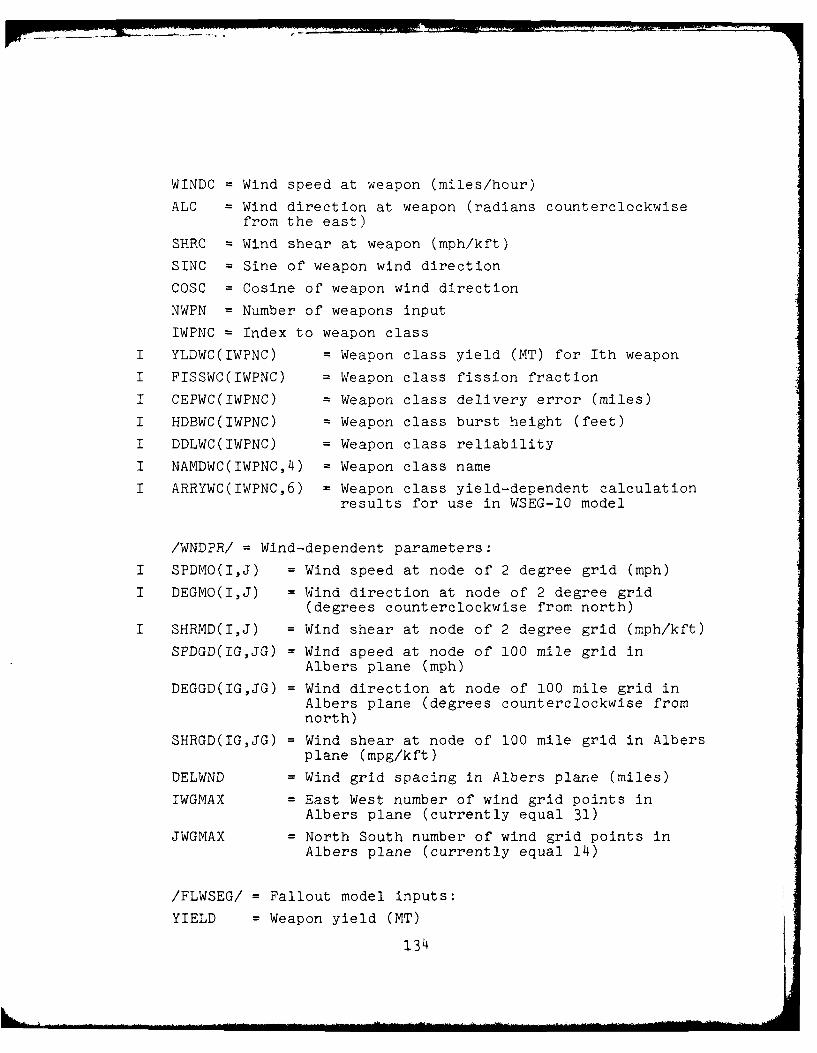
WINDC = Wind speed at weapon (miles/hour)

ALC =Wind direction at weapon (radians counterclockwisefrom the east)

SHRC = Wind shear at weapon (mph/kft)

SINC = Sine of weapon wind direction

COSC = Cosine of weapon wind direction

NWPN = Number of weapons input

IWPNC = Index to weapon class

I YLDWC(IWPNC) = Weapon class yield (MT) for Ith weapon

I FISSWC(IWPNC) = Weapon class fission fraction

I CEPWC(IWPNC) = Weapon class delivery error (miles)

I HDBWC(IWPNC) = Weapon class burst height (feet)

I DDLWC(IWPNC) = Weapon class reliability

I NAMDWC(IWPNC,4) = Weapon class name

I ARRYWC(IWPNC,6) = Weapon class yield-dependent calculationresults for use in WSEG-10 model

/WNDPR/ = Wind-dependent parameters:

I SPDMO(I,J) = Wind speed at node of 2 degree grid (mph)

I DEGMO(I,J) = Wind direction at node of 2 degree grid(degrees counterclockwise from north)

SHRMD(I,J) = Wind shear at node of 2 degree grid (mph/kft)

SPDGD(IG,JG) = Wind speed at node of 100 mile grid inAlbers plane (mph)

DEGGD(IG,JG) = Wind direction at node of 100 mile grid inAlbers plane (degrees counterclockwise fromnorth)

SHRGD(IG,JG) = Wind shear at node of 100 mile grid in Albers

plane (mpg/kft)

DELWND = Wind grid spacing in Albers plane (miles)

IWGMAX = East West number of wind grid points inAlbers plane (currently equal 31)

JWGMAX = North South number of wind grid points inAlbers plane (currently equal 14)

/FLWSEG/ = Fallout model inputs:

YIELD = Weapon yield (MT)134

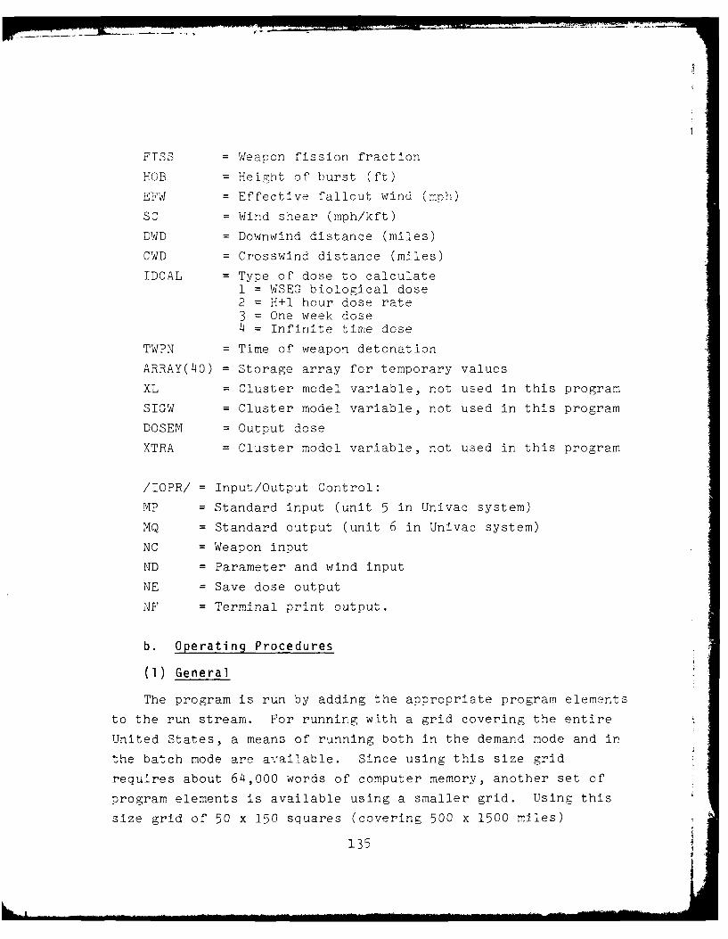
FISS = Weapon fission fraction

HOB = Height of burst (ft)

EFW = Effective fallout wind (mph)

SC = Wind shear (mph/kft)

DWD = Downwind distance (miles)

CWD = Crosswind distance (miles)

IDCAL = Type of dose to calculate1 = WSEG biological dose2 = H+l hour dose rate3 = One week dose4 = Infinite time dose

TWPN = Time of weapon detonation

ARRAY(40) = Storage array for temporary values

XL = Cluster model variable, not used in this program

SIGW = Cluster model variable, not used in this program

DOSEM = Output dose

XTRA = Cluster model variable, not used in this program

/IOPR/ = Input/Output Control:

MP = Standard input (unit 5 in Univac system)

MQ = Standard output (unit 6 in Univac system)

NC = Weapon input

ND = Parameter and wind input

NE = Save dose output

NF = Terminal print output.


(1) General

The program is run by adding the appropriate program elements

to the run stream. For running with a grid covering the entire

United States, a means of running both in the demand mode and in

the batch mode are available. Since using this size grid

requires about 64,000 words of computer memory, another set of

program elements is available using a smaller grid. Using this

size grid of 50 x 150 squares (covering 500 x 1500 miles)

135

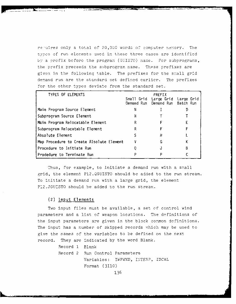
re-'uires only a total of 20,000 words of computer memory. The

iypes of run elements used in these three cases are identified

b' a prefix before the program (GUISTO) name. For subprograms,

the prefix preceeds the subprogram name. These prefixes are

given in the following table. The prefixes for the small grid

demand run are the standard set defined earlier. The prefixes

for the other types deviate from the standard set.

TYPES OF ELEMENTS PREFIXSmall Grid Large Grid Large GridDemand Run Demand Run Batch Run

Main Program Source Element N I D

Subprogram Source Element N T T

Main Program Relocatable Element R F E

Subprogram Relocatable Element R F F

Absolute Element S H L

Map Procedure to Create Alsolute Element V G K

Procedure to Initiate Run Q J B

Prodedure to Terminate Run P P C

Thus, for example, to initiate a demand run with a small

grid, the element P12.QGUISTO should be added to the run stream.

To initiate a demand run with a large grid, the element

P12.JGUISTO should be added to the run stream.

(2) Input Elements

Two input files must be available, a set of control wind

parameters and a list of weapon locations. The definitions of

the input parameters are given in the block common definitions.

The input has a number of skipped records which may be used to

give the names of the variables to be defined on the next

record. They are indicated by the word Blank.

Record 1 Blank

Record 2 Run Control Parameters

Variables: IWPWND, INTERP, IDCAL

Format (3110)

136

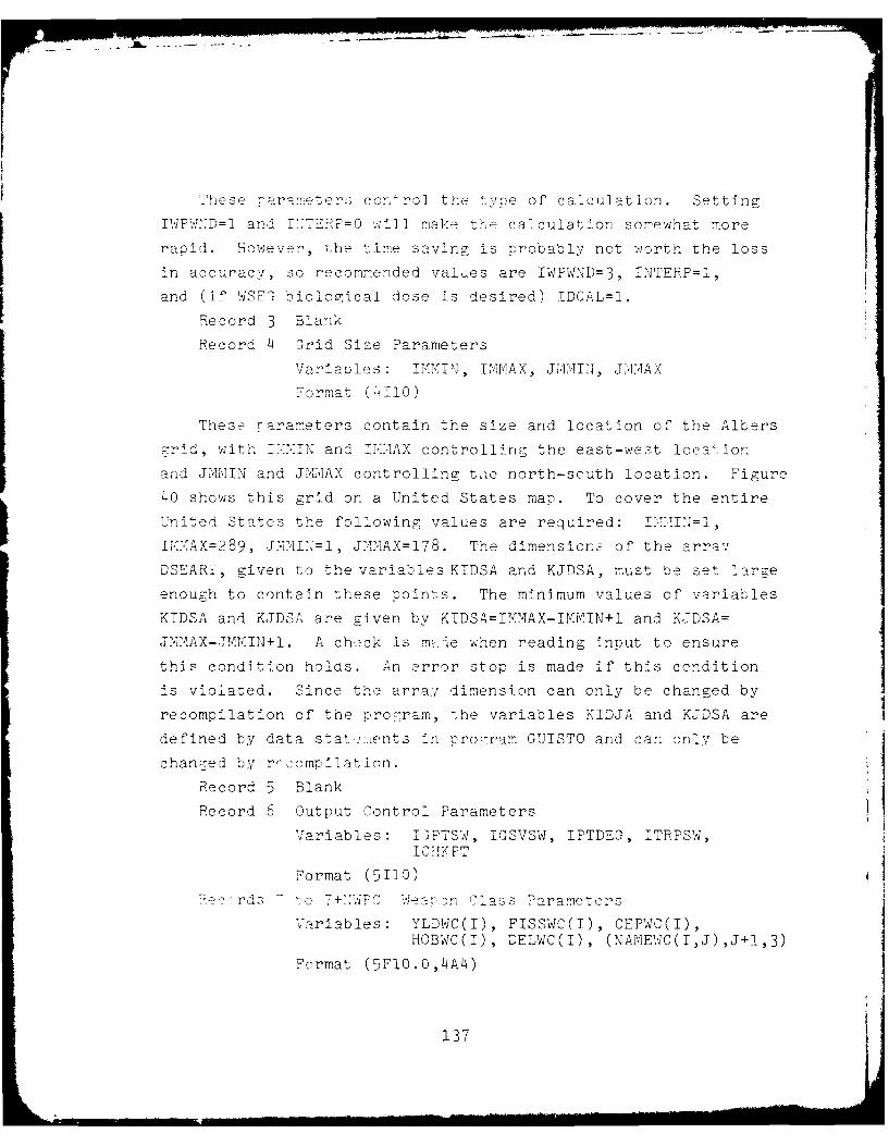
Ihese paramTeters con ccl the tv-e of calculation. Setting

IWP'I.i,'D=l and LIERP=0 will make the calculation somewhat more

ranid. However, the time saving- is probably not worth the loss

in accuracy, so recommended values are IWPWND=3, INTERP=l,

and (if WSFI biological dose is desired) TDCAL=l.Record 3 Blank

Record 4 3rid Size Parameters

Variaules: IMIVF'J, I2MAX, JMJIN, JMMAX

ormat r TiBl

These rarameters contain the size and location of the Albers

grid, with IhMIN and IIDAX controlling the east-west location

and JMJIN and JMAAX controlling t.ie north-south location. Figure

40 shows this grid on a United States map. To cover the entire

United States the following values are required: IMyTU=I,

IMyAX=289, JMMILJ=I, JMMAX=l78. The dimensions of the array

DSEARY, given to the variables KIDSA and KJDSA, must be set !arge

enough to contain these points. The minimum values of variables

KIDSA and KJDSA are given by KIDSA=IMMAX-IMMIN+l and KJDSA=

JMMAX-JMMIN+l. A check is made when reading input to ensure

this condition holds. An error stop is made if this condition

is violated. Since the arrai dimension can only be changed by

recompilation of the pro,-ram, the variables KIDJA and KJDSA are

defined by data stat,:Jents in program GUISTO and can only be

chanced by romnilation.

Record 5 Blank

Record 6 Output Control Parameters

Variables: TIPTSW, IGSVSW, IPTDEG, ITRPSW,ICHK PT

Format (5110)

r ds o 7+ KWFC Deon Class Parameters

Variables: YLDWC(I), FISSWC(I), CEPWC(I),HOBWC(I), DELWC(I), (NAP4EWC(I,J),J+l,3)

Format (5FI0.0,4A4)

137

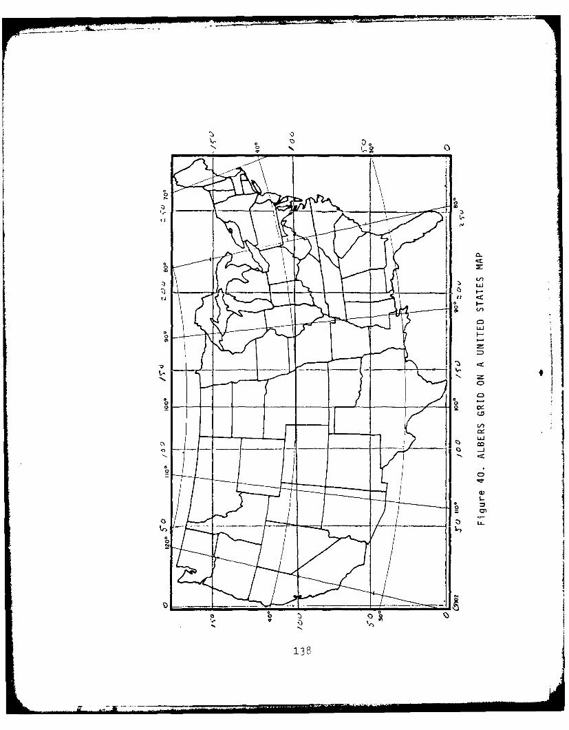
0

oc

0

0

0

0 0

133J

In this program only YLDWC, FISWC, and HOC re used.

Any values may be used for the other variables. Any chanze

in any values of the variables YLDWC, FISSjZC or HOBWC requires

a new weapon class. Each separate weapon class requires an

individual record.

Records 7+NWPC to 7+NWPC+434

Variables: (SPDMO(I,J), DEFMO(I,J), SHRMO(I,J), !=1,1)

J=l,31Format (20X, 3F10.4)

These records are fallout wind speed, direction and shear

on a two degree grid using from 25 to 50 degrees latitude and

from 65 to 125 degrees longitude. The wind speed and shear

are input in knots and immediately converted to miles/hour.

The wind direction is input in degrees counterclockwise from

the north. The wind data may be prepared in this format from

a daily wind by using the program SHRGRD. The second file

needed for input defines the weapons, with one record for each

weapon processed. The input is

Variables: FLAT, FLON, IWPNC

Format 2F10.0, 1 4

Here, FLAT is the weapon latitude, FLON is weapon longitude,

and IWPNC is weapon class.


The algorithms implemented will be described by subprogram.

Obvious bookkeeping steps will be omitted to simplify the

discussion.

Program GRDFAL

The main program guides the calls to other subprograms. To

start the program, the subroutines INVAL and INIT are called;

for each weapon, subroutine CLSIN is then called to read data

for that weapon, and CALDOS is called to process this weapon.

139

These pairs of subroutine calls are repeated until all weapons

have been processed. Finally the subroutines which output the

grid doses are called.

Subroutine INVAL

In addition to reading input data, this subroutine puts the

wind data on a rectangular grid in the Albers plane with 100

miles spacing. To do this the latitude and longitude of each

grid point are found by calling the subroutine ALBERS for the

inverse transformation. Linear interp~olation is then performed

on the input wind grid, which has 2 degree spacing, to find

wind values. On the Albers grid, since the conical Albers trans-

formation performs a local rotation of the coordinate system,

this rotation is added to the wind direction.

Subroutine CLSIN

This subroutine reads individual weapons and locates the

weapons on the Albers grid. The grid coordinates are XC, YC.

In addition, the wind at the weapon is obtained by interpolation

on the Albers grid. After the last weapon has been processed,

ILAST is set to 1.

Subroutine CALDOS

This subroutine calculates the fallout dose at a set of

grid points related to weapon location and wind directions and

distributes these doses to the storage grid DOSARY. If the

parameter IWPWND is set to one, the downwind direction of the

weapon grid points in the direction of the wind at the weapon,

and the crosswind directions are perpendicular. The grid

spacing is variable, but currently set to ten miles, the same

spacing as the storage grid. If the parameter IWPWND is not

one, the downwind distance is increased, in a ,uccession of

steps, by a distance of ten miles in the direction of the local

wind. At each downwind distance, the crosswind distance is

perpendicular to the local wind direction. Within the accuracy

140

of this ten mile integration, the hot line of the fallout follows

the wind stream.

If the value of IWPWND is three, an attempt is made to

compensate for varying wind speed by multiplying the distance

increase by the ratio to wind speed at the weapon to local

wind speed. To preserve normalization, the doses must also be

multiplied by this ratio.

Upon entering the calculation, the wind-velocity-sensitive

portions of the WSEG-10 calculations are performed. The program

then steps upwind in ten mile steps until the hot line dose is

less than the value of DOSMIN, currently set at 1R. The program

returns to ground zero and then steps downwind until the hot

line is less than DOSMIN.

At each downwind distance, the downwind-distance-sensitive

portion of the WSEG-10 model is called to get the hot line dose.

Distances are then stepped off by ten mile increments in the

crosswind direction, and doses calculated at the grid points,

until the dose is less than DOSMIN.

After proceeding for 100 miles, a check is made to see if

none of the locations for a given downwind distance are within

the storage grid. If this is the case, the calculation for

this weapon is terminated since the pattern has been blown out-

side the region of interest.

If the switch INTERP is 0, at each calculated point the dose

is allocated to the nearest storage grid point. If the switch

INTERP is 1, the dose is allocated to the four surrounding grid

points, by linear interpolation. If 1,J are the coordinates of

the grid point southwest of the calculation point, and f isxthe fraction of the grid spacing distance from the point I,J to

the calculated point in increasing J direction (north), then

the dose to be added, DA, is added to the stored dose DG by:

141

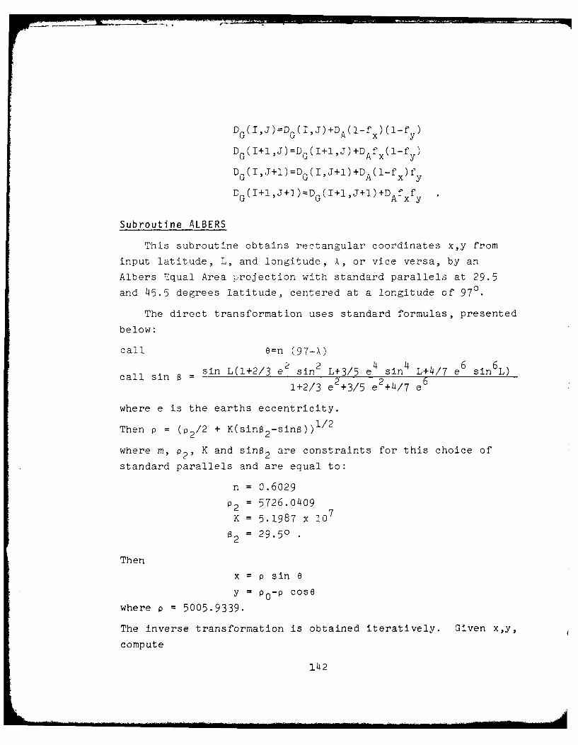
DG(I,J)=DG(I,J)+D (1-f )(1-f

GUA x yD G(I+I,J)=D G(I+I,J)+DA fx (-fy)

DG(I,J+)=DG(I,J+)+DA(-fx)f y

DG (I+l,J+1)=DG(I+1,J+1)+DAf fxy

Subroutine ALBERS

This subroutine obtains rectangular coordinates x,y from

input latitude, L, and longitude, X, or vice versa, by an

Albers Equal Area projection with standard parallels at 29.5

and 45.5 degrees latitude, centered at a longitude of 970.

The direct transformation uses standard formulas, presented

below:

call e=n (97-X)

c sin L(1+2/3 ee sin 2 L+3/5 e4 sin 4 L+4/7 e6 sin 6L)2 2 61+2/3 e +3/5 e +4/7 e

where e is the earths eccentricity.

Then p = (P2/ 2 + K(sin 2 -sin ))11 2

where m, p2, K and sin8 2 are constraints for this choice of

standard parallels and are equal to:

n = 0.6029

P2 = 5726.0409K = 5.1987 x 10

62 = 29.50 "

Then

x = p sin ey = pO-p Cose

where p = 5005.9339.

The inverse transformation is obtained iteratively. Given x,y,

compute

142

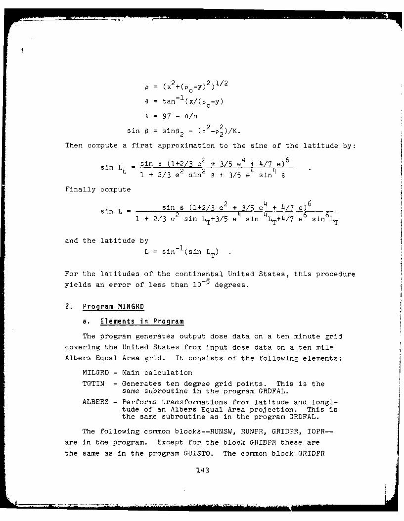
p = (x2 +(po-y)

2 ) 1/2

e = tan- (x/(po-y)

A = 97 - e/n

sin a = sin$2 - (p 2 2 )/K.

Then compute a first approximation to the sine of the latitude by:

sin sin (1+2/3 e2 + 3/5 e

4 + 4/7 e)6

si t=2 2 4 41 + 2/3 e sin B + 3/5 e sin B

Finally compute

2 4 6sin B (1+2/3 e + 3/5 e + 4/7 e)

2i siL 4

s1L + 213 e2 sin LT+3/5 e4 sin 4LT+4/ 7 e6 sin 6LT

and the latitude by

L = sin-l(sin LT)

For the latitudes of the continental United States, this procedure

yields an error of less than l0- 5 degrees.

2. Program MINGRD


The program generates output dose data on a ten minute grid

covering the United States from input dose data on a ten mile

Albers Equal Area grid. It consists of the following elements:

MILGRD - Main calculation

TGTIN - Generates ten degree grid points. This is thesame subroutine in the program GRDFAL.

ALBERS - Performs transformations from latitude and longi-tude of an Albers Equal Area projection. This isthe same subroutine as in the program GRDFAL.

The following common blocks--RUNSW, RUNPR, GRIDPR, IOPR--

are in the program. Except for the block GRIDPR these are

the same as in the program GUISTO. The common block GRIDPR

143

contains the variables used to control the ten minute grid

generation. They are IGRS1, IGRS2, IGRD, JGRD, IGRDF, JGRDF,

NGRSPT, TRGGLA, TRGGLO. These parameters are defined in the

documentation for the program GRDFAL.


The program is run by adding the element P12.QMINGRD to the

run stream. Two input files must be available to the program.The first file contains the input parameters necessary to definethe ten minute grid. These are the same data as are used in the

grid definitions from the program GUISTO. An output file must

also be available to receive the array of doses on the ten

minute grid. Each output file record contains the four defin-

ing parameters--IGRD, JGRD, IGRDF, JGRDF--grid point latitude

and longitude, and the dose. The output format is 414, 2F9.4,

F10.4.


The program is primarily a bookkeeping program. The program

is initiated by reading the grid definition parameters and the

Albers grid doses. A check is made of the header record for the

dose data to ensure the dimensions of the program array are

large enough to contain input data; if not, an error stop is made.

Next a series of calls on the subroutine TGTIN are made to

generate a series of ten minute grid points. For each grid

point, a call to the subroutine ALBERS is made to generate a

location on the Albers grid. A check is made to ensure the

point is on the Albers grid; if not, an error stop is made. If

the point is inside the grid, then linear interpolation is per-

formed on the four surrounding Albers grid points to get the dose

at the target point. The dose is then written on the output file.

The process is repeated until all ten minute grid points have

been generated by the subroutine TGTIN, at which point the program

is terminated.144 (

I

3. Program RAWGRD


This program converts either fallout winds or raw winds on

the grid used by Global Weather Central for daily wind reporting

to winds on a two degree grid covering the United States. The

program consists of a single main program with no subprograms.


The program is initiated by adding the element P12.RAWGRD to

the run stream. An input file must be available which consists

of fallout winds on the GWC grid if the parameter IOCT=l, or

raw winds on the GWC grid if the parameter IOCT=2. The param-

eter IOCT is currently set to 2 on the program. Only this

option will be described since the other option is obtained by

simply bypassing some calculations. An output file to receive

the grid winds must also be made available to the program. When

the program is initiated, tne prompt "input first three letters

of month desired" will be received. The month is selected by

typing the first three letters of the name and a carriage return.


The program is mostly bookkeeping. When the program is

initiated, the wind data are read into storage. The wind data

are at five levels: 700, 500, 300, 200 and 100 millibars, labeled

A to E. Only data for wind grid coordinates II=1 to 22 and

JJ=l to 14 are saved since this is adequate to cover the contin-

ental United States.

The wind data are averaged as they are read to get fallout

winds. The averaging method is the same as in the SIDAC program

of the Command and Control Technical Center. Since only higher

yield weapons are considered in the assessment program, only

high level fallout winds are used. The effective fallout wind

145

at level E, WE is obtained from the raw wind at other levels,A Ef

W to , by

Ef 0.19W E + 0.17WD + 0 .16WC + o.184wB + 0.289WAWf = .1 w

The averaging is actually done on the north-south and east-west

components of the wind. The constants are based on the average

time a particle stays at the various levels in its descent. To

compute a wind shear, the fallout wind at level is also needed.

This is computed by

Wf = 0.11 7WD + 0.231WC + 0.2 5WB + 0.3 9 8WA

The fallout wind shear is then computed by the fallout wind

speed times the sine of the absolute value of the difference

of the wind directions at level D and E, all divided by 20.

Next, points are generated on a two degree latitude/longitude

grid ranging from, 1 atitude L = from 24 to 50 degrees and,

longitude A = from 65 to 125 degrees. For each point, generated

grid coordinates are calculated by

II = 24 + 31.18(cos(A - -.-- )) tan ( L )

JJ = 26 - 31.8 (sin(X - "-)) tan ( 2' L )

The values of II and JJ are truncated to integers and the

inverse of the above transformation used to get the latitude

and longitude of the wind grid point. From this the distance

from the wind grid point to the monitor point is calculated.

The process is repeated to calculate the distances of the other

three wind grid points surrounding the monitor point from the

monitor points. If DA... DD are the distances and WA... WD are

the winds at the four wind grid points, then the wind at the

monitor point, WM, is estimated by

WA/DA + WB/DB + Wc/DC + W D/D D

M l/DA + l/D B + l/D C + l/DD

146

The averaging is performed on north-south and east-west com-

ponents of the wind. This averaging method is the same used

in the SIDAC damage assessment system. The latitude/longitude

of the two degree grid points, the wind speed, wind direction

and wind shear are then written on the output file. The process

is repeated until all two degree grid points have been processed.

147

REFERENCES

[I] Hayes-Jones, R., Schmidt, L. and Stekler, H., ResidualCapability Assessment and the FPA Data Base: AnAssessment (U), P-1483, The Institute for DefenseAnalyses, Arlington, VA, July 1980, SECRET.

[2] Schmidt, L.A., Analytical Representation of BlastDamage for Several Types of Targets, P-1373, TheInstitute for Defense Analyses, Arlington, VA,October 1978.

[3] Schmidt, L.A., A Parametric Study of ProbabilisticFire Spread Effects, P-1372, The institute for DefenseAnalyses, Arlington, VA, September 1979.

[4] Schmidt, L.A., Documentation of Current IDA ComputerMaterial Developed for DCPA, IDA Working Paper, TheInstitute for Defense Analyses, Arlington, VA,January 1977.

[5] Schmidt, L.A., Interactive ADAGIO Program as an Aid toCrises Relocation Planning, P-1183, The Institute forDefense Analyses, Arlington, VA, November 1975.

[6] McGill, J., et.al., Methodologies for Evaluating theVulnerability of National Systems, S-394, The Institutefor Defense Analyses, Arlington, VA, June 1972.

[7] Schmidt, L.A., A Methodology for Fallout Risk Assessment,P-1065, The Institute for Defense Analyses, Arlington,VA, January 1975.

[8] Miercort, F.A., Description of a Fast Running FireSpread Model, P-988, The Institute for Defense Analyses,Arlington, VA, December 1973.

[9] Miller, C.F., The Analysis and Correlation of FalloutPattern Data, DC-FR-1216-II, Contract #DAHC-20-71-C-0273, The Dikewood Corporation, Alberquerque, NM, inthree separately bound parts: PART I: "Summary of theMethods and Derived Values of Scale Parameters," (U),July 1970, SECRET; PART II: "Derivation of a StatisticalFallout Pattern Computational System," (U), May 1973,

149

FMWUN pAGE DLAiLAUJo FILMD

SECRET; Part III: "Computer Program Users Instructions,"March 1979, SECRET.

[10] Miller, C.F., Fallout Modifications Due to UnusualBurst Conditions, DC-FR-1219, Contract #DAHC-20-73-C-0170, The Dikewood Corporation, Alberquerque, NM,December 1974.

[ill Pearsall, E.S., et.al., A Study of Active and PassiveSystems for the Defense of Urban Population Centers,S-388, The Institute for Defense Analyses, Arlington,VA, September 1971.

[12] Schmidt, L.A., "Simplified Nationwide Blast RiskCalculation for Evacuated and Unevacuated ShelteredPopulations," Memorandum to David Benson, DCPA,14 October 1977.

[13] Greene, J.C., "Response to DCPA Questions on Fallout,"DCPA Research Report #20, November 1973, prepared forSubcommittee on Fallout, Advisory Committee on CivilDefense, National Academy of Sciences, with notes andcomments by J.C. Greene, DCPA.

[14] Bauer, E., "Dispersion of Tracers in the Atmosphereand Ocean: Survey and Comparison of Experimental Data,"Geophysical Research, 79,6, Pp.789-95, February 1974.

150

I

DISTRIBUTION LIST

Federal Emergency Management (60) Mr. Edward L. Hill (2)Agency Research Triangle Institute

Mitigation and Research Research Triangle ParkATrN: Administrative Officer .ic 27702Washingkton, DC 20472 Director, Defense Nuclear (1)

Assistant Secretary of the (1) AgencyArmy (R&D) ATIN: r-. David Auton

ATr N: Assistant for Research Washington, DC 20305Washington, DC 20301 Defense Advanced Research (1)

Chief of Naval Research (1) Projects AgencyWashington, DC 20306 1400 Wilson Boulevard

Defense Technical Information (12) Arlington, VA 22209

Center Defense Intelligence Agency (1)Cameron Station (DI-7)Alexandria, VA 22314 Washington, DC 20301

Oak Ridge National Laboratory (1) Department of Energy (1)ATT : Librarian Technical Information ServiceP. 0. Box X Oak Ridge, TN 37830Oak Ridge, TN 37830 Commanding Officer (1)

Kip. Phillip M. Smith (1) U. S. Army Combat DevelopmentAssoc late Director, ComandNatural Resources & Commercial Institute of Nuclear Studies

Services Fort Bliss, TX 79916Office of Science and Technology Director (1)

PolicyExecutive Office Bldg. Lovelace FoundationWashinton, DCe 20500 5200 Gisbon Blvd. S. E.Washington, DC 20500 Albuquerque, NM 87108

Los Alamos Scientific Laboratroy (1) Dr. Walter Wood (1)ATI7: Document Library Dikewood CorporationLos Alamos, Vl 87544 1613 University Blvd., N. E.

The Rand Corporation (1) Albuquerqu,, NM 87106ATTN: Document Library Dr. Eugene Sevin (1)1700 Main Street 10 West 35th StreetSanta Monica, CA 90406 Chicago, IL 60610

Dr. Eugene P. Wigner (1)Oak Ridge National LaboratoryOak Ridge, TN 37831

151

Director, U. S. Army Engineer (1) Dr. Daniel Willard (1)Waterays Experiment Station Office of Operations Research

AT17.: Nuclear Weapons Effects Branch Office of the Under SecretaryP. o. Box 631 Department of the ArmyVicksburg, ES 39180 Washington, DC 20301

Institute for Defense Analyses (60) Mr. Anatole Longinow ()A i: Dr. T .. Scl-nidt ITT Research Institute-0- .i .y-'avy Drive 10 West 35th StreetArlington, VA 222U2 Chicago, IL 61616

Dr. John Bilheimer (1) Dr. Charles E. Fritz 1)Systan, Inc. Program Director343 Second Street Contingency Planning andP. 0. Box U Emergency ServicesLos Altos, CA 94022 Commission on Sociotechnical

Dr. Conrad Chester (1) Systems

Oak Ridge National Laboratory National Research Council

P. 0. Box o 2101 Constitut-on Avenue

Oak Ridge, TN 37830 Washington, DC 2018

Ohio State University (1) U. A. Air Force Special (1)Weapons CenterDisaster Research Center Kirtland Air Force Base

127-129 West 10th Avenue

Columbus, OH 43201 ATTN: LibraryAlbuquerque, N....

Mr. Clark Henderson (1)IDr. Richard Laurino(iSRI International, Inc. Center for Planning andMenlo Park, CA 94025 Research, Inc.

Mr. Carsten M. Haaland (1) 2843 East Bayshore - S,.ite 104Oak Ridge National Laboratory Palo Alto, CA 94304P. 0. BxXOak Ridge, TN 37830 Mr. Walmer E. Strope (1)

5600 Columbia Pike - Suite

Dr. Roger J. Sullivan (1) 101System Planning Corporation Falls Church, VA 220411500 Wilson Bouldvard Emergency Technology Divsiion (1)Arlington, VA 22209 Oak Ridge National Laboratory

Dr. Lewis V. Spencer (1) ATIN: LibrarianRadiation Theory Section 4.3 P. 0. Box XNational Bureau of Standards Oak Ridge, TN 37830Washington, DC 20234 Chief Engineer (1)

Los Alamos Scientific Laboratory (1) ATTN: E2GMCODATL7: Document Library Department of the ArmyLos Alamos, UNI 87545 Washington, DC 20314

152

Army Nuclear Defense Laboratory (1)ATIN: Technical LibraryEdgewood, MD 21010

National Academy of Sceinces (1)Advisory Committee on EnergencyPlanning

ATTN: Dr. Lauriston Taylor2101 Constitution Avenue, N. W.Washington, DC 204l8

Dr. Martin 0. Cohen (1)Matehmtical Applications Group, Inc.3 Westchester PlazaElmsford, NY 10523

Dr. Charles Eisenhauer (1)National Bureau of StandardsCenter for Radiation ResearchWashington, DC 20234

Assistant Secretary of the Air (1)Force (R&E)

Room 4E968, The PentagonWashington, DC 20330

Director for Defense Nuclear Agency (1)ATTN: Technical LibraryWashington, DC 20305

153

10~~~ L1to 10 -0244 -2- ID 4-)

40J' CO 4-) 4m ul 0D C 4 H 0 4) 0, to.

O. '0 (.04 )

0a 0 -.0 -

49 b tI 4o>3 I(D 043 :rl 43

02 4-14 0) r)~0 43 02L)00

ba 4 43 U c0 )0 0 -4

0d -0 . J

A I-C C) "\ 0 -)~02 ~M 40 ) 440

0 202 1641,143 ! -I HH 4.) 0

40))- .r-4 443 .1 a 43

z43 020 -4 01 I 0 Ct -

44 -Y. WIr :J0V

*~a) 4 0C'ZO) IC 431 0 L

43~ 0 4-) 0 420 43.2

44 4.) >. , 4 400).8 4

to 02Q

a) c.4 p

00) C. C0 8).4 t~* 3 H0 0

Lfl3'- $ . 01 02C 84 ~1Go 4. 0 -P 04 02 DWI

CC4 0 0243 0 CG02 B, -10t I. ' Je

020 02 '*'1 4" 02 02 H 4 40 1) 2443 - IJ. 0022 ~ 0

Eu. - DTIC

Documents

Transcript of Eu. - DTIC