AD-A10 497 MISSOURI UNIV-ROLLA DEPT OF ENGINEERING MANAGEMENT F/G 5/1.EMPIRICAL DETERMINATION OF WRSK COMPONENT FAILURE DISTRIBUTIONS--ETCIU)MAY 81 H E METZNER F33615-79-R-5134

UNCLASSIFIED NLflflllllllllllIIIIIIEEIIEEIEEEEEEIIIIIIEEIIIIEEEEEEEEEEEIIEEEEIIIEIIE.mmhEEEEEEmhhEE

FINAL REPORT ON

CONTRACT F33615-79-R-5134

EMPIRICAL DETERMINATION OFWRSK COMPONENT FAILURE DISTRIBUTIONS

PREPARED BY

H. E. METZNER, Ph.D.ASSOCIATE PROFESSOR AND PRINCIPAL INVESTIGATOR

DEPARTMENT OF ENGINEERING MANAGEMENTUNIVERSITY OF MISSOURI-ROLLA

PREPARED FOR

UNITED STATES AIR FORCEAIR FORCE BUSINESS RESEARCH MANAGEMENT CENTER

WRIGTH-PAATERSON AIR FORCE BASEDAYTON, OHIO DT1C

IE'ECTE~f

MAY 1981 S SEP 23 1g81

D

This research was conducted under the sponsorship of the Air Force BusinessResearch Management Center, Wright-Patterson AFB, Ohio. The views

LA.J expressed herein are solely those of the author(s) and do not represent.jthose of the United States Air Force.

Approved p.-.]..c rcicosegDistzibi,-,n UJli ed

S1 9 22 056

._ICuNIT', CL ASSIFICATION OF THIS PAGE (When ft.F,,trrd),

REPORT DOCUMENTATION PAGE READ INSTRUCTIONSI RLPGRT NUMBER 12. GOVT ACCESSION NO. 3 RECIPIENT'S CATALOG NUMBER

14 TITLE ,end Subtitle) 5. TO~E RP M S EN

Empirical Determination of WRSK CpmponentFiaXFailure Distributions S. . igr .4,

7 AUTtaORt. G. CONTRACT OR GRANT NUMBER(s)

H.E etzner .(F33615-79-R1-5134i fr9 PERFORMING ORGANIZATION NAME AND ADDRESS 10. PROGRAM ELEMENT. PROJECT. TASK

Departmient of Engineering Mgt AREA & WORK UNITNUBR

University of Missouri-RollaRolla,_Missouri 65401 ______________

11 CONTROLLING OFFICE NAME AND ADDRESS 2./fE-PRTr *T--Air Force Business Research Mgt Cti' (AFBIR4C/RDCB) /1 may X981/

Wright-Patterson AFB, OH 45433 137__uMr

4 MONITORING AGENCY NAME & ADDRESS(,t different from Controlling Office) IS. SECURITY CLASS. (of this report)

Air Force Business Research Mgt Ctr (AFBRMC/RDCB) UnclassifiedWright-Patterson AFB, OH 45433, s.DCAsFcTO;ONRDN

16. DISTRIBUTION STATEMENT (of this Report)

Distribution Unlimited - Approved for public release.

17. DISTRIBUTION STATEMENT (of the abstract entered in Block 20. if different from Report)

Distribution Unlimited - Approved for public release.

IS. SUPPLEMENTARY NOTES

19. KEY WORDS (Continue on reverse aide if necessary anid idantIl6' by block number)

WRSKMean Time between Failure\Failure RatePoisson Distribution

201 ABSTRACT (Continue ont reverse aide If necessay nd iddentity by block number)

Current methodology for determining components of a War Readiness Spares Kit(WRSK) is based on mean times to failure for the entire U.S. Air Forceinventory. Failures on a specific aircraft type during a calendar periodare divided by flying hours logged on that aircraft type during the sameperiod. Kit configuration is then optimized using the Poisson distributionto approximate kit demand behavior. The Poisson process requires a single

(cont'd on reverse)

DD I jAN73m, 1473 EDITION OF I NOV 65 IS OBSOLETE

SECURITY CLASSIFICATION OF THIS PAGE (When Dete Bator

SICURITY CLASSIFICATION OF THIS PAOE(Whl £1aP(at&0Z. d)

0 ABSTRACT

statistic, mean value of distribution, for which world-wide mean time tofailures is used.

There are several alternatives to the Poisson distribution. Negativebinomial distribution has been suggested as a more appropriate model,and it has been demonstrated that the WRSK configuration would changeunder this assumption.

To test the suitability of both distributions, two analyses wereundertaken of mean time to verified failures of the fleet and assumedconstant failure rate of WRSK items among the fleet. In both analyses,the hypothesis that data is Poisson distributed could not be rejectedfor the majority of the cases. In several cases, however, the Poissondistribution was rejected as an adequate fit for the data and the nega-tive binomial was a viable alternative. Negative binomial also appearedto be a better model in some of the cases where the Poisson distributioncould not be rejected.

AccessionFo

NTIS GPA&!lDTIC TABUnLni_,unced -Justifictclon4

Distribution/Ava ilabil ity Colas'Irva I and/ar

Dist Special

SECURITY CLASSIFICATION OF , I-AGE(When Data KWt

ACKNOWLEDGEMENTS

No major study can be accomplished without a great deal of help and

encouragement. This study is no exception. The principal investigator is

eternally grateful to:

Major Paul Gross, Jr. for encouragement in beginning this project.

Captain Gary Gummersall for bridging the gap between the theoretical and

actual, between the plan and the possible.

Majors Mathis and Gambill for help in understanding the scope of the

problem.

Lt. West, Lt. Llukey, Sgt. Wood and Mr. Furgerson for so willingly

interrupting their routines to supply the necessary data at Moody and Cannon.

Captain Rogers, Sgts. Booth, Adams, Chubb, and especially Blakely at Moody

and Sgts. Bently, Cummins, Dovereall and Hoffman at Cannon for explaining the

intricacies of their work and difficulties in the investigation.

Messeurs. Don Cazel and Chuck Gross from AFLC for initiation into Air

Force terminology and logistics data gathering systems.

Especially appreciated was the enthusiasm and committment of those

associated with the project at the University of Missouri-Rolla. In

particular, the principal investigator recognizes his debt to:

Dr. Lee 8ain for patiently explaining the intricacies of statistical

distributions and developing the missing statistical tools.

Dr. Henry Wiebe for recognizing the pitfalls in the statistics.

Ted Mercer for herding the effort in data collection.

Allison de Kanel for organizing the literary research and analysis of the

data.

Sam Brunner for bringing the power of the computer to bear on the data and

making the analysis a reality.

Donna Kreisler for producing the finished report.

!*

Jim Lathimer, Lance Groseclose, Don Henniger and Bill Schonfeld for their

aid in carrying the daily burden.

Without the help of competent people, no extensive work can be

completed. It is impossible to state the debt owed those listed and many

others who aided and encouraged this study. It is a pleasure to have been

associated with such willing, enthusiastic and highly competent individuals.

Zi

ABSTRACT

The current methodology by which the components of a War Readiness Spares

Kit (WRSK) are determined are based on mean times to failure for the entire

U.S. Air Farce inventory. The failures on a specific aircraft type during a

calendar period are divided by the flying hours logged on that aircraft type

during the same period. The configuration of the kit is then optimized using

the Poisson distribution to approximate the demand behavior on the kit. The

Poisson process requires a single statistic, the mean value of distribution,

for which the world-wide mean time to failures is used.

There are several alternatives to the use of a Poisson distribution. In

particular, the negative binomial distribution has been suggested as a more

appropriate model and it has been demonstrated that the configuration of the

WRSK would change under this assumption.

Underlying the two distributions is a theoretical difference. The

Poisson process arises when a fleet of aircraft have a constant failure rate

associated with each component airplane, but the failure rates among the

airplanes are distributed as a Poisson distribution. The negative binomial

arises when the constant failure rates of the individual airplanes are

distributed as a gamm~a distribution.

In order to test the suitability of the distributions, it is necessary to

investigate the true distribution of failures among airplanes. The data are

too aggregated to achieve this end after they have been collected from the

bases, so data gathering was done at the base level. Maintenance records and

flying hour records were each gathered from their points of origin.

Two such attempts to gather data were undertaken, one at Moody Air Force

Base and the other at Cannon Air Force Base. The flying hour data at Moody

were incomplete, and it was not possible to construct a sufficiently large

iii

I- -. .--.

numnber of failure intervals for analysis. The data from Cannon were complete

and the analysis proceeds from this data base.

Seven thousand and fifty-eight flying records, covering seventy-six

airplanes from July 1979 to September 1980, were obtained from Cannon.

Merging these records with the maintenance data produced 1146 intervals

between verified failures of forty-one removable components on seventy-five

airplanes. The 46 planes which flew at least 200 hours showed 1026 failures

on 58 WUCs in their first 200 hours, while the 14 planes which flew at least

300 hours showed 323 failures on 43 WLJCs in their first 300 hours.

Two types of analysis were undertaken. The first was an analysis of the

mean time to verified failures for the fleet. in the majority of the cases,

the hypothesis that the data is Poisson distributed could not be rejected,

however, in some cases the Poisson distribution was rejected as an adequate

fit of the data. The negative binomial is a viable alternative fit for the

data. Even in some cases where the Poisson could not be rejected, the

negative binomial appears to be a better model.

The second analysis tests the hypothesis that toe assumed constaot

failure rate of WRSK items is Poisson distributed among the fleet aircraft.

Again, the hypothesis could not be rejected for the majority of WRSK items,

but could be rejected for several, indicating that the Poisson model is not an

adequate fit for the fleet rate-of-failure distribution.

A test of effect of surge was run. Although there were several surge

exercises during the period for which data were collected, there was only one

major exercise, Coronet Hammner. Eighteen airplanes took part in this

exercise. Those items which were affected by Coronet Hammer could be isolated

and were dropped from the data set. The two tests were repeated. The

interval test on the total fleet failure distribution for the reduced set

showed no deviation from the adequacy of Poisson distribution. The

iv

rate-of-failure distribution among airplanes in the fleet failed to show more

homogeneity without consideration of surge-stressed items. The lack of

confirmation that surge affects the rate of failure, makes the conclusions

suspect. Since the aircraft that took part in Coronet Hammer flew more hours,

they are over-represented in the sample. If they also display lower failure

rates and were therefore selected, the results would be consistant.

V

TABLE OF CONTENTS

ACKNOWLEDGEMENTS . . . . . . . . . .. . . . . . . . .. .. . . . . i

ABSTRACT ............. .............................. .. iii

LIST OF ILLUSTRATIONS ........... ....................... vi

LIST OF TABLES ........... ........................... .vii

I. INTRODUCTION ......... ............................ I

A. BACKGROUND COMMENTS ........ .................... ... I

B. CALCULATION OF THE INITIAL WRSK .... .............. . .. I

C. OPTIMIZATION OF THE WRSK ...... ................. . .. 3

D. DISCRETE AND CONTINUOUS DISTRIBUTIONS ..... ........... 5

E. POSSIBLE INADEQUACY OF THE POISSON ...... ............ 7

F. IMPLICATIONS OF NON-POISSON FAILURES ..... ........... 9

G. DISTINCTION BETWEEN FAILURES AND DEMANDS ..... ......... 13

H. FACTORS INFLUENCING FAILURES ..... ............... ... 14

I. OBJECTIVES OF THIS STUDY ...... ................. ... 15

J. REVIEW OF LITERATURE ....... ................... ... 15

1. Proschan; Ascher and Feingold .... ............. ... 15

2. Bain and Wright ........ .................... ... 20

3. Fiorentino ........... ...................... 21

4. Other studies of Operational Data .............. ... 21

II. METHOD ............ ............................ ... 24

A. OVERVIEW OF RESEARCH DESIGN AND METHODS USED ........ ... 24

B. DATA COLLECTION ........ ...................... ... 24

vi

Table of Contents (continued) Pg

C. SELECTION OF SUB.JECTS .. ... ....... .........27

1. Selection of Aircraft. .. ...... ....... .. 27

2. Selection of Aircraft Components. .... ........27

3. Extraction of Data. ... ........ ........29

0. DETECTION AND REMOVAL OF ERRORS IN THE

MAINTENANCE DATA .. ...... ....... ....... 30

1. Introduction. ... ........ ....... ... 30

2. Sloppy Records. ... ........ ....... .. 31

3. Typographic Errors. .... ....... ....... 33

4. "Orphan Parts". .... ....... ....... .. 34

E. M'ERGING MAINTENANCE AND FLYING INFORMATION .. ........34

F. PROCEDURE FOR ANALYSIS OF MAINTENANCE DATA FROM

ANALOG EQUIPM'.ENT. ........ .............. 35

111. RESULTS. .. .............. ............. 38

A. DATA OBTAINED. .. ................ ..... 38

1. Introduction .. ................ .... 38

2. Interfailure Intervals. ......... ....... 38

3. Failures .. ................ ...... 42

B. ANALYSIS OF INTERFAILURE INTERVALS. ........ .... 43

1. Introduction .. ............... ..... 43

2. Development of Plots. ......... ........ 43

C. ANALYSIS OF FAILURE COUNT .. ......... ....... 53

1. Introduction .. ...... ....... ....... 53

2. Variance-to-mean ratio .. ...... ....... .. 53

3. XlTest for Equal Means of Poisson Planes. .. ......54

4. Estimation of Negative Binomial Parameters. ... ... 54

vii

Table of Contents (continued) Page

0. DISCUSSION OF RESULTS OF ANALYSIS

OF INTERFAILURE TIMES .. ........ ........... 55

1. Plots of Empirical and Theoretical

Fraction Surviving. ......... ......... 55

a. 51ABE. .. ................ ..... 56

b. 51ABH. .. ................. ....

c. 51CAC. .. ................. ..... 6

d. 61AAO. .. ................ ..... 56

e. 61ABO. .. ................. .... 56

f. 61ACO. .. ................. .... 56

g. 61BAO. .. ................ ..... 63

h. 65BAO . .. ..................... 63

i. 73NAO. .. ................ ..... 63

j. 73PAO. .. ................ ..... 63

k. 73PB . .. ................ ..... 63

1.- 73PDO. .. ................ ..... 63

m. 73QA0. .. ................ ..... 63

n. 73RB0. .. ................ ..... 63

o. 73RE0. .. ................ ..... 63

p. 73SB0. .. ................ ..... 73

q. 73SDO. .. ............... ...... 73

2. Estimation of Negative Binomial Parameters .. ..... 73

E. DISCUSSION OF RESULTS OF ANALYSIS OF

FAILURE COUNT. .. ................. .... 73

1. Variance-to-mean ratio. ......... ....... 73

2. X -Test for Equal Means of Poisson Planes. .. ..... 81

3. Estimation of Negative Binomial Parameters .. ..... 84

Table of Contents (continued) Pg

F. CONCLUSION OF ANALYSIS .. .................. 84

IV. ANALYSIS OF THE EFFECT OF SURGE .. ......... ...... 91

A. INTRODUCTION. ....... ..... ..... ....... 91

B. ANALYSIS OF INTERFAILURE INTERVALS. ......... ... 92

C. ANALYSIS OF FAILURE COUN4T.. ......... ....... 95

0. CONCLUSIONS. .. ............... ....... 96

V. LIMITATIONS OF THE STUDY .. ................ .. 99

A. INTRODUCTION .. ................ ...... 99

B. LIMITATIONS OF SAMP'LE SELECTION .. ........ ..... 99

C. LIMITATIONS OF DATA COLLECTION .. ............. 100

D. LIMITATIONS OF ANALYSIS. .. ................. 101

VI. CONCLUSIONS AND RECOMMIENDATIONS. .. .............. 103

A. FAILURE DISTRIBUTIONS OF WRSK COMPONENTS. .......... 103

B. OTHER AREAS OF INVESTIGATION .. .............. 104

BIBLIOGR~APHY .. ....... ................. ... 105

APPENDIX

I. .. ............... .............. 108

II. .. ........ ................. .... 109

III .. ........ .................. ... 114

ix

LIST OF ILLUSTRATIONS

Figure Page

1. Work Un~it Code Hierarchy. .. ..... ........ .. 28

2. Empirical and Theoretical Fraction Surviving for 51ABE . 57

3. Empirical and Theoretical Fraction Surviving for 51ABH . 56

4. Empirical and Theoretical Fraction Surviving for 51CAC . 59

5. Empirical and Theor~tical Fraction Surviving for 6lAAO . 60

6. Empirical and Theoretical Fraction Surviving for 61ABO 61

7. Empirical and Theoretical Fraction Surviving for 61ACO . 62

8. Empirical and Theoretical Fraction Surviving for 61BAO . 64

9. Empirical and Theoretical Fraction Surviving for 658PA) 65

10. Empirical and Theoretical Fraction Surviving for 73NA~O . 66

11. Empirical and Theoretical Fraction Surviving for 73PAO) 67

12. Empirical and Theoretical Fraction $.irviving for 73PB0 68

13. Empirical and Theoretical Fraction Surviving for 73PD0 69

14. Empirical and Theoretical Fraction Surviving for 73QAO 70

15. Empirical and Theoretical Fraction Surviving for 73RBiO . 71

16. Empirical and Theoretical Fraction Surviving for 73REO 72

17. Empirical and Theoretical Fraction Surviving for 73SBO 74.

18. Empirical and Theoretical Fraction Surviving for 73SDO 75

x

LIST OF TABLES

TABLE Page

I. CHARACTERISTICS OF A-7D WRSKS ..... ............... ... 11

II. PERFORMANCE OF A-7D POISSON WRSK

UNDER NEGATIVE BINOMIAL DEMAND ..... ............... ... 11

III. DIFFERENCES IN DEPTH OF STOCKAGE OF HIGH COST ITEMS

BETWEEN POISSON AND NEGATIVE BINOMIAL A-7D WRSKS ........ . 12

IV. ACTION TAKEN CODES ACCEPTED BY MAINTLOG .............. .. 32

V. WORK UNIT CODES WITH AT LEAST ONE FAILURE INTERVAL ....... 39

VI. FAILURE COUNT STATISTICS FOR FIRST 200 HOURS OF PLANES

THAT FLEW AT LEAST 200 HOURS ...... ................ ... 44

VII. FAILURE COUNT STATISTICS FOR FIRST 300 HOURS OF PLANES

WHICH FLEW AT LEAST 300 HOURS ..... ............... ... 47

VIII. WORLDWIDE MEAN TIMES BETWEEN FAILIURE AND EMPIRICAL

MEAN TIMES BETWEEN VERIFIED FAILURES .... ............ .. 50

IX. TEST OF THE EXPONENTIALITY OF INTERFAILURE INTERVALS .... 52

X. VARIANCE-TO-MEAN RATIO OF FAILURES AT 200 FLYING HOURS . . . 76

XI. VARIANCE-TO-MEAN RATIO OF FAILURES AT 300 FLYING HOURS . . . 78

XII. COMPARISON OF VARIANCE-TO-MEAN RATIOS AT 200 AND

300 HOURS ........... ........................ ... 79

XIII. CHI SQUARE TEST OF VARIANCE-TO-MEAN RATIO .. ......... ... 82

XIV. SUMMARY DATA FOR CORONET HAMMER ....... .............. 85

XV. ESTIMATE OF NEGATIVE BINOMIAL PARAMETERS FROM

FAILURE DATA ........... ........................ 86

XVI. ESTIMATES OF AVERAGE INTENSITY ....... ............... 88

xi

List of Tables (Continued) Page

XVII. TEST OF THE EXPONENTIALITY OF INTERFAILURE INTERVALS

OF WUC IN NON-SURGE ........ .................... .. 93

XVIII. COMPARISON OF THE TEST STATISTICS FOR THE TOTAL SET AND

NON-SURGE SET OF INTERFAILURE INTERVAL DATA .. ........ . 94

XIX. CHI SQUARE TEST OF VARIANCE-TO-MEAN RATIO FOR NON-SURGE

CONDITIONS ............ ......................... 97

xi

I. INTRODUCTION

A. BACKGROLD COMENTS

The mission of the United States Air Force requires it to be ready to

provide operational airplanes anywhere in the world on short notice. The de-

ployment of these airplanes will not always include immediate access to normal

supply channels for spare parts, yet maintenance will certainly be required.

The War Readiness Spares Kit (WRSK) is an air transportable package of

spare parts designed to maintain a specified number of airplanes as a fleet

capable of performing its mission for a specified period of time, in case the

airplanes are deployed beyond the reach of normal supply channels.

For example, a typical Fll10 WRSK is designed to support twenty-four

planes for a thirty day, 1723 flying hour program. It contains 994 component

items with from 1 to 144 units of each item, ranging in cost from $0.01 per

unit to $566,500.00 per unit, for a total of 3366 units and a total cost of

$144,849,767.00.

In order to make the best use of the taxpayers' dollars, it is important

that no more parts be included in the WRSK than will be necessary to maintain

the fleet for the desired flying hour period and mission. For the F111D kit,

a ten percent excess in stockage may cost over fourteen million dollars. Yet,

it is also important that the kit actually be capable of supporting the fleet

as it is intended.

B. CALCULATION OF THE INITIAL WRSK

The determination of which items will be included in the WRSK is both a

mechanical and a political process. It is influenced to some extent by the

apparent likelihood of failure of an item, to some extent by safety considera-

tions, and to some extent by interaction among the system manager and his

-1-

using organizations. The process of selection has been thoroughly described

elsewhere (Rasussen and Stover, 1978: 10-14). In summnary, the following

factors are considered by the system manager in preparing a list of candidates

for inclusion (Morrison and Probst, 1975, cited in Rasmussen and Stover, 1978:

10-11):

1. Probability of demand

2. mission essentiality

3. Dimension (certain size limitations are set due to palletization re-

quirements)

4. Maintenance capability

5. Remove and replace time

If it were possible to say precisely how maniy of each item would break

down during deployment, the kit could be made up of just those exact parts, in

the precise quantities that would be needed. In fact, there is uncertainty.

It is necessary to estimate how many units of each item will be neeoec. This

estimate is based on information about past performance of the part. For ex-

ample, if it is known that in the past, four transducers failed in twelve hun-

dred flying hours, then, asg "nIng a constant failure rate, ten transducers

would fail in three thousand flying hours. This information can be calculated

for each individual part, or Item.

Onice the list of items has been developed, the quantity of each item to

be included In the WRSK must be calculated. In general, a demand rate ex-

pressed in units per flying hour is multiplied by the total flying hour pro-

gram that the kit is designed to support. The calculations include modifica-

tions to allow for repair Capability, if any, at the deployment site.

If the item is not repairable, the initial list quantity is obtained as

follows (Rasmussen and Stover, 1978: 14):

-2-

Initial list quantity = 0 X QPA X R , where

D = Organizational and field maintenance demand rate, in units

per unit flying hour,

WA = Quantity of the item per aircraft, and

R = Wartime flying hour program.

If the item is repairable, the initial list quantity is obtained as fol-

lows (Rasmussen and Stover, 1978: 14):

Initial list quantity = DO X QPA X R + BR X QPA X RC , where

DO = Organizational and field maintenance demand rate, in

units per unit flying hour,

BR = Base repair rate of the item, and

RC = Base repair cycle program--the number of days required to repair

the item, usually impressed as three days.

Additional modifications may be used to allow for setup time of repair

facilities at the forward site, and for a flying hour program that varies

daily.

The list.is then negotiated with the using major command, taking into ac-

count whether or not the item is a safety-of-flight or a time change item.

The FlllD kit described above was designed by this method.

C. OPTIMIZATION OF THE WRSK

After the kit is initially calculated, it is optimized. Optimization re-

fers to improving the efficiency with which money is spent on the WRSK. The

resulting kit costs no more than the initial kit, and is at least as adequate

as the original kit was. For the WRSK, adequacy is measured in terms of the

expected number of Stock Due Outs (SO0's), or outstanding backorders, and the

expected number of Not Mission Capable (NMC) airplanes. There are several

methods of optimization available (Messinger and Shooman, 1970). In the case

-3-

of the WRSK, optimization is accomplished by a process known as marginal anal-

ysis.

As Chen pointed out (1979: 9), marginal analysis may begin with an empty

Initial kit, or with a large initial kit, or with the existing kit composi-

tion, but "different initial kits will result in different final kit composi-

tions, which, in turn, vary greatly in terms of cost and level of readiness."

Chen endorsed using the conventional kit as a starting point (1979: 15). CThen

also developed an algorithm to use another optimization method, the branch aric

bound technique, to optimize the WRSK (1979: 17-29).

The WRSK is currently calculated using marginal analysis, with the con-

ventional kit as the initial kit.

As an example, the F111D WRSK described above was optimized by the use of

the marginal analysis technique. The total cost of the kit dropped from

$144,849,767.00 to $129,527,231.00. a savings of 10.5%. The expected number

of I14C aircraft dropped from 11.32 to 11.29, and the expected S00 dropped from

563.016 to 476.610. The total number of units rose from 3366 with the con-

ventional kit to 4277 with the marginal analysis kit. So, in this case, the

performance of the kit was Iiproved under both criteria, while the cost was

reduced by over ten percent.

This improvement is obtained by comparing the advantage to be gained by

including any one item with~ the advantage to be gained by adding any other.

The item which gives the greater advantage per dollar provides the more effi-

cient use of the money allocated for the WRSK.

In comparing advantage, it is necessary to compare the relative like-

lihood of events. This can be done by the use of probability distributions.

Probability distributions allow calculations that will give the likelihood of

one failure, or two failures, or of any number of failures, if enough is known

about the past behavior of the part. For the Poisson distribution, all that

it is necessary to know is the average failure rate, and since this informa-

tion is convenient to obtain and simple to calculate, as demonstrated above,

the Poisson distribution is used in the WRSI( calculations.

Using the Poisson probability distribution, also called the Poisson prob-

ability density function, it is possible to calculate the expected number of

S00 and of NMC aircraft. Then, that spare can be added to the stock that re-

duces the expected number of SDO and t442 at the lowest possible additional

cost.

For example, suppose both a discriminator, costing $511.90, and a valve,

costing $9,322.00, have the same expected number of failures, and the same ex-

pected number of Not Mission Capable aircraft if they are not added to the

WRSK. The advantage of removing an aircraft from talC status costs $511.90 if

the discriminator is included, and $9,322.00 if the valve is included. So the

discriminator provides the same advantage, more cheaply.

The actual calculations for the WRSK allow for cases with more than one

unit of the same item on the airplane, and with different failure rates. With

the large number of items included in the WRS(, the marginal analysis calcula-

tions are computerized.

The initial or "conventional" kit, the marginal analysis kit, and the

other optimization procedure developed by Chen all depend on the use of an av-

erage total demand rate calculated on data gathered on all bases worldwide.

Because this average demand rate is used, a Poisson probability distribution

is used to calculate the likelihood of failure, and expected SO~s and NM4C air-

craft.

D. DISCRETE AND CONTINUOUS DISTRIBUTIONS

The Poisson distribution is a member of a class of distributions that are

called discrete distributions, because they give the likelihood of whole

items--how many events occur in a period of time, how many holes are dug in an

-5-

acre, and so on. This is called a discrete distribution because the items be-

ing counted are discrete, or separate, and indivisible. For a discrete dis-

tribution, it is possible to say, "there is a ten percent chance of failure in

the first ten minutes," but it is not possible to say, "there is a twenty per-

cent chance of half a failure in fifteen minutes." The event in question is

indivisible.

On the other hand, suppose the question is, huw much time occurs between

failures? There might be an hour between failures, or half an hour, or

twenty-three and a third seconds. Time is not discrete, or indivisible, and

the type of probability distribution that is used to discuss the distribution

of time is called a continuous distribution, because it gives the likelihood

of a continuous item.

Either a continuous or a discrete distribution may be used to describe a

given situation, discrete if the events or occurrences are being counted, con-

tinuous if the intervals between events or occurrences are being examined.

There is an intimate relationship between certain discrete and certain

continuous distributions. In any case where a Poisson discrete distribution

describes the distribution of events, the exponential continuous distribution

describes the distribution of the intervals between events. This result is

extremely useful because, if it is difficult or impractical to examine one set

of statistics, it may still be possible to examine the other set, and if one

type of distribution can be established, it establishes the other. Proving

the presence of a Poisson discrete distribution proves the exponential contin-

uous distribution. This result is so important that the entire system is re-

ferred to as a Poisson process. When a Poisson process is referred to, it

automatically implies an exponential continuous distribution of the inter-

arrival times.

-6-

Another discrete distribution is the negative binomial distribution.

Like the Poisson, it is used when the distribution of the discrete events is

needed. When a lot of individual airplanes have different constant occurrence

rates for some event, and the different constants are distributed by the gamma

distribution, then the negative binomial describes the total distribution over

all individuals.

It has recently been shown (Bain and Wright, 1981) that a certain contin-

uous distribution, related to Snedecor's F, is to be expected when the nega-

tive binomial distribution describes the distribution of the events. If the

Bain-Wright interarrival times are present, then the negative binomial de-

scribes the distribution of events. If it can be shown that a negative bino-

mial distribution describes the distribution of events, then a Bain-Wright

interarrival distribution has also been demonstrated. If one is known, the

other is known.

Among other continuous distributions, Hahn and Shapiro (1967: 118) note,

"the gammia and log-normal distributions have been advanced as time-to-failure

distributions on both theoretical and empirical grounds."

Other discrete distributions which might describe the distribution of

failures include the Pascal and the geometric distributions. The negative bi-

nomial distribution is a generalization of the Pascal distribution, and the

two are often discussed together, while the geometric distribution is a spe-

cial case of the Pascal distribution.

E. POSSIBLE INADEQUACY OF THE POISSON

As mentioned above, the Poisson distribution is currently used to cal-

culate the WRSK. The use of the Poisson carries with it certain implica-

tions: that the failures are independent, and that the failure rate is a con-

stant. If the failure rate of a part were not constant, or If the failure of

a part depended on the previous history of the equipment, another probability

-7-

distribution might be more appropriate for that part. This does not mean that

the Poisson would not be adequate to describe worldwide behavior and need for

that spare part. In any case where data from a large number of sources are

being combined, a certain smoothing effect occurs. Thus, demand for a part

over the entire Air Force may indeed follow a Poisson distribution, but that

may be because the aggregation of a large number of sources has eliminated the

effects at the unit level of such variables as weather, experience of the

mechanics, personnel transfers, command emphasis, and so on. Large peaks of

demand at the local level are smoothed out by the time they reach the depot

supply point.

At the local level, or even at the level of the individual airplane,

there may be another probability model that would better describe the distri-

bution of failures of some items included in the WRSK. would that have any

significant effect on the ability of the WRSK to support a fleet?

In a very focused attempt to examine the failure distributions of air-

craft equipment, Johnson and McCoy (1978) studied the behavior of three iner-

tial measurement units. They based their analysis on the arrival dates of un-

serviceable units at the maintenance depot, without regard for possible mar-

shaling of shipments. Thus (Johnson and McCoy, 1978: 15), "multiple arrivals

on a given date were indicated by multiple occurrences of that date on the

file." The file of "failure" dates was then sorted chronologically, and par-

titioned into overlapping data sets. The first eight quarters of data were

grouped into the first subset, then the initial quarter was dropped and the

ninth added, to form the second population subset, and so on. Each of these

"base periods" for each IMU was ar,,,ysed separately.

The Kolmogorov-Smirnov test was used to determine if any of the popula-

tior, subsets fit the Poisson distribution. None of the base periods of any of

the 'nree IMU's could be fit to the Poisson distribution.

-8-

The next test performed was a calculation of the variance-to-mean rat-').

The variance-to-mean ratio of the Poisson distribution is unity, while for a

binomial distribution the ratio is less than one (indicating the variance is

less than the mean), while for the negative binomial distribution, the ratio

is greater than one. (The mean is what is usually called the "average," while

the variance describes how spread out the data is.) In all data subsets, the

variance-to-mean ratio was greater than one. This led Johnson and McCoy to

test the data for fit to the negative binomial distribution. Out of

thirty-six of these data subsets for the three IMU's, twenty-two were fit to

tne negative binomial, at a ninety-percent confidence level. The other sub-

sets could not be fit to any distribution by the statistical analysis package

used by Johnson and McCoy.

Johnson and McCoy recommnended (1978: 48, 49) further tests of both the

logarithmic Poisson distribution (which is a generalization of the Poisson)

and the negative binomial distribution. However, they noted (1978: 7):

"If the requirements computation were not sensitive to the differences indemand embodied in alternative probability distributions, significantlyimproved, accuracy would not be expected. If the requirements computationwere, however, sensitive to these differences, the magnitude of thechange would indicate whether an improved technique would pay for itselfin savings or whether its effect would warrant the costs associated withimplementation."

F. IMP'LICATIONS OF NON-POISSON FAILURES

In a Rand Corporation Working Note, Lu (1977: 2) noted that one feature

of the marginal analysis method of computation (which is called the D0:29) is:

"that it makes an explicit assumption that demand for spare parts...can be represented by a certain probability function. In this way, theuncertainty inherent in spares demand can be explicitly modeled. But re-sults may depend on a particular assumption regarding the probabilityfunction.

"In 0029, it is assumed that the probability density function of demandsfor spares during a period for which the WRSK is designed to provide sup-port is the Poisson distribution. It may be necessary to perform an em-pirical investigation to resolve this question. However, first, a para-metric analysis should be undertaken to gain insight into the effect ofincorrect specifications of the probability function."

-9-

The Working Note reported on the results of that parametric analysis.

Four WRSKs were constructed for the A-70, one based on the assumption of thef

Poisson distribution, the others based on the assumption of a negative bino-

mial distribution.

The characteristics of the WRSK with a Poisson assumption and of the

WRSKS with the negative binomial assumption are shown in Table I. There are

three negative binomial WRSKs because, unlike the Poisson, which has one para-

meter, the average number of failures, the negative binomial has two para-

meters. A parameter is used to completely specify tne shape or form of a ois-

tribution.

The WRSK based on the Poisson assumption was then evaluated to see how

responsive it would be to a situation in which the demand distribution was in

fact a negative binomial. The results are shown in Table Il. As Lu concluded:

"if the assumption about demand distribution is incorrect, the expectedperformance of the WRSK can be grossly overstated. The most seriouspractical implication of such a misspecification is that it could lead tounderstating WRSK requirements."

Another interesting conclusion of the Working Note was that the compo-

sition of the Poisson WRSK and of the Negative Binomial WRSK with vari-

ance-to-mean Ratio 2.5 were significantly different. See Table III. The con-

clusion of this comparison was (Lu, 1977: 9),

"if we switch from the Poisson distribution to the negative binomial dis-tribution, the stockage of more than half of the items would beaffected. For a handful of high-cost and high-demand items, there willbe a little less depth in the stockage, but for a large number oflow-cost items, there will be an increased stockage. Thus, the compo-sitions of the resulting kits are quite different. Implications of thisdifference require further investigation."

To reiterate, Lu concluded, (1979: 10)

"First, we found that if we use the Poisson density function to approxi-mate demands and it turns out that the demands follow a negative binomialdistribution, then our estimates of the characteristics of a WRSK basedon the Poisson assumption are too optimistic. Secondly, if a new kitwere to be determined based nn the negative binomial assumption,

-10-

TABLE ICHARACTERISTICS OF A-7D WRSKS

Poisson Negative Binomial withVariance-to-Mean Ratio

1.5 2.0 2.5

Cost ($million) 4.97 4.99 4.95 4.91

Stock Outages 60.5 69.6 77.2 73.4

NORS (NMC Aircraft) 6.4 7.7 8.8 9.8

Source: Lu, 1977, Tables 2 and 3: 7, 6

TABLE IIPERFORMANCE OF A-7D POISSON WRSKUNDER NEGATIVE BINOMIAL DEMAND

Variance-to-Mean Ratio of

Negative Binomial Demand

1.5 2.0 2.5

S0 72.2 81.6 89.3

NORS 7.7 8.9 9.9

Source: Lu, 1977, Table 3: 8

-1i-

TABLE IIIDIFFERENCES IN DEPTH OF STOCKAGE OF

HIGH COST ITEMS

BETWEEN POISSON AND NEGATIVE BINOMIAL A-7D WRSKS

2.5

Item Unit Cost Poisson WRSK NegativeBinomial

WRSK

RT Unit $ 4,257 19 18

Receiver 5,302 20 17

Receiver 30,890 14 12

Processor 19,274 18 15

I M U 54,075 12 11

Computer 98,314 10 9

Display 33,472 15 13

Source; Lu, 1977, Table 4: 9

-12-

the composition of this new kit will be quite different from that of theoriginal one.

"The above findings suggest that empirical investigation is needed todetermine which probability density function will fit demand data better."

As a direct result of that conclusion, this study is an empirical invest-

igation of failure distribution.

G. DISTINCTION BETWEEN FAILURES AND DEMANDS

It is worth noting at this point that there is a difference between fail-

ures and demands. At the depot level, there is virtually no distinction be-

cause, if an item which has not failed is removed from an airplane at the unit

level, it is tested and returned to stock at the unit or base level, and never

generates a demand at the depot level. However, at the unit or base level,

the distinction between demands and failures is more significant. Several

items may be removed from an airplane for testing and be replaced at once from

the spares stock. This generates a local demand, but all of those removed

parts which are not failures are checked out and returned to stock. Thus,

only a portion of demands may be classified as true failures. Conversely,

there may be failures which are not demands from an airplane. Items in stock

are periodically tested, and a failure of one of these items will result in a

demand on depot (or in a repair at the local level, if the item is locally

reparable) without being the result of airplane operation, and thus having no

functional relationship to flying hours, or sorties. Similarly, "hangar

queens," airplanes which serve as sources for cannibalized parts and are only

rarely flown, serve as a virtual extension of supply. A part may be removed

from one of these airplanes and tested as non-operational. The failure of

this part might be due to degradation, or to damage when other parts were re-

moved from the airplane, but it can hardly be related to the operation of the

source airplane.

What factors might influence failures in an airplane?

-13-

FL. -rn rn n

H. FACTORS INFLUENCING FAILURES

Bendle and tHjmble (1978) considered, from a theoretical point of view,

four different aspects of operating history which might influence failure and

degradation behavior. The four different aspects were: total elapsed calen-

dar time, total accumulated "on" time, length of current operating history,

and random environments. The unit was modeled as being capable of failing in

any one of the first three modes, all operating independently of the others.

The authors assumed a constant hazard rate in each of the first three modes,

thus invoking once again the assumption of Poisson behavior. As ir. the case

of devices connected in series, failure in any one mode caused failure of thle

unit. Degradation of the unit was a function of the first three modes plus

random environment.

In this present study, the failure behavior is consioered to be in-

fluenced by flying hours, which, for the airplane itself, corresponds approxi-

mately to accumulated "on" time. It is recognized that individual items of

equipment may not be operated constantly while the airplane is in flight; an

extreme example would be tires, which are stressed on landing and takeoff.

It has been shown empirically that other factors affect failure behavior.

Tadashi (1975) showed that there were strong seasonal trends in the mean

time to failure of the Air Data Computer, correlating (Tadashi, 1975: 98-99)

"with a special training program for the Japanese Air Force: namely, aflying technical competition for each Air Force Base had been held regu-larly in the spring, and pilots tend to become more critical of equipment(Air Data Computer) operation having an impact on aircraft flight sta-bility in a competition season. For this reason maintenance service menalso become more critical of equipment performance ouring groundinspection."

mean time to failure dropped in the spring, not as a result of the number

of flying hours changing, but rather because of the circumstances under which

the flights were occurring. This leads to the question, does failure behavior

-14-

in peacetime training accurately predict failure behavior under surge con-

ditions or under wartime deployment? Does the length or frequency of sorties

have an impact on the failure rate as a function of time? Hunsaker, Conway,

and Doherty determined (1977:v) that:

"the length cf time for a sortie has little affect [sic] on the number ofmaintenance writeups following. Therefore, an increase in sorties for agiven period with no change in flying hours wouid geerate additionalmaintenance writeups."

They also noted (1977:v) that "some WUC's [Work Unit Codes] are sensitive

to specific types of mission flown."

Therefore, it can be seen that the type of mission, the circumstances

surrounding the mission, the attitude of maintenance personnel, and the length

and frequency of mission may all effect the failure behavior of an item of

equipment.

This study examines failures which result from aircraft operation.

I. OBJECTIVES OF THIS STUDY

The basic objectives of this study are:

I. Determine the probability distribution function(s) of peace-time

failures resulting in demands from a WRSK.

II. Determine the probability distribution function(s) of surge

failures resulting in demands from a WRSK.

III. Determine the relationship between peacetime failures and surge

failures.

In order to accomplish these objectives, operational data will be

examined.

J. REVIEW OF LITERATURE

I. Proshcan; Afcher and Feingold. There have been other studies of op-

erational data which examined empirical failure distributions. One of the

most well known of these is the study conducted by Proschan in 1963. Proschan

-15-

examined data from a fleet of thirteen airplanes on failure of at, air conli-

tioning system. The airplanes were all Boeing 720 jet,, and the data covere.

an extended period of time.

Proschan's data and paper were extensively reviewed by Ascher and

Feingold (1979). Both papers are discussed below.

Proschan's study had two major similarities to this study. First, "ne

original aim was to make predictions and decisions for the entire fleet of 72o

jets (rather than for individual airplanes)," so Proscrhan pooled data from the

airplanes as part of his preliminary analysis.

Second, the air conditioning system may be regarded as a reparable "black

box" component with unknown subcomponents. It is worth noting here that the

WRSK in-ludes both reparable and non-reparable itemF, corresponding to the two

maintenance concepts used by the Air Force: "remove and replace" ("RR"), aiid

"remove, repair and replace" ("RRR").

The two concepts apply to components of the airplane known as LRUs, or

Line Replacable Units. These units may be thought of as "black boxes" with

unknown, undifferentiated contents. An LRU is removed from the airplane when

there is an indication that the unit has failed, whether because the function

which it should perform is not being accomplished, or because there is a sys-

tem indication such as a warning light, or because of visible damage, or for

any other reason.

Once an LRU is removed from the airplane, it is immediately replaced by a

like item. This is the "remove and replace" part of both the RR and the RRR

maintenance concepts. The item is then bench checked, that is, tested in a

shop, to determine if it has in fact failed. If it has not failed, it is

placed with the stock of replacements. Depending on the turnaround time in

the shop, efficiency of the mechanics, and so on, it might even be immediately

-16-

reinstalled on the airplane it was removed from, but this cannot be assumed,

and is not required. Rather, the unit is meant to be replaced at once.

Only after a failure has been verified, does the treatment of the LRU

vary between the RR and the RRR maintenance concepts. In the RR concept no

maintenance capability or spares are available to repair the LRU at the for-

ward site. The LRU is either disposed of or returned to the rear support area

or the next higher level of maintenance support for repair. Under the RRR

concept, the items may be repaired at the deployed maintenance shop, and cer-

tain spare parts may be stocked. These parts are called Shop Replaceable

UnIts, or SRU's, and may be regarded as the subcomponents of the black box

which was removed from the airplane. One or more of these subcomponents may

have failed or been damaged, causing the component, or LRU, to fail. SRL~s may

also be reparable, and are also classified as either RR or RRR items. In

their discussion of Proschan's paper, Ascher and Feingold made a strong dis-

tinction between repairable and non-repairable systems. The distinction de-

velops from two commonly used meanings of "failure rate." One of these mean-

ings represents whether or not there is an increasing or decreasing tendency

for an item to fail the longer it is used. Ascher and Feingold preferred the

term "force of mortality" for this concept. It is also sometimes called the

"hazard rate." The other meaning is the tendency of successive items in the

same system to have progiessively longer or shorter lives, which might be the

result of system deterioration or improvement. Ascher and Feingold illustrat-

ed this distinction with the following example (1979: 154):

"Assume that a sequence of light bulbs are placed in a socket, each re-placing the previously burned out bulb. Assume further that each bulbwears out, i.e., the longer it operates, the more likely it is to fail inthe next unit interval . . . . However, further assume that the succes-sive bulbs have longer and longer lives,. .. ... nder these assumptions,the times between successive failures will tend to become larger andlarger in spite of the increasing force of mortality within

-17-

each failure interval. If the usual terminology were used to describethis situation, a statement such as the following would have to be made:the overall 'failure rate' is decreasing even though the 'failure rate'within each interval is increasing."

Ascher and Feingold thus distinguished between wearout of a reparable and

of a non-repairable item (1979: 154-155):

"For non-repairable items, the relationship of increasing force ofmortality to wearout is straight-forward: the older the unit (as meas-ured from the time it was first put into service) the greater the chancethat failure will occur in the next unit of time. For a repairable item,however, wearout in the sense of increasing force of mortality is a prop-erty of an interval between successive failures. This follows from thefact that the 'age' associated with force of mortality is the time sincelast repair instead of the time since the system was first put into ser-vice. Therefore, aging in the different sense, that times between suc-cessive failure of a repairable system are getting smaller, should bereferred to by another term, e.g., 'deterioration'."

As a consequence of the distinction they draw between repairable and

non-repairable systems, Ascher and Felngold conclude (1979: 158),

"even when the homogeneous Poisson Process is the appropriate model for arepairable system, this model is not equivalent to an exponentialdistribution used as a model for a nonrepairable item."

In Proschan's study, the air conditioning system would be a repairable item,

for which the Poisson Process is an appropriate model. In this study, gener-

ally, an RR item would be a nonrepairable item, for which the Poisson Process

would not be appropriate. However, no strict correlation can be made between

RRR and repairable in the sense of the distinction in question; apparently the

air conditioners in the Proschan study were identified with a particular air-

plane, whereas RRR units will not necessarily be returned to the same airplane

from which they were removed. They must be assumed to be "good-as-new" in

whichever plane they are returned to.

This assumption of "good-as-new" does not, however, correspond to an as-

sumption of "independent but identically distributed," as Ascher and Feingold

imply. The WRSK components fall into an intermediate category between the air

cond;tioner systems and the transistors Ascher and Feinguld offer as

-18-

alternatives. The WRSK components will be treated here as if an exponential

model were equivalent to a homogeneous Poisson process (and analogously, as if

the Bain-Wright distribution were equivalent to the Negative Binomial process).

Proschan studied the distribution of failure intervals, rather than the

distribution of the number of failures in a given time interval. That is, he

was working in the continuous, rather than in the discrete mode. His test for

an exponential fit of the failure intervals has implications for the distri-

bution of the number of failures in a given time interval, since he was defi-

nitely working in a situation where the exponential model was equivalent to

the Poisson process.

Proschan first pooled all the interarrival times and computed their

mean. By the Maximum Likelihood Estimator, if the data fit an exponential

distribution, that mean would be its parameter. Using the Kolmogorov-Smirnov

test, he tested the exponential distribution (with its parameter estimated

from the data) against the data. Although he was unable to reject the expo-

nential distribution, he concluded that the fit was not good, because his data

crossed the theoretical line only once. That is analogous to comparing data

against a straight line, and finding that, although there is not a statistical

rejection, the data is all below the line to a certain point, and then all a-

bove it. The indication is that the data would better fit a line with a dif-

ferent slope.

Proschan then tested the data for each individual airplane to see whether

successive intervals between failures would show a trend. He used the Mann

nonparametric test against trend for individual airplanes, then pooled the

data using the Fisher procedure, and again found no significant evidence of

trend. He therefore concluded (Proschan, 1963: 180) that, "it would be appro-

priate to consider the successive intervals between failures for a single

-19-

airplane to be governed by a single probability distribution." His next step

was to test whether the distribution of intervals between failures was expo-

nential for each plane. He performed the Proschan-Pyke test, ranking and nor-

malizing the intervals for each plane, then pooling the data for the different

airplanes (Proschan, 1963: 381),

"without necessarily assuming that the failure intervals for differentplanes have identical distributions; rather . . that each plane has aconstant failure rate (equivalent to the assumption of an exponentialdistribution), the constant being different for the different airplanes."

His conclusion from this was that (1963: 381),

"no conclusive evidence exists that the intervals between failures forthe individual airplanes have increasing failure rates rather than con-stant failure rates. Putting it more positively, it seems safe to acceptthe exponential distribution as describing the failure interval,although to each plane may correspond a different failure rate."

Ascher and Feingold pointed out (1979: 156) that it would have been inap-

propriate to perform the Proschan-Pyke test if it had not already been demon-

strated by the Mann test that there was no trend in the data, and that there-

fore the data could be assumed to be lID (independent and identically distri-

buted).

In the final section of his paper, Proschan discussed whether the dif-

ferent planes had different failure rates. He pooled the failure intervals

from all the planes, applied the Proschan-Pyke test, and concluded, "the

pooled distribution has a decreasing failure rate, as would be expected if the

individual airplanes each displayed a different constant failure rate."

2. Bain and Wright. Recently, Proschan's data was reexamined by Bain

and Wright (1981) who used it to illustrate the continuous interarrival dis-

tribution for the negative binomial distribution. The analysis assumed that

each plane had an individual constant failure rate, and that the failure rates

were distributed according to the gamma distribution. Using those airplanes

with at least 1000 flying hours, Bain and Wright estimated the average

-20-

intensity (that is, the average of the individual constant failure rates) an.-

was able to calculate the reliability of an air conditioner, and the number of

spares required to be 95% certain of completing 100 flying hours.

3. Fiorentino. Fiorentino (1979) generally followed Proschan's proce-

dure with failure intervals from ground electronic systems. First, however,

he plotted cumulative failures against cumulative operating time for each of

the twelve equipments he was testing. In some cases, the resulting curve was

concave upward, and in some cases concave downward, but in most cases there

was no clear indication of reliability change.

Fiorentino applied the Mann test for trend to each of the equipments he

was working with. He then applied a goodness-of-fit test for exponentiality,

and accepted the exponential for nine of the twelve cases. Finally, he

graphed the fitted reliability function against the empirical data, as

Proschan did. One of his equipments crossed the theoretical line only once

from above, but his pooled data fit the theoretical line very well.

4. Other Studies of Operational Data. Other studies of operational data

include a case history by Tadashi (1976) of a mechanical, rathei than an elec-

trical device. Seventy-three percent of the removals over a seven year period

were due to preventive maintenance. The average time between overhauls was

about 400 hours. The removal time followed a Weibull plot, with a change in

the shape parameter at 45 hours, after which the Weibull approximated an expo-

nential.

Another example of development of an empirical failure distribution is

found in Bilikam and Moore (1977). Data regarding aircraft and missile fail-

ures was considered to be grouped because it was known within what time span

the equipment failed (during the mission) but not at what precise time the

failure occurred. This is precisely analogous to the information available

about the WRSK components. Bilikam and Moore developed Maximum Likelihood

-21-

Estimators for these data, assuming a 2-parameter Weibull distribution, and

also for the exponential distribution.

In a sequel to the above paper, Bilikam and Moore (1978) examined failure

data on one type of aircraft engine component, as well as operational inter-

vals for equipment which did not fail. Since, in this case, the actual fail-

ure times were known, the data were treated differently. Maximum likelihood

estimators were obtained, and used to generate a simulation for botm the expo-

nential and Weibull models. The authors did not make any aecision as to whicrn

was more accurate.

Rather than determining the distribution for failure of parts of an air-

craft, Cockburn (1973) developed methods for modeling the failure times of an

entire aircraft from data which gave the mission duration and functional sta-

tus of the aircraft at the end of the mission. The data were grouped by mis-

sion duration, and were considered to be censored. Two models were considered

for the distribution: the Weibull, and the exponential, which may be consid-

ered a special case of the Weibull. As Cockburn pointed out (1973: 13),

"the Weibull distribution is an appropriate model whenevpr the system iscomposed of a large number of components and failure is essentially du;to the most severe flaw among a large number of flaws."

Several estimation methods were used to develop the parameters for the model.

Maximum likelihood estimates were used as well. These parameters were used to

estimate the probability that the equipment would survive a mission of spec-

ific duration.

The negative binomial distribution has been suggested elsewhere as a pos-

sible demand distribution. Mitchell (1976) investigated the use of bivariate

distributions in aircraft logistical problems:

"Applications of bivariate distributions to certain aircralU logisticalproblems are investigated. Primarily, a bivariate negative binomialdistribution is filled to spare parts demand data in two periods and to

-22-

monthly abort data on either side of a large scale maintenance event anit is shown how the associated sample distributions can be useful inparts inventory control and investigating the effect of maintenanceon an aircraft's performance."

In oroer to gather operational data, the present investigators

studied FlllD airplanes at Cannon Air Force base.

-23-

II. METHOD

A. OVERVIEW OF RESEARCH DESIGN AND METHODS USED

Data regarding maintenance actions on selected aircraft components were

gathered from Cannon Air Force Base, New Mexico. Data regarding the flying

hours of aircraft at Cannon were also gathered. The maintenance data were

screened to eliminate records of Questionable accuracy, ana to identity fail-

ures of the aircraft components. The failure and flight records were tnen

merged to provide statistics such as interfailure intervals, number ot faij-

ures in a given period of time, and so on. These statistics were tnen ana-

lyzed and compared with the theoretical Poisson process and with the negative

binomial process in an effort to establish the best fit for each component.

The data were then sorted by date and aircraft into sets stressed by surge and

unstressed by surge. These sets were then compared through the same sorts of

analysis as above.

B. DATA COLLECTION

In order to draw meaningful conclusions from maintenance data, there must

be an adequate amount of reliable, relevant information. There have been pre-

vious attempts to use maintenance records to develop failure and reliability

descriptions, only to find the information either sparse, dirty (thit is, un-

reliable--"pencil magic"), or simply irrelevant to the question at hand.

As Vesely and Merren point out (1976: 158), "data collection in itself is

of no particular value. The payoff comes from extracting the proper informa-

tion from data." In some cases, extracting the proper information is ex-

tremely difficult.

-24-

In an attempt to derive reliability and maintainability parameters from

Navy R & M data, Klivans (1977) broke the derivable parameters into four

classes:

I. MTBMA (mean time between maintenance actions)

2. MTBR (mean time between removals)

3. MTBVF (mean time between verified failures)

4. MTBMEF (mean time between mission-essential failures)

Note that Klivans is working with mean times between events--that is,

whether explicitly or not, with the Poisson process.

"The specification requires that reliability be demonstrated by measuringthe mean time between mission-essential failures (MTBI EF) in a fleet op-erating environment. The MTBMEF is based on those failures that woulcabort or appreciably degrade . . . system performance in any of itsmissions...

"The Navy R & M data available from carrier deployment are riot detailedenough to calculate MTBMEF. Therefore, to ensure that MTBMF could bederived, a control data source was established at Miramar NAS foroperational system usage." (Klivans, 1977: 27)

It was necessary for Klivans to use data other than those obtained under

ordinary operational and maintenance recording procedures. In this present

study, the aim was to use records collected under normal operating conditions

as the source of data.

The source of the maintenance data used in this study is the Maintenance

Data Collection System. The MDC system was designed primarily as a base level

maintenance management system. The objectives of the system are to provide

maintenance managers with information on the maintenance accomplished by as-

signed personnel, to identify the reasons why the work was required, and thr

actions required to complete the maintenance job. All maintenance actions in-

volving direct labor expenditure such as scheduled inspection, preventive

maintenance, and unscheduled maintenance, both on-line and off-line, are re-

ported in the MDC system.

-25-

The determination of a failure distribution is curife-itly bacIc i0l te re-

peateu failure of an item over time measured in flyinjg hours. DatiA (in air-

craft operations are collected through the Maintenance Mangemerit Infoimatirr

and Control System (MMICS). These systems are meroed to provide an aver;aIe.

Given that X failures in a certain item (ioentifiec by WOC, Work Uit Coue'

occurreO in a time period such as three months, during wnich time Y flyln2

hours were generated at the same activity center, the mean time between fail-

ures can be calculated as X/Y. This procedure masks ary difference among air-

planes, any trends, and the influence of surge or sortie length variations.

Unfortunately, the mean time between failures obtained cannot even be consid-

ered to provide a mean time between verified failures. The accuracy of the

maintenance data is extremely suspect. In his study of maintenance informa-

tion about ground electronic systems Fiorentino (1979: 71)) noted,

"the Air Force field technician is primarily motivated to 'fix' theequipment and not to isolate failure causes. As a result, the field datatend to reflect replacement actions which were performed to facilitatethe repair rather than specifics regarding the cause of failure."

The following problems were noted with field maintenance data in th-at

study (Fiorentino, 1979: 21-22):

"Both the AFM 66-1 and AFM 65-110 data records were incomplete. For ex-ample, it was possible to match the Job Control Number (66-i data) withthe Equipment Status Report Numbers (65-110) in only 54% of the total re-ported malfunctions. In addition, some of the malfunctions involved mul-tiple board or part replacements without any indication of which board orpart was the primary cause of failure. In other instances, a singleboard replacement was indicated in the data without any follow-on partfailures or replacements. It was also found that some of the failureswere in redundant channels, and did not cause system outages or were inassociated test equipment. Other malfunctions listed in the data werediscovered during the performance of daily or phased inspections forwhich the equipment is taken down on a scheduled basis.

"Lastly, some apparent malfunctions were linked with extensive trouble-shooting times, but with no subsequent repair or replacementactions."

-26-

Similar problems were expected in gathering data for this study. Major

emphasis was put on developing criteria to screen the maintenance data in

order to provide a reliable verified failure. Theoretically, it should be

possible to identify mission-essential failures based on the presence or ab-

sence of an abort code; however, not all WRSK( items are mission-essential, so

it was not within the scope of this study to carry the screening procedure

that far.

C. SELECTION OF SUBJECTS

1. Selection of Aircraft. The data were gathered from Cannon Air Forct

Base, New Mexico. Cannon is the home of the 27th Tactical Fighter Wing, maao&

up of F111D aircraft. All FillDs which had records of flight operations and

maintenance actions still on file at Cannon were subjects of this stuoy,

though the inventory actually at Cannon changes over time due to depot level

overhaul and other reasons.

2. Selection of Aircraft Components. For maintenance purposes, airplane

systems, subsystems, components, and subcomponents are identified by symbols

called Work Unit Codes. A Work Lknit Code (WUC) is a five-character,

alpha-numeric symbol, which identifies the item on which the maintenance ac-

tion was performed. The first two digits of the symbol identify the major

system in the airplane, the third identified the sub-system within the speci-

fied system, and, in general, the fourth digit identifies the component and

the fifth the subcomponent (see Figure 1). In the figure, WUC 73000 refers to

the Bombing Navigation system; 73H00 refers to the Navigational Set, Inertial,

subsystem; 73HCO refers to the Navigational Computer Uniit component; and 73HCB

refers to the Network, Input-output, No. 1, subcomponent.

Work Unit Codes to be studied were selected in the following manner:

First, the WRSK list for the F111D was examined, and all EOQ (economic

order quantity) items were eliminated from consideration.

-27-

F--

b zwz 0

F- d a -0

w ~>-0F- L) a. 0

>- D

LO (n L) E

Next, in order to simplify the data gathering, all items listed with a

QPA (quantity per application, or number of items on the airplane) greater

than one were eliminated.

Of the remaining WUCs in the WRSK, those with the largest apparent fail-

ure rate, according to the worldwide depot demand rate, were referenced in the

technical manual for the FlllD. There were only two years of data available,

and items with low failure rates might not fail often enough in those two

years to be analyzed. Also, each run of the data extraction program could

only accommodate 150 WUCs, and it was desired to minimize the number of runs,

while obtaining the maximum possible amount of data.

If the WRSK item was a component, and had a WUC in the form XXXXO, such

as 73HC0, then 73HC0, and all its subcomponents were included in the extrac-

tion list. In this case, 73HC0, 73HCA, 73HCB, 73HCC, 73HCD, 73HCE, 73HCF,

73HCG, 73HCH, 73HCJ, 73HCK, 73FCL, 73HCP, 73HCQ, 73HCR, 73HC5, and 73HC1 would

all have been included in the extraction list.

On the other hand, if the WRSK item was a subcomponent, with a WUC in the

form XXXXA, such as 73HCB, then 73HCB and its parent component, 73CHO would

have been included in the extraction list. The parent WUC must be included to

extract data about the subcomponent.

The resulting list of over 300 WJCs was increased to total 450 by in-

cluding some WUCs with apparently low failure rates. 450 WUCs required three

runs of the extraction program at Cannon.

3. Extraction of Data. The data required were obtained directly from MDCS

and MMICS at the base level through the use of two programs developed by the

Design Data Center at Gunter Air Force Base and one developed by the Logistics

Center at Wright-Patterson Air Force Base. See Appendix II. Two of the

programs extracted flight data, and one program extracted maintenance data.

Two programs were necessary for the flight data because "current" and

-29-

"historical" flight information were stored in different formats. The data

extracted were the same, however. The maintenance information which the ex-

traction program NBDQ99 extracted included the following:

1. The Mission esign Series of the airplane, in this case FlilD.

2. The airplane's "Tail Number," or serial number.

3. The Job Control Numsber. The first three digits are the Julian day

the Job was initiated; the last four digits are a unique identifier

for work begun on that day.

4. Station location code: identifies the Base; in this case, Cannon.

5. The Work Un~it Code.

6. The Action Taken Code, indicating, e.g., removal, failure, etc.

7. when discovered: a code telling when the malfunction was discovered

8. The year.

9. The stop day. The Julian data of completion of the action reported

in this entry, but not necessarily the final action under this job

Control Nuimber.

The flight information which the programs NRFRtMC and NFBRAA extracted in-

cluded the following:

1. The tail number of the plane.

2. The Julian date of the flight.

3. The total number of hours flown on this date.

4i. The total number of landings on this date.

5. The total number of sorties on this date.

6. The total number of full stops on this date.

7. The identity of the unit owning the plane.

0. DETECTION AND) REMOVAL OF ERRORS IN THE MAINTENANCE DATA

1. Introduction. The effort to purify the data from the MOCS was con-

cent-ated on three possible sources of error: sloppy recordskeeping,

-30-

-I"OW

typographic error, and the problem of the "orphan part." Eradication of

"false" failures rather than retention of historically true failures received

priority.

The computer program which screened the MOCS data is called the MAINTLOG

program. It was developed at the Computer Center of the UiYversity of

Missouri-Rolla. See Appendix III.

In order to verify a failure, MAINTLOG required at least two Action Taken

entries--at least one removal/replacement action, and at least one shop action

indicating a failure had occurred.

Table IV lists the Action Taken Codes accepted by MAINTLOG in each cate-

gory.

2. Sloppy Records. It must be reemphasized that, while mechanics gen-

erally appreciate the equipment they work on, and enjoy fixing it, the same

enthusiasm, thoroughness, and intensity of effort is not apparent in filling

out required paperwork. Unilike supply personnel, who have a vested interest

in filling out their forms properly (the items they have ordered come in)

maintenance personnel do not receive any similar benefits as a natural conse-

quence of paperwork. On the contrary, paperwork provides a disincentive in

the time that is lost in filling it out, which might (it would seem to a

mechanic) more productively be spent in fixing something.

Further, it is not always possible to complete maintenance records as the

work is being done. They must be filled out after the fact, from memory.

It Is not surprising, then, that there is some mistrust of the accuracy

of the maintenance records. This mistrust is particularly understandable when

considering those statistics likely to be padded--length of time spent on a

Job by the mechanic, and so on. However, the aim of this study is to isolate

equipment failures. The verification process in large part consists of en-

suring that some work was actually done on the part in question, and that the

-31-

TABLE IV

ACTION TAKEN CODES ACCEPTED BY MAINTLO6

Code Action Description

Removal/ P Removal

Replacement R Remove and replace

Q Installed

A Bench checked and repaired

Failure C Bench checked--repair deferred

D Bench checked--transferred to an-

other base or unit

1 through 9 Bench checked but not repairable

at the reporting station, returned

to depot, or condemned

F Repair

G Repair and/or replacement of minor

parts, hardware, and softgoods

-32-

item removed from the aircraft did receive some shop action afterwards which

indicated it had failed. By requiring two actions, the chance of accepting a

WUIC which had been entered in lieu of coffee break is reduced. This

confirmation process has other benefits also, as will be discussed below.

3. Typographic Errors. Any unrepeated typographic error in the Airplane

Tail Nuimber or in the Job Control Numnber causes the entry to be discarded be-

cause ofthe MAINTLOG requirement for at least two entries.

Discarding an entry with a typographic error does not necessarily result

in the loss of the entry recorded. Entries are frequently duplicated in the

MOCS records (possibly two mechanics working the same plane have both reported

the same action), and the information lost with a typographic error might well

be retained in a duplicate entry.

Repeated typographic errors in the airplane tail number would have no ef-

fect as long as the new tail number does not mimic an actual tail number; with

no flight data recorded under the erroneous tail number, failures recorded

under that number would not generate a failure interval.

The Job Control Number is composed of two segments: the Julian date on

which the Job Control Nmber was assigned, and the sequence number (which may

encode administrative information). As mentioned above, an unrepeated error

in the Job Control Nu&mber is discarded. in an actual example of this sort of

error, a series of 29 entries under JCN nl363055 was followed by 0363059 and

then 0366305. In the first case, a nine was entered instead of a five; in the

second case the six was entered twice, which shifted the other digits over.

MAINTLOG would discard the last two entries, but it would also report the

failure based on the first 29 records.

A repeated typographic error in the sequence number of the JCN may result

in loss of a true failure (if the shop action code and the removal/replacement

code are recorded under two different Job Control Numbers), or in a report of

-33-

r1

a failure under an incorrect JCN (if the shop action code and the removal/'

replacement code are recorded under the incorrect 3CN), or in a multiple re--

cord of a single failure (if several of the maintenance actions had been re-

corded more than once, a shop action code and removal/replacement code may

have been reported under both the correct and the incorrect 3CN).

A repeated error in the Julian date of the JCN will distort the reported!

flying hours between failures, unless the recorded Julian date is outside the

period of analysis. In that case the failure is lost.

4. "Orphan Parts." When a part is removed from an airplano tor shop

testing, a tag is placed on it. The tag connects the part to its source air-

plane. If the tag were lost or torn off, the part could not be traced back tn

its source airplane. Other parts may be in the shop which came out of base

stock. There are periodic checks of base stocks to ensure no deterioration

during storage.

In order to confirm that the part whose shop action was recorded was ac-

tually removed from the airplane it was recorded under, an Action Taken Code

showing either removal, removal and replacement, or installation of the part

on the same airplane under the same Job Control Number is required. if a

higher level part, such as the subsystem containing the failed component, or

the subsystem or component containing the failed subcomponent, had a recorded

removal or replacement action, the MAINTLOC requirement is satisfied.

E. MERGING MAINTENANCE AND FLYING INFORMATION

The data obtained from the MMICS and MOCS systems must be merged in order

to obtain information about failures as a function of flying hours. The cal-

endar dates of verified failures, taken from the Julian date of the Jote Con-

trol Nu&mber, are used as boundaries for the summation of information from the

flying data. All flying hours recorded for the airplane in question, between

the boundary dates, are summed up to provide the time between failures of' thie

-34-

WUIC which failed on the two boundary dates. If the plane flew on one or both

of the boundary dates, failure was arbitrarily assumed to have occurred at the

midpoint of that day's flying hours, otherwise it was assumed that the failure

occurred at the completion of the last flight before the failure. The times

between failure resulting, then, must be considered to be grouped, because the

exact moment of failure is unknown. The data as a whole must be considered to

be censored, because failures of each WUIC were not recorded on each plane, and

some long times to failure may have been lost as a result.

F. PROCEDURE FOR ANALYSIS OF MAINTENANCE DATA FROM ANALOG EQUIF4ENT

The F111D airplane is a digital system. Other airplanes in the Air force

inventory, such as the F4, are analog systems. Certain aspects of the analy-

sis of maintenance data for an analog system must be handled differently than

for a digital system. For example, mast subcomponents in the F4 are shop re-

movable items rather than line removable Items. Since removal/replacement ac-

tions are recorded only for equipment on line, that is, on the airplane, re-

movals are not entered for shop removable subcomponents of the F4. In order

to verify the origin of the subcomponent, a removal of the parent component

must be on record.

A digital system has a much greater capability than an analog system for

built in testing. Built in testing (BIT) refers to testing equipment in place

on the airplane, rather than taking it to the shop for testing in a mockup.

This advantage is due to the degree of degradation of signal in the system re-

quired to cause failure. In an analog system, a ten percent error in an input

signal results in a ten percent error in the output. A small degradation in

each of a series of items may result in a serious distortion of output. In

contrast, digital equipment is a go/no go technology. If the input signal is

within a range of acceptable values, it is adjusted to the target value. If

there were a ten percent error in each of a series of items, the error in

-35-

input signal to each item would be corrected. An error onttside of the

acceptable range would result in no output signal at all. Thus, it is mucth

easier to identify and correct faulty equipment in a digital system than in ar

analog system.

The effect of this difference in technology means that when an iter is

removed from a digital system, there is a strong indication that it h.as

failed, and not an associated piece of equipment. In contrast, many items may

oe removed from an analog system for testing in the shop as a result of or, -

suspected failure. It is here assumed that when several compnnents are t,--

moved from the same analog subsystem for preliminary testing, not all the re-

movals may be recorded. Therefore, it is assumed that a shop action inal-

cating failure may be verifiable by a removal/replacement action on a related

component or subsystem. The degree of relationship desired may be entered as

a parameter to MAINTLOG.

Notice thr, a W C has five characters. If a parameter of "5" is entered

to MAINTLOG, the analysis will require a removal/replacement action on the

subcomponent in question itself, or on its parent component or subsyste;.

This is the procedure that is followed for a digital system such as the 1Il.

A parameter of "4" may also be entered. In this case, the first four

characters of the Work Unit Code are considered to be significant If there

is a removal shown on any item with the first four characters, for example,

73HC, that removal is considered to validate the failure of any item with

those same first four digits which has a shop action code indicating failure.

It should be noted that the results with a parameter of 4 entered shoulo be

the same as with a parameter of 5, because there should be no removal/replace-

ment codes for shop removable units, and most subcomponents in an analog sys-

tem are shop removable.

-36-

A parameter of 13"1 may also be entered to MAINTLOG. The first three

digits of the Work Unit Code are considered to be significant. If there is a

removal/replacement action shown on any item Which has, for example, the first

three characters 73H, that action is considered to validate the failure of any

item with Uiose same first three digits. In practice, this means an assumnp-

tion that if any part of the subsystem was removed from the airplane, any

other part of the subsystem may also be assumed to have been removed.

it is recommwended that this capability of MAINTLOG be reserved for the

analysis of analog systems, after discussion with personnel familiar with the

procedures followed by maintenance workers. It must be based on a reasonable

assessment that not all removals are recorded properly, and that the only

realistic way to capture true failures from the maintenance records is to re-

lax the validation requirements.j

For digital equipment, a parameter of "15" should be used.

-37-

TII. RESULTS

A. DATA OBTAINED

1. Introduction. Seven thousand and fifty-eight flying records, cover-

ing seventy-six airplanes from July 1979 to September 1980, were obtaineo from

Cannon. Merging these records with the maintenance data produced 1146 intei-

vdls between verified failures of forty-one WUC's on seventy-five airplanes.

The 46 planes which flew at least 200 hours showed 1026 verified failures or.

58 WUCs in their first 200 hours, while the 14 planes which flew at least 3f,'

hours showed 323 verified failures on 43 WUCs in their first 300 hours.

2. Interfailure Intervals. Table V shows now many failure intervals

were obtained for each Work Unit Code which had any. The table also gives the

worldwide mean time between failures for the WUC. This figure was calculated

from the total demand rate, which is in units per hundred flying hours. The

source of the total demand rate figure is the D029 Product List. For example,

for WUC 51ABN, the total demand rate was 0.3333, giving a worldwide mean time

between failures of 300.00.

Although the correlation is not exact, it can be seen that for those

items with a reasonably short world mean time between failures toe data :,-

tained were much denser. This is not unreasonable; for a failure interval to

be found, there must be at least two failures; if the failures are relativel

rare events, there may not have been a long enough record of flying hours nn

any one plane for two failures to occur. Of the seventy-six airplanes of

which flying records were obtained, only forty-six had over two hundred flying

hours for the period coverea. Items with worldwide mean times between fail-

ures of several hundred flying hours would naturally have very few failure in-

tervals show up in this data.

Of the forty-one WUC's listed in Table V, seventeen had more than ten

-38-

TABLE VWORK UNIT CODES

WITH AT LEAST ONE FAILURE INTERVAL

WUL worldwioe Number No. of NotesMean Times of Planes

Between Failures Intervals(Flying Hours)

13CDA 1767 3 3

13ECA 2096 1 1

13ECB 2577 i 1

14BCA 1013 1 1

14BCD 1202 1 1

14BCE 901 1 1

16CAC 826 2 1

44AAH 119 1 1

44AAJ 132 1 1

51ABA 699 1 1

51ABE 445 20 14 1

51ABH 303 12 7 1

51ABL 584 1 1

51ABN 300 10 8

51CAC 235 17 16 1

61AAO 150 36 28 1

61ABO (153;842)129 22 16 1 & 2

61ACO (11494;168)166 21 19 1 & 2

-39-

TABLE V (Continued)

WUC Worldwide Niimt'er No. ot N, f esMean Times of Planes

between Failures Interval,(Flying Hours)

61BAD 332 11 ln

61BC0 I16

65AAO 231

65BAO 102 23 12

65BC0 il1 l

658DO 167 2

71CAO 1637 6

71CBO 1319 3

71ZCO 2062 4

73KDO 7b7 1 1

73KG0 988 2 2

73KMO 685 3

73NAO 43 134 58

73NBO 307 4 3

73PAO 94 44 1 A 3

73PBO 43 122 58 1

73PDO '(3 167 7 1

73PPO 7 7 1 & 3

73OAt01 ] z

TABLE V (Continued)

WUC Worldwide Number No. of NotesMean Times of Planes

Between Failures Intervals(Flying Hours)

73RBO 69 117 46 1

73REO 28 219 66 1

73SBO 176 27 21 1

73S00 208 20 17 1

Notes:

1 - Plotted

2 - Two Items

3 - Not on WRSK list: no world mean available

-41-

interfailure intervals. These were selected for further analysis i, tre r1,-

tinuous domain.

Items 61ABO and 61ACO were listed twice in the D29 Product List, with,

two different national stock numbers, two different nomenclatures, two dif-

ferent prices, and two different total demand rates each. The figure-, Jr

Table V for these WUC's give in parentheses the individual times between fail-

ure for each listing. Table V also gives the time between failure which wool,:

correspond to the sum of the two demand rates.

Items 73PA0 and 73PPO were not on the D029 Product List, and tnus fr,

total demand rate was available. These WUC's were included in the extraction

list because some of their subcomponents are in the WRSK.

3. Failures. Recall that, in the discrete domain, the information aiL-

lyzed is the event count, rather than the length of the interval between

events. A constant length of time,4 , must be selected as a basis for compar-

ison. In this case, two lengths of time were selected for analysis. First,

two hundred hours was selected, and the number of failures occurring during

the first two hundred flying hours of each plane which had two hundred flying

hours was obtained. Those planes which did not fly at least two hundre:: hc,.r

were not considered. This means that some information was lost, but sori in-

formation was also gained: cases with no failures or with only one failure

are now included in the analysis. Next, three hundred hours was selected, and

the number of failures occurring during the first three hundred flying hours

of those planes which flew at least three hundred hours was obtained. Those

planes which did not fly at least three hundred hours were not now consio-

ered. The reason for analyzing the data for both two hundred and three hun-

dred hours was the striking difference in depth and breadth of data obtained.

-42-

Table VI, for two hundred hours, gives the mean and variance of the num-

ber of failures obtained on each plane for each WUC, as well as the total num-

ber of failures over all planes, and the maximum number of failures any plane

showed for that WUC. For every WUC the minimum was 0, which means that for

every WUC at least one plane did not show a failure in two hundred flying

hours.

Table VII gives the same information for three hundred hours: the mear.

and variance of the number of failures, as well as the sum, the maximum, and

the minimum number of failures shown on a plane. For every WUC except 73RE0

the minimum count was 0; for 73REO it was 2, indicating every one of the 14

planes had at least two failures of 73REO.

B. ANALYSIS OF INTERFAILURE INTERVALS

The procedures followed in examining the interfailure intervals is a

graphic technique, following Proschan (1963), the second is a statistical test

of exponentiality.

The times between failures from each airplane were pooled (that is, con-

sidered as a group), and the fraction surviving was calculated, and plotted

against interval length.

Consider the following example:

Suppose three airplanes had the following failure intervals on item

XXXXO: the first plane had a thirty hour interval, the second plane had a

fifteen hour interval and a five hour interval, and the third plane had inter-

vals of fifteen and fifty hours.

Imagine that instead of three airplanes, the five operating units repre-

sented by the failure intervals all ran at the same time, with their intervals

starting at the same moment.

Up to five hours, all five units would be operating, which would be a

fraction surviving of 100%. At five hours, one of the units (from the second

-43-

TALE VIFAILURE COUNT STATISTICS FOR FIPST

200 HOURS OF PLANES THAT FLEW A1 LfAA5200 HOURS

WUc mean Variance (s 2) Max SuB

13AAA 0.06541739 0.06231884 1

13BCA 0.04347826 0.04251208 i

13BCB 0.04347826 0.04251208 1

13BCC 0.02173913 0.02173913 1

13COA 0.08695652 0.12560386

13ECA 0.08695652 0.08115942 1

13HCB 0.04347826 0.04251208 1

14BCA 0.06521739 0.06231884 i

14BC0 0.08695652 0.08115942 1 4

14BCE 0.04347826 0.04251208

16CAC 0.10869565 0.14347826 2 5

44RRH 0.06521739 0.06231884 1 3

44AAJ 0.06521739 0.06231884 1 3

46DAA 0.02173913 0.02173913 1 1

498AA 0.02173913 0.02173913 1 1

51ABA 0.10869565 0.09903382 5 5

51AB0 0.04347826 0.04251208 1

51ABE 0.43478261 0.65120773 3?

51ABH 0.26086957 0.37487923 3 12

51AHL 0.08695652 0.08115942 I a

-44-

TABLE VI (Continued)

WUC Mean (x) Variance (s2) Max Sum

51ABN 0.30434783 0.39420290 2 14

51ABQ 0.02173913 0.02173913 1 1

51CAA 0.08695652 0.08115942 1 4

51CAC 0.41304348 0.29227053 2 19

61AAO 0.67391304 0.75797101 4 31

61ABO 0.54347826 0.65362319 3 25

61ACO 0.47826087 0.43285024 2 22

61BAO 0.32608696 0.31352657 2 15

61BB0 0.04347826 0.04251208 1 2

618C0 0.15217391 0.17632850 2 7

65AAO 0.23913043 0.18599034 1 11

658A0 0.56521739 0.42898551 2 26

658C0 0.21739130 0.21835749 2 10

65BD 0.10869565 0.09903382 1 5

71CAO 0.19565217 0.42753623 3 9

71CB0 0.17391304 0.19130435 2 8

71DO0 0.02173913 0.02173913 1 1

71ZAO 0.06521739 0.06231884 1 3

71Z80 0.06521739 0.06231884 1 3

71ZCO 0.15217391 0.13188406 1 7

71ZDO 0.02173913 0.02173913 1 1

73ETO 0.04347826 0.04251208 1 2

-45-

TABLE VI (Continued)

WUC Mean (X) Variance (s2) Max Sum

73KDO 0.08695652 0.0811594? 1 4

73KMO 0.15217391 0.176328511 2 7

73NAO 1.91304348 2.92560386 7 F

73NB0 0.26086957 0.24154589 2 1K

73PAO 1.69565217 1.46086957 4 7

73PB0 2.06521739 2.64009662 6

73P00 2.52173913 4.52173913 10 11L

73PPD 0.06521739 0.06231884 1 3

73PPO 0.26086957 0.24154589 2 1i

73QAO 0.23913043 0.23043478 2 II

73RB0 1.69565217 2.74975845 9 78

73REO 3.47826087 4.21062802 9 160

73SB0 0.54347826 0.74251208 4 25

73S00 0.34782609 0.27632850 2 16

73SF0 0.10869565 0.09903382 1 5

75BAK 0.15217391 0.13188406 1 7

- 'A I

TABLE VIIFAILURE COUNT STATISTICS FOR FIRST

300 HOURS OF PLAN'ES WHICH FLEW AT LEAST 300 HOURS

2WUIC mean (X) Variance (s) max Sum

13BCB 0.07142857 0.07142857 1 1

13ECA 0.07142857 0.07142857 1 1

14BCA 0.07142857 0.07142857 1 1

14BC0 0.07142857 0.07142857 1 1

16CAC 0.07142857 0.07142857 1 1

44AAH 0.14285714 0.13186813 1 2

44AAJ 0.07142857 0.07142857 1 1

49BAA 0.14285714 0.13186813 1 2

51ABE 0.07142857 0.07142857 1 1

51ABH 0.50000000 0.57692308 2 7

51ABN 0.28571429 0.37362637 2 4

51ABQ 0.14285714 0.13186813 1 2

51CAC 0.57142857 0.57142857 2 8

61AAO 0.78571429 0.48901099 2 11

61ABO 0.71428571 1.14285714 3 10

61ACO 0.50000000 0.57692308 2 7

61BAO 0.28571429 0.21978022 1 4

618C0 0.14285714 0.28571429 2 2

65AAO 0.21428571 0.18131868 1 3

65BAO 0.85714286 1.20879121 3 12

65BCO 0.14285714 0.13186813 1 2

-47-

Table VII (Continued)

WUC Mean (X) Variance (s2 ) Max Sum

65BD0 0.14285714 0.13186813 1 2

71CA0 0.07142857 0.07142857 1 1

71CBO 0.28571429 0.37362637 2

71ZBO 0.07142857 0.07142857 1 1

71ZCO 0.14285714 0.13186813 1 2

73ETO 0.07142857 0.07142857 1 1

73KDO 0.14285714 0.13186813 1 2

71KMO 0.21428571 0.18131868 1 3

73NAO 2.21428571 4.79670330 8 31

73NB0 0.35714286 0.24725275 1 5

73PAO 1.64285714 1.78571429 4 23

73PB0 1.50000000 0.88461538 4 21

73PDO 2.64285714 4.40109890 7 37

73PPD 0.14285714 0.13186813 1 2

73PPO 0.21428571 0.18131868 1 3

73QAO 0.35714286 0.24725275 1 5

73RB0 1.92857143 1.91758242 5 27

73REO 3.71428571 2.83516484 7 52

73SB0 0.64285714 0.55494505 2 9

73SD0 0.35714286 0.40109890 2 5

73SF0 0.07142857 0.07142857 1 1

758AK 0.21428571 0,18131868 1 3

-1.8-

plane) fails, so from five hours on, 80% of the units are surviving. At f if-

teen hours, two of the units fail at once, so there are 40% of the original

units surviving. The fraction surviving drops to 20% at thirty hours, and to

0% at fifty hours, as the last of the five units fails.

If the units were failing according to a Poisson process, with a Poisson

failure distribution and an exponential interarrival distribution, then the

fraction surviving should follow a curve described by the following equation:

Fraction Surviving-e(-t/R) , where ",T" is the mean time between failures,

and 'It" is the argumnent time.

In order to compare the empirical plot of fraction surviving with the

theoretical, the mean time to failure of the verified failure intervals was

calculated, and this is shown in Table VIII.

The mean times between verified failures which resulted from the data

were generally shorter than the worldwide mean times to failure. This is not

surprising, since, as discussed above, the mean time between failures which

result from the data may be expected to be shorter than the worldwide mean

times to failure, since extremely long Intervals are not included. However,

several of the Work Unidt Codes which had a large number of intervals had a

mean time between vrrified failures that was quite close to the worldwide

mean. Particularly note the empirical mean time between failures of 73PD0,

which is less than 0.102 hrs, or seven minutes off from the worldwide mean

time between failures. Especially considering the grouping of failure times

caused by sortie length, this is very close agreement. Also surprising are

the cases of items 73NAO, 73PBO, and 73RE0, which like 73PDO, have an empiri-

cal mean time between verified failures which is greater than the worldwide

mean time between failures. There are two probable explanations for this re-

sult: first, it may reflect a local variation at Cannon from the worldwide

mean, due to such causes as climate, missions, surges, and so on; second, it

-49-

TABLE VIIIWORLDWIDE EAN TIMES bETWEEN FAILURE

AND EMPIRICAL MEAN TIMES BETWEEN VERIFIED FAILURES

Work Unit Code World MTBF Empirical MTBVF

51ABE 445.03782 66.e,(

51ABH 303.49012 67.00

51CAC 235.01762 82.511k

61AAO 149.9925 80.5472

61ABO two items 72.4727

61ACO two items 90.095-

61BAO 332.4468 72.1818

65BAO 101.71905 81.360(

73NAO 43.47259 54.7321

73PAO not available 55.1404

73PB0 43.10159 49.5951

73PDO 42.582183 42.6844

73QAO 156.88735 98.3923

73RBO 68.808917 45.5145

73REO 28.353511 38.4795

735BO 175.62346 83.081'

7350 207.64119 71.1i1

-,0 -

may reflect poor maintenance records, which would lead to loss of some true

failures due to an inability to verify them according to MAINTLOG's standards.

Figures 2 through 18 show the empirical fraction surviving and the theo-

retical curve with the empirical mean as parameter. The data were not com-

pared against the worldwide mean; this is an examination of the shape of the

fraction surviving curve, rather than an attempted goodness-of-fit test.

3. Test of Exponentiality. To test the exponentiality of the intervals

between failures, or rather the exponentiality of time-to-failure, the WE0

statistic can be calculated and evaluated. (Hahn and Shapiro, 1967:298-299)

The WE statistic is calculated by the formula:n

2E (xi-x) 2

i=WWE

The test is two sided in that the observed samples can be rejected as

non-exponential if the WE0 statistics do not fall in the tabled intervals.

The test also requires a known value above which all values of x, the inter-

arrival times, lie, in this case 0. The tables (Hahn and Shapiro, 1967:334)

record values for sample sizes of 7 to 35 so not all WUC's can be tested by

this method.

Those six WUC's for which there are more than 35 values can be tested by

a chi-squared goodness-of-fit test. The mean of the data for each sample is

used to determine the values in flying hours that theoretically divide the

data points into ten equal intervals. The actual counts of failures falling

between the various boundries are determined and compared with the theoreti-

cal. The formula is:

2 _k (k, 2 -

1.~ v=~~ -51-

TABLE IX

TEST OF THE EXPONENIIALITY OF INTERFAILUHE INWERVALS

WUC NR MEAN STD DEv S/M WEQ/X"

51ABL 20 64.66 67.114 1.04 0.05

51AbH Iz 67.01 67.44 1.01 0. 08/;

51ABN i0 53.55 78.78 1.L7 0.21t*

51CAC 17 82.51 71.72 0.87 0. 044

61AAO 36 80.54 64.96 0.81 0.01&

61ABO 22 72.47 53.32 0.74 0.02?

61ACO 21 90.10 67.95 0.75 0.021

61BAO 11 72.18 69.01 0.9( 0.087

65AAO 9 90.47 57.2P1 0..04

65BA0 23 81.36 61.04 0.75 0.024

2

73NAO 134 54.73 56.40 1.0 X: i-1. o

73PAO 94 55.14 54.48 0.99 X = 9.40

73PB0 122 49.60 56.27 1.13 X22.75A

73PDO 167 42.68 41.16 0.96 x2=10.78

73QAO 13 98.39 84.91 0.86 0.057

73RB0 117 45.51 46.85 1.03 X :10.44

73REO 219 38.48 41.43 1.08 X2= 7.44

73SB0 27 83.08 66.03 0.79 0.023

73SD0 20 71.11 75.93 1.07 0.05/

* significant at P<.05 for X2 with 8 degrees of freedom, the critical value

is 15.5 for P = .005

-52-

where k is the number of intervals, always 10 here; n is the number of

failures and Mi is the count in each interval. The degrees of freedom are

k-2, or 8. Table IX records the results.

Only two WUC's, 51ABN and 73PBO, of the 19 tested are significantly dif-

ferent from the exponential. The hypothesis of exponentiality may be rejected

at the 95% confidence level for these two. The graph of fraction surving for

73PBO, Figure 12, is much like Proschan's description of airborne air condi-

tioner failures (Proschan:1963). The plot of actual failures is uniformly be-

low the theoretical and until it crosses at about 58 flying hours and then is

uniformly above it, at least until tail of the distribution about 200 flying

hours. The implication is that 73PBO is negative binomially distributed.

C. ANALYSIS OF FAILURE COUNT

I. Introduction. Three procedures were carried out with the count of

failures. All three involved manipulation of the mean and variance of the

number of failures in two hundred hours. The first procedure was the calcula-

tion of the variance-to-mean ratio, which is characteristically 1 for the

Poisson distribution, and greater than 1 for the negative binomial. The

second procedure was a chi square test for equal means. The third procedure

was an estimation of the parameters of a negative binomial distribution to fit

the data, if applicable.

2. Variance-to-mean ratio. The variance-to-mean ratio may be used to

characterize the Poisson, the binomial, and the negative binomial distribu-

tions. The variance-to-mean ratio is by definition equal to 1 for the Poisson

distribution. The variance equals the mean, and that single parameter is the

parameter of the Poisson distribution. The variance-to-mean ratio for the bi-

nomial distribution is characteristically less than one, and the vari-

ance-to-mean ratio of the negative binomial distribution is greater than

-53-

one. The mean and the variance of the count of failures in two hunj!f.d t,0ji.

was calculateo. and their ratio taker.2

3. x Test for Equal Means of Poisson Planes. Although, as mentionec

above, the variance-to-mean ratio is characteristic of the Poisson anu nega-

tive binomial distributions, some random fluctuations must be expected. wnt

does the ratio become statistically significant?

The following test for equal means of n Poisson samples uses the vari-

ance-to-mean ratio in a J test:

(n-l)s /x '-x(n-1)

In this case, n equals the number of planes, eL:h plane being a data

point. The number of planes with at least two hundred flying hours was

forty-six, so the critical value of the test would be for X2(45). The number

of planes with at least three hundred hours was 14, so the critical value

would be y (13).

4. Estimation of Negative Binomial Parameters. Bain and Wright (1981)

developed procedures for estimating the parameters of a negative birromdah dis-

tribution from the interarrival times. The negative binomial distribulior, of

failures is considered to be a compound Poisson process, in which individud,

planes have a Poisson failure distribution, and the means for each plare fol-

low the gamma distribution. The parameters of the negative binomial aistrit -

tion, Y and K, and the average intensity (the average of the means of the

planes) can be calculated as follows:

B-A A2

A ~ B-A2

where nA= ) (rf-l)/n Tr

n9B = (r-)(ri-2)/n I

-54--o • rj

~5/4l

Tr is the cumulative time to the rth failure (in this case, time 0

for each plane starts with the first failure, so Tr would be the r + 1 st

failure). n is the number of planes. The average intensity, E(v), is K x'Y

A negative K or Y is meaningless because of the derivation; a refinement of

the estimation to prevent negative parameters was presented by 8ain and

Wright, but was not implemented in this study. However, the expected value

E(v) Is A, which may be readily calculated as above. A is analogous to the

Poisson expected number of failures. For this analysis, those planes which

had any failure intervals at all were included in the count of data points, n,

but as can be seen from the formula for A, those planes which had only one

failure interval do not contribute to A. As B is given above, only those

planes with at least three failure intervals contribute to B. Therefore, the

anlaysis is only valid for data where at least three failures are determined.

It must be noted that this estimation is predicated on the existance of a

negative binomial. If the failures are not negatively binomically

distributed, the estimations are, of course, invalid. Bain and Wright stated

that, in the discrete or count case, K and y can be estimated by the following

equations:S (s2/x) -1; K = 2 2-

/X) K X /(S -X)

This calculation can only be performed when s2/ is greater than 1. y

and K can again be used to provide E(V), and, as Bain and Wright showed, even

if Y and K are different, their product E(v) may be very close. This is be-

cause, as K gets large, the gamma distribution approaches the normal.

D. DISCUSSION OF RESULTS OF ANALYSIS OF INTERFAILURE TIMES

1. Plots of Empirical and Theoretical Fraction Surviving. The empirical

and theoretical fraction surviving were plotted for the seventeen Work Unit

Codes with more than ten interfailure points. It cannot be overemphasized

-55-

that, with as few as eleven data points, the plot is suggestive, but hardly

definitive.

a. 51ABE. Figure 2 shows the empirical and theoretical fraction sur-

viving for 51ABE. The data points are clustered below the theoretical curve

up to about 80 flying hours, and then are above the curve to about 155 flying

hours, and then below it again. This suggests that there may not be a single

mean for the 14 planes which had failure intervals for 51ABE. Note, however,

that the data mean was 64.66 flying hours, while the worldwide mean was 445

hours.

b. 51ABH. All but one point of Figure 3 is below the theoretical

curve. This indicates that the failure intervals may not have been exponen-

tial. it is important to keep in mind that these data, covering only 12 fail-

ure intervals and 7 planes, are extremely sparse, and the sample mean of 67

hours is only one fifth the worldwide mean of 303.

c. 51CAC. Again on Figure 4, a series of runs may be noted; with the

caveat that these data are extremely sparse, they do not seem to represent an

exponential interarrival distribution. Note that the derived mean is only a-

bout one quarter the size of the worldwide mean.

d. 61AAO. These data (in Figure 5) seem to cluster above and then below

the theoretical line. They cover 36 intervals on 28 planes. These points

were ordered, that is, arranged in ascending order, so some runs are to be ex-

pected, but they are some indication that the means may not be equal.

e. 61ABO. Figure 6 gives the empirical and theoretical fraction sur-

viving for 61ABO. 61ABO was listed twice in the 0029 product list, with two

different demand rates for the two different items. Since both items are

found on all planes, no conclusions can be drawn.

f. 6lACO. Figure 7 shows 61ACO. This Work Unit Code also stands for

two items.

-56-

(S)

4 I-04 -G

O )

0

CD~ z c

CDl D -4

LiU

* -1 j

I-4

0

CDC

CD m

C -4

.4

L

-57-

CV~

W

CD-T

0 0D

M cLi i

< - 0

z 0V) H --

CD\0

6-4-4

-- K

&S CD)

-58-

CVJ

CD-

OD4 0

CD.

co U

CDI

~ :, >4 cl 0

C.) V)

< c

C.) LL.m 14

CS L-

OD 1-4

CS))

1-4

~0CSC

CY m

-4

CD14CL

CS) CD CIDCS0CID S) G Q () LE

-59-

Cr,

N

N

4 -4

CDC

64

Vi)

< 0

L) U) >* (

*44*Q)

1-4

LI) 0

LI)

cli 1-4

* E

OD (0 N I

-60-

'Cj

C-4

-D co

cc C.,

CD L

L-

r-

OD -1

CO CU

-- 4

41 E

(0 (0 v*% '-

O.IJ~)IaHI z 0 LAZCD

CIDCDJ

CD,

CD '

u

CD

co z

&LL m : :

UL)

4

4 0

Q14(0 c

-u

c'.44 C-E

0 L)

0L~Uj 0 m > 0 0

-62-

g. 61BAO. With 11 data points, it is not safe to draw very strong con-

clusions about this WUC. The derived mean is only about one quarter the

length of the worldwide mean. Figure 8 shows most points are below the theo-

retical line.

h. 65BAO. Figure 9 shows the points, representing 23 intervals on 18

planes, clustering, first above and then below the line, indicating there may

not be a single mean on all 18 planes.

i. 73NAO. Figure 10 is extremely interesting. This large number of

points, covering 134 intervals on 58 planes, clearly is below the theoretical

curve up to about 60 hours, then above it until the theoretical and empiricai

trends meet at the tail of the curve. This seems to indicate a possible nega-

tive binomial distribution.

j. 73PAO. Like Figure 10, Figure 11 shows very dense data, representing

94 failures on 49 planes. Extended runs above and below the theoretical line

may be marked here also. 73PAD is apparently not a WRSK item, since it was

not listed in the D029 Product List.

k. 73PBO, Very strong trends on a large amount of data may be noted in

Figure 12. The derived mean is quite close to the worldwide mean.

I. 73P0O. The derived mean time between failures of 73PDO is within

minutes of the worldwide mean, and Figure 13 would seem to indicate that 73PDO

follows a Poisson process, except for the bulges at 50 and 100 hours.

m. 73QAO. The sparse data of 73QAO, in Figure 14, have a Jerived mean

time between failures of about half the length of the worldwide mean.

n. 73RBO. Figure 15 shows 73RBO clustering strongly above and then be-

low the line, crossing only once. It seems unlikely that 73RBO follows a

Poisson process.

o. 73REO0. Figure 16 shows the theoretical and empirical fraction sur-

viving for 73REO. Although there is a strong trend below and then above

-63-

CDC

CD

CS-D

S c

464

44 L'

I

CDCW CIDc)

CD M c

cp C CS)CS)ODt

Ch- ww L.)w z

N

4 C

M

c>

cx >< '-

CDD

I0'44C

4

-o F

4 10.

CY -4

_-4

46 CD

Ci) P CDCD -4

-65-.

. . . .. . .0

(r)

LL)

CD-

LP M

CD Fz -

CS) > S C-)

m CC-

-66-

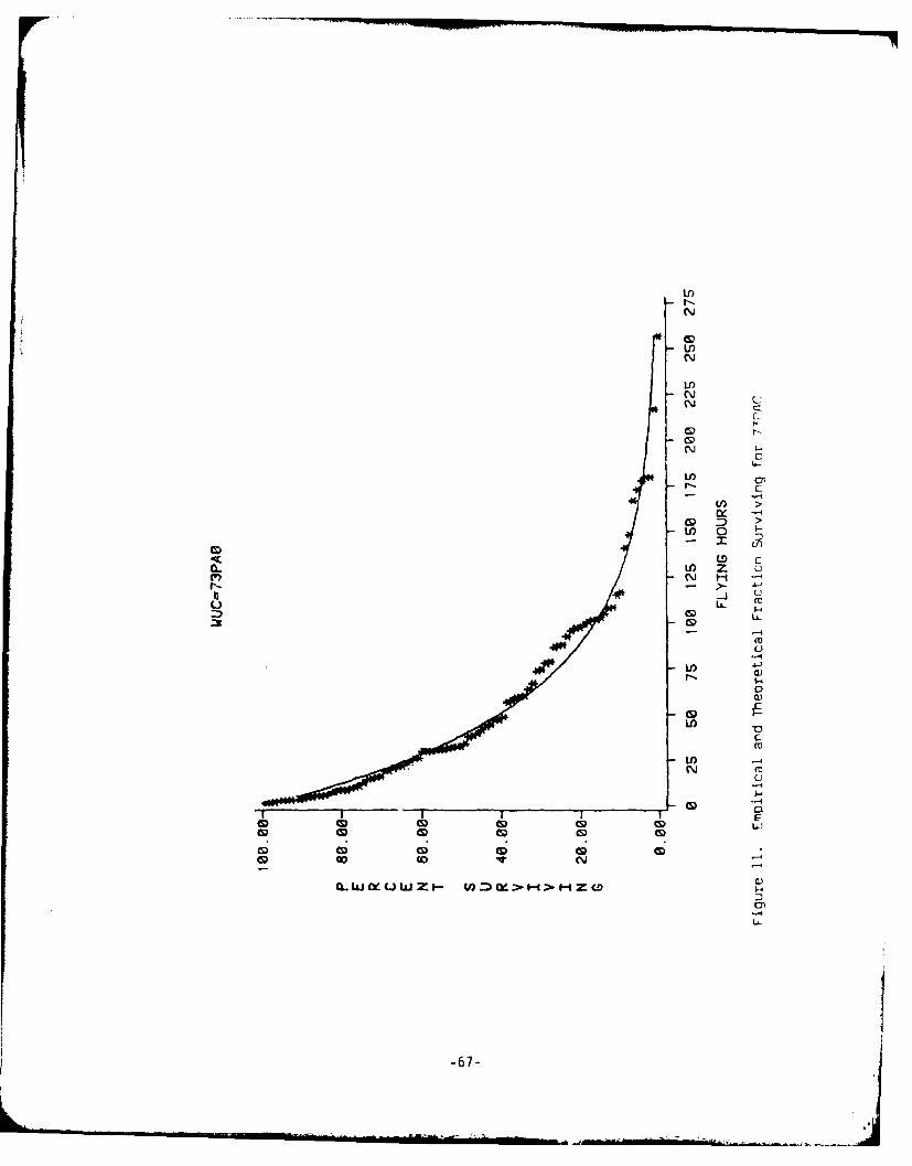
U)N

CS)

CD4.-

F.-

() >

U) 0 -

CDD O

0-Li) Z 0(~)N H-

Li)co

CD

CYC

-67-

I)

(S)

U) V

(S) U) m Lo

4)) HG- w- c

U ~ ccLJO~

rQ-

0LO-

Uf) Il

CN

0 -cc

G) CD CD0NCD Ca C CD CD

I-..

D.

Lb

U)

NY c

czi

&4

0

CDC

U) CU

N0a-)

U)-

(DL LiI CD ~ -4 C LL)

-69-

c',J

CV'

-M SC

U) 0

CK

0Y

CR u

Z2 - LL

U-

0

U)U

CD Cl

70-1

U)

N>

CY

~~L)

Q))

U) 0wc

LD Z

CC-

L)

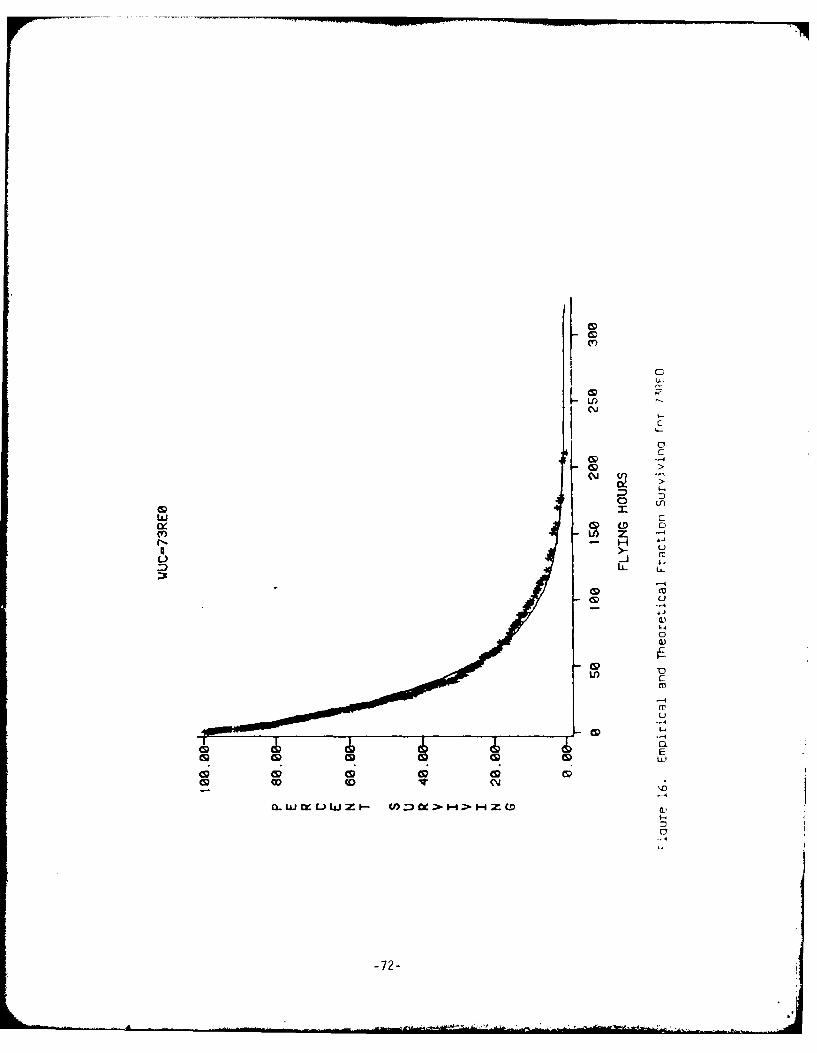
CDC

C,")

CDC

w Cj0

4L) -4CI >

D.

:3

0 C)

-4

CD

0'

0 0 0 0 0

-72-

the line, it cannot be said from the figure whether it is statistically sig-

nificant.

p. 73SB0. This figure (17) shows strong clusters above and below the

line.

q. 73S00. Figure 18 shows a large deviation from the theoretical

curve. The derived mean is about a third the worldwide mean.

2. Estimation of Negative Binomial Parameters. Parameters for the nega-

tive binomial distribution were estimated for those Work Unit Codes for which

graphs were prepared. The same warnings regarding the sparseness of the data

must be kept in mind, as were emphasized in the discussion of the plots.

These parameters are of interest when compared with the results of the estima-

tion of parameters from the discrete data.

E. DISCUSSION OF RESULTS OF ANALYSIS OF FAILURE COUNT

1. Variance-to-mean ratio. Tables X and XI give the variance-to-mean

ratio for the failure counts of planes with 200 and 300 flying hours, respect-

ively. The tables also indicate the range of values and the sum of the fail-

ures obtained.. In every case except 73REO at 300 hours, there was at least

one plane which flew the whole period with no failure on the WUC in question.

Although the variance-to-mean ratio is suggestive, the results illustrate

the need for caution. Table XII shows the results at 200 flying hours and 300

flying hours for those WUCs which had failures in both cases. The table also

gives the total number of failures in each case. In some cases, apparently,

most of the failures were concentrated on those planes that flew fewer trar)

300 hours.

There is substantial agreement on some WUCs; for example, 73NAO shows a

ratio of 1.5 at 200 hours, and of 2.2 at 300 hours; 73PDO shows a ratio of 1.F

-73-

N

CDN

mm

44 N

Q'

too

- D((f0- C

CS) CD - r

-74-,

Ii

U)r

If-

4 CY

4 ~ -

CD6 m

CD cCN H -

CD-

-4

041 .4

(V

-4

4

-75-4

TABLE X

VARIANCE-TO-MEAN RATIO OF FAILURES AT 200 FLYING HOURS

WUC Var/Mean Max Sum WUC Var/Mean Max Sum

13AAA 0.9555555 1 3 51ABN 1.2952380 1 1,

13BCA 0.9777778 1 2 51ABQ 1.0000000 1 1

13BCB 0.9777778 1 2 51CAA 0.9333333 1

13BCC 1.0000000 1 1 51CAC 0.7076023 2 J

13CDA 1.4444444 2 4 61AAO 1.1247311 4 31

13ECA 0.9333333 1 4 61ABO 1.2026666 3 25

13HCB 0.9777778 1 2 61ACO 0.9050505 2 2',

14BCA 0.9555555 1 3 61BAO 0.9614814 2 15

14BCD 0.9333333 1 4 61BBO 0.9777778 1 2

14BCE 0.9777778 1 2 61BCO 1.1587301 2 7

16CAC 1.3200000 2 5 65AAO 0.7777778 i ii

44AAH 0.9555555 1 3 65BA0 0.7589743 2 1K

44AAJ 0.9555555 1 3 65BC0 1.0044444 2 10

46DAA 1.0000000 1 1 658O 0.9111119 1 5

498AA 1.0000000 1 1 71CAO 2.1851852 3 9

51ABA 0.9111111 1 5 71CBO 1.1000000 2 6

51ABD 0.9777778 1 2 7100 1.0000000 1 1

51ABE 1.4977777 3 20 71ZAO 0.9555555 1 3

51ABH 1.4370370 3 12 71ZBO 0.9555555 1 3

51ABL 0.9333333 1 4 71ZCO 0.8666666 1 7

-76-

TABLE X (Continued)

WUC Var/Mean Max Sum WUC Var/Mean Max Sum

71ZDO 1.000000 1 1 73PP0 0.9555555 1 3

73ETO 0.9777778 1 2 73PPO 0.9259258 2 12

73KDO 0.9333333 1 4 73QAO 0.9636363 2 11

73KtJMO 1.1587301 2 7 73RB0 1.6216524 9 78

73NAO 1.5292929 7 88 73REO 1.2105555 9 160

73NBO 0.9259258 2 12 73SB0 1.3662222 4 25

73PAO 0.8615384 4 78 73SO 0.7944444 2 16

73PBO 1.2783626 6 95 73SF0 0.9111111 1 5

73P0 1.7931034 10 116 75BAK 0.8666666 1 7

-77-

TABLE XIVARIANCE-TO-MEAN RATIO OF FAILURES AT 300 FLYING HOURS

WUC Var/Mean Max Sum WUC Var/Mean Max Sum

138C8 1.0000000 1 1 71CAO 1.0000000 1 1

13ECA 1.0000000 1 1 71CBO 1.3076922 2 4

14BCA 1.0000000 1 1 71ZBO 1.0000000 1 1

14BCD 1.0000000 1 1 71ZCO 0.9230769 1 2

16CAC 1.0000000 1 1 73ETO 1.0000000 1 1

44AAH 0.9230769 1 2 73KDO 0.9230769 1 2

44AA.J 1.0000000 1 1 73KMO 0.8461538 1 3

498AA 0.9230769 1 2 73NA0 2.1662531 8 31

51ABE 1.0000000 1 1 73N80 0.6923076 1 5

51ABH 1.1538461 2 7 73PAO 1.0869565 4 23

51ABN 1.3076919 2 4 73PBO 0.5897435 4 21

51ABQ 0.9230769 1 2 73PDO 1.6652806 7 37

51CAC 1.0000000 2 8 73PPD 0.9230769 1 2

61AAO 0.6223776 2 11 73PPO 0.8461538 1 3

61A80 1.5999999 3 10 73QAO 0.6923076 1 5

61ACO 1.1538461 2 7 73R80 0.9943020 5 27

61BAO 0.7692307 1 4 73REO 0.7633136 7 52

618C0 2.0000000 2 2 73S80 0.8632478 2 9

65AA0 0.8461538 1 3 73SDO 1.1230769 2 5

658A0 1.4102564 3 12 73SFO 1.0000000 1 1

65BC0 0.9230769 1 2 75BAK 0.8461538 1 3

65800 0.9230769 1 2

-78-

TABLE XIICOWARISON OF VARIANCE-TO-MEAN RATIOS AT 200 AND 300 HOURS

200 Hours 300 HoursWUC Var/mean Sum Var/mean Sum

138CB 0.9777778 2 1.0000000 1

14BCA 0.9555555 3 1.0000000 1

148CD 0.9333333 4 1.0000000 1

16CAC 1.3200000 5 1.0000000 1

44AAH 0.9555555 3 0.9230769 2

44AAJ 0.9555555 3 1.0000000 1

49BAA 1.0000000 1 0.9230769 2

51ABE 1.4977777 20 1.0000000 1

51ABh 1.437037 12 1.1538461 7

51ABN 1.295238 14 1.3076919 451ABQ 1.0000000 1 0.9230769 2

51CAC 0.7076023 19 1.0000000 8

61AAO 1.1247311 31 0.6223776 11

61ABQ 1.2026666 25 1.5999999 10

61ACO 0.9050505 22 1.1538461 7

61BA0 0.9614814 15 0.7692307 4

618CO 1.1587301 7 2.0000000 2

65AAO 0.7777778 11 0.8461538 3

658A0 0.7589743 16 1.4102564 12

658C0 1.0044444 10 0.9230769 2

65BD0 0.9111119 5 0.9230769 2

-79-

TABLE XII (Continued)

200 Hours 300 HoursWUC Var/mean Sum Var/mean Sum

71CAO 2.1851852 9 1.0000000 1

71CBO 1.1000000 8 1.3076922 4

71ZBO 0.9555555 3 1.0000000 1

71ZCO 0.8666666 7 0.9230769 2

73ETO 0.9777778 2 1.0000000 1

73KDO 0.9333333 4 0.9230769 2

73KMO 1.1587301 7 0.8461538 3

73NAO 1.5292929 88 2.1662531 31

73NB0 0.9259258 12 0.6923076 5

73PAO 0.8615384 78 1.0869565 23

73PB0 1.2783626 95 0.5897435 21

73P00 1.7931034 116 1.6652806 37

73PPD 0.9555555 3 0.9230769 2

73PPO 0.9259258 12 0.8461538 3

73QAO 0.9636363 11 0.6923076 5

73RB0 1.6216524 78 0.994302 27

73REO 1.2105555 160 0.7633136 52

73580 1.3662222 25 0.8632478 9

7350 0.7944444 16 1.1230769 5

73SF0 0.9111111 5 1.0000000 1

75BAK 0.8666666 7 0.8461538 3

-80-

at 200 hours and 1.7 at 300 hours. In some cases there is not as much agree-

ment. The results of the next test indicated whether the variance-to-mean

ratio was statistically significant.

2. X2 Test for Equal Means of Poisson Planes. The X2 test described in

the analysis section was performed on the variance-to-mean ratios. The

sparseness of the data dictates caution in interpreting the results of the

chi-square test. Hald (1952: 727) cites Sukhatme (1938) in noting that, if

the value of the estimated mean (which would be the mean number of failures in

this case) is as small as between 1 and 5, the chi-square approximation is

still good even if there are only a few data points (in this case, between 5

and 15 airplanes); if the estimated mean is even smaller, (about 1) there

should be more data points (more than 15 airplanes). There were 46 planes

with 200 flying hours, and 14 planes with 300 flying hours. The chi-square

values were calculated for all cases where the mean was at least 0.5.

Table XIII gives the mean, variance-to-mean ratio, and the chi-square

value for each case, and tells whether the hypothesis of equal means may be

rejected, and if so, at what confidence level. Note that in some cases, the

hypothesis of equal means for a WUC cannot be rejected for one data set, but

can be rejected for the other. The Poisson distribution may be rejected for

61ABO with .90 confidence for those planes with 300 flying hours, but not for

the planes with 200 flying hours. This may be due to the fact that, as previ-

ously mentioned, 61ABO represents two different items of supply. Of more in-

terest is the rejection of the Poisson at 200 flying hours for 73PBO and

73RBO, but the failure to reject the Poisson for these WUCs at 300 flying

hours. This indicates that these WUC's display more homogeneous behavior on

the planes at 300 hours than on the planes at 200 hours. One possible source

of this distinction is the proportion of planes that had undergone surge in

each group. All eighteen planes that participated in the surge Coronet Hammer

-81-

AD-AlAS 497 MISSOURI UN! V-ROLLA DEPT OP ENGINEERING MANAGEMENT F/G 5/1EMPIRICAL DETERMINATION OF WRSK COMPONENT FAILURE OISTRIBUTIONS--ETCIU)MAY A1 H E METZNER 36579R53

UNCLASSIFIED NL

TABLE XIIICHI SQUARE TEST OF VARIANCE-TO-MEAN RATIO

200 HoursWUC Mean s 45(s /x) Poisson?

61AAO 0.67391304 1.1247311 50.612899

61ABO 0.54347826 1.20266666 54.119997

658A0 0.56521739 0.7589743 34.153843

73NAO 1.91304348 1.5292929 68.818181 reject at .975

73PAO 1.68565217 0.8615384 38.769228

73PB0 2.06521739 1.2783626 57.526317 reject at .90

73PDO 2.52173913 1.7931034 80.689653 reject at .995

73R80 1.69565217 1.6216524 72.974358 reject at .99

73REO 3.47826087 1.2105555 54.474997

300 Hours

WUC Mean s2 i 13(s2/i) Poisson?

51ABH 0.50000000 1.1538461 15.001299

51CAC 0.57142857 1.0000000 13.000000

61AAO 0.78571429 0.6223776 8.0909088

61A80 0.71428561 1.5999999 20.799998 reject at .90

61ACO 0.50000000 1.1538461 14.999999

658A0 0.85714286 1.4102564 18.333333

73NAO 2.21428571 2.1662531 28.161290 reject at .99

73PAO 1.64285714 1.0869565 14.130434

-82-

TABLE XIII (Cor'inued)

WUC Mean 3002/ 45(s2x) Poisson?

73PBO 1.50000000 0.5897435 7.6666655

73P00 2.64285714 1.6652806 21.648647 reject at .90

73RBO 1.92857143 0.9943020 12.925926

73REO 3.71428571 0.7633136 9.9230768

Chi Square Percentiles

.90 .95 .975 .99 .995

13 19.8 22.4 24.7 27.7 29.8

45 57.5 61.7 65.4 70.0 73.2

(Source: Hahn and Shapiro, 1967: 314, 315)

-83-

flew at least 200 hours in the total period covered by this study. The pro-

portion of Coronet Hammer planes rose to 9 out of 14 in the group that had

flown at least 300 hours, an increase from 40 (18/46) to 64% (9/14).

Table XIV summarizes the different conditions under which the home sta-

tion and deployed Coronet Hammer planes were operated during the surge. The

surge lasted from 6 May to 9 June 1980.

It can be seen that it was not the length of sorties flown that changed

for the surged aircraft, bu* rather the frequency of the sorties.

Finally, note that it is not possible to reject the Poisson distribution

for 51ABH, 51CAC, 61AAO, 61ACO, 65BAO, 73PAO, or 73REO from either set of

data, and that it is possible to reject the Poisson for 73NAO and 73PDO from

both sets of data.

3. Estimation of Negative Binomial Parameters. The negative binomial

parameters y and K, as well as the average intensity E(v) were calculated from

the mean and the variance. Table XV gives the results obtained from the data

obtained at 200 and at 300 hours.

F. CONCLUSION. OF ANALYSIS

As a result of each method of analysis used on the data, an estimate of

the average intensity of failure has been obtained. The various estimates are

compiled in Table XVI. In some cases the estimates diverge widely from each

other and from the worldwide total demand rate. It must be assumed that an

adequate sample of true failures was not obtained in these cases. However, in

other cases such as 73REO and 73PDO, no more than a factor of 3 divides the

smallest estimate from the largest, or from the worldwide total demand rate.

A discrepancy of this order of magnitude may reflect differences between op-

erating conditions at Cannon and at other locations, and may also reflect some

loss of data due to poor recordskeeping. In these cases, at least, a repre-

sentative sample of failures may be assumed to have been obtained.

-84-

TABLE XIV

SIJ4MRY DATA FOR CORONET HAMMER

Home Station Deployed

Ninber of Planes 47.1 (on the average) i8

Sortie Rate (avg.) 0.38 .1.5

(sorties per dey

per plane)

Sortie Length 2.353 2.338

(avg.)

Total Hours Flown 971.8 1,347.1

-85-

TABLE XVESTIMATE OF NEGATIVE BINOMIAL PARAM'ETERS FROM FAILURE DATA

200 Flying HoursWUC K E(v)

13CDA 0.00222222 0.1956522 0.000434782

16CAC 0.00160000 0.3396736 0.000543478

51ABE 0.00248889 0.8734472 0.002173913i

51ABH 0.00218519 0.5969044 0.001304348

51ABN 0.00147619 1.030855 0.001521739

61BCO 0.00079365 0.958695 0.000760869

658CO 0.00002222 48.917272 0.001086957

71CAO 0.00592593 0.1650813 0.000978261

71CBO 0.00050000 1.73913 0.000869565

73KMO 0.00079365 0.958695 0.000760869

73NAO 0.00264646 3.6143375 0.009565217

73PBO 0.00139181 7.4191617 0.010326086

73PDO 0.00396552 3.179584 0.012608695

73RB0 0.00310826 1.7748475 0.008478261

73REO 0.00105278 16.519443 0.017391304

73SBO 0.00183111 1.484012 0.002717391

-86-

TABLE XV (Continued)

300 Flying Hours

WUC Y K E(v)

51ABH 0.0051282 1.413044 0.001666667

51ABN 0.00102564 0.9285707 0.000952381

658A0 0.00136752 2.0892851 O. 0'nd57143

71CBO 0.00102564 0.9285707 0.000952381

73NAO 0.00388751 1.8986321 0.007380952

73PAO 0.00028986 18.892861 0.005476190

73PDO 0.00221760 3.9725444 0.008809524

73S0 0.00041026 2.9017811 0.001190476

-87-

TABLE XVIESTIMATES OF AVERAGE INTENSITY

WUC Worldwide 1 A 200 300Total i

Demand Rate E(v) E(v)

13COA 0.000566 .... 0.0004348 --

16CAC 0.001210 -- -- 0.0005435 --

51ABE 0.002247 0.0154655 0.00000323939 0.0021739 --

51ABH 0.003295 0.0149235 0.00650613 0.0013043 0.0016667

51ABN 0.003333 -- -- 0.0015217 0.0009524

51CAC 0.004255 0.0121194 0.00735294 --

61AAO 0.006667 0.012415 0.00301424 ....

61BAO 0.003008 0.0138539 0.000725163 --

61BC0 0.000860 -- -- 0.007609 --

65BAO 0.009831 0.0122909 0.00148495 -- 0.0028571

65BC0 0.009011 -- -- 0.0010870 --

71CAO 0.000611 .... 0.009783 --

71CBO 0.000758 .... 0.008696 0.0009524

73KMO 0.001459 -- -- 0.0007609 --

73NAO 0.023003 0.0182708 0.00332362 0.0095652 0.0073810

73PAO -- 0.0181355 0.00532502 -- 0.0054762

73PB0 0.023201 0.0201632 0.0135108 0.0103261 --

73P00 0.023484 0.0234277 0.0147474 0.0126087 0.0088095

73QAO 0.006374 0.0101633 0.00177683 -- --

-88-

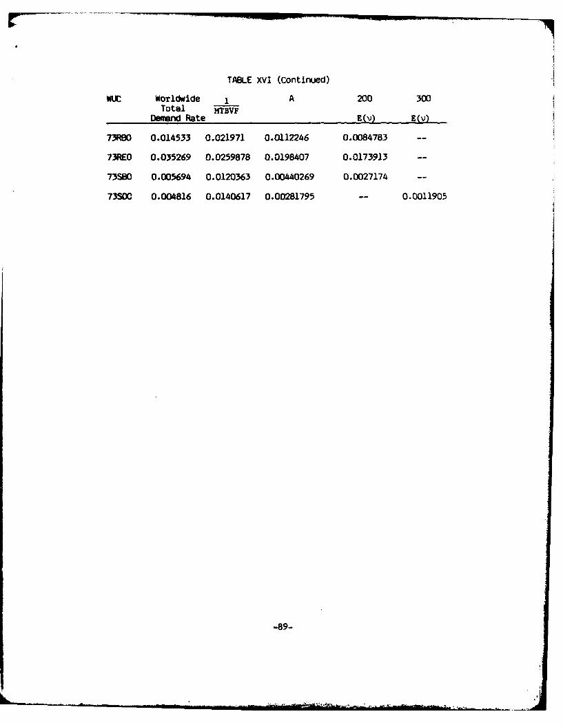
TABLE XVI (Continued)

WUC Worldwide 1 A 200 300Total MTBVF

Demand Rate E(v) E(v)

73RBO 0.014533 0.021971 0.0112246 0.0084783 --

73REO 0.035269 0.0259878 0.0198407 0.0173913 --

73SB0 0.005694 0.0120363 0.00440269 0.0027174 --

73S00 0.004816 0.0140617 0.00281795 -- 0.0011905

-89-

- - - - ~ 'vdQ ..,_. i

Of particular interest is the difference between the estimates of failure

intensity from the failure data for airplanes with 200 flying hours and those

with 300 flying hours. This suggests that estimates of deployment require-

ments for spares from peacetime needs may not always be accurate.

-90-

IV. ANALYSIS OF THE EFFECT OF SURGE

A. INTRODUCTION

The primary purpose of the WRSK is to support aircraft which are to be

deployed under wartime conditions. If the failure distribution is signifi-

cantly different under these conditions than under normal useage, then the

WRSK will not be properly configured if the number and types of WUC's included

are based on normal useage. The assumption that wartime failure distributions

are the same as the distributions of normal useage induced failures needs to

be addressed.

The 27th Tactical Fighter Wing did not engage in any conflicts during the

period for which data was recorded. The Wing did, however, take part in an

extended deployment exercise, Coronet Hammer.

It is possible to isolate the effect of Coronet Hammer on the distribu-

tion of malfunctions, and draw some conclusions. How valid these are for the

case of wartime deployment depends upon the similarity between mission pro-

files.

To test the effect of Coronet Hammer, all malfunctions on items installed

before but not failing before the exercise and all malfunctions on WUC's in-

stalled during the exercise were removed with their intervals or times to

failure. This includes items installed before and removed during or after

surge, those WUC's installed during surge and removed during or after surge.

This reduced the data from 1146 failure intervals to 971 failure intervals.

The 175 intervals removed were on WUC's that had experienced the surge condi-

tions of Coronet Hammer.

The 175 intervals are spread among too many different WUC's and airplanes

to be handled as a set. In addition, the differences in amount of surge con-

ditions and normal conditions of useage will vary widely. Therefore the set

of WUC's which failed without the effects of Coronet Hammer is analyzed to

-91-

determine whether there are differences to the total set.

There are two analysis conducted. The first analysis is concerned with

the interval data on mean time to verified failure. The second analysis is

concerned with the discrete data which describes the distribution of differ-

ences in failure rates among aircraft.

8. ANALYSIS OF INTERFAILURE INTERVALS

The interfailure interval data recorded under non-surge conditions were

subjected to identical testing as the total set. The results are shown on

Table XVII. Unlike the total data set, the results of the analysis of which

are shown on Table IX, the hypothesis of exponentiality cannot be rejected at

the 95% confidence level for any of the 19 WUC's. The effect of removal of

surge-stressed items is to produce a set of data more closely distributed as

the exponential. Table XVIII records the values of WE0 for 95% confidence

of acceptance of the hypothesis of exponentiality or the critical value for

the chi-squared test of goodness-of-fit for eight degrees of freedom.

In five of six cases where the x2 goodness-of-fit were calculated, the

fit worsened when surge-stressed data are included. In one case 73PBO the hy-

pothesis of exponentiality of the total set is rejected where it is excepted

on the non-surge set. Likewise, 51ABN is rejected as exponential when

surge-stressed data are included and exponentiality is accepted when they are

not.

Some caution is advisable. In every case, more data are available for

the total set than the non-surge set due simply to inclusion of those fail-

ures. It is unlikely that increasing the number of failure intervals is

solely the reason for the difference in fit because the 19 cases analyzed in

the interval test contained anywhere from 8 to 219 intervals and simple in-

creases in number to not affect the goodness-of-fit. There are other condi-

tions that might influence the fit, however, if there was a difference in

-92-

TABLE XVIITEST OF THE EXPONENTIALITY OF INTERFAILURE

INTERVALS OF WUC IN NON-SURGE

Wuc NR MEAN STD DEV S/M WEo/X2

51ABE 16 55.92 66.15 1.18 0.087

51ABH 11 72.93 67.38 0.92 0.078

51ABN 9 31.07 35.99 1.15 0.149

51CAC 15 80.03 70.21 0.88 0.051

61AAO 34 79.75 66.80 0.84 0.020

61A80 17 68.02 50.11 0.74 0.032

61ACO 19 79.49 62.01 0.78 0.032

61BAO 9 69.04 69.84 1.01 0.114

65AA0 8 81.39 53.87 0.66 0.055

65BA0 20 65.92 47.46 0.72 0.026

73NA0 106 49.03 45.58 0.93 X2= 8.34

73PAO 84 50.86 50.14 0.99 X2= 7.33

73PB0 106 44.97 50.44 1.12 X2 =14.94

73P'00 137 43.82 42.20 0.96 X2= 4.97

73QAO 10 93.67 80.36 0.86 0.074

73RBO 102 44.38 45.49 1.03 X2=10.55

73REO 185 38.65 41.11 1.06 X2= 4.95

73580 23 75.93 61.42 0.81 0.028

7350 18 54.24 57.69 1.06 0.063

-93-

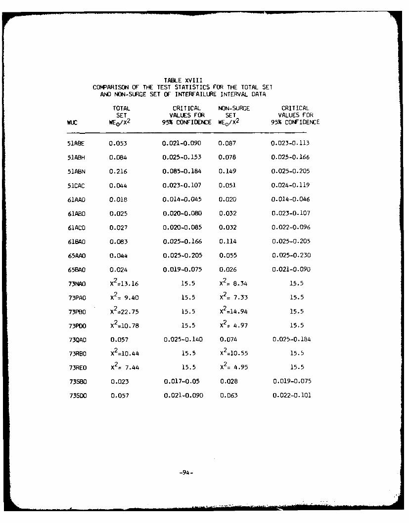
TABLE XVIIICOMPARISON OF THE TEST STATISTICS FOR THE TOTAL SET

AND NON-SURGE SET OF INTERFAILURE INTERVAL DATA

TOTAL CRITICAL NON-SURGE CRITICALSET VALUES FOR SET VALUES FOR

WUC WEo/X 2 95% CONFIDENCE WEo/X 2 95% CONFIDENCE

51ABE 0.053 0.021-0.090 0.087 0.023-0.113

51ABH 0.084 0.025-0.153 0.078 0.025-0.166

51ABN 0.216 0.085-0.184 0.149 0.025-0.205

51CAC 0.044 0.023-0.107 0.05] 0.024-0.119

61AAO 0.018 0.014-0.045 0.020 0.014-0.046

61ABO 0.025 0.020-0.080 0.032 0.023-0.107

61AC0 0.027 0.020-0.085 0.032 0.022-0.096

61BAO 0.083 0.025-0.166 0.114 0.025-0.205

65AAO 0.044 0.025-0.205 0.055 0.025-0.230

65BAO 0.024 0.019-0.075 0.026 0.021-0.090

73NAO x2=13.16 15.5 X2= 8.34 15.5

73PAO X2= 9.40 15.5 X2= 7.33 15.5

73PBO X 2=22.75 15.5 X2 =14.94 15.5

73P00 x2=10.78 15.5 X2= 4.97 15.5

73QAO 0.057 0.025-0.140 0.074 0.025-0.184

73RBO X2=10.44 15.5 X2=10.55 15.5

73REO X2= 7.44 15.5 X2= 4.95 15.5

73SB0 0.023 0.017-0.05 0.028 0.019-0.075

73SDO 0.057 0.021-0.090 0.063 0.022-0.101

-94-

recordkeeping during Coronet Hammer that tended to either unduly lengthen or

shorten the intervals recorded consistantly, the findings would reflect these

changes instead of or in addition to actual effects of surge. Such situations

as increased inability to verify malfunctions or failure to officially recog-

nize malfunctions in non-mission essential equipment under surge conditions

could lead to the worsening fit.

The choice of that set of aircraft for participation which, for whatever

reason, fail at lower rates would tend to confuse the analysis. Those air-

craft which took part in Coronet Hammer have more recorded flying hours than

those which did not. This bases the sanle somewhat and the goodness-of-fit

could reflect the aircraft selection rather than the effects of surge.

Nonetheless, inclusion of surge-stressed items tends to bias the good-

ness-of-fit from the exponential and toward the negative binomial as an appro-

priate model.

C. ANALYSIS OF FAILURE COUNT

The purpose of the analysis of failure count is to determine whether

rates of failure of a WUC are Poisson distributed among airplanes. If the

rates of failure are Poisson distributed in the fleet and the rate is con-

stant, though different, in each airplane, the resulting combined distribution

of the fleet as a whole will be Poisson. The WRSK, which is meant to support

a fleet, would reflect a Poisson distribution as well. If the rates of fail-

ure among airplanes is gamma distributed rather than Poisson distributed, the

model of fleet failures would appropriately be negative binomial.

The effect of surge may be to shift the rate of failure of airplanes,

making the distribution of fialure rates non-Poisson. To test this possibil-

ity, the distribution of failure rates among airplanes can be tested

-95-

for Poisson distribution without the inclusion of failures of stressed by

surge. If there is a tendancy toward the Poisson, it would indicate that

*failure rates are shifted by surge.

* In the description of count failure for the entire fleet and all data,

only five item distributions were rejected in the chi-square test for a

Poisson distribution of failures among airplanes. These WUC's were 73NAO and

73PO0 at both 200 and 300 hours, 73PB0, and 73f8Ci at 200 hours and 61ABO at

300 hours.

The results reported on Table XIX indicate that removing surge-stressea

items does not improve the homogeneity of the 46 aircraft with 200 flying

hours or the 14 aircraft with 300 flying hours.

0. CON~CLUSIONS

The interval test indicates that surge-stressed items do fail differently

than items not so stressed. The discrete test indicates that the airplanes

are different in rate of failure and this difference is independent of the

surge-stressed items.

The lack of confirmation of the two tests would tend to place the con-

clusion that surge affects the rate of failure and therefore the time to fail-

ure in doubt. The selection of aircraft to be flown in surge and the fact

that these aircraft flew more hours on the average and therefore supplied more

data to the study affects the conclusions. It cannot be assured that this bi-

as is not the cause of the rejection of the Poisson in the interval test.

-96-

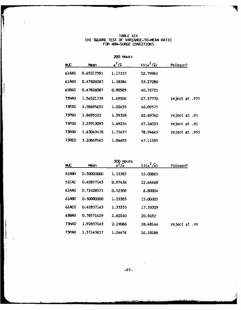
TABLE XIXCHI SQUARE TEST OF VARIANCE-TO-MEAN RATIO

FOR NON-SURGE CONDITIONS

200 Hours

WUC Mean s 2 A 45(s 2 /X) Poisson?

61AAO 0.65217391 1.17333 52.79985

61ABO 0.47826087 1.18384 53.27280

65BAO 0.47826087 0.90505 40.72725

73NAO 1.56521739 1.49506 67.27770 reject at .975

73PAO 1.58695652 1.02435 46.09575

73PBO 1.8695522 1.39328 62.69760 reject at .95

73PDO 2.23913093 1.49234 67.16025 reject at .90

73RBO 1.63043478 1.75437 78.94665 reject at .995

73REO 3.10869565 1.04693 47.11185

300 Hours

WUC Mean s2ix 13(s 2/x) Poisson?

51A64 0.50000000 1.15385 15.00005

51CAC 0.42857143 0.97436 12.66669

61AAO 0.71428571 0.52308 6.80004

61ABO 0.50000000 1.15385 15.00005

61ACO 0.42857143 1.33333 17.33329

65BAO 0.78571429 1.60140 20.8182

73NA0 1.92857143 2.19088 28.48144 reject at .99

73PAO 1.57143857 1.24476 16.18188

-97-

TABLE XIX (Continued)

300 HoursWUC Mean 62/g 45(s 2/ ) Poisson?

73PBO 1.07142857 0.64103 8.33339

73P00 2.07142857 1.66844 21.68972 reject at .90

73RBO 1.50000000 1.20513 15.66669

73REO 3.00000000 0.76923 9.99999

-98-

V. LIMITATIONS OF THE STUDY

A. INTRODUCTION

Every study has limitations in the ability to generalize from Lts

findings. The limitations are primarily a function of the assumptions of ade-

quacy in three areas, sample selection, data collection and data analysis.

The limitations of this study are here discussed.

B. LIMITATIONS OF SAMPLE SELECTION

The sample selected for this study was the 27th Tactical Fighter Wing

stationed at Cannon Air Force Base. The 27th Tactical Fighter Wing has F-111

aircraft in its inventory.

1) Only one aircraft type was used, the F-lllD. The conclusions are

therefore limited to that aircraft type. In a stricter sense, the conclusions

are limited to the F-111D aircraft of the 27th Tactical Fighter Wing. In par-

ticular, the F-ill was chosen as a sample because of its characteristic as a

digital system. It is more readily apparent when a digital system fails and

the failure is more easily isolated than in an analog system. Consequently,

while the results may be generalizable to other F-111 wings and perhaps to

other aircraft which are digital systems, it would be more difficult to just-

ify generalization to analog systems such as the F-4. Attempts to replicate

this study on the F-A aircraft at Moody Air Force Base failed for lack of con-

tinuous data over a sufficiently long period with respect to the average time

to failure of the WRSK items. Even the generalization of the study findings

to other F-111 and other digital systems may be questioned, and the tests may

be replicated to determine generality.

2) The assumption implicit in the Choice of Cannon Air Force Base is

that the 27th Tactical Fighter Wing is typical of all F-Ill Wings. Yet, with

respect to maintenance records, they are superior. If that superiority is

-99-

prevalent in other maintenance procedures as well, the findings may loose gen-

erality.

3) The assumption is made that WUC's for which there are sufficient data

for analysis are typical of all WUC's. The flying time for the aircraft

ranged from 0 to 403.2 hours. Only those WUC's with relatively short mean

time to failure generated a large number of intervals for analysis. These are

items upon which the tests of distribution are based. If these items are fun-

damentally different from other WC's, the study does not generate validly

generalizable conclusions. Since the findings here are consistant with other

studies found in the literature, the likelihood that these WUC's are different

in their pattern of failure is remote. Nonetheless, some items may not fit

the patterns found here.

C. LIMITATIONS OF DATA COLLECTION

The data collected for the study were extrated from existing Air Force

records at the Air Force Base itself. No new data were generated for this

study.

1) The assumption has been made that failure reports not verified are

not failures. If there is no verification in the Action Taken Code, then the

malfunction indication was dropped from the data and the interval continued.

The effect of this assuaption is to increase the individual times to failure

since the recorded interval would have been divided into two or more by inclu-

sion of unverified malfunctions. The effect of inclusion would be to shorten

the mean time to failure, and make it easier to reject the Poisson process as

descriptive of the data. The conservative method is to ignor unverified fail-

ures.

2) Because data were available for the two year period just prior to

collection, it must be presumed that these are typical of all periods, and

that the activities and mission profiles of these aircraft are typical of

-100-

• o4

general useage throughout the Air Force.

3) It must be assumed that the data collection during exercise Coronet

Hammner was identical to data collection during normal conditions at Cannon Air

Farce Base.

0. LIMITATIONS OF ANALYSIS

The analysis of the data necessitates several assumptions which bear on

the generalizability of the conclusions.

1) The assumption is made that the F-111D is a mature aircraft with a

constant failure rate. New aircraft types introduced into Air Force inventory

may exhibit a falling rate of failure due to improvement in manufacture or de-

sign based on feedback on performance of initial units deployed. Maintenance

procedures and mechanics' learning also would lead to improvement in failure

rate after introduction, though at some point, it is anticipated that failure

rate would become constant or nearly so. The aircraft under study were intro-

duced into Air Farce inventory in 1968, twelve years before the data were coil-

lected. The assumption therefore, would appear justified.

2) The assumption is made that the previous history of the replacement

item is irrelevant and does not effect future failures. The source of the re-

placement part may be from the WRSK, from depot or base repair functions, or

the item may be new or cannibalized from other aircraft or from "hangar

queens." The issue of new verses repaired items is not handled here. Whether

the source of the replacement item effects the length of time that the re-

placed item functions cannot be analyzed with techniques used here. The data

to determine the source of the replacement item was not recorded. If WRSK i-

tems are always new or reconditioned under special circumstances, the results

of the study may not be generalizable from the failure distributions of items

from more normal sources. Since this is not the case, and the WRSK

-101-

items will be drawn from the same selection of sources as captured here, the

point is moot for this study, though that may not always be the case.

3) Insufficient data was collected to determine the effects on failure

rate of mission profile. In order to determine these effects, mission pro-

files must be stipulated so that these sorties may be separated and tested a-

gainst the base-line data gathered under normal useage.

4) The assumption is made that roronet Hammer is a good representation of

the conditions for which the WRSK would be employed. No information on the

mission profiles is available. The data gathering, ability to determine valid

failures, and the reporting of these failures is assumed to be the same as

normal conditions at Cannon.

-102-

VI. CONCLUSIONS AND RECOM4ENDATIONS

A. FAILURE DISTRIBUTIONS OF WRSK COMPONENTS

The Poisson process has been used for years in predicting reliability and

maintenance behavior for many complex physical and electronic systems. The

Poisson process, with exponential time-to-failure, is convenient and elegant.

It is, however, apparently not accurate in describing the failure behavior of

some components of the F111D airplane. This discrepancy is statistically sig-

nificant in some cases.

It has been demonstrated here that the Poisson process does not descrioe

some components of the F111D WRSK. It has also been demonstrated that failure

behavior was not constant for different flying intervals. The demonstrated

effects of surge on the WRSK components is to shift the distribution of times

to failure of the fleet from the exponential, and the data is better described

as negative binomial. Both the statistical analysis ano the graphic demon-

strations indicate that the Poisson process is not a bad approximation to the

data and may be used for calculation of the logistic needs of the fleet. The

general effect of approximating a negative binomial with a Poisson distribu-

tion is to initially underestimate the spares requirements and later overesti-

mate them dependent upon the point at which the curves cross.

For the determination of WRSK configuration, however, using fleet data

Poisson distributed will lead to error. It may well be that the distribution

of failures under surge conditions is also Poisson, merely with a different

mean, sufficiently different to distort the fleet data significantly away from

the Poisson in some cases. insufficient data was collected during Coronet

Hammer to make a determination of its Shape or parameters independent of

other, non-surge data. Further investigation in this area is recommended.

Determining the influence of surge was one of the objectives of this study,

-103-

but this objective has not been accomplished here due to ambiguous and contra-

dictory results. The shifts of distributions from Poisson to negative binio-

mial may be due to the particular airplanes from which data was collected,

rather than from surge conditions.

Further empirical study of' failure behavior is recormmended because of the

immviense strategic and financial stake in the WRSK. A~ more extended study

would pick up longer times between failures, and rarer single failures, than

were obtained in this study. In order to conduct a more extended study, data

covering several calendar years must be available. It is most strongly recom-

mended that maintenance and flying records be maintained indefinitely in the

field, for use in future empirical studies.

B. OTHER A.REAS OF INVESTIGATION

The flying and maintenance data merging procedure used in this study has

enormous potential as a tool to answer other questions than were addressed

here. For instance, Is there a pattern of maintenance and failure behavior

which precedes a crash, and which can be used to predict which airplanes are

vulnerable to a crash? The historical records of planes which crashed due to

equipment malfunction could be examined and compared with the records of other

planes with similar operational background.

Similarly, the maintenance and failure behavior of planes operated in

different climatic regions could be compared to determine what changes in

maintenance behavior can be expected when planes are deployed from, for ex-

ample, a desert to a subarctic region. It is possible that the changes would

not simply involve the rate of failure of certain parts, but the pattern of

failure as well, e.g., from a Poisson to a negative binomial failure process.

An empirical study of this sort could be used in tailoring WRSK kits for spe-

cific contingency missions.

-104-

BIBLIOGRAPHY

Ascher, Harold, and Harry Feingold. "The Aircraft Air Conditioner Data

Revisited," Proceedings 1979 Annual Reliability and Maintainability Symposium,

153-159.

Bain, Lee 3., and F. T. Wright. "The Interarrival Time for Negative Bo-

nomially Distributed Events." In preparation. Mathematics Department, Uni-

versity of Missouri-Rolla, 1981.

Bendle, A., and S. Humble. "Operating History and Failure and Degrada-

tion Tendencies," IEEE Transactions on Reliability, R-27, 1 (April, 1978),

75-76.

Bilikam, J. Edward, and Albert H. Moore. "Estimation of Mission Reli-

ability from Multiple Independent Grouped Censored Samples," IEEE Transactions

on Reliability, R-26, 1 (April, 1977), 57-60.

Bilikam, 3. Edward, and Albert H. Moore. "Estimation of Reliaoility from

Multiple Independent Grouped Censored Samples with Failure Times Known," IEEE

Transactions on Reliability, R-27, 5 (December, 1978), 329-331.

Chen, Der-San. "Discrete Optimization with Nonseparable Functions: Deter-

mination of a Kit Composition for War Readiness Spare Parts." Final Report on

Contract AFOSR-78-3549. Rept. No.: BER-237-69, University Bureau of Engineer-

ing Research, Alabama University, July 1979.

Cockburn, Robert N., "Estimation of an Aeronautical Equipment Mission Re-

liability." Master's thesis, GSA/MA/73-1, Air Force Institute of Technology,

Wright-Patterson AFB OH, May, 1973.

Fiorentino, Eugene. "The Use of Air Force Field Maintenance Data for R &

M Assessments of Ground Electronic Systems," In-House Report, RADC-TR-79-103,

Rome Air Development Center (RBRT), Griffiss AFB NY, April, 1979.

-105-

Hahn, Gerald J., and Samuel S. Shapiro. Statistical Models in Engineer-

ing. New York: John Wiley & Sons, 1967.

Hald, A. Statistical Theory with Engineering Applications. New York:

John Wiley and Sons, 1952.

Hunsaker, H. D., F. Conway, and E. R. Doherty. "Logistics Impact of Sor-

tie Oriented Air Crew Training." AFLC Technical Report Nr. 76-7, Air Force

Logistics Command, Wright-Patterson AFB OH, April, 1977.

Johnson, David R., and Judith M. McCoy. "An Analysis of the Demand Dis-

tributions for Selected Inertial Measurement Units in the Air Force Inven-

tory." Master's thesis, LSSR 5-78A, Air Force Institute of Technology,

wright-Patterson AFB OH, June, 1978.

Klivans, Larry S., "An Improved Management Approach to Upgrade Avionic

System Reliability," IEEE Transactions on Reliability, April, 1977, 23-28.

Lu, John Y. "A Note on Some Aspects of 0029: War Reserves Spares Compu-

tation System." Working Note 10008-AF, Rand Corporation, Santa Monica,

California, November, 1977.

Messinger, Martin, and Martin L. Shooman. "Techniques for Optimum Spares

Allocation: A Tutorial Review," IEEE Transactions on Reliability, R-19,4

(November, 1970), 156-66.

Mitchell, Charles Raymond. "On Some New Bivariate Negative Binomial and

Gamma Distributions," Dissertation Abstracts International, XXXVII, 6

(December, 1976), 2961-62B.

Morrison, Captain Jimmie G., USAF, and Captain Richard A. Probst, USAF.

"The Mechanized Computation of USAF War Readiness Spares Kits (WRSK) Candi-

dates List." Unpublished master's thesis, SLSR 41-75-B, AFIT/SL,

Wright-Patterson AFB OH, August, 1975.

Proschan, Frank. "Theoretical Explanation of Observed Decreasing Failure

Rate," Technometrics, V, 3 (August, 1963), 375-383.

-106-

Rasmussen, Captain Robert K., USAF, and Captain William D. Stover, USAF.

"A Simulation Model for Assessing WRSK Capability at Unit Level." Master's

thesis, LSSR 4-78A, Air Force Institute of Technology, Wright-Patterson AF6

OH, June, 1976.

Sukhatme, P. V. "On the Distribution of in Samples of the Poisson

Series." Suppl. Journal of the Royal Statistical Society, V, 1935, 75-79.

Tadashi, Murate. "Reliability Case History of an Airborne Air Data Com-

puter," IEEE Transactions on Reliability, R-24, 2 (June, 1975), 98-102.

Tadashi, Murate. "Reliability Case History of an Airborne Air Turbine

Starter,"IEEE Transactions on Reliability, R-25, 5 (December, 1976), 302-303.

Vesely, William E., and George T. Merren. "Analysis of Component Relia-

bility Data," IEEE Transactions on Reliability, R-25, 3 (August, 1976),

158-163.

-107-

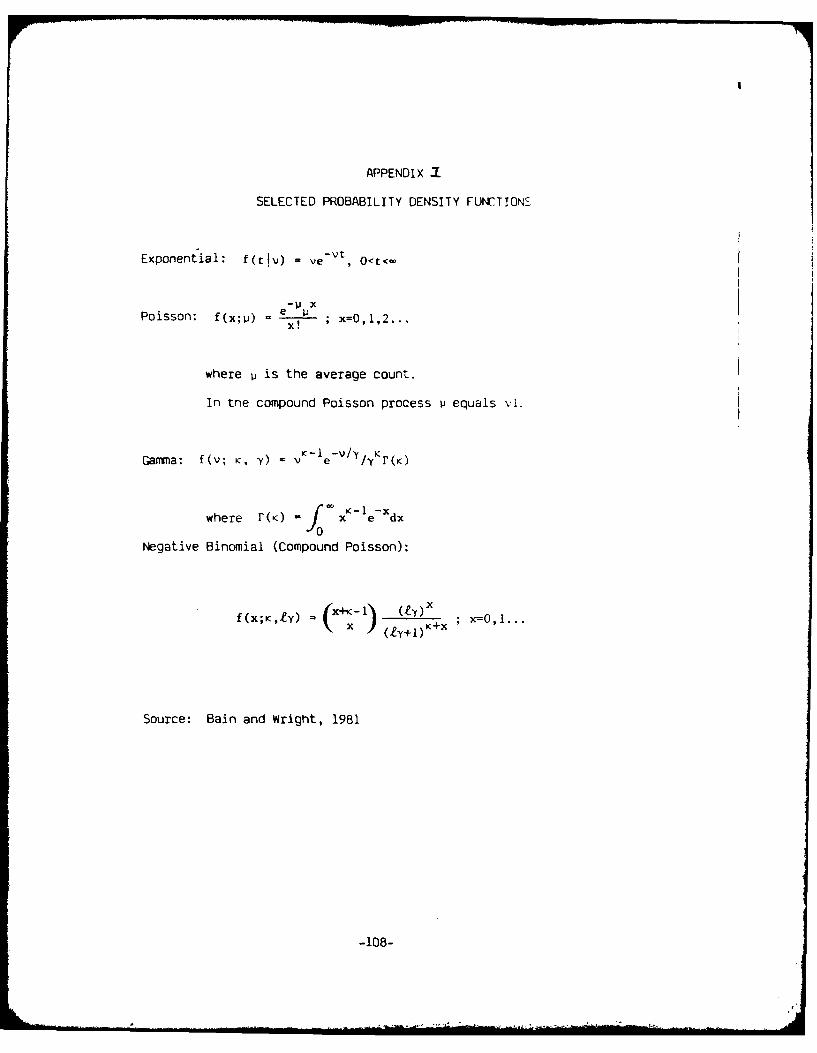
APPENDIX

SELECTED PROBABILITY DENSITY FUNCTIONS

Exponential: f(tlv) = vevt, O<t<w

Poisson: f(x; j) = ; x=0,1,2...

where u is the average count.

In tne compound Poisson process v equals vi.

Gamma: f(v; K, y) = VK- e-,/YK r(K)

where r(K) =f xK-1e-Xdx

Negative Binomial (Compound Poisson):

f(x;K,ey) 'x-1) (lY) x 10,I...(.ty+,)K+x "

Source: Bain and Wright, 1981

-108-

APPENDIX II

PROJECT - Air Force WRSK data analysis

USERS - Dr. Henry Metzner, Engineering Management

OBJECTIVE - scan a series of records depicting maintenance action, trans-

forming this sequence of events into a set of intervals representing failure

interarrival times. Correlate failure interval boundary dates with flying log

records for each interval yielding a log record of flying information for each

failure interval.

Statistical analysis may then be applied to the interarrival times to advise

Air Force on efficient configurations of War Readiness Spares Kit, based on

failure distributions.

SYSTEM COMPONENTS - IBM Job Control Language streams, PL/I programs, SAS and

SAS/GRAPH programs, TSO CLISTs and CMS EXECs.

HARDWARE USED - Amdahl 470/V7 (node = UMMVSA), IBM 4341 (node = UMRVMB), IBM

3279 Color graphics terminal attached to UMMVSA, Tek (Tektronix) 4014 graphics

terminal and 4662 plotter attached UMRVMB.

ORGANIZATION - The system components are designed to satisfy specific subsets

of the overall objective. The majority is performed in the single applica-

tion, MAINTLOG. Other components are used to provide support functions such

as sorting and moving of datasets, and statistical and graphic functions. The

breakout is into the following steps -

-109-

I. COMBINE - a JCL stream to

a. merge several tapes of maintenance data (each containing only a few

feet of data on a 2400' tape) into one large tape dataset.

b. merge several flying tapes into a single tape containing two data-

sets, afbase.HISTORY and afbase.CURRENT, containing history data from

archives and current data from online data, respectively.

2. MAINSRT - a PL/I program which invokes the SORT utility to create a sort-

ed copy of the maintenance data, omitting data not used by the mainten-

ance data logging routine.

3. FORMIOAD - a JCL stream to reformat the HISTORY and CURRENT flying infor-

mation into a common format, then load the data into a VSAM ESDS with an

alternate index.

4. MAINTLOG - a PL/I program with invoking JCL stream to log maintenance

intervals and times to first failure, with flying information for each

time period logged.

5. FLYREPT - a PL/I program and associated jobstream to produce cumulative

flying hours per plane, to be used in selecting planes for computing

count statistics.

6. GRAFEXP - a SAS/GRAPH program and associated CMS EXEC or TSO CLIST to

product graphs, by WUC, of % survival rate vs. length of interval from

interval log output by (4).

7. GRAFIND - a SAS/GRAPH program with EXEC or CLIST to produce graphs of

t ean time between failures per plane, by WUC, from failure intervals.

8. MEANSI - a SAS program with JCL stream to produce means and variances for

count data derived from two files produced by (4) (intervals and singles)

and the flying summary produced by (5).

9. MEANS2 - a SAS programs with JCL stream to produce means and variances

for interval data.

-110-

W_............................

Detailed Componert Descriptions

1. COMBINE - this JCL stream consists of 3 IEBGENER STEPS. The first uti-

lizes a concatenation in the SYSUT1 file, with one DO statement per main-

tenance tape. The SYSUT2 file is for the new maintenance file, written

at the highest density available (6250 BPI at this installation). Con-

trol statements placed in the input stream file SYSIN are used to refor-

mat the records, omitting some unnecessary fields.

The second step creates the HISTORY dataset from flying information

derived from archived data. Each history tape is identified by one DD

card in the concatenation for SYSUT1. SYSUT2 specifies the output file,

which is named afbase.HISTORY, where "afbase" is the name of the base

where the tapes originated.

The third step is similar to the first except there is only one cur-

rent tape in the input file SYSUT1 and the output file is called

afbase.CURRENT.

2. MAINTSRT - this PL/I program calls the system SORT interface, PLISRTD,

with input and output exit routines MNTINP and MNTOUT, respectively.

MNTINP is used as the input routine (called the E15 exit in VS/SORT term-

inology) to provide input data for SORT, one record per invocation. This

routine inserts the appropriate year ahead of the job control day and

translates zeros to blanks in the WUC so they will collate correctly.

MNTOUT, the SORT E35 exit, puts back the zeros and outputs the record.

3. FORMLOAD - this JCL stream consists of two IEBGENER steps and one IOCAMS

step. The first IEBGENER step translates the HISTORY dataset in file

SYSUT1 into the common format used in the final flying file and puts in

into the dataset afbase.BOTH in the file SYSUT2. The control cards are

stored in a member named HISTORY in a partitioned dataset and referenced

-111-

in file SYSIN.

The second IEBGENER step formats and appends the CURRENT dataset, using

control cards in member CURRENT.

The third step invokes IDCAMS, the Access Method Services utility pro-

gram, to define and build the VSAM Entry Sequenced Data Set (ESDS) and

the alternate index, which allows keyed access to data with not neces-

sarily unique keys. The control cards to perform these functions are in

members afbasDEL and afbasAMS, where "afbas" is the name of the Air Force

base, truncated to five characters if necessary.

4. MAINTLOG - this PL/I program is the central program in the system. The

preceeding steps were performed, using simple system utilities, to mas-

sage the data into a simple format to be processed by this program. The

output of this program supplies the primary inputs to the statistical

analysis phase.

The program operates in a hierarchical fashion on groups of data.

The largest group considered at one time is data for one aircraft.

For each aircraft, the data is further broken down into Job Control

groups, that is, groups of maintenance actions having the same Job Con-

trol Number (JCN) and date.

Within a JCN group, the data is sorted by WUC. The program scans the

group, building a list of maintenance actions taken for each WUC. Then

those lists are checked to confirm removal (without which the actions are

ignored) and to determine if a part failure is indicated. If a failure

is indicated, then an entry with the job control date and WUC is made in

the failure structure for the aircraft. If two failures have occurred

previously, the interval between them is logged.

Following processing of the last JCN group for an aircraft, the fail-

ure structure is scanned, and the last interval for each WUC is

-112-

logged.

Logging of intervals is performed by the subroutine Log-Action, which

invokes the subroutine FLYING to sum flying information from the VSAM

ESDS over the period between two dates. If one or both dates lies out-

side the period specified in the JCL as the limits for this run, the in-

terval is not logged.

5. FLYREPT - this program reads the flying ESDS sequentially and accumulates

flying hours, landings, sorties and full stops for each aircraft.

6. GRAFEXP - this SAS/GRAPH procedure inputs maintenance intervals produced

by (4), sorts the data by length of interval, obtains the means, calcu-

lates points along the exponential curve for Poisson-distributed data

with the same mean, calculates percent surviving each unique interval

length, and plots the curves along with the percent surviving by WUC.

7. GRAFIND - A SAS/GRAPH procedure which reads in interval values, calcu-

lates the mean time between failures for each aircraft/WUC combination,

and graphs these means, by WUC.

B. MEANSI - A SAS procedure to analyze count data. This procedure uses time

to first failure and time between failures to provide a cutoff at x num-

ber of hours, so that only the failures occurring in that time are ac-

cepted. The flying time time summary produced in (5) Is used to elimi-

nate aircraft that flew less than x hours, and to include zero occurrence

statistics in the means. The mean and variance are calculated, also the

ratio between tham.

9. MEANS2 - A SAS procedure to print means, variances, and var/mean for in-

terval data. Note that the x hours restriction no longer exists.

-113-

APPENDIX III

USE OF EXTRACTION PROGRAWS

NRFRMCThis program extracts data from the current WMICS (flight) data base. It

may be run with the MMICS on line.

FOR-A7The format for NRFRMC is:

?EX NRFRI.c?DATA AFBRMIR(parameter card, as below)?END

The "?" symbol represents the numerals 1, 2, and 3 overstruck in the sarrcolumn. (ultipunch)

PREPARE CONTROL (PARAMETER) CARPBefore running this program, check with the MMICS operator to determine

when a "Delete History" was last run (the system monitor may do this). Forexample, if a "Delete History" was run on I May 80, and the program is to berun on 18 September 80, then the control (parameter) card for program NRFRt.?will appear as follows: columns 1 through 10 will be the inclusive Julianoates for the current data files, in this case "8012280262", columns 13through 17 will be the type of aircraft, for example, "FlllD", and column 19will be the MMICS UNIT ID, for example, "A".

RUN NRFRMCTo run NRFRMC, the following MMICS file must be present on disk: ZRFWA,

ZRFOOB, ZRFOQC, and ZRFQOT. Load NRFRMC to disk. Read the appropriateexecute deck, as described above, into the card reader. The program willproduce an AFBRMI list and an AFPRMP tape. These will contain the extracteddata from the current data base.

TAPE OUTPUTThe FILE-ID of the output tape is AFBRMP. It is formatted in 80 character

records. The blocking factor is 10 records.

PRINTED OUTPUTThe FILE-ID of the output is AFBRM1. This listing is an 80-80 list of the

outmpt tape and is in the same format as the tape record.

-114- i

........ U_

TABLE IFORMAT OF CONTROL (PARAMETER) CAR)NRFRMC (CURRENT FLIGHT EXTRACTION)

Card Column Example Remarks

1 - 5 80122 A five-digit numeric symbol givingthe Julian date of the inclusivebeginning day of the period fromwhich data is to be extractec

6 - 10 80262 A five-digit numeric symbol givingthe Julian date of the inclusiveending day of the desired period

11 - 18 --FlIID- The dashes represent blankspaces. This is nominally aneight character alpha-numericsymbol designating the type ofaircraft for which data will beextracted, including three spacesfor the mission, three for thedesign, and two for the series.If the standard designation of theaircraft, or MDS, does not use alleight spaces, as in the example,the symbol must be positioned sothat each element lies in theappropriate field. If the programruns, but extracts no data, checkthe parameter card for an error in

positioning here.

19 A A single letter, the MMICS UNITID. This field may be leftblank. If the field is leftblank, all aircraft, regardless ofunit of assignment, will bescanned.

-11 5-

TABLE 2FORMAT OF TAPE OUTPUTAFBRMP (CURRENT FLIGHT)AND LIST OUTPUT AFBRMI

Byte Position Example Remarks

i - 7 --FIIID The dashes represent blankspaces. A seven charcteralpha-numeric symbol, giving theMDS of the equipment (three placesfor the mission, three for thedesign, one for the series)

8 - 15 78005111 Eight-digit numeric symbol, givingthe aircraft serial number

16 - 20 79152 Five-dicit numeric symbol; aJulian (ate

21 - 23 035 Three-diqit numeric symbol; totalhours and tenths flown on this Oate

24 - 27 LXSW Four letters: the station locationcode

28 - 30 003 Three digit number; the totalnumber of landings on this date

31 - 33 P02 Three digit number; total numberof sorties flown on this date

34 - 42 032TFWCE Nine characters; number, kind andtype of owning unit

43 - 45 OP2 Three-digit number; total full

stop landings this date

46 - 70 25 blank filler

71 - 75 A5111 Five character alpha-numeric;

MMICS equipment-ID

76 - 80 1 Five-digit number; record sequencenumber

-116-

NFBRAAThis program runs against the MMICS (flight) history tapes (ARF53T).

FORMATThe Format for NFBRAA is:

?EX NFBRAA DATA AFBROC(parameter card, as below)?END

The "?" symbol represents the numerals 1, 2, and 3 overstruck in the samecolumn. (Multipunch)

CONTROL (PARAMETER) CARDThis program must be run against every ARF53T tape that is in the library,

going as far back as the data extraction is desired. There may be one ARF531tape for each month, or the base may create an ARF53T with several months ofdata. Contact the MMICS operator to find out how much data is on each tape(the system monitor may do this). For example, if prooram NFBRAA is being runagainst an ARF53T tape that contains data for August 1980, then the Juliandates on the control card will be 80214 to 8P244. The format on this caro isthe same as the format for the control card for program NRFR.C.

OUTPUTThe output of NFBRAA includes a list coded AFBRMR. Note that it is not

formatted the same as the output of NRFRMC.

-117-

. .',

TABLE 3FORMAT Of NFBRAA OUTPUT (FLIGHT HISTORY)

AFBRMR

Column Example Remarks

1 - 8 68t00511 Equipmepnt ID; in this case theairplane's tail number. Eightdigits

9 - 15 --F604E The dashes represent blankspaces. Seven characters givingthe Mission Design Series, withthree places for the Mission,three for the Design, and one fotthe Series

16-20 B0111 Five digits giving the Julian date

21 - 23 P25 Three digits; total hours andtenths flown on this date

24 - 27 Blank

28 - 29 P1 Two digit number; total landingsthis date

30 - 31 pi Two digit number; total number ofsorties flown on this date

32 - 40 0347TFGWG Nine characters; number, kind andtype of owning unit

41 - 43 i Three digits; total full stoplandings this date

44 - 80 Blank

-118-

NBDQ99This is the object code for the program to extract MDC (maintenancf:)

data. This program is run against the 6-month history ABD6DA tapes for MDC.Each run will take approximately two to three hours of processing time.

FORMATrhe--rmat for NE0Q99 is as follows.

?EX NBDQ99?DATA ABFQ9C(card deck, as below)?EN:

The "?" symbol stands for the numerals 1, 2, and 3 overstruck in the samecolumn. (Multipunch)

CARD DECKThe card deck will consist of one "A" card, several "B" cards, ano one or

more "C" cards. Depending on how many WUC's have been selected for cataextraction, more than one card deck may be required. No more than 150 WUr'smay be included in a deck.

The "A" card specifies the type of aircraft and the time soan (within thuperiod covered by the history tapes) to be scanned.

The "B" cards, up to ten of them, list those WUC's regarding whicrmaintenance lata is to be extracted.

The "C" cards specify which individual airplanes are to be included. Upto 105 may be listed, or one card may be used if all airplanes are to beincluded.

OUTPUTOutput will be an ABFQ9P tape and an ABFQ9L list.

SPECIAL NOTEIt is not possible to extract data regarding a sub-component (an item with

the lowest level WUC, such as 73CAH) unless its parent component (such as73CA0) is included in the extraction list. It is not necessary to include allother subcomponents in order to gather data on that single desiredsubcomponent. If more than one deck of WUC's is necessary, the parentcomponent and the subeomponent must be run together. This may mean repeatingthe parent component in two runs if a subcomponent list must be broken up.

-119-"

TABLE 4FORMAT OF INPUT TO NBDQ99 (MAINTENANCE EXTRACTION)

"A" CARD

Column Example Remarks

i A$A

2 - iC' Blank

11 -17 --F4E The dashes represent blankspaces. A seven-characteralpha-numeric symbol giving the

MDS of the airplane; three placesfor the mission, three for thedesign, three for the series. Ifthe standard designation of theaircraft ooes not use all sevenspaces, as in the example, thesymbol must be positioneo so thateach element lies in theappropriate field. If the programruns, but extracts no data, checkthe "A" card for an error inpositioning here.

18 - 29 Blank

30 - 39 7930779365 The inclusive Julian datescovering the period regardingwhich data is to be extracted

-or-30 - 32 ALL If the entire period covered by

this ABD6DA tape is of interest.

40 - 80 Blank-or-

33 - 80

-120-

TABLE 5FORMAT OF INPUT TO NBDQ99 (MAINTENANCE EXTRACTION)

"B" CARDS

Column Example Remarks

I B "B"

2 - 5 Blank

6 - 80 23CA023CAA23CAB ..... Starting in column six, the caromay be filled with five-characterWUC's. Each card will holdfifteen WUC's, and up to ten suchcards may be used in the deck eachtime NBDQ99 is run. Each cardmust begin with the "B" and fourblank spaces

-121 -

TABLE 6FORMAT OF INPUT TO NBDQ99 (MAINTENANCE EXTRACTIO)

"C" CARDS

Column Example Remark-

I C C "l

2 -Blank

- 8( A4095A4096.... Starting in column six, the cardis filled with five-characterequipment ID's, of which the firstcharacter is the prefix of theequipment classification code, inthe example "A" for aircraft, anathe last four characters are thelast four positions of theequipment serial number, in thiscase, the aircraft tail number.Each card will hold up to fifteenequipment ID's, an up to sevensuch cards may be used, for apossible total of 105 airplanesEach card must beoin with the "C"and four blank spaces

--or--6 - 8 ALL If data regarding all airplanes on

the tape are to be extracted

9 - 80 Blank

-122-

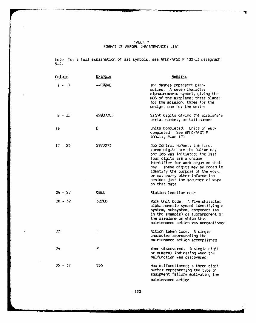
TABLE 7FORMAT CF ABFQ9L (MAINTENANCE) LIST

Note--for a full explanation of all symbols, see AFLC/AFSC P 400-11 paragraph9-4.

Column Example Remarks

1 - 7 --F014E The dashes represent blankspaces. A seven characteralpha-numeric symbol, giving theMDS of the airplane; three placesfor the mission, three for thedesign, one for the series

8 - 15 69007303 Eight digits giving the airplane'sserial number, or tail number

16 Units Completed. Units of workcompleted. See AFLC/AFSC P400-11, 9-4c (7)

17 - 23 2993273 Job Control Number; the firstthree digits are the Julian Oaythe Job was initiated; the lastfour digits are a uniqueidentifier for work begun on thatday. These digits may be coded toidentify the purpose of the work,or may carry other informationbesides just the sequence of workon that date

24 - 27 QSEU Station location code

28 - 32 522E0 Work Unit Code. A five-characteralpha-numeric symbol identifying asystem, subsystem, component (asin the example) or subcomponert ofthe airplane on which thismaintenance action was accomplished

33 F Action taken code. A singlecharacter representing themaintenance action accomplished

34 P When discovered. A single digitor numeral indicating when themalfunction was discovered

35 - 37 255 How malfunctioned; a three digitnumber representing the type ofequipment failure motivating themaintenance action

-123-

Column Example Remarks

38 - 39 78 Year

40O - 42 319 Stop day; the julian date thisaction (see the action taken code)was completed; this is notnecessarily the final action thatwill be taken under this joncontrol number

435 - 46 6615 Federal supply class; supplycategory of equipment. This maybe left blank if no supply actionis involved

47 - 55 753088110 The dashes represent blankspaces. A nine-character partnumber. May be blank, if nosupply action is involved

56 - 6i Blank

62 - 66 A7303 ID Number. Consists of the lastfive characters of thesix-character ID number describedin AFLC/AFSC P 400-11, 9-4 (3):The first character is the prefixof the equipment classificationcode, in the example "A"' foraircraft; The last fourcharacters are normally the lastfour positions of the equipmentserial number; thus, columns 64-66should duplicate columns 12-15.

67 - 75 034TFGWG Organization; number, kind, andtype

76 - 80 90953 Sequence number; this is a recordcount for each entry

-124-

.0 0 0 co0

\0 'Isk \0 0'A 'A.-4 A'

N N 'A N N

It 4 V-I

0C\ 0'% C\ a\

0 0\0

Nl (N Nll

-t r4 41

\0 0 \.00 '0 \O

N4 N Nr N7

'.0 0 \0 \0

4 0 4 4

V-A 0 ,vio-N N

ON Cd c0% 4- 0. +-' C7% C'00 0 0 0 : 0ON- N 0 N- 0 N-\0 1.0 \0 \.0W

'A0 'AN cm VN Z:44 ztI4 .

N' 9( C~ NC 0 0

0% 00%;0'

CC0-40 OF-4 4-4 00 4-4 0 11 -N- 0 NNC~ 0 a~. 0 r% D

NO m04- \0- '0% z'A) U0 'A . ) 'AN- 0) 'ANC c4 -I 'G P-4 4 4 .4 4- N- xC14 (c'. N4 (4 1(- (V - 4

4CIS v4~ V4 .4 4 -.4 % .- 4 0nV- 0 xVI (V- 0 nV- x. no IC M0 N1' <

ON O\~ -tk 0%4 CO 0% 4co 0 m 0 COs 0

N- N- N- N%D '.0w \ 0 11'0'Ar 1; 'Az NAA'4_4t

0I 4)' 0 'CA 0 4-Nl &4. CV- n . NV N-, 4 m W4* .k .4* ;I ~ §-4

NOj 0f b.0 t D NO. 4 t NO0C\ ~C *-4 O0%'VA .-H 0% -4 -44 all00 r.4 CO 0. PLO CO v4 40 ZN- t- N0% NC . NVJ c C w

\0 W4 \ON C* 000 \04t 4t'A\ ' V4 'AW .N

.4 .4 , wi-40 N V-4 o 40

0\ \0 01%00 all000 N coNC 0.4 0

\00 Go'0 4 \0'A''A N1 WA 4 "A '4. CN 4 W4 4n vi NnO.40 It4 .4'.m 0 C\)

a% a% a%

'0 N- 0 '0o~

C 4 4 1

IQ Nl- 0" a'CC) co co CINC- .4 - Nl- 't

l1l-

.4 - .4 4'0 (z'0 %00

C- CN -%0 N- \0 0

44z V 4\

M V-4 C NV ca r4 co.-4 N- u) -4 L) .4 a(7%C CY) a\ m to

m" co 00 u"N -N- 4 - N- N-

'0 0 0\0 V"\

SCN -z CV 0 aN~ .4 NIC~ N all~.- 4 %A) CQ '4 '4 .4

<0 z t 40 Z 4zt0 ML4 C\a a\ N- .-

- 4 0 N1- 0 Nl- Vt'I 0'0\0 \0 '0 V"

4) x1 CmI 4 -44

N~ i4 N ~ N 'M.-4 '10 ca '-4 C -4 (tj cd

C-0 --- x ("0 x (0 N~ xa\ < ;0) a, N'i Cz CjMO C) 00 J1)Nl- (IN N- N - =D\ CM \D' '00 L4 U)

N4 C ~ I.. N N - 4.4N .3 4 " Ni N

a' 0 "-4 00 .4 0 n' W0% <) I0i, a\ -)0"LN - cr N- Nl- N'0 N~ %0 \'o -tV-1 <' V'\ Cl\

N~ C'I Nv N N.4 N .- .4

'10 0 -0 ia'\ -\a a\ a

'0 N '0 \ 0 --

4 4 4

26-~.

DA-T

FILMi