AD-RL61 562 THE AREA-TINE COMPLEXITY OF SORTINO(U) ILLINOIS UNIV AT 1'5URBANA APPLIED COMPUTATION THEORY GROUP 0 BILARDIDEC 94 RCT-52 N9994-84-C-S149

UNCLSSIFIED F/O 12/1 ML

I flhhE..hhhhII|I fflfflfflfIfllfllIfEBhhhhIhEIhhhEEIIIIIIIEEIII

SlfllfllflfllflflIIIIl

lllllllllllIIIu

W ,, ., ' ,

1 2r

il

NATIONA III[IJO TADRS -19S-

L. 16

m& 1 .0

11111 bLL 1iIMi8

111125 11111.4 .

MICROCOPY RESOLUTION TEST CHART

NATIONAL BUREAU OF STANDARDS -1963 -A

C.,

:% i . .. ...... : : .. ..

'-.-.

• .'..'. .. .. "..'.. ......... .. ,. ..:. '.... ... '. .... , : ;. '. .. ..".. .-,. . .. ,. .. , , .%' .'..' T..' .'..'%'..,%. , " .," ..,,s.,.,, .. , - ,

REPORT ACT-52 DECEMBER 1984

-PLIED COMP"2iig

THE AREA-TIMECOMPLEXITY OF SORTING

ELCTE

"-I APPROVEDAM

OF !LLINCYN

*h d .4

UNLASIFIE£D

t. cume7v cL.sSipecA"ioN OF Tmi,8 PAGE

REPORT DOCUMENTATION PAGEMI RPORT 58CWRITY C kASIPICATION l. 0ESTRICTIVE MARKINGS

Un___ _ssi__edNone

!2& $IC;JRI'fv CL..AUIPFICATION A ITVI I3f1 Inrk[IU-AVA Lft1 1LITV, P REPORT5Cprove 2or puoLic re ease, distributionN/A unl imited20. I CLASSIPICAIOWdOWNGR01AOING SCEGOULIEN/A7 PGMPoRMNO ORGANIZATION RIP0RT NUMUERIS) I. MONITORING ORGANIZATION REPORT NUMSERES)ACT-52 UILU-ENG 84-2218R-report # R-1024 N/A

I Se.NGME OF PIIMORMING ORGANIZATION OPICS SYMBOL 7& NAME OP MONITORING ORGANIZATIONoordinated Science Laboratory L4ue9bI., IBM Fellowship, National Science Foundation,niversity of Illinois N/A Joint Services Electronics Program

Z. ACOXESS 1Cle9. S& a" ZIP C*Ae 7. A00R111i3 (My. Stm d ZIP cde)1101 W. Springfield Avenue 800 N. Quincy StreetUrbana, IL 61801 Arlington, VA 22217

* "OP O PUNOION so w RING Em. OFFICE SYMBOL 9. PRtocuREMENT NsTRruMENT iONTIPICATION NUMERORGANIZATION IX1Fellowship, i r Wuksiuj N00014-84-C-0149

a. AOORass CiLty. SteAl nd ZIP Como 10. SOURCE OF PUNOING NOS.

0ePROGRAM PROJECT TASK WORK UNIT800 X. Quincy Street LEMENT NO. NO.Arlington, VA 2221711. ?It, I ,." .eun~y Cauatlcea,, [ne Irea-£1meComplexity of Sorting N/A N/A N/A N/A12. PE[RSONAL. AUJWISI

ianfranco BilardiM rv.vs OF REpr 130. TIME COVEREO 14. OATE OP REPORT Yr., Wa.. D.ay S. PAGI COUNTechnical PROM _o December 1984

I1. SUPPLiMENTA Y NOTA TION

./AI.COSATI COOlS IL. SUBJECT TERMS $Contgrne oot ewrw gf neesomv~ mmg &Anafy by bgw* xaumftrp

* 8 LO ROIJP $sU. ;M.

It. ASSRMACT 'Cann Ima n iew if weemwp and Idmesity by bas.e N&Mubwp,This thesis studies the minimum area A - ak(T) required by a layout of a VLSI circuit that

, ik

sorts n k-bit keys in time T.The square tessellation technique is introduced as a powerful tool to establish area-

time lower bounds, based on the information exchanged across the boundary of a suitable setof square cells that tessellate the layout region. When the information exchange is due tothe fact that variables output on one side of the cell boundary are functions of variablesinput on the other side, the square tessellation yields bounds on the AT2 measure. 'mhen, onthe other hand, the information exchange is due to the fact that the cell saturates itsstorage resources and sends some information outside for temporary storage, the squaretessellation yields bounds on the AT measure. Both AT and AT lower bounds are obtained orsor-in_. The forner dominate in fast computations, while the latter dominate in slowcomou :ations.

."he analysis indicates that the nature of the ?roblem varies considerably with the2o.0. Z s CA.AI Ll1v CP ASTqAC 2

1. AS43IACT SFA C "ITV C'-ASS;P!CAr,*CN

-.4t.S1'G -iL47j SAM i A S as P-. - :T~c .4lPS0 Z

22. 'APME .P A1SPCNSSII.5 ,NOIVIOLJA. J2:5 Th:,.9:cNr %MSEA€ wI-ca .'.C'

DC FORM 11473, 83 APR 101IC-4O :P I AN 73T SO 1.6711.RA

S. . -. ... .. . .. . . . .. . .

TVrt AqqTVTrn

SICUrITY CLAM PICATION OP TIS PAGE

relative size of n and k. and suggests a classification of keys into short (k < logn),long (k > 2 logn), and of medium length.

Optimal or near-optimal designs of VLSI sorters are proposed for the entire range ofn, k, and T, confirming the inherent validity of the lower-bound analysis.

I

I

!

I.-

. 9 .

i

THE AREA-TIME COMPLEXITY OF SORTING

Gianfranco BilardL Ph.D.Department of Electrical and Computer EngineeringUniversity of Illinois at Urbana-Champaign, 1985

This thesis studies the minimum area A - A. (T) required by a layout of a VLSI circuit that

sorts n k -bit keys in time T.

The square tessellation technique is introduced as a powerful tool to establish area-time lower

bounds, based on the information exchanged across the boundary of a suitable set of square cells that

r tessellate the layout region. When the information exchange is due to the fact that variables output on

" one side of the cell boundary are functions of variables input on the other side, the square tesellation

yields bounds on the AT 2 measure. When, on the other hand, the information exchange is due to the

Ufact that the cell saturates its storage resources and sends some information outside for temporary

storage, the square tessellation yields bounds on the AT measure. Both AT 2 and AT lower bounds are

obtained for sorting. The former dominate in fast computations, while the latter dominate in slow

computations.

The analysis indicates that the nature of the problem varies considerably with the relative size of

" n and k , and suggests a classification of keys into short (k 4 logn ), long (k > 21ogn ), and of medium

length.

Optimal or near-optimal designs of VLSI sorters are proposed for the entire range of n, k, and T,

-. confirming the inherent validity of the lower-bound analysis.

I..

_ .!,. ,' . '-k ~ laL.ha~ dn' 6.,.:, ln dmn an.'.'i. . .. " ' ' i .. .. .. . .- , . ... .. .

o'7.

iv

ACKNOWLEDGEMENTS

My advisor, Professor Franco P. Preparata, has had a profound influence on this thesis and on my

L-, scientific development.

Many discussions with Scot Hornick, Xiaolong Jin, Majid Sarrafzadeh, Alberto Segre, Prasoon

Tiwari, and loannis Tollis are reflected in this work in various ways. To Alberto, Majid and Scot, I am

also particularly indebted for their help in preparing the final version of this manuscript.

Several conversations with Tom Leighton have provided me with considerable insight on VLSI

sorting; it has been very beneficial to learn of Tom's results in their early stages.

Phyllis Young and Mary Runnells have been very patient in typing this manuscript.

The work reported in this thesis has been mainly supported by an IBM fellowship, with partial

support, at different times, by National Science Foundation grant MCS 81-05552 and by the Joint Ser-

5 vices Electronics Program under contract N00014-84-C-0149.

Finally, I want to express my gratitude to Marinella, my wife, for her love and support.

i Accession For

"NTIS GRA&IDTIC TABUnannoune-9ed":" ~Just ifi.:t ,

,%°,

£_ By.

Distri_-tAvmila.h4

Dist I - .'

.I

I

U .

.. U- .. . . . . . . . .

TABLE OF CONTENTS

CHAPTER PAGE

1 INTRODUCTION 1p

- 1.1 VLSI Computation 1

1.2 Problem Statement and Organization of the Thesis 6

2 PRELIMINARIES 10

2.1 Introduction 10

2.2 Encoding Multisets 15

3 LOWER BOUND TECHNIQUES 24

3.1 The Dichotomy Lower Bound on the Layout Area 25

3.2 Information Exchange Area-Time Lower Bounds (AT 2 Theory) 32

3.3 Saturation Area-Time Lower Bounds 37

4 LOWER BOUNDS FOR CYCLIC SHIFT AND SORTING 42L

4.1 Cyclic Shift . _42

4.2 Sorting 48

4.3 Area-Time Lower Bounds for the Comparator-Exchanger 74

5 ALGORITHMS AND ARCHITECTURES 79

5.1 Introduction 79

5.2 Parallel Algorithms for Sorting 80

. 5.3 Parallel Architectures 88

6 OPTIMAL VLSI SORTERS FOR KEYS OF LENGTH k - logn + O(logn) 101

r 6.1 Introduction 101

. 6.2 Networks for Bitonic Sorting 104

!i"~

-" " " '

' '"-""*-"; . ' " .. * *-' * * "-" ' .. * * . .. .~.*"" ' "-"- "",'* .p ft*.*** "" "- "

* ' ' ", -"" "- "".

- . . . . -* -77

vi

6.3 Networks for Merge-Enumeration Sorting 124

6.4 Other Optimal Networks 137

7 SORTING KEYS OF ARBITRARY LENGTH 139

7.1 Introduction 139

7.2 Sorters for Keys of Medium Length 140

7.3 Sorters for Short Keys 152

-7.4 Sorters for Long Keys 163

8 CONCLUSIONS 175

REFERENCES 179

rVITA 183

U-

THlE AREA-TEME COMPLEXITY OF SORTING

BY

I GIANFRANCO BILARDI

Laur., Universiti di Padova, 1978MLS, University of Illinois, 1982

U THESIS

Submitted in partial fulfillment of the requirementsfor the degree of Doctor of Philosophy in Electrical Engineering

in the Graduate College of theUniversity of Illinois at Urbana-Champaign. 1985

Urbana, Illinois

r

Copyright by

Gianfranco Bilardi

1985

N. 77, 01 1. P7.. -- . - 777r

OIAPTERli

Un

IN TRODU CTION

1.1 VLSI COMPUTATION

The breakthroughs in the field of electronic devices, which have lead to Very-Large-Scale-

Inlegration (VLSI) technology,.open new avenues to the system designer in almost all areas of electri-

cal engineering [MC79, Mu82 New system-theoretic concepts are necesry to take full advantage of

the new technological potential, although existing theories will be an invaluable startiag point, accord-

ing to a pattern typical in scientific research.

We shall focus on computing systems, which will be among the first to be affected by the VLSI

technological revolution. However, considering that communication and control systems make an

increasing use of digital techniques for signal processing (a particular kind of computation), we realize

*: that computing is fundamental for all electrical engineering.

* The main feature that makes VLSI a very attractive environment for computing systems is the

possibility to deploy - at a reasonable cost - a large number of procesm cooperating in the execution of

a given task. This possibility has been long pursued in the hope of increasing the system's computa-

tional throughput by means of concurrency of operations.

A sytematic development of the notion of concurrency implies a radical departure from the archi-

tecture of the traditional Von Neumann computer. and from the sequential nature of the corresponding

algorithms, given as sequences of very elementary instructions each of which is to be executed in suc-

cession by the same processor. The departure from the uni-processor architecture poses the fundamental

question of how to interconnect many processors so that they can efficiently exchange information

when cooperating in solving a given problem. The interconnection network is in fact the most relevant

feature of a parallel architecture and strongly constrains its computational capabilities. A formal wav

I.]

"v " " " ' " " " "" "' '""' " " ' "". ' " " """ " ' " '''" "" " '" """ ."'. .".. .'" '"°I.::-. :-.:-:...-:..:-:-2---. .:. . . ..--- -- -. .-' ..-.- -.-,-.-, -, - -- , -...-.-. ..- ..-- -.-. ..,*. - -- .-. , ,* - - . -

2

to view a parallel architecture consists of associating to it a graph whose vertices correspond to proces- -

,.. sors and whose arcs correspond to data path. The attempt to define a general purpose architecture,

* whose interconnection network can support any processor-to-processor data transfer that an algorithm

may require, leads to consider the fully interconnected graph. This architecture, under an equivalent

formulation known as Shared Memory Machine, has in fact been extensively used in the first theoreti-

cal studies of parallel computing. However, practical considerations on limited fan-in and fan-out fac-

tors, and also on cost-effectiveness., show that the fully interconnected architecture is not a realistic

model for a computer, and motivate the investigation of architectures with simpler interconnection

that still support efficiently the execution of parallel algorithms. Thus we are led to the following

situation. Each computational problem calls for the joint design of an algorithm and an architecture.

The mbest" architecture may change with the problem. Only a posteriori after careful analysis of many

problems, may we fnd out whether there are general-purpose, or at least broad-purpose architectures,

which are efficient for a large class of problems.

In this context an appraisal of a design must be based not only on algorithmic performance, typi-

cally characterized by time complexity, but also on some other measure capturing the 'architectural

complexity'. The traditional count of processors is not an adequate measure because it totally disre-

gards the communication aspects of the system. Other mathematically reasonable candidates could be

related to the number of edges, or to the maximum degree, or to the diameter of the interconnection

graph. However, none of these measures seems to reflect completely the cost of actually building the

architecture in any technology of current interest.

It is then of the greatest theoretical interest the fact that VLSI technology naturally offers an

attractive measure of architectural complexity, the chip area. Due to the integrated nature of VLSI

te-hnology, where processing elements (transistors) and communication elements (wires) are realized in

the same medium (the silicon chip), chip area effectively accounts for the cost of all relevant aspects of

the Tystem, and its minimization is a major concern in industrial applications.

..... *.....°-,' .- . -. ,-.'-... .. -.. .... .- - "...... -"-•• .............. , 1

h 3

The fact that the architecture to solve a problem is not given in advance - as it was in traditional

algorithm design for the Von Neumann machine - brings a new interesting consequence: the architec-

tural complexity can be traded for the efficiency of the computation. In the context of VLSI computa-

tion, this phenomenon takes the form of area-time trade-off, and plays a central role in the theory.

The rigorous development of a computation theory for VLSI rests on the definition of a model of

comptiaion that captures the ential traits of the technology and allows for mathematical treatment

of system design. A VLSI model of computation is today available, as the result of the effort of several

authors [T80,BK8I,Se73,Sa79,C.181,BPP82,BL8 4 and will be described in the next section. The

assumptions of the model will be stated axiomatically. For their justification, which is sometimes based

on a rather delicate and subtle analysis, we refer the reader to the literature cited above.

1.1.1 The VLSI Model of Computation

A VLSI chip can be viewed as a computation graph whose vertices are information processing

S devices and whose arcs are wires, that is, electrical connections responsible for information transfer as

well as for power supply and distribution of timing waveforms. A given computation graph is to be

laid out in conformity with the rules dictated by technology. The esence of these rules is formally

accounted for in the model as follows.

Area Assumptions

(AI) (Wire Area) All wires have minimum width X > 0 (which includes both the actual wire width

and the clearance between wire and any other chip region), and at most v wires (v an :nteger

> 2) can ,overlap at any point (hypothesis of bounded number of layers).

.2) (Transistor-Port .rea. Transistors and I/O ports have minimum areas c, X' and c. X-, respec-

tive , . for constants c- and cp.

A31 (Chio Area The chip area is at least the sum of the area of the wires, of the transistos, and of

.he L 0 nor.s and it is at most the area of the smallest recuanzie (or convex region) enclosin2

ecal 'avout of the graph.

".--..' ,--,.--..'.,-.. .. .,.. .,-.. ,.. .. .. .- .--.....-.-..,..... .. .. ..-.-.... ... ,-.. .. ,.. . . . . . .-.. ...-.-... ,,-,, ,,.- .-

. .... .. ....... - - -

4

The area assumptions allow a straightforward appraisal of the area of any given design. To appraise

the computation time of an algorithm we need some assumption on the timing of elementary actions, as

the gate switching and the signal transmission on wires. For simplicity, in the sequel switching time is

subsumed under propagation time.

Time Assumptions

(TI) (Propagation Time Along a Wire. A bit requires a constant time r to propagate along a wire,

irrespective of its length (synchronous model).

(T2) (Algorithm Time): The computation time of an algorithm is the time of the longest sequence of

wire propagation times between beginning and completion of the computation.

Asumption (TI) is not immediate to jutify, and it is in fact false at the physical level The essence of

the justification is that, although a detailed analysis of the electric phenomenon of wire propagation

[BPP82] shows that constant transmission time can be achieved on long wires only if proportionately

large driving transistors are deployed, results of layout theory [BL84] ensure that a layout of the coin-

putation graph can always be found in which large drivers can be accommodated without substantial

degradation of area and time performance.

The transfer of information within the chip is constrained not only by wire bandwidth, but also

by fan-in and fan-out capabilities of logic gates. This fact is accounted for by the following assump-

tions.

Fan-in and Fan-oia Assumptions

'Fl) (Bounded Fan-in) The number of input lines of a logic gate is upper bounded by a constant

(F2) (Bounded Fan-our): The number of output lines of a logic gate is lower bounded by a constant

Other assumptions are often stated in the VLSI computation literature when studying lower and

uppr bounds for specific problems. These assumptions are not dictated by technological constraints, but

ra.her by reasons of various kinds, for instance to avoid trivial or -neanmingless solutions. "o enforce

.. . .

features that are appealing for practical application, or to simplify the analysis. Most of these auxiliary

assumptions concern the 1/O protocol. We list here the most common ones

Protocol Assumptions

(PI) (Semelective Proco= . The input data of the problem are available only once at the input ports.

(P2) (Tims-Dezerminate Proocol): Input and output data are available at prespecified (instance

independent) time.

(P3) (Place-Determinate Proocol): Input and output data are available at prespecifhed (instance

independent) ports.

(P4) (Boundary Protocol) All I/O ports are on the boundary of the layout region.

r (P5) (Word-Local Prorco4 All the bits of a given input word enter the chip at the same input port.

Unless explicitly stated otherwise, assumptions on area, time, fan-in and fan-out, assumptions P1,

P2. and P3 on 1/O protocols will hold throughout this thesis. Instead. P4 and P5 will always be expli-

citlv mentioned when adopted.

It is worth observing that, although all our networks will exhibit bounded fan-in and bounded

fan-out. assumptions Fl and F2 will not be needed in most of our lower-bound proofs.

- Usually. when discussing asymptotic analysIS, the specific values of some of the constants in the

model such as c,, cp. X. and r, are not relevant, and can all be conventionally chosen equal to one.

It is also convenient, when considering layouts of computation graphs, to restrict the attention to

* embeddings on a suitable rectangular grid. Generally, this restriction could be easily removed at the

-nce of more elaborate proofs. which would not add particular insight to the analysis..

1.1.2 The VLSI Complexity of a Computational Problem

Once a model of computation for VLSI is defined, algorithms for various problems can be proposed

r and analyzed. and a coherent theory can be developed. Several authors have proposed ;Vrformance

measures. ty;icallya function of the area A and of the t:me T of the form .4T, with resec: to which

-oA.

A'.o - * * 4 , . . . r , , , ' ~

6 N

optimality can be defined. In our opinion, however, the following approach is more fundamental

Given a computation problem IL to any chip that solves II for an input of size n. in time To, and

area A(- we can associate a point of coordinates (T o,4 A) in a plane, which we call time-area plane. The

set of all designs corresponds then to a region in this plane. The objective of VLSI complexity theory is

then the determination of such region. Since if a point (To .A O) is feasible then (T 0,A) is feasible for

any A > Ao (just waste some ar=ea), the objective can be reformulated as follows.

Given a computation problem 1I. its VLSI complexity is described by the family of curves

A = a, (T), one for each value n of the problem size, where a (T A mintAo there is a chip that

* solves 11 on instances of size n with performance (T , 0)1."

Usually there is a minimum value T,3 ,(n) of the computation time below which no feasible

design exist and a maximum value T u(n) above which a, (T) is constant, meaning that no savings

*i in area result from slowing down the computation. In conclusion we would like to find, for a given

problem. the value of ao (T), for T E(T .,(n ).T .(n )I. Typically a, (T) is determined within a con-

stint factor by establishing suitable lower and upper bounds. As expected, a., (T) is increasing in n and

decreasing in T. expressing the fact that a faster computation requires more computing resources.

1.2 PROBLEM STATEMN AND ORGANIZATION OF THE THESIS

1.2.1 Sorting

Sorting is a fundamental combinatorial operation, and is among the most frequently performed

'" by computing systems. Thus. the VLSI complexity of sorting has received a lot of attention by

researchers. But, in spite of intensive study, this problem does not cease to offer extremely intriguing

questions, and to reveal heretofore unsuspected facets. ..

Formally, the inlk)-sorring problem is defined as follows

(1) The input is a sequence of n k-bit keys, each a member of a finite set of integers.

I :"-- -.-- .- : :--. ..."----..:----°":-:-.". ".."""." " '4"."... "."........... "

hI

" (2) The output is a rearrangement of the input keys, so that they form a nondecreasing sequence.

Throughout this thesis, we represent the input of the (nJc)-sorting problem as an n xk array of

binary variables

*"X =iX;s:i 0, 1,.. n -1 j =09 .. k -1l

where X,' is the coefficient of 2' in the binary representation of the i -th input key. The i -th row of

X, denoted by X,, represents the i -th input key, and the j -th column of X, denoted by X ,, represents

the j -th least significant position. A similar notation is adopted for the output array Y.

One could be tempted to analyze the complexity of sorting as a function of nk, the total number

of input bits. However, as will be fully substantiated in the following chapter, the nature of sorting

is strongly influenced by the relative size of n and k. Thus, it is appropriate to state the objective of our

* study as the determination of the minimum area A = a,. (T) sufficient to lay out a circuit that solves

the (nkc)-sorting problem, as a function of n and k.

m1.2.2. Thesis Outline

- This thesis is organized in two parts, respectively devoted to the study of lower and upper bounds

3 to the area-time complexity of sorting.

In Chapter 2, after a review of known area-time lower-bound techniques, we study the subject of

multiset encoding, which turns out to be deeply related to sorting. In fact, although the input to the

(n*)-sorting problem is given as a sequence of keys, the output depends exclusively on the multiset

underlying the input sequence. In the VLSI environment. where comutation is governed by the fow

of information in the two-dimensional chip, the information-theoretic content of :he input multiset has

a f undamental induence on the area-time complexity of sorting. The fact that this information content

is ver- sensitive to the reative sizes of n and k is the primary reason for which the nature of sorting is

-.- stron2-v devndent on the length of the keys.

The traditional bisection .low technique is not adequate to study the area-time complexity of sort-

1.* :rg, except for a srecial interval of key ler.gths. In Chapter 3 we introduce the notion of square

o. . %*.,'% .'. ...- .. ' " * . . * , -. . - . . . - . . . .-• . *. .. " • .. ", . .•'. -.- -. " o-.-: %,, *- . * . - ...

tesllation, a partition of the layout region into square cells of identical size, and we show how to

obtain area-time lower bounds in terms of the information exchanged across the boundary of the tel-

lation cells. A novel feature of these bounds is that their form depends upon the nature of the mechan-

ism forcing the information exchange. When the information exchange is due to the fact that the van-

ables output on one side of the cell boundary are functions of variables input on the other side, the

square tessellation technique yields lower bounds on the AT measure. This mechanism has been exten-

sively studied in the literature, especially in connection with the bisection technique. In addition to it,

we consider here for the first time another mechanism, which we call sarauion, occurring when a cell

of the tessellation fills all its storage in the course of the computation. and sends some information to

the rest of the chip for the only purpose of temporary storage, to request it back at a later time. When -

the information exchange is due to saturation, the square tessellation technique yields bounds on the

AT measure.

The effectiveness of the general techniques developed in Chapter 3 is demonstrated in Chapter 4.

" where several lower bounds are obtained for two problems cyclic shift and sorting. Here the keys are

- cla.sified into short (k 4 logn), long (k > 2logn), and medium-length. Medium-length keys have been

heretofore the object of investigation, and can be adequately studied by bisection techniques. It is for

short and long keys that the full power of the square tessellation techniques becomes evident. For both

* cases, AT 2 and AT lower bounds can be established, and it is interesting to observe that the AT 2 bound

dominates in fast computation, while the AT bound dominates in slow computation. In the last section

of Chapter 4 we obtain bounds for the problem of comparison exchange, a special case of sorting where

the keys are just two. The bound is on the AT 'logA measure, and rests crucially on the bounded fan-in

*assumption, unlike the bounds mentioned above that hold even for circuits with unbounded fan-in and

fan-out.

In Chapter 5 we turn our attention to upper bounds, and review some wet' known parallel algo-

rithms for sor-ing, as well as some networks of processors particularly suited to VLSI implementations.

7-

.-o9

In Chapter 6 we study (nk)-sorting for k - logn + O(logn). After explaining why this particular

U value of keylength plays a central role in the construction of sorting circuits, we turn our attention to

specific designs. We rst consider the bitonic sorting algorithm, and propose two architectures, the

pleated cube-connected-cycles, and the mesh of cube-connected-cycles, both of which achieve optimal

area-time performance in a wide spectrum of computation times. The fastest bitonic sorter works in

time T -'O(log'n ). To obtain faster sorters we then turn our attention to another algorithm. the

merge-enumeration combination. A network that combines the cube-connected-cycles and the

orthogonal-trees architectures executes this algorithm in 0(Iogn) time and optunal area.

In Chapter 7 we consider the (nk)-sorting problem for arbitrary k. and we propose three sorting

-. networks, respectively tailored to short, medium-length, and long keys. The algorithms presented in

this chapter are new. The ones for short and medium-length keys exploit efficient encodings of schemes

' for multisets. while the algorithm for long keys takes advantage of the non-word-locality of the I/0

protocoL The fact that the resulting VLSI designs are optimal or near-optimal confirms the inherent

[ validity of the lower-bound analysis developed in Chapters 3 and 4.

Some closing remarks are finally presented in Chapter 8.

..

r"

oo.

* . . . . . 2. S A -, P A -. A . - - -

r

PART I

LOWER BOUNDSr

S

p

a-

r

i

- .~.-. *1~ M * . . . .

CHAPTER 2

PRELIM INARIES

2.1 LN'RODUCTION

Part I is devoted to the study of lower bounds on the area-time complexity of sorting. However,

the techniques that we develop are general, and will probably be useful to investigate several other

problems.

We recall from Chapter 1 that the VLSI complexity of a computational problem II is described by

the family of functions

A a (T), T E [T mjn )IT.(n ) 2.1

where n is the input size, ac, (T) is the area of the smallest design that solves 1 in time T. T . is the

minimum time required to solve I1 (regardless of the area), and Tm, is a time such that, for T >

T =, a, (T) is constant with respect to T.

Area-time lower bounds can be stated in different forms. The most common are

A = (l(f (n,T). 2.2

T f (f n.A)). 2.3

g(A.T) = (f(n)). 2.4. where f If g, and f are suitable functions. It is usually a simple matter to convert one of the

above forms into another. The choice of the form to be used in a specific case is only a matter of con-

venience.

* . .. '

2.1.1 Layout Theory

Since a VLSI chip can be viewed as the layout of a given computation graph, some useful tools to

establish area-time lower bounds can be borrowed from layout theory, a chapter of graph theory which

studies, among other things, the problem of determining the minimum area needed to embed a given

graph in the plane, according to some specified layout rules.

Typically, lower bounds (and also upper bounds) on the layout area are given in terms of some

auxiliary quantities associated with the graph, which are hopefully easier to compute or to bound than

the area itself. Among the most interesting auxiliary quantities proposed in the literature are the bisec-

tion width [TSOI, the crosing number [L81al the wire area [L81al the separator [Ls8Ob, Va8l, and the

bifurcator [LS2,BL&41

When applying layout theory to obtain area-time lower bounds, we do not deal with a specific

-. graph, but with all the graphs that can support the computation to solve a given problem IL in a given

time T. Thus, our goal is to show how this computational property of the graph implies a bound, either

U directly on the area, or on some related auxiliary quantities. Some techniques have been proposed in the

literature to achieve this goal, and we briefly review them in the next section.

2.1.2 Area-Time Lower-Bound Techniques

To date, all known area-time lower bounds belong to one of the three following clas

(I) Input-outpuz bounds. They are of the form

-kT = l(si:e of in.ul + si:eof outrpu) 2.5

and are a trivial consequence of the fact that the area is at least proportional to the number of l,'O

pors. which in turn is at least proportional to the maximum number of bits that the chip inputs or

outputs in a time unit- For boundary chips. (where all the 1/0 ports are placed on the boundary of zhe

.ayout region), the 1. 0 bound becomes

. .. . .

12

pT - fl(sieof input + size of output) 2.6

where p is the perimeter of the layout region. Bound (2.6) is usually combined with other consicdra-

tions to obtain area-time bounds.

(2) Functional dependence bounds. Functional dependence of the output variables on the input vari-

ables can sometimes be exploited to strengthen the I/O bound, as in [Jh8Ol, where it has been shown

that, for the addition of binary integers with n bits,

A = W2.log(2-)) 2.7

or equivalently,

AT/logA = (1(n). 2.

The argument to establish the bound is rather subtle, and we will discuss it in detail in Section 4.3,

where we apply it to the problem of comparison exchange.

(3) Information-Exchange Bounds. Almost all the nontrivial known lower bounds on area-time com-

plexity are of the type

AT 2 = ((n)). 2.9

where I (n) is the bisection-information of the problem II being considered, a very important notion

introduced by Thompson [T80. Informally, the bisection width b of a graph G = (V,). is the

minimum number of edges to be removed in order to separate a set of ,Vl/2 vertices from its comple-

ment. (For formal definitions and generalizations see [T80], and also Section 3.1.) The bisection-

information arguments are based on two facts: (i) the layout area is at least proportional to the square

of the bisection width: (ii) any computation graph that solves a given problem fi must support an

information exchange I (n) through its bisection, where I (n) is a function associated with l. The

bound (2.9) follows easily from (i) and (ii), considering that b I (n ),'T. The evaluation of I(n)

requires an argument tailored to the particular problem being studied. Indeed. considerable attention

has been devoted to the sub ict of information exchange. which we survey briefly in the next section.

............. ... .......-..•."."-.'-.......'. -. '..•.. "._..............,'..' """ """""" """'""n * Y*

% _..', '..'... .. *... .. Jx1n ,.& & L dL -

.

13

2.1 .3 Information exchange

In recent years the study of both distributed and VLSI computing has generated considerable

interest in the analysis of the amount of information that different procesmors have to exchange when

cooperating in solving a given problem.

Several quantitative definitions of the information exchange I associated to a problem II have

been proposed, and several techniques to lower bound I have been developed. The objective of this sec-

tion is to recall the main concepts at an intuitive level, and to indicate the appropriate references, where

a more detailed treatment of the subject can be found.

The general framework is one in which two processors P and P cooperate to solve a problem l.

or equivalently to compute a function f. The basic question is: How many bits do the processors have

to exchange during the computation? The answer is obviously dependent on a number of assumptions,

and different authors have made different asumptios. We list some of them here.

I/O-Variable assignment. In the simplest case the assignment of I/0 variables to processors is

completely specified. In applications to VLSI we are typically interested in a class of assignments. and

the information exchange must be minimized over the class. ([Y79], [T8OI, [BK81, (AA8 O [Y81,

(LS81. sBGS21 (IS82] (Sa79, (Vu831 [184], (AUYS3.)

Communication protocol We may consider a one directional link, say from P 1 to P, (one-way

communication) or a link for each direction (two-way communication), ([Y79D. We may also impose

bounds on how many messages can be exchanged, a message being a run of bits sent by P, to P

Alternatively. we may bound the length of the messages. and so forth ([PS82] [DGS84).

Type of computation. The computation performed by P , and F : can be assumed to be deter-

" ministic, or nondeterministic. or randomized (Las Vegas). ([MS82, [PS821, [LS81], [DGS84, [Y75],

.- ,L"tYS3i.)

Compiexity nwasure. Finally, we can count the bits exchanged by P and P, n the worst case

instance, or in several kinds of average case [Km83].

"..

14

The above list of assumptions is by no means exhaustive, but should give an idea of the variety of

issues which are addressed in this area of study. Typical results that can be found in the literature con-

- cern: (i) general lower-bound techniques; (ii) bounds on the information exchange of specific functions;

" (iii) the study of complexity classes related to various definitions of I; and (iv) conditions under which

the bound AT2 = f)(j2) is valid in the VLSI model

A complete account of the theory of information exchange is not our present objective. However,

we will return to this subject to propose some new developments, with relevant applications to VLSI

complexity.

2.1.4 Summary of Part I

The input to a sorting problem is a multiset, and for this reason efficient schemes to encode mul-

tiets are essential to obtain good algorithms. Moreover, the fact that the efficiency of a given encoding

:- scheme is very sensitive to the ratio between the size of the multiset and the size of the universe from

which the elements are drawn, makes the nature of the sorting problem vary considerably with the

. length of the keys being sorted. Thus, both lower-bound arguments and upper-bound constructions

greatly benefit from a solid understanding of the subject "encoding of multisets" which is treated in -

- Section 2.2

Chapter 3 is devoted to general lower-bound techniques. In Section 3.1 we gen.tralize the notion

of bisection width by introducing the notion of dichotomy width of a graph, a quantity very useful to -

, .lower bound the layout area of some graphs. In Section 3.2 we show that a suitable generalization of

*-~tne traditional concept of information exchange can be used to lower bound the dichotomy width of

computation graphs. When combined with those of Section 3.1, these results provide powerful tools to

lower bound the area-time complexity of computational problems.

The traditional bisection-information techniques as well as the generalization proposed in Section

3.2 capture the idea that if some variabies output at a given place carry information on other vaiables

-rut at a different place, then some kind of information tIlow between the two places will be required

.- o.

. - . . . . -° .

15

by the computation. However, there are cases where the information is input in a place close to where

it must be output, and nevertheless it must be temporarily transferred to a different place, due to the

fact that all local storage is saturated. In Section 3.3 we show how this intuition can be formalized by

* defining the notion of information exchange under bounded storage. We also develop a general tech-

nique to obtain area-time lower bounds based on this notion.

In Chapter 4 we apply the results of Chapter 3 to specific problems. In Section 4.1 we derive

lower bounds for the information exchange and the area-time complexity of cyclic shift. Although

cyclic shift is an interesting problem in its own rights, our main motivation to analyze it is due to the

relationship between cyclic shift and sorting, to be systematically exploited in Section 4.2 where we

finally concentrate on the sorting problem.

r Section 4.2 is organized in three subsections, respectively devoted to the study of three different

- ranges of key lengths. Several new lower bounds are obtained both on the AT 2 measure (using the

dichotomy-information technique), and on the AT measure (using the saturation technique). As we

U shall see, the AT 2 bounds dominate in fast computations, whereas the AT bounds dominate in slow

computations.

Finally, in Section 4.3 we discuss the area-time lower bounds for the comparator-exchanger.

which can be viewed as a sorter of two keys. Here we have to investigate the notion of functional

dependence and its effect on the area-time performance. Crucial to this type of argument is the notion

of bounded fan-in digital circuits.

2.2 R4CODrqG MULTISETS

This section is devoted to the study of efficient encodings of multisets. We are interested in mul-

• .tisets because:

(i) The input to a sorting problem is a muluset (the ordering of the elements in the input list !s

immaterial).

16

(fi) A sorted list can be viewed as a canonical representation of the underlying multiset (two lists

of elements represent the same multiset if and only if they are identical when sorted). -

The study of efficient encodings of multisets will provide us with a background both for the

information-based lower bounds of Chapter 4, and and for the upper bound constructions of Chapters 6

and 7.

A muldisei S is a collection of elements from a totally ordered set U called the universe, with

repetitions allowed. In the sequel we are only concerned with finite multisets and finite universes so

that. without loss of generality, we can use the following notation:

S = X, X ,... ,-1} 2.10

U {0,1 .... r -1. 2.11

Thus, n is the size of the multiset, and r is the size of the universe. Usually we think of the elements

of U as encoded in binary, and we denote by k = 1Iogr I the number of bits needed - encode an ele-

ment. Since the order of the element of S is immaterial. representation (2.10) is not unique, and gi'en

any permutation 7r (0). 7" ( 7)..... ir (n -1) of the integers 0,1...., n -1. we can also write

S = IX Ao..,,X.. ~ x .

This representation becomes unique if we add the constraint that X,, <X , , for

i 0,l....n-2 , or in other words if we require that the sequence . . be

sorted in nondecreasing order. From this standpoint sorting becomes the operation of computing a

canonical repcresentation for a multset.

Other representations are clearly posible. and could be more convenient in some situations. In

carticular, in VLSI computation we are interested in nonredundant representations because they require

less bandwidth for transmission.

A - I..

L 17

2.2.1 Counting Arguments

- l A simple combinatorial argument shows that the number of multisets of size n in a universe of

size r is + r-) Thus, the number of bits necessary to encode a multiset is

e e(nr log1+n 1J 2.12

* If we use Stirling's approximation for the factorial, after some manipulations we can rewrite Eq. (2.12)

as

e(n.r)=nlog(l +r/n) + rlog( + n /r) + lower order terms. 2.13

It is interesting to consider the asymptotic behavior of dnr) when r is an increasing function of n, as in

the following examples.

. (l)r/n 0 e(nr) r(log n -logr)

(r =6 r =roconstwn, e (n r,)r,, logn)

(2) r = n Xconstant e (n 0)(n)

(r =n, e(n.n) - 2n)

(3) r/n oo e(nr) - n(logr logn)L(i = ?z,=consan . e(no) n oogr)

Certainly there are encodings of multisets that use strictly etjr bits. However, we are interested in

encodings that either arise naturally from problems, or that. although artificially introduced, preserve

some intuitive meaning, and are useful in multiset manipulations.

2.2.2 List Encoding

The most natural way to describe a multiset consists in giving a list of its elements, tn any order.

Clearly ej,,, (n .') = nlogr =nk bits are used for this representation. Thus, the list encoding is ot.m a

(in the order) if and only if the universe is large enough. namely if

-

18 .

k f logn +0 (ogn) 2.14

or, equivalently, if r > n (14 for some a > 0. The list encoding becomes very inefficient for a

small universe. In the extreme case of r =2,e ,(n ,2)= n whereas e (n,2) Iogn . Therefore we

turn out attention to another method.

2.2.3 Multiplicity Encoding

Another simple way to specify a multiset is to say how many occurrences it contains of any given

element of the universe. Formally, we introduce the multiplicity function .i )A ( i = 0,1 .... r - 1)

of multiset S defined as

(i)-nmber of occurrences of element i in multiset S. 2.15

Since (i) is at most n, (i) can be represented with jlog (n + 1) 1 !iogn + I bits. and hence S can be.

encoded with e.,, (n , r) = r (logn + 1) bits. This encoding is optimal in the order when

k =logn -fl (ogn) 2.16

or.equivalently, if r < n for some a > 0. Slightly better results can be obtained by using a

variable length encoding for AL (i). For example we can encode integer h with 2 Ilog (h + I) bits by

using the empty string for h - 0. The multiplicity function can then be represented by the list

bA(0), ( ) .... A (r - I ) with the commas encoded as'01P Thus we can use a total number of bits

e (n r= ~2 lo~g(i + 1) + 2(r -)

It is eas to see that, under the constraint 1A(0) -, (1) +... ( r -) = ,

e',(n,)-= 0 (rlog(n/r 1)+r )

which is optimal for r <n . For r>n, we must resort to different techniques.

. .

~1 19

-2.2.4 The Izse"-and-Pruie Encoding

5In this section we propose a new encoding for multisets which is based on a sorting method and is

not as natural as the list and the multiplicity schemes, but it is simple and elegant. Moreover it can be

effectively used in some sorting algorithms.

* Let us begin with a simple observation. In a sorted sequence of n elements of k bits each, the

sequence of bits in the most significant position is a run of zeros followed by a run of ones. Therefore it

can be completely descrnt-, oy specifying how many zeros there are, which only requires Logn bits

* instead of the n bits taken in the list representation. In general, in a sorted sequence the j-th most

significant position (from the left) contains at most 2' alternating runs of zeros or ones. Thus, for

j < logn not all the binary sequences of n bits are candidates to be the j-th position of a sorted

sequence, and therefore less than n bits are needed to encode that position.

We could try to exploit systematically the above observations and build an efficient encoding

U based on the length of runs of identical bits in each bit position of the seqaence. but the resulting

scheme would be rather awkward and difficult to manipulate. However, the above discussion reveals

an important property: the leftmost bit positions in a sorted sequence carry less information than the

number of bits devoted to then positions in the list. As it turns out, if we have some extra knowledge

" about our sorted sequence, we may even completely reconstruct the sequence by looking only at its

. least significant position! This is a consequence of the following result.

Theorem 21. If S = {X,... X,-1) is a multiset drawn from the universe U = r0,1.....- -l I,

" and T is the sorted list of the union of S and U, then there is a one-to-one correspondence between S

and the sequence of bits in the least significant position of T.

Proof. T is the concatenation of r subsequences the i-th of which consists of, u (i) + 1 copies of ele-

ment i =0...., r -1), where /A () is the multiplicity function of S. The situation is illustrated in Fig-

ure 2.1. The least significant bits of T are the concatenation of r sequences, the i-th of which consists of

S(i ) + 1 identical bits each equal to i modulo 2. Thus, from the least significant bits we can recover

* ' *

20

(r-1)SlT: zero$ ones 1 i "".

a(O)+l O411)+1 1i+1 /A(r-11+1

Figure 2.1. The structure of sequence T.

the multiplicity encoding of S, and S itself. The converse is obvious. 0

,Remark. It follows from Theorem 2.1 that the sequence of bits in the least significant position of T is a

valid encoding of S, requiring n + r bits. For r = n the encoding is optimal up to lower order

terms. For r >> n or r << n the encoding is highly inefficient. However, for r > n, the follow-

ing generalization of Theorem 21 yields a better result.

Theorem 2.. Let for simplicity n = 2",r = 2&,and s = 24' be powers of two. Let also

S = iXO,...,XP-,} be a multiset from the universe U = (O.....r-l , and

U (s) = .s r .. ,r-s) be a sampling of U with period s. Define T as the sorted list of the union

of S and U (s). Then, there is a one-to-one correspondence between S and the sequence formed by the

(r +1 least significant bits of the elements of T.

Proof. We introduce the notation

A'= mulztiset of the prejxes of length k -a, of the elements in multiset A

and we define U(s)'and T ' accordingly. Clearly U(s)'=10,1, r'-l where r'r/s . Thus

we can apply Theorem 2.1 to multiset S' and universe U (s )'. to reconstruct T' from the (k - ) -th

most significant bit position of T. Then we easily reconstruct the entire T by concatenating most and

7%

MIAX

21

lean signiicant position of each element. Finally we obtain S T - U (s).

. Rmark. Theorem 2.2 reduces to Theorem 2.1 when o = 0.

• We call inserr-and-prune encoding the representation of S obtained by augmenting S with U (s) and

A sorting the result (therefore effectively insering the wrted U(s) into the sorted S), and by subsequently

removing (prwng) the k - 7 - I most signifcant bits of each element. The number of bits required

by this encoding is

ei,(n ) =(o+l)(n + 2-Or 2.17

For r<n .the choice a=0 minimizes *I, (njr) giving ep (nAr)n +r and the encoding is not

optimaL For r > n , the choice o = log (r/n) yields an optimal encoding with

ei,, (n 0)O (n (log (r /n )+ 1)). 2.18

Summary of in-ert-and-prune encoding. If S is a multiset of n elements of k =logn +h bits, we can

encode it with eip (h + 1 ) 2n bits by the following procedure.

1. Add toS then elements {2Ai :i -0,... n--1

2. Sort the resulting multiset.

3. Retain only the bits in the (h +1) least signifcant positions.

*': A picture of the encoding scheme is given in Figure 2.2.

2.29 Two-Stage Encoding

Given a multiset S with a multiplicity function L (i), i --0,..., r -1. we define the distribution

function

M(i)= "s(i), i-',1.....-1. 2.19

Obviously (M (0), (1),..... M (r -1)) is a sorted sequence with all elements less than or equal to n. If

- n ,r , we can then encode this sequence by the insert-and-prune method. Since the size of the

' ... .......... ' ..: .... . . "-". ..-.. .-. • . . -*.** . .. .*.-.-. .. .-.... ..'.% . , ."-".'.'--.'. .., . . . ., %,'."-'-"-

22

tog n-1 Redundant Bitsbits

k bits h+1bits Useful Bits -

bits

2n Elements

Figure 2.2. The isert-and-prune (sp) encoding scheme.

sequence is r, and the ae of the elements is logn -iogr -l+(ogn -logr +1), the two-stage encoding of

S uses a number of bits

e (n,r )-2r (Zogn -ogr +)=0 (rIog (n/r +r)),. 2.20

which is octLmal.

2.2.6 Summary of Optimal Encodings

We summarize the encodings described in the previous section in Figure 2.3, where we show the

ranges of k in which each of the encodings is optimal We recall that the results are of an asymptotic

nature, and are based on the assumption that k increases with n.

For completeness, we report here that a multiset S = {X0 ... ,. -,I can be represented by speci-

fying the difference between consecutive elements in the sorted arrangement of S. This encoding is

' . . . . .-. . . ' " o . • . . . . . . . . . . . . .

1- 23

efficient when r n, and has been successfully exploited in [Lo83] to obtain optimal sorting algo-

!rithms on a distributed System.

.(n,r) OV l( og(n/r + 1)) e(n,r) 0(n log (rn + 1))

Two-Stage Encoding -- -- Insert-and-Prune Encoding

Multiplicity List4-Encoding - o.0 Encoding

k log n-92(log n) k -logn -of log n) k-Ilog n + ofogn) k -log n +l(og n)

Figure 2.1 Ranges of optimality of encoding schemes for multisets.

IL

CHAPTER 3

LOWER-BOUND TECHNIQUES

The lower-bound techniques of this chapter use a combination of a geometric argument, based on

a suitable subdivision of the layout region, and an information-theorezic argument, based on the infor-

mation exchange between a region of the geometic subdivision and the remaining part of the layout.

Two basic methods to subdivide the layout region will be considered.

(i) Bipatitio. It is the classical method introduced by [T8O1 whereby the subdivision is obtained

by cutting the layout into two regions eparated by a straight line (or a imple deformation thereof).

(ii) Square tesseUation. It is a method that we shall introduce in the next section. and consists in

subdividing the layout region in a mesh of square cells all of the same size.

We shall also make use of two basic information-theoretic notions.

(a) Information exchange. It is the clasical notion studied by several authors, as briefly reported

in Section 2.1.3, and will be formally defined in Section 3.2.

(b) Bounded-storage informoion-exchwige. It will be formally defined in Section 3.3 as a

*. refinement of (a) when a bounded storage is assumed for the processors that execute the computation.

and is instrumental to study information-exchange in saturation conditions.

When classified with respect to the geometric and the information-theoretic notions of which they

make use, the lower-bound techniques can be of one of the four types: (i)-(a), (i)-(b), (i)-(a), (ii0b).

As we shall see, types (i)-(a) and (i-a) yield lower bounds on the AT 2 measure, and type (ii)-(b)

yields lower bounds on the AT measure. Presently, we do not know of any useful application of tech-

nique (i)4b).

-- - .- r r--u -- - - .

25

In all the applications where we shall make of the square-t llation technique, although we sub-

divide the layout into many regions, we only need to consider the information exchange occurring

between one region and the rest of the layout.

Thus, in both the bipartition and the square tesellation techniques, we are effectively studying

a the information exchange that occurs between a set of nodes of the computation graph, and its comple-

ment. We refer to a partition of the vertex set of a graph into two sets as to a dichotomy of the graph.

As we shall see, dichotomies, and the related notion of dichotomy-width (to be formally defined in Sec-

tion 3.1) play a relevant role in lower-bound theory.

To avoid terminological confusion, we stres the point that dichotomy is a topological notion per-

taining to a graph. while bipartition is a geometric notion pertaining to a layout (of a graph). The two

concepts should be kept distinct, although any bipartition of the layout induces a dichotomy of the

graph-

We shall use the term bisection only in a topological denotation, to refer to a dichotomy which is

(roughly) balanced with respect to a given weight of the vertices of the graph. This is in agreement

with the original definition given in 1TS01. Instead. we shall not use the term bisection to denote a

geometric cut of the layout, even if it induces a bisection in the corresponding graph.

3.1 THE DICHOTOMY LOWER BOUND ON THE LAYOUT AREA

In this section we present a new technique to obtain lower bounds on the layout area of graphs.

The technique is based on the notion of dichotomy which generalizes the notion of bisection.

Given a graph G - (V X ) we call dichotomy a partition D =(V ,V ) of the vertex set V, and we

denote by 8(D) the number of edges of G that connect V to V . We define the dichotomy width with

- respect to a class r of dichotomies of G, as the minimum number of edges that have to be removed in

order to disconnect V from V, over all dichotomies in r. Formally we have the following definition.

Definition 3.1. Given a graph G - (V .E). and a class r of dichotomies of G. the r - dichotomy width is

S. . . .... . . . . . ,. .*

- . . . . r c~ -- * - V.-- - - - -

26

defined as

Sr min8(D).DTir

SRemak. i r=ID: Iv,1 ,/2 where N =I V 1, then 8r becomes the minimum bisection width as

defined by Thompson [TSO

In the sequel we consider some choices of F that enable us to prove a lower bound on the layout

am in terms of 8r . We begin with the simple can in which F is the class of all dichotomies( V 1, V 2)

with V m (m <N -IVI):

r.4 V1 =MI. 3.2

To simplify the notation, we write S(m )for &r., the dichotomy width of G with respect to r..

We discuss now some concepts that are useful in relating the layout area A of a graph to its

dichotomy width 8(m). A graph is to be laid out on the layo grid. a plane grid the vertices of which

have integer coordinates in a suitable cartesian frame of reference. A layout of a graph is an assign-

ment of nodes to vertices of the grid, and of edges to paths of grid edges. where different edges of G

share only grid vertices. This restriction implies that all nodes have degree at most four, a property we

shall always assume when discussing layouts of graphs. *,m

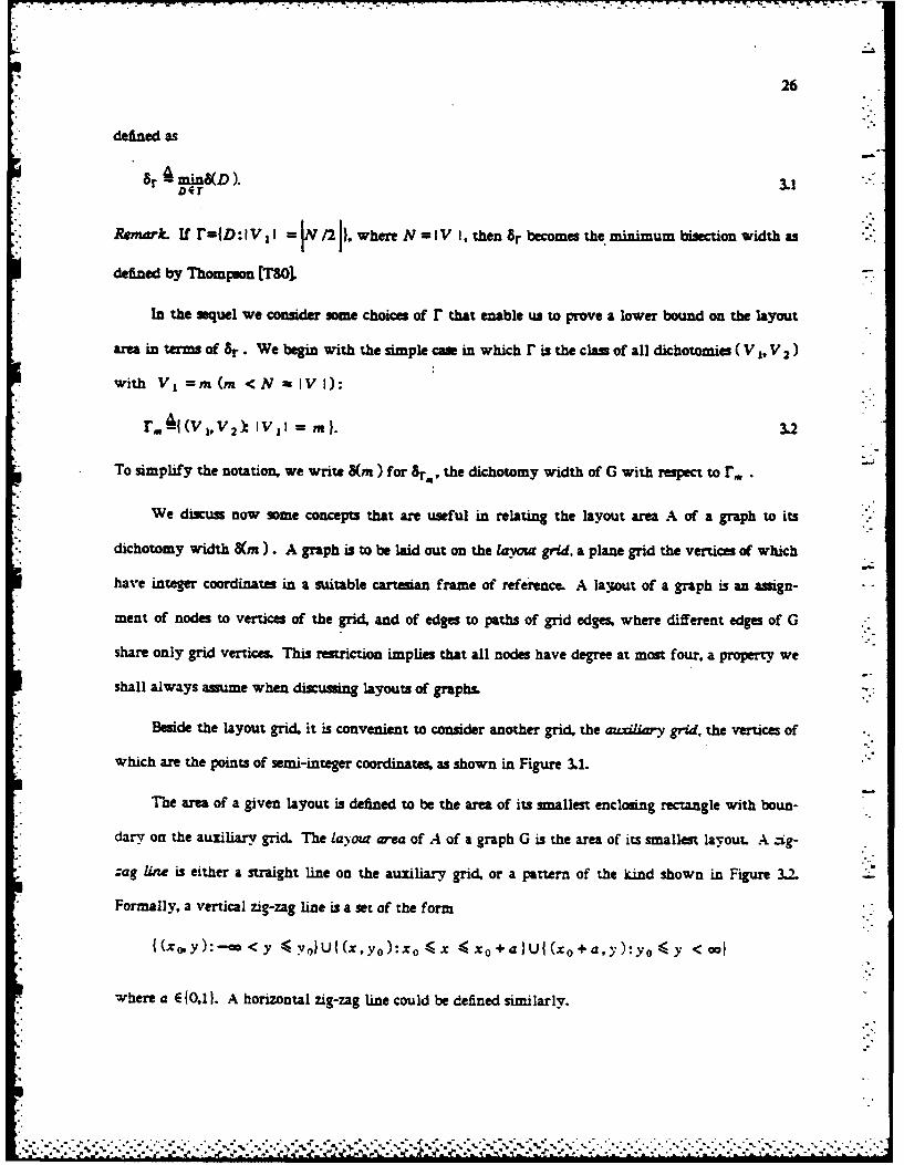
Beside the layout grid, it is convenient to consider another grid, the auxiaiy grid. the vertices of

- which are the points of semi-integer coordinates, as shown in Figure 3.1.

The area of a given layout is defined to be the area of its smallest enclosing rectangle with boun-

" dary on the auxiliary grid. The layout area of A of a graph G is the area of its smallest layout. A .ig-

:ag line is either a straight line on the auxiliary grid or a pattern of the kind shown in Figure 3.. -

Formally, a vertical zig-zag line is a set of the form

(xo, y):--C<y 4YolU(x,yo):Xo<X <xo+a)UI(xo+a,y):yo<y <001

_ where a E 10,1). A horizontal zig-zag line could be defined similarly.

27

.. L ..... 4

-.-- ' -,-" ---, '-

I 7 " -i " -

_ 1 I " I "I " I" -- "I i

i Io I n-1 f

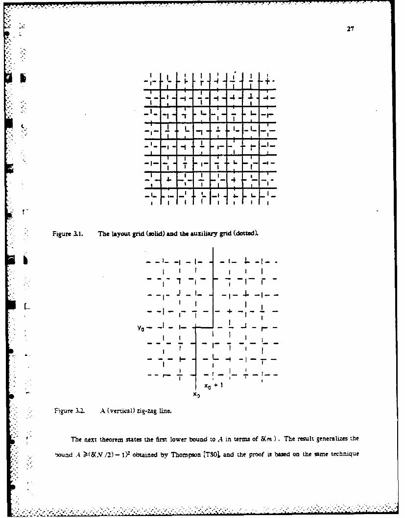
Figure 3.1. The layouat grid (solid) and the auiliary grid (dotted).

I I I I I

-- "- .....

II I I I

I1 II_~

--- i ---- I I

x0 4.

,o.o

Figure 3.. A (vertical) zig-zag line.

The next theorem states the first lower bound to A in terms of 8(m) The result generalizes the

h3ound A >,(8.V /2) - I)' obtained by Thompson [TSO1, and the proof is based on the same technique

,-. . . I

.. . . . . . . . . . . . . . . . . .

- , - --.. . . . . . ' - - . . . . - - . . ". . .. . . , . - -

28

introduced by [T80], which we call a bipartiin technique because it is based on a suitable partition of

the layout into two regions.

Theorem 3J. If a graph G has dichotomy width 8(m , then the sides 1, and 1, of the smallest enclos-

ing rectangle R of any layout of G have length at least 8(m ,whence

A > (8(m)-1)2 = 0(8 2(m)). 3.3

Proof. It is easy to show that there exists a vertical zig-zag line which splits R into two regions

(separated by either l7 or 1+1 grid segments), one containing m nodes of G, and the other N -m By

the definition of r -dichotomy width at least 8(m) edges cros the boundary between the two regions,

and therefore l + I , 8(m ) or ly , 8(m)- 1

The next theorem provides another bound on A in terms of 8(m). The bound is better than (3.3)

*'- whenever m - o(N). The proof introduce a novel technique, which we call the square tess a"ion

technique, because it is based on a partition of the layout region into a mesh of square cells, all of the

same size.

Theorem 3.2. For every graph G = (V,E), and every m <N,

A =l [ 82(m • 3.4

Proof. Given a layout of G (on the unit grid), let R be the smallest enclosing rectangle (on the auxili-

ary grid). Let us consider on the auxiliary grid a mesh of square cells with sides of length -

Ijm )-1)/41. and such that one cell has a vertex overlapping with the southwest coner of R (see

Figure 3.3).

We claim that no cell of the mesh contains m or more nodes of G. In fact if a cell contains m or

,.. more nodes then we can find a zig-zag line that cuts the cells into two polygons one of which, called P,

contains exactly m nodes. (See Figure 3.4.) This polygon has a perimeter

4 p 41 =4 (m)-1/4J 4 8(m)-I, so that less than 8(m) edges can cros it, contradicting the

* **

F 29

|R

*. K

*Fi-ure 3.3. Square tessellation of the layout (to the proof of Theorem 3.2,.

definition of 8m.We conclude that at least IN -'nI elso the mesh contain some nodes of G. and

-he-eiore overlap wi~th R. The total area of these nonempty cells is then

S(M,

IIf

-I I

......... . ......

. . . . . . . . . . . . . . . .. . . . . . . . . . . . . . . .

.. . . . . . . . . . . . . . . . . .

30

Pm Nodes

~I= [(((m)-1)/4]

Figure 3.4. A cell with m nodes or more.

Due to some nonempty cells which have only a partial overlap with R. the layout area A can be

smaller than A, . However these cells can occur only at the boundary of R. Since Theorem 3.1 ensures

that the length of each side of R is at least four times the length I of the side of the cell R contains at

leasT 16 cells, so that it is easy to show that A > 16/25 Ac . Thus.

A- > I_6 N (8(,nm 1) - N-- ~ a -)2 .5m 3.625 rn

and the theorem is proved. 7,

Remcrk. Equation 3.6 yields a better bound than Equation 3.3 for m < N '25.

In general the best bound that we can obtain for the area of a given graph G from Theorem 3.Z

corr.esponds to the value mo of m that maximizes in the function A (rn )/m . For most of the

.L 31

computation graphs considered in the area-time literature m -N /2 ( or more in general m,=0 (N)).

b and Theorem 3.1 is sufficient to obtain good lower bounds. This fact accounts for the success of biparti-

tion techniques, and has lead researchers to focus almost exclusively on balanced partitions of computa-

S .tion graphs. However, the computation graphs that solve some important problems, including sorting,

have a A(m) function whose maximum is achieved for values of m considerably smaller than N. In

these cases, the notion of dichotomy and the square tessellation technique developed in the present sec-

tion are instrumental to obtain tig/w bounds.

When applying dichotomy arguments to computation graphs, we often need to consider a class r

more general than r. . For example we may focus on the set U of the nodes that are input ports, and

we may want 8 r to represent the minimum number of edges to be removed from G in order to discon-

nect a set V I containing m input ports from its complement V 2 In this case the appropriate definition

for r is

r {m. 3.7

of course. if U =V. we obtain again r,. We can take one more step toward generality and consider a

graph G with each vertex v has a weight m (v). For example m (v) could be the number of input bits

read by mode v during the computation. Then we may setL

. =I(V,V 2 ): m(v)m1. 3.8

"*. Obviously 3.8 reduces to 3.7 when m(v )I for v EU , and m(;) = 0 for v r" -- . When dealing

with a weighted graph it is more useful to include in r all dichotomies (V .V ) such that V I has glo-

"al "veight :n a given interval [m ,,-n :1. in fact we can state the following result.

Theorem 3.3. Let G - (V E) be a graph where each node v has a nonnegative integer weight nf v). Let

n= . -n v),and !et n (v) m - m 1 + . for any v. w we define

m ,- ...-V

-.

32

then we have

A 0

m24

Proof. The argument is the same as the one made to prove Theorem 3.2. except that the claim made on

the square cell of side I - (Or - 1)/4 will now state that the global weight of the nodes inside the cell

is less than m 2 .The bound m(v) 4. m 2 -m I + I ensures that if a cell has global weight m 2 or more

then it is always possible to construct a zig-zag cut delimiting a polygon with a perimeter p 4 8r - ,

which includes a set of nodes with global weight in the interval [m 1^' 2]. Thus, less than 8r edges con-

nect the set V I of the nodes inside the polygon to the set V 2 of the nodes outside the polygon, contrad-

icting the fact that (V 1,V 2)EF. o

Remark. Theorem 3.2 is a special case of Theorem 3.3, and is obtained by setting mi = m 2 = m and

m (v)1 for all v's.

3.2 INFORMATION EXCHANGE AREA-TIME LOWER BOUNDS (AT2 THEORY)4.

In this section we introduce the notion of information exchange for a computational problem 1.

and we relate it to the dichotomy width and to the AT 2 measure of computation graphs for 1

Information Exchange. Let P I and P be two processors cooperating to solve problem l. Let " be

the set of input and output variables of U each of which is assumed to be binary. We call I/0 assign-

ntn a partition 7 -("VI ,'2 ) of 1, where 14 is the set of variables that have to be input or output by

processor P, (s - 1.2 ). We define the information exchange of 11 under assignment ) as %I

I (7) - the minimum over all the algorithms (that solve 17 under the variable

assignment 71) of the maximum over all the problem instances of the

number of bits exchanged between P 1 and P.3.11

In other words, for any algorithm that solves 17 under -n there is at least a problem instance for which

P and P: exchange I (,) or more bits, and no integer larger than I (,) enjoys the same propery.

. . .. . . . . . . ..ow

r- 33

We also define the information exchange for a class H of assignments as

i - mini (r). 3.12

Infornazion and Dichotomy. Given a computation graph G - (V ,E ) and a dichotomy D = (V 1,V 2) of

its nodes, we can identify P, with the subgraph of G on vertex set V, (s - 1,2). This choice of PI and

PM P defines in a natural way an I/O assignment -n (D) = (V,T2) where V is the set of variables input

or output by nodes in , ,s - 1.2). We are then able to relate the notion of dichotomy width to that of

information exchange.

Theorem 3.4. Let H be a class of 1/O assignments for problem I with information exchange H Let

G (V.E) be a computation graph that solves 1 in time T, and let 8r be the dichotomy width of

r =W (D)EH }. Then.

8r> IF./ 3.13

Proof. If D =(vV,)E r then -n(D)EH and I(-,(D)) I y Thus. V t must be able to

exchange IH bits with V, in time T. and therefore must be connected to V2 by at least 1lq/T edges.

' Hence, for eachD Er, 8(D) > I:iT,andSr = min8(D):D E r > ' .T C

AT 2 measure. We are now ready to state a result of major importance for the .7 2 theory.

* Theorem 3-5. Given a computation graph G for problem l. if the class r = :(D) EH generated

by a class H of 10 assignments satisfies the conditions of Theorem 3.3. for a suitable choice of r , m.

* and of the weighting function m10. then the following lower bound holds on the area-time perfor-

mance of G:

~ .- 2 A 7.=l - 3.14

Proof. It suffices to combine 3.13 and 3.10.

T,e AT- lower bound 3.14 is a far reaching result because for many interesting ompuLational ro.b-

~~~~~~~~~~~~. . ..-..-.-. ....-..... •. .- .......... •.-.. ....-..... •.. ... ..- ..--.. -... %.. -"-'*." *"*"k" % -" "e." *" - ." " . ." . o "-" . -: ." 'J .". ."- .".". ."."... .- ". .". .".".. ...... . . . . .-.. . . . . . . . . . . . . ."' " b'

34

lems we are able to (i) find a clan H to which Theorem 3.5 is applicable, and (ii) compute or bound the

information exchange IH.

A Format for H. In several applications it is convenient to focus on a suitable set ? of I/O variables,

and to define H as

H = n,m1 -5 i1.(flV u i n 2 }. 3.15

* If we let mlv) be the number of variables in U that are input or output by node v during the compu-

tation, then the clas r of dichotonues associated to H is

r = K(V1V 2):m, <. m.(, 316V;V1

and, if M(v) m 2 -m 1 + I all the conditions are satisfied for the validity of the bound

.-T2= 0 ((M/m 2)I,1 ),where M is the total number of variables in U. Thus, classes of 1/O assign-

ments of the kind specified by 3.15 are good candidates when studying the area-time complexity by

means of Theorem 3.5. For this reason we further investigate the nature of I.,

5ome Properties of IH . An interesting case of class H is obtained from .16 whenm = n= m

i.e.

H,, 1 = 1,7 ,. I n' = m I . 3.1.?

In fact the classe H,. enable us to decompose H as

H = H, UHm.I. ... U Hm2 , 3.18

and, if we denote by I (m) the information exchange of H. we can wrte

Is= min{I(mt).....I(m:)}. 3.19 ..i3.1

A simple, but useful, observation is that, for any m =1 ..... n, we have

(m)-Z(m-l) < 1. 3.20

In fact, by just sending a bit from P to P. (from P 2 to P1 ] we can always transform an assignment

. . . . .. °*~ . . a ~

h35

in Hm [H, -,.] into one in Hm_, [Hm 1. Using the fact that I (0)=0 as the base, and Equation 3.20

as the inductive step of an inductive reasoning, we easily prove that I (m) 4 m . Another interesting

consequence of 3.20 is that

1(m2)-1H m 2 -m, 3.21

-- a result that may simplify the derivation of bounds on 1H

A refinement on the AT 2 Bound. The fact that IH is related to I (m,) by 3.21 suggests the possibility

of obtaining a bound on AT 2 directly in terms of I (m 2), a quantity easier to handle than 1H . Such a

bound is indeed provided by the next theorem. As we shall see from the proof, the result is not trivial.

and requires the combination of several arguments.

Theorem 3.6. Let G be a computation graph for problem II. Let '4 be a set of 1/0 (binary) variables

" of 1 , of cardinality M. If H. is the class of the assignments such that exactly m variables of 14 are

assigned to P . and I (m) is the information exchange of Hm , then there exists a constant X such that

AT 2 > X M 1 2 (m)/m = fl(M 1 2 (m)/m ). 3.22

.-. Proof. Since a node v can read at most one (binary) variable per unit of time. m (v) ( T , and con-

dition m (v) < m -mI is ensured by the choice m =m,m1 = m -T in the definition 3.16 of H.

With this choice. relations 3.13 and 3.21 imply that

SI >I I(m)-T.

and Theorem 3.5 (whose hypotheses are all satisfied) yields the bound

.x7 > 1 'W (m)-T) 'in. 3.23

* for some constant X,. 'If we retrace the proof of 3.23 we can see what a = 1/25 will do.)

When T approaches 1(m) from below, bound 3.23 may become weak, but because 7" s large -. e

.xce.zt .A.T: to reman !arge. In fact

.AT >, number varzabies be intut or autput by G) M ,

I'

36

and we have another bound

AT ) M T. 3.24

Combining 3.23 and 3.24 we obtain

AT 2 - maIXIM (I(m)-T)2 /m,MT. 3.25

To prove that

max I{jM (I(m)-T) 21mMT) jA X 1M1 2 (m)/2m 3.26

we select for T the value

T 1 Y2(m)A2 1(m) + A).

where A = mA, and we argue as follows.

(i) ForT .T MT X I Ml(m )/2m . lnfact l(m) m ,and X, canbetaken 1/2,so

that21(m)+A 4 2 A - 2m/) 1 . ThusTO0 1 2 (m)/(2m/A,).

(ii) For T : ToAiM(1(m)-T) 2/m ? X1 MP(m)/2m . Since To < 1(m) the function

(I (m)- T )2/m in the interval [ O,T 0 ] is decreasing, and achieves its in n im at T =T To. The

value at the minimum is (I(m)-To)2/m = (m) 1/2 + A > 2 which yields theA 41 ,2hih iedsth

desired result.

Equation 3.26 proves the theorem. Since) -A ,/2, X can be taken to be 1150. a

Remark. The value of To used in the proof is an approximation of the (smallest) root of the equation

in the unknown T obtained by equating the two bounds 3.24 and 3.25. The exact root would give a

slightly better bound for X , at the expense of more algebraic manipulations.

Remark. Although we have just proved that bound 3.22 holds for any T, the proof itself shows that.

for T > To, the bound is weak, and that AT > M provides more information on the area-time

complexity of problem n. However, when the computation is slow, the complexity is usually deter-

" " "2 .

37

mined by other phenomena, as the ones to be discussed in the next section.

Boundary Chips. We briefly discuss now the situation where all the 1/O ports are on the boundary of

the layout region, which for simplicity we consider to be a rectangle R of dimensions L, and 1, In

this case, as we have mentioned in Section 3.1, the 1/O bounds requires p = fn (M I7T) where M is

the input size. Thus, for the larger side of the rectangle. say, the horizontal side of length 1, , we have

I 1, = (MIT). On the other hand, we have also seen in Theorem 3.3 that both L, and 1, are at least

8(m) and we know that 8(m) >I (m)YT . Thus, A = 1, = fl((MT XI (m) )) . In conclu-

sion. the performance of boundary chips satisfies the bound

T.42 = fl(M I (m)). 3.27

Remmk. The value of m that yields the best bound in 3.27 is not necessarily the same that would give

the best bound in 322.

3.3 SATURATION AR.A-TMI E LOWER BOUNDS

When we ideally isolate a region of the layout of a VLSI system. not only is the bandwidth

*: between this region and the remaining part of the layout bounded by the perimeter of the region. but

also the amount of information that can be stored within the region is bounded by its area. This fact

has important consequences for the area-time performance of some computations. In this section we

' develop techniques to expres these effects in a quantitative manner.

Informazion-Exchange Under Bounded Storage. We consider again the by now familiar framework,

-n whxch two processors P I and P., cooperate to solve a given problem Ii. However, we add a new ele-

ment to the picture by assuming that only a limited amount of storage is available in each processor.

Storage Limitations may affect :he information exchange. In fact during the computation. one of

the two processors may fill its storage (a situation referred to as satu-ation") and hence be forced to

send some information to its mate for temporary storage. At a later time. this information will return

to the original processor, wnen its memory is no longer saturated. Each bit involved in this process goes

- . . ... .. * . N- 2*.* *

. . . .. . -5.. ' ' ., " .. .j

.- -• . . , " • . • • . • , . . . - - - ) * . . . -. ,, " . . .. . . . ). ' o .

.. .......... •........ .. .. . .. .. .. . .. .. ..-

38

back and forth, contributing twice to the information exchange.

Them considetions lead to the following formal definition of the information exchange of ,

with respec to a given 1/0 assignment 71 under the condition that P I and P 2 can store at most s 1 and 7

s 2 bits of information respectively.

1 (7) [ s2 ) the minimum over all algorithms (that solve II under assignment q , and under

storage bounds s, and s 2 for PI and P 2 ), of the maximum over all the problem

instances of the number of bits exchanged between P 1 and P 2

Similarly, the information exchange for a clan H of asignments can be defined as

IN (S '1 2) AMIn( 7 IS ,S 2) 3.2970 H

Remark. The functions 1(1 s ,s 2) and I,, (s Is 2) are both noncreusng in each of the two variables

s 1 and S. (Mor storage never hurts.)

As in previous sections, of particular interest is the family of assignment clams defined with

respect to a suitable set of 1/0 variables of the problem. that is

H. q {a77 1 ,kfl.(U V I I m. 3.30

For convenience of notation, we write I (m I s Is 2) instead of lMa (s ,s 2)

The Square-Tesselaricn Technique. We now show that by combining bounds on the information

exchange with bounded storage with the square-tessellation technique we can obtain amatime lower

bounds.

We recall from Section 3. that a computation graph G is to be laid out on the layout grid, and

that it is also useful to introduce the auxiliary grid whose vertices are the centers of the elementary

cells of the layout grid.

Let us consider on the auxiliary grid a square cell with a side of length I as shown in Figure 3..

We can identify the part of the graph laid out within the cell with processor P , and the un laid out

~~. .o .. . . ..

.... ... ... . . .-.-.-.-.-.-.-.-.- % . _. ... - .,,.,, '..,-. , ,'.'," , -.-- ".-. - . .. ,...."..,...., .' '-

39

IP| -

P1

Figure 3.5. A cell of the square tessellation can be viewed as a processor P , with storage boundedby 12. Identifying P, with the rest of the layout, the bandwidth between P and P, isbounded by 41.

outside the cell with processor P 2. Obviously, the storage of P is upper bounded by 1 2 The storage

of P, is also upper bounded by A -12 , where A is the area of the layoug of the graph. However, in

the sequel we will not make use of this bound.

if m variables of 14 are input or output (by nodes of the computation graph laid out) within the

cell then the information exchange across the boundary of the cell is at least

I :m .U.4 - '12) >, I(m 1l2,- c).

Since the perimeter of the cell is 4. we can conclude thatkLk

7 >I I(m 1?+ eo)/41. 3.31

G:ven a te-seilation of the layout region with square ceils of side Z, we can argue that. since 'I

variables are input or output in area A. there exists at least a ceH, C of the tessellation for which the

number of variables of .j handled by C is

40

m > M 2/A. 3.32

pIf we could And a cell of the temellation for which m is exactly MI 2/A , we could state the bound

T 0 1 (M12/A I 12, c )/41,

from Equation 3.31, which i indeed an area-time lower bound. A cell with m exactly equal to MI 2/A -

does not always exist, but we can argue as follows to obtain a bound.

We know that, dnce at most T variables can be input or output by a node in time T". there exists a

suitable zig-rag line that cuts the cell C into two regions one of which inputs and outputs a number

(M12/A + h )ofvariables of ., with 0 h < T . Moreover, the perimeter of this region is at most

41 and the area is at most 12 Thus, we can claim that an amount I(M 2 /A + h It2 o ) of informa-

tion must cram the boundary of this region. Hence,

T 0 I(MI2/A +h I I 2, ao)14,for some h E [0,T' -11 3.33

We can formally summarize the preceding discussion by stating the following theorem. --

Theorem 3.7. Let G be a computation graph for problem l. Let be a set of 1/O (binary) variables

.- of n , of cardinality M. If H, is the class of assignments such that exactly m variables of '4 are

assigned to P 1 , and I (m Is, o ) is the information exchange of H, when P has s bits of storage, then

*the area-time performance of any layout of G satisfies the bound

'T > min I(MI2/A +h 112, o)/4L 3.340Oa ( A T

*. Proof. Obvious from Equation 3.33.

.* Remark. To obtain the best pomible bound from 3.34 we must choose the value of I that maximizes

*" the right hand side. (We can choose I as we wish, since the inequality holds for arbitrary 1.)

Remark. In most cases in the range of interest, I (m I s, co) is increasing with m, so that the minimum

in 3.34 is achieved for h =0. Then we can state the bound as

S.. * . b ~ b .-

i. . . . . ..°

. ., *

41

T > max I (M1 2/A 112, O )/41. 3.35

In all applications of 3.35 made in what follows (Theorems 4.5. 4.10, and 4.18) it turns out that, for the

value l of I that maximizes the lower bound, I(m Itjca) = I3m ,where 01 is a constant. Then weI.%

. can -rite the bound as

AT >, MlM), 3.36

with 3 = 1/4 . Usually L is an increasing function of the problem size, and therefore 3.36 is a better

.__ bound than the straightforward Ii0 bound AT = fl(M).

o

- .-. ....- .... *..... -

S. . .. oa........

CHAPTER 4

LOWER BOUNDS

FOR CYCLIC SHIFT AND SORTING

4.1 CYCLIC SEHFT

Several lower-bound arguments for sorting are based on the fact that sorting circuits are capable

of performing cyclic shifts on a suitable sequence of words. In this section we derive some results on

the information exchange and the AT 2 measure for the cyclic shift problem. This will afford us the

possibility to illustrate the lower bounds techniques of the preceding sections by applying them to a

relatively simple problem. -

Shift arguments have been fin proposed by [BKSO] and (AA80] to lower bound the AT 2 perfor-

mance of integer multipliers, and they have also been successfully applied to sorting by [184] whose

results will be reviewed in Section 4.2.2.

Definition. The input of the (n4)-cyclic shift problem is a pair (p2) where p is an integer between 0

and n-1, and

Z -Z j: i =0,....,n-1;j 0O,,...,q-l1.

is an n xq array of n words of q symbols each. The output is an array W with the same format as Z.

such that

Wi = ZGP)Mo-.

In the following we shall assume that Z has binary entries. No assumption is made instead on the

encoding used for the integer p, the size of the shift.

.......................................

- - - a a.. a. t-.--.

43

Information Exchange. With reference to the framework of Section 3.2, let 7 = (7 ,) be an 1/0

assignment for the inqk)-cyclic-shift problem. We need to define a number of quantities that are func-

tions of 7:-

b. number of input words whose -th bit is input by PI.

c number of output words whose j -th bit is output by P•.

B -bo+b I+"" +b9 -1 (global number of Z entries input by P 1),

CI +" +c9.- 1 (global number of W entries output by P 1).

For a given shift p, it is easy to see that input position lij) contributes one bit to the information

exchange if and only if Z' and W' -P )fd ame assigned to different procesors. An immediate conse-

quence is that

1()>,I B -C 1. 4.1

Let 6, be the information exchange due to the )-th position summed over all the n different shifts.

We claim that

4, -b(n - c1 ) + (n -b )c 4.2

In fact, each of the b bits input by P is output by P2 In - c,) times., and., symmetrically, each of

the n -b bits input by P 2 is output by P c. times.

By the pidgeon-hole principle there is a shift size with information exchange not smaller than the

t- average, which ensures that

We can then derive bounds on I (I) if we are able to bound the 6, 's. With the motivation that 6.

tends to be large when the output bits of position j are about equally split between P and P, We

clasif, the positions as follows. For given yE[O,1!21 we define

-. . . ..n .c. .( -,.n .4. . ,

. - ., . . . . ."

44

Q 141j: c1 > 0 -V)n, 4.4b

Q2 Ij: cj < yn), 4.4'

q, I Q, ,s =0,1,2, qo+ql+q 2 =q 4.5

B, bs 0,1,2. 4.6

We can think of positions in Q0 as "balanced', and positions in Q, as P, -biased, s 1- We show now

that the information exchange of a given assignment is at least proportional to the number of balanced

positions.

Theorem 4.1. The information exchange of any asignment 7 for the (ntq)-cycic-shift problem satisfies

the inequality

I(-q) > yqon. 4.7

Proof. If jEQ 0o, then both cj and n -c. are > yv ,and

. j b:( -c)+(n -b,)cj b, b n + (t -b, )yn = yn 2. 4.8

Combining the last inequality with 4.3 we obtain

'. I(i) > (1/n Oj.,€ >., (U/n )q oyn- 2 "yqAZ

jEQO

Theorem 4.1 implies that q o < I/(yn ),and hence that q + q 2 q -I(yn).

However, in some applications we need a bound on qI (or q2) alone, which can be obtained in

terms of the total number of inputs of P , as shown by the following theorem.

Theorem 4.2. The information exchange I (,n) of any assignment -n of the (nqkyclic-shift problem.

such that P reads exactly B entries of Z, satisfies the bound

I1(,) > -XB - B 1), 4.9

and,sinceB n q, -

. . ,. . . . . . . w

.......

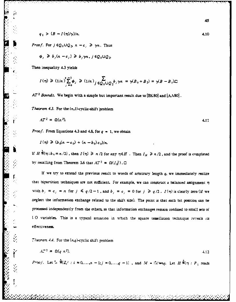
45

ii ZI > (B - I (71)/-,)/n. 4.10

Proof. ForjEQoUQ., n -c, y n'. Thus

> bj(n-cl) > bjyn, jEQUQ,.

Then inequality 4.3 yields

-(-) > (i/n) v. > (1/) o ,= y(B+B 2) = (B -B 1 )000 iEQ0 UQb

AT 2 Bounds. We begin with a simple but important result due to [BKSO] and [AA8O].

Theorem 4.3. For the (n,l)-cclic-shift 'problem

A-T - (n 2). 4.11

Proof. From Equations 4.3 and 4.8, for q - 1, we obtain

iI( (bO(n -c 0 ) + (n -bo)co)/n.

If H =7:bA-n/2 , then I (n) > n /2 for any n EH . Then IH n n/2,andthe proof iscnmpleted

by recalling from Theorem 3.6 that AT " = U 01

If we try to extend the previous result to words of arbitrary length q. we immediately realize

- that bipartition techniques are not sufficient. For example, we can construct a balanced a.zignment t

with b, = c, = n for j 4, q/2-1,andb, = c, = O for j > q/2. I(71) is clearly zero (if we

neglect the information exchange related to the shift size). The point is that each bit position can be

* processed independently from the others, so that information exchanges remain confined to small sets of

T 0 variables. This is a typical situation in which the square tessellation technique reveals its

effectivenes.

Theorem 4.4. For the (n q)-cyclic shift problem

-t 2 fl(q n-). 4.12

Proof. Let 4-Zj: i =0 ... - 0,...q -1 and M Let-n. Let P reads

* .p.

...... .......... ........... o

46

exactly n/2 input variables }. We recall from Theorem 4.2 that, for ',E[O,1/2], 1 (7)) > y(B -B ) -

and we distinguish to case:

(i) Q is empty, so that, being B 0 and B - n/ we obtain

1 (7)) > (-y, n

(ii) Q is not empty, so that at least for one j, c, > (1- -/)n. Thus C >c > (1 -)n, and

recalling 4.1 we obtain

1(r) C -B > (1-y)n -1/2n =(i/2--y ).

If we choose =1/3 , we see that in both cases 1(71)> n/6. In conclusion H >f/ 6 , and, from

Theorem 3.6, with M nq, m B -n/2, and 1H > n/6, we obtain

AT2=fPIijiI n [ '.j (qn2) C

We will see next that, for suitably slow computations,* the saturation technique allows us to derive

better bound than that one provided by Theorem 4.4.

Information Exchange Under Bounded Storage. We consider now the case when P1 has a storage

capacity of s bits, and we show that, if s < n, the storage limitations really affect the information

exchange. First, we need to prove a simple, but important lemma.

Lemma 4.1. In a cyclic shifter with a place-determinate I/O protocol all bits of Z must be input

before any bit of W can be output.

Proof. For two arbitrary indices i I and i 2 (0 i Li 2 n- 1), we can find a suitable shift size such

that W,j = ZI. Thus. W, cannot be output before Z is input.

Remark. A simple consequence of this lemma is that, for every j, there is a time t such that all bits of

Z I have been input, and no bit of W I has been output. Then n bits describing Z are stored in the

shifter at time rt It should be clear that these n bits need not necessarily be Z , .. ,Z for the

........................ • . .

~47

system is free to encode data arbitrarily for intermediate steps of the computation. However, since

Z ',. .., - are unrelated, any encoding of them requires at least n bits for a suitable value of the

variables, ie. for a suitable problem instance.

Theorem 4.5. Any (n q)-cyclic shifter satisfies the bound

AT > l(qn %/n ). 4.13

Proof. Let 7) be an 1/O assignment such that PI outputs c, bits of position W . If c, > s then at

the instant t, (when all inputs of Z J have been input, but no output of W j has been released) at least

c - of the bits that have to be output by P1 are stored in P 2 . Eventually, these bits have to be

transferred to PI in order to be output, thus cotributing an amount (c, - s) to the information

exchange. If we let (x )+ denote x when x > 0. and zero otherwise, we can write

1 (77l , .0) >q (c, -S . 4.14

=0

if we consider a value s 4, (1--y)n ,for some yE[0,1/21, and we recall that Q1 = I] :c, > (l-,)n

and that q1 = 1Q I then Equation 4.14 easily yields

. I(i s, ) >I (cj-s,) q((l---y)n-s). 4.15

*. From Theorem 4.2, we also know that I (71), and a fortiori I (7) I s ,o) , satisfies the bound

7 1 (-n i s ,cc) >,y(B-nq 1 ). 4.16

where B is the number of bits input by P I according to L O assignment rT. A linear combination of

• bounds 4.1 and 4.1l with coefficients v and (1 -- s /n) respectively, yields

SI('n I s,oo) > y( 1-l-s//n ))B .4.17

where, as usual, 0 4 y -4 1/2 and 0 4 s in 1 -y • The best bound is obtained when y (-s/n )/2

and is9.

9.--- -- - - ~% .

- 9-...........................................................................-9

ro

47

system is free to encode data arbitrarily for intermediate steps of the computation. However, since

z ... ,zt-1 are unrelated, any encoding of them requires at least n bits for a suitable value of the

variables, i.e. for a suitable problem instance.

Theorem 4.5. Any (n q)-cyclic shifter satisfies the bound

AT > W(qn -). 4.13

Proof. Let 71 be an I/O assignment such that PI outputs c bits of position W'. If c, > , then at

the instant tI (when all inputs of Z I have been input, but no output of W ' has been released) at least

_ -s of the bits that have to be output by P 1 are stored in P 2 . Eventually, these bits have to be

-transferred to P 1 in order to be output, thus cotributing an amount (c, -s) to the information

exchange. If we let x ). denote x when x > 0, and zero otherwise, we can write

1 (71Is ,cc) > (c, -S). 4.14i ;=0

if we consider a value s 4. (l-,y)n ,for some yE[0,112], and we recall that Q1 = Ij :c, > (l--y)n

* and that q I = i I then Equation 4.14 easily yields

,.. '(It s,c) > (c,-s,) > q1((1-)n-s). 4.15jEq1

From Theorem 4.2. we also know that 1 (71), and a fortiori 1 (7 I s ,cs), satisfies the bound

1" (71 1 s ,cc) >, -I(B -nq 1). 4.16

where B is the number of bits input by P according to IO assignment 77. A linear combination of

bounds 41Aand 4.1l with coefficients -y and (0 -y-s /n) respectively, yields

(7) 1 s, o) > y(1 - /-s/n ))B 4.17

where, as usuai, 0 4 1I/2 and 0 4 sin 4< l-- •The best bound is obtained when = (l-s 'n )/2

and is

48

(- I sm) 1 1-s /n )B. 4.18 "

Then. by applying Theorem 3.7 to the class of assignments 7) such that P1 inputs exactly B bits, and

recalling that in our case M - nq, we obtain

T >. min .0.(-4 2 ! +hII~o4h <T4A r

and thus

T > -_.( 1-2/n)w/A. 4.19

The best bound is obtained for I f n/3 and is

AT 1> lqn - - O(n 4 ), 4.20

I-.

where Vl= /24,r3). 0 "

From Equations 4.20 and 4.12 we have seen that for any (nq)-cyclic shifter, and constants /10 and

32 , AT > 1 qn V/ ,and AT 2 1 n 2 . The latter bound is stronger for T < (02/01) n , while

the former is stronger for T > (02/01)%/n . This fact indicates that the complexity of cyclic shift is

dominated by pure information exchange for relatively fast computations, but is affected by storageI,

limitations for slower computations.

4.2 SORT7hG.

We are finally ready to apply the general techniques described in the preceding sections to the

derivation of area-time lower bounds for the sorting problem.

For the purposes of this section we classify sorting problems according to the relationship between

the length k of te key and the number n of keys. There are three cases that need to be analyze,'

separately, and for which we introduce the following terminology.

short ktvs: I 4 k 4 logn 4.21a

. . . . . . .,]

49

medium -length keys: logn < k < 2logn 4.21b

long keys: 2logn 4 k. 4.21c

, Between this clmifcation of sorting problems, and the classification of multisets according to the range

of optimality of different encoding schemes there is an intimate relationship, which will become more

and more apparent as we proceed.

In each of the three cases defined above we will derive several lower bounds using different tech-

- niques. The bounds will be of the AT 2 type when the dichotomy or the square tessellation techniques

*are used in combination with the unconstrained information exchange, and will be of the AT type

when the square tessellation technique is combined with the saturated information exchange.

The dichotomy technique gives satisfactory results only for keys of medium length, whereas the

square tessellation technique yields the best bounds for short and long keys.

AT 2 and AT bounds complement each other in the sense that the former are better for T < To,

and the latter are better for T > T 2 , when To is a suitable computation tume for which the two

bounds coincide.

Notation. We recall from Chapter 1 that the input of the (nk)-sorting problem can be viewed as anpn xk array of binary variables

X = (XI : i =0,1,.... n -;j k -l.k -2,...,0,

where X-' is the coefficient of 2J in the binary representation of the i-th input key. The i-th row of X.

X. represents the ;-th input key, and the j-th column of X, X' . represents the .-th least signifcant

• " position. A similar notation is adopted for the ouput array Y.

Remark. Here and hereafter n is generally assumed to be a power of 2. While this sLm-plifies the treat-

ment of several details, this assumption is not a serious restriction for asymptotic anlysis. In fact the

*complexity of sorting n keys (n being here an arbitrary integer) is never smaller than the complex.,ty

of sorting , keys. where t, is the largest power of two not exceeding it, and it is never larger than the

1I

50

complexity of sorting n 2 keys, where n 2 is the smallest power of two not smaller than n.

Finally, we recall that r -- 2* is the cardinality of the set from which keys to be sorted are

drawn. -..

4.2.1 Short Keys.

Let P I and P 2 be two procesrs cooperating in solving an (nO-sorting problem, with k 4 logn

To give some intuition, let us consider the situation in which P I reads keys X ,...,X, 2-1 , and P 2

reads keys X....,X, and let us try to estimate the information exchange I necessary to complete

the sorting. We can argue as follows. From the analysis of the encoding of multisets developed in Sec-

tion 2.2, we know that each processor can encode its input using 9(rlog (1 + n /r)) bits, and send the

encoding to the other processor. Then each processor obtains complete information about the input, and

can compute all the outputs it is required to produce without further communication with its mate.

Thus, we can conclude that I= O(rog 0 +n/r)). It would not be difcult to prove that in this

situation the outlined algorithm minimizes the information exchange. and that indeed

I = 9(rlog (1 + n/r)). However, the class H of the assignments such that P I reads exactly /2."

input keys does not have the properties to guarantee AT- = Q(I 2 ), because there might be no cut of

the layout such that (nearly) half of the keys are input on either side of the cut, unless we assume a

word-local protocol (see Section i.I). In the next theorem we circumvent this difficulty by restricting -

our attention to the least significant bit position of the input. This choice is not random, and is sug-

gested by the fact that insert-and-prune encodings allow the reconstruction of the entire input by look-

ing only at the least significant bit position of the output (see Theorem 2.1). The following result has

been obtained independently by [Sg84a].

Theorem 4.6. Any VLSI (nJ)-sorter, with k 4 logn ,satisfies the bound

AT = n (r 2log 2 ( + n/r)), 4.22

where r = 2k

Proof. With reference to the general framework of Section 3.2 let us consider the set

- i =0.1. .... n -I of the bits in the least significant portion of the input keys. Let H be the

clas of I/0 assignments such that exactly n/2 of the variables of 74 are read by P j, and let I be the

information exchange of H. Because of Theorem 3.6, to prove Equation 4.22 it is enough to show that

I = n(rog (+n/r)).

Given 7EH , we can assume, without loss of generality, that the n/2 members of V input by P,

belong to keys X OX .... ,X /2-i . We also divide both the input and the output keys into r/2 seg-

ments of 2n/r consecutive words each (see Figure 4.1):

x-seg:(h ) -Xh u , :q =O,1,...,2n/r -1 , 4.23.

[,y -seg (h ) -IY^ 2, , I:q = 0,I ..... 2n /r - 1, 4.24

for h = 0.1 ..... 1. We say that y-seg(h) is P, -biased (s - 1,2) if at least half of the Is.b. of keys in

2

the segment are output by P, . There is one processor, say P,, such that there are at least r? 4 indices

hh11 .... 4 ./4-1 for which y-segfh) is P, - biased. Let h.r / 4,/9s .... , ,.-' be the remaining indices.

. We now construct a subproblem of sorting by setting all the bits of each input key, except the

*least significant one, to a constant value, such that

Xp P 2 /,ni - = 2hp + Xvz, p =0,1 ... ,/2 -- 1, q= 0,... .2n/Ir -,

o""" where i . is arbitrary. In the corresponding output, y-seg (h,) contains the sorted sequence of

x-seglp) with the k-I leading bits of each key representing h. The Is. bits

S....... .> r.2.,, :,- form a string of zeros followed by a string of consecutive ones. The

number of zeros : obviously equals the number of variables X " , X2,, Ir +2n /r -1 which are

zero. Thus, there are Zn/r4l possible outcomes for each y-seg. The situation is illustrated in Figure 4.1.

Let us now focus on values of h. with p < r/4. All the Is. bits of x-segf p) are input by P1 . and

r at least n/r ls.b. of y-seg(h:) are output by P, . Thus, P, is capable to produce at least n. r-I

different outcomes, and therefore to distinguish among n/r-1 intervals in which -, can fall. This is

*'!- * *- * ~ -- .

!77. - .-.

52.1

~.

Xk-1 X1 X0 yk-1 - y1yO

0 0 7

___ __ __o _ __ _ x __ _ __ _ __ _X2nr..1 - 4 Y2nir..i 0

:-I

Xp2n/r Ip Yp2n/r P 0- - z~zeros

X(I_+1)2n/r-1 _ p __P+1)2n/r- P 1

r xn-2n/r-I Ir/2-1 Y-n-1r12-1

Xn-1 Ir/2-1 Yn-1 r/2--1

Input Array X Output Array Y

Figure 4.1. Input and output arrays in the proof of Theorem 4.6.

possible only if Zog(n/rl) bits relative to x-seg(p) are communicated to P 2 and P 1 . This being true

.. for r/4 unrelated segments we conclude as desired, that

" ... .. .. .. . .'- .*. *... -o .' - . *- .. *. **. . ... -, .-4L

r 53

I > r/4 log(n/r +1) 0 (r og(nlr +1)). 0 4.25

If we combine the bound in Equation 4.25 with the bound in Equation 3.27 on the performance

of boundary chips (in our case M - nk) we obtain the following result.

* Theorem 4.7. Any VLSI (nk)-sorter, with k 4 Logn , and with all its I/0 ports on the boundary,

- satisfies the bound

AT" Q (nkrlog ( + n Ir)) 4.26

where r -2.

We have seen that for a protocol assigning half of the input keys to each procesor the informa-

tion exchange is 1 -O(rlog (1 + n /r)), but the situation can be dramatically different for other proto-

cols, as illustrated by the next theorem.

Theorem 4.8. Given an (nA)-sorting problem, with k < logn. let H be the class of the I/O assignments

such that P 1 inputs bit positions X 0 , X L .... X 2- and P . inputs bit positions XkI/2 X x2 1 .... X -t

(k is even for simplicity). Then the information exchange of H is

I = £1(kn). 4.27

*Proof. We plan to transform the string equality problem to our sorting problem. In the string equal-

ity problem there are two input strings, W 1 and W, of length h each. and there is one output bit

. which is I if and only if W I = W 2 - It is easy to show that if processor P, inputs stringW ,s W 1.2

then the solution of string equality requires an information exchange I - h (see for example, [Y79], and

S [XSs2P.

To carry out the transformation we set the first r input keys (r < n) to the constant value

X = i, i - O.l.....r -1). From Theorem 2.1 we know that output position Y) is sufficient to recon-

-" struct the entire input multiset.

• Let us now define the strings W and W,. 1W1 is the row-major spelling of the array

o-

[. . . .'... . . . . . . . . . . . . . . . .- .-........

S . p - * :..°

!€ "" .- ". "' .. e"" .'o ' .'"'."-' -. '"-".". ' "'-'-.'.-'- .'-.-.-.'.. .. . . . -. '- - ". ", "." '. . ,""""S* " -".""

54

W is the row-major spelling of the array

(Refer to Figure 4.2). Itis clear thatW I W 2 if and only if Xil XJ 1 2 for i r..n-1,andj

Xk_1 xk/2 xkt2- 1 ... 0(

X(. 0

x

(n-r) X k/2 array (n-r) X k/2 arraythat yields W, that yields W2when read in when read inrow-major order jik/2 x'row-major order

}Corresponding bitsK___i- mW, and W2

* Figure 4.2. Configuration of the input array X in the proof of Theorem 4.8.

V.- 55

* 0, ... .k /2-1. This is equivalent to saying that each key X, (i r ) in the input multiset is the con-

catenation of two identical strings, a property of the multiset which is independent of its representa-

tion. and can therefore be verified once YO is known. Now let P, be the processor that outputs more

variables of Y 0 (break a tie arbitrarily ). Let P, and P 3-, sort the input by exchanging 1' bits, and let

P 3-, receive 1" 4 n /2 bits to describe the components of Y I that it is required to output. With no

further communication, P, is now able to decide equality of WI and W 2 • whose length is

h =(n -r )k/2. Then ' + P > (n -r )k/2, and P > (n -r )k/2 - n/2 = 11(kn). 0

The AT 2 = (r 21og 2(1 + n /r)) obtained by bipartition techniques is weaker than the I/O bound

AT = l(kn ) for a wide range of values of r and T. However, we can greatly improve the AT 2 lower

bound by the square t Rellation method.

.[

Theorem 4.9. Any VLSI (nk)-sorter, with k < logn, satisfies the bound

- AT - = O(nr), 4.28

3 wherer =2'

- Proof. We plan to show that an L/O assignment in which P reads exactly r/2 bits of the least

significant input position requires an information exchange fG(r) . Equation 4.28 will then follow

from Theorem 3.6 with 14 ={X,' : i =0,....,n -l},M -L -nm-r/landI = (2(r).

We begin by showing that, chosen an arbitrary set of input bits

O-:. = T {X,. .. x o 2-1 4.29

* " and an arbitrar- set of output bits

1".)yO 2-o 4.30

• .. with t. <-: ,- , the remaining input bits can be set to constant values to enforce the conditon

Y ) = X i =0,,.... ,r/2-.

More specifically we set

.+ ._ _,,,,=,.,., ,.. ; ....... ,......... .. ......

56

X, =2i +X, , i =0,1 .... ,r/2-1,

and we divide the remaining n-r input keys arbitrarily into r12 + 1 sets such that, for i - 0,1... r12-1,

the i -th set contains (tc -ti -- 1) keys whose value is set to 2I (tI 0) , and the (rl2)-h set contains

(n - 1- t, /-1) keys whose value is set to r-1. The output sequence corresponding to this input is

shown in Figure 4.3, and it satisfies Equation 4.31.

Now, let us consider a protocol that assigns exactly r/2 variables of 1( to P1 and n - r/2 (D r /2)

to P2 . Let P, be the processor that outputs more entries of Y 0 (break a tie arbitrarily). We can

always find two sets U . and as in 4.29 and 4.30 such that V4, is input by P 3-, and 4 . is

output by P, . Equation 4.31 implies that r/2 bits input by P3., are output by P, , for a suitable

value of input variables not in U.. Hence, I > r/2 = O(r ),as desired. 0

We shall now prove an AT lower bound on the performance of an (n*)-sorter for k < logn. The

proof is based on information exchange under bounded storage (saturation). However, the technique of

Section 3.3 will be applied not to the entire computation interval [0,71, but just to suitably defined

subintervals.

Theorem 4.10. Any VLSI (nA)-sorter, with k <,Logn, satisfies the bound

AT = a(nvr) 4.32

where r = 2.

Proof. For some real o'E[O, 1/2, in any temIlation of the layout with square cells of area a r

there is at least one cell C that outputs m > n o'r /A bits belonging to Y , the least significant output

position. Based on the output schedule of cell C, we partition the interval [OX ] into consecutive inter-

vals [:t + 1, 11 (where i - 0, 1 ... L-1, with r o - - I, and tL A T ),in such a way that, in each

interval. C outputs between r/2 and r (1/2 + c') bits of YO. We can always find such a partition, since

the cell can output at most oyr bits at any given time. Furthermore. since cell C outputs ID.

m > n a'r/A bits of Y 0 the number of intervals is at least L >n al((1/2 + )A)

. . . . .L'. ", '- , ". ' -" " .- "- " '. "- . " . ". ", ' ' ' . '" -"." .' ." . "" ." ,, ''". '..-' . -.- ""4 - . .' ,' . '".- """, ''; ""- ,""" -.- -" -

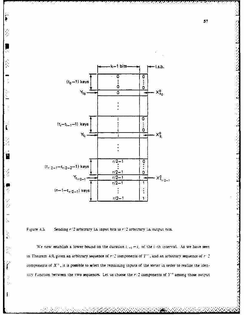
57,, ;:.-.",-.,. ..-j.t_ .-.m. _ , I-:,...-

k-i.-i. I.s.b..-"

" 0 0 .

(to-1) keys

Yto 0 0

, i 0(tr 2 ti-ti--1) keys r

Yt si

r/2-1 O.(tr. 2_1-tr/2_2-1) keys,

r/2-1 0

Yll 2-r/2-1 x

Les r/;-1 1" . ~(n-l-tr/2_ 1 ) keys ""

• . ~r/2-1 1.

Fngure 4.3. Sending r'2 arbitrary I.s input bits to r'2 arbitrary l.s. output bits.

I-

We now emblish a lower bound on the duration - t, of the -th interval. As we have seen

in Theorem 4.9, given an arbitrary sequence of r',2 components of Y", and an arbitrary sequence of r 2

components of X', it is possible to select the remaining inputs of the sorter iz order to realize the iden-

tuzv, function between the two gequencs. Let us choose the r.12 components of Y" among those output

Iv

58

by cell C in I, +ltz +1, and the r/2 components of X 0 in any arbitrary way. Then, since X' must be

completely input before any bit of Y 0 can be output, during the interval [Ir +,Iz, +11 cell C outputs r/2

bits that are already in the system at the beginning of the interval Since C could store at most or of

them, the remaining (1/2 - o')r must flow across the boundary of the cell, whose length is 4 , dur-

ing the interval. Hence,

, +- t, 1- (/2 - =, vr"; (1/2 - ,r 4v*-) .33

and

L -1 -

T = (t +1 - t) + 1 L %17 (1/2-o)/(443).4Ia)

* Recalling the bound on L we obtain

AT 1/2- , 4.354 1/2 + O.

which completes our proof. (Inequality 4.35 yields the best bound for a - (,7 - 7)/4 - 0.138). C

From Theorem 4.10 and Theorem 4.9 we know that there exist constants 01 and 02 such that the

performance of any (n*)-sorter, with k 4 logn , satisfies the bounds AT > Oin %1r , and

AT 2 > 0-nr . These bounds coincide at time To (0 2/0x)',r . The AT bound is stronger for T>T. -

* and the AT 2 bound is stronger for T < To.

The next two theorems provide us with some more information on the feasibility region of the

sorting problem, for short keys. -

The first theorem gives a lower bound on the area, regardless of the computation time. The same

result has been independently obtained in [Sg84a] with a difrerent proof.

The second theorem gives a lower bound on computation time, regardless of the area.

Theorem 4.11. The area of any q.SlI (n.k)-sorter, with the k CIogn , satisfies the bound

A = l(r log( + n/r)). 4.3L

Proof. As we have already seen, due to the functional dependence of the variables in Y"'' upn the

. . . . . . . . . .

59

- variables in X , and to the time-determinate property of the I/0 protocol that there is a time t such

that all the components of X o are input not later than t , and all the components of Y" are output

after t . We have also seen that if we set the first r input keys to the constant value X, i, i - 0..

2*2 . r-1, the remaining part of the input multiset IX,,... ,X, -,I can be uniquely reconstructed from y.-

Thus, a representation of IX .... ,X, -1) is essentially stored in the system at time to , and we know

- (see Eq. 2.13) that (r log(1 + n/r ))bits are necesary to encode this multiset. C3

Theorem 4.12. The computation time of any VLSI (nk)-sorter, with k < logn, satisfies the bound

- T = l(ogn ). 4.37

Proof. Equation 4.37 follows from the assumption of bounded fan-in when considering that the com.-

ponents of Y 0 depend on all the nk input variables. 0

4.2.2 Medium-Length Keys

In this section we turn out attention to the (nLogn h)-sorting problem, and we derive bounds for

0 < h < logn.

A simple observation, which is useful for lower bound arguments. is that by setting the logn

leading bits of the input keys to an appropriate value, we can force the output sequence to be an arbi-

trary permutation of the input sequence. In particular the h least significant bits can be chosen arbi-

trarily to creat information flow.

This observation was originally exploited by Thompson [TSO1 to show that, for word-local proto-

zois. and k = .og + O(ogn , AT 2 = (r 2log2nQ. A straightforward generalization of Thompson'sL

argument allows to prove the following theorem.

* I Theorem 4.13. Any VLSI (n, logn - h)-sorter, with h > 0, and with word-local protocol, satisfes the

bound

AT = fl(n h 2). 4.3

I,

. . . . . . . . . . . .

60 .

Proof. We will prove the theorem by showing that the class of I/O asignments

H = 17: P I inputs exactly n/2 keys I has information exchange I = (n h).

Without law of generality we can assume that P I inputs keys X o,... ,X, /2- and that P 2 outputs

at least n/2 keys, say Y.eY,...'Y,,,2_1 . Let Y. 2 ,...,Y, be the remaining keys. By setting the

ogn leading bits of X, to the binary representation of integer a, we ensure that Y,, X, i= 0,.... n-

1. Thus, the h least significant bits of each key input by P1 are output by P 2 , and

I > nh/2 = 0 (nh),asclaimed.D

No better bounds could be obtained on I under the word-local protocol, since 0(nk) bits are

sufficient to encode the entire inptt. The important question instead is the removal of the "word-local

restriction.

Some preliminary considerations and an example will help us put in the proper perspective the

nature of the problems arising when dealing with arbitrary protocols.

The output of the sorter is a permutation of the input, so that

Y, = X i =0,1...n-l 4.39

where wr(O),r(I), .. ,r(n -1) is a permutation of 0, 1, ... , n-I. Focussing on the bit position of index j

of the date we have

Yi =X 4i) i =0,1, ... ,-1. 4AO :.

Thus, there is an information flow from the input to the output ports of the same position. which we

call primry flow. The primary flow of each position is, in a way, self-contained, because each bit

involved enters the system and leaves the system maintaining its identity. However, the exact destina-

tion of each bit within its own position depends on ir , which, for position j, is determined by the value

of the data in positions j, j +I...., k-I. Thus, there is another kind of informationflowing from most

significant to least significant positions, which we call secondary flow.

As we can see from the proof of Theorem 4.13, the complexity of word-local sorting is based

exclusively on primary flow. Let us now consider an example of protocol which requires exclusively

L ...... ...............• : ..-.-' ""-;- " • • '-"'." "-. .." " .'". "" .""- "'..''--''. '.",-,a '"," .' ; -.-".". '-".. ,. ,-". '. / .-" -. . :

61

secondary flow.

p. Example. We want to estimate the information exchange of the protocol that assigns the leading posi-

tionsXJ ,Y .j-k/2. k-I toP ,and the leastignificant positionsX' Y j0 j-O. .. k/2-110

" P 2 Since each bit position is completely input and output by the same processor, there is no primary

flow. However, P 2 needs information on the relative order of the most significant part of the keys in

order to know which permutation to apply to the least significant ones. Thus, we are in the presence of

secondary flow alone.

It is clear that, no matter how large k is, I 4 rdogn . In fact the leading bits of P I can be sorted

ignoring the bits of P , so that no information transfer is needed for P .to P On the other hand, all

that P 2 needs to know about the portion of keys dealt with by P I is the relative order, which can be

encoded in no more than nlogn bits.

We can also show that, for k - 2 logn, I Log (n!) = (nlogn - lower order terms). In fact, let us

p consider the class of instances of the problem such that X, = 2k ,2"r(i) + i (i - 0. n-I),'where

SI(O) .. (n -1) is a permutation of 0 ..... n-I. The corresponding output is Y, = 2/2 i + 7r-1 (i ) (i -

S 0. n-I). Thus, at least log n bits (to describe 7r ) are sent from P to P , In conclusion, for k -2

L - Zogn, I - nlogn-( Iower order terms).

A more detailed analysis would show that, for I 1< k < 2 logn , I 2nk /2, and that for k > 2

logn I -nLogn . regardless of k. The fact that secondary flow never exceeds nlogn has important conse-

quences, as we shall soon see. C

When analyzing arbitrary protocols, primary flow and secondary flow must be considered smui-

-. taneously. In fact, in particular situations one of the two may be negligible but, as we shall see, they

cannot be simultaneously small.

" - Leighton [L84j has shown how to combine primary and secondary flow bounds with the nehp o

* .c-;c ic shif7t arguments. His result was stated in the Form AT 2 0 (n 2logan )for k ~7!ognI.W "

62

Exploiting similar ideas, although with a rather more elaborate construction, we will show that

AT 2 fl(n 2h 2) for 0 < h - k - Logn < logn. An obvious consequence is that for k ( + a)ogn,

(a >0), AT 2 0(n 2log2n ) However, some discussion is in order, to clarify a subtle point. The i0 nota-

tion is misleading here (at least it has mislead us for some time), and it is better to rewrite the bounds

in the following form: For k - (1+ a )Iogn. (a > 0),AT 2 > c(ac W 2n , where c(a) depends on a.

but is independent of n. The crucial point we want to address is that, for reasons that the next

theorems on lower bounds will clarify and that are essentially related to the saturation behavior of

secondary flow, the dependence of c (a) on a is quadratic for a << 1 , but is linear for a >> 1.

This fact, together with Leighton's observation that, when k > > logn, one can construct VLSI sorters

whose complexity is subquadratic in k [L841 shows that it would not be appropriate to consider a prob-

lem with k - 1.1 logn and a problem with k - 100 logn in the same class, although. superficially, we

cansay that AT 2 = fl(n 2log2 n ) in both cases.

We are then motivated to distinguish between medium-length and long keys. Obviously the

choice of k - 2 logn as separation of the two classes is rather conventional.but it will serve our purpose.

With this premise, we shall now prove the AT 2 bound for medium-length keys.

Theorem 4.14. Any VI.SI (n, logn + h)-sorter, with 0 < h < logn, satisfies the bound

AT = O(n2h2). 4.41

Proof. We begin by partitioning the input array as X - [D, E, F] where D, E. F are blocks of d. Zogn -

d. and h consecutive columns respectively. The partition of the generic key X, is shown in Figure 4.4.

We shall prove Eq. 4.41 by showing that I = 1i (n h ) for the class of input assignments such

that P I and P, input each exactly nd/2 of the entries of D. Below we shall derive two lower bounds

on I, and we will see that at least one of these bounds is not smaller than n." 12.

Adopting the same notation as in Section 4.1 we let c, be the number of components of Y out-

§. :"' . '.- .,,..'.'.',-' 9 :im <.-'.-.. .. . .. .. .-... : , - ... .. .• ."*.- .• ," . '. -" ." ,_" , ". •" " ,

63

m,

k

*d log n-d h

Figure 4.4. Partition of k~ey X, ,for the proof of Theorem 4.14.

put by P, I We also let. for yE 0, 1/2] and Q fj:<h, n 4,c 4 (- -y)nL. .

1 ~j :hc, > (I- n )andQ2 ij <h, ,c, < y n ).Finally we denote by q, the cardinality

of QXii i0, 1, 2.

PrimarY Flow Bound. By suitably choosing the entries of D and E. we can produce any of the n cyclic

S shifis of array F. Then we can use the notation of Section 4.1 and Theorem 4.1. with Z F, and a h

to obtain the bound

> qn4.42

which is valid for any E 0, 1/2 and where q is a function of '.

S"Secondary Flow Bcund. Without loss of generality let q 1 a, so that q I (h - q ,)i2. Let also

be a Wt

* . ?- - - -- -.. . . . . . C- - - - - -

64

but they will be thought of as ordered from most to least significant as they are in X). We then con-

sider the following clan of input instances, where I 42d and a - n/L Let input array X be partitioned

into a blocks each of I consecutive rows, and let the entries of the (i+1)-st block (i - 0..... a-) be set so .

that: (see also Figure 4.5)

D E F-0 0 Q

wol1) 0 0 0 0 0 fqt(O) 0

0- 0- AO0 -I-S - o1@-,to) 0-'s o

0 ,o-(I) 0.. (O) i 0 0

•~~- 0_11 -

_1 a-1 I-0 I-1 a-I1 w,' 1-1) 0

d

(a) The Input Array X (h) The Output Array Y

Figure 4.5. Configuration of inputs and outputs in the proof of Theorem 4.14. In the actual arraysX and Y, the columns of blocks Q and F-Q are mixed, but the left-to-right order of thecolumns in each block is maintained.

. . . . . . . .. . .. - . C * * * * . ..

C%

65

*.- (1) The rows of D have values ,r (0)...., , ( -1). where ir, is a permutation of 0,.... 1-1.

O(2) The rows of E are all identical and equal to i.

(3) The rows of Q have values 0 ..... 1-1.

" (4) The rows of F -Q are set to zero

It can be easily shown that if we partition the output array 1' into t blocks each of a consecutive rows.

the (s + 1)-st block from the top (s -0.... 2-1) has the following structure (see also Figure 4.Sb).

(1) The rows of D have value s.

* (2) The rows of E have value 0,...,a-1.

(3) The rows of Q have values 7rT(s ), j-I(s ),... (sr:

(4) The rows of F -Qhave value zero.

Thus, permutations ,o.VL .... .1-1 can be uniquely reconstructed from outputs in Q so that Q carries

* ail logl - lower order terms) and bits of information relative to section D of the input. Since P 1 inputs

only nd/2 of the bits describing .... ,r_ . and outputs at least (U- -y)nd of the bits of Q from

which l,. ... ' -t can be recovered, we conclude that at least (1 - ) nd - nd /2 bits are transferred

from PF to P If we choose d = q I we obtain

I > (1/2-y)q In > (/2-)yX(h -qO)/2 ]n, .43

where again E[0,1/2] and q0 is a function of y.

Combining the Bounds. If we select 3 = 1/6, bounds 4.42 and 4.43 become

SI > n q /6 4.44

I > n (h -q 0 )/6. 4.45

Thus,

I > max(n qo0/6,n(h -q 0 /6)) > nh/12.

.. .,- ...-.,,. ,.. .-. ,,. ..- , , .. ,._. .... .- -, . ., . -, .. ,, . ... ,,.. .,.,.. .... .- ,.... ... .,..... ,

66

(A slightly larger constant than 1/12 is obtained if we optmz the choice of -y ,which yields

If we combine Inequality 4.46 with the bound in Equation 3.27 on the performance of boundary

*chips (in our can M =Oaiogn) we obtain the following result.

*Theorem 4.15. Any VLSI (njogn+h)-sorter, with O<h<logn, and with all its I/0 ports on the boun-

dary satisfis the bound

AT 2 -.n 2hlogn) 4.47

We end this section on medium-length keys with some results on milnmum area and on

Sminimum computation time. The result on the area (actually generalized to multilective 1/0 protocols)

as well as the one on the AT 2-measure of Theorem 4.14 have been independently derived by [Sg4bl

with a different approach.

Theorem 4J6. Thearea of any VLSWnogn+h) +horter, with 0<h < alogn, satish s the bound

A G (n h. 4.48

Proof. Due to the functional dependence of the variables in Y on the variables in X with

j j .i and to the time- detenate property ofthe/protocoL there is a time rsuch that all the

components of XI 1,X e -2 TX Ifltn X h are input not later than r, and all the components of

-Ij~ -2...Y 0are output after *

Now. let us consider the me clas of input instances as in Theorem 4.14, which is also illustrated

in Figure 4.5Sa. At time t* all entries of array D have been already input, and no entry of Q has been

* ~output yet. However, Q is an equivalent encoding of DA and hence fl(a I log 0 )= Wln 0) bits that

* represent D must be stored by the system at time t*. 0

Simple fan-in arguments allow us to prove the following result.

Theorem 4.17. The computation time of any VLSI (niogn + h)-wrter with 0 < h <1ogn, lognisies the

Thoe 4... , " - aenptntlerta *anal e oen, si fie

compnens o X -iX -- X 2".

I" -" - ... ,yo reoupu ate t*.*. *

-).. .vh ' p 6''p JV :..'--

67

bound

T - f l(ogn). 4.49

4.2.3 Long Keys

As we have anticipated in the preceding section, for k > 2 logn, bipartition techniques are not

very useful, because there are input-balanced protocols for which the information exchange does not

exceed nlogn, regardless of k.

However, we intuitively expect the area-time complexity of the (nk)-sorting problem to be

increasing with k, for fixed n. For example, the trivial I/O bound tells us that AT = (2(k n). But we

know more;, in fact, a sorter of n keys of length k is trivially a cyclic shifter of n words of length k-

logn (the least significant part of the keys), and hence it satisfies the bound AT 2 = 0( (k -logn )n 2 ,

"* 'according to Theorem 4.4.

* h This bound can be further improved by taking into account the f4ct that a suitable choice of the

. logn leading bit positions of the input keys of a sorter, can force at the output an arbitrary permutation

i of the keys. (not only the cyclic shifts).

. "" Theorem 4.18. Any VLSI (n)-sorter. with k > 2 logn satisfies the bound

AT 0 [L(nlogn )2j• 4.50;log,

Proof. To simplify some details of the proof we assume k > 3 logn . (For 2 Logn ( k < 3 logn

the result is a simple consequence of Theorem 4.14, in any case.) Since an appropriate selection of the

logn leading bit positions of the input produces an arbitrary cyclic shift of the remaining positions, we

can use some of the results derived in Section 4.1. Let us first recall some notations. We denote by b,[respectively c, ] the number of input [respectively output] keys whose j-th bit is input [output] by

P,. Then for given yC(O, 1/2] Qij:j <k logn,c, <-y n and q, - IQ,! i l .Moreover

we let

f • .--. 4..

B b., and Bi= b, i =1,2.jEQ0

The plan of the proof is to show that any I/O assignment in which P reads B -rdogn bits that

belong to positions X k-iop -1 .... ,0, requires an information exchange of I = (l(nlogn) bits. Equa-

tion 4.0 will then follow from Theorem 3.6 with '(-{XJ:O i 4 n-1, 0 j 4. k -logn -,

M =I 'I=(k -logn)nm B-nlogn, and I = (nogn).

Prinary Flow. By applying Inequality 4.9, and considering that, IS, q n, and that in our case

B - nlogn, we obtain

I >, -y(rdogn -n q1). 4.51

HIf we reverse the role of P I and P 2 in Theorem 4.52, and we consider that P 2 reads

(k - 2 logn )n > nlogn bits of ',then Inequality 4.9 yields

-.J

1 >, -(nlogn- n q 2). 4.52

Secondary Flow. Let P, (s - 12) be the processor that reads the majority of the bits that belong to the

logn leading bit positions (break a tie arbitrarily). We will then show that the secondary flow

increases with q, . To be specific we will assume that s - 2 and we will bound the secondary flow

from P 2 to P , which we finally combine with Eq. 4.51. (If s - 1, we can argue in a similar fashion

resorting on Eq. 4.52.) After selecting arbitrarily a set Q of (logn - q z) bit positions of significance less

than (k-logn) and not in Q1 , we defne the set

We then consider the following class of input instances. We set:

(1) The leading logn bits of X, to the value ri) where ir(i) is a permutation of 0,.... n-l.

(2) The logn bits of Xj which belong to positions in Q to the value.

(3) All remaining bits to the value zero.

69

Then. the input array Y has the following structure.

(1) The leading logn bits of Y, represent integer i.

(2) The logn bits of Y, which belong to positions in Q represent integer r-li).* .%

(3) All remaining bits are zero.

Thus. r can be recovered from the output positions {Y" j E Q .Since P outputs at least

, q 1 0 -,y)n bits of these positions, and it reads at most 1/2 nlogn bits among those that specify r',

'- then

I > (-y)q n-l/2nlogn, 4.53

bits of information on ir have to be communicated by P 2 to P I

Combining the Bounds. If we multiply both sides of bound 4.51 by (I - y) , and both sides of bound

4.53 by y , and we sum the sides of the resulting bounds, we obtain

*I y 0 /2 - ),) ogn. 4-53

For y = 1/4, 1 > rdogn /16 Then. by Theorem 3.6 we have completed the proof. 0

We derive now an AT bound for sorting of long keys, using saturation techniques.

ML

Theorem 4.19. Any VLSI (nic)-sorter. with k > 2 logn satisfies the bound

AT = fl (kn -hig). 4.55

Proof. In this proof we introduce several parameters whose value will be later specified to optimize

the lower bound. The reader could find it useful to asume - in following the argument - that

y - 1/12. c" = 5/24,e = 1/4, - 1.and f3 - 3/8 . Although suboptimal, this choice of the parame-

ters will give the right feeling for their range, and will also simplify the arithmetic.

. We plan :o lower bound the information exchange with oounded storage I (m I s, ) and then

: L apply Theorem 3.7. We consider the clas of I/O assignments such that exactly m of the variabies L.

O 1X;.:O 4i4.n -1, O j <k -ogn - I re input by P I As usual we denote bv c, te

* , . ...-. , . .. . * . . ~ : * * ~ - - . **

70

number of bits of position Y which are output by P I and - for 0 < v < 1/2 - we let

Q, = j :c, >(I-3)nO 0 j 4k -logn -11, and q, = I 1. As we have repeatedly seen. a

trivial transformation of cyclic shift yields the following bound to the information exchange (under

unbounded storage).

I > y(m -n q). 4.56

Obviously, this bound holds a fortiori when the storage of P 1 is bounded, but we need to combine it

with other bounds in order to obtain the desired result. The following observations provide some

insight on how a bound on the storage may affect the information exchange.

(a) At the time when the last bit of a given position is input no bits of that position have been out- a.-

put. Therefore n bits are stored in the system (P 1 and P 2) at that time.

" (b) If during the time interval t r.] the system outputs p bits belonging to X positions in set Q1 ,

then at least p -X X -n of those bits are output by P I (In fact. from the definition of Q 1 ,at

most y n bits per position are output by P 2)

W (c) If, at a given time t, p bits that have to be output by P 1 are stored in the system, and P has a

storage bound of s bits, then at least p - s bits are stored in P.2 at time t, and they will eventu-

ally be sent to P1 thus contributing an amount p-s to the information exchange.

(d) If during the time interval [to1 PI outputs q bits which belong to a set Qi1QI of X 4 logn

positions, then at least (q-s) bits are transferred from P 2 to P I during the same interval, for an

appropriate clas of problem instances. The idea is that the outputs of P 1 carry q bits of informa-

tion on the sorting permutation, and at most s of them could have been in P at time t z The

details of the argument are similar to those of the proof of Theorem 4.17. We need to set the logn

leading bits of X, to represent 7r(i) (where i7(0), .... ,r(n -1) is a permutation of (0, .... n-1).

We also augment Q I to Q* by adding (logn - X ) arbitrary positions, and we set the logn bits of X

that belong to Q* to the value i. Then the output position of Q will be 7r-w,0), ... ,7r-(n -1)

where or is the inverse of 7r and q bits of 7r are output by P1 .

...................................... .

- : 71

In order to exploit the preceding observation systematically in the analysis of information

exchange. we need to define several quantities. We begin by decomposing the interval [0,T] during

which the computation takes place, according to the I/O prorocol, which is assumed to be place-

determinate and time-determinate.

If we focus on a given position j, we see that the variables of X are generally input at different

times. We are particularly interested in the time when the Ls. bit(s) of a given position are input. For

our proof, we need to consider, for each time t, the number XCt ) of positions in Q I whose last bit(s) are

input exactly at time t. (For example, (t ) is zero when no bit is input at time t, but also when all the

bits inprt at time t belong to positions for which some bits remain to be input.) We will treat

separately the instants when X(t) is large from the instants when Vt ) is small In fact, in the first case

we can immediately see that there must be a large saturation and secondary flow.

* Formally, for a given E (0 < E 1 l),we distinguish the times t', ' , < .. < r., when

M(:) > E logn ,from the timest' 1 < t'2 < < t', when Xt) < e logn .Since for all theq

i positions of Q the input is completed at some time. we have

"Z Vr' + Z ) = q457

• We now consider separately the contribution to the information exchange due to positions whose input

is completed in each of the two sequences. We assume that P can store s = a. niogn bits (0<a" < 1).

Sequence r' . If we apply observation (a) to each of the (t ') positions whose input is completed

exactly at .i me : ', . we see that at least V(t 'h )n bits are in the system at this time. From obser,:at-on

(b) at least (I - y)AW )n of these bits have to be output by P • Finally, observation (c). with

t , l p = 1 -)X(t ', n and s = o" nlogn , allows the conclusion that the bit positions we are

considering contribute [( --,/)M: ' )-' a logn In bits to the information exchange. If we sum over a il

w-,, ,e obtain a global contribution

" :" I'= :I -Y) Z )~ 'n -u a-r.1--gn. 4

°.. .. . . . . . . .

. . . . . . . . . . . . . ..-. - , .

72

Since X(z ') e Elogn ,we obtain

XU >0) u 4logn,A-I

and substituting for u in Eq. 4.58 we finally can write

-> (1--oIe) _(CA)n. 4.59A =1

Sequence t. We decompose the interval [0,7] into consecutive intervals [t A, + 1, t " for i 0 0, 1,..

L. (Here indices h l,...,hr E{O,1....,v I and we have added to the sequence t two points, t -

and t'" T.) The decomposition is chosen in such a way that, for a given ( < I)and for i -0,

At..(- e)logn < -A X(") , logn. 4.60

A MA, +1

* Such a decomposition always exists, since Vt ") < e logn .Moreover,

L , > t )f( logn), 4.61A =1

sice at most f Logn positions complete their input in any given interval We will evaluate the contri-

bution to the information exchange given by each of the intervals of the decomposition. Let us focus

. on one specific time interval, say[ r 2r . For a given such that 0 < e < -Ewe distinguish two

(i) p < 0 rnogn . If p < niogn ,at time t 2 at least (- -)flCgn bits are in the system. -

and at most / n/ogn of them have to be output by P,. Thus, at least ((1- ,Y)f - - )niogn

bits have to be output by P I, and, due to storage limitations, at least

I o > (l(1- y) - e --- )nlogn 4.62

of these bits are in P 2, and v!ill eventually flow to P contributing to the information exchange.

(ii) p > 3 nlogn . If p > nlogn ,at least 0 nogn- nogn of these bits are output by P I

and observation (d) (with q = (13 - ,) rdogn and (f - ) logn < , < iogn) allows the con-

• .. - .. , . .. . -. -. - - - .. .-.-. ;. ,,,.', . . ... ..- ,.., - .. . ,-. -- / .- ,.'-" /....-.--.,.",.,, .,%'--..-*.,'

73

. clusion that in the interva.' f l,7] there is a contribution to the information exchange

, ( - a -- ogn • 4.63

.-* Now, if we chose ( - - E)/2 , then I "- I " , and in either case the interval [rt.1 "r contributes

'o = =(( -E)/2 - y - ) n/ogn bits. 4.64

Recalling Ineq. 4.61, we see that the global contribution of the L intervals of the decomposition is

P > ((0 - e)/2 - -- /) ( ) n. 4.65

If we chose e = E(O/E + 1/2)/(r/E - 1/2) , the coefficients of bounds 4.59 and 4.65 become equal.

and by summing the contributions of the sequences of t ', and t " we obtain

1 0 --y-O'/E)n q 1 4.66,

where we have used Eq. 4.57. A linear combination of bounds 4.50 and 4.66 with coefficients

S(1 - y o/e) and y respectively, yields

I / (-y I/(1- E)) m. 4.67

We now chose 0 (1 - o7/E)/2 to maximize the right hand side, so that 4.67 becomes

I I(rn on.logn ,c) > 1/4(1-olE)m, 4.68

where we have used the appropriate notation for the information exchange. At this point we are

ready to apply Theorem 3.7, which states that

T >, I (MI 2/A I h2, co)/41. 4.69

In our case M = (k - logn)n, and I = -/, and we can rearrange bounds 4.69 and 4.68 as

1.A- .4> I - * k - logn)n -. 'o. 4.7016T

For a given a. . the best bound is obtained by maximizing e. But E Ls subject to the constramintr

= -Eao/E - 1i2)/(./E - 1,,2) 1 1 , so that o/E (1 + E)/(2(1 - E)). Under this constrar.nt the

:awer bound on .4 is maximzzed by the choice e 1/%/12 nd

+*.

o° .' " -. .- - ."%" , . ," . .. .,'...-. •%.°, .- %" .-. .".. .- " . , '.... .-.,.-.,"-.".-'...-.. . . . . . .".. . . . . . .". ... ., -.. '.'. ... .

V°7/4

-(= + 1)/(2(12 + I2)). C

From Theorem 4.19 and Theorem 4.18 we know that there exist constants A, and 02 such that the

performance of any (n*)-sorter, with k 2 ogn satisfies the bounds AT >3kn 4Zgn and

AT 2 N 02kn (niogn) . These bounds coincide at time T 0 = (l 2 /0 1 )rzlogn • The AT bound is

stronger for T > T 0 and the AT 2 bound is stronger for T < T o.

We complete the discussion of this section with two simple results on the minimum area and the

minimum computation time for sorter of long keys. The first result has been originally proved by

(L84], but it is also a trivial corollary of Theorem 4.16. The second result follows, as usual. by simple

fan-in considerations.

Theorem 4.20. The area of any VLSI (n& )-sorter, with k 2 logn ,satisfies the bound

A = fl(nlogn). 4.71

"" Theorem 4.21. The computation time of any VLSI (n k )-sorter, with k > 2 Logn , satisfies the bound

T = f(ogn + log k). 4.72

Remark. Bound 4.72 is indeed satisfied by all sorters, but the dependence on k becomes relevant only

for very long words, i.e., when log k = O(logn). We conclude Section 4.2 summarizing the main

Sresults in Table 4.1.

4.3 AREA-TLME LOWER BOUMNS FOR THE COMPARATOR-EXCHANGER

Usually comparison-exchange is formulated as a problem whose input consists of wo keys X ,,

and X , and whose output consists of two keys Y and Y such that

Y = min (X oX ), 4.73

Y = max (Xo,X 1 ). 4.74

Comparison-exchange is an interesting operation in its own right, and it is a primitive of many sortLng

. .,.- -. .

- .....................................-...... **. . .

75

P TABLE 4.1. SL'MARY OF LOWER BOL'NDS FOR (n k )-SORTING

Length of the 1,k 4<logn Logn <k <21ogn 21ogn 4kLower Bound Keys

TCbLMJuCs (r a 2') (h - k -_o_______"_-- Biparition "

+ AT - 2 0(r 2og-+n /r )) AT 2 -a (n 2h 2 ) AT 2 - (n 2-og n)Information Exchange '

, Square Tesselation+ AT-= 2(r) AT 2 =f(nk(nlogn))

Information ExchangeSquare Temelation -"

t*AT = (n %67) AT - (nk V;Z -).Saturated Information

Exchange

Storage A = (rog ( +n /r)) A f (Unh) A = (/.ogn)

Bounded Fin-in T = log,= ( logn = (ogno+Logk

1 algorithms. However, our main motivation to study its area-time complexity comes from the fact that

comparison-exhcnage is indeed the (2.k)-sorting problem. and its analysis will provide us with useful

-: insight into the phenomena that determine the complexity of sorting when the length k of the keys is

. very large with respect to their number n.

The lower bound technique that we shall adopt is different from the ones we have applied in :he

*: preceding sections, and it is based on the notion of functional dependence.

The notion of functional dependence has been introduced in the context of VLSI computation by

-T. Johnson [JhSO]. In order to derive an area-time lower bound for binary addition, a problem similar to

" comparison-exchange in several respects.

W

........................ *. . . . .

. . . .. . . . . . . . . . . . . . . . . . .* **"

76

Let us now recall the formal definition of functional dependence. -

DefinLion. Given a function y - f(m), where x - (x ,..,x)and y - (y ... ,y) are boolean vectors,

we say that y, is functionally dependent on x, if there exist two boolean vectors x' and x * that

differ only in the i -th component, such that y'= f (x ), and 7 " f (x . differ in the j -th component. -

SExample. In the compaison-exchange problem, Y O is functionally dependent on X1' for any

j .jand i O, ; Y4 ° is not functionally dependent on Xi for any j < j 0 and i O1.

*l Time-Deerminacy. For time-determinate protocols the functional dependence of yj on x, implies that :.x, must be input before yj is output, because there are input instances in which yj remains indeter-

minate until x, is known. However, more complex phenomena take place when we bring into the pic-

" tmre the asumption of bounded fan-in, which was not needed when analyzing the aspects of the compu-

i tation that depend only on information exchange.

Bounded Fan-In. We explicitly assume now that in our circuits the gates that compute boolean func-

-. tions have a number of input lines upper-bounded by a constant f ,. As is well known, this assump-

tion implies that if an output variable y is functionally dependent on s input variables, then at least

* Tlogf s time must elapse between the instant when the first of the input variables is read, and the

- instant when y is output, where "is the minimum delay of a boolean gate, and /1 is the maximum

fan-in. Hereafter, since the value of r and f, affects only constant factors, we assume for simplicity

that = 1 and f 2.

Compuaaional Friction. Although the previous considerations are often useful to bound the computa-

tion time of some -roblem, they do not exhaust all the consequences of functional dependence. In fact,

if s variables x ,... ,x, , are input at the same time, and if there happen to exist s output variables

•y 1, . y, such that, not only each y, depends on all si 's but also the y's carry I bits of information on

* the x's, the system must be capable of storing I bits for at least logs time steps. Thus, if we make an

analogy in which the information is viewed as a fluid flowing from input ports to output ports we can

77

say that the functional dependence acts as a kind of friction that slows down the flow, keeping it

below capacity.

In a VLSI system the 1/0 capacity is determined by the area, and implies the trivial 1/0 bound

AT = (I (input size + output size), already discussed in Section 3.1. When functional dependence

plays a role in slowing down the 1/0 information flow, we intuitively expect the AT measure to satisfy

a stronger lower bound.

This in indeed the case for comparison-exchanger, as shown in the following theorem.

Theorem 4.22. Any comparator-exchange of keys of length k satisfies the bound

A = f2((k/T)log(k/T)), 4.75

which can be also rewritten as

AT/log A = n (k. 4.76

Proof. For t - 1. 2, .... T, let Sit) be the set of bits of X,) and X j that are input exactly at time t, and

let s (t AI S (t ) I We partition SWr) into two subsets So(t ) and S 1(t ) of equal size stt)/2, the

significance of the bits of S 1(t) • We consider now the set C o(t ) containing all the output bits thatj

* belong to a position j such that at least one of X ' and X 1 is input exactly at time t. Formally,

Co(t) -Y '.X eSo ) or X ES(t )IU{lYiJXI Eso(t) or X ESo(t)I.

• On set Co( ) we can make two important observations:

(i) All variables in C)(t ) are functionally dependent on all variables in S 1(t). Therefore, no vari-

able Ln C(t ) can be output before time t log(st).,'2).

(ii) From the value of the variables in Co() - possibly with the addition of one extra bit specifying

w'-hether X, or X I is the smaller key - we can uniquely reconstruct the value of the variables in

S,, ) . Therefore, from time r to the time when the first variable of Co(t) is output. at leas.t sft)'2

bits of information concerning S,)t ) must be stored by the system.

......................................- ~.....'.

78

Combining these two observations, we conclude that the s(t) variables input exactly at time t give a

contribution of at least (s(t)12)Log(s(t)/2) bit X tmne uni to the storage x time product, and hence to

the AT product. Thus,

AT > s (t)/2 log (s (t)/2), 4.77

T

where obviously . (t) 2k. Under this constraint, the right hand side of 4.77 is minimie whent ml

st) - 2k/T for each t - 1, .... T. Thus,

AT > k log (k7) 4.78

which proves 4.75. This can be also rewritten as 4.76 after simple algebraic manipulations. 0

It is worth comparing Theorem 4.22 with Johnson's work [J80] from which we have borrowed

the main idea, in order to clarify two superficial differences. First, although the area-time complexity

of binary addition is exactly the sam as the complexity of comparison-exchange, [J80] states the lower

bounds in a form different from ( and probably lea clear than) Equations 4.75 and 4.76, in an attempt

to formulate the results as a bound on a measure of the AT* type. Second. while in our proof we bound

essentially the amount of time that the input information must spend inside the system, Johnson

bounds from below the duration of intervals during which a given amount of information is output by

the system. However, this difference is only superficial, because it is obvious that when the storage has

been saturated by inputs on which the system is still performing some computation, both the input

flow and the output flow must necessarily slow down.

. . - • + . • • : . . . ° ° o . . ..

PART II

UPPER BOUNDS

I

'U'

r ' .

CHAPTE 5

ALGORITHMS AND ARCHITECTURES

p

5.1 INTRODUCTION

In Part II of this thesis we turn our attention to the design of VLSI sorting circuits A VLSI

design has two fundamental aspects the algorithm and the architecture. Both aspects have been exten-

sively investigated by many researcher, and the valuable knowledge that has been accumulated is

r very useful for our study of VLSI sorting.

In Chapter 5 we review known parallel sorting algorithms and known parallel architectures that

will be basic ingredients of our sorters. An effort has been made to give a unified presentation of the

subject, but there is no attempt to make an exhaustive survey. Only algorithms and architectures that

we actually use in subsequent chapters are indeed described.

In Chapter 6 we propose a variety of optimal sorters for keys of length k = Logn + (Logn ). The

* designs are all based on previously known algorithms or simple variants thereof, and their novelty con-

sists in the development of the appropriate architecture. amenable to compact layouts.

In Chapter 7 we consider arbitrary key lengths and propose optimal or near-optimal designs.

- Several algorithrs are new, and in fact it can be proven that for certain ranges of key lengths none of

the zlassical sorting algorithms can achieve area-time optimality.

The performance of the proposed design is contrasted with the appropriate lower bounds. How-

ever. the presentational subdivision into lower and upper bounds, which considerably simplifies the

-" exposition. does not reflect the real development of the problem analysis. An attempt to better relate

lower bounds and upper bounds is made in Chapter 8 where the main results of the entire thesis are

surn arized and compared with each other.

!.'. .- '... .- '.,,.'.,.- .. ,'.. ,- - ... '.." ',.. .. .-,.- - -. . .......... . ,.... . ...... .' .% .",...',,,...$.,... -.%, .4.Ii ildd d i 'i~lii'.4i. ........... , tv ...

80

5.2 PARALLEL ALGORITHMS FOR SORTING

In this section we review some xnown algorithms for parallel sorting, which will be implemented

in the design of VLSI sorter I.:

5.2.1 The Combination Scheme

Several sorting algorithms can be viewed as particular cases of a rather general scheme, which we

now describe.

We call combination the operation that produces from m sorted sequences of I elements each one

sorted sequence of ml elements. A network implementing this operation is called an (ml)-combiner.

When m - 2. combination reduces to merging.

Given n - m Im ... m 2 elements, we can sort them in d stages according to the following scheme

that we call combine-sort.

At stage I we perform n/m 1 combination operations, each on m sequences of I element each. At

stage 2 we perform n /m Im , combinations, each on m , sequences of m elements each, and at stage i we

perform n /m ... m, combination, each on mz sequences of length m ... _n, -1. Finally, at stage d we

combine md sequences of length n /m into one sequence of length n, which is the output of the

combine-sort scheme. A diagrammatic illustration of the scheme is given in Figure 5.1 in the form of a

rooted tree. Each node of this tree is a suitable combiner. An (m, ,-,_.)-combiner, 1 <i 4<d, performs

the combination of n (sorted) sequences of length 1i_-; here 1o - 1 and l1 -_- m n;" m _1 for i > 1.

Note that each level of the tree corresponds to a stage of the combination scheme, and that there are

n,-Ili nodes at leveli, 1 4 i 4 d.

Several known sorting algorithms can be cast in the combine-sort scheme. Each algorithm is

characterized by a particular factorization of n = m I ... md (note that the order of the factors is

relevant here), and by the specification of how the combination is to be performed.

We shall discus some important algorithms in the following sections.

% .

r1

I

; l~nd.1-m.--i

{ --: n -

oCbr Combinero

Fiur 51 Dagmo comn-. rt sce. ttt .. t-

..... 1n/mI MmI Id2 .M-f-)(d I !: Combiner Combiner Combiner

, t ...tt .- t tt - t -- o:

* 5.2.2 Merge-Sort

M'Verge-sJort is aspecial case of combine-sort, obtained when n = 2d. and m1 -in, - ...- , m4 -_.

Merge-sort can be further specialized by specifying how to r~erform the combination of two sequenes.

C better known as mergg.

r.1n

o!. t

Figur 5.. Darm fcmic-otcee

5-2-2Merge.Sor

,'. ~ ~ M e g -s r is.' a sp ca ca' of- .om-.-"b..'-.-.'in'e.''... ... - sort,-'-.' obaie w he "- ,2' d..; '' an'd'....''''-.-' .m;-';-' ';,-; ' -.-- m .',-N -ge-,sort" " can be - l fute seilid lb si vinl . ... .. topfom tecm iainoIw euns

82

Two important algorithms called bitonic merge and odd-even merge have been proposed by

Batcher [Ba68 Originally formulated for a network of comparators, both agorithms are also amenable

to efficient VLSI implementation.

We shall make systematic use of bitonic merge, and correspondingly of bitonic sort, which exhibit

a high degree of symmetry in the pattern of data interaction. Therefore, these algorithms are com-

pactly described below, with these conventions: A10O-i] is the input array;, d is a binary parameter

specifying either increasing (d-0) or decreasing order (d-1, COMPEX(ahbd) is a primitive operation

which rearranges two numbers a and b in increasing or decreasing order depending upon the value of d.

The array A[0,-I1 is sorted by a call B-SORT(A[0.n-1,0) of the following procedure (where n and b

are powers of2Y) 7

procedure B-SORT(A[id+b-I]d)

begin if b-2 then (Ali,-[i+ID COMX(AiL+b+Id>,

else begin B-SORT(A[i + 1)10 RT~i + -I + b-III2 2

B-IMGE(Afii+b-I1d)

end

end

procedure B-MERGE(A[i+b-lbd)

begin if b-2 then (AUiL41i+1D -CONfPEX(A4i1d)

else begin for each 0 4 j <b/2 pardo

+ .+ +j] - COMPE(A i+,-i + b -+jbd

22B-MERGE(A[id + 114) BMERGE(A . b i+b-l])

2

end

end

k1) In the followin algol-like program commas are used -o separate concurrent steps. and semicolons are used to separateneps to be sequentially executed.

83

Odd-even merge is also a very interesting algorithm, but we do not describe it here, since we will

not make direct use of it in our constructions. However, in Section 5.2.4. we shall describe the

multiway-shuffle-combination algorithm, from which odd-even merge can be obtained as a special case.

5.2.3 Merge-Enumeration Combination

A parallel algorithm for the (mJ)-combiner which we call merge-enwneration has been intro-

duced in [P78] and is based on the following ideas. The m input sequences S 0.. , S. - are pairwise

merged to compute for each i,j E{O,1,..., m -1I1, and each h E{O,I..., 1 -11. and the number C,,(h ) of

elements of sequence S. that are less than the h-th element of sequence S,. C,j(h ) is readily obtained

as the difference of the ranks of this element in the merge of S, and S, and in Si in the output

sequence of the combiner;, thus, to complete the operation, we simply need to store each element in the

position specified by its rank. The primitive operation of the scheme - the merging of two sequences -

can be done, for example, by Batcher's bitonic merger.

It can be shown CP781 that a proper implementation of merge-enumeration combination runs in

time 0 (log(mi )), that is, in time logarithmic in the size of the output sequence.

A very interesting case of the algorithm is obtained when 1 -1 so that each of the input

sequences. S,,... ,S, , consists of just one element, and merging degenerates to comparison-exchange.

Instead. in this case the combiner itself becomes a sorter, and - more specifically - the Mull er-Preparata

*. sorter orginally proposed in [NP75].

In (P78] the merge-enumeration combination has been introduced to construct sorting algorithms

for the shared-memory machine, that run in 0 (logn ) time and require for their execution the smallest

possible number of processors. In fact, Preparata has shown that, by choosing for the combine-sort

scheme the vaiues d - loglogn/1og1,'(1-a )) and -n., = n1 : with 0 < a < I. the resulting

sorting algorithms can be executed in time (Xlog n/a ) by O(W-') processors. The sorting scheme

corresponding to a given a can be described as follows. The n-input sequence is split into n* (m. in

our terminology) sequences of n *' (Z,j-L in our terminology) ciements each. These sequences dre

-. . . . . . . . . ...-

. . . . . . . . . . . . . . . .

84

sorted recursively, and then combined by an (md Jd -,)-combiner. The recursion stops when sequences

of length I are obtained. We can obtain the values for d and m 1 ... , mj by a simple analysis of the

unfolded recursive process.

- In Section 6.3 we shall explore new significant choices of d and m 1 ^ 2, ... , md that minimize the

complexiy of a VLSI implementation of merge-enumeration combine-sort.

5.2.4 Multiway-Shuffie Combination

The Multiway-shuffle -combination algorithm has been introduced by Leighton [LS4] (under the

name of column sort), and is a generalization of the odd-even merge of Batcher [Ba68l-

We recall that, if N = N IN 2, the N I -shuffle is defined as follows:

N I-shuffle (O,1.... N -1)-

(0,N 2 ,...,(N -1)N 2, 1,N 2+1...,(N 1-1)N,+1...,N 2 -1,2N 2 -1....N -1).

The N 1-unshuffle is defined as the inverse permutation of the N -shuffle. It is easily seen that, on

N IN 2 elements, the N -shuffle is identical to the N -unshuffle. A simple way to obtain the N 1

shuffle of a sequence of NI N 2 elements is to write the sequence into an N xN 2 array in row major

order, and read the same array in column major order. (See Figure 5.2.)

We are now ready to describe the multiway-shuffle combination. which is also illustrated by a

block diagram in Figure 5.3. S 0,S .,- ,S,-i are the m sorted sequences of I elements each

Si = (si(O),i(1) ... siQ-1)), i 0,..., r-1 5.1

and they have to be combined in the sorted sequence

S = ((O),s(1) ... s(ml-1)) - combinaion (S,.... S.-). 5.2

The algorithm consists of the following stages.

I. Apply a p-unshuffle to the sequence of ml elements obtained by concatenating So. S I, ... S, _L. If

we define the subsequences

'. ".- ." . "-"... -. " . . "'... ". ".-.. -".-.. .-."."........."...."........'"."......,"..-.'...-....-.".-........".".".....-"."............. ..... ...

AD-A16L 562 THE AfER-TIME CONPLEXITY OF SORTINO(U) ILLINOIS UNIV AT 2' -URBANA APPLIED COMPUTATION THEORY GROUP 0 BILARDIDEC 84 RCT-52 N08814-84-C-9149

UNCLASSIFIED F/G L2/1 U.

Emmmmmnmmmmllflflfllllllllmlhhhlhhh/hEEEmmmhhhhhhhhhl

I llll lflflfgl l llEIIIII/II/I/II/

1111 .8 112.2

liiim, il '.'

11111-25 AhI o_____

MICROCOPY RESOLUTION TEST CHARTNATIONAL BUREAU OF STANDARDS - 1963- A

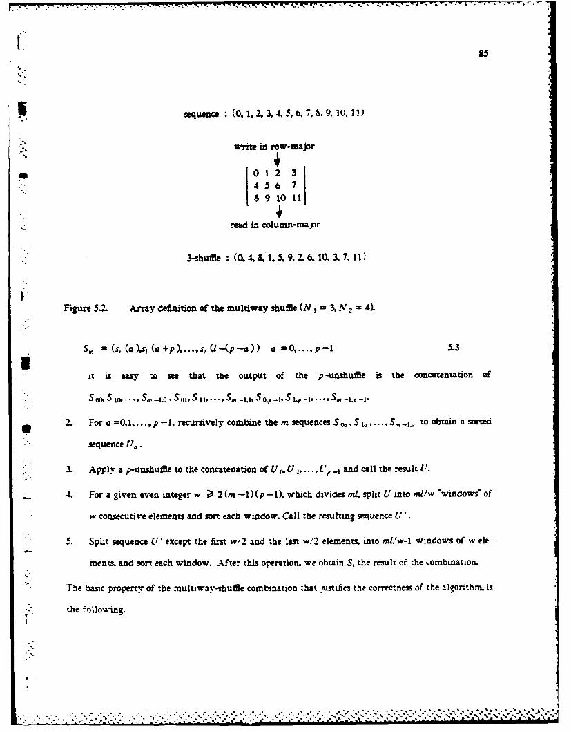
5 sequence :(0, 1.2, 3. 4. 5. 6, 7. 9. 10. 11)

write in raw-major

0 123456 7

89 10 11

.ed in column-major

3-shuffle (0. 4. 8,1, 5. 9, 2, 6. 10, 3. 7. 11)

Figure 5.2. Arry definition of the multiway shuffle (N 1 3, N - 4).

S. = (s, (a).5i (a+p) .... s, (l-(p-a)) a =0... p- 5.3

it is easy to see that the output of the p -unshuffle is the concatentation of

'"SooPS IOP. * Sm-L.oIS II , .. ISm -1.1S o.P-IV S LP-... S, -t.p --1.

2. For a =0,1...., p--1. recursively combine them sequences S.., S Ia.....Sm-t to obtain a sorted

sequence Uo.

- 3. Apply a p-unshuffle to the concatenation of U , U L. ,,..._ and call the result U.

4. For a given even integer w > 2 (m -1) (p -1), which divides m4 split U into m1Uw "windows* of

w consecutive elements and sort each window. Call the resulting sequence U'.

5. Split sequence U' except the first w/2 and the last w/2 elements, into mnw-l windows of w ele-

ments. and sort each window. After this operation. we obtain S, the result of the combination.

"'*' The basic property of the nultiway-shuffle combination that j ustifies the correctness of the algorithrm. is

- the following.I

...........................................

so S, Sin-1--"AA A ,

I p-Unshuffle of ml Elements ElSi l 1 sill S ' 1 S n i

0 '0 0 --, 0 M-1,ql I I SO., P-1 1..P-1- Sm- -1

(m. ip) Combiner (m. tip) Combiner (m, li/p) Combiner

U0 Ut up- 1

- - - p-Shuffle of ml Elements

Sorter of Sorter of Sorter ofw Elements w Elements w Elements

Sorter of Sorter of Sorter ofw Elements w Elements w Elements

S

Figure 5.3. Block diagram of multiway-shuffte combiner. Single lines carry one element., double

lines carry a sequence of l (mp ) elements.

Properry. If a given input element has position ht, in sequence U and position hs in sequence S .

then

Ih . - hsl (M -D (p -1) . 5.4

More W. Kifically, if ht; , bp + a for some b -0,1,. .,Wl/p -1, then'-

r" 87

"L + (m-)a -(m--1)(p-l) h Lt. + (m-l)a . 5.5

S Remark. As we have aready mentioned, the preceding algorithm is essentially equivalent to the one

proposed in [L84]. The proof of the above property is also similar to the one proposed by Leighton. and

it is therefore omitted here. However, our description of the algorithm is rather different from the one

given in [L841 because we do not restrict ourselves to the case pm, a case in which the unshuSling and

the shuffling operations can be described as row-majpr to column-major anspositions of a suitable

I xm array where the input sequences are orginally placed.

Remark. Odd-even merge is the special case of multiway-shuffle combination obtained for m - p - 2.

A simple analysis shows that the running time of multiway-shufle (m4)-combination when p -

U m, is T - O Wog/fllogm T ),.,, (m 2 ) ), where T, is the running time of the sorting algorithm that we

chose to deploy in stages 4 and 5.

A combine-sort scheme based on multiway-suffle combination. with

im = . = ... Md m (a constant independent of n), and recursively using multiway-shuffle

- to sort the windows in steps 4 and 5 results in a running time T = O( log'n ). The net result s a

rather cumbersome method to obtain the same performance as can be achieved by a simple merge-sort-

Nevertheles, multiway-shuffle combination is a remarkable algorithm, and it turns out to be very

useful in some VLSI designs.

£ - 5.2.5 The AKS Network

Ajtai. Komlo. and Szemeredi .-KS83 recently proposed a sorting network (referred :o hereafter

as the AKS network), of 0 (n logn ) comparators and (logn) depth. Their construction is of great

• .- theoretical interest, for it shows that 0 (n logn ) comparisons suffice to sort n elements, even under the

constraint that comparisons be nonadaptively executed in 0(logn). parallel stages. At present, the AKS

network appears not suitable for practical implementation, due to the large value of the constants:

however, improvements are conceivable that could make the network more attractive for real-world

-- " *.** ~* **.**I * .--. I . ... . . . . . . . . .i

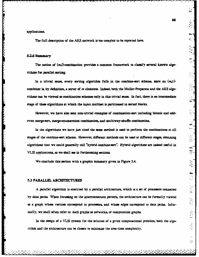
8

applications.

The full description of the AKS network is too complex to be reported here.

5.26 Summary

The notion of (,W)-combination provides a common framework to classify several known algo-

rithms for parallel sorting.

In a trivial sense, every sorting algorithm falls in the combine-sort scheme, since an (mi)-

. combiner is, by definition, a sorter of m elements. Indeed, both the Muller-Preprata and the AKS algo-

.. rithms can be viewed as combination schemes only in this trivial sense. In fact, there as no intermediate

stage of thes algorithms at which the input multiuet is partitioned in sorted blocks.

However, we have also seen non-trivial examples of combination-sort including bitonic and odd-

even merge-sort, merge-enumeration combination, and multiway-shuffe combination.

In the algorithms we have just cited the seme method is used to perform the combinations at all

-" stages of the combine-sort scheme. However, different methods can be used at diferent stages obtaining

algorithms that we could generally call hybrid combine-sort". Hybrid algorithm are indeed useful in

.. VLSI applications, as we shall see in forthcoming sections.

We conclude this section with a graphic summary given in Figure 5.4.

S5.3 PARALLEL ARC -EM CTURES

A parallel algorithm is executed by a parallel architecture, which is a set of procesors connected

. by data paths. When focusing on the interconnection pattern, the architecture can be formally viewed

as a graph whose vertices correspond to processors, and whose edges correspond to data paths. Infor-

mally, we shall often refer to such graphs as networks, or computation graphs.

In the design of a VLSI system for the solution of a given computational problem, both the algo-

rithm and the architecture can be chosen to minimize the area-time complexity.

89

(m, I)-Combination

Merge-Eniumeration Multiway-ShuffleCombination Combination

Sorting 01 = 1) Merging (m 2)-. / N . y 1.. /

.MUAl-reparata Odd-EvenAKSMAlgoririmhm Merging

AKS Algorithm ABitonic Merging

Comparison-ExchangeF (m 2,1 1)

Figure 5.4. Hierarchy of fundamental operations in parallel sorting. A solid arrow points toward asubcase obtained by specializing the parameters definng the size of the input operands.

i A dashed arrow points toward a subcase obtained by specifying the al,2rithm by whichthe operation is performed.

Since the solutions of different problems requires different algorithms, it is a priori quite plausible

that they also require different architectures. However, the experience gained by recent research in the

field of VLSI computation (a representative, but by no means exhaustive, list of reference is [BKSl]

[BK821. [BP84a], [BP84b. [BS84] [GKT79, [Ku82j (Llal [L831, [Ls8Oal [Me831, [MP841 [.\lBS31

[PV8O], [PV8Ial [PV8Ibl [T80ol [T83al, [T83b) shows that in several cases algorithms for different

problems can be efficiently executed by the same achitecture. (For example the radix-2 Fourier

transform and bitonic merging are both efficiently executed by the shuffle-exchange networL)

A detailed analysis of these cases reveals that although the nature of the operations performed on

the input data may be radically different, the pattern according to which the -rocessors exchange data

"* among each other is exactly the same.

r

I-I

~ *.- . *.. .. . . .

. . .. . . . . . . . . . . . . . . . . .... . . . .

IPo

- .- ° r

90

Preparata [P84] proposes to classify algorithms according to paradigms, determined exclusively by

their communication paertns, and to characterize the architectures in relation to the paradigms that

they can execute efficiently.

When a paradigm encompasss algorithms for several useful problems, the supporting architecture

can be considered of the broad-pwrpose type. its capabilities being intermediate between those of a

special-purpose achitmecure, exclusively dedicated to a given task, and those of a general-purpose archi-

tecture that can execute any conceivable algorithms.

As observed in [P84], the results emerging from current research on the design of efficient VLSI

systems for the solution of fundamental computational problems strongly suggest that a few powerful

and highly regular architectures can be used to satisfy a majority of computational requirements.

The study of the sorting problem confirms this indication. As we shall see in the next chapters,

all the known basic broad-purpoe architecture, alone or combined in novel ways, are instrumental to

obtain VLSI sorters with optimal area-time performance. For this reason, we briefly review them ia

the remainder of this section.

5.3.1 The Binary Cube and its Emulators

The binry cube. The P -dimensional binry cube (Pe77] is a network ofN = 2' processors

labelled from 0 to N-I as P(O),, I)... ,/(N-1), with a direct connection (called a nk ) between each

pair of processors whose binary numberings differ in exactly one position. If we let C. (h) be the

integer obtained by complementing the coefficient of 2' in the binary representation of integer h. then

the j-th dimension of the cube is the set of edges E,,-{(h , Cj (h)): 0 4 h < N ). (See Figure .. )

Among the algorithms supported by the binary cube are those whose input is an array of data

Af0I, A[J],... ,A[N-l] with component A[i] intially loaded in processors PU), and whose execution con-

siss of a sequence of steps such that at a given step, only the edges of one dimension are active. A pair

of processors connected by an edge of that dimension exchange their data and operate on them.

.....................................................

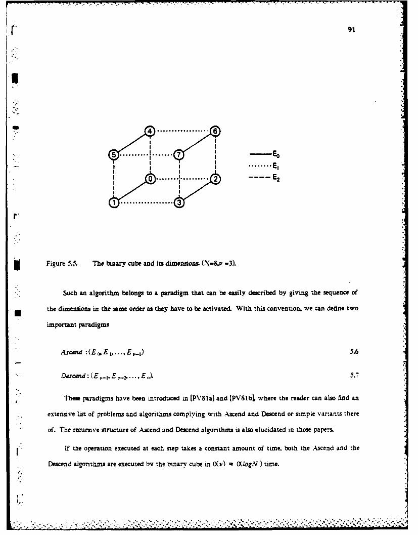
......... . .. 1

91

4 ......... 6- 4 6

-- E

............... 3

Figure 5.5. The binary cube and its dimensions. (N-8,, -3).

Such an algorithm belongs to a paradigm that can be easily described by giving the sequence of

the dimensions in the same order as they have to be activated. With this convention, we can define twoU

important paradigms

Ascend :(E fE..... E E-j) 5.6

"- • De scend : (E ,_, - 2 .. E.,). .

These paradigms have been introduced in (PVSla] and [PV81b, where the reader can also find an

extensive list of problems and algorithms complying with Ascend and Descend or simple var:ants there

* of. The recursive structure of Ascend and Descend algorithms is also elucidated in those papers.

If the operation executed at each step takes a constant amount of time. both the Ascend and the

Descend algorithms are executed by the bina,-y cube in 0(&) = O(IogN ) time.

~~~~~~~~~~~.-...................................-.....-..... .... . ... .. ...-.....-. .. -- ..- .'. , .- .-. .'-.- .,- .- .....-. ,,

92

Although the cube is a theoretically fundamental network, it is not very attractive for pratical

implementations, because the number of edges per processor inceases with N. This drawback of the

cube has naturally suggested the search for simpler networks capable of emulating the cube without

significant los in performance, at least in the execution of algorithms that can be cast in the Ascend

and Descend paradigms. We describe now some of these emulators.

The shuffle-exchange network. For an even integer N, the shuffle prmwutatzon is the bijective function

shuffle (h) -2 h mod (N-i), for h E 10, 1 ... , N-21, and shuffle (N-i) - N-1. The shuffle-exchange is

a graph with N vertices labelled from 0 to N-i, and with two kinds of edges: the exchange-edges..

which are bidirectional, and connect vertices 2h and 2h.i, for h-4,I.... N/2-1, and the ransfer

edges, which are directed, and go from vertex h to vertex shuffle(h), for h 0,... N-1. (See Figure

. 5.6.)

As a network of proceors P (O),P (1)...,P (N -1), the shuffle-xchange has several attractive

features [St7i] most of which are summarized by the fact that it can emulate, in a simple and elegant

way, the Descend paradigm of the binary cube.

*Figure 5.6. The shuffle-exchange graph for N & 8

...... *... . .. . . -. . - -

.. . . .. .

J-- *

93

A Descend algorithm is in fact executed by the shuffle-exchange in v phases, each of which con-

sists of a transfer step. in which processor h sends its content to processor shuffie(h) along the transfer

edge (h, suffte (h)) and an operation step. in which processors connected by an exchange edge communi-

cate with each other and perform operations. An interesting property of the shuffle permutation, when

*N is a power of two, is that the binary spelling of shuffte(h) is the left cyclic shift of the spelling of h.

Therefore, if N - 2' , shuffle (C , (h)) = C, (shuffle (h)), which means that h and Cj will reside in

processors connected by an exchange edge after j executions of the routing step, as required by the Des-

cend paradigm on a u-dimensional cube. This proves that the shuffle-exchange emulates the cube

correctly. Moreover, since the &-th power of the shuffle is the indentity, after Y steps all the items are

back in the orginal procesors (although they have been transformed by computation).

The inverse permutation of the shuffle, known as unshuifie, is also interesting. The unshuffle-

exchange would in fact emulate the Ascend paradigm in the same way as the shuffle-exchange emulates

the Descend paradigm. Indeed, the transfer edges of the shuffe-exchange are often defined as bidirec-

tional so that both of shuffling and the unshuffing of the data can be accomplished in one transfer step.

In this case, it is easily seen that both the Ascend and the Descend algorithms have an 0(IogN)

running time on the shuffle-exchange network.

As to the area performance, the shuffle-exchange graph can be laid out in A = O((N iLogN )2) area,

which is optimal [KLLM83"

.nk attractive feature of the shuffle-exchange network is the simplicity of the emulation algo-

rithm consisting of an alternation of transfer steps with operation steps. the transfer steps being all per-

f)rred according to the same permutation, i. e. the shuffle. A natural question is whether we can

obtain other emulators of the descend paradigm by using permutations different from the shuffle. This

question s answered in [BJ841 where it is shown such permutations exist, but they are so closely related

to the shufle that there is nothing to loose in restricting our attention to the shuffle itself.

However, there are other interesting emulators of the binary cube, which use schemes to transfer

the data more complex than a simple permutation.

* . ~. . . . . . . .. . . .. . . . . . . . . . . . . . . .

The inear array. The linear array is a network of N proceeors P(0),P(1),...,P(N -1), with a

bidirectional edge between P (i -1) and P (i ), for i 1.2,... , -1.

The data contained in a linear array can be easiy shuffled (the content of P(h) is sent to

P (shuffle(h)), or unshuffled in N/2-1 transfer steps (for N even) as shown by [PV81al

If N - 2", an operation step requiring the use of cube dimension E(0 4 j < ) can be

peformed by the linear army as follows. (Refer to to Figure 5.7.) The entire array is decomposed in

N /21" subarrays each of 2"1 consecutive procesm Each subarray, in parallel and independently of

the others, will shuffle its data to create the corrtec adjacencius required by the cube dimension B, and 71

to allow for the execution of the operation step Then. the original order of the data is restored by

unshuffling the subarrays. This procem requires one operation step, and 2 (2J1I/2-l) = 2 1*-2 "

-.,

transfer steps.

Initial 0 1 2 3 4 5 6 7 8 9 10 11 12 13 14 15

Shuffle 0 1 2 3-4 S 6 7 8 9 10 11-12 13 14 15of 0 1 2-4 3-5 6 7 8 9 10-12 11-13 14 15

Subarrays 0 1-4 2-5 3-6 7 8 9-12 10-13 11-14 15Operation 0-4 1-5 2-6 3-7 8-12 9-13 10-14 11-15

Unshuffle 0' 4- f' 5-2' 6'- 3' 7' 8' IZ- V 13-10Y 14-11' 15'of 0 1' -2' 5-' 6' 7' 8' 9' Il- 0' 13-- 11' 14' 15'

Subarravs 1' 2' 4'- 3 5' 6' 7' 8' 9' 10' 12'- 11' 13' 14' 15'

Final ( 1' 2' 3' 4' 5' 6' 7' 8' 9' 10' 11' 12' 13' 14' 15'

Figure 5.7. Execution of operations of cube dimension E 2 with a linear array of N = 16 procesors"

r 95

Thus, the Ascend and Descend paradigms can be executed by the linear array in Y operation steps

and £(21 *-2)<2 N transfer steps. The same result holds for any cube paradigm in which all the &'

dimemsions are activated exactly once, in any arbitrary order. In conclusion we obtain T - O(N), and

clearly A - (N).

The rectangular mesh. The (s xt) rectangular mesh is a two-dimensional array of N - st processors

Pi, i - 0 ..... s-1. and j - O , 1, .... t, , where each row and each column is interconnected as a linear

* array.

Let N 2". s = 20, and t =-21 and let the mesh be loaded with the input vector A [0, ...

A [N -II of the Ascend paradigm in column-majpr order, so that processor P,' stores A [i +sj) (refer to

Figure 5.8).

If the procesors were connected as a cube, with cube processors P (i + js) correspondng to mesh

3 processors P, , dimensions E, E is .... E,-, would remain associated with the columns, and dimensions

E ,, E ,4i .... E , (o+" - v) would remain aociated with the rows of the mesh (see Figure 5.8).

n

0 4 8 12 16 20 24 28

1 5 9 13 17 21 25 29

2 6 10 14 18 22 26 30

3 1 11 15 10 23 2 31

" Figure 5.8. A (4x8) rectangular mesh. When the indices of the cube processors are mapped into thearray in column-mawor order dimensions E,) and EI are associated with colums anddimensions E E 3. and E4 are asociated with rows. (N 32. s -4,- 8. o" - 2. r - 3.,

p . . . . . -

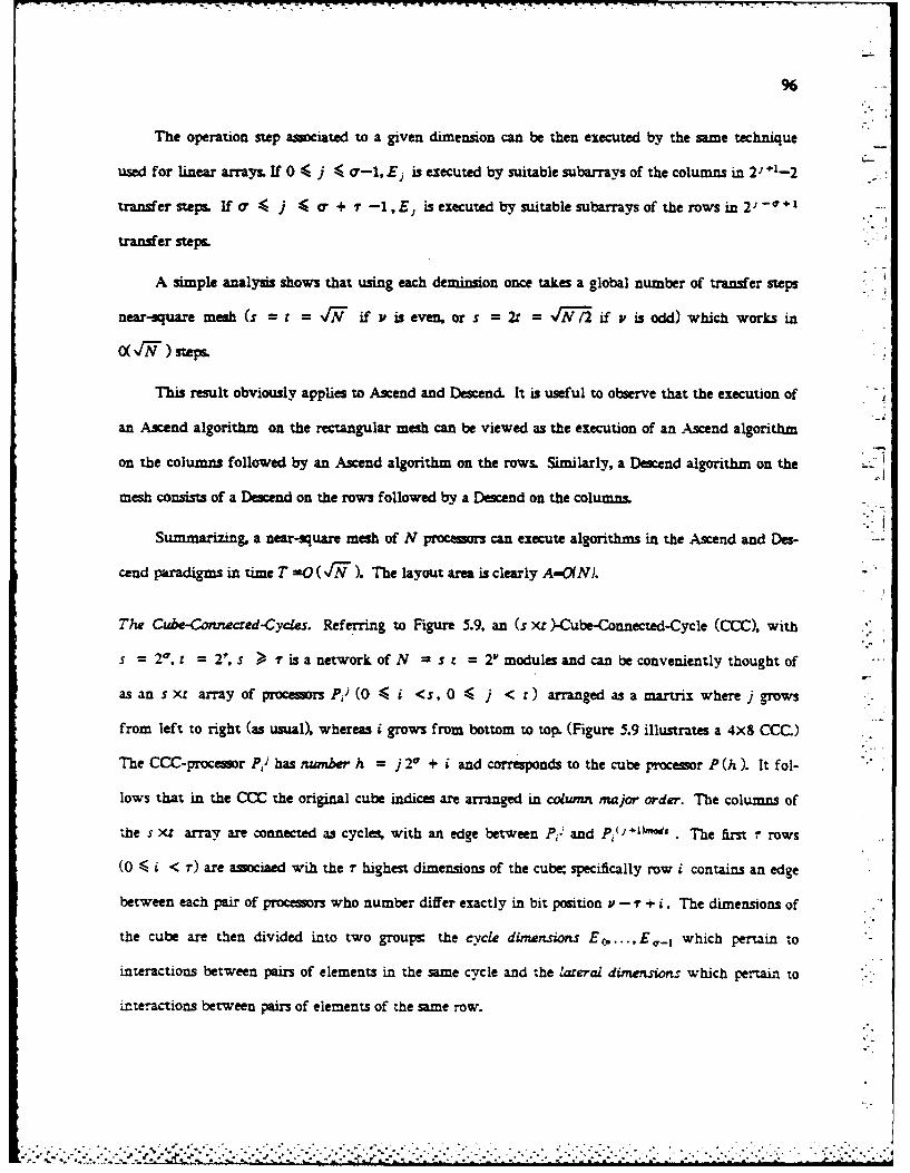
The operation step associated to a given dimension can be then executed by the same technique

used for linear arrays. If 0 4 j 4 o-l, E, is executed by suitable subarrays of the columns in 2 +1-2

transfer steps. If o" 4 j 4 a, + r -1 E, is executed by suitable subarrays of the rows in 2' +1

transfer steps.

A simple analysis shows that using each dembision once takes a global number of transfer steps

near-square mesh (s = t - v" if P is even, or s = 2= -- if P is odd) which works in

0tN-) steps.

This result obviously applies to Ascend and Descend. It is useful to observe that the execution of

an Ascend algorithm on the rectangular mesh can be viewed as the execution of an Ascend algorithm

on the columns followed by an Ascend algorithm on the rows. Similarly, a Descend algorithm on the

mesh consists of a Descend on the rows followed by a Descend on the columns.

Summarizing, a near-square mesh of N processors can execute algorithms in the Ascend and Des-

cend paradigms in time T -0 (.r"f). The layout area is clearly A-O(N).

The Cube-Connueced-Cycles. Referring to Figure 5.9. an (s xt )-Cube-Connected-Cycle (CCC), with

s = 2 1 t = 2", s > r is a network of N = s = 21 modules and can be conveniently thought of

as an s x× array of procesors Pi (0 4 i <s, 0< j < r) arranged as a martrix where j grows

from left to right (as usual), whereas i grows from bottom to top. (Figure 5.9 illustrates a 4x8 CCC.)

The CCC-procesor PJ has nnuber h = j 2 + i and corresponds to the cube processor P (h). It fol-

lows that in the CCC the original cube indices are arranged in column major order. The columns of

the s Xt array are connected as cycles, with an edge between Pi' and P, ''"'*. The first r rows

(0 K, i < r) are asociaed wih the r highest dimensions of the cube; specifically row i contains an edge

between each pair of processors who number differ exactly in bit position P - r + i. The dimensions of

the cube are then divided into two groups the cycle dimensions E0, ..., E,_ which pertain to

interactions between pairs of elements in the same cycle and the larerai dimensions which pertain to

interactions between pairs of elements of the same row.

-4

97

37 i 19 23 27 31

E4 2 810 14 i 22 26 30

E3 ,19 5131 291{21.

U Figure 5.9. A 4X8 CCC. Proceors are labelled with their numbem The correspondence between

rows and dimensions is also shown. (. -5, ? = 3).

To execute a cycle dimension E,, the CCC works esentially as a set of N /2' l independent

linear arrays of length 2' 1 each of which performs the shuffle-operation-unshuffle procedure already

- described. Thus, the execution of E 0, E 1 .... E -I globally require O (s) time.

To execute a lateral dimension E , (0 4 I < r), a sequence of s operation steps is peformed

by the lateral connections in row a , interleaved with s cyclic shifts of the cycles. When the lateral

dimensions have to be executed in the order E n,-.., E -, their execution can be overlapped by a suit-

able pipelirung technique, so that the total time is just O(s).

In conclusion a (s xt )-CCC can execute an Ascend algorithm in T 0 0(s) computation time. A

similar performance can also be achieved for a Descend algorithm.

As to the area. it can be shown (PV8I] that a (s xz )-CCC with 4 s and t can be laid

out in .4 = 0 (t 2) area which is optimal.

.-.: =>- ..- , .z :., ,,, .- " " .---......

99

For a given N - 2', by chasing s in the range [logN, 4N we can achieve a perfomance

AT 2 = O(t 2s 2) - O(N2) for any computation time T E[f(logN X),O( ")

Comparison of Cube Emulators. The performance of the emulators of the cube we have

described for the Ascend and the Descend paradigm is summerized in Table 3.1. The shufl-exchange.

the linear array and the mesh all have the ame AT 2 = (N 2) performance, which is optimal In the

following chapter we usually deploy cube-connected-cycles for the execution of Ascend and Dmend

algorithms, especially because of its area-time trade-off feature that allows to choose the value of the

computation time from a wide range. It must also be said that, for (T - O " ), the mesh i usually

pieferable for the simplicity of its interconnection. For T - 0 (log N ), the shuffle-exchange is attrac-

tive for the elegance of the emulation algorithm. However, the optimal layout of the shuffle-exchangeas

very irregular, which is not a desirable feature for VLSI systems.

The linear array is indeed a poor emulator of the cube, at least when judged by its area-time per-

formance. However, it is very useful as a component of more complex networks, as we have alreac.-

seen in the case of the rectangular mesh and of the CCC.

TABLE 5.1. AREA-TIME PERFORMANCE OF CUBE EMULATORS.

I PerformanceTIIE AREA

Architecture____________________________

Suffle-Exchange T - e(logN) A = e(N 2/7 2)

Linear Array T = e(N) A = O(N 3 1/T 2 )

Square Mesh T i e ) A =e(N 2/T 2)

CCC T E fl (ogN)),0(,I)] A 9(N7T 2)

i : • .. .. " " " . .' " .' " " " -" .',.' --', f. -', . . . . '. ," " . *", - - " . . . . . . . , . , ." "

5.3.2 The Tree and the Orthogonal Trees

The bmnary tree. Several computations require the N-fold replication of a given data item. or some

Lind of combination of N distinct data items to generate a single one. These operations are efficiently

executed in 0 (ogN) steps by a fully balanced binary tree with N = 21 leaves and N-I internal

nodes. This graph can be laid out in G(N ) area if there is no constraint on the placement of the leaves.

and in G N/ogN ) area the leaves must be placed on the boundary of the layout region [BKSO]

:The orthogonal trees. (Refer to Figure 5.10) The two-dimensional orthogonal tree network (OT) [LSI.,

\N B31 conms of N = n 2 processors Pj (i, j -01.... , n-1), and 2n fully balanced binary trees

CT, .C,.- (the column trees), and RT t .... RT.,i (the row trees). The leaves of CT, are then

procesmrs F, .... .,P, and the leaves of BT, are the processors p P ... p.

, 0 P

I __rOd

U dJ

ST. T

" RT

Figure 5.10. Orthogonal-tree network for N = 16.

..... ..... .°- . .....- .oo . .. ... j.o •..... •.. o.".. .. .. ..-.'.''.' _.'*,.' "f : "_'' '. ', -,:- :. .''. 3":'-' '.' .''._ , " ' '" ": " -'" " ': "" " " : " " " " -'" " " "" . " " -'" " " "" - " '-'

100

Optimal layouts of the OTs have are A RN log2N) [1-81]. Algorithms consisting of a con-

stant number of replication and combination operations along the row and the column trees, are exe-

cutedby the OTsintime T =0(logN)I

The OT network is very versatile and will be used is several of our sorters Multidimensional

OTs can also be defined. An interesting application of three-dimensional OTs to matrix multiplication

can be found in [PVSO].

.7--.

- ' . ' - - - '- ---

~ 6 q

CHAPTER 6

OPTIMAL VLSI SORTERSFOR KEYS OF LENGTH k =I ogn + 0 (1 ogn)

6.1 LNTRODUCflON

In most of the investigations on VLSI sorting the length of the keys has been asumed to be of the

form k -(0- a ) log n, for some constant a > 0. Since the results of thee investigations are indeedr

valid as long as (U+a) log n k 4. (0 + a 2) log n. for some constants a,>a,>O, it is slightly more

appropriate to refer to a length of the form k-log n + 0log n), not to suggest that, say. k-2 log n + log

log n is excluded by our considerations.

In retrospect, we can jusify the attention given to the case k-( I a ) log n for two reasons: (1 )this

*' case of the sorting problem is the easiest (or the least difficult) to analyze, and (2) its complete solution

is instrumental to make progress on other cases. While the second reason will be substantiated only in

Chapter 7. where we will show that a sorter of key with k - (U+ a )log n is a useful building block or

* sorters of both short and long keys, the first reason can be already explained on the basis of the lower

bound results of Part L

In fact, while short and long keys have to be studied with the more sophisticated square-

tessellation technique, the case k-( I a ) log n - which partially overlays with medium-length keys (c

< I), and partially with long keys (>, 1) - can be analized by the bipartition technique (although. as

S we have observed in Section 4.2, the dependence of the complexity on a , for a > 1. can be really

understood only by the square tessellation bound).

17 Indeed, from Theorems 4.14. 4.15, 4.16. and the assumption k > (I+a ) Log n for some an, >0.

- w;e obtain

-... . ---" , .",. . . . . .. -. .. -,-', -, . . ....- i ,. * *l ** . . .. "*... . .. .. * . .- .. n

V1

102

AT 2 (n 2 log 2 n) 6.1 "-

T = nflogn) 6.2

A = Wflogn) 6.3

In this chapter, we will study several VLSI sorters, the analysis of which will allow the conclu-

" sion that the optimality curve of the (n, log n + G (log n))- rting problem is described by

A = O(n2log nIT2), T E[ (ogn) O(% ; )3 6.4

As we shall see, the main difficulty in obtaining optimal VLSI sorteis for k - Iogn + 8 (logn) con-

sists in designing the appropriate architecture. For the algorithms instead, it will be sufficient to resort

to (minor adaptations of) the known results reviewed in Section 5.2. The situation will be different for

"" short and long keys, which will require new algorithm as well as new architectures.

This fact is not without explanation. The first parallel sorting algorithms have been conceived for

either the shared-memory-machine or the network-of-comparators models of computation, whose prim-

itive operations are at the word leveL Thus, the keys were treated as indivisible entities that maintain

their identity throughout the entire computation.

The indivisibility of the key is a very restrictive constraint in the VLSI model of computation.

* and conflict with area-time optimality.

Indeed, to port short keys it is not convenient to maintain a list encoding of the input multiset in

the intermediate stages of the computation, because it is very inefficient, and requires superfluous

* bandwidth in transmision. Thus. no algorithm that maintains the identity of the keys can achieve

. optimality.

The same conclusion is true also for rather long keys (logn o(k)) but for a different reason. The

, list representation is indeed efficient in this case, but we still need to fragment the keys to avoid a large

primary flow. In fact, we have already seen that even when the %indivisibility' of keys is required only

*' at the I/O ports (word-locality) the AT 2 complexity of (nk)-$orting is asymptotically quadratic in k

(Theorem 4.14). while without this restriction the complexity is only linear in k (Theorem 4.18).

. . ... -.... .,-., .... . . .. . . . .. .. . . .

Fo

103

The case k - logn + 0 (logn) is made special (and, superficially, simpler than others) by two cir-

cumstances. One is that the list encoding is optimal for this length (within a constant factor). The other %

is that any strategy to decrease the primary flow below 0 (nlogn) by suitably decomposing the keys

would fail to yield better area-time performance due to the presence of an irreducible 9 (rdogn) secon-

dary flow.

in conclusion, for k = logn + CLogn ) the indivisibility of the keys (word-locality) is not a draw-

back, and classical sorting algorithms turn out to be instrumental to obtain area-time optimal designs.

With this premise. w now turn our attention to the effective construction of NILS] sorters. Many

designs have been proposed in the early literature, and reference [T83] surveys several of them. Here,

j: we recall only the designs that come closer to AT 2 = l(n2 log2 n ) lower bounds, which are:

(i) a mash-connecred bitonic sorter (IBa68, (T8O1 [TK77], [NS79D with optimal performance

A = 9(n 2log2n IT 2) at 2 = 9(4n), and other four designs all with suboptimal performance

A = G(n 2log4n/ T 2) which are:

(ii) a shuffle-exchange bitonic sorter at T = Cog 3n ) ([St7l]IT80]KLL.M83D

(iii) a cube-connecred-cycies bitonic sorter, for T E[t(log 3n), 0 (llogn )] (IPV8D1)

• " (iv) a pipelined Batchr's nerwork , at T" = qQog 2n ) (VLSI estimate in [T$31)

(v) an orthogonol-tree-conneced (ILS1], (N IB3D Muller-Preparta sorter [MP7!] at T = 9(ogn).

The (Log -n) gap between lower and upper bound for .4T 2 exhibited by the last four designs has

ndeed been one of the original motivations for the work reported in this thesis. The remainder of this

. chapter is devoted to the discus on of VLSI sorters with optimal performance. For several of them, a

description is already available in the literature.

Section 6.2 is devoted to bitonic sorting. Our approach will consist in focussing on the underlying

..* paradigm, which is of the cube type. but more complex than the Ascend or the Descend paradigms. and

in constructing efficient architectures for that paradigm.

* ........

104

Section 6.3 is devoted to merge-enumeration sort, which allows to achieve minimum computation

time T - O(logn). New architectures are also considered, based on a mixing of orthogonal trees and

cube-connected-cycles.

Section 6.4 concludes the chapter with a brief report on other area-time optimal networks imple-"

menting multiway-shuffie sort and the AKS algorithm.

6.2 NETWORKS FOR BITONIC SORTING

6.2.1 The Bitonic Sorting Paradigm

The bitonic sorting of n = 2" elements (reviewed in Section 5.2.2) consists of v merging phases,

M o, .... , -. , with phase Mi performing the merging of pairs of sequences of length 2'

Bitonic merging, on the other hand, complies with the Descend paradigm of the binary cube

[PV81a so that the execution of phase Mi on the binary cube requires the successive use of dimensions

E, E, ... ,X 2 o . Thus, the schedule of use of the dimensions for a complete sorting is the one shown

below (Figure 6.1). which will be called the bicoric sorting paradigm.

phase I active cube dimension

M,. E E,,

E, E,, ,

, 1 : E 2 E1 tE,,

AE -. E E,: ..

Figure 6.1. The bitonic sorting paradigm.

L ...~~~~~~~~~~~~~~~~~~~~.............. .................. ?............. .........-...........-.-...-..--.- ,....'..

* ., , .. -. -. . . . .... ...

105

We shall now analyze the performance of some of the known emulators of the cube on the

bitonic sorting pamdigm, and we shall then propose new and more efficient emulators.

Some considerations will put the problem in the proper perspective, and will indicate the

difficulties to be overcome for its solution.

The area-time performance of the emulators of the cube reported in Section 5.3.1 pertains to the

Ascend and Descend paradigms. The area is estimated under the assumption that links between proces-

sors are realized with unit bandwidth, so that they can be laid out in unit width, and the computation

time is estimated under the assumption that both operation and transfer steps take unit (or constant)

time.

When the actual data processed by the algorithm have length k, the estimate on the AT 2 measure

must be muliciplied by k , although we can usually still choose whether the penalty is to be paid in

area or in time. In fact for a given b with 1 4, b 4 k ,if we realize all the links with bandwidth b* k

we obtain an area Ab = b 2A , and - usually - a time T1 = LT , so that A Tb2 k 2A IT .

The reason for which we cannot claim that Tb always equals (k/b)T 1 is that, although a larger

bandwidth automatically yields a proportional speed-up in transfer steps. it does not guarantee a

speed-up in operation steps. However, most of the time operation steps can be performed in kib time, at

least as long as k/b is not small For example, in sorting, the operation step usually involves a

comparison-exchange which can be performed n time kib (and area b 2 ) as long as k lb = M(log k),f

or equivalently, b - O(klog k).

Thus, the optimal emulators of the Ascend and Decend paradigms, achieve a performance

AT 2 = O(.V 2k 2) on operands of length k. If N - n. and k - logn + 0 (logn), AT 2 = O(n 2 logn).

In order to attain the 472 = f(n 2log2n) lower bound for (n , ogn + (ogn ) )-sor-tmg -y

means of the bitonic algorithm, we must be able to execute the entire bitonic sorting paradigm in the

same order of time as the much simpler Descend paradigm. It is indeed surprising that this is possible.

i.* * .. *o .*.*•.*-.-° ..-..- o*--.

106

6.2.2 The Linear Array -

Although the linear array is far from being an optimal emulator of the cube even for the simple

Ascend and Descend paradigms, the study of its performance on the execution of bitonic sorting will

provide us with some useful insights.

With reference to the discussion of Section 5.3.1, we shall consider a linear array of N - n proces-

sors. where n is the number of keys to be sorted. Each processor will be endowed with O(k) bits of

memory, to allow the storage of a key of length k, and with a serial comparator-exchange that works

in 0(k) time. We can then lay out a processor in a region of O) width and Ok) height. The connec-

tion between P(i-1) and P(i) can be realized with bandwidth k, to allow the execution of transfer steps

in one time unit. The entire array can then be easily laid out in 0 (n) x O (k) area. (See Figure 6.2.)

The running time of bitonic sorting on the linear array is readily estimated. The operation steps

are (P + l)Y/2 - 0(log 2n) in number, and each takes Ok) time, so that, globally, the comparison-

exchange steps take Tt = (log 2n ) time. As for the data transfer we recall from Section 5.3.1 that

execution of E, is done in 2)~ -2 steps. Since the bitonic sorting uses dimension E, exactly P -

tumes, globally the transfer steps take T2 < (v-j)2'" = 0(n) time. In conclusion, for-'-

k = logn + 9(logn ),T is negligible with respect to T ,and the total sorting time is T O(n).

0(k) P0 P, -

-'Oln) . .

6 L-s

FRgure 6.2. Layout of linear array for bitonic sorting.

... ..... .. .. . .-... . ... ..... .

107

At first, this is.surprising since we would intuitively expect that the bitonic sorting paradigm,

which consists of i'(v-i) 2 steps on the cube, would require more time than the descend paradigm con-

sisting of an v steps on the cube. However, a closer analysis reveals that the dimensions more frequently

used by bitonic sorting are the lowest, which also happen to be the ones that require lea time on the

linear array. Obviously, this is a fortunate accident, but the principle that the most frequently used

dimension should be the ones with the fastest execution will be a useful guideline for subsequent

developments.

6.2.3 The Mesh

Let n = 2" and, for simplicity, let P be even. We consider now the execution of bitonic sortingt

with a (4 xv 1 )-mesh. The n processors of the mesh will be equippped with a serial comparator,

and with 0(k) bits of storage. They will be laid out in an O (b) .0 (b) region, with %1k 4 b 4 k, to

allow bandwidth b for both the horizontal and the vertical connections. The global layout area is then -.

A -0(b 2n).

The 0(log2 n) comparison-exchange steps globally take 0(klog2n) time, which, for

k = logn + 0 (Logn), will be completely negligible with respect to the time used for transfer steps.

As we have seen in Section 5.3.1, the execution of dimensions E, and E,,2, uses 2/ -2

" transfer steps, for j - 0,1, .. ,/2 - 1. A simple calculation shows that the total number of transfer

steps is 0 ( v_ logn ), and hence the computation time is of order 0 ( V log2n b ).

Summarizing, if k logn + (Logn), A 0 (b 2n ) and T = 0('. log-n/b) so that

AT - 0 (n 2log'n) which is within a factor 0 (Log -) of the lower bound. We observe that, since

b E[v- ,k ], the computation time can be chosen in the range T E[Q(%'nIogn ),0('n log3 '2 n )].

• .By using a more efficient implementation of bitonic sorting on the mesh. [TK77] and [NS791 have

* managed to reduce the number of transfer steps to 0 (,/n'. Using this result in the above analysis we

obtain the :ollowing theorem.

Theorem 6.1. Bitonic sorting of n keys of length k -- logn + O9(ogn) can be executed bv a

*.. -. .... ........-....-...: -.... ' . ........-.'., ,-'...-.......-.-........ ..... ... , ,".

,° .'

108

('/n xj"-mesh with optimal AT 2 =(nogn)for T E[n('-fn).O('_ )1.Io

The original description of the algorithm in [TK77] and [NS79] is rather complex, but it can be

simplified by using an approach that focusses on the paradigm.

Indeed, in the next section we shall develop a framework in which the optimal algorithm for

bitonic sorting on the mesh can be easily obtained as a specialization of a general principle.

* 6.2.4 E ficient Use of Cube Emulators for Arbitrary Paradigms.

Any emulation procedure by which a given graph G-IV.E), with IV I = N =2' , emulates the

* v-dimensional binary cube is based on a one-to-one correspondence between the vertices of G and the

vertices of the cube, such that v EV corresponds to f (v)E(0,1,.... N -11. The emulation procedure is

correct when, if the processor asociated with v EV is initially loaded with the same input data A[iTv)]

that in the cube are loaded in procesor Pf (,). then upon termination the processor aociated with v

contains the same output data Atf (v )] that the cube contains in P ,.

We investigate now the possibility of modifying the function / for a fixed graph G. In particu-

lar, let o (0),...,a (v-1) be a permutation of the dimensions (0,..., v-1), and let ir(O),..., ir(N -1) a

permutation of 10, ... N -1 such that if h has the binar representation h . 1h ,.....h0 ,then "Kh) has

" the representation h -0h w- ..2)" . h -'(or Thus, if h and h' are connected by an edge in E. then

wr(h ) and i(h') are connected by an edge in E . We consider the correspondence between G and the

cube defined by / ,(v )*1r( / (v)) (see Figure 6.3).

If for the pair (Gf) there is a procedure that emulates the execution of dimension E, in time

for the pair (G, / ) the same procedure will emulate the execution of dimension E o in time T,.

Given a paradigm consisting of an arbitrary schedule of use of the cube dimensions

* (Ed 1,E , .... ,. 2)v we can ask for which the pair (G, / ) achieves the minimum emulation time.

The answer is not difficult. Let js(j ) be the number of times that E, is used by the paradigm (;A

" is the multiplicity function of multiset Id jd ..... If ?p ..... p,-t is the sequence of the

.............................................................

• " '." ".". ."' . ."' ' "-"' '.". ' . * . ." .. " .. .. . . ." . -,, .,'', -.. ,' .. . '. ". ", . ." "-

--

--

-.

109

f

G

U (~~ ~ ~(p) ~~ ) and ~ ~ ~= the ueqneo infl~~a gdi

orde of~ 0 11 ecr a ng e tU f and fim un er or est en e ie .~ ~ ,t e

dimsre ins arrn e dt e ll t a the Ann in i e ua i s tihe sequce~e 01 thMenl rran gediof in.

and) ). aive qb)%

E Am ~ p Bz) . So ti n t h un e h) Let G .E) e te uare he n d

order ): of n de r ain e.ui o t is anSe

tonh3iev av e ed an eato p r~ toe u e n t

resp ie to a tol~ f~ r a li ht he nflg of b e muer ti o th t f (. 1 25 + j h

r ~ eu~o tutIe mere andf

G-TV-us. heI

Sorn19 onthe 'Nles...Le..av.describe.an.....................wit

<

.

< In Sction..31wn

V.~~ ... -

. -

110

To T,/ 2 < T I Tv/2+1 < .. < T 2- "

and (q (O,v/2,1v/2+ 1, ... v/2-1v-).

For the bitonic sorting paradigm (E ,E 1,E;... ;E .... Eo) dimension E. is used A(q -- q

times, so that u(O) > g(1) > ... > (--1) and (po . - (O,1 ..... v-). From Eq. 6.6, the

permutation a" that minimizes the emulation time is

a' -- (7(O), .... oriv--)) = (0, /2,.1/2+1.... /2-1,v-1).

For the emulation time. Eq 6 yields

T - LM(Ph YTqh

Y/2-1 ?

= ((P2h )T? + .(P2h)T ,)A =0

= (j (V-2h )T, + /',v-2h -I)T ,,.-,,)

a'I2-I

= (2v-4h -IX2 +1-2)'-

= O(2v'3) = O(1).

The permutation (" and the numbering / f are illustrated in Figure 6.4, for P = 4. In general if i

and j respectively have binary representations j .2-1 ../2-2 j J q and i ,/2_i_ "'"2- i i., then h =

/(i.j) = 2 /j +i has the binary representation j,2_ ... ji4,12-1 ..- i q. and f 0,(i,j) r(h) has the

binary representation j i/2-1i I/2-_ i Ii i 4"

The 1 0 Format. Usually the format of the input array .4[01 ..... .n-l] and of the output array

-A TO!,... ,A IN -1] are imposed a priori on our emulator G by global system considerations, and must be

consistent with the L'O format of other parts of the system that are interfaced with G. As a conse-

quence, at the end of the input phase. the data may be loaded into the processors of G in an order that

differs from the one required by the emulation algorithm. A similar situation might occur for the out-

*.. .. ....... ... ..... .;....... .-... -. .-. '.,., .. . -.. ..- - .,-.. ..,,. ..-.-..$ f -: . -......- - . .. ...-........ .. ....... ,

I..I

Jho hJo

iJ a

00 01 10 11 00 01 10 11

00 0 4 6 12 00 0 2 8 10i lio 01 1 3 9 14

1 10 2 6 1014 10 4 6 12 1411 3 J 7 1 11 IT 11 5 7 13 115

Figure 6.4. Column-major numbering f", and optimal numbering f ., for the bitonic sorting para-digm on a (4x4) mesh.

put data.

In such a situation the emulation procedure must be preceded and followed by a suitable permu-

tation of the data. This problem can be solved by resorting to the Benes permutation algorithm.

Originally formulated for a network of switches (Be64], Benes' algorithm can be also cast in a

cube paradigm consisting of a Descend followed by an Ascend (PVSia]. The schedule of use of theIdimensions is then

(E;11. E v-,..•.,E 1, E (. I, .. .. -,E I-).

At each operation step, a pair of processors connected along the active dimension. may or may not

exchange their data. according to the value of a control bit. Each permutation of size 2' can be realized

by this algorithm, by a suitable choice of the control hits.

Although the parallel computation of the control bits for an arbitrary permutation is not a simple

task. in the application we are considering the permutations of data to be realized are known at design

" time. Thus. the control bits can be precomputed and stored in the processors, provided that each proces-

i: sor is endowed with 0(zu) = O (Zog.V ) storage.

.'>K.>...:.>.x .. ><

112

In conclusion, by adding to the computation time the usually negligible overhead corresponding to

a constant number of Ascend and Decend algorithms, any (a priori known) I/O format can be combined

with any correspondence of processors between the cube and the emulator.

The Benes permutation algorithm could be exploited to build emulation procedures more sophisti-

cated than the one described in this section. In fact, for a paradigm in which the frequency of use of

the dimensions is strongly time dependent, it may be convenient to dynamically change the allocation

of the dimensions during the execution of the algorithm. This approach, however, will be not further

pursued in this thesis (being inapplicable to the sorting problem).

6.2.5 The Cube-Connected-Cycles.

We have seen that the mesh-connected bitonic sorter is area-time optimal for slow computation.

To obtain faster sorters we turn our attention to the CCC which we already know to be optimal for the

Descend paradigm in a wide range of computation times.

As we have seen in Section 5.3.1, in an (s Xt )-CCC (s = 2 1 t = 2"s >,n =sr = 2") the cube

dimensions are naturally divided into two groups: the cycle dimensions E *E .... .E ~. and the

lateral dimensions E,,E,.,...,EUM.--. (o+r - i). A cycle dimension E, (0 4j 4 o--) is exe-

cuted in T. = 21 -- 2 transfer steps. A lateral dimension E., (0 4 j r -1) is executed by pipe-

lining the data around the complete cycle, and therefore uses uses T s transfer steps. However,

when all the lateral dimensions have to be executed consecutively. O(s) transfer steps are sufficient

(rather than 0 ("s)) because the pipelined mode of operation allows to overlap the execution of

different dimensions.

In a paradigm Like bitonic sorting, where in several merging phases only some of the lateral

dimensions are executed, the emulation procedure becomes inefficient. In fact, each , the last

= 0 (iogn) merging phases Ml /,... , -! .. ,, requires the use of a set of cosecutive lateral dimensions "

(more specifically, Eq,.,,...,E, are used during phase M,,, ), and therefore takes (s) transfer ste.s.

Thus, the CCC executes the sorting paradigm in 0 (rs) - C(sLogn) transfer steps.

"-.-.- - -'.- .. '';..-'',.'''. -''.- ".,-'-' . -',.", ,"' -. '-" . .- , ":,.:.i-. ':'_ , ,:-" .. - ... . : ..- ; - -.

113 .4

We recall from the discussion of Section 6.2.1 that to attain the lower bound for sorting we need

to keep the number of transfer steps in the bitonic sorting paradigm of the same order as in the Descend

paradigm. which, for the CCC, is OIs.

At firs, the problem might seem similar to the one already encountered for the mesh, where we

have reduced the number of trasfer steps from 0 (N'n logn ) to O (% ) by a more appropriate alloca-

tion of the dimensions. However, for the CCC we face a more difficult situation because the dimensions

S, already obey t'- -*- _.,le that the most frequently used ones are those with the least execution time.

The problem is that most of the dimensions have a high execution time.

Thus, a fast and efficient execution of the bitonic sorting paradigm requires the development of

new networks. In the next two sections we shall describe the pleated-cube-connected-cycles, and the

mesh of cube-connected-cycles, and show that they are area-time optimal emulators of the bitonic sort-

ing paradigm.

6.2.6 The Pleated-Cube-Connected-Cycles (PCCC)

* Description. There is a basic observation that. when recursively applied, leads to the modification of

Ithe CCC into the PCCC, and to a performance gain. The informal argument goes as follow% for any

given integer A. the highest dimensions E v- ... ,E -B are used only during the last A merging

S .Phases. We could then depoly 24 "smallo CCCs, each with n /24 processors, to execute the first P,-3

phases of merging in parallel, and subsequently supply the intermediate results to a alarge CCC, with

n processors. to complete the execution of the sorting algorithm. The advantage of this strategy is that

- the smaller machines have short cycles, and work faster, while a large CCC would have to use its full

cvcle length in all stages of the algorithm. The transfer of results from the small CCC to the large

* CCC an actually be accomplished with no data movement by simply reconfiguring the network.

- Indeed, the reconfguration of the 24 small CCCs to the large one can be realized by suitably embedding

the former into the latter. We first lay out the 2' (L x .)-CCC5 in a 2x" - array (see Figure 6.5).

.....,.'"'":',, ". '............"..."-a "" i...... '. .... ..... l ' - .. .

114

Note (again refer to Figure 6.5) that each cycle of a CCC in the lower tier faces at its upper end the

lower end of a cycle in an upper tier CCC. Next we modify the layout by merging each pair of facing

cycles into a single cycle with s processors and by using the last available $-I rows of the top tier

CCCs to realize the lateral connections for £ -- ... ,E .- (see Figure 6.4). We obtain an s xz array,

where in each column we have to provide a suitable switch to reconfigure the two original length-s/2

cycles into a single length-s cycle.

In the machine we have just described, the highest 0 -1 dimensions are lateraL but the 0 -th one is

a cycle dimension. The next r - a + I dimensions are again lateral and the remaining (a" - 1) ones

are cycle dimension. For the first Y - 0 merging phases of the sorting paradigm, the 20 CCCs are

decoupled and work in parallel Consider now phase M,-, (1 4 a 4, 0). which corresponds to the

execution of the sequence E,-.,...,Eo . The (lateral) dimensions _ and the cycle

dimension E.- are executed using the full cycle length: next, the cycles are reconfigured to half

length. and E,_ ..... E0 are executed in the "small" CCCL

Before proceeding further, we consider the permissible values of the parameters (. s, and t. Since

the top s/2 rows of the full network must support 7 lateral dimensions, (ie. in each cycle there must

be at least one processor per dimension), we have:

-- 6.7

Since ( - 1), the number of lateral dimensions connecting the "small1 CCCs in Figure 6.5, must satisfy

1 (0 -I) "we trivially have:

2 < 8< + 1 6.S

We shall now complete the modification of the CCC by fully exploiting the key idea which led

to the network of Figure 6.5. This is achieved by defining as an (s xt )-pieared CCC (PCCC) the net-

work of Figure 6.5 where each of the 20 component networks is itself a recursively defined

S t(x 2-1-)-PCC (rather than a conventional CCC). Note that 0 is a design parameter.

• ~ ~~~~~~~~~ ....... ....-.... -...... ...........-.- ,-.. .... •..]

, U". r w -5.. .... r- .. t-. . . . . . . . . . . . . .

115 ..

tecneto to - fom-h CC

NOe

ccc (a,"

A F (u .. Cns wti n the be (a) ang n t f p oesmal s P (a ere-e =o f t h e c

oo • . ,

. . . . ..- '. .U . . U . '- . ..• . *

rt116

, whose rows support lateral connections. Starting from the highest dimension E,,-,, lateral and cycle

,. dimensions are interleaved, (0-i) to one. This interleaving continues until we reach cycle dimension

SE .,& where the cycle length, 24-1, is still adequate to accommodate the -r lateral dimensions. Thus,

from the condition 20 - 1 > r we obtain

A 0- - log271 6.9

and X is called the depth of iWuerlecig. At this point the remaining Y -X 0 dimensions are assigned

as follows. the higher r- ( - 1)A >- 0 are lateral and the lower c - X are cycle dimensions. Obvi-

ously we have

- I + , 6.10

. and the cycles are reconfiguble to any length 2-y whereo - X 4. y 4. (r. Note that there are

21 -1 reconfiguring switches per column.

An (8X16)-PCCC with t = 3 is illustrated in Figure 6.6. Notice that conditions 6.7 and 6.8 are

, automatically satisfied. Moreover, from 6.9 the maximum permisible value of X is 1, whence condition

",* 6.7 is confortably satisfied. Incidentally, note that, for the same value 0 = 3, the smallest PCCC with -

= 2 has 256 proceors (t =16,s =16.3 = 3).

Due to the above interleaving of dimensions. procesor P,' in the PCCC-array corresponds to

cube-processor P,, where h = j 27 + i and h' is the integer obtained by permuting the binar; -

re'resentation of h according to the above interleaving scheme. This is illustrated in Figure 6.7.

Performance Analysis. In this section we give an upper bound to the area of the PCCC and to

the time used to execute bitonic sorting. The PCCC is to be laid out in the rectangular grid. We will

assume that a pCCC processor is endowed with a serial comparator and (k) bits of storage so that it fits

in an 0(1 )xO (k ) area. We also assume that edges have unit width. Data transmission takes place in

serial fashion. Then the width of the (s xt )-PCCC is easily seen to be 0(t), if we lay out each cycle in

a constant number of vertical tracks. It is easy to see that an array row associated with the o-th

' : ighes lateral dimension (a = I. ) (no matter what is the index of t.he dimension in the cube) is

............ ,....,......... o. . . ....... ..... . .- ,.. %•.

I -I

0o 0

Figure 6.6. An (8 x 16)-PCCC with 0-3. Since X I we have one reconliguring switch per cycle.

118

Figure 6.7. Bit position permutation induced by the pleating scheme (the arrangements of the h'and h are above and below, respectively.)

laid out with r /21 tracks. When we consider the multiplicity of each dimension, i.e. the number of

rows associated with it as a result of Opleating, we obtain the following formula for the height of the

PCCCQ

height t + •+-- +2_+.4. + + _- +

+2 + + + 0 (ks)

By evaluating this sum. for 0 2 we have height 0 (At + ks) while for 0 > 2 we have

height - 0 (t + ks) . Since in the cam 0 > 2 the height does not depend upon A , hereafter we

further restrict 3 to be > 3. Moreover, we add the condition s 4 n , so that height O f(t). We

then conclude that A = 0 (width xhaight) = 2X :).

. . . .."- "."".""-- ..'. .+ + .. "' I,;, " "+

""" " "" " """ ', ."""" + ' -

+tt""" " "l" ["' "". "" " "°

" . * " " ""," n : "

"+'"+"- +

: ". .,' - , .- ',. . - -, -. '. -. -- . -t ' ,. .- . .- ,- -,. . , . .• - . . " j- -•

119

The analysis of the computation time requires some additional discussion. A cycle dimension asso-

U ciated with arrays of length 1 uses (1-I) steps. by the technique explained in Section 5.3.1. The execu-

tion of a set of consecutive lateral dimensions on a cycle of length I requires no more than 41 steps (21

comparison exchanges and 21 shifts of the cycles). For our convenience we consider first the highest X0

1 dimensions, and we group them in X sets of size B, which are executed 0.20 . , times respectively.

Since the execution of each set requires 4 41 steps, with I = r /2' . for the i-th group (i 0,...A-)

we can upper bound the total number of steps i'l for these dimensions as follows

*'T< 4stI + 2 + + ...+ < 16s .2 4 2-

The remaining dimensions are handled by a set of (--x -L)-CCCs, which have a cycle length C1ogn)

2 k 284

=(since 2 1022r 9(7) = (ogn)). Thus, referring to the well-known behavior of the conven-2A

*tional CCC, we know that the entire set of the last 14-A0 dimensions can be executed in O(logn) steps.

On the other hand, the entire set is executed Of/ogn) times, thus they globally require r, = 0 (log 2 n)

_- steps. Finally, recalling that k is the operand length, the total computation time T is given by

1 k(T' + r+ )= O(k(s + logn))and.fors fl(log2n )we have T ,O-s).

We can summarize the preceding discussion as follows.

Theorem 6.2. The pleated CCC can sort keys of length k in time T - 0(ks) and area

.4 = O(n -./s2) for any s in the range [O(log 2 n )0 ( vW ]. For k = ogn +9 ( logn the performance

is .7 = 9(n 21ogn )forT EV' CI(log 3n). 0 ("g5)

• . The PCCC has been first proposed in [BP-ta], where a detailed description of the control structure

Ls also given.

•~~~ ~~ - - - - -" - - - - - - - - - - - . .. . . . . . . . . . .

120

6.2.7 The Mesh-of-CCC

.Another network that can execute the bitonic sorting paradigm with the same area-time perfor-

mance of the PCCC is the mesh-of-CCC (MCCC), a suitable "hybridization" of mesh and CCC.

An (Nm)-MCCC, with N = 2", m = 21, and t 4 N/M 2 -- 2" (r = to - 2) consists of M 2 CCC

modules, each with t cycles of length r. The Nm proceuors of the MCCC are conveniently indexed as

P J4 : O(ij< m, 04, p< t", 0 4 q < . 6.11

For a fixed pair (i the set IPI- : 04p< ,0 q < r ) is connected as an (xt)-CCC, and, for a fixed

q, the set of processors (Pi.4 : 0 4 i,j < m) is mesh connected (with i and j as row and column

indices, respectively).

The MCCC graph can be laid out in a square of area A = 0 (N 2/M 2), since each CCC requires

0 (N 2/M 4) area, and channels of width 0 (N 2/m 2) allow a straightforward implementation of mesh

connections.

We discuss now the prop-erties of the MCCC as an emulator of the binary cube. To avoid possible

confusion, let us immediately say that the CCC modules will not be deployed in the standard mode

described in Section 5.3.1. In fact a (rxi )-CCC will be used to process only r (rather than vXt ) data

items. This is accomplished by storing the data in row(O) (i.e., processors FJ4 : 04q < t , for fixed i

and j) and by sending the data through the cycle for execution of the dimensions. Only the r lateral

dimensions of the CCC are then used. and therefore the length of the cycle r does not need to be a -

power of two. An (N.n)-CCC will emulate a u-dimensional binary-cube whose processors are

P (O).P (1) .... .P (N-I). We establish the following correspondence between MCCC processors and

cube processor

P,--' P,,. h = j N /m + i N im 2 + q. 6.12

It is easy to see that dimensions E ,.,-- are assigned to the CCC modules, dimensions

E _..E - are assigned to the mesh columns, and finally dimensions E .. ,.. , are assigned

to the mesh rows. Applying the by now familiar techniques for emulating the cube with a CCC or a

'-o .o €........"-...........o..-.-..."_....".. • Oo. o"- °o°'o° °".o O . ,O°o"°o°'.' '. o°%°° °o°% o'.. *.•*o-'.o .°%..............'"" " ''''' ,N "' '. ." ... .. "."........." " - .. " .................

121

linear array, an Ascend (or Descend) algorithm can be executed in 0 (7+m) word steps. On operands of

length k, with bit-serial transmissions and operations, the computation time is T = 0 ( (rn+m ) k ). For

- min the range (logN), o( N logN considering thatv = 0(logN ), we obtain T -O(mk).

In conclusion, for Ascend and Descend, the MCCC achieves AT = 0 (N 2k 2), for

* T E[fl(k logN ).O(k 4Nl1ogN )I which is optimal (A varant of this result has been proved by

CA83] for a network similar to the MCCC.)

It would not be difficult to see that the MCCC, in the form just described, does not achieve

optimal performance when executing the Bitonic Sorting paradigm. However, it is also easy to realize

that the problem lies in the assignment of the topmost 21A dimensions. As we have already seen for the

LX ordinary mesh, the best strategy consists in an alternate assignment of these dimensions to columns and

rows. Formally, if

= 21i, 2j,, = h = 1(2i, +j)22J

we then establish between the processors of the MCCC and those of the cube the correspondence:

P,' -- P,. h = hWN /m 2 +q. 6.13

S With this correspondence, dimensions E, .X..E _ of the binary cube are amigned to the CCC modules.

dimensions E ,,E . are assigned to the mesh rows, and dimensions E ,.,E are assigned to the

mesh columns. When executing the bitonic sorting paradigm 0 (rlogn) word steps are used by the

CCCs. In fact there are v = logn merging phases, and each of them involves no more than r CCC

dimensions. As for the mesh dimensions, they are used exactiv in the same way as in a bitonic sorting

* .. algorithm un the mesh. and therefore their execution takes O(m) word steps. Globally, 0 (m + i logN)

word-steps are needed. Since r = 0 (ZogN), for operands of length c and for

* m E'Lfl(og:N. 0(, ,Vk] we obtain T - (mk). Recalling that A O(.V 2/m2) we have proved

the following theorem. (The number of keys n equals the parameter V of the NICCC.)

*"neorem 6.3. The mesh-of-CCC can sort n keys of length I in time T - 0(km) and area

- = 0(.x-,'.n-), for any n in the range [ff(log:n) .0(' 1 7;c For k Zogvi + Cog e

............... *.**.~ . -. * .... ...

122

performance is AT 2 = O(n 2log2n), for T E[fl(og In ),0(V ogn).

We have already obtained three optimal sorters implementing the bitonic algorithm and respec-

tively based on the mesh, the pleated CCC, and the mesh-of-CCC It is indeed possible to construct

several other optimal emulators of the binary cube, by suitable combinations of known emulators (for

example the shuffle-exchange can be used to define the mesh-of-shuffles, or the shuffle-of-meshes, or the

shuffle-connected-cycles). Although a systematic classification of the emulators of the cube is a problem

interesting in its own right, it would not shed further light on bitonic sorting, and therefore we do not

pursue it here.

However, there is one aspect of the PCCC and of the MCCC which is not saxisfactory, namely

that they do not achieve computation times smaller that fl(Iog 3n ), while the only obvious lower

bound is fl(/og 'n ), since there are (logn + l)logn/2 consecutive steps in the bitonic sorting paradigm.

The discrepancy is obviously due to the fact that a bit-serial mode is adopted both for transmis-

sion and comparison-exchange operations. In fact, we can speed up the execution of bitonic sorting by

resorting to parallel comparison-exchange, but - for k = (Iogn) - each comparison step requires

fl(logk) = (loglogn ) time, so that the global sorting time is still £(Iog 2nLoglogn).

To circumvent this difficulty we need to apply the pipeline principle not only to the words of a

given sequence, but also to the bits of a given word. Prior to modifying the MCCC according to this

idea, we discuss a mode of operation of the CCC network, which we call the bit-pipeline mode is con-

trast with the standard mode, which we call the word-pipeline mode.

For concreteness, we shall illustrate the bit-pipeline mode in the case of the bitonic merge algo-

rzthm, which is indeed a Descend algorithm where the operation steps consist in comparison-exchanges.

To sort a bitonic sequence of size n = 21 we display a (Yx21)-CCC with Y21 processors P "

(0 < i < Y, 0 j < n). All processors in row(O) (i.e-, P(,P,)' .... O,P-) are also equipped with a

shift register cpable to store k-bit operands. All the edges are realized with unit bandwidth. and data

transmission is serial.

=,, : :.' " :a' ' " - . .- ".-.....,.... ... ,.... ..... , - m

123

A bitonic ,-ector (qBa68D A[O1 .... A[n-1] is initially input with component A[j loaded in P

3 Then, at each dimension E ,. E .. .E 0 pairs of elements are compared and, if necissaryexchanged to

place the smaller of the two in the cycle with the smaller number. More specifically, each procesor

...- reads the inputs starting from the most signijiant bit and compares them. As long "is the two inputs

q agree, they are transmitted to the next processor in the same cycle. As soon as a discrepancy is detected,

a switch is set and from then on. the remaining substrings of each operand follew a fxed path.

independently of their value.

For operands of k bits, the algorithm takes 0 (k +v) units of time, in contrast with the 0 (k )

units of time used in word-pipeline mode. If k -logn), as for the keys considered in this chapter, then

T - O(logn).I.

Let us now consider an (n m)-MCCC for the execution of the bitonic sorting paradigm. where the

CCC modules function in the bit-pipeline mode. The only difference in performance is that the first "

dimensions (,r = logn -2 logm ) use O(,r+k ) steps, each time that a group of them is executed, namely

for each merging phase. Thus. since r = 0 (logn ), k - O(logn), and the merging phases are Y = logn,

the CCC dimensions E, ...,. _ globally take 0 (log 2n )time. Nothing is changed for the mesh

dimensions E,,....,-v,wbich take O (mlogn) time, so that. for the entire algorithm.

T -- 0(log2 n +mlogn).

By considering m in the range [Q(l(ogm),O(v7Iogn )I, we have then proved the following

theorem.

Theorem 6.4. The mesh-of-CCC can sort in keys of lenth k =Zog - O(logn) wtt

•" AT (nlon)fo T E'fl (log 2n ), O(,/ ogn).

We have now exhausted the potential of bitonic sorting. To obtain faster sorters we have to con-

S sider other algorithms.

. -). . . . . . . . . . . . . . . . .

124

6.3 NETWORKS FOR MIERGE-ENUMERATION SORTING

In this section we concentrate on "very fast" VLSI sorters. The main objective is to design sorters

with minimum running time T = 0(logn ). To achieve area-time optimality, these sorters must have

areaA = 0(n 2).

The first O(ogn) time VLSI sorter has proposed by [L81] and [NMB83 and it is based on the

.Muller-Preparata algorithm executed by the orthogonal-tree (OT) network. We briefly review it in the

sequel.

6.3.1 The Orthogonal-Tree Sorter.

To sort n keys X ,-... ,X, -1 of length k, let us consider an OT network as the one discribed in Sec-

tion 5.3.2. The Muller-Preparata algorithm (see Section 5.2.3) is executed as follows.

I. Key X; is input at the root of row tree RT,, and broadcast to the leaf procesors P,",P, ..p, '

(i - 0,1,... An-i).

2. Processor P! sends its context X, to the root of column tree CT., which in turn broadcasts it to

the leaf processors Po ,PP ....,P- ( -0,1...,n -1).

3. Processor P, - which we assume to be equipped with (k) bits of memory, and with a serial corn-

parator - compares Xi and XI, and produces a bit C,,. C, is one if X, > X, or if X, = X1 .

and i > j, and C,) is zero otherwise (i.J - 0,... n -1).

S4. The internal nodes of row tree RT, - which we assume to be equipped with a serial adder with a

one-bit delay feedback on the carry - compute the sum C: Z C, . The sum is indeed produced

at the root and will then be broadcast to all the leaves. Obviously C. is the rank of X, in the

sorted output (i = 0,1, ... n -I).

.5. Processor P, compares C, with j. If C, Wj, P,' remains idle. If C, = j. P, sends its content X

to the root of tree C7.

• "o '. i •• °o " ooo"-. . . . . . . . . . . . . . . . . ... " ' " '""J w, 2... .l c ~ , .-s---~d~ .sk.m .a.b~ ~a I , • , . t - '. .. .

125

6. The root of CT, can now output the number received from the leaf, which will be Y1 (as usual

Y oX P .... ,, -I is the sorted sequence corresponding to multiset X ,X 1. ... ,X, - ).

Both operations and data transmison are done bit-serially, so that all the edges of the OT can be

realized with unit bandwidth. It is easy to see that each step of the algorithm takes at most C(k + logn)

time. Thus, for k = logn + O(logn ), the global running time is T = G(logn)I

The OT is area-time suboptimal because its area is A = 0 (n 21og 2n ). However, it is an interesting

network, and it is also useful as a building block of optimal networks, as we shall see in the following

sections.

r 6.3.2 A Network for the Merge-Enumeration Combiner

We now turn our attention to the clas of merge-enumeration combine-sort algorithms (Section

= 5.2.3). Since the original description of these algorithms [P78] is related to the shared-memory machine,

we need to investigate possible implementations with finite degree networks.

We begin by proposing a parallel network for the fundamental block of the sorter, namely the

" (m2)-combiner, where we will assume that m = 2" and 1 - 2 1 are powers of two. This network will

SI accept as input m sorted sequences of I elements each,

S S (0(O),s(1),...s(i -1)) i

and produce as output a single sorted sequence S, which is the combination of S,".... ,S, _ , and has

L =m 1 =2"% elements

S = (s (0).a (1),...,s (L -1)).

The (ml)-combiner will execute the algorithm based on pairwise merging as outlined in the

. preceding section. Its organization is illustrarted in Figure 6.8. It consists of m - modules (eazh capable

. of merging two sequences of length I and of computing partial ranks), laid out as a square m X,-n meshi I"and indexed as M,. "i,,j - 0,1. ... ,m-l). The modules of each row are interconnected as the leaves oC a

- inarv tree of bandwidth 1; so are the modules of each column. Thus, the combiner has the structure

f~i'..'."-A'.. . . . . . . . . . .'. ".

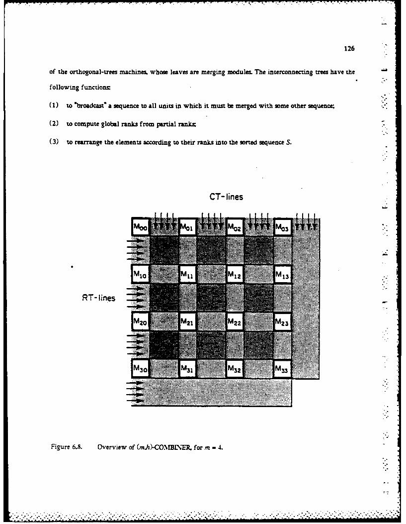
126

of the orthogonal-trees machines, whose leaves are merging modules. The interconnecting trees have the

following functions:

(1) to "broadcast* a sequence to all units in which it must be merged with some other sequence;

(2) to compute global ranks from partial ranks

(3) to rearrange the elements according to their ranks into the sorted sequence S.

CT- lines

. .. .~..... . . . . . . .

... .......

"07 -6 - R."-X7

127-,

We will now describe in some detail the merging modules and the inerconnecring trees.

Merging modules. Merging module M;J will merge sequences S, and S, and compute C,1 (h), for h -

0 ..... 1-1. We recall that C, (h) is the number of elements of S that are les than (respectively lea

than or equal) s, (h) when i 4 j, (when i > j). Each module is realized as a (X + 1 X21')-CCC (See

Figure 6.9.) We shall refer to the procefors of module Mi as micromodules and we shall index them

asP,1, withO p < r +l, andO4 q < 2X l

2 2 , 2 27222

Bq

0,0 0,1 0,2 0,3 0,4 0,5 0,6 7

RT-Iines CT-tines

FirsT sorted sequence Second sorted sequence

Figure 6.9. .Merging unit M,.. realized by a (3.2 3 )-CCC. used to merge two sequences with four ele-ments each.

... . . ..* .- • * . o . ° .. . .. ,.

128

The layout area of a merging module is of order 0 (h 2) (Section 5.3.1).

Interconnecting trees. As indicated earlier, the merging modules are interconnected by two families of

L - ml complete binary trees with m = 2M leaves and bandwidth 1. We will refer to these families as

the row trees and column trees.

The lines of the row trees and the column trees are respectively labelled RT (h) and CT, (h),

i - 0.... m-l;h- 0.... -1. The trees and the merging modules are connected through a small inter-

face, whose structure will be fully specified in connection with the description of the combination algo-

rithm in the next section. At this point we just my that the leaves of KT (h) are., from left to right,

connected to the CCC micromodules P, .A A ' ... .PI' ; the leaves of CT(h) ar connected to the

CCC micromodules P& X O .... ..- ; in other words, the row trees and the column trees

are respectively connected to the RT and CT lines of the merging modules. The connection between

each leaf of a tree and the coresponding CCC micromodule is realized through a buffer register of the

appropriate size (adequate to store one element to be sorted). The situation is illustrated in Figure 6.10.

CTo(3)... CT(O)

Mio M2 Mi3 j

RTi (0) ____

"- T , HiTH -I T iN i I :

Figure 6.10. Interconnection of modules and trees.

". .. .. .. ..""' , . .- *;-*,... *-

* "i ' . ....... ... . .............. .. . . . .. .. .....

129

6-3.3 The Combination Algorithm

• " We describe now how the merge-enumeration algorithm can be executed by the network intro-

duced in the preceding section. For convenience we split the algorithm into several phases.

(A) Input of Data and Broadcasting to Merging Modules

. Element sl (h) is input at the root of tree AT, (h), and is then broadcast to all leaves of the tree.

At this point, the left half of row(O) in module M,, contains the sequence S,. To fill the right halves of

row(O) of all modules, we proceed as follows. First, in each "diagonal" module M the sequence S, is

copied in the second half of row(O). (This can be done by using the connection of row(,) between the

left and the right half of the machine.) Next, from micromodule PF/-iA, which is a leaf of CT, (h),

element sI(h) is broadcast (through the root) to all other leaves of the same tree. At this point, the

merging module Mi contains S and S, in row(O) and merging can begin.

* (B) Merging and Partial Rank Computation

. .Merging can be executed by resorting to the bitonic algorithm, and using the CCC modules in a

"- bit-pipeline node, as explained in Section 6.2.7. However, in order to execute bitonic merging. we first

* need to reverse the order of S.. This is accomplished by an Ascend algorithm in which columns I to

21-1 of each M,, exchange their data at dimensions Eo,... .E.- while columns 0 to 1-1. remain idle.

All the columns are idle at dimension E .

Now the data are ready and bitonic merging can be executed. At the end of merging, the result

resides in row(O) of the CCC, and the element in P,-'-1 0 4 h 4 21-1 . has rank h in merge

(S, S, ). Now we want to transmit the ranks of s, (0).... .s, ( -I) to processors P,.;J .... ,p , respec-

tively. This is accomplished by retracing backwards the path traversed by each element s, (j). and is

•- easily done if eac P- keeps track of whether it exchanged or not the operands during the merging

sprocess. So, all we have to do is to run the machine backwards, with an Ascend algorithm, which

applies to the ranks the inverse of the permutation that merged the elements. At the end of this .pnase.

procesor P.,?, 0 4 h 4 L -1, stores the number of elements in merge (S,,S.) that are less than s, U.

"* ..".. .-* o--*., .-,, .,......,.*-.:.- ,.- ,*.,,".''...'.-' .-. ".--.--"..-..".".---.. ..:. .. ,.-.-. ..... .-..-....-. .-.-.. . .'--' -,*

130

If from this number we subtract h we obtain Cj (h). the number of elements of S, which are less than

s, (h). We call the C,,'s partial ranks because from them we can compute the rank of each s, (h) in

on -

the sorted sequence S as C, (h)= Ci (h).)no

(C) Total Rank Computation

It is immediate to see that at the end of phase B the partial ranks C, 0(h ).Ci 1(h ),.... , -1(h) of

s, (h) are available exactly at the leaves of row tree RT, (h). By having in each internal node of the

tree a full adder with I-bit delay feedback on the carry, we can then obtain at the root of RT the sum

C, (h) of the values stored at the leaves. The nodes work as serial adders and the tree is used in a pipe-

lined fashion, so that the time required is 0 (s+), where IA = logre is the depth of the tree, and X+1

is the wordlength of the operands (note that Cj (h) 4 21). Within the same order of time, we can

subsequently broadcast Ci(h) from the root to the leaves. (Indeed Ci (h) < 21-*. so it can be

expressed by A + jA bits.)

(D) Sorting Permutation and Output of Data

We want to output the elements s(O).... .sL-J) of the sorted sequence from the roots of the

column trees, and, specifically, we want the root of CT,(h) to output element s(j21+ h). This

corresponds to a natural right-to-left order of the column trees as they appear in the layout of Figure

6.10.

Considering a generic element s; (p) with rank C, (p). the binary spellings of the integers j and

h so that s, (p) will emerge from the root of column tree CT. (h) are readily obtained by taking the

AL most significant bits and the X less significant bits of the rank C, (p) to represent h and j, respec-

tively. Thus, as a first step, we "activate" in Mi the elements of sequence S that have to emerge from

trees CT, 's, and "inhibit" all other elements. The active elements are those whose rank C, (p) has the A

most significant bits agreeing with the column number j of the merging module. Next. we rearrange

the active elements in M,, so that si (p) is sent to P:.SOA with h = (p) mod I.

. .

131

This operation is essentially a permutation of the active (and non-active) elements, and can be

5 done by using the CCC as an emulator of the Benes network [Be641 The setting of the switches.

although nontrivial, is greatly simplified with respect to the general case by the fact that the active ele-

ments do not change their relative order. The desired rearrangement can be done by using the idea of

concentration introduced in [NS82, and expan.ion, which could be viewed as the inverse of concentra-

tion. If t elements are active in the given module, they are first sent to the r leftmost colums of the

CCC (concentration), and then routed to the destination columns (expansion). A straightforward adap-

tation of the algorithm that is proposed in [NS82] for concentration in the cube-machine shows that an

Ascend and a Descend phase is all that is required to rearrange data on our CCC. Some bits required to

set the switches must be precomputed. This task could be performed by the CCC or (to keep the micro-

module structure as simple as posible), the task can be assigned to a binary tree of full adders whose

leaves would be contained in the interface between the CCC and the row-trees.

During the entire rearrangement task, computation takes place only in the left-half of the CCC

* without using dimension E,. We then transfer each active element from P/.o? to P'J"-' ' with a

• straightforward use of dimension E,

At this point element s (j 2k + h )is in FJ,-t (where the value of i is determined by the inputa* sequence to which s Q 2 + h ) originally belongs), and is ready to be transmitted to the root of

CT (h ), where it is output.

Performance Analysis and Modification of the Network. Since both the CCCs and the inter-

connecting trees work in pipeline in bit-serial mode, any operation takes time proportional to the sum

of the operand length and the pipe depth. For the CCC, the depth is X + I and the operand length is

either k (input words) or X + 1 (partial ranks). Since a constant number of Ascend and Descend algo-

rithms are executed, we conclude that 0(X + k ) total time is spent in the CCCs. For the trees the depth

is /it + 1, and the operand length is either k (input words) or X + 1A (total ranks). Since a constant

r number of fan-in and fan-out algorithms are executed, we conclude that 0 (A + A4 + k) total tune is

spent in the trees. Thus, the time spent in the interconnecting trees dominates that spent in the CCCs.

-......................... ~ ...- *-, *. .

132

Recalling that a full binary tree on m aligned leaves is laid out in height (Iogm) and that there are I

row and column trees, we conclude

Lemma 6.). A full-tree (2",2x)-combiner of keys of length k can be laid out in a square of width

0(IA21 0)) and operates in time T O(A + 14 + k).

We now observe that when k 11(2)1, then T = 0 (X + k ). In this case the time performance

of the trees is insignificantly degraded if we realize them as comb-trees, rather than as full binary trees.

The depth increases from 1 to 2"' (which is tolerable in time since 20 = 0 (k )), but the layout area

decreases by a factor of 0 ( 2). We conclude:

Lemma 6.2. A comb-tree (2,2')-combiner of keys of length k = W(20) can be laid out in a square of

width 0 (2"1) and operates in time T = (X + k).

Summry of Symbols for an (n)-Combiner

Sizes m = 2", 1 21,L =ml, k =kevIength.

Input sequences

Si = (s(O),si() ... ,si(U-)) =0,1....,m-l.

Output sequence:

S =(s (0),s (1),.... s U/ -1)).

Merging modules (X + 1.2 " ')-CCC's

.\f, :i~j =0,1 .... ^r-I

P/. :0 4p< X+l, 0 4 q< 2',micromodulesof M.

Row-trees and column-tree.-

R,.(h).CT,(h):0 .. i,. < m-1, 0 .h < I...

* 133

6.34 The Sorter

5 The combiner can be used to construct a general network for combination-sort. As an intermedi-

ate step in the construction, we introduce a new operation called coalescence. Given a collection of n

* elements, partitioned into n /,-1 sorted subsequences each containing l, -1 elements, and given a multi-

*1 pie , of 1, -1, which is also a divisor of n, we call (n ; 1, -1: 1 )-coalescence the operation of combining (in

the sense defined earlier) consecutive blocks of n, = 1, /L, -1 sequences.

If we refer to the tree of Figure 5.1. we can easily see that each level of the tree corresponds to a

coalescence of the input sequence. If we call coalescer a network that performs a coalescence, we can

build a combination- sorter by cascading a suitable set of coalescers, as shown in Figure 6.11.

The coalescer. An (n ;, - 1: , )-coalescer can be easily constructed by using n, i L /L, (m, ,L,_.)-

-combiners. Let us assume for simplicty, that n, is a perfect square. We can then lay out the combiners

in an 4'./ X 'array with input and output lines running in a chosen direction. say. parallel to the

3 rows. 0

To estimate the area of the coalescer, we first assume to use full-tree combiners, so that the side of

the combiner has a length of 0 (, Logre, ) (parallel to the rows). Using Lemma 6.1 we have

pHeight 0 0(T, l logm_ +tn,L =

I !oFn,_

Width = -Tj logm) = oj. .

An example with n - 4 is shown in Figure 6.12. The computation time is readily found as

T = 0 (k+k +iogm, ). We conclude:

-" Lemma 6J. An (n ',:. -t-,4) full-tree coalescer can be laid out in a rectangie

" -Z , + logm./ Ii7)) xO (nogm, /-\, ) and operates in time T - O (X + k + logm,) (k is -he

input keyiength. n, -- n /1, m, n Ir). When k logrn - (ogn ). then 7, F 0 (iogn.

................".".- - - ," -- ,- ', " -" :" ". ",",. " " "" ," -'"* ."" ."-" "."".. .'*"' ". " ..

134

(n;1:mi)Coalescer

(n;ml: m1in2) 1Coalescer I

(n;m1. . md2:ml ... Md-)JCoalescer

(n;ml..-mdl:n) 1Coolescer j

Figure 6.11. Combination-santer as a cascade of coalescems

135

(milti-1) :m i,

Combiner Combiner

1i lines .} i lines

I-

Inputs Combiner Outputs

I ___ _>__IL

Figure 6.12. Layout of an (n; 1, -1: 1, )-coalescer with n, n /l, (m, = 1,/1, 1, _ c)-ombiner. (In thefigure, n, = 4.)

Similarly, Lemma 6.2 yields the following result:

Lemma 6.4. An (n ;1,_ :l, ) comb-tree coalescer can be laid out in a rectangle 0(n) xO(nlogm, ',)

and operates in time Tc = O (7 + k + m, ). If both k and m, are C(logn). then T- = 0 (logn).

An Optimal VLSI Sorter. We now show that there is a combination-sorter for keys of length

k = logn +O(logn ) that sorts n elements in time T - O(logn) and area A = 0 (n 2 ), thus achieving the

known lower bound for this problem. The sorter we propose is given by the block diagram in Figure

' 6.13. By the previous Lemmas 6.3 and 6.4 we see that the coalescers can be :aid out in area

.. . . . .. . . . . .. . . . . . . . . . . . . . . . . .

• -- .:: L:4:.;:-.k;. ;>-. .:. .g4: : :-':.: .: ; -",:'-':' •-(•. , :." .. " ., "',,".-

136

(wideh x heightO0(n) x 0(n), 0(noglogn/logn x 0(n), and 0(n) xO(n), respectively. It is

also clear that the total time is O logn). So we have:

Theorem 6.5. There is a VLSI merge-enumeration sorter of n keys of length k = Logn +O(Logn) with

area A = 0 (n 2), and computaton tine T - Ologni.

Remark. The first coalescer stage of the sorter we have just described consists of logan sorters, each pro-

cesing a sequence of n /og 2n keys. These sorters are essential]y orthogonal-tree sorters of the type

described in Section 6.3.1. Strictly speaking, for I - 1, the (nl)-combiner of Section 6.3.2 consists of two

families of binary trees (RTo(O),... ,A', .- (O)) and (cT7(O), ... ,CTm-(O)) such that the j-th leaf of

RT, (0) and the i-th leaf of CT,(O) are constructed (they indeed form the merging module M,1 ),

whereas in the OT network they would be identified.

(n;1 n/ log2 n)

Coolescerfull-tree

(n;n/ log n n/ loqn)

Coolescerfull-tree

(n;n/ogn: n)

Coalescercomb-tree

Figure 6.13. An optimal VL.I merge-enumeration sorter with three coalesce.m

........-..'.. .-...- ..,...--. ... -. '....-..'.,:':'.".....',..-.,.''-. '", ,,- " . .-. . '. .. ",:"-.

137

6.3-5 Sorting in TimeT E[ (ogn )O(log% )-

U We have seen that AT 2 = O(n log-n) can be achieved for T = O(ogn ) (Theorem 6.5) and for

T E[fn(og' n),O(,f"'gn )] (Theorems 6.1, 6.2, 6.4). It is natural to try to extend the result to the

* interval T E[ flogn ,0 (logn For this purpose we start from the following observation. A

combine-sorter with ni s input can sort (in time 0(slogn) the area 0 (n 2/s 2)) s = 21 sequences of nis

elements each. These sequences can then be fed, say one per column, into an (m.s)-MCCC. At this point,

the sequence in each CCC module is already sorted, and the MCCC is ready (after inverting the orderU

of some sequenes to comply with bitonic sorting rules) to execute the last 2o merging phases. (For the

sake of simplicity we will ignore the fact that only a' phses would be really necesary after the work

done by the combination-sorter.) A simple analysis allows us to conclude that, in the process, the MCCC

executes Ollogs+s) steps using 0(logn) time for each. thus running for a total time T - 0(slognL. We can

then state

Theorem 6.6. There is a VISI sorter of n keys of length k = iogn + C(ogn) with optimal

.4T - = (n2log2n ) for any computation time T E[fl(ogn ).O( 'g )]

* With Theorem 6.6. the characterization of the area-time complexity of the (n, Logn + 9(logn ) )-

sorting problem is complete (within multiplicative constant factors).

..." 6.4 OTHER OPTiMAL ET ORKS

For completeness, we report here two other interesting results concerning optimal

(., .. ogn -Oltogn ) -sorters.

The first result is due to Leighton [L841 and provides a design that achieves optLmal

A7 r, = Onlog2 n) for T E [ liogn ),O( Nrgn) The network consists of a suitabl; intercon-

nec:ed familv of OT-networks. The algorithm is a combine-sort of the hybrid type, with the first stage

of combinations performed with the Muller-P-eparata algorithm, and the remaining stages tone or two

4ependiag on T) peorrned with the multiway-shuffle algorithm

. ,-'. . .. .', ','.', .- . - .. , . . - ,' -'-i-,. *. , -.-..... ,. . .,.-" .N.' . .- . .,. .-.. ,'. :,,* ,".,,':, .. >

138

We refer the reader to [L84] for more details. However, we shall return to Leighton's algorithm in

Section 7.2, where we study circuits to sort keys of medium length.

The second result is due to Bilardi and Preparaa [BP4c] who have shown that the AKS network

* (AKS83] can be optimally laid out in area A = O(n ), while maintaining a sorting time T - O(ogn)

on keys of O(Logn) bits.

The details are rather intricate, and hence are not repeated here. An open question, as far as we

know, is the existence of optimal networks that execute the AKS sorting algorithm in time greater than

(Logn ). Obviously, the answer to this question would not improve the characterization of the area-

time complexity of sorting, since we have already several optimal constructions, but could shed some

light on the algorithm itself.

7 .- ..

CHAPTER 7

Iil

SORTING KEYS OF ARBITRARY LENGTH

7.1 INTRODUCTI

* In Chapter 6. we have studied in depth the (nA)-sorting problem for the special, but important,

case when k - logn + 9 (logn). In this chapter we consider the general problem of sorting keys of arbi-

trary length.

The classification of keys into short (k 4< logn). medium-length (logn < k < 2 logn), and long

. (21ogn 4. k ), introduced in Chapter 4 in the context of lower-bound arguments, maintains its validity

when considering circuit constructions. Indeed, a different algorithm and a different network are

* appropriate to each of the above three intervals of key lengths.

The difference between the VLSI model and other models of parallel compu:ation reveals its full

extent in the present chapter, where an attempt to optimize the area-time performance of VLSI sorters

leads to the formulation of novel sorting algorithms

For short and medium-length keys the efficiency of the new algorithms is based on the use of the

& appropriate encoding schemes for the multisets being processed. For long keys the efficiency of the algo-

rithms rests instead on the adoption of non word-local I/O protocols that induce a partition of the chip

into regions within which primary flow is confined, and among wtuch oniy secondary iow Ls

* exchanged.

All the algorithms we shall consider in this chapter make use at some stage, of an (t',logn - 9

. (Iogn))-sorting procedure. Thus, the constructions confirm that the keylength k - logn -0 (log,.) plays

a special role, as a careful analysis of lower-bound arguments had already indicated in Section 6.1.

i.

...... ...... ,........ ........-...-.--...-..... .. ..-. .......-.-.. ,.,.. ......- . ......-.... .:......-.-.... ...-. . : .:.. . .,

140

Sorting algorithms and networks for medium-length. short, and long keys are respectively dis-

cussed in the next three sections of the chapter.

7.2 SORTERS FOR KEYS OF MEDIUM LENGTH

In this section we derive upper bounds for the (nt ,ogn +h )-sorting problem for 0O<h < logit. We

recall from Theorem 4.14 and 4.15 that

AT2 O(n 2h 2) 7.1

and. for boundary chips,

AT 2 =n(n 2h logit) 7.2

When h G(logn) lower bounds 7.1 and 7.2 are of theame order and they are both achieved

by the constructions of Chapter 6. However, a careful analysis of the upper bounds reveals that they

are of the form AT 2 = 0I(n(L<ogn + h P) so that even if/h is zero we have AT 2 9= G~ 21%2n)I Thus.

* for h -o(logn). the sorters of Chapter 6 are slightly suboptimal.

In the following, we shall see that the performance of the sorters can indeed be improved by

exploiting the fact that a multiset of it keys of length k -logn +h can be encoded with 2n (h +1) bits,

as it has been shown in Section 2.2-4.

In the design of our sorter for keys of medium length, we shall us an approach very frequently

adopted in the design of VLSI networks, which can be formulated as follows. Let nI be a problem

* amenable to a divide-and-conquer solution, and let us assume that we are trying to solve UI with target

performance AT 2 -0 (nt 2) on input instances of size n. Additionally, let us suppose that a design for

rI is known with performance A OT 2 0 (g (n )n, 2), where g (nt) a monotone increasing function of

n - i5 the gap between the performance of the known design and the target. Then, if we decompose the

problem into gin) subproblems of size nt Ig (nIt) we can solve the subproblems with g(n) networks of

performance (A4)(n Ig (it ),T o(n /g (nt M.) globally achieving

.. .. [. .. ,... .. . .--a ...-

141

A 1T g(n)O(g(n/g(n))n2/g(n)) = O(n 2 ).

Thus, to obtain the desired result, we are left with the problem of combining the solutions to the g(n)

subproblems in area and time of the same order as A1 and T respectively.

This approach effectively transforms the task from the design of the entire system to the design of

a subsystem for the combination step of the divide and conquer strategy. According to intuition, the

better is the construction that we use for the subproblems, i.e. the smaller is the gap g(n). the smaller is

the number of subproblem. that have to be combined, and therefore the easier is the combination step.

For the sorting problem we are presently considering, we already know several designs achieving

A oT S 0 (n 2log2n and we can try to follow the above approach. For concreteness, we refer to the

boundary chip case, so that our target is a design with performance .4 2 0 ('t 2 h logn), and

g (n) = logn /h. Thus, we can sort logn 1h sequences of nh logn elements each within an am-time

performance allowed by our objective, and we are then left with the problem of combining these

sequences.

For this combination we shall use Leighton's multiway-shufe algorithm, for reasons that will be

apparent as description of the sorter unfolds and that, at this point, we can informally explain as fol-

lows.

- To attain the AT 2 = nL(n 2 h logn) lower bound we cannot afford to maintain the list represen-

* tation of the input multiset throughout the entire algorithm. Indeed, this would imply an O(nZogn)

"' information exchange across a suitable bisection of the network, whereas we can only afford an 0 (nh)

- information exchange. Thus. it is essential to compactly encode the multiset. or some part thereof, in the

stages of the algorithm that pose the heaviest demand in terms of global rearrangement of data.

We shall indeed use the insert-and-prune encoding scheme to solve this problem. On the other

hand, when a muluset is compactly encoded, the individual elements are not easily accessible for opera-

tions, say. as comparison-exchanges, therefore it is very desirable to be able to use the compact form

-. oniv for data transmission and to recover the natural list representation wherever operations are to be

* executed.

• . . . . ... .• " •%

142

The multiway-shuffle combination is ideally suited to our purposes, because the only global rear-

rangement of data occurs when shuffling and unshuffLing the keys, while the other stages of the algo--

rithm require data interactions only within the blocks of a suitable partition of the input multiset.,.'b.

There is a difficulty, however. The insert-and-prune encoding is itself based on sorting a sequence

of length twice as large as the one being encoded. Thus, using the sorters of Chapter 6, we cannot encode

the entire input multiset at once without exceeding our target performance. Hence, encoding will be

applied to suitable subsets of keys. However, this entails a los in the efficiency of the encoding. (The

reader will easily convince himself that the optimal encoding of S IUS 2 requires fewer bits than the

sum of the number of bits required to encode SI and S, separately.) This difficulty will be at least

partially overcome by resorting to a recursive technique.

We have presented the main ideas involved in the design of the sorter of medium-length keys,

and we are ready to give a detailed description of the construction.

The ideas we have informally presented above will be combined according to the following

scheme, illustrated in Figure 7.1, consisting of three basic steps:

1. Given a sorter design. we show how to constuct an encoder/decoder of multisets based on the

insert-and-prune method. The area-time performance of the encoder/decoder will be a function

of the performance of the sorter used in the construction.

2. Given designs of an encoder/decoder and of a multiway shuffler/unshuffter, we show how to con-

struct another shufflier/unshuifter whose performance is better than the one of the original

shuffleri'unshuffter.

3. Given designs of a shuffier/unshuffler and of a sorter, we show how to construct a new sorter

(with improved performance) by resorting to multiway-shutle combination.

The scheme will be iteratively applied. The first stage of the iteration will use a sorter of perfor-

mance AT 2 = 0 (n 21og2n), and a straightforward implementation of shuffner and unshuffler with the

same performance. Subsequent stages will use as a starting point the designs for the sorter and for the

shuffler'unshufier obtained in the previous stage.

.-..... .................... . . .

143

7Sorter Shuffler/Unshuff ler

Insert--and-

-Prune

Shuff leNew Shuffler/Unshuffler

New Sorter

Figure 7.1. Basic steps in the construction of sorters for keys of medium length.

* In Sections 7.2.1 and 712.2 we shall describe in detail the basic steps of Figure 7.1. Indeed one of

* them. which is the multiway-shuffle combination sort. has already been discussd in Section 5.2.4.

The ideas we have introduced could be applied to obtain bounaary-chip sorters as well as non-

boundary-chip sorters, although the construction of the latter is somewhat more involved. For the sakeb

of simplicity, we shall develop the boundary-chip case, and we shall adopt the following conventions.

All our circuits for sorting, encoding/decoding, and shuffling/unshuffiing will be laid out in a region of

rectangular shape, with the input ports on the north side and the output ports on the South side of the

rectangle. The width of the rectangle will then be proportional to the number of IVO bits divided by

comtputation time. The height will instead depend on the bisecion flow that we are able to achieve.

144

and will be our objective limitation (to be reduced). Thus, for a complete (nlogn + h)-sorter, our target

is a width 0 (nlogn /T and a height 0 (nh IT).

7.2.1 Insert-and-Prune Encoder and Decoder

We recall from Section 2.2.4 that the insert-and-prune encoding of a multiset {X X,. -., X 1 -4 of

words of length logn +h is obtained by sorting the multiset

IX,,...,X,_-1)}U{2i:i= 0,...-n -1),

and pruning the logn - 1 most significant bits of each word in the resulting sequence.

Thus, an insert-and-prune encoder can be easily realized by a simple modifcation of any of the

sorters described in Chapter 6. Indeed, it is sufcient to consider a (2n Logn +h )-sorter such that n of the

input keys are prestored and have the fixed values 0 2 1 ,2x2h .... (n - 1 )2h . The performance of such

encoder is then AT 2 = 0(n 2 logn) for T E[O(logn), 0 (,n l1n

The decoder is slightly more complex. Let the insert-and-prune encoding of X,... X,, con-

sists of the sequence of 2n words (W,,W ,...,W , -1) ofIt I bits each with W, W,hW,- W,

The following algorithm enables us to obtain the X's from the W's.

1. For i =0,1,..., 2n -1, compute the value of the binary variable bi defined as

b= 0 if either (i - 0) or(i > 0 and W,11 W, "-

= 1 if(i > 0 and WAW, ).

2. Compute the cumulative sum of the sequence b, defined as B, w b. where

Bi = BIOfn -lB/-iO -2 ... Bi I B, is a word of logn bits.

3. Form a new list W2 .... W _ where W b, B1°1 -1... B, 'W, ... W, '

4. Sort the W ,, and prune the most signifcant list of each key. The first n keys of the resulting-

sequence are = s-orr (X,..., X.- 1 ), and they form the sorted list representation

of the multiset encoded by (W ..., W 3, - ).

......... ......... . . ... .- . -. . . ..r'" '' '" "' '" "'" '' '" "", -" " . . . . . . . . . . . . . . . ."i i " " "i " . . . . . . . . ..Iii - - . ., "; i

145

-- Step 4 poses the heaviest demand of area-time resources. Thus, the insert- and-prune decoder can be also

realized with AT 2 = O(n 2log-n ), forT E fl(Logn ),O(%I )].

In general, we can use the construction outlined above to obtain an encoder or a decoder from any

given sorter. It is also convenient for our applications to combine the encoder and the decoder into one

block, whose performance is stated in the following lemma.

Lemma 7.1. Given a design for an (nk)-sorter with computation time T, (n ,k) and height H, (n ,k),

we can construct an encoder/decoder with time and height respectively given by

TED (n,k) f T,(n,k) 7.3

and

+ HED (n ,k ) H , (nk ),7.4

S"-where and 7) are suitable constants (independent of n and k), greater than one.

7.2.2 Reducing the Bandwidth for Shuffling and Unshufflin"

The multiway-shuffie combination (Section 5.24) is so denoted because two of the steps of the

algorithm respectively consist of a p-unshuffle and of a p-shuffle of ml elements (where p divides 1).

Indeed, these two steps are the only ones that require a global rearrangement of the input keys.

and therefore pose the heaviest demand of bandwidth. Thus, it is crucial to be able to perform the

shuffling and the unshuffling very efficiently.

" In general. both the multiway shuffle and the multiway unshuffle of N words of K bits can each

- be executed by a circuit that works in time s and has width O(NK,' T .) and height

H. < oNKTs;. = 0 (NK /Ts..), where o" is a constant. The lengthy, but rather straightforward

" details are not given here. (A network for similar operations is described in some detail in [BS 84L)

Although in the general case the performance of the circuit mentioned above is optimaL in the

specihc application we have in mind, the shuffie and unshuffle are performed on sequences that can be

decomposed into sorted subsequences, which can be compressed by encoding techniques. As a result we

.,. +" , . ". t" - - +- .. . -. . + .+ i . ,'. °i . - • • m Il . m • • - • +, '+ -

146

can achieve a smaller height for the circuit.

We shall exploit the following decomposition of the multiway-unshuffe and of the inultiway-

shuffe permutations. illustrated in Figure 7.2

I Elements I Elements

Ip-Unshuff Is p-Unshuffl 1softI Elements oftI Elementsj

p-Unshuffte of mp Sequences

ml Elements

FP-84S6

Figure 7.1. Cascade decomposition of the p-LNSHLTFLE of ml elements. (Arrows represent se-quences of Lip elements.)

C .. - . - ..

147/

(I) The p-unshuffle of ml elements (where p divides 1) can be performed by (la) applying a p-

unshuffe to each of the m subsequences that we can form with I consecutive elements, and then

(Ib) applying a p-unshuffle to the sequence of the mp sequences (regarded as single words) of U/p

consecutive elements in the arrangement resulting from (la).

(2) The p-shuffle of nd elements (where p divides 1) can be performed by (2a) applying a p-shuffle to

mp sequences (regarded as single words) of UIp consecutive elements, and then (2b) applying a p-

shuffle to each of the m subsequences of I consecutive elements in the arrangement resulting from

(2a).

We plan to use a shuffler/unshuffler block as part of a multiway-shufle combiner. In this context,

the sequence to be shuffled or unshuffied consists of m sorted subsequences of I consecutive elements

each. In this case, it is easy to see that the sequences that are regarded as words in the second stage of

the decomposition are sorted. Thus, they can be encoded by the insert-and-prune method, and then be

recovered with appropriate decoding. This consideration suggests the scheme of Figure 7.3 for the entire

unshuffle operation. A similar scheme works for the shuffle. Obviously the same method would not, - .

work for unsorted inputs, since after encoding we would be able to recover only the multiset underly-

ing the encoded sequence, but not the sequence itself.

" If in the design of Figure 7.3 we make the unshuffling blocks bidirectional, and we replace

-. encoders and decoders with encoder/decoder blocks, we obtain a network that can also shuffle. We now

analyze the performance of such shuffler/unshuffler block., for the case when p = m and under the

assumption that we use building blocks with the following features (for later convenience, we use a

superscript i to denote quantities related to building blocks, and a superscr:pt (i + I) to denote quantities

related to the overall design).

(a) The encoder/decoder blocks which operate on sequences of n /m : elements (n - ml) of c bits each.

work in time T L kr /m ,k) and have height Hk,(n im 2jk).

(b) The shuffler.,unshuffler blocks which operate on sequences of n,.m elements of k bits each. work in

time . (n /m ,k ), and have height Hs'.(n /m I).

%. .S. ..

148

Sorted Sequence Sorted Sequence

p-Unshuffle p-Unshuff leof I Elements of I Elements

E E E .. E

P-Unshuffle of mp Sequences

Figure 7.3. Cascade decomposition of the p-LNSHL:FFLE of m elements when each of the Mnsubsequences input by blocks of the first stage are sorted. Encoders (E) and decoders (D)operate on subsequences of U/p elements.

(c) The shuffler/unshuffter block. which operates on M2 (encoded) seuences is realized according to

the straightforward method mentioned at the beginning of this section. Here N m , since the

items being shuffled are m 2 and each item consists of a sequence of n /m 2 words each represented

i ,-

149

*2 with h, .- k -logn + 2 lgm bits (see the insert-and-prune encoding). Thus,

HS - o2 nh,, ITs. 7-

. It is then easy to see that the performance of the entire shuffier/unshufer circuits obtained by cascad-

'" ing the different stages is given by

H' 1 (nk) = 20"rh /11'T"s + Hsi, (n/mk) + 2jD (t/m 2 ,k) 7.6

* Ts.t(n,k) = Ts. + rst, (n/m,k) + 2 Tjk (n/m ). 7.7

7.2.3 The Sorters

We consider now a network consisting f a set of m (n/mk)-sorters and of an m-

* shuffer/unshuffier of n keys. Such a network can easily perform all the steps required by the

" multiway-shufSe combination algorithm described in Section 5. Obviously. the m sorters can also

* prepare the sorted sequences to be processed by the combiner, and - with small adaptations - they can

also perform the sorting operation in the "windows" (refer to Secti8n 5.2.4).

• ".- Thus, if we realize the sorters with a design with performance Ts(n/m.k). H}(n im.k ). and the

"-" shufferunshuffler with a design with performance H'(,k ), T.t'(n ,k ), we obtain a sorter with glo-

Sbal performance given by the following relations

H'(n.k) 4 Hs}ACn k) + H(n/m A) 7.8

T1''(n.k) 4 "y T '(n k) + y2T,(n/mk) 7.9

where yi and y-_ are constants. In fact the (nim,'-sorters. and the shudler/unshuffler are activated a

constant number of times during the entire algorithm.

With reference to Figure 7.1, we have now completed the description of the step that ailow to

,"a oin the "new shuffler/unshuffer" and the "new sorer, given a sorter and a shuffherunshufIer. We

shal' repeatedlv use these steps to construct a sequence of designs. as follows.

. .. . . . . *..

150

We begin with a design for the sorter having performance

Hsq(n,k) Ts(n.k) 4 Cs'nk 7.10

where Cs' is a constant. Such performance can be achieved by any of the sorters described in Chapter

6, as long as

r.togn 4 Ts'(nk) 4< 7.11

for suitable constants 7s and es For the shuffler/unshumer we begin with the straightforward imple-

mentation that achieves

Hsj.(n,k) Tst,(n,k) 4 onk 7.12

as long as

i' < TsL,(n,k) 4 " 7.13

- -

for suitable constants -r and rs.-

We can then define a sequence of designs where the (i+1)-th one is obtained from the i-th one

according to the scheme illustrated in Figure 7.1. A value rn, must also be chosen for the parameter m

specifying how many sequences of n/m keys are to be presorted by sorters of the i-th type. We shall

choose mi = L, (n) where L, is the i-th iterate of the logarithm, formally defined by

L I(n) l Iogn 7.14

L(,) A l L,_(n), i > 1 7.15

We claim that the sequence of sorters and shuffier/unshuffiers so denned satisfies the relations

H: T' < C nh, 7.16

H, Ts}j 4 C}. '.h, 7.17 ""

.'or n large enough, when CS and CS. are constants, and

-. 1i

.- .- . - . ,- - ... . . . . - - .. . - , - , '. ' -. . .. . -. . . ¢ '. -' , . - ' . .. . ...--. ' . .. .-. ..' . .. - .. ''-...

.... 151

" h, k -logn + 2 L,(n). 7.18

a Inequalities 7.16 and 7.17 can be proved by induction. For i - 1, they follow from 7.10 and 7.12 with

any Cs1 greater than or equal to o.

In general, using 7.3, 7.4. 7.8, 7.9. 7.10 and 7.12, substituting L,(m) for m, and taking 7.16 and

7.17 as inductive hypotheses, we obtain

HDT'D 4 7 C pn h, 7.19

51 1 2 a nh, I/Ts. 7.20

+ C .S nh, (L, (n) Ts'(n IL, (n ),k))

+ ' C AnJ,(L 2(n )TA(n/L, 2(n ),k))

" Tt,7 < T1 . + T1r(n/Lj(n),k) + 2T'(n/L,2 (n),k) 7.21

HS " < , + H4(n/L:(n).k) 7.22

7> -i'I " 2 T s(nlL.(n ).k 7.23

We are further allowed to choose T'(niL, (n ),k) and T'Z.(n IL, (n ),k) within the range of possible

sorting and sauing. 'unshuffing computation times relative to the i-th design. If we choose them to be

proportional to T'L.. then inequalities 7.20 and 7.21 imply that

H: - T 1 < 2 4 cn h - . o (n h, IL. (n) ). 7.24

= . O(L." ). then ./LJ',: = C(1). and we obtain

-."i ThJt 7 2 o a h: I + lower order terms 7.25

Under t e ,rr assum.t:os. inequalities 7.24 and 7.25 ,:eld for !.he sorter-.J--'. . 2 ! -cwer order er- .2b

.................................... aC .2

. . . . . . . . . . . . . . . .. . . . . .

152 -

S7.27

C"2 a a, 7.28

then 7.26 and 7.25 show that inequalities 7.16 and 7.17 hold for i + 1.

The previous discussion can be summarized as in the following theorem.

Theorem 7.1 For any i 1,an (n ogn + O (Li (n) ))-sorter with I/0 ports on the boundary can be

constructed, such that

AT 2 = 0 (n 21ognLi (n)) 7.29

forT E [n(logn )O (V (n )]. Such sorter is optimal if k - logn + 9(Li(n)).

The ideas exploited in this section could also be used to design non-boundary

(n ,logn +0 (Li (n )))-sorters with AT =0 (n 2L, 2(n)). However the constructions are rather ela-

borate and do not add further insight to the problem of sorting medium words, and therefore are not

reported here.

7.3 SORTERS FOR SHORT KEYS

In this section we derive upper bounds for the (nk)-sorting problem when the keys are short, i.e.

when k l logn. or equivalently, when the size: = 2k of the universe is not larger than the size n of

the multiset being sorted.

We recall from Chapter 4 the lower bounds for this problem. We restrict our attention to word-

local designs. In fact, as indicated by Theorem 4.8, non-word-local protocols lead to larger information

exchange than word-local ones.

It is useful to introduce the quantity

d -n/r 7.30

which, as we shall see below, plays an important role. Then. for boundary chips, we have from

Theorem 4.7 that

.4c

153

.AT:f (d logn r2 log r) 7.31

For non-boundary chips, Theorems 4.9 and 4.10 respectively yield,

AT 2 C(d r 2 ) 7.32

and

.AT Q(d r312) 7.33

Furthermore, Theorems 4.11 and 4.12 tell us that

A = rnr log(U +n/r)) 7.34

and

T = fl(logn ). 7.35

.3.1 The Algorithm

Here we propose a new sorting algirithm. specifically tailored to short keys, and we also describe a

VLSI implementation of it, whose performance comes very close to the above lower bounds.

The main idea of the algorithm consists in using an efficient encoding for multisets of small keys

in the intermediate stages of the sorting process. We shall in fact encode a muitiset S by means of its

distribution function. Let us recall (Equation 2.15) that if S is a multiset on the universe

U = 10, .... ,r -I }. then the multiplicity of an element i E U is defined as

;4( - number of occirrences of element i ir. rnu.iset S,

. - aria -he distribution function (,Equation 2.19) is defined as the vector

" s.-;e but useful crorerY is that -he disxribution of the union of two multsets S and R is sitarlv

* Aq

- ),:h ' ",:ous niea-n- of the svmboi- Thus. we can sa:; that the mergig , f two seiuenc.s is

........ ...... .........., .................... ..... ,.. . ,. ,,

154

transformed - in the distribution encoding - into the sum of their distribution functions. This property

is used to design the following simple algorithm"'

1. (ENCODE) Subdivide the input multiset X, -.... X , -) into d - n/r submultisets of r keys each,

and compute the distribution function of each submultiset.

2. (TALLY) Sum the d distribution functions (as r-componenit vectors) obtained in Step 1. to pro-

duce the (global) distribution function of the entire input multiset.

3. (BROADCAST) Replicate the global distribution function d times.

4. (DECODE) From the i-th replica of the distribution function obtain the r consecutive output keys

Y,-tr +,0 ... , Yir ,-r (- = 0,..... d -1), with a suitable decoding procedure.

The rationale for Step 4 is the wish to deploy decoders comparable to the corresponding encoders; this

creates the need for Step 3, the d-way replication of the distribution vector.

A preliminary step is the discussion of the algorithms for encoding and decoding, which turn out

to be based on merging and sorting operations.

7.3.2. Transcoding Operations

In order for the algorithm outlined above to be efficient, we need an efficient way to obtain the

distribution encoding of a multiset from its list representation, and vice versa. We propose now some

algorithms to perform these transformations of encodings.

List-to-Disrribaion (Encoding). Given a multiset S represented by a list X ,X . ... X- with

X. EU = 0,.I...., r -11. we define a sorted list

Z - (Z 1, .,Z,.. _.) Z sort (S UU). 7.37

Iff ;(i) is the multiplicity of i in S. then the structure of Z is a concatenation of runs of identical svm-

bols

z (0 ...... ........ r -I .. .-) 7.3.

...... I .... ... ...

- .. = . • . ..

155

If we consider the last element in a run of the form i ...... L (underscored in 7.38), we can see that its

index in the sequence Z is b = M (i) + i, where M (i) () +() + ... + u(i ). The last element in

. a run can be easily recognized because it differs from its successor. Thus, we can construct a sequence

W'defined as

1b-Z, if ZI Z6, (rha is, WA M (Zb) 3n if Z' 4 iZ"

If we sort W' and define W - sorr (W '), all the elements of W' that are equal to n will occupy the

last n position of W, and we can extract the distribution of M of multiset S from the first r positions,

M -(M(0),..., M(r-1)) (Wo,...., W,_.) 7.40

If necessary, the multiplicity could be obtained as /A(i) M M (i -1), where M (-1) -0.

Example.

S = J112,4,4,4,6,7,7}, (n = 10). U =10.1 3,5,6.71. (r - 8).

' Z =(OO1 1 31 o,,., o,, o&lo)

W =(1.3,4,,,,,10,10....,10)

M - (1.3,4.4.1.7,,10)

I (1 1,0.3,0,1,2).

Disrribwion-ro-Lisz (decoding). Given the distribution vector f (M (O).M (I).... M (r -1) ) of a

multiset S. whose sorted list representation is (Y ,... ,Y ' we want to compute a set of p consecu-

z:ve elements of :h.s idst starting at 1,, Le. we want to compute (', , .... Y .. _1). Obviousiy. if 5

= O,and r - .. we obtain the entire sorted sequence of S. However, as we shall see. it is useful to be able

• *- . :o compute different portions of sequence (Y, ,... ,',, _) independently of each oter.

The method propned .s based on the following idea. If Y = i, then there are at least A - I ele-

rnents of S not larger than i. and at most h elements smaller than i. so that M (i- 1) h < M,

Thus. w" "e :nsert h (0 h . -I into the sor.ed sequence M - AiI 'iO.... -) .and find the

156

value i such that M i -I) 4 h < M(i ) we can conclude that Yh .=

Then, if we want to compute Yb ,Y 6 1 ,... .Yb r-1, we have to simultaneously insert the elements

of the sequence B = (bb+,... b +p-1 ) into sequence M, which can be done by merging M and B.

For later use, we first append to each of the keys to be merged a tag field with value zero for elements

in M, and with value one for elements in B. Then we merge M and B in a stable way obtaining a

*sequence

W =merge (M ,B). 7.41

In sequence W, an element h of B follows M (0),M4 (1),...,M (Y -1), as well as b, b +1,... h -1, and

will therefore occupy the (Yh + h -b )-th position. If the q-th element of W comes from sequence B

(which we can test from the tag field) and has value h, then we update it as

Wq=q -(Wq -b )= Y. 7.42

At this point, by a simple unmerge of the sequences of zero tags and one tags, we obtain a sequence of

one-tag elements equal to (Yb. Yb + X . + -1).

Example. M - (1,3,4,4,7,7,8,10). (Multiset S is the same as in the previous example.) B = (6.7,S),

e e.b -6, and p -3. If we denote "tag-one' by underscoring we have

W -(1,2,4,4,6 7,a.10).

The three underscored elements W.W., and W 9 are updated according to 7.42 yielding

W4 4-(6-6) =4,W 7= 7-(7-6)-6,W - 9-(8-6) ,sothatYb =4.Y. = 6and Ys =7.

In general, the elements of both M (M(0)..... M(r-1)) and B (bb +1..... b +p-l) are

numbers in the range 0,1. ... ,n-1, and their binary representation requires logn bits. We discuss now

some modifications of the above procedure that allow us to work with numbers with kl bits, at least

in the case when b = ir, and p = r, which is needed in our sorting algorithm.

If B = (it ,ir +1.... ir +/r -1), we can replace M (h) by ir whenever M (h) < ir, and by (i+l)r

whenever M(h) > (i.1)r, without affecting the order of elements of sequences B and M. This observa-

tion suggests the definition of a new sequence, which we call the i-modified distribution function. i.e.

S.-.. . . . .......... ....... ... ... ." ....... .

!.Q 1717-177.W.

L

ir if M(h) < irm..M(h)ff M (h) if ir 4 M (h) 4 Ui+Dr 7.43

(i +Dr if M(h) > (i +)r

Then. the sequence (Yw .,, ... .Y,+,_-) can be obtained by a straightforward modification of the

*., above decoding procedure, operating on the squences , =(A,(0),....M (r-)), and

, (0,1,.... r -1), rather than on sequences M and B. The advantage lies in the fact that elements of

M, and N can be represented with k~l bit (instead of logn).

In the sorting algarthm outlined in Section 7.3.1. both the encoding and the decoding procedures

are applied to multisets of r elements of k - log r bits each. It is then easy to see that both the encoder

*, "and the decoder can be realized as simple modifications of a (2rjog r+l) sorter. These modifications can

be done without affecting the (order of the) area-time performance of the sorter itself.

7.3.3 The Network

We discuss Ars a nonpipelined version of the network. and then we obtain the area-time trade-off

by means of a pipelined version.

We recall that n. r - 2. . and d n n.'r are powers of two, and we introduce the following subse-

quences of the input and of the output sequences of the sorter.

We also consider the distribution function of muluset S.

. ),t~~:= (, 0),.... V, tr -1))

which is a vector with r (k -l)-bit components.

.r,. The .onpipe'ined version of :he sorting network is the cascade of four parts. iilustr .:ec in Ft-ure

7.4. each pe-form-.'g one of the four ste-s of the algor.thn.

158

n/fr blocksr Keys r Keys r Keys

ENC ENC .. ENC

r Tally Trees

-*--r Logn Sits

BroadcastrTrees

DEC DEC DEC

-..

r Keys r Keys r Keys

Figure 7.4. Structure of the network for sorting a set of short keys.

(a) (ENCODERS) Encoders E,..Ed.Ieach capable of computing the distribution of a given (r*)-

multiset. Encoder E inputs S. and computes M.. We asume that each encoder has r input

lines and r output lines, and that 1/0 operations on words are bit-serial.p

(b) (TALLY TREES) Tally trees .L.. ,TL,. -1.~ T each a full binary tree on d leaves. where a node at

distance I from the leaves is equipped with an 01-bit storage and an 1-bit operand carry-save

adder, and is connected to its father by 0 (1) wires. The j-th leaf of tally tree TL,, is connected to

the h-th output line of encoder E,,. from which it will read - in bit serial fashion, LSB first - the

distribution value Mr,(h). By summing Mjh),...Md.(h ). TLA computes I(hJ. Thus each

tree tallies d k-bit numbers to produce a (k~ilogd) - logn bit result. The operation of a tally tree

./ ko4

159

is illustrated in Figure 7.5. First, for each bit position we obtain a logd-bit count of its I's (this is

*. done by suitable adders at the nodes of the tree);, next the bit-counts are added with the correct

alignment (carry-release) at the root of the tree. Each of these additions is performed in 0(1)

- time on a redundant carry-save representation. The conversion from carry-save to standard is

done at the end of the step m time 0(k). Note that at any time only one level of the tree is occu-

pied by data generated by a given bit position.

* . (c) (BROADCAST TREES) Broadcast trees BC.... ,BC, _ , are similar in structure to the tally trees,

but different in the functional capabilities of their nodes. The h-th leaf of broadcast tree BC, is

connected to the h-th input line of decoder D,, to which the value MF (h)mod r must be

transmitted. Let Jo be such that jot < M(h) < (jo+l)r. Then leaves 0,1.... jn-1 of BCS

-| must receive the value r, leaf J o receives M (h)mod r, and leaves j 0 +l....4 -1 must receive

'- the value 0. This is done as follows. The logd - logn-k most significant bits of M(h), which are

indeed the binary expansion of j , are used to set leaf j o to receive the k least significant bits of

M(h) and to appropriately force all other*leaves. This would be trivial if logn time were allowed

-- Output

Carry= Release

"- LSB j "i

input " I" 1 L -og R

Binary Counting

i- F!. '-r-" " T Tai:: -tree f n :o ,"

%I'

-... .I-.

160

for this operation. However, since we only allow time kthe logd MS-bits are injected in parallel

into the root, and trace the path to leaf j o losing one (most significant) bit at each level: the least

significant k bits follow serially.

(d) (DECODERS) Decoders Dt, ...,Di- , each capable of computing the portion Ri of the output

sequence from the appropriate modified distribution of the entire input multiset. The I/O opera-

tions are performed with a protocol similar to the one used by the encoders.

An important remark is that the above network has period k. Therefore it can be used in a pipe-

line fashion with this period. This leads to the final sorting network. Letting d =.d ld 2 and r = rr 2

(since d and r are powers of 2, so are their factors), the network has d 2 encoders and d 2 decoders, each

with r 2 input and output lines. Correspondingly, there are r2 tally and broadcast trees, each with d 2

leaves. In this network. a given encoder will proces d I different multisets (E, will process

S 1 .s,.#.. 'Si + -d ), and a given decoder will compute d I diferent subsequences of the output (D,

computes R i R ,. .. Rj+d 2). Each "wavefront" has a depth of k-bits, so that the period of the net-

work matches the depth of each pipelined wavefront.

,.3.4 Area-Time Performance

We shall focus on encoders and tally trees since decoders and broadcast trees are analogous.

An encoder with r 2 I/O lines can be realized as a modification of an (rlogr -0 (logr))-sorter (see

Chapter 6), with performance A 0 (r),T 0 (kr/r 2). for r 2 in the range lkr 4 r: 4 r.

The tally tree structure, with d , leaves and edge-bandwidth r 2, can be laid out in 0 (d .r-- ) area.

by using the H-tree scheme. This area also accounts for the encoder modules.

Finally, adding the contribution of the r logn-bit registers deployed to store the . values of the

distribution, we obtain a global area

A 0 (d r + rlogn) 7.4

where I K< d d.

............................... S ". .,.-.

• .-.,- ..-,;, - .. , ,.. ,....., .. .€',-."'"-""."-'""-'" '"'-"""".".'-""."'-..- ..... " ".........-.....-..- '-..-. ;-1'2... .'-" -. .- ,. > --"-:

161

The running time is of the form (for suitable constants C1 and C 2).

T T = C 1 (Ckrd I + logd 2). 7.45

In fact, an encoder spends 0 (kr 1) time to proces the r 1 data wavefronts for each of the d I sub-

problems assigned to it. A similar performance is achieved by the tally trees when used in pipeline,

with the addition of the terms logd, representing the depth of the pipe. Recalling that

r r /r d I =d 'd 2, and d -n r, 7.45 can be rewritten as

T C I(Ckn /(rd 2) + logd 2). 7.46

At this point, the analysis of the network performance is complete. However, we can still optim-

ize the choice of r 2 and d2 Formally, for each feasible value T of the computation time, we should

minimize A (as given by 7.44) with respect to d, and r 2, which are subject to the appropriate con-

straints.

On an intuitive basis we expect the following facts. The minimum computation time should be

achieved by the network with the maximum degree of parallelism. .e. with maximum r, and d , To

- obtain slower networks we have two posubilities: one is to slow down the encoders and the decoders

(by decreabing r,). and the other is to decrease their number (d,). As long as it is possible, we prefer to

decrease r 2, because the area depends quadratically on r,, and linearly on d, (see 7.44). However.

when r." reaches its lower limit ikr , the only option left is decreasing d.

Thus, we shall obtain that for fast computations the area depends quadratically on I 'T. and for

slow computations the area depends linearly on 1.'. This result is not surprising since we had already

found a similar behavior for the lower bounds.

On a more quantitative basis we Lqtroduce the variable

' -,r~n- , C~kn ,/(dlogd ) ' 7.47

[" and distinguish two case=

.x*.

- ..-..- _.

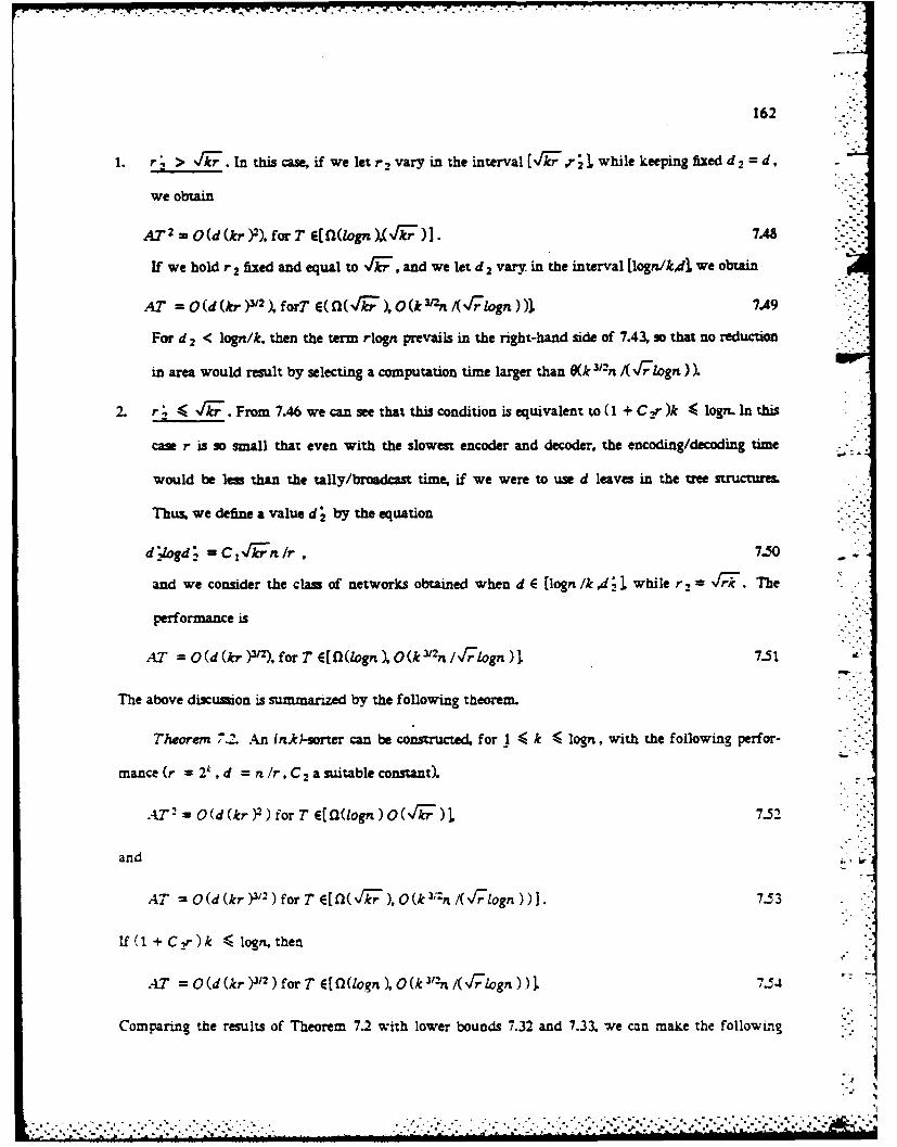
162

r' > Jr .ln this case, if we let r, vary in the interval [-rr "while keeping fixed d 2 d,

we obtain

AT 2 = 0(d(kr)2), forT E(n(logn),(kr)]. 7.48

If we hold r 2 fixed and equal to VW, and we let d 2 vary. in the interval [logn/kdl we obtain

AT = 0(d (kr )31 2 )forT E(n(fkVr 0),O(k -n/(t ogn))9 749

For d 2 < logn/k, then the term rlogn prevails in the right-hand side of 7.43, so that no reduction

in area would result by selecting a computation time larger than (k 31-n /Jr logn)).

2. r 4 < 9. From 7.46 we can see that this condition is equivalent to (I + Cr )k < logn. In this

case r is so small that even with the slowest encoder and decoder, the encoding/decoding time

would be lea than the tally/broadcast time, if we were to use d leaves in the tree structures.

Thus. we define a value d; by the equation

d ogd C, V n/r 7-50

and we consider the class of networks obtained when d E [logn/k41. while r, r-". The

performance is

AT = O(d (kr )312), for T E[(l(logn ), O(k 3'n Iffiogn )I 7.51

The above discussion is summarized by the following theorem.

Theorem 7.2. An (nic)-sorter can be constructed, for I ( k 4, logn, with the following perfor-

mance (r = 2', d = n/r, C 2 a suitable constant).

AT = O(d (kr )2 for T Et 0(logn) 0 (v 7) 7.52

and

A = O (d (kr)312 )forT E [(l ), 0 (k 3::n//TIrogn))]. 7.53

If (1 + C )k 1ogn. then

AT O(d(kr)312 ) forT E[fQ(logn ),O(k 3 2n /(rlogn))] 7.4

Comparing the results of Theorem 7.2 with lower bounds 7.32 and 7.33. we can make the following

*1

r 163observations. In the range of computation times where the governing bounds are of the AT 2 form.

* there is an 0 (k )gap. In the range where the governing bounds are of the AT form, the gap is instead

0 (k 3 /2).

In fact,. when manipulating multisets of r keys, in the form either of lists or of distributions, our

circuits function on an 0 (kr )-bit representation of the multisets, where 0 (r ) bits are sufficient from

an information-theoretic viewpoint.

One potentially useful modification is the use of sorter for medium-length keys, since encoders

and decoders are based on (2r.og(2r)s.. However, this would create a new problem. that is once

we keep the multisets of size r encoded with 0 (r) bits, it is not immediate to see how the multiplicity

of different multisets can be tallied.

Remark. The network described in Section 7.1.3 can also be laid out with all the 1/O ports on the boun-

dary. A simple analysis would show

*A 0 (d Iogd r n + rlogn) 7-55

* and a result analogous to Theorem 1.2 can be obtained.

~'SORTERS FOR LONG KEYS

In this section we derive upper bounds for the (n.k)-srting problem when the keys are long, ie-

when k 2 logn.

We summarize first whiat we already "now about the problem. The case of word-i-ocal protocols

* is easiiv taken care of. In fact, it is not difficult to realize that all const.-uctions proposed in Chapter 6

achieve AT 2 = Gk 2n 2) on keys of arbitrary length k, thus attaining the A4T 2 =l f(k 2-,) lower

bouna f Theorem 4.13.

Thus. we turn. our at-.ent.,on -o nion-word-local protocols. it is uiseful to deitne the ;uan-:.t::

A u'.

.................... .. . . * .. . . . .

... .. .. .. .. .. .. .. .. .. .. .. I h ag fcmuaint sweetegvrigbud ar of *h AT . " for

. tereLsan ( :)ga. I te rng v'er ... g.ering.ondsar.o......fo.,.hega....nsea

..... (k z. . . . . . . . . . . .*. * * .* . .

.'. .. . . . . . .. . . . .. .f.... mnpltn uis frkyintefr ihr fI o d....uton, u

,.A rut.ucino n k)btrpeetto o h ut~es hr ()bt r u¢etfo

.. -. A . -~- ..-.. . . . .

164

which, as we shall soon see, plays an interesting role in the sorting of long words. Considering that k -

dlogn, the lower bounds obtained in Theorems 4.18 and 4.19 can be respectively restated as

AT2 1 0(dWloon)2) 7.57

and

AT= l(d (niogn ). 7.58

Furthermore, Theorems 4.20 and 4.21 tell us that

A = 0 (nIogn) 7.59

regardless of d (or k), and

T = (logn +logk = (logn .logd) 7.60

The performance of known constructions discussed in Chapter 6 is

.AT = 0(k -n) 0 (d 2 (niogn)2 ) 7.61

as we have mentioned above. Comparing bounds 7.57 and 7.61 we see that there is an 0 (d) gap so that

the known designs are optimal only if d = 0(1). The general case, when d increases with n,. needs

further investigation.

We shall present a new design of an (n)-sorter whose performance comes very close to the lower

bounds 7.57 and 7.58.

-7.4.1 A Non Word-Local Sorting Algorithm

From the preceding discussion. it is obvious that to improve the AT " - 0 (d 2 (nogn )2) upper

bound we have to resort to non-word local algorithms. Moreover, the form of the lower bounds, which

are linear in d, suggests the decomposition of the problem in d subproblems, whose solutions are corn-

bined with small information exchange.

The approach that we shall follow consists of decomposing the keys in blocks of consecutive bits.

and then processing together the homologous blocks of different keys. A similar approach has been

. .. . .. . . . . . . .

165

considered by Leighton.' Some notation will be useful for our discussion. (Refer to Figure 7.6.)

For simplicity we assume that n - 21 (so that Iogn = Y is an integer) and that

k d Logn = d t,. for integer d. We observe that to require that k/logn is an integer is not a serious

constraint, since we can always comply with it by adding less than logn bit positions to the keys

without changing the input size significantly.

With the above assumption,& we can partition each key into d blocks of consecutive bits. We

denote the h-th (least significant) block of key X, by

X; (h) =X. (h I)- ... Xih , 7.62

for h = 0,1...., d -1. (See Figure 7.6). A similar partition can be also considered for the output keys,

defining

k

(h+1)a' Iha'"I " n -1 .

n Xj Xi(h)

X(h)1

E._._ 0orne ___cla__re for -_________

Fz-e' . ,ome.,,.ature for ,nt, ut d±ara.-"

-- . *.........***-* * * .'* . 9 -

.................................................................................

A '~ *. .- - . . . . . . . . . . . . .- ". .1

166

Y, (h) y. (h +) - I ... Y, . 7.63

It is obvious that, for given h, (Y 0(h ),... ,Y - 1(h)) is a permutation of (X O(h ), 1,X, .(h)). This

permutation is functionally dependent on the values of the bits in blocks h. h+], ... d -J, as we have

already seen in Section 4.2, where the information transfer caused by this dependence has been infor-

mally called *secondary fLow".

The rank of key X, in the multiset {X ,, is the number of keys in the multiset that are

strictly smaller than Xj. Formally

rank (X,)={j :Xj < XII. 7.64

The following property of the rank is very useful for us. Suppose that each key X o,.., X-I is

viewed as the concatenation of three strings, namely

X = L,* Ci R-

where * denotes string concatenation. Moreover the number of bits of L, is not a function of , and

similarly for Cj and R,. Then if we define

rank (C 1)= I(j:C1 < Cjl 7.65

and we view rank (C) as a binary string of u bits, we have that

rank (X,) - rank (L,* rank (C,). R,). 7.66

Equation 7.66 follows from the fact that X1 < X, if and only if

L. rank (C1 )* R1 < L. * rank (C,)* R,, whose proof is almost immediate.

If we consider the decomposition

X,= X, (d-) ...-1 X, (h)..... X, (0)

of the input keys. and we repeatedly apply Equation 7.66 we obtain

rank (X,) - rank (rank (X, (d-l))*...s rank (X,(h))* ... * rank (X.(0))), 7.67

which. in words. says that the rank of the concatenation is the rank of the concatenation of the ranks. . -

.. .. . . . o , . . . . . . . . .o o., . . •.-.,.•. .- o • " - .. . .o*.... .....- %*°. %

L-167

This property allows us to reduce the computation of the rank of long keys to the computation of the

rank of small substrings of the keys themselves, but we do not know yet how to compute the rank of

the substrings. This problem can be solved by the following procedure, which is based on sorting.

W(i) (TEND) To compute the rank of the elements of IX oX .... , -,I form a new set of keys

= * i , i = 0,.... n - where i is represented with v bits.

(ii) (SORT) Sort . to obtain a sorted sequence -- ,...F - Then

where 0r(), ... ,7r(n -1) is a permutation of 0,..., n -1.

(iii) (RANK) Compute rank (X (j)) as one plus the maximum index j such that X (j I < X 1 , If

no such index exists, then let rank (X )) = 0.

(iv) (EXTRACT) Form a new set of keysZ, = 7r(i)s rank(X, ,))* X ,,)and sort IZ. .

to obtain the sequence (Xc.... X -1)where = i rank (X:)* X,.

Example. An example will illustrate the ranking algorithm. For simplicity we use digits instead of

bits.

(X,,...X 6) = (7,6,1,4,4,7,9)

(X.* 0,.... Xb 6) = (70,61,1 43,44.75.96)

(X AO * 17(O), .. X K6) * r(6)) (12.43,44.61,70.75,96)

"" (X .I..0 ,X 6)) = (1,4.4,6,7,7,9)

(rank (X ran X (X 6) - (0,1,1.3.4.4.6).

Once 'he .an-ks have been computed they can be used to sort. each of the blocks (into which the keys

have been partitioned) independently of one another. Indeed. if

- '* = ."~nk (X.) X,(h),

,.- anc ,W ... W. - ) is the sorted sequence corresonding to -V... ....-. then it is easy to see that

• " = ,rc.rt (1", i, Y:. ( ,. ..'

. . . . . . . . . . .. . . . . . . .

- -- - - - - - - - - - - -

168

Summarizing the preceding discussion. we obtain the following divide-and-conquer sorting algo-

rithm

1. (DIVIDE) Decompose the input keys XD,. X,-...1 into d blocks of v logn consecutive bits each,

so that =X,(d-) ... X (h)* ... *X, (o).

2. (SUBPROBLEMS) For each h-O ... d-1, compute rank (X o(h )).....rank (X,. _(h)) with respect

to multiset IX o(h -... .- (h )}.

* 3. (MARRY) Compute the ranks of the Xi 's using Equation 7.66. More specifically, with the simpli-

fying assumption d = 2 b, we compute the right-hand side of 7.66 with a fully balanced tree of

operations. Each operation has two input sequences and produces as output the sequence of the

ranks of their concatenation.

* 4. (ROLTE) Replicate the sequence (rank (X ),... ,rank (X, -/i ) ) d times - one for each block -

and sort the sequence (rank (Xo0 )* X 0(h),...,rank (X,.-.1)* X,._(h)) for h -0.1 ... .d-1, to -:

obtain the seqence (rank (Y o) * Y o(h ),...,rank (0Y, -1) Y. -.(h))-

5. (OLTPUT) Obtain the output keys Y0 ,...,,_ asY, = Y,(d-1) .... ... * Y,(0).

The algorithm we have just described has a shortcoming. In fact all the input keys must be read

.. (step 1) in order to compute rank (Xo),... ,rank (X. -1) (steps 2 and 3), and no data can be output until

* step 5. This shortcoming can be eliminated by modifying the algorithm according to the observation

that to arrange in the correct order the bits of a given block it is sufficient to know the ranks of the

blocks of greater significance.

We can proceed as follows. For simplicity, let d = d id,. Let us also denote by X(h) the portion

of the array X corresponding to the h-th block of the keys. (The rows of Xfh) are X )(h ), ... .X,_ _ (h ).)

Then, we organize X (d -1),X (d -2),.... X (0) in a d xd, array with the index of the block in row-

' major order (see Figure. 7~.7). - "

.'.. *.'-.... .. .-. *. ,. •-. .- . . . . . . .... . .. . .-.. ..- •. . . * .. . .

169

d, blocks

X(O) X(1). X(dr4)

wavefronts

Xfd-d 2 ) Xld-d2 +1) . . d-1)

Figure 7.7. Organizing of the input for the pipelined sorting algorithm.

We propose a pipelined sorting algorithm with d1 wavef ronts of data. each of which is a row of

the array just defined, and consists of d, blocks.

* The topmost wavefront is processd exactly as described in the nonpipelined version of the algo-

rithm. However, the ranks computed at step 3 are stored for later use. In fact for the second wavef ront.

once the ranks are computed they have to be further concatenated with the ranks of the amrs wave-

front, and the ranks of the concatenation wvill drive the permutation of :he data in the second wave-

front. The computation proceeds in a similar fashion for the remaining wavefronts.

7.4.2 The Network

We zow desc-ibe a network cacable of executing -he nirtlined version of the sorting a lgor::h.rr

: esc-ibed above. with eiffcient area-time performance.

170

Figure 7.8 shows a high level representation of the network consisting of two tree structures and

a family of linear arrays, whose interconnection and nodes are to be described in the following.

" (a) The ranking tree. This component is a fully balanced binary tree on d 2 leaves, and d 2-- internal

nodes. Both the leaves and the internal nodes are essentially sorting modules with some further

capabilities to compute the ranks of a sequence, although a leaf module performs a function

'I,.

d2.

T T .7.'

Figure 7.8. Structure of the network for sorting a set of long keys.

*guTindwoo IS-L jo f£zoal.t Oaiflt~udWoo

v jo iuamdoIaAap olp oz ainqTjiuoo lp taqi iM adotq osle *M& So[I aq2 pm plog Iaqlour

91 a.121P 2JXAw SP.zo0..x JO SUT2JOS to SinSgzat alyq aginos oi paou. swolqojd taxo azS Im ol Injun aq

gl~n mpA sxswtp stin ui poonpomn sidamwo er.= p~u pur '~nvtuo~, 'punoq-atol eu

wjtU~3flpJ1 MAj JO £.zOGin -r'Iuz.as~ Pt lwarjo

103 adoq aiqvuomie v si awnl 'swaqoidtazqio jo uoonnias alp .zoj wazrnujbalp ul m sdoid iSs= IA

u!r pacn &7rzo%au aqi jo osle u i s! a~~ zr e~p er Lni sql 'Au.=v .uq aql

sein~nis otsuq aarti jo siuwdol*Ap go POADIA aq tua WC 30 fly'S~oMC %1Jwou &o 92!A it pa1CppSoo

2AWR Ca qgnoqiW- iiseti sit1i ui pouviwuxe £CIJos jo spuflj jUCAas alp jo aiueTiue exp uo SunLo

Aq apim aq os~r uuw uoTmndmoo IM £03 wssomv TwuJaS Jo IUoflAjasqo gutisazmn amos

*Siuos jo.&2!xejdwoo swm-uaqsi jo uonpvzr~m

-3=zqo M eijdmo o~ cappo.u s! -1oA& toqiunj ivq Sunuip 'puo .z1o onjm-eznbs *tD iAq

sw EI*AI n PSAt vim Aoqv RI~ Sq pOMsSgns esoiD uuqD .zeSrv £!1IR2!s an L £idtqo jo spunoq xaddn aip

'pnpul -maqi umqo (n papeeu uorD jo japzto um os2 jo mm it aav smulqoidqns alpi oi suoiinjos oqi

aunqmao ca sou.nossaz ouri-vav aip %vqM swnsu it .snuwq aiuunxoazddv Kluo st M.Sx~ul *Aoqtv aqj.

SIl

..................................................

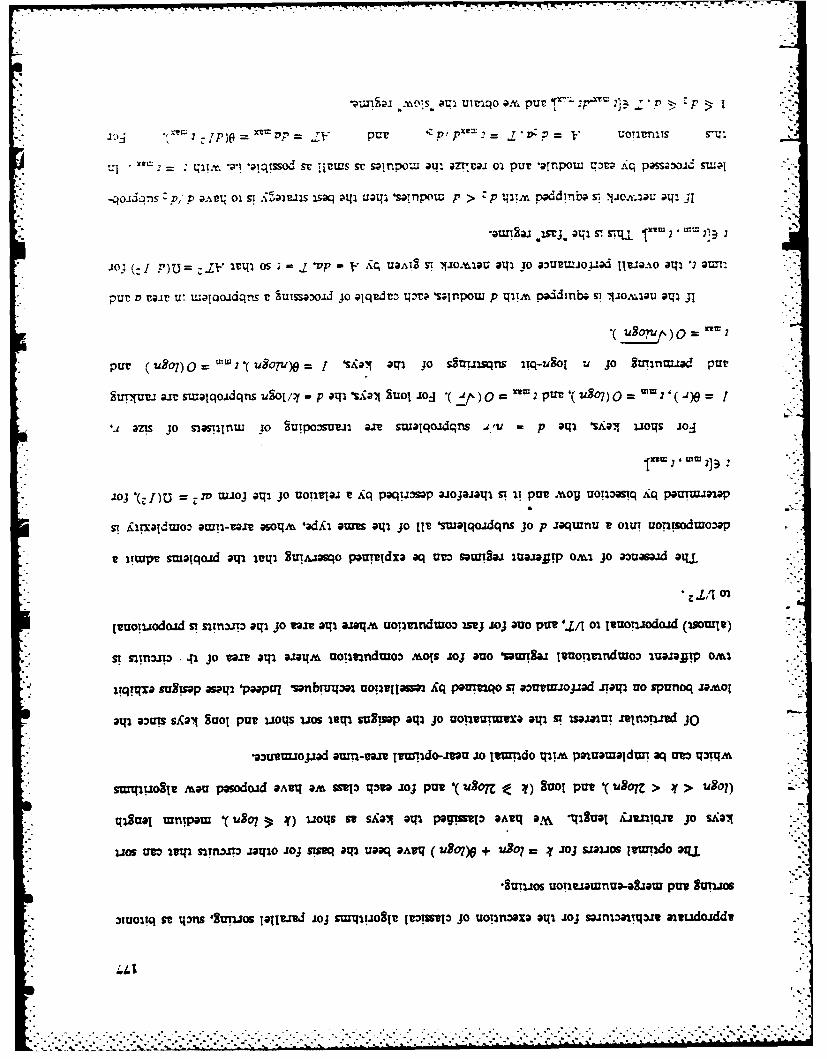
.cs.( aU7m iulmqO a. Pur :'P" 21Z z '

2 1F pu ,/P":2 oLv,=' UO!TflXIS Sk,

q2*y 2P- al=so sr -i us sr szlr.pou au, azTuaj oi pur vjnou; pup~ q pmssowti IU

*qljl V.2,; Z) 1"l O ST S'WlIZ.S 152q tP1 Ualul 'nPOt p > p tpopddinbp s- -jcal 114 A

-Q=22.1 .=J. alql r SID, noz 2 .* x 21~ 1

.I0 (4 P) U ClI I41 Os Z 'v V y .j UaA1s 5 SToxl ail 10 a 1u~-.Oj.d l1ria-tO atl '2 awl:

* put V aitr4 u! tuaiqolidqns r Suissa:)oai jo al tt -r, ;Irnpou p iqtA% paddinba si O w1 j j

* put! (2.40) 0= UI 2'1807Lf)e I J iw SAqI jCp JOsgtZsqn2S iq-tigoi u jo SuTmiad par

SuT-fur-i air stcalqo.1dqns ugol/' p iqi'sS 2 Suoli .og *Q 0 = 2 PUT'(u807)0 = 2 '(100 1

.i zis lo sisnu jo StZipo~Simi ant swalqo.1dqns .,u. p aq si 'SA J 1lls 10o

.10i (r. 1) uj iv tuI.og ai jo uonviaiz r iq paCjiflsap a.Ioy~a1ai s! v parut ouj uo:~omq tAq pau~tn.1.1p

&7 iirwdumo atut-trur noim 'ad.K aus axii jo l~ %wax.qojdqns jo p .zaqwnu r ounr uonrsoduo-vp

r liuxpt suzlqoid atli ivi Stn .wsqo paurltdxa aq um~ sauWISS mu.aap oi&i jo aouasaizd atU

1-cuotuodoid ms-in=3.n atp jo ri air anti.,& Uo!tndwoo 2=tj toj auo PUT ', 0.L1 oi uon.odomd (usonr,)

* gy s~tn~.o 1 jo t.Zt ali1 u.W14M uotlinnduzoo xors tioj auo vunsalx liumo1ndmoo iu..zajTpo

iuqqrax su2LQsP as2 'paapt vanb~utp.1 uonvIrIa2 £q peumo s7 e"uvajooad rteq2 Uo spunoq zauol

21D90 TS alj SUOt PUT U04S U.OS WED~ SUS!Mp aql JO OUITlUT~lVIa NPf S! MM~hUT Jtmlnopivd jo

.gouvmuuojjad aum-vm zu !wido-.mu .o Iumndo tp;,i pva amaidw aq am~ q~tqA

SMID!1o82 MAOU pesdo.Id aA3Iq OX 03~ IWU .10 PUT '(tdO7Z JE 71) Snot put '( tor 7 > ly> U201) -

qlsual tumpax (u8ol !p Z) U.104 ST SX2iO~ tR P2POI *A~q 2M -igSuai t.Zintqz jo s.A~x

Ins UtW IM S21fl.1T .1S40 .10 SISI Mq Uaq vAI4 (1427)0 + u2O7 -y Zri sm0 S.os IvwTdo aqjL

*SUaOS UOnutiatnua-aslzew PUT BUrUo

Oiuolrq gotm q s 'Smuos iltt'w'd 103 mSU41olOr tt'!'Po j0 umoa~1za aqi to03 saxmm7~T4q aivudoiddv

at~;i mopa~p t~q *sauni uo!1Unduwoo Inj~Wut1U jo a~uw aamua at ui slwauo jrumndo Pauhxsav

~-'-%4 ~a\ -anr-PT M~A 219 ui uoilualt 0jquuap!SUOD JO 121.12 aq otl'l~ '(U2o7)e + U207 -y

s' Soua 1 a-j alp waip 'Simlos U1o6 arm Irad r jo AX1s Ilj.iw v tf~t~ un a Ariq D..

*sunoq .zaddn o,. uopuauri.no p~uini QAVE[ am sanbTU

* -tpai punoi-.iaol ino Xq painidro amt uotimndtwo3 ai jo si~adse iutA;lai 2!1p Ila toq aO s o 0

irtli os -*suo msj u! s~tuxuOP iauuoj at alpqi% suoitmndwoz %ols in s22ruTuop .1222il 2tu.J *pQU!tqo

aCj woo piinoq LV ut pur .Lv we tioc 'Splo.A suoi JO SUmxos put w6&P uoiqs jo Smu.os '13~qs *

sm igmis sm;lqomd otp~ads moj ;mm LV' atp no sptnoq waol sp1a!g uoT uwzrnu Jo asnt.-q uopulflam

L'J fl8 812D aq pasu?13xa UOItUUojUT 0143 jo SUJS1uTM DIU -ar1S Litmodwlt £03 murl S1 01 flOTllr

-mo0jin aiuos spuan put -Uounnduio3 ag Suunp suoptroo Ljom sit dn szli s!oemowd o&w atp jo auo

uaqA% saznooo -uoTIInve se 01 paaw pt -awU =gJ aD £03 ajaiq p&.Wptuo3 'wspC43atWtaouv

-am13Jau 1uauna ot jo Isocm uT

auop s! i! so I~ nj, jo su0Ttlri3 1Ut2suoo ant 2v1 wU jo salIvA 01 uo!iu8113 O!i1 Sullrla uviT~ .12!11W 'J jo

U0T13ufl3 r sr I 30 a3£~uI3Us otfl 8tua3AU1 01 l 1uam smo~q 1!'nXa *punoqtao uISMO ISqi b~1saATS

a-t0Jamp pq Pu,'W( zu,. IsearW!XK 131q1 wt jo onleA v st aq% Watqojd Iq3 10f4 (W/( Wk~ 1)0 =3 ZLV

so poals eq uUw punoql u0!lllb m bs ati 'uoT1VIou v'l 'i!A , £.qo Mi on pou~mm amz ui-jy I

pur tommd euo o-i pouun m )% jo sojquuuA w uaet sjome~od oxi Mq £q paguvq~x* uonvmmIjui

urnw r i (Ut/f £q souap ax 'japTSuoD o2 3a& ax sajqITlA / oa 30as aip s! yL A1 *izoaaod zaiqlo

aiII jo salqiuiA indwz aip jo suon~unj am tzom~d DUO JO 3CQIUIgA indlno arqi jo otuos uaqA& iuad

q ST iuCIuo.RAua moSSmid-oxi exp ! LToqv O Iw UAas Aq pmvtSmaAu! &I*A!Suvzxo 'wuewo au

-aguvq~x uotiuuuojm ei~ lSmozoj wmirpo ituuollivnduto~ .oi uodn spuadep anbTu

-itC1 UOuvjo CITI MR pOU!MCqo SpUnoq 241 JO wJOJ 0411141 U29q 334 BUTp~ ku!s0£1u! gZa y

wpunoci .WSuo= qonw S=PTA

-oid i1 '(s£0410 fCu= f£cqqojid put) spiot Suo j o Sumuos pim 'Epiox 2Jo3 jo lupios lij.4 *fTC~e

91.

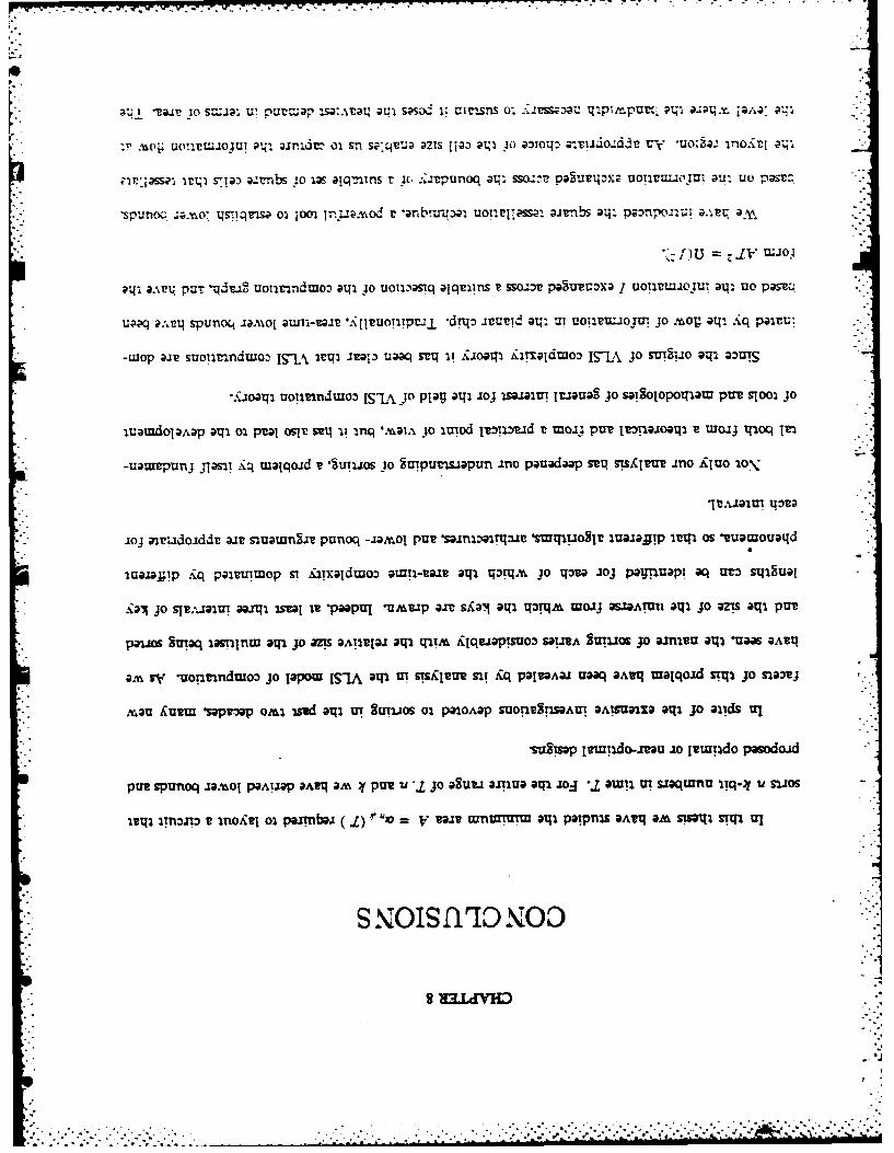
-r oao. u0%!1T!U.IOjUT al~ a.'nd= 01 sn sivcIvu; azis tliZ pr4i I() aCvu1O1d~ IJO :-, 3 lflOtq a;;

iwpsw m i I) a -tbs 4o ias aq--ns r ic. o-,rpunoq aq: sso:-- oeSu~y4ZX; UOTIMvU0ioU- aU Uo , r

-s AV pt urnonwo iet- %od ro~e~ -ari qe1~i n V al air.1 bs patu tneJ ouiu a.142 ao y

-Lwop air suonrandtuwo jn-1. irtr rra,,3 uaaq silt vr 9.ioai4l i&iadtuoO Ig-ixj sJOll S~Oi3ta 3w

So uoTitnJtuo3 ISIA J0 pa 3141 i03 ISCIatT Tt.Iuag jo sig0Ip1TlatuUT loo S1jo

'lUDCldO3A~lp aeql 0o1 P~a oslt sq ii inq 'M~Jo lulod jwjinid r moitj pur jwaoq v uwo.; trfloci I

-uurpunj jgmi S q aialqoid r 'Sutuos JO StnPU1rLpufl ino pauadaap srq MtsSrur ino iquo -i.

-. iCIun UnaC

* .zoj eariadoiddr a~ir swau3n~ar punoqi -at~ol PUT 'sum eirtpu Vrtliuo v uaijCDp ir14i os 'u3Louaqd

2ue.wipp Sq pa:nui~op si hJrxaldwo. atun-van t *2 qarqAM j0 xjtC o10 Pognu~p qU~ 4O

* ~ jo JOslijauIU 331142 iscal i paopul ThM&wp a1m sga,3 a42 ttPti4& moij wuoAmnT o11 j0 OZ!S 3142 PUT

* ~paum Sineq iarlnnz Olf jo a=I aAUiS.1a aiji tlit &jqzLaP!suo3 s3LflA Suuo2Ks 0o azniu alil 'u3s QA31

a, rV' -uontinduioa jo lopow ISIA atp v! qsAI3ur nt Sq P0t33A31 U33q 2At14 malqoid nip~ jo S-4alvj

* ~ xu gurm -,api~p oxi )S-d 3142 u7 &11210S 0 p3oiAap suoKt~drAUn DAIISXD aqi jo alids ul

=Imrsp lictudo-inu .zo Itwldo pasodo.Ld

PUT SPUnoq .w.'Aoj PaALI3P DA34 OAM -Y PUT Ui ' jo aguLI ainuo at42 to_4 -, ouni tU sjauqwnu iq-;yj u ws1

13112 ITT13ZT v inofl o2 pumTi j) r I' 1V van3 tununuim 3142 potPfl2s DA11 Sm~q 5 S1 T1 UI

SNOS i Oois irioNTLO

I I3JAVN

-w~un uot-imndmw alqso jo a amUi al a u! irtunido 2uim st V.L

D t -u pup I y - p suonnmflqns Ja;v~ LL, woij PQUmqD sl RL uotzivlaH -f004

(CL )O,(4 Som LO)J 103 ((.I:Y~)80? l'y)0 v

.2or3uL1O.d Sm.onlo3 air iix paim%=r~uoo aq umtlruioudo V -t-,x uta.Aoay.L

*Aiefloo linual~lu! 2inMoflloj ax splali . mjoa.L '.y p put, 'I ugo ~~IuB1IV-, u

*spuno4 joAo1 all ButAp u! nl!oldxa

uaq iou sueq ii'qi uolipuoo I 'S.upunoq aqi no w.od 0/1 HIL sill paqgmSp aAIvl a twwIO aqj (

-Suruonium tipoo& ami unr, ~il3 SmI9 a1~ fO S IAjnqo oK.

(p Sol+ u~oz) U L s! sumi uoT!Uildtuoo uo purioq tjOaol Mq OlriA '( P807-007)0= Aaqo

* ujwsp vsoiuv .rno Iriql s! malqojd waxour 'jpi Mi Mi sopmsag ,&ixeidwoo awn-ugz, aq jo uopMz

* -nzurgomo.ldwoo v umqo oi papaou s! 3,poA& itaqxn; 'sf.2- Snot Sunucx jo tualqozd ai jo si&ru Mq

UTi 4 U-Iaq aAzq UO!1304p iqgu aip niq sdns izqi u LIoTpu! del aq2 jo wzis lirms aqi iiinoqijyv

19.Z ifloir Siu puo~l ujMol (uiolu)U V a1i ai ZU S1Isnoeum

-TinwT uRTvP ST11J -*Aoqu pa*!Iou 1SPi3JlR *A!q am Sa 'Usnp WtAMOls ot i 1C) o sawo~eq pt d l!Jr

Satqorurwiop It3T.& 'd2S(1 uou P)807)0 UTt Si Ull% uB~Olu/ P)OQ !Y0 07ut O)t0 a

J.4 spunoq .za&Ol ptu .zaddn Uwiazaq di (u~olf 21) S07) o p. Sol 0

ul 91 *Jli [ U2O7ld rPSl 07)( 2J&07 p 807) u], £ 104 SUoflAJ~qO ou !

-Aolo tTO a-Ir a= ai A V!74 put L;- sptoq JaAoi qit& C-4 matoqj. jo sitnsa qi intiudMOC

. a . . 1 7 . ,

-olsc.O .- p~it'at-qo ST Ioi,'maqn, IV ;t!j -p~rg plq S7, T P [mt I () 1o u~C7Lr,

;, tpr. W43 Ul 4; q Umlj pu -OL- uoravnbg 02 8ipio.- !P 1 1 2 02/y0; Z

irq Ytns lp afljrA aq 'p .10j 'OUISot;D tq paUTVICqo ST ~.10Aqlq ZJIV .14 *tA1rig,@s

............ pur qg suoiirnb3 jo suonrjndTUVW1 aldlIi~S uo Pasrq tpnTU~la Si iooiad PtI *x

*~ / P) r(( USO7Jf P~l 0'o)p p2rf 9 J -103 U2O7U)L1~ U8 077J,.. 8'027P)f L

pup

9-1" U31( U r p807)O 0U207 P8o1) U]D 103 rUOW) Pr 207P)O o :.LV

-aUt~iJW ;YMoo Jt 1M127r() 03 'peMWUoD aq uwla.~uos-Qy2J) tr r-.. tuolZa

WOaj0oal SUM&fl0J OIp ixq palm2 se -sitArtlaq

am~pmkia.wU jo uziads 3uzm2siuflr ur si aiatql uSisap 28moTs at puv 1S1S1 Vl2 ua.&ia

-Vq- purioq sa,4aP 1? ii svurnido pnpu! s! u~sop taos srItu

*(227u/' P)O 0=

(U807) 0 V

Kq UDA!I St USrSs sri jo soum~ioped *U jro

-JmTp Lsjrq a4I2 pule opou ajg~le 0m smwuagp a=z q~viM 11110 I p ~pu 0U '( 11074f)Q= qft

P2D31 91 p PPut q tiloq 2Z~tMUTM 01 PaQU 31 'W.M D11 nrwtU!W 01 IUT&at & pPVlSU 31

£LLuso *(87d0)O=U80Z/3Y) 807 U201)O o £ J

PUT

WLL (c U P)O 0 (1 807/r 74 Y)O 0

uTnqo ax flloisniouoz' ul

snqL -v jo iied taasim aip 'K(sln~id aioux 'io

* OL*L (('P U80) o z 'Psolz = p

UOTI

-rnb sq is~s iriq, anIrt ai p 103j ssoop 2.s 'snujL -awn uonl1ndwo: ati jo .lsPio a,41 Ul utn ou si

aaIZp 301 Z Urtil IOIIVS SMO10aq P U~tAk% 'JIA05JIjW -(V97.0S) TMa 2SqI 250jamqtl pt Z- p SMS.Murl p

gumrsUs.IP *ISAS2&OH -Z =p asooip plnoiqs az u. 7 ; = pip 1u1LflS0 2~1 Ipun It pSol Z + 'p

2zTmpTumwoJ/(t)6 q s! agu .lqtwmd iman-uuu tp1 j. ~pSol Z + Tp zTWTUT

01 pUr q 2ZtWTXt'fl 01 aAtMi SMi Vq 1t13 ST i -uonni alqtid mmuj Bafl uI2q0 0a 2x!SP a.& r

#I.tIEui 1o3 -aoddnS -u011!TuX SUIos uiu8 01 .wpio ui sa tuxp.ds sinai suujapzuo sq UILaq 21A

1:(U)o'( U2o~ )U] qpuu U20o1pIP= -ynmui=o~a.

E* lr-v~i *23uvuwoad aum temai s znmndo 01 q pt z p It p .0j s~lv.A al uv~ (a OnWW3.1 1!j

697L q/ U074 p So z+ P)o= .L

S! awuor T~ndmo* jvqojI sq (IlU0.;Am jo .zaqinnu 5211) Itp smid I(adTd

atjl jo qidop 0211) p~ So Z0 oi Iuuodoizd st udsos 3%q jo aqwvtu lvqoiS u iv l2 uspisua3

uOo7 jo aldpItni IWeS vst

q 41ua[ 2oxm s.a5i u 30 m5umnbas fo paruioji.d an3 put 5dS1 2unjzos aip jo ...v1m .1ap1Jl SLiTuo!%nd

-woD ant 2vip suoniuado aiD 'popul t( ")O( u~~u,)U]9 q n~ ip OI.1d Impl (qlUb07Uo V! pau1oj

* -id~ eq t~ s.npowsi~ 3 suon~zsd owuq 52vqi an ca iin si i! '5 uopnndmoo aip ol sV

* 297.(Cqlpsolp)Q= v

a* 511vi 1211 puv 35am 9) ox( q) 0 im aAITI pJotwIu ap jo sS~lpow 2t11v iv a1Ts?1 &oT u MOU

srnmKo3Jd *T±-l.TV M.L

t'pN

;-jW a. c a U!2JO 'C'i4'. P10 I2o pu Salgtal.I -j10'0 UZAIAS2 JO SA-17i :0 PtZuflDas am2 imp -uviIr7.S-

~ ~: ~1O~i~ fl0~flalt tl r-II114T2 inoiqti.A ~A!~ aq s..a2 u:)Tl v

swlnpo~iu1_ IP SOTZ o XrU

:rui c sr pa 3aruo) .;pnq u,. paxoms Iirjodwliai .I )olq ayt jo sA;' alg jr .u ~i su

iaIru a2U i tW2T paoL12.!j2aj 0q2 'l.fl i205-pU upr.q al JO jwl r Aq indui sl 3Doic aurgs

P14 uaqt- aw!i: at~i pur za. Suijurt iq jo jra r Aq indrn st Imlq ei~ utl atuni aq u~aamo

tII~1~oa2 tT jo t- da~s ui paqujm~p sr v~r Butpuods..uoo aqi o2 Stpwp 3 pq u~at-g r 30

* SA'i tT2~UtflU~d t S2ISU~ UtlIedO~!sq T~t is~npot Strtios A11t1 U SA

s~a- at~ 'Onninad T sisux 103ad euo 1jW2 ass 12. 1UJa a Inl

ua,%i le oi Sipuodsaio' maunbas 8uT-42.x atp jo saida3 : ' a~al I$gol ialjv 1142i os aauafbasW

* 0142 50A10301 IT~~~qf, 134M UIJ '00.1 SU!IUU. 014) JO 100.1 0141 01 P713aU'U03S aO341J 010

S0.%al0 p uo oon f-muq pa~uulvq ftlnj e osle m~ uauodwo37 sn14j *as.L. iAoS-puv-JsPpvoig8 v.L (q)

-uos iqguL 0141 kq pw3Tpoid no4i put *uos ijal

* ox iAq ponpozd &7=uuax *12dais sTnotA.tai atp 2 pwindwo3 s-4ur-i 0142 <114~j 01 Ij01 moij) Alamu

'souoibas aaxqi jo u0111u0113U0 aqj s-Arui qtpnqt 'onpotu ioo in tXq pofuld si ajoi lutoods V

*SDPOU

guu~dsgo om.1 atp. tq poonpoid uatbas 0141 jo uon11U013t103 OgTAud Kq pou~uiqo aouatbas

*~ ~ ~ aq 014 uama IO O 31JO S- u1J 041 Suinduzoo ui sisso~ apou t2u.ImU uw jo goTlilodo 3%Iq tUj

* v-iuw~ qnoqi Sutindwoo jo pLIW (q) 1 - uX.. ( qyX y AW *10( U LT SA0S014 2 SUIA 10301 JO W=?00

* 3101~a 2 0o LIoLnlIdo omqU 041 '&l 130ods 01ol, 0anpow apou-ImmIOui Uv io.Ij iua1j.UP tK4142T4s

*~ IW.1

179

REFERENCES[AA 80] H. Abelson and P. Andreae, *Information transfer and area-time trade-offs for VLSI multi-

plication." Communications of the ACM, vol. 23, n 1, pp. 20-22: January 1980.[AG 83] A. Aggarwal. "On 1/O piacement in VLSI circuits," Proc. 21st Annual Allerton Conference

on Communication. Control. and Computing, Monticello, IL, pp. 236-243; October 1983.[AKS 831 M. Aitai, J. Komlos and E. Szemeredi. "An O(nlogn) sorting network.," Proc. 15th Annual

ACM Symposium on Theory of Computing, Boston. MA, pp. 1-9; April 1983.[AUY 831 A.V.Aho. J.D. Ullman and M. Yannakakis, "On notions of information transfer in VLSI

circuits." Proc. 15th CAM Symposium on Theory of Computing, Boston. MA, pp. 133-139,April 1983.

[Ba 68] K. E. Batcher, "Sorting networks and their applications," Proc. AFIPS Spring Joint Com-puter ConferencevoL 32, pp. 307-314, April 1968.

[Be 64] V. E. Benes, "Optimal rearrangeable multi-stage connecting networks," Bell Syst. Tech. J.voL 43, n. 4, pp. 1641-1656; July 1964.

[BG 82] M. P. Brent and L M. Goldschlager, "Some area-time tradeoffs for VLSL" SIAM J. on Corn-put. voL 11. a. 4, pp. 737-747; November 1982.

[BJ 84] G. Bilardi and X. Jin, *Permutation exchange graphs that emulate the binary cube,"Mathematical System Theory, voL 17, n. 3, pp. 193-198; June 1984.

[BK 80] R. P. Brent and H. T. Kung, "On the area of binary tree layouts," Information ProcessingLetrersvoL 11. n. 1, pp. 46-48; August 1980.

[BK S1] R. P. Brent and H. T. Kung, "The chip comple.ity of binary arithmetic," Journal of theACM, voL 28. n. 3, pp. 521-534; July 1981.

[BK 821 R. P. Brent and H. T. Kung. "A regular layout fpr parallel adders." IEEE Trans. on Comp,vol C-31, n. 3, pp. 260-264; March 1982.

[BL 34] S. N. Bhatt and F. T. Leighton. "A framework for solving VLSI graph layout problems." 1.of Comp. and Syst. Sci, voL 28, n. 2, pp. 300-342; April 1984.

[BP 34a] G. Bilardi and F. P. Preparata. "An architecture for bitonic sorting with optimal VLSI per-formance." IEEE Trans. Comp, vol. C-33, n. 7, pp. 646-651: July 1984.

* [BP 84b] G. Bilardi and F. P. Preparata, "A minimum area VLSI network for O(logN) time sorting,"Proc. 16th Annual ACM Symposium on Theory of Computing, Washington. D. C., pp. 64-70: April 1984.

4BP 84c] G. Bilardi and F. P. Preparata. "The VLSI optimality of the AKS sorting network," In 'or-marion Processing Letters, to appear.

[BPP 32] G. Bilardi, NI. Pracchi. and F. P. Preparata. "A critique of network speed in VLSI models ofcomputation." IEEE 1. of Solid-State Circuits, vol. SC-17, :. 4. pp. 696-702: August 1982.

SES S-41 G. Bilardi and M. Sarrafzadeh. "Optimal discrete Four:er transform in VLSI." nternationaiWorkshop on Parallel Com ting and VLSI. Amalfi. Italy. May 1984.

31CM S1 B. Chazelle and L Monier, "A model of computation for VLSI with related complexityresults." Proc. 13th Annual ACM Symposium on Theory: of Computing, Milwaukee. WI.pp. 318-325: May 1981.

, DGS 841 P. Duris. Z. Galil and G. Schnitger, "Lower bounds on communication complexity," Prx.16th Annual ACM Symposium on Thecry of Computing, Washington, D. C., pp. Sl-1:August 1984.

IGHT -91 L. 1. Guibas. H. T. Kung and C. D. Thomcson. "Direct VLSI -mplementation of combina-ronal algo th.ms." P-oc. Conference on VLSI Archizecture, Design, Fabricazwn. 1alid.

L=, af Tecbnr.; ;anuarv 1979.

- .- - ,. L .. . . . . . . . . . . . . . . .,. ..

180

[Jh 80] R. B. Johnson, *The complexity of a VLSI adder," Information Processing Letters, vol 11, "n. 2, pp. 92-93; October 1980.

[JK 84] J. Ja' Ja' and V. K. P. Kumar, *Information transfer in distributed computing with applica-tions to VLSL' Jotunal of the ACM, vol 31, n. 1, pp. 150-162; January 1984.

[KL 78) IL T. Kung and C. E Leis-rson, "Systolic arrays (for VLSI)," Symposium on Sparse MatrixComputations, Knoxville, TN, pp. 256-282: November 1978.

[KLLM 83] D. Kleitman, F. T. Leighton, .NL Lepley, and G. L Miller, "An asymptotically optimal lay-out for the shuffle-exchange graph" J. of Comp. and Sysz. Sci, voL 6, n. 3, pp. 339-361;June 1983.

[Ki 83] V. K. P. Kumar, Communicarion Complexity of Various VLSI Models, Ph.D. Thesis. Dept.of Comp. Science, Penmsylvania State Umversity- August 1983.

[KR 82] K. Keutzer and E. Robertson, "The M-shuffle as an interconnection network for SIIDmachines,' Proc. of 20th Annual Allerton Conference on Communication, Control, andComputing, Monticello, IL, pp. 264-271; October 1982.

[Ku 82) H. T. Kung, 'Why systolic architectures?' Computer Magazine, vol. 15, n. 1, pp. 37-46;January 1982.

[L 81a] F. T. Leighton, Layouts for the shuffl,-exchange graph and lower bound techniques, Ph.D.Thesis, Dept. of Mathematics, MIT, August 1981.

*i EL 81b] F. T. Leighton, 'New lower bound techniques for VLSI: Proc. 22nd Annual Symposium onthe Foundations of Computer Science, Nashville, TN, pp. 1-11; October 1981.

EL 82] F. T. Leighton, 'A layout strategy which is provably good," Proc. 14th Annual ACM Sym- ".posium on Theory of Computing, San Francisco. CA, pp. 85-98; May 1982.

EL 83] F. T. Leighton, 'Parallel computation using meshes of trees,' submitted for publication.

[L 84] F. T. Leighton, 'Tight bounds on the complexity of parallel sorting.' Proc. 16th AnnualACM Symposium on Theory of Computing, Washington, D. C., pp. 71-80: April 1984.

[Lo 83] M. C. Loui. "The complexity of sorting on distributed systems," Tech. Report ACT-39,Coordinated Science Laboratory, University of IllinoisUrbana, IL; September 1983.

[Is 80a C. E. Leiserson, Area effizient VLSI computation, Ph.D. Thesis, Dept. of Comp. Science,Carnegie-Mellon University;, November 1980.

[Ls 80b] C. E. Leiserson. 'Area-efficient graph layouts (for VLSI)," Proc. 21st Annual Symposium onFoundations of Computer Science, Syracuse, NY, pp. 270-281; October 1980.

[LS 81] R. 1. Upton and R. Sedgewick. 'Lower bounds for VLSL" Proc. 13th Annual ACM Sympo-sium on Theory of Computing. Milwaukee. WI pp. 300-306; May 1131.

[Me 83] K. Mehlhorn. "AT - optimal VLSI integer division and integer square rooting," submittedfor publication.

[MC 791 C. A. Mead and L. Conway, Inzroduction to VLSI Systems, Reading, MA, Addison-Wesley; July 1979.

[MP 75] D. E. Muller and F. P. Preparata, "Bounds to complexities of networks for sorting andswitching," Journal of ACM, vol 22, n. . pp. 195-201; April 1975.

-MP 831 K. Mehlhorn and F. P. Preparata, ".Area-time optimal VLSI integer multiplier w::hminimum computation time," Information and Control, vol. 58, nos. 1-3. pp. 137-156: Julv1983.

* (MS 82] K. Mehlhorn and E. M. Schmidt. 'Las Vegas is better than determinism in VLSI and W. :-buted computing,' Proc. 14th .4nnual ACM Symposium on Theory of Comptini,?.Francisco, CA. pp. 330-337; May 1982.

. .

....=. '...-.. ..---...... "m .... ,. ..... ..........

FAD-RI61 562 THE AREA-TINE COAPLEXITY OF SORTING(U) ILLINOIS UNIV OT 31'3

URBANA APPLIED CONPUTRTION THEORY GROUP G BILARDI

DEC 94 RCT-52 N98114-84-C-S149UNCLASSIFIED F/O 11 NL

- * -• - - .- -. - _ - -_. : - . . . . o . - ° - o.. .. _:" - - : . - . , . - .-

-tL 2.2 -

zr

ILS>

o.

11111L

MICROCOPY RESOLUTION TEST CHART

NATIONAL BUREAU OF STANDARDS - 1963 - A

RIP.

.77.

181"-,

[Mu 82] S. Muroga, VLSI System Design, J. Wiley, New York: 1982.[NMB 83] D. D. Nath, & N. Maheshwari and P. C. P. Bhatt, "Efficient VLSI networks for parallel pro-

cemng based on orthogonal trees, IEEE Trans. on Comp, vol C-32. a. 6, pp. 569-581;June 1983.

ENS 79] D. Nasimi and S. Sahni, "Bitonic sort on a mesh-connected parallel computer: IEEETrans. on Comp., vol. C-2& n. 1, pp. 2-7; January 1979.

(NS 821 D. Nasimi and S. Sahni. "Parallel permutation and sorting algorithms and a new general-ized connection network. Jownal of ACM, vol. 20. n. 3, pp. 642-667; July 1982.

[P 78] F. P. Prepamrm, *New parallel sorting schemes, IEEE Trans. Comp, vol. C-27, n. 7, pp. . -

669-673; July 197&"[P 84] F.P. Preparata, "VLSI algorithms and architectures" Proceedings of 11th Symposium on

Mathematical Foundatins of Computer Science, Praha, Czechoslovakia; September 1984.

(Pc 77] .L C. Pease, "The indirect binary n-cube microprocesor array," IEEE Trans. on Comp,vol. C-26, n. 5. pp. 458-473; May 1977.

[PS 84] C. H. Papadimitriou and M. Sipser, "Communication complexity," I. Comput. System Sc..,vol 28, n. 2, pp. 260-263; April 1984.

' (PV 801 F. P. Preparata and J. Vuillemin, "Area-time optimal VLSI networks for multiplyingmatrices," Information Processing Letters. vol 11, n. 2, pp. 77-80: October 1980.

[PV 81a] F. P. Preparata and J. Vuillemin, "The cube-connected-cycles A versatile network forparallel computation," Communications of the ACM. voL 24. n. 5, pp. 300-309: May 1981.

[PVS1b] F. P. Preparata and J. Vuillemin, "Axea-time optimal VLSI networks for computing integermultiplication and discrete Fourier transform." Proc. of I. C. A. L. P, Haifa. Israel pp. 29-40, July 1981.

[Sa 79] J. E. Savage, "Area-time tradeoffs for matrix multiplication and related ,roblems in VLSImodels," Proc. of the 17th Annual Alerton Conference on Communications. Control andComputing. Monticello, IL, pp. 670-676: October 1979.

LSe 79] C. L Seitz, "System timing," in Introduction to VLSI Svtrems, C. Mead and L Conway,Eds. Reading, M.A Addison-Wesley, ch. 7; July 1979.

[Sg 8-a] A. Siegel. "Optimal area VLSI circuits for sorting," submitted for publication.

[Sg 84b] A. Siegel. "Tight area bounds and provably good AT 2 bounds for sorting circuits." Tech.Report #122 Courant Institute, New York 'niveruity; June 1984.

[St 711 H. S.Stone. "Parallel processing with the perfect shuffle," IEEE Trans. on Comp. vol. C-20.n. 2. pp. 153-161: February 1971.

*T SO1 C. D. Thompson. A compiexiy theory for VLSI. Ph.D. Thesis. Dept. of Comp. Science,Carnegie-Mellon University; August 1980.

IT 53a] C. D. Thompson. "Fourier transforms in VLSL" IEEE Trans. Comp. vol. C-3. r. 11. pp.1047-1057; November 1983.

T 83b] C. D. Thompson. "The VLSI complexity of sorting," IEEE Trans. Comp, vol. C-32. n. 12.pp. 1171-1184: December 1983.

"TK 77] C. D. Thompson and H. T. Kung, "Sorting on a mesh-connec-ed computer." Communications-" o the ACM, -'ol. 20, n. 4, pp. 263-271; April 1977.

US 31 J. D. Lllman. CcmputationaL .4 pects of VLSI, Computer Science Press 1983.'a 81] L G. Valiant. "Universality considerations in V"LSI ctrcuits" IEEE Trans. on CO'Mp. VOi.

C-30, .. 2. pp. 13-140: February 1981.LVu 3] J. Vuiilemin. "A combLnatorial limit :o the computing power of VLSI circxxts." IEEE

:rans. on Comp. voL C-32, n. 3, p. 294-310C, March 1983.

. %. .. .... .. ..... .... .. .-..: .., :,...' .......',..r ..- . '.. ' r V_ 1_ , .'_1 '':..'' .:.,.

182

[Y 79] A. r- C Yao. *Some complexity questions related to distributive computing,* Proc. 11thAnnual ACM Symposium an Theory of Computing, Atlanta. GA. pp. 209-213. April 1979.

[Y 81] A. C r- Yao, "The entropic limitations on VLSI computations* Proc. 13th Annual ACMSymposium on Thaory of Computing, Milwaukee, WI, pp. 308-311.- April 1981.

.*~~ *~.L ~ 9~~*. P1. ) ~' W P * .P 17.v.~.. - -- - -

183

VITA

(ianfranco Bilardi was born in Reggio Calabria, Italy, on March S. 1956. He received the Laurca

in Ingegneria Elettronica degree from Universita di Padova in 1978 and the M.S. degree in Electrical

Engineering from the University of Illinois at Urbana-Champaign in 1982. where he was a Research

ILI Assistant in the Coordinated Science Laboratory until 1984. He was awarded an International Rotary

Fellowship in 1980. and an IBNI Graduate Fellowhip in 1982 and 1983.

-.

FILMED

1-6

* DTIC- .. .,. .