NAVAL POSTGRADUATE

SCHOOL

MONTEREY, CALIFORNIA

THESIS

Approved for public release; distribution is unlimited

OTTER: AN OPTIMIZED TRANSIT TOOL AND EASY REFERENCE

by

Warren Korban Blackburn

March 2016

Thesis Advisor: Emily Craparo Co-Advisor: Connor McLemore Second Reader: Dan Nussbaum

THIS PAGE INTENTIONALLY LEFT BLANK

i

REPORT DOCUMENTATION PAGE Form Approved OMB No. 0704–0188

Public reporting burden for this collection of information is estimated to average 1 hour per response, including the time for reviewing instruction, searching existing data sources, gathering and maintaining the data needed, and completing and reviewing the collection of information. Send comments regarding this burden estimate or any other aspect of this collection of information, including suggestions for reducing this burden, to Washington headquarters Services, Directorate for Information Operations and Reports, 1215 Jefferson Davis Highway, Suite 1204, Arlington, VA 22202-4302, and to the Office of Management and Budget, Paperwork Reduction Project (0704-0188) Washington, DC 20503. 1. AGENCY USE ONLY (Leave blank)

2. REPORT DATE March 2016

3. REPORT TYPE AND DATES COVERED Master’s thesis

4. TITLE AND SUBTITLE OTTER: AN OPTIMIZED TRANSIT TOOL AND EASY REFERENCE

5. FUNDING NUMBERS

6. AUTHOR(S) Warren Korban Blackburn

7. PERFORMING ORGANIZATION NAME(S) AND ADDRESS(ES) Naval Postgraduate School Monterey, CA 93943-5000

8. PERFORMING ORGANIZATION REPORT NUMBER

9. SPONSORING /MONITORING AGENCY NAME(S) AND ADDRESS(ES)

N/A

10. SPONSORING / MONITORING AGENCY REPORT NUMBER

11. SUPPLEMENTARY NOTES The views expressed in this thesis are those of the author and do not reflect the official policy or position of the Department of Defense or the U.S. Government. IRB Protocol number ____N/A____.

12a. DISTRIBUTION / AVAILABILITY STATEMENT Approved for public release; distribution is unlimited

12b. DISTRIBUTION CODE

13. ABSTRACT (maximum 200 words)

Fuel efficiency is a priority for the Chief of Naval Operations (CNO), as stated in the CNO’s Position Report: 2014. While a number of fuel-saving measures have been implemented in recent years, the effects of operational transit speed on fuel consumption have not been adequately understood as a variable.

Ships’ commanding officers use fuel-usage curves to determine the most efficient propulsion-plant speed. Fuel efficiency is typically gauged by maintaining a consistent optimal speed. Often there are combinations of speeds that are more efficient than a constant speed. The transit fuel planner, developed in the Naval Postgraduate School’s operations research department by Brown, Kline, Rosenthal, and Washburn in 2007, calculates speed combinations to achieve fuel savings for a given single ship. This thesis adds additional capacities based upon common principles.

We provide an omnibus tool, the Optimized Transit Tool and Easy Reference (OTTER), with two complementary components: Dynamic OTTER and Static OTTER. Dynamic OTTER is a versatile, interactive transit-planning tool for any ship class that accommodates drill scheduling, a critical feature. The second tool, Static OTTER, is a generic, optimal solution to individual ship transit-speed combinations, in the form of a printable reference sheet that can be used independently. These products are being implemented by United States Navy surface ships and will yield significant fuel savings, equating to additional time on station.

14. SUBJECT TERMS OTTER, fuel optimization, transit fuel planner, fuel savings, fuel consumption, replenishment at sea planner surface fleet, surface action group planner

15. NUMBER OF PAGES

107 16. PRICE CODE

17. SECURITY CLASSIFICATION OF REPORT

Unclassified

18. SECURITY CLASSIFICATION OF THIS PAGE

Unclassified

19. SECURITY CLASSIFICATION OF ABSTRACT

Unclassified

20. LIMITATION OF ABSTRACT

UU NSN 7540–01-280-5500 Standard Form 298 (Rev. 2–89) Prescribed by ANSI Std. 239–18

ii

THIS PAGE INTENTIONALLY LEFT BLANK

iii

Approved for public release; distribution is unlimited

OTTER: AN OPTIMIZED TRANSIT TOOL AND EASY REFERENCE

Warren Korban Blackburn Lieutenant Commander, United States Navy

B.A., Thomas Edison State College, 2003 B.S.A.S.T., Thomas Edison State College, 2004

Submitted in partial fulfillment of the requirements for the degree of

MASTER OF SCIENCE IN OPERATIONS RESEARCH

from the

NAVAL POSTGRADUATE SCHOOL March 2016

Approved by: Emily Craparo Thesis Advisor

Connor McLemore Co-Advisor

Dan Nussbaum Second Reader

Patricia Jacobs Chair, Department of Operations Research

iv

THIS PAGE INTENTIONALLY LEFT BLANK

v

ABSTRACT

Fuel efficiency is a priority for the Chief of Naval Operations (CNO), as stated in

the CNO’s Position Report: 2014. While a number of fuel-saving measures have been

implemented in recent years, the effects of operational transit speed on fuel consumption

have not been adequately understood as a variable.

Ships’ commanding officers use fuel-usage curves to determine the most efficient

propulsion-plant speed. Fuel efficiency is typically gauged by maintaining a consistent

optimal speed. Often there are combinations of speeds that are more efficient than a

constant speed. The transit fuel planner, developed in the Naval Postgraduate School’s

operations research department by Brown, Kline, Rosenthal, and Washburn in 2007,

calculates speed combinations to achieve fuel savings for a given single ship. This thesis

adds additional capacities based upon common principles.

We provide an omnibus tool, the Optimized Transit Tool and Easy Reference

(OTTER), with two complementary components: Dynamic OTTER and Static OTTER.

Dynamic OTTER is a versatile, interactive transit-planning tool for any ship class that

accommodates drill scheduling, a critical feature. The second tool, Static OTTER, is a

generic, optimal solution to individual ship transit-speed combinations, in the form of a

printable reference sheet that can be used independently. These products are being

implemented by United States Navy surface ships and will yield significant fuel savings,

equating to additional time on station.

vi

THIS PAGE INTENTIONALLY LEFT BLANK

vii

TABLE OF CONTENTS

I. INTRODUCTION..................................................................................................1 A. BACKGROUND ........................................................................................1 B. LITERATURE REVIEW .........................................................................5 C. OBJECTIVES ............................................................................................9 D. SCOPE, LIMITATIONS AND ASSUMPTIONS .................................10 E. CONTRIBUTIONS AND OUTLINE ....................................................10

II. MODEL ................................................................................................................11 A. TRANSIT FUEL PLANNER LINEAR PROGRAM (TFP-LP) .........12 B. DISCUSSION ...........................................................................................12

III. THE USER INTERFACE ...................................................................................15 A. DYNAMIC OTTER .................................................................................15

1. Dynamic OTTER Schedule Builder Pseudocode ......................16 2. Time Until Speed Change ............................................................20 3. Dynamic OTTER Output ............................................................21 4. Dynamic OTTER Settings ...........................................................22

B. STATIC OTTER ......................................................................................24

IV. RESULTS .............................................................................................................27 A. DATA COLLECTION ............................................................................27 B. MAXIMUM SPREAD BETWEEN SHIPS ...........................................28 C. TIME TO SPEED CHANGE ..................................................................31 D. ANALYZING MULTI-SPEED FUEL OPTIMIZATION ...................33 E. CONFIGURATION MATTERS ............................................................35

V. CONCLUSIONS AND RECOMMENDATIONS .............................................37 A. CONCLUSIONS ......................................................................................37 B. IMPLEMENTATION CHALLENGES ................................................37 C. FUTURE WORK .....................................................................................38

APPENDIX A. FUEL CURVES .....................................................................................39

APPENDIX B. OTTER STATIC TOOLS ....................................................................49

APPENDIX C. TTSC ANALYSIS .................................................................................61

viii

APPENDIX D. DYNAMIC OTTER VBA CODE ........................................................67

LIST OF REFERENCES ................................................................................................85

INITIAL DISTRIBUTION LIST ...................................................................................87

ix

LIST OF FIGURES

Figure 1. Average underway barrels of oil and time (hours) per ship .........................1

Figure 2. Average barrels per ship and percent underburn annually ...........................3

Figure 3. CG47 class total-ship fuel consumption GPNM vs. speed (with stern flap) ..............................................................................................................4

Figure 4. PIM window example ..................................................................................5

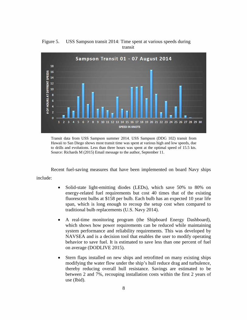
Figure 5. USS Sampson transit 2014: Time spent at various speeds during transit............................................................................................................8

Figure 6. LCS1 class total ship fuel consumption GPNM vs. speed (with stern flap) ............................................................................................................14

Figure 7. Dynamic OTTER input ..............................................................................15

Figure 8. Schedule builder timeline ..........................................................................16

Figure 9. OTTER transit vs. PIM center ...................................................................20

Figure 10. Dynamic OTTER output ............................................................................22

Figure 11. User-defined settings .................................................................................23

Figure 12. Create a new ship type ...............................................................................24

Figure 13. Static OTTER.............................................................................................25

Figure 14. Spread among ships during a group transit of CG and DDG1 ..................29

Figure 15. Spread values for all ship pairs analyzed ...................................................31

Figure 16. Frequency of TTSC across all ships modeled............................................32

Figure 17. Big T (average speed vs. big T) .................................................................33

Figure 18. Average hours earned at various average speeds .......................................34

Figure 19. Detailed hours earned at various average speeds .......................................35

Figure 20. CG 47 class total ship fuel consumption (with stern flap) (GPNM) ..........39

Figure 21. DDG51 FLT 1 and II class total ship fuel consumption (with stern flap) (GPNM) .............................................................................................40

Figure 22. DDG51 FLT IIA class total ship fuel consumption (with stern flap) (GPNM) .....................................................................................................41

Figure 23. LCS1 total ship fuel consumption (GPNM) ..............................................42

Figure 24. LCS2 total ship fuel consumption (GPNM) ..............................................43

Figure 25. FFG7 class total ship fuel consumption (with stern flap) (GPNM) ...........44

Figure 26. LSD41 class total ship fuel consumption (GPNM) ...................................45

x

Figure 27. LSD49 class total ship fuel consumption (GPNM) ...................................46

Figure 28. LHD8 class total ship fuel consumption (GPNM) .....................................47

Figure 29. CG Static OTTER ......................................................................................50

Figure 30. DDG1 Static OTTER .................................................................................51

Figure 31. DDG2 Static OTTER .................................................................................52

Figure 32. LCS1 Static OTTER ..................................................................................53

Figure 33. LCS2 Static OTTER ..................................................................................54

Figure 34. LHA1 Static OTTER .................................................................................55

Figure 35. LHD1 Static OTTER .................................................................................56

Figure 36. LPD4 Static OTTER ..................................................................................57

Figure 37. LSD41 Static OTTER ................................................................................58

Figure 38. LSD49 Static OTTER ................................................................................59

Figure 39. LHD8 Static OTTER .................................................................................60

Figure 40. CG TTSC ...................................................................................................61

Figure 41. DDG1 TTSC ..............................................................................................62

Figure 42. DDG2A TTSC ...........................................................................................62

Figure 43. FFG7 TTSC ...............................................................................................63

Figure 44. LCS1 TTSC ...............................................................................................63

Figure 45. LCS2 TTSC ...............................................................................................64

Figure 46. LHA1 TTSC...............................................................................................64

Figure 47. LHD1 TTSC...............................................................................................65

Figure 48. LPD4 TTSC ...............................................................................................65

Figure 49. LSD41 TTSC .............................................................................................66

Figure 50. LSD49 TTSC .............................................................................................66

xi

LIST OF TABLES

Table 1. Fuel saving techniques and their estimated savings ....................................6

Table 2. USS Freedom (LCS1) with average speed requirement of 19 kts .............27

Table 3. Average spread among ships using Dynamic OTTER ..............................30

Table 4. 90% of time spread—using Dynamic OTTER ..........................................30

xii

THIS PAGE INTENTIONALLY LEFT BLANK

xiii

LIST OF ACRONYMS AND ABBREVIATIONS

BOSC Battlegroup Optimum Speed Calculator

CBG carrier battle group

CG guided missile cruiser

CO commanding officer

DDG guided missile destroyer

DFM diesel fuel, marine

DOD Department of Defense

FFG guided missile frigate

FY fiscal year

GAO Government Accountability Office

GPH gallons per hour

GPNM gallons per nautical mile

HR hour

kts knots or nautical miles per hour

LCS littoral combat ship

LHA landing-helicopter assault

LHD landing-helicopter dock

LP linear program

LPD landing-platform dock

LSD dock landing ship

NM nautical miles

NPS Naval Postgraduate School

OOD officer of the deck

OTTER Optimized Transit Tool and Easy Reference

PIM plan of intended movement

RASP replenishment-at-sea planner

SAG surface-action group

TFP transit fuel planner

TTSC time to speed change

xiv

THIS PAGE INTENTIONALLY LEFT BLANK

xv

EXECUTIVE SUMMARY

This thesis describes a fuel-saving tool that may be used in daily shipboard

operations, at the fleet level, and in planning offices. The transit fuel planner (TFP)

developed in the Naval Postgraduate School’s Operations Research department by

Brown, Kline, Rosenthal, and Washburn in 2007, calculates speed combinations to

achieve fuel savings for a given single ship; this thesis adds additional capacities based

upon common principles by expanding the optimization to multiple ships and events.

This research develops a decision aide that is easy to use and distribute to military

operators and planners.

Our optimization tool is dubbed the Optimized Transit Tool and its Easy

Reference (OTTER). OTTER is made up of two components. “Dynamic OTTER”

enables planners at the ship and group levels to factor in variables such as drills and

evolutions (e.g., flight operations and man-overboard exercises) when calculating optimal

speed combinations for travel. For example, suppose the Littoral Combat Ship, USS

Freedom (LCS1) is required to transit at 19 knots (kts) average speed for 24 hours. The

commanding officer (CO) may operate at any speed, so long as the ship stays inside a

moving operating window. To meet training requirements, COs often run drills at slow

speed and then catch up with the operating window. If a CO runs a four-hour drill at five

kts and then accelerates to meet the expected arrival time, the combined speeds will yield

extremely high burn rates. Sacrificing drills in this situation would save significant fuel,

but this may not be an option. Dynamic OTTER optimally builds drills and evolutions

into a schedule while allowing the user to update shaft-limit changes and fuel-curve data.

Dynamic OTTER can also produce a standalone reference sheet of optimal speed

combinations for each class of ship, based on known fuel-consumption rates. This

reference sheet, “Static OTTER,” could be added to CO standing orders for use by the

officer of the deck (OOD).

Our results show significant fuel savings at high speeds for cruisers and

destroyers, although savings of less than 1% are seen at normal transit speeds of 14 to 20

xvi

kts. In contrast, LCS-class ships see enormous savings under the same average transit

speeds, adding significant time on station to the fleet at no additional cost. OTTER, using

fuel curves for the first LCS class ship, could gain an 18% increase in fuel saved,

equating to 10,368 gallons or an additional 57 hours on station at 8 kts. Figure A shows

significant improvement in fuel economy both with and without scheduled drills.

Figure A. USS Freedom (LCS1) hours earned on station from 24 hour transit

USS Freedom (LCS1), with an average speed requirement of 19 kts, can earn 113 hours on station by using speed combinations recommended in OTTER with no drills or 83 hours on station with 4 hours of drills at 5 kts.

Speed profileAvg burned

(GPH)

48 hour transit

total (gal)

Additional Time on station at 8

kts (hrs) Comments

W/o Drills 19 kts 2,428 116,544 0 Constant speed

W/o Drills 15 kts / 35 kts 1,996 95,827 113 With OTTER

W/ Drills 5 kts / 22 kts 2,537 121,753 0 Catch up

W/ Drills 5 kts / 15 kts / 35 kts 2,221 106,611 83 With OTTER

xvii

ACKNOWLEDGMENTS

I would like first to acknowledge my dear companion in this mission of life, Lani

Blackburn, who has been my greatest support for 18 years. Lani, I fall in love with you

more each day. I hope our children, Weston, Connor, and Emily, will someday find a best

friend as I have in you.

There are a few NPS professors I will always remember. Professor Emily Craparo

opened my mind to the complexities of linear and non-linear optimization with a smile.

Professor, your promise was fulfilled—I lived through it. I would like also to thank

Connor McLemore, who skillfully taught powerful, complex ideas using simple tools.

Alan Howard and Dan Nussbaum from the Energy Academic Group provided travel

funding to San Diego for me to compete in the Athena Conference (and take a first-place

award). Brandon Naylor was a talented man that turned out to be a great friend and

associate. I would pick you on my team anytime. Finally, I thank the professors and staff

in the Operations Research Department for their professionalism and the knowledge they

imparted to me.

xviii

THIS PAGE INTENTIONALLY LEFT BLANK

1

I. INTRODUCTION

A. BACKGROUND

Over the past 15 years, U.S. naval ships have consumed an annual average of

nearly 500 million gallons of marine diesel fuel (DFM) at an estimated annual cost of $2

billion (Pehlivan 2015). In 2009, the Navy established aggressive goals for reducing

consumption of energy at sea (DODLIVE 2015). Since that announcement, ships have

consumed approximately 20% less fuel, with fiscal year (FY) 2013 consumption at the

lowest, totaling 345 million gallons (Pehlivan 2015). Figure 1 depicts average underway

barrels and hours per ship.

Figure 1. Average underway barrels of oil and time (hours) per ship

Total underway fuel consumption rates for FY 1999 through 2013. The overall decrease in fuel consumption per ship reflects conservation measures, despite a concurrent increase in underway hours per ship. Source: Hasan P (2015) Email message to the author, June 19.

Steam and gas turbine U.S. Navy ships are powered by multiple engines. The

term “engineering configuration” refers to a ship-specific available combination of

engines. A ship with four General Electric LM2500 gas turbines, for example, may be

2

operated in three different engineering configurations: one, two, or four engines online,

with each additional engine adding to the available horsepower and fuel burn rate of the

ship (Schrady et al. 1996). For a ship to reach higher speeds, more horsepower and often

more engines are required. Ship speed limits may be imposed upon each engine

configuration because of safety concerns determined by engineers (Ibid). Ships record

fuel burn rates at each engineering configuration during performance trials; this thesis

refers to the resulting fuel burn data as “fuel curves.”

Fuel usage aboard naval ships has steadily decreased since 2009 due to

conservation measures. Simultaneously, ships are being removed from the fleet due to

budget cuts, thereby increasing average underway time per ship. Figure 2 depicts this

trend, as well as an increase in underburn, defined as the fuel saved annually on a specific

ship, as compared with a baseline three-year average (FY 1999–2001). Fleet efficiency is

imperative if the Navy is to sustain its mission and reduce fuel consumption.

Fuel-saving measures needing structural modifications require a significant

investment of money in the beginning of the program, ideally earning back the money

invested within a few years of implementation. Software improvements can also provide

fuel savings, but they require managers that maintain support for the software

development and application. Each of these technologies adds to the efficiency of the

fleet. As RADM Thomas Eccles said, “No single technology will enable the Navy to

achieve its energy goals” (McCoy 2012).

3

Figure 2. Average barrels per ship and percent underburn annually

Annual average underburn per ship and percent underburn for FY 1999 through 2012. Underburn is defined as the amount of fuel saved compared to a baseline established from FY 1999—FY 2001, inclusive. Note the overall increase in fuel saved per ship due to conservation. Source: Hasan P (2015) Email message to the author, June 19.

While a number of fuel-saving measures have been implemented in recent years,

improvements in operational transit speeds have been limited. Commanding officers do

use fuel curves to configure ship’s propulsion plants for optimal efficiency at given

constant speeds. If time or distance constraints demand a speed that is less than optimal,

COs often apply common sense speed alternatives to save fuel; for example, a ship may

drive at higher speeds for a time and then switch to a slower, more economical speed

while maintaining a satisfactory position from a mission perspective. Figure 3 shows

fuel-burn rates in gallons per nautical mile (GPNM) vs. ship speed in knots (kts) for a

guided-missile cruiser (CG). Driving at the minimum point of the lowest curve (15.5 kts

at trail shaft in Figure 3) at constant speed would return the absolute minimal burn rate

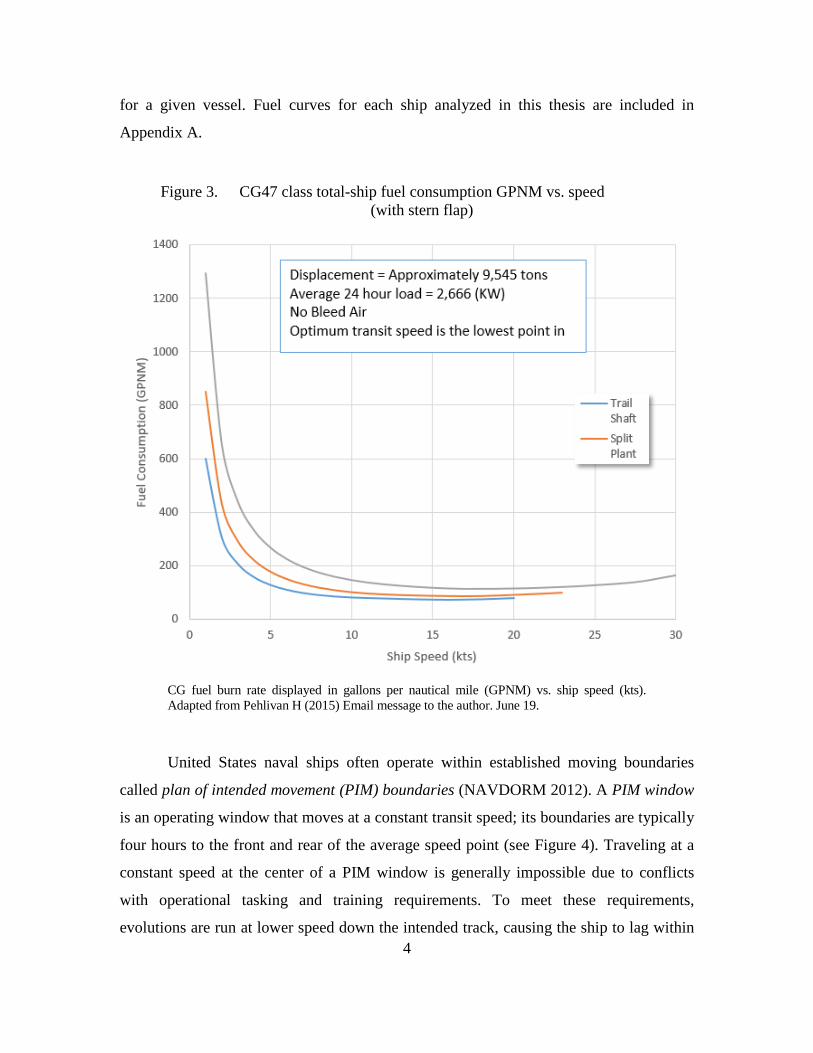
4

for a given vessel. Fuel curves for each ship analyzed in this thesis are included in

Appendix A.

Figure 3. CG47 class total-ship fuel consumption GPNM vs. speed (with stern flap)

CG fuel burn rate displayed in gallons per nautical mile (GPNM) vs. ship speed (kts). Adapted from Pehlivan H (2015) Email message to the author. June 19.

United States naval ships often operate within established moving boundaries

called plan of intended movement (PIM) boundaries (NAVDORM 2012). A PIM window

is an operating window that moves at a constant transit speed; its boundaries are typically

four hours to the front and rear of the average speed point (see Figure 4). Traveling at a

constant speed at the center of a PIM window is generally impossible due to conflicts

with operational tasking and training requirements. To meet these requirements,

evolutions are run at lower speed down the intended track, causing the ship to lag within

5

the PIM window and requiring it to “catch up” with other ships after the drill is complete.

Such training requirements complicate the problem of optimizing transit speed to

minimize fuel consumption. Often, a ship will travel at a combination of higher and lower

speeds to accommodate training requirements. There exist optimal combinations of burn

rates for several constant required speeds that are more efficient than the original burn

rate, depending on specific ship configurations and respective burn rates.

Figure 4. PIM window example

PIM window is based upon a four-hour allowance forward and behind of the allowed average speed determined by higher authority.

B. LITERATURE REVIEW

The transit fuel planner (TFP) developed in the Department of Operations

Research at the Naval Postgraduate School (NPS) prescribes optimal transit speeds to

minimize fuel consumption based on the propulsion-plant configuration for a single ship

(Brown et al. 2007). This thesis introduces the Optimized Transit Tool and Easy

Reference (OTTER), which uses the concepts derived in the TFP to find optimal speeds

and implement them in a useful manner (Brown, et al. 2011).

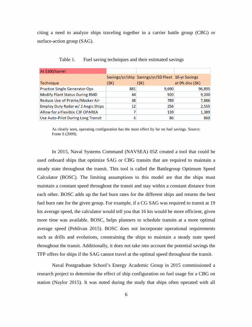
NPS student S. Fonte compares several fuel-saving techniques in his 2009 thesis,

as shown in Table 1. The technique with the highest savings per year across his analysis

was based upon efficient engineering configuration. Fonte noted that after the

introduction of the TFP, follow up work was “waiting to be explored” (Fonte 2009). In

2014, NPS student Dustin K. Crawford proposed follow-up work to modify the TFP,

6

citing a need to analyze ships traveling together in a carrier battle group (CBG) or

surface-action group (SAG).

Table 1. Fuel saving techniques and their estimated savings

As clearly seen, operating configuration has the most effect by far on fuel savings. Source: Fonte S (2009).

In 2015, Naval Systems Command (NAVSEA) 05Z created a tool that could be

used onboard ships that optimize SAG or CBG transits that are required to maintain a

steady state throughout the transit. This tool is called the Battlegroup Optimum Speed

Calculator (BOSC). The limiting assumptions to this model are that the ships must

maintain a constant speed throughout the transit and stay within a constant distance from

each other. BOSC adds up the fuel burn rates for the different ships and returns the best

fuel burn rate for the given group. For example, if a CG SAG was required to transit at 19

kts average speed, the calculator would tell you that 16 kts would be more efficient, given

more time was available. BOSC, helps planners to schedule transits at a more optimal

average speed (Pehlivan 2015). BOSC does not incorporate operational requirements

such as drills and evolutions, constraining the ships to maintain a steady state speed

throughout the transit. Additionally, it does not take into account the potential savings the

TFP offers for ships if the SAG cannot travel at the optimal speed throughout the transit.

Naval Postgraduate School’s Energy Academic Group in 2015 commissioned a

research project to determine the effect of ship configuration on fuel usage for a CBG on

station (Naylor 2015). It was noted during the study that ships often operated with all

7

engines running during certain evolutions in order to be prepared for quicker response.

Operating at an optimal engine configuration, CG and DDG class ships would spend

between 50 and 100 percent more time conducting operations before needing to refuel.

This study recommended coordination between CBG components in order to relax the

requirements upon the CG and DDG escort ships in order to increase their operational

capability.

The LCS is the newest class ships added to the Navy fleet and has as of today

received little analysis with regards to fuel usage. In 2014, the Government

Accountability Office (GAO) reported that “Fleet users said LCS fuel constraints

contributed to a low average transit speed that, coupled with the very long distances ships

have to travel within the 7th Fleet theater, make it hard for LCS to easily or efficiently get

around the theater” (Government Accountability Office [GAO] 14-749 2014).

In the summer of 2014, the Navy conducted an experiment directing USS

Sampson (DDG 102) to travel to Hawaii and back at a PIM speed of 15.5 kts, the

minimum point on Sampson’s fuel curve. This is the ship’s most efficient speed, if

maintained constantly. The ship was outfitted with a monitoring system that recorded

fuel-burn rate and speed at 10-minute intervals throughout the transit. As shown in Figure

5, several factors contributed to decreased efficiency. Less than three hours was spent at

optimal speed. Two-thirds of the time was spent at trail-shaft configuration, while the

other third was spent at either full power or split plant (SURFPAC 2015). Maintaining an

optimal transit speed of 15.5 kts could have saved 20,334 gallons of fuel, or 12.2%,

equating to an additional 30 hours at 8 kts on station. The experiment demonstrated that a

ship maintaining a constant speed of 15.5 kts for a seven-day transit is unrealistic, given

the training and operational requirements a commander must fulfill. A primary objective

of this thesis is to provide a decision tool that promotes awareness of fuel consumption

while accounting for the operational realities inherent in naval operations.

8

Figure 5. USS Sampson transit 2014: Time spent at various speeds during transit

Transit data from USS Sampson summer 2014. USS Sampson (DDG 102) transit from Hawaii to San Diego shows most transit time was spent at various high and low speeds, due to drills and evolutions. Less than three hours was spent at the optimal speed of 15.5 kts. Source: Richards M (2015) Email message to the author, September 11.

Recent fuel-saving measures that have been implemented on board Navy ships

include:

• Solid-state light-emitting diodes (LEDs), which save 50% to 80% on energy-related fuel requirements but cost 40 times that of the existing fluorescent bulbs at $158 per bulb. Each bulb has an expected 10 year life span, which is long enough to recoup the setup cost when compared to traditional bulb replacements (U.S. Navy 2014).

• A real-time monitoring program (the Shipboard Energy Dashboard), which shows how power requirements can be reduced while maintaining system performance and reliability requirements. This was developed by NAVSEA and is a decision tool that enables the user to modify operating behavior to save fuel. It is estimated to save less than one percent of fuel on average (DODLIVE 2015).

• Stern flaps installed on new ships and retrofitted on many existing ships modifying the water flow under the ship’s hull reduce drag and turbulence, thereby reducing overall hull resistance. Savings are estimated to be between 2 and 7%, recouping installation costs within the first 2 years of use (Ibid).

9

• The Smart Voyage Planning Decision Aid is a computer software module that uses a ship’s Electronic Chart Display and Information System and information from meteorologists to determine an efficient and optimized route accounting for currents, waves and weather (Ibid). Fleet adoption of this system is in the initial stages.

C. OBJECTIVES

We develop a mathematical model incorporated in an Optimized Transit Tool and

its Easy Reference dubbed “OTTER.” A major objective of this thesis is to determine the

potential fuel savings of multiple ships moving together in convoy, as well as the

operational requirements involved in keeping all such ships within a prescribed PIM

window.

OTTER is made up of two components. “Dynamic OTTER” enables planners at

the ship and group levels to factor in drills and evolutions, which occur typically at slow

speeds (5 kts), when calculating optimal speed combinations for travel. For example, the

USS Freedom (LCS1) is required to transit at 19 knots (kts) average speed for 24 hours.

The commanding officer (CO) may operate at any speed, so long as he or she stays inside

a moving operating window. To meet training requirements, COs often run drills at slow

speed and then catch up with the operating window. If a CO runs a four-hour drill at five

kts and then accelerates to 22 kts meet the expected arrival time, the combined speeds

will yield extremely poor burn rates when averaged. Sacrificing drills in this situation

would save significant fuel, but this may not be an option. Dynamic OTTER optimally

builds drills and evolutions into a schedule while allowing the user to update shaft-limit

changes and fuel-curve data.

Dynamic OTTER can also produce a standalone reference sheet of optimal speed

combinations for each class of ship, based on known fuel-consumption rates. This

reference sheet, “Static OTTER,” would be a valuable addition to CO standing orders for

use by the officer of the deck (OOD).

In the analysis section of this thesis, we calculate the average and 90th percentile

distances between ships traveling inside a common PIM window. Additionally, we

calculate and analyze the time required until a CO must change speeds in order to stay

10

within the PIM window for various situations. These two values give the CO knowledge

to support maneuvering decisions in transit routes.

D. SCOPE, LIMITATIONS AND ASSUMPTIONS

This thesis focuses on United States Navy surface-fleet, fossil-fuel ships. This

flexible tool can serve as a basis for additional, comprehensive planning tools. While this

thesis discusses a particular set of ships, further study of fuel optimization may be applied

to any engineering platform with multiple fuel/distance curves.

Oceanic winds and currents affect ship speed during transit. To employ the static

reference sheet, the OOD must determine the effect of current and wind using existing

methodology before applying results from OTTER. If, for example, the required ship

speed over ground is 12 kts, but there is a 2-kts current pushing back, the OOD adjusts

the speed through water to 14 kts. We assume basic seamanship skills for simple

navigation calculations using speed and direction manually entered into the calculation

using Dynamic OTTER.

While Dynamic OTTER allows for the scheduling of drills in the short term,

Static OTTER requires that the user calculate the new speed of advance after drills are

complete. This new average speed can be used with the Static OTTER reference sheet to

determine the most efficient speed combinations for the remaining transit.

E. CONTRIBUTIONS AND OUTLINE

The main contributions of this research are the proving and application of simple

linear optimization of fuel curves across engineering configurations and the development

of OTTER as a tool to implement this research in the fleet. The mathematics behind the

linear programming model and how it was implemented are demonstrated in Chapter II.

Static and Dynamic OTTER description and implementation tools are described in

Chapter III. After providing examples and analysis results in Chapter IV, this thesis

concludes with recommendations for implementation and potential future work.

11

II. MODEL

OTTER solves a linear program (LP) similar to the TFP in order to determine the

optimal combination of speeds for each of the ships in a convoy, subject to the constraints

that each ship arrive at the desired destination at a prescribed time while performing any

required drills. The time and distance values used in the formulation account for

requested drills, ocean current, starting and ending distance from the center of PIM, and

the overall effect of the scheduled drills upon forward progress in reference to center of

PIM. Although the relative positioning of the ships during transit is an important practical

consideration, the LP does not explicitly calculate or prescribe individual ships’ positions

as a function of time. Rather, after performing the optimization, OTTER determines a

schedule of speed changes to guarantee that each ship remains within the PIM window.

Dynamic OTTER applies the faster of the two speeds first, putting the ship toward

the forward half of the window. This models the current CO behavior and is most

realistic. Drills are scheduled according to specified user input times. The schedule is

broken down into time increments in number of minutes specified by the user.

The linear optimization model is shown next, followed by an explanation of the

variables and constraints. This model simply calculates the most efficient speeds to travel

at for a specified time and distance and is modified from the TFP model (Brown et al.

2007). The schedule builder is described in great detail in Chapter III.

12

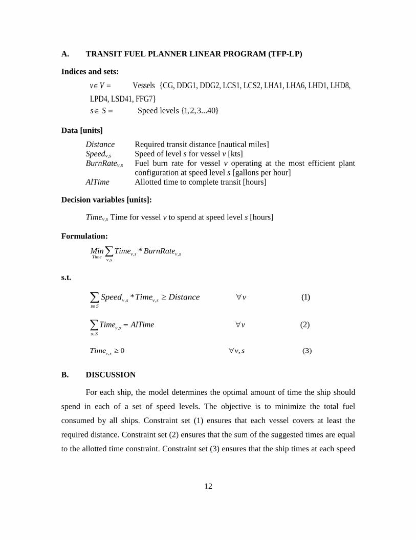
A. TRANSIT FUEL PLANNER LINEAR PROGRAM (TFP-LP)

Indices and sets:

Vessels {CG, DDG1, DDG2, LCS1, LCS2, LHA1, LHA6, LHD1, LHD8, LPD4, LSD41, FFG7}v V∈ =

Speed levels {1,2,3...40}s S∈ =

Data [units]

Distance Required transit distance [nautical miles] Speedv,s Speed of level s for vessel v [kts] BurnRatev,s Fuel burn rate for vessel v operating at the most efficient plant

configuration at speed level s [gallons per hour] AlTime Allotted time to complete transit [hours]

Decision variables [units]:

Timev,s Time for vessel v to spend at speed level s [hours]

Formulation:

, ,,

* v s v sTime v sMin Time BurnRate∑

s.t.

, ,* (1)v s v ss S

Speed Time Distance v∈

≥ ∀∑

, (2)v ss S

Time AlTime v∈

= ∀∑

, 0 , (3)v sTime v s≥ ∀

B. DISCUSSION

For each ship, the model determines the optimal amount of time the ship should

spend in each of a set of speed levels. The objective is to minimize the total fuel

consumed by all ships. Constraint set (1) ensures that each vessel covers at least the

required distance. Constraint set (2) ensures that the sum of the suggested times are equal

to the allotted time constraint. Constraint set (3) ensures that the ship times at each speed

13

are non-negative. Each ship has unique speed profiles and fuel burn rates. Speeds chosen

for a specific transit are only chosen from the specific ship’s profile ensuring feasibility.

For a SAG with 10 vessels, the optimization model contains 300 decision

variables and 320 constraints. It solves in 0.5 seconds on an Intel 2.4GHz, 32-bit laptop

with 4GB RAM.

Figure 6 walks through an example of how this optimization works using the

LCS1 class ship. The states listed in the figure are the various engineering modes

available to the LCS1. The straight line on connecting state 4 and 8 is the fuel burn rate

possible if the ship travels at combinations of 15 kts and 35 kts. We present the following

example:

• IF: a speed of 22 kts is ordered to be maintained, on average,

• THEN: 65% of the time should be spent at 15 kts in “state 4” mode

• AND: 35% of the time should be spent at 35 kts in “state 8” mode,

• RESULTING: in a savings of 468 gallons per hour (GPH) or 43 GPNM.

14

Figure 6. LCS1 class total ship fuel consumption GPNM vs. speed (with stern flap)

An example of an optimized speed combination of 15 kts and 35 kts. LCS1 fuel burn rate displayed in gallons per nautical mile (GPNM) vs. ship speed (kts). The OTTER solution at 22-kts average speed returns 102 GPNM instead of the 145 GPNM in state 8 only. Adapted from Pehlivan H (2015).

It is important to note that in an optimal solution, each ship will spend a nonzero

amount of time traveling at most two speeds, excluding drills. This principle can be

proven by first assuming the negation. Assume there are three speeds that minimize the

average fuel consumption for a given speed. These three speeds on Figure 6 would form a

triangle. The minimum burn rate on this triangle would be found along the lowest edge

which is a combination of exactly two points. Therefore, proving that as time segments

become infinitesimally small, there will always exist at least one but at most two speeds

that will be optimal.

15

III. THE USER INTERFACE

This chapter describes the user interfaces for Dynamic OTTER and Static

OTTER.

A. DYNAMIC OTTER

Dynamic OTTER solves for the optimal speed combinations for the given

engineering plant configurations, constrained by user-defined drill periods. The user sets

the drill time, duration, and effect on forward progress down track as input, as seen in

Figure 7. Dynamic OTTER is built in the Visual Basic for Applications (VBA) language

in the Microsoft Excel framework.

Figure 7. Dynamic OTTER input

Dynamic OTTER requests transit distance and time, start time, time interval and the effect of ocean current on the transit. The user can add two separate drill starting times, durations, and effects on transit.

Dynamic OTTER’s schedule builder output was inspired by the NPS CBG study

done by Naylor (Naylor 2015). The study used a tool called the Fuel Usage Study

Extended Demonstration (FUSED) which created a ship schedule by hour allowing the

scheduler to analyze the fuel usage of the ships over time. OTTER’s schedule builder

output allowed calculations such as distance traveled, distance between ships in the

16

group, and cumulative fuel used. It also enables the scheduling of drills and optimization

of the remaining time and distance values. A pictorial representation of an output

schedule that could be built using Dynamic OTTER can be seen on Figure 8.

Figure 8. Schedule builder timeline

Timeline for a 48-hour transit scheduled into one-hour time increments (TI) with two four-hour drills (DN) scheduled. The drill event is annotated by a start time ( ,v dnDSI ), drill

speed ( ,v dnDS ) and a duration ( ,v dnDDI ) for each vessel.

1. Dynamic OTTER Schedule Builder Pseudocode

Sets:

• Ships (CG, DDG, etc.) V

• Drill numbers (1, 2) DN

• Time intervals (1, 2, 3...) TI

• Speed options (1, 2) SP

Input:

• Distance to travel (nm) D

• Time for transit to be complete (hrs) T

• Transit start time for ship v (mm/dd/yy hh:mm) TS

• Transit time interval size (min) M

• Ocean current relative to PIM (kts) OC

• Drill start time for ship v and drill number dn (mm/dd/yy hh:mm) ,v dnDS

• Drill duration for ship v and drill number dn (hrs) ,v dnDD

17

• Forward progress for ship v during drill number dn (nm) ,v dnDP

• Drill speed for ship v during drill number dn (kts) ,v dnDSP

• Start offset for ship v (nm) vSO

• Ending offset for ship v (nm) vEO

Compute values: • Current progress of vessel v at time interval ti (nm) ,v tiCP

• Front boundary of PIM window at time interval ti tiFB

• Back boundary of PIM window at time interval ti tiBB

• Time intervals in transit (integer) *60TTIM

=

• Travel time at interval ti (mm/dd/yy hh:mm) * 60

ti MTT =

• Final distance for ship v after drills (nm)

, - + - v v dn v v

dnFD D DP EO SO v V= ∀ ∈∑

• Remaining time for ship v drills (min) ,dn

v v dnRT TI DDI v V= − ∀ ∈∑

• PIM speed (kts) DPIMSPT

=

• PIM window center progress (nm) * PIM PIMSP TT=

• Drill number dn start intervals for ship v (integer)

,

, ,v dn vv dn

DS TSDSI v V dn DN

M−

= ∀ ∈ ∈

• Drill number dn duration intervals for ship v (integer)

,

,

*60 ,v dn

v dn

DDDDI v V dn DN

M= ∀ ∈ ∈

18

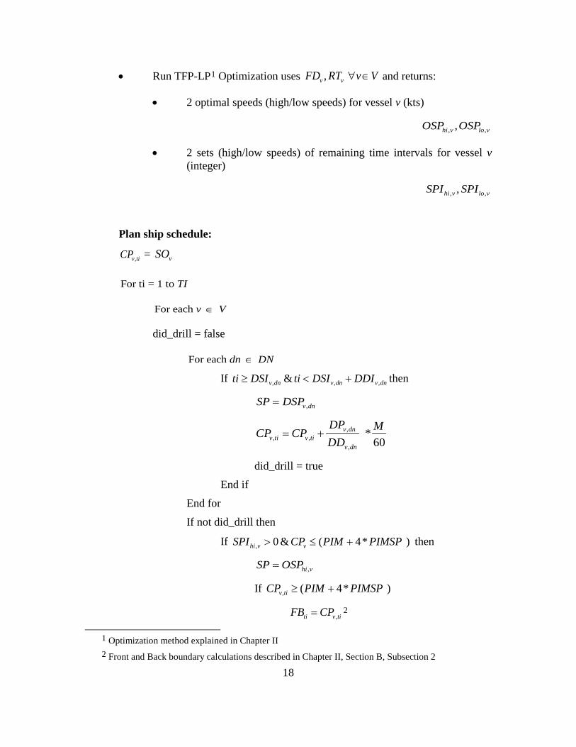
• Run TFP-LP1 Optimization uses , v vFD RT v V∀ ∈ and returns:

• 2 optimal speeds (high/low speeds) for vessel v (kts)

, ,,hi v lo vOSP OSP

• 2 sets (high/low speeds) of remaining time intervals for vessel v (integer)

, ,,hi v lo vSPI SPI

Plan ship schedule:

,v tiCP = vSO

For ti = 1 to TI

For each v V∈

did_drill = false

For each dn DN∈

If , , ,&v dn v dn v dnti DSI ti DSI DDI≥ < + then

,v dnSP DSP=

,, ,

,

*60

v dnv ti v ti

v dn

DP MCP CPDD

= +

did_drill = true

End if

End for

If not did_drill then

If , 0 & ( 4* )hi v vSPI CP PIM PIMSP> ≤ + then

,hi vSP OSP=

If , ( 4* )v tiCP PIM PIMSP≥ +

,ti v tiFB CP= 2

1 Optimization method explained in Chapter II 2 Front and Back boundary calculations described in Chapter II, Section B, Subsection 2

19

End if

Else

,lo vSP OSP=

If , ( 4* )v tiCP PIM PIMSP≤ −

,ti v tiBB CP= **

End if

End if

, , *60v ti v tiMCP CP SP= +

End if

End for

End for

The Dynamic OTTER schedule builder pseudocode builds the arrays and user

specified values that will be used to include the ship types used, offset and drill

parameters, new and old fuel burned variables. The interval size M is chosen from a drop

down cell of values that are factors of 60. This ensures that M is always an integer. After

clearing the old schedule, it updates the schedule headers for each ship chosen on the

planner with the appropriate ship types.

The code then loops through the entire range of time intervals scheduled and

determines whether to plan a drill, high speed value or low speed value. The modeler

sends the ship to the forward half of the operating window by using the faster of the two

speeds first. If the chosen time interval is large (60 min), the processing time will be

nearly instantaneous.

Now that the schedule builder has calculated the current position ,v tiCP for each

vessel v and time interval ti, and we have the PIM window center position PIM over each

time interval ti, we can plot these two for position comparison on the transit. As seen in

Figure 9, the OTTER plan maintains a close position to PIM center even with the

scheduled drills.

20

Figure 9. OTTER transit vs. PIM center

Transit distance relative to average speed (PIM center) using Dynamic OTTER schedule builder. This is a DDG Flt 1 48 hour transit at 24 kts average speed with 2 four hour drills scheduled during the transit. Fuel saved during this transit was 70,646 gal or 96 hours of additional time on station compared to typical ship behavior.

After the schedule has been built, the comparative burn rates are calculated based

upon a surge speed that is defined by user settings. This surge speed is sub optimum and

representative of actual CO behavior during sprint and drift operations. These old burn

rates are compiled and compared to the new total fuel burned and values are output as

fuel saved. This is also converted to extra time on station by using the ship’s average

burn rate at 8 kts. Actual VBA code for Dynamic OTTER can be found in Appendix D.

The OTTER schedule builder runs extremely quickly. It requires approximately

1.0 second to plan a 48-hour transit in 5-minute increments for a SAG with 10 ships. The

resulting file size is 671 KB, making it easy to share via email or download.

2. Time Until Speed Change

Another valuable capability this thesis describes is a method of calculating PIM

boundaries. The time until speed change (TTSC) is defined as the time (in hours) until a

ship is required to change speed to stay within the PIM window. Normally the ship CO

must determine when to change speeds in order to stay within the PIM window

boundaries. Assuming the ship starts a transit at the center of an authorized PIM window,

21

the time to change speed can be calculated for both the front and back of the PIM

window.

In the pseudocode, the front boundary tiFB and the back boundary tiBB were saved,

recording the time at which a forward or back boundary was reached. These moving

boundaries in time are not to be crossed, so they serve as a guide in Static OTTER as well

as in our analysis Chapter as TTSC.

3. Dynamic OTTER Output

Dynamic OTTER returns a schedule indicating the PIM center, each ship

position, engineering configuration, and speed in each time step. The fuel burned, saved,

and equivalent time on station is shown for each ship. The “largest spread” value reported

in the header is the greatest difference between ship positions at any point in time. Each

ship will stay within the PIM window during the transit. Figure 10 shows the output from

Dynamic OTTER, a schedule broken down into time increments for each ship modeled.

22

Figure 10. Dynamic OTTER output

OTTER output returns a schedule broken down by time intervals and start-time specified for each ship, showing the optimal speed and engineering mode to be used.

4. Dynamic OTTER Settings

To update ship parameters such as shaft limits or maximum speed, the user

completes an interactive form for each engineering configuration, as depicted in Figure

11. This is required when engineering limits are imposed due to engineering casualties, or

as higher authority directs. The fuel curves can also be updated after ship performance

trials. New fuel-curve data may result in significant changes in the findings for optimal

speed.

23

Figure 11. User-defined settings

User-defined settings enable the user to update shaft limits for each engineering configuration used. It also enables constraints for time intervals between speed and mode changes.

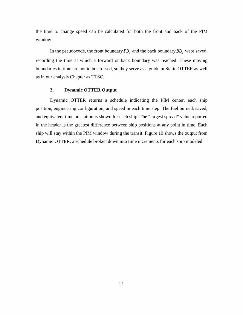
Users also have the ability to add new ship types (Figure 12) through the settings

tab. Users must have ship configuration data such as burn rates and propulsion limits for

each mode. When the user inputs this data, the spreadsheet parameters are updated

allowing for validation and implementation into both Dynamic and Static OTTER

calculations.

When ship types are no longer needed, users can delete the ship from the database

through the user-defined settings for that particular ship. This permanent removal deletes

the worksheet and all associations to that worksheet in the name manager.

The CO may decide that changing engineering modes impacts the personnel on

the ship and therefore wants to limit the frequency. The settings page has parameters such

as the minimum time between mode or speed changes to allow for these customizations.

24

Figure 12. Create a new ship type

New ship type input form from Dynamic OTTER settings page. User may input propulsion limits which will be saved on a new worksheet in OTTER for new optimal transits and Static worksheet creation.

B. STATIC OTTER

The interface of Static OTTER, depicted in Figure 13, is a user-friendly reference

sheet customized to specific ship parameters. Once the proper fuel curves and shaft limits

have been verified for a ship, this reference sheet is available for printing. Static OTTER

has a speed combination for several requested average speeds. It also gives the

percentage of time a user should spend at each of the two speeds. It shows the time until a

PIM boundary is met based upon a 4 hour PIM operating window and the ship starting

point is from the middle of PIM. Because of these assumptions, operators should always

note their position inside the PIM window and ensure boundaries are not violated.

The reference sheet contains detailed instructions and examples. More static tools

can be found in Appendix B. Additional sheets can be made and printed from Dynamic

OTTER. The spreadsheet also notes the source of the fuel-curve data; this note can be

updated by the user through Dynamic OTTER when changes are made to the baseline

fuel burn rates.

25

Figure 13. Static OTTER

Static OTTER can be used to minimize fuel consumption by combining two ship speeds instead of maintaining a single constant speed.

26

THIS PAGE INTENTIONALLY LEFT BLANK

27

IV. RESULTS

We now demonstrate the benefits of applying linear optimization to fuel curves in

the following example. Suppose LCS1 is in a 48-hour transit and is required to maintain

an average speed of 19 kts. Using a standard approach, if the CO decided to run a four-

hour drill at five kts and then adjusted the ship’s speed to catch up to the expected arrival

time (5 kts/21 kts), less-efficient burn rates would be achieved. However, if after running

drills the more efficient speed combinations were used (5 kts/15 kts/35 kts), significant

fuel would be saved (see Table 2). A CO need not sacrifice drills to save fuel and extend

on-station endurance. Dynamic OTTER optimally builds the drill into the schedule at the

time specified by the user.

Table 2. USS Freedom (LCS1) with average speed requirement of 19 kts

USS Freedom reduction in fuel burn rates when OTTER is used, earning many more hours on station before refueling is required.

A. DATA COLLECTION

For our computational experiments, we used ship performance data collected by

Naval Surface Warfare Center, Carderock Division, in West Bethesda, Maryland, during

initial sea trials of the lead ship in a class (Pehlivan 2015). Users can update fuel usage

data in OTTER as needed accounting for the slight changes in fuel burn as equipment

ages.

In order to apply realistic ship transits to the model, we used data collected by

Commander Naval Surface Force, U.S. Pacific Fleet Energy Office in 2014 from the USS

Speed profileAvg burned

(GPH)

48 hour transit

total (gal)

Additional Time on station at 8

kts (hrs) Comments

W/o Drills 19 kts 2,428 116,544 0 Constant speed

W/o Drills 15 kts / 35 kts 1,996 95,827 113 With OTTER

W/ Drills 5 kts / 22 kts 2,537 121,753 0 Catch up

W/ Drills 5 kts / 15 kts / 35 kts 2,221 106,611 83 With OTTER

28

Sampson during transit from San Diego to Hawaii and back (Richards 2015). Speed and

configuration profile data were collected every 10 minutes for the duration of the transit.

This data shows the real transit habits of COs at sea. While a constant transit speed is

most convenient to model, it is often unrealistic. Fuel savings were substantially greater

using OTTER than using a conservative constant-speed model.

Because burn rates are not stochastic, simulations or trial runs were not required

to validate the model. We ran the optimization model over the entire speed range for each

ship to produce Static OTTER reference sheets. These new burn rates are independent of

other ship transits. Groups of ships could still use reference sheets independently if their

constraints are only to remain inside the PIM window. Closer grouping requirements will

be addressed in the next section.

B. MAXIMUM SPREAD BETWEEN SHIPS

When a group of ships travels in a SAG, higher authority will dictate the

maximum distance between ships during the transit for force protection or logistical

reasons. Transiting as a group requires daily planning coordination between COs to

ensure these boundaries are not violated. OTTER considers the four hour ahead and

behind of the PIM window center as acceptable boundaries for planning. Figure 14

depicts the spread in distance during an example 48-hour transit that a CG and DDG1

would experience following the Dynamic OTTER “Short Term Schedule”

recommendations.

With a simple evaluation by the CO or OOD, the spreads could be reduced

significantly with no impact on fuel savings. The deviation from the proposed transit plan

might be to alternate speeds more frequently than otherwise proposed. Dynamic OTTER

has the ability to constrain the spread distance to a specified parameter. This feature does

not affect the fuel savings; rather, the effect is seen through more frequent speed or mode

changes.

29

Figure 14. Spread among ships during a group transit of CG and DDG1

Distance between a CG and DDG1 with an average transit speed of 14 kts. These spread distances are due to the differences in proposed transit speeds. The CG travels at 15 kts and then 10 kts while the DDG1 travels at constant 14 kts. The maximum spread between the ships is 37 nm with no additional constraints applied.

Changing some engine configurations may require significant effort for some

ships. Intuitively, the larger the spread allowed, the less frequently the ship will have to

change engineering modes. If the optimal speeds are followed in their respective ratios as

provided by Static OTTER, the fuel savings will be the same, regardless of the frequency

of mode changes. In short, the cost of earning a small spread between ships is more

frequent engine configuration changes.

Following the recommended OTTER solution with no spread minimization, Table

3 shows the average spread between two ships traveling in a SAG. For example, if a CG

and a DDG1 transit in a SAG together, they will, on average be 11 NM apart. Table 4

shows the 90th percentile of the data. Similarly, a CG and DDG1 traveling together

would be less than 30 NM apart 90% of the time.

30

Table 3. Average spread among ships using Dynamic OTTER

With a four-hour PIM window established, the average distance between two ships is shown. This average was calculated over the speed range (1-30 kts for CG) of the slower of the two ships analyzed.

Table 4. 90% of time spread—using Dynamic OTTER

With a four-hour PIM window established, 90% of the time the distance between ships will be less than the expressed value.

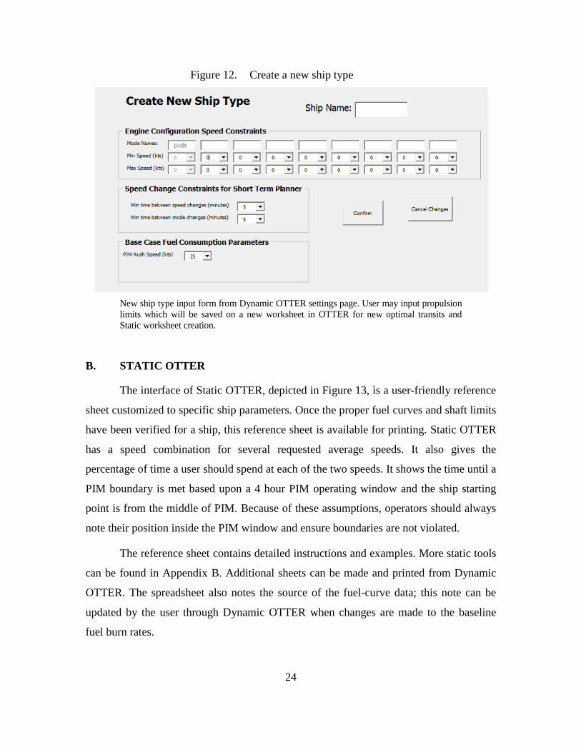
From each of the combinations in Tables 3 and 4, we created a histogram to

represent the number of times during a 48 hour transit (broken down into five minute

intervals), that one of the (nCr10,2=45) 45 ship pairs shown on the y axis, across all

common speed ranges, would be a particular distance apart. This is a good way of

quickly visually portraying the ship pair separation distances. Figure 15 compiles these

CG DDG1 DDG2A LCS1 LCS2 LHA1 LHD1 lSD41 LPD4 FFG7CG NA 30 23 77 25 26 35 28 32 26DDG1 NA 24 89 19 30 33 23 28 20DDG2A NA 23 79 30 8 23 30 22LCS1 NA 77 76 58 76 32 77LCS2 NA 29 33 30 30 32LHA1 NA 34 19 30 19LHD1 NA 33 20 33LSD41 NA 26 5LPD4 NA 27FFG7 NA

90% of time spread is less than X (NM)

31

48 histograms together into a three dimensional graph. By design the ships are

constrained to the common PIM window. This design keeps their spread distances to a

minimum, and as one can see from the figure, the majority of the time is spent with very

minor distances between them.

Figure 15. Spread values for all ship pairs analyzed

Spread distances (x axis) between ship pairs (y axis) and the frequency (z axis) that particular spread distance occurs.

C. TIME TO SPEED CHANGE

As described in Chapter III, the TTSC values are a measure of the frequency of

mode shifts. A low TTSC value means that these shifts occur at higher frequency, likely

adding some burden on the engineering crew. TTSC results could be considered highly

reasonable with no times less than one hour, and only 3% of situations require a time of

one hour. A cumulative summary of TTSC is shown in Figure 16. The TTSC are usually

greater than 100 hours which is typically negligible. Individual ship TTSC for the ships

analyzed are included in Appendix C.

32

Figure 16. Frequency of TTSC across all ships modeled

These are TTSC (x axis) vs. number of occurrences (y axis) accumulated over CG, DDG1, DDG2A, LCS1, LCS2, LHA1, LHD1, LSD41, LPD4, LSD49 and FFG7 ships.

Another metric to represent the additional engineering burden required to stay

within a PIM window is a quantity we denote as big T. Big T represents the PIM window

size in nm divided by the percentage of time spent at one of two optimal speeds. To

calculate these values we assume that the ships are operating in a standard four hour

window with no drills and there is time to complete the transit. The same variables and

definitions from Chapter III are used, with the addition of ,lo vPT which is defined as the

optimal percentage of time for vessel v to spend at lo speed or its counterpart hi speed.

These values are output from the TFP optimizer. Big T can be defined as the following:

Big T = , ,

*4( )*hi v hi v

PIMSP hrsOSP PIMSP PT−

=, ,

*4( )*hi v lo v

PIMSP hrsPIMSP OSP PT−

Figure 17 is a graph of every big T value for the range of average speeds for different

ship types. It is observable that on average, at lower speeds big T values are lower,

meaning that the impactful mode changes would be experienced at average speeds under

10 kts. The outlier to this trend is the LCS1 (shown in purple), where lower big T values

33

exist at higher transit speeds, owing to the unique engineering plant on that ship that

allows greater savings at higher average speeds.

Figure 17. Big T (average speed vs. big T)

Big T times are expressed as the time until a ship is forced to change speeds in order to stay inside of the standard operating envelope using OTTER. This figure shows a standard 4 hour PIM operating window. For example: At 25 kts average speed, LCS1 will have to change speeds at intervals of (20 hours *50%) = 10 hours. In order to stay inside the PIM operating window. Twenty hours came from the y-axis and the fraction is an output of the TFP optimization.

D. ANALYZING MULTI-SPEED FUEL OPTIMIZATION

In practice, COs currently tend to operate in the forward region of their moving

PIM window. This allows the CO more flexibility to perform drills and evolutions such

as flight operations as needed. Keeping this in mind, Dynamic OTTER models the base-

case ship fuel usage as a forward operating ship. It surges the ship to the forward edge of

the window using a user-defined surge speed established on the settings page (27 kts for a

CG) and then operates at the forward edge until a drill is run or the destination is reached

on time.

34

OTTER then creates a schedule using the optimal speed combinations to position

the ship in the forward part of the window, as the CO would desire. The key difference

between the base case and the OTTER solution is the use of the inefficient surge speed in

the base case. Surging forward is done so frequently for operational reasons that it has

been adopted as a common practice called “sprint and drift” (Friedman 2014). The

concept is sound, but without knowing the optimal speeds to sprint and drift, the sprint

and drift solution is sub-optimal and therefore, unnecessarily wasteful.

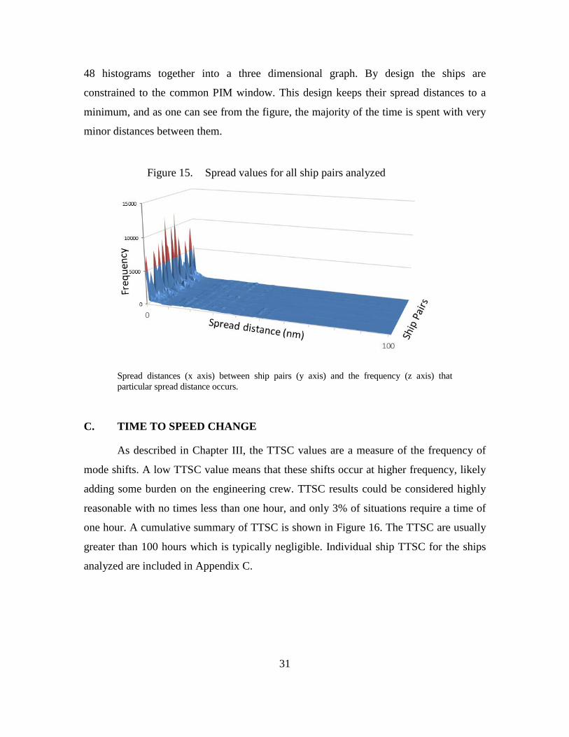
We compared the base case with the Dynamic OTTER solution over 48 hour

transits in Figure 18. We assumed no drills were scheduled with a 5 minute incremental

resolution. The spread constraint was set at 40 nm and the on station speed was assumed

to be 8 kts. For average transit speeds of 15–20 kts, on average a ship could earn 20–35

hours on station. The base case modeled typical CO transit behavior. A more

comprehensive graph for each ship is included in Figure 19.

Figure 18. Average hours earned at various average speeds

Additional average hours earned by following OTTER recommendations for a sample of ships traveling in a SAG for a range of average speeds. For example, with a PIM of 15 kts, the ships capable of traveling 15 kts earn about 20 hours of on station time at 8 kts per 48-hour transit, on average.

35

Figure 19. Detailed hours earned at various average speeds

Additional hours on station (at 8 kts) by following OTTER recommendations for a sample of ships traveling in a SAG for a range of average speeds over a 48 hour transit.

E. CONFIGURATION MATTERS

Ships do not always operate under the most efficient configurations. This may be

due to readiness conditions required for an exercise or possibly engineering restrictions.

Operating under the optimal engineering-plant configuration and speed are vital

components in an efficient transit. For the LCS1 example in Table 2, OTTER proposes a

combination of 15 kts and 35 kts at the optimal configuration without drills, resulting in

an additional 113 hours on station (at 8 kts) compared to a constant speed. If the user

decides to operate under a less efficient engineering mode at the same durations (state 9

vs. state 6/7), the fuel saved will be reduced significantly—from an earned 113 hours on

station to 87 hours.

Not all engineering plants are created equal. Boiler plants with only two modes of

operation-single or dual boiler mode-do not experience an improvement at all in the

majority of their speed ranges (see Appendix B). In contrast, LCS1, has a total of nine

engineering configuration modes of operation, allowing for optimization between each

36

mode giving the LCS class ships enormous opportunity gains in fuel efficiency because

of the plant configuration modes.

Applying OTTER to the transit shown in Figure 5 would save 3,329 gallons,

which equates to an additional five hours on station at 8 kts-a 1.5% improvement in

efficiency. The improvement on the CG and DDG are significant, but not extraordinary.

The LCS1-class ship however, could have earned 14% improvement, equating to 37,703

gallons, or an additional 206 hours on station at 8 kts.

37

V. CONCLUSIONS AND RECOMMENDATIONS

A. CONCLUSIONS

This thesis provides a tool that optimizes fuel usage across a group of ships in an

impactful way. Benefits of its use are displayed in units of earned time on station to show

the operational impact of fuel savings.

B. IMPLEMENTATION CHALLENGES

Designing an intuitive and easily distributable tool for routine use by fleet and

shipboard commanders was the goal of this research. Walt DeGrange, a developer of the

Replenishment-at-Sea Planner (RASP), laments the indifference that operations-research

analyst’s typical experience:

[We] spend months developing the perfect optimal scheduling model by defining the problem, collecting the data, refining the model, enhancing the user interface and including customer feedback and then finally deploying the model. After all this work the customer does not use the model and reverts to legacy practices. What went wrong? (DeGrange 2012)

This thesis faced these challenges of implementation through direct fleet

involvement. Briefs were given to the Fleet Forces Command, Commander, Surface

Forces, Commander Destroyer Squadron 31 (to include an operational trial in April

2016), Rand Corporation, Office of Naval Research and the Office of the Chief of Naval

Operations—Joint Logistics Engagement. OTTER has been tested and distributed with a

reference point of contact at Naval Postgraduate School for technical support in the

Energy Academic Group.

Implementation of this tool could have taken many different forms, but because

we wanted a model that would be directly applicable and used in the fleet, we chose to

use Microsoft Excel with no add-ins or external required software. This stand-alone file

can be used on Navy computers afloat and ashore. This feature is potentially the most

valuable of all.

38

C. FUTURE WORK

A few modeling variants could yield additional insight. This thesis models speed

changes as instantaneous time points. Further modeling of speed ups and slowdowns

during these speed changes may result in meaningful results. Another variant of the

schedule might build it using closed form calculations for times to speed change, thus

eliminating the need to iterate over discrete time periods. Alternatively, a more

comprehensive optimization model could simultaneously determine optimal speeds and

build a schedule for the battle group.

Application toward other engineering platforms such as train transport or aviation

could be explored. Any multi-modal engineering platform with different burn rates could

benefit from linear optimization. Implementation of OTTER toward Navy oilers and

supply support ships may provide additional fuel savings that are worth investigation.

39

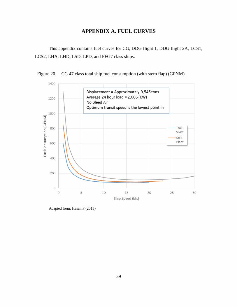
APPENDIX A. FUEL CURVES

This appendix contains fuel curves for CG, DDG flight 1, DDG flight 2A, LCS1,

LCS2, LHA, LHD, LSD, LPD, and FFG7 class ships.

Figure 20. CG 47 class total ship fuel consumption (with stern flap) (GPNM)

Adapted from: Hasan P (2015)

40

Figure 21. DDG51 FLT 1 and II class total ship fuel consumption (with stern flap) (GPNM)

Source: Hasan P (2015)

41

Figure 22. DDG51 FLT IIA class total ship fuel consumption (with stern flap) (GPNM)

Source: Hasan P (2015)

42

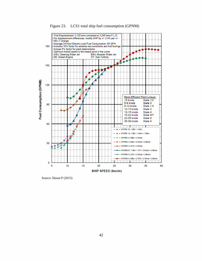
Figure 23. LCS1 total ship fuel consumption (GPNM)

Source: Hasan P (2015)

43

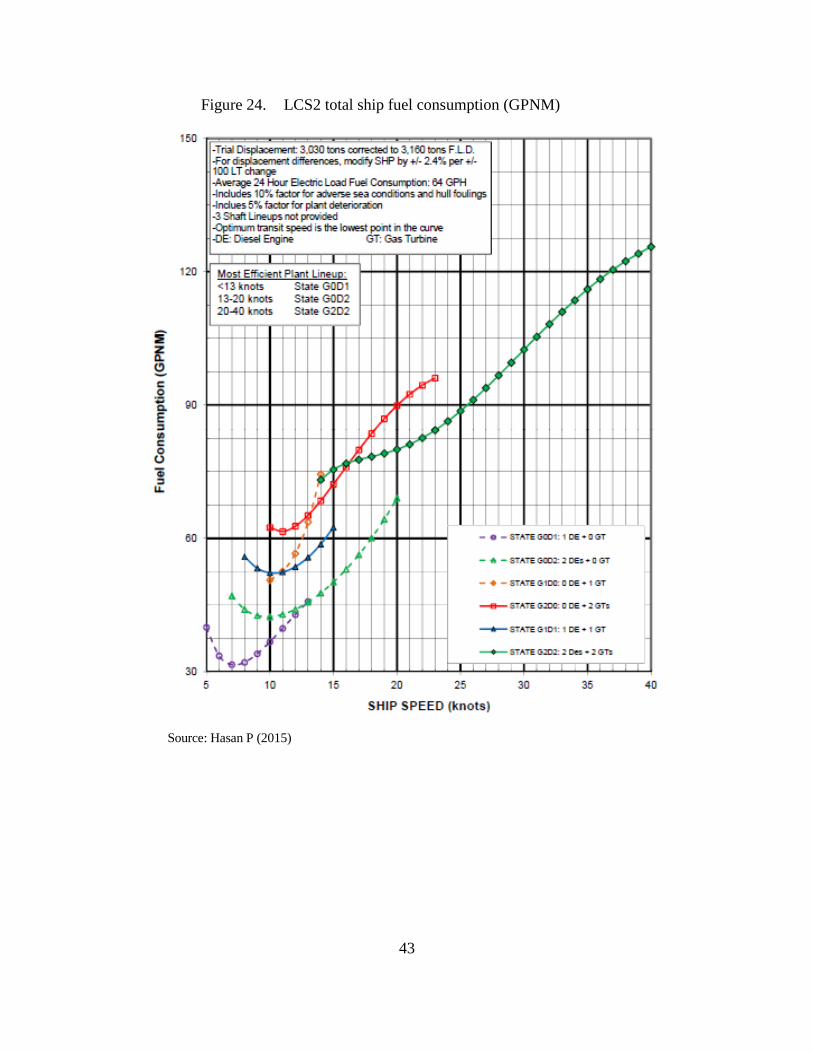
Figure 24. LCS2 total ship fuel consumption (GPNM)

Source: Hasan P (2015)

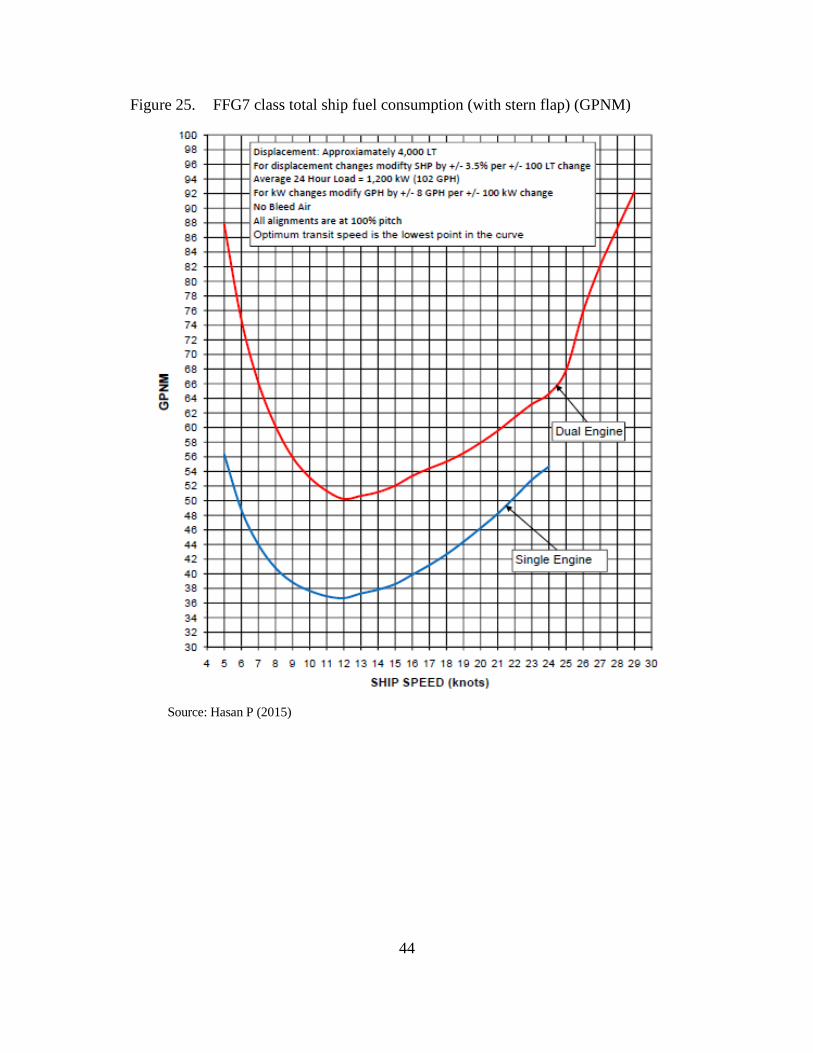
44

Figure 25. FFG7 class total ship fuel consumption (with stern flap) (GPNM)

Source: Hasan P (2015)

45

Figure 26. LSD41 class total ship fuel consumption (GPNM)

Source: Hasan P (2015)

46

Figure 27. LSD49 class total ship fuel consumption (GPNM)

Source: Hasan P (2015)

47

Figure 28. LHD8 class total ship fuel consumption (GPNM)

Adapted from Pehlivan H (2015)

48

THIS PAGE INTENTIONALLY LEFT BLANK

49

APPENDIX B. OTTER STATIC TOOLS

This appendix contains OTTER static tools for CG, DDG flight 1, DDG flight 2A,

LCS1, LCS2, LHA, LHD1, LHD8, LSD, LPD, and FFG7 class ships. Reference sheets

are to be used independently with no required assumptions. Fuel performance dates for

each class ship are annotated on the sheet.

50

Figure 29. CG Static OTTER

51

Figure 30. DDG1 Static OTTER

52

Figure 31. DDG2 Static OTTER

53

Figure 32. LCS1 Static OTTER

54

Figure 33. LCS2 Static OTTER

55

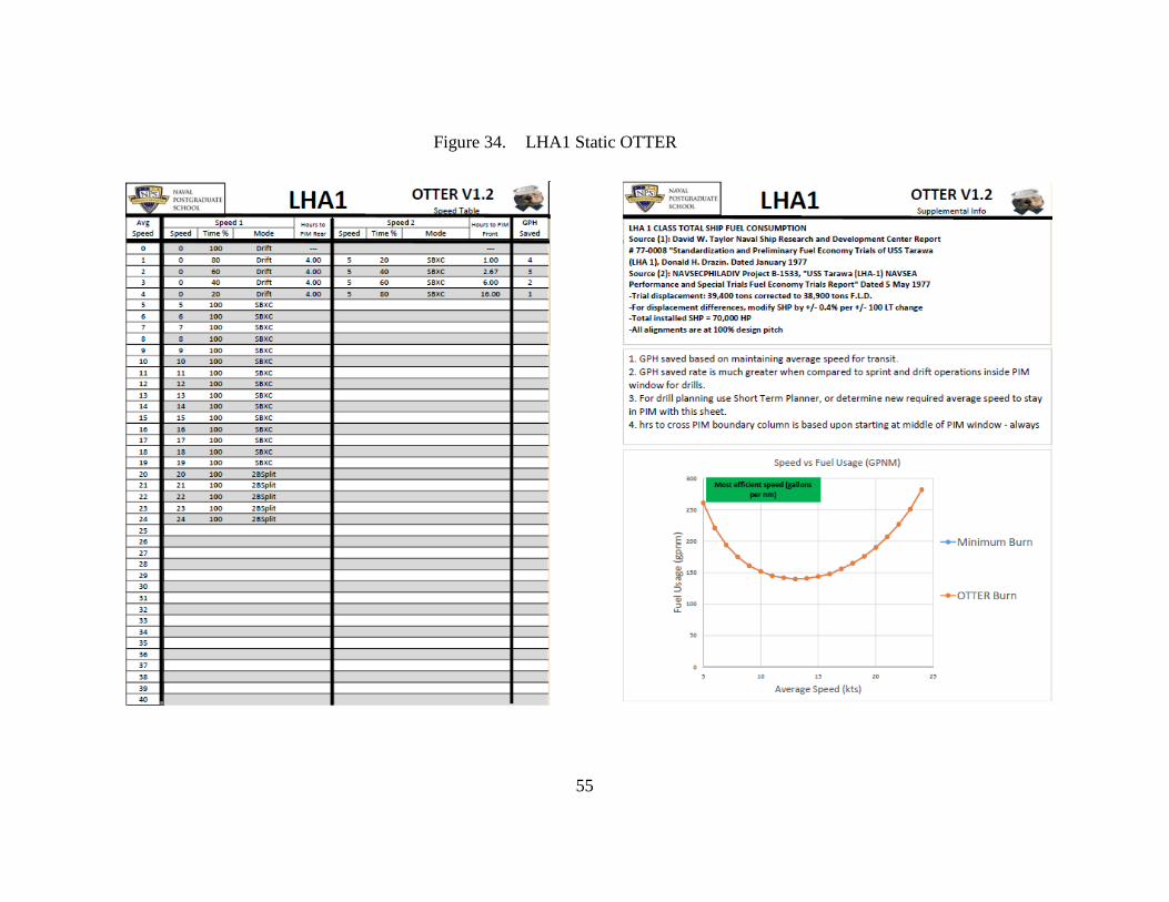
Figure 34. LHA1 Static OTTER

56

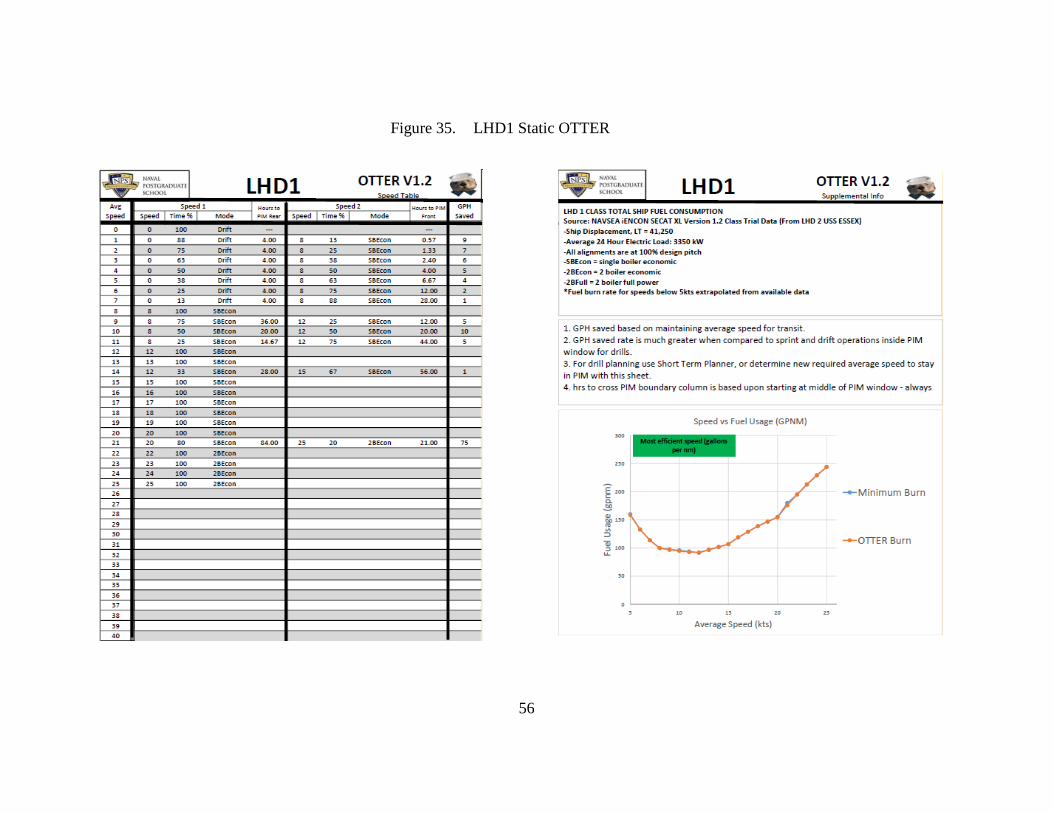
Figure 35. LHD1 Static OTTER

57

Figure 36. LPD4 Static OTTER

58

Figure 37. LSD41 Static OTTER

59

Figure 38. LSD49 Static OTTER

60

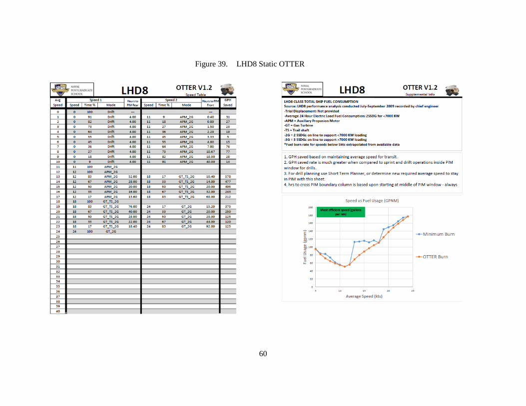
Figure 39. LHD8 Static OTTER

61

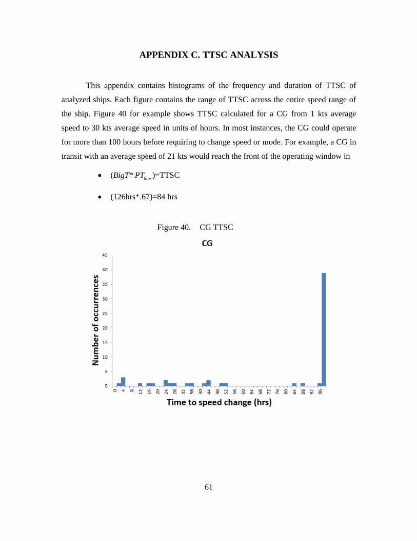
APPENDIX C. TTSC ANALYSIS

This appendix contains histograms of the frequency and duration of TTSC of

analyzed ships. Each figure contains the range of TTSC across the entire speed range of

the ship. Figure 40 for example shows TTSC calculated for a CG from 1 kts average

speed to 30 kts average speed in units of hours. In most instances, the CG could operate

for more than 100 hours before requiring to change speed or mode. For example, a CG in

transit with an average speed of 21 kts would reach the front of the operating window in

• (BigT* ,lo vPT )=TTSC

• (126hrs*.67)=84 hrs

Figure 40. CG TTSC

62

Figure 41. DDG1 TTSC

Figure 42. DDG2A TTSC

63

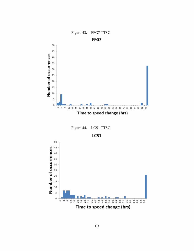
Figure 43. FFG7 TTSC

Figure 44. LCS1 TTSC

64

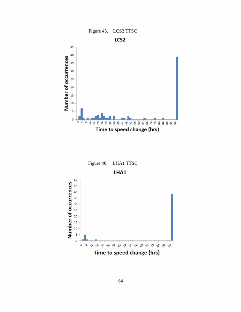
Figure 45. LCS2 TTSC

Figure 46. LHA1 TTSC

65

Figure 47. LHD1 TTSC

Figure 48. LPD4 TTSC

66

Figure 49. LSD41 TTSC

Figure 50. LSD49 TTSC

67

APPENDIX D. DYNAMIC OTTER VBA CODE

‘groups try to stay at front of window, so instead of spread constraint, have groups constrained such that ‘every speed change must last at least an hour and groups try to be at front of window for drills ‘any speed change must last at least an hour. large changes cause engine config change, small changes insignificant ‘assuming drill times of < 4 hours and no drills with negative forward progress, spread will be at most 4 hours. ‘assume that in all other cases groups will be moving as a single (combined) unit Public startTime As Date ‘time and date at start of model Public intervalSize As Integer ‘time interval size in minutes Public intervalCount As Integer ‘total number of intervals Public currentInterval As Integer ‘current time interval in the schedule Public currentSpeeds() As Integer Public targetDistance As Double Public PIMDistance As Double Public averageSpeed As Double Public oceanSpeed As Double Public Const maxSpeed = 40 Public minSpeedDuration As Integer ‘minimum number of time intervals between speed changes Public Const scheduleStartRow = 6 ‘first row of schedule for speeds, with ship header row as row 1 Public Const headerStartRow = 10 Public bShips() As battleShip ‘holds the battleships Public shipNames() As String ‘holds the name of each ship type Public maxSpread As Double ‘maximum spread between two ships at any time Public maxSpreadAllowed As Integer ‘max spread allowed by user Public countDrillsInSpread As Boolean Public Type battleShip ‘count As Integer ‘number of type of ship shipType As String ‘Type of ship distance As Double ‘distance traveled thus far finalOffset As Double ‘final offset from PIM window center at end of travel initialOffset As Double ‘initial offset from PIM window center at start of travel drillStarts(2) As Integer ‘time intervals when this ship starts a drill drillDurations(2) As Integer ‘duration of drills in time intervals drillSpeeds(2) As Integer ‘speed during drill drillFP(2) As Double ‘forward progress made by each drill per time interval speedIntervals(maxSpeed) As Integer ‘array containing how many time intervals to spend at each speed (index) fuelBurned As Double ‘fuel burned under given schedule fuelBurnedOld As Double ‘fuel burned under old practices, extrapolated from daily average ‘engineConfig(maxSpeed) As String ‘array of engine configurations with speed as index offset As Double ‘distance from center of PIM window highSpeed As Integer ‘fastest travel speed lowSpeed As Integer ‘slowest travel speed biggestLeap As Double ‘biggest possible speed change multiplied by interval. Used to determine impossible spread lastSpeedChangeTime As Integer ‘time interval where last speed change took place lastModeChangeTime As Integer ‘time interval where last mode change took place lastSpeed As Integer ‘speed at which ship was traveling during last interval index As Integer ‘position in bShips array

68

minSpeedTime As Integer ‘minimum number of intervals required before changing speeds (same engine config) minModeTime As Integer ‘minimum number of intervals required before changing engine configs RushSpeed As Integer ‘speed at which to rush to front of PIM window rushing As Boolean ‘whether or not ship is rushing to catch up countInSpread As Boolean ‘determines whether or not to include ship in spread. needNewSpeeds As Boolean ‘targetDist As Double ‘target distance to be at at a a certain time ‘targetTime As Integer ‘time interval pertaining to targetDist End Type Sub buildSchedule() ‘master subroutine that calls all subs/functions needed to build and present the schedule countDrillsInSpread = False currentInterval = 0 With ThisWorkbook.Sheets(“Short Term Planner”) ‘set startTime, intervalSize, and currentInterval startTime = .Range(“PlannerStartTime”).Value targetDistance = .Range(“PlannerDistance”).Value intervalSize = .Range(“PlannerTimeInterval”).Value intervalCount = .Range(“PlannerDuration”).Value * 60 / intervalSize ‘change this to accomodate different ship limits minSpeedDuration = 60 / intervalSize ‘reset PIM and average Speed PIMDistance = 0 averageSpeed = .Range(“PlannerAverageSpeedLand”).Value oceanSpeed = .Range(“PlannerOceanCurrent”).Value maxSpreadAllowed = .Range(“PlannerMaxSpread”).Value End With maxSpread = 0 ‘create ships and populate arrays Call buildArrays ‘clear old schedule and update the headers on the Schedule sheet Call clearSchedule Call updateHeaders ‘label timeline Call labelTimeline ‘plan ship schedules Call planShipSchedules Call getOldBurnRate Call recordFuelSaved ThisWorkbook.Sheets(“Short Term Schedule”).Select Application.Calculation = xlCalculationAutomatic End Sub Sub planShipSchedules() ‘for each ship, iterates through each time interval to place speeds and drills Dim ship As battleShip For currentInterval = 0 To intervalCount - 1

69

‘check spread status For j = 0 To UBound(bShips) ship = bShips(j) Call checkSpreadAfterDrills(ship) Next j ‘get this interval’s speeds For j = 0 To UBound(bShips) ship = bShips(j) If currentInterval < ship.drillStarts(1) Then ‘before drill 1 currentSpeeds(j) = getIntervalSpeed(ship, False) ElseIf currentInterval >= ship.drillStarts(1) And currentInterval < ship.drillStarts(1) + ship.drillDurations(1) Then ‘drill 1 ElseIf currentInterval < ship.drillStarts(2) Then ‘after drill 1, before drill 2 currentSpeeds(j) = getIntervalSpeed(ship, False) ElseIf currentInterval >= ship.drillStarts(2) And currentInterval < ship.drillStarts(2) + ship.drillDurations(2) Then ‘drill 2 Else ‘after drill 2 currentSpeeds(j) = getIntervalSpeed(ship, False) End If Next j ‘record this interval’s speeds For j = 0 To UBound(bShips) ship = bShips(j) If currentInterval < ship.drillStarts(1) Then ‘before drill 1 Call recordSpeed(ship, currentSpeeds(j)) ElseIf currentInterval >= ship.drillStarts(1) And currentInterval < ship.drillStarts(1) + ship.drillDurations(1) Then ‘drill 1 Call recordDrill(ship, currentInterval) ElseIf currentInterval < ship.drillStarts(2) Then ‘after drill 1, before drill 2 Call recordSpeed(ship, currentSpeeds(j)) ElseIf currentInterval >= ship.drillStarts(2) And currentInterval < ship.drillStarts(2) + ship.drillDurations(2) Then ‘drill 2 Call recordDrill(ship, currentInterval) Else ‘after drill 2 Call recordSpeed(ship, currentSpeeds(j)) End If Next j If findSpread() > maxSpread Then maxSpread = findSpread() End If If findSpread() > maxSpreadAllowed Then With ThisWorkbook.Sheets(“Short Term Schedule”) For i = (1) To 44 Step 3 ‘go to correct row

70

row = scheduleStartRow + currentInterval ‘record speed and current distance .Range(“ShipHeaders”).Cells(row, i).Interior.ColorIndex = 54 .Range(“ShipHeaders”).Cells(row, i + 1).Interior.ColorIndex = 54 .Range(“ShipHeaders”).Cells(row, i + 2).Interior.ColorIndex = 54 Next i End With End If Next currentInterval If maxSpread > maxSpreadAllowed Then MsgBox (“Broke Spread”) End If ThisWorkbook.Sheets(“Short Term Schedule”).Range(“ScheduleLargestSpread”).Cells(1, 1).Value = maxSpread End Sub Sub getOldBurnRate() ‘get old fuel burn for comparison ‘uses same daily burn calculation as TFP Dim ship As battleShip Dim fuel As Double Dim days As Double Dim drillHoursPerDay As Integer Dim avgSpeed As Double ‘average speed after acounting for PIM position days = intervalCount * (intervalSize / 60) / 24 For j = 0 To UBound(bShips) ship = bShips(j) With ThisWorkbook.Sheets(“Short Term Schedule”) Call getOldFuelWithPIM(ship) .Range(“ShipHeaders”).Cells(2, 3 * j + 1).Value = “Fuel Burned: “ & Application.WorksheetFunction.Round(bShips(j).fuelBurned, 1) & “ gallons” .Range(“ShipHeaders”).Cells(3, 3 * j + 1).Value = “Fuel saved: “ & Application.WorksheetFunction.Round(bShips(j).fuelBurnedOld - bShips(j).fuelBurned, 1) & “ gallons” .Range(“ShipHeaders”).Cells(4, 3 * j + 1).Value = “Extra ToS: “ & Application.WorksheetFunction.Round((bShips(j).fuelBurnedOld - bShips(j).fuelBurned) / Sheets(bShips(j).shipType).Range(LCase(bShips(j).shipType) & “ToSRate”).Cells(1, 1).Value, 1) & “ hours” End With With ThisWorkbook.Sheets(“Comparison Schedule”) .Range(“ShipHeaders”).Cells(2, 3 * j + 1).Value = “Fuel Burned: “ & Application.WorksheetFunction.Round(bShips(j).fuelBurnedOld, 1) & “ gallons” End With Next j End Sub Sub updateHeaders() ‘update the headers/boxes on the schedule page to reflect the ship names and transit parameters With ThisWorkbook.Sheets(“Short Term Schedule”) ‘clear previous ship headers .Range(“ShipHeaders”).Value = ““ ‘write in new ship headers i = 1 For s = 0 To UBound(bShips) .Range(“ShipHeaders”).Cells(1, i).Value = “Ship “ & s + 1 & “: “ & bShips(s).shipType ‘ship names .Range(“ShipHeaders”).Cells(5, i).Value = “Spd (kts)” ‘ship names .Range(“ShipHeaders”).Cells(5, i + 1).Value = “Dist (nm)” ‘distance

71

.Range(“ShipHeaders”).Cells(5, i + 2).Value = “Mode” ‘engine config i = i + 3 Next s ‘populate transit summary boxes .Range(“ScheduleDistance”).Value = ThisWorkbook.Sheets(“Short Term Planner”).Range(“PlannerDistance”).Value .Range(“ScheduleDuration”).Value = ThisWorkbook.Sheets(“Short Term Planner”).Range(“PlannerDuration”).Value .Range(“ScheduleOceanCurrent”).Value = ThisWorkbook.Sheets(“Short Term Planner”).Range(“PlannerOceanCurrent”).Value .Range(“ScheduleTimeInterval”).Value = ThisWorkbook.Sheets(“Short Term Planner”).Range(“PlannerTimeInterval”).Value .Range(“ScheduleStartTime”).Value = ThisWorkbook.Sheets(“Short Term Planner”).Range(“PlannerStartTime”).Value End With With ThisWorkbook.Sheets(“Comparison Schedule”) ‘clear previous ship headers .Range(“ShipHeaders”).Value = ““ ‘write in new ship headers i = 1 For s = 0 To UBound(bShips) .Range(“ShipHeaders”).Cells(1, i).Value = “Ship “ & s + 1 & “: “ & bShips(s).shipType ‘ship names .Range(“ShipHeaders”).Cells(4, i).Value = “Spd (kts)” ‘ship names .Range(“ShipHeaders”).Cells(4, i + 1).Value = “Dist (nm)” ‘distance .Range(“ShipHeaders”).Cells(4, i + 2).Value = “Mode” ‘engine config i = i + 3 Next s ‘populate transit summary boxes .Range(“ScheduleDistance”).Value = ThisWorkbook.Sheets(“Short Term Planner”).Range(“PlannerDistance”).Value .Range(“ScheduleDuration”).Value = ThisWorkbook.Sheets(“Short Term Planner”).Range(“PlannerDuration”).Value .Range(“ScheduleOceanCurrent”).Value = ThisWorkbook.Sheets(“Short Term Planner”).Range(“PlannerOceanCurrent”).Value .Range(“ScheduleTimeInterval”).Value = ThisWorkbook.Sheets(“Short Term Planner”).Range(“PlannerTimeInterval”).Value .Range(“ScheduleStartTime”).Value = ThisWorkbook.Sheets(“Short Term Planner”).Range(“PlannerStartTime”).Value End With End Sub Sub clearSchedule() ‘clears the schedule page With ThisWorkbook.Sheets(“Short Term Schedule”) .Rows(scheduleStartRow + headerStartRow - 1 & “:” & .Rows.count).Delete End With With ThisWorkbook.Sheets(“Comparison Schedule”) .Rows(scheduleStartRow + headerStartRow - 1 & “:” & .Rows.count).Delete End With End Sub Sub labelTimeline() ‘creates timeline on schedule sheet based on intervals

72

i = 2 Dim dist As Double Dim time As Date With ThisWorkbook.Sheets(“Short Term Schedule”) time = .Range(“ScheduleStartTime”).Value dist = 0 While (i - 2) * intervalSize / 60 < .Range(“ScheduleDuration”).Value .Range(“TimeHeader”).Cells(i, 1).Value = DateAdd(“n,” (i - 2) * intervalSize, time) .Range(“TimeHeader”).Cells(i, 2).Value = dist i = i + 1 dist = dist + (averageSpeed * (intervalSize / 60)) Wend End With i = 2 With ThisWorkbook.Sheets(“Comparison Schedule”) time = .Range(“ScheduleStartTime”).Value dist = 0 While (i - 2) * intervalSize / 60 < .Range(“ScheduleDuration”).Value .Range(“TimeHeader”).Cells(i, 1).Value = DateAdd(“n,” (i - 2) * intervalSize, time) .Range(“TimeHeader”).Cells(i, 2).Value = dist i = i + 1 dist = dist + (averageSpeed * (intervalSize / 60)) Wend End With End Sub Sub buildArrays() ‘populate the array of bShips and shipNames ‘clear previous values from arrays and set to size 0 ReDim shipNames(0) ReDim bShips(0) ReDim currentSpeeds(0) Dim tempSpeedArray(40) As Integer With ThisWorkbook.Sheets(“Short Term Planner”) ‘count ship types used in this model Dim i As Integer i = -1 For Each s In .Range(“PlannerShipType”).Cells If s.Text <> “none” Then i = i + 1 End If Next s ‘safety in case no bShips If i < 0 Then Exit Sub End If ‘resize ship arrays ReDim shipNames(i) As String ReDim bShips(i) As battleShip ReDim currentSpeeds(i) ‘populate ship arrays i = 0 For s = 1 To .Range(“PlannerShipType”).Cells.count

73

If .Range(“PlannerShipType”).Cells(s, 1).Text <> “none” Then ‘add to shipNames shipNames(i) = .Range(“PlannerShipType”).Cells(s, 1).Text ‘create new battleship Dim bShip As battleShip bShip.shipType = shipNames(i) bShip.distance = .Range(“PlannerStartingOffset”).Cells(s, 1).Value bShip.initialOffset = .Range(“PlannerStartingOffset”).Cells(s, 1).Value bShip.finalOffset = .Range(“PlannerFinalOffset”).Cells(s, 1).Value bShip.drillStarts(1) = getInterval(CDate(.Range(“Drill1StartTime”).Cells(s, 1).Value)) If bShip.drillStarts(1) > 0 Then bShip.drillDurations(1) = Round(.Range(“Drill1Duration”).Cells(s, 1).Value * 60 / intervalSize, 0) bShip.drillSpeeds(1) = .Range(“Drill1Speed”).Cells(s, 1).Value bShip.drillFP(1) = .Range(“Drill1ForwardProgress”).Cells(s, 1).Value / bShip.drillDurations(1) + (oceanSpeed * intervalSize / 60) Else bShip.drillDurations(1) = 0 bShip.drillSpeeds(1) = 0 bShip.drillFP(1) = 0 End If bShip.drillStarts(2) = getInterval(CDate(.Range(“Drill2StartTime”).Cells(s, 1).Value)) If bShip.drillStarts(2) > 0 Then bShip.drillDurations(2) = Round(.Range(“Drill2Duration”).Cells(s, 1).Value * 60 / intervalSize, 0) bShip.drillSpeeds(2) = .Range(“Drill2Speed”).Cells(s, 1).Value bShip.drillFP(2) = .Range(“Drill2ForwardProgress”).Cells(s, 1).Value / bShip.drillDurations(2) + (oceanSpeed * intervalSize / 60) Else bShip.drillDurations(2) = 0 bShip.drillSpeeds(2) = 0 bShip.drillFP(2) = 0 End If bShip.countInSpread = True bShip.needNewSpeeds = False bShip.lastSpeed = 0 bShip.rushing = False bShip.fuelBurned = 0 bShip.fuelBurnedOld = 0 ‘get slowest, fastest speeds, and biggest leap bShip.lowSpeed = getSlowestSpeed(bShip) bShip.highSpeed = getFastestSpeed(bShip) bShip.RushSpeed = ThisWorkbook.Sheets(UCase(bShip.shipType)).Range(LCase(bShip.shipType) & “RushSpeed”).Cells(1, 1).Value ‘get # intervals spent at each speed Call getSpeedIntervalsArray(bShip, bShip.speedIntervals) ‘min speed and mode times bShip.minModeTime = Application.WorksheetFunction.RoundUp(ThisWorkbook.Sheets(UCase(bShip.shipType)).Range(LCase(bShip.shipType) & “ModeMinTime”).Cells(1, 1).Value / intervalSize, 0) bShip.minSpeedTime = Application.WorksheetFunction.RoundUp(ThisWorkbook.Sheets(UCase(bShip.shipType)).Range(LCase(bShip.shipType) & “SpeedMinTime”).Cells(1, 1).Value / intervalSize, 0) ‘initialize last change times bShip.lastSpeedChangeTime = -bShip.minSpeedTime ‘set to -minSpeedtime so speed can change at time interval 0

74

bShip.lastModeChangeTime = -bShip.minModeTime ‘set to -minModetime so speed can change at time interval 0 ‘record bship index bShip.index = i ‘add bShip to the bShips array bShips(i) = bShip i = i + 1 End If Next s End With End Sub Function getInterval(time As Date) As Integer ‘updated for V2 ‘compares a given time to the transit start time and interval size to return the corresponding time interval ‘define startTime, intervalSize if there isn’t one defined With ThisWorkbook.Sheets(“Short Term Planner”) startTime = .Range(“PlannerStartTime”).Value intervalSize = .Range(“PlannerTimeInterval”).Value End With If startTime > time Then getInterval = -1 Else ‘get time difference in minutes Dim minutesDiff As Integer minutesDiff = DateDiff(“n,” startTime, time) ‘convert to inteval #, 0 indexed getInterval = Round(minutesDiff / intervalSize, 0) End If End Function Function getSlowestSpeed(s As battleShip) As Integer ‘returns the slowest speed remaining for a ship For i = 0 To maxSpeed If s.speedIntervals(i) > 0 Then s.lowSpeed = i getSlowestSpeed = i Exit For End If Next i End Function Function getFastestSpeed(s As battleShip) As Integer ‘returns the fastest speed remaining for a ship For i = maxSpeed To 0 Step -1 If s.speedIntervals(i) > 0 Then s.highSpeed = i getFastestSpeed = i Exit For End If Next i End Function

75

Function findSpread() As Double ‘returns the current spread of the group in nm findSpread = bShips(findHead).distance - bShips(findTail).distance - (bShips(findHead).lastSpeed - bShips(findTail).lastSpeed) * intervalSize / 60 End Function Function findHead() As Integer ‘returns the bShips index of ship at front of pack Dim maxDist As Double maxDist = -9999 For s = 0 To UBound(bShips) If maxDist < bShips(s).distance And bShips(s).countInSpread = True Then maxDist = bShips(s).distance findHead = s End If Next s End Function Function findTail() As Integer ‘returns the bShips index of ship at back of pack Dim minDist As Double minDist = 9999 For s = 0 To UBound(bShips) If minDist > bShips(s).distance And bShips(s).countInSpread = True Then minDist = bShips(s).distance findTail = s End If Next s End Function Function getPIMLeadAtTime(t As Integer) As Double ‘returns the PIM leading edgedistance at given time interval getPIMLeadAtTime = (4 + (t * intervalSize / 60)) * averageSpeed End Function Function getIntervalSpeed(ship As battleShip, bypass As Boolean) As Integer ‘returns the speed at which the ship will travel for this interval getIntervalSpeed = ship.lastSpeed ‘hold current speed as default Dim PIMGain As Double ‘distance gained on PIM window by traveling at a speed Dim dur As Integer ‘min time intervals required to hold a speed Dim speed As Integer ‘only possibly change speeds if have been at current speed for long enough or no more time at last speed ‘If currentInterval - ship.lastSpeedChangeTime >= minSpeedDuration Or ship.speedIntervals(ship.lastSpeed) = 0 Then If ship.needNewSpeeds = True Then Call getSpeedIntervalsArray(ship, ship.speedIntervals) Call getSpeedIntervalsArray(bShips(ship.index), bShips(ship.index).speedIntervals) End If If currentInterval - ship.lastSpeedChangeTime >= ship.minSpeedTime Or ship.speedIntervals(ship.lastSpeed) = 0 Then ‘iterate through possible speeds, highest speed 1st For speed = maxSpeed To 0 Step -1 ‘only consider speeds that the ship will use

76

If ship.speedIntervals(speed) > 0 Then ‘only consider speeds in same mode unless minModeTime has passed since last mode change If StrComp(modeAtSpeed(ship, speed), modeAtSpeed(ship, ship.lastSpeed)) = 0 Or currentInterval - ship.lastModeChangeTime >= ship.minModeTime Or bypass = True Then ‘adjust min required duration If speed = ship.lastSpeed Then ‘can hold current speed for an interval ok dur = 1 ElseIf ship.speedIntervals(speed) < ship.minSpeedTime Then ‘Or ship.speedIntervals(speed) < ship.minModeTime Then ‘if speed has fewer than minSpeedDuration intervals remaining dur = ship.speedIntervals(speed) Else If StrComp(modeAtSpeed(ship, speed), modeAtSpeed(ship, ship.lastSpeed)) = 0 Then dur = ship.minSpeedTime Else dur = ship.minModeTime End If End If x = ship.index ‘choose speed if it won’t break PIM if held for min duration gain = (speed + oceanSpeed) * intervalSize * dur / 60 ‘min possible gain on PIM If ship.distance + gain <= getPIMLeadAtTime(currentInterval + dur) And checkSpread(ship, speed, dur) = True Then ‘ship can travel at this speed for the min required duration getIntervalSpeed = speed ‘prioritize high speeds ‘if set to rush after drills, and ship is recovering after drills If Sheets(“Short Term Planner”).RushAfterDrillsButton.Value = True And ship.countInSpread = False Then If ship.rushing = True Then ‘rush behavior overrides speed getIntervalSpeed = ship.RushSpeed End If End If Exit For Else x = 3 End If End If End If If speed = 0 And bypass = False Then q = ship.shipType q2 = currentInterval getIntervalSpeed = getIntervalSpeed(ship, True) End If Next speed End If End Function Sub recordSpeed(ship As battleShip, speed As Integer) ‘records the given speed for the given ship type into the schedule. ‘Also updates ship’s speed array and distance for the ship ‘ship.distance = ship.distance + speed * intervalSize / 60

77

bShips(ship.index).speedIntervals(speed) = ship.speedIntervals(speed) - 1 ‘find right column in header array With ThisWorkbook.Sheets(“Short Term Schedule”) i = 1 + 3 * ship.index ‘go to correct row row = scheduleStartRow + currentInterval ‘record speed and current resulting distance .Range(“ShipHeaders”).Cells(row, i).Value = speed .Range(“ShipHeaders”).Cells(row, i + 1).Value = ship.distance .Range(“ShipHeaders”).Cells(row, i + 2).Value = ThisWorkbook.Sheets(UCase(ship.shipType)).Range(LCase(ship.shipType) & “ModeUsed”).Cells(speed + 1, 1).Value ‘update speed change time if speed changed If speed <> ship.lastSpeed Then .Range(“ShipHeaders”).Cells(row, i).Interior.ColorIndex = 27 .Range(“ShipHeaders”).Cells(row, i + 1).Interior.ColorIndex = 27 .Range(“ShipHeaders”).Cells(row, i + 2).Interior.ColorIndex = 27 If modeAtSpeed(ship, speed) <> modeAtSpeed(ship, ship.lastSpeed) Then bShips(ship.index).lastModeChangeTime = currentInterval .Range(“ShipHeaders”).Cells(row, i).Interior.ColorIndex = 45 .Range(“ShipHeaders”).Cells(row, i + 1).Interior.ColorIndex = 45 .Range(“ShipHeaders”).Cells(row, i + 2).Interior.ColorIndex = 45 End If bShips(ship.index).lastSpeedChangeTime = currentInterval bShips(ship.index).lastSpeed = speed ElseIf ship.countInSpread = False Then .Range(“ShipHeaders”).Cells(row, i).Interior.ColorIndex = 43 .Range(“ShipHeaders”).Cells(row, i + 1).Interior.ColorIndex = 43 .Range(“ShipHeaders”).Cells(row, i + 2).Interior.ColorIndex = 43 End If bShips(ship.index).fuelBurned = bShips(ship.index).fuelBurned + CDbl(intervalSize / 60) * ThisWorkbook.Sheets(UCase(ship.shipType)).Range(LCase(ship.shipType) & “BurnRateUsed”).Cells(speed + 1, 1).Value ‘burn fuel during transit End With bShips(ship.index).distance = bShips(ship.index).distance + CDbl((speed + oceanSpeed) * intervalSize / 60) End Sub Sub recordDrill(ByRef ship As battleShip, time As Integer) ‘records the drills for the given ship into the schedule ‘determin which drill Dim drillNum As Integer If time < ship.drillStarts(2) Or ship.drillStarts(2) < 0 Then drillNum = 1 Else: drillNum = 2 End If bShips(ship.index).countInSpread = False With ThisWorkbook.Sheets(“Short Term Schedule”) i = 1 + 3 * ship.index ‘go to correct row row = scheduleStartRow + currentInterval ‘record speed and current distance

78

.Range(“ShipHeaders”).Cells(row, i).Value = “Drill “ & drillNum & “; “ & ship.drillSpeeds(drillNum)

.Range(“ShipHeaders”).Cells(row, i).Interior.ColorIndex = 20

.Range(“ShipHeaders”).Cells(row, i + 1).Value = ship.distance

.Range(“ShipHeaders”).Cells(row, i + 1).Interior.ColorIndex = 20

.Range(“ShipHeaders”).Cells(row, i + 2).Value = ThisWorkbook.Sheets(UCase(ship.shipType)).Range(LCase(ship.shipType) & “ModeUsed”).Cells(ship.drillSpeeds(drillNum), 1).Value .Range(“ShipHeaders”).Cells(row, i + 2).Interior.ColorIndex = 20 ‘update distance bShips(ship.index).distance = bShips(ship.index).distance + ship.drillFP(drillNum) bShips(ship.index).fuelBurned = bShips(ship.index).fuelBurned + CDbl(intervalSize / 60) * ThisWorkbook.Sheets(UCase(ship.shipType)).Range(LCase(ship.shipType) & “BurnRateUsed”).Cells(ship.drillSpeeds(drillNum) + 1, 1).Value ‘burn fuel during drill End With End Sub Sub getSpeedIntervalsArray(ByRef ship As battleShip, ByRef intervals() As Integer) ‘populates the ships speedintervals array. ‘still needs to be tested. ‘ReDim intervals(40) ‘get required distance and time Dim drillDist As Double Dim drillTime As Integer Dim dist As Double Dim duration As Integer ship.needNewSpeeds = False drillDist = 0 drillTime = 0 If currentInterval <= ship.drillStarts(1) Then drillDist = drillDist + ship.drillDurations(1) * ship.drillFP(1) + (oceanSpeed * (ship.drillDurations(1)) * (intervalSize / 60)) drillTime = drillTime + ship.drillDurations(1) End If If currentInterval <= ship.drillStarts(2) Then drillDist = drillDist + ship.drillDurations(2) * ship.drillFP(2) + (oceanSpeed * ship.drillDurations(2) * (intervalSize / 60)) drillTime = drillTime + ship.drillDurations(2) End If ‘distance of transit - drill dist - starting position - (ocean speed * (time-drill time)) dist = targetDistance + ship.finalOffset - ship.distance - oceanSpeed * (intervalCount - currentInterval - drillTime) * (intervalSize / 60) - drillDist ‘+ (ship.lastSpeed * (intervalSize / 60)) duration = intervalCount - currentInterval - drillTime ‘run the solver for this ship Call solveShip(ship.shipType, dist, duration, intervalSize) ‘populate speedIntervals, adjust for non-integers in solver Dim temp As Double Dim foundLow As Boolean foundHigh = False For i = 40 To 0 Step -1 temp = ThisWorkbook.Sheets(“Solver”).Range(“SolverIntervalRange”).Cells(i + 1, 1).Value

79

If temp > 0.01 And foundHigh = False Then If temp - Application.WorksheetFunction.RoundDown(temp, 0) > 0.05 Then intervals(i) = Application.WorksheetFunction.RoundUp(temp, 0) Else intervals(i) = Application.WorksheetFunction.RoundDown(temp, 0) End If foundHigh = True Else If temp - Application.WorksheetFunction.RoundDown(temp, 0) > 0.95 Then intervals(i) = Application.WorksheetFunction.RoundUp(temp, 0) Else intervals(i) = Application.WorksheetFunction.RoundDown(temp, 0) End If End If Next i End Sub Function modeAtSpeed(ship As battleShip, speed As Integer) As String ‘returns the mode for a given ship and speed modeAtSpeed = ThisWorkbook.Sheets(UCase(ship.shipType)).Range(LCase(ship.shipType) & “ModeUsed”).Cells(speed + 1, 1).Value End Function Sub getOldFuelWithPIM(ByRef ship As battleShip) ‘gets the total fuel used by given ship under old practices. Assumes ships will rush to ‘front of pim window, and hold pim speed while at front. Each ship has its own rush speed ‘check that rush speed set for ship can complete transit on time ‘get distance to be traveled by non-drill transit distcheck = (averageSpeed * intervalCount * intervalSize / 60) - ship.drillFP(1) * ship.drillDurations(1) - ship.drillFP(2) * ship.drillDurations(2) + ship.finalOffset - ThisWorkbook.Sheets(“Short Term Planner”).Range(“PlannerStartingOffset”).Cells(ship.index + 1, 1).Value intervalCountTran = intervalCount - ship.drillDurations(1) - ship.drillDurations(2) ‘get # intervals spent transiting, not including drills If (ship.RushSpeed + oceanSpeed) * intervalCountTran * intervalSize / 60 < distcheck Then ‘rush speed too low, reset to highest possible speed MsgBox (“Ship “ & ship.index & “ of type “ & ship.shipType & “ rush speed is too low to complete transit on time.” & vbNewLine & “Fuel comparison calculator will use a rush speed of “ & getMaxSpeed(ship) & “kts instead of the user-specified “ & ship.RushSpeed & “kts.” & vbNewLine & “This has no impact on the generated schedule and will only affect the predicted fuel saved by using OTTER.”) bShips(ship.index).RushSpeed = getMaxSpeed(ship) ship.RushSpeed = getMaxSpeed(ship) If (ship.RushSpeed + oceanSpeed) * intervalCountTran * intervalSize / 60 < distcheck Then ‘even max speed is too slow MsgBox (“Even the new rush speed is too slow. Brandon should build some checks into the start of the scheduling process to make sure that this can’t happen”) End If End If Dim time As Date Dim speed As Integer Dim dist As Double Dim pimDist As Double

80

Dim burn As Double time = startTime dist = ThisWorkbook.Sheets(“Short Term Planner”).Range(“PlannerStartingOffset”).Cells(ship.index + 1, 1).Value pimDist = 0 ‘With ThisWorkbook.Sheets(“ScheduleTesting”) With ThisWorkbook.Sheets(“Comparison Schedule”) ‘record ship in test schedule For i = 0 To intervalCount - 1 j = 1 + 3 * ship.index ‘go to correct row row = scheduleStartRow + i - 1 ‘until 1st drill If i < ship.drillStarts(1) Then ‘rush to front of window If dist + ((ship.RushSpeed + oceanSpeed) * intervalSize / 60) <= pimDist + 4 * averageSpeed Then speed = ship.RushSpeed ‘hold pim speed Else speed = Application.WorksheetFunction.RoundDown(averageSpeed, 0) - oceanSpeed End If ‘record speed and current resulting distance .Range(“ShipHeaders”).Cells(row, j).Value = speed .Range(“ShipHeaders”).Cells(row, j + 1).Value = dist .Range(“ShipHeaders”).Cells(row, j + 2).Value = ThisWorkbook.Sheets(UCase(ship.shipType)).Range(LCase(ship.shipType) & “ModeUsed”).Cells(speed + 1, 1).Value burn = burn + CDbl(intervalSize / 60) * ThisWorkbook.Sheets(UCase(ship.shipType)).Range(LCase(ship.shipType) & “BurnRateUsed”).Cells(speed + 1, 1).Value ‘burn fuel during transit dist = dist + (speed + oceanSpeed) * intervalSize / 60 pimDist = pimDist + averageSpeed * intervalSize / 60 time = DateAdd(“n,” intervalSize, time) ‘do drill 1 ElseIf i >= ship.drillStarts(1) And i < ship.drillStarts(1) + ship.drillDurations(1) Then speed = ship.drillSpeeds(1) .Range(“ShipHeaders”).Cells(row, j).Value = speed .Range(“ShipHeaders”).Cells(row, j + 1).Value = dist .Range(“ShipHeaders”).Cells(row, j + 2).Value = ThisWorkbook.Sheets(UCase(ship.shipType)).Range(LCase(ship.shipType) & “ModeUsed”).Cells(speed + 1, 1).Value .Range(“ShipHeaders”).Cells(row, j).Interior.ColorIndex = 20 .Range(“ShipHeaders”).Cells(row, j + 1).Interior.ColorIndex = 20 .Range(“ShipHeaders”).Cells(row, j + 2).Interior.ColorIndex = 20 burn = burn + CDbl(intervalSize / 60) * ThisWorkbook.Sheets(UCase(ship.shipType)).Range(LCase(ship.shipType) & “BurnRateUsed”).Cells(speed + 1, 1).Value ‘burn fuel during transit

81

dist = dist + ship.drillFP(1) pimDist = pimDist + averageSpeed * intervalSize / 60 time = DateAdd(“n,” intervalSize, time) ‘until 2nd drill ElseIf i >= ship.drillStarts(1) + ship.drillDurations(1) And i < ship.drillStarts(2) Then ‘rush to front of window If dist + ((ship.RushSpeed + oceanSpeed) * intervalSize / 60) <= pimDist + 4 * averageSpeed Then speed = ship.RushSpeed ‘hold pim speed Else speed = Application.WorksheetFunction.RoundDown(averageSpeed, 0) - oceanSpeed End If .Range(“ShipHeaders”).Cells(row, j).Value = speed .Range(“ShipHeaders”).Cells(row, j + 1).Value = dist .Range(“ShipHeaders”).Cells(row, j + 2).Value = ThisWorkbook.Sheets(UCase(ship.shipType)).Range(LCase(ship.shipType) & “ModeUsed”).Cells(speed + 1, 1).Value burn = burn + CDbl(intervalSize / 60) * ThisWorkbook.Sheets(UCase(ship.shipType)).Range(LCase(ship.shipType) & “BurnRateUsed”).Cells(speed + 1, 1).Value ‘burn fuel during transit dist = dist + (speed + oceanSpeed) * intervalSize / 60 pimDist = pimDist + averageSpeed * intervalSize / 60 time = DateAdd(“n,” intervalSize, time) ‘do drill 2 ElseIf i >= ship.drillStarts(2) And i < ship.drillStarts(2) + ship.drillDurations(2) Then speed = ship.drillSpeeds(2) .Range(“ShipHeaders”).Cells(row, j).Value = speed .Range(“ShipHeaders”).Cells(row, j + 1).Value = dist .Range(“ShipHeaders”).Cells(row, j + 2).Value = ThisWorkbook.Sheets(UCase(ship.shipType)).Range(LCase(ship.shipType) & “ModeUsed”).Cells(speed + 1, 1).Value .Range(“ShipHeaders”).Cells(row, j).Interior.ColorIndex = 20 .Range(“ShipHeaders”).Cells(row, j + 1).Interior.ColorIndex = 20 .Range(“ShipHeaders”).Cells(row, j + 2).Interior.ColorIndex = 20 burn = burn + CDbl(intervalSize / 60) * ThisWorkbook.Sheets(UCase(ship.shipType)).Range(LCase(ship.shipType) & “BurnRateUsed”).Cells(speed + 1, 1).Value ‘burn fuel during transit dist = dist + ship.drillFP(2) pimDist = pimDist + averageSpeed * intervalSize / 60 time = DateAdd(“n,” intervalSize, time) ‘until destination Else ‘rush to front of window If dist + 4 * averageSpeed <= targetDistance + ship.finalOffset Then If dist + ((ship.RushSpeed + oceanSpeed) * intervalSize / 60) <= pimDist + 4 * averageSpeed Then speed = ship.RushSpeed Else speed = Application.WorksheetFunction.RoundDown(averageSpeed, 0)

82

End If ‘hold pim speed Else ‘speed = Application.WorksheetFunction.RoundDown(averageSpeed, 0) - oceanSpeed speed = Application.WorksheetFunction.RoundUp((targetDistance - dist + ship.finalOffset) / ((intervalCount - i) * intervalSize / 60), 0) End If .Range(“ShipHeaders”).Cells(row, j).Value = speed .Range(“ShipHeaders”).Cells(row, j + 1).Value = dist .Range(“ShipHeaders”).Cells(row, j + 2).Value = ThisWorkbook.Sheets(UCase(ship.shipType)).Range(LCase(ship.shipType) & “ModeUsed”).Cells(speed + 1, 1).Value burn = burn + CDbl(intervalSize / 60) * ThisWorkbook.Sheets(UCase(ship.shipType)).Range(LCase(ship.shipType) & “BurnRateUsed”).Cells(speed + 1, 1).Value ‘burn fuel during transit dist = dist + (speed + oceanSpeed) * intervalSize / 60 pimDist = pimDist + averageSpeed * intervalSize / 60 time = DateAdd(“n,” intervalSize, time) End If If speed <> ship.lastSpeed Then .Range(“ShipHeaders”).Cells(row, j).Interior.ColorIndex = 27 .Range(“ShipHeaders”).Cells(row, j + 1).Interior.ColorIndex = 27 .Range(“ShipHeaders”).Cells(row, j + 2).Interior.ColorIndex = 27 If modeAtSpeed(ship, speed) <> modeAtSpeed(ship, ship.lastSpeed) Then .Range(“ShipHeaders”).Cells(row, j).Interior.ColorIndex = 45 .Range(“ShipHeaders”).Cells(row, j + 1).Interior.ColorIndex = 45 .Range(“ShipHeaders”).Cells(row, j + 2).Interior.ColorIndex = 45 End If End If ship.lastSpeed = speed ‘exit condition If dist >= targetDistance + ship.finalOffset Then Exit For End If Next i bShips(ship.index).fuelBurnedOld = burn End With End Sub Function getMaxSpeed(ship As battleShip) As Integer Dim s As String s = ship.shipType getMaxSpeed = Application.max(ThisWorkbook.Sheets(UCase(s)).Range(LCase(s) & “ModeMaxSpeed”)) End Function Function checkSpread(ByRef ship As battleShip, speed As Integer, intervals As Integer) As Boolean i = ship.index Dim tempDist As Double

83

tempDist = ship.distance + speed * intervalSize / 60 Dim predictedSpread As Double Dim maxPredictedSpread As Double ‘check against ships that have already set their speeds for this interval For j = 0 To i - 1 If bShips(j).countInSpread = True Then predictedSpread = (ship.distance - bShips(j).distance) + CDbl((intervals) * intervalSize / 60) * CDbl(speed - currentSpeeds(j)) ‘+ speed * intervalSize / 60 If (Application.WorksheetFunction.max(predictedSpread, -predictedSpread)) > maxSpreadAllowed And ship.countInSpread = True Then ‘And currentInterval <> 0 Then checkSpread = False Exit Function End If End If Next j ‘check against ships that still have to set speed (assume their speed = their lastSpeed) For j = i + 1 To UBound(bShips) If bShips(j).countInSpread = True Then If currentInterval <> 0 Then predictedSpread = (ship.distance - bShips(j).distance) + CDbl(intervals * intervalSize / 60) * CDbl(speed - bShips(j).lastSpeed) Else predictedSpread = (ship.distance - bShips(j).distance) + CDbl(intervals * intervalSize / 60) * CDbl(speed - getAssumedStartSpeed(bShips(j))) End If If (Application.WorksheetFunction.max(predictedSpread, -predictedSpread)) > maxSpreadAllowed And ship.countInSpread = True Then ‘And currentInterval <> 0 checkSpread = False Exit Function End If End If Next j checkSpread = True End Function Sub checkSpreadAfterDrills(ByRef ship As battleShip) i = ship.index Dim maxSpreadNow As Double Dim sprd As Double For j = 0 To i - 1 sprd = ship.distance - bShips(j).distance ‘- (ship.lastSpeed - bShips(j).lastSpeed) * intervalSize / 60 maxSpreadNow = Application.WorksheetFunction.max(maxSpreadNow, sprd, -sprd) Next j For j = i + 1 To UBound(bShips) sprd = ship.distance - bShips(j).distance ‘- (ship.lastSpeed - bShips(j).lastSpeed) * intervalSize / 60 maxSpreadNow = Application.WorksheetFunction.max(maxSpreadNow, sprd, -sprd) Next j If maxSpreadNow < maxSpreadAllowed And ship.countInSpread = False Then bShips(i).countInSpread = True ship.countInSpread = True If Sheets(“Short Term Planner”).RushAfterDrillsButton.Value = True Then bShips(i).needNewSpeeds = True ship.needNewSpeeds = True bShips(i).rushing = False ship.rushing = False ship.countInSpread = True

84

bShips(i).countInSpread = True End If Else If Sheets(“Short Term Planner”).RushAfterDrillsButton.Value = True Then ship.rushing = True bShips(i).rushing = True End If End If End Sub Function getAssumedStartSpeed(ship As battleShip) As Integer getAssumedStartSpeed = 0 For i = 40 To 0 Step -1 If ship.speedIntervals(i) <> 0 Then getAssumedStartSpeed = i Exit For End If Next i End Function Sub recordFuelSaved() fuel = 0 For s = 0 To UBound(bShips) fuel = fuel + bShips(s).fuelBurnedOld - bShips(s).fuelBurned Next s ThisWorkbook.Sheets(“Short Term Schedule”).Range(“ScheduleFuelSaved”).Value = fuel End Sub

85

LIST OF REFERENCES

Brown G, Kline J, Rosenthal R, and Washburn AR (2007) Steaming on convex hulls, Interfaces, 37:342–352.

Brown G, Kline J, Rosenthal R, and Washburn A (2011) Mixed mode fuel minimization, U.S. Patent 8,050,849, November 1.

Crawford, DK (2014) Alternative practices to improve surface fleet fuel efficiency. Master’s thesis, Naval Postgraduate School, Monterey, CA.

DeGrange W (2012) Why Won’t You Use My Model? Difficulties in Implementing Optimal Scheduling Models, New Horizons: The Role of Operations Research in Planning DOD’s Future, 3RD Annual Military Applications Society Conf. (Monterey, CA), March 27–28.

DODLIVE (2015, January 25). U.S. Navy Energy, Environment and Climate Change, http://greenfleet.DODlive.mil/energy-conservation-measures-ecms/.

U.S. Navy (2014) CNO’s Position Report: 2014. Accessed 25 January 2016, www.navy.mil/cno/docs/141104_PositionReport.pdf.

Fonte S (2009) “A cost estimation analysis of U.S. Navy ship fuel-saving techniques and technologies.” MS Thesis, Naval Postgraduate School Monterey, California.

Friedman N (2014) Fighting the Great War at Sea, Strategy, Tactics and Technology (Seaforth Publishing, Barnsley, Great Britain).

GAO-14-749 (2014) Government Accountability Office Report to Congressional Committees, Littoral Combat Ship July.

McCoy M (2012) NAVSEA Reducing Fleet Energy Consumption Currents (U.S. Navy, Chief of Naval Operations Energy and Environmental Readiness Division) Summer edition.

NAVDORM (2012) COMNAVSURFOR/COMNAVAIRFOR Instruction 3530.4 Ch. 2.

Naylor B (2015) “CVN Speed of advance” Project Report, Naval Postgraduate School Monterey, CA.

Pehlivan H (2015) Email message to the author. June 19. Fuel consumption rates for CG1, CG2, DDG1, DDG2, LHA, LHD, LPD, LSD, LCS1, LCS2.

Richards M (2015) Email message to the author, September 11. Transit data from USS Sampson summer 2014.

Schrady D, Smyth G, Vassian R (1996) Predicting Ship Fuel Consumption: Update, MS Thesis, Naval Postgraduate School Monterey, CA.

86

THIS PAGE INTENTIONALLY LEFT BLANK

87

INITIAL DISTRIBUTION LIST

1. Defense Technical Information Center Ft. Belvoir, Virginia 2. Dudley Knox Library Naval Postgraduate School Monterey, California