IIIIIIIIH - DTIC
298
fflr Fr ropv U.S. Army Corps of Engineers Water Resources Support Center JUNE 1988 Institute for Water Resources IWR REPORT 88-R-6 IWR-MAIN WATER USE FORECASTING SYSTEM VERSION 5.1 00 LfL .DIz -- DTIC IIIIIIIIH __ ELECTE9 V/ r F:73 198 CIE USER'S MANUAL AND SYSTEM DESCRIPTION 89, 2 02
-
Upload
khangminh22 -
Category
Documents
-
view
0 -
download
0
Transcript of IIIIIIIIH - DTIC

fflr Fr ropv
U.S. ArmyCorps of EngineersWater Resources Support Center JUNE 1988Institute for Water Resources IWR REPORT 88-R-6
IWR-MAIN WATER USEFORECASTING SYSTEMVERSION 5.1
00
LfL
.DIz --
DTICIIIIIIIIH __ ELECTE9V/ r F:73 198
CIE
USER'S MANUAL ANDSYSTEM DESCRIPTION
89, 2 02

UNCLASSIFIED
S;CA RITY CLASSiFICATION OF THIS PAGE
Frm Ap~provedREPORT DOCUMENTATION PAGE OA8No 0704.1e8
Exp Date Jun30, 1986
la REPORT SECURITY CLASSIFICATION lb RESTRICTIVE MARKINGS
Unclassified'2a SECURITY CLASSIFICATION AUTHORITY 3 DISTRIBUTION/ AVAILABILITY Of REPORT
2b DECLASSIFICATIONI DOWNGRADING SCHEDULE Unlimited
4 PERFORMING ORGANIZATION REPORT NUMBER(S) S MONITORING ORGANIZATION REPORT NUMBER(S)
IWR Report 88-R-6
6a NAME OF PERFORMING ORGANIZATION 6b OFFICE SYMBOL 7a. NAME OF MONITORING ORGANIZATION
Planning & Management (If applicable) Water Resources Support CenterConsultants LTD. Institute for Water Resources
6c. ADDRESS (City, State, and ZIP Code) 7b. ADDRESS (City, State, and ZIP Code)808 West Main Street Casey BuidingCarbondale, IL 62901 Ft. Belvoir, VA 22060-5586
8a. NAME OF FUNDING/SPONSORING 8b. OFFICE SYMBOL 9. PROCUREMENT INSTRUMENT IDENTIFICATION NUMBERORGANIZATION (If applicable)
DACW72-87-M-0596
8c. ADDRESS (City, State, and ZIP Code) 10. SOURCE OF FUNDING NUMBERS
PROGRAM PROJECT TASK WORK UNITELEMENT NO. NO. NO. ACCESSION NO
11 TITLE (Include Security Classification)
IWR-MAIN Water Use Forecasting System-Version 5.1-User's Manual and System Description
12. PERSONAL AUTHO(S) Davis, W.Y., Rodrigo, D.M., Opitz, E.M., Dziegielewski, B., Baumann,D.D.,and Boland, J.J.13a. TYPE OF REPORT 113b. TIME COVERED 14. DATE OF REPORT (Year, Month, Day) 115. PAGE COUNT
Finalm FROM TO December 1987 32416. SUPPLEMENTARY NOTATION
17 COSATI CODES 18. SUBJECT TERMS' (Continue on reverse if necessary and identify by block number)
FIELD GROUP SUB-GROUP Water Use Forecasting Model; "IBM-PC/eompatible;.Residential;Conme ric al /Ins t i ut ional.,Indfis a Fi; -Pu-b l--c -nc count ed;
Water Conservation; iisagregate Forecasts, '4 *
19. ABSTRACT (Continue on reverse if necessary and identify by block number)-w The IWR-MAIN Water Use Forecasting System is a sophisticated and flexible computerprogram designed for estimating and forecasting municipal water requirements. The IWR-MAINSystem is sectorally, spatially, and seasonally disaggregate. Water requirements areestimated separately for the residential, commercial/institutional, industrial, and public/unaccounted sectors of the study area. Within these major sectors, water use estimates arefurther disaggregated into individual categories such as metered and sewered residences,commercial istablishments, and three-digit SIC manufacturing categories. Definition of thestudy area .s a city, county, or water utility service area provides for spatial disaggregationAdditionally, IWR-MAIN forecasts are presented as summer daily water use, winter daily wateruse, average daily water use, and maximum-day summer water use. THE IWR-MAIN System can alsoproduce water use forecasts which take into account long-term impacts of demand management orconservation practices that may be or have been implemented in the study area. (-"r&. ,-.
20 DISTRIBUTIO1 I AVAILABILITY OF ABSTRACT 21 ABSTRACT SECURITY CLASSIFICATION
[ UNCLASSIFIEDIUNLIMITED 0 SAME AS RPT Q3 DTIC USERS Unclassified
22a NAME OF RESPONSIBLE INDIVIDUAL 22b TELEPHONE (Include Area Code) 22c OFFICE SYMBOL
Darrell Nolton, Resarch Division 1 (202)355-3084 CEWRC-IWR-R
DO FORM 1473, 84 MAR 83 APR edition may be used until exhausted SECURITY CLASSIFICATION OF THIS PAGEAll other editions are obsolete UNCLASSIFIED
S.

IWR-MAIN WATER USE FORECASTING SYSTEM, VERSION 5.1:USER'S MANUAL AND SYSTEM DESCRIPTION
by
William Y. DavisDaniel M. Rodrigo
Eva M. OpitzBenedykt Dziegielewski
Duane D. BaumannJohn J. Boland
Prepared for
U.S. ARMY CORPS OF ENGINEERSINSTiTUTE FOR WATER RESOURCES
FORT BELVOIR, VIRGINIA 22060
by
Planning and Management Consultants, Ltd.808 West Main Street
P.O. Box 1316____-
Carbondale, Illinois 6291 Accesson For
(618) 549-2832 DT A
Jnu', t r I f i
under Byt~u tn _
Contract No. DACW72-87-M-0596 jf -n! 11 Uty Cod e
December 1987

PREFACE
The municipal water industry faces massive capital investment needs in order to maintain existing andfuture supplies as well as to maintain the water supply infrastructure. For effective water system planning, theseneeds must be assessed realistically taking into consideration the potential variability of water use. Understand-ing and managing water use can result in substantial savings in capital investments in the long run. One wayto realize these savings is from precise estimates of future water demand.
The IWR-MAIN Water Use Forecasting System is a sophisticated and flexible computer programdesigned for estimating and forecasting municipal water requirements. The IWR-MAIN System produceswater use forecasts that are sectorally, spatially, and seasonally disaggregate. Water requirements are estimatedseparately for the residential, commercial/institutional, industrial, and public/unaccounted sectors of the studyarea. Within these major sectors, water use estimates are further disaggregated into individual categories suchas metered and sewered residences, commercial establishments, and three-digit SIC manufacturing categories.Definition of the study area as a city, county, or water utility service area provides for spatial disaggregation.Additionally, IWR-MAIN forecasts are presented as summer daily water use, winter daily water use, averagedaily water use, and maximum-day summer water use. The IWR-MAIN System can also produce water useforecasts which take into account long-term impacts of demand management or conservation practices that maybe or have been implemented in the study area. It is only through these highly disaggregated demand forecaststhat patterns and trends of water use and the potential of water conservation measures can be clearlydemonstrated.
The results produced by the IWR-MAIN System can provide water planners and water supply agencies
with data which may be used to:
(1) plan for the expansion of system capacity (sources, transmission, treatment);
(2) size and expand the distribution systems (network design problems);
(3) prepare contingency plans for water shortages caused by droughts or source contamination;
(4) evaluate the effectiveness (or water savings) of alternative conservation measures;
(5) perform sensitivity analyses with varying assumptions about the prices of water, weather condi-tions, and other determinants of water use; and
(6) assess utility revenues with improved precision.
Therefore, reliable forecasts of water demand are essential for these water planning needs and water policydecisions.
This manual is designed to allow the user complete flexibility in using the IWR-MAIN System. The inputof available socioeconomic data will determine the sectoral disaggregation of the IWR-MAIN System water useforecasts. Furthermore, the availability of disaggregated information concerning existing urban water useincreases the potential for calibrating the forecast models to local area conditions and, therefore, improves theaccuracy of the forecasts. The user is strongly encouraged to spend considerable effort to obtain the mostaccurate forecast as possible and to effectively evaluate the potential reduction available from waterconservation measures.
The IWR-MAIN System is presented in two major parts.
Part I (User's Manual) contains a simplified example to illustrate how to use and understand the workingsof the IWR-MAIN System. The user is presented with each of the available menus and data entry screens. Abrief descriptioa of the input data is also provided with each data entry screen.
v

Part II (System Description and Procedures) presents detailed information concerning the IWR-MAINSystem for the more analytical user. Data characteristics and sources, computational procedures and equations,and water demand forecasting concepts are discussed. Part II also gives the user information about verificationand calibration procedures in order to produce more accurate forecasts.
In addition, there are four appendixes which include an example application, the historical development,utility programs, and technical aspects of the IWR-MAIN System.
Version 5.1 of the IWR-MAIN System as described in this document includes a number of modificationsand improvements from version 5.0. Modifications include the expansion of the external projection Data Entryscreens, revised commercial and industrial water use coefficients, a commercial and industrial price adjustmentoption, a residential metered and sewered sector calibration option, a modified report format for the residentialsector output, the reporting of water conservation effectiveness by individual measure, a faster Print/Viewprocedure, and two new utilities.
vi

ACKNOWLEDGMENTS
The completion of this manual was possible thanks to the valuable input and support from the Institutefor Water Resources, particularly Mike Krouse, Contracting Officer, and Darrell Nolton.
Also, a substantial contribution to the final report was made by James Crews, Chief of Operations Branch,U.S. Army Corps of Engineers, whose numerous suggestions and thorough review improved the quality of themanual.
Finally, many aspects of the production of this manual would have been impossible without the hard workand capable support of the following team members of Planning and Management Consultants, Ltd.:
Duane BaumannNancy BaumannJeff DeWittRenee DillardJackie MuellerBrenda PounderCraig StrusTeresa WhiteWiliam Wright
vii

TABLE OF CONTENTS
PART I - USER'S MANUAL
1. INTRODUCTION I-i
2. GETTING STARTED 1-32.1 Hardware Requirements 1-32.2 Software Setup 1-3
Configuring the Disk Operating System (DOS) Diskette 1-32.3 Installation on Hard Drive System 1-42.4 Accessing IWR-MAIN: The System Menu 1-5
3. DATA ENTRY/UPDATE PROCEDURE 1-73.1 Introduction to Data Entry/Update 1-7
Create New File (Option #1) 1-8Load Existing File (Option #2) 1-8Add More Data/Revise Existing Data (Option #3) 1-8Save Current File with New Filename (Option #4) 1-9Change Subgroups/Forecast Choices (Option #5) 1-9Save Current File and/or Return to System Menu (Option #6) 1-9Function Keys 1-9Other Keys 1-10
3.2 The Parameter Control Screen 1-11Data Subgroups and Study Area Name 1-11Forecast Years and Forecasting Methods 1-11
3.3 Base Year Screens 1-12Screen 1.1 - Municipal Base Year Data 1-13Screen 1.2 - Municipal Base Year Screen (Optional Data) 1-15Screens 2.1 and 2.2 - Residential Subgroups: Flat Rate and Sewered 1-16Screens 3.1 and 3.2 - Residential Subgroups: Flat Rate and Unsewered 1-17Screens 4.1 and 4.2 - Residential Subgroups: Metered and Sewered 1-18Screens 5.1 and 5.2 - Residential Subgroups: Master-Metered Apartments 1-20Screen 6.1 - Commercial Employment 1-21Screen 6.2 - User-Added Commercial Parameters 1-22Screens 7.1 through 7.6 - Industrial Employment 1-23Screen 7.7 - User-Added Industrial Parameters and Nonresidential Prices 1-24Screen 8.1 - Public/Unaccounted 1-25Screens 8.2 and 8.3 - User-Added Public/Unaccounted Parameters 1-26
3.4 Projection Screens Used by Internal Growth Models 1-26Screens 9.1 and 9.2 - Projection Data for Internal Growth Models 1-27Screens 9.3 and 9.4 - Projection Data for Internal Growth Models:Employment by Industry Group 1-28
3.5 Historical Parameter Screens 1-29Screens 10.1 and 10.2 - Residential Subgroups 1-29Screens 11.1 through 11.4 - Commercial Subgroups 1-30Screens 12.1 through 12.a - Industrial Subgroups 1-31Screens 13.1 and 13.2 - Public/Unaccounted Subgroups 1-32
3.6 External Projection Screens 1-32Screens 14.x1 - Residential - Direct External Projections 1-33Screens 14.x.2 and 14.x.3 - Commercial - Direct External Projections 1-34Screens 14.x4 through 14.x7 - Industrial - Direct External Projections 1-34Screens 14.x.8 and 14.x.9 - Public/Unaccounted Direct External Projections 1-35
ix

TABLE OF CONTENTS (Continued)
3.7 Conservation Screens 1-36Screen 15.1 - Selection of Measures 1-37Screen 15.2 - Selection of Sectors 1-38Screen 16.1 - Determination of Reduction Factors 1-39Screen 16.2 - Reduction Factors (Indoor Use) 1-40Screen 16.3 - Reduction Factors (Outdoor Use) 141Screen 16.4 - Reduction Factors (Maximum-Day Use) 1-42Screen 17.1 - Determination of Coverage Factors 1-43Screens 17.2 through 17.x - Determination of Coverage Factors 1-44
3.8 Terminating Data/Entry 1-45
4. EDIT/VALUDATE PROCEDURE 1-474.1 Introduction to Edit/Validate 1-474.2 Input Data Verification 1-484.3 Creation of the DAT and .WOR Files 1-484.4 Creation of the .ULB and .WOR Files 1-484.5 An Added Feature 1-49
5. RUN MODEL PROCEDURE 1-515.1 Introduction to Run Model 1-515.2 Description of the Computational Sequence 1-51
6. PRINT/VIEW PROCEDURE 1-556.1 Introduction to Print/View 1-556.2 Description of the .RPx Files 1-5563 Operation of Print/View 1-56
7. EXIT TO DOS 1-59
8. MINIMUM DATA REQUIREMENTS--A GUIDE FOR FIRST-TIME USERS 1-61
9. QUICK REFERENCE 1-71
X

TABLE OF CONTENTS (Continued)
PART H - SYSTEM DESCRIPTION AND PROCEDURES
1. INTRODUCTION II-1
2. CONCEPTUAL AND ORGANIZATIONAL STRUCTURE 11-32.1 Determinants of Water Demana 11-32.2 Water Use Forecasting Approaches 11-3
Time Extrapolation 11-3Single Coefficient Requirements Methods 11-3Multiple Coefficient Requirements Models 11-4Multiple Coefficient Demand Models 11-4Disaggregated Water Use Forecasts 11-4
2.3 IWR-MAIN Water Use System Overview 11-4Forecasting and Estimating Methods of IWR-MAIN 11-5Conservation Effectiveness 11-5Past Applications 11-6
3. INPUT DATA CHARACTERISTICS 1-133.1 Base Year Data 11-13
General Municipal Identification Data H-13Residential Data 11-15Commercial/Institutional Data 11-17Industrial Data 11-17Public/Unaccounted Data 11-17
3.2 Projection Data 11-31Projection Methods 11-31Key Projection Data 11-31Historical Data 11-31External Data 11-32
Residential 11-32Commercial/Institutional 11-33Industrial 11-33Public/Unaccounted 11-33
3.3 Conservation Data 11-333.4 Possible Data Sources 11-34
4. COMPUTATIONAL METHODS 11-374.1 Water Use Equations H-37
Residential Use Models 1-37Metered and Sewered Models 1-38Flat Rate Models 11-38Apartment Models 11-39
Commercial/Institutional Coefficients H-39Industrial Coefficients 11-40Public/Unaccounted Coefficients 11-41
4.2 Parameter Projection Methods 11-55Projections Made External to the IWR-MAIN System 11-55Projection by Extrapolation of Local HistoricalData 11-55Projection by Internal Growth Models 11-56
The GROWTH Subroutine 11-56Data Colection 11-56
II

TABLE OF CONTENTS (Continued)
Projection Models 11-57Housing Models 11-57Employment Models 11-59
4.3 Conservation Methods 11-60The Conservation Effectiveness Algorithm 11-60Description of the Conservation Measures 11-62
Public Education Program 1I-62Metering 11-63Pressure Reduction 11-63Pricing Policy (Rate Reform) 1I-63Rationing 11-63Sprinkling Restriction 11-63Industrial Reuse/Recycle 11-63Commercial Reuse/Recyde 11-63Leak Detection and Repair 11-63Retrofit of Showerheads and Toilets 1-64Moderate Plumbing Code 11-64Advanced Plumbing Code 1-64Low Water-Using Landscapes for New Construction 11-64Low Water-Using Landscapes for Existing Areas 11-64
Reduction Factors 11-64Pricing Policy 11-65Rationing 11-66Leak Detection and Repair 1-66Retrofit, Moderate Plumbing Code, and AdvancedPlumbing Code 11-66
Coverage Factors 11-67Interaction Factors 11-67Effectiveness of Individual Measures 11-68
4.4 Structure of the IWR-MAIN Libraries 11-77The Library of Water Use Coefficients (COFLB51 and WOR) 11-77The Library of Conservation Coefficients (LCC) 11-78The Library of Climatic Variables (FLONLAT) 11-79
5. MODEL VERIFICATION AND CALIBRATION 11-855.1 Purpose of Verification and Calibration 1-85
Reasons for Forecast Discrepancies 11-855.2 Verification Data 11-86
Water Use Records 11-86Supplemental Data 11-87
5.3 Verification and Calibration Procedure 11-87Step 1 - Initial Forecast Run 11-87Step 2- A ErW Adjustments Run 11-87
Substep 1. Weather Adjustments 11-87Substep 2. Adjustments for Winter Irrigation 1-89Substep 3. Adjustment for Existing Conservation 11-89Substep 4. Adjustment of Nonresidential Water Use Rates 11-89
Step 3 - Detailed Verification Run 1-90Step 4 -- Verification of Growth Models 11-91
xii

TABLE OF CONTENTS (Continued)
APPENDIX A: COMPREHENSIVE EXAMPLE OF USING THE IWR-MAIN SYSTEM A-1Exhibit A-1. Input Data Screens A-11Exhibit A-2. Revised Coefficient Library A-27Exhibit A-3. Output Reports A-33Exhibit A-4. Conservation Output (.COV) File A-73
APPENDIX B: HISTORICAL DEVELOPMENT OF THE IWR-MAIN SYSTEM B-1APPENDIX C: TECHNICAL EXHIBITS C-1
Exhibit C-1. Description and Use of IWR-MAIN Utilities C-1Exhibit C-2. Description of IWR-MAIN Execution, Batch, and Data Files C-19Exhibit C-3. IWR-MAIN System Flow Chart Diagrams C-25
APPENDIX D: GUIDELINE FOR MAINFRAME COMPUTER USE D-1
REFERENCESINDEX
, , I I

LIST OF TABLES
1-1 Minimum Data Requirements for Estimation of Base Year Unrestricted Water Use 1-631-2 Minimum Data Requirements for Estimation of Forecast Year Unrestricted Water Use 1-651-3 Minimum Data Requirements for Estimation of Restricted Water Use 1-671-4 Internal Crosschecks for Input Data 1-6811-1 Organization of the IWR-MAIN System H-811-2 Example of Econometric Demand Model 11-911-3 Example of Unit Use Coefficient 11-1011-4 Backcasts Performed with the IWR-M -.AN System 11-111-5 Parameters Required for Analysis of Each Residential Subgroup 11-1911-6 List of Commercial and Institutional Categories as Contained in the IWR-MAIN System 11-2011-7 Commercial and Institutional Category Cross-Reference with SIC Codes 11-2111-8 List of Industrial Categories as Contained in the IWR-MAIN System 11-2611-9 Data Types and Possible Sources H-3511-10 Metered and Sewered Residential Models 11-42II-11 Flat Rate and Sewered Residential Models 11-4411-12 Flat Rate and Unsewered Residential Models H-4511-13 Master-Metered Apartment Models 1-461-14 Commercial and Institutional Categories and Water Use Coefficients 11-471-15 Industrial Categories and Water Use Coefficients 11-4911-16 Public/Unaccounted Categories and Water Use Coefficients 11-5411-17 Reduction Factor Values in the Library of Conservation Coefficients 11-6911-18 Values in the Library of Conservation Coefficients for the Calculation of
Coverage Factors H-71H-19 Interaction Factor Values in the Library of Conservation Coefficients:
Indoor Dimension 11-741-20 Interaction Factor Values in the Library of Conservation Coefficients:
Outdoor Dimension 11-751-21 Interaction Factor Values in the Library of Conservation Coefficients:
Maximum-Day Dimension 1-7611-22 Residential Equation Constants in the Library of Water Use Coefficients 1-8011-23 Format of the Library of Water Use Coefficients 11-82H-24 Format of the Library of Conservation Coefficients 11-84A-1 Comparisons of Actual and Estimated Water Use (1980) A-9B-1 Summary of Released and Unreleased IWR-MAIN System Versions B-3C-1 Spreadsheet-Compatible File Format (fdename.PRN) C-4C-2 IWR-MAIN External Projections C-5C-3 Index File for IWR-MAIN Parameter Projections C-6C-4 Index of Select State and County Codes C-10C-5 Employment Codes/SIC Categories for the Employment File of the External
Projection Module C-17
xv

UST OF FIGURES
U1-1 IR-MAIN System and Forecasting Options 11-7H1-2 Relationship Between Base Year Data and Water Use Estimates 11-14

IWVR-MAIN WATER USE FORECASTING SYSTEM
PART I
USER'S MANUAL ,

1. INTRODUCTION
The IWR-MAIN Water Use Forecasting System is a computerized planning tool for estimating currentand future water requirements. This User's Manual is designed to provide a guide to the use of the IWR-MAINSystem for individuals with minimal computer experience. The guide follows a step-by-step format and includesthe basic operational procedures regarding the installation and implementation of the IWR-MAIN System.
Chapter 2 provides you (the user) with the hardware requirements and assistance in "getting started" withthe operation of the program. Chapter 3 guides you through the data entry and update procedures using theIWR-MAIN data screens. Chapters 4 through 7 describe the other procedures and operations of the IWR-MAIN System. All available menu screens and data entry screens are included. The data entry screens are shownwith sample data to help illustrate the data format.
Chapter 8 is a guide of minimum data requirements for the first-time user. A procedure is provided tofamiliarize the user with the data entry process and the successful generation of a water use forecast. Theminimum data required in each data entry screen for a successful forecast are provided in the tables of Chapter8. Chapter 9 is a quick reference of key elements described in Part I, the User's Manual.
I-1

2. GETTING STARTED
2.1 HARDWARE REQUIREMENTS
The IWR-MAIN System is designed to be used with IBM PC/XT/AT or compatible microcomputer. Theminimum hardware requirements for the microcomputer are:
- Two floppy drives (if using a PC system)- One floppy drive and hard drive (if using an XT/AT system)- At least 320K of random access memory-A monochrome or color monitor with graphics card adaptor- A printer port (if using a printer)- DOS Version 2.0 or higher
2.2 SOFTWARE SETUP
The IWR.MAIN System is contained on six diskettes:
Diskette #1: Includes the data entry and print/view procedures and one of the IWR-MAIN libraries.Diskette #2: Includes the edit/validate procedures and two IWR-MAIN libraries.Diskette #3: Includes the IWR-MAIN run model procedure.Diskette #4: Includes one of the IWR-MAIN libraries and sufficient free bytes for the temporary file
PROJD.Diskette #5. Contains the External Projection Module utility and its data.Diskette #6: Contains a utility for updating data files from previous 1WR-MAIN versions and a utility
for generating a data file from a .DAT file. For a complete discussion of all utilities, seeAppendix C.
Backup copies should be made of the six IWR-MAIN program diskettes. To do so, insert an IWR-MAIN disketteinto drive A and a formatted blank diskette into drive B and type:
copy a.*. b:x
where a: and b: are drive specifications. Store the originals in a cool dry place.
Configuring the Disk Operating System (DOS) Diskette
Before using the IWR-MAIN System, your current version of DOS must be modified to include a specialIWR-MAIN configuration. Do n=t modify your original DOS diskette; rather, make the modification on abackup copy of DOS.
Included on IWR-MAIN Diskette #1 is a configuration file labeled CONFIG.SYS. This CONFIG.SYSfile allows IWR-MAIN to use the graphic capability of the monitor display, assigns the proper files for opening,and increases the buffer size to 20.
To modify your DOS version, first make a copy of your DOS diskette. Insert your DOS diskette in driveA and a formatted blank diskette in drive B and type:
dlskcopy a: b:
1-3

Then insert the IWR-MAIN Diskette #1 in drive A and copy the CONFIG.SYS file to your new DOS diskette:
copy a:CONFIG.SYS b.
If a CONFIG.SYS file already exists on your DOS, modify the file using a text editor to include thefollowing (order is not important):
device = ANSI.SYSbuffer = 20files = 15
Note that an ANSI.SYS file must be located on the DOS version you are modifying. The specialconfiguration should not affect other programs or your DOS operation.
In systems without a hard disk, this modified DOS diskette must be "booted" first before using the IWR-MAIN System. Just insert the system diskette in drive A and "reboot" the computer (press CTRL, ALT, andDEL at the same time). After entering in the date and time, press return to get the familiar A > prompt. InsertIWR-MAIN Diskette #1 in drive A and a clean data diskette in drive B.
The IWR-MAIN System may be accessed from Diskette #1, 2, or 3. At various stages during the use ofIWR-MAIN, you will be prompted to switch IWR-MAIN diskettes in drive A.
2.3 INSTALLATION ON HARD DRIVE SYSTEM
The most effective way to use IWR-MAIN is to install it on a hard (fixed) drive. You should fullyunderstand directories and pathing before loading anything onto a hard drive (see DOS manual).
Included on IWR-MAIN Diskette #1 is an "install" program which when activated will systematically loadall IWR-MAIN files from the six program diskettes onto your hard disk. It will first create a subdirectory calledMAIN51 and then copy all the files from Diskette #1 through Diskette #6 to this subdirectory. To activate the"install" program, insert the IWR-MAIN Diskette #1 in drive A. You must change drives if you are alreadyin drive C by typing A:. Now type INSTALL and press RETURN. The install program will prompt you whento switch diskettes.
After all files have been successfully copied onto your hard disk, the "install" program will take you backto the "root" directory. These IWR-MAIN files use up an estimated 1.3 megabytes of hard disk memory. Nowtype TYPE CONFIG.SYS and press RETURN. This will display your CONFIG.SYS file. If the threeconfigurations shown above in section 2.2 are not included in your CONFIG.SYS file, edit your file accordingly.
The ANSI.SYS file (from the DOS version which "boots" your hard drive) must be on the "root" directory.If not, copy ANSI.SYS from your DOS diskette onto the "root" directory. Now you should have three key fileson your "root" directory which will be activated every time you "boot" or turn on the computer:
COMMAND.COM (from your DOS version)ANSI.SYS (from your DOS version)CONFIG.SYS (from IWR-MAIN Diskette #1 or your previously existing file)
It is extremely j3qg= that the ANSI.SYS file be from the same version of DOS as theCOMMAND.COM file which is located in the "root" directory.
You have the option of using the MAIN51 subdirectory for saving/retrieving your data files as well assaving them on floppy diskettes. The advantages of saving data files on the hard drive are faster access and runtime and increased storage capabilities.
1-4

Note that IWR-MAIN during its program run may create more than eight data files (the size of eachfile will be determined by the amount of data and number of forecast years). Since the standard double-sided, double-density floppy diskette holds approximately 360K of memory bytes, large files may not fit onthe floppy. At this time, there is no provision in IWR-MAIN to allow data diskettes to be switched, andthus the program run will be terminated prematurelyupon the full use of memory space on the data diskette.Therefore, it may be necessary to store the data files in the hard drive or on a high-density diskette (if a 12megabyte floppy drive is available).
2.4 ACCESSING IWR-MAIN: THE SYSTEM MENU
To run IWR-MAIN, first access the appropriate IWR-MAIN directory or diskette and then followthese instructions:
Type BVRMMNivms RETURN
The IWR-MAIN Identification Screen appears:
The
IWR-NAIN SYSTEM
Forecasting Hunicipat and Industrfat Water Needs Program
Version 5.1
This program is maintained by the U.S. Army Corps of Engineers,Institute for Water Resources, Casey BuiLding, Ft. SeLvoir, VA 22060
703-355-2217
This program is publc domain software and mst incLude this heading.
strike any key to continue...
Press any key
'-5

The IWR-MA1N System Menu will appear:
WNt MAIN System Menu
Enter Fitenam _ (my include drive but not extension)
1) Data Entry/Update
2) Edit/Validate
3) Run Model
4) Print/View Reports
5) Change FiLnma
6) Exit to DOS
Enter your selection
There are six procedures available on the System Menu Screen; each will be discussed in detail in thefollowing chapters. To start using WR-MAIN, type in a filename (up to eight characters long with nopunctuation) without an extension. If the drive for your data diskette is different from the program drive, youmust include a drive specification.
For example:
testdty or btestdty
After typing in a filename, press RETURN. To change the filename, select procedure #5 (changefilename) and then retype the name.
1-6

3. DATA ENTRY/UPDATE PROCEDURE
3.1 INTRODUCTION TO DATA ENTRY/UPDATE
IWR MAIN Systm Mom
Enter FLename b:teetefty (my include drive but not extension)
1) Data Entry/Update
2) Edit/Validate
3) Run Model
4) Print/View Reports
5) Change Film
6) Exit to DOS
Enter your selection
The process for inputting data into the IWR-MAIN System is through a detailed series of screens. Usingthe cursor and function keys, you can manipulate screens and enter data.
Select procedure #1 (Data Entry/Update) on the System Menu (you do not need to press return). TheData Entry Main Screen (screen #0), which allows the selection of the following six options, will appear:
1-7

1WR MAIN System Screen No. 0
Data Entry Main Screen
1) Create New File Data FiLe: b:testcity
2) Load Existing FiLe
3) Add More Data/Revise Existing Data
4) Save Current File With New FilMenm
5) Change Subgroups/Forecast Choices
6) Save Current File and/or Return to System Menu
Enter SeLection:
Fl-Hetp, F2-Mtfn Screen, F3-Goto screen -. F4-Itank fieLd.F5-Screen NumbersF6-Copy dowm - rows, Arrow move cursor, PgDn & P0Jp change screen, Esc-1gnore
The specified filename will appear in the upper right corner, and the function key descriptions will appearat the bottom of the screen. One of the six options may be selected by entering the appropriate option number;it is not necessary to press the return key. The following briefly describes each option as well as the functionkeys.
Create New File (Option #1)
Select this option to create a new data file. This option invokes the Parameter Control Screen that promptsyou as to which water use categories are to be considered and which types of forecast techniques are to be used.Based on the selection of water use sectors, forecast year(s), and forecast type(s), the page down (PgDn) keywill move you through the selected Data Entry screens.
Ifpreceeded by the Load Existing File option, then this optionwill provide access to the Parameter ControlScreen of the loaded data file. In this case, the Create New File option functions the same as the ChangeSubgroups/Forecast Choices option.
Load Existing File (Option #2)
The selection of this option will allow you to access previously created data files. The filename of theexisting data file should have been specified previously on the IWR-MAIN System Menu. This procedure willload the existing data file into the program memory. Once the file is loaded, use either Option #1, 3, or 5 toedit the data.
If you have data files which were created with either IWR-MAIN version 4.0 or 5.0, see Appendix C fordirections on using the utility which will couvert your old data file to the new version 5.1 data file format.
Add More Data/Revise Existing Dat (Option #3)
Subsequent to loading an existing data file, the selection of this option will allowyou either to revise edstingdata or to add new data. This option may also be used to review a data file. The first screen to appear after
1-8
the selection of this option is the Municipal Base Year Data Screen (1.1). Anymodification of existing data mustbe saved for subsequent uses.
Save Current File with New Filename (Option #4)
This option allows you to save the contents of the current data file under a different filename. You willbe prompted to enter in the new filename after which the program will check for other files with this same name.If another file is found with the same filename as that which you entered, you willbe asked if you wish to overwritethe contents of that file with the contents of the file currently in the IWR-MAIN System. If you do not wish tooverwrite that existing file, type "N" (no). You will thenbe asked if youwish to return to the IWR-MAIN SystemMenu. Enter "N" (no) if you wish to stay in the current Data Entry Main Screen (Screen No. 0). If the newfilename which you specify is unique, or if you respond "Y" (yes) to the existing file overwrite prompt, theprogram will save the current file under the new filename and ask if you wish to return to the IWR-MAIN SystemMenu.
With this option, you can load and modify an existing data file and save the modified file under a differentname, thus preserving your original data file. Also, if you wish to save any changes to your original file, you maydo so using option #6. If you wish to generate a forecast with your new data file, return to the system menuand change filename using procedure #5 of that menu.
Change Subgroups/Forecast Choices (Option #5)
The "Change Subgroup/Forecast Choices" option provides access to the Parameter Control Screen. Ifan existing data file is loaded, this option can be used to modify the selection of water use sectors, conservationsubroutine, forecast year(s), and forecast type(s). Note that any change in water use sectors or forecast choicesmay require appropriate data modifications or additions. Changes to existing data in the Parameter ControlScreen and subsequent Data Entry screens should be saved for subsequent uses using option #6. From theParameter Control Screen, the page down (PgDn) key allows you to access the appropriate Data Entry screens.
Save Current File and/or Return to System Menu (Option #6)
This option will ask if you wish to save the current file. Enter "Y" (yes) if you wish to do so. The programwill search for the existence of a file with the same name, and if found, you will be asked if you wish to overwritethe contents of that file with the contents of the file currently in the IWR-MAIN System. If you do not wish tooverwrite the existing file, type "N" (no). You will then be asked if you wish to return to the IWR-MAIN SystemMenu. Enter "N" (no) if you wish to stay in the current Data Entry Main Screen (Screen No. 0). If your currentfile is new, or if you respond "Y" (yes) to the existing file overwrite prompt, the program will save the currentfile and then ask if you wish to return to the IWR-MAIN System Menu. If you enter "N" (no) to the first prompt"Do you want to save file?" then you will be asked if you wish to return to the IWR-MAIN System Menu.
Function Keys
F1 - This key will access the on-line help facility. It will change as the screens change (although not allscreens have corresponding help statements). There maybe more than one screen of the help text,in which case the page down (PgDn) key will scroll the text of the help file.
F2. This key will take you back to the Data Entry Main Screen. Use, the F2 key and then option #6(or option #4) of the Data Entry Main Screen to end a data entry session.
F3 - This key will take you to any selected screen by typing in the screen number.
1-9

F4 - This key will blank the field of entry on which the cursor is located. Do not attempt to blank a field
by entering ....... " or by using the space key as these will cause errors during the model run.
F5 - This key will bring up the screen index and give an option to go to a specified screen.
F6 - This key has twofunctions. In the first set of screens (1.1- 14.x.9), it will act as a copy down function.In the second set of screens (15.1 - 17.x), it will copy values and underscores from previous screens.
Othe Keys
The arrow (cursor) keys move the cursor mark through the screen.
The PgUp and PgDn keys scroll the screens up or down.
The ESC key will ignore the last selection or entry you made (works only on screens 1.1 - 14.x.9).
The backspace key has limited use; when it is not allowed to function, a"beep" will sound, otherwiseit deletes the last character typed.
For illustrative purposes, an example file called TESTCITY is displayed on the screens throughout thischapter. This examie file is not a complete file; rather, it is used toillustrate the entry procedure using the IWR-MAIN screens. A more comprehensive example is provided in Appendix A.
As we begin the data entry procedure, verify that TESTCITY is the current file (i.e., the word TESTC1TYor B:TESTCITY should follow the message "Data File:" in the upper right portion of the Data Entry MainScreen). If TESTCITY is not the current file, return to the System Menu (option #6), change filenames, andreturn to the Data Entry Main Menu. Now select option #1 or #5 to access the Parameter Control Screen.
Note that in the Data Entry Main Menu screen, only the keys F1, F3, and PgDn are operable. The F3 andPgDn keys will skip over the Parameter Control Screen and will access empty data screens unless a data file hasbeen previously loaded (option #2). Thus, in this screen these two keys operate the same as option #3.
1-10

3.2 THE PARAMETER CONTROL SCREEN
When selecting either option #1 (Create New File) or option #5 (Change Forecast Choices) of the DataEntry Main Screen, the Parameter Control Screen will appear.
IWg MAIN System
Parameter Control Screen Type(s) of Forecasting
Data Subgroups ('Y' if Desired) 1 - Internal Growth Models2 - Extrapolation of Local Historical
Residential 3 - Direct External ProjectionsY Flat Rate-SeweredY Flat Rate-Unsewered FORECAST FORECASTY Metered-Sewered YEAR METHOD YEAR METHODY Master Metered Apartment 1990 1 2 3
Y Conmerciat/InstitutionaL
Y Industrial
Y Public/Unaccounted (entry doesnot affect default Loss andfree service calculations)
Y Conservation Data
City Name: Test City USA
Fl-Hetp, F2-return to monu, F4-Btnk field, Pgen-Enter Data
Data Subgroups and Study Area Name
The first column of the Parameter Control Screen lists the types of water use categories (data subgroups)you may wish to address in the water use estimation or forecast. Entering "Y" (yes) means you desire to usethese subgroups. Use the down cursor key to move down the column. If you wish to use the conservationsubroutine to calculate restricted water use, enter "Y" for conservation. Leaving subgroups blank means youdo not wish them to be included in a water use estimation. Based on your selections, only Data Entry screensappropriate to each selected subgroup will appear throughout the Data Entry procedure.
You may then type in the study are a .This name will appear on the data files and output reportsthat are created during the run of IWR-MAIN. Type in any identifying name up to 24 characters including bothuppercase and lowercase, punctuation and numerical values, and then press RETURN. The cursor will moveback to the first character of the name in case you wish to retype the name. Use the right cursor key to moveto the top of the forecast year column.
Forecast Years and Forecasting Methods
If you wish to obtain forecasts of water use for other than the base year, you must specify the forecast year(which must be greater than the base year) and the methods of forecasting you wish to use. The year value mustbe a four-digit numerical value. If you make a mistake, you must finish typing the entire year and then returnto that cell to reenter the correct value. You may specify up to 24 forecast years. For the projection ofsocioeconomic data from which the water use estimates are made, IWR-MAIN allows you to select from threeforecast methods. Any one method, any combination of two, or all three methods can be used. Different choicesand combinations may be used for each forecast year. To select the forecasting methods, enter the numbers1, 2, and/or 3 in the blanks next to each specified forecast year and press any cursor key (not RETURN). Thefollowing lists the three methods of forecasting socioeconomic data.
1-11

(1) Internal Growth Models
The IWR-MAIN program contains a subroutine called GROWTH which uses econometricgrowth models based on observed historical trends in housing and employment throughout theU.S. These models were estimated from data collected at the Standard Metropolitan StatisticalArea (SMSA) level by the U.S. Bureau of the Census. Use of the internal growth model withoutthe other two methods substantially reduces the data requirements of the System. However, theuse of either or both of the other two methods in addition to the growth models allows thesocioeconomic projections to better reflect local area conditions.
(2) Extrapolation of Local Historical Parameters
Parameters for housing, disaggregated employment, water distribution losses, and free service canbe extrapolated from historic values of these parameters as provided by the user.
(3) Direct External Projections
The same parameters for housing, disaggregated employment, distribution losses, and free servicecan be provided by the user with external projections made by outside sources such as planningagencies, U.S. Bureau of Census, or the IWR-MAIN external projection utility.
The example data file TESTCITY has all the subgroups and the conservation subroutine selected. It hasone forecast year with all three forecasting methods selected. When all the desired entries have been made onthe Parameter Control Screen, press the PgDn key to advance to the Municipal Base Year Data Screen (1.1).
3.3 BASE YEAR SCREENS
Screens 1.1 through 8.2 allow you to input data which describe the study area in the base year. Highlightedlines or columns in screens 1.1 through 5.1 indicate required data. Furthermore, base year data m= be enteredfor all data subgroups selected in the Parameter Control Screen. Optional data may be added wheneveravailable. Much of the optional data is utilized by the internal growth models, thus any additional informationprovided may enhance the parameter projections.
Note that all price and income must be in constant 1980 dollars. Also, when entering input data on thescreens, do not use commas.
1-12

Screen 1.1 - Municipal Base Year Data
Screen 1.1 is the first screen which appears after the Parameter Control Screen.
IWR MAIN System Screen No. 1.1
MunicipaL Data - Base Year Data
Required data -- Test City USAData include central city? (YzI) 1 .PRN file requested? (Yal) 1CaLendar year of base year data 1980 Latitude (degrees) 35Resident population 479899 Longitude (degrees) 110Median household income (1980S) 22024Total base year employment 197438 5 yrs before base year 168486
Choose one --1. Dept. Commerce Composite Const. Cost Index for base year (U.S.) 143.32. Alternate const. cost index for 1980 (CCAL) ..... for base year .....
Optional climatic data (in inches) --Enter actual values for calibration purposes only.
Summer season -- normal actual Maximum-day --Evapotranspiration ........... Evapotranspiration .....Precipitation ..........Moisture deficit ..........
F1-Help, F2-Hain Screen, F3-Goto screen _, F4-Blank fieLd,F-Screen NumbersF6-Copy down _ rows, Arrows move cursor, PV~n & PgUp change screen, Ec-Ignore
The required data (minimum data which must be entered for a successful run of the IWR-MAIN program)are highlighted.
(1) Data to include central city? - the study area includes the central business district of themetropolitan area. This information is used by the internal growth models. Press the "1" key foryes or leave it blank for no.
(2) C -- the base year of the study (e.g., 1980).(3) Reidenit oplg ation -- study area resident population for the base year.(4) Median household income -- the median of the distribution of household income for the base year.
It must be expressed in 1980 dollars.(5) Total areaem oment -- the total employment for the area including manufacturing, commercial,
and government for the base year (excluding agriculture, agricultural services, and mining).(6) Total employment 5 years prior -- the total employment five years before the base year.(7) .PRN ile reuested? - selection of this entry causes IWR-MAIN to create a file with the extension
(.PRN) during the Run Model procedure. This file, which incluces the results of the forecast run,is designed to facilitate data analysis with a spreadsheet program. Press the "1" key for yes or leaveit blank for no.
(8) Latu( -- the latitude of the study area in rounded degrees. This will be used togetherwith 1gU~m& to select the rain and evapotranspiration measurements for the study area from alibrary of long-term average weather coefficients contained in IWR-MAIN.
(9) Lo 'tude (de's - the longitude of the study area in rounded degrees. This, like latitude, willdetermine long-term average weather for the study area.
(10) Department of Commerce Comosite Construction Cost Index for base year (US., -- 143.3 for1980. If the base year is other than 1980, any suitable construction cost index can be used as longas both the 1980 value (CCAL) and the base year value are provided.
Optional climatic data (in inches) refers to the summer season (typically June, July, and August)evapotranspiration, precipitation, and moisture deficit. Note that all references to evapotranspiration in this
1-13

manual are for potential evapotranspiration. When the "normal" evapotranspiration and precipitation meas-urements are provided, IWR-MAIN will not use the long-term averages based on latitude and longitude. Thiswill speed up the processing, as the program will not have to read an additional library. IWR-MAIN usesevapotranspiration and precipitation to calculate "normal" moisture deficit; therefore, the provision of moisturedeficit causes the values for evapotranspiration and precipitation to be ignored.
The long-term average summer season rainfall and evapotranspiration for combinations of latitude andlongitude are stored in the library of climatic variables (FLONLAT). If one or both of these two "normal"variables is missing from the data input, and if no value is provided for "normal" moisture deficit, then the rainfalland/or evapotranspiration are read from the library file. See Part II, section 4.4, for a description of the libraryfile.
If you wish to adjust the residential metered and sewered summer water use for actual weather conditionsin a specific year to calibrate the forecast model, enter the actual weather values for the calibration year in thecolumn marked "actual." As with the "normal" weather data, provision of the "actual" moisture deficit valuewill cause the values for "actual" evapotranspiration and precipitation to be ignored. If the "actual" moisturedeficit value is not provided, both the "actual" evapotranspiration and precipitation values must be entered forthe weather adjustment factor to be calculated and used. See Part II, section 5.3, for a detailed description ofthe use of the "actual" weather data in the calibration process. So that the forecasts of water use are reflectiveof normal weather conditions, the "actual" weather data should be deleted prior to making any final forecastruns.
The maximum-day evapotranspiration measurement is the only additional climatic parameter requiredfor the calculation of maximum-day water use. If this value is not provided, IWR-MAIN will use one of twodefault values based on the longitude of the study area. If the longitude is less than 115, the default value is 0.29inches; otherwise, the default is 0.25 inches.
For a reference of possible data sources where municipal data may be obtained, see Part II, section 3.4.
1-14
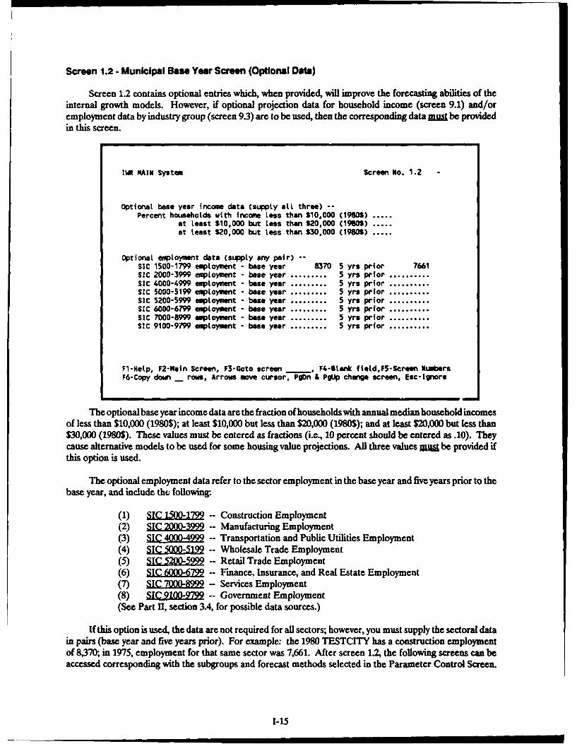
Screen 1.2 - Municipal Base Year Screen (Optional Data)
Screen 1.2 contains optional entries which, when provided, will improve the forecasting abilities of theinternal growth models. However, if optional projection data for household income (screen 9.1) and/oremployment data by industry group (screen 9.3) are to be used, then the corresponding data m= be providedin this screen.
iWR MAIN System Screen No. 1.2 -
Optional base year income data (supply aLL three) --Percent households with income less than $10,000 (1980$) .....
at least $10,000 but Less than $20,000 (1960) .....at least 520,000 but less than $30,000 (1980S).
Optional employment data (supply any pair) --SIC 1500-1799 empLoyment - base year 8370 5 yrs prior 7661SIC 2000-3999 employment - base year ......... 5 yrs prior ..........SIC 4000-4999 employment - base year ......... 5 yrs prior ..........SIC 5000-5199 employment - base year ......... 5 yr$ prior ..........SIC 5200-5999 employment - base year ......... 5 yrs prior ..........SIC 6000-6799 employment - base year ......... 5 yrs prior ..........SIC 7000-8999 employment - base year ......... 5 yrs prior ..........SIC 9100-9799 emptoyment - base year ......... 5 yrs prior ..........
Fl-Help, F2-Nain Screen, F3-Goto screen _ , F4-Blnk fieLd,F5-Screen NumersF6-Copy down - rows, Arrows move cursor, Pg)n & Pg.Jp change screen, Eso-Ignore
The optional base year income data are the fraction of households with annual median household incomesof less than $10,000 (1980$); at least $10,000 but less than $20,000 (1980$); and at least $20,000 but less than$30,000 (1980$). These values must be entered as fractions (i.e., 10 percent should be entered as .10). Theycause alternative models to be used for some housing value projections. All three values must be provided ifthis option is used.
The optional employment data refer to the sector employment in the base year and five years prior to thebase year, and include the following.
(1) SIC 500-1799- Construction Employment(2) SIC 2000-3999- Manufacturing Employment(3) SIC 4000499-- Transportation and Public Utilities Employment(4) SIC 5000-5199- Wholesale Trade Employment
(5) SIC 5200- - Retail Trade Employment(6) SIC 6000-6799- Finance, Insurance, and Real Estate Employment(7) SIC 7000-8999 Services Employment(8) SIC 9100- - Government Employment(See Part II, section 3.4, for possible data sources.)
If this option is used, the data are not required for all sectors; however, you must supply the sectoral datain pairs (base year and five years prior). For example: the 1980 TESTCITY has a construction employmentof 8,370- in 1975, employment for that same sector was 7,661. After screen 1.2, the folowing screens can beaccessed corresponding with the subgroups and forecast methods selected in the Parameter Control Screen.
1-15

Screens 2.1 and 2.2 - Residential Subgroups: Flat Rate and Sewered
This subgroup includes occupied housing units that do not face a charge that varies with the quantity ofwater used. These customers pay a flat rate for water/wastewater services or are renter-occupied where theowner pays the water/wastewater bill. Such customers, therefore, face a zero marginal price and are notexpected to react to changes in price. This category may include housing units contained in buildings with twoor three units per structure and mobile home parks where a single meter serves allunits. All units in this categoryare served by a public sewer system.
Screens 2.1 and 2.2 (not shown) allocate space for 25 sets of flat rate and sewered data, where each setrepresents a specified property value range.
lWR MAIN System Screen No. 2.1
Municipat Data - Residential Subgroups - Flat Rate SeweredBase Year Property
VaLue Ranges Persons Assessment Density No of UnitsLow ($100s) High No/Unit Factor Units/Acre In Range
0 99.99 2.23 ... 4.00 124.3
.......* .... ... .... .4.*... .
Fl-Help, F2-Main screen, F3-Goto screen _, 4-Blank fioeidF-Screen NumersF6-Copy down _ rows, Arrows move cursor, Pg~n & PgUp change screen, Esc-Ignore
The input data for each flat rate and sewered value range may include:
(1) Lw -- lower limit of the property value range in $100s at base year price levels(2) High - upper limit of the property value range in $100s at base year price levels(3) Permn f .UiL -- persons per housing unit for the value range(4) A -- optional housing assessment factor for value ranges, if using assessed
valuation rather than market value (equals the ratio of assessed value to market value)(5) Density (Units/A e) -- average density of housing units per acre for the value range(6) N, ofUni -- number of housing units within the value range(See Part II, section 3.4, for possible data sources.)
For example: the first value range ($0 to $9,999) has 2.23 persons per housing unit, a density of four unitsper acre, and 1,243 housing units within that value range.
Note that water use calculations for each range are based on the midrange value. Due to the sensitivityof residential water requirements to home value, it is r mmended that no individual value range be larger thannecessary, preferably less than $10,00 from the lower to upper value range. Value ranges should be enteredin order of increasing midrange value. This is true for all residential subgroups.
1-16

Screens 3.1 and 3.2 - Residential Subgroups: Flat Rate and Unsewered
This subgroup includes occupied housing units similar to the above category except that customers arenot served by a public sewer system. Wastewater disposal is by means of a private septic tank, cesspool, or othermethod.
Screens 3.1 and 3.2 (not shown) allocate space for 25 sets of flat rate and unsewered data.
IM PAIN System Screen No. 3.1
MunicipeL Data - ResidentiaL Subgroups - FLat Rate SepticBase Year Property
VaLue Ranges Persons Assessment Density No of UnitsLow (S100s) High No/Unit Factor Units/Acre In Range
0 99.99 2.23 ... 4.00 450
.,e. ,, *e= .e eloQe..... .........
l..... .,..... .... . l = o... ...
=*Q =I* .Q. o...... . .... .. e.....
Fl-Help, F2-Main Screen, F3-Goto screen , F4-Btnk field,FS-Scren NumbersF6-Copy down - rows, Arrows move cursor, Pon & PgUp change screen, Esc-ignore
The input data for each flat rate and unsewered value range may include:
(1) Lo -- lower limit of the property value range in $100s at base year price levels(2) likh -- upper limit of the property value range in $100s at base year price levels(3) Persons ft. /Unit) -- persons per housing unit for the specified value range(4) Assesmt Factor - optional housing assessment factor for value ranges, if using assessed
valuations rather than market value(5) Density (Units/Acre) .- density of housing units per acre for the specified value range(6) NoofUnits -- number of housing units within the specified value range(See Part II, section 3.4, for possible data sources.)
For example: the first value range (SO to $9,999) has 2.23 persons per housing unit, a density of four unitsper acre, and 450 housing units within that value range.
1-17

Screens 4.1 and 4.2 - Residential Subgroups: Metered and Sewered
This subgroup includes single-family occupied housing units that are individually metered and are servedby a public sewer system. These housing units are considered owner-occupied or occupied by renters who areresponsible for paying the water and wastewater bill.
Screens 4.1 and 4.2 (not shown) allocate space for 25 sets of metered and sewered data.
IWi PAIN Systm Screen No. 4.1
M4unicpet Data - Residential - Metered SeweredBill
Base Year Property Price of Water Density DifferenceVaLue Ranges Annuatl Summer Assess Units No of Units S/BitL Period
Low (100s) High S/K-Gal S/K-Gal Factor /Acre in Range AnmuL Summer
0 99.99 0.75 0.49 .... 4.00 4496 2.53 1.65
..... .. ....... .... o ..... .... ..... ........° ...... ....
FI-Neip, F2-9afn Screen, F3-Goto screen , F4-Btak fieldF5-Screen NumbersF6-Cop down _ raw, Arrows wove cursor, Pq)n & P" change screec -Ignore
The input data for each metered and sewered data value range may include:
(1) la- - lower limit of the property value range in $Os at base year price levels(2) Hijgh - upper limit of the property value range in $10s at base year price levels(3) Pe ofWaer--
Ann- ainnual marginal price of water for the specified value range (dollars per 1,000gallons) in 1980$Sum= - summer marginal price of water for the specified value range (dollars per 1,000gallons) in 1980(See Part 11, section 3.1, for a detailed explanation of the price variables.)
(4) Assessmet mact -- optional assessment factor for value ranges if assessed valuation isused rather than market value (default value is one (1.0))
(5) Density (UnitlAcre) -- density of housing units per acre for the specified value range(6) No.Jof it -- number of housing units within the specified value range(7) iliffrenc --
Anna - annual bill difference for a specified value range (dollars per billing period) in198M 1Smmr - summer bill difference for a specified value range (dollars per billing period) in1980s
(See Part II, section 3.4, for possible data sources.)
Note that bill difference variable describes thediffrn in the consumer's actual total bill and what wouldbe charged if all units of water were sold at the marginal price.
1-18

The following is one example of how to calculate the bill difference:
EXAMPLE OF BILL DIFFERENCE CALCULATION
Rate Structure Water ServiceService Charge 1.03 Dollars/MonthUp to 5,000 Gal./Mo. 0.60 Dollars/1,000 Gal.5,001-10,000 Gal./Mo. 0.50 Dollars/1,000 Gal.All over 10,000 GaL/Mo. 0.40 Dollars/1,000 Gal.
Wastewater ServiceAll Water Use 0.35 Dollars/1,000 Gal.
Billing Period Is One Month
Average Annual Water Use in Value Range350 Ga./Day 350 x 31 = 10,850 GaLMo.
Marginal Price 0.40 + 0.35 = 0.75 Dollars/1,000 Gal.
Bill DifferenceTotal Bill: Service Charge 1.03 Dollars
Up to 5,000 Gal. 4.75 Dollars5,001-10,000 Gal. 4.25 DollarsOver 10,000 Gal. 9&4 Dollars
10.67 Dollars
Less 0.75 x 10,850/1,000 8.14 DollarsEquals Annual Bill Difference 2.53 Dollars
The example of metered and sewered data in the screen shows that in the first value range ($0 to $9,999)a customer pays an annual marginal price of $0.75 per 1,000 gallons and a summer marginal price of $0.49 per1,000 gallons; the annual bill difference is $2.53 per billing period and the summer bill difference is $1.65 perbilling period. There are 4,496 housing units in this value range with a density of four units per acre.
1-19

Screens 5.1 and 5.2 - Residential Subgroups: Master-Motered Apartments
This subgroup includes occupied housing units in structures with four or more units. The structure maybe untoetered or provided with a single (master) meter. These customers face a zero marginal price of waterand have limited opportunity to engage in outdoor (seasonal) water use.
Screens 5.1 and 5.2 (not shown) contain 25 sets of master-metered apartment data.
IWR MAIN System Screen No. 5.1
municipal Data - Residential - master Metered ApartmentsBase Year Property
Value Ranges Persons Assessment No of UnitsLow ($100s) High No/Unit Factor in Range
0 149.99 2.92 .... 5954
....... ~. .. ... . .. ... o~e e t~aile ele.J *w. . . .. l
..... ... ... ....
*°*.IQ ,,II *. ll . i°. . . . ~e
FI-Nelp, F2-Nafn Screen, F3-Goto screw F4-Btnk fietd,F5-Screen Nulmbersf6-Copy down _ raw, Arrows move cursor, Pg~n &PgUp change screwn, Esc-Ignore
The input data for each master-metered apartment value range may include:
(1) Low - lower Uinit of the property value range in $100s at base year price levels(2) Hi - upper limit of the property value range in $100s at base year price levels(3) Persons ftoUnit - persons per housing unit for the specified value range(4) Assessmegnt Facor - optional household assessment factor for value ranges ifusn
asesdvaluation rather than market value(5) No f nt -- number of housing units within the specified value range(See Part II, section 3A4 for possible data sources.)
For example: the first value range ($0 to $14,999) has 2.92 persons per housing unit and 5,954 housingI
units within that value range.
Note that through the use of the alternate construction cost indexes, property values entered in screens2.1 through 3.2 in base year dollars are converted internally to 1980 dollars.
1-20
....... .. . . . .. -- l I.i i . .

Screen 6.1 - Commercial Employment
Screen 6.1 contains 23 specified commercial employment categories.
IWR MAIN System Screen No. 6.1
Municipal Data - Commercial Employment
Total Employment
Description Description
COO1 MisceLLaneous Comm.ercial 30301 C013 Hotels, Restaurants .......C002 Vocational School ....... C014 Electric, Gas Utilities .......C003 Miscellaneous Retail ....... C015 Public Administration 56319CO4 Boarding Houses ....... C016 SchooLs, Universities ......COOS Transportation Terminal ....... COlT Race Tracks ......C006 Barbers, Cleaning ....... C018 Labs, Water Utilities ......COO7 Power Laundries ....... C019 Health Services ......COOS Landscaping ....... C020 Medical Offices, Bakeries ......C009 Miscellaneous Wholesale ....... C021 Nursing Facilities ......C010 Recreational Facilities ....... C022 Hospitals ......C011 Food and Auto Retail ....... C023 Zoological, etc. Gardens ......C012 Dance Studios .......
Fl-Help, F2-Main Screen, F3-Goto screen -, F4-Blank field,FS-Screen NumbersF6-Copy down _ rows, Arrows move cursor, Pg)n & PgUp change screen, Esc-Ignore
These categories represent combinations of Standard Industrial Classification (SIC) categories (see PartII, section 3.1). Enter the total employment for those categories which are represented in the study area. Leaveblank those categories which do not apply.
For example: Miscellaneous Commercial (CO01) has 30,301 employees, whereas Public Administration(CO15) has 56,319 employees.
Note that none of the commercial categories are highlighted; however, if the commercial/institutionalsubgroup was selected in the Parameter Control Screen, then employment data mus be entered for at least onecategory on screen 6.1 or 6.2. (See Part II, section 3.4, for possible data sources.) See the description of screen7.7 for an adjustment of commercial water use for average commercial water prices.
1-21

Screen 6.2 - User-Added Commercial Parameters
Screens 6.2 and 6.3 (not shown) contain space for 27 additional user-specified commercial categories.
IR MAIN System Screw No. 6.2
Municipal Data - User Added Commercial Parameters
CoefficientsNo of Am Avg Max Day
Label Description Employment Units Unit Parameter (Gattons/Day/Unit)
C024 Car Washes ....... 70 Buildings 10000, 15500C025 ...................... ..................................C026 ...................... ..................................C027 ...................... ..................................C028 ................ ....... ......... ................ ......... .........C029 ................ ...... ....... ................ ......... .........C030 ...................... ..................................C031 ...................... ..................................C032 ...................... ..................................C033 .......................... ................ ......... .........C034 .......................... ................ ......... .........C035 ...................... ..................................C036 ................ ...... ..... ................. ......... .........C037 .......................... ................ ......... .........
Fl-Help, F2-Main Screen, F3-Goto screen F4-Utarn fietd,F5-Scren NumbersF6-Copy down _ rows, Arrows move cursor, Pg~n & PgUp change screen, Esc-Ignore
Enter in a brief description (such as car washes), either employment (if known) or the number of units,and the unit parameter (such as buildings or employees). Then the average annual and maximum-day wateruse coefficients (gallons per day per unit or per employee) must both be entered. For example: there are 70car washes in the study area, and they use approximately 10,000 gallons per day per unit (average annual use).
Note that a specific water use type should not be addressed in both screens 6.1 and 6.2 (i.e., do not includecar wash employment in screen 6.1 and then include car wash buildings in screen 6.2). Where it is not feasibleto provide employment data for any of the categories on screen 6.1, it is possible to include all commercial/institutional use in one or more categories on screen 6.2 (e.g., total commercial use), provided that suitable wateruse data are available to calculate water use coefficients in gallons per day per unit. Therefore, total commercialwater use in the base year is addressed in one of three ways: (1) by providing total commercial employmentdisaggregated into up to the 23 categories in screen 6.1, (2) by developing one or more user-added categoriesin screen 6.2, or (3) by using a combination of the two previous approaches.
1-22

Screens 7.1 through 7.6 - Industrial Employment
Screens 7.1 through 7.6 (72 through 7.6 not shown) contain 198 categories of manufacturing employmentwhich are organized by Standard Industrial Classification (SIC) codes.
IWR MAIN System Screen No. 7.1Municipat Data - Industrial Employment
Total EmploymentSIC Description SIC Description201 eat Products 282 209 Misc Foods & Kindred prod .......2011 Meat Packing Plants ....... 211 Cigarettes .......2013 Sausages &Prepared Meats ....... 212 Cigars .......2016 Poultry Dressing Plants ....... 213 Chewing & Smoking Tobacco .......2017 PouLtry & Egg Processing ....... 214 Tobacco Stemming&Redrying .......202 Dairy Products ....... 221 Weaving MiLLs, Cotton .......203 Preserved Fruits & Veggys ....... 222 Weaving Mills, Synthetics .......204 Grain Milt Products ....... 223 Weaving&Finish Mtlts,Wool .......205 Bakery products ....... 224 Narrow Fabric Mills .......2051 Bread, Cake & Ret. Prods 120 225 Knitting Mills2052 Cookies & Crackers 29 226 Textile Flnlshng,exc.Woot......206 Sugar & Confectionery prd ....... 227 Floor Covering Mills ......207 Fats & Oils ....... 228 Yarn & Thread Mills .......208 Beverages ....... 229 Misc. Textile Goods2082 Malt Beverages ....... 230 AppereL&Other Textile Prd.2086 Bottled& Canned Soft Dks ....... 241 Logging Camps&Lg Contrctr .......2087 Flavoring Extracts&Syrup .......
Fl-Hetp, F2-Main Screen, F3-Goto screen _, F4-Btank field,F5-Screen NumbersF6-Copy down _ rows, Arrow move cursor, Pg)n & P"Jp change screen, Esc-Ignore
If a three-digit SIC category is disaggregated into four-digit subcategories, you may specify employmentdata at either the three-digit level or the four-digit level. However, if you specify employment at the three-digitlevel you cannot specify it at the four-digit level as well Furthermore, if you specify employment at the four-digit level, all four-digit categories within the given three-digit category m= contain a value of zero or greater.
For example: Meat Products (SIC 201) has an employment of 282. Employment for the four-digit SICsubcategories within Bakery Products (SIC 205) is 120 for SIC 2051 and 29 for SIC 2052.
Note that none of the categories are highlighted; however, if the industrial subgroup was selected in theParameter Control Screen, then employment data mus be entered for at least one category on screens 7.1through 7.7. (See Part II, section 3.4, for possible data sources.)
1-23

Screen 7.7 - User-Added Industrial Parameters and Nonresidential Prices
Screen 7.7 provides two additional industrial categories that may be user-specified.
IWR MAIN System Screen No. 7.7
Muicipat Data - User Added Industrial Parameters
CoefficientsAm Avg Max Day
Labal Description EmpLoyment GaLs/Day Gets/Day
1199 High Tech Gadgets 1345 178.9 198.9
1200 . ..... .... .... . .....
Municipal Data - Ccmrciat and Industrial Water Prices
MarginaL Price in Base Year Marginal Price Concurrent withWater Use Coefficients
$/1000 gallons S/1000 gallons
Commercial .88 .95
industrial ......
Fl-Hetp, F2-Ma|n Screen, F3-Goto screen _, F4-BSla fletd,FS-Screen NwsersF6-Copy down _ rows, Arrows move cursor, PgDn & P0Jp change screen, Esc-Ignore
Since the specified water use parameter is employment, the corresponding water use coefficient must beentered as gallons per employee per day. Note that the water-using activities should not appear more than once(Le., employment counted in one or more categories on screens 7.1 through 7.6 should not be addressed againon screen 7.7). Where it is not feasible to provide employment data for anyof the industrial categories on screens7.1 through 7.6, it is possible to include all manufacturing use as one or two categories on screen 7.7 (e.g., totalmanufacturing), provided suitable water use and employment data are available to calculate water use peremployee coefficients.
Nonresidential water use is calculated by multiplying the category parameter (e.g., employment) by thecategory's water use coefficient. The coefficients for the 23 commercial and 198 industrial specified categorieswere developed from survey data as explained in Part II, section 4.1. The commercial coefficients are from 1984data while the industrial coefficients are from 1982 data. Given that nonresidential water users respond toincreases in water and wastewater prices as indicated by a price elasticity for the commercial or industrial sector,the estimated water use can be adjusted for any price difference between the base year and the year in whichthe water use coefficients were estimated. If you wish to make this adjustment for price differences for eithersector (or both), enter the marginal price in dollars per thousand gallons for the sector in both the base yearand the year of the coefficients (1984 for commercial coefficients and 1982 for industrial coefficients). Note thatthe year of the coefficients may change if you revise the coefficients in the library. (See Part II, section 5.3, fora discussion of adjusting nonresidential water use rates.) Both prices must be entered for a sector in order tocompute the price adjustment, and both prices must be entered in 1980$. See Part II, section 4.1, for detailsof the nonresidential price adjustment computation.
For example: user-added industrial category 1199, High Tech Gadgets, has an employment of 1,345 andan annual average and maximum-day coefficient of 178.9 gallons per employee per day and 198.9 gallons peremployee per day, respectively, Also, marginal commercial price in the base year is $0.88 per 1,000 gallons andthe marginal price concurrent with water use coefficients (1984) is $0.95 per 1,000 gallons in 1980 dollars.
1-24

Screen 8.1 - Public/Unaccounted
Screen 8.1 allows data to be entered for public/unaccounted subgroups.
IWUR MAIN System Screen No. 8.1
Municipal Data - Pubtic/Unaccounted
Resident Annual Average Max DailyCategory Population GaLtons/Day Gals/Day
Distribution Losses
Free Service
If water use is given, Average and Max-Day must both be entered.
Fl-Hetp, F2-Maln Screen, F3-Goto screen _ , F4-tank fteld,FS-Screen NuibersF6-Copy dowm - rows, Arrows move cursor, PgDn & PgJp change screen, Esc-Ignore
When no parameters on this screen are provided, distribution loss is calculated as a percentage (asprovided in the Library of Water Use Coefficients-FLSS) of the total municipal water use (or production).However, if you enter a nonzero value for population, the model will calculate distribution losses on a per capitabasis (using the library coefficient-LOSS). Free service is ajb calculated on a per capita basis using residentpopulation from screen 1.1 and can only be suppressed by setting the library coefficient (FSER) to zero. Notethat the population entered on screen 8.1 is the population jrw by the distribution system and, therefore, maynot be the same as the population provided on screen 1.1.
Alternatively, direct estimates of public/unaccounted use (distribution losses and free service) in SWJMgir can be supplied for both average annual and maximum-day water use and will override the calculationsdescribed above.
1-25

Screens 8.2 and 8.3 - User-Added Public/Unaccounted Parameters
Screen 8.2 contains 27 additional user-specified public/unaccounted water use parameters.
1WR MAIN System Screen No. 8.2
Municipal Oats - User Added Pubt ic/Unrccounted Parameters
CoefficientsNo of Ann Avg Max Day
Label Description Units Unit Parameter (Gallons/Day/Unit)
POOl State Parks 125 Restrooms 1000 2000P002................ ......... ................ ......... .........P003 ................ .......................... ......... ......P00 ......................... ....................... .........P005................ . ........ ................ .......... I......P006 .................................................. ........P007 ................ . ...........................................POl ................ ......... ................ ......... ........P009 ..........................................................Polo ................ ......... ................ ......... .........Poll............ ......... ................ ......... .........P012............ ......... ................ ......... .........P013 ........................................... ...............P014 .......................... ................ ......... .......
Fl-Hetp, F2-1ain Screen, F3-Goto screen _, F4-Stank fietd,F5-Screen NumbersF6-Copy down _ rows, Arrows move cursor, Pg~n & P"Jp change screen, Esc-Ignore
If you have information on a specific public water use category (that is not accounted for elsewhere), youmay provide a description of the category, number of units, unit parameter, and water use coefficients in gallonsper day per unit.
For example: state parks in the study area are known to have 125 restrooms (units) which consume 1,000gallons per day per unit annually and 2,000 gallons per day per unit on a maximum-use day. Before defininga user-added category, it should be determined that the water-using activity is not included in some othercategory (e.g., commercial or industrial).
3.4 PROJECTION SCREENS USED BY INTERNAL GROWTH MODELS
Projection screens contain parameters which are used by the internal growth models to projectdisaggregated parameter data for the forecast years selected. Regardless of the forecast method selected,certain parameters (population, median household income, and total employment) = be provided for eachforecast year. These required data are highlighted on each screen. When used, the optional data (total numberof households and households by income range) improve the performance of the internal growth models.
1-26

Screens 9.1 and 9.2 - Projection Data for Internal Growth Models
Screens 9.1 and 9.2 (not shown) allow projection data to be provided for the forecast years specified inthe Parameter Control Screen.
IW MAIN System Screen No. 9.1
Projection Data for Internal Growth Models
Year Poputatn Medr HH Total Total No. % Households u/Income (1980S)>Base Income Employmnt Househlds <10,000 10,000-- 20,000--
(19805) <20,000 <30,000
1990 532761 2472 208722 153259 ........ ........ ............ ................................ ................ ........... ........ ....... ........ ........ ........ ........ ............ ........ ....... . ....... ........ ........ ........ ........
........... ... .. .... ........... ........ . ..... .........
...................................................... .... .. ... ................................ ........
..o...................... ........ .......... ........
F1-Help, F2-Main Screen, F3-Goto screen -, F4-BLank field,F5-Screen NumbersF6-Copy down _ rows, Arrows move cursor, PgDn & P9ip change screen, Esc-Ignore
Screens 9.1 and 9.2 contain the following parameters for which data may be providedL
Required:(1) Popjation -- total resident population for study area(2) Median Household Income (1980S) - annual median household income expressed in 1980
dollars(3) Total Emplyment -- total employment for study areaOptional:(4) Total No. Households -- total number of occupied housing units in the study area(5) Percent Households with Income (1980S) --
< 10,000 -fraction of households in the study area with an annual median household incomeof less than $10,000 (in 1980 dollars)10,000 - < 20,000 - fraction of households with an annual median household income of atleast $10,000 but less than $20,000 (in 1980 dollars)20,000 - < 30,000 - fraction of household with an annual median household income of atleast $20,000 but less than $30,000 (in 1980 dollars)
Note that if these optional parameters for household income are used, all three fractionsmust be provided, and corresponding data must be entered in screen 1.2. (See Part HI,section 3.4, for possible data sources.)
For example: in the forecast year 1990, projected population is estimated to be 532,761 and the householdincome to be $24,472. Projected employment is estimated to be 208,722, and the total number of housing unitsis projected to be 153,259. [Screen 9.2 is a continuation of screen 9.1.]
1-27

Screens 9.3 and 9.4 - Projection Data for Internal Growth Models: Employment by IndustryGroup
Screens 9.3 and 9.4 (Dot shown) allow employment projection data to be provided for 24 forecast years.
1W MAIN System Screwn Mo. 9.3
Projection Date for Internet Growth Models
Eo~toyment by Indu~stry Group~ (sic Codes)
Year 1500- - 2000-- 4000-- 5000-- 5200-- 6000-- 7000-- 9100--Passe 1799 3999 4999 5199 5999 6799 899 9799
990 9191 ........... ....... ....... ....... ....... .......
.......... ....... ....... ....... ....... ....... .......
......... ............. .........................
................ .................. ......
FI-Usip, FZ-PmIn Screem. F3-So. screwn * 4-litw fieldFS-Icreen W14 reF46-Copy down_ rus Arrewsi -. tcsor* Pq)n & ftup chwee screwn, Isc-iWae
Employment is entered by major industry groups (e.g., construction, manufacturing, retail). See thedescription of screen 1.2 on page 1-15 for the list of the major industrial groups. Note that if these optionalparameters are provided, corresponding data must be entered in screen 1.2. It is desirable, but not necessary,to supply data for all groups for a specified forecast year.
For example: in the year 1990, projected employment for SIC categories 1500-1799 (construction) is 9,191.
1-28

3.5 HISTORICAL PARAMETER SCREENS
When extrapolation of local historical data is selected as a forecast method on the Parameter ControlScreen, you will be prompted to provide historical data for the water use parameters. For any of the HistoricalParameter screens used, you must provide actual data for aLj9NLpast years which may include the baseyear but not more than seven years. The IWR-MAIN System will use this information to perform a straight-line extrapolation of parameter data to the forecast years. You maybe selective in that you do not have to providehistorical data for all screens or all categories.
Screens 10.1 and 10.2 - Residential Subgroups
Screens 10.1 and 10.2 (not shown) contain historical data parameters for each of the residentialsubgroups. The flat rate and sewered and the flat rate and unsewered data are entered in screen 10.1, while themetered and sewered and the master-metered apartment data are entered in screen 10.2.
IWR MAIN System Screen No. 10.1
Projection by Extrapolation of Local Historical Trends
Residential -- Flat Rate-Sewered -- No. Housing Units
Year Low Grp. Grp. 2 Grp. 3 High Grp. Totaa.... ........ * ....... .. ... .......•
i
• . . e.......
... ° oo .. o o, °. °° ...... . .. .. .° . .. .
°l .oo °. . . = ... ........ ...... . i. .....
Residential -- Flat Rate-Unsewered -- No. Housing Units
Year Low Grp. Grp. 2 Grp. 3 High Grp. Total
F -Help, *2-Main Screen, P3-Goto scree , P.BLank Ie F5-Screen Numbers
F6-Copy down _ rows, Arrows move cursor, Pg~n & PgUp change screen, Esc-Ignore
Specifythe years forwhich the historical parameter data are tobe entered for agiven residential subgroup(e.g., flat rate and sewered), and enter the number of occupied units in each of the following value range groups.
(1) Low Grou (Group 1) -- total housing units in all value ranges having midrange valuesless than $25,000 when expressed in 1980 dollars
(2) iao 2 - total housing units in all value ranges having midrange values greater than$25,000 but less than $50,000 when expressed in 1980 doilars
(3) G -- total housing units in all value ranges having midrange values greater than$50,000 but less than $100,000 when expressed in 1980 dollars
(4) id Grou (Group 4) -- total housing units in all value ranges having midrange valuesgreater than $100,000 when expressed in 1980 dollars
(5) Total - total number of housing units in the specified year
1-29

Screens 11.1 through 11.4- Commercial Subgroups
Screens 11.1 through 11.4 (11.2 through 11.4 not shown) contain the 50 commercial water use categories.
IWR MAIN System Screen No. 11.1Projection Data by Extrapolation of Historical ComnerciaL Parameters
Year 1960 1965 1970 1975 .... .... ....Cool 28000 29000 29580 30000 ...........................C002 ........ ......... ......... ......... . ........ .........C003 ........ ........ .......... .......................... .C00O ......... ......... ......... ......... ......... ............coos ................. ......... ......... ......... ............C006 ......... ........ ......... ......... ....... .. .........C007 ..................... ............. -....... ........coos ................. ......... ......... ......... ............C009 ......... ......... °............... ......... ..... ......Colo ......................................................Coil .....................................................C012 .....................................................
Bold fields indicate those used in base year.
Fl-Hetp, FZ-Main Screen, F3-Goto screen F4-Otank fietd,FS-Screen NumbersF6-Copy down _ rows, Arrows move cursor, PgD' & PgiJp change screen, Esc-lgnore
The line labeled YEAR is highlighted and tlt. two.ysar must be entered. The year values must befour-digit numerical values and may include the base year. The year entered above each column in screen 11.1will automatically appear above the corresponding column in the remaining screens (11.2 through 11.4).
All commercial categories used in the base year input screens will be highlighted to facilitate data entry.Enter the historical years and the number of employees (or other parameter if user-specified) in each categoryfor which you desire a historical extrapolation. Not all categories used in the base year need to be addressed.
For example: since C001 was used in the base year (screen 6.1), it is highlighted. Actual data values areprovided for the years 1960, 1965, 1970, and 1975.
1-30

Screens 12.1 through 12.s - Industrial Subgroups
Screens 12.1 through 12.a contain the 200 industrial water use categories.
IWR MAIM System See HeLp (F1 key) for explanation Screen No. 12.1Projection Data by Extrapolatfon of Historical Industrfat Parameters
Year 1950 1960 1970 .... .... .... ....201 ......... ........ .. ...ee m .........e ......... ... ...e .........
2011 ......... ......... ................. ......... ....... ...........2013 ........................... ......... .................. .........2016 ......... ......... .................. ................... .........2017 ......... .......... ......... .......... ......... .......... .........202 ......... ......... ......... ......... ......... ......... .........203 ......... ......... ......... ......................................2052 ......... .......... ......... .......... ......... .......... .........205 ........................... ......... ......... .......... ........2051 300 296 278.......... ................... .........2052 ......... ......... ......... ......... ......... ......... .........206 ................... ........ .................. ......... .........207 .................. ......... ......... ......... ......... .........208 ......... ......... ......... .................. ......... .........2082 ......... ................... ................... ...................2086 ......... ................... ................... ...................2087 ......... ................... ................... ...................209 ......... ......... ......... .................. ......... .........211 ......... ......... ......... ......... ......... ......... .........212 ......... ......... ......... ......... ......... ......... .........Fl-Help, F2-Main Screen, F3-Goto screen _, F4-Slank fietd,F5-Screen NwbersF6-Copy doen _ rows, Arrows move cursor, Pg)n & PgUp change screen, Esc-Ignore
As with the commercial secor, at last to M are required. The years and all those categories usedin the base year will be highlighted. Supply the years and employment for the categories for which you desirehistorical extrapolation. Again, not all highlighted categories need to be addressed.
For example: category 2051was used in the base year (screen 7.1) and, therefore, it is highlighted. Actualdata values are provided for the years 1950, 1960, and 1970.
1-31

Screens 13.1 and 13.2 - Public/Unaccounted Subgroups
Screens 13.1 and 13.2 (not shown) provide space for historical parameters for the public/unaccountedsectors. The categories correspond with those provided in screens 8.1 and 8.2.
IWR MAIN System Screen No. 13.1Projection Data by Extrapotation of Historicat Pubtic/Unaccounted
Year ..... ..... ..... ..... ..... ..... ....LOSS ......... ......... ......... ... ..... ......... ....... . .........
P011 ......... ......... ......... ......... ......... ......... .........P0 2 ......... ...... .. ......... ......... ......... ......... .........P0023......... ......... ................. ................. .......P0034............... ......... ......... ......... ......... .........P004 ......... ......... ................. ................. .......P006 ............... ......... ......... ......... ......... .........P0067............... ......... ......... ......... ......... .........P007 ............... ......... ......... ......... ......... .........P009 ............... ......... ......... ......... ......... .........Polo0............... ......... ......... ......... ......... .........Poll ......... ......... ................. ................. .......P012 ................ ......... ......... ......... ......... .........
BoLd fields indicate those used in base year.FP-Hetp, F2-Main Screen, F3-Goto screen _, F4-Btank fieLdFS-Screen usLersF6-Copy down _ rows, Arrows move cursor, Pg)n & P"Jp change screen, Ec-Ignore
As with the commercial and industrial Historical Parameter screens, the line YEAR is highlighted andentry of atleast..wo Mw are required. Year values must be four-digit numerical values. The lines LOSS(distribution losses) and FSER (free service) are highlighted, as well as any user-specified categories that wereselected in the base year. Enter historical population for LOSS and FSER for the respective per capitacalculations. Enter the parameter data for whichever user-added category historical information is known.LOSS and FSER are highlighted even though data may not have been entered in screen 8.1 because defaultvalues are assumed for these parameters from the population data in screen 9.1. Parameters projected fromhistorical data will take precedence over growth model projections.
3.6 EXTERNAL PROJECTION SCREENS
These screens allow direct external projections of parameters used in the four major subgroups:residential, commercial, industrial, and public/unaccounted for each of the first ten specified forecast years. Itis not necessary that data be entered for all of the forecast years or all water use subgroups. Enter data in thoseyears and those categories for which you have specific information.
For each of the forecast years a series of nine screens are available (one residential, two commercial, fourindustrial, and two public/unaccounted). The residential screen for the second forecast year follows the public/unaccounted screen(s) for the first forecast year. Thus, you will have access to all the external projection screensof one year before proceeding to the next forecast year. The screen numbers reflect the sequence of both yearsand sectors. For example, the screens for the first forecast year are screens 14. 1.1 through 14.1.9 while the screensfor the second forecast year are numbered 14.2.1 through 14.2.9. In the following screen descriptions, the letterx within the screen number represents the forecast year corresponding to a given screen.
1-32

Screen 14.x.1 - Residential - Direct External Projections
IWR MAIN System Screen No. 14.1.1Direct External Projections: 1990 - Residential
Category & No. Units Category & No. UnitsValue Range in VaLue Range in
Group Group Group Group
FWG1 ........ FPG1 ........FUG2 ........ FPG2 ........FWG3 ........ FPG3 ........FWG4 ........ FPG4 ........FWTL ........ FPTL ........
M4d 37338 APG1 ........MWG2 ........ APG2 ........4WG3 ........ APG3 ........MWG4 APG4 ........NWTL ii0;5 APTL ........
Fl-Help, F2-Nain Screen, F3-Goto screen , 4-Btank fietd,FS-Screen NumbersF6-Copy down _ rows, Arrows move cursor, Pg~n & PgUp change screen, Eac-Ignore
If you wish to supply external projections for the residential sector, enter the number of occupied housingunits for anyof the specified category andvalue range groups. The first two characters of the group label indicatethe residential subgroup. The last two characters are either the price range of corresponding subgrotups or atotal count. All price ranges should be expressed in 1980 dollars. The allowed combinations include:
Residential Subgrops(1) FP - flat rate and unsewered(2) FW - flat rate and sewered(3) AP - master-metered apartment(4) MW - metered and sewered
Value RaMe Grou(1) G1 - midrange market value less than $25,000 (1980$)(2) G2 - midrange market value of at least $25,000 but not more than $50,000 (1980$)(3) G3 - midrange market value of at least $50,000 but not more than $100,000 (1980$)(4) G4 - midrange market value of at least $100,000 (1980$)(5) TL - total occupied housing units
For example: for 1990, it is estimated that 37,338 metered and sewered housing units will be in valueranges having midrange values in the low value group ($0 -$25,000 expressed in 1980 dollars). The total numberof housing units in the metered and sewered housing subgroup is estimated to be 110,015. These two residentialcategories are labeled MWG1 and MWTL, respectively.
1-33

Screens 14.x.2 and 14.x.3 - Commercial - Direct External Projections
IWR MAIN System Screen No. 14.1.2Direct External Projections: 1990 - Commercial
Category Parameter Employment Category Parameter Employment
cool .......... .......... cola .......... ..........C002 .......... .......... C019 .......... ..........C003 .......... .......... C020 .......... ..........C004 .......... .......... C021 .......... ..........C005 .......... .......... C022 .......... ..........C006 .......... .......... C023 .......... ..........C007 .......... .......... C024 .......... ..........Coos .......... .......... C025 .......... ..........C009 .......... .......... C026 .......... ..........CO 10. .......... .......... C027 .......... ..........Coil .......... .......... C028 .......... ..........CO12 .......... .......... C029 .......... ..........C013 .......... .......... C030 .......... ..........CO14 ........... .......... C031 .......... ..........C015 .......... 62000 C032 .......... ..........C016 ........... .......... C033 .......... ..........CO17 ..................... C034 .......
F1-Help, F2-Mafn Screen, F3-Goto screen -, F-Itank fieid,FS-Scren NumbersF6-Copy down _ rows, Arrows move cursor, Pg~n & P".p change screen, Eac-Ignore
The categories for the commercial sector correspond to the CO1-C050 groupings observed in screens6.1 and 6.2. The SIC categories contained in each COxx grouping are specified in Tables 3-2 and 3-3 of Part II,section 3.1. Note that the categories for which data were entered in screens 6.1 and 6.2 are highlighted. However,data entry is neither limited to nor required for these categories. Enter the number of employees for any ofcategories C001-C023, and use whatever user-specified parameter you indicated for categories C024-C050.Press the page down (PgDn) key to access additional screens for categories C035-C050.
Screens 14Jx4 through 14.7 - Industrial - Direct External Projections
lIW MAIN System Screen No. 14.1.4
Direct External Projections: 1990 - Industrial
Category Employment Category Employment Category Employment
1001 .......... 1018 .......... 1035 ..........1002 .......... 1019 .......... 1036 ..........1003 .......... 1020 .......... 1037 ..........1004 .......... 1021 .......... 1038 ..........1005 .......... 1022 .......... 1039 ..........1006 1023 .......... 1040 ..........10078 1024 ......... 1 041 ..........1008 .......... 1025 .......... 1042 ..........1009 .......... 1026 .......... 1043 ..........1010 .......... 1027 .......... 104 ..........1011 .......... 1028 .......... 1045 ..........1012 .......... 1029 .......... 1046 ..........1013 .......... 1030 .......... 1047 ..........1014 .......... 1031 .......... 1048 ..........1015 .......... 1032 .......... 1049 ..........1016 .......... 1033 .......... 1050 ..........1017 .......... 1034 .......... 1051 ..........
Fl-Netp, F2-Nan Screen, F3-Goto scren _, P4-Btank fietd,FS-Screen Numbers
F6-Copy dom _ rows, Arrows ao cursor, Pgin & PgUP change screen, Esc-Ignore
1-34

The I001-1200 categories for the industrial sector correspond to the groupings used in screens 7.1 to 7.7
For a crossreference between SIC codes used in screens 7.1 to 7.6 and the corresponding (Ixx) categories, see
Part II, Table 3-4. Note that the categories for which data were entered in screens 7.1 to 7.6 are highlighted.
Data entry is neither limited to nor required for these categories. The parameter requested is employment for
the corresponding category. As with the data entry for screens 7.1 to 7.6, do not enter parameter values which
are for both the three-digit and four-digit SIC level of the same category. Use the page down (PgDn) key to
access the additional screens.
Screens 14.x(8 and 14jL9 - Public/Unaccounted - Direct External Projections
IWR MAIN System Screen No. 14.1.8Direct External Projections: 1990 - Pubticunaccounted
Water Use (gaLLons per day) FractionalLabel Parameter Ariual ave. Max. Daily Percent
FLSSLOSS .......... .......... ..........FSER .......... .......... ..........Pool ...... ... .......... ..........P002 . . ... ......... ... . . .P003 .......... .......... ..........P004 .......... .......... ..........PODS . . . . . . ..........P006 .. .. . . .. . . .. .. .P007 . .. .. . .. . . . ... .
P009 .......... .......... ..........Polo .......... .......... ..........Pol1 .......... .......... ..........P012 .......... .......... ..........P013 .......... .......... ..........P014 .. .. . .. .. . .. .. .
Fl-Help, F2-Hain Screen, F3-Goto screen _, F-ltank ffetd,F5-Screen NL.bersF6-Copy dotm _ rows, Arrows move cursor, Pg~n & P"Jp change screen Esc-Ignore
Direct external projections for the public and unaccounted-for categories may be entered in a number
of ways. Projections for distribution losses may be entered as (1) a fractional percent (FLSS) of total municipal
water use, (2) the population served (parameter for LOSS) for a per capita computation, or (3) the estimated
average annual and maximum-day water use in gallons per day. See Part II, section 4.1, for a discussion of the
alternative calculations of distribution losses. If the percent of total municipal water use is entered, the value
mu be entered as a decimal (e.g., 20 percent unaccounted would be entered as 0.20).
External projections for free service (FSER) may be entered as either the population served for a per
capita computation or as direct estimates of the average annual and maximum-day water use in gallons per day.Similarly, projections for any user-added public category POO1-P027 may be entered as a parameter or as
estimates of average annual and maximum-day water use. The parameter value, if used, must correspond with
the parameter unit for a given category as specified on screen 8.2 or 83. Water use estimates, if used, are ingallons per day.
Note that the three labels FLSS, LOSS, and FSER are all highlighted. If no data are provided for eitherFLSS or LOSS, distribution losses will be calculated using the default percentage loss from the library. Likewise,if no data are provided for FSER, the free service will be calculated using the population for the forecast yearin screen 9.1 and the default per capita water use. Public user-added categories specified in screen 8.2 will alsobe highlighted.
1-35

3.7 CONSERVATION SCREENS
When the Conservation Data option is selected on the Parameter Control Screen, IWR-MAIN willgenerate estimates of water use which are restricted by conservation measures defined in the following screens.
Restrictedwater use reflects the effectiveness of the conservationmeasures during the base year and eachforecast year. By definition, effectiveness is calculated as the product of three quantities: unrestricted wateruse, the reduction factor, and the coverage factor (Baumann et al., 1980).
Emdt - Rm * CMt * 0 8
where
Emsd, is the effectiveness of measure m in sector s for dimension d in year t measured in gallons perday.
RMW is the fraction reducion in the use of water for the dimension of water use d (e.g., indoor use) forsector s (e.g., metered and sewered) expected as a result of implementing measure m (e.g., aconservation-oriented plumbing code).
C= is the === of measure m in sector s at time t expressed as a fraction of sectoral water use; e.g.,if a plumbing code is implemented in the community on January 1, 1987, then the coverage value for themetered and sewered sector s in the future year t is defined as the proportion of the metered and sewereduse affected by the plumbing code. This can be approximated by the ratio of new housing units to thetotal projected number of units for that year.
Qud is the projected unrestricted water use for the dimension of water use d in sector s at time t in quantityper unit time (gallons per day). The water use dimensions are indoor, outdoor, and maximum-day use.See Part I, section 4.3, for details.
The IWR-MAIN Lbrary of Conservation Coefficients (LCC) contais default values for reduction factors andselected parameters for the internal calculation of coverage factors. If you select conservation measures witoutspecifying the reduction or coverage factors, the LCC will provide these factors for you. Alternately, you maydecide to provide some ora of the reduction and coverage factors for the selected conservation measures. Ifonly some values are provided, the LCC will provide the others. See Part I1, section 4.3, for an explanation anda listing of the conservation parameters in the library.
1-36

Screen 15.1 - Selection of Measures
Screen 15.1 enables you to select up to 18 conservation measures by specifying the year of initiation forthe desired measures. Fourteen measures are specified and will have reduction and coverage factors availablein the hlbrary. Four additional measures can be user-specified; if used, the reduction and coverage factors ma=be provided by the user.
IWR MAIN System SeLection of Measures and Year of Initiation Screen 15.1Enter year for those measures desired
Number Measure Description Year
1 Public Education Program 19752 Metering ....3 Pressure Reduction ....4 Pricing Policy (Rate Reform) ....5 Rationing (Per Capita) ....6 SprinkLing Restrictions ....7 IndustriaL Reuse/RecycLe ....8 Commerciat Reuse/RecycLe ....9 Leak Detection and Repair ....
10 Retrofit of Showerheads and ToiLets11 Moderate PLumbing Code 198012 Advanced PLumbing Code ....13 Low-Water Use Landscaping (New) ....14 Low-Water Use Landscaping (Retrofit) ....15 User-Specified Measure Number 1 ....16 User-Specified Measure Number 2 ....17 User-Specified Measure Number 3 ....18 User-Specified Measure Mumber 4 ....
Fl-Hetp, F2-Main Screen, F3-Goto screen _ , F4-Stank fietd,F5-Screen numbersUp and down arrows move cursor, Pe~n & PgUp change screen
For example: measure 1, Public Education Program, started in 1975. This measure consists of directmail campaigns, news media campaigns, and/or special events. Measure 11, Moderate Plumbing Code, startedin 1980. This measure requires water-saving devices for all new construction. See Part II, section 4.3, for a fulldescription of all the model-specified conservation measures.
All four digits designating a given calendar year must be specified. Any mistakes must be corrected aftertyping the complete four-digit year. If you specify an initiation year greater than the base year, the measure willnot have an impact on unrestricted water use until some future date (after its implementation date). An ini-tiation year less than or equal to the base year indicates that the conservation measure is already in effect.
1-37

Screen 15.2 - Selection of Sectors
Screen 15.2 enables you to specify the sectors that will be affected by the implementation of a givenconservation measure. Only those measures selected in screen 15.1 will appear in screen 15.2. Entering "Y"means the specified sector will be affected by the conservation measure, while a blank indicates that the sectoris not affected by the measure.
IW MAIN System Setection of Sectors for Each Measure Screen 15.2Enter a Y for each desired sector for each measure
SECTORS: RESIDENTIAL COhSERCL INDUSTRL PUBLIC UNACCOUNTMEASURES METERED FLATRATE APARTMNT & OTHER
EDUCATION Y V V Y Y YERATE CODE Y Y Y
F1-Help, F2-Main Screen, F3-Goto screen _, 4-Ltank fietd,FS-Screen numbersArrows move cursor, Pq~n & PgUp change screen
For example: measure 1, Public Education Program identified on screen 15.2 as Education, will affectall the residential sectors, the commercial, the industrial, and the public and other sectors. Alternately, theModerate Plumbing Code is designed to affect only the residential sectors.
1-38

Screen 16.1 - Determination of Reduction Factors
Screen 16.1 prompts you as to whether all the reduction factors should be obtained from the Library ofConservation Coefficients or whether you want to specify some.orall of the values.
iWR MAIN System Determination of Reduction Factors Screen 16.1
Do you wish to have ait of the Reduction Factors retrieved from theLibrary of Conservation Coefficients, or do you wish to specify some ofthem yourself?
Type L to retrieve from Library, S to Specify some
Current entry is: S New choice (if any):
Fl-ltp, F2-Main Screen, F3-Goto screen _ , F5-Screen numbersPqn and Pg"p change screen
The Current Entry will show "L" if you are creating a new file or if "L" was previously specified. "S"will show as the current entry if you are viewing the Data Entry screens of a data file in which reduction factorswere specified. Enter "S" if you want to specify some (or all) of the valut., or enter "L" to obtain all the valuesfrom the library. The Current Entry will automatically switch to indicate your most recent entry. When "S"is entered, screen 16.1 will be followed by screens 16.2 through 16.4. There is one screen for each dimension:indoor, outdoor, and maximum-day use. When "LV is entered, screen 16.1 will be followed by screen 17.1.
Note that if using user-specified conservation measures, you muspecify all applicablevalues. No defaultlibrary values are available for these measures. Omission of the reduction factor for a user-specified measurewill result in zero effectiveness for the affected measure and dimension.
1-39

Screen 16.2 - Reduction Factors (Indoor Use)
Screen 16.2 allows for the input of the expected indoor water use reduction resulting from theimplementation of a selected conservation measure.
IWdR MAIN System Deterunation of Reduction Factors Screen 16.2I1NOOR USE Enter RedJction Factors between 0.000 and 1.000
SECTORS: RESIDENTIAL COIERCL INOUSTRL PUBLIC UNACCOUNTMEASURES METERED FLATRATE APARTMNT & OTHER
EDUCATION 0.030 0.030 0.030 0.028 0.028 0.025MODERATE CODE 0.250 0.180 0.180
Fl-Hetp, F2-1ain Screen, F3-Goto screew F_-BLank fietd,FS-Screen numbersF6-Copy from previous dimension, Arrows move cursor, PgDn & P9Jp change screen
The reduction factors are entered as a fraction of reduction in water use for each measure and applicablesector. Spaces are made available for the measures and sectors specified in the preceding screens. However,you must decide if a selected measure is applicable to indoor use, outdoor use, or both. Enter a value between0.000 and 1.000 (it a= begin with a decimal (.), a zero, or a 1). Pressing the right cursor key adds the remainingzeros after the number. Leaving sectors blank will force the library to provide the default values.
For example: measure 1, Education, has a value of 0.030 for metered and sewered housing;, this impliesthat for this sector, the reduction of unrestricted indoor water use is expected to be 3 percent as a result of theeducation program.
1-401

Screen 16.3 - Reduction Factors (Outdoor Use)
Screen 16.3 has the same purpose as screen 162, except that it reflects reduction factors for outdoor use.
IW MAIN System Oetermination of Reduction Factors Screen 16.3OUTDOOR USE Enter Seduction Factors between 0.000 and 1.000
SECTORS: RESIDENTIAL COMEERCL INDUSTRL PUBLIC UNACCOUNTMEASURES METERED FLATRATE APARTHNT & OTHER
EDUCATION 0.030 0.030 0.030 0.028 0.028 0.025MODERATE CODE 0.000 0.000 0.000
F1-Hetp, F2-Main Screen, F3-Goto screen _ , F4-Stank fieLdF5-Screen nmbersF6-Copy from previous dimension, Arrows move cursor, Pq~n & P"ip change screen
In addition to entering the desired reduction values, you have the option of copying values for thatmeasure and that sector from the previous screen by pressing the F6 key when the cursor is at the appropriatefield or leaving the field blank to use the library coefficients.
1-41

Screen 16.4 - Reduction Factors (Maximum-Day Use)
Screen 16.4 has the same purpose as screens 16.2 and 16.3, except that it reflects reduction factors formaximum-day use. Note that residential maximum-day water use is calculated as maximum-day sprinkling useplus indoor use. (See the maximum-day use equations in Tables 4-1 through 4-4.) Conservation adjustmentscalculated using the maximum-day reduction factors are applied to the maximum-day sprinkling use while theindoor use is adjusted for conservation using the indoor reduction factors.
IWR MAIN System Determination of Reduction Factors Screen 16.4MAX-DAY USE Enter Reduction Factors between 0.000 and 1.000
SECTORS: RESIDENTIAL COMMERCL INDUSTRL PUBLIC UNACCOUNT
MEASURES METERED FLATRATE APARTMNIT & OTHER.. .......----------------------------------------------- ------------
EDUCATION 0.030 0.030 0.030 0.028 0.028 0.025MODERATE CODE 0.250 0.180 0.180
Fl-Hetp, F2-Main Screen, F3-Goto screen _, F4-Blank fletd,M-Scren rumers
F6-Copy from previoas dimension, Arrows move cursor, Pgln & PgUp change screen
Again, reduction factors can be entered, the F6 key can be used to copy values from screen 163, or thespaces can be left blank to use the library coefficients.
1-42

Screen 17.1 - Determination of Coverage Factors
Screen 17.1 allows you to specify whether you want to use the library coefficients for the calculation ofcoverage factors (default) or whether you want to specify smerll of the coverage values. (See Part II, section4.3, for a description of the default calculation of coverage factors.)
lWR MAIN System Determination of Coverage Factors Screen 17.1
co you wfsh to have all of the Coverage Factors computed from theLibrary of Conservation coefficients, or do you wish to specify sow ofthem yoursetf?
Type L to compute from Library, S to Specify some
Current entry is: S New choice (if any):
Fl-Help, F2-Main Screen, F3-Goto screen _ , FS-Screen numbersPgDn and P"Jp change screen
As in screen 16.1, the Current Entry will show "L" if you are creating a new file or viewing Data Entry
screens of a data file in which coverage factors were not previously specified. Type "S" to specify some (or all)values, or type "L" for the default calculation of all the values for all the years. Since the market penetrationof some conservation measures may vary over time, a screen is presented for the base year and each forecastyear if "S" is entered.
Note that if using user-specified conservation measures, you m= specify all applicable values. Omissionof the coverage factor for a user-specified measure will result in zero effectiveness for that measure and timeperiod.
1-43

Screens 17.2 through 17x - Determination of Coverage Factors
The first screen (17.2) is for the base year. The following screens (17.3- 17.x) are for the specified forecastyears as listed on the Parameter Control Screen.
113 MAIN System Determination of Coverage Factors Screen 17.2Base Year: 1960 Enter Coverage Factors between 0.000 and 1.000
SECTORS: RESIDENTIAL COMMERCL INOUSTRL PUBLIC UNACCOUNTMEASURES METERED FLATRATE APARTMHT & OTHER
EDUCATION 0.850 0.850 0.850 0.680 0.680 0.580MODERATE CODE 0.500 0.450 0.450
Fl-Hetp, F2-Main Screen, F3-Goto screen ,F4-Btank field, F5-Screen rumbersF6-Copy frem previous year, Arrows move cursor; Pg~n and PgUp change screen
Entering the coverage factors is similar to entering the reduction factors. Values m=st be between 0.000and 1.000 and begin with either a decimal (.), zero, or a 1.
The right cursor key will fill in the remaining zeros after a number. The F6 key can be used to copy valuesfrom previous screens (F6 cannot be used on the first screen 17.2). Leaving values blank will cause IWR-MAINto calculate coverage factors using coefficients provided in the library.
For example: an entry of 0.85 for metered and sewered housing implies that 85 percent of unrestrictedwater use in metered and sewered housing is affected by the education program.
1-44

Screen 18 appears when all data have been entered as specified by the Parameter Control Screen.
IWR MAIN System Screen No. 18
End of data Screens, F2 - to save data and run Model, Pg~n - review screens
Fl-Help, F2-Nain Screen, F3-Goto screen _, FR-Blank fieLd,FS-Screen NumbersF6-Copy down _ rows, Arrows move cursor, Pg~n & PWOp change screw., Esc-Ignore
3.8 TERMINATING DATA/ENTRY
After entering the data using the IWR-MAIN screens, press the F2 key to return to the Data Entry MainScreen. Here you have the option of editing and making changes (option #3), saving the file under anew name(option #4), editing the Parameter Control Screen (option #5), or returning to the System Menu with a file saveoption (option #6).
It is very important that Create New File (option #1) or Load Existing File (option #2) are not selectedbefore saving the current file. Selecting either option will cause the current file to be destroyed.
To end a data entry or editing session, press F2. Then select option #6. Save the data file you have justleft by responding "Y" (yes) to both the save file and overwrite file prompts and confirm return (Y) to the IWR-MAIN System Menu.
1-45

IWR M4AIN System Screen No. 0
Data Entry Main Screen
1) Create Now Fite Data Fite: b:testcity
2) Load Existing File
3) Add More Data/Revise Existing Data
4) Save Current Fite With New Filename
S) Change Subgroups/Forecast Choices
6) Save Current Fi te and/or Return to System Menu
Enter Selection:
Fl-Help, F2-Nain Screen, F3-Goto screenw F4-Utar* foiedFS-Screen NumbersF6-Copy down _ rows, Arrows move cursor, Pgn £P"J change screen, Eac- Ignore
1-40

4. EDIT/VALIDATE PROCEDURE
4.1 INTRODUCTION TO EDIT/VAUDATE
11 MAIN Systm Menu
Enter Filename b:testcity (my incLude drive but not extension)
1) Data Entry/Update
2) Edit/VaLidate
3) Run Nodel
4) Print/View Reports
5) Change Filenam
6) Exit to DOS
Enter your selection
If you are ready to run the model after the data have been entered or edited on the IWR-MAIN screens,you must then perform the Edit/Validate procedure. When IWR-MAIN saved your screen-inputted data file,the data file was saved without a filename extension. If you were to edit this fide using DOS or any full-screeneditor you would see a long, narrow string of numbers in a seemingly unformatted structure (actually it isformatted, but the format is only meaningful to the Data Entry procedure).
The purposes of the Edit/Validate procedure are (1) to internally check whether all required data havebeen entered and (2) to create and format the files needed for execution of IWR-MAIN. This procedure doesnot provide the user with the ability to edit the data. If errors occur during either the Edit/Validate or Run Modelprocedure, return to the Data Entry procedure to correct the source of the error.
After saving the file and returning to the Main System Menu from the Data Entry procedure, select Edit/Validate (procedure #2). The Edit/Validate procedure must be performed after you create or edit a file(procedure #1) and before you run the model (procedure #3). Depending on the size of your input file andthe type of hardware used, this procedure may take between one and three minutes. The following sectionsdescribe the activities which occur during the Edit/Validate procedure.
During this procedure, screen messages are displayed corresponding with the various subroutinesperformed within the procedure. At any time you may stop the scrolling of these messages on your screen bypressing the PAUSE key on your keyboard. If your keyboard does not have a PAUSE key, consult your operatingsystem manual for the appropriate combination of keys to pause, or temporarily interrupt, processing. Pressany key to continue.
1-47
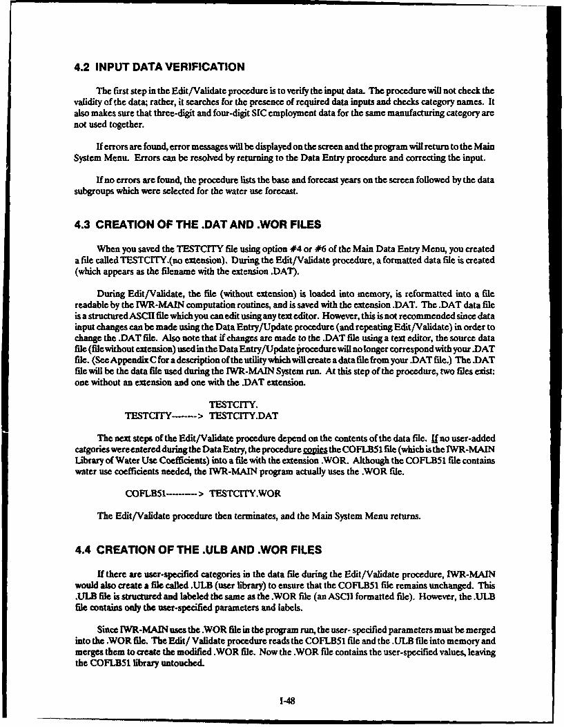
4.2 INPUT DATA VERIFICATION
The first step in the Edit/Validate procedure is to verify the input data. The procedure will not check thevalidity of the data; rather, it searches for the presence of required data inputs and checks category names. Italso makes sure that three-digit and four-digit SIC employment data for the same manufacturing category arenot used together.
If errors are found, error messages will be displayed on the screen and the program will return to the MainSystem Menu. Errors can be resolved by returning to the Data Entry procedure and correcting the input.
If no errors are found, the procedure lists the base and forecast years on the screen followed by the datasubgroups which were selected for the water use forecast.
4.3 CREATION OF THE .DAT AND .WOR FILES
When you saved the TESTCrTY file using option #4 or #6 of the Main Data Entry Menu, you createda file called TESTCITY.(no extension), During the Edit/Validate procedure, a formatted data file is created(which appears as the filename with the extension .DAT).
During Edit/Validate, the file (without extension) is loaded into memory, is reformatted into a filereadable by the IWR-MAIN computation routines, and is saved with the extension .DAT. The .DAT data fileis a structured ASCII file which you can edit using any text editor. However, this is not recommended since datainput changes can be made using the Data Entry/Update procedure (and repeating Edit/Validate) in order tochange the .DAT file. Also note that if changes are made to the .DAT file using a text editor, the source datafile (file without extension) used in the Data Entry/Update p-rocedure will no longer correspond with your .DATfile. (See Appendix C for a description of the utility which will create a data file from your .DAT file.) The DATfile will be the data file used during the IWR-MAIN System run. At this step of the procedure, two files exist:one without an extension and one with the .DAT extension.
TESTCITY.TESTCrI ------ > TESTCrrY.DAT
The next steps of the Edit/Validate procedure depend on the contents of the data file. If no user-addedcatgories were entered during the Data Entry, the procedure sopio the COFLB51 file (which is the IWR-MAINLibrary of Water Use Coefficients) into a file with the extension WOR. Although the COFLB51 file containswater use coefficients needed, the IWR-MAIN program actually uses the .WOR file.
COFLB5I------- > TESTCITY.WOR
The Edit/Validate procedure then terminates, and the Main System Menu returns.
4.4 CREATION OF THE .ULB AND WOR FILES
If there are user-specified categories in the data file during the Edit/Validate procedure, IWR-MAINwould also create a file called .ULB (user library) to ensure that the COFLB51 file remains unchanged. This.ULB file is structured and labeled the same as the .WOR file (an ASCII formatted file). However, the .ULBfile contains only the user-specified parameters and labels.
Since IWR.MAIN uses the .WOR file in the program run, the user- specified parameters must be mergedinto the .WOR file. The Edit/ Validate procedure reads the COFLB51 file and the .ULB file into memory andmerges them to create the modified .WOR file. Now the .WOR file contains the user-specified values, leavingthe COFLB51 library untouched.
1-48
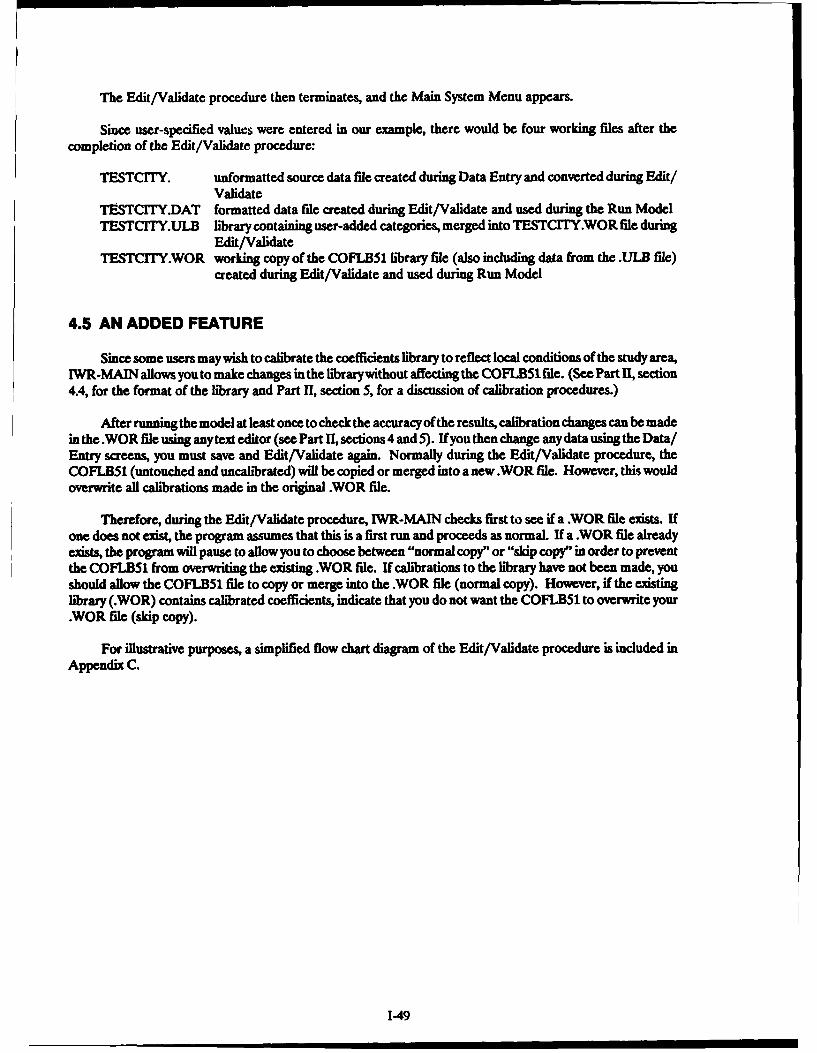
The Edit/Validate procedure then terminates, and the Main System Menu appears.
Since user-specified values were entered in our example, there would be four working files after thecompletion of the Edit/Validate procedure:
TESTCITY. unformatted source data file created during Data Entry and converted during Edit/Validate
TESTCITY.DAT formatted data file created during Edit/Validate and used during the Run ModelTESTCITY.ULB library containing user-added categories, merged into TESTCITY.WOR file during
Edit/ValidateTESTCITY.WOR working copy of the COFLB51 library file (also including data from the .ULB file)
created during Edit/Validate and used during Run Model
4.5 AN ADDED FEATURE
Since some users may wish to calibrate the coefficients library to reflect local conditions of the study area,IWR-MAIN allows you to make changes in the library without affecting the COFLB51 file. (See Part H, section4.4, for the format of the library and Part II, section 5, for a discussion of calibration procedures.)
After running the model at least once to check the accuracy of the results, calibration changes can be madein the.WOR file using anytext editor (see Part H, sections 4 and 5). If you then change any data using the Data/Entry screens, you must save and Edit/Validate again. Normally during the Edit/Validate procedure, theCOFLB51 (untouched and uncalibrated) will be copied or merged into a new .WOR file. However, this wouldoverwrite all calibrations made in the original .WOR file.
Therefore, during the Edit/Validate procedure, IWR-MAIN checks first to see if a .WOR file exists. Ifone does not exist, the program assumes that this is a first run and proceeds as normaL If a .WOR file alreadyexists, the program will pause to allow you to choose between "normal copy" or "skip copy" in order to preventthe COFLB51 from overwriting the existing .WOR file. If cahbrations to the library have not been made, youshould allow the COFLB51 file to copy or merge into the .WOR file (normal copy). However, if the existinglibrary (.WOR) contains calibrated coefficients, indicate that you do not want the COFLB51 to overwrite your.wOR file (skip copy).
For illustrative purposes, a simplified flow chart diagram of the Edit/Validate procedure is included inAppendix C.
1-49

5. RUN MODEL PROCEDURE
5.1 INTRODUCTION TO RUN MODEL
1UR MAIN System MeM
Enter Fitename b:testcity (my include drive but not extension)
1) Data Entry/Update
2) Edit/VaLidate
3) Run Model
4) Print/View Reports
5) Change Film
6) Exit to DOS
Enter your selection
After sucwssful completion of the Edit/Validate procedure, the next step is to perform the Run Modelprocedure. In order to compute the water use forecast, this Run Model procedure uses the .DAT and .WORfiles created by Edit/Validate along with two IWR-MAIN libraries FLONIAT and LCC. In addition, if thereare forecast years selected, a temporary scratch file PROJD will be created and used throughout the Run Modelprocedure. To start the Run Model procedure, select procedure #3 on the Main System Menu.
During the run of the IWR-MAIN System, the model goes through a detailed series of computationalprocedures. A brief description is provided below along with the screen messages which appear during theprocedures.
5.2 DESCRIPTION OF THE COMPUTATIONAL SEQUENCE
The first step performed by the Run Model procedure is the assignment of filenames to all the files usedor created. As in the Edit/Validate procedure, all permanent files have the same name but have differentextensions. These files will be displayed on the screen after the message:
THE FOLLOWING FILE(S) ASSIGNED FOR THIS RUN OF MAINIWRL
Note that MAIN1WR is a filename used within the routine and is not a reference to the entire IWR-MAINSystem. The procedure then reads the data (.DAT) file. The following message appears on the screen:
READING FILE (fllename).DAT
This message is followed by the word REDINP (reading input) and the contents of the .DAT file. If errors arepresent in subgroup names, parameter names, or the form of the Construction Cost Index, they will be identified
1-51

and the program will terminate and return to the Main System Menu. If an error occurs, the program will pauseto allow you to read the error indicators. Another way to observe these error messages is to have your printeron fine and to press the Ctrl and PrtSc keys before selecting procedure #3 (Run Model). Now everythingdisplayed on the screen will be captured by the printer. When the procedure returns to the System Menu,remember to press the Ctrl and PrtSc keys again in order to end the routing of displays to the printer.
During the reading of the .DAT file, the model checks for conservation data. If these data are present,the user-specified data are displayed on the screen as they are read. The model then reads the Library ofConservation Coefficients (LCC). If conservation measures are not indicated in the .DAT file, the modelbypasses the reading of the LCC and goes to the next step.
There is a pause while the procedure checks to see if forecast years are present. If no forecast years havebeen selected, the model proceeds to the reading of the.WOR file. If forecast years are detected, the forecastyear data are displayed on the screen as they are read from the .DAT file, and the data are checked for validprojection input subgroups. There is another pause while the GROWTH subroutine projects water useparameters by using historical extrapolations and/or the internal growth models. These projections are storedinto a temporary file PROJD, and the model then reads the WOR file.
After the routine reads the ENDINPUT statement from the .DAT file, the .WOR file containing the wateruse coefficients is read into memory, and the message appears on the screen:
READING FILE (filename).WOR
If the climatic variables evapotranspiration (EVAP) and/or rainfall (RAIN) were not specified by you, theroutine will read these variables from the Library of Climatic Variables (FLONLAT). This library contains long-term averages of rainfall and evapotranspiration based on the longitude and latitude of the study area.
IWR-MAIN is now ready to begin computing water use one year at a time beginning with the base year.Screen messages appear as the calculation of unrestricted water use for each selected sector begins:
RESIDENTIAL USAGE ROUTINE
f you have provided actual weather data for calibration purposes (see the description of screen 1.1), thecalculated weather adjustment factor for residential metered summer water use will be shown on the screen.
COMMERCIAL/INSTITUTIONAL USAGE ROUTINE
INDUSTRIAL USAGE ROUTINE
PUBLIC/UNACCOUNTED USAGE ROUTINE
If conservation is specified, the message appears on the screen:
CONSERVATION ROUTINE
Conservation coverage factors that you have not provided for the given year are calculated based on the LCCcoefficients and parameter units in the .DAT file. These calculated factors are written into a .COV file alongwith the user-specified coverage factors, if any. This .COV file contains the coverage factors for eachconservation measure for each year. The file is labeled and can be viewed and/or printed by any text editor.The purpose of the file is to allow you to view all coverage factors, both user- and model-specified, for all theselected measures. Estimated water savings for each measure are calculated for each sector and dimension.These savings per measure are also written to the .COV file.
Restricted water use for the year is then calculated for each sector. Results of the computations of bothunrestricted and restricted water use for each sector for the year are written to an output file. There is one output
1-52

file generated for each year. The base year output is written to the file .RP1, and the first forecast year is written
to the file RP2, etc. The message appears on the screen:
WRITING REPORTS 1 THRU 12 TO FILE (fllename).RP
If forecast years are present, the message will appear:
LOADING FORECAST YEAR DATA
The projected parameter data will be read from the temporary file PROJD. Calculation of water use for eachsector will follow, and the results will be written to the output file for that year. The corresponding messageswill appear on the screen, and the process will be repeated for every specified forecast year. If there is at leastone specified forecast year, a summary report will be written to the last output file, and the message will appear:
WRITING SUMMARY REPORT TO FILE (flename).RPx
If you specified in screen 1.1 that the data base file .PRN be produced, the file will be created at this stageand the message will appear:
WRITING RESULTS TO DATA BASE FILE (filename).PRN
This file contains summary results of the forecast without labels and can be used with data base and spreadsheetprograms for data manipulation and graphics. For more information concerning this feature, see Appendix C.
The program then checks for any additional input data, and the message appears:
CHECKING INPUT FOR ADDITIONAL DATA
If data are found, the procedure returns to the read input step, otherwise you will get the message:
NO ADDITIONAL DATA FOUND
Finally, an index (.MAT) f'de is created for the reports, and the temporary PROJD file is deleted. Uponcompletion of the Run Model procedure, the program automatically exits to the System Menu. The followingmessage will appear before the system returns to the System Menu:
PROGRAM NORMAL EXIT
Remember to disengage the printer (Ctrl -PrtSc) if you were having the screen messages sent to your printer.
Simplified and detailed flow chart diagrams of the Run Model procedure are included in Appendix C.
1-53

6. PRINT/VIEW PROCEDURE
6.1 INTRODUCTION TO PRINT/VIEW
IWR MAIN System Menu
Enter FiLenam b:testcity (may include drive but not extension)
1) Data Entry/Updat
2) Edit/Vatidate
3) Run Model
4) Print/View Reports
5) Change FiLm
6) Exit to DOS
Enter your selection
The Print/View procedure allows you to either print or view on screen the completed reports of the wateruse forecast. The Run Model procedure must have been successfully performed for the chosen filename at sometime prior to the selection of this procedure. The Print/View procedure uses the .MAT and .RPx files createdby the Run Model procedure to search for and display the reports for a given year(s). To activate Print/Viewselect procedure #4 on the Main System Menu.
6.2 DESCRIPTION OF THE .RPx FILES
During the Run Model procedure, an output report file is generated for each year for which water use iscomputed. The base year output is written to the output .RP1 file, and the first forecast year output is writtento the .RP2 file. Thus, for x number of years, report files .RP1 through .RPx will be generated. If ten reportsare generated, they would be written to files .RPI through .RPA. The summary report (report no. 13) is alwayswritten to the last year's file. The .RPx files contain the reports for each year. These reports are numbered 1-13.
1 Fatr RUe aTi2 Flat Rate and Unsewered2 Flat Rate and Sewered
3 Master-Metered Apartments4 Metered and Sewered5 Residential Summary6 Commercial/Institutional, Unrestricted7 Commercial w/Conservation8 Industrial, Unrestricted
1-55

9 Industrial w/Conservation10 Public/Unaccounted, Unrestricted11 Public w/Conservation12 Municipal Summary13 Forecast Summary
Note that the reports are in standard ASCII format and may also be viewed or printed with a text editor.Also note that reports 1-5,12, and 13 show both unrestricted and restricted water use if conservation is indicated.
6.3 OPERATION OF PRINT/VIEW
After selecting procedure #4 on the Main System Menu, the list of reports available from your forecastrun will appear.
OPENING FILES - PLEASE WAITTHE FOLLOWING REPORTS ARE AVAILABLE:
YEAR: 1980, REPORT(S): 12 3 4 5 6 7 9 10 11 12YEAR. 1990, REPORT(S): 12 3 4 5 6 7 8 9 10 1112Report 13 (summary) was generated
Notice only two years, 1980 and 1990, are listed. In this example, TESTCITY has all 12 reports for both yearsand a summary report (#13).
After the list of available reports, press the return key and the options for selecting years and reports willbe displayed.
SPECIFY THE DESIRED YEAR AND REPORT(S) IN ONE OF THE FOLLOWING FORMATS,PRESS CENTER] AFTER EACH LINE THEN SPECIFY EITHER 'P OR "" WHEN ALLSELECTIONS HAVE BEEN COMPLETED.year report(s) - specify year and report(s) separated by a comma and in ascending order, e4g '1990
5,9,12''' reports(s) - selects specified report(s) for all years, e.g. * 2,3"year ' - selects all reports for a specified year, e.g. '1990 '0., - selects all reports for all years'Ss - selects Summary report no. 13'C, - clears all oeisting selections"N-/1L - name or list available reportsOpp/wr - print or view all selectionsPIT - exit to main menu, quit
You may now specify the year and the reports for that year which you wish to either view or print. Enter theyear and report numbers in the following format:
1990 5,10,12
Note that the year is specified as four digits followed by one space and that the report numbers are separatedby commas and are in ascending order. If you wish to select the same report(s) for all years, use the format:
O5,10,12
In this case, the asterisk is before the space and signifies all years. Likewise, you may select all reports for a givenyear using the format:
19900
1-56

In this format, the asterisk is after the space and signifies all reports for that year. All reports for all years maybe selected using the format:
If the summary report no. 13 was generated, it may be selected by specifying summary ("S").
Once a selection has been made, press the return key. The print/view routine will search for the specifiedreports and send those reports to a temporary file (.WRK). When this process is complete, the routine will returnto the screen and display all of your previous selections. You may enter another year/report specification, viewthe names or list the available reports ("N" or "L"), or dear all previous selections ("C"). When your list ofspecifications is complete, enter "P" or "V" and press return to send your selections to either the printer or thescreen. You may also quit ("0") the print/view routine at this time which will automatically clear all selections,delete the .WRK file, and return you to the IWR-MAIN System Menu. Additional year/report specificationsadd those reports to the existing .WRK file until you select either dear ("C") or quit ("Q"). Selection of print("P") or view ("V") will send the contents of the .WRK file to the printer or screen, respectively. (Be sure yourprinter is connected and turned on.)
Note that the size of the .WRK file depends on how many reports are selected. When using diskettes,selecting all ("* ") will cause a large .WRK file to be created. If the space on the data diskette is exhausted,the program will terminat.
After printing or viewing the selected reports, the routine returns to the screen and displays all previousselections. Again, you have available all the specification options. You may either dear the previous selections("C") and specify new selections or return to the IWR-MAIN System Menu ("Q").
1-57

7. EXIT TO DOS
IWR MAIN System Menu
Enter Fitename b:testcity (may incLude drive but not extension)
1) Data Entry/Update
2) Edit/VaLidate
3) Run ModeL
4) Print/View Reports
5) Change FiLename
6) Exit to DOS
Enter your seLection
Select option #6 (Exit to DOS) after all options have been successfully completed to return to the DOSsystem. You may end the session by exiting to DOS any time the System Menu screen appears. In.reie, youmay wish to see the directory of the data files created by IWR-MAIN. To do this just type:
dir b:(fllename).*
where b: indicates the drive in which the data files are located. For our example TESTCITY, eight data fileshave been ,-eated. These are listed and briefly described below.
TESTCITY. unformatted source data file created during Data Entry and convertedduring Edit/Validate
TESTCITY.DAT formatted data file created during Edit/Validate and used during RunModel
TESTCITY.ULB library containing user-added categories which is merged intoTESTCITY.WOR file during Edit/Validate
TESTCITY.WOR working library created during Edit/Validate and used during Run ModelTESTCITY.COV contains coverage factors for specified conservation measures and is
created during Run ModelTESTCrIY.RPx x number of files, each containing output reports for a given year, created
during Run ModelTESTCITY.PRN a data base fide containing output results created during Run ModelTESTCITY.MAT a matrix file used by Print/View to list and locate reportsTESTCITY.WRK a scratch file created by Print/View to search and display the reports
All of these files are in standard ASCII format and may be viewed or printed using standard DOS commandsor edited through use of a line or screen editor. However, unless you are familiar with the IWR-MAIN programand the consequences of editing data files created by the program, altering these files is M recommended.
1-59
I I I I i I I I I'S !

Once a complete run has been executed, you may return to the IWR-MAIN System at any time to editor update the files, print or view the reports, or rerun the model.
A complete simplified flow chart diagram of the entire IWR-MAIN System is included in Appendix C.
1-60

8. MINIMUM DATA REQUIREMENTS-A GUIDE FORFIRST-TIME USERS
For first-time users of IWR-MAIN, Table I-1 provides a guide to inputting data for generatingsuccessful runs of the program. The forecasts generated by following Table 1 are for the base year only withoutconservation and without forecast years. See the description of the corresponding screen in section 3.3 for anexplanation of the input data and Part II, sections 3.1 through 3.4, for greater detail of input data characteris-tics.
Access the Parameter Control Screen and select one data subgroup (by specifying a Y"'). At this point,do not specify any forecast years or forecast methods. Enter the required municipal data and data for yourspecified subgroup, save the file, select the Edit/Validate procedure, and then select the Run Model procedure.If errors occur during Edit/Validate or Run Model, recheck your input data. Use the Print/View procedureto review your output. When you have successfully generated a base year water use estimate with one subgroup,return to the Data Entry procedure and select an additional subgroup on the Parameter Control Screen. Thenenter the data required for the additional subgroup and proceed with the error-checking procedure. Proceedwith this step-by-step method until all desired subgroups have been addressed.
In order to generate water use estimates for each specified forecast year, you must (at the veryminimum) provide population, median household income, and total employment to the internal growth modelsfor each specified forecast year. Any additional methods will serve to improve the accuracy of the forecastedsocioeconomic data in reflecting local area conditions and, therefore, will improve the accuracy of the water useforecasts. Data for forecast years are entered in the projection screens which are described in sections 3.4through 3.6. These screens are available depending upon the forecast years and methods selected on theParameter Control Screen.
Minimum data requirements for generating successful runs using the different forecast methods arelisted in Table 1-2. Once you have successfully generated a base year forecast, access the Parameter ControlScreen and enter a forecast year(s) with only the internal growth models forecast method selected. Then enterthe required data of the internal growth models for each specified forecast year. Save your file, select the Edit/Validate and Run Model procedures. If there are errors, go back to Data Entry and check your input. Use thePrint/View procedure to check your output and note the number of parameter units projected for eachsubgroup. When you have successfully generated a forecast using the internal growth models, return to the Pa-rameter Control Screen and specify an additional forecast method, either extrapolation from historical data ordirect external projections. Enter the appropriate data for the additional forecast method and again save yourfile, select Edit/Validate, and Run Model. If there are errors, recheck your inputs. When the Run Modelprocedure is successfully completed, use the Print/View procedure to review your output and compare theprojected parameter units with those generated by the internal growth models. It is up to you, the user, to judgethe validity and reasonableness of the projected parameters generated by IWR-MAIN from the input provided.
Once an unrestricted water use forecast has been generated, return to the Parameter Control Screenand specify a "Y" for conservation. Use the F3 key to go directly to screen 15.1 and enter a year of initiation forone of the conservation measures. Then select at least one sector for that measure in screen 15.2. Be sure thatthe sector selected is one for which a water use forecast is being generated. Then specify "L" in both screens16.1 and 17.1 so that all the reduction and coverage factors will be provided by IWR-MAIN. Save the file, selectEdit/Validate, and Run Model. Use the Print/View procedure to review the output and observe the differencesbetween the unrestricted and restricted forecasts. Use a text editor to print or view the file with the extension.COV in order to observe the coverage factors calculated by IWR-MAIN and the effectiveness of the measure.Now you can return to screens 16.1 and 17.1, specify"S" in each one, and experiment with different combinationsof reduction factors and coverage factors and evaluate their impact on conservation effectiveness. The minimumdata requirements for estimation of restricted water use are provided in Table 1-3.
1-61

During the Edit/Validate and Run Model procedures, there are error-checking routines which checkfor input errors. However, these are not checks for the validity of the data. Table 1-4 contains a list of internalcrosschecks which you may follow in testingthe soundness ofyour input data. When examining the rate of growthfor a given parameter, you must be the judge of what is reasonable growth for the given parameter and timeinterval for your study area. Remember that the direct external projection data entered in screens 14.x.1 through14.x.9 take precedence over the other parameter projection methods and thus maybe used to control the growthof a given parameter.
1-62

TABLE 141
MINIMUM DATA REQUIREMENTS FOR ESTIMATIONOF BASE YEAR UNRESTRICTED WATER USE
Sector/Subgroup Screen Data Comments
MUNICIPAL 1.1 -calendar year of base year Municipal data are required regardless of-latitude of study area subgroup selection in the Parameter Control-longitude of study area Screen.-resident population-median household income-total base year employment-employment 5 years before
base year-composite construction cost index
RESIDENTIAL Select any or all residential subgroups in theParameter Control Screen and provide inputfor selected subgroup(s) as follows:
Flat rate andsewered 2.1 -low and high value range Select "flat rate and sewered" in the Parameter
-persons per unit Control Screen. Specify value ranges and enter-units per acre data for each value range.-number of units
Flat rate andunsewered 3.1 -low and high value range Select "flat rate and unsewered" in the Para-
-persons per unit meter Control Screen. Specify value ranges-units per acre and enter data for each value range.-number of units
Metered andsewered 4.1 -low and high value range Select "metered and sewered" in the Parameter
-annual marginal price Control Screen. Specify value ranges and enter-summer marginal price data for each value range.-units per acre-number of units-annual bill difference-summer bill difference
Master meteredapartment 5.1 -low and high value range Select "master metered apartments" in the
-persons per unit Parameter Control Screen. Specify value-number of units ranges and enter data for each value range.
1-63

TABLE I-1 (Conaued)
Sector/Subgroup Screen Data Comments
COMMERCIAL 6.1 -employment by category Select "commercial" in the Parameter ControlScreen. Commercial sector data may be input
6. -category description in one of two ways: (1) specify employment for-category employment or both at least one category in screen 6.1 or (2) createnumber of units and unit at least one category in screen 6.2. If screenparameter 6.1 is not used, one category in screen 6.2 may
-annual average water use represent the entire commercial sector. If-maximum-day water use employment is provided for some, but not all,
categories in screen 6.1, categories created inscreen 6.2 may represent the remainder of thesector. Note that employment specified inscreen 6.1 uses water use coefficients stored inthe library file while water use coefficientsmust be supplied for any category created inscreen 6.2.
INDUSTRIAL 7.1-7.6 -employment by either three- Select "industrial" in the Parameter Controldigit or four-digit SIC code Screen. Industrial sector data may be entered
in one of two ways: (1) specify employment for7.7 -category description at least one category in screens 7.1-7.6 or (2)
-category employment create one or two categories in screen 7.7-annual average water use which represent the entire sector. Employ--maximum-day water use ment specified in screens 7.1-7.6 uses water use
coefficients in the library file while water usecoefficients must be supplied for any categorycreated in screen 7.7.
PUBLIC/UNAC-COUNTED 8.1 -population served by system Even without "public/unaccounted" selected in
-annual average distribution the Parameter Control Screen, IWR-MAINlosses will generate a forecast of distribution losses
-maximum-day distribution and free service water use using default valueslosses and the required municipal data. To override
-annual average free service the default calculations, select "public/unac--maximum-day free service counted" in the Parameter Control Screen and
enter data in screen &l. For distribution8.2 -category description losses, enter in population served by the system
-number of units for a per capita calculation, or enter both-unit parameter annual average and maximum-day water use.-annual average water use To specify free service, enter both annual-maximum-day water use average and maximum-day free service.
Additional public water use categories may becreated by entering all the data for a categoryin screen 8.2.
1-64
maremmmmmmmmmi iI~iiiiH~im m=MW

TABLE 1-2
MINIMUM DATA REQUIREMENTS FOR ESTIMATIONOF FORECAST YEAR UNRESTRICTED WATER USE
ForecastMethod Screen Data Comments
INTERNALGROWTHMODELS 9.1 -population These data are required for any forecast year
-median household income listed in the Parameter Control Screen, even if-employment forecast method "1" is not specified.
(Options) 9.1 -number of households If percent households in income group is used,-percent household in income similar data must be provided for the base yeargroups in screen 1.2.
(Options) 9.3 -employment by industry group If used, similar data must be provided for thesame group(s) for the base year and 5 yearsprior in screen 12.
EXTRAPOLA-TION OF HIS-TORICAL DATA-OPTIONAL
10.1-102 -historical years Specify forecast method "2" in the Parameter-number of housing units by Control Screen beside the forecast year(s) forsubgroup and range which this method is to be used. Enter residen-
tial, commercial, industrial, or public/unac-11.1-11.4 -historical years counted data. Base year data must have been
-commercial category empL entered for whichever sector(s) forecast-, are tobe generated. For residential data, enter at least
12.1-12.a -historical years two historical years for any residential subgroup-industrial category empl. in screen 10.1 or 102 and enter the number of
units for at least one range group for those years.13.1-13.2 -historical years For commercial or industrial data, enter at least
-population served for dis- two historical years in screen 11.1 or 12.1, res-tribution losses (LOSS) and pectively. Categories specified in the base yearfree service (FSER) will be highlighted; enter the historical employ-
-category parameter for user- ment for any highlighted category for the histori-added categories cal year entered. For public/unaccounted data,
enter at least two historical years in screen 13.1.Enter historical population for distribution lossesor free service for the years specified. If anyuser-added public categories were specified inscreen 8.2, you may enter historical parametervalues for those historical years.
1-65

TABLE 1-2 (Cottnued)
ForecastMethod Screen Data Comments
DIRECTEXTERNALPROJECTIONS-OPTIONAL
14.x.1 -number of housing units by Specify forecast method " in the Parametersubgroup and range Control Screen beside the forecast year(s) for
which direct external projections are available.14.x.2- -commercial category empL Be sure that sector(s) have been selected in the
Parameter Control Screen and that base year14.x.3 -commercial category parameter data have been entered for each sector for which
external projections are being provided. Screens14.x4- -industrial category empl. 14.x.1-14.x.9 are repeated for each forecast year14.x.7 forwhich "3 isspecified in the Parameter Control
Screen. The "r in the screen number refers to14x8- the forecast year. Enter the projected number of14.x9 -population for distribution housing units for any residential subgroup and
loss (LOSS) value range combination for the residential-annual average distribution loss sector. For the commercial sector, enter employ--max:imum-day distribution loss ment projections for any of the C001-C023 cate--population for free service gories used in the base year and parameter(FSER) projections for anyuser-added categories. Enter
-annual average free service projected employment for any industrial cate--max:imum-day free service gory used in the base year for the industrial-number of parameter units for sector. Projections for the public/unaccounteduser-added public categories sector may be entered in a number of ways.-average annual water use Projected distribution losses may be entered as-madmum-day water use (1) a fractional percent (e.g., 0.15) of total mu--fractional percent distribution nicipal water use, (2) as projected population forloss (FLSS) a per capita calculation, or (3) as projected an-
nual average and maximum-day losses in gallonsper day. Projected free service water use datamay be entered as the projected population for aper capita calculation or as projected annualaverage and maximum-day water use in gallonsper day. Projected data for user-added public
categories may be entered as the projected pa-rameter value or as the annual average andmaximum-day water use in gallons per day.
1-66

TABLE 1-3
MINIMUM DATA REQUIREMENTS FOR ESTIMATIONOF RESTRICTED WATER USE
Screen Data Comments
15.1 -year of initiation of conservation Select "conservation' in the Parameter Control Screen inmeasure(s) order to access the conservation screens. Select a couser-
vation measure in screen 15.1 by entering a year of initia-152 -sectors affected by measure tion for that measure. The year may be before, equal to,
or after the base year. Indicate in screen 152 whichsector(s) are affected by the conservation measureselected in screen 15.1. The description of measures inPart H, section 4.3, indicates the sectors which may beappropriately used with each measure.
16.1 -specification of reduction factors Specify ' in screen 16.1 to use the default reductionfactors for the selected measures and sectors. Specifica-
162 -indoor use reduction factors by tion of "S" will provide access to screens 16.2-16.4 and will(optional) measure and sector allow you to specify some or all reduction factors. If some,
but not all, reduction factors are provided in screens 16.2-16.3 -outdoor use reduction factors by 16.4, the default factors will be used for those not provided.(optional) measure and sector
16.4 -maximum-day use reduction factor(optional) by measure and sector
17.1 -specification of coverage factors Specify "L" in screen 17.1 to have the coverage factorscalculated by IWR-MAIN using default coefficients.
17.2-17.x -coverage factors by year, measure, Specification of "5" will provide access to one coverage(optional) and sector factor screen for each year beginning with screen 172 for
the base year. Any coverage factors not provided inscreens 17.2-17.x will be calculated using default values.
1-67

TABLE 1-4
INTERNAL CROSSCHECKS FOR INPUT DATA
ScreenNumber Parameter Crosscheck
1.2 -employment--base year and five If employment for all eight groups is provided, sumsyears prior should equal total employment (base year and five
years prior) in screen 1.1.
6.1 and 6.2 -commercial employment Sum of commercial employment should equal baseyear employment minus SIC 2000-3999 employmentin screen 1.2.
7.1-7.7 -industrial employment Sum ofindustrial employment should equal SIC 2000-3999 employment in screen 1.2.
9.1 -projected population, income, and Should be compared to values in screen 1.1 for rate ofemployment growth.
-projected total households Should be compared to sum of number of units inscreens 2.1 through 5.1 for rate of growth.
9.3 -projected employment by group Sim for each year should equal projected employ-ment in screen 9.1.
Projected group employment should be compared tocorresponding values in screen 1.2 for rate of growth.
10.1 and -historical housing If provided, housing by value range groups should be10.2 comparedto base year number of unitsin correspond-
ing value ranges in screens 2.1 through 5.1 for rate ofgrowth.
11.1-12.a -historical commercial and industrial Should be compared to base year employment foremployment by category corresponding categories in screens 6.1 through 7.7
for rate of growth.
13.1 and -historical public/unaccounted Shouldbecomparedtocorrespondingbaseyearpara-13.2 parameters meters in screens &1 and 8.2 for rate of growth.
14.x1 -externally projected housing byvalue Should be compared to number of base year units inrange group correspondingvalue ranges in screens 2.1 through5.1,
or projected values in previous forecast years, for rateof growth.
If provided, totals for each housing type should sum tototal projected housing for the forecast year in screen9.1
1-68
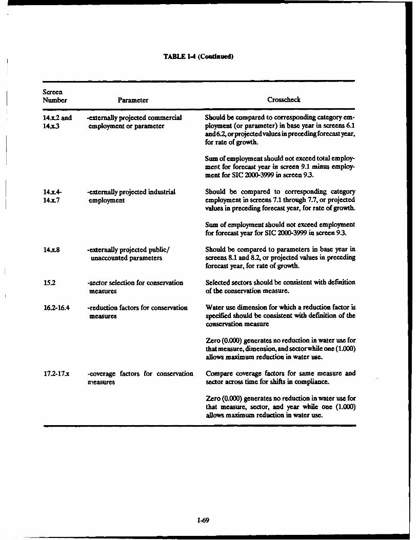
TABLE 1-4 (Continued)
ScreenNumber Parameter Crosscheck
14.x.2 and -externally projected commercial Should be compared to corresponding category em-14.x.3 employment or parameter ployment (or parameter) in base year in screens 6.1
and 6.2, or projected values in preceding forecast year,for rate of growth.
Sum of employment should not exceed total employ-ment for forecast year in screen 9.1 minus employ-ment for SIC 2000-3999 in screen 9.3.
14.x.4- -externally projected industrial Should be compared to corresponding category14.x.7 employment employment in screens 7.1 through 7.7, or projected
values in preceding forecast year, for rate of growth.
Sum of employment should not exceed employmentfor forecast year for SIC 2000-3999 in screen 9.3.
14.x.8 -externally projected public/ Should be compared to parameters in base year inunaccounted parameters screens 8.1 and 8.2, or projected values in preceding
forecast year, for rate of growth.
15.2 -sector selection for conservation Selected sectors should be consistent with definitionmeasures of the conservation measure.
16.2-16.4 -reduction factors for conservation Water use dimension for which a reduction factor ismeasures specified should be consistent with definition of the
conservation measure
Zero (0.000) generates no reduction in water use forthat measure, dimension, and sector while one (1.000)allows maximum reduction in water use.
172-17.x -coverage factors for conservation Compare coverage factors for same measure andLneasures sector across time for shifts in compliance.
Zero (0.000) generates no reduction in water use forthat measure, sector, and year while one (1.000)allows maximum reduction in water use.
1-69

9. QUICK REFERENCE
Accessing IWR-MAIN, 1-5, 1-6 Employment, 1-13,1-15,1-27,1-28 (also seeAdd More Data/Revise Existing Data option, commercial employment and industrial
1-8,1-9,1-45 employment)Added calibration feature, 1-49 Errors, 1-47,1-48,1-51,1-52,1-61,1-62ANSISYS file, 1-3 ESC key, 1-10Backspace key, 1-10 Exit to DOS, 1-59Base year screens, 1-12 External projection screens, 1-32, 1-33, 1-34,Bill difference example, 1-19 1-35,1-61,1-62Change Filename option, 1-6 Residential, 1-33Change Subgroups/Forecast Choices option, Commercial, 1-34
1-9,1-45 Industrial, 1-34,1-35Climatic variables, 1-13,1-14,1-52 Public/unaccounted, 1-35COFLB51, see Library of Water Use Coeffi- Extrapolation of local historical parameters,
cients 1-12COMMAND.COM file, 1-4 F1 key, 1-9Commercial employment, 1-15,1-21,1-22,1-28, F2 key, 1-9,145
1-30,1-34 F3 key, 1-9Commercial subgroup, 1-11, 1-20,1-21, 1-23, F4 key, 1-10
1-29,1-33,1-35,1-55 (also see conservation F5 key, 1-10sectors) F6 key, 1-10,1-41,1-42, 1-44
Commercial user-added parameters, 1-22,1-30, Flat rate and sewered subgroup, 1-11, 1-16,1-34 1-29,1-33, 1-55
Computation sequence of Run Model, 1-51, Flat rate and unsewered subgroup, 1-11, 1-17,1-52,1.53 1-29,1-33,1-55
CONFIG.SYS file, 1-3, 1-4 FLONLAT, see Library of Climatic VariablesConfiguring DOS, 1-3,1-4 Forecast methods, 1-11,1-12Conservation coverage factors, see coverage Forecast years, 1-11, 1-32,1-44,1-55
factors Hardware requirements, 1-3Conservation effectiveness, 1-36, 1-39, 1-43, Historical parameter screens, 1-29, 1-61
1-52,1-61 Residential, 1-29Conservation measures, 1-11, 1-36,1-37,1-61 Commercial, 1-30Conservation reduction factors, see reduction Industrial, 1-31
factors Public/unaccounted, 1-32Conservation screens, 1-36 Indoor use, 1-36, 1-40Conservation sectors, 1-36, 1-38 Industrial employment, 1-15,1-23,1-24,1-28,.COV file, 1-52,1-59,1-61 1-31,1-34Coverage factors, 1-36, 1-37, 1-43, 1-44, 1-52, Industrial subgroup, 1-11, 1-22, 1-23,1-30, 1-33,
1-61 1-35,1-55 (also see conservation sectors)Create New File option, 1-8, 1-45 Industrial user-added parameters, 1-24, 1-31,Creation of .DAT and .WOR files, 1-48 1-34Creation of .ULB and .WOR files, 1-48, 1-49 Input data, see data, minimum requirementsCursor (arrow) keys, 1-10, 1-40,1-44 Input data verification, 1-48, 1-52.DAT file, 1-48,1-49, 1-51, 1-52, 1-59 Install program, 1-4Data crosschecks, 1-62 Installation on hard drive system, 1-4Data Entry Main screen, 1-7, 1-8, 1-9,1-45 Internal growth models, 1-12, 1-26, 1-61Data Entry/Update procedure, 1-7, 1-47, 1-61 IWR-MAIN identification screen, I-5Data file, 1-47,1-48,1.49,1-59 IWR-MAIN System diskettes, 1-3Data, minimum requirements, 1-61 IWR-MAIN System Menu, 1-6Data subgroups, 1-6,1-1 Library of Climatic Variables (FLONLAT),Direct external projections, 1-12, 1-32 1-14, 1-51, 1-52DOS, 1-3,14 Library of Conservation Coefficients (LCC),Edit/Validate procedure, 1-47, 1-51, 1-61 1-36, 1-39, 1-40, 1-41,1-42, 1-43, 1-44, 1-51,
1-52
1-71

Library of Water Use Coefficients(COFLB51), 1-25, 1-48, 1-49
Load Existing File option, 1-8,1-45Master-metered apartments subgroup, 1-11,
1-20, 1-29, 1-33, 1-55.MAT index file, 1-53,1-55,1-59Maximum-day use, 1-36, 1-42Metered and sewered subgroup, 1-11, 1-18,
1-19, 1-29, 1-33, 1-55Memory requirements, 1-3, 1-4, 1-5Municipal base year data, 1-13,1-14
Optional data, 1-15Nonresidential prices, 1-24Outdoor use, 1-36,1-41Parameter Control Screen, 1-10, 1-11, 1-12,
1-15, 1-21, 1-23,1-27,1-29, 1-36, 1-44, 1-61Pause, 1-47PgDn key, 1-10PgUp key, 1-10Print/View procedure, 1-55,1-61.PRN file, 1-13, 1-53, 1-59PROJD file, 1-3, 1-51, 1-52, 1-53Property values, 1-20 (also €e value range)Projection data used by inteaal growth
models, 1-26, 1-27,1-28Public/unaccounted, 1-11, 1-25, 1-26, 1-32, 1-35,
1-56Public/unaccounted user-added parameters,
1.-26,1-32, 1-35Reduction factors, 1-36,1-37, 1-39, I-0, 1-41,
1-42,1-61Required data, 1-12,1-13, 1-14,1-26,1-48,1-61
(also see data, minimum requirements)Residential subgroups, 1-11, 1-16,1-17,1-18,
1-20,1-29,1-33 (also see conservationsectors)
Restricted water use, 1-11, 1-36, 1-52Return to System Menu (with file save option),
1-9.RPx files, 1-53, 1-55, 1-59Run Model procedure, 1-47, 1-51, 1-52, 1-53,
1-55, 1-61Save Current File with New Filename option,
1-9, 145Save Current File with Return to Menu option,
1-9, 1-45Software setup, 1-3Study area name, 1-11Terminating Data/Entry, 1-45.ULB file, 1-48,1-49,1-59Unrestricted water use, 1-36,1-52,1-55,1-56,
1-61Value range, 1-16, 1-17, 1-18,1-19,1-20, 1-29,
1-33.WOR file, 1-48, 1-49, 1-51, 1.52, 1-59.WRK search file, 1-57, 1-59
1-72

fIWR-'MAIN WATER USE FORECASTING SYSTEM
PART H
SYSTEM DESCRIPTION AND PROCEDURES

1. INTRODUCTION
Using a step-by-step approach, Part I presents a "User's Manual" of the IWR-MAIN System, guiding theu',er through the operation of the system. Alternately, Part II provides a more detailed description of the IWR-MAIN System.
Chapter 2 presents an overview of the most widely used water use forecasting approaches and then brieflypresents the approaches used by the IWR-MAIN System. Chapter 3 describes, in detail, the input datarequirements and options and then continues with a presentation of available data sources. Chapter 4 presentsthe m.thods used by IWR-MAIN to compute unrestricted and restricted water use. Also in chapter 4 is adiscussion of the three parameter projection methods and the structure of the IWR-MAIN libraries. In someapplications of IWR-MAIN, the user may wish to verify the IWR-MAIN estimates and, if necessary, performcalibrations. Chapter 5 discusses why discrepancies may exist, how to verify estimates, and how to performcalibrations.
Part II is intended to provide the user with a conceptual and methodological understanding of the IWR-MAIN Water Use Forecasting System. The use of this "System Description," along with the "User's Manual,"will allow users to effectively apply IWR-MAIN to various planning situations.
Il

2. CONCEPTUAL AND ORGANIZATIONALSTRUCTURE
2.1 DETERMINANTS OF WATER DEMAND
The level and pattern of municipal water use (both spatial and temporal) are determined by demographic,socioeconomic, and climatic characteristics of the water service area. These may include:
(1) Resident and seasonal population(2) Number, market value, and types of housing units(3) Employment in service industries(4) Manufacturing employment and output(5) Water and wastewater prices and rate structures(6) Irrigated acreage in residential and commercial/institutional use(7) Personal income(8) Climate (i.e., arid or humid)(9) Weather conditions(10) Water-using appliances(11) Conservation activities
The forecasts of future water requirements and use are linked to the future values of these water usedeterminants. The latter may be projected by any number of methods, depending on data and other availableinformation. These methods include the use ofjudgment, consensus, simple extrapolation, shift-share analyses,multiple regression methods, simulation models, and other techniques.
Water use forecasting methods translate projected values of one or more of the above explanatoryvariables into future water use. Available forecasting methods make various assumptions regarding the numberand type of explanatory variables, the nature of the relationship between explanatory variables and water use,and the way in which that relationship may change over time. Several methods of water use forecasting arediscussed in the following section. This discussion is based, in part, on the work of C. Vaughan Jones et al.Following the discussion of water use forecasting approaches is a description of the organizational structure ofthe IWR-MAIN Water Use Forecasting System.
2.2 WATER USE FORECASTING APPROACHES
Time Extrapolation
Time extrapolation of water use data is ba--ed on the assumption that future water use is determined bywater use trends in the past; no other data or information need be considered. Usually, the change in water useover time is extrapolated into the future. The extrapolation may be accomplished by graphical or mathematicalmeans, and the change over time may be assumed to follow a linear, logistic, exponential, or other function.
Single Coefficient Requirements Methods
The per capita requirements approach estimates future water use as the product of projected service areapopulation and a projected value of per capita water use. Future service area population is determined usingone of the methods mentioned above. The per capita water use coefficient may be assumed to be fixed overtime or may itself be the subject of a projection. Its value and, where applicable, rate of change may bedetermined from past water use patterns in the study area, from data for other areas, or from national data. Thecoefficient value may also be obtained from reference works, or it may simply be assumed.
11-3

A variant of the per capita requirements approach is the per customer (or per connection) requirementsmethod, which substitutes the number of customers for the resident population. This reflects the empirical factthat water use is better correlated with number of customers than with population served. Per customer methodsare most frequently used in conjunction with sectorally disaggregate forecasts, where they may be applied tononresidential sectors.
Other single coefficient methods are in common use, based on a range of parameters. Industrial wateruse is commonly forecast on a per employee basis, for example, while specific categories of commercial andindustrial water use are frequently expressed as a (single coefficient) function of other variables, such as numberof hospital beds, hotel rooms, etc. A recent study of water use at military installations used single coefficientmethods to express water use for each of a number of use categories as a function of the floor area of buildingsin that category (Langowski, 1984).
Multiple Coefficient Requirements Models
Future water use, either aggregate or sectoral, can be expressed as a mathematical function of two or moreexplanatory variables. The functional form is chosen to provide an acceptable fit of the model to historic data,and the coefficients are estimated statistically, usually by multiple regression analysis. Models which do notinclude the price of water, or other economic factors, as an explanatory variable are known as requirementsmodels (since they imply that water use is an absolute requirement, unaffected by economic choice). Thevariables are chosen because of past correlation with water use, and any number maybe included, although morethan five or six is unusual. Multiple coefficient models used in forecasting may have been estimated from historicdata for the same study area, or they may be based on data for one or more other study areas, a larger region,or the nation.
Multiple Coefficient Demand Models
Multiple coefficient demand models differ from multiple coefficient requirements models in one keyrespect: demand models include the price of water to the user, as well as related economic variables such asincome, among the explanatory variables. Also, demand models are usually constructed according toeconometric methods, where the structure of the model and the list of potential explanatory variables reflectassumptions regarding causal, rather than simply arising from observed correlation. The possibility ofimproperly included or specified variables is, therefore, reduced. Attention is usually given to supplying ascomplete a set of explanatory variables as possible, thus minimizing the unexplained variance in the dependentvariable (water use).
Disaggregated Water Use Forecasts
Disaggregated water use forecasting separately specifies water use for each sector, season, or region,utilizing the best available model for each type of water use. This method permits the use of explanatory variablesunique to a given type of water use and generally yields a more accurate composite forecast.
2.3 IWR-MAIN WATER USE SYSTEM OVERVIEW
IWR-MAIN is a computerized water use forecasting system which contains a range of forecasting models,socioeconomic parameter-generating procedures, and data management techniques. Amongits major featuresare a high level of disaggregation of water use categories and considerable user flexibility in selecting forecastmethods and assumptions. Because of the level of disaggregation, the system is able to reflect water usedifferences between communities with different types of water-using activities.
11-4

Forecasting and Estimating Methods of IWR-MAIN
The IWR-MAIN System divides urban water users into four major sectors: residential, commercial/institutional, industrial, and public/unaccounted. Each sector is further disaggregated to a number of categoriesfor forecasting purposes. A maximum of 380 categories can be accommodated, but most forecasts utilizeapproximately 130 specific categories of water use.
A mixture of water use estimating techniques is employed in the computational subroutines of IWR-MAIN (see Table II-1). For some user sectors, water use is estimated by means of econometric demand modelscontaining a number of explanatory variables (including price in the case of residential users with water meters).Other uses are predictedby means of requirements models, usually of the unit use coefficient type. The originalform of the IWR-MAIN System used demand models adapted from the work of Howe and Linaweaver (1967).Some of these have been replaced with results from later work by Howe (1982) (see example in Table 11-2).Commercial/institutional and industrial customer sectors are disaggregated by three- and four-digit StandardIndustrialClassification (SIC) categories. Unit use coetticients (per employee) are assigned to each commercialand industrial category (e.g., Table 11-3).
In each time period, water use is calculated as a function of a set of parameters, or explanatory variables.Each of these parameters must be projected to the forecast year for which water use is to be estimated. IWR-MAIN provides three alternative approaches for projecting future values of the determinants of water use:
(1) Projection by internal growth models(2) Projection by extrapolation of local historic data provided by the user(3) Use of projections made external to the IWR-MAIN System, as provided by the user
Any of the three methods can be used for any given parameter and for any forecast year, independent of methodsused for other parameters or for other forecast years. See Figure 1I- 1 for a graphic representation of IWR-MAINand its forecasting options.
Conservation Effectiveness
The conservation subroutine of the IWR-MAIN System contains 14 specified conservation measures andfour additional measures which may be user-specified. As a result of this option, IWR-MAIN is able to produceestimates of future water use both with (restricted water use) and without (unrestricted water use) the effectsof municipal water conservation measures.
The water conservation effectiveness algorithm was developed which utilizes estimates of (1) treduction in water use attributable to a given water conservation measure in a given municipal sector, (2) hMs (or compliance) of a given measure in a given sector; and (3) the effectiveness or expected reductionin water use for a given measure calculated as the product of the above two quantities and the unrestricted wateruse estimate for a given sector:
Emat =Rmw Crt * Qstd
where
Emadt =the effectiveness of measure in in water use dimension d(e.g., indoor use) in sector s (e.g.,multifamily residential) at time t (e.g., 1990)
Rid= the reduction of measure m in sector s and dimension dcow the coverage of measure m in sector s in time tQ5W the unrestricted water use projected for sector s in time t and dimension d
For conservation purposes, the dimensions of water use are indoor, outdoor, and maximum-day use.
11-5

When more than one conservation measure is selected for a given municipal sector, the algorithm accountsfor possible interactions of measures before providing the estimate of water use as restricted by the conservationmeasures.
Past Applications
During the original development of the system, IWR-MAIN was used to "backcast" water use--that is,to estimate past water use based on known values of predictor parameters for that time period-for a numberof communities. Table 11-4 summarizes the results of these early experiences, together with four more recentresults of the IWR-MAIN System. These results show a rather close agreement between predicted and actuallevels of water use, especially for larger cities. Errors in estimates of aggregate water use range from 03 to 3.1percent for six areas with annual water use of more than 3.0 million gallons per day (mgd). The smaller areasshowed errors in the 3.2 to 8.4 percent range. It should be noted that no water use data are required to use theIWR-MAIN System--backcasts were based entirely on demographic and socioeconomic data and did not involvecalibration of the water use models, except for the three most recent studies in Table 11-4 which used somecoefficients calculated from local data. Still IWR-MAIN successfully reproduced water use in areas with percapita use rates ranging from 70 to 250 gallons per person per day.
11-6

E 7> E u
z z
00
Ezw
:R 5
Ur
H-7

TABLE 11-1
ORGANIZATION OF THE IWR.MAIN SYSTEM
Sector Water Use Category Forecast Method
Residential Metered and sewered residences Econometric demand modelsFlat rate and sewered residences Mult. coef. rqrmts. modelsFlat rate and unsewered residences Mull coef. rqrmts. modelsMaster-metered apartments Mult. coe. rqrmts. models
Commercial/ Up to 50 user categories, includ- Unit use coefficientsInstitutional ing 23 categories defined as groups (per employee)
of four-digit SIC codes
Industrial Up to 200 user categories, includ- Unit use coefficientsing 198 manufacturing categories (per employee)defined by three-digit and four-digit SIC codes
Public/ Up to 30 user categories, such Unit use coefficients orUnaccounted as distribution system losses per capita requirements
and free service
11-8

TABLE 11-2
EXAMPLE OF ECONOMETRIC DEMAND MODEL
Mean Sprinkling Use for Metered and Sewered Residences inUnited States, East of 100th Meridan
0 (385.0 + 2.876 V - 285.8 Ps - 435 Is + 157.77*B*MD)Nr
where
Q - mean summer water use for category, gallons per day
V = median market value for residence within specified value range, $1,000
Ps = marginal price of water in summer, dollars per 1,000 gallons
Is = effective summer bill difference variable, dollars per billing period
B = irrigable land per dwelling unit, acres per unit
MD = summer season moisture deficit, inches
Nr = number of residences in value range
1-9

TABLE 11-3
EXAMPLE OF UN{IT USE COEFFICIENT
Mean Annual Water Use for Commercial/Institutional Category C016(Schools & Universities)
Q=C*p
where
0 = mean annual water use for category, gallons per day
C = water use coefficient for schools, gallons per day per employee (current value - 35.7 gallonsper day per employee)
P = employment in SIC codes 8211 through 8229 (Category C016)
11-10

TABLE 11.4
BACKCASTS PERFORMED WITH THE IWR-MAIN SYSTEM
Year of Records EstimateData Location Sector (mgd) (mgd)
1963 Baltimore, MD Residential 97.3 95.2Public/commercial 19.6 19.2Industrial 42.0 45.1TOTAL 158.9 159.5
1963 Park Forest, IL Residential 1.7 1.6Commercial 0.2 0.2TOTAL 1.9 1.8
1965 Baton Rouge, LA Residential n/a 14.0Commercial/industrial n/a .3.2Public & unaccounted n/a 4.4TOTAL 23.8 23.6
1965 Park Forest, IL Residential 1.9 1.8Commercial 0.2 0.2TOTAL 2.1 1.9
1967 Park Forest, IL Residential 1.9 1.8Commercial 0.2 0.2TOTAL 2.0 2.0
1968 Anne Arundel Co., MD Residential/commercial 0.3 0.3(Kings Heights Dist.)
1980 Chester, PA Residential 5.0 7.5Commercial/inst. 1.5 3.2Industrial 12.0 11.1Public & unaccounted 5.2 2.1TOTAL 23.7 23.9
1984 Indianapolis, IN Residential 46.5 46.5Nonresidential 37.8 40.4TOTAL 84.3 86.9
1984 Phoenix, AZ Residential 152.9 152.4Commercial/inst. 50.7 50.8Industrial 11.8 12.0Public/unaccounted 6.6 9.0
1985 Springfield, EL Residential 10.2Commercial/inst. 4.5Industrial -0.8TOTAL 15.1 15.5
il-11

3. INPUT DATA CHARACTERISTICS
Two kinds of data are required to use the IWR-MAIN System: (1) actual values of demographic andsocioeconomic determinants (or parameters) of water use for the base year and (2) projected values of selectedparameters for each specified forecast year. If the conservation algorithm is used, information regarding theimplementation of conservation measures must be provided. 1WR-MAIN is designed to accommodate avariable degree of data availability. Therefore, the amount of time and effort required to prepare a forecastdepends on the level of disaggregation of the water use sectors, the level of detail in the input data, and the sizeof the study area.
The following sections present the input data requirements and characteristics of the IWR-MAIN System(version 5.1). Also included is a list of possible sources for these input data. The data are entered through theIWR-MAIN Data Entry screens and converted into a structured ASCII .DAT file used in the IWR-MAIN RunModel procedure. In order to provide a cross-reference between the data entered through the Data Entryscreens and the converted data labels appearing in the .DAT file, a description and cross-reference table isincluded in Appendix C.
3.1 BASE YEAR DATA
Base year data are used to estimate current water requirements and also serve as a reference point forprojections of future parameters. If necessary, associated base year water use estimates may also be used tocalibrate the computational equations or coefficients to localized conditions (see chapter 5).
There are four major municipal sectors addressed by the IWR-MAIN System: residential commercial/institutional, industrial, and public/unaccounted. For the base year it is also necessary to provide data describinggeneral study area characteristics. See Figure H-2 for a graphic display of the relationship between the base yearinput data and the water use estimates that are obtained.
General Municipal Identification Data
Some of the input data provided for this subgroup are used by IWR-MAIN as identification informationfor the output displays, while other parameters are needed for computations, parameter projections, and systemcontrol. The first piece of identification information is the name of the study area. This is entered on theParameter Control Screen. Several examples include:
Los Angeles (Burbank)Chicago, ILAustin, Texas
General municipal identification data may be either required or optional and are entered on Data Entry screens1.1 and 1.2. These data include:
(1) Data to include central city? -- a value of one (1) indicates that the central business district isincluded within the study area; a blank or a zero indicates that it is not.
(2) .PRN file requested? - supplying this variable with a value of one causes the results of water useestimates to be written to an external file with the extension (.PRN). This file can be read byspreadsheet and data base programs (gpZignal).
(3) Calendar year of base ar -- calendar year of base year parameter values.(4) Laiud a d ' - study area latitude and longitude (in degrees). These values are required
by the system to extract climatic data fror_ ihe Library of Climatic Variables.(5) Resident DMuation -- population of the study area in the base year. This value is required for all
forecasts and may be used for the computation of public/unaccounted requirements.
11-13

Q 6
~j1I 2
Z Z 22 L r- I W
00MWIQ
m~z W ca
w ZwzI I
z L - Ji L -1
ZI
- I I I z
.4 z
AA
11-14

(6) Median household income -- median household income for the study area, expressed in 1980dollars.
(7) Total base ya empo1ment -- total study area employment (except agricul re, forestry, fishing,and mining) in the base year. This value is required for all forecasts and includes reportedemployment by firms or individuals located within the study area, without respect to location ofthe residences of those employed.
(8) Total employment 5 years before - total study area employment (except agriculture, forestry,fishing, and mining) five years before the base year.
(9) Dearent of Commerce Nationa Cmpgle Costucio Cost Index - base year constructioncost index adjusts home value to 1980 price levels prior to computation of residential waterrequirements. If this value is not provided, the alternative (CCAL and CCBL) must be used. The1980 value is 143.3 (where 1977 = 100).
(10) Alternative Construction Cost Index [CCAL and CCBLJ -- alternative cost index Values must besupplied for 1980 (CCAL) and the base year (CCBL).
(11) Evaptanliration and pcinition -- values for summer season potential evapotranspiration(inches) and summer season precipitation (inches). Although seasons may vary by region, thesummer season is most commonly defined as June, July, and August. When provided, the "normal"values are used to calculate the summer season moisture deficit which is used in the estimation ofresidential water use. The Library of Climatic Variables is read if one of these values is presentand if the moisture deficit is not provided. When provided, the "actual" values are used to calculatethe actual moisture deficit for calibration of the residential metered and sewered summer wateruse as described in section 5.3. The "actual" values should be deleted prior to a final forecast run
(12) Maximum-day otential evagotransniration -- value for potential evapotranspiration during the24-hour period with the highest water use of the year. When provided, this value (in inches) is usedin place of the default value in the calculation of maximum-day sprinkling water use for meteredand sewered housing (92lgA).
(13) Ms ure defiit - summer season moisture deficit in inches. When provided, the "normal" valueis used in the calculation of summer water use in areas east of the 100th meridian. It overrides theuse of Library of Climatic Variables and user-supplied climatic data (gpfi=aD . The "actual" value,when provided, is used to calibrate a forecast for actual weather conditions in a specific calibrationyear. See Part II, section 53, for details.
(14) Fraction of households with base year income: (< S10.000): ($10.000-420.000): (S20.000-430.000)- fractiuc. of households with base year income, measared in 1980 dollars, in respective valueranges 2do ).
(15) Emp ent by sector -- construction (SIC 1500-1799); manufacturing (SIC 2000-3999); transpor-tation, communication, and utilities (SIC 4000-4999);wholesale trade (SIC 5000-5199); retail trade(SIC 5206-5999); finance and banking (SIC 6000-6799); services (SIC 7000-8999); and government(SIC 9100-9799), for base year and five years prior. All values are not required; but both base yearand five years prior values are required for each sector specified (qgtignJa).
Residentil Data
Current data describing the residential sector of a study area may be prepared and entered under any ofthe four residential housing types: flat rate and sewered (data screens 2.1 and 2.2); flat rate and unsewered (datascreens 3.1 and 32); metered and sewered (data screens 4.1 and 42); and master-metered apartments (datascreens 5.1 and 52). Each housing type represents a major subgroup in the IWR-MAIN System and is describedbelow.
(1) Flat rate and sewered-- includes housing units that do not face a charge which varies with quantityof water used: those that pay a flat rate forwater/wastewater services or are renter-occupied wherethe owner pays the water/wastewater bill. Such customers, therefore, face a zero marginal priceand are not expected to react to changes in price. This category may also include housing unitscontained in buildings with two or three units per structure and mobile home parks where a singlemeter serves all units All units in this category are served by a public sewer system.
U-15

(2) Flat rate and unsewered -- includes housing units similar to the above category except thatcustomers are not served by a public sewer system. Wastewater disposal is, therefore, by meansof a private septic tank, cesspool, or other method.
(3) Metered and sewered-- includes single-family housing units that are individually metered and areserved by a public sewer system. These housing units are considered owner-occupied or occupiedby renters who are responsible for paying the water and wastewater bill.
(4) Master-metered arments - includes housing units located in structures with four or more units.The structure maybe unmetered or provided with a single (master) meter. Individual housing unitsface a zero marginal price of water and have little opportunity to engage in outdoor (seasonal)water use.
All subgroups need not be addressed; however, each subgroup has certain data requirements (see Table 11-5).Based on these data, IWR-MAIN estimates winter, summer, average annual, and maximum-day water use usinginternal multiple coefficient computational equations. The residential input data parameters include:
(1) Value rangs (low and hih) - lower and upper limits, respectively, of a property value range,expressed in ($100s) at base year price levels. These values represent either market value orassessed value, provided there is a known and reasonably consistent relationship between assessedand market values.
(2) Pros(. /W - population density expressed in average number of persons per housing unit.A different value may be used for each value range, if suitable data are available. This value isrequired for all residential subgroups except metered and sewered.
(3) Denity(units/ar -- housing density expressed in dwelling units per gross acre, including streetsand driveways. This value may be different for each value range. It is not required for master-metered apartments. Typical housing density values range from approximately 1.25 to 9.5 unitsper acre with a mean of about 4.0.
(4) Prie of water (anual and summer - annual and summer marginal price of water, including anycharges billed as a percentage of water price or as a function of water use. Annual marginal priceis estimated by averaging, over all billing periods, the price in effect for the last units of water used1-, is anywastewater charges or other surcharges. Summer marginal price is estimated by averagingincremental charges over the April-September period. Marginal prices are calculated from baseyear rate schedules but expressed in 1980 dollars. Marginal prices may differ from one value rangeto another and should reflect expected water use levels (annual and summer). These values areonly required for metered and sewered housing.
(5) Bill difference (annual and summer) - annual and summer bill difference variables. The billdifference variable captures the effects of changes in consumers' residual income caused byincreased or decreased water bills as a result ofchanges in rate designs. Bill difference is calculatedas the difference between the actual total water bill and a hypothetical bill defined as the productof the quantity consumed and the effective marginal price. The result is expressed in dollars perbilling period. Since this calculation, like that for marginal price, requires knowledge of winter andsummer water use, it may be recursive in nature: an IWR-MAIN run can be made usingapproximate values for annual and summer marginal prices and bill difference variables. Thisgenerates a per customer water use estimate for each value range which can be used to recalculatethe marginal prices and bill difference variables for the next run. These variables are required onlyfor metered and sewered units and are calculated from base year rate structures but expressed in19e0 dollars.
(6) AsimsiLac - ratio of assessed value to current market value. This value must be providedwhen value ranges are expressed in terms of assessed, rather than market, value. The default valueis one (1). A different value for each value range may be used, provided suitable data are available.
Up to 25 value ranges may be used within each residential subgroup. Due to the sensitivity of the residentialwater use requirements to home value, it is recommended that no individual value range be larger thannecessary, preferably less than $10,000 from low to high.
11-16

Commercial/Inatltutlonal Data
The IWR-MAIN System includes 23 built-in commercial/institutional categories to estimate waterrequirements for this sector [COO-C023J. These categories are designed to account for all urban nonmanu-facturing employment (they do not include most forms of agricultural, forestry, fishing, or mining employment)and are organized as combinations of Standard Industrial Classification (SIC) groups. See Tables II-6 and H-7 for a listing and cross-reference of commercial and institutional categories. Commercial employment isentered in data screen 6.1. If local conditions require the consideration of additional categories of water use,or if specially defined categories are to be used in place of those provided, the user can define up to 27 additionalcommercial/institutional categories. This requires that the user specify the necessary information using datascreens 6.2 and 6.3.
When using the additional user-specified commercial categories [CO24-C0501, parameters other thanemployment can be used to estimate water use, provided that the water use coefficients are supplied. In the caseof the 23 built-in categories, IWR-MAIN multiplies water use coefficients contained in the Library of WaterUse Coefficients by the employment provided for a specific [Cfxtl category.
If the price difference adjustment for the commercial sector is to be used, the marginal water price forthe commercial sector in both the base year and the year concurrent with the commercial water use coefficientsmust be entered in data screen 7.7. Prices are entered as dollars per 1,000 gallons in 1980 dollars.
Industrial Data
Water use in the industrial sector is also estimated based on the per employee water use coefficientscontained in the IWR-MAIN Library of Water Use Coefficients. Manufacturing employment, disaggregatedby SIC codes, may be assigned to a possible 198 industrial categories as shown in Table 11-8. These employmentdata are entered in screens 7.1 through 7.6. Up to two additional user-specified categories (1199 and 12001 maybe provided, or user-supplied categories may replace any ofthe existing categories. For the industrial user-addedcategory, screen 7.7 requests a category description, the employment, and the gallons per day per employeecoefficients. Parameters other than employment are not accepted in this category.
If the price difference adjustment is to be used for the industrial sector, the marginal water price for thesector in both the base year and the year concurrent with the industrial water use coefficients must be enteredin data screen 7.7. Prices are entered as dollars per 1,000 gallons in 1980 dollars.
Public/Unaccounted Data
Two different methods of calculating public/unaccounted water requirements are available. The firstproduces calculations based on water use parameters and requires the input of population data in screen 8.1.Note that the population entered on screen 8.1 is not necessarily the population residing in the study area, butrather the population r&ad by the distribution system. If a value for population is provided, distribution losses(including leakage and apparent losses caused by cumulative meter misregistration) will be calculated on a percapita basis using default coefficients in the water use coefficient library and the supplied population. The defaultlibrary coefficient is 15 gallons per capita per day. However, if a value of zero is entered or if no value forpopulation is supplied in screen 8.1, IWR-MAIN calculates distribution losses as a percentage of the totalmunicipal water use (the default value is 15 percent of production or 17.65 percent of water use). Free service(including water supplies to all nonrevenue-producing users) is always calculated as a per capita estimate usingresident population from the general Municipal Base Year Data Screen (1.1) and from screen 9.1 for forecastyears and the default value of five gallons per capita per day. The default coefficients can be changed by editingthe library with a text editor. See section 4.4 for the structure of the library file.
The second method of public/unaccounted water use estimation by IWR-MAIN is through directestimates supplied by the user for distribution losses, free service, and 14 additional user-specified parameters
11-17

[POOI-P014]. Using screen 8.1, direct estimates for distribution losses and free service are entered as gallonsper day for both average annual and maximum-day use. If desired, direct estimates of parameters as well aswater use coefficients (in gallons per day per unit) may be entered in screen 8.2 for the user-specified publiccategories.
The provision of water use estimates for one category (distribution loss or free service) does not precludethe use of per capita or default calculations for the other category. However, if two methods are selected forthe same category, the direct water use estimate will override the results of the default and per capita estimates.
H1-18

TABLE 11-5
PARAMETERS REQUIRED FOR ANALYSISOF EACH RESIDENTIAL SUBGROUP
Subgroups
Master-Metered- Flat Rate- Flat Rate- Metered
Residential Parameters Sewered Sewered Unsewered Apartments
Value ranges fordwelling units X X X X
Number of dwelling units
in each value range X X X X
Housing density X* X X
Population density X X X
Annual marginal price of water X
Summer marginal price of water X
Bill difference (annual) X
Bill difference (summer) X
Assessment factor (whenassessed value used) X X X X
*Not required for metered and sewered areas west of 100th meridian.
H-19

TABLE 11-6
LIST OF COMMERCIAL AND INSTITUTIONALCATEGORIES AS CONTAINED IN THE IWR-MAIN SYSTEM
Category Category Name SIC Codes Included
COOl Miscellaneous commercial All codes not listed below and not in the range 2000-3999
C002 Vocational school 8243,8244,8249,8291-99,8331-39,8611-99
C003 Miscellaneous retail 5201-5399,5601-99,5701-99,5901-99,7031-39,7833,
8231-39
C004 Boardinghouses 7021-29,7041-49
C005 Transportation terminal 4171,4581-89
C006 Barbers, cleaning 7212-17,7221-7249
'0 Power laundries 7211,7218
C008 Landscaping 0181-89,0781-0789,4971-79
C009 Miscellaneous wholesale 1501-1799,4172,4221-39,4959,5001-99,5111-39,5151-99,7261-69,7511-39,7549,7601-99,7811-19,8351-59,8901-99
Colo Recreational facilities 7997
Coil Food and auto retail 5411-59,5463,5491-5599, 5813,7832,7931-39
C012 Dance studios 7911-19
C013 Hotels, restaurants 5812,7011-19,7992,7996,7999,8411-19
C014 Electric, gas utilities 4911-39,4953,4961-69
C015 Public administration 9101-9799
C016 Schools, universities 8211-29
C017 Racetracks 7948
C018 Laboratories, water utilities 4941-49,4952,5141-49,7542,8071-8079
C019 Health services 8081-99
C020 Medical offices, bakeries 5462,8011-49
C021 Nursing facilities 8051-59
C022 Hospitals 8061-69
C023 Zoological, etc., gardens 8421-29
11-20

TABLE 11-7
COMMERCIAL AND INSTIUMIONAL CATEGORYCROSS-REFERENCE WITH SIC CODES
SIC Water Use SIC Water Use SIC Water UseCode Category Code Category Code Category
A. AGRICULTURE, FORESTRY, AND FISHING
0111 n/a 0211 n/a 0741 n/a0112 n/a 0212 n/a 0742 n/a0115 n/a 0213 n/a 0751 n/a0116 n/a 0214 n/a 0752 n/a0119 n/a 0219 n/a 0761 n/a0131 n/a 0241 n/a 0762 n/a0132 n/a 0251 n/a 0781 080133 n/a 0252 n/a 0782 080134 n/a 0253 n/a 0783 080139 n/a 0254 n/a 0811 n/a0161 n/a 0259 n/a 0821 n/a0171 n/a 0271 n/a 0843 n/a0172 n/a 0272 n/a 0849 n/a0173 n/a 0279 n/a 0851 n/a0174 n/a 0291 n/a 0912 n/a0175 n/a 0711 n/a 0913 V/a0179 n/a 0721 n/a 0919 n/a0181 08 0722 n/a 0921 n/a0182 08 0723 n/a 0971 n/a0189 08 0724 n/a0191 n/a 0729 n/a
B. MINING
1011 n/a 1213 n/a 1454 n/a1021 n/a 1311 n/a 1455 n/a1031 n/a 1321 n/a 1459 n/a1041 n/a 1381 n/a 1472 n/a1044 n/a 1382 n/a 1473 n/a1051 n/a 1389 n/a 1474 n/a1061 n/a 1411 n/a 1475 n/a1081 n/a 1422 n/a 1476 n/a1092 n/a 1423 n/a 1477 n/a1094 n/a 1429 n/a 1479 n/a1099 n/a 1442 n/a 1481 n/a1111 n/a 1446 n/a 1492 n/a1112 n/a 1452 n/a 1496 n/a1211 n/a 1453 n/a 1499 n/a
C. CONSTRUCTION
1521 09 1711 09 1781 091522 09 1721 09 1791 09
11-21

TABLE 11-7 (Continued)
SIC Water Use SIC Water Use SIC Water UseCode Category Code Category Code Category
1531 09 1731 09 1793 091541 09 1741 09 1794 091549 09 1742 09 1795 091611 09 1743 09 1796 091622 09 1751 09 1799 091623 09 1752 091629 09 1761 09
D. MANUFACTURING
[SIC Codes 2001-3999 included in Industrial Submodell
E. TRANSPORTATION AND PUBLIC UTLITIES
4011 01 4422 01 4783 014013 01 4423 01 4784 014041 01 4431 01 4789 014111 01 4441 01 4811 014119 01 4452 01 4821 014121 01 4453 01 4832 014131 01 4454 01 4833 014141 01 4459 01 4899 014142 01 4463 01 4911 144151 01 4464 01 4922 144171 05 4469 01 4923 144172 09 4511 01 4924 144212 01 4521 01 4925 144213 01 4582 05 4931 144214 01 4583 05 4932 144221 09 4612 01 4939 144222 09 4613 01 4941 184224 09 4619 01 4952 184225 09 4712 01 4953 144226 09 4722 01 4959 094231 09 4723 01 4961 144311 01 4742 01 4971 084411 01 4743 014421 01 4782 01
F. WHOLESALE TRADE
5012 09 5083 09 5144 185013 09 5084 09 5145 185014 09 5085 09 5146 185021 09 5086 09 5147 185023 09 5087 09 5148 185031 09 5088 09 5149 18
11-22
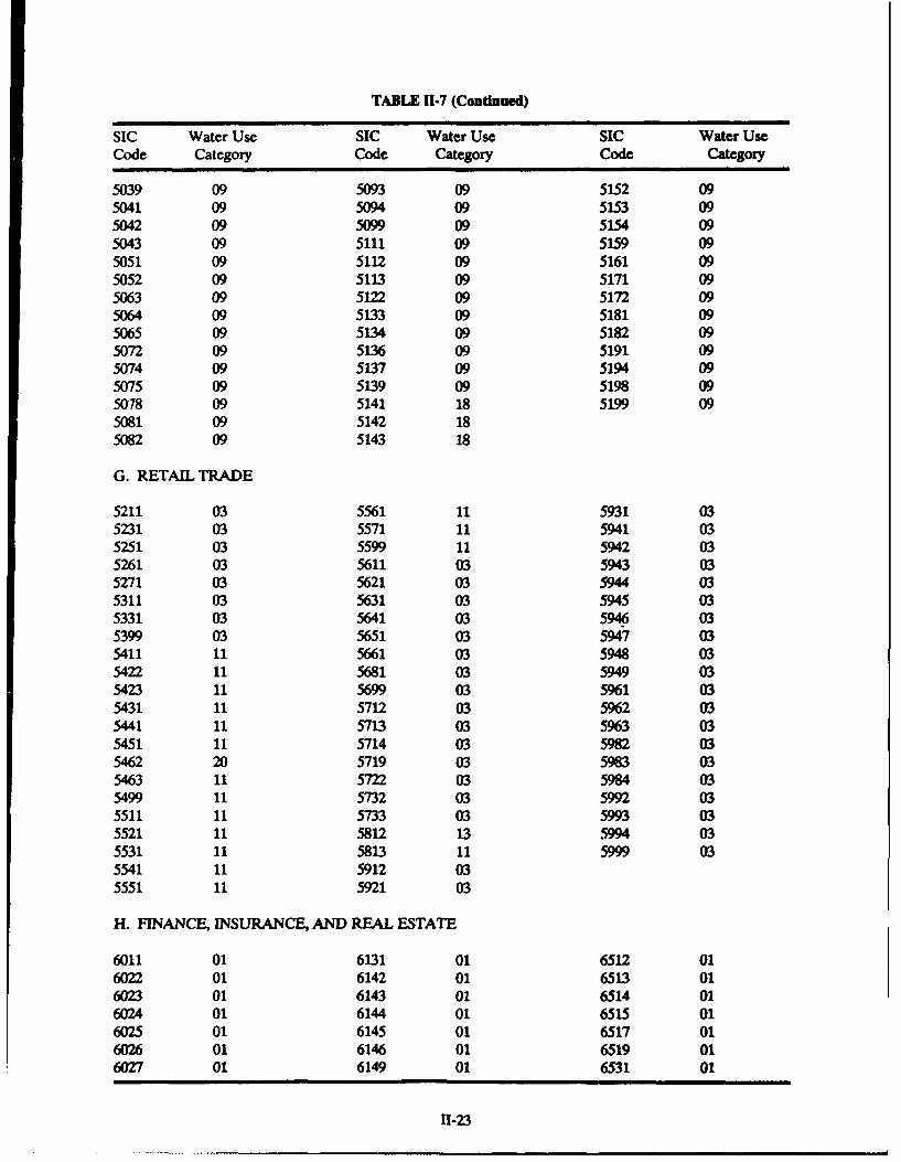
TABLE 11-7 (Continued)
SIC Water Use SIC Water Use SIC Water UseCode Category Code Category Code Category
5039 09 5093 09 5152 095041 09 5094 09 5153 095042 09 5099 09 5154 095043 09 5111 09 5159 095051 09 5112 09 5161 095052 09 5113 09 5171 095063 09 5122 09 5172 095064 09 5133 09 5181 095065 09 5134 09 5182 095072 09 5136 09 5191 095074 09 5137 09 5194 095075 09 5139 09 5198 095078 09 5141 18 5199 095081 09 5142 185082 09 5143 18
G. RETAIL TRADE
5211 03 5561 11 5931 035231 03 5571 11 5941 035251 03 5599 11 5942 035261 03 5611 03 5943 035271 03 5621 03 5944 035311 03 5631 03 5945 035331 03 5641 03 5946 035399 03 5651 03 5947 035411 11 5661 03 5948 035422 11 5681 03 5949 035423 11 5699 03 5961 035431 11 5712 03 5962 035441 11 5713 03 5963 035451 11 5714 03 5982 035462 20 5719 03 5983 035463 11 5722 03 5984 035499 11 5732 03 5992 035511 11 5733 03 5993 035521 11 5812 13 5994 035531 11 5813 11 5999 035541 11 5912 035551 11 5921 03
H. FINANCE, INSURANCE, AND REAL ESTATE
6011 01 6131 01 6512 016022 01 6142 01 6513 016023 01 6143 01 6514 016024 01 6144 01 6515 016025 01 6145 01 6517 016026 01 6146 01 6519 016027 01 6149 01 6531 01
[1-23

TABLE 11-7 (Continued)
SIC Water Use SIC Water Use SIC Water UseCode Category Code Category Code Category
6028 01 6153 01 6541 016032 01 6159 01 6552 016033 01 6162 01 6553 016034 01 6163 01 6611 016042 01 6211 01 6711 016044 01 6221 01 6722 016052 01 6231 01 6723 016054 01 6281 01 6724 016055 01 6311 01 6725 016056 01 6321 01 6732 016059 01 6324 01 6733 016112 01 6331 01 6792 016113 01 6351 01 6793 016122 01 6361 01 6794 016123 01 6371 01 6799 016124 01 6399 016125 01 6411 01
I. SERVICES
7011 13 7396 01- 8021 207021 04 7397 01 8031 207032 03 7399 01 8041 207033 03 7512 09 8042 207041 04 7513 09 8049 207211 07 7519 09 8051 217212 06 7523 09 8059 217213 06 7525 09 8062 227214 06 7531 09 8063 227215 06 7534 09 8069 227216 06 7535 09 8071 187217 06 7538 09 8072 187218 07 7539 09 8081 197219 01 7542 18 8091 197221 06 7549 09 8111 017231 06 7622 09 8211 167241 06 7623 09 8221 167251 01 7629 09 8222 167261 09 7631 09 8231 037299 01 7641 09 8241 017311 01 7692 09 8243 027312 01 7694 09 8244 027313 01 7699 09 8249 027319 01 7813 09 8299 027321 01 7814 09 8321 017331 01 7819 09 8331 027332 01 7823 01 8351 097333 01 7824 01 8361 017339 01 7829 01 8399 017341 01 7832 11 8411 13
11-24

TABLE 11-7 (Continued)
SIC Water Use SIC Water Use SIC Water UseCode Category Code Category Code Category
7342 01 7833 03 8421 237349 01 7911 12 8611 027351 01 7922 01 8621 027361 01 7929 01 8631 027362 01 7932 11 8641 027369 01 7933 11 8651 027372 01 7941 01 8661 027374 01 7948 17 8699 027379 01 7992 13 8811 017391 01 7993 01 8911 017392 01 7996 13 8922 017393 01 7997 10 8931 017394 01 7999 13 8999 097395 01 8011 20
J. PUBLIC ADMINISTRATION
9111 15 9229 15 9532 159121 15 9311 15 9611 159131 15 9411 15 9621 159199 15 9431 15 9631 159211 15 9441 15 9641 159221 15 9451 15 9651 159222 15 9511 15 9661 159223 15 9512 15 9711 159224 15 9531 15 9721 15
L NONCLASSFIABLE ESTABLISHMENTS
9999 n/a
n/a = not assigned.
I-25

TABLE 114
LIST OF INDUSTRIAL CATEGORIESAS CONTAINED IN THE IWR-MAIN SYSTEM
Data SiCName No. Industrial Category
1001 201 Meat Products1002 2011 Meat Packing Plants1003 2013 Sausages & Other Prepared Meats1004 2016 Poultry Dressing Plants1005 2017 Poultry & Egg Processing1006 202 Dairy Products1007 203 Preserved Fruits & Vegetables1008 204 Grain Mill Products1009 205 Bakery products1010 2051 Bread, Cake & Related Products1011 2052 Cookies & Crackers1012 206 Sugar & Confectionery Products1013 207 Fats & Oils1014 208 Beverages1015 2082 Malt Beverages1016 2086 Bottled & Canned Soft Drinks1017 2087 Flavoring Extracts & Syrups, nec1018 209 Misc. Foods & Kindred Products1019 211 Cigarettes1020 212 Cigars1021 213 Chewing & Smoking Tobacco1022 214 Tobacco Stemming & Redrying1023 221 Weaving Mills, Cotton1024 m Weaving Mills, Synthetics1025 223 Weaving & Finishing Mills, Wool1026 224 Narrow Fabric Mills1027 225 Knitting Mills1028 226 Textile Finishing, exc. Wool1029 227 Floor Covering Mills1030 228 Yarn & Thread Mills1031 229 Misc. Textile Goods1032 230 Apparel & Other Textile Products1033 241 Logging Camps & Logging Contractors1034 242 Sawmills & Planing Mills1035 243 Millwork, Plywood & Struct. Members1036 244 Wood Containers1037 245 Wood Buildings & Mobile Homes1038 249 Misc. Wood Products1039 251 Household Furniture1040 252 Office Furniture1041 253 Public Building & Related Furniture1042 254 Partitions & Fixtures1043 259 Misc. Furniture & F'xures1044 261 Pulp Mills1045 262 Paper Mills, exc. Building Paper1046 263 Paperboard Mills1047 264 Misc. Converted Paper Products
I1-26

TABLE 11-8 (Continued)
Data SICName No. Industrial Category
104 265 Paperboard Containers & BoxesU,,49 266 Building Paper & Board Mills1050 270 Printing & Publishing1051 281 Industrial Inorganic Chemicals1052 282 Plastics Materials & Synthetics1053 283 Drugs1054 2831 Biological Products1055 2833 Medicinals & Botanicals1056 2834 Pharmaceutical Preparations1057 284 Soap, Cleaners & Toilet Goods1058 285 Paints & Allied Products1059 286 Industrial Organic Chemicals1060 2861 Gum & Wood Chemicals1061 2865 Cyclic Crudes & Intermediates1062 2869 Industrial Organic Chemicals, nec1063 287 Agricultural Chemicals1064 289 Misc. Chemical Products1065 291 Petroleum Refining1066 295 Paving & Roofing Materials1067 299 Misc. Petroleum & Coal Products1068 301 Tires & Inner Tubes1069 302 Rubber & Plastics Footwear1070 303 Reclaimed Rubber1071 304 Rubber & Plastics Hose & Belting1072 306 Fabricated Rubber Products, nec1073 307 Misc. Plastics Products1074 311 Leather Tanning & Finishing1075 313 Boot & Shoe Cut Stock & Findings1076 314 Footwear exc. Rubber1077 315 Leather Gloves & Mittens1078 316 Luggage1079 317 Handbags & Personal Leather Goods1080 319 Leather Goods, nec1081 321 Flat Glass1082 322 Glass & Glassware, Pressed or Blown1083 323 Products of Purchased Glass1084 324 Cement, Hydraulic1085 325 Structural Clay Products1086 326 Pottery & Related Products1087 327 Concrete, Gypsum & Plaster Products1088 328 Cut Stone & Stone Products1089 329 Misc. Nonmetallic Mineral Products1090 331 Blast Furnace & Basic Steel Products1091 3312 Blast Furnaces & Steel Mills1092 3313 Electrometallurgical Products1093 3315 Steel Wire & Related Products1094 3316 Cold Finishing of Steel Shapes1095 3317 Steel Pipe & Tubes1096 332 Iron & Steel Foundries
11-27

TABLE 114 (Continued)
Data SICName No. Industrial Category
1097 3321 Gray Iron Foundries1098 3322 Malleable Iron Foundries1099 3324 Steel Investment Foundries1100 3325 Steel Foundries, nec1101 333 Primary Nonferrous Metals1102 334 Secondary Nonferrous Metals1103 335 Nonferrous Rolling & Drawing1104 336 Nonferrous Foundries1105 339 Misc. Primary Metal Products1106 341 Metal Cans & Shipping Containers1107 342 Cutlery, Hand Tools & Hardware1108 343 Plumbing & Heating. exc. Electric1109 344 Fabricated Structural Steel Products1110 3441 Fabricated Structural Metal1111 3442 Metal Doors, Sash & Trim1112 3443 Fabricated Plate Work (Boiler Shops)1113 3444 Sheet Metal Work1114 3446 Architectural Metal Work1115 3448 Prefabricated Metal Buildings1116 3449 Misc. Metal Work1117 345 Screw Machine Products, Bolts, etc.1118 346 Metal Forgings & Stampings1119 3462 Iron & Steel Forgings1120 3463 Nonferrous Forgins1121 3465 Automotive Stampings1122 3466 Crowns & Closures1123 3469 Metal Stampings, nec1124 347 Metal Services, necI125 348 Ordnance & Accessories, nec1126 349 Misc. Fabricated Metal Products1127 351 Engines & Turbines1128 352 Farm & Garden Machinery1129 353 Construction & Related Machinery1130 3531 Construction Machinery1131 3532 Mining Machinery1132 3533 Oil Field Machinery1133 3534 Elevators & Moving Stairways1134 3535 Conveyors & Conveying Equipment1135 3536 Hoists, Cranes & Monorails1136 3537 Industrial Trucks & Tractors1137 354 Metalworking Machinery1138 355 Special Industry Machinery1139 356 General Industrial Machinery1140 357 Office & Computing Machines1141 3572 Typewriters1142 3573 Electronic Computing Equipment1143 3574 Calculating & Accounting Machines1144 3576 Scales & Balances, cxc. Laboratory1145 3579 Office Machines, nec1146 358 Refrigeration & Service Machinery
11-28

TABLE 114 (Continued)
Data SICName No. Industrial Category
1147 3581 Automatic Merchandising Machines1148 3582 Commercial Laundry Equipment1149 3585 Refrigeration & Heating Equipment1150 3586 Measuring & Dispensing Pumps1151 3589 Service Industry Machinery, nec1152 359 Misc. Machinery, exc. Electrical1153 3592 Carburetors, Pistons, Rings, Valves1154 3599 Machinery, exc. Electrical, nec1155 361 Electric Distributing Equipment1156 362 Electrical Industrial Apparatus1157 363 Household Appliances1158 364 Electric Lighting & Wiring Equipment1159 365 Radio & TV Receiving Equipment1160 366 Communication Equipment1161 367 Electronic Components & Accessories1162 3671 Electron Tubes, Receiving Type1163 3672 Cathode Ray Television Picture Tubes1164 3673 Electron Tubes, Transmitting1165 3674 Semiconductors & Related Devices1166 3675 Electronic Capacitors1167 3676 Electronic Resistors1168 3677 Electronic Coils & Transformers1169 3678 Electronic Connectors1170 3679 Electronic Components, nec1171 369 Misc. Electrical Equipment & Supplies1172 371 Motor Vehicles & Equipment1173 3711 Motor Vehicles & Car Bodies1174 3713 Truck & Bus Bodies1175 3714 Motor Vehicle Parts & Accessories1176 3715 Truck Trailers1177 372 Aircraft & Parts1178 3721 Aircraft1179 3724 Aircraft Engines & Engine Parts1180 3728 Aircraft Equipment, nec1181 373 Ship & Boat Building & Repairing1182 374 Railroad Equipment1183 375 Motorcycles, Bicycles & Parts1184 376 Guided Missiles, Space Vehicles, Parts1185 379 Misc. Transportation Equipment1186 381 Engineering & Scientific Instruments1187 382 Measuring & Controlling Devices1188 383 Optical Instruments & Lenses1189 384 Medical Instruments & Supplies1190 385 Opthalmic Goods1191 386 Photographic Equipment & Supplies1192 387 Watches, Clocks & Watchcases1193 391 Jewelry, Silverware & Plated Ware1194 393 Musical Instruments1195 194 Toys & Sporting Games
11-29

TABLE 114 (Ctdanied)
Data SICName No. Industrial Category
I196 395 Pens, Pencils, Office & Art Supplies1197 396 Costume Jewelry & Notions1198 399 Misc. Manufactures
nec = not elsewhere classified.
11-30

3.2 PROJECTION DATA
Projection Methods
IWR-MAIN allows for three different methods of projecting water use parameters. Any combination ofthese methods may be used for any specified forecast year. Each forecast year is treated kdcW dalnU& thusthe specification of one method for the first forecast year does not mean that the same method or combinationof methods must be used for a subsequent forecast year. The three methods of projection, specified on theParameter Control Screen, include:
(1) Projection by internal growth models(2) Projection by extrapolation of local historical data(3) Use of projections made external to the IWR-MAIN System
Key Projection Data
IWR-MAIN requires certain key projection data regardless of the projection methods used. The datavalues entered on data screens 9.1 through 9.4 include:
(1) Yar - calendar year of water use forecast (not more than 50 years after the base year).(2) P -- total resident population in the study area in forecast year.(3) Median household income - projected median household income in forecast year, expressed in
1980 dollars.
(4) Total emloment -- total study area employment in forecast year.(5) Total nmbr of households - total number of housing units in forecast year (odna.(6) Fraction of households with forecast year income: (<S10.000): (S10.000-S20.000): (120.000-
$3.00- fraction of households with forecast year income in respective ranges. Income rangesare expressed in 1980 dollars (giuDn .
(7) Emplment bysector - construction (SIC 1500-1799); manufacturing (SIC 2000-3999); transpor-tation, communication, and utilities (SIC 4000-4999); wholesale trade (SIC 5000-5199); retail trade(SIC 5200-5999); finance and banking (SIC 6000-6799); services (SIC 7000-8999); and government(SIC 9100-9799) employment for forecast year (gdiD).
Included on the IWR-MAIN Utility Diskette (Diskette #5) is an External Projection. Module whichprovides key socioeconomic projections for selected areas in the United States (see Appendix C). Theseprojections may be used as a data source for the key projection data.
Historical Data
Certain water use parameters may be projected by extrapolating local historical data. These projectionswill overri projections generated by the internal growth models. Extrapolation of local historical data willoccur whenever a but not more than seven, data points are provided for the parameter in one of thesubgroups described below.
Projection by extrapolation of historical trends may be selected for residential parameters by entering thenecessary data using screens 10.1 and 10.2. The residential parameters consist of the number of housing unitswithin all value ranges whose midpoints (midrange values expressed in 1980 dollars) fall into one of the followinggroups:
Price Rane and OtherGroup 1 (low) - units with market value < $25,000Group 2 - units with market value $25,000-$50,000
11-31

Group 3 units with market value $50,000-$100,000Group 4 (high) -- units with market value > $100,000Total -- total housing units
Commercial/institutional and industrial category parameters may also be projected by extrapolation oflocal historical trends using data screens 11.1 to 11.4 (commercial/institutional) and 12.1 to 12.a (industrial).These screens directly correspond to the Base Year screens 6.1 and 6.2 (commercial/institutional) and screens7.1 through 7.7 (industrial). If values were input into these Base Year screens, those categories ([COxx] andSIC categories) will be highlighted in the Historical Parameter screens. Data must be entered for aleastftw3=[ but not more than seven years, and may include the base year.
Public/unaccounted historical parameters are entered on screens 13.1 and 13.2. These parameters maybe projected by extrapolation of historical data for two to seven years. Parameters include population (numberof persons) for distribution loss [LOSS] and per capita water use for free service [FSER]. If any user-specifiedparameters [POO1-P014J were included in Base Year screen 8., these parameter variables will be highlightedin the Historical Parameter screen. The parameter units for each category [POxx] should be the same as thosespecified in the Base Year screen (i.e., if [POO1] was specified as restrooms in the Base Year screen, parameterunits to be extrapolated in the Historical Parameter screens should be restrooms for [11]).
External Data
Water use parameters may also be projected by direct external input, replacing any historical extrapola-tions or internal projections. These external estimates are projections from outside sources and will sugersedethe results of the historical extrapolations and parameters generated by the internal growth models.
External projections are entered in data screens 14.x through 14.x.9 where xis a designated forecast year.Each municipal sector (residential, commercial, industrial, and public/unaccounted) is represented on aseparate screen(s). Not all municipal sectors or forecast years need be addressed.
ResldentlMl
The possible combinations for the residential subgroup parameter labels are:
Residential Suwrou[FWJ - flat rate and sewered[FP] - fiat rate and unsewered
[MW] -- metered and sewered[AP] - master-metered apartment
Price Rane and Other[G1] - units with midrange market value < $25,000[G2] - units with midrange market value $25,000-$50,000[G3] - units with midrange market value $50,000-4100,000[G41 -- units with midrange market value > $100,000ITL] - total housing units
Parameter units are housing units. The parameter labels consist of one residential subgroup and one pricerange (or total). For example, MWG1, MWTL, FPG4, APTL.
11-32

Commercial/Institutional
In the case of the commercial/institutional subgroup, the parameter labels are the [COxx] categories andthe parameter units are employment for [C01-CO23]. For categories [C024-C0501 parameter units may beemployment or any other user-specified unit as previously specified in data screens 6.2 and 6.3.
Industrial parameter labels are the [1001-11981 categories which directly correspond to SIC codesappearing in data screens 7.1 through 7.6; see Table 11-8 for a cross-reference between SIC codes and [Icm]categories. The user may also provide projection data for the two additional industrial categories [1199 and 1200]provided that the categories were specified in screen 7.7.
PubllclUnaccounted
Public/unaccounted parameters are entered as direct external projections in units as specified in screens8.1 and82, or water use (average annual and maximum-day) maybe entered. If distribution losses are specifiedfor future years, they maybe entered as a percent of total municipal, the population base (parameter) from whichto calculate per capita loss, or the water loss in gallons per day. Free service data maybe entered asthe populationbase or the water use in gallons per day. Parameter categories include:
[FLSSJ - percent distribution loss (percent of total municipal water use)[LOSS] - distribution losses (population or gallons per day)[FSERJ - free service (population or gallons per day)[PMO1-P027] - user-specified categories (units or gallons per day)
3.3 CONSERVATION DATA
The conservation routine will generate estimates of restricted water use if the conservation option isselected on the Parameter Control Screen. The restricted water use incorporates the reduction of water useachieved by the selected conservation measures. The effectiveness, or the magnitude of this reduction, iscalculated as the product of unrestricted water use times the reduction and coverage parameters. Data screen15.1 enables the user to select up to 14 specified conservation measures, defined within the model, and fouradditional user-specified measures. These measures are selected by entering the year of implementation nextto the corresponding measure. The implementation year may be a past or a current year (existing measure)or a future year (future measure). The sectors to which the selected measures apply are specified on screen 15.2.
The 14 specified measures have default values for reduction factors and for the calculation of coverageresiding in the Library of Conservation Coefficients (LCC). IWR-MAIN allows the user the option of specifyingall or some of the reduction and coverage factors while letting the LCC provide the others. On the other handthe user may specify that the LCC provide all of the reduction factors and calculate all of the coverage factors.However, if uernaCgimeasures are selected, all reduction and coverage factors for these measures m=be specified by the user because a value of zero is assigned to them in the LCC.
Reduction factors are specified for each measure and sector for indoor use (data screen 16.2), outdooruse (data screen 16.3), and maximum-day sprinkling use (data screen 16.4). Reduction factors represent afraction reduction of water use and must be between 0.000 and 1.000.
Coverage factors may also be specified for each measure and sector for the base year (data screen 17.2)and for each selected forecast year (data screens 17.3 to 17.x). Entry of these coverage factors is similar to thatof the reduction factors in that only values between 0.000 and 1.00 are allowed.
11-33

3.4 POSSIBLE DATA SOURCES
As stated previously, two kinds of data are required to use the IWR-MAIN System: (1) actual values ofall demographic and socioeconomic determinants (or parameters) of water use for the base year and (2)projected values of selected determinants for each forecast year. If the conservation procedure is selected, aminimum amount of information is required about the implementation ofconservation measures. If verificationof the IWR-MAIN base year water use estimates is desired, actua water r e reco-As (preferably disaggregatedby customer class) should be obtained.
The level of difficulty of the data collection effort depends, to a large extent, on the level of user sectordisaggregation and the study area definition. Water use can be separately forecast by IWR-MAIN for each offour major sectors (residential, commercial/institutional, industrial, and unaccounted) and for up to approxi-mately 380 individual categories. For example, at the maximum level of residential disaggregation, fourresidential subgroups may be addressed: fiat rate and sewered, flat rate and unsewered, metered and sewered,and master-metered apartments. Within each subgroup, 25 home value ranges maybe specified. Data collectionat this level of detail may require a significant amount of time and effort. Alternatively, at a low level ofdisaggregation, residential data could be aggregated into the metered and sewered and apartment subgroups(assuming a single-family and multifamily distinction) and address only 10 value ranges in each. Similaraggregations can be applied to the commercial/institutional and industrial sectors. However, it should be notedthat the more aoregated the modeL the fewer the data requirements. the reater the need for calibration againstlocal water use, and the lower the confidence which can be placed in the resulting forecast.
The study area definition also determines the level of data collection efforts. This is because the mostdetailed, disaggregate socioeconomic data are available for major urban cities, counties, and standardmetropolitan statistical areas. The smaller the study area in size and population, the less the availability ofdisaggregate socioeconomic data and the more reliance which must be placed on data from local agencies. Incases where socioeconomic data are available for a large area (county) but not available for small areas (city),the large area data can be disaggregated by a shift-share method. In its simplest form, this method is based ona historical record of small-area shares of the large-area aggregate.
There are three major sources of data available to IWR-MAIN users. First, data may be obtained frompublished reports, most notably from the U.S. Bureau of the Census or the Bureau of Labor Statistics. Thesepublications can be found in most research libraries. Second, data maybe obtained from local. regional, or stateagencies, including water resource boards, employment security divisions, departments of community andeconomic affairs, and planning agencies. Listings of state and regional agencies may be found in most publiclibraries. Third, independent firms specializing in economic or market-oriented data may also be utilized.Common data sources for selected variables are shown in Table 11-9.
11-34

40
j
Loi-nu a
~4 0
~ JOoj.we cl~
0 (~3 o
Q. i -1,- 1
-U
70S..
lie 0-1. 4 .90.
.'t. ...
W4 C ri 44 4
u-35

9 V-
0 78 1k
111-3

4. COMPUTATIONAL METHODS
This chapter presents the computational methods used by IWR-MAIN to estimate unrestricted andrestricted water use and to forecast water use parameters. The data bases used to derive the water use equationsand coefficients are presented and discussed. To facilitate verification of water use coefficients under localconditions, this chapter concludes with a discussion of the correspondence between the water use models andthe data contained in the IWR-MAIN coefficient libraries.
4.1 WATER USE EQUATIONS
As mentioned briefly in chapter 2, the computational procedures of IWR-MAIN are a mixture of wateruse estimating techniques (refer to Table U-1). This section presents the water use estimating methods for eachof the major urban water use sectors.
Residential Use Models
Most of the residential water use models contained in IWR-MAIN are based on data collected from theResidential Water Use Research Project by the Johns Hopkins University. Under sponsorship by the TechnicalStudies Program of the Federal Housing Administration and in cooperation with 16 participating utilities, theJohns Hopkins University conducted studies between 1961 and 1966 to (1) determine the water use patternsand demand rates imposed on water systems in residential areas and (2) determine the major factors influencingresidential water use. Master-meter, punched tape recorder systems were installed to continuously monitorwater flow into 39 homogeneous residential areas. The 39 study areas were served by 16 water utilities andranged in size from 34 dwelling units to 2,373 dwelling units. The resulting data from this study consisted ofobservations on average values (per dwelling unit) of the relevant water use explanatory variables for 39 studyareas (Linaweaver et aL, 1966; Howe and Linaweaver, 1967).
Using the data generated by the Residential Water Use Research Projec, Howe and Linaweaver (1967)provided a comprehensive econometric analysis, yielding water use models for five categories of residentialwater use:
(1) Metered and sewered residences in the western United States(2) Metered and sewered residences in the eastern United States(3) Metered residences with septic tanks(4) Flat rate and sewered residences(5) Apartment areas
Some of the explanatory variables used in the demand analysis included-
(1) Market value of residence(2) Number of persons per dwelling unit(3) Age of dwelling unit(4) Average water pressure(5) Marginal water and sewer charge(6) Irrigable area per dwelling unit(7) Summer potential evapotranspiration in inches
For each housing category, regression equations were estimated for domestic demand, summer sprinklingdemand, and maximum-day demand.
11-37

In 1982, Howe reestimated some of the Howe and Linaweaver (1967) equations, incorporating anexplanatory variable that had not been considered previously: the bill difference variable. The bill differenceis calculated as the difference between the total water/wastewater bill and the product of marginal water/wastewater price and water use. It is expressed in dollars per billing period and reflects the additional impacton disposable *, -ome, beyond that of the marginal price, imposed by the particular rate structure in use. Howeonly attempted reestimation of the metered and sewered equations, and the resulting significant equationsreplaced those in IWR-MAIN from Howe and Linaweaver (1967). Howe's updated results indicated a substan-tially improved fit of the models to the data.
Currently, the IVR-MAINSystem contains four residential water use categories: (1) flat rate and seweredresidences, (2) flat rate and unsewered residences, (3) metered and sewered residences, and (4) master-meteredapartments. IWR-MAIN water use estimates for the residential sector are presented in 1,000 gallons per dayfor the dimensions of winter, summer, average annual, and maximum-day water use. The water demandfunctions for each residential category are presented in the following sections.
Metered and Sewwed Models
The metered and sewered housing category includes single-family residential units that are individuallymetered and are served by a public sewer system. The housing units are considered owner-occupied or occupiedby renters who are responsible for paying the water and wastewater bill. The residential demand models formetered and sewered water use are presented in Table 11-10. Based on Howe and Linaweaver (1967) and Howe(1982), these models were later revised to include new coefficient values to permit housingvalue and price datato be provided in 1980, rather than 1960, dollars.
The price elasticity of water demand in the winter usage equation is -0.20 when the effects of change inthe water rate structure on disposable income that are captured by the bill difference are ignored and -0.06 whensuch effects are taken into account. The elasticity of home value (a proxy for income) is 0.32.
The price elasticities of summer demand are -0.52 for the west (without the effects of bill difference) and-0.57 for the east (including the effects of bill difference). Corresponding home value elasticities are 0.43 and0.34.
Note that the summer eastern equation includes the moisture deficit (MD) variable. The summer westernequation is the sum of a summer sprinkling term and the domestic water use. The summer sprinkling term ofthe western equation includes a weather adjustment factor (WF) which permits the calibration of the model toactual weather conditions of a specific year. The weather adjustment factor has a default value of 1.0. Thecalibration procedure is described in Part 11, section 5.3.
Flatae Mdels
The flat rate categories include housing units that are occupied by customers who face a zero marginalprice. The distinction between the flat rate and sewered and the flat rate and unsewered is the use of a publicsewer system. Flat rate units maybe single-family customers who pay a flat charge for their water and wastewaterservices. Alternatively, flat rate units may also include low-density multifamily customers (duplex, mobilehomes) who are not individually metered or renter-occupied households where the owner pays the water andwastewater bill.
The residential water use models for flat rate and sewered water use are presented in Table I-11. Thewinter water use model is based on the Johns Hopkins University sample of flat rate and apartment customersand exhibits a housing value elasticity of 0.33. The summer water use model is based on the sample of flat rate,single-family customers. The corresponding housing value elasticity for summer demand is 0.70.
The residential water use models for flat rate and unsewered water use are presented in Table 11-12. Thewinter water use model is based on the Johns Hopkins University sample of customers with septic tanks.
11-38

However, no significant summer sprinkling water use equations were derived by Howe and Linaweaver (1967)for septic tank users. Therefore, the summer sprinkling model for flat rate and unsewered customers is the sameas that for flat rate and sewered customers. The housing value elasticity for summer water demand is 0.64.
Apartment Models
The master-metered apartment category refers to housing units which face a zero marginal price and havelittle opportunity to engage in outdoor (seasonal) water uses. It is assumed that these units are provided withsewer services.
The residential water use models for master-metered apartment water use are presented in Table -13.The winter water use model is based on the Johns Hopkins University sample of flat rate and apartmentcustomers and exhibits a housing value elasticity of 0.33. Summer and maximum-day apartment water use areset equal to 1.433 times winter day use. This factor was derived from the observed summer and winter wateruse in the five apartment areas included in the Johns Hopkins University study.
Commercial/Institutional Coefficients
The calculation of commercial and institutional water use is based on the single coefficient requirement,or unit use, method. Commercial/institutional water use is estimated on a per employee basis using thefollowing formulas:
(Qa)c = (C.)c * Pc * ADJ
and
(Om.i)c = (CnW,)c * Pc * ADJ
where
Q = water usage for a particular category, gallons per dayC = commercial/institutional water use coefficient, gallons per employee per dayP - water use parameter, employmentADJ = price difference adjustment; ADJ = (PRb/PRc)e
PRb = marginal price paid by average customer during the base yearPRc marginal price paid by average customer during the year for which coefficient c was establishede = price elasticity for sector
and subscripts indicate the following water use types:
a = average annual usec = commercial/institutional use categorymidy - madmum-day use
Table 11-14 presents the 23 commercial/institutional water use categories specified by the IWR-MAINSystem. The 23 categories are the result of identifying and aggregating four-digit SIC categories by similar wateruse activities. The water use coefficients for each category were derived from a 1984 survey of 2,261establishments served by 41 water utilities (Boland et al., 1985). For each surveyed establishment, annual wateruse and employment were obtained.
The price difference adjustment is calculated using the ratio of marginal prices in the base year and theyear concurrent with the water use coefficients. These prices are provided by the user in the input data. Theelasticity of commercial water use with respect to price is read from the library of water use coefficients (see
11-39

Part II, section 4.4). The default value of -0.80 was selected from a range of commercial price elasticities reportedby Boland et al. (1984). See the discussion of price elasticities in the description of reduction factors for the pricepolicy conservation measure in Part H, section 4.3. The user may wish to estimate the price elasticity for thecommercial sector of a given study area and replace the default value in the library. No price adjustment is madefor user-added categories given that the user must compute and input the coefficients for these categories.
Industrial Coefficients
Industrial water use is also calculated based on the single coefficient requirement (per employee) method.Industrial water use is estimated using the following formulas.
(Qa)n - (C.)n * ADJ
and
(Qnxdy). - (Cmy)n * Pn * ADJ
where
0 - water usage for a particular category, gallons per dayC - industrial water use coefficient, gallons per employee per dayP - water use parameter, employmentADJ - price difference adjustment; ADJ - (PRb/PRc)cPRb - marginal price paid by average customer during the base yearPRc - marginal price paid by average customer during the year for which coefficient c was establishede - price elasticity for sector
and subscripts indicate the following water use types:
a - average annual usen - industrial use categorymxdy - m aimum-day use
The water use rates per employee were derived from the US. Bureau of the Census report entitled "WaterUse in Manufacturing" (US. Bureau of the Census, 1986). The census data were obtained from several sourcesincluding a special survey of 10,262 establishments reporting a total water intake of 20 million gallons or morein the 2 Cens a n The Industry Division of the Bureau of the Census performed a specialemployment tabulation for the original survey respondents to permit the calculation of per employee use ratesat the three- and four-digit SIC categories. Table IU-15 presents 198 employee use coefficients obtained bydividing total annual intake of water from pbi sources by the reported number of employees and the numberof days in a year (365) for each SIC category.
Two sets of coefficients were developed. The first set represents use rates reported by the panel of 10,262establishments which account for 96 percent of total water use estimated for manufacturers. The coefficientsin this set represent establishments which use large quantities of water. The second set represents "average"establishments. The employee use coefficients in this set were calculated by making adjustments for the percentof total water intake and the percent of total employment accounted for by establishments included in the firstset. For example, for category 1055 representing four-digit SIC code 2833 (cellulosic manmade fibers) thecoefficient in the first set is 1,200.0 gallons per employee per day. The coefficient for the "average* establishmentsin this industry was calculated according to the formula.
C. - C * (f/fo) - 1,200.0 * (0.627/0.992) - 758.5 ged
I-40

where
Ca = water use coefficient for average establishment in the category in gallons per employee per day (ged)C1 = water use coefficient for large water-using establishments in the category in gallons per employee per
day (ged)fE = fraction of total employment in SIC category 28 accounted for byestablishments usinglarge quantities
of waterfQ = fraction of totalwater intake in SIC category28 accounted for by establishments using large quantities
of water
The second set of coefficients, representing "average" establishments, are contained in the IWR-MAINcoefficient library.
As in the adjustment of commercial water use, the price difference adjustment for industrial water useutilizes the ratio of marginal industrial water price in the base year to the marginal industrial water price in theyear concurrent with the industrial water use coefficients. The default industrial price elasticity of -0.65 wasselected from a range of aggregate elasticities for the industrial sector reported by Boland et al. (1984). Therange is shown in the discussion of price elasticities for the reduction factor for the price policy conservationmeasure in Part IT, section 4.3. As with the commercial price elasticity, the user may wish to estimate the priceelasticity for the industrial sector of a given study area and replace the default value in the library. No priceadjustment is made for user-added categories.
Public/Unaccounted Coefficients
Public water use is calculated based on a single coefficient requirement method using the followingformulas:
(0 a)pu = (Ca)pU * Ppu
and
(Omxdy)pu = (Cmxdy)pu * Ppu
where
0 = water usage for a particular category, gallons per dayC = public/unaccounted water use coefficient, gallons per day per unitP = water use parameter, units
and subscripts indicate the following water use types:
a = average annual usepu = public/unaccounted use categorymxdy = maximum-day use
IWR-MAIN has two built-in public/unaccounted water use categories: free service and distributionlosses. Free service is calculated on a per capita basis using resident population as the parameter if average dailyfree service in gallons per day is not provided. Distribution losses are also calculated on a per capita basisprovided that the population served by the distribution system is given. Alternatively, if the population servedis not provided and if the daily losses in gallons per day are not provided, distribution losses are calculated ona percentage basis using total municipal water use as the parameter. Table 11-16 presents the public/unaccounted water use categories and the corresponding water use coefficients. Water use for user-addedpublic/unaccounted categories is calculated based on parameters and coefficients provided by the user.
11-41

TABLE 11-10
METERED AND SEWERED RESIDENTIAL MODELS
(0 D). =(234 + 1.451 V/Fa- 45.9 P,- 2.59 I,)Nr
- (0.48 * 58.777 * Ps -0703 * (V/Fa)0.42)Nr * 2.0 * WF + (QD)m
- (385.0 + 2.876 V/Fa - 285.8 Ps - 435 Is + 157.77 * BO MD)Nr
where
B - 0.803 * Hd 1 26
w = (MD.,W/MD)md
3. Averae annual uAn
A),w = [(QD),m + (O,)d ,]1/2.0
(Q)dmce = [(QD)ms + (o) J/2O
4. Maximumda ni a
(Qmn~ms,w - (2,227.34 *Em2 06 * (V/Fa)0-413) Nr
(Qnw)me = (0.000046 * B0- 18 "Em- 10"4 * p. 5 (V/Fa)0 .3 1 ) Nr
5. Maimum-dav usage
(Qwmxdy)maw = (QD)msw + (m,),w
Definition of symbols
Q - water usage for a particular category, gallons per dayV - average home value in a range of value $1,000
VMi n + Vmu*V =
2 * 1,000
Fa - assessment factor
P. - effective annual marginal price of water, dollars per 1,000 gallonsIs - effective annual bill difference variable, dollars per billing periodPs = effective summer marginal price of water, dollars per 1,000 gallons
- effective summer bill difference variable, dollars per billing period
11-42

TABLE 11-10 (Continued)
B - irrigable land per dwelling unit, acres per unitMD - summer season moisture deficit in inches
MD = E -O.6R
E = summer season potential evapotranspiration, inchesR - summer season precipitation, inchesHd = housing density, units per acreEm maximum-day evapotranspiration, inches = 0.25 for west and 0.29 for eastNr - number of residences in value range rWF - weather adjustment factor
Subsurnt and smerscint of water use Matw
ms - metered and sewered residential useD - winter, or domestic, water uses - summer season usew west of 100th meridiane east of 100th meridiana average annual usemxs maximum-day sprinkling usemxdy maximum-day useactual = actual weather data value for specific calibration yearmd - elasticity of water use with respect to moisture deficit
11-43

TABLE II-1I
FLAT RATE AND SEWERED RESIDENTIAL MODELS
(QD)fs - (28.9 + 1.576 V/Fa + 33.6 DpN r
(Q,)s - (0.41 * 44573 (V/Fa) 0.)Nr 2 2-0 + (QD)f,
3. Anerae annual usage
(Qaa) - [c(QD)f. + (Q.j/2.0
4. Mandmum~da sm~nkling nag.
(Qmxjft - (1,609.59 * BO.93 * (V/Fa)O-M)Nr
5. Maximum-day usag
(Qmy), = (OD)f, + (Qin)f,
Definition of symbols
Q - water usage for a particular category, gallons per day
V - average home value in a range of value, $1,000
VMU + VMa1V=
2 * 1,000
Fa = assessment factorD P = population density per residenceB - irrigable land per dwelling unit, acres per unitNr - number of residences in value range r
Subscripts of water use tUes
fs - flat rate and sewered residential useD - winter, or domestic, water useS - summer season usea = average annual usemxs m imum-day sprinkling usemxdy - maximum-day use
11-44

TABLE 11-12
FLAT RATE AND UNSEWERED RESIDENTIAL MODELS
(O)ft= (302 + 39.5 D)Nr
(Qdft - (0.41 * 44-7 * (V/Pa)0 . )Nr * 2.0 + (OD)ft
3- A&eam annual g
(Qa)ft - [(QD)ft + (o J-/2.0
4. MaXimum-day sprinklin use
(O )ft = (1,60.9 * B0. 93 * (V/Fa)°M)Nr
5. Maximum-da sa
(Q.umxy)ft - (QD)ft + (Qn)ft
Definition of ymg
Q - water usage for a particular category, gallons per dayV = average home value in a range of value, $1,000
Vulin + VMUV.=
2 1,000
Fa = assessment factorDP f= population density per residenceB = irrigable land per dwelling unit, acres per unitN, = number of residences in value range r
Subscrints of water use UM
ft - flat rate and unsewered residential useD - winter, or domestic, water uses - summer season usea = average annual usems - maximum-day sprinkling usemxdy - maximum-day use
1I-45

TABLE 11-13
MASTER-METERED APARTMENT MODELS
(OD)ap - (28.9 + 1.576 V/Fa + 33.6 Dd)r
(Qj)p -1.433 • (QD)ap
3. Average annual umsag
(0a)ap = [(QD).p + (QjqJ/2.0
4. Maximum-dav sminklng AU
(Omz)ap = (Q) ap- (00)p
5. Maximum-day usage
(0 mxdy)ap = (QD)ap + (ma)sp
Definition of smjbols
0 - water usage for a particular category, gallons per dayV - average home value in a range of value, $1,000
VMin + V=XV+
2"1,000
Fa = assessment factorD = population density per residenceN_ = number of residences in value range r
Subscriots of water use tMes
ap - master-metered apartment residential useD - winter, or domestic, water uses - summer season usea = average annual usemu - maximum-day sprinkling usemxdy = maximum-day use
1146

TABLE 11.14
COMMERCIAL AND INSTrTUTIONALCATEGORIES AND WATER USE COEFFICIENTS
Water UseCoefficient
Cate- Water Use (gallons/gory Category Name SIC Codes Type employee/day)
C001 Miscellaneous commercial All codes not none 47.2listed below
C002 Vocational school 8243,8244,8249, Sr 72.08291-99,8331-39,8611-99
C003 Miscellaneous retail 5201-5399,5601-99, Sp 19.35701-99,5901-99,7031-39,7833,8231-39
C004 Boardinghouses 7021-29,7041-49 SrFr 101.6
C005 Transportation terminal 4171,4581-89 SpFp 86.2
C006 Barbers, cleaning 7212-17,7221-7249 Pa 380.2
C007 Power laundries 7211,7218 BPa 276.9
C008 Landscaping 0181-89,0781-0789, Ps 153.14971-79
C009 Miscellaneous wholesale 1501-1799,4172, 0 19.14221-39,4959,5001-99,5111-39,5151-99,7261-69,7511-39,7549,7601-99,7811-19,8351-59,8901-99
C010 Recreational facilities 7997 SrO 225.5
C011 Food and auto retail 5411-59,5463,5491-5599, Sp,O 31.35813,7832,7931-39
C012 Dance studios 7911-19 Sr,Sp,O 213.0
C013 Hotels, restaurants 5812,7011-19,7992, Sp,Fp,O 186.67996,7999,8411-19
C014 Electric, gas utilities 4911-39,4953,4961-69 B,O 6.7
C015 Public administration 9101-9799 Fe,B,O 70.6
C016 Schools, universities 8211-29 Sr,Fe,FrB,O 55.6
n-47

TABLE 11.14 (Continued)
Water UseCoefficient
Cate- Water Use (galons/gory Category Name SIC Codes Type employee/day)
C017 Racetracks 7948 Sp,Fe,FpB,O 341.5
C018 Laboratories, water utilities 4941-49,4952,5141-49, PaO 80.5
7542,8071-8079
C019 Health services 8081-99 SrPaO 33.0
C020 Medical offices, bakeries 5462,8011-49 SpPaO 54.9
C021 Nursing facilities 8051-59 SrSpFe, 107.5Fr,Pa,O
C022 Hospitals 8061-69 SrSp,Fe,Fr, 82.2Fp,B,Pa,O
C023 Zoological, etc., gardens 8421-29 SpFeFp, 720.7PsO
Definition of water use types
Note that codes are assignedwhere a significant fractionof total water use is for the named special purpose.Water use by employees for sanitary purposes is assumed to be present in all categories. Water use for seasonalpurposes such as air conditioning and incidental lawn and shrub irrigation is not separately specified; this usemay occur for any SIC code, depending on the type and location of building.
Sr Sanitary use by residents, students, or other defined nonemployee population.Sp Sanitary use by patrons or general public.Fe Food preparation use, food served to ex, llioe.Fr Food preparation use, food served to reidents, students, or other defined nonemployee population.Fp Food preparation use, food served to g1m or general public.B Water use for boiler feed.Pa Water use as input to production of goods or services, including water incorporated into product, not
seasonal in nature.Ps Water used as input to production ofgoods or services, includingwater incorporated into product, seasonal
in nature.0 Other water uses, including vehicle washing, floor and driveway cleaning, etc.
Source: Boland et al., 1985 and unpublished reports.
11-48

TABLE 11-15
INDUSTRIAL CATEGORIES AND WATER USE COEFFICIENTS
192 Coefficients(Gallons/Employee/Day)
SIC Large AverageCategory Code Establishments Establishments
1001 201 635.2 343.81002 2011 477.8 258.61003 2013 901.7 488.11004 2016 755.8 409.11005 2017 371.5 201.11006 202 654.8 354.41007 203 715.5 38731008 204 1,391.0 753.01009 205 147.9 80.11010 2051 140.0 [11 75.8I011 2052 163.9 [1] 88.71012 206 595.8 322.51013 207 1,484.0 80331014 208 1,2773 691.41015 2082 2,6813 1,451.41016 2086 602.1 325.91017 2087 958.9 519.11018 209 1,286.7 696.51019 211 250.0 [2] 201.21020 212 250.0 [2] 201.21021 213 250.0 [2] 201.21022 214 250.0 [2] 201.21023 221 263.8 [4] 145.61024 222 322.7 178.11025 223 245.9 135.71026 224 263.8 [41 145.61027 225 731.06 403.41028 226 1,0763 593.91029 227 980.1 540.91030 228 486.5 268.51031 229 315.1 173.91032 230 24-3 [9] 24.31033 241 88.4 41.3 [10]1034 242 2,384.7 [4] 310.71035 243 238.8 41.3 [1011036 244 238.8 [11] 41.3 [10]1037 245 238.8 [11] 41-3 [1011038 249 794.9 [5] 103.61039 251 151.4 [61 64.91040 252 77.6 [6] 413 [10]1041 253 109.1 [4] 46.81042 254 297.8 127.71043 259 109.1 [41 46.81044 261 8,303.7 3,518.3
11-49

TABLE 11-15 (Coanned)
1982 Coefficients
(Gallons/Employce/Day)SIC Large Average
Category Code Establishments Establishments
1045 262 2,194.2 929.71046 263 5,827.4 2,461.11047 264 526.4 [5] 223.01048 265 215.5 [4] 91.31049 266 593.8 [4] 251.61050 270 37.9 [41 37.91051 281 1,8613 1,176.61052 282 527.2 33331053 283 531.9 336.21054 2831 292.2 184.71055 2833 1,200.0 758.51056 2834 459.4 290.41057 284 447.8 283.11058 285 402.9 254.71059 286 1,796.0 1,135.31060 2861 1,796.0 [3] 1,135.31061 2865 1,796.0 [3] 1,135.31062 2869 1,796.0 [3] 1.13531063 287 1,328.6 839.91064 289 712.5 450.11065 291 3,780.0 2,638.91066 295 559.1 390.31067 299 1,217.7 850.11068 301 264.7 [4] 87.31069 302 78.3 41.31070 303 264.7 [4] 87.31071 304 264.7 [4] 8731072 306 439.1 144.91073 307 624.8 206.21074 311 626.9 [7] 60.11075 313 626.9 [71 60.11076 314 626.9 [71 60.11077 315 626.9 [7] 60.11078 316 626.9 [7] 60.11079 317 626.9 [7] 60.11080 319 626.9 [7] 60.11081 321 375.1 [4] 156.61082 322 332.4 138.81083 323 375.1 [4] 156.61084 324 375.1 [4] 156.61085 325 576.8 240.81086 326 210.7 88.01087 327 4403 183.8108 328 652.3 272.41089 329 375.1 [41 156.61090 331 550.6 348.3
1l-50

TABLE 11.15 (Continued)
1982 Coefficients
(Gallons/Employe/Day)SIC Large Average
Category Code Establishments Establishments
1091 3312 537.0 339.71092 3313 3653 231.11093 3315 435.9 275.71094 3316 467.8 295.91095 3317 982.5 621.51096 332 842.4 532.91097 3321 1,077.5 681.61098 3322 608.8 [4] 385.11099 3324 608.8 [41 385.11100 3325 311.3 196.91101 333 259.6 164.21102 334 684.9 433.21103 335 479.0 303.01104 336 292.2 184.81105 339 913.2 577.71106 341 723.7 301.91107 342 231.7 96.71108 343 706.1 294.61109 344 329.4 137.41110 3441 256.1 [4] 106.81111 3442 373.6 155.91112 3443 378.9 158.11113 3444 202.9 84.61114 3446 256.1 [4] 106.81115 3448 256.1 [4] 106.81116 3449 256.1 [4] 106.81117 345 293.5 122.41118 346 240.6 100.41119 3462 525.1 219.11120 3463 1,009.4 421.11121 3465 150.7 62.91122 3466 168.4 [41 70.31123 3469 168.4 [4] 70.3I124 347 1,019.4 425.31125 348 136.2 56.81126 349 245.9 102.61127 351 168.815] 66.11128 352 1,281.5 [4] 501.71129 353 103.4 41.3 [1011130 3531 113.5 [41 44.41131 3532 113.5 [4] 44.41132 3533 79.7 41.3 [1011133 3534 113.5 [4] 44.41134 3535 113.5 141 44.4
1135 3536 113.5 [4] 44.41136 3537 113.5 [4] 44.4
11-51

TABLE 11-15 (Continued)
1982 Coefficients(Gallons/Employee/Day)
SIC Large AverageCategory Code Establishments Establishments
1137 354 107.0 41.91138 355 250.3 [5] 98.01139 356 149.6 58.61140 357 108.1 42.31141 3572 108.1 [8] 42.31142 3573 108.1 [8] 42.31143 3574 108.1 [81 42.31144 3576 108.1 [8] 42.31145 3579 108.1 [8] 42.31146 358 356.8 139.71147 3581 119.1 [4] 46.61148 3582 119.1 [4] 46.61149 3585 374.2 146.51150 3586 182.6 71.51151 3589 119.12[4] 46.61152 359 165.8 [5] 64.91153 3592 186.18(41 72.91154 3599 99.62 39.01155 361 251.9 145.21156 362 329.4 189.91157 363 298.0 171.81158 364 221.7 127.81159 365 196.5 [4] 113.31160 366 80.2 46.21161 367 228.4 131.71162 3671 294.5 [4] 169.81163 3672 228.4 [8] 131.71164 3673 228.4 [8] 131.71165 3674 239.5 138.11166 3675 115.1 66.41167 3676 168.59(41 97.21168 3677 228.418] 131.71169 3678 127.9 73.71170 3679 241.6 139.31171 369 196.5 [4] 113.31172 371 299.9 217.91173 3711 280.86[4] 204.01174 3713 280.86[41 204.01175 3714 320.4 232.81176 3715 299.9 [81 217.91177 372 151.6 [4] 110.11178 3721 151.6 [81 110.11179 3724 151.6 [81 110.11180 3728 151.6 [81 110.11181 373 151.6 [4] 110.11182 374 294.9 214.2
11-52

TABLE 11-15 (Continued)
1982 Coefficients(Gailons/Employee/Day)
SIC Large AverageCategory Code Establishments Establishments
1183 375 456.6 331.71184 376 140.9 102.41185 379 234.8 170.61186 381 91.3 43.71187 382 109.7 52.61188 383 122.1 [4] 58.51189 384 122.1 [4] 58.51190 385 122.1 [41 58.51191 386 122.1 [4 58.51192 387 122.1 [4] 58.51193 391 203.8 [4] 93.91194 393 203.8 [4] 93.91195 394 240.7 110.91196 395 222.1 102.41197 396 203.8 [4] 93.91198 399 203.8 [4] 93.9
Notes:
[11 Ifno public intake is reported for a four-digit SIC category, the four-digit level assumes the same public/total intake ratio as the three-digit leveL
[2] Since public intake is not reported for category.21, the ratio of public/total intake observed in 1977 isassumed for 1982 and is applied to three-digit categories 211, 212, 213, and 214.
[3] A coefficient is estimated for SIC 286; however, no information is provided for its four-digit categories.Therefore, three-digit coefficient is assumed for the four-digit leveL
[4] Three-digit coefficients are estimated as total water use for two-digit SIC category, less reported (or
estimated) three-digit water use divided by corresponding employment.
[51 If no public intake is reported, the category assumes the public/total intake ratio as observed in 1977.
[61 Three-digit public/total ratio is same as that for two-digit SIC category.
[7] Where no three-digit SIC information is available, a two-digit coefficient is assumed.
[8] Where no four-digit SIC information is available, a three-digit coefficient is assumed.
[9] Estimated from an independent survey. SIC 23 is based on a sample of three establishments with 145employees. SIC 27 is based on a sample of five establishments with 1,873 employees.
[101 Coefficient represents average sanitary use derived from the 1982 survey.
[11] SIC 244 and 245 are assumed to reflect a water use pattern similar to SIC 243.
Source: U.S. Bureau of the Census, 1986, and a special tabulation by the U.S. Bureau of the Census (see pageIl-40 for explanation)."G/E/D - gallons per employee per day.
11-53

TABLE 11-16
PUBUC/UNACCOUNTED CATEGORIESAND WATER USE COEFFICIENTS
AverageAnnual
Category Category Name Parameter Coefficients
FLSS Distribution loss Total water use 0.15(percent)
LOSS Distribution loss Population 14.90 GPD(per capita)
FSER Free service Population 5.20 GPD(per capita)
GPD gallons per person per day.
11-54

4.2 PARAMETER PROJECTION METHODS
For each forecast year, water use is calculated as a function of water use parameters (e.g., housing units,marginal price, employment). Some of these parameters are projected to the forecast year for which water useis to be estimated. The IWR-MAIN System provides three alternative methods for projecting future values ofthe determinants of water use. Parameters which can be projected are:
(1) Projection by internal growth models(2) Projection by extrapolation of local historical data provided by the users(3) Use of projections made external to the IWR-MAIN System, as provided by the user
In general, for each forecast year, and for each projected parameter, the projection method may beselected independen of other parameters and other years. A considerable range of options are available foreach forecast year. At the minimum, the user may supply only population, total employment, and medianhousehold income for the forecast year, and IWR-MAIN will internally generate values for all other projectedparameters.
When several different projection options are employed for a given year, the possibility of conflicts orinconsistent assumptions must be considered. IWR-MAIN resolves these internal conflicts by a system ofpriorities. In general, the external projections sgrsede those made by extrapolation of historical trends, which,in turn, supersede those made by the internal growth models.
Projections Made External to the IWR-MAIN System
Situations may frequently arise where-some degree of knowledge is available on the likely growth ofspecific parameters. This may come about because of a detailed study which has been made of some aspect ofthe community's economy, or because of plans on the part of an industry or commercial enterprise to expand,relocate, or phase out an operation. In any of these situations, it is desirable to bypass alternative methods ofprojecting parameter values and to provide the projected value of the affected parameters directly from sourcesexternal to the IWR-MAIN System. This capability is available by simply providing projections of the selectedwater use parameters.
The external projection option in the IWR-MAIN System has a secondary purpose that, in manyapplications, may overshadow the first in importance. Use of the internal growth models, or projection byextrapolation of historical trends, yields a deterministic set of projections which are used to estimate adeterministic set of water requirements. All urban or water supply planners are familiar with the largeuncertainties implicit in all projections. One useful method of exploring those uncertainties is by testing thesensitivity of the final forecast to ranges of values for various critical projections. Tests of this type can be carriedout by using the external projection option of the IWR-MAIN System. The recommended procedure is toprocess the IWR-MAIN System in the normal manner and review the output reports, thus determining whichparameters appear the most significant in affecting overall water requirements and which parameter valuesappear suspect in thejudgment of the system user. A second run is made with each forecast year repeated severaltimes (e.g., 1990, 1990, 1990, 1995, 1995, 1995). Each iteration of each forecast year contains direct externalprojections of those parameters previously identified as critical or suspect, with a range of values constructedto represent the range of reasonable parameter estimates utilized over the various iterations. In this manner,a range of water requirement forecasts will result for each forecast year which embraces the probable variationin the parameters studied.
Projection by Extrapolation of Local Historical Data
In the course of applying the IWR-MAIN System, many situations will arise where no special knowledgeof the future growth of a given parameter is available, yet there are good reasons for believing that the internalgrowth projections made within the IWR-MAIN System will be inappropriate. In a resort city, for example, the
[1-55
growth of hotels and motels cannot be predicted from growth experienced in otherwise similar cities which arecommercially or industrially oriented. Problems of this type arise when the study area is not a self-sufficientcommunity, or when a particular industry so dominates a community that fluctuations in its national marketaffect the growth of other businesses and services. In each of these cases, provided no other information isavailable, it is usually prudent to base projections on a simple extrapolation of recent trends, rather than to relyon the internal growth models.
Where this projection option is utilized, additional data must be gathered for the study area. Values mustbe provided for the parameter for at last, but not more than seven, different years. One of these years maybe the base year. It is usually desirable to provide as many data points as possible, particularly if the historicaltrend of the parameter has not been linear. Historical data may be provided for components of each municipalsector; for example, data may be provided for housing categories, commercial categories, industrial categories,and public/unaccounted categories.
Projection by Internal Growth Models
The GROWTH Subroutine
IWR-MAIN in its present version (5.1) contains a fully operative and complete internal parameterprojection capability. This internal capability is incorporated into the GROWTH subroutine of the IWR-MAINSystem. In past versions (2.0 to 2.4) this GROWTH subroutine was limited for certain uses only. Versions 3.0,3.1, and 32 contained no internal forecasting procedures pending completion of the research which went intoversion 4.0. In its present form, the GROWTH subroutine provides internal projections of the followingparameters:
(1) Total number of housing units(2) Number of housing units per category(3) Number of housing units per value range(4) Employment per major industry group(5) Employment per commercial/institutional category(6) Employment per industrial category
GROWTH also contains logic which gives precedence to any direct external or historical extrapolationprojections (if supplied). Since consistency and interrelationships among projections are also important, it isnecessary to adjust values of internal projections based on external values supplied by the user. Therefore, thefinal set of projections makes the bestu of all information supplied.
Data Collodion
The GROWTH subroutine derives its internal projections from econometric models of changes inhousing and employment. These models were estimated from data colected at the Standard MetropolitanStatistical Area (SMSA) level by the U.S. Bureau of the Census. Housing, demographic, and economic datawere used to estimate the housing equations, while the employment equations were based on employment data.
Housing data were collected for the years 1960,1970, and 1980 for each of the counties and independentcities included in the 318 SMSAs defined for the 1980 Census. Employment data were obtained for the years1972,1977, and 1982 for the 318 SMSAs. Employment was disaggregated by major 1972 Standard IndustrialClassification (SIC) categories using the U.S. Bureau of the Census' Economic Census series (CewMof
enss . tgL aiirade, etc.) and the U.S. Bureau of the Census' County BiAUattna . Thefollowing major industry groups were used
11-56

(1) Total employment (except mining, forestry, and agriculture)(2) Total construction employment (SIC 15-17)(3) Total manufacturing employment (SIC 20-39)(4) Total transportation, communication, and utility employment (SIC 40-49)(5) Total wholesale employment (SIC 50-51)(6) Total retail employment (SIC 52-59)(7) Total finance and banking employment (SIC 60-67)(8) Total services employment (SIC 70-89)(9) Total government employment (SIC 90-99)
In addition, within each major industry group, employment at the two-digit SIC category level was alsoobtained.
Prolection Models
The projection models used in the GROWTH subroutine were estimated from available data usingordinary least squares regression analysis. Equations were estimated in both linear and log-linear forms, atvarious levels of aggregation, and were specified in a number of alternate forms. Out of some several hundredregression runs, the equations which provided the best combinations of explanatory power and suitability withrespect to data requirements were selected for inclusion in the IWR-MAIN System. The models used tointernally project water use parameters are described in the following subsections.
HojuigMg!j[s. The equations selected for the residential sector project the following variables:
(1) PGRP1 -- percent of total housing units with forecast year market value less than $25,000 expressedin 1980 dollars (value group 1)
(2) PRP2 - percent of total housing units with forecast year market value at least $25,000, but lessthan $50,000 expressed in 1980 dollars (value group 2)
(3) PGRP3 -- percent of total housing units with forecast year market value at least $50,000, but lessthan $100,000 expressed in 1980 dollars (value group 3)
(4) PGRP -- percent of total housing units with forecast year market value at least $100,000 expressedin 1980 dollars (value group 4)
(5) MWGL MWG2. MWG3. MWG4 -- number of metered and sewered housing units in value groups1, 2, 3, and 4, respectively
(6) FWG1. FWG2. FWG3. FWG4 -- number of flat rate and sewered housing units in value groups1, 2, 3, and 4, respectively
(7) FPGI. FPG2. FPG3. FPG4 -- number of flat rate and unsewered housing units in value groups 1,2, 3, and 4, respectively
(8) APG1.APG2.APG3. APG4-- number of master-metered apartment housing units in value groups1, 2, 3, and 4, respectively
(9) MWTI WLT! FPTL ApT!-- total number of housing units in metered and sewered, flat rateand sewered, flat rate and unsewered, and master-metered apartment categories, respectively
(10) HTO - total number of housing units (all categories)
The econometric projection equations selected for inclusion in tie GROWTH subroutine are:
PGRP1 - 69.035 - 4.209"CCOD - 0.002627*TICOMf + 30.0*PICOM - 0.120*PPOPU (1)
PGRP2 - - 91.235 + 0.779"CCOD - 0.000814*TICOMf + 1.247*ICO1 + 1.236"ICO2 + 3.153"1CO3 (2)
PGRP2 - 74.674 - 3.248CCOD - 0.001757*TICOMf - 5.9*PPOPU (alternative) (2a)
PGRP3 = - 22.301 + 3.854"CCOD + 0.002888*TICOMf + 13.9*PPOPU - 21.2*PICOM (3)
11-57

PGRP4 =100.00 - PGRP1 - PGRP2 - PGRP3 (4)
HTOTf 2384.441 + 0.364-POPUf (5)
where subscripts b and f refer to base and forecast years, respectively,
and
CCOD - 1 if study area contains central city;, - 0 otherwiseCDAT = base yearFDAT = forecast yearPOPLY - resident popuilationTICOM = median household income expressed in 1980 dollarsPPOPU = -PPf'O~b)1/FACDAT)PICOM - (ICOM/COM) 1/(DAT-a)AT)IC01 - fraction of households with income less than $10,00 expressed in 1980 dollarsIC02 - fracton of households with income at least $10,000, but lIns than $20,000 expressed in 1980
doomarIC03 - fraction of households with income at least $20,000, but less than $30,000 expressed in [98
dollars
The following equations describe the relationships among projected parameters and illustrate the way inwhich the results of the econometric models are used to generate the complete set of projected parameters.
HTOTb - MWTL, + FWTLb + FM-rb + A"4r~ (6)
mwTLf - (HTOTf/HTOTb)*MWTL-o (7)
FWTI1 = (HTOT/Trb)FWTI, (8)
M4rL = (HTfOTf/HTOTb)*FPTLJ (9)
APTL~f - (TOTf/HTOTb,) *AMrL (10)
MWG1f - (MWGLJ(MWGlb +FWGlb +FPG1I 3 +APGlb))HTOTf*(PGRP1/100.) (11)
FWGIf - (FWG~b/(MWG1+WG'b+FPGkb+APGlb))-HTOTf((PGRPI/100.) (12)
FPG1f - (FPGlb/(MWGlb +FWGlb +FPG1I,+PG 1 ))*HTOTg$(PGRP1/100.) (13)
APG1f - (APG1I,/(MWGlb+FWGlb+FPGb+APGb))HTOTf*(PGRPl/100.) (14)
MWG2f = (MWG2b/(MWG2b + FWG2b +FPG 2b +APG2b))*HTOTf*(PGRP2/100.) (15)
FWG2f - (FWG2b/(MWG2l,+ FWG2,,+ F 0 2 b +APG2b))*HTOTf*(PGRP2/100.) (16)
FPG2 f - (FG2g/(MWG2b+FWG2b+FPG2b+APG2b))*HTQTf(PGRP2/100.) (17)
APG2f - (APGVb(MWG2b +FWG 2 b +FPG 2b +APG2b))OHTOTf(PGRP2/100.) (18)
MWG3f - (MWG3b,/(MWG3b,+FWG3b+FPG3b+APG3b))*HTOTf*(PGRP3/100.) (19)
FWG3f - (FWGVb(MWG3b +FWG3b + FPG3b +APG3)HTOTf(PGRP3/100.) (20)
FPG3f - (FPGVb(MWG3b + WG3b,+ FPG3b +APG3b))HT-fOTf,(PGRP3/100.) (21)
Hl-59

APG3f = (APG3b/(MWG3 b +FWG3b+FPG3b+APG3b)) *HTOTf*(PGRP3/100.) (22)
MWG4f = (MWG4b/(MWG4b + FWG4b + FPG4b +APG4b))*HTOTf*(PGRP4/100.) (23)
FWG4f = (FWG4b/(MWG4b+FWG4b+FPG4 b +APG4b)) * HTOTf *(PGRP4/100.) (24)
FPG4f = (FPG4b/(MWG4b + FWG4b + FPG4b +APG4b)) *HTOTf*(PGRP4/100 .) (25)
APG4f = (APG4b/(MWG4b + FWG4b +FPG4b +APG4b))*HTOTf*(PGRP4/100.) (26)
EmDlovment Modela. A projection of total employment is made by calculating the compound rate ofgrowth (expressed as fraction per five years) implied by total employment data given for base and forecast years.This growth rate is applied to the base year employment total to obtain employment projections for the end ofeach five-year period.
The employment equations are used to estimate the percent of total employment in each of the majoremployment sectors:
(1) M - percent of total employment in construction industries (SIC 1500-1799)(2) PEMP3 - percent of total employment in manufacturing industries (SIC 2000-3999)(3) PEP- percent of total employment in transportation, communication, and utilities industries
(SIC 4000-4999)(4) PFMP5 - percent of total employment in wholesale trade (SIC 5000-5199)(5) PEMP6 - percent of total employment in retail trade (SIC 5200-5999)(6) PEM7 - percent of total employment in finance industries (SIC 6000-6799)(7) PEMP - percent of total employment in service industries (SIC 7000-8999)(8) PEMP9 - percent of total employment in government (SIC 9000-9999)
The econometric projection equations selected for inclusion in the GROWTH subroutine are:
PEMP2 = 3.092 + 0.038*(EMT2. 5 /EMPL . 5) + 066*(EW2.0/EMPL.1) (27)
PEMP3 = 8.027 + 0.414*(EMP3.5 /EMPL 5 ) + 0.220*(EMP3. 10/EMPL. 10) (28)
PEMP4 = 3.199 + 0.27*(EMP4. 5/EMPL. 5) + 0.187*(EMP4. 10/EMPL. 0) (29)
PEMP5 = 5.039 + 0.014*(EMP5.5 /EMPL.. 5) + 0.442*(EMP5.1/EMPL.,.10 ) (30)
PEMP6 = 18.145 + 0.176*(EMP6.5/EMPL. 5) + 0.062*(EMP6.I0/EMPL.10) 0.000007*EMPL (31)
PENP7 = 2.958 + 0.342*(EMP7.E/EMPL 5) + 0.122*(EMP7. 10/EMPL 10) + 0.00OO*OEMPL, (32)
PEMPS = 15315 + 0.363"(E 8. 5 /EMPL.. 5) + 0.I12*(EM8. 1 0/EMPL..10) (33)
PEMP9 - 5.841 + 0.306"*(EMP9. 5/EMP..s) + 0.205*(EMP./EMP.. 10) - 0.0000VEMPL~b (34)
Where subscripts -5 and -10 refer to periods five years and ten years before base year, respectively,
and
EMPL = total employment in the study areaEMP2 - employment in construction industries (SIC 1500-1799)EMP3 - employment in manufacturing industries (SIC 2000-3999)EMP4 - employment in transportation, communication, and utilities industries (SIC 4000-4999)
11-59

EMPS = employment in wholesale trade (SIC 5000-5199)EMP6 = employment in retail trade (SIC 5200-5999)EMP7 = employment in finance industries (SIC 6000-6799)EMP8 = employment in service industries (SIC 7000-8999)EMP9 = employment in government (SIC 9000-9999)
Note that user-added commercial category parameters may be specified as either an employment or auser-specified parameter. If the employment parameter is used, then the internal growth subroutine willgenerate parameter projections for those categories. Otherwise, the user must provide the parameterprojections for each forecast year in the external projection screens. Parameter projections for the public user-added categories will be generated based on a ratio of base year to forecast year population.
4.3 CONSERVATION METHODS
The Conservation Effectiveness Algorithm
Water conservation measures have the effect of reducing water use and thus become an integral part ofthe forecast. The methodology followed in the determination of the effectiveness of conservation measures isdescribed in a manual prepared for the U.S. Corps of Engineers (Baumann et al, 1980). This manual describesthe concepts, procedures, and measurement techniques applicable to the development and evaluation of waterconservation programs.
There are three important parameters in the determination of effectiveness of each measure: (1) thefraction reduction in water use (R), (2) the coverage or market penetration (C), and (3) the projected wateruse without conservation (Q). These parameters are used in the equation:
E.,et - R *(1)
where
Emsdt the effectiveness of measure m (e.g., plumbing code) inwater use dimension d (e.g., indoor)in sector s (e.g., residential metered and sewered) at time t (e.g., year 1990), measured ingallons per day or other suitable units.
RM = the frtion m .jion in the use of water for the dimension of water use d (e.g., indoor use)for sector s (e.g., residential metered and sewered) expected as a result of implementingmeasure m (e.g., conservation-oriented plumbing code).
C = the .mz of measure m in use sector s at time t expressed as a fraction of sectorial wateruse; e.g., if a plumbing code is implemented in the community on January 1,1987, then thecoverage value for the residential metered and sewered sector (s) in the future year (t) isdefined as the proportion of the sector water use occurring in dwelling units built since theimplementation date. This can be approximated by the ratio of the new housing units tothe total projected number of units for that year.
Q$- the projected unreited water use for the dimension of water use d in sector s at time tin quantity per unit time (million gallons per day or acre-feet per year).
The water use dimensions for conservation are indoor, outdoor, and maximum-day sprinkling use. Thethree components of effectiveness are estimated with the following considerations: (1) reduction factors arespecific for each measure, sector, and dimension; (2) coverage factors are specific for each measure, sector, andtime period; and (3) unrestricted water demand is specific for each sector, dimension, and time period. Thus,the effectiveness of a measure is specific for each measie, setor dimeWoM and time pc
11-60

A precise evaluation of each of the three parameters for each community, water use sector, dimension,and time period is critically important for the proper evaluation of the expected water savings (Emdt) that willoccur upon the implemen tion of each measure.
This estimation technique requires information on the prevailing habits and patterns of water use in thestudy area. Water-using activities inside and outside residential homes, business buildings, and other facilitiesmust be known in order to compare the anticipated reduction in water use for a typical nonconserving householdor establishment. The annual jndoor and otdor residential water use estimates are derived from the IWR-MAIN forecasts of residential winter and summer water use with winter use equal to indoor use and summeruse minus winter use equal to outdoor use. Calibration procedures used in preparation of the demand forecastallow the user to a4jg the residential winter and summer forecasts to prevailing habits and patterns of wateruse in the study area (see section 5.3). Indoor water use for the nonresidential sectors requires the multiplicationof annual water use by a factor representing the percentage of total water use which is used indoors for eachnonresidential sector in the study area.
In order to obtain further disaggregation of indoor use, it is usuallynecessary to use the results of the studiesof the intensity and frequency of fixture or appliance use conducted in the study area or in other areas of thecountry. The typical frequencies and intensities of fixture use have to be defined for conserving andnonconserving households, commercial establishments, and other types of users (see Brown and Caldwell,1984). This information is utilized in the determination of the fraction reduction in water use to be achievedby the implementation of a specific water conservation measure.
Active water conservation programs often involve the application of more than one water conservationmeasure to a given municipal sector. In this situation, the effectiveness of each additional measure is adjustedby an interaction factor which accounts for the interaction between various measures. This interaction causesthe effectiveness of the combined measures tobe different than if each measure were considered separately (seeRichards, McCall, and Deb, 1984).
The combined effectiveness of conservation measures for a given sector is calculated as:
Elm = El + (a12 * E2) + (aD * a23 * E3) (2)
where
E23 = the combined effectiveness of measures 1, 2, and 3E1 = the effectiveness of measure 1 when implemented aloneE 2 = the effectiveness of measure 2 when implemented aloneE3 = the effectiveness of measure 3 when implemented alonea12 -f the interaction factor for measure 2 added to measure 1a13 = the interaction factor for measure 3 added to measure 1a23 =i the interaction factor for measure 3 added to measure 2
Two or more conservation measures, each of which affects differentwater use dimensions and/or differentsectors, show no interaction and thus have an interaction factor of 1.0. For example, plumbing codes affectingresidential indoor water use and an ordinance restricting lawn size affecting residential outdoor use would havean interaction factor of 1.0. However, the effectiveness of each of these two measures may be diminished (orpreempted) by the effects of an educational campaign directed at modifying water use behaviors both indoorand outdoor. Interaction factors are estimated with consideration of all possible pairings of measures for eachof the three water use dimensions (indoor, outdoor, and maximum-day).
Actual computation of conservation effectiveness by IWR-MAIN consists of the calculation of aconservation g for each sector and dimension which is then used to calculate the water use asrestricted by the specified combination of conservation measures (restricted water use) for each sector anddimension. The formulas used are:
11-61

P , i 1 R d * CO * 'm,m+j,d) (3)
m,-1
and
Qcd = Qu,s,d (1 - Ps,d) (4)
where
t = the year for which the forecast is being calculatedm = a measure applicable in the current year, sector, and dimensionn = the number of applicable measuress = water use sectord = dimension of water useP.d = the adjustment factor for the effect of all applicable measures for sector s and dimension
dR.d = reduction factor for measure m, sector s, and dimension dcm t = coverage factor for measure m and sector s for current year tIn,m+jd interaction factor for the combination of measures m and m +j for dimension d, where
j = I through nQu~d = unrestricted water use for sector s and dimension dQe.d = restricted water use for sector s and dimension d
Again, because conservation measures may affect either indoor use, outdoor use, or both, unrestricted wateruse for the residential sectors is c from winter, summer, annual, and maximum-day use to indoor,outdoor, and maximum-day use for application in the conservation algorithm. Indoor use equals winter use,outdoor use equals summer use minus winter use, and maximum-day use remains the same (maximum-daysprinkling use plus winter use). Unrestricted water use for the commercial, industrial, and public sectors ismultiplied by an indoor factor from the Library of Conservation Coefficients (LCC) to produce the indoor usefor each of these sectors. The indoor factors are set at 0.80, implying that 80 percent of water use in each ofthese sectors is indoor use. These values may be changed in the LCC using any text editor (see section 4.4).Particularly, the public sector indoor/outdoor factor should be reduced when public sector user categories(screen 82) are used which include swimming pools or the irrigation of parks or school sports fields. Once therestricted water use has been determined for each sector, the conversion process is reversed to producerestricted water use estimates for each sector using the same dimensions as shown in the output reports (winter,summer, annual, and maximum-day).
Description of the Conservation Measures
There are 14 specific water conservation measures and four additional user-specified measures listed inData Entry Screen 15.1. The following is a brief description of the 14 specific measures followed by a discussionof reduction, coverage, and interaction factors for each measure.
Pubit Educatio r sm
Public education programs typically consist of direct mail campaigns, news media campaigns, and/orspecial events. Direct mail campaigns refer to the mailing of water conservation literature or "bill stuffers" tocustomers. News media campaigns include the provision of material to newspapers and the use of radio andtelevision to disseminate information on water conservation. Special events include lectures, films, andprograms for school and civic groups.
11-62

Metering as a water conservation measure refers to the installation of water-metering devices onpreviously unmetered residential, commercial, industrial, or other connections.
Pressure Reduction
Installation of pre'sure-reducing valves in service lines can affect all sectors and dimensions. However,if there are concerns about pressure in a given area the measures may only be applicable to new construction.
PrIcIna Policy (Rate Reform)
Water conservation by metered customers can be promoted via changes in price structures or rates. Thecalculation of the reduction factor for a change in pricing policy requires knowledge of the price elasticity forthe service area by sector and dimension, as well as the magnitude and type of change in prices. See the discussionof reduction factors for details.
Ratloning
Rationing is typically used as an emergency water conservation measure which restricts the total quantityused by a customer. Although no restrictions are imposed regarding types of water usage, fines may be imposedfor noncompliance with the limit on total quantity used.
Swinklina Restrictlon
Sprinkling restrictions represent restrictions, or bans, on specific uses of water. .These are temporaryrestrictions on outdoor water use applicable to the residential, commercial, industrial, and public sectors.Restrictions may include the avoidance of runoff from landscape irrigation, limiting of such irrigation toalternate days, and limiting the outdoor use to the hours from midnight to noon.
Industrial Reuse!Recvclp
Implementation of the industrial reuse/recycle measure promotes the use of cost-effective water-savingtechnologies in industrial processes. This measure can be targeted toward existing industrial customers notcurrently using such technologies, as well as targeting new industries locating within the service area.
Commercial Reuse/Recycle
Reuse or recycling of water used in commercial processes can be achieved in a manner similar to that usedin the industrial sector.
Leak Detection and Regair
Leak detection and repair as a conservation measure address unaccounted water use. Detection of leaksand the repair and replacement of pipelines can reduce losses and lower the percent of total production whichis not accounted for by the metering records.
11-63

Retrofit of Showerhads and Toilets
The installation of low-flow showerheads and toilet dams (or inserts) in all structures with nonconservingfixtures will reduce indoor water use in the residential, commercial, industrial, and other sectors.
Moderate Plumbing Code
Plumbing codes requiring water-saving devices for all new construction can reduce water demand inresidential indoor use. Moderate water-saving devices include low-flow showerheads using a maximum of 3.0gallons per minute, low-flush toilets using 3.5 gallons per flush cycle, low-flow faucets using a maximum of 2.75gallons per minute, and water-efficient dishwashers.
AdvanCd Plumbin Code
Plumbing codes for all new construction requiring advanced water- saving devices can further reduceinterior use from the reduction brought about by the moderate plumbing code measure. Advanced water-savingdevices include low-flow showerheads using a maximum of 0.5 gallons per minute and low-flush toilets using0.5 gallons per flush cycle. Implementation of the advanced plumbing codes is aumed to follow theimplementation of the moderate plumbing code measure. In the event that a study area does not haverequirements for moderate water-saving devices in the plumbing code, but the impact of requiring advancedwater-saving devices is to be assessed, the user should specify both the moderate and advanced plumbing codemeasures in order to measure the full impact of the transition from nonconserving to advanced devices.
Low Water-Usina Landscaes for New Constructlon
Water used for landscape irrigation comprises the majority of outdoor water use and accounts for muchof the increase in water consumption during maximum-use days. Reduction of water required by turf andlandscape plants via the use of lowwater-usingplants and grasses can be encouraged in new construction throughthe offering of reduced connection fees, or be mandated through city ordinances or other statutes.
Low Wader-Usina Landscaaes for Existina Areas
Municipalities can encourage the conversion of traditional high water-using landscapes to water-conserving landscapes through contests, education programs, and demonstration gardens, as well as throughthe offering of tax rebates for retrofitted landscapes.
Reduction Factors
Reduction factors measure thea W in water use for a given water use sector and dimensionwhich is expected to result from a given conservation practice. For example, the percent reduction associatedwith the implementation of plumbing codes requiring installation of low-flow showerheads and low water-usingtoilets is calculated as:
R - (S/O) (5)
where
R - the fraction reduction of average daily indoor residential useS - the water savings resulting from installation of conserving devices, gallons per person per day0,in - the average residential indoor water use, gallons per person per day
11-64

Reduction factors calculated for a specific study area maybe entered through screens 16.1,16.2,16.3, and16.4 by dimension (indoor, outdoor, and maximum-day use) for the measures and sectors specified on screens15.1 and 15.2, respectively. Reduction factors nMt provided for the specified measures and sectors will beobtained from the library of Conservation Coefficients (LCC). The reduction factors in the LCC are arrangedby measure, dimension, and sector. The values in the LCC are shown in Table 11-17. These values are basedon a review of water conservation literature. The values for measures, sectors, and dimensions not shown inTable 11-17 are zero. The reduction factor values specified through the data input screens will overe the valuesin the LCC and are saved in the data files. Thus, if site-specific values are available, modification of the reductionfactor values in the LCC is not necessary, although this is possible using a text editor. Reduction factors mustbe between 0.0 and 1.0.
In addition to the information provided in Table 11-17, further explanation of the reduction factors forsome of the measures follows.
The fraction reduction in water use for each sector is found by the following expression:
RrSd - 1_ (6)
where
Rmd= fraction reduction in water use for dimension d in sector s as a result of implementing measurem
P1 = marginal price faced by users in sector s and dimension d, without change in price structureP2 = marginal price faced by users in sector s and dimension d, wjL.change in price structuree = price elasticity of demand for sector s and dimension dincluding the effects of bill difference
where applicable
The percent change in price (P2P 1) m=st be determined for the specific application (study area). Notethat the changes in indoor and outdoor water use dimensions should be related to winter and summer prices,respectively. If there is significant outdoor winter water use in a study area, then P1 and P2 for the outdoor usedimension should be determined by weighing the winter and summer prices by the distribution of winter andsummer outdoor use. Similarly, if there are price blocks for a given sector, the percent change in price for thesector is determined by weighing the percent change in price for each block by the distribution of customers byblocks. The assumed change in price used in the calculation of values for the LCC was 50 percent.
Estimates of the picla ities by sector and dimension may be calculated for the specific area. Bolandet aL (1984) reviewed more than 50 studies on the effect of price on water use and provided estimated rangesof price elasticity of water demand by sector and dimension. From these estimated ranges, the midpoints wereselected for the calculation of the reduction factors for pricing policy in the LCC. The ranges and selectedelasticities are:
Sector and Dimension S
Residential winter use 0.0 to -0.10 -0.06Residential summer use
Eastern U.S. -0.50 to -0.60 -0.57Western U.S. n/a -0.52
11-65

CommercialIndividual -0.20 to -1.40 -0.80Aggregate n/a
IndustrialIndividul -0.30 to -6.71Aggregate -0.50 to -0.80 -0.65
Baumann et al. (1981) suggest that the reduction in residential maximum-day water use with respect toprice changes is 1.8 times the reduction of residential summer use (p. 192). Thus, once the reduction factorsfor the summer dimension of the residential sectors have been determined, the reduction factors for themaximum-day dimension can be calculated.
RBatiolog
Water-rationing goals are specified in terms of the percent reduction desired in water use per sector.Richards et al. (1984) report the relationship of achieved reduction to reduction goals as:
R = 0.115 + 0.732 (GOAL) (7)
where the value for GOAL is the desired percent reduction expressed as a fraction.
This formula is used to convert the ded reduction goal per sector into the corresponding reductionfactors. Summer reduction is assumed for maximum-day. The reduction goal of 20 percent reduction (0.20)was assumed for the value in the LCC, thus producing a reduction factor of 0.261. This reduction is assumedconstant across all sectors except unaccounted.
Look Detection and RealR
The percent reduction in unaccounted water use due to leak detection and repair programs varies withthe intensity of the program and the initial conditions of the system. Richards et aL (1984) report reduction asa function of unaccounted water use as:
R = 1.33 (unaccounted/total) (8)
Nonetheless, Richards et aL recommend using the desired percent of unaccounted use as the redution factorfor leak detection and repair. The national average of unaccounted water as a percent of total production isapproximately 11.4 percent (AWWA, 1981). The desired percent of unaccounted water use for the reductionfactor in the LCC is 10 percent.
Retrofit. Moderate Plumbina Code. and Advanced Plumbina Code
The reduction factors for these measures varywith the water savings generated by the conservation devicesinstalled and the existing level of indoor water use. Again, the formula used is:
R - (S/Q (5)
where
R - the fraction reduction of average daily indoor residential useS - the water savings resulting from installation of conserving devices, gallons per person per day0,a - the average residential indoor water use, gallons per person per day
11-66

The values for S and Qi. used for the calculation of reduction factors for the LCC are noted in Table 11-17 for the respective measures. Note that the value of Oi for the advanced plumbing code is IQ= than Oi.for the moderate plumbing code, thus reflecting the assumption that the advanced plumbing code follows theenactment of the moderate plumbing code.
Coverage Factors
Coverage factors are an indication of the pagrdtLof water use within a given sector affected by a givenmeasure at a given point in time. Coverage factors may be approximated by the percent of water users who arein compliance with, or who have adopted, a given measure. The value of the coverage factor may be expectedto increase over time as more users comply with a given measure, or decrease as the water-saving devices wearout with time.
Coverage factors are ntcontained within the library (LCC), rather there are values associated with eachmeasure which are used in conjunction with other data parameters to calculate the coverage factor for a givenmeasure, sector, and year. These values in the LCC are arranged by measure and sector. These values mayrepresent the rates of initial market penetration, adoption, attrition, or demolition depending on the specificmeasure and sector as shown in Table 11-18. Values not shown in Table 11-18 are zero. Coverage factor valuesrange from 0.0 and 1.0.
Modification of values in the LA'brary of Conservation Coefficients is possible using a text editor; however,there are two notes regarding modification of values for the calculation of coverage factors. First, the valuesin the LCC are used in differnways for different measures as shown in Table U-18. The input of a value ina column not used in the calculation of coverage for a given measure will not affect the computation of thecoverage factor for that measure. See section 4.4 for a discussion of the structure of the library.
Secondly, coverage factors may be entered in Data Entry screens for each measure and sector specifiedon screens 15.1 and 152 and for each year as specified on the Parameter Control Screen. The option to specifycoverage factors is available on screen 17.1, and coverage factors are entered for each year beginning with thebase year (screen 17.2). These specified coverage factors are saved in the data file and 9vrrkidthe computationof a coverage factor for the specific measure, sector, and year. Thus modification of the values in the LCC forthe computation of coverage factors is not necessary. Any coverage factors agLspeciflied for selected measures,sectors, and time periods will be calculated using the values in the LCC. This second comment represents thepreferred method of modifying coverage factor values.
Coverage factors are calculated in a separate subroutine during the calculation of the water use forecastfor each year. The calculation of the coverage factor for a given measure is skipped over if the year of initiationof the measure, as specified on screen 15.1, is greater than the year for which the calculations are being madeat that time. The coverage factors used for each year in a forecast run, whether from the screens or calculatedfrom LCC values, are written to the ogpjg ilCy. This file may be viewed or printed with any text editor.
Interaction Factors
Interaction factors are used to adjust the effectiveness of conservation measures for any interactionbetween measures. The method of this adjustment is described at the beginning of this section. The Libraryof Conservation Coefficients contains an interaction factor value for each possible pairing of the measures listedon screen 15.1 for each of the three water use dimensions (indoor, outdoor, and maximum-day). These valuesare shown in Tables 11-19 through 1-21 for the three water use dimensions. Most values are adapted fromRichards et al. (1984). A value of 1.0 indicates that there is no interaction, or diminution, of the effectivenessof the two measures being considered. A value of 0.0 indicates that the interaction of the two measures nullifiesthe effectiveness of the second, or additional, measure; or that the combination of measures is inappropriatefor the given dimension. Note that the interaction factors for all combinations of measures which include a MLgr &jirkmeasure have a value of 1.0 and may need to be changed depending upon the definition of the user-specified measure.
11-67

Effectiveness of Individual Measures
The conservation routine calculates the adjustment factor (P) for the effect of all applicable measures fora given sector and dimension. This adjustment factor is used to determine the restricted water use for that sectorand dimension. In addition, the routine calculates the effectiveness of each individual measure for each sectorand dimension. The results of these calculations are written to the conservation output file (.COV) by measure,sector, and dimension for each year. The total effectiveness of measures by sector and dimension is calculatedand written to the .COV file for each year along with the total impact of interaction factors on effectiveness bysector and dimension. Finally, the total adjusted effectiveness, that is, total effectiveness minus the impact ofthe interaction factors, is calculated and written to the .COV file by sector and dimension for each year. TheoCOV file may be viewed or printed using any text editor. Evaluation of the effectiveness of individualconservation measures is pertinent to the determination of the cost effectiveness of a given measure. SeeAppendix A for an example of the .COV file.
11-68

IC=
0 00
~e00e00 o~o0007o00eo"S
7 ) 4) 4S gr 7
: wo;J4
0 0 0 0
4) 11 *1 *9
88 8~ 8 8"O"Oa9S
*a fieI--
_ ~ 000
a)
11-69

u 4)
U 0
79 0
o Go
2 .~ A
4) 0
ad VS. a A C *Z8 0 cc
a ~ H-70

to- 154
0.0 't
0.4
U-
Od .0. u 2
000
-11-71

b0 _. o~'j
II
IVIE
~- oWA~
>~
78 *IL
o~z EU-72

* 4).~ a
OOh4)_ 0
4
C 4)
oa C0
o *~
M *i. 0 04)
0
0'... a .~ 4)
. a*~8 '~*I 14~ q ~ U
'3 ~jg*~ I~ c~iI ~ 23 4)
I 4)
a* 4) ___ - 0
S -*1 q a
0 o o o
a a.i .i3 0 0
~b. 0
0I
- .~ ..Lh. .jL a~o 'S
.3 11i111
ci E.
I j~jI
11-73

,-4 -4 "4 o4 -4 o 4 1-4 4 o 4 4
-~ 0 0 0 0 00CDC0 0 0 0 do
V4 00q* 0 0 0 0 0 q q q q0*00000000000000000004 -4 4 -
- - 414-44 4 044 0 '4 C 4 -44
- 000 V401-00 4 -4 "44 4 4 4 -
m - z
w 4 4 4 4-0 - -4- 4 4 4-4ow
z0
P0 0 0 0 00 0 0 0
Pi 0W v 0 0 v- 94P- - 0P - -4 ' -4 -4
I 2d a
C?- 0 C
a ra
11-74

00 V4 O OOOO T..4 V4 4 .4 V
00 0 0 0 0 0 0 0 0 0 0 4
q0?'00'?'4?4"?
> 00 00 0 00 0 00 04)4000d D -
o- 000000000000V04000V4W40V
q q q q q q q q A q q q q J
* ~ C 0 o ooo oo0.Co o0.0
W '
43)
ooo q o oooo6o o o
U-75
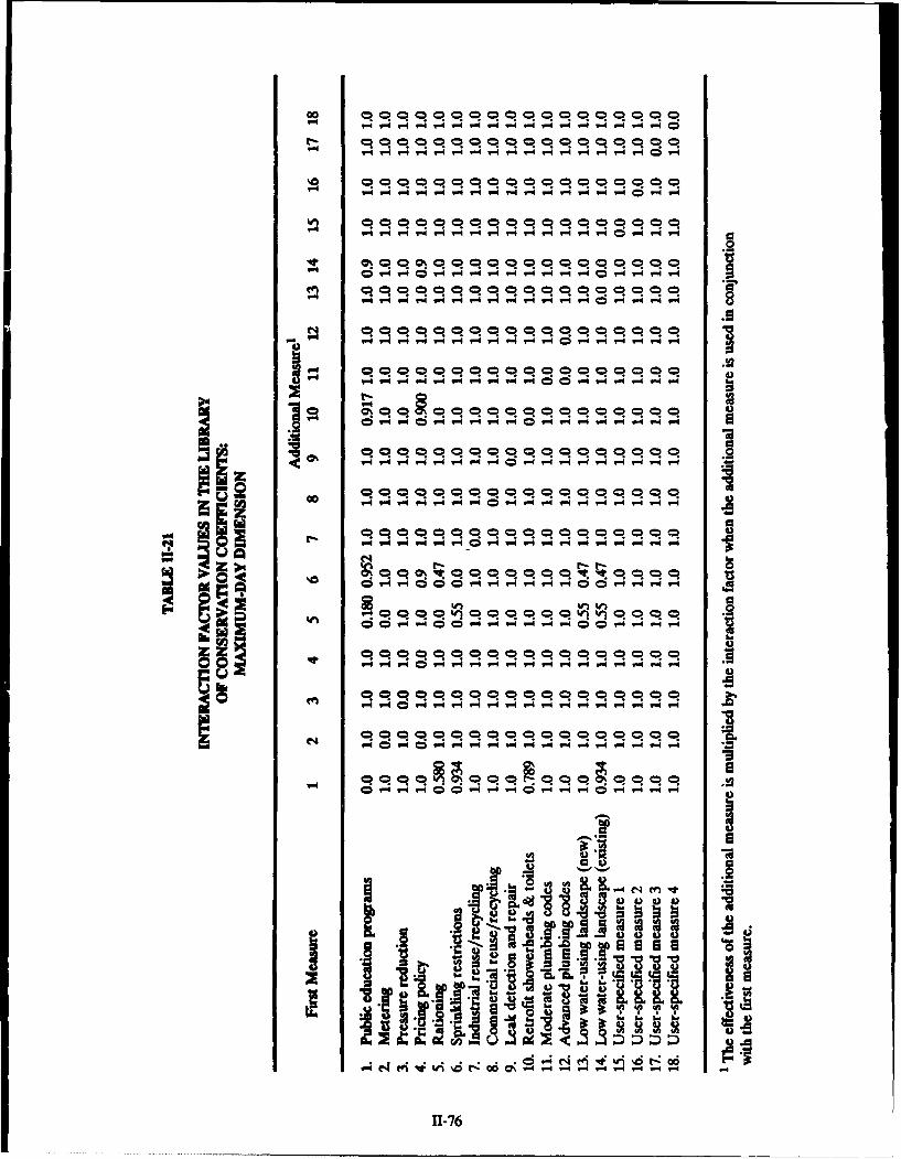
"-4"4o4q o -4 o- 94 o4 -4V- 94 4 -49- - "9- - - -- - - 4 4" 4V4T4V - = -
V- 4-4T4 Pooo O P4P4P- 94 4 -4P4"4 4 9-
'0- C? Cq q ? q ? C? C? q qq q
-4 V-4 W4 P- -4 9- 4 v-4 V-4 - a
4 - -4r-4v-4v- V- v- v- V4 V4 4V-4V0
v-4v-4 V4 W4 -4 4 4 14 " T4 V4 V4 4 o 1- P4 V4
;0 0 0 0000 q q q q q
z ;04 1 1
z zV- - 1 4 - 4 4W -
C? C?
.4
C6 0
- -7
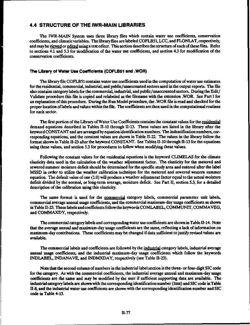
4.4 STRUCTURE OF THE IWR-MAIN LIBRARIES
The IWR-MAIN System uses three library files which contain water use coefficients, conservationcoefficients, and climatic variables. The library files are labeled COFLB51, LCC, and FLONLAT, respectively,and maybe viewed or edit using a text editor. This section describes the structure of each of these files. Referto sections 4.1 and 53 for modification of the water use coefficients, and section 4.3 for modification of theconservation coefficients.
The Ubrary of Water Use Coefficients (COFLB51 and .WOR)
The library file COFLB51 contains water use coefficients used in the computation of water use estimatesfor the residential, commercial, industrial, and public/unaccounted sectors used in the output reports. The filealso contains category labels for the commercial, industrial, and public/unaccounted sectors. During the Edit/Validate procedure this file is copied and relabeled as the filename with the extension WOR. See Part I foran explanation of this procedure. During the Run Model procedure, the .WOR file is read and checked for theproper location of labels and values within the file. The coefficients are then used in the computational routinesfor each sector.
The first portion of the Library of Water Use Coefficients contains the constant values for the residentialdemand equations described in Tables IH-10 through 11-13. These values are listed in the library after thekeyword CONSTANT and are arranged by equation identification numbers. The indentification numbers, cor-responding equations, and the constant values are shown in Table 11-22. The values in the library follow theformat shown in Table 11-23 after the keyword CONSTANT. See Tables 11-10 through 11-13 for the equationsusing these values, and section 5.3 for procedures to follow when modifying these values.
Following the constant values for the residential equations is the keyword CIMELAS for the climateelasticity data used in the calculation of the weather adjustment factor. The elasticity for the metered andsewered summer moisture deficit should be determined for the specific study area and entered after the labelMSSD in order to utilize the weather calibration technique for the metered and sewered western summerequation. The default value of one (1.0) will produce a weather adjustment factor equal to the actual moisturedeficit divided by the normal, or long-term average, moisture deficit. See Part 11, section 5.3, for a detaileddescription of the calibration using this elasticity.
The same format is used for the cmrial category labels, commercial parameter unit labels,commercial average annual usage coefficients, and the commercial maximum-day usage coefficients as shownin Table 11-23. These labels and coefficients follow the keywords COMLABEL, COMMUNIT, COMMAVEG,and COMMAXDY, respectively.
The commercial category labels and corresponding water use coefficients are shown in Table 11-14. Notethat the average annual and maximum-day usage coefficients are the same, reflecting a lack of information onmaximum-day contributions. These coefficients may be changed if data sufficient to justify revised values areavailable.
The commercial labels and coefficients are followed by the industrial category labels, industrial averageannual usage coefficients, and the industrial maximum-day usage coefficients which follow the keywordsINDLABEL, INDANAVE, and INDMXDAY, respectively (see Table 11-23).
Note that the second column of numbers in the industrial label section is the three- or four-digit SIC codefor the category. As with the commercial coefficients, the industrial average annual and maximum-day usagecoefficients are the same and may be modified by the user if sufficient supporting data are available. Theindustrial category labels are shown with the corresponding identification number (Ixxx) and SIC code in Table11-8, and the industrial water use coefficients are shown with the corresponding identification number and SICcode in Table 4-15.
11-77

The industrial labels and coefficients are followed by the commercial and industrial p eastiii. Thelabels CLAS and ILAS identify the commercial and industrial elasticities, respectively.
The nonresidential labels and coefficients are followed by the public nd unaccounte average annualwater usage coefficients, maximum-day usage coefficients, and category labels. These follow the keywordsPUBCOFAA, PUBCOFMD, and PUBLABEL, respectively, as shown in Table 11-23. The labels andcoefficients for the public and unaccounted sectors are shown in Table 11-16. Note that the library file ends withthe keyword ENDI.
Through the use of the Data Entry screens, the user may supply additional commercial, industrial, andpublic categories. The label, parameter unit, and water usage coefficient for each user-added category aremerged into the Library of Water Use Coefficients during the Edit/Validate procedure. These user-addedcategories appear in the .WOR file, never in the COFLB51 file. See the description of the Edit/Validateprocedure in Part I for additional explanation of this process.
The Ubrary of Consevation Coefficients (LCC)
The library file LCC contains coefficients used in the computation of the restricted water use estimates.This computation uses reduction factors, coverage factors, interaction factors, and nonresidential indoor/outdoor factors as explained in section 4.3. Reduction factors and coverage factors may be specified by the uservia the Data Entry screens for the conservation measures and corresponding water use sectors, which areselected by the user.
Reduction factors not specifiedby the user for selected measures and sectors are read from the LCC duringthe Run Model procedure. Similarly, if coverage factors for selected measures and sectors are not provided bythe user, values are read from the LCC which are used in conjunction with other parameters (e.g., housing units,employment) to calculate coverage factors for the specified measure and sector. These calculations areexplained in Table 11-1&
The values for the reduction factors are arranged in the LCC by measure, dimension, and sector as shownin Table 11-24. Note that the conservation measure names are abbreviated to five characters and appear in thesame sequence as they appear on screen 15.1. The water use dimensions of indoor, outdoor, and maximum-day use am abbreviated to I, 0, and MD, respectively. The sectors are abbreviated as follows:
(1) M1PL - municipal (this column is not utilized)(2) RMET1 -- residential, metered and sewered(3) BELAI - residential, flat and sewered, and flat and unsewered(4) RAPf - residential, apartment(5) COMM - commercial/institutional(6) - industrial(7) EUBL - public and other(8) UNACC - unaccounted
Note that the values for the "municipal" sector are =o used in the program. All nonzero values for reductionfactors are shown in Table 11-17.
Values used for the calculation of coverage factors appear in the LCC after the reduction factors. Thesevalues are arranged by measure, sector, and rates as shown in Table 11-24. The measures and sectors use thesame abbreviations as used with the reduction factors. Again, the values for the municipal sector are not utilized.The rates are abbreviated as INITL, ADOPT, ATTRN, and DEMOL for initial, adoption, attrition, anddemolition rates, respectively. The nonzero values and their use in the computation of coverage factors areshown in Table 11-18.
11-78

The values used in the computation of coverage factors are followed by three matrices of interactionfactors. There is a matrix of interaction factors for each of the water use dimensions: indoor, outdoor, andmaximum-day. Each matrix contains all possible pairings of conservation measures and a corresponding valueas shown in Table 1-24.
Note that the conservation measures are abbreviated to five characters as used for the reduction factorand coverage calculation values. The interaction factor value for a given pair of measures may be read as thepercent effectiveness of the &g measure expected when the first measure is used in conjunction with the secondmeasure. For example, EDUCNRATNG 0.580 indicates that only 58 percent of the effectiveness of a waterconservation educational program (EDUCN) is expected when a water-rationing program (RATNG) is alsoin effect. The values for the interaction factors are shown in Tables 1I-19 through 11-21 for the three dimensions,respectively.
Following the matrices of interaction factors are the nonresidential indoor/outdoor factors. These factorsare used in the conversion of commercial, industrial, and public water use into the indoor and outdoor wateruse dimensions in preparation for the application of the calculated adjustment factor for each sector anddimension. This process is described in section 4.3.
As previously described, the user may specify reduction and coverage factors with the Data Entry screens.These user-specified values are saved in the data file which is read during the Run Model procedure prior tothe reading of the LCC. Reduction and coverage calculation values will not be read from the LCC file for, asures and sectors for which the user has specified a reduction or coverage factor, respectively. Thus, it is
not necessary to modify the reduction or coverage calculation values in the LCC. However, there are W DataEntry screens corresponding with the interaction factors or the nonresidential indoor/outdoor factors. Thus,any changes in these values which the user wishes to make should be made in the LCC. Itis advised that if changesare to be made, the original LCC file be copied and renamed for archival purposes. The IWR-MAIN Systemwill read the file named LCC.
The Ubrary of Climatic Variabl (FLONLAT)
The library file FLONLAT contains long-term averages for rainfall (RAIN) and evapotranspiration(EVAP) for latitude and longitude coordinates in the continental United States. The FLONLAT file is readduring the Run Model procedure if values for RAIN and/or EVAP are not provided by the user on Data EntryScreen 1.1, and if the residzndial metered and sewered sector is selected on the Parameter Control Screen. Thedata within the library are arranged as follows:
EVAPTRANLATD 48. LONG 67. RAIN 9. EVAP 12.LATD 47. LONG 67 RAIN 8. EVAP 13.LATD 46. LONG 67. RAIN 7. EVAP 13.
The RAIN and EVAP variables are based on long-term weather data as of 1967 and may not representshifts in the long-term averages which have occurred in some parts of the country. However, updated long-termaverages for these variables may be specified on screen 1.1 for a given study area; thus modification of theFLONLAT file by the user is not necessary.
Il-79

TABLE 11-22
RESIDENTIAL EQUATION CONSTANTS
IN THE LIBRARY OF WATER USE COEFFICIENTS
EquationIdentifi- Equation Constant Constantcation Number Usage* Number Value
E011 1 Metered and sewered, winter 1 + 234.000E01.2 1 2 + 1.451E013 1 3 - 45.900E014 1 4 - 2.590
E021 2 Flat rate and sewered, winter, 1 + 28.900E022 2 and apartment, winter 2 + 1.576E023 2 3 + 33.600
E024 3 Apartment, summer 1 + 1.433
E041 4 Flat rate and unsewered, 1 + 30.200E042 4 winter 2 + 39.50
E051 5 Metered and sewered, 1 + 0.480E052 5 summer west 2 + 58.777E053 5 3 - 0.703E054 5 4 + 0.429
E061 6 Metered and sewered, 1 + 385.000E062 6 summer east 2 + 2.876E063 6 3 -285.800
E064 6 4 - 4.350E065 6 5 + 157.770
E071 7 Flat rate and sewered, 1 + 0.410E072 7 summer 2 + 44.573E073 7 3 + 0.783
E091 9 Flat rate and unsewered, 1 + 0.410E092 9 summer 2 + 445n3E093 9 3 + 0.783
E101 10 Irrigable land per dwelling unit; used 1 + 0.803E102 10 in metered and sewered, summer 2 1260
E111 11 Metered and sewered, 1 + 2,227-W4E112 11 maximum-day west 2 + 2.060E113 11 3 + 0.41M0
E121 12 Metered and sewered, 1 + 0.000046485EIZZ 12 maxmum-day east 2 + 0.118Elm3 12 3 - 10.400E12A 12 4 - 1250E125 12 5 + 0.931
11-80

TABLE 11-22 (Continued)
EquationIdentifi- Equation Constant Constantcation Number Usage* Number Value
E131 13 Flat rate and sewered, 1 + 1,609.590E132 13 maximum-day 2 + 0.943E133 13 3 + 0.523
E151 15 Flat rate and unsewered, I + 1,609590E152 15 maximum-day 2 + 0.943E153 15 3 + 0.23
*See Tables 11-10 through 11-13 for corresponding equations.
11-81

TABLE 11-23
FORMAT OF THE LIBRARY OF WATER USE COEFFICIENTS
CONSTANTE011 234.0 E012 1.451 E013 -45.9E014 -2.59 E021 28.9 E022 1.576E023 33.6 E041 30.2 E042 39.5
ENDDCLIMEIAS (El ASTICITIES FOR WEATHER ADJUSTMENT FACTORS)MSSD 1.0ENDDCOOMLABELC001 MIS. COMMERCIAL C002 VOC. SCHOOLS C003 MISC. RETAILC004 BOARDING HOUSES C005 TRANSP. TERMINAL C006 BARBER, CLEANING
ENDDCOMMUNITC001 EMPLOYEES C002 EMPLOYEES 0)03 EMPLOYEESC004 EMPLOYEES C005 EMPLOYEES - C006 EMPLOYEES
ENDDCOMMAVEG EXPECTED USAGE VALUESC001 47.2 C002 72.0 C003 19.3C004 101.6 C005 86.2 C006 380.2
ENDDCOMMAXDY EXPECTED USAGE VALUESC)01 47.2 C002 72.0 C003 19.3C004 101.6 C005 86.2 C006 380.2
ENDD
INDLABEL1001 201 MEAT PRODUCTS 1001 2011 MEAT PACKING PLANTS1003 2013 SAUSAGES, ETC. 1004 2016 POULTRY DRESSING1005 2017 POULTRY & EGG DRSG 1006 202 DAIRY PRODUCTS
ENDD
11-82

TABLE 11-23 (Continued)
INDANAVE1001 343.8 1002 258.6 1003 488.11004 409.1 1005 201.1 1006 354.4
ENDDINDMXDAY1001 343.8 1002 258.6 1003 488.11004 409.1 1005 201.1 1006 354.4
ENDDELASTCTY (COMMERCIAL AND INDUSTRIAL PRICE ELASTICITY)CLAS -0.80 ILAS -0.65ENDDPUBCOFAALOSS 14.9 FSER 5.2 FLSS 0.15ENDPUBCOFMDLOSS 14.9 FSER 52 FLSS 0.15ENDDPUBLABELLOSS LOSS (PER CAP.) FSER FREE SERVICE FLSS LOSS (PERCENT)ENDDENDI
11-83

TABLE 11-24
FORMAT OF THE LIBRARY OF CONSERVATION COEFFICIENTS
REDUCTION FACTORSMEASURE MUNPL RMETR RFLAT RAPMT COMM IND PUBL UNACC
EDUCN-I 0.089 0.089 0.089 0.089 0.089 0.089 0.089 0.0EDUCN-O 0.089 0.089 0.089 0.089 0.089 0.089 0.089 0.0EDUCN-MD 0.089 0.089 0.089 0.089 0.089 0.089 0.089 0.0
COVERAGE FACTORSMEASURE IN1TL ADOPT ATrRN DEMOL
EDUCNMUNPL 0.750 0.0 0.0 0.0EDUCNRMETR 0.750 0.0 0.0 0.0EDUCNRFLAT 0.750 0.0 0.0 0.0EDUCNRAPMT 0.750 0.0 0.0 0.0EDUCNCOMM 0.750 0.0 0.0 0.0EDUCNIND 0.750 0.0 0.0 0.0EDUCNPUBL 0.750 0.0 0.0 0.0EDUCNUNACC 0.750 0.0 0.0 0.0
INTERACTION FACTOR MATRIX (IFACT)INDOOREDUCNEDUCN 0.000 EDUCNMETER 1.000 EDUCNPRESS 1.000 EDUCNPRICE 1.000EDUCNRATNG 0.S80 EDUCNSPRNG 0.000 EDUCNINDRR 1.000 EDUCNCOMRR 1.000EDUCNLEAKR 1.000 EDUCNRETRO 0.789 EDUCNCODEM 1.000 EDUCNCODEA 1.000EDUCNLWULN 0.000 EDUCNLWULR 0.000 EDUCNMSEO1 1.000 EDUCNMSE02 1.000EDUCNMSE03 1.000 EDUCNMSE04 1.000
NONRESIDENTIAL INDOOR/OUTDOOR FACTORSCOMMERCIAL 0.800INDUSTRIAL 0.800PUBLIC 0.800
11-84

5. MODEL VERIFICATION AND CALIBRATION
5.1 PURPOSE OF VERIFICATION AND CALIBRATION
Verification and calibration of the IWR-MAIN System are usually undertaken to verify and/or improvethe accuracy of water use equations in reproducing the actual water use by various sectors of the municipal systemunder study. The precision with which IWR-MAIN estimates water use can be tested by preparing a forecastof water use for one or more historical years. A comparison of IWR-MAIN estimates with actual records ofwater use may reveal discrepancies which need to be analyzed and corrected prior to performing the forecasts.
In most recent applications of IWR-MAIN, the calibration forecasts were typically prepared for the baseyear of 1980 and one forecast year of 1985. The availability and quality of socioeconomic data and the valuesof other determinants of water use for these two years are good, since they represent, respectively, the year ofthe Census and the year of Census estimates.
Reasons for Forecast Discrepancies
There areseveral reasons why the unadjusted estimates of water use produced byIWR-MAIN may divergefrom observed values. These are:
(1) The icd for the forecast year (and/or base year) may be in error. A substantialmargin of error can be expected even in the Census data for the Census year, with a larger errorassociated witi ; itermediate years. In addition, geographical areas served by water utilities rarelycoincide with political subdivisions or Census tracts for which socioeconomic data are collected.This may lead to imprecise estimates of population, housing units, employment, and other datawhich correspond to the water service area.
(2) Waer use rord may include a substantial error especially when a large number of individualaccounts are aggregated by computer to arrive at total water sales, or when meter-reading cyclesdo not coincide with calendar dates. When water production records are used in the comparison,the potential for error is usually smaller, although problems with uncalibrated master-meters atwater treatment plants have been experienced by some systems.
(3) There are disenancies in itions of water users and water use dimensions between IWR-MAIN and utility records. For example, winter use is defined by IWR-MAIN as domestic (orindoor use) in an average day. Many utilities define winter use as average daily use during wintermonths (e.g., November to April or December to February).
(4) IWR-MAIN estimates water use for average weather conditions; therefore, it is necessary to makeweather adjustments while attempting to reproduce water use in a particular calendar year. Forexample, the year 1980 can be extrcmely wet and cool (i.e., with low summer moisture deficit),indicating low water use, while 1985 may be dry and hot, indicating higher water requirements.
(5) The residential water demand equations have been developed based on prevailing patterns ofwater use during the mid-1960s. Few communities practiced water conservation at that time, andthe unrestricted IWR-MAIN results do not account for the effects of conservation measures.These effects have to be estimated based on documented water savings and market penetrationof each measure for each calibration year and subtracted from the unrestricted demand forecastbefore the IWR-MAIN estimates can be ,ompared with actual records.
(6) In some areas of the country, homeowners plant winter grass and practice wne jgagion. Sucha practice was not common in the mid-1960s when the original IWR-MAIN equations were
11-85

developed. The IWR-MAIN seasonal use equations have to be modified for such areas to reflectthe winter irrigation use.
(7) The relationships between water use and its determinants may not be applicable to a given localityor may have changed since the mid- 1960s. Eaici of price, income (i.e., home value), moisturedeficit, and the number of people per residence may be inappropriate for some locations. Thesehave to be verified if the prediction error is substantial.
(8) Water use for nonresidential sectors is estimated by IWR-MAIN based on unit use coefficients(daily use per employee or other parameter unit) derived from nationwide data. These coefficientsmay not reflect local rates of water use and have to be adjusted using local information.
(9) The values ofresidential homes in some areas of the countryinclude a substantial location premimwhich has little bearing on water use, except for measuring the ability of the residents to pay forwater. If home value is taken to represent the stock of water-using fixtures, appliances, andarchitectural features of the residential landscape, then a four-bedroom single-family house witha replacement value of $75,000 is expected to have similar capital water-using stock regardless ofits location. The presence of a substantial location premium will bias the estimates of water use.
Some of these factors can be incorporated into IWR-MAIN forecasts on an a 9_& ri basis (e.g., actualweather conditions, water conservation, winter irrigation, and adjustment of home values may be performedprior to generating the forecast estimates), while other factors such as elasticities of water use determinants haveto be tested and adjusted, if necessary, based on relationships observed in the study area. The following sectionsdescribe the data required and the procedures that may be used to verify and calibrate the IWR-MAIN modelto the conditions of a particular study area.
5.2 VERIFICATION DATA
Water Use Records
Ideally, the data for verifying the IWR-MAIN estimates of water use derived from socioeconomic datadescribing a service area during calibration years should be comprised of detailed records of water use by alluser sectors and all use dimensions selected in the preparation of an IWR-MAIN forecast. However, in mostapplications, the availability of water use records will be limited. Some larger utilities will maintain monthlywater use records for several aggregate categories of users such as single-family residential units, smallcommercial users, large industrial users, and others. However, many utilities will not generate and maintainwater use statistics by user sectors. Thus, only aggregate monthly sales may be available. Finally, if watercustomers are not individually metered, the verification has to be limited to the use of aggregate productionrecords, although again there are few utilities in the country which do not have meters at water treatment plants.In such extreme situations verification and calibration of the IWR-MAIN model are not possible except for arough comparison of IWR-MAIN estimates with estimated water withdrawals from supply sources.
Typically, water utilities will maintain computer records of monthly water consumption for all individualcustomers. The length of record may be 12 months (or 12 billing periods) or more with earlier records storedon computer tapes or microfiche. Each customer's file may contain account number, name, address, meter size,meter readings and dates, consumption (or water use), and amount billed. If individual customer files containcodes identifying the type of customer, then a computer program may be prepared to produce summaries bycustomer type.
Without the identification of customer types, an approximate separation of users by residential andnonresidential categories can be performed based on the connection size with a manual classification of thelargest users. Alternately, a random sample of customer accounts maybe taken in order to obtain the percentageof total water use and average customer use for each major user sector (i.e., residential, commercial, industrial,public, and others).
11-86

Supplemental Data
In addition to water use records, verification of IWR-MAIN requires the following types of information:
(1) Prevailing weather conditions (temperature and precipitation) during calibration years(2) Water and sewer rates in effect prior to and during the calibration years(3) Water use and employment in selected commercial establishments and manufacturing plants
served by the utility(4) Information on past and current water conservation programs (i.e., the estimated water savings
and market penetration of conservation measures)
Additional data may be required in cases where the discrepancies between IWR-MAIN estimates andactual water use records warrant additional adjustments in the predictive equations or estimating proceduresof IWR-MAIN.
5.3 VERIFICATION AND CALIBRATION PROCEDURE
The process of the verification and calibration of IWR-MAIN is comprised of four major steps. Theseare given below.
Step 1 - Initial Forecast Run
As a basis for verification and initial adjustmonts, a forecast for a base year and one or more projectionyears should be prepared with all default parameters of IWR-MAIN. Since IWR-MAIN is designed for long-term forecasting, it would be most appropriate to use as an example the year 1970 as the base year and 1975,1980, and 1985 as forecast years. A complete set of socioeconomic data (Le., population, housing, employment,and income) should be assembled for each year and entered as an input file. The results of the forecast shouldbe compared with actual water use records in order to obtain a crude assessment of the accuracy of IWR-MAIN.The results will reveal the particular sectors of water use that may need to be further investigated. However,the discrepancies between forecast results and actual water use records may not be representative of the forecasterror, since this initial run does not incorporate a number of factors that will affect water use estimates (e.g.,actual weather, price levels, conservation programs, and others).
Step 2 - A Priori Adjustments Run
In this step, a set of adjustments to IWR-MAIN is performed on the basis of prior knowledge of differencesbetween the implicit assumptions of the model and actual conditions of the forecast. There are four types ofadjustments that are made on the basis of prior knowledge. These are discussed below.
_ubstep 1. Weather Adiustments
In order to compare water use records with IWR-MAIN estimates, sprinkling and summer demand equa-tions must be adjusted to reflect actual weather conditions. Only the equations for the metered and seweredresidential subgroup utilize weather variables. The eastern and western equations for this subgroup are handleddifferently, as shown below. A procedure is also described which may be applied to the summer water useequations for the other residential subgroups. The two equations from Table II-10 for summer (seasonal plusdomestic) demand in metered and sewered residential houses are:
(OXme - 385.0 + 2.876V- 285.8P&- 4.35I s + 155.77 (B*MD) (1)
11-87

and
(s)asw (2 * 0.48 * 58.TTPs-0"? 3 * V 0429) * WF + (Qd)MN (2)
where
(Q)MS. and (Qd)., represent metered and sewered summer water use in eastern and western areas ofthe country, respectively, in gallons per unit per day
and
Ps = summer price of water (including sewer charges if applicable)V = market value of the residence in 1980 dollars
- summer bill difference, in 1980 dollarsB - irrigated lot area in acresMD = summer moisture deficit (during June, July, and August)WF = weather adjustment factor0 d - domestic (indoor) water use in gallons per unit per day
The value of B is calculated as:
B = 0.803 HD S1 2 6 (3)
where
HDES = housing density in housing units per acre
and the value of WF is calculated as:
wr = (MD. /MD)md
where
MDwmw = actual summer moisture deficit for a specific calibration yearmd = elasticity of water use with respect to moisture deficit
In order to account for the influence of weather in the base year or a forecast year for the eastern U.S.,the MD variable in equation (1) should reflect the ac1 weather conditions in the year of verification. Notethat the demarcation of east and west by IWR-MAIN is 100 degrees longitude. Actual summer evapotranspi-ration and precipitation can be entered in the data input screen 1.1. If actual weather factors are not used, MDin equation (1) is represented by the normal moisture deficit as calculated from normal values or those readfrom the IWR-MAIN LAbrary of Climatic Variables.
For western areas, the summer demand equation (2) consists of a summer sprinkling term plus thedomestic water use. To account for the influence of weather in the base year or a forecast year, the sprinklingterm is adjusted by the weather adjustment factor (WF) which is a ratio of the actual to normal summer moisturedeficits. (Future years assume normal weather, thus the weather adjustment factor would have a value of one(1).)
In the present version of IWR-MAIN, only one set of weather parameters can be used during the run ofthe model. To generate weather-adjusted estimates for the base year and forecast years, the actual weather datamust be changed and model runs must be performed for eah year. Once the final verification runs have beencompleted (see Step 3), the actual weather data should be deleted before generating forecasts. Forecast runsshould assume normal weather conditions.
11-88

The elasticity for the weather adjustment factor is read from the Library of Water Use Coefficients andmaybe revised by the user to reflect the elasticity of metered and sewered summer water use to moisture deficit.The default value of 1.0 results in a weather adjustment factor equal to the ratio of the actual and normal moisturedeficits.
To introduce the weather adjustment factor into the equations for flat-rate and sewered or flat-rate andunsewered water use, the weather adjustment factor is multiplied by the intercept of the sprinkling term (0.41),and the product replaces the value of the intercept in the Library of Water Use Coefficients. See section 4.4for a description of the library format and Table 11-22 for the identification code (E071 and E091) of theseintercepts. This same procedure may be used to account for the influence of weather in apartment summer useby multiplying the sprinkling multiplier (1.433) by the weather adjustment factor and replacing the multipliervalue (E024) in the library with the product. These adjusted intercep will have to be changed in the libraryfor the base year and lad forecast year used for verification, and corresponding model runs must be performedeach time.
SubsteO 2. Adluatments for Winter Irrigation
In some urban areas of the country located in the South (Florida) and Southwest (Texas, New Mexico,Arizona, Nevada, California), residential lawns are overseeded with winter grass and irrigated during wintermonths. The IWR-MAIN System equations for winter water use are designed to measure only indoor wateruse. Sprinkling demand and other outdoor uses are accounted for in summer equations; however, the originaldemand models were estimated based on data collected during the early 1960s when winter irrigation was notpracticed extensively.
Prior to making adjustments for winter irrigation in residential equations, it is necessary to investigate theg j distribution of annual water use to determine the portion of irrigation water use which occurs during
winter months. As a rule of thumb, in cities where winter irrigation is practiced, the irrigation requirementsmay constitute 10 to 20 percent of annual outdoor use. The estimates of water use in summer should be increasedby this percentage to account for winter irrigation. For western areas, the intercept of the sprinkling term (seedescription above) can be divided by the percent of summer outdoor use. IWR-MAIN estimates of winter wateruse will be Iwer than actual water use records, given that the winter equations only represent indoor (domestic)use.
SubsteD 3. Adlustment for Existing Conservation
Since the 1975-76 California drought, many municipalities in California and other states have adoptedlong-term (or nonemergency) conservation programs. These programs often include educational campaigns,revised plumbing codes for new construction, leak detection and repair, conservation-oriented rate reforms, andother activities. The existence of these programs is reflected in the observed levels of water use. Therefore,the IWR-MAIN estimates must be adjusted for the effectiveness of all conservation measures that have beenimplemented. In practice, the comparisons should be made between water use records and the restricted useestimates of IWR .MAIN. Reduction factor and coverage factor coefficients should be obtained for eachmeasure. If there are no data available on these parameters, IWR-MAIN library values could be used, althoughthe local estimates are dearly preferred for calibration runs.
SubsteO 4. Adlustment of Nonresidential Water Use Rates
The initial forecast run (Step 1) will reveal the need to verify the IWR-MAIN default coefficients for peremployee water use in various commercial and manufacturing categories. Per employee use rates should beverified for the largest utility customers by dividing their average annual water use by the number of employees.Ideally, a sample of nonresidential customers (including the largest users) should be taken with a size sufficientto verify all per employee coefficients used in the forecast. Due to difficulties involved in obtaining employment
11-89

data, a point will be reached where obtaining additional observations on water use and employment can nolonger be justified. The coefficients most critical for the forecast are those representing commercial andmanufacturing categories which have bidgb. ent or show high projected growth of employment and thosewhich are -lara-guMnx users.
If the default coefficients in the library are replaced with revised coefficients and if the nonresidential pricedifference adjustments are used, it may be necessary to revise the commercial or industrial average price in theyear concurrent with the water use coefficients in the input data (screen 7.7).
Step 3 - Detailed VwIfication Run
Upon completion of the a priori adjustments in Step 2, the IWR-MAIN runs should be performed. Theresulting estimates of water use for the base year and all calibration years should be compared with actual valuesto determine whether the IWR-MAIN water use models need to be adjusted. The computational equations forthe residential subgroups may require calibration if the estimates of water use obtained with IWR-MAIN differfrom actual use by more than 2 to 3 percent. The type of adjustments that will be required will depend on thepattern of prediction errors. At -least two distinct patterns may be present.
(1) The IWR-MAIN estimates exhibit a systematic error of overpredicting (or underpredicting) actualwater use in all calibration years (including the base year) where the percent error is approximatelythe same for all years. This pattern of prediction error indicates that water use in the study areais characterized by a higher (or lower) base use than that observed in the data which were usedto derive the IWR-MAIN demand models.
(2) The IWR-MAIN estimates do not exhibit a systematic error, that is, water use is underestimatedin some years and overestimated in others. This type of error indicates that the slopes (orelasticities) of basic determinants of water use in demand equations are in error. Thesedeterminants include combinations of variables including price, income, moisture deficit, andpopulation density per residence.
In the case of the first type of error, the calibration procedure involves adjusting the intercepts ofappropriate demand models to fit the observed water use. The calculation of the adjusted intercepts in lineardemand models is illustrated in the following example:
Actual indoor (winter) use 10365 MGDIWR-MAIN estimate 12.209 MGDNumber of metered and sewered housing units 41,561 unitsOriginal IWR-MAIN intercept 234 gallons per
unit per dayRequired adjustment:
(10.365- 12.209)(106)/41,561 = -44.4 gallons per unit per day
New intercept 234 - 44.4 = 189.6 gallons per unit per day
In multiplicative models such as those used for estimating summer use in western areas of the country, theintercepts are adjusted by a constant multiplier derived by comparing actual and predicted water use, asillustrated in the following example:
Actual indoor (winter) use 10365 MGDActual indoor and outdoor (summer) use 26.653 MGDIWR-MAIN estimate of summer use 29.250 MGDOriginal IWR-MAIN sprinkling intercept 0.480
11-90

Required adjustment (assuming prior adjustment of the intercept in win equation):
(26.653 - 10/365)/(2920 - 10.365) = 0.86
New intercept 0.48 x 0.86 = 0.410
In the case of the second type of error, the intercepts may be adjusted to achieve an improved fit of themodel to actual water use for all calibration years; however, at some point this adjustment procedure will leadto reduced errors in some years at the expense of increased errors in others. To bring the IWR-MAIN estimatescloser to actual values, it will be necessary to modify the coefficients of individual independent variables in thedemand models. The variableswhich are likely to have inappropriate coefficients include price and income. Theerror in IWR-MAIN estimates providesvery limitedpossibilities for verifying elasticities of these variables, sinceonly their combined effect can be observed. A preferred procedure in such cases is to reestimate the demandmodels in question using 20 to 30 data points on annual (or seasonal) water use in the study area. Although time-series data are preferred, cross-sectional or pooled data sets can be generated if there is more than one utility.
In many previous applications of IWR-MAIN, the water demand models performed relatively well, andthere was no need to reestimate the coefficients of price, income, and population density. The elasticity of themoisture deficit was usually verified based on a small sample of water use records. Elasticities of price, income,and population density seem to show little variation within each of the two climatic zones of the country: aridwest and humid east.
Step 4 - Verfication of Growth Models
In IWR-MAIN applications which rely on internal growth models, separate runs can be performed inorder to verify the econometric equations which allocate total housing units and employment to various forecastcategories based on income, population, and other economicgrowth factors. Internally projected values for pastyears may be compared to actual data from the study area while values projected for future years may becompared to any existing projections for the area. Direct external projections supplied by the user replaceparameters generated by the growth models. Thus, total housing units, housing units for a given subgroup andmarket value group, employment for a given commercial category, and/or employment for a given industrialcategory may be specified for each forecast year. (See the description of screen 14.1 in Part I and the discussionof the external projections in Part II, section 4.2.) If data for these parameters are available, the externalprojection can be entered for the forecast years. Note that external projections for one forecast year have noimpact on projections generated by the growth models for other forecast years. Additional runs maybe executedto observe the impact of the external projections on the redistribution of values generated by the internal growthmodels.
Similarly, historical data for the study area may be entered into the program, runs made, and the impactof the historical trends on the projections can be compared to existing projections. In this manner, a projectionmethod or combination of methods may be selected which generates a set of projected values most appropriatefor the given study area.
11-91

APPENDIX A
COMPREHENSIVE EXAMPL4; F USINGTHE IWR-MAIN SW-
Exhibit A-i: Input Screens
Exhibit A-2. Revised Coefficient Library (.WOR) File
Exhibit A-3: Output Reports
Exhibit A-4: Conservation Output (.COV) File

COMPREHENSIVE EXAMPLE OF USING THE IWR-MAIN SYSTEM
For illustrative purposes, a comprehensive example using the IWR-MAIN System was performed usingempirical data from a southwestern U.S. city. Unlike TESTCrTY, this example is a complete and actual forecastusing the best available data and information for the study area. The water use estimation was completed forthe base year (1980) and two forecast years (1990 and 2000).
STUDY AREA
Aridwest is a large southwestern city with a 1980 population of 425,259. This population represents over88 percent of the total county population. Aridwest's steady growth is projected to continue. The city has asubstantial industrial base with over 35,800 employed in manufacturing for the year 1980.
The study area experiences typical southwestern climatic conditions. Mean summer temperatures rangefrom 80 to 83 degrees Fahrenheit. The mean annual precipitation is about eight inches. Mean wintertemperatures rarely fall below 45 degrees Fahrenheit.
SOCIOECONOMIC INPUT DATA
General Municipal Data
The required base year population and total employment for the study area were obtained from U.S.Census Reports. The median household income for the base year was provided by local city data sources. Totalsummer season (June-August) precipitation and summer potential evipotranspiration were calculated forAridwest using monthly temperature and rainfall data provided by the National Oceanic and AtmosphericAdministration (NOAA). Projections for the years 1990 and 2000 of population, household income, and totalemployment were supplied by the city planning department.
Residential Data
Housing Stock Data
The housing stock data provided by the city were classified into three housing types in order to facilitatea more accurate estimation of water use. Each housing type represents a major subgroup in the IWR-MAINSystem and is described below.
(1) The metered and sewered housing subgroup includes single-family residential units that areindividually metered and are served by a sewer system. These housing units are considered owner-occupied or occupied by renters who are responsible for paying the water bill. All single-familysubgroups were grouped into the metered and sewered category. The number of "other"(nonsewer) single-family units was relatively small and was thus included in the metered andsewered category.
(2) The flat rate and sewered category includes housing units contained in buildings with two or threeunits per structure and mobile home parks. It is assumed these units are served by a single meter
A-1

and that where renter-occupied, the owner is responsible for payingthe water bill Such customers,therefore, face a zero marginal price and are not expected to react to price. All sewered mobilehomes and two-family units were aggregated as flat rate and sewered.
(3) The aparmrnent category refers to housing units which face a zero marginal price of water and havelittle opportunity to engage in outdoor (seasonal) water uses. This includes master-meteredapartments, represented by housing units contained in structures with three or more units. It isassumed that all these units are provided with sewer services.
The market value of a residence is used by IWR-MAIN as one of the major determinants of water use.The reported home values for single-family residences are available from census reports. For multifamilydwellings, the contract rent of a renter-occupied unit was converted to equivalent home values using thefollowing formula-
(1 + i)N- 1F(1)
i(1 + i)N
where
F = a series present worth discounting factori = typical 1980 mortage rate in Aridwest = 1.167 percent per month (14.00 percent per year)N = 360 months
The product of the monthly rent and the conversion factor, F, is the estimated home value in 1980 dollars.
Suolemental Data for Housing Subarouoe
In addition to the distribution of housing units by home value ranges, each subgroup requires supplemen-tal data that are used in the computation of water use estimates. Used onlyin the metered and sewered category,the price variables (marginal price and bill difference) were calculated by applying the 1980 Aridwest WaterUtility (AWU) water and sewer price schedules to average monthly usage per single-family account. Themarginal price of water/sewer is the price paid for the last unit of water consumed. The bill difference variablecaptures the effects of changes in consumers' residual income caused by increased or decreased water bills asa result of changes in rate designs and is calculated as the difference between the actual total water bill and theproduct of the quantity consumed and the effective marginal price.
The price estimates were initially assumed to be constant across all housing value ranges. Usingpreliminary IWR-MAIN output reports, the appropriate price blocks for each value range in the subgroups weredetermined by calculating average usage per account in the winter season and average usage per account in thesummer season. This procedure indicated that water use in higher value homes shifted the average user intothe second price block. Whenever the marginal price variables indicated a shift to the second block, thecorresponding bill difference variables were also adjusted.
The number of persons per household is a water use parameter in the flat rate and sewered and theapartment categories. This information was obtained for owner- and renter-occupied housing units by valuerange in the Aridwest Standard Metropolitan Statistical Area (SMSA).
Projections of total housing units and housing units by type were provided by the city planning department.
A-2

Commercial and Industrial Data
Base Year
The commercial/institutional employment data for the base year were obtained from the U.S. CensusReport. This employment was then disaggregated into 23 IWR-MAIN commercial/institutional categories,each representing a combination of Standard Industrial Classification (SIC) codes (see Part 11, Table 11-6).
Base year employment data for manufacturing (industrial) were also provided by the U.S. Census. Thesedata were distributed by SIC codes and assigned to a possible 198 IWR-MAIN industrial categories (see PartII, Table H-8).
Prolectons
Sector employment projections (Le., manufacturing, construction, services, government) for the years1990 and 2000 were obtained and entered directly into IWR-MAIN. Distribution of sector employment intocommercial and industrial categories is performed by the internal growth models of IWR-MAIN. Externalprojections for six industrial categories served as upper bounds for the growth models. These externalprojections were based on a water resources report for the state in which Aridwest is located. The report statesthat 90 percent of industrial water use at the state level is attributed to four industries in SIC groups 20,26,28,and 33. Growth rates provided by the report were applied to the actual 1980 Aridwest industrial employment.
Public/Unaccounted Data
Historical water production and usage data from the Aridwest Water Utility (AWU) indicate an averageannual loss of 11 percent of the total metered use.
CONSERVATION INPUT DATA
Aridwest is very active in water conservation and in 1980 had four major conservation programs which werealready reducing water usage in the AWU service area. These conservation measures include amendment ofplumbing codes, promotion of desert landscaping, water conservation educational programs, and leak detectionand repair. It is anticipated that these existing water conservation measures will continue to reduce water usage.The following is a brief description of each measure and an example of how reduction factors were calculatedfor these measures.
Plumbing Code
Amendments to the city plumbing codes in 1977 required that all new and replacement toilets be designedto use no more than four gallons of water for a flush cycle. Furthermore, all new and replacement showers wereto be equipped with a flow control device that limits water flow from the head to a maximum three gallons perminute at 50 pounds per square inch pressure.
The fraction reduction of water use (R) is calculated as:
R = (Sd/Qi) (2)
A-3

where
R = fraction of average daily residential useSd = water savings resulting from installation of a conserving device, gallons per person per dayQin = average indoor water use, gallons per person per day
Expected water savings from installation of water-conserving toilets and low-flow showerheads arereported as 13.0 gallons per person per day for single-family residences and 16.3 gallons per person per day formultifamily residences. The reduction factor for the plumbing code is calculated based on equation (2) as:
RP- r,=ngiy = (13.0/164) = 0.079Rduplex = (16.3/107) = 0.152Rapartment = (163/107) - 0.152
The fraction of average daily (annual) consumption that would be affected by the enforcement of therevised plumbing code is the number of new homes that would comply with the code, less 5 percent for exemp-tions of the special-purpose showerheads specified in the plumbing code, plus the number of remodeled unitscomplying with the codes. Assuming that the number of remodeled units equals 5 percent of the number of newunits, the coverage factor can be determined as the ratio of new units to total units.
D~ Landsaping
In 1971 a landscaping program was adopted by the utility to promote desert landscaping through an annualcontest. The fraction reduction of water use resulting from the conversion of turf area to low water-using aridlandscape is calculated as:
R = (a) (b) (c) (d) (3)
where
R = fraction reduction of average daily residential usea = percent area converted to desert landscapeb = percent reduction in the water application ratec = percent irrigation of outdoor used percent outdoor use of annual use
The portion of turf area converted to desert landscaping is assumed at 30 percent. The percent reductionin irrigation use as a result of converting to low water-using plants is calculated from the difference in applicationrates. The water use ranges of plants in desert climates are:
Low water-requiring plants 10-20 inches per yearMedium water-requiring plants 20-35 inches per yearHigh water-requiring plants 35-50 inches per year
See Water Conservation for Domestic Users. with Special Reference to Warm Desert Climates a handbookprepared by the University of Arizona for the city of Tucson, 1977. The average application rate for turf areasis estimated to be 42 inches per year, the midpoint of the high water-use range, while the application rate fordesert landscaping is estimated to be 20 inches per year. Thus, the reduction in irrigation use is approximately50 percent. The portion of outdoor water usage attributed to irrigation is assumed at 80 percent of outdoor wateruse.
The fraction reduction of residential water use for single-family, duplex-triplex, and apartments iscalculated as:
A-4

RSF -=3) .0 (.80) (.43) -0O.052RD.T - (.30) (.50) (.80) (27) = 0.032RAp = (30) (.50) (.80) (.19) - 0.023
The coverage of the voluntary desert landscaping program was reported as being 18 percent of single-family residences in 1985 with an expected increase of 1 percent of all housing units per year. Given that theprogram began in 1971, coverage for 1980 was extrapolated to 11.6 percent of 1980 single-family housing.
Education Programs
Water conservation education programs pursued by AWU include the "stuffers," or literature enclosedwith water bills, distribution of the booklet Water 'omservationin Yor Home, an outreach program of lecturesand films presented to schools and civic groups, and an outreach specialist who provides written material to localnewspapers.
Reduction factt ses for school educational programs vary from .035 to .05 in California and vary nationwidefrom .023 to .092. A reduction value of 0.035 was assumed as representative of the educational programsconductedby AWU. The coverage factor is assumed as 0.95 percent due to the high intensity of the educationalcampaign. The residential water use is assumed as the major sector targeted by the education programs.
Leek Detection and Repair
Since 1966, AWU has operated a leak detection and repair program in which six to eight miles of pipelinehave been either repaired or replaced every year. The effect of this program has been a reduction of water lossesto approximately 10 percent of total production or 11 percent of metered use. Continuation of this programis expected to further reduce water losses. It is assumed that if the current program is maintained at the currentlevel for the next 15 years, the percent of water unaccounted for will decrease from the current 11 percent ofmetered use to 9 percent in 1990, 8 percent in 1995, and remain at the 8 percent level thereafter.
VERIFICATION AND CAUBRATION PROCEDURES
Verification and calibration of the 1WR-MAIN System are usually undertaken to verify and/or improvethe accuracy of water use equations in reproducing the actual water Lsebyvarious sectors of tbe municipal systemunder study. Typically, the procedure is conducted in two steps. First, the coefficients of computationalequations and the national water use coefficients contained in the system's library are verified using theinformation on local conditions. Second, the coefficients of relevant independent variables of computationalequations maybe further tested by preparing a short-term forecast for a year with known actual water use. Aftertesting, the revised coefficients are entered in the library and are used in estimating water use in future years.
The most recent year for which all socioeconomic and other determinants of water use are available is 1980,the year of the last available US. Census of Population and Housing. The 1980 Census data, the Aridwest 1985socioeconomic projections, and NOAA weather data were used to prepare preliminary water use forecasts for1980 and 1985. The procedures used in verifying and calibrating the IWR-MAIN System are discussed below.
Adjustments of Residential Demand Models
The demand equations for each residential subgroup are presented below with a discussion of theverification and calibration of the individual predictive equations.
A-5

Motred and Sewered Models
The winter (or indoor) demand for water by metered residences is estimated by IWR-MAIN using thefollowing equation:
(Qd)ms = 234.0 + 1.451V - 45.9Pa -25.91 (4)
where
(Qd)mw = water use in gallons per dwelling unit per dayV = home value in $1,000P. = marginal price of water (including sewer charges) in winter in dollars per 1,000 gallonsI = effective bill difference variable during the winter in season dollars
The price elasticity of water demand at the mean values of price and water use in the above equation is -0.20when the effects of disposable income that are captured by the bill difference are ignored and -0.06 when sucheffects are taken into account. The elasticity of home value (a proxy for income) is 022.
The equation for summer demand used by IWR-MAIN is:
(Q) = (0.48 "58.77 * p -0."W * vo.429) * (MDi/MD)e *2.0 + (Qd)w (5)
where
(Qsm --represents summer water use in gallons per unit per dayP5 = summer price of waterV = home value in $1,000
In order to produce estimates of 1980 and 1985 consumption which depend on actual weather in thoseyears, the summer equations are adjusted by the weather adjustment factor (MDi/MDn)e, where e is themoisture deficit elasticity. This adjustment factor accounts for the deviation from normal weather conditionsto permit a more accurate comparison of forecast results to the recorded water use. All other forecasts assumednormal weather conditions for which the weather factor assumes the value of 1. Adjustment of the weather(moisture deficit) factor required knowledge of the average moisture deficit for the MAidwest area, as well asthe moisture deficit for the summer of 1980 and 1985. Averages for 29 years of monthly temperature andprecipitation were used to calculate the long-term, or normal, moisture deficit using the formula-
MD= (PE -0.6R) (6)
where
MD = summer moisture deficitPE - summer potential evapotranspirationR = summer precipitation
Potential evapotranspiration (PE) was calculated using Thornthwaite's equation (Dunne and LeopOid, aterin Enrnmentlpnning. 1978). The actual (1980 and 1985) and normal moisture deficit data were enteredinto IWR-MAIN for calibration for the respective years.
The weather adjustment factors required calculation of the moisture deficit elasticity (e), which wasestimated from residential summer outdoor water use from 1977 to 1984. Summer outdoor water use iscalculated as the average water use inJune, July, and August minus the domestic, or indoor, water use. Domesticwater use is represented by the lowest average monthly value in gallons per day per account (GPD per account).Using water use records from AWU, domestic water use is determined to be 308.9 GPD per account (January)for single family, 458.45 GPD per account (January) for duplex-triplex, and 2,367.1 GPD per account (March)
A-6

for apartments. Summer outdoor water use for the three residential sectors is also provided by AWU.Regressions of summer outdoor water use on moisture deficit for the three-month periods produced functionsof:
Ost = 537.1 + 101.1 * MDOdt m 1961.0 + 8.1 * MDOp =8383 - 4.634 MD
where Os Odt, and Op are the three-month outdoor water use for single-family, duplex-triplex, and apartment,respectively. Summer outdoor water use in apartments showed no significant responsiveness to weather,therefore no adjustments for weather were made for this sector. Elasticity for the single-family, or residentialmetered and sewered sector, of 0.7 was entered into the ARIDWEST.WOR file, and the weather adjustmentfactor was calculated by IWR-MAIN.
Calibration of the residential equations to local conditions required an adjustment of the summerequations for winter irrigation. The distribution of outdoor water use shows that 12 percent of outdoor wateruse occurs in the winter months (November-April) for single-family and duplex-triplex. The IWR-MAINSystem equations for winter water use do not account for winter outdoor use, while the summer water useequations account for all outdoor water use. Thus, the coefficient for the sprinkling demand term in the summerequation is increased to incorporate the winter irrigation. The sprinkling demand term in the summer useequation divided by the percent of summer outdoor use (88 percent) provides the revised formula for summerdemand. IWR-MAIN estimates of water use in winter (or indoor u-e) will be lower than actual records for thewinter months due to the shifting of winter irrigation into summer estimates. However, the "winter" equationshould provide reliable estimates of indoor water usage.
Flat Rate and ARartment Models
The winter derand by flat rate and sewered and apartment units is estimated by IWR-MAIN using thefollowing equations:
(Qd)fp = (28.9 + 1.576V + 33.6D) (7)
where
(Qd)fs = winter water use in flat rate and sewered units in gallons per unit per day
(Qd),p = winter water use in apartments in gallons per unit per dayV = home valueD = persons per household
The summer demand equation for flat rate and sewered is:
(Qf, = (0.4144.573"V 0-'7) * (MDi/MDn)e * 2.0 + (Qd)f$ (8)
The equation for master-metered apartments is:
(Q)aP = 1.433-(Qd),p (9)
As with single residences, the summer demand equations for flat rate and sewered dwellings were adjustedfor weather variations for 1980 and 1985. However, since the IWR-MAIN System does not automatically adjustthe water use for this sector, the equation intercept has adjust, d by the weather factor and replaced in theARLDWEST.WOR file for the calibration runs. The adjustments for weather in 1980 and 1985 were forverification purposes only and were not utilized in forecasts.
A-7

Preliminary estimates of flat rate and apartment water use indicated a tendency to overestimate expectedsummer flat rate and apartment water use per unit. This discrepancy is most likely attributable to the differencesin the classification of housing types used by the socioeconomic data sources and the utility records. While AWUreports resioential customers as single-family, duplex-triplex, and apartments, the housing data providedexternally used a format of one-, two-, three-family and more, and mobile home units. Furthermore, the classi-fication of housing types used by the IWR-MAIN System does not provide perfect compatability with eitherformat. However, at the total residential level the estimates of annual water use based on the U.S. Census andcity housing data closely replicate the total annual water use by residential customers recorded by AWU.
Adjustment of Commercial/Institutional Coefficients
IWR-MAIN computes water use in 23 commercial categories based on employment data. The numberof employees in each category is multiplied by per employee use coefficients. The commercial water usecoefficients were obtained from a survey of water use for 2,261 establishments located in 41 cities in the UnitedStates. As a part of this sample, a total of 342 establishments were located in the Census region which includesAridwest.
In order to verify the applicability of these national average coefficients for Aridwest, the regionalcoefficients and coefficients obtained through a list of 186 AWU 1984 customers using 10 million gallons peryear were examined. Three types of adjusted coefficients were used in place of the coefficients contained in theIWR-MAIN library.
(1) For six commercial/institutional categories, per employee coefficients were determined based onthe actual consumption records shown on 'lie 1984 AWU listing.
(2) For four categories, the employment accounted for by the large-quantity customers was insuffi-cient to represent the per employee coefficient for the entire category. Weighted-averagecoefficients were calculated for these categories based on the employment accounted for by thelarge-quantity user (see example of similar calculations for industrial categories in the followingsection).
(3) For five categories, regional-use coefficients were used, since no members of these categories werefound in the 1984 AWU listing.
Nine coefficients out of 23 were left unchanged in the IWR-MAIN ibary, since no local or regional observa-tions were available.
Adjustment of Coefficients for Manufacturing (Industrial)
The IWR-MAIN System estimates water purchases by manufacturing establishments using separate peremployee coefficients for 198 different SIC classifications. The Library of Water Use Coefficients of IWR-MAIN contains national average per employee usage coefficients that were developed based on a survey of about10,000 plants conducted by the Bureau of the Census (1982 Census of Water Use in Manufacturing). Thesecoefficients were verified as to their accuracy in reflecting local industrial demands in Aridwest as describedbelow.
A listing of AWU 1984 customers using 10 million gallons or more per year was used to calculate peremployee water use for the largest industrial water customers based on employment information in eachestablishment. The per employee coefficients generated from the AWU records and the 1982 census of sanitaryuse coefficients were used to calculate weighted coefficients for the entire industrial category. For example, totalemployment for SIC 203 (preserved fruits and vegetables) was 679 employees. One plant from this group with58 employees was found on the AWU list and its water use was 1,444.5 gallons per employee per day. The sanitaryuse coefficient was 81.0 gallons per employee per day. The weighted average coefficient was calculated as:
A-8

CSJC 203 = [(1444.5 58) + (81.0 * 621)1/(679) = 197.5 gals/emp/day
For the remaining industries not found on the largest user list, the library coefficients were adjusted to reflectonly sanitary use (restrooms, lunchrooms, and cafeterias) at the two- and three-digit SIC levels reported in the1982 Census survey. The AWU 1980 records show that approximately 2.4 MGD was sold to industry, thusindicating that the city water is used by many industries primarily for sanitary purposes.
MODEL RUN
The results of the WR-MAIN water use forecast for 1980 are not substantially different from the actual1980 water use for the AWU service area. Estimated total municipal water use is 2.3 vercent over the actualtotal municipal water use, indicating that the calibration procedures were unnecessary. These comparisonsbetween actual AWU water consumption and IWR-MAIN estimates are shown in Table A-1.
The following is the complete data file shown as inputted to the IWR-MAIN data entry screens for thisexample. The revised library of coefficients file ARIDWEST.WOR, the IWR-MAIN water use reports for theyears 1980, 1990, and 2000, and the coverage output file ARIDWEST.COV are also included.
TABLE A-1
COMPARISONS OF ACTUAL AND ESTIMATED WATER USE (1980)(MGD)
PMCL IWR-MAIN Estimate of AverageDay Annual Water Use
AWU Service Area*
Actual Average Day Unadjusted for Adjusted forAnnual Water Use Existing Existing Conser-
AWU Billing Records Conservation vation(1) (2) (3)
Metered and sewered 45.567 44.160 42.427Flat rate 1.758 3.526 3.381Master-metered .3 _M29 6 1Total residential 52.760 54.215 52.039
Commercial 21.931 23.923 23.923
Industrial 2.439 2.930 2.930
Total metered use 77.130 81.068 78.892
*Water use estimate shown is adjusted for 1980 weather conditions and winter sprinkling.
A-9

EXHIBIT A-1INPUT DATA SCREENS
lWR MAIN System
Parameter Control Screen Type(s) of Forecasting
Data Subgroups ('Y' if Desired) 1 - Internal Growth Models2 - Extrapolation of Local Historical
Residential 3 - Direct External ProjectionsY Flat Rate-Sewered
FLat Rate-Unsewered FORECAST FORECASTMetered-Sewered YEAR METHOD YEAR METHOD
Y Master Metered Apartment 1990 1 - 32000 1 3
Y Commerciatl/InstitutionaL
Y Industrial
Y Public/Unaccounted (entry doesnot affect default Loss andfree service calculations)
Y Conservation Data
City Nam: ARIDWEST USA
Fl-Help, F2-return to menu, F4-Btank field, Pgen-Enter Data
IWR MAIN System Screen No. 1.1
Manicipal Data - Base Year Data
Required data -- ARIDWEST USAData include central city? (Y=I) 1 .PRN file requested? (YaI)Calendar year of base year data 1980 Latitude (degrees) 35Resident population 479899 Longitude (degrees) 110Median household income (1980 ) 22024Total base year employment 197438 5 yrs before base year 168486
Choose one --1. Dept. Commerce Composite Const. Cost Index for base year (U.S.) 143.32. Alternate conast. cost index for 1980 (CCAL) ..... for base year .....
Optional climatic data (in inches) --Enter actual values for calibration purposes only.
Suimmer season -- normal actual Maximum-day --Evapotranspiration 18.24 ..... Evapotranspi ration .....Precipitation 3.74 .....Moisture deficit 16.00 .....
Fl-Help, F2-MaIn Screen, F3-Goto screen * , F4-Blank fieLd,FS-Screen NmbersF6-Copy down _ row, Arrows move cursor, Pg0n & PgUp change screen, Esc-Ignore
A-11

IW MAIN System Screen No. 1.2
Optional base year income data (supply alL three) --Percent househoLds ilth income lees than 510,000 (1980) ..
at Least 510,000 but Less than 520,000 (196005).at Least $20,000 but less then $30,000 (19805).
Optional eumployment data (supply any pair) --SIC 1500-1799 amptoymimnt -base year 8370 5 yrs prior 7661SIC 2000-3999 employment -base year 35893 5 yrs prior 29623SIC 4000-4999 empLoyvmnt -base year 10639 5 yrs prior 9959SIC 5000-5199 employment - base year 9712 5 yrs prior 8274SIC 5200-5999 employment - base year 29967 5 yr. prior 25447SIC 6000-6799 emtoyment -base year 7256 5 yr. prior 6196SIC 7000-899 empLoyment -base year 39262 5 yrs prior 32681SIC 9100-9799 employment -base year 56319 5 yrs prior 48445
Fl-Hetp, P2-Mafn Screen, P3-Goto screen -,4-Blank ffetd,FS-Screen NumbersF6-Copy down _ rows, Arrows move cursor, Pgn &P"J change screew, Eso-Ignore
iWa MAIN System Screen No. 2.1
Municipal Data - ResidentiaL Subigrou.ps - Flat Rate SaweredBase Year PropertyVae s Rangs Persona Assessment Density No of Units
Low (S100) High No/Unit Factor Units/Acre In Range
0 99.99 2.23 ... 4.00 1693100 149.99 2.92 ... 4.00 2334150 199.99 2.92 ... 4.00 2515200 254.99 2.73 ... 4.00 1313255 299.99 2.40 ... 4.00 1256300 349.99 2.16 ... 4.00 452350 399.99 2.29 ... 4.00 206400 509.99 3.37 ... 4.00 413510 999.99 4.00 ... 4.00 2
.. .. . .. .. ..... . .. .... . . . . .
P1-Help, P2-Main Screen, P3-Goto screen , 4-Blank field,F5-Screen NugbersF6-Copy down - row, Arrow mome cursor, PgDn &PgUp change screen, Esc- Ignore
A-12
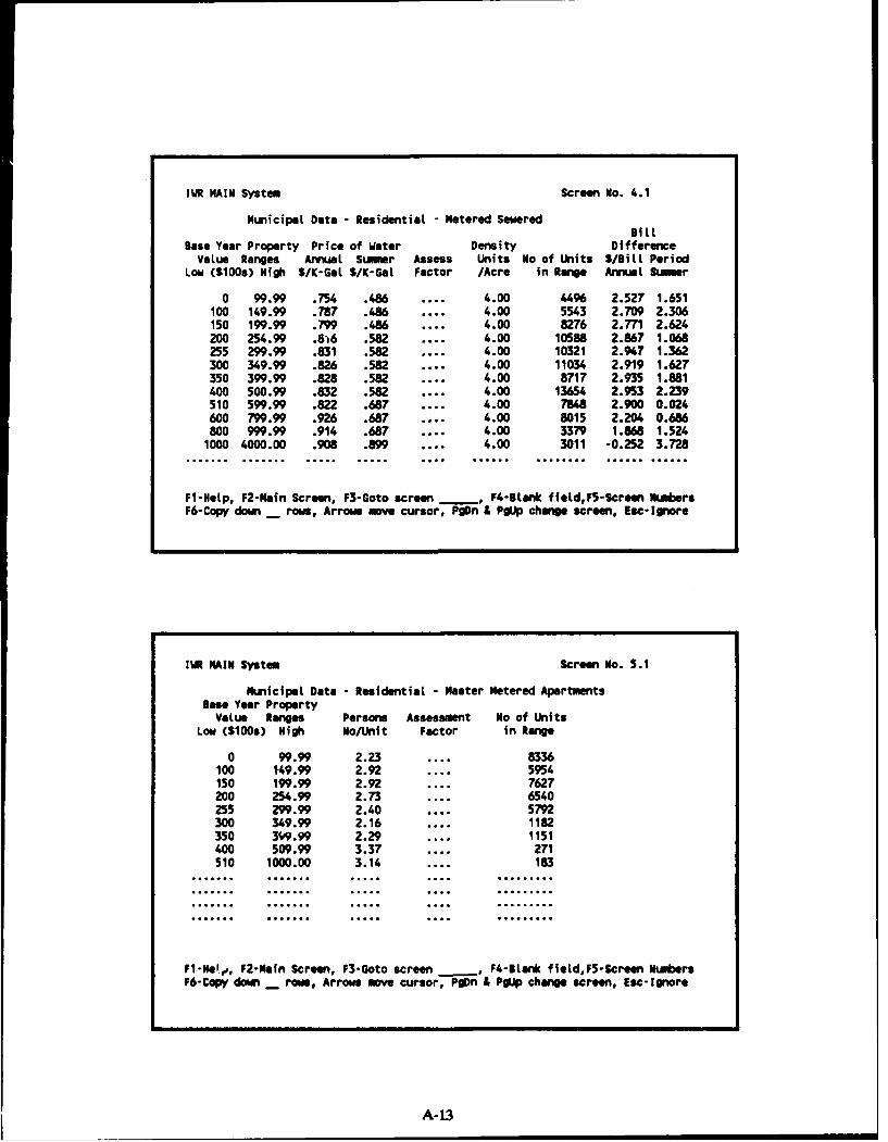
IWR MAIN System Screen No. 4.1
Mnicipal Data -Residential - Metered SeweredBill
Base Year Property Price of Water Density DifferenceValue Ranges Annual Suer Assess Units No of Units $/Sill Period
Low ($100s) High S/K-Gal S/K-Gal Factor /Acre In Range Annual Sumer
0 99.99 .754 .486 .... 4.00 1.96 2.527 1.651100 149.99 .787 .4.86 .... 4.00 5543 2.709 2.306150 199.99 .799 .486 .... 4.00 8276 2.771 2.624200 254.99 .8',6 .582 .... 4.00 10588 2.867 1.068255 299.99 .831 .582 .... 4.00 10321 2.947 1.362300 349.99 .826 .5U2 .... 4.00 11034 2.919 1.627350 399.99 .828 .582 .... 4.00 8717 2.935 1.881400 500.99 .832 .582 .... 4.00 13654 2.953 2.239510 599.99 .822 .687 .... 4.00 7848 2.900 0.024600 799.99 .926 .687 .... 4.00 8015 2.204 0.686800 999.99 .914 .687 .... 4.00 3379 1.868 1.5241000 4000.00 .908 .899 .... 4.00 3011 -0.252 3.728
Fl-Help, F2-Nain Screen, F3-Goto screen -, F4-Btank f fetd,FS-Screen NmbersF6-Copy down os Arrows move cursor, Pgn & PoJp change screen, Eec-Ignore
IWR MAIN System Screen No. 5.1
Munilcipal Data - Residential - Master Metered ApartmentsBase Year Property
Value Ranges Persons Assessment No of UnitsLow CS100s) High No/Unit Factor In Range
0 99.99 2.23 .... 8336100 149.99 2.92 . . .. 5954150 199.99 2.92 .... 7627200 254.99 2.73 .... 6540255 299.99 2.40 .... 579300 349.99 2.16 .... 1182350 3W.99 2.29 .... 1151400 509.99 3.37 .... 271510 1000.00 3.14 .... 183
Fl-Hey, P2-Main Screen, P3-Goto screen F 4-lank field,F5-Screen NumbersP6-Copw down _ row, Arrows move cursor, P)n IPgO change screen, Esc- Ignore
A-13

JUR M4AIN System Screen No. 6.1
Muniicipal Data - Com~mercial Employment
Total Employment
Description Description
COOl Miscellaneous Commgercial 30301 c013 Hotels, Restaurants 9118C002 Vocational School 1079 C014 Electric, Gas Utilities 3585C003 Miscellaneous Retail 12667 C015 Public Administration 56319C004 Boarding Houses 48 C016 Schools, universities 10438C0O5 Transportation Terminal 154 C017 Race Tracks....C006 Barbers, Cleaning 1016 COla Labs, Water Utilities 2259C007 Power Laundries ...iiC019 Health Services 610COOS Landscaping 24C020 Medical offices, Bakeries 1664C009 Miscellaneous Whiolesale 1836 C021 Nursing Facilities 489COlO Recreational Facilities 292 C022 Hospitals 3855COIl Food and Auto Retail 9264 C023 Zoological, etc. Gardens......C012 Dance Studios 18
P1-Help, P2-Main Screwn, P3-Goto screwn F,4-Blank field,F5-Screen NmbersP6-Copy down _ rows, Arrows move cursor, Pg)n & PgJp change screen, Ese- Ignore
IWR M4AIN System Screen No. 7.1Miclpst Data industrial Eaploymmnt
Total Employmentsic Description sic Description201 Meat Products 282 209 Misc Foods & Kindred prod 2812011 meat Pecking Plants .... 211 Cigarettes....2013 Sausages &repered eats-------.212 Cigars....2016 Poultry Dressing Plants-------- 213 Chewing & Smoking Tobacco ...2017 Poultry & Egg Processing ....... 214 Tobacco stemmingl~edrying .......202 Dairy Produicts 316 221 Weaving Mills, Cotton ....203 Preserved Fruits & Veggys 679 222 Weaving Mills, Synthetics .......204 Grain Mill Products 365 223 Weaving&pinish Milts,Woot .......205 Bakery produacts 291 224 Narrow Fabric Mills ....2051 Bread. Cake & Ret. Prods-------.225 Knitting Mills 112052 Cookies & Crackers .... 226 Textile Finishng,exc.WooL .......206 Sugar & Confectionery prd 37 227 Floor Covering Mills ...207 Pate & Oils 56 228 Yarn & Thread Mills2206 Beverages 306 229 Misc. Textile Goods 542062 Mlt Beverages .... 230 Apparei&Other Textile Prd 149622066 Gottleg Caried Soft Oka ....... 241 Logging Caiips&Lg Contrctr ...2067 Flavoring Extract@&Syrup ...
Fi-Netp, P2-Main Screen, F3-Goto screen _, P4-Blank field.FS-Screen NumbersP6-Copy downe _ rows, Arrows move cursor, Pgn & P0.Jp change screen, Esc- Ignore
A-14

IWR MAIN System Screen No. 7.2Munwicipal Data - Industrial Employment
Total Emrploymentsic Description sic Description242 Sawiills & Planing Milts.........281 Industrial Inorganic Chem 2243 Millwork,Plywmood9Str.Me=m 734 282 Plastics MaterilalSynths 11244 Wood Containers 13 283 Drugs 14245 Wood Bidg. & Mobile Homes 26 2831 Biological Products ....249 Misc. Wood Products 38 2833 Nedicinals & Botanicals....251 Household Furniture 86 2834 Pharmaceutical Prep. ....252 Office Furniture .... 284 Soap,Cteaners&Toilet Good ...253 Public Bldg & Rel. Furn ..........285 Paints & Allied Products 100254 Partitions & Fixtures 24 286 Industrial Organic Chems ........259 Misc. Furniture &Fixtures 10 2861 Gum & Wood Chemicals ....261 Pulp Mills .... 28365 Cyclic Crudes glntermed.......262 Paper MfIIs,exc.BldgPaper ........ 2869 Industrial Organic Cheme .......263 Paperboard Mills .... 287 Agricultural Chemicals 16264 Misc. Cony. Paper Prods 675 289 Misc. Chemical Products 4265 Paperboard Containers&Box 307 291 Petroleum Refining 164266 Bldg Paper 9 Board Mills.........295 Paving IMoofing Materials .......270 Printing 9 Publishing 1629
Fl -Help, P2-Main Screen, F3-Goto screen _, P4-Blank fifeld, F5-Screen NumbersF6-Copy down _ rows, Arrows move cursor , Pqn & P"J change screwn, Esc- Ignore
1WR M4AIN System Screen Mo. 7.3municipal Date - Industrial Employment
Total Employinentsic Description sic Description299 Misc. Petrol & Coal prods ........ 324 Cement, Hydraulic 157301 Tires & Inner Tubes .... 325 Structural Clay Products 10302 Rubber &Plastics Footwear ........ 326 Pottery &Related Products .......303 Reclaimed Rubber .... 327 Concrete,Gypsizn&Ptast Prs 616304 Rubber&Pstic Hose&Beltg ........ 328 Cut Stone &Stone Products .......306 Fabricated Rubber Prods 242 329 Misc Nonmetal Mineral Prs 101307 Misc Plastics Products 341 331 Blast Furn LBAS Steel Prs 508311 Leather Tanning&Finishing ........ 3312 Blast Furns &Steel Mills .......313 Soot&Shoe Cut Stock&Findg ill 3313 Electrometallurglcal Prs .......314 Footwear exc. Rubber 2200 3315 Steel Wire Mel Products .......315 Leather Gloves 9 Mittens 47 3316 Cold Finish of Steel Prs .......316 Luggage 3317 Steel Pipe & Tubes ...317 Handbagsa~ers. Leather Prs.....332 iron & Steel Foundries 9319 Leather Goods, nec 7 3321 Gray Iron Founadries ....321 Flat Glass ... .. 3322 Malleable Iron Foundries .......322 GLass&Gwsre,pressedIlown ........ 3324 Steel Investment Foundrs .......323 Prods of Purchased Glass 5 3325 Steel Foundries, nec ....
P1-Help, F2-Nain Screen, F3-Goto screen _,,F4-Blank fiotd,F5-Screen NumbersP6-Copy down _ rows, Arrows move cursor , Pg)n &Pgup change screen, Esc- Ignore
A-15

IWR MAIN System Screen No. 7.4Municipal Data -Industrial Emrployment
Total Employamentsic Description sic Description333 Primary Nonferrous Metals 1420 3462 Iron & Steel Forgings ....334 Secondary Nonferrous MottI........3463 Nonferrous Forgings ....335 Nonferrous RoLling&brawln 255 3465 Automotive Stampings ....336 Nonferrous Foundries 238 3466 Crowns & Closures....339 Misc Primry Metal prods........ 3469 metal Stampings, nec ...341 Metal Cans&Shipg Ctainers ....... 347 Metal Services, nec 7342 Cutiery,HandToolsI~ardwre ....... 348 Ordnrance & Accessries,nec 41343 Ptiabfig&Neatng, ex Elec ........ 349 Misc. Fabricated Met Prds 12344 Fabrictd Struct Steel Pes 843 351 Engines & Turbines 403441 Fabricated Structl Metal ........ 352 Farm & Garden Machinery ....3442 Metal, Doors, Sash & Trim ....... 353 ConstructiontRel Machinry ...3443 Fabricated Plate Work .... 3531 Construction Machinery ....34" Sheet Metal Work 3532 Mining Machinery3446 Architectural Metal Work....3533 Oil Field Machinery3448 Prefab Metal Buildings......... 3534 ELevatrsfloving Stairwiay ...3449 Misc. Metal Work .... 3535 Conveyors&Convey Equipmt .......345 Screw Machine Prs,boLts,e 10 3536 Hoists, Cranesi~onorails .......346 Metal Forgings &tampings 9 3537 Industrial Trucks&Tractr ...
Fl-Help, F2-Main Screen, F3-Goto screenw F4-BLank fleld,F5-Screen NumbersF6-Copy down _ rows, Arrows move cursor, P9Dn &PgUp change screen, Esc- Ignore
zIa MAIN System Screen No. 7.5Municipal Data - industrial Employment
Total Employmentsic Description sic Description354 Metalworking Machinery 129 3599 Machinery,exc Electr nec .......355 Sped: Industrial Mchinery ....... 361 Electr Distribting equaipt 202356 Genrt Industrial Nchinery 376 362 Elect Industrial appratus 135357 Office&Coputing Machines ....... 363 Household Appliances 1003572 Typewriters .... 364 Elect Lighting&wiring eqp 95357- Electo Computing Equipmt ....... 365 Radio & TV Reclevng equip 2363574 CaLcg &ccountg Machines ....... 366 Commnication Equipment 12283576 Scaes&Balances,exc. *Lab ....... 367 Electronic Coilponents&acc 16053579 Office Machines, nec .... 3671 Electron Tubes,Recv Type .......358 Refrigerto&Svc Mchlnry 183 3672 Cath Ray Tete Pict Tubes .......3581 Auto Merchandising Mchns ....... 3673 Electron tubes,Xmit Type ...3582 Commercial Laundry Eqpmt ....... 3674 SemiconductorsReL devcs .......358 Refrig & Heating Equiipmt ....... 3675 Electronic Capacitors ....3586 esuringl~ispensng Pups ....... 3676 Electronic Resistors ....3589 Swc Indstry Nchnery,nec ....... 3677 Electronic Coils&Xformrs .......359 Misc. Nachnery,exc.Etect 187 3678 Electronic Connectors ....3592 Carb,Pfstons,rlngs,valv ....... 3679 Electronic Cmponents,nec .......
Fi-Nelp, F2-Nafn Screen, F3-Goto screenw F4-Blank fieLd,F5-Screen NubersF6-Copy down _ rows, Arrows move cursor, Pg)n &Pgtp change screen, Esc-Ignore
A-16

IWE MAIN System Screen No. 7.6Municipal Data - Inclustriat EmpIoyuet
Total Employmentsic Description sic Description369 Misc. Electr EquilksupLys 355 379 Misc Transportn Equipmnt .......371 Motor Vehicles &Equipmnt 491 381 EngineeringtSci Instrment 13711 Motor Vehctes&car bodies ....... 382 Measuring&Controlllng dvc 3593713 Truck & Bus Bodies .... 383 Optical Instrants Slenses .......3714 Motor vhicLe parts Lftcca ........ 384 Medcl Instrumwts& suqpLys 163715 Truck Trailers ... i385 Opthatmic Goods 113372 Aircraft & Parts 11386 Photographic Eqpmt &Supps .......3721 Aircraft .... 387 Watches, CLocks&clokcases .......3724 Aircraft engs Lang parts ....... 391 Jewelry, Silverware&platd 313728 Aircraft Equzipment, nec........ 393 Musical instruments ....373 ShipLicat Bldg IMepairing ....... 394 Toys 9 Sporting Games 1068374 Railroad Equipment .... 395 Pens,PencfLsOffc&art Sup ...375 Motorcyctes,blcycle~parts ....... 396 Costume Jewelry 9 Notions 75376 Guided Mlssiles,space vth ....... 399 Misc. Manufactures 66
P1-Help, P2-Main Screen, P3-Goto screen _, 4-Blank fieLd,PS-Screen NumbersP6-Copy down _ rows, Arrow* move cursor, Pgn 9 PO change screwn, Esc- Ignore
IWR MAIN System Screen No. 9.1
Projection Data for Internal Growth Models
Year Populatn Me~h HN Total Total No. % Households w/Income (1980S)>Base income Eiiploymt Househlds <10,000 10,000-- 20,000--
(1960s) <20,000 <30,000
1990 586432 25851 226958 172413 .... .... ....2000 679366 2858 277855 196469 .... .... ....
P1-Help. P2-Main Screen, F3-Goto screen _ P4K-Blank fietd,F5-Screen NumbersP6-Copy down _ rows, Arrows move cursor, Pg)n L P"~ change screwn, Esc- Ignore
A-17

IWR MAIN System Screen No. 9.3
Projection Data for Internal Growth Models
Employmnt by Industry Group (SIC Codes)
Year 1500-- 2000-- 4000- - 5000-- 5200-- 6000-- 7000-- 9100-->Base 1799 3999 4999 5199 5999 6799 899 9799
1990 12657 50147 10363 9506 33276 8236 40773 620002000 14337 61801 13526 12053 47491 11137 52610 64900
P1-Help, P2-Main Scrw, P3-Goto screen -,4-Stank fleLd,F5-Screen NumbersP6-Copy down _ rows, Arrows move cursor, Pgn &Pg~p change screwn, Eac- Ignore
IWR MAIN System screen Mo. 14.1.1Direct External Projections: 1990 - Residential,
Category & No. Units Category & No. UnitsValue Range In Value Range in
Group Group Group Group
FWGI ..... PG1 ....FWG2 ..... PPG2 ....PFiG3 ..... PPG3 ....PWG4 FPG4 ....P1111 121FPTL ....
MIOG1 36936 APG1 ....WWdG2 57417 APG2 ....iWdG3 20712 APG3 ....WdG4 ..... APG4 i iWTL 115065 APTI 53
P1-Help, P2-Main Screen, P3-Goto screen , 4-Lank fietd,P5-Screen NumbersP6-Copy down _ rows, Arrow move cursor, Pg)n & PgUp change screen, Esc- Ignore
A-18

IWR MAIN System Screen No. 14.1.4
Direct External Projections: 1990 - Indiastriat
Category Emptoyumnt Category Emptoyment Category Employmnt
1001 . ..... 1018 ...... 1035 .....1002 ...... 1019 ...... 1036 .....1003 ...... 1020 ...... 1037 .....1004 ...... 1021 ...... 1038 .....1005 ...... 1022 ...... 1039 .....1006 ...... 1023 ...... 1040 .....1007 860 1024 ...... 1041 .....1008 462 1025 ...... 1042 .....1009 ...... 1026 ...... 1043 .....1010 .... 0. 27 ...... 1044 .....1011 .... 0. 28 ...... 1045 .....1012 ...... 1029 ...... 1046 .....1013 ...... 1030 ...... 1047 10091014 ...... 1031 ...... 048 .....1015 .. ... 1032 ....... 049 .....1016 ...... 1033 . .... 1050 .....1017 ...... 1034 ...... 1051 .....
Fl-Help, F2-Main screen, F3-Soto screw _ , F4-Ilar* ffetdF5-Screen NumbersF6-Copy down~ _ rows, Arrow move cursor, Pg~n & P"~ change scream, Eac- Ignore
IWR MAIN System Screen No. 14.1.5
Direct External Projections: 1990 -Industrial
Category Emptoyment Category Emptoy'uent Category EavpLoy nsnt
1052 ...... 1069 ...... 1086 .....153 ...... 1070 ...... 1087 .....1054 ...... 1071 1088.. os .....1055 ...... 1072 ...... 1089 .....1056 ...... 1073 ...... 1090 6831057 ...... 1074 ...... 1091 .....1058 ...... 1075 ...... 1092 .....1059 ...... 1076 109...3IM ......1060 10.... 77 ...... 1094 .....1061 ...... 1078 ...... 1095 .....1062 ...... 1079 ...... 1096 .....1063 ...... 1080 ...... 1097 .....1064 ...... 1081 ...... 1098 .....1065 ...... 1082 ...... 1099 .....1066 ...... 1083 ...... 1100 .....1067 ...... 1084 ...... 1101 19091068 ...... 1085 ...... 1102 .....
Fl-Help, P2-Main Screen, F3-Goto screen _ ,P4-Blank I ietd,F5-Screen NumbersP6-Copy down _ rows, Arrows move cursor, Pgn & Pgl~p change screew, Eac-Ignore
A-19

JUR MAIN System Screew No. 14.1.7Direct External Projections: 1990 -xinutrial
Category Employmnent Category Employment Category Employment
1154 ...... 1170 ...... 1186 ..1155 ...... 1171 ...... 1187501156 ...... 1172 ...... 1188 .....1157 ...... 1173 ...... 1189 .....1158 ...... 1174 ...... 1190 .....1159 ...... 1175 ...... 1191 .....1160 ...... 1176 ...... 1192 .....1161 ...... 1177 ...... 1193 .....1162 ...... 1178 ...... 1184 .....1163 ...... 1179 ...... 1195 .....1164 ...... 18e0 ..... 1196 .....1165 ...... 1181 ...... 1197 .....1166 ...... 1182 ...... 1196 .....1167 ...... 1183 ...... 1199 .....1168 ...... 1184 ...... 1200 .....1169 ...... 1185 .....
Fl-Help, F2-Msin Screwn, F3-Goto screen- F4-Ilank field,F5-Screen NumbersF6-Copy down _ rows, Arrows move cursor, Pqn &PgJp change screen, Esc- Ignore
IW MAIN System Screen No. 14.2.1Direct External Projections: 2000 - Residential
Category & No. Units Category & No. UnitsValue Range in Value Range in
Group Group Group Group
FWI ..... FPG1 ....FI.'2 ..... FPG2 ....FWG3 ..... FPG3 ....FWdG4 .. FPG4 ....FIETL 190FPTL ....
NMI 45837 APGI .....MWG2 62731 APG2 ....NWG3 22395 APG3 ....MWG4 ..... APG4MWTL 130963 APTI 17
Fl-Help, P2-Main Screen, F3-Goto screen -,F.- BLank fietd,F5-Screen NumbersF6-CapV down _ rows, Arrows move cursor, Pg~n & PgUp change screen, Esc-Ignore
A-20

IWR MAIN System Screem No. 14.2.4
Direct External Projections: 2000 - Induastrial
Category Employmnent Category Employment Category Emloyment
1001 ...... 1018 ...... 1035 .....1002 ...... 1019 ...... 1036 .....1003 ...... 1020 ...... 1037 .....1004 ...... 1021 ...... 1038 .....1005 ...... 1022 ...... 1039 .....1006 ...... 1023 ...... 1040 .....1007 1116 1024 ...... 1041 .....1008 600 1025 ...... 1042 .....1009 ...... 1026 ...... 1043 .....1010 ...... 1027 ...... 1044 .....1011 ...... 1028 ...... 1045 .....1012 ...... 1029 ...... 1046 .....1013 ...... 1030 ...... 1047 12301014 ...... 1031 ...... 1048 .....1015 ...... 1032 ...... 1049 .....1016 ...... 1033 ...... 1050 .....1017 ...... 1034 ...... 1051 .....
P1-HeLp, P2-Main Screen, F3-Goto screen __, F4-Btank fild,PS-Screen NtWersP6-Copy down _ rows, Arrows move cursor, P0)n & P90 change screen, Esc- Ignore
1WR 1MAIN System Screen No. 14-2.5
Direct External Projections: 2000 - Industrial
Category Employment Category Employment Category Employment
1052 ...... 1069 ...... 1086 .....1053 ...... 1070 ...... 1087 .....1054 ...... 1071 ...... 108 .....1055 ...... 1072 ...... 1089 .....1056 ...... 1073 ...... 1090 7181057 ...... 1074 ...... 1091 .....1058 ...... 1075 ...... 1092 .....1059 ...... 1076 .... 093IM ......1060 ...... 1077 ...... 1094 .....1061 ...... 1078 ...... 1095 .....1062 ...... 1079 ...... 1096 .....1063 ...... 1080 ...... 1097 .....1064 ...... 1081 ...... 10986 .....1065 ...... 1082 ...... 1099 .....1066 ...... 1083 ...... 1100 .....1067 ...... 1084 ...... 1101 1 20061068 ...... 1085 ...... 1102 .....
P1-Help, P2-Main Screen, P3-Goto screen _ , P4-Btank field.F5-Screen NumbersP6-Copy down _ rows, Arrows move cursor, PgDn & PgJp change screen, Eec-Ignore
A-21

IUR M4AIN System Screen Mo. 14.2.7
Direct External Projections: 2000 - Industrial
Category Employmuent Category Employment Category Employment
1154 ...... 1170 ...... 11861155 ...... 1171 ...... 1187611156 ...... 1172 ...... 1188 .....1157 ...... 1173 ...... 1189 .....1158 ...... 1174 ...... 1190 .....1159 ...... 1175 . ..... 1191 .....1160 ...... 1176 ...... 1192 .....1161 ...... 1177 ...... 1193 .....1162 ...... 1178 ...... 1184 .....1163 ...... 1179 ...... 1195 .....1164 ...... 1180 ...... 1196 .....1165 ...... 1181 ...... 1197 .....1166 ...... 1182 ...... 1198 .....1167 ... 18..i3 ...... 1199 .....1168 ...... 1184 ...... 1200 .....1169 ...... 1185 .....
Fl-Help, F2-Main Screen, F3-Goto screen P64-Stank fletdPS-Screen NumbersP6-Copy down _ rows, Arrows move cursor, Pgn & P".J change screen, Esc- Ignore
IwR MAIN System Selection of Measures and Year of initiation Screen 15.1Enter year for those measures desired
Nuber Measure Description Year...............................----------------
1 Public Education Program 19802 Metering ..3 Pressure Reduction ..4 Pricing Policy (Rate Reform) ..5 Rationing (Per Capita) ..6 Sprinkling Restrictions ..7 Industrial Reuse/Recycle ..a Commercial Reuse/Recycle9 Leak Detection and Repair 16
10 Retrofit of Showerheads and Toilets11 Moderate Pltubing Code 1712 Advanced Plumbing Code ..13 Low-Uater use Landscaping (New) 197114 Low-Water Use Landscaping (Retrofit) ...15 User-Specified Measure Number 1 .. ..
16 User-Specified Measure Nmwber 2 ..17 user-Specified Measure Number 3 ..18 User-Specified Measure Number 4 ..
Fl-Help, P2-Main Screen, F3-Goto screen F 4-Blank fieLd,F5-Screen nitrsUp and down arrows move cursor, Pg)n & PgUp change screen
A-22

IWR MAIN System SeLection of Sectors for Each Measure Screen 15.2Enter a Y for each desired sector for each measure
SECTORS: RESIDENTIAL COIMERCL INDUSTRL PUBLIC UNACCOUNTMEASURES METERED FLATRATE APARTMT & OTHER
EDUCATION Y Y YLEAK REPAIR yMODERATE CODE Y y yLANDSCAPE-NEW Y Y Y
Fl-Nelp, F2-Main Screen, F3-Goto screen _ , F4-8tank ffetd,F5-Screen mmersArrows move cursor, Pq~n & P"Jp change screen
IWR MAIN System Determination of Reduction Factors Screen 16.2
INDOOR USE Enter Reduction Factors between 0.000 and 1.000SECTORS: RESIDENTIAL COMMERCL INDUSTRL PUBLIC UNACCOUNT
MEASURES METERED FLATRATE APARTMT & OTHER------------------------------------------------------------EDUCATION 0.035 0.035 0.035LEAK REPAIR 0.273
MODERATE CODE 0.079 0.152 0.152LANDSCAPE-NEW 0.000 0.000 0.000
Fl-Hetp, F2-Main Screen, F3-Goto screen _, F4-Btank fietd,F5-Screen rudbers
F6-Copy from previous dimension, Arrows move cursor, Pq)n & PgUp change screen
A-23

IWR MAIN System Determneation of Reduction Factors Screen 16.3OUTDOOR USE Enter Reduction Factors between 0.000 and 1.000
SECTORS: RESIDENTIAL COI4ERCL INDUSTRI PUBLIC UNACCOUNTMEASURES METERED FLATRATE APARTMNT & OTHER... .--- - - -------- . .. -- ---- -- °- °----- ............ . ....... ... °...o°.°°.°°°
EDUCATION 0.035 0.035 0.035LEAK REPAIR 0.273MODERATE CODE 0.000 0.000 0.000LANDSCAPE-NEW 0.052 0.032 0.023
Fl-ltp, F2-Main Screen, F3-Goto screen , F4-Btank f IeLd.F5-Screen n- IrsF6-Copy from previous dimension, Arrow move cursor, PgDn & P"Jp change screen
IMR MAIN System Determinetfon of Reduction Factors Screen 16.4MAX-DAY USE Enter Reduction Factors between 0.000 and 1.000
SECTORS: RESIDENTIAL COSUERCL INOUSTRL PUBLIC UNACCOUNTMEASURES METERED FLATRATE APARTlNT & OTHER............ ..... ................................ ......... ................ .....
EDUCATION 0.035 0.035 0.035LEAK REPAIR 0.273MODERATE CODE 0.079 0.152 0.152LANDSCAPE-NEW 0.052 0.032 0.023
Fl-Netp, F2-Nain Screen, F3-Goto screen , F4-Bt*nk fieLd,F5-Screen ntersF6-Copy from previous dimension, Arrow move cursor, Pg~n & PgUp change screen
A-24

IWR MAIN Systen Determination of Coverage Factors Screen 17.2Base Year: 1960 Enter Coverage Factors between 0.000 and 1.000
SECTORS: RESIDENTIAL COISERCL INDUSTRI. PUBLIC UNACCO.JNTMEASURES METERED FLATRATE APARTMNT & OTHER
EDUCATION 0.950 0.950 0.950LEAK REPAIR 0.000MODERATE CODE 0.097 0.097 0.097LANDSCAPE-NEWi 0.077 0.077 0.077
Fl-Help, F2-Main Screen, P3-Goto scream ,F4-Itank fieLd, F5-Screen iubersF6-Copy from previous year, Arrows move cursor, Pqn and P0JP change screwn
IW~ MAIN Systom Determination of Coverage Factors Screen 17.3Forecast Year: 1990 Enter Coverage Factors between 0.000 and 1.000
SECTORS: RESIDENTIAL CIERCL INDUSTRL PUBLIC UNACCOUNTMEASURES METERED FLATRATE APARTM4NT & OTHER
EDUCATION 0.950 0.950 0.950LEAK REPAIR 0.667MODERATE CODE 0.163 0.163 0.163LANDSCAPE-NEW 0.166 0.166 0.166
Fl-Help, F2-Rafn Screen, F3-Goto screen _ 4-t-Bank field, F5-Screen nuibersF6-Copy from previous year, Arrows move cursor, Pgn and P"~ change screen
A-25

lIW MAIN System Determination of Coverage Factors Screen 17.4Forecast Year: 2000 Enter Coverage Factors between 0.000 and 1.000
SECTORS: RESIDENTIAL COIUERCL INDUSTRL PUBLIC UACCOUNTMEASURES METERED FLATRATE APARTMNT & OTHER
EDUCATION 0.950 0.950 0.950LEAK REPAIR 1.000MODERATE CODE 0.275 0.275 0.275LANDSCAPE-NEW 0.240 0.240 0.240
F1-Hetp, F2-Nafn Screen, F3-Goto scren _ ,F4-Ilank ffetd, FS-Screen nmbersF6-Copy from previous year, Arrows move cursor, PqDn and P"Jp change screen
A-26

EXHIBIT A-2REVISED COEFFICIENT LIBRARY
ICONSTANT (FOR IWR MAIN VERSION 5.1)EOI1 234.0 E012 1.451 E013 -45.9E014 -2.59 E021 28.9 E022 1.576E023 33.6 E041 30.2 E042 39.5E051 0.5453 E052 58.777 E053 -0.703E054 0.429 E061 385.0 E062 2.876E063 -285.8 E064 -4.35 E065 157.77E071 0.4658 E072 44.573 E073 0.783E091 0.4658 E092 44.573 E093 0.783El01 0.803 E102 -1.26 Elll 2227.34E112 2.06 E113 0.413 E121 .000046485E122 0.118 E123 -10.4 E124 -1.25E125 0.931 E131 1609.59 E132 0.943E133 0.523 E151 1609.59 E152 0.943E153 0.523 E024 1.433ENDD
ICLIMELAS (ELASTICITIES FOR WEATHER ADJUSTMENT FACTORS)MSSD 1.0ENDD
1COMLABELC001 MISC. COMMERCIAL C002 VOC. SCHOOLS C003 MISC. RETAILC004 BOARDING HOUSES C005 TRANSP. TERMINAL C006 BARBER, CLEANINGC007 POWER LAUNDRIES C008 LANDSCAPING C009 MISC. WHOLESALEC010 RECREATION FACL. COIl FOOD AUTO RETAIL C012 DANCE STUDIOSC013 HOTELS, RESTRNTS C014 ELEC, GAS UTIL. C015 PUBLIC ADMINIST.C016 SCHOOLS, UNIV. C017 RACE TRACKS C018 LABS, WTR UTIL.C019 HEALTH SERVICES C020 MED. OFF. BAKERS C021 NURSING FACIL.C022 HOSPITALS C023 ZOOLOGICAL GRDNSENDD
1COMMUNITC001 EMPLOYEES C002 EMPLOYEES C003 EMPLOYEESC004 EMPLOYEES C005 EMPLOYEES C006 EMPLOYEESC007 EMPLOYEES C008 EMPLOYEES C009 EMPLOYEESC010 EMPLOYEES COl EMPLOYEES C012 EMPLOYEESC013 EMPLOYEES C014 EMPLOYEES C015 EMPLOYEESC016 EMPLOYEES C017 EMPLOYEES C018 EMPLOYEESC019 EMPLOYEES C020 EMPLOYEES C021 EMPLOYEESC022 EMPLOYEES C023 EMPLOYEESENDD
iCOMMAVEG EXPECTED USAGE VALUESCOO1 96.5 C002 76.5 C003 26.63C004 101.6 C005 187.8 C006 1022.01C007 273.9 C008 106.7 C009 40.1CONO 832.7 COil 131.1 C012 70.600C013 494.3 C014 108.8 C015 125.20C016 300.7 C017 341.5 C018 442.85C019 125.3 C020 108.5 C021 307.7C022 204.36 C023 450.8ENDDICOMMAXDY EXPECTED USAGE VALUESCOOl 96.5 C002 76.5 C003 26.63C004 101.6 C005 187.8 C006 1022.01C007 273.9 C008 106.7 C009 40.1C010 832.7 COl 131.1 C012 70.600C013 494.3 C014 108.8 C015 125.20C016 300.7 C017 341.5 C018 442.85C019 125.3 C020 108.5 C021 307.7
A-2

C022 204.16 C023 450.8ENDD
lINDILBEL1001 201 MEAT PRODUCTS 1002 2011 MEAT PACKNG PLANTS1003 2013 SAUSAGES, ETC. 1004 2016 POULTRY DRESSING1005 2017 POULTRY & EGG DRSG 1006 202 DAIRY PRODUCTS1007 203 PRSRVD FRUITS, VEG 1008 204 GRAIN KILL PRDCTS1009 205 BAKERY PRODUCTS 1010 2051 BREAD, CAKE, ETC.1011 2052 COOKIES, CRACKERS 1012 206 SUGAR & CONFECTNRY1013 207 FATS & OILS 1014 208 BEVERAGES1015 2082 MALT BEVERAGES 1016 2086 SOFT DRINKS1017 2087 EXTRACTS, SIRUPS 1018 209 MISC. FOODS, ETC.1019 211 CIGARETTES 1020 212 CIGARS1021 213 CHENG & SMKNG TOB 1022 214 TOBACCO STEMMING1023 221 COTTON WEAVING 1024 222 SYNTHETIC WEAVING1025 223 WOOL WEAVING, FIN. 1026 224 NARROW FABRIC MLLS1027 225 KNITTING MILLS 1028 226 TEXTILE FINISHING1029 227 FLOOR COVERING MLS 1030 228 YARN & THREAD MLLS1031 229 MISC. TEXTILE MLLS 1032 230 APPAREL, ETC.1033 241 LOGGING CAMPS, ETC 1034 242 SAW & PLANING MLLS1035 243 MILLWORK, PLYWOOD 1036 244 WOOD CONTAINERS1037 245 WOOD BUILDINGS ETC 1038 249 MISC. WOOD PRODCTS1039 251 HOUSEHOLD FRNITURE 1040 252 OFFICE FURNITURE1041 253 PUBLIC BLDG. FURN. 1042 254 PARTITIONS, FIXTRS1043 259 MISC. FURNITURE 1044 261 PULP HILLS1045 262 PAPER MLLS,EXC.PPR 1046 263 PAPERBOARD MILLS1047 264 MISC. CONV. PAPER 1048 265 PAPERBOARD CONTNRS1049 266 BUILDNG PAPER, BRD 1050 270 PRINTING, PUBLSHNG1051 281 IND. ORGANIC CHEM. 1052 282 PLASTICS, SYNTHTCS1053 283 DRUGS 1054 2831 BIOLOGICAL PRODCTS1055 2833 MEDICINALS, BOTAN. 1056 2834 PHARMACEUTICALS1057 284 SOAP & TOILET GDS 1058 285 PAINTS & ALLIED PR1059 286 IND. ORGANIC CHEM. 1060 2861 GUM & WOOD PRODCTS1061 2865 CYCLIC CRUDESINTR 1062 2869 ORGANIC CHEM. NEC1063 287 AGRICULTURAL CHEM. 1064 289 MISC. CHEM. PRDCTS1065 291 PETROLEUM REFINING 1066 295 PAVING & ROOFING1067 299 MISC. PET. & COAL 1068 301 TIRES & TUBES1069 302 RUBBER FOOTWEAR 1070 303 RECLAIMED RUBBER1071 304 RUBBER HOSE, BELTG 1072 306 FABRIC.RUBBER, NEC1073 307 MISC. PLASTICS PRD 1074 311 LEATHER TANNING1075 313 BOOT, SHOE STOCK 1076 314 FOOTWEAR, EX. RUBR1077 315 LEATHER GLOVES 1078 316 LUGGAGE1079 317 HANDBAGS, ETC. 1080 319 LEATHER GOODS, NEC1081 321 FLAT GLASS 1082 322 GLASS & GLASSWARE1083 323 PURCHASD GLASS PRD 1084 324 HYDRAULIC CEMENT1085 325 STRUCTURL CLAY PRD 1086 326 POTTERY & RELATED1087 327 CONCRETE, GYPSUM 1088 328 CUT STONE & STONE1089 329 MISC.NONMET.MINERL 1090 331 BLAST FURNC & STEL1091 3312 FURNACES, STEEL ML 1092 3313 ELECTROMETALLURGCL1093 3315 COLD WIRE & REIATD 1094 3316 COLD FINSHNG STEEL1095 3317 STEEL PIPE & TUBES 1096 332 IRON, STEEL FOUNDR1097 3321 GRAY IRON FOUNDRY 1098 3322 MALLEABLE IRON FND1099 3324 STEEL INVSTMNT FND 1100 3325 STEEL FOUNDRY, NEC1101 333 PRIMARY NONFERROUS 1102 334 SECONDARY NONFERRS1103 335 NONFERROUS ROLLING 1104 336 NONFERROUS FOUNDRY1105 339 MISC.PRIMARY METAL 1106 341 METAL CANS, CONTNR1107 342 CUTLERY,HAND TOOLS 1108 343 PLUMBING, HEATING1109 344 STRUCTRL STEEL PRD 1110 3441 FABRICATED STRCTRL1111 3442 METAL DOORS, SASH 1112 3443 FABRICATED PLATE
A-28

1113 3444 SHEET METAL WORK 1114 3446 ARCHITCTRL METAL1115 3448 PREFAB METAL BLDGS 1116 3449 MISC. METAL WORK1117 345 SCREW MACHNE PRODS 1118 346 METAL FORGINGS,ETC1119 3462 IRON & STEEL FRGNG 1120 3463 NONFERROUS FORGNGS1121 3465 AUTOMOTIVE STMPNGS 1122 3466 CROWNS & CLOSURES1123 3469 METAL STMPNGS, NEC 1124 347 METAL SERVICES,NEC1125 348 ORDNANCE & ACCESS. 1126 349 MISC. FAB. METAL1127 351 ENGINES & TURBINES 1128 352 FARM, GARDEN MACH.1129 353 CONSTR, RELTD MACH 1130 3531 CONSTRUCTION MACH.1131 3532 MINING MACHINERY 1132 3533 OIL FIELD MACHNRY1133 3534 ELEVATORS, ETC. 1134 3535 CONVEYORS, ETC.1135 3536 HOISTS, CRANES 1136 3537 IND. TRUCKS, TRCTR1137 354 METALWORKING MACH. 1138 355 SPEC. IND. MACHNRY1139 356 GENERAL IND. MACH. 1140 357 OFFICE & COMPTNG1141 3572 TYPEWRITERS 1142 3573 ELECTRONIC CMPUTNG1143 3574 CALCULTNG, ACCNTG 1144 3576 SCALES,BALANCES1145 3579 OFFICE MACH., NEC 1146 358 REFRIGRATN & SERV.1147 3581 AUTO. MERCH. MACH. 1148 3582 COMM.LAUNDRY EQPMT1149 3585 REFRIGRTN & HEATNG 1150 3586 MEASURING PUMPS1151 3589 SERVICE IND. MACH. 1152 359 MISC.MACH,EXC.ELEC1153 3592 CARBURETORS, ETC. 1154 3599 MACH,EXC.ELEC,NEC1155 361 ELEC. DIST. EQUIP. 1156 362 ELEC. IND. APPARTS1157 363 HOUSEHOLD APPLIANC 1158 364 ELEC.LIGHTNG, WRNG1159 365 RADIO, TV RECEIVNG 1160 366 COMMUNICATION EQPT1161 367 ELECTR. COMPONENTS 1162 3671 ELECTRON TUBES,REC1163 3672 CATHODE RAY TUBES 1164 3673 ELECTRON TUBES,TRN1165 3674 SEMICONDUCTORSETC 1166 3675 CAPACITORS1167 3676 RESISTORS 1168 3677 COILS, TRANSFORMRS1169 3678 ELECTR. CONNECTORS 1170 3679 ELECTR. COMP.,NEC1171 369 MISC.ELEC.EQUIPMNT 1172 371 MOTOR VEHICLES,ETC1173 3711 VEHICLES, CAR BODY 1174 3713 TRUCK, BUS BODIES1175 3714 MOTOR VEHICLE PRTS 1176 3715 TRUCK TRAILERS1177 372 AIRCRAFT & PARTS 1178 3721 AIRCRAFT1179 3724 AIRCRAFT ENGINES 1180 3728 AIRCRAFT EQUIPMENT1181 373 SHIP, BOAT BLDNG 1182 374 RAILROAD EQUIPMENT1183 375 MOTORCYCLES, ETC. 1184 376 MISSILES, SPACE1185 379 MISC.TRANSP.EQPMNT 1186 381 ENG.,SCIENCE INSTR1187 382 MEASURNG,CNTRL DEV 1188 383 OPTICAL INSTRUMNTS1189 384 MEDICAL INSTRUMNTS 1190 385 OPTHALMIC GOODS1191 386 PHOTOGRPHC EQUIPMT 1192 387 WATCHES, CLOCKS1193 391 JEWLERY,SILVERWARE 1194 393 MUSICAL INSTRUMNTS1195 394 TOYS, SPORTING GDS 1196 395 PENS,PENCILS,ETC.1197 396 COSTUME JEWELRY 1198 399 MISC. MANUFACTURESENDD1INDANAVEI001 81.0 1002 477.8 1003 901.71004 755.8 1005 371.5 1006 371.81007 197.5 1008 81.0 1009 81.01010 140.0 1011 163.9 1012 81.01013 81.0 1014 338.0 1015 2681.31016 602.1 1017 958.9 1018 81.01019 250.0 1020 250.0 1021 250.01022 250.0 1023 263.8 1024 322.71025 245.9 1026 263.8 1027 159.761028 1076.3 1029 980.1 1030 51.21031 41.1 1032 63.5 1033 88.41034 2384.7 1035 50.3 1036 72.31037 72.3 1038 72.3 1039 59.51040 77.6 1041 109.1 1042 59.5
A-29

1043 59.5 1044 8303.7 1045 2194.21046 5827.4 1047 32.4 1048 56.51049 593.8 1050 37.9 1051 65.101052 76.6 1053 80.2 1054 292.21055 1200.0 1056 459.4 1057 447.81058 23.6 1059 1796.0 1060 1796.01061 1796.0 1062 1796.0 1063 65.101064 65.10 1065 61.2 1066 559.11067 1217.7 1068 264.7 1069 78.31070 264.7 1071 264.7 1072 291.11073 72.1 1074 23.3 1075 23.31076 23.3 1077 23.3 1078 23.31079 23.3 1080 23.3 1081 375.11082 332.4 1083 38.3 1084 38.31085 38.3 1086 210.7 1087 38.31088 652.3 1089 50.4 1090 48.801091 537.0 1092 365.3 1093 435.91094 467.8 1095 982.5 1096 48.801097 1077.5 1098 608.8 1099 608.81100 311.3 1101 434.1 1102 684.91103 48.8 1104 158.1 1105 913.21106 723.7 1107 231.7 1108 706.11109 29.9 1110 256.1 Illl 373.61112 378.9 1113 202.9 1114 256.11115 256.1 1116 256.1 1117 48.91118 33.1 1119 525.1 1120 1009.41121 150.7 1122 168.4 1123 168.41124 535.0 1125 46.2 1126 34.31127 40.1 1128 1281.5 1129 103.41130 113.5 1131 113.5 1132 79.71133 113.5 1134 113.5 1135 113.51136 113.5 1137 325.3 1138 250.31139 40.1 1140 108.1 1141 108.11142 108.1 1143 108.1 1144 108.11145 108.1 1146 45.1 1147 119.11148 119.1 1149 374.2 1150 182.61151 119.12 1152 34.8 1153 186.181154 99.62 1155 31.5 1156 39.91157 33.8 1158 26.4 1159 26.61160 22.1 1161 69.50 1162 294.51163 228.4 1164 228.4 1165 239.51166 115.1 1167 168.59 1168 228.41169 127.9 1170 241.6 1171 34.81172 51.2 1173 280.86 1174 280.861175 320.4 1176 299.9 1177 24.51178 151.6 1179 151.6 1180 151.61181 151.6 1182 294.9 1183 456.61184 140.9 1185 234.8 1186 45.71187 20.6 1188 122.1 1189 28.11190 38.3 1191 122.1 1192 122.11193 12.8 1194 203.8 1195 109.31196 222.1 1197 12.8 1198 12.80ENDD1INDMXDAY1001 81.0 1002 477.8 1003 901.71004 755.8 1005 371.5 1006 371.81007 197.5 1008 81.0 1009 81.01010 140.0 1011 163.9 1012 81.01013 81.0 1014 338.0 1015 2681.3
A-30
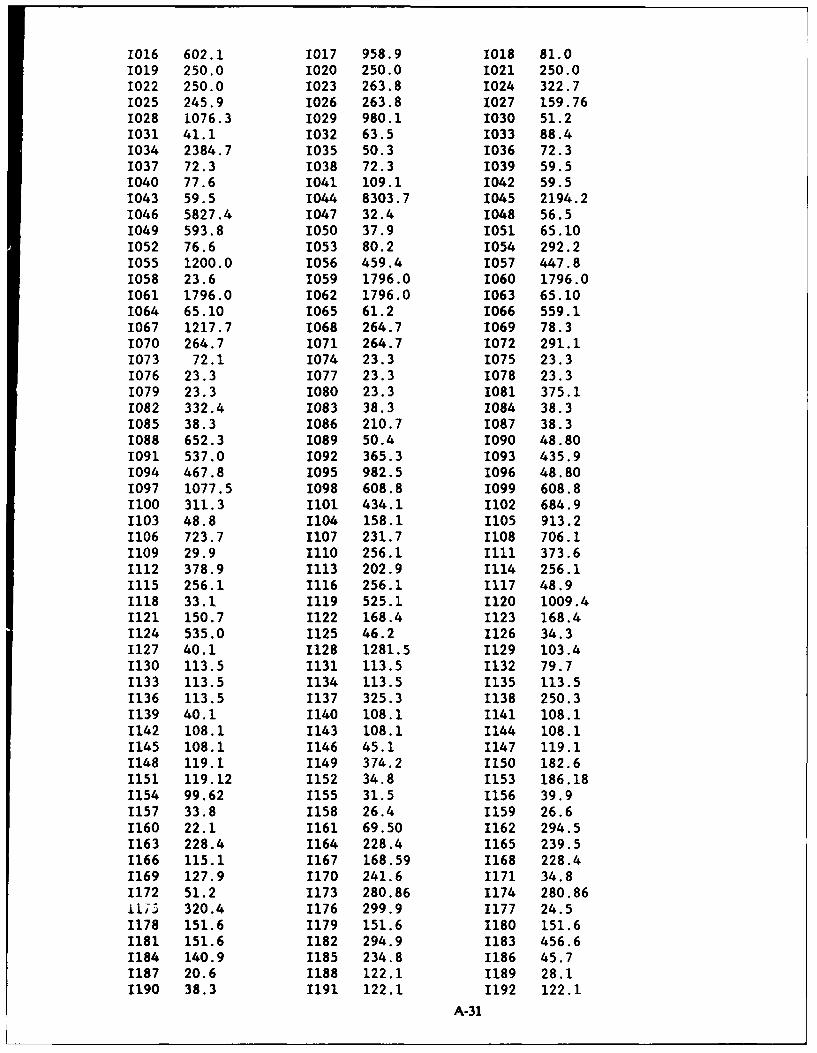
1016 602.1 1017 958.9 1018 81.01019 250.0 1020 250.0 1021 250.01022 250.0 1023 263.8 1024 322.71025 245.9 1026 263.8 1027 159.761028 1076.3 1029 980.1 1030 51.21031 41.1 1032 63.5 1033 88.41034 2384.7 1035 50.3 1036 72.31037 72.3 1038 72.3 1039 59.51040 77.6 1041 109.1 1042 59.51043 59.5 1044 8303.7 1045 2194.21046 5827.4 1047 32.4 1048 56.51049 593.8 1050 37.9 1051 65.101052 76.6 1053 80.2 1054 292.21055 1200.0 1056 459.4 1057 447.81058 23.6 1059 1796.0 1060 1796.01061 1796.0 1062 1796.0 1063 65.101064 65.10 1065 61.2 1066 559.11067 1217.7 1068 264.7 1069 78.31070 264.7 1071 264.7 1072 291.11073 72.1 1074 23.3 1075 23.31076 23.3 1077 23.3 1078 23.31079 23.3 1080 23.3 1081 375.11082 332.4 1083 38.3 1084 38.31085 38.3 1086 210.7 1087 38.31088 652.3 1089 50.4 1090 48.801091 537.0 1092 365.3 1093 435.91094 467.8 1095 982.5 1096 48.801097 1077.5 1098 608.8 1099 608.81100 311.3 1101 434.1 1102 684.91103 48.8 1104 158.1 1105 913.21106 723.7 1107 231.7 1108 706.11109 29.9 1110 256.1 Illl 373.61112 378.9 1113 202.9 1114 256.11115 256.1 1116 256.1 1117 48.91118 33.1 1119 525.1 1120 1009.41121 150.7 1122 168.4 1123 168.41124 535.0 1125 46.2 1126 34.31127 40.1 1128 1281.5 1129 103.41130 113.5 1131 113.5 1132 79.71133 113.5 1134 113.5 1135 113.51136 113.5 1137 325.3 1138 250.31139 40.1 1140 108.1 1141 108.11142 108.1 1143 108.1 1144 108.11145 108.1 1146 45.1 1147 119.11148 119.1 1149 374.2 1150 182.61151 119.12 1152 34.8 1153 186.181154 99.62 1155 31.5 1156 39.91157 33.8 1158 26.4 1159 26.61160 22.1 1161 69.50 1162 294.51163 228.4 1164 228.4 1165 239.51166 115.1 1167 168.59 1168 228.41169 127.9 1170 241.6 1171 34.81172 51.2 1173 280.86 1174 280.861t;i 320.4 1176 299.9 1177 24.51178 151.6 1179 151.6 1180 151.61181 151.6 1182 294.9 1183 456.61184 140.9 1185 234.8 1186 45.71187 20.6 1188 122.1 1189 28.11190 38.3 1191 122.1 1192 122.1
A-31

1193 12.8 1194 203.8 1195 109.31196 222.1 1197 12.8 1198 12.80ENDD
1ELASTCTY COMMERCIAL AND INDUSTRIAL PRICE ELASTICITYCLAS -0.80 ILAS -0.65ENDD
1PUBCOFAALOSS 0.00 FSER 0.0 FLSS 0.11ENDD
1PUBCOFMDLOSS 0.00 FSER 0.0 FLSS 0.11ENDD
IPUBLABELLOSS LOSS (PER CAP.) FSER FREE SERVICE FLSS LOSS (PERCENT)ENDDENDI
A-32

EXHIBIT A-3 OUTPUT REPORTS REPORT NO. 1980- 2
IWR MAIN SYSTEM VER. 5.1
STUDY AREA - ARIDWEST USA CURRENT WATER USE FOR YEAR - 1980
RESIDENTIAL SECTOR
FIAT RATE-SEWERED AREAS
VALUE RANGE UNITS UNRESTRICTED USE RESTRICTED USE($1000) (#) (GAL/DAY/UNIT) (GAL/DAY/UNIT)
(1980 VALUE)WINTER SUMMER ANNUAL WINTER SUMMER ANNUAL
.0 - 10.0 1693. 112. 258. 185. 106. 248. 177.10.0 - 15.0 2334. 147. 447. 297. 140. 429. 284.15.0 - 20.0 2515. 155. 545. 350. 147. 524. 335.20.0 - 25.5 1313. 156. 636. 396. 149. 611. 380.25.5 - 30.0 1256. 153. 714. 433. 146. 686. 416.30.0 - 35.0 452 153. 787. 470. 145. 757. 451.35.0 - 40.0 206. 165. 874. 520. 157. 841. 499.40.0 - 51.0 413. 214. 1039. 626. 204. 999. 601.51.0 - 100.0 2. 282. 1509. 896. 269. 1452. 860.
TOTAL UNITS 10184.
AVERAGE DAY PER UNIT 148. 545. 347. 141. 524. 332.MAXIMUM DAY PER UNIT 1262. 1262. 1199. 1199.
PERCENTAGE REDUCTIONS -
AVERAGE DAY 4.8 3.9 4.1MAXIMUM DAY 5.0 5.0
A-33

REPORT NO. 1980- 3
IWR MAIN SYSTEM VER. 5.1
STUDY AREA - ARIDWEST USA CURRENT WATER USE FOR YEAR - 1980
RESIDENTIAL SECTOR
MASTER-METERED APARTMENTS
VALUE RANGE UNITS UNRESTRICTED USE RESTRICTED USE($1000) (#) (GAL/DAY/UNIT) (GAL/DAY/UNIT)
(1980 VALUE)WINTER SUMMER ANNUAL WINTER SUMMER ANNUAL
.0 - 10.0 8336. 112. 160. 136. 106. 153. 130.10.0 - 15.0 5954. 147. 210. 178. 140. 201. 170.15.0 - 20.0 7627. 155. 222. 188. 147. 212. 179.20.0 - 25.5 6540. 156. 224. 190. 149. 214. 182.25.5 - 30.0 5792. 153. 220. 186. 146. 210. 178.30.0 - 35.0 1182. 153. 219. 186. 145. 209. 177.35.0 - 40.0 1151. 165. 236. 201. 157. 226. 191.40.0 - 51.0 271. 214. 306. 260. 204. 293. 248.51.0 - 100.0 183. 253. 363. 308. 241. 347. 294.
TOTAL UNITS 37036.
AVERAGE DAY PER UNIT 145. 208. 176. 138. 199. 168.MAXIMUM DAY PER UNIT 208. 208. 198. 198.
PERCENTAGE REDUCTIONS -
AVERAGE DAY 4.8 4.4 4.6MAXIMUM DAY 4.9 4.9
A-34

REPORT NO. 1980- 4
IWR MAIN SYSTEM VER. 5.1
STJDY AREA - ARIDWEST USA CURRENT WATER USE FOR YEAR - 1980
RESIDENTIAL SECTOR
METERED-SEWERED AREAS
VALUE RANGE UNITS UNRESTRICTED USE RESTRICTED USE($1000) (#) (GAL/DAY/UNIT) (GAL/DAY/UNIT)
(1980 VALUE)WINTER SUMMER ANNUAL WINTER SUMMER ANNUAL
.0 - 10.0 4496. 200. 412. 306. 192. 396. 294.10.0 - 15.0 5543. 209. 524. 366. 200. 503. 352.15.0 - 20.0 8276. 216. 579. 397. 207. 557. 382.20.0 - 25.5 10588. 222. 580. 401. 213. 558. 386.25.5 - 30.0 10321. 228. 619. 424. 219. 595. 407.30.0 - 35.0 11034. 236. 653. 444. 226. 628. 427.35.0 - 40.0 8717. 243. 687. 465. 233. 660. 447.40.0 - 50.1 13654. 254. 734. 494. 243. 706. 474.51.0 - 60.0 7848. 269. 737. 503. 258. 708. 483.60.0 - 80.0 8015. 287. 804. 546. 276. 773. 524.80.0 - 100.0 3379. 318. 893. 605. 305. 859. 582.
100.0 - 400.0 3011. 556. 1294. 925. 533. 1244. 888.
TOTAL UNITS 94882.
AVERAGE DAY PER UNIT 252. 679. 465. 242. 653. 447.MAXIMUM DAY PER UNIT 1023. 1023. 978. 978.
PERCENTAGE REDUCTIONS -
AVERAGE DAY 4.1 3.9 3.9MAXIMUM DAY 4.4 4.4
A-35

REPORT NO. 1980- 5
IWR MAIN SYSTEM VER. 5.1
STUDY AREA - ARIDWEST USA CURRENT WATER USE FOR YEAR - 1980
RESIDENTIAL SECTOR
SUMMARY
CATEGORY UNITS UNRESTRICTED USE RESTRICTED USE(#) (1000 G/D) (1000 G/D)
WINTER SUMMER ANNUAL WINTER SUMMER ANNUAL- AVERAGE DAY -
FLAT RATE/SWR 10184. 1510. 5550. 3530. 1438. 5333. 3385.APARTMENTS 37036. 5370. 7695. 6532. 5112. 7355. 6234.METERED/SEWRD 94882. 23895. 64433. 44164. 22917. 61945. 42431.
TOTALS 142102. 30775. 77678. 54226. 29467. 74633. 52050.
- MAXIMUM DAY -
RESIDENTIAL SECTOR 117582. 117582. 112300. 112300.
PERCENTAGE REDUCTIONS -
AVERAGE DAY 4.3 3.9 4.0MAXIMUM DAY 4.5 4.5
SUMMER EVAPOTRANSPIRATION (INCHES) - 18.24
SUMMER PRECIPITATION (INCHES) - 3.74
MAX. DAY EVAPOTRANSPIRATION (INCHES) - .29
A-36

REPORT NO. 1980- 6
IWR MAIN SYSTEM VER. 5.1
STUDY AREA - ARIDWEST USA CURRENT WATER USE FOR YEAR - 1980
COMMERCIAL/INSTITUTIONAL SECTOR
CATEGORY TYPE OF UNITS UNRESTRICTED USE
UNIT (#) (1000 G/D)
WINTER SUMMER ANNUAL
MISC. COMMERCIAL EMPLOYEES 30301. 2924.0 2924.0 2924.0VOC. SCHOOLS EMPLOYEES 1079. 82.5 82.5 82.5MISC. RETAIL EMPLOYEES 12667. 337.3 337.3 337.3BOARDING HOUSES EMPLOYEES 48. 4.9 4.9 4.9TRANSP. TERMINAL EMPLOYEES 154. 28.9 28.9 28.9BARBER, CLEANING EMPLOYEES 1016. 1038.4 1038.4 1038.4LANDSCAPING EMPLOYEES 274. 29.2 29.2 29.2MISC. WHOLESALE EMPLOYEES 18368. 736.6 736.6 736.6RECREATION FACL. EMPLOYEES 292. 243.1 243.1 243.1FOOD AUTO RETAIL EMPLOYEES 9264. 1214.5 1214.5 1214.5DANCE STUDIOS EMPLOYEES 18. 1.3 1.3 1.3HOTELS, RESTRNTS EMPLOYEES 9118. 4507.0 4507.0 4507.0ELEC, GAS UTIL. EMPLOYEES 3585. 390.0 390.0 390.0PUBLIC ADMINIST. EMPLOYEES 56319. 7051.1 7051.1 7051.1SCHOOLS, UNIV. EMPLOYEES 10438. 3138.7 3138.7 3138.7LABS, WTR UTIL. EMPLOYEES 2259. 1000.4 1000.4 1000.4HEALTH SERVICES EMPLOYEES 610. 76.4 76.4 76.4MED. OFF. BAKERS EMPLOYEES 1664. 180.5 180.5 180.5NURSING FACIL. EMPLOYEES 489. 150.5 150.5 150.5HOSPITALS EMPLOYEES 3855. 787.8 787.8 787.8
TOTAL SECTOR EMPLOYMENT 161818.
AVERAGE DAY 23923.4 23923.4 23923.4MAXIMUM DAY 23923.4 23923.4
A-37

REPORT NO. 1980- 7
IWR MAIN SYSTEM VER. 5.1
STUDY AREA - ARIDWEST USA CURRENT WATER USE FOR YEAR - 1980
COMMERCIAL/INSTITUTIONAL SECTOR
CATEGORY TYPE OF UNITS RESTRICTED USE
UNIT (#) (1000 G/D)
WINTER SUMMER ANNUAL
MISC. COMMERCIAL EMPLOYEES 30301. 2924.0 2924.0 2924.0
VOC. SCHOOLS EMPLOYEES 1079. 82.5 82.5 82.5
MISC. RETAIL EMPLOYEES 12667. 337.3 337.3 337.3
BOARDING HOUSES EMPLOYEES 48 4.9 4.9 4.9
TRANSP. TERMINAL EMPLOYEES 154. 28.9 28.9 28.9
BARBER, CLEANING EMPLOYEES 1016. 1038.4 1038.4 1038.4
LANDSCAPING EMPLOYEES 274. 29.2 29.2 29.2
MISC. WHOLESALE EMPLOYEES 18368. 736.6 736.6 736.6
RECREATION FACL. EMPLOYEES 292. 243.1 243.1 243.1
FOOD AUTO RETAIL EMPLOYEES 9264. 1214.5 1214.5 1214.5
DANCE STUDIOS EMPLOYEES 18. 1.3 1.3 1.3
HOTELS, RESTRNTS EMPLOYEES 9118. 4507.0 4507.0 4507.0
ELEC, GAS UTIL. EMPLOYEES 3585. 390.0 390.0 390.0
PUBLIC ADMINIST. EMPLOYEES 56319. 7051.1 7051.1 7051.1
SCHOOLS, UNIV. EMPLOYEES 10438. 3138.7 3138.7 3138.7
LABS, WTR UTIL. EMPLOYEES 2259. 1000.4 1000.4 1000.4
HEALTH SERVICES EMPLOYEES 610. 76.4 76.4 76.4
MED. OFF. BAKERS EMPLOYEES 1664. 180.5 180.5 180.5
NURSING FACIL. EMPLOYEES 489. 150.5 150.5 150.5
HOSPITALS EMPLOYEES 3855. 787.8 787.8 787.8
TOTAL SECTOR EMPLOYMENT 161818.
AVERAGE DAY 23923.4 23923.4 23923.4
MAXIMUM DAY 23923.4 23923.4
- PERCENTAGE REDUCTIONS -
AVERAGE DAY .0 .0 .0
MAXIMUM DAY .0 .0
A-38

REPORT NO. 1980- 8
IWR MAIN SYSTEM VER. 5.1
STUDY AREA - ARIDWEST USA CURRENT WATER USE FOR YEAR - 1980
INDUSTRIAL SECTOR
SIC CATEGORY TYPE OF UNITS UF.t-'-TRICTED USE
CODE UNIT (#) (10O0 G/D)
WINTER SUMMER ANNUAL
201 MEAT PRODUCTS EMPLOYEES 282. 22.8 22.8 22.8202 DAIRY PRODUCTS EMPLOYEES 316. 117.5 117.5 117.5203 PRSRVD FRUITS, VEG EMPLOYEES 679. 134.1 134.1 134.1204 GRAIN MILL PRDCTS EMPLOYEES 365. 29.6 29.6 29.6205 BAKERY PRODUCTS EMPLOYEES 291. 23.6 23.6 23.6206 SUGAR & CONFECTNRY EMPLOYEES 37. 3.0 3.0 3.0207 FATS & OILS EMPLOYEES 56. 4.5 4.5 4.5208 BEVERAGES EMPLOYEES 306. 103.4 103.4 103.4209 MISC. FOODS, ETC. EMPLOYEES 281. 22.8 22.8 22.8225 KNITTING MILLS EMPLOYEES 11. 1.8 1.8 1.8228 YARN & THREAD MLLS EMPLOYEES 2. .1 .1 .1229 MISC. TEXTILE MLLS EMPLOYEES 54. 2.2 2.2 2.2230 APPAREL, ETC. EMPLOYEES 14962. 950.1 950.1 950.1243 MILLWORK, PLYWOOD EMPLOYEES 734. 36.9 36.9 36.9244 WOOD CONTAINERS EMPLOYEES 13. .9 .9 .9245 WOOD BUILDINGS ETC EMPLOYEES 26. 1.9 1.9 1.9249 MISC. WOOD PRODCTS EMPLOYEES 38. 2.7 2.7 2.7251 HOUSEHOLD FRNITURE EMPLOYEES 86. 5.1 5.1 5.1254 PARTITIONS, FIXTRS EMPLOYEES 24. 1.4 1.4 1.4259 MISC. FURNITURE EMPLOYEES 10. .6 .6 .6264 MISC. CONV. PAPER EMPLOYEES 675. 21.9 21.9 21.9265 PAPERBOARD CONTNRS EMPLOYEES 307. 17.3 17.3 17.3270 PRINTING, PUBLSHNG EMPLOYEES 1629. 61.7 61.7 61.7281 IND. ORGANIC CHEM. EMPLOYEES 2. .1 .1 .1282 PLASTICS, SYNTHTCS EMPLOYEES 11. .8 .8 .8283 DRUGS EMPLOYEES 14. 1.1 1.1 1.1285 PAINTS & ALLIED PR EMPLOYEES 100. 2.4 2.4 2.4287 AGRICULTURAL CHEM. EMPLOYEES 16. 1.0 1.0 1.0289 MISC. CHEM. PRDCTS EMPLOYEES 4. .3 .3 .3291 PETROLEUM REFINING EMPLOYEES 164. 10.0 10.0 10.0306 FABRIC.RUBBER, NEC EMPLOYEES 242. 70.4 70.4 70.4307 MISC. PLASTICS PRD EMPLOYEES 341. 24.6 24.6 24.6313 BOOT, SHOE STOCK EMPLOYEES ill. 2.6 2.6 2.6314 FOOTWEAR, EX. RUBR EMPLOYEES 2200. 51.3 51.3 51.3315 LEATHER GLOVES EMPLOYEES 47. 1.1 1.1 1.1319 LEATHER GOODS, NEC EMPLOYEES 7. .2 .2 .2323 PURCHASD GLASS PRD EMPLOYEES 5. .2 .2 .2324 HYDRAULIC CEMENT EMPLOYEES 157. 6.0 6.0 6.0325 STRUCTURL CLAY PRD EMPLOYEES 10. .4 .4 .4327 CONCRETE, GYPSUM EMPLOYEES 616. 23.6 23.6 23.6
A-39

CONTINUATION OF REPORT NO. 1980- 8
329 MISC.NONMET.MINERL EMPLOYEES 101. 5.1 5.1 5.1331 BLAST FURNC & STEL EMPLOYEES 508. 24.8 24.8 24.8332 IRON, STEEL FOUNDR EMPLOYEES 96. 4.7 4.7 4.7333 PRIMARY NONFERROUS EMPLOYEES 1420. 616.4 616.4 616.4335 NONFERROUS ROLLING EMPLOYEES 255. 12.4 12.4 12.4336 NONFERROUS FOUNDRY EMPLOYEES 238. 37.6 37.6 37.6344 STRUCTRL STEEL PRD EMPLOYEES 843. 25.2 25.2 25.2345 SCREW MACHNE PRODS EMPLOYEES 10. .5 .5 .5346 METAL FORGINGS,ETC EMPLOYEES 9. .3 .3 .3347 METAL SERVICESNEC EMPLOYEES 79. 42.3 42.3 42.3348 ORDNANCE & ACCESS. EMPLOYEES 41. 1.9 1.9 1.9349 MISC. FAB. METAL EMPLOYEES 12. .4 .4 .4351 ENGINES & TURBINES EMPLOYEES 40. 1.6 1.6 1.6354 METALWORKING MACH. EMPLOYEES 129. 42.0 42.0 42.0356 GENERAL IND. MACH. EMPLOYEES 376. 15.1 15.1 15.1358 REFRIGRATN & SERV. EMPLOYEES 183. 8.3 8.3 8.3359 MISC.MACH,EXC.ELEC EMPLOYEES 187. 6.5 6.5 6.5361 ELEC. DIST. EQUIP. EMPLOYEES 202. 6.4 6.4 6.4362 ELEC. IND. APPARTS EMPLOYEES 135. 5.4 5.4 5.4363 HOUSEHOLD APPLIANC EMPLOYEES 100. 3.4 3.4 3.4364 ELEC.LIGHTNG, WRNG EMPLOYEES 95. 2.5 2.5 2.5365 RADIO, TV RECEIVNG EMPLOYEES 236. 6.3 6.3 6.3366 COMMUNICATION EQPT EMPLOYEES 1228. 27.1 27.1 27.1367 ELECTR. COMPONENTS EMPLOYEES 1605. 111.5 111.5 111.5369 MISC.ELEC.EQUIPMNT EMPLOYEES 355. 12.4 12.4 12.4371 MOTOR VEHICLES,ETC EMPLOYEES 491. 25.1 25.1 25.1372 AIRCRAFT & PARTS EMPLOYEES 11. .3 .3 .3381 ENG.,SCIENCE INSTR EMPLOYEES 1. .0 .0 .0382 MEASURNG,CNTRL DEV EMPLOYEES 359. 7.4 7.4 7.4384 MEDICAL INSTRUMNTS EMPLOYEES 16. .4 .4 .4385 OPTHALMIC GOODS EMPLOYEES 113. 4.3 4.3 4.3391 JEWLERY,SILVERWARE EMPLOYEES 31. .4 .4 .4394 TOYS, SPORTING GDS EMPLOYEES 1068. 116.7 116.7 116.7396 COSTUME JEWELRY EMPLOYEES 75. 1.0 1.0 1.0399 MISC. MANUFACTURES EMPLOYEES 66. .8 .8 .8
TOTAL SECTOR EMPLOYMENT 35945.
AVERAGE DAY 2938.7 2938.7 2938.7MAXIMUM DAY 2938.7 2938.7
A-40

REPORT NO. 1980- 9
IWR MAIN SYSTEM VER. 5.1
STUDY AREA - ARIDWEST USA CURRENT WATER USE FOR YEAR - 1980
INDUSTRIAL SECTOR
SIC CATEGORY TYPE OF UNITS RESTRICTED USE
CODE UNIT (#) (1000 G/D)
WINTER SUMMER ANNUAL
201 MEAT PRODUCTS EMPLOYEES 282. 22.8 22.8 22.8202 DAIRY PRODUCTS EMPLOYEES 316. 117.5 117.5 117.5203 PRSRVD FRUITS, VEG EMPLOYEES 679. 134.1 134.1 134.1204 GRAIN MILL PRDCTS EMPLOYEES 365. 29.6 29.6 29.6205 BAKERY PRODUCTS EMPLOYEES 291. 23.6 23.6 23.6206 SUGAR & CONFECTNRY EMPLOYEES 37. 3.0 3.0 3.0207 FATS & OILS EMPLOYEES 56. 4.5 4.5 4.5208 BEVERAGES EMPLOYEES 306. 103.4 103.4 103.4209 MISC. FOODS, ETC. EMPLOYEES 281. 22.8 22.8 22.8225 KNITTING MILLS EMPLOYEES 11. 1.8 1.8 1.8228 YARN & THREAD MLLS EMPLOYEES 2. .1 .1 .1229 MISC. TEXTILE MLLS EMPLOYEES 54. 2.2 2.2 2.2230 APPAREL, ETC. EMPLOYEES 14962. 950.1 950.1 950.1243 MILLWORK, PLYWOOD EMPLOYEES 734. 36.9 36.9 36.9244 WOOD CONTAINERS EMPLOYEES 13. .9 .9 .9245 WOOD BUILDINGS ETC EMPLOYEES 26. 1.9 1.9 1.9249 MISC. WOOD PRODCTS EMPLOYEES 38. 2.7 2.7 2.7251 HOUSEHOLD FRNITURE EMPLOYEES 86. 5.1 5.1 5.1254 PARTITIONS, FIXTRS EMPLOYEES 24. 1.4 1.4 1.4259 MISC. FURNITURE EMPLOYEES 10. .6 .6 .6264 MISC. CONV. PAPER EMPLOYEES 675. 21.9 21.9 21.9265 PAPERBOARD CONTNRS EMPLOYEES 307. 17.3 17.3 17.3270 PRINTING, PUBLSHNG EMPLOYEES 1629. 61.7 61.7 61.7281 IND. ORGANIC CHEM. EMPLOYEES 2. .1 .1 .1282 PLASTICS, SYNTHTCS EMPLOYEES 11. .8 .8 .8283 DRUGS EMPLOYEES 14. 1.1 1.1 1.1285 PAINTS & ALLIED PR EMPLOYEES 100. 2.4 2.4 2.4287 AGRICULTURAL CHEM. EMPLOYEES 16. 1.0 1.0 1.0289 MISC. CHEM. PRDCTS EMPLOYEES 4. .3 .3 .3291 PETROLEUM REFINING EMPLOYEES 164. 10.0 10.0 10.0306 FABRIC.RUBBER, NEC EMPLOYEES 242. 70.4 70.4 70.4307 MISC. PLASTICS PRD EMPLOYEES 341. 24.6 24.6 24.6313 BOOT, SHOE STOCK EMPLOYEES 111. 2.6 2.6 2.6314 FOOTWEAR, EX. RUBR EMPLOYEES 2200. 51.3 51.3 51.3315 LEATHER GLOVES EMPLOYEES 47. 1.1 1.1 1.1319 LEATHER GOODS, NEC EMPLOYEES 7. .2 .2 .2323 PURCHASD GLASS PRD EMPLOYEES 5. .2 .2 .2324 HYDRAULIC CEMENT EMPLOYEES 157. 6.0 6.0 6.0325 STRUCTURL CLAY PRD EMPLOYEES 10. .4 .4 .4327 CONCRETE, GYPSUM EMPLOYEES 616. 23.6 23.6 23.6
A-41

CONTINUATION OF REPORT NO. 1980- 9
329 MISC.NONMET.MINERL EMPLOYEES 101. 5.1 5.1 5.1
331 BLAST FURNC & STEL EMPLOYEES 508. 24.8 24.8 24.8
332 IRON, STEEL FOUNDR EMPLOYEES 96. 4.7 4.7 4.7333 PRIMARY NONFERROUS EMPLOYEES 1420. 616.4 616.4 616.4335 NONFERROUS ROLLING EMPLOYEES 255. 12.4 12.4 12.4336 NONFERROUS FOUNDRY EMPLOYEES 238. 37.6 37.6 37.6344 STRUCTRL STEEL PRD EMPLOYEES 843. 25.2 25.2 25.2345 SCREW MACHNE PRODS EMPLOYEES 10. .5 .5 .5346 METAL FORGINGS,ETC EMPLOYEES 9. .3 .3 .3347 METAL SERVICES,NEC EMPLOYEES 79. 42.3 42.3 42.3348 ORDNANCE & ACCESS. EMPLOYEES 41. 1.9 1.9 1.9349 MISC. FAB. METAL EMPLOYEES 12. .4 .4 .4351 ENGINES & TURBINES EMPLOYEES 40. 1.6 1.6 1.6354 METALWORKING MACH. EMPLOYEES 129. 42.0 42.0 42.0356 GENERAL IND. MACH. EMPLOYEES 376. 15.1 15.1 15.1358 REFRIGRATN & SERV. EMPLOYEES 183. 8.3 8.3 8.3359 MISC.MACH,EXC.ELEC EMPLOYEES 187. 6.5 6.5 6.5361 ELEC. DIST. EQUIP. EMPLOYEES 202. 6.4 6.4 6.4362 ELEC. IND. APPARTS EMPLOYEES 135. 5.4 5.4 5.4363 HOUSEHOLD APPLIANC EMPLOYEES 100. 3.4 3.4 3.4364 ELEC.LIGHTNG, WRNG EMPLOYEES 95. 2.5 2.5 2.5365 RADIO, TV RECEIVNG EMPLOYEES 236. 6.3 6.3 6.3366 COMMUNICATION EQPT EMPLOYEES 1228. 27.1 27.1 27.1367 ELECTR. COMPONENTS EMPLOYEES 1605. 111.5 111.5 111.5369 MISC.ELEC.EQUIPMNT EMPLOYEES 355. 12.4 12.4 12.4371 MOTOR VEHICLES,ETC EMPLOYEES 491. 25.1 25.1 25.1372 AIRCRAFT & PARTS EMPLOYEES 11. .3 .3 .3381 ENG.,SCIENCE INSTR EMPLOYEES 1. .0 .0 .0382 MEASURNG,CNTRL DEV EMPLOYEES 359. 7.4 7.4 7.4
384 MEDICAL INSTRUMNTS EMPLOYEES 16. .4 .4 .4385 OPTHALMIC GOODS EMPLOYEES 113. 4.3 4.3 4.3391 JEWLERY,SILVERWARE EMPLOYEES 31. .4 .4 .4
394 TOYS, SPORTING GDS EMPLOYEES 1068. 116.7 116.7 116.7
396 COSTUME JEWELRY EMPLOYEES 75. 1.0 1.0 1.0399 MISC. MANUFACTURES EMPLOYEES 66. .8 .8 .8
TOTAL SECTOR EMPLOYMENT 35945.
AVERAGE DAY 2938.7 2938.7 2938.7MAXIMUM DAY 2938.7 2938.7
PERCENTAGE REDUCTIONS -
AVERAGE DAY .0 .0 .0MAXIMUM DAY .0 .0
A-42
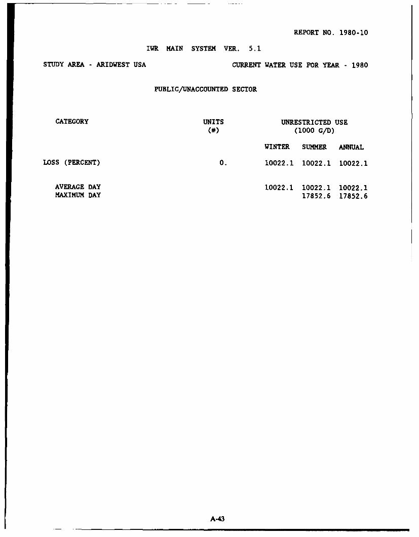
REPORT NO. 1980-10
IWR MAIN SYSTEM VER. 5.1
STUDY AREA - ARIDWEST USA CURRENT WATER USE FOR YEAR - 1980
PUBLIC/UNACCOUNTED SECTOR
CATEGORY UNITS UNRESTRICTED USE
(#) (1000 G/D)
WINTER SUMMER ANNUAL
LOSS (PERCENT) 0. 10022.1 10022.1 10022.1
AVERAGE DAY 10022.1 10022.1 10022.1MAXIMUM DAY 17852.6 17852.6
A43

REPORT NO. 1980-11
IWR MAIN SYSTEM VER. 5.1
STUDY AREA - ARIDWEST USA CURRENT WATER USE FOR YEAR - 1980
PUBLIC/UNACCOUNTED SECTOR
CATEGORY UNITS RESTRICTED USE
(#) (1000 G/D)
WINTER SUMMER ANNUAL
LOSS (PERCENT) 0. 10022.1 10022.1 10022.1
AVERAGE DAY 10022.1 10022.1 10022.1
MAXIMUM DAY 17852.6 17852.6
PERCENTAGE REDUCTIONS -
AVERAGE DAY .0 .0 .0
MAXIMUM DAY .0 .0
A44

REPORT NO. 1980-12
IWR MAIN SYSTEM VER. 5.1
STUDY AREA - ARIDWEST USA CURRENT WATER USE FOR YEAR - 1980
MUNICIPAL SUMMARY
UNRESTRICTED USE RESTRICTED USE(1000 G/D) (1000 G/D)
ANNUAL MAXIMUM ANNUAL MAXIMUMAVERAGE DAY* AVERAGE DAY*
RESIDENTIAL 54226. 117582. 52050. 112301.
COMMERCIAL/INSTL 23923. 23923. 23923. 23923.
INDUSTRIAL 2939. 2939. 2939. 2939.
PUBLIC/UNACCOUNTED 10022. 17853. 10022. 17853.
TOTAL MUNICIPAL 91110. 154466. 88934. 149185.
* NOTE: THE MAXIMUM DAY MUNICIPAL TOTAL IS THE SUM OF THE ANNUAL AVERAGEMUNICIPAL TOTAL AND THE LARGEST SECTORAL DIFFERENCE BETWEEN ANNUAL ANDMAXIMUM DAY USE.
PERCENTAGE REDUCTIONS
ANNUAL MAXIMUMAVERAGE DAY
RESIDENTIAL 4.0 4.5
COMMERCIAL/INSTL .0 .0
INDUSTRIAL .0 .0
PUBLIC/UNACCOUNTED .0 .0
TOTAL MUNICIPAL 2.4 3.4
A-45

REPORT NO. 1990- 2
IWR MAIN SYSTEM VER. 5.1
STUDY AREA - ARIDWEST USA PREDICTED WATER USE FOR YEAR - 1990
RESIDENTIAL SECTOR
FLAT RATE-SEWERED AREAS
VALUE RANGE UNITS UNRESTRICTED USE RESTRICTED USE($1000) (#) (GAL/DAY/UNIT) (GAL/DAY/UNIT)
(1980 VALUE)WINTER SUMMER ANNUAL WINTER SUMMER ANNUAL
.0 - 10.0 824. 112. 258. 185. 105. 246. 176.10.0 - 15.0 1137. 147. 447. 297. 138. 427. 282.15.0 - 20.0 1225. 155. 545. 350. 146. 521. 333.20.0 - 25.5 639. 156. 636. 396. 147. 608. 378.25.5 - 30.0 4576. 153. 714. 433. 144. 683. 414.30.0 - 35.0 1647. 153. 787. 470. 144. 753. 449.35.0 - 40.0 751. 165. 874. 520. 155. 837. 496.40.0 - 51.0 1505. 214. 1039. 626. 201. 995. 598.51.0 - 100.0 12. 282. 1509. 896. 266. 1445. 856.
TOTAL UNITS 12315.
AVERAGE DAY PER UNIT 158. 698. 428. 149. 668. 408.MAXIMUM DAY PER UNIT 1536. 1536. 1439. 1439.
- PERCENTAGE REDUCTIONS -
AVERAGE DAY 5.8 4.3 4.6MAXIMUM DAY 6.3 6.3
A-46

REPORT NO. 1990- 3
IWR MAIN SYSTEM VER. 5.1
STUDY AREA - ARIDWEST USA PREDICTED WATER USE FOR YEAR - 1990
RESIDENTIAL SECTOR
MASTER- METERED APARTMENTS
VALUE RANGE UNITS UNRESTRICTED USE RESTRICTED USE($1000) (#) (GAL/DAY/UNIT) (GAL/DAY/UNIT)
(1980 VALUE)WINTER SUMMER ANNUAL WINTER SUMMER ANNUAL
.0 - 10.0 4017. 112. 160. 136. 105. 152. 129.10.0 - 15.0 2869. 147. 210. 178. 138. 199. 169.15.0 - 20.0 3676. 155. 222. 188. 146. 210. 178.20.0 - 25.5 3152. 156. 224. 190. 147. 213. 180.25.5 - 30.0 20883. 153. 220. 186. 144. 208. 176.30.0 - 35.0 4262. 153. 219. 186. 144. 208. 176.35.0 - 40,0 4150. 165. 236. 201. 155. 224. 190.40.0 - 51.0 977. 214. 306. 260. 201. 291. 246.51.0 - 100.0 1048. 253. 363. 308. 239. 344. 292.
TOTAL UNITS 45033.
AVERAGE DAY PER UNIT 154. 221. 188. 145. 209. 177.MAXIMUM DAY PER UNIT 221. 221. 208. 208.
PERCENTAGE REDUCTIONS -
AVERAGE DAY 5.8 5.2 5.4MAXIMUM DAY 5.9 5.9
A-47

REPORT NO. 1990- 4
IWR MAIN SYSTEM VER. 5.1
STUDY AREA - ARIDWEST USA PREDICTED WATER USE FOR YEAR - 1990
RESIDENTIAL SECTOR
METERED- SEWERED AREAS
VALUE RANGE UNITS UNRESTRICTED USE RESTRICTED USE($1000) (#) (GAL/DAY/UNIT) (GAL/DAY/UNIT)
(1980 VALUE)WINTER SUMMER ANNUAL WINTER SUMMER ANNUAL
.0 - 10.0 5746. 200. 412. 306. 191. 394. 293.10.0 - 15.0 7084. 209. 524. 366. 199. 501. 350.15.0 - 20.0 10576. 216. 579. 397. 206. 554. 380.20.0 - 25.5 13531. 222. 580. 401. 212. 555. 384.25.5 - 30.0 13553. 228. 619. 424. 218. 592. 405.30.0 - 35.0 14489. 236. 653. 444. 225. 625. 425.35.0 - 40.0 11446. 243. 687. 465. 232. 657. 444.40.0 - 50.1 17929. 254. 734. 494. 242. 702. 472.51.0 - 60.0 8448. 269. 737. 503. 257. 705. 481.60.0 - 80.0 8627. 287. 804. 546. 274. 769. 522.'80.0 - 100.0 3637. 318. 893. 605. 303. 854. 579.
TOTAL UNITS 115065.
AVERAGE DAY PER UNIT 240. 655. 448. 229. 626. 428.MAXIMUM DAY PER UNIT 973. 973. 922. 922.
- PERCENTAGE REDUCTIONS -
AVERAGE DAY 4.6 4.3 4.4MAXIMUM DAY 5.3 5.3
A-48

REPORT NO. 1990- 5
IWR MAIN SYSTEM VER. 5.1
STUDY AREA - ARIDWEST USA PREDICTED WATER USE FOR YEAR - 1990
RESIDENTIAL SECTOR
SUMMARY
CATEGORY UNITS UNRESTRICTED USE RESTRICTED USE(#) (1000. G/D) (1000 G/D)
WINTER SUMMER ANNUAL WINTER SUMMER ANNUAL- AVERAGE DAY -
FLAT RATE/SWR 12315. 1950. 8592. 5271. 1837. 8223. 5030.APARTMENTS 45033. 6942. 9947. 8444. 6539. 9433. 7986.METERED/SEWRD 115065. 27661. 75332. 51497. 26385. 72060. 49222.
TOTALS 172413. 36553. 93871. 65212. 34761. 89716. 62238.
MAXIMUM DAY
RESIDENTIAL SECTOR 140789. 140789. 133123. 133123.
PERCENTAGE REDUCTIONS -
AVERAGE DAY 4.9 4.4 4.6MAXIMUM DAY 5.4 5.4
SUMMER EVAPOTRANSPIRATION (INCHES) - 18.24
SUMMER PRECIPITATION (INCHES) - 3.74
MAX. DAY EVAPOTRANSPIRATION (INCHES) - .29
A-49

REPORT NO. 1990- 6
IWR MAIN SYSTEM VER. 5.1
STUDY AREA - ARIDWEST USA PREDICTED WATER USE FOR YEAR - 1990
COMMERCIAL/INSTITUTIONAL SECTOR
CATEGORY TYPE OF UNITS UNRESTRICTED USE
UNIT (#) (1000 G/D)
WINTER SUMMER ANNUAL
MISC. COMMERCIAL EMPLOYEES 33301. 3213.6 3213.6 3213.6VOC. SCHOOLS EMPLOYEES 1145. 87.6 87.6 87.6MISC. RETAIL EMPLOYEES 14363. 382.5 382.5 382.5BOARDING HOUSES EMPLOYEES 51. 5.2 5.2 5.2TRANSP. TERMINAL EMPLOYEES 153. 28.8 28.8 28.8BARBER, CLEANING EMPLOYEES 1078. 1101.8 1101.8 1101.8LANDSCAPING EMPLOYEES 423. 45.2 45.2 45.2MISC. WHOLESALE EMPLOYEES 18371. 736.7 736.7 736.7RECREATION FACL. EMPLOYEES 310. 258.0 258.0 258.0FOOD AUTO RETAIL EMPLOYEES 10504. 1377.1 1377.1 1377.1DANCE STUDIOS EMPLOYEES 19. 1.3 1.3 1.3HOTELS, RESTRNTS EMPLOYEES 9675. 4782.6 4782.6 4782.6ELEC, GAS UTIL. EMPLOYEES 3568. 388.2 388.2 388.2PUBLIC ADMINIST. EMPLOYEES 63353. 7931.7 7931.7 7931.7SCHOOLS, UNIV. EMPLOYEES 11076. 3330.6 3330.6 3330.6LABS, WTR UTIL. EMPLOYEES 2397. 1061.6 1061.6 1061.6HEALTH SERVICES EMPLOYEES 647. 81.1 81.1 81.1MED. OFF. BAKERS EMPLOYEES 1766. 191.6 191.6 191.6NURSING FACIL. EMPLOYEES 519. 159.7 159.7 159.7HOSPITALS EMPLOYEES 4091. 836.0 836.0 836.0
TOTAL SECTOR EMPLOYMENT 176811.
AVERAGE DAY 26000.8 26000.8 26000.8MAXIMUM DAY 26000.8 26000.8
A-50

REPORT NO. 1990- 7
IWR MAIN SYSTEM VER. 5.1
STUDY AREA - ARIDWEST USA PREDICTED WATER USE FOR YEAR - 1990
COMMERCIAL/INSTITUTIONAL SECTOR
CATEGORY TYPE OF UNITS RESTRICTED USE
UNIT (#) (1000 G/D)
WINTER SUMMER ANNUAL
MISC. COMMERCIAL EMPLOYEES 33301. 3213.6 3213.6 3213.6VOC. SCHOOLS EMPLOYEES 1145. 87.6 87.6 87.6MISC. RETAIL EMPLOYEES 14363. 382.5 382.5 382.5BOARDING HOUSES EMPLOYEES 51. 5.2 5.2 5.2TRANSP. TERMINAL EMPLOYEES 153. 28.8 28.8 28.8BARBER, CLEANING EMPLOYEES 1078. 1101.8 1101.8 1101.8LANDSCAPING EMPLOYEES 423. 45.2 45.2 45.2MISC. WHOLESALE EMPLOYEES 18371. 736.7 736.7 736.7RECREATION FACL. EMPLOYEES 310. 258.0 258.0 258.0FOOD AUTO RETAIL EMPLOYEES 10504. 1377.1 1377.1 1377.1DANCE STUDIOS EMPLOYEES 19. 1.3 1.3 1.3HOTELS, RESTRNTS EMPLOYEES 9675. 4782.6 4782.6 4782.6ELEC, GAS UTIL. EMPLOYEES 3568. 388.2 388.2 388.2PUBLIC ADMINIST. EMPLOYEES 63353. 7931.7 7931.7 7931.7SCHOOLS, UNIV. EMPLOYEES 11076. 3330.6 3330.6 3330.6LABS, WTR UTIL. EMPLOYEES 2397. 1061.6 1061.6 1061.6HEALTH SERVICES EMPLOYEES 647. 81.1 81.1 81.1IED. OFF. BAKERS EMPLOYEES 1766. 191.6 191.6 191.6.URSING FACIL. EMPLOYEES 519. 159.7 159.7 159.7.OSPITALS EMPLOYEES 4091. 836.0 836.0 836.0
TOTAL SECTOR EMPLOYMENT 176811.
AVERAGE DAY 26000.8 26000.8 26000.8MAXIMUM DAY 26000.8 26000.8
- PERCENTAGE REDUCTIONS -
AVERAGE DAY .0 .0 .0MAXIMUM DAY .0 .0
A-51

REPORT NO. 1990- 8
IWR MAIN SYSTEM VER. 5.1
STUDY AREA - ARIDWEST USA PREDICTED WATER USE FOR YEAR - 1990
INDUSTRIAL SECTOR
SIC CATEGORY TYPE OF UNITS UNRESTRICTED USE
CODE UNIT (#) (1000 G/D)
WINTER SUMMER ANNUAL
201 MEAT PRODUCTS EMPLOYEES 248. 20.1 20.1 20.1202 DAIRY PRODUCTS EMPLOYEES 278. 103.3 103.3 103.3203 PRSRVD FRUITS, VEG EMPLOYEES 860. 169.9 169.9 169.9204 GRAIN MILL PRDCTS EMPLOYEES 462. 37.4 37.4 37.4205 BAKERY PRODUCTS EMPLOYEES 256. 20.7 20.7 20.7206 SUGAR & CONFECTNRY EMPLOYEES 33. 2.6 2.6 2.6207 FATS & OILS EMPLOYEES 49. 4.0 4.0 4.0208 BEVERAGES EMPLOYEES 269. 90.9 90.9 90.9209 MISC. FOODS, ETC. EMPLOYEES 247. 20.0 20.0 20.0225 KNITTING MILLS EMPLOYEES 26. 4.2 4.2 4.2228 YARN & THREAD MLLS EMPLOYEES 5. .2 .2 .2229 MISC. TEXTILE MILLS EMPLOYEES 128. 5.3 5.3 5.3230 APPAREL, ETC. EMPLOYEES 22344. 1418.9 1418.9 1418.9243 MILLWORK, PLYWOOD EMPLOYEES 687. 34.5 34.5 34.5244 WOOD CONTAINERS EMPLOYEES 12. .9 .9 .9245 WOOD BUILDINGS ETC EMPLOYEES 24. 1.8 1.8 1.8249 MISC. WOOD PRODCTS EMPLOYEES 36. 2.6 2.6 2.6251 HOUSEHOLD FRNITURE EMPLOYEES 97. 5.8 5.8 5.8254 PARTITIONS, FIXTRS EMPLOYEES 27. 1.6 1.6 1.6259 MISC. FURNITURE EMPLOYEES 11. .7 .7 .7264 MISC. CONY. PAPER EMPLOYEES 1009. 32.7 32.7 32.7265 PAPERBOARD CONTNRS EMPLOYEES 400. 22.6 22.6 22.6270 PRINTING, PUBLSHNG EMPLOYEES 2017. 76.4 76.4 76.4281 IND. ORGANIC CHEM. EMPLOYEES 4. .3 .3 .3282 PLASTICS, SYNTHTCS EMPLOYEES 23. 1.8 1.8 1.8283 DRUGS EMPLOYEES 30. 2.4 2.4 2.4285 PAINTS & ALLIED PR EMPLOYEES 212. 5.0 5.0 5.0287 AGRICULTURAL CHEM. EMPLOYEES 34. 2.2 2.2 2.2289 MISC. CHEM. PRDCTS EMPLOYEES 8. .6 .6 .6291 PETROLEUM REFINING EMPLOYEES 263. 16.1 16.1 16.1306 FABRIC.RUBBER, NEC EMPLOYEES 255. 74.1 74.1 74.1307 MISC. PLASTICS PRD EMPLOYEES 359. 25.9 25.9 25.9313 BOOT, SHOE STOCK EMPLOYEES 160. 3.7 3.7 3.7314 FOOTWEAR, EX. RUBR EMPLOYEES 3176. 74.0 74.0 74.0315 LEATHER GLOVES EMPLOYEES 68. 1.6 1.6 1.6319 LEATHER GOODS, NEC EMPLOYEES 10. .2 .2 .2323 PURCHASD GLASS PRD EMPLOYEES 6. .2 .2 .2324 HYDRAULIC CEMENT EMPLOYEES 176. 6.7 6.7 6.7325 STRUCTURL CLAY PRD EMPLOYEES 11. .4 .4 .4327 CONCRETE, GYPSUM EMPLOYEES 690. 26.4 26.4 26.4
A-52

CONTINUATION OF REPORT NO. 1990- 8
329 MISC.NONMET.MINERL EMPLOYEES 113. 5.7 5.7 5.7331 BLAST FURNC & STEL EMPLOYEES 683. 33.3 33.3 33.3332 IRON, STEEL FOUNDR EMPLOYEES 74. 3.6 3.6 3.6333 PRIMARY NONFERROUS EMPLOYEES 1909. 828.7 828.7 828.7335 NONFERROUS ROLLING EMPLOYEES 197. 9.6 9.6 9.6336 NONFERROUS FOUNDRY EMPLOYEES 183. 29.0 29.0 29.0344 STRUCTRL STEEL PRD EMPLOYEES 1298. 38.8 38.8 38.8345 SCREW MACHNE PRODS EMPLOYEES 15. .8 .8 .8346 METAL FORGINGS,ETC EMPLOYEES 14. .5 .5 .5347 METAL SERVICES,NEC EMPLOYEES 122. 65.1 65.1 65.1348 ORDNANCE & ACCESS. EMPLOYEES 63. 2.9 2.9 2.9349 MISC. FAB. METAL EMPLOYEES 18. .6 .6 .6351 ENGINES & TURBINES EMPLOYEES 73. 2.9 2.9 2.9354 METALWORKING MACH. EMPLOYEES 236. 76.7 76.7 76.7356 GENERAL IND. MACH. EMPLOYEES 687. 27.5 27.5 27.5358 REFRIGRATN & SERV. EMPLOYEES 334. 15.1 15.1 15.1359 MISC.MACH,EXC.ELEC EMPLOYEES 342. 11.9 11.9 11.9361 ELEC. DIST. EQUIP. EMPLOYEES 315. 9.9 9.9 9.9362 ELEC. IND. APPARTS EMPLOYEES 210. 8.4 8.4 8.4363 HOUSEHOLD APPLIANC EMPLOYEES 156. 5.3 5.3 5.3364 ELEC.LIGHTNG, WRNG EMPLOYEES 148. 3.9 3.9 3.9365 RADIO, TV RECEIVNG EMPLOYEES 368. 9.8 9.8 9.8366 COMMUNICATION EQPT EMPLOYEES 1914. 42.3 42.3 42.3367 ELECTR. COMPONENTS EMPLOYEES 2502. 173.9 173.9 173.9369 MISC.ELEC.EQUIPMNT EMPLOYEES 553. 19.3 19.3 19.3371 MOTOR VEHICLES,ETC EMPLOYEES 851. 43.6 43.6 43.6372 AIRCRAFT & PARTS EMPLOYEES 19. .5 .5 .5381 ENG.,SCIENCE INSTR EMPLOYEES 3. .1 .1 .1382 MEASURNG,CNTRL DEV EMPLOYEES 501. 10.3 10.3 10.3384 MEDICAL INSTRUMNTS EMPLOYEES 47. 1.3 1.3 1.3385 OPTHALMIC GOODS EMPLOYEES 332. 12.7 12.7 12.7391 JEWLERY,SILVERWARE EMPLOYEES 21. .3 .3 .3394 TOYS, SPORTING GDS EMPLOYEES 738. 80.6 80.6 80.6396 COSTUME JEWELRY EMPLOYEES 52. .7 .7 .7399 MISC. MANUFACTURES EMPLOYEES 46. .6 .6 .6
TOTAL SECTOR EMPLOYMENT 50147.
AVERAGE DAY 3894.8 3894.8 3894.8MAXIMUM DAY 3894.8 3894.8
A-53

REPORT NO. 1990- 9
IWR MAIN SYSTEM VER. 5.1
STUDY AREA - ARIDWEST USA PREDICTED WATER USE FOR YEAR - 1990
INDUSTRIAL SECTOR
SIC CATEGORY TYPE OF UNITS RESTRICTED USE
CODE UNIT (#) (1000 G/D)
WINTER SUMMER ANNUAL
201 MEAT PRODUCTS EMPLOYEES 248. 20.1 20.1 20.1202 DAIRY PRODUCTS EMPLOYEES 278. 103.3 103.3 103.3203 PRSRVD FRUITS, VEG EMPLOYEES 860 169.9 169.9 169.9204 GRAIN MILL PRDCTS EMPLOYEES 462 37.4 37.4 37.4205 BAKERY PRODUCTS EMPLOYEES 256 20.7 20.7 20.7206 SUGAR & CONFECTNRY EMPLOYEES 33 2.6 2.6 2.6207 FATS & OILS EMPLOYEES 49 4.0 4.0 4.0208 BEVERAGES EMPLOYEES 269 90.9 90.9 90.9209 MISC. FOODS, ETC. EMPLOYEES 247 20.0 20.0 20.0225 KNITTING MILLS EMPLOYEES 26 4.2 4.2 4.2228 YARN & THREAD MLLS EMPLOYEES 5 .2 .2 .2229 MISC. TEXTILE MLLS EMPLOYEES 128. 5.3 5.3 5.3230 APPAREL, ETC. EMPLOYEES 22344. 1418.9 1418.9 1418.9243 MILLWORK, PLYWOOD EMPLOYEES 687. 34.5 34.5 34.5244 WOOD CONTAINERS EMPLOYEES 12. .9 .9 .9245 WOOD BUILDINGS ETC EMPLOYEES 24. 1.8 1.8 1.8249 MISC. WOOD PRODCTS EMPLOYEES 36. 2.6 2.6 2.6251 HOUSEHOLD FRNITURE EMPLOYEES 97. 5.8 5.8 5.8254 PARTITIONS, FIXTRS EMPLOYEES 27. 1.6 1.6 1.6259 MISC. FURNITURE EMPLOYEES 11. .7 .7 .7264 MISC. CONV. PAPER EMPLOYEES 1009. 32.7 32.7 32.7265 PAPERBOARD CONTNRS EMPLOYEES 400. 22.6 22.6 22.6270 PRINTING, PUBLSHNG EMPLOYEES 2017. 76.4 76.4 76.4281 IND. ORGANIC CHEM. EMPLOYEES 4. .3 .3 .3282 PLASTICS, SYNTHTCS EMPLOYEES 23. 1.8 1.8 1.8283 DRUGS EMPLOYEES 30. 2.4 2.4 2.4285 PAINTS & ALLIED PR EMPLOYEES 212. 5.0 5.0 5.0287 AGRICULTURAL CHEM. EMPLOYEES 34. 2.2 2.2 2.2289 MISC. CHEM. PRDCTS EMPLOYEES 8. .6 .6 .6291 PETROLEUM REFINING EMPLOYEES 263. 16.1 16.1 16.1306 FABRIC.RUBBER, NEC EMPLOYEES 255. 74.1 74.1 74.1307 MISC. PLASTICS PRD EMPLOYEES 359. 25.9 25.9 25.9313 BOOT, SHOE STOCK EMPLOYEES 160. 3.7 3.7 3.7314 FOOTWEAR, EX. RUBR EMPLOYEES 3176. 74.0 74.0 74.0315 LEATHER GLOVES EMPLOYEES 68. 1.6 1.6 1.6319 LEATHER GOODS, NEC EMPLOYEES 10. .2 .2 .2323 PURCHASD GLASS PRD EMPLOYEES 6. .2 .2 .2324 HYDRAULIC CEMENT EMPLOYEES 176. 6.7 6.7 6.7325 STRUCTURL CLAY PRD EMPLOYEES 11. .4 .4 .4327 CONCRETE, GYPSUM EMPLOYEES 690. 26.4 26.4 26.4
A-54

CONTINUATION OF REPORT NO. 1990- 9
329 MISC.NONMET.MINERL EMPLOYEES 113. 5.7 5.7 5.7331 BLAST FURNC & STEL EMPLOYEES 683. 33.3 33.3 33.3332 IRON, STEEL FOUNDR EMPLOYEES 74. 3.6 3.6 3.6333 PRIMARY NONFERROUS EMPLOYEES 1909. 828.7 828.7 828.7335 NONFERROUS ROLLING EMPLOYEES 197. 9.6 9.6 9.6336 NONFERROUS FOUNDRY EMPLOYEES 183. 29.0 29.0 29.0344 STRUCTRL STEEL PRD EMPLOYEES 1298. 38.8 38.8 38.8345 SCREW MACHNE PRODS EMPLOYEES 15. .8 .8 .8346 METAL FORGINGS,ETC EMPLOYEES 14. .5 .5 .5347 METAL SERVICESNEC EMPLOYEES 122. 65.1 65.1 65.1348 ORDNANCE & ACCESS. EMPLOYEES 63. 2.9 2.9 2.9349 MISC. FAB. METAL EMPLOYEES 18. .6 .6 .6351 ENGINES & TURBINES EMPLOYEES 73. 2.9 2.9 2.9354 METALWORKING MACH. EMPLOYEES 236. 76.7 76.7 76.7356 GENERAL IND. MACH. EMPLOYEES 687. 27.5 27.5 27.5358 REFRIGRATN & SERV. EMPLOYEES 334. 15.1 15.1 15.1359 MISC.MACH,EXC.ELEC EMPLOYEES 342. 11.9 11.9 11.9361 ELEC. DIST. EQUIP. EMPLOYEES 315. 9.9 9.9 9.9362 ELEC. IND. APPARTS EMPLOYEES 210. 8.4 8.4 8.4363 HOUSEHOLD APPLIANC EMPLOYEES 156. 5.3 5.3 5.3364 ELEC.LIGHTNG, WRNG EMPLOYEES 148. 3.9 3.9 3.9365 RADIO, TV RECEIVNG EMPLOYEES 368. 9.8 9.8 9.8366 COMMUNICATION EQPT EMPLOYEES 1914. 42.3 42.3 42.3367 ELECTR. COMPONENTS EMPLOYEES 2502. 173.9 173.9 173.9369 MISC.ELEC.EQUIPMNT EMPLOYEES 553. 19.3 19.3 19.3371 MOTOR VEHICLES,ETC EMPLOYEES 851. 43.6 43.6 43.6372 AIRCRAFT & PARTS EMPLOYEES 19. .5 .5 .5381 ENG.,SCIENCE INSTR EMPLOYEES 3. .1 .1 .1382 MEASURNG,CNTRL DEV EMPLOYEES 501. 10.3 10.3 10.3384 MEDICAL INSTRUMNTS EMPLOYEES 47. 1.3 1.3 1.3385 OPTHALMIC GOODS EMPLOYEES 332. 12.7 12.7 12.7391 JEWLERY, SILVERWARE EMPLOYEES 21. .3 .3 .3394 TOYS, SPORTING GDS EMPLOYEES 738. 80.6 80.6 80.6396 COSTUME JEWELRY EMPLOYEES 52. .7 .7 .7399 MISC. MANUFACTURES EMPLOYEES 46. .6 .6 .6
TOTAL SECTOR EMPLOYMENT 50147.
AVERAGE DAY 3894.8 3894.8 3894.8MAXIMUM DAY 3894.8 3894.8
PERCENTAGE REDUCTIONS
AVERAGE DAY .0 .0 .0MAXIMUM DAY .0 .0
A-55

REPORT NO. 1990-10
IWR MAIN SYSTEM VER. 5.1
STUDY AREA - ARIDWEST USA PREDICTED WATER USE FOR YEAR - 1990
PUBLIC/UNACCOUNTED SECTOR
CATEGORY UNITS UNRESTRICTED USE
(#) (1000 G/D)
WINTER SUMMER ANNUAL
LOSS (PERCENT) 0. 11754.9 11754.9 11754.9
AVERAGE DAY 11754.9 11754.9 11754.9MAXIMUM DAY 21095.8 21095.8
A-56

REPORT NO. 1990-11
IWR MAIN SYSTEM VER. 5.1
STUDY AREA - ARIDWEST USA PREDICTED WATER USE FOR YEAR - 1990
PUBLIC/UNACCOUNTED SECTOR
CATEGORY UNITS RESTRICTED USE
(#) (1000 G/D)
WINTER SUMMER ANNUAL
LOSS (PERCENT) 0. 9614.4 9614.4 9614.4
AVERAGE DAY 9614.4 9614.4 9614.4
MAXIMUM DAY 17254.5 17254.5
PERCENTAGE REDUCTIONS -
AVERAGE DAY 18.2 18.2 18.2MAXIMUM DAY 18.2 18.2
A-57

REPORT NO. 1990-12
IWR MAIN SYSTEM VER. 5.1
STUDY AREA - ARIDWEST USA PREDICTED WATER USE FOR YEAR - 1990
MUNICIPAL SUMMARY
UNRESTRICTED USE RESTRICTED USE(1000 G/D) (1000 G/D)
ANNUAL MAXIMUM ANNUAL MAXIMUMAVERAGE DAY* AVERAGE DAY*
RESIDENTIAL 65212. 140789. 62238. 133122.
COMMERCIAL/INSTL 26001. 26001. 26001. 26001.
INDUSTRIAL 3895. 3895. 3895. 3895.
PUBLIC/UNACCOUNTED 11755. 21096. 9614. 17254.
TOTAL MUNICIPAL 106863. 182439. 101748. 172632.
* NOTE: THE MAXIMUM DAY MUNICIPAL TOTAL IS THE SUM OF THE ANNUAL AVERAGEMUNICIPAL TOTAL AND THE LARGEST SECTORAL DIFFERENCE BETWEEN ANNUAL ANDMAXIMUM DAY USE.
PERCENTAGE REDUCTIONS
ANNUAL MAXIMUMAVERAGE DAY
RESIDENTIAL 4.6 5.4
COMMERCIAL/INSTL .0 .0
INDUSTRIAL .0 .0
PUBLIC/UNACCOUNTED 18.2 18.2
TOTAL MUNICIPAL 4.8 5.4
A-58

REPORT NO. 2000- 2
IWR MAIN SYSTEM VER. 5.1
STUDY AREA - ARIDWEST USA PREDICTED WATER USE FOR YEAR - 2000
RESIDENTIAL SECTOR
FLAT RATE-SEWERED AREAS
VALUE RANGE UNITS UNRESTRICTED USE RESTRICTED USE
($1000) (#) (GAL/DAY/UNIT) (GAL/DAY/UNIT)
(1980 VALUE)WINTER SUMMER ANNUAL WINTER SUMMER ANNUAL
.0 - 10.0 1123. 112. 258. 185. 103. 244. 174.
10.0 - 15.0 1549. 147. 447. 297. 136. 423. 280.
15.0 - 20.0 1669. 155. 545. 350. 143. 517. 330.
20.0 - 25.5 871. 156. 636. 396. 145. 605. 375.
25.5 - 30.0 4696. 153. 714. 433. 142. 679. 410.
30.0 - 35.0 1690. 153. 787. 470. 141. 749. 445.
35.0 - 40.0 770. 165. 874. 520. 153. 833. 493.
40.0 - 51.0 1544. 214. 1039. 626. 198. 989. 593.
51.0 - 100.0 17. 282. 1509. 896. 261. 1438. 849.
TOTAL UNITS 13930.
AVERAGE DAY PER UNIT 157. 677. 417. 145. 644. 395.
MAXIMUM DAY PER UNIT 1498. 1498. 1376. 1376.
- PERCENTAGE REDUCTIONS -
AVERAGE DAY 7.5 4.9 5.4
MAXIMUM DAY 8.2 8.2
A-59

REPORT NO. 2000- 3
IWR MAIN SYSTEM VER. 5.1
STUDY AREA - ARIDWEST USA PREDICTED WATER USE FOR YEAR - 2000
RESIDENTIAL SECTOR
MASTER-METERED APARTMENTS
VALUE RANGE UNITS UNRESTRICTED USE RESTRICTED USE($1000) (#) (GAL/DAY/UNIT) (GAL/DAY/UNIT)
(1980 VALUE)WINTER SUMMER ANNUAL WINTER SUMMER ANNUAL
.0 - 10.0 5507. 112. 160. 136. 103. 150. 127.10.0 - 15.0 3933. 147. 210. 178. 136. 197. 166.15.0 - 20.0 5038. 155. 222. 188. 143. 207. 175.20.0 - 25.5 4320. 156. 224. 190. 145. 210. 177.25.5 - 30.0 21560. 153. 220. 186. 142. 206. 174.30.0 - 35.0 4400. 153. 219. 186. 141. 205. 173.35.0 - 40.0 4284. 165. 236. 201. 153. 221. 187.40.0 - 51.0 1009. 214. 306. 260. 198. 287. 242.51.0 - 100.0 1525. 253. 363. 308. 234. 340. 287.
TOTAL UNITS 51576.
AVERAGE DAY PER UNIT 154. 220. 187. 142. 206. 174.MAXIMUM DAY PER UNIT 220. 220. 203. 203.
- PERCENTAGE REDUCTIONS -
AVERAGE DAY 7.5 6.4 6.9MAXIMUM DAY 7.7 7.7
A-60

REPORT NO. 2000- 4
IWR MAIN SYSTEM VER. 5.1
STUDY AREA - ARIDWEST USA PREDICTED WATER USE FOR YEAR - 2000
RESIDENTIAL SECTOR
METERED- SEWERED AREAS
VALUE RANGE UNITS UNRESTRICTED USE RESTRICTED USE($1000) (#) (GAL/DAY/UNIT) (GAL/DAY/UNIT)
(1980 VALUE)WINTER SUMMER ANNUAL WINTER SUMMER ANNUAL
.0 - 10.0 7130. 200. 412. 306. 189. 392. 290.10.0 - 15.0 8791. 209. 524. 366. 198. 498. 348.15.0 - 20.0 13125. 216. 579. 397. 204. 551. 377.20.0 - 25.5 16791. 222. 580. 401. 210. 552. 381.25.5 - 30.0 14807. 228. 619. 424. 216. 588. 402.30.0 - 35.0 15830. 236. 653. 444. 223. 621. 422.35.0 - 40.0 12506. 243. 687. 465. 229. 653. 441.40.0 - 50.1 19589. 254. 734. 494. 240. 698. 469.51.0 - 60.0 9134. 269. 737. 503. 254. 701. 478.60.0 - 80.0 9328. 287. 804. 546. 272. 764. 518.80.0 - 100.0 3933. 318. 893. 605. 300. 849. 575.
TOTAL UNITS 130963.
AVERAGE DAY PER UNIT 239. 650. 444. 226. 618. 422.MAXIMUM DAY PER UNIT 963. 963. 901. 901.
PERCENTAGE REDUCTIONS -
AVERAGE DAY 5.5 4.9 5.1MAXIMUM DAY 6.4 6.4
A-61

REPORT NO. 2000- 5
IWR MAIN SYSTEM VER. 5.1
STUDY AREA - ARIDWEST USA PREDICTED WATER USE FOR YEAR - 2000
RESIDENTIAL SECTOR
SUMMARY
CATEGORY UNITS UNRESTRICTED USE RESTRICTED USE(#) (1000 G/D) (1000 G/D)
WINTER SUMMER ANNUAL WINTER SUMMER ANNUAL- AVERAGE DAY -
FLAT RATE/SWR 13930. 2187. 9429. 5808. 2023. 8969. 5496.APARTMENTS 51576. 7932. 11367. 9650. 7337. 10638. 8988.METERED/SEWRD 130963. 31330. 85096. 58213. 29607. 80915. 55261.
TOTALS 196469. 41449. 105892. 73671. 38967. 100522. 69745.
- MAXIMUM DAY -
RESIDENTIAL SECTOR 158371. 158371. 147672. 147672.
- PERCENTAGE REDUCTIONS -
AVERAGE DAY 6.0 5.1 5.3MAXIMUM DAY 6.8 6.8
SUMMER EVAPOTRANSPIRATION (INCHES) - 18.24
SUMMER PRECIPITATION (INCHES) - 3.74
MAX. DAY EVAPOTRANSPIRATION (INCHES) - .29
A-62

REPORT NO. 2000- 6
IWR MAIN SYSTEM VER. 5.1
STUDY AREA - ARIDWEST USA PREDICTED WATER USE FOR YEAR - 2000
COMMERCIAL/INSTITUTIONAL SECTOR
CATEGORY TYPE OF UNITS UNRESTRICTED USE
UNIT (#) (1000 G/D)
WINTER SUMMER ANNUAL
MISC. COMMERCIAL EMPLOYEES 44669. 4310.6 4310.6 4310.6VOC. SCHOOLS EMPLOYEES 1466. 112.1 112.1 112.1MISC. RETAIL EMPLOYEES 20340. 541.6 541.6 541.6BOARDING HOUSES EMPLOYEES 65. 6.6 6.6 6.6TRANSP. TERMINAL EMPLOYEES 199. 37.3 37.3 37.3BARBER, CLEANING EMPLOYEES 1380. 1410.7 1410.7 1410.7LANDSCAPING EMPLOYEES 476. 50.8 50.8 50.8MISC. WHOLESALE EMPLOYEES 23112. 926.8 926.8 926.8RECREATION FACL. EMPLOYEES 397. 330.3 330.3 330.3FOOD AUTO RETAIL EMPLOYEES 14875. 1950.2 1950.2 1950.2DANCE STUDIOS EMPLOYEES 24. 1.7 1.7 1.7HOTELS, RESTRNTS EMPLOYEES 12388. 6123.2 6123.2 6123.2ELEC, GAS UTIL. EMPLOYEES 4621. 502.8 502.8 502.8PUBLIC ADMINIST. EMPLOYEES 65801. 8238.3 8238.3 8238.3SCHOOLS, UNIV. EMPLOYEES 14181. 4264.2 4264.2 4264.2LABS, WTR UTIL. EMPLOYEES 3069. 1359.1 1359.1 1359.1HEALTH SERVICES EMPLOYEES 829. 103.8 103.8 103.8MED. OFF. BAKERS EMPLOYEES 2261. 245.3 245.3 245.3NURSING FACIL. EMPLOYEES 664. 204.4 204.4 204.4HOSPITALS EMPLOYEES 5237. 1070.3 1070.3 1070.3
TOTAL SECTOR EMPLOYMENT 216054.
AVERAGE DAY 31790.1 31790.1 31790.1MAXIMUM DAY 31790.1 31790.1
A-63

REPORT NO. 2000- 7
IWR MAIN SYSTEM VER. 5.1
STUDY AREA - ARIDWEST USA PREDICTED WATER USE FOR YEAR - 2000
COMMERCIAL/INSTITUTIONAL SECTOR
CATEGORY TYPE OF UNITS RESTRICTED USE
UNIT (#) (1000 G/D)
WINTER SUMMER ANNUAL
MISC. COMMERCIAL EMPLOYEES 44669. 4310.6 4310.6 4310.6VOC. SCHOOLS EMPLOYEES 1466. 112.1 112.1 112.1MISC. RETAIL EMPLOYEES 20340. 541.6 541.6 541.6BOARDING HOUSES EMPLOYEES 65. 6.6 6.6 6.6TRANSP. TERMINAL EMPLOYEES 199. 37.3 37.3 37.3BARBER, CLEANING EMPLOYEES 1380. 1410.7 1410.7 1410.7LANDSCAPING EMPLOYEES 476. 50.8 50.8 50.8MISC. WHOLESALE EMPLOYEES 23112. 926.8 926.8 926.8RECREATION FACL. EMPLOYEES 397. 330.3 330.3 330.3FOOD AUTO RETAIL EMPLOYEES 14875. 1950.2 1950.2 1950.2DANCE STUDIOS EMPLOYEES 24. 1.7 1.7 1.7HOTELS, RESTRNTS EMPLOYEES 12388. 6123.2 6123.2 6123.2ELEC, GAS UTIL. EMPLOYEES 4621. 502.8 502.8 502.8PUBLIC ADMINIST. EMPLOYEES 65801. 8238.3 8238.3 8238.3SCHOOLS, UNIV. EMPLOYEES 14181. 4264.2 4264.2 4264.2LABS, WTR UTIL. EMPLOYEES 3069. 1359.1 1359.1 1359.1HEALTH SERVICES EMPLOYEES 829. 103.8 103.8 103.8MED. OFF. BAKERS EMPLOYEES 2261. 245.3 245.3 245.3NURSING FACIL. EMPLOYEES 664. 204.4 204.4 204.4HOSPITALS EMPLOYEES 5237. 1070.3 1070.3 1070.3
TOTAL SECTOR EMPLOYMENT 216054.
AVERAGE DAY 31790.1 31790.1 31790.1MAXIMUM DAY 31790.1 31790.1
- PERCENTAGE REDUCTIONS -
AVERAGE DAY .0 .0 .0MAXIMUM DAY .0 .0
A-64

REPORT NO. 2000- 8
IWR MAIN SYSTEM VER. 5.1
STUDY AREA - ARIDWEST USA PREDICTED WATER USE FOR YEAR - 2000
INDUSTRIAL SECTOR
SIC CATEGORY TYPE OF UNITS UNRESTRICTED USE
CODE UNIT (#) (1000 G/D)
WINTER SUMMER ANNUAL
201 MEAT PRODUCTS EMPLODYEES 214. 17.3 17.3 17.3202 DAIRY PRODUCTS EMPLOYEES 239. 89.0 89.0 89.0203 PRSRVD FRUITS, VEG EMPLOYEES 1116. 220.4 220.4 220.4204 GRAIN MILL PRDCTS EMPLOYEES 600. 48.6 48.6 48.6205 BAKERY PRODUCTS EMPLOYEES 220. 17.9 17.9 17.9206 SUGAR & CONFECTNRY EMPLOYEES 28. 2.3 2.3 2.3207 FATS & OILS EMPLOYEES 42. 3.4 3.4 3.4208 BEVERAGES EMPLOYEES 232. 78.4 78.4 78.4209 MISC. FOODS, ETC. EMPLOYEES 213. 17.2 17.2 17.2225 KNITTING MILLS EMPLOYEES 40. 6.4 6.4 6.4228 YARN & THREAD MLLS EMPLOYEES 7. .4 .4 .4229 MISC. TEXTILE MLLS EMPLOYEES 195. 8.0 8.0 8.0230 APPAREL, ETC. EMPLOYEES 28686. 1821.6 1821.6 1821.6243 MILLWORK, PLYWOOD EMPLOYEES 590. 29.7 29.7 29.7244 WOOD CONTAINERS EMPLOYEES 10. .8 .8 .8245 WOOD BUILDINGS ETC EMPLOYEES 21. 1.5 1.5 1.5249 MISC. WOOD PRODCTS EMPLOYEES 31. 2.2 2.2 2.2251 HOUSEHOLD FRNITURE EMPLOYEES 111. 6.6 6.6 6.6254 PARTITIONS, FIXTRS EMPLOYEES 31. 1.8 1.8 1.8259 MISC. FURNITURE EMPLOYEES 13. .8 .8 .8264 MISC. CONV. PAPER EMPLOYEES 1230. 39.9 39.9 39.9265 PAPERBOARD CONTNRS EMPLOYEES 455. 25.7 25.7 25.7270 PRINTING, PUBLSHNG EMPLOYEES 2249. 85.3 85.3 85.3281 IND. ORGANIC CHEM. EMPLOYEES 7. .4 .4 .4282 PLASTICS, SYNTHTCS EMPLOYEES 36. 2.8 2.8 2.8283 DRUGS EMPLOYEES 46. 3.7 3.7 3.7285 PAINTS & ALLIED PR EMPLOYEES 328. 7.7 7.7 7.7287 AGRICULTURAL CHEM. EMPLOYEES 52. 3.4 3.4 3.4289 MISC. CHEM. PRDCTS EMPLOYEES 13. .9 .9 .9291 PETROLEUM REFINING EMPLOYEES 360. 22.0 22.0 22.0306 FABRIC.RUBBER, NEC EMPLOYEES 263. 76.7 76.7 76.7307 MISC. PLASTICS PRD EMPLOYEES 371. 26.8 26.8 26.8313 BOOT, SHOE STOCK EMPLOYEES 197. 4.6 4.6 4.6314 FOOTWEAR, EX. RUBR EMPLOYEES 3896. 90.8 90.8 90.8315 LEATHER GLOVES EMPLOYEES 83. 1.9 1.9 1.9319 LEATHER GOODS, NEC EMPLOYEES 12. .3 .3 .3323 PURCHASD GLASS PRD EMPLOYEES 6. .2 .2 .2324 HYDRAULIC CEMENT EMPLOYEES 176. 6.8 6.8 6.8325 STRUCTURL CLAY PRD EMPLOYEES 11. .4 .4 .4327 CONCRETE, GYPSUM EMPLOYEES 692. 26.5 26.5 26.5
A-65

CONTINUATION OF REPORT NO. 2000- 8
329 MISC.NONMET.MINERL EMPLOYEES 113. 5.7 5.7 5.7331 BLAST FURNC & STEL EMPLOYEES 718. 35.0 35.0 35.0332 IRON, STEEL FOUNDR EMPLOYEES 56. 2.7 2.7 2.7333 PRIMARY NONFERROUS EMPLOYEES 2006. 870.8 870.8 870.8335 NONFERROUS ROLLINC EMPLOYEES 148. 7.2 7.2 7.2336 NONFERROUS FOUNDRY EMPLOYEES 138. 21.8 21.8 21.8344 STRUCTRL STEEL PRD EMPLOYEES 1679. 50.2 50.2 50.2345 SCREW MACHNE PRODS EMPLOYEES 20. 1.0 1.0 1.0346 METAL FORGINGS,ETC EMPLOYEES 18. .6 .6 .6347 METAL SERVICES,NEC EMPLOYEES 157. 84.2 84.2 84.2348 ORDNANCE & ACCESS. EMPLOYEES 82. 3.8 3.8 3.8349 MISC. FAB. METAL EMPLOYEES 24. .8 .8 .8351 ENGINES & TURBINES EMPLOYEES 93. 3.7 3.7 3.7354 METALWORKING MACH. EMPLOYEES 299. 97.3 97.3 97.3356 GENERAL IND. MACH. EMPLOYEES 872. 35.0 35.0 35.0358 REFRIGRATN & SERV. EMPLOYEES 424. 19.1 19.1 19.1359 MISC.MACH,EXC.ELEC EMPLOYEES 434. 15.1 15.1 15.1361 ELEC. DIST. EQUIP. EMPLOYEES 417. 13.1 13.1 13.1362 ELEC. IND. APPARTS EMPLOYEES 278. 11.1 11.1 11.1363 HOUSEHOLD APPLIANC EMPLOYEES 206. 7.0 7.0 7.0364 ELEC.LIGHTNG, WRNG EMPLOYEES 196. 5.2 5.2 5.2365 RADIO, TV RECEIVNG EMPLOYEES 487. 12.9 12.9 12.9366 COMMUNICATION EQPT EMPLOYEES 2533. 56.0 56.0 56.0367 ELECTR. COMPONENTS EMPLOYEES 3311. 230.1 230.1 230.1369 MISC.ELEC.EQUIPMNT EMPLOYEES 732. 25.5 25.5 25.5371 MOTOR VEHICLES,ETC EMPLOYEES 1200. 61.4 61.4 61.4372 AIRCRAFT & PARTS EMPLOYEES 27. .7 .7 .7381 ENG.,SCIENCE INSTR EMPLOYEES 7. .3 .3 .3382 MEASURNG,CNTRL DEV EMPLOYEES 616. 12.7 12.7 12.7384 MEDICAL INSTRUMNTS EMPLOYEES 107. 3.0 3.0 3.0385 OPTHALMIC GOODS EMPLOYEES 752. 28.8 28.8 28.8391 JEWLERY,SILVERWARE EMPLOYEES 13. .2 .2 .2394 TOYS, SPORTING GDS EMPLOYEES 455. 49.7 49.7 49.7396 COSTUME JEWELRY EMPLOYEES 32. .4 .4 .4399 MISC. MANUFACTURES EMPLOYEES 28. .4 .4 .4
TOTAL SECTOR EMPLOYMENT 61801.
AVERAGE DAY 4573.3 4573.3 4573.3MAXIMUM DAY 4573.3 4573.3
A-66

REPORT NO. 2000- 9
IWR MAIN SYSTEM VER. 5.1
STUDY AREA - ARIDWEST USA PREDICTED WATER USE FOR YEAR - 2000
INDUSTRIAL SECTOR
SIC CATEGORY TYPE OF UNITS RESTRICTED USE
CODE UNIT (#) (1000 G/D)
WINTER SUMMER ANNUAL
201 MEAT PRODUCTS EMPLOYEES 214. 17.3 17.3 17.3202 DAIRY PRODUCTS EMPLOYEES 239. 89.0 89.0 89.0203 PRSRVD FRUITS, VEG EMPLOYEES 1116. 220.4 220.4 220.4204 GRAIN MILL PRDCTS EMPLOYEES 600. 48.6 48.6 48.6205 BAKERY PRODUCTS EMPLOYEES 220. 17.9 17.9 17.9206 SUGAR & CONFECTNRY EMPLOYEES 28. 2.3 2.3 2.3207 FATS & OILS EMPLOYEES 42. 3.4 3.4 3.4208 BEVERAGES EMPLOYEES 232. 78.4 78.4 78.4209 MISC. FOODS, ETC. EMPLOYEES 213. 17.2 17.2 17.2225 KNITTING MILLS EMPLOYEES 40. 6.4 6.4 6.4228 YARN & THREAD MLLS EMPLOYEES 7. .4 .4 .4229 MISC. TEXTILE MLLS EMPLOYEES 195. 8.0 8.0 8.0230 APPAREL, ETC. EMPLOYEES 28686. 1821.6 1821.6 1821.6243 MILLWORK, PLYWAOOD EMPLOYEES 590. 29.7 29.7 29.7244 WOOD CONTAINERS EMPLOYEES 10. .8 .8 .8245 WOOD BUILDINGS ETC EMPLOYEES 21. 1.5 1.5 1.5249 MISC. WOOD PRODCTS EMPLOYEES 31. 2.2 2.2 2.2251 HOUSEHOLD FRNITURE EMPLOYEES ill. 6.6 6.6 6.6254 PARTITIONS, FIXTRS EMPLOYEES 31. 1.8 1.8 1.8259 MISC. FURNITURE EMPLOYEES 13. .8 .8 .8264 MISC. CONV. PAPER EMPLOYEES 1230. 39.9 39.9 39.9265 PAPERBOARD CONTNRS EMPLOYEES 455. 25.7 25.7 25.7270 PRINTING, PUBLSHNG EMPLOYEES 2249. 85.3 85.3 85.3281 IND. ORGANIC CHEM. EMPLOYEES 7. .4 .4 .4282 PLASTICS, SYNTHTCS EMPLOYEES 36. 2.8 2.8 2.8283 DRUGS EMPLOYEES 46. 3.7 3.7 3.7285 PAINTS & ALLIED PR EMPLOYEES 328. 7.7 7.7 7.7287 AGRICULTURAL CHEM. EMPLOYEES 52. 3.4 3.4 3.4289 MISC. CHEM. PRDCTS EMPLOYEES 13. .9 .9 .9291 PETROLEUM REFINING EMPLOYEES 360. 22.0 22.0 22.0306 FABRIC.RUBBER, NEC EMPLOYEES 263. 76.7 76.7 76.7307 MISC. PLASTICS PRD EMPLOYEES 371. 26.8 26.8 26.8313 BOOT, SHOE STOCK EMPLOYEES 197. 4.6 4.6 4.6314 FOOTWEAR, EX. RUBR EMPLOYEES 3896. 90.8 90.8 90.8315 LEATHER GLOVES EMPLOYEES 83. 1.9 1.9 1.9319 LEATHER GOODS, NEC EMPLOYEES 12. .3 .3 .3323 PURCHASD GLASS PRD EMPLOYEES 6. .2 .2 .2324 HYDRAULIC CEMENT EMPLOYEES 176. 6.8 6.8 6.8325 STRUCTURL CLAY PRD EMPLOYEES 11. .4 .4 .4327 CONCRETE, GYPSUM EMPLOYEES 692. 26.5 26.5 26.5
A-67

CONTINUATION OF REPORT NO. 2000- 9
329 MISC.NONMET.MINERL EMPLOYEES 113. 5.7 5.7 5.7331 BLAST FURNC & STEL EMPLOYEES 718. 35.0 35.0 35.0332 IRON, STEEL FOUNDR EMPLOYEES 56. 2.7 2.7 2.7333 PRIMARY NONFERROUS EMPLOYEES 2006. 870.8 870.8 870.8335 NONFERROUS ROLLING EMPLOYEES 148. 7.2 7.2 7.2336 NONFERROUS FOUNDRY EMPLOYEES 138. 21.8 21.8 21.8344 STRUCTRL STEEL PRD EMPLOYEES 1679. 50.2 50.2 50.2345 SCREW MACHNE PRODS EMPLOYEES 20. 1.0 1.0 1.0346 METAL FORGINGS,ETC EMPLOYEES 18. .6 .6 .6347 METAL SERVICES,NEC EMPLOYEES 157. 84.2 84.2 84.2348 ORDNANCE & ACCESS. EMPLOYEES 82. 3.8 3.8 3.8349 MISC. FAB. METAL EMPLOYEES 24. .8 .8 .8351 ENGINES & TURBINES EMPLOYEES 93. 3.7 3.7 3.7354 METALWORKING MACH. EMPLOYEES 299. 97.3 97.3 97.3356 GENERAL IND. MACH. EMPLOYEES 872. 35.0 35.0 35.0358 REFRIGRATN & SERV. EMPLOYEES 424. 19.1 19.1 19.1359 MISC.MACH,EXC.ELEC EMPLOYEES 434. 15.1 15.1 15.1361 ELEC. DIST. EQUIP. EMPLOYEES 417. 13.1 13.1 13.1362 ELEC. IND. APPARTS EMPLOYEES 278. 11.1 11.1 11.1363 HOUSEHOLD APPLIANC EMPLOYEES 206. 7.0 7.0 7.0364 ELEC.LIGHTNG, WRNG EMPLOYEES 196. 5.2 5.2 5.2365 RADIO, TV RECEIVNG EMPLOYEES 487. 12.9 12.9 12.9366 COMMUNICATION EQPT EMPLOYEES 2533. 56.0 56.0 56.0367 ELECTR. COMPONENTS EMPLOYEES 3311. 230.1 230.1 230.1369 MISC.ELEC.EQUIPMNT EMPLOYEES 732. 25.5 25.5 25.5371 MOTOR VEHICLES,ETC EMPLOYEES 1200. 61.4 61.4 61.4372 AIRCRAFT & PARTS EMPLOYEES 27. .7 .7 .7381 ENG.,SCIENCE INSTR EMPLOYEES 7. .3 .3 .3382 MEASURNGCNTRL DEV EMPLOYEES 616. 12.7 12.7 12.7384 MEDICAL INSTRUMNTS EMPLOYEES 107. 3.0 3.0 3.0385 OPTHAUIIC GOODS EMPLOYEES 752. 28.8 28.8 28.8391 JEWLERY,SILVERWARE EMPLOYEES 13. .2 .2 .2394 TOYS, SPORTING GDS EMPLOYEES 455. 49.7 49.7 49.7396 COSTUME JEWELRY EMPLOYEES 32. .4 .4 .4399 MISC. MANUFACTURES EMPLOYEES 28. .4 .4 .4
TOTAL SECTOR EMPLOYMENT 61801.
AVERAGE DAY 4573.3 4573.3 4573.3
MAXIMUM DAY 4573.3 4573.3
PERCENTAGE REDUCTIONS -
AVERAGE DAY .0 .0 .0MAXIMUM DAY .0 .0
A-68

REPORT NO. 2000-10
IWR MAIN SYSTEM VER. 5.1
STUDY AREA - ARIDWEST USA PREDICTED WATER USE FOR YEAR - 2000
PUBLIC/UNACCOUNTED SECTOR
CATEGORY UNITS UNRESTRICTED USE(#) (1000 G/D)
WINTER SUMMER ANNUAL
LOSS (PERCENT) 0. 13599.7 13599.7 13599.7
AVERAGE DAY 13599.7 13599.7 13599.7MAXIMUM DAY 24068.3 24068.3
A-69

REPORT NO. 2000-11
IWR MAIN SYSTEM VER. 5.1
STUDY AREA - ARIDWEST USA PREDICTED WATER USE FOR YEAR - 2000
PUBLIC/UNACCOUNTED SECTOR
CATEGORY UNITS RESTRICTED USE
(#) (1000 G/D)
WINTER SUMMER ANNUAL
LOSS (PERCENT) 0. 9887.0 9887.0 9887.0
AVERAGE DAY 9887.0 9887.0 9887.0
MAXIMUM DAY 17497.7 17497.7
- PERCENTAGE REDUCTIONS -
AVERAGE DAY 27.3 27.3 27.3MAXIMUM DAY 27.3 27.3
A-70

REPORT NO. 2000-12
IWR MAIN SYSTEM VER. 5.1
STUDY AREA - ARIDWEST USA PREDICTED WATER USE FOR YEAR - 2000
MUNICIPAL SUMMARY
UNRESTRICTED USE RESTRICTED USE(1000 G/D) (1000 G/D)
ANNUAL MAXIMUM ANNUAL MAXIMUMAVERAGE DAY* AVERAGE DAY*
RESIDENTIAL 73670. 158371. 69744. 147672.
COMMERCIAL/INSTL 31790. 31790. 31790. 31790.
INDUSTRIAL 4573. 4573. 4573. 4573.
PUBLIC/UNACCOUNTED 13600. 24068. 9887. 17498.
TOTAL MUNICIPAL 123633. 208334. 115995. 193922.
* NOTE: THE MAXIMUM DAY MUNICIPAL TOTAL IS THE SUM OF THE ANNUAL AVERAGEMUNICIPAL TOTAL AND THE LARGEST SECTORAL DIFFERENCE BETWEEN ANNUAL ANDMAXIMUM DAY USE.
PERCENTAGE REDUCTIONS
ANNUAL MAXIMUMAVERAGE DAY
RESIDENTIAL 5.3 6.8
COMMERCIAL/INSTL .0 .0
INDUSTRIAL .0 .0
PUBLIC/UNACCOUNTED 27.3 27.3
TOTAL MUNICIPAL 6.2 6.9
A-71

SUMMARY REPORT NO. 13
IWR MAIN SYSTEM
VER. 5.1
STUDY AREA - ARIDWEST USA
(1000 GALLONS PER DAY)
......................... UNRESTRICTED USE ............... RESTRICTED USE ........
RUN ANNUAL MAXIMUM ANNUAL MAXIMUMNO. YEAR AVERAGE DAY AVERAGE DAY
.................................. oe~~o*........eeoe*oe**............o°.
1 1980 91110. 154466. 88934. 149185.2 1990 106863. 182439. 101748. 172632.3 2000 123633. 208334. 115995. 193922.
...................................... ... e . . . ,......,A-f..* ..l. ...
A-72

EXHIBIT A-4 CONSERVATION OUTPUT (.COV) FILECOVERAGE FACTORS SPECIFIED BY USER AND COMPUTED FROM
LIBRARY OF CONSERVATION COEFFICIENTSAND
EFFECTIVENESS OF MEASURES BY SECTOR AND DIMENSION
ONLY SELECTED MEASURES ARE INCLUDED. VALUES FOR UNSELECTED SECTORS OF SELECTEDMEASURES ARE SET TO 0.000.
COVERAGE FACTORS FOR YEAR: 1980.
SECTORS: RESIDENTIAL COMMERCL INDUSTRL PUBLIC UNACCOUNTMEASURES METERED UNMETERD APARTMNT & OTHER
EDUCATION .950 .950 .950 .000 .000 .000 .000LEAK REPAIR .000 .000 .000 .000 .000 .000 .000MODERATE CODE .097 .097 .097 .000 .000 .000 .000LANDSCAPE-NEW .077 .077 .077 .000 .000 .000 .000
EFFECTIVENESS OF MEASURES FOR YEAR: 1980.(1000 GALLONS PER DAY)
SECTORS: RESIDENTIAL COMMERCL INDUSTRL PUBLIC UNACCOUNTMEASURES METERED UNMETERD APARTMNT & OTHER
EDUCATIONINDOOR 794.493 50.214 178.538 .000 .000 .000 .000OUTDOOR 1347.907 134.308 77.307 .000 .000 .000 .000MAX-DAY 3226.341 427.400 255.846 .000 .000 .000 .000
LEAK REPAIRINDOOR .000 .000 .000 .000 .000 .000 .000OUTDOOR .000 .000 .000 .000 .000 .000 .000MAX-DAY .000 .000 .000 .000 .000 .000 .000
MODERATE CODEINDOOR 183.104 22.266 79.169 .000 .000 .000 .000OUTDOOR .000 .000 .000 .000 .000 .000 .000MAX-DAY 743.563 189.521 113.449 .000 .000 .000 .000
LANDSCAPE-NEWINDOOR .000 .000 .000 .000 .000 .000 .000OUTDOOR 162.316 9.953 4.118 .000 .000 .000 .000MAX-DAY 388.519 31.673 13.627 .000 .000 .000 .000
TOTAL EFFECTIVENESSINDOOR 977.596 72.480 257.708 .000 .000 .000 .000OUTDOOR 1510.223 144.261 81.425 .000 .000 .000 .000MAX-DAY 4358.423 648.594 382.922 .000 .000 .000 .000
IMPACT OF INTERACTION FACTORSINDOOR .000 .000 .000 .000 .000 .000 .000OUTDOOR .000 .000 .000 .000 .000 .000 .000MAX-DAY .000 .000 .000 .000 .000 .000 .000
ADJUSTED EFFECTIVENESSINDOOR 977.596 72.480 257.708 .000 .000 .000 .000OUTDOOR 1510.223 144.261 81.425 .000 .000 .000 .000MAX-DAY 4358.423 648.594 382.922 .000 .000 .000 .000
--------------------------------------------------------------------
A-73

COVERAGE FACTORS FOR YEAR: 1990.
SECTORS: RESIDENTIAL COMMERCL INDUSTRL PUBLIC UNACCOUNTMEASURES METERED UNMETERD APARTMNT & OTHER
EDUCATION .950 .950 .950 .000 .000 .000 .000LEAK REPAIR .000 .000 .000 .000 .000 .000 .667MODERATE CODE .163 .163 .163 .000 .000 .000 .000LANDSCAPE-NEW .166 .166 .166 .000 .000 .000 .000
EFFECTIVENESS OF MEASURES FOR YEAR: 1990.(1000 GALLONS PER DAY)
SECTORS: RESIDENTIAL COMMERCL INDUSTRL PUBLIC UNACCOUNTMEASURES METERED UNMETERD APARTMNT & OTHER
EDUCATIONINDOOR 919.740 64.835 230.806 .000 .000 .000 .000OUTDOOR 1585.050 220.859 99.939 .000 .000 .000 .000MAX-DAY 3721.604 628.880 330.744 .000 .000 .000 .000
LEAK REPAIRINDOOR .000 .000 .000 .000 .000 .000 1712.368OUTDOOR .000 .000 .000 .000 .000 .000 428.092MAX-DAY .000 .000 .000 .000 .000 .000 3841.359
MODERATE CODEINDOOR 356.195 48.311 171.983 .000 .000 .000 .000OUTDOOR .000 .000 .000 .000 .000 .000 .000MAX-DAY 1441.296 468.605 246.452 .000 .000 .000 .000
LANDSCAPE-NEWINDOOR .000 .000 .000 .000 .000 .000 .000OUTDOOR 411.493 35.284 11.476 .000 .000 .000 .000MAX-DAY 966.162 100.469 37.978 .000 .000 .000 .000
TOTAL EFFECTIVENESSINDOOR 1275.935 113.147 402.789 .000 .000 .000 1712.368OUTDOOR 1996.544 256.144 111.414 .000 .000 .000 428.092MAX-DAY 6129.062 1197.954 615.175 .000 .000 .000 3841.359
IMPACT OF INTERACTION FACTORSINDOOR .000 .000 .000 .000 .000 .000 .000OUTDOOR .000 .000 .000 .000 .000 .000 .000MAX-DAY .000 .000 .000 .000 .000 .000 .000
ADJUSTED EFFECTIVENESSINDOOR 1275.935 113.147 402.789 .000 .000 .000 1712.368OUTDOOR 1996.544 256.144 111.414 .000 .000 .000 428.092MAX-DAY 6129.062 1197.954 615.175 .000 .000 .000 3841.359
A-74

COVERAGE FACTORS FOR YEAR: 2000.
SECTORS: RESIDENTIAL COMMERCL INDUSTRL PUBLIC UNACCOUNTMEASURES METERED UNMETERD APARTMNT & OTHER
EDUCATION .950 .950 .950 .000 .000 .000 .000LEAK REPAIR .000 .000 .000 .000 .000 .000 1.000MODERATE CODE .275 .275 .275 .000 .000 .000 .000LANDSCAPE-NEW .240 .240 .240 .000 .000 .000 .000
EFFECTIVENESS OF MEASURES FOR YEAR: 2000.(1000 GALLONS PER DAY)
SECTORS: RESIDENTIAL COMMERCL INDUSTRL PUBLIC UNACCOUNTMEASURES METERED UNMETERD APARTMNT & OTHER
EDUCATIONINDOOR 1041.709 72.715 263.747 .000 .000 .000 .000OUTDOOR 1787.724 240.802 114.202 .000 .000 .000 .000MAX-DAY 4193.862 694.033 377.949 .000 .000 .000 .000
LEAK REPAIRINDOOR .000 .000 .000 .000 .000 .000 2970.168OUTDOOR .000 .000 .000 .000 .000 .000 742.542MAX-DAY .000 .000 .000 .000 .000 .000 6570.656
MODERATE CODEINDOOR 680.635 91.414 331.567 .000 .000 .000 .000OUTDOOR .000 .000 .000 .000 .000 .000 .000MAX-DAY 2740.200 872.498 475.136 .000 .000 .000 .000
LANDSCAPE-NEWINDOOR .000 .000 .000 .000. .000 .000 .000OUTDOOR 671.001 55.620 18.959 .000 .000 .000 .000MAX-DAY 1574.117 160.306 62.745 .000 .000 .000 .000
TOTAL EFFECTIVENESSINDOOR 1722.344 164.129 595.314 .000 .000 .000 2970.168OUTDOOR 2458.725 296.422 133.162 .000 .000 .000 742.542MAX-DAY 8508.180 1726.837 915.830 .000 .000 .000 6570.656
IMPACT OF INTERACTION FACTORSINDOOR .000 .000 .000 .000 .000 .000 .000OUTDOOR .000 .000 .000 .000 .000 .000 .000MAX-DAY -.001 .000 .000 .000 .000 .000 .000
ADJUSTED EFFECTIVENESSINDOOR 1722.344 164.129 595.314 .000 .000 .000 2970.168OUTDOOR 2458.725 296.422 133.162 .000 .000 .000 742.542MAX-DAY 8508.181 1726.837 915.830 .000 .000 .000 6570.656
A-75

APPENDIX B
HISTORICAL DEVELOPMENTOF THE IWR-MAIN SYSTEM

HISTORICAL DEVELOPMENT OF THE IWR-MAIN SYSTEM
MAIN I
The IWR-MAIN System was based on the MAIN System developed by Hittman Associates, Inc., in thelate 1960s for the U.S. Office of Water Resources Research. The MAIN (versions 1.0,1.1, and 2.0) ForecastingSystem was in turn based on earlier work by Howe and Linaweaver (1967), Wolff et al. (1966), and otherinvestigators. Most of these investigators were involved with the Residential and Commercial Water UseResearch Projects carried on at the Johns Hopkins University. These two studies generated the best water usedata to date. The work of the investigators of the Residential Water Use Research Project resulted in significantinsights into the explanatory factors affecting residential water use. The data base consists of observations onaverage values for water use and socioeconomic and climatic characteristics for 39 residential areas served by16 water utilities. Recordings of water consumption in 15-minute intervals were taken for periods ranging fromtwo to three years during 1961-63. These were later aggregated to hourly, daily, seasonal, and annual figures.In-house (domestic) and summer-sprinkling (outdoor) uses were separated. Howe and Linaweaver (1967) usedthis massive data base to estimate demand models for the eastern and western parts of the country. Thesedemand models were considered to be among the best predictive equations of residential water demand.
The MAIN System was intended to provide a computer-based program which would allow the preparationof disaggregate water use forecasts using the best models and approaches available at the time. Research fromthe Johns Hopkins University and Howe and Linaweaver (1967), as well as data gathered from the U.S. Census,American Water Works Association, and others, resulted in a series of sophisticated models of water use. TheMAIN System was sectorally disaggregated in that it allowed for independent calculations of water estimatesfor metered and flat rate sewered residences, commercial establishments, manufacturing categories (by SICcodes), and public/unaccounted water requirements. Version 2.0 of the MAIN System, also known as MAINI, provided growth models to project water use parameters used in these calculations.
IWR-MAIN
In the early 1980s, the Institute for Water Resources (IWR), U.S. Army Corps of Engineers, selected theMAIN System as a tool for improving water use forecasting practices within the Corps and renamed it the IWR-MAIN Water Use Forecasting System. Major modifications to the IWR-MAIN System (versions 2.1 to 2.3)included:
(1) Changes in the computer program to allow operation on time-shared computer systems.
(2) Changes in the residential model and other socioeconomic coefficients to accept values in 1980constant dollars.
In 1985 the IWR-MAIN System (versions 2.4 to 3.2) underwent substantial modifications which included:
(1) Development of a PC version to allow for IBM or compatible personal computer use.
(2) Replacement of water use computational models with new models and coefficients based on dataand research literature available in 1984:
a. Residential Sector: demand models were changed to reflect new estimates by Howe (1982)based on the addition of the bill difference variable.
B-i

b. Commercial/Institutional Sector: unit use parameters for this sector were changed fromestablishment characteristics (e.g., square footage of offices, car stalls of drive-ins, seats ofrestaurants) to employment parameters for commercial categories (COxx) based on SICgroupings of nonmanufacturing establishments.
c. Industrial Sector. parameter unit use coefficients were updated based on the 19Z Censusof Manufacturers: Water Use in Manufacturinf survey.
d. Public/Unaccounted Sector: changes were made allowing the option of calculatingdistribution losses as a specified fraction of total water use.
(3) Elimination of peak-hour water use and the metered and septic tank residential category. A
category for master-metered apartments was added.
(4) Various changes in displays of the PC version and the mainframe interfaces.
Version 4.0, released in 1986, contained completely respecified and reestimated internal growth models.These econometric models were based on historical Census data gathered at the SMSA (Standard MetropolitanStatistical Area) level for the years 1960,1970, and 1980 (housing data) and 1972,1979, and 1982 (employmentdata). Modifications to the PC version included changes in the data entry screens, editing, execution, and theoutput of reports.
Version 5.0, released in 1987, provided a new conservation subroutine allowing the option of computingrestricted water use based on conservation measures. The industrial sector water use coefficients were updatedto reflect the 1982 Census of Manufacturers: Water Use in Manufacturing Slight enhancements were also madeto the PC version.
Version 5.1, released in December, 1987, provides an expanded number of entries in the externalprojection screens, a nonresidential price adjustment factor, a residential metered summer weather adjustmentfactor for calibration purposes, revised commercial and industrial coefficients, the computation of conservationeffectiveness by individual measure, new save file options, a more efficient print/view routine, and more detailedhelp files. Utilities were also added for converting data files from previous versions to the current data file formatand for conversion from a .DAT file to a data file. See Table B-1 for a complete historical development of theIWR-MAIN System.
B-2

TABLE B-1
SUMMARY OF RELEASED AND UNRELEASED IWR-MAIN SYSTEM VERSIONS
Version Generic Release Application Author, Documentation, NotesNo. Name Date
1.0 MAIN I 1968 Estimating M&I water use Hittman Associates, Inc.,(no internal forecasting Columbia, MDcapability)
Report HIT-336, "MAIN I - A Sys-tem of Computerized Models forCalculating and Evaluating Munici-pal Water Requirements," 2 vols.,June 1968
Program written in ANSI FOR-TRAN IV (FORTRAN 66) for batchprocessing on mainframe computers
Water use computational modelsbased on data and literature availablein 1967 Note: Computer program
and documentation contained errors
1.1 MAIN I 1968 Estimating M&I water use Hittman Associates, Inc.,(no internal forecasting Columbia, MDcapability)
Report HIT-336 (addendum) "Ad-dendum to Final Report - MAIN I -A System of Computerized Modelsfor Calculating and Evaluating Mu-nicipal Water Requirements," Octo-ber 1969
Release 1.0 errors corrected
2.0 MAIN H 1969 Estimating & forecasting Hittman Associates, Inc.,M&I water use (limited internal Columbia, MDforecasting capability)
Report HIT-413, "ForecastingMunicipal Water Requirements -The MAIN 11 System," 2 vols., Sep-tember 1969
Water use computational modelsunchanged from release 1.1; twointernal and one external forecastingmethods added
B-3

TABLE B-I (Continued)
Version Generic Release Application Author, Documentation, NotesNo. Name Date
2.1 IWR-MAIN 1982 Estimating & forecasting Institute for Water Resources,M&I water use (limited internal US. Army Corps of Engineers,forecasting capability) Fort Belvoir, VA
[no published documentation]
Similar to release 2.0, modified foruse on CDC computer at BoeingComputer Service Co. (batch proces-sing)
2.2 IWR-MAIN 1983 Estimating & forecasting Institute for Water Resources,M&I water use (imited U.S. Army Corps of Engineers,internal forecasting Fort Belvoir, VAcapability)
"Forecasting Municipal and Indus-trial Water Use: IWR-MAIN SystemUser's Guide for Interactive Process-ing and User's Manual," researchreport 83R-3 July 1983
Residential model coefficients modi-fied to accept prices and housingvalues in 1980 dollars.
External procedures IWREDIT,IWRRUN, and IWRPRNT providedto facilitate data loading, execution,and report generation on Boeingsystem (quasiinteractive mode)
2.3 IWR-MAIN 1984 Estimating & forecasting Institute for Water Resources,M&I water use (limited U.S. Army Corps of Engineers,internal forecasting Fort Belvoir, VAcapability)
[documentation not released]
Similar to release 2.2, modified foruse on CDC Cybernet System
B-4

TABLE B-1 (Continued)
Version Generic Release Application Author, Documentation, NotesNo. Name Date
2.4 IWR-MAIN 1985 Estimating & forecasting Institute for Water Resources,M&I water use (limited U.S. Army Corps of Engineers,internal forecasting Fort Belvoir, VAcapability)
[documentation not released]
Similar to release 23, modified foruse on IBM or IBM-compatible per-sonal computer
Interactive user interface provided tofacilitate data entry, editing, execu-tion, and report generation (e.g.,IWREDIT, IWRRUN, andIWRPRINT)
3.0 IWR-MAIN 1985 Estimating M&I water use Institute for Water Resources,(internal forecasting U.S. Army Corps of Engineers,capability deactivated) Fort Belvoir, VA
[documentation not released]
Water use computational modelsreplaced with new models based on
data and literature available in 1984;commercial/institutional and indus-trial categories revised
Calculation of peak hour water useomitted; minor changes to displays;metered-septic tank residential cate-
gory deleted, category added formaster-metered apartments; op-tional method of calculating distribu-tion losses added; provision made foruser input of climatic data; internalparameter projection proceduresoperational for residential sectoronly
B-5

TABLE B-1 (Continued)
Version Generic Release Application Author, Documentation, NotesNo. Name Date
3.1 IWR-MAIN 1985 Estimating M&I water use Institute for Water Resources,(internal forecasting US. Army Corps of Engineers,capability deactivated) Fort Belvoir, VA
[documentation not released]
Similar to version 3.0, except ma-chine-specific UNPACK subroutineeliminated, new nonspecificDCODE subroutine provided; in-creased error-checking for input andlibrary data
3.2 IWR-MAIN 1985 Estimating M&I water use Institute for Water Resources,(internal forecasting U.S. Army Corps of Engineers,capability deactivated) Fort Belvoir, VA
[documentation not released]
Similar to version 3.0, modified foruse on IBM or IBM-compatible per-sonal computer
Interactive user interface provided tofacilitate data entry, editing, execu-tion, and report generation
4.0 IWR-MAIN 1986 Estimating & forecasting Institute for Water Resources,M&I water use (fully U.S. Army Corps of Engineers,operative and complete Fort Belvoir, VAinternal forecasting capability)
[documentation not released]
This version is for both mainframeand IBM-compatible PC applica-tions
Provided new, complete internalforecasting procedures, similar tothose in versions 2.x, except based ondata and research available in 1985.External procedures IWREDIT,IWRRUN, and IWRPRNT nolonger supported. Interactive userinterface provided for PC applica-tions to facilitate data entry, editing,and execution. New utility providedfor report review and generation
B-6

TABLE B-1 (Continued)
Version Geueric Release Application Author, Documentation, NotesNo. Name Date
5.0 lWR-MAIN 1987 Estimating & forecast- Institute for Water Resources,ing M&I water use and U.S. Army Corps of Engineers,evaluation of conservation Fort Belvoir, VAmeasures (fully operative andcomplete internal forecasting "IWR-MAIN Water Use Forecast-capability) ing System: User's Manual and Sys-
tem Description," two parts, March1987
Water Conservation Algorithmadded. Changes in industrial sectorwater use coefficients reflecting 1982data
Enhancements made to the PersonalComputer version including dataentry, editing, execution, and outputreporting
5.1 IWR-MAIN 1987 Estimating & forecast- Institute for Water Resources,ing M&I water use and U.S. Army Corps of Engineers,evaluation of conser- Fort Belvoir, VAvation measures(fully operative and "IWR-MAIN Water Use Forecast-complete internal fore- ing System: User's Manual and Sys-casting capability) tem Description," two parts, Decem-
ber 1987
Expansion of external projectionscreens. Updated nonresidentialcoefficients and nonresidential priceadjustment factor added. Residen-tial summer weather adjustment fac-tor added for calibration purposes.Computation of effectiveness of indi-vidual conservation measures added.More efficient Print/View routineprovided and new utilities added.
B-7

APPENDIX C
TECHNICAL EXHIBITS
Exhibit C-i: Description and Use of the IWR-MAIN Utilities
Exhibit C-2: Description of the IWR-MAIN Execution, Batch, andData Files
Exhibit C-3: IWR-MAIN System Flow Chart Diagrams

WI5A N OULTIES
DlATA BPASE
An (;',r . 4cliles for graphic displayor other data rr!- c it~ 11 a U:jble name DBASE (data-,cr.,n I. )has -in~ i or ti,e f -eCcast will be written toa data K-wfile -ti
-1i PR"" -~z ij r each selected forecast year.Ths ae ~~-)'i v -hc re, iential summary results,
hoWPc-,tf. are -T
Trhe PRN rca W.-I' 1! iIrm iis a standard ASCII formatfile which can c5v' rk: t~ z. .1ismg the appropriate software
rlivro-Tmn. 11.' "-i flu .ila. 1 uscd as aguide for inserting labelsto yeur work heu ic
UATA FILE CON!-.'FERSI~ 10l !'
The data File eo~i) ~,Prtr>rans which will (1) convert adata file(without. extension ~erj~~d~~WR WM 5 to a data file foir use with version 5.1 and (2)convert a version'~I_ i C('h'O1 ~e~o)
To convert an (".d %vers on Jta e ~ w. inert diskette #6 into drive A: or use theprogram from vour ha.-.i2~ At !hr l-i
The progrm will as;k !t. c i wi. -'- r
where d: i, Jriz'e, pec; '' :,7 'T*',,_ 'k.:v-on;40) r 5.0) of IWR-MAIN wasused to gene,.see the h FAt.
The (c)NvEp r t1i;1,,w'il i -o ii me - -ie c 'itc of the data file and save the new5.1 I' ;rsion ti n-icr~c~ ic2 ci. ot Lie ,Ioii data file will be saved under the

The second data file conversion utility essentially reverses the Edit/Validate procedure in that it generatesa data file without extension from a .DAT file. Thus, if changes have been made in the version 5.1 .DAT filewith a text editor, the file may be reverted back to a data file which can be loaded into the Data Entry screens.To use this utility, insert diskette #6 into drive A: or use the program from your hard drive. At the DOS prompt:
type REVERTpress RETURN
The program will then ask for the filename of the .DAT file from which to generate the data file. You need notenter the extension (.DAT) as this is assumed. The program will reverse the formatting process and save thenew data file under the same filename without an extension. If an old data file of the same name (withoutextension) exists, the old data file will be renamed with the extension .OLD. Thus, the .DAT file will remainunchanged, and the data file of the same- name without extension will be your new data file.
EXTERNAL PROJECTION MODULE
The External Projection ModLe was set up as a reference data bank for use with the IWR-MAIN System.It contains county-level forecasts of population, employment (aggregate and/or disaggregate), housing units,and income. Where no county-level forecasts are available, state and regional forecasts are provided. TableC-2 presents the list of usable projections that were collected and received during a 1985 survey.
These projections are coded in a format readable by the External Projection Module. To access this
module, insert Diskette #5 in drive A: or load the entire contents of the diskette onto a hard drive and type:
A > PROJECT
The user is then asked to enter a state code number (must be two digits) or a two-character state abbreviation.(i.e., IL, AR, OK). Entering "QQ" terminates the Projection Module. Table C-3 lists all the states containedin the projection module, the projection type available, the state code number, and the source and publicationyear of the projection data.
For anyselected state, the module will fist the available projection types. The user has the option of viewingone of the listed projection tyes by entering:
"P* for population projections"H" for housing projections"!" for income projectimns"E" for employment projeitmtims
or alternately may chtKose another state by entering "Q". Once a projection type has been selected, the modulewill indicate how many lines of data are available. If you wish to view these data, enter the range of lines youwish to examine. For example, for the state of Illinois, there are 500 lines of population projection data available.If you want to view the first 20 lines, enter #1, #2(1 (or 1, 20). This will result in the first 20 lines of data to scrollacross the screen. If you only wish to view tne first line, enter #1, #1. A range must be provided, and a commamust separate the range.
If the population file is ak.cesed in the External Projection Module, datawillbe presented inthe followingformat:
R CODE BS YfvAN-POPUI.fN Y.AR-PoPUI.N'4 YFAR-POPULTN YEAR-POPULTN YEAR-POPULTN1 001 P 80 1-;. 0071701 19'J 0074498 1995 0076228 2000 0077205 2005 00788741 001 P 80 2010 i) ', 64 2015 o(i2155 2020 0084205 2025 0086512i 003 P 80 1,Y?5 i 31237 19%) (V)12472 1995 0012619 2000 0013070 2005 0013653I 003 P 80 2010 1)14211 2015 0014698 2020 0016139 2025 0017184
C-2

"R" specifies the aggregation level of the data such that R = I indicates county-level data, R =2 indicates state-level data, and R = 3 indicates SMSA-level data. "CODE" specifies a numeric code for a county or SMSA withinthe selected state (see Table C-4 for a listing of select county codes). "P" indicates that the presented data areprojections rather than historical data. "BS" specifies the base year of the projection data. These entries arethen followed by a forecast year and its population projection. The combination of year/projection is repeatedfor as many years as projection data are available. Depending upon the number of projection years, data fora specific county may exceed one line.
If the housing projection file is accessed, data will be presented in the following format:
R CODE BS YEAR-HOUSING YEAR-HOUSING YEAR-HOUSING YEAR-HOUSING YEAR-HOUSING1 001 P 80 1990 0011200 2000 00129001 003 P 80 1990 0119000 2000 01314001 005 P 80 1990 0027600 2000 00312001 007P 80 1990 0003500 2000 0003600
Definitions of the variables are the same as for population, except that housing units are the measuredparameter.
If the income projection file is accessed, data will be presented in the following format:
R CODE BS YEAR-INCME YEAR-INCME YEAR-INCME YEAR-INCME YEAR-INCME YEAR-INCME1 007 P 72 1985 05373 1990 06138 1995 06895 2000 076871 019 P 72 1985 05221 1990 05841 1995 06563 2000 073811 027 P 72 1985 04781 1990 05413 1995 06127 2000 069431 031 P 72 1965 06851 1990 07663 1995 08597 2000 093911 043 P 72 1985 07495 1990 08384 1995 09405 2000 1C275
Definition of these variables are the same as for population and housing, except that "BS" indicates the year ofthe dollar values, and personal income (in "BS" year dollar values) is the measured parameter.
If the employment projection file is accessed, data will be presented in the following format:
R CODE BS YEAR SIC-EMPLMT SIC-EMPLMT SIC-EMPLMT SIC-EMPLMT SIC-EMPLMT1 007 P so 1985 0001 012318 0002 036315 1500 000056 1600 000191 1700 0001161 007 P so 1985 0003 005909 2000 000640 2300 000059 2400 000002 2700 0000731 007P 80 1985 2800 000019 3000 000178 3300 000164 3400 000146 3500 0006141 007 P so 1985 3700 003557 3800 000006 3900 000451 0004 000593 4700 0003411 007 P so 1985 4800 000236 4900 000016 0005 000300 0006 001061 0007 000401I 007P so 1985 0008 001480 7200 000100 0009 0012241 007 P so 1990 0001 013311 0002 000414 1500 000064 1600 000217 1700 0001331 007 P so 1990 0003 006538 2000 000603 2300 000063 2400 000003 2700 0000771 007 P 80 1990 2800 000022 3000 000189 3300 000185 3400 000155 3500 0006671 007 P 80 1990 3700 004072 3800 000007 3900 000495 0004 000623 4700 000363
Definitions of these variables are the same as for population except for "SIC-EMPLMT." Also, the projectionyear is only specified once per line and, therefore, any data presented on that line reflects the same specifiedforecast year. The disaggregation level of employment projections varied from state to state; some states projectonly total employment whereas others project employment by major industry sectors (construction, manufac-turing, services) or by two-digit SIC codes. Therefore, for each forecast year, employment ("EMPLMT") maybe provided at various disaggregation levels as defimed by the codes labeled in the "SIC" category. Table C-5provides the definitions of the "SIC" variable codes.
After a projection file has been viewed for a particular state, enter "0,0" to se lect anot her projection file. Thenselect another projection file to view for the state or enter "'0 to chooe 'mother state. At this point, enter astate code or eater "Q Q' to exit the projection module.
C-3

Line 1-25 -- R~iei
Line 1 - Base vIa.;
co; umL -. "at -k -- go'-
C~ii~fliifl r - I..I! wac usc, and
,mc,;num n-
Columns iA- ,~--
Columns -X
Lies 2-25 -- Foi;:casr Y-ar ck.-;
Columns as ahcv -
Lines 26-50 -- Nonresidtni4, - nJ
Line 26 - Base year re, 1 !
Columns 1-3 - -Qcryin- 1 i'A~ tO-., r-c i nloy.yncn in cateszory,coluI nn r.-:2 a i i *,i - ul, "t T U.)S pc I i ve tIV~.
Columns 4-6 - IndustH~ -thcgcr rfj, 4 L, r~~'Vni in cat%,grv; columns 5-6 areaverage annua; :c) mAxra -r' -)
Columns 7 -9 - Pi-Ii- ii.c:c m- ~' r vrgan
and inja.xi'w u.,!
Columns i0-L 1 I'i LA.- ; jcn *Lr C01uinn11S 11-12 areaverageck ~ i ia- ~ -~
Lines 27-50 - Foreciast:a c -~f, ui
Coiumn; ss
*The formnat of Lines 1 -30 -7! I(A. -- ~ Note thait allwater use is given in galloiis ;x: di,

TABLE C-2
IWR.MAIN EXTERNAL PROJEC-nONS
POPULATION HOUSING EMPLOYMENT INCOME
Alabama-C Arkansas-C Af kansas-C Illu.ois-CArizona-C California-C Delaware-C New Mexico-CArkansas-C District of District of Hawaii-CCalifornia-C Columbia-SM Columbia-,SM N. Carolina-STColorado-C Indiana-C Hawaii-CDelaware-C Maryland-C Iffinois-CDistrict of Minnesota-C Maryland-CColumbia-SM Wisconsin-C New Mexico-C
Florida-C N. Carolina-STHawaii-C Tennessee-STIllinois-C Utah-STIndiana-CIowa-CKentucky-CLouisiana-CMaine-CMaryland-CMinnesota-CMontana-CNebraska-CNevada-CNew Jersey-CNew Mexico-CNorth Carolina-CNorth Dakota-COhio-COregon-CPennsylvania-CSouth Carolina-CTennessee-CTexas-CUtah-CVermont-CVirginia-CWashington-STWisconsin-C
C = county SM =SMSA ST= state

TABLE C-3
INDEX FILE FOR IWR-MAIN PARAMETER PROJECTIONS
00 - DISTRICT OF COLUMBIA:P - COOP Forecasting, Round I Technical Report - 1984. Sent by Metropolitan Policy Program,
Metropolitan Washington Council of Governors.H - COOP Forecasting, Round III Technical Report - 1984. Sent by Metropolitan Policy Program,
Metropolitan Council of Governors.E - COOP Forecasting, Round Ill Technical Report - 1984. Sent by Metropolitan Policy Program,
Metropolitan Council of Governors.
01 - ALABAMA:P - Standard Population Projections: Alabama Counties - 1983. By Department of Economic and
Community Affairs, Montgomery, Alabama 36130.
04 - ARIZONA:P - Arizona Department of Economic Security, Population Statistics Unit - 1984.
05 - ARKANSAS:P - Arkansas Population Projections to 1990, by County- Research Memorandum. By Industrial
Research Center, University of Arkansas.H - Projections for Jefferson County. By Southeast Arkansas Regional Planning Commission, ?ine
Bluff.E - Projections for Jefferson County. By Southeast Arkansas Regional Planning Commission, Pine
Bluff.
06 - CALIFORNIA:P - California Population Projections: Report 83 P-i, Population Research Unit, 1025 P Street,
Sacramento, California. 1983.H - Household Projections for California Counties, Population Research Unit, 1025 P Street,
Sacramento, California. 1984.
08 - OLORADO:P - Printout. Demographic Section of the Colorado Division of Local Governments. Department of
Local Affairs, Denver, CO.
10 - DELAWARE:P - Delaware Population Consortium. Sent by Delaware Development Office, Dover.E - College of Urban Affairs and Public Policy. Sent by Delaware Development Office, Dover.
12- FLORIDA:P - 1980 Base Year, Population Projection (low estimate), Executive Office of Governor, Tallahas-
see.
C-6

TABLE C-3 (Continued)
15 - HAWAII:P - Population and Economic Projections for Hawaii, 1980-2005. By the Department of Planning and
Economic Development. 1984.E - Employment Projections. By Department of Planning and Economic Development. 1984.
17 - ILLINOIS:P - Illinois Population Trends 1970-2025. Bureau of the Budget. 1984.E - Employment Projections. Bureau of the Budget. 1984I - Economic Projections. Bureau of the Budget. 1984.
18 - INDIANA:P - Indiana Business Review, Volume 58, 1983.H - Indiana Business Review, Volume 65, 1984.
19 - IOWA:P - Population Projections. By Office of State Demographer, Office for Planning and Management.
1984.
21 - KENTUCKY:P - How Many Kentuckians: Population Forecast, 1980-2020. 1984. By Urban Studies Center,
College of Urban and Public Affairs, University of Louisville.
22 - LOUISIANA:P - Middle - Population Projections. By University of New Orleans, Division of Business and
Economic Research.
23 - MAINE:P - Population Projections. By Bureau of Health, Planning and Development. 1984.
24 - MARYLAND:P - Population Projections 1980-2000, Report 1, 1984. By Maryland Department of State Planning.H - Projections of Housing Demand, Number, and Size. By Maryland Department of State Planning.
1984.E - Employment in Maryland, Trends and Projections 1967-2000. By Maryland Department of State
Planning. 1984.
27 - MINNESOTA:P - Population Notes, Minnesota. Department of Energy and Planning. 1982.H - Low-Estimate Housing Projections. By State Demography Unit, Minnesota State Planning
Agency. 1983.
C-7

TABLE C-3 (Continued)
30 - MONTANA:P - Montana County Population Projections. By Census and Economic Information Center, Montana
Department of Commerce. 1983.
31- NEBRASKA:P - County Projections (Medium Series). By Bureau of Business Research, University of Nebraska-
Lincoln. 1982.
32- NEVADA:P - Population Projections. By Bureau of Business and Business and Economic Research. 1983.
34 - NEW JERSEY:P - Revised Total and Age and Sex Population Projections 1985-2000. By Office of Demographic and
Economic Analysis, Department of Labor, Trenton, NJ. 1983.
35 - NEW MEXICO:P - Population Projections. By Bureau of Business and Economic Research, Institute for Applied
Research Services. 1983.E - Employment Projections. By Bureau of Business and Economic Research, University of New
Mexico. 1983.I - Economic Projections. By Bureau of Business and Economic Research, University of New
Mexico. 1983.
37 - NORTH CAROLINA:P - Population Projections. By North Carolina Long-Term Economic-Demographic Projection 1985.
Office of State Budget and Management.E - State Employment Projections. By Office of State Budget and Management. 1984.
38 - NORTH DAKOTA:P - Population Projections (Low Estimate). By AG Economics Statistical Series. Issue No. 39. 1982.
39 - OHIO:P - Ohio Data Center, Department of Development. 1983.
41 - OREGON:P - Population Projections: Oregon and Counties: 1980-2000. By School of Urban and Public Affairs,
Portland State University. 1983.
42 - PENNSYLVANIA:P - 1970,80, 90 Population by Sex and Age: County Detail. By Department of Health, State Health
Data Center, 1984.
C"-9

TABLE C-3 (Continued)
45 - SOUTH CAROLINA:P - Population Projections by County- 1985-2000. By South Carolina State Data Center. 1984.
47 -TENNESSEE:P - Population Projections (Low Projection-Series #3). By Department of Sociology, University of
Tennessee, Knoxville. 1983.E - State Employment Projections. By Tennessee Employment Projections 1984-1990. 1984.
48 -TEXAS:P - Population and Projections for the State of Texas 1970-2000. By Texas Department of Water
Resources. 1982.
49 -UTAH:P - Utah Base-Line Provisional Population Projections Table 9. 1983.E - State Employment Projections. Utah Process Economic & Demographic Projections. 1984.
50 - VERMONT:P - Vermont Population Projections: 1985-2000. By Vermont Department of Health, State Planning
Office. 1983.
51 - VIRGINIA:P - Virginia Population Projections to 2000. By Department of Planning and Research, Richman, VA.
1983.
53 - WASHINGTON:P - Forecasts of State Population by Sex and Age: 1985-2010. 1984.
55 - WISCONSIN:P - Projections of Population. By Demographic Services Center, Wisconsin Department of Admini-
stration. 1983.H - Projected Total Households. By Demographic Services Center, Department of Administration.
1984.
P = population, E = employment, H = housing, and I = income
Note that Washington D.C. was the only SMSA forecast and therefore has a state code of "00".
C-9

TABLE C-4
INDEX OF SELECT STATE AND COUNTY CODES
ALABAMA01 003 Baldwin 01 097 Mobile01 051 Elmore 01 101 Montgomery01 055 Etowah 01 113 Russell01 073 Jefferson 01 117 Shelby01 083 Limestone 01 125 Tuscaloosa01 089 Madison 01 127 Walker
ARIZONA04 013 Maricopa 04 019 Pima
ARKANSAS05 033 Crawford 05 119 Pulaski05 035 Crittenden 05 125 Saline05 069 Jefferson 05 131 Sebastian05 091 Miller
CALIFORNIA06 001 Alameda 06 071 San Bernardino06 013 Contra Costa 06 073 San Diego06 019 Fresno 06 073 San Francisco06 029 Kern 06 077 San Joaquin06 037 Los Angeles 06 081 San Mateo06 041 Main 06 083 Santa Barbara06 053 Monterey 06 085 Santa Clara06 055 Napa 06 095 Solano06 059 Orange 06 097 Sonoma06 061 Placer 06 099 Stanislaus06 065 Riverside 06 111 Ventura06 067 Sacramento 06 113 Yolo
COLORADO08 001 Adams 08 041 El Paso08 005 Arapahoe 08 059 Jefferson08 013 Boulder 08 101 Pueblo08 031 Denver
CONNECTICUT09 001 Fairfield 09 007 Middlesex09 003 Hartford 09 009 New Haven09 005 Litchfield 09 013 Tolland
DELAWARE10 003 New Castle
C-10

TABLE C-4 (Continued)
FLORIDA12 001 Alachua 12 073 Leon12 011 Broward 12 095 Orange12 025 Dade 12 099 Palm Beach12 031 Duval 12 103 Pinellas12 033 Escambia 12 113 Santa Rosa12 057 Hillsborough 12 117 Seminole
GEORGIA13 021 Bibb 13 095 Dougherty13 051 Chatham 13 121 Fulton13 053 Chattahoochee 13 135 Gwinnett13 063 Clayton 13 153 Houston13 067 Cobb 13 510 Columbus City13 089 De Kalb 13 245 Richmond
HAWAII15 003 Honolulu
IDAHO16 001 Ada
ILULNOIS17 007 Boone 17 119 Madison17 019 Champaign 17 143 Peoria17 031 Cook 17 163 St Clair17 042 Du Page 17 167 Sangamon17 089 Kane 17 179 Tazewell17 111 McHenry 17 197 Will17 113 McLean 17 201 Winnebago17 115 Macon 17 203 Woodford
INDIANA18 003 Allen 18 099 Marshall18 011 Boone 18 097 Marion18 019 Clark 18 109 Morgan18 021 Clay 18 127 Porter18 029 Dearborn 18 141 St Joseph18 035 Delaware 18 145 Shelby18 043 Floyd 18 153 Sullivan18 057 Hamilton 18 157 Tippecanoe18 059 Hancock 18 163 Vanderburgh18 063 Hendricks 18 165 Vermilion18 081 Johnson 18 167 Vico18 089 Lake 18 173 Warrick18 095 Madison
IOWA19 013 Black Hawk 19 155 Pottawattamie19 061 Dubuque 19 193 Woodbury19 153 Polk
C-11

TABLE C-4 (Continued)
KANSAS20 015 Butler 20 177 Shawnee20 091 Johnson 20 209 Wyandotte20 173 Sedgwick
KENTUCKY21 015 Boone 21 101 Henderson21 019 Boyd 21 111 Jefferson21 037 Campbell 21 117 Kenton21 067 Fayette
LOUISIANA22 015 Bossier 22 055 Lafayette22 017 Caddo 22 071 Orleans22 019 Calcasieu 22 073 Ouachita22 033 East Baton Rouge 22 087 St Bernard22 051 Jefferson 22 103 St Tammany
MAINE23 001 Androscoggin 23 005 Cumberland
MARYLAND24 003 Anne Arundel 24 027 Howard24 005 Baltimore 24 031 Montgomery24 013 Carroll 24 033 Prince Georges24 015 Cecil 24 510 Baltimore City24 025 Harford
MASSACHUSETTS25 003 Bermshire 25 017 Middlesex25 005 Bristol 25 021 Norfolk25 009 Essex 25 023 Plymouth25 013 Hampden 25 027 Worcester25 015 Hampshire
MICHIGAN26 017 Bay 26 099 MacComb26 037 Clinton 26 115 Monroe26 045 Eaton 26 121 Muskegon26 049 Genessee 26 125 Oakland26 065 lngham 26 139 Ottawa26 075 Jackson 26 145 Saginaw26 077 Kalamazoo 26 161 Washtenaw26 081 Kent 26 163 Wayne26 087 Lapeer
MINNESOTA27 003 Anoka 27 109 Olmsted27 027 Clay 27 123 Ramsey27 037 Dakota 27 137 St Louis27 053 Hennepin 27 163 Washington
C-12

TABLE C-4 (Condinied)
MISSISSIPPI28 047 Harrison 28 121 Rankin28 049 Hines
MISSOURI29 019 Boone 29 095 Jackson29 021 Buchanan 29 099 Jefferson29 037 Cass 29 165 Platte29 047 Clay 29 183 St Charles29 071 Franklin 29 189 St Louis29 077 Greene 29 510 St Louis City
MONTANA30 013 Cascade 30 111 Yellowstone
NEBRASKA31 043 Dakota 31 109 Lancaster31 055 Douglas 31 153 Sarpy
NEVADA32 003 Clark 32 031 Washoe
NEW HAMPSHIRE33 011 Hillsborough 33 015 Rockingham33 013 Merrimack
NEW JERSEY34 001 Atlantic 34 017 Hudson34 003 Bergen 34 021 Mercer34 005 Burlington 34 027 Morris34 007 Camden 34 031 Passaic34 011 Cumberland 34 033 Salem34 013 Essex 34 039 Union34 015 Gloucester 34 041 Warren
NEW MEXICO35 001 Bernalillo
NEW YORK36 001 Albany 36 073 Orleans36 005 Bronx 36 075 Oswego36 007 Broome 36 081 Queens36 029 Erie 36 083 Rensselaer36 043 Herkimer 36 085 Richmond36 047 Kig 36 087 Rockland36 051 Livingston 36 091 Saratoga36 053 Madison 36 093 Schenectady36 055 Monroe 36 103 Suffolk36 059 Nassau 36 107 Tioga36 061 New York 36 117 Wayne36 063 Niagara 36 119 Westchester36 065 Oneida
C-13

TABLE C.4 (Contined)
NORTH CAROLINA37 019 Brunswick 37 129 New Hanover37 021 Buncombe 37 135 Orange37 051 Cumberland 37 151 Randolph37 063 Durham 37 179 Union37 067 Forsyth 37 183 Wake37 067 Guilford 37 197 Yadkin37 119 Mecklenberg
NORTH DAKOTA38 017 Cass
OHIO39 003 Allen 39 099 Mahoning39 013 Belmont 39 103 Medina39 017 Butler 39 109 Miami39 023 Clark 39 113 Montgomery39 025 Clermont 39 129 Pickaway39 035 Cuyahoga 39 133 Portage39 041 Delaware 39 135 Preble39 049 Franklin 39 137 Putnam39 055 Geauga 39 139 Richland39 057 Greene 39 151 Stark39 061 Hamilton 39 153 Summit39 081 Jefferson 39 155 Trumbull39 085 Lake 39 161 Van Wert39 087 Lawrence 39 165 Warren39 093 Lorain 39 173 Wood39 095 Lucas
OKLAHOMA40 017 Canadian 40 109 Oklahoma40 027 Cleveland 40 113 Osage40 031 Comanche 40 135 Sequoyah40 037 Creek 40 143 Tulsa40 079 Le Flore
OREGON41 005 Clackamas 41 051 Multnomah41 039 Lane 41 053 Polk41 047 Marion
PENNSYLVANIA42 001 Adams 42 071 Lancaster42 003 Allegheny 42 077 Lehigh42 007 Beaver 42 079 Luzerne42 011 Berks 42 091 Montgomery42 013 Blair 42 095 Northampton42 017 Bucks 42 099 Perry42 021 Cambria 42 101 Philadelphia42 029 Chester 42 111 Somerset
C-14

TABLE C.4 (Continued)
42 041 Cumberland 42 115 Susquehanna42 043 Dauphin 42 125 Washington42 045 Delaware 42 129 Westmoreland42 049 Erie 42 133 York42 069 Lackawanna
RHODE ISLAND44 001 Bristol 44 007 Providence44 003 Kent 44 009 Washington44 005 Newport
SOUTH CAROLINA45 003 Aiken 45 045 Greenville45 015 Berkeley 45 077 Pickens45 019 Charleston
SOUTH DAKOTA46 099 Minnehaha
TENNESSEE47 001 Anderson 47 157 Shelby47 009 Blount 47 165 Sumner47 037 Davidson 47 189 Wilson47 093 Knox
TEXAS48 009 Archer 48 257 Kaufman48 029 Bexar 48 291 Liberty48 037 Bowie 48 303 Lubbock48 039 Brazoria 48 309 McClennan48 041 Brazos 48 329 Midland48 061 Cameron 48 339 Montgomery48 085 Collin 48 355 Nueces48 113 Dallas 48 361 Orange48 121 Denton 48 375 Potter48 135 Ector 48 381 Randall48 139 Ellis 48 397 Rockwall48 141 El Paso 48 409 San Patricio48 157 Fort Bend 48 423 Smith48 167 Galveston 48 439 Tarrant48 181 Grayson 48 441 Taylor48 201 Harris 48 451 Tom Green48 215 Hidalgo 48 453 Travis48 245 Jefferson 48 479 Webb48 251 Johnson 48 485 Wichita48 253 Jones
UTAH49 011 Davis 49 049 Utah49 035 Salt Lake 49 057 Weber
C-15

TABLE C-4 (Continued)
VIRGINIA51 009 Amherst 51 550 Chesapeake City51 013 Arlington 51 600 Fairfax City51 031 Campbell 51 610 Falls Church City51 041 Chesterfield 51 650 Hampton City51 059 Fairfax 51 680 Lynchburg City51 085 Hanover 51 700 Newport News City51 087 Henrico 51 710 Norfolk City51 107 Loudon 51 740 Portsmouth City51 153 Prince William 51 760 Richmond City51 161 Roanoke 51 770 Roanoke City51 199 York 51 775 Salem City51 510 Alexandria City 51 810 Virginia Beach City
WASHINGTON53 011 Clark 53 061 Snohomish53 033 King 53 063 Spokane53 053 Pierce
WEST VIRGINIA54 009 Brooke 54 051 Marshall54 011 Cabell 54 069 Ohio54 029 Hancock 54 099 Wayne54 039 Kanawha
WISCONSIN55 009 Brown 55 087 Outagamie55 015 Calumet 55 089 Ozaukee55 031 Douglas 55 101 Racine55 059 Kenosha 55 133 Waukesha55 079 Milwaukee 55 139 Winnebago
DISTRICT OF COLUMBIA00 001 Washington
For a complete listing of state, county, and SMSA codes, see County and City Data Book published by the U.S.Bureau of the Census.
C-16

TABLE C-S
EMPLOYMENT CODES/SIC CATEGORIES FOR THE EMPLOYMENT FILEOF THE EXTERNAL PROJECTION MODULE
Codes Definition
0001 Total employment0002 Total construction employment (SIC 1500-1799)0003 Total manufacturing employment (SIC 2000-3999)0004 Total TCU employment (SIC 4000-4999)0005 Total wholesale employment (SIC 5000-5199)0006 Total retail employment (SIC 5200-5999)0007 Total finance employment (SIC 6000-6799)0008 Total services employment (SIC 7000-8999)0009 Local government employment
0100 Agricultural projection-crops0200 Agricultural production--livestock0700 Agricultural services0800 Forestry0900 Fishing, hunting, and trapping1000 Metal mining1100 Anthracite mining1200 Bituminous coal and lignite mining1300 Oil and gas extraction1400 Nonmetallic minerals, except fuels1500 General building contractors1600 Heavy construction contractors1700 Special trade contractors2000 Food and kindred products2100 Tobacco manufactures2200 Textile mill products2300 Apparel and other textile products2400 Lumber and wood products2500 Furniture and fixtures2600 Paper and allied products2700 Printing and publishing2800 Chemicals and allied products2900 Petroleum and coal products3000 Rubber and miscellaneous plastics products3100 Leather and leather products3200 Stone, clay, and glass products3300 Primary metal industries3400 Fabricated metal products3500 Machinery, except electrical3600 Electric and electronic equipment3700 Transportation equipment3800 Instruments and related products3900 Miscellaneous manufacturing industries
C-17

TABLE C-S (Continued)
Codes Definition
4000 Railroad transportation4100 Local and interurban passenger transit4200 Trucking and warehousing4300 Us. postal service4400 Water transportation4500 Transportation by air4600 Pipe lines, except natural gas4700 Transportation services4800 Communication4900 Electric, gas, and sanitary services5000 Wholesale -lade-durable goods5100 Wholesale uade-nondurable goods5200 Building materials and garden supplies5300 General merchandise stores5400 Food stores5500 Automotive dealers and service stations5600 Apparel and accessory stores5700 Furniture and home furnishings stores5800 Eating and drinking places5900 Miscellaneous retail6000 Banking6100 Credit agencies other than banks6200 Security, commodity brokers, and services6300 Insurance carriers6400 Insurance agents, brokers, and service6500 Real estate6600 Combined real estate, insurance, etc.6700 Holding and other investment offices7000 Hotels and other lodging places7200 Personal services7300 Business services7500 Auto repair, services, and garages7600 Miscellaneous repair services7800 Motion pictures7900 Amusement and recreation services8000 Health services8100 Legal services8200 Educational services8300 Social services8400 Museums, botanical, zoological gardens8600 Membership organizations8800 Private households8900 Miscellaneous services
C-18

EXHIBIT C-2
DESCRIPTION OF IWR-MAIN EXECUTION, BATCH,AND DATA FILES
This exhibit provides brief descriptions of the IWR-MAIN System and data files. In addition, a cross-reference between the data entered in the Data Entry screens and converted data subgroups and labels appear-ing in the .DAT file is also included.
BAC LES
IWRMAIN.BAT - Main calling routine. It brings up the Main Menu and thereafter controls all major options(i.e., Edit/Validate, Print/View). For use with floppy diskettes, it should be on the first four IWR-MAINdiskettes.
MENU.BAT - Called initially by IWRMAIN.BAT. Used internally to return to Main Menu. It also should beon the first four IWR-MAIN diskettes.
CAUl RESP.BAT - Used internally to direct control to various modules. This is an empty file which is createdand deleted by IWR-MAIN as needed.
INSTALL.BAT - Installs IWR-MAIN 5.1 onto a hard drive and creates a subdirectory MAIN51. It should beon all IWR-MAIN diskettes.
EXEUTALE FIE
MENU51.EXE, REFORMS1.EXE, RFUSLB51.EXE, DATENT51.EXE, EDIT51.EXE, andMERGE51.EXE - Compiled versions of C source programs written for PC use. These routines performdata entry, checking and editing, reformatting, displaying of menus, etc.
MA!N51.EXE - Compiled version of FORTRAN source programs which contain the computational routinesof the Run Model procedure.
PRINT51.EXE - Compiled version of FORTRAN source program for displaying and printing reports.
HELP51HLP - Text help file used by C language routines to display on-line help messages.
SCRLST51.HLP - Text help file used by C language to display list of screens for Data/Entry.
PRINT51.HLP - Text help file used by PRINT51.EXE.
LBARX ILMCOFLB51 - Library of Water Use Coefficients.
C-19

FLONLAT - Library of Climatic Variables. Contains values of RAIN and EVAP variables for specificlongitudes and latitudes throughout the contiguous (48) United States.
LCC - Library of Conservation Coefficients. Contains values for reduction factors, parameter factors tocalculate coverage factors, and interaction factors.
MISCELLANEOU FILE
MAINSYS.CTL - Holds name of data file last used; written and deleted by MENU51.EXE.
PROJD - Temporary file created to store parameter projections by the GROWTH subroutine in theMAIN51.EXE module. This file is created and deleted during the Run Model procedure. When usingdiskettes, this file is written to diskette #4.
(filename).(no extension) - Unformatted source data file created by DATENT51.EXE.
(flename).DAT - Formatted data file created by REFORM51.EXE and read by MAIN51.EXE.
(filename).ULB - User's specified library, created by RFUSLB51.EXE when ever additional categories arespecified.
(filename).WOR -Workinglibrarycreatedby RFUSLB51.EXE andMERGE51.EXE. It isa copy of COFLB51merged with user-specified (.ULB) values (if any).
(filename).COV- Conservation output file containing coverage factors and effectiveness of individual conser-vation measures. Created during MAIN51.EXE when conservation data are present.
(filename) .RPx- Report file, Contains IWR-M .aN water use reports created by MAIN51.EXE for each year.Base year output is a .RP1, first forecast yea is .RP2, etc.
(filename).MAT - Matrix index file. Used by the PRINT51.EXE module to list and locate report numbers.
(filename).PRN - Data base file. Created whenever user specifies the option and contains results of the wateruse forecast which can be used with spreadsheet and database software.
(flename).WRK - Temporary file used by PRINT51.EXE to search and display the reports.
DESCRIPTION OF THE .DAT DATA FILE
During the Edit/Validate procedure, the data entered in the IWR-MAIN data screens are converted intoa structured ASCII format (DAT file). This file is used during the Run Model procedure and is scrolled onthe screen during the REDINPUT routine. Therefore, the user should be somewhat familiar with not only thestructure of this .DAT file but the labels and subgroups as well.
When all possible options are selected, the data will be structured and labeled under the following majorsubgroups (labels of data within a subgroup are underlined):
CITYDATA- subgroup containing the study area name, base year, general municipal data(screens 1.1 and 1.2).
CCOD- indicates that a central business district is included in the study area
C-20

-- supplying this variable name with a value of one causes results, disaggegatedby sectorand season, to be printed to an external file with extension .PRN. This file can be readby spreadsheet programs (g.glig ).
CDAT-- calendar year for base year estimateLTD -- latitude of study areaLONG-- longitude of study areaPOPU - study area resident populationIQOM -- median household incomeCCBN -- US. Dept. of Commerce National Composite Construction Cost Index for base year;,
if CCBN is omitted, CCAL and CCBL must be provided (index base for CCBN is 1977;1980 = 1433)
C - 1980 value of any appropriate alternative cost or price index; required only if CCBNnot provided
COBL - base year value of index used for CCAL; required only if CCBN not provided_VAF-- summer season potential evapotranspiration (22ii na)
RAM - moan precipitation (2vig1W)EVMX-- maximum-day potential evapotranspiration in inches (QiUa1)EVNT-- summer season moisture deficit in inches (99ljguW)SV -- actual summer potential evapotranspiration, for verification purposes (2adQual)SRNA -- actual summer precipitation, for verification purposes (QDligA&)SMDA-- actual summer moisture deficit, for verification purposes (agig")ICO1 - fraction of households with base year income less than $10,000 expressed in 1980
dollars (gpiMW)IC2- fraction of households with base year income at least $10,000, but not more than
$20,000 expressed in 1980 dollars (g iwW)- fraction of households with base year income at least $20,000, but not more than
$30,000 expressed in 1980 dollars (PJaign.)EM EMT5 - total study area employment during base year and five years prior to base year
respectivelyE - employment in construction industries for base year and five years prior to
base year, respectively (gfigaa)E-- employment in manufacturing industries for base year and five years prior to
base year, respectively (gZWWE - employment in transportation, communications, and utilities industries for
base year and five years prior to base year, respectively (QjUQWE - employment in wholesale trade for base year and five years prior to base year,
respectively (gniwW)E-- employment in retail trade for base year and five years prior to base year,
respectively (92fig=DE -- employment in finance industries for base year and five years prior to base
year, respectively (Qija)E -- employment in service industries for base year and five years prior to base year
(209")E -- employment in government for base year and five years prior to base year
(QZW"na)
Residential data are structured into four major subgroups:
FIATSEWR - subgroup containing flat rate and sewered units (screens 2.1 and 2.2)FLATSEPr - subgroup contains flat rate and unsewered units (screens 3.1 and 3.2)METRSEWR -- subgroup containing metered and sewered units (screens 4.1 and 4.2)APARTMNT - subgroups containing master-metered apartment units (screens 5.1 and 5.2)
C-21

Data labels for these subgroups include:
- lower limit of property value rangeVALX- upper limit of property value rangeWL - persons per household (for all subgroups except METERSEWR)
AMT-- housing assessment factor for value ranges if using assessed valuation rather thanmarket value (QgdQ=D
- housing density, dwelling units per acre (for all subgroups except APARTMNT)NUMB~ - number of housing unitsANPR- annual marginal price of water and wastewater services (only METRSEWR)SMPR- summer marginal price of water and wastewater services (only METRSEWR)IFA - annual bill difference variable (only METERSEWR)
DIMS - summer bill difference variable (only METERSEWR)
Commercial/institutional and industrial data are structured within three major subgroups:
COMMEMPL - subgroup containing commercial employment (screen 6.1)COMMPARM -- subgroup containing commercial parameters (screens 6.2 and 6.3)INDPARM - subgroup containing industrial employment (screens 7.1 through 7.7)
Categories within these subgroups include:
=0 to - commercial/institutional categoriesI=1 to I= - industrial categories
Marginal nonresidential prices are in the subgroup:
NRPRICES - subgroup containing nonresidential pricesCM - marginal price of water for commercial establishments in base year
- marginal price of water for commercial establishments in year concurrent with com-mercial water use coefficients
JB~ - marginal price of water for industrial establishments in base year- marginal price of water for industrial establishments in year concurrent with industrial
water use coefficients
Public/Unaccounted data are contained in the following three subgroups:
PUBPARAM - using parameters and coefficients contained in the library to calculate LMand FR water use (screen 8.1)
PUBANAVE andPUBMAXDY - subgroups containing user-specified water use in gallons per day or gallons
per day per unit (screens 8.1 and 82)
Within these subgroups the data categories include:
LMS - distribution losses (can be calculated by parameters or direct estimates of water use)f= - free servicewater use (can be calculatedby parameters or direct estimates of water use)poto
- user-specified public categories (only calculated by direct estimates of water use)
The following subgroup appears if the conservation option is used:
CONSERVE - subgroup containing key conservation parametersi- number of measures selected
- (two lines) year of initiation of measure; nine positions per line, each positioncorresponds with specific measure (screen 15.1)
C-22

SECTORS -- (one line for each selected measure) indicates selected sector for givenmeasure, seven positions per line, each position corresponds with specificsector (screen 15.2)
R UCTION FACTORS andCOVEAGE FACORS -- "L" indicates all values obtained from hlbrary, "S" indicates some
or all values specifiedFOREC TYEARS - number of forecast years, from Parameter Control Screen
Reduction or coverage factor data, if specified (S), include:
DMENSION - 1 = indoor use, 2 = outdoor use, 3 = maximum-day useMEASURE - specific measure (1-18 from screen 15.1)SECTOR -- specific sector (1-7 from screen 15.2)VLUE -- reduction factor or coverage factor as indicated by REDFACT or
COVFACT, respectivelyYEAR - 00 = base year, 1 = first forecast year, 2 = second forecast year, etc.
Each forecast year is specified by the appearance of the subgroup:
NEWYEAR- subgroup containing key projections of water parameters
Within every NEWYEAR subgroup the following data categories will be present:
YE.AR - calendar year of water use forecastPOPU -- total resident population in study areaICOM - median household income
- total study area employmentHTOT - total number of housing units (ggig")ICO1 - fraction of households with iorecast year income less than $10,000 expressed in
1980 dollars (gqfina)ICO2 - fraction of households with forecast year income at least $10,000, but not more
than $20,000 expressed in 1980 dollars (QULiQW)- fraction of households with forecast year income at least $20,000, but not more
than $30,000 expressed in 1980 dollars (optional)- employment in construction industries (gi=AJ)
EMP3 - employment in manufacturing industries (gfign)- employment in TCU industries (QgLiga)-- employment in wholesale trade (QIig")
EMP6- employment in retail trade (g iga)EM / - employment in finance industries (2Zjga)EM8 - employment in service industries (2j.iaj)E- employment in government (QfimAl)
Historical data, if provided, will be contained within the following subgroups:
HNUMHOMS - historical residential data, number of housing units in specified category andvalue range group (see combinations below under NUMHOMES)
HCOMPARM - historical commercial parameter, category specified by QhzHINDPARM - historical industrial parameter, category specified by I=HPUBPARM - historical public/unaccounted parameter, category specified by
M or
Parameters within each of these subgroups are listed by year:
- calendar year of data points immediately following
C-23

Residential housing projections will be included within the following subgroup:
NUMHOMES - subgroup containing external housing projections
Data within this subgroup are given for a specific combination of category and value range group (e.g.,MWG4, APTL):
FW - flat rate and seweredEE - flat rate and unseweredMW - metered and sewered
- apartment- value range group one (no. units)- value range group two (no. units)- value range group three (no. units)- value range group four (no. units)
TL - Total (no. units)
Nonresidential projections will be included within the following subgroups:
COMFPARM - subgroup of external commercial parameter projections, category specifiedbyMMg
COMFEMPL - subgroup ofexternal commercial employment projections, category specifiedbyMMu
INDPROJT - subgroup ofexternal industrial employment projections, category specified by
PUBANAVE andPUBMAXDY - subgroups of external public/unaccounted water use in specified categories,
category specified by LQS 5M or MR
C-24

EXHIBIT C-3
IWR-MAIN SYSTEM FLOW CHART DIAGRAMS
SIMPLIFIED FLOW CHART OF IWR-MAIN SYSTEMSTART
EnterFLI* Name
Create New Input DataDATA EMI, or or SAVE Data
ENTRY Load Existing Source FIle
FIle Change Data FILE
EDIT/ Read and
VALIDATE Check sourceDatasource File DAT
File H R*format
h ULBfor YES
User-Addedata
NO 07 WOR
Read Film Compute 'heeRUN and Make Forecas& for
MODEL Parameter for Each Year onvervat, n CompuP. one Option Y Coverage.4d
Restricted -COV
Y NO Forecast
Another write
you OutputReports
.RPT0
write
PRINT Read/VIEW MATREPORT andAPT
MATPrint
Reports
or
CHANGE view
LE NAME
IWR-MAIN
EXIT
REPORTS
C-25

SIMPLIFIED FLOW CHART OF THE EDIT/VALIDATE PROCEDURE
Data EXITSucFieChock Data ROUTINESData File ErroDINa roblms M age Return to
+IN4..tamenu
ser-AddSue O frEitn o
tol AllowNorma
ChoCok orr Skipk
Data WNORFAL
oReforma CMeYu
UserLibary COFB5 ora Si

SIMPLIFIED FLOW CHART OF RUN MODEL PROCEDURE
START' " / Display
Asig File Names|AineFile w ith Extensions
Read Check Read
.DAT Cosrain YES- LCC
NO
fo -E. Water Use POI
<i > Parameters
Read
.WOR
~~~~Compute Cvrg n
f o r Ye a r Ep t R e s tr ic te dfor aYearForecast
CheckWritefor Output
AnotherReports
<i RPT
SummaryReport
epo i
i'IDelete
PROJD
Return to Menu
C-7

FLOW CHART OF THE RUN MODEL PROCEDURE
START
OpenFiles
Fe N *am" s• Fl N ame •Extnsion swhE
tnin/
Read Base DisplayYearDDa
Base YearYea DtaData
lonsUser-SpecifiS
Ratd Conservation UsrSecfeCreate. COV File t Deratio
f or Opio a
ForeastDajetin Yer at
NOCaptulate
Projections YerOJDt
Ch ied.Prcs -E frHsoia

Read Ubraryof Water Use WORCoefficients
Check Read ClimateEvap At Rain NO-* Data and FLONLAT
't Zero CalculateEvaportranspiration
Y s
F-
I
BeenComputation ofWater Use For
Each Year
Base Read ProjectionX Year or Forecast Year--b Data for PROM
Forecast YearYearE>- F
IBase Yew
Us* Wel"LormnEquations for
Metersewersurnmerand Max'Day
hec n t d: water Use Compute.atfor th n YE U-
Residential YE G er Residentialor ual Use Eastern Water Use for
0 100 Equations fw Each SubSectormew smw
- 9--,P<* .N Summ*r andNO Max-Day Watar Use
forChiC Compute
Commercial/n
om *nnai/ -YEInstitutionai InstitutionalCop-in.'-tit.S"to f l ater
<t > Water Use
NO
Ch"It for ComputeInduiectnW YE&-O Industrial
< 3ft4w Sector
NO
C-29

Sector and YES-- and Unaccounted
for Coverage WhereConservation YES-O Not User .COV
Specified
f ComputeI Restricted Water
Use for EachSector
BeoonReporting ofCalculations
Cbeck j Calculats SectorlOt YES-- Tomal and Write
rSt* ReportsI through 5
Cbeck for Calculate Sector
Coelfiercial, YES-p Totas and Write
Intttoa0eot nSector

Tof WsrndiritRReport 13
CheckWrt
YS- for YE 0 Smmr
Che WriRlts
Write 1rit
Fiile
NORA
CekTRernt
ES AddiMnu
<&Y Input

APPENDIX D
GUIDELINE FOR MAINFRAME COMPUTER USEOF THE IWR-MAIN SYSTEM

GUIDELINE FOR MAINFRAME COMPUTER USE
The 1WR-MAIN Water Use Forecasting System operated primarily on mainframe computers until thedevelopment of version 3.2. Versions 4.0 and 5.0 of IWR-MAIN were adapted for mainframe use after beingdeveloped for PC use. Version 5.1 has not yet been adapted for mainframe use. The following is a brief guidelinefor the mainframe use of IWR-MAIN; however, due to differences in compilers used on individual mainframesystems, this guideline does not address the adaptation of IWR-MAIN to any specific computer system. Similarguidelines would apply to version 5.1, although the new version generates a variable number of .RPx files.
The PC version of IWR-MAIN contains the file MAIN51.EXE which consists of 10 FORTRAN modulescompiled for use on IBM-compatible personal computers using a FORTRAN-T7 compiler. Nine of theseFORTRAN modules are required for use on the mainframe. (The other module controls the writing of theoutput to the .RPT file and the creation of the .MAT file.) These modules are:
MAIN51 CALCSUBREDINP DISPSUBREDCOF UTILSUBGROWSUB CONSERGROWTH
The FORTRAN source codes for these modules are available from the U.S. Army Corps of Engineers,Institute for Water Resources, Casey Building, Fort Belvoir, Virginia 22060, (703) 355-2217. Once loaded onthe mainframe, the source code files for these modules are merged into one file with the MAIN51 module first.The sequence of the other modules after MAIN51 is not important. This merged MAIN51 must then becompiled with a FORTRAN-T7 compiler to produce an executable module named MAIN51. Modificatioswithin the source code may be necessary in order to achieve compatibility with the specific compiler being used.
In addition to the executable MAIN51 module, the three library files (COFLB51, FLONLAT, and LCC)are needed and may be tiploaded directly from the diskettes of the PC version. The file COFLB51 should berenamed COEFLIB. One additional file needed for the execution of IWR-MAIN is an input data file. Tk;; filemay be created on the mainframe using a text editor; however, the format of the file must exactly follow thatof the .DAT file produced by the Edit/Validate procedure of the PC version. Therefore, the PC version of IWR-MAIN is recommended for inputting data and creation of the .DAT file which can then be renamed as DATAand uploaded to the mainframe. If later changes are desired within the input data file, these changes can bemade on the mainframe using a text editor.
Within the MAIN51 source code module, the AFNAME subroutine is provided to assign MS-DOSfilename extensions that correspond to the data file, the library files, and the control file, as well as the outputfile generated by the program. The input/output units assigned to these files and the extensions used aredescribed in comment statements in approximately lines 25 through 50 of MAIN51. To operate on themainframe, the statement CALL AFNAME(FILE6,6,2) will need to be "commented out" and definitions ofthe FILE6 subfiles will need to be inserted.
FLE6(1) = 'COEFLIB' the COFLIB51 libraryF[LE6(2) = 'OUTPUT' the output reportFILE6(3) - 'DATA' the data inputFILE6(4) = 'DATBASE' the optional data base outputFILE6(5) = 'INDEX' the index of the output reportsFILE6(6) = 'COVER' the conservation coverage factors
D-1

The FLONLAT and LCC files are not assigned extensions in the PC version and thus will be opened by theprogram without modifications. The six subfiles will then need to be defined externally with the correspond-ing auxliary file in the file definition statements of the batch file used to execute the program. The followingis an example of a CMS batch file used to execute IWR-MAIN.
& CONTROL CMSFl COEFLIB DISK PCMAIN COFLB A (RECFM F LRECL 80 BLOCK 80Fl FLONLAT DISK PCMAIN LONLAT A (RECFM F ILRECL 80 BLOCK 80FT LCC DISK PCMAIN LCC A (RECFM F LRECL 80 BLOCK 80F DATA DISK CITY DAT A (RECFM F LRECL 80 BLOCK 80FT INDEX DISK REPORT INDEX A (RECFM F LRECL 80 BLOCK 80Fl OUTPUT DISK OUTPUT LISTING A (RECFM F LRECL IMO BLOCK 150FI COVER DISK COVER FACTOR A (RECFM F LRECL 80 BLOCK 80GLOBAL TXTLIB VFORTLIB VALTLIB CMSLIBLOAD MAIN51 (NOMAP CLEAR START
Note that PCMAIN COFLB A, PCMAIN LONLAT A, PCMAIN LCC A, and CITY DAT A are the namesof the files on the external disk along with the MAIN51 EXE A. The output report generated in this exampleOUTPUT LISTING A (and the report index) may then be viewed with a text editor or sent to a printer.
D-2

REFERENCES
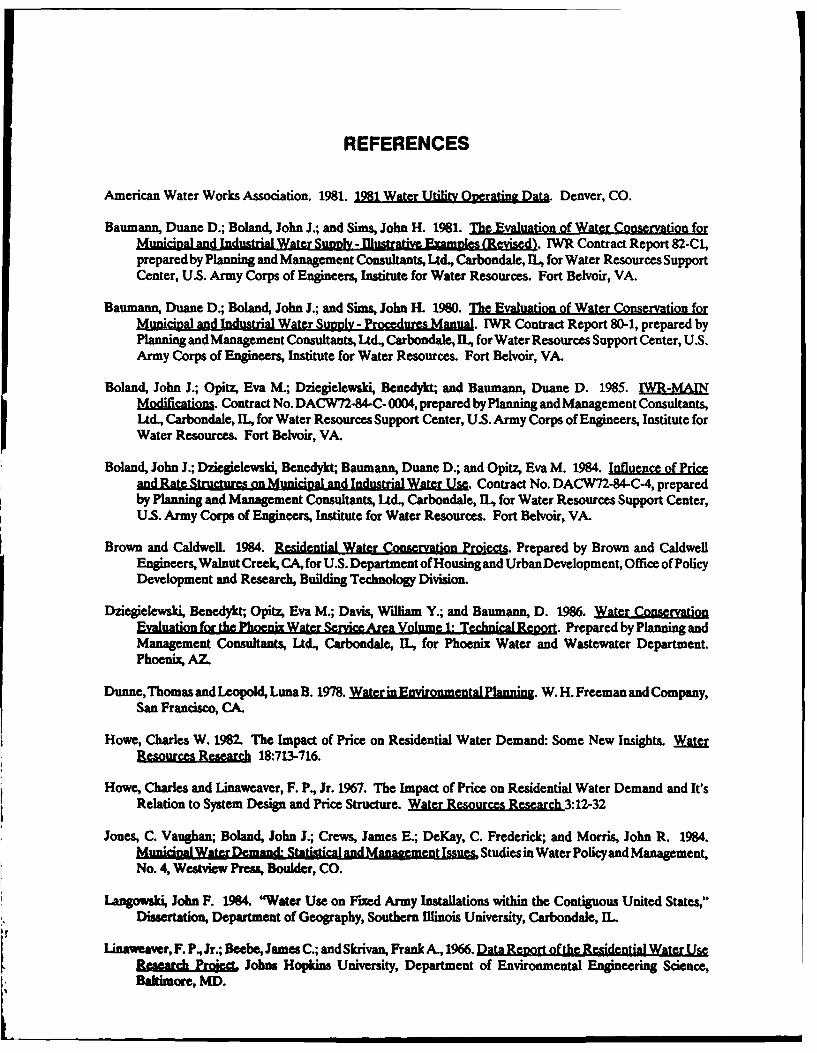
REFERENCES
American Water Works Association. 1981. 1981 Water Utility ORerating Data. Denver, CO.
Baumann, Duane D.; Boland, John J.; and Sims, John H. 1981. The Evaluation of Water Conservation forMunicinal and Industrial Water Sua - lheative Eampls (Revised). IWR Contract Report 82-C1,prepared by Planning and Management Consultants, Ltd., Carbondale, IL, for Water Resources SupportCenter, U.S. Army Corps of Engineers, Institute for Water Resources. Fort Belvoir, VA.
Baumann, Duane D.; Boland, John J.; and Sims, John H. 1980. The Evaluation of Water Conservation forMunicipal and Industrial Water Supply - Procedures Manual. IWR Contract Report 80-1, prepared byPlanning and Management Consultants, Ltd., Carbondale, I, for Water Resources Support Center, U.S.Army Corps of Engineers, Institute for Water Resources. Fort Belvoir, VA.
Boland, John J.; Opitz, Eva M.; Dziegielewski, Benedykt; and Baumann, Duane D. 1985. 1WR-MAINM. Contract No. DACW72-84-C- 0004, prepared by Planning and Management Consultants,Ltd., Carbondale, 11, for Water Resources Support Center, U.S. Army Corps of Engineers, Institute forWater Resources. Fort Belvoir, VA.
Boland, John J.; Dziegielewski, Benedykt; Baumann, Duane D.; and Opitz, Eva M. 1984. Influenfriceand Rate Structures on Municipal and Industrial Water Use. Contract No. DACW72-84-C-4, preparedby Planning and Management Consultants, Ltd., Carbondale, IL, for Water Resources Support Center,U.S. Army Corps of Engineers, Institute for Water Resources. Fort Belvoir, VA.
Brown and CaldwelL 1984. Residential Water Conservation Pro ects. Prepared by Brown and CaldweilEngineers, Walnut Creek, CA, for U.S. Department of Housing and Urban Development, Office of PolicyDevelopment and Research, Building Technology Division.
Dziegielewski, Benedykt; Opitz, Eva M.; Davis, William Y.; and Baumann, D. 1986. Water Conservation
Evauation for the Phoenix Water Service Area Volume le Technical Regrt. Prepared by Planning andManagement Consultants, Ltd., Carbondale, IL, for Phoenix Water and Wastewater Department.Phoenix, AZ.
Dunne, Thomas and Leopold, Luna B. 1978. Water in Envomental Plannng. W. H. Freeman and Company,San Francisco, CA.
Howe, Charles W. 1982. The Impact of Price on Residential Water Demand: Some New Insights. AtResorces Research 18:713-716.
Howe, Charles and Linaweaver, F. P., Jr. 1967. The Impact of Price on Residential Water Demand and It'sRelation to System Design and Price Structure. Water Resources Research 3:12-32
Jones, C. Vaughan; Boland, John J.; Crews, James E.; DeKay, C. Frederick; and Morris, John R. 1984.M lil Water Demand, Statitia and ment L%= Studies in Water Policy and Management,No. 4, Westview Press, Boulder, CO.
Langowski, John F. 1984. "Water Use on Fixed Army Installations within the Contiguous United States,"Dissertation, Department of Geography, Southern Illinois University, Carbondale, IL
Linaweaver, F. P, Jr.; Beebe, James C.; and Skrivan, Frank A., 1966. Data Renort of the Residential Water UseReseach Emig& Johns Hopkins University, Department of Environmental Engineering Science,Baltimore, MD.

Richards, W. G.; McCall, D. J.; and Deb, A. K 1984. "Algorithm for Determining the Effectiveness of WaterConservation Measures," Technical Report EL-84-3, prepared by Roy F. Weston, Inc., West Chester, PA,for the U.S. Army Engineer Waterways Experiment Station, CE, Vicksburg, MS.
United States Bureau of the Census. 1986. 1982Water Use in Manufauring. Census of Manufacturing, Supt.of Doc. No. C 3.24/12.
United States Bureau of the Census. 1983. County and City Data Book
Wolff, Jerome B., F.P. Linaweaver, Jr., and John C. Geyer. 1966. Water Use in Selected Commercial andInstitutional Establishments in the Baltimore Metrolitan Ar Johns Hopkins University.

INDEX

IWR-MAIN INDEX
Accessing IWR-MAIN, 1-5, 1-6 Commercial/institutional employment, 1-15,Add More Data/Revise Existing Data option, 1-21, 1.22, 1-28, 1-30, 1-34, 11-17, H-39, 11-56,
I-8, 1-9, 1-45 11-60Added calibration feature, 1-49 Commercial/institutional parameters (seeAdjustment factor commercial/institutional categories)
Conservation (see conservation algorithm) Commercial/institutional subgroupWeather (see calibration and verification) Data input characteristics, 11-17, 11-32 (alsoWinter irrigation (see calibration and verifi- see commercial/institutional categories)
cation) Water use model, 11-5, 11-39Advanced Plumbing Code measure, 1-37, 11-64, Comprehensive example of IWR-MAIN
1-66,11-69, H-73 application, A-1American Water Works Association, 11-66, B-1 Computational sequence, 1-51, 1-52, 1-53, C-27,Annual average use [average annual] (see C-28
dimension in forecasting use) Configuration file (CONFIG.SYS), 1-3, 1-4ANSI.SYS file, 1-3 Conservation adjustment factor, H-61, 11-62,Assessment factor, 1-16, 1-17, 1-18, 1-20, 11-16 11-68Backcasts of IWR-MAIN System, 11-6 Conservation algorithm, 11-60Backspace key, 1-10 Conservation data sources, 11-33, 11-61Base year employment, 1-13, 11-15, 11-35, 11-59, Conservation effectiveness, 1-36, 1-39, 1-43,
A-3, C-20, C-21 1-52,1-61,11-5,11-33, 11-60, 11-61, H-68Base year input data characteristics, 11-13 Effectiveness equation, 1-36, 11-5, I-60Base year screens, 1-12 Conservation input data, 11-33, 11-60, A-3, A-4,Batch files, C-18 A-5Baumann, Duane, 1-36, 11-60, 11-66, 11-69 Conservation measures, 1-11, 1-36, 1-37, 1-61,Bill difference variable, 1-19, 11-16, 11-19, 11-38, 11-62, 11-63, 11-64
11-42, A-2, A-3, B-2, C-21 Conservation screens, 1-36Boland, John, 11-39,11-65,11-69 Conservation sectors, 1-36,1-38,11-60, 11-61,Brown and Caldwell, 11-61, 11-69 U-62, 1-65,11-69, 1-71,11-78Calibration and verification, 1-52, 11-61, 1-85, Conservation subroutine, 1-36, 1-52, 1-61, 1-60
1-86, 11-87, 11-88, 11-89, H-90, H-91, A-6, Construction Cost Index, 1-13,11-15A-7, A-8, A-9, A-10, A-i1 (also see added Construction employment, 1-15, 1-28, 1-15,calibration feature) 11-31, 11-57, 11-59, C-21, C-23
Central city, 1-13,11-13,11-57,11-58, C-20 CONVERT utility, C-iChange Filename option, 1-6 .COV file, 1-52, 1-59, 1-61, 11-67, 11-68, A-9,Change Subgroups/Forecast Choices option, A-73, C-20
1-9, 1-45 Coverage factor, 1-36, 1-37, 1-43, 1-44, 1-52, 1-61City name [study area name), 1-11, 11-13, C-20 H-33, 1-60, 11-67, H-71, 11-78 (also seeClimatic variables (also see evapotranspiration; conservation algorithm; .COV file; Library
moisture deficit; precipitation), 1-13, 1-14, of Conservation Coefficients1-52 Create New File option, 1-8, 1-45
COFLB51 library, 1-48, 1-49, C-19 (also see Creation of .DAT and .WOR files, 1-48creation of .WOR and .ULB files; Library Creation of .ULB and WOR files, 1-48, 1-49of Water Use Coefficients) Cursor (arrow) keys, 1-10, 1-40, 1-44
COMMAND.COM file, 1-4 .DAT file, 1-48,1-49, 1-51,1-52, 1-59,11-13, C-i,Commercial Reuse/Recycle measure, 1-37, C-2, C-20
11-63, 11-69,11-72 Data crosschecks, 1-62Commercial/institutional categories, 1-11, 1-21, Data Entry Main screen, 1-7, 1-45
1-22, 1-30, 1-34, 11-17, 11-20, 1-32, 11-33, Data Entry/Update procedure, 1-7, 1-47, 1-6111-39, 11-77, 1-89 Data files, 1-47, 1-48, 1-49,1-59, C-1, C-2, C-20
Commercial/institutional coefficients, 11-39, Data sources, 11-34, 11-3511-40, 11-47, 11-77, 11-89, 11-90 Data subgroups, 1-11, 1-61, 11-13
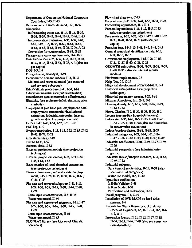
Department of Commerce National Composite Flow chart diagrams, C-25Cost Index, 1-13, 1-15 Forecast year, 1-11, 1-32, 1-44, 1-55, 11-31, C-23
Determinants of water demand, 11.3, 1-37 Forecasting approaches, II-3, H-4Dimension Forecasting methods, I-11, 1-12, 11-5, 11-33
In forecasting water use, 11-14, H-16, H-37, (also see projection techniques)11-38,11-39, 11-42, 11-44, 11-45, H-46, 11-85 Free services, 1-25, 1-32, 1-35,11-17, U-18, H-32,
In conservation evaluation, 1-36, 1-39, 1-40, 11-33,1141,11-54,11-78 (also see per1-41, 1-42, 11-5, 11-33, 11-60, 11-61, 11-62, capita)11-64,11-67, 11-68, 11-69, 11-78, 11-79, A-73 Function keys, 1-9, 1-10, 1-41, 1-42, 1-44,1-45
Conversion for conservation, 11-61,11-62 General municipal identification data, 1-13,Disaggregate water use forecasts, 11-4, 11-5 1-14, 11-13,11-15Distribution loss, 1-25, 1-32,1-35, 11-17,11-18, Government employment, 1-15, 1-28, 1-15,
11-32,11-33,11-41,11-54, U-78, A-3 (also see 11-31, H-57, U-60, C-21, C-23per capita) GROWTH subroutine, U-56,11-57,11-58, I-59,
DOS, 1-3, 1-4 11-60, 11-91 (also see internal growthDziegielewski, Benedykt, 11-69 models)Econometric demand models, 114,11-37 Hardware requirements, 1-3
Metered and sewered model (see metered Help files, 1-9, C-19and sewered subgroup) Historical development of IWR-MAIN, B-1
Edit/Validate procedure, 1-47, 1-51, 1-61 Historical extrapolation (see projectionEducation measure, (see public education) techniques)Effectiveness (see conservation effectiveness) Historical parameter screens, 1-29, 1-61Elasticity, (see moisture deficit elasticity;, price Hittman Associates, Inc., B-1, B-3
elasticity) Housing density, 1-16, 1-17,1-18, 1-16, H-19,Employment (see base year employment; total 11-42, C-22
employment; commercial/institutional Howe, Charles, H-5, U-37,11-38, U-39, B-1categories; industrial categories; internal Income (see median household income)growth models; key projection data) Indoor use, 1-36, 1-40, H-5, H-33, 11-60, 11-61,
Errors, 1-47, 1-48, 1-51, 1-52, 1-61, 1-62 11-62, H-65, 1-78, 11-90 (also see dimensionESC key, 1-10 in conservation evaluation)Evapotranspiration, 1-13,1-14,1-52,11-15, H42, Indoor/outdoor factor, 11-61,11-62, 11-79
11-43, 11-79, C-21 Industrial categories, 1-23, 1-24,1-31, 1-34,Executable files, C-19 1-17, 11-26,11-32, 11-33, 1-40, U-77,11-89Exit to DOS, 1-59 Industrial coefficients, 11-40, 11-49,11-77, 11-89,External data, 11-32 11-90External projection module (see projection Industrial parameters (see industrial cate-
techniques) gories)External projection screens, 1-32,1-33,1-34, Industrial Reuse/Recycle measure, 1-37,11-63,
1-35, 1-61, 1-62 11-69, 11-72Extrapolation of local historical parameters Industrial subgroup
(see projection techniques) Data input characteristics, U-17, 11-32 (alsoFinance, insurance, and real estate employ- see industrial categories)
ment, 1-15, 1-28, 11-15, 1-31, 11-57, U-60, Water use model, U-5, 1-40C-21, C-23 Input data verification
Flat rate and sewered subgroup, 1-11, 1-16, In Edit/Validate, 1-481-29, 1-33,1-55,11-15,11-38, 1-44,11-78, In Run Model, 1-52C-21 Verification and calibration, 11-85
Data input characteristics, 1-5, 11-16 Install program, 14, C-19Water use model, 11-44 Installation of IWR-MAIN on hard drive
Flat rate and unswered subgroup, 1-11, 1-17, systems, 1-41-29,1-33, 1-55, 11-16,11-38, 1145, 11-78, Institute for Water Resources, U.S. ArmyC-21 Corps of Engineers, 1-5, B-1, B-4, B-5, B-6,
Data input characteristics, 11-16 B-7, D-1Water use model, 11-45 Interaction factors, 1-61,11-62,11-67, 11-68,
FLONlAT library (see Library of Climatic U-74, 11-75, 11-76, 11-79 (also see conserva-Variables) tion algorithm)

Internal growth models (see projection Maximum-day use, 1-36,1-42,11-6,11-33,11-60,techniques) 11-61,11-62,11-65,11-78 (also see dimension
Irrigable area, 11-3,11-42,11-43,11-44,11-45, in forecasting water use and in conserva-11-8 tion evaluation)
IWR-MAIN program diskettes, 1-3 Median household income, 1-13, I-Z7, 11-15,IWR-MAIN system menu, 1-6 11-31,11-58, C-21, C-23 (also see keyIWR-MAIN system overview, 11-4, 11-5,11I-6 projection data; base year data; determi-IWR-MAIN utility disk (see external projec- nants of water demand)
dion module) Metered and sewered subgroup, 1-11, 1-18,Johns Hopkins University Residential Water 1-19, 1-29, 1-33, 1-55, U-16, 11-37,11-38,
Use Research Report, 11-37, B-i 11-78, C-21Jones, C., 11-3 Data input characteristics, 11-16Key projection data, 1-26, 1-27,1-28,11-31, Water use model, 11-38,11-42,11-43
11-56, C-23 Metering measure, 1-37,11-63, U-69, 11-71Langowski, .,11H4 Moderate Plumbing Code measure, 1-37,1-38,Latitude, 1-13,11-13,11-79, C-21 1[-6",11-66,11-69, 11-73, A-3, A-4LCC library (see Library of Conservation Moisture deficit, 1-14,11-15, 11-38, 11-42, 11-43,
Coefficients) 11-85Leak Detection and Repair measure, 1-37, In weather adjustment, 11-38, 11-77,11-86,
11-63, 11-66, H-69,11-72, A-5 11-88,11-89, A-6, A-7Library files, 1-3, 11-77, C-19, C-20 Elasticity, 11-77,11-86,11-88,11-89,11-91, A-6,Library of Climatic Variables [FLONIAT], A-7
1-14, 1-51, 1-52,1U-13, 11-15, 11-79, C-20 Multiple coefficient requirements methods,Li.brary of Conservation Coefficients [LCCJ, 11-4
1-33, 1-39, 1-40, 1-41, 1-42,1-43, 144, 1-51, Flat rate and sewered model (see flat rate1-52, 11-33, H-62, 11-65,11-67,11-78, C-20 and sewered subgroup)
Library of Water Use Coefficients [COFLBS11, Flat rate and unsewered model (see flat rate1-25,1-48,1-49,11-17,11-39,11-41, 11-77, and unsewered subgroup)C-19 (also see.WOR file) Master-metered apartments model (se
Linaweaver, F., 11-37,11-38, 11-39, B-i master-metered apartments subgroup)Load Existing File option, IA8,1-45 Municipal base year data (see general munici-Longitude, 1-13,11-13, 11-79, C-21 pal identification data)Low Water-Using Landscapes measure, 1-37, Nonresidential price adjustment, 1-24,11-39,
11-64,11-69, 11-73 1-40, 11-41,11-90MAIN I1, B-1, B-3 Outdoor use, 1-36, 141,11-6,11-33, 11-60,11-61,Mainframe computer application of IWR- 11-62, 11-65,1U-67,11-78,11-79,11-90 (also
MAIN, D-1 see dimension in conservation evaluation)Manufacturing employment, 1-15, 1-28, 11-15, Output reports, 1-55, 1-56,1-57, A-33 (also se
11-31, 11-57, 11-59, C-21, C-23 Print/View procedure)Marginal price, 1-18, 1-19,11-15,11-16, 11-37, Parameter Control screen, I-10, 1-11, 1-12, 1-15,
11-38,11-39,11-42, 11-65, C-22 (also see non- 1-21, 1-23,1I-27, 1-29,1-36,1I-44,1-61,1U-13,residential price adjustment) 11-31,11-33
Market value of residence, 1-16, 1-17, 1-18, 1-19, Pause key, 1-471-20, 1-29, 1-33, 11-3, 11-16, 11-31, 11-32, Per capita, 11-311-37, 11-42, 11-44,11-45,11-46,11-57,11-62, Per capita estimate of distribution loss, 11-17,C-22 1141
Master-metered apartments subgroup, 1-11, Per capita estimate of free service, 11-17,1-20, 1-29,1-33, 1-55,11-16, 11-39, 11-46, 11-4111-78, C-21 Persons per unit, 1-16, 1-17, 1-20, 11-16,11-37,
Data input characteristics, 11-16 1144, 11-45, 11-46, C-22Water use model, 11-39, 11-46 PgDn key, I-10
.MAT fie 1-53, 1-55, 1-59, C-20 PgUp key, I-10Maximum-day evapotranspiration, 1-14,11-15, Population (see base year input data; resident
11-42,11-43 population; key projection data; determi-nants of water demand)

Precipitation, 1- 14, 1-52, 11-I15, 11-43, C-21 Restricted water use, 1-11, 1-36, 1-52, 11-5, 11-89Pressure Reduction measure, 1-37, 11-63, 11-69, Retail trade employment, 1-15, 1-28 11-15,
11-71 11-61,11-64, C-21, C-23Price elasticity Retrofit of Showerheads and Toilets measure,
In demand models, 11-38 1-37,11-63, 11-66,11-69,11-72In nonresidential price adjustment, 11-39, Return to System Menu (with File Save
11-40, 11-41, 11-78 option), 1-9In Pricing Policy measure, 11-65 REVERT utility, C-2In verification and calibration, 11-86,11-91 Richards, W., f1-61, 11-66, 11-67, 11-69
Price of water, 11-3, 11-4, 11-15, 11-16, 11-17, .RPx files, 1-53, 1-55, 1-59, C-2011-37,11-38 (also see marginal price and Run Model procedure, 1-47,1-51,1-52,1-53,nonresidential price adjustment) 1-55, 1-61, 11-77
Pricing Policy (rate reform) measure, 1-37, Save Current* File with New Filename option,11-63, 11-65, 11-69, 11-71 1-9, 1-45
Print/View procedure, 1-55, 1-61 Save Current File with Return to Menu option,.PRN data base file, 1-13, 1-53, 1-59, 11-13, 1-9,1-45
C-20, C-21 Sector, 1-36, 1-38, 11-5 (also see disaggregatedPROJD file, 1-3, 1-51, 1-52, 1-53, C-20 water demand forecasts; IWR-MAIN
Creation/deletion, 1-52, 1-53 (also see System overview, conservation sectors)GROWTH subroutine) Services employment, 1-15, 1-28,11-15,1H-31,
Projection screens used by internal growth 11-57, 11-60, C-21, C-23models, 1-26, 1-27,1-28 Sewer charge, 11-15 (also see marginal price)
Projection techniques, 11-5,11-31,11-55 SIC classification, 1-15,1-21,1-23,11-15,11-39,Internal growth models, 1-11.1-26,1-61,11-5, 11-, 11-47, 11-49,11-59
11-31, 11-55,1H-56, 11-57,11-58,1U-59,11-60 Single coefficient requirement methods (seeExtrapolation of local historical trends, 1-12, unit use coefficient)
11-5, 11-31, 11-32,11-55, 11-56 Socioeconomic data, 11-3,11-13,11-37,11-85External projections, 1-12, 11-5,11-31, 11-32, Software setup, 1-3
11-33,11-55 Sprinkling Restriction measure, 1-37,1B-63,Property values, (see market values) 11-69, 11-72Public Education Program measure, 1-37, 1-38, Summer use (see dimensions in forecasted
1-0, 1-"4,11-62, U-69,11-71, A-S use)Public/unaccounted categories, 1-11, 1-25, 1-26, Terminating Data/Entry, 1-45
1-32,I-35,-56,1-17, 11-32,11-41, U-60, Total employment, 1-13, 1-27,1U-15,11-31,1U-56,11-78, C-22 11-59, C-21, C-23 (also see base year
Public/unaccounted coefficients, 11-54 employment; key projection dataPublic/unaccounted paraiziaers (see public/' Total number of households, 1-27, 11-31, 11-57,
unaccounted categories) C-23Public/unaccounted subgroup Transportation/public utilities employment,
Data input characteristics, 11-17, 11-32 (also 1-15, 1-28, 11-15, 11-31, 11-57,11-59, C-21,see public/unaccounted categories) C-23
Water use model, 11-41 U.S. Census of Manufactures: Water Use inRainfall, 11-79 (also see precipitation) Manufacturing, 11-35, 11-40, 11-49, B-2Rationing measure, 1-37, U-63, 11-66,11-69, .ULB file, 1-48, 1-49, 1-59, C-20
11-72 Unit use coefficient, 11-3, 11-5,11-39,11H40,Reduction factor, 1-36, 1-37, 1-39, 1410, 1-41, 11-41
1-42,1-61,11-5, 11-33,11-60,11-61, 11-62, Unrestricted water use, 1-36,1-52,1-55,1-,56,11-64,1U-65,1U-66,11-69, 11-78 (also see 1-61, 11-5, 11-33,11-60, U-85conservation algorithm; LCC), User-specified measures, 1-37, 1-39,143,1U-33,
Required data, 1-12,1-13, 1-14,1-26,1I-8, 1-61 11-62, 11-67 (also see conservation mecas-Resident population, 1-13, 1-25, 1-26, 1-27, ures)
13-13,1U-31,11-41,19-58, C-21, C-23 Utilities, 1-3, 148, C-iResidential subgroup, 1-11, 1-15, 1-16, 1-17, Value range, (see market value)
1-19, 1-28, 1-32, 11-15, 11-32, 11-37, 11-77, Weather adjustment factor, 1-14, 1-52, Ul-15,C-21 (also see conservation sectors) 11-38, 11-42, 11-77, 11-85, 11-87, 11-88

Wholesale trade employment, 1-15,1-28,11-15,11-31,11-57,11-60, C-21, C-23
Winter use (we dimension in forecated use).WRK file, 1-57, 1-59, C-20Wolff, Jerome, B-1.WOR file, 1-48, 1-49,1-5i, 1-52, 1-59, 11-77,
C-20 (also see COFLB5O; added calibra-tin feature)