On Mathematics in the History of Sub-Saharan Africa 1 - CORE
Upload
khangminh22Category
view
1download
0
Mathematics for Engineers and Engineers’ Mathematics
David Pearce
A Thesis in
the Department of
Mathematics and Statistics
Presented in Partial Fulfillment of the Requirements For the degree of Master in the Teaching of Mathematics at
Concordia University Montreal, Quebec, Canada
August 2015
© David Pearce

ii
CONCORDIA UNIVERSITY
School of Graduate Studies
This is to certify that the thesis prepared
By: David Pearce
Entitled: Mathematics for Engineers and Engineers’ Mathematics
and submitted in partial fulfillment of the requirements for the degree of
Master in the Teaching of Mathematics
complies with the regulations of the University and meets the accepted standards with respect to
originality and quality.
Signed by the final examining committee:
Nadia Hardy Chair
Syed Twareque Ali Examiner
Anna Sierpinska Supervisor
Approved by ________________________________________________
Chair of Department or Graduate Program Director
________________________________________________
Dean of Faculty
Date September 1, 2015

iii
Abstract
Mathematics for Engineers and Engineers’ Mathematics
David Pearce
This thesis is composed of two parts. In the first part, the mathematics that engineering students and
mathematics students are to be taught and expected to learn is identified by means of an analysis of the
content of the courses each group of students has to take, and of the types of tasks each group is given
in the final examinations of these courses. The aim is to determine if there are any significant
differences between the education of the two groups.
In the second part, I demonstrate how professional engineers use mathematics to develop
mathematical models that can be applied in solving tasks in their professional practice. Examples of
mathematical models from the studies of statics, mechanics of materials, and structural analysis are
presented, culminating in a discussion of the use of matrices in matrix structural analysis and the
physical representation of eigenvectors and eigenvalues and what they mean to a structural engineer.
The comparison, analyses, and demonstrations are performed from an anthropological point of view
using the Anthropological Theory of the Didactic (ATD). From this perspective it will be shown that the
similarities between the mathematical praxeologies of engineers and mathematicians are limited
principally to the tasks and techniques, while the differences are found in the level of the technology
and theory.
iv
Acknowledgements
I would not have been able to complete this thesis without the help and encouragement of many people.
First and foremost I must thank Dr. Anna Sierpinska for her vast knowledge, insightful remarks, guidance,
and genuine interest in the life and career of a former professional civil engineer. I left the profession to
pursue a degree in mathematics education in part because of my lifelong enjoyment of mathematics,
but mainly because I had grown bored and unhappy with being an engineer. To have to revisit aspects of
a career I had deliberately abandoned was challenging at times, but I enjoyed being able to look at it
through the eyes of a mathematician. The idea for the topic of this thesis was entirely Anna’s, and so I
have her to thank for giving me that first push in the right direction, and for making sure I saw this
project to its completion.
I owe thanks to former colleagues at the engineering firm CIMA+, most notably Peter Pietraszek and
Marie-Claude Michaud, for providing with workplace documents for analysis demonstration purposes.
To all my Concordia classmates, thank you for lending me your ears, and for allowing me to vent some
steam when the pressure built up. I am particularly thankful to Erin Murray, Steven Pileggi, and Dalia
Challita. Thank you for helping me push through my writer’s block, for your moral support and
encouragement, and most importantly for your friendship.
Lastly, to my wife Stephanie, thank you for staying by my side through all of this. Your love means more
to me than I could ever hope to show you. But I’ll sure as hell try.
v
Table of Contents
1 Introduction .......................................................................................................................................... 1
2 Theoretical framework ......................................................................................................................... 6
2.1 Praxeology ..................................................................................................................................... 6
2.2 Institutional perspective ............................................................................................................... 7
2.3 Didactic and institutional transposition ...................................................................................... 10
2.4 Validation of the chosen framework .......................................................................................... 11
3 Literature review ................................................................................................................................. 15
3.1 Mathematics education for engineers ........................................................................................ 15
3.2 Mathematics in vocational education ........................................................................................ 17
3.3 Mathematical applications and mathematical modelling .......................................................... 22
3.4 Mathematics as a service subject ............................................................................................... 27
3.5 Mathematics in the workplace ................................................................................................... 30
3.6 Geometry, measurement and error ........................................................................................... 35
4 Mathematics for engineers ................................................................................................................. 41
4.1 Accreditation of an engineering program ................................................................................... 41
4.2 Accredited engineering programs in Quebec ............................................................................. 44
4.3 Mathematics in accredited civil engineering programs .............................................................. 46
4.3.1 Methodology for the analysis of final exams ...................................................................... 48
4.3.2 Pre-university linear algebra ............................................................................................... 50
4.3.3 Pre-university calculus ........................................................................................................ 57
4.3.4 University level calculus ...................................................................................................... 61
4.3.5 Differential equations ......................................................................................................... 68
4.3.6 Probability and statistics ..................................................................................................... 75
4.3.7 Numerical methods ............................................................................................................. 84
4.3.8 Engineering geometry ......................................................................................................... 90
4.4 Summary of results ..................................................................................................................... 96
5 Engineers’ mathematics .................................................................................................................... 100
5.1 Analytical models and empirical models .................................................................................. 101
5.2 The mathematics of mechanics ................................................................................................ 104
vi
5.2.1 Units and numerical accuracy ........................................................................................... 105
5.2.2 Statics ................................................................................................................................ 110
5.2.3 Mechanics of materials ..................................................................................................... 119
5.2.4 Structural analysis ............................................................................................................. 127
5.3 Matrix structural analysis .......................................................................................................... 130
5.3.1 The elastic stiffness matrix ................................................................................................ 131
5.3.2 The eigenvectors of an elastic stiffness matrix ................................................................. 142
5.4 Mathematics in the engineer’s workplace................................................................................ 148
5.4.1 Dossier de calculs .............................................................................................................. 149
6 Conclusions and recommendations .................................................................................................. 155
6.1 Similarities in mathematical praxeologies ................................................................................ 155
6.2 Differences in mathematical praxeologies ............................................................................... 156
6.2.1 Differences in tasks and techniques .................................................................................. 158
6.2.2 Differences in technologies and theories .......................................................................... 158
6.3 A general view of an engineer’s mathematical praxeology ...................................................... 162
6.4 Limitations of this thesis and recommendations for future studies ......................................... 163
7 References ........................................................................................................................................ 165
8 Appendices ........................................................................................................................................ 168
8.1 Websites of accredited engineering programs in Quebec ....................................................... 168
8.2 List of mathematics courses in the accredited engineering programs in Quebec ................... 168
8.2.1 Pre-university linear algebra ............................................................................................. 169
8.2.2 Pre-university calculus ...................................................................................................... 171
8.2.3 University level calculus .................................................................................................... 173
8.2.4 Differential equations ....................................................................................................... 176
8.2.5 Probability and statistics ................................................................................................... 178
8.2.6 Numerical methods ........................................................................................................... 180
8.2.7 Engineering geometry ....................................................................................................... 181
8.3 Final exams from mathematics courses at McGill and Concordia ............................................ 183
8.3.1 Pre-university linear algebra ............................................................................................. 183
8.3.2 Pre-university calculus ...................................................................................................... 193
8.3.3 University level calculus .................................................................................................... 200
8.3.4 Differential equations ....................................................................................................... 216
8.3.5 Probability and statistics ................................................................................................... 230

vii
8.3.6 Numerical methods ........................................................................................................... 252
8.4 Structural analysis software report .......................................................................................... 276
viii
List of Figures
Figure 1 - Applied force and reaction forces on a beam (drawing is my own) ............................................. 9
Figure 2 - Calculating the average gradient (slope) of a train track. (Wake, 2014) .................................... 20
Figure 3 - Simply supported beam with concentrated load at centre (drawing is my own) ...................... 21
Figure 4 - Statics problem: a crane lifting a mass (Beer & Johnston, 2007, p. 166) ................................... 23
Figure 5 - Crosswind and its components (drawing is my own) ................................................................. 34
Figure 6 - Symbols for water mains and valve chambers (drawing is my own) .......................................... 37
Figure 7 - Measuring with partial dimensions (top) and cumulated dimensions (bottom) (adapted from
Eberhard (2000)) ......................................................................................................................................... 38
Figure 8 - MATH 204 - Vectors and Matrices (Concordia), December 2014, question 4............................ 52
Figure 9 - MATH 204 - Vectors and Matrices (Concordia), December 2014, question 8............................ 53
Figure 10 - MATH 204 - Vectors and Matrices (Concordia), December 2014, question 5.......................... 53
Figure 11 - MATH 204 - Vectors and Matrices (Concordia), December 2014, question 2.......................... 54
Figure 12 - MATH 251 - Linear Algebra I (Concordia), December 2013, questions 4, 5, and 6 .................. 54
Figure 13 - MATH 252 - Linear Algebra II (Concordia), April 2013, questions 7, 8, and 9 .......................... 55
Figure 14 - MATH 204 - Vectors and Matrices (Concordia), December 2014, question 10........................ 56
Figure 15 - MATH 251 - Linear Algebra I (Concordia), December 2014, question 9 ................................... 56
Figure 16 - MATH 203 - Calculus 1 (Concordia), December 2014, question 7 ............................................ 59
Figure 17 - MATH 203 - Calculus 1 (Concordia), December 2014, question 4 ............................................ 59
Figure 18 - MATH 205 - Calculus 2 (Concordia), December 2014, questions 3 and 4 ................................ 60
Figure 19 - MATH 203 - Calculus 1 (Concordia) and MATH 205 - Calculus 2 (Concordia), bonus questions
.................................................................................................................................................................... 60
Figure 20 - MATH 262 - Intermediate Calculus (McGIll), December 2010, question 6 .............................. 64
Figure 21 - MATH 264 - Advanced Calculus I (Concordia), December 2014, question 2 ............................ 64
Figure 22 - MATH 264 - Advanced Calculus I (Concordia), December 2014, formulas............................... 64
Figure 23 - ENGR 233 - Applied Advanced Calculus (Concordia), December 2014, questions 3 and 4 ...... 65
Figure 24 - MATH 264 - Advanced Calculus I (Concordia), December 2014, question 4 ............................ 65
Figure 25 - MATH 264 - Advanced Calculus (McGill), April 2007, questions 5 and 6 ................................. 66
Figure 26 - List of symbols (Beer & Johnston, 1992, p. xvii) ....................................................................... 67
Figure 27 - ENGR 233 - Applied Advanced Calculus (Concordia), December 2014, questions 7 and 8 ...... 67
Figure 28 - MATH 264 - Advanced Calculus (McGill), April 2007, question 3 ............................................. 67
Figure 29 - MATH 265 - Advanced Calculus II (Concordia), December 2014, questions 5 and 6 ............... 68
Figure 30 - MATH 263 - Ordinary Differential Equations for Engineers (McGill), December 2012, question
7 .................................................................................................................................................................. 70
Figure 31 - MATH 263 - Ordinary Differential Equations for Engineers (McGill), December 2012, question
8 .................................................................................................................................................................. 71
Figure 32 - ENGR 311 - Transform Calculus and Partial Differential Equations (Concordia), August 2009,
question 4 ................................................................................................................................................... 71
Figure 33 - MATH 370 - Ordinary Differential Equations (Concordia), December 2014, questions 3 and 4
.................................................................................................................................................................... 71
ix
Figure 34 - ENGR 213 - Applied Ordinary Differential Equations (Concordia), December 2014, questions 3,
6, and 7........................................................................................................................................................ 72
Figure 35 - MATH 263 - Ordinary Differential Equations for Engineers (McGill), December 2012, question
3 through 6 .................................................................................................................................................. 73
Figure 36 - ENGR 213 - Applied Ordinary Differential Equations (Concordia), December 2014, question 5
.................................................................................................................................................................... 73
Figure 37 - ENGR 213 - Applied Ordinary Differential Equations (Concordia), December 2014, question 4
.................................................................................................................................................................... 74
Figure 38 - MATH 370 - Ordinary Differential Equations (Concordia), December 2014, question 5 ......... 74
Figure 39 - ENGR 371 - Probability and Statistics in Engineering (Concordia), April 2013, question 3 ...... 77
Figure 40 - ENGR 371 - Probability and Statistics in Engineering (Concordia), April 2013, question 4 ...... 78
Figure 41 - ENGR 371 - Probability and Statistics in Engineering (Concordia), April 2013, question 7 ...... 79
Figure 42 - CIVE 302 - Probabilistic Systems (McGill), April 2006, question 3 ............................................ 80
Figure 43 - CIVE 302 - Probabilistic Systems (McGill), April 2006, question 6 ............................................ 80
Figure 44 - STAT 249 - Probability I (Concordia), December 2011, questions 3, 4, and 5 .......................... 82
Figure 45 - STAT 249 - Probability I (Concordia), December 2011, question 9 ........................................... 82
Figure 46 - STAT 250 - Statistics (Concordia), December 2013, questions 6 and 7 .................................... 83
Figure 47 - STAT 250 - Statistics (Concordia), December 2013, question 1 ................................................ 83
Figure 48 - ENGR 391 - Numerical Methods in Engineering (Concordia), December 2013, question 4 (b) 86
Figure 49 - ENGR 391 - Numerical Methods in Engineering (Concordia), December 2013, question 4 (a) 87
Figure 50 - CIVE 320 - Numerical Methods (McGill), December 2007, question 3 ..................................... 87
Figure 51 - CIVE 320 - Numerical Methods (McGill), December 2007, questions 5, 7, and 9 .................... 88
Figure 52 - CIVE 320 - Numerical Methods (McGill), December 2007, question 6 ..................................... 88
Figure 53 - MATH 354 - Numerical Analysis (Concordia), December 2012, question 2 ............................. 89
Figure 54 - ENGR 391 - Numerical Methods in Engineering (Concordia), December 2013, question 1 ..... 89
Figure 55 - MATH 354 - Numerical Analysis (Concordia), December 2011, question 5 ............................. 90
Figure 56 - Orthographic drawing of a bridge spanning a river (Used with permission of CIMA+) ............ 91
Figure 57 - Chevron-shaped parcels of land (drawing is my own) .............................................................. 93
Figure 58 - Example of a structural member with a rectangular cross-section .......................................... 94
Figure 59 - Common geometric cross-sectional shapes for structural members (Beer & Johnston, 2007, p.
486) ............................................................................................................................................................. 95
Figure 60 - SI prefixes and multiplication factors (Beer & Johnston, 2007) ............................................. 106
Figure 61 - General notes from an engineering plan (Used with permission of CIMA+) .......................... 107
Figure 62 - Chainage and elevation of a bridge abutment ....................................................................... 108
Figure 63 - Cross-section of a proposed bridge ........................................................................................ 108
Figure 64 - Applying a force to a block and pushing it. Applying two forces: the block does not move
(drawing is my own) .................................................................................................................................. 111
Figure 65 - Applying a force: rotating a book (drawing is my own) .......................................................... 111
Figure 66 - Applying a moment to a door (1) (drawing is my own) .......................................................... 112
Figure 67 - Applying a moment to a door (2) (drawing is my own) .......................................................... 112
Figure 68 - Statics problem (Beer & Johnston, 2007, p. 173) ................................................................... 113
Figure 69 - Boards with rectangular cross-sections (drawing is my own) ................................................ 115
Figure 70 - Rectangular cross-sections (drawing is my own) .................................................................... 115
Figure 71 - Moment of inertia of a rectangular cross-section (drawing is my own) ................................ 116
x
Figure 72 - Wide-flange and American standard cross sections (Beer & Johnston, 2007, p. 486) ........... 117
Figure 73 - Statics textbook problems: finding the moment of inertia of geometric shapes (Beer &
Johnston, 2007, p. 493) ............................................................................................................................. 118
Figure 74 - Moments of inertia of common geometric shapes (adapted from (Beer & Johnston, 2007, p.
inside back cover)) .................................................................................................................................... 118
Figure 75 - Properties and dimensions of structural shapes (Canadian Institute of Steel Construction,
2000, pp. 6-48) .......................................................................................................................................... 119
Figure 76 - Stress in a structural member (drawing is my own) ............................................................... 120
Figure 77 - Elongation a steel rod (drawing is my own) ........................................................................... 121
Figure 78 - Stress-strain diagram for a ductile material (drawing is my own) .......................................... 122
Figure 79 - Beam diagrams and formulae (Canadian Institute of Steel Construction, 2000, pp. 5-132) .. 126
Figure 80 - Potential displacements of a beam (drawing is my own) ....................................................... 131
Figure 81 - Potential forces in a beam (drawing is my own) .................................................................... 132
Figure 82 - Plane frame (drawing is my own) ........................................................................................... 134
Figure 83 - Stiffness matrix entries for displacement d1 (drawing is my own) ........................................ 137
Figure 84 - Stiffness matrix entries for displacement d4 (drawing is my own) ........................................ 138
Figure 85 - Supports: Roller support (left), Pinned support (centre), Fixed support (right) (drawing is my
own) .......................................................................................................................................................... 140
Figure 86 - Deformed shape of a plane frame (Software provided with (Kassimali, 1999)) .................... 142
Figure 87 - Plane truss (drawing is my own) ............................................................................................. 143
Figure 88 - Results from a structural analysis: deformed shape of a plane truss (Software provided with
(Kassimali, 1999)) ...................................................................................................................................... 144
Figure 89 - Eigenvectors of a plane truss: applied force and resulting displacement are in the same
direction (drawing is my own) .................................................................................................................. 146
Figure 90 - Critical load analysis of a column - P- effect ......................................................................... 148
Figure 91 - Dossier de calculs: Base plate dimensions (Source: Obtained from a licensed engineer) ..... 150
Figure 92 - Dossier de calculs: Checking base plate thickness (Source: Obtained from a licensed engineer)
.................................................................................................................................................................. 151
Figure 93 - Dossier de calculs: Checking concrete pedestal bearing stress (Source: Obtained from a
licensed engineer) ..................................................................................................................................... 152
Figure 94 - Dossier de calculs: Checking anchor bolt resistance (Source: Obtained from a licensed
engineer) ................................................................................................................................................... 153
Figure 95 - Diverging educational paths of mathematics students and engineering students ................ 157
Figure 96 - Visualization of an engineer's mathematical praxeology ....................................................... 162
xi
List of Tables
Table 1 - Sample table: Relative frequency of tasks on a final exam.......................................................... 49
Table 2 - Relative frequency of tasks: MATH 204 - Vectors and Matrices (Concordia), December 2014 .. 51
Table 3 - Relative frequency of tasks: MATH 251 - Linear Algebra I (Concordia), December 2013 ........... 51
Table 4 - Relative frequency of tasks: MATH 252 - Linear Algebra II (Concordia), April 2013.................... 51
Table 5 - Relative frequency of tasks: MATH 203 - Calculus I (Concordia), December 2014 ..................... 58
Table 6 - Relative frequency of tasks: MATH 205 - Calculus II (Concordia), December 2014 .................... 58
Table 7 - Relative frequency of tasks: ENGR 233 - Applied Advanced Calculus (Concordia), December
2014 ............................................................................................................................................................ 62
Table 8 - Relative frequency of tasks: MATH 262 - Intermediate Calculus (McGill), December 2010 ....... 63
Table 9 - Relative frequency of tasks: MATH 264 - Advanced Calculus (McGill), April 2007 ...................... 63
Table 10 - Relative frequency of tasks: MATH 264 - Advanced Calculus I (Concordia), December 2014 ... 63
Table 11 - Relative frequency of tasks: MATH 265 - Advanced Calculus II (Concordia), April 2014 ........... 63
Table 12 - Relative frequency of tasks: ENGR 213 - Applied Ordinary Differential Equations (Concordia),
December 2014 ........................................................................................................................................... 69
Table 13 - Relative frequency of tasks: ENGR 311 - Transform Calculus and Partial Differential Equations
(Concordia), August 2009 ........................................................................................................................... 70
Table 14 - Relative frequency of tasks: MATH 263 - Ordinary Differential Equations for Engineers (McGill),
December 2012 ........................................................................................................................................... 70
Table 15 - Relative frequency of tasks: MATH 370 - Ordinary Differential Equations (Concordia),
December 2014 ........................................................................................................................................... 70
Table 16 - Relative frequency of tasks: ENGR 371 - Probability and Statistics in Engineering (Concordia),
April 2013 .................................................................................................................................................... 76
Table 17 - Relative frequency of tasks: CIVE 302 - Probabilistic Systems (McGill), April 2006 ................... 76
Table 18 - Relative frequency of tasks: STAT 249 - Probability I (Concordia), December 2011 ................. 76
Table 19 - Relative frequency of tasks: STAT 250 - Statistics (Concordia), December 2013 ...................... 76
Table 20 - Relative frequency of tasks: ENGR 391 - Numerical Methods in Engineering (Concordia),
December 2013 ........................................................................................................................................... 85
Table 21 - Relative frequency of tasks: CIVE 320 - Numerical Methods (McGill), December 2007 ........... 85
Table 22 - Relative frequency of tasks: MATH 354 - Numerical Analysis (Concordia), December 2011 .... 85
Table 23 - Relative frequency of tasks: MATH 354 - Numerical Analysis (Concordia), December 2012 .... 85
Table 24 - Summary of the relative frequency of tasks: Pre-university linear algebra .............................. 96
Table 25 - Summary of the relative frequency of tasks: Pre-university calculus ........................................ 96
Table 26 - Summary of the relative frequency of tasks: University level calculus ..................................... 97
Table 27 - Summary of the relative frequency of tasks: Differential equations ......................................... 97
Table 28 - Summary of the relative frequency of tasks: Probability and statistics..................................... 98
Table 29 - Summary of the relative frequency of tasks: Numerical methods ............................................ 98
Table 30 - Classification of tasks: MATH 204 - Vectors and Matrices (Concordia), December 2014 ....... 183
Table 31 - Classification of tasks: MATH 251 - Linear Algebra I (Concordia), December 2013 ................ 186
Table 32 - Classification of tasks: MATH 252 - Linear Algebra II (Concordia), April 2013 ......................... 190
xii
Table 33 - Classification of tasks: MATH 203 - Calculus 1 (Concordia), December 2014 ......................... 193
Table 34 - Classification of tasks: MATH 205 - Calculus 2 (Concordia), December 2014 ......................... 197
Table 35 - Classification of tasks: ENGR 233 - Applied Advanced Calculus (Concordia), December 2014 200
Table 36 - Classification of tasks: MATH 262 - Intermediate Calculus (McGill), December 2010 ............ 202
Table 37 - Classification of tasks: MATH 264 - Advanced Calculus (McGill), April 2007 ........................... 206
Table 38 - Classification of tasks: MATH 264 - Advanced Calculus I (Concordia), December 2014 .......... 209
Table 39 - Classification of tasks: MATH 265 - Advanced Calculus II (Concordia), April 2014 .................. 213
Table 40 - Classification of tasks: ENGR 213 - Applied Ordinary Differential Equations (Concordia),
December 2014 ......................................................................................................................................... 216
Table 41 - Classification of tasks: ENGR 311 - Transform Calculus and Partial Differential Equations
(Concordia), August 2009 ......................................................................................................................... 219
Table 42 - Classification of tasks: MATH 263 - Ordinary Differential Equations for Engineers (McGill),
December 2012 ......................................................................................................................................... 222
Table 43 - Classification of tasks: MATH 370 - Ordinary Differential Equations (Concordia), December
2014 .......................................................................................................................................................... 226
Table 44 - Classification of tasks: ENGR 371 - Probability and Statistics in Engineering (Concordia), April
2013 .......................................................................................................................................................... 230
Table 45 - Classification of tasks: CIVE 302 - Probabilistic Systems (McGill), April 2006 .......................... 234
Table 46 - Classification of tasks: STAT 249 - Probability I (Concordia), December 2011 ........................ 244
Table 47 - Classification of tasks: STAT 250 - Statistics (Concordia), December 2013 ............................. 249
Table 48 - Classification of tasks: ENGR 391 - Numerical Methods in Engineering (Concordia), December
2013 .......................................................................................................................................................... 252
Table 49 - Classification of tasks: CIVE 320 - Numerical Methods (McGill), December 2007 .................. 263
Table 50 - Classification of tasks: MATH 354 - Numerical Analysis (Concordia), December 2011 ........... 268
Table 51 - Classification of tasks: MATH 354 - Numerical Analysis (Concordia), December 2012 ........... 272
1
1 INTRODUCTION
The purpose of this thesis is to compare the mathematics education of engineers with that of
mathematicians, and to show how professional engineers use mathematics in practice. More specifically,
in the first part of the thesis, the mathematics that engineering students and mathematics students are
to be taught and expected to learn is identified by means of an analysis of the content of the courses
each group of students has to take, and of the types of tasks each group is given in the final
examinations of these courses. The aim is to determine if there are any significant differences between
the education of the two groups. The second part of the thesis is a demonstration of how engineers use
mathematics to develop mathematical models that can be applied in solving tasks in their professional
practice, and how this application of mathematics differs from the interests of mathematicians. The
comparison, analyses and demonstrations are performed from an anthropological point of view using
the Anthropological Theory of the Didactic (ATD).
Before proceeding, a brief word must be said about the term “engineer.” The engineering profession has
a lengthy and rich history, and as a result the term “engineer” is very broad. The profession comprises
many disciplines whose foundational principles vary. Engineering encompasses the fields of civil
engineering, mechanical engineering, chemical engineering, electrical engineering, and materials
engineering. Within the past forty or so years there has been the emergence of relatively new fields
such as computer engineering and software engineering. Within each of these fields we can find
multiple sub-disciplines. A civil engineer, for example, may work as a structural engineer, municipal
engineer, hydraulic and hydrological engineer, environmental engineer, or transportation engineer. For
reasons of brevity, this thesis will restrict the meaning of the term engineer to civil engineers, and, in
particular cases, only structural engineers and concepts of structural engineering may be referenced.
2
This topic is of particular interest to me since I earned my bachelor’s degree in civil engineering, with a
focus on structural engineering, from McGill University in 2003. After working as a project engineer for a
private consulting firm, including three years as a professionally licensed engineer, I left the profession
and returned to school in order to earn a graduate degree in mathematics education. I always had a
particular fondness for mathematics, and enjoyed studying civil engineering due to its nature as an
applied science involving plenty of mathematical formulae.
Changing direction of study and profession required taking mathematics courses for “generalist”
mathematicians (undergraduate and graduate mathematics students). As a student in these courses I
had the feeling of entering a very different culture from the one I had experienced as an engineering
student and as a practicing engineer.
For example, engineers in practice will approximate the values of irrational numbers such as √ and π as
1.414 and 3.14. Fewer or more decimal places may be used in the approximation depending on the
context of the calculation they are being used for. It is also an accepted scientific practice to use
numbers with an appropriate number of significant figures. Many of the numbers used in engineering
calculations represent measurable quantities: in this case, numbers are accompanied by units. If a length
is measured in millimeters with a ruler which has no finer unit than a millimetre, it would not make
sense to say that the length is, say, √ . For a mathematician, however, the number √
represents an abstract number, for example, a root of the equation and saying that the
roots of this equation are 12.73 and -12.73 would be considered a serious inaccuracy. Units and their
conversions are not usually the mathematician’s concern.
I also noticed differences in the things that pique a mathematician’s interest. While taking a course that
involved second order logic, I noticed that mathematicians are mainly motivated by finding
generalizations of mathematical properties and proving theorems. In a linear algebra course I was
3
impressed by the level of importance placed on proving theorems, not just as a detail in the course
lectures, but as tasks given on assignments and exams as well. Revisiting such tasks that I had not
encountered since my days as a CEGEP student gave me a new appreciation for them. In being able to
prove a theorem one can better understand its meaning and its purpose, which will lead to correctly
applying the theorem as well.
I wished to see if more of these differences existed, and to understand their nature. This led me to
identifying and collecting data about different institutions, namely the institutions of academic
mathematics, mathematics courses in university programs for engineering and mathematics students,
and the engineering profession itself. I then sought a theoretical framework that would help me to
analyze and structure my observations of the data. The theoretical framework of the ATD models the
mathematical knowledge of an institution in terms of units called praxeologies. Within an institution’s
mathematical praxeology there is a block of practical knowledge that contains a task to accomplish and
a technique to accomplish it. Every praxeology also has a theoretical block that contains two levels of
discourse. The praxeology’s technology classifies the tasks into different types, describes the techniques
for solving the types of tasks in more general terms, and justifies their use in performing the tasks, and
there is also the theory which is a system of all formal arguments that justify the technology. This model,
along the concept of institution, provides an appropriate framework for comparing the mathematical
knowledge that engineering and mathematics students are expected to learn, and for demonstrating
how mathematics is used in practice by professional engineers.
The structure of the thesis is as follows. In chapter 2 I will discuss the theoretical framework of the ATD
in more detail, defining the concepts of praxeology, institution, and didactic and institutional
transposition of mathematical knowledge. The chapter concludes with a justification of the chosen
framework.
4
In the literature review in chapter 3, I will present the findings of several research papers on the
mathematics education and the use of the mathematics in the workplace of various vocations and
trades, including engineering. In this chapter an important distinction will be made between
mathematical applications and the process of mathematical modelling, and the role that each plays in an
engineer’s education and practice. The concept of mathematics as a service subject is also addressed.
Service mathematics courses teach mathematics to students whose main area of study is not academic
mathematics itself. Engineering students fit this description.
Chapter 4 is titled “Mathematics for engineers”, and it comprises an analysis of the mathematical tasks
given to engineering students on the final exams of their required mathematics courses. These tasks are
compared and contrasted with those given to mathematics students on final exams from comparable
courses. Also included in the chapter is an institutional perspective on why engineers are required to
learn the mathematics that they do.
In chapter 5, “Engineers’ mathematics”, particular attention is paid to how engineers use mathematics
to develop mathematical models. Examples of mathematical models from the fields of statics,
mechanics of materials, and structural analysis are presented, and in the discussion of each I also
mention aspects that would be of interest to a mathematician. A specific model called the direct
stiffness matrix, and the physical representation of eigenvalues and eigenvectors of a matrix, is
discussed at length. In this chapter I also present and analyze workplace documents prepared by a
professional engineer in the design of a structure.
At the outset of this project I had hoped to address a common concern among students in mathematics
courses: “Why do we have to learn this?” The second part of this thesis is an attempt to answer this
question by demonstrating how engineers use mathematics in models at the heart of their field.

5
Engineering students have to learn about eigenvalues because they can be used to solve important tasks
in structural engineering.
On a larger scale, mathematics education researchers are interested in how various tradespeople use
mathematics because it helps to broaden our view of what mathematics is, and what it means to have
mathematical knowledge. ATD is useful in understanding how mathematics is used in practice and
structuring our descriptions of this practice. This thesis is my contribution to this understanding.
6
2 THEORETICAL FRAMEWORK
The present chapter discusses the theoretical framework of this thesis, the Anthropological Theory of
the Didactic (ATD) developed by Chevallard (1999). My principle sources of inspiration for choosing this
framework are the works of Sierpinska et al. on sources of students’ frustration in pre-university level
pre-requisite mathematics courses (Sierpinska, Bobos, & Knipping, 2008), as well as Hardy’s study on
college students’ perceptions of institutional practices regarding limits of rational functions (Hardy,
2009). In the following sections, I will discuss the basic concepts of the ATD – praxeology, institution,
and didactic transposition – and then argue why this framework is suitable for the purposes of this study.
2.1 PRAXEOLOGY
The ATD is an epistemological framework in which the principal objects of study are institutionalized
practices, and was developed as a means of describing the practice of teaching and learning
mathematics (Chevallard, 1999). In this framework, the learning of mathematics is not something that
occurs at an individual level, as in theories of cognition, but rather as a collective activity by the
members of an institution. Furthermore, the mathematical knowledge itself is developed by institutions,
not individuals. The concept of an institution is discussed is section 2.2.
The cornerstone of the ATD is the notion that institutional knowledge can be organized into units called
praxeologies. Each praxeology is composed of two blocks: a practical block, called the praxis, and a
theoretical block, called the logos.
In each praxeology, the practical block consists of a collection of tasks to be accomplished, and the
techniques that are used to accomplish them. The praxis can be thought of as the “know how” portion
of a praxeology; when given a mathematical task, knowing how to complete it is indicative of practical
knowledge.
7
The theoretical block of the praxeology contains two levels of discourse: the technology and the theory.
Technology classifies the tasks into different types, describes the techniques for solving the types of
tasks in more general terms, and justifies their use in performing the tasks. Theory is a system of all
formal arguments that justify the technology. Theory, in particular, provides the rationale underlying the
classification of the tasks and techniques into particular types and makes explicit the assumptions and
theoretical arguments that allow us to claim that the techniques “work”, going beyond the experience
of seeing them work in particular cases. Thus, the logos can be thought of as the “knowledge” block of
the praxeology; having completed a mathematical task with a technique, the theoretical block provides
the justification for the use of that technique.
In summary, the two blocks of a praxeology – [tasks & techniques] - [technology & theory] – suggest
that the practices of mathematicians and engineers may differ not only in the types of tasks they
perform, but in the nature of the theories they call upon to justify the techniques they use to accomplish
those tasks.
2.2 INSTITUTIONAL PERSPECTIVE
While knowledge can be organized into praxeologies, the knowledge itself is created by human activity
within institutions. This raises an important question: what is an institution? While the term is not
explicitly defined in the ATD, the institutional perspective used by Sierpinska et al. (2008) remedies this
by adopting a definition based on the work of Peters (1999) in the domain of Institutional Theory.
According to Peters, there are four features that define an institution. As summarized in Sierpinska
(2008) they are:
1. An institution is a structural feature of a society. The structure may be formal, requiring a legal
framework, or an informal network of organizations.
2. An institution has some stability over time.
8
3. An institution constrains its participants through rules and norms.
4. Members of an institution share certain values and goals, and give common meaning to the
basic actions of the institution.
The works of Hardy (2009), and, more recently, Castela (2015) further encapsulate these features by
defining an institution as a stable social organization that offers a framework which allows repetitive
interactions between individuals whose aim is to fulfill certain tasks. In the course of fulfilling its tasks,
an institution takes purposeful collective action, subjecting its members to its expectations and
regulating the members’ actions through the use of rules, norms, and strategies (which Castela calls
“rituals”).
Rules are understood as explicitly stated regulations that must be followed, as breaking them will invoke
sanctions against a member of the institution. In a university mathematics class, or the research
mathematicians’ community, a rule to be followed is that one must obey the axioms and theorems of
mathematics. Not doing so results in mathematical contradiction and unfeasible results, or
consequences such as the mathematics student failing an exam, or the research mathematician having
his or her paper rejected in the review process. In engineering professional practice, an example of a
rule that is enforced is the use of legally mandated design codes. The sanctions against professional
engineers have a legal weight that those for mathematicians don’t: criminal charges may be laid against
the engineer who doesn’t follow the appropriate design code. This is understandable, since not
following the design code could result in the loss of lives.
Norms, on the other hand, are accepted customs that don’t need to be explicitly stated, and not
following them will not lead to sanctions. An example given in Hardy (2009) is a precept to use a certain
technique to solve a type of limit task, common in college level calculus course: evaluating the limit of a
function whose expression contains a radical in the denominator. The norm for solving such problems is
9
to multiply the numerator and the denominator of the rational function by the conjugate of the
expression that contains the radical. An example of a norm from engineering is drawn from the field of
statics, the mechanics of rigid bodies, which engineering students study in their first year of university,
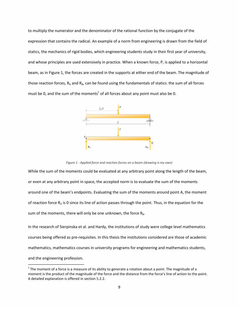
and whose principles are used extensively in practice. When a known force, P, is applied to a horizontal
beam, as in Figure 1, the forces are created in the supports at either end of the beam. The magnitude of
those reaction forces, RA and RB, can be found using the fundamentals of statics: the sum of all forces
must be 0, and the sum of the moments1 of all forces about any point must also be 0.
Figure 1 - Applied force and reaction forces on a beam (drawing is my own)
While the sum of the moments could be evaluated at any arbitrary point along the length of the beam,
or even at any arbitrary point in space, the accepted norm is to evaluate the sum of the moments
around one of the beam’s endpoints. Evaluating the sum of the moments around point A, the moment
of reaction force RA is 0 since its line of action passes through the point. Thus, in the equation for the
sum of the moments, there will only be one unknown, the force RB.
In the research of Sierpinska et al. and Hardy, the institutions of study were college level mathematics
courses being offered as pre-requisites. In this thesis the institutions considered are those of academic
mathematics, mathematics courses in university programs for engineering and mathematics students,
and the engineering profession.
1 The moment of a force is a measure of its ability to generate a rotation about a point. The magnitude of a
moment is the product of the magnitude of the force and the distance from the force’s line of action to the point. A detailed explanation is offered in section 5.2.2.
10
2.3 DIDACTIC AND INSTITUTIONAL TRANSPOSITION
The theoretical block of an institution’s praxeology preserves the institution’s activity as a practice and
communicates it to others, so that they, too, can participate in it (Hardy, 2009, p. 344). In other words,
the technology and theory not only serve to justify an institution’s tasks and techniques, but also makes
them teachable and learnable to others either within the same institution or within another. When one
institution imports the praxeology of another with didactic intentions, then the knowledge of the
praxeology undergoes didactic transposition (Chevallard, 1985; Castela & Romo Vasquez, 2011).
Consider the teaching of mathematics to engineering students. The mathematics that is taught
originates in the institution of academic mathematics which, according to Castela (2015) has the status
of the “reference point” for mathematical knowledge. However, the engineering students are not
members of the institution of academic mathematics, but of the institution of mathematics courses in
an engineering program. They are taught a certain didactic transposition of the academic mathematics.
But engineers also use mathematics in the workplace. When using mathematics in their professional
practice, engineers adapt (“transpose”) the praxeology of academic mathematics in order to use
techniques and their associated technologies and theories in order to accomplish engineering tasks. But
since the purpose isn’t didactic, the mathematical knowledge is said to undergo institutional
transposition (Castela & Romo Vasquez, 2011).
Referring again to Hardy (2009, p. 343), mathematical knowledge in an educational institution can take
on different forms:
1. Scholarly knowledge, which is the wealth of knowledge that is produced by the professionals of
an institution. An example of mathematical scholarly knowledge is, for example, the theory of
vector spaces over an arbitrary field.
11
2. Knowledge to be taught, which is found in the curriculum documents of a course that seeks to
impart some of the scholarly knowledge. The syllabus of an undergraduate Linear Algebra
course may contain only a selection of results of the theory of finite dimensional real vector
spaces.
3. Knowledge actually taught which can be found in a teacher’s lecture notes and the tasks that
are prepared for the students. In the Linear Algebra course from the previous example, the
teacher may choose to refer students to the textbook for the proofs of theorems and only
illustrate the theorems on examples in class.
4. Knowledge to be learned, which is interpreted by the students as the minimum amount of
knowledge needed to complete the tasks. This knowledge can be deduced from assessment
instruments such as assignments and exams. In the Linear Algebra course, it may sometimes be
enough to know how to solve typical computational exercises to pass the course; reasoning
based on the theorems introduced in the course to solve simple conceptual problems (e.g., of
the “Show that…” type) is usually required to obtain a high grade.
5. Knowledge actually learned which is reflected in the students’ responses to the assessments
that they’ve been given.
The first part of this thesis focuses on the mathematical knowledge that is to be taught and to be
learned by both engineering and mathematics students. Course descriptions and syllabi are used to
determine the knowledge to be taught, and final exams are used to determine the knowledge to be
learned.
2.4 VALIDATION OF THE CHOSEN FRAMEWORK
The chosen framework encapsulates all of the elements that are necessary for describing and analyzing
the mathematics that engineers are expected to learn in their education – what I call mathematics for
12
engineers (chapter 4) – and the mathematics used by engineers in their practice – referred to as
engineer’s mathematics (chapter 5). The knowledge in the institutions of interest can be modelled by
praxeologies; the mathematics courses in engineering programs and the engineering profession itself
both meet the requirements of being classified as institutions, and the knowledge imparted in both of
these institutions is a result of the transposition, both didactic and institutional, of knowledge produced
in the institution of mathematics.
The successful completion of a mathematics course in an engineering program requires that the
students perform a number of mathematical tasks on assignments, tests, and exams. Each of these tasks
can be accomplished using techniques that they are expected to learn. The technology and theories that
justify the use of those techniques are found in the students’ textbooks and in the discourse of the
lectures they attend. When it comes to the profession of engineering, even large projects such as the
design of a multi-storey building can be broken down into a series of smaller design tasks (design of the
foundations, design of the structural framework made up of beams and columns and their connections,
design of the concrete slabs for the floors, etc.), each with their own techniques. In this case the
technology and theories that describe and justify the techniques are not only their mathematical
soundness, but take the form of legally mandated design codes and manuals that an engineer must use
to perform these design tasks (e.g., the National Building Code of Canada, the Handbook of Steel
Construction, the Concrete Design Handbook, etc., are documents that have all been certified by the
Canadian Standards Association, CSA). The contents of these documents, which include the appropriate
formulae for design and analysis, have been developed and refined through decades of engineering
science research.
Besides having knowledge that can be modelled by praxeologies, mathematics courses in engineering
programs and the engineering profession itself both fit Peters’ (1999) description of an institution.
Engineering mathematics courses are a structural feature of accredited engineering programs which are
13
entrenched in the higher education institution that they find themselves in. Since 1965 the accreditation
of engineering programs has been overseen by the Canadian Engineering Accreditation Board (CEAB),
though some programs pre-date its existence. For example, the Department of Civil Engineering and
Applied Mechanics at McGill University was established in 1871, and the École Polytechnique, affiliated
with Université de Montréal, opened its doors in 1873. The actions and behaviours of students in these
programs are constrained by the rules, norms, and strategies put into place by the universities and the
individual mathematics courses in the programs. Courses that teach pure mathematics must be taken as
pre-requisites for several of the core engineering courses. Failure to pass a mathematics course can lead
to sanctions that include academic probation or possibly expulsion from the program. All of the students
in the engineering programs share a common goal and graduating and beginning their careers as
engineers. But in order to undertake a career in that profession a minimum level of mathematical
competence is required, not only at the behest of the university, but by the members of the profession
as well. Thus, the mathematics courses are a welcome means to a desired end.
For its part, the engineering profession also fits Peters’ (1999) description. The professional practice of
all engineers is a formal structure of Canadian society. The practice is overseen by the constituent
associations of Engineers Canada. The associations are the provincial and territorial engineering
regulatory bodies that license professional engineers in their jurisdiction. In Quebec, the association is
the Ordre des ingénieurs du Québec (OIQ), a professional order that was established by the Engineers
Act of Quebec’s National Assembly in 1974. Only members of the OIQ are legally allowed to practice
engineering and refer to themselves by the exclusive title of Engineer (Eng), or Ingénieur (ing.). In other
provinces, the term Professional Engineer, abbreviated P.Eng., is used. This gives engineers the same
status of a profession as doctors and lawyers. Furthermore, to ensure that its members respect the
shared values of the institution, professional orders such as the OIQ have instituted rules that require
their members to take part in a minimum number of hours of professional and educational development
14
activities each year, beyond the scope of their regular professional duties. Violating this rule leads to
sanctions that include revocation of one’s professional license. The shared values in question are found
in the sense of ethics that engineers uphold. According to the OIQ’s Code of Ethics, an engineer is
required to respect, first and foremost, their obligations towards the safety of the general public. This
primary value is also the result of engineers recognizing the effects of the profession’s past failures.
Lastly, the mathematical knowledge that engineering students are expected to learn in their
mathematics courses, and the knowledge that engineers use in their professional practice, are the result
of transpositions, both didactic and institutional, as was discussed earlier. One question that this thesis
will investigate is whether the mathematics that engineering students are expected to learn has been
transposed in such a way that it is different from that which mathematics students are expected to learn.
The key to answering this question may lie in the notion that engineering mathematics is applied
mathematics (Blum & Niss, 1991), and relies heavily on the development and use of mathematical
models. These concepts will be further explained in section 3.3.
15
3 LITERATURE REVIEW
This chapter presents and discusses the findings of several research studies in mathematics education
on the nature of the mathematical content in courses offered to students in different educational
settings, including mathematics taught to engineering students, mathematics taught in vocational
education, the teaching of mathematical applications and modelling, mathematics as a service subject,
and mathematics as it is used in the workplace. The final section illustrates an example of the teaching
and use of geometry, measurement, and error in measurement at vocational schools.
The discussions in the sections that follow will be interspersed with comments that compare and
contrast the findings in the literature with the educational and workplace mathematics of engineers
based mainly on my experience. More detailed analysis of mathematics for engineering students and
professional engineers will appear in chapters 4 and 5.
3.1 MATHEMATICS EDUCATION FOR ENGINEERS
The following section summarises the recent works of Castela and Romo-Vazquez and their studies in
the mathematics education of engineering students at the Vocational Institute at the University of Evry
in France (Castela, 2015; Castela & Romo Vasquez, 2011; Romo Vasquez & Castela, 2010). Using the
framework of the ATD, they studied how mathematics is used by students in an engineering project
design course, focusing on the use of Laplace transforms as a technique for completing the task of
solving linear differential equations, and comparing how the technique is taught in mathematics
textbooks with how it is taught in engineering textbooks.
This study showed that engineering students select the techniques they need for their tasks based on
practicality. The chosen techniques were never justified by a technology and theory that relied solely on
mathematical concepts and definitions, but on whether the techniques allowed them to quickly obtain
16
the results of their calculations and whether or not the results made physical sense in the context of
their design tasks. The students were allowed to use computer software for more difficult tasks, and
while this allowed the students to explore some of the parameters of their designs, it had the effect of
“black-boxing” the mathematics, making it less visible. But this did not seem important to the students.
How the mathematics was validated was not as relevant as choosing the correct mathematical model
and the values to input into that model. Ultimately the research found that the students’ work itself
could not be reduced to mathematics alone, since their tasks also required knowledge of physical and
engineering sciences.
In the comparison of how Laplace transforms are taught in engineering and mathematics textbooks, it
was noted that the technique taught in the engineering textbook was altered slightly from the
traditional mathematical technique. The motivation behind the altered technique is that it results in
functions whose arguments are formatted so that there is added value for the engineer. From the
results of the transform, the engineer can determine properties of the function directly from its
expression without having to do any algebraic manipulations or simplifications. Furthermore, while the
mathematics textbooks focused on the comprehensive and accurate presentation of the technique
using theorems and proofs, the engineering textbook gave a lower priority to proofs and instead
correlated the technique with its use in a vocational context (Castela, 2015).
In terms of the ATD framework, the engineering textbook appropriated the praxeology from academic
mathematics and augmented the theoretical block with a new description of the Laplace transform
technique, and new justifications that are based on the practicality of the technique’s application. If
engineers’ mathematics is different from that of mathematicians, the difference is most likely found in
the theoretical block of the praxeology, as engineers complement mathematical praxeology with
elements of engineering knowledge.
17
3.2 MATHEMATICS IN VOCATIONAL EDUCATION
A series of papers in Educational Studies in Mathematics (2014) explored the mathematics of specialized
vocational disciplines, with the goal of characterizing and developing the vocational mathematical
knowledge. The study examined the education of students who were learning to be electricians,
practitioners in various pipe trades (welders & plumbers), laboratory technicians, and business school
graduate students.
The studies involving the electrician and pipe trade apprentices were done at vocational schools in
western Canada, while the others took place at schools in various European countries. This would be the
equivalent to technical programs at a Quebec CEGEP for skilled trade workers, a construction
certification from the Régie de bâtiment du Québec (RBQ), or other vocational and/or continuing
education institutions. It should be mentioned, however, that engineering education is not vocational. In
order to obtain a degree in engineering, a student from Quebec is required to do a two-year pre-
university science program at CEGEP, followed by a three-year university education. As will be shown in
chapter 4, mathematics courses are required in an engineer’s education. So while the studies presently
discussed are not representative of an engineer’s situation, they can still offer insight into the
transposition of academic mathematics for didactic purposes.
The general findings in the papers of LaCroix (2014) and Roth (2014) are that the mathematics taught to
future practitioners of various trades is directly shaped by the immediate and practical requirements of
the workplace, where it’s more important to get the job done efficiently than to worry about theoretical
rigour precision. The generalizations, formalities, and internal consistencies of academic mathematics
are absent from the workplace. In the classroom, the instructors, who are themselves qualified and
experienced tradespeople, are more concerned that their students get answers to problems that are
18
“close enough”, than they are with the methods that are used to find the answers. Essentially, the old
adage of “time is money”, prevalent in the workplace, is applied to their school work as well.
Electrician apprentices do learn the basic trigonometric functions (sine, cosine, tangent, and cotangent),
in an effort to explain the demands of the electrical code, a legal document that is to be followed in
doing electrical work. The code itself contains no mathematics, just general rules for the installation of
electrical conduits. But, while the trigonometric functions justify the work methods that ensure the code
is followed, on the job, trigonometry is replaced by “rules of thumb” that allow electrical conduits to be
installed efficiently, cables passed through the conduits easily, and the tools and equipment of their
trade to be used safely. Similarly, pipe trade apprentices who need to join two pipes at a specified angle
eventually learn how to eyeball a fit that is “more or less” correct, without the rigorous use of
trigonometry. This is in stark contrast to engineering design codes (for example: CSA-S6 – Canadian
Highway Bridge Design Code; CSA-S16.1 – Limit States Design of Steel Structures; CSA-A23.3 – Design of
Concrete Structures), which contain a multitude of mathematical formulae to be used in the design and
analysis of steel and concrete structures. The mathematics found in these codes was developed and
refined through extensive engineering research and testing of mathematical models.
Further evidence that the “why” of mathematics is less relevant than the “how” of the workplace can be
found in the interactions between the students and their instructors. In the pipe trade training course,
the instructor announced to his students that they would not use all of the mathematics that they were
taught. The electrician apprentices for their part claimed that they did not see or use any trigonometry
during the job site training portion of their course, and questioned the pertinence of learning it, even
though it is a requirement for earning their certification. It is mentioned that the instructors “colluded”
with their students to learn the mathematics simply for the sake of obtaining certification (Roth, 2014).
19
Coben and Weeks (2014) argue that mathematics education can be made more authentic and more
meaningful for all vocational trades by exposing the students to more appropriate and authentic tasks
and problems in which the mathematics is present, but no more explicitly than they are in the workplace.
In other words, the problems given to students in the electrical and pipe trades should be designed to
show exactly how trigonometry is helpful in accomplishing a task such as offsetting an electrical conduit,
and how the rules of thumb they will eventually use can be derived from these same mathematical
functions.
However, doing so doesn’t guarantee an improved mathematical understanding. Wake (2014) presents
vignettes of research studies in which students were brought to various workplaces and exposed to
practical uses of the mathematics they were learning. In one study, college students following a pre-
vocational engineering course visited the workplace of a practicing railway engineer. The railway
engineer showed the students how to calculate the average downhill gradient (slope) of a railway track
composed of three sections of track each with a different gradient. In discussions following the visit, it
was revealed that the students believed that they could simply average the three values of slope, in the
same way they had learned to find the average of a set of integers. The proper technique requires using
the individual gradients to calculate the total change in elevation (rise or fall) of each of the three
sections. The total change in elevation, , is then divided by the total distance, , along all three
sections, and thus the average slope is found to be
. The railway engineer who explained the
technique to the students used the chart in Figure 2 to perform his calculations in his actual practice.
20
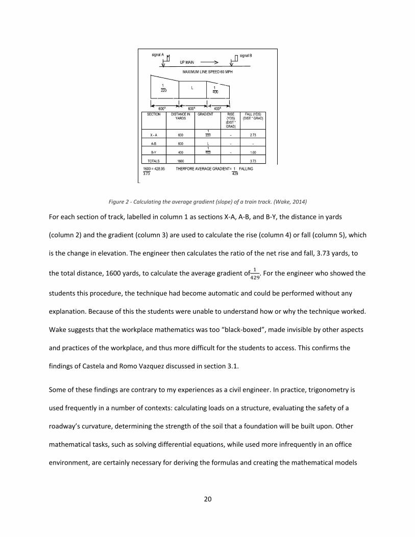
Figure 2 - Calculating the average gradient (slope) of a train track. (Wake, 2014)
For each section of track, labelled in column 1 as sections X-A, A-B, and B-Y, the distance in yards
(column 2) and the gradient (column 3) are used to calculate the rise (column 4) or fall (column 5), which
is the change in elevation. The engineer then calculates the ratio of the net rise and fall, 3.73 yards, to
the total distance, 1600 yards, to calculate the average gradient of
. For the engineer who showed the
students this procedure, the technique had become automatic and could be performed without any
explanation. Because of this the students were unable to understand how or why the technique worked.
Wake suggests that the workplace mathematics was too “black-boxed”, made invisible by other aspects
and practices of the workplace, and thus more difficult for the students to access. This confirms the
findings of Castela and Romo Vazquez discussed in section 3.1.
Some of these findings are contrary to my experiences as a civil engineer. In practice, trigonometry is
used frequently in a number of contexts: calculating loads on a structure, evaluating the safety of a
roadway’s curvature, determining the strength of the soil that a foundation will be built upon. Other
mathematical tasks, such as solving differential equations, while used more infrequently in an office
environment, are certainly necessary for deriving the formulas and creating the mathematical models
21
that are used in practice. For example, the different formulae for calculating the deformation of a beam
under a given load can be obtained by solving the differential equation:
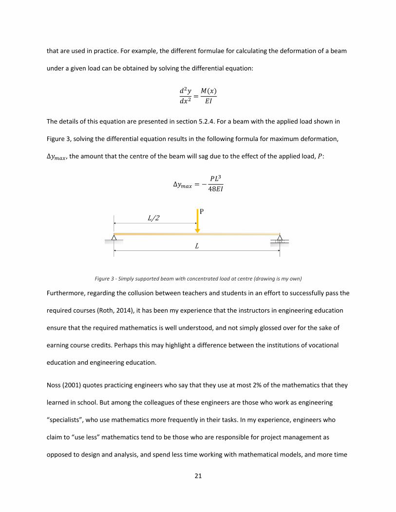
The details of this equation are presented in section 5.2.4. For a beam with the applied load shown in
Figure 3, solving the differential equation results in the following formula for maximum deformation,
, the amount that the centre of the beam will sag due to the effect of the applied load, :
Figure 3 - Simply supported beam with concentrated load at centre (drawing is my own)
Furthermore, regarding the collusion between teachers and students in an effort to successfully pass the
required courses (Roth, 2014), it has been my experience that the instructors in engineering education
ensure that the required mathematics is well understood, and not simply glossed over for the sake of
earning course credits. Perhaps this may highlight a difference between the institutions of vocational
education and engineering education.
Noss (2001) quotes practicing engineers who say that they use at most 2% of the mathematics that they
learned in school. But among the colleagues of these engineers are those who work as engineering
“specialists”, who use mathematics more frequently in their tasks. In my experience, engineers who
claim to “use less” mathematics tend to be those who are responsible for project management as
opposed to design and analysis, and spend less time working with mathematical models, and more time
22
managing budgets and schedules. And while their mathematical tasks may be less advanced than those
of the specialists, a project manager must be able to communicate with and understand what their
specialists tell them. Thus, the mathematics in an engineer’s education is not to be taken as lightly as it
appears to be in some vocations.
3.3 MATHEMATICAL APPLICATIONS AND MATHEMATICAL MODELLING
Several papers in Applications and modelling in learning and teaching mathematics (Blum, Berry, Biehler,
Huntley, Kaiser-Messmer, & Profke, 1989) discuss courses dedicated to the teaching of mathematical
modelling in various countries including the UK, the United States, and Canada. These courses are
offered to students of different disciplines and vocations including engineers, psychologists,
mathematics teachers, and geologists.
It is important to understand the difference between mathematical applications and mathematical
models. A mathematical application is the use of mathematics, its concepts, its objects, and its rules, to
solve a problem in which some aspect is based in the real world (Blum & Niss, 1991; Galbraith, Henn, &
Niss, 2007). Applications are useful in order to show students how mathematics can be used to solve
every-day or otherwise relevant tasks. A mathematical model, on the other hand, is a mapping that
transfers the objects that we wish to study from the real world into objects in a mathematical domain.
Mathematical models are idealized representations of the real world. The task of modelling involves
creating or designing an appropriate mathematical description of an extra-mathematical situation or
phenomenon. However, applications and models are not completely distinct; in every application of
mathematics there is an underlying mathematical model with built-in assumptions that are either
explicit or implicit.
The following problem is an example of a mathematical application:
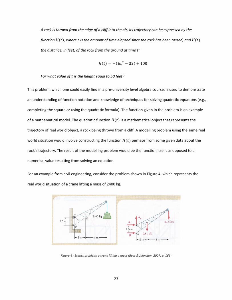
23
A rock is thrown from the edge of a cliff into the air. Its trajectory can be expressed by the
function , where is the amount of time elapsed since the rock has been tossed, and
the distance, in feet, of the rock from the ground at time :
For what value of is the height equal to 50 feet?
This problem, which one could easily find in a pre-university level algebra course, is used to demonstrate
an understanding of function notation and knowledge of techniques for solving quadratic equations (e.g.,
completing the square or using the quadratic formula). The function given in the problem is an example
of a mathematical model. The quadratic function is a mathematical object that represents the
trajectory of real world object, a rock being thrown from a cliff. A modelling problem using the same real
world situation would involve constructing the function perhaps from some given data about the
rock’s trajectory. The result of the modelling problem would be the function itself, as opposed to a
numerical value resulting from solving an equation.
For an example from civil engineering, consider the problem shown in Figure 4, which represents the
real world situation of a crane lifting a mass of 2400 kg.
Figure 4 - Statics problem: a crane lifting a mass (Beer & Johnston, 2007, p. 166)
24
The crane is connected to a vertical wall by supports located at points A and B. The engineer’s task
consists of finding the magnitude and direction of the forces in two supports that keep the crane in
place. The force at support B can be found by applying mathematics and using the following equation:
With this equation solved, the horizontal component of the force in support A can be found by solving
the equation:
Lastly, the vertical component of the force in support A is determined by solving the equation:
Each of these equations is an example of an application of mathematics, since the numerical values and
the symbols for unknown values all represent real world quantities. The underlying mathematical model
that leads to these equations is that of a fundamental physical principle called static equilibrium which
states that the sum of all forces and moments acting on a body must be zero. This model is expressed
symbolically as:
∑ ∑
This model was developed through a reformulation of Newton’s first law of motion. The concepts of
force, moments, and static equilibrium are discussed in further detail in chapter 5, but are included here
solely to highlight the difference between a mathematical application and the underlying mathematical
model.
Every mathematical model, including those used in engineering, is constructed with certain implicit or
explicit assumptions about the physical objects it represents and the mathematical objects it uses to
25
represent them. In the example of the rock being thrown from the cliff, the model (the function )
most likely assumes that the force of gravity acting on the rock is constant, and that the rock encounters
no resistance from the wind. These assumptions aren’t explicitly stated in the application problem, but if
one were tasked with creating the model, those assumptions would need to be made explicit. Another
implicit assumption is the domain of the function . Since the independent variable is the time
elapsed since a certain moment, the values of are restricted to non-negative real numbers. Similarly,
the mathematical model for the principle of static equilibrium assumes that the objects upon which the
forces are acting are rigid, i.e., they do not bend or twist. When an engineer uses the principles of statics
to solve such problems, this assumption is entirely implicit, even though it is not a true representation of
reality.
In my experience as an engineering student, some early courses involved a combination of both
application and modelling problems, particularly in courses that included laboratory sessions. In the
laboratory, experiments were performed and data was analyzed in order to confirm the validity of
established models. In more advanced courses, the textbooks and professors presented how certain
models came to be developed; it was not up to the students to create the models as they were too
complex. Once advanced models were learned and understood, application problems became more
prominent, but the student had to determine which model was needed to solve the application problem.
An important question asked by the authors of selected readings in Blum (1989) is whether the
mathematics that is used in creating mathematical models should be taught before or after students
learn to model mathematically. According to Bkouche (1989), one can learn how to model, for example,
with vectors before being taught vector theory. Consider students learning how to represent physical
forces being applied to objects and the resulting accelerations (based on Newton’s laws) with vector
arrows, prior to learning the underlying mathematics of generalized vector spaces. The same could be
imagined for learning and using rates of change of functions before learning the formal definition of the
26
derivative. The mathematical theory can be taught after the students have learned to build models, as a
means of unifying various representations, and reinforcing their models.
Alternatively to Bkouche’s (1989) perspective, a polytechnic in the UK offers a “first course in
mathematical modelling”, which ensures that all of the necessary formal mathematics is taught to the
students before they need to use it to create a mathematical model (Edwards & Hamson, 1989). Their
philosophy is to learn the math before learning the model. The reasons for this method are that most
situations that are modelled in this particular course have little to do with classical mechanics and
physics, and that the mathematics is less inherent in the situations themselves. Examples of case studies
include:
Hospital corridor: can a bed be moved around a right-angle bend in a corridor?
Order of play: how is a badminton match game order fixed when only 1 court is available?
On the buses: how do buses become congested despite timetabling on a typical city route?
Conifer trees: estimate the height against time as trees grow, allowing for seasonal growth.
Attempting to build a model for a real world situation in which the mathematics is not apparent can be
difficult if one’s knowledge of mathematical objects is limited. Learning about new mathematical objects
can allow a student to see an otherwise benign real world situation with a new perspective (Edwards &
Hamson, 1989).
Teague (1989) expresses an interesting thought when comparing pure mathematics with applied
mathematics. In his view, much of the mathematics taught in secondary school, such as simplifying
expressions or solving equations, is analogous to simply practicing finger exercises when learning to play
the piano. In order to “play the music” of real mathematics, which includes creating and using
mathematical models, one must be able to perform these manipulations, but there is more to playing
music than the finger exercises.
27
3.4 MATHEMATICS AS A SERVICE SUBJECT
The concept of mathematics as a service subject contrasts with the literature on vocational mathematics
education. Since engineering mathematics is not vocational mathematics, it more appropriately fits the
definition of mathematics as a service subject, i.e., mathematics that is taught to students who are
primarily engaged in studying other subjects. Engineers will use mathematics extensively in their work,
but they will not be mathematicians. The rise of service mathematics was a response to a need. In the
case of engineering, it is the need for engineering graduates to be mathematically competent (Howson,
et al., 1988).
For the universities and other institutions of learning there is also the need to ensure that all of the
students entering their programs have a common level of knowledge. At both McGill University and
Concordia University, engineering students who are originally from outside of Quebec are required to
extend their program by one year. During their first year, these students take courses in the
fundamentals of physics, chemistry, and mathematics, including pre-university linear algebra and
calculus. The mathematics courses in this year of study are service courses, intended to bring these
students to the same level of knowledge as those who will enter the engineering program from CEGEP
the following year.
The International Commission on Mathematical Instruction (ICMI) compiled selected papers on the
teaching of mathematics as a service subject in an attempt to answer a few questions on the matter,
including questions that are pertinent to this thesis, such as:
Who teaches service mathematics courses?
Are there differences in how service mathematics courses are taught and assessed, in
comparison with mathematics courses for mathematicians?
Do the students encounter any obstacles in the form of language or symbolism?
28
Another issue of concern is determining which topics should be taught in a service mathematics course.
Howson et al. (1988) present two points of view to help address this question. The first approach is to
consider mathematics as a tool that students use to solve concrete problems drawn from their own
discipline. Abstract mathematical notions that are not directly related to relevant applications should be
discarded. Alternatively, though not completely dissimilar in approach, mathematics can be viewed as a
language, and the students should know how to read it, and communicate with it. Since much of the
literature in their discipline is written in the language of mathematics, knowing how to read it will allow
the students to learn more about their own subjects on their own.
The universities at Southampton (UK) and Orsay (Université Paris-Sud, France), for their part, have
adopted similar attitudes. For these schools, service mathematics is meant to acquaint the students with
the mathematical techniques that will be useful or essential in their core discipline courses. The teaching
of service mathematics is meant to be done quickly, without the need to elaborate on the history or
underlying theorems behind these techniques. In particular, they propose that engineers should be
required to learn calculus, but not analysis. This is in fact presently the case for engineering students in
Quebec.
When it comes to determining who should teach the service mathematics courses (those who teach in
the discipline itself, or mathematicians and mathematics teachers), the majority of contributors appear
to favour those from outside of mathematics. Teachers from the service discipline are aware of the
profession’s needs, and will also be able to properly structure the courses so that the mathematics that
are needed can be taught immediately preceding a core course in which they will be needed. This can
also provide uniformity in the use of language and symbolism between the mathematics and the core
courses. Lastly, students in the service discipline will be more motivated, as they will feel more
connected to a teacher from their field. A student from Cardiff (Wales, UK) offered the opinion that
“engineering students should be taught by engineers, or at least by mathematicians who are based in
29
the engineering faculty. The biggest single problem is motivation, and this is best achieved if the
teaching is done by engineers who are respected by the students as engineers and who can draw
examples to illustrate the mathematics from their own work.”
The argument is strengthened by mentioning the additional work that would be required of a
mathematician to teach to non-mathematicians. They would have to learn the language and symbolism
of the service discipline, adapt it to a mathematical framework, provide mathematical analysis and
techniques, and translate it back into the students’ language.
So one could ask, is it easier for an engineer to teach the fundamentals of the mathematics that they use,
or for mathematicians to provide engineering context to the mathematics that they teach?
In discussing how service mathematics courses should be taught, Howson (1988) states that there is
nothing sacrosanct about the order in which mathematical topics are presented: fundamental concepts
of a subject can be taught before showing students how to solve problems based on those concepts, or
the concepts can be introduced while working through an example. In my own research on engineering
programs at universities in Quebec (chapter 4) I found that some mathematics courses teach the
concept of limit prior to infinite series, while others introduce the limit after teaching infinite series, thus
supporting Howson’s view.
Blum and Niss (1991) also characterize engineering mathematics as being different from vocational
mathematics, and classify it as a service subject. In mathematics courses for engineers, the focus is not
on the mathematics itself but on the other subjects in which mathematics will provide a service. In their
research, the characterization of mathematics instruction is analyzed by considering the educational
histories, the purpose, and the organizational framework of mathematics instruction. In terms of
educational history, engineering mathematics is classified as a service subject, while mathematics taught
to mathematicians or mathematics teachers is not. The purpose of mathematics instruction for
30
engineers is to provide students with mathematical knowledge as it relates to other subjects in their
field (mechanics, thermodynamics, structural analysis, etc.). Engineering mathematics is further
characterized by the organizational framework in which it is found. In fact, it can be classified into two
frameworks: it can be taught as a separate subject in mathematics courses, or as part of, and integrated
into, one or more engineering courses. These separate frameworks can lead to a division of labour
among the mathematics and engineering professors such that the mathematics courses may be entirely
devoid of mathematical modelling, and are instead organized so as to present all of the mathematical
concepts that will be needed in the subject being serviced, while the applications and modelling will take
place in the extra-mathematical courses. The results of my research, presented in chapter 4, fit this
description fairly well.
3.5 MATHEMATICS IN THE WORKPLACE
The edited volume Education for Mathematics in the Workplace (2000) presents a number of studies on
mathematical knowledge and the use of mathematics at both school and work. The main theoretical
framework of the book is based on the Anthropological Theory of the Didactic: that mathematics is a
human activity that takes place in all kinds of contexts and situations; however, in the workplace, the
mathematics is deeply entrenched in a given profession’s activities, and is not always visible either to
outside observers, or to the workers themselves (Noss, Hoyles, & Pozzi, 2000).
Evans (2000) discusses the problem that workers have in “transferring” their mathematical knowledge
from school to the workplace, i.e., applying what they have learned at school to non-pedagogical
contexts, such as their work environment. Of particular note is that there is no guarantee that transfer
will even occur; in other words “book smarts” do not always transfer to “street smarts”. For example, a
student who is capable of properly subtracting fractions from whole numbers (e.g., performing the
operation
) using subtraction techniques in a classroom setting may not be able to perform the
31
same task on a construction site where they are handed a two-foot long piece of lumber and asked to
make it three and quarter inches shorter.
To say that mathematical knowledge can be transferred implies that it can be applied to similar
problems but in different contexts. This is based on the assumptions that:
Learning is the transmission of knowledge from a teacher to a student.
The mathematical knowledge that is needed to solve a problem can be removed from the
context of the problem. In the context of the ATD, this would mean that there exists
mathematical knowledge that is independent of any task to accomplish, or technique to
accomplish that task.
A problem can be reduced to its mathematics, and that a mathematical strategy can be used to
solve problems across different contexts.
But are these assumptions justified? Mathematics is learned in a socially constructed environment, with
established and ongoing activities, social relationships, and language. Thus there are more factors at
play than just the interaction between the teacher and the student. Furthermore, changing the
environment in which a person finds themselves can change the mathematical strategies that they use.
Recall the studies of Castela and Romo-Vazquez presented in section 3.1, and the finding that much of
the students’ work could not be reduced to mathematics alone. Referring to my earlier example of a
construction worker cutting a two-foot long piece of lumber, by changing the context of the problem
(subtracting a fraction from a whole number) from a school exercise to a work situation, the
mathematical strategy of using techniques of subtraction becomes too time-consuming and ultimately
useless; making the two-foot piece of lumber three and quarter inches shorter one simply has to
measure
inches on a tape measure, and make the cut at that length. Determining the length of
lumber that remains is not necessary. Moreover, since the construction site environment has additional
32
pressures and stresses such as loud noises and having to work quickly and efficiently while following
safety regulations, the mathematical knowledge of subtraction becomes only a small part of the total
knowledge engaged when working.
Rather than thinking about how mathematical knowledge is transferred in the sense described by Evans,
this thesis considers that mathematical knowledge undergoes institutional transposition. The difficulty
in reconciling school mathematics with work mathematics may occur in the transposition that the
mathematical knowledge undergoes between institutions.
In the same volume, Noss et al. (2000) present a study showing that professionals and practitioners (i.e.,
labourers) use mathematics differently than mathematicians. While mathematicians study mathematics
for its own sake, professionals are driven by a pragmatic agenda: they study mathematics to solve
problems external to mathematics. They must solve problems efficiently and effectively using
mathematical knowledge and expertise, but their professional concerns take precedence over
mathematical concerns. For the practitioners, a theorem must, first of all, “work” as a tool in solving
their practical problems; for mathematicians, a theorem must be, first of all, “true” and then important
for the advancement of a theory; it is better if it is also non-trivial. This brings to mind the studies
discussed in section 3.2 involving electricians.
The theory of situated abstraction (a term coined by Noss) focuses on the similarities in the structures of
“mathematics in learning” and “mathematics at work.” Other theories, such as situated cognition and
policy-driven studies, tend to emphasize the differences between the two. From the perspective of
situated abstraction, the authors performed an exploratory study to examine the relationship between
practical, professional, and mathematical knowledge in three professions: commercial airline pilots,
bankers, and nurses. Their goal was to locate the mathematics that was used at work, searching for
“visible mathematics” in the day-to-day activities of the different professions. Visible mathematics could
33
take the form of conventional mathematical symbolism and representation, or the use of concepts,
strategies, and methods of a mathematics classroom. However, it was found that, in routine tasks, very
little of the practitioners’ mathematics is visible. Even the workers themselves failed to notice when
they are using mathematics, or simply did not regard what they were doing as “mathematical.” The
visible mathematics that was found took the form of:
Finding solutions in procedural ways, with the use of algorithms and spreadsheets to perform
menial computations, particularly by bankers.
Routine gathering and interpreting of data.
Using “look up” methods, i.e., the use of tables and charts containing pre-calculated values for
similar or general problems (rather than using analytic formulas or functions for calculating their
values).
Look up methods are used to solve problems that are already well-understood, and can circumvent the
need to work in the realm of school mathematics. But an understanding of the underlying mathematics
that lead to the development of the look up tables is still a necessity for those who use them; otherwise
the values in the tables may not be properly interpreted. For example, a pilot deciding whether or not to
land in wintery conditions must quickly calculate the normal component of crosswinds acting on the
aircraft. In Figure 5, the crosswind is represented by the red arrow, and its components are represented
by the blue arrows. The normal component of the crosswind acts orthogonal to the direction of travel,
and the amount of force it exerts on the plane is critical in determining whether it is safe to land.
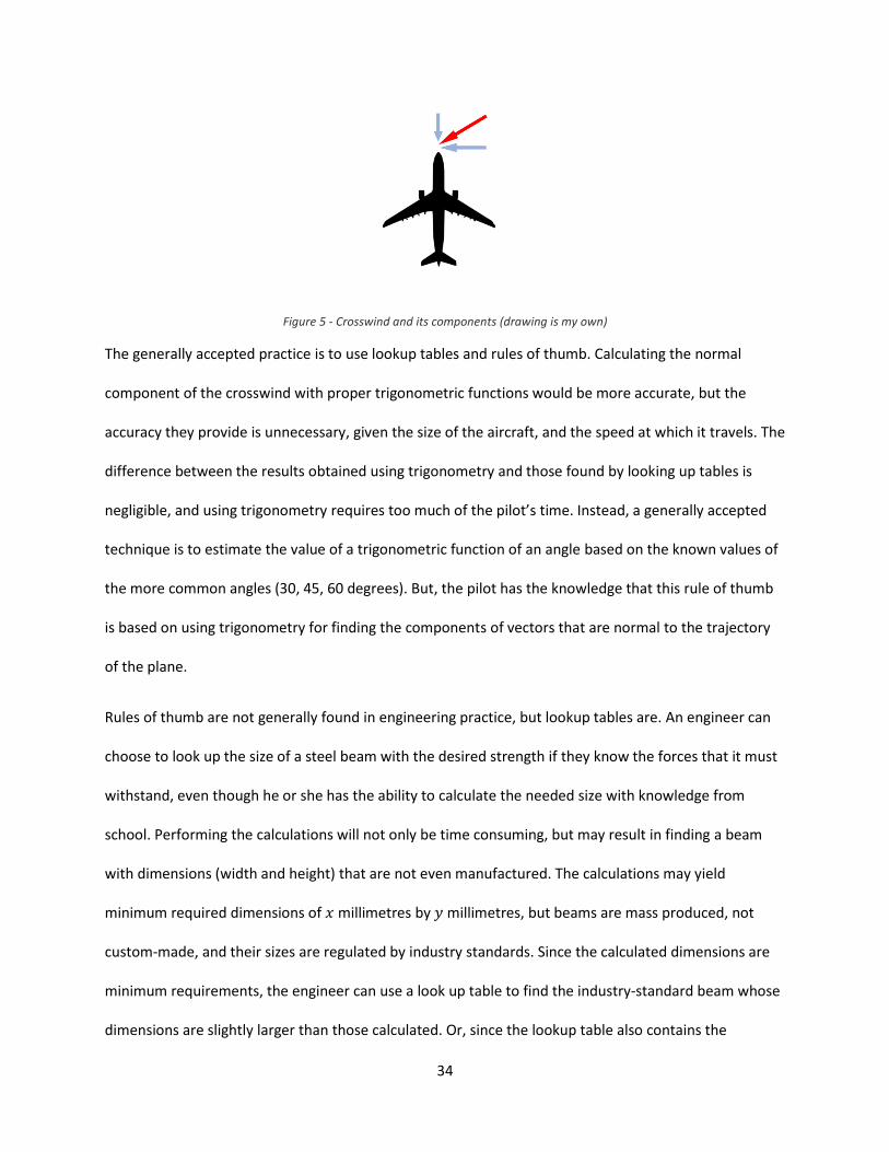
34
Figure 5 - Crosswind and its components (drawing is my own)
The generally accepted practice is to use lookup tables and rules of thumb. Calculating the normal
component of the crosswind with proper trigonometric functions would be more accurate, but the
accuracy they provide is unnecessary, given the size of the aircraft, and the speed at which it travels. The
difference between the results obtained using trigonometry and those found by looking up tables is
negligible, and using trigonometry requires too much of the pilot’s time. Instead, a generally accepted
technique is to estimate the value of a trigonometric function of an angle based on the known values of
the more common angles (30, 45, 60 degrees). But, the pilot has the knowledge that this rule of thumb
is based on using trigonometry for finding the components of vectors that are normal to the trajectory
of the plane.
Rules of thumb are not generally found in engineering practice, but lookup tables are. An engineer can
choose to look up the size of a steel beam with the desired strength if they know the forces that it must
withstand, even though he or she has the ability to calculate the needed size with knowledge from
school. Performing the calculations will not only be time consuming, but may result in finding a beam
with dimensions (width and height) that are not even manufactured. The calculations may yield
minimum required dimensions of millimetres by millimetres, but beams are mass produced, not
custom-made, and their sizes are regulated by industry standards. Since the calculated dimensions are
minimum requirements, the engineer can use a look up table to find the industry-standard beam whose
dimensions are slightly larger than those calculated. Or, since the lookup table also contains the
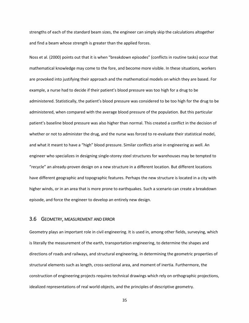
35
strengths of each of the standard beam sizes, the engineer can simply skip the calculations altogether
and find a beam whose strength is greater than the applied forces.
Noss et al. (2000) points out that it is when “breakdown episodes” (conflicts in routine tasks) occur that
mathematical knowledge may come to the fore, and become more visible. In these situations, workers
are provoked into justifying their approach and the mathematical models on which they are based. For
example, a nurse had to decide if their patient’s blood pressure was too high for a drug to be
administered. Statistically, the patient’s blood pressure was considered to be too high for the drug to be
administered, when compared with the average blood pressure of the population. But this particular
patient’s baseline blood pressure was also higher than normal. This created a conflict in the decision of
whether or not to administer the drug, and the nurse was forced to re-evaluate their statistical model,
and what it meant to have a “high” blood pressure. Similar conflicts arise in engineering as well. An
engineer who specializes in designing single-storey steel structures for warehouses may be tempted to
“recycle” an already-proven design on a new structure in a different location. But different locations
have different geographic and topographic features. Perhaps the new structure is located in a city with
higher winds, or in an area that is more prone to earthquakes. Such a scenario can create a breakdown
episode, and force the engineer to develop an entirely new design.
3.6 GEOMETRY, MEASUREMENT AND ERROR
Geometry plays an important role in civil engineering. It is used in, among other fields, surveying, which
is literally the measurement of the earth, transportation engineering, to determine the shapes and
directions of roads and railways, and structural engineering, in determining the geometric properties of
structural elements such as length, cross-sectional area, and moment of inertia. Furthermore, the
construction of engineering projects requires technical drawings which rely on orthographic projections,
idealized representations of real world objects, and the principles of descriptive geometry.
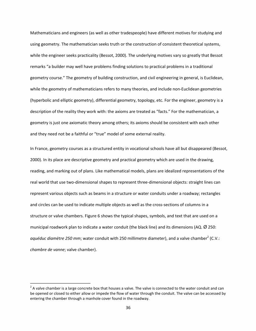
36
Mathematicians and engineers (as well as other tradespeople) have different motives for studying and
using geometry. The mathematician seeks truth or the construction of consistent theoretical systems,
while the engineer seeks practicality (Bessot, 2000). The underlying motives vary so greatly that Bessot
remarks “a builder may well have problems finding solutions to practical problems in a traditional
geometry course.” The geometry of building construction, and civil engineering in general, is Euclidean,
while the geometry of mathematicians refers to many theories, and include non-Euclidean geometries
(hyperbolic and elliptic geometry), differential geometry, topology, etc. For the engineer, geometry is a
description of the reality they work with: the axioms are treated as “facts.” For the mathematician, a
geometry is just one axiomatic theory among others; its axioms should be consistent with each other
and they need not be a faithful or “true” model of some external reality.
In France, geometry courses as a structured entity in vocational schools have all but disappeared (Bessot,
2000). In its place are descriptive geometry and practical geometry which are used in the drawing,
reading, and marking out of plans. Like mathematical models, plans are idealized representations of the
real world that use two-dimensional shapes to represent three-dimensional objects: straight lines can
represent various objects such as beams in a structure or water conduits under a roadway; rectangles
and circles can be used to indicate multiple objects as well as the cross-sections of columns in a
structure or valve chambers. Figure 6 shows the typical shapes, symbols, and text that are used on a
municipal roadwork plan to indicate a water conduit (the black line) and its dimensions (AQ. Ø 250:
aquéduc diamètre 250 mm; water conduit with 250 millimetre diameter), and a valve chamber2 (C.V.:
chambre de vanne; valve chamber).
2 A valve chamber is a large concrete box that houses a valve. The valve is connected to the water conduit and can
be opened or closed to either allow or impede the flow of water through the conduit. The valve can be accessed by entering the chamber through a manhole cover found in the roadway.
37
Figure 6 - Symbols for water mains and valve chambers (drawing is my own)
In mathematics, the solution to a geometric problem may require a formal proof of existence of an
object or a relation between properties, a construction of an object satisfying certain conditions, and
theoretical precision. In vocational and professional practices, a solution doesn’t require the same
exactitude. To a mathematician, the ratio of any circle’s circumference to its diameter is always ; for an
engineer, the decimal approximation of 3.14 may be “good enough” for many calculations. A project’s
construction plans need only be “sufficiently precise” in relation to desired tolerances to be considered
acceptable. For example, connecting a steel beam to a column can be done as long as there is enough
“wiggle room” for inserting the bolts. While the plan may state the required dimensions to the
millimetre, variation in the fabrication of the steel pieces cannot be completely eliminated.
This is not to suggest that there isn’t any amount of care taken, or precision required, when civil
engineers use mathematics in their work of designing and executing engineering projects. In fact, the
opposite is true – but it is a different precision and care about different aspects. Engineers raise
questions about the nature and magnitude of errors and tolerances in calculations and in measurements.
Eberhard (2000) discusses geometry and measurement as used by the students taking part in an actual
construction project being overseen by their technical high school. At this school the students are being
trained to become foremen and skilled workers, earning a Brevet de Technicien. The students use
measuring techniques to transfer dimensions from a plan into physical markings on the ground, a
process called marking out. They must then verify that their physical markings match the specified
dimensions on the plan.
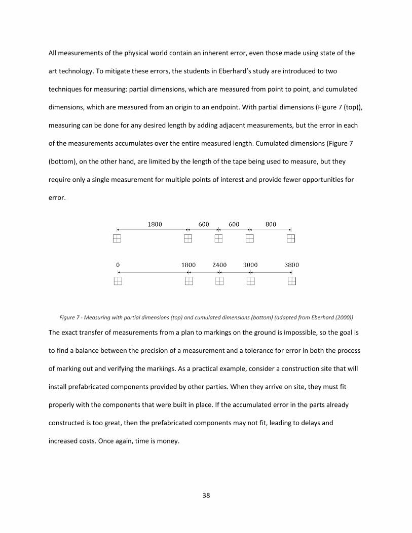
38
All measurements of the physical world contain an inherent error, even those made using state of the
art technology. To mitigate these errors, the students in Eberhard’s study are introduced to two
techniques for measuring: partial dimensions, which are measured from point to point, and cumulated
dimensions, which are measured from an origin to an endpoint. With partial dimensions (Figure 7 (top)),
measuring can be done for any desired length by adding adjacent measurements, but the error in each
of the measurements accumulates over the entire measured length. Cumulated dimensions (Figure 7
(bottom), on the other hand, are limited by the length of the tape being used to measure, but they
require only a single measurement for multiple points of interest and provide fewer opportunities for
error.
Figure 7 - Measuring with partial dimensions (top) and cumulated dimensions (bottom) (adapted from Eberhard (2000))
The exact transfer of measurements from a plan to markings on the ground is impossible, so the goal is
to find a balance between the precision of a measurement and a tolerance for error in both the process
of marking out and verifying the markings. As a practical example, consider a construction site that will
install prefabricated components provided by other parties. When they arrive on site, they must fit
properly with the components that were built in place. If the accumulated error in the parts already
constructed is too great, then the prefabricated components may not fit, leading to delays and
increased costs. Once again, time is money.
39
Since there is always error involved in measurement, we might well ask how the notion of error is taught
in vocational schools. The general teaching of mathematics in France (as of 2000) does not include the
topic of error in measurements, though it was taught in the 1960’s (Eberhard, 2000). As it relates to the
use of partial and cumulated dimensions, it could be explained that the latter technique is favourable if
measurement error is thought of as either an uncertainty in measurement (the model of uncertainties),
or as a random variable with a characteristic standard deviation (the model of probabilities). Eberhard
(2000) states that “the algebraic theory of uncertainties or the probability theory of errors *could+ work
together as a basis for theoretical understanding”, and could also help in showing why the use
cumulated dimensions is preferred. But the teachers at schools awarding the Brevet de technicien are
not required to teach the theoretical notion of error. In their view, using cumulated dimensions is
preferred simply because it maximizes the efficiency of construction site. It is noted that the teaching of
errors in measurement is found in a surveying textbook in a course for a Brevet de Technicien Supérieur.
The notion of error in measurement is taught in some, but not all, engineering programs. In the
engineering profession it arises in the fabrication of materials and construction of projects, but less so in
the design process. It is usually the subject of contractual clauses that specify tolerances for error;
clauses that surveyors, contractors, and fabricators are legally required to respect. Since it as a concept
that is known in construction, it would be useful for engineers to have the knowledge of it as well, if only
as a means of ensuring clear and precise communication between designers and builders.
The final topic of discussion in this section, which also relates to measuring and to communication
between engineers and labourers, is the system of units used in measuring. In professional engineering
design, there is an emphasis on the use of the metric system. But in the construction industry, use of the
imperial system is still widespread, even in Canada. In a study of engineering technician apprentices,
Ridgway (2000) discusses a “strong feeling” amongst employers at engineering technology companies of
an apparent decline in basic number skills of their applicants, with the most frequent problem cited

40
being a lack of awareness and familiarity with imperial units. In engineering education, many textbook
application problems do make a point of presenting problems with imperial units, but any given problem
is usually uses one system, either metric or imperial. Rarely are problems shown that require the use of
both systems, and conversion between the two in order to find a solution.
41
4 MATHEMATICS FOR ENGINEERS
In this chapter I present details from the mathematics courses that a student must take in order to
obtain a degree in civil engineering, and will compare and contrast them with the mathematics to be
taught to, and expected to be learned by mathematics students.
The mathematical concepts to be taught to both groups of students were determined from course
descriptions in university calendars and course outlines (syllabi). The mathematics that the students are
expected to learn was determined from final examination questions (tasks). The bulk of the chapter is a
comparative analysis of the tasks on final examinations from comparable courses. Comparisons of the
necessary techniques to accomplish the given tasks are also analyzed. The analysis classifies the tasks
according to their nature as either computational or conceptual, as well as by their mathematical
content: are the tasks (1) purely mathematical, (2) mathematical applications, or do they require (3)
mathematical modelling. Counting the number of tasks in each classification will allow me to quantify
the differences, and similarities, between mathematics courses taken by engineers and those taken by
mathematics students.
Prior to presenting the details of my research, I will first discuss the institutional reasons for engineering
programs to teach the mathematics that they do, and will discuss the general education of engineering
students in Quebec.
4.1 ACCREDITATION OF AN ENGINEERING PROGRAM
The education of an engineer is regulated by the Canadian Engineering Accreditation Board (CEAB), a
standing committee of the national professional organization Engineers Canada. Established in 1965, the
CEAB is responsible for accrediting engineering programs at higher education institutions in Canada.
According to the CEAB, the purpose of accreditation is to inform the professional engineering
42
organizations (such as the Ordre des ingénieurs du Québec) which programs are capable of producing
graduates who are academically qualified to begin the process of becoming a professional engineer3.
Among the requirements for a program to be accredited is an adequate curriculum with the goal that
graduates demonstrate competence in university level mathematics, natural sciences, engineering
fundamentals, and specialized engineering knowledge appropriate to the program (Canadian
Engineering Accreditation Board, 2013).
The CEAB quantifies curriculum content using Accreditation Units (AU), with 1 AU corresponding to
either one hour of lecture or two hours of laboratory or scheduled tutorial. An accredited engineering
program must include, in its entirety, a minimum of 1,950 AU. A minimum of 195 AU, that is one-tenth
of the entire program, and up to 225 AU, must be dedicated exclusively to mathematics courses. The
topics covered in the mathematics courses must include linear algebra, differential and integral calculus,
differential equations, probability, statistics, and numerical analysis (Canadian Engineering Accreditation
Board, 2013).
The bulk of the program, a minimum of 900 AU, is to be dedicated to courses in engineering science and
engineering design. The courses devised for engineering science must involve the “application of
mathematics to practical problems through the development of mathematical or numerical techniques,
modelling, simulation, and experimental procedures” (Canadian Engineering Accreditation Board, 2013).
These courses may involve the development of mathematical or numerical techniques, modelling,
simulation, and experimental procedures. Such courses are considered to be at the core of engineering
education. For civil engineering programs they include courses such as statics, mechanics of materials,
dynamics and thermodynamics. In other words, the core engineering courses are to include
mathematical applications to engineering problems. This would not prevent mathematics courses from
3 A bachelor’s degree in engineering is only one of the requirements for becoming a professional engineer.
Obtaining a license also entails acquiring a minimum amount of work experience, and passing a professional licensing exam.
43
including application problems, but modelling problems would most likely be left for the core
engineering courses.
Engineering design, for its part, is meant to integrate mathematics, natural sciences, engineering
sciences, and complementary studies in a creative, iterative, and open-ended design process, subject to
constraints which may be governed by standards or legislation to varying degrees depending upon the
discipline (Canadian Engineering Accreditation Board, 2013). The concept of engineering design and the
design process is perhaps most closely associated with the professional practice of engineering and the
execution of engineering projects.
At this point it is important to recall what is meant by mathematical applications and mathematical
models. An application is the use of mathematics, its concepts, its objects, and its rules, to solve a
problem in the real world (Blum & Niss, 1991; Galbraith, Henn, & Niss, 2007). Applications are useful in
order to show students how mathematics can be used to solve relevant tasks. But in every application of
mathematics there is an underlying mathematical model. A mathematical model is an idealized
representation of the real world; it is a mapping of physical objects into objects of a mathematical
domain. The task of modelling involves creating or designing an appropriate mathematical description of
an extra-mathematical situation or phenomenon.
Based on the requirements of the CEAB, within an accredited engineering program I should expect to
find courses that are dedicated solely to teaching mathematics, as well as engineering courses that have
mathematical application and modelling problems embedded within them. Thus, I may not find tasks
that involve mathematical applications and modelling in the mathematics courses themselves, since
they would instead appear in the engineering courses.
The accreditation criteria of the CEAB reinforce the notion that engineering programs are institutions as
defined by the chosen theoretical framework. And since the CEAB is overseen by the Engineers Canada,
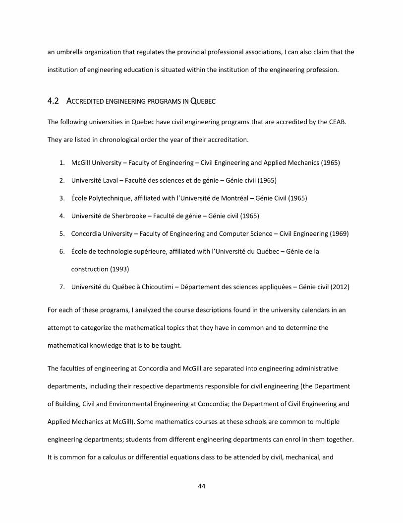
44
an umbrella organization that regulates the provincial professional associations, I can also claim that the
institution of engineering education is situated within the institution of the engineering profession.
4.2 ACCREDITED ENGINEERING PROGRAMS IN QUEBEC
The following universities in Quebec have civil engineering programs that are accredited by the CEAB.
They are listed in chronological order the year of their accreditation.
1. McGill University – Faculty of Engineering – Civil Engineering and Applied Mechanics (1965)
2. Université Laval – Faculté des sciences et de génie – Génie civil (1965)
3. École Polytechnique, affiliated with l’Université de Montréal – Génie Civil (1965)
4. Université de Sherbrooke – Faculté de génie – Génie civil (1965)
5. Concordia University – Faculty of Engineering and Computer Science – Civil Engineering (1969)
6. École de technologie supérieure, affiliated with l’Université du Québec – Génie de la
construction (1993)
7. Université du Québec à Chicoutimi – Département des sciences appliquées – Génie civil (2012)
For each of these programs, I analyzed the course descriptions found in the university calendars in an
attempt to categorize the mathematical topics that they have in common and to determine the
mathematical knowledge that is to be taught.
The faculties of engineering at Concordia and McGill are separated into engineering administrative
departments, including their respective departments responsible for civil engineering (the Department
of Building, Civil and Environmental Engineering at Concordia; the Department of Civil Engineering and
Applied Mechanics at McGill). Some mathematics courses at these schools are common to multiple
engineering departments; students from different engineering departments can enrol in them together.
It is common for a calculus or differential equations class to be attended by civil, mechanical, and
45
electrical engineering students. This could make the task of writing relatable application problems more
difficult for the professors. Writing application problems, in general, is not easy for professors who are,
for the most part, mathematicians and not engineers.
The Université du Québec is a network of universities located in various cities and regions across the
province, including Montreal (UQAM), Trois-Rivières (UQTR), and Gatineau (UQO). Only the school
located in Chicoutimi (UQAC) offers a degree in civil engineering, while degrees in other disciplines
(mechanical, electrical, chemical, and industrial engineering) are offered elsewhere. The École de
technologie supérieure (ÉTS) is an engineering- and technology-specific institution affiliated with the
Université du Québec. While they do not offer a degree in civil engineering, they do have a program that
leads to a bachelor’s degree in construction engineering. The difference between the two degrees
appears to be that the construction engineering program focuses on the management of civil
engineering construction projects as opposed to engineering design and analysis. Some of its courses
are entirely unique to this program, including a course on estimating the costs of construction projects
and establishing project schedules. In my professional experience, these tasks were learned “on the job.”
In all programs, after completing common core courses, students can choose to focus their studies on
one of a number of sub-disciplines. In civil engineering, for example, a student can choose to study
structural engineering, environmental engineering, or transportation engineering, among others. École
Polytechnique de Montréal has a unique feature. Students enrolled in its program have the additional
option of a thematic orientation called mathématiques de l’ingénieur (mathematics for engineers). The
purpose of this orientation is to allow students to acquire knowledge in advanced applied mathematics,
and broaden their abilities to model mathematically in order to solve engineering problems (École
Polytechnique de Montréal). École Polytechnique is a renowned research facility, and as such it is
important for them to offer proper training for students who wish to focus on research in engineering
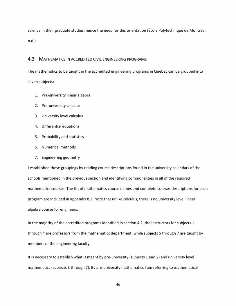
46
science in their graduate studies, hence the need for this orientation (École Polytechnique de Montréal,
n.d.).
4.3 MATHEMATICS IN ACCREDITED CIVIL ENGINEERING PROGRAMS
The mathematics to be taught in the accredited engineering programs in Quebec can be grouped into
seven subjects:
1. Pre-university linear algebra
2. Pre-university calculus
3. University level calculus
4. Differential equations
5. Probability and statistics
6. Numerical methods
7. Engineering geometry
I established these groupings by reading course descriptions found in the university calendars of the
schools mentioned in the previous section and identifying commonalities in all of the required
mathematics courses. The list of mathematics course names and complete courses descriptions for each
program are included in appendix 8.2. Note that unlike calculus, there is no university level linear
algebra course for engineers.
In the majority of the accredited programs identified in section 4.2, the instructors for subjects 1
through 4 are professors from the mathematics department, while subjects 5 through 7 are taught by
members of the engineering faculty.
It is necessary to establish what is meant by pre-university (subjects 1 and 2) and university level
mathematics (subjects 3 through 7). By pre-university mathematics I am referring to mathematical
47
content that is also taught either in CEGEP (for students from Quebec) or in high school (for students
from other provinces). Universities offer pre-university mathematics courses for various reasons. For
one, students from outside of the province who move to Quebec to attend university may not have
necessarily taken a course in linear algebra or calculus prior to starting their university education, while
those who are from Quebec have. In Quebec, linear algebra and calculus are required to graduate from
CEGEP, and are taken not only by students who want to be engineers, but also by those who will enter
other science programs such as biology, physiology, and computer science. There is also a need, from
the universities’ perspective, to ensure that all of their students have the same level of mathematical
knowledge before they begin courses in the engineering program. Some topics covered in pre-university
calculus courses – differentiation and integration of single-variable functions, for example – are
important and necessary concepts that are required in first year engineering courses such as statics and
mechanics of materials. The pre-university courses are also necessary for students who were accepted
into an engineering program on the condition that they retake the pre-university courses in order to
improve their academic standing, or for students who return to school after a prolonged absence and
lack the prerequisites to enter their desired program.
Because of these pre-university level courses, the first year of study at Concordia and McGill may differ
for some students. For example, when I attended McGill, my first year of study included mathematics
courses only at the university level. However, my classmates included many students from Ontario and
other provinces that were in their second year at the school. They had spent the previous year, while I
was finishing CEGEP, taking pre-university mathematics (and natural science) courses. This is referred to
as year U0 (undergraduate year 0) at McGill, and EC (extended credit) at Concordia. Thus, for students
from Quebec who are not required to retake pre-university level mathematics courses (subjects 3 to 7),
more than half of their mathematics courses are taught by professors from the engineering faculty, as
opposed to professors of mathematics.

48
4.3.1 Methodology for the analysis of final exams
In the sections that follow I present the results of my analysis of final exams from mathematics courses
taken by engineering students, and from comparable courses taken by mathematics students, focusing
only on the programs at Concordia and McGill. Final exams were chosen instead of textbooks since they
give us the most insight into what mathematics students are expected to learn during the course.
One final exam from each course is analyzed. The engineering exams that I chose were similar to those
that I wrote as an engineering student, and in my experience as a mathematics instructor final exams for
mathematics courses do not change very much from one year to the next (at least in these universities).
As a result of this I claim that the chosen exams represent institutionalized mathematical knowledge to
be learned by the students of the respective courses.
The exams were analyzed by categorizing the tasks in two ways. First, the nature of each task is
classified as either computational or conceptual. I make this distinction from the point of view of a
mathematics educator, with the institution used as a reference model being that of mathematics
courses in university programs. Various mathematics textbooks, including Lay (2016), describe the
exercises contained within as either computational or conceptual. While computational tasks require
routine calculations, conceptual tasks demand a bit more thought as well as a justification of their
solutions. This particular distinction in ways of knowing and doing mathematics has been studied and
discussed in mathematics education practically forever.
To identify the computational tasks on the final exams, I searched for keywords such as “find”,
“evaluate”, or “compute”, in the problem’s text. Tasks that explicitly state which technique the student
should use to solve the problem also fall into this category. Conceptual tasks were identified as those
that required proving a given statement or showing an equality to be true or false (problems that used
phrases such as “show that”, or “prove”), or demonstrating an understanding of mathematical concepts
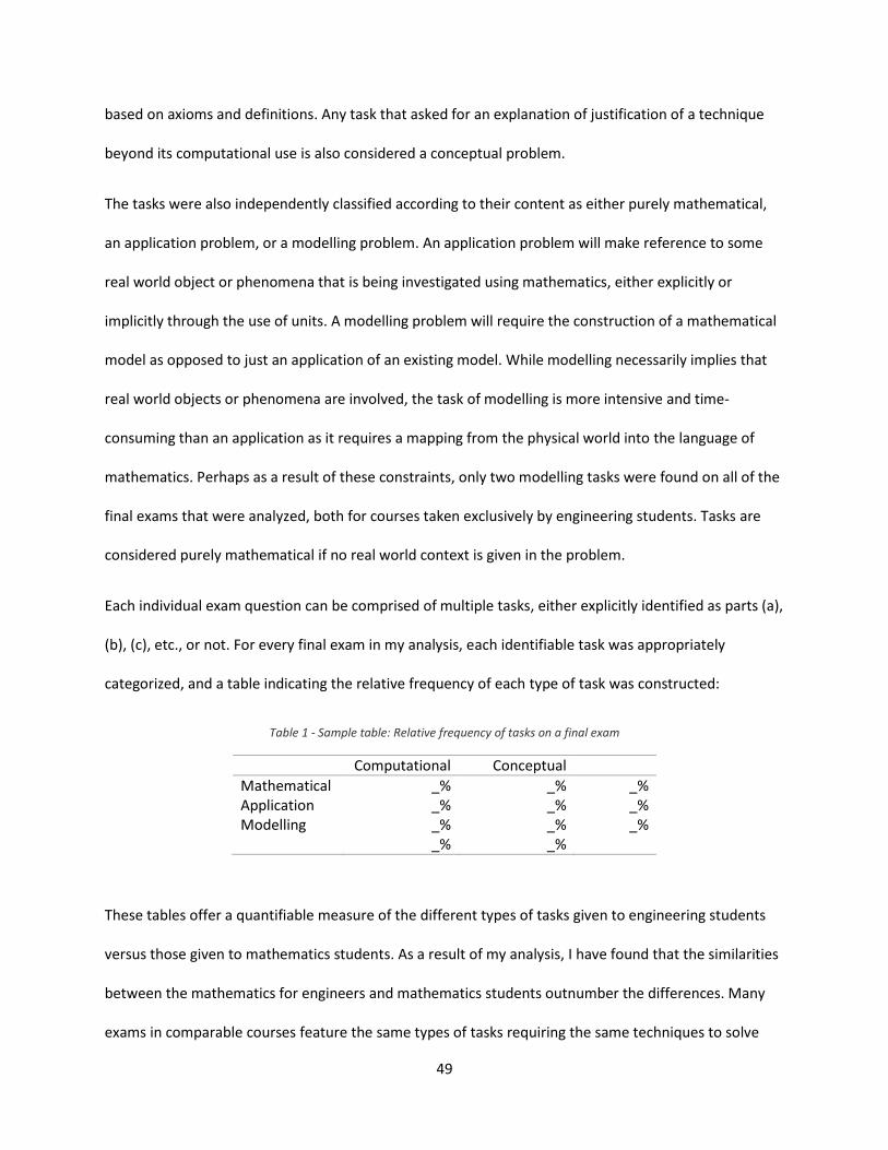
49
based on axioms and definitions. Any task that asked for an explanation of justification of a technique
beyond its computational use is also considered a conceptual problem.
The tasks were also independently classified according to their content as either purely mathematical,
an application problem, or a modelling problem. An application problem will make reference to some
real world object or phenomena that is being investigated using mathematics, either explicitly or
implicitly through the use of units. A modelling problem will require the construction of a mathematical
model as opposed to just an application of an existing model. While modelling necessarily implies that
real world objects or phenomena are involved, the task of modelling is more intensive and time-
consuming than an application as it requires a mapping from the physical world into the language of
mathematics. Perhaps as a result of these constraints, only two modelling tasks were found on all of the
final exams that were analyzed, both for courses taken exclusively by engineering students. Tasks are
considered purely mathematical if no real world context is given in the problem.
Each individual exam question can be comprised of multiple tasks, either explicitly identified as parts (a),
(b), (c), etc., or not. For every final exam in my analysis, each identifiable task was appropriately
categorized, and a table indicating the relative frequency of each type of task was constructed:
Table 1 - Sample table: Relative frequency of tasks on a final exam
Computational Conceptual
Mathematical _% _% _% Application _% _% _% Modelling _% _% _% _% _%
These tables offer a quantifiable measure of the different types of tasks given to engineering students
versus those given to mathematics students. As a result of my analysis, I have found that the similarities
between the mathematics for engineers and mathematics students outnumber the differences. Many
exams in comparable courses feature the same types of tasks requiring the same techniques to solve
50
them, use the same notation, and feature a similar number of purely mathematical and application
problems.
The exams that were analyzed are included in their entirety in appendix 8.3.
4.3.2 Pre-university linear algebra
Topics taught in pre-university linear algebra include solving systems of linear equations, matrix algebra,
evaluating determinants and inverses of square matrices, the geometry and algebra of vectors in ,
operations on vectors (dot product and cross product), the geometry of lines and planes, an
introduction to vector spaces and subspaces, an introduction to linear transformations, eigenvalues and
eigenvectors of matrices, and the diagonalisation of matrices using their eigenvectors and eigenvalues.
This list is not written to suggest that linear algebra courses contain a random collection of disconnected
topics, but rather to simply highlight what concepts the students are expected to learn in such a course.
The courses offered in this subject are MATH 204 – Vectors and Matrices at Concordia, and MATH 133 –
Linear Algebra and Geometry, at McGill. I was unable to obtain any documentation about final exams for
MATH 133. Concordia’s MATH 204 is not reserved for engineering students. It is offered to students in
many programs, including mathematics students who may need it as a prerequisite for their university
level linear algebra courses MATH 251 – Linear Algebra I, and MATH 252 – Linear Algebra II.
I analyzed final exams from these two university level courses as well as from MATH 204. Since
engineering students do not take university level linear algebra, it is assumed that the topics covered in
MATH 204 represent all that engineers need to know of the domain of linear algebra. They are assumed
not to need to know the theory of general vector spaces and linear transformations over arbitrary
vector spaces that justifies, at the level of “theory” in the model of praxeology, the techniques and
elements of “technology” learned in MATH 204.
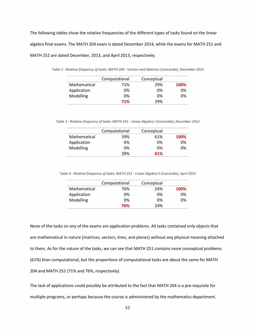
51
The following tables show the relative frequencies of the different types of tasks found on the linear
algebra final exams. The MATH 204 exam is dated December 2014, while the exams for MATH 251 and
MATH 252 are dated December, 2013, and April 2013, respectively.
Table 2 - Relative frequency of tasks: MATH 204 - Vectors and Matrices (Concordia), December 2014
Computational Conceptual
Mathematical 71% 29% 100% Application 0% 0% 0% Modelling 0% 0% 0% 71% 29%
Table 3 - Relative frequency of tasks: MATH 251 - Linear Algebra I (Concordia), December 2013
Computational Conceptual
Mathematical 39% 61% 100% Application 0% 0% 0% Modelling 0% 0% 0% 39% 61%
Table 4 - Relative frequency of tasks: MATH 252 - Linear Algebra II (Concordia), April 2013
Computational Conceptual
Mathematical 76% 24% 100% Application 0% 0% 0% Modelling 0% 0% 0% 76% 24%
None of the tasks on any of the exams are application problems. All tasks contained only objects that
are mathematical in nature (matrices, vectors, lines, and planes) without any physical meaning attached
to them. As for the nature of the tasks, we can see that MATH 251 contains more conceptual problems
(61%) than computational, but the proportions of computational tasks are about the same for MATH
204 and MATH 252 (71% and 76%, respectively).
The lack of applications could possibly be attributed to the fact that MATH 204 is a pre-requisite for
multiple programs, or perhaps because the course is administered by the mathematics department.
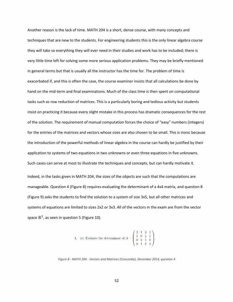
52
Another reason is the lack of time. MATH 204 is a short, dense course, with many concepts and
techniques that are new to the students. For engineering students this is the only linear algebra course
they will take so everything they will ever need in their studies and work has to be included; there is
very little time left for solving some more serious application problems. They may be briefly mentioned
in general terms but that is usually all the instructor has the time for. The problem of time is
exacerbated if, and this is often the case, the course examiner insists that all calculations be done by
hand on the mid-term and final examinations. Much of the class time is then spent on computational
tasks such as row reduction of matrices. This is a particularly boring and tedious activity but students
insist on practicing it because every slight mistake in this process has dramatic consequences for the rest
of the solution. The requirement of manual computation forces the choice of “easy” numbers (integers)
for the entries of the matrices and vectors whose sizes are also chosen to be small. This is ironic because
the introduction of the powerful methods of linear algebra in the course can hardly be justified by their
application to systems of two equations in two unknowns or even three equations in five unknowns.
Such cases can serve at most to illustrate the techniques and concepts, but can hardly motivate it.
Indeed, in the tasks given in MATH 204, the sizes of the objects are such that the computations are
manageable. Question 4 (Figure 8) requires evaluating the determinant of a 4x4 matrix, and question 8
(Figure 9) asks the students to find the solution to a system of size 3x5, but all other matrices and
systems of equations are limited to sizes 2x2 or 3x3. All of the vectors in the exam are from the vector
space , as seen in question 5 (Figure 10).
Figure 8 - MATH 204 - Vectors and Matrices (Concordia), December 2014, question 4
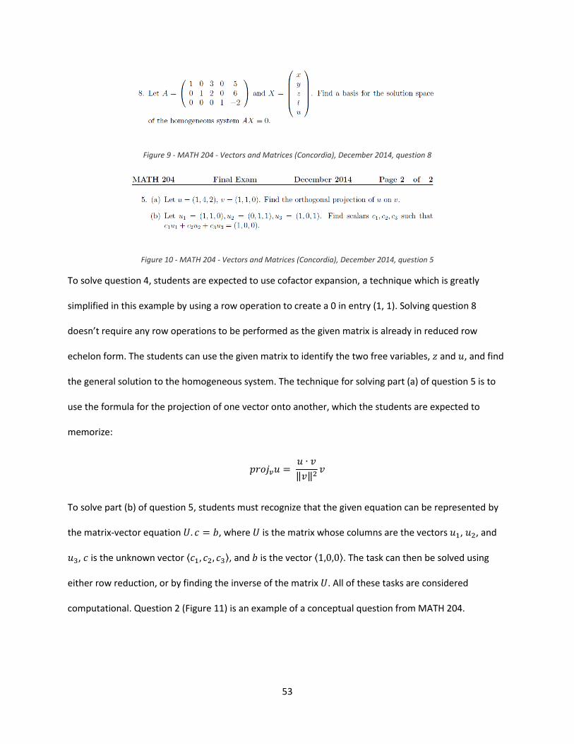
53
Figure 9 - MATH 204 - Vectors and Matrices (Concordia), December 2014, question 8
Figure 10 - MATH 204 - Vectors and Matrices (Concordia), December 2014, question 5
To solve question 4, students are expected to use cofactor expansion, a technique which is greatly
simplified in this example by using a row operation to create a 0 in entry (1, 1). Solving question 8
doesn’t require any row operations to be performed as the given matrix is already in reduced row
echelon form. The students can use the given matrix to identify the two free variables, and , and find
the general solution to the homogeneous system. The technique for solving part (a) of question 5 is to
use the formula for the projection of one vector onto another, which the students are expected to
memorize:
‖ ‖
To solve part (b) of question 5, students must recognize that the given equation can be represented by
the matrix-vector equation , where is the matrix whose columns are the vectors , , and
, is the unknown vector ⟨ ⟩, and is the vector ⟨ ⟩. The task can then be solved using
either row reduction, or by finding the inverse of the matrix . All of these tasks are considered
computational. Question 2 (Figure 11) is an example of a conceptual question from MATH 204.
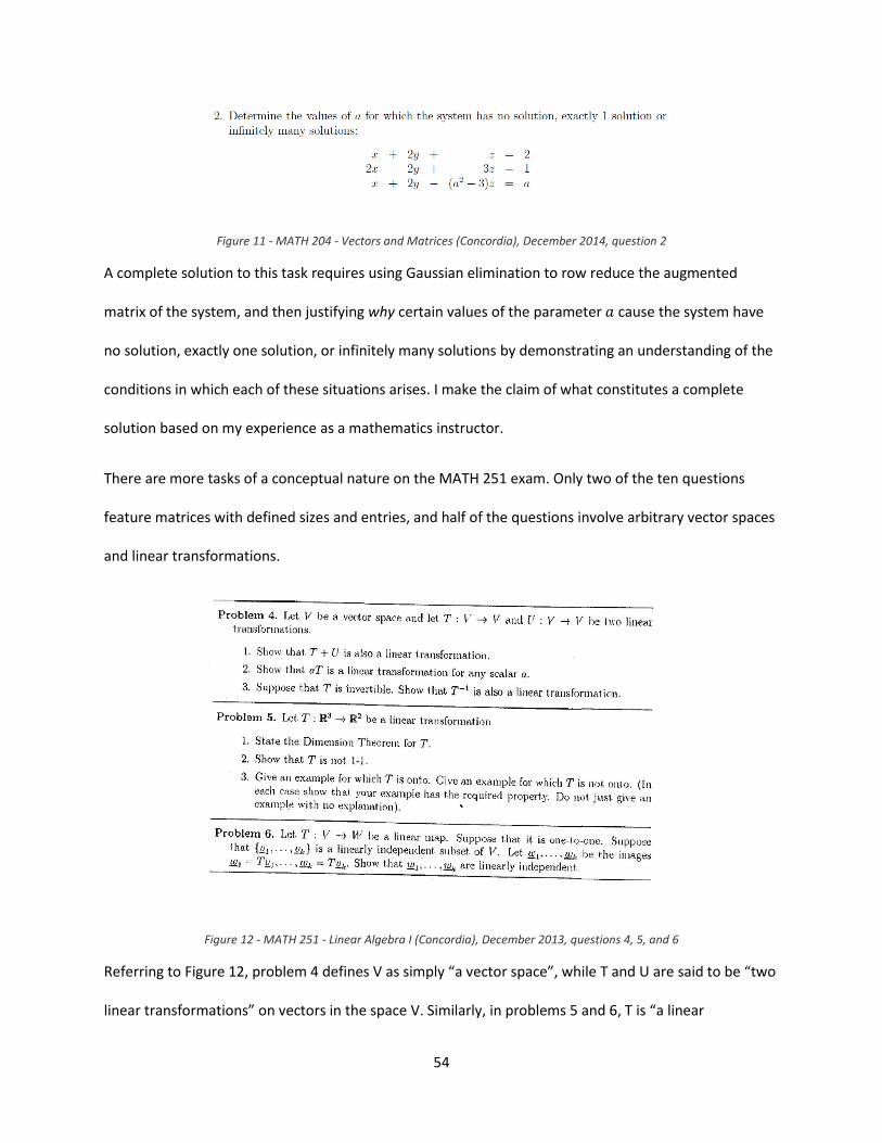
54
Figure 11 - MATH 204 - Vectors and Matrices (Concordia), December 2014, question 2
A complete solution to this task requires using Gaussian elimination to row reduce the augmented
matrix of the system, and then justifying why certain values of the parameter cause the system have
no solution, exactly one solution, or infinitely many solutions by demonstrating an understanding of the
conditions in which each of these situations arises. I make the claim of what constitutes a complete
solution based on my experience as a mathematics instructor.
There are more tasks of a conceptual nature on the MATH 251 exam. Only two of the ten questions
feature matrices with defined sizes and entries, and half of the questions involve arbitrary vector spaces
and linear transformations.
Figure 12 - MATH 251 - Linear Algebra I (Concordia), December 2013, questions 4, 5, and 6
Referring to Figure 12, problem 4 defines V as simply “a vector space”, while T and U are said to be “two
linear transformations” on vectors in the space V. Similarly, in problems 5 and 6, T is “a linear
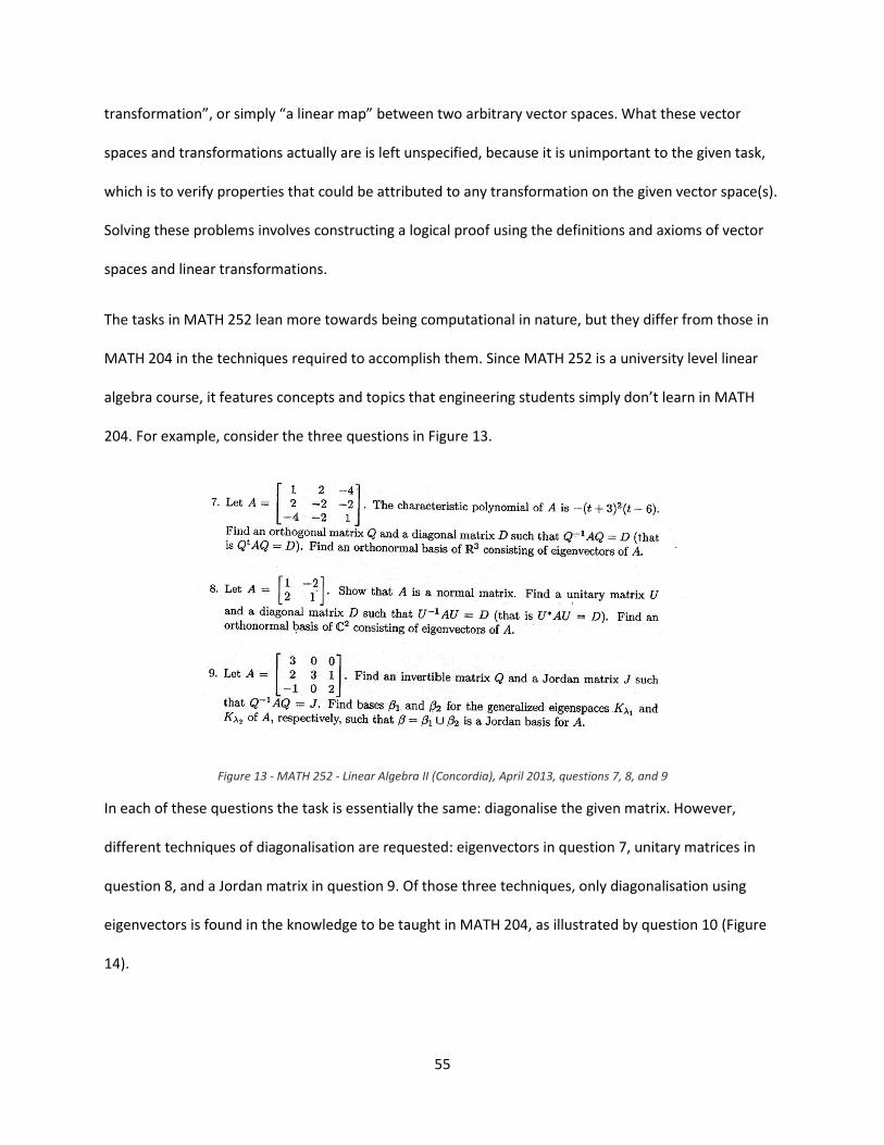
55
transformation”, or simply “a linear map” between two arbitrary vector spaces. What these vector
spaces and transformations actually are is left unspecified, because it is unimportant to the given task,
which is to verify properties that could be attributed to any transformation on the given vector space(s).
Solving these problems involves constructing a logical proof using the definitions and axioms of vector
spaces and linear transformations.
The tasks in MATH 252 lean more towards being computational in nature, but they differ from those in
MATH 204 in the techniques required to accomplish them. Since MATH 252 is a university level linear
algebra course, it features concepts and topics that engineering students simply don’t learn in MATH
204. For example, consider the three questions in Figure 13.
Figure 13 - MATH 252 - Linear Algebra II (Concordia), April 2013, questions 7, 8, and 9
In each of these questions the task is essentially the same: diagonalise the given matrix. However,
different techniques of diagonalisation are requested: eigenvectors in question 7, unitary matrices in
question 8, and a Jordan matrix in question 9. Of those three techniques, only diagonalisation using
eigenvectors is found in the knowledge to be taught in MATH 204, as illustrated by question 10 (Figure
14).
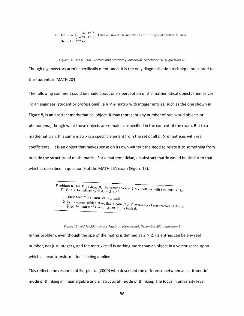
56
Figure 14 - MATH 204 - Vectors and Matrices (Concordia), December 2014, question 10
Though eigenvectors aren’t specifically mentioned, it is the only diagonalisation technique presented to
the students in MATH 204.
The following comment could be made about one’s perception of the mathematical objects themselves.
To an engineer (student or professional), a matrix with integer entries, such as the one shown in
Figure 8, is an abstract mathematical object. It may represent any number of real world objects or
phenomena, though what those objects are remains unspecified in the context of the exam. But to a
mathematician, this same matrix is a specific element from the set of all matrices with real
coefficients – it is an object that makes sense on its own without the need to relate it to something from
outside the structure of mathematics. For a mathematician, an abstract matrix would be similar to that
which is described in question 9 of the MATH 251 exam (Figure 15).
Figure 15 - MATH 251 - Linear Algebra I (Concordia), December 2014, question 9
In this problem, even though the size of the matrix is defined as , its entries can be any real
number, not just integers, and the matrix itself is nothing more than an object in a vector space upon
which a linear transformation is being applied.
This reflects the research of Sierpinska (2000) who described the difference between an “arithmetic”
mode of thinking in linear algebra and a “structural” mode of thinking. The focus in university level
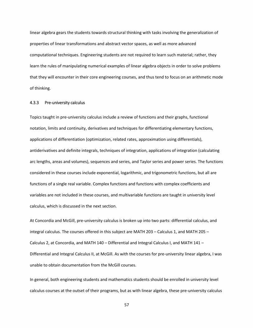
57
linear algebra gears the students towards structural thinking with tasks involving the generalization of
properties of linear transformations and abstract vector spaces, as well as more advanced
computational techniques. Engineering students are not required to learn such material; rather, they
learn the rules of manipulating numerical examples of linear algebra objects in order to solve problems
that they will encounter in their core engineering courses, and thus tend to focus on an arithmetic mode
of thinking.
4.3.3 Pre-university calculus
Topics taught in pre-university calculus include a review of functions and their graphs, functional
notation, limits and continuity, derivatives and techniques for differentiating elementary functions,
applications of differentiation (optimization, related rates, approximation using differentials),
antiderivatives and definite integrals, techniques of integration, applications of integration (calculating
arc lengths, areas and volumes), sequences and series, and Taylor series and power series. The functions
considered in these courses include exponential, logarithmic, and trigonometric functions, but all are
functions of a single real variable. Complex functions and functions with complex coefficients and
variables are not included in these courses, and multivariable functions are taught in university level
calculus, which is discussed in the next section.
At Concordia and McGill, pre-university calculus is broken up into two parts: differential calculus, and
integral calculus. The courses offered in this subject are MATH 203 – Calculus 1, and MATH 205 –
Calculus 2, at Concordia, and MATH 140 – Differential and Integral Calculus I, and MATH 141 –
Differential and Integral Calculus II, at McGill. As with the courses for pre-university linear algebra, I was
unable to obtain documentation from the McGill courses.
In general, both engineering students and mathematics students should be enrolled in university level
calculus courses at the outset of their programs, but as with linear algebra, these pre-university calculus
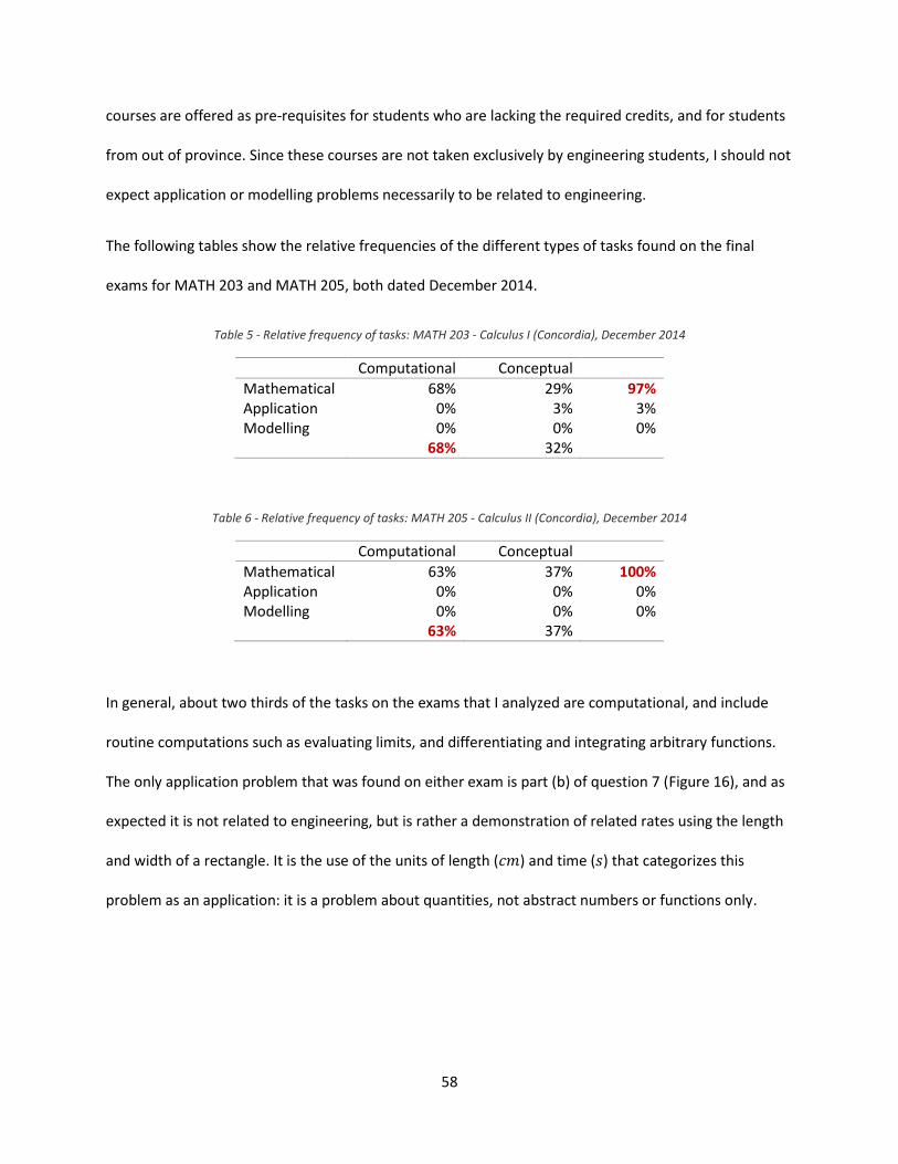
58
courses are offered as pre-requisites for students who are lacking the required credits, and for students
from out of province. Since these courses are not taken exclusively by engineering students, I should not
expect application or modelling problems necessarily to be related to engineering.
The following tables show the relative frequencies of the different types of tasks found on the final
exams for MATH 203 and MATH 205, both dated December 2014.
Table 5 - Relative frequency of tasks: MATH 203 - Calculus I (Concordia), December 2014
Computational Conceptual
Mathematical 68% 29% 97% Application 0% 3% 3% Modelling 0% 0% 0% 68% 32%
Table 6 - Relative frequency of tasks: MATH 205 - Calculus II (Concordia), December 2014
Computational Conceptual
Mathematical 63% 37% 100% Application 0% 0% 0% Modelling 0% 0% 0% 63% 37%
In general, about two thirds of the tasks on the exams that I analyzed are computational, and include
routine computations such as evaluating limits, and differentiating and integrating arbitrary functions.
The only application problem that was found on either exam is part (b) of question 7 (Figure 16), and as
expected it is not related to engineering, but is rather a demonstration of related rates using the length
and width of a rectangle. It is the use of the units of length ( ) and time ( ) that categorizes this
problem as an application: it is a problem about quantities, not abstract numbers or functions only.
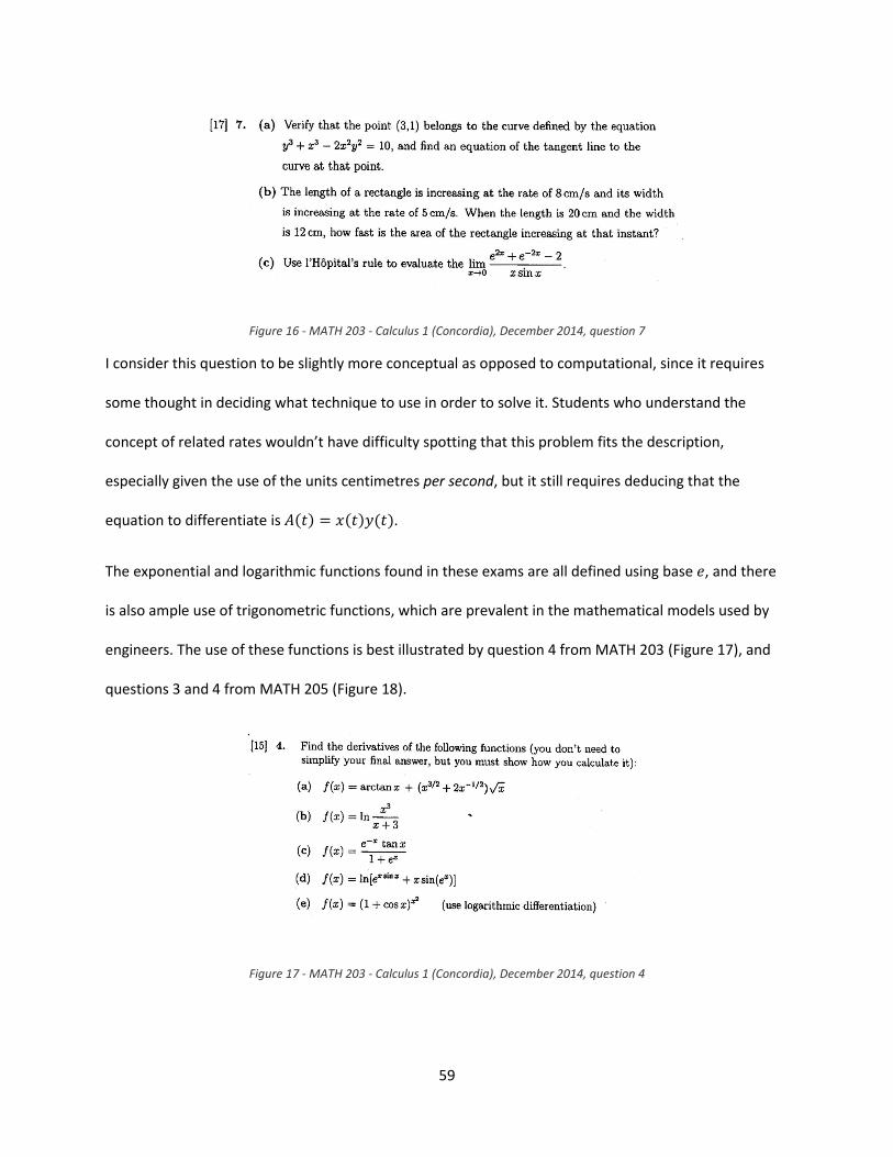
59
Figure 16 - MATH 203 - Calculus 1 (Concordia), December 2014, question 7
I consider this question to be slightly more conceptual as opposed to computational, since it requires
some thought in deciding what technique to use in order to solve it. Students who understand the
concept of related rates wouldn’t have difficulty spotting that this problem fits the description,
especially given the use of the units centimetres per second, but it still requires deducing that the
equation to differentiate is .
The exponential and logarithmic functions found in these exams are all defined using base , and there
is also ample use of trigonometric functions, which are prevalent in the mathematical models used by
engineers. The use of these functions is best illustrated by question 4 from MATH 203 (Figure 17), and
questions 3 and 4 from MATH 205 (Figure 18).
Figure 17 - MATH 203 - Calculus 1 (Concordia), December 2014, question 4
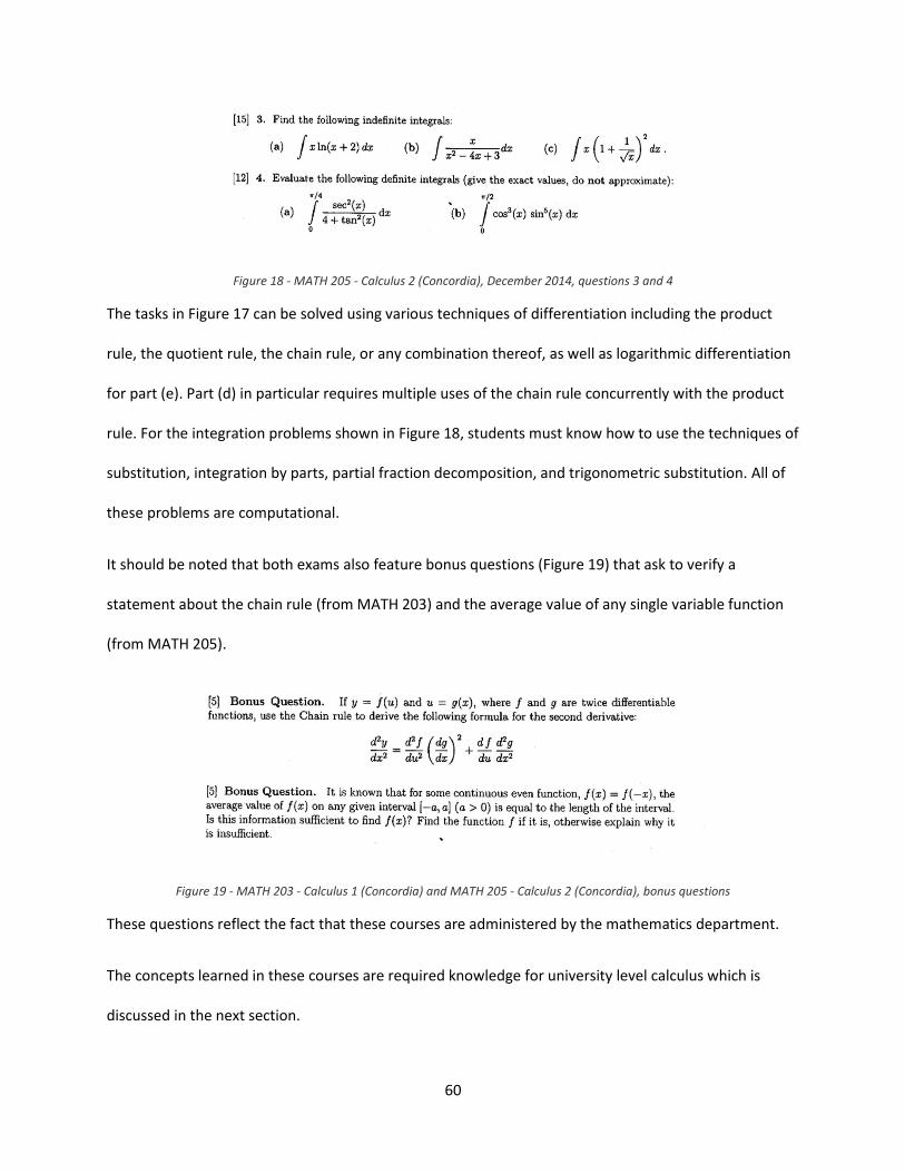
60
Figure 18 - MATH 205 - Calculus 2 (Concordia), December 2014, questions 3 and 4
The tasks in Figure 17 can be solved using various techniques of differentiation including the product
rule, the quotient rule, the chain rule, or any combination thereof, as well as logarithmic differentiation
for part (e). Part (d) in particular requires multiple uses of the chain rule concurrently with the product
rule. For the integration problems shown in Figure 18, students must know how to use the techniques of
substitution, integration by parts, partial fraction decomposition, and trigonometric substitution. All of
these problems are computational.
It should be noted that both exams also feature bonus questions (Figure 19) that ask to verify a
statement about the chain rule (from MATH 203) and the average value of any single variable function
(from MATH 205).
Figure 19 - MATH 203 - Calculus 1 (Concordia) and MATH 205 - Calculus 2 (Concordia), bonus questions
These questions reflect the fact that these courses are administered by the mathematics department.
The concepts learned in these courses are required knowledge for university level calculus which is
discussed in the next section.
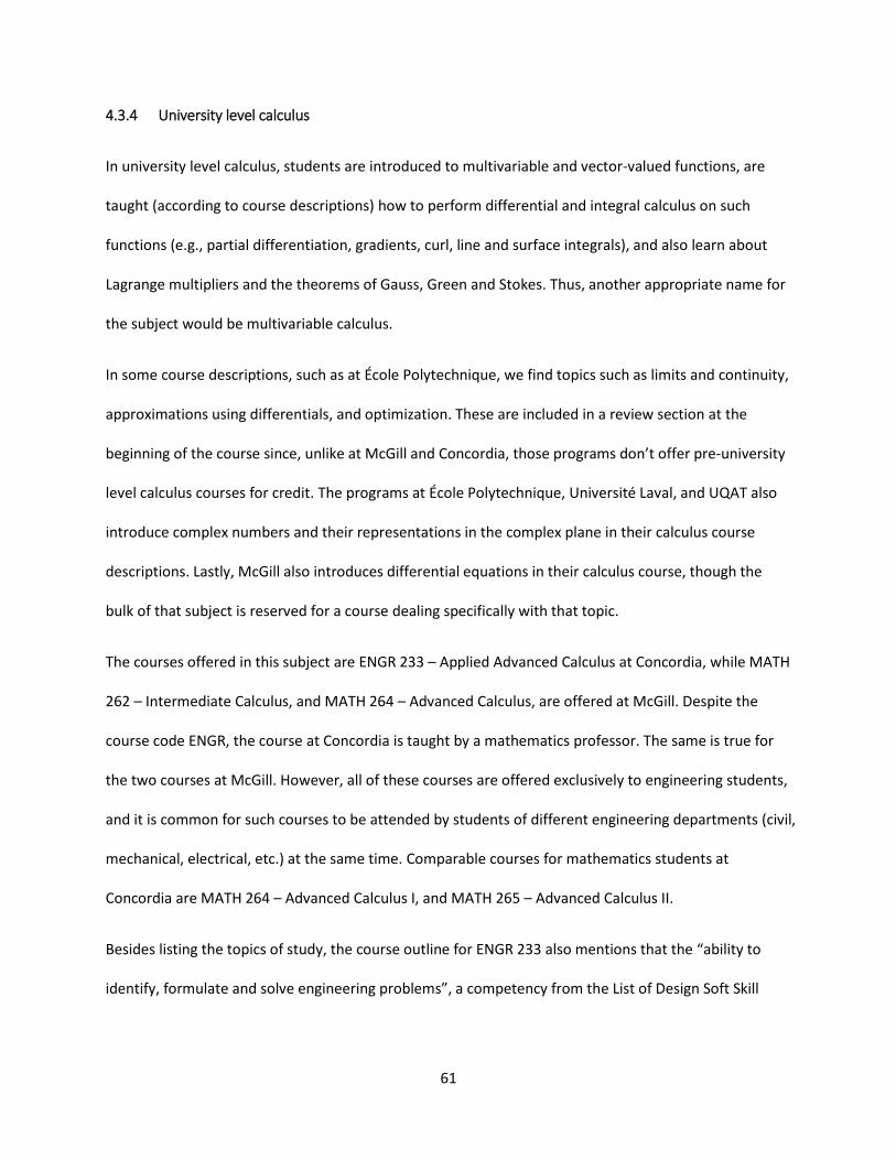
61
4.3.4 University level calculus
In university level calculus, students are introduced to multivariable and vector-valued functions, are
taught (according to course descriptions) how to perform differential and integral calculus on such
functions (e.g., partial differentiation, gradients, curl, line and surface integrals), and also learn about
Lagrange multipliers and the theorems of Gauss, Green and Stokes. Thus, another appropriate name for
the subject would be multivariable calculus.
In some course descriptions, such as at École Polytechnique, we find topics such as limits and continuity,
approximations using differentials, and optimization. These are included in a review section at the
beginning of the course since, unlike at McGill and Concordia, those programs don’t offer pre-university
level calculus courses for credit. The programs at École Polytechnique, Université Laval, and UQAT also
introduce complex numbers and their representations in the complex plane in their calculus course
descriptions. Lastly, McGill also introduces differential equations in their calculus course, though the
bulk of that subject is reserved for a course dealing specifically with that topic.
The courses offered in this subject are ENGR 233 – Applied Advanced Calculus at Concordia, while MATH
262 – Intermediate Calculus, and MATH 264 – Advanced Calculus, are offered at McGill. Despite the
course code ENGR, the course at Concordia is taught by a mathematics professor. The same is true for
the two courses at McGill. However, all of these courses are offered exclusively to engineering students,
and it is common for such courses to be attended by students of different engineering departments (civil,
mechanical, electrical, etc.) at the same time. Comparable courses for mathematics students at
Concordia are MATH 264 – Advanced Calculus I, and MATH 265 – Advanced Calculus II.
Besides listing the topics of study, the course outline for ENGR 233 also mentions that the “ability to
identify, formulate and solve engineering problems”, a competency from the List of Design Soft Skill

62
Competencies found in documentation by the CEAB, is relevant to the course. Analyzing the course’s
final exam should reveal whether this competency is in fact expected to develop in students.
Since there is only one calculus course for engineers at Concordia, some topics that are to be taught in
the courses at McGill are not found in Concordia’s ENGR 233 course outline. These include series and
power series which are taught at the beginning of McGill’s MATH 262, and the introduction to partial
differential equations at the end of McGill’s MATH 264. In essence, infinite series is a topic that students
in ENGR 233 are expected to have learned prior to attending the course, and partial differential
equations are taught to them in a separate differential equations course (section 4.3.5). Regardless,
there is still considerable overlap in the topics on the course outlines for all of the courses offered to
engineers and mathematics students at Concordia and McGill. Among them are vector geometry and
vector-valued functions, differential and integral calculus of vector-valued functions and multivariable
functions, line integrals and the theorems of Green and Stokes.
The following tables show the relative frequencies of the different types of tasks found on the final
exams from the following courses: ENGR 233, dated December 2014; MATH 262, dated December 2010;
MATH 264 for engineers at McGill, dated April 2007; MATH 264 for mathematics students at Concordia,
dated December 2014; MATH 265, dated April 2014.
Table 7 - Relative frequency of tasks: ENGR 233 - Applied Advanced Calculus (Concordia), December 2014
Computational Conceptual
Mathematical 78% 0% 78% Application 11% 0% 11% Modelling 0% 11% 11% 89% 11%
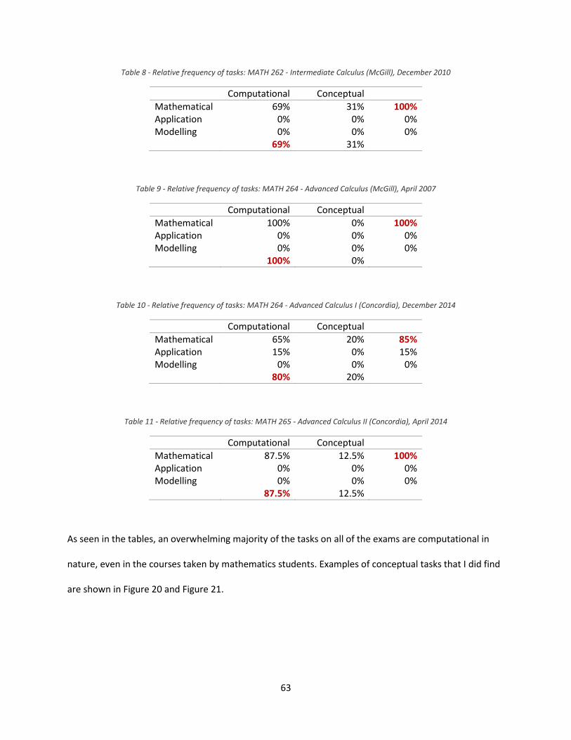
63
Table 8 - Relative frequency of tasks: MATH 262 - Intermediate Calculus (McGill), December 2010
Computational Conceptual
Mathematical 69% 31% 100% Application 0% 0% 0% Modelling 0% 0% 0% 69% 31%
Table 9 - Relative frequency of tasks: MATH 264 - Advanced Calculus (McGill), April 2007
Computational Conceptual
Mathematical 100% 0% 100% Application 0% 0% 0% Modelling 0% 0% 0% 100% 0%
Table 10 - Relative frequency of tasks: MATH 264 - Advanced Calculus I (Concordia), December 2014
Computational Conceptual
Mathematical 65% 20% 85% Application 15% 0% 15% Modelling 0% 0% 0% 80% 20%
Table 11 - Relative frequency of tasks: MATH 265 - Advanced Calculus II (Concordia), April 2014
Computational Conceptual
Mathematical 87.5% 12.5% 100% Application 0% 0% 0% Modelling 0% 0% 0% 87.5% 12.5%
As seen in the tables, an overwhelming majority of the tasks on all of the exams are computational in
nature, even in the courses taken by mathematics students. Examples of conceptual tasks that I did find
are shown in Figure 20 and Figure 21.
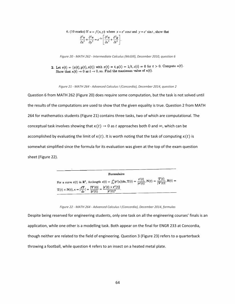
64
Figure 20 - MATH 262 - Intermediate Calculus (McGIll), December 2010, question 6
Figure 21 - MATH 264 - Advanced Calculus I (Concordia), December 2014, question 2
Question 6 from MATH 262 (Figure 20) does require some computation, but the task is not solved until
the results of the computations are used to show that the given equality is true. Question 2 from MATH
264 for mathematics students (Figure 21) contains three tasks, two of which are computational. The
conceptual task involves showing that as approaches both and , which can be
accomplished by evaluating the limit of . It is worth noting that the task of computing is
somewhat simplified since the formula for its evaluation was given at the top of the exam question
sheet (Figure 22).
Figure 22 - MATH 264 - Advanced Calculus I (Concordia), December 2014, formulas
Despite being reserved for engineering students, only one task on all the engineering courses’ finals is an
application, while one other is a modelling task. Both appear on the final for ENGR 233 at Concordia,
though neither are related to the field of engineering. Question 3 (Figure 23) refers to a quarterback
throwing a football, while question 4 refers to an insect on a heated metal plate.
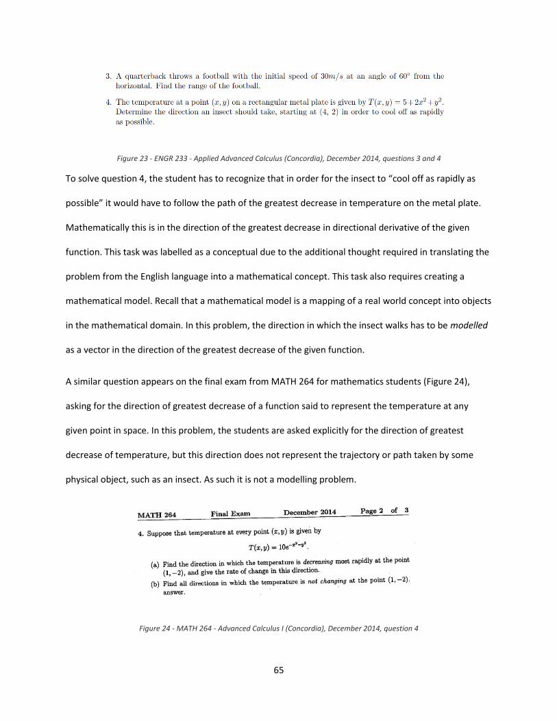
65
Figure 23 - ENGR 233 - Applied Advanced Calculus (Concordia), December 2014, questions 3 and 4
To solve question 4, the student has to recognize that in order for the insect to “cool off as rapidly as
possible” it would have to follow the path of the greatest decrease in temperature on the metal plate.
Mathematically this is in the direction of the greatest decrease in directional derivative of the given
function. This task was labelled as a conceptual due to the additional thought required in translating the
problem from the English language into a mathematical concept. This task also requires creating a
mathematical model. Recall that a mathematical model is a mapping of a real world concept into objects
in the mathematical domain. In this problem, the direction in which the insect walks has to be modelled
as a vector in the direction of the greatest decrease of the given function.
A similar question appears on the final exam from MATH 264 for mathematics students (Figure 24),
asking for the direction of greatest decrease of a function said to represent the temperature at any
given point in space. In this problem, the students are asked explicitly for the direction of greatest
decrease of temperature, but this direction does not represent the trajectory or path taken by some
physical object, such as an insect. As such it is not a modelling problem.
Figure 24 - MATH 264 - Advanced Calculus I (Concordia), December 2014, question 4
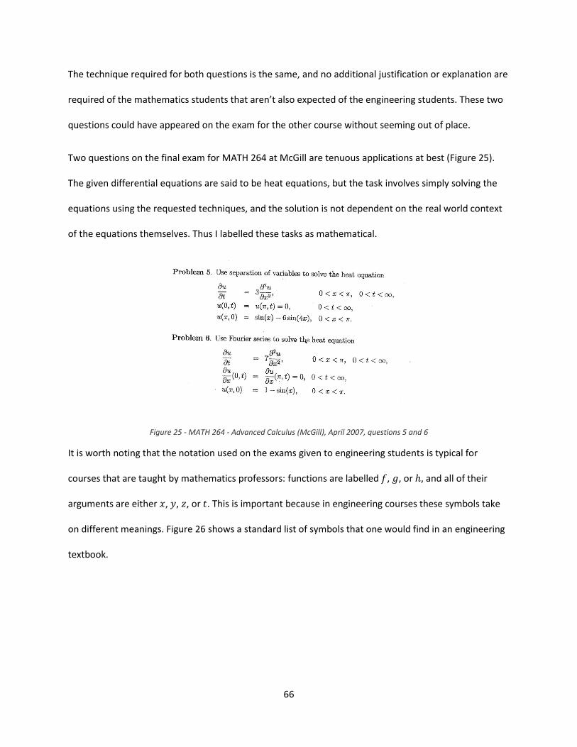
66
The technique required for both questions is the same, and no additional justification or explanation are
required of the mathematics students that aren’t also expected of the engineering students. These two
questions could have appeared on the exam for the other course without seeming out of place.
Two questions on the final exam for MATH 264 at McGill are tenuous applications at best (Figure 25).
The given differential equations are said to be heat equations, but the task involves simply solving the
equations using the requested techniques, and the solution is not dependent on the real world context
of the equations themselves. Thus I labelled these tasks as mathematical.
Figure 25 - MATH 264 - Advanced Calculus (McGill), April 2007, questions 5 and 6
It is worth noting that the notation used on the exams given to engineering students is typical for
courses that are taught by mathematics professors: functions are labelled , , or , and all of their
arguments are either , , , or . This is important because in engineering courses these symbols take
on different meanings. Figure 26 shows a standard list of symbols that one would find in an engineering
textbook.
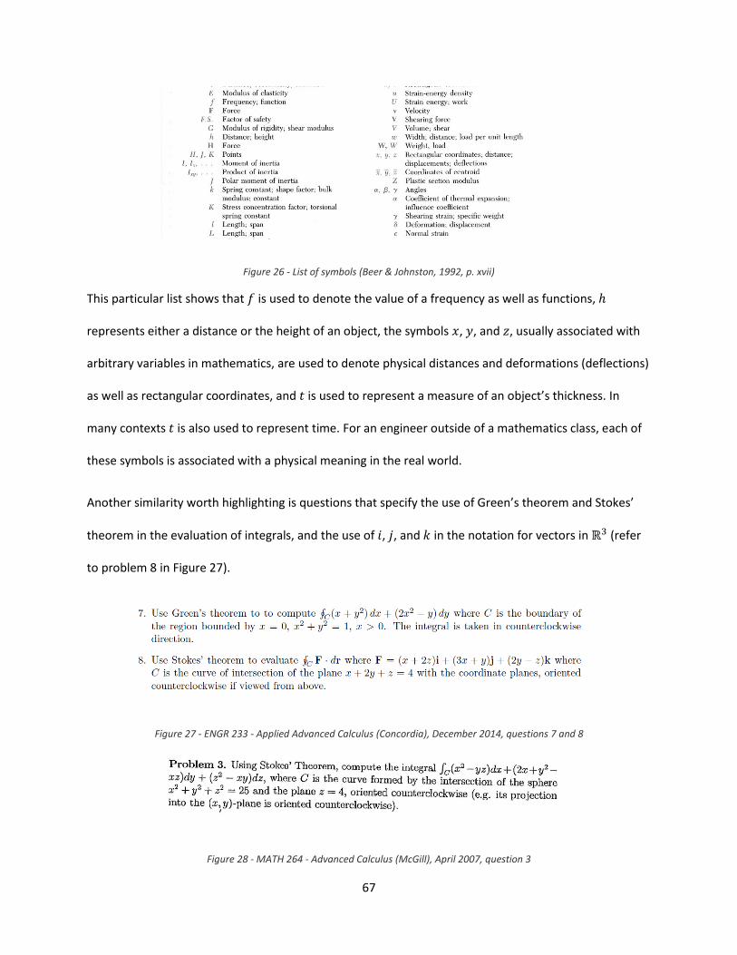
67
Figure 26 - List of symbols (Beer & Johnston, 1992, p. xvii)
This particular list shows that is used to denote the value of a frequency as well as functions,
represents either a distance or the height of an object, the symbols , , and , usually associated with
arbitrary variables in mathematics, are used to denote physical distances and deformations (deflections)
as well as rectangular coordinates, and is used to represent a measure of an object’s thickness. In
many contexts is also used to represent time. For an engineer outside of a mathematics class, each of
these symbols is associated with a physical meaning in the real world.
Another similarity worth highlighting is questions that specify the use of Green’s theorem and Stokes’
theorem in the evaluation of integrals, and the use of , , and in the notation for vectors in (refer
to problem 8 in Figure 27).
Figure 27 - ENGR 233 - Applied Advanced Calculus (Concordia), December 2014, questions 7 and 8
Figure 28 - MATH 264 - Advanced Calculus (McGill), April 2007, question 3
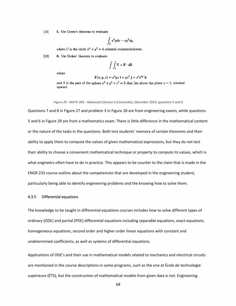
68
Figure 29 - MATH 265 - Advanced Calculus II (Concordia), December 2014, questions 5 and 6
Questions 7 and 8 in Figure 27 and problem 3 in Figure 28 are from engineering exams, while questions
5 and 6 in Figure 29 are from a mathematics exam. There is little difference in the mathematical content
or the nature of the tasks in the questions. Both test students’ memory of certain theorems and their
ability to apply them to compute the values of given mathematical expressions, but they do not test
their ability to choose a convenient mathematical technique or property to compute its values, which is
what engineers often have to do in practice. This appears to be counter to the claim that is made in the
ENGR 233 course outline about the competencies that are developed in the engineering student,
particularly being able to identify engineering problems and the knowing how to solve them.
4.3.5 Differential equations
The knowledge to be taught in differential equations courses includes how to solve different types of
ordinary (ODE) and partial (PDE) differential equations including separable equations, exact equations,
homogeneous equations, second order and higher order linear equations with constant and
undetermined coefficients, as well as systems of differential equations.
Applications of ODE’s and their use in mathematical models related to mechanics and electrical circuits
are mentioned in the course descriptions in some programs, such as the one at École de technologie
supérieure (ÉTS), but the construction of mathematical models from given data is not. Engineering
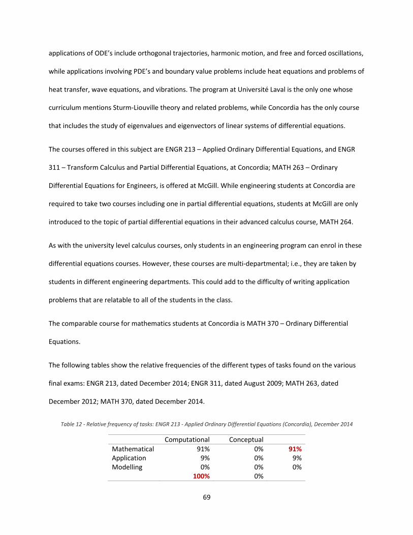
69
applications of ODE’s include orthogonal trajectories, harmonic motion, and free and forced oscillations,
while applications involving PDE’s and boundary value problems include heat equations and problems of
heat transfer, wave equations, and vibrations. The program at Université Laval is the only one whose
curriculum mentions Sturm-Liouville theory and related problems, while Concordia has the only course
that includes the study of eigenvalues and eigenvectors of linear systems of differential equations.
The courses offered in this subject are ENGR 213 – Applied Ordinary Differential Equations, and ENGR
311 – Transform Calculus and Partial Differential Equations, at Concordia; MATH 263 – Ordinary
Differential Equations for Engineers, is offered at McGill. While engineering students at Concordia are
required to take two courses including one in partial differential equations, students at McGill are only
introduced to the topic of partial differential equations in their advanced calculus course, MATH 264.
As with the university level calculus courses, only students in an engineering program can enrol in these
differential equations courses. However, these courses are multi-departmental; i.e., they are taken by
students in different engineering departments. This could add to the difficulty of writing application
problems that are relatable to all of the students in the class.
The comparable course for mathematics students at Concordia is MATH 370 – Ordinary Differential
Equations.
The following tables show the relative frequencies of the different types of tasks found on the various
final exams: ENGR 213, dated December 2014; ENGR 311, dated August 2009; MATH 263, dated
December 2012; MATH 370, dated December 2014.
Table 12 - Relative frequency of tasks: ENGR 213 - Applied Ordinary Differential Equations (Concordia), December 2014
Computational Conceptual
Mathematical 91% 0% 91% Application 9% 0% 9% Modelling 0% 0% 0% 100% 0%
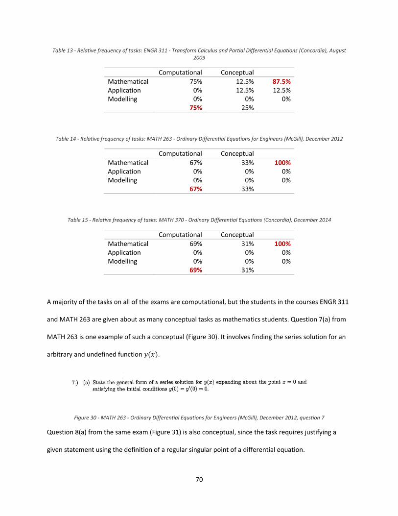
70
Table 13 - Relative frequency of tasks: ENGR 311 - Transform Calculus and Partial Differential Equations (Concordia), August 2009
Computational Conceptual
Mathematical 75% 12.5% 87.5% Application 0% 12.5% 12.5% Modelling 0% 0% 0% 75% 25%
Table 14 - Relative frequency of tasks: MATH 263 - Ordinary Differential Equations for Engineers (McGill), December 2012
Computational Conceptual
Mathematical 67% 33% 100% Application 0% 0% 0% Modelling 0% 0% 0% 67% 33%
Table 15 - Relative frequency of tasks: MATH 370 - Ordinary Differential Equations (Concordia), December 2014
Computational Conceptual
Mathematical 69% 31% 100% Application 0% 0% 0% Modelling 0% 0% 0% 69% 31%
A majority of the tasks on all of the exams are computational, but the students in the courses ENGR 311
and MATH 263 are given about as many conceptual tasks as mathematics students. Question 7(a) from
MATH 263 is one example of such a conceptual (Figure 30). It involves finding the series solution for an
arbitrary and undefined function .
Figure 30 - MATH 263 - Ordinary Differential Equations for Engineers (McGill), December 2012, question 7
Question 8(a) from the same exam (Figure 31) is also conceptual, since the task requires justifying a
given statement using the definition of a regular singular point of a differential equation.
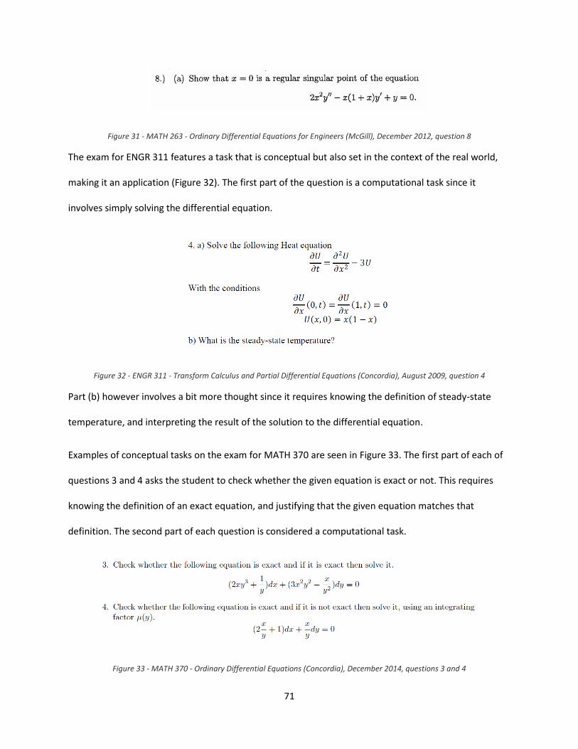
71
Figure 31 - MATH 263 - Ordinary Differential Equations for Engineers (McGill), December 2012, question 8
The exam for ENGR 311 features a task that is conceptual but also set in the context of the real world,
making it an application (Figure 32). The first part of the question is a computational task since it
involves simply solving the differential equation.
Figure 32 - ENGR 311 - Transform Calculus and Partial Differential Equations (Concordia), August 2009, question 4
Part (b) however involves a bit more thought since it requires knowing the definition of steady-state
temperature, and interpreting the result of the solution to the differential equation.
Examples of conceptual tasks on the exam for MATH 370 are seen in Figure 33. The first part of each of
questions 3 and 4 asks the student to check whether the given equation is exact or not. This requires
knowing the definition of an exact equation, and justifying that the given equation matches that
definition. The second part of each question is considered a computational task.
Figure 33 - MATH 370 - Ordinary Differential Equations (Concordia), December 2014, questions 3 and 4
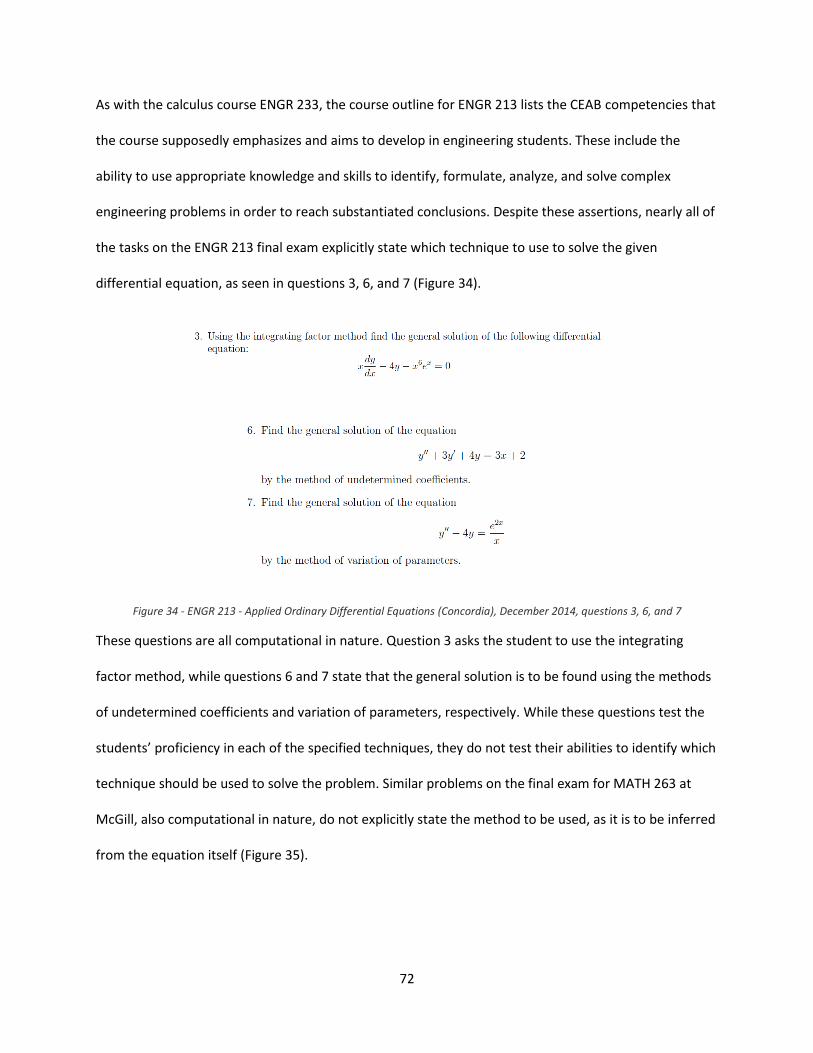
72
As with the calculus course ENGR 233, the course outline for ENGR 213 lists the CEAB competencies that
the course supposedly emphasizes and aims to develop in engineering students. These include the
ability to use appropriate knowledge and skills to identify, formulate, analyze, and solve complex
engineering problems in order to reach substantiated conclusions. Despite these assertions, nearly all of
the tasks on the ENGR 213 final exam explicitly state which technique to use to solve the given
differential equation, as seen in questions 3, 6, and 7 (Figure 34).
Figure 34 - ENGR 213 - Applied Ordinary Differential Equations (Concordia), December 2014, questions 3, 6, and 7
These questions are all computational in nature. Question 3 asks the student to use the integrating
factor method, while questions 6 and 7 state that the general solution is to be found using the methods
of undetermined coefficients and variation of parameters, respectively. While these questions test the
students’ proficiency in each of the specified techniques, they do not test their abilities to identify which
technique should be used to solve the problem. Similar problems on the final exam for MATH 263 at
McGill, also computational in nature, do not explicitly state the method to be used, as it is to be inferred
from the equation itself (Figure 35).
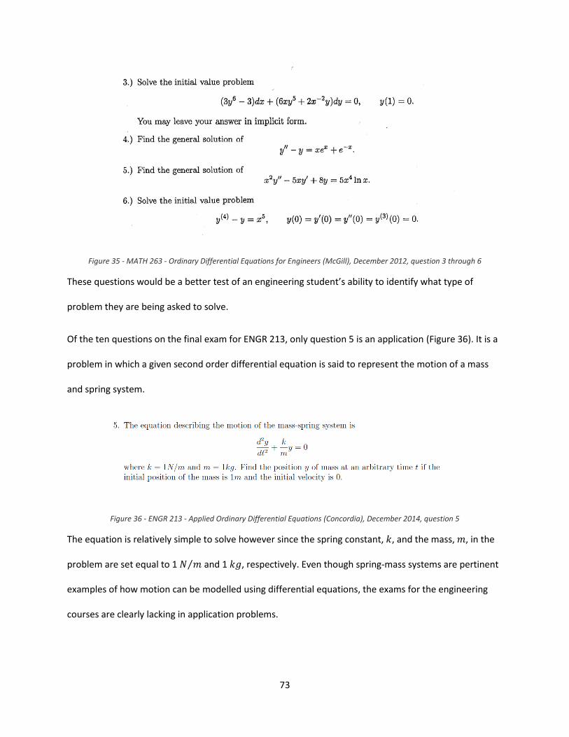
73
Figure 35 - MATH 263 - Ordinary Differential Equations for Engineers (McGill), December 2012, question 3 through 6
These questions would be a better test of an engineering student’s ability to identify what type of
problem they are being asked to solve.
Of the ten questions on the final exam for ENGR 213, only question 5 is an application (Figure 36). It is a
problem in which a given second order differential equation is said to represent the motion of a mass
and spring system.
Figure 36 - ENGR 213 - Applied Ordinary Differential Equations (Concordia), December 2014, question 5
The equation is relatively simple to solve however since the spring constant, , and the mass, , in the
problem are set equal to 1 ⁄ and 1 , respectively. Even though spring-mass systems are pertinent
examples of how motion can be modelled using differential equations, the exams for the engineering
courses are clearly lacking in application problems.
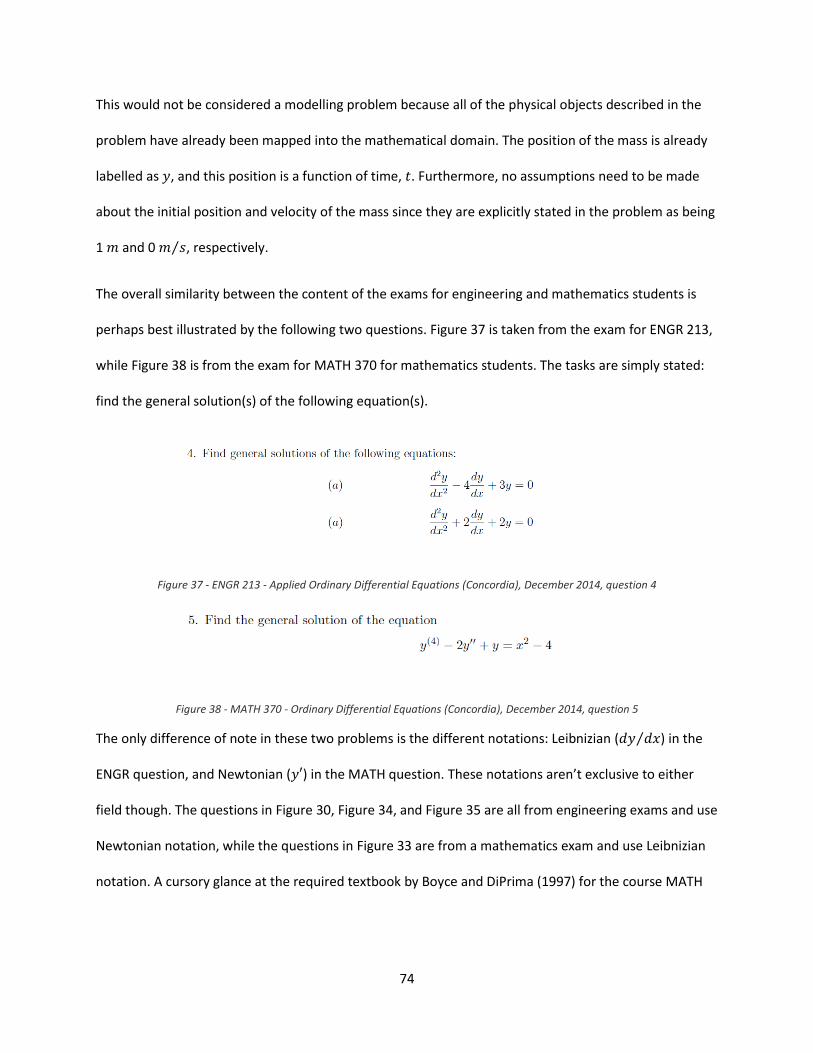
74
This would not be considered a modelling problem because all of the physical objects described in the
problem have already been mapped into the mathematical domain. The position of the mass is already
labelled as , and this position is a function of time, . Furthermore, no assumptions need to be made
about the initial position and velocity of the mass since they are explicitly stated in the problem as being
1 and 0 ⁄ , respectively.
The overall similarity between the content of the exams for engineering and mathematics students is
perhaps best illustrated by the following two questions. Figure 37 is taken from the exam for ENGR 213,
while Figure 38 is from the exam for MATH 370 for mathematics students. The tasks are simply stated:
find the general solution(s) of the following equation(s).
Figure 37 - ENGR 213 - Applied Ordinary Differential Equations (Concordia), December 2014, question 4
Figure 38 - MATH 370 - Ordinary Differential Equations (Concordia), December 2014, question 5
The only difference of note in these two problems is the different notations: Leibnizian ( ⁄ ) in the
ENGR question, and Newtonian ( ) in the MATH question. These notations aren’t exclusive to either
field though. The questions in Figure 30, Figure 34, and Figure 35 are all from engineering exams and use
Newtonian notation, while the questions in Figure 33 are from a mathematics exam and use Leibnizian
notation. A cursory glance at the required textbook by Boyce and DiPrima (1997) for the course MATH
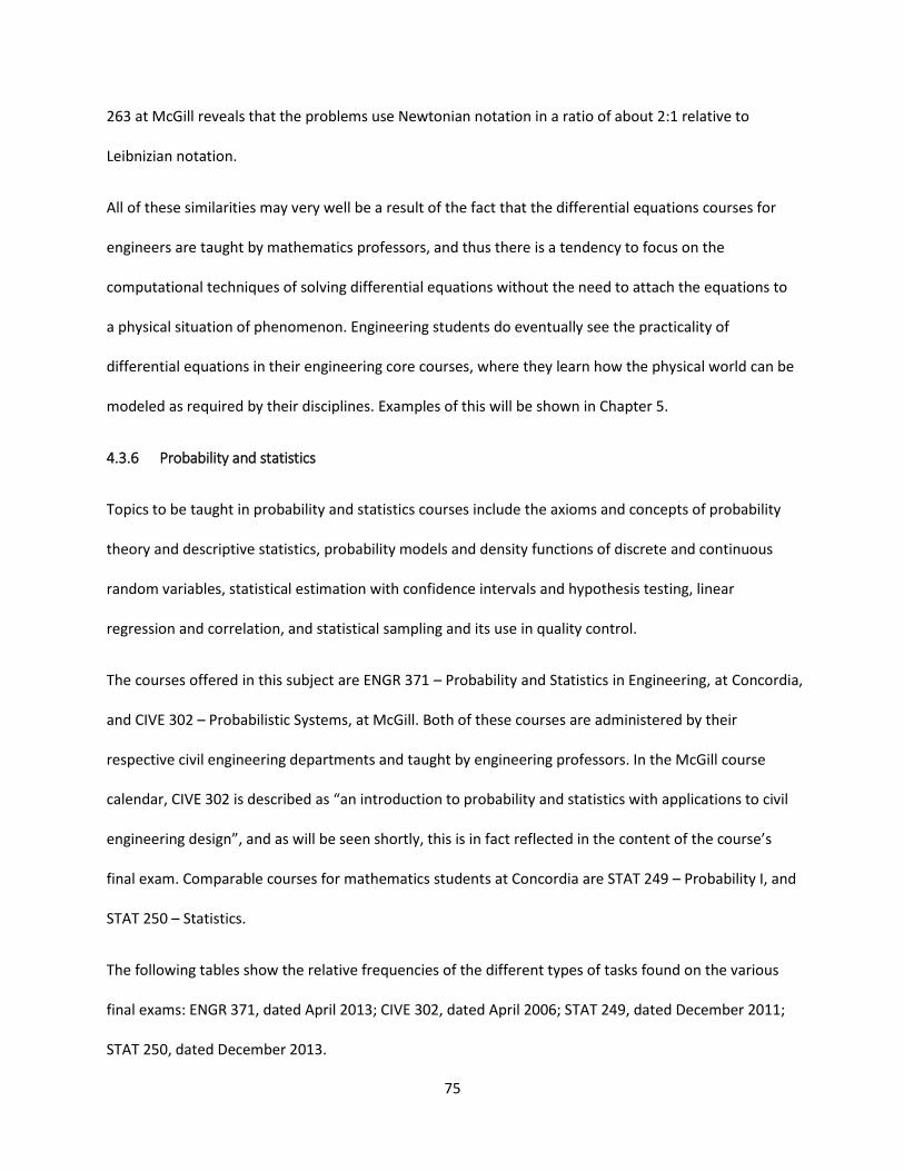
75
263 at McGill reveals that the problems use Newtonian notation in a ratio of about 2:1 relative to
Leibnizian notation.
All of these similarities may very well be a result of the fact that the differential equations courses for
engineers are taught by mathematics professors, and thus there is a tendency to focus on the
computational techniques of solving differential equations without the need to attach the equations to
a physical situation of phenomenon. Engineering students do eventually see the practicality of
differential equations in their engineering core courses, where they learn how the physical world can be
modeled as required by their disciplines. Examples of this will be shown in Chapter 5.
4.3.6 Probability and statistics
Topics to be taught in probability and statistics courses include the axioms and concepts of probability
theory and descriptive statistics, probability models and density functions of discrete and continuous
random variables, statistical estimation with confidence intervals and hypothesis testing, linear
regression and correlation, and statistical sampling and its use in quality control.
The courses offered in this subject are ENGR 371 – Probability and Statistics in Engineering, at Concordia,
and CIVE 302 – Probabilistic Systems, at McGill. Both of these courses are administered by their
respective civil engineering departments and taught by engineering professors. In the McGill course
calendar, CIVE 302 is described as “an introduction to probability and statistics with applications to civil
engineering design”, and as will be seen shortly, this is in fact reflected in the content of the course’s
final exam. Comparable courses for mathematics students at Concordia are STAT 249 – Probability I, and
STAT 250 – Statistics.
The following tables show the relative frequencies of the different types of tasks found on the various
final exams: ENGR 371, dated April 2013; CIVE 302, dated April 2006; STAT 249, dated December 2011;
STAT 250, dated December 2013.

76
Table 16 - Relative frequency of tasks: ENGR 371 - Probability and Statistics in Engineering (Concordia), April 2013
Computational Conceptual
Mathematical 16% 4% 20% Application 56% 24% 80% Modelling 0% 0% 0% 72% 28%
Table 17 - Relative frequency of tasks: CIVE 302 - Probabilistic Systems (McGill), April 2006
Computational Conceptual
Mathematical 12.5% 0% 12.5% Application 75% 12.5% 87.5% Modelling 0% 0% 0% 87.5% 12.5%
Table 18 - Relative frequency of tasks: STAT 249 - Probability I (Concordia), December 2011
Computational Conceptual
Mathematical 39% 11% 50% Application 50% 0% 50% Modelling 0% 0% 0% 89% 11%
Table 19 - Relative frequency of tasks: STAT 250 - Statistics (Concordia), December 2013
Computational Conceptual
Mathematical 42% 23% 65% Application 12% 23% 35% Modelling 0% 0% 0% 54% 46%
Once again a majority of the tasks are computational in nature. However, the engineering exams contain
a significant number of applications, and considerably more than on the math exams (80% and 87.5%
versus 50% and 35%). Moreover, the applications on the engineering exams are related to their field,
particularly on the McGill exam.
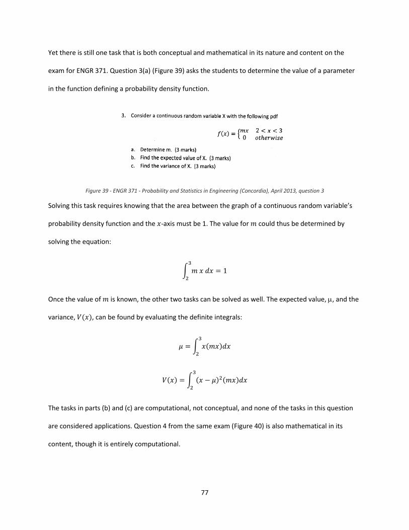
77
Yet there is still one task that is both conceptual and mathematical in its nature and content on the
exam for ENGR 371. Question 3(a) (Figure 39) asks the students to determine the value of a parameter
in the function defining a probability density function.
Figure 39 - ENGR 371 - Probability and Statistics in Engineering (Concordia), April 2013, question 3
Solving this task requires knowing that the area between the graph of a continuous random variable’s
probability density function and the -axis must be 1. The value for could thus be determined by
solving the equation:
∫
Once the value of is known, the other two tasks can be solved as well. The expected value, , and the
variance, , can be found by evaluating the definite integrals:
∫
∫
The tasks in parts (b) and (c) are computational, not conceptual, and none of the tasks in this question
are considered applications. Question 4 from the same exam (Figure 40) is also mathematical in its
content, though it is entirely computational.
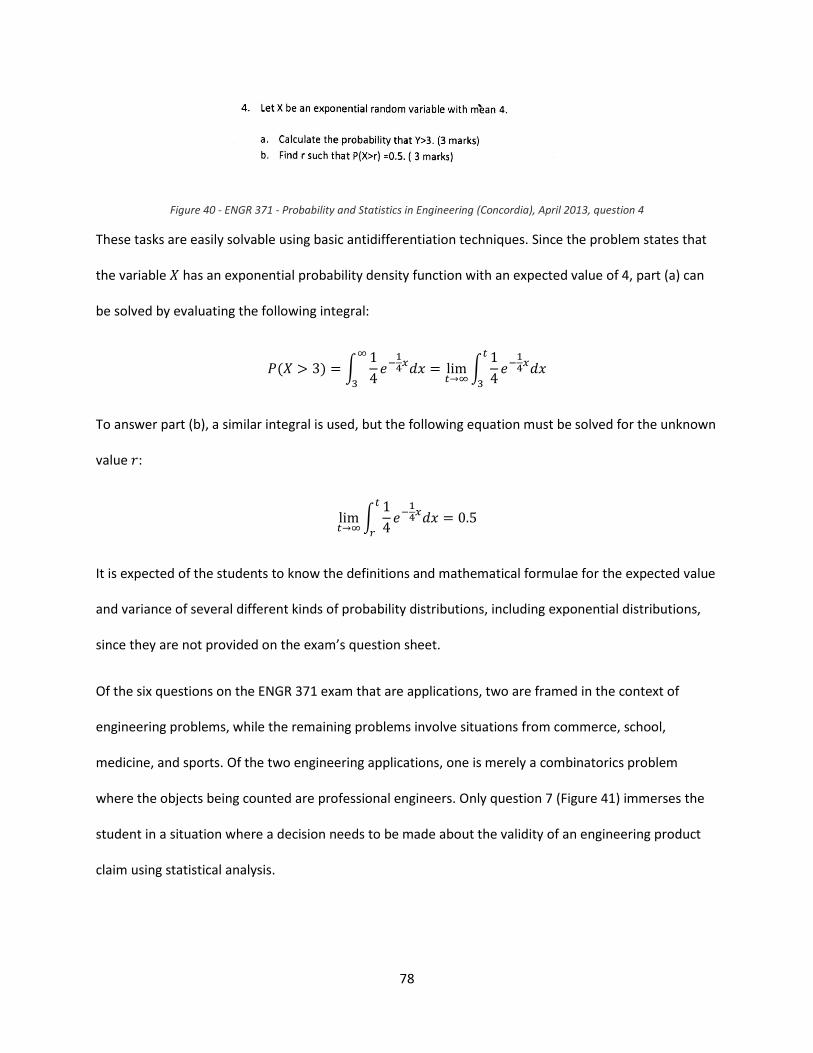
78
Figure 40 - ENGR 371 - Probability and Statistics in Engineering (Concordia), April 2013, question 4
These tasks are easily solvable using basic antidifferentiation techniques. Since the problem states that
the variable has an exponential probability density function with an expected value of 4, part (a) can
be solved by evaluating the following integral:
∫
∫
To answer part (b), a similar integral is used, but the following equation must be solved for the unknown
value :
∫
It is expected of the students to know the definitions and mathematical formulae for the expected value
and variance of several different kinds of probability distributions, including exponential distributions,
since they are not provided on the exam’s question sheet.
Of the six questions on the ENGR 371 exam that are applications, two are framed in the context of
engineering problems, while the remaining problems involve situations from commerce, school,
medicine, and sports. Of the two engineering applications, one is merely a combinatorics problem
where the objects being counted are professional engineers. Only question 7 (Figure 41) immerses the
student in a situation where a decision needs to be made about the validity of an engineering product
claim using statistical analysis.
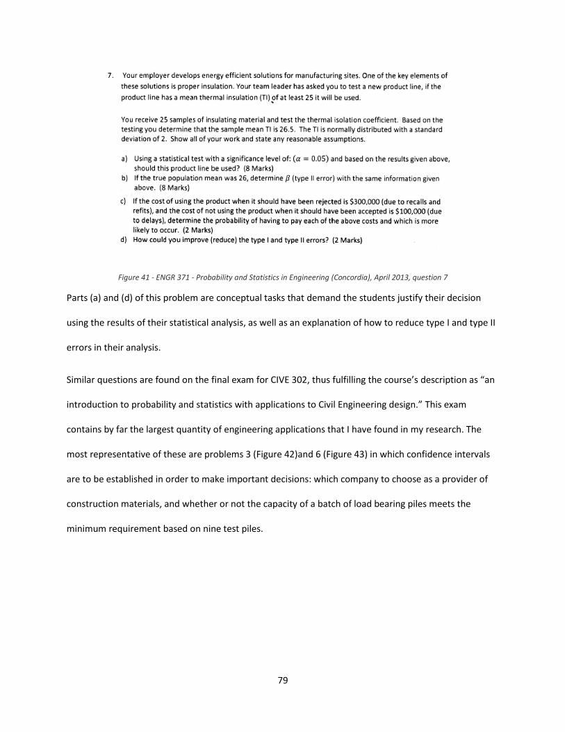
79
Figure 41 - ENGR 371 - Probability and Statistics in Engineering (Concordia), April 2013, question 7
Parts (a) and (d) of this problem are conceptual tasks that demand the students justify their decision
using the results of their statistical analysis, as well as an explanation of how to reduce type I and type II
errors in their analysis.
Similar questions are found on the final exam for CIVE 302, thus fulfilling the course’s description as “an
introduction to probability and statistics with applications to Civil Engineering design.” This exam
contains by far the largest quantity of engineering applications that I have found in my research. The
most representative of these are problems 3 (Figure 42)and 6 (Figure 43) in which confidence intervals
are to be established in order to make important decisions: which company to choose as a provider of
construction materials, and whether or not the capacity of a batch of load bearing piles meets the
minimum requirement based on nine test piles.

80
Figure 42 - CIVE 302 - Probabilistic Systems (McGill), April 2006, question 3
Figure 43 - CIVE 302 - Probabilistic Systems (McGill), April 2006, question 6
Note that in both of these problems, the real world concepts of material durability (figure 42) and pile
capacity (figure 43) have already been modeled as statistical variables. In the former, the durability is
measured by the amount of wear in the material, and labelled as and for the different materials.
Labels aren’t given explicitly in the latter problem, but by giving the student the sample mean, standard
81
deviation, and explicitly stating the null hypothesis (in part (a)), the work of modelling the situation has
already been done.
Some parts of these questions are computational, but those that involve making a decision and then
justifying that decision are conceptual in nature. This type of statistical analysis is frequently performed
by professional engineers involved in the construction of structures that are built on foundation support
piles. Since it is too costly to test the strength of each individual pile, random tests are performed and
the results analyzed statistically to determine whether or not there are any structural deficiencies.
The exams for mathematics students are decidedly more mathematical in their content than their
engineering counterparts, but there are still a considerable number of applications. This may very well
be due to the nature of the topics of probability and statistics themselves, and their historical
development.
Indeed, the applications on the mathematics students’ exams are set in a variety of real world situations
including forming a committee from a group of men and women, the distribution of grades in professors’
courses, the tossing of an unfair coin, the distribution of certain types of rare birds, and accidents
occurring on a stretch of road. Three of these questions are shown in Figure 44. It is worth noting that
these questions are all entirely computational in their nature.
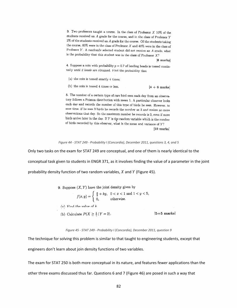
82
Figure 44 - STAT 249 - Probability I (Concordia), December 2011, questions 3, 4, and 5
Only two tasks on the exam for STAT 249 are conceptual, and one of them is nearly identical to the
conceptual task given to students in ENGR 371, as it involves finding the value of a parameter in the joint
probability density function of two random variables, and (Figure 45).
Figure 45 - STAT 249 - Probability I (Concordia), December 2011, question 9
The technique for solving this problem is similar to that taught to engineering students, except that
engineers don’t learn about join density functions of two variables.
The exam for STAT 250 is both more conceptual in its nature, and features fewer applications than the
other three exams discussed thus far. Questions 6 and 7 (Figure 46) are posed in such a way that
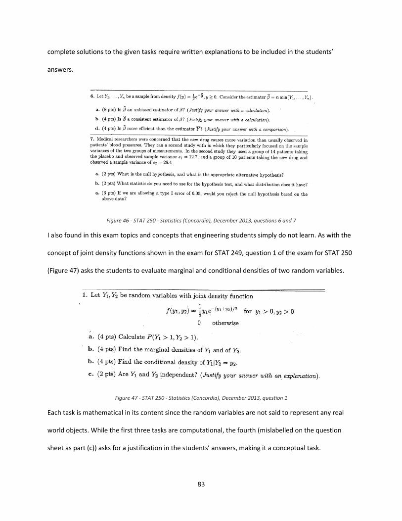
83
complete solutions to the given tasks require written explanations to be included in the students’
answers.
Figure 46 - STAT 250 - Statistics (Concordia), December 2013, questions 6 and 7
I also found in this exam topics and concepts that engineering students simply do not learn. As with the
concept of joint density functions shown in the exam for STAT 249, question 1 of the exam for STAT 250
(Figure 47) asks the students to evaluate marginal and conditional densities of two random variables.
Figure 47 - STAT 250 - Statistics (Concordia), December 2013, question 1
Each task is mathematical in its content since the random variables are not said to represent any real
world objects. While the first three tasks are computational, the fourth (mislabelled on the question
sheet as part (c)) asks for a justification in the students’ answers, making it a conceptual task.
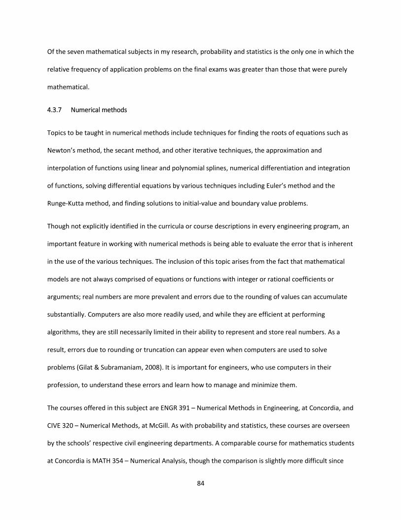
84
Of the seven mathematical subjects in my research, probability and statistics is the only one in which the
relative frequency of application problems on the final exams was greater than those that were purely
mathematical.
4.3.7 Numerical methods
Topics to be taught in numerical methods include techniques for finding the roots of equations such as
Newton’s method, the secant method, and other iterative techniques, the approximation and
interpolation of functions using linear and polynomial splines, numerical differentiation and integration
of functions, solving differential equations by various techniques including Euler’s method and the
Runge-Kutta method, and finding solutions to initial-value and boundary value problems.
Though not explicitly identified in the curricula or course descriptions in every engineering program, an
important feature in working with numerical methods is being able to evaluate the error that is inherent
in the use of the various techniques. The inclusion of this topic arises from the fact that mathematical
models are not always comprised of equations or functions with integer or rational coefficients or
arguments; real numbers are more prevalent and errors due to the rounding of values can accumulate
substantially. Computers are also more readily used, and while they are efficient at performing
algorithms, they are still necessarily limited in their ability to represent and store real numbers. As a
result, errors due to rounding or truncation can appear even when computers are used to solve
problems (Gilat & Subramaniam, 2008). It is important for engineers, who use computers in their
profession, to understand these errors and learn how to manage and minimize them.
The courses offered in this subject are ENGR 391 – Numerical Methods in Engineering, at Concordia, and
CIVE 320 – Numerical Methods, at McGill. As with probability and statistics, these courses are overseen
by the schools’ respective civil engineering departments. A comparable course for mathematics students
at Concordia is MATH 354 – Numerical Analysis, though the comparison is slightly more difficult since
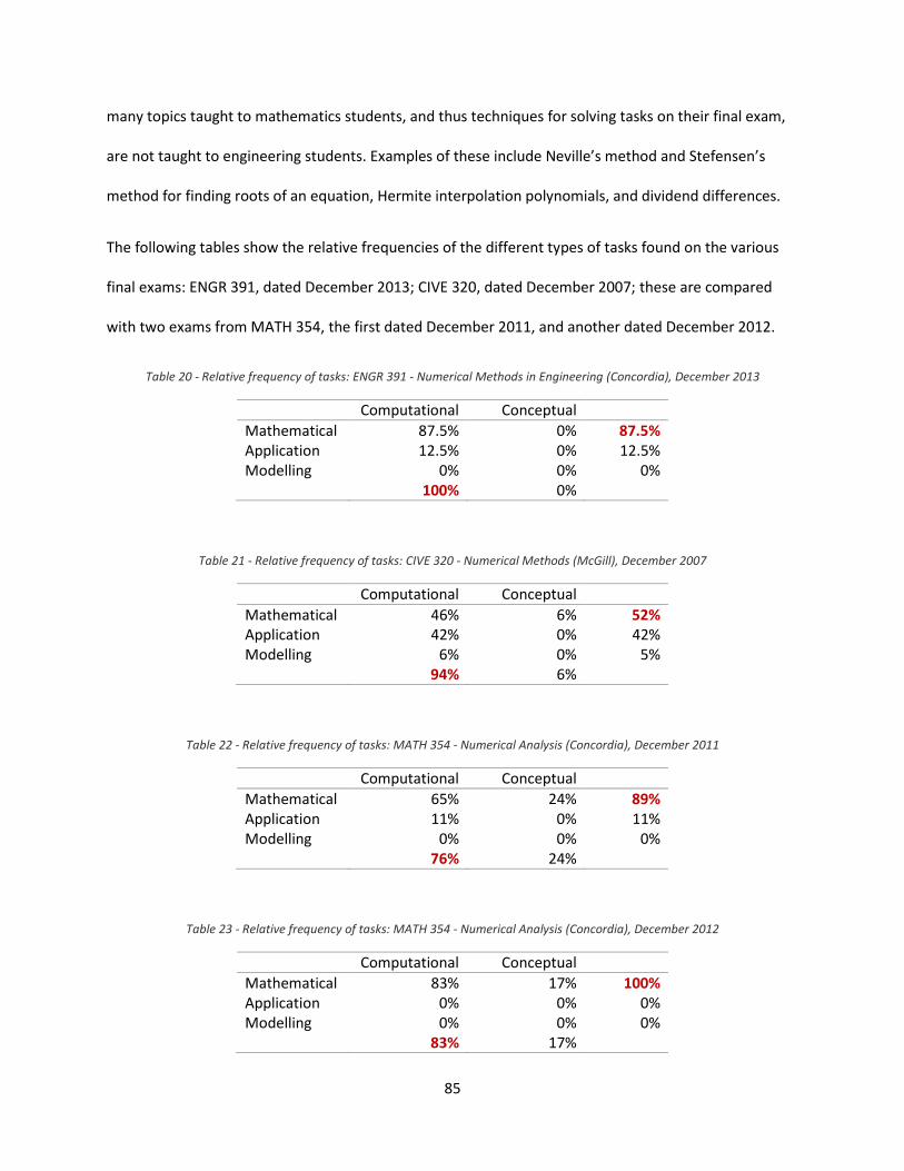
85
many topics taught to mathematics students, and thus techniques for solving tasks on their final exam,
are not taught to engineering students. Examples of these include Neville’s method and Stefensen’s
method for finding roots of an equation, Hermite interpolation polynomials, and dividend differences.
The following tables show the relative frequencies of the different types of tasks found on the various
final exams: ENGR 391, dated December 2013; CIVE 320, dated December 2007; these are compared
with two exams from MATH 354, the first dated December 2011, and another dated December 2012.
Table 20 - Relative frequency of tasks: ENGR 391 - Numerical Methods in Engineering (Concordia), December 2013
Computational Conceptual
Mathematical 87.5% 0% 87.5% Application 12.5% 0% 12.5% Modelling 0% 0% 0% 100% 0%
Table 21 - Relative frequency of tasks: CIVE 320 - Numerical Methods (McGill), December 2007
Computational Conceptual
Mathematical 46% 6% 52% Application 42% 0% 42% Modelling 6% 0% 5% 94% 6%
Table 22 - Relative frequency of tasks: MATH 354 - Numerical Analysis (Concordia), December 2011
Computational Conceptual
Mathematical 65% 24% 89% Application 11% 0% 11% Modelling 0% 0% 0% 76% 24%
Table 23 - Relative frequency of tasks: MATH 354 - Numerical Analysis (Concordia), December 2012
Computational Conceptual
Mathematical 83% 17% 100% Application 0% 0% 0% Modelling 0% 0% 0% 83% 17%
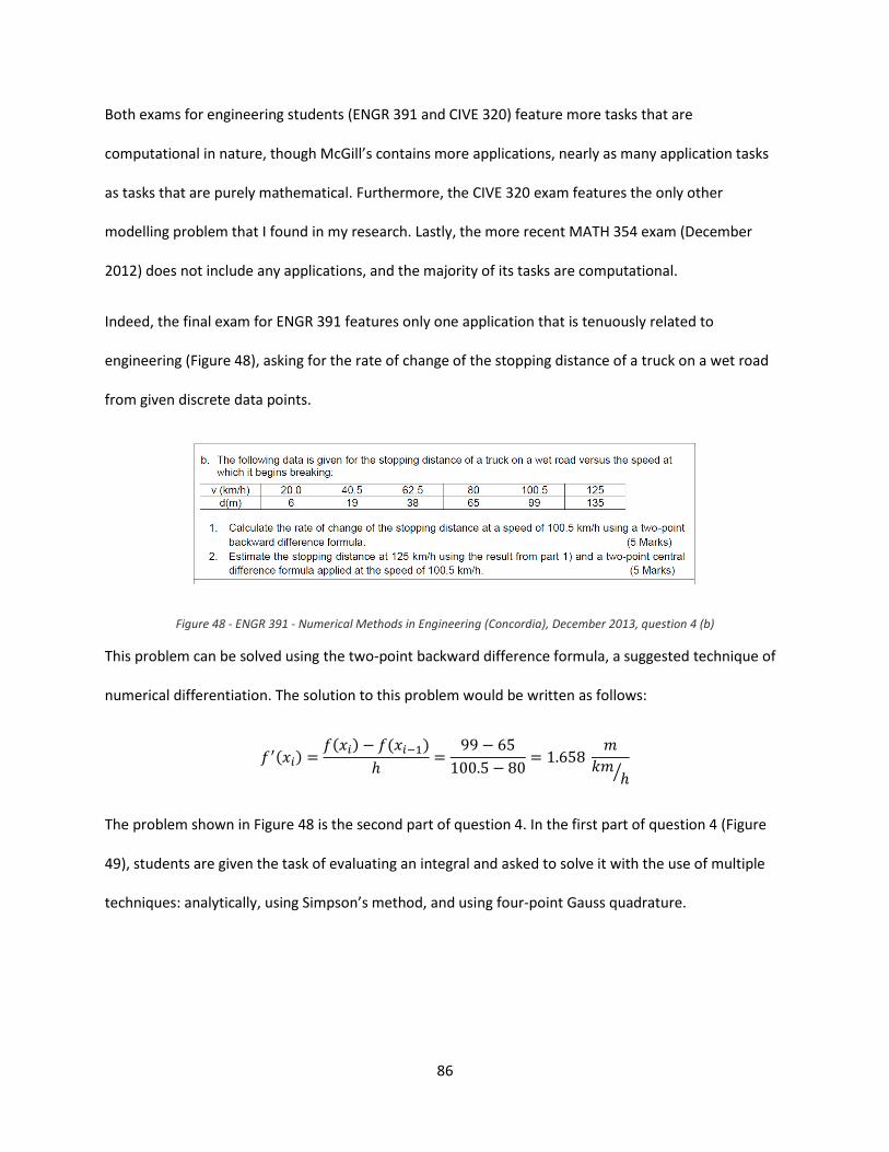
86
Both exams for engineering students (ENGR 391 and CIVE 320) feature more tasks that are
computational in nature, though McGill’s contains more applications, nearly as many application tasks
as tasks that are purely mathematical. Furthermore, the CIVE 320 exam features the only other
modelling problem that I found in my research. Lastly, the more recent MATH 354 exam (December
2012) does not include any applications, and the majority of its tasks are computational.
Indeed, the final exam for ENGR 391 features only one application that is tenuously related to
engineering (Figure 48), asking for the rate of change of the stopping distance of a truck on a wet road
from given discrete data points.
Figure 48 - ENGR 391 - Numerical Methods in Engineering (Concordia), December 2013, question 4 (b)
This problem can be solved using the two-point backward difference formula, a suggested technique of
numerical differentiation. The solution to this problem would be written as follows:
⁄
The problem shown in Figure 48 is the second part of question 4. In the first part of question 4 (Figure
49), students are given the task of evaluating an integral and asked to solve it with the use of multiple
techniques: analytically, using Simpson’s method, and using four-point Gauss quadrature.
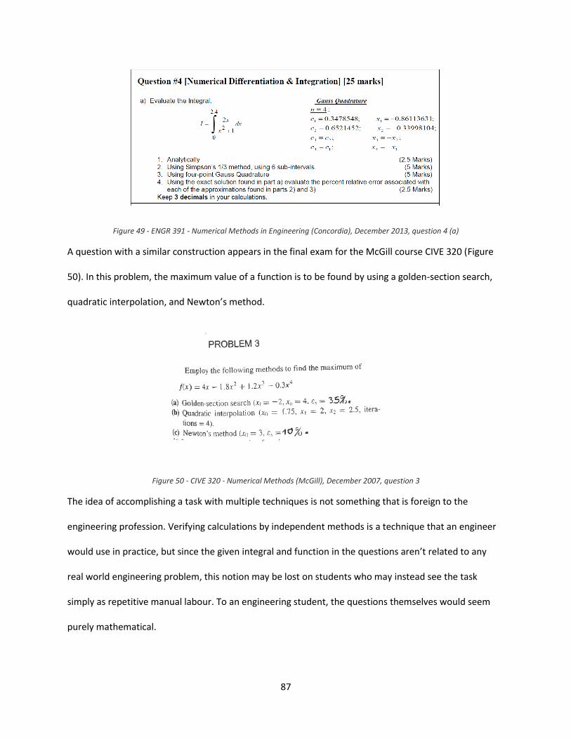
87
Figure 49 - ENGR 391 - Numerical Methods in Engineering (Concordia), December 2013, question 4 (a)
A question with a similar construction appears in the final exam for the McGill course CIVE 320 (Figure
50). In this problem, the maximum value of a function is to be found by using a golden-section search,
quadratic interpolation, and Newton’s method.
Figure 50 - CIVE 320 - Numerical Methods (McGill), December 2007, question 3
The idea of accomplishing a task with multiple techniques is not something that is foreign to the
engineering profession. Verifying calculations by independent methods is a technique that an engineer
would use in practice, but since the given integral and function in the questions aren’t related to any
real world engineering problem, this notion may be lost on students who may instead see the task
simply as repetitive manual labour. To an engineering student, the questions themselves would seem
purely mathematical.
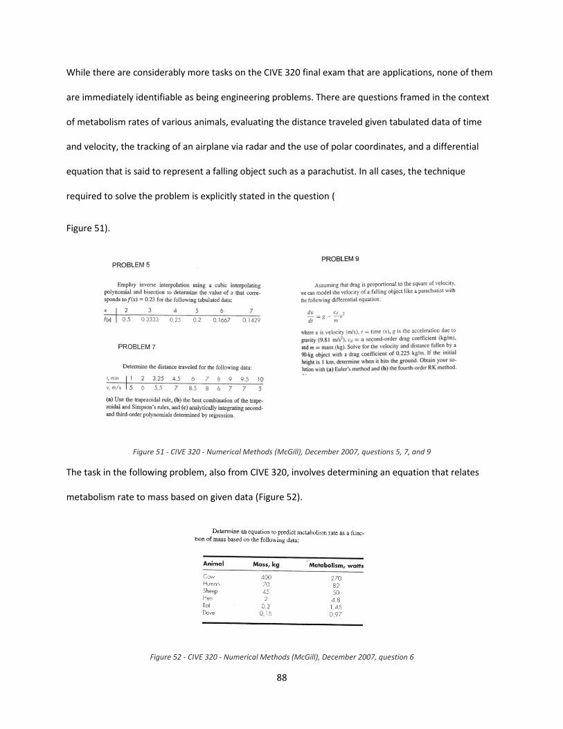
88
While there are considerably more tasks on the CIVE 320 final exam that are applications, none of them
are immediately identifiable as being engineering problems. There are questions framed in the context
of metabolism rates of various animals, evaluating the distance traveled given tabulated data of time
and velocity, the tracking of an airplane via radar and the use of polar coordinates, and a differential
equation that is said to represent a falling object such as a parachutist. In all cases, the technique
required to solve the problem is explicitly stated in the question (
Figure 51).
Figure 51 - CIVE 320 - Numerical Methods (McGill), December 2007, questions 5, 7, and 9
The task in the following problem, also from CIVE 320, involves determining an equation that relates
metabolism rate to mass based on given data (Figure 52).
Figure 52 - CIVE 320 - Numerical Methods (McGill), December 2007, question 6
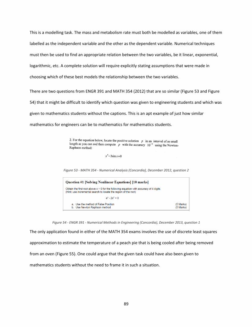
89
This is a modelling task. The mass and metabolism rate must both be modelled as variables, one of them
labelled as the independent variable and the other as the dependent variable. Numerical techniques
must then be used to find an appropriate relation between the two variables, be it linear, exponential,
logarithmic, etc. A complete solution will require explicitly stating assumptions that were made in
choosing which of these best models the relationship between the two variables.
There are two questions from ENGR 391 and MATH 354 (2012) that are so similar (Figure 53 and Figure
54) that it might be difficult to identify which question was given to engineering students and which was
given to mathematics students without the captions. This is an apt example of just how similar
mathematics for engineers can be to mathematics for mathematics students.
Figure 53 - MATH 354 - Numerical Analysis (Concordia), December 2012, question 2
Figure 54 - ENGR 391 - Numerical Methods in Engineering (Concordia), December 2013, question 1
The only application found in either of the MATH 354 exams involves the use of discrete least squares
approximation to estimate the temperature of a peach pie that is being cooled after being removed
from an oven (Figure 55). One could argue that the given task could have also been given to
mathematics students without the need to frame it in such a situation.
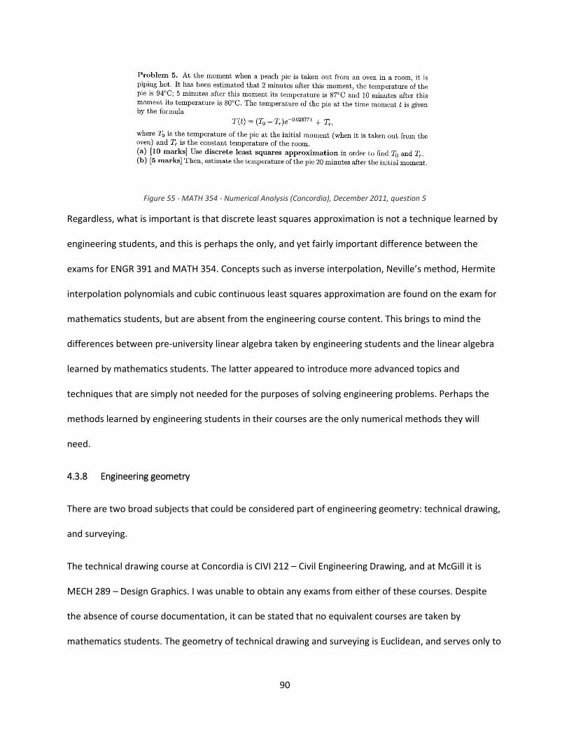
90
Figure 55 - MATH 354 - Numerical Analysis (Concordia), December 2011, question 5
Regardless, what is important is that discrete least squares approximation is not a technique learned by
engineering students, and this is perhaps the only, and yet fairly important difference between the
exams for ENGR 391 and MATH 354. Concepts such as inverse interpolation, Neville’s method, Hermite
interpolation polynomials and cubic continuous least squares approximation are found on the exam for
mathematics students, but are absent from the engineering course content. This brings to mind the
differences between pre-university linear algebra taken by engineering students and the linear algebra
learned by mathematics students. The latter appeared to introduce more advanced topics and
techniques that are simply not needed for the purposes of solving engineering problems. Perhaps the
methods learned by engineering students in their courses are the only numerical methods they will
need.
4.3.8 Engineering geometry
There are two broad subjects that could be considered part of engineering geometry: technical drawing,
and surveying.
The technical drawing course at Concordia is CIVI 212 – Civil Engineering Drawing, and at McGill it is
MECH 289 – Design Graphics. I was unable to obtain any exams from either of these courses. Despite
the absence of course documentation, it can be stated that no equivalent courses are taken by
mathematics students. The geometry of technical drawing and surveying is Euclidean, and serves only to
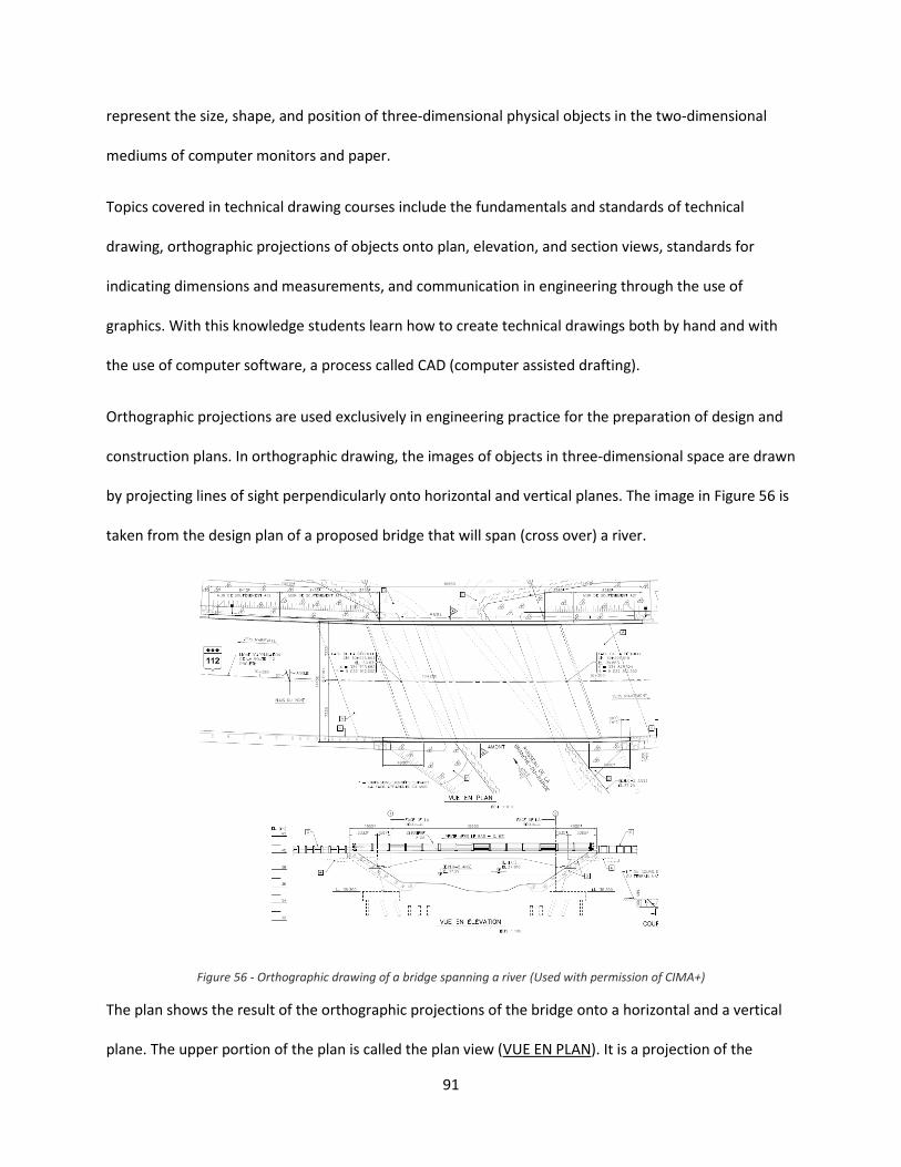
91
represent the size, shape, and position of three-dimensional physical objects in the two-dimensional
mediums of computer monitors and paper.
Topics covered in technical drawing courses include the fundamentals and standards of technical
drawing, orthographic projections of objects onto plan, elevation, and section views, standards for
indicating dimensions and measurements, and communication in engineering through the use of
graphics. With this knowledge students learn how to create technical drawings both by hand and with
the use of computer software, a process called CAD (computer assisted drafting).
Orthographic projections are used exclusively in engineering practice for the preparation of design and
construction plans. In orthographic drawing, the images of objects in three-dimensional space are drawn
by projecting lines of sight perpendicularly onto horizontal and vertical planes. The image in Figure 56 is
taken from the design plan of a proposed bridge that will span (cross over) a river.
Figure 56 - Orthographic drawing of a bridge spanning a river (Used with permission of CIMA+)
The plan shows the result of the orthographic projections of the bridge onto a horizontal and a vertical
plane. The upper portion of the plan is called the plan view (VUE EN PLAN). It is a projection of the
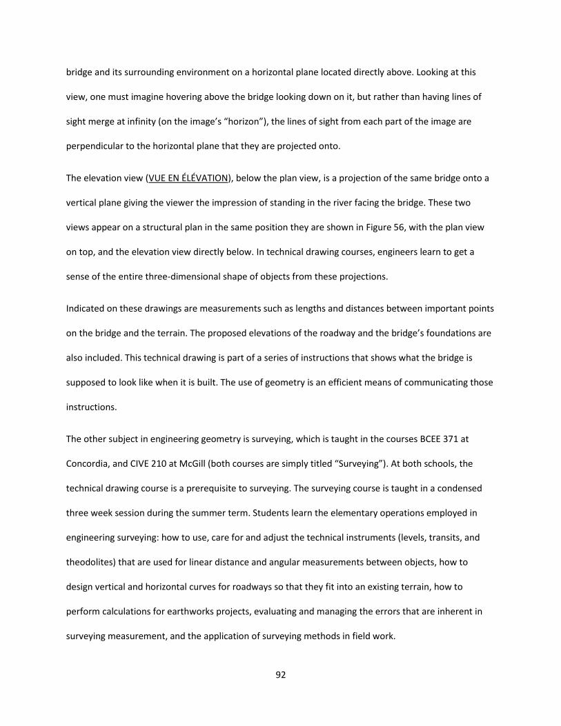
92
bridge and its surrounding environment on a horizontal plane located directly above. Looking at this
view, one must imagine hovering above the bridge looking down on it, but rather than having lines of
sight merge at infinity (on the image’s “horizon”), the lines of sight from each part of the image are
perpendicular to the horizontal plane that they are projected onto.
The elevation view (VUE EN ÉLÉVATION), below the plan view, is a projection of the same bridge onto a
vertical plane giving the viewer the impression of standing in the river facing the bridge. These two
views appear on a structural plan in the same position they are shown in Figure 56, with the plan view
on top, and the elevation view directly below. In technical drawing courses, engineers learn to get a
sense of the entire three-dimensional shape of objects from these projections.
Indicated on these drawings are measurements such as lengths and distances between important points
on the bridge and the terrain. The proposed elevations of the roadway and the bridge’s foundations are
also included. This technical drawing is part of a series of instructions that shows what the bridge is
supposed to look like when it is built. The use of geometry is an efficient means of communicating those
instructions.
The other subject in engineering geometry is surveying, which is taught in the courses BCEE 371 at
Concordia, and CIVE 210 at McGill (both courses are simply titled “Surveying”). At both schools, the
technical drawing course is a prerequisite to surveying. The surveying course is taught in a condensed
three week session during the summer term. Students learn the elementary operations employed in
engineering surveying: how to use, care for and adjust the technical instruments (levels, transits, and
theodolites) that are used for linear distance and angular measurements between objects, how to
design vertical and horizontal curves for roadways so that they fit into an existing terrain, how to
perform calculations for earthworks projects, evaluating and managing the errors that are inherent in
surveying measurement, and the application of surveying methods in field work.
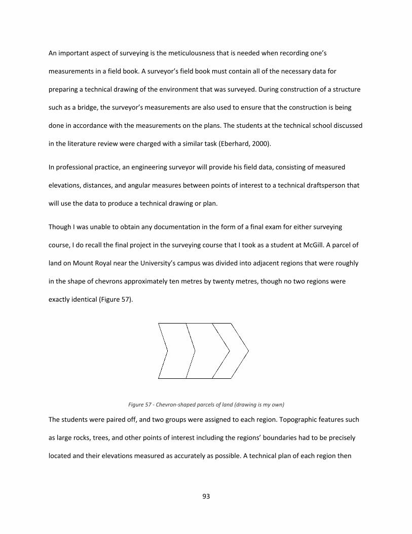
93
An important aspect of surveying is the meticulousness that is needed when recording one’s
measurements in a field book. A surveyor’s field book must contain all of the necessary data for
preparing a technical drawing of the environment that was surveyed. During construction of a structure
such as a bridge, the surveyor’s measurements are also used to ensure that the construction is being
done in accordance with the measurements on the plans. The students at the technical school discussed
in the literature review were charged with a similar task (Eberhard, 2000).
In professional practice, an engineering surveyor will provide his field data, consisting of measured
elevations, distances, and angular measures between points of interest to a technical draftsperson that
will use the data to produce a technical drawing or plan.
Though I was unable to obtain any documentation in the form of a final exam for either surveying
course, I do recall the final project in the surveying course that I took as a student at McGill. A parcel of
land on Mount Royal near the University’s campus was divided into adjacent regions that were roughly
in the shape of chevrons approximately ten metres by twenty metres, though no two regions were
exactly identical (Figure 57).
Figure 57 - Chevron-shaped parcels of land (drawing is my own)
The students were paired off, and two groups were assigned to each region. Topographic features such
as large rocks, trees, and other points of interest including the regions’ boundaries had to be precisely
located and their elevations measured as accurately as possible. A technical plan of each region then
94
had to be drafted by each independent pair of students. The plans of each region were then assembled
to see if they fit together as they did in reality.
In this sense, engineering geometry closely fits the etymology of the subject, namely the measurement
of the earth. But there is more to be said about an engineer’s geometry beyond the topics of technical
drawing and surveying. At its core, the geometry used by engineers is Euclidean, and is concerned with
representing the three-dimensional physical objects as images on a two-dimensional plane. Euclidean
geometry assumes that for all intents and purposes the world is flat, and remains so underneath any
object or parcel of land that is being measured. It is essentially a very “local” geometry. In this geometry,
the surface of the earth is a “horizontal plane”, and “vertical planes” are orthogonal to it. Orthographic
projection takes physical objects and projects their image onto three planes which are pairwise
orthogonal to each other, with the horizontal plane being parallel to the surface of the earth.
Another aspect of this geometry is the use of pairwise orthogonal axes to describe the position and
orientation of objects in the physical world. A structural engineer’s task in the analysis and design of a
structure focuses on the members that make up the structure. Each structural member has a position
and orientation within the structure. In terms of geometry, a member can be thought of as a regular
prism, such as the object shown in Figure 58.
Figure 58 - Example of a structural member with a rectangular cross-section
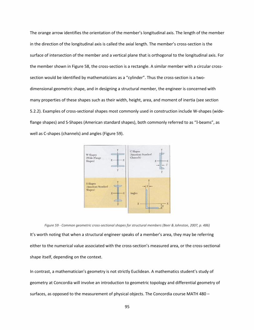
95
The orange arrow identifies the orientation of the member’s longitudinal axis. The length of the member
in the direction of the longitudinal axis is called the axial length. The member’s cross-section is the
surface of intersection of the member and a vertical plane that is orthogonal to the longitudinal axis. For
the member shown in Figure 58, the cross-section is a rectangle. A similar member with a circular cross-
section would be identified by mathematicians as a “cylinder”. Thus the cross-section is a two-
dimensional geometric shape, and in designing a structural member, the engineer is concerned with
many properties of these shapes such as their width, height, area, and moment of inertia (see section
5.2.2). Examples of cross-sectional shapes most commonly used in construction include W-shapes (wide-
flange shapes) and S-Shapes (American standard shapes), both commonly referred to as “I-beams”, as
well as C-shapes (channels) and angles (Figure 59).
Figure 59 - Common geometric cross-sectional shapes for structural members (Beer & Johnston, 2007, p. 486)
It’s worth noting that when a structural engineer speaks of a member’s area, they may be referring
either to the numerical value associated with the cross-section’s measured area, or the cross-sectional
shape itself, depending on the context.
In contrast, a mathematician’s geometry is not strictly Euclidean. A mathematics student’s study of
geometry at Concordia will involve an introduction to geometric topology and differential geometry of
surfaces, as opposed to the measurement of physical objects. The Concordia course MATH 480 –
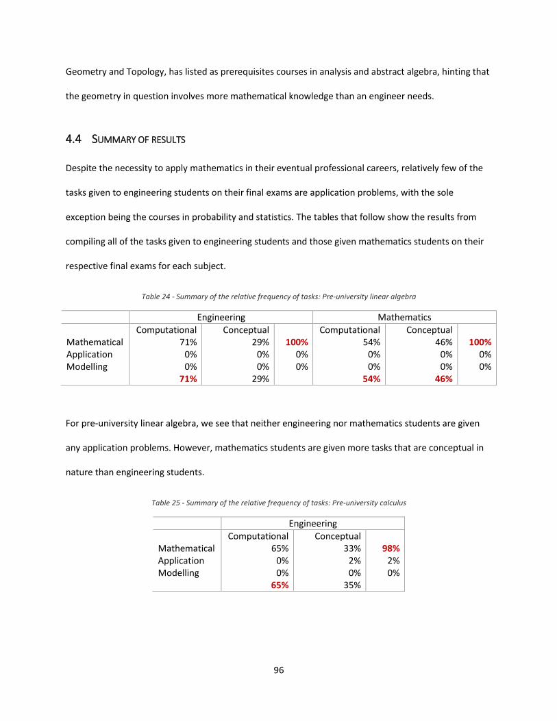
96
Geometry and Topology, has listed as prerequisites courses in analysis and abstract algebra, hinting that
the geometry in question involves more mathematical knowledge than an engineer needs.
4.4 SUMMARY OF RESULTS
Despite the necessity to apply mathematics in their eventual professional careers, relatively few of the
tasks given to engineering students on their final exams are application problems, with the sole
exception being the courses in probability and statistics. The tables that follow show the results from
compiling all of the tasks given to engineering students and those given mathematics students on their
respective final exams for each subject.
Table 24 - Summary of the relative frequency of tasks: Pre-university linear algebra
Engineering Mathematics
Computational Conceptual Computational Conceptual Mathematical 71% 29% 100% 54% 46% 100% Application 0% 0% 0% 0% 0% 0% Modelling 0% 0% 0% 0% 0% 0% 71% 29% 54% 46%
For pre-university linear algebra, we see that neither engineering nor mathematics students are given
any application problems. However, mathematics students are given more tasks that are conceptual in
nature than engineering students.
Table 25 - Summary of the relative frequency of tasks: Pre-university calculus
Engineering
Computational Conceptual Mathematical 65% 33% 98% Application 0% 2% 2% Modelling 0% 0% 0% 65% 35%
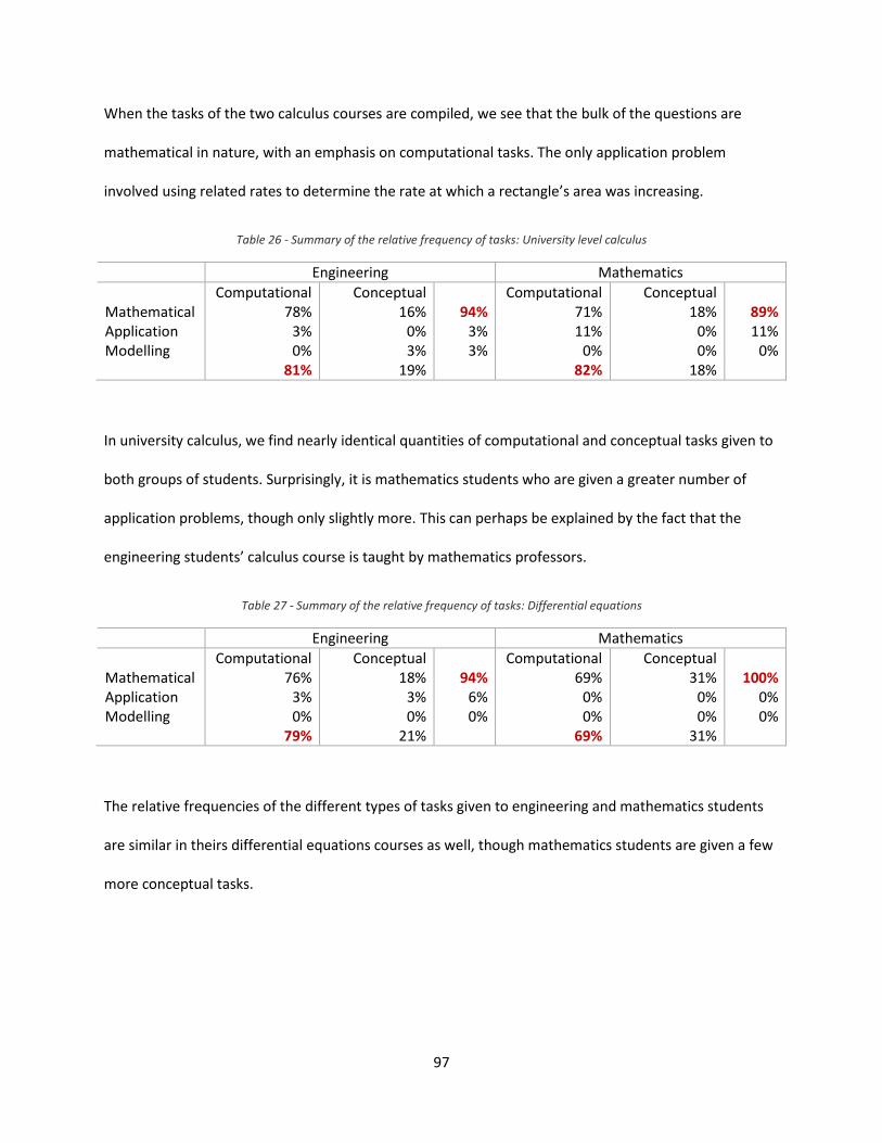
97
When the tasks of the two calculus courses are compiled, we see that the bulk of the questions are
mathematical in nature, with an emphasis on computational tasks. The only application problem
involved using related rates to determine the rate at which a rectangle’s area was increasing.
Table 26 - Summary of the relative frequency of tasks: University level calculus
Engineering Mathematics
Computational Conceptual Computational Conceptual Mathematical 78% 16% 94% 71% 18% 89% Application 3% 0% 3% 11% 0% 11% Modelling 0% 3% 3% 0% 0% 0% 81% 19% 82% 18%
In university calculus, we find nearly identical quantities of computational and conceptual tasks given to
both groups of students. Surprisingly, it is mathematics students who are given a greater number of
application problems, though only slightly more. This can perhaps be explained by the fact that the
engineering students’ calculus course is taught by mathematics professors.
Table 27 - Summary of the relative frequency of tasks: Differential equations
Engineering Mathematics
Computational Conceptual Computational Conceptual Mathematical 76% 18% 94% 69% 31% 100% Application 3% 3% 6% 0% 0% 0% Modelling 0% 0% 0% 0% 0% 0% 79% 21% 69% 31%
The relative frequencies of the different types of tasks given to engineering and mathematics students
are similar in theirs differential equations courses as well, though mathematics students are given a few
more conceptual tasks.
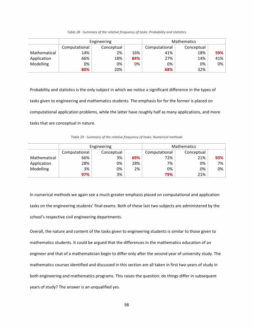
98
Table 28 - Summary of the relative frequency of tasks: Probability and statistics
Engineering Mathematics
Computational Conceptual Computational Conceptual Mathematical 14% 2% 16% 41% 18% 59% Application 66% 18% 84% 27% 14% 41% Modelling 0% 0% 0% 0% 0% 0% 80% 20% 68% 32%
Probability and statistics is the only subject in which we notice a significant difference in the types of
tasks given to engineering and mathematics students. The emphasis for for the former is placed on
computational application problems, while the latter have roughly half as many applications, and more
tasks that are conceptual in nature.
Table 29 - Summary of the relative frequency of tasks: Numerical methods
Engineering Mathematics
Computational Conceptual Computational Conceptual Mathematical 66% 3% 69% 72% 21% 93% Application 28% 0% 28% 7% 0% 7% Modelling 3% 0% 2% 0% 0% 0% 97% 3% 79% 21%
In numerical methods we again see a much greater emphasis placed on computational and application
tasks on the engineering students’ final exams. Both of these last two subjects are administered by the
school’s respective civil engineering departments.
Overall, the nature and content of the tasks given to engineering students is similar to those given to
mathematics students. It could be argued that the differences in the mathematics education of an
engineer and that of a mathematician begin to differ only after the second year of university study. The
mathematics courses identified and discussed in this section are all taken in first two years of study in
both engineering and mathematics programs. This raises the question: do things differ in subsequent
years of study? The answer is an unqualified yes.
99
Engineering students complete their studies with courses in engineering sciences. For all intents and
purposes, their mathematics education is finished after their second year. Mathematics students,
however, learn about concepts and topics that for the most part remain foreign to engineers (both
students and professionals). These include topics in mathematical logic, real and complex analysis,
abstract algebra, and measure theory. These courses explore the inner workings of mathematics; they
provide the “theory” in the academic mathematics praxeology.
Instead of diving deeper into the theory behind the rules of mathematics, engineers take the rules they
have learned for manipulating mathematical objects – matrices and vectors, derivatives and integrals of
functions, differential equations, numerical methods – and use them to solve problems in the
engineering domain.
100
5 ENGINEERS’ MATHEMATICS
In chapter 4 it was shown that the types of mathematical tasks given to engineering students and the
topics they are expected to learn in their mathematics courses are not noticeably different from those
learned by mathematics students in the first two years of their university education. But the education
of engineers isn’t limited to mathematics classes. They must also learn about the physical sciences in
order to be able to describe, understand, and predict physical phenomena. The goal of an engineer’s
mathematics education is to express these phenomena symbolically using mathematical models, and it
is precisely this use of mathematics to model the physical world that differentiates an engineer’s
mathematics from that of the mathematician.
The present chapter will explore how engineers use mathematics to create models of the physical world
in order to solve engineering problems, and will focus particularly on the models used in the field of
structural engineering. Structural engineering comprises the tasks of design, analysis, construction, and
maintenance of all manner of modern structures including conventional shelters such as houses, office
buildings, and commercial warehouses, as well as specialized structures such as bridges, highway
overpasses and interchanges, and hydroelectric dams.
The chapter begins with a brief explanation of two types of models: analytical and empirical. Established
mathematical models, their assumptions, and how they were developed, are presented to students in
their engineering textbooks. These models are then used by students in application problems. Examples
of these models from the subjects of statics, mechanics of materials, and structural analysis will be
shown in section 5.2. As they are presented, observations will be made about which aspects of the
models are important to engineers, and which aspects a mathematician may see that an engineer might
overlook.
101
Section 5.3 contains an in-depth examination of a mathematical model of matrix structural analysis.
Included in this section is a discussion of the concept of eigenvalues and eigenvectors in the context of
matrix structural analysis. My intention is to show the physical meaning of an abstract mathematical
concept in an engineering context.
The final section of this chapter presents documents from a professional engineer’s dossier de calculs
that will illustrate how the mathematics used in professional practice rests upon the extensive research
and refinement of the mathematical models developed by professional and research engineers.
5.1 ANALYTICAL MODELS AND EMPIRICAL MODELS
In chapter 4 I showed that mathematics courses taken during an engineer’s education provide tasks that
involve applications, but there were none that required the student to create a mathematical model. In
the current chapter I will show that many of the mathematical models used by engineers are introduced
in the textbooks of engineering core courses. I will present some of these models, explain how they are
developed, and show that the tasks given to engineering students involve applications of these models.
Engineers make use of two different types of mathematical models: analytical models and empirical
models. Analytical models are developed directly from foundational principles of physical sciences. In
their physics courses, for example, engineering students learn about kinematics, the study of the motion
of objects, without regard for the cause of the motion. The laws of how things fall were developed long
before Newton described why things fall (Tipler, 1991). Kinematics relates three physical quantities: the
displacement of an object, its velocity, and its acceleration. Displacement is the change in an object’s
position in space:
102
Velocity is defined as the rate of change of displacement. This is expressed mathematically as:
for average velocity, and:
for instantaneous velocity. Similarly, acceleration is defined as the rate of change of velocity, and is
expressed as:
for average acceleration, and:
for instantaneous acceleration. But, if the acceleration is constant (as it is for objects that are dropped
or fall on Earth) then velocity varies linearly with time. This leads to the development of the four
equations of kinematics that can be used to solve problems:
Each equation can be used depending on the context of the problem that one wishes to solve, on what
information is known, and what information is sought. The last equation would be used if one wants to
103
know the final velocity, , of an object as it hits the ground when dropped from a known height, ,
without any regard to the time it took to fall (Tipler, 1991). These four equations are all derived through
analytical means directly from the relationships between displacement, velocity, and acceleration.
An example of an analytical model used specifically by structural engineers is the various formulae for
calculating the moment of inertia of common geometric shapes. These formulae, and how they are
developed, will be shown and discussed in section 5.2.2.
Empirical models on the other hand are developed through experimentation, and are often refined with
statistical analysis. Such models cannot be derived solely by analytical means. A well-known example of
an empirical model is Hooke’s Law which states that the force, F, required to stretch a spring is directly
proportional to the length, X, that it is stretched: . This relationship is usually investigated in high
school physics classes, and could not be determined based on the principles of mechanics alone. A
similar relationship arises in the study of mechanics of materials, and is presented in section 5.2.3.
The design codes that structural engineers are obligated to follow in the design and analysis of
structures are peppered with equations that were derived empirically. Historically, research engineers
have always been interested in determining the effects that small changes in the shape, size, and
configuration of structural members may have on a structure’s performance. The only way to determine
those effects is to perform controlled experiments and analyze the results. The result is the empirical
models that are found in the design codes.
Recall that the use of these models to solve a problem results in an application of mathematics, but the
development of the equations themselves in order to represent physical reality is done through the
process of mathematical modelling. The mathematical models that are introduced throughout section
5.2 will be identified as either analytical or empirical in nature.
104
5.2 THE MATHEMATICS OF MECHANICS
Civil engineering is a multidisciplinary field encompassing many different kinds of engineering disciplines
including environmental engineering, transportation engineering, and structural engineering among
others. Prior to my career as a graduate student, I was employed as a licensed structural engineer,
hence my interest in writing on the topic of this thesis. The remainder of this chapter will therefore
focus solely on the mathematics used by structural engineers.
Structural engineering is an advanced discipline that stems from applied mechanics, particularly the
fields of statics, which is the study of rigid bodies at rest, and the mechanics of materials, which is the
study of deformable bodies4. All structures, be they houses, bus shelters, skyscrapers, or bridges, must
be static, i.e., they must not move from their location after being exposed to some force pushing it or
pulling on it. But they are not rigid bodies; they are subject to deformations due to the properties of the
materials they are made from. A bus shelter may sway due to the gust of a strong wind (it will deform),
but it should not move from where it was built (it will be static against the applied force of the wind).
While mechanics and mathematics may seem to be distinct subjects, historically there is very little
separation between the two. Bkouche (1989) neatly summarizes the close relationship between the two
fields and how each has allowed a better understanding of the other. It is in applying mathematics to
the problems from which its concepts and theories were born, among which are physical problems, that
we see its power. The formalisation of mathematics in the late nineteenth century removed it from its
empirical origins in mechanics and physics. Prior to this, the lines between the two fields of study were
blurred. Consider the works of Newton and Euler who are celebrated for their discoveries in both
mathematics and mechanics. Newton’s laws of motion are well-tested mathematical models that are
generally accepted as being correct, and weren’t superseded in their accuracy or generality until
4 Deformable bodies are objects whose shapes can be altered by stretching, compressing, bending, or twisting. In
the field of statics, objects are assumed to be un-deformable, i.e., rigid.
105
Einstein’s theory of relativity. Euler is also recognized for his contributions to mechanics as well and is
remembered for models that he developed through experimentation and equations that that are named
in his honour.
The sections that follow will present some mathematical models from statics, mechanics of materials,
and structural analysis, along with an introduction to the underlying physical principles that they
represent. Certain details will be highlighted to indicate the differences in what an engineer and a
mathematician may notice about the mathematics used in the models. I begin by discussing the
important concept of units, without which there would perhaps be no understanding of the measure of
the physical world.
5.2.1 Units and numerical accuracy
Units are vital to a proper description of physical quantities. The number 10 by itself may or may not
convey any meaning to the reader, but if one is asked to hold a toothbrush weighing 10 grams in one
hand, and a bowling ball weighing 10 kilograms in the other, suddenly the number 10 can take on
different meanings. It is worth noting that in the tasks from various exams shown in chapter 4, units of
measure only appear in application questions, when objects from the physical world are involved.
In mechanics, there are three fundamental units of measure that are considered base units, i.e., they are
defined arbitrarily, and are used to derive other units (Beer & Johnston, 2007). These are the units of
time, length, and mass. Two systems are still in use to describe these units: the Système International
(SI), also known as the metric system, and the U.S. Customary system, commonly referred to as the
Imperial system. In the SI system, the base units for time, length, and mass are, respectively, the second
( ) the metre ( ) and the kilogram ( ).
A fourth unit that is considered fundamental to mechanics is that of force. Its unit of measure in the SI
system is called the newton ( ), and it is derived from the base units of time, length, and mass. A force
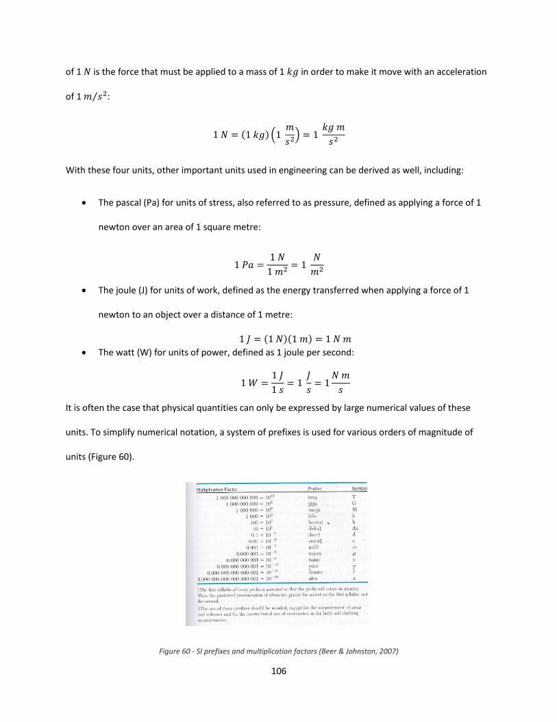
106
of 1 is the force that must be applied to a mass of 1 in order to make it move with an acceleration
of 1 ⁄ :
(
)
With these four units, other important units used in engineering can be derived as well, including:
The pascal (Pa) for units of stress, also referred to as pressure, defined as applying a force of 1
newton over an area of 1 square metre:
The joule (J) for units of work, defined as the energy transferred when applying a force of 1
newton to an object over a distance of 1 metre:
The watt (W) for units of power, defined as 1 joule per second:
It is often the case that physical quantities can only be expressed by large numerical values of these
units. To simplify numerical notation, a system of prefixes is used for various orders of magnitude of
units (Figure 60).
Figure 60 - SI prefixes and multiplication factors (Beer & Johnston, 2007)
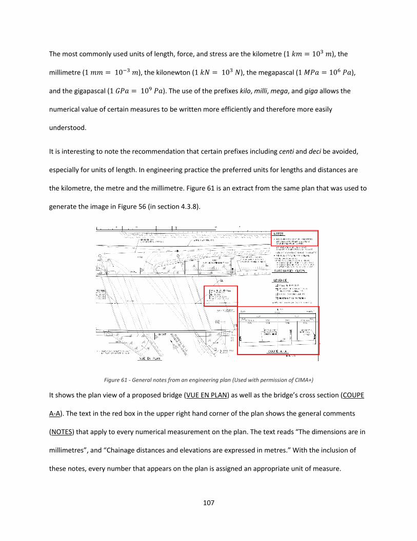
107
The most commonly used units of length, force, and stress are the kilometre ( ), the
millimetre ( ), the kilonewton ( ), the megapascal ( ),
and the gigapascal ( ). The use of the prefixes kilo, milli, mega, and giga allows the
numerical value of certain measures to be written more efficiently and therefore more easily
understood.
It is interesting to note the recommendation that certain prefixes including centi and deci be avoided,
especially for units of length. In engineering practice the preferred units for lengths and distances are
the kilometre, the metre and the millimetre. Figure 61 is an extract from the same plan that was used to
generate the image in Figure 56 (in section 4.3.8).
Figure 61 - General notes from an engineering plan (Used with permission of CIMA+)
It shows the plan view of a proposed bridge (VUE EN PLAN) as well as the bridge’s cross section (COUPE
A-A). The text in the red box in the upper right hand corner of the plan shows the general comments
(NOTES) that apply to every numerical measurement on the plan. The text reads “The dimensions are in
millimetres”, and “Chainage distances and elevations are expressed in metres.” With the inclusion of
these notes, every number that appears on the plan is assigned an appropriate unit of measure.
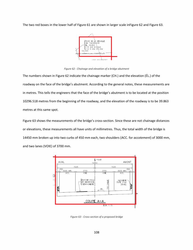
108
The two red boxes in the lower half of Figure 61 are shown in larger scale inFigure 62 and Figure 63.
Figure 62 - Chainage and elevation of a bridge abutment
The numbers shown in Figure 62 indicate the chainage marker (CH.) and the elevation (ÉL.) of the
roadway on the face of the bridge’s abutment. According to the general notes, these measurements are
in metres. This tells the engineers that the face of the bridge’s abutment is to be located at the position
10296.518 metres from the beginning of the roadway, and the elevation of the roadway is to be 39.863
metres at this same spot.
Figure 63 shows the measurements of the bridge’s cross-section. Since these are not chainage distances
or elevations, these measurements all have units of millimetres. Thus, the total width of the bridge is
14450 mm broken up into two curbs of 450 mm each, two shoulders (ACC. for accotement) of 3000 mm,
and two lanes (VOIE) of 3700 mm.
Figure 63 - Cross-section of a proposed bridge
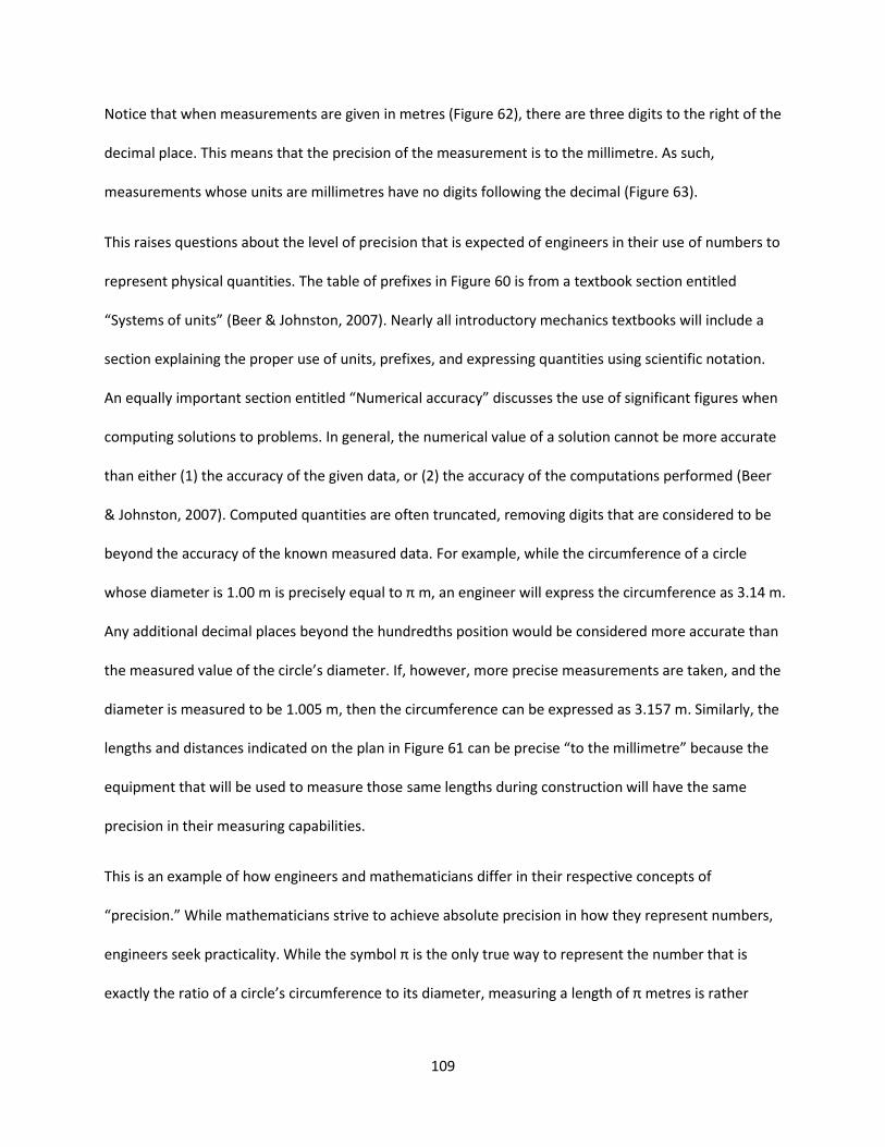
109
Notice that when measurements are given in metres (Figure 62), there are three digits to the right of the
decimal place. This means that the precision of the measurement is to the millimetre. As such,
measurements whose units are millimetres have no digits following the decimal (Figure 63).
This raises questions about the level of precision that is expected of engineers in their use of numbers to
represent physical quantities. The table of prefixes in Figure 60 is from a textbook section entitled
“Systems of units” (Beer & Johnston, 2007). Nearly all introductory mechanics textbooks will include a
section explaining the proper use of units, prefixes, and expressing quantities using scientific notation.
An equally important section entitled “Numerical accuracy” discusses the use of significant figures when
computing solutions to problems. In general, the numerical value of a solution cannot be more accurate
than either (1) the accuracy of the given data, or (2) the accuracy of the computations performed (Beer
& Johnston, 2007). Computed quantities are often truncated, removing digits that are considered to be
beyond the accuracy of the known measured data. For example, while the circumference of a circle
whose diameter is 1.00 m is precisely equal to π m, an engineer will express the circumference as 3.14 m.
Any additional decimal places beyond the hundredths position would be considered more accurate than
the measured value of the circle’s diameter. If, however, more precise measurements are taken, and the
diameter is measured to be 1.005 m, then the circumference can be expressed as 3.157 m. Similarly, the
lengths and distances indicated on the plan in Figure 61 can be precise “to the millimetre” because the
equipment that will be used to measure those same lengths during construction will have the same
precision in their measuring capabilities.
This is an example of how engineers and mathematicians differ in their respective concepts of
“precision.” While mathematicians strive to achieve absolute precision in how they represent numbers,
engineers seek practicality. While the symbol π is the only true way to represent the number that is
exactly the ratio of a circle’s circumference to its diameter, measuring a length of π metres is rather
110
impractical since it requires a level of precision that cannot be achieved. Thus engineers use precision
relative to the context of the physical problem which they are trying to solve.
Lastly, there is another unit of measure that I have neglected to mention thus far but that is important
to every engineering project that a professional engineer will work on. That unit is the dollar ($).
Structural engineers design and construct all manners of structure that much resist applied loads and
have limited deformations, but they must also be built efficiently and economically. Professional
engineers who work in the role of project manager are chiefly responsible for ensuring that the
monetary aspects of the project are met.
5.2.2 Statics
Statics is the study of rigid bodies, i.e., objects that are assumed to remain un-deformed when acted
upon by external forces. The principle of static equilibrium is at the heart of the subject. Static
equilibrium is an interpretation of Newton’s first law of motion which states that an object at rest will
remain at rest unless it is acted upon by an external force. But the effects of any external force applied
to an object can be countered by applying a second force that is equal in magnitude but opposite in
direction to the first. Thus Newton’s first law can be restated as: an object will be in static equilibrium if
the net sum of the external forces acting upon it is 0.
Applying a force is akin to the act of pushing or pulling on an object. Imagine pushing a large block.
When pushed with enough force the block moves in the same direction that the force is applied (Figure
64). Applying a second force of equal magnitude but in the opposite direction on the block will stop the
block from moving; the block will be static.
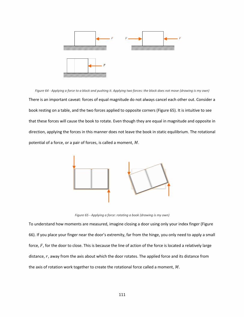
111
Figure 64 - Applying a force to a block and pushing it. Applying two forces: the block does not move (drawing is my own)
There is an important caveat: forces of equal magnitude do not always cancel each other out. Consider a
book resting on a table, and the two forces applied to opposite corners (Figure 65). It is intuitive to see
that these forces will cause the book to rotate. Even though they are equal in magnitude and opposite in
direction, applying the forces in this manner does not leave the book in static equilibrium. The rotational
potential of a force, or a pair of forces, is called a moment, .
Figure 65 - Applying a force: rotating a book (drawing is my own)
To understand how moments are measured, imagine closing a door using only your index finger (Figure
66). If you place your finger near the door’s extremity, far from the hinge, you only need to apply a small
force, , for the door to close. This is because the line of action of the force is located a relatively large
distance, , away from the axis about which the door rotates. The applied force and its distance from
the axis of rotation work together to create the rotational force called a moment, .
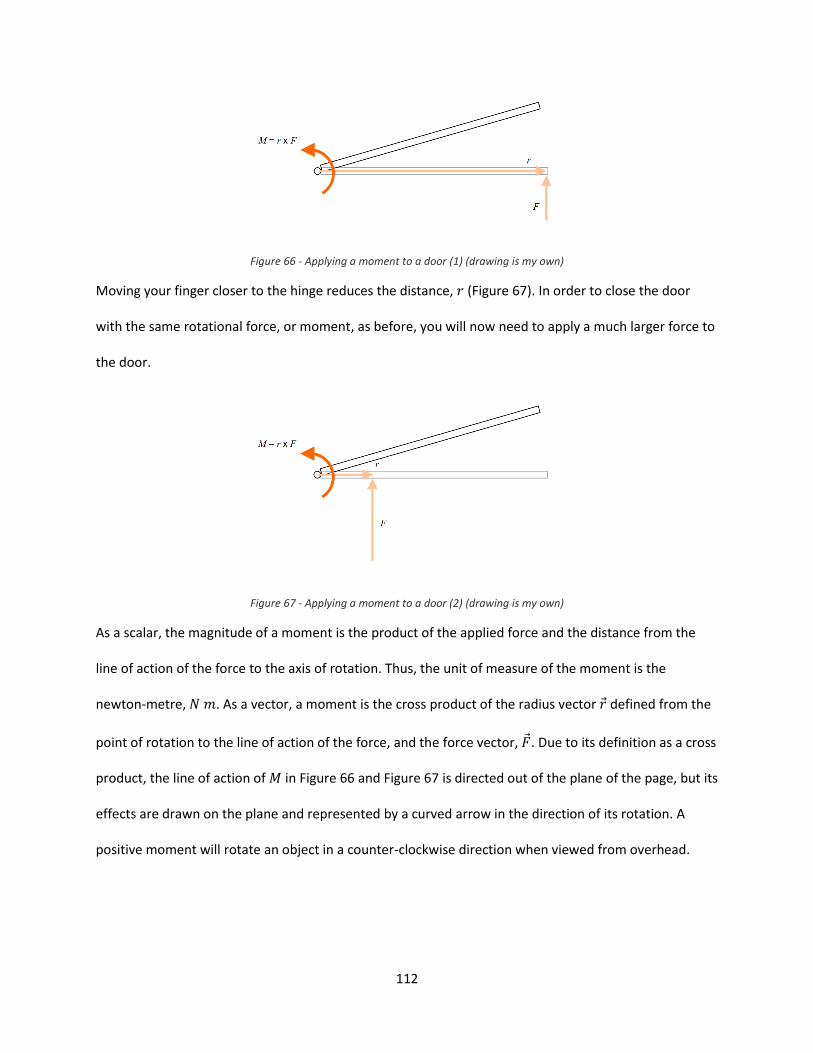
112
Figure 66 - Applying a moment to a door (1) (drawing is my own)
Moving your finger closer to the hinge reduces the distance, (Figure 67). In order to close the door
with the same rotational force, or moment, as before, you will now need to apply a much larger force to
the door.
Figure 67 - Applying a moment to a door (2) (drawing is my own)
As a scalar, the magnitude of a moment is the product of the applied force and the distance from the
line of action of the force to the axis of rotation. Thus, the unit of measure of the moment is the
newton-metre, . As a vector, a moment is the cross product of the radius vector ⃗ defined from the
point of rotation to the line of action of the force, and the force vector, ⃗. Due to its definition as a cross
product, the line of action of in Figure 66 and Figure 67 is directed out of the plane of the page, but its
effects are drawn on the plane and represented by a curved arrow in the direction of its rotation. A
positive moment will rotate an object in a counter-clockwise direction when viewed from overhead.
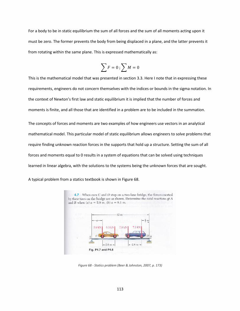
113
For a body to be in static equilibrium the sum of all forces and the sum of all moments acting upon it
must be zero. The former prevents the body from being displaced in a plane, and the latter prevents it
from rotating within the same plane. This is expressed mathematically as:
∑ ∑
This is the mathematical model that was presented in section 3.3. Here I note that in expressing these
requirements, engineers do not concern themselves with the indices or bounds in the sigma notation. In
the context of Newton’s first law and static equilibrium it is implied that the number of forces and
moments is finite, and all those that are identified in a problem are to be included in the summation.
The concepts of forces and moments are two examples of how engineers use vectors in an analytical
mathematical model. This particular model of static equilibrium allows engineers to solve problems that
require finding unknown reaction forces in the supports that hold up a structure. Setting the sum of all
forces and moments equal to 0 results in a system of equations that can be solved using techniques
learned in linear algebra, with the solutions to the systems being the unknown forces that are sought.
A typical problem from a statics textbook is shown in Figure 68.
Figure 68 - Statics problem (Beer & Johnston, 2007, p. 173)
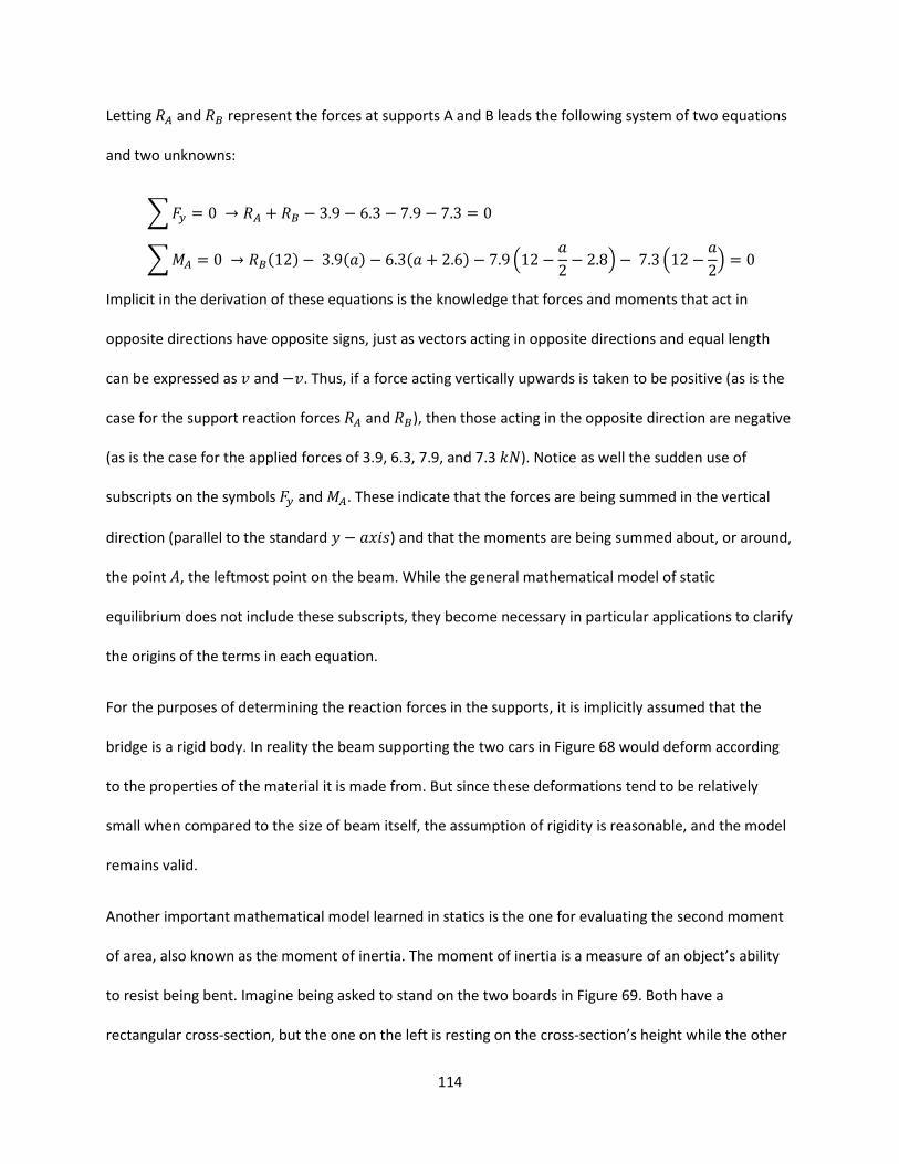
114
Letting and represent the forces at supports A and B leads the following system of two equations
and two unknowns:
∑
∑ (
) (
)
Implicit in the derivation of these equations is the knowledge that forces and moments that act in
opposite directions have opposite signs, just as vectors acting in opposite directions and equal length
can be expressed as and . Thus, if a force acting vertically upwards is taken to be positive (as is the
case for the support reaction forces and ), then those acting in the opposite direction are negative
(as is the case for the applied forces of 3.9, 6.3, 7.9, and 7.3 ). Notice as well the sudden use of
subscripts on the symbols and . These indicate that the forces are being summed in the vertical
direction (parallel to the standard ) and that the moments are being summed about, or around,
the point , the leftmost point on the beam. While the general mathematical model of static
equilibrium does not include these subscripts, they become necessary in particular applications to clarify
the origins of the terms in each equation.
For the purposes of determining the reaction forces in the supports, it is implicitly assumed that the
bridge is a rigid body. In reality the beam supporting the two cars in Figure 68 would deform according
to the properties of the material it is made from. But since these deformations tend to be relatively
small when compared to the size of beam itself, the assumption of rigidity is reasonable, and the model
remains valid.
Another important mathematical model learned in statics is the one for evaluating the second moment
of area, also known as the moment of inertia. The moment of inertia is a measure of an object’s ability
to resist being bent. Imagine being asked to stand on the two boards in Figure 69. Both have a
rectangular cross-section, but the one on the left is resting on the cross-section’s height while the other
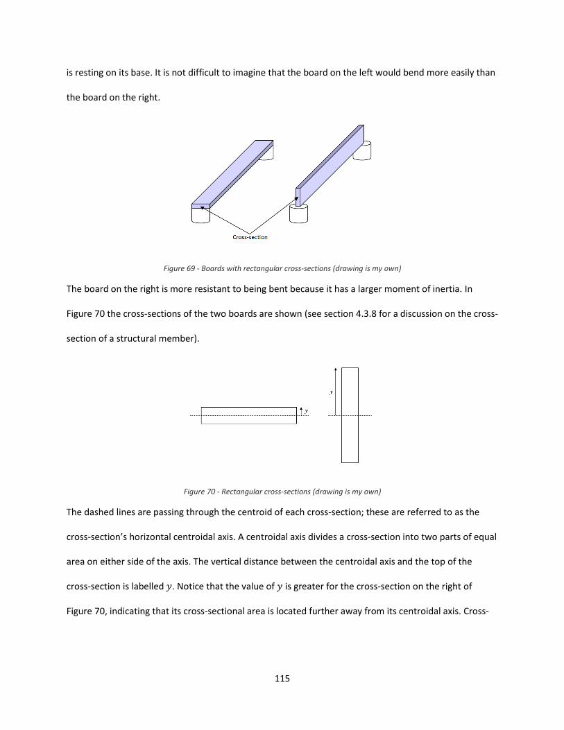
115
is resting on its base. It is not difficult to imagine that the board on the left would bend more easily than
the board on the right.
Figure 69 - Boards with rectangular cross-sections (drawing is my own)
The board on the right is more resistant to being bent because it has a larger moment of inertia. In
Figure 70 the cross-sections of the two boards are shown (see section 4.3.8 for a discussion on the cross-
section of a structural member).
Figure 70 - Rectangular cross-sections (drawing is my own)
The dashed lines are passing through the centroid of each cross-section; these are referred to as the
cross-section’s horizontal centroidal axis. A centroidal axis divides a cross-section into two parts of equal
area on either side of the axis. The vertical distance between the centroidal axis and the top of the
cross-section is labelled . Notice that the value of is greater for the cross-section on the right of
Figure 70, indicating that its cross-sectional area is located further away from its centroidal axis. Cross-
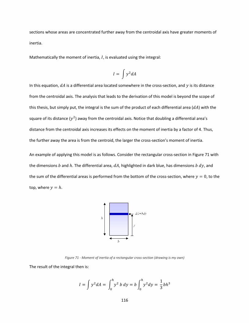
116
sections whose areas are concentrated further away from the centroidal axis have greater moments of
inertia.
Mathematically the moment of inertia, , is evaluated using the integral:
∫
In this equation, is a differential area located somewhere in the cross-section, and is its distance
from the centroidal axis. The analysis that leads to the derivation of this model is beyond the scope of
this thesis, but simply put, the integral is the sum of the product of each differential area ( ) with the
square of its distance ( ) away from the centroidal axis. Notice that doubling a differential area’s
distance from the centroidal axis increases its effects on the moment of inertia by a factor of 4. Thus,
the further away the area is from the centroid, the larger the cross-section’s moment of inertia.
An example of applying this model is as follows. Consider the rectangular cross-section in Figure 71 with
the dimensions and . The differential area, , highlighted in dark blue, has dimensions , and
the sum of the differential areas is performed from the bottom of the cross-section, where , to the
top, where .
Figure 71 - Moment of inertia of a rectangular cross-section (drawing is my own)
The result of the integral then is:
∫ ∫
∫
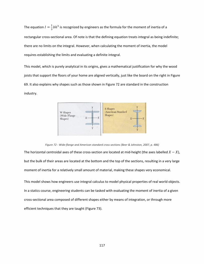
117
The equation
is recognized by engineers as the formula for the moment of inertia of a
rectangular cross-sectional area. Of note is that the defining equation treats integral as being indefinite;
there are no limits on the integral. However, when calculating the moment of inertia, the model
requires establishing the limits and evaluating a definite integral.
This model, which is purely analytical in its origins, gives a mathematical justification for why the wood
joists that support the floors of your home are aligned vertically, just like the board on the right in Figure
69. It also explains why shapes such as those shown in Figure 72 are standard in the construction
industry.
Figure 72 - Wide-flange and American standard cross sections (Beer & Johnston, 2007, p. 486)
The horizontal centroidal axes of these cross-section are located at mid-height (the axes labelled ),
but the bulk of their areas are located at the bottom and the top of the sections, resulting in a very large
moment of inertia for a relatively small amount of material, making these shapes very economical.
This model shows how engineers use integral calculus to model physical properties of real world objects.
In a statics course, engineering students can be tasked with evaluating the moment of inertia of a given
cross-sectional area composed of different shapes either by means of integration, or through more
efficient techniques that they are taught (Figure 73).

118
Figure 73 - Statics textbook problems: finding the moment of inertia of geometric shapes (Beer & Johnston, 2007, p. 493)
Solving such tasks is simplified by using formulas for the moment of inertia of standard geometric
shapes such as rectangles, triangles, and circles (Figure 74).
Figure 74 - Moments of inertia of common geometric shapes (adapted from (Beer & Johnston, 2007, p. inside back cover))
However, once one becomes a practicing engineer, even these tasks no longer become necessary since
the moments of inertia of standard cross-sections have already been evaluated and the values compiled
in tables found in design manuals. The table in Figure 75 is taken from the Handbook of Steel
Construction (2000) and includes various geometric properties for different wide-flange shapes,
standard in the design and construction of steel structures.
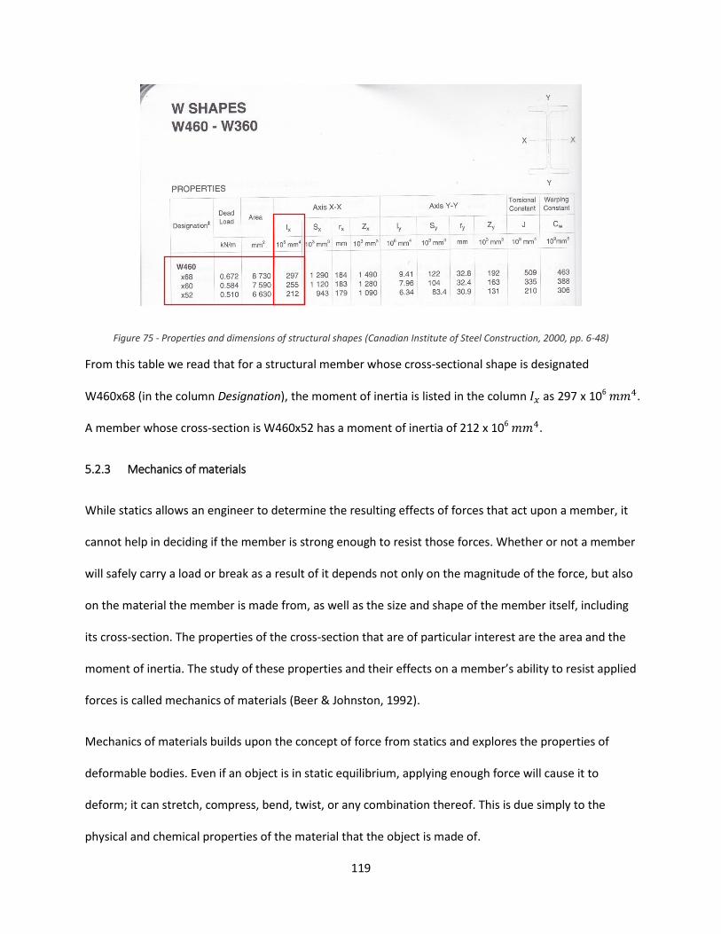
119
Figure 75 - Properties and dimensions of structural shapes (Canadian Institute of Steel Construction, 2000, pp. 6-48)
From this table we read that for a structural member whose cross-sectional shape is designated
W460x68 (in the column Designation), the moment of inertia is listed in the column as 297 x 106 .
A member whose cross-section is W460x52 has a moment of inertia of 212 x 106 .
5.2.3 Mechanics of materials
While statics allows an engineer to determine the resulting effects of forces that act upon a member, it
cannot help in deciding if the member is strong enough to resist those forces. Whether or not a member
will safely carry a load or break as a result of it depends not only on the magnitude of the force, but also
on the material the member is made from, as well as the size and shape of the member itself, including
its cross-section. The properties of the cross-section that are of particular interest are the area and the
moment of inertia. The study of these properties and their effects on a member’s ability to resist applied
forces is called mechanics of materials (Beer & Johnston, 1992).
Mechanics of materials builds upon the concept of force from statics and explores the properties of
deformable bodies. Even if an object is in static equilibrium, applying enough force will cause it to
deform; it can stretch, compress, bend, twist, or any combination thereof. This is due simply to the
physical and chemical properties of the material that the object is made of.
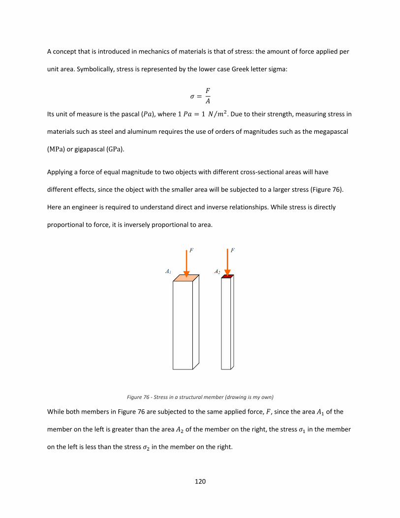
120
A concept that is introduced in mechanics of materials is that of stress: the amount of force applied per
unit area. Symbolically, stress is represented by the lower case Greek letter sigma:
Its unit of measure is the pascal ( ), where ⁄ . Due to their strength, measuring stress in
materials such as steel and aluminum requires the use of orders of magnitudes such as the megapascal
( ) or gigapascal ( ).
Applying a force of equal magnitude to two objects with different cross-sectional areas will have
different effects, since the object with the smaller area will be subjected to a larger stress (Figure 76).
Here an engineer is required to understand direct and inverse relationships. While stress is directly
proportional to force, it is inversely proportional to area.
Figure 76 - Stress in a structural member (drawing is my own)
While both members in Figure 76 are subjected to the same applied force, , since the area of the
member on the left is greater than the area of the member on the right, the stress in the member
on the left is less than the stress in the member on the right.
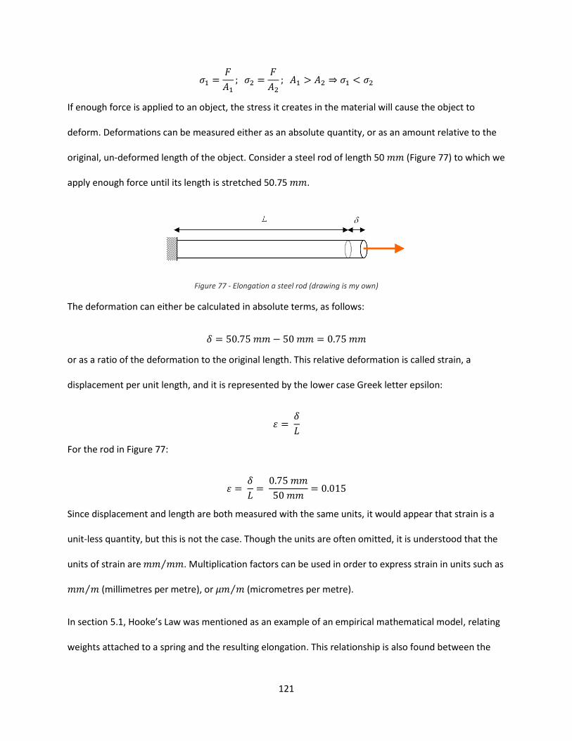
121
If enough force is applied to an object, the stress it creates in the material will cause the object to
deform. Deformations can be measured either as an absolute quantity, or as an amount relative to the
original, un-deformed length of the object. Consider a steel rod of length 50 (Figure 77) to which we
apply enough force until its length is stretched 50.75 .
Figure 77 - Elongation a steel rod (drawing is my own)
The deformation can either be calculated in absolute terms, as follows:
or as a ratio of the deformation to the original length. This relative deformation is called strain, a
displacement per unit length, and it is represented by the lower case Greek letter epsilon:
For the rod in Figure 77:
Since displacement and length are both measured with the same units, it would appear that strain is a
unit-less quantity, but this is not the case. Though the units are often omitted, it is understood that the
units of strain are ⁄ . Multiplication factors can be used in order to express strain in units such as
⁄ (millimetres per metre), or ⁄ (micrometres per metre).
In section 5.1, Hooke’s Law was mentioned as an example of an empirical mathematical model, relating
weights attached to a spring and the resulting elongation. This relationship is also found between the
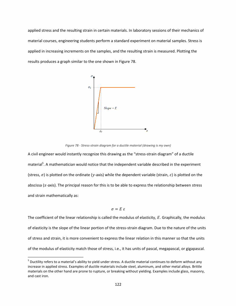
122
applied stress and the resulting strain in certain materials. In laboratory sessions of their mechanics of
material courses, engineering students perform a standard experiment on material samples. Stress is
applied in increasing increments on the samples, and the resulting strain is measured. Plotting the
results produces a graph similar to the one shown in Figure 78.
Figure 78 - Stress-strain diagram for a ductile material (drawing is my own)
A civil engineer would instantly recognize this drawing as the “stress-strain diagram” of a ductile
material5. A mathematician would notice that the independent variable described in the experiment
(stress, ) is plotted on the ordinate ( -axis) while the dependent variable (strain, ) is plotted on the
abscissa ( -axis). The principal reason for this is to be able to express the relationship between stress
and strain mathematically as:
The coefficient of the linear relationship is called the modulus of elasticity, . Graphically, the modulus
of elasticity is the slope of the linear portion of the stress-strain diagram. Due to the nature of the units
of stress and strain, it is more convenient to express the linear relation in this manner so that the units
of the modulus of elasticity match those of stress, i.e., it has units of pascal, megapascal, or gigapascal.
5 Ductility refers to a material’s ability to yield under stress. A ductile material continues to deform without any
increase in applied stress. Examples of ductile materials include steel, aluminum, and other metal alloys. Brittle materials on the other hand are prone to rupture, or breaking without yielding. Examples include glass, masonry, and cast iron.
123
The values and indicated on the axes in Figure 78 are referred to as the yield stress and yield strain
of the material. If the applied stress remains below the value , then the linear relation holds true, and
the material is said to be elastic. Much like how a rubber band returns to its original shape after being
stretched, the strain in elastic materials is eliminated once the applied stress is removed. Applying
stresses greater than causes excessive and permanent deformations in the material. At this point the
material is said to become plastic. This is represented by the horizontal portion of the stress-strain
diagram, indicating that strain, and therefore deformation, can increase without any corresponding
increase in applied stress.
In general, an engineer seeks to design a structure so that the stresses in its structural members remain
below the yield stress of the material they are made from. If this is achieved, then the members will not
rupture. It is also important that the resulting deformations do not exceed the yield strain, as excessive
deformations in a structure are unfavourable as well. Recall that the principle of static equilibrium
depends on the assumption that the deformations of bodies are negligible. If this assumption is violated
then a mathematical model at the heart of structural analysis becomes invalidated.
The modulus of elasticity appears in nearly every mathematical model that is used in structural analysis.
The proper choice of material is vital to a structure’s ability to resist the loads that are applied to it. And
yet, the mathematics behind its development is remarkably simple: ratios of forces to areas (stress),
deformations to lengths (strain), and the linear relationship found through empirical tests. It is the use
of mathematics to describe these concepts that allows material properties such as elasticity to be
understood.
The linear equation relating stress and strain via the modulus of elasticity is an empirical model that can
be used for introductory application problems in mechanics of materials. But more advanced
mathematics is required in order to develop concepts that are needed in structural analysis. Differential

124
equations are used, for example, in a model for determining the maximum amount that a beam will
deform when it is bent under an applied load (Beer & Johnston, 1992). A beam is a horizontal structural
member, and its deformed shape is referred to as its elastic curve. While the details of its development
are beyond the scope of this thesis, the following differential equation is used to relate the second
derivative of the elastic curve to the bending moment (the bending force) in the beam, as well as the
beam’s modulus of elasticity and moment of inertia:
The function whose second derivative is shown is the equation of the beam’s elastic curve, with
representing the vertical distance that the beam is bent, and the horizontal position along the length
of the beam. Note that the symbols and are used to represent physical distances in the horizontal
and vertical directions, and are not simply arbitrary variables. is the magnitude of the bending
moment at a position along the length of the beam. Depending on what external forces are being
applied to the beam, the bending moment at any position, , along the length of the beam will vary.
and are, respectively, the modulus of elasticity of the material the beam is made of and the moment of
inertia of the beam’s cross-section. The product is called the flexural rigidity of a member’s cross-
section.
Deriving this differential equation requires analyzing the curvature of the elastic curve . In the
analysis, the assumption is made that ⁄ , the slope of the elastic curve, is very small compared to
unity. As such, the actual differential equation:
[ (
)
]
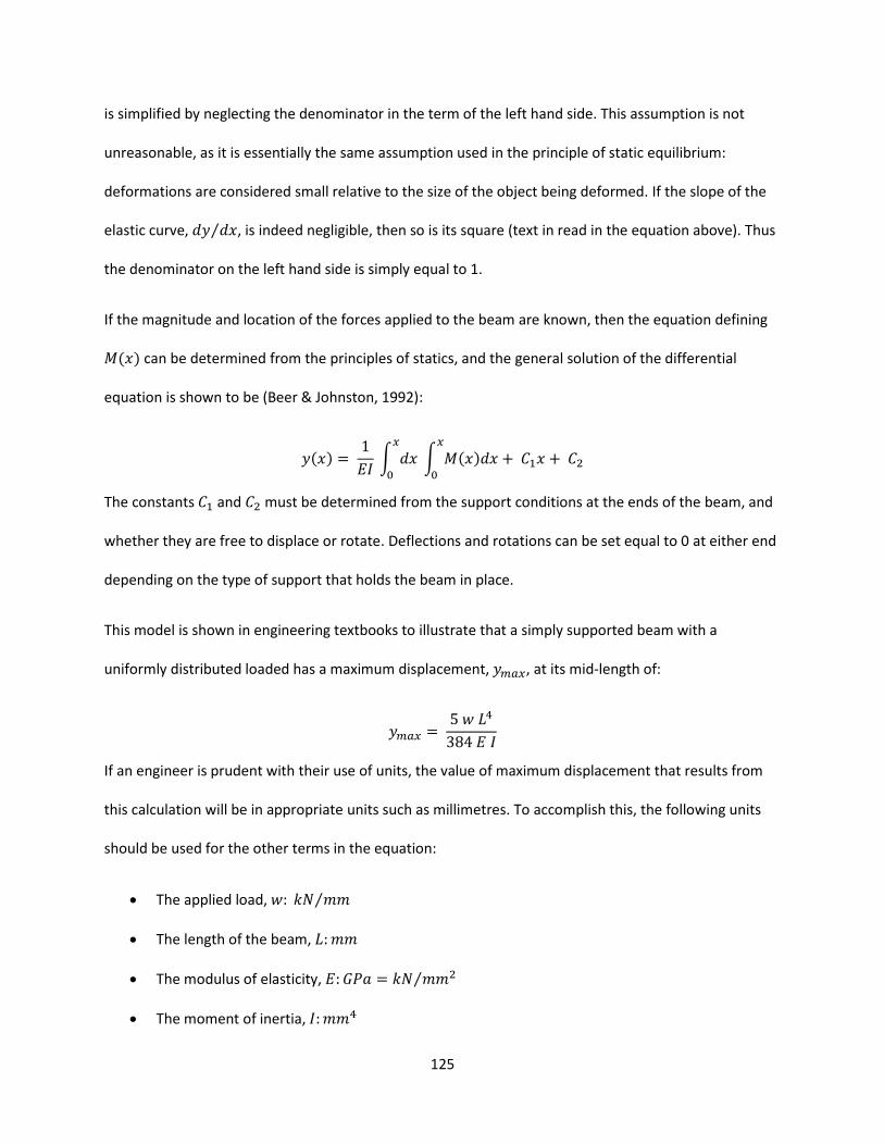
125
is simplified by neglecting the denominator in the term of the left hand side. This assumption is not
unreasonable, as it is essentially the same assumption used in the principle of static equilibrium:
deformations are considered small relative to the size of the object being deformed. If the slope of the
elastic curve, ⁄ , is indeed negligible, then so is its square (text in read in the equation above). Thus
the denominator on the left hand side is simply equal to 1.
If the magnitude and location of the forces applied to the beam are known, then the equation defining
can be determined from the principles of statics, and the general solution of the differential
equation is shown to be (Beer & Johnston, 1992):
∫
∫
The constants and must be determined from the support conditions at the ends of the beam, and
whether they are free to displace or rotate. Deflections and rotations can be set equal to 0 at either end
depending on the type of support that holds the beam in place.
This model is shown in engineering textbooks to illustrate that a simply supported beam with a
uniformly distributed loaded has a maximum displacement, , at its mid-length of:
If an engineer is prudent with their use of units, the value of maximum displacement that results from
this calculation will be in appropriate units such as millimetres. To accomplish this, the following units
should be used for the other terms in the equation:
The applied load, ⁄
The length of the beam,
The modulus of elasticity, ⁄
The moment of inertia,
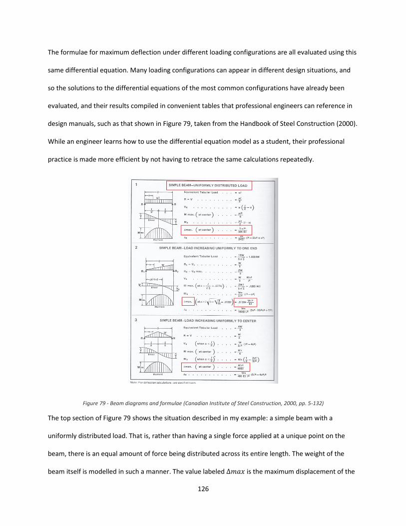
126
The formulae for maximum deflection under different loading configurations are all evaluated using this
same differential equation. Many loading configurations can appear in different design situations, and
so the solutions to the differential equations of the most common configurations have already been
evaluated, and their results compiled in convenient tables that professional engineers can reference in
design manuals, such as that shown in Figure 79, taken from the Handbook of Steel Construction (2000).
While an engineer learns how to use the differential equation model as a student, their professional
practice is made more efficient by not having to retrace the same calculations repeatedly.
Figure 79 - Beam diagrams and formulae (Canadian Institute of Steel Construction, 2000, pp. 5-132)
The top section of Figure 79 shows the situation described in my example: a simple beam with a
uniformly distributed load. That is, rather than having a single force applied at a unique point on the
beam, there is an equal amount of force being distributed across its entire length. The weight of the
beam itself is modelled in such a manner. The value labeled is the maximum displacement of the
127
beam under the described loading condition. The bottom section of the figure shows that a simple beam,
with a distributed load that increases uniformly from 0 at either end to some amount at its centre,
will experience a maximum deformation of:
Models such as these are essential in performing structural analysis, discussed in the next section.
5.2.4 Structural analysis
The goal of structural analysis is to predict the performance of a structure under prescribed forces, or
loads. Loads can come from a variety of sources including the weight of the structure itself, from the use
of the structure’s occupants, and from other external effects such as wind, snow, earthquakes, and
temperature changes. The performance characteristics that a structural engineer is interested in
determining are the stresses in the structural members, the deflections or deformations of the structure,
and the magnitude of the reaction forces in the structure’s supports.
Structural analysis is one phase in the iterative process of structural design. The analysis phase allows
the engineer to verify whether a design meets the criteria for safety (resistance to loads) and
serviceability (limited deformation). If either of these criteria isn’t met, the design is revised, and the
analysis is performed anew.
A crucial step prior to the analysis is estimating the loads, or forces, that will act upon the structure. The
National Building Code of Canada (NBCC) is the model code6 upon which provincial jurisdictions base
their own design and construction codes. Part 4 of the NBCC states that structural design be performed
6 The word “model” in this case does not refer to a mathematical model, but is used in the sense of a guide. The
various provincial building codes are written using the National Building Code of Canada as a model for their content.
128
using a method called limit states design. In limit states design, the factored resistance of a structure
must be greater than the factored effect of the loads applied to the structure. This is expressed as:
and alternatively as:
This inequality features prominently in design and analysis calculations performed by practicing
engineers. Examples of its use will be shown in section 5.4.
The key to understanding limit states design lies in the use of the word “factored.” In brief, the design
process will over-estimate the magnitude of applied loads and under-estimate the strength of the
structural members. This provides a margin of safety in the design of the structure. As the name implies,
the process involves multiplying the values of calculated loads and resistances by factors. The terms
“factored resistance” and “factored loads” can each be written symbolically as (Canadian Institute of
Steel Construction, 2000):
On the left hand side of the inequality, is the resistance of a structural member. It is evaluated using
models developed in mechanics of materials and in specialized courses on the design of structures. For
the terms on the right-hand side of the inequality, the NBCC includes formulae and tables that are to be
used to estimate the various loads that a structure must resist. Included among these are (National
Research Council of Canada, 2010):
Dead loads ( ): the weight of the structure itself and all of the materials used in its construction
Live loads ( ): the load on an area of floor or roof depending on the intended use and
occupancy; loads due to ice, snow, and rain are also considered live loads
Wind loads ( ): the load caused by wind blowing on the structure
129
Loads induced the structure by changes in temperature ( )
The various coefficients are load factors, while and are the importance factor and the load
combination factor, respectively. These factors have the effect of amplifying the prescribed loads that
are applied to the structure in the analysis. The values assigned to them are chosen from pre-
determined load combinations that are prescribed either by the NBCC, or the appropriate design manual.
For example, in the Handbook of Steel Construction, clause 7.2.3 of the Limit States Design of Steel
Structures states that the load factors are to taken as:
Thus, the loads are automatically increased by either 25%, or up to 50% of those suggested by the NBCC.
The value of , however, may be less than 1. This would appear to have the effect of reducing the
estimated load, but this is actually not the case. In the Handbook of Steel Construction, the value of is
taken to be 1.00 when the structure is analyzed under the effects of only one of the loads , , and ,
but it can be taken to be 0.70 when the effects two of , , and are analyzed. In other words, when
analyzing the structure’s performance against only live loads, , 100% of the factored loads must be
applied to the structure in the analysis. But, when analyzing its performance against live loads, , and
wind loads, , only 70% of the factored loads need to be applied in the analysis. The underlying reason
for this is due to statistical analysis. The load estimates for and provided by the NBCC are the
maximum loads that the structure could expect to encounter in its life. The probability that the structure
will have to resist the maximum values of and simultaneously is small; hence the estimated
130
factored loads can be reduced. This is an example of how statistics are intrinsic to some empirical
mathematical models used in the engineer’s design process.
Engineers have several techniques available to accomplish the task of structural analysis. Since the
advent of computer programming, techniques involving linear algebra and matrices have become
prevalent. Such techniques are collectively referred to as matrix structural analysis. The most widely
used analysis technique, called the direct stiffness method, is described in some detail in the following
section since it can illustrate some different perceptions that engineers and mathematicians have of
matrices as mathematical objects.
5.3 MATRIX STRUCTURAL ANALYSIS
In the previous sections I described the fundamental principles of structural engineering and how
engineers use the mathematics they learn to create mathematical models that represent various
physical concepts such as forces, stress and strain, the modulus of elasticity, and the moment of inertia.
These principles gave way to a brief introduction to structural analysis and its goal of predicting the
performance of a structure under the effects of applied loads. The purpose of these sections was also to
lay the groundwork for the text that follows, which explains how matrix structural analysis is used as a
technique to accomplish the task of predicting structural performance.
In preparation for my research for this thesis, a discussion about linear algebra and its practical uses
prompted the following question: do matrix properties such as eigenvectors have any physical meaning
to a structural engineer? The answer, as I will show, is yes, they do. After presenting the details of matrix
structural analysis, I will discuss the physical representations of eigenvectors in this context. However, it
will then be shown that, for a structural engineer, an eigenvector’s physical representation holds no
interest in the task of structure analysis, specifically because of what they represent. This is not to
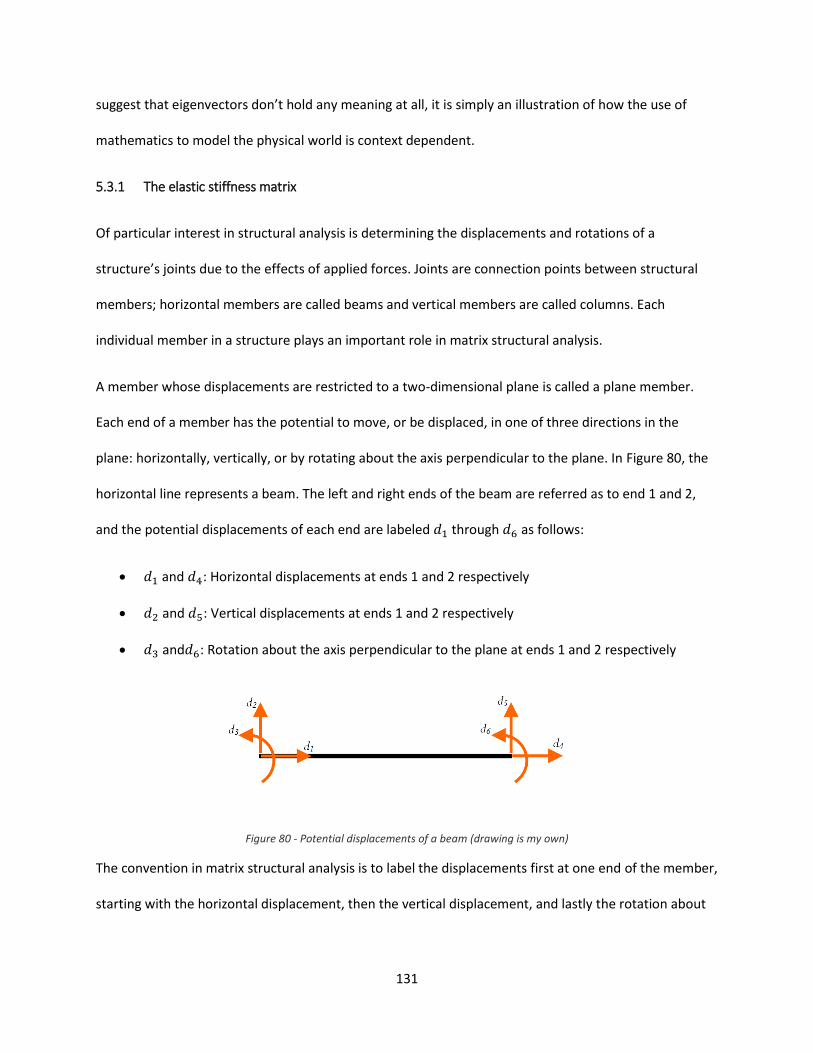
131
suggest that eigenvectors don’t hold any meaning at all, it is simply an illustration of how the use of
mathematics to model the physical world is context dependent.
5.3.1 The elastic stiffness matrix
Of particular interest in structural analysis is determining the displacements and rotations of a
structure’s joints due to the effects of applied forces. Joints are connection points between structural
members; horizontal members are called beams and vertical members are called columns. Each
individual member in a structure plays an important role in matrix structural analysis.
A member whose displacements are restricted to a two-dimensional plane is called a plane member.
Each end of a member has the potential to move, or be displaced, in one of three directions in the
plane: horizontally, vertically, or by rotating about the axis perpendicular to the plane. In Figure 80, the
horizontal line represents a beam. The left and right ends of the beam are referred as to end 1 and 2,
and the potential displacements of each end are labeled through as follows:
and : Horizontal displacements at ends 1 and 2 respectively
and : Vertical displacements at ends 1 and 2 respectively
and : Rotation about the axis perpendicular to the plane at ends 1 and 2 respectively
Figure 80 - Potential displacements of a beam (drawing is my own)
The convention in matrix structural analysis is to label the displacements first at one end of the member,
starting with the horizontal displacement, then the vertical displacement, and lastly the rotation about
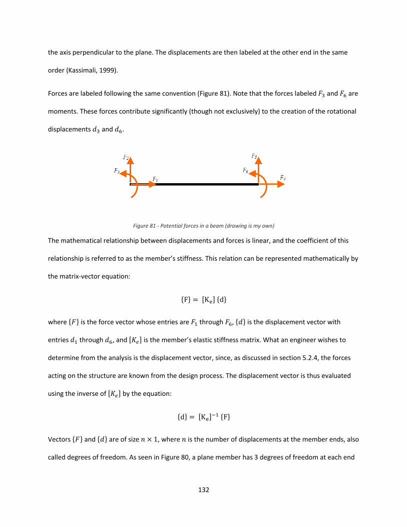
132
the axis perpendicular to the plane. The displacements are then labeled at the other end in the same
order (Kassimali, 1999).
Forces are labeled following the same convention (Figure 81). Note that the forces labeled and are
moments. These forces contribute significantly (though not exclusively) to the creation of the rotational
displacements and .
Figure 81 - Potential forces in a beam (drawing is my own)
The mathematical relationship between displacements and forces is linear, and the coefficient of this
relationship is referred to as the member’s stiffness. This relation can be represented mathematically by
the matrix-vector equation:
{ } [ ] { }
where { } is the force vector whose entries are through , { } is the displacement vector with
entries through , and [ ] is the member’s elastic stiffness matrix. What an engineer wishes to
determine from the analysis is the displacement vector, since, as discussed in section 5.2.4, the forces
acting on the structure are known from the design process. The displacement vector is thus evaluated
using the inverse of [ ] by the equation:
{ } [ ] { }
Vectors { } and { } are of size , where is the number of displacements at the member ends, also
called degrees of freedom. As seen in Figure 80, a plane member has 3 degrees of freedom at each end
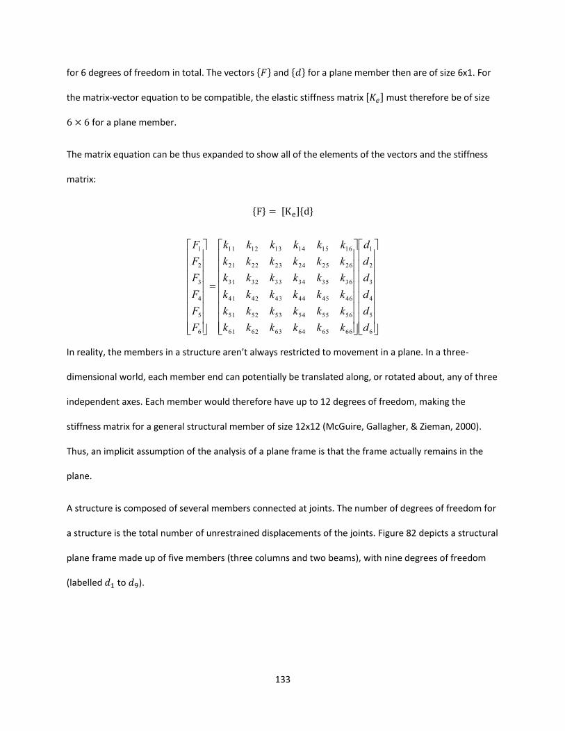
133
for 6 degrees of freedom in total. The vectors { } and { } for a plane member then are of size 6x1. For
the matrix-vector equation to be compatible, the elastic stiffness matrix [ ] must therefore be of size
for a plane member.
The matrix equation can be thus expanded to show all of the elements of the vectors and the stiffness
matrix:
{ } [ ]{ }
6
5
4
3
2
1
666564636261
565554535251
464544434241
363534333231
262524232221
161514131211
6
5
4
3
2
1
d
d
d
d
d
d
kkkkkk
kkkkkk
kkkkkk
kkkkkk
kkkkkk
kkkkkk
F
F
F
F
F
F
In reality, the members in a structure aren’t always restricted to movement in a plane. In a three-
dimensional world, each member end can potentially be translated along, or rotated about, any of three
independent axes. Each member would therefore have up to 12 degrees of freedom, making the
stiffness matrix for a general structural member of size 12x12 (McGuire, Gallagher, & Zieman, 2000).
Thus, an implicit assumption of the analysis of a plane frame is that the frame actually remains in the
plane.
A structure is composed of several members connected at joints. The number of degrees of freedom for
a structure is the total number of unrestrained displacements of the joints. Figure 82 depicts a structural
plane frame made up of five members (three columns and two beams), with nine degrees of freedom
(labelled to ).
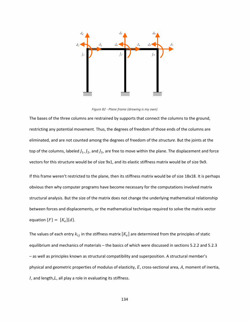
134
Figure 82 - Plane frame (drawing is my own)
The bases of the three columns are restrained by supports that connect the columns to the ground,
restricting any potential movement. Thus, the degrees of freedom of those ends of the columns are
eliminated, and are not counted among the degrees of freedom of the structure. But the joints at the
top of the columns, labeled , , and , are free to move within the plane. The displacement and force
vectors for this structure would be of size 9x1, and its elastic stiffness matrix would be of size 9x9.
If this frame weren’t restricted to the plane, then its stiffness matrix would be of size 18x18. It is perhaps
obvious then why computer programs have become necessary for the computations involved matrix
structural analysis. But the size of the matrix does not change the underlying mathematical relationship
between forces and displacements, or the mathematical technique required to solve the matrix vector
equation { } [ ]{ }.
The values of each entry in the stiffness matrix [ ] are determined from the principles of static
equilibrium and mechanics of materials – the basics of which were discussed in sections 5.2.2 and 5.2.3
– as well as principles known as structural compatibility and superposition. A structural member’s
physical and geometric properties of modulus of elasticity, , cross-sectional area, , moment of inertia,
, and length, , all play a role in evaluating its stiffness.
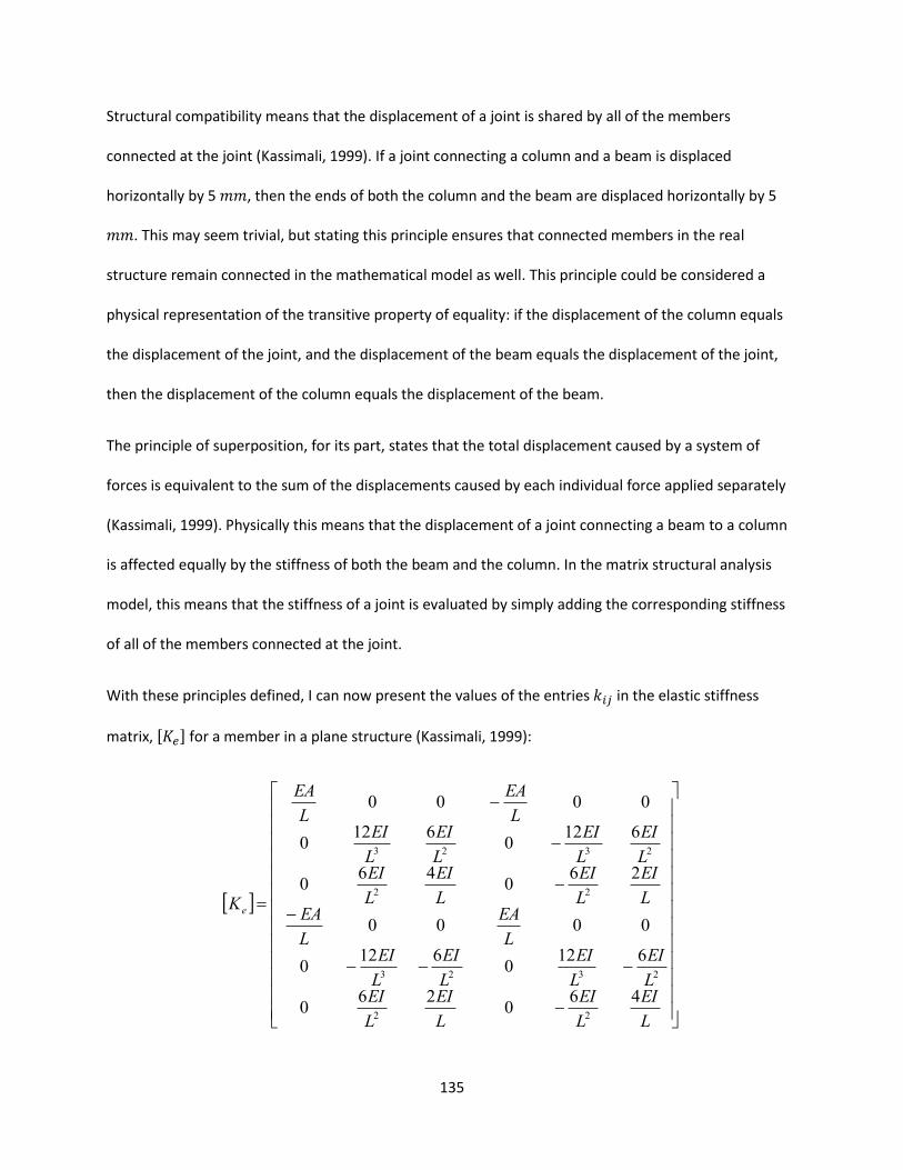
135
Structural compatibility means that the displacement of a joint is shared by all of the members
connected at the joint (Kassimali, 1999). If a joint connecting a column and a beam is displaced
horizontally by 5 , then the ends of both the column and the beam are displaced horizontally by 5
. This may seem trivial, but stating this principle ensures that connected members in the real
structure remain connected in the mathematical model as well. This principle could be considered a
physical representation of the transitive property of equality: if the displacement of the column equals
the displacement of the joint, and the displacement of the beam equals the displacement of the joint,
then the displacement of the column equals the displacement of the beam.
The principle of superposition, for its part, states that the total displacement caused by a system of
forces is equivalent to the sum of the displacements caused by each individual force applied separately
(Kassimali, 1999). Physically this means that the displacement of a joint connecting a beam to a column
is affected equally by the stiffness of both the beam and the column. In the matrix structural analysis
model, this means that the stiffness of a joint is evaluated by simply adding the corresponding stiffness
of all of the members connected at the joint.
With these principles defined, I can now present the values of the entries in the elastic stiffness
matrix, [ ] for a member in a plane structure (Kassimali, 1999):
L
EI
L
EI
L
EI
L
EIL
EI
L
EI
L
EI
L
EIL
EA
L
EAL
EI
L
EI
L
EI
L
EIL
EI
L
EI
L
EI
L
EIL
EA
L
EA
Ke
460
260
6120
6120
0000
260
460
6120
6120
0000
22
2323
22
2323
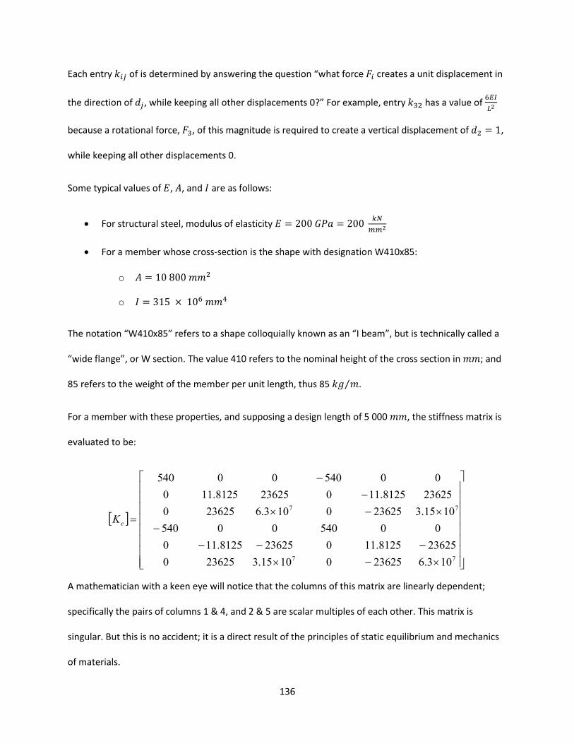
136
Each entry of is determined by answering the question “what force creates a unit displacement in
the direction of , while keeping all other displacements 0?” For example, entry has a value of
because a rotational force, , of this magnitude is required to create a vertical displacement of ,
while keeping all other displacements 0.
Some typical values of , , and are as follows:
For structural steel, modulus of elasticity
For a member whose cross-section is the shape with designation W410x85:
o
o
The notation “W410x85” refers to a shape colloquially known as an “I beam”, but is technically called a
“wide flange”, or W section. The value 410 refers to the nominal height of the cross section in ; and
85 refers to the weight of the member per unit length, thus 85 ⁄ .
For a member with these properties, and supposing a design length of 5 000 , the stiffness matrix is
evaluated to be:
77
77
103.62362501015.3236250
236258125.110236258125.110
0054000540
1015.3236250103.6236250
236258125.110236258125.110
0054000540
eK
A mathematician with a keen eye will notice that the columns of this matrix are linearly dependent;
specifically the pairs of columns 1 & 4, and 2 & 5 are scalar multiples of each other. This matrix is
singular. But this is no accident; it is a direct result of the principles of static equilibrium and mechanics
of materials.
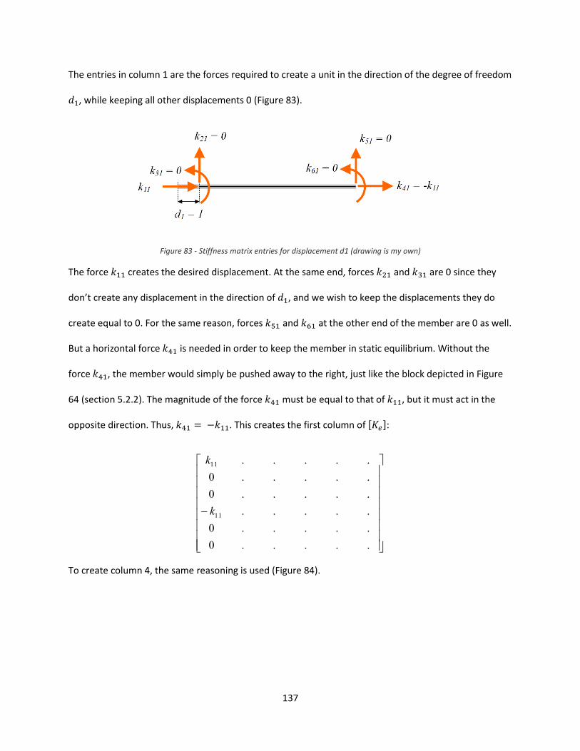
137
The entries in column 1 are the forces required to create a unit in the direction of the degree of freedom
, while keeping all other displacements 0 (Figure 83).
Figure 83 - Stiffness matrix entries for displacement d1 (drawing is my own)
The force creates the desired displacement. At the same end, forces and are 0 since they
don’t create any displacement in the direction of , and we wish to keep the displacements they do
create equal to 0. For the same reason, forces and at the other end of the member are 0 as well.
But a horizontal force is needed in order to keep the member in static equilibrium. Without the
force , the member would simply be pushed away to the right, just like the block depicted in Figure
64 (section 5.2.2). The magnitude of the force must be equal to that of , but it must act in the
opposite direction. Thus, . This creates the first column of [ ]:
.....0
.....0
.....
.....0
.....0
.....
11
11
k
k
To create column 4, the same reasoning is used (Figure 84).
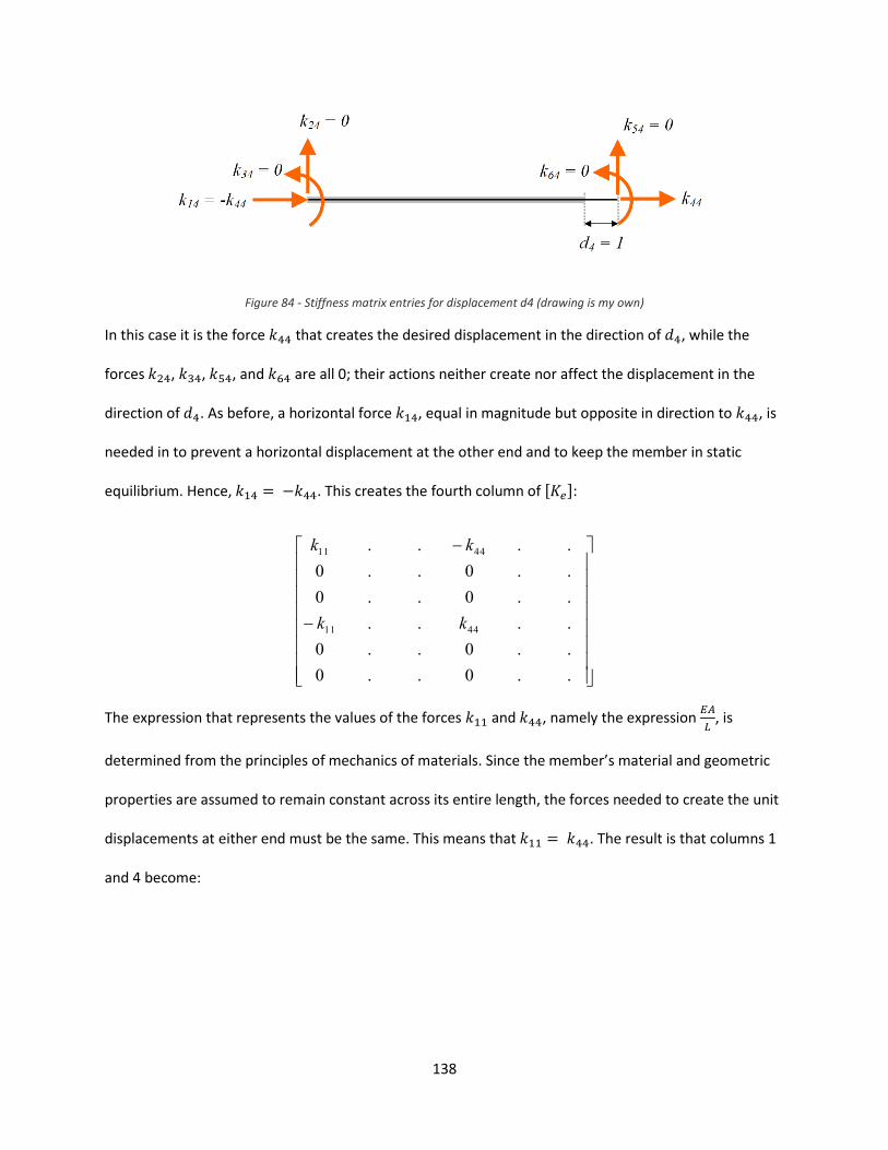
138
Figure 84 - Stiffness matrix entries for displacement d4 (drawing is my own)
In this case it is the force that creates the desired displacement in the direction of , while the
forces , , , and are all 0; their actions neither create nor affect the displacement in the
direction of . As before, a horizontal force , equal in magnitude but opposite in direction to , is
needed in to prevent a horizontal displacement at the other end and to keep the member in static
equilibrium. Hence, . This creates the fourth column of [ ]:
..0..0
..0..0
....
..0..0
..0..0
....
4411
4411
kk
kk
The expression that represents the values of the forces and , namely the expression
, is
determined from the principles of mechanics of materials. Since the member’s material and geometric
properties are assumed to remain constant across its entire length, the forces needed to create the unit
displacements at either end must be the same. This means that . The result is that columns 1
and 4 become:
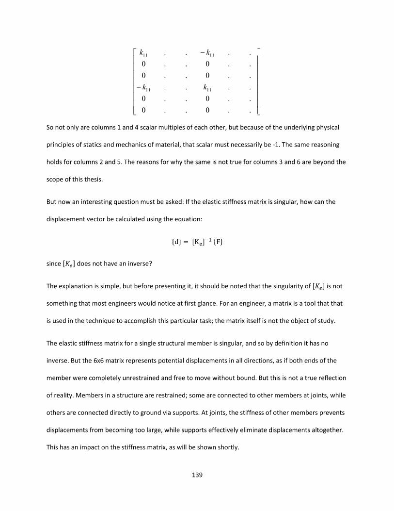
139
..0..0
..0..0
....
..0..0
..0..0
....
1111
1111
kk
kk
So not only are columns 1 and 4 scalar multiples of each other, but because of the underlying physical
principles of statics and mechanics of material, that scalar must necessarily be -1. The same reasoning
holds for columns 2 and 5. The reasons for why the same is not true for columns 3 and 6 are beyond the
scope of this thesis.
But now an interesting question must be asked: If the elastic stiffness matrix is singular, how can the
displacement vector be calculated using the equation:
{ } [ ] { }
since [ ] does not have an inverse?
The explanation is simple, but before presenting it, it should be noted that the singularity of [ ] is not
something that most engineers would notice at first glance. For an engineer, a matrix is a tool that that
is used in the technique to accomplish this particular task; the matrix itself is not the object of study.
The elastic stiffness matrix for a single structural member is singular, and so by definition it has no
inverse. But the 6x6 matrix represents potential displacements in all directions, as if both ends of the
member were completely unrestrained and free to move without bound. But this is not a true reflection
of reality. Members in a structure are restrained; some are connected to other members at joints, while
others are connected directly to ground via supports. At joints, the stiffness of other members prevents
displacements from becoming too large, while supports effectively eliminate displacements altogether.
This has an impact on the stiffness matrix, as will be shown shortly.
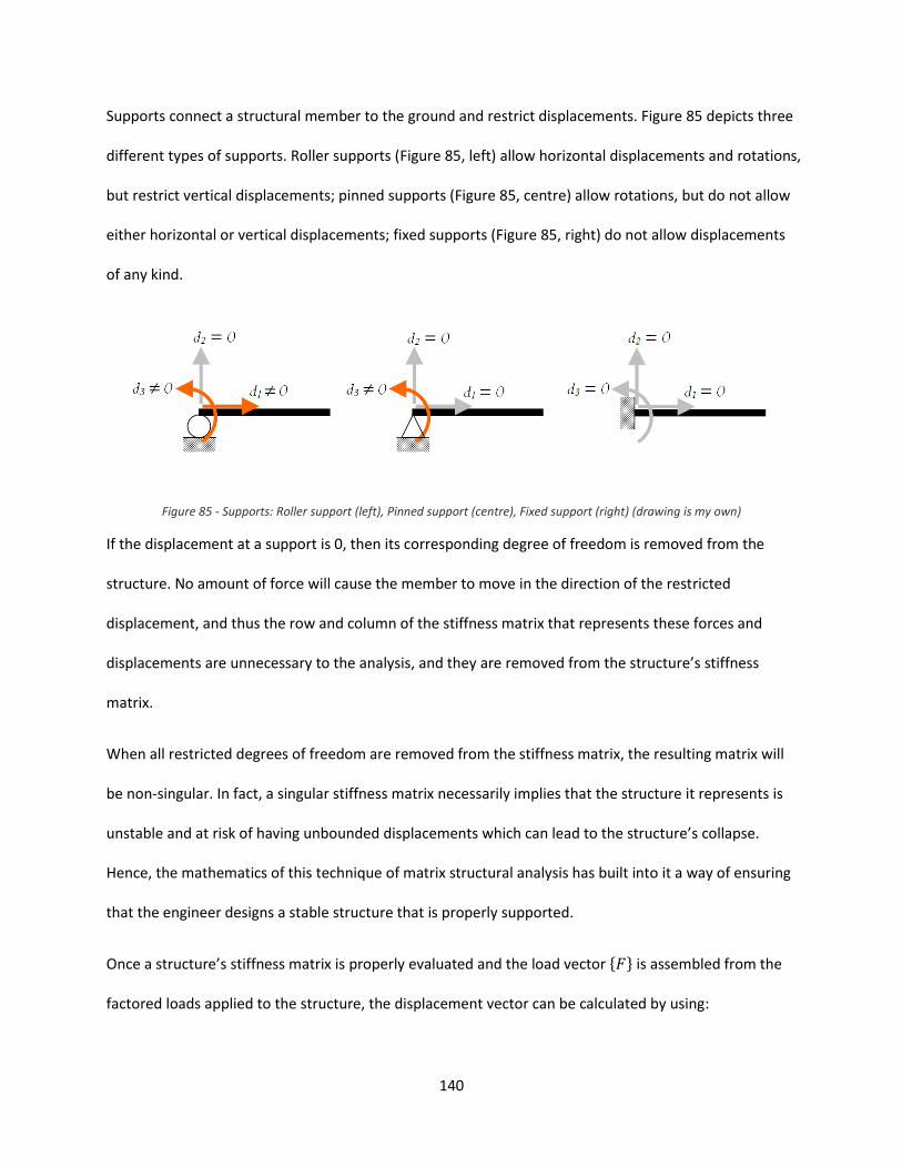
140
Supports connect a structural member to the ground and restrict displacements. Figure 85 depicts three
different types of supports. Roller supports (Figure 85, left) allow horizontal displacements and rotations,
but restrict vertical displacements; pinned supports (Figure 85, centre) allow rotations, but do not allow
either horizontal or vertical displacements; fixed supports (Figure 85, right) do not allow displacements
of any kind.
Figure 85 - Supports: Roller support (left), Pinned support (centre), Fixed support (right) (drawing is my own)
If the displacement at a support is 0, then its corresponding degree of freedom is removed from the
structure. No amount of force will cause the member to move in the direction of the restricted
displacement, and thus the row and column of the stiffness matrix that represents these forces and
displacements are unnecessary to the analysis, and they are removed from the structure’s stiffness
matrix.
When all restricted degrees of freedom are removed from the stiffness matrix, the resulting matrix will
be non-singular. In fact, a singular stiffness matrix necessarily implies that the structure it represents is
unstable and at risk of having unbounded displacements which can lead to the structure’s collapse.
Hence, the mathematics of this technique of matrix structural analysis has built into it a way of ensuring
that the engineer designs a stable structure that is properly supported.
Once a structure’s stiffness matrix is properly evaluated and the load vector { } is assembled from the
factored loads applied to the structure, the displacement vector can be calculated by using:
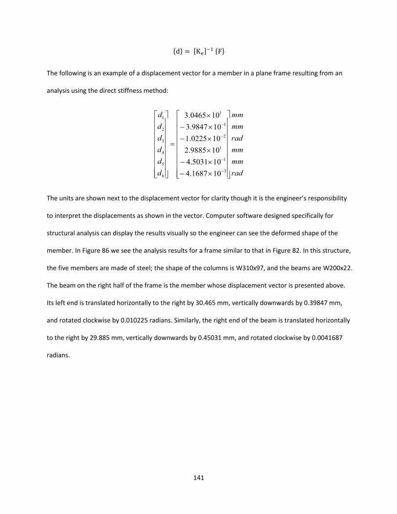
141
{ } [ ] { }
The following is an example of a displacement vector for a member in a plane frame resulting from an
analysis using the direct stiffness method:
rad
mm
mm
rad
mm
mm
d
d
d
d
d
d
3
1
1
2
1
1
6
5
4
3
2
1
101687.4
105031.4
109885.2
100225.1
109847.3
100465.3
The units are shown next to the displacement vector for clarity though it is the engineer’s responsibility
to interpret the displacements as shown in the vector. Computer software designed specifically for
structural analysis can display the results visually so the engineer can see the deformed shape of the
member. In Figure 86 we see the analysis results for a frame similar to that in Figure 82. In this structure,
the five members are made of steel; the shape of the columns is W310x97, and the beams are W200x22.
The beam on the right half of the frame is the member whose displacement vector is presented above.
Its left end is translated horizontally to the right by 30.465 mm, vertically downwards by 0.39847 mm,
and rotated clockwise by 0.010225 radians. Similarly, the right end of the beam is translated horizontally
to the right by 29.885 mm, vertically downwards by 0.45031 mm, and rotated clockwise by 0.0041687
radians.
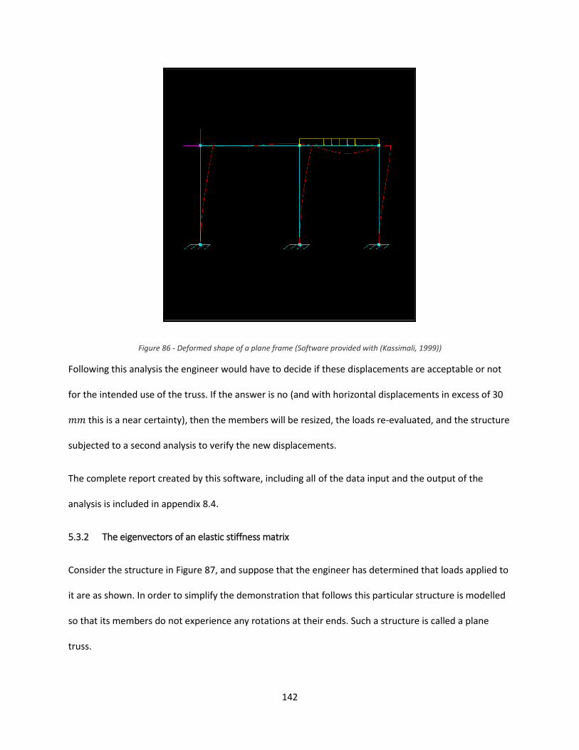
142
Figure 86 - Deformed shape of a plane frame (Software provided with (Kassimali, 1999))
Following this analysis the engineer would have to decide if these displacements are acceptable or not
for the intended use of the truss. If the answer is no (and with horizontal displacements in excess of 30
this is a near certainty), then the members will be resized, the loads re-evaluated, and the structure
subjected to a second analysis to verify the new displacements.
The complete report created by this software, including all of the data input and the output of the
analysis is included in appendix 8.4.
5.3.2 The eigenvectors of an elastic stiffness matrix
Consider the structure in Figure 87, and suppose that the engineer has determined that loads applied to
it are as shown. In order to simplify the demonstration that follows this particular structure is modelled
so that its members do not experience any rotations at their ends. Such a structure is called a plane
truss.
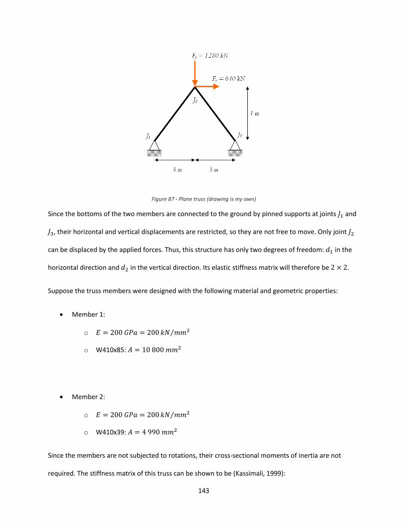
143
Figure 87 - Plane truss (drawing is my own)
Since the bottoms of the two members are connected to the ground by pinned supports at joints and
, their horizontal and vertical displacements are restricted, so they are not free to move. Only joint
can be displaced by the applied forces. Thus, this structure has only two degrees of freedom: in the
horizontal direction and in the vertical direction. Its elastic stiffness matrix will therefore be .
Suppose the truss members were designed with the following material and geometric properties:
Member 1:
o ⁄
o W410x85:
Member 2:
o ⁄
o W410x39:
Since the members are not subjected to rotations, their cross-sectional moments of inertia are not
required. The stiffness matrix of this truss can be shown to be (Kassimali, 1999):
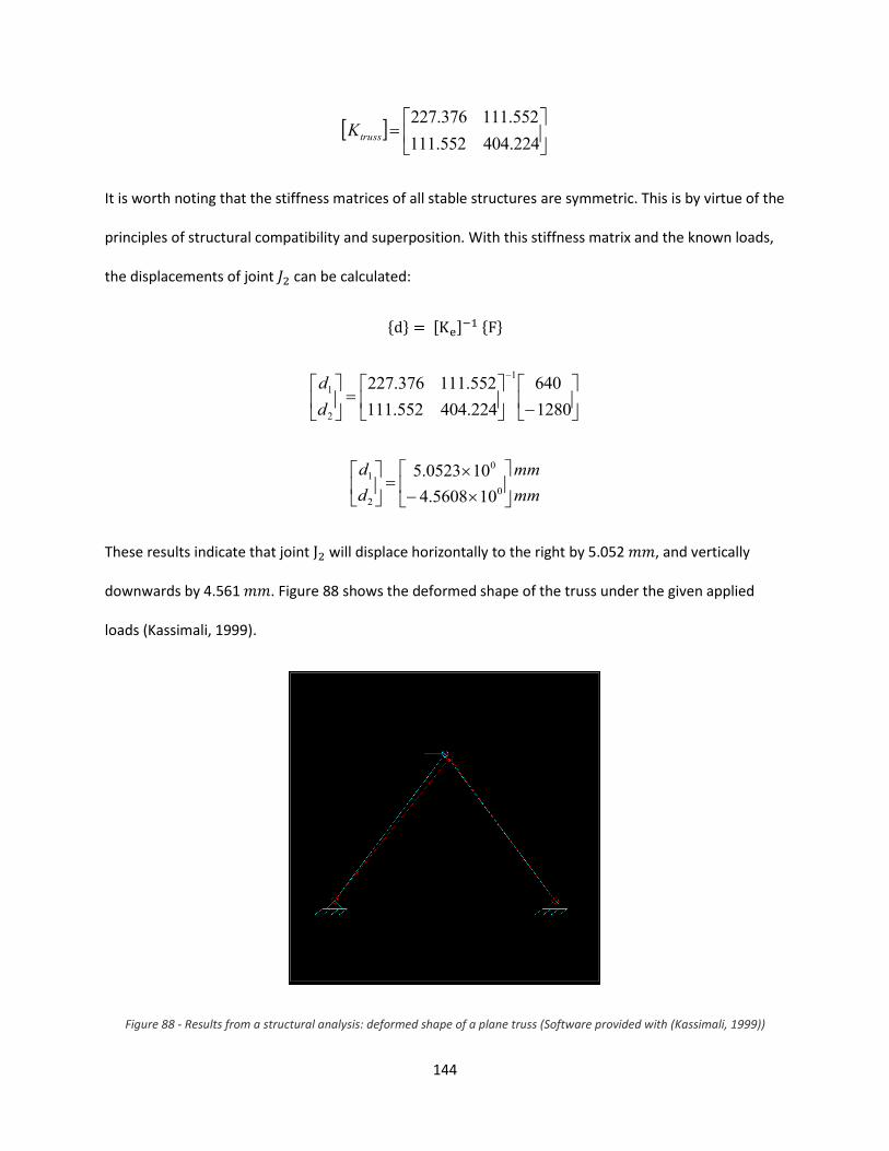
144
224.404552.111
552.111376.227trussK
It is worth noting that the stiffness matrices of all stable structures are symmetric. This is by virtue of the
principles of structural compatibility and superposition. With this stiffness matrix and the known loads,
the displacements of joint can be calculated:
{ } [ ] { }
1280
640
224.404552.111
552.111376.2271
2
1
d
d
mm
mm
d
d
0
0
2
1
105608.4
100523.5
These results indicate that joint will displace horizontally to the right by 5.052 , and vertically
downwards by 4.561 . Figure 88 shows the deformed shape of the truss under the given applied
loads (Kassimali, 1999).
Figure 88 - Results from a structural analysis: deformed shape of a plane truss (Software provided with (Kassimali, 1999))
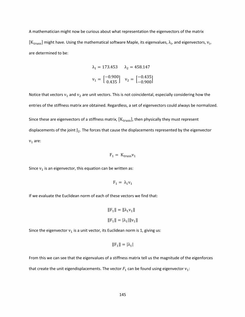
145
A mathematician might now be curious about what representation the eigenvectors of the matrix
[ ] might have. Using the mathematical software Maple, its eigenvalues, , and eigenvectors, ,
are determined to be:
*
+ *
+
Notice that vectors and are unit vectors. This is not coincidental, especially considering how the
entries of the stiffness matrix are obtained. Regardless, a set of eigenvectors could always be normalized.
Since these are eigenvectors of a stiffness matrix, [ ], then physically they must represent
displacements of the joint . The forces that cause the displacements represented by the eigenvector
are:
Since is an eigenvector, this equation can be written as:
If we evaluate the Euclidean norm of each of these vectors we find that:
‖ ‖ ‖ ‖
‖ ‖ | |‖ ‖
Since the eigenvector is a unit vector, its Euclidean norm is 1, giving us:
‖ ‖ | |
From this we can see that the eigenvalues of a stiffness matrix tell us the magnitude of the eigenforces
that create the unit eigendisplacements. The vector can be found using eigenvector :

146
[ ] [
] *
+ *
+ *
+
Expressing vectors and in terms of their magnitude and direction yields:
Notice that the magnitude of is the eigenvalue . The interpretation of this is that applying a force
with magnitude of 173.453 at an angle of 154.20 with the horizontal direction results in a
displacement of 1 in the same direction as the applied force. This is the physical representation of
the eigenvectors of a structure’s elastic stiffness matrix. This situation is represented in Figure 89 (not to
scale). The same interpretation exists for eigenvalue , and eigenvector , along with its associated
eigenforce, . The direction of these latter vectors is orthogonal to the direction of vectors and .
Figure 89 - Eigenvectors of a plane truss: applied force and resulting displacement are in the same direction (drawing is my own)
Though it is interesting to discover that eigenvectors in this model do have physical meaning, it is
unfortunately irrelevant to the structural engineer performing this analysis. Recall that structural
analysis is only one stage in the design process. Prior to analyzing a structure, the engineer must first
ascertain the loads that will be applied to it. Thus, the forces acting on the structure are known ahead of
time; their magnitudes and direction are pre-determined. It is the displacements that are sought, and
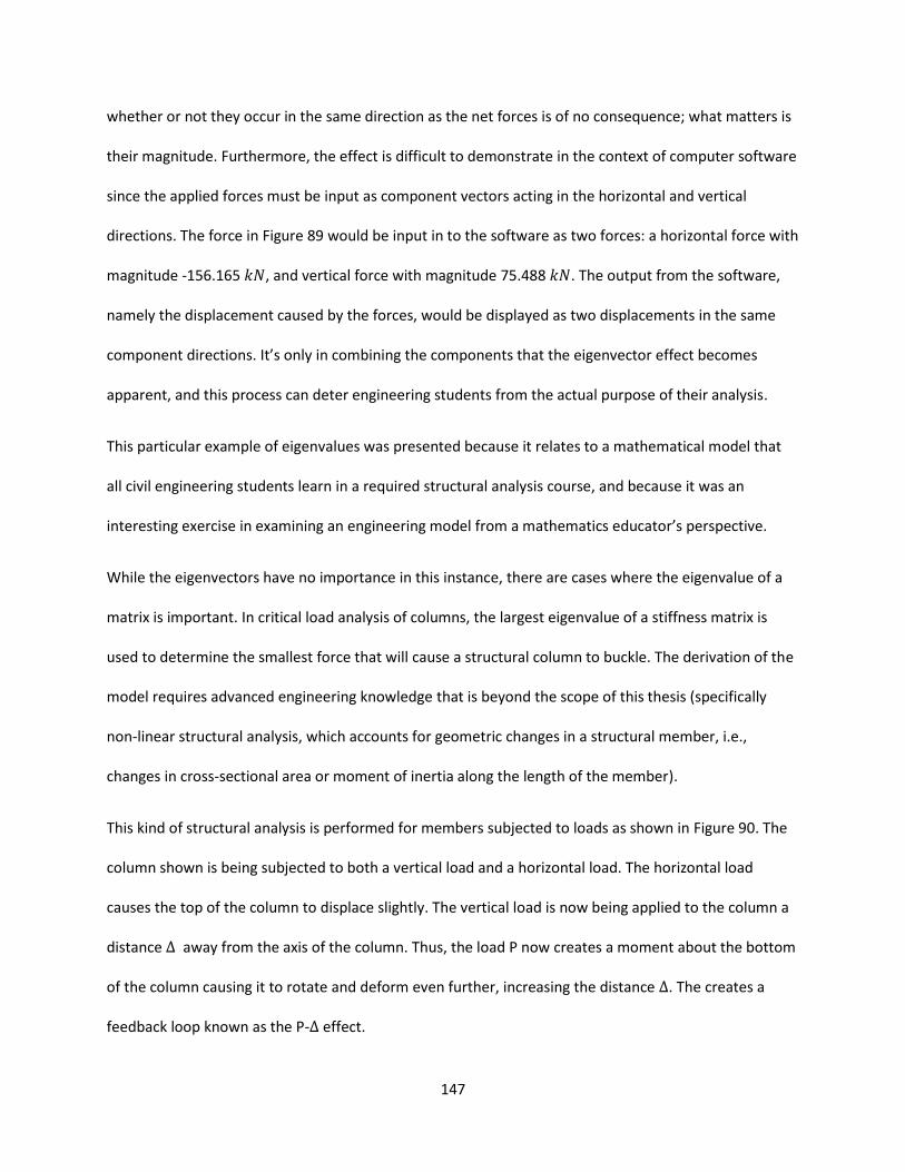
147
whether or not they occur in the same direction as the net forces is of no consequence; what matters is
their magnitude. Furthermore, the effect is difficult to demonstrate in the context of computer software
since the applied forces must be input as component vectors acting in the horizontal and vertical
directions. The force in Figure 89 would be input in to the software as two forces: a horizontal force with
magnitude -156.165 , and vertical force with magnitude 75.488 . The output from the software,
namely the displacement caused by the forces, would be displayed as two displacements in the same
component directions. It’s only in combining the components that the eigenvector effect becomes
apparent, and this process can deter engineering students from the actual purpose of their analysis.
This particular example of eigenvalues was presented because it relates to a mathematical model that
all civil engineering students learn in a required structural analysis course, and because it was an
interesting exercise in examining an engineering model from a mathematics educator’s perspective.
While the eigenvectors have no importance in this instance, there are cases where the eigenvalue of a
matrix is important. In critical load analysis of columns, the largest eigenvalue of a stiffness matrix is
used to determine the smallest force that will cause a structural column to buckle. The derivation of the
model requires advanced engineering knowledge that is beyond the scope of this thesis (specifically
non-linear structural analysis, which accounts for geometric changes in a structural member, i.e.,
changes in cross-sectional area or moment of inertia along the length of the member).
This kind of structural analysis is performed for members subjected to loads as shown in Figure 90. The
column shown is being subjected to both a vertical load and a horizontal load. The horizontal load
causes the top of the column to displace slightly. The vertical load is now being applied to the column a
distance away from the axis of the column. Thus, the load P now creates a moment about the bottom
of the column causing it to rotate and deform even further, increasing the distance . The creates a
feedback loop known as the P- effect.
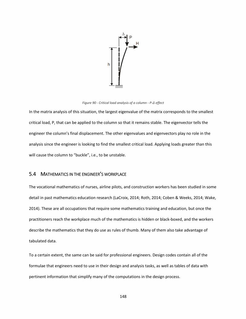
148
Figure 90 - Critical load analysis of a column - P- effect
In the matrix analysis of this situation, the largest eigenvalue of the matrix corresponds to the smallest
critical load, P, that can be applied to the column so that it remains stable. The eigenvector tells the
engineer the column’s final displacement. The other eigenvalues and eigenvectors play no role in the
analysis since the engineer is looking to find the smallest critical load. Applying loads greater than this
will cause the column to “buckle”, i.e., to be unstable.
5.4 MATHEMATICS IN THE ENGINEER’S WORKPLACE
The vocational mathematics of nurses, airline pilots, and construction workers has been studied in some
detail in past mathematics education research (LaCroix, 2014; Roth, 2014; Coben & Weeks, 2014; Wake,
2014). These are all occupations that require some mathematics training and education, but once the
practitioners reach the workplace much of the mathematics is hidden or black-boxed, and the workers
describe the mathematics that they do use as rules of thumb. Many of them also take advantage of
tabulated data.
To a certain extent, the same can be said for professional engineers. Design codes contain all of the
formulae that engineers need to use in their design and analysis tasks, as well as tables of data with
pertinent information that simplify many of the computations in the design process.
149
As a student, an engineer will learn how to calculate the factored resistance of a steel beam and
determine whether or not their choice of beam will be able to resist the factored loads. But since the
cross-sectional shapes used in steel construction are all standardised, their resistances for various
lengths of beams have already been calculated and the results tabulated. Once an engineer knows the
factored load that a beam must resist, they can look up an adequately sized cross-section size in a table
that lists beam resistances.
Recall that not all practicing engineers are involved in the design process. Many are charged with project
management, ensuring that a structure meets not only design specifications prescribed by code, but also
those specified by the client, and that the project is completed on time and on budget. The most
arduous mathematics used by these engineers is in the proper management of resources and personnel
in an effort to complete a project efficiently. The use of tabulated data is thus a necessity for the
designers to work efficiently.
5.4.1 Dossier de calculs
Returning to the tasks of a structural design engineer, another important outcome of structural analysis
is the magnitude of the forces in the structure’s supports. The forces applied to the structure are
supported by the structural members and transferred into the ground via the supports. The supports
therefore have to be designed to resist the loads that pass through them.
In this section, I present the details a work document called a dossier de calculs that was prepared by a
practicing engineer for the design of a structural support. The document contains calculations that serve
to determine the factored resistance of the support, and to verify that the resistance is greater than the
factored loads, as prescribed by the limits states design model described in section 5.2.4. The
calculations are written on a sheet graph paper with numbered rows and columns which will make
identifying calculations in the images easier on the reader.
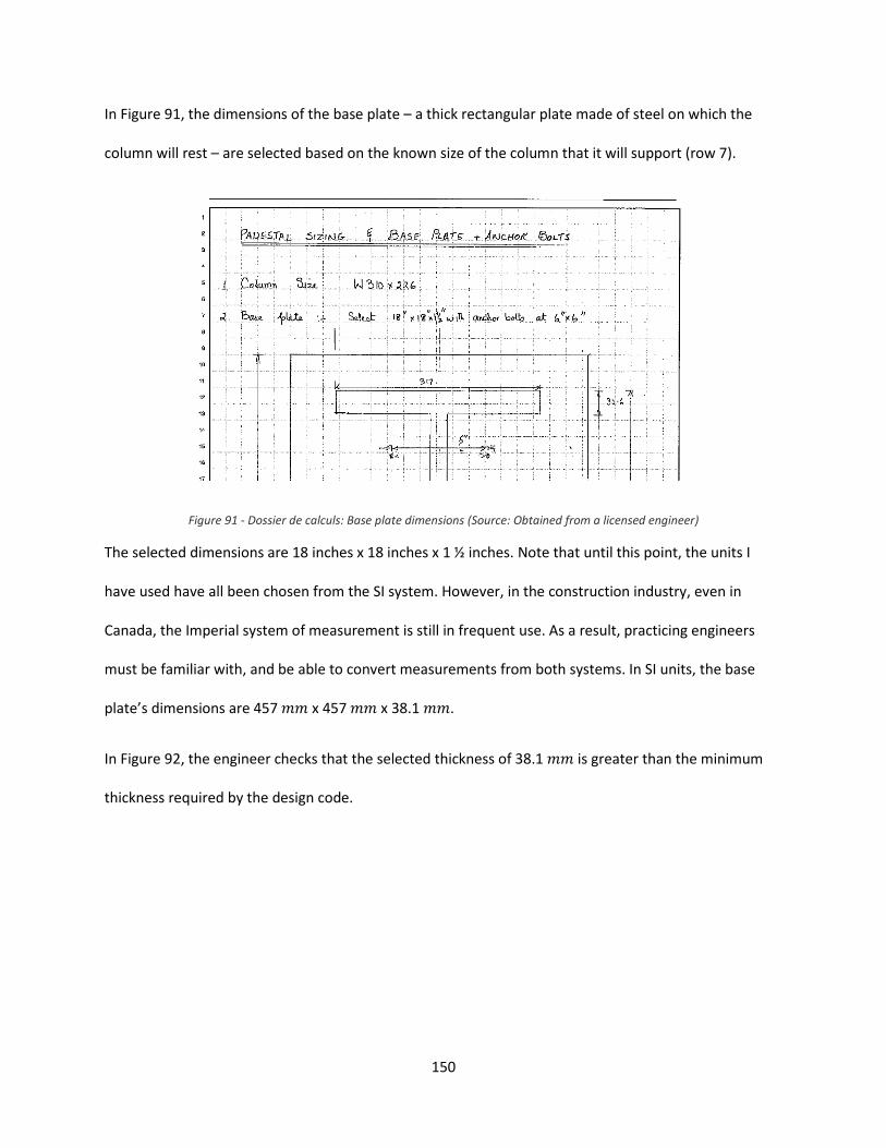
150
In Figure 91, the dimensions of the base plate – a thick rectangular plate made of steel on which the
column will rest – are selected based on the known size of the column that it will support (row 7).
Figure 91 - Dossier de calculs: Base plate dimensions (Source: Obtained from a licensed engineer)
The selected dimensions are 18 inches x 18 inches x 1 ½ inches. Note that until this point, the units I
have used have all been chosen from the SI system. However, in the construction industry, even in
Canada, the Imperial system of measurement is still in frequent use. As a result, practicing engineers
must be familiar with, and be able to convert measurements from both systems. In SI units, the base
plate’s dimensions are 457 x 457 x 38.1 .
In Figure 92, the engineer checks that the selected thickness of 38.1 is greater than the minimum
thickness required by the design code.
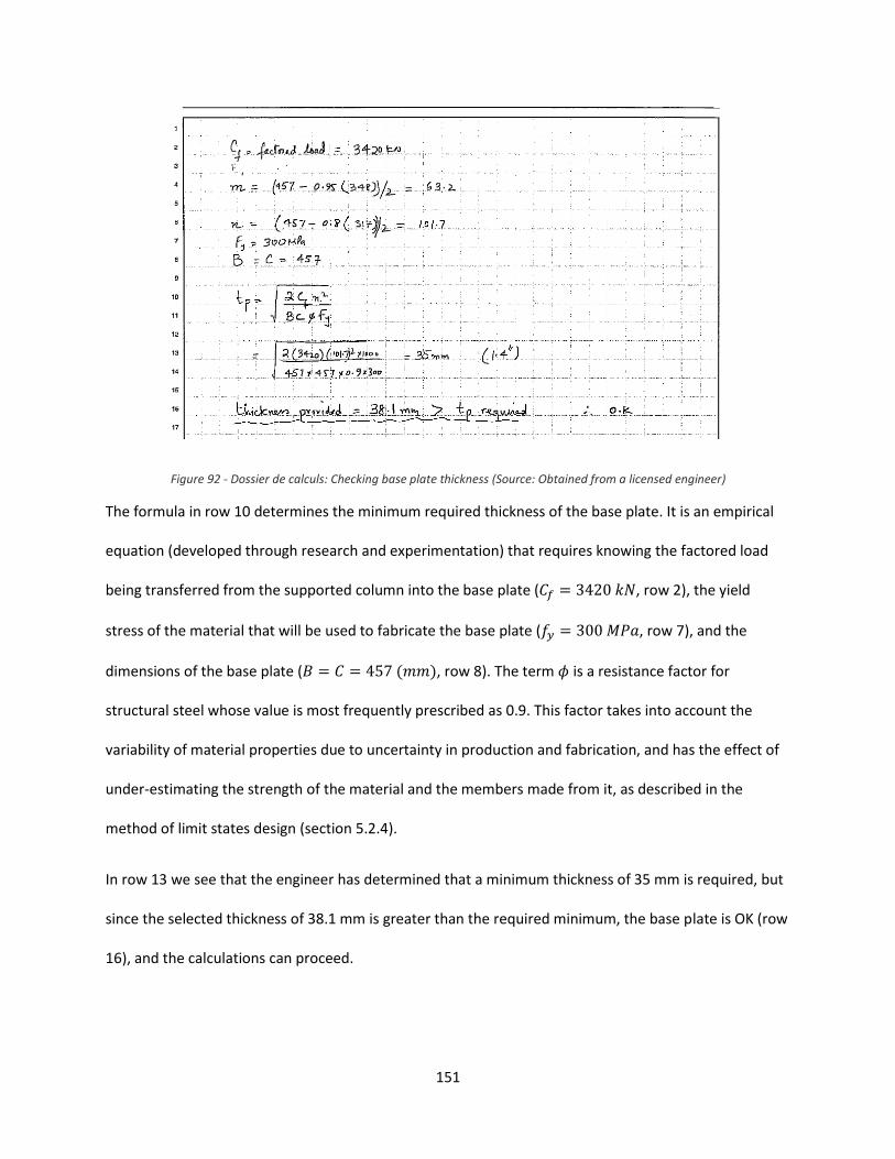
151
Figure 92 - Dossier de calculs: Checking base plate thickness (Source: Obtained from a licensed engineer)
The formula in row 10 determines the minimum required thickness of the base plate. It is an empirical
equation (developed through research and experimentation) that requires knowing the factored load
being transferred from the supported column into the base plate ( , row 2), the yield
stress of the material that will be used to fabricate the base plate ( , row 7), and the
dimensions of the base plate ( , row 8). The term is a resistance factor for
structural steel whose value is most frequently prescribed as 0.9. This factor takes into account the
variability of material properties due to uncertainty in production and fabrication, and has the effect of
under-estimating the strength of the material and the members made from it, as described in the
method of limit states design (section 5.2.4).
In row 13 we see that the engineer has determined that a minimum thickness of 35 mm is required, but
since the selected thickness of 38.1 mm is greater than the required minimum, the base plate is OK (row
16), and the calculations can proceed.
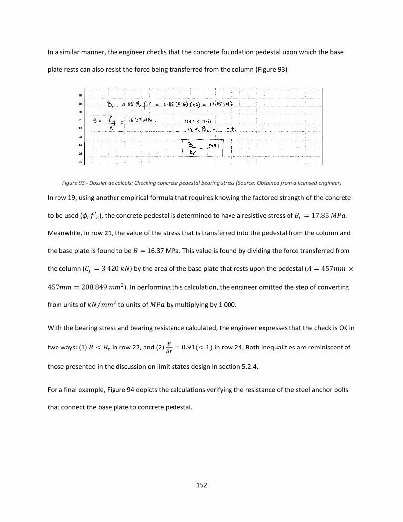
152
In a similar manner, the engineer checks that the concrete foundation pedestal upon which the base
plate rests can also resist the force being transferred from the column (Figure 93).
Figure 93 - Dossier de calculs: Checking concrete pedestal bearing stress (Source: Obtained from a licensed engineer)
In row 19, using another empirical formula that requires knowing the factored strength of the concrete
to be used ( ), the concrete pedestal is determined to have a resistive stress of .
Meanwhile, in row 21, the value of the stress that is transferred into the pedestal from the column and
the base plate is found to be 16.37 MPa. This value is found by dividing the force transferred from
the column ( ) by the area of the base plate that rests upon the pedestal (
). In performing this calculation, the engineer omitted the step of converting
from units of ⁄ to units of by multiplying by 1 000.
With the bearing stress and bearing resistance calculated, the engineer expresses that the check is OK in
two ways: (1) in row 22, and (2)
in row 24. Both inequalities are reminiscent of
those presented in the discussion on limit states design in section 5.2.4.
For a final example, Figure 94 depicts the calculations verifying the resistance of the steel anchor bolts
that connect the base plate to concrete pedestal.
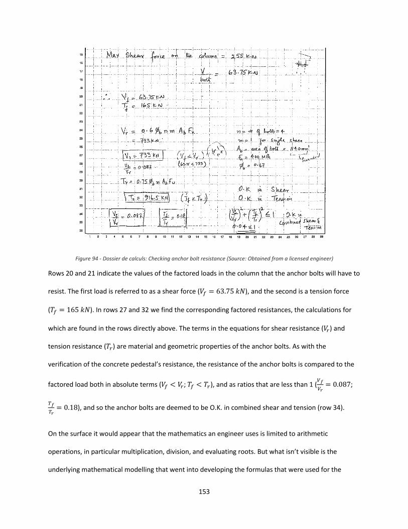
153
Figure 94 - Dossier de calculs: Checking anchor bolt resistance (Source: Obtained from a licensed engineer)
Rows 20 and 21 indicate the values of the factored loads in the column that the anchor bolts will have to
resist. The first load is referred to as a shear force ( ), and the second is a tension force
( ). In rows 27 and 32 we find the corresponding factored resistances, the calculations for
which are found in the rows directly above. The terms in the equations for shear resistance ( ) and
tension resistance ( ) are material and geometric properties of the anchor bolts. As with the
verification of the concrete pedestal’s resistance, the resistance of the anchor bolts is compared to the
factored load both in absolute terms ( ; ), and as ratios that are less than 1 (
;
), and so the anchor bolts are deemed to be O.K. in combined shear and tension (row 34).
On the surface it would appear that the mathematics an engineer uses is limited to arithmetic
operations, in particular multiplication, division, and evaluating roots. But what isn’t visible is the
underlying mathematical modelling that went into developing the formulas that were used for the
154
calculations. Nor do we see the decision making and logic that went into the selection of the sizes of the
base plate and the anchor bolts during the design. Much like the workplaces discussed in the research
reviewed in chapter 3, where the mathematics was not always visible to the practitioner, the
mathematics that is visible in the engineer’s workplace does not tell the whole story of the profession.
The engineer must decide which clauses of a design code apply and which don’t. In terms of the
engineering profession’s praxeology, if performing the design is the task, then selecting the appropriate
formulas from the handbook is part of the technique along with competent use of mathematics. The
technology is found in the design codes themselves, in the text that describes when and how each
formula is to be used, and the fields of engineering design, engineering science and engineering
research that lead to the development of the design codes and their acceptance by the Canadian
Standards Association and professional engineering societies are the theory.
155
6 CONCLUSIONS AND RECOMMENDATIONS
Before identifying and describing the differences between an engineer’s and a mathematician’s
mathematics, I will first address the similarities that I found during my research. While the similarities in
mathematical praxeologies of engineers and mathematicians are limited mainly to the tasks and
techniques, differences are found in all levels of the praxeologies: tasks, techniques, technologies, and
theories. Some of the differences are overt, such as in the standardised symbolism used by engineers.
Others, while less obvious, are still describable in the terms of the ATD. A general view of an engineer’s
mathematical praxeology is presented towards the end of this chapter, which then concludes with a
discussion on the limitations of this thesis, and proposals for future studies.
6.1 SIMILARITIES IN MATHEMATICAL PRAXEOLOGIES
The results of my analysis of final exams presented in chapter 4 show that there are some similarities in
the mathematics expected to be learned by engineering students and mathematics students, though
they are mainly limited to the tasks given to students on their final exams and the techniques that both
groups of students can use to accomplish the tasks.
I did not intend to find these similarities, and in fact they surprised me to a certain extent. They were
found, however, because I needed to identify what mathematics an engineering student is required to
learn in order to obtain a degree, and wanted to compare it with the mathematics to be learned by
mathematics students in comparable courses.
The most striking examples of similarities are found in problems from the differential equations and
numerical methods courses, in particular the problems shown in Figure 52 - CIVE 320 - Numerical
Methods (McGill), December 2007, question 6, and Figure 53 - MATH 354 - Numerical Analysis
(Concordia), December 2012, question 2.
156
It could be argued that, to a certain extent, the technology in the mathematical praxeologies of the
institutions of mathematics courses is similar as well. In the exams that were analyzed for chapter 4, I
was unable to find any instances where the amount of justification of a technique seemed to be greater
for mathematicians than it was for engineers. That is, the level of discourse for describing and justifying
the use of certain techniques was about the same for both groups. In fact, many questions on
engineering exams specifically asked the students to justify their answers. Furthermore, the fact that the
exams for some mathematics courses taken exclusively by engineers feature questions that are entirely
conceptual in nature and mathematical in content shows that engineers are expected to have some
level of understanding of pure mathematics (for example, see Figure 39 - ENGR 371 - Probability and
Statistics in Engineering (Concordia), April 2013, question 3, and Figure 40 - ENGR 371 - Probability and
Statistics in Engineering (Concordia), April 2013, question 4).
But it should be noted that these similarities occur only in the first two years of university education,
when the topics and concepts learned by both groups are essentially the same. After the first two years,
the educational paths of the two groups diverge, and differences arise. These are discussed in the next
section.
6.2 DIFFERENCES IN MATHEMATICAL PRAXEOLOGIES
For engineering students and mathematics students, the courses in linear algebra, calculus, probability
and statistics, numerical methods, and differential equations are all required to be taken in the first two
years of study. Considering the similarities in mathematical content in the first two years, the logical
question to ask is “do things differ in the next two years of study?” The answer is an unqualified yes. The
divergent educational paths of mathematicians and engineers are illustrated in Figure 95.
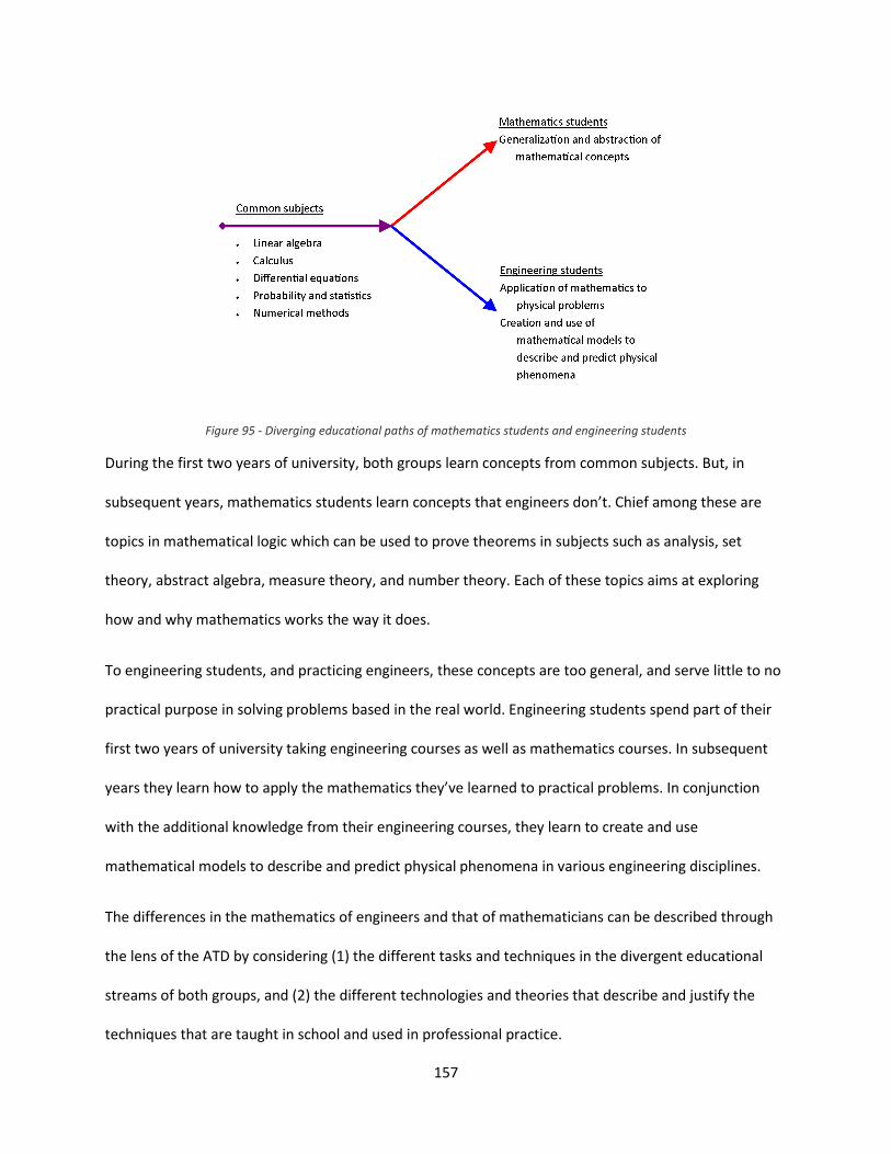
157
Figure 95 - Diverging educational paths of mathematics students and engineering students
During the first two years of university, both groups learn concepts from common subjects. But, in
subsequent years, mathematics students learn concepts that engineers don’t. Chief among these are
topics in mathematical logic which can be used to prove theorems in subjects such as analysis, set
theory, abstract algebra, measure theory, and number theory. Each of these topics aims at exploring
how and why mathematics works the way it does.
To engineering students, and practicing engineers, these concepts are too general, and serve little to no
practical purpose in solving problems based in the real world. Engineering students spend part of their
first two years of university taking engineering courses as well as mathematics courses. In subsequent
years they learn how to apply the mathematics they’ve learned to practical problems. In conjunction
with the additional knowledge from their engineering courses, they learn to create and use
mathematical models to describe and predict physical phenomena in various engineering disciplines.
The differences in the mathematics of engineers and that of mathematicians can be described through
the lens of the ATD by considering (1) the different tasks and techniques in the divergent educational
streams of both groups, and (2) the different technologies and theories that describe and justify the
techniques that are taught in school and used in professional practice.
158
6.2.1 Differences in tasks and techniques
As previously mentioned, in their later university education, mathematics students learn concepts that
engineering students don’t. For mathematics students, the subject of linear algebra is taught from the
perspective of linear transformations over abstract vector spaces; courses in logic introduce them to the
concept of “mathematical thinking”; they learn how to prove the fundamental theorems of arithmetic,
algebra, and calculus in real and complex analysis; and courses in abstract algebra, measure theory, and
number theory generalize other mathematical concepts. These concepts equip the students with new
techniques to accomplish new types of tasks, including, perhaps most importantly, proving
mathematical theorems, a task that engineers simply never encounter in either their engineering
courses or their professional practice.
Engineering students, on the other hand, use the techniques that they learned in their mathematics
courses in conjunction with knowledge from the physical sciences to accomplish tasks that involve the
creation and application of mathematical models to solve problems in engineering. Examples of this are
shown in chapter 5, including the use of differential equations to model the deflection of a structural
beam, and the necessity of statistical analysis in developing the model of limit states design.
6.2.2 Differences in technologies and theories
Arguably the most important differences in the mathematical praxeologies of engineers and
mathematicians are found at the levels of technology and theory. Among these differences are the ones
found in the standardised symbolism used by engineers, discussed in the next section.
6.2.2.1 Differences in standardised symbolism
Standardised symbolism belongs to the technology of the engineer’s mathematical praxeology because
it is codified knowledge that serves to communicate to each member of the institution of the
159
professional practice of engineering how to properly communicate numerical information with each
other.
Differences in standardised symbolism of engineers versus that of mathematicians include the ways in
which real numbers are represented. While mathematicians prefer precision and use symbols such as ,
√ , and
, engineers will often approximate the values of these numbers as 3.14, 1.414, and 0.5. The
level of precision of the approximation will vary depending on the context of the task the number is
being used for, and will depend on the accuracy of measurements or of the values in a given data set.
Also belonging to standardised symbolism is the use of units in application problems. When
mathematicians encounter application problems they will use units as well, since it is the units that give
the numbers physical meaning. But engineering science has led to the creation of new units of measure
that are, for the most part, unknown to mathematicians. Examples of these are the newton for units of
force, and the pascal for units of pressure.
Other examples mentioned in this thesis are the use of standard prefixes (Figure 60 - SI prefixes and
multiplication factors ) for units of measure. Some professional mathematicians may be surprised to
learn that the preferred unit of measure for the size of small objects is the millimetre, and not the
centimetre. Consider as well the sigma notation that omitted indices in the model of static equilibrium
(section 5.2.2), and the integral that didn’t include limits in the model of the moment of inertia (section
5.2.3). While a mathematician would certainly include the indices and limits, their omission is justified in
the engineer’s technology by the context in which the symbols are being used.
6.2.2.2 Differences in technologies in education
The research of Castela and Romo Vasquez proposes that engineers augment the technology of their
mathematical praxeology with justifications based on practicality and efficiency, and not solely on
160
mathematical consistency (Castela & Romo Vasquez, 2011). The theory of their praxeologies is also
rooted in the natural and engineering sciences. Not everything an engineer does can be reduced to
mathematics alone, thus, their technology and theory also includes knowledge from the physical
sciences. This was exemplified by the study on the different methods of teaching Laplace transforms to
engineering students (see section 3.1).
A comparable difference can be seen from the point of view of mathematicians. The new techniques
that mathematics students learn in their later university courses augment the level of discourse, i.e., the
technology, of the techniques that they learned in their earlier courses. Proving the fundamental
theorem of calculus in an analysis course, for example, adds to the justification of its use in the calculus
course taken earlier in their education. Engineers, however, never add this mathematical content to the
technology of their mathematical praxeology.
While engineers augment their praxeologies with knowledge learned in physical sciences,
mathematicians augment their own praxeologies with more mathematics. Thus, there is a difference in
the technologies of the institutions of engineering education and mathematics education.
6.2.2.3 Differences in technologies and theories in professional practice
The differences in technologies and theories become more evident when we examine an engineer’s
professional practice. Evidence of the claim that not everything an engineer does can be reduced to
mathematics alone was shown in section 5.4. The knowledge embedded in the engineer’s dossier de
calculs involves more than just the visible calculations using arithmetic and algebra. The engineer must
decide which formulas necessarily apply to the structure he is designing, and which don’t. These
decisions must be justified, and doing so requires more than just mathematics. Furthermore, the
formulas themselves that are used in the engineer’s design calculations were developed through
161
extensive empirical testing and mathematical modelling, and the creation of these models also requires
knowledge from the physical sciences.
Recall from section 4.1 the accreditation requirements for an engineering program. The bulk of a
program is to be dedicated to courses in engineering science and engineering design (Canadian
Engineering Accreditation Board, 2013). While engineering design combines mathematics, natural
sciences, and engineering sciences, it is an iterative process of applications of mathematical models.
Engineering science, on the other hand, applies mathematics to practical problems through the
development of mathematical models. In a sense, while engineering designers apply mathematical
models, engineering scientists (i.e. academic engineers) create the mathematical models that are used
in practice, including those that appear in design codes. In this way, the theory of the engineer’s
mathematical praxeology is also augmented by extra-mathematical concepts.
For a final example of how an engineer’s mathematical praxeology includes more than just mathematics,
consider the case of the London Millennium Pedestrian Bridge. Not long after it opened in the year 2000,
the bridge began to sway excessively. Pedestrians began adjusting their footsteps to counter the effects
of the swaying; this caused the bridge to sway even more creating a positive feedback loop. According to
Noss (2001), the failure in the bridge’s design wasn’t in the mathematics or the mathematical models
that the engineers used, but in the design code. The bridge was designed using existing techniques
specified by the appropriate bridge design code. At the time of its design, though, lateral vibrations in
pedestrian bridges were simply not a matter of consideration as it is generally vertical vibrations that are
of more concern. In terms of the ATD, the existing techniques, while mathematically sound, failed when
applied in the real world. Following extensive research on the cause of the vibrations (Dallard, et al.,
2001), a new technique, in the form of an additional clause, was added to the design code. The new
clause found in the British Standard on bridge live loading, BD 37, contained in volume 1 of the Design
Manual for Roads and Bridges states:
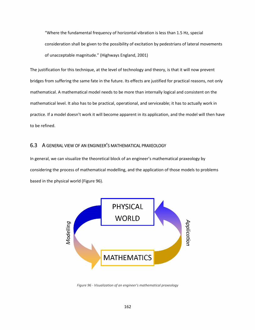
162
“Where the fundamental frequency of horizontal vibration is less than 1.5 Hz, special
consideration shall be given to the possibility of excitation by pedestrians of lateral movements
of unacceptable magnitude.” (Highways England, 2001)
The justification for this technique, at the level of technology and theory, is that it will now prevent
bridges from suffering the same fate in the future. Its effects are justified for practical reasons, not only
mathematical. A mathematical model needs to be more than internally logical and consistent on the
mathematical level. It also has to be practical, operational, and serviceable; it has to actually work in
practice. If a model doesn’t work it will become apparent in its application, and the model will then have
to be refined.
6.3 A GENERAL VIEW OF AN ENGINEER’S MATHEMATICAL PRAXEOLOGY
In general, we can visualize the theoretical block of an engineer’s mathematical praxeology by
considering the process of mathematical modelling, and the application of those models to problems
based in the physical world (Figure 96).
Figure 96 - Visualization of an engineer's mathematical praxeology
163
Modelling is the process that maps elements from the real world into the mathematical domain, while
application problems involve using a mathematical model to solve a problem that involves extra-
mathematical elements.
A mathematician’s praxeology must be consistent entirely within the realm of mathematics. An
engineer’s mathematical praxeology, on the other hand, requires that the mathematics work when they
are applied in the physical world. For a mathematician, a mathematical proof requires only the use of
valid mathematics. For an engineer, the proof is in the successful application of mathematics.
6.4 LIMITATIONS OF THIS THESIS AND RECOMMENDATIONS FOR FUTURE STUDIES
The findings of this thesis are based on limited amounts of data. The statistics in section 4.3, for example,
should be taken with a grain of salt. My analysis included exams from only two schools, and focused on
a single school year for each course. While the final exams for most of these courses don’t tend to
change very much over a relatively short time span (the earliest exam that I referenced is eight years old
at the time of writing), and the engineering exams that I analyzed didn’t strike me as any different from
those I that wrote as a student in the early 2000’s, having more time to analyze exams from multiple
years would certainly result in a more accurate representation of the relative frequencies of the
different type of tasks.
For the subject of engineering geometry I had no exams to analyze, and my discussion of the topic was
based largely on documents from professional practice and on past personal experience. Engineering
surveying requires extensive use of trigonometry. Analyzing exams from surveying courses could offer a
wealth of information into how engineers use trigonometry in practice, in particular how precise their
calculations and approximations have to be in order to be considered “correct.”

164
It would be pertinent to analyze final exams from engineering courses to see if, in fact, more modelling
problems are given when compared with their mathematics courses. Since the exams analyzed for this
thesis are clearly lacking in modelling problems, the engineering courses would almost certainly have to
offer more of them in order to comply with the requirements of the Canadian Engineering Accreditation
Board.
165
7 REFERENCES
Beer, F., & Johnston, E. (1992). Mechanics of materials. London: McGraw-Hill, Inc.
Beer, F., & Johnston, E. (2007). Vector Mechanics for Engineers: Statics. New York: McGraw-Hill, Inc.
Bessot, A. (2000). Geometry at work - examples from the building industry. In A. Bessot, & J. Ridgway,
Education for mathematics in the workplace (pp. 143-157). Dordrecht: Kluwer Academic
Publishers.
Bkouche, R. (1989). Mathematics and physics: where is the difference? In W. Blum, J. Berry, R. Biehler, I.
Huntley, G. Kaiser-Messmer, & L. Profke, Applications and modelling in learning and teaching
mathematics (pp. 49-54). Chichester: Ellis Horwood Limited.
Bkouche, R. (1989). Mathematics and physics: where is the difference? In J. B.-M. W. Blum, Applications
and modelling in learning and teaching mathematics (pp. 49-54). Chichester: Ellis Horwood
Limited.
Blum, W., & Niss, M. (1991). Applied mathematical problem solving, modelling, applications, and links to
other subjects—State, trends and issues in mathematics instruction. Educational studies in
mathematics, 22(1), 37-68.
Blum, W., Berry, J., Biehler, R., Huntley, I., Kaiser-Messmer, G., & Profke, L. (1989). Applicatinos and
modelling in learning and teaching mathematics. Chichester: Ellis Horwood Limited.
Boyce, W., & DiPrima, R. (1997). Elementary Differential Equations and Boundary Value Problems, Sixth
Edition. New York: John Wiley & Sons, Inc.
Canadian Engineering Accreditation Board. (2013). Accreditation Criteria and Procedures Report 2013.
Ottawa: Engineers Canada.
Canadian Institute of Steel Construction. (2000). Handbook of Steel Construction Seventh Edition.
Alliston: Universal Offset Limited.
Castela, C. (2015). When praxeologies move from an institution to another one: The transpositive effects.
23rd annual meeting of the Southern African association for research in mathematics, science
and technology, SAARMSTE 2015, Tuesday 13–Friday 16 January 2015, (pp. 6-19). Maputo,
Mozambique.
Castela, C., & Romo Vasquez, A. (2011). Des mathématiques à l'automatique: étude des effets de
transposition sur la transformée de Laplace dans la formation des ingénieurs. Recherches en
Didactique des Mathématiques, 31(1), 79-130.
Chevallard, Y. (1985). La transposition didactique. Du savoir savant au savoir enseigné. Grenoble: La
Pensee Sauvage.
Chevallard, Y. (1999). L'analyse des pratiques enseignantes en théorie anthropologique du didactique.
Recherches en didactique des mathématiques, 19(2), 221-265.
166
Coben, D., & Weeks, K. (2014). Meeting the mathematical demands of the safety-critical workplace:
medication dosage calculation problem-solving for nursing. Educational Studies in Mathematics,
86(2), 253-270.
Dallard, P., Fitzpatrick, A., Flint, A., Le Bourva, S., Low, A., Ridsdill Smith, R., et al. (2001, November 20).
The London Millennium Footbridge. The Structural Engineer, pp. 17-33.
Eberhard, M. (2000). Forms of mathematical knowledge relating to measurement in vocational training
for the building industry. In A. Bessot, & J. Ridgway, Education for mathematics in the workplace
(pp. 37-51). Dordrecht: Kluwer Academic Publishers.
École Polytechnique de Montréal. (n.d.). La génie civil - Programmes de génie au baccalauréat. Retrieved
February 1, 2015, from Polytechnique Montréal:
http://www.polymtl.ca/etudes/bc/information/civil.php#thematiques
École Polytechnique de Montréal. (n.d.). Recherche - École Polytechnique - Recherche et innovation.
Retrieved February 1, 2015, from Polytechnique Montréal:
http://www.polymtl.ca/recherche/index.php
Edwards, D., & Hamson, M. (1989). A first course in mathematical modelling. In W. Blum, J. Berry, R.
Biehler, I. Huntley, G. Kaiser-Messmer, & L. Profke, Applications and modelling in learning and
teaching mathematics (pp. 288-291). Chichester: Ellis Horwood Limited.
Evans, J. (2000). The transfer of mathematics learning from school to work not straightforward but not
impossible either. In A. Bessot, & J. Ridgway, Education for mathematics in the workplace (pp. 5-
15). Dordrecht: Kluwer Academic Publishers.
Galbraith, P., Henn, H., & Niss, M. (2007). Modelling and Applications in Mathematics Education. New
York: Springer.
Gilat, A., & Subramaniam, V. (2008). Numerical methods for engineers and scientists: an introduction
with appliactions using MATLAB. Hoboken: John Wiley & Sonc, Inc.
Hardy, N. (2009). Students' perceptions of institutional practices: the case of limits in college level
Calculus courses. Educational Studies in Mathematics, 72(3), 341-358.
Highways England. (2001). Design Manual for Roads and Birdges, Volume 1, Section 2, Part 14. London:
Highways England.
Howson, A., Kahane, J.-P., Kelly, P., Lauginie, P., Nemetz, T., Simons, F., et al. (1988). Mathematics as
service subject. In R. Clements, P. Lauginie, & E. de Turckheim, Selected papers on the teaching
of mathematics as a service subject (pp. 1-16). Vienna: Springer.
Kassimali, A. (1999). Structural Analysis. Pacific Grove: PWS Publishing.
LaCroix, L. (2014). Learning to see pipes mathematically: preapprentices’ mathematical activity in pipe
trades training. Educational Studies in Mathematics, 86(2), 157-176.
Lay, D. C. (2016). Linear Algebra and its Applications, Fifth Edition. Boston: Pearson Education, Inc.
167
McGuire, W., Gallagher, R., & Zieman, R. (2000). Matrix structural analysis. New York: John Wiley & Sons,
Inc.
National Research Council of Canada. (2010). National Building Code of Canada. Ottawa: CNRC.
Noss, R. (2001). For a learnable mathematics in the digital cultures. Educational Studies in Mathematics,
48(1), 21-46.
Noss, R., Hoyles, C., & Pozzi, S. (2000). Working knowledge: mathematics in use. In A. Bessot, & J.
Ridgway, Education for mathematics in the workplace (pp. 16-35). Dordrecht: Kluwer Academic
Publishers.
Peters, B. (1999). Institutional theory in political science. London, New York: Continuum.
Ridgway, J. (2000). The mathematical needs of engineering apprentices. In A. Bessot, & J. Ridgway,
Education for mathematics in the workplace (pp. 189-197). Dordrecht: Kluwer Academic
Publishers.
Romo Vasquez, A., & Castela, C. (2010). Mathematics in the training of engineers: an approach from two
different perspectives. Educational Interfaces between Mathematics and Industry (EIMI) (pp.
533-540). Bedford, MA: COMAP .
Roth, W. (2014). Rules of bending, bending the rules: the geometry of electrical conduit bending in
college and workplace. . Educational Studies in Mathematics, 86(2), 177-192.
Sierpinska, A. (2000). On some aspects of students' thinking in linear algebra. In J.-L. Dorier, On the
teaching of linear algebra (pp. 209-246). Dortrecht: Kluwer.
Sierpinska, A., Bobos, G., & Knipping, C. (2008). Sources of students’ frustration in pre-university level,
prerequisite mathematics courses. Instructional Science, 36(4), 289-320.
Teague, D. (1989). Modelling in an american high school. In W. Blum, J. Berry, R. Biehler, I. Huntley, G.
Kaiser-Messmer, & L. Profke, Applications and modelling in learning and teaching mathematics
(pp. 262-266). Chichester: Ellis Horwood Limited.
Teague, D. (1989). Modelling in an american high school. In J. B.-M. W. Blum, Applications and modelling
in learning and teaching mathematics (pp. 262-266). Chichester: Ellis Horwood Limited.
Tipler, P. (1991). Physics for Scientists and Engineers. New York, NY: Worth Publishers, Inc.
Wake, G. (2014). Making sense of and with mathematics: The interface between academic mathematics
and mathematics in practice. . Educational Studies in Mathematics, 86(2), 271-290.
168
8 APPENDICES
8.1 WEBSITES OF ACCREDITED ENGINEERING PROGRAMS IN QUEBEC
General information about the accredited civil engineering programs in Quebec can be found on the
following university websites:
1. McGill University: www.mcgill.ca/engineering
2. Université Laval: www.fsg.ulaval.ca
3. École Polytechnique: www.polymtl.ca
4. Université de Sherbrooke: www.usherbrooke.ca/genie
5. Concordia University: www.encs.concordia.ca
6. École de technologie supérieure: www.etsmtl.ca
7. Université du Québec à Chicoutimi: http://programmes.uqac.ca/7480
8.2 LIST OF MATHEMATICS COURSES IN THE ACCREDITED ENGINEERING PROGRAMS IN QUEBEC
The tables in the sections that follow include the complete list of required mathematics courses in the
seven accredited engineering programs in Quebec. The courses are grouped together by subject
following the same order as section 4.3.
Some courses are listed in multiple subjects, e.g., the course MAT165 - Algèbre linéaire et analyse
vectorielle at École de technologie supérieure is listed in both pre-university linear algebra and
university level calculus. This is because there are a substantial number of topics in the course
description that qualify the course for both subjects.
These course descriptions were used to define the different groups of mathematics subjects whose
exams were analyzed in section 4.3.
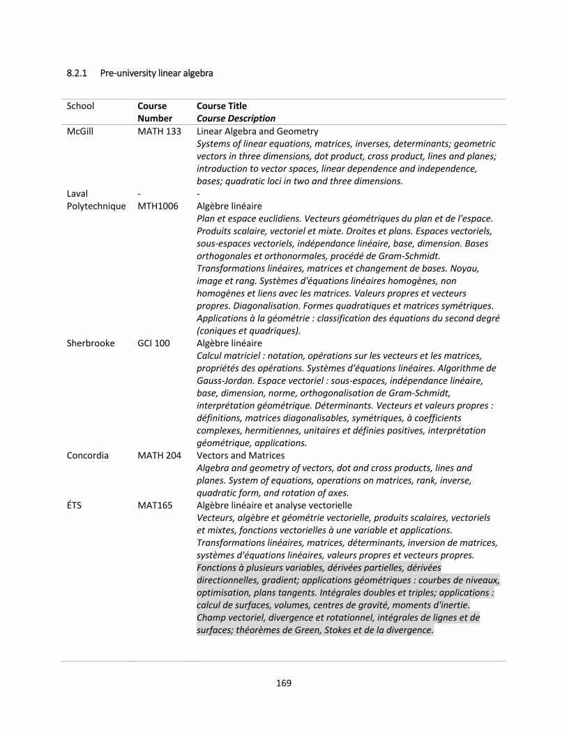
169
8.2.1 Pre-university linear algebra
School Course Number
Course Title Course Description
McGill MATH 133 Linear Algebra and Geometry Systems of linear equations, matrices, inverses, determinants; geometric vectors in three dimensions, dot product, cross product, lines and planes; introduction to vector spaces, linear dependence and independence, bases; quadratic loci in two and three dimensions.
Laval - - Polytechnique MTH1006 Algèbre linéaire
Plan et espace euclidiens. Vecteurs géométriques du plan et de l'espace. Produits scalaire, vectoriel et mixte. Droites et plans. Espaces vectoriels, sous-espaces vectoriels, indépendance linéaire, base, dimension. Bases orthogonales et orthonormales, procédé de Gram-Schmidt. Transformations linéaires, matrices et changement de bases. Noyau, image et rang. Systèmes d'équations linéaires homogènes, non homogènes et liens avec les matrices. Valeurs propres et vecteurs propres. Diagonalisation. Formes quadratiques et matrices symétriques. Applications à la géométrie : classification des équations du second degré (coniques et quadriques).
Sherbrooke GCI 100 Algèbre linéaire Calcul matriciel : notation, opérations sur les vecteurs et les matrices, propriétés des opérations. Systèmes d'équations linéaires. Algorithme de Gauss-Jordan. Espace vectoriel : sous-espaces, indépendance linéaire, base, dimension, norme, orthogonalisation de Gram-Schmidt, interprétation géométrique. Déterminants. Vecteurs et valeurs propres : définitions, matrices diagonalisables, symétriques, à coefficients complexes, hermitiennes, unitaires et définies positives, interprétation géométrique, applications.
Concordia MATH 204 Vectors and Matrices Algebra and geometry of vectors, dot and cross products, lines and planes. System of equations, operations on matrices, rank, inverse, quadratic form, and rotation of axes.
ÉTS MAT165 Algèbre linéaire et analyse vectorielle Vecteurs, algèbre et géométrie vectorielle, produits scalaires, vectoriels et mixtes, fonctions vectorielles à une variable et applications. Transformations linéaires, matrices, déterminants, inversion de matrices, systèmes d'équations linéaires, valeurs propres et vecteurs propres. Fonctions à plusieurs variables, dérivées partielles, dérivées directionnelles, gradient; applications géométriques : courbes de niveaux, optimisation, plans tangents. Intégrales doubles et triples; applications : calcul de surfaces, volumes, centres de gravité, moments d'inertie. Champ vectoriel, divergence et rotationnel, intégrales de lignes et de surfaces; théorèmes de Green, Stokes et de la divergence.
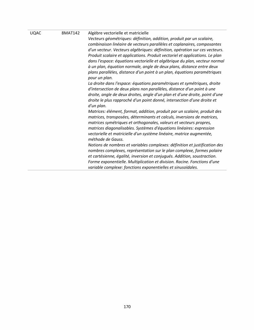
170
UQAC 8MAT142 Algèbre vectorielle et matricielle Vecteurs géométriques: définition, addition, produit par un scalaire, combinaison linéaire de vecteurs parallèles et coplanaires, composantes d'un vecteur. Vecteurs algébriques: définition, opération sur ces vecteurs. Produit scalaire et applications. Produit vectoriel et applications. Le plan dans l'espace: équations vectorielle et algébrique du plan, vecteur normal à un plan, équation normale, angle de deux plans, distance entre deux plans parallèles, distance d'un point à un plan, équations paramétriques pour un plan. La droite dans l'espace: équations paramétriques et symétriques, droite d'intersection de deux plans non parallèles, distance d'un point à une droite, angle de deux droites, angle d'un plan et d'une droite, point d'une droite le plus rapproché d'un point donné, intersection d'une droite et d'un plan. Matrices: élément, format, addition, produit par un scalaire, produit des matrices, transposées, déterminants et calculs, inversions de matrices, matrices symétriques et orthogonales, valeurs et vecteurs propres, matrices diagonalisables. Systèmes d'équations linéaires: expression vectorielle et matricielle d'un système linéaire, matrice augmentée, méthode de Gauss. Notions de nombres et variables complexes: définition et justification des nombres complexes, représentation sur le plan complexe, formes polaire et cartésienne, égalité, inversion et conjugués. Addition, soustraction. Forme exponentielle. Multiplication et division. Racine. Fonctions d'une variable complexe: fonctions exponentielles et sinusoïdales.

171
8.2.2 Pre-university calculus
School Course Number
Course Title Course Description
McGill MATH 140 Calculus 1 Review of functions and graphs. Limits, continuity, derivative. Differentiation of elementary functions. Antidifferentiation. Applications.
MATH 141 Calculus 2 The definite integral. Techniques of integration. Applications. Introduction to sequences and series.
Laval - - Polytechnique - - Sherbrooke - - Concordia MATH 203 Differential and Integral Calculus I
Functional notation. Differentiation of polynomials. The power, product, quotient, and chain rules. Differentiation of elementary functions. Implicit differentiation. Higher derivatives. Maxima and minima. Applications: tangents to plane curves, graphing, related rates. Approximations using the differential. Antiderivatives, definite integrals, area.
MATH 205 Differential and Integral Calculus II Techniques of integration: substitutions, integration by parts, partial fractions. Improper integrals. Physical applications of the definite integral. Infinite series: tests for convergence. Power series, Taylor’s theorem.
ÉTS MAT145 Calcul différentiel et intégral Analyse : généralités sur les fonctions de R dans R; calcul différentiel : limites, dérivée, dérivée des fonctions élémentaires, règles de dérivation, étude de graphe, optimisation, etc. Calcul intégral : intégrales indéfinies, méthode d'intégration, utilisation des tables, intégrales définies, application (calcul d'aires, de volumes, de longueurs d'arc), méthodes numériques, intégrales impropres, etc. Suites et séries. Développements limités (Taylor, Maclaurin), évaluation de fonctions et d'intégrales définies à l'aide des séries.
UQAC 8GMA102 Calcul différentiel et intégral Rappels sur les ensembles et nombres réels. Valeur absolue, droite orientée, inéquations. Fonctions et graphes, fonctions élémentaires: puissances, exponentielles, logarithmiques, trigonométriques, hyperboliques, fonctions inverses et composées. Forme implicite. Lieux géométriques et les coniques. Représentations paramétriques. Définition d'une limite et ses propriétés. Calcul de limites de fonctions algébriques. Continuité d'une fonction et propriétés des fonctions continues. Dérivée: définition, existence, propriétés et calculs. Formules de dérivation, dérivation en chaîne, dérivation implicite. Différentielle. Applications des dérivées: extremums de fonctions, tracé d'une courbe, modélisation et optimisation, théorèmes des accroissements finis, limites des formes indéterminées: règle de l'Hôpital. Approximations d'une fonction par série. Applications au génie. Intégrales indéfinies. Intégrales définies:

172
définition et propriétés. Théorème fondamental du calcul. Applications: calcul des aires planes, des aires et volumes de révolution, centre de gravité, moment d'inertie, pression des fluides, travail, longueur d'arc. Intégration numériques. Intégrales impropres.
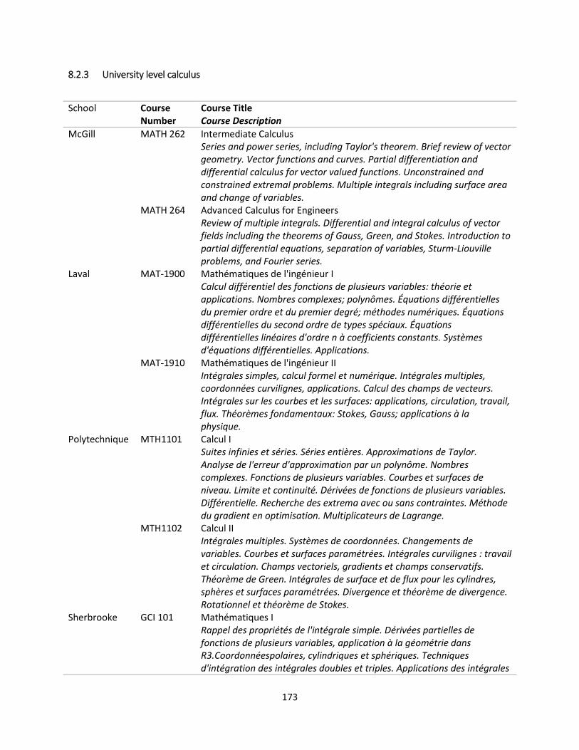
173
8.2.3 University level calculus
School Course Number
Course Title Course Description
McGill MATH 262 Intermediate Calculus Series and power series, including Taylor's theorem. Brief review of vector geometry. Vector functions and curves. Partial differentiation and differential calculus for vector valued functions. Unconstrained and constrained extremal problems. Multiple integrals including surface area and change of variables.
MATH 264 Advanced Calculus for Engineers Review of multiple integrals. Differential and integral calculus of vector fields including the theorems of Gauss, Green, and Stokes. Introduction to partial differential equations, separation of variables, Sturm-Liouville problems, and Fourier series.
Laval MAT-1900 Mathématiques de l'ingénieur I Calcul différentiel des fonctions de plusieurs variables: théorie et applications. Nombres complexes; polynômes. Équations différentielles du premier ordre et du premier degré; méthodes numériques. Équations différentielles du second ordre de types spéciaux. Équations différentielles linéaires d'ordre n à coefficients constants. Systèmes d'équations différentielles. Applications.
MAT-1910 Mathématiques de l'ingénieur II Intégrales simples, calcul formel et numérique. Intégrales multiples, coordonnées curvilignes, applications. Calcul des champs de vecteurs. Intégrales sur les courbes et les surfaces: applications, circulation, travail, flux. Théorèmes fondamentaux: Stokes, Gauss; applications à la physique.
Polytechnique MTH1101 Calcul I Suites infinies et séries. Séries entières. Approximations de Taylor. Analyse de l'erreur d'approximation par un polynôme. Nombres complexes. Fonctions de plusieurs variables. Courbes et surfaces de niveau. Limite et continuité. Dérivées de fonctions de plusieurs variables. Différentielle. Recherche des extrema avec ou sans contraintes. Méthode du gradient en optimisation. Multiplicateurs de Lagrange.
MTH1102 Calcul II Intégrales multiples. Systèmes de coordonnées. Changements de variables. Courbes et surfaces paramétrées. Intégrales curvilignes : travail et circulation. Champs vectoriels, gradients et champs conservatifs. Théorème de Green. Intégrales de surface et de flux pour les cylindres, sphères et surfaces paramétrées. Divergence et théorème de divergence. Rotationnel et théorème de Stokes.
Sherbrooke GCI 101 Mathématiques I Rappel des propriétés de l'intégrale simple. Dérivées partielles de fonctions de plusieurs variables, application à la géométrie dans R3.Coordonnéespolaires, cylindriques et sphériques. Techniques d'intégration des intégrales doubles et triples. Applications des intégrales
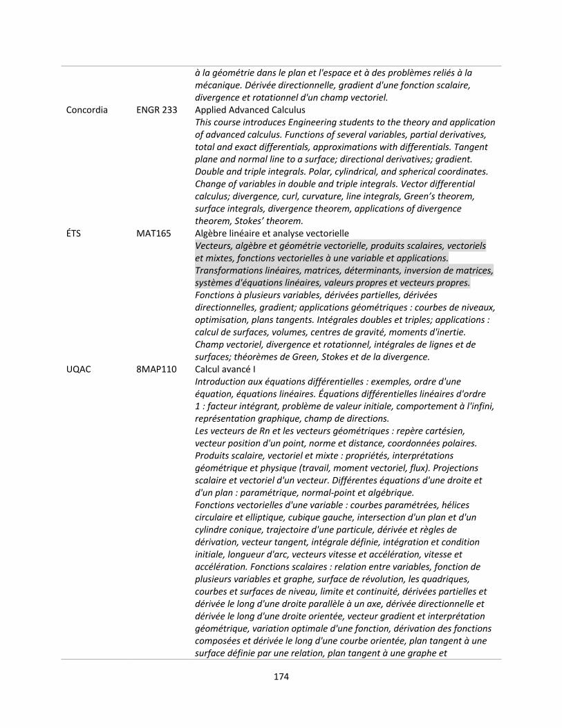
174
à la géométrie dans le plan et l'espace et à des problèmes reliés à la mécanique. Dérivée directionnelle, gradient d'une fonction scalaire, divergence et rotationnel d'un champ vectoriel.
Concordia ENGR 233 Applied Advanced Calculus This course introduces Engineering students to the theory and application of advanced calculus. Functions of several variables, partial derivatives, total and exact differentials, approximations with differentials. Tangent plane and normal line to a surface; directional derivatives; gradient. Double and triple integrals. Polar, cylindrical, and spherical coordinates. Change of variables in double and triple integrals. Vector differential calculus; divergence, curl, curvature, line integrals, Green’s theorem, surface integrals, divergence theorem, applications of divergence theorem, Stokes’ theorem.
ÉTS MAT165 Algèbre linéaire et analyse vectorielle Vecteurs, algèbre et géométrie vectorielle, produits scalaires, vectoriels et mixtes, fonctions vectorielles à une variable et applications. Transformations linéaires, matrices, déterminants, inversion de matrices, systèmes d'équations linéaires, valeurs propres et vecteurs propres. Fonctions à plusieurs variables, dérivées partielles, dérivées directionnelles, gradient; applications géométriques : courbes de niveaux, optimisation, plans tangents. Intégrales doubles et triples; applications : calcul de surfaces, volumes, centres de gravité, moments d'inertie. Champ vectoriel, divergence et rotationnel, intégrales de lignes et de surfaces; théorèmes de Green, Stokes et de la divergence.
UQAC 8MAP110 Calcul avancé I Introduction aux équations différentielles : exemples, ordre d'une équation, équations linéaires. Équations différentielles linéaires d'ordre 1 : facteur intégrant, problème de valeur initiale, comportement à l'infini, représentation graphique, champ de directions. Les vecteurs de Rn et les vecteurs géométriques : repère cartésien, vecteur position d'un point, norme et distance, coordonnées polaires. Produits scalaire, vectoriel et mixte : propriétés, interprétations géométrique et physique (travail, moment vectoriel, flux). Projections scalaire et vectoriel d'un vecteur. Différentes équations d'une droite et d'un plan : paramétrique, normal-point et algébrique. Fonctions vectorielles d'une variable : courbes paramétrées, hélices circulaire et elliptique, cubique gauche, intersection d'un plan et d'un cylindre conique, trajectoire d'une particule, dérivée et règles de dérivation, vecteur tangent, intégrale définie, intégration et condition initiale, longueur d'arc, vecteurs vitesse et accélération, vitesse et accélération. Fonctions scalaires : relation entre variables, fonction de plusieurs variables et graphe, surface de révolution, les quadriques, courbes et surfaces de niveau, limite et continuité, dérivées partielles et dérivée le long d'une droite parallèle à un axe, dérivée directionnelle et dérivée le long d'une droite orientée, vecteur gradient et interprétation géométrique, variation optimale d'une fonction, dérivation des fonctions composées et dérivée le long d'une courbe orientée, plan tangent à une surface définie par une relation, plan tangent à une graphe et
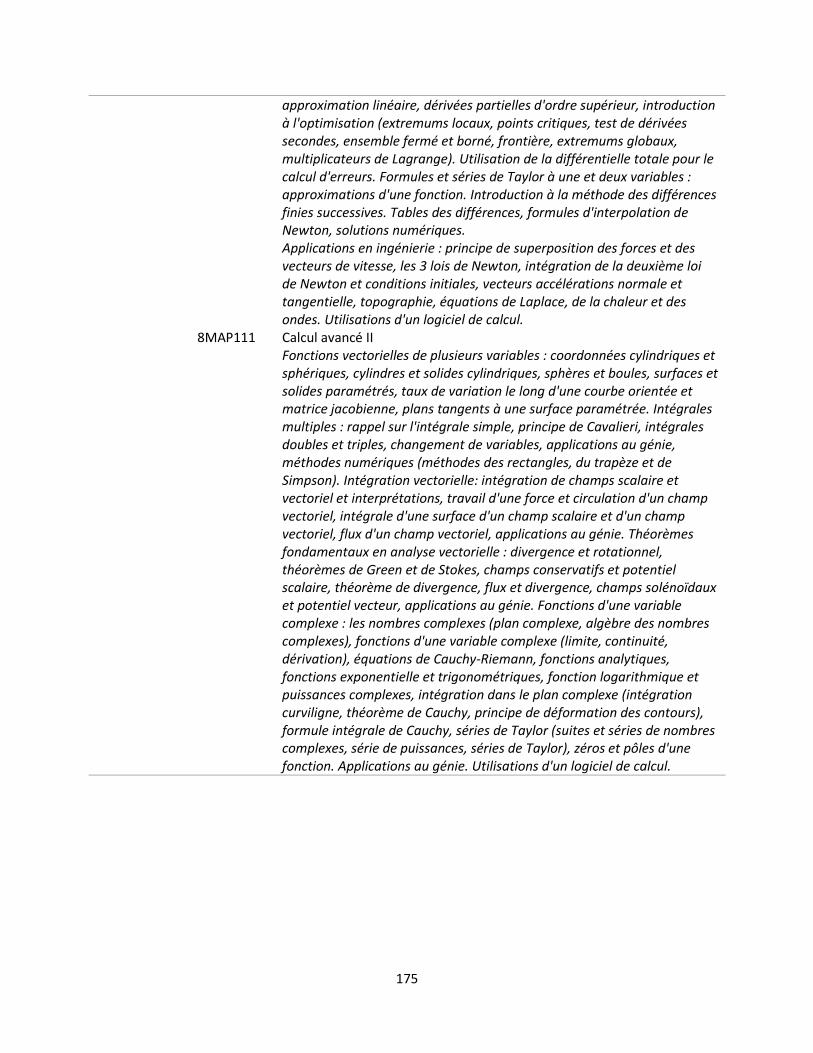
175
approximation linéaire, dérivées partielles d'ordre supérieur, introduction à l'optimisation (extremums locaux, points critiques, test de dérivées secondes, ensemble fermé et borné, frontière, extremums globaux, multiplicateurs de Lagrange). Utilisation de la différentielle totale pour le calcul d'erreurs. Formules et séries de Taylor à une et deux variables : approximations d'une fonction. Introduction à la méthode des différences finies successives. Tables des différences, formules d'interpolation de Newton, solutions numériques. Applications en ingénierie : principe de superposition des forces et des vecteurs de vitesse, les 3 lois de Newton, intégration de la deuxième loi de Newton et conditions initiales, vecteurs accélérations normale et tangentielle, topographie, équations de Laplace, de la chaleur et des ondes. Utilisations d'un logiciel de calcul.
8MAP111 Calcul avancé II Fonctions vectorielles de plusieurs variables : coordonnées cylindriques et sphériques, cylindres et solides cylindriques, sphères et boules, surfaces et solides paramétrés, taux de variation le long d'une courbe orientée et matrice jacobienne, plans tangents à une surface paramétrée. Intégrales multiples : rappel sur l'intégrale simple, principe de Cavalieri, intégrales doubles et triples, changement de variables, applications au génie, méthodes numériques (méthodes des rectangles, du trapèze et de Simpson). Intégration vectorielle: intégration de champs scalaire et vectoriel et interprétations, travail d'une force et circulation d'un champ vectoriel, intégrale d'une surface d'un champ scalaire et d'un champ vectoriel, flux d'un champ vectoriel, applications au génie. Théorèmes fondamentaux en analyse vectorielle : divergence et rotationnel, théorèmes de Green et de Stokes, champs conservatifs et potentiel scalaire, théorème de divergence, flux et divergence, champs solénoïdaux et potentiel vecteur, applications au génie. Fonctions d'une variable complexe : les nombres complexes (plan complexe, algèbre des nombres complexes), fonctions d'une variable complexe (limite, continuité, dérivation), équations de Cauchy-Riemann, fonctions analytiques, fonctions exponentielle et trigonométriques, fonction logarithmique et puissances complexes, intégration dans le plan complexe (intégration curviligne, théorème de Cauchy, principe de déformation des contours), formule intégrale de Cauchy, séries de Taylor (suites et séries de nombres complexes, série de puissances, séries de Taylor), zéros et pôles d'une fonction. Applications au génie. Utilisations d'un logiciel de calcul.
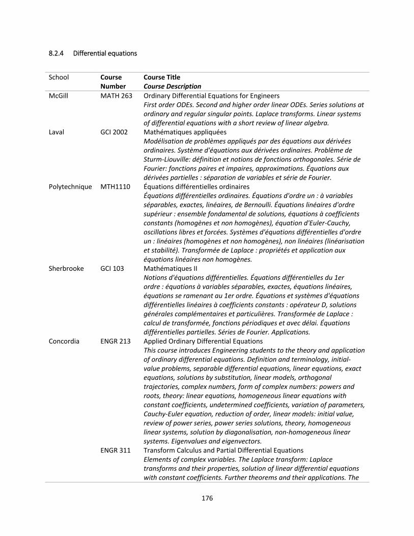
176
8.2.4 Differential equations
School Course Number
Course Title Course Description
McGill MATH 263 Ordinary Differential Equations for Engineers First order ODEs. Second and higher order linear ODEs. Series solutions at ordinary and regular singular points. Laplace transforms. Linear systems of differential equations with a short review of linear algebra.
Laval GCI 2002 Mathématiques appliquées Modélisation de problèmes appliqués par des équations aux dérivées ordinaires. Système d'équations aux dérivées ordinaires. Problème de Sturm-Liouville: définition et notions de fonctions orthogonales. Série de Fourier: fonctions paires et impaires, approximations. Équations aux dérivées partielles : séparation de variables et série de Fourier.
Polytechnique MTH1110 Équations différentielles ordinaires Équations différentielles ordinaires. Équations d'ordre un : à variables séparables, exactes, linéaires, de Bernoulli. Équations linéaires d'ordre supérieur : ensemble fondamental de solutions, équations à coefficients constants (homogènes et non homogènes), équation d'Euler-Cauchy, oscillations libres et forcées. Systèmes d'équations différentielles d'ordre un : linéaires (homogènes et non homogènes), non linéaires (linéarisation et stabilité). Transformée de Laplace : propriétés et application aux équations linéaires non homogènes.
Sherbrooke GCI 103 Mathématiques II Notions d'équations différentielles. Équations différentielles du 1er ordre : équations à variables séparables, exactes, équations linéaires, équations se ramenant au 1er ordre. Équations et systèmes d'équations différentielles linéaires à coefficients constants : opérateur D, solutions générales complémentaires et particulières. Transformée de Laplace : calcul de transformée, fonctions périodiques et avec délai. Équations différentielles partielles. Séries de Fourier. Applications.
Concordia ENGR 213 Applied Ordinary Differential Equations This course introduces Engineering students to the theory and application of ordinary differential equations. Definition and terminology, initial-value problems, separable differential equations, linear equations, exact equations, solutions by substitution, linear models, orthogonal trajectories, complex numbers, form of complex numbers: powers and roots, theory: linear equations, homogeneous linear equations with constant coefficients, undetermined coefficients, variation of parameters, Cauchy-Euler equation, reduction of order, linear models: initial value, review of power series, power series solutions, theory, homogeneous linear systems, solution by diagonalisation, non-homogeneous linear systems. Eigenvalues and eigenvectors.
ENGR 311 Transform Calculus and Partial Differential Equations Elements of complex variables. The Laplace transform: Laplace transforms and their properties, solution of linear differential equations with constant coefficients. Further theorems and their applications. The
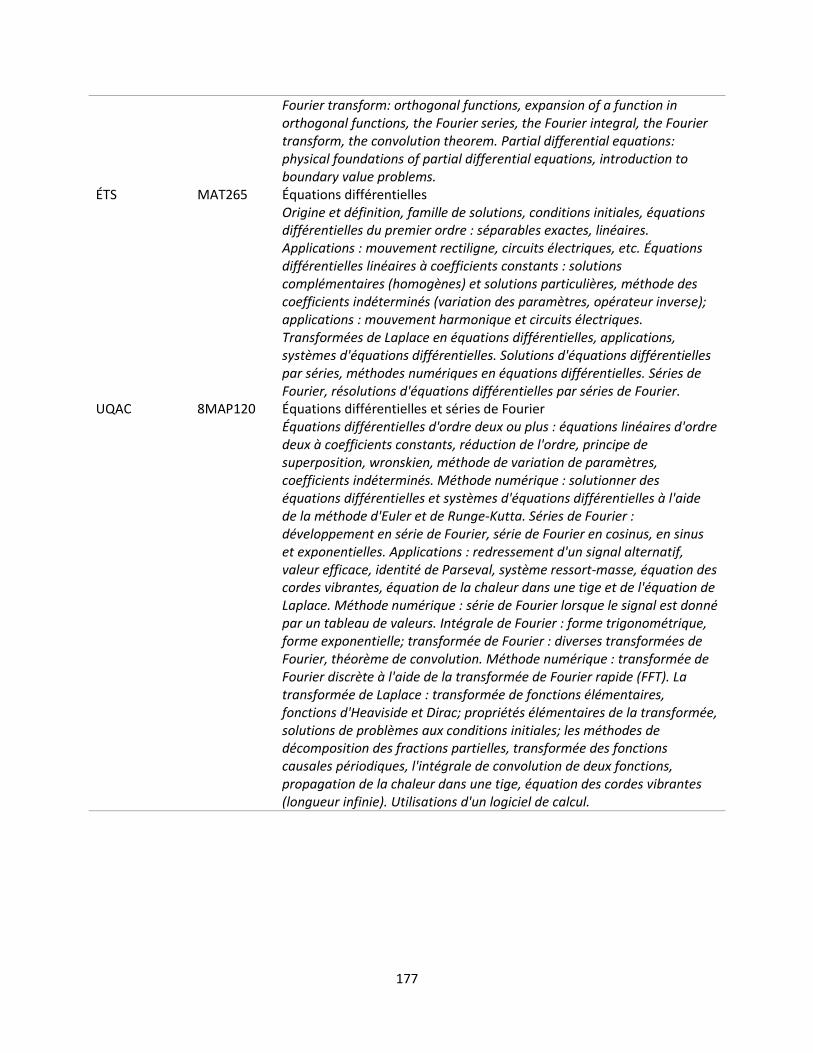
177
Fourier transform: orthogonal functions, expansion of a function in orthogonal functions, the Fourier series, the Fourier integral, the Fourier transform, the convolution theorem. Partial differential equations: physical foundations of partial differential equations, introduction to boundary value problems.
ÉTS MAT265 Équations différentielles Origine et définition, famille de solutions, conditions initiales, équations différentielles du premier ordre : séparables exactes, linéaires. Applications : mouvement rectiligne, circuits électriques, etc. Équations différentielles linéaires à coefficients constants : solutions complémentaires (homogènes) et solutions particulières, méthode des coefficients indéterminés (variation des paramètres, opérateur inverse); applications : mouvement harmonique et circuits électriques. Transformées de Laplace en équations différentielles, applications, systèmes d'équations différentielles. Solutions d'équations différentielles par séries, méthodes numériques en équations différentielles. Séries de Fourier, résolutions d'équations différentielles par séries de Fourier.
UQAC 8MAP120 Équations différentielles et séries de Fourier Équations différentielles d'ordre deux ou plus : équations linéaires d'ordre deux à coefficients constants, réduction de l'ordre, principe de superposition, wronskien, méthode de variation de paramètres, coefficients indéterminés. Méthode numérique : solutionner des équations différentielles et systèmes d'équations différentielles à l'aide de la méthode d'Euler et de Runge-Kutta. Séries de Fourier : développement en série de Fourier, série de Fourier en cosinus, en sinus et exponentielles. Applications : redressement d'un signal alternatif, valeur efficace, identité de Parseval, système ressort-masse, équation des cordes vibrantes, équation de la chaleur dans une tige et de l'équation de Laplace. Méthode numérique : série de Fourier lorsque le signal est donné par un tableau de valeurs. Intégrale de Fourier : forme trigonométrique, forme exponentielle; transformée de Fourier : diverses transformées de Fourier, théorème de convolution. Méthode numérique : transformée de Fourier discrète à l'aide de la transformée de Fourier rapide (FFT). La transformée de Laplace : transformée de fonctions élémentaires, fonctions d'Heaviside et Dirac; propriétés élémentaires de la transformée, solutions de problèmes aux conditions initiales; les méthodes de décomposition des fractions partielles, transformée des fonctions causales périodiques, l'intégrale de convolution de deux fonctions, propagation de la chaleur dans une tige, équation des cordes vibrantes (longueur infinie). Utilisations d'un logiciel de calcul.
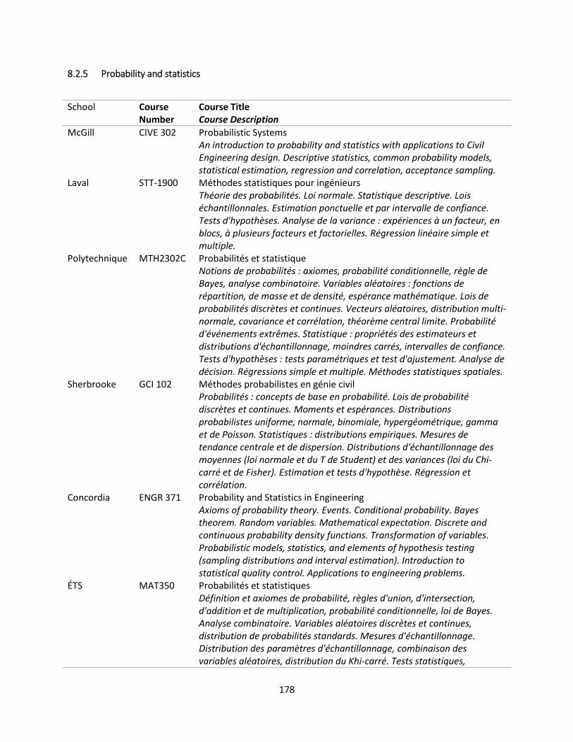
178
8.2.5 Probability and statistics
School Course Number
Course Title Course Description
McGill CIVE 302 Probabilistic Systems An introduction to probability and statistics with applications to Civil Engineering design. Descriptive statistics, common probability models, statistical estimation, regression and correlation, acceptance sampling.
Laval STT-1900 Méthodes statistiques pour ingénieurs Théorie des probabilités. Loi normale. Statistique descriptive. Lois échantillonnales. Estimation ponctuelle et par intervalle de confiance. Tests d'hypothèses. Analyse de la variance : expériences à un facteur, en blocs, à plusieurs facteurs et factorielles. Régression linéaire simple et multiple.
Polytechnique MTH2302C Probabilités et statistique Notions de probabilités : axiomes, probabilité conditionnelle, règle de Bayes, analyse combinatoire. Variables aléatoires : fonctions de répartition, de masse et de densité, espérance mathématique. Lois de probabilités discrètes et continues. Vecteurs aléatoires, distribution multi-normale, covariance et corrélation, théorème central limite. Probabilité d'événements extrêmes. Statistique : propriétés des estimateurs et distributions d'échantillonnage, moindres carrés, intervalles de confiance. Tests d'hypothèses : tests paramétriques et test d'ajustement. Analyse de décision. Régressions simple et multiple. Méthodes statistiques spatiales.
Sherbrooke GCI 102 Méthodes probabilistes en génie civil Probabilités : concepts de base en probabilité. Lois de probabilité discrètes et continues. Moments et espérances. Distributions probabilistes uniforme, normale, binomiale, hypergéométrique, gamma et de Poisson. Statistiques : distributions empiriques. Mesures de tendance centrale et de dispersion. Distributions d'échantillonnage des moyennes (loi normale et du T de Student) et des variances (loi du Chi-carré et de Fisher). Estimation et tests d'hypothèse. Régression et corrélation.
Concordia ENGR 371 Probability and Statistics in Engineering Axioms of probability theory. Events. Conditional probability. Bayes theorem. Random variables. Mathematical expectation. Discrete and continuous probability density functions. Transformation of variables. Probabilistic models, statistics, and elements of hypothesis testing (sampling distributions and interval estimation). Introduction to statistical quality control. Applications to engineering problems.
ÉTS MAT350 Probabilités et statistiques Définition et axiomes de probabilité, règles d'union, d'intersection, d'addition et de multiplication, probabilité conditionnelle, loi de Bayes. Analyse combinatoire. Variables aléatoires discrètes et continues, distribution de probabilités standards. Mesures d'échantillonnage. Distribution des paramètres d'échantillonnage, combinaison des variables aléatoires, distribution du Khi-carré. Tests statistiques,
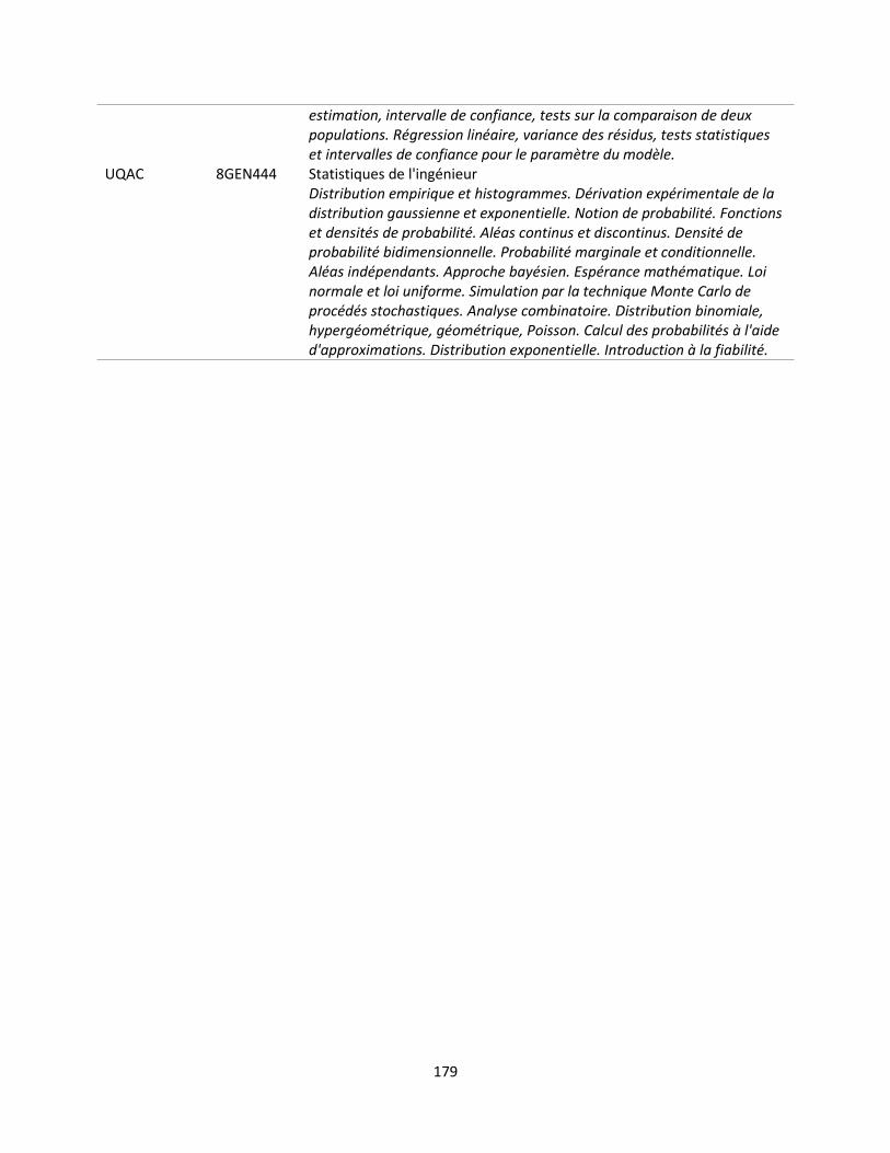
179
estimation, intervalle de confiance, tests sur la comparaison de deux populations. Régression linéaire, variance des résidus, tests statistiques et intervalles de confiance pour le paramètre du modèle.
UQAC 8GEN444 Statistiques de l'ingénieur Distribution empirique et histogrammes. Dérivation expérimentale de la distribution gaussienne et exponentielle. Notion de probabilité. Fonctions et densités de probabilité. Aléas continus et discontinus. Densité de probabilité bidimensionnelle. Probabilité marginale et conditionnelle. Aléas indépendants. Approche bayésien. Espérance mathématique. Loi normale et loi uniforme. Simulation par la technique Monte Carlo de procédés stochastiques. Analyse combinatoire. Distribution binomiale, hypergéométrique, géométrique, Poisson. Calcul des probabilités à l'aide d'approximations. Distribution exponentielle. Introduction à la fiabilité.
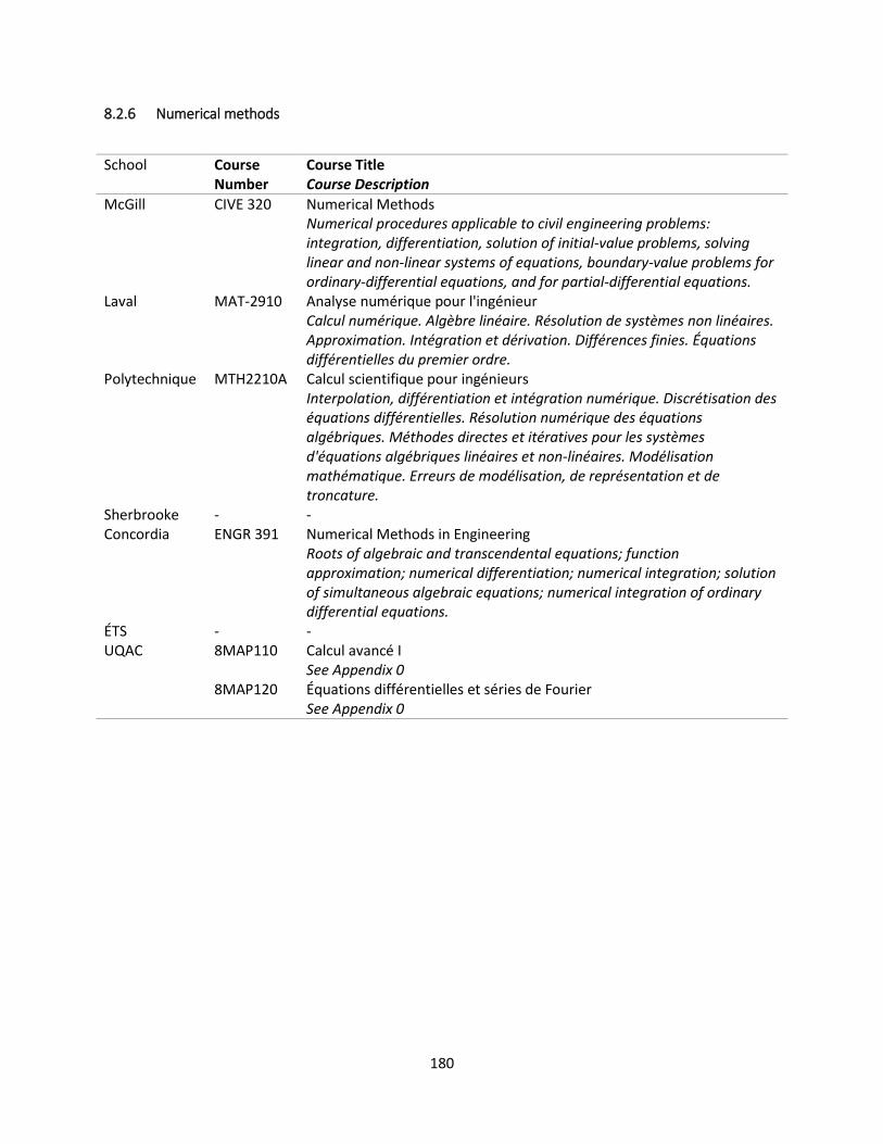
180
8.2.6 Numerical methods
School Course Number
Course Title Course Description
McGill CIVE 320 Numerical Methods Numerical procedures applicable to civil engineering problems: integration, differentiation, solution of initial-value problems, solving linear and non-linear systems of equations, boundary-value problems for ordinary-differential equations, and for partial-differential equations.
Laval MAT-2910 Analyse numérique pour l'ingénieur Calcul numérique. Algèbre linéaire. Résolution de systèmes non linéaires. Approximation. Intégration et dérivation. Différences finies. Équations différentielles du premier ordre.
Polytechnique MTH2210A Calcul scientifique pour ingénieurs Interpolation, différentiation et intégration numérique. Discrétisation des équations différentielles. Résolution numérique des équations algébriques. Méthodes directes et itératives pour les systèmes d'équations algébriques linéaires et non-linéaires. Modélisation mathématique. Erreurs de modélisation, de représentation et de troncature.
Sherbrooke - - Concordia ENGR 391 Numerical Methods in Engineering
Roots of algebraic and transcendental equations; function approximation; numerical differentiation; numerical integration; solution of simultaneous algebraic equations; numerical integration of ordinary differential equations.
ÉTS - - UQAC 8MAP110 Calcul avancé I
See Appendix 0 8MAP120 Équations différentielles et séries de Fourier
See Appendix 0
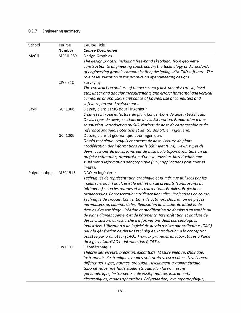
181
8.2.7 Engineering geometry
School Course Number
Course Title Course Description
McGill MECH 289 Design Graphics The design process, including free-hand sketching; from geometry construction to engineering construction; the technology and standards of engineering graphic communication; designing with CAD software. The role of visualization in the production of engineering designs.
CIVE 210 Surveying The construction and use of modern survey instruments; transit, level, etc.; linear and angular measurements and errors; horizontal and vertical curves; error analysis, significance of figures; use of computers and software; recent developments.
Laval GCI 1006 Dessin, plans et SIG pour l'ingénieur Dessin technique et lecture de plan. Conventions du dessin technique. Devis: types de devis, sections de devis. Estimation. Préparation d’une soumission. Introduction au SIG. Notions de base de cartographie et de référence spatiale. Potentiels et limites des SIG en ingénierie.
GCI 1009 Dessin, plans et géomatique pour ingénieurs Dessin technique: croquis et normes de base. Lecture de plans. Modélisation des informations sur le bâtiment (BIM). Devis: types de devis, sections de devis. Principes de base de la topométrie. Gestion de projets: estimation, préparation d’une soumission. Introduction aux systèmes d’information géographique (SIG): applications pratiques et limites.
Polytechnique MEC1515 DAO en ingénierie Techniques de représentation graphique et numérique utilisées par les ingénieurs pour l'analyse et la définition de produits (composants ou bâtiments) selon les normes et les conventions établies. Projections orthogonales. Représentations tridimensionnelles. Projections en coupe. Technique du croquis. Conventions de cotation. Description de pièces normalisées ou commerciales. Réalisation de dessins de détail et de dessins d'assemblage. Création et modification de dessins d'ensemble ou de plans d'aménagement et de bâtiments. Interprétation et analyse de dessins. Lecture et recherche d'informations dans des catalogues industriels. Utilisation d'un logiciel de dessin assisté par ordinateur (DAO) pour la génération de dessins techniques. Introduction à la conception assistée par ordinateur (CAO). Travaux pratiques en laboratoires à l'aide du logiciel AutoCAD et introduction à CATIA.
CIV1101 Géométronique Théorie des erreurs, précision, exactitude. Mesure linéaire, chaînage, instruments électroniques, modes opératoires, corrections. Nivellement différentiel, types, normes, précision. Nivellement trigonométrique topométrique, méthode stadimétrique. Plan laser, mesure goniométrique, instruments à dispositif optique, instruments électroniques, modes opératoires. Polygonation, levé topographique,
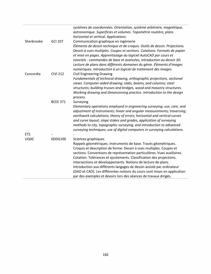
182
systèmes de coordonnées. Orientation, système arbitraire, magnétique, astronomique. Superficies et volumes. Topométrie routière, plans horizontal et vertical. Applications.
Sherbrooke GCI 107 Communication graphique en ingénierie Éléments de dessin technique et de croquis. Outils de dessin. Projections. Dessin à vues multiples. Coupes et sections. Cotations. Formats de papier et mise en pages. Apprentissage du logiciel AutoCAD par cours et tutoriels - commandes de base et avancées, introduction au dessin 3D. Lecture de plans dans différents domaines du génie. Éléments d'images numériques. Introduction à un logiciel de traitement des images.
Concordia CIVI 212 Civil Engineering Drawing Fundamentals of technical drawing, orthographic projections, sectional views. Computer-aided drawing; slabs, beams, and columns; steel structures; building trusses and bridges, wood and masonry structures. Working drawing and dimensioning practice. Introduction to the design process.
BCEE 371 Surveying Elementary operations employed in engineering surveying; use, care, and adjustment of instruments; linear and angular measurements; traversing; earthwork calculations; theory of errors; horizontal and vertical curves and curve layout; slope stakes and grades, application of surveying methods to city, topographic surveying, and introduction to advanced surveying techniques; use of digital computers in surveying calculations.
ÉTS - - UQAC 6DDG100 Sciences graphiques
Rappels géométriques. Instruments de base. Tracés géométriques. Croquis et description de forme. Dessin à vues multiples. Coupes et sections. Conventions de représentation particulières. Vues auxiliaires. Cotation. Tolérances et ajustements. Classification des projections. Intersections et développements. Notions de lecture de plans. Introduction aux différents langages de dessin assisté par ordinateur (DAO et CAO). Les différentes notions du cours sont mises en application par des exemples et devoirs lors des séances de travaux dirigés.
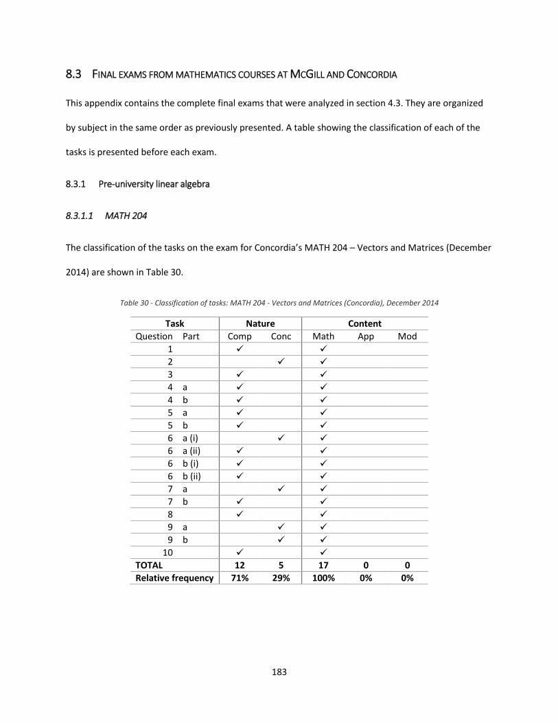
183
8.3 FINAL EXAMS FROM MATHEMATICS COURSES AT MCGILL AND CONCORDIA
This appendix contains the complete final exams that were analyzed in section 4.3. They are organized
by subject in the same order as previously presented. A table showing the classification of each of the
tasks is presented before each exam.
8.3.1 Pre-university linear algebra
8.3.1.1 MATH 204
The classification of the tasks on the exam for Concordia’s MATH 204 – Vectors and Matrices (December
2014) are shown in Table 30.
Table 30 - Classification of tasks: MATH 204 - Vectors and Matrices (Concordia), December 2014
Task Nature Content
Question Part Comp Conc Math App Mod
1
2
3
4 a
4 b
5 a
5 b
6 a (i)
6 a (ii)
6 b (i)
6 b (ii)
7 a
7 b
8
9 a
9 b
10
TOTAL 12 5 17 0 0
Relative frequency 71% 29% 100% 0% 0%
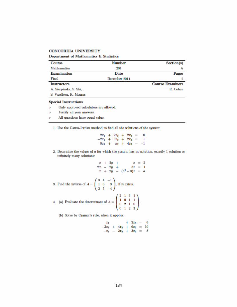
184
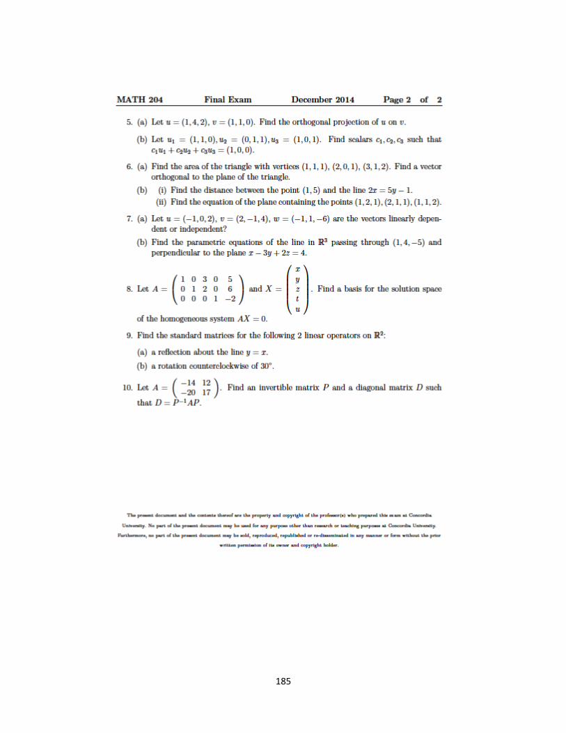
185
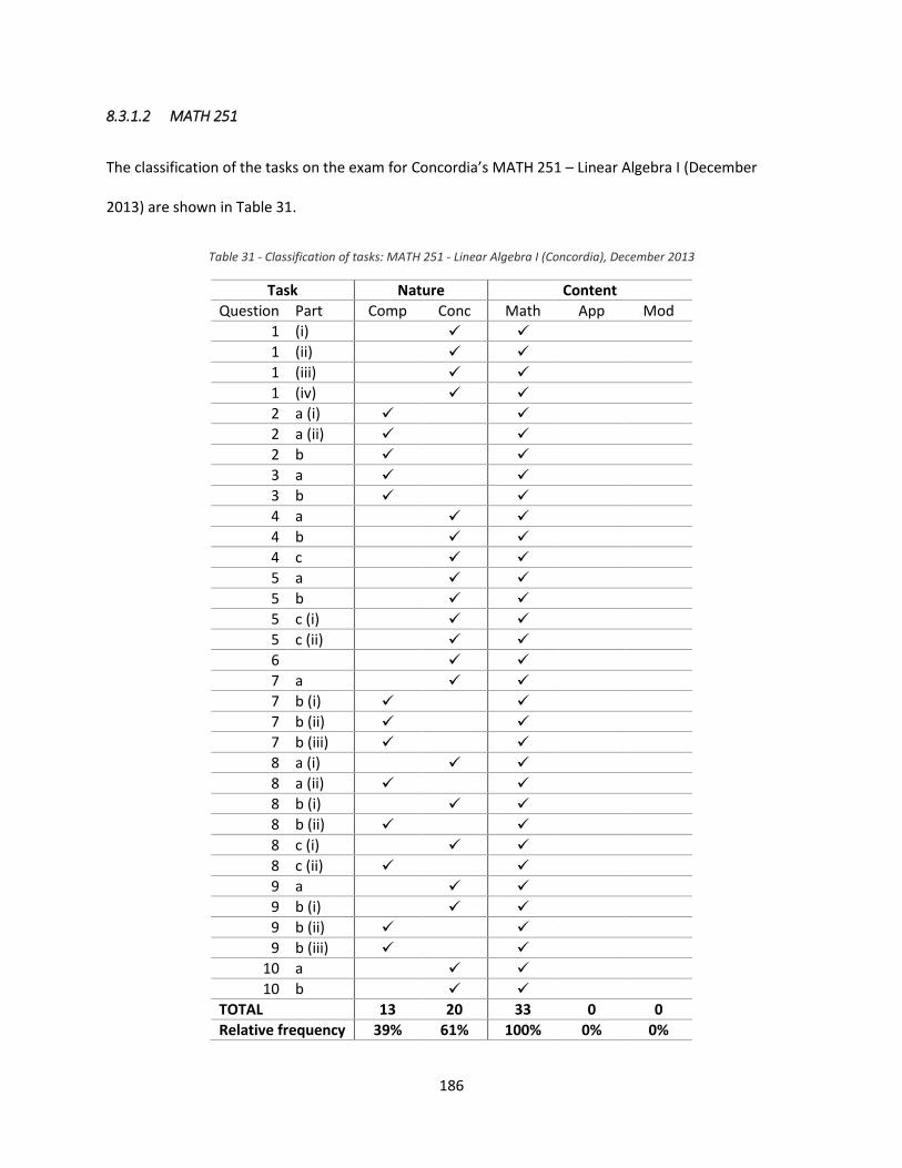
186
8.3.1.2 MATH 251
The classification of the tasks on the exam for Concordia’s MATH 251 – Linear Algebra I (December
2013) are shown in Table 31.
Table 31 - Classification of tasks: MATH 251 - Linear Algebra I (Concordia), December 2013
Task Nature Content
Question Part Comp Conc Math App Mod
1 (i)
1 (ii)
1 (iii)
1 (iv)
2 a (i)
2 a (ii)
2 b
3 a
3 b
4 a
4 b
4 c
5 a
5 b
5 c (i)
5 c (ii)
6
7 a
7 b (i)
7 b (ii)
7 b (iii)
8 a (i)
8 a (ii)
8 b (i)
8 b (ii)
8 c (i)
8 c (ii)
9 a
9 b (i)
9 b (ii)
9 b (iii)
10 a
10 b
TOTAL 13 20 33 0 0
Relative frequency 39% 61% 100% 0% 0%
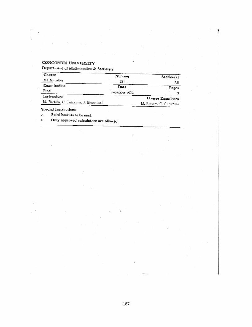
187
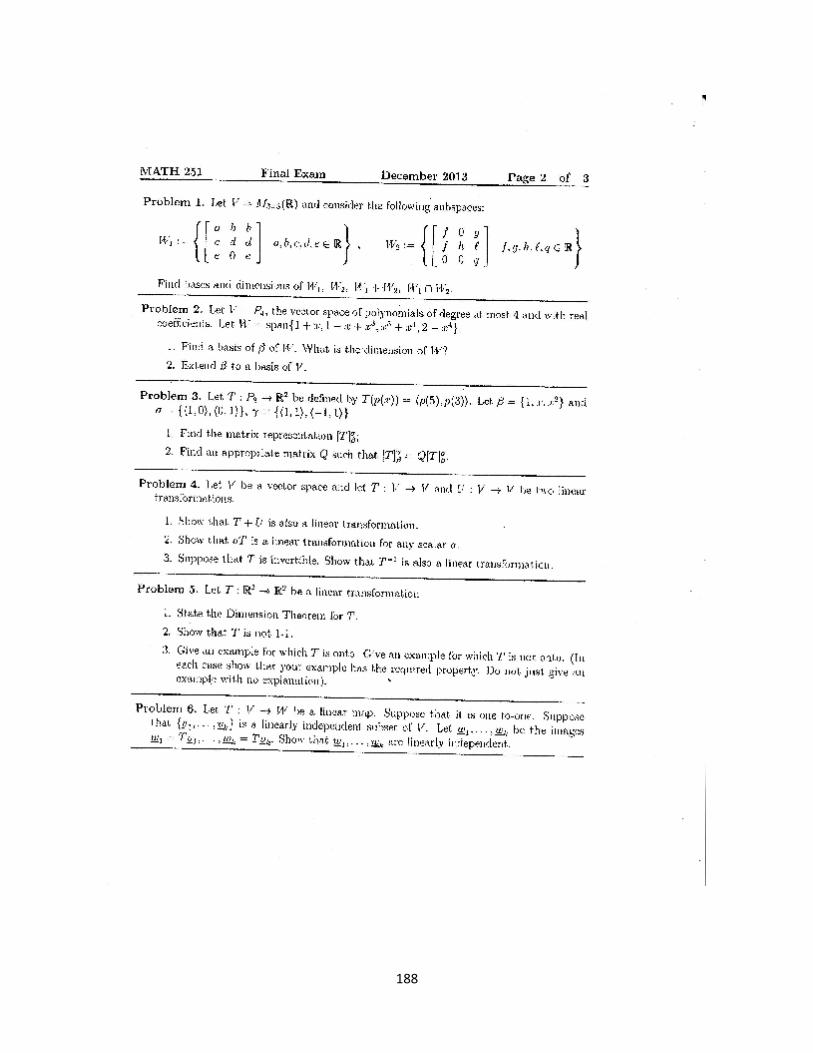
188
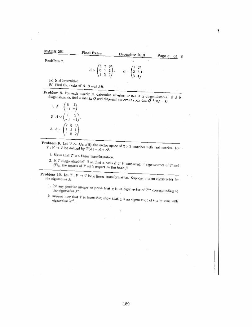
189
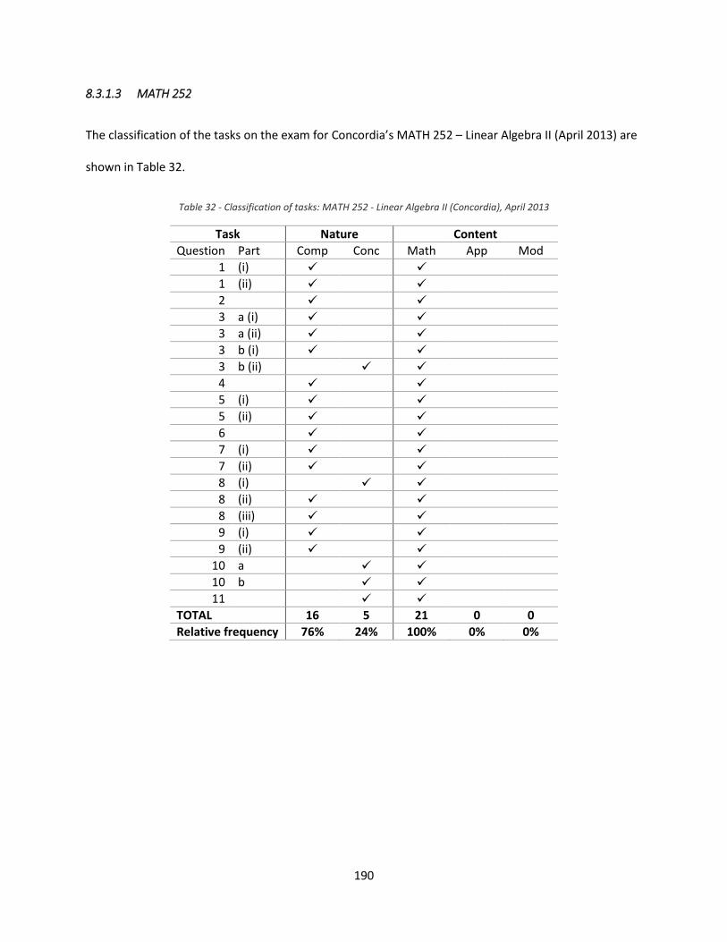
190
8.3.1.3 MATH 252
The classification of the tasks on the exam for Concordia’s MATH 252 – Linear Algebra II (April 2013) are
shown in Table 32.
Table 32 - Classification of tasks: MATH 252 - Linear Algebra II (Concordia), April 2013
Task Nature Content
Question Part Comp Conc Math App Mod
1 (i)
1 (ii)
2
3 a (i)
3 a (ii)
3 b (i)
3 b (ii)
4
5 (i)
5 (ii)
6
7 (i)
7 (ii)
8 (i)
8 (ii)
8 (iii)
9 (i)
9 (ii)
10 a
10 b
11
TOTAL 16 5 21 0 0
Relative frequency 76% 24% 100% 0% 0%
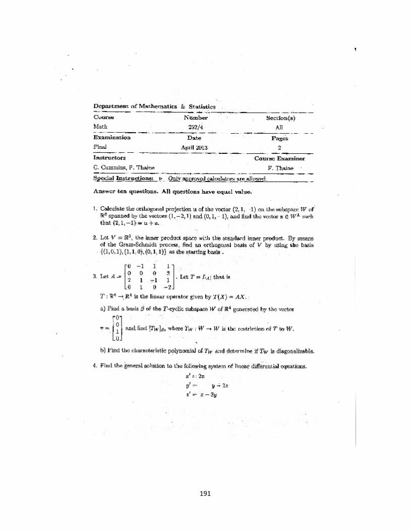
191

192
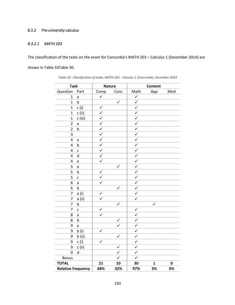
193
8.3.2 Pre-university calculus
8.3.2.1 MATH 203
The classification of the tasks on the exam for Concordia’s MATH 203 – Calculus 1 (December 2014) are
shown in Table 33Table 30.
Table 33 - Classification of tasks: MATH 203 - Calculus 1 (Concordia), December 2014
Task Nature Content
Question Part Comp Conc Math App Mod
1 a
1 b
1 c (i)
1 c (ii)
1 c (iii)
2 a
2 b
3
4 a
4 b
4 c
4 d
4 e
5 a
5 b
5 c
6 a
6 b
7 a (i)
7 a (ii)
7 b
7 c
8 a
8 b
9 a
9 b (i)
9 b (ii)
9 c (i)
9 c (ii)
9 d
Bonus
TOTAL 21 10 30 1 0
Relative frequency 68% 32% 97% 3% 0%
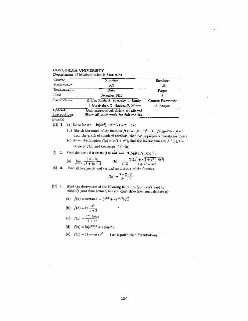
194
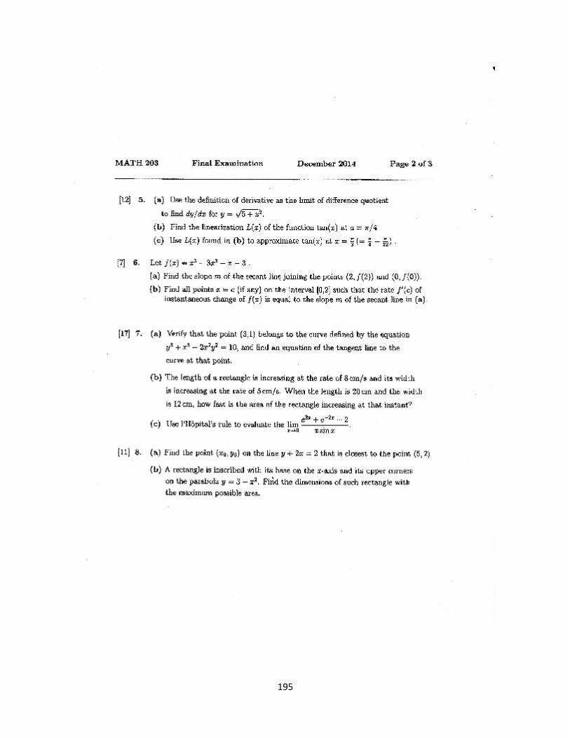
195
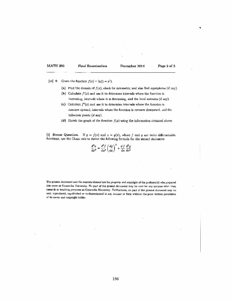
196
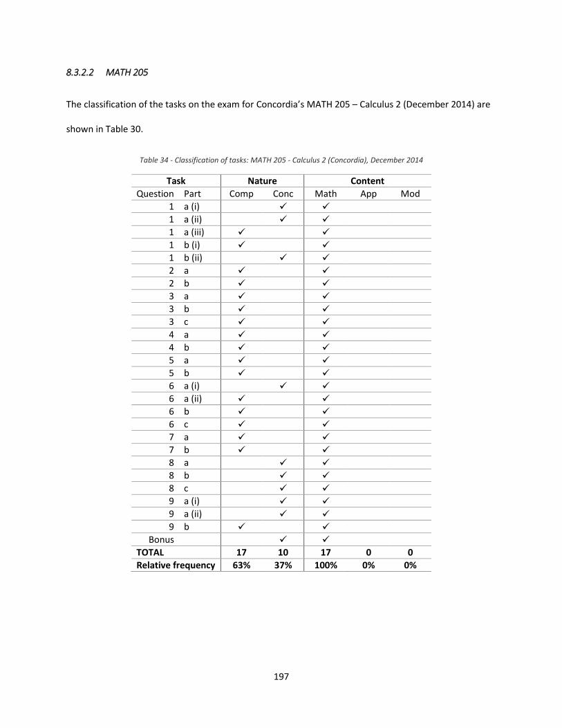
197
8.3.2.2 MATH 205
The classification of the tasks on the exam for Concordia’s MATH 205 – Calculus 2 (December 2014) are
shown in Table 30.
Table 34 - Classification of tasks: MATH 205 - Calculus 2 (Concordia), December 2014
Task Nature Content
Question Part Comp Conc Math App Mod
1 a (i)
1 a (ii)
1 a (iii)
1 b (i)
1 b (ii)
2 a
2 b
3 a
3 b
3 c
4 a
4 b
5 a
5 b
6 a (i)
6 a (ii)
6 b
6 c
7 a
7 b
8 a
8 b
8 c
9 a (i)
9 a (ii)
9 b
Bonus
TOTAL 17 10 17 0 0
Relative frequency 63% 37% 100% 0% 0%
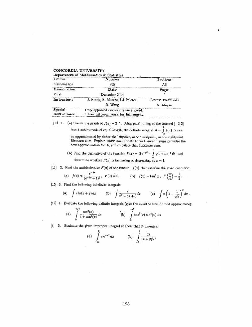
198
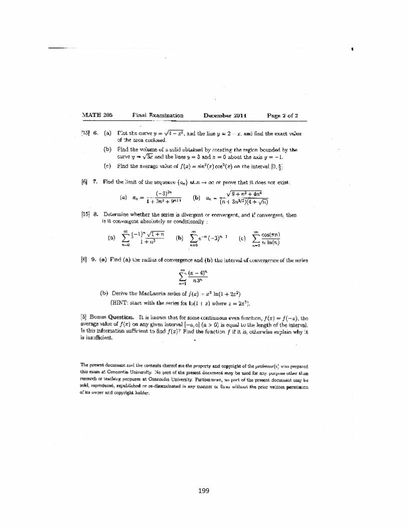
199
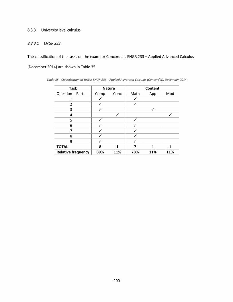
200
8.3.3 University level calculus
8.3.3.1 ENGR 233
The classification of the tasks on the exam for Concordia’s ENGR 233 – Applied Advanced Calculus
(December 2014) are shown in Table 35.
Table 35 - Classification of tasks: ENGR 233 - Applied Advanced Calculus (Concordia), December 2014
Task Nature Content
Question Part Comp Conc Math App Mod
1
2
3
4 5
6
7
8
9
TOTAL 8 1 7 1 1
Relative frequency 89% 11% 78% 11% 11%

201
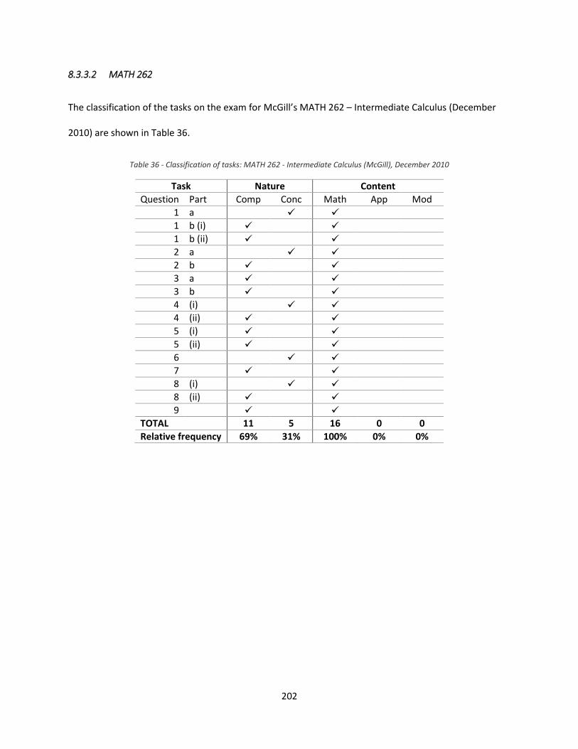
202
8.3.3.2 MATH 262
The classification of the tasks on the exam for McGill’s MATH 262 – Intermediate Calculus (December
2010) are shown in Table 36.
Table 36 - Classification of tasks: MATH 262 - Intermediate Calculus (McGill), December 2010
Task Nature Content
Question Part Comp Conc Math App Mod
1 a
1 b (i)
1 b (ii)
2 a
2 b
3 a
3 b
4 (i)
4 (ii)
5 (i)
5 (ii)
6
7
8 (i)
8 (ii)
9
TOTAL 11 5 16 0 0
Relative frequency 69% 31% 100% 0% 0%
203
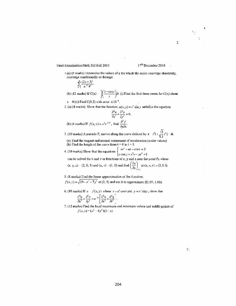
204
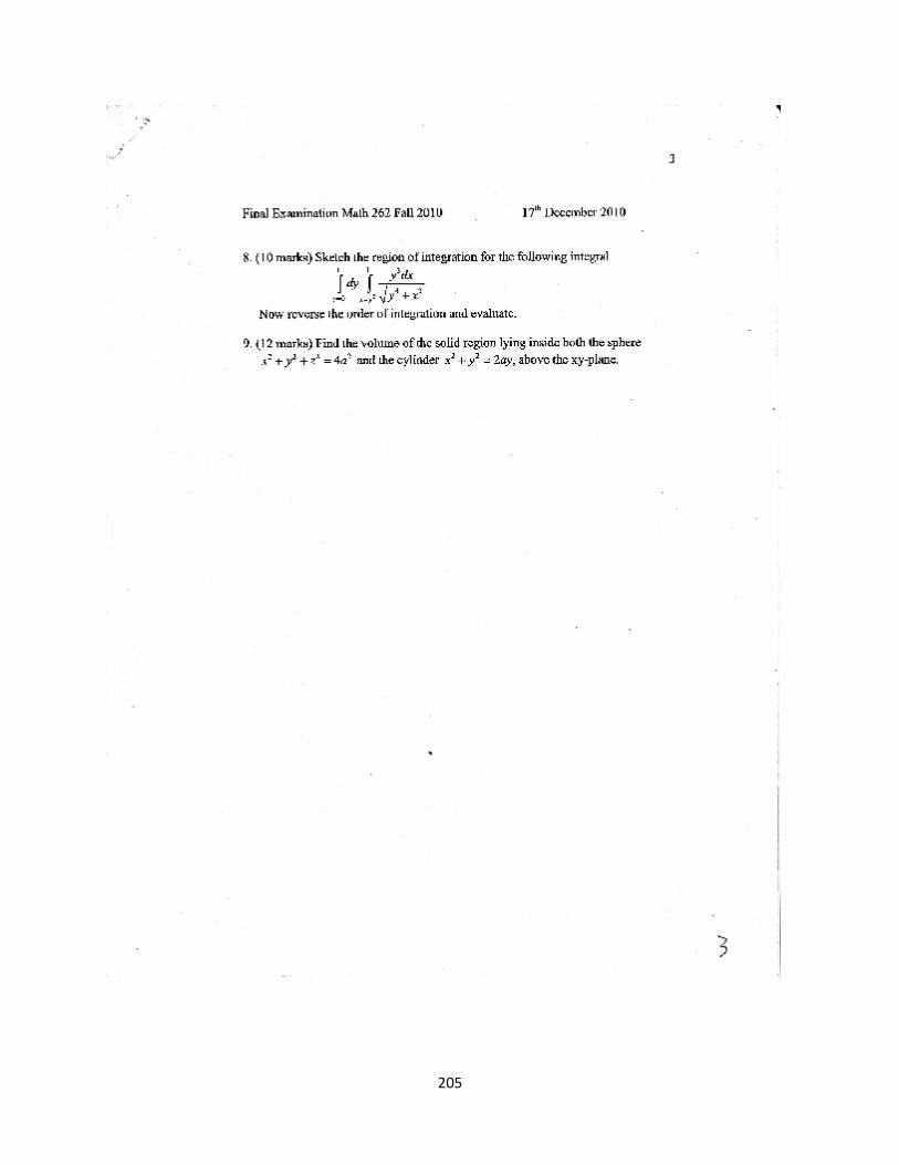
205
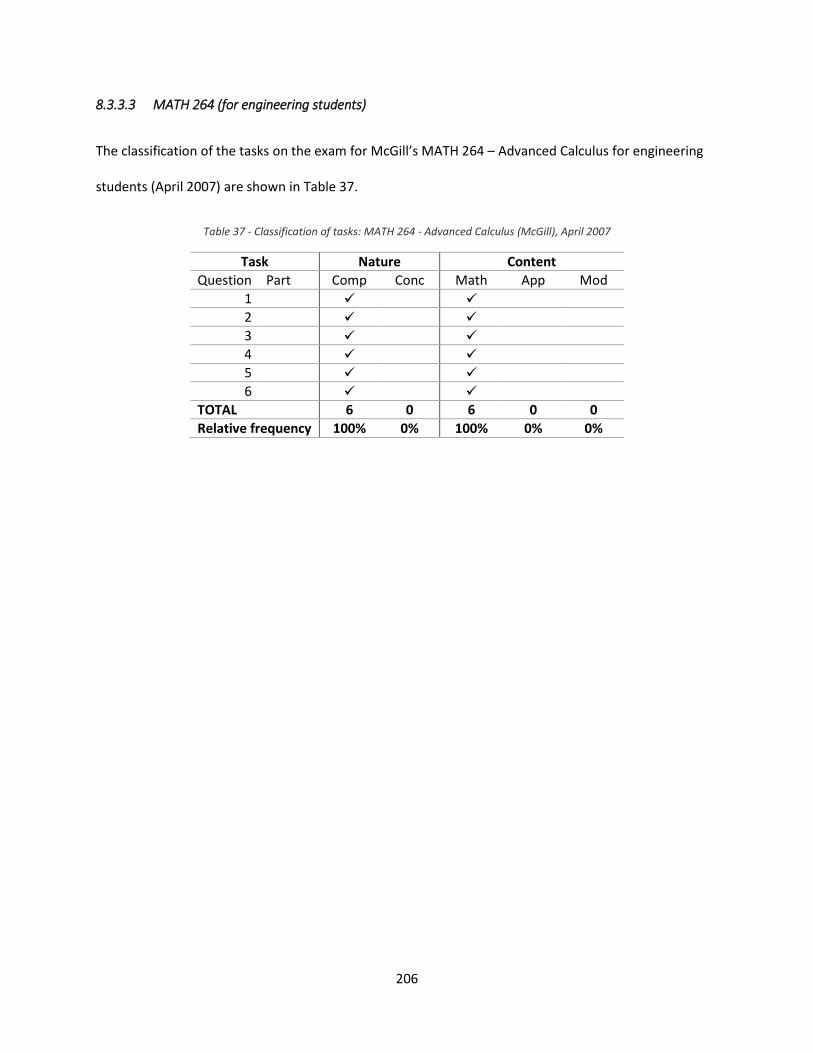
206
8.3.3.3 MATH 264 (for engineering students)
The classification of the tasks on the exam for McGill’s MATH 264 – Advanced Calculus for engineering
students (April 2007) are shown in Table 37.
Table 37 - Classification of tasks: MATH 264 - Advanced Calculus (McGill), April 2007
Task Nature Content
Question Part Comp Conc Math App Mod
1
2
3
4
5
6
TOTAL 6 0 6 0 0
Relative frequency 100% 0% 100% 0% 0%
207
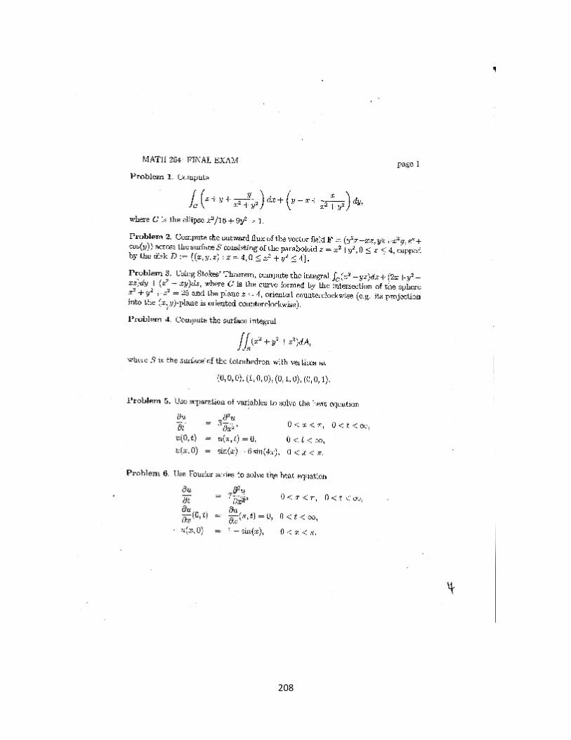
208
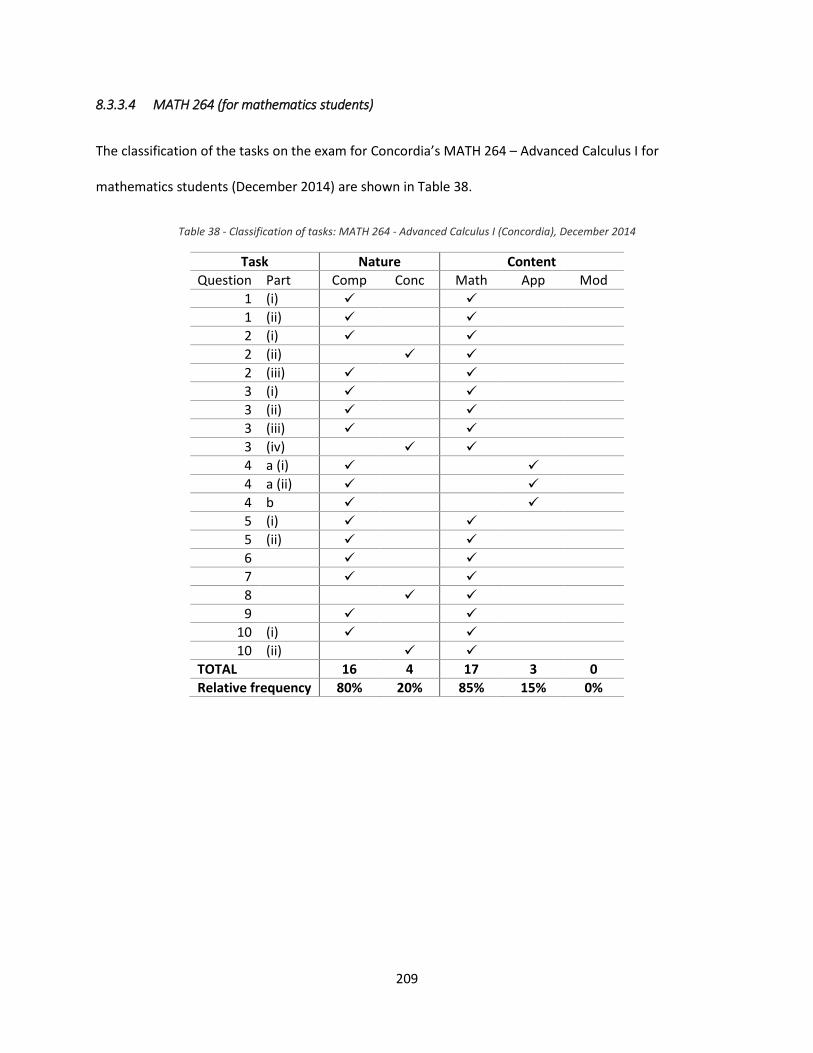
209
8.3.3.4 MATH 264 (for mathematics students)
The classification of the tasks on the exam for Concordia’s MATH 264 – Advanced Calculus I for
mathematics students (December 2014) are shown in Table 38.
Table 38 - Classification of tasks: MATH 264 - Advanced Calculus I (Concordia), December 2014
Task Nature Content
Question Part Comp Conc Math App Mod
1 (i)
1 (ii)
2 (i)
2 (ii)
2 (iii)
3 (i)
3 (ii)
3 (iii)
3 (iv)
4 a (i)
4 a (ii)
4 b
5 (i)
5 (ii)
6
7
8
9
10 (i)
10 (ii)
TOTAL 16 4 17 3 0
Relative frequency 80% 20% 85% 15% 0%
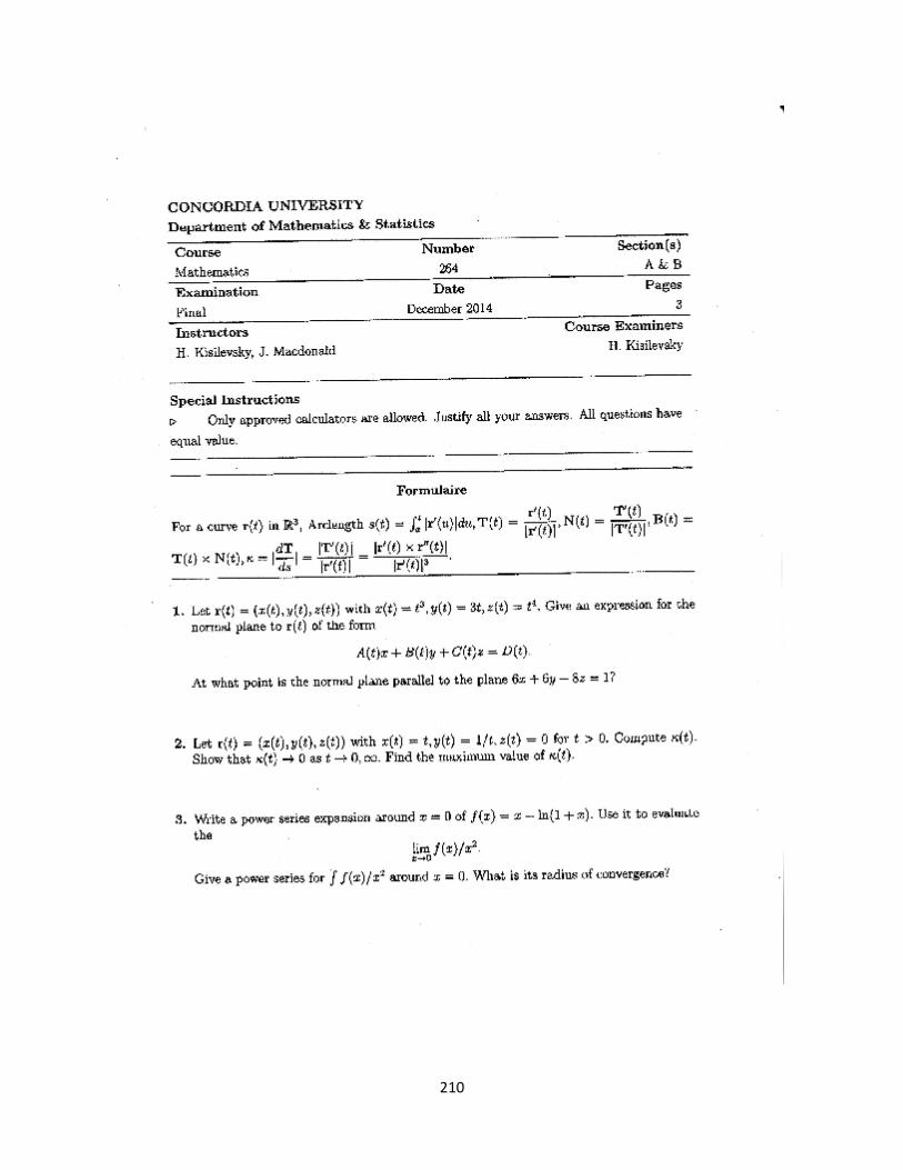
210
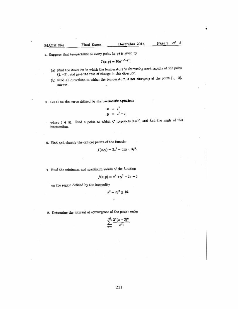
211
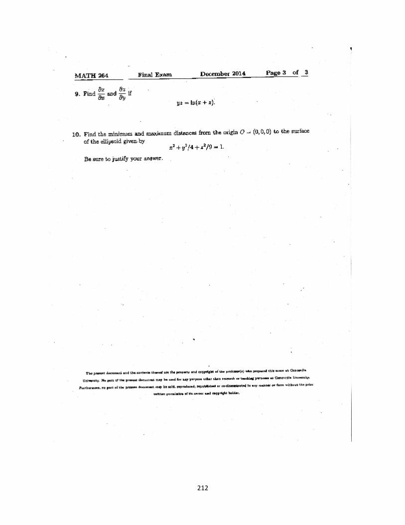
212
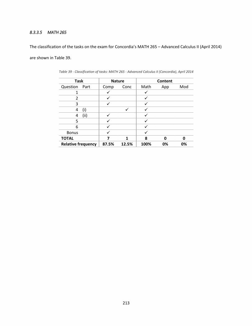
213
8.3.3.5 MATH 265
The classification of the tasks on the exam for Concordia’s MATH 265 – Advanced Calculus II (April 2014)
are shown in Table 39.
Table 39 - Classification of tasks: MATH 265 - Advanced Calculus II (Concordia), April 2014
Task Nature Content
Question Part Comp Conc Math App Mod
1
2
3
4 (i)
4 (ii)
5
6
Bonus
TOTAL 7 1 8 0 0
Relative frequency 87.5% 12.5% 100% 0% 0%
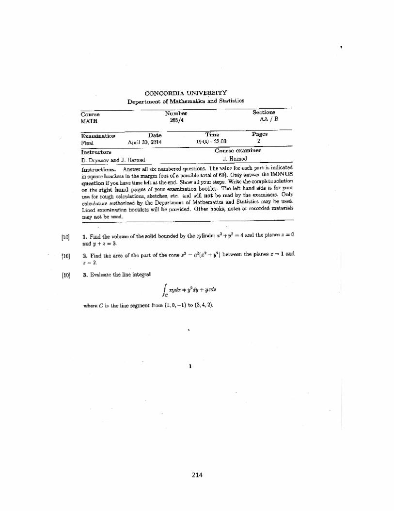
214
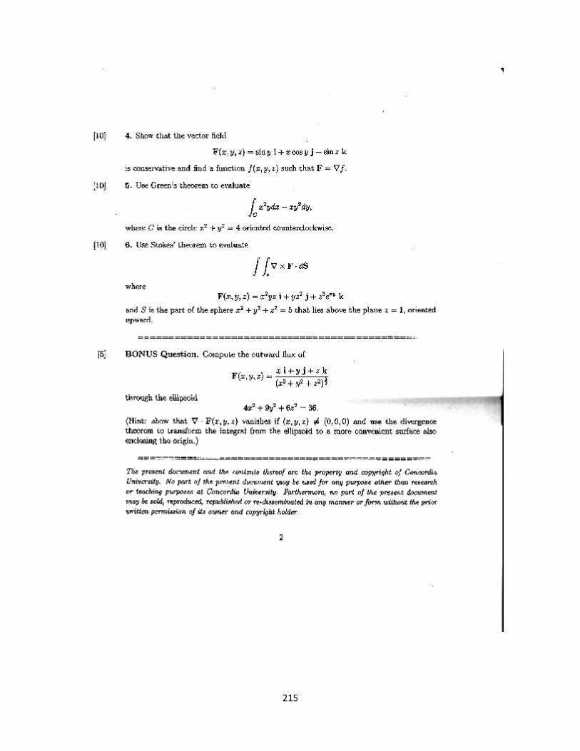
215
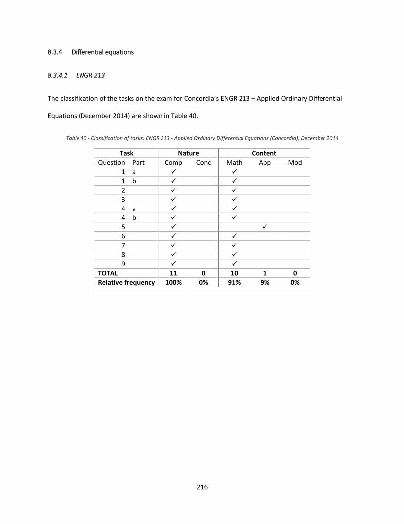
216
8.3.4 Differential equations
8.3.4.1 ENGR 213
The classification of the tasks on the exam for Concordia’s ENGR 213 – Applied Ordinary Differential
Equations (December 2014) are shown in Table 40.
Table 40 - Classification of tasks: ENGR 213 - Applied Ordinary Differential Equations (Concordia), December 2014
Task Nature Content
Question Part Comp Conc Math App Mod
1 a
1 b
2
3
4 a
4 b
5
6
7
8
9
TOTAL 11 0 10 1 0
Relative frequency 100% 0% 91% 9% 0%
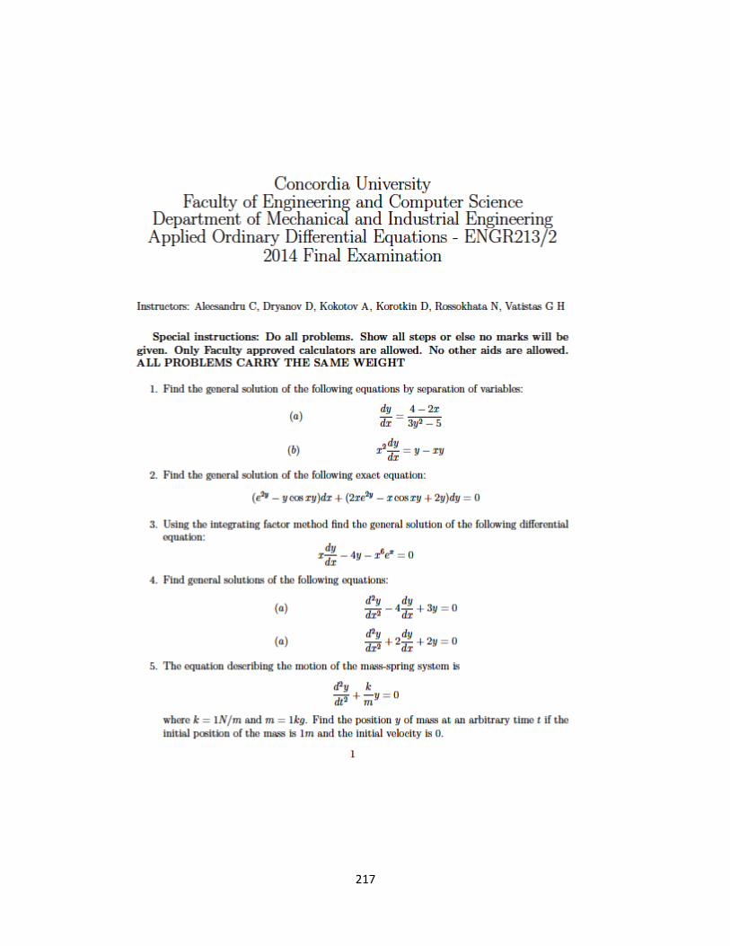
217
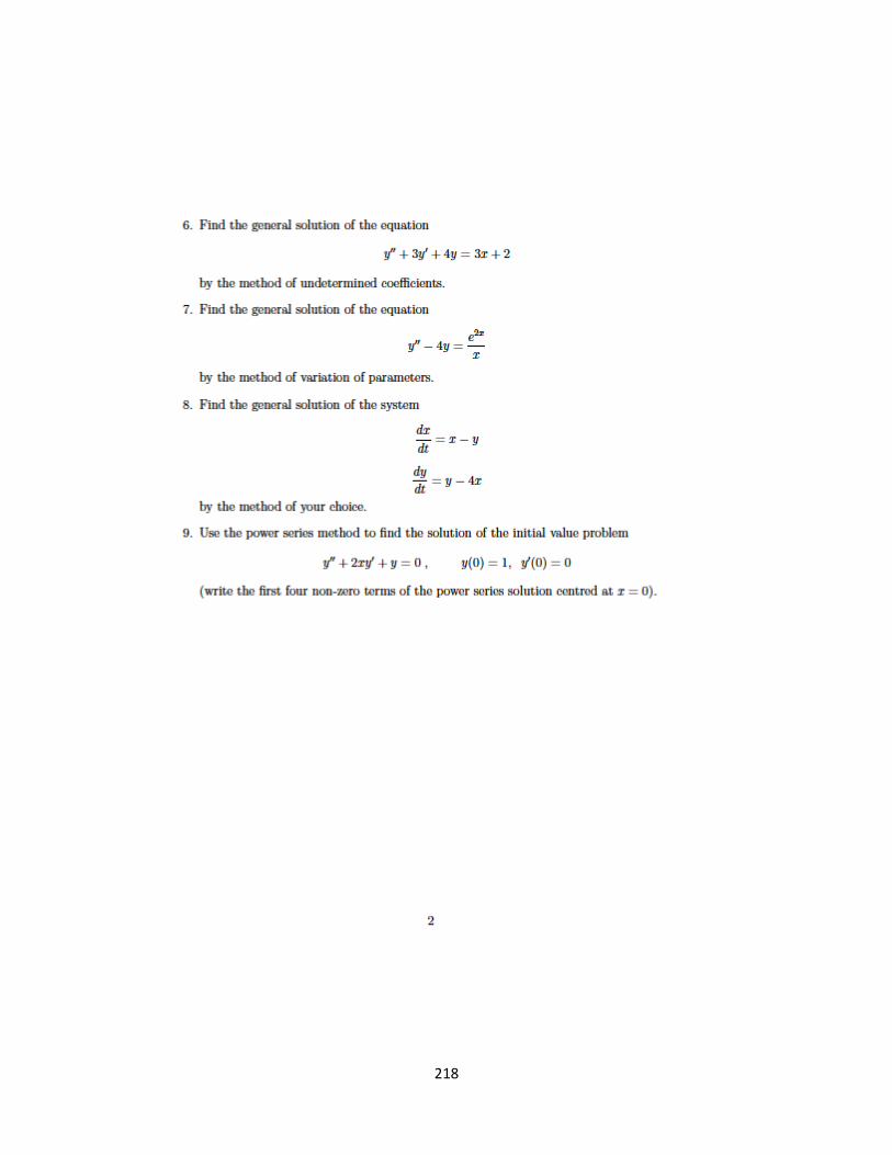
218
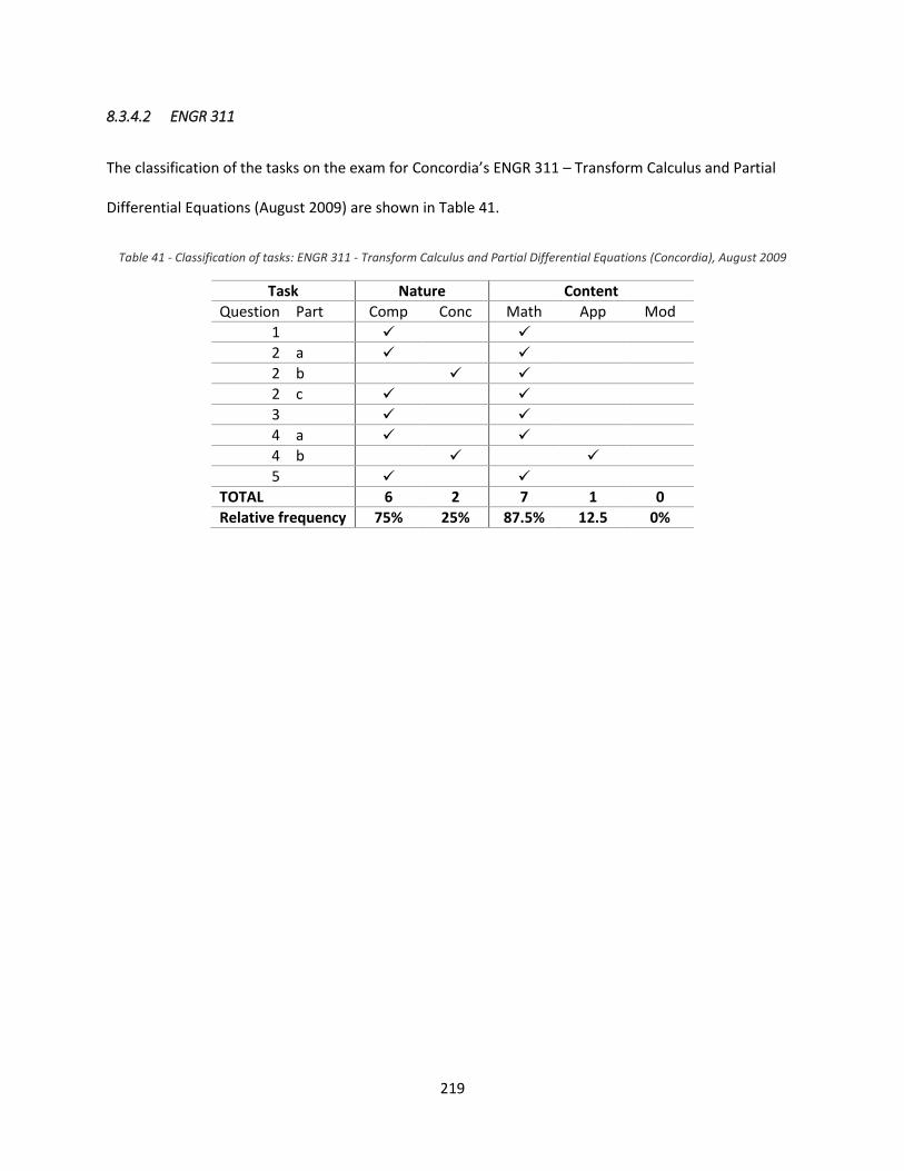
219
8.3.4.2 ENGR 311
The classification of the tasks on the exam for Concordia’s ENGR 311 – Transform Calculus and Partial
Differential Equations (August 2009) are shown in Table 41.
Table 41 - Classification of tasks: ENGR 311 - Transform Calculus and Partial Differential Equations (Concordia), August 2009
Task Nature Content
Question Part Comp Conc Math App Mod
1
2 a
2 b
2 c
3
4 a
4 b
5
TOTAL 6 2 7 1 0
Relative frequency 75% 25% 87.5% 12.5 0%
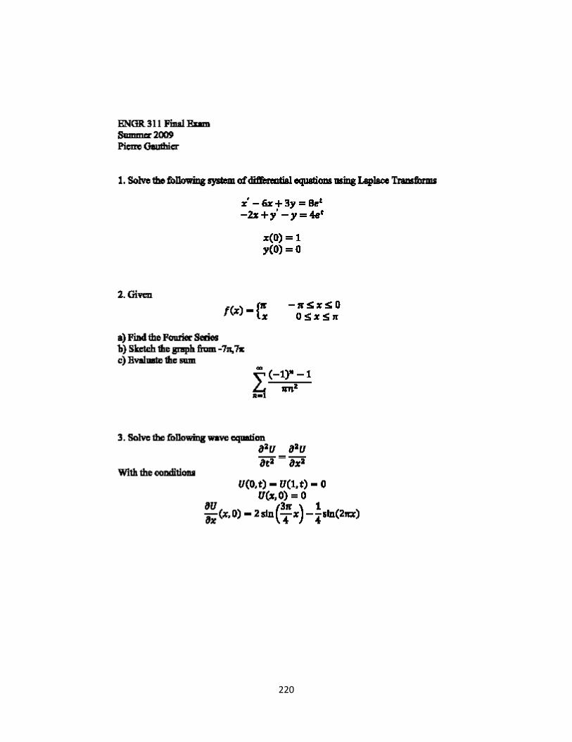
220
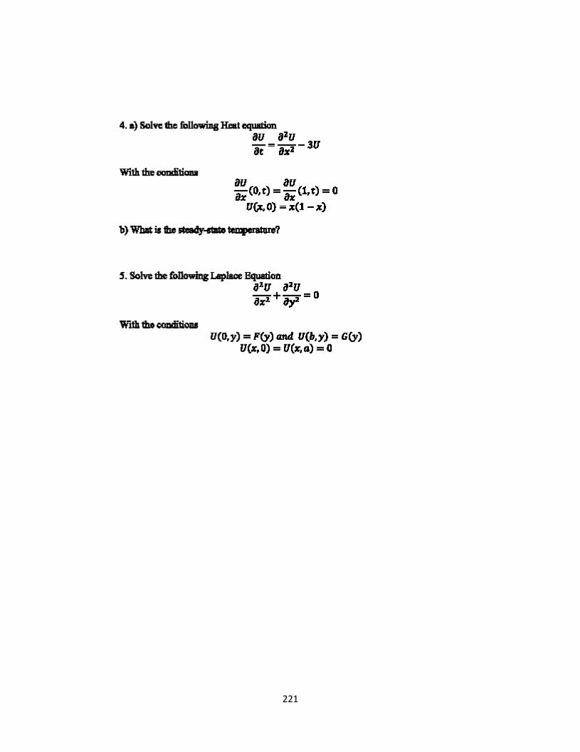
221
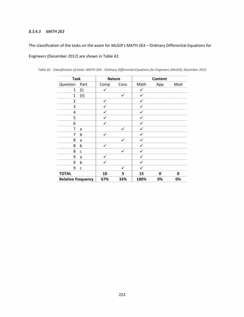
222
8.3.4.3 MATH 263
The classification of the tasks on the exam for McGill’s MATH 263 – Ordinary Differential Equations for
Engineers (December 2012) are shown in Table 42.
Table 42 - Classification of tasks: MATH 263 - Ordinary Differential Equations for Engineers (McGill), December 2012
Task Nature Content
Question Part Comp Conc Math App Mod
1 (i)
1 (ii)
2
3
4
5
6
7 a
7 b
8 a
8 b
8 c
9 a
9 b
9 c
TOTAL 10 5 15 0 0
Relative frequency 67% 33% 100% 0% 0%
223
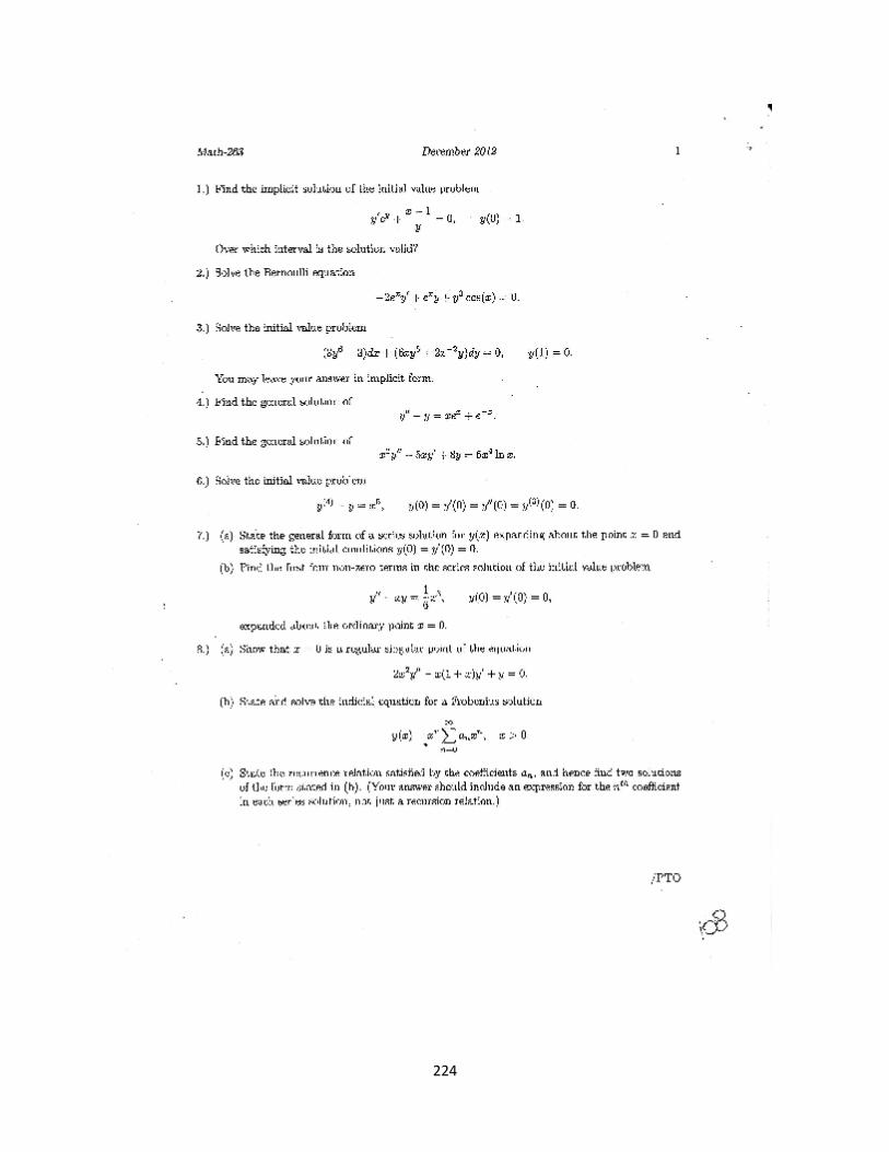
224
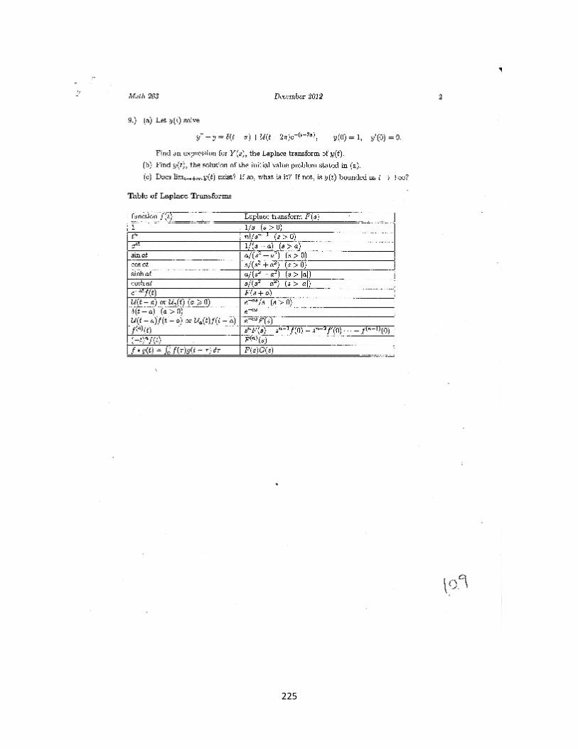
225
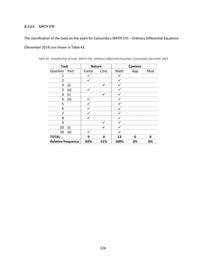
226
8.3.4.4 MATH 370
The classification of the tasks on the exam for Concordia’s MATH 370 – Ordinary Differential Equations
(December 2014) are shown in Table 43.
Table 43 - Classification of tasks: MATH 370 - Ordinary Differential Equations (Concordia), December 2014
Task Nature Content
Question Part Comp Conc Math App Mod
1
2
3 (i)
3 (ii)
4 (i)
4 (ii)
5
6
7
8
9
10 (i)
10 (ii)
TOTAL 9 4 13 0 0
Relative frequency 69% 31% 100% 0% 0%
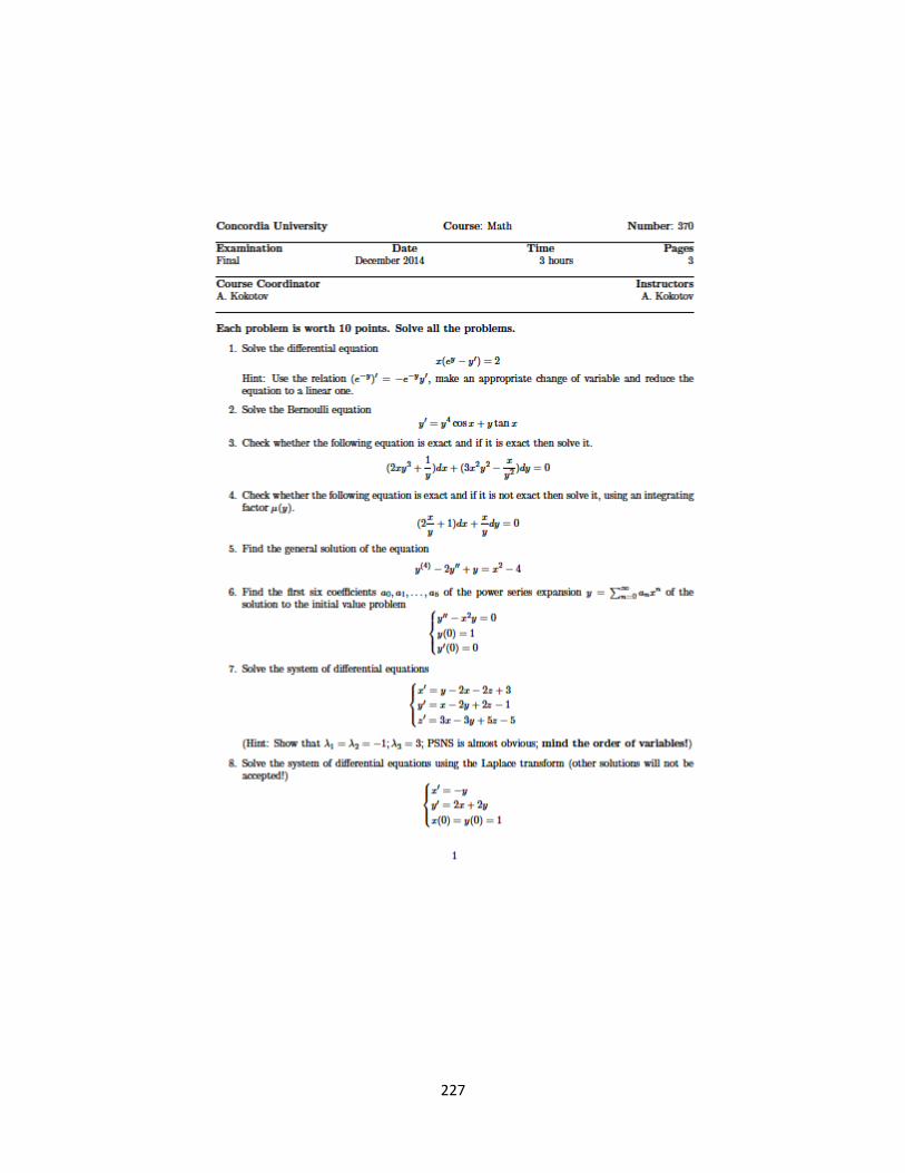
227
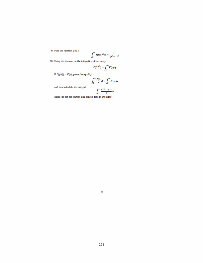
228
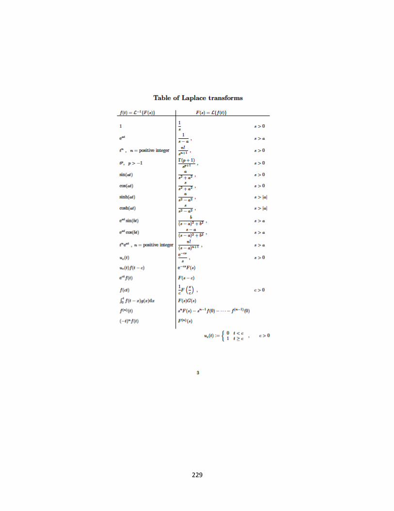
229
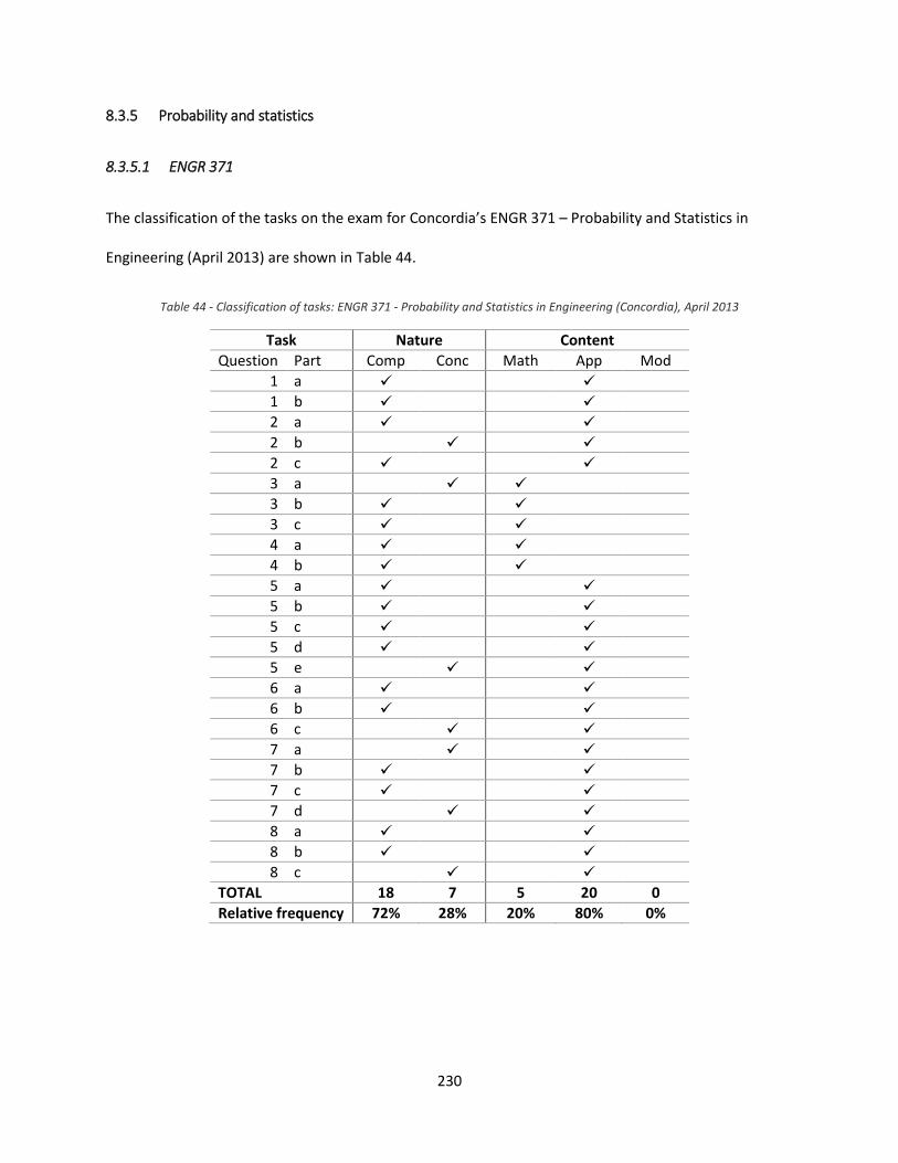
230
8.3.5 Probability and statistics
8.3.5.1 ENGR 371
The classification of the tasks on the exam for Concordia’s ENGR 371 – Probability and Statistics in
Engineering (April 2013) are shown in Table 44.
Table 44 - Classification of tasks: ENGR 371 - Probability and Statistics in Engineering (Concordia), April 2013
Task Nature Content
Question Part Comp Conc Math App Mod
1 a
1 b
2 a
2 b
2 c
3 a
3 b
3 c
4 a
4 b
5 a
5 b
5 c
5 d
5 e
6 a
6 b
6 c
7 a
7 b
7 c
7 d
8 a
8 b
8 c
TOTAL 18 7 5 20 0
Relative frequency 72% 28% 20% 80% 0%
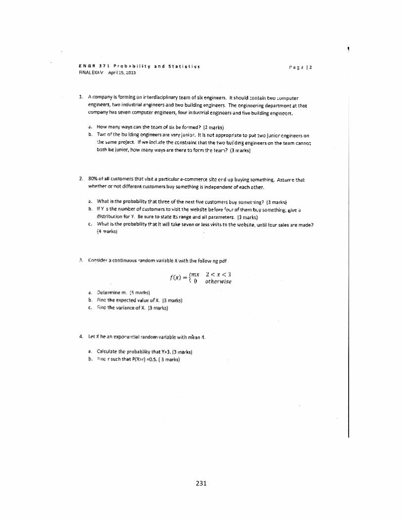
231
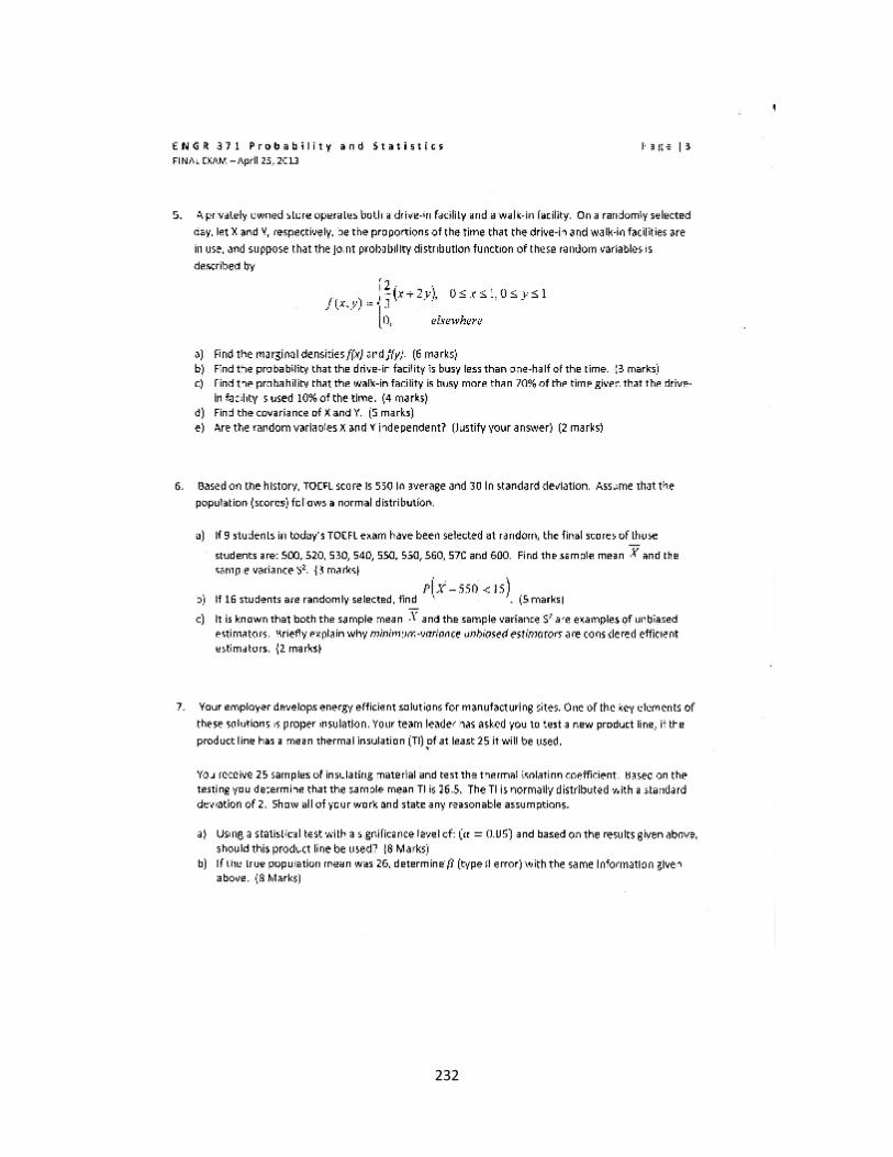
232
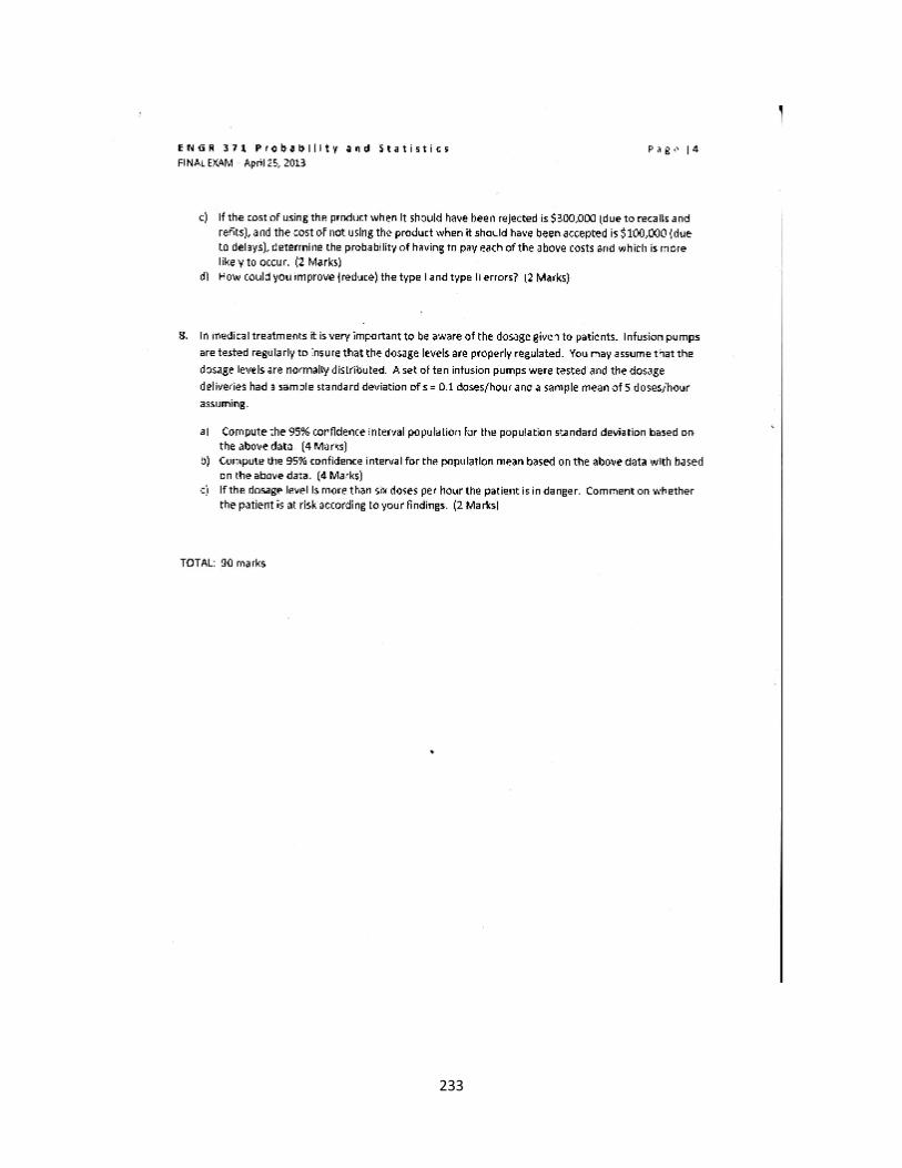
233
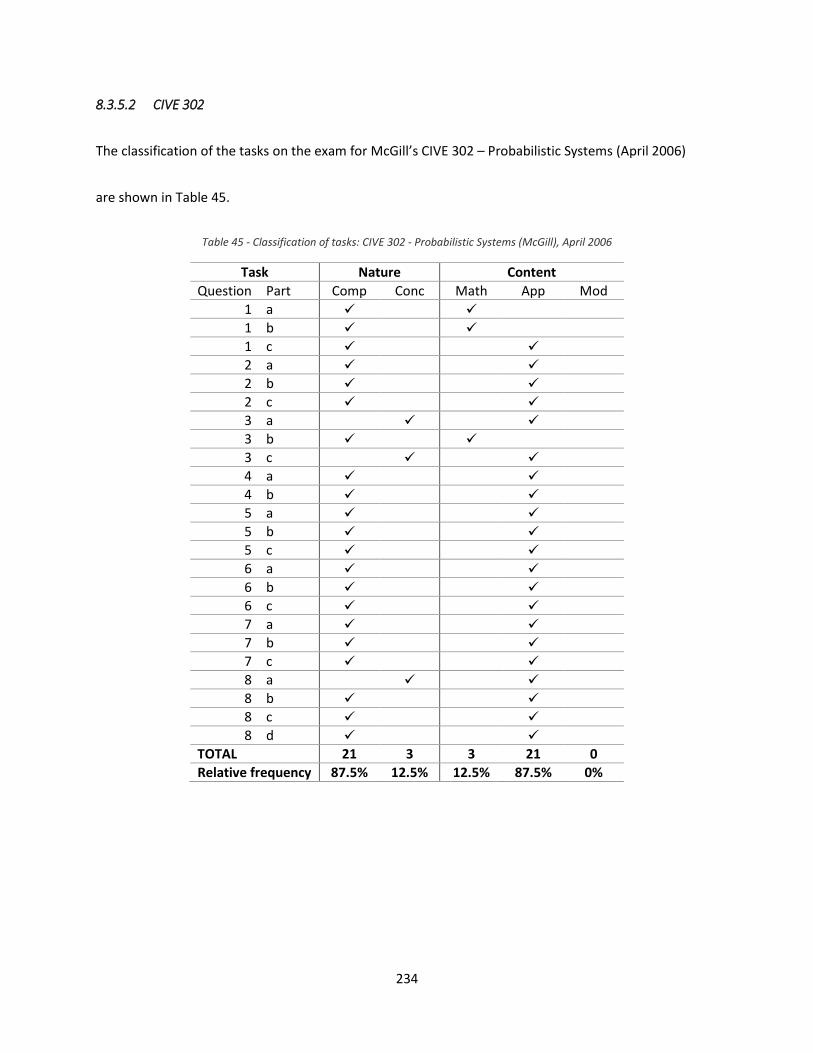
234
8.3.5.2 CIVE 302
The classification of the tasks on the exam for McGill’s CIVE 302 – Probabilistic Systems (April 2006)
are shown in Table 45.
Table 45 - Classification of tasks: CIVE 302 - Probabilistic Systems (McGill), April 2006
Task Nature Content
Question Part Comp Conc Math App Mod
1 a
1 b
1 c
2 a
2 b
2 c
3 a
3 b
3 c
4 a
4 b
5 a
5 b
5 c
6 a
6 b
6 c
7 a
7 b
7 c
8 a
8 b
8 c
8 d
TOTAL 21 3 3 21 0
Relative frequency 87.5% 12.5% 12.5% 87.5% 0%
235
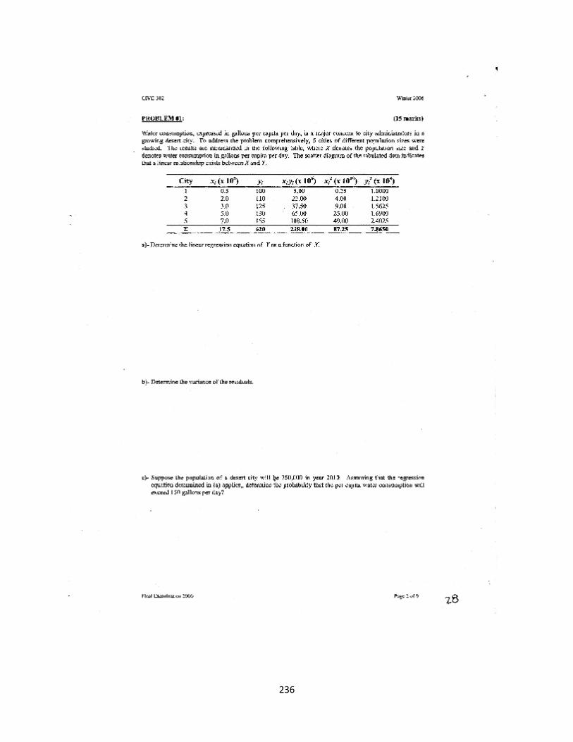
236

237

238

239

240
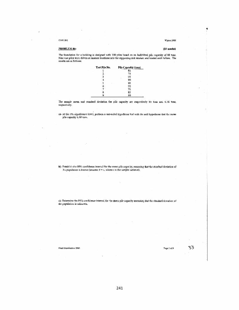
241

242
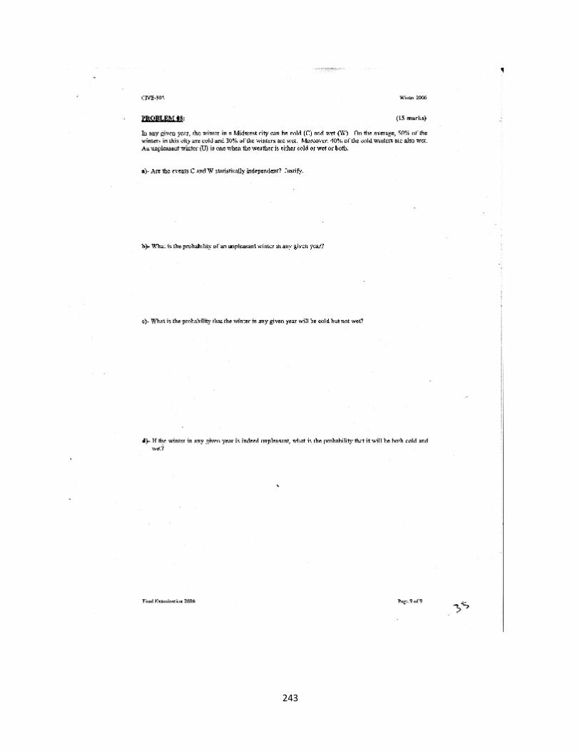
243
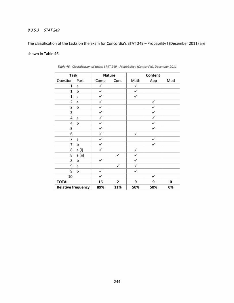
244
8.3.5.3 STAT 249
The classification of the tasks on the exam for Concordia’s STAT 249 – Probability I (December 2011) are
shown in Table 46.
Table 46 - Classification of tasks: STAT 249 - Probability I (Concordia), December 2011
Task Nature Content
Question Part Comp Conc Math App Mod
1 a
1 b
1 c
2 a
2 b
3
4 a
4 b
5
6
7 a
7 b
8 a (i)
8 a (ii)
8 b
9 a
9 b
10
TOTAL 16 2 9 9 0
Relative frequency 89% 11% 50% 50% 0%
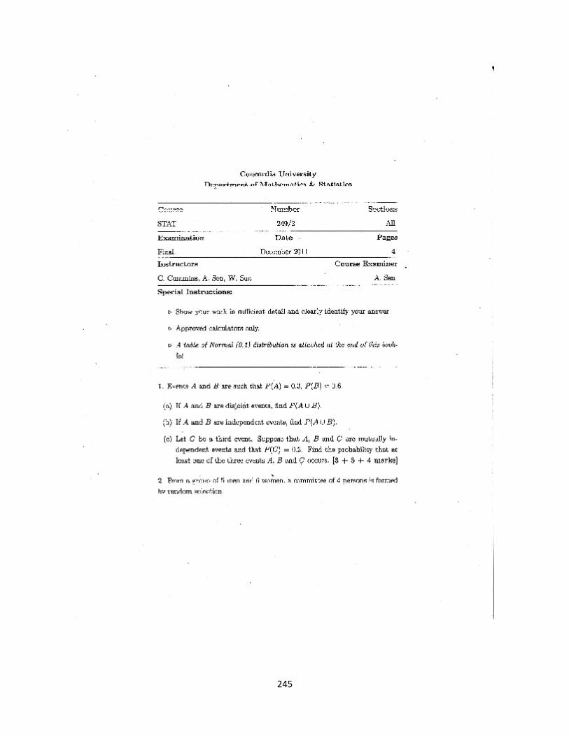
245
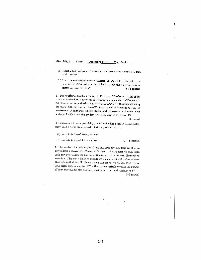
246
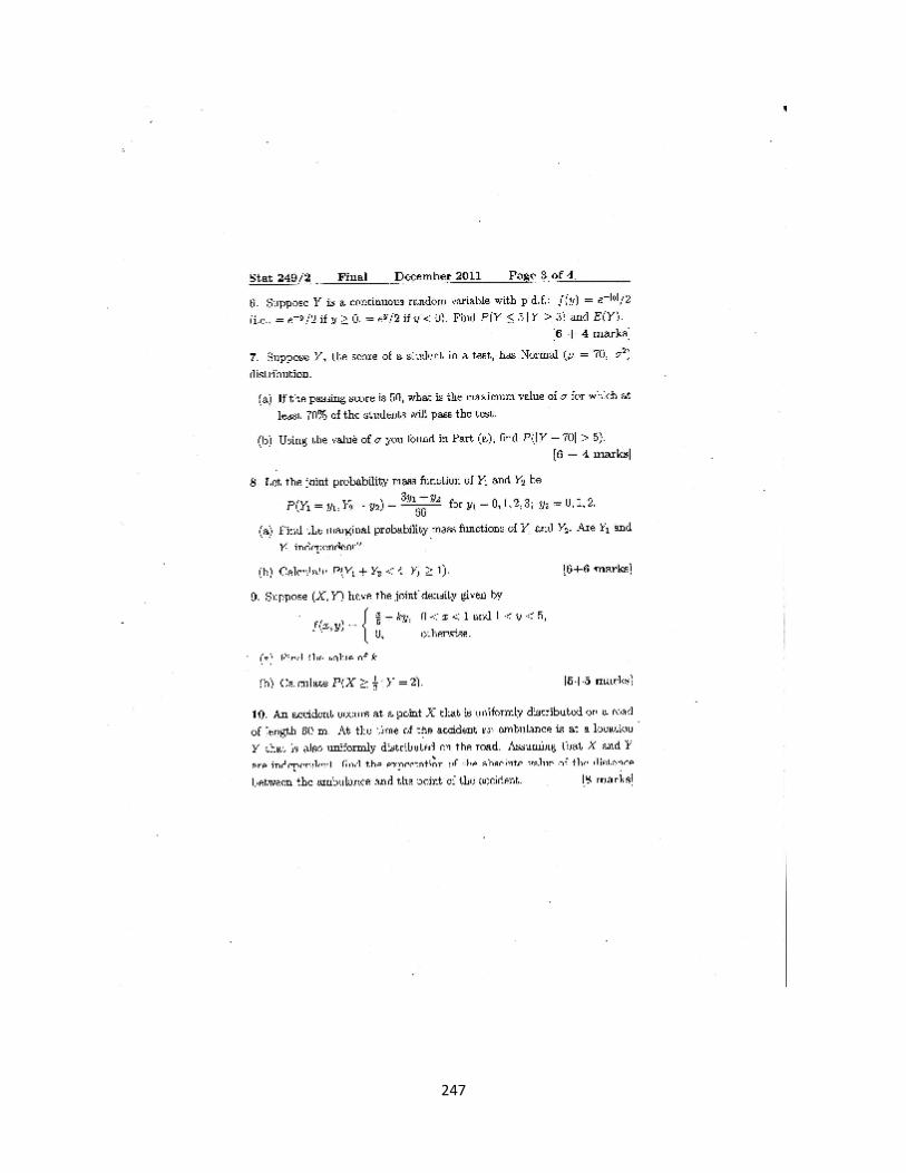
247
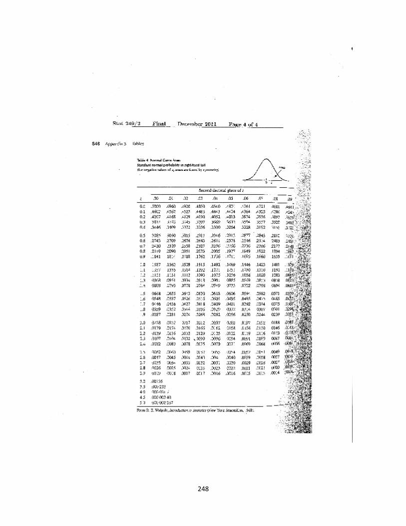
248
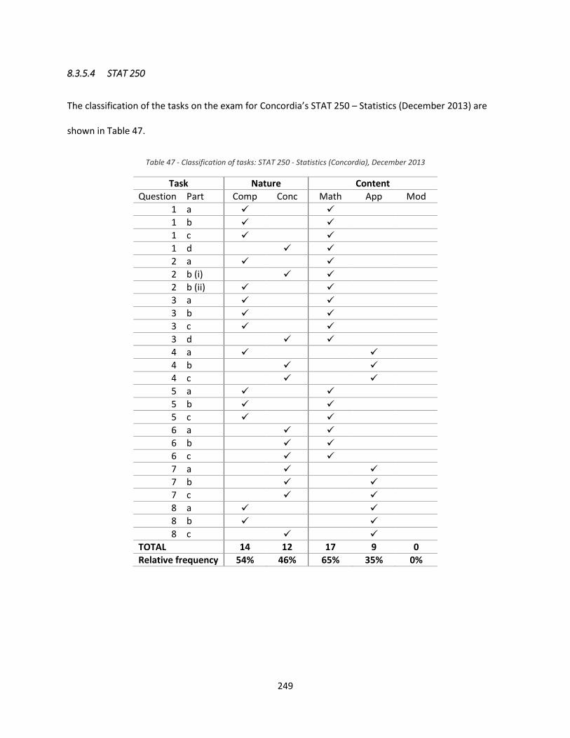
249
8.3.5.4 STAT 250
The classification of the tasks on the exam for Concordia’s STAT 250 – Statistics (December 2013) are
shown in Table 47.
Table 47 - Classification of tasks: STAT 250 - Statistics (Concordia), December 2013
Task Nature Content
Question Part Comp Conc Math App Mod
1 a
1 b
1 c
1 d
2 a
2 b (i)
2 b (ii)
3 a
3 b
3 c
3 d
4 a
4 b
4 c
5 a
5 b
5 c
6 a
6 b
6 c
7 a
7 b
7 c
8 a
8 b
8 c
TOTAL 14 12 17 9 0
Relative frequency 54% 46% 65% 35% 0%
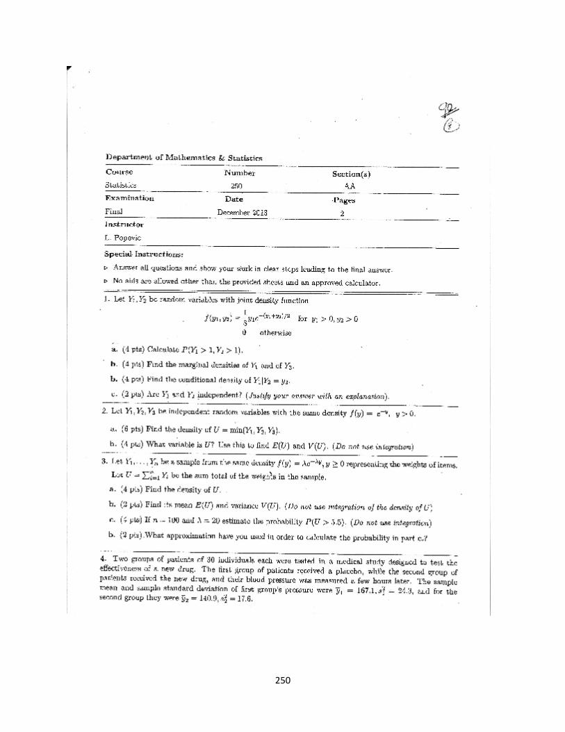
250

251

252
8.3.6 Numerical methods
8.3.6.1 ENGR 391
The classification of the tasks on the exam for Concordia’s ENGR 391 – Numerical Methods in
Engineering (December 2013) are shown in Table 48.
Table 48 - Classification of tasks: ENGR 391 - Numerical Methods in Engineering (Concordia), December 2013
Task Nature Content
Question Part Comp Conc Math App Mod
1 a
1 b
2 a (i)
2 a (ii)
2 b (i)
2 b (ii)
3 a
3 b
4 a (i)
4 a (ii)
4 a (iii)
4 a (iv)
4 b (i)
4 b (ii)
5 a
5 b
TOTAL 16 20 14 2 0
Relative frequency 100% 0% 87.5% 12.5% 0%

253

254
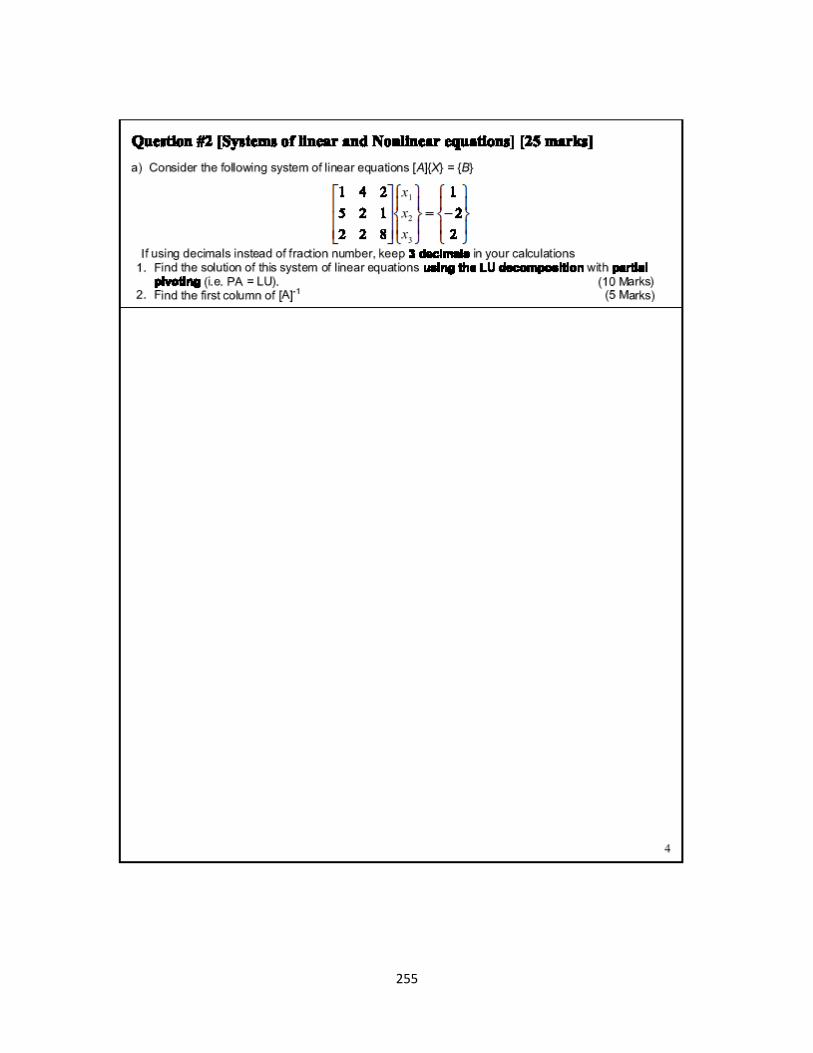
255
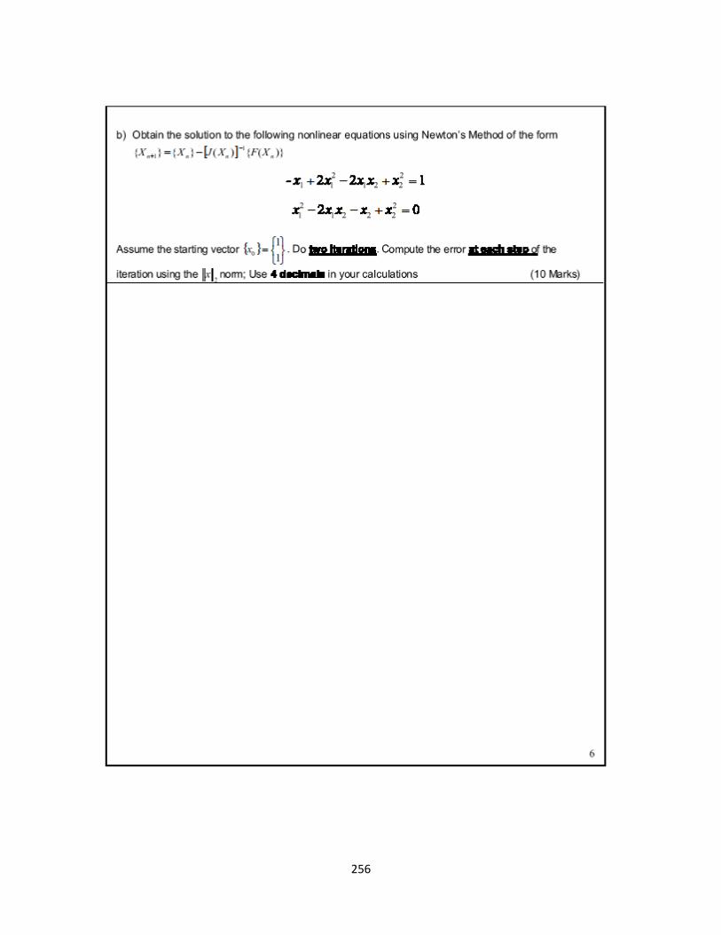
256
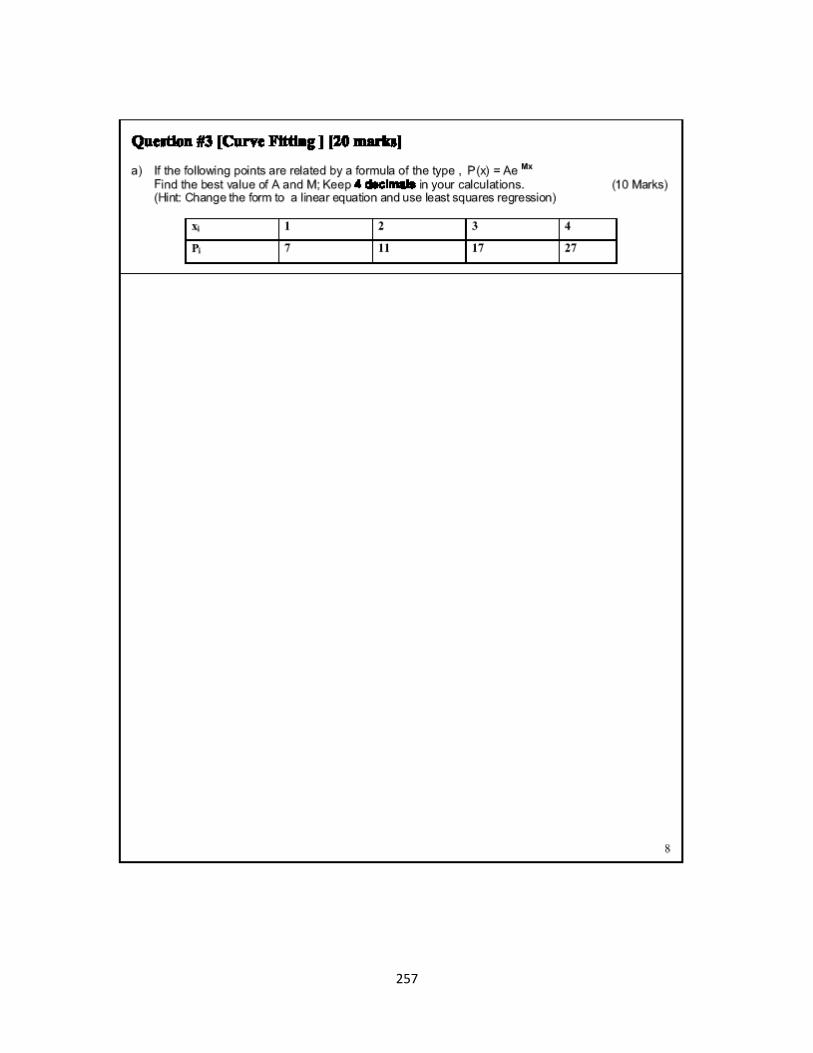
257

258
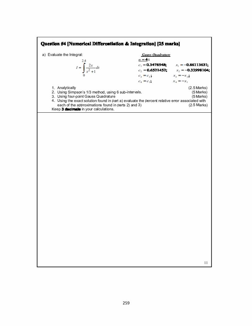
259
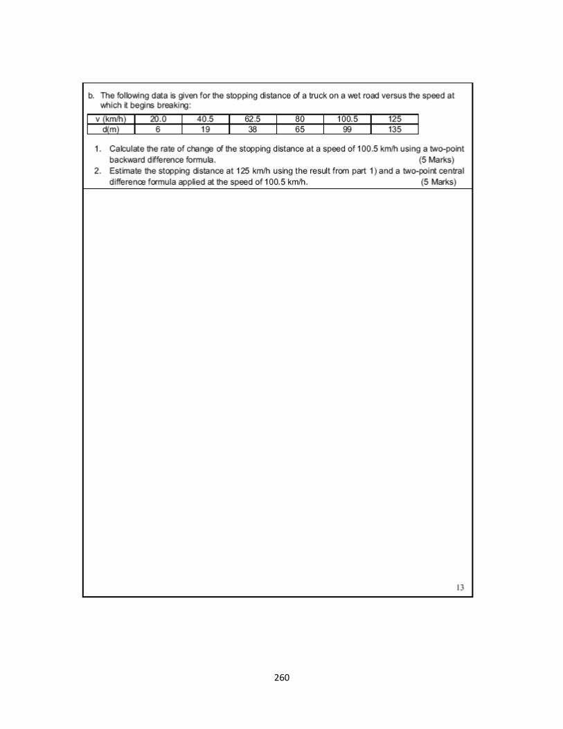
260
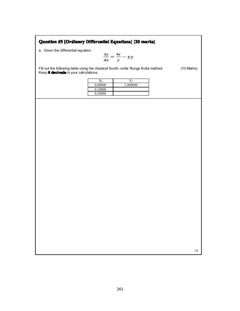
261

262
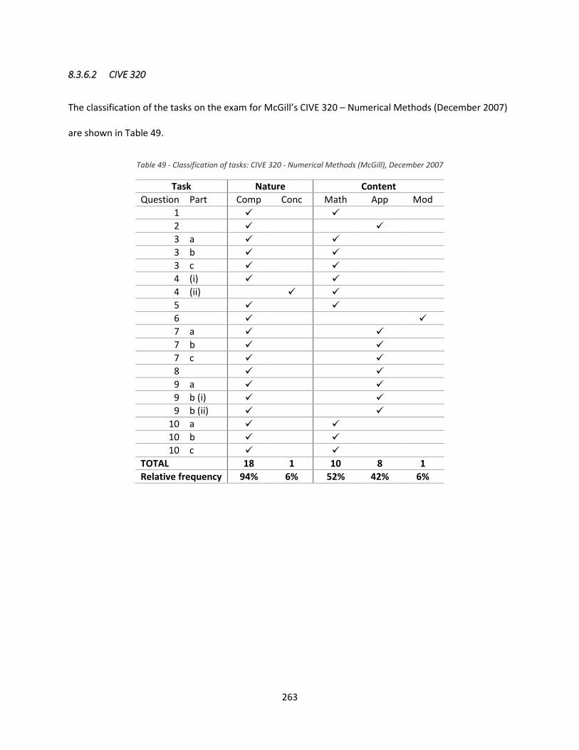
263
8.3.6.2 CIVE 320
The classification of the tasks on the exam for McGill’s CIVE 320 – Numerical Methods (December 2007)
are shown in Table 49.
Table 49 - Classification of tasks: CIVE 320 - Numerical Methods (McGill), December 2007
Task Nature Content
Question Part Comp Conc Math App Mod
1
2
3 a
3 b
3 c
4 (i)
4 (ii)
5
6 7 a
7 b
7 c
8
9 a
9 b (i)
9 b (ii)
10 a
10 b
10 c
TOTAL 18 1 10 8 1
Relative frequency 94% 6% 52% 42% 6%
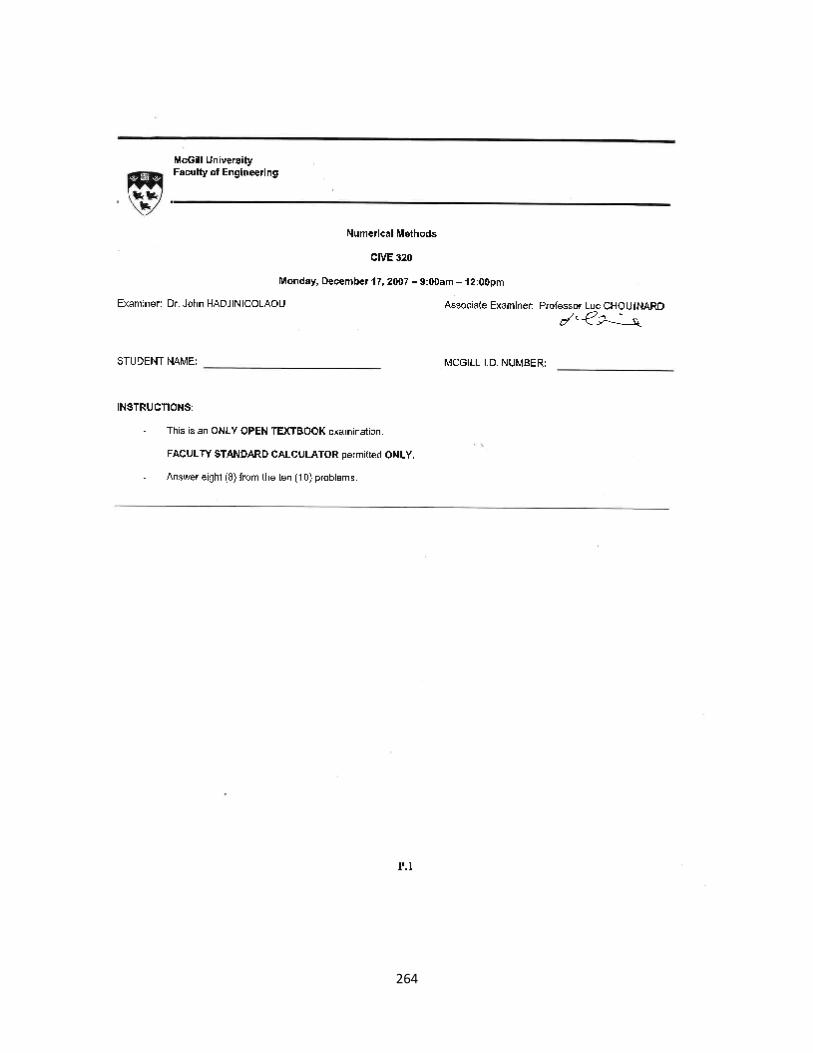
264
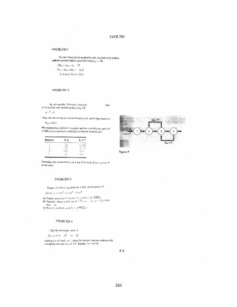
265
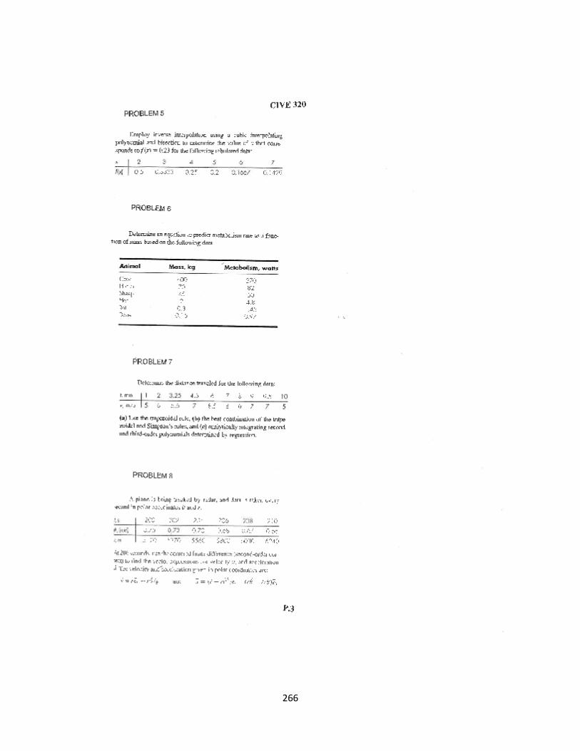
266
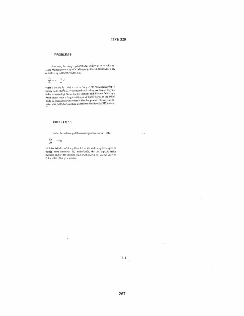
267
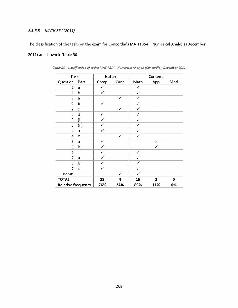
268
8.3.6.3 MATH 354 (2011)
The classification of the tasks on the exam for Concordia’s MATH 354 – Numerical Analysis (December
2011) are shown in Table 50.
Table 50 - Classification of tasks: MATH 354 - Numerical Analysis (Concordia), December 2011
Task Nature Content
Question Part Comp Conc Math App Mod
1 a
1 b
2 a
2 b
2 c
2 d
3 (i)
3 (ii)
4 a
4 b
5 a
5 b
6
7 a
7 b
7 c
Bonus
TOTAL 13 4 15 2 0
Relative frequency 76% 24% 89% 11% 0%
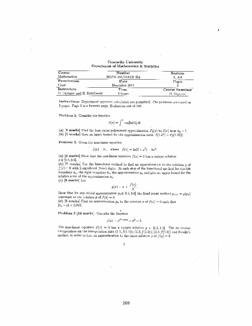
269
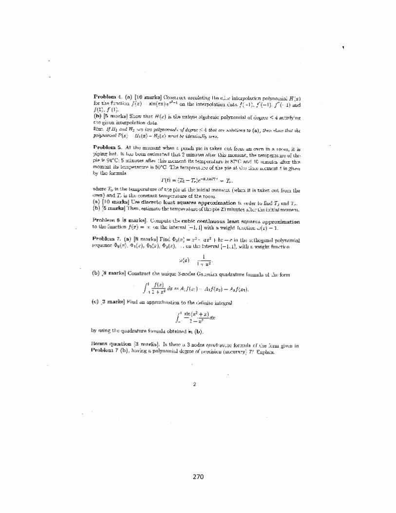
270
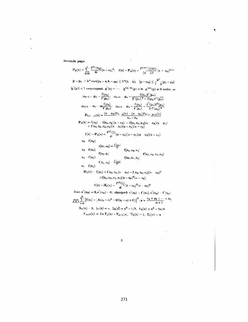
271
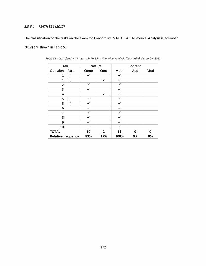
272
8.3.6.4 MATH 354 (2012)
The classification of the tasks on the exam for Concordia’s MATH 354 – Numerical Analysis (December
2012) are shown in Table 51.
Table 51 - Classification of tasks: MATH 354 - Numerical Analysis (Concordia), December 2012
Task Nature Content
Question Part Comp Conc Math App Mod
1 (i)
1 (ii)
2
3
4
5 (i)
5 (ii)
6
7
8
9
10
TOTAL 10 2 12 0 0
Relative frequency 83% 17% 100% 0% 0%
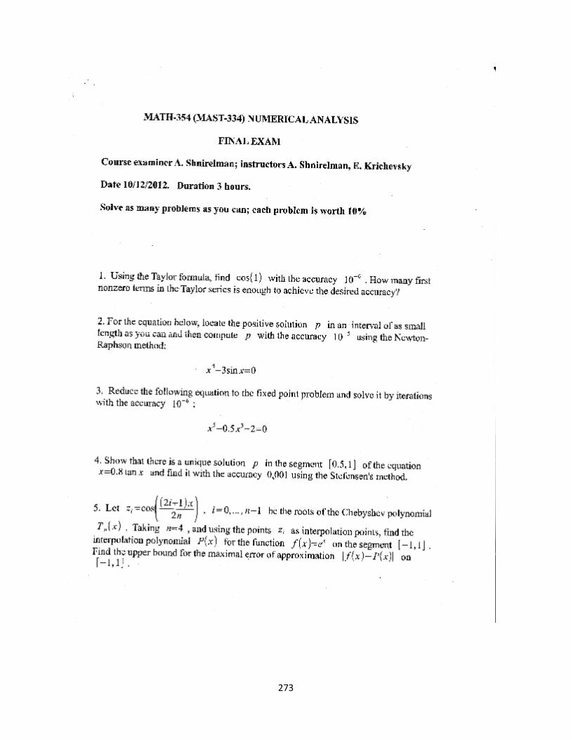
273
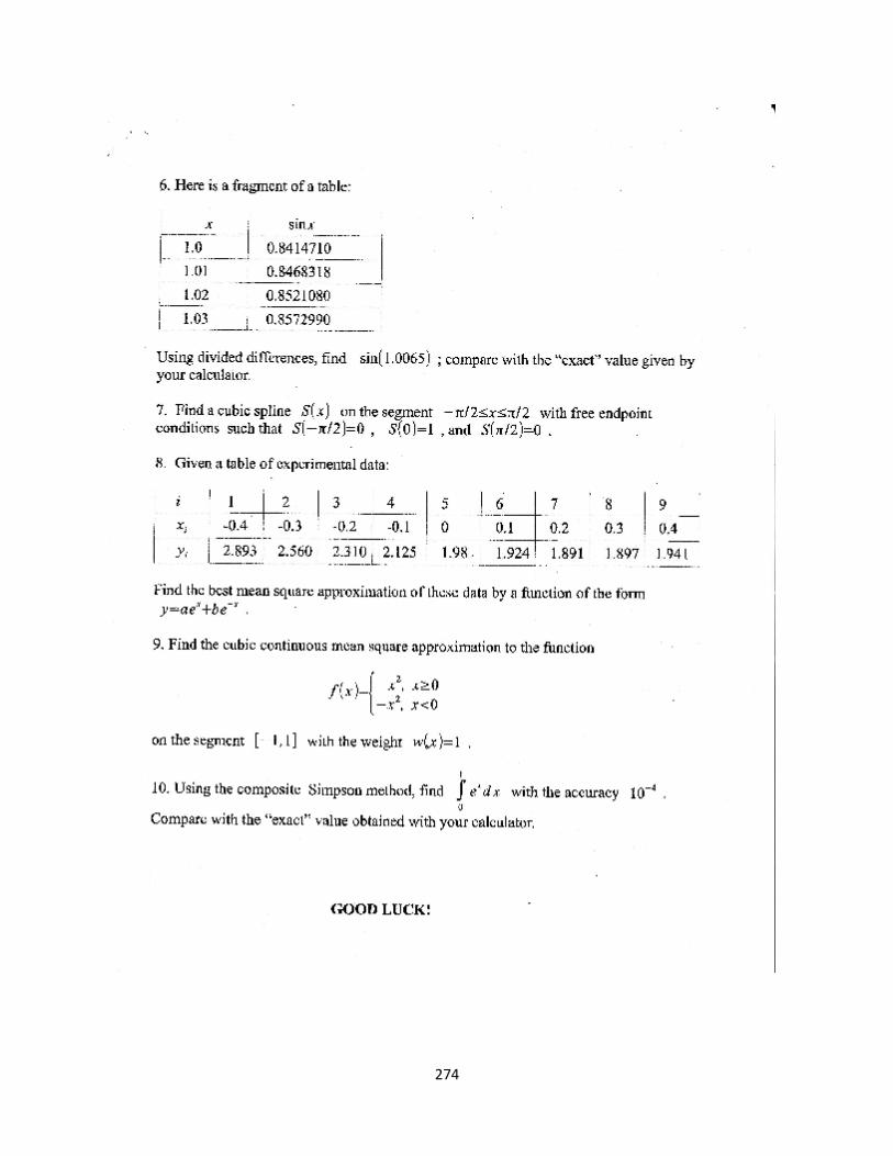
274
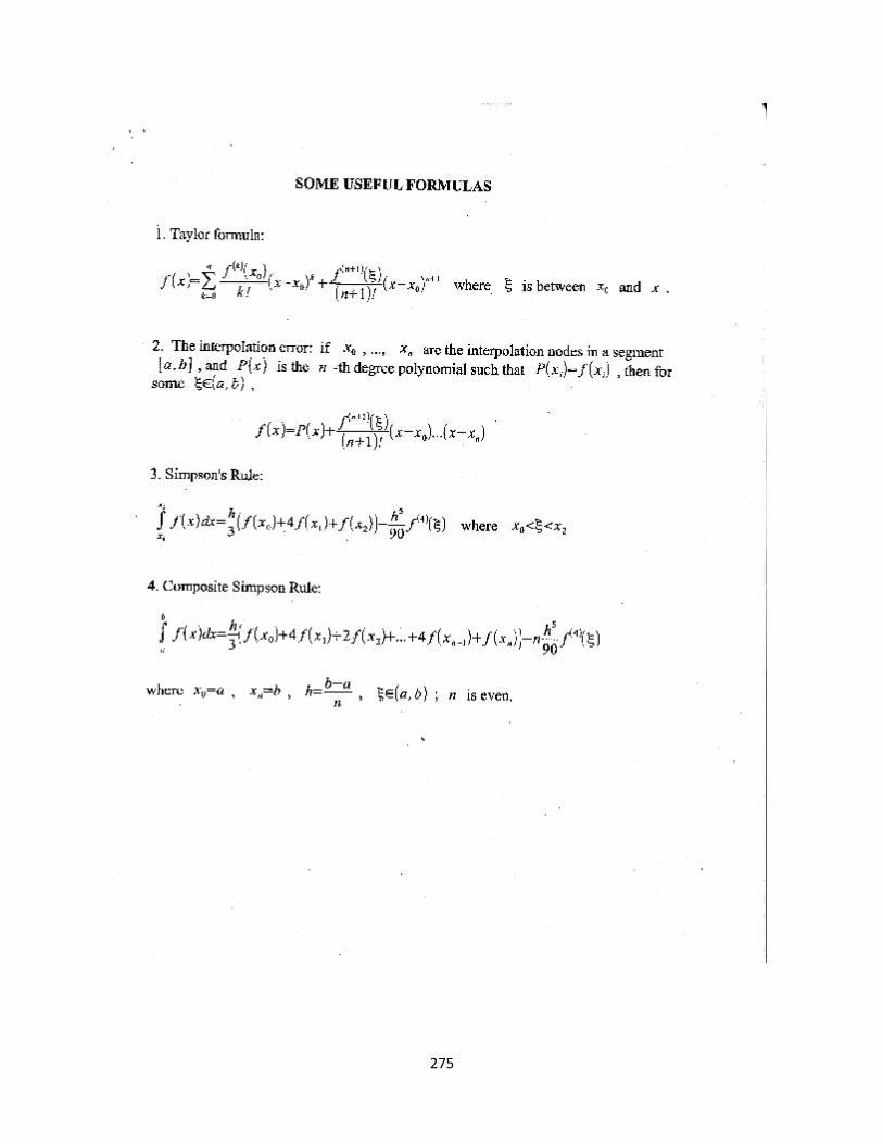
275

276
8.4 STRUCTURAL ANALYSIS SOFTWARE REPORT
The appendix contains the report that is generated by the structural analysis software that is bundled
with the engineering textbook Structural Analysis by Kassimali (1999). This software was used to
generate the images of the deformed plane frame and plane truss in section 5.3. The report includes the
data that was input into the software to describe geometry and material of the structural members as
well as the applied forces, and the output of the analysis that the software performed using the direct
stiffness method.
At the outset of the analysis, a decision must be made about what units will be used when inputting the
structure’s data. I chose to use the units of millimetres ( ) for distance and kilonewtons ( ) for force.
The results of the analysis are therefore displayed in the same units. This makes interpreting the results
of the analysis easier.
A detailed explanation of the information included in the report follows.
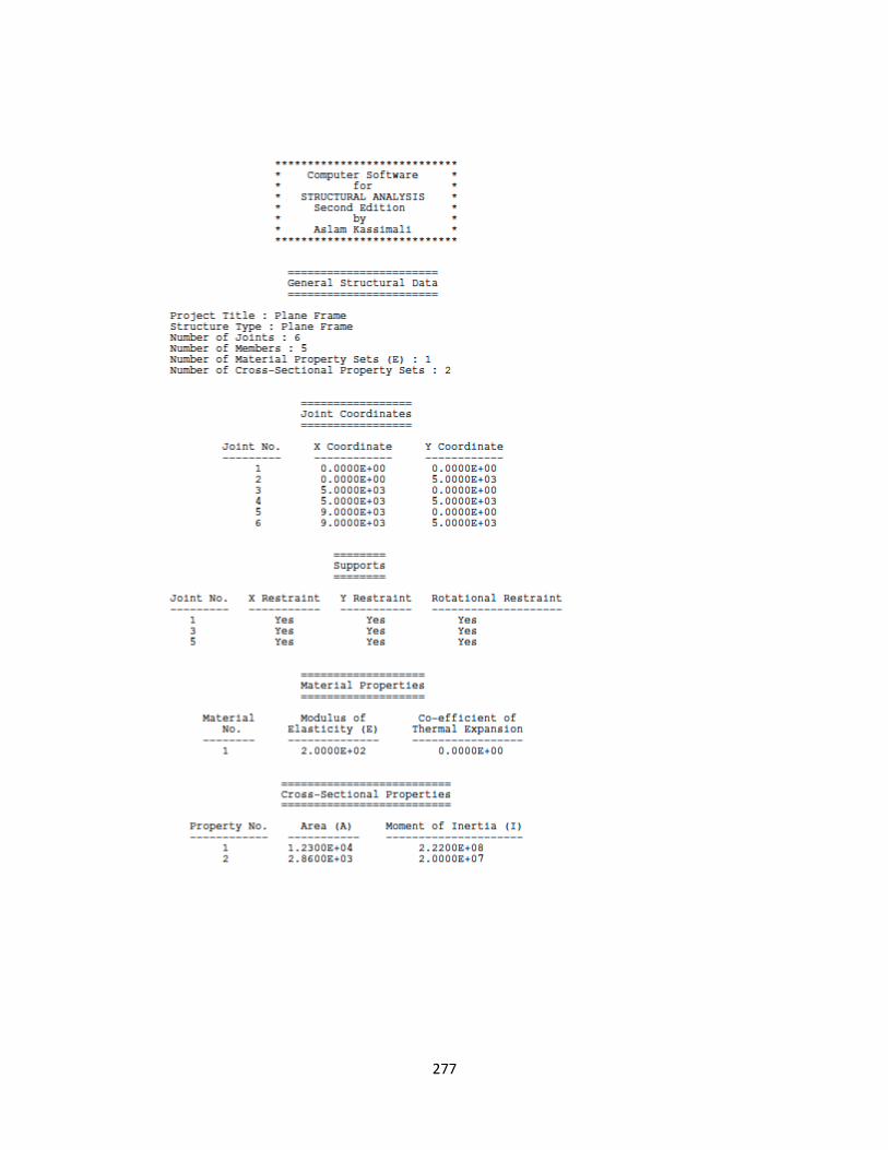
277
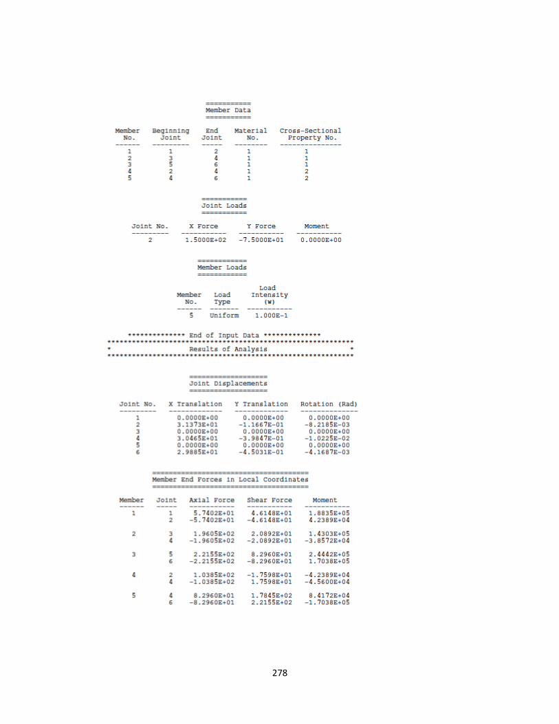
278
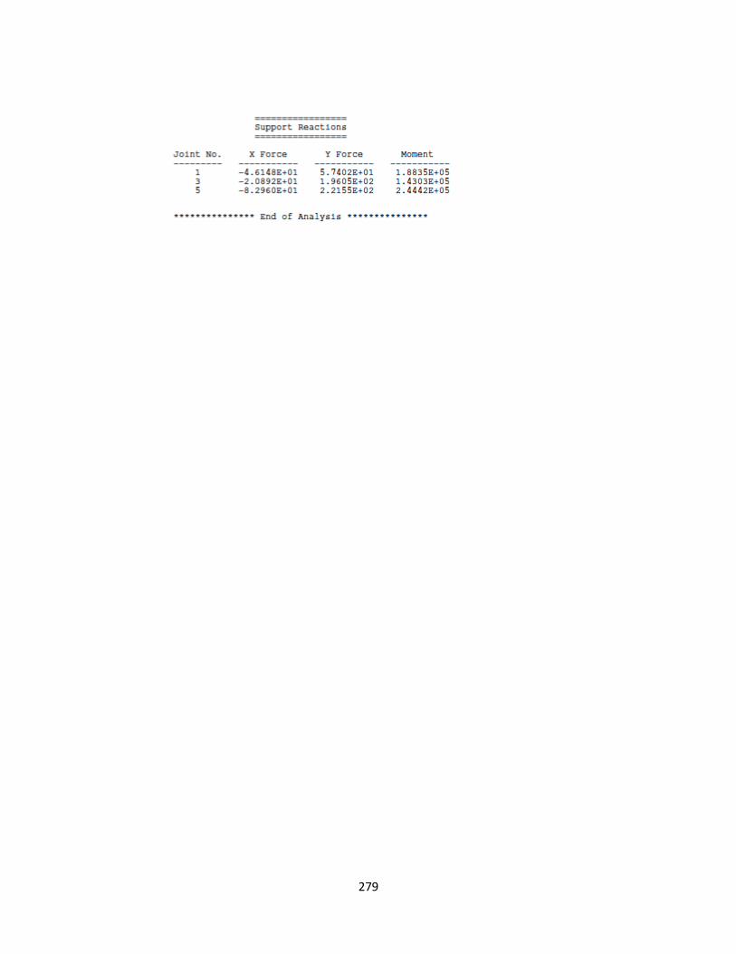
279
280
Joint coordinates
Joint coordinates are entered in millimetres. Joint 1 is chosen as the origin with coordinates (0, 0). Joint
6 is furthest away from the origin located at coordinates ( ). This indicates that the
frame is 9 metres long and 5 metres high.
Material properties
The modulus of elasticity is entered using units of gigapascals (GPa) since , making
this consistent with our chosen units. The value that is entered is:
This is the modulus of elasticity of structural steel.
Cross-sectional properties
The values for cross-sectional area and moment of inertia are entered in units of and ,
respectively Two values are entered for each property since two different shapes are used in the design.
Cross-section 1 is the shape W310x97 and cross-section 2 is the shape W200x22. The entered value for
the area of cross-section 1 is:
Member data
This section indicates where each member begins and ends, and associates with each member a
material and a cross-section. Member 2 begins at joint 3 and ends at joint 4, is assigned the properties
of material 1, and the cross-sectional properties of the shape W310x97 (cross-section 1). Since only one
modulus of elasticity was entered, only one material is defined in this analysis, and so all of the
members are assigned material 1. Two cross-sections were defined though, so some members are
assigned cross-section 1, while others are assigned cross-section 2.
281
Joint loads
The loads applied at joint 2 are entered using units of kilonewtons. The horizontal (X) force is:
Member loads
The uniformly distributed load applied to member 5 is entered using units of kilonewtons per millimetre
( ). While such loads are usually defined in units of , this would lead to an inconsistency in
the units, and the results of the analysis would not be reliable. The entered value for the distributed
load is:
Joint displacements
Since the data was entered with consistent units, the results of the analysis are reliable and are
displayed using the same units as the inputted data. Thus, the X translation of joint 4 is:
The rotations are measured in radians. The rotation at joint 6 is:
Member end forces
The member end forces are the forces that are carried by the members. The results show the forces in
units of kilonewtons and the moments in units of kilonewton-millimetres. The axial force in member 3
is:
The moment in member 3 at joint 5 is:
282
Support reactions
The support reactions are the forces that are transferred from the frame into the supports that connect
it to the ground. These are the forces that the supports themselves must resist. At join 3, the support
must resist a vertical (Y) force of:
It must also resist a moment of:
Copyright © 2022 FDOKUMEN