Download - Jordan Engineers Association

Index

Causes of Falling from Heights among Indoor ELV Operators in Construction Sites

6

Solving the Inventory Control problem Under Constant Deterioration and Partial Backlogged Backorders using simple fixed-point and Genetic algorithms

13

CREATING KNOWLEDGE ENVIRONMENT DURING LEAN PRODUCT DEVELOPMENT PROCESS OF A JET ENGINE

27

ENTREPRENEURSHIP IN JORDAN- INDI STARTUP COMPANY FOR SUPPLY CHAIN FULFILLMENT

39

IoT-WSN system for improving manual order-picking operation

50

SUPPLY CHAIN STREAMLINING AT SAMEH MALL: Inventory Management, CPFR, and Vehicle Routing Optimization

59

On the Relationship between Transformational Leadership, System thinking, and Innovation

69

Analysis and Assessment for Rheological and Dispersions of Polymer Grade: Twin Screw Design

74

Causes of Falling from Heights among Indoor ELV Operators in Construction Sites

Salaheddine Bendak, [email protected]. Department of Industrial Engineering and Engineering

Management, College of Engineering, University of Sharjah, Sharjah, United Arab Emirates

Mohamed Khamis Alnaqbi, [email protected]. Department of Industrial Engineering and

Engineering Management, College of Engineering, University of Sharjah, Sharjah, United Arab Emirates

In-Ju Kim, [email protected]. Department of Industrial Engineering and Engineering Management,

College of Engineering, University of Sharjah, Sharjah, United Arab Emirates

ABSTRACT

Falling from heights is a major contributor to fatal injuries in construction sites. This study aims to determine causes

of such falls among indoor extra low voltage operators, who frequently use ladders and scaffolds, using

questionnaires based on the WORM model. Results revealed that age of operators affected their perceptions of

ladder and scaffold safety whilst education level did not and that half of the operators were not trained. Results also

revealed that experienced operators were more confident about their safety than less experienced operators and that

both did not pay enough attention to safety requirements.

Keywords: Falling from heights, construction sites, extra low voltage, in-door.

1. INTRODUCTION

Every workplace encounters work-related safety issues so the best way to minimize risk is to identify and prevent

causes of accidents. According to data from the Abu Dhabi Statistics Center in 2013, workers in the construction

sector shows a high number of accidents amongst five main economic activities in the city of Abu Dhabi (Abu

Dhabi Statistics Center, 2014). Falls were the leading cause of death and the third leading cause of non-fatal injuries

in the U.S. in 2013 on construction sites (Passmore et al., 2019). Statistics suggest that many safety rules need to be

established in order to reduce the number of deaths in the construction sector (Nadhim et al., 2016). A recent study

from an Arabian Gulf investigated a main reason for accidents in the construction industry and reported that falls

from a height or a same level were 14.1% (Fass et al., 2017).

Due to their high numbers in construction sites, the published literature has focused on the safety of civil contractors

and how to prevent falls from heights for those workers in construction sites (Al-Sayegh, 2008; Fass et al., 2017).

However, there are many other types of workers in construction sites such as extra-low voltage (ELV) contractors

who are responsible for extra low voltage systems. Such systems typically include CCTV, public address system,

lighting controls, electrical cables, IT network cable, and other similar systems. The work of such operators happens

at different height levels in indoor and outdoor areas of construction sites.

6

The current study aims to assess causes of fall from heights amongst indoor ELV contractors who work on

government projects with the Directorate of Public Works in Sharjah, one of the seven emirates that constitute the

United Arab Emirates (UAE). This directorate is responsible for supervising all government projects in Sharjah from

the beginning until the handover to the end user of the building. Moreover, ELV operators are usually subcontracted

to the main contractor who is responsible for providing safe equipment such as ladders and scaffolds and proper

instructions. Such ELV operators have usually a high risk of falling form ladders and scaffolds based on unofficial

statistics solicited from the Directorate of Public Works and such falls are the focus of this study.

This study also aims to determine the leading causes of falls from height and to suggest recommendations to

minimise the risk of falling from heights.

2. METHODS

2.1 Data Collection

Two questionnaires were developed to investigate safety performance of both subcontractors and main contractors.

Both questionnaires were based on the Workgroup Occupational Risk Model (WORM) that supports management

decisions for risk reduction (Aneziris et al., 2012). Both questionnaires were made short (to be easier to be

administered) and suitable for the UAE work environment. The first questionnaire aimed to determine causes of fall

from heights experienced by subcontracted ELV operators while working at indoor heights at or above ceiling level.

This questionnaire was distributed to almost all operators (estimated to be 200) who are subcontracted to do ELV

work of construction projects of the Directorate of Public Works within the Emirate of Sharjah government by the

main construction contractors. The targeted sample size was 100, which is similar to the study conducted by

Aneziris et al. (2012). The second questionnaire aimed to evaluate the main contractor’s role in ensuring the safety

of subcontracted indoor ELV operators and other related operational aspects and was oriented to safety

engineers/managers.

2.2 Procedure

The two questionnaires were presented and explained to safety engineers of all six construction companies involved

in indoor ELV work for the Directorate of Public Works in the government of Sharjah. After securing their

approval, they were asked to distribute the first questionnaire to their subcontracted indoor ELV operators through

their supervisors. Then those supervisors were asked to collect filled questionnaires and return them directly to the

research team without any interference from the main contractors. The same safety engineers were also asked to

respond to the second questionnaire. The final sample size was 138 operators for the first questionnaire and six

safety engineers for the second. It should be noted that most of those safety engineers has also other operational

roles in their companies (i.e. they were also responsible for areas other than safety).

2.3 Statistical analyses

The first five questions (age, educational level, years of experience, work nature, and provider of the ladder or

scaffolds) were considered as input sources for statistical analysis purposes. The next points were related to training

on using ladder, checking ladder safety before using it, getting training on using scaffolds, checking scaffolds before

using, the opinion of outcome when falling from ladder, the opinion of outcome to fall from scaffolds and why do

some operators are falling from ladder and scaffolds. Non-parametric Kruskal-Wallis test was used for statistical

analysis since output variables had a limited number of levels and, thus, were not normally distributed. A

significance level of 0.05 was adopted in this study.

7

3. RESULTS

3.1 Operator Questionnaire Results

Table 1 shows questionnaire results for ELV operators. As shown in Table 1, 43.1% of operators were aged between

25 and 31 years of age the least number of operators was aged between 18 and 24 years.

It was found that about 42% of them had a high school degree and about 25% of them had a diploma. In terms of

work experience, the majority (about 61%) of operators had more than 5 years of work experience whilst about 40%

of them had 0 to 4 years of work experience. According to the work nature of ELV operators, 29.5% of them were

A/C operators, 25.5% were electrical operators, 18.1% were firefighting operators and 22.7% were IT/AV operators.

Table 1 also shows that 65.9% of the operators were provided ladders and scaffolds by their own (subcontracted)

companies and 34.1% by the main contractors. Either way, some of the operators raised concerns on whether the

provided ladders and/or scaffolds were fully inspected in a professional way.

As shown in Table 1, almost half (49.2%) of the operators reported that they received brief training on how to use a

ladder and scaffolds. Many operators indicated on the questionnaire that some of the indoor areas reached more than

8 meters of height and that they were not trained to work at such heights. So, it is recommended that proper training

should be provided to those operators to minimize fall incidents. Moreover, eventhough almost half of the operators

did not receive official trainings as shown in Table 1, most of them reported to inspect their ladders and scaffolds

before using them by themselves (90.1% for ladders and 87.8% for scaffolds).

Another finding of the questionnaire shown in Table 1 is that falls from ladders are usually less serious and lead to

more minor injuries than falls from scaffolds which led to more serious injuries. Questionnaire results also showed

that the death rate from the scaffold falls (15.1%) is more than five times higher than the case of ladder falls (3%).

The last part of the questionnaire was about seeking main reasons to falls from ladders or scaffolds. The major

reported cause was that operators did not pay attention to safety aspects of their ladders and scaffolds. This result

was reported by 68.9% of responding operators. The second reason was the lack of training on the usage of ladders

and scaffolds, which was given by 28% of responding operators. In addition, about 3% of the operators did not

receive any training for the usage of ladders and scaffolds.

3.2 Main Contractors Questionnaire Results

Table 2 shows questionnaire results from safety engineers of the main contractors. Firstly, results reveal that safety

engineers were at least 25 years old with at least one university degree. About half of them had 0 to 4 years of work

experience whilst the other half had 5 to 9 years work experience.

All the safety engineers stated that they provided ladders and scaffolds to the subcontractors with the pre safety

checkups. They also agreed on the importance of checking ladders and scaffolds before using them either by their

own operators or by subcontractors. However, it was noticed that the inspection method for both ladders and

scaffolds was not clearly defined.

3.3 Statistical Analyses

3.3.1 Effects of Age

For ELV operators questionnaire, the null hypothesis is that the output is not changing due of age and the results are

shown in Table 3.

8

Table 1. Summary responses to the first questionnaire by ELV operators.

No. Question Options (Total 132)

1 Age (years) 18-24 25-31 32-39 40+

18 (13.6%) 57 (43.1%) 37 (28%) 20 (15.1%)

2 Education level Primary school or less High school Diploma+

30 (22.7%) 55 (41.6%) 46 (24.8%)

3 Experience (years) 0-4 5-9 10+

53 (40.1%) 36 (27.2%) 43 (32.5%)

4 Work Nature A/C Electrical Fire fighting IT/AV

39 (29.5%) 39 (25.5%) 24 (18.1%) 30 (22.7%)

5 Ladder/Scaffolds provider my company Main contractor

87 (65.9%) 45 (34.1%)

6 Ladder training Yes No

65 (49.2%) 67 (50.8%)

7 Ladder safety check Yes No

119 (90.1%) 13 (9.9%)

8 Scaffolds training Yes No

65 (49.2%) 67 (50.8%)

9 Scaffolds safety check Yes No

116 (87.8%) 16 (12.2%)

10 Fall from ladder outcome No injury Minor Major Death

24 (18.1%) 74 (56%) 30 (22.7%) 4 (3%)

11 Fall from scaffolds outcome No injury Minor Major Death

24 (18.1%) 38 (28.7%) 50 (37.8%) 20 (15.1%)

12 Why do operators fall from a

ladder?

Operators do not pay

attention to safety aspects

Operators are not

trained to use them Both

91 (68.9%) 37 (28%) 4 (3%)

Table 2. Summary of questionnaire responses by safety engineers of main contractors.

No. Questions Options (Total 6)

1 Age (years) 18-24 25-31 32-39 40+ 0 (0%) 5 (83.3%) 1 (16.6%) 0 (0%)

2 Position Project Manager Project Engineer Safety Engineer

0 (0%) 1 (16.6%) 5 (83.3%)

3 Experience (years) 0-4 5-9 10+

3 (50%) 3 (50%) 0 (0%)

4 Ladder/Scaffolds providing to subcontractor

Yes No 6 (100%) 0 (0%)

5 Ladder and scaffolds Check Yes No

6 (100%) 0 (0%)

6 Utilizing Safety checklist Yes No

5 (83.3%) 1 (16.6%)

7 Fall from ladder outcome No injury Minor Major Death

0 (0%) 1 (16.6%) 5 (83.3%) 0 (0%)

8 Fall from scaffolds outcome No injury Minor Major Death

0 (0%) 0 (0%) 6 (100%) 0 (0%)

9 Using safety criteria to choose ladder and scaffolds

Yes No 6 (100%) 0 (0%)

10 Official training on setting up ladder and scaffolds

Yes No 6 (100%) 0 (0%)

11 Inspect ladder and scaffolds regularly

Yes No 6 (100%) 0 (0%)

9

Table 3: Effects of age on output variables.

No. Output variable p-value Decision on null hypothesis

1 Ladder training 0.019 Reject

2 Ladder check 0.047 Reject

3 Scaffolds training 0.275 Accept

4 Scaffolds check 0.002 Reject

5 Likely outcome to fall from ladder 0.065 Accept

6 Likely outcome to fall from scaffolds 0.833 Accept

7 Why operators fall from ladder and scaffolds 0.047 Reject

As shown in Table 3, age of operators apparently affected the ladder training, ladders check, scaffolds check and,

eventually, falls from ladders and scaffolds. From crosstabulating training against age, it was found that more than

60% of the 18-24 and 25-30 age groups did not receive training on ladder use whilst more than 60% of the age

groups had training on them.

Regarding the ladder safety inspection according to the age groups, only 70% of the first age group (18-24 years)

checked their ladders whilst at least 90% of the remaining three groups examined the ladders before using them.

Concerning the scaffold inspection according to the age groups, only 38% of the first group checked their scaffolds

whilst 43% of the second one, 62% of the third one, and 50% of the last one checked scaffolds before using them.

3.3.2 Level of education

As shown in Table 4, all output variables were not significantly affected by the education level of responders except

scaffold training. More than half of the operators with a diploma or university degree reported to have received

training on the use of scaffolds while less than half of the remaining groups did not get scaffold training (p = 0.002).

Table 4. Effects of education level on output variables.


1 Ladder training 0.125 Accept

2 Ladder check 0.206 Accept

3 Scaffold training 0.002 Reject

4 Scaffold check 0.101 Accept

5 Likely outcome to fall from ladders 0.527 Accept


7 Why operators fall from ladder and scaffolds 0.976 Accept

3.3.3 Effects of years of work experience

As shown in Table 5, the output was not changed by the years of work experiences with two exceptions. Almost

60% from the two least experienced groups did not receive ladder training whilst 70% of the most experienced

operators got training on the use of ladders. There was no meaningful explanation for the second statistically

significant result.

Table 5: Effects of years of experience on output variables.





4 Scaffolds check 0.075 Accept




10

3.3.4 Nature of work

As shown in Table 6, most of the output variables were affected by the type of work. Almost 60% of electrical

operators and firefighters received trainings on ladders whilst this ration for the other two types of work was less

than 50% (only 23 % in case of IT contractors).

For scaffold training, results were similar to the case of ladders. It is worth mentioning that in the case of inspection

of scaffolds, the vast majority of operators (75% of AC operators and 100% of IT operators) reported that they

check scaffolds before using them.

Table 6: Effect of work nature on output variables.




3 Scaffolds training 0.025 Reject

4 Scaffolds check 0.035 Reject

5 Likely outcome to fall from ladder 0.000 Reject

6 Likely outcome to fall from scaffolds 0.000 Reject


3.3.5 Provider of ladders and scaffolds

As shown in Table 7, output variables were not affected by the provider of ladders and scaffolds. This means that

ELV operators thought that the seven output variables were not dependent on the main contractor (provider).

Table 7: Effects of ladders and scaffolds provider on output variables.


1 Ladder training 0.604 Accept



4 Scaffolds check 0.790 Accept



7 Why operators fall from ladder and scaffolds 1.000 Accept

4. CONCLUSIONS

Falls from ladders and scaffolds are a leading cause of accidents in construction sites. Results of the current study

clearly show that there are significant factors that contribute to indoor falls from ladders and scaffolds in

construction sites. One of the most striking findings from this study is that almost 50% of operators did not receive

training on the use of ladders and scaffolds. Thus, it is recommended that concerned parties such as authorities and

construction contractors should offer specified safety trainings on the use of ladders and scaffolds for construction

operators. Also, it is proposed to stipulate an official safety tag (or sticker) scheme on ladders and scaffolds that

follow international safety standards so the operator should know how to choose the proper ladder or scaffold.

Another finding from this study is about the lack of national safety standards for ladders and scaffolds in the UAE.

This issue was identified by dealing with both governmental agencies and contractors approached to conduct this

study. Therefore, it is strongly recommended that federal authorities should develop such a national standard to

meet international safety norms for ladders and scaffolds.

11

REFERENCES

Abu Dhabi Statistics Center. (2014). Occupational Health and Safety. Retrieved from

https://www.scad.gov.abudhabi/release%20documents/occupational%20health%20and%20safety%20eng.pdf.

Al-Sayegh, S. M. (2008). Risk assessment and allocation in the UAE construction industry. International Journal of

Project Management, 26(4), 431-438.

Aneziris, O.N., Topali, E. and Papazoglou, I.A. (2012). Occupational risk of building construction. Reliability

Engineering and Safety System, 12, 36-46.

Bunting, J., Branche, C., Trahan, C. and Goldenhar, L. (2017). A national safety stand-down to reduce construction

worker falls. Journal of Safety Research, 60, 103-111.

Fass, S., Yousef, R., Liginlal, D. and Vyasa, P. (2017). Understanding causes of fall and struck-by incidents: What

differentiates construction safety in the Arabian Gulf? Applied Ergonomics, 58, 515-526.

Nadhim, E. A., Hon, C., Xia, B., Stewart, I. and Famg, D. (2016). Falls from Height in the Construction Industry: A

Critical Review of the Scientific Literature. International Journal of Environmental Research and Public Health,

13, 638-657.

Montgomery, D.C. (2013). Design and Analysis of Experiments (8th edition). John Wiley and Sons, New Jersey.

Passmore, D., Chae, C., Borkovskaya, V., Baker, R. and Yim, J-H (2019). Severity of U.S. Construction Worker

Injuries, 2015-2017. XXII International Scientific Conference “Construction the Formation of Living

Environment” (FORM-2019). E3S Web of Conferences 97, 06038.

https://doi.org/10.1051/e3sconf/20199706038

12

https://www.sciencedirect.com/science/article/pii/S0951832011002407#!



https://www.sciencedirect.com/science/article/abs/pii/S0003687016300898#!




SOLVING THE INVENTORY CONTROL PROBLEM UNDER CONSTANT DETERIORATION

AND PARTIAL BACKLOGGED BACKORDERS USING SIMPLE FIXED-POINT AND

GENETIC ALGORITHMS

Dima AYESH, [email protected] The Industrial Engineering Department, The University of Jordan, Amman

11942, JORDAN

Mahmoud A. BARGHASH, [email protected] The Industrial Engineering Department, The University of

Jordan, Amman 11942, JORDAN

ABSTRACT

This work intended to develop a model for constant deteriorating rate in inventory under permissible delay in payment

and back order cancellation when lead time demand follows a normal distribution. It is required to minimize the total

variable cost per unit of time by finding the optimal order Quantity (Q) and Reordering point (R). A mathematical

formulation was developed for the inventory problem, then two solution procedures were used to solve the developed

model which are fixed-point dynamic programming model and Genetic algorithm. The model was validated using an

example from the literature. Also sensitivity analysis was conducted to study the effect of model parameters on order

quantity, reorder point and total annual cost. The results of two solution procedures; fixed-point dynamic programming

and genetic algorithm were compared, which shows that the genetic algorithm gave slightly different values for the

optimal Q and R than the fixed-point algorithm but the same value of Total Annual Cost (TAC). Sensitivity analysis

shows that the optimal order quantity is moderately sensitive to changes in annual Demand (D) and unit cost of item

(p), and optimal reorder point is less sensitive to changes in the D and p. But, the minimum total annual cost TAC is

highly sensitive to changes in the value of D and p.

Keywords: Inventory control, genetic algorithm, partial backlogs, constant deterioration.

Notation

A: Fixed ordering cost

rc: Interest rate applicable to the stock value after credit period

D: Annual demand

rd: Customers penalty rate for non-fulfilled backorders

Q: Order quantity

n(R): Number of unit short;

−=R

dxxfRxRn )()()(

p: Unit cost of item

π: Unit shortage cost

13

mailto:[email protected]


μ: Mean lead time demand

h: Unit holding cost

tc: Credit period

β: Percent of lost sales

θ: Deteriorate rate.

( R-μ) : Safety stock.

cg: Cost of lost customer good well.

x: Demand during lead time random variable.

k: Safety stock

1.0 INTRODUCTION

Today, inventory management is considered to be an important field in supply chain management. Once the efficient

and effective management of inventory is carried out throughout the supply chain, service provided to the customer

ultimately gets enhanced. Hence, to ensure minimal cost for the supply chain, the determination of the level of

inventory to be held at various levels in a supply chain is unavoidable. Minimizing the total supply chain cost refers

to the reduction of holding and shortage cost in the entire supply chain. In other words, during the process of supply

chain management, the stock level at each member of the supply chain should account to minimum total supply chain

cost, and the three main factors are: The cost of holding the stock (e.g., based on the interest rate), the cost of placing

an order (e.g., for raw material stocks) or the set-up cost of production and the cost of shortage, i.e., what is lost if the

stock is insufficient to meet all demand.

Economic order quantity is the level of inventory that minimizes the total inventory holding costs and ordering costs.

It is one of the oldest classical inventory control techniques. EOQ only applies under the following assumptions: The

ordering cost is constant, the demand rate is constant, the lead time is fixed, the purchase price of the item is constant

i.e. no discount is offered, the replenishment is made instantaneously ;ie the whole batch is delivered at once and

payment for items is made immediately (Krajewski 1999).

In real life these assumptions are not all applicable at the same time. Goyal (1985) developed a mathematical model

to determine the optimum EOQ under permissible delay in payment. Chung and Huang (2009) extended Goyal's

generalized model by allowing shortages in Goyal model. Sana and Chaudhuri (2008) studied various types of

deterministic demand when delay in payment is permissible also they included supplier offers of percent discount on

purchased items. Chung, et al. (2005) deals with this problem of EOQ with permissible delay in payment taking into

account the ordered quantity, that is when ordered quantity is less than threshold quantity at which delay in payment

is permitted then payments for products must be made immediate. Huang (2007) developed an inventory model where

supplier offers retailer partial credit period when the ordered quantity is less than predetermined one. Teng, et al.(2005)

includes the assumption that the selling price is the same as purchasing cost and developed an algorithm that optimizes

the price and order quantity when delay in payment is permissible. Ouyang, et al. (2009) developed Goyal (1985)

model while relaxing the classical EOQ model in the following ways: Retailers selling price is higher than its purchase

cost, interest rate is not necessarily higher than the retailers investment return rate, many selling items deteriorate

continuously and Supplier may offer partial delay in payment if order quantity is less than pre-determined one. Liao,

et al. (2000) developed an inventory model for deteriorating items while including a delay in payments and considering

14

http://en.wikipedia.org/wiki/Lead_time

inflation rate when shortages were not allowed and consumption rate depend on initial stock. Ouyang, et al.(2006)

developed an inventory model for non-instantaneous deteriorating inventory with permissible delay in payment.

Also Wu, et al. (2006) considered an appropriate inventory model for non-instantaneous deteriorating items with

permissible delay in payment. Huang and Liao (2008) introduce a simple method to find the optimal ordering policy

for deteriorating inventory under the assumption of permissible delay in payment for constant demand and no

shortages were allowed and when deteriorating rate is exponential. Shah and Mishra (2010) relaxed the EOQ model

to include deteriorating inventory with constant deteriorating rate when demand is stock dependent. Geetha and

Uthayakumar (2010) developed an EOQ model for non-instantaneous deteriorating items with permissible delay in

payment and allowing shortages and partial backlogging. Here backlogging rate is considered to depend on waiting

time for the next replenishment. Basu and Sinha (2007) presents a general inventory model with assumptions that

inventory deteriorating rate is time dependent and follows a Weibull distribution, backlogging is partial and depends

on waiting time, also demand rate is time dependent with permissible delay in payment. Moreover, it follows that

increase in permissible delay decreases total cost which means that there is an inverse relation between total cost and

the permissible payment period. Dye, et al. (2006) introduced an inventory model where backlogging rate of

unsatisfied demand linearly depends on the total number of customer in waiting line during shortage period. Yuo and

Hsieh (2007) investigates a production planning problem where inventory deteriorate at constant rate, demand is price

dependent, backorders are allowed and customer may cancel backorder before receiving them. Bookbinder and

Cakanyildirim (1999) studied a two-stage system with a constant demand rate. They developed two probabilistic

models. In the first, lead time is exogenous and in the second model lead time is endogenous. Wu (2001) dealt with

probabilistic inventory environment to find the optimal continuous review (Q, R) inventory policy under delay in

payment. Chang (2002) extended Wu's 2001 model to include the ordering cost as one of the decision variables. Chang

(2002) explore the (Q, R) inventory policy as well as the investment strategy for ordering cost reduction under

conditions of permissible delay in payments, where the relationship between ordering cost and its investment is

formulated by the widely utilized logarithmic function.

Mondal and Maiti (2002) proposed a soft computing approach to solve non-linear Multi-item fuzzy EOQ models

using GA. Radhakrishnan, et al. (2009) proposed an innovative and efficient methodology that uses Genetic

Algorithms to precisely determine the most probable excess stock level and shortage level required for inventory

optimization in the supply chain such that the total supply chain cost is minimal. Maiti, et al. (2009) studied an

inventory model where demand of the item depends on selling price, lead-time is stochastic in nature, and retailer

has to pay some advance payment at the time of ordering and is eligible for a price discount against extra advance

payment. Shortages are completely backlogged and are met as soon as new order arrives. Gupta, et al. (2009) solved

the inventory model with advance payment and interval valued inventory costs problem with interval coefficient

by a real-coded genetic algorithm (RCGA) with ranking selection, whole arithmetical crossover and non-uniform

mutation for non-integer decision variables. Maiti (2011) used GA to make managerial decision for an inventory

model of a newly launched product.

In this study, a formulation was developed that extends Wu (2001) model to include deterioration inventory, partially

backlogged backorders and permissible delay in payment. This model is then solved using simple fixed-point dynamic

programming algorithm and genetic algorithm. Finally, the model was validated using a numerical example.

Sensitivity analysis was conducted using the fixed-point dynamic programming algorithm.

2.0 MODEL FORMULATION AND SOLUTION

In our study, we extended Wu's (2001) model to include deteriorating inventory, back order cancellation in the light

of credit period and the optimal order quantity and reorder point are determined. The objective is to choose Q and R

15

to minimize the total cost including the average inventory holding, ordering and backorder costs, deteriorating cost

and order cancellation cost (the cost resulted from lost customer goodwill). It is noted that when a delay in payments

is permitted, the buyers could reduce their total cost by paying later, and in this case, larger quantities are preferred

because of the credit period offered by the suppliers. It is assumed that the inventory in our model is deteriorating with

constant rate with time θ, (See Figure 1) where θ applies on the on hand inventory till it is equal to zero, β is the

cancellation rate, μ is the mean of lead time demand, tc is delay (credit) period, D is the annual demand and R is the

replenishment point.

Figure 1: Graphical representation for inventory system.

2.1 Formulation

The formulation is made assuming demand X is constant over time, lead time demand is following a normal

distribution with (μ,σ2) and density function f(DL), shortages are permitted and partially backlogged, delay in payment

is permitted and Inventory items deteriorate with constant rate θ. Also, consider that the reorder point is R.

The reorder point is the sum of expected demand during lead time (μ) and safety stock (SS). The safety stock SS is

assumed to be a constant k multiplied by the standard deviation σ ; ie kσ.

R=μ+ kσ (1)

where k(≥0) is the safety factor

Thus the expected number of units short per cycle is n (R),

(2)

By substituting R=μ+ kσ and z = (x –μ)/σ where x=σz+μ to standardize the random variable x, then:

−=R

dxxfRxRn )()()(

16

( ) dzzkzdzzkzdxxfRxk kR

)()()()()()()(

−=+−+=−

And )](1[)()()()()( kkkdzzkdzzzdzzkzkk k

−−=−=−

Then

)3()](1[)()()()( kkkdxxfRxRnR

−−=−=

Where and Φ denote the standard normal PDF and CDF (probability and cumulative distribution function)

respectively. To make equation more simple we assumed that

Ψ(k) = (k)-k[1-Φ(k)] (4)

This means that

(5)

2.1.1 Total Annual Cost Function TAC

Total annual cost the inventory includes the ordering cost, cycle inventory cost, safety stock cost, shortage cost, lost

sales cost, interest charged for on hand inventory and deterioration cost. Also we execluded from the TAC interest

earned from demand sales during credit period, interest earned from sales of back orders from previous period as

follows:

• pD+ Q

ADcost Ordering =

• 2

hQcostinventory Cycle =

• 2Q

pr)t-Dt-(Qat tcinventory handOn for chargedInterest c

2

cc =

• )t--)(Rpr +(hcoststock Safety cc =

• Q

n(R)D =cost Shortage

• Q

)Dc+(p n(R) =cost salesLost

g

• 2Q

rptD- =periodcredit during sales demand from earnedInterest d

2

c

2

)()( kRn =

17

• Q

Drpt n(R)- =period previous from backorders of sales from earnedInterest dc

• Q

D t P =costion Deteriorat c

So the Total Annual Cost (TAC) function is:

And by substituting equation (5) in equation (6) we find that:

In order to find the optimum order quantity, and optimum reordering point, we find the first derivative of the TAC

function with respect to Q then with respect to k, and then we solve the system of equations using fixed-point and

Genetic Algorithms.

2.1.2 First derivative of TAC with respect to Q

To find the equation representing Q, The derivative of equation (7) will be evaluated then it is made equal to zero.

In order to find the derivative of the total annual cost with respect to order quantity (Q), the elements of the TAC (Q,

R) was derived with respect to Q as follows:

(8)Q

D t P +

Q

Drpt )( +

2Q

rptD

Q

)Dc+(p )(-+

Q

D)(-+

2Q

tpr )-(D -

2

pr +

2

h

Q

AD-=

Q

TAC

2

c

2

dc

2

d

2

c

2

2

g

22

2

cc

2

c

2

k

kk

+

And by making equation (8) equal to zero and simplifying we find that:

)6(Q

D t P

Q

Drpt n(R)

2Q

rptD

Q

)Dc+(p n(R)

Q

n(R)D )t--)(Rpr +(h

2Q

pr 2t-Dt-Q

2

hQpD+

Q

AD),(

cdcd

2

c

2g

cc

ccc

+−−+

++++=RQTAC

)7(Q

D t P

Q

Drpt (k)

2Q

rptD

Q

)Dc+(p (k)

Q

(k)D )t--)(Rpr +(h

2Q

pr 2t-Dt-Q

2

hQpD+

Q

AD),(

cdcd

2

c

2g

cc

ccc

+

−−

+

++++=kQTAC

18

(9)

)/2pr+(h

Dr(k)pt-

2

rptD-Dtp+

)Dc+(p(k)+(k)D+2

tpr )-(D+AD

=Q

c

dcd

2

c

2

c

g

2

cc

2

2.1.3 First derivative of TAC with respect to k

To find the equation representing k, the derivative of equation (7) with respect to k is evaluated, and then the derivative

equalized to zero.

(10)Q

1)-(K)( Drpt +

Q

1)-(K))D(c+(p +

Q

1)-(K)( D +prc) +(h =

k

TAC dcg

And by making equation (10) equal to zero, the result is in equation 11.

Drpt +)Dc+(p +D

)pr +(h Q=(k))-(1

dcg

c

(11)

2.1.4 Simple fixed-point algorithm

First we developed a simple fixed-point algorithm to solve the above mentioned formulation. First the order quantity

Q0 is set to the Economic Order Quantity (EOQ), and use equation (11) to find value of k i for the initial condition,

then using the value of ki in equation (9) we find the next value of Qi+1, the termination criteria for this algorithm is

when Qi = Qi-1 and ki=ki-1. This algorithm is run under the conditions of order Quantity Q is positive and safety factor

k is positive too.

The simple fixed-point algorithm runs as follows;

Step0: Set EOQ= hAD /2 as an estimate of Q i.e. Q0=EOQ ; i=0.

Step1: Use equation 11 with Qi=Qo to find k, ki=k.

Step2: Use equation 9 with k=ki to find Qi if Qi=Qi-1 and ki=ki-1 then stop otherwise set i=i+1, go to step1,

Q>0, k≥0.

Step3: Find R and TAC (Q, k) for the optimal values of k and Q.

2.1.5 Genetic Algorithm

Genetic algorithms were first introduced in the 1960s by Holland and his students. However, several other scientists

worked on evolution strategies. The more general case Such as Rechenberg (1965, 1973) which introduced "evolution

strategies", Schwefel (1975, 1977). Fogel et al (1966) developed "evolutionary programming”. Within Hollands

concept, Genetic algorithms include functions such as: Selection, crossover and mutation. The problem is represented

as chromosomes and a population. These concepts are inspired by the biological evolution concepts. Genetic

algorithms are inspired by Darwin's theory about evolution. Solution to a problem solved by genetic algorithms is

evolved. Algorithm is started with a set of solutions represented by chromosomes called population. Solutions from

one population are taken and used to form a new population. This is motivated by hope, that the new population will

19

be better than the old one. Offspring are selected according to their fitness; the more suitable they are the more chances

they have to reproduce. This is repeated until some condition -for example number of populations or improvement of

the best solution- is satisfied. Das, et al. (2010) and Huapt and Huapt (2004) described the steps of genetic algorithm

as:

[Start] Generate random population of n chromosomes (suitable solutions for the problem) Popi

1. [Fitness] Evaluate the fitness f(x) of each chromosome x in the population

2. [New population] Create a new population by repeating following steps until the new population

is complete

1. [Selection] Select two parent chromosomes from a population according to their fitness

(the better fitness, the bigger chance to be selected)

2. [Crossover] With a crossover probability cross over the parents to form a new offspring

(children). If no crossover was performed, offspring is an exact copy of parents.

3. [Mutation] With a mutation probability mutate new offspring at each locus (position in

chromosome).

4. [Accepting] Place new offspring in a new population

3. [Replace] Use new generated population for a further run of algorithm

4. [Test] If the end condition is satisfied, stop, and return the best solution in current population

5. [Loop] Go to step 2

In this work, population 0 is prepared by random generation composed of 20 individuals. Other populations (i th) are

generated by the GA algorithm. Then the total cost TAC is estimated using equation 6. The fitness is merely a

normalized variable of the TAC, by dividing by the sum of TAC for all individuals, where the sum of all TAC’s is 1.

The ith individuals are then sorted according to their fitness (Figure 2), and a uniform random number generator is

then used to select parent 1 and 2. A crossover is then applied whereby chunks of these two parents are exchanged

within the crossover points. Mutation is randomly done where we replace any 0 by 1 and any 1 by 0. These two

children become individuals in Population i+1. The process is repeated till population i+1 is fully populated.

=

=

=

−

−

=n

i

iintoi

iintoi

i

TACTACMAX

TACTACMAX

Fitrness

11

1

)(

)(

(12)

Figure 2: A schematic for the genetic algorithm.

20

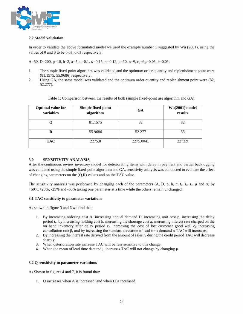
2.2 Model validation

In order to validate the above formulated model we used the example number 1 suggested by Wu (2001), using the

values of θ and β to be 0.03, 0.03 respectively.

A=50, D=200, p=10, h=2, π=5, tc=0.1, rc=0.15, rd=0.12, μ=50, σ=9, cg=6,ᵦ=0.03, θ=0.03.

1. The simple fixed-point algorithm was validated and the optimum order quantity and replenishment point were

(81.1575, 55.9686) respectively.

2. Using GA, the same model was validated and the optimum order quantity and replenishment point were (82,

52.277).

Table 1: Comparison between the results of both (simple fixed-point use algorithm and GA).

Optimal value for

variables

Simple fixed-point

algorithm GA

Wu(2001) model

results

Q 81.1575 82 82

R 55.9686 52.277 55

TAC 2275.0 2275.0041 2273.9

3.0 SENSITIVITY ANALYSIS

After the continuous review inventory model for deteriorating items with delay in payment and partial backlogging

was validated using the simple fixed-point algorithm and GA, sensitivity analysis was conducted to evaluate the effect

of changing parameters on the (Q,R) values and on the TAC value.

The sensitivity analysis was performed by changing each of the parameters (A, D, p, h, π, tc, rd, rc, μ and σ) by

+50%;+25%; -25% and -50% taking one parameter at a time while the others remain unchanged.

3.1 TAC sensitivity to parameter variations

As shown in figure 3 and 6 we find that:

1. By increasing ordering cost A, increasing annual demand D, increasing unit cost p, increasing the delay

period tc, by increasing holding cost h, increasing the shortage cost π, increasing interest rate charged on the

on hand inventory after delay period rc, increasing the cost of lost customer good well cg increasing

cancellation rate β, and by increasing the standard deviation of lead time demand σ TAC will increases.

2. By increasing the interest rate derived from the amount of sales rd during the credit period TAC will decrease

sharply.

3. When deterioration rate increase TAC will be less sensitive to this change.

4. When the mean of lead time demand μ increases TAC will not change by changing μ.

3.2 Q sensitivity to parameter variations

As Shown in figures 4 and 7, it is found that:

1. Q increases when A is increased, and when D is increased.

21

2. Q decreases by increasing unit purchase cost p, increasing unit holding cost h, by increasing the shortage cost

π, by increasing the value of interest rate charged on the on hand inventory after delay period rc, by increasing

the interest rate derived from the amount of sales during the credit period rd and by increasing standard

deviation of lead time demand σ.

3. Q will decrease slightly when the cost of lost customer good well cg, deterioration rate θ and cancellation rate

β increase.

4. When increasing the delay period tc and mean of lead time demand μ Q has no change in value.

3.3 R sensitivity to parameter variations

As shown in Figures 5 and 8 we find that:

1. R increases by increasing annual demand rate D, standard deviation of lead time demand σ, shortage cost π

and mean of lead time demand μ.

2. R will slightly decrease by increasing ordering cost A, holding cost h, interest rate charged on the on hand

inventory after delay period rc and unit cost p.

3. R has a slight increase by increasing deterioration rate θ, cancellation rate β, delay period tc, interest rate derived

from the amount of sales during the credit period rd and cost of lost customer good well cg.

Note: red color represents increasing effect on the variable and the blue one represents decreasing effect on the

variable.

Figure 3: Tornado Diagram illustrate the effect of changing model variables on TAC.

1000.0 1500.0 2000.0 2500.0 3000.0 3500.0

D

A

σ

π

θ

μ

tcTAC

50.0000 60.0000 70.0000 80.0000 90.0000 100.0000 110.0000

A

D

σ

tc

μ

θ

cg

β

rd

π

rc

p

h

Q

22

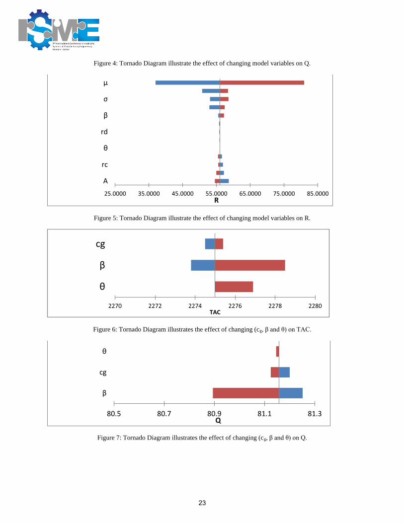
Figure 4: Tornado Diagram illustrate the effect of changing model variables on Q.

Figure 5: Tornado Diagram illustrate the effect of changing model variables on R.

Figure 6: Tornado Diagram illustrates the effect of changing (cg, β and θ) on TAC.

Figure 7: Tornado Diagram illustrates the effect of changing (cg, β and θ) on Q.

25.0000 35.0000 45.0000 55.0000 65.0000 75.0000 85.0000

μ

σ

β

rd

θ

rc

A

R

2270 2272 2274 2276 2278 2280

cg

β

θ

TAC

80.5 80.7 80.9 81.1 81.3

θ

cg

β

Q

23

Figure 8: Tornado Diagram illustrates the effect of changing (cg, β and θ) on R.

4.0 CONCLUSIONS AND RECOMMENDATIONS

The effect of credit period into continuous review inventory model for deteriorating items and back order cancellation

was incorporated in this study. The lead-time demand was considered to have a normal distribution. We developed an

algorithm procedure and we also used GA to obtain the optimal ordering strategy for our model, see table 1. From the

table 1 we find that GA gives slightly different optimal values for Q and R than the fixed-point but the Q value obtained

from GA was equal to that one in Wu (2001) model. Also, TAC is almost the same for both algorithms but it is larger

than the one obtained from Wu (2001) model. And that refers to the deterioration cost and order cancellation cost.

Furthermore, the effects of parameters on the optimal strategy were also included. It is found that the optimal order

quantity is moderately sensitive to changes in D and p, and optimal reorder point has minor sensitivity to changes in

the D and p. But, the minimum total annual cost TAC is highly sensitive to changes in the value of D and p.

Increasing cancellation rate will increase the cost largely, for that managers must have a plane to reduce back ordering

and keep low standard deviation of lead time demand in order to reduce the negative response of customers. It is found

that, the deterioration rate has a slight effect on the values of Q, R and TAC. It is also found that, larger values of

credit period gave lower values for Q and TAC, and that means that the customer will buy less quantity in order to

take the benefits of permissible delay in payment more frequently. And if the holding cost h is high supplier must

order less quantity of inventory to keep TAC in its minimum values.

5.0 REFERENCES

1. Basu, M. and Sinha, S. (2007), An inflationary inventory model with time dependent demand with weibull

distribution deterioration and partial backlogging under permissible delay in payment. Control and Cybernetics,

63,203-217.

2. Bookbinder, S.H and Cakanyldirim,M. (1999), Random lead times and expedited orders in (Q,R) inventory

system. European Journal for Operation Research, 115, 300-313.

3. Chang, hung-Chi (2002), A note on permissible delay in payment for Q, R Inventory system with ordering cost

reduction. Information and management sciences, 13(4), 1-11.

4. Chung K. Goyal, S.K. and Huang, Y.F. (2005), The optimal inventory policies under permissible delay in

payments depending on the ordering quantity. International Journal of Production Economics, 95, 203–213.

5. Chung, K. and Huang, C.(2009), An Ordering Policy with allowable Shortages and Permissible Delay in Payment.

Applied Mathematical Modeling, 33, 2518-2525.

6. Chung, K.J (1998), A theorem on the determination of economic order quantity under conditions of Permissible

delay in payment. Computer operation research, 25, 49-52.

50 51 52 53 54 55 56 57 58

β

cg

θ

R

24

7. Chung, Ken-jen, (2009), A complete proof on the solution procedure for non-instantaanous deteriorating items

with permissible delay in payment. Computers and Industrial Engineering, 56, 267-273.

8. Das D., Roy A. and Kar S.(2010), Improving production policy for a deteriorating item under permissible delay

in payments with stock-dependent demand rate. Computers and Mathematics with Applications, 60, 1973-

1985.

9. Dye, C.Y. Chang, H.J. and Teng, J.T. (2006), A deteriorating inventory model with time-varying demand and

shortage-dependent partial backlogging. European Journal of Operational Research, 172, 417–429.

10. Fogel, L. J., Owens, A. J., & Walsh, M. J. (1965). Artificial intelligence through a simulation of evolution. In M.

Maxfield, A. Callahan, & L. J. Fogel (Eds.), Biophysics and Cybernetic Systems: Proc. of the 2nd Cybernetic

Sciences Symposium (pp. 131–155). Washington, D.C.: Spartan Books.

11. Fogel, L. J., Owens, A. J., & Walsh, M. J. (1966). Artificial intelligence through simulated evolution. New York,

NY: Wiley & Sons.

12. Geetha, K.V. and Uthayakumar, R. (2010), Economic design of an inventory policy for non-instantaneous

deteriorating items under permissible delay in payments. Journal of Computational and Applied Mathematics,

233, 2492-2505.

13. Goyal, S.K. (1986), Economic Order Quantyt Under Conditions of Delay in Payment. Operational Research

Society, 36,335-338.

14. Gupta R.K., Bhunia A.K. and Goyal S.K. (2009), An application of Genetic Algorithm in solving an inventory

model with advance payment and interval valued inventory costs. Mathematical and Computer Modelling, 49,

893_905.

15. Haupt R. and Haupt s.E (2004), Practical Genetic Algorithm, 2nd edition, Hoboken- New Jersey: John Wiley &

Sons, Inc.

16. Huang, K. and Liao, J.(2008),a simple method to locate the optimal solution for exponentially deteriorating items

under trade credit financing. Computers and Mathematics with applications,56, 965-977.

17. Huang, Y. (2007), Economic Order Quantity under Conditionally Permissible Delay in Payment. European

Journal of Operational Research, 176, 911-924.

18. Hung, K. (2009), a complete proof on the solution procedure for non-instantaneous deteriorating items with

permissible delay in payment. Computers and Industrial Engineering, 56, 267-273.

19. Krajewski, L. J., Ritzman, L. P., & Malhotra, M. K. (1999). Operations management 36 Singapore: Addison-

Wesley.

20. Liao, Jui-Jung (2007), On an EPQ model for deteriorating items under permissible delay in payments. Applied

Mathematical Modeling, 31, 393–403.

21. Liao H.C. Tsai, C.H. and Su, C.T. (2000), An inventory model with deteriorating items under inflation when a

delay in payment is permissible. International Journal of Production Economics, 63, 207-214.

22. Maiti A.K., Maiti M.K. and Maiti M. (2009), Improving inventory model with stochastic lead-time and price

dependent demand incorporating advance payment. Applied Mathematical Modeling, 33 , 2433–2443.

23. Maiti, Manas Kumar (2011), A fuzzy genetic algorithm with varying population size to solve an inventory model

with credit-linked promotional demand in an imprecise planning horizon. European Journal of Operational

Research. under press.

24. Ouyang, L.Y. Wu, K.S. and Yang, C.T. (2006), a study on an inventory model for non- instantaneous deteriorating

items with permissible delay in payments. Computers & Industrial Engineering, 51, 637–651.

25. Ouyang,L. Teng,J. Goyal, S.K. and yang,C.(2009), An Economic Order Quantity for Deteriorating Items with

partially Permissible Delay in Payment Linked to Order Quantity. European Journal of operations Research,

194, 418-431.

26. Radhakrishnan P., Prasad V.M. and Gopalan M.R.(2009),Optimizing Inventory Using Genetic Algorithm for

Efficient Supply Chain Management. Journal of Computer Science, 5 (3), 233-241.

27. Rechenberg, I. 1965. Cybernetic Solution Path of an Experimental Problem. Ministry of Aviation, Royal Aircraft

Establishment (U.K.).

28. Rechenberg, I. 1973. Evolutionsstrategie: Optimierung Technischer Systeme nach Prinzipien der Biologischen

Evolution. Frommann−Holzboog (Stuttgart).

25

29. S. Mondala, M. Maiti(2002), Multi-item fuzzy EOQ models using genetic algorithm. Computers & Industrial

Engineering, 44, 105–117.

30. Sana, S.S. and Chaudhuri, K.S.(2008), A deterministic EOQ model with delays in payment and price-discount

offers. European Journal of Operational Research, 184, 509–533.

31. Schwefel, H. −P. 1975. Evolutionsstrategie und numerische Optimierung. Ph.D. thesis, Technische Universität

Berlin.

32. Schwefel, H. −P. 1977. Numerische Optimierung von Computer−Modellen mittels der Evolutionsstrategie. Basel:

Birkhäuser.

33. Shah, N.H and Mishra, P. (2010), An EOQ model for deteriorating items under supplier credits when demand is

stock dependent. Yugoslav Journal of operations Research, 20, 145-156.

34. Teng, J., Chang C., and Goyal S.K.( 2005), Optimal Pricing ordering policy under permissible delay in payment.

International Jurnal of Production Sciences, 97, 121-129.

35. Wu, Kun-Shan (2001), Continuous Review Inventory Model with Permissible Delay in Payment. Information

and Management Sciences, 12(1), 57-66.

36. Yuo, P.S. and Hsieh, Y.C. (2007), A Lot Size Model for Deteriorating Inventory with Back-Order Cancellation.

IEA/AIE, 1002–1011.

26

CREATING KNOWLEDGE ENVIRONMENT DURING LEAN PRODUCT DEVELOPMENT

PROCESS OF A JET ENGINE

Zehra C. ARACI, [email protected] . Abu Dhabi School of Management, Abu Dhabi, UAE

Jan H. BRAASCH, [email protected] . Dubai Airports, Dubai, UAE

Muhammad U. TARIQ, [email protected] . Abu Dhabi School of Management, Abu Dhabi, UAE

Emre M. C. SIMSEKLER, [email protected] . Khalifa University of Science and Technology, Abu

Dhabi, UAE

Ahmed AL-ASHAAB, [email protected] . Cranfield University, Cranfield, UK

ABSTRACT

Product development process is one of the most challenging stages of a product life cycle due to several reasons.

Having right knowledge environment during the design process may eliminate waste of cost and time. Aim of this

paper is to demonstrate a case study where designers can investigate the conflicting parameters about a product and

make their decisions based on an accurate knowledge environment that is created by trade-off curves. The product in

consideration is a turbofan jet engine with a requirement of noise reduction during takeoff while keeping up with the

high quality standards.

Keywords: Knowledge creation and visualisation, Knowledge management, Lean product development, New product

development, Trade-off curves, Aircraft engine noise reduction, Decision-making

1. INTRODUCTION

Due to rapid technological changes, organisations are under pressure to be agile enough in order to respond to the fast

changing demand. This agility can be gained by improving their product development activities. However, designers

face several challenges, especially, during the early stages of developing a new product. These challenges could be

addressed by the lean product development (LeanPD) approach. During the LeanPD process, it is essential to have a

right knowledge environment in order to achieve a robust optimal design. Trade-off curves (ToCs) provide this

environment by creating and visualising the knowledge that is based on the physical insights of the product as well as

experienced data (e.g. outcomes of R&D, data from successful or failed projects).

There are two major areas that this paper addresses; the first is to improve the product development processes by

creating right knowledge environment and the second is to support decision-making in reducing takeoff noise level of

an aircraft jet engine. There are several challenges that the manufacturing industry faces during their product

development processes. Some of these challenges are rework, late design changes, communication challenges between

departments and most importantly lack of knowledge (Khan et al., 2013). Having right knowledge environment

supports designers or product developers to increase the project success rate, to reduce rework during product

development and to reduce manufacturing costs that are caused by inaccurate design solutions (Araci et al., 2017). In

order to create such a knowledge environment, trade-off curves are effective LeanPD tools to be used throughout the

product development processes.

27






Trade-off curves are primarily used by Wright Brothers who succeeded to operate an aircraft for the first time

(Kennedy et al., 2014). Air transportation has gained a significant popularity, and form of aircrafts considerably

improved since then. Efficiency of aircraft production has increased due to the technology changes but most

importantly because of the knowledge-gained throughout all these years. Thanks to the developments, these days,

many international and even domestic flights are preferred as an alternative means of transportation compared to road

transport. However, there are still a lot to improve, such as the noise level which is a challenging factor in air

transportation.

2. LITERATURE REVIEW

2.1. The Role of Trade-off Curves within Lean Product Development

Open, global markets have been a key driver of growth and profit for manufacturing companies over the last 75 years.

This trend can be expected to continue despite recent political developments in some countries. However, with the

access to international means of production and markets also comes international competition. Combined with the

increasing digitalization that lowers entry barriers, this has created pressure on companies to provide high-quality

products and services in an environment of often rapidly changing demand. This need for flexibility and short time-

to-market timeframes makes an efficient product development (PD) process a key success factor. Demand cycles,

especially in consumer markets, are now often characterized by extremely short durations while, at the same time,

carrying huge revenue potentials. Sustaining market share (or even improving) it depends on the timely development

of products that service this short-lived demand, and companies with such capabilities have a distinctive,

differentiating competitive advantage. Efficient PD capabilities rely on a number of management systems, tools and

techniques that allow companies to leverage organizational knowledge and continuously improve processes. For

companies, efficient development of new products, as well as access to organisational knowledge, have become

important assets (Wang and Wang, 2012; Nonaka et al., 2014).

As shown in Figure 1, new products are often the result of a company having identified an unsatisfied customer

demand. Traditionally, the development of these new products has been hindered by inefficiencies in the PD process.

Among these are lack of knowledge or insufficient research, last-minute changes to the design and associated rework,

ineffective process planning and scheduling, internal communication challenges and lack of organizational

accountability and process ownership (Khan et al., 2013). Each of these have the potential to significantly increase

the time-to-market for any new product. In order to address each of these factors, the Lean Product and Process

Development (LeanPPD) model has increasingly found application in the manufacturing industries. However, a

successful implementation of the LeanPPD model necessitates the presence of a number of enablers, namely value-

focused planning and development, the set-based concurrent engineering (SBCE) process, top-down technical

leadership, a culture of continuous improvement and a knowledge-based environment (Khan et al., 2013). Among

these, SBCE in particular is recognized as a primary driver of efficiency in PD (Al-Ashaab et al., 2013). SBCE arrives

at the optimum product/solution through an iterative process comprising of the creation of a design-set, the

communication, the trade-off and the narrowing down of the set of potential design solutions (Sobek, Ward and Liker,

1999). This approach, however, heavily relies on access to organizational knowledge, which provides the context for

the SBCE process to meet organizational objectives. It is thus imperative that organizations create a knowledge-

environment if they aim to improve the efficiency of their PD process. Using an appropriate knowledge-environment

in SBCE, companies can reuse and share organizational and process knowledge, and enhance the quality of decisions

made during the PD process. (Baxter et al., 2009; Lindlöf et. al., 2013; Kennedy et al., 2014; Maksimovic et al., 2014).

28

Figure 1. Scope of the paper (why trade-off curves?)

While companies are consequently endeavoring to maximise use of their organizational knowledge, it is almost never

easily accessible, or even quantifiable. One of the models that define and explain the creation of knowledge in

organisations is the SECI model proposed by Nonaka et al. (2000), which refers to the Socialisation, Externalisation,

Combination and Internalisation of knowledge. With regards to organizational knowledge, the key mode of the SECI

model is Externalisation, the process of converting tacit knowledge (i.e. experience, individual knowledge) into

explicit knowledge such as documents, reports and drawings (Nonaka, Toyama and Konno, 2000). In this context,

Tyagi et al. (2015) have proposed Trade-off Curves (TOC) as a vital tool the externalisation mode of the SECI model,

as they provide a knowledge-based environment by illustrating and documenting internal knowledge, and thereby

making it accessible for use in the PD process (Raudberget, 2010; Correia, Stokic and Faltus, 2014).

The ability of TOCs to create and visualize knowledge in a simple manner is a key enabler of SBCE applications

(Morgan and Liker, 2006; Kennedy, Sobek and Kennedy, 2014). They enable engineers and product designers to

compare, in the early stages of design – and therefore ahead of any significant investments of time or monetary

resources -, several alternative solutions despite any conflicting attributes that these solutions might have (Ward and

Sobek, 2014). TOCs visualize knowledge from previous projects, and allow the company to reuse it without the danger

of previously gained knowledge having to be “reinvented” (Ward and Sobek, 2014). A third key capability of TOCs

is their visualization of underlying physical features and fundamental principles of the product under development,

which is essential to making a rigorous and correct decision during the SBCE process (Araci et al., 2016).

It is an inherent property of product development processes that the objectives of stakeholders participating in them

differ, as do the properties, the shapes, materials and functionalities being considered for the product. In an

environment of conflicting objectives, factors, parameters and elements, accurate decision making is crucial. Impacts

of favoring one property over another need to be understood and traded off against one another with a view to

maximizing positive effects on the objective. TOCs are tools to visualize these relationships and support the decision-

making (Otto and Antonsson, 1991; Bitran and Morabito, 1999).

TOCs are defined as follows: A trade-off curve establishes a relationship between two or more design parameters,

which is more useful than trade-off data (Sobek et al., 1999).

ToCs can be generated in two-dimensional, three-dimensional or multi-dimensional form, depending on the

analytic/analysis need or different types of products. If the design team would like to see relationships between more

than two design parameters, in order to make a more accurate decision, these relationships can be visually projected

29

on a three-dimensional trade-off curve (Otto and Antonsson, 1991; Raudberget, 2010) or multi-dimensional trade-off

curve (Haselbach and Parker, 2012).

Trade-off curves have been widely referred to in the literature, especially from the 1960s onwards (Pershing, 1968),

within a range of disciplines from finance and environmental science to engineering and computer science. In line

with real-life manufacturing situations, the most prominent use of trade-off curves is to visualize multi-objective (or

multi-criteria) problems with conflicting objective functions. Data for such trade-off curves, however, is often readily

available or generated (by algorithms and mathematical calculations) and does not serve the purpose of externalizing

organizational knowledge.

On the other hand, the number of publications that mention trade-off curves within the PD context is very limited.

Kennedy, Sobek and Kennedy (2014) reported that the earliest use of trade-off curves in PD was by the Wright

Brothers in the late 1800s. Unlike many of their rivals, they succeeded in the first manned and heavier-than-air flight,

despite their lower budget and even in a shorter time. It is believed that a part of this success was attributable to the

use of trade-off curves in the early stages of their PD.

In more recent times, Toyota has used trade-off curves as a knowledge visualization tool, in order to facilitate their

SBCE application (Sobek et al., 1999). There, trade-off curves are part of “jidoka”, which refers to a visual

management technique that Toyota integrated into their PD process from lean manufacturing (Morgan and Liker,

2006). Now, they visually display subsystem knowledge in a graph so that engineers are able to explore the design

space (Ward and Sobek, 2014) and evaluate design alternatives (Kerga et al., 2014). Moreover, in a lean product

development context, trade-off curves avoid the reinvention of previously considered design solutions during

prototyping (Womack, 2006). Hence, engineers save time that they can spend on new and innovative solutions.

Previous research exhaustively demonstrated how trade-off curves can be generated and utilised throughout the stages

of set based concurrent engineering (Araci et. al., 2017). This paper aims to show an application of trade-off curves

in the early stage of design of a complex product which is a turbofan jet engine.

2.2. Aircraft Noise Challenge

Aircraft noise is a significant issue and it has direct effect on the human hearing. It is well established fact that it can

cause hearing problems in humans. Unwanted noise can create problems which can distract communication, reduce

quality of communication, and increases stress. Aircraft noise compatibility has been the serious issue that reduced

the growth of the commercial aviation. Already a number of European airports have reached their maximum

environmental load capacity before starting the use of runway and other infrastructure. One of the important challenges

faced by environmental management authorities and advisory council for Aeronautics research is to reduce the current

noise of aircrafts by 50% (-10db/operation). Different solutions have been tested to control the overall noise at the

airports. However, the noise in the surroundings of the airports have been a trouble and remains high at take-off and

landing time (Chandiramani, 1974).

Airports are trying technological solutions and several measures to reduce the noise like restrictions on use of land,

approved procedures to take-off and landing, compensation to residents, and operations restrictions), but it has failed

to reduce the noise due to increase in air traffic (Papamoschou, 2018). Aircraft manufacturers see more demand of

aircrafts which comply with the regulations and policies set by the airports. In near future, airports have to deal with

the increased traffic and few traffic slots along with oil shortage which will create greater problems. Environmental

issues can only be solved by using the sustainable air transport, which involves new engine designs and fuselages,

design of new procedures and more air traffic paths.

30

Commercial aircraft segments are focusing to manage the airframe-engine combination along with other components

such as flaps, under-carriage with different noise attributes to enhance the air transport (Zaman & Bridges & Huff,

2012). Currently, there is lack of clear link between the certified noise levels as per air craft manufacturers and required

noise level regulations. Frequency of the noise emitted from different components of the aircrafts still need to be

measured in real time as it cannot be measured in static position. International civil association organizations (ICAO)

is also working on new set of regulations and taking strict rules to reduce the noise levels. Other than setting the

regulations, the aircraft noise levels impact on the social environment still need to be calculated in monetary terms.

Different social cost factors depend on the size of the airport, number of terminals/hubs, flights per day, and level of

noise contours (Naqavi, Zhong-Nan, Mahak, and Strange 2016).

Social and environmental impact of the aircrafts both include the take-off and landing noise levels. Social costs vary

by the emission depending on the aircraft category, engine type, and damage done by the engine pollution on the

human health, materials, and climate. Over the past few years the results indicated the link between the environmental

cost and traffic volume on an airport. Organizations are working on predicting the noise levels emitted from engines

by using the upwinding method that uses a finite volume method based on splitting algorithm of Roe and monoton up

centered schemes for conservation laws (MUSCL) to flow over a grid structure (Nogueira, Sirotto, Fuzaro Miotto,

Cavalieri, Cordioli, Wolf, 2018).

3. AN APPLICATION OF TRADE-OFF CURVES IN REDUCING JET ENGINE NOISE

3.1. Work Principles of a Turbofan Jet Engine

Review of the related literature showed that there are certain parameters that influence the reduction of take-off noise.

Additionally, understanding the physical/technical details about a jet engine facilitated identifying parameters to focus

on. A jet engine is key component of most modern aircraft, as it provides, by jet propulsion, required to reach speeds

that enable heavier-than-air flight. The jet engine’s most common form is the turbofan engine, which is illustrated in

Figure 2. A forward force is generated by accelerating the entering gas (air) between the entrance and the exit of the

engine. The “General Thrust Equation” defines thrust as the difference between the product of mass flow at the exit

(𝑚 ̇𝑒) and the gas speed differential between exit and entry (𝑉𝑒−𝑉0), and the product of mass flow at the entrance (�̇�0)

and the gas speed differential (𝑉𝑒−𝑉0). By definition, all air entering the engine must also leave it, from which follows

that 𝑚 ̇𝑒=𝑚 ̇0 at all times.

Figure 2. A turbofan jet engine illustrating the airflow to generate thrust (Najjar and Balawneh, 2015)

31

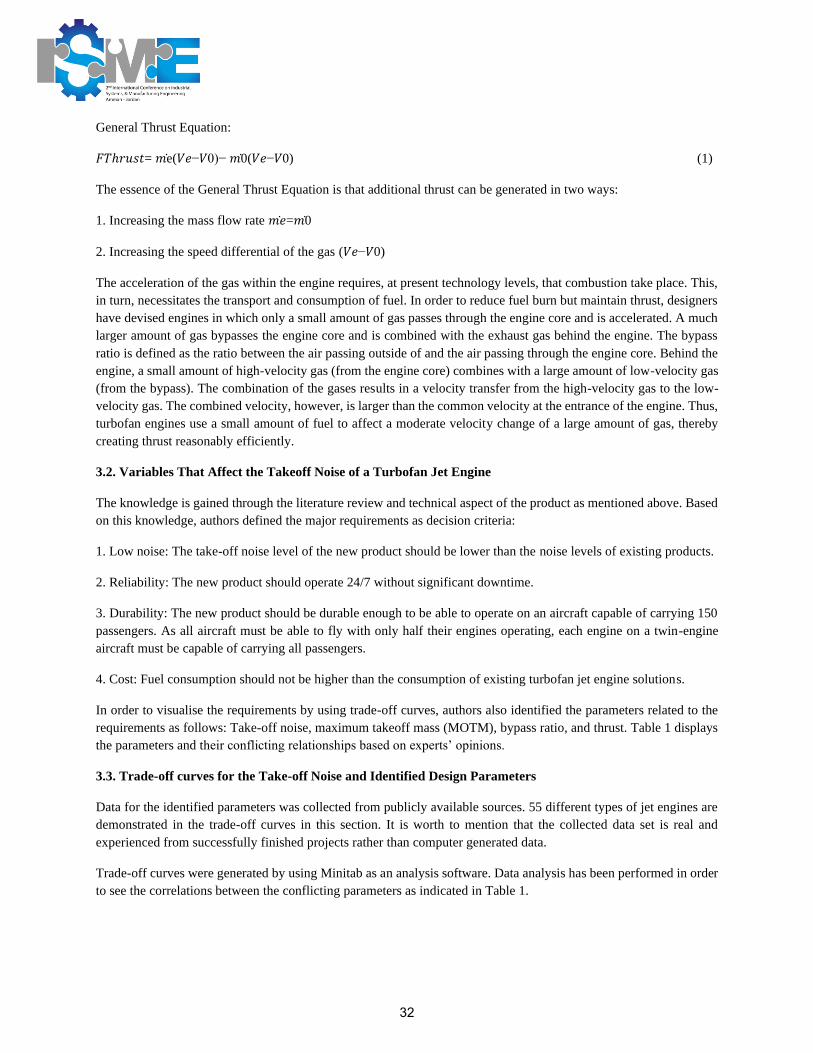
General Thrust Equation:

𝐹𝑇ℎ𝑟𝑢𝑠𝑡= 𝑚 ̇e(𝑉𝑒−𝑉0)− 𝑚 ̇0(𝑉𝑒−𝑉0) (1)

The essence of the General Thrust Equation is that additional thrust can be generated in two ways:

1. Increasing the mass flow rate 𝑚 ̇𝑒=𝑚 ̇0

2. Increasing the speed differential of the gas (𝑉𝑒−𝑉0)

The acceleration of the gas within the engine requires, at present technology levels, that combustion take place. This,

in turn, necessitates the transport and consumption of fuel. In order to reduce fuel burn but maintain thrust, designers

have devised engines in which only a small amount of gas passes through the engine core and is accelerated. A much

larger amount of gas bypasses the engine core and is combined with the exhaust gas behind the engine. The bypass

ratio is defined as the ratio between the air passing outside of and the air passing through the engine core. Behind the

engine, a small amount of high-velocity gas (from the engine core) combines with a large amount of low-velocity gas

(from the bypass). The combination of the gases results in a velocity transfer from the high-velocity gas to the low-

velocity gas. The combined velocity, however, is larger than the common velocity at the entrance of the engine. Thus,

turbofan engines use a small amount of fuel to affect a moderate velocity change of a large amount of gas, thereby

creating thrust reasonably efficiently.

3.2. Variables That Affect the Takeoff Noise of a Turbofan Jet Engine

The knowledge is gained through the literature review and technical aspect of the product as mentioned above. Based

on this knowledge, authors defined the major requirements as decision criteria:

1. Low noise: The take-off noise level of the new product should be lower than the noise levels of existing products.

2. Reliability: The new product should operate 24/7 without significant downtime.

3. Durability: The new product should be durable enough to be able to operate on an aircraft capable of carrying 150

passengers. As all aircraft must be able to fly with only half their engines operating, each engine on a twin-engine

aircraft must be capable of carrying all passengers.

4. Cost: Fuel consumption should not be higher than the consumption of existing turbofan jet engine solutions.

In order to visualise the requirements by using trade-off curves, authors also identified the parameters related to the

requirements as follows: Take-off noise, maximum takeoff mass (MOTM), bypass ratio, and thrust. Table 1 displays

the parameters and their conflicting relationships based on experts’ opinions.

3.3. Trade-off curves for the Take-off Noise and Identified Design Parameters

Data for the identified parameters was collected from publicly available sources. 55 different types of jet engines are

demonstrated in the trade-off curves in this section. It is worth to mention that the collected data set is real and

experienced from successfully finished projects rather than computer generated data.

Trade-off curves were generated by using Minitab as an analysis software. Data analysis has been performed in order

to see the correlations between the conflicting parameters as indicated in Table 1.

32

Table 1: Conflicting relationships between the design parameters of a low noise jet engine

No. Parameters and Relationships Conflicts between the design parameters

1 Thrust vs. Take-off Noise Level

Engine noise was defined as 100% of the aircraft take-off noise. As

aircraft take off with full power, thrust and fuel consumption are at

a maximum. It was surmised that the noise level is related to the

amount of thrust generated.

2 Bypass Ratio vs. Take-off Noise

Level

In order to achieve high thrust but low noise, the bypass ratio of the

engine can be increased. In order to increase the bypass ratio, the

fan diameter should be increased so that the air intake increases.

However, a larger fan results in the engine being heavier and this

leads a higher bypass ratio with a higher thrust but heavier aircraft.

Consequently, possibility of reducing aircraft engine noise

becomes challenging.

3 Maximum Takeoff Mass (MTOM)

vs. Take-off Noise Level

As mentioned above, in general, larger and heavier aircraft produce

more noise than lighter aircrafts. Through increasing the bypass

ratio by increasing the fan diameter, the engine weight will also

increase which will increase the MTOM.

Take-off Noise vs. Thrust, Bypass Ratio, MTOM:

The metric for take-off noise level is EPNdB which means effective perceived noise in decibel and the metric for

thrust is defined as newton (N).

Figure 3 shows a positive correlation between the noise and thrust which means that higher thrust causes higher takeoff

noise. However, there is one design solution found with a high thrust (284,500 N) but relatively low noise (90.1

EPNdb) compared to other design solutions.

Take-off noise vs. Bypass Ratio:

Simply, bypass ratio is the mass flow of air going into the engine core and burnt divided by the mass flow of air going

around the engine core and exiting the engine as it is. For example, a bypass ratio of 10:1 means that 11 units of air is

drawn into the engine, 10 units go around (bypass) the engine core and exit, but 1 unit go through the engine core and

burn. High bypass ratio is the desirable factor in this case as it is believed that high bypass ratio results with low noise

engine. However, when we analysed the data for bypass ratio and take-off noise (see Figure 4), it was found that there

is no considerable relationship between these two parameters. In fact, a design solution has been defined with a high

bypass ratio but relatively low take-off noise.

Three dimensional trade-off curve has been generated in order to understand if all these three parameters are related

to each other; and, consequently, whether they are giving the same feasible design solution. As shown in Figure 5, it

was found that one engine has the potential to be considered within the design set in the early stage of product

development. Further discussions are provided in the following section.

Authors carried some more investigations to understand the relationships between take-off noise, thrust and maximum

take-off mass (MTOM). MTOM is the weight of the aircraft in kg with an assumption that it operates full capacity

(passengers and fuel). It was found that there is a positive strong relation between thrust and maximum take-off mass

which eventually means heavier aircraft requires more thrust (see Figure 6). The effect of MTOM on take-off noise

has been investigated and displayed in Figure 7 as a three dimensional trade-off curve. It appears that MTOM does

33

not have a significant impact on the noise, however, may facilitate noise reduction indirectly. Next section provides

more details about the findings and discussions.

Figure 1. Correlations between take-off noise and thrust

Figure 2. Correlations between take-off noise and bypass ratio

Figure 3. Correlations between take-off noise, thrust and bypass ratio

34

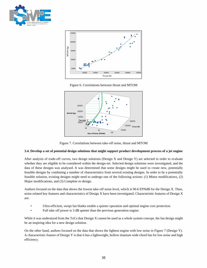
Figure 6. Correlations between thrust and MTOM

Figure 7. Correlations between take-off noise, thrust and MTOM

3.4. Develop a set of potential design solutions that might support product development process of a jet engine

After analysis of trade-off curves, two design solutions (Design X and Design Y) are selected in order to evaluate

whether they are eligible to be considered within the design-set. Selected design solutions were investigated, and the

data of these designs was analysed. It was determined that some designs might be used to create new, potentially

feasible designs by combining a number of characteristics from several existing designs. In order to be a potentially

feasible solution, existing designs might need to undergo one of the following actions: (1) Minor modifications, (2)

Major modifications, and (3) Complete re-design.

Authors focused on the data that shows the lowest take-off noise level, which is 90.6 EPNdB for the Design X. Then,

noise-related key features and characteristics of Design X have been investigated. Characteristic features of Design X

are:

• Ultra-efficient, swept fan blades enable a quieter operation and optimal engine core protection.

• Full take off power is 3 dB quieter than the previous generation engine.

While it was understood from the ToCs that Design X cannot be used as a whole system concept, the fan design might

be an inspiring idea for a new design solution.

On the other hand, authors focused on the data that shows the lightest engine with low noise in Figure 7 (Design Y).

A characteristic feature of Design Y is that it has a lightweight, hollow titanium wide chord fan for low noise and high

efficiency.

35

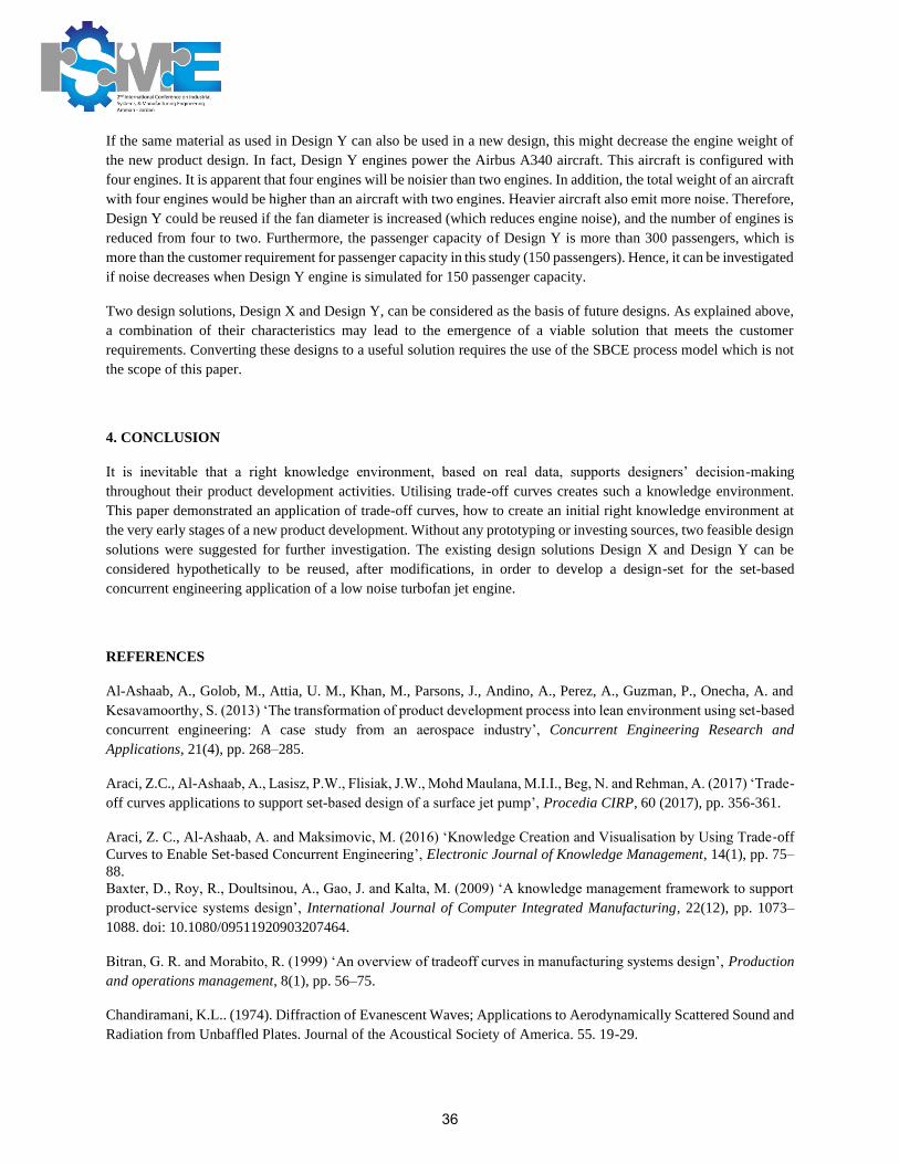
If the same material as used in Design Y can also be used in a new design, this might decrease the engine weight of

the new product design. In fact, Design Y engines power the Airbus A340 aircraft. This aircraft is configured with

four engines. It is apparent that four engines will be noisier than two engines. In addition, the total weight of an aircraft

with four engines would be higher than an aircraft with two engines. Heavier aircraft also emit more noise. Therefore,

Design Y could be reused if the fan diameter is increased (which reduces engine noise), and the number of engines is

reduced from four to two. Furthermore, the passenger capacity of Design Y is more than 300 passengers, which is

more than the customer requirement for passenger capacity in this study (150 passengers). Hence, it can be investigated

if noise decreases when Design Y engine is simulated for 150 passenger capacity.

Two design solutions, Design X and Design Y, can be considered as the basis of future designs. As explained above,

a combination of their characteristics may lead to the emergence of a viable solution that meets the customer

requirements. Converting these designs to a useful solution requires the use of the SBCE process model which is not

the scope of this paper.

4. CONCLUSION

It is inevitable that a right knowledge environment, based on real data, supports designers’ decision-making

throughout their product development activities. Utilising trade-off curves creates such a knowledge environment.

This paper demonstrated an application of trade-off curves, how to create an initial right knowledge environment at

the very early stages of a new product development. Without any prototyping or investing sources, two feasible design

solutions were suggested for further investigation. The existing design solutions Design X and Design Y can be

considered hypothetically to be reused, after modifications, in order to develop a design-set for the set-based

concurrent engineering application of a low noise turbofan jet engine.

REFERENCES

Al-Ashaab, A., Golob, M., Attia, U. M., Khan, M., Parsons, J., Andino, A., Perez, A., Guzman, P., Onecha, A. and

Kesavamoorthy, S. (2013) ‘The transformation of product development process into lean environment using set-based

concurrent engineering: A case study from an aerospace industry’, Concurrent Engineering Research and

Applications, 21(4), pp. 268–285.

Araci, Z.C., Al-Ashaab, A., Lasisz, P.W., Flisiak, J.W., Mohd Maulana, M.I.I., Beg, N. and Rehman, A. (2017) ‘Trade-

off curves applications to support set-based design of a surface jet pump’, Procedia CIRP, 60 (2017), pp. 356-361.

Araci, Z. C., Al-Ashaab, A. and Maksimovic, M. (2016) ‘Knowledge Creation and Visualisation by Using Trade‑off

Curves to Enable Set‑based Concurrent Engineering’, Electronic Journal of Knowledge Management, 14(1), pp. 75–

88.

Baxter, D., Roy, R., Doultsinou, A., Gao, J. and Kalta, M. (2009) ‘A knowledge management framework to support

product-service systems design’, International Journal of Computer Integrated Manufacturing, 22(12), pp. 1073–

1088. doi: 10.1080/09511920903207464.

Bitran, G. R. and Morabito, R. (1999) ‘An overview of tradeoff curves in manufacturing systems design’, Production

and operations management, 8(1), pp. 56–75.

Chandiramani, K.L.. (1974). Diffraction of Evanescent Waves; Applications to Aerodynamically Scattered Sound and

Radiation from Unbaffled Plates. Journal of the Acoustical Society of America. 55. 19-29.

36

Correia, A. T., Stokic, D. and Faltus, S. (2014) ‘Mechanisms for communication and knowledge sharing for set-based

concurrent engineering’, International Journal of Product Development, 19(5), pp. 328–347.

Haselbach, F. and Parker, R. (2012) ‘Hot End technology for advanced, low emission large civil aircraft engines’, in

Grant, I. (ed.) 28th International Congress of the Aeronautical Sciences, p. 3.

Kennedy, B. M., Sobek, D. K. and Kennedy, M. N. (2014) ‘Reducing rework by applying set-based practices early in

the systems engineering process’, Systems Engineering, 17(3), pp. 278–296.

Kerga, E., Taisch, M., Terzi, S., Bessega, W. and Rosso, A. (2014) ‘Set-based concurrent engineering innovation

roadmap (SBCE IR): a case on Adiabatic Humidification’, International Journal of Design Creativity and Innovation,

2(4), pp. 1–32.

Khan, M. S., Al-Ashaab, A., Shehab, E., Haque, B., Ewers, P., Sorli, M. and Sopelana, A. (2013) ‘Towards lean

product and process development’, International Journal of Computer Integrated Manufacturing, 26(12), pp. 1105–

1116.

Lindlöf, L., Söderberg, B. and Persson, M. (2013) ‘Practices supporting knowledge transfer – an analysis of lean

product development’, International Journal of Computer Integrated Manufacturing, 26(12), pp. 1128–1135. doi:

10.1080/0951192X.2011.651160.

Maksimovic, M., Al-Ashaab, A., Shehab, E., Flores, M., Ewers, P., Haque, B., Furian, R., von Lacroix, F. and

Sulowski, R. (2014) ‘Industrial challenges in managing product development knowledge’, Knowledge-Based Systems.

Elsevier, 71, pp. 101–113. doi: 10.1016/j.knosys.2014.07.016.

Morgan, J. M. and Liker, J. K. (2006) The Toyota product development system: integrating people, process, and

technology. New York: Productivity Press.

Najjar, Y.S.H. and Balawneh, I.A.I. (2015) ‘Optimization of gas turbines for sustainable turbojet propulsion’,

Propulsion and Power Research, 4 (2), p. 114-121

Naqavi, Iftekhar & Wang, Zhong-Nan & Tucker, P & Mahak, M & Strange, Paul. (2016). Far-field noise prediction

for jets using large-eddy simulation and Ffowcs Williams-Hawkings method. International Journal of Aeroacoustics.

15. 10.1177/1475472X16672547.

Nogueira, Petrônio & R. Sirotto, José & Fuzaro Miotto, Renato & V. Cavalieri, André & Cordioli, Julio & Wolf,

William. (2018). Acoustic Radiation of Subsonic Jets at the Vicinity of an Inclined Flat Plate. 10.2514/6.2018-2976.

Nonaka, I., Kodama, M., Hirose, A. and Kohlbacher, F. (2014) ‘Dynamic fractal organizations for promoting

knowledge-based transformation – A new paradigm for organizational theory’, European Management Journal, 32(1),

pp. 137–146. doi: 10.1016/j.emj.2013.02.003.

Nonaka, I., Toyama, R. and Konno, N. (2000) ‘SECI, Ba and Leadership: a Unified Model of Dynamic Knowledge

Creation’, Long Range Planning, 33(1), pp. 5–34. doi: 10.1016/S0024-6301(99)00115-6.

Otto, K. N. and Antonsson, E. K. (1991) ‘Trade-off strategies in engineering design’, Research in Engineering Design.

Springer, 3(2), pp. 87–103.

Papamoschou, Dimitri. (2018). Wavepacket modeling of the jet noise source. International Journal of Aeroacoustics.

17. 52-69. 10.1177/1475472X17743653.

37

Pershing, B. (1968) ‘Dragster Aerodynamics, Streamlining versus Weight’, in Aerodynamics of Sports and

Competition Automobiles, Proc of the AIAA Symp; Los Angeles, CA, USA, pp. 39–51.Raudberget, D. (2010) ‘Practical

applications of set-based concurrent engineering in industry’, Strojniski Vestnik/Journal of Mechanical Engineering,

56(11), pp. 685–695.

Sobek, D. K., Ward, A. C. and Liker, J. K. (1999) ‘Toyota’s principles of set-based concurrent engineering’, Sloan

management review, 40(2), pp. 67–84.

Tyagi, S., Cai, X., Yang, K. and Chambers, T. (2015) ‘Lean tools and methods to support efficient knowledge

creation’, International Journal of Information Management. Elsevier Ltd, 35(2), pp. 204–214. doi:

10.1016/j.ijinfomgt.2014.12.007.

Wang, Z. and Wang, N. (2012) ‘Knowledge sharing, innovation and firm performance’, Expert Systems with

Applications, 39(10), pp. 8899–8908. doi: 10.1016/j.eswa.2012.02.017.

Ward, A. C. and Sobek, D. K. (2014) Lean product and process development. 2nd edn. Cambridge, MA, USA: Lean

Enterprise Institute.

Womack, J. (2006) ‘A lesson to be learned’, Manufacturing Engineer, 85(2), pp. 4–5.

Zaman, K & Bridges, James & L. Huff, D. (2012). Evolution from ‘tabs’ to ‘chevron technology’ - a review. Noise

Notes. 11. 27-48. 10.1260/1475-4738.11.1.27.

38

ENTREPRENEURSHIP IN JORDAN- INDI STARTUP COMPANY FOR SUPPLY CHAIN

FULFILLMENT

Laith AbuHilal, [email protected], Industrial Professor at German Jordanian University

ABSTRACT

This paper presents a project that established a startup company for supply fulfillment, incorporated through a

mobile application. This mobile app connects the abundant supply of trucks available in the marketplace, as well as

excess pallet positions of storage space, to individuals, startups, and even businesses seeking to deliver their

products and store them, enabling new businesses to rapidly kick off their businesses without having to invest in

assets. It connects logistics services providers and individuals with excess capacity to rent out their assets and

generate revenue streams, opening wide sales channels through the online space. The paper describes the evolution

of a company from an idea, to the full inception and incorporation. The project followed a scientific and structured

managerial approach, utilizing the Entrepreneurship Roadmap, User Experience Methodology, as well as several

industrial engineering and marketing tools. The Entrepreneurial Roadmap starts with the ideation phase, followed by

Business Model, Business Plan, Integration, Prototype, Investment and Implementation phases.

INTRODUCTION

With the increased deficit in the macro economy in Jordan, the need for job creation has become the paramount

focus of governments, as well as the private sector. Entrepreneurship is one of the main solutions for such dilemma

to provide new opportunities in the marketplace, and the global cyber space enabled the cascading of such

companies and to expand regionally and globally.

In order to tackle this economic dilemma, the project has two main sections, one for the establishment of a new

startup company incorporated through a mobile application, and the second provides a roadmap for establishment of

an incubator to incubate new business ideas, allowing for sustainability and repeatability.

An entrepreneurial project is proposed, a business model and plan is detailed and presented to various investors,

followed by the incorporation of a real-life startup company. The company is based on a mobile application which

provides a platform for supply chain solutions, linking businesses and individuals with abundant logistics capacity in

terms of trucking and warehouse space, to individuals and startups seeking logistics services, on pay-per-use basis

without the need to invest in assets.

The app provides a win-win mutually beneficial business proposition for both sides, the logistics providers and the

parties seeking logistics services. The trucks and warehouses owners will provide the same service level as

specialized 3PLs but at lower rates, as there will be no added investment costs for the warehousing space providers.

While the logistics service seekers will also benefit from lower rates and wider selection of providers, entailing

faster trucking services and closer warehouses. The startup company out of this research will be commercialized

and globally networked through a mobile application. The project will tackle two main logistics resources:

1. Delivery Resources: the main objective to allow for pooling of delivery resources and matching the

demand for delivery with extra supply. This would leverage the extra capacity that individual truck

owners, or logistics companies with extra trucking capacity, may offer, for the startup and micro

companies to deliver their items seamlessly.

39


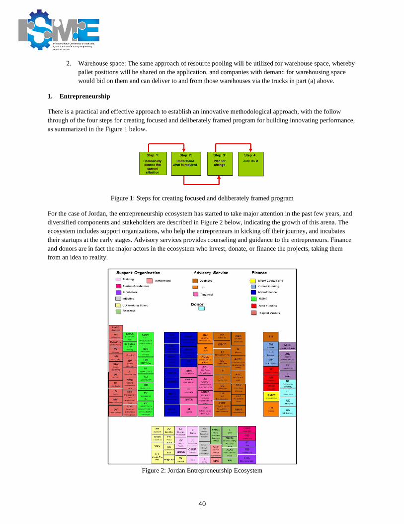
2. Warehouse space: The same approach of resource pooling will be utilized for warehouse space, whereby

pallet positions will be shared on the application, and companies with demand for warehousing space

would bid on them and can deliver to and from those warehouses via the trucks in part (a) above.

1. Entrepreneurship

There is a practical and effective approach to establish an innovative methodological approach, with the follow

through of the four steps for creating focused and deliberately framed program for building innovating performance,

as summarized in the Figure 1 below.

Figure 1: Steps for creating focused and deliberately framed program

For the case of Jordan, the entrepreneurship ecosystem has started to take major attention in the past few years, and

diversified components and stakeholders are described in Figure 2 below, indicating the growth of this arena. The

ecosystem includes support organizations, who help the entrepreneurs in kicking off their journey, and incubates

their startups at the early stages. Advisory services provides counseling and guidance to the entrepreneurs. Finance

and donors are in fact the major actors in the ecosystem who invest, donate, or finance the projects, taking them

from an idea to reality.

Figure 2: Jordan Entrepreneurship Ecosystem

40

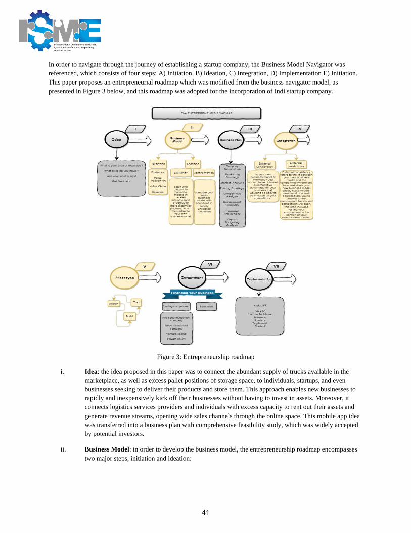
In order to navigate through the journey of establishing a startup company, the Business Model Navigator was

referenced, which consists of four steps: A) Initiation, B) Ideation, C) Integration, D) Implementation E) Initiation.

This paper proposes an entrepreneurial roadmap which was modified from the business navigator model, as

presented in Figure 3 below, and this roadmap was adopted for the incorporation of Indi startup company.

Figure 3: Entrepreneurship roadmap

i. Idea: the idea proposed in this paper was to connect the abundant supply of trucks available in the

marketplace, as well as excess pallet positions of storage space, to individuals, startups, and even

businesses seeking to deliver their products and store them. This approach enables new businesses to

rapidly and inexpensively kick off their businesses without having to invest in assets. Moreover, it

connects logistics services providers and individuals with excess capacity to rent out their assets and

generate revenue streams, opening wide sales channels through the online space. This mobile app idea

was transferred into a business plan with comprehensive feasibility study, which was widely accepted

by potential investors.

ii. Business Model: in order to develop the business model, the entrepreneurship roadmap encompasses

two major steps, initiation and ideation:

41

a. Initiation: Indi aims to target these difficulties by creating a platform that connects all the truck

drivers, warehouses and customers together. By simply using the application, the customers shall

be able to navigate between different warehouses and truck drivers, obtain quotations and select

the best option. The high level value stream map is given in Figure 4 below.

Figure 4: High Level Value Stream Map

b. Ideation: Uber and Airbnb business models were selected and studied to help in building the app

business model due to the similarities between both apps. In order to develop the detailed idea,

business canvas model was detailed as shown in Table 1 below, which depicts all the stakeholders

and components related to the project.

42

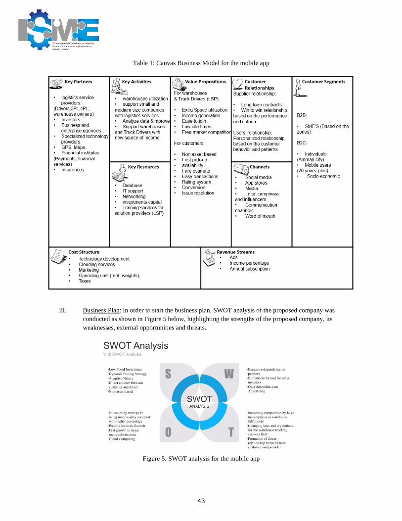
Table 1: Canvas Business Model for the mobile app

iii. Business Plan: in order to start the business plan, SWOT analysis of the proposed company was

conducted as shown in Figure 5 below, highlighting the strengths of the proposed company, its

weaknesses, external opportunities and threats.

Figure 5: SWOT analysis for the mobile app

43

In order to assess the feasibility and validity of the concept, surveys were conducted for the potential users and

SMEs, warehouse owners, and truck owners as shown in Fgiure 6 below. All the surveys proved the high potential

and acceptability of the project, and led to the next step of financial projections.

Figure 6: Market research surveys

Financial Projections

In order to examine if the business meets the organizational requirements and to analyse the technical evaluation of

the mobile app, a feasibility study is carried out. Two main points of reference are present in this feasibility study.

First, the cost needed to fulfil the objectives of the project. Second, the total profit that is to be acquired and earned

when the mobile app is launched and already operating, as can be seen in Figure 7 below.

44

Figure 7: Financial Projections

iv. Integration: Process Mapping was conducted in order to show the relationship between the entities

mentioned above and the system, and show how the data is moving among them. Sample process mapping

is shown in Figure 8 below, while tens of detailed process maps were conducted for detailing all the

processes of Indi mobile app.

45

Figure 8: Truck Ordering Process Map

v. Prototype: In the mobile application prototype phase, there have been many researches suggesting that

a system’s first impression is defined by the quality of its design. In other words, the visuals of a

system will determine whether or not it will impress its users, which makes the designing stage a very

important stage amongst all. It also tackled the functionality aspects of how the system’s database was

built. In order to ensure professionally sound design, the User Experience methodological approach

was followed, which has the main phases as shown in Figure 9 below.

Figure 9: User Experience Design Process

i. Sketch Phase: After researching and setting the overall process maps, the detailed sketches of the

logo, as well as the screens were conducted. Figure 10 below shows the logo sketching, whereas

in the next phase of Design the screens were shown in Figure 11 below.

Figure 10: sketch of the logo

ii. Design Phase:

46

Figure 11: Design of the Indi mobile app

vi. Investment: The process flow for attracting and selecting the investors is shown in Figure 12 below.

While Figure 13 shows the detailed company valuation and financial projections utilized for company

evaluation.

47

Figure 12: Investor Selection Roadmap

Figure 13: Financial

Projections and Company

Evaluation

vii. Implementation: The implementation was conducted after attracting and selecting potential investors,

and a contract was signed with the investor, and a contract for building the mobile app was signed.

Wewillassumethatthefirst3months,thesaleswillbe1/4,then1/3,then1/2oftheprojectedmonthlysales.

Month1 Month2 Month3 Month4 Month5 Month6 Month7 Month8 Month9 Month10 Month11 Month12 Total

Cashinflowfromsales 6,080 8,107 12,160 24,320 24,320 24,320 24,320 24,320 24,320 24,320 24,320 24,320 245,227

PersonnelExpense (3,700) (3,700) (3,700) (8,900) (8,900) (8,900) (8,900) (8,900) (8,900) (8,900) (8,900) (8,900) (91,200)

MarketingExpense (23,558) (8,558) (8,558) (2,558) (2,558) (2,558) (2,558) (2,558) (2,558) (2,558) (2,558) (2,558) (63,700)

OperatingExpense (2,300) (2,300) (2,300) (2,300) (2,300) (2,300) (2,300) (2,300) (2,300) (2,300) (2,300) (2,300) (27,600)

Software (12,000)

Furnitureandequipment (10,000)

TotalExpense (51,558) (14,558) (14,558) (13,758) (13,758) (13,758) (13,758) (13,758) (13,758) (13,758) (13,758) (13,758) (204,500)

Incomefromoperations (45,478) (6,452) (2,398) 10,562 10,562 10,562 10,562 10,562 10,562 10,562 10,562 10,562 40,727

CumulativeCash (45,478) (51,930) (54,328) (43,767) (33,205) (22,643) (12,082) (1,520) 9,042 19,603 30,165 40,727 40,727

viii.CashflowStatement

48

Figure 14: Contracts with the investor and mobile app developer

CONCLUSION

This project describes the evolution of a company from an idea, to the full inception and incorporation. The project

followed a scientific and structured managerial approach, utilizing the Entrepreneurship Roadmap, User Experience

Methodology, as well as several industrial engineering and marketing tools. The Entrepreneurial Roadmap starts

with the ideation phase, followed by Business Model, Business Plan, Integration, Prototype, Investment and

Implementation phases. The idea was developed through a mobile app, which enables all of those parties to connect

swiftly and virtually in a seamless cyberspace. Lastly, The real-life implementation of the company was through

legal contractual agreements for the incorporation of the company, ‘Indi, as well as the contracts for the

development of the mobile app to be utilized and launched expeditiously.

The project showed the high potential of this mobile app to all potential partners, investors, customers, truck owners

and individuals, which will be followed through by the team in the coming months through full launch and hopefully

global expansion if ‘Indi as a genuine and original mobile app.

REFERENCES

1. O'Sullivan, David (2002). "Framework for Managing Development in the Networked Organisations". Journal of

Computers in Industry 47 (1): 77-88.

2. Peters Hisrich. 1998 Entrepreneurship, Irwin McGraw–Hill, U.S.A.

3. Christensen C.M., [1997] The Innovator’s Dilemma, Harvard Business School Press, Boston, Massachusetts.

4. Waters, D. (2002). Logistics: An Introduction to Supply Chain Management. Basingstoke: Palgrave.

49

IoT-WSN system for improving manual order-picking operation

Tala Shammas, [email protected]. Industrial Engineering Department, German Jordanian

University, Amman, Jordan

Yazeed Haddadin, [email protected]. Industrial Engineering Department, German Jordanian


Safwan Altarazi, [email protected]. Industrial Engineering Department, German Jordanian


ABSTRACT

The networking of resources, information, objects, and people through the internet has shifted the way

businesses are managed; warehousing is not an exception. The current research aims to develop an Internet-of-

Things system for improving the manual-order-picking process in warehouses. The architecture of the proposed

system consists of strain gauges, light emitting diodes, microcontrollers, liquid-crystal display screens, and a single-

board computer. The proposed system was tested regarding its performance, reliability, and economic feasibility.

The implementation of the system demonstrated its ability to reduce human errors in the picking process,

decrease the order-picking time, and provide real-time status of stock keeping units inventory.

Keywords: Internet of Things; Wireless Sensor Networks; Warehousing, Manual-order-picking

1. INTRODUCTION

Internet of Things (IoT), sometimes called Internet of Everything, is a system of interconnected objects

(machines, machinery, animals or people) and sensors that are built within or physically attached to these objects;

with internet connectivity that collects and sends information to a centralized middleware which in turn organizes

and processes data to be used in different applications according to a pre-defined algorithms [1-3]. These sensors

can use various types of local area connections such as Radio Frequency Identification (RFID) and Wireless Fidelity

(Wi-Fi). In fact, the IoT was inspired by members of the RFID community, that envisioned an opportunity of

learning information about a uniquely identified object by searching the internet or database that belongs to a

specific RFID tag. The other key technologies that are involved in IoT include Wi-Fi, barcode, Bluetooth, and

Wireless Sensor Networks (WSN). IoT market has been massively growing in the past several years and is expected

to go from USD 157.05 Billion in 2016 to USD 661.74 Billion by 2021 [4]. Experts have estimated an amount of 50

billion devices to be connected to the internet by the year 2020 which is a huge leap in comparison to almost 18

billion by the end of 2015 [5]. These IoT applications have been and will be implemented in fields such as

healthcare, smart surveillance, smart cities, supply chain management, etc.

Today’s warehouse is a complex system of interconnected and interrelated activities that should seamlessly work

together. The typical old-school perception of a warehouse of just storing products without adding value as-well-as

being a cost-burden to the supply chain is unsound anymore [6]. With the help of internet, e-commerce, and

supply chain integration; warehouses are now a value-adding entity to the supply chain. It is a crucial and integral

part in supply chain networks, costing 2 to 5 % of their total sales [7]. Interestingly, the order-picking function,

usually classified as manual or automated, is the most costly task compared to the other warehousing functions of

50




receiving, storing, and shipping [6]. The quicker and more accurate the order-picking activity becomes, the more

efficient and cost saving the warehouse is, however, manual order-picking warehouses are prone to human errors,

consequently resulting in greater time consumption [6,8].

Literature about IoT solutions in warehousing is scarce. Radio frequency identification (RFID) technology has

been widely used to track and control materials flow and processes in supply chains [9,10]. Particularly, Yang [8]

emphasized that RFID technology and WSN should be used as an infrastructure for order fulfilment processes

where stock keeping units (SKUs) and locations in the warehouse are equipped with RFID tags and certain readers

attached to pickers, forklifts, and pallets. Other research viewed RFID as the appropriate methodology for IoT

inventory management solutions [11,12].

Generally, IoT warehousing systems depend mainly on RFID technology rather than WSN. The aim of this

research is to develop an IoT-WSN based system for the manual-order-picking process. The proposed system

would significantly reduce the human error in the picking process resulting in decreasing the picking time. In

addition, the IoT-WSN system would continuously track the inventory in a warehouse; in fact, this system might be

the sole reference of instantaneous warehouse inventory count.

2. ORDER PICKING

The order picking entails collecting SKUs in specific quantities and assembling them in a consolidation area

before shipment to satisfy customers' orders [13]. It is the most important warehousing function as it consumes

about 55% of all warehouses operational costs [6]. Two kinds of order picking classes are known in practice;

manual which employs humans and automated that mostly relies on conveyors and robots to pick, sort, and pack

orders. Manual-order-picking activities are more common than automated ones [14,15]. Order-picking is classified

into picker-to-parts and parts-to-picker systems. According to de Koster et al. [14], the majority of manual-order-

picking systems are picker-to-parts systems. In picker-to-parts the order picker receives the pick list and then

travels in an electrical forklift or by pushing a cart through the picking zone. The SKUs are then collected and

transported to the shipping dock where they are loaded to the shipping truck. The proposed IoT-WSN system is

handling the picker-to-parts manual-order-picking system.

The time of order picking can be classified into four main categories; travel time, search time, pick time, and

setup time. The travel and search time, which accounts for about 70% of the total time [16], can be optimized

through adopting appropriate operational policies for storage, routing, and picking [17]; routing policies are of

interest for order picking operation. Different routing heuristics can be followed in manual-order-picking such as

traversal routing (S-shape), largest gap, and aisle-by-aisle [18]. Traversal routing entails fully traversing an aisle if it

was entered. In the largest gap heuristics, a picker enters an aisle as far as the largest gap; largest gap is defined as

the distance between two adjacent picks or between the first pick and the front aisle, or between the last pick and

the back aisle. In the aisle-by-aisle heuristic, every main aisle is visited once. The order picker starts at the depot

point and goes to the left most aisle containing required-picking SKUs. Every ordered item in this main aisle are

picked and a cross aisle is chosen, such that traveled distance is minimized, to continue to the next main aisle, and

the same process is repeated again. The proposed IoT-WSN system is adopting the aisle-by-aisle manual-order-

picking class.

3. THE PROPOSED IoT-WSN SYSTEM

No universal IoT architecture is available today; some researchers demonstrated it as a 3-layer architecture [2],

consisting of a perception, network, and application layer. Others [19,20] viewed it as 4-layer architecture, namely:

sensing layer, networking layer, service layer, and an interface layer. Ultimately, both opinions point to the same

system but with different detailing; for instance, the service and interface layer of the 4-layer architecture can be

51

combined in the application layer of the 3-layer architecture. The proposed IoT-WSN system’s architecture is made

up of three layers: Perception, network and application layer, as shown in figure 1. The outer most layer

(perception layer), concerned with gathering the data from the warehousing environment; consists of strain

gauges, amplifier circuit HX711, microcontrollers (ESP NodeMCU), liquid-crystal displays (LCD) and light emitting

diodes (LED). The network layer that is embodied by the Raspberry Pi is where the data processing takes place in

addition to functioning as an internet provider. The processed data is then sent to the interactive and final layer of

the system−the application layer. This layer receives, organizes, and illustrates all the important information for

management and controlling, in an easy-to-read electronic management reports.

In details, a storage location rack comprises of a strain gauge, amplifier circuit (HX711), LED, LCD and an ESP

NodeMCU microcontroller which connects all these components together and also connects the storage location

to the Raspberry Pi through internet. Strain gauges are used to measure SKUs’ weights on the racks, HX711

converts the strain gauge reading into digital form and sends the tuned reading to the ESP NodeMCU. Then, the

ESP NodeMCU converts the weight reading into number of SKUs available (for example a 20 kg decrease in weight

is equivalent to 3 SKUs picked off the storage rack) through an algorithm coded with C language. For order picking

routing, an algorithm based on aisle by aisle heuristic embedded in the Raspberry Pi is executed. Storage locations’

addresses are built in the code. The picker follows the route through the lighting of aisles’ overhead lights and the

sequential lighting of storage locations. The aisle light will be turned on if it includes at least one turned on storage

rack light. The sequential lighting decision is made by lighting the closest address number storage rack’s LED, which

will turn off when the picker pulls the ordered SKUs, by sending information of the pulled quantity from the ESP

NodeMCU to the Raspberry Pi. Then the following address number storage location’s LED will be turned on, so on

and so forth. Aisles lights will be turned off when all its storage racks’ lights turn off. To help picking the correct

SKUs, the LCD displays the required number SKUs to be collected; simply expressed just in one figure, or in multi

figures such as number of cartons, retail boxes, and single pieces. During picking, the network layer calculates the

amount that has been picked and changes the readings on the LCD indicating how much more of each category

(carton, retail box, single piece) the picker still has to pick. Automatically after picking, the system counts the SKUs

picked, checks if the picker has picked the correct amount (through calculating the weight on the storage racks),

and warns the picker if incorrect amount was picked. After the completion of the order picking process, Raspberry

Pi provides the top management with processed order reports that include the identity of the picker, the date and

time the order is processed, type and number of SKUs collected.

To place an order and to deliver management reports, the system is connected with a website where the

Raspberry Pi is functioning as its server. Figure 2 represents how data is flowed within the system’s layers and

along with the website. The Raspberry Pi and the website exchange data regarding the customer order

requirements and the management report. The ESP NodeMCU receives weight reading data from the strain gauge,

exchanges data with Raspberry Pi to send information to the storage racks for the sequential lighting process.

Finally, the ESP NodeMCU also exchanges data with the Raspberry Pi when the ordered SKUs are picked resulting

in receiving data for turning the respective LED off and turning the next one on.

52

Fig. 1: The proposed IoT-WSN system’s architecture

Fig. 2: Data flows within the systems components

4. PILOT SYSTEM IMPLEMENTATION

The system’s pilot implementation took place in two stages. First, a single aisle with four storage locations was

built and tested; the testing verified the functionality of the system as it was supposed to, for example, LCD

screens did turn off after the end of picking, weights measurements were accurate indicators of actual SKUs in

storage racks, accurate management reports were generated, etc. In the second stage implementation, the system

was built for a close to real-life 3X4 m warehouse zone (figure 3) which composes of three aisles each with four

storing racks. For this stage, three preliminary validation studies were conducted: time and motion to validate the

performance advantage of the system, failure mode and effect analysis (FMEA) to discover the system’s potential

failures in its early design phase, and feasibility study to validate the economics of implementing such system.

53

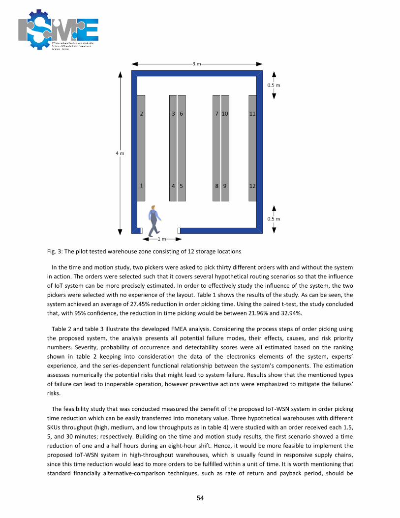
Fig. 3: The pilot tested warehouse zone consisting of 12 storage locations

In the time and motion study, two pickers were asked to pick thirty different orders with and without the system

in action. The orders were selected such that it covers several hypothetical routing scenarios so that the influence

of IoT system can be more precisely estimated. In order to effectively study the influence of the system, the two

pickers were selected with no experience of the layout. Table 1 shows the results of the study. As can be seen, the

system achieved an average of 27.45% reduction in order picking time. Using the paired t-test, the study concluded

that, with 95% confidence, the reduction in time picking would be between 21.96% and 32.94%.

Table 2 and table 3 illustrate the developed FMEA analysis. Considering the process steps of order picking using

the proposed system, the analysis presents all potential failure modes, their effects, causes, and risk priority

numbers. Severity, probability of occurrence and detectability scores were all estimated based on the ranking

shown in table 2 keeping into consideration the data of the electronics elements of the system, experts’

experience, and the series-dependent functional relationship between the system’s components. The estimation

assesses numerically the potential risks that might lead to system failure. Results show that the mentioned types

of failure can lead to inoperable operation, however preventive actions were emphasized to mitigate the failures’

risks.

The feasibility study that was conducted measured the benefit of the proposed IoT-WSN system in order picking

time reduction which can be easily transferred into monetary value. Three hypothetical warehouses with different

SKUs throughput (high, medium, and low throughputs as in table 4) were studied with an order received each 1.5,

5, and 30 minutes; respectively. Building on the time and motion study results, the first scenario showed a time

reduction of one and a half hours during an eight-hour shift. Hence, it would be more feasible to implement the

proposed IoT-WSN system in high-throughput warehouses, which is usually found in responsive supply chains,

since this time reduction would lead to more orders to be fulfilled within a unit of time. It is worth mentioning that

standard financially alternative-comparison techniques, such as rate of return and payback period, should be

54

implemented to clearly reveal the feasibility of the proposed system, however, this implementation would need

real case figures.

Table 1: Time and motion study results

Order Address of storage

location

Time without the system (sec.) Time with the system (sec.) Reduction in average

Order picking time (%) Picker1 Picker2 Average Picker1 Picker2 Average

1 1,3,4 34 36 35 28 31 29.5 15.71

2 2,4,6 62 63 62.5 48 49 48.5 22.40

3 1,2,10 80 78 79 51 53 52 34.18

4 4,8,11 76 79 77.5 60 57 58.5 24.52

5 5,7,8 65 63 64 31 35 33 48.44

6 5,7,9 64 66 65 45 47 46 29.23

7 9,10,11 89 91 90 33 36 34.5 61.67

8 1,5,9 78 76 77 62 59 60.5 21.43

9 2,6,10 80 82 81 59 57 58 28.40

10 4,6,9 78 76 77 60 63 61.5 20.13

11 1,2,3,4 35 36 35.5 26 28 27 23.94

12 2,4,5,6 64 65 64.5 48 45 46.5 27.91

13 3,4,10,12 68 70 69 51 49 50 27.54

14 4,8,9,11 78 81 79.5 58 56 57 28.30

15 5,7,8,12 68 66 67 51 55 53 20.90

16 1,4,5,7,9 80 83 81.5 60 64 62 23.93

17 2,4,9,10,11 70 72 71 52 53 52.5 26.06

18 1,5,6,10,12 84 82 83 63 59 61 26.51

19 2,4,6,10,11 82 80 81 61 58 59.5 26.54

20 1,4,6,8,9 80 78 79 60 63 61.5 22.15

21 1,5 58 60 59 43 44 43.5 26.27

22 11,12 35 32 33.5 26 28 27 19.40

23 1,2,6,8,10,12 84 82 83 63 65 64 22.89

24 6,7,8,9,10,11,12 68 70 69 51 53 52 24.64

25 12 28 26 27 21 19 20 25.93

26 1,3,5,7,9,11 82 84 83 61 58 59.5 28.31

27 2,4 30 27 28.5 22 25 23.5 17.54

28 1,12 55 53 54 41 39 40 25.93

29 5,6,7,8 37 39 38 28 30 29 23.68

30 9,10,11,12 64 38 51 48 33 40.5 20.59

Ranking Severity Occurrence Detectability

1 No effect Failure is unlikely Almost certain

2 System operable with minimal

interference Relatively few failures High certainty

3 System operable with some degradation in performance

Occasional failures Moderate certainty

4 System operable with significant

degradation in performance Repeated failure Low certainty

5 System inoperable Failure is almost inevitable Absolute uncertainty

Table 2: FMEA ranking criteria 1

55

Table 3: FMEA analysis

Process function Potential failure

mode

Potential effect/s of

failure Seve

rity

Potential cause(s)/ mechanism(s) of

failure

Occ

urr

ence

Det

ecta

bili

ty

RP

N

Recommended actions to take

Order sent from website to the Raspberry Pi

Order not reaching the Raspberry Pi

Unfulfilled order

5

Power supply down 2 1 10 Add redundant electrical generator

Security issues in website

1 2 10 Use fata protection and user privacy

No internet coverage

1 1 5 Add redundant Raspberry Pi Hardware failure in

the Raspberry Pi 2 3 30

Raspberry Pi sends SKU quantity and route to ESP NodeMCU(s)

order picking process will miss storage location(s)

Unfulfilled order

5

Power supply down for (some) storage location(s)

3 3 45

Periodic inspection on storage locations’ readiness

Hardware failure in (some) ESP NodeMCU(s)

4 3 60 Add a redundant ESP NodeMCU

Software failure in (some) ESP NodeMCU(s)

2 4 40 Periodic verification of code execution

Failure in (some) LED(s)

3 1 15 Periodic inspection on storage locations’ readiness

Failure in (some) LCD(s)

3 1 15

Raspberry Pi receives information from ESP NodeMCU regarding pulling the required amount

No information was sent to the Raspberry Pi from the ESP NodeMCU, preventing the next storage location from turning on its LED

Unfulfilled order

5

Power supply down 2 1 10 Add redundant electrical generator

No internet coverage

1 1 5 Add redundant Raspberry Pi Hardware failure in

Raspberry Pi 2 3 30

Hardware failure in ESP NodeMCU(s)

4 3 60 Add a redundant ESP NodeMCU

Software failure in ESP NodeMCU(s)

2 4 40 Periodic verification of code execution

Miss-positioning of strain gauge(s)

5 4 100 Customize strain gauge to properly fit in the storage location

Faulty wire(s) in strain gauge(s)

5 4 100

Faulty wire(s) in HX711(s)

5 4 100

56

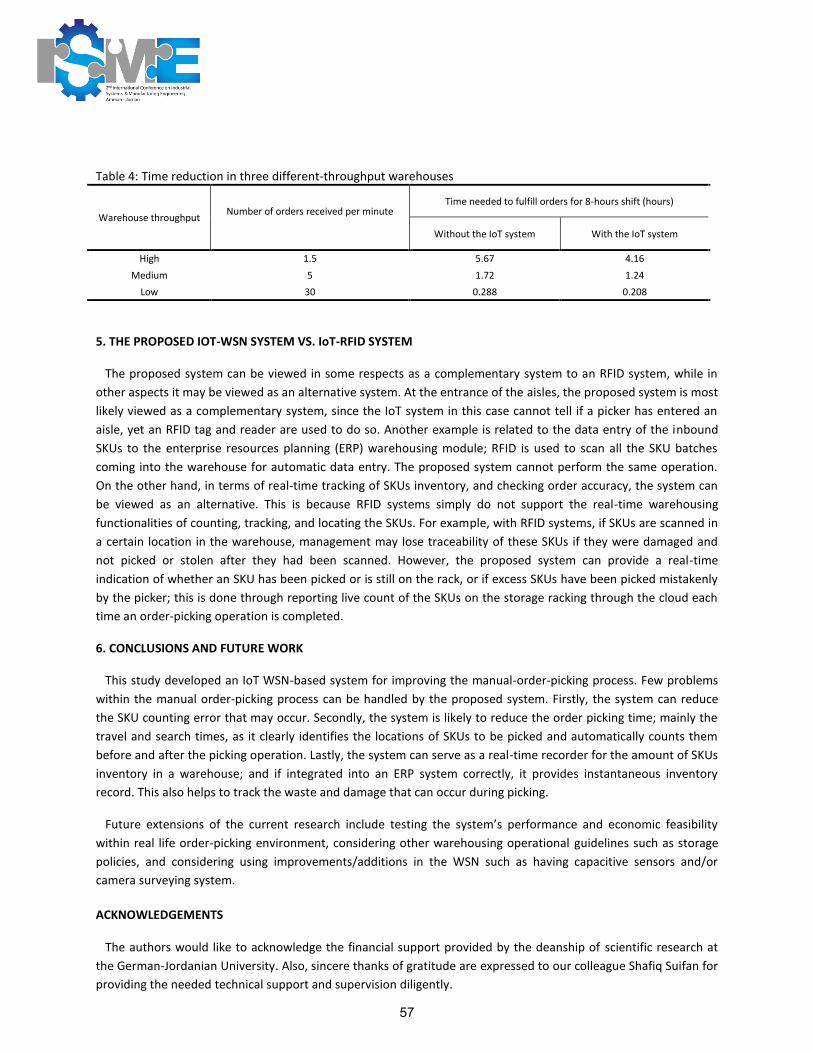
Table 4: Time reduction in three different-throughput warehouses

Warehouse throughput Number of orders received per minute

Time needed to fulfill orders for 8-hours shift (hours)

Without the IoT system With the IoT system

High 1.5 5.67 4.16

Medium 5 1.72 1.24

Low 30 0.288 0.208

5. THE PROPOSED IOT-WSN SYSTEM VS. IoT-RFID SYSTEM

The proposed system can be viewed in some respects as a complementary system to an RFID system, while in

other aspects it may be viewed as an alternative system. At the entrance of the aisles, the proposed system is most

likely viewed as a complementary system, since the IoT system in this case cannot tell if a picker has entered an

aisle, yet an RFID tag and reader are used to do so. Another example is related to the data entry of the inbound

SKUs to the enterprise resources planning (ERP) warehousing module; RFID is used to scan all the SKU batches

coming into the warehouse for automatic data entry. The proposed system cannot perform the same operation.

On the other hand, in terms of real-time tracking of SKUs inventory, and checking order accuracy, the system can

be viewed as an alternative. This is because RFID systems simply do not support the real-time warehousing

functionalities of counting, tracking, and locating the SKUs. For example, with RFID systems, if SKUs are scanned in

a certain location in the warehouse, management may lose traceability of these SKUs if they were damaged and

not picked or stolen after they had been scanned. However, the proposed system can provide a real-time

indication of whether an SKU has been picked or is still on the rack, or if excess SKUs have been picked mistakenly

by the picker; this is done through reporting live count of the SKUs on the storage racking through the cloud each

time an order-picking operation is completed.

6. CONCLUSIONS AND FUTURE WORK

This study developed an IoT WSN-based system for improving the manual-order-picking process. Few problems

within the manual order-picking process can be handled by the proposed system. Firstly, the system can reduce

the SKU counting error that may occur. Secondly, the system is likely to reduce the order picking time; mainly the

travel and search times, as it clearly identifies the locations of SKUs to be picked and automatically counts them

before and after the picking operation. Lastly, the system can serve as a real-time recorder for the amount of SKUs

inventory in a warehouse; and if integrated into an ERP system correctly, it provides instantaneous inventory

record. This also helps to track the waste and damage that can occur during picking.

Future extensions of the current research include testing the system’s performance and economic feasibility

within real life order-picking environment, considering other warehousing operational guidelines such as storage

policies, and considering using improvements/additions in the WSN such as having capacitive sensors and/or

camera surveying system.

ACKNOWLEDGEMENTS

The authors would like to acknowledge the financial support provided by the deanship of scientific research at

the German-Jordanian University. Also, sincere thanks of gratitude are expressed to our colleague Shafiq Suifan for

providing the needed technical support and supervision diligently.

57

REFERENCES

[1] H. Kagermann, W., Wahlster, J. Helbig, Recommendations for implementing the strategic initiative INDUSTRIE 4.0: Securing the future of German manufacturing industry, Forschungsunion, 2013.

[2] J. Gubbi, R. Buyya S. Marusic, M. Palaniswami, Internet of Things (IoT): A vision, architectural elements, and future directions, Future Generation Computer Systems, 29 (2013) 1645-1660.

[3] H. Becker, What is the Internet of Things and Why is it Important? Technology Guide, 2013, accessed February 3 2018, http://www.technologyguide.com/feature/internet-of-things/.

[4] B. Ahlgren, H. Markus, E. Ngai, Internet of Things for Smart Cities: Interoperability and Open Data, IEEE Internet Computing, 20 (2016) 52-56.

[5] TriStar, The internet of things defines the future for manufacturers, accessed February 3 2018, http://www.tristar.com/what-the-internet-of-things-means-to-manufacturers/.

[6] J. Tompkins, J. White, Y. Bozer, J. Tanchoco, Facilities planning. John Wiley & Sons, New York, 2010.

[7] E. Frazelle, E. Frazelle, World-class warehousing and material handling. McGraw-Hill, New York, 2002.

[8] J. Yang, Design and implementation of intelligent logistics warehouse management system based on Internet of things. In: ICLEM 2012: Logistics for Sustained Economic Development—Technology and Management for Efficiency, 2012.

[9] P. Reaidy, A. Gunasekaran, A. Spalanzani, Bottom-up approach based on internet of things for order fulfilment in a collaborative warehousing environment, International Journal of Production Economics,159 (2015) 29-40.

[10] A. Gul, M. Usman, T. Soomro, Internet of things (IOT): An overview, Journal of Information & Communication Technology, 10 (2016) 121-130.

[11] K. Evangelos, N. Tselikas, A. Boucouvalas, Integrating RFIDs and smart objects into a Unified Internet of Things architecture, Advances in Internet of Things, 1 (2011) 5-12.

[12] S. Trab, E. Bajic, A. Zouinkhi, M. Abdelkrim, H. Chekir, R. Ltaief, Product allocation planning with safety compatibility constraints in IoT-based warehouse, Procedia Computer Science, 73 (2015) 290-297.

[13] D. Piasecki, Order Picking: Methods and Equipment for Piece Pick, Case Pick, and Pallet Pick Operations, InventoryOps, accessed February 3 2018, http://www.inventoryops.com/order_picking.htm.

[14] R. De Koster, T. Le-Duc, K. Roodbergen, Design and control of warehouse order-picking: A literature review. European Journal of Operations Reserach, 182 (2007) 481-501.

[15] M. Shqair, S. Altarazi, S. Al-Shihabi, A statistical study employing agent-based modeling to estimate the effects of different warehouse parameters on the distance travelled in warehouses, Simulation Modelling Practice and Theory, 49 (2014) 122-135.

[16] S. Henn, S. Koch, G. Wäscher, (2012). Order batching in order picking warehouses: a survey of solution approaches. In Warehousing in the Global Supply Chain (pp. 105-137). Springer London.

[17] S. Altarazi, M. Ammouri, Concurrent manual-order-picking warehouse design: a simulation-based design of experiments approach, International Journal of Production Research, 2018, doi.org/10.1080/00207543.2017.1421780.

[18] K. Roodbergen, Routing order pickers in a warehouse, Roodbergen.com, accessed February 3 2018,

http://www.roodbergen.com/warehouse/background.php#6

[19] R. Khan, S. Khan, R. Zaheer, S. Khan, Future internet: the internet of things architecture, possible applications and key challenges. In: Frontiers of Information Technology, 10th International Conference on. IEEE, 2012.

[20] L. Da Xu, W. He, S. Li, Internet of things in industries: A survey. IEEE Transactions on industrial informatics, 10 (2014) 2233-2243.

58

SUPPLY CHAIN STREAMLINING AT SAMEH MALL: Inventory Management, CPFR, and Vehicle

Routing Optimization

Laith AbuHilal, [email protected], GJU Industrial Professor and GM at Sameh Mall Group. Zaid

Farkouh, Tala Hamarneh, Tariq AbuFeilat, German Jordan University

ABSTRACT

This paper describes a project embarked upon to streamline the supply chain of Sameh Mall through process

mapping and improvements. It starts with Inventory Management, demand planning and forecasting, providing a

detailed roadmap for implementing the most suitable replenishment systems, which was found to be the Periodic-

Ordering (P-System). The implementation entailed defining the Target stock level for all items at each branch, and

automating the ordering weekly, connecting the branches directly with suppliers, while still leveraging the

economies of scale and central commercial negotiations. Collaborative Planning, Forecasting and Replenishment

(CPFR) was introduced through a simulation model that highlighted the value of information sharing while

implementing the P-System. The paper also tackles the analysis of fleet management and vehicle routing, whereby a

Capacitated Vehicle Routing Problem model was developed using CPLEX language.

INTRODUCTION

According to Mentzer et al (2001) , supply chain is a set of three or more entities directly involved in the upstream

and downstream flow of products, services, finances, and information from a source to the customer.

Sameh mall is one of the leading retailers in Jordan, with over 21 branches. With the current major expansion, the

company needs a solid supply chain in order to enable fulfillment of customer demands on continuous basis, while

optimizing the stock levels ensuring the right products are delivered to the right locations at the right time with the

right cost and quality. The company did not have a supply chain department, and the functions of supply chain were

defragmented among several departments, leading to several ineffectiveness facets, including: 1. Suppliers having to

lead the ordering process, standing in lines within the purchasing department, and “pushing” buyers to induce more

stocks of their products at stores, 2. The above led to overstocks of items including slow moving items, while often

times the fast moving staple items were not replenished fast enough, leading to overstocks and out of stocks. 3. If

suppliers with important items did not have strong sales force, or poor communication with the buyers, their

important products would not be replenished or even be listed into the range. 4. The stores were just hammered with

piles of stock, without any influence on the stock levels, posing a push system of what is forced by the purchasing

department and suppliers, rather than a pull system based on customers’ needs and demands. 5. As the stores’

management was not involved in the replenishment process, they were not able to respond effectively and swiftly to

the variations in supply chain, for example if one item was out of stock from a supplier, they were not able to

expeditiously order its replacement from alternate suppliers.

Through analyzing the above ineffective supply chain, it was concluded that streamlining should be conducted in

two phases: 1. In the short term to provide stores with the tools to order in a pull fashion, with reports providing

suggested orders based on target stock levels of each item, called Max for each items, which is based on the

movement of the item and its demand. This phase enabled the evolution of the culture from push to pull, enabled the

suppliers to work with all stores rather with merely the central purchasing department, allowed for the cleansing of

data including the pack sizes, accurate stock levels of items, as well as items attributes, all of which included

inaccuracies. 2. The second phase was to automate the ordering completely, whereby after the data cleansing and

establishing the pull culture, the company became ready for full automation, whereby the Max levels for each item

were calculated scientifically, and the system was made ready for automating the ordering algorithm.

59


In order to further optimize the supply chain and replenishment effectiveness, Information Sharing and basic CPFR

was studied using a simulation model. The engagement started with mapping the replenishment process, and the

basic functionality simulated is providing the supplier with visibility into the stock levels and sales of the different

items at the different stores, in order to produce to actual demand rather to forecast, and enable swift replenishment

based on real-time data.

The movement of trucks and replenishment of produce as well as imported items to stores was tackled, whereby the

Capacitated Vehicle Routing problem was modeled using mixed integer linear programming utilizing CPLEX

programming language, and the optimal routing of trucks among zones was found, and real-life implementation of

such routes was adopted by the transportation department at Sameh Mall.

1. Demand Planning and Inventory Management system

CPIM APICS defines inventory as “those stocks or items used to support production (raw materials and work-in-

process items), supporting activities and customer service (finished goods and spare parts)”. Sameh mall did not

have a Supply Chain department, and hence its functions were defragmented among several departments, and had

numerous inefficiencies. Figure 1 below describes the overall value chain at Sameh mall, whereas Figure 2 below

describes the detailed ordering process.

Figure 1: overall value chain at Sameh Mall

Figure 2: Detailed ordering process

Items creation

& ranging

1

Purchasing

Stores

Operations

Supplier

4Review stock

and approve

Receive per

PO

Merchandise

and sell

6

Process Owner Loop until Approval

2

3

Review Stock

and suggest

orders

Make OrdersManager’s

Approval

Orders triggered

by supplier!

Paperwork! Physical flow of

paper! Time!

Often Large

Quantities and

mistakes

Invoice

5

• Ordering from purchasing

department

- Range

- Items Creation

- Items Ordering

- Pricing

- Ordering of

promotions

Stores have to accept all orders

made by buyers

Display the items, as they can with

severe shortage in back-store

warehousing space, and

showroom display space

OrderingPurchasing

Suppliers’ sales

representatives visit the

purchasing department, to

negotiate orders.

Purchasing department

issue the orders as they

see fit

Operations

Operations Receiving and Sales

Ordering On Delta System:

1. Triggered by suppliers

2. Negotiated with buyers,

without any scientific

criteria

60

As can be shown in Figure 2 above, the ordering process itself did not engage the stores management, and the stocks

were pushed onto them. Moreover, the buyers did not have scientific formulas but rather the orders were both

triggered and negotiated by the sales representatives, rendering the process more commercial rather than supply

chain centric, leading to major issues including:

1. Over stocking of items whose sales representatives had effective sales and commercial leverage, even if

their items were not demanded at the same pace by customers.

2. Out of stock of major fast-moving items whose sales representatives did not follow through effectively.

Leading to ineffective availability of items at stores.

3. The stores operations had severe storage issues, whereby they did not have enough back-store warehousing

areas, leading to mishandling and damages. Moreover, the stores lost track of items stored at the back-

areas, leading to lack of display of vital items as well as expiries.

4. The stores operations did not have enough display areas for all the pushed items, leading to cluttered

merchandising at stores.

5. The stores had to return items to suppliers, including items that expired at the back-stores, leading to issues

with the suppliers.

6. The lack of synchronization between purchased items and sold items led to overall cashflow issues.

In order to streamline this process, a short-term solution was proposed as shown in Figure 3 below, that allowed for

stores to trigger the orders leading to:

1. Leverage their on-the-ground real-time knowledge of the demand levels, resolving most of the issues

described in the current ordering process above.

2. Allowing for stores management to order items that are out of stock from the suppliers with replacement

items.

Figure 3: Short-Term ordering process

As can be shown in figure 3 above, the Out of Stock Report (OOS) was automated for all items that are out of stock,

and the suggested orders were given to stores management based on the Periodic Inventory management system (P-

System), which was selected due to the following reasons:

Unprinted

orders

No

Items creation

& rangingPurchasing

Receive per

PO

What to order Make Orders

Report of OOS items,

suggested quantities

Operations

Management

Supplier RepReceive the

orderRep visit

store?

Arrange

Delivery

Yes

Print

Unprinted

Orders

Print order

Print OrderOrders

OOS

61

1. Suppliers typically need to schedule their deliveries to stores of Sameh mall as well as other competitors.

Hence the best inventory management system would be a time-based system, allowing for orders on

specific days, and scheduled deliveries on certain dates. A real-life effective example is to calculate the

orders of all items on Fridays, and schedule the deliveries during the week.

2. If a Re-Order point and Economic Order Quantity (ROP) model is adapted, the reorder points of different

items from the same supplier could be reached on different days. Hence the supplier would receive

different orders of different items on different days, rendering the delivery process scattered and

unconsolidated.

Implementation of the periodic system was practically implemented through the following steps:

1. Historical demand data was analyzed, and outliers were filtered out using the Interquartile Range method:

a. The data was sorted in a pivot table on excel.

b. The 1st and 3rd Quartiles (Q1 & Q3) were calculated, and the Interquartile Range (IQR) (Q3 - Q1)

was calculated.

• Upper Limit = Q3 + 0.5*IQR. (1)

• Lower Limit = Q1 – 0.5*IQR. (2)

c. Any data point that falls out the limits was filtered out.

2. The P-Max, or Target level, were calculated using two methods:

a. Setting the Target Max at two weeks stock cover: whereby the average weekly demand was

calculated and extrapolated for 2 weeks as a set target level.

b. P-System Method: this method takes the safety stock into consideration. Which was found using

the following equation:

• SS = Z*SL, where Standard Deviation During Lead Time

(SL) = Weekly Average * Square Root of Lead Time. And Z

is determined from the normal distribution Z-Table,

depending on the desired Service Level.

• Initial Max = Average Weekly Demand * (Lead Time for Max (L = 2 weeks) + Review

Period (P = 1 week)) + Z*S(L+P). (3)

• S(L+P) = S * Square Root of (P+L), Where S is the standard deviation for the data (weekly

demand) of an item. (4)

• Max = Min + SPK_Multiplier * ((Initial Max – Min)/Pack Size), the SPK_Multiplier = 1. (5)

3. The two main methods, 2-weeks stock cover and the P-system Max were compared, and they gave

reasonably close results, however the P-system Max provided a forecasted stock cover closer to 2 weeks

and was selected accordingly.

A newly developed Supply Chain team was incepted to handle the calculations of the Max for all items at all

branches, and follow through on the implementation of the suggested orders reports. The operations team was very

62

cooperative, leading to immediate swift transition, which all led to increasing the availability from the 60% to above

90% rapidly, while controlling the stock cover and reducing it from about 30 days to below 21 days.

The next phase to fully automate the ordering, as shown in Figure 4 below, whereby the ERP system was

programmed to trigger the orders automatically every Friday calculating the required orders which are the Target

level minus the current inventory level of each item.

Figure 4: Phase 2 fully automated ordering process

Moreover, the IT department was able to automatically send those orders to suppliers upon approval by store

management via e-Fax directly to the suppliers. This implementation led to dramatic saving in time, reduction of

human intervention and tighter connectivity. It has also allowed for Information Sharing and CPFR. Enabling

suppliers to have access to their items’ stock levels at the different stores allowed for producing to actual demand

rather than forecast, and synchronized the fulfilment process expeditiously and effectively. CPFR also engages

suppliers in long-term annual promotional calendars, and strategic marketing and promotional campaigns, enabling

the supplier to better plan their purchasing budget and forecasts, and allowing for better pricing and global supply

chain optimization. A simulation model of the multi-echelon supply chain was introduced and what if analysis

conducted. A simulation model for the P-system was developed as shown in Figure 5 below, highlighting how the

system works and mimicking the replenishment of stock triggered every Friday, and delivery during the week. The

next step was to introduce information sharing mimicking CPFR, as shown in Figure 6 below. Whereby the supplier

now has access to the actual stock levels at each store, and can make the replenishment decisions swiftly as needed,

eliminating any stock outs and out of stock costs, while at the same time reducing any over stocks and holding costs.

The comparison among the scenarios is provided in Table 1 below, highlighting a major saving in supply chain cost

with the information sharing with suppliers.

Items creation

& ranging

1

Purchasing

Operations

ManagementReceive per

POWhat to order

Review &

Make Orders

4

Orders triggered by branches

based on Min & Max

32

delta

63

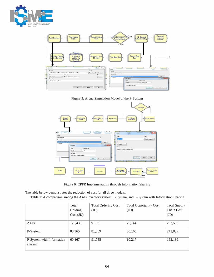
Figure 5: Arena Simulation Model of the P-System

Figure 6: CPFR Implementation through Information Sharing

The table below demonstrates the reduction of cost for all three models:

Table 1: A comparison among the As-Is inventory system, P-System, and P-System with Information Sharing

Total

Holding

Cost (JD)

Total Ordering Cost

(JD)

Total Opportunity Cost

(JD)

Total Supply

Chain Cost

(JD)

As-Is 120,433 91,931 70,144 282,508

P-System 80,365 81,309 80,165 241,839

P-System with Information

sharing

60,167 91,755 10,217 162,139

64

As noticed from table 1, the resulted model, information sharing with a P-System, will result in a decrease of the

total supply chain cost by 42%.

2. Vehicle Routing problem at Sameh Mall

Using CPLEX User’s Manual, Version 12, Release 7, This part is done using CPLEX. The project is concerned

with the study of minimizing the total cost by minimizing the distances between depot and the 21 branches of Sameh

mall as well as between each of the branches throughout the kingdom. The problem is mainly in the current situation

for the logistics network of Sameh Mall, where the trucks all move from Al-Zarqa’ and Sahab to every other branch,

which increases the distance crossed due to having trucks move from two different depots to all branches, which in

turn increases transportation costs. Therefore, the Vehicle Routing Problem (VRP) CPLEX model was created

according to the to-be situation, where all trucks move from the main depot (Sahab) to every other branch, which

decreases the distance crossed and therefore decreasing transportation costs.

The model is created under the following main constraints: (1) each route begins and ends at the depot. (2) each

branch is visited exactly once. (3) the total demand of each route does not exceed the capacity of the vehicle.

The transportation network is highlighted in Figure 7 below, indicating how the flow and transfer of goods currently

takes place. The trucks as well as the drivers reside in Al-Zarqa’, in addition to having Al-Zarqa’ depot still running

and supplying branches and Sahab depot.

Figure 7: Schematic illustration of the warehouses and branches

As seen from the preceding illustration, it is deduced that Al-Zarqa’ warehouse supplies Sahab depot as well as all

other branches, Sahab depot supplies each of the 21 branches, branches supply one another when truck visits more

than one branch per trip and no minimization of distances or transportation costs were taken into consideration.

There are 6 inhouse trucks as well as over 10 rented trucks available to deliver the products from the depot in Sahab

to the 21 branches. Each truck has a limited capacity and each truck costs an average of JOD 550 for the monthly

consumption of fuel, in addition to the maintenance costs that is checked periodically after a specific amount of

distance travelled. The trucks capacity is defined by the volume which is 1.67x4x1.80 = 12 m3 . The resulting total

transportation cost should be minimized through the built-up CVRP CPLEX model. That could be done by

evaluating the total transportation costs through finding the optimal distance travelled per truck.

The original distance matrix illustrated before whose dimension is (21×21) nodes, is contemplated as one linear

programming problem with a large-scale data. However due to the close distance among stores, they were clustered

into zones, each zone is represented by multiple branches found within the same region. The following table

represents the zones adopted and implemented within the model.

65

There are five zones defined as per Table 2 below, whereas Figure 8 depicts the geographical spread of the zones.

Table 2: The five zones of stores to be supplied by trucks

Zone A Zone B Zone C Zone D Zone E

Airport Road Marka Hashmi Shamali Azraq Irbid

Khalda Ruseifah Wehdat Jerash

Mecca Street Army Circle Ras Al Ain Ein Basha

Tabarbour Autostrad Al Yasmeen

Sweileh New Zarqa Abu Alanda

Shafa Badran Ghwairah

Figure 8: Geographical spread of the stores’ zones

The shown five zones are the destinations to which the trucks will travel from/to Depot as well as between each

other is shown in Table 3 below.

Table 3: zones distance matrix

66

The CVRP is depicted in the following mixed integer linear programming model where 𝑑𝑖𝑗 , 𝑥𝑖𝑗 𝑘 , and 𝑦𝑖

𝑘 are

decision variables, while N, Q, q and V are parameters.

Let:

• 𝑑𝑖𝑗𝑟𝑒𝑝𝑟𝑒𝑠𝑒𝑛𝑡𝑠 𝑡ℎ𝑒 𝑑𝑖𝑠𝑡𝑎𝑛𝑐𝑒 (𝑐𝑜𝑠𝑡) 𝑏𝑒𝑡𝑤𝑒𝑒𝑛 𝑡ℎ𝑒 𝑛𝑜𝑑𝑒𝑠 (𝑏𝑟𝑎𝑛𝑐ℎ𝑒𝑠 𝑎𝑛𝑑 𝑑𝑒𝑝𝑜𝑡)

• 𝑥𝑖𝑗𝑘 = {

1 𝑖𝑓 𝑡ℎ𝑒 𝑡𝑟𝑢𝑐𝑘 𝑘 𝑣𝑖𝑠𝑖𝑡𝑠 𝑡ℎ𝑒 𝑏𝑟𝑎𝑛𝑐ℎ 𝑗 𝑑𝑖𝑟𝑒𝑐𝑡𝑙𝑦 𝑎𝑓𝑡𝑒𝑟 𝑏𝑟𝑎𝑛𝑐ℎ 𝑖 0 𝑜𝑡ℎ𝑒𝑟𝑤𝑖𝑠𝑒

• 𝑦𝑖𝑘 = {

1 𝑖𝑓 𝑡ℎ𝑒 𝑏𝑟𝑎𝑛𝑐ℎ 𝑖 𝑖𝑠 𝑠𝑒𝑟𝑣𝑒𝑑 𝑏𝑦 𝑡ℎ𝑒 𝑡𝑟𝑢𝑐𝑘 𝑘 (𝑑𝑒𝑚𝑎𝑛𝑑 𝑖𝑠 𝑠𝑢𝑓𝑓𝑖𝑐𝑒𝑑)0 𝑜𝑡ℎ𝑒𝑟𝑤𝑖𝑠𝑒

• 𝑁 = {𝑛0, 𝑛1, 𝑛2, … , 𝑛𝑛} 𝑤ℎ𝑒𝑟𝑒 𝑛0 𝑖𝑠 𝑡ℎ𝑒 𝑑𝑒𝑝𝑜𝑡 𝑎𝑛𝑑 𝑛1, … , 𝑛𝑛 𝑟𝑒𝑝𝑟𝑒𝑠𝑒𝑛𝑡 𝑎𝑙𝑙 21 𝑏𝑟𝑎𝑛𝑐ℎ𝑒𝑠

• 𝑄 𝑟𝑒𝑝𝑟𝑒𝑠𝑒𝑛𝑡𝑠 𝑡ℎ𝑒 𝑐𝑎𝑝𝑎𝑐𝑖𝑡𝑦 𝑜𝑓 𝑒𝑎𝑐ℎ 𝑡𝑟𝑢𝑐𝑘 𝑘, 𝑘 ∈ 𝑉 (𝑣𝑒ℎ𝑖𝑐𝑙𝑒𝑠 𝑎𝑟𝑒 ℎ𝑜𝑚𝑜𝑔𝑒𝑛𝑒𝑜𝑢𝑠)

• 𝑞 𝑟𝑒𝑝𝑟𝑒𝑠𝑒𝑛𝑡𝑠 𝑡ℎ𝑒 𝑑𝑒𝑚𝑎𝑛𝑑 𝑜𝑓 𝑏𝑟𝑎𝑛𝑐ℎ 𝑖 𝑜𝑟 𝑗, 𝑖, 𝑗 ∈ 𝑁

• 𝑉 = {𝑣1, 𝑣2, 𝑣3, … , 𝑣𝑚} 𝑤ℎ𝑒𝑟𝑒 𝑣1, … , 𝑣𝑚 𝑟𝑒𝑝𝑟𝑒𝑠𝑒𝑛𝑡 𝑎𝑙𝑙 16 𝑡𝑟𝑢𝑐𝑘𝑠

67

After stating the needed parameters, the objective function is concerned with finding the minimum distance crossed

for each truck per day. The value we get from this function represents the optimal solution that minimizes

transportation costs due to finding the optimal route to be travelled. The objective function is defined in a certain

summation to minimize the distance crossed and therefore minimize transportation costs; where it classifies the

distance between branch “i” and branch “j” multiplied by “x”, whereas x identifies if the truck “k” has traveled

between branch “i” and “j”. (12)

The latter objective function is subject to the list of constraints mentioned above on the model.

CPLEX Model Result:

After the implementation of the preceding CPLEX model, the following

optimal distance (z) for the daily route to be crossed per truck has been

obtained: From the figure, we conclude that the optimal route to be crossed is

475.3 kilometers per day.

The optimal routes for each truck are illustrated by the diagram, Where each

truck crosses 475.3 km per day. This value should minimize the total

transportation cost.

CONCLUSION

This paper described the work on a major supply chain streamlining project at Sameh Mall. The project started with

a lack of supply chain department, and defragmented supply chain functions distorted among departments. This led

to severe issues in availability, over stock, complex processes, ineffective and slow delivery of items to stores. With

the scientific tools utilized, including process mapping, simulation modeling, and optimization, the project had

major success in all of the highlighted fronts. For the inventory management, it was found that the Periodic ordering

P-System was the most effective, and it was implemented successfully converting the culture from a push-centric to

a pull based on customer demand. Moreover, the full system was automated utilizing and algorithm built into the

ERP. Information sharing was modeled using simulation and proved to have major supply chain cost reduction. For

the vehicle routing, a flexible model was developed which can be expanded and utilized repeatedly by the

transportation department. The model allows for adding of any new branches or zones, as well as trucks, and varying

the demand levels at the stores, and re-running the model to determine the optimal solution of assignment of trucks

to stores.

REFERENCES

1. Chopra, S.; Meindl, P. Supply Chain Management: Strat- egy, Planning, and Operation. PrenticeHall, 2001

2. Chang, Y.; Makatsoris, H. Supply chain modeling using simulation. University of Cambridge; Institute for

Manufacturing, I.J. of Simulation, Vol.2, No.1, 2001

3. W. David Kelton, Simulation with Arena, 5thEddition, Mc Graw Hill

4. Paolo Toth and Daniele Vigo, Vehicle Routing: Problems, Methods and Applications, 2ndEddition.

5. IBM ILOG CPLEX Optimization Studio, CPLEX User’s Manual, Version 12, Release 7

6. Zahra Lotfi, Muriati Mukhtar and ShanorbanunSahran and Ali TaeiZadeh, Information Sharing in Supply

Chain Management, University Kebangsaan, Malaysia 2013

7. MENTZER, J.T, ET AL. Defining supply chain management. Journal of Business Logistics. Vol. 22, n.2,

p.125, 20001

8. APICS CPIM Basics of Supply Chain Management 2016

Figure 9: Optimal routes for each truck

68

On the Relationship between Transformational Leadership, System thinking, and Innovation

Mohammad Al-Qawabah, [email protected] . Mofakerati Co. Amman, Jordan

Abstract:

Leadership is recognized as one of the main factors to affect the success of organizations and to lead them to

excellence. In our current world, disciplines, fields of thinking, and operations are becoming more connected. It

becomes apparent and almost impossible to innovate while focusing on one discipline or exploring a one-dimensional

space of knowledge. Developing new business ideas, creating new products, and establishing new systems entails

seeing the interdependences between components, disciplines, and many fields of practical sciences; this is when the

importance of System Thinking comes to establish connections to the big picture of a business reality, and being able

to see not only the tree but the whole forest. This paper conceptually explores the primary relationship between one

of the prominent leadership theories; Transformational Leadership (TL), System Thinking and Innovation, and utilizes

their knowledge to develop conceptual notes that connect these fields. It also develops primary recommendations for

managers and leaders to employ leadership and system thinking to develop new ideas and create a new culture of

innovation

Keywords: Transformational Leadership, System Thinking, Innovation.

1. INTRODUCTION

It is well known that one of the aspects related to innovation is the ability to see connections between things, ideas,

and disciplines! Innovation is hard when we only think in one dimension, aspect, and particular narrow topic! An

excellent example of this is the invention of the smartphone, where many ideas were connected; the idea of sending

commands through a screen (hardware), the ability to send commands to make phone calls, and establishing software

platform that incubates diverse applications. The technology was there; the touch screen existed, the ability to make

phone calls existed, and the software for specific functions and applications was there! It was the ability to think

through these separate systems and to see the link between them and integrate them in one, is the one that led to the

birth of smartphones.

It is challenging to see relationships and connections beyond the boundaries of disciplines and separate systems! The

ability to see links between different streams of knowledge and beyond labels, time, and space is system thinking!

However, it is very challenging to develop the discipline of system thinking among employees so they can innovate!

Here the role of leadership comes and plays the role of influencing and developing subordinates’ mentality and

provoke a change toward developing system thinking!

This paper establishes a primary relation between transformational leadership, system thinking, and

innovation by theoretically introducing each concept and then explore the conceptual relationship between the three

theoretical terms.

2. METHODOLOGY:

The paper reviews Transformational Leadership, System Thinking, and Innovation on the conceptual level: conceptual

components and definitions are identified and explored. Then conceptual links between the three disciplines were

made on the bases of causality, if such conceptual links or relations can be established or recognized. The conceptual

links established can draw a blueprint for a conceptual framework that can be developed in the future by researchers

and theorists to a conceptual framework that can integrate the three disciplines. The paper suggests in its concluding

remarks how these conceptual links can be used in real-world by Transformational leaders to enhance innovation.

69


3. LITERATURE REVIEW

3.1 Transformational Leadership:

In general, management is about perfecting the statuesque by setting specific goals, bring order and produce standards,

consistency, and predictability. In contrast, leaders produce an environment that challenges the statuesque, generates

dramatic change, even chaos [Kotter, 1999; Ofori, 2008; Zaleznik, 1992] and developing new reality.

Transformational leadership is all about change and transformation [Bass & Riggio, 2006; Northouse, 2018]. As an

example, and in contrast to previous theories, it extended through the visionary aspects of the leaders’ role to include

‘the management of meaning’ [Bryman, 1996].

The concept of transformational leadership was originated by Burns in 1978. He noted that leadership could not be in

its core transactional; it is more complex. Burns pointed out that “The transformational leader recognizes and exploits

an existing need or demand of a potential follower. But, beyond that, the transforming leader looks for potential

motives in the followers, seeks to satisfy higher needs, and engages the full person of the follower” [Burns 1978, p.4].

One of the remarkable models of transformational leadership is the model of Bass and his colleagues [1985, 1990]. It

was built on the work of Burns [1978]. Bass [1998, 2006] suggested that in order for leaders to accomplish superior

results, they need to incorporate the following four components:

1- Idealized Influence (Charisma) (II): Leaders under this component show astonishing capabilities and determination,

they are recognized to have realistic vision and mission [Bass & Avolio, 1994; Bass & Riggio, 2006]. Moreover, they

demonstrate high ethical and moral standards. This makes them respected and endured by their followers.

Transformational leaders start to look as role models for their subordinates.

2- Inspiration Motivation (IM): This component, makes leaders act in ways that inspire and motivate their subordinates

by providing meaning and challenges to their work. Leaders get their subordinates involved in the process of

envisioning and embodying an attractive future [Bass & Riggio, 2006]. In order to raise the mindfulness and

understanding of mutually desired goals, leaders use symbols and simplified emotional appeals. Enthusiasm, team

spirit, and optimism rouse as a result [Bass & Avolio, 1990, 1994; Bass & Riggio, 2006].

3- Intellectual Stimulation (IS): When leaders practice this component, subordinates are encouraged to question their

own beliefs, values, assumptions, and expectations. Moreover, the status quo is questioned, and followers develop

new inquires and start to explore creative ways and methods of achieving the organization’s mission and vision [Bass

& Avolio 1994; Bass & Riggio 2006]. Followers are involved more in the process of addressing solutions in more

creative ways. They develop new solutions as their assumptions and how they see things have changed by working

with their leaders. There is no public criticism of individuals’ mistakes. Leaders, themselves question their own

assumptions, values, expectations, and beliefs. They also lead the organization through a continuous process of

questioning and reforming, which includes the organization’s values, strategic objectives, and visions [Bass & Avolio,

1990; Bass & Riggio, 2006].

4 - Individualized Consideration (IC): This transformational element of leadership starts with recognizing and

understanding the unique needs and concerns of each subordinate. This leads to the leader treating and working with

his/her subordinates differently, following their needs and potentials; nevertheless, they still treat them equitably [Bass

& Avolio, 1994; Bass & Riggio, 2006].

Moreover, leaders try to elevate followers’ needs and potential; accordingly, leaders delegate new inquiries,

assignments, and tasks to subordinates and provide them with new learning opportunities [Bass & Avolio, 1994; Bass

& Riggio, 2006]. However, the role of transformational leader required him/her to develop the organizational culture

70

to be supportive to individual's growth. A transformational leader acts in accordance with this component as a mentor

or coach.

3.2 System Thinking:

Senge’s [1990] viewpoint of learning organization was the main factor contributing to the development of System

Thinking!! The main point to realize in this regard is that organizations are the result of how the members of these

organizations think and interact [Garavan, 1997].

Understand system thinking starts by recognizing that business, enterprises and other endeavors are systems connected

tightly by unseen fabrics of interrelated actions and relationships, which often take years to produce effects on each

other [Senge, 1990], and that cause and effect are mostly and for the most important things don’t share the same space

and time. “Systems thinking is a conceptual framework, a body of knowledge and tools that has been developed to

make the full patterns clearer and to help us see how to change them effectively” [Senge 1990, p.7].

3.3 Innovation:

By studying six successful large Japanese companies, Nonaka (1991) argues that knowledge is the most primary and

sustainable source of competitive advantage. He argued in his model, The Knowledge-Creating Company that

companies should use four processes for creating knowledge:

Socialization: In which a tacit knowledge from one person can be passed to another person, experiences can be shared.

In this part, one-person can acquire much tacit knowledge from many colleges and partners.

Externalization: It is about the conversion of tacit knowledge to explicit knowledge. It involves the ability to articulate

tacit knowledge to become explicit knowledge. By this, a tacit knowledge becomes shared among the organizations

as explicit knowledge.

Combination: It is about recognizing and combining discrete pieces and parts of explicit knowledge. This might

involve systematizing explicit knowledge within the organization.

Internalization: It is about processing explicit knowledge to become tacit knowledge. The organization starts this by

embodying such knowledge in its practices, culture, systems...etc.

Though Nonaka’s (1991) theory and its four stages of knowledge creation are essential for knowledge creation,

criticism was established against the theory due to its lack of emphasis on learning [Jashapara, 2011]. It was also

recognized that such a model did not identify how knowledge is really created [Bereiter, 2002]. It is also recognized

that disciplines of learning organizations can contribute to enhancing each of the four processes. For example, in the

internalization processes if individuals lack system thinking, their ability to recognize ideas, the cause, and effect of

problems, even recognize creative ideas and patterns will be limited.

Generally speaking, Innovation is about creating something that did not exist before [Jashapara, 2011]! One of the

ways to do that is by recognizing abstract ideas and integrate them into a product or service that provides new ways

of fulfilling consumer desires and needs.

4. RELATIONSHIP BETWEEN TL, SYSTEM THINKING, AND INNOVATION:

Innovation is related to developing new products, services, and systems by connecting and integrating discrete and

different ideas. It can be seen, from theoretical point of view, that innovation can be linked to system thinking. It can

be established from the definitions of both terms that the ability of system thinking to link ideas that seemingly are

71

separate and disconnected to a coherent body of ideas that can produce meaningful things is vital for innovation. Such

ability associated with system thinking can be seen as the process to lead to innovation in many cases.

Accordingly, it is apparent that innovation is a result that can be enhanced by the employment of System Thinking.

System thinking can be recognized in relation to innovation as a mechanism to connect ideas, seemingly desecrate

abstract ideas, different functions, and different systems in order to develop new ideas and embody them in new

systems, functions, products, and services (innovations). However, developing System Thinking, which is a new way

of thinking and seeing the world, the industrial engineering complex you work in, and even seeing the specific different

parts you are exploring in an R&D center in a totally different way is all hard to do and hard to develop. It is almost

impossible to develop system thinking using conventional management methods. This is the domain of leadership, as

leadership is all about change and transformation [Kotter, 1999; Northouse, 2018]. Here, leadership can be considered

the driver for developing the discipline of System Thinking, which contributes to Innovation.

Out of the four components of TL, one component can be linked conceptually to the development of System thinking;

Intellectual Stimulation! Intellectual Stimulation is the most component theoretically related to the discipline of

System thinking and can be linked with causality relationship to it. One of the primary behaviors associated with

Intellectual Stimulation is for leaders to create a ‘holistic’ picture that incorporates different views of problem [Bass

& Avolio, 1993]. All behaviors associated with IS can be directed to develop the intellect or the way of thinking

behind System thinking.

A grant innovation or an innovation, in general, discovers the connection between different, separate, seemingly

unconnected ideas and integrates them in a new design that produces new grant value to customers, users, companies

or to humanity! This entails the use of system thinking! One expert who knows everything about a specific topic

(seeing the tree) cannot develop grant innovation as he/she does not see the other trees (ideas) or areas of knowledge

that his/her ideas should connect to. A good example of how such connection can be established is the case of

Neuralink.

Though Chang & Lee (2007) stated that TL has positive effect in the discipline of learning organizations, including

system thinking, it should be noted that employees and people in general don’t shift there thinking or learn new

approach of thinking easily; such a practice need for them to engage in an unlearning process and then to learn. System

thinking is the approach by which the potential connection between abstract ideas can be seen and realized, and

accordingly innovation achieved. But surly, the whole unlearning and learning process needs stimulation and

motivation. This is when two other components of TL come to play and provide the drive behind adopting system

thinking approach of thinking. These two components are Idealized Influence and Inspirational Motivation. Both

components help in painting a good and realistic picture of the future, a vision that can be shared, and become the

future everyone is trying to create. Transformational leaders communicate the vision toward the new change by

employing idealized influence and becoming a living example of how to use system thinking as a tool for innovation,

all done in connection with the vision of the organization. Intellectual Stimulation component of TL provides the

‘how’ toward developing System thinking. However, Inspirational motivation and Idealized influence provide the

‘Why’ and the motivation for the shift needed toward System Thinking.

5. CONCLUDING REMARKS AND RECOMMENDATIONS:

Innovation is hard to do; the ability to connect and recognize abstract and discrete ideas that can be linked, articulated,

and integrated to develop new outstanding products is a hard thing, which needs the skill of System Thinking.

Leadership is recognized for its ability to change individuals and organizations. Among leadership theories,

transformational leadership is recognized to be one of the well-established and used leadership theories. However, it

was not recognized on the theoretical level how transformational leaders can develop the discipline of System

Thinking which enhances innovation. This conceptual paper establishes theoretical remarks on the importance of the

72

component of Intellectual Stimulation in developing the discipline of System Thinking. However, it should be noted

that the two other components of TL; mainly Idealized Influence and Inspirational Motivation should be employed to

enhance establishing the context by which System Thinking can be developed.

It should be noted that such conceptual remarks are primary ones. More in-depth conceptualization is needed to link

transformational leadership theory, System thinking, and Innovation all together. However, this paper attempt to

initiate such theoretical discussion around the link between these three concepts.

REFERENCES

Bass, B. M., & Avolio, B. J. (1994), Improving organizational effectiveness through transformational leadership,

Sage Publications Inc.

Bass, B. M., & Riggio, R. E. (2006), Transformational leadership. Mahway: NJ: Lawrence Erlbaum Associates.

Bereiter, C. (2002), Education and Mind in the Knowledge Age. Publisher: Lawrence Erlbaum Associates. Place of

Publication: Mahwah, NJ.

Burns, J. M. (1978), Leadership. NY: Harper & Row.

Chang, S.-C., & Lee, M.S. (2007), “A study on relationship among leadership, organizational culture, the operation

of learning organization and employees' job satisfaction”, The Learning Organization, 14[2]: 155-185.

Jashapara, A. (2011), Knowledge Management: an Integrated Approach. FT Prentice Hall: Pearson. Harlow,

England.

Garavan, T. (1997), “The learning organization: a review and evaluation”, The learning organization, 4[1]: 18-29.

Kotter, J. P. (1999), John P. Kotter on what leaders really do: Harvard Business School Press.

Nonaka, I. (1991), The Knowledge-Creating Company; Harvard Business Review.

Northouse, P. G. (2018), Leadership: Theory and practice: Sage publications.

Ofori, G. (2008), “Leadership for future construction industry: Agenda for authentic leadership”. International

Journal of Project Management, 26[6]: 620-630

Zaleznik, A. (1992), “Managers and leaders: are they different?” Harvard Business Review, 70[2]: 126-135.

73

The 2nd International Conference on Industrial, Systems

and Manufacturing Engineering (ISME’19)

----------------------------------------------------------------------

ANALYSIS AND ASSESSMENT FOR RHEOLOGICAL AND DISPERSIONS OF POLYMER GRADE: TWIN SCREW DESIGN

Jamal Al Sadi [email protected]. [email protected] Department of Engineering, Jadara University, Irbid, Jordan

ABSTRACT

The objective of this work, to study the characteristics of a mixture of the two Lexan polycarbonates PC1 and PC2, having different (MFI), the characterizations

were run in three stages : The first stage: The two polycarbonate resins (PC1/PC2) were PC1 content (30wt%-pph) of MFI (25gm/10mins) and PC2 content (70 wt.%-pph )

of MFI (6.5gm/10mins )were melt-blended using (Coperion) a Co-rotating twin screw extruder( SB). The grades included four different color pigments and three additives.

This grade rheologically characterized using the rotational rheometer and MFI tester. The second stage, the same material was included the same composition were blended

in steps of eleven in a Thermo Haake Mini Lab II twin-screw micro compounder (ML). The steps (%PC1/%PC2) were (100%/0%), (90%/10%), (80%, 20%)… (0%/100%).

This resulted in eleven batches. They were rheologically characterized at 230 °C. This characterization was empirically validated the Cox Merz rule for the blend for both

ML and SB. Further experimental design dictated a sample without pigment and additive (WOP) consisting of simply PC resin, and an example with PC resin mixed with

pigment and additives (WP) to study the characterization of polycarbonate formulation. The results of complex viscosity at 230oC for the blends are presented shear thinning

behaviour at the higher frequencies, and the viscosity decreased in the presence of pigments and additives by approximately 20%. The third stage, the investigation aims to

identify a fundamental characterization study by steering a systematic PC blends at various interactions of different PC% blends were have a significant effect on dispersion

but do not appear to follow the "rule of mixing"

Keywords: PC Blends, Cox Merz, Rheology, Dispersion, screw design, Color

1. INTRODUCTION

Demand for plastic products is continuously growing with population increase and higher living standards. Imparting colors to plastics is a combination of art and science

and plays a key role in production of attractive products for variety of costumer demands. It requires a good understanding of the processing parameters and formulation of

compositions including color pigments and their dispersion.

This research presents experimental observations and statistical analysis to investigate scientific reasons for the compounded plastics. Material processing issues were

investigated. Different methodologies were developed and applied to study and improve the understanding of color matching, color stability and consistency of compounded

plastic materials, in order to minimize wastage. The method studied effects of Polycarbonate blends and rheological characterization.

The results of characterizations indicate that the variation in polycarbonate resin blends (with pigment and additive and without) significantly affected rheological

properties and hence color deviations. To achieve this goal, the research work was undertaken in two phases each with their own objectives. The first phase utilized the results

of the polycarbonate blends, characterization and the dispersions. The second phase utilized the results identification of the various groups of materials and sets of processing

conditions that cause color mismatch issues by employing proper rheological characterizations. In later stages in the future, the research will integrate these results with TGA

and FTIR. Plastics production is an important industrial sector in the world. However, producing the right plastic color with minimal rejection is a challenge for plastic

manufacture. The subject of color has been of great interest, likely for thousands of years. The color science involves the quantification of human perception.

In their paper on “Manufacturing Processing Improvements Using Business Intelligence” have used the Business intelligence for production data analysis. They

found that the processing parameters causing rejects can be quickly identified and solved [1]. A few studies have been carried out by various researchers regarding the

effects of processing parameters on color during the compounding of polymers [2, 3].

Alsadi performed a few experiments to determine the effects of different processing parameters on polycarbonate colors, when same material formulations are

subjected to varying conditions. [4]. Difficulties with the dispersion of pigments, or in obtaining a uniform blend, can be overcome by reducing the resin viscosity and

extending the mixing time [5]. Rheology as a concept is relevant for all Colour mismatch, which can arise, due to problems with formulations, interactions between materials

and processing conditions, such as high operating temperatures or high processing shear rates, and poor pigment dispersion. Variations in the raw material properties can

also be part of the problem system of additives and resins can be formulated to modify viscosity, increase mechanical prosperities, improve thermal stability, or improve

wear performance [6].

Many researchers have studied the importance and effects of adding the pigment to the base resin, especially since it has been shown that incorporating additives

into polymeric materials during production often affects rheological, mechanical, and optical properties in an unpredictable way [7, 8, 9]. Rheology as a conception is

74

applicable for all types of materials (solid, semi-solid and fluid) like polymers and their composites. Rheological properties are an important link between the processing

steps and the final performance of the product [10, 11].

This study included additional literature reviews, investigation for the rheological characterization of the materials, Melt flow adjustment (MFA). Haake mixer and viscosity

measurements [12, 13, 14, 15, 16]. More recent studies have indicated that the effective processing conditions were dependent on the materials used or blending different

materials (resins, additives, pigments, and fillers) to improve the rheological characteristics [14, 16, 17, 18, 19, 20].

The effect of particle sizes, parameters like temperature, pressure, and amount of additive can be determined and used for improving processing conditions [21, 22].

The significant result of the processing variables was correlated with the rheological result. The viscosity was shown to effect the dispersion operation of the pigment in the

plastic. This simulates the effect of the addition of colorant on compounding plastic as were rheologically tested, which is clearly reflected in lowering viscosity and decreasing

the absorbance value. By considering the above results, it makes sense that the addition of colorant will minimize not only the viscosity but also the absorbance mechanisms

therefore degradation and yellowing will be decreased as was seen for samples subjected to earlier study [23].

The rheological characteristics of different polycarbonate formulations and their effect on improvement of colour matching in plastic production were studied. The

dispersion of pigments and additives has a strong influence on color matching and the properties of the plastics product. Mixing pigments, additives, and polycarbonates of

different MFI exhibits a strong influence on viscosity and material properties increasing of dynamic strain frequency will increase the storage loss modulus and shear thinning

of the formulation.

In this study, the polycarbonate blends were characterize at 230oC. In this study Lexan* PC resins were subjected to various blends formulations steps.

Characterization results were correlated to the dispersion of two different melt flow indexes polycarbonates with and without additives. The variation in polycarbonate

content for the compounded formulations were represented the most significant factors on properties and design color matching models. The investigation aims to identify

a fundamental characterization at different blends. This study, perform the underlying science by steering a systematic PC blends at various interactions. In addition, more

results were investigated such as the effect of different screw, additives and the minute PC1/PC2% blends were have a significant effect on dispersion.

2. MATERIALS AND EXPERIMENTAL PROCEDURE

This research investigated two grades of PC resins referred to as R1 and R2 in the thesis, each having a different melt flow index (MFI). One had an MFI of 25 and the

other had an MFI of 6.5g/10min, respectively, here forth. The resins are manufactured by General Electric (GE) and traded under the name of Lexan. Color pigments were

in the form of powders; four different color pigments, black, white, red and yellow were used. In addition, three additives were also used called F1, F2, and F3 in this work.

One was a stabilizer, one a light stabilizer, and the third offers weather resistant properties.

2.1 Compounding Equipment

Various equipment was employed for compound processing and sample preparation, rheological characterization, color quantification, and microstructural characterization.

2.1.1 Mixer

A 3-D material movement super floater, manufactured by KAWATA MFG CO. Ltd., it was used for dry blending. The model was SFC-50. It produces high degree

of mixing of various materials of differing densities, and was used for preparation of compounds prior to melt compounding in the extruders. Compounding was carried out

using two different extruders, one Coperion (TSE) named SB and the other Minilab (TSE) named ML.

2.1.2 Material Preparation, Coperion Extruder (SB)

This system was located at the manufacturing IP site in Ontario. The extruder was an intermeshing co-rotating twin-screw extruder (TSE) manufactured by Coperion

Germany, with a 25.5 mm screw diameter, L-to-D ratio of 37 and a 27kW motor. It had nine heating zones for the barrel and one for the die, and the system is shown in

Figure1. Upon exiting the die, the extrudate was quenched in cold water, dried using air and then converted into pellets via a pelletizer. The pellets were then molded by

using injection molding into three rectangular colour chips (3x2x0.1”). The injection-molding machine used was manufactured by Kawaguchi Co. and was a KM100 model

with a clamp tonnage of 85 ton, shown in Figure 2. It consisted of two main parts: an injection component and a clamping component. The KM100 was used to produce

samples for further characterizations and colour quantification, and were processed at approximately 1000 PSI (28 MPa) and 280°C. The specimen was then dried in the at

lab room temperature for further optical microscopic tests and characterization measurements. For simplicity, the compounding process that involved this extruder will be

abbreviated to SB in this document.

Experimentation was carried out at the manufacturing plant (SB). The materials were extruded in an intermeshing, 25.5 mm, Coperion twin co-rotating screw

extruder. The total weight of the colour additives (pigment and additive) was 0.86%. The two PC resins, R1 and R2, were used in a ratio of 30 and 70 wt. %, respectively.

Table 1 shows the formulation used. The additives and pigments were mixed with the resins at a 100:0.86 ratio and were batch blended by a super floater.

75

Table 1. Composition of compounding material

S.No. Ingredients Material Name PPH weight Unit

1 R1 Bisphenol A (BPA) 30 4.95 gm

2 R2 Bisphenol A (BPA) 70 10.05 gm

3 F 1 Weather resistant(L) 0.035 0.00525 ml

4 F 2 Stabilizer (Liquid) 0.065 0.00975 ml

5 F 3 Light Stabilizer 0.2 0.03 gm

6 White White Pigment 0.278 0.041625 gm

7 Black Black Pigment 0.036 0.0054 gm

8 Red Red Pigment 0.175 0.02625 gm

9 Yellow Yellow Pigment 0.071 0.01065 gm

2.1.3 Material Preparation, Haake Minilab (ML)

The second extruder was a Thermo Haake Minilab II twin-screw micro compounder manufactured by Thermo Fisher scientific. It had a filling volume of 7 ml (5gm),

operating pressure of 200 bar, speed range of 10-360 rpm/min, two heating zones, maximum temperature of 350-420 0C, and a screw diameter of 5/14 mm. For obtaining a

flow curve, the operating conditions of the Minilab TSE were kept at 255°C with a 200-rpm screw speed. The compounding process employing this extruder has been

abbreviated to ML, shown in Figure 3.

To study effects of blending of two resins, a Thermo Haake Minilab II twin screw micro compounder was used to prepare PC formulations with both resins individually

as well as by varying the composition of the resins in steps of ten for a total of eleven blends. The concentration ratios between the two polycarbonate resins used in %R1/%R2

were 100%/0%), 90%/10%, 80%/20%, …, and 0%/100%. Shown in Figure 4.

The eleven batches were prepared both with and without pigments and additives (WA&WOA) for characterization of the viscosity. Strain shear rate (SSR), dynamic

strain sweep (DSS), and dynamic frequency sweep (DFS) were used to study the material’s rheological properties and simulate viscosity models. This helped in understanding

the factors of rheology that have bearings on colour variations by studying the effect of rheology, particle size distribution, and the dispersion. Figure 4. Presents a schematic

that summarizes the steps in the compounding process.

Figure: 1 2ZSK26, 27Kw, Coperion Co-Rotating-TSE Figure 2: Mold.Machine-KM100 Kawaguchi Figure 3: HAAKE Minilab- II Micro Compounder

76

2.1.4 Experimental Set Up

Experimentation was carried out at the manufacturing IP plant- (SB). The materials were extruded on an intermeshing; a twin- Co-rotating screw

extruder (TSE). The same formulation materials were used to blend the two-polycarbonate resins with various additives and the 4 pigments to produce colored

plastic chips. The Lexan polycarbonate resins in powders form were blended in ratio per wt. 30/70 %. The melt flow index (MFI) for PC1 was 25 gm/10min

and the (MFI) of PC2 was 6.5 gm/10min.We varied one parameter while the others remained fixed. Upon exiting the die, the extrudate was quenched in cold

water, air dried, and converted in to pellets using a pelletizer.

Using injection molding, the pellets from each run were molded into three rectangular chips (3”x2”x0.1”), which were then analyzed for their allowable colour value

dE* 0.85, and measured with a spectrophotometer (CE 7000A, X rite- Inc. USA). The target colour output in terms of CIE L*, a*, b* values was taken as L*= 69.59,

a*= 1.43, and b*= 16.59. Standard Observer Function was 1964-10, and D65 light. Disk-shaped specimens (D=25mm) were prepared from the molded rectangular color

chips were used for rheological and dispersion analysis

For the purposes of the Minilab extruder experiment (ML), a mixture of two pure Lexan polycarbonates without pigment and additives (WOP) and with various pigments

and additives (WP) at 230 °C and 200 rpm were used. Figure 5 presents a schematic that summarizes the Wt. % in the compounding process.

2.1.5 Effect of Processing Parameters on Color Output (dE*)

These extrudate pallets were produced by the designed experiment at a temperatures at 230ºC, .(general trends )(GT) , these pallets were molded by the injection

molding machine to produce rectangular colour chips (3x2x0.1” in dimensions). Injection pressure and temperature were maintained at about 28 MPa (1000 PSI), and at

280°C, respectively. Utilizing a spectrophotometer, colour measurements were carried out at three different spots in each specimen (coupons), to obtain the tristimulus values

(L*,a*,b*). The target values for L*, a*, b* were defined as 68.5, 1.43, and 15.7, respectively. The colour differences were then measured as dL*, da*, db*, dE*, and dC*.

In addition, the same produced color chip samples were used to perform rheological and (GT) spectrum microscopy characterizations and color difference (dE*)

[24]. It has shown the value of color difference were slightly increasing at the temperature 230 ºC at a fixed feed rate and speed. However, the color difference value (dE*)

is dE*=1.3). [25]

3. RESULTS AND DISCUSSION

3.1 Rheological Behaviour at 230 oC

The measurements were performed by rotational rheometer, TA instrument (ARES-G2, used parallel-plate with 25mm diameter and gap size of 1.0 mm) was used to

measure the viscosity o PC blends. The tests were performed at 230 oC in three different modes: Dynamic Strain Sweep (DSS) from 0-100% strain, Dynamic Frequency Sweep

(DFS) from 0-70 Hz and Steady Sweep-Rate (SSR) from 0 to 500 1/s. The strain sweep was executed at 10 Hz while dynamic frequency sweep was accomplished at strain of

10%. The strain sweep is used primarily to find the linear viscoelastic region of the material. To perform a strain sweep test at a couple of different frequencies, the typical

Figure 4. Composition of R1-R2 (Polycarbonate resins) blends Figure 5. Typical composition of a color polycarbonate composition PCs 30%.

77

frequency used either 1 Hz or 10Hz. The response of the material to the shear thinning was monitored at a constant frequency at 10Hz. The reason for selection of the different

strains and frequencies was to analyze the rheological behavior of the compositions on both regions of linear and non-linear viscoelasticity, with different formulations and

temperatures.

The current study demonstrates the need to implement more precise measurements while weighing the pigment amount, particularly when working with sensitive

formulations. The latest technology provides a spectral match, where instrumental methods help to reduce the amount of practice required and decrease the learning curve

when developing visual evaluation skills. Material and processing issues will be addressed so that better formulations can be determined in order to improve colour matching.

Therefore, compounded plastic in eleven batches (0%, 10%...., 100%R2) were used in this study; Viscosity behaves differently at different temperatures and the different

wt% formulation. The viscosity results were shown in Figure 6 and 7(WOP&WP).

The results of complex viscosity at 230oC vs. frequency for the blends without additives (WOA) are presented in Figure 6 Blend 100% R1 exhibited the lowest

viscosity with a solid like behaviour at the low frequencies compared to blend 0% R2, while both presented shear thinning behaviour at the higher frequencies. With addition

of R2 into the R1 resin, viscosity of the blends increased substantially. The dynamic responses of R1/R2 blends do not appear to follow the "rule of mixing" which expects

variation of the parameter to be in proportion to the amounts of constituent elements of the blend. The increase in viscosity with addition of R2 may be due to solvation of

the highly entangled structure of R2 molecules in R1 molecules. Similarly, Figure 6 presents viscosity of blends where some amounts of pigments and additives (WA) are

added. Resin R2 (100%) shows a higher viscosity and exhibits a strong shear thinning effect while Resin R1 (100%) shows a lower viscosity in comparison to 100% R2 and

the other blends. However, it illustrates that the blends do not follow the rule of mixing in terms of viscosity; in general, viscosity of the blends decreased in the presence of

pigments and additives by approximately 20%.

Figure 6. Complex viscosity at 230 °C ,without additives and pigments

78

Figure 7. Viscosity: (WP) versus Angular frequency e.g. Rheological Characteristics -at (230 °C) for PC% Blends

3.2 Melt flow index (MFI) with respect to (WOP&WP)

Figure 8. Variation in melt flow index (MFI) with respect to polycarbonate Resin R2, wt. % Figure 9. Steps of PC variations in formulation - at 230 °C

This study examined two grades of PC resins referred to as R1 and R2, each having a different melt flow index (MFI). R1 had an MFI of 25 (100%) and the R2 had

an MFI of 6.5g/10min (0%) respectively. In this experiment, MFI is proportional with resin%. And the composition with pigment and additives (WP) is significantly affected

the MFI or viscosity.in this case was noticed a Linear decreasing in MFI when Increasing the R2 resin %.

The measurement of melt flow index (MFI) was performed for the PC blends; the results were shown in Figure 8. It indicates that an increase in the content of Resin R1

significantly increased the MFI of blends. It shows that for the blend with 100 wt. % of Resin R1, the MFI was higher with additives (WA) than when no additives were used

(WOA). The MFI was 33 gm/10min with additives and 28.22 gm/10min without additives. Similar results were observed when only Resin R2 was contained in the blend

(100 wt. % of Resin R2): 10.2 g/10min vs. 8.10 g/10min, with and without additives, respectively. For the blend containing both Resin 1 and Resin 2 (30 wt. %-70 wt. %),

the one produced in SB (used a coperion lab twin screw) showed a lower MFI (11.58 g/10min) than both ML-WOA (12.25 g/10min) and ML-WA (12.56 g/10min)

Generally, the pigment loading increases the viscosity. It increases the particulate matter in the polymer melt. Additives are used to decrease the viscosity. A stabilizer

may or may not affect the rheology. However, there are many different types of additives that do not affect the rheology. Decreasing the PC1 (C017 – higher MFI) content

increased the storage modulus. The same results were obtained when increasing the temperature. From among the models available, Carreau Model and the Cross viscosity

model show consonance with the behavior that is observed with respect to certain polymers that are a matter of interest for the industry [25].

3.3 Effect of composition (PC blends) on Viscosity

79

Pigment slightly causes the increase in the viscosity to reach optimal dispersion; the right amount of energy must be available. While there is a variety of equipment

available for this purpose, a simple increase in temperature can facilitate and accelerate chemical reactions between constituents in the polymer system. Although the stability

of the colorant varies from polymer to polymer, it is imperative that the pigment should not be subjected to higher temperatures for an extended amount of time. Thus, it is

essential that the pigment and polymer’s properties be well known beforehand. This knowledge can prevent degradation due to elevated processing temperatures or

environmental exposure. [26].

Inorganic coloured pigments are the most widely used pigments and have many advantages, such as being easier to disperse in contrast with organic colorants, are heat

stable, and lightfast, weatherable, insoluble, and opaque. Their better dispersability is a result of having a large average particle size that can be 5 to 20 times larger than

organic colorants. In addition, inorganic pigments are less prone to compaction in high intensity mixing, and show less colour shift with an increase in dispersion energy.

[27]. Concentrates need to melt at or below the temperature of the finished compound and have a similar viscosity to that of the resin they are being immersed in. The

viscosity of the polymer system increases with increases in pigment levels and dispersion. The viscosity continues to increase until shear forces become high enough that the

heat, due to friction, results in the decomposition of the polymer during compounding. In effect, the polymer is being overfi lled with pigment, as there are not sufficient

polymer chains between the pigment particles to slip and slide [28].

Additives decrease the viscosity; there are three possible points available to prevent this increase in viscosity: the first is to use a lower molecular weight grade of

polymer, with a higher melt flow than the letdown polymer; the second set is to use plasticizers and other additives to lube the resin, in order to reduce the melt viscosity; and

the third set is to minimize pigment loading in the concentrate [29]. As such, the coloring process must take into account the effect on additives and the properties being

optimized in addition to the effect on the colorants and polymer [30].

Also, the processing parameters were affected by the variation in viscosity and variation in colour values increasing temperature always reducing the viscosity because Van

der Waals forces are relatively weak [31].

In order to modify properties of a polymer system, a formulator has available to him/her over 50 different polymers that come in multiple grades with countless additives.

Polymers and additives come in a variety of physical forms, melting points, and thermal stabilities. It is not surprising that the number of compounding processes is so large,

with yet more variation within these processes [32].

Consequently, the compounded plastic in eleven batches (0%, 10%...., 100% R2) were used in this study; Viscosity behaves differently at the different wt. %

formulation. The two polycarbonate resins (PC1/PC2) were R1 content of MFI (25gm/10mins) and R2 content of MFI (6.5gm/10mins Figure 9 shows that when (100-0%)

was shown the lower viscosity.R1(MFI) higher than R2(MFI).A decrease in viscosity was observed in a formulation that was blended with additives. Additional analysis

was conducted for the same compositions. For grade analysis, results showed that pigments interacted differently with different grades. Changing the amount of resin

significantly affected pigment behaviour (i.e. pigment sensitivity) and ultimately the output color of plastic on a given production line.

3.4 Validity of Cox Merz rule for (ML&SB) Processes

According to the empirical Cox-Merz rule, (η () =η*(ω)), for polymer melts, the absolute value of the complex viscosity, * (), at an angular frequency, ω, matches

the shear viscosity, (), at the same value of shear rate. The agreement between the steady viscosity and complex viscosity was shown to be very good for each extrusion

process. Figure 10 presents the results for the blends containing 30 wt. % of Resin R1 processed at temperatures of 230oC. The constant regime of complex viscosity coincided

with that of shear viscosity. Figure10: presents the validity of Cox Merz rule for the blend containing 30 wt. % of Resin R1processed a 230 oC temperatures for ML-SB

processes.

Figure 10. Validity of Cox Merz rule for the blend of 30 wt. % at 230 °C for ML-SB Figure11. Comparison of viscosity for (ML and SB) at 230 °C

80

3.5 Comparisons of Viscosity for (ML (Minilab extruder& SB (Coperion Extruder))

The material with a higher viscosity had a higher proportion of small pigment particles and higher number of particles. This hypothesis was supported by the

results of the samples of pigmented polycarbonate for the experiments involving the Minilab extruder for eleven batches grades using the same color. This result was

compared with the factory color chip sample (SB); the material with lower viscosity had a higher proportion of small pigment particles and lower number of particles.

Thus, a minute controlling of viscosity can yield better dispersion of compounding materials during the extrusion process. Moreover, the high viscous materials subjected

to the reason behind the design of the machine, blending and mixing process, and possible experimental errors, all might bearing these results and play a role in color

deviation.

From figure 11 it is shown that the viscosity of SB is higher than ML and that it could be affected at a certain variation. In this study the most influential variation

factors on viscosity are the formulation (Wt. %) of polycarbonates, variation of processing parameters (temperature); also, it could be the configuration and design of

extruders, Residence Time Distribution; RTD, delta pressure, blending and premixing, addition of fillers (pigment and additives), dispersions, and the most possible

reason is the effect of additives on ML [33, 34].

3.6 Particle size distributions (PSD)

Figure 12. particle size distribution (PSD) for eleven steps –Wt. % PC blends

Figure 12 shows the PSD for eleven steps, that the dispersion is affected at a certain PC% blends. Furthermore; variation in the Wt. % of PC blends is played a key

role in mixing, so that the blends effect the viscosity and ultimately it does effect the rules of particle size distribution or the sizes of particles. The average size of particles

around 1-3 micron and the number of particles 55-71%.The investigation of the results shows that the viscosity is affected at a certain PC% blends ultimately, it doesn’t

follow the ‘rules of dispersion’ for polycarbonates at varying shear rates .Moreover, variation in the Wt. % of PC blends is played a key role in dispersion, so that it doesn’t

follow the rules of particle size distribution or the size of particles.

81

Figure 13. Particle size distributions (PSD) for 3 levels at a certain PC blends.

Consequently, the particle size distribution for 3 levels has similar results, the compounded plastic in three batches (0%, 30%...., 100% R2) were used in this study;

Figure 13 shows that the dispersion is affected at a certain PC% blends. Viscosity behaves differently at the different PC wt. % formulation. The two polycarbonate resins

(PC1/PC2) were R1 content of MFI (25gm/10mins) and R2 content of MFI (6.5gm/10mins ), R1(MFI) higher than R2(MFI).Figure 13 shows that when PC% is (100-

0%) ,it was shown the lower No. of particle% and lower viscosity as was shown in Figure 9

.

A decrease in viscosity was observed in a formulation that was blended with additives. Additional analysis was conducted for the same compositions, for grade

analysis; the results showed that a minute variation in PC% interacted differently with particle size distribution. Changing the amount of resin significantly affected the

color behaviour (i.e. pigment sensitivity) and ultimately the output color of plastic.

3.7 Characterization of the Compounded Plastic

This current work characterizes the influence of compounding process on rheological and thermal behaviour of the final products. This will help understanding additional

dispersion issues that have bearing on colour variations in different compounded process. The framework can be used for designing a blend of PCs resins (ML) with various

combinations of pigment and additives (WA) and without addition of pigments and additives (WOA) systems and with (Coperion TSE & Injection molding) process (SB).

Materials of different formulations processed with different screw configuration designs were attributes for several applications in the colouring plastic industry. Materials

which include pigments and additives (WA) have lower viscosity than the materials without them (WOA) and (SB). The viscosity was affected by the following factors:

extrusion and blending type, processing parameters such as temperature, and injection molding (SB) having a significant effect on homogenization process and the

rheological characteristics of compounds. The blending and mixing process are paramount to the screw design. Therefore, the processing screw design of SB significantly

results in slightly higher viscosity than ML. The experimental characterization of the compounded plastic will enable to perform the design of the proper experiments with

consistent parameters.

4. Conclusions

To conclude, minute variations of the formulation significantly affected viscosity. Varying the amount of polycarbonate (R1 and R2) and additives in the formulation

were blended in steps of eleven in a Mini Lab II micro compounder (ML) and in Coperion twin extruder (SB, were proved to be the most effective factor on the rheological

characteristics and the color variation. The results of complex viscosity at 230oC vs. frequency for the PC blends, consequently, the compounded plastic in eleven batches

(0%, 10%...., 100% R2) were used in this study; Viscosity behaves differently at the different wt. % formulation. This played a significant role in the rheological properties

of the final product as well as the dispersion of colorant particles.

The main factor in reducing viscosity was due to the minute amount of different polycarbonate and fillers (pigment and additives) were added for each of the polycarbonate

formulations. The analysis of the results show that the viscosity is affected at a certain variation.The blending and mixing process are paramount to the dispersion of pigments,

in general, viscosity of the blends decreased in the presence of polycarbonate and additives by approximately 20%.

The lab test for MFI and viscosity, for the same grade, confirmed the inverse proportional correlations between the viscosity and melt flow index (MFI). Finally, minute

variations of the formulation and variation of the screw design significantly affected viscosity. This study will enable us to perform the design of the proper experiments with

consistent parameters.

82

The dynamic responses of R1/R2 blends do not appear to follow the "rule of mixing" which expects variation of the parameter to be in proportion to the amounts of

constituent elements of the blend .This empirically validated the Cox Merz rule for both screws and it doesn’t follow the ‘rules of mixture and dispersion’ for polycarbonates

at varying shear rates .Moreover, Screw design played a key role in blending and mixing, so that the one in (Coperion -TSE) SB developed enhanced color than (Minilab-

extruder)ML. Consequently, Viscosity behaves differently at the different wt. % formulation. when the PC weight % was equal (100-0%), the lower viscosity and lower No.

of particles. Accordingly ,higher viscosity have shown better color, therefore ,the higher level of shear rate doesn’t degraded the color ,ultimately, maintain a better color

variation.

5. REFERENCES

1. F. Bourennani , J. Alsadi, G. M. Rizvi and D. Ross , "Manufacturing Processing Improvements Using Business Intelligence," Journal of Information Technology, vol. 2,

no. 3, pp. 125-131, 2011.

2. S.-P. . Rwei , "Distributive Mixing in a Single-Screw Extruder – Evaluation in the Flow Direction," Polymer Engineering and Science, 2001.

3. A. Wong , "Screw Configuration Effects on The Color Mixing Characteristics Of Polymer In Single-Screw Extrusion".

4. J. AlSadi , M. Rabbani , S. Ahmed , G. Rizvi , R. Clarke and D. Ross , "Effect of Processing Parameters on Colour During Compounding," in Annual Technical conference

of the Society of Plastics Engineers (ANTEC), Boston, USA, 2011.

5. D. Meade , Introduction to colorant selection and Application Technology, in Coloring of Plastics Fundamentals, 2nd ed., R. Charvat , Ed., 2004.

6. B. Mulholland, "Effect of Additives on the Color & Appearance of Plastics," ANTEC, Ticona Engineering Polymers , 2007.

7. J. Birmingham , "Volatility of Titanium Dioxide Pigments in Polyethylene Film Extrusions," ANTEC, p. 3290–3294, 1995.

8. E. Jaffe , C. Campell , S. Hendi and F. Babler , "Rheologically Effective Organic Pigments," J.Coating Technol, p. 47–54, 1994.

9. D. Williams and M. Bevis, "The Effects of Recycled Plastics and Compound Additives on the Properties of Injection-Moulded Polypropylene Co-Polymer," J. Mater.

Sci, p. 2834–2842, 1980.

10. A. Mishra and Kumar, Scientific Journal & Industrial Research, vol. 67, 2008.

11. D. J and K. Wissburn , In Melt Rheology and its Role in Plastics Processing: Theory and Applications Van Nostrand Reinhold, New York: Kluwer Academic Publishers,

1990.

12. K. H, H. Lee and J. Wook , "Rheological properties of branched polycarbonate prepared by an ultrasound-assisted intensive mixer," Korea-Australia Rheology Journal,

vol. 19, no. 1, pp. 1-5, 2007.

13. P. R. Hornsby, "Rheology, Compounding and Processing of Filled Thermoplastics," Mineral Fillers in Thermoplastics I, pp. 155-217, 1999.

14. A.-G. M and P. Pötschke , "Rheological characterization of melt processed polycarbonate multiwalled carbon nanotube composites," Non-Newtonian Fluid Mech, pp.

2-6, 2005.

15. C. K and W. Cook , "Structure-Property Relationships of Blends of Polycarbonate," Polymer engineering and science, vol. 43, no. 11, pp. 1727-1739, 2003.

16. B. V and P. Kitchloo , "Rheological characterization of polycarbonate resins and its applications," Society of Plastics Engineers , pp. 103-106, 2011.

17. H. S, K. Tapan and S. Chattopadhyay, "Dynamic and capillary rheology of LDPE-EVA–based thermoplastic elastomer: Effect of silica nanofiller," Polymer Composites,

vol. 31, no. 3, p. 377–391, 2010.

18. S. E, A. Hossein and Behravesh, "Rheological Investigation of Wood-Polypropylene Composites in Rotational Plate Rheometer," Journal of Polymers and the

Environment , pp. 998-1006, 2012.

19. A. S, W. Leelapornpisit, A. Derdouri and P. Carreau, "Morphology and Properties of Microinjected Polycarbonate/MWCNT Nanocomposites," in 66th Annual Technical

Conference of the Society of Plastics Engineers, 2008.

20. M. Khan , "Rheological and mechanical properties of ABS/PC blends," Korea-Australia Rheology Journal , vol. 17, no. 1, pp. 1-7, 2005.

21. N. Mangesana, R. Chikuku and A. Mainza, "The effect of particle sizes and solids concentration on the rheology of silica sand based suspensions," Journal of the South

African Institute of Mining & Metallurgy / SAIMM, vol. 108, no. 4, pp. 237-243, 2008.

22. M. Zaeh and R. Hess , "Impact of stabilizers on the color of pigmented polymer articles Geneva," Switzerland, Clariant Business Unit Additives - Geneva, 2002.

23. . G. Helleloid, "On the computation of viscosity-shear rate temperature master curves for polymeric liquids," Morehead Electronic Journal of Applicable Mathematics,

vol. 1, pp. 1-11, 2001

24. Alsadi J, Saeed U, Ahmad S, Rizvi G, Ross D. Processing issues of color mismatch: Rheological characterization of polycarbonate blends. Polymer Engineering &

Science; 2015, 55: 1994-2001

25. J. AlSadi , M. Rabbani , S. Ahmed , G. Rizvi , R. Clarke and D. Ross , "Effect of Processing Parameters on Colour During Compounding," in Annual Technical

conference of the Society of Plastics Engineers (ANTEC), Boston, USA, 2011.

26. O. Verhoyen and F. Dupret, "A simplified method for introducing the Cross viscosity law in the numerical simulation of Hele-Shaw flow," Journal of Non-Newtonian

Fluid Mechanics, vol. 74, pp. 25-46, 1998

27. P. Lewis, "Organic Colorant," Colouring of Plastics, Fundamentals, 2004.

28. R. G, "Inorganic Colored pigments," Colouring of Plastics, Fundamentals, p. 127, 2004.

29 . C. JM, "Dry Color Concentrate Manufacture," Colouring of Plastics, 2004.

30 . B. Mulholland, "Effect of Additives on coloring Plastics," Colouring of Plastics, 2004.

31. P. R. Hornsby, "Rheology, Compounding and Processing of Filled Thermoplastics," Mineral Fillers in Thermoplastics I, pp. 155-217, 1999.

32. S. Russel, "Color Compounding," Colouring of Plastics, 2004.

33. B. Mulholland, "Effect of Additives on the Color & Appearance of Plastics," ANTEC, Ticona Engineering Polymers , 2007.

34. R. Gray and R. Lee , "Influence of Co-Additive Interactions on Stabilizer Performance," ANTEC, p. 2683–2687, 1996

83

Download - Jordan Engineers Association

Documents

Transcript of Download - Jordan Engineers Association