Financial mathematics

Péter Kevei

November 15, 2020

Contents1 Introduction 4

1.1 Forward . . . . . . . . . . . . . . . . . . . . . . . . . . . . . . 41.2 Options . . . . . . . . . . . . . . . . . . . . . . . . . . . . . . 51.3 Put–call parity . . . . . . . . . . . . . . . . . . . . . . . . . . 7

2 Portfolio, claim, and hedging in discrete time 72.1 Portfolio . . . . . . . . . . . . . . . . . . . . . . . . . . . . . . 72.2 Strategies in a more general market . . . . . . . . . . . . . . . 8

2.2.1 Dividend . . . . . . . . . . . . . . . . . . . . . . . . . . 92.2.2 Consumption and investment . . . . . . . . . . . . . . 92.2.3 Transaction costs . . . . . . . . . . . . . . . . . . . . . 9

2.3 Claim and hedging . . . . . . . . . . . . . . . . . . . . . . . . 92.4 Binomial market . . . . . . . . . . . . . . . . . . . . . . . . . 10

2.4.1 One-step market . . . . . . . . . . . . . . . . . . . . . 102.4.2 N -step market . . . . . . . . . . . . . . . . . . . . . . 11

3 Arbitrage and pricing in discrete time 123.1 Arbitrage . . . . . . . . . . . . . . . . . . . . . . . . . . . . . 123.2 Reminder: conditional expectation and martingales . . . . . . 13

3.2.1 Conditional expectation . . . . . . . . . . . . . . . . . 133.2.2. Martingálok . . . . . . . . . . . . . . . . . . . . . . . . 143.2.3. Megállási idő . . . . . . . . . . . . . . . . . . . . . . . 15

3.3 Martingale measures . . . . . . . . . . . . . . . . . . . . . . . 163.3.1 EMM in binomial markets . . . . . . . . . . . . . . . . 173.3.2 Pricing with EMM . . . . . . . . . . . . . . . . . . . . 18

1

3.4 General one-step market . . . . . . . . . . . . . . . . . . . . . 203.5 Complete markets . . . . . . . . . . . . . . . . . . . . . . . . . 253.6 Proof of the difficult part of Theorem 3 . . . . . . . . . . . . . 273.7 Proof of the difficult part of Theorem 7 . . . . . . . . . . . . . 29

4 Girsanov’s theorem in discrete time 304.1 Second proof of the difficult part of Theorem 3 . . . . . . . . . 304.2 ARCH processes . . . . . . . . . . . . . . . . . . . . . . . . . 35

5 Pricing and hedging European options 375.1 Complete markets . . . . . . . . . . . . . . . . . . . . . . . . . 375.2 Homogeneous binomial market – CRR formula . . . . . . . . . 385.3 Incomplete markets . . . . . . . . . . . . . . . . . . . . . . . . 39

6 American options 396.1 Reminder: Doob’s optional sampling theorem . . . . . . . . . 406.2 Optimal stopping problems . . . . . . . . . . . . . . . . . . . . 416.3 Pricing American options . . . . . . . . . . . . . . . . . . . . . 436.4 American vs. European options . . . . . . . . . . . . . . . . . 45

7 Stochastic integration 477.1. Az Itô-formula . . . . . . . . . . . . . . . . . . . . . . . . . . . 477.2. Alkalmazások . . . . . . . . . . . . . . . . . . . . . . . . . . . 48

8. Folytonos idejű piacok 508.1. Piacok általában . . . . . . . . . . . . . . . . . . . . . . . . . 51

9. Mértékváltás 549.1. Girsanov-tétel . . . . . . . . . . . . . . . . . . . . . . . . . . . 549.2. Black–Scholes modell . . . . . . . . . . . . . . . . . . . . . . . 59

9.2.1. Ekvivalens martingálmérték és az igazságos ár . . . . . 609.2.2. A Black–Scholes-formula . . . . . . . . . . . . . . . . . 62

9.3. A CRR-formulától a Black–Scholes-formuláig . . . . . . . . . . 63

10 Interest rate models 6610.1 The general setup . . . . . . . . . . . . . . . . . . . . . . . . . 6610.2 Short rate diffusion models . . . . . . . . . . . . . . . . . . . . 68

10.2.1. Ornstein–Uhlenbeck-folyamat . . . . . . . . . . . . . . 6810.2.2 Vasicek model . . . . . . . . . . . . . . . . . . . . . . . 70

2

10.2.3 Hull–White model . . . . . . . . . . . . . . . . . . . . 7310.2.4 Cox–Ingersoll–Ross model . . . . . . . . . . . . . . . . 74

10.3 The Heath–Jarrow–Morton model . . . . . . . . . . . . . . . . 7610.3.1 Forward rate . . . . . . . . . . . . . . . . . . . . . . . 7610.3.2 The Heath–Jarrow–Morton model . . . . . . . . . . . . 77

3

ST0

y

−KK

Figure 1: Payoff of a forward

1 IntroductionThese notes are based on the Hungarian lecture notes by Gáll and Pap [3],on Shiryaev’s monograph [4], and on Elliott and Kopp [2].

There are two type of financial instruments: the basic financial units andtheir derivatives.

Underlying:• bond: risk-free asset, basically money. Its price is deterministic Bt;• stock: risky asset. Its price is a random, modeled by a stochastic

process St = (S1t , . . . , S

dt ).

Derivatives are bets on the underlying. They are used to share or reducerisk. Here we consider forward contracts and options.

1.1 Forward

A forward contract is an agreement to buy or sell an asset (stock) for a pricepreviously agreed K in the future time T .

From the buyers point of view, at time T his wealth is ST − K, that isthe payoff function is f(s) = s−K.

We want to determine the fair price of this contract, and to understandthe meaning of ’fair’. Assume B0 = 1.

4

Seller’s point of view: At time 0, we can buy a stock for S0. Then at timeT selling a stock for K and paying back the loan S0 ·BT , we have K−S0BT .Therefore,

K ≥ S0BT .

Buyer’s point of view: At time 0, we sell a stock for S0. At time T wepay K for a stock, and the our wealth is S0BT −K. Thus,

K ≤ S0BT .

We see that the fair price has to be K = S0BT . Otherwise, either theseller or the buyer would have a strategy providing riskless profit (arbitrage).

Example 1. Let S0 = 40, Bt = ert, r = 0.1 being the annual interest, T = 1year. What is the fair price of this forward, and what is the value of thecontract after half a year if S0.5 = 45?

The forward price at time 0 is

K = S0B1 = 40 · e0.1 = 44.2.

At time t = 0.5 the forward price

K2 = S0.5B0.5 = 45 · e12

0.1 = 47.3.

Thus the current value of the contract

e−12r(47.3− 44.2) = 2.9.

1.2 Options

An option is right to do something but not an obligation. European optioncan be executed only at the expiration date, while American options can beexecuted at any time.

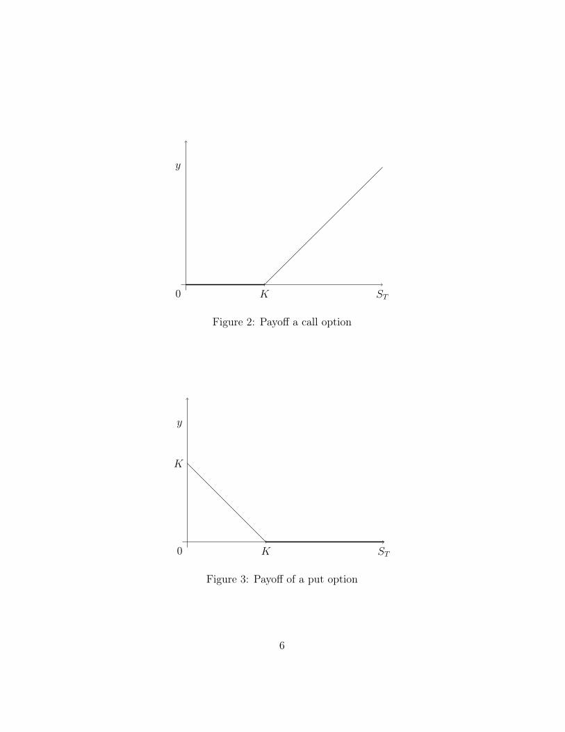
The writer of a European call option agrees to sell a stock for a previouslyagreed price K. Clearly, the buyer of this option will not use his right ifST < K. The payoff function for the buyer is f(s) = (s−K)+

In case of a put option the writer agrees to buy a stock for K. The payofffunction of the buyer

5

ST0

y

K

Figure 2: Payoff a call option

ST0

y

K

K

Figure 3: Payoff of a put option

6

1.3 Put–call parity

The aim of the course is to determine the fair price of an option, and under-stand the fairness. However, there is a simple relation between call and putprices regardless of the underlying market model.

Let CK be the fair price of the call, and PK be the fair price of the put,both with strike price K. Then, from the payoff functions it is easy to seethat having put, a stock, and −1 call results at the expiration date (regardlessof the stock price) a wealth K. That is, after discounting

K

BT

= P + S0 − C.

This is the put-call parity.

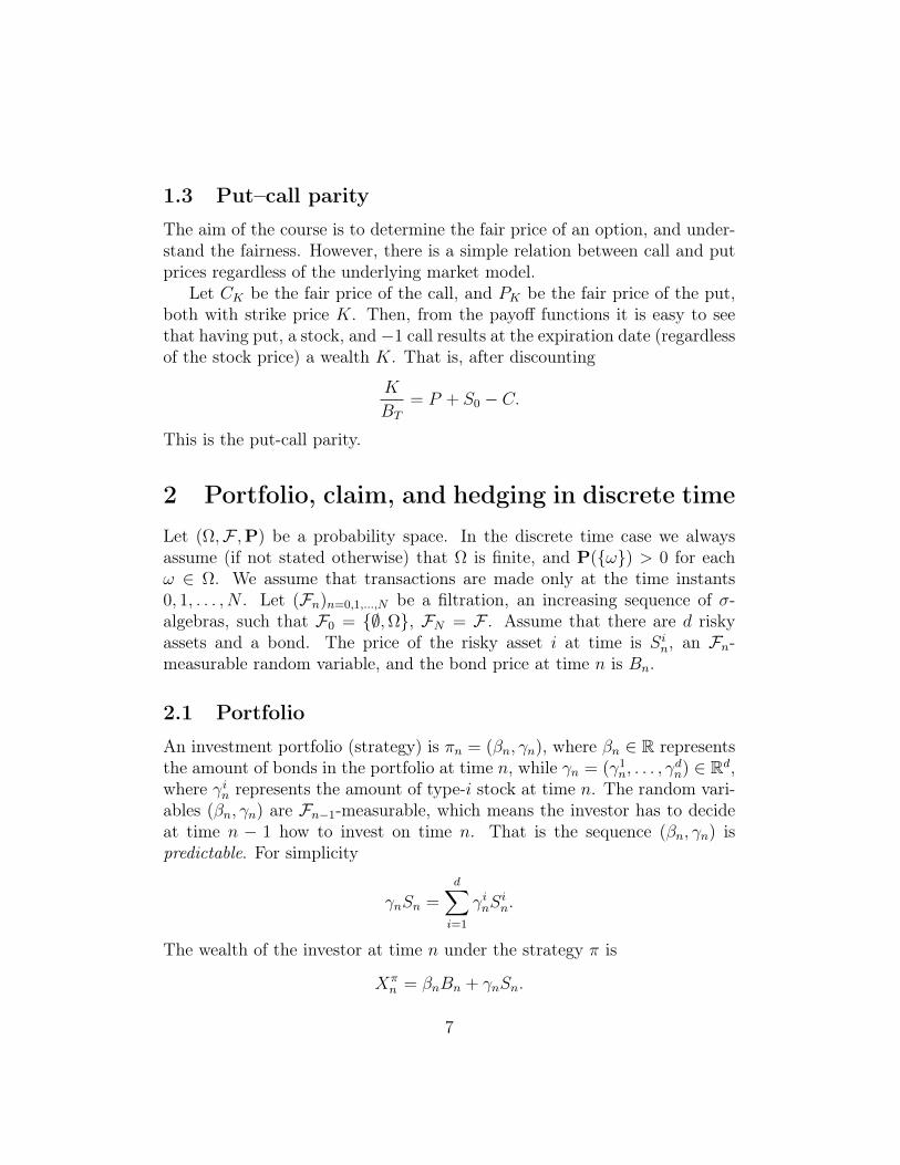
2 Portfolio, claim, and hedging in discrete timeLet (Ω,F ,P) be a probability space. In the discrete time case we alwaysassume (if not stated otherwise) that Ω is finite, and P(ω) > 0 for eachω ∈ Ω. We assume that transactions are made only at the time instants0, 1, . . . , N . Let (Fn)n=0,1,...,N be a filtration, an increasing sequence of σ-algebras, such that F0 = ∅,Ω, FN = F . Assume that there are d riskyassets and a bond. The price of the risky asset i at time is Sin, an Fn-measurable random variable, and the bond price at time n is Bn.

2.1 Portfolio

An investment portfolio (strategy) is πn = (βn, γn), where βn ∈ R representsthe amount of bonds in the portfolio at time n, while γn = (γ1

n, . . . , γdn) ∈ Rd,

where γin represents the amount of type-i stock at time n. The random vari-ables (βn, γn) are Fn−1-measurable, which means the investor has to decideat time n − 1 how to invest on time n. That is the sequence (βn, γn) ispredictable. For simplicity

γnSn =d∑i=1

γinSin.

The wealth of the investor at time n under the strategy π is

Xπn = βnBn + γnSn.

7

This is the value process of the investment portfolio.A strategy is self-financing (SF) if the investor does not take out money

from, and does not invest money to the portfolio after time 0. That is π isself-financing if

Xπn−1 = βnBn−1 + γnSn−1 for all n.

For a sequence an put ∆an = an − an−1.lemma:SF

Lemma 1. The following are equivalent:(i) π is SF;(ii) ∆Xπ

n = βn∆Bn + γn∆Sn;(iii) Bn−1∆βn + Sn−1∆γn = 0.

Proof. We have

∆Xn = Xn −Xn−1

= βnBn − βn−1Bn−1 + γnSn − γn−1Sn−1

= βn(Bn −Bn−1) + (βn − βn−1)Bn−1 + γn(Sn − Sn−1) + (γn − γn−1)Sn−1

= βn∆Bn + ∆βnBn−1 + γn∆Sn + ∆γnSn−1,

and the equivalence follows.

In what follows, unless otherwise stated all the strategies are meant to beSF.

We can decompose the value process as

Xπn = Xπ

n−1 + ∆Xπn = . . .

= Xπ0 +

n∑i=1

(βi∆Bi + γi∆Si)

=: Xπ0 +Gπ

n,

where Gπn is the gain process. So the value of the strategy is the initial

investment plus the gain.

2.2 Strategies in a more general market

Previously, we assumed that there are no transaction cost (market is fric-tionless), shares pay no dividend, and apart from time 0, there is neitherinvestment, nor consumption. Here we see how to handle this.

8

2.2.1 Dividend

Assume that stock-i pays a dividend δin = Din − Di

n−1 ≥ 0 at n, where δin,and Di

n are adapted processes. Then the change in the value process is

∆Xπn = βn∆Bn + γn(∆Sn + δn),

and the value of the portfolio

Xπn = βnBn + γn(Sn + δn).

Then, π is self-financing portfolio if

Bn−1∆βn + Sn−1∆γn = δn−1γn−1.

Indeed, the dividend obtained in time n− 1 is reinvested in the portfolio.

2.2.2 Consumption and investment

The consumption and investment can be included as well. Let (Cn), (In) beadapted nondecreasing random sequences with C0 = I0 = 0. Then, if aninvestor takes out ∆Cn and invests ∆In then

∆Xπn = βn∆Bn + γn∆Sn + ∆In −∆Cn

Xπn = βnBn + γnSn.

2.2.3 Transaction costs

If ∆γn > 0 then we buy share, and pay an extra cost λ, that is we pay(1 + λ)Sn−1∆γn. While if ∆γn < 0 we sell, and paying transaction costmeans receiving less money, say −(1 − µ)Sn−1∆γn. Then an SF strategysatisfies (see (iii) in Lemma 1)

Bn−1∆βn + (1 + λ)Sn−1∆γnI(∆γn > 0) + (1− µ)Sn−1∆γnI(∆γn < 0) = 0.

2.3 Claim and hedging

Let fN be a nonnegative random variable, which is the payoff function, orobligation, or contingent claim. A strategy π is an upper (x, fN)-hedge, ifP-almost surely

Xπ0 = x, Xπ

N ≥ fN .

9

It is a lower (x, fN)-hedge, if a.s.

Xπ0 = x, Xπ

N ≤ fN .

The hedge is perfect if = holds a.s.Put

C∗(fN) = infx : ∃ upper (x, fN)-hedge ,

and similarly

C∗(fN) = supx : ∃ lower (x, fN)-hedge .

For the class of upper (x, fN)-hedge strategies put H∗(x, fN ,P), and for thelower H∗(x, fN ,P).

lemma:hedgeLemma 2. For any payoff function fN there exists an x such that there isan upper (x, fN)-hedge.

Proof. Put

x =B0

BN

maxω∈Ω|fN(ω)|.

Then the (trivial) strategy πn ≡ ( xB0, 0) (start with enough money and don’t

do anything) is an upper hedge.

2.4 Binomial marketss:bin

2.4.1 One-step market

Consider a one-step binomial market with d = 1 stock. That is Ω = 0, 1,F0 = ∅,Ω, F1 = F = 2Ω. Assume that P(0) ∈ (0, 1). The bond priceB1 = (1 + r)B0, that is r > −1 is the interest rate, and for some a < b,S1 = (1 + ρ)S0, ρ ∈ a, b. Say, ρ(1) = b, ρ(0) = a. Let f be a payoff, thatis f(0) = f0, f(1) = f1. We construct a perfect hedge.

Using the strategy π1 = (β1, γ1) we want that

Xπ1 = β1B1 + γ1S1 = f a.s.

Since there are only two possibilities, a.s. means

β1B0(1 + r) + γ1S0(1 + a) = f0

β1B0(1 + r) + γ1S0(1 + b) = f1.

10

Solving the linear system

γ1 =1

S0

f1 − f0

b− a, β1 =

f1 − (1 + b)f1−f0b−a

B0(1 + r).

This is deterministic, so F0-measurable, as it should be. The initial cost ofthis strategy is

Xπ0 = B0β1 + S0γ1 =

1

1 + r

(r − ab− a

f1 +b− rb− a

f0.

)If a < r < b this can be written as

Xπ0 =

1

1 + rEQf,

with the probability measure Q(0) = (b−r)/(b−a), Q(1) = (r−a)/(b−a).

This shows that the ’fair’ price of the payoff is EQf/(1 + r). Note thatthis does not depend on the probability measure P.

2.4.2 N-step market

Assume we have only one stock, d = 1. For the bond Bn = (1 + rn)Bn−1,and for the share Sn = (1 + ρn)Sn−1, where ρn ∈ an, bn.

Exercise 1. Give a concrete construction of the probability space and thefiltration!

Solution 1. Let

Ω = 0, 1N = ω = (ω1, . . . , ωN) : ωi ∈ 0, 1.

Define the random variables ρn : Ω→ an, bn as

ρn(ω) =

an, if ωn = 0,

bn, if ωn = 1.

For the filtration let Fn = σ(ρ1, . . . , ρn), i.e. the natural filtration generatedby the variables ρ1, . . . , ρn.

Consider any payoff function fN . A perfect hedge can be constructedrecursively, using the simple one-step market. Indeed, a two-step model canbe seen as 3 one-step markets.

11

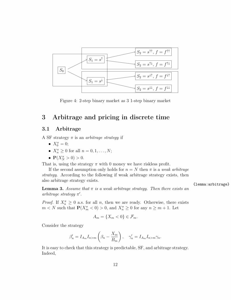
S0

S1 = s↑

S1 = s↓

S2 = s↑↑, f = f ↑↑

S2 = s↑↓, f = f ↑↓

S2 = s↓↑, f = f ↓↑

S2 = s↓↓, f = f ↓↓

Figure 4: 2-step binary market as 3 1-step binary market

3 Arbitrage and pricing in discrete time

3.1 Arbitrage

A SF strategy π is an arbitrage strategy if• Xπ

0 = 0;• Xπ

n ≥ 0 for all n = 0, 1, . . . , N ;• P(Xπ

N > 0) > 0.That is, using the strategy π with 0 money we have riskless profit.

If the second assumption only holds for n = N then π is a weak arbitragestrategy. According to the following if weak arbitrage strategy exists, thenalso arbitrage strategy exists.

lemma:arbitrageLemma 3. Assume that π is a weak arbitrage strategy. Then there exists anarbitrage strategy π′.

Proof. If Xπn ≥ 0 a.s. for all n, then we are ready. Otherwise, there exists

m < N such that P(Xπm < 0) > 0, and Xπ

n ≥ 0 for any n ≥ m+ 1. Let

Am = Xm < 0 ∈ Fm.

Consider the strategy

β′n = IAmIn>m

(βn −

Xm

Bm

), γ′n = IAmIn>mγn.

It is easy to check that this strategy is predictable, SF, and arbitrage strategy.Indeed,

12

(i) predictable: for n ≤ m this is clear, since β′n = 0 and γ′n = 0, while forn > m Am is Fm-measurable and thus Fn−1-measurable as well, andβn, γn are Fn−1-measurable by the assumption.

(ii) SF: for n ≤ m this is again clear. For n = m+ 1

Bm∆β′m+1+Sm∆γ′m+1 = IAm (Bmβm+1(ω)−Xπm(ω) + Smγm+1(ω)) = 0,

since π is SF. For n > m + 1 we have ∆β′n = IAm∆βn, and ∆γ′n =IAm∆γn, and the result follows, using again that π is SF.

(iii) arbitrage: we have

Xπ′

n = IAmIn>m

(βnBn + γnSn −

XπmBn

Bm

),

where the sum of the first two terms in the bracket is nonnegative bythe definition of m and the last is strictly negative on Am, which provesthe statement.

Exercise 2. Assume that a < b < r in the one-step binomial model. Givean arbitrage strategy.

Assume that an < bn < rn for some n in the N -step binomial model.Give an arbitrage strategy.

3.2 Reminder: conditional expectation and martingales

3.2.1 Conditional expectation

Let (Ω,F ,P) a probability space and G ⊂ F a sub-σ-algebra. Let X bea random variable with E|X| < ∞. The conditional expectation of X withrespect to the σ-algebra G, E[X|G] is the almost surely uniquely determinedrandom variable which• G-measurable, i.e. for any Borel set B ∈ B E[X|G])−1(B) ∈ G;• for any G ∈ G ∫

G

X dP =

∫G

E[X|G] dP .

The conditional probability of A ∈ A with respect to G P(A|G) =E[IA|G]. Then the second condition above can be written as for all G ∈ G

P(A ∩G) =

∫G

P(A|G) dP .

13

3.2.2. Martingálok

Ebben a fejezetben összefoglaljuk a diszkrét idejű martingálokra vonatkozólegfontosabb állításokat. Csörgő Sándor jegyzetét [1] követjük.

Legyen (Ω,F ,P) egy valószínűségi mező, és ezen (Fn)n egy filtráció (azazσ-algebrák monoton bővülő rendszere, F0 ⊂ F1 ⊂ . . . ⊂ Fn ⊂ Fn+1 ⊂ . . . ⊂A), és (Xn)n véletlen változók sorozata. Az (Xn)n sorozat adaptált az (Fn)filtrációhoz, ha minden n esetén Xn mérhető Fn szerint. Az (Xn,Fn) sorozatmartingál, ha(i) (Xn) adaptált az (Fn) filtrációhoz;(ii) E|Xn| <∞ minden n esetén;(iii) E[Xn+1|Fn] = Xn m.b.

Az Xn,Fn sorozat szubmartingál (szupermartingál), ha (i), (ii) teljesül,és E[Xn+1|Fn] ≥ Xn (E[Xn+1|Fn] ≥ Xn) m.b. minden n esetén.

Vegyük észre, hogy (Xn,Fn) pontosan akkor martingál, ha szubmartingálés szupermartingál. Továbbá, szubmartingál mínusz egyszerese szupermart-ingál, ezért minden szubmartingálokra bizonyított állítás megfelelője igazszupermartingálokra, és martingálokra is.

1. Proposition. Legyen I véges vagy végtelen intervallum a számegyenesen,P(Xn ∈ I) = 1 minden n esetén, ϕ : I → R konvex függvény, ϕ(Xn)integrálható.(i) Ha (Xn,Fn) martingál, akkor (ϕ(Xn),Fn) szubmartingál.(ii) Ha (Xn,Fn) szubmartingál és ϕ monoton nemcsökkenő függvény, akkor

(ϕ(Xn),Fn) szubmartingál.

Bizonyítás. (i): A martingál definíciója és a feltételes várható értékre vonat-kozó Jensen-egyenlőtlenség szerint

ϕ(Xn) = ϕ (E[Xn+1|Fn]) ≤ E [ϕ(Xn+1)|Fn] ,

ami éppen az állítás. A (ii) bizonyítása hasonlóan megy.

3. Exercise. Lássuk be (ii) állítást!

Véletlen változók egy (Zn) sorozata előrejelezhető az (Fn) filtrációra néz-ve, ha minden n esetén Zn mérhető Fn−1 szerint.

14

1. Theorem (Doob-felbontás). Legyen (Xn,Fn) szubmartingál, F0 = ∅,Ω.Ekkor létezik (Mn, Zn) sorozat, melyre Xn = Mn + Zn, ahol (Mn,Fn) mart-ingál, Z1 = 0, Z1 ≤ Z2 ≤ . . . m.b., és Zn előrejelezhető. Továbbá, ez azelőállítás egyértelmű.

Az állítás azt mondja, hogy a szubmartingálban benne levő driftet letudjuk választani.

Bizonyítás. Legyen Z1 = 0 m.b., és n ≥ 2 esetén Zn =∑n

k=2 E[Xk −Xk−1|Fk−1]. A szubmartingál definíciója szerint Zn m.b. monoton nemcsök-kenő, hiszen

Zn − Zn−1 = E[Xn −Xn−1|Fn−1] ≥ 0 m.b.

Az előrejelezhetőség is világos. (Ezzel leválasztottuk a driftet.) LegyenMn =Xn−Zn. Könnyen ellenőrizhető, hogy ez valóban martingál. Ezzel a létezéstbeláttuk.

Az egyértelműség bizonyítása a következőképp megy. Legyen M∗n, Z

∗n

egy, a feltételeknek eleget tevő sorozat. Ekkor a feltétel szerint Z∗1 = 0 = Z1

m.b. Teljes indukcióval bizonyítunk. Tegyük fel, hogy n − 1 esetén igaz azállítás, azaz Z∗n−1 = Zn−1 m.b., és M∗

n−1 = Mn−1 m.b. Ekkor

Z∗n = E[Z∗n|Fn−1] előrejelezhetőség= E[Xn −M∗

n|Fn−1] definíció= E[Xn|Fn−1]−M∗

n−1 martingálság= E[Xn|Fn−1]−Mn−1 indukciós feltétel= E[Xn −Mn|Fn−1] martingálság= E|Zn|Fn−1] definíció= Zn előrejelezhetőség.

A (Zn) folyamat az (Xn,Fn) martingál növekvő folyamata.

3.2.3. Megállási idő

A τ : Ω→ N nemnegatív egész értékű (kiterjesztett) véletlen változó megál-lási idő az (Fn) filtrációra nézve, ha minden n esetén τ ≤ n ∈ Fn.

Vegyük észre, hogy a definícióban megengedjük, hogy τ pozitív valószí-nűséggel vegye fel a ∞ értéket.

15

4. Lemma. Az alábbiak ekvivalensek:(i) τ megállási idő;(ii) τ > n ∈ Fn minden n esetén;(ii) τ = n ∈ Fn minden n esetén.

Bizonyítás. A bizonyítás a σ-algebra elemi tulajdonságain múlik.

4. Exercise. Bizonyítsuk be a lemmát!

Legyen τ megállási idő az Fn filtrációra. A τ előtti események σ-algebrája / pre-τ σ-algebra az

Fτ = A ∈ A : A ∩ τ ≤ n ∈ Fn,∀n

formulával definiált σ-algebra.

5. Exercise. Mutassuk meg, hogy Fτ valóban σ-algebra!

Az Fτ σ-algebra azt információt tartalmazza, amit éppen a τ megállásiidőig gyűjtünk össze.

Legyen Xn véletlen változók egy sorozata, τ megállási idő. Ekkor Xτ

az a véletlen változó, melyre Xτ (ω) = Xτ(ω)(ω), ω ∈ Ω.

2. Proposition. (i) Ha τ megállási idő, akkor τ mérhető Fτ szerint.(ii) Ha τ ≡ k, akkor Fτ = Fk (azaz a jelölés konzisztens).(iii) Ha σ, τ megállási idők, akkor minσ, τ = σ ∧ τ és maxσ, τ = σ ∨ τ

is megállási idők.(iv) Ha σ ≤ τ m.b., akkor Fσ ⊂ Fτ .(v) Ha Xn adaptált és τ megállási idő, akkor Xτ mérhető Fτ szerint.

Bizonyítás. A σ-algebra tulajdonságain múlik.

6. Exercise. Bizonyítsuk be az állítást!

3.3 Martingale measures

A probability measure Q is called equivalent martingale measure (EMM) ifP ∼ Q and (Sin/Bn,Fn) is a Q-martingale for each i = 1, 2, . . . , d.

16

3.3.1 EMM in binomial markets

In a one-step binomial market the martingale property is easy to check.Indeed, (Si/Bi)i=0,1 is a martingale iff

EQ

[S1

B1

∣∣∣∣F0

]=S0

B0

.

We have

EQ

[S1

B1

∣∣∣∣F0

]= EQ

S1

B1

= Q(ρ = a)(1 + a)S0

(1 + r)B0

+ (1−Q(ρ = a))(1 + b)S0

(1 + r)B0

=S0

B0

.

Solving the equation we obtain that

Q(ρ = a) =b− rb− a

, and Q(ρ = b) =r − ab− a

.

That is Q(0) = (b − r)/(b − a), Q(1) = (r − a)/(b − a). This is theprobability measure Q we obtained at pricing.

Let us see the general N -step model. Then

Sn =n∏i=1

(1 + ρi)S0,

thus the martingale property reads as

EQ

[SnBn

∣∣∣∣Fn−1

]=Sn−1

Bn−1

n = 0, 1, . . . N.

Using the properties of conditional expectation we have

EQ

[SnBn

∣∣∣∣Fn−1

]=Sn−1

Bn−1

1

1 + rnEQ[1 + ρn|Fn−1].

Therefore Sn/Bn is a Q-martingale iff

EQ[ρn|Fn−1] = rn.

17

This condition exactly tells that under the new measure Q the risky assetbehaves as the bond on average. Using that ρn ∈ an, bn, we obtain asabove

Q(ρn = an|Fn−1) =bn − rnbn − an

, and Q(ρn = bn|Fn−1) =rn − anbn − an

.

Note the conditioning on Fn−1 gives a constant, meaning that ρn is indepen-dent of Fn−1 under the measure Q.

We obtained the following.thm:binom-EMM

Theorem 2. In the binomial market if an < rn < bn for each n then thereexists a unique EMM Q given by the formulas above. Moreover, under Q therandom variables ρ1, . . . , ρN are independent.

In the proof we used the following simple result.

Exercise 7. Assume that Y ∈ a, b and

P(Y = a|F) = p a.s.

Show that Y is independent of F .

Note that the original measure P is irrelevant.In the special case of the homogeneous binomial market we get that

Q(SN = S0(1 + b)k(1 + a)N−k) =

(N

k

)qk(1− q)N−k, k = 0, 1, . . . , N.

3.3.2 Pricing with EMMprop:Xbar-mtg

Proposition 3. If Q is an EMM then (Xπ

n = Xπn/Bn)n is a Q-martingale

for any SF strategy π.

Proof. Easily follows from the SF property. Indeed, using that βn, γn are

18

Fn−1-measurable

EQ

[Xπn

Bn

∣∣∣∣Fn−1

]= EQ

[βn + γn

SnBn

∣∣∣∣Fn−1

]= βn + γnEQ

[SnBn

∣∣∣∣Fn−1

]= βn + γn

Sn−1

Bn−1

=βnBn−1 + γnSn−1

Bn−1

=Xπn−1

Bn−1

,

where the last equality follow from the self-financing property.

The following main result is the first fundamental theorem of asset pricing.thm:emm-arb

Theorem 3. There exists an EMM if and only if the market is arbitrage-free.

Proof. Let Q be an EMM and π be any strategy with Xπ0 = 0. Then, by the

previous statement

EQXπN

BN

= EQXπ

0

B0

= 0.

Thus XN ≥ 0 P-a.s., then also Q-a.s., which implies XN ≡ 0 Q-a.s., thusP-a.s.

We prove the converse later.

Assume that fN is a replicable payoff, i.e. there is a prefect hedge π. Thismeans that

XπN = fN a.s.

Then the fair price for fN is the initial cost of the portfolio, Xπ0 = x. By the

martingale property

EQfNBN

= EQXπN

BN

mtg= EQ

Xπ0

B0

=x

B0

.

That is, the fair price x for a replicable payoff fN is

x =B0

BN

EQf.

19

In particular, it also follows that for a replicable f , the value EQf is thesame for any EMM Q.

Summarizing, we proved the following:thm:pricing

Theorem 4. Consider an arbitrage-free market and let f be a replicablepayoff. Then the fair price of f is

C(f) = C∗ = C∗ =B0

BN

EQf,

where Q is any EMM.

3.4 General one-step market

Assume that B1 = B0(1 + r) with a deterministic interest rate r > −1 and

S1 = S0(1 + ρ),

where ρ > −1 is a random variable, the unique source of randomness in themodel. Let

F (x) = P(ρ ≤ x), x ∈ R,be the distribution function of ρ. Then F induces a probability measure(denoted by P) on the Borel sets of (−1,∞) (or R). If F is concentrated ona, b then we get back the previous one-step binomial model.

Assume without loss of generality that B0 = 1. Consider a payoff functionf : R→ R as a function of the stock price S1. A strategy π is an upper hedgeif

β(1 + r) + γS0(1 + ρ) ≥ f(S0(1 + ρ)) a.s. (1) eq:1step-hedgeeq:1step-hedge

A probability measure on (R,B) is Q is EMM if P ∼ Q (meaning that P isabsolutely continuous to Q (P(A) = 0 whenever Q(A) = 0) and conversely)if and only if Sn/Bn is Q-martingale, that is

EQS1

B1

=S0

B0

.

This meansEQρ = r.

That is a probability measure Q which is equivalent to P is EMM iff∫RρdQ(ρ) = r.

20

Taking expectation with respect to the EMM Q

β(1 + r) + S0γ(1 + r) ≥ EQf(S0(1 + ρ)).

For the initial cost β + γS0 we have

β + γS0 ≥ EQf(S0(1 + ρ))

1 + r.

For the class of EMM’s put

P(P) = Q : Q probability measure ,Q ∼ P, (Sn/Bn)n is Q-martingale.

Then

C∗(f) = infβ + γS0 : (β, γ) is an upper hedge

≥ supQ∈P(P)

EQf(S0(1 + ρ))

1 + r.

(2) eq:onestep-C*lowereq:onestep-C*lower

Similarly, for the lower price

C∗(f) = supβ + γS0 : (β, γ) is a lower hedge

≤ infQ∈P(P)

EQf(S0(1 + ρ))

1 + r.

(3) eq:onestep-C_*uppereq:onestep-C_*upper

Assume now that ρ ∈ [a, b] for some −1 ≤ a < b < ∞. To ease notationput

f(x) = f(S0(1 + x)), x ∈ [a, b], (4) eq:onestep-feq:onestep-f

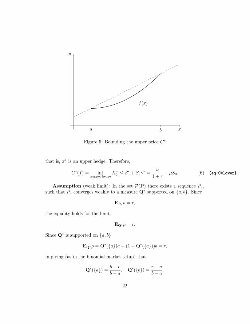
and assume that f is convex and continuous on [a, b]. By convexity,

f(x) ≤ f(b)− f(a)

b− a(1 + x) +

(1 + b)f(a)− (1 + a)f(b)

b− a=: µS0(1 + x) + ν.

(5) eq:conv-ineqeq:conv-ineq

Indeed, the left-hand side is a linear function equals to f(a) at a, and f(b)at b. Introduce the strategy,

π∗ = (β∗, γ∗) :=

(ν

1 + r, µ

).

Then, by (5)Xπ∗

1 = ν + µS0(1 + ρ) ≥ f(ρ),

21

x

y

a b

f(x)

Figure 5: Bounding the upper price C∗

that is, π∗ is an upper hedge. Therefore,

C∗(f) = infπupper hedge

Xπ0 ≤ β∗ + S0γ

∗ =ν

1 + r+ µS0. (6) eq:C*lowereq:C*lower

Assumption (weak limit): In the set P(P) there exists a sequence Pn,such that Pn converges weakly to a measure Q∗ supported on a, b. Since

EPnρ = r,

the equality holds for the limit

EQ∗ρ = r.

Since Q∗ is supported on a, b

EQ∗ρ = Q∗(a)a+ (1−Q∗(a))b = r,

implying (as in the binomial market setup) that

Q∗(a) =b− rb− a

, Q∗(b) =r − ab− a

.

22

Note that Q∗ is, in general, not equivalent to P. In fact, it is only equivalentin the binomial market setup.

By the convergence of Pn (here we use the continuity of f)

supQ∈P(P)

EQf(ρ)

1 + r≥ lim

n→∞EPn

f(ρ)

1 + r

= EQ∗f(ρ)

1 + r

= Q∗(a) f(a)

1 + r+ (1−Q∗(a)) f(b)

1 + r

= β∗ + γ∗S0 ≥ C∗(f).

Combining with (6) we obtained the following.

Theorem 5. Assume that the payoff function is convex and continuous on[a, b], and that the weak limit assumption holds. Then

C∗(f) = supQ∈P(P)

EQf(ρ)

1 + r=b− rb− a

f(a)

1 + r+r − ab− a

f(b)

1 + r,

and the supremum is attained on the measure Q∗.

Exercise 8. Let ρ be uniform random variable on [a, b]. Show that the weaklimit property holds. Construct Pn explicitly!

Try to weaken the condition on the distribution of ρ.

Let’s see the lower price C∗(f). Assume again that f in (4) is continuousand convex. Then

f(ρ) ≥ f(r) + (ρ− r)λ(r), (7) eq:onestep-convex-lowereq:onestep-convex-lower

for some λ(r). Here λ(r) = f ′(r) if f is smooth, but this is not assumed.If Q ∈ P(P) then taking expectation in (7) and noting that EQρ = r we

haveinf

Q∈P(P)EQf(ρ) ≥ f(r).

Consider the strategy

β∗ =f(r)

1 + r− λ(r), γ∗ =

λ(r)

S0

.

23

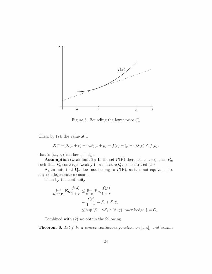
x

y

a br

f(x)

Figure 6: Bounding the lower price C∗

Then, by (7), the value at 1

Xπ∗1 = β∗(1 + r) + γ∗S0(1 + ρ) = f(r) + (ρ− r)λ(r) ≤ f(ρ),

that is (β∗, γ∗) is a lower hedge.Assumption (weak limit-2): In the set P(P) there exists a sequence Pn,

such that Pn converges weakly to a measure Q∗ concentrated at r.Again note that Q∗ does not belong to P(P), as it is not equivalent to

any nondegenerate measure.Then by the continuity

infQ∈P(P)

EQf(ρ)

1 + r≤ lim

n→∞EPn

f(ρ)

1 + r

=f(r)

1 + r= β∗ + S0γ∗

≤ supβ + γS0 : (β, γ) lower hedge = C∗.

Combined with (2) we obtain the following.

Theorem 6. Let f be a convex continuous function on [a, b], and assume

24

that the weak limit-2 assumption holds. Then

C∗(f) = infQ∈P(P)

EQf(ρ)

1 + r=

f(r)

1 + r,

and the infimum is attained at the measure Q∗.

3.5 Complete markets

We proved that if EMM exists then we have the fair price for any replicablepayoff. A market is complete if any payoff is replicable.

We have seen in Theorem 4 that on a complete arbitrage-free market anypayoff f has a unique well-defined fair price B0EQf/BN .

In section 2.4 we showed that a binomial market is complete.The second fundamental theorem of asset pricing is the following.

thm:complete-marketTheorem 7. Consider an arbitrage-free market with EMM Q. Then thefollowing are equivalent:(i) the market is complete;(ii) Q is the unique EMM;(iii) for any Q-martingale (Mn) there exists a predictable sequence γn such

that Mn can be represented as

Mn = M0 +n∑k=1

γk

(SkBk

− Sk−1

Bk−1

)= M0 +

n∑k=1

d∑i=1

γik

(SikBk

−Sik−1

Bk−1

).

Proof. We prove again the easy parts (i)⇒ (ii), and (iii)⇔ (i), and postponethe difficult (ii) ⇒ (i) implication later.

(i) ⇒ (ii): Assume that Q1 and Q2 are EMM’s. Consider any A ∈ F .We show that Q1(A) = Q2(A) implying the uniqueness. Let π be a perfecthedge to f = IA. Then Xπ

n/Bn is both Q1 and Q2 martingale, so

Q1(A) = EQ1f = EQ1XπN = BNEQ1

XπN

BN

= BNXπ

0

B0

= . . . = Q2(A).

(i)⇒ (iii): Consider a Q-martingale Mn. There exists a strategy πn suchthat a.s.

XπN = BNMN .

25

Using that both Mn and Xπn/Bn are martingales

Mn = EQ[MN |Fn] = EQ

[XπN

BN

|Fn]

=Xπn

Bn

= βn + γnSnBn

.

Thus, using that π is SF

Mn −Mn−1 = ∆βn + γnSnBn

− γn−1Sn−1

Bn−1

= γn

(SnBn

− Sn−1

Bn−1

)+

1

Bn−1

(Bn−1∆βn + Sn−1∆γn)

= γn

(SnBn

− Sn−1

Bn−1

),

as claimed.(iii) ⇒ (i): Consider a payoff f . We are looking for a strategy π such

that XπN = f Q-a.s. We know that (Xπ

n/Bn)n is a martingale, so this shouldbe (Mn). Now the following choice is clear: let

Mn = EQ

[f

BN

|Fn].

Then Mn is a martingale, therefore by the assumption

Mn = M0 +n∑k=1

γk∆SkBk

.

Letβn = Mn − γn

SnBn

,

and consider the strategy πn = (βn, γn). To see that this is indeed a strategywe have to show that it is predictable and SF. The sequence γn is predictableby the assumption (iii), and βn is predictable because all the terms in Mn

are Fn−1-measurable except γnSn/Bn, which is subtracted. To see that it isSF note that

Bn−1∆βn + Sn−1∆γn

= Bn−1

(Mn −Mn−1 − γn

SnBn

+ γn−1Sn−1

Bn−1

)+ Sn−1∆γn

= Bn−1

(γn∆

SnBn

− γnSnBn

+ γn−1Sn−1

Bn−1

)+ Sn−1∆γn = 0,

26

showing that π is SF. It is clearly a perfect hedge since

XπN = βNBN + γNSN = BNMN = f,

as claimed.

3.6 Proof of the difficult part of Theorem 3

Here we use strongly that Ω is finite, and let |Ω| = k.Assume that there is no arbitrage strategy. Let

V0 = X : Ω→ R r.v. |∃π : Xπ0 = 0 and Xπ

N = X,

andV1 = X : Ω→ R r.v. |X ≥ 0,EX ≥ 1.

We identify a random variable X : Ω → R with a vector in Rk, as X ↔(X(ω1), . . . , X(ωk)). Clearly, V0 is a linear subspace and V1 is convex set inRk.

Since there is no arbitrage strategy, V0∩V1 = ∅. Therefore, by the Kreps–Yan theorem, there exists a linear functional ` : Rk → R such that `|V0 ≡ 0and `(v1) > 0 for all v1 ∈ V1. A linear function in Rk (in any Hilbert space)is a inner product, thus there exists q ∈ Rk such that

`(v) = 〈v, q〉.

Define the random variables

Xi(ωj) = δi,j1

P(ωi).

Then Xi ≥ 0 and EXi = 1, so Xi ∈ V1. Furthermore

`(Xi) =qi

P(ωi)> 0,

implying qi > 0 for any i. Define the probability measure Q as

Q(ωi) =qi∑ki=1 qi

.

It is clear that Q ∼ P. We have to check that (Sn/Bn) is a Q-martingale.First we need a lemma.

27

Lemma 5. Let (Xn)Nn=1 be an adapted process. If for any stopping timeτ : Ω→ 0, . . . , N

EXτ = EX0,

then (Xn) is martingale.

Proof. We show that Xn = E[XN |Fn], which implies that X is martingale.Let A ∈ Fn and consider the stopping time

τA(ω) =

n, ω ∈ A,N, otherwise.

This is indeed a stopping time, since τA ≤ k = ∅ for k < n, and A fork ≥ n, which is Fk-measurable. Then, by the assumption

EX0 = EXτA = EXnI(A) + EXNI(Ac).

With A = ∅ we see that EX0 = EXN , implying

EXnI(A) = EXNI(A).

This exactly means thatXn = E[XN |Fn],

as claimed.

We show that (Sn/Bn) satisfies the condition of the lemma above. Let τbe a stopping time and define the strategy

βn =SτBτ

I(τ ≤ n− 1)− S0

B0

, γn = I(τ > n− 1).

Since τ < n = τ ≤ n − 1 ∈ Fn−1, the sequence (βn, γn) is predictable.Furthermore,

Bn−1∆βn + Sn−1∆γn =SτBτ

Bn−1I(τ = n− 1)− Sn−1I(τ = n− 1) = 0,

so it is SF. Finally,

Xπ0 = −S0

B0

B0 + S0 = 0,

28

V2

V0

y

Figure 7: Choice of y

so XπN ∈ V0. Therefore

0 = EQXπN = EQβNBN + γNSN

EQ

((SτBτ

I(τ ≤ N − 1)− S0

B0

)BN +

SτBτ

I(τ = N)BN

)= BNEQ

(SτBτ

− S0

B0

).

That is (Sn/Bn) is indeed a Q-martingale.

3.7 Proof of the difficult part of Theorem 7

Here we prove the implication (ii) ⇒ (i).We use the notation of the previous proof. Let

V2 = X : Ω→ R r.v. |EQX = 0.

Then V2 is a linear subspace in Rk and we have seen in the previous proofthat V0 ⊂ V2. We claim that equality holds.

Assume first that this is indeed true. Then for any claim X the centeredversion X − EQX ∈ V2 = V0, meaning that there is a perfect hedge. Thusthe market is complete. So we only have to show that V0 = V2.

Assume on the contrary that V0 6= V2. Then there is an y ∈ V2, which isorthogonal to V0. Since qi > 0 (see the previous proof) for all i = 1, . . . , k,

29

we may choose ε > 0 small enough such that

q′i = qi − εyi > 0 for all i.

As both q and y are orthogonal to V0, q′ is also orthogonal. Define themeasure

Q′(ωi) =q′i∑ki=1 q

′i

.

Exactly as in the previous proof we can show thatQ′ is EMM. The uniquenessof the EMM implies

q′i∑ki=1 q

′i

=qi∑ki=1 qi

,

that is, using also the definition of q′,

q = αq′ = αq − αεy,

with α =∑qi/∑q′i. Thus

(1− α)q = −αεy.

But y and q are orthogonal, which is a contradiction. The proof is complete.

4 Girsanov’s theorem in discrete time

4.1 Second proof of the difficult part of Theorem 3

Assume that d = 1 and first consider the one-step model with B0 = B1 = 1.The stock price S0 is known, and the only randomness here is S1.

Exercise 9. The no arbitrage assumption (in this simple market) is equiva-lent to

P(∆S1 > 0)P(∆S1 < 0) > 0.

Furthermore, (Sn) is Q-martingale if

EQS1 = S0.

Therefore we have to construct a measure Q such that EQ∆S1 = 0. This isdone in the following lemma.

30

Lemma 6. Let X be a random variable on (R,B(R),P) such that P(X >0)P(X < 0) > 0. Then there exists a probability measure Q ∼ P such thatEQX = 0. Furthermore, for any a ∈ R

EQeaX <∞.

Proof. Define the probability measure

P1(dx) = ce−x2

F (dx),

where F (x) = P(X ≤ x) and c−1 =∫R e−x2F (dx). That is

P1(A) =

∫A

ce−x2

F (dx).

Then P1 is equivalent to F . (Recall that µ is absolute continuous with respectto ν, µ ν if µ(A) = 0 whenever ν(A) = 0. And µ and ν are equivalent,µ ∼ ν, if µ ν and ν µ.) Let

ϕ(a) = EP1eaX =

∫ReaxP1(dx) = c

∫Reax−x

2

F (dx).

Clearly, ϕ(a) < ∞ for any a as the function eax−x2 is bounded on R. Notethat ϕ is convex, because ϕ′′ > 0. Put

Za(x) =eax

ϕ(a).

ThenQa(dx) = Za(x)P1(dx)

is a probability measure for any a, and Qa ∼ P1 ∼ F . Again, this means

Qa(A) =

∫A

Za(x)P1(dx) =c

ϕ(a)

∫A

eax−x2

F (dx).

Letϕ∗ = inf

a∈Rϕ(a).

Since P1(X > 0) > 0 and P1(X < 0) > 0 we obtain that

lima→±∞

ϕ(a) =∞.

31

Therefore, the infimum is attained, i.e. there is a∗ such that ϕ(a∗) = ϕ∗.Then ϕ′(a∗) = 0, thus

0 = ϕ′(a∗) = EP1Xea∗X = ϕ(a∗)EP1X

ea∗X

ϕ(a∗)= ϕ(a∗)EQa∗X.

Thus the measure Qa∗ works.

Exercise 10. Prove rigorously that

lima→±∞

ϕ(a) =∞.

Exercise 11. Let X ∼ N(µ, σ2). Determine the measure constructed aboveexplicitly.

Next we extend the previous lemma for a general N -step market.

Exercise 12. The no arbitrage assumption implies that for any n a.s.

P(∆Sn > 0|Fn−1)P(∆Sn < 0|Fn−1) > 0.

As a preliminary result we have to understand how to compute conditionalexpectation under different measures.

lemma:condexp-measurechangeLemma 7. Let (Ω,F , (Fn)n=0,1,...,N ,P) a filtered probability space, and Z anonnegative random variable EPZ = 1. Define the new probability measureQ as

dQ = ZdP,

that isQ(A) =

∫A

ZdP.

Put Zn = EP[Z|Fn]. For any adapted process (Xn)

Zn−1EQ[Xn|Fn−1] = EP[XnZn|Fn−1].

Proof. Both sides are Fn−1-measurable. We have to prove that for any A ∈Fn−1 ∫

A

Zn−1EQ[Xn|Fn−1]dP =

∫A

XnZndP. (8) eq:cemlemma-0eq:cemlemma-0

32

First note that

EP[ZXn|Fn] = XnEP[Z|Fn] = XnZn. (9) eq:cemlemma-1eq:cemlemma-1

Therefore, for an Fn−1-measurable Y

EP[Zn−1Y |Fn−1] = YEP[Z|Fn−1],

implying for any A ∈ Fn−1 that∫A

Zn−1Y dP =

∫A

YEP[Z|Fn−1]dP

=

∫A

EP[ZY |Fn−1]dP =

∫A

Y ZdP.

Choosing Y = EQ[Xn|Fn−1] we obtain∫A

Zn−1EQ[Xn|Fn−1]dP =

∫A

EQ[Xn|Fn−1]ZdP

=

∫A

EQ[Xn|Fn−1]dQ definition of Q

=

∫A

XndQ conditional exp.

=

∫A

XnZdP definition of Q

=

∫A

XnZndP, by (9)

which is (8).

As a simple but useful corollary we obtain the following.cor:p-q-mtg

Corollary 1. The adapted process (Xn) is Q-martingale if and only if (XnZn)is P-martingale.

lemma:existence-emmLemma 8. Let (Xn)Nn=1 be an adapted process, and assume that

P(Xn > 0|Fn−1)P(Xn < 0|Fn−1) > 0.

Then there exists a probabilty measure Q ∼ P such that (Xn) is a Q-martingale difference.

33

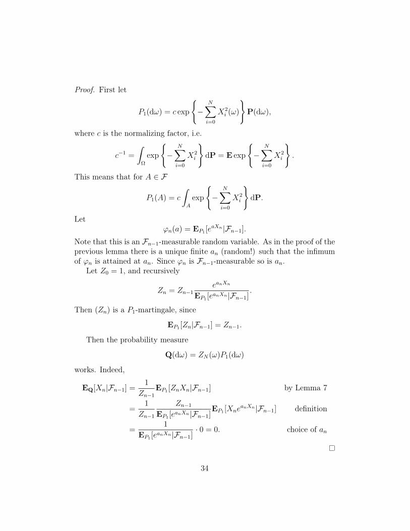
Proof. First let

P1(dω) = c exp

−

N∑i=0

X2i (ω)

P(dω),

where c is the normalizing factor, i.e.

c−1 =

∫Ω

exp

−

N∑i=0

X2i

dP = E exp

−

N∑i=0

X2i

.

This means that for A ∈ F

P1(A) = c

∫A

exp

−

N∑i=0

X2i

dP.

Letϕn(a) = EP1 [e

aXn|Fn−1].

Note that this is an Fn−1-measurable random variable. As in the proof of theprevious lemma there is a unique finite an (random!) such that the infimumof ϕn is attained at an. Since ϕn is Fn−1-measurable so is an.

Let Z0 = 1, and recursively

Zn = Zn−1eanXn

EP1 [eanXn|Fn−1]

.

Then (Zn) is a P1-martingale, since

EP1 [Zn|Fn−1] = Zn−1.

Then the probability measure

Q(dω) = ZN(ω)P1(dω)

works. Indeed,

EQ[Xn|Fn−1] =1

Zn−1

EP1 [ZnXn|Fn−1] by Lemma 7

=1

Zn−1

Zn−1

EP1 [eanXn|Fn−1]

EP1 [XneanXn|Fn−1] definition

=1

EP1 [eanXn|Fn−1]

· 0 = 0. choice of an

34

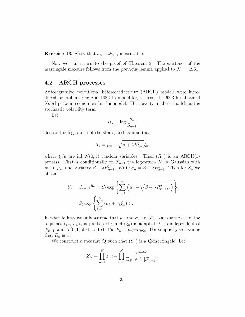
Exercise 13. Show that an is Fn−1-measurable.

Now we can return to the proof of Theorem 3. The existence of themartingale measure follows from the previous lemma applied to Xn = ∆Sn.

4.2 ARCH processes

Autoregressive conditional heteroscedasticity (ARCH) models were intro-duced by Robert Engle in 1982 to model log-returns. In 2003 he obtainedNobel prize in economics for this model. The novelty in these models is thestochastic volatility term.

LetRn = log

SnSn−1

denote the log-return of the stock, and assume that

Rn = µn +√β + λR2

n−1ξn,

where ξn’s are iid N(0, 1) random variables. Then (Rn) is an ARCH(1)process. That is conditionally on Fn−1 the log-return Rn is Gaussian withmean µn, and variance β + λR2

n−1. Write σn = β + λR2n−1. Then for Sn we

obtain

Sn = Sn−1eRn = S0 exp

n∑k=1

(µk +

√β + λR2

k−1ξk

)

= S0 exp

n∑k=1

(µk + σkξk)

.

In what follows we only assume that µn and σn are Fn−1-measurable, i.e. thesequence (µn, σn)n is predictable, and (ξn) is adapted, ξn is independent ofFn−1, and N(0, 1) distributed. Put hn = µn+σnξn. For simplicity we assumethat Bn ≡ 1.

We construct a measure Q such that (Sn) is a Q-martingale. Let

ZN =N∏n=1

zn :=N∏n=1

eanhn

EP[eanhn |Fn−1],

35

wherean = −µn

σ2n

− 1

2. (10) eq:disc-girs-0eq:disc-girs-0

Introduce the new measure Q as

dQ = ZNdP,

and let Zn = EP[ZN |Fn] =∏n

i=1 zi.By Corollary 1, to show that Sn is Q-martingale we have to show that

SnZn is a P-martingale. We have

EP[SnZn|Fn−1] = Sn−1Zn−1EP[ehn(1+an)|Fn−1]

EP[eanhn|Fn−1].

Therefore we have to check that

EP[ehn(1+an)|Fn−1] = EP[eanhn|Fn−1]. (11) eq:disc-girs-1eq:disc-girs-1

Recall that for a standard normal ξ

Eetξ = et2

2 ,

thusEeµ+σξ = eµ+σ2

2 .

Since an in (11) is Fn−1-measurable and given Fn−1 the variable hn is Gaus-sian N(µn, σ

2n), we obtain

EP[ehn(1+an)|Fn−1] = eµn(1+an)+σ2n(1+an)2

2 ,

andEP[ehnan|Fn−1] = eµnan+

σ2na2n

2 ,

By the choice of an in (10)

µn(1 + an) +σ2n(1 + an)2

2= µnan +

σ2na

2n

2.

Indeed, by (10)

µn + σ2n

(1

2+ an

)= 0.

That is, (11) holds.We proved the following.

36

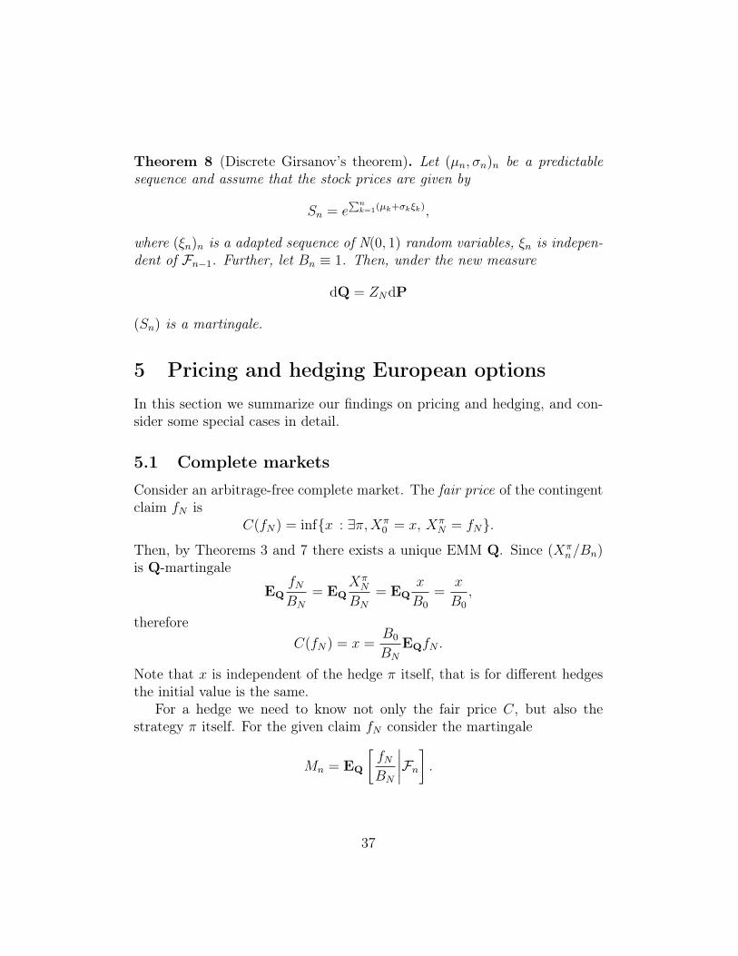
Theorem 8 (Discrete Girsanov’s theorem). Let (µn, σn)n be a predictablesequence and assume that the stock prices are given by

Sn = e∑nk=1(µk+σkξk),

where (ξn)n is a adapted sequence of N(0, 1) random variables, ξn is indepen-dent of Fn−1. Further, let Bn ≡ 1. Then, under the new measure

dQ = ZNdP

(Sn) is a martingale.

5 Pricing and hedging European optionsIn this section we summarize our findings on pricing and hedging, and con-sider some special cases in detail.

5.1 Complete markets

Consider an arbitrage-free complete market. The fair price of the contingentclaim fN is

C(fN) = infx : ∃π,Xπ0 = x, Xπ

N = fN.

Then, by Theorems 3 and 7 there exists a unique EMM Q. Since (Xπn/Bn)

is Q-martingale

EQfNBN

= EQXπN

BN

= EQx

B0

=x

B0

,

thereforeC(fN) = x =

B0

BN

EQfN .

Note that x is independent of the hedge π itself, that is for different hedgesthe initial value is the same.

For a hedge we need to know not only the fair price C, but also thestrategy π itself. For the given claim fN consider the martingale

Mn = EQ

[fNBN

∣∣∣∣Fn] .

37

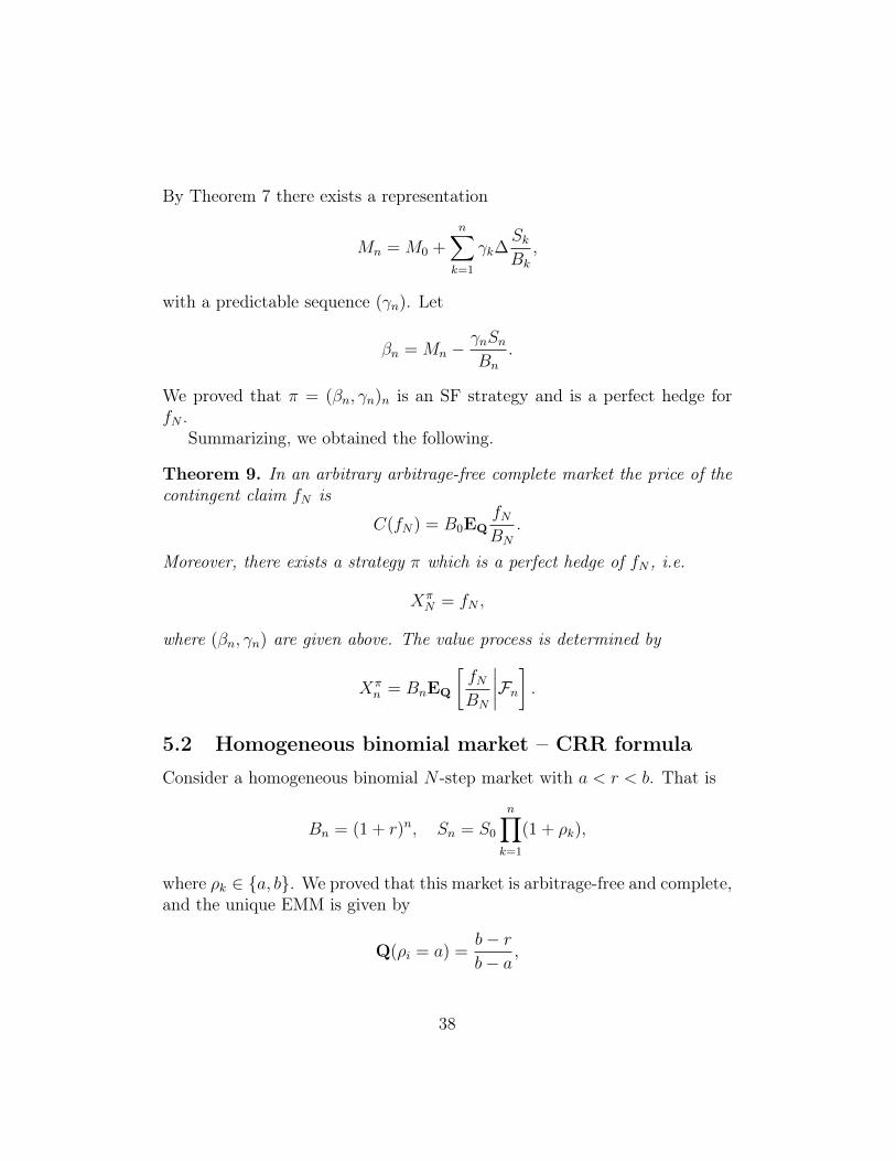
By Theorem 7 there exists a representation

Mn = M0 +n∑k=1

γk∆SkBk

,

with a predictable sequence (γn). Let

βn = Mn −γnSnBn

.

We proved that π = (βn, γn)n is an SF strategy and is a perfect hedge forfN .

Summarizing, we obtained the following.

Theorem 9. In an arbitrary arbitrage-free complete market the price of thecontingent claim fN is

C(fN) = B0EQfNBN

.

Moreover, there exists a strategy π which is a perfect hedge of fN , i.e.

XπN = fN ,

where (βn, γn) are given above. The value process is determined by

Xπn = BnEQ

[fNBN

∣∣∣∣Fn] .5.2 Homogeneous binomial market – CRR formula

Consider a homogeneous binomial N -step market with a < r < b. That is

Bn = (1 + r)n, Sn = S0

n∏k=1

(1 + ρk),

where ρk ∈ a, b. We proved that this market is arbitrage-free and complete,and the unique EMM is given by

Q(ρi = a) =b− rb− a

,

38

and ρi’s are independent. If the claim fN only depends on the final price SN ,and not on the whole trajectory, i.e.

fN(ω) = fN(SN(ω)),

then the pricing formula simplifies, and we obtain the Cox–Ross-Rubinsteinformula:

C(fN) =1

(1 + r)N

N∑k=0

fN(S0(1 + b)k(1 + a)N−k)

(N

k

)qk(1− q)N−k,

where q = r−ab−a .

5.3 Incomplete markets

We assume that the market is arbitrage-free, but there are various EMM’s.Let P(P) be the set of EMM’s.

In incomplete markets there are contingent claims which are not repli-cable, that is, there is no perfect hedge. The upper price of a claim fNis

C∗(fN) = infx : π, Xπ0 = x, Xπ

N ≥ fN.

We proved the following result in a one-step market. Without a proof westate the general version.

Theorem 10. The upper price of the claim fN in an arbitrage-free incom-plete market is given by

C∗(fN) = supQ∈P(P)

B0EQfNBN

.

6 American optionsWhile European options can be exercised only at the terminal dateN , Ameri-can options can be exercised at any time. Formally, instead of a fixed randompayoff function fN , a sequence of payoffs (fn)n=0,1,...,N is given, where fn isFn-measurable, i.e. (fn)n is adapted to (Fn)n. So fn is the random payoffif the option is exercised at time n. Clearly, the exercise time has to be astopping time.

39

6.1 Reminder: Doob’s optional sampling theorem

11. Theorem (Opcionális megállási tétel (Doob)). Legyen (Xn,Fn) szub-martingál, σ, τ megállási idők, σ ≤ τ m.b. Tegyük fel, hogy E|Xσ| < ∞,E|Xτ | <∞ és lim infn→∞

∫τ>n |Xn|dP = 0. Ekkor E[Xτ |Fσ] ≥ Xσ m.b.

A tétel feltételei mellett, ha Xn,Fn martingál, akkor E[Xτ |Fσ] = Xσ

m.b.

Bizonyítás. Tegyük fel, hogy τ korlátos, τ ≤ m. A szubmartingál és a felté-teles várható érték definíciója szerint azt kell megmutatnunk, hogy mindenA ∈ Fσ eseményre ∫

A

(Xτ −Xσ) dP ≥ 0.

Írjuk át az integrandust

Xτ −Xσ =τ∑

k=σ+1

(Xk −Xk−1) =m∑k=2

I(σ < k ≤ τ)(Xk −Xk−1)

alakba. Vegyük észre, hogy A ∩ σ < k ≤ τ = (A ∩ σ ≤ k − 1) ∩ τ ≤k − 1c. Itt a metszet első tagja Fσ definíciója szerint Fk−1-mérhető, amásodik tagja pedig a megállási idő definíciója szerint, így a metszet maga iselem az Fk−1 σ-algebrának. Ezt, feltételes várható érték és a szubmartingáldefinícióját használva∫

A

(Xτ −Xσ)dP =

∫A

m∑k=2

I(σ < k ≤ τ)(Xk −Xk−1)dP

=m∑k=2

∫A∩σ<k≤τ

(Xk −Xk−1)dP

=m∑k=2

∫A∩σ<k≤τ

(E[Xk|Fk−1]−Xk−1) dP ≥ 0,

ami éppen a bizonyítandó.Az általános esetben a τ, σ megállási időkről át kell térni a τ ∧ n, σ ∧ n

korlátos megállási időkre, és belátni, hogy a kimaradó tagok 0-hoz tartanakegy részsorozat mentén. Ezt nem bizonyítjuk, a részletekért lásd [1].

2. Corollary. Ha E|Xτ | <∞ és lim infn→∞∫τ>n |Xn|dP = 0, akkor ha

40

(i) Xn,Fn szubmartingál, akkor E[Xτ |F1] ≥ X1 m.b., és persze EXτ ≥EX1;

(ii) Xn,Fn martingál, akkor E[Xτ |F1] = X1 m.b., és persze EXτ = EX1.

Fontos megjegyezni, hogy a tételben szereplő feltételek nem csupán tech-nikai feltételek. Legyen Sn egy egyszerű szimmetrikus bolyongás az egye-nesen. Ő martingál a az általa generált természetes filtrációra nézve. Tud-juk, hogy az egydimenziós bolyongás rekurrens, ezért majdnem biztosan el-éri az 1-et. Legyen az elérés időpontja τ . Ekkor τ megállási idő, és perszeSτ ≡ 1 6= S0 = 0. Csak a lim infn→∞

∫τ>n |Xn|dP = 0 feltétellel lehet baj,

és valóban, ez nem teljesül.

6.2 Optimal stopping problems

Consider a probability space with a filtration (Ω,F , (Fn)n=0,1,...,N ,P), andlet

MNn = τ : τ is a stopping time, τ ∈ n, . . . , N.

To ease notation we suppress N in the upper index. Consider a sequenceof nonnegative adapted random variables (Xn)n, and define by backwardinduction its Snell-envelope (Zn)n as follows. We are interested in the value

ZN = XN , Zn = maxXn,E[Zn+1|Fn], n < N.

For a stopping time τ the stopped process is denoted by Zτ , i.e.

Zτn = Zτ∧n,

where a ∧ b = mina, b.

Proposition 4. Let (Zn) be the Snell-envelope of (Xn) with Xn ≥ 0 a.s.(i) Z is the smallest supermartingale dominating X.(ii) The random variable τ ∗ = minn : Zn = Xn is a stopping time and

the stopped process Zn∧τ∗ = Zτ∗n is martingale.

Proof. From the definition it is clear that Z is supermatingale and dominatesX. Let Y be another supermartingale dominating X. Then YN ≥ XN = ZN .Assuming that Yn ≥ Zn we have

Yn−1 ≥ maxE[Yn|Fn−1], Xn−1 ≥ maxE[Zn|Fn−1], Xn−1 = Zn−1.

41

Thus the minimality follows.To see that τ ∗ is stopping time note that

τ ∗ = n = ∩n−1k=0Zk > Xk ∩ Zn = Xn.

For the last assertion note that

Zτ∗

n − Zτ∗

n−1 = I(τ ∗ ≥ n)(Zn − Zn−1).

On the event τ ∗ ≥ n we have Zn−1 = E[Zn|Fn−1] therefore

E[I(τ ∗ ≥ n)(Zn − Zn−1)|Fn−1] = 0.

A stopping time σ is optimal if

EXσ = supτ∈M0

EXτ .

Proposition 5. The stopping time τ ∗ is optimal for X, and

Z0 = EXτ∗ = supτ∈M0

EXτ .

Proof. Since Zτ∗ is martingale

Z0 = Zτ∗

0 = EZτ∗

N = EZτ∗ = EXτ∗ .

On the other hand for any stopping time τ the process Zτ is supermartingale(by Doob’s optional sampling), thus

Z0 = EZτ0 ≥ EZτ ≥ EXτ .

Proposition 6. The stopping time σ is optimal iff the following two condi-tions hold.(i) Zσ = Xσ;(ii) Zσ is martingale.

42

Proof. If (i) and (ii) hold than σ is optimal. This follows exactly as theoptimality of τ ∗.

Conversely, assume that σ is optimal. We have seen that supτ EXτ = Z0

thusZ0 = EXσ ≤ EZσ,

by the dominance of Z. By Doob’s otional stopping theorem Zσ is super-martingale, therefore EZσ ≤ Z0, implying that

EXσ = EZσ.

Since Zn ≥ Xn this implies Xσ = Zσ a.s., proving (i).By the optimality EZσ = Z0, while the supermartingale property implies

Z0 ≥ EZσ∧n ≥ EZσ.

ThusEZσ∧n = EZσ = EE[Zσ|Fn].

Furthermore, by Doob’s optional stopping

Zσ∧n ≥ E[Zσ|Fn],

implying Zσ∧n = E[Zσ|Fn]. Thus (Zσn) is indeed a martingale.

6.3 Pricing American options

Let us return to our pricing problem. Assume that we have an arbitrage-freecomplete market, that is the EMM Q is unique. Let (fn)n=0,...,N be the payoffof an American option. A hedging strategy now has to fulfil the conditions

Xπn ≥ fn, n = 0, 1, . . . , N,

as the option can be exercised at any time. A hedge is minimal, if for astopping time τ ∗ we have Xπ

τ∗ = fτ∗ .By Doob’s optional stopping (Xπ

0 /B0, Xπτ /Bτ ) is martingale for any stop-

ping time τ , i.e.x

B0

= EQXπ

0

B0

= EQXπτ

Bτ

≥ EQfτBτ

.

Therefore the initial cost of the hedge is at least

x ≥ B0 supτ∈MN

0

EQfτBτ

.

43

At time N we needXπN ≥ fN .

At time N − 1 the holder either exercise the option or continues to time N ,(in that case we discount the price), therefore

XπN−1 ≥ max

fN−1,

BN−1

BN

EQ[fN |FN−1]

.

Dividing by BN−1

XπN−1

BN−1

≥ max

fN−1

BN−1

,EQ

[fNBN

∣∣∣∣FN−1

].

Thus, we see the connection with the Snell-envelope.For a hedging strategy π we have that

(i) (Xπn/Bn)n is a Q-martingale (since Q is EMM and π is SF), and

(ii) (Xπn/Bn) dominates (fn/Bn) (since π is a hedge).

Therefore, the value process of a hedge is larger than the Snell-envelope of(fn/Bn), i.e.

Xπn

Bn

≥ Zn, n = 0, 1, . . . , N, (12) eq:di-american-1eq:di-american-1

where (Zn) is the Snell-envelope of (fn/Bn). The Snell-envelope (Zn) isa supermartingale, therefore by the Doob-decomposition (that’s stated forsubmartingale, but multiply with −1) we have

Zn = Mn − An, n = 0, 1, . . . , N, (13) eq:di-american-2eq:di-american-2

where Mn is a Q-martingale, and (An) is an increasing predictable sequence,A0 = 0. Comparing (12) and (13) we see that

Xπn

Bn

≥Mn.

On the other hand, the market is complete, which implies (see the easy partsof the proof of Theorem 7) that there exists a strategy π such that

Xπn

Bn

= Mn, n = 0, 1, . . . , N.

This is a minimal hedging strategy with initial cost

x

B0

=Xπ

0

B0

= M0 = Z0.

44

thm:price-di-americanTheorem 12. Consider an aribtrage-free complete market with unique EMMQ. Let (fn) be the nonnegative payoff sequence of an American option. Let(Zn) be the Snell-envelope of the discounted payoff sequence (fn/Bn). Thefair price for this option is

C = B0Z0 = B0 supτ∈MN

0

EQfτBτ

= B0EQfτ∗

Bτ∗,

where τ ∗ is an (not unique in general) optimal exercise time given by

τ ∗ = min

n :

fnBn

= Zn

.

Furthermore, there exists a SF strategy π which is an optimal hedge withinital cost C and

Xπτ∗ =

fτ∗

Bτ∗.

6.4 American vs. European options

Clearly, an American option with payoff sequence (fn)n=0,1,...,N worth at leastas a European option with payoff fN . However, in some cases the fair pricesare equal.

Consider an American call option with strike price K, that is

fn = f(Sn) = (Sn −K)+.

Assume that the deterministic sequence (Bn) is nondecreasing (i.e. the inter-est rate is nonnegative). Let (Zn) denote the Snell envelope of (fn/Bn), thatis

ZN =fNBN

, Zn = max

fnBn

,E [Zn+1|Fn]

, n = 0, 1, . . . , N − 1.

45

Using that (Sn/Bn) is a Q-martingale, by Jensen’s inequality

fN−1

BN−1

=(SN−1 −K)+

BN−1

=

(SN−1

BN−1

− K

BN−1

)+

≤ EQ

[(SNBN

− K

BN−1

)+

∣∣∣∣FN−1

]Jensen’s inequality

≤ EQ

[(SNBN

− K

BN

)+

∣∣∣∣FN−1

]by BN ≥ BN−1

= EQ

[(SN −K)+

BN

∣∣∣∣FN−1

]= EQ[ZN |FN−1].

This means that at time N − 1 it is always good to hold the option andcontinue to step N .

An induction argument shows that at any time it is better to hold theoption. Indeed, assume for some n

fnBn

≤ EQ[Zn+1|Fn].

46

We just proved this for n = N − 1. The same way as above we have

fn−1

Bn−1

=(Sn−1 −K)+

Bn−1

=

(Sn−1

Bn−1

− K

Bn−1

)+

≤ EQ

[(SnBn

− K

Bn−1

)+

∣∣∣∣Fn−1

]Jensen’s inequality

≤ EQ

[(SnBn

− K

Bn

)+

∣∣∣∣Fn−1

]by Bn ≥ Bn−1

= EQ

[(Sn −K)+

Bn

∣∣∣∣Fn−1

]= EQ

[fnBn

∣∣∣∣Fn−1

]≤ EQ

[EQ[Zn+1|Fn]

∣∣Fn−1

]induction

≤ EQ[Zn|Fn−1] Z supermartingale

Thus τ ∗ ≡ N is an optimal stopping time, which means that no matter whathappens, we wait until the end. Then the American option behaves as theEuropean, so the prices are equal.

Theorem 13. Assume that the market is arbitrage free and complete, andthe interest rate is nonnegative. Then the price of a European call optionequals to the price of the American call option.

7 Stochastic integration

7.1. Az Itô-formula

Ezek után belátjuk az Itô-formulát.

14. Theorem (Itô-formula (1944)). Legyen Xt = X0 +∫ t

0Ksds+

∫ t0HsdWs

Itô-folyamat, és f ∈ C2 kétszer folytonosan differenciálható függvény. Ekkor

f(Xt) = f(X0) +

∫ t

0

f ′(Xs)dXs +1

2

∫ t

0

f ′′(Xs)H2sds.

47

A következőkben bevezetjük a többdimenziós Itô-folyamatokat.A W = (W 1,W 2, . . . ,W r) egy r-dimenziós Brown-mozgás, ha a kompo-

nensei függetlenek, és minden komponens egy SBM. Az (Xt) egy d-dimenziósItô-folyamat, ha az i-edik komponense

X it = X i

0 +

∫ t

0

Kisds+

r∑j=1

∫ t

0

H i,js dW j

s , (14) eq:multid-itoeq:multid-ito

ahol∫ T

0|Ki

s|ds < ∞,∫ T

0(H i,j

s )2ds < ∞ m.b., és Ki, H i,j Ft-adaptált folya-matok, i = 1, 2, . . . , d, j = 1, 2, . . . , r.

15. Theorem (Többdimenziós Itô-formula). Legyen (Xt) egy többdimenziósItô-folyamat, (14) formula szerint, és f : R1+d → R, f ∈ C1,2. Ekkor

f(t,X1t , . . . , X

dt ) = f(0, X1

0 , . . . , Xd0 ) +

∫ t

0

∂

∂sf(s,X1

s , . . . , Xds ) ds

+d∑i=1

∫ t

0

∂

∂xif(s,X1

s , . . . , Xds ) dX i

s

+1

2

d∑i,j=1

∫ t

0

∂2

∂xi∂xjf(s,X1

s , . . . , Xds )

r∑k=1

H i,ks Hj,k

s ds.

7.2. Alkalmazások

Az Itô-formulára nézünk néhány alkalmazást.

2. Example. Parciális integrálás I. Legyen (X, Y ) kétdimenziós Itô-fo-lyamat

Xt = X0 +

∫ t

0

Ks ds+

∫ t

0

Hs dWs

Yt = Y0 +

∫ t

0

Ls ds+

∫ t

0

Gs dWs,

ahol K,L,H,G olyanok amilyennek lenniük kell. Ekkor∫ t

0

XsdYs = XtYt −X0Y0 −∫ t

0

YsdXs −∫ t

0

HsGsds.

48

Vegyük észre, hogy a hagyományos parciális integrálási formulában (ami-kor tehát X, Y determinisztikus, korlátos változású függvények) nem szerepelaz utolsó tag.

A bizonyításhoz alkalmazzuk az Itô-formulát az (X, Y ) folyamatra, és azf(x, y) = xy függvényre. Ekkor a (14) formula szerinti szereposztás:

r = 1, d = 2, K1s = Ks, K

2s = Ls, H

1,1s = Hs, H

2,1s = Gs.

Mivel ∂f∂x

= y, ∂f∂y

= x, ∂2f∂2x

= ∂2f∂2y

= 0, és ∂2f∂x∂y

= ∂2f∂y∂x

= 1, így

XtYt = X0Y0 +

∫ t

0

YsdXs +

∫ t

0

XsdYs +1

22

∫ t

0

HsGsds,

ami rendezés után éppen az állítás.

3. Example. Parciális integrálás II. Egy kicsit módosítjuk az előző pél-dát. Legyen W egy W -től független SBM, és (X, Y ) kétdimenziós Itô-folya-mat

Xt = X0 +

∫ t

0

Ks ds+

∫ t

0

Hs dWs

Yt = Y0 +

∫ t

0

Ls ds+

∫ t

0

Gs dWs,

ahol K,L,H,G olyanok amilyennek lenniük kell. Ekkor∫ t

0

XsdYs = XtYt −X0Y0 −∫ t

0

YsdXs.

Ennek bizonyítása ugyanúgy megy, mint az előbb. Vegyük észre, hogy ittd = r = 2, és a két folyamatot különböző Wiener-folyamat hajtja meg, ezértnem jelenik meg az extra tag.

4. Example. Korábban már meghatároztuk az∫WsdWs sztochasztikus in-

tegrál értékét. Most meghatározzuk az Itô-formula segítségével.A Wiener-folyamat Itô-folyamatként való reprezentációja Ks ≡ 0, Hs ≡

1. Legyen f(x) = x2. Az Itô-formula szerint

W 2t = W 2

0 +

∫ t

0

2WsdWs +1

2

∫ t

0

2ds.

49

Ezt átrendezve kapjuk a már ismert∫ t

0

WsdWs =W 2t − t2

formulát. Innen azt is rögtön látjuk, hogy W 2t − t martingál, hiszen min-

den sztochasztikus integrál martingál (na nem mintha a direkt bizonyításbonyolult lett volna).

14. Exercise. Az Itô-formula alkalmazásával igazoljuk, hogy Y (t) = et/2 cosWt

martingál!

15. Exercise. Mutassuk meg, hogy∫ t

0

W 2s dWs =

1

3W 3t −

∫ t

0

Wsds,

és ∫ t

0

W 3s dWs =

1

4W 4t −

3

2

∫ t

0

W 2s ds.

16. Exercise. Legyen W = (W 1, . . . ,W r) r-dimenziós SBM, r ≥ 2, éslegyen R a W hossza, azaz

Rt =

√√√√ r∑i=1

(W i)2.

Igazoljuk, hogy Rt teljesíti a

dRt =r − 1

2Rt

dt+r∑i=1

W it

Rt

dW it

differenciálegyenletet! Ez a sztochasztikus Bessel-egyenlet, és Rt a Bessel-folyamat.

8. Folytonos idejű piacokA sztochasztikus integrálelmélettel felvértezve rátérünk a folytonos idejű pi-aci modellek tárgyalására.

50

8.1. Piacok általában

Az alapfogalmak a diszkrét időben már megismert fogalmak természetes foly-tonos idejű megfelelői.

A továbbiakban a [0, T ] véges időhorizonton dolgozunk, T < ∞. Adottegy (Ω,A,P) valószínűségi mező, azon egy (Ft) filtráció. A piacon két termékadott, egy kockázatmentes és egy kockázatos. A kötvény a kockázatmentes,az árfolyamata (Bt) egy determinisztikus folyamat, a részvény a kockázatos,árfolyamata (St) egy pozitív véletlen sztochasztikus folyamat, ami adaptáltaz (Ft) filtrációhoz. Továbbá azt is feltesszük, hogy (St) az (Ft) filtrációhozadaptált Itô-folyamat.

A stratégia / portfólió egy (πt = (βt, γt)) folyamat, ami adaptált (hátpersze, hiszen nem látunk a jövőbe), és∫ T

0

|βt|dt <∞,∫ T

0

γ2t dt <∞, m.b.

A (βt) folyamat jelenti a t-ben birtokunkban levő kötvény, (γt) pedig a rész-vény mennyiségét. Természetesen mindkét folyamat lehet negatív is.

A (π) portfólió értéke t-ben

Xπt = βtBt + γtSt, (15) eq:ertekfolyeq:ertekfoly

ez a portfólió értékfolyamata.Az önfinanszírozó stratégiát szeretnénk definiálni a diszkrét idő analo-

gonjaként. Az, hogy nem fektetek be plusz pénzt a portfóliómba, és nemis veszek ki belőle, azt jelenti, hogy amikor az n-edik napon este átrende-zem a portfóliómat, akkor az összérték meg kell egyezzen az n-edik napon aportfólióm értékével, azaz

βn+1Bn + γn+1Sn = βnBn + γnSn,

és a βn+1, γn+1 változók Fn-mérhetőek. Felírva, hogy Xn+1 = βn+1Bn+1 +γn+1Sn+1, azt kapom, hogy a portfólióm értékének megváltozása

Xn+1 −Xn = βn+1(Bn+1 −Bn) + γn+1(Sn+1 − Sn).

Ez azt jelenti, hogy az értékfolyamat megváltozása a kötvényár és a részvény-ár megváltozásából tevődik össze, külső forrást nem veszünk igénybe. Ennekaz egyenletnek a folytonos megfelelője a

dXπt = βtdBt + γtdSt

51

sztochasztikus differenciálegyenlet. Ez lesz az önfinanszírozóság definíciója.Azt mondjuk, hogy a (πt = (βt, γt)) stratégia önfinanszírozó, ha teljesül

adXπ

t = βtdBt + γtdSt (16) eq:onfineq:onfin

sztochasztikus differenciálegyenlet.Az (St = StB0/Bt) folyamat a diszkontált részvényárfolyamat, az (X

π

t =Xπt B0/Bt) folyamat pedig a diszkontált értékfolyamat.Mostantól feltesszük, hogy a folytonos kamatráta r > 0, azaz

Bt = ert, t ≥ 0.

EkkorSt = e−rtSt, és X

π

t = e−rtXπt .

all:onfin-ekv7. Proposition. A (πt = (βt, γt)) stratégia pontosan akkor önfinanszírozó,ha

Xπ

t = Xπ0 +

∫ t

0

γsdSs, t ∈ [0, T ].

Bizonyítás. Tegyük fel, hogy π önfinanszírozó. Az Itô-formula alapján

dXπ

t = d(e−rtXπ

t

)= −re−rtXπ

t dt+ e−rtdXt

= −re−rt(βtert + γtSt)dt+ e−rt(βtde

rt + γtdSt)

= −re−rtγtStdt+ e−rtγtdSt

= γtd(e−rtSt

),

amint állítottuk.Megfordítva, tegyük fel, hogy

dXπ

t = γtdSt.

Mivel Xπt = βte

rt + γtSt, így a bal oldal

dXπ

t = −re−rtXπt dt+ e−rtdXπ

t = −e−rtβtdBt − re−rtγtStdt+ e−rtdXπt .

A jobb oldalγtdSt = −re−rtγtStdt+ γte

−rtdSt.

A két oldal egyenlőségéből adódik, hogy

dXπt = βtdBt + γtdSt,

ami éppen az önfinanszírozóság definíciója.

52

Bevezetjük az arbitrázs fogalmát. A π önfinanszírozó stratégia arbitrázs-stratégia, ha Xπ

0 = 0 m.b., XT ≥ 0 m.b., és PXπT > 0 > 0. A piac

arbitrázsmentes, ha nincs arbitrázsstratégia.Ez a fogalom fejezi ki azt, hogy 0 kezdőtőkével indulva, biztosan nyerünk,

azaz ingyen ebédhez jutunk. Természetes feltenni, hogy a valóságban arbit-rázs nem létezik a piacon, hiszen ha létezne, akkor mindenki ezt a stratégiátjátszaná meg, ezzel módosítva az árakat, és így nagyon gyorsan megszűnneaz arbitrázslehetőség. Diszkrét idejű piacon láttuk, hogy (bizonyos feltételekmellett) az arbitrázsmentesség ekvivalens azzal, hogy létezik piacon olyan, azeredeti P mértékkel ekvivalens mérték, melyre nézve a diszkontált részvény-árfolyamat martingál. Ez bizonyos feltételek mellett a folytonos esetben isigaz, ráadásul az egyik irányú implikáció most is nagyon egyszerű.

Tegyük fel, hogy van a piacon egy olyan Q valószínűségi mérték, melyreP ∼ Q (azaz a két mérték ekvivalens, azaz P Q és Q P), és az(St) folyamat martingál. Az ilyen mértéket ekvivalens martingálmértéknek(EMM) nevezzük. Legyen π egy tetszőleges önfinanszírozó stratégia. A 7Állítás szerint ekkor az értékfolyamat

Xπ

t = Xπ0 +

∫ t

0

γsdSs.

Mivel (St) Q-martingál, és Xπ

t e szerinti sztochasztikus integrál, ezért az(X

π

t ) folyamat is Q-martingál. (Vegyük észre, hogy ugyanezt az állítástbeláttuk a diszkrét piacok esetén is.) Eszerint

EQXπ

T = EQXπ0 .

Mivel P ∼ Q, ezért ha Xπ0 = 0, Xπ

T ≥ 0 P-m.b., akkor Q-m.b. is. Nade EQX

π

T = EQXπ0 = 0, amiből következik, hogy Xπ

T ≡ 0 Q-m.b., de ígyP-m.b. is.

Ezzel beláttuk az alábbit.

16. Theorem. Ha az (Ω,A,P, (St), (Bt = ert), (Ft)) folytonos idejű piaconlétezik Q EMM, akkor a piac arbitrázsmentes.

Természetesen folytonos idejű piacon is tekinthetünk opciókat, ill. tet-szőleges követeléseket. Az egyik célunk az ilyen követelések igazságos áránakdefiniálása, meghatározása, ill. fedezeti portfólió összeállítása. Igazságos áratés fedezeti stratégiát csak speciális esetben adunk meg a következő fejezetben,

53

azonban a definíciót kimondjuk és néhány tulajdonságot bebizonyítunk azáltalános esetben.

Az fT egy véletlen követelés, ha FT -mérhető. A π egy fedezeti stratégiafT -re x kezdőtőkével, röviden (fT , x)-fedezet, ha

XπT ≥ fT m.b., és Xπ

0 = x.

Az fT követelés igazságos ára a legkisebb olyan x érték, melyre létezik (fT , x)-fedezet, azaz

CT (fT ) = infx ≥ 0 : létezik (fT , x)-fedezet .

Tegyük fel, hogy a piacon létezik EMM, legyen Q egy ilyen. Ekkor tet-szőleges π (fT , x)-fedezetre

x = EQXπ0 = EQX

π

t = EQe−rTXπ

T ≥ EQe−rTfT .

Ezzel beláttuk, hogyC(T, fT ) ≥ EQ(e−rTfT ). (17) eq:ia-ineqeq:ia-ineq

9. MértékváltásA diszkrét idejű piacok elméletében láttuk mennyire fontos az ekvivalensmartingálmérték, ugyanis ez alapján tudtunk árazni. Jelen fejezet célja, hogymegértsük hogy változik egyes folyamatok dinamikája ha megváltoztatjuk amértéket, vagy másképpen, hogyan vezessünk be olyan mértéket, ami szerinta folyamatunk martingál lesz.

9.1. Girsanov-tétel

17. Theorem (Lévy tétele a Wiener-folyamat karakterizációjáról). LegyenMt folytonos martingál, melyre M0 = 0. Ha M2

t − t martingál, akkor Mt

Wiener-folyamat.

Megjegyezzük, hogy a folytonossági feltétel nélkül nem igaz az állítás.Hiszen ha Nt 1 intenzitású Poisson-folyamat, akkor Nt − t és (Nt − t)2 − t ismartingál.

Az új mérték bevezetése diszkrét modell esetén nem jelentett nehézséget.Folytonos modelleknél a dolog nem ilyen egyszerű.

54

Legyen (Ω,A,P) egy valószínűségi mező, (Ft) egy filtráció, és Q egymásik valószínűségi mérték (Ω,A)-n, ami abszolút folytonos P-re, jelbenQ P. Legyen M∞ a Q Radon–Nikodym-deriváltja,

M∞ =dQ

dP,

ami azt jelenti, hogy

Q(A) =

∫A

M∞dP.

Mivel a továbbiakban általában több mértékkel dolgozunk, ezért a vár-ható érték alsó indexében jelöljük, hogy melyik szerint vesszük a várhatóértéket; azaz EPX =

∫ΩXdP és EQX =

∫ΩXdQ. Továbbá a P mérték

szerinti martingálokat röviden P-martingálnak, a Q mérték szerintieket Q-martingálnak nevezzük.

Definiáljuk azMt = EP[M∞|Ft]

P-martingált. A következő lemma megadja a P- és Q-martingálok köztikapcsolatot a Radon–Nikodym-derivált segítségével.

lemma:p-q-mtg9. Lemma. Az (Xt) Ft-adaptált sztochasztikus folyamat pontosan akkor Q-martingál, ha az (MtXt) folyamat P-martingál.

Bizonyítás. MivelEP[M∞Xt|Ft] = XtMt,

így minden A ∈ Ft eseményre∫A

XtM∞dP =

∫A

XtMtdP.

Ezért, ha A ∈ Fs ⊂ Ft, akkor∫A

XtdQ =

∫A

XtM∞dP =

∫A

XtMtdP∫A

XsdQ =

∫A

XsM∞dP =

∫A

XsMsdP.

Az (Xt) folyamat pontosan akkor Q-martingál, ha a bal oldalak egyenlőekminden A ∈ Fs halmazra, és s < t esetén, ami persze pontosan akkor teljesül,ha a jobb oldalak egyenlőek, ami azt jelenti, hogy (MtXt) P-martingál.

55

Legyen

ζst =

∫ t

s

XudWu −1

2

∫ t

s

X2udu, ζt = ζ0

t ,

ahol Xt adaptált folyamat. Ekkor Zt = eζt kielégíti a

Zt = 1 +

∫ t

0

ZsXsdWs

sztochasztikus differenciálegyenletet. (Ezt a formulát használni fogjuk aGirsanov-tétel bizonyításánál.)

A fenti sztochasztikus differenciálegyenletet differenciálegyenletes jelölés-sel

dZt = ZtXtdWt, Z0 = 1,

alakba írható.A ζ folyamatot Itô-folyamatként felírva

ζt =

∫ t

0

−1

2X2udu+

∫ t

0

XudWu.

Legyen f(x) = ex, ekkor az Itô-formula szerint

Zt = eζt = 1 +

∫ t

0

eζsdζs +1

2

∫ t

0

eζsX2sds

= 1 +

∫ t

0

eζs(−1

2X2sds+XsdWs

)+

1

2

∫ t

0

eζsX2sds

= 1 +

∫ t

0

eζsXsdWs

= 1 +

∫ t

0

ZsXsdWs,

amint állítottuk. Azt is rögtön látjuk, hogy Zt martingál.

17. Exercise. Legyen ζt mint fent. Mutassuk meg, hogy a Yt = e−ζt folyamatkielégíti a

dYt = YtX2t dt−XtYtdWt, Y0 = 1,

sztochasztikus differenciálegyenletet!

56

18. Theorem (Girsanov-tétel). Legyen (θt) adaptált folyamat, melyre∫ T

0θ2sds <

∞ m.b., és tegyük föl, hogy

Λt = exp

−∫ t

0

θsdWs −1

2

∫ t

0

θ2sds

(18) eq:Lambdaeq:Lambda

P-martingál, ahol (Wt) SBM a P mérték szerint. Definiáljuk a Qθ = Qmértéket a

dQθ

dP

∣∣∣∣FT

= ΛT

formulával. Ekkor a Wt = Wt +∫ t

0θsds SBM a Q-mérték szerint.

1. Remark. Tanultuk, hogy a Λt folyamat martingál. Akkor meg miérttesszük föl a Girsanov-tételben, hogy martingál? A helyzet az, hogy a mart-ingálsághoz kell integrálhatóság, ami nem feltétlenül igaz, ha a θt folyamatnagy lehet. Ha bizonyos momentumfeltétel teljesül, akkor már Λt ténylegmartingál. Lényegében a „tegyük föl, hogy” helyett gondolhatunk „legyen”-tis.

Bizonyítás. Először azt kell belátni, hogy Q tényleg valószínűségi mérték.Láttuk, hogy

Λt = 1−∫ t

0

ΛsθsdWs,

ami martingál, ígyEPΛT = EPΛ0 = 1,

és mivel ΛT > 0 ezért Q tényleg valószínűségi mérték.Most megmutatjuk, hogy a W folyamat teljesíti a Lévy-féle karakterizá-

ciós tétel feltételeit a Q mérték szerint.A folytonosság nyilvánvaló, hiszen W folytonos, és Q << P. Mivel Λt

martingál, ezért a 9 Lemma szerint (Wt) pontosan akkor Q-martingál, ha(WtΛt) P-martingál. Írjuk fel az Itô-formulát az f(x, y) = xy függvényre a

Wt =

∫ t

0

θsds+

∫ t

0

1dWs

Λt = 1−∫ t

0

ΛsθsdWs,

57

kétdimenziós Itô-folyamattal. Eszerint

ΛtWt =

∫ t

0

WsdΛs +

∫ t

0

ΛsdWs +

∫ t

0

−Λsθsds

= −∫ t

0

WsΛsθsdWs +

∫ t

0

Λs (θsds+ dWs)−∫ t

0

Λsθsds

=

∫ t

0

Λs(1− θsWs)dWs,

ami P-martingál. Tehát (Wt) valóban Q-martingál.Ahhoz, hogy a (W 2

t − t) folyamat Q-martingál, megint azt mutatjuk meg,hogy (W 2

t − t)Λt P-martingál. Először felírjuk (W 2t − t) Itô-folyamatos rep-

rezentációját. Az Itô-formulát az x2 függvényre felírva

W 2t = 2

∫ t

0

WsdWs +1

2

∫ t

0

2dt,

amit rendezve, és beírva Wt előállítását

W 2t − t = 2

∫ t

0

Ws (θsds+ dWs) .

A kétváltozós Itô-formulát felírva, mint az előbb

Λt(W2t − t) =

∫ t

0

Λs2Ws (θsds+ dWs) +

∫ t

0

(W 2s − s)dΛs −

∫ t

0

Λsθs2Wsds

=

∫ t

0

[2ΛsWs − (W 2

s − s)Λsθs

]dWs

adódik, ami P-martingál. Tehát (W 2t − t) Q-martingál, és ezzel az állítást

beláttuk.

Végül, bizonyítás (és precíz állítás) nélkül megemlítjük, hogy minden foly-tonos martingál előállítható, mint egy megfelelő adaptált folyamat Wiener-folyamat szerinti sztochasztikus integrálja. Vagyis minden szemimartingálItô-folyamat.

19. Theorem (Martingál reprezentációs tétel). Legyen (Wt) SBM az (Ω,A,P)valószínűségi mezőn, és legyen (Ft) a hozzá tartozó filtráció, azaz a (Wt) által

58

generált filtráció, amihez hozzávesszük a P-null halmazokat. Ha (Mt) foly-tonos, négyzetintegrálható martingál, M0 = 0 m.b., akkor létezik olyan (Yt)adaptált folyamat, melyre

Mt =

∫ t

0

YsdWs.

9.2. Black–Scholes modell

Ebben a részben egy speciális folytonos modellben kiszámítjuk a követelé-sek igazságos árát, és megadunk egy tökéletes replikáló portfóliót. Speciálisesetként levezetjük a híres Black–Scholes-formulát, ami az európai call opcióigazságos árát adja meg.

Legyen r > 0, µ ∈ R és σ > 0. Legyen (Ω,A,P) valószínűségi mező, (Wt)SBM a [0, T ] intervallumon, T < ∞, és Ft a (Wt)-hez tartozó filtráció. ABlack–Scholes-modellben a kötvényárfolyamatot és a részvényárfolyamatot a

dBt = rBt dt, B0 = 1,

dSt = µSt dt+ σSt dWt, S0 = S0,(19) eq:black-shcholeseq:black-shcholes

differenciálegyenletek határozzák meg.A kötvényárra Bt = ert adódik, amit már a korábbiakban is feltettünk.Az St Itô-folyamatként való felírása

St = S0 +

∫ t

0

µSsds+

∫ t

0

σSsdWs.

Az f(x) = log x függvénnyel felírva az Itô-formulát

logSt = logS0 +

∫ t

0

1

Ss(µSsds+ σSsdWs) +

1

2

∫ t

0

− 1

S2s

σ2S2sds

= logS0 + σWt +

(µ− σ2

2

)t.

Innen kapjuk, hogy

St = S0 · eσWt+

(µ−σ

2

2

)t. (20) eq:exp-BMeq:exp-BM

Ez a folyamat az exponenciális Brown-mozgás.A differenciálegyenletes alakból azt is látjuk, hogy ez pontosan akkor

martingál, ha a korlátos változású rész ≡ 0, azaz µ = 0.

59

Vegyük észre, hogy ez a megoldás nem teljes, hiszen a logaritmus függvénynem kétszer folytonosan deriválható, a 0-ban nem definiált. Így az előbbigondolatmenet csak segít megtalálni a megoldást.

18. Exercise. Igazoljuk az Itô-formula segítségével, hogy (20) valóban meg-oldása a differenciálegyenletnek!

(A feladat egy konstruktívabb megoldása az, hogy felírjuk az Itô-formulátegy általános f függvénnyel, majd megválasztjuk úgy az f -et, hogy minélegyszerűbb egyenletet kapjunk. Az f(x) = log x választás esetén a martingálrészben az integrandus a konstans függvény lesz.)

9.2.1. Ekvivalens martingálmérték és az igazságos ár

Olyan mértéket szeretnénk megadni, mely szerint (St), a diszkontált rész-vényár martingál. Ezt a Girsanov-tétel segítségével adjuk meg. A (19)egyenlet alapján rövid számolás után kapjuk, hogy

dSt = St ((µ− r)dt+ σdWt) = StσdW µt , (21) eq:tildeSeq:tildeS

aholW µt = Wt +

µ− rσ

t. (22) eq:tildeWeq:tildeW

Ha találunk egy olyan Pµ mértéket mely szerint a W µt folyamat SBM,

akkor a (21) differenciálegyenlet szerint az (St) folyamat Pµ-martingál. AGirsanov-tétel éppen ilyen Pµ mértéket definiál. Legyen θt ≡ θ = µ−r

σ, és

dPµ

dP

∣∣∣∣FT

= ΛT = exp

−∫ T

0

θdWs −1

2

∫ T

0

θ2ds

= e−θWT− θ

2T2 .

A Girsanov-tétel szerint (W µt ) éppen Pµ-SBM, és így (St) Pµ-martingál.

Mivel ΛT > 0 m.b., így P ∼ Pµ, tehát Pµ EMM. Sőt, meg is határozhatjukaz (St) dinamikáját Pµ szerint. Az (21) egyenletet megoldva

St = S0 · eσWµt −

σ2

2t. (23) eq:S-mueq:S-mu

Megmutatjuk, hogy a Black–Scholes-modellben az igazságos ár a (17)formulában szereplő alsó becslés. Legyen fT egy tetszőleges olyan követelés,melyre Ef 2

T <∞. Tekintsük az

Nt = EPµ

[e−rTfT |Ft

], 0 ≤ t ≤ T,

60

Pµ-martingált. A martingál reprezentációs tétel szerint létezik olyan Yt adap-tált folyamat, hogy

Nt = N0 +

∫ t

0

YsdWµs , (24) eq:N-defeq:N-def

ahol persze N0 = EPµe−rTfT . Definiáljuk a πt = (βt, γt) stratégiát a

βt = Nt −Ytσ, γt =

Ytert

σSt

formulával.

10. Lemma. A (πt = (βt, γt)) stratégia önfinanszírozó, és Xπ

t = Nt.

Bizonyítás. A definíció alapján

Xπt = βtBt + γtSt =

(Nt −

Ytσ

)ert +

Ytσert = ertNt,

azaz Xπ

t = Nt.Ahhoz, hogy megmutassuk, hogy π önfinanszírozó, a 7 Állítás szerint azt

kell belátni, hogy dXπ

t = γtdSt. Mivel Xπ

t = Nt, így (24) alapján

dXπ

t = dNt = YtdWµt .

Ugyanakkor (21) szerint

γtdSt = γtStσdW µt = YtdW

µt ,

ahol az utolsó egyenlőségnél használtuk π definícióját. Ezzel az állítást be-láttuk.

MivelXπT = erTNT = erTEPµ

[e−rTfT |FT

]= fT ,

így a lemma szerint π egy tökéletes fT -fedezetXπ0 = N0 = EPµe

−rTfT kezdetitőkével. Ezzel beláttuk az alábbit. tetel:bs-arazas20. Theorem. A Black–Scholes-modellben egy fT követelés igazságos ára

CT (fT ) = EPµe−rTfT .

Továbbá a πt = (βt, γt),

βt = Nt −Ytσ, γt =

Ytert

σSt,

egy tökéletes fedezeti stratégia, ahol Nt = EPµ [e−rTfT |Ft], és Nt = N0 +∫ t0YsdW

µs .

61

9.2.2. A Black–Scholes-formula

A Black–Scholes-formula az európai call opció árára vonatkozik. Egy Kkötési árú európai call opció kifizetési függvénye fT = (ST −K)+. A 20 Tételszerint az igazságos ár

CT (K) = EPµ

(e−rT (ST −K)+

).

A (23) formula alapján

ST = S0erT eσW

µT−

σ2

2T ,

ahol W µT ∼ N(0, T ) a Pµ mérték szerint. Tehát, bevezetve egy Z standard

normális véletlen változót

CT (K) = EPµ

(e−rT (ST −K)+

)= EPµ

(S0e

σWµT−

σ2

2T − e−rTK

)+

= E(S0e

σ√TZ−σ

2

2T − e−rTK

)+

=1√2π

∫ ∞γ

(S0e

σ√Tx−σ

2

2T − e−rTK

)e−

x2

2 dx

= S01√2π

∫ ∞γ

e−(x−σ

√T )2

2 dx− e−rTK(1− Φ(γ))

= S0

(1− Φ(γ − σ

√T ))− e−rTK(1− Φ(γ)),

aholγ =

1

σ√T

[log

K

S0

+

(σ2

2− r)T

].

ACT (K) = S0

(1− Φ(γ − σ

√T ))− e−rTK(1− Φ(γ))

árazási formula a híres Black–Scholes-formula, melyet 1973-ban publikált Fis-cher Black és Myron Scholes. A mögöttes elméletet később Merton általáno-sította. Munkájukért 1997-ben Scholes és Merton közgazdasági Nobel-díjatkapott, Black azért maradt ki, mert 1995-ben meghalt.

62

9.3. A CRR-formulától a Black–Scholes-formuláig

Ebben a részben megmutatjuk, hogy a Black–Scholes árazási formulát meg-kaphatjuk úgy, mint a homogén binomiális piacon a Cox–Ross–Rubinsteinárazási formula határértékét. Ez a rész a [2] jegyzet 2.6 fejezetén alapul.

A folytonos modellt a [0, T ] intervallumon tekintjük. A folytonosan szá-mított kamatláb r > 0, és σ > 0 rögzített paraméter, a volatilitás. A diszkrétmodellben legyen

0 = τ0 < τ1 < . . . < τN = T, τi =i

NT.

Ezek a lehetséges kereskedési időpontok az N -lépéses binomiális modellben.Vezessük be a T/N = h jelölést. Majd az N →∞ határátmenetet vizsgáljuk.Jelölje BN

τn , SNτn a kötvény, ill. a részvény árát a τn időpontban az N -edik

piacon. Az N -lépéses diszkrét idejű homogén binomiális piac paramétereilegyenek rN , aN , és bN .

Most megválasztjuk az rN , aN , bN paramétereket. Legyen B0 = 1. Foly-tonos időben a kötvényár t-ben Bt = ert. Diszkrét időben a t-hez tartozóosztópont τbtN/T c, ahol bxc az x egészrészét jelöli, ezt a későbbiekben elhagy-juk. Tehát

ert = Bt ≈ BNτ tNT

= (1 + rN)btNTc.

Ha rN = rT/N = rh, akkor a jobb oldal N → ∞ esetén konvergál a baloldalhoz. Legyen

rN = rT

N= rh. (25) eq:r-valaszteq:r-valaszt

(A későbbiekben említés nélkül többször felhasználjuk, hogy h = T/N .) Ha-sonló okoskodással megmutatható, hogy ahhoz, hogy VarSNτN határértékeN →∞ esetén létezzen, nagyjából az kell, hogy

log1 + bN1 + rN

= σ√h, log

1 + aN1 + rN

= −σ√h (26) eq:ab-valaszteq:ab-valaszt

teljesüljön. Az N -edik modellben így választjuk a paramétereket. Belátjuk,hogy ilyen választás mellett a K kötési árú európai call opció binomiálismodell alapján számolt igazságos ára N →∞ esetén a Black–Scholes-árhozkonvergál.

A binomiális modellben meghatároztuk az egyértelmű ekvivalens martin-gálmértéket. Ez az volt, mely szerint a részvényár

p∗N =rN − aNbN − aN

63

valószínűséggel (1+bN)-szeresére nő, 1−p∗N valószínűséggel (1+aN)-szeresére,és az N -lépés során ezek egymástól függetlenül történnek. Vagyis a részvény-ár eloszlása a P∗N EMM szerint

SNτN = S0(1 + bN)YN (1 + aN)N−YN = S0

(1 + bN1 + aN

)YN(1 + aN)N ,

ahol YN ∼ Binom(N, p∗N). A CRR árazási formula szerint a K kötési árúeurópai call igazságos ára

CN(K) = E∗N(SNτN −K)+

BNτN

. (27) eq:crr-areq:crr-ar

Most meghatározzuk ennek a határértékét. A centrális határeloszlás-tételszerint

YN −Np∗N√Np∗N(1− p∗N)

D−→ N(0, 1), N →∞, (28) eq:Y_N-conveq:Y_N-conv

ha 0 < lim infN→∞ p∗N ≤ lim supN→∞ p

∗N < 1, de majd megmutatjuk, hogy

ez teljesül, sőt limN→∞ p∗N = 1/2. A fenti formula bal oldalát kialakítva az

SNτN -ben,(1 + bN1 + aN

)YN(1 + aN)N = exp

YN log

1 + bN1 + aN

+N log(1 + aN)

= exp

YN −Np∗N√Np∗N(1− p∗N)

√Np∗N(1− p∗N) log

1 + bN1 + aN

+N

(p∗N log

1 + bN1 + aN

+ log(1 + aN)

).

Látjuk, hogy (28) alapján a

limN→∞

√Np∗N(1− p∗N) log

1 + bN1 + aN

, és limN→∞

N

(p∗N log

1 + bN1 + aN

+ log(1 + aN)

)határértékeket kell meghatároznunk. A (26) formula és a Taylor-sorfejtésszerint

1 + bN = eσ√h(1 + rN) =

(1 + σ

√h+

σ2

2h+O(h3/2)

)(1 + rh)

= 1 + σ√h+

(σ2

2+ r

)h+O(h3/2),

64

így

bN = σ√h+

(σ2

2+ r

)h+O(h3/2),

és ugyanígy

aN = −σ√h+

(σ2

2+ r

)h+O(h3/2).

Innen kapjuk, hogy

p∗N =rN − aNbN − aN

=σ√h− σ2

2h+O(h3/2)

2σ√h+O(h3/2)

=1

2 +O(h)− σ√h+O(h)

4 +O(h)

=1

2− σ

4

√h+O(h).

Rögtön látjuk, hogy p∗N → 1/2, tehát (28) valóban teljesül. A kapott aszimp-totikákat visszaírva a kérdéses limeszekbe (h = T/N), és felhasználva alog(1 + x) = x − x2/2 + O(x3), x → 0, sorfejtést (az elsőrendű sorfejtésnem elég!), kapjuk hogy

limN→∞

√Np∗N(1− p∗N) log

1 + bN1 + aN

= limN→∞

√p∗N(1− p∗N)2σ

√T = σ

√T ,

és

limN→∞

N

(p∗N log

1 + bN1 + aN

+ log(1 + aN)

)= lim

N→∞N

([1

2− σ

4

√T

N+O(N−1)

]2σ

√T

N− σ

√T

N+ r

T

N+O(N−3/2)

)

=

(r − σ2

2

)T.

Mindezt visszaírva (27)-be

limN→∞

CN(K) = e−rTE∗(S0e

σ√TZ+T

(r−σ

2

2

)−K

)+

= E∗(S0e

σ√TZ−σ

2

2T − e−rTK

)+,

65

ami éppen a Black–Scholes-formulában kapott ár. Ezzel beláttuk, amit akar-tunk.

Itt persze a határátmenet jogosságáról hallgattunk. Valójában van egyeloszlásbeli konvergenciánk, mert (28)-ból következik a részvényár eloszlás-beli konvergenciája. Innen a momentumkonvergencia tétel alapján akkorkövetkezik a várható értékek konvergenciája, ha megmutatjuk az egyenletesintegrálhatóságot. Mint már sokszor, ezt nem bizonyítjuk.

Azt is fontos megemlíteni, hogy nemcsak a részvényár lejáratkori eloszlásakonvergál a Black–Scholes-modellben szereplő lejáratkori eloszláshoz, hanemaz egész folyamat is (tehát mint a [0, T ] intervallumon értelmezett folytonosfüggvény) eloszlásban konvergál az exponenciális Brown-mozgáshoz. Ennekigazolása azonban már kifinomultabb technikát igényel.

10 Interest rate models

10.1 The general setup

In what follows we are interested in options on bonds instead of stocks.Therefore, we assume that the stock price Bt is also random. The bond priceis given by

Bt = exp

∫ t

0

rudu

, (29) eq:bondeq:bond

where rt, the interest rate is an adapted stochastic process. The time intervalis [0, T ]. The stock price is given by

St = S0 +

∫ t

0

µ(u)Sudu+

∫ t

0

σuSudWu, (30) eq:stockeq:stock

with some adapted process µ and σ. Note that the bond price Bt is a stochas-tic process too, but it is much smoother than the stock price St, as it is theexponential of the Lebesgue integral of a stochastic process. In particular,the path of Bt are of bounded variation, while the path of St are not. (Re-call that an Itô process is of bounded variation if and only if the stochasticintegral part vanishes.)

We want to find an equivalent martingale measure. For the discounted

66

stock price St = St/Bt

dStBt

= d(Ste−∫ t0 rudu

)= e−

∫ t0 rudSt + St(−rt)e−

∫ t0 rududt

= St ((µt − rt)dt+ σtdWt)

= StσtdWt,

where

Wt =

∫ t

0

θsds+Wt,

with θs = µs−rsσs

. Applying Girsanov’s theorem Wt is SBM under the measureQθ, where

dQθ

dP= exp

−∫ T

0

θsdWs −1

2

∫ T

0

θ2sds

.

Therefore, under Qθ the discounted stock price St is a martingale, i.e. Qθ isan equivalent martingale measure.

We are not interested in the specific form of the underlying risky asset(St) in (30), but we assume that there exists a unique equivalent martingalemeasure (that is (St/Bt) is martingale). This will be the only measure onthe probability space, therefore it is denoted by P (instead of Qθ).

Formally, let (Ω,A, (Ft),P) be a filtered probability space, (ru) an adaptedstochastic process, and (Bt) is given by (29). We assume that the risky as-set (St) is an adapted stochastic process, such that (St/Bt)t is a martingaleunder P, and P is the unique such measure.

A zero coupon bond (elemi kötvény) maturing at time T is a claim thatpays 1 at time T . Its value at time t ∈ [0, T ] is denoted by P (t, T ), 0 ≤ t ≤T ≤ T .

From the pricing theorem we see that the fair price of the zero couponbond at time 0 is

P (0, T ) = E

[1

BT

],

thus at time 0 ≤ t ≤ T

P (t, T ) = BtE

[1

BT

∣∣∣Ft] = E

[exp

−∫ T

t

rudu

∣∣∣Ft] . (31) eq:P(tT)eq:P(tT)

67

A term structure model (hozamgörbe modell) is a mathematical model forthe prices P (t, T ).

We are interested in pricing bond options. The fair price at time 0 of aEuropean call option with strike price K at expiry date T1 for a zero couponbound with expiry date T2, where T2 > T1, is given by

Ee−∫ T10 rudu (P (T1, T2)−K)+ . (32) eq:bond-calleueq:bond-calleu

10.2 Short rate diffusion models

In short rate diffusion models the interest rate rt is given as a solution of astochastic differential equation.

10.2.1. Ornstein–Uhlenbeck-folyamat

Tekintsük az ún. Langevin-egyenletet

dYt = −µYt dt+ σ dWt, Y0 független az σ(Ws : s ≥ 0) σ-algebrától,

ahol µ > 0, σ > 0. A homogén egyenlet megoldása e−µt, és így differenciál-egyenletek elméletéből ismert módszer szerint eµtYt differenciálját tekintjük.Ez

d(eµtYt

)= eµt dYt + µ eµtYt dt = eµt σ dWt,

amit integrálva kapjuk a Langevin-egyenlet megoldását

Yt = e−µt(Y0 +

∫ t

0

eµs σ dWs

).

Mivel determinisztikus függvény Wiener-folyamat szerinti sztochasztikus in-tegrálja normális eloszlású, így

Yt − e−µtY0

normális eloszlású, várható értéke és szórásnégyzete

EYt = e−µtEY0,

EY 2t = e−2µtEY 2

0 + e−2µt

∫ t

0

σ2 e2µs ds = e−2µtEY 20 +

σ2

2µ(1− e−2µt).

68

Innen látjuk, hogy Yt eloszlásban konvergál egy N(0, σ2/(2µ)) eloszláshoz,amint t→∞. Ez adja az ötletet, hogy válasszuk az Y0 kezdeti értéket ilyeneloszlásúnak. Ezzel a kezdeti eloszlással

Yt ∼ N(

0,σ2

2µ

),

és (Yt) egy Gauss-folyamat. Meghatározzuk a kovarianciafüggvényét, ahon-nan látjuk, hogy (Yt) egy stacionárius Gauss-folyamat.

Vegyük észre, hogy az

Yt = e−µt(Y0 +

∫ t

0

σ eµu dWu

)előállítás alapján

Yt − e−µ(t−s)Ys = e−µt∫ t

s

σ eµu dWu, t > s, (33) eq:ou-fgteq:ou-fgt

ami független a σ(Wu : u ≤ s) σ-algebrától. Ezért

Cov(Yt, Ys) = EYtYs = E(Yt − e−µ(t−s)Ys + e−µ(t−s)Ys

)Ys

= e−µ(t−s) EY 2s =

σ2

2µe−µ(t−s),

ami csak a t−s különbségtől függ, azaz az (Yt) folyamat valóban stacionárius.A (33) formulából levezetjük, hogy az (Yt) folyamat Markov-folyamat,

majd meghatározzuk az átmenetsűrűségeket is. Valóban, ha A ∈ B(R),akkor

PYt ∈ A|Yu : u ≤ s, Ys = x= PYt − e−µ(t−s)Ys ∈ A− e−µ(t−s)x|Yu : u ≤ s, Ys = x= PYt − e−µ(t−s)Ys ∈ A− e−µ(t−s)x.

Az Yt − e−µ(t−s)Ys változó 0 várható értékű normális eloszlású, melynek szó-rásnégyzete (33) alapján

E(Yt − e−µ(t−s)Ys

)2= e−2µt

∫ t

s

σ2e2µudu =σ2

2µ

(1− e−2µ(t−s)) .

69

Ebből következik s helyére 0-t helyettesítve, hogy

pt(·|x) ∼ N(e−µtx,

σ2

2µ

(1− e−2µt

)),

vagyis az átmenetsűrűségek

ρt(y|x) =

õ

πσ2(1− e−2µt)exp

−µ(y − e−µtx)2

σ2(1− e−2µt)

.

Az (Yt) folytonos trajektóriájú stacionárius Markov-folyamatot Ornstein–Uhlenbeck-folyamatnak (OU) nevezzük. Megmutatható, hogy az OU-folya-mat az egyetlen ilyen tulajdonságú folyamat.

Végül felírjuk a Kolmogorov-egyenleteket az átmenetsűrűségekre. A Kol-mogorov-hátra egyenlet

∂

∂tρt(y|x) = −µx ∂

∂xρt(y|x) +

σ2

2

∂2

∂x2ρt(y|x),

alakú. Ezt az egyenletet Fokker–Planck-egyenletnek nevezik. Az előre egyen-let pedig

∂

∂tρt(y|x) = − ∂

∂y(−µyρt(y|x)) +

σ2

2

∂2

∂y2ρt(y|x).

10.2.2 Vasicek model

For r0, a, b, σ given positive numbers let rt is given by the stochastic differ-ential equation

drt = a(b− rt)dt+ σdWt, (34) eq:vasicekeq:vasicek

where Wt is a standard Brownian motion. Thus rt is a translated Ornstein–Uhlenbeck process. Indeed, Xt = rt − b satisfies

dXt = drt = −aXtdt+ σdWt,

thus

Xt = e−at(X0 +

∫ t

0

easσdWs

),

from which

rt = b+ e−at(r0 − b+

∫ t

0

easσdWs

).

70

Thus rt is normally distributed for any fixed t with mean

Ert = b+ e−at(r0 − b)

and varianceVar(rt) =

σ2

2a(1− e−2at).

This implies that rt can take arbitrarily large negative values, which is notvery realistic.

Now we determine the distribution of P (t, T ). By (31)

P (t, T ) = E

[exp

−∫ T

t

rudu

∣∣∣Ft]= e−b(T−t)E

[exp

−∫ T

t

Xudu

∣∣∣Ft] ,where Xt = rt − b as above. Since Xt is a Markov process, we have that

P (t, T ) = e−b(T−t)E exp

−∫ T−t

0

Xudu

, (35) eq:vasicek-pteq:vasicek-pt

where X is the solution to the Langevin equation

dXs = −aXs + σdWs, X0 = x0 = rt − b. (36) eq:vasicek-initialeq:vasicek-initial

Therefore, we need to determine the distribution of∫ t

0

Xudu.

We have seen that (Xu) is a continuous Gaussian process, therefore its inte-gral is Gaussian too. Since EXu = e−atx0, we have

E

∫ t

0

Xudu = x0

∫ t

0

e−audu =x0

a(1− e−at).

71

Furthermore, for t ≥ s

Cov(Xt, Xs) = Ee−at∫ t

0

σeaudWue−as∫ s

0

σeaudWu

= σ2e−a(t+s)E

(∫ s

0

eaudWu

)2

= σ2e−a(t+s)

∫ s

0

e2audu

=σ2

2ae−a(t+s)

(e2as − 1

).

Therefore

Var

(∫ t

0

Xudu

)= Cov

(∫ t

0

Xudu,

∫ t

0

Xudu

)= E

∫ t

0

(Xu − EXu)dv

∫ t

0

(Xv − EXv)dv

=

∫ t

0

∫ t

0

E(Xu − EXu)(Xv − EXv)dudv

=

∫ t

0

∫ t

0

Cov(Xu, Xv)dudv

= 2

∫ t

0

∫ v

0

Cov(Xu, Xv)dudv

= 2

∫ t

0

∫ v

0

σ2

2ae−a(u+v)

(e2au − 1

)dudv

=σ2

2a3

(at− 3 + 4e−at − e−2at

).

Thus we have the expectation and variance of the Gaussian random variable∫ t0Xudu. Since Eet(aZ+b) = ea

2t2/2+bt for Z ∼ N(0, 1), we have

E exp

∫ t

0

Xudu

= exp

−x0

a(1− e−at) +

σ2

4a3

(at− 3 + 4e−at − e−2at

).

Substituting back into (35) and using the initial condition (36), we obtain

P (t, T ) = exp− b(T − t)− rt − b

a(1− e−a(T−t))

+σ2

4a3

(a(T − t)− 3 + 4e−a(T−t) − e−2a(T−t)).

72

The fair price of a European call option with strike price K at T1 for azero coupon bond with expiry T2 > T1 is

C(K;T1, T2) = Ee−∫ T10 rtdt (P (T1, T2)−K)+ . (37) eq:vasicek-eucalleq:vasicek-eucall

Since P (T1, T2) is determined by rT1 , to evaluate the latter integral we needthe joint distribution of

∫ T10rtdt and rT1 . They are jointly Gaussian, and

their covariance is

Cov

(∫ t

0

rudu, rt

)=

∫ t

0

Cov(ru, rt)du

=

∫ t

0

σ2

2ae−a(t+u)(e2au − 1)du

=σ2

2a2(1− 2e−at + e−2at).

Therefore, the fair price in (37) is

C(K; , T1, T2)

= Ee−U

(exp

− b(T2 − T1)− V − b

a(1− e−a(T2−T1))

+σ2

4a3

(a(T2 − T1)− 3 + 4e−a(T2−T1) − e−2a(T2−T1)

)−K

)+

,

where (U, V ) is a two dimensional normal random vector with covariancematrix (

σ2

2a3

(aT1 − 3 + 4e−aT1 − e−2aT1

)σ2

2a2(1− 2e−aT1 + e−2aT1)

σ2

2a2(1− 2e−aT1 + e−2aT1) σ2

2a(1− e−2aT1).

)The main point here is that there exists an explicit formula, which can

be computed numerically easily.

10.2.3 Hull–White model

This is a simple generalization of the Vasicek model, where we allow the pa-rameters to be time dependent. Assume that for some deterministic functionsa, b, and σ

drt = (a(t)− b(t)rt)dt+ σ(t)dWt, r0 = r0 > 0. (38) eq:HWeq:HW

73

Then the solution is

r(t) = e−β(t)

(r0 +

∫ t

0

eβ(u)a(u)du+

∫ t

0

eβ(u)σ(u)dWu

).

where β(t) =∫ t

0b(u)du.

10.2.4 Cox–Ingersoll–Ross model

In the Vasicek and the Hull–White model the distribution of rt is normalfor any t, therefore it can take any large negative number, which is not sorealistic. In the following model rt is nonnegative.

First consider n independent Ornstein–Uhlenbeck processes, that is

dXi(t) = −1

2αXi(t)dt+

σ

2dWi(t), i = 1, 2, . . . , n,

where W1, . . . ,Wn are independent standard Brownian motions. Then

Xi(t) = e−α2t

(Xi(0) +

σ

2

∫ t

0

eα2sdWi(s)

).

Putrt = X2

1 (t) + . . .+X2n(t).

Using the multivariate version of Itô’s formula

drt =n∑i=1

2Xi(t)dXi(t) +n∑i=1

σ2

4dt

= −αrtdt+ σn∑i=1

Xi(t)dWi(t) +nσ2

4dt

=

(nσ2

4− αrt

)dt+ σ

√rt

n∑i=1

Xi(t)√rt

dWi(t).

The process

Wt =n∑i=1

∫ t

0

Xi(u)√ru

dWi(u)

74

is a continuous martingale, such that

W 2t = 2

∫ t

0

WudWu +n∑i=1

∫ t

0

Xi(u)2

rudu

= 2

∫ t

0

WudWu + t,

which means that W 2t − t is a martingale too. Therefore, by Lévy’s charac-

terization of the Wiener process we obtain that Wt is a SBM. Substitutingback we have

drt =

(nσ2

4− αrt

)dt+ σ

√rtdWt

withWt SBM. This is the definition of the Cox–Ingersoll–Ross (CIR) process.The CIR process with parameters a > 0, b > 0, σ > 0 is the solution of

the stochastic differential equation

drt = (a− brt)dt+ σ√rtdWt. (39)

Note that existence and uniqueness result for SDE’s does not apply here,because the function

√x is not Lipschitz at 0. However, it can be shown that

a unique strictly positive solution exist for a ≥ σ2/2. We have seen this fora = nσ2/4.

We have seen that at determining the fair price of a European call weneed the joint distribution of (rt,

∫ t0rudu). The joint Laplace transform of

the vector can be determined explicitly. We state the following result withoutproof.

Theorem 21. For any u ≥ 0, v ≥ 0

E exp

−urt − v

∫ t

0

rsds

= e−aφu,v(t)−r0ψu,v(t),

where

φu,v(t) = − 2

σ2log

(2γet(b+γ)/2

σ2u(eγt − 1) + γ − b+ eγt(γ + b)

)ψu,v(t) =

u(γ + b) + eγt(γ − b) + 2v(eγt − 1)

σ2u(eγt − 1) + γ − b+ eγt(γ + b),

where γ =√b2 + 2σ2v.

75

Therefore, using the result above and the Markov property the value ofthe zero coupon bound

P (t, T ) = E[e−

∫ Tt rudu

∣∣∣Ft]= E

[e−

∫ T−t0 rudu

∣∣∣r0 = rt

]= exp −aφ0,1(T − t)− rtψ0,1(T − t)

The price of a European call option with strike price K at T1 for a zerocoupon bound with expiry T2 > T1

C(K;T1, T2)

= E[e−

∫ T10 rudu (exp −aφ0,1(T2 − T1)− rT1ψ0,1(T2 − T1) −K)+

].

This is not an explicit formula, but we now the joint Laplace transform ofthe vector (

∫ T10rudu, rT1), therefore it is numerically computable.

10.3 The Heath–Jarrow–Morton model

10.3.1 Forward rate

Assume that at time t we buy one zero coupon bond with expiry T and shortsell P (t, T )/P (t, T + ε) unit zero coupon bond with expiry T + ε. The valueof this portfolio at t

P (t, T )− P (t, T )

P (t, T + ε)P (t, T + ε) = 0,

so it costs nothing. What happens is that at time T we borrow 1 dollar, andwe have to pay P (t, T )/P (t, T + ε) at time T + ε. Therefore the interest ratewe pay at time T is R(t, T, T + ε)

P (t, T )

P (t, T + ε)= eεR(t,T,T+ε),

that isR(t, T, T + ε) = −1

ε(logP (t, T + ε)− logP (t, T )) .

Thus the instantaneous forward interest rate at time T calculated at time t,called forward rate is

f(t, T ) = limε↓0

R(t, T, T + ε) = − ∂

∂TlogP (t, T ). (40)

76

Intuitively, it is clear that at time t we predict the interest at time t toequal the short rate rt, that is rt = f(t, t). In what follows we prove thisstatement.

lemma:forward-shortLemma 11. For any t ∈ [0, T ]

f(t, t) = rt.

Proof. As logP (t, t) = 0

logP (t, T ) =

∫ T

t

∂

∂TlogP (t, u)du = −

∫ T

t

f(t, u)du,

we obtainP (t, T ) = e−

∫ Tt f(t,u)du. (41) eq:P-feq:P-f

Differentiating∂

∂TP (t, T ) = −f(t, T )P (t, T ),

which at t = T∂

∂TP (t, T )

∣∣∣∣T=t

= −f(t, t),

On the other hand, differentiating

P (t, T ) = E[e−

∫ Tt rudu

∣∣∣Ft]we obtain

∂

∂TP (t, T ) = E

[−rT e−

∫ Tt rudu

∣∣∣Ft]which at T = t

∂

∂TP (t, T )

∣∣∣T=t

= −rt,

and the statement follows.

10.3.2 The Heath–Jarrow–Morton model

The Heath–Jarrow–Morton (HJM) model describes the dynamic of the for-ward rate f(t, T ) with the SDE

df(t, T ) = α(t, T )dt+ σ(t, T )dWt, (42) eq:HJMeq:HJM

77

which holds for every 0 ≤ t ≤ T ≤ T , where α and σ are adapted processes.Note that the model has two time scales. In the followings we determine

the necessary conditions on α and σ. We have

d

(−∫ T

t

f(t, u)du

)= f(t, t)dt−

∫ T

t

(df(t, u))du

= rtdt−∫ T

t

(α(t, u)dt+ σ(t, u)dWt)du

= rtdt− α∗(t, T )dt− σ∗(t, T )dWt,

where

α∗(t, T ) =

∫ T

t

α(t, u)du, σ∗(t, T ) =

∫ T

t

σ(t, u)du.

Here we use a stochastic version of Fubini’s theorem, which we did not evenformulate. Put

Xt = logP (t, t) = −∫ T

t

f(t, u)du.

Then the above calculation gives

dXt = (rt − α∗(t, T ))dt− σ∗(t, T )dWt.

Thus

dP (t, T ) = eXt(rt − α∗(t, T ) +

1

2σ∗(t, T )2

)dt− eXtσ∗(t, T )dWt

= P (t, T )

[(rt − α∗(t, T ) +

1

2σ∗(t, T )2

)dt− σ∗(t, T )dWt

].

Under the equivalent martingale measure the discounted value process ofa zero coupon bond

e−∫ t0 ruduP (t, T )

is a martingale. Since

d(e−

∫ t0 ruduP (t, T )

)= e−

∫ t0 rududP (t, T )− rte−

∫ t0 ruduP (t, T )dt

= e−∫ t0 ruduP (t, T )

[(−α∗(t, T ) +

1

2σ∗(t, T )2

)dt− σ∗(t, T )dWt

],

78

which is martingale if and only if for any 0 ≤ t ≤ T ≤ T

α∗(t, T ) =1

2σ∗(t, T )2.

Substituting back the definition of α∗ and σ∗, after differentiation we obtainthat

α(t, T ) = σ(t, T )

∫ T

0

σ(t, u)du. (43) eq:HJM-alpha-sigmaeq:HJM-alpha-sigma

We proved the following.

Theorem 22. If the HJM model is determined by the SDE (42) then neces-sarily (43) holds.

References[1] S. Csörgő. Fejezetek a valószínűségelméletből. Polygon, 2010.

[2] R. J. Elliott and P. E. Kopp. Mathematics of financial markets. SpringerFinance. Springer-Verlag, New York, second edition, 2005.

[3] J. Gáll and G. Pap. Bevezetés a pénzügyi matematikába. Polygon, 2010.

[4] A. N. Shiryaev. Essentials of stochastic finance, volume 3 of AdvancedSeries on Statistical Science & Applied Probability. World Scientific Pub-lishing Co., Inc., River Edge, NJ, 1999. Facts, models, theory, Translatedfrom the Russian manuscript by N. Kruzhilin.

79