MATLAB Mathematics
590
MATLAB ® Mathematics R2015a
-
Upload
khangminh22 -
Category
Documents
-
view
2 -
download
0
Transcript of MATLAB Mathematics

MATLAB®
Mathematics
R2015a

How to Contact MathWorks
Latest news: www.mathworks.com
Sales and services: www.mathworks.com/sales_and_services
User community: www.mathworks.com/matlabcentral
Technical support: www.mathworks.com/support/contact_us
Phone: 508-647-7000
The MathWorks, Inc.3 Apple Hill DriveNatick, MA 01760-2098
MATLAB® Mathematics© COPYRIGHT 1984–2015 by The MathWorks, Inc.The software described in this document is furnished under a license agreement. The software may be usedor copied only under the terms of the license agreement. No part of this manual may be photocopied orreproduced in any form without prior written consent from The MathWorks, Inc.FEDERAL ACQUISITION: This provision applies to all acquisitions of the Program and Documentationby, for, or through the federal government of the United States. By accepting delivery of the Programor Documentation, the government hereby agrees that this software or documentation qualifies ascommercial computer software or commercial computer software documentation as such terms are usedor defined in FAR 12.212, DFARS Part 227.72, and DFARS 252.227-7014. Accordingly, the terms andconditions of this Agreement and only those rights specified in this Agreement, shall pertain to andgovern the use, modification, reproduction, release, performance, display, and disclosure of the Programand Documentation by the federal government (or other entity acquiring for or through the federalgovernment) and shall supersede any conflicting contractual terms or conditions. If this License failsto meet the government's needs or is inconsistent in any respect with federal procurement law, thegovernment agrees to return the Program and Documentation, unused, to The MathWorks, Inc.
Trademarks
MATLAB and Simulink are registered trademarks of The MathWorks, Inc. Seewww.mathworks.com/trademarks for a list of additional trademarks. Other product or brandnames may be trademarks or registered trademarks of their respective holders.Patents
MathWorks products are protected by one or more U.S. patents. Please seewww.mathworks.com/patents for more information.

Revision History
June 2004 First printing New for MATLAB 7.0 (Release 14), formerlypart of Using MATLAB
October 2004 Online only Revised for MATLAB 7.0.1 (Release 14SP1)March 2005 Online only Revised for MATLAB 7.0.4 (Release 14SP2)June 2005 Second printing Minor revision for MATLAB 7.0.4September 2005 Second printing Revised for MATLAB 7.1 (Release 14SP3)March 2006 Second printing Revised for MATLAB 7.2 (Release 2006a)September 2006 Second printing Revised for MATLAB 7.3 (Release 2006b)September 2007 Online only Revised for MATLAB 7.5 (Release 2007b)March 2008 Online only Revised for MATLAB 7.6 (Release 2008a)October 2008 Online only Revised for MATLAB 7.7 (Release 2008b)March 2009 Online only Revised for MATLAB 7.8 (Release 2009a)September 2009 Online only Revised for MATLAB 7.9 (Release 2009b)March 2010 Online only Revised for MATLAB 7.10 (Release 2010a)September 2010 Online only Revised for MATLAB 7.11 (Release 2010b)April 2011 Online only Revised for MATLAB 7.12 (Release 2011a)September 2011 Online only Revised for MATLAB 7.13 (Release 2011b)March 2012 Online only Revised for MATLAB 7.14 (Release 2012a)September 2012 Online only Revised for MATLAB 8.0 (Release 2012b)March 2013 Online only Revised for MATLAB 8.1 (Release 2013a)September 2013 Online only Revised for MATLAB 8.2 (Release 2013b)March 2014 Online only Revised for MATLAB 8.3 (Release 2014a)October 2014 Online only Revised for MATLAB 8.4 (Release 2014b)March 2015 Online only Revised for Version 8.5 (Release 2015a)


v
Contents
Matrices and Arrays1
Creating and Concatenating Matrices . . . . . . . . . . . . . . . . . . 1-2Overview . . . . . . . . . . . . . . . . . . . . . . . . . . . . . . . . . . . . . . . . 1-2Constructing a Simple Matrix . . . . . . . . . . . . . . . . . . . . . . . . 1-3Specialized Matrix Functions . . . . . . . . . . . . . . . . . . . . . . . . 1-4Concatenating Matrices . . . . . . . . . . . . . . . . . . . . . . . . . . . . . 1-6Matrix Concatenation Functions . . . . . . . . . . . . . . . . . . . . . . 1-7Generating a Numeric Sequence . . . . . . . . . . . . . . . . . . . . . . 1-8
Matrix Indexing . . . . . . . . . . . . . . . . . . . . . . . . . . . . . . . . . . . . 1-11Accessing Single Elements . . . . . . . . . . . . . . . . . . . . . . . . . 1-11Linear Indexing . . . . . . . . . . . . . . . . . . . . . . . . . . . . . . . . . . 1-12Functions That Control Indexing Style . . . . . . . . . . . . . . . . 1-12Accessing Multiple Elements . . . . . . . . . . . . . . . . . . . . . . . . 1-13Using Logicals in Array Indexing . . . . . . . . . . . . . . . . . . . . 1-16Single-Colon Indexing with Different Array Types . . . . . . . 1-19Indexing on Assignment . . . . . . . . . . . . . . . . . . . . . . . . . . . 1-19
Getting Information About a Matrix . . . . . . . . . . . . . . . . . . . 1-21Dimensions of the Matrix . . . . . . . . . . . . . . . . . . . . . . . . . . 1-21Classes Used in the Matrix . . . . . . . . . . . . . . . . . . . . . . . . . 1-22Data Structures Used in the Matrix . . . . . . . . . . . . . . . . . . 1-23
Resizing and Reshaping Matrices . . . . . . . . . . . . . . . . . . . . . 1-24Expanding the Size of a Matrix . . . . . . . . . . . . . . . . . . . . . . 1-24Diminishing the Size of a Matrix . . . . . . . . . . . . . . . . . . . . 1-28Reshaping a Matrix . . . . . . . . . . . . . . . . . . . . . . . . . . . . . . . 1-28Preallocating Memory . . . . . . . . . . . . . . . . . . . . . . . . . . . . . 1-30
Shifting and Sorting Matrices . . . . . . . . . . . . . . . . . . . . . . . . 1-33Shift and Sort Functions . . . . . . . . . . . . . . . . . . . . . . . . . . . 1-33Shifting the Location of Matrix Elements . . . . . . . . . . . . . . 1-33Sorting the Data in Each Column . . . . . . . . . . . . . . . . . . . . 1-34

vi Contents
Sorting the Data in Each Row . . . . . . . . . . . . . . . . . . . . . . . 1-35Sorting Row Vectors . . . . . . . . . . . . . . . . . . . . . . . . . . . . . . 1-36
Operating on Diagonal Matrices . . . . . . . . . . . . . . . . . . . . . . 1-38Diagonal Matrix Functions . . . . . . . . . . . . . . . . . . . . . . . . . 1-38Constructing a Matrix from a Diagonal Vector . . . . . . . . . . 1-38Returning a Triangular Portion of a Matrix . . . . . . . . . . . . 1-39Concatenating Matrices Diagonally . . . . . . . . . . . . . . . . . . . 1-39
Empty Matrices, Scalars, and Vectors . . . . . . . . . . . . . . . . . . 1-40Overview . . . . . . . . . . . . . . . . . . . . . . . . . . . . . . . . . . . . . . . 1-40The Empty Matrix . . . . . . . . . . . . . . . . . . . . . . . . . . . . . . . 1-41Scalars . . . . . . . . . . . . . . . . . . . . . . . . . . . . . . . . . . . . . . . . . 1-43Vectors . . . . . . . . . . . . . . . . . . . . . . . . . . . . . . . . . . . . . . . . 1-44
Full and Sparse Matrices . . . . . . . . . . . . . . . . . . . . . . . . . . . . 1-45Overview . . . . . . . . . . . . . . . . . . . . . . . . . . . . . . . . . . . . . . . 1-45Sparse Matrix Functions . . . . . . . . . . . . . . . . . . . . . . . . . . . 1-45
Multidimensional Arrays . . . . . . . . . . . . . . . . . . . . . . . . . . . . 1-47Overview . . . . . . . . . . . . . . . . . . . . . . . . . . . . . . . . . . . . . . . 1-47Creating Multidimensional Arrays . . . . . . . . . . . . . . . . . . . 1-49Accessing Multidimensional Array Properties . . . . . . . . . . . 1-52Indexing Multidimensional Arrays . . . . . . . . . . . . . . . . . . . 1-53Reshaping Multidimensional Arrays . . . . . . . . . . . . . . . . . . 1-57Permuting Array Dimensions . . . . . . . . . . . . . . . . . . . . . . . 1-59Computing with Multidimensional Arrays . . . . . . . . . . . . . . 1-61Organizing Data in Multidimensional Arrays . . . . . . . . . . . 1-63Multidimensional Cell Arrays . . . . . . . . . . . . . . . . . . . . . . . 1-64Multidimensional Structure Arrays . . . . . . . . . . . . . . . . . . . 1-65
Summary of Matrix and Array Functions . . . . . . . . . . . . . . 1-67
Linear Algebra2
Matrices in the MATLAB Environment . . . . . . . . . . . . . . . . . 2-2Creating Matrices . . . . . . . . . . . . . . . . . . . . . . . . . . . . . . . . . 2-2Adding and Subtracting Matrices . . . . . . . . . . . . . . . . . . . . . 2-3Vector Products and Transpose . . . . . . . . . . . . . . . . . . . . . . . 2-4

vii
Multiplying Matrices . . . . . . . . . . . . . . . . . . . . . . . . . . . . . . . 2-6Identity Matrix . . . . . . . . . . . . . . . . . . . . . . . . . . . . . . . . . . . 2-8Kronecker Tensor Product . . . . . . . . . . . . . . . . . . . . . . . . . . . 2-8Vector and Matrix Norms . . . . . . . . . . . . . . . . . . . . . . . . . . . 2-9Using Multithreaded Computation with Linear Algebra
Functions . . . . . . . . . . . . . . . . . . . . . . . . . . . . . . . . . . . . . 2-10
Systems of Linear Equations . . . . . . . . . . . . . . . . . . . . . . . . . 2-11Computational Considerations . . . . . . . . . . . . . . . . . . . . . . 2-11General Solution . . . . . . . . . . . . . . . . . . . . . . . . . . . . . . . . . 2-12Square Systems . . . . . . . . . . . . . . . . . . . . . . . . . . . . . . . . . . 2-13Overdetermined Systems . . . . . . . . . . . . . . . . . . . . . . . . . . . 2-15Underdetermined Systems . . . . . . . . . . . . . . . . . . . . . . . . . 2-18Using Multithreaded Computation with Systems of Linear
Equations . . . . . . . . . . . . . . . . . . . . . . . . . . . . . . . . . . . . 2-20Iterative Methods for Solving Systems of Linear Equations . 2-21
Inverses and Determinants . . . . . . . . . . . . . . . . . . . . . . . . . . 2-23Introduction . . . . . . . . . . . . . . . . . . . . . . . . . . . . . . . . . . . . . 2-23Pseudoinverses . . . . . . . . . . . . . . . . . . . . . . . . . . . . . . . . . . 2-24
Factorizations . . . . . . . . . . . . . . . . . . . . . . . . . . . . . . . . . . . . . . 2-27Introduction . . . . . . . . . . . . . . . . . . . . . . . . . . . . . . . . . . . . . 2-27Cholesky Factorization . . . . . . . . . . . . . . . . . . . . . . . . . . . . 2-27LU Factorization . . . . . . . . . . . . . . . . . . . . . . . . . . . . . . . . . 2-28QR Factorization . . . . . . . . . . . . . . . . . . . . . . . . . . . . . . . . . 2-30Using Multithreaded Computation for Factorization . . . . . . 2-33
Powers and Exponentials . . . . . . . . . . . . . . . . . . . . . . . . . . . . 2-35Positive Integer Powers . . . . . . . . . . . . . . . . . . . . . . . . . . . . 2-35Inverse and Fractional Powers . . . . . . . . . . . . . . . . . . . . . . 2-35Element-by-Element Powers . . . . . . . . . . . . . . . . . . . . . . . . 2-36Exponentials . . . . . . . . . . . . . . . . . . . . . . . . . . . . . . . . . . . . 2-36
Eigenvalues . . . . . . . . . . . . . . . . . . . . . . . . . . . . . . . . . . . . . . . . 2-39Eigenvalue Decomposition . . . . . . . . . . . . . . . . . . . . . . . . . . 2-39Multiple Eigenvalues . . . . . . . . . . . . . . . . . . . . . . . . . . . . . . 2-40Schur Decomposition . . . . . . . . . . . . . . . . . . . . . . . . . . . . . . 2-41
Singular Values . . . . . . . . . . . . . . . . . . . . . . . . . . . . . . . . . . . . 2-42

viii Contents
Random Numbers3
Random Numbers in MATLAB . . . . . . . . . . . . . . . . . . . . . . . . . 3-2
Why Do Random Numbers Repeat After Startup? . . . . . . . . . 3-3
Create Arrays of Random Numbers . . . . . . . . . . . . . . . . . . . . 3-4
Random Numbers Within a Specific Range . . . . . . . . . . . . . . 3-6
Random Integers . . . . . . . . . . . . . . . . . . . . . . . . . . . . . . . . . . . . 3-7
Random Numbers from Normal Distribution with SpecificMean and Variance . . . . . . . . . . . . . . . . . . . . . . . . . . . . . . . . 3-8
Random Numbers Within a Sphere . . . . . . . . . . . . . . . . . . . . . 3-9
Generate Random Numbers That Are Repeatable . . . . . . . . 3-11Specify the Seed . . . . . . . . . . . . . . . . . . . . . . . . . . . . . . . . . 3-11Save and Restore the Generator Settings . . . . . . . . . . . . . . 3-12
Generate Random Numbers That Are Different . . . . . . . . . 3-15
Managing the Global Stream . . . . . . . . . . . . . . . . . . . . . . . . . 3-17Random Number Data Types . . . . . . . . . . . . . . . . . . . . . . . 3-21
Creating and Controlling a Random Number Stream . . . . . 3-23Substreams . . . . . . . . . . . . . . . . . . . . . . . . . . . . . . . . . . . . . 3-24Choosing a Random Number Generator . . . . . . . . . . . . . . . 3-25
Multiple streams . . . . . . . . . . . . . . . . . . . . . . . . . . . . . . . . . . . 3-31
Replace Discouraged Syntaxes of rand and randn . . . . . . . 3-34Description of the Former Syntaxes . . . . . . . . . . . . . . . . . . 3-34Description of Replacement Syntaxes . . . . . . . . . . . . . . . . . 3-35Replacement Syntaxes for Initializing the Generator with an
Integer Seed . . . . . . . . . . . . . . . . . . . . . . . . . . . . . . . . . . 3-35Replacement Syntaxes for Initializing the Generator with a
State Vector . . . . . . . . . . . . . . . . . . . . . . . . . . . . . . . . . . 3-36If You Are Unable to Upgrade from Former Syntax . . . . . . . 3-37

ix
Sparse Matrices4
Computational Advantages of Sparse Matrices . . . . . . . . . . . 4-2Memory Management . . . . . . . . . . . . . . . . . . . . . . . . . . . . . . 4-2Computational Efficiency . . . . . . . . . . . . . . . . . . . . . . . . . . . 4-3
Constructing Sparse Matrices . . . . . . . . . . . . . . . . . . . . . . . . . 4-4Creating Sparse Matrices . . . . . . . . . . . . . . . . . . . . . . . . . . . 4-4Importing Sparse Matrices . . . . . . . . . . . . . . . . . . . . . . . . . . 4-8
Accessing Sparse Matrices . . . . . . . . . . . . . . . . . . . . . . . . . . . . 4-9Nonzero Elements . . . . . . . . . . . . . . . . . . . . . . . . . . . . . . . . . 4-9Indices and Values . . . . . . . . . . . . . . . . . . . . . . . . . . . . . . . 4-11Indexing in Sparse Matrix Operations . . . . . . . . . . . . . . . . 4-11Visualizing Sparse Matrices . . . . . . . . . . . . . . . . . . . . . . . . 4-14
Sparse Matrix Operations . . . . . . . . . . . . . . . . . . . . . . . . . . . . 4-16Efficiency of Operations . . . . . . . . . . . . . . . . . . . . . . . . . . . 4-16Permutations and Reordering . . . . . . . . . . . . . . . . . . . . . . . 4-17Factoring Sparse Matrices . . . . . . . . . . . . . . . . . . . . . . . . . . 4-21Systems of Linear Equations . . . . . . . . . . . . . . . . . . . . . . . . 4-29Eigenvalues and Singular Values . . . . . . . . . . . . . . . . . . . . 4-32References . . . . . . . . . . . . . . . . . . . . . . . . . . . . . . . . . . . . . . 4-35
Functions of One Variable5
Function Summary . . . . . . . . . . . . . . . . . . . . . . . . . . . . . . . . . . 5-2
Representing Polynomials . . . . . . . . . . . . . . . . . . . . . . . . . . . . 5-3
Evaluating Polynomials . . . . . . . . . . . . . . . . . . . . . . . . . . . . . . 5-4
Roots of Polynomials . . . . . . . . . . . . . . . . . . . . . . . . . . . . . . . . . 5-5
Roots of Scalar Functions . . . . . . . . . . . . . . . . . . . . . . . . . . . . 5-6Solving a Nonlinear Equation in One Variable . . . . . . . . . . . 5-6Using a Starting Interval . . . . . . . . . . . . . . . . . . . . . . . . . . . 5-8

x Contents
Using a Starting Point . . . . . . . . . . . . . . . . . . . . . . . . . . . . . 5-9
Derivatives . . . . . . . . . . . . . . . . . . . . . . . . . . . . . . . . . . . . . . . . 5-11
Convolution . . . . . . . . . . . . . . . . . . . . . . . . . . . . . . . . . . . . . . . 5-12
Partial Fraction Expansion . . . . . . . . . . . . . . . . . . . . . . . . . . 5-13
Polynomial Curve Fitting . . . . . . . . . . . . . . . . . . . . . . . . . . . . 5-17
Characteristic Polynomials . . . . . . . . . . . . . . . . . . . . . . . . . . 5-19
Computational Geometry6
Overview . . . . . . . . . . . . . . . . . . . . . . . . . . . . . . . . . . . . . . . . . . . 6-2
Triangulation Representations . . . . . . . . . . . . . . . . . . . . . . . . 6-32-D and 3-D Domains . . . . . . . . . . . . . . . . . . . . . . . . . . . . . . 6-3Triangulation Matrix Format . . . . . . . . . . . . . . . . . . . . . . . . 6-4Querying Triangulations Using the triangulation Class . . . . 6-6
Delaunay Triangulation . . . . . . . . . . . . . . . . . . . . . . . . . . . . . 6-17Definition of Delaunay Triangulation . . . . . . . . . . . . . . . . . 6-17Creating Delaunay Triangulations . . . . . . . . . . . . . . . . . . . 6-19Triangulation of Point Sets Containing Duplicate Locations 6-47
Spatial Searching . . . . . . . . . . . . . . . . . . . . . . . . . . . . . . . . . . . 6-50Introduction . . . . . . . . . . . . . . . . . . . . . . . . . . . . . . . . . . . . . 6-50Nearest-Neighbor Search . . . . . . . . . . . . . . . . . . . . . . . . . . 6-50Point-Location Search . . . . . . . . . . . . . . . . . . . . . . . . . . . . . 6-54
Voronoi Diagrams . . . . . . . . . . . . . . . . . . . . . . . . . . . . . . . . . . 6-59Plot 2-D Voronoi Diagram and Delaunay Triangulation . . . . 6-59Computing the Voronoi Diagram . . . . . . . . . . . . . . . . . . . . . 6-63
Types of Region Boundaries . . . . . . . . . . . . . . . . . . . . . . . . . 6-68Convex Hulls vs. Nonconvex Polygons . . . . . . . . . . . . . . . . . 6-68Alpha Shapes . . . . . . . . . . . . . . . . . . . . . . . . . . . . . . . . . . . 6-72

xi
Computing the Convex Hull . . . . . . . . . . . . . . . . . . . . . . . . . . 6-76Computing the Convex Hull Using convhull and convhulln . 6-76Convex Hull Computation Using the delaunayTriangulation
Class . . . . . . . . . . . . . . . . . . . . . . . . . . . . . . . . . . . . . . . . 6-81Convex Hull Computation Using alphaShape . . . . . . . . . . . 6-84
Interpolation7
Gridded and Scattered Sample Data . . . . . . . . . . . . . . . . . . . . 7-2
Interpolating Gridded Data . . . . . . . . . . . . . . . . . . . . . . . . . . . 7-4Gridded Data Representation . . . . . . . . . . . . . . . . . . . . . . . . 7-4Grid-Based Interpolation . . . . . . . . . . . . . . . . . . . . . . . . . . . 7-18Interpolation with the interp Family of Functions . . . . . . . . 7-25Interpolation with the griddedInterpolant Class . . . . . . . . . 7-37
Interpolation of Multiple 1-D Value Sets . . . . . . . . . . . . . . . 7-50
Interpolation of 2-D Selections in 3-D Grids . . . . . . . . . . . . 7-52
Interpolating Scattered Data . . . . . . . . . . . . . . . . . . . . . . . . . 7-54Scattered Data . . . . . . . . . . . . . . . . . . . . . . . . . . . . . . . . . . 7-54Interpolating Scattered Data Using griddata and griddatan 7-57scatteredInterpolant Class . . . . . . . . . . . . . . . . . . . . . . . . . 7-61Interpolating Scattered Data Using the scatteredInterpolant
Class . . . . . . . . . . . . . . . . . . . . . . . . . . . . . . . . . . . . . . . . 7-61Interpolation of Complex Scattered Data . . . . . . . . . . . . . . . 7-71Addressing Problems in Scattered Data Interpolation . . . . . 7-73
Interpolation Using a Specific Delaunay Triangulation . . . 7-83Nearest-Neighbor Interpolation Using a delaunayTriangulation
Query . . . . . . . . . . . . . . . . . . . . . . . . . . . . . . . . . . . . . . . 7-83Linear Interpolation Using a delaunayTriangulation Query 7-84
Extrapolating Scattered Data . . . . . . . . . . . . . . . . . . . . . . . . 7-86Factors That Affect the Accuracy of Extrapolation . . . . . . . . 7-86Compare Extrapolation of Coarsely and Finely Sampled
Scattered Data . . . . . . . . . . . . . . . . . . . . . . . . . . . . . . . . 7-86Extrapolation of 3-D Data . . . . . . . . . . . . . . . . . . . . . . . . . . 7-90

xii Contents
Optimization8
Function Summary . . . . . . . . . . . . . . . . . . . . . . . . . . . . . . . . . . 8-2
Optimizing Nonlinear Functions . . . . . . . . . . . . . . . . . . . . . . . 8-3Minimizing Functions of One Variable . . . . . . . . . . . . . . . . . 8-3Minimizing Functions of Several Variables . . . . . . . . . . . . . . 8-5Maximizing Functions . . . . . . . . . . . . . . . . . . . . . . . . . . . . . . 8-6fminsearch Algorithm . . . . . . . . . . . . . . . . . . . . . . . . . . . . . . 8-6
Curve Fitting via Optimization . . . . . . . . . . . . . . . . . . . . . . . . 8-9Curve Fitting by Optimization . . . . . . . . . . . . . . . . . . . . . . . 8-9Creating an Example File . . . . . . . . . . . . . . . . . . . . . . . . . . . 8-9Running the Example . . . . . . . . . . . . . . . . . . . . . . . . . . . . . 8-10Plotting the Results . . . . . . . . . . . . . . . . . . . . . . . . . . . . . . 8-10
Set Options . . . . . . . . . . . . . . . . . . . . . . . . . . . . . . . . . . . . . . . . 8-12How to Set Options . . . . . . . . . . . . . . . . . . . . . . . . . . . . . . . 8-12Options Table . . . . . . . . . . . . . . . . . . . . . . . . . . . . . . . . . . . 8-12Tolerances and Stopping Criteria . . . . . . . . . . . . . . . . . . . . 8-13Output Structure . . . . . . . . . . . . . . . . . . . . . . . . . . . . . . . . . 8-14
Iterative Display . . . . . . . . . . . . . . . . . . . . . . . . . . . . . . . . . . . 8-16
Output Functions . . . . . . . . . . . . . . . . . . . . . . . . . . . . . . . . . . . 8-18What Is an Output Function? . . . . . . . . . . . . . . . . . . . . . . . 8-18Creating and Using an Output Function . . . . . . . . . . . . . . . 8-18Structure of the Output Function . . . . . . . . . . . . . . . . . . . . 8-20Example of a Nested Output Function . . . . . . . . . . . . . . . . 8-20Fields in optimValues . . . . . . . . . . . . . . . . . . . . . . . . . . . . . 8-23States of the Algorithm . . . . . . . . . . . . . . . . . . . . . . . . . . . . 8-23Stop Flag . . . . . . . . . . . . . . . . . . . . . . . . . . . . . . . . . . . . . . . 8-24
Plot Functions . . . . . . . . . . . . . . . . . . . . . . . . . . . . . . . . . . . . . 8-26What Is A Plot Function? . . . . . . . . . . . . . . . . . . . . . . . . . . 8-26Example: Plot Function . . . . . . . . . . . . . . . . . . . . . . . . . . . . 8-26
Troubleshooting and Tips . . . . . . . . . . . . . . . . . . . . . . . . . . . . 8-29
Reference . . . . . . . . . . . . . . . . . . . . . . . . . . . . . . . . . . . . . . . . . 8-30

xiii
Function Handles9
Defining Functions . . . . . . . . . . . . . . . . . . . . . . . . . . . . . . . . . . 9-2Introduction . . . . . . . . . . . . . . . . . . . . . . . . . . . . . . . . . . . . . 9-2Functions In Files . . . . . . . . . . . . . . . . . . . . . . . . . . . . . . . . . 9-2Anonymous Functions . . . . . . . . . . . . . . . . . . . . . . . . . . . . . . 9-2Function Plotting Function . . . . . . . . . . . . . . . . . . . . . . . . . . 9-3
Parameterizing Functions . . . . . . . . . . . . . . . . . . . . . . . . . . . . 9-9Overview . . . . . . . . . . . . . . . . . . . . . . . . . . . . . . . . . . . . . . . . 9-9Parameterizing Using Nested Functions . . . . . . . . . . . . . . . . 9-9Parameterizing Using Anonymous Functions . . . . . . . . . . . 9-10
Calculus10
Ordinary Differential Equations . . . . . . . . . . . . . . . . . . . . . . 10-2Function Summary . . . . . . . . . . . . . . . . . . . . . . . . . . . . . . . 10-2Initial Value Problems . . . . . . . . . . . . . . . . . . . . . . . . . . . . 10-4Types of Solvers . . . . . . . . . . . . . . . . . . . . . . . . . . . . . . . . . 10-5Solver Syntax . . . . . . . . . . . . . . . . . . . . . . . . . . . . . . . . . . . 10-8Integrator Options . . . . . . . . . . . . . . . . . . . . . . . . . . . . . . . . 10-9Examples . . . . . . . . . . . . . . . . . . . . . . . . . . . . . . . . . . . . . . . 10-9Troubleshooting . . . . . . . . . . . . . . . . . . . . . . . . . . . . . . . . . 10-36
Types of DDEs . . . . . . . . . . . . . . . . . . . . . . . . . . . . . . . . . . . . 10-43Constant Delay DDEs . . . . . . . . . . . . . . . . . . . . . . . . . . . . 10-43Time-Dependent and State-Dependent DDEs . . . . . . . . . . 10-43DDEs of Neutral Type . . . . . . . . . . . . . . . . . . . . . . . . . . . . 10-44Evaluating the Solution at Specific Points . . . . . . . . . . . . . 10-44History and Initial Values . . . . . . . . . . . . . . . . . . . . . . . . . 10-44Propagation of Discontinuities . . . . . . . . . . . . . . . . . . . . . . 10-44
Discontinuities in DDEs . . . . . . . . . . . . . . . . . . . . . . . . . . . . 10-46
DDE with Constant Delays . . . . . . . . . . . . . . . . . . . . . . . . . . 10-47
State-Dependent Delay Problem . . . . . . . . . . . . . . . . . . . . . 10-50

xiv Contents
Cardiovascular Model with Discontinuities . . . . . . . . . . . . 10-54
DDE of Neutral Type . . . . . . . . . . . . . . . . . . . . . . . . . . . . . . . 10-58
Initial Value DDE of Neutral Type . . . . . . . . . . . . . . . . . . . 10-62
Boundary-Value Problems . . . . . . . . . . . . . . . . . . . . . . . . . . 10-66Function Summary . . . . . . . . . . . . . . . . . . . . . . . . . . . . . . 10-66Boundary Value Problems . . . . . . . . . . . . . . . . . . . . . . . . . 10-67BVP Solver . . . . . . . . . . . . . . . . . . . . . . . . . . . . . . . . . . . . 10-67Integrator Options . . . . . . . . . . . . . . . . . . . . . . . . . . . . . . . 10-70Examples . . . . . . . . . . . . . . . . . . . . . . . . . . . . . . . . . . . . . . 10-71
Partial Differential Equations . . . . . . . . . . . . . . . . . . . . . . . 10-91Function Summary . . . . . . . . . . . . . . . . . . . . . . . . . . . . . . 10-91Initial Value Problems . . . . . . . . . . . . . . . . . . . . . . . . . . . 10-91PDE Solver . . . . . . . . . . . . . . . . . . . . . . . . . . . . . . . . . . . . 10-92Integrator Options . . . . . . . . . . . . . . . . . . . . . . . . . . . . . . . 10-95Examples . . . . . . . . . . . . . . . . . . . . . . . . . . . . . . . . . . . . . . 10-96
Selected Bibliography for Differential Equations . . . . . . 10-107
Integration to Find Arc Length . . . . . . . . . . . . . . . . . . . . . 10-108
Complex Line Integrals . . . . . . . . . . . . . . . . . . . . . . . . . . . . 10-109
Singularity on Interior of Integration Domain . . . . . . . . 10-112
Analytic Solution to Integral of Polynomial . . . . . . . . . . . 10-114
Integration of Numeric Data . . . . . . . . . . . . . . . . . . . . . . . 10-115
Fourier Transforms11
Discrete Fourier Transform (DFT) . . . . . . . . . . . . . . . . . . . . 11-2Introduction . . . . . . . . . . . . . . . . . . . . . . . . . . . . . . . . . . . . . 11-2Visualizing the DFT . . . . . . . . . . . . . . . . . . . . . . . . . . . . . . 11-3

xv
Fast Fourier Transform (FFT) . . . . . . . . . . . . . . . . . . . . . . . . 11-8Introduction . . . . . . . . . . . . . . . . . . . . . . . . . . . . . . . . . . . . . 11-8The FFT in One Dimension . . . . . . . . . . . . . . . . . . . . . . . . . 11-9The FFT in Multiple Dimensions . . . . . . . . . . . . . . . . . . . 11-22
Function Summary . . . . . . . . . . . . . . . . . . . . . . . . . . . . . . . . 11-28


1
Matrices and Arrays
• “Creating and Concatenating Matrices” on page 1-2• “Matrix Indexing” on page 1-11• “Getting Information About a Matrix” on page 1-21• “Resizing and Reshaping Matrices” on page 1-24• “Shifting and Sorting Matrices” on page 1-33• “Operating on Diagonal Matrices” on page 1-38• “Empty Matrices, Scalars, and Vectors” on page 1-40• “Full and Sparse Matrices” on page 1-45• “Multidimensional Arrays” on page 1-47• “Summary of Matrix and Array Functions” on page 1-67

1 Matrices and Arrays
1-2
Creating and Concatenating Matrices
In this section...
“Overview” on page 1-2“Constructing a Simple Matrix” on page 1-3“Specialized Matrix Functions” on page 1-4“Concatenating Matrices” on page 1-6“Matrix Concatenation Functions” on page 1-7“Generating a Numeric Sequence” on page 1-8
Overview
The most basic MATLAB® data structure is the matrix: a two-dimensional, rectangularlyshaped data structure capable of storing multiple elements of data in an easily accessibleformat. These data elements can be numbers, characters, logical states of true orfalse, or even other MATLAB structure types. MATLAB uses these two-dimensionalmatrices to store single numbers and linear series of numbers as well. In these cases,the dimensions are 1-by-1 and 1-by-n respectively, where n is the length of the numericseries. MATLAB also supports data structures that have more than two dimensions.These data structures are referred to as arrays in the MATLAB documentation.
MATLAB is a matrix-based computing environment. All of the data that you enter intoMATLAB is stored in the form of a matrix or a multidimensional array. Even a singlenumeric value like 100 is stored as a matrix (in this case, a matrix having dimensions 1-by-1):
A = 100;
whos A
Name Size Bytes Class
A 1x1 8 double array
Regardless of the class being used, whether it is numeric, character, or logical true orfalse data, MATLAB stores this data in matrix (or array) form. For example, the string'Hello World' is a 1-by-11 matrix of individual character elements in MATLAB. Youcan also build matrices composed of more complex classes, such as MATLAB structuresand cell arrays.

Creating and Concatenating Matrices
1-3
To create a matrix of basic data elements such as numbers or characters, see
• “Constructing a Simple Matrix” on page 1-3• “Specialized Matrix Functions” on page 1-4
To build a matrix composed of other matrices, see
• “Concatenating Matrices” on page 1-6• “Matrix Concatenation Functions” on page 1-7
Constructing a Simple Matrix
The simplest way to create a matrix in MATLAB is to use the matrix constructoroperator, []. Create a row in the matrix by entering elements (shown as E below) withinthe brackets. Separate each element with a comma or space:
row = [E1, E2, ..., Em] row = [E1 E2 ... Em]
For example, to create a one row matrix of five elements, type
A = [12 62 93 -8 22];
To start a new row, terminate the current row with a semicolon:
A = [row1; row2; ...; rown]
This example constructs a 3 row, 5 column (or 3-by-5) matrix of numbers. Note that allrows must have the same number of elements:
A = [12 62 93 -8 22; 16 2 87 43 91; -4 17 -72 95 6]
A =
12 62 93 -8 22
16 2 87 43 91
-4 17 -72 95 6
The square brackets operator constructs two-dimensional matrices only, (including 0-by-0, 1-by-1, and 1-by-n matrices). To construct arrays of more than two dimensions, see“Creating Multidimensional Arrays” on page 1-49.
For instructions on how to read or overwrite any matrix element, see “Matrix Indexing”on page 1-11.

1 Matrices and Arrays
1-4
Entering Signed Numbers
When entering signed numbers into a matrix, make sure that the sign immediatelyprecedes the numeric value. Note that while the following two expressions areequivalent,
7 -2 +5 7 - 2 + 5
ans = ans =
10 10
the next two are not:
[7 -2 +5] [7 - 2 + 5]
ans = ans =
7 -2 5 10
Specialized Matrix Functions
MATLAB has a number of functions that create different kinds of matrices. Some createspecialized matrices like the Hankel or Vandermonde matrix. The functions shown in thetable below create matrices for more general use.
Function Description
ones Create a matrix or array of all ones.zeros Create a matrix or array of all zeros.eye Create a matrix with ones on the diagonal and zeros elsewhere.accumarray Distribute elements of an input matrix to specified locations in an
output matrix, also allowing for accumulation.diag Create a diagonal matrix from a vector.magic Create a square matrix with rows, columns, and diagonals that add
up to the same number.rand Create a matrix or array of uniformly distributed random numbers.randn Create a matrix or array of normally distributed random numbers
and arrays.randperm Create a vector (1-by-n matrix) containing a random permutation of
the specified integers.

Creating and Concatenating Matrices
1-5
Most of these functions return matrices of type double (double-precision floating point).However, you can easily build basic arrays of any numeric type using the ones, zeros,and eye functions.
To do this, specify the MATLAB class name as the last argument:
A = zeros(4, 6, 'uint32')
A =
0 0 0 0 0 0
0 0 0 0 0 0
0 0 0 0 0 0
0 0 0 0 0 0
Examples
Here are some examples of how you can use these functions.
Creating a Magic Square Matrix
A magic square is a matrix in which the sum of the elements in each column, or eachrow, or each main diagonal is the same. To create a 5-by-5 magic square matrix, use themagic function as shown.
A = magic(5)
A =
17 24 1 8 15
23 5 7 14 16
4 6 13 20 22
10 12 19 21 3
11 18 25 2 9
Note that the elements of each row, each column, and each main diagonal add up to thesame value: 65.
Creating a Diagonal Matrix
Use diag to create a diagonal matrix from a vector. You can place the vector along themain diagonal of the matrix, or on a diagonal that is above or below the main one, asshown here. The -1 input places the vector one row below the main diagonal:
A = [12 62 93 -8 22];
B = diag(A, -1)
B =
0 0 0 0 0 0

1 Matrices and Arrays
1-6
12 0 0 0 0 0
0 62 0 0 0 0
0 0 93 0 0 0
0 0 0 -8 0 0
0 0 0 0 22 0
Concatenating Matrices
Matrix concatenation is the process of joining one or more matrices to make a newmatrix. The brackets [] operator discussed earlier in this section serves not only as amatrix constructor, but also as the MATLAB concatenation operator. The expressionC = [A B] horizontally concatenates matrices A and B. The expression C = [A; B]vertically concatenates them.
This example constructs a new matrix C by concatenating matrices A and B in a verticaldirection:
A = ones(2, 5) * 6; % 2-by-5 matrix of 6's
B = rand(3, 5); % 3-by-5 matrix of random values
C = [A; B] % Vertically concatenate A and B
C =
6.0000 6.0000 6.0000 6.0000 6.0000
6.0000 6.0000 6.0000 6.0000 6.0000
0.9501 0.4860 0.4565 0.4447 0.9218
0.2311 0.8913 0.0185 0.6154 0.7382
0.6068 0.7621 0.8214 0.7919 0.1763
Keeping Matrices Rectangular
You can construct matrices, or even multidimensional arrays, using concatenationas long as the resulting matrix does not have an irregular shape (as in the secondillustration shown below). If you are building a matrix horizontally, then each componentmatrix must have the same number of rows. When building vertically, each componentmust have the same number of columns.
This diagram shows two matrices of the same height (i.e., same number of rows) beingcombined horizontally to form a new matrix.

Creating and Concatenating Matrices
1-7
The next diagram illustrates an attempt to horizontally combine two matrices of unequalheight. MATLAB does not allow this.
Matrix Concatenation Functions
The following functions combine existing matrices to form a new matrix.
Function Description
cat Concatenate matrices along the specified dimensionhorzcat Horizontally concatenate matricesvertcat Vertically concatenate matricesrepmat Create a new matrix by replicating and tiling existing matricesblkdiag Create a block diagonal matrix from existing matrices
Examples
Here are some examples of how you can use these functions.
Concatenating Matrices and Arrays
An alternative to using the [] operator for concatenation are the three functionscat, horzcat, and vertcat. With these functions, you can construct matrices(or multidimensional arrays) along a specified dimension. Either of the followingcommands accomplish the same task as the command C = [A; B] used in the sectionon “Concatenating Matrices” on page 1-6:
C = cat(1, A, B); % Concatenate along the first dimension
C = vertcat(A, B); % Concatenate vertically
Replicating a Matrix
Use the repmat function to create a matrix composed of copies of an existing matrix.When you enter
repmat(M, v, h)

1 Matrices and Arrays
1-8
MATLAB replicates input matrix M v times vertically and h times horizontally. Forexample, to replicate existing matrix A into a new matrix B, use
A = [8 1 6; 3 5 7; 4 9 2]
A =
8 1 6
3 5 7
4 9 2
B = repmat(A, 2, 4)
B =
8 1 6 8 1 6 8 1 6 8 1 6
3 5 7 3 5 7 3 5 7 3 5 7
4 9 2 4 9 2 4 9 2 4 9 2
8 1 6 8 1 6 8 1 6 8 1 6
3 5 7 3 5 7 3 5 7 3 5 7
4 9 2 4 9 2 4 9 2 4 9 2
Creating a Block Diagonal Matrix
The blkdiag function combines matrices in a diagonal direction, creating what is calleda block diagonal matrix. All other elements of the newly created matrix are set to zero:
A = magic(3);
B = [-5 -6 -9; -4 -4 -2];
C = eye(2) * 8;
D = blkdiag(A, B, C)
D =
8 1 6 0 0 0 0 0
3 5 7 0 0 0 0 0
4 9 2 0 0 0 0 0
0 0 0 -5 -6 -9 0 0
0 0 0 -4 -4 -2 0 0
0 0 0 0 0 0 8 0
0 0 0 0 0 0 0 8
Generating a Numeric Sequence
Because numeric sequences can often be useful in constructing and indexing intomatrices and arrays, MATLAB provides a special operator to assist in creating them.
This section covers

Creating and Concatenating Matrices
1-9
• “The Colon Operator” on page 1-9• “Using the Colon Operator with a Step Value” on page 1-9
The Colon Operator
The colon operator (first:last) generates a 1-by-n matrix (or vector) of sequentialnumbers from the first value to the last. The default sequence is made up ofincremental values, each 1 greater than the previous one:
A = 10:15
A =
10 11 12 13 14 15
The numeric sequence does not have to be made up of positive integers. It can includenegative numbers and fractional numbers as well:
A = -2.5:2.5
A =
-2.5000 -1.5000 -0.5000 0.5000 1.5000 2.5000
By default, MATLAB always increments by exactly 1 when creating the sequence, even ifthe ending value is not an integral distance from the start:
A = 1:6.3
A =
1 2 3 4 5 6
Also, the default series generated by the colon operator always contains incrementsrather than decrements. The operation shown in this example attempts to incrementfrom 9 to 1 and thus MATLAB returns an empty matrix:
A = 9:1
A =
Empty matrix: 1-by-0
The next section explains how to generate a nondefault numeric series.
Using the Colon Operator with a Step Value
To generate a series that does not use the default of incrementing by 1, specify anadditional value with the colon operator (first:step:last). In between the startingand ending value is a step value that tells MATLAB how much to increment (ordecrement, if step is negative) between each number it generates.

1 Matrices and Arrays
1-10
To generate a series of numbers from 10 to 50, incrementing by 5, use
A = 10:5:50
A =
10 15 20 25 30 35 40 45 50
You can increment by noninteger values. This example increments by 0.2:
A = 3:0.2:3.8
A =
3.0000 3.2000 3.4000 3.6000 3.8000
To create a sequence with a decrementing interval, specify a negative step value:
A = 9:-1:1
A =
9 8 7 6 5 4 3 2 1

Matrix Indexing
1-11
Matrix Indexing
In this section...
“Accessing Single Elements” on page 1-11“Linear Indexing” on page 1-12“Functions That Control Indexing Style” on page 1-12“Accessing Multiple Elements” on page 1-13“Using Logicals in Array Indexing” on page 1-16“Single-Colon Indexing with Different Array Types” on page 1-19“Indexing on Assignment” on page 1-19
Accessing Single Elements
To reference a particular element in a matrix, specify its row and column number usingthe following syntax, where A is the matrix variable. Always specify the row first andcolumn second:
A(row, column)
For example, for a 4-by-4 magic square A,
A = magic(4)
A =
16 2 3 13
5 11 10 8
9 7 6 12
4 14 15 1
you would access the element at row 4, column 2 with
A(4, 2)
ans =
14
For arrays with more than two dimensions, specify additional indices following the rowand column indices. See the section on “Multidimensional Arrays” on page 1-47.

1 Matrices and Arrays
1-12
Linear Indexing
You can refer to the elements of a MATLAB matrix with a single subscript, A(k).MATLAB stores matrices and arrays not in the shape that they appear when displayedin the MATLAB Command Window, but as a single column of elements. This singlecolumn is composed of all of the columns from the matrix, each appended to the last.
So, matrix A
A = [2 6 9; 4 2 8; 3 5 1]
A =
2 6 9
4 2 8
3 5 1
is actually stored in memory as the sequence
2, 4, 3, 6, 2, 5, 9, 8, 1
The element at row 3, column 2 of matrix A (value = 5) can also be identified as element6 in the actual storage sequence. To access this element, you have a choice of using thestandard A(3,2) syntax, or you can use A(6), which is referred to as linear indexing.
If you supply more subscripts, MATLAB calculates an index into the storage columnbased on the dimensions you assigned to the array. For example, assume a two-dimensional array like A has size [d1 d2], where d1 is the number of rows in the arrayand d2 is the number of columns. If you supply two subscripts (i, j) representing row-column indices, the offset is
(j-1) * d1 + i
Given the expression A(3,2), MATLAB calculates the offset into A's storage column as(2-1) * 3 + 3, or 6. Counting down six elements in the column accesses the value 5.
Functions That Control Indexing Style
If you have row-column subscripts but want to use linear indexing instead, you canconvert to the latter using the sub2ind function. In the 3-by-3 matrix A used in theprevious section, sub2ind changes a standard row-column index of (3,2) to a linear indexof 6:

Matrix Indexing
1-13
A = [2 6 9; 4 2 8; 3 5 1];
linearindex = sub2ind(size(A), 3, 2)
linearindex =
6
To get the row-column equivalent of a linear index, use the ind2sub function:
[row col] = ind2sub(size(A), 6)
row =
3
col =
2
Accessing Multiple Elements
For the 4-by-4 matrix A shown below, it is possible to compute the sum of the elements inthe fourth column of A by typing
A = magic(4);
A(1,4) + A(2,4) + A(3,4) + A(4,4)
You can reduce the size of this expression using the colon operator. Subscript expressionsinvolving colons refer to portions of a matrix. The expression
A(1:m, n)
refers to the elements in rows 1 through m of column n of matrix A. Using this notation,you can compute the sum of the fourth column of A more succinctly:
sum(A(1:4, 4))
Nonconsecutive Elements
To refer to nonconsecutive elements in a matrix, use the colon operator with a step value.The m:3:n in this expression means to make the assignment to every third element inthe matrix. Note that this example uses linear indexing:
B = A;
B(1:3:16) = -10
B =

1 Matrices and Arrays
1-14
-10 2 3 -10
5 11 -10 8
9 -10 6 12
-10 14 15 -10
MATLAB supports a type of array indexing that uses one array as the index into anotherarray. You can base this type of indexing on either the values or the positions of elementsin the indexing array.
Here is an example of value-based indexing where array B indexes into elements 1, 3, 6,7, and 10 of array A. In this case, the numeric values of array B designate the intendedelements of A:
A = 5:5:50
A =
5 10 15 20 25 30 35 40 45 50
B = [1 3 6 7 10];
A(B)
ans =
5 15 30 35 50
If you index into a vector with another vector, the orientation of the indexed vector ishonored for the output:
A(B')
ans =
5 15 30 35 50
A1 = A'; A1(B)
ans =
5
15
30
35
50
If you index into a vector with a nonvector, the shape of the indices is honored:
C = [1 3 6; 7 9 10];
A(C)
ans =

Matrix Indexing
1-15
5 15 30
35 45 50
The end Keyword
MATLAB provides the keyword end to designate the last element in a particulardimension of an array. This keyword can be useful in instances where your programdoes not know how many rows or columns there are in a matrix. You can replace theexpression in the previous example with
B(1:3:end) = -10
Note The keyword end has several meanings in MATLAB. It can be used as explainedabove, or to terminate a conditional block of code such as if and for blocks, or toterminate a nested function.
Specifying All Elements of a Row or Column
The colon by itself refers to all the elements in a row or column of a matrix. Using thefollowing syntax, you can compute the sum of all elements in the second column of a 4-by-4 magic square A:
sum(A(:, 2))
ans =
34
By using the colon with linear indexing, you can refer to all elements in the entirematrix. This example displays all the elements of matrix A, returning them in a column-wise order:
A(:)
ans =
16
5
9
4
.
.
.
12
1

1 Matrices and Arrays
1-16
Using Logicals in Array Indexing
A logical array index designates the elements of an array A based on their position in theindexing array, B, not their value. In this masking type of operation, every true elementin the indexing array is treated as a positional index into the array being accessed.
In the following example, B is a matrix of logical ones and zeros. The position of theseelements in B determines which elements of A are designated by the expression A(B):
A = [1 2 3; 4 5 6; 7 8 9]
A =
1 2 3
4 5 6
7 8 9
B = logical([0 1 0; 1 0 1; 0 0 1]);
B =
0 1 0
1 0 1
0 0 1
A(B)
ans =
4
2
6
9
The find function can be useful with logical arrays as it returns the linear indices ofnonzero elements in B, and thus helps to interpret A(B):
find(B)
ans =
2
4
8
9
Logical Indexing – Example 1
This example creates logical array B that satisfies the condition A > 0.5, and uses thepositions of ones in B to index into A:
rng(0,'twister'); % Reset the random number generator

Matrix Indexing
1-17
A = rand(5);
B = A > 0.5;
A(B) = 0
A =
0 0.0975 0.1576 0.1419 0
0 0.2785 0 0.4218 0.0357
0.1270 0 0 0 0
0 0 0.4854 0 0
0 0 0 0 0
A simpler way to express this is
A(A > 0.5) = 0
Logical Indexing – Example 2
The next example highlights the location of the prime numbers in a magic square usinglogical indexing to set the nonprimes to 0:
A = magic(4)
A =
16 2 3 13
5 11 10 8
9 7 6 12
4 14 15 1
B = isprime(A)
B =
0 1 1 1
1 1 0 0
0 1 0 0
0 0 0 0
A(~B) = 0; % Logical indexing
A
A =
0 2 3 13
5 11 0 0
0 7 0 0
0 0 0 0
find(B)
ans =

1 Matrices and Arrays
1-18
2
5
6
7
9
13
Logical Indexing with a Smaller Array
In most cases, the logical indexing array should have the same number of elements asthe array being indexed into, but this is not a requirement. The indexing array may havesmaller (but not larger) dimensions:
A = [1 2 3;4 5 6;7 8 9]
A =
1 2 3
4 5 6
7 8 9
B = logical([0 1 0; 1 0 1])
B =
0 1 0
1 0 1
isequal(numel(A), numel(B))
ans =
0
A(B)
ans =
4
7
8
MATLAB treats the missing elements of the indexing array as if they were present andset to zero, as in array C below:
% Add zeros to indexing array C to give it the same number of
% elements as A.
C = logical([B(:);0;0;0]);
isequal(numel(A), numel(C))
ans =
1

Matrix Indexing
1-19
A(C)
ans =
4
7
8
Single-Colon Indexing with Different Array Types
When you index into a standard MATLAB array using a single colon, MATLAB returns acolumn vector (see variable n, below). When you index into a structure or cell array usinga single colon, you get a comma-separated list (see “Access Data in a Structure Array”and “Access Data in a Cell Array” for more information.)
Create three types of arrays:
n = [1 2 3; 4 5 6];
c = {1 2; 3 4};
s = cell2struct(c, {'a', 'b'}, 1); s(:,2)=s(:,1);
Use single-colon indexing on each:
n(:) c{:} s(:).a
ans = ans = ans =
1 1 1
4 ans = ans =
2 3 2
5 ans = ans =
3 2 1
6 ans = ans =
4 2
Indexing on Assignment
When assigning values from one matrix to another matrix, you can use any of the stylesof indexing covered in this section. Matrix assignment statements also have the followingrequirement.
In the assignment A(J,K,...) = B(M,N,...), subscripts J, K, M, N, etc. may be scalar,vector, or array, provided that all of the following are true:
• The number of subscripts specified for B, not including trailing subscripts equal to 1,does not exceed ndims(B).

1 Matrices and Arrays
1-20
• The number of nonscalar subscripts specified for A equals the number of nonscalarsubscripts specified for B. For example, A(5, 1:4, 1, 2) = B(5:8) is validbecause both sides of the equation use one nonscalar subscript.
• The order and length of all nonscalar subscripts specified for A matches the orderand length of nonscalar subscripts specified for B. For example, A(1:4, 3, 3:9)= B(5:8, 1:7) is valid because both sides of the equation (ignoring the one scalarsubscript 3) use a 4-element subscript followed by a 7-element subscript.

Getting Information About a Matrix
1-21
Getting Information About a Matrix
In this section...
“Dimensions of the Matrix” on page 1-21“Classes Used in the Matrix” on page 1-22“Data Structures Used in the Matrix” on page 1-23
Dimensions of the Matrix
These functions return information about the shape and size of a matrix.
Function Description
length Return the length of the longest dimension. (The length of a matrix orarray with any zero dimension is zero.)
ndims Return the number of dimensions.numel Return the number of elements.size Return the length of each dimension.
The following examples show some simple ways to use these functions. Both use the 3-by-5 matrix A shown here:
A = 10*gallery('uniformdata',[5],0);
A(4:5, :) = []
A =
9.5013 7.6210 6.1543 4.0571 0.5789
2.3114 4.5647 7.9194 9.3547 3.5287
6.0684 0.1850 9.2181 9.1690 8.1317
Example Using numel
Using the numel function, find the average of all values in matrix A:
sum(A(:))/numel(A)
ans =
5.8909
Example Using ndims, numel, and size
Using ndims and size, go through the matrix and find those values that are between 5and 7, inclusive:

1 Matrices and Arrays
1-22
if ndims(A) ~= 2
return
end
[rows cols] = size(A);
for m = 1:rows
for n = 1:cols
x = A(m, n);
if x >= 5 && x <= 7
disp(sprintf('A(%d, %d) = %5.2f', m, n, A(m,n)))
end
end
end
The code returns the following:
A(1, 3) = 6.15
A(3, 1) = 6.07
Classes Used in the Matrix
These functions test elements of a matrix for a specific data type.
Function Description
isa Detect if input is of a given data type.iscell Determine if input is a cell array.iscellstr Determine if input is a cell array of strings.ischar Determine if input is a character array.isfloat Determine if input is a floating-point array.isinteger Determine if input is an integer array.islogical Determine if input is a logical array.isnumeric Determine if input is a numeric array.isreal Determine if input is an array of real numbers.isstruct Determine if input is a MATLAB structure array.
Example Using isnumeric and isreal
Pick out the real numeric elements from this vector:

Getting Information About a Matrix
1-23
A = [5+7i 8/7 4.23 39j pi 9-2i];
for m = 1:numel(A)
if isnumeric(A(m)) && isreal(A(m))
disp(A(m))
end
end
The values returned are
1.1429
4.2300
3.1416
Data Structures Used in the Matrix
These functions test elements of a matrix for a specific data structure.
Function Description
isempty Determine if input has any dimension with size zero.isscalar Determine if input is a 1-by-1 matrix.issparse Determine if input is a sparse matrix.isvector Determine if input is a 1-by-n or n-by-1 matrix.

1 Matrices and Arrays
1-24
Resizing and Reshaping Matrices
In this section...
“Expanding the Size of a Matrix” on page 1-24“Diminishing the Size of a Matrix” on page 1-28“Reshaping a Matrix” on page 1-28“Preallocating Memory” on page 1-30
Expanding the Size of a Matrix
You can expand the size of any existing matrix as long as doing so does not give theresulting matrix an irregular shape. (See “Keeping Matrices Rectangular” on page 1-6).For example, you can vertically combine a 4-by-3 matrix and 7-by-3 matrix because allrows of the resulting matrix have the same number of columns (3).
Two ways of expanding the size of an existing matrix are
• Concatenating new elements onto the matrix• Storing to a location outside the bounds of the matrix
Note If you intend to expand the size of a matrix repeatedly over time as it requires moreroom (usually done in a programming loop), it is advisable to preallocate space for thematrix when you initially create it. See “Preallocating Memory” on page 1-30.
Concatenating Onto the Matrix
Concatenation is most useful when you want to expand a matrix by adding new elementsor blocks that are compatible in size with the original matrix. This means that the size ofall matrices being joined along a specific dimension must be equal along that dimension.See “Concatenating Matrices” on page 1-6.
This example runs a user-defined function compareResults on the data in matricesstats04 and stats03. Each time through the loop, it concatenates the results of thisfunction onto the end of the data stored in comp04:
col = 10;
comp04 = [];

Resizing and Reshaping Matrices
1-25
for k = 1:50
t = compareResults(stats04(k,1:col), stats03(k,1:col));
comp04 = [comp04; t];
end
Concatenating to a Structure or Cell Array
You can add on to arrays of structures or cells in the same way as you do with ordinarymatrices. This example creates a 3-by-8 matrix of structures S, each having 3 fields: x, y,and z, and then concatenates a second structure matrix S2 onto the original:
Create a 3-by-8 structure array S:
for k = 1:24
S(k) = struct('x', 10*k, 'y', 10*k+1, 'z', 10*k+2);
end
S = reshape(S, 3, 8);
Create a second array that is 3-by-2 and uses the same field names:
for k = 25:30
S2(k-24) = struct('x', 10*k, 'y', 10*k+1, 'z', 10*k+2);
end
S2= reshape(S2, 3, 2);
Concatenate S2 onto S along the horizontal dimension:
S = [S S2]
S =
3x10 struct array with fields:
x
y
z
Adding Smaller Blocks to a Matrix
To add one or more elements to a matrix where the sizes are not compatible, you canoften just store the new elements outside the boundaries of the original matrix. TheMATLAB software automatically pads the matrix with zeros to keep it rectangular.
Construct a 3-by-5 matrix, and attempt to add a new element to it using concatenation.The operation fails because you are attempting to join a one-column matrix with one thathas five columns:
A = [ 10 20 30 40 50; ...

1 Matrices and Arrays
1-26
60 70 80 90 100; ...
110 120 130 140 150];
A = [A; 160]
Error using vertcat
CAT arguments dimensions are not consistent.
Try this again, but this time do it in such a way that enables MATLAB to makeadjustments to the size of the matrix. Store the new element in row 4, a row that doesnot yet exist in this matrix. MATLAB expands matrix A by an entire new row by paddingcolumns 2 through 5 with zeros:
A(4,1) = 160
A =
10 20 30 40 50
60 70 80 90 100
110 120 130 140 150
160 0 0 0 0
Note Attempting to read from nonexistent matrix locations generates an error. You canonly write to these locations.
You can also expand the matrix by adding a matrix instead of just a single element:
A(4:6,1:3) = magic(3)+100
A =
10 20 30 40 50
60 70 80 90 100
110 120 130 140 150
108 101 106 0 0
103 105 107 0 0
104 109 102 0 0
You do not have to add new elements sequentially. Wherever you store the new elements,MATLAB pads with zeros to make the resulting matrix rectangular in shape:
A(4,8) = 300
A =
10 20 30 40 50 0 0 0
60 70 80 90 100 0 0 0
110 120 130 140 150 0 0 0
0 0 0 0 0 0 0 300

Resizing and Reshaping Matrices
1-27
Expanding a Structure or Cell Array
You can expand a structure or cell array in the same way that you can a matrix. Thisexample adds an additional cell to a cell array by storing it beyond the bounds ofthe original array. MATLAB pads the data structure with empty cells ([]) to keep itrectangular.
The original array is 2-by-3:
C = {'Madison', 'G', [5 28 1967]; ...
46, '325 Maple Dr', 3015.28}
Add a cell to C{3,1} and MATLAB appends an entire row:
C{3, 1} = ...
struct('Fund_A', .45, 'Fund_E', .35, 'Fund_G', 20);
C =
'Madison' 'G' [1x3 double]
[ 46] '325 Maple Dr' [3.0153e+003]
[1x1 struct] [] []
Expanding a Character Array
You can expand character arrays in the same manner as other MATLAB arrays, but itis generally not recommended. MATLAB expands any array by padding uninitializedelements with zeros. Because zero is interpreted by MATLAB and some otherprogramming languages as a string terminator, you may find that some functions treatthe expanded string as if it were less than its full length.
Expand a 1-by-5 character array to twelve characters. The result appears at first to be atypical string:
greeting = 'Hello'; greeting(1,8:12) = 'World'
greeting =
Hello World
Closer inspection however reveals string terminators at the point of expansion:
uint8(greeting)
ans =
72 101 108 108 111 0 0 87 111 114 108 100
This causes some functions, like strcmp, to return what might be considered anunexpected result:
strcmp(greeting, 'Hello World')

1 Matrices and Arrays
1-28
ans =
0
Diminishing the Size of a Matrix
You can delete rows and columns from a matrix by assigning the empty array [] to thoserows or columns. Start with
A = magic(4)
A =
16 2 3 13
5 11 10 8
9 7 6 12
4 14 15 1
Then, delete the second column of A using
A(:, 2) = []
This changes matrix A to
A =
16 3 13
5 10 8
9 6 12
4 15 1
If you delete a single element from a matrix, the result is not a matrix anymore. Soexpressions like
A(1,2) = []
result in an error. However, you can use linear indexing to delete a single element, or asequence of elements. This reshapes the remaining elements into a row vector:
A(2:2:10) = []
results in
A =
16 9 3 6 13 12 1
Reshaping a Matrix
The following functions change the shape of a matrix.

Resizing and Reshaping Matrices
1-29
Function Description
reshape Modify the shape of a matrix.rot90 Rotate the matrix by 90 degrees.fliplr Flip the matrix about a vertical axis.flipud Flip the matrix about a horizontal axis.flip Flip the matrix along the specified direction.transpose Flip a matrix about its main diagonal, turning row vectors into
column vectors and vice versa.ctranspose Transpose a matrix and replace each element with its complex
conjugate.
Examples
Here are a few examples to illustrate some of the ways you can reshape matrices.
Reshaping a Matrix
Reshape 3-by-4 matrix A to have dimensions 2-by-6:
A = [1 4 7 10; 2 5 8 11; 3 6 9 12]
A =
1 4 7 10
2 5 8 11
3 6 9 12
B = reshape(A, 2, 6)
B =
1 3 5 7 9 11
2 4 6 8 10 12
Transposing a Matrix
Transpose A so that the row elements become columns. You can use either thetranspose function or the transpose operator (.') to do this:
B = A.'
B =
1 2 3
4 5 6
7 8 9

1 Matrices and Arrays
1-30
10 11 12
There is a separate function called ctranspose that performs a complex conjugatetranspose of a matrix. The equivalent operator for ctranpose on a matrix A is A':
A = [1+9i 2-8i 3+7i; 4-6i 5+5i 6-4i]
A =
1.0000 + 9.0000i 2.0000 -8.0000i 3.0000 + 7.0000i
4.0000 -6.0000i 5.0000 + 5.0000i 6.0000 -4.0000i
B = A'
B =
1.0000 -9.0000i 4.0000 + 6.0000i
2.0000 + 8.0000i 5.0000 -5.0000i
3.0000 -7.0000i 6.0000 + 4.0000i
Rotating a Matrix
Rotate the matrix by 90 degrees:
B = rot90(A)
B =
10 11 12
7 8 9
4 5 6
1 2 3
Flipping a Matrix
Flip A in a left-to-right direction:
B = fliplr(A)
B =
10 7 4 1
11 8 5 2
12 9 6 3
Preallocating Memory
Repeatedly expanding the size of an array over time, (for example, adding more elementsto it each time through a programming loop), can adversely affect the performance ofyour program. This is because
• MATLAB has to spend time allocating more memory each time you increase the sizeof the array.

Resizing and Reshaping Matrices
1-31
• This newly allocated memory is likely to be noncontiguous, thus slowing down anyoperations that MATLAB needs to perform on the array.
The preferred method for sizing an array that is expected to grow over time is to estimatethe maximum possible size for the array, and preallocate this amount of memory for it atthe time the array is created. In this way, your program performs one memory allocationthat reserves one contiguous block.
The following command preallocates enough space for a 25,000 by 10,000 matrix, andinitializes each element to zero:
A = zeros(25000, 10000);
Building a Preallocated Array
Once memory has been preallocated for the maximum estimated size of the array, youcan store your data in the array as you need it, each time appending to the existing data.This example preallocates a large array, and then reads blocks of data from a file into thearray until it gets to the end of the file:
blocksize = 5000;
maxrows = 2500000; cols = 20;
rp = 1; % row pointer
% Preallocate A to its maximum possible size
A = zeros(maxrows, cols);
% Open the data file, saving the file pointer.
fid = fopen('statfile.dat', 'r');
while true
% Read from file into a cell array. Stop at EOF.
block = textscan(fid, '%n', blocksize*cols);
if isempty(block{1}) break, end;
% Convert cell array to matrix, reshape, place into A.
A(rp:rp+blocksize-1, 1:cols) = ...
reshape(cell2mat(block), blocksize, cols);
% Process the data in A.
evaluate_stats(A); % User-defined function
% Update row pointer
rp = rp + blocksize;

1 Matrices and Arrays
1-32
end
Note If you eventually need more room in a matrix than you had preallocated, you canpreallocate additional storage in the same manner, and concatenate this additionalstorage onto the original array.

Shifting and Sorting Matrices
1-33
Shifting and Sorting Matrices
In this section...
“Shift and Sort Functions” on page 1-33“Shifting the Location of Matrix Elements” on page 1-33“Sorting the Data in Each Column” on page 1-34“Sorting the Data in Each Row” on page 1-35“Sorting Row Vectors” on page 1-36
Shift and Sort Functions
Use these functions to shift or sort the elements of a matrix.
Function Description
circshift Circularly shift matrix contents.sort Sort array elements in ascending or descending order.sortrows Sort rows in ascending order.issorted Determine if matrix elements are in sorted order.
You can sort matrices, multidimensional arrays, and cell arrays of strings along anydimension and in ascending or descending order of the elements. The sort functions alsoreturn an optional array of indices showing the order in which elements were rearrangedduring the sorting operation.
Shifting the Location of Matrix Elements
The circshift function shifts the elements of a matrix in a circular manner along oneor more dimensions. Rows or columns that are shifted out of the matrix circulate backinto the opposite end. For example, shifting a 4-by-7 matrix one place to the left movesthe elements in columns 2 through 7 to columns 1 through 6, and moves column 1 tocolumn 7.
Create a 5-by-8 matrix named A and shift it to the right along the second (horizontal)dimension by three places (you would use [0,-3] to shift to the left by three places):
A = [1:8; 11:18; 21:28; 31:38; 41:48]

1 Matrices and Arrays
1-34
A =
1 2 3 4 5 6 7 8
11 12 13 14 15 16 17 18
21 22 23 24 25 26 27 28
31 32 33 34 35 36 37 38
41 42 43 44 45 46 47 48
B = circshift(A, [0, 3])
B =
6 7 8 1 2 3 4 5
16 17 18 11 12 13 14 15
26 27 28 21 22 23 24 25
36 37 38 31 32 33 34 35
46 47 48 41 42 43 44 45
Now take A and shift it along both dimensions: three columns to the right and two rowsup:
A = [1:8; 11:18; 21:28; 31:38; 41:48];
B = circshift(A, [-2, 3])
B =
26 27 28 21 22 23 24 25
36 37 38 31 32 33 34 35
46 47 48 41 42 43 44 45
6 7 8 1 2 3 4 5
16 17 18 11 12 13 14 15
Since circshift circulates shifted rows and columns around to the other end of amatrix, shifting by the exact size of A returns all rows and columns to their originallocation:
B = circshift(A, size(A));
all(B(:) == A(:)) % Do all elements of B equal A?
ans =
1 % Yes
Sorting the Data in Each Column
The sort function sorts matrix elements along a specified dimension. The syntax for thefunction is
sort(matrix, dimension)

Shifting and Sorting Matrices
1-35
To sort the columns of a matrix, specify 1 as the dimension argument. To sort alongrows, specify dimension as 2.
This example makes a 6-by-7 arbitrary test matrix:
A=floor(gallery('uniformdata',[6 7],0)*100)
A =
95 45 92 41 13 1 84
23 1 73 89 20 74 52
60 82 17 5 19 44 20
48 44 40 35 60 93 67
89 61 93 81 27 46 83
76 79 91 0 19 41 1
Sort each column of A in ascending order:
c = sort(A, 1)
c =
23 1 17 0 13 1 1
48 44 40 5 19 41 20
60 45 73 35 19 44 52
76 61 91 41 20 46 67
89 79 92 81 27 74 83
95 82 93 89 60 93 84
issorted(c(:, 1))
ans =
1
Sorting the Data in Each Row
Use issorted to sort data in each row. Using the example above, if you sort each row ofA in descending order, issorted tests for an ascending sequence. You can flip the vectorto test for a sorted descending sequence:
A=floor(gallery('uniformdata',[6 7],0)*100);
r = sort(A, 2, 'descend')
r =
95 92 84 45 41 13 1
89 74 73 52 23 20 1
82 60 44 20 19 17 5
93 67 60 48 44 40 35
93 89 83 81 61 46 27

1 Matrices and Arrays
1-36
91 79 76 41 19 1 0
issorted(fliplr(r(1, :)))
ans =
1
When you specify a second output, sort returns the indices of the original matrix Apositioned in the order they appear in the output matrix.
[r,index] = sort(A, 2, 'descend');
index
index =
1 3 7 2 4 5 6
4 6 3 7 1 5 2
2 1 6 7 5 3 4
6 7 5 1 2 3 4
3 1 7 4 2 6 5
3 2 1 6 5 7 4
The second row of index contains the sequence, 4 6 3 7 1 5 2, which means thatthe second row of matrix r is comprised of A(2,4), A(2,6), A(2,3), A(2,7), A(2,1),A(2,5), and A(2,2).
Sorting Row Vectors
The sortrows function keeps the elements of each row in its original order, but sorts theentire row of vectors according to the order of the elements in the specified column.
The next example creates a random matrix A:
A=floor(gallery('uniformdata',[6 7],0)*100);
A =
95 45 92 41 13 1 84
23 1 73 89 20 74 52
60 82 17 5 19 44 20
48 44 40 35 60 93 67
89 61 93 81 27 46 83
76 79 91 0 19 41 1
To sort in ascending order based on the values in column 1, you can call sortrows withjust the one input argument:
sortrows(A)

Shifting and Sorting Matrices
1-37
r =
23 1 73 89 20 74 52
48 44 40 35 60 93 67
60 82 17 5 19 44 20
76 79 91 0 19 41 1
89 61 93 81 27 46 83
95 45 92 41 13 1 84
To base the sort on a column other than the first, call sortrows with a second inputargument that indicates the column number, column 4 in this case:
r = sortrows(A, 4)
r =
76 79 91 0 19 41 1
60 82 17 5 19 44 20
48 44 40 35 60 93 67
95 45 92 41 13 1 84
89 61 93 81 27 46 83
23 1 73 89 20 74 52

1 Matrices and Arrays
1-38
Operating on Diagonal Matrices
In this section...
“Diagonal Matrix Functions” on page 1-38“Constructing a Matrix from a Diagonal Vector” on page 1-38“Returning a Triangular Portion of a Matrix” on page 1-39“Concatenating Matrices Diagonally” on page 1-39
Diagonal Matrix Functions
There are several MATLAB functions that work specifically on diagonal matrices.
Function Description
blkdiag Construct a block diagonal matrix from input arguments.diag Return a diagonal matrix or the diagonals of a matrix.trace Compute the sum of the elements on the main diagonal.tril Return the lower triangular part of a matrix.triu Return the upper triangular part of a matrix.
Constructing a Matrix from a Diagonal Vector
The diag function has two operations that it can perform. You can use it to generate adiagonal matrix:
A = diag([12:4:32])
A =
12 0 0 0 0 0
0 16 0 0 0 0
0 0 20 0 0 0
0 0 0 24 0 0
0 0 0 0 28 0
0 0 0 0 0 32
You can also use the diag function to scan an existing matrix and return the valuesfound along one of the diagonals:
A = magic(5)

Operating on Diagonal Matrices
1-39
A =
17 24 1 8 15
23 5 7 14 16
4 6 13 20 22
10 12 19 21 3
11 18 25 2 9
diag(A, 2) % Return contents of second diagonal of A
ans =
1
14
22
Returning a Triangular Portion of a Matrix
The tril and triu functions return a triangular portion of a matrix, the formerreturning the piece from the lower left and the latter from the upper right. By default,the main diagonal of the matrix divides these two segments. You can use an alternatediagonal by specifying an offset from the main diagonal as a second input argument:
A = magic(6);
B = tril(A, -1)
B =
0 0 0 0 0 0
3 0 0 0 0 0
31 9 0 0 0 0
8 28 33 0 0 0
30 5 34 12 0 0
4 36 29 13 18 0
Concatenating Matrices Diagonally
You can diagonally concatenate matrices to form a composite matrix using the blkdiagfunction. See “Creating a Block Diagonal Matrix” on page 1-8 for more information onhow this works.

1 Matrices and Arrays
1-40
Empty Matrices, Scalars, and Vectors
In this section...
“Overview” on page 1-40“The Empty Matrix” on page 1-41“Scalars” on page 1-43“Vectors” on page 1-44
Overview
Although matrices are two dimensional, they do not always appear to have a rectangularshape. A 1-by-8 matrix, for example, has two dimensions yet is linear. These matrices aredescribed in the following sections:
• “The Empty Matrix” on page 1-41
An empty matrix has one or more dimensions that are equal to zero. A two-dimensional matrix with both dimensions equal to zero appears in the MATLABapplication as []. The expression A = [] assigns a 0-by-0 empty matrix to A.
• “Scalars” on page 1-43
A scalar is 1-by-1 and appears in MATLAB as a single real or complex number (e.g., 7,583.62, -3.51, 5.46097e-14, 83+4i).
• “Vectors” on page 1-44
A vector is 1-by-n or n-by-1, and appears in MATLAB as a row or column of real orcomplex numbers:
Column Vector Row Vector
53.2 53.2 87.39 4-12i 43.9
87.39
4-12i
43.9

Empty Matrices, Scalars, and Vectors
1-41
The Empty Matrix
A matrix having at least one dimension equal to zero is called an empty matrix. Thesimplest empty matrix is 0-by-0 in size. Examples of more complex matrices are those ofdimension 0-by-5 or 10-by-0.
To create a 0-by-0 matrix, use the square bracket operators with no value specified:
A = [];
whos A
Name Size Bytes Class
A 0x0 0 double array
You can create empty matrices (and arrays) of other sizes using the zeros, ones, rand,or eye functions. To create a 0-by-5 matrix, for example, use
A = zeros(0,5)
Operating on an Empty Matrix
The basic model for empty matrices is that any operation that is defined for m-by-nmatrices, and that produces a result whose dimension is some function of m and n, shouldstill be allowed when m or n is zero. The size of the result of this operation is consistentwith the size of the result generated when working with nonempty values, but instead isevaluated at zero.
For example, horizontal concatenation
C = [A B]
requires that A and B have the same number of rows. So if A is m-by-n and B is m-by-p,then C is m-by-(n+p). This is still true if m, n, or p is zero.
As with all matrices in MATLAB, you must follow the rules concerning compatibledimensions. In the following example, an attempt to add a 1-by-3 matrix to a 0-by-3empty matrix results in an error:
[1 2 3] + ones(0,3)
Error using +
Matrix dimensions must agree.

1 Matrices and Arrays
1-42
Common Operations
The following operations return zero on an empty array:
A = [];
size(A), length(A), numel(A), any(A), sum(A)
These operations return a nonzero value on an empty array :
A = [];
ndims(A), isnumeric(A), isreal(A), isfloat(A), isempty(A), ...
all(A), prod(A)
Using Empty Matrices in Relational Operations
You can use empty matrices in relational operations such as “equal to” (==) or “greaterthan” (>) as long as both operands have the same dimensions, or the nonempty operandis scalar. The result of any relational operation involving an empty matrix is the emptymatrix. Even comparing an empty matrix for equality to itself does not return true, butinstead yields an empty matrix:
x = ones(0,3);
y = x;
y == x
ans =
Empty matrix: 0-by-3
Using Empty Matrices in Logical Operations
MATLAB has two distinct types of logical operators:
• Short-circuit (&&, ||) — Used in testing multiple logical conditions (e.g., x >= 50 &&x < 100) where each condition evaluates to a scalar true or false.
• Element-wise (&, |) — Performs a logical AND, OR, or NOT on each element of amatrix or array.
Short-circuit Operations
The rule for operands used in short-circuit operations is that each operand must beconvertible to a logical scalar value. Because of this rule, empty matrices cannot be usedin short-circuit logical operations. Such operations return an error.
The only exception is in the case where MATLAB can determine the result of a logicalstatement without having to evaluate the entire expression. This is true for the following

Empty Matrices, Scalars, and Vectors
1-43
two statements because the result of the entire statements are known by considering justthe first term:
true || []
ans =
1
false && []
ans =
0
Element-wise Operations
Unlike the short-circuit operators, all element-wise operations on empty matrices areconsidered valid as long as the dimensions of the operands agree, or the nonemptyoperand is scalar. Element-wise operations on empty matrices always return an emptymatrix:
true | []
ans =
[]
Note This behavior is consistent with the way MATLAB does scalar expansion withbinary operators, wherein the nonscalar operand determines the size of the result.
Scalars
Any individual real or complex number is represented in MATLAB as a 1-by-1 matrixcalled a scalar value:
A = 5;
ndims(A) % Check number of dimensions in A
ans =
2
size(A) % Check value of row and column dimensions
ans =
1 1
Use the isscalar function to tell if a variable holds a scalar value:
isscalar(A)

1 Matrices and Arrays
1-44
ans =
1
Vectors
Matrices with one dimension equal to one and the other greater than one are calledvectors. Here is an example of a numeric vector:
A = [5.73 2-4i 9/7 25e3 .046 sqrt(32) 8j];
size(A) % Check value of row and column dimensions
ans =
1 7
You can construct a vector out of other vectors, as long as the critical dimensions agree.All components of a row vector must be scalars or other row vectors. Similarly, allcomponents of a column vector must be scalars or other column vectors:
A = [29 43 77 9 21];
B = [0 46 11];
C = [A 5 ones(1,3) B]
C =
29 43 77 9 21 5 1 1 1 0 46 11
Concatenating an empty matrix to a vector has no effect on the resulting vector. Theempty matrix is ignored in this case:
A = [5.36; 7.01; []; 9.44]
A =
5.3600
7.0100
9.4400
Use the isvector function to tell if a variable holds a vector:
isvector(A)
ans =
1

Full and Sparse Matrices
1-45
Full and Sparse Matrices
In this section...
“Overview” on page 1-45“Sparse Matrix Functions” on page 1-45
Overview
It is not uncommon to have matrices with a large number of zero-valued elements and,because the MATLAB software stores zeros in the same way it stores any other numericvalue, these elements can use memory space unnecessarily and can sometimes requireextra computing time.
Sparse matrices provide a way to store data that has a large percentage of zero elementsmore efficiently. While full matrices internally store every element in memory regardlessof value, sparse matrices store only the nonzero elements and their row indices. Usingsparse matrices can significantly reduce the amount of memory required for data storage.
You can create sparse matrices for the double and logical classes. All MATLAB built-in arithmetic, logical, and indexing operations can be applied to sparse matrices, orto mixtures of sparse and full matrices. Operations on sparse matrices return sparsematrices and operations on full matrices return full matrices.
For more information about the computational advantages and construction of sparsematrices, see “Memory Management” on page 4-2 and “Creating Sparse Matrices” onpage 4-4.
Sparse Matrix Functions
This table shows some of the functions most commonly used when working with sparsematrices.
Function Description
full Convert a sparse matrix to a full matrix.issparse Determine if a matrix is sparse.nnz Return the number of nonzero matrix elements.nonzeros Return the nonzero elements of a matrix.

1 Matrices and Arrays
1-46
Function Description
nzmax Return the amount of storage allocated for nonzero elements.spalloc Allocate space for a sparse matrix.sparse Create a sparse matrix or convert full to sparse.speye Create a sparse identity matrix.sprand Create a sparse uniformly distributed random matrix.

Multidimensional Arrays
1-47
Multidimensional Arrays
In this section...
“Overview” on page 1-47“Creating Multidimensional Arrays” on page 1-49“Accessing Multidimensional Array Properties” on page 1-52“Indexing Multidimensional Arrays” on page 1-53“Reshaping Multidimensional Arrays” on page 1-57“Permuting Array Dimensions” on page 1-59“Computing with Multidimensional Arrays” on page 1-61“Organizing Data in Multidimensional Arrays” on page 1-63“Multidimensional Cell Arrays” on page 1-64“Multidimensional Structure Arrays” on page 1-65
Overview
An array having more than two dimensions is called a multidimensional array in theMATLAB application. Multidimensional arrays in MATLAB are an extension of thenormal two-dimensional matrix. Matrices have two dimensions: the row dimension andthe column dimension.
You can access a two-dimensional matrix element with two subscripts: the firstrepresenting the row index, and the second representing the column index.
Multidimensional arrays use additional subscripts for indexing. A three-dimensionalarray, for example, uses three subscripts:

1 Matrices and Arrays
1-48
• The first references array dimension 1, the row.• The second references dimension 2, the column.• The third references dimension 3. This illustration uses the concept of a page to
represent dimensions 3 and higher.
To access the element in the second row, third column of page 2, for example, you use thesubscripts (2,3,2).
As you add dimensions to an array, you also add subscripts. A four-dimensional array, forexample, has four subscripts. The first two reference a row-column pair; the second twoaccess the third and fourth dimensions of data.
Most of the operations that you can perform on matrices (i.e., two-dimensional arrays)can also be done on multidimensional arrays.

Multidimensional Arrays
1-49
Note The general multidimensional array functions reside in the datatypes directory.
Creating Multidimensional Arrays
You can use the same techniques to create multidimensional arrays that you use for two-dimensional matrices. In addition, MATLAB provides a special concatenation functionthat is useful for building multidimensional arrays.
This section discusses
• “Generating Arrays Using Indexing” on page 1-49• “Extending Multidimensional Arrays” on page 1-50• “Generating Arrays Using MATLAB Functions” on page 1-50• “Building Multidimensional Arrays with the cat Function” on page 1-51
Generating Arrays Using Indexing
One way to create a multidimensional array is to create a two-dimensional array andextend it. For example, begin with a simple two-dimensional array A.
A = [5 7 8; 0 1 9; 4 3 6];
A is a 3-by-3 array, that is, its row dimension is 3 and its column dimension is 3. To add athird dimension to A,
A(:,:,2) = [1 0 4; 3 5 6; 9 8 7]
MATLAB responds with
A(:,:,1) =
5 7 8
0 1 9
4 3 6
A(:,:,2) =
1 0 4
3 5 6
9 8 7
You can continue to add rows, columns, or pages to the array using similar assignmentstatements.

1 Matrices and Arrays
1-50
Extending Multidimensional Arrays
To extend A in any dimension:
• Increment or add the appropriate subscript and assign the desired values.• Assign the same number of elements to corresponding array dimensions. For numeric
arrays, all rows must have the same number of elements, all pages must have thesame number of rows and columns, and so on.
You can take advantage of the MATLAB scalar expansion capabilities, together with thecolon operator, to fill an entire dimension with a single value:
A(:,:,3) = 5;
A(:,:,3)
ans =
5 5 5
5 5 5
5 5 5
To turn A into a 3-by-3-by-3-by-2, four-dimensional array, enter
A(:,:,1,2) = [1 2 3; 4 5 6; 7 8 9];
A(:,:,2,2) = [9 8 7; 6 5 4; 3 2 1];
A(:,:,3,2) = [1 0 1; 1 1 0; 0 1 1];
Note that after the first two assignments MATLAB pads A with zeros, as needed, tomaintain the corresponding sizes of dimensions.
Generating Arrays Using MATLAB Functions
You can use MATLAB functions such as randn, ones, and zeros to generatemultidimensional arrays in the same way you use them for two-dimensional arrays.Each argument you supply represents the size of the corresponding dimension in theresulting array. For example, to create a 4-by-3-by-2 array of normally distributedrandom numbers:
B = randn(4,3,2)
To generate an array filled with a single constant value, use the repmat function.repmat replicates an array (in this case, a 1-by-1 array) through a vector of arraydimensions.

Multidimensional Arrays
1-51
B = repmat(5, [3 4 2])
B(:,:,1) =
5 5 5 5
5 5 5 5
5 5 5 5
B(:,:,2) =
5 5 5 5
5 5 5 5
5 5 5 5
Note Any dimension of an array can have size zero, making it a form of empty array. Forexample, 10-by-0-by-20 is a valid size for a multidimensional array.
Building Multidimensional Arrays with the cat Function
The cat function is a simple way to build multidimensional arrays; it concatenates a listof arrays along a specified dimension:
B = cat(dim, A1, A2...)
where A1, A2, and so on are the arrays to concatenate, and dim is the dimension alongwhich to concatenate the arrays.
For example, to create a new array with cat:
B = cat(3, [2 8; 0 5], [1 3; 7 9])
B(:,:,1) =
2 8
0 5
B(:,:,2) =
1 3
7 9
The cat function accepts any combination of existing and new data. In addition, you cannest calls to cat. The lines below, for example, create a four-dimensional array.
A = cat(3, [9 2; 6 5], [7 1; 8 4])
B = cat(3, [3 5; 0 1], [5 6; 2 1])

1 Matrices and Arrays
1-52
D = cat(4, A, B, cat(3, [1 2; 3 4], [4 3;2 1]))
cat automatically adds subscripts of 1 between dimensions, if necessary. For example, tocreate a 2-by-2-by-1-by-2 array, enter
C = cat(4, [1 2; 4 5], [7 8; 3 2])
In the previous case, cat inserts as many singleton dimensions as needed to create afour-dimensional array whose last dimension is not a singleton dimension. If the dimargument had been 5, the previous statement would have produced a 2-by-2-by-1-by-1-by-2 array. This adds additional 1s to indexing expressions for the array. To access thevalue 8 in the four-dimensional case, use
Accessing Multidimensional Array Properties
You can use the following MATLAB functions to get information about multidimensionalarrays you have created.
• size — Returns the size of each array dimension.
size(C)
ans =
2 2 1 2
rows columns dim3 dim4
• ndims — Returns the number of dimensions in the array.
ndims(C)
ans =
4
• whos — Provides information on the format and storage of the array.
whos
Name Size Bytes Class
A 2x2x2 64 double array
B 2x2x2 64 double array
C 4-D 64 double array

Multidimensional Arrays
1-53
D 4-D 192 double array
Grand total is 48 elements using 384 bytes
Indexing Multidimensional Arrays
Many of the concepts that apply to two-dimensional matrices extend to multidimensionalarrays as well.
To access a single element of a multidimensional array, use integer subscripts. Eachsubscript indexes a dimension—the first indexes the row dimension, the second indexesthe column dimension, the third indexes the first page dimension, and so on.
Consider a 10-by-5-by-3 array nddata of random integers:
nddata = fix(8 * randn(10,5,3));
To access element (3,2) on page 2 of nddata, for example, use nddata(3,2,2).
You can use vectors as array subscripts. In this case, each vector element must be a validsubscript, that is, within the bounds defined by the dimensions of the array. To accesselements (2,1), (2,3), and (2,4) on page 3 of nddata, use
nddata(2,[1 3 4],3);
The Colon and Multidimensional Array Indexing
The MATLAB colon indexing extends to multidimensional arrays. For example, to accessthe entire third column on page 2 of nddata, use nddata(:,3,2).
The colon operator is also useful for accessing other subsets of data. For example,nddata(2:3,2:3,1) results in a 2-by-2 array, a subset of the data on page 1 of nddata.This matrix consists of the data in rows 2 and 3, columns 2 and 3, on the first page of thearray.
The colon operator can appear as an array subscript on both sides of an assignmentstatement. For example, to create a 4-by-4 array of zeros:
C = zeros(4, 4)
Now assign a 2-by-2 subset of array nddata to the four elements in the center of C.

1 Matrices and Arrays
1-54
C(2:3,2:3) = nddata(2:3,1:2,2)
Linear Indexing with Multidimensional Arrays
MATLAB linear indexing also extends to multidimensional arrays. In this case,MATLAB operates on a page-by-page basis to create the storage column, againappending elements columnwise. See “Linear Indexing” on page 1-12 for an introductionto this topic.
For example, consider a 5-by-4-by-3-by-2 array C.

Multidimensional Arrays
1-55
Again, a single subscript indexes directly into this column. For example, C(4) producesthe result

1 Matrices and Arrays
1-56
ans =
0
If you specify two subscripts (i,j) indicating row-column indices, MATLAB calculatesthe offset as described above. Two subscripts always access the first page of amultidimensional array, provided they are within the range of the original arraydimensions.
If more than one subscript is present, all subscripts must conform to the original arraydimensions. For example, C(6,2) is invalid because all pages of C have only five rows.
If you specify more than two subscripts, MATLAB extends its indexing schemeaccordingly. For example, consider four subscripts (i,j,k,l) into a four-dimensionalarray with size [d1 d2 d3 d4]. MATLAB calculates the offset into the storage columnby
(l-1)(d3)(d2)(d1)+(k-1)(d2)(d1)+(j-1)(d1)+i
For example, if you index the array C using subscripts (3, 4, 2, 1), MATLAB returns thevalue 5 (index 38 in the storage column).
In general, the offset formula for an array with dimensions [d1 d2 d3 ... dn] usingany subscripts (s1 s2 s3 ... sn) is(sn-1)(dn-1)(dn-2)...(d1)+(sn-1-1)(dn-2)...(d1)+...+(s2-1)(d1)+s1
Because of this scheme, you can index an array using any number of subscripts. Youcan append any number of 1s to the subscript list because these terms become zero. Forexample,
C(3,2,1,1,1,1,1,1)
is equivalent to
C(3,2)
Avoiding Ambiguity in Multidimensional Indexing
Some assignment statements, such as
A(:,:,2) = 1:10
are ambiguous because they do not provide enough information about the shape of thedimension to receive the data. In the case above, the statement tries to assign a one-dimensional vector to a two-dimensional destination. MATLAB produces an error for

Multidimensional Arrays
1-57
such cases. To resolve the ambiguity, be sure you provide enough information about thedestination for the assigned data, and that both data and destination have the sameshape. For example:
A(1,:,2) = 1:10;
Reshaping Multidimensional Arrays
Unless you change its shape or size, a MATLAB array retains the dimensions specifiedat its creation. You change array size by adding or deleting elements. You changearray shape by re-specifying the array's row, column, or page dimensions whileretaining the same elements. The reshape function performs the latter operation. Formultidimensional arrays, its form is
B = reshape(A,[s1 s2 s3 ...])
s1, s2, and so on represent the desired size for each dimension of the reshaped matrix.Note that a reshaped array must have the same number of elements as the original array(that is, the product of the dimension sizes is constant).
M reshape(M, [6 5])
The reshape function operates in a columnwise manner. It creates the reshaped matrixby taking consecutive elements down each column of the original data construct.
C reshape(C, [6 2])

1 Matrices and Arrays
1-58
Here are several new arrays from reshaping nddata:
B = reshape(nddata, [6 25])
C = reshape(nddata, [5 3 10])
D = reshape(nddata, [5 3 2 5])
Removing Singleton Dimensions
MATLAB automatically removes trailing singleton dimensions (dimensions whose sizesare equal to 1) from all multidimensional arrays. For example, if you attempt to createan array of size 3-by-2-by-1-by-1, perhaps with the command rand(3,2,1,1), thenMATLAB strips away the singleton dimensions at the end of the array and creates a 3-by-2 matrix. This is because every array technically has an infinite number of trailingsingleton dimensions. A 3-by-2 array is the same as an array with size 3-by-2-by-1-by-1-by-1-by-...
For example, consider the following 2-by-2 matrix, A.
A = eye(2)
A =
1 0
0 1
A is a 2-by-2 identity matrix.
Find the size of the fourth dimension of A.
size(A,4)
ans =
1
Although A is a 2-by-2 matrix, the size of the fourth dimension in A is 1. In fact, the sizeof each dimension beyond the second is 1.
The first two dimensions of an array are never stripped away, since they are alwaysrelevant.
size(3)

Multidimensional Arrays
1-59
ans =
1 1
Even a scalar in MATLAB is a 1-by-1 matrix.
MATLAB creates singleton dimensions if you explicitly specify them when you create orreshape an array, or if you perform a calculation that results in an array dimension ofone:
B = repmat(5, [2 3 1 4]);
size(B)
ans =
2 3 1 4
The squeeze function removes singleton dimensions from an array:
C = squeeze(B);
size(C)
ans =
2 3 4
The squeeze function does not affect two-dimensional arrays; row vectors remain rows.
Permuting Array Dimensions
The permute function reorders the dimensions of an array:
B = permute(A, dims);
dims is a vector specifying the new order for the dimensions of A, where 1 correspondsto the first dimension (rows), 2 corresponds to the second dimension (columns), 3corresponds to pages, and so on.

1 Matrices and Arrays
1-60
For a more detailed look at the permute function, consider a four-dimensional array Aof size 5-by-4-by-3-by-2. Rearrange the dimensions, placing the column dimension first,followed by the second page dimension, the first page dimension, then the row dimension.The result is a 4-by-2-by-3-by-5 array.
You can think of permute's operation as an extension of the transpose function, whichswitches the row and column dimensions of a matrix. For permute, the order of the

Multidimensional Arrays
1-61
input dimension list determines the reordering of the subscripts. In the example above,element (4,2,1,2) of A becomes element (2,2,1,4) of B, element (5,4,3,2) of Abecomes element (4,2,3,5) of B, and so on.
Inverse Permutation
The ipermute function is the inverse of permute. Given an input array A and a vector ofdimensions v, ipermute produces an array B such that permute(B,v) returns A.
For example, these statements create an array E that is equal to the input array C:
D = ipermute(C, [1 4 2 3]);
E = permute(D, [1 4 2 3])
You can obtain the original array after permuting it by calling ipermute with the samevector of dimensions.
Computing with Multidimensional Arrays
Many of the MATLAB computational and mathematical functions acceptmultidimensional arrays as arguments. These functions operate on specific dimensions ofmultidimensional arrays; that is, they operate on individual elements, on vectors, or onmatrices.
Operating on Vectors
Functions that operate on vectors, like sum, mean, and so on, by default typicallywork on the first nonsingleton dimension of a multidimensional array. Most of thesefunctions optionally let you specify a particular dimension on which to operate. There areexceptions, however. For example, the cross function, which finds the cross product oftwo vectors, works on the first nonsingleton dimension having length 3.
Note In many cases, these functions have other restrictions on the input arguments —for example, some functions that accept multiple arrays require that the arrays be thesame size. Refer to the online help for details on function arguments.
Operating Element-by-Element
MATLAB functions that operate element-by-element on two-dimensional arrays, likethe trigonometric and exponential functions in the elfun directory, work in exactly the

1 Matrices and Arrays
1-62
same way for multidimensional cases. For example, the sin function returns an arraythe same size as the function's input argument. Each element of the output array is thesine of the corresponding element of the input array.
Similarly, the arithmetic, logical, and relational operators all work with correspondingelements of multidimensional arrays that are the same size in every dimension. If oneoperand is a scalar and one an array, the operator applies the scalar to each element ofthe array.
Operating on Planes and Matrices
Functions that operate on planes or matrices, such as the linear algebra and matrixfunctions in the matfun directory, do not accept multidimensional arrays as arguments.That is, you cannot use the functions in the matfun directory, or the array operators *,^, \, or /, with multidimensional arguments. Supplying multidimensional arguments oroperands in these cases results in an error.
You can use indexing to apply a matrix function or operator to matrices within amultidimensional array. For example, create a three-dimensional array A:
A = cat(3, [1 2 3; 9 8 7; 4 6 5], [0 3 2; 8 8 4; 5 3 5], ...
[6 4 7; 6 8 5; 5 4 3]);
Applying the eig function to the entire multidimensional array results in an error:
eig(A)
??? Undefined function or method 'eig' for input
arguments of type 'double' and attributes 'full 3d real'.
You can, however, apply eig to planes within the array. For example, use colon notationto index just one page (in this case, the second) of the array:
eig(A(:,:,2))
ans =
12.9129
-2.6260
2.7131
Note In the first case, subscripts are not colons; you must use squeeze to avoid anerror. For example, eig(A(2,:,:)) results in an error because the size of the inputis [1 3 3]. The expression eig(squeeze(A(2,:,:))), however, passes a valid two-dimensional matrix to eig.

Multidimensional Arrays
1-63
Organizing Data in Multidimensional Arrays
You can use multidimensional arrays to represent data in two ways:
• As planes or pages of two-dimensional data. You can then treat these pages asmatrices.
• As multivariate or multidimensional data. For example, you might have a four-dimensional array where each element corresponds to either a temperature or airpressure measurement taken at one of a set of equally spaced points in a room.
For example, consider an RGB image. For a single image, a multidimensional array isprobably the easiest way to store and access data.
To access an entire plane of the image, use
redPlane = RGB(:,:,1);

1 Matrices and Arrays
1-64
To access a subimage, use
subimage = RGB(20:40,50:85,:);
The RGB image is a good example of data that needs to be accessed in planes foroperations like display or filtering. In other instances, however, the data itself might bemultidimensional. For example, consider a set of temperature measurements taken atequally spaced points in a room. Here the location of each value is an integral part ofthe data set—the physical placement in three-space of each element is an aspect of theinformation. Such data also lends itself to representation as a multidimensional array.
Now to find the average of all the measurements, use
mean(mean(mean(TEMP)));
To obtain a vector of the “middle” values (element (2,2)) in the room on each page, use
B = TEMP(2,2,:);
Multidimensional Cell Arrays
Like numeric arrays, the framework for multidimensional cell arrays in MATLAB is anextension of the two-dimensional cell array model. You can use the cat function to buildmultidimensional cell arrays, just as you use it for numeric arrays.
For example, create a simple three-dimensional cell array C:
A{1,1} = [1 2;4 5];
A{1,2} = 'Name';
A{2,1} = 2-4i;

Multidimensional Arrays
1-65
A{2,2} = 7;
B{1,1} = 'Name2';
B{1,2} = 3;
B{2,1} = 0:1:3;
B{2,2} = [4 5]';
C = cat(3, A, B);
The subscripts for the cells of C look like
Multidimensional Structure Arrays
Multidimensional structure arrays are extensions of rectangular structure arrays. Likeother types of multidimensional arrays, you can build them using direct assignment orthe cat function:
patient(1,1,1).name = 'John Doe';
patient(1,1,1).billing = 127.00;
patient(1,1,1).test = [79 75 73; 180 178 177.5; 220 210 205];
patient(1,2,1).name = 'Ann Lane';
patient(1,2,1).billing = 28.50;
patient(1,2,1).test = [68 70 68; 118 118 119; 172 170 169];
patient(1,1,2).name = 'Al Smith';
patient(1,1,2).billing = 504.70;
patient(1,1,2).test = [80 80 80; 153 153 154; 181 190 182];
patient(1,2,2).name = 'Dora Jones';
patient(1,2,2).billing = 1173.90;
patient(1,2,2).test = [73 73 75; 103 103 102; 201 198 200];
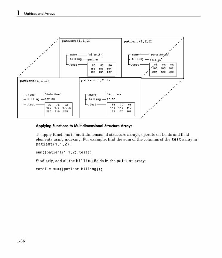
1 Matrices and Arrays
1-66
Applying Functions to Multidimensional Structure Arrays
To apply functions to multidimensional structure arrays, operate on fields and fieldelements using indexing. For example, find the sum of the columns of the test array inpatient(1,1,2):
sum((patient(1,1,2).test));
Similarly, add all the billing fields in the patient array:
total = sum([patient.billing]);

Summary of Matrix and Array Functions
1-67
Summary of Matrix and Array Functions
This section summarizes the principal functions used in creating and handling matrices.Most of these functions work on multidimensional arrays as well.
Functions to Create a Matrix
Function Description
[a,b] or [a;b] Create a matrix from specified elements, or concatenate matricestogether.
accumarray Construct a matrix using accumulation.blkdiag Construct a block diagonal matrix.cat Concatenate matrices along the specified dimension.diag Create a diagonal matrix from a vector.horzcat Concatenate matrices horizontally.magic Create a square matrix with rows, columns, and diagonals that
add up to the same number.ones Create a matrix of all ones.rand Create a matrix of uniformly distributed random numbers.repmat Create a new matrix by replicating or tiling another.vertcat Concatenate two or more matrices vertically.zeros Create a matrix of all zeros.
Functions to Modify the Shape of a Matrix
Function Description
ctranspose Flip a matrix about the main diagonal and replace each elementwith its complex conjugate.
flip Flip a matrix along the specified dimension.fliplr Flip a matrix about a vertical axis.flipud Flip a matrix about a horizontal axis.reshape Change the dimensions of a matrix.rot90 Rotate a matrix by 90 degrees.

1 Matrices and Arrays
1-68
Function Description
transpose Flip a matrix about the main diagonal.
Functions to Find the Structure or Shape of a Matrix
Function Description
isempty Return true for 0-by-0 or 0-by-n matrices.isscalar Return true for 1-by-1 matrices.issparse Return true for sparse matrices.isvector Return true for 1-by-n matrices.length Return the length of a vector.ndims Return the number of dimensions in a matrix.numel Return the number of elements in a matrix.size Return the size of each dimension.
Functions to Determine Class
Function Description
iscell Return true if the matrix is a cell array.ischar Return true if matrix elements are characters or strings.isfloat Determine if input is a floating point array.isinteger Determine if input is an integer array.islogical Return true if matrix elements are logicals.isnumeric Return true if matrix elements are numeric.isreal Return true if matrix elements are real numbers.isstruct Return true if matrix elements are MATLAB structures.
Functions to Sort and Shift Matrix Elements
Function Description
circshift Circularly shift matrix contents.issorted Return true if the matrix elements are sorted.sort Sort elements in ascending or descending order.

Summary of Matrix and Array Functions
1-69
Function Description
sortrows Sort rows in ascending order.
Functions That Work on Diagonals of a Matrix
Function Description
blkdiag Construct a block diagonal matrix.diag Return the diagonals of a matrix.trace Compute the sum of the elements on the main diagonal.tril Return the lower triangular part of a matrix.triu Return the upper triangular part of a matrix.
Functions to Change the Indexing Style
Function Description
ind2sub Convert a linear index to a row-column index.sub2ind Convert a row-column index to a linear index.
Functions for Working with Multidimensional Arrays
Function Description
cat Concatenate arrays.circshift Shift array circularly.ipermute Inverse permute array dimensions.ndgrid Generate arrays for n-dimensional functions and interpolation.ndims Return the number of array dimensions.permute Permute array dimensions.shiftdim Shift array dimensions.squeeze Remove singleton dimensions.


2
Linear Algebra
• “Matrices in the MATLAB Environment” on page 2-2• “Systems of Linear Equations” on page 2-11• “Inverses and Determinants” on page 2-23• “Factorizations” on page 2-27• “Powers and Exponentials” on page 2-35• “Eigenvalues” on page 2-39• “Singular Values” on page 2-42

2 Linear Algebra
2-2
Matrices in the MATLAB Environment
In this section...
“Creating Matrices” on page 2-2“Adding and Subtracting Matrices” on page 2-3“Vector Products and Transpose” on page 2-4“Multiplying Matrices” on page 2-6“Identity Matrix” on page 2-8“Kronecker Tensor Product” on page 2-8“Vector and Matrix Norms” on page 2-9“Using Multithreaded Computation with Linear Algebra Functions” on page 2-10
Creating Matrices
The MATLAB environment uses the term matrix to indicate a variable containing realor complex numbers arranged in a two-dimensional grid. An array is, more generally,a vector, matrix, or higher dimensional grid of numbers. All arrays in MATLAB arerectangular, in the sense that the component vectors along any dimension are all thesame length.
Symbolic Math Toolbox™ software extends the capabilities of MATLAB software tomatrices of mathematical expressions.
MATLAB has dozens of functions that create different kinds of matrices. There are twofunctions you can use to create a pair of 3-by-3 example matrices for use throughout thischapter. The first example is symmetric:
A = pascal(3)
A =
1 1 1
1 2 3
1 3 6
The second example is not symmetric:
B = magic(3)
B =

Matrices in the MATLAB Environment
2-3
8 1 6
3 5 7
4 9 2
Another example is a 3-by-2 rectangular matrix of random integers:
C = fix(10*rand(3,2))
C =
9 4
2 8
6 7
A column vector is an m-by-1 matrix, a row vector is a 1-by-n matrix, and a scalar is a 1-by-1 matrix. The statements
u = [3; 1; 4]
v = [2 0 -1]
s = 7
produce a column vector, a row vector, and a scalar:
u =
3
1
4
v =
2 0 -1
s =
7
For more information about creating and working with matrices, see “Creating andConcatenating Matrices”.
Adding and Subtracting Matrices
Addition and subtraction of matrices is defined just as it is for arrays, element byelement. Adding A to B, and then subtracting A from the result recovers B:
A = pascal(3);

2 Linear Algebra
2-4
B = magic(3);
X = A + B
X =
9 2 7
4 7 10
5 12 8
Y = X - A
Y =
8 1 6
3 5 7
4 9 2
Addition and subtraction require both matrices to have the same dimension, or one ofthem be a scalar. If the dimensions are incompatible, an error results:
C = fix(10*rand(3,2))
X = A + C
Error using plus
Matrix dimensions must agree.
w = v + s
w =
9 7 6
Vector Products and Transpose
A row vector and a column vector of the same length can be multiplied in either order.The result is either a scalar, the inner product, or a matrix, the outer product :
u = [3; 1; 4];
v = [2 0 -1];
x = v*u
x =
2
X = u*v
X =
6 0 -3
2 0 -1

Matrices in the MATLAB Environment
2-5
8 0 -4
For real matrices, the transpose operation interchanges aij and aji. MATLAB uses theapostrophe operator (') to perform a complex conjugate transpose, and uses the dot-apostrophe operator (.') to transpose without conjugation. For matrices containing allreal elements, the two operators return the same result.
The example matrix A is symmetric, so A' is equal to A. But, B is not symmetric:
B = magic(3);
X = B'
X =
8 3 4
1 5 9
6 7 2
Transposition turns a row vector into a column vector:
x = v'
x =
2
0
-1
If x and y are both real column vectors, the product x*y is not defined, but the twoproducts
x'*y
and
y'*x
are the same scalar. This quantity is used so frequently, it has three different names:inner product, scalar product, or dot product.
For a complex vector or matrix, z, the quantity z' not only transposes the vector ormatrix, but also converts each complex element to its complex conjugate. That is, the signof the imaginary part of each complex element changes. So if
z = [1+2i 7-3i 3+4i; 6-2i 9i 4+7i]
z =
1.0000 + 2.0000i 7.0000 - 3.0000i 3.0000 + 4.0000i

2 Linear Algebra
2-6
6.0000 - 2.0000i 0 + 9.0000i 4.0000 + 7.0000i
then
z'
ans =
1.0000 - 2.0000i 6.0000 + 2.0000i
7.0000 + 3.0000i 0 - 9.0000i
3.0000 - 4.0000i 4.0000 - 7.0000i
The unconjugated complex transpose, where the complex part of each element retains itssign, is denoted by z.':
z.'
ans =
1.0000 + 2.0000i 6.0000 - 2.0000i
7.0000 - 3.0000i 0 + 9.0000i
3.0000 + 4.0000i 4.0000 + 7.0000i
For complex vectors, the two scalar products x'*y and y'*x are complex conjugates ofeach other, and the scalar product x'*x of a complex vector with itself is real.
Multiplying Matrices
Multiplication of matrices is defined in a way that reflects composition of the underlyinglinear transformations and allows compact representation of systems of simultaneouslinear equations. The matrix product C = AB is defined when the column dimension of Ais equal to the row dimension of B, or when one of them is a scalar. If A is m-by-p and Bis p-by-n, their product C is m-by-n. The product can actually be defined using MATLABfor loops, colon notation, and vector dot products:
A = pascal(3);
B = magic(3);
m = 3; n = 3;
for i = 1:m
for j = 1:n
C(i,j) = A(i,:)*B(:,j);
end
end
MATLAB uses a single asterisk to denote matrix multiplication. The next two examplesillustrate the fact that matrix multiplication is not commutative; AB is usually not equalto BA:

Matrices in the MATLAB Environment
2-7
X = A*B
X =
15 15 15
26 38 26
41 70 39
Y = B*A
Y =
15 28 47
15 34 60
15 28 43
A matrix can be multiplied on the right by a column vector and on the left by a rowvector:
u = [3; 1; 4];
x = A*u
x =
8
17
30
v = [2 0 -1];
y = v*B
y =
12 -7 10
Rectangular matrix multiplications must satisfy the dimension compatibility conditions:
C = fix(10*rand(3,2));
X = A*C
X =
17 19
31 41
51 70
Y = C*A
Error using mtimes
Inner matrix dimensions must agree.

2 Linear Algebra
2-8
Anything can be multiplied by a scalar:
s = 7;
w = s*v
w =
14 0 -7
Identity Matrix
Generally accepted mathematical notation uses the capital letter I to denote identitymatrices, matrices of various sizes with ones on the main diagonal and zeros elsewhere.These matrices have the property that AI = A and IA = A whenever the dimensions arecompatible. The original version of MATLAB could not use I for this purpose becauseit did not distinguish between uppercase and lowercase letters and i already served asa subscript and as the complex unit. So an English language pun was introduced. Thefunction
eye(m,n)
returns an m-by-n rectangular identity matrix and eye(n) returns an n-by-n squareidentity matrix.
Kronecker Tensor Product
The Kronecker product, kron(X,Y), of two matrices is the larger matrix formed from allpossible products of the elements of X with those of Y. If X is m-by-n and Y is p-by-q, thenkron(X,Y) is mp-by-nq. The elements are arranged in the following order:
[X(1,1)*Y X(1,2)*Y . . . X(1,n)*Y
. . .
X(m,1)*Y X(m,2)*Y . . . X(m,n)*Y]
The Kronecker product is often used with matrices of zeros and ones to build up repeatedcopies of small matrices. For example, if X is the 2-by-2 matrix
X =
1 2
3 4
and I = eye(2,2) is the 2-by-2 identity matrix, then the two matrices
kron(X,I)

Matrices in the MATLAB Environment
2-9
and
kron(I,X)
are
1 0 2 0
0 1 0 2
3 0 4 0
0 3 0 4
and
1 2 0 0
3 4 0 0
0 0 1 2
0 0 3 4
Vector and Matrix Norms
The p-norm of a vector x,
x xp ip
p
= ( )∑1/
,
is computed by norm(x,p). This is defined by any value of p > 1, but the most commonvalues of p are 1, 2, and ∞. The default value is p = 2, which corresponds to Euclideanlength:
v = [2 0 -1];
[norm(v,1) norm(v) norm(v,inf)]
ans =
3.0000 2.2361 2.0000
The p-norm of a matrix A,
AAx
xp
x
p
p
= max ,
can be computed for p = 1, 2, and ∞ by norm(A,p). Again, the default value is p = 2:

2 Linear Algebra
2-10
C = fix(10*rand(3,2));
[norm(C,1) norm(C) norm(C,inf)]
ans =
19.0000 14.8015 13.0000
Using Multithreaded Computation with Linear Algebra Functions
MATLAB software supports multithreaded computation for a number of linear algebraand element-wise numerical functions. These functions automatically execute onmultiple threads. For a function or expression to execute faster on multiple CPUs, anumber of conditions must be true:
1 The function performs operations that easily partition into sections that executeconcurrently. These sections must be able to execute with little communicationbetween processes. They should require few sequential operations.
2 The data size is large enough so that any advantages of concurrent executionoutweigh the time required to partition the data and manage separate executionthreads. For example, most functions speed up only when the array contains severalthousand elements or more.
3 The operation is not memory-bound; processing time is not dominated by memoryaccess time. As a general rule, complicated functions speed up more than simplefunctions.
The matrix multiply (X*Y) and matrix power (X^p) operators show significant increasein speed on large double-precision arrays (on order of 10,000 elements). The matrixanalysis functions det, rcond, hess, and expm also show significant increase in speedon large double-precision arrays.

Systems of Linear Equations
2-11
Systems of Linear Equations
In this section...
“Computational Considerations” on page 2-11“General Solution” on page 2-12“Square Systems” on page 2-13“Overdetermined Systems” on page 2-15“Underdetermined Systems” on page 2-18“Using Multithreaded Computation with Systems of Linear Equations” on page 2-20“Iterative Methods for Solving Systems of Linear Equations” on page 2-21
Computational Considerations
One of the most important problems in technical computing is the solution of systems ofsimultaneous linear equations.
In matrix notation, the general problem takes the following form: Given two matrices Aand b, does there exist a unique matrix x, so that Ax = b or xA = b?
It is instructive to consider a 1-by-1 example. For example, does the equation7x = 21
have a unique solution?
The answer, of course, is yes. The equation has the unique solution x = 3. The solution iseasily obtained by division:x = 21/7 = 3.
The solution is not ordinarily obtained by computing the inverse of 7, that is 7–
1 = 0.142857..., and then multiplying 7–1 by 21. This would be more work and, if 7–1 isrepresented to a finite number of digits, less accurate. Similar considerations apply tosets of linear equations with more than one unknown; the MATLAB software solves suchequations without computing the inverse of the matrix.
Although it is not standard mathematical notation, MATLAB uses the divisionterminology familiar in the scalar case to describe the solution of a general system ofsimultaneous equations. The two division symbols, slash, /, and backslash, \, correspond

2 Linear Algebra
2-12
to the two MATLAB functions mrdivide and mldivide. mrdivide and mldivide areused for the two situations where the unknown matrix appears on the left or right of thecoefficient matrix:
x = b/A Denotes the solution to the matrix equation xA = b.x = A\b Denotes the solution to the matrix equation Ax = b.
Think of “dividing” both sides of the equation Ax = b or xA = b by A. The coefficientmatrix A is always in the “denominator.”
The dimension compatibility conditions for x = A\b require the two matrices A and b tohave the same number of rows. The solution x then has the same number of columns asb and its row dimension is equal to the column dimension of A. For x = b/A, the roles ofrows and columns are interchanged.
In practice, linear equations of the form Ax = b occur more frequently than those of theform xA = b. Consequently, the backslash is used far more frequently than the slash.The remainder of this section concentrates on the backslash operator; the correspondingproperties of the slash operator can be inferred from the identity:
(b/A)' = (A'\b').
The coefficient matrix A need not be square. If A is m-by-n, there are three cases:
m = n Square system. Seek an exact solution.m > n Overdetermined system. Find a least-squares solution.m < n Underdetermined system. Find a basic solution with at most
m nonzero components.
The mldivide Algorithm
The mldivide operator employs different solvers to handle different kinds of coefficientmatrices. The various cases are diagnosed automatically by examining the coefficientmatrix. For more information, see the “Algorithms” section of the mldivide referencepage.
General Solution
The general solution to a system of linear equations Ax = b describes all possiblesolutions. You can find the general solution by:

Systems of Linear Equations
2-13
1 Solving the corresponding homogeneous system Ax = 0. Do this using the nullcommand, by typing null(A). This returns a basis for the solution space to Ax = 0.Any solution is a linear combination of basis vectors.
2 Finding a particular solution to the nonhomogeneous system Ax = b.
You can then write any solution to Ax = b as the sum of the particular solution to Ax = b,from step 2, plus a linear combination of the basis vectors from step 1.
The rest of this section describes how to use MATLAB to find a particular solution toAx = b, as in step 2.
Square Systems
The most common situation involves a square coefficient matrix A and a single right sidecolumn vector b.
Nonsingular Coefficient Matrix
If the matrix A is nonsingular, the solution, x = A\b, is then the same size as b. Forexample:
A = pascal(3);
u = [3; 1; 4];
x = A\u
x =
10
-12
5
It can be confirmed that A*x is exactly equal to u.
If A and b are square and the same size, x= A\b is also that size:
b = magic(3);
X = A\b
X =
19 -3 -1
-17 4 13
6 0 -6
It can be confirmed that A*x is exactly equal to b.

2 Linear Algebra
2-14
Both of these examples have exact, integer solutions. This is because the coefficientmatrix was chosen to be pascal(3), which is a full rank matrix (nonsingular).
Singular Coefficient Matrix
A square matrix A is singular if it does not have linearly independent columns. If A issingular, the solution to Ax = b either does not exist, or is not unique. The backslashoperator, A\b, issues a warning if A is nearly singular and raises an error condition if itdetects exact singularity.
If A is singular and Ax = b has a solution, you can find a particular solution that is notunique, by typing
P = pinv(A)*b
P is a pseudoinverse of A. If Ax = b does not have an exact solution, pinv(A) returns aleast-squares solution.
For example:
A = [ 1 3 7
-1 4 4
1 10 18 ]
is singular, as you can verify by typing
rank(A)
ans =
2
Since A is not full rank, it has some singular values equal to zero.
Note: For information about using pinv to solve systems with rectangular coefficientmatrices, see “Pseudoinverses” on page 2-24.
Exact Solutions
For b =[5;2;12], the equation Ax = b has an exact solution, given by
pinv(A)*b

Systems of Linear Equations
2-15
ans =
0.3850
-0.1103
0.7066
Verify that pinv(A)*b is an exact solution by typing
A*pinv(A)*b
ans =
5.0000
2.0000
12.0000
Least-Squares Solutions
However, if b = [3;6;0], Ax = b does not have an exact solution. In this case,pinv(A)*b returns a least-squares solution. If you type
A*pinv(A)*b
ans =
-1.0000
4.0000
2.0000
you do not get back the original vector b.
You can determine whether Ax = b has an exact solution by finding the row reducedechelon form of the augmented matrix [A b]. To do so for this example, enter
rref([A b])
ans =
1.0000 0 2.2857 0
0 1.0000 1.5714 0
0 0 0 1.0000
Since the bottom row contains all zeros except for the last entry, the equation does nothave a solution. In this case, pinv(A) returns a least-squares solution.
Overdetermined Systems
This example shows how overdetermined systems are often encountered in various kindsof curve fitting to experimental data.

2 Linear Algebra
2-16
A quantity, y, is measured at several different values of time, t, to produce the followingobservations. You can enter the data and view it in a table with the following statements.
t = [0 .3 .8 1.1 1.6 2.3]';
y = [.82 .72 .63 .60 .55 .50]';
B = table(t,y)
B =
t y
___ ____
0 0.82
0.3 0.72
0.8 0.63
1.1 0.6
1.6 0.55
2.3 0.5
Try modeling the data with a decaying exponential function
.
The preceding equation says that the vector y should be approximated by a linearcombination of two other vectors. One is a constant vector containing all ones and theother is the vector with components exp(-t). The unknown coefficients, and , canbe computed by doing a least-squares fit, which minimizes the sum of the squares ofthe deviations of the data from the model. There are six equations in two unknowns,represented by a 6-by-2 matrix.
E = [ones(size(t)) exp(-t)]
E =
1.0000 1.0000
1.0000 0.7408
1.0000 0.4493
1.0000 0.3329
1.0000 0.2019
1.0000 0.1003

Systems of Linear Equations
2-17
Use the backslash operator to get the least-squares solution.
c = E\y
c =
0.4760
0.3413
In other words, the least-squares fit to the data is
The following statements evaluate the model at regularly spaced increments in t, andthen plot the result together with the original data:
T = (0:0.1:2.5)';
Y = [ones(size(T)) exp(-T)]*c;
plot(T,Y,'-',t,y,'o')

2 Linear Algebra
2-18
E*c is not exactly equal to y, but the difference might well be less than measurementerrors in the original data.
A rectangular matrix A is rank deficient if it does not have linearly independent columns.If A is rank deficient, the least-squares solution to AX = B is not unique. The backslashoperator, A\B, issues a warning if A is rank deficient and produces a least-squaressolution if the system has no solution and a basic solution if the system has infinitelymany solutions.
Underdetermined Systems
This example shows how the solution to underdetermined systems is not unique.Underdetermined linear systems involve more unknowns than equations. The matrix

Systems of Linear Equations
2-19
left division operation in MATLAB finds a basic solution, which has at most m nonzerocomponents for an m-by-n coefficient matrix.
Here is a small, random example:
R = [6 8 7 3; 3 5 4 1]
rng(0);
b = randi(8,2,1)
R =
6 8 7 3
3 5 4 1
b =
7
8
The linear system Rp = b involves two equations in four unknowns. Since the coefficientmatrix contains small integers, it is appropriate to use the format command to displaythe solution in rational format. The particular solution is obtained with
format rat
p = R\b
p =
0
17/7
0
-29/7
One of the nonzero components is p(2) because R(:,2) is the column of R with largestnorm. The other nonzero component is p(4) because R(:,4) dominates after R(:,2) iseliminated.
The complete general solution to the underdetermined system can be characterized byadding p to an arbitrary linear combination of the null space vectors, which can be foundusing the null function with an option requesting a rational basis.
Z = null(R,'r')
Z =

2 Linear Algebra
2-20
-1/2 -7/6
-1/2 1/2
1 0
0 1
It can be confirmed that R*Z is zero and that the residual R*x - b is small for anyvector x, where
x = p + Z*q.
Since the columns of Z are the null space vectors, the product Z*q is a linear combinationof those vectors:
Z q x xu
wux wx* .= ( ) Ê
ËÁ
ˆ
¯˜ = +v v v v
1 2 1 2
To illustrate, choose an arbitrary q and construct x.
q = [-2; 1];
x = p + Z*q;
Calculate the norm of the residual.
format short
norm(R*x - b)
ans =
2.6645e-15
Using Multithreaded Computation with Systems of Linear Equations
MATLAB software supports multithreaded computation for a number of linear algebraand element-wise numerical functions. These functions automatically execute onmultiple threads. For a function or expression to execute faster on multiple CPUs, anumber of conditions must be true:
1 The function performs operations that easily partition into sections that executeconcurrently. These sections must be able to execute with little communicationbetween processes. They should require few sequential operations.
2 The data size is large enough so that any advantages of concurrent executionoutweigh the time required to partition the data and manage separate execution

Systems of Linear Equations
2-21
threads. For example, most functions speed up only when the array contains severalthousand elements or more.
3 The operation is not memory-bound; processing time is not dominated by memoryaccess time. As a general rule, complicated functions speed up more than simplefunctions.
inv, lscov, linsolve, and mldivide show significant increase in speed on largedouble-precision arrays (on order of 10,000 elements or more) when multithreading isenabled.
Iterative Methods for Solving Systems of Linear Equations
If the coefficient matrix A is large and sparse, factorization methods are generally notefficient. Iterative methods generate a series of approximate solutions. MATLAB providesseveral iterative methods to handle large, sparse input matrices.
pcg
Preconditioned conjugate gradients method. This method is appropriate forHermitian positive definite coefficient matrix A.
bicg
BiConjugate Gradients Methodbicgstab
BiConjugate Gradients Stabilized Methodbicgstabl
BiCGStab(l) Methodcgs
Conjugate Gradients Squared Methodgmres
Generalized Minimum Residual Methodlsqr
LSQR Methodminres
Minimum Residual Method. This method is appropriate for Hermitian coefficientmatrix A.
qmr

2 Linear Algebra
2-22
Quasi-Minimal Residual Methodsymmlq
Symmetric LQ Methodtfqmr
Transpose-Free QMR Method

Inverses and Determinants
2-23
Inverses and Determinants
In this section...
“Introduction” on page 2-23“Pseudoinverses” on page 2-24
Introduction
If A is square and nonsingular, the equations AX = I and XA = I have the same solution,X. This solution is called the inverse of A, is denoted by A-1, and is computed by thefunction inv.
The determinant of a matrix is useful in theoretical considerations and some types ofsymbolic computation, but its scaling and round-off error properties make it far lesssatisfactory for numeric computation. Nevertheless, the function det computes thedeterminant of a square matrix:
A = pascal(3)
A =
1 1 1
1 2 3
1 3 6
d = det(A)
X = inv(A)
d =
1
X =
3 -3 1
-3 5 -2
1 -2 1
Again, because A is symmetric, has integer elements, and has determinant equal to one,so does its inverse. However,
B = magic(3)
B =

2 Linear Algebra
2-24
8 1 6
3 5 7
4 9 2
d = det(B)
X = inv(B)
d =
-360
X =
0.1472 -0.1444 0.0639
-0.0611 0.0222 0.1056
-0.0194 0.1889 -0.1028
Closer examination of the elements of X, or use of format rat, would reveal that theyare integers divided by 360.
If A is square and nonsingular, then, without round-off error, X = inv(A)*B istheoretically the same as X = A\B and Y = B*inv(A) is theoretically the same as Y =B/A. But the computations involving the backslash and slash operators are preferablebecause they require less computer time, less memory, and have better error-detectionproperties.
Pseudoinverses
Rectangular matrices do not have inverses or determinants. At least one of the equationsAX = I and XA = I does not have a solution. A partial replacement for the inverse isprovided by the Moore-Penrose pseudoinverse, which is computed by the pinv function:
format short
C = fix(10*gallery('uniformdata',[3 2],0));
X = pinv(C)
X =
0.1159 -0.0729 0.0171
-0.0534 0.1152 0.0418
The matrix
Q = X*C
Q =
1.0000 0.0000

Inverses and Determinants
2-25
0.0000 1.0000
is the 2-by-2 identity, but the matrix
P = C*X
P =
0.8293 -0.1958 0.3213
-0.1958 0.7754 0.3685
0.3213 0.3685 0.3952
is not the 3-by-3 identity. However, P acts like an identity on a portion of the space in thesense that P is symmetric, P*C is equal to C, and X*P is equal to X.
Solving a Rank-Deficient System
If A is m-by-n with m > n and full rank n, each of the three statements
x = A\b
x = pinv(A)*b
x = inv(A'*A)*A'*b
theoretically computes the same least-squares solution x, although the backslashoperator does it faster.
However, if A does not have full rank, the solution to the least-squares problem is notunique. There are many vectors x that minimize
norm(A*x -b)
The solution computed by x = A\b is a basic solution; it has at most r nonzerocomponents, where r is the rank of A. The solution computed by x = pinv(A)*b is theminimal norm solution because it minimizes norm(x). An attempt to compute a solutionwith x = inv(A'*A)*A'*b fails because A'*A is singular.
Here is an example that illustrates the various solutions:
A = [ 1 2 3
4 5 6
7 8 9
10 11 12 ];
does not have full rank. Its second column is the average of the first and third columns. If
b = A(:,2)

2 Linear Algebra
2-26
is the second column, then an obvious solution to A*x = b is x = [0 1 0]'. But noneof the approaches computes that x. The backslash operator gives
x = A\b
Warning: Rank deficient, rank = 2, tol = 1.4594e-014.
x =
0.5000
0
0.5000
This solution has two nonzero components. The pseudoinverse approach gives
y = pinv(A)*b
y =
0.3333
0.3333
0.3333
There is no warning about rank deficiency. But norm(y) = 0.5774 is less thannorm(x) = 0.7071. Finally,
z = inv(A'*A)*A'*b
fails completely:
Warning: Matrix is close to singular or badly scaled.
Results may be inaccurate. RCOND = 9.868649e-018.
z =
-0.8594
1.3438
-0.6875

Factorizations
2-27
Factorizations
In this section...
“Introduction” on page 2-27“Cholesky Factorization” on page 2-27“LU Factorization” on page 2-28“QR Factorization” on page 2-30“Using Multithreaded Computation for Factorization” on page 2-33
Introduction
All three of the matrix factorizations discussed in this section make use of triangularmatrices, where all the elements either above or below the diagonal are zero. Systems oflinear equations involving triangular matrices are easily and quickly solved using eitherforward or back substitution.
Cholesky Factorization
The Cholesky factorization expresses a symmetric matrix as the product of a triangularmatrix and its transposeA = R′R,
where R is an upper triangular matrix.
Not all symmetric matrices can be factored in this way; the matrices that have such afactorization are said to be positive definite. This implies that all the diagonal elementsof A are positive and that the off-diagonal elements are “not too big.” The Pascal matricesprovide an interesting example. Throughout this chapter, the example matrix A has beenthe 3-by-3 Pascal matrix. Temporarily switch to the 6-by-6:
A = pascal(6)
A =
1 1 1 1 1 1
1 2 3 4 5 6
1 3 6 10 15 21
1 4 10 20 35 56
1 5 15 35 70 126
1 6 21 56 126 252

2 Linear Algebra
2-28
The elements of A are binomial coefficients. Each element is the sum of its north andwest neighbors. The Cholesky factorization is
R = chol(A)
R =
1 1 1 1 1 1
0 1 2 3 4 5
0 0 1 3 6 10
0 0 0 1 4 10
0 0 0 0 1 5
0 0 0 0 0 1
The elements are again binomial coefficients. The fact that R'*R is equal to Ademonstrates an identity involving sums of products of binomial coefficients.
Note: The Cholesky factorization also applies to complex matrices. Any complex matrixthat has a Cholesky factorization satisfiesA′ = Aand is said to be Hermitian positive definite.
The Cholesky factorization allows the linear systemAx = b
to be replaced byR′Rx = b.
Because the backslash operator recognizes triangular systems, this can be solved in theMATLAB environment quickly with
x = R\(R'\b)
If A is n-by-n, the computational complexity of chol(A) is O(n3), but the complexity ofthe subsequent backslash solutions is only O(n2).
LU Factorization
LU factorization, or Gaussian elimination, expresses any square matrix A as the productof a permutation of a lower triangular matrix and an upper triangular matrixA = LU,

Factorizations
2-29
where L is a permutation of a lower triangular matrix with ones on its diagonal and U isan upper triangular matrix.
The permutations are necessary for both theoretical and computational reasons. Thematrix
0 1
1 0
cannot be expressed as the product of triangular matrices without interchanging its tworows. Although the matrix
e 1
1 0
can be expressed as the product of triangular matrices, when ε is small, the elementsin the factors are large and magnify errors, so even though the permutations are notstrictly necessary, they are desirable. Partial pivoting ensures that the elements of L arebounded by one in magnitude and that the elements of U are not much larger than thoseof A.
For example:
[L,U] = lu(B)
L =
1.0000 0 0
0.3750 0.5441 1.0000
0.5000 1.0000 0
U =
8.0000 1.0000 6.0000
0 8.5000 -1.0000
0 0 5.2941
The LU factorization of A allows the linear system
A*x = b
to be solved quickly with

2 Linear Algebra
2-30
x = U\(L\b)
Determinants and inverses are computed from the LU factorization using
det(A) = det(L)*det(U)
and
inv(A) = inv(U)*inv(L)
You can also compute the determinants using det(A) = prod(diag(U)), though thesigns of the determinants might be reversed.
QR Factorization
An orthogonal matrix, or a matrix with orthonormal columns, is a real matrix whosecolumns all have unit length and are perpendicular to each other. If Q is orthogonal, thenQ′Q = 1.
The simplest orthogonal matrices are two-dimensional coordinate rotations:
cos( ) sin( )
sin( ) cos( ).
q q
q q−
For complex matrices, the corresponding term is unitary. Orthogonal and unitarymatrices are desirable for numerical computation because they preserve length, preserveangles, and do not magnify errors.
The orthogonal, or QR, factorization expresses any rectangular matrix as the product ofan orthogonal or unitary matrix and an upper triangular matrix. A column permutationmight also be involved:A = QR
orAP = QR,
where Q is orthogonal or unitary, R is upper triangular, and P is a permutation.
There are four variants of the QR factorization—full or economy size, and with or withoutcolumn permutation.

Factorizations
2-31
Overdetermined linear systems involve a rectangular matrix with more rows thancolumns, that is m-by-n with m > n. The full-size QR factorization produces a square, m-by-m orthogonal Q and a rectangular m-by-n upper triangular R:
C=gallery('uniformdata',[5 4], 0);
[Q,R] = qr(C)
Q =
0.6191 0.1406 -0.1899 -0.5058 0.5522
0.1506 0.4084 0.5034 0.5974 0.4475
0.3954 -0.5564 0.6869 -0.1478 -0.2008
0.3167 0.6676 0.1351 -0.1729 -0.6370
0.5808 -0.2410 -0.4695 0.5792 -0.2207
R =
1.5346 1.0663 1.2010 1.4036
0 0.7245 0.3474 -0.0126
0 0 0.9320 0.6596
0 0 0 0.6648
0 0 0 0
In many cases, the last m – n columns of Q are not needed because they are multipliedby the zeros in the bottom portion of R. So the economy-size QR factorization produces arectangular, m-by-n Q with orthonormal columns and a square n-by-n upper triangularR. For the 5-by-4 example, this is not much of a saving, but for larger, highly rectangularmatrices, the savings in both time and memory can be quite important:
[Q,R] = qr(C,0)
Q =
0.6191 0.1406 -0.1899 -0.5058
0.1506 0.4084 0.5034 0.5974
0.3954 -0.5564 0.6869 -0.1478
0.3167 0.6676 0.1351 -0.1729
0.5808 -0.2410 -0.4695 0.5792
R =
1.5346 1.0663 1.2010 1.4036
0 0.7245 0.3474 -0.0126

2 Linear Algebra
2-32
0 0 0.9320 0.6596
0 0 0 0.6648
In contrast to the LU factorization, the QR factorization does not require any pivotingor permutations. But an optional column permutation, triggered by the presence of athird output argument, is useful for detecting singularity or rank deficiency. At each stepof the factorization, the column of the remaining unfactored matrix with largest normis used as the basis for that step. This ensures that the diagonal elements of R occur indecreasing order and that any linear dependence among the columns is almost certainlybe revealed by examining these elements. For the small example given here, the secondcolumn of C has a larger norm than the first, so the two columns are exchanged:
[Q,R,P] = qr(C)
Q =
-0.3522 0.8398 -0.4131
-0.7044 -0.5285 -0.4739
-0.6163 0.1241 0.7777
R =
-11.3578 -8.2762
0 7.2460
0 0
P =
0 1
1 0
When the economy-size and column permutations are combined, the third outputargument is a permutation vector, rather than a permutation matrix:
[Q,R,p] = qr(C,0)
Q =
-0.3522 0.8398
-0.7044 -0.5285
-0.6163 0.1241
R =
-11.3578 -8.2762
0 7.2460
p =

Factorizations
2-33
2 1
The QR factorization transforms an overdetermined linear system into an equivalenttriangular system. The expression
norm(A*x - b)
equals
norm(Q*R*x - b)
Multiplication by orthogonal matrices preserves the Euclidean norm, so this expression isalso equal to
norm(R*x - y)
where y = Q'*b. Since the last m-n rows of R are zero, this expression breaks into twopieces:
norm(R(1:n,1:n)*x - y(1:n))
and
norm(y(n+1:m))
When A has full rank, it is possible to solve for x so that the first of these expressions iszero. Then the second expression gives the norm of the residual. When A does not havefull rank, the triangular structure of R makes it possible to find a basic solution to theleast-squares problem.
Using Multithreaded Computation for Factorization
MATLAB software supports multithreaded computation for a number of linear algebraand element-wise numerical functions. These functions automatically execute onmultiple threads. For a function or expression to execute faster on multiple CPUs, anumber of conditions must be true:
1 The function performs operations that easily partition into sections that executeconcurrently. These sections must be able to execute with little communicationbetween processes. They should require few sequential operations.
2 The data size is large enough so that any advantages of concurrent executionoutweigh the time required to partition the data and manage separate execution

2 Linear Algebra
2-34
threads. For example, most functions speed up only when the array contains severalthousand elements or more.
3 The operation is not memory-bound; processing time is not dominated by memoryaccess time. As a general rule, complicated functions speed up more than simplefunctions.
lu and qr show significant increase in speed on large double-precision arrays (on order of10,000 elements).

Powers and Exponentials
2-35
Powers and Exponentials
In this section...
“Positive Integer Powers” on page 2-35“Inverse and Fractional Powers” on page 2-35“Element-by-Element Powers” on page 2-36“Exponentials” on page 2-36
Positive Integer Powers
If A is a square matrix and p is a positive integer, A^p effectively multiplies A by itselfp-1 times. For example:
A = [1 1 1;1 2 3;1 3 6]
A =
1 1 1
1 2 3
1 3 6
X = A^2
X =
3 6 10
6 14 25
10 25 46
Inverse and Fractional Powers
If A is square and nonsingular, A^(-p) effectively multiplies inv(A) by itself p-1 times:
Y = A^(-3)
Y =
145.0000 -207.0000 81.0000
-207.0000 298.0000 -117.0000

2 Linear Algebra
2-36
81.0000 -117.0000 46.0000
Fractional powers, like A^(2/3), are also permitted; the results depend upon thedistribution of the eigenvalues of the matrix.
Element-by-Element Powers
The .^ operator produces element-by-element powers. For example:
X = A.^2
A =
1 1 1
1 4 9
1 9 36
Exponentials
The function
sqrtm(A)
computes A^(1/2) by a more accurate algorithm. The m in sqrtm distinguishes thisfunction from sqrt(A), which, like A.^(1/2), does its job element-by-element.
A system of linear, constant coefficient, ordinary differential equations can be written
where x = x(t) is a vector of functions of t and A is a matrix independent of t. Thesolution can be expressed in terms of the matrix exponential
.
The function
expm(A)
computes the matrix exponential. An example is provided by the 3-by-3 coefficientmatrix,

Powers and Exponentials
2-37
A = [0 -6 -1; 6 2 -16; -5 20 -10]
A =
0 -6 -1
6 2 -16
-5 20 -10
and the initial condition, x(0).
x0 = [1 1 1]'
x0 =
1
1
1
The matrix exponential is used to compute the solution, x(t), to the differential equationat 101 points on the interval .
X = [];
for t = 0:.01:1
X = [X expm(t*A)*x0];
end
A three-dimensional phase plane plot shows the solution spiraling in towards the origin.This behavior is related to the eigenvalues of the coefficient matrix.
plot3(X(1,:),X(2,:),X(3,:),'-o')

2 Linear Algebra
2-38

Eigenvalues
2-39
Eigenvalues
In this section...
“Eigenvalue Decomposition” on page 2-39“Multiple Eigenvalues” on page 2-40“Schur Decomposition” on page 2-41
Eigenvalue Decomposition
An eigenvalue and eigenvector of a square matrix A are, respectively, a scalar λ and anonzero vector υ that satisfyAυ = λυ.
With the eigenvalues on the diagonal of a diagonal matrix Λ and the correspondingeigenvectors forming the columns of a matrix V, you haveAV = VΛ.
If V is nonsingular, this becomes the eigenvalue decompositionA = VΛV–1.
A good example is provided by the coefficient matrix of the ordinary differential equationin the previous section:
A =
0 -6 -1
6 2 -16
-5 20 -10
The statement
lambda = eig(A)
produces a column vector containing the eigenvalues. For this matrix, the eigenvaluesare complex:
lambda =
-3.0710
-2.4645+17.6008i
-2.4645-17.6008i

2 Linear Algebra
2-40
The real part of each of the eigenvalues is negative, so eλt approaches zero as t increases.The nonzero imaginary part of two of the eigenvalues, ±ω, contributes the oscillatorycomponent, sin(ωt), to the solution of the differential equation.
With two output arguments, eig computes the eigenvectors and stores the eigenvalues ina diagonal matrix:
[V,D] = eig(A)
V =
-0.8326 0.2003 - 0.1394i 0.2003 + 0.1394i
-0.3553 -0.2110 - 0.6447i -0.2110 + 0.6447i
-0.4248 -0.6930 -0.6930
D =
-3.0710 0 0
0 -2.4645+17.6008i 0
0 0 -2.4645-17.6008i
The first eigenvector is real and the other two vectors are complex conjugates of eachother. All three vectors are normalized to have Euclidean length, norm(v,2), equal toone.
The matrix V*D*inv(V), which can be written more succinctly as V*D/V, is withinround-off error of A. And, inv(V)*A*V, or V\A*V, is within round-off error of D.
Multiple Eigenvalues
Some matrices do not have an eigenvector decomposition. These matrices are notdiagonalizable. For example:
A = [ 6 12 19
-9 -20 -33
4 9 15 ]
For this matrix
[V,D] = eig(A)
produces
V =

Eigenvalues
2-41
-0.4741 -0.4082 -0.4082
0.8127 0.8165 0.8165
-0.3386 -0.4082 -0.4082
D =
-1.0000 0 0
0 1.0000 0
0 0 1.0000
There is a double eigenvalue at λ = 1. The second and third columns of V are the same.For this matrix, a full set of linearly independent eigenvectors does not exist.
Schur Decomposition
The MATLAB advanced matrix computations do not require eigenvalue decompositions.They are based, instead, on the Schur decompositionA = USU′.
where U is an orthogonal matrix and S is a block upper triangular matrix with 1-by-1and 2-by-2 blocks on the diagonal. The eigenvalues are revealed by the diagonal elementsand blocks of S, while the columns of U provide a basis with much better numericalproperties than a set of eigenvectors. The Schur decomposition of this defective exampleis
[U,S] = schur(A)
U =
-0.4741 0.6648 0.5774
0.8127 0.0782 0.5774
-0.3386 -0.7430 0.5774
S =
-1.0000 20.7846 -44.6948
0 1.0000 -0.6096
0 0 1.0000
The double eigenvalue is contained in the lower 2-by-2 block of S.
Note: If A is complex, schur returns the complex Schur form, which is upper triangularwith the eigenvalues of A on the diagonal.

2 Linear Algebra
2-42
Singular Values
A singular value and corresponding singular vectors of a rectangular matrix A are,respectively, a scalar σ and a pair of vectors u and v that satisfyAv = σuA′u = σv.
With the singular values on the diagonal of a diagonal matrix Σ and the correspondingsingular vectors forming the columns of two orthogonal matrices U and V, you haveAV = UΣA′U = VΣ.
Since U and V are orthogonal, this becomes the singular value decompositionA = UΣV′.
The full singular value decomposition of an m-by-n matrix involves an m-by-m U, anm-by-n Σ, and an n-by-n V. In other words, U and V are both square and Σ is the samesize as A. If A has many more rows than columns, the resulting U can be quite large,but most of its columns are multiplied by zeros in Σ. In this situation, the economy sizeddecomposition saves both time and storage by producing an m-by-n U, an n-by-n Σ andthe same V.
The eigenvalue decomposition is the appropriate tool for analyzing a matrix whenit represents a mapping from a vector space into itself, as it does for an ordinarydifferential equation. However, the singular value decomposition is the appropriate toolfor analyzing a mapping from one vector space into another vector space, possibly with adifferent dimension. Most systems of simultaneous linear equations fall into this secondcategory.
If A is square, symmetric, and positive definite, then its eigenvalue and singular valuedecompositions are the same. But, as A departs from symmetry and positive definiteness,the difference between the two decompositions increases. In particular, the singularvalue decomposition of a real matrix is always real, but the eigenvalue decomposition of areal, nonsymmetric matrix might be complex.
For the example matrix
A =
9 4
6 8
2 7

Singular Values
2-43
the full singular value decomposition is
[U,S,V] = svd(A)
U =
0.6105 -0.7174 0.3355
0.6646 0.2336 -0.7098
0.4308 0.6563 0.6194
S =
14.9359 0
0 5.1883
0 0
V =
0.6925 -0.7214
0.7214 0.6925
You can verify that U*S*V' is equal to A to within round-off error. For this smallproblem, the economy size decomposition is only slightly smaller:
[U,S,V] = svd(A,0)
U =
0.6105 -0.7174
0.6646 0.2336
0.4308 0.6563
S =
14.9359 0
0 5.1883
V =
0.6925 -0.7214
0.7214 0.6925

2 Linear Algebra
2-44
Again, U*S*V' is equal to A to within round-off error.

3
Random Numbers
• “Random Numbers in MATLAB” on page 3-2• “Why Do Random Numbers Repeat After Startup?” on page 3-3• “Create Arrays of Random Numbers” on page 3-4• “Random Numbers Within a Specific Range” on page 3-6• “Random Integers” on page 3-7• “Random Numbers from Normal Distribution with Specific Mean and Variance” on
page 3-8• “Random Numbers Within a Sphere” on page 3-9• “Generate Random Numbers That Are Repeatable” on page 3-11• “Generate Random Numbers That Are Different” on page 3-15• “Managing the Global Stream” on page 3-17• “Creating and Controlling a Random Number Stream” on page 3-23• “Multiple streams” on page 3-31• “Replace Discouraged Syntaxes of rand and randn” on page 3-34

3 Random Numbers
3-2
Random Numbers in MATLAB
When you create random numbers using software, the results are not random in a strict,mathematical sense. However, software applications, such as MATLAB, use algorithmsthat make your results appear to be random and independent. The results also passvarious statistical tests of randomness and independence. These apparently random andindependent numbers are often described as pseudorandom and pseudoindependent. Youcan use these numbers as if they are truly random and independent. One benefit of usingpseudorandom, pseudoindependent numbers is that you can repeat a random numbercalculation at any time. This approach can be useful in testing or diagnostic situations.
Although repeatability can be useful, it is possible to repeat your results accidentallywhen you really want different results. There are several ways to avoid this problem. Thedocumentation contains several examples that show how to ensure that your results aredifferent when that is your intention.
Note: You can assume any reference to random numbers in the MATLAB documentationis actually referring to pseudorandom numbers, unless otherwise stated.
Related Examples• “Generate Random Numbers That Are Repeatable” on page 3-11• “Generate Random Numbers That Are Different” on page 3-15

Why Do Random Numbers Repeat After Startup?
3-3
Why Do Random Numbers Repeat After Startup?
All the random number functions, rand, randn, randi, and randperm, draw valuesfrom a shared random number generator. Every time you start MATLAB, the generatorresets itself to the same state. Therefore, a command such as rand(2,2) returns thesame result any time you execute it immediately following startup. Also, any script orfunction that calls the random number functions returns the same result whenever yourestart.
If you want to avoid repeating the same random number arrays when MATLAB restarts,then execute the command,
rng('shuffle');
before calling rand, randn, randi, or randperm. This command ensures that you do notrepeat a result from a previous MATLAB session.
If you want to repeat a result that you got at the start of a MATLAB session withoutrestarting, you can reset the generator to the startup state at any time using
rng('default');
When you execute rng('default'), the ensuing random number commands returnresults that match the output of a new MATLAB session. For example,
rng('default');
A = rand(2,2)
A =
0.8147 0.1270
0.9058 0.9134
The values in A match the output of rand(2,2) whenever you restart MATLAB.
See Alsorng

3 Random Numbers
3-4
Create Arrays of Random Numbers
There are four fundamental random number functions: rand, randi, randn, andrandperm. The rand function returns real numbers between 0 and 1 that are drawnfrom a uniform distribution. For example,
r1 = rand(1000,1);
r1 is a 1000-by-1 column vector containing real floating-point numbers drawn from auniform distribution. All the values in r1 are in the open interval (0, 1). A histogram ofthese values is roughly flat, which indicates a fairly uniform sampling of numbers.
The randi function returns double integer values drawn from a discrete uniformdistribution. For example,
r2 = randi(10,1000,1);
r2 is a 1000-by-1 column vector containing integer values drawn from a discrete uniformdistribution whose range is 1,2,...,10. A histogram of these values is roughly flat, whichindicates a fairly uniform sampling of integers between 1 and 10.
The randn function returns arrays of real floating-point numbers that are drawn from astandard normal distribution. For example,
r3 = randn(1000,1);
r3 is a 1000-by-1 column vector containing numbers drawn from a standard normaldistribution. A histogram of r3 looks like a roughly normal distribution whose mean is 0and standard deviation is 1.
You can use the randperm function to create arrays of random integer values that haveno repeated values. For example,
r4 = randperm(15,5);
r4 is a 1-by-5 array containing randomly selected integer values on the closed interval,[1, 15]. Unlike randi, which can return an array containing repeated values, the arrayreturned by randperm has no repeated values.
Successive calls to any of these functions return different results. This behavior is usefulfor creating several different arrays of random values.
See Alsorand | randi | randn | randperm

Create Arrays of Random Numbers
3-5
Related Examples• “Random Numbers Within a Specific Range” on page 3-6• “Random Integers” on page 3-7• “Random Numbers from Normal Distribution with Specific Mean and Variance” on
page 3-8
More About• “Random Numbers in MATLAB” on page 3-2

3 Random Numbers
3-6
Random Numbers Within a Specific Range
This example shows how to create an array of random floating-point numbers that aredrawn from a uniform distribution in the open interval (50, 100).
By default, rand returns normalized values (between 0 and 1) that are drawn froma uniform distribution. To change the range of the distribution to a new range, (a, b),multiply each value by the width of the new range, (b – a) and then shift every value bya.
First, initialize the random number generator to make the results in this examplerepeatable.
rng(0,'twister');
Create a vector of 1000 random values. Use the rand function to draw the values from auniform distribution in the open interval, (50,100).
a = 50;
b = 100;
r = (b-a).*rand(1000,1) + a;
Verify the values in r are within the specified range.
r_range = [min(r) max(r)]
r_range =
50.0261 99.9746
The result is in the open interval, (50,100).
Note: Some combinations of a and b make it theoretically possible for your results toinclude a or b. In practice, this is extremely unlikely to happen.

Random Integers
3-7
Random Integers
This example shows how to create an array of random integer values that are drawnfrom a discrete uniform distribution on the set of numbers, –10, –9,...,9, 10.
The simplest randi syntax returns double-precision integer values between 1 and aspecified value, imax. To specify a different range, use the imin and imax argumentstogether.
First, initialize the random number generator to make the results in this examplerepeatable.
rng(0,'twister');
Create a 1-by-1000 array of random integer values drawn from a discrete uniformdistribution on the set of numbers, –10, –9,...,9, 10. Use the syntax, randi([iminimax],m,n]).
r = randi([-10 10],1,1000);
Verify that the values in r are within the specified range.
r_range = [min(r) max(r)]
r_range =
-10 10

3 Random Numbers
3-8
Random Numbers from Normal Distribution with Specific Meanand Variance
This example shows how to create an array of random floating-point numbers that aredrawn from a normal distribution having a mean of 500 and variance of 25.
The randn function returns a sample of random numbers from a normal distributionwith mean 0 and variance 1. The general theory of random variables states that if x isa random variable whose mean is m
x and variance is s
x
2 , then the random variable,
y, defined by y ax b= + ,where a and b are constants, has mean m my xa b= + and
variance s sy xa2 22
= . You can apply this concept to get a sample of normally distributedrandom numbers with mean 500 and variance 25.
First, initialize the random number generator to make the results in this examplerepeatable.
rng(0,'twister');
Create a vector of 1000 random values drawn from a normal distribution with a mean of500 and a standard deviation of 5.
a = 5;
b = 500;
y = a.*randn(1000,1) + b;
Calculate the sample mean, standard deviation, and variance.
stats = [mean(y) std(y) var(y)]
stats =
499.8368 4.9948 24.9483
The mean and variance are not 500 and 25 exactly because they are calculated from asampling of the distribution.

Random Numbers Within a Sphere
3-9
Random Numbers Within a Sphere
This example shows how to create random points within the volume of a sphere, asdescribed by Knuth [1]. The sphere in this example is centered at the origin and has aradius of 3.
One way to create points inside a sphere is to specify them in spherical coordinates. Thenyou can convert them to Cartesian coordinates to plot them.
First, initialize the random number generator to make the results in this examplerepeatable.
rng(0,'twister')
Calculate an elevation angle for each point in the sphere. These values are in the openinterval, , but are not uniformly distributed.
rvals = 2*rand(1000,1)-1;
elevation = asin(rvals);
Create an azimuth angle for each point in the sphere. These values are uniformlydistributed in the open interval, .
azimuth = 2*pi*rand(1000,1);
Create a radius value for each point in the sphere. These values are in the open interval,, but are not uniformly distributed.
radii = 3*(rand(1000,1).^(1/3));
Convert to Cartesian coordinates and plot the result.
[x,y,z] = sph2cart(azimuth,elevation,radii);
figure
plot3(x,y,z,'.')
axis equal

3 Random Numbers
3-10
If you want to place random numbers on the surface of the sphere, then specify a constantradius value to be the last input argument to sph2cart. In this case, the value is 3.
[x,y,z] = sph2cart(azimuth,elevation,3);
References
[1] Knuth, D. The Art of Computer Programming. Vol. 2, 3rd ed. Reading, MA: Addison-Wesley Longman, 1998, pp. 134–136.

Generate Random Numbers That Are Repeatable
3-11
Generate Random Numbers That Are Repeatable
Specify the Seed
This example shows how to repeat arrays of random numbers by specifying the seed first.Every time you initialize the generator using the same seed, you always get the sameresult.
First, initialize the random number generator to make the results in this examplerepeatable.
rng('default');
Now, initialize the generator using a seed of 1.
rng(1);
Then, create an array of random numbers.
A = rand(3,3)
A =
0.4170 0.3023 0.1863
0.7203 0.1468 0.3456
0.0001 0.0923 0.3968
Repeat the same command.
A = rand(3,3)
A =
0.5388 0.2045 0.6705
0.4192 0.8781 0.4173
0.6852 0.0274 0.5587
The first call to rand changed the state of the generator, so the second result is different.
Now, reinitialize the generator using the same seed as before. Then reproduce the firstmatrix, A.
rng(1);

3 Random Numbers
3-12
A = rand(3,3)
A =
0.4170 0.3023 0.1863
0.7203 0.1468 0.3456
0.0001 0.0923 0.3968
In some situations, setting the seed alone will not guarantee the same results. This isbecause the generator that the random number functions draw from might be differentthan you expect when your code executes. For long-term repeatability, specify the seedand the generator type together.
For example, the following code sets the seed to 1 and the generator to MersenneTwister.
rng(1,'twister');
Set the seed and generator type together when you want to:
• Ensure that the behavior of code you write today returns the same results when yourun that code in a future MATLAB release.
• Ensure that the behavior of code you wrote in a previous MATLAB release returns thesame results using the current release.
• Repeat random numbers in your code after running someone else’s random numbercode.
See the rng reference page for a list of available generators.
Save and Restore the Generator Settings
This example shows how to create repeatable arrays of random numbers by savingand restoring the generator settings. The most common reason to save and restoregenerator settings is to reproduce the random numbers generated at a specific point inan algorithm or iteration. For example, you can use the generator settings as an aid indebugging.
First, initialize the random number generator to make the results in this examplerepeatable.
rng(1,'twister');

Generate Random Numbers That Are Repeatable
3-13
Save the generator settings in a structure, s.
s = rng;
Create an array, A, of random integer values between 1 and 10.
A = randi(10,3,3)
A =
5 4 2
8 2 4
1 1 4
Repeat the same command.
A = randi(10,3,3)
A =
6 3 7
5 9 5
7 1 6
The first call to randi changed the state of the generator, so the second result isdifferent.
Now, return the generator to the original state stored in s, and reproduce the first array,A.
rng(s);
A = randi(10,3,3)
A =
5 4 2
8 2 4
1 1 4
Unlike reseeding, which reinitializes the generator, this approach allows you to save andrestore the generator settings at any point.
See Alsorng

3 Random Numbers
3-14
Related Examples• “Generate Random Numbers That Are Different” on page 3-15
More About• “Random Numbers in MATLAB” on page 3-2

Generate Random Numbers That Are Different
3-15
Generate Random Numbers That Are DifferentThis example shows how to avoid repeating the same random number arrays whenMATLAB restarts. This technique is useful when you want to combine results from thesame random number commands executed different MATLAB sessions.
All the random number functions, rand, randn, randi, and randperm, draw valuesfrom a shared random number generator. Every time you start MATLAB, the generatorresets itself to the same state. Therefore, a command such as rand(2,2) returns thesame result any time you execute it immediately following startup. Also, any script orfunction that calls the random number functions returns the same result whenever yourestart.
One way to get different random numbers is to initialize the generator using a differentseed every time. Doing so ensures that you don’t repeat results from a previous session.
Execute the rng('shuffle') command once in your MATLAB session before callingany of the random number functions.
rng('shuffle')
You can execute this command in a MATLAB Command Window, or you can add it toyour startup file, which is a special script that MATLAB executes every time you restart.
Now, execute a random number command.
A = rand(2,2);
Each time you call rng('shuffle'), it reseeds the generator using a different seedbased on the current time.
Alternatively, specify different seeds explicitly. For example,
rng(1);
A = rand(2,2);
rng(2);
B = rand(2,2);
Arrays A and B are different because the generator is initialized with a different seedbefore each call to the rand function.
Note: Frequent reseeding of the generator does not improve the statistical propertiesof the output and does not make the output more random in any real sense. Reseeding

3 Random Numbers
3-16
can be useful when you restart MATLAB or before you run a large calculation involvingrandom numbers. However, reseeding the generator too frequently within a session is nota good idea because the statistical properties of your random numbers can be adverselyaffected.
See Alsorng
Related Examples• “Generate Random Numbers That Are Repeatable” on page 3-11
More About• “Random Numbers in MATLAB”• “Startup Options in MATLAB Startup File”

Managing the Global Stream
3-17
Managing the Global Stream
rand, randn, and randi draw random numbers from an underlying random numberstream, called the global stream. The rng function provides a simple way to control theglobal stream. For more comprehensive control, the RandStream class allows you to get ahandle to the global stream and control random number generation.
Get a handle to the global stream as follows:
globalStream = RandStream.getGlobalStream
globalStream =
mt19937ar random stream (current global stream)
Seed: 0
NormalTransform: Ziggurat
Return the properties of the stream with the get method:
get(globalStream)
Type: 'mt19937ar'
NumStreams: 1
StreamIndex: 1
Substream: 1
Seed: 0
State: [625x1 uint32]
NormalTransform: 'Ziggurat'
Antithetic: 0
FullPrecision: 1
Now, use the rand function to generate uniform random values from the global stream.
rand(1,5);
Use the randn and randi functions to generate normal random values and integerrandom values from the global stream.
A = randi(100,1,5);
A = randn(1,5);
The State property is the internal state of the generator. You can save the State ofglobalStream.
myState = globalStream.State;

3 Random Numbers
3-18
Using myState, you can restore the state of globalStream and reproduce previousresults.
myState = globalStream.State;
A = rand(1,100);
globalStream.State = myState;
B=rand(1,100);
isequal(A,B)
ans =
1
rand, randi, and randn access the global stream. Since all of these functions accessthe same underlying stream, a call to one affects the values produced by the others atsubsequent calls.
globalStream.State = myState;
A = rand(1,100);
globalStream.State = myState;
randi(100);
B = rand(1,100);
isequal(A,B)
ans =
0
The global stream is a handle object of the RandStream class.RandStream.getGlobalStream returns a handle. The properties of the global streamcan be viewed or modified from any handle to the stream.
stream1=RandStream.getGlobalStream;
stream2=RandStream.getGlobalStream;
stream1.NormalTransform='Polar';
stream2.NormalTransform
ans =
Polar
The following table shows the methods available for the RandStream class. Staticmethods are indicated with the syntax RandStream.methodName.

Managing the Global Stream
3-19
Method Description
RandStream Create a random number streamRandStream.create Create multiple independent random
number streamsget Get the properties of a random streamRandStream.list List available random number generator
algorithmsRandStream.getGlobalStream Get the global random number streamRandStream.setGlobalStream Set the global random number streamset Set a property of a random streamreset Reset a stream to its initial internal staterand Generate pseudorandom numbers from a
uniform distributionrandn Generate pseudorandom numbers from a
standard normal distributionrandi Generate pseudorandom integers from a
uniform discrete distributionrandperm Random permutation of a set of values
The properties of a random stream are given the following table.
Property Description
Type (Read-only) Generator algorithm used bythe stream. RandStream.list specifiesthe possible generators.
Seed (Read-only) Seed value used to create thestream.
NumStreams (Read-only) Number of streams in thegroup in which the current stream wascreated.
StreamIndex (Read-only) Index of the current streamfrom among the group of streams withwhich the current stream was created.

3 Random Numbers
3-20
Property Description
State Internal state of the generator. Do notdepend on the format of this property. Thevalue you assign to S.State must be avalue previously read from S.State.
Substream Index of the substream to which thestream is currently set. The default is 1.Multiple substreams are not supportedby all generator types; the multiplicativelagged Fibonacci generator (mlfg6331_64)and combined multiple recursive generator(mrg32k3a) support substreams.
NormalTransform Transformation algorithm used byrandn(s, ...) to generate normalpseudorandom values. Possible values are'Ziggurat', 'Polar', or 'Inversion'.
Antithetic Logical value indicating whether Sgenerates antithetic pseudorandom values.For uniform values, these are the usualvalues subtracted from 1. The default isfalse.
FullPrecision Logical value indicating whether sgenerates values using its full precision.Some generators can create pseudorandomvalues faster, but with fewer random bits,if FullPrecision is false. The default istrue.
Suppose you want to repeat a simulation. The RandStream class gives you several waysto replicate output. As shown in the previous example, you can save the state of theglobal stream.
myState=GlobalStream.State;
A=rand(1,100);
GlobalStream.State=myState;
B=rand(1,100);
isequal(A,B)
ans =

Managing the Global Stream
3-21
1
You can also reset a stream to its initial settings with the method reset.
reset(GlobalStream)
A=rand(1,100);
reset(GlobalStream)
B=rand(1,100);
isequal(A,B)
ans =
1
Random Number Data Types
rand and randn generate values in double precision by default.
GlobalStream=RandStream.getGlobalStream;
myState=GlobalStream.State;
A=rand(1,5);
class(A)
ans =
double
To specify the class as double explicitly:
GlobalStream.State=myState;
B=rand(1,5,'double');
class(B)
ans =
double
isequal(A,B)
ans =
1
rand and randn will also generate values in single precision.

3 Random Numbers
3-22
GlobalStream.State=myState;
A=rand(1,5,'single');
class(A)
ans =
single
The values are the same as if you had cast the double precision values from the previousexample. The random stream that the functions draw from advances the same wayregardless of what class of values is returned.
A,B
A =
0.8235 0.6948 0.3171 0.9502 0.0344
B =
0.8235 0.6948 0.3171 0.9502 0.0344
randi supports both integer types and single or double precision.
A=randi([1 10],1,5,'double');
class(A)
ans =
double
B=randi([1 10],1,5,'uint8');
class(B)
ans =
uint8

Creating and Controlling a Random Number Stream
3-23
Creating and Controlling a Random Number Stream
In this section...
“Substreams” on page 3-24“Choosing a Random Number Generator” on page 3-25
The RandStream class allows you to create a random number stream. This is usefulfor several reasons. For example, you might want to generate random values withoutaffecting the state of the global stream. You might want separate sources of randomnessin a simulation. Or you may need to use a different generator algorithm than the oneMATLAB software uses at startup. With the RandStream constructor, you can createyour own stream, set the writable properties, and use it to generate random numbers.You can control the stream you create the same way you control the global stream. Youcan even replace the global stream with the stream you create.
To create a stream, use the RandStream constructor.
myStream=RandStream('mlfg6331_64');
rand(myStream,1,5)
ans =
0.6530 0.8147 0.7167 0.8615 0.0764
The random stream myStream acts separately from the global stream. The functionsrand, randn, and randi will continue to draw from the global stream, and will not affectthe results of the RandStream methods rand, randn and randi applied to myStream.
You can make myStream the global stream using the RandStream.setGlobalStreammethod.
RandStream.setGlobalStream(myStream)
RandStream.getGlobalStream
ans =
mlfg6331_64 random stream (current global stream)
Seed: 0
NormalTransform: Ziggurat
RandStream.getGlobalStream==myStream

3 Random Numbers
3-24
ans =
1
Substreams
You may want to return to a previous part of a simulation. A random stream can becontrolled by having it jump to fixed checkpoints, called substreams. The Substreamproperty allows you to jump back and forth among multiple substreams. To use theSubstream property, create a stream using a generator that supports substreams.(See “Choosing a Random Number Generator” on page 3-25 for a list of generatoralgorithms and their properties.)
stream=RandStream('mlfg6331_64');
RandStream.setGlobalStream(stream)
The initial value of Substream is 1.
stream.Substream
ans =
1
Substreams are useful in serial computation. Substreams can recreate all or part of asimulation by returning to a particular checkpoint in stream. For example, they can beused in loops.
for i=1:5
stream.Substream=i;
rand(1,i)
end
ans =
0.6530
ans =
0.3364 0.8265
ans =
0.9539 0.6446 0.4913
ans =

Creating and Controlling a Random Number Stream
3-25
0.0244 0.5134 0.6305 0.6534
ans =
0.3323 0.9296 0.5767 0.1233 0.6934
Each of these substreams can reproduce its loop iteration. For example, you can return tothe 5th substream. The result will return the same values as the 5th output above.
stream.Substream=5;
rand(1,5)
ans =
0.3323 0.9296 0.5767 0.1233 0.6934
Choosing a Random Number Generator
MATLAB software offers six generator algorithms. The following table summarizesthe key properties of the available generator algorithms and the keywords usedto create them. To return a list of all the available generator algorithms, use theRandStream.list method.
Generator algorithms
Keyword Generator Multiple Stream andSubstream Support
Approximate Period InFull Precision
mt19937ar Mersenne twister(default)
No2 1
19937-
dsfmt19937 SIMD-oriented fastMersenne twister
No2 1
19937-
mcg16807 Multiplicativecongruentialgenerator
No2 2
31-
mlfg6331_64 Multiplicative laggedFibonacci generator
Yes2
124
mrg32k3a Combined multiplerecursive generator
Yes2
127
shr3cong Shift-registergenerator summed
No2
64

3 Random Numbers
3-26
Keyword Generator Multiple Stream andSubstream Support
Approximate Period InFull Precision
with linearcongruentialgenerator
swb2712 Modified subtractwith borrowgenerator
No2
1492
Some of the generators (mcg16807, shr3cong, swb2712) provide for backwardscompatibility with earlier versions of MATLAB. Two generators (mrg32k3a,mlfg6331_64) provide explicit support for parallel random number generation. Theremaining generators (mt19937ar, dsfmt19937) are designed primarily for sequentialapplications. Depending on the application, some generators may be faster or returnvalues with more precision.
Another reason for the choice of generators has to do with applications. Allpseudorandom number generators are based on deterministic algorithms, and all will faila sufficiently specific statistical test for randomness. One way to check the results of aMonte Carlo simulation is to rerun the simulation with two or more different generatoralgorithms, and MATLAB software's choice of generators provide you with the means todo that. Although it is unlikely that your results will differ by more than Monte Carlosampling error when using different generators, there are examples in the literaturewhere this kind of validation has turned up flaws in a particular generator algorithm (see[11] for an example).
Generator Algorithms
mcg16807
A 32-bit multiplicative congruential generator, as described in [12], with multipliera = 7
5 , modulo m = -2 131 . This generator has a period of 2 2
31- and does not
support multiple streams or substreams. Each U(0,1) value is created using asingle 32-bit integer from the generator; the possible values are all multiples of( )2 1
31 1-
- strictly within the interval (0,1). The randn algorithm used by defaultfor mcg16807 streams is the polar algorithm (described in [1]). Note: This generatoris identical to the one used beginning in MATLAB Version 4 by both the rand andrandn functions, activated using rand('seed',s) or randn('seed',s).
mlfg6331_64

Creating and Controlling a Random Number Stream
3-27
A 64-bit multiplicative lagged Fibonacci generator, as described in [8], with lagsl = 63 , k = 31 . This generator is similar to the MLFG implemented in the SPRNG
package. It has a period of approximately 2124 . It supports up to 2
61 parallelstreams, via parameterization, and 2
51 substreams each of length 272 . Each U(0,1)
value is created using one 64-bit integer from the generator; the possible values areall multiples of 2
53- strictly within the interval (0,1). The randn algorithm usedby default for mlfg6331_64 streams is the ziggurat algorithm [5], but with themlfg6331_64 generator underneath.
mrg32k3a
A 32-bit combined multiple recursive generator, as described in [3]. This generatoris similar to the CMRG implemented in the RngStreams package. It has a periodof 2
127 , and supports up to 263 parallel streams, via sequence splitting, and 2
51
substreams each of length 276 . Each U(0,1) value is created using two 32-bit
integers from the generator; the possible values are multiples of 253- strictly within
the interval (0,1). The randn algorithm used by default for mrg32k3a streams is theziggurat algorithm [5], but with the mrg32k3a generator underneath.
mt19937ar
The Mersenne Twister, as described in [9], has period 2 119937
- and each U(0,1)value is created using two 32-bit integers. The possible values are multiples of2
53- in the interval (0,1). This generator does not support multiple streams orsubstreams. The randn algorithm used by default for mt19937ar streams is theziggurat algorithm [5], but with the mt19937ar generator underneath. Note: Thisgenerator is identical to the one used by the rand function beginning in MATLABVersion 7, activated by rand('twister',s).
dsfmt19937
The Double precision SIMD-oriented Fast Mersenne Twister, as described in [10], isa faster implementation of the Mersenne Twister algorithm. The period is 2 1
19937-
and the possible values are multiples of 252- in the interval (0,1). The generator
produces double precision values in [1,2) natively, which are transformed to createU(0,1) values. This generator does not support multiple streams or substreams.
shr3cong

3 Random Numbers
3-28
Marsaglia's SHR3 shift-register generator summed with a linear congruentialgenerator with multiplier a = 69069 , addend b = 1234567 , and modulus 2
32- . SHR3
is a 3-shift-register generator defined as u u= + + +( )( )( )I L I R I L13 17 5 , where I is the
identity operator, L is the left shift operator, and R is the right shift operator. Thecombined generator (the SHR3 part is described in [5]) has a period of approximately2
64 . This generator does not support multiple streams or substreams. Each U(0,1)value is created using one 32-bit integer from the generator; the possible values areall multiples of 2
32- strictly within the interval (0,1). The randn algorithm usedby default for shr3cong streams is the earlier form of the ziggurat algorithm [7],but with the shr3cong generator underneath. This generator is identical to theone used by the randn function beginning in MATLAB Version 5, activated usingrandn('state',s).
Note: The SHR3 generator used in [4] (1999) differs from the one used in [5] (2000).MATLAB uses the most recent version of the generator, presented in [5].
swb2712
A modified Subtract-with-Borrow generator, as described in [6]. This generator issimilar to an additive lagged Fibonacci generator with lags 27 and 12, but is modifiedto have a much longer period of approximately 2
1492 . The generator works nativelyin double precision to create U(0,1) values, and all values in the open interval (0,1)are possible. The randn algorithm used by default for swb2712 streams is theziggurat algorithm [5], but with the swb2712 generator underneath. Note: Thisgenerator is identical to the one used by the rand function beginning in MATLABVersion 5, activated using rand('state',s).
Transformation Algorithms
Inversion
Computes a normal random variate by applying the standard normal inversecumulative distribution function to a uniform random variate. Exactly one uniformvalue is consumed per normal value.
Polar
The polar rejection algorithm, as described in [1]. Approximately 1.27 uniform valuesare consumed per normal value, on average.

Creating and Controlling a Random Number Stream
3-29
Ziggurat
The ziggurat algorithm, as described in [5]. Approximately 2.02 uniform values areconsumed per normal value, on average.
References
[1] Devroye, L. Non-Uniform Random Variate Generation, Springer-Verlag, 1986.
[2] L'Ecuyer, P. and R. Simard. “TestU01: A C Library for Empirical Testing of RandomNumber Generators,” ACM Transactions on Mathematical Software, 33(4):Article 22. 2007.
[3] L'Ecuyer, P., R. Simard, E. J. Chen, and W. D. Kelton. “An Objected-OrientedRandom-Number Package with Many Long Streams and Substreams.”Operations Research, 50(6):1073–1075. 2002.
[4] Marsaglia, G. “Random numbers for C: The END?” Usenet posting to sci.stat.math.1999. Available online at http://groups.google.com/group/sci.crypt/browse_thread/thread/ca8682a4658a124d/.
[5] Marsaglia G., and W. W. Tsang. “The ziggurat method for generating randomvariables.” Journal of Statistical Software, 5:1–7. 2000. Available online at http://www.jstatsoft.org/v05/i08.
[6] Marsaglia, G., and A. Zaman. “A new class of random number generators.” Annals ofApplied Probability 1(3):462–480. 1991.
[7] Marsaglia, G., and W. W. Tsang. “A fast, easily implemented method forsampling from decreasing or symmetric unimodal density functions.” SIAMJ.Sci.Stat.Comput. 5(2):349–359. 1984.
[8] Mascagni, M., and A. Srinivasan. “Parameterizing Parallel Multiplicative Lagged-Fibonacci Generators.” Parallel Computing, 30: 899–916. 2004.
[9] Matsumoto, M., and T. Nishimura.“Mersenne Twister: A 623-DimensionallyEquidistributed Uniform Pseudorandom Number Generator.” ACM Transactionson Modeling and Computer Simulation, 8(1):3–30. 1998. Available online at
[10] Matsumoto, M., and M. Saito.“A PRNG Specialized in Double Precision FloatingPoint Numbers Using an Affine Transition.” Monte Carlo and Quasi-Monte Carlo

3 Random Numbers
3-30
Methods 2008, 10.1007/978-3-642-04107-5_38. 2009. Available online at http://www.math.sci.hiroshima-u.ac.jp/~%20m-mat/MT/ARTICLES/dSFMT.pdf.
[11] Moler, C.B. Numerical Computing with MATLAB. SIAM, 2004. Available online athttp://www.mathworks.com/moler
[12] Park, S.K., and K.W. Miller. “Random Number Generators: Good Ones Are Hard toFind.” Communications of the ACM, 31(10):1192–1201. 1998.

Multiple streams
3-31
Multiple streams
MATLAB software includes generator algorithms that allow you to create multipleindependent random number streams. The RandStream.create factory method allowsyou to create three streams that have the same generator algorithm and seed value butare statistically independent.
[s1,s2,s3]=RandStream.create('mlfg6331_64','NumStreams',3)
s1 =
mlfg6331_64 random stream
StreamIndex: 1
NumStreams: 3
Seed: 0
NormalTransform: Ziggurat
s2 =
mlfg6331_64 random stream
StreamIndex: 2
NumStreams: 3
Seed: 0
NormalTransform: Ziggurat
s3 =
mlfg6331_64 random stream
StreamIndex: 3
NumStreams: 3
Seed: 0
NormalTransform: Ziggurat
As evidence of independence, you can see that these streams are largely uncorrelated.
r1=rand(s1,100000,1);
r2=rand(s2,100000,1);
r3=rand(s3,100000,1);
corrcoef([r1,r2,r3])
ans =
1.0000 -0.0017 -0.0010
-0.0017 1.0000 -0.0050

3 Random Numbers
3-32
-0.0010 -0.0050 1.0000
By using different seeds, you can create streams that return different values and actseparately from one another.
s1=RandStream('mt19937ar','seed',1);
s2=RandStream('mt19937ar','seed',2);
s3=RandStream('mt19937ar','seed',3);
Seed values must be integers between 0 and 2 132
- . With different seeds, streamstypically return values that are uncorrelated.
r1=rand(s1,100000,1);
r2=rand(s2,100000,1);
r3=rand(s3,100000,1);
corrcoef([r1,r2,r3])
ans =
1.0000 0.0030 0.0045
0.0030 1.0000 -0.0015
0.0045 -0.0015 1.0000
For generator types that do not explicitly support independent streams, different seedsprovide a method to create multiple streams. However, using a generator specificallydesigned for multiple independent streams is a better option, as the statistical propertiesacross streams are better understood.
Depending on the application, it might be useful to create only some of the streams in aset of independent streams. The StreamIndex property returns the index of a specifiedstream from a set of factory-generated streams.
numLabs=256;
labIndex=4;
s1=RandStream.create('mlfg6331_64',
'NumStreams',numLabs,'StreamIndices',labIndex)
s1=
mlfg6331_64 random stream
StreamIndex: 4
NumStreams: 256
Seed: 0
NormalTransform: Ziggurat

Multiple streams
3-33
Multiple streams, since they are statistically independent, can be used to verify theprecision of a simulation. For example, a set of independent streams can be used torepeat a Monte Carlo simulation several times in different MATLAB sessions or ondifferent processors and determine the variance in the results. This makes multiplestreams useful in large-scale parallel simulations.
Note: Not all generators algorithms support multiple streams. See the table of generatoralgorithms in “Choosing a Random Number Generator” on page 3-25 for a summary ofgenerator properties.

3 Random Numbers
3-34
Replace Discouraged Syntaxes of rand and randn
In this section...
“Description of the Former Syntaxes” on page 3-34“Description of Replacement Syntaxes” on page 3-35“Replacement Syntaxes for Initializing the Generator with an Integer Seed” on page3-35“Replacement Syntaxes for Initializing the Generator with a State Vector” on page3-36“If You Are Unable to Upgrade from Former Syntax” on page 3-37
Description of the Former Syntaxes
In earlier versions of MATLAB, you controlled the random number generator used bythe rand and randn functions with the 'seed', 'state' or 'twister' inputs. Forexample:
rand('seed',sd)
randn('seed',sd)
rand('state',s)
randn('state',s)
rand('twister',5489)
These syntaxes referred to different types of generators, and they will be removed in afuture release for the following reasons:
• The terms 'seed' and 'state' are misleading names for the generators.• All of the former generators except 'twister' are flawed.• They unnecessarily use different generators for rand and randn.
To assess the impact this change will have on your existing code, execute the followingcommands at the start of your MATLAB session:
warning('on','MATLAB:RandStream:ActivatingLegacyGenerators')
warning('on','MATLAB:RandStream:ReadingInactiveLegacyGeneratorState')

Replace Discouraged Syntaxes of rand and randn
3-35
Description of Replacement Syntaxes
Use the rng function to control the shared generator used by rand, randn, randi andall other random number generation functions like randperm, sprand, and so on. Tolearn how to use the rng function to replace the former syntaxes, take a few momentsto understand what the former syntaxes did. This should help you to see which new rngsyntax best suits your needs.
The first input to the former syntaxes of rand(Generator,s) or randn(Generator,s)specified the type of the generator, as described here.
Generator = 'seed' referred to the MATLAB v4 generator, not to the seedinitialization value.
Generator = 'state' referred to the MATLAB v5 generators, not to the internalstate of the generator.
Generator = 'twister' referred to the Mersenne Twister generator, now theMATLAB startup generator.
The v4 and v5 generators are no longer recommended unless you are trying to exactlyreproduce the random numbers generated in earlier versions of MATLAB. The simplestway to update your code is to use rng. The rng function replaces the names for the randand randn generators as follows.
rand/randn Generator Name rng Generator Name
'seed' 'v4'
'state'
'v5uniform' (for rand) or'v5normal' (for randn)
'twister' 'twister' (recommended)
Replacement Syntaxes for Initializing the Generator with an Integer Seed
The most common uses of the integer seed sd in the former rand(Generator,sd)syntax were to:
• Reproduce exactly the same random numbers each time (e.g., by using a seed such as0, 1, or 3141879)

3 Random Numbers
3-36
• Try to ensure that MATLAB always gives different random numbers in separate runs(for example, by using a seed such as sum(100*clock))
The following table shows replacements for syntaxes with an integer seed sd.
• The first column shows the former syntax with rand and randn.• The second column shows how to exactly reproduce the former behavior with the new
rng function. In most cases, this is done by specifying a legacy generator type such asthe v4 or v5 generators, which is no longer recommended.
• The third column shows the recommended alternative, which does not specify theoptional generator type input to rng. Therefore, if you always omit the Generatorinput, rand, randn, and randi just use the default Mersenne Twister generator thatis used at MATLAB startup. In future releases when new generators supersede theMersenne Twister, this code will use the new default.
Former rand/randn Syntax Not Recommended: ReproduceFormer Behavior Exactly By SpecifyingGenerator Type
RecommendedAlternative: Does NotOverride GeneratorType
rand('twister',5489) rng(5489,'twister') rng('default')
rand('seed',sd)
randn('seed',sd)rng(sd,'v4')
rand('state',sd) rng(sd,'v5uniform')
randn('state',sd) rng(sd,'v5normal')
rng(sd)
rand('seed',sum(100*clock)) rng(sum(100*clock),'v4') rng('shuffle')
Replacement Syntaxes for Initializing the Generator with a State Vector
The most common use of the state vector (shown here as st) in the previousrand(Generator,st) syntax was to reproduce exactly the random numbers generatedat a specific point in an algorithm or iteration. For example, you could use this vector asan aid in debugging.
The rng function changes the former pattern of saving and restoring the state of therandom number generator as shown in the next table. The example in the left columnassumes that you are using the v5 uniform generator. The example in the right columnuses the new syntax, and works for any generator you use.

Replace Discouraged Syntaxes of rand and randn
3-37
Former Syntax Using rand/randn New Syntax Using rng
% Save v5 generator state.
st = rand('state');
% Call rand.
x = rand;
% Restore v5 generator state.
rand('state',st);
% Call rand again and hope
% for the same results.
y = rand
% Get generator settings.
s = rng;
% Call rand.
x = rand;
% Restore previous generator
% settings.
rng(s);
% Call rand again and
% get the same results.
y = rand
For a demonstration, see this instructional video.
If You Are Unable to Upgrade from Former Syntax
If there is code that you are not able or not permitted to modify and you know that it usesthe former random number generator control syntaxes, it is important to remember thatwhen you use that code MATLAB will switch into legacy mode. In legacy mode, rand andrandn are controlled by separate generators, each with their own settings.
Calls to rand in legacy mode use one of the following:
• The 'v4' generator, controlled by rand('seed', ...)• The 'v5uniform' generator, controlled by rand('state', ...)• The 'twister' generator, controlled by rand('twister', ...)
Calls to randn in legacy mode use one of the following:
• The 'v4' generator, controlled by randn('seed', ...)• The 'v5normal' generator, controlled by randn('state', ...)
If code that you rely on puts MATLAB into legacy mode, use the following command toescape legacy mode and get back to the default startup generator:
rng default
Alternatively, to guard around code that puts MATLAB into legacy mode, use:

3 Random Numbers
3-38
s = rng % Save current settings of the generator.
... % Call code using legacy random number generator syntaxes.
rng(s) % Restore previous settings of the generator.

4
Sparse Matrices
• “Computational Advantages of Sparse Matrices” on page 4-2• “Constructing Sparse Matrices” on page 4-4• “Accessing Sparse Matrices” on page 4-9• “Sparse Matrix Operations” on page 4-16

4 Sparse Matrices
4-2
Computational Advantages of Sparse Matrices
In this section...
“Memory Management” on page 4-2“Computational Efficiency” on page 4-3
Memory Management
Using sparse matrices to store data that contains a large number of zero-valued elementscan both save a significant amount of memory and speed up the processing of that data.sparse is an attribute that you can assign to any two-dimensional MATLAB matrix thatis composed of double or logical elements.
The sparse attribute allows MATLAB to:
• Store only the nonzero elements of the matrix, together with their indices.• Reduce computation time by eliminating operations on zero elements.
For full matrices, MATLAB stores every matrix element internally. Zero-valued elementsrequire the same amount of storage space as any other matrix element. For sparsematrices, however, MATLAB stores only the nonzero elements and their indices. Forlarge matrices with a high percentage of zero-valued elements, this scheme significantlyreduces the amount of memory required for data storage.
The whos command provides high-level information about matrix storage, including sizeand storage class. For example, this whos listing shows information about sparse and fullversions of the same matrix.
M_full = magic(1100); % Create 1100-by-1100 matrix.
M_full(M_full > 50) = 0; % Set elements >50 to zero.
M_sparse = sparse(M_full); % Create sparse matrix of same.
whos
Name Size Bytes Class Attributes
M_full 1100x1100 9680000 double
M_sparse 1100x1100 5004 double sparse
Notice that the number of bytes used is fewer in the sparse case, because zero-valuedelements are not stored.

Computational Advantages of Sparse Matrices
4-3
Computational Efficiency
Sparse matrices also have significant advantages in terms of computational efficiency.Unlike operations with full matrices, operations with sparse matrices do not performunnecessary low-level arithmetic, such as zero-adds (x+0 is always x). The resultingefficiencies can lead to dramatic improvements in execution time for programs workingwith large amounts of sparse data.
For more information, see “Sparse Matrix Operations” on page 4-16.

4 Sparse Matrices
4-4
Constructing Sparse Matrices
In this section...
“Creating Sparse Matrices” on page 4-4“Importing Sparse Matrices” on page 4-8
Creating Sparse Matrices
• “Converting Full to Sparse” on page 4-4• “Creating Sparse Matrices Directly” on page 4-5• “Creating Sparse Matrices from Their Diagonal Elements” on page 4-7
MATLAB never creates sparse matrices automatically. Instead, you must determine if amatrix contains a large enough percentage of zeros to benefit from sparse techniques.
The density of a matrix is the number of nonzero elements divided by the total number ofmatrix elements. For matrix M, this would be
nnz(M) / prod(size(M));
or
nnz(M) / numel(M);
Matrices with very low density are often good candidates for use of the sparse format.
Converting Full to Sparse
You can convert a full matrix to sparse storage using the sparse function with a singleargument.
S = sparse(A)
For example:
A = [ 0 0 0 5
0 2 0 0
1 3 0 0
0 0 4 0];
S = sparse(A)

Constructing Sparse Matrices
4-5
produces
S =
(3,1) 1
(2,2) 2
(3,2) 3
(4,3) 4
(1,4) 5
The printed output lists the nonzero elements of S, together with their row and columnindices. The elements are sorted by columns, reflecting the internal data structure.
You can convert a sparse matrix to full storage using the full function, providedthe matrix order is not too large. For example A = full(S) reverses the exampleconversion.
Converting a full matrix to sparse storage is not the most frequent way of generatingsparse matrices. If the order of a matrix is small enough that full storage is possible, thenconversion to sparse storage rarely offers significant savings.
Creating Sparse Matrices Directly
You can create a sparse matrix from a list of nonzero elements using the sparse functionwith five arguments.
S = sparse(i,j,s,m,n)
i and j are vectors of row and column indices, respectively, for the nonzero elementsof the matrix. s is a vector of nonzero values whose indices are specified by thecorresponding (i,j) pairs. m is the row dimension for the resulting matrix, and n is thecolumn dimension.
The matrix S of the previous example can be generated directly with
S = sparse([3 2 3 4 1],[1 2 2 3 4],[1 2 3 4 5],4,4)
S =
(3,1) 1
(2,2) 2
(3,2) 3
(4,3) 4

4 Sparse Matrices
4-6
(1,4) 5
The sparse command has a number of alternate forms. The example above uses a formthat sets the maximum number of nonzero elements in the matrix to length(s). Ifdesired, you can append a sixth argument that specifies a larger maximum, allowing youto add nonzero elements later without reallocating the sparse matrix.
The matrix representation of the second difference operator is a good example of a sparsematrix. It is a tridiagonal matrix with -2s on the diagonal and 1s on the super- andsubdiagonal. There are many ways to generate it—here's one possibility.
D = sparse(1:n,1:n,-2*ones(1,n),n,n);
E = sparse(2:n,1:n-1,ones(1,n-1),n,n);
S = E+D+E'
For n = 5, MATLAB responds with
S =
(1,1) -2
(2,1) 1
(1,2) 1
(2,2) -2
(3,2) 1
(2,3) 1
(3,3) -2
(4,3) 1
(3,4) 1
(4,4) -2
(5,4) 1
(4,5) 1
(5,5) -2
Now F = full(S) displays the corresponding full matrix.
F = full(S)
F =
-2 1 0 0 0
1 -2 1 0 0
0 1 -2 1 0
0 0 1 -2 1
0 0 0 1 -2

Constructing Sparse Matrices
4-7
Creating Sparse Matrices from Their Diagonal Elements
Creating sparse matrices based on their diagonal elements is a common operation, so thefunction spdiags handles this task. Its syntax is
S = spdiags(B,d,m,n)
To create an output matrix S of size m-by-n with elements on p diagonals:
• B is a matrix of size min(m,n)-by-p. The columns of B are the values to populate thediagonals of S.
• d is a vector of length p whose integer elements specify which diagonals of S topopulate.
That is, the elements in column j of B fill the diagonal specified by element j of d.
Note: If a column of B is longer than the diagonal it's replacing, super-diagonals aretaken from the lower part of the column of B, and sub-diagonals are taken from the upperpart of the column of B.
As an example, consider the matrix B and the vector d.
B = [ 41 11 0
52 22 0
63 33 13
74 44 24 ];
d = [-3
0
2];
Use these matrices to create a 7-by-4 sparse matrix A:
A = spdiags(B,d,7,4)
A =
(1,1) 11
(4,1) 41
(2,2) 22
(5,2) 52
(1,3) 13

4 Sparse Matrices
4-8
(3,3) 33
(6,3) 63
(2,4) 24
(4,4) 44
(7,4) 74
In its full form, A looks like this:
full(A)
ans =
11 0 13 0
0 22 0 24
0 0 33 0
41 0 0 44
0 52 0 0
0 0 63 0
0 0 0 74
spdiags can also extract diagonal elements from a sparse matrix, or replace matrixdiagonal elements with new values. Type help spdiags for details.
Importing Sparse Matrices
You can import sparse matrices from computations outside the MATLAB environment.Use the spconvert function in conjunction with the load command to import textfiles containing lists of indices and nonzero elements. For example, consider a three-column text file T.dat whose first column is a list of row indices, second column is a listof column indices, and third column is a list of nonzero values. These statements loadT.dat into MATLAB and convert it into a sparse matrix S:
load T.dat
S = spconvert(T)
The save and load commands can also process sparse matrices stored as binary data inMAT-files.

Accessing Sparse Matrices
4-9
Accessing Sparse MatricesIn this section...
“Nonzero Elements” on page 4-9“Indices and Values” on page 4-11“Indexing in Sparse Matrix Operations” on page 4-11“Visualizing Sparse Matrices” on page 4-14
Nonzero Elements
There are several commands that provide high-level information about the nonzeroelements of a sparse matrix:
• nnz returns the number of nonzero elements in a sparse matrix.• nonzeros returns a column vector containing all the nonzero elements of a sparse
matrix.• nzmax returns the amount of storage space allocated for the nonzero entries of a
sparse matrix.
To try some of these, load the supplied sparse matrix west0479, one of the Harwell-Boeing collection.
load west0479
whos
Name Size Bytes Class Attributes
M_full 1100x1100 9680000 double
M_sparse 1100x1100 5004 double sparse
west0479 479x479 24564 double sparse
This matrix models an eight-stage chemical distillation column.
Try these commands.
nnz(west0479)
ans =
1887
format short e

4 Sparse Matrices
4-10
west0479
west0479 =
(25,1) 1.0000e+00
(31,1) -3.7648e-02
(87,1) -3.4424e-01
(26,2) 1.0000e+00
(31,2) -2.4523e-02
(88,2) -3.7371e-01
(27,3) 1.0000e+00
(31,3) -3.6613e-02
(89,3) -8.3694e-01
(28,4) 1.3000e+02
.
.
.
nonzeros(west0479);
ans =
1.0000e+00
-3.7648e-02
-3.4424e-01
1.0000e+00
-2.4523e-02
-3.7371e-01
1.0000e+00
-3.6613e-02
-8.3694e-01
1.3000e+02
.
.
.
Note: Use Ctrl+C to stop the nonzeros listing at any time.
Note that initially nnz has the same value as nzmax by default. That is, the number ofnonzero elements is equivalent to the number of storage locations allocated for nonzeros.However, MATLAB does not dynamically release memory if you zero out additional array

Accessing Sparse Matrices
4-11
elements. Changing the value of some matrix elements to zero changes the value of nnz,but not that of nzmax.
However, you can add as many nonzero elements to the matrix as desired. You are notconstrained by the original value of nzmax.
Indices and Values
For any matrix, full or sparse, the find function returns the indices and values ofnonzero elements. Its syntax is
[i,j,s] = find(S)
find returns the row indices of nonzero values in vector i, the column indices in vectorj, and the nonzero values themselves in the vector s. The example below uses find tolocate the indices and values of the nonzeros in a sparse matrix. The sparse functionuses the find output, together with the size of the matrix, to recreate the matrix.
[i,j,s] = find(S)
[m,n] = size(S)
S = sparse(i,j,s,m,n)
Indexing in Sparse Matrix Operations
Because sparse matrices are stored in compressed sparse column format, there aredifferent costs associated with indexing into a sparse matrix than there are with indexinginto a full matrix. Such costs are negligible when you need to change only a few elementsin a sparse matrix, so in those cases it’s normal to use regular array indexing to reassignvalues:
B = speye(4);
[i,j,s] = find(B);
[i,j,s]
ans =
1 1 1
2 2 1
3 3 1
4 4 1

4 Sparse Matrices
4-12
B(3,1) = 42;
[i,j,s] = find(B);
[i,j,s]
ans =
1 1 1
3 1 42
2 2 1
3 3 1
4 4 1
In order to store the new matrix with 42 at (3,1), MATLAB inserts an additional rowinto the nonzero values vector and subscript vectors, then shifts all matrix values after(3,1).
Using linear indexing to access or assign an element in a large sparse matrix will fail ifthe linear index exceeds intmax.
S = spalloc(2^30,2^30,2)
S(end) = 1
Maximum variable size allowed by the program is exceeded.
To access an element whose linear index is greater than intmax, use array indexing:
S(2^30,2^30) = 1
S =
(1073741824,1073741824) 1
While the cost of indexing into a sparse matrix to change a single element is negligible, itis compounded in the context of a loop and can become quite slow for large matrices. Forthat reason, in cases where many sparse matrix elements need to be changed, it is bestto vectorize the operation instead of using a loop. For example, consider a sparse identitymatrix:
n = 10000;
A = 4*speye(n);
Changing the elements of A within a loop takes considerably more time than a similarvectorized operation:
tic; A(1:n-1,n) = -1; A(n,1:n-1) = -1; toc

Accessing Sparse Matrices
4-13
Elapsed time is 0.001899 seconds.
tic; for k = 1:n-1, C(k,n) = -1; C(n,k) = -1; end, toc
Elapsed time is 0.286563 seconds.
The difference in execution time in this example is over two orders of magnitude. SinceMATLAB stores sparse matrices in compressed sparse column format, it needs to shiftmultiple entries in A during each pass through the loop.
Preallocating the memory for a sparse matrix and then filling it in an element-wisemanner similarly causes a significant amount of overhead in indexing into the sparsearray:
S1 = spalloc(1000,1000,100000);
tic;
for n = 1:100000
i = ceil(1000*rand(1,1));
j = ceil(1000*rand(1,1));
S1(i,j) = rand(1,1);
end
toc
Elapsed time is 26.281000 seconds.
Constructing the vectors of indices and values eliminates the need to index into thesparse array, and thus is significantly faster:
i = ceil(1000*rand(100000,1));
j = ceil(1000*rand(100000,1));
v = zeros(size(i));
for n = 1:100000
v(n) = rand(1,1);
end
tic;
S2 = sparse(i,j,v,1000,1000);
toc
Elapsed time is 0.078000 seconds.
For that reason, it’s best to construct sparse matrices all at once using a constructionfunction, like the sparse or spdiags functions.
For example, suppose you wanted the sparse form of the coordinate matrix C:

4 Sparse Matrices
4-14
C =
4 0 0 0 1
0 4 0 0 1
0 0 4 0 1
0
1
0
1
0
1
4
1
1
4
----
Ê
Ë
ÁÁÁÁÁÁ
ˆ
¯
˜˜˜˜˜˜
Construct the five-column matrix directly with the sparse function using the tripletpairs for the row subscripts, column subscripts, and values:
i = [1 5 2 5 3 5 4 5 1 2 3 4 5]';
j = [1 1 2 2 3 3 4 4 5 5 5 5 5]';
s = [4 1 4 1 4 1 4 1 -1 -1 -1 -1 4]';
C = sparse(i,j,s)
C =
(1,1) 4
(5,1) 1
(2,2) 4
(5,2) 1
(3,3) 4
(5,3) 1
(4,4) 4
(5,4) 1
(1,5) -1
(2,5) -1
(3,5) -1
(4,5) -1
(5,5) 4
The ordering of the values in the output reflects the underlying storage by columns. Formore information on how MATLAB stores sparse matrices, see John R. Gilbert, CleveMoler, and Robert Schreiber's Sparse Matrices In Matlab: Design and Implementation,(SIAM Journal on Matrix Analysis and Applications, 13:1, 333–356 (1992)).
Visualizing Sparse Matrices
It is often useful to use a graphical format to view the distribution of the nonzeroelements within a sparse matrix. The MATLAB spy function produces a template view ofthe sparsity structure, where each point on the graph represents the location of a nonzeroarray element.
For example:

Accessing Sparse Matrices
4-15
Load the supplied sparse matrix west0479, one of the Harwell-Boeing collection.
load west0479
View the sparsity structure.
spy(west0479)

4 Sparse Matrices
4-16
Sparse Matrix Operations
In this section...
“Efficiency of Operations” on page 4-16“Permutations and Reordering” on page 4-17“Factoring Sparse Matrices” on page 4-21“Systems of Linear Equations” on page 4-29“Eigenvalues and Singular Values” on page 4-32“References” on page 4-35
Efficiency of Operations
• “Computational Complexity” on page 4-16• “Algorithmic Details” on page 4-16
Computational Complexity
The computational complexity of sparse operations is proportional to nnz, the numberof nonzero elements in the matrix. Computational complexity also depends linearly onthe row size m and column size n of the matrix, but is independent of the product m*n, thetotal number of zero and nonzero elements.
The complexity of fairly complicated operations, such as the solution of sparse linearequations, involves factors like ordering and fill-in, which are discussed in the previoussection. In general, however, the computer time required for a sparse matrix operation isproportional to the number of arithmetic operations on nonzero quantities.
Algorithmic Details
Sparse matrices propagate through computations according to these rules:
• Functions that accept a matrix and return a scalar or constant-size vector alwaysproduce output in full storage format. For example, the size function always returnsa full vector, whether its input is full or sparse.
• Functions that accept scalars or vectors and return matrices, such as zeros, ones,rand, and eye, always return full results. This is necessary to avoid introducing

Sparse Matrix Operations
4-17
sparsity unexpectedly. The sparse analog of zeros(m,n) is simply sparse(m,n).The sparse analogs of rand and eye are sprand and speye, respectively. There is nosparse analog for the function ones.
• Unary functions that accept a matrix and return a matrix or vector preserve thestorage class of the operand. If S is a sparse matrix, then chol(S) is also a sparsematrix, and diag(S) is a sparse vector. Columnwise functions such as max andsum also return sparse vectors, even though these vectors can be entirely nonzero.Important exceptions to this rule are the sparse and full functions.
• Binary operators yield sparse results if both operands are sparse, and full results ifboth are full. For mixed operands, the result is full unless the operation preservessparsity. If S is sparse and F is full, then S+F, S*F, and F\S are full, while S.*F andS&F are sparse. In some cases, the result might be sparse even though the matrix hasfew zero elements.
• Matrix concatenation using either the cat function or square brackets producessparse results for mixed operands.
• Submatrix indexing on the right side of an assignment preserves the storage formatof the operand unless the result is a scalar. T = S(i,j) produces a sparse resultif S is sparse and either i or j is a vector. It produces a full scalar if both i and jare scalars. Submatrix indexing on the left, as in T(i,j) = S, does not change thestorage format of the matrix on the left.
Permutations and Reordering
• “Reordering for Sparsity” on page 4-19• “Reordering to Reduce Bandwidth” on page 4-20• “Approximate Minimum Degree Ordering” on page 4-20
A permutation of the rows and columns of a sparse matrix S can be represented in twoways:
• A permutation matrix P acts on the rows of S as P*S or on the columns as S*P'.• A permutation vector p, which is a full vector containing a permutation of 1:n, acts on
the rows of S as S(p,:), or on the columns as S(:,p).
For example, the statements
p = [1 3 4 2 5]
I = eye(5,5);

4 Sparse Matrices
4-18
P = I(p,:);
e = ones(4,1);
S = diag(11:11:55) + diag(e,1) + diag(e,-1)
produce:
p =
1 3 4 2 5
P =
1 0 0 0 0
0 0 1 0 0
0 0 0 1 0
0 1 0 0 0
0 0 0 0 1
S =
11 1 0 0 0
1 22 1 0 0
0 1 33 1 0
0 0 1 44 1
0 0 0 1 55
You can now try some permutations using the permutation vector p and the permutationmatrix P. For example, the statements S(p,:) and P*S produce
ans =
11 1 0 0 0
0 1 33 1 0
0 0 1 44 1
1 22 1 0 0
0 0 0 1 55
Similarly, S(:,p) and S*P' produce
ans =
11 0 0 1 0
1 1 0 22 0
0 33 1 1 0
0 1 44 0 1

Sparse Matrix Operations
4-19
0 0 1 0 55
If P is a sparse matrix, then both representations use storage proportional to n andyou can apply either to S in time proportional to nnz(S). The vector representationis slightly more compact and efficient, so the various sparse matrix permutationroutines all return full row vectors with the exception of the pivoting permutationin LU (triangular) factorization, which returns a matrix compatible with the full LUfactorization.
To convert between the two representations, let I = speye(n) be an identity matrix ofthe appropriate size. Then,
P = I(p,:)
P' = I(:,p)
p = (1:n)*P'
p = (P*(1:n)')'
The inverse of P is simply R = P'. You can compute the inverse of p with r(p) = 1:n.
r(p) = 1:5
r =
1 4 2 3 5
Reordering for Sparsity
Reordering the columns of a matrix can often make its LU or QR factors sparser.Reordering the rows and columns can often make its Cholesky factors sparser. Thesimplest such reordering is to sort the columns by nonzero count. This is sometimes agood reordering for matrices with very irregular structures, especially if there is greatvariation in the nonzero counts of rows or columns.
The function p = colperm(S) computes this column-count permutation. The colpermcode has only a single line.
[ignore,p] = sort(sum(spones(S)));
This line performs these steps:
1 The inner call to spones creates a sparse matrix with ones at the location of everynonzero element in S.

4 Sparse Matrices
4-20
2 The sum function sums down the columns of the matrix, producing a vector thatcontains the count of nonzeros in each column.
3 full converts this vector to full storage format.4 sort sorts the values in ascending order. The second output argument from sort is
the permutation that sorts this vector.
Reordering to Reduce Bandwidth
The reverse Cuthill-McKee ordering is intended to reduce the profile or bandwidth of thematrix. It is not guaranteed to find the smallest possible bandwidth, but it usually does.The function symrcm(A) actually operates on the nonzero structure of the symmetricmatrix A + A', but the result is also useful for asymmetric matrices. This ordering isuseful for matrices that come from one-dimensional problems or problems that are insome sense “long and thin.”
Approximate Minimum Degree Ordering
The degree of a node in a graph is the number of connections to that node. This is thesame as the number of off-diagonal nonzero elements in the corresponding row of theadjacency matrix. The approximate minimum degree algorithm generates an orderingbased on how these degrees are altered during Gaussian elimination or Choleskyfactorization. It is a complicated and powerful algorithm that usually leads to sparserfactors than most other orderings, including column count and reverse Cuthill-McKee.Because the keeping track of the degree of each node is very time-consuming, theapproximate minimum degree algorithm uses an approximation to the degree, ratherthan the exact degree.
The following MATLAB functions implement the approximate minimum degreealgorithm:
• symamd — Use with symmetric matrices.• colamd — Use with nonsymmetric matrices and symmetric matrices of the form A*A'
or A'*A.
See “Reordering and Factorization” on page 4-22 for an example using symamd.
You can change various parameters associated with details of the algorithms using thespparms function.
For details on the algorithms used by colamd and symamd, see [5]. The approximatedegree the algorithms use is based on [1].

Sparse Matrix Operations
4-21
Factoring Sparse Matrices
• “LU Factorization” on page 4-21• “Cholesky Factorization” on page 4-25• “QR Factorization” on page 4-26• “Incomplete Factorizations” on page 4-27
LU Factorization
If S is a sparse matrix, the following command returns three sparse matrices L, U, and Psuch that P*S = L*U.
[L,U,P] = lu(S)
lu obtains the factors by Gaussian elimination with partial pivoting. The permutationmatrix P has only n nonzero elements. As with dense matrices, the statement [L,U] =lu(S) returns a permuted unit lower triangular matrix and an upper triangular matrixwhose product is S. By itself, lu(S) returns L and U in a single matrix without the pivotinformation.
The three-output syntax
[L,U,P] = lu(S)
selects P via numerical partial pivoting, but does not pivot to improve sparsity in the LUfactors. On the other hand, the four-output syntax
[L,U,P,Q]=lu(S)
selects P via threshold partial pivoting, and selects P and Q to improve sparsity in the LUfactors.
You can control pivoting in sparse matrices using
lu(S,thresh)
where thresh is a pivot threshold in [0,1]. Pivoting occurs when the diagonal entry in acolumn has magnitude less than thresh times the magnitude of any sub-diagonal entryin that column. thresh = 0 forces diagonal pivoting. thresh = 1 is the default. (Thedefault for thresh is 0.1 for the four-output syntax).

4 Sparse Matrices
4-22
When you call lu with three or less outputs, MATLAB automatically allocates thememory necessary to hold the sparse L and U factors during the factorization. Exceptfor the four-output syntax, MATLAB does not use any symbolic LU prefactorization todetermine the memory requirements and set up the data structures in advance.
Reordering and Factorization
This example shows the effects of reordering and factorization on sparse matrices.
If you obtain a good column permutation p that reduces fill-in, perhaps from symrcmor colamd, then computing lu(S(:,p)) takes less time and storage than computinglu(S).
Create a sparse matrix using the Bucky ball example.
B = bucky;
B has exactly three nonzero elements in each row and column.
Create two permutations, r and m using symrcm and symamd respectively.
r = symrcm(B);
m = symamd(B);
The two permutations are the symmetric reverse Cuthill-McKee ordering and thesymmetric approximate minimum degree ordering.
Create spy plots to show the three adjacency matrices of the Bucky Ball graph withthese three different numberings. The local, pentagon-based structure of the originalnumbering is not evident in the others.
figure
subplot(1,3,1)
spy(B)
title('Original')
subplot(1,3,2)
spy(B(r,r))
title('Reverse Cuthill-McKee')
subplot(1,3,3)
spy(B(m,m))
title('Approx Min Degree')

Sparse Matrix Operations
4-23
The reverse Cuthill-McKee ordering, r, reduces the bandwidth and concentrates all thenonzero elements near the diagonal. The approximate minimum degree ordering, m,produces a fractal-like structure with large blocks of zeros.
To see the fill-in generated in the LU factorization of the Bucky ball, use speye, thesparse identity matrix, to insert -3s on the diagonal of B.
B = B - 3*speye(size(B));
Since each row sum is now zero, this new B is actually singular, but it is still instructiveto compute its LU factorization. When called with only one output argument, lu returnsthe two triangular factors, L and U, in a single sparse matrix. The number of nonzeros

4 Sparse Matrices
4-24
in that matrix is a measure of the time and storage required to solve linear systemsinvolving B.
Here are the nonzero counts for the three permutations being considered.
• lu(B) (Original): 1022• lu(B(r,r)) (Reverse Cuthill-McKee): 968• lu(B(m,m)) (Approximate minimum degree): 636
Even though this is a small example, the results are typical. The original numberingscheme leads to the most fill-in. The fill-in for the reverse Cuthill-McKee ordering isconcentrated within the band, but it is almost as extensive as the first two orderings.For the approximate minimum degree ordering, the relatively large blocks of zeros arepreserved during the elimination and the amount of fill-in is significantly less than thatgenerated by the other orderings.
The spy plots below reflect the characteristics of each reordering.
figure
subplot(1,3,1)
spy(lu(B))
title('Original')
subplot(1,3,2)
spy(lu(B(r,r)))
title('Reverse Cuthill-McKee')
subplot(1,3,3)
spy(lu(B(m,m)))
title('Approx Min Degree')

Sparse Matrix Operations
4-25
Cholesky Factorization
If S is a symmetric (or Hermitian), positive definite, sparse matrix, the statement belowreturns a sparse, upper triangular matrix R so that R'*R = S.
R = chol(S)
chol does not automatically pivot for sparsity, but you can compute approximateminimum degree and profile limiting permutations for use with chol(S(p,p)).
Since the Cholesky algorithm does not use pivoting for sparsity and does not requirepivoting for numerical stability, chol does a quick calculation of the amount of memoryrequired and allocates all the memory at the start of the factorization. You can use

4 Sparse Matrices
4-26
symbfact, which uses the same algorithm as chol, to calculate how much memory isallocated.
QR Factorization
MATLAB computes the complete QR factorization of a sparse matrix S with
[Q,R] = qr(S)
or
[Q,R,E] = qr(S)
but this is often impractical. The unitary matrix Q often fails to have a high proportionof zero elements. A more practical alternative, sometimes known as “the Q-less QRfactorization,” is available.
With one sparse input argument and one output argument
R = qr(S)
returns just the upper triangular portion of the QR factorization. The matrix R provides aCholesky factorization for the matrix associated with the normal equations:
R'*R = S'*S
However, the loss of numerical information inherent in the computation of S'*S isavoided.
With two input arguments having the same number of rows, and two output arguments,the statement
[C,R] = qr(S,B)
applies the orthogonal transformations to B, producing C = Q'*B without computing Q.
The Q-less QR factorization allows the solution of sparse least squares problems
minimize Ax b-2
with two steps
[c,R] = qr(A,b)
x = R\c
If A is sparse, but not square, MATLAB uses these steps for the linear equation solvingbackslash operator:

Sparse Matrix Operations
4-27
x = A\b
Or, you can do the factorization yourself and examine R for rank deficiency.
It is also possible to solve a sequence of least squares linear systems with differentright-hand sides, b, that are not necessarily known when R = qr(A) is computed. Theapproach solves the “semi-normal equations”
R'*R*x = A'*b
with
x = R\(R'\(A'*b))
and then employs one step of iterative refinement to reduce round off error:
r = b - A*x
e = R\(R'\(A'*r))
x = x + e
Incomplete Factorizations
The ilu and ichol functions provide approximate, incomplete factorizations, which areuseful as preconditioners for sparse iterative methods.
The ilu function produces three incomplete lower-upper (ILU) factorizations: the zero-fill ILU (ILU(0)), a Crout version of ILU (ILUC(tau)), and ILU with threshold droppingand pivoting (ILUTP(tau)). The ILU(0) never pivots and the resulting factors onlyhave nonzeros in positions where the input matrix had nonzeros. Both ILUC(tau) andILUTP(tau), however, do threshold-based dropping with the user-defined drop tolerancetau.
For example:
A = gallery('neumann', 1600) + speye(1600);
nnz(A)
ans =
7840
nnz(lu(A))
ans =
126478
shows that A has 7840 nonzeros, and its complete LU factorization has 126478 nonzeros.On the other hand, the following code shows the different ILU outputs:

4 Sparse Matrices
4-28
[L,U] = ilu(A);
nnz(L)+nnz(U)-size(A,1);
ans =
7840
norm(A-(L*U).*spones(A),’fro’)./norm(A,’fro’)
ans =
4.8874e-017
opts.type = 'ilutp';
opts.droptol = 1e-4;
[L,U,P] = ilu(A, opts);
nnz(L)+nnz(U)-size(A,1)
ans =
31147
norm(P*A - L*U,’fro’)./norm(A,’fro’)
ans =
9.9224e-005
opts.type = ‘crout’;
nnz(L)+nnz(U)-size(A,1)
ans =
31083
norm(P*A-L*U,'fro')./norm(A,'fro')
ans =
9.7344e-005
These calculations show that the zero-fill factors have 7840 nonzeros, the ILUTP(1e-4)factors have 31147 nonzeros, and the ILUC(1e-4) factors have 31083 nonzeros. Also,the relative error of the product of the zero-fill factors is essentially zero on the patternof A. Finally, the relative error in the factorizations produced with threshold dropping ison the same order of the drop tolerance, although this is not guaranteed to occur. See theilu reference page for more options and details.
The ichol function provides zero-fill incomplete Cholesky factorizations (IC(0)) aswell as threshold-based dropping incomplete Cholesky factorizations (ICT(tau)) ofsymmetric, positive definite sparse matrices. These factorizations are the analogs ofthe incomplete LU factorizations above and have many of the same characteristics. Forexample:
A = delsq(numgrid('S',200));
nnz(A)
ans =

Sparse Matrix Operations
4-29
195228
nnz(chol(A,'lower'))
ans =
7762589
shows that A has 195228 nonzeros, and its complete Cholesky factorization withoutreordering has 7762589 nonzeros. By contrast:
L = ichol(A);
nnz(L)
ans =
117216
norm(A-(L*L').*spones(A),'fro')./norm(A,'fro')
ans =
3.5805e-017
opts.type = 'ict';
opts.droptol = 1e-4;
L = ichol(A,opts);
nnz(L)
ans =
1166754
norm(A-L*L','fro')./norm(A,'fro')
ans =
2.3997e-004
IC(0) has nonzeros only in the pattern of the lower triangle of A, and on the patternof A, the product of the factors matches. Also, the ICT(1e-4) factors are considerablysparser than the complete Cholesky factor, and the relative error between A and L*L'is on the same order of the drop tolerance. It is important to note that unlike the factorsprovided by chol, the default factors provided by ichol are lower triangular. See theichol reference page for more information.
Systems of Linear Equations
There are two different classes of methods for solving systems of simultaneous linearequations:
• Direct methods are usually variants of Gaussian elimination. These methods involvethe individual matrix elements directly, through matrix operations such as LU orCholesky factorization. MATLAB implements direct methods through the matrixdivision operators / and \, which you can use to solve linear systems.

4 Sparse Matrices
4-30
• Iterative methods produce only an approximate solution after a finite number of steps.These methods involve the coefficient matrix only indirectly, through a matrix-vectorproduct or an abstract linear operator. Iterative methods are usually applied only tosparse matrices.
Direct Methods
Direct methods are usually faster and more generally applicable than indirect methods,if there is enough storage available to carry them out. Iterative methods are usuallyapplicable to restricted cases of equations and depend on properties like diagonaldominance or the existence of an underlying differential operator. Direct methods areimplemented in the core of the MATLAB software and are made as efficient as possiblefor general classes of matrices. Iterative methods are usually implemented in MATLAB-language files and can use the direct solution of subproblems or preconditioners.
Using a Different Preordering
If A is not diagonal, banded, triangular, or a permutation of a triangular matrix,backslash (\) reorders the indices of A to reduce the amount of fill-in—that is, thenumber of nonzero entries that are added to the sparse factorization matrices. The newordering, called a preordering, is performed before the factorization of A. In some cases,you might be able to provide a better preordering than the one used by the backslashalgorithm.
To use a different preordering, first turn off both of the automatic preorderings thatbackslash might perform by default, using the function spparms as follows:
defaultParms = spparms('autoamd',0);
spparms('autommd',0);
Now, assuming you have created a permutation vector p that specifies a preordering ofthe indices of A, apply backslash to the matrix A(:,p), whose columns are the columnsof A, permuted according to the vector p.
x = A (:,p) \ b;
x(p) = x;
spparms(defaultParms);
The command spparms(defaultParms) restores the controls to their prior state, incase you use A\b later without specifying an appropriate preordering.

Sparse Matrix Operations
4-31
Iterative Methods
Eleven functions are available that implement iterative methods for sparse systems ofsimultaneous linear systems.
Functions for Iterative Methods for Sparse Systems
Function Method
bicg Biconjugate gradientbicgstab Biconjugate gradient stabilizedbicgstabl Biconjugate gradient stabilized (l)cgs Conjugate gradient squaredgmres Generalized minimum residuallsqr Least squaresminres Minimum residualpcg Preconditioned conjugate gradientqmr Quasiminimal residualsymmlq Symmetric LQtfqmr Transpose-free quasiminimal residual
These methods are designed to solve Ax = b or minimize the norm of b – Ax. For thePreconditioned Conjugate Gradient method, pcg, A must be a symmetric, positivedefinite matrix. minres and symmlq can be used on symmetric indefinite matrices. Forlsqr, the matrix need not be square. The other seven can handle nonsymmetric, squarematrices and each method has a distinct benefit.
All eleven methods can make use of preconditioners. The linear system
Ax b=
is replaced by the equivalent system
M Ax M b- -
=1 1
The preconditioner M is chosen to accelerate convergence of the iterative method. Inmany cases, the preconditioners occur naturally in the mathematical model. A partial

4 Sparse Matrices
4-32
differential equation with variable coefficients can be approximated by one with constantcoefficients, for example. Incomplete matrix factorizations can be used in the absence ofnatural preconditioners.
The five-point finite difference approximation to Laplace's equation on a square,two-dimensional domain provides an example. The following statements use thepreconditioned conjugate gradient method preconditioner M = L*L', where L is the zero-fill incomplete Cholesky factor of A.
A = delsq(numgrid('S',50));
b = ones(size(A,1),1);
tol = 1e-3;
maxit = 100;
L = ichol(A);
[x,flag,err,iter,res] = pcg(A,b,tol,maxit,L,L');
Twenty-one iterations are required to achieve the prescribed accuracy. On the otherhand, using a different preconditioner may yield better results. For example, usingichol to construct a modified incomplete Cholesky, the prescribed accuracy is met afteronly 15 iterations:
L = ichol(A,struct('type','nofill','michol','on'));
[x,flag,err,iter,res] = pcg(A,b,tol,maxit,L,L');
Background information on these iterative methods and incomplete factorizations isavailable in [2] and [6].
Eigenvalues and Singular Values
Two functions are available that compute a few specified eigenvalues or singular values.svds is based on eigs.
Functions to Compute a Few Eigenvalues or Singular Values
Function Description
eigs Few eigenvaluessvds Few singular values
These functions are most frequently used with sparse matrices, but they can be usedwith full matrices or even with linear operators defined in MATLAB code.
The statement

Sparse Matrix Operations
4-33
[V,lambda] = eigs(A,k,sigma)
finds the k eigenvalues and corresponding eigenvectors of the matrix A that are nearestthe “shift” sigma. If sigma is omitted, the eigenvalues largest in magnitude are found. Ifsigma is zero, the eigenvalues smallest in magnitude are found. A second matrix, B, canbe included for the generalized eigenvalue problem: Aυ = λBυ.
The statement
[U,S,V] = svds(A,k)
finds the k largest singular values of A and
[U,S,V] = svds(A,k,0)
finds the k smallest singular values.
This example shows how to find the smallest eigenvalue and eigenvector of a sparsematrix.
Set up the five-point Laplacian difference operator on a 65-by-65 grid in an L-shaped,two-dimensional domain.
L = numgrid('L',65);
A = delsq(L);
Determine the order and number of nonzero elements.
size(A)
nnz(A)
ans =
2945 2945
ans =
14473
A is a matrix of order 2945 with 14,473 nonzero elements.

4 Sparse Matrices
4-34
Compute the smallest eigenvalue and eigenvector.
[v,d] = eigs(A,1,0);
Distribute the components of the eigenvector over the appropriate grid points andproduce a contour plot of the result.
L(L>0) = full(v(L(L>0)));
x = -1:1/32:1;
contour(x,x,L,15)
axis square
The numerical techniques used in eigs and svds are described in [6].

Sparse Matrix Operations
4-35
References
[1] Amestoy, P. R., T. A. Davis, and I. S. Duff, “An Approximate Minimum DegreeOrdering Algorithm,” SIAM Journal on Matrix Analysis and Applications, Vol.17,No. 4, Oct. 1996, pp. 886-905.
[2] Barrett, R., M. Berry, T. F. Chan, et al., Templates for the Solution of Linear Systems:Building Blocks for Iterative Methods, SIAM, Philadelphia, 1994.
[3] Davis, T.A., Gilbert, J. R., Larimore, S.I., Ng, E., Peyton, B., “A Column ApproximateMinimum Degree Ordering Algorithm,” Proc.SIAM Conference on Applied LinearAlgebra, Oct. 1997, p. 29.
[4] Gilbert, John R., Cleve Moler, and Robert Schreiber, “Sparse Matrices in MATLAB:Design and Implementation,” SIAM J. Matrix Anal. Appl., Vol. 13, No. 1,January 1992, pp. 333-356.
[5] Larimore, S. I., An Approximate Minimum Degree Column Ordering Algorithm, MSThesis, Dept. of Computer and Information Science and Engineering, Universityof Florida, Gainesville, FL, 1998.
[6] Saad, Yousef, Iterative Methods for Sparse Linear Equations. PWS PublishingCompany, 1996.


5
Functions of One Variable
• “Function Summary” on page 5-2• “Representing Polynomials” on page 5-3• “Evaluating Polynomials” on page 5-4• “Roots of Polynomials” on page 5-5• “Roots of Scalar Functions” on page 5-6• “Derivatives” on page 5-11• “Convolution” on page 5-12• “Partial Fraction Expansion” on page 5-13• “Polynomial Curve Fitting” on page 5-17• “Characteristic Polynomials” on page 5-19

5 Functions of One Variable
5-2
Function Summary
The following table lists the MATLAB polynomial functions.
Function Description
conv Multiply polynomialsdeconv Divide polynomialsfzero Find root of continuous function of one variablepoly Polynomial with specified rootspolyder Polynomial derivativepolyfit Polynomial curve fittingpolyval Polynomial evaluationpolyvalm Matrix polynomial evaluationresidue Partial-fraction expansion (residues)roots Find polynomial roots
Symbolic Math Toolbox software contains additional specialized support for polynomialoperations.

Representing Polynomials
5-3
Representing Polynomials
MATLAB software represents polynomials as row vectors containing coefficients orderedby descending powers. For example, consider the equation
p x x x( ) = - -3
2 5
This is the celebrated example Wallis used when he first represented Newton's method tothe French Academy. To enter this polynomial into MATLAB, use
p = [1 0 -2 -5];

5 Functions of One Variable
5-4
Evaluating Polynomials
The polyval function evaluates a polynomial at a specified value. To evaluate p at s = 5,use
polyval(p,5)
ans =
110
It is also possible to evaluate a polynomial in a matrix sense. In this casep(x) = x3 – 2x – 5 becomes p(X ) = X 3 – 2X – 5I, where X is a square matrix and I is theidentity matrix. For example, create a square matrix X and evaluate the polynomial p atX:
X = [2 4 5; -1 0 3; 7 1 5];
Y = polyvalm(p,X)
Y =
377 179 439
111 81 136
490 253 639

Roots of Polynomials
5-5
Roots of Polynomials
The roots function calculates the roots of a polynomial:
r = roots(p)
r =
2.0946
-1.0473 + 1.1359i
-1.0473 - 1.1359i
By convention, the MATLAB software stores roots in column vectors. The function polyreturns to the polynomial coefficients:
p2 = poly(r)
p2 =
1 8.8818e-16 -2 -5
poly and roots are inverse functions, up to ordering, scaling, and roundoff error.

5 Functions of One Variable
5-6
Roots of Scalar Functions
In this section...
“Solving a Nonlinear Equation in One Variable” on page 5-6“Using a Starting Interval” on page 5-8“Using a Starting Point” on page 5-9
Solving a Nonlinear Equation in One Variable
The fzero function attempts to find a root of one equation with one variable. You cancall this function with either a one-element starting point or a two-element vector thatdesignates a starting interval. If you give fzero a starting point x0, fzero first searchesfor an interval around this point where the function changes sign. If the interval is found,fzero returns a value near where the function changes sign. If no such interval is found,fzero returns NaN. Alternatively, if you know two points where the function valuediffers in sign, you can specify this starting interval using a two-element vector; fzero isguaranteed to narrow down the interval and return a value near a sign change.
The following sections contain two examples that illustrate how to find a zero of afunction using a starting interval and a starting point. The examples use the functionhumps.m, which is provided with MATLAB. The following figure shows the graph ofhumps.
x = -1:.01:2;
y = humps(x);
plot(x,y)
xlabel('x');
ylabel('humps(x)')
grid on

Roots of Scalar Functions
5-7
Setting Options For fzero
You can control several aspects of the fzero function by setting options. You set optionsusing optimset. Options include:
• Choosing the amount of display fzero generates — see “Set Options” on page8-12, “Using a Starting Interval” on page 5-8, and “Using a Starting Point” onpage 5-9.
• Choosing various tolerances that control how fzero determines it is at a root — see“Set Options” on page 8-12.
• Choosing a plot function for observing the progress of fzero towards a root — see“Plot Functions” on page 8-26.

5 Functions of One Variable
5-8
• Using a custom-programmed output function for observing the progress of fzerotowards a root — see “Output Functions” on page 8-18.
Using a Starting Interval
The graph of humps indicates that the function is negative at x = -1 and positive at x =1. You can confirm this by calculating humps at these two points.
humps(1)
ans =
16
humps(-1)
ans =
-5.1378
Consequently, you can use [-1 1] as a starting interval for fzero.
The iterative algorithm for fzero finds smaller and smaller subintervals of [-1 1]. Foreach subinterval, the sign of humps differs at the two endpoints. As the endpoints of thesubintervals get closer and closer, they converge to zero for humps.
To show the progress of fzero at each iteration, set the Display option to iter usingthe optimset function.
options = optimset('Display','iter');
Then call fzero as follows:
a = fzero(@humps,[-1 1],options)
Func-count x f(x) Procedure
2 -1 -5.13779 initial
3 -0.513876 -4.02235 interpolation
4 -0.513876 -4.02235 bisection
5 -0.473635 -3.83767 interpolation

Roots of Scalar Functions
5-9
6 -0.115287 0.414441 bisection
7 -0.115287 0.414441 interpolation
8 -0.132562 -0.0226907 interpolation
9 -0.131666 -0.0011492 interpolation
10 -0.131618 1.88371e-07 interpolation
11 -0.131618 -2.7935e-11 interpolation
12 -0.131618 8.88178e-16 interpolation
13 -0.131618 8.88178e-16 interpolation
Zero found in the interval [-1, 1]
a =
-0.1316
Each value x represents the best endpoint so far. The Procedure column tells youwhether each step of the algorithm uses bisection or interpolation.
You can verify that the function value at a is close to zero by entering
humps(a)
ans =
8.8818e-16
Using a Starting Point
Suppose you do not know two points at which the function values of humps differ in sign.In that case, you can choose a scalar x0 as the starting point for fzero. fzero firstsearches for an interval around this point on which the function changes sign. If fzerofinds such an interval, it proceeds with the algorithm described in the previous section. Ifno such interval is found, fzero returns NaN.
For example, set the starting point to -0.2, the Display option to Iter, and call fzero:
options = optimset('Display','iter');
a = fzero(@humps,-0.2,options)
Search for an interval around -0.2 containing a sign change:
Func-count a f(a) b f(b) Procedure

5 Functions of One Variable
5-10
1 -0.2 -1.35385 -0.2 -1.35385 initial interval
3 -0.194343 -1.26077 -0.205657 -1.44411 search
5 -0.192 -1.22137 -0.208 -1.4807 search
7 -0.188686 -1.16477 -0.211314 -1.53167 search
9 -0.184 -1.08293 -0.216 -1.60224 search
11 -0.177373 -0.963455 -0.222627 -1.69911 search
13 -0.168 -0.786636 -0.232 -1.83055 search
15 -0.154745 -0.51962 -0.245255 -2.00602 search
17 -0.136 -0.104165 -0.264 -2.23521 search
18 -0.10949 0.572246 -0.264 -2.23521 search
Search for a zero in the interval [-0.10949, -0.264]:
Func-count x f(x) Procedure
18 -0.10949 0.572246 initial
19 -0.140984 -0.219277 interpolation
20 -0.132259 -0.0154224 interpolation
21 -0.131617 3.40729e-05 interpolation
22 -0.131618 -6.79505e-08 interpolation
23 -0.131618 -2.98428e-13 interpolation
24 -0.131618 8.88178e-16 interpolation
25 -0.131618 8.88178e-16 interpolation
Zero found in the interval [-0.10949, -0.264]
a =
-0.1316
The endpoints of the current subinterval at each iteration are listed under the headingsa and b, while the corresponding values of humps at the endpoints are listed under f(a)and f(b), respectively.
Note: The endpoints a and b are not listed in any specific order: a can be greater than bor less than b.
For the first nine steps, the sign of humps is negative at both endpoints of the currentsubinterval, which is shown in the output. At the tenth step, the sign of humps is positiveat the endpoint, -0.10949, but negative at the endpoint, -0.264. From this point on,the algorithm continues to narrow down the interval [-0.10949 -0.264], as describedin the previous section, until it reaches the value -0.1316.

Derivatives
5-11
Derivatives
The polyder function computes the derivative of any polynomial. To obtain thederivative of the polynomial p = [1 0 -2 -5],
q = polyder(p)
q =
3 0 -2
polyder also computes the derivative of the product or quotient of two polynomials. Forexample, create two polynomials a and b:
a = [1 3 5];
b = [2 4 6];
Calculate the derivative of the product a*b by calling polyder with a single outputargument:
c = polyder(a,b)
c =
8 30 56 38
Calculate the derivative of the quotient a/b by calling polyder with two outputarguments:
[q,d] = polyder(a,b)
q =
-2 -8 -2
d =
4 16 40 48 36
q/d is the result of the operation.

5 Functions of One Variable
5-12
Convolution
Polynomial multiplication and division correspond to the operations convolution anddeconvolution. The functions conv and deconv implement these operations.
Consider the polynomials a(s) = s2 + 2s + 3 and b(s) = 4s2 + 5s + 6. To compute theirproduct,
a = [1 2 3]; b = [4 5 6];
c = conv(a,b)
c =
4 13 28 27 18
Use deconvolution to divide a(s) back out of the product:
[q,r] = deconv(c,a)
q =
4 5 6
r =
0 0 0 0 0

Partial Fraction Expansion
5-13
Partial Fraction Expansion
Partial fraction expansion simplifies a fraction of two polynomials by writing it as a sumof simple fractions. This makes the expression easier to integrate or transform.
Expansion with Real Roots
Consider a fraction of two polynomials
The partial fraction expansion of F(s) is the sum of simple fractions
Represent F(s) in terms of the coefficients of b(s) and a(s).
b = [-4 8];
a = [1 6 8];
Find the partial fraction expansion using residue with b and a as inputs. The returnedvalues of r, p, and k represent the partial fraction expansion.
[r,p,k] = residue(b,a)
r =
-12
8
p =
-4
-2
k =
[]

5 Functions of One Variable
5-14
For more information on r, p, and k, please see the last section "Definition andImplementation Using residue".
Convert the partial fraction expansion back to polynomial form using r, p, and k asinputs to residue.
[b2,a2] = residue(r,p,k)
b2 =
-4 8
a2 =
1 6 8
Expansion with Complex Roots and Equal Degree of Numerator and Denominator
If the degree of the numerator is equal to the degree of the denominator, the output k canbe nonzero.
Consider a fraction of two polynomials F(s) with complex roots and equal degree ofnumerator and denominator, where F(s) is
Find the partial fraction expansion of F(s).
b = [2 1 0 0];
a = [1 0 1 1];
[r,p,k] = residue(b,a)
r =
0.5354 + 1.0390i
0.5354 - 1.0390i
-0.0708 + 0.0000i

Partial Fraction Expansion
5-15
p =
0.3412 + 1.1615i
0.3412 - 1.1615i
-0.6823 + 0.0000i
k =
2
residue returns the complex roots and poles, and a constant term in k, representing thepartial fraction expansion
Expansion with Numerator Degree Greater Than Denominator Degree
When the degree of the numerator is greater than the degree of the denominator, k is avector that represents the coefficients of a polynomial in s.
Find the partial fraction expansion of a fraction where the degree of the numerator islarger than the degree of the denominator.
b = [2 0 0 1 0];
a = [1 0 1];
[r,p,k] = residue(b,a)
r =
0.5000 - 1.0000i
0.5000 + 1.0000i
p =
0.0000 + 1.0000i
0.0000 - 1.0000i

5 Functions of One Variable
5-16
k =
2 0 -2
k represents the polynomial , where r, p, and k represent the partial fractionexpansion
Definition and Implementation Using residue
Consider the fraction F(s) of two polynomials b and a of degree n and m, respectively
The fraction F(s) can be represented as a sum of simple fractions
This sum is the partial fraction expansion of F. The values are the residues, thevalues are the poles, and is a polynomial in s. For most textbook problems,
is 0 or a constant.
The residue function finds the partial fraction expansion of F(s). The syntax isresidue(b,a) where b and a are vectors of coefficients of b(s) and a(s), specified as b= [bn,...,b0] and a = [am,...,a0]. The output arguments are r, p, and k, whichspecify the residues, poles, and polynomial in s as
r = [rM ... r2 r1]
p = [pM ... p2 p1]
k = [kN ... k2 k1]
The output arguments use the syntax [r,p,k] = residue(b,a).

Polynomial Curve Fitting
5-17
Polynomial Curve Fitting
polyfit finds the coefficients of a polynomial that fits a set of data in a least-squaressense:
p = polyfit(x,y,n)
x and y are vectors containing the x and y data to be fitted, and n is the degree of thepolynomial to return. For example, consider the x-y test data
x = [1 2 3 4 5];
y = [5.5 43.1 128 290.7 498.4];
A third degree polynomial that approximately fits the data is
p = polyfit(x,y,3)
p =
-0.1917 31.5821 -60.3262 35.3400
Compute the values of the polyfit estimate over a finer range, and plot the estimate overthe real data values for comparison:
x2 = 1:.1:5;
y2 = polyval(p,x2);
plot(x,y,'o',x2,y2)
grid on
5 Functions of One Variable
5-18
See Also“Programmatic Fitting” | polyfit | polyval

Characteristic Polynomials
5-19
Characteristic Polynomials
The poly function also computes the coefficients of the characteristic polynomial of amatrix:
A = [1.2 3 -0.9; 5 1.75 6; 9 0 1];
poly(A)
ans =
1.0000 -3.9500 -1.8500 -163.2750
The roots of this polynomial, computed with roots, are the characteristic roots, oreigenvalues, of the matrix A. (Use eig to compute the eigenvalues of a matrix directly.)


6
Computational Geometry
• “Overview” on page 6-2• “Triangulation Representations” on page 6-3• “Delaunay Triangulation” on page 6-17• “Spatial Searching” on page 6-50• “Voronoi Diagrams” on page 6-59• “Types of Region Boundaries” on page 6-68• “Computing the Convex Hull” on page 6-76

6 Computational Geometry
6-2
Overview
MATLAB software provides a variety of tools to solve problems that are geometric innature. These problems encompass simple geometric queries such as point-in-polygontests, to more complex problems such as nearest-neighbor queries. Convex hulls,Delaunay triangulations, and Voronoi diagrams are examples of fundamental geometricalgorithms that MATLAB provides. These algorithms have many practical uses in thescientific development.
MATLAB provides both function-based and class-based tools for computational geometry.The function-based tools are convenient when the output from the function is sufficientlycomplete to get you to the solution. The class-based tools are more versatile because theyprovide complementary methods that are often needed to work with the resulting data.A function typically takes input, performs some computation, and outputs the result inmatrix format.
In contrast, a class may take input, perform some computation, cache the result andprovide methods that allow you to query and work with the result more efficiently. Forexample, the delaunay function creates a triangulation from a set of points and returnsthe triangulation in an array. The delaunayTriangulation class also triangulatesa set of points. In addition, it allows you to modify the triangulation and it providesmethods for finding nearest neighbors and traversing the triangulation data structure,etc. These methods are very efficient because the class holds the triangulation inmemory.

Triangulation Representations
6-3
Triangulation Representations
2-D and 3-D Domains
Triangulations are often used to represent 2-D and 3-D geometric domains in applicationareas such as computer graphics, physical modeling, geographic information systems,medical imaging, and more. The map polygon shown here
can be represented by the triangulation on the map shown below.

6 Computational Geometry
6-4
The triangulation decomposes a complex polygon into a collection of simpler triangularpolygons. You can use these polygons for developing geometric-based algorithms orgraphics applications.
Similarly, you can represent the boundary of a 3-D geometric domain using atriangulation. The figure below shows the convex hull of a set of points in 3-D space.Each facet of the hull is a triangle.
Triangulation Matrix Format
MATLAB software uses a matrix format to represent triangulations. This format has twoparts:
• The vertices, represented as a matrix in which each row contains the coordinates of apoint in the triangulation.
• The triangulation connectivity, represented as a matrix in which each row defines atriangle or tetrahedon.
This figure shows a simple 2-D triangulation.

Triangulation Representations
6-5
The following table shows the vertex information.
Vertices
Vertex ID x-coordinate y-coordinateV1 2.5 8.0V2 6.5 8.0V3 2.5 5.0V4 6.5 5.0V5 1.0 6.5V6 8.0 6.5
The data in the previous table is stored as a matrix in the MATLAB environment. Thevertex IDs are labels used for identifying specific vertices. They are shown to illustratethe concept of a vertex ID, but they are not stored explicitly. Instead, the row numbers ofthe matrix serve as the vertex IDs.

6 Computational Geometry
6-6
The triangulation connectivity data is shown in this table.
Connectivity
Triangle ID IDs of Bounding VerticesT1 5 3 1T2 3 2 1T3 3 4 2T4 4 6 2
The data in this table is stored as a matrix in the MATLAB environment. The triangleIDs are labels used for identifying specific triangles. They are shown to illustrate theconcept of a triangle ID, but they are not stored explicitly. Instead, the row numbers ofthe matrix serve as the triangle IDs.
You can see that triangle T1 is defined by three vertices, {V5, V3, V1}. Similarly,T4 is defined by the vertices, {V4, V6, V2}. This format extends naturally to higherdimensions, which require additional columns of data. For example, a tetrahedron in 3-Dspace is defined by four vertices, each of which have three coordinates, (x, y, z).
You can represent and query the following types of triangulations using MATLABsoftware:
• 2-D triangulations consisting of triangles bounded by vertices and edges• 3-D surface triangulations consisting of triangles bounded by vertices and edges• 3-D triangulations consisting of tetrahedra bounded by vertices, edges, and faces
Querying Triangulations Using the triangulation Class
The matrix format provides a compact low-level, array-based representation fortriangulations. When you use triangulations to develop algorithms, you might need moreinformation about the geometric properties, topology, and adjacency information.
For example, you might compute the triangle incenters before plotting the annotatedtriangulation shown below. In this case, you use the incenters to display the trianglelabels (T1, T2, etc.) within each triangle. If you want to plot the boundary in red, youneed to determine the edges that are referenced by only one triangle.

Triangulation Representations
6-7
The triangulation Class
You can use triangulation to create an in-memory representation of any 2-D or3-D triangulation data that is in matrix format, such as the matrix output from thedelaunay function or other software tools. When your data is represented usingtriangulation, you can perform topological and geometric queries, which you can useto develop geometric algorithms. For example, you can find the triangles or tetrahedraattached to a vertex, those that share an edge, their circumcenters, and other features.
You can create a triangulation in one of two ways:
• Pass existing data that you have in matrix format to triangulation. This datacan be the output from a MATLAB function, such as delaunay or convhull. Youalso can import triangulation data that was created by another software application.When you work with imported data, be sure the connectivity data references thevertex array using 1-based indexing instead of 0-based indexing.
• Pass a set of points to delaunayTriangulation. The resulting Delaunaytriangulation is a special kind of triangulation. This means you can perform anytriangulation query on your data, as well as any Delaunay-specific query. Inmore formal MATLAB language terms, delaunayTriangulation is a subclass oftriangulation.

6 Computational Geometry
6-8
Creating a triangulation from Matrix Data
This example shows how to use the triangulation matrix data to create a triangulation,explore what it is, and explore what it can do.
Create a matrix, P, that contains the vertex data.
P = [ 2.5 8.0
6.5 8.0
2.5 5.0
6.5 5.0
1.0 6.5
8.0 6.5];
Define the connectivity, T.
T = [5 3 1;
3 2 1;
3 4 2;
4 6 2];
Create a triangulation from this data.
TR = triangulation(T,P)
TR =
triangulation with properties:
Points: [6x2 double]
ConnectivityList: [4x3 double]
Access the properties in a triangulation in the same way you access the fields of astruct. For example, examine the Points property, which contains the coordinates ofthe vertices.
TR.Points
ans =
2.5000 8.0000

Triangulation Representations
6-9
6.5000 8.0000
2.5000 5.0000
6.5000 5.0000
1.0000 6.5000
8.0000 6.5000
Next, examine the connectivity.
TR.ConnectivityList
ans =
5 3 1
3 2 1
3 4 2
4 6 2
The Points and ConnectivityList properties define the matrix data for thetriangulation.
The triangulation class is a wrapper around the matrix data. The real benefit is theusefulness of the triangulation class methods. The methods are like functions thataccept a triangulation and other relevant input data.
The triangulation class provides an easy way to index into the ConnectivityListproperty matrix. Access the first triangle in the triangulation.
TR.ConnectivityList(1,:)
ans =
5 3 1
Another way of getting the first triangle is TR(1,:).
Examine the first vertex of the first triangle.
TR(1,1)

6 Computational Geometry
6-10
ans =
5
Examine the second vertex of the first triangle.
TR(1,2)
ans =
3
Now, examine all the triangles in the triangulation.
TR(:,:)
ans =
5 3 1
3 2 1
3 4 2
4 6 2
Use triplot to plot the triangulation. The triplot function is not atriangulation method, but it accepts and can plot a triangulation.
figure
triplot(TR)
axis equal

Triangulation Representations
6-11
Use the triangulation method, freeBoundary, to query the free boundary andhighlight it in a plot. This method returns the edges of the triangulation that are sharedby only one triangle. The returned edges are expressed in terms of the vertex IDs.
boundaryedges = freeBoundary(TR)';
Now plot the boundary edges as a red line.
hold on
plot(P(boundaryedges,1),P(boundaryedges,2),'-r','LineWidth',2)
hold off

6 Computational Geometry
6-12
You can use the freeBoundary method to validate a triangulation. For example, if youobserved red edges in the interior of the triangulation, then it would indicate a problemin how the triangles are connected.
Creating a triangulation Using delaunayTriangulation
This example shows how to create a Delaunay triangulation usingdelaunayTriangulation.
When you create a Delaunay triangulation using the delaunayTriangulationclass, you automatically get access to the triangulation methods becausedelaunayTriangulation is a subclass of triangulation.
Create a delaunayTriangulation from a set of points.

Triangulation Representations
6-13
P = [ 2.5 8.0
6.5 8.0
2.5 5.0
6.5 5.0
1.0 6.5
8.0 6.5];
DT = delaunayTriangulation(P)
DT =
delaunayTriangulation with properties:
Points: [6x2 double]
ConnectivityList: [4x3 double]
Constraints: []
The resulting delaunayTriangulation object has the properties, Points andConnectivityList, just like a triangulation object.
You can access the triangulation using direct indexing, just like triangulation. Forexample, examine the connectivity of the first triangle.
DT(1,:)
ans =
5 3 1
Next, examine the connectivity of the entire triangulation.
DT(:,:)
ans =
5 3 1
3 4 1
1 4 2
4 6 2

6 Computational Geometry
6-14
Use the triplot function to plot the triangulation.
triplot(DT)
axis equal
The parent class, triangulation, provides the incenter method to compute theincenters of each triangle.
IC = incenter(DT)
IC =
1.8787 6.5000
3.5000 6.0000

Triangulation Representations
6-15
5.5000 7.0000
7.1213 6.5000
The returned value, IC, is an array of coordinates representing the incenters of thetriangles.
Now, use the incenters to find the positions for placing triangle labels on the plot.
hold on
numtri = size(DT,1);
trilabels = arrayfun(@(P) {sprintf('T%d', P)}, (1:numtri)');
Htl = text(IC(:,1),IC(:,2),trilabels,'FontWeight','bold', ...
'HorizontalAlignment','center','Color','blue');
hold off

6 Computational Geometry
6-16
Instead of creating a Delaunay triangulation using delaunayTriangulation, you coulduse the delaunay function to create the triangulation connectivity data, and then passthe connectivity data to triangulation. For example,
P = [ 2.5 8.0
6.5 8.0
2.5 5.0
6.5 5.0
1.0 6.5
8.0 6.5];
T = delaunay(P);
TR = triangulation(T,P);
IC = incenter(TR);
Both approaches are valid in this example, but if you want to create a Delaunaytriangulation and perform queries on it, then you should use delaunayTriangulationfor these reasons:
• The delaunayTriangulation class provides additional methods that are useful forworking with triangulations. For example, you can to perform nearest-neighbor andpoint-in-triangle searches.
• It allows you to edit the triangulation to add, move, or remove points.• It allows you to create constrained Delaunay triangulations. This allows you to create
a triangulation for a 2-D domain.
See Alsodelaunay | delaunayTriangulation | freeBoundary | triangulation | triplot
More About• “Triangulation Representations” on page 6-3• “Delaunay Triangulation” on page 6-17• “Spatial Searching” on page 6-50

Delaunay Triangulation
6-17
Delaunay Triangulation
In this section...
“Definition of Delaunay Triangulation” on page 6-17“Creating Delaunay Triangulations” on page 6-19“Triangulation of Point Sets Containing Duplicate Locations” on page 6-47
Definition of Delaunay Triangulation
Delaunay triangulations are widely used in scientific computing in many diverseapplications. While there are numerous algorithms for computing triangulations, it is thefavorable geometric properties of the Delaunay triangulation that make it so useful.
The fundamental property is the Delaunay criterion. In the case of 2-D triangulations,this is often called the empty circumcircle criterion. For a set of points in 2-D, a Delaunaytriangulation of these points ensures the circumcircle associated with each trianglecontains no other point in its interior. This property is important. In the illustrationbelow, the circumcircle associated with T1 is empty. It does not contain a point in itsinterior. The circumcircle associated with T2 is empty. It does not contain a point in itsinterior. This triangulation is a Delaunay triangulation.
The triangles below are different. The circumcircle associated with T1 is not empty. Itcontains V3 in its interior. The circumcircle associated with T2 is not empty. It containsV1 in its interior. This triangulation is not a Delaunay triangulation.

6 Computational Geometry
6-18
Delaunay triangles are said to be “well shaped” because in fulfilling the emptycircumcircle property, triangles with large internal angles are selected over ones withsmall internal angles. The triangles in the non-Delaunay triangulation have sharp anglesat vertices V2 and V4. If the edge {V2, V4} were replaced by an edge joining V1 and V3,the minimum angle would be maximized and the triangulation would become a Delaunaytriangulation. Also, the Delaunay triangulation connects points in a nearest-neighbormanner. These two characteristics, well-shaped triangles and the nearest-neighborrelation, have important implications in practice and motivate the use of Delaunaytriangulations in scattered data interpolation.
While the Delaunay property is well defined, the topology of the triangulation is notunique in the presence of degenerate point sets. In two dimensions, degeneracies arisewhen four or more unique points lie on the same circle. The vertices of a square, forexample, have a nonunique Delaunay triangulation.

Delaunay Triangulation
6-19
The properties of Delaunay triangulations extend to higher dimensions. Thetriangulation of a 3-D set of points is composed of tetrahedra. The next illustration showsa simple 3-D Delaunay triangulation made up of two tetrahedra. The circumsphere of onetetrahedron is shown to highlight the empty circumsphere criterion.
A 3-D Delaunay triangulation produces tetrahedra that satisfy the empty circumspherecriterion.
Creating Delaunay Triangulations
MATLAB provides two ways to create Delaunay triangulations:
• The functions delaunay and delaunayn• The delaunayTriangulation class
The delaunay function supports the creation of 2-D and 3-D Delaunay triangulations.The delaunayn function supports creating Delaunay triangulations in 4-D and higher.
Tip Creating Delaunay triangulations in dimensions higher than 6-D is generally notpractical for moderate to large point sets due to the exponential growth in requiredmemory.

6 Computational Geometry
6-20
The delaunayTriangulation class supports creating Delaunay triangulations in 2-Dand 3-D. It provides many methods that are useful for developing triangulation-basedalgorithms. These class methods are like functions, but they are restricted to work withtriangulations created using delaunayTriangulation. The delaunayTriangulationclass also supports the creation of related constructs such as the convex hull and Voronoidiagram. It also supports the creation of constrained Delaunay triangulations.
In summary:
• The delaunay function is useful when you only require the basic triangulation data,and that data is sufficiently complete for your application.
• The delaunayTriangulation class offers more functionality for developingtriangulation-based applications. It is useful when you require the triangulation andyou want to perform any of these operations:
• Search the triangulation for triangles or tetrahedra enclosing a query point.• Use the triangulation to perform a nearest-neighbor point search.• Query the triangulation's topological adjacency or geometric properties.• Modify the triangulation to insert or remove points.• Constrain edges in the triangulation—this is called a constrained Delaunay
triangulation.• Triangulate a polygon and optionally remove the triangles that are outside of the
domain.• Use the Delaunay triangulation to compute the convex hull or Voronoi diagram.
Using the delaunay and delaunayn functions
The delaunay and delaunayn functions take a set of points and produce a triangulationin matrix format. Refer to “Triangulation Matrix Format” on page 6-4 for moreinformation on this data structure. In 2-D, the delaunay function is often used toproduce a triangulation that can be used to plot a surface defined in terms of a set ofscattered data points. In this application, it’s important to note that this approachcan only be used if the surface is single-valued. For example, it could not be used toplot a spherical surface because there are two z values corresponding to a single (x, y)coordinate. A simple example demonstrates how the delaunay function can be used toplot a surface representing a sampled data set.
This example shows how to use the delaunay function to create a 2-D Delaunaytriangulation from the seamount data set. A seamount is an underwater mountain. The

Delaunay Triangulation
6-21
data set consists of a set of longitude (x) and latitude (y) locations, and correspondingseamount elevations (z) measured at those coordinates.
Load the seamount data set and view the (x, y) data as a scatter plot.
load seamount
plot(x,y,'.','markersize',12)
xlabel('Longitude'), ylabel('Latitude')
grid on
Construct a Delaunay triangulation from this point set and use triplot to plot thetriangulation in the existing figure.
tri = delaunay(x,y);

6 Computational Geometry
6-22
hold on, triplot(tri,x,y), hold off
Add the depth data (z) from seamount to lift the vertices and create the surface. Create anew figure and use trimesh to plot the surface in wireframe mode.
figure
hidden on
trimesh(tri,x,y,z)
xlabel('Longitude'),ylabel('Latitude'),zlabel('Depth in Feet');

Delaunay Triangulation
6-23
If you want to plot the surface in shaded mode, use trisurf instead of trimesh.
A 3-D Delaunay triangulation also can be created using the delaunay function. Thistriangulation is composed of tetrahedra.
This example shows how to create a 3-D Delaunay triangulation of a random dataset. The triangulation is plotted using tetramesh, and the FaceAlpha option addstransparency to the plot.
X = gallery('uniformdata',[30 3],0);
tet = delaunay(X);
faceColor = [0.6875 0.8750 0.8984];
tetramesh(tet,X,'FaceColor', faceColor,'FaceAlpha',0.3);

6 Computational Geometry
6-24
MATLAB provides the delaunayn function to support the creation of Delaunaytriangulations in dimension 4-D and higher. Two complementary functions tsearchnand dsearchn are also provided to support spatial searching for N-D triangulations. See“Spatial Searching” on page 6-50 for more information on triangulation-based search.
Using the delaunayTriangulation Class
The delaunayTriangulation class provides another way to create Delaunaytriangulations in MATLAB. While delaunay and delaunayTriangulationuse the same underlying algorithm and produce the same triangulation,delaunayTriangulation provides complementary methods that are useful fordeveloping Delaunay-based algorithms. These methods are like functions that arepackaged together with the triangulation data into a container called a class. Keeping

Delaunay Triangulation
6-25
everything together in a class provides a more organized setup that improves ease of use.It also improves the performance of triangulation-based searches such as point-locationand nearest-neighbor. delaunayTriangulation supports incremental editing of theDelaunay triangulation. You also can impose edge constraints in 2-D.
“Triangulation Representations” on page 6-3 introduces the triangulation class,which supports topological and geometric queries for 2-D and 3-D triangulations.A delaunayTriangulation is a special kind of triangulation. This meansyou can perform any triangulation query on a delaunayTriangulation inaddition to the Delaunay-specific queries. In more formal MATLAB language terms,delaunayTriangulation is a subclass of triangulation.
This example shows how to create, query, and edit a Delaunay triangulation from theseamount data using delaunayTriangulation. The seamount data set contains (x, y)locations and corresponding elevations (z) that define the surface of the seamount.
Load and triangulate the (x, y) data.
load seamount
DT = delaunayTriangulation(x,y)
DT =
delaunayTriangulation with properties:
Points: [294x2 double]
ConnectivityList: [566x3 double]
Constraints: []
The Constraints property is empty because there aren't any imposed edgeconstraints. The Points property represents the coordinates of the vertices, and theConnectivityList property represents the triangles. Together, these two propertiesdefine the matrix data for the triangulation.
The delaunayTriangulation class is a wrapper around the matrix data, and it offers aset of complementary methods. You access the properties in a delaunayTriangulationin the same way you access the fields of a struct.
Access the vertex data.
DT.Points;

6 Computational Geometry
6-26
Access the connectivity data.
DT.ConnectivityList;
Access the first triangle in the ConnectivityList property.
DT.ConnectivityList(1,:)
ans =
205 230 262
delaunayTriangulation provides an easy way to index into the ConnectivityListproperty matrix.
Access the first triangle.
DT(1,:)
ans =
205 230 262
Examine the first vertex of the first triangle.
DT(1,1)
ans =
205
Examine all the triangles in the triangulation.
DT(:,:);
Indexing into the delaunayTriangulation output, DT, works like indexing into thetriangulation array output from delaunay. The difference between the two are the extramethods that you can call on DT (for example, nearestNeighbor and pointLocation).

Delaunay Triangulation
6-27
Use triplot to plot the delaunayTriangulation. The triplot functionis not a delaunayTriangulation method, but it accepts and can plot adelaunayTriangulation.
triplot(DT);
axis equal
xlabel('Longitude'), ylabel('Latitude')
grid on
Alternatively, you could use triplot(DT(:,:), DT.Points(:,1),DT.Points(:,2)); to get the same plot.
Use the delaunayTriangulation method, convexHull, to compute the convex hulland add it to the plot. Since you already have a Delaunay triangulation, this method

6 Computational Geometry
6-28
allows you to derive the convex hull more efficiently than a full computation usingconvhull.
hold on
k = convexHull(DT);
xHull = DT.Points(k,1);
yHull = DT.Points(k,2);
plot(xHull,yHull,'r','LineWidth',2);
hold off
You can incrementally edit the delaunayTriangulation to add or remove points.If you need to add points to an existing triangulation, then an incremental addition isfaster than a complete retriangulation of the augmented point set. Incremental removal

Delaunay Triangulation
6-29
of points is more efficient when the number of points to be removed is small relative tothe existing number of points.
Edit the triangulation to remove the points on the convex hull from the previouscomputation.
figure
plot(xHull,yHull,'r','LineWidth',2);
axis equal
xlabel('Longitude'),ylabel('Latitude')
grid on
% The convex hull topology duplicates the start and end vertex.
% Remove the duplicate entry.
k(end) = [];
% Now remove the points on the convex hull.
DT.Points(k,:) = []
% Plot the new triangulation
hold on
triplot(DT);
hold off
DT =
delaunayTriangulation with properties:
Points: [274x2 double]
ConnectivityList: [528x3 double]
Constraints: []

6 Computational Geometry
6-30
There is one vertex that is just inside the boundary of the convex hull that was notremoved. The fact that it is interior to the hull can be seen using the Zoom-In tool in thefigure. You could plot the vertex labels to determine the index of this vertex and removeit from the triangulation. Alternatively, you can use the nearestNeighbor method toidentify the index more readily.
The point is close to location (211.6, -48.15) Use the nearestNeighbor method to find thenearest vertex.
vertexId = nearestNeighbor(DT, 211.6, -48.15)
vertexId =

Delaunay Triangulation
6-31
50
Now remove that vertex from the triangulation.
DT.Points(vertexId,:) = []
DT =
delaunayTriangulation with properties:
Points: [273x2 double]
ConnectivityList: [525x3 double]
Constraints: []
Plot the new triangulation.
figure
plot(xHull,yHull,'r','LineWidth',2);
axis equal
xlabel('Longitude'),ylabel('Latitude')
grid on
hold on
triplot(DT);
hold off

6 Computational Geometry
6-32
Add points to the existing triangulation. Add 4 points to form a rectangle around thetriangulation.
Padditional = [210.9 -48.5; 211.6 -48.5; ...
211.6 -47.9; 210.9 -47.9];
DT.Points(end+(1:4),:) = Padditional
DT =
delaunayTriangulation with properties:
Points: [277x2 double]
ConnectivityList: [548x3 double]

Delaunay Triangulation
6-33
Constraints: []
Close all existing figures.
close all
Plot the new triangulation.
figure
plot(xHull,yHull,'r','LineWidth',2);
axis equal
xlabel('Longitude'),ylabel('Latitude')
grid on
hold on
triplot(DT);
hold off

6 Computational Geometry
6-34
You can edit the points in the triangulation to move them to a new location. Edit the firstof the additional point set (the vertex ID 274).
DT.Points(274,:) = [211 -48.4];
Close all existing figures.
close all
Plot the new triangulation
figure
plot(xHull,yHull,'r','LineWidth',2);
axis equal

Delaunay Triangulation
6-35
xlabel('Longitude'),ylabel('Latitude')
grid on
hold on
triplot(DT);
hold off
Use the a method of the triangulation class, vertexAttachments, to find theattached triangles. Since the number of triangles attached to a vertex is variable, themethod returns the attached triangle IDs in a cell array. You need braces to extract thecontents.
attTris = vertexAttachments(DT,274);
hold on
triplot(DT(attTris{:},:),DT.Points(:,1),DT.Points(:,2),'g')

6 Computational Geometry
6-36
hold off
delaunayTriangulation also can be used to triangulate points in 3-D space. Theresulting triangulation is composed of tetrahedra.
This example shows how to use a delaunayTriangulation to create and plot thetriangulation of 3-D points.
P = gallery('uniformdata',30,3,0);
DT = delaunayTriangulation(P)
faceColor = [0.6875 0.8750 0.8984];
tetramesh(DT,'FaceColor', faceColor,'FaceAlpha',0.3);

Delaunay Triangulation
6-37
DT =
delaunayTriangulation with properties:
Points: [30x3 double]
ConnectivityList: [117x4 double]
Constraints: []
The tetramesh function plots both the internal and external faces of the triangulation.For large 3-D triangulations, plotting the internal faces might be an unnecessaryuse of resources. A plot of the boundary might be more appropriate. You can use thefreeBoundary method to get the boundary triangulation in matrix format. Then passthe result to trimesh or trisurf.

6 Computational Geometry
6-38
Constrained Delaunay Triangulation
The delaunayTriangulation class allows you to constrain edges in a 2-Dtriangulation. This means you can chose a pair of points in the triangulation andconstrain an edge to join those points. You can picture this as “forcing” an edge betweenone or more pairs of points. The following example shows how edge constraints can affectthe triangulation.
The triangulation below is a Delaunay triangulation because it respects the emptycircumcircle criterion.
Triangulate a set of points with an edge constraint specified between vertex V1 and V3.
Define the point set.
P = [2 4; 6 1; 9 4; 6 7];
Define a constraint, C, between V1 and V3.
C = [1 3];
DT = delaunayTriangulation(P,C);
Plot the triangulation and add annotations.
triplot(DT)
% Label the vertices.
hold on
numvx = size(P,1);
vxlabels = arrayfun(@(n) {sprintf('V%d', n)}, (1:numvx)');
Hpl = text(P(:,1)+0.2, P(:,2)+0.2, vxlabels, 'FontWeight', ...
'bold', 'HorizontalAlignment','center', 'BackgroundColor', ...

Delaunay Triangulation
6-39
'none');
hold off
% Use the incenters to find the positions for placing triangle labels on the plot.
hold on
IC = incenter(DT);
numtri = size(DT,1);
trilabels = arrayfun(@(P) {sprintf('T%d', P)}, (1:numtri)');
Htl = text(IC(:,1),IC(:,2),trilabels,'FontWeight','bold', ...
'HorizontalAlignment','center','Color','blue');
hold off
% Plot the circumcircle associated with the triangle, T1.
hold on
[CC,r] = circumcenter(DT);
theta = 0:pi/50:2*pi;
xunit = r(1)*cos(theta) + CC(1,1);
yunit = r(1)*sin(theta) + CC(1,2);
plot(xunit,yunit,'g');
hold off

6 Computational Geometry
6-40
The constraint between vertices (V1, V3) was honored, however, the Delaunay criterionwas invalidated. This also invalidates the nearest-neighbor relation that is inherent in aDelaunay triangulation. This means the nearestNeighbor search method provided bydelaunayTriangulation cannot be supported if the triangulation has constraints.
In typical applications, the triangulation might be composed of many points, and arelatively small number of edges in the triangulation might be constrained. Sucha triangulation is said to be locally non-Delaunay, because many triangles in thetriangulation might respect the Delaunay criterion, but locally there might be sometriangles that do not. In many applications, local relaxation of the empty circumcircleproperty is not a concern.

Delaunay Triangulation
6-41
Constrained triangulations are generally used to triangulate a nonconvex polygon. Theconstraints give us a correspondence between the polygon edges and the triangulationedges. This relationship enables you to extract a triangulation that represents the region.The following example shows how to use a constrained delaunayTriangulation totriangulate a nonconvex polygon.
Define and plot a polygon.
figure()
axis([-1 17 -1 6]);
axis equal
P = [0 0; 16 0; 16 2; 2 2; 2 3; 8 3; 8 5; 0 5];
patch(P(:,1),P(:,2),'-r','LineWidth',2,'FaceColor',...
'none','EdgeColor','r');
% Label the points.
hold on
numvx = size(P,1);
vxlabels = arrayfun(@(n) {sprintf('P%d', n)}, (1:numvx)');
Hpl = text(P(:,1)+0.2, P(:,2)+0.2, vxlabels, 'FontWeight', ...
'bold', 'HorizontalAlignment','center', 'BackgroundColor', ...
'none');
hold off

6 Computational Geometry
6-42
Create and plot the triangulation together with the polygon boundary.
figure()
subplot(2,1,1);
axis([-1 17 -1 6]);
axis equal
P = [0 0; 16 0; 16 2; 2 2; 2 3; 8 3; 8 5; 0 5];
DT = delaunayTriangulation(P);
triplot(DT)
hold on;
patch(P(:,1),P(:,2),'-r','LineWidth',2,'FaceColor',...
'none','EdgeColor','r');
hold off

Delaunay Triangulation
6-43
% Plot the standalone triangulation in a subplot.
subplot(2,1,2);
axis([-1 17 -1 6]);
axis equal
triplot(DT)
This triangulation cannot be used to represent the domain of the polygon because sometriangles cut across the boundary. You need to impose a constraint on the edges that arecut by triangulation edges. Since all edges have to be respected, you need to constrain alledges. The steps below show how to constrain all the edges.
Enter the constrained edge definition. Observe from the annotated figure where you needconstraints (between (V1, V2), (V2, V3), and so on).

6 Computational Geometry
6-44
C = [1 2; 2 3; 3 4; 4 5; 5 6; 6 7; 7 8; 8 1];
In general, if you have N points in a sequence that define a polygonal boundary, theconstraints can be expressed as C = [(1:(N-1))' (2:N)'; N 1];.
Specify the constraints when you create the delaunayTriangulation.
DT = delaunayTriangulation(P,C);
Alternatively, you can impose constraints on an existing triangulation by setting theConstraints property: DT.Constraints = C;.
Plot the triangulation and polygon.
figure('Color','white')
subplot(2,1,1);
axis([-1 17 -1 6]);
axis equal
triplot(DT)
hold on;
patch(P(:,1),P(:,2),'-r','LineWidth',2, ...
'FaceColor','none','EdgeColor','r');
hold off
% Plot the standalone triangulation in a subplot.
subplot(2,1,2);
axis([-1 17 -1 6]);
axis equal
triplot(DT)

Delaunay Triangulation
6-45
The plot shows that the edges of the triangulation respect the boundary of the polygon.However, the triangulation fills the concavities. What is needed is a triangulation thatrepresents the polygonal domain. You can extract the triangles within the polygon usingthe delaunayTriangulation method, isInterior. This method returns a logicalarray whose true and false values that indicate whether the triangles are inside abounded geometric domain. The analysis is based on the Jordan Curve theorem, and theboundaries are defined by the edge constraints. The ith triangle in the triangulation isconsidered to be inside the domain if the ith logical flag is true, otherwise it is outside.
Now use the isInterior method to compute and plot the set of domain triangles.
% Plot the constrained edges in red
figure('Color','white')

6 Computational Geometry
6-46
subplot(2,1,1);
plot(P(C'),P(C'+size(P,1)),'-r','LineWidth', 2);
axis([-1 17 -1 6]);
% Compute the in/out status
IO = isInterior(DT);
subplot(2,1,2);
hold on;
axis([-1 17 -1 6]);
% Use triplot to plot the triangles that are inside.
% Uses logical indexing and dt(i,j) shorthand
% format to access the triangulation.
triplot(DT(IO, :),DT.Points(:,1), DT.Points(:,2),'LineWidth', 2)
hold off;

Delaunay Triangulation
6-47
Triangulation of Point Sets Containing Duplicate Locations
The Delaunay algorithms in MATLAB construct a triangulation from a unique setof points. If the points passed to the triangulation function, or class, are not unique,the duplicate locations are detected and the duplicate point is ignored. This producesa triangulation that does not reference some points in the original input, namely theduplicate points. When you work with the delaunay and delaunayn functions, thepresence of duplicates may be of little consequence. However, since many of the queriesprovided by the delaunayTriangulation class are index based, it is important tounderstand that delaunayTriangulation triangulates and works with the uniquedata set. Therefore, indexing based on the unique point set is the convention. This data ismaintained by the Points property of delaunayTriangulation.

6 Computational Geometry
6-48
The following example illustrates the importance of referencing the unique data setstored within the Points property when working with delaunayTriangulation:
P = gallery('uniformdata',[25 2],0);
P(18,:) = P(8,:)
P(16,:) = P(6,:)
P(12,:) = P(2,:)
DT = delaunayTriangulation(P)
When the triangulation is created, MATLAB issues a warning. The Points propertyshows that the duplicate points have been removed from the data.
DT =
delaunayTriangulation with properties:
Points: [22x2 double]
ConnectivityList: [31x3 double]
Constraints: []
If for example, the Delaunay triangulation is used to compute the convex hull, the indicesof the points on the hull are indices with respect to the unique point set, DT.Points.Therefore, use the following code to compute and plot the convex hull:
K = DT.convexHull();
plot(DT.Points(:,1),DT.Points(:,2),'.');
hold on
plot(DT.Points(K,1),DT.Points(K,2),'-r');
If the original data set containing the duplicates were used in conjunction with theindices provided by delaunayTriangulation, then the result would be incorrect. ThedelaunayTriangulation works with indices that are based on the unique data setDT.Points. For example, the following would produce an incorrect plot, because K isindexed with respect to DT.Points and not P:
K = DT.convexHull();
plot(P(:,1),P(:,2),'.');
hold on
plot(P(K,1),P(K,2),'-r');
It’s often more convenient to create a unique data set by removing duplicates priorto creating the delaunayTriangulation. Doing this eliminates the potential forconfusion. This can be accomplished using the unique function as follows:
P = gallery('uniformdata',[25 2],0);
P(18,:) = P(8,:)
P(16,:) = P(6,:)

Delaunay Triangulation
6-49
P(12,:) = P(2,:)
[~, I, ~] = unique(P,'first','rows');
I = sort(I);
P = P(I,:);
DT = delaunayTriangulation(P) % The point set is unique
More About• “Spatial Searching” on page 6-50

6 Computational Geometry
6-50
Spatial Searching
In this section...
“Introduction” on page 6-50“Nearest-Neighbor Search” on page 6-50“Point-Location Search” on page 6-54
Introduction
MATLAB provides the necessary functions for performing a spatial search using eithera Delaunay triangulation or a general triangulation. The search queries that MATLABsupports are:
• Nearest-neighbor search (sometimes called closest-point search or proximity search).• Point-location search (sometimes called point-in-triangle search or point-in-simplex
search, where a simplex is a triangle, tetrahedron or higher dimensional equivalent).
Given a set of points X and a query point q in Euclidean space, the nearest-neighborsearch locates a point p in X that is closer to q than to any other point in X. Given atriangulation of X, the point-location search locates the triangle or tetrahedron thatcontains the query point q. Since these methods work for both Delaunay as well asgeneral triangulations, you can use them even if a modification of the points violates theDelaunay criterion. You also can search a general triangulation represented in matrixformat.
While MATLAB supports these search schemes in N dimensions, exact spatial searchesusually become prohibitive as the number of dimensions extends beyond 3-D. You shouldconsider approximate alternatives for large problems in up to 10 dimensions.
Nearest-Neighbor Search
There are a few ways to compute nearest-neighbors in MATLAB, depending on thedimensionality of the problem:
• For 2-D and 3-D searches, use the nearestNeighbor method provided by thetriangulation class and inherited by the delaunayTriangulation class.

Spatial Searching
6-51
• For 4-D and higher, use the delaunayn function to construct the triangulationand the complementary dsearchn function to perform the search. While theseN-D functions support 2-D and 3-D, they are not as general and efficient as thetriangulation search methods.
This example shows how to perform a nearest-neighbor search in 2-D withdelaunayTriangulation.
Begin by creating a random set of 15 points.
X = [3.5 8.2; 6.8 8.3; 1.3 6.5; 3.5 6.3; 5.8 6.2; 8.3 6.5;...
1 4; 2.7 4.3; 5 4.5; 7 3.5; 8.7 4.2; 1.5 2.1; 4.1 1.1; ...
7 1.5; 8.5 2.75];
Plot the points and add annotations to show the ID labels.
plot(X(:,1),X(:,2),'ob')
hold on
vxlabels = arrayfun(@(n) {sprintf('X%d', n)}, (1:15)');
Hpl = text(X(:,1)+0.2, X(:,2)+0.2, vxlabels, 'FontWeight', ...
'bold', 'HorizontalAlignment','center', 'BackgroundColor', ...
'none');
hold off

6 Computational Geometry
6-52
Create a Delaunay triangulation from the points.
dt = delaunayTriangulation(X);
Create some query points and for each query point find the index of its correspondingnearest neighbor in X using the nearestNeighbor method.
numq = 10;
rng(0,'twister');
q = 2+rand(numq,2)*6;
xi = nearestNeighbor(dt, q);
Add the query points to the plot and add line segments joining the query points to theirnearest neighbors.

Spatial Searching
6-53
xnn = X(xi,:);
hold on
plot(q(:,1),q(:,2),'or');
plot([xnn(:,1) q(:,1)]',[xnn(:,2) q(:,2)]','-r');
vxlabels = arrayfun(@(n) {sprintf('q%d', n)}, (1:numq)');
Hpl = text(q(:,1)+0.2, q(:,2)+0.2, vxlabels, 'FontWeight', ...
'bold', 'HorizontalAlignment','center', ...
'BackgroundColor','none');
hold off

6 Computational Geometry
6-54
Performing a nearest-neighbor search in 3-D is a direct extension of the 2-D examplebased on delaunayTriangulation.
For 4-D and higher, use the delaunayn and dsearchn functions as illustrated in thefollowing example:
Create a random sample of points in 4-D and triangulate the points using delaunayn:
X = 20*rand(50,4) -10;
tri = delaunayn(X);
Create some query points and for each query point find the index of its correspondingnearest-neighbor in X using the dsearchn function:
q = rand(5,4);
xi = dsearchn(X,tri, q)
The nearestNeighbor method and the dsearchn function allow the Euclideandistance between the query point and its nearest-neighbor to be returned as an optionalargument. In the 4-D example, you can compute the distances, dnn, as follows:
[xi,dnn] = dsearchn(X,tri, q)
Point-Location Search
A point-location search is a triangulation search algorithm that locates the simplex(triangle, tetrahedron, and so on) enclosing a query point. As in the case of the nearest-neighbor search, there are a few approaches to performing a point-location search inMATLAB, depending on the dimensionality of the problem:
• For 2-D and 3-D, use the class-based approach with the pointLocationmethod provided by the triangulation class and inherited by thedelaunayTriangulation class.
• For 4-D and higher, use the delaunayn function to construct the triangulation andthe complementary tsearchn function to perform the point-location search. Althoughsupporting 2-D and 3-D, these N-D functions are not as general and efficient as thetriangulation search methods.
This example shows how to use the delaunayTriangulation class to perform a pointlocation search in 2-D.
Begin with a set of 2-D points.

Spatial Searching
6-55
X = [3.5 8.2; 6.8 8.3; 1.3 6.5; 3.5 6.3; 5.8 6.2; ...
8.3 6.5; 1 4; 2.7 4.3; 5 4.5; 7 3.5; 8.7 4.2; ...
1.5 2.1; 4.1 1.1; 7 1.5; 8.5 2.75];
Create the triangulation and plot it showing the triangle ID labels at the incenters of thetriangles.
dt = delaunayTriangulation(X);
triplot(dt);
hold on
ic = incenter(dt);
numtri = size(dt,1);
trilabels = arrayfun(@(x) {sprintf('T%d', x)}, (1:numtri)');
Htl = text(ic(:,1), ic(:,2), trilabels, 'FontWeight', ...
'bold', 'HorizontalAlignment', 'center', 'Color', ...
'blue');
hold off

6 Computational Geometry
6-56
Now create some query points and add them to the plot. Then find the index of thecorresponding enclosing triangles using the pointLocation method.
q = [5.9344 6.2363;
2.2143 2.1910;
7.0948 3.6615;
7.6040 2.2770;
6.0724 2.5828;
6.5464 6.9407;
6.4588 6.1690;
4.3534 3.9026;
5.9329 7.7013;
3.0271 2.2067];

Spatial Searching
6-57
hold on;
plot(q(:,1),q(:,2),'*r');
vxlabels = arrayfun(@(n) {sprintf('q%d', n)}, (1:10)');
Hpl = text(q(:,1)+0.2, q(:,2)+0.2, vxlabels, 'FontWeight', ...
'bold', 'HorizontalAlignment','center', ...
'BackgroundColor', 'none');
hold off
ti = pointLocation(dt,q);
Performing a point-location search in 3-D is a direct extension of performing a point-location search in 2-D with delaunayTriangulation.

6 Computational Geometry
6-58
For 4-D and higher, use the delaunayn and tsearchn functions as illustrated in thefollowing example:
Create a random sample of points in 4-D and triangulate them using delaunayn:
X = 20*rand(50,4) -10;
tri = delaunayn(X);
Create some query points and find the index of the corresponding enclosing simplicesusing the tsearchn function:
q = rand(5,4);
ti = tsearchn(X,tri,q)
The pointLocation method and the tsearchn function allow the correspondingbarycentric coordinates to be returned as an optional argument. In the 4-D example, youcan compute the barycentric coordinates as follows:
[ti,bc] = tsearchn(X,tri,q)
The barycentric coordinates are useful for performing linear interpolation. Thesecoordinates provide you with weights that you can use to scale the values at each vertexof the enclosing simplex. See “Interpolating Scattered Data” for further details.

Voronoi Diagrams
6-59
Voronoi Diagrams
In this section...
“Plot 2-D Voronoi Diagram and Delaunay Triangulation” on page 6-59“Computing the Voronoi Diagram” on page 6-63
The Voronoi diagram of a discrete set of points X decomposes the space around each pointX(i) into a region of influence R{i}. This decomposition has the property that an arbitrarypoint P within the region R{i} is closer to point i than any other point. The region ofinfluence is called a Voronoi region and the collection of all the Voronoi regions is theVoronoi diagram.
The Voronoi diagram is an N-D geometric construct, but most practical applications arein 2-D and 3-D space. The properties of the Voronoi diagram are best understood usingan example.
Plot 2-D Voronoi Diagram and Delaunay Triangulation
This example shows the Voronoi diagram and the Delaunay triangulation on the same 2-D plot.
Use the 2-D voronoi function to plot the voronoi diagram for a set of points.
figure()
X = [-1.5 3.2; 1.8 3.3; -3.7 1.5; -1.5 1.3; ...
0.8 1.2; 3.3 1.5; -4.0 -1.0;-2.3 -0.7; ...
0 -0.5; 2.0 -1.5; 3.7 -0.8; -3.5 -2.9; ...
-0.9 -3.9; 2.0 -3.5; 3.5 -2.25];
voronoi(X(:,1),X(:,2))
% Assign labels to the points.
nump = size(X,1);
plabels = arrayfun(@(n) {sprintf('X%d', n)}, (1:nump)');
hold on
Hpl = text(X(:,1), X(:,2), plabels, 'FontWeight', ...
'bold', 'HorizontalAlignment','center', ...
'BackgroundColor', 'none');
% Add a query point, P, at (0, -1.5).
P = [0 -1];

6 Computational Geometry
6-60
plot(P(1),P(2), '*r');
text(P(1), P(2), 'P', 'FontWeight', 'bold', ...
'HorizontalAlignment','center', ...
'BackgroundColor', 'none');
hold off
Observe that P is closer to X9 than to any other point in X, which is true for any point Pwithin the region that bounds X9.
The Voronoi diagram of a set of points X is closely related to the Delaunay triangulationof X. To see this relationship, construct a Delaunay triangulation of the point set X andsuperimpose the triangulation plot on the Voronoi diagram.
dt = delaunayTriangulation(X);

Voronoi Diagrams
6-61
hold on
triplot(dt,'-r');
hold off
From the plot you can see that the Voronoi region associated with the point X9 is definedby the perpendicular bisectors of the Delaunay edges attached to X9. Also, the verticesof the Voronoi edges are located at the circumcenters of the Delaunay triangles. You canillustrate these associations by plotting the circumcenter of triangle {|X9|,|X4|,|X8|}.
To find the index of this triangle, query the triangulation. The triangle contains thelocation (-1, 0).
tidx = pointLocation(dt,-1,0);

6 Computational Geometry
6-62
Now, find the circumcenter of this triangle and plot it in green.
cc = circumcenter(dt,tidx);
hold on
plot(cc(1),cc(2),'*g');
hold off
The Delaunay triangulation and Voronoi diagram are geometric duals of each other. Youcan compute the Voronoi diagram from the Delaunay triangulation and vice versa.
Observe that the Voronoi regions associated with points on the convex hull areunbounded (for example, the Voronoi region associated with X13). The edges in thisregion "end" at infinity. The Voronoi edges that bisect Delaunay edges (X13, X12) and

Voronoi Diagrams
6-63
(X13, X14) extend to infinity. While the Voronoi diagram provides a nearest-neighbordecomposition of the space around each point in the set, it does not directly supportnearest-neighbor queries. However, the geometric constructions used to compute theVoronoi diagram are also used to perform nearest-neighbor searches.
Computing the Voronoi Diagram
This example shows how to compute a 2–D and 3–D Voronoi diagram.
MATLAB software provides functions to plot the Voronoi diagram in 2-D and tocompute the topology of the Voronoi diagram in N-D. In practice, Voronoi computationis not practical in dimensions beyond 6-D for moderate to large data sets, due to theexponential growth in required memory.
The voronoi plot function plots the Voronoi diagram for a set of points in 2-D space. InMATLAB there are two ways to compute the topology of the Voronoi diagram of a pointset:
• Using the MATLAB function voronoin• Using the the delaunayTriangulation method, voronoiDiagram.
The voronoin function supports the computation of the Voronoi topology for discretepoints in N-D (N ≥ 2). The voronoiDiagram method supports computation of theVoronoi topology for discrete points 2-D or 3-D.
The voronoiDiagram method is recommended for 2-D or 3-D topology computations asit is more robust and gives better performance for large data sets. This method supportsincremental insertion and removal of points and complementary queries, such as nearest-neighbor point search.
The voronoin function and the voronoiDiagram method represent the topology of theVoronoi diagram using a matrix format. See “Triangulation Matrix Format” on page 6-4for further details on this data structure.
Given a set of points, X, obtain the topology of the Voronoi diagram as follows:
• Using the voronoin function
[V,R] = voronoin(X)
• Using the voronoiDiagram method

6 Computational Geometry
6-64
dt = delaunayTriangulation(X);
[V,R] = voronoiDiagram(dt)
V is a matrix representing the coordinates of the Voronoi vertices (the vertices are theend points of the Voronoi edges). By convention the first vertex in V is the infinite vertex.R is a vector cell array length size(X,1), representing the Voronoi region associatedwith each point. Hence, the Voronoi region associated with the point X(i) is R{i}.
Define and plot the voronoi diagram for a set of points
X = [-1.5 3.2; 1.8 3.3; -3.7 1.5; -1.5 1.3; 0.8 1.2; ...
3.3 1.5; -4.0 -1.0; -2.3 -0.7; 0 -0.5; 2.0 -1.5; ...
3.7 -0.8; -3.5 -2.9; -0.9 -3.9; 2.0 -3.5; 3.5 -2.25];
[VX,VY] = voronoi(X(:,1),X(:,2));
h = plot(VX,VY,'-b',X(:,1),X(:,2),'.r');
xlim([-4,4])
ylim([-4,4])
% Assign labels to the points X.
nump = size(X,1);
plabels = arrayfun(@(n) {sprintf('X%d', n)}, (1:nump)');
hold on
Hpl = text(X(:,1), X(:,2)+0.2, plabels, 'color', 'r', ...
'FontWeight', 'bold', 'HorizontalAlignment',...
'center', 'BackgroundColor', 'none');
% Compute the Voronoi diagram.
dt = delaunayTriangulation(X);
[V,R] = voronoiDiagram(dt);
% Assign labels to the Voronoi vertices V.
% By convention the first vertex is at infinity.
numv = size(V,1);
vlabels = arrayfun(@(n) {sprintf('V%d', n)}, (2:numv)');
hold on
Hpl = text(V(2:end,1), V(2:end,2)+.2, vlabels, ...
'FontWeight', 'bold', 'HorizontalAlignment',...
'center', 'BackgroundColor', 'none');
hold off

Voronoi Diagrams
6-65
R{9} gives the indices of the Voronoi vertices associated with the point site X9.
R{9}
ans =
5 7 17 12 9
The indices of the Voronoi vertices are the indices with respect to the V array.
Similarly, R{4} gives the indices of the Voronoi vertices associated with the point site X4.
R{4}

6 Computational Geometry
6-66
ans =
5 9 11 8 6
In 3-D a Voronoi region is a convex polyhedron, the syntax for creating the Voronoidiagram is similar. However the geometry of the Voronoi region is more complex. Thefollowing example illustrates the creation of a 3-D Voronoi diagram and the plotting of asingle region.
Create a sample of 25 points in 3-D space and compute the topology of the Voronoidiagram for this point set.
X = -3 + 6.*gallery('uniformdata',[25 3],0);
dt = delaunayTriangulation(X);
Compute the topology of the Voronoi diagram.
[V,R] = voronoiDiagram(dt);
Find the point closest to the origin and plot the Voronoi region associated with this point.
tid = nearestNeighbor(dt,0,0,0);
XR10 = V(R{tid},:);
K = convhull(XR10);
defaultFaceColor = [0.6875 0.8750 0.8984];
trisurf(K, XR10(:,1) ,XR10(:,2) ,XR10(:,3) , ...
'FaceColor', defaultFaceColor, 'FaceAlpha',0.8)
title('3-D Voronoi Region')

Voronoi Diagrams
6-67
More About• “Spatial Searching” on page 6-50

6 Computational Geometry
6-68
Types of Region Boundaries
In this section...
“Convex Hulls vs. Nonconvex Polygons” on page 6-68“Alpha Shapes” on page 6-72
Convex Hulls vs. Nonconvex Polygons
The convex hull of a set of points in N-D space is the smallest convex region enclosing allpoints in the set. If you think of a 2-D set of points as pegs in a peg board, the convex hullof that set would be formed by taking an elastic band and using it to enclose all the pegs.
x = gallery('uniformdata',20,1,20);
y = gallery('uniformdata',20,1,30);
plot(x,y,'r.','MarkerSize',10)
hold on
k = convhull(x,y);
plot(x(k),y(k))
title('The Convex Hull of a Set of Points')
hold off

Types of Region Boundaries
6-69
A convex polygon is a polygon that does not have concave vertices, for example:
x = gallery('uniformdata',20,1,30);
y = gallery('uniformdata',20,1,40);
k = convhull(x,y);
plot(x(k),y(k))
title('Convex Polygon')

6 Computational Geometry
6-70
You can also create a boundary of a point set that is nonconvex. If you "vacuum pack"the convex hull from above, you can enclose all of the points in a nonconvex polygon withconcave vertices:
k = boundary(x,y,0.9);
plot(x(k),y(k))
title('Nonconvex Polygon')

Types of Region Boundaries
6-71
The convex hull has numerous applications. You can compute the upper bound on thearea bounded by a discrete point set in the plane from the convex hull of the set. Theconvex hull simplifies the representation of more complex polygons or polyhedra. Forinstance, to determine whether two nonconvex bodies intersect, you could apply a seriesof fast rejection steps to avoid the penalty of a full intersection analysis:
• Check if the axis-aligned bounding boxes around each body intersect.• If the bounding boxes intersect, you can compute the convex hull of each body and
check intersection of the hulls.
If the convex hulls did not intersect, this would avoid the expense of a morecomprehensive intersection test.

6 Computational Geometry
6-72
While convex hulls and nonconvex polygons are convenient ways to represent relativelysimple boundaries, they are in fact specific instances of a more general geometricconstruct called the alpha shape.
Alpha Shapes
The alpha shape of a set of points is a generalization of the convex hull and a subgraph ofthe Delaunay triangulation. That is, the convex hull is just one type of alpha shape, andthe full family of alpha shapes can be derived from the Delaunay triangulation of a givenpoint set.
x = gallery('uniformdata',20,1,10);
y = gallery('uniformdata',20,1,20);
plot(x,y,'r.','MarkerSize',20)
hold on
shp = alphaShape(x,y,100);
plot(shp)
title('Convex Alpha Shape')
hold off

Types of Region Boundaries
6-73
Unlike the convex hull, alpha shapes have a parameter that controls the level of detail,or how tightly the boundary fits around the point set. The parameter is called alphaor the alpha radius. Varying the alpha radius from 0 to Inf produces a set of differentalpha shapes unique for that point set.
plot(x,y,'r.','MarkerSize',20)
hold on
shp = alphaShape(x,y,.5);
plot(shp)
title('Nonconvex Alpha Shape')
hold off

6 Computational Geometry
6-74
Varying the alpha radius can sometimes result in an alpha shape with multipleregions, which might or might not contain holes. However, the alphaShape function inMATLAB® always returns regularized alpha shapes, which prevents isolated or danglingpoints, edges, or faces.
plot(x,y,'r.','MarkerSize',20)
hold on
shp = alphaShape(x,y);
plot(shp)
title('Alpha Shape with Multiple Regions')
hold off

Types of Region Boundaries
6-75
See AlsoalphaShape | convhull
More About• “Using the delaunayTriangulation Class” on page 6-24• “Triangulation Matrix Format” on page 6-4• Using alphaShape Objects

6 Computational Geometry
6-76
Computing the Convex Hull
In this section...
“Computing the Convex Hull Using convhull and convhulln” on page 6-76“Convex Hull Computation Using the delaunayTriangulation Class” on page 6-81“Convex Hull Computation Using alphaShape” on page 6-84
MATLAB provides several ways to compute the convex hull:
• Using the MATLAB functions convhull and convhulln• Using the convexHull method provided by the delaunayTriangulation class• Using the alphaShape function with an alpha radius of Inf.
The convhull function supports the computation of convex hulls in 2-D and 3-D. Theconvhulln function supports the computation of convex hulls in N-D (N ≥ 2). Theconvhull function is recommended for 2-D or 3-D computations due to better robustnessand performance.
The delaunayTriangulation class supports 2-D or 3-D computation of the convex hullfrom the Delaunay triangulation. This computation is not as efficient as the dedicatedconvhull and convhulln functions. However, if you have a delaunayTriangulationof a point set and require the convex hull, the convexHull method can compute theconvex hull more efficiently from the existing triangulation.
The alphaShape function also supports the 2-D or 3-D computation of the convex hullby setting the alpha radius input parameter to Inf. Like delaunayTriangulation,however, computing the convex hull using alphaShape is less efficient than usingconvhull or convhulln directly. The exception is when you are working with apreviously created alpha shape object.
Computing the Convex Hull Using convhull and convhulln
The convhull and convhulln functions take a set of points and output the indicesof the points that lie on the boundary of the convex hull. The point index-basedrepresentation of the convex hull supports plotting and convenient data access. Thefollowing examples illustrate the computation and representation of the convex hull.

Computing the Convex Hull
6-77
The first example uses a 2-D point set from the seamount dataset as input to theconvhull function.
Load the data.
load seamount
Compute the convex hull of the point set.
K = convhull(x,y);
K represents the indices of the points arranged in a counter-clockwise cycle around theconvex hull.
Plot the data and its convex hull.
plot(x,y,'.','markersize',12)
xlabel('Longitude')
ylabel('Latitude')
hold on
plot(x(K),y(K),'r')

6 Computational Geometry
6-78
Add point labels to the points on the convex hull to observe the structure of K.
[K,A] = convhull(x,y);
convhull can compute the convex hull of both 2-D and 3-D point sets. You can reuse theseamount dataset to illustrate the computation of the 3-D convex hull.
Include the seamount z-coordinate data elevations.
close(gcf)
K = convhull(x,y,z);

Computing the Convex Hull
6-79
In 3-D the boundary of the convex hull, K, is represented by a triangulation. This is a setof triangular facets in matrix format that is indexed with respect to the point array. Eachrow of the matrix K represents a triangle.
Since the boundary of the convex hull is represented as a triangulation, you can use thetriangulation plotting function trisurf.
trisurf(K,x,y,z,'Facecolor','cyan')
The volume bounded by the 3-D convex hull can optionally be returned by convhull, thesyntax is as follows.
[K,V] = convhull(x,y,z);

6 Computational Geometry
6-80
The convhull function also provides the option of simplifying the representation ofthe convex hull by removing vertices that do not contribute to the area or volume. Forexample, if boundary facets of the convex hull are collinear or coplanar, you can mergethem to give a more concise representation. The following example illustrates use of thisoption.
[x,y,z] = meshgrid(-2:1:2,-2:1:2,-2:1:2);
x = x(:);
y = y(:);
z = z(:);
K1 = convhull(x,y,z);
subplot(1,2,1)
defaultFaceColor = [0.6875 0.8750 0.8984];
trisurf(K1,x,y,z,'Facecolor',defaultFaceColor)
axis equal
title(sprintf('Convex hull with simplify\nset to false'))
K2 = convhull(x,y,z,'simplify',true);
subplot(1,2,2)
trisurf(K2,x,y,z,'Facecolor',defaultFaceColor)
axis equal
title(sprintf('Convex hull with simplify\nset to true'))

Computing the Convex Hull
6-81
MATLAB provides the convhulln function to support the computation of convex hullsand hypervolumes in higher dimensions. Though convhulln supports N-D, problemsin more than 10 dimensions present challenges due to the rapidly growing memoryrequirements.
The convhull function is superior to convhulln in 2-D and 3-D as it is more robust andgives better performance.
Convex Hull Computation Using the delaunayTriangulation Class
This example shows the relationship between a Delaunay triangulation of a set of pointsin 2-D and the convex hull of that set of points.

6 Computational Geometry
6-82
The delaunayTriangulation class supports computation of Delaunay triangulationsin 2-D and 3-D space. This class also provides a convexHull method to derive theconvex hull from the triangulation.
Create a Delaunay triangulation of a set of points in 2-D.
X = [-1.5 3.2; 1.8 3.3; -3.7 1.5; -1.5 1.3; 0.8 1.2; ...
3.3 1.5; -4.0 -1.0; -2.3 -0.7; 0 -0.5; 2.0 -1.5; ...
3.7 -0.8; -3.5 -2.9; -0.9 -3.9; 2.0 -3.5; 3.5 -2.25];
dt = delaunayTriangulation(X);
Plot the triangulation and highlight the edges that are shared only by a single trianglereveals the convex hull.
triplot(dt)
fe = freeBoundary(dt)';
hold on
plot(X(fe,1), X(fe,2), '-r', 'LineWidth',2)
hold off

Computing the Convex Hull
6-83
In 3-D, the facets of the triangulation that are shared only by one tetrahedron representthe boundary of the convex hull.
The dedicated convhull function is generally more efficient than a computation basedon the convexHull method. However, the triangulation based approach is appropriateif:
• You have a delaunayTriangulation of the point set already and the convex hull isalso required.

6 Computational Geometry
6-84
• You need to add or remove points from the set incrementally and need to recomputethe convex hull frequently after you have edited the points.
Convex Hull Computation Using alphaShape
This example shows how to compute the convex hull of a 2-D point set using thealphaShape function.
alphaShape computes a regularized alpha shape from a set of 2-D or 3-D points. Youcan specify the alpha radius, which determines how tightly or loosely the alpha shapeenvelops the point set. When the alpha radius is set to Inf, the resulting alpha shape isthe convux hull of the point set.
Create a set of 2-D points.
X = [-1.5 3.2; 1.8 3.3; -3.7 1.5; -1.5 1.3; 0.8 1.2; ...
3.3 1.5; -4.0 -1.0; -2.3 -0.7; 0 -0.5; 2.0 -1.5; ...
3.7 -0.8; -3.5 -2.9; -0.9 -3.9; 2.0 -3.5; 3.5 -2.25];
Compute and plot the convex hull of the point set using an alpha shape with alpha radiusequal to Inf.
shp = alphaShape(X,Inf);
plot(shp)

Computing the Convex Hull
6-85


7
Interpolation
• “Gridded and Scattered Sample Data” on page 7-2• “Interpolating Gridded Data” on page 7-4• “Interpolation of Multiple 1-D Value Sets” on page 7-50• “Interpolation of 2-D Selections in 3-D Grids” on page 7-52• “Interpolating Scattered Data” on page 7-54• “Interpolation Using a Specific Delaunay Triangulation” on page 7-83• “Extrapolating Scattered Data” on page 7-86

7 Interpolation
7-2
Gridded and Scattered Sample Data
Interpolation is a method for estimating the value at a query location that lies withinthe domain of a set of sample data points. A sample data set defined by locations X andcorresponding values V can be interpolated to produce a function of the form V = F(X).This function can then be used to evaluate a query point Xq, to give Vq = F(Xq). This is asingle-valued function; for any query Xq within the domain of X it will produce a uniquevalue Vq. The sample data is assumed to respect this property in order to produce asatisfactory interpolation. One other interesting characteristic is that the interpolatingfunction passes through the data points. This is an important distinction betweeninterpolation and curve/surface fitting. In fitting, the function does not necessarily passthrough the sample data points.
The computation of the value Vq is generally based on the data points in theneighborhood of the query point Xq. There are numerous approaches to performinginterpolation. In MATLAB interpolation is classified into two categories depending onthe structure of the sample data. The sample data may be ordered in a axis-aligned gridor they may be scattered. In the case of a gridded distribution of sample points, you canleverage the organized structure of the data to efficiently find the sample points in theneighborhood of the query. Interpolation of scattered data on the other hand requires atriangulation of the data points, and this introduces an additional level of computation.
The two approaches to interpolation are covered in the following sections:
• The “Interpolating Gridded Data” on page 7-4 section covers 1-D interpolation,and the N-D (N ≥ 2) interpolation of sample data in axis-aligned grid format:
• The “Interpolating Scattered Data” on page 7-54 section covers the N-D (N ≥ 2)interpolation of scattered data:

Gridded and Scattered Sample Data
7-3

7 Interpolation
7-4
Interpolating Gridded Data
In this section...
“Gridded Data Representation” on page 7-4“Grid-Based Interpolation” on page 7-18“Interpolation with the interp Family of Functions” on page 7-25“Interpolation with the griddedInterpolant Class” on page 7-37
Gridded Data Representation
• “Grid Representation” on page 7-4• “Types of Grid Representations” on page 7-13• “Grid Approximation Techniques” on page 7-15
Grid Representation
This example shows how to create a 2-D grid using meshgrid and ndgrid.
In MATLAB®, gridded data means data ordered in a grid. You can understand ordereddata by thinking about how MATLAB stores data in matrices.
Define some data.
A = gallery('uniformdata',[3 5],0)
A =
0.9501 0.4860 0.4565 0.4447 0.9218
0.2311 0.8913 0.0185 0.6154 0.7382
0.6068 0.7621 0.8214 0.7919 0.1763
MATLAB stores the data in a matrix. You can think of A as a set of places for theelements that are ordered by the indices of the matrix. The linear indices of A are:

Interpolating Gridded Data
7-5
Any element in the matrix can be retrieved by indexing, that is, by asking for theelement at that place in the matrix. The ith element in A is retrieved by A(i).
Retrieve the 7th element in A.
A(7)
ans =
0.4565
For an m-by-n matrix, you can find the column elements adjacent to the ith element byoffsetting i by 1. To find the row elements adjacent to the ith element, offset i by m.
Retrieve the column elements adjacent to A(7).
A(6),A(8)
ans =
0.7621
ans =
0.0185
MATLAB uses a similar idea for creating data grids. A grid is not just a set of pointsthat meet certain geometric properties. Rather, a gridded data set relies on an orderedrelationship among the points in the grid. The adjacency information readily availablein the grid structure is very useful for many applications and particularly grid-basedinterpolation.
MATLAB provides two functions for creating grids:

7 Interpolation
7-6
• meshgrid creates 2-D and 3-D grids that are Cartesian axis aligned. To create a 2-Dgrid, the syntax is [X,Y] = meshgrid(xgv, ygv) where xgv is a vector of length ,and ygv is a vector of length n. meshgrid replicates xgv to form the n-by-|m| matrixX, and it replicates ygv to form another n-by-|m| matrix Y. X and Y represent thecoordinates of the grid points. The rows of X are aligned with the horizontal X-axis,and the columns of Y are aligned with the negative Y-axis.
• ndgrid creates N-D grids that are array space aligned. In array space the axesare row, column, page, etc. The calling syntax is [X1, X2, X3,...,Xn] =ndgrid(x1gv, x2gv, x3gv,...,xngv) where x1gv,x2gv,x3gv,...,xngvare vectors that span the grid in each dimension. X1,X2,X3,...,Xn are outputarrays that can be used for evaluating functions of multiple variables and formultidimensional interpolation.
Use meshgrid to create a 2-D axis aligned grid from two vectors, xgv and ygv.
xgv = [1 2 3];
ygv = [1 2 3 4 5];
[X,Y] = meshgrid(xgv, ygv)
X =
1 2 3
1 2 3
1 2 3
1 2 3
1 2 3
Y =
1 1 1
2 2 2
3 3 3
4 4 4
5 5 5
Now use ndgrid to create a 2-D space aligned grid from the same two vectors, xgv andygv.
[X1,X2] = ndgrid(xgv,ygv)

Interpolating Gridded Data
7-7
X1 =
1 1 1 1 1
2 2 2 2 2
3 3 3 3 3
X2 =
1 2 3 4 5
1 2 3 4 5
1 2 3 4 5
Notice that ndgrid's X1 is the transpose of meshgrid's X. The same is true for X2 and Y.
For a given set of inputs, the meshgrid and ndgrid functions will produce grids withexactly the same coordinates. The only difference between their outputs is the format ofthe coordinate arrays. Plot both outputs and see that they are the same.
figure()
[X1_ndgrid,X2_ndgrid] = ndgrid(1:3,1:5);
Z = zeros(3,5);
mesh(X1_ndgrid,X2_ndgrid,Z,'EdgeColor','black')
axis equal;
% Set the axis labeling and title
h1 = gca;
h1.XTick = [1 2 3];
h1.YTick = [1 2 3 4 5];
xlabel('ndgrid Output')

7 Interpolation
7-8
figure()
[X_meshgrid,Y_meshgrid] = meshgrid(1:3, 1:5);
mesh(X_meshgrid,Y_meshgrid,Z','EdgeColor','black')
axis equal;
% Set the axis labeling and title
h2 = gca;
h2.XTick = [1 2 3];
h2.YTick = [1 2 3 4 5];
xlabel('meshgrid Output')

Interpolating Gridded Data
7-9
Depending on how you intend to use your grid, you may prefer one format or the other.Some functions in MATLAB might require your data to have a meshgrid format whileothers might require an ndgrid format.
Converting Between Grid Formats
To convert a 2-D grid output from meshgrid to the ndgrid format, transpose thecoordinate matrices:
[X_meshgrid,Y_meshgrid] = meshgrid(1:3, 1:5);
[X1_ndgrid,X2_ndgrid] = ndgrid(1:3,1:5);
isequal(X_meshgrid',X1_ndgrid)
ans =

7 Interpolation
7-10
1
isequal(Y_meshgrid',X2_ndgrid)
ans =
1
You can also use the permute function.
isequal(permute(X_meshgrid,[2 1]),X1_ndgrid)
ans =
1
To convert a 3-D meshgrid to ndgrid, transpose each page of the coordinate array. Fora given array my_array, permute(my_array, [2 1 3]) interchanges the rows andcolumns, and the net effect is the transposition of every page:
[X_meshgrid,Y_meshgrid,Z_meshgrid] = meshgrid(1:3, 1:5, [1 2]);
[X1_ndgrid,X2_ndgrid,X3_ndgrid] = ndgrid(1:3,1:5, [1 2]);
isequal(permute(X_meshgrid,[2 1 3]),X1_ndgrid)
ans =
1
isequal(permute(Y_meshgrid,[2 1 3]),X2_ndgrid)
ans =
1
isequal(permute(Z_meshgrid,[2 1 3]),X3_ndgrid)
ans =
1
Grid Vectors
The inputs that you pass to the grid functions are called grid vectors. The grid vectorsimplicitly define the grid. Consider two vectors, x1gv = (1:3) and x2gv = (1:5).You can think of these vectors as a set of coordinates in the x1 direction and a set ofcoordinates in the x2 direction, like so:

Interpolating Gridded Data
7-11
Each arrow points to a location. You can use these two vectors to define a set of gridpoints, where one set of coordinates is given by x1gv and the other set of coordinates isgiven by x2gv. When the grid vectors are replicated they form two coordinate arrays thatmake up the full grid:
Monotonic and Nonmonotonic Grids
Your input grid vectors may be monotonic or nonmonotonic. Monotonic vectorscontain values that either increase in that dimension or decrease in that dimension.Conversely, nonmonotonic vectors contain values that fluctuate. If the input grid vectoris nonmonotonic, such as [2 4 6 8 3 1], ndgrid outputs the following:

7 Interpolation
7-12
[X1,X2] = ndgrid([2 4 6 3 1])
X1 =
2 2 2 2 2
4 4 4 4 4
6 6 6 6 6
3 3 3 3 3
1 1 1 1 1
X2 =
2 4 6 3 1
2 4 6 3 1
2 4 6 3 1
2 4 6 3 1
2 4 6 3 1
Your grid vectors should be monotonic if you intend to pass the grid to other MATLABfunctions.
Uniform and Nonuniform Grids
A uniform grid is one in which all neighboring points in a given dimension have equalspacing. For example, [X1, X2] = ndgrid([1 3 5 9],[11 13 15]) is a uniformwith a spacing of 2 units in each dimension.
It is not necessary for the spacing in a uniform grid to be equal in all dimensions. Forexample, [X1, X2] = ndgrid([1 2 3 4],[11 13 15]) is considered uniform eventhough the spacing in X1 and X2 are different.
A grid whose spacing varies within any dimension is a nonuniform grid. For example,[X1, X2] = ndgrid([1 5 6 9],[11 13 15]) creates a nonuniform grid becausethe spacing varies along the first dimension.

Interpolating Gridded Data
7-13
Uniform Uniform Nonuniform
Types of Grid Representations
MATLAB allows you to represent a grid in one of three representations: full grid,compact grid, or default grid. The compact grid and default grid are used primarily forconvenience and improved efficiency.
Full Grid
A full grid is one in which the points are explicitly defined. The outputs of ndgrid andmeshgrid define a full grid.
Compact Grid
The explicit definition of every point in a grid is expensive in terms of memory. Thecompact grid representation is a way to dispense with the memory overhead of a fullgrid. The compact grid representation stores just the grid vectors instead of the fullgrid. (For information on how the griddedInterpolant class uses the compact gridrepresentation, see “Interpolation with the griddedInterpolant Class” on page 7-37.)
Default Grid
For many cases, when you are analyzing data, you care about both the distances betweenpoints in the grid and their value. For example, a data set might represent rainfall atspecific points in a geographic area. In this case, you would care about the value at eachgrid point and the distance between a point and its neighbor. In other cases, you mightcare only about the value for a given point and not about the relative distances. Forexample, you could be working with input data from an MRI scan where the distancebetween the points is completely uniform. In this case, you would care about the valuesof the points, but you can be certain of a completely uniform grid. In this case, the defaultgrid representation is useful. The default grid representation stores the value at a gridpoint explicitly and creates grid point coordinates implicitly.
This example shows how you can use the default grid instead of the full grid to produce aplot.
Create a grid and a function that you want to plot.
[X,Y] = meshgrid(11:15,11:16);
Z = X.^2 + Y.^2;
Use the full grid that you created with meshgrid by using X and Y.

7 Interpolation
7-14
figure()
surf(X,Y,Z)
title('Full Grid')
In contrast, have MATLAB create a default grid instead of using the full grid.
figure()
surf(Z)
title('Default Grid')

Interpolating Gridded Data
7-15
Notice the difference in the scaling of the axes. When you plot the full grid the X- and Y-axis have ranges of 11 to 15 and 10 to 16 respectively. When you plot the default grid theX- and Y-axis have ranges of 1 to m and 1 to n where Z is m-by-|n|.
Grid Approximation Techniques
In some cases, you may need to approximate a grid for your data. An approximate gridcan be idealized by a standard MATLAB grid by choosing an appropriate set of gridvectors. For example, a grid can have points that lie along curved lines. A data set likethis might occur if your data is longitude and latitude based:

7 Interpolation
7-16
In this case, although the input data cannot be gridded directly, you can approximatestraight grid lines at appropriate intervals:
You can also use the default grid.Degenerate Grid
A degenerate grid is a special case of grid where one or more dimensions of the grid aresingletons. A singleton dimension can be internal, as in 7:7 in this example:
[X1,X2,X3] = ndgrid(1:2:10,7:7,1:3:15);
or a singleton dimension can be trailing:
[X1,X2,X3] = ndgrid(1:2:10,1:3:15,7:7);
You can create a degenerate grid if you are trying to take a slice of a larger data set. Forexample, you may want to analyze just a slice of a 3-D MRI scan. In this case, you will

Interpolating Gridded Data
7-17
need a slice of data from a multidimensional grid, such as the dotted slice in the followingfigure:
If you use indexing to extract the desired data, the resultant grid is degenerate in the X3dimension:
[X1,X2,X3] = ndgrid(1:3);
X1_slice = X1(:,:,2)
X1_slice =
1 1 1
2 2 2
3 3 3
X2_slice = X2(:,:,2)
X2_slice =
1 2 3
1 2 3
1 2 3
X3_slice = X3(:,:,2)
X3_slice =
2 2 2
2 2 2
2 2 2
The concept of data gridding is very important for understanding the ways in whichMATLAB does grid-based interpolation.

7 Interpolation
7-18
Grid-Based Interpolation
• “Benefits of Using Grid-Based Interpolation” on page 7-18• “Interpolation versus Fit” on page 7-21• “Interpolation Methods” on page 7-21
In grid-based interpolation, the data to be interpolated is represented by an orderedgrid. For example, an arrangement of temperature measurements over a rectangularflat surface at 1-cm intervals from top-to-bottom vertically and left-to-right horizontallyis considered 2-D gridded data. Grid-based interpolation provides an efficient way toapproximate the temperature at any location between the grid points.
Benefits of Using Grid-Based Interpolation
Grid-based interpolation provides significant savings in computational overhead becausethe gridded structure allows MATLAB to locate a query point and its adjacent neighborsvery quickly. To understand how this works, consider the following points on a 1-D grid:
The lines connecting adjacent points represent the cells of the grid. The first cell occursbetween x = 1 and x = 3, the second occurs between x = 3 and x = 5, and so on.Each number represents a coordinate in the grid. If you want to query the grid at x = 6,you would have to use interpolation because 6 is not explicitly defined in the grid. Sincethis grid has a uniform spacing of 2, you can narrow down the location of the query pointwith a single integer division (6/2 = 3). This tells you that the point is in the 3rd cellof the grid. Locating a cell in a 2-D grid involves performing this operation once in eachdimension. This operation is called a fast lookup, and MATLAB uses this technique onlywhen the data is arranged in a uniform grid.
This fast lookup efficiently locates the cell containing a query point Xq. A binary searchproceeds as follows:
1 Locate the center grid point.2 Compare Xq to the point at the center of the grid.

Interpolating Gridded Data
7-19
3 If Xq is less than the point found at the center, eliminate all of the grid pointsgreater than central point from the search. Similarly, if Xq is greater than the onefound at the center, we eliminate all of the grid points that are less than the centralpoint. Note that by doing this, we have reduced the number of points we must searchby half.
4 Find the center of the remaining grid points and repeat from Step 2 until you are leftwith one grid point on either side of your query. These two points mark the boundaryof the cell that contains Xq.
To illustrate the power of binary searches, consider the following example. Before theadvent of electronic credit card authorizations, the only protection merchants hadagainst fraudulent credit card purchases was to compare the account number on eachcustomer's credit card against a list of "bad" account numbers. These lists were boundbooklets with tens of thousands of card numbers arranged in ascending order. Howmany comparisons would be required to search through a list of 10,000 account numbersfor one sale? It turns out that for any list of n ordered items, the maximum number of

7 Interpolation
7-20
comparisons will be no more than the number of times you can divide the list in half,or log2(n). Therefore, the credit card search will take no more than log2(10e3) orabout 13 comparisons. That's a pretty impressive if you consider how many comparisonsit would take to perform a sequential search.
By contrast, consider a problem with a scattered data set.
x = rand(20,1);
y = rand(20,1);
scatter(x,y)
To find the points in close proximity to a query point would require many moreoperations. If your data can be approximated as a grid, grid-based interpolation willprovide substantial savings in computation and memory usage.

Interpolating Gridded Data
7-21
If your data is scattered, you can use the tools detailed in “Interpolating Scattered Data”on page 7-54.
Interpolation versus Fit
The interpolation methods available in MATLAB create interpolating functions thatpass though the sample data points. If you were to query the interpolation function ata sample location, you would get back the value at that sample data point. By contrast,curve and surface fitting algorithms do not necessarily pass through the sample datapoints.
Interpolation Methods
Grid-based interpolation offers several different methods for interpolation. Whenchoosing an interpolation method, keep in mind that some require more memory orlonger computation time than others. However, you may need to trade off these resourcesto achieve the desired smoothness in the result. The following table provides an overviewof the benefits, trade-offs, and requirements for each method.
Method Description Continuity Memory Usage andPerformance
Requirements
Nearest Neighbor The interpolatedvalue at a querypoint is the valueat the nearestsample grid point.
Discontinuous • Modestmemoryrequirements
• Fastestcomputationtime
• Requires 2 gridpoints in eachdimension.
Next Neighbor The interpolatedvalue at a querypoint is the valueat the next samplegrid point.
Discontinuous Same memoryrequirementsand computationtime as nearestneighbor.
• Availablefor 1Dinterpolationonly.
• Requires atleast 2 gridpoints.
Previous Neighbor The interpolatedvalue at a querypoint is the valueat the previoussample grid point.
Discontinuous Same memoryrequirementsand computationtime as nearestneighbor.
• Availablefor 1Dinterpolationonly.

7 Interpolation
7-22
Method Description Continuity Memory Usage andPerformance
Requirements
• Requires atleast 2 gridpoints.
Linear The interpolatedvalue at aquery point isbased on linearinterpolationof the valuesat neighboringgrid points ineach respectivedimension.
C0 • Requiresmore memorythan nearestneighbor.
• Requires morecomputationtime thannearestneighbor.
• Requires atleast 2 gridpoints in eachdimension.
Pchip The interpolatedvalue at a querypoint is based on ashape-preservingpiece-wise cubicinterpolationof the values atneighboring gridpoints.
C1 • Requires morememory thanlinear.
• Requires morecomputationtime thanlinear.
• Availablefor 1Dinterpolationonly.
• Requires atleast 4 gridpoints.
Cubic The interpolatedvalue at a querypoint is based oncubic interpolationof the valuesat neighboringgrid points ineach respectivedimension.
C1 • Requires morememory thanlinear.
• Requires morecomputationtime thanlinear.
• Grid musthave uniformspacing,though thespacing in eachdimension doesnot have to bethe same.
• Requiresat least 4points in eachdimension.

Interpolating Gridded Data
7-23
Method Description Continuity Memory Usage andPerformance
Requirements
Spline The interpolatedvalue at a querypoint is based on acubic interpolationof the valuesat neighboringgrid points ineach respectivedimension.
C2 • Requires morememory thancubic.
• Requires morecomputationtime thancubic.
• Requires 4points in eachdimension.

7 Interpolation
7-24
Comparison of Four Interpolation Methods
MATLAB provides support for grid-based interpolation in several ways:
• The interp family of functions: interp1, interp2, interp3, and interpn.• The griddedInterpolant class.
Both the interp family of functions and griddedInterpolant support N-Dgrid-based interpolation. However, there are memory and performance benefits tousing the griddedInterpolant class over the interp functions. Moreover, thegriddedInterpolant class provides a single consistent interface for working withgridded data in any number of dimensions.

Interpolating Gridded Data
7-25
Interpolation with the interp Family of Functions
• “The interp1 Function” on page 7-25• “1-D Extrapolation With interp1” on page 7-26• “The interp2 Function” on page 7-29• “The interp3 Function” on page 7-32• “The interpn Function” on page 7-32
The interp1 Function
This example shows how the interp1 function can be used to interpolate a set of samplevalues using the 'pchip' method.
The function interp1 performs one-dimensional interpolation. Its most general form is:
Vq = interp1(X,V,Xq,method)
where X is a vector of coordinates and V is a vector containing the values at thosecoordinates. Xq is a vector containing the query points at which to interpolate, andmethod is an optional string specifying any of four interpolation methods: 'nearest','linear', 'pchip', or 'spline'.
Create a set of 1-D grid points X and corresponding sample values V.
X = [1 2 3 4 5];
V = [12 16 31 10 6];
Interpolate over finer intervals with 0.1 spacing.
Xq = (1:0.1:5);
Vq = interp1(X,V,Xq,'pchip');
Plot the samples and interpolated values.
plot(X,V,'o');
hold on
plot(Xq,Vq,'-');
legend('samples','pchip');
hold off

7 Interpolation
7-26
1-D Extrapolation With interp1
This example shows how to use the 'extrap' option to interpolate beyond the domain ofyour sample points.
Define the sample points and values.
X = [1 2 3 4 5];
V = [12 16 31 10 6];
Specify the query points, Xq, that extend beyond the domain of X.
Xq = (0:0.1:6);
Vq = interp1(X,V,Xq,'pchip','extrap');

Interpolating Gridded Data
7-27
Plot the results.
figure
plot(X,V,'o');
hold on
plot(Xq,Vq,'-');
legend('samples','pchip');
hold off
In an alternative approach, you can introduce additional points to gain more control overthe behavior in the extrapolated regions. For example, you can constrain the curve toremain flat in the extrapolated region by extending the domain with repeated values.
X = [0 1 2 3 4 5 6];

7 Interpolation
7-28
V = [12 12 16 31 10 6 6];
Specify the query points, Xq, that extend further beyond the domain of X.
Xq = (-1:0.1:7);
Interpolate using 'pchip'. You can omit the 'extrap' option because it is the defaultwith the 'pchip' and 'spline' methods.
Vq = interp1(X,V,Xq,'pchip');
Plot the results.
figure
plot(X,V,'o');
hold on
plot(Xq,Vq,'-');
legend('samples','pchip');
hold off

Interpolating Gridded Data
7-29
The interp2 Function
This example shows how the interp2 function can be used to interpolate the coarselysampled peaks function over a finer grid.
The interp2 and interp3 functions perform two and three-dimensional interpolationrespectively, and they interpolate grids in the meshgrid format. The calling syntax forinterp2 has the general form:
Vq = interp2(X,Y,V,Xq,Yq,method)
where X and Y are arrays of coordinates that define a grid in meshgrid format, and Vis an array containing the values at the grid points. Xq and Yq are arrays containingthe coordinates of the query points at which to interpolate. method is an optional string

7 Interpolation
7-30
specifying any of four interpolation methods: 'nearest', 'linear', 'cubic', or'spline'.
The grid points that comprise X and Y must be monotonically increasing and shouldconform to the meshgrid format.
Create a coarse grid and corresponding sample values.
[X,Y] = meshgrid(-3:1:3);
V = peaks(X,Y);
Plot the sample values.
surf(X,Y,V)
title('Sample Grid');

Interpolating Gridded Data
7-31
Generate a finer grid for interpolation.
[Xq,Yq] = meshgrid(-3:0.25:3);
Use interp2 to interpolate at the query points.
Vq = interp2(X,Y,V,Xq,Yq,'linear');
Plot the results.
surf(Xq,Yq,Vq);
title('Refined Grid');

7 Interpolation
7-32
The interp3 Function
This example shows how to use interp3 to interpolate a 3-D function at a single querypoint and compare it to the value generated by an analytic expression.
interp3 works in the same way as interp2 except that it takes two additionalarguments: one for the third dimension in the sample grid and the other for the thirddimension in the query points,
Vq = interp3(X,Y,Z,V,Xq,Yq,Zq,method).
As is the case with interp2, the grid points you supply to interp3 must bemonotonically increasing and should conform to the meshgrid format.
Define a function that generates values for X, Y, and Z input.
generatedvalues = @(X,Y,Z)(X.^2 + Y.^3 + Z.^4);
Create the sample data.
[X,Y,Z] = meshgrid((-5:.25:5));
V = generatedvalues(X,Y,Z);
Interpolate at a specific query point.
Vq = interp3(X,Y,Z,V,2.35,1.76,0.23,'cubic')
Vq =
10.9765
Compare Vq to the value generated by the analytic expression.
V_actual = generatedvalues(2.35,1.76,0.23)
V_actual =
10.9771
The interpn Function
This example shows how the interpn function can be used to interpolate a coarselysampled function over a finer grid using the 'cubic' method.

Interpolating Gridded Data
7-33
The function interpn performs n-dimensional interpolation on grids that are in thendgrid format. Its most general form is:
Vq = interpn(X1,X2,X3,...Xn,V,Y1,Y2,Y3,...,Yn,method)
where X1,X2,X3,...,Xn are arrays of coordinates that define a grid in ndgrid format,and V is an array containing the values at the grid points. Y1,Y2,Y3,...,Yn are arrayscontaining the coordinates of the query points at which to interpolate. method is anoptional string specifying any of four interpolation methods: 'nearest', 'linear','cubic', or 'spline'.
The grid points that comprise X1,X2,X3,...Xn must be monotonically increasing andshould conform to the ndgrid format.
Create a set of grid points and corresponding sample values.
[X1,X2] = ndgrid((-5:1:5));
R = sqrt(X1.^2 + X2.^2)+ eps;
V = sin(R)./(R);
Plot the sample values.
mesh(X1,X2,V)
title('Sample Grid');

7 Interpolation
7-34
Create a finer grid for interpolation.
[Y1,Y2] = ndgrid((-5:.5:5));
Interpolate over the finer grid and plot the results.
Vq = interpn(X1,X2,V,Y1,Y2,'cubic');
mesh(Y1,Y2,Vq)
title('Refined Grid');

Interpolating Gridded Data
7-35
interpn has an alternate syntax: Vq = interpn(V,ntimes,method) that allows youto interpolate over a grid that is an integer number of times finer than the sample grid.In the previous code, Y1 and Y2 queried the interpolant over a grid that contained oneextra point between each of the samples. The following code demonstrates how you canachieve the same result with ntimes=1.
Interpolate over a finer grid using ntimes=1.
Vq = interpn(V,1,'cubic');
Plot the result.
mesh(Vq)

7 Interpolation
7-36
title('Refined Grid with NTIMES');
Notice that the plot is scaled differently than in the previous example. This is because wecalled mesh and passed the values only. The mesh function used a default grid based onthe dimensions of Vq. The output values are the same in both cases.
You can also supply nonunifom grid of query points. This can be useful if you areinterested in querying the interpolant at a higher resolution in one region of the grid.The following code shows how this can be done.
Interpolate over a biased grid.
[Y1, Y2] = ndgrid([-5 -4 -3 -2.5 -2 -1.5 -1.25 -1 -0.75 -0.5 -0.20 0]);

Interpolating Gridded Data
7-37
Vq = interpn(X1,X2,V,Y1,Y2,'cubic');
Plot the result.
mesh(Y1,Y2,Vq);
title('Biased Grid');
Interpolation with the griddedInterpolant Class
Like the interpn function, the griddedInterpolant class provides a single interfacefor grid-based interpolation in n dimensions. However griddedInterpolant offers thefollowing additional benefits:

7 Interpolation
7-38
• It offers substantial performance improvements for repeated queries to theinterpolant.
• It offers additional performance improvements and savings in memory consumptionbecause it stores the sample points as a compact grid.
griddedInterpolant accepts sample data that conforms to the ndgrid format. If youwish to create a griddedInterpolant with meshgrid data, you will need to convertthe data to the ndgrid format. See “Converting meshgrid Data to the ndgrid Format” onpage 7-39 for a demonstration of how to convert 2-D and 3-D meshgrids.
The griddedInterpolant class supports the five interpolation methods that arealso supported by interpn: nearest, linear, pchip, cubic, and spline. HowevergriddedInterpolant offers greater performance with less overhead.
Constructing the Interpolant
An interpolant is a function that preforms interpolation. You create the interpolant bycalling the griddedInterpolant constructor and passing the sample data: the grid andcorresponding sample values. You can also specify the interpolation method if you wish tooverride the default “linear” method. The calling syntax has the following forms:
• For 1-D interpolation, you can pass x, a set of points, and v, a vector of the samelength containing the corresponding values.
F = griddedInterpolant(x,v)
• For higher dimensions, you can supply a full grid. X1,X2,...,Xn specify the grid asa set of n n-D arrays. These arrays conform to the ndgrid format and are the samesize as the sample array V.
F = griddedInterpolant(X1,X2,...,Xn,V)
• If you know that the distances between adjacent sample points are uniform, you canlet griddedInterpolant create a default grid by passing only the sample points V.
F = griddedInterpolant(V)
• You can also specify the coordinates of your sample data as a compact grid. Thecompact grid is represented by a set of vectors. These vectors are then packaged into acell array by enclosing them in curly braces; for example,{x1g,x2g,...,xng} wherevectors x1g,x2g,...,xng define the grid coordinates in each dimension.
F = griddedInterpolant({x1g,x2g,...,xng},V)

Interpolating Gridded Data
7-39
• You can also specify the interpolation method as a final input argument with any ofthe calling syntaxes. This example specifies nearest neighbor interpolation.
F = griddedInterpolant({x1g,x2g,x3g},V,'nearest')
Querying the Interpolant
The griddedInterpolant, F, is evaluated in the same way as you would call a function.Your query points may be scattered or gridded, and you can pass them to F in any of thefollowing ways:
• You can specify an m-by-n matrix Xq, which contains m scattered points in ndimensions. The interpolated values Vq are returned as an m-by-1 vector.
Vq = F(Xq)
• You can also specify the query points as a series of n column vectorsx1q,x2q,...,xnq of length m. These vectors represent m points in n dimensions.The interpolated values Vq are returned as an m-by-1 vector.
Vq = F(x1q,x2q,...,xnq)
• You can specify the query points as a series of n n-dimensional arrays representinga full grid. The arrays X1q,X2q,...,Xnq are all the same size and conform to thendgrid format. The interpolated values Vq will also be the same size.
Vq = F(X1q,X2q,...,Xnq)
• You can also specify the query points as a compact grid. x1gq,x2gq,...,xngq arevectors that define the grid points in each dimension.
Vq = F({x1gq,x2gq,...,xngq})
For example, in 2-D:
Vq = F({(0:0.2:10),(-5:0.5:5)});
Converting meshgrid Data to the ndgrid Format
The griddedInterpolant class accepts ndgrid formatted sample data. If you wantto create a griddedInterpolant with meshgrid data, you should convert it to thendgrid format first.
The following example outlines the steps for converting 2-D meshgrid data to thendgrid format. We begin by creating the meshgrid and corresponding sample values:

7 Interpolation
7-40
[X,Y] = meshgrid(-2:.1:2,-1:.1:1);
V=0.75*Y.^3-3*Y-2*X.^2;
To convert X, Y, and V to ndgrid format, follow these steps:
1 Transpose each array in the grid as well as the sample data.
X=X';
Y=Y';
V=V';
2 Now create the interpolant.
F = griddedInterpolant(X,Y,V);
To convert a 3-D meshgrid, we use the permute function. Again, we’ll start by creatingthe meshgrid and corresponding sample values:
[X,Y,Z] = meshgrid(-5:5,-3:3,-10:10);
V = X.^3 + Y.^2 + Z;
To convert X, Y, Z, and V to ndgrid format, follow these steps:
1 Use the permute function to interchange the rows and columns of each array. Thenet effect will be the transpose of every page.
P = [2 1 3];
X = permute(X,P);
Y = permute(Y,P);
Z = permute(Z,P);
V = permute(V,P);
2 Now create the interpolant.
F = griddedInterpolant(X,Y,Z,V);
griddedInterpolant in One Dimension
This example shows how to create and plot a 1-D interpolant usinggriddedInterpolant with a cubic interpolation method.
Create a coarse grid and sample values.
X = [1 2 3 4 5];
V = [12 6 15 9 6];

Interpolating Gridded Data
7-41
Construct the griddedInterpolant using a cubic interpolation method.
F = griddedInterpolant(X,V,'cubic')
F =
griddedInterpolant with properties:
GridVectors: {[1 2 3 4 5]}
Values: [12 6 15 9 6]
Method: 'cubic'
ExtrapolationMethod: 'cubic'
The GridVectors property contains the compact grid specifying the coordinates of thesample values V. The Method property is a string specifying the interpolation method.Notice that we specified 'cubic' when we created F. If you omit the Method argument,the default interpolation method, linear, will be assigned to F.
You can access any of the properties of F in the same way you would access the fields in astruct.
F.GridVectors; % Displays the grid vectors as a cell array
F.Values; % Displays the sample values
F.Method; % Displays the interpolation method
Interpolate over finer intervals with 0.1 spacing.
Xq = (1:0.1:5);
Vq = F(Xq);
Plot the result.
plot(X,V,'o');
hold on
plot(Xq,Vq,'-');
legend('samples','Cubic Interpolation');

7 Interpolation
7-42
griddedInterpolant in Two Dimensions
This example shows how to create and plot a 2-D interpolant usinggriddedInterpolant.
In two dimensions and higher, you can specify the sample coordinates as an ndgrid, acompact grid, or a default grid. In this example, we'll supply an ndgrid.
Create a coarse grid and sample values.
[X,Y] = ndgrid(-1:.3:1,-2:.3:2);
V = 0.75*Y.^3 - 3*Y - 2*X.^2;
Construct the griddedInterpolant.

Interpolating Gridded Data
7-43
F = griddedInterpolant(X,Y,V,'spline');
Interpolate over finer intervals with 0.1 spacing.
[Xq,Yq] = ndgrid(-1:.1:1,-2:.1:2);
Vq = F(Xq,Yq);
Plot the result.
figure()
surf(X,Y,V);
view(65,60)
title('Sample Data');
figure()
surf(Xq,Yq,Vq);
view(65,60)
title('Refined with Spline');

7 Interpolation
7-44

Interpolating Gridded Data
7-45
griddedInterpolant in Three Dimensions
This example shows how to create a 3-D interpolant and evaluate over a slice plane soyou can plot the values on that plane.
Create a full grid and sample values.
[X,Y,Z] = ndgrid((-5:2:5));
V = X.^3 + Y.^2 + Z.^2;
Construct the griddedInterpolant.
F = griddedInterpolant(X,Y,Z,V,'cubic');

7 Interpolation
7-46
Since we already created the full grid to generate our sample values, we had nothing tolose in passing it to griddedInterpolant. In practice however, it's common to load thesample data into MATLAB from disk. The compact grid can very beneficial in such casesbecause it allows you to specify the entire grid in a form that is much more economical interms of memory. If we had loaded V into MATLAB instead of calculating it from a fullgrid, we could have created a compact grid to conserve memory in our workspace. Forexample,
gv = {(-5:2:5),(-5:2:5),(-5:2:5)};
F = griddedInterpolant(gv,V,'cubic');
Now interpolate over a plane at Z = 2 with 0.25 spacing.
[Xq,Yq,Zq] = ndgrid((-5:.25:5),(-5:.25:5),2:2);
Vq = F(Xq,Yq,Zq);
Plot the result.
surf(Xq,Yq,Vq);
title('Refined with Linear Interpolation');

Interpolating Gridded Data
7-47
griddedInterpolant in Four Dimensions
In this example, we’ll create a 4-D interpolant and evaluate it at a single point
1 Create a coarse grid and sample values.
[X1,X2,X3,X4] = ndgrid((-5:2:5));
V = X1.^3 + X2.^2 + X3.^2 +X4;
2 Construct the griddedInterpolant.
F = griddedInterpolant(X1,X2,X3,X4,V,'linear');
3 Query the griddedInterpolant at a single point.
Vq = F([-3.2 2.1 4.7 -1.3])

7 Interpolation
7-48
MATLAB outputs the following:
ans =
-10.1000
.
Other Ways of Working with griddedInterpolant
Depending on the arrangement of your query points, you may prefer one evaluationsyntax over the others. For example, if we create the following interpolant:
[X,Y]=ndgrid(-1:.25:1,-2:.25:2);
V=0.75*Y.^3-3*Y-2*X.^2;
F = griddedInterpolant(X,Y,V);
We can query F using a full grid to give the values at the grid points:
[Xq,Yq] = ndgrid(-1:.1:0,-2:.1:0);
Vq = F(Xq,Yq);
We can also interpolate over the same grid using the compact grid format:
gvq = {-1:.1:0,-2:.1:0};
Vq = F(gvq);
We can also query a single point:
Vq = F(.315,.738)
which returns:
Vq =
-2.1308
or a random set of scattered points:
rng('default')
Vq = F(rand(3,2))
which returns:
Vq =

Interpolating Gridded Data
7-49
-3.4919
-3.3557
-0.3515
We can also examine the Values in F:
F.Values(1,3)
which returns:
ans =
-0.0313
Now we’ll replace the Values array:
F.Values = 2*V;
You can edit the properties in F on-the-fly. For example, you can replace the interpolationmethod as follows:
F.Method = 'cubic';
You can also replace the GridVectors in F. First, we’ll examine GridVectors:
gv = F.GridVectors;
gv{1}
gv is a cell array, and gv{1} displays the first grid vector:ans =
-1.0000 -0.7500 -0.5000 -0.2500 0 0.2500 0.5000 0.7500 1.0000
Now we’ll replace the GridVectors in F by creating a new cell array new_gv:
new_gv = {(0:0.3:1),(0:0.3:1)};
F.GridVectors = new_gv;

7 Interpolation
7-50
Interpolation of Multiple 1-D Value Sets
This example shows how to interpolate three 1-D data sets in a single pass usinggriddedInterpolant. This is a faster alternative to looping over your data sets.
Define the x-coordinates that are common to all values sets.
x = (1:5)';
Define the sets of sample points along the columns of matrix V.
V = [x, 2*x, 3*x]
V =
1 2 3
2 4 6
3 6 9
4 8 12
5 10 15
Create a 2-D grid of sample points.
samplePoints = {x, 1:size(V,2)};
This compact notation specifies a full 2-D grid. The first element, samplePoints{1},contains the x-coordinates for V, and samplePoints{2} contains the y-coordinates. Theorientation of each coordinate vector does not matter.
Create the interpolant, F, by passing the sample points and sample values togriddedInterpolant.
F = griddedInterpolant(samplePoints,V);
Create a 2-D query grid with 0.5 spacing along x over all columns of V.
queryPoints = {(1:0.5:5),1:size(V,2)};
Evaluate the interpolant at the x-coordinates for each value set.
Vq = F(queryPoints)
Vq =
1.0000 2.0000 3.0000
1.5000 3.0000 4.5000

Interpolation of Multiple 1-D Value Sets
7-51
2.0000 4.0000 6.0000
2.5000 5.0000 7.5000
3.0000 6.0000 9.0000
3.5000 7.0000 10.5000
4.0000 8.0000 12.0000
4.5000 9.0000 13.5000
5.0000 10.0000 15.0000
See AlsogriddedInterpolant
Related Examples• “Interpolation with the griddedInterpolant Class” on page 7-37

7 Interpolation
7-52
Interpolation of 2-D Selections in 3-D Grids
This example shows how to reduce the dimensionality of the grid plane arrays in 3-D tosolve a 2-D interpolation problem.
In some application areas, it might be necessary to interpolate a lower dimensionalplane of a grid; for example, interpolating a plane of a 3-D grid. When you extract thegrid plane from the 3-D grid, the resulting arrays might be in 3-D format. You can usethe squeeze function to reduce the dimensionality of the grid plane arrays to solve theproblem in 2-D.
Create a 3-D sample grid and corresponding values.
[X,Y,Z] = ndgrid(1:5);
V = X.^2 + Y.^2 +Z;
Select a 2-D sample from the grid. In this case, the third column of samples.
x = X(:,3,:);
z = Z(:,3,:);
v = V(:,3,:);
The 2-D plane occurs at Y=3, so the Y dimension has been fixed. x, z, and v are 5-by-1-by-5 arrays. You must reduce them to 2-D arrays before evaluating the interpolant.
Reduce x, z, and v down to 2-D arrays using the squeeze function.
x = squeeze(x);
z = squeeze(z);
v = squeeze(v);
Interpolate the 2-D slice over a finer grid of query points.
[Xq,Zq] = ndgrid(1:0.5:5);
Vq = interpn(x,z,v,Xq,Zq);
Plot the results.
figure
surf(Xq,Zq,Vq);
xlabel('Xq');
ylabel('Zq');
zlabel('Vq');

Interpolation of 2-D Selections in 3-D Grids
7-53
See Alsointerpn | squeeze
More About• “Gridded Data Representation” on page 7-4

7 Interpolation
7-54
Interpolating Scattered Data
In this section...
“Scattered Data” on page 7-54“Interpolating Scattered Data Using griddata and griddatan” on page 7-57“scatteredInterpolant Class” on page 7-61“Interpolating Scattered Data Using the scatteredInterpolant Class” on page 7-61“Interpolation of Complex Scattered Data” on page 7-71“Addressing Problems in Scattered Data Interpolation” on page 7-73
Scattered Data
Scattered data consists of a set of points X and corresponding values V, where the pointshave no structure or order between their relative locations. There are various approachesto interpolating scattered data. One widely used approach uses a Delaunay triangulationof the points.
This example shows how to construct an interpolating surface by triangulating the pointsand lifting the vertices by a magnitude V into a dimension orthogonal to X.
There are variations on how you can apply this approach. In this example, theinterpolation is broken down into separate steps; typically, the overall interpolationprocess is accomplished with one function call.
Create a scattered data set on the surface of a paraboloid.
X = [-1.5 3.2; 1.8 3.3; -3.7 1.5; -1.5 1.3; ...
0.8 1.2; 3.3 1.5; -4.0 -1.0; -2.3 -0.7;
0 -0.5; 2.0 -1.5; 3.7 -0.8; -3.5 -2.9; ...
-0.9 -3.9; 2.0 -3.5; 3.5 -2.25];
V = X(:,1).^2 + X(:,2).^2;
hold on
plot3(X(:,1),X(:,2),zeros(15,1), '*r')
axis([-4, 4, -4, 4, 0, 25]);
grid
stem3(X(:,1),X(:,2),V,'^','fill')
hold off
view(322.5, 30);

Interpolating Scattered Data
7-55
Create a Delaunay triangulation, lift the vertices, and evaluate the interpolant at thequery point Xq.
figure('Color', 'white')
t = delaunay(X(:,1),X(:,2));
hold on
trimesh(t,X(:,1),X(:,2), zeros(15,1), ...
'EdgeColor','r', 'FaceColor','none')
defaultFaceColor = [0.6875 0.8750 0.8984];
trisurf(t,X(:,1),X(:,2), V, 'FaceColor', ...
defaultFaceColor, 'FaceAlpha',0.9);
plot3(X(:,1),X(:,2),zeros(15,1), '*r')

7 Interpolation
7-56
axis([-4, 4, -4, 4, 0, 25]);
grid
plot3(-2.6,-2.6,0,'*b','LineWidth', 1.6)
plot3([-2.6 -2.6]',[-2.6 -2.6]',[0 13.52]','-b','LineWidth',1.6)
hold off
view(322.5, 30);
text(-2.0, -2.6, 'Xq', 'FontWeight', 'bold', ...
'HorizontalAlignment','center', 'BackgroundColor', 'none');
This step generally involves traversing of the triangulation data structure to find thetriangle that encloses the query point. Once you find the point, the subsequent steps

Interpolating Scattered Data
7-57
to compute the value depend on the interpolation method. You could compute thenearest point in the neighborhood and use the value at that point (the nearest-neighborinterpolation method). You could also compute the weighted sum of values of the threevertices of the enclosing triangle (the linear interpolation method). These methods andtheir variants are covered in texts and references on scattered data interpolation.
Though the illustration highlights 2-D interpolation, you can apply this technique tohigher dimensions. In more general terms, given a set of points X and correspondingvalues V, you can construct an interpolant of the form V = F(X). You can evaluate theinterpolant at a query point Xq, to give Vq = F(Xq). This is a single-valued function;for any query point Xq within the convex hull of X, it will produce a unique value Vq.The sample data is assumed to respect this property in order to produce a satisfactoryinterpolation.
MATLAB provides two ways to perform triangulation-based scattered data interpolation:
• The functions griddata and griddatan• The scatteredInterpolant class
The griddata function supports 2-D scattered data interpolation. The griddatanfunction supports scattered data interpolation in N-D; however, it is not practical indimensions higher than 6-D for moderate to large point sets, due to the exponentialgrowth in memory required by the underlying triangulation.
The scatteredInterpolant class supports scattered data interpolation in 2-D and 3-Dspace. Use of this class is encouraged as it is more efficient and readily adapts to a widerrange of interpolation problems.
Interpolating Scattered Data Using griddata and griddatan
The griddata and griddatan functions take a set of sample points, X, correspondingvalues, V, and query points, Xq, and return the interpolated values, Vq. The callingsyntax is similar for each function; the primary distinction is the 2-D / 3–D griddatafunction lets you define the points in terms of X, Y / X, Y, Z coordinates. These twofunctions interpolate scattered data at predefined grid-point locations; the intent is toproduce gridded data, hence the name. Interpolation is more general in practice. Youmight want to query at arbitrary locations within the convex hull of the points.
This example shows how the griddata function interpolates scattered data at a set ofgrid points and uses this gridded data to create a contour plot.

7 Interpolation
7-58
Plot the seamount data set (a seamount is an underwater mountain). The data setconsists of a set of longitude (x) and latitude (y) locations, and corresponding seamountelevations (z) measured at those coordinates.
load seamount
plot3(x,y,z,'.','markersize',12)
xlabel('Longitude')
ylabel('Latitude')
zlabel('Depth in Feet')
grid on
Use meshgrid to create a set of 2-D grid points in the longitude-latitude plane and thenuse griddata to interpolate the corresponding depth at those points.

Interpolating Scattered Data
7-59
figure
[xi,yi] = meshgrid(210.8:0.01:211.8, -48.5:0.01:-47.9);
zi = griddata(x,y,z,xi,yi);
surf(xi,yi,zi);
xlabel('Longitude')
ylabel('Latitude')
zlabel('Depth in Feet')
Now that the data is in a gridded format, compute and plot the contours.
figure
[c,h] = contour(xi,yi,zi);
clabel(c,h);
xlabel('Longitude')
ylabel('Latitude')

7 Interpolation
7-60
You can also use griddata to interpolate at arbitrary locations within the convex hull ofthe dataset. For example, the depth at coordinates (211.3, -48.2) is given by:
zi = griddata(x,y,z, 211.3, -48.2);
The underlying triangulation is computed each time the griddata function is called.This can impact performance if the same data set is interpolated repeatedly withdifferent query points. The scatteredInterpolant class described in “InterpolatingScattered Data Using the scatteredInterpolant Class” on page 7-61 is more efficientin this respect.
MATLAB software also provides griddatan to support interpolation in higherdimensions. The calling syntax is similar to griddata.

Interpolating Scattered Data
7-61
scatteredInterpolant Class
The griddata function is useful when you need to interpolate to find the values at aset of predefined grid-point locations. In practice, interpolation problems are often moregeneral, and the scatteredInterpolant class provides greater flexibility. The classhas the following advantages:
• It produces an interpolating function that can be queried efficiently. That is, theunderlying triangulation is created once and reused for subsequent queries.
• The interpolation method can be changed independently of the triangulation.• The values at the data points can be changed independently of the triangulation.• Data points can be incrementally added to the existing interpolant without triggering
a complete recomputation. Data points can also be removed and moved efficiently,provided the number of points edited is small relative to the total number of samplepoints.
• It provides extrapolation functionality for approximating values at points that falloutside the convex hull. See “Extrapolating Scattered Data” on page 7-86 for moreinformation.
scatteredInterpolant provides the following interpolation methods:
• 'nearest' — Nearest-neighbor interpolation, where the interpolating surface isdiscontinuous.
• 'linear' — Linear interpolation (default), where the interpolating surface is C0continuous.
• 'natural' — Natural-neighbor interpolation, where the interpolating surface is C1continuous except at the sample points.
The scatteredInterpolant class supports scattered data interpolation in 2-Dand 3-D space. You can create the interpolant by calling scatteredInterpolantand passing the point locations and corresponding values, and optionally theinterpolation and extrapolation methods. See the scatteredInterpolant referencepage for more information about the syntaxes you can use to create and evaluate ascatteredInterpolant.
Interpolating Scattered Data Using the scatteredInterpolant Class
This example shows how to use scatteredInterpolant to interpolate a scatteredsampling of the peaks function.

7 Interpolation
7-62
Create the scattered data set.
X = -3 + 6.*gallery('uniformdata',[250 2],0);
V = peaks(X(:,1),X(:,2));
Create the interpolant.
F = scatteredInterpolant(X,V)
F =
scatteredInterpolant with properties:
Points: [250x2 double]
Values: [250x1 double]
Method: 'linear'
ExtrapolationMethod: 'linear'
The Points property represents the coordinates of the data points, and the Valuesproperty represents the associated values. The Method property represents theinterpolation method that performs the interpolation. The ExtrapolationMethodproperty represents the extrapolation method used when query points fall outside theconvex hull.
You can access the properties of F in the same way you access the fields of a struct. Forexample, use F.Points to examine the coordinates of the data points.
Evaluate the interpolant.
scatteredInterpolant provides subscripted evaluation of the interpolant. It isevaluated the same way as a function. You can evaluate the interpolant as follows. Inthis case, the value at the query location is given by Vq. You can evaluate at a singlequery point:
Vq = F([1.5 1.25])
Vq =
1.3966

Interpolating Scattered Data
7-63
You can also pass individual coordinates:
Vq = F(1.5, 1.25)
Vq =
1.3966
You can evaluate at a vector of point locations:
Xq = [0.5 0.25; 0.75 0.35; 1.25 0.85];
Vq = F(Xq)
Vq =
1.0880
1.8127
2.3472
You can evaluate F at grid point locations and plot the result.
[Xq,Yq] = meshgrid(-2.5:0.125:2.5);
Vq = F(Xq,Yq);
surf(Xq,Yq,Vq);
xlabel('X','fontweight','b'), ylabel('Y','fontweight','b');
zlabel('Value - V','fontweight','b');
title('Linear Interpolation Method','fontweight','b');

7 Interpolation
7-64
Change the interpolation method.
You can change the interpolation method on the fly. Set the method to 'nearest'.
F.Method = 'nearest';
Reevaluate and plot the interpolant as before.
Vq = F(Xq,Yq);
figure
surf(Xq,Yq,Vq);
xlabel('X','fontweight','b'),ylabel('Y','fontweight','b')
zlabel('Value - V','fontweight','b')
title('Nearest neighbor Interpolation Method','fontweight','b');

Interpolating Scattered Data
7-65
Change the interpolation method to natural neighbor, reevaluate, and plot the results.
F.Method = 'natural';
Vq = F(Xq,Yq);
figure
surf(Xq,Yq,Vq);
xlabel('X','fontweight','b'),ylabel('Y','fontweight','b')
zlabel('Value - V','fontweight','b')
title('Natural neighbor Interpolation Method','fontweight','b');

7 Interpolation
7-66
Replace the values at the sample data locations.
You can change the values V at the sample data locations, X, on the fly. This is usefulin practice as some interpolation problems may have multiple sets of values at thesame locations. For example, suppose you want to interpolate a 3-D velocity field that isdefined by locations (x, y, z) and corresponding componentized velocity vectors (Vx, Vy,Vz). You can interpolate each of the velocity components by assigning them to the valuesproperty (V) in turn. This has important performance benefits, because it allows you toreuse the same interpolant without incurring the overhead of computing a new one eachtime.
The following steps show how to change the values in our example. You will compute thevalues using the expression, .

Interpolating Scattered Data
7-67
V = X(:,1).*exp(-X(:,1).^2-X(:,2).^2);
F.Values = V;
Evaluate the interpolant and plot the result.
Vq = F(Xq,Yq);
figure
surf(Xq,Yq,Vq);
xlabel('X','fontweight','b'), ylabel('Y','fontweight','b')
zlabel('Value - V','fontweight','b')
title('Natural neighbor interpolation of v = x.*exp(-x.^2-y.^2)')

7 Interpolation
7-68
Add additional point locations and values to the existing interpolant.
This performs an efficient update as opposed to a complete recomputation using theaugmented data set.
When adding sample data, it is important to add both the point locations and thecorresponding values.
Continuing the example, create new sample points as follows:
X = -1.5 + 3.*rand(100,2);
V = X(:,1).*exp(-X(:,1).^2-X(:,2).^2);
Add the new points and corresponding values to the triangulation.
F.Points(end+(1:100),:) = X;
F.Values(end+(1:100)) = V;
Evaluate the refined interpolant and plot the result.
Vq = F(Xq,Yq);
figure
surf(Xq,Yq,Vq);
xlabel('X','fontweight','b'), ylabel('Y','fontweight','b');
zlabel('Value - V','fontweight','b');

Interpolating Scattered Data
7-69
Remove data from the interpolant.
You can incrementally remove sample data points from the interpolant. You also canremove data points and corresponding values from the interpolant. This is useful forremoving spurious outliers.
When removing sample data, it is important to remove both the point location and thecorresponding value.
Remove the 25th point.
F.Points(25,:) = [];
F.Values(25) = [];

7 Interpolation
7-70
Remove points 5 to 15.
F.Points(5:15,:) = [];
F.Values(5:15) = [];
Retain 150 points and remove the rest.
F.Points(150:end,:) = [];
F.Values(150:end) = [];
This creates a coarser surface when you evaluate and plot:
Vq = F(Xq,Yq);
figure
surf(Xq,Yq,Vq);
xlabel('X','fontweight','b'), ylabel('Y','fontweight','b');
zlabel('Value - V','fontweight','b');
title('Interpolation of v = x.*exp(-x.^2-y.^2) with sample points removed')

Interpolating Scattered Data
7-71
Interpolation of Complex Scattered Data
This example shows how to interpolate scattered data when the value at each samplelocation is complex.
Create the sample data.
X = -3 + 6 .* gallery('uniformdata',[250 2],0);
V = complex(X(:,1).*X(:,2), X(:,1).^2 + X(:,2).^2);
Create the interpolant.
F = scatteredInterpolant(X,V);

7 Interpolation
7-72
Create a grid of query points and evaluate the interpolant at the grid points.
[Xq,Yq] = meshgrid(-2.5:0.125:2.5);
Vq = F(Xq,Yq);
Plot the real component of Vq.
VqReal = real(Vq);
figure
surf(Xq,Yq,VqReal);
xlabel('X');
ylabel('Y');
zlabel('Real Value - V');
title('Real Component of Interpolated Value');

Interpolating Scattered Data
7-73
Plot the imaginary component of Vq.
VqImag = imag(Vq);
figure
surf(Xq,Yq,VqImag);
xlabel('X');
ylabel('Y');
zlabel('Imaginary Value - V');
title('Imaginary Component of Interpolated Value');
Addressing Problems in Scattered Data Interpolation
Many of the illustrative examples in the previous sections dealt with the interpolation ofpoint sets that were sampled on smooth surfaces. In addition, the points were relatively

7 Interpolation
7-74
uniformly spaced. For example, clusters of points were not separated by relatively largedistances. In addition, the interpolant was evaluated well within the convex hull of thepoint locations.
When dealing with real-world interpolation problems the data may be more challenging.It may come from measuring equipment that is likely to produce inaccurate readings oroutliers. The underlying data may not vary smoothly, the values may jump abruptly frompoint to point. This section provides you with some guidelines to identify and addressproblems with scattered data interpolation.
Input Data Containing NaNs
You should preprocess sample data that contains NaN values to remove the NaN values asthis data cannot contribute to the interpolation. If a NaN is removed, the correspondingdata values/coordinates should also be removed to ensure consistency. If NaN values arepresent in the sample data, the constructor will error when called.
The following example illustrates how to remove NaNs.
Create some data and replace some entries with NaN:
x = rand(25,1)*4-2;
y = rand(25,1)*4-2;
V = x.^2 + y.^2;
x(5) = NaN; x(10) = NaN; y(12) = NaN; V(14) = NaN;
This code errors:
F = scatteredInterpolant(x,y,V);
Instead, find the sample point indices of the NaNs and then construct the interpolant:
nan_flags = isnan(x) | isnan(y) | isnan(V);
x(nan_flags) = [];
y(nan_flags) = [];
V(nan_flags) = [];
F = scatteredInterpolant(x,y,V);
The following example is similar if the point locations are in matrix form. First, createdata and replace some entries with NaN values.
X = rand(25,2)*4-2;
V = X(:,1).^2 + X(:,2).^2;

Interpolating Scattered Data
7-75
X(5,1) = NaN; X(10,1) = NaN; X(12,2) = NaN; V(14) = NaN;
This code errors:
F = scatteredInterpolant(X,V);
Find the sample point indices of the NaN and then construct the interpolant:
nan_flags = isnan(X(:,1)) | isnan(X(:,2)) | isnan(V);
X(nan_flags,:) = [];
V(nan_flags) = [];
F = scatteredInterpolant(X,V);
Interpolant Outputs NaN Values
griddata and griddatan return NaN values when you query points outside the convexhull using the 'linear' or 'natural' methods. However, you can expect numericresults if you query the same points using the 'nearest' method. This is because thenearest neighbor to a query point exists both inside and outside the convex hull.
If you want to compute approximate values outside the convex hull, you should usescatteredInterpolant. See “Extrapolating Scattered Data” on page 7-86 for moreinformation.
Handling Duplicate Point Locations
Input data is rarely “perfect” and your application could have to handle duplicate datapoint locations. Two or more data points at the same location in your data set can havedifferent corresponding values. In this scenario, scatteredInterpolant merges thepoints and computes the average of the corresponding values. This example shows howscatteredInterpolant performs an interpolation on a data set with duplicate points.
1 Create some sample data that lies on a planar surface:
x = rand(100,1)*6-3;
y = rand(100,1)*6-3;
V = x + y;
2 Introduce a duplicate point location by assigning the coordinates of point 50 to point100:
x(50) = x(100);
y(50) = y(100);
3 Create the interpolant. Notice that F contains 99 unique data points:

7 Interpolation
7-76
F = scatteredInterpolant(x,y,V)
4 Check the value associated with the 50th point:
F.Values(50)
This value is the average of the original 50th and 100th value, as these two data pointshave the same location:
(V(50)+V(100))/2
In this scenario the interpolant resolves the ambiguity in a reasonable manner. Howeverin some instances, data points can be close rather than coincident, and the values atthose locations can be different.
In some interpolation problems, multiple sets of sample values might correspond to thesame locations. For example, a set of values might be recorded at the same locations atdifferent periods in time. For efficiency, you can interpolate one set of readings and thenreplace the values to interpolate the next set.
Always use consistent data management when replacing values in the presence ofduplicate point locations. Suppose you have two sets of values associated with the 100data point locations and you would like to interpolate each set in turn by replacing thevalues.
1 Consider two sets of values:
V1 = x + 4*y;
V2 = 3*x + 5*y
2 Create the interpolant. scatteredInterpolant merges the duplicate locations andthe interpolant contains 99 unique sample points:
F = scatteredInterpolant(x,y,V1)
Replacing the values directly via F.Values = V2 means assigning 100 values to 99samples. The context of the previous merge operation is lost; the number of samplelocations will not match the number of sample values. The interpolant will requirethe inconsistency to be resolved to support queries.
In this more complex scenario, it is necessary to remove the duplicates prior to creatingand editing the interpolant. Use the unique function to find the indices of the uniquepoints. unique can also output arguments that identify the indices of the duplicatepoints.
[~, I, ~] = unique([x y],'first','rows');

Interpolating Scattered Data
7-77
I = sort(I);
x = x(I);
y = y(I);
V1 = V1(I);
V2 = V2(I);
F = scatteredInterpolant(x,y,V1)
Now you can use F to interpolate the first data set. Then you can replace the values tointerpolate the second data set.
F.Values = V2;
Achieving Efficiency When Editing a scatteredInterpolant
scatteredInterpolant allows you to edit the properties representing the samplevalues (F.Values) and the interpolation method (F.Method). Since these propertiesare independent of the underlying triangulation, the edits can be performed efficiently.However, like working with a large array, you should take care not to accidentally createunnecessary copies when editing the data. Copies are made when more than one variablereferences an array and that array is then edited.
A copy is not made in the following:
A1 = magic(4)
A1(4,4) = 11
However, a copy is made in this scenario because the array is referenced by anothervariable. The arrays A1 and A2 can no longer share the same data once the edit is made:
A1 = magic(4)
A2 = A1
A1(4,4) = 32
Similarly, if you pass the array to a function and edit the array within thatfunction, a deep copy may be made depending on how the data is managed.scatteredInterpolant contains data and it behaves like an array—in MATLABlanguage, it is called a value object. The MATLAB language is designed to give optimumperformance when your application is structured into functions that reside in files.Prototyping at the command line may not yield the same level of performance.
The following example demonstrates this behavior, but it should be noted thatperformance gains in this example do not generalize to other functions in MATLAB.
This code does not produce optimal performance:
x = rand(1000000,1)*4-2;

7 Interpolation
7-78
y = rand(1000000,1)*4-2;
z = x.*exp(-x.^2-y.^2);
tic; F = scatteredInterpolant(x,y,z); toc
tic; F.Values = 2*z; toc
You can place the code in a function file to execute it more efficiently.
When MATLAB executes a program that is composed of functions that reside in files, ithas a complete picture of the execution of the code; this allows MATLAB to optimize forperformance. When you type the code at the command line, MATLAB cannot anticipatewhat you are going to type next, so it cannot perform the same level of optimization.Developing applications through the creation of reusable functions is general andrecommended practice, and MATLAB will optimize the performance in this setting.
Interpolation Results Poor Near the Convex Hull
The Delaunay triangulation is well suited to scattered data interpolation problemsbecause it has favorable geometric properties that produce good results. These propertiesare:
• The rejection of sliver-shaped triangles/tetrahedra in favor of more equilateral-shapedones.
• The empty circumcircle property that implicitly defines a nearest-neighbor relationbetween the points.
The empty circumcircle property ensures the interpolated values are influenced bysample points in the neighborhood of the query location. Despite these qualities, in somesituations the distribution of the data points may lead to poor results and this typicallyhappens near the convex hull of the sample data set. When the interpolation producesunexpected results, a plot of the sample data and underlying triangulation can oftenprovide insight into the problem.
This example shows an interpolated surface that deteriorates near the boundary.
Create a sample data set that will exhibit problems near the boundary.
t = 0.4*pi:0.02:0.6*pi;
x1 = cos(t)';
y1 = sin(t)'-1.02;
x2 = x1;
y2 = y1*(-1);
x3 = linspace(-0.3,0.3,16)';
y3 = zeros(16,1);

Interpolating Scattered Data
7-79
x = [x1;x2;x3];
y = [y1;y2;y3];
Now lift these sample points onto the surface and interpolate the surface.
z = x.^2 + y.^2;
F = scatteredInterpolant(x,y,z);
[xi,yi] = meshgrid(-0.3:.02:0.3, -0.0688:0.01:0.0688);
zi = F(xi,yi);
mesh(xi,yi,zi)
xlabel('X','fontweight','b'), ylabel('Y','fontweight','b')
zlabel('Value - V','fontweight','b')
title('Interpolated Surface');

7 Interpolation
7-80
The actual surface is:
zi = xi.^2 + yi.^2;
figure
mesh(xi,yi,zi)
title('Actual Surface')
To understand why the interpolating surface deteriorates near the boundary, it is helpfulto look at the underlying triangulation:
dt = delaunayTriangulation(x,y);
figure
plot(x,y,'*r')
axis equal
hold on

Interpolating Scattered Data
7-81
triplot(dt)
plot(x1,y1,'-r')
plot(x2,y2,'-r')
title('Triangulation Used to Create the Interpolant')
hold off
The triangles within the red boundaries are relatively well shaped; they are constructedfrom points that are in close proximity and the interpolation works well in this region.Outside the red boundary, the triangles are sliver-like and connect points that are remotefrom each other. There is not sufficient sampling to accurately capture the surface, so itis not surprising that the results in these regions are poor. In 3-D, visual inspection ofthe triangulation gets a bit trickier, but looking at the point distribution can often helpillustrate potential problems.

7 Interpolation
7-82
The MATLAB® 4 griddata method, 'v4', is not triangulation-based and is not affectedby deterioration of the interpolation surface near the boundary.
[xi,yi] = meshgrid(-0.3:.02:0.3, -0.0688:0.01:0.0688);
zi = griddata(x,y,z,xi,yi,'v4');
mesh(xi,yi,zi)
xlabel('X','fontweight','b'), ylabel('Y','fontweight','b')
zlabel('Value - V','fontweight','b')
title('Interpolated surface from griddata with v4 method','fontweight','b');
The interpolated surface from griddata using the 'v4' method corresponds to theexpected actual surface.

Interpolation Using a Specific Delaunay Triangulation
7-83
Interpolation Using a Specific Delaunay Triangulation
In this section...
“Nearest-Neighbor Interpolation Using a delaunayTriangulation Query” on page7-83“Linear Interpolation Using a delaunayTriangulation Query” on page 7-84
Nearest-Neighbor Interpolation Using a delaunayTriangulation Query
This example shows how to perform nearest-neighbor interpolation on a scattered set ofpoints using a specific Delaunay triangulation.
Create a delaunayTriangulation of a set of scattered points in 2-D.
P = -2.5 + 5*gallery('uniformdata',[50 2],0);
DT = delaunayTriangulation(P)
DT =
delaunayTriangulation with properties:
Points: [50x2 double]
ConnectivityList: [87x3 double]
Constraints: []
Sample a parabolic function, V(x, y), at the points specified in P.
V = P(:,1).^2 + P(:,2).^2;
Define 10 random query points.
Pq = -2 + 4*gallery('uniformdata',[10 2],1);
Perform nearest-neighbor interpolation on V using the triangulation, DT. UsenearestNeighbor to find the indices of the nearest-neighbor vertices, vi, for the set ofquery points, Pq. Then examine the specific values of V at the indices.
vi = nearestNeighbor(DT,Pq);
Vq = V(vi)
Vq =

7 Interpolation
7-84
5.3163
0.3453
4.3026
1.2579
1.9435
5.9194
3.9030
0.4172
11.7282
0.8641
Linear Interpolation Using a delaunayTriangulation Query
This example shows how to perform linear interpolation on a scattered set of points witha specific Delaunay triangulation.
You can use the triangulation method, pointLocation, to compute the enclosingtriangle of a query point and the magnitudes of the vertex weights. The weights arecalled barycentric coordinates, and they represent a partition of unity. That is, the sum ofthe three weights equals 1. The interpolated value of a function, V, at a query point is thesum of the weighted values of V at the three vertices. That is, if the function has values,V1, V2, V3 at the three vertices, and the weights are B1, B2, B3, then the interpolatedvalue is (V1)(B1) + (V2)(B2) + (V3)(B3).
Create a delaunayTriangulation of a set of scattered points in 2-D.
P = -2.5 + 5*gallery('uniformdata',[50 2],0);
DT = delaunayTriangulation(P)
DT =
delaunayTriangulation with properties:
Points: [50x2 double]
ConnectivityList: [87x3 double]
Constraints: []
Sample a parabolic function, V(x, y), at the points in P.
V = P(:,1).^2 + P(:,2).^2;
Define 10 random query points.

Interpolation Using a Specific Delaunay Triangulation
7-85
Pq = -2 + 4*gallery('uniformdata',[10 2],1);
Find the triangle that encloses each query point using the pointLocation method.In the code below, ti contains the IDs of the enclosing triangles and bc contains thebarycentric coordinates associated with each triangle.
[ti,bc] = pointLocation(DT,Pq);
Find the values of V(x, y) at the vertices of each enclosing triangle.
triVals = V(DT(ti,:));
Calculate the sum of the weighted values of V(x, y) using the dot product.
Vq = dot(bc',triVals')'
Vq =
5.9456
1.1222
4.7963
0.9373
2.3533
3.4219
2.3104
0.7728
8.0479
1.0886
See AlsodelaunayTriangulation | nearestNeighbor | pointLocation
More About• “Interpolating Scattered Data” on page 7-54

7 Interpolation
7-86
Extrapolating Scattered Data
In this section...
“Factors That Affect the Accuracy of Extrapolation” on page 7-86“Compare Extrapolation of Coarsely and Finely Sampled Scattered Data” on page7-86“Extrapolation of 3-D Data” on page 7-90
Factors That Affect the Accuracy of Extrapolation
scatteredInterpolant provides functionality for approximating values at points thatfall outside the convex hull. The 'linear' extrapolation method is based on a least-squares approximation of the gradient at the boundary of the convex hull. The values itreturns for query points outside the convex hull are based on the values and gradients atthe boundary. The quality of the solution depends on how well you’ve sampled your data.If your data is coarsely sampled, the quality of the extrapolation is poor.
In addition, the triangulation near the convex hull boundary can have sliver-liketriangles. These triangles can compromise your extrapolation results in the same waythat they can compromise interpolation results. See “Interpolation Results Poor Near theConvex Hull” on page 7-78 for more information.
You should inspect your extrapolation results visually using your knowledge of thebehavior outside the domain.
Compare Extrapolation of Coarsely and Finely Sampled Scattered Data
This example shows how to interpolate two different samplings of the same parabolicfunction. It also shows that a better distribution of sample points produces betterextrapolation results.
Create a radial distribution of points spaced 10 degrees apart around 10 concentriccircles. Use bsxfun to compute the coordinates, and .
theta = 0:10:350;
c = cosd(theta);
s = sind(theta);

Extrapolating Scattered Data
7-87
r = 1:10;
x1 = bsxfun(@times,r.',c);
y1 = bsxfun(@times,r.',s);
figure
plot(x1,y1,'*b')
axis equal
Create a second, more coarsely distributed set of points. Use the gallery function tocreate random samplings in the range, [-10, 10].
x2 = -10 + 20*gallery('uniformdata',[25 1],0);
y2 = -10 + 20*gallery('uniformdata',[25 1],1);

7 Interpolation
7-88
figure
plot(x2,y2,'*')
Sample a parabolic function, v(x,y), at both sets of points.
v1 = x1.^2 + y1.^2;
v2 = x2.^2 + y2.^2;
Create a scatteredInterpolant for each sampling of v(x,y).
F1 = scatteredInterpolant(x1(:),y1(:),v1(:));
F2 = scatteredInterpolant(x2(:),y2(:),v2(:));
Create a grid of query points that extend beyond each domain.

Extrapolating Scattered Data
7-89
[xq,yq] = ndgrid(-20:20);
Evaluate F1 and plot the results.
figure
vq1 = F1(xq,yq);
surf(xq,yq,vq1)
Evaluate F2 and plot the results.
figure
vq2 = F2(xq,yq);
surf(xq,yq,vq2)

7 Interpolation
7-90
The quality of the extrapolation is not as good for F2 because of the coarse sampling ofpoints in v2.
Extrapolation of 3-D Data
This example shows how to extrapolate a well sampled 3-D gridded dataset usingscatteredInterpolant. The query points lie on a planar grid that is completelyoutside domain.
Create a 10-by-10-by-10 grid of sample points. The points in each dimension are in therange, [-10, 10].
[x,y,z] = ndgrid(-10:10);

Extrapolating Scattered Data
7-91
Sample a function, v(x,y,z), at the sample points.
v = x.^2 + y.^2 + z.^2;
Create a scatteredInterpolant, specifying linear interpolation and extrapolation.
F = scatteredInterpolant(x(:),y(:),z(:),v(:),'linear','linear');
Evaluate the interpolant over an x-y grid spanning the range, [-20,20] at an elevation, z =15.
[xq,yq,zq] = ndgrid(-20:20,-20:20,15);
vq = F(xq,yq,zq);
figure
surf(xq,yq,vq)

7 Interpolation
7-92
The extrapolation returned good results because the function is well sampled.
8
Optimization
• “Function Summary” on page 8-2• “Optimizing Nonlinear Functions” on page 8-3• “Curve Fitting via Optimization” on page 8-9• “Set Options” on page 8-12• “Iterative Display” on page 8-16• “Output Functions” on page 8-18• “Plot Functions” on page 8-26• “Troubleshooting and Tips” on page 8-29• “Reference” on page 8-30

8 Optimization
8-2
Function Summary
The following table lists the MATLAB optimization functions.
Function Description
fminbnd Minimize a function of one variable on a fixed intervalfminsearch Minimize a function of several variablesfzero Find zero of a function of one variablelsqnonneg Linear least squares with nonnegativity constraintsoptimget Get optimization options structure parameter valuesoptimset Create or edit optimization options parameter structure
To maximize a function, see “Maximizing Functions” on page 8-6. For information onsolving single-variable nonlinear equations, see “Roots of Scalar Functions” on page 5-6.

Optimizing Nonlinear Functions
8-3
Optimizing Nonlinear Functions
In this section...
“Minimizing Functions of One Variable” on page 8-3“Minimizing Functions of Several Variables” on page 8-5“Maximizing Functions” on page 8-6“fminsearch Algorithm” on page 8-6
Minimizing Functions of One Variable
Given a mathematical function of a single variable, you can use the fminbnd functionto find a local minimizer of the function in a given interval. For example, consider thehumps.m function, which is provided with MATLAB. The following figure shows thegraph of humps.
x = -1:.01:2;
y = humps(x);
plot(x,y)
xlabel('x')
ylabel('humps(x)')
grid on

8 Optimization
8-4
To find the minimum of the humps function in the range (0.3,1), use
x = fminbnd(@humps,0.3,1)
x =
0.6370
You can ask for a tabular display of output by passing a fourth argument created by theoptimset command to fminbnd:
opts = optimset('Display','iter');

Optimizing Nonlinear Functions
8-5
x = fminbnd(@humps,0.3,1,opts)
Func-count x f(x) Procedure
1 0.567376 12.9098 initial
2 0.732624 13.7746 golden
3 0.465248 25.1714 golden
4 0.644416 11.2693 parabolic
5 0.6413 11.2583 parabolic
6 0.637618 11.2529 parabolic
7 0.636985 11.2528 parabolic
8 0.637019 11.2528 parabolic
9 0.637052 11.2528 parabolic
Optimization terminated:
the current x satisfies the termination criteria using OPTIONS.TolX of 1.000000e-04
x =
0.6370
This shows the current value of x and the function value at f(x) each time a functionevaluation occurs. For fminbnd, one function evaluation corresponds to one iteration ofthe algorithm. The last column shows what procedure is being used at each iteration,either a golden section search or a parabolic interpolation. For more information, see“Iterative Display” on page 8-16.
Minimizing Functions of Several Variables
The fminsearch function is similar to fminbnd except that it handles functions ofmany variables, and you specify a starting vector x0 rather than a starting interval.fminsearch attempts to return a vector x that is a local minimizer of the mathematicalfunction near this starting vector.
To try fminsearch, create a function three_var of three variables, x, y, and z.
function b = three_var(v)
x = v(1);
y = v(2);
z = v(3);
b = x.^2 + 2.5*sin(y) - z^2*x^2*y^2;

8 Optimization
8-6
Now find a minimum for this function using x = -0.6, y = -1.2, and z = 0.135 asthe starting values.
v = [-0.6 -1.2 0.135];
a = fminsearch(@three_var,v)
a =
0.0000 -1.5708 0.1803
Maximizing Functions
The fminbnd and fminsearch solvers attempt to minimize an objective function. If youhave a maximization problem, that is, a problem of the form
max ( ),x
f x
then define g(x) = –f(x), and minimize g.
For example, to find the maximum of tan(cos(x)) near x = 5, evaluate:
[x fval] = fminbnd(@(x)-tan(cos(x)),3,8)
x =
6.2832
fval =
-1.5574
The maximum is 1.5574 (the negative of the reported fval), and occurs at x = 6.2832.This answer is correct since, to five digits, the maximum is tan(1) = 1.5574, which occursat x = 2π = 6.2832.
fminsearch Algorithm
fminsearch uses the Nelder-Mead simplex algorithm as described in Lagarias et al. [1].This algorithm uses a simplex of n + 1 points for n-dimensional vectors x. The algorithmfirst makes a simplex around the initial guess x0 by adding 5% of each component x0(i)to x0, and using these n vectors as elements of the simplex in addition to x0. (It uses0.00025 as component i if x0(i) = 0.) Then, the algorithm modifies the simplex repeatedlyaccording to the following procedure.

Optimizing Nonlinear Functions
8-7
Note: The keywords for the fminsearch iterative display appear in bold after thedescription of the step.
1 Let x(i) denote the list of points in the current simplex, i = 1,...,n+1.2 Order the points in the simplex from lowest function value f(x(1)) to highest f(x(n+1)).
At each step in the iteration, the algorithm discards the current worst point x(n+1),and accepts another point into the simplex. [Or, in the case of step 7 below, itchanges all n points with values above f(x(1))].
3 Generate the reflected pointr = 2m – x(n+1),
wherem = Σx(i)/n, i = 1...n,
and calculate f(r).4 If f(x(1)) ≤ f(r) < f(x(n)), accept r and terminate this iteration. Reflect5 If f(r) < f(x(1)), calculate the expansion point s
s = m + 2(m – x(n+1)),
and calculate f(s).
a If f(s) < f(r), accept s and terminate the iteration. Expandb Otherwise, accept r and terminate the iteration. Reflect
6 If f(r) ≥ f(x(n)), perform a contraction between m and the better of x(n+1) and r:
a If f(r) < f(x(n+1)) (i.e., r is better than x(n+1)), calculatec = m + (r – m)/2
and calculate f(c). If f(c) < f(r), accept c and terminate the iteration. Contractoutside Otherwise, continue with Step 7 (Shrink).
b If f(r) ≥ f(x(n+1)), calculatecc = m + (x(n+1) – m)/2
and calculate f(cc). If f(cc) < f(x(n+1)), accept cc and terminate the iteration.Contract inside Otherwise, continue with Step 7 (Shrink).
7 Calculate the n pointsv(i) = x(1) + (x(i) – x(1))/2

8 Optimization
8-8
and calculate f(v(i)), i = 2,...,n+1. The simplex at the next iteration is x(1),v(2),...,v(n+1). Shrink
The following figure shows the points that fminsearch might calculate in the procedure,along with each possible new simplex. The original simplex has a bold outline. Theiterations proceed until they meet a stopping criterion.
m
x(n+1)
r
x(1)
v(n+1)
s
c
cc

Curve Fitting via Optimization
8-9
Curve Fitting via Optimization
In this section...
“Curve Fitting by Optimization” on page 8-9“Creating an Example File” on page 8-9“Running the Example” on page 8-10“Plotting the Results” on page 8-10
Curve Fitting by Optimization
This section gives an example that shows how to fit an exponential function of the formAe–λt to some data. The example uses the fminsearch solver to minimize the sumof squares of errors between the data and an exponential function Ae–λt for varyingparameters A and λ.
Creating an Example File
To run the example, first create a file that:
• Accepts vectors corresponding to the x- and y-coordinates of the data• Returns the parameters of the exponential function that best fits the data
To do so, copy and paste the following code into a file and save it as fitcurvedemo in adirectory on the MATLAB path.
function [estimates, model] = fitcurvedemo(xdata, ydata)
% Call fminsearch with a random starting point.
start_point = rand(1, 2);
model = @expfun;
estimates = fminsearch(model, start_point);
% expfun accepts curve parameters as inputs, and outputs sse,
% the sum of squares error for A*exp(-lambda*xdata)-ydata,
% and the FittedCurve. FMINSEARCH only needs sse, but we want
% to plot the FittedCurve at the end.
function [sse, FittedCurve] = expfun(params)
A = params(1);
lambda = params(2);
FittedCurve = A .* exp(-lambda * xdata);

8 Optimization
8-10
ErrorVector = FittedCurve - ydata;
sse = sum(ErrorVector .^ 2);
end
end
The file calls the function fminsearch, which finds parameters A and lambda thatminimize the sum of squares of the differences between the data and the exponentialfunction A*exp(-lambda*t). The nested function expfun computes the sum of squares.
Running the Example
To run the example, first create some random data to fit. The following commandscreate random data that is approximately exponential with parameters A = 40 andlambda = .5.
xdata = (0:.1:10)';
ydata = 40 * exp(-.5 * xdata) + randn(size(xdata));
To fit an exponential function to the data, enter
[estimates, model] = fitcurvedemo(xdata,ydata)
This returns estimates for the parameters A and lambda,
estimates =
40.1334 0.5025
and a function handle, model, to the function that computes the exponential functionA*exp(-lambda*t).
Plotting the Results
To plot the fit and the data, enter the following commands.
plot(xdata, ydata, '*')
hold on
[sse, FittedCurve] = model(estimates);
plot(xdata, FittedCurve, 'r')
xlabel('xdata')
ylabel('f(estimates,xdata)')
title(['Fitting to function ', func2str(model)]);

Curve Fitting via Optimization
8-11
legend('data', ['fit using ', func2str(model)])
hold off
The resulting plot displays the data points and the exponential fit.

8 Optimization
8-12
Set Options
In this section...
“How to Set Options” on page 8-12“Options Table” on page 8-12“Tolerances and Stopping Criteria” on page 8-13“Output Structure” on page 8-14
How to Set Options
You can specify optimization parameters using an options structure that you createusing the optimset function. You then pass options as an input to the optimizationfunction, for example, by calling fminbnd with the syntax
x = fminbnd(fun,x1,x2,options)
or fminsearch with the syntax
x = fminsearch(fun,x0,options)
For example, to display output from the algorithm at each iteration, set the Displayoption to 'iter':
options = optimset('Display','iter');
Options Table
Option Description Solvers
Display A flag indicating whether intermediate stepsappear on the screen.
• 'notify' (default) displays output only ifthe function does not converge.
• 'iter' displays intermediate steps (notavailable with lsqnonneg). See “IterativeDisplay” on page 8-16.
• 'off' displays no intermediate steps.• 'final' displays just the final output.
fminbnd,fminsearch,fzero, lsqnonneg

Set Options
8-13
Option Description Solvers
FunValCheck Check whether objective function values arevalid.
• 'on' displays an error when the objectivefunction or constraints return a value that iscomplex or NaN.
• 'off' (default) displays no error.
fminbnd,fminsearch,fzero
MaxFunEvals The maximum number of function evaluationsallowed. The default value is 500 for fminbndand 200*length(x0) for fminsearch.
fminbnd,fminsearch
MaxIter The maximum number of iterations allowed.The default value is 500 for fminbnd and200*length(x0) for fminsearch.
fminbnd,fminsearch
OutputFcn Display information on the iterations of thesolver. The default is [] (none). See “OutputFunctions” on page 8-18.
fminbnd,fminsearch,fzero
PlotFcns Plot information on the iterations of thesolver. The default is [] (none). For availablepredefined functions, see “Plot Functions” onpage 8-26.
fminbnd,fminsearch,fzero
TolFun The termination tolerance for the function value.The default value is 1.e-4. See “Tolerances andStopping Criteria” on page 8-13.
fminsearch
TolX The termination tolerance for x. The defaultvalue is 1.e-4. See “Tolerances and StoppingCriteria” on page 8-13.
fminbnd,fminsearch,fzero, lsqnonneg
Tolerances and Stopping Criteria
The number of iterations in an optimization depends on a solver's stopping criteria.These criteria include several tolerances you can set. Generally, a tolerance is a thresholdwhich, if crossed, stops the iterations of a solver.
Tip Generally, set the TolFun and TolX tolerances to well above eps, and usually above1e-14. Setting small tolerances doesn’t guarantee accurate results. Instead, a solver can

8 Optimization
8-14
fail to recognize when it has converged, and can continue futile iterations. A tolerancevalue smaller than eps effectively disables that stopping condition.
• TolX is a lower bound on the size of a step, meaning the norm of (xi – xi+1). If thesolver attempts to take a step that is smaller than TolX, the iterations end. Solverssometimes use TolX as a relative bound, meaning iterations end when |(xi – xi+1)| <TolX*(1 + |xi|), or a similar relative measure.
�
�
TolFun
�
� �
TolX
1
2
34 5
Iterations endwhen the last stepis smaller thanTolFun or TolX
• TolFun is a lower bound on the change in the value of the objective function during astep. If |f(xi) – f(xi+1)| < TolFun, the iterations end. Solvers sometimes use TolFun asa relative bound, meaning iterations end when |f(xi) – f(xi+1)| < TolFun(1 + |f(xi)|), ora similar relative measure.
• MaxIter is a bound on the number of solver iterations. MaxFunEvals is a bound onthe number of function evaluations.
Output Structure
The output structure includes the number of function evaluations, the number ofiterations, and the algorithm. The structure appears when you provide fminbnd orfminsearch with a fourth output argument, as in
[x,fval,exitflag,output] = fminbnd(@humps,0.3,1);
or
[x,fval,exitflag,output] = fminsearch(@three_var,v);

Set Options
8-15
The output structure is not an option that you choose with optimset. It is an optionaloutput for fminbnd and fminsearch.

8 Optimization
8-16
Iterative Display
You obtain details of the steps solvers take by setting the Display option to 'iter'with optimset. The displayed output contains headings and items from the followinglist.
Heading Information Displayed Solvers
Iteration Iteration number, meaning the number of stepsthe algorithm has taken
fminsearch
Func-count Cumulative number of function evaluations fminbnd,fminsearch,fzero
x Current point fminbnd, fzerof(x) Current objective function value fminbnd, fzeromin f(x) Smallest objective function value found fminsearch
Algorithm used during the iteration• initial
• golden (golden section search)• parabolic (parabolic interpolation)
fminbnd
• initial simplex
• expand
• reflect
• shrink
• contract inside
• contract outside
For details, see “fminsearch Algorithm” on page8-6.
fminsearch
Procedure
• initial (initial point)• search (search for an interval containing a
zero)• bisection
fzero

Iterative Display
8-17
Heading Information Displayed Solvers
• interpolation (linear interpolation orinverse quadratic interpolation)
a, f(a), b, f(b) Search points and their function values whilelooking for an interval with function values ofopposite signs
fzero

8 Optimization
8-18
Output Functions
In this section...
“What Is an Output Function?” on page 8-18“Creating and Using an Output Function” on page 8-18“Structure of the Output Function” on page 8-20“Example of a Nested Output Function” on page 8-20“Fields in optimValues” on page 8-23“States of the Algorithm” on page 8-23“Stop Flag” on page 8-24
What Is an Output Function?
An output function is a function that an optimization function calls at each iteration ofits algorithm. Typically, you might use an output function to generate graphical output,record the history of the data the algorithm generates, or halt the algorithm based on thedata at the current iteration. You can create an output function as a function file, a localfunction, or a nested function.
You can use the OutputFcn option with the following MATLAB optimization functions:
• fminbnd
• fminsearch
• fzero
Creating and Using an Output Function
The following is a simple example of an output function that plots the points generatedby an optimization function.
function stop = outfun(x, optimValues, state)
stop = false;
hold on;
plot(x(1),x(2),'.');
drawnow

Output Functions
8-19
You can use this output function to plot the points generated by fminsearch in solvingthe optimization problem
min ( ) min .x x
xf x e x x x x x= + + +( )1 4 2 212
22
1 2 2
To do so,
1 Create a file containing the preceding code and save it as outfun.m in a directory onthe MATLAB path.
2 Enter the command
options = optimset('OutputFcn', @outfun);
to set the value of the Outputfcn field of the options structure to a functionhandle to outfun.
3 Enter the following commands:
hold on
objfun=@(x) exp(x(1))*(4*x(1)^2+2*x(2)^2+x(1)*x(2)+2*x(2));
[x fval] = fminsearch(objfun, [-1 1], options)
hold off
This returns the solution
x =
0.1290 -0.5323
fval =
-0.5689
and displays the following plot of the points generated by fminsearch:

8 Optimization
8-20
Structure of the Output Function
The function definition line of the output function has the following form:
stop = outfun(x, optimValues, state)
where
• stop is a flag that is true or false depending on whether the optimization routineshould quit or continue. See “Stop Flag” on page 8-24.
• x is the point computed by the algorithm at the current iteration.• optimValues is a structure containing data from the current iteration. “Fields in
optimValues” on page 8-23 describes the structure in detail.• state is the current state of the algorithm. “States of the Algorithm” on page 8-23
lists the possible values.
The optimization function passes the values of the input arguments to outfun at eachiteration.
Example of a Nested Output Function
The example in “Creating and Using an Output Function” on page 8-18 does notrequire the output function to preserve data from one iteration to the next. When this

Output Functions
8-21
is the case, you can write the output function as a function file and call the optimizationfunction directly from the command line. However, if you want your output function torecord data from one iteration to the next, you should write a single file that does thefollowing:
• Contains the output function as a nested function—see “Nested Functions” inMATLAB Programming Fundamentals for more information.
• Calls the optimization function.
In the following example, the function file also contains the objective function as a localfunction, although you could also write the objective function as a separate file or as ananonymous function.
Since the nested function has access to variables in the file that contains it, this methodenables the output function to preserve variables from one iteration to the next.
The following example uses an output function to record the points generated byfminsearch in solving the optimization problem
min ( ) min .x x
xf x e x x x x x= + + +( )1 4 2 212
22
1 2 2
The output function returns the sequence of points as a matrix called history.
To run the example, do the following steps:
1 Open a new file in the MATLAB Editor.2 Copy and paste the following code into the file.
function [x fval history] = myproblem(x0)
history = [];
options = optimset('OutputFcn', @myoutput);
[x fval] = fminsearch(@objfun, x0,options);
function stop = myoutput(x,optimvalues,state);
stop = false;
if isequal(state,'iter')
history = [history; x];
end
end
function z = objfun(x)

8 Optimization
8-22
z = exp(x(1))*(4*x(1)^2+2*x(2)^2+x(1)*x(2)+2*x(2));
end
end
3 Save the file as myproblem.m in a directory on the MATLAB path.4 At the MATLAB prompt, enter
[x fval history] = myproblem([-1 1]);
The function fminsearch returns x, the optimal point, and fval, the value of theobjective function at x.
x,fval
x =
0.1290 -0.5323
fval =
-0.5689
In addition, the output function myoutput returns the matrix history, which containsthe points generated by the algorithm at each iteration, to the MATLAB workspace. Thefirst four rows of history are
history(1:4,:)
ans =
-1.0000 1.0000
-1.0000 1.0000
-1.0750 0.9000
-1.0125 0.8500
The final row of points in history is the same as the optimal point, x.
history(end,:)
ans =
0.1290 -0.5323
objfun(history(end,:))
ans =
-0.5689

Output Functions
8-23
Fields in optimValues
The following table lists the fields of the optimValues structure that are provided by allthree optimization functions, fminbnd, fminsearch, and fzero.
The “Command-Line Display Headings” column of the table lists the headings,corresponding to the optimValues fields that are displayed at the command line whenyou set the Display parameter of options to 'iter'.
optimValues Field(optimValues.field)
Description Command-Line DisplayHeading
funcCount Cumulative number offunction evaluations
Func-count
fval Function value at currentpoint
min f(x)
iteration Iteration number — startsat 0
Iteration
procedure Procedure messages Procedure
States of the Algorithm
The following table lists the possible values for state:
State Description
'init' The algorithm is in the initial state before the firstiteration.
'interrupt' The algorithm is performing an iteration. In thisstate, the output function can interrupt the currentiteration of the optimization. You might want theoutput function to do this to improve the efficiency ofthe computations. When state is set to 'interrupt',the values of x and optimValues are the same as atthe last call to the output function, in which state isset to 'iter'.
'iter' The algorithm is at the end of an iteration.'done' The algorithm is in the final state after the last
iteration.

8 Optimization
8-24
The following code illustrates how the output function might use the value of state todecide which tasks to perform at the current iteration.
switch state
case 'init'
% Setup for plots or dialog boxes
case 'iter'
% Make updates to plots or dialog boxes as needed
case 'interrupt'
% Check conditions to see whether optimization
% should quit
case 'done'
% Cleanup of plots, dialog boxes, or final plot
end
Stop Flag
The output argument stop is a flag that is true or false. The flag tells theoptimization function whether the optimization should quit or continue. The followingexamples show typical ways to use the stop flag.
Stopping an Optimization Based on Data in optimValues
The output function can stop an optimization at any iteration based on the current datain optimValues. For example, the following code sets stop to true if the objectivefunction value is less than 5:
function stop = myoutput(x, optimValues, state)
stop = false;
% Check if objective function is less than 5.
if optimValues.fval < 5
stop = true;
end
Stopping an Optimization Based on Dialog Box Input
If you design a UI to perform optimizations, you can make the output function stop anoptimization when a user clicks a Stop button. The following code shows how to do this,assuming that the Stop button callback stores the value true in the optimstop field ofa handles structure called hObject stored in appdata.
function stop = myoutput(x, optimValues, state)
stop = false;

Output Functions
8-25
% Check if user has requested to stop the optimization.
stop = getappdata(hObject,'optimstop');

8 Optimization
8-26
Plot Functions
In this section...
“What Is A Plot Function?” on page 8-26“Example: Plot Function” on page 8-26
What Is A Plot Function?
The PlotFcns field of the options structure specifies one or more functions that anoptimization function calls at each iteration to plot various measures of progress whilethe algorithm executes. Pass a function handle or cell array of function handles. Thestructure of a plot function is the same as the structure of an output function. For moreinformation on this structure, see “Output Functions” on page 8-18.
You can use the PlotFcns option with the following MATLAB optimization functions:
• fminbnd
• fminsearch
• fzero
The predefined plot functions for these optimization functions are:
• @optimplotx plots the current point• @optimplotfval plots the function value• @optimplotfunccount plots the function count (not available for fzero)
To view or modify a predefined plot function, open the function file in the MATLABEditor. For example, to view the function file for plotting the current point, enter:
edit optimplotx.m
Example: Plot Function
View the progress of a minimization using fminsearch with the plot function@optimplotfval:
1 Write a file for the objective function. For this example, use:
function f = onehump(x)
Plot Functions
8-27
r = x(1)^2 + x(2)^2;
s = exp(-r);
f = x(1)*s+r/20;
2 Set the options to use the plot function:
options = optimset('PlotFcns',@optimplotfval);
3 Call fminsearch starting from [2,1]:
[x ffinal] = fminsearch(@onehump,[2,1],options)
4 MATLAB returns the following:
x =
-0.6691 0.0000
ffinal =
-0.4052

8 Optimization
8-28

Troubleshooting and Tips
8-29
Troubleshooting and Tips
Here is a list of typical problems and recommendations for dealing with them.
Problem Recommendation
The solution found by fminbnd orfminsearch does not appear to be aglobal minimum.
There is no guarantee that you have a global minimumunless your problem is continuous and has only oneminimum. Starting the optimization from a numberof different starting points (or intervals in the case offminbnd) may help to locate the global minimum orverify that there is only one minimum. Use differentmethods, where possible, to verify results.
Sometimes an optimization problem hasvalues of x for which it is impossible toevaluate f.
Modify your function to include a penalty function togive a large positive value to f when infeasibility isencountered.
The minimization routine appearsto enter an infinite loop or returns asolution that is not a minimum (or not azero in the case of fzero).
Your objective function (fun) may be returning NaN orcomplex values. The optimization routines expect onlyreal numbers to be returned. Any other values maycause unexpected results. To determine whether this isthe case, set
options = optimset('FunValCheck', 'on')
and call the optimization function with options asan input argument. This displays an error when theobjective function returns NaN or complex values.
Optimization problems may take many iterations to converge. Most optimizationproblems benefit from good starting guesses. Providing good starting guesses improvesthe execution efficiency and may help locate the global minimum instead of a localminimum.
Sophisticated problems are best solved by an evolutionary approach, whereby a problemwith a smaller number of independent variables is solved first. Solutions from lowerorder problems can generally be used as starting points for higher order problems byusing an appropriate mapping.
The use of simpler cost functions and less stringent termination criteria in the earlystages of an optimization problem can also reduce computation time. Such an approachoften produces superior results by avoiding local minima.

8 Optimization
8-30
Reference
[1] Lagarias, J. C., J. A. Reeds, M. H. Wright, and P. E. Wright. “Convergence Propertiesof the Nelder-Mead Simplex Method in Low Dimensions.” SIAM Journal ofOptimization, Vol. 9, Number 1, 1998, pp. 112–147.

9
Function Handles
• “Defining Functions” on page 9-2• “Parameterizing Functions” on page 9-9

9 Function Handles
9-2
Defining Functions
In this section...
“Introduction” on page 9-2“Functions In Files” on page 9-2“Anonymous Functions” on page 9-2“Function Plotting Function” on page 9-3
Introduction
MATLAB functions are written to named files or are produced at the command line asanonymous functions. In either case, a function handle is used to pass the function as aninput argument to a function function.
Functions In Files
Consider the example function:
f xx x
( )( . ) . ( . ) .
.=− +
+− +
−1
0 3 0 01
1
0 9 0 046
2 2
A file for the function is humps.m. Its contents look like this:
function y = humps(x)
y = 1./((x - 0.3).^2 + 0.01) ...
+ 1./((x - 0.9).^2 + 0.04) - 6;
To evaluate humps at 2.0, first use the @ symbol to obtain a function handle. Use thefunction handle in the same way you would use a function name to call a function:
fh = @humps;
fh(2.0)
ans =
-4.8552
Anonymous Functions
Consider again the example function:

Defining Functions
9-3
f xx x
( )( . ) . ( . ) .
.=− +
+− +
−1
0 3 0 01
1
0 9 0 046
2 2
A second way to represent the function in the MATLAB is to create an anonymousfunction at the command line, as follows:
fh = @(x)(1./((x-0.3).^2 + 0.01) ...
+ 1./((x-0.9).^2 + 0.04)-6);
You evaluate fh at 2.0 the same way you do with a function handle for a file-definedfunction:
fh(2.0)
ans =
-4.8552
Anonymous functions can have any number of arguments. The following anonymousfunction has two input arguments x and y:
fh = @(x,y)(y*sin(x)+x*cos(y));
fh(pi,2*pi)
ans =
3.1416
Function Plotting Function
This example shows how to use the fplot function to plot a mathematical functionbetween a given set of axes limits.
You can control the x-axis limits only, or both the x- and y-axis limits.
Plot the humps.m function over the x-axis range [-5 5].
fplot(@humps,[-5 5])
grid on

9 Function Handles
9-4
Zoom in on the function by selecting y-axis limits of -10 and 25.
fplot(@humps,[-5 5 -10 25])
grid on

Defining Functions
9-5
You can also pass the function handle for an anonymous function for fplot to graph.
fplot(@(x)2*sin(x+3),[-1 1])

9 Function Handles
9-6
You can plot more than one function on the same graph with one call to fplot. If you usethis with a function, then the function must take a column vector x and return a matrixwhere each column corresponds to each function, evaluated at each value of x.
If you pass an anonymous function consisting of several functions to fplot, theanonymous function also must return a matrix where each column corresponds to eachfunction evaluated at each value of x
fplot(@(x)[2*sin(x+3),humps(x)],[-5 5])

Defining Functions
9-7
This plots the first and second functions on the same graph.
Note that the anonymous function
fh = @(x)[2*sin(x+3),humps(x)];
evaluates to a matrix of two columns, one for each function, when x is a column vector.
fh([1;2;3])
ans =
-1.5136 16.0000

9 Function Handles
9-8
-1.9178 -4.8552
-0.5588 -5.6383
See Alsofunction_handle
Related Examples• “Create Functions in Files”
More About• “Anonymous Functions”

Parameterizing Functions
9-9
Parameterizing Functions
In this section...
“Overview” on page 9-9“Parameterizing Using Nested Functions” on page 9-9“Parameterizing Using Anonymous Functions” on page 9-10
Overview
This topic explains how to store or access extra parameters for mathematical functionsthat you pass to MATLAB function functions, such as fzero or integral.
MATLAB function functions evaluate mathematical expressions over a range of values.They are called function functions because they are functions that accept a functionhandle (a pointer to a function) as an input. Each of these functions expects that yourobjective function has a specific number of input variables. For example, fzero andintegral accept handles to functions that have exactly one input variable.
Suppose you want to find the zero of the cubic polynomial x3 + bx + c for different valuesof the coefficients b and c. Although you could create a function that accepts three inputvariables (x, b, and c), you cannot pass a function handle that requires all three of thoseinputs to fzero. However, you can take advantage of properties of anonymous or nestedfunctions to define values for additional inputs.
Parameterizing Using Nested Functions
One approach for defining parameters is to use a nested function—a function completelycontained within another function in a program file. For this example, create a filenamed findzero.m that contains a parent function findzero and a nested functionpoly:
function y = findzero(b,c,x0)
y = fzero(@poly,x0);
function y = poly(x)
y = x^3 + b*x + c;
end

9 Function Handles
9-10
end
The nested function defines the cubic polynomial with one input variable, x. The parentfunction accepts the parameters b and c as input values. The reason to nest polywithin findzero is that nested functions share the workspace of their parent functions.Therefore, the poly function can access the values of b and c that you pass to findzero.
To find a zero of the polynomial with b = 2 and c = 3.5, using the starting point x0 =0, you can call findzero from the command line:
x = findzero(2,3.5,0)
x =
-1.0945
Parameterizing Using Anonymous Functions
Another approach for accessing extra parameters is to use an anonymous function.Anonymous functions are functions that you can define in a single command, withoutcreating a separate program file. They can use any variables that are available in thecurrent workspace.
For example, create a handle to an anonymous function that describes the cubicpolynomial, and find the zero:
b = 2;
c = 3.5;
cubicpoly = @(x) x^3 + b*x + c;
x = fzero(cubicpoly,0)
x =
-1.0945
Variable cubicpoly is a function handle for an anonymous function that has one input,x. Inputs for anonymous functions appear in parentheses immediately following the @symbol that creates the function handle. Because b and c are in the workspace when youcreate cubicpoly, the anonymous function does not require inputs for those coefficients.
You do not need to create an intermediate variable, cubicpoly, for the anonymousfunction. Instead, you can include the entire definition of the function handle within thecall to fzero:
b = 2;

Parameterizing Functions
9-11
c = 3.5;
x = fzero(@(x) x^3 + b*x + c,0)
x =
-1.0945
You also can use anonymous functions to call more complicated objective functions thatyou define in a function file. For example, suppose you have a file named cubicpoly.mwith this function definition:
function y = cubicpoly(x,b,c)
y = x^3 + b*x + c;
end
At the command line, define b and c, and then call fzero with an anonymous functionthat invokes cubicpoly:
b = 2;
c = 3.5;
x = fzero(@(x) cubicpoly(x,b,c),0)
x =
-1.0945
Note: To change the values of the parameters, you must create a new anonymousfunction. For example:
b = 10;
c = 25;
x = fzero(@(x) x^3 + b*x + c,0);
See Alsofunction_handle
More About• “Nested Functions”• “Anonymous Functions”


10
Calculus
• “Ordinary Differential Equations” on page 10-2• “Types of DDEs” on page 10-43• “Discontinuities in DDEs” on page 10-46• “DDE with Constant Delays” on page 10-47• “State-Dependent Delay Problem” on page 10-50• “Cardiovascular Model with Discontinuities” on page 10-54• “DDE of Neutral Type” on page 10-58• “Initial Value DDE of Neutral Type” on page 10-62• “Boundary-Value Problems” on page 10-66• “Partial Differential Equations” on page 10-91• “Selected Bibliography for Differential Equations” on page 10-107• “Integration to Find Arc Length” on page 10-108• “Complex Line Integrals” on page 10-109• “Singularity on Interior of Integration Domain” on page 10-112• “Analytic Solution to Integral of Polynomial” on page 10-114• “Integration of Numeric Data” on page 10-115

10 Calculus
10-2
Ordinary Differential Equations
In this section...
“Function Summary” on page 10-2“Initial Value Problems” on page 10-4“Types of Solvers” on page 10-5“Solver Syntax” on page 10-8“Integrator Options” on page 10-9“Examples” on page 10-9“Troubleshooting” on page 10-36
Function Summary
• “ODE Solvers” on page 10-2• “Evaluation and Extension” on page 10-3• “Solver Options” on page 10-3• “Output Functions” on page 10-3
ODE Solvers
The following table lists the initial value problem solvers, the kind of problem you cansolve with each solver, and the method each solver uses.
Solver Solves These Kinds of Problems Method
ode45 Nonstiff differential equations Runge-Kuttaode23 Nonstiff differential equations Runge-Kuttaode113 Nonstiff differential equations Adamsode15s Stiff differential equations and
DAEsNDFs (BDFs)
ode23s Stiff differential equations Rosenbrockode23t Moderately stiff differential
equations and DAEsTrapezoidal rule

Ordinary Differential Equations
10-3
Solver Solves These Kinds of Problems Method
ode23tb Stiff differential equations TR-BDF2ode15i Fully implicit differential
equationsBDFs
Evaluation and Extension
You can use the following functions to evaluate and extend solutions to ODEs.
Function Description
deval Evaluate the numerical solution using the output of ODEsolvers.
odextend Extend the solution of an initial value problem for an ODE
Solver Options
An options structure contains named properties whose values are passed to ODE solvers,and which affect problem solution. Use these functions to create, alter, or access anoptions structure.
Function Description
odeset Create or alter options structure for input to ODEsolver.
odeget Extract properties from options structure created withodeset.
Output Functions
If an output function is specified, the solver calls the specified function after everysuccessful integration step. You can use odeset to specify one of these sample functionsas the OutputFcn property, or you can modify them to create your own functions.
Function Description
odeplot Time-series plotodephas2 Two-dimensional phase plane plot

10 Calculus
10-4
Function Description
odephas3 Three-dimensional phase plane plotodeprint Print to command window
Initial Value Problems
• “First Order ODEs” on page 10-4• “Higher Order ODEs” on page 10-4• “Initial Values” on page 10-5
First Order ODEs
An ordinary differential equation (ODE) contains one or more derivatives of a dependentvariable y with respect to a single independent variable t, usually referred to as time. Thederivative of y with respect to t is denoted as y ′, the second derivative as y ′′, and so on.Often y(t) is a vector, having elements y1, y2, ..., yn.
MATLAB solvers handle the following types of first-order ODEs:
• Explicit ODEs of the form y ′ = f (t, y)• Linearly implicit ODEs of the form M(t, y) y ′ = f (t, y), where M(t, y) is a matrix• Fully implicit ODEs of the form f (t, y, y′) = 0 (ode15i only)
Higher Order ODEs
MATLAB ODE solvers accept only first-order differential equations. To use the solverswith higher-order ODEs, you must rewrite each equation as an equivalent system offirst-order differential equations of the formy′ = f(t,y)
You can write any ordinary differential equationy(n) = f(t,y,y′,...,y(n − 1))
as a system of first-order equations by making the substitutionsy1 = y, y2 = y′,..., yn = y(n − 1)
y1= y, y2 = y', ... , yn = y(n − 1)
The result is an equivalent system of n first-order ODEs.

Ordinary Differential Equations
10-5
¢ =
=
=
¢
¢
y y
y
f t y y
y
y yn n
1 2
2 3
1 2
M
…( , , , ),
For example, you can rewrite the second-order van der Pol equation
by making the substitution
The resulting system of first-order ODEs is
Initial Values
Generally there are many functions y(t) that satisfy a given ODE, and additionalinformation is necessary to specify the solution of interest. In an initial value problem,the solution of interest satisfies a specific initial condition, that is, y is equal to y0 at agiven initial time t0. An initial value problem for an ODE is then
¢ =
( ) =
y f t y
y t y
( , )
.0 0
If the function f (t, y) is sufficiently smooth, this problem has one and only onesolution. Generally there is no analytic expression for the solution, so it is necessary toapproximate y(t) by numerical means.
Types of Solvers
• “Nonstiff Problems” on page 10-6• “Stiff Problems” on page 10-6

10 Calculus
10-6
• “Fully Implicit ODEs” on page 10-7
Nonstiff Problems
There are three solvers designed for nonstiff problems:
ode45 Based on an explicit Runge-Kutta (4,5) formula, the Dormand-Prince pair. It is a one-step solver – in computing y(tn), it needsonly the solution at the immediately preceding time point, y(tn–1).In general, ode45 is the best function to apply as a “first try” formost problems.
ode23 Based on an explicit Runge-Kutta (2,3) pair of Bogacki andShampine. It may be more efficient than ode45 at crudetolerances and in the presence of mild stiffness. Like ode45,ode23 is a one-step solver.
ode113 Variable order Adams-Bashforth-Moulton PECE solver. It maybe more efficient than ode45 at stringent tolerances and whenthe ODE function is particularly expensive to evaluate. ode113is a multistep solver—it normally needs the solutions at severalpreceding time points to compute the current solution.
Stiff Problems
Not all difficult problems are stiff, but all stiff problems are difficult for solvers notspecifically designed for them. Solvers for stiff problems can be used exactly like theother solvers. However, you can often significantly improve the efficiency of these solversby providing them with additional information about the problem. (See “IntegratorOptions” on page 10-9.)
There are four solvers designed for stiff problems:
ode15s Variable-order solver based on the numerical differentiationformulas (NDFs). Optionally it uses the backward differentiationformulas, BDFs (also known as Gear's method). Like ode113,ode15s is a multistep solver. If you suspect that a problem is stiffor if ode45 failed or was very inefficient, try ode15s.
ode23s Based on a modified Rosenbrock formula of order 2. Because it isa one-step solver, it may be more efficient than ode15s at crudetolerances. It can solve some kinds of stiff problems for whichode15s is not effective.

Ordinary Differential Equations
10-7
ode23t An implementation of the trapezoidal rule using a “free”interpolant. Use this solver if the problem is only moderately stiffand you need a solution without numerical damping.
ode23tb An implementation of TR-BDF2, an implicit Runge-Kutta formulawith a first stage that is a trapezoidal rule step and a secondstage that is a backward differentiation formula of order 2. Likeode23s, this solver may be more efficient than ode15s at crudetolerances.
Fully Implicit ODEs
The solver ode15i solves fully implicit differential equations of the formf(t,y,y') = 0
using the variable order BDF method. The basic syntax for ode15i is
[t,y] = ode15i(odefun,tspan,y0,yp0,options)
The input arguments are
odefun A function that evaluates the left side of the differential equation ofthe form f(t,y,y') = 0.
tspan A vector specifying the interval of integration, [t0,tf]. To obtainsolutions at specific times (all increasing or all decreasing), usetspan = [t0,t1,...,tf].
y0, yp0 Vectors of initial conditions for y(t0) and y'(t0), respectively. Thespecified values must be consistent; that is, they must satisfyf(t0,y0,yp0) = 0.
options Optional integration argument created using the odeset function.See the odeset reference page for details.
The output arguments contain the solution approximated at discrete points:
t Column vector of time pointsy Solution array. Each row in y corresponds to the solution at a time
returned in the corresponding row of t.
See the ode15i reference page for more information about these arguments.

10 Calculus
10-8
Solver Syntax
All of the ODE solver functions, except for ode15i, share a syntax that makes it easyto try any of the different numerical methods, if it is not apparent which is the mostappropriate. To apply a different method to the same problem, simply change the ODEsolver function name. The simplest syntax, common to all the solver functions, is
[t,y] = solver(odefun,tspan,y0,options)
where solver is one of the ODE solver functions listed previously.
The basic input arguments are
odefun function handle that evaluates the system of ODEs. Thefunction has the form
dydt = odefun(t,y)
where t is a scalar, and dydt and y are column vectors.tspan Vector specifying the interval of integration. The solver
imposes the initial conditions at tspan(1), and integratesfrom tspan(1) to tspan(end).
y0 Vector of initial conditions for the problem
See also “Initial Value Problems” on page 10-4.options Structure of optional parameters that change the default
integration properties.
“Integrator Options” on page 10-9 tells you how to createthe structure and describes the properties you can specify.
The output arguments contain the solution approximated at discrete points:
t Column vector of time pointsy Solution array. Each row in y corresponds to the solution at a
time returned in the corresponding row of t.
See the reference page for the ODE solvers for more information about these arguments.

Ordinary Differential Equations
10-9
Integrator Options
The default integration properties in the ODE solvers are selected to handle commonproblems. In some cases, you can improve ODE solver performance by overriding thesedefaults. You do this by supplying the solvers with an options structure that specifiesone or more property values.
For example, to change the value of the relative error tolerance of the solver from thedefault value of 1e-3 to 1e-4,
1 Create an options structure using the function odeset by entering
options = odeset('RelTol', 1e-4);
2 Pass the options structure to the solver as follows:
• For all solvers except ode15i, use the syntax
[t,y] = solver(odefun,tspan,y0,options)
• For ode15i, use the syntax
[t,y] = ode15i(odefun,tspan,y0,yp0,options)
For a complete description of the available options, see the reference page for odeset.
Examples
• “van der Pol Equation (Nonstiff)” on page 10-10• “van der Pol Equation (Stiff)” on page 10-12• “van der Pol Equation (Parameterizing the ODE)” on page 10-13• “van der Pol Equation (Evaluating the Solution)” on page 10-14• “Euler Equations (Nonstiff)” on page 10-15• “Fully Implicit ODE” on page 10-16• “Finite Element Discretization” on page 10-17• “Large Stiff Sparse Problem” on page 10-20• “Event Location” on page 10-23• “Advanced Event Location” on page 10-26• “Differential-Algebraic Equations” on page 10-29• “Nonnegative Solutions” on page 10-31• “Additional Examples” on page 10-35

10 Calculus
10-10
van der Pol Equation (Nonstiff)
This example illustrates the steps for solving an initial value ODE problem:
1 Rewrite the problem as a system of first-order ODEs. Rewrite the van der Polequation (second-order)
¢¢ - -( ) ¢ + =y y y y1 12
1 11 0m ,
where μ > 0 is a scalar parameter, by making the substitution y'1 = y2. The resultingsystem of first-order ODEs is
¢ =
¢ = -( ) -
y y
y y y y
1 2
2 1
2
2 11m .
2 Code the system of first-order ODEs. Once you represent the equation as asystem of first-order ODEs, you can code it as a function that an ODE solver can use.The function must be of the form
dydt = odefun(t,y)
Although t and y must be the function's two arguments, the function does not needto use them. The output dydt, a column vector, is the derivative of y.
The code below represents the van der Pol system in the function, vdp1. The vdp1function assumes that μ = 1. The variables y1 and y2 are the entries y(1) and y(2)of a two-element vector.
function dydt = vdp1(t,y)
dydt = [y(2); (1-y(1)^2)*y(2)-y(1)];
Note that, although vdp1 must accept the arguments t and y, it does not use t in itscomputations.
3 Apply a solver to the problem.
Decide which solver you want to use to solve the problem. Then call the solver andpass it the function you created to describe the first-order system of ODEs, the timeinterval on which you want to solve the problem, and an initial condition vector.
For the van der Pol system, you can use ode45 on time interval [0 20] with initialvalues y(1) = 2 and y(2) = 0.

Ordinary Differential Equations
10-11
[t,y] = ode45(@vdp1,[0 20],[2; 0]);
This example uses @ to pass vdp1 as a function handle to ode45. The resultingoutput is a column vector of time points t and a solution array y. Each row in ycorresponds to a time returned in the corresponding row of t. The first column of ycorresponds to y1, and the second column to y2.
Note: For information on function handles, see the function_handle, func2str,and str2func reference pages.
4 View the solver output. You can simply use the plot command to view the solveroutput.
plot(t,y(:,1),'-',t,y(:,2),'--')
title('Solution of van der Pol Equation, \mu = 1');
xlabel('time t');
ylabel('solution y');
legend('y_1','y_2')
As an alternative, you can use a solver output function to process the output. The solvercalls the function specified in the integration property OutputFcn after each successful

10 Calculus
10-12
time step. Use odeset to set OutputFcn to the desired function. See Solver OutputProperties, in the reference page for odeset, for more information about OutputFcn.
van der Pol Equation (Stiff)
This example presents a stiff problem. For a stiff problem, solutions can change on atime scale that is very short compared to the interval of integration, but the solution ofinterest changes on a much longer time scale. Methods not designed for stiff problems areineffective on intervals where the solution changes slowly because they use time stepssmall enough to resolve the fastest possible change.
When μ is increased to 1000, the solution to the van der Pol equation changesdramatically and exhibits oscillation on a much longer time scale. Approximatingthe solution of the initial value problem becomes a more difficult task. Because thisparticular problem is stiff, a solver intended for nonstiff problems, such as ode45, is tooinefficient to be practical. A solver such as ode15s is intended for such stiff problems.
The vdp1000 function evaluates the van der Pol system from the previous example, butwith μ = 1000.
function dydt = vdp1000(t,y)
dydt = [y(2); 1000*(1-y(1)^2)*y(2)-y(1)];
Note: This example hardcodes μ in the ODE function. The vdpode example solves thesame problem, but passes a user-specified μ as a parameter to the ODE function.
Now use the ode15s function to solve the problem with the initial condition vector of [2;0], but a time interval of [0 3000]. For scaling reasons, plot just the first component ofy(t).
[t,y] = ode15s(@vdp1000,[0 3000],[2; 0]);
plot(t,y(:,1),'-');
title('Solution of van der Pol Equation, \mu = 1000');
xlabel('time t');
ylabel('solution y_1');

Ordinary Differential Equations
10-13
van der Pol Equation (Parameterizing the ODE)
The preceding sections showed how to solve the van der Pol equation for two differentvalues of the parameter µ. In those examples, the values µ = 1 and µ=1000 are hard-coded in the ODE functions. If you are solving an ODE for several different parametervalues, it might be more convenient to include the parameter in the ODE function andassign a value to the parameter each time you run the ODE solver. This section explainshow to do this for the van der Pol equation.
One way to provide parameter values to the ODE function is to write a MATLAB file that
• Accepts the parameters as inputs.• Contains ODE function as a nested function, internally using the input parameters.• Calls the ODE solver.
The following code illustrates this:
function [t,y] = solve_vdp(mu)
tspan = [0 max(20, 3*mu)];
y0 = [2; 0];

10 Calculus
10-14
% Call the ODE solver ode15s.
[t,y] = ode15s(@vdp,tspan,y0);
% Define the ODE function as nested function,
% using the parameter mu.
function dydt = vdp(t,y)
dydt = [y(2); mu*(1-y(1)^2)*y(2)-y(1)];
end
end
Because the ODE function vdp is a nested function, the value of the parameter mu isavailable to it.
To run the MATLAB file for mu = 1, enter
[t,y] = solve_vdp(1);
To run the code for µ = 1000, enter
[t,y] = solve_vdp(1000);
See the vdpode code for a complete example based on these functions.
van der Pol Equation (Evaluating the Solution)
The numerical methods implemented in the ODE solvers produce a continuous solutionover the interval of integration [a,b]. You can evaluate the approximate solution, S(x), atany point in [a,b] using the function deval and the structure sol returned by the solver.For example, if you solve the problem described in “van der Pol Equation (Nonstiff)” onpage 10-10 by calling ode45 with a single output argument sol,
sol = ode45(@vdp1,[0 20],[2; 0]);
ode45 returns the solution as a structure. You can then evaluate the approximatesolution at points in the vector xint = 1:5 as follows:
xint = 1:5;
Sxint = deval(sol,xint)
Sxint =
1.5081 0.3235 -1.8686 -1.7407 -0.8344
-0.7803 -1.8320 -1.0220 0.6260 1.3095

Ordinary Differential Equations
10-15
The deval function is vectorized. For a vector xint, the ith column of Sxintapproximates the solution y(xint(i)).
Euler Equations (Nonstiff)
rigidode illustrates the solution of a standard test problem proposed by Krogh forsolvers intended for nonstiff problems [8].
The ODEs are the Euler equations of a rigid body without external forces.
¢ =
¢ = -
¢ = -
y y y
y y y
y y y
1 2 3
2 1 3
3 1 20 51. .
For your convenience, the entire problem is defined and solved in a single MATLAB file.The differential equations are coded as the local function f. Because the example callsthe ode45 solver without output arguments, the solver uses the default output functionodeplot to plot the solution components.
To run this example, type rigidode at the command line.
function rigidode
%RIGIDODE Euler equations: rigid body without external forces
tspan = [0 12];
y0 = [0; 1; 1];
% Solve the problem using ode45
ode45(@f,tspan,y0);
% ------------------------------------------------------------
function dydt = f(t,y)
dydt = [ y(2)*y(3)
-y(1)*y(3)
-0.51*y(1)*y(2) ];

10 Calculus
10-16
Fully Implicit ODE
The following example shows how to use the function ode15i to solve the implicit ODEproblem defined by Weissinger's equationty2(y')3 – y3(y')2 + t(t2 + 1)y' – t2y = 0
with the initial value y(1) = (3/2)1/2. The exact solution of the ODE isy(t) = (t2 + 0.5)1/2
The example uses the function weissinger, which is provided with MATLAB, tocompute the left-hand side of the equation.
Before calling ode15i, the example uses a helper function decic to compute a consistentinitial value for y'(t0). In the following call, the given initial value y(1) = (3/2)1/2 is heldfixed and a guess of 0 is specified for y'(1). See the reference page for decic for moreinformation.
t0 = 1;
y0 = sqrt(3/2);
yp0 = 0;
[y0,yp0] = decic(@weissinger,t0,y0,1,yp0,0);
You can now call ode15i to solve the ODE and then plot the numerical solution againstthe analytical solution with the following commands.
[t,y] = ode15i(@weissinger,[1 10],y0,yp0);

Ordinary Differential Equations
10-17
ytrue = sqrt(t.^2 + 0.5);
plot(t,y,t,ytrue,'o');
Finite Element Discretization
fem1ode illustrates the solution of ODEs that result from a finite element discretizationof a partial differential equation. The value of N in the call fem1ode(N) controls thediscretization, and the resulting system consists of N equations. By default, N is 19.
This example involves a mass matrix. The system of ODEs comes from a method of linessolution of the partial differential equation
eu
t
u
x
t- ∂
∂=
∂
∂
2
2
with initial conditionu(0,x) = sin(x)
and boundary conditionsu(t,0) = u(t,π) = 0.
An integer N is chosen, h is defined as π/(N + 1), and the solution of the partialdifferential equation is approximated at xk = kh for k = 0, 1, ..., N+1 by

10 Calculus
10-18
u t x c t xk k k
k
N
, ( ) ( ).( ) ==Â f
1
Here ϕk(x) is a piecewise linear function that is 1 atxk and 0 at all the otherxj. A Galerkindiscretization leads to the system of ODEs
M t c Jc c t
c t
c tN
( ) , ( )
( )
( )
¢ = =
È
Î
ÍÍÍ
˘
˚
˙˙˙
where
1
M
and the tridiagonal matrices M(t) and J are given by
M
he i j
he i ji j
t
t, =
=
= ±
Ï
Ì
ÔÔ
Ó
ÔÔ
-
-
2
3
61
0
if
if
otherwise.
and
J
hi j
hi ji j, =
-=
= ±
Ï
Ì
ÔÔ
Ó
ÔÔ
2
11
0
if
if
otherwise.
The initial values c(0) are taken from the initial condition for the partial differentialequation. The problem is solved on the time interval [0,π].
In the fem1ode example, the properties
options = odeset('Mass',@mass,'MStateDep','none','Jacobian',J)
indicate that the problem is of the form M(t)y' = Jy. The nested function mass(t)evaluates the time-dependent mass matrix M(t) and J is the constant Jacobian.

Ordinary Differential Equations
10-19
To run this example, type fem1ode at the command line. From the command line, youcan specify a value of N as an argument to fem1ode. The default is N = 19.
function fem1ode(N)
%FEM1ODE Stiff problem with a time-dependent mass matrix
if nargin < 1
N = 19;
end
h = pi/(N+1);
y0 = sin(h*(1:N)');
tspan = [0; pi];
% The Jacobian is constant.
e = repmat(1/h,N,1); % e=[(1/h) ... (1/h)];
d = repmat(-2/h,N,1); % d=[(-2/h) ... (-2/h)];
% J is shared with the derivative function.
J = spdiags([e d e], -1:1, N, N);
d = repmat(h/6,N,1);
% M is shared with the mass matrix function.
M = spdiags([d 4*d d], -1:1, N, N);
options = odeset('Mass',@mass,'MStateDep','none', ...
'Jacobian',J);
[t,y] = ode15s(@f,tspan,y0,options);
figure;
surf((1:N)/(N+1),t,y);
set(gca,'ZLim',[0 1]);
view(142.5,30);
title(['Finite element problem with time-dependent mass ' ...
'matrix, solved by ODE15S']);
xlabel('space ( x/\pi )');
ylabel('time');
zlabel('solution');
%--------------------------------------------------------------
function yp = f(t,y)
% Derivative function.
yp = J*y; % Constant Jacobian provided by outer function
end % End nested function f
%--------------------------------------------------------------
function Mt = mass(t)

10 Calculus
10-20
% Mass matrix function.
Mt = exp(-t)*M; % M is provided by outer function
end % End nested function mass
%--------------------------------------------------------------
end
Large Stiff Sparse Problem
brussode illustrates the solution of a potentially large stiff sparse problem. The problemis the classic “Brusselator“ system [3] that models diffusion in a chemical reaction
¢ = + - + +( ) - +( )
¢ = - + +( )
- +u u v u N u u u
v u u v N
i i i i i i i
i i i i
1 4 1 2
3 1
2 2
1 1
2
a
a22
1 12v v vi i i- +- +( ).
and is solved on the time interval [0,10] with α = 1/50 andui(0) = 1 + sin(2πxi)vi(0) = 3
where, for i = 1,...,N, xi = i/(N + 1). There are 2N equations in the system, but theJacobian is banded with a constant width 5 if the equations are ordered as u1, v1, u2,v2, ...

Ordinary Differential Equations
10-21
In the call brussode(N), where N corresponds to N, the parameter N ≥ 2 specifies thenumber of grid points. The resulting system consists of 2N equations. By default, N is20. The problem becomes increasingly stiff and the Jacobian increasingly sparse as Nincreases.
The nested function f(t,y) returns the derivatives vector for the Brusselator problem.The local functionjpattern(N) returns a sparse matrix of 1s and 0s showing thelocations of nonzeros in the Jacobian ∂f/∂y. The example assigns this matrix to theproperty JPattern, and the solver uses the sparsity pattern to generate the Jacobiannumerically as a sparse matrix. Providing a sparsity pattern can significantly reducethe number of function evaluations required to generate the Jacobian and can accelerateintegration.
For the Brusselator problem, if the sparsity pattern is not supplied, 2N evaluations of thefunction are needed to compute the 2N-by-2N Jacobian matrix. If the sparsity pattern issupplied, only four evaluations are needed, regardless of the value of N.
To run this example, type brussode at the command line. From the command line, youcan specify a value of N as an argument to brussode. The default is N = 20.
function brussode(N)
%BRUSSODE Stiff problem modeling a chemical reaction
if nargin < 1
N = 20;
end
tspan = [0; 10];
y0 = [1+sin((2*pi/(N+1))*(1:N));
repmat(3,1,N)];
options = odeset('Vectorized','on','JPattern',jpattern(N));
[t,y] = ode15s(@f,tspan,y0,options);
u = y(:,1:2:end);
x = (1:N)/(N+1);
surf(x,t,u);
view(-40,30);
xlabel('space');
ylabel('time');
zlabel('solution u');
title(['The Brusselator for N = ' num2str(N)]);

10 Calculus
10-22
% --------------------------------------------------------------
function dydt = f(t,y)
c = 0.02 * (N+1)^2;
dydt = zeros(2*N,size(y,2)); % preallocate dy/dt
% Evaluate the two components of the function at one edge of
% the grid (with edge conditions).
i = 1;
dydt(i,:) = 1 + y(i+1,:).*y(i,:).^2 - 4*y(i,:) + ...
c*(1-2*y(i,:)+y(i+2,:));
dydt(i+1,:) = 3*y(i,:) - y(i+1,:).*y(i,:).^2 + ...
c*(3-2*y(i+1,:)+y(i+3,:));
% Evaluate the two components of the function at all interior
% grid points.
i = 3:2:2*N-3;
dydt(i,:) = 1 + y(i+1,:).*y(i,:).^2 - 4*y(i,:) + ...
c*(y(i-2,:)-2*y(i,:)+y(i+2,:));
dydt(i+1,:) = 3*y(i,:) - y(i+1,:).*y(i,:).^2 + ...
c*(y(i-1,:)-2*y(i+1,:)+y(i+3,:));
% Evaluate the two components of the function at the other edge
% of the grid (with edge conditions).
i = 2*N-1;
dydt(i,:) = 1 + y(i+1,:).*y(i,:).^2 - 4*y(i,:) + ...
c*(y(i-2,:)-2*y(i,:)+1);
dydt(i+1,:) = 3*y(i,:) - y(i+1,:).*y(i,:).^2 + ...
c*(y(i-1,:)-2*y(i+1,:)+3);
end % End nested function f
end % End function brussode
% --------------------------------------------------------------
function S = jpattern(N)
B = ones(2*N,5);
B(2:2:2*N,2) = zeros(N,1);
B(1:2:2*N-1,4) = zeros(N,1);
S = spdiags(B,-2:2,2*N,2*N);
end;

Ordinary Differential Equations
10-23
Event Location
ballode models the motion of a bouncing ball. This example illustrates the eventlocation capabilities of the ODE solvers.
The equations for the bouncing ball are:y'1 = y2y'2 = –9.8
In this example, the event function is coded in the local functionevents
[value,isterminal,direction] = events(t,y)
which returns
• A value of the event function• The information whether or not the integration should stop when value = 0
(isterminal = 1 or 0, respectively)• The desired directionality of the zero crossings:
-1 Detect zero crossings in the negative direction only0 Detect all zero crossings1 Detect zero crossings in the positive direction only
10 Calculus
10-24
The length of value, isterminal, and direction is the same as the number of eventfunctions. The ith element of each vector, corresponds to the ith event function. For anexample of more advanced event location, see orbitode (“Advanced Event Location” onpage 10-26).
In ballode, setting the Events property to @events causes the solver to stop theintegration (isterminal = 1) when the ball hits the ground (the height y(1) is 0)during its fall (direction = -1). The example then restarts the integration with initialconditions corresponding to a ball that bounced.
To run this example, type ballode at the command line.
function ballode
tstart = 0;
tfinal = 30;
y0 = [0; 20];
refine = 4;
options = odeset('Events',@events,'OutputFcn', @odeplot,...
'OutputSel',1,'Refine',refine);
set(gca,'xlim',[0 30],'ylim',[0 25]);
box on
hold on;
tout = tstart;
yout = y0.';
teout = [];
yeout = [];
ieout = [];
for i = 1:10
% Solve until the first terminal event.
[t,y,te,ye,ie] = ode23(@f,[tstart tfinal],y0,options);
if ~ishold
hold on
end
% Accumulate output.
nt = length(t);
tout = [tout; t(2:nt)];
yout = [yout; y(2:nt,:)];
teout = [teout; te]; % Events at tstart are never reported.
yeout = [yeout; ye];
ieout = [ieout; ie];

Ordinary Differential Equations
10-25
ud = get(gcf,'UserData');
if ud.stop
break;
end
% Set the new initial conditions, with .9 attenuation.
y0(1) = 0;
y0(2) = -.9*y(nt,2);
% A good guess of a valid first time step is the length of
% the last valid time step, so use it for faster computation.
options = odeset(options,'InitialStep',t(nt)-t(nt-refine),...
'MaxStep',t(nt)-t(1));
tstart = t(nt);
end
plot(teout,yeout(:,1),'ro')
xlabel('time');
ylabel('height');
title('Ball trajectory and the events');
hold off
odeplot([],[],'done');
% --------------------------------------------------------------
function dydt = f(t,y)
dydt = [y(2); -9.8];
% --------------------------------------------------------------
function [value,isterminal,direction] = events(t,y)
% Locate the time when height passes through zero in a
% decreasing direction and stop integration.
value = y(1); % Detect height = 0
isterminal = 1; % Stop the integration
direction = -1; % Negative direction only
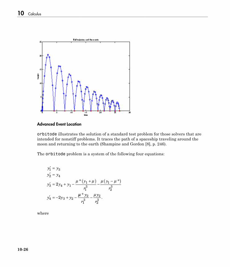
10 Calculus
10-26
Advanced Event Location
orbitode illustrates the solution of a standard test problem for those solvers that areintended for nonstiff problems. It traces the path of a spaceship traveling around themoon and returning to the earth (Shampine and Gordon [8], p. 246).
The orbitode problem is a system of the following four equations:
¢ =
¢ =
¢ = + -+( )
--( )
¢ = - + -
y y
y y
y y yy
r
y
r
y y y
1 3
2 4
3 4 11
13
1
23
4 3 2
2
2
m m m m* *
mm m*.
y
r
y
r
2
13
2
23
-
where

Ordinary Differential Equations
10-27
m
m m
m
m
=
= -
= +( ) +
= -( ) +
1
82 45
1
1 1
2
22
2 1
2
22
.
*
* .
r y y
r y y
The first two solution components are coordinates of the body of infinitesimal mass,so plotting one against the other gives the orbit of the body. The initial conditionshave been chosen to make the orbit periodic. The value of μ corresponds to a spaceshiptraveling around the moon and the earth. Moderately stringent tolerances are necessaryto reproduce the qualitative behavior of the orbit. Suitable values are 1e-5 for RelToland 1e-4 for AbsTol.
The nested events function includes event functions that locate the point of maximumdistance from the starting point and the time the spaceship returns to the starting point.Note that the events are located accurately, even though the step sizes used by theintegrator are not determined by the location of the events. In this example, the ability tospecify the direction of the zero crossing is critical. Both the point of return to the initialpoint and the point of maximum distance have the same event function value, and thedirection of the crossing is used to distinguish them.
To run this example, type orbitode at the command line. The example uses the outputfunction odephas2 to produce the two-dimensional phase plane plot and let you to see theprogress of the integration.
function orbitode
%ORBITODE Restricted three-body problem
mu = 1 / 82.45;
mustar = 1 - mu;
y0 = [1.2; 0; 0; -1.04935750983031990726];
tspan = [0 7];
options = odeset('RelTol',1e-5,'AbsTol',1e-4,...
'OutputFcn',@odephas2,'Events',@events);
[t,y,te,ye,ie] = ode45(@f,tspan,y0,options);
plot(y(:,1),y(:,2),ye(:,1),ye(:,2),'o');
title ('Restricted three body problem')

10 Calculus
10-28
ylabel ('y(t)')
xlabel ('x(t)')
% --------------------------------------------------------------
function dydt = f(t,y)
r13 = ((y(1) + mu)^2 + y(2)^2) ^ 1.5;
r23 = ((y(1) - mustar)^2 + y(2)^2) ^ 1.5;
dydt = [ y(3)
y(4)
2*y(4) + y(1) - mustar*((y(1)+mu)/r13) - ...
mu*((y(1)-mustar)/r23)
-2*y(3) + y(2) - mustar*(y(2)/r13) - mu*(y(2)/r23) ];
end % End nested function f
% --------------------------------------------------------------
function [value,isterminal,direction] = events(t,y)
% Locate the time when the object returns closest to the
% initial point y0 and starts to move away; stop integration.
% Also locate the time when the object is farthest from the
% initial point y0 and starts to move closer.
%
% The current distance of the body is
%
% DSQ = (y(1)-y0(1))^2 + (y(2)-y0(2))^2
% = <y(1:2)-y0(1:2),y(1:2)-y0(1:2)>
%
% A local minimum of DSQ occurs when d/dt DSQ crosses zero
% heading in the positive direction. Compute d(DSQ)/dt as
%
% d(DSQ)/dt = 2*(y(1:2)-y0(1:2))'*dy(1:2)/dt = ...
% 2*(y(1:2)-y0(1:2))'*y(3:4)
%
dDSQdt = 2 * ((y(1:2)-y0(1:2))' * y(3:4));
value = [dDSQdt; dDSQdt];
isterminal = [1; 0]; % Stop at local minimum
direction = [1; -1]; % [local minimum, local maximum]
end % End nested function events
end

Ordinary Differential Equations
10-29
Differential-Algebraic Equations
hb1dae reformulates the hb1ode example as a differential-algebraic equation (DAE)problem. The Robertson problem coded in hb1ode is a classic test problem for codes thatsolve stiff ODEs.
¢ = - +
¢ = - - ◊
¢ = ◊
y y y y
y y y y y
y y
1 14
2 3
2 1
4
2 3
7
2
2
3
7
2
2
0 04 10
0 04 10 3 10
3 10
.
.
..
Note: The Robertson problem appears as an example in the prolog to LSODI [4].
In hb1ode, the problem is solved with initial conditions y1(0) = 1, y2(0) = 0, y3(0) = 0 tosteady state. These differential equations satisfy a linear conservation law that is used toreformulate the problem as the DAE

10 Calculus
10-30
¢ = - +
¢ = - - ◊
= + + -
y y y y
y y y y y
y y y
1 14
2 3
2 1
4
2 3
7
2
2
1 2 3
0 04 10
0 04 10 3 10
0 1
.
.
..
These equations do not have a solution for y(0) with components that do not sum to 1.The problem has the form of My' = f(t,y) with
M =
È
Î
ÍÍÍ
˘
˚
˙˙˙
1 0 0
0 1 0
0 0 0
.
M is singular, but hb1dae does not inform the solver of this. The solver must recognizethat the problem is a DAE, not an ODE. Similarly, although consistent initial conditionsare obvious, the example uses an inconsistent value y3(0) = 10–3 to illustrate computationof consistent initial conditions.
To run this example, type hb1dae at the command line. Note that hb1dae
• Imposes a much smaller absolute error tolerance on y2 than on the other components.This is because y2 is much smaller than the other components and its major changetakes place in a relatively short time.
• Specifies additional points at which the solution is computed to more clearly show thebehavior of y2.
• Multiplies y2 by 104 to make y2 visible when plotting it with the rest of the solution.• Uses a logarithmic scale to plot the solution on the long time interval.
function hb1dae
%HB1DAE Stiff differential-algebraic equation (DAE)
% A constant, singular mass matrix
M = [1 0 0
0 1 0
0 0 0];
% Use inconsistent initial condition to test initialization.
y0 = [1; 0; 1e-3];
tspan = [0 4*logspace(-6,6)];
% Use the LSODI example tolerances.'MassSingular' is left

Ordinary Differential Equations
10-31
% at its default 'maybe' to test the automatic detection
% of a DAE.
options = odeset('Mass',M,'RelTol',1e-4,...
'AbsTol',[1e-6 1e-10 1e-6],...
'Vectorized','on');
[t,y] = ode15s(@f,tspan,y0,options);
y(:,2) = 1e4*y(:,2);
semilogx(t,y);
ylabel('1e4 * y(:,2)');
title(['Robertson DAE problem with a Conservation Law, '...
'solved by ODE15S']);
xlabel('This is equivalent to the stiff ODEs in HB1ODE.');
% --------------------------------------------------------
function out = f(t,y)
out = [ -0.04*y(1,:) + 1e4*y(2,:).*y(3,:)
0.04*y(1,:) - 1e4*y(2,:).*y(3,:) - 3e7*y(2,:).^2
y(1,:) + y(2,:) + y(3,:) - 1 ];
Nonnegative Solutions
If certain components of the solution must be nonnegative, use odeset to set theNonNegative property for the indices of these components.

10 Calculus
10-32
Note: This option is not available for ode23s, ode15i, or for implicit solvers (ode15s,ode23t, ode23tb) applied to problems where there is a mass matrix.
Imposing nonnegativity is not always a trivial task. We suggest that you use this optiononly when necessary, for example in instances in which the application of a solution orintegration will fail otherwise.
Consider the following initial value problem solved on the interval [0, 40]:
y' = - |y|, y(0) = 1
The solution of this problem decays to zero. If a solver produces a negative approximatesolution, it begins to track the solution of the ODE through this value, the solutiongoes off to minus infinity, and the computation fails. Using the NonNegative propertyprevents this from happening.
In this example, the first call to ode45 uses the defaults for the solver parameters:
ode = @(t,y) -abs(y);
[t0,y0] = ode45(ode,[0, 40], 1);
The second uses options to impose nonnegativity conditions:
options = odeset('NonNegative',1);
[t1,y1] = ode45(ode,[0, 40], 1, options);
This plot compares the numerical solution to the exact solution.

Ordinary Differential Equations
10-33
Here is a more complete view of the code used to obtain this plot:
ode = @(t,y) -abs(y);
options = odeset('Refine',1);
[t0,y0] = ode45(ode,[0, 40], 1,options);
options = odeset(options,'NonNegative',1);
[t1,y1] = ode45(ode,[0, 40], 1, options);
t = linspace(0,40,1000);
y = exp(-t);
plot(t,y,'b-',t0,y0,'ro',t1,y1,'b*');
legend('Exact solution','No constraints','Nonnegativity', ...
'Location','SouthWest')
The kneeode Example
The kneeode example solves the “knee problem” by imposing a nonnegativity constrainton the numerical solution. The initial value problem is
ε*y' = (1-x)*y - y^2, y(0) = 1

10 Calculus
10-34
For 0 < ε < 1, the solution of this problem approaches null isoclines y = 1 - x andy = 0 for x < 1 and x > 1, respectively. The numerical solution, when computed withdefault tolerances, follows the y = 1 - x isocline for the whole interval of integration.Imposing nonnegativity constraints results in the correct solution.
Here is the code that makes up the kneeode example:
function kneeode
%KNEEODE The "knee problem" with Nonnegativity constraints.
% Problem parameter
epsilon = 1e-6;
y0 = 1;
xspan = [0, 2];
% Solve without imposing constraints
options = [];
[x1,y1] = ode15s(@odefcn,xspan,y0,options);
% Impose nonnegativity constraint
options = odeset('NonNegative',1);
[x2,y2] = ode15s(@odefcn,xspan,y0,options);
figure
plot(x1,y1,'b.-',x2,y2,'g-')
axis([0,2,-1,1]);
title('The "knee problem"');
legend('No constraints','nonnegativity')
xlabel('x');
ylabel('solution y')
function yp = odefcn(x,y)
yp = ((1 - x)*y - y^2)/epsilon;
end
end % kneeode
The derivative function is defined within nested function odefcn. The value of epsilonused in odefcn is obtained from the outer function:
function yp = odefcn(x,y)
yp = ((1 - x)*y - y^2)/epsilon;
end

Ordinary Differential Equations
10-35
The example solves the problem using the ode15s function, first with the defaultoptions, and then by imposing a nonnegativity constraint. To run the example, typekneeode at the MATLAB command prompt.
Here is the output plot. The plot confirms correct solution behavior after imposingconstraints.
Additional Examples
The following additional examples are available. Type
edit examplename
to view the code and
examplename
to run the example.
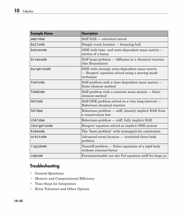
10 Calculus
10-36
Example Name Description
amp1dae Stiff DAE — electrical circuitballode Simple event location — bouncing ballbatonode ODE with time- and state-dependent mass matrix —
motion of a batonbrussode Stiff large problem — diffusion in a chemical reaction
(the Brusselator)burgersode ODE with strongly state-dependent mass matrix
— Burgers' equation solved using a moving meshtechnique
fem1ode Stiff problem with a time-dependent mass matrix —finite element method
fem2ode Stiff problem with a constant mass matrix — finiteelement method
hb1ode Stiff ODE problem solved on a very long interval —Robertson chemical reaction
hb1dae Robertson problem — stiff, linearly implicit DAE froma conservation law
ihb1dae Robertson problem — stiff, fully implicit DAEiburgersode Burgers' equation solved as implicit ODE systemkneeode The “knee problem” with nonnegativity constraintsorbitode Advanced event location — restricted three body
problemrigidode Nonstiff problem — Euler equations of a rigid body
without external forcesvdpode Parameterizable van der Pol equation (stiff for large μ)
Troubleshooting
• General Questions• Memory and Computational Efficiency• Time Steps for Integration• Error Tolerance and Other Options

Ordinary Differential Equations
10-37
• Other Types of Equations• Other Common Problems
General Questions
Question Answer
How do the ODE solvers differ from integral? integral solves problems of the form y' = f(t).The ODE solvers handle more general problemsy' = f(t,y), linearly implicit problems that involvea mass matrix M(t,y)y' = f(t,y), and fully implicitproblems f(t,y,y') = 0.
Can I solve ODE systems in which there aremore equations than unknowns, or vice versa?
No.
Memory and Computational Efficiency
Question Answer
How large a problem can I solve with the ODEsuite?
The primary constraints are memory andtime. At each time step, the solvers fornonstiff problems allocate vectors of lengthn, where n is the number of equations in thesystem. The solvers for stiff problems allocatevectors of length n but also allocate an n-by-nJacobian matrix. For these solvers it may beadvantageous to use the sparse option.
If the problem is nonstiff, or if you are usingthe sparse option, it may be possible to solvea problem with thousands of unknowns. Inthis case, however, storage of the result can beproblematic. Try asking the solver to evaluatethe solution at specific points only, or call thesolver with no output arguments and use anoutput function to monitor the solution.
I'm solving a very large system, but only careabout a couple of the components of y. Is thereany way to avoid storing all of the elements?
Yes. The user-installable output functioncapability is designed specifically for thispurpose. When you call the solver withno output arguments, the solver doesnot allocate storage to hold the entiresolution history. Instead, the solver calls

10 Calculus
10-38
Question Answer
OutputFcn(t,y,flag) at each time step. Tokeep the history of specific elements, write anoutput function that stores or plots only theelements you care about.
What is the startup cost of the integration andhow can I reduce it?
The biggest startup cost occurs as the solverattempts to find a step size appropriate to thescale of the problem. If you happen to know anappropriate step size, use the InitialStepproperty. For example, if you repeatedly call theintegrator in an event location loop, the last stepthat was taken before the event is probably onscale for the next integration. See ballode for anexample.
Time Steps for Integration
Question Answer
The first step size that the integrator takes istoo large, and it misses important behavior.
You can specify the first step size with theInitialStep property. The integrator tries thisvalue, then reduces it if necessary.
Can I integrate with fixed step sizes? No.
Error Tolerance and Other Options
Question Answer
How do I choose RelTol and AbsTol? RelTol, the relative accuracy tolerance, controlsthe number of correct digits in the answer.AbsTol, the absolute error tolerance, controlsthe difference between the answer and thesolution. At each step, the error e in componenti of the solution satisfies
|e(i)|
≤max(RelTol*abs(y(i)),AbsTol(i))
Roughly speaking, this means that youwant RelTol correct digits in all solutioncomponents except those smaller than

Ordinary Differential Equations
10-39
Question Answer
thresholds AbsTol(i). Even if you are notinterested in a component y(i) when it issmall, you may have to specify AbsTol(i) smallenough to get some correct digits in y(i) so thatyou can accurately compute more interestingcomponents.
I want answers that are correct to the precisionof the computer. Why can't I simply set RelTolto eps?
You can get close to machine precision, but notthat close. The solvers do not allow RelTolnear eps because they try to approximate acontinuous function. At tolerances comparable toeps, the machine arithmetic causes all functionsto look discontinuous.
How do I tell the solver that I don't care aboutgetting an accurate answer for one of thesolution components?
You can increase the absolute error tolerancecorresponding to this solution component. If thetolerance is bigger than the component, thisspecifies no correct digits for the component.The solver may have to get some correct digitsin this component to compute other componentsaccurately, but it generally handles thisautomatically.
Other Types of Equations
Question Answer
Can the solvers handle partial differentialequations (PDEs) that have been discretized bythe method of lines?
Yes, because the discretization producesa system of ODEs. Depending on thediscretization, you might have a form involvingmass matrices – the ODE solvers provide forthis. Often the system is stiff. This is to beexpected when the PDE is parabolic and whenthere are phenomena that happen on verydifferent time scales such as a chemical reactionin a fluid flow. In such cases, use one of the foursolvers: ode15s, ode23s, ode23t, ode23tb.
If there are many equations, set the JPatternproperty. This might make the differencebetween success and failure due to the

10 Calculus
10-40
Question Answer
computation being too expensive. For anexample that uses JPattern, see “Large StiffSparse Problem” on page 10-20. When thesystem is not stiff, or not very stiff, ode23 orode45 is more efficient than ode15s, ode23s,ode23t, or ode23tb.
Parabolic-elliptic partial differential equationsin 1-D can be solved directly with the MATLABPDE solver, pdepe. For more information,see “Partial Differential Equations” on page10-91.
Can I solve differential-algebraic equation (DAE)systems?
Yes. The solvers ode15s and ode23t can solvesome DAEs of the form M(t,y)y' = f(t,y) whereM(t,y) is singular. The DAEs must be of index 1.ode15i can solve fully implicit DAEs of index 1,f(t,y,y') = 0. For examples, see amp1dae, hb1dae,or ihb1dae.
Can I integrate a set of sampled data? Not directly. You have to represent the data as afunction by interpolation or some other schemefor fitting data. The smoothness of this functionis critical. A piecewise polynomial fit like aspline can look smooth to the eye, but rough toa solver; the solver takes small steps where thederivatives of the fit have jumps. Either use asmooth function to represent the data or useone of the lower order solvers (ode23, ode23s,ode23t, ode23tb) that is less sensitive to this.
What do I do when I have the final and not theinitial value?
All the solvers of the ODE suite allow you tosolve backwards or forwards in time. The syntaxfor the solvers is [t,y] = ode45(odefun,[t0tf],y0);and the syntax accepts t0 > tf.
Other Common Problems

Ordinary Differential Equations
10-41
Question Answer
The solution doesn't look like what I expected. If you're right about its appearance, you need toreduce the error tolerances from their defaultvalues. A smaller relative error tolerance isneeded to compute accurately the solutionof problems integrated over “long” intervals,as well as solutions of problems that aremoderately unstable.
You should check whether there are solutioncomponents that stay smaller than theirabsolute error tolerance for some time. If so,you are not asking for any correct digits inthese components. This may be acceptable forthese components, but failing to compute themaccurately may degrade the accuracy of othercomponents that depend on them.
My plots aren't smooth enough. Increase the value of Refine from its defaultof 4 in ode45 and 1 in the other solvers. Thebigger the value of Refine, the more outputpoints. Execution speed is not affected much bythe value of Refine.
I'm plotting the solution as it is computed and itlooks fine, but the code gets stuck at some point.
First verify that the ODE function is smoothnear the point where the code gets stuck. If itisn't, the solver must take small steps to dealwith this. It may help to break tspan into pieceson which the ODE function is smooth.
If the function is smooth and the code is takingextremely small steps, you are probably trying tosolve a stiff problem with a solver not intendedfor this purpose. Switch to ode15s, ode23s,ode23t, or ode23tb.
My integration proceeds very slowly, using toomany time steps.
First, check that your tspan is not too long.Remember that the solver uses as manytime points as necessary to produce a smoothsolution. If the ODE function changes on a timescale that is very short compared to the tspan,

10 Calculus
10-42
Question Answer
the solver uses a lot of time steps. Long-timeintegration is a hard problem. Break tspan intosmaller pieces.
If the ODE function does not change noticeablyon the tspan interval, it could be that yourproblem is stiff. Try using ode15s, ode23s,ode23t, or ode23tb.
Finally, make sure that the ODE function iswritten in an efficient way. The solvers evaluatethe derivatives in the ODE function many times.The cost of numerical integration dependscritically on the expense of evaluating the ODEfunction. Rather than recompute complicatedconstant parameters at each evaluation, storethem in globals or calculate them once and passthem to nested functions.
I know that the solution undergoes a radicalchange at time t where
t0 ≤ t ≤ tf
but the integrator steps past without “seeing” it.
If you know there is a sharp change at time t,it might help to break the tspan interval intotwo pieces, [t0 t] and [t tf], and call theintegrator twice.
If the differential equation has periodiccoefficients or solution, you might restrict themaximum step size to the length of the period sothe integrator won't step over periods.

Types of DDEs
10-43
Types of DDEs
In this section...
“Constant Delay DDEs” on page 10-43“Time-Dependent and State-Dependent DDEs” on page 10-43“DDEs of Neutral Type” on page 10-44“Evaluating the Solution at Specific Points” on page 10-44“History and Initial Values” on page 10-44“Propagation of Discontinuities” on page 10-44
Constant Delay DDEs
A system of differential equations (DDEs) with constant delays has the following form:
¢ = - -y t f t y t y t y t k( ) ( , ( ), ( ), , ( )).t t1 …
Here, t is the independent variable, y is a column vector of dependent variables, and y′ represents the first derivative of y with respect to t. The delays, τ1,…,τk, are positiveconstants.
The dde23 function solves DDEs of the form given by Equation 10-1 with history y(t) =S(t) for t <t0.
The solutions of DDEs are generally continuous, but they have discontinuities in theirderivatives. The dde23 function tracks discontinuities in low-order derivatives. Itintegrates the differential equations with the same explicit Runge-Kutta (2,3) pairand interpolant used by ode23. The Runge-Kutta formulas are implicit for step sizesbigger than the delays. When y(t) is smooth enough to justify steps this big, the implicitformulas are evaluated by a predictor-corrector iteration.
Time-Dependent and State-Dependent DDEs
Equation 10-1 is a special case of
¢ =y t f t y t y dy y dyp( ) ( , ( ), ( ), ..., ( ))1

10 Calculus
10-44
that involves delays, dy1,..., dyk, which can depend on both time, t, and state, y. Thedelays, dyj(t, y), must satisfy dyj(t, y) ≤ t on the interval [t0, tf] with t0 < tf.
The ddesd function finds the solution, y(t), for DDEs of the form given by Equation 10-2with history y(t) = S(t) for t < t0. The ddesd function integrates with the classic four-stage, fourth-order explicit Runge-Kutta method, and it controls the size of the residualof a natural interpolant. It uses iteration to take steps that are longer than the delays.
DDEs of Neutral Type
Delay differential equations of neutral type involve delays in y ′ as well as y:
¢ = ¢ ¢y t f t y t y dy y dy y dyp y dypp q( ) ( , ( ), ( ), ..., ( ), ( ),..., ( )).1 1
The delays in the solution must satisfy dyi(t,y) ≤ t. The delays in the first derivative mustsatisfy dypj(t,y) < t so that y ′ does not appear on both sides of the equation.
The ddensd function solves DDEs of neutral type by approximating them with DDEs ofthe form given by Equation 10-2. For more information, see Shampine [1].
Evaluating the Solution at Specific Points
Use the deval function and the output from any of the DDE solvers to evaluate thesolution at specific points in the interval of integration. For example, y = deval(sol,0.5*(sol.x(1) + sol.x(end))) evaluates the solution at the midpoint of theinterval of integration.
History and Initial Values
When you solve a DDE, you approximate the solution on an interval [t0,tf] with t0 < tf. TheDDEs show how y ′(t) depends on values of the solution (and possibly its derivative) attimes prior to t. For example, Equation 10-1 shows that y ′(t0) depends on y(t0 – τ1),…,y(t0– τk) for positive constants τj. Because of this, a solution on [t0, tk] depends on values ithas at t ≤ t0. You must define these values with a history function, y(t) = S(t) for t <t0.
Propagation of Discontinuities
Generally, the first derivative of the solution has a jump at the initial point. This isbecause the first derivative of the history function, S(t), generally does not satisfy the

Types of DDEs
10-45
DDE at this point. A discontinuity in any derivative of y(t) propagates into the futureat spacings of τ1,…, τk when the delays are constant, as in Equation 10-1. If the delaysare not constant, the propagation of discontinuities is more complicated. For neutralDDEs of the form given by Equation 10-1 or Equation 10-2, the discontinuity appears inthe next higher order derivative each time it is propagated. In this sense, the solutiongets smoother as the integration proceeds. Solutions of neutral DDEs of the form givenby Equation 10-3 are qualitatively different. The discontinuity in the solution does notpropagate to a derivative of higher order. In particular, the typical jump in y ′(t) at t0propagates as jumps in y ′(t) throughout [t0, tf].
References
[1] Shampine, L.F. “Dissipative Approximations to Neutral DDEs.” Applied Mathematics& Computation, Vol. 203, 2008, pp. 641–648.

10 Calculus
10-46
Discontinuities in DDEs
If your problem has discontinuities, it’s best to communicate them to the solver using anoptions structure. To do this, use the ddeset function to create an options structurecontaining the discontinuities in your problem.
There are three properties in the options structure that you can use to specifydiscontinuities; InitialY, Jumps, and Events. The property you choose depends on thelocation and nature of the discontinuities.
Nature of Discontinuity Property Comments
At the initial value t = t0 InitialY Generally the initial value y(t0) is thevalue S(t0) returned by the historyfunction, meaning the solution iscontinuous at the initial point. If thisis not the case, supply a differentinitial value using the InitialYproperty.
In the history, i.e., thesolution at t <t0, or in theequation coefficients for t>t0
Jumps Provide the known locations t of thediscontinuities in a vector as the valueof the Jumps property. Applies only todde23.
State-dependent Events dde23, ddesd, and ddensd use theevents function you supply to locatethese discontinuities. When the solverfinds such a discontinuity, restartthe integration to continue. Specifythe solution structure for the currentintegration as the history for the newintegration. The solver extends eachelement of the solution structureafter each restart so that the finalstructure provides the solution for thewhole interval of integration. If thenew problem involves a change in thesolution, use the InitialY propertyto specify the initial value for the newintegration.

DDE with Constant Delays
10-47
DDE with Constant Delays
This example shows how to use dde23 to solve a system of DDEs with constant delays.
Click ddex1.m or type edit ddex1.m in a command window to view the code for thisexample in an editor.
The differential equations are:
y t y t
y t y t y t
y t y t
1 1
2 1 2
3 2
1
1 0 2
¢ = -
¢ = - + -
¢ =
( ) ( )
( ) ( ) ( . )
( ) ( ).
The history of this problem is constant:
y t
y t
y t
1
2
3
1
1
1
( )
( )
( )
=
=
=
for t ≤ 0.
1 Create a new program file in the editor. This file will contain a main function andtwo local functions.
2 Define the first-order DDE as a local function.
function dydt = ddex1de(t,y,Z)
ylag1 = Z(:,1);
ylag2 = Z(:,2);
dydt = [ylag1(1); ylag1(1)+ylag2(2); y(2)];
end
3 Define the solution history as a local function.
function S = ddex1hist(t)
S = ones(3,1);
end
4 Define the delays, τ1,…,τk in the main function.

10 Calculus
10-48
lags = [1,0.2];
5 Solve the DDE by calling dde23 in the main function. Pass the DDE function, thedelays, the solution history, and interval of integration, [0,5], as inputs.
sol = dde23(@ddex1de,lags,@ddex1hist,[0,5]);
The dde23 function produces a continuous solution over the whole interval ofintegration [t0,tf].
6 Plot the solution returned by dde23. Add this code to your main function.
plot(sol.x,sol.y);
title('An example of Wille and Baker');
xlabel('time t');
ylabel('solution y');
legend('y_1','y_2','y_3','Location','NorthWest');
7 Evaluate the solution at 10 equally spaced points over the interval of integration.Then plot the results on the same axes as sol.y. Add this code to the main function.
tint = linspace(0,5,10);
Sint = deval(sol,tint)
hold on
plot(tint,Sint,'o');
8 Run your program to generate and plot the results.

DDE with Constant Delays
10-49
See Alsofunction_handle
Related Examples• “Create Functions in Files”• “Run Functions in the Editor”

10 Calculus
10-50
State-Dependent Delay Problem
This example shows how to use ddesd to solve a system of two DDEs with a state-dependent delay. This system of DDEs was used as a test problem by Enright andHayashi [1].
Click ddex3.m or type edit ddex3.m in a command window to view the complete codefor this example in an editor.
The equations for this system are:
y t y t
y t y e y t ey t y t
1 2
2 21
22 1
2 2
¢ =
¢ = - ◊ ◊- -
( ) ( )
( ) ( ) ( ) .( ( )) ( ( ))
The analytical solution
y t t
y t t
1
2 1
( ) log( )
( ) /
=
=
is used as the history for t ≤ 0.1 and the equations are solved on [0.1, 5] with ddesdrather than dde23. The ddesd function is appropriate in this case because the firstfactor in the second equation has the form y2(d(y)) with a delay that depends on thesecond component of the solution.
1 Create a new program file in the editor. This file will contain a main function andthree local functions.
2 Code the system of DDEs as a local function.
function dydt = ddex3de(t,y,Z)
dydt = [y(2); -Z(2)*y(2)^2*exp(1 - y(2))];
end
3 Define the delay as a local function.
function d = ddex3delay(t,y)
d = exp(1 - y(2));
end
4 Define the solution history as a local function.

State-Dependent Delay Problem
10-51
function v = ddex3hist(t)
v = [log(t); 1./t];
end
5 Define the interval of integration and solve the system. Add this code to the mainfunction in your program file.
tspan = [0.1 5];
sol = ddesd(@ddex3de,@ddex3delay,@ddex3hist,tspan);
6 Use the history function to calculate the analytical solution within the integrationinterval. Add this code to the main function.
texact = linspace(0.1,5);
yexact = ddex3hist(texact);
7 Plot the numerical solution on the same axes as the analytical solution. Add thiscode to the main function.
figure
plot(texact,yexact,sol.x,sol.y,'o')
legend('y_1, exact','y_2, exact','y_1, ddesd','y_2, ddesd')
xlabel('time t')
ylabel('solution y')
title('D1 problem of Enright and Hayashi')
8 Run your program to generate and plot the results.

10 Calculus
10-52
References
[1] Enright, W.H. and H. Hayashi. “The Evaluation of Numerical Software for DelayDifferential Equations.” In Proceedings of the IFIP TC2/WG2.5 workingconference on Quality of numerical software: assessment and enhancement. (R.F.Boisvert, ed.). London, UK: Chapman & Hall, Ltd., pp. 179-193.
See Alsofunction_handle

State-Dependent Delay Problem
10-53
Related Examples• “Create Functions in Files”• “Run Functions in the Editor”

10 Calculus
10-54
Cardiovascular Model with Discontinuities
This example shows how to use dde23 to solve a cardiovascular model that has adiscontinuous derivative as presented by Ottesen [1].
Click ddex2.m or type edit ddex2.m in a command window to view the code for thisexample in an editor.
This is a problem with 1 delay, constant history, and 3 differential equations with 14physical parameters. The system is heavily influenced by peripheral pressure, R, whichdecreases exponentially from 1.05 to 0.84, beginning at t = 600. As a result, the systemhas a discontinuity in a low-order derivative at t = 600.
1 Create a new program file in the editor. This file will contain a main function and anested function. The main function accepts no inputs and returns no outputs.
2 Define the physical parameters. Add this code to the main function.
p.ca = 1.55;
p.cv = 519;
p.R = 1.05;
p.r = 0.068;
p.Vstr = 67.9;
p.alpha0 = 93;
p.alphas = 93;
p.alphap = 93;
p.alphaH = 0.84;
p.beta0 = 7;
p.betas = 7;
p.betap = 7;
p.betaH = 1.17;
p.gammaH = 0;
3 Define the solution history. Add this code to the main function.
P0 = 93;
Paval = P0;
Pvval = (1 / (1 + p.R/p.r)) * P0;
Hval = (1 / (p.R * p.Vstr)) * (1 / (1 + p.r/p.R)) * P0;
history = [Paval; Pvval; Hval];
4 Define the delay, tau. Add this code to the main function.
tau = 4;

Cardiovascular Model with Discontinuities
10-55
5 Define the location of discontinuity, which occurs at t = 600. Add this code to themain function.
options = ddeset('Jumps',600);
When your DDE has discontinuities in low-order derivatives, and you know thelocations in advance, it is better to use ddeset with the Jumps property.
6 Solve the DDE over the interval [0, 1000]. Add this code to the main function.
sol = dde23(@ddex2de,tau,history,[0,1000],options);
The function, @ddex2de, which defines the system of DDEs, is the first inputargument. You define this function in 8.
7 Plot the solution. Add this code to the main function.
figure
plot(sol.x,sol.y(3,:))
title('Heart Rate for Baroflex-Feedback Mechanism.')
xlabel('time t')
ylabel('H(t)')
8 Define the system of DDEs as a nested function inside the main function.
function dydt = ddex2de(t,y,Z)
if t <= 600
p.R = 1.05;
else
p.R = 0.21 * exp(600-t) + 0.84;
end
ylag = Z(:,1);
Patau = ylag(1);
Paoft = y(1);
Pvoft = y(2);
Hoft = y(3);
dPadt = - (1 / (p.ca * p.R)) * Paoft ...
+ (1/(p.ca * p.R)) * Pvoft ...
+ (1/p.ca) * p.Vstr * Hoft;
dPvdt = (1 / (p.cv * p.R)) * Paoft...
- ( 1 / (p.cv * p.R)...
+ 1 / (p.cv * p.r) ) * Pvoft;
Ts = 1 / ( 1 + (Patau / p.alphas)^p.betas );

10 Calculus
10-56
Tp = 1 / ( 1 + (p.alphap / Paoft)^p.betap );
dHdt = (p.alphaH * Ts) / (1 + p.gammaH * Tp) ...
- p.betaH * Tp;
dydt = [ dPadt; dPvdt; dHdt];
end
This function is nested so that the main function can access the 14 parametersdefined in 2.
9 Run your program to calculate the solution and display the plot.
References
[1] Ottesen, J. T. “Modelling of the Baroflex-Feedback Mechanism with Time-Delay.” J.Math. Biol. Vol. 36, Number 1, 1997, pp. 41–63.
See Alsofunction_handle
Related Examples• “Create Functions in Files”

Cardiovascular Model with Discontinuities
10-57
• “Run Functions in the Editor”

10 Calculus
10-58
DDE of Neutral Type
This example shows how to use ddensd to solve the neutral DDE presented by Paul [1]for 0 ≤ t ≤ π.
Click ddex4.m or type edit ddex4.m in a command window to view the code for thisexample in an editor.
The equation isy '(t) = 1 + y(t) – 2y(t/2)2 – y '(t – π)
with history:y(t) = cos (t) for t ≤ 0.
1 Create a new program file in the editor. This file will contain a main function andfour local functions.
2 Define the first-order DDE as a local function.
function yp = ddefun(t,y,ydel,ypdel)
yp = 1 + y - 2*ydel^2 - ypdel;
end
3 Define the solution delay as a local function.
function dy = dely(t,y)
dy = t/2;
end
4 Define the derivative delay as a local function.
function dyp = delyp(t,y)
dyp = t-pi;
end
5 Define the solution history as a local function.
function y = history(t)
y = cos(t);
end
6 Define the interval of integration and solve the DDE using the ddensd function. Addthis code to the main function.
tspan = [0 pi];
sol = ddensd(@ddefun,@dely,@delyp,@history,tspan);

DDE of Neutral Type
10-59
7 Evaluate the solution at 100 equally spaced points between 0 and π. Add this code tothe main function.
tn = linspace(0,pi);
yn = deval(sol,tn);
8 Plot the results. Add this code to the main function.
figure
plot(tn,yn);
xlim([0 pi]);
ylim([-1.2 1.2])
xlabel('time t');
ylabel('solution y');
title('Example of Paul with 1 equation and 2 delay functions')
9 Run your program to calculate the solution and display the plot.

10 Calculus
10-60
References
[1] Paul, C.A.H. “A Test Set of Functional Differential Equations.” Numerical AnalysisReports. No. 243. Manchester, UK: Math Department, University of Manchester,1994.
See Alsofunction_handle

DDE of Neutral Type
10-61
Related Examples• “Create Functions in Files”• “Run Functions in the Editor”

10 Calculus
10-62
Initial Value DDE of Neutral Type
This example shows how to use ddensd to solve the initial value DDE presented byJackiewicz [1] for 0 ≤ t ≤ 0.1.
Click ddex5.m or type edit ddex5.m in a command window to view the code for thisexample in an editor.
The equation isy '(t) = 2cos(2t) y(t/2)2cos(t) + log(y '(t/2)) – log(2cos(t)) – sin(t).
This is an initial value DDE because the delays are zero at t0. The initial conditions are:y(0) = 1y '(0) = s,where s is the solution of:2 + log(s) – log(2) = 0.This equation is satisfied by s1 = 2 and s2 = 0.4063757399599599.
1 Create a new program file in the editor. This file will contain a main function andone local function.
2 Define the DDE as a local function.
function yp = ddefun(t,y,ydel,ypdel)
yp=2*cos(2*t)*ydel^(2*cos(t))+log(ypdel)-log(2*cos(t))-sin(t);
end
3 Define the solution delay and derivative delay. Add this line to the main function.
delay = @(t,y) t/2;
You can use one anonymous function to handle both delays since they are the samein the equation.
4 Define the initial conditions, y0 and s1, and the interval of integration, tspan. Addthis code to the main function.
y0 = 1;
s1 = 2;
tspan = [0 0.1];
5 Solve the DDE for 0 ≤ t ≤ 0.1, with initial conditions y(0) = 1, and y '(0) = 2. Add thiscode to the main function.
sol1 = ddensd(@ddefun,delay,delay,{y0,s1},tspan);

Initial Value DDE of Neutral Type
10-63
6 Solve the equation again, this time using y '(0) = 0.4063757399599599. Add this codeto the main function.
s2 = 0.4063757399599599;
sol2 = ddensd(@ddefun,delay,delay,{y0,s2},tspan);
7 Plot the results. Add this code to the main function.
figure
plot(sol1.x,sol1.y,sol2.x,sol2.y);
legend('y''(0) = 2','y''(0) = .40638','Location','NorthWest');
xlabel('time t');
ylabel('solution y');
title('Two solutions of Jackiewicz''s initial-value NDDE');
8 Run your program to calculate and plot the solutions for each value of s.

10 Calculus
10-64
References
[1] Jackiewicz, Z. “One step Methods of any Order for Neutral Functional DifferentialEquations.” SIAM J. Numer. Anal. Vol. 21, Number 3. 1984. pp. 486–511.
See Alsofunction_handle
Related Examples• “Create Functions in Files”

Initial Value DDE of Neutral Type
10-65
• “Run Functions in the Editor”

10 Calculus
10-66
Boundary-Value ProblemsIn this section...
“Function Summary” on page 10-66“Boundary Value Problems” on page 10-67“BVP Solver” on page 10-67“Integrator Options” on page 10-70“Examples” on page 10-71
Function Summary
• “BVP Solver” on page 10-66• “BVP Helper Functions” on page 10-66• “BVP Solver Options” on page 10-66
BVP Solver
Solver Description
bvp4c Solve boundary value problems for ordinary differentialequations.
bvp5c Solve boundary value problems for ordinary differentialequations.
BVP Helper Functions
Function Description
bvpinit Form the initial guess for bvp4c.deval Evaluate the numerical solution using the output of bvp4c.
BVP Solver Options
An options structure contains named properties whose values are passed to bvp4c, andwhich affect problem solution. Use these functions to create, alter, or access an optionsstructure.
Function Description
bvpset Create/alter the BVP options structure.

Boundary-Value Problems
10-67
Function Description
bvpget Extract properties from options structure created withbvpset.
Boundary Value Problems
The BVP solver is designed to handle systems of ordinary differential equationsy′ = f(x, y)
where x is the independent variable, y is the dependent variable, and y′ represents thederivative of y with respect to x dy/dx.
See “First Order ODEs” on page 10-4 for general information about ODEs.
Boundary Conditions
In a boundary value problem, the solution of interest satisfies certain boundaryconditions. These conditions specify a relationship between the values of the solutionat more than one x. In its basic syntax, bvp4c is designed to solve two-point BVPs, i.e.,problems where the solution sought on an interval [a, b] must satisfy the boundaryconditionsg(y(a), y(b)) = 0
Unlike initial value problems, a boundary value problem may not have a solution,may have a finite number of solutions, or may have infinitely many solutions. As anintegral part of the process of solving a BVP, you need to provide a guess for the requiredsolution. The quality of this guess can be critical for the solver performance and even fora successful computation.
There may be other difficulties when solving BVPs, such as problems imposed on infiniteintervals or problems that involve singular coefficients. Often BVPs involve unknownparameters p that have to be determined as part of solving the problemy′ = f(x, y, p)g(y(a), y(b), p) = 0
In this case, the boundary conditions must suffice to determine the value of p.
BVP Solver
• “The BVP Solver” on page 10-68• “BVP Solver Syntax” on page 10-68

10 Calculus
10-68
• “BVP Solver Options” on page 10-70
The BVP Solver
The function bvp4c solves two-point boundary value problems for ordinary differentialequations (ODEs). It integrates a system of first-order ordinary differential equationsy′ = f(x, y)
on the interval [a, b], subject to general two-point boundary conditionsbc(y(a),y(b)) = 0
It can also accommodate other types of BVP problems, such as those that have any of thefollowing:
• Unknown parameters• Singularities in the solutions• Multipoint conditions
In this case, the number of boundary conditions must be sufficient to determine thesolution and the unknown parameters.
bvp4c produces a solution that is continuous on [a,b] and has a continuous firstderivative there. You can use the function deval and the output of bvp4c to evaluate thesolution at specific points on the interval of integration.
bvp4c is a finite difference code that implements the 3-stage Lobatto IIIa formula. Thisis a collocation formula and the collocation polynomial provides a C1-continuous solutionthat is fourth-order accurate uniformly in the interval of integration. Mesh selection anderror control are based on the residual of the continuous solution.
The collocation technique uses a mesh of points to divide the interval of integration intosubintervals. The solver determines a numerical solution by solving a global systemof algebraic equations resulting from the boundary conditions, and the collocationconditions imposed on all the subintervals. The solver then estimates the error of thenumerical solution on each subinterval. If the solution does not satisfy the tolerancecriteria, the solver adapts the mesh and repeats the process. The user must provide thepoints of the initial mesh as well as an initial approximation of the solution at the meshpoints.
BVP Solver Syntax
The basic syntax of the BVP solver is

Boundary-Value Problems
10-69
sol = bvp4c(odefun,bcfun,solinit)
The input arguments are
odefun A function handle that evaluates the differential equations. It has thebasic form
dydx = odefun(x,y)
where x is a scalar, and dydx and y are column vectors. odefun canalso accept a vector of unknown parameters and a variable number ofknown parameters, (see “BVP Solver Options” on page 10-70).
bcfun Handle to a function that evaluates the residual in the boundaryconditions. It has the basic form
res = bcfun(ya,yb)
where ya and yb are column vectors representing y(a) and y(b),and res is a column vector of the residual in satisfying the boundaryconditions. bcfun can also accept a vector of unknown parameters anda variable number of known parameters, (see “BVP Solver Options” onpage 10-70).
solinit Structure with fields x and y: x Ordered nodes of the initial mesh. Boundary
conditions are imposed at a = solinit.x(1) andb = solinit.x(end).
y Initial guess for the solution with solinit.y(:,i) aguess for the solution at the node solinit.x(i).
The structure can have any name, but the fields must be named xand y. It can also contain a vector that provides an initial guess forunknown parameters. You can form solinit with the helper functionbvpinit. See the bvpinit reference page for details.
The output argument sol is a structure created by the solver. In the basic case thestructure has fields x, y, yp, and solver.
sol.x Nodes of the mesh selected by bvp4csol.y Approximation to y(x) at the mesh points of sol.xsol.yp Approximation to y′(x) at the mesh points of sol.x

10 Calculus
10-70
sol.solver 'bvp4c'
The structure sol returned by bvp4c contains an additional field if the problem involvesunknown parameters:
sol.parameters Value of unknown parameters, if present, found by the solver.
The function deval uses the output structure sol to evaluate the numerical solution atany point from [a,b].
BVP Solver Options
For more advanced applications, you can specify solver options by passing an inputargument options.
options Structure of optional parameters that change the default integrationproperties. This is the fourth input argument.
sol = bvp4c(odefun,bcfun,solinit,options)
You can create the structure options using the function bvpset. Thebvpset reference page describes the properties you can specify.
Integrator Options
The default integration properties in the BVP solver bvp4c are selected to handlecommon problems. In some cases, you can improve solver performance by overridingthese defaults. You do this by supplying bvp4c with an options structure that specifiesone or more property values.
For example, to change the value of the relative error tolerance of bvp4c from the defaultvalue of 1e-3 to 1e-4,
1 Create an options structure using the function bvpset by entering
options = bvpset('RelTol', 1e-4);
2 Pass the options structure to bvp4c as follows:
sol = bvp4c(odefun,bcfun,solinit,options)
For a complete description of the available options, see the reference page for bvpset.

Boundary-Value Problems
10-71
Examples
• “Mathieu's Equation” on page 10-71• “Continuation” on page 10-75• “Singular BVPs” on page 10-81• “Multipoint BVPs” on page 10-85• “Additional Examples” on page 10-89
Mathieu's Equation
• “Solving the Problem” on page 10-71• “Finding Unknown Parameters” on page 10-74• “Evaluating the Solution” on page 10-75
Solving the Problem
This example determines the fourth eigenvalue of Mathieu's Equation. It illustrates howto write second-order differential equations as a system of two first-order ODEs and howto use bvp4c to determine an unknown parameter λ.
The task is to compute the fourth (q = 5) eigenvalue lambda λ of Mathieu's equationy′′ + (λ – 2 q cos 2x)y = 0
Because the unknown parameter λ is present, this second-order differential equation issubject to three boundary conditionsy(0) = 1y′(0) = 0y′(π) = 0
Note: The file, mat4bvp.m, contains the complete code for this example. All the functionsrequired by bvp4c are coded in this file as nested or local functions. To see the code inan editor, type edit mat4bvp at the command line. To run it, type mat4bvp at thecommand line.
1 Rewrite the problem as a first-order system. To use bvp4c, you must rewritethe equations as an equivalent system of first-order differential equations. Using asubstitution y1 = y and y2 = y′, the differential equation is written as a system of twofirst-order equationsy1′ = y2

10 Calculus
10-72
y2′ = –(λ – 2q cos 2x)y1
Note that the differential equations depend on the unknown parameter λ. Theboundary conditions becomey1(0) – 1 = 0y2(0) = 0y2(π) = 0
2 Code the system of first-order ODEs. Once you represent the equation as a first-order system, you can code it as a function that bvp4c can use. Because there is anunknown parameter, the function must be of the form
dydx = odefun(x,y,parameters)
The following code represents the system in the function, mat4ode. Variable q isshared with the outer function:
function dydx = mat4ode(x,y,lambda)
dydx = [ y(2)
-(lambda - 2*q*cos(2*x))*y(1) ];
end % End nested function mat4ode
3 Code the boundary conditions function. You must also code the boundaryconditions in a function. Because there is an unknown parameter, the function mustbe of the form
res = bcfun(ya,yb,parameters)
The code below represents the boundary conditions in the function, mat4bc.
function res = mat4bc(ya,yb,lambda)
res = [ ya(2)
yb(2)
ya(1)-1 ];
4 Create an initial guess. To form the guess structure solinit with bvpinit, youneed to provide initial guesses for both the solution and the unknown parameter.
The function mat4init provides an initial guess for the solution. mat4init uses y= cos4x because this function satisfies the boundary conditions and has the correctqualitative behavior (the correct number of sign changes).
function yinit = mat4init(x)
yinit = [ cos(4*x)
-4*sin(4*x) ];

Boundary-Value Problems
10-73
In the call to bvpinit, the third argument, lambda, provides an initial guess for theunknown parameter λ.
lambda = 15;
solinit = bvpinit(linspace(0,pi,10),@mat4init,lambda);
This example uses the @ symbol to pass mat4init as a function handle to bvpinit.5 Apply the BVP solver. The mat4bvp example calls bvp4c with the functions
mat4ode and mat4bc and the structure solinit created with bvpinit.
sol = bvp4c(@mat4ode,@mat4bc,solinit);
6 View the results. Complete the example by displaying the results:
a Print the value of the unknown parameter λ found by bvp4c.
fprintf('Fourth eigenvalue is approximately %7.3f.\n',...
sol.parameters)
b Use deval to evaluate the numerical solution at 100 equally spaced points inthe interval [0, π], and plot its first component. This component approximatesy(x).
xint = linspace(0,pi);
Sxint = deval(sol,xint);
plot(xint,Sxint(1,:))
axis([0 pi -1 1.1])
title('Eigenfunction of Mathieu''s equation.')
xlabel('x')
ylabel('solution y')
The following plot shows the eigenfunction associated with the final eigenvalue λ= 17.097.

10 Calculus
10-74
Finding Unknown Parameters
The bvp4c solver can find unknown parameters p for problems of the formy′ = f(x,y,p)bc(y(a), y (b),p) = 0
You must provide bvp4c an initial guess for any unknown parameters in the vectorsolinit.parameters. When you call bvpinit to create the structure solinit, specifythe initial guess as a vector in the additional argument parameters.
solinit = bvpinit(x,v,parameters)
The bvp4c function arguments odefun and bcfun must each have a third argument.
dydx = odefun(x,y,parameters)
res = bcfun(ya,yb,parameters)
While solving the differential equations, bvp4c adjusts the value of unknown parametersto satisfy the boundary conditions. The solver returns the final values of these unknownparameters in sol.parameters.

Boundary-Value Problems
10-75
Evaluating the Solution
The collocation method implemented in bvp4c produces a C1-continuous solution overthe whole interval of integration [a,b]. You can evaluate the approximate solution, S(x),at any point in [a,b] using the helper function deval and the structure sol returned bybvp4c.
Sxint = deval(sol,xint)
The deval function is vectorized. For a vector xint, the ith column of Sxintapproximates the solution y(xint(i)).
Continuation
• “Introduction” on page 10-75• “Using Continuation to Solve a BVP” on page 10-75• “Using Continuation to Verify Consistency” on page 10-78
Introduction
To solve a boundary value problem, you need to provide an initial guess for the solution.The quality of your initial guess can be critical to the solver performance, and to beingable to solve the problem at all. However, coming up with a sufficiently good guess canbe the most challenging part of solving a boundary value problem. Certainly, you shouldapply the knowledge of the problem's physical origin. Often a problem can be solved as asequence of relatively simpler problems, i.e., a continuation.
This example shows how to use continuation to:
• Solve a difficult BVP• Verify a solution's consistent behavior
Using Continuation to Solve a BVP
This example solves the differential equationεy′′ + xy′ = επ2 cos(πx) – πx sin(πx)
for ε = 10–4, on the interval [–1 1], with boundary conditions y(–1) = –2 and y(1) = 0. For0 < ε <1, the solution has a transition layer at x = 0. Because of this rapid change in thesolution for small values of ε, the problem becomes difficult to solve numerically.

10 Calculus
10-76
The example solves the problem as a sequence of relatively simpler problems, i.e., acontinuation. The solution of one problem is used as the initial guess for solving the nextproblem.
Note: The file, shockbvp.m, contains the complete code for this example. All requiredfunctions are coded as nested functions in this file. To see the code in an editor, typeedit shockbvp at the command line. To run it, type shockbvp at the command line.
Note: This problem appears in [1] to illustrate the mesh selection capability of a wellestablished BVP code COLSYS.
1 Code the ODE and boundary condition functions. Code the differentialequation and the boundary conditions as functions that bvp4c can use:
The code below represents the differential equation and the boundary conditions inthe functions shockODE and shockBC. Note that shockODE is vectorized to improvesolver performance. The additional parameter ε is represented by e and is sharedwith the outer function.
function dydx = shockODE(x,y)
pix = pi*x;
dydx = [ y(2,:)
-x/e.*y(2,:) - pi^2*cos(pix) - pix/e.*sin(pix) ];
end % End nested function shockODE
function res = shockBC(ya,yb)
res = [ ya(1)+2
yb(1) ];
end % End nested function shockBC
2 Provide analytical partial derivatives. For this problem, the solver benefits fromusing analytical partial derivatives. The code below represents the derivatives infunctions shockJac and shockBCJac.
function jac = shockJac(x,y)
jac = [ 0 1
0 -x/e ];
end % End nested function shockJac
function [dBCdya,dBCdyb] = shockBCJac(ya,yb)
dBCdya = [ 1 0

Boundary-Value Problems
10-77
0 0 ];
dBCdyb = [ 0 0
1 0 ];
end % End nested function shockBCJac
shockJac shares e with the outer function.
Tell bvp4c to use these functions to evaluate the partial derivatives by setting theoptions FJacobian and BCJacobian. Also set 'Vectorized' to 'on' to indicate thatthe differential equation function shockODE is vectorized.
options = bvpset('FJacobian',@shockJac,...
'BCJacobian',@shockBCJac,...
'Vectorized','on');
3 Create an initial guess. You must provide bvp4c with a guess structure thatcontains an initial mesh and a guess for values of the solution at the mesh points.A constant guess of y(x) ≡ 1 and y′(x) ≡ 0, and a mesh of five equally spaced pointson [–1 1] suffice to solve the problem for ε = 10–2. Use bvpinit to form the guessstructure.
sol = bvpinit([-1 -0.5 0 0.5 1],[1 0]);
4 Use continuation to solve the problem. To obtain the solution for the parameterε = 10–4, the example uses continuation by solving a sequence of problems for ε = 10–
2, 10–3, 10–4. The solver bvp4c does not perform continuation automatically, but thecode's user interface has been designed to make continuation easy. The code uses theoutput sol that bvp4c produces for one value of e as the guess in the next iteration.
e = 0.1;
for i=2:4
e = e/10;
sol = bvp4c(@shockODE,@shockBC,sol,options);
end
5 View the results. Complete the example by displaying the final solution
plot(sol.x,sol.y(1,:))
axis([-1 1 -2.2 2.2])
title(['There is a shock at x = 0 when \epsilon = '...
sprintf('%.e',e) '.'])
xlabel('x')
ylabel('solution y')

10 Calculus
10-78
Using Continuation to Verify Consistency
Falkner-Skan BVPs arise from similarity solutions of viscous, incompressible, laminarflow over a flat plate. An example isf ′′′ + ff ′′ + β(1 – (f ′)2) = 0
for β = 0.5 on the interval [0, ∞] with boundary conditions f(0) = 0, f ′(0) = 0, and f ′(∞) = 1.
The BVP cannot be solved on an infinite interval, and it would be impractical to solve itfor even a very large finite interval. So, the example tries to solve a sequence of problemsposed on increasingly larger intervals to verify the solution's consistent behavior as theboundary approaches ∞.
The example imposes the infinite boundary condition at a finite point called infinity.The example then uses continuation in this end point to get convergence for increasinglylarger values of infinity. It uses bvpinit to extrapolate the solution sol for onevalue of infinity as an initial guess for the new value of infinity. The plot of eachsuccessive solution is superimposed over those of previous solutions so they can easily becompared for consistency.

Boundary-Value Problems
10-79
Note: The file, fsbvp.m, contains the complete code for this example. All requiredfunctions are coded as nested functions in this file. To see the code in an editor, typeedit fsbvp at the command line. To run it, type fsbvp at the command line.
1 Code the ODE and boundary condition functions. Code the differentialequation and the boundary conditions as functions that bvp4c can use. The problemparameter beta is shared with the outer function.
function dfdeta = fsode(eta,f)
dfdeta = [ f(2)
f(3)
-f(1)*f(3) - beta*(1 - f(2)^2) ];
end % End nested function fsode
function res = fsbc(f0,finf)
res = [f0(1)
f0(2)
finf(2) - 1];
end % End nested function fsbc
2 Create an initial guess. You must provide bvp4c with a guess structure thatcontains an initial mesh and a guess for values of the solution at the mesh points. Acrude mesh of five points and a constant guess that satisfies the boundary conditionsare good enough to get convergence when infinity = 3.
infinity = 3;
maxinfinity = 6;
solinit = bvpinit(linspace(0,infinity,5),[0 0 1]);
3 Solve on the initial interval. The example obtains the solution for infinity =3. It then prints the computed value of f ′′(0) for comparison with the value reportedby Cebeci and Keller [2]:
sol = bvp4c(@fsode,@fsbc,solinit);
eta = sol.x;
f = sol.y;
fprintf('\n');
fprintf('Cebeci & Keller report that f''''(0) = 0.92768.\n')
fprintf('Value computed using infinity = %g is %7.5f.\n', ...
infinity,f(3,1))
The example prints

10 Calculus
10-80
Cebeci & Keller report that f''(0) = 0.92768.
Value computed using infinity = 3 is 0.92915.
4 Setup the figure and plot the initial solution.
figure
plot(eta,f(2,:),eta(end),f(2,end),'o');
axis([0 maxinfinity 0 1.4]);
title('Falkner-Skan equation, positive wall shear, ...
\beta = 0.5.')
xlabel('\eta')
ylabel('df/d\eta')
hold on
drawnow
shg
5 Use continuation to solve the problem and plot subsequent solutions.The example then solves the problem for infinity = 4, 5, 6. It uses bvpinit toextrapolate the solution sol for one value of infinity as an initial guess for thenext value of infinity. For each iteration, the example prints the computed valueof f ′′(0) and superimposes a plot of the solution in the existing figure.
for Bnew = infinity+1:maxinfinity
solinit = bvpinit(sol,[0 Bnew]); % Extend solution to Bnew.

Boundary-Value Problems
10-81
sol = bvp4c(@fsode,@fsbc,solinit);
eta = sol.x;
f = sol.y;
fprintf('Value computed using infinity = %g is %7.5f.\n', ...
Bnew,f(3,1))
plot(eta,f(2,:),eta(end),f(2,end),'o');
drawnow
end
hold off
The example prints
Value computed using infinity = 4 is 0.92774.
Value computed using infinity = 5 is 0.92770.
Value computed using infinity = 6 is 0.92770.
Note that the values approach 0.92768 as reported by Cebeci and Keller. Thesuperimposed plots confirm the consistency of the solution's behavior.
Singular BVPs
• “Introduction” on page 10-82

10 Calculus
10-82
• “Emden's equation” on page 10-82
Introduction
The function bvp4c solves a class of singular BVPs of the form
¢ = +
= ( )
yx
Sy f x y
g y y b
1
0 0
( , )
( ), ( )
It can also accommodate unknown parameters for problems of the form
¢ = +
= ( )
yx
Sy f x y p
g y y b p
1
0 0
( , , )
( ( ), ( ),
Singular problems must be posed on an interval [0,b] with b > 0. Use bvpset to pass theconstant matrix S to bvp4c as the value of the 'SingularTerm' integration property.Boundary conditions at x = 0 must be consistent with the necessary condition for asmooth solution, Sy(0) = 0. An initial guess should also satisfy this necessary condition.
When you solve a singular BVP using
sol = bvp4c(@odefun,@bcfun,solinit,options)
bvp4c requires that your function odefun(x,y) return only the value of the f(x, y) termin Equation 5-2.Emden's equation
Emden's equation arises in modeling a spherical body of gas. The PDE of the model isreduced by symmetry to the ODE
¢¢ + ¢ + =yx
y y2
05
on an interval [0,1]. The coefficient 2/x is singular at x = 0, but symmetry implies theboundary condition y′(0) = 0. With this boundary condition, the term
20
xy¢( )

Boundary-Value Problems
10-83
is well-defined as x approaches 0. For the boundary condition y( ) /1 3 2= , this BVP hasthe analytical solution
y xx
( )
/
= +Ê
ËÁÁ
ˆ
¯˜̃
-
13
21 2
Note: The file, emdenbvp.m, contains the complete code for this example. It contains allthe required functions coded as local functions. To see the code in an editor, type editemdenbvp at the command line. To run it, type emdenbvp at the command line.
1 Rewrite the problem as a first-order system and identify the singular term.Using a substitution y1 = y and y2 = y′, write the differential equation as a system oftwo first-order equations
y y
yx
y y
1 2
2 2 152
¢ =
¢ = - -
The boundary conditions become
y
y
2
1
0 0
1 3 2
( )
( ) /
=
=
Writing the ODE system in a vector-matrix form
y
y x
y
y
y
y
1
2
1
2
2
1
5
1 0 0
0 2
¢
¢
È
Î
ÍÍ
˘
˚
˙˙
=-
È
ÎÍ
˘
˚˙È
ÎÍ
˘
˚˙ +
-
È
ÎÍÍ
˘
˚˙˙
the terms of Equation 5-2 are identified as
S =-
È
ÎÍ
˘
˚˙
0 0
0 2

10 Calculus
10-84
and
f x yy
y( , ) =
-
È
ÎÍÍ
˘
˚˙˙
2
15
2 Code the ODE and boundary condition functions. Code the differentialequation and the boundary conditions as functions that bvp4c can use.
function dydx = emdenode(x,y)
dydx = [ y(2)
-y(1)^5 ];
function res = emdenbc(ya,yb)
res = [ ya(2)
yb(1) - sqrt(3)/2 ];
3 Setup integration properties. Use the matrix as the value of the'SingularTerm' integration property.
S = [0,0;0,-2];
options = bvpset('SingularTerm',S);
4 Create an initial guess. This example starts with a mesh of five points and aconstant guess for the solution.
y x
y x
1
2
3 2
0
( ) /
( )
∫
∫
Use bvpinit to form the guess structure
guess = [sqrt(3)/2;0];
solinit = bvpinit(linspace(0,1,5),guess);
5 Solve the problem. Use the standard bvp4c syntax to solve the problem.
sol = bvp4c(@emdenode,@emdenbc,solinit,options);
6 View the results. This problem has an analytical solution
y xx
( )
/
= +Ê
ËÁÁ
ˆ
¯˜̃
-
13
21 2
The example evaluates the analytical solution at 100 equally spaced points and plotsit along with the numerical solution computed using bvp4c.

Boundary-Value Problems
10-85
x = linspace(0,1);
truy = 1 ./ sqrt(1 + (x.^2)/3);
plot(x,truy,sol.x,sol.y(1,:),'ro');
title('Emden problem -- BVP with singular term.')
legend('Analytical','Computed');
xlabel('x');
ylabel('solution y');
Multipoint BVPs
In multipoint boundary value problems, the solution of interest satisfies conditions atpoints inside the interval of integration. The bvp4c function is useful in solving suchproblems.
The following example shows how the multipoint capability in bvp4c can improveefficiency when you are solving a nonsmooth problem. The following equations are solvedon 0 ≤ x ≤ λ for constant parameters n, κ, λ > 1, and η = λ2/(n × κ2). These are subject toboundary conditions v(0) = 0 and C(λ) = 1:
v' = (C - 1)/n
C' = (v * C - min(x,1))/h
The term min(x,1) is not smooth at xc = 1, and this can affect the solver's efficiency.By introducing an interface point at xc = 1, smooth solutions can be obtained on [0,1]

10 Calculus
10-86
and [1,λ]. To get a continuous solution over the entire interval [0,λ], the example imposesmatching conditions at the interface.
Note: The file, threebvp.m, contains the complete code for this example, and it solves theproblem for λ = 2, n = 0.05, and several values of κ. All required functions are coded asnested functions in threebvp.m. To see the code in an editor, type edit threebvp atthe command line. To run it, type threebvp at the command line.
The example takes you through the following steps:
1 Determine the interfaces and divide the interval of integration intoregions. Introducing an interface point at xc = 1 divides the problem into tworegions in which the solutions remain smooth. The differential equations for the tworegions are
Region 1: 0 ≤ x ≤ 1
v' = (C - 1)/n
C' = (v * C - x)/h
Region 2: 1 ≤ x ≤ λ
v' = (C - 1)/n
C' = (v * C - 1)/h
Note that the interface xc = 1 is included in both regions. At xc = 1, bvp4cproduces a left and right solution. These solutions are denoted as v(1-), C(1-) andv(1+), C(1+) respectively.
2 Determine the boundary conditions. Solving two first-order differentialequations in two regions requires imposing four boundary conditions. Two of theseconditions come from the original formulation; the others enforce the continuity ofthe solution across the interface xc = 1:
v(0) = 0
C(l ) - 1 = 0
v(1-) - v(1+) = 0
C(1-) - C(1+) = 0
Here, v(1-), C(1-) and v(1+), C(1+) denote the left and right solution at theinterface.

Boundary-Value Problems
10-87
3 Code the derivative function. In the derivative function, y(1) correspondsto v(x), and y(2) corresponds to C(x). The additional input argument regionidentifies the region in which the derivative is evaluated. bvp4c enumerates regionsfrom left to right, starting with 1. Note that the problem parameters n and η areshared with the outer function:
function dydx = f(x,y,region)
dydx = zeros(2,1);
dydx(1) = (y(2) - 1)/n;
% The definition of C'(x) depends on the region.
switch region
case 1 % x in [0 1]
dydx(2) = (y(1)*y(2) - x)/h ;
case 2 % x in [1 l ]
dydx(2) = (y(1)*y(2) - 1)/h ;
end
end % End nested function f
4 Code the boundary conditions function. For multipoint BVPs, the argumentsof the boundary conditions function, YL and YR, become matrices. In particular, thekth column YL(:,k) represents the solution at the left boundary of the kth region.Similarly, YR(:,k) represents the solution at the right boundary of the kth region.
In the example, y(0) is approximated by YL(:,1), while y(λ) is approximatedby YR(:,end). Continuity of the solution at the internal interface requires thatYR(:,1) = YL(:,2). Nested function bc computes the residual in the boundaryconditions:
function res = bc(YL,YR)
res = [YL(1,1) % v(0) = 0
YR(1,1) - YL(1,2) % Continuity of v(x) at x=1
YR(2,1) - YL(2,2) % Continuity of C(x) at x=1
YR(2,end) - 1]; % C(l ) = 1
end % End nested function bc
5 Create an initial guess. For multipoint BVPs, when creating an initial guess usingbvpinit, use double entries in xinit for the interface point xc. This example uses aconstant guess yinit = [1;1]:
xc = 1;
xinit = [0, 0.25, 0.5, 0.75, xc, xc, 1.25, 1.5, 1.75, 2];
solinit = bvpinit(xinit,yinit)

10 Calculus
10-88
For multipoint BVPs, you can use different guesses in different regions. To do that,you specify the initial guess for y as a function using the following syntax:
solinit = bvpinit(xinit,@yinitfcn)
The initial guess function must have the following general form:
function y = yinitfcn(x,region)
switch region
case 1 % x in [0, 1]
y = [1;1]; % initial guess for y(x) 0 £ £x 1
case 2 % x in [1, l ]
y = [1;1]; % initial guess for y(x), 1 £ £x l
end
6 Apply the solver. The bvp4c function uses the same syntax for multipoint BVPs asit does for two-point BVPs:
sol = bvp4c(@f,@bc,solinit);
The mesh points returned in sol.x are adapted to the solution behavior, but themesh still includes a double entry for the interface point xc = 1. Correspondingcolumns of sol.y represent the left and right solution at xc.
7 View the results. Using deval, the solution can be evaluated at any point in theinterval of integration.
Note that, with the left and right values computed at the interface, the solutionis not uniquely defined at xc = 1. When evaluating the solution exactly at theinterface, deval issues a warning and returns the average of the left and rightsolution values. Call deval at xc-eps(xc) and xc+eps(xc) to get the limit valuesat xc.
The example plots the solution approximated at the mesh points selected by thesolver:
plot(sol.x,sol.y(1,:),sol.x,sol.y(2,:),'--')
legend('v(x)','C(x)')
title('A three-point BVP solved with BVP4C')
xlabel(['\l = ',num2str(l ), ...
', \k = ',num2str(k ),'.'])
ylabel('v and C')

Boundary-Value Problems
10-89
Additional Examples
The following additional examples are available. Type
edit examplename
to view the code and
examplename
to run the example.
Example Name Description
emdenbvp Emden's equation, a singular BVPfsbvp Falkner-Skan BVP on an infinite intervalmat4bvp Fourth eigenfunction of Mathieu's equationshockbvp Solution with a shock layer near x = 0

10 Calculus
10-90
Example Name Description
twobvp BVP with exactly two solutionsthreebvp Three-point boundary value problem
Additional examples are provided by “Tutorial on Solving BVPs with BVP4C,” availableat http://www.mathworks.com/bvp_tutorial.

Partial Differential Equations
10-91
Partial Differential Equations
In this section...
“Function Summary” on page 10-91“Initial Value Problems” on page 10-91“PDE Solver” on page 10-92“Integrator Options” on page 10-95“Examples” on page 10-96
Function Summary
• “PDE Solver” on page 10-91• “PDE Helper Function” on page 10-91
PDE Solver
This is the MATLAB PDE solver.
PDE Initial-Boundary ValueProblem Solver
Description
pdepe Solve initial-boundary value problems for systems ofparabolic and elliptic PDEs in one space variable and time.
PDE Helper Function
PDE Helper Function Description
pdeval Evaluate the numerical solution of a PDE using the outputof pdepe.
Initial Value Problems
pdepe solves systems of parabolic and elliptic PDEs in one spatial variable x and time t,of the form
c x t uu
x
u
tx
xx f x t u
u
xs x tm m
, , , , , , ,
∂∂
ÊËÁ
ˆ¯̃
∂∂
=∂∂
∂∂
ÊËÁ
ˆ¯̃
Ê
ËÁ
ˆ
¯˜ +-
,, , .uu
x
∂∂
ÊËÁ
ˆ¯̃

10 Calculus
10-92
The PDEs hold for t0 ≤ t ≤ tf and a ≤ x ≤ b. The interval [a, b] must be finite. m can be 0,1, or 2, corresponding to slab, cylindrical, or spherical symmetry, respectively. If m > 0,then a ≥ 0 must also hold.
In Equation 10-5, f(x,t,u,∂u/∂x) is a flux term and s(x,t,u,∂u/∂x) is a source term. The fluxterm must depend on ∂u/∂x. The coupling of the partial derivatives with respect to timeis restricted to multiplication by a diagonal matrix c(x,t,u,∂u/∂x). The diagonal elementsof this matrix are either identically zero or positive. An element that is identically zerocorresponds to an elliptic equation and otherwise to a parabolic equation. There must beat least one parabolic equation. An element of c that corresponds to a parabolic equationcan vanish at isolated values of x if they are mesh points. Discontinuities in c and/or sdue to material interfaces are permitted provided that a mesh point is placed at eachinterface.
At the initial time t = t0, for all x the solution components satisfy initial conditions of theform
u x t u x( , ) ( ).0 0=
At the boundary x = a or x = b, for all t the solution components satisfy a boundarycondition of the form
p x t u q x t f x t uu
x( , , ) ( , ) , , , .+ ∂
∂ÊËÁ
ˆ¯̃
= 0
q(x,t) is a diagonal matrix with elements that are either identically zero or never zero.Note that the boundary conditions are expressed in terms of the f rather than partialderivative of u with respect to x ∂u/∂x. Also, of the two coefficients, only p can depend onu.
PDE Solver
The PDE Solver
The MATLAB PDE solver, pdepe, solves initial-boundary value problems for systems ofparabolic and elliptic PDEs in the one space variable x and time t. There must be at leastone parabolic equation in the system.
The pdepe solver converts the PDEs to ODEs using a second-order accurate spatialdiscretization based on a fixed set of user-specified nodes. The discretization method isdescribed in [9]. The time integration is done with ode15s. The pdepe solver exploits the

Partial Differential Equations
10-93
capabilities of ode15s for solving the differential-algebraic equations that arise whenEquation 10-5 contains elliptic equations, and for handling Jacobians with a specifiedsparsity pattern. ode15s changes both the time step and the formula dynamically.
After discretization, elliptic equations give rise to algebraic equations. If the elementsof the initial conditions vector that correspond to elliptic equations are not “consistent”with the discretization, pdepe tries to adjust them before beginning the time integration.For this reason, the solution returned for the initial time may have a discretization errorcomparable to that at any other time. If the mesh is sufficiently fine, pdepe can findconsistent initial conditions close to the given ones. If pdepe displays a message that ithas difficulty finding consistent initial conditions, try refining the mesh. No adjustmentis necessary for elements of the initial conditions vector that correspond to parabolicequations.
PDE Solver Syntax
The basic syntax of the solver is:
sol = pdepe(m,pdefun,icfun,bcfun,xmesh,tspan)
Note: Correspondences given are to terms used in “Initial Value Problems” on page10-91.
The input arguments are
m Specifies the symmetry of the problem. m can be 0 = slab,1 = cylindrical, or 2 = spherical. It corresponds to m inEquation 10-5.
pdefun Function that defines the components of the PDE. It computesthe terms c, f, and s in Equation 10-5, and has the form
[c,f,s] = pdefun(x,t,u,dudx)
where x and t are scalars, and u and dudx are vectors thatapproximate the solution u and its partial derivative withrespect to x. c, f, and s are column vectors. c stores the diagonalelements of the matrix c.
icfun Function that evaluates the initial conditions. It has the form
u = icfun(x)

10 Calculus
10-94
When called with an argument x, icfun evaluates and returnsthe initial values of the solution components at x in the columnvector u.
bcfun Function that evaluates the terms p and q of the boundaryconditions. It has the form
[pl,ql,pr,qr] = bcfun(xl,ul,xr,ur,t)
where ul is the approximate solution at the left boundary xl =a and ur is the approximate solution at the right boundary xr= b. pl and ql are column vectors corresponding to p and thediagonal of q evaluated at xl. Similarly, pr and qr correspond toxr. When m > 0 and a = 0, boundedness of the solution near x = 0requires that the f vanish at a = 0. pdepe imposes this boundarycondition automatically and it ignores values returned in pl andql.
xmesh Vector [x0, x1, ..., xn] specifying the points at which a numericalsolution is requested for every value in tspan. x0 and xncorrespond to a and b, respectively.
Second-order approximation to the solution is made on the meshspecified in xmesh. Generally, it is best to use closely spacedmesh points where the solution changes rapidly. pdepe doesnot select the mesh in x automatically. You must provide anappropriate fixed mesh in xmesh. The cost depends strongly onthe length of xmesh. When m > 0, it is not necessary to use a finemesh near x = 0 to account for the coordinate singularity.
The elements of xmesh must satisfy x0 < x1 < ... < xn. Thelength of xmesh must be ≥ 3.

Partial Differential Equations
10-95
tspan Vector [t0, t1, ..., tf] specifying the points at which a solutionis requested for every value in xmesh. t0 and tf correspond to t0and tf , respectively.
pdepe performs the time integration with an ODE solverthat selects both the time step and formula dynamically. Thesolutions at the points specified in tspan are obtained using thenatural continuous extension of the integration formulas. Theelements of tspan merely specify where you want answers andthe cost depends weakly on the length of tspan.
The elements of tspan must satisfy t0 < t1 < ... < tf. Thelength of tspan must be ≥ 3.
The output argument sol is a three-dimensional array, such that
• sol(:,:,k) approximates component k of the solution u.• sol(i,:,k) approximates component k of the solution at time tspan(i) and mesh
points xmesh(:).• sol(i,j,k) approximates component k of the solution at time tspan(i) and the mesh
point xmesh(j).
PDE Solver Options
For more advanced applications, you can also specify as input arguments solver optionsand additional parameters that are passed to the PDE functions.
options Structure of optional parameters that change the defaultintegration properties. This is the seventh input argument.
sol = pdepe(m,pdefun,icfun,bcfun,...
xmesh,tspan,options)
See “Integrator Options” on page 10-95 for more information.
Integrator Options
The default integration properties in the MATLAB PDE solver are selected to handlecommon problems. In some cases, you can improve solver performance by overridingthese defaults. You do this by supplying pdepe with one or more property values in anoptions structure.

10 Calculus
10-96
sol = pdepe(m,pdefun,icfun,bcfun,xmesh,tspan,options)
Use odeset to create the options structure. Only those options of the underlying ODEsolver shown in the following table are available for pdepe. The defaults obtained byleaving off the input argument options are generally satisfactory. “Integrator Options”on page 10-9 tells you how to create the structure and describes the properties.
PDE Properties
Properties Category Property Name
Error control RelTol, AbsTol, NormControlStep-size InitialStep, MaxStep
Examples
• “Single PDE” on page 10-96• “System of PDEs” on page 10-101• “Additional Examples” on page 10-106
Single PDE
• “Solving the Equation” on page 10-96• “Evaluating the Solution” on page 10-101
Solving the Equation
This example illustrates the straightforward formulation, solution, and plotting of thesolution of a single PDE
p2
2
2
∂
∂=
∂
∂
u
t
u
x
.
This equation holds on an interval 0 ≤ x ≤ 1 for times t ≥ 0. At t = 0, the solution satisfiesthe initial condition
u x x( , ) sin .0 = p
At x = 0 and x = 1, the solution satisfies the boundary conditions

Partial Differential Equations
10-97
u t
eu
xt
t
( , )
( , ) .
0 0
1 0
=
+∂
∂=
-p
Note: The file, pdex1.m, contains the complete code for this example. It contains allthe required functions coded as local functions. To see the code in an editor, type editpdex1 at the command line. To run it, type pdex1 at the command line. See “PDE SolverSyntax” on page 10-93 for more information.
1 Rewrite the PDE. Write the PDE in the form
c x t uu
x
u
tx
xx f x t u
u
xs x tm m
, , , , , , ,
∂∂
ÊËÁ
ˆ¯̃
∂∂
=∂∂
∂∂
ÊËÁ
ˆ¯̃
Ê
ËÁ
ˆ
¯˜ +-
,, , .uu
x
∂∂
ÊËÁ
ˆ¯̃
This is the form shown in Equation 10-5 and expected by pdepe. See “Initial ValueProblems” on page 10-91 for more information. For this example, the resultingequation is
p 2 0 00
∂∂
= ∂∂
∂∂
ÊËÁ
ˆ¯̃
+u
t
x
x
xu
x
with parameter m = 0 and the terms
c x t uu
x
f x t uu
x
u
x
s x t uu
x
, , ,
, , ,
, , ,
∂∂
ÊËÁ
ˆ¯˜ =
∂∂
ÊËÁ
ˆ¯̃
= ∂∂
∂∂
ÊËÁ
ˆ¯
p 2
˜̃ = 0.
2 Code the PDE. Once you rewrite the PDE in the form shown above (Equation 10-5)and identify the terms, you can code the PDE in a function that pdepe can use. Thefunction must be of the form
[c,f,s] = pdefun(x,t,u,dudx)

10 Calculus
10-98
where c, f, and s correspond to the c, f, and s terms. The code below computes c, f,and s for the example problem.
function [c,f,s] = pdex1pde(x,t,u,DuDx)
c = pi^2;
f = DuDx;
s = 0;
3 Code the initial conditions function. You must code the initial conditions in afunction of the form
u = icfun(x)
The code below represents the initial conditions in the function pdex1ic.
function u0 = pdex1ic(x)
u0 = sin(pi*x);
4 Code the boundary conditions function. You must also code the boundaryconditions in a function of the form
[pl,ql,pr,qr] = bcfun(xl,ul,xr,ur,t)
The boundary conditions, written in the same form as Equation 10-7, are
u tu
x
t x( , ) ( , )0 0 0 0 0+ ׶
∂= = at
and
peu
x
t xt-
+ ׶
∂= =1 1 0 1( , ) . at
The code below evaluates the components p(x,t,u) and q(x,t) of the boundaryconditions in the function pdex1bc.
function [pl,ql,pr,qr] = pdex1bc(xl,ul,xr,ur,t)
pl = ul;
ql = 0;
pr = pi * exp(-t);
qr = 1;

Partial Differential Equations
10-99
In the function pdex1bc, pl and ql correspond to the left boundary conditions (x =0), and pr and qr correspond to the right boundary condition (x = 1).
5 Select mesh points for the solution. Before you use the MATLAB PDE solver,you need to specify the mesh points (t,x) at which you want pdepe to evaluate thesolution. Specify the points as vectors t and x.
The vectors t and x play different roles in the solver (see “PDE Solver” on page10-92). In particular, the cost and the accuracy of the solution depend stronglyon the length of the vector x. However, the computation is much less sensitive to thevalues in the vector t.
This example requests the solution on the mesh produced by 20 equally spacedpoints from the spatial interval [0,1] and five values of t from the time interval [0,2].
x = linspace(0,1,20);
t = linspace(0,2,5);
6 Apply the PDE solver. The example calls pdepe with m = 0, the functionspdex1pde, pdex1ic, and pdex1bc, and the mesh defined by x and t at whichpdepe is to evaluate the solution. The pdepe function returns the numericalsolution in a three-dimensional array sol, where sol(i,j,k) approximates the kthcomponent of the solution, uk, evaluated at t(i) and x(j).
m = 0;
sol = pdepe(m,@pdex1pde,@pdex1ic,@pdex1bc,x,t);
This example uses @ to pass pdex1pde, pdex1ic, and pdex1bc as function handlesto pdepe.
Note: See the function_handle (@), func2str, and str2func reference pages,and the @ section of MATLAB Programming Fundamentals for information aboutfunction handles.
7 View the results. Complete the example by displaying the results:
a Extract and display the first solution component. In this example, the solutionu has only one component, but for illustrative purposes, the example “extracts”it from the three-dimensional array. The surface plot shows the behavior of thesolution.
u = sol(:,:,1);

10 Calculus
10-100
surf(x,t,u)
title('Numerical solution computed with 20 mesh points')
xlabel('Distance x')
ylabel('Time t')
b Display a solution profile at tf , the final value of t. In this example, tf = t = 2.
figure
plot(x,u(end,:))
title('Solution at t = 2')
xlabel('Distance x')
ylabel('u(x,2)')

Partial Differential Equations
10-101
Evaluating the Solution
After obtaining and plotting the solution above, you might be interested in a solutionprofile for a particular value of t, or the time changes of the solution at a particular pointx. The kth column u(:,k) (of the solution extracted in step 7) contains the time historyof the solution at x(k). The jth row u(j,:) contains the solution profile at t(j).
Using the vectors x and u(j,:), and the helper function pdeval, you can evaluate thesolution u and its derivative ∂u/∂x at any set of points xout
[uout,DuoutDx] = pdeval(m,x,u(j,:),xout)
The example pdex3 uses pdeval to evaluate the derivative of the solution at xout = 0.See pdeval for details.
System of PDEs
This example illustrates the solution of a system of partial differential equations. Theproblem is taken from electrodynamics. It has boundary layers at both ends of theinterval, and the solution changes rapidly for small t.
The PDEs are

10 Calculus
10-102
∂
∂=
∂
∂- -( )
∂
∂=
∂
∂+ -( )
u
t
u
x
F u u
u
t
u
x
F u u
1
2
1
2 1 2
2
2
1
2 1 2
0 024
0 170
.
.
where F(y) = exp(5.73y) – exp(–11.46y). The equations hold on an interval 0 ≤ x ≤ 1 fortimes t ≥ 0.
The solution u satisfies the initial conditions
u x
u x
1
2
0 1
0 0
( , )
( , )
∫
∫
and boundary conditions
∂
∂∫
∫
∫
∂
∂∫
u
x
t
u t
u t
u
x
t
1
2
1
2
0 0
0 0
1 1
1 0
( , )
( , )
( , )
( , ) .
Note: The file, pdex4.m, contains the complete code for this example. It contains allthe required functions coded as local functions. To see the code in an editor, type editpdex4 at the command line. To run it, type pdex4 at the command line.
1 Rewrite the PDE. In the form expected by pdepe, the equations are
1
1
0 024
0 170
1
2
1
2
È
ÎÍ
˘
˚˙ ◊ *
∂
∂
È
ÎÍ
˘
˚˙ =
∂
∂
∂ ∂( )∂ ∂( )
È
ÎÍ
˘
˚t
u
u x
u x
u x
. /
. /˙̇ +
- -( )-( )
È
ÎÍ
˘
˚˙
F u u
F u u
1 2
1 2 .
The boundary conditions on the partial derivatives of u have to be written in terms ofthe flux. In the form expected by pdepe, the left boundary condition is

Partial Differential Equations
10-103
0 1
0
0 024
0 170
0
02
1
2u
u x
u x
È
ÎÍ
˘
˚˙ +
È
ÎÍ
˘
˚˙ ◊ *
∂ ∂( )∂ ∂( )
È
ÎÍ
˘
˚˙ =
È
ÎÍ
. /
. /
˘̆
˚˙
and the right boundary condition is
u u x
u x
1 1
2
1
0
0
1
0 024
0 170
0
0
-È
ÎÍ
˘
˚˙ +
È
ÎÍ
˘
˚˙ ◊ *
∂ ∂( )∂ ∂( )
È
ÎÍ
˘
˚˙ =
È. /
. / ÎÎÍ
˘
˚˙ .
2 Code the PDE. After you rewrite the PDE in the form shown above, you can code itas a function that pdepe can use. The function must be of the form
[c,f,s] = pdefun(x,t,u,dudx)
where c, f, and s correspond to the c, f , and s terms in Equation 10-5.
function [c,f,s] = pdex4pde(x,t,u,DuDx)
c = [1; 1];
f = [0.024; 0.17] .* DuDx;
y = u(1) - u(2);
F = exp(5.73*y)-exp(-11.47*y);
s = [-F; F];
3 Code the initial conditions function. The initial conditions function must be ofthe form
u = icfun(x)
The code below represents the initial conditions in the function pdex4ic.
function u0 = pdex4ic(x);
u0 = [1; 0];
4 Code the boundary conditions function. The boundary conditions functionsmust be of the form
[pl,ql,pr,qr] = bcfun(xl,ul,xr,ur,t)
The code below evaluates the components p(x,t,u) and q(x,t) (Equation 10-7) of theboundary conditions in the function pdex4bc.
function [pl,ql,pr,qr] = pdex4bc(xl,ul,xr,ur,t)
pl = [0; ul(2)];
ql = [1; 0];

10 Calculus
10-104
pr = [ur(1)-1; 0];
qr = [0; 1];
5 Select mesh points for the solution. The solution changes rapidly for small t.The program selects the step size in time to resolve this sharp change, but to see thisbehavior in the plots, output times must be selected accordingly. There are boundarylayers in the solution at both ends of [0,1], so mesh points must be placed there toresolve these sharp changes. Often some experimentation is needed to select themesh that reveals the behavior of the solution.
x = [0 0.005 0.01 0.05 0.1 0.2 0.5 0.7 0.9 0.95 0.99 0.995 1];
t = [0 0.005 0.01 0.05 0.1 0.5 1 1.5 2];
6 Apply the PDE solver. The example calls pdepe with m = 0, the functionspdex4pde, pdex4ic, and pdex4bc, and the mesh defined by x and t at which pdepeis to evaluate the solution. The pdepe function returns the numerical solution in athree-dimensional array sol, where sol(i,j,k) approximates the kth componentof the solution, μk, evaluated at t(i) and x(j).
m = 0;
sol = pdepe(m,@pdex4pde,@pdex4ic,@pdex4bc,x,t);
7 View the results. The surface plots show the behavior of the solution components.
u1 = sol(:,:,1);
u2 = sol(:,:,2);
figure
surf(x,t,u1)
title('u1(x,t)')
xlabel('Distance x')
ylabel('Time t')

Partial Differential Equations
10-105
figure
surf(x,t,u2)
title('u2(x,t)')
xlabel('Distance x')
ylabel('Time t')

10 Calculus
10-106
Additional Examples
The following additional examples are available. Type
edit examplename
to view the code and
examplename
to run the example.
Example Name Description
pdex1 Simple PDE that illustrates the straightforward formulation,computation, and plotting of the solution
pdex2 Problem that involves discontinuitiespdex3 Problem that requires computing values of the partial
derivativepdex4 System of two PDEs whose solution has boundary layers at both
ends of the interval and changes rapidly for small t.pdex5 System of PDEs with step functions as initial conditions

Selected Bibliography for Differential Equations
10-107
Selected Bibliography for Differential Equations
[1] Ascher, U., R. Mattheij, and R. Russell, Numerical Solution of Boundary ValueProblems for Ordinary Differential Equations, SIAM, Philadelphia, PA, 1995, p.372.
[2] Cebeci, T. and H. B. Keller, “Shooting and Parallel Shooting Methods for Solvingthe Falkner-Skan Boundary-layer Equation,” J. Comp. Phys., Vol. 7, 1971, pp.289-300.
[3] Hairer, E., and G. Wanner, Solving Ordinary Differential Equations II, Stiff andDifferential-Algebraic Problems, Springer-Verlag, Berlin, 1991, pp. 5-8.
[4] Hindmarsh, A. C., “LSODE and LSODI, Two New Initial Value Ordinary DifferentialEquation Solvers,” SIGNUM Newsletter, Vol. 15, 1980, pp.10-11.
[5] Hindmarsh, A. C., and G. D. Byrne, “Applications of EPISODE: An ExperimentalPackage for the Integration of Ordinary Differential Equations,” NumericalMethods for Differential Systems, L. Lapidus and W. E. Schiesser eds., AcademicPress, Orlando, FL, 1976, pp 147-166.
[6] Ottesen, J. T., “Modelling of the Baroflex-Feedback Mechanism with Time-Delay,” J.Math. Biol., Vol. 36, 1997.
[7] Shampine, L. F., Numerical Solution of Ordinary Differential Equations, Chapman &Hall Mathematics, 1994.
[8] Shampine, L. F., and M. K. Gordon, Computer Solution of Ordinary DifferentialEquations, W.H. Freeman & Co., 1975.
[9] Skeel, R. D. and M. Berzins, “A Method for the Spatial Discretization of ParabolicEquations in One Space Variable,” SIAM Journal on Scientific and StatisticalComputing, Vol. 11, 1990, pp. 1-32.
[10] W.H. Enright and H. Hayashi, “The Evaluation of Numerical Software for DelayDifferential Equations,” R. Boisvert (Ed.), The Quality of Numerical Software:Assessment and Enhancement, Chapman & Hall, London, 1997, pp. 179-192.

10 Calculus
10-108
Integration to Find Arc Length
This example shows how to parametrize a curve and compute the arc length usingintegral.
Consider the curve parameterized by the equationsx(t) = sin(2t), y(t) = cos(t), z(t) = t,
where t ∊ [0,3π].
Create a three-dimensional plot of this curve.
t = 0:0.1:3*pi;
plot3(sin(2*t),cos(t),t)
The arc length formula says the length of the curve is the integral of the norm of thederivatives of the parameterized equations.
4 2 12 2
0
3
cos( ) sin( ) .t t dt+ +∫p
Define the integrand as an anonymous function.
f = @(t) sqrt(4*cos(2*t).^2 + sin(t).^2 + 1);
Integrate this function with a call to integral.
len = integral(f,0,3*pi)
len =
17.2220
The length of this curve is about 17.2.

Complex Line Integrals
10-109
Complex Line Integrals
This example shows how to calculate complex line integrals using the 'Waypoints'option of the integral function. In MATLAB, you use the 'Waypoints' option todefine a sequence of straight line paths from the first limit of integration to the firstwaypoint, from the first waypoint to the second, and so forth, and finally from the lastwaypoint to the second limit of integration.
Define the Integrand with an Anonymous Function
Integrate
e
zdz
z
CÑÚ ,
where C is a closed contour that encloses the simple pole of e
z
z
at the origin.
Define the integrand with an anonymous function.
fun = @(z) exp(z)./z;
Integrate Without Using Waypoints
You can evaluate contour integrals of complex-valued functions with a parameterization.In general, a contour is specified, and then differentiated and used to parameterize theoriginal integrand. In this case, specify the contour as the unit circle, but in all cases, theresult is independent of the contour chosen.
g = @(theta) cos(theta) + 1i*sin(theta);
gprime = @(theta) -sin(theta) + 1i*cos(theta);
q1 = integral(@(t) fun(g(t)).*gprime(t),0,2*pi)
q1 =
-0.0000 + 6.2832i
This method of parameterizing, although reliable, can be difficult and time consumingsince a derivative must be calculated before the integration is performed. Even for simplefunctions, you need to write several lines of code to obtain the correct result. Since theresult is the same with any closed contour that encloses the pole (in this case, the origin),

10 Calculus
10-110
instead you can use the 'Waypoints' option of integral to construct a square ortriangular path that encloses the pole.
Integrate Along a Contour That Encloses No Poles
If any limit of integration or element of the waypoints vector is complex, then integralperforms the integration over a sequence of straight line paths in the complex plane. Thenatural direction around a contour is counterclockwise; specifying a clockwise contouris akin to multiplying by -1. Specify the contour in such a way that it encloses a singlefunctional singularity. If you specify a contour that encloses no poles, then Cauchy’sintegral theorem guarantees that the value of the closed-loop integral is zero.
To see this, integrate fun around a square contour away from the origin. Use equallimits of integration to form a closed contour.
C = [2+i 2+2i 1+2i];
q = integral(fun,1+i,1+i,'Waypoints',C)
q =
2.7756e-16 - 7.7716e-16i
The result is on the order of eps and effectively zero.
Integrate Along a Contour with a Pole in the Interior
Specify a square contour that completely encloses the pole at the origin, and thenintegrate.
C = [1+i -1+i -1-i 1-i];
q2 = integral(fun,1,1,'Waypoints',C)
q2 =
0.0000 + 6.2832i
This result agrees with the q1 calculated above, but uses much simpler code.
The exact answer for this problem is 2πi.
2*pi*i
ans =

Complex Line Integrals
10-111
0.0000 + 6.2832i

10 Calculus
10-112
Singularity on Interior of Integration Domain
This example shows how to split the integration domain to place a singularity on theboundary.
Define the Integrand with an Anonymous Function
The integrand of the complex-valued integral
1
1
1
1
1
x ydxdy
+--ÚÚ
has a singularity when x = y = 0 and is, in general, singular on the line y = -x.
Define this integrand with an anonymous function.
fun = @(x,y) ((x+y).^(-1/2));
Integrate Over a Square
Integrate fun over a square domain specified by - £ £1 1x , - £ £1 1y .
format long;
q = integral2(fun,-1,1,-1,1)
Warning: Non-finite result. The integration was unsuccessful.
Singularity likely.
q =
Inf - 3.486553786882412e+06i
If there are singular values in the interior of the integration region, the integration failsto converge and returns a warning.
Split the Integration Domain into Two Triangles
You can redefine the integral by splitting the integration domain into complementarypieces and adding the smaller integrations together. Avoid integration errors andwarnings by placing singularities on the boundary of the domain. In this case, you cansplit the square integration region into two triangles along the singular line y = -x andadd the results.

Singularity on Interior of Integration Domain
10-113
q1 = integral2(fun,-1,1,-1,@(x)-x);
q2 = integral2(fun,-1,1,@(x)-x,1);
q = q1 + q2
q =
3.771236166328260 - 3.771236166328255i
The integration succeeds when the singular values are on the boundary.
The exact value of this integral is 8 2
31-( )i .
8/3*sqrt(2)*(1-i)
ans =
3.771236166328253 - 3.771236166328253i

10 Calculus
10-114
Analytic Solution to Integral of Polynomial
This example shows how to use the polyint function to integrate polynomialexpressions analytically. Use this function to evaluate indefinite integral expressions ofpolynomials.
Define the Problem
Consider the real-valued indefinite integral,
( ) .4 2 45 3
x x x dx- + +Ú
The integrand is a polynomial, and the analytic solution is
2
3
1
2
1
24
6 4 2x x x x k- + + + ,
where k is the constant of integration. Since the limits of integration are unspecified, theintegral function family is not well-suited to solving this problem.
Express the Polynomial with a Vector
Create a vector whose elements represent the coefficients for each descending power of x.
p = [4 0 -2 0 1 4];
Integrate the Polynomial Analytically
Integrate the polynomial analytically using the polyint function. Specify the constant ofintegration with the second input argument.
k = 2;
I = polyint(p,k)
I =
0.6667 0 -0.5000 0 0.5000 4.0000 2.0000
The output is a vector of coefficients for descending powers of x. This result matches theanalytic solution above, but has a constant of integration k = 2.

Integration of Numeric Data
10-115
Integration of Numeric Data
This example shows how to integrate a set of discrete velocity data numerically usingtrapz to approximate the total distance traveled. The integral family only acceptsfunction handles as inputs, so those functions cannot be used with discrete data sets. Usetrapz when a functional expression is not available for integration.
View the Velocity Data
Consider the following velocity data and corresponding time data.
vel = [0 .45 1.79 4.02 7.15 11.18 16.09 21.90 29.05 29.05 ...
29.05 29.05 29.05 22.42 17.9 17.9 17.9 17.9 14.34 11.01 ...
8.9 6.54 2.03 0.55 0];
time = 0:24;
This data represents the velocity of an automobile (in m/s) taken at 1 s intervals over 24s.
Plot the velocity data points and connect each point with a straight line.
figure
plot(time,vel,'-*')
grid on
title('Automobile Velocity')
xlabel('Time (s)')
ylabel('Velocity (m/s)')

10 Calculus
10-116
The slope is positive during periods of acceleration, zero during periods of constantvelocity, and negative during periods of deceleration. At time t = 0, the vehicle is at restwith vel(1) = 0 m/s. The vehicle accelerates until reaching a maximum velocity at t= 8 s of vel(9) = 29.05 m/s and maintains this velocity for 4 s. It then decelerates tovel(14) = 17.9 m/s for 3 s and eventually back down to rest. Since this velocity curvehas multiple discontinuities, a single continuous function cannot describe it.
Calculate the Total Distance Traveled
trapz performs discrete integration by using the data points to create trapezoids, so itis well suited to handling data sets with discontinuities. This method assumes linearbehavior between the data points, and accuracy may be reduced when the behavior

Integration of Numeric Data
10-117
between data points is nonlinear. To illustrate, you can draw trapezoids onto the graphusing the data points as vertices.
xverts = [time(1:end-1);time(1:end-1);time(2:end);time(2:end)];
yverts = [zeros(1,24);vel(1:end-1);vel(2:end);zeros(1,24)];
hold on
p = patch(xverts,yverts,'b','LineWidth',1.5);
trapz calculates the area under a set of discrete data by breaking the region intotrapezoids. The function then adds the area of each trapezoid to compute the total area.
Calculate the total distance traveled by the automobile (corresponding to the shadedarea) by integrating the velocity data numerically using trapz.

10 Calculus
10-118
distance = trapz(time,vel)
distance =
345.2200
The distance traveled by the automobile in t = 24 s is about 345.22 m.

11
Fourier Transforms
• “Discrete Fourier Transform (DFT)” on page 11-2• “Fast Fourier Transform (FFT)” on page 11-8• “Function Summary” on page 11-28

11 Fourier Transforms
11-2
Discrete Fourier Transform (DFT)
In this section...
“Introduction” on page 11-2“Visualizing the DFT” on page 11-3
Introduction
Spectral analysis is the process of identifying component frequencies in data. For discretedata, the computational basis of spectral analysis is the discrete Fourier transform (DFT).The DFT transforms time- or space-based data into frequency-based data.
The DFT of a vector x of length n is another vector y of length n:
y xpjp
j
j
n
+ +
=
-
= Â1 1
0
1
w
where ω is a complex nth root of unity:
wp
=-
ei n2 /
This notation uses i for the imaginary unit, and p and j for indices that run from 0 ton–1. The indices p+1 and j+1 run from 1 to n, corresponding to ranges associated withMATLAB vectors.
Data in the vector x are assumed to be separated by a constant interval in time or space,dt = 1/fs or ds = 1/fs, where fs is the sampling frequency. The DFT y is complex-valued.The absolute value of y at index p+1 measures the amount of the frequency f = p(fs / n)present in the data.

Discrete Fourier Transform (DFT)
11-3
Time or space
domain
p
jp
j
j
n
s
s
dt fn
pdf f n
+ +
=
−
=
=
+=
∑1 1
0
1
11
Frequency
domain
Frequency
content
abs(y)n1 1
ω
Data
x
y x
The first element of y, corresponding to zero frequency, is the sum of the data in x. ThisDC component is often removed from y so that it does not obscure the positive frequencycontent of the data.
Visualizing the DFT
The documentation example function fftgui opens a graphical user interface thatallows you to explore the real and imaginary parts of a data vector and its DFT. (Herefft refers to efficient computation of the DFT by the MATLAB fft function, asdiscussed in “Fast Fourier Transform (FFT)” on page 11-8.)
Add the examples folder to your path for access to the function fftgui.
addpath(fullfile(matlabroot,'/help/matlab/math/examples'))
If x is a vector,
fftgui(x)
plots the real and imaginary parts of both x and its DFT (fft(x)). Use your mouse todrag points in any of the plots and the points in the other plots respond to the changes.

11 Fourier Transforms
11-4
For example, use fftgui to display the DFT of a unit impulse at x(1):
x = [1 zeros(1,11)];
fftgui(x)

Discrete Fourier Transform (DFT)
11-5
The transform is quite different if the unit impulse is at x(2):
x = [0 1 zeros(1,10)];
fftgui(x)

11 Fourier Transforms
11-6
The following commands display DFTs of square and sine waves, respectively:
x = [ones(1,25),-ones(1,25)];
fftgui(x)

Discrete Fourier Transform (DFT)
11-7
t = linspace(0,1,50);
x = sin(2*pi*t);
fftgui(x)
The midpoint of the DFT (or the point just to the right of the midpoint if the length iseven), corresponding to half the sampling frequency of the data, is the Nyquist point. Forreal x, the real part of the DFT is symmetric about the Nyquist point, and the imaginarypart is antisymmetric about the Nyquist point.

11 Fourier Transforms
11-8
Fast Fourier Transform (FFT)
In this section...
“Introduction” on page 11-8“The FFT in One Dimension” on page 11-9“The FFT in Multiple Dimensions” on page 11-22
Introduction
DFTs with a million points are common in many applications. Modern signal and imageprocessing applications would be impossible without an efficient method for computingthe DFT.
Direct application of the definition of the DFT (see “Discrete Fourier Transform (DFT)”on page 11-2) to a data vector of length n requires n multiplications and n additions—atotal of 2n2 floating-point operations. This does not include the generation of the powersof the complex nth root of unity ω. To compute a million-point DFT, a computer capableof doing one multiplication and addition every microsecond requires a million seconds, orabout 11.5 days.
Fast Fourier Transform (FFT) algorithms have computational complexity O(n log n)instead of O(n2). If n is a power of 2, a one-dimensional FFT of length n requires less than3n log2 n floating-point operations (times a proportionality constant). For n = 220, that isa factor of almost 35,000 faster than 2n2.
The MATLAB functions fft, fft2, and fftn (and their inverses ifft, ifft2, andifftn, respectively) all use fast Fourier transform algorithms to compute the DFT.
When using FFT algorithms, a distinction is made between the window length andthe transform length. The window length is the length of the input data vector. It isdetermined by, for example, the size of an external buffer. The transform length is thelength of the output, the computed DFT. An FFT algorithm pads or chops the input toachieve the desired transform length. The following figure illustrates the two lengths.

Fast Fourier Transform (FFT)
11-9
Transform
length
n
Window
length
m
y = fft(x,n)
yx
FFT
Buffer Pad / ChopEfficient
DFT
The execution time of an FFT algorithm depends on the transform length. It is fastestwhen the transform length is a power of two, and almost as fast when the transformlength has only small prime factors. It is typically slower for transform lengths thatare prime or have large prime factors. Time differences, however, are reduced toinsignificance by modern FFT algorithms such as those used in MATLAB. Adjusting thetransform length for efficiency is usually unnecessary in practice.
The FFT in One Dimension
• “Introduction” on page 11-9• “Basic Spectral Analysis” on page 11-10• “Spectral Analysis of a Whale Call” on page 11-14• “Data Interpolation Using FFT” on page 11-18
Introduction
The MATLAB fft function returns the DFT y of an input vector x using a fast Fouriertransform algorithm:
y = fft(x);
In this call to fft, the window length m = length(x) and the transform length n =length(y) are the same.
The transform length is specified by an optional second argument:
y = fft(x,n);
In this call to fft, the transform length is n. If the length of x is less than n, x is paddedwith trailing zeros to increase its length to n before computing the DFT. If the length of xis greater than n, only the first n elements of x are used to compute the transform.

11 Fourier Transforms
11-10
Basic Spectral Analysis
The FFT allows you to efficiently estimate component frequencies in data from a discreteset of values sampled at a fixed rate. Relevant quantities in a spectral analysis are listedin the following table. For space-based data, replace references to time with references tospace.
Quantity Description
x Sampled datam = length(x) Window length (number of samples)fs Samples/unit timedt = 1/fs Time increment per samplet = (0:m-1)/fs Time range for datay = fft(x,n) Discrete Fourier transform (DFT)abs(y) Amplitude of the DFT(abs(y).^2)/n Power of the DFTfs/n Frequency incrementf = (0:n-1)*(fs/n) Frequency rangefs/2 Nyquist frequency
Consider the following data x with two component frequencies of differing amplitude andphase buried in noise.
fs = 100; % Sample frequency (Hz)
t = 0:1/fs:10-1/fs; % 10 sec sample
x = (1.3)*sin(2*pi*15*t) ... % 15 Hz component
+ (1.7)*sin(2*pi*40*(t-2)) ... % 40 Hz component
+ 2.5*gallery('normaldata',size(t),4); % Gaussian noise;
Use fft to compute the DFT y and its power.
m = length(x); % Window length
n = pow2(nextpow2(m)); % Transform length
y = fft(x,n); % DFT
f = (0:n-1)*(fs/n); % Frequency range
power = y.*conj(y)/n; % Power of the DFT
nextpow2 finds the exponent of the next power of two greater than or equal to thewindow length (ceil(log2(m))) and pow2 computes the power. Using a power of two

Fast Fourier Transform (FFT)
11-11
for the transform length optimizes the FFT algorithm, though in practice there is usuallylittle difference in execution time from using n = m.
To visualize the DFT, plots of abs(y), abs(y).^2, and log(abs(y)) are all common. Aplot of power versus frequency is called a periodogram.
plot(f,power)
xlabel('Frequency (Hz)')
ylabel('Power')
title('{\bf Periodogram}')
The first half of the frequency range (from 0 to the Nyquist frequency fs/2) is sufficientto identify the component frequencies in the data, since the second half is just a reflectionof the first half.

11 Fourier Transforms
11-12
In many applications it is traditional to center the periodogram at 0. The fftshiftfunction rearranges the output from fft with a circular shift to produce a 0-centeredperiodogram.
y0 = fftshift(y); % Rearrange y values
f0 = (-n/2:n/2-1)*(fs/n); % 0-centered frequency range
power0 = y0.*conj(y0)/n; % 0-centered power
plot(f0,power0)
xlabel('Frequency (Hz)')
ylabel('Power')
title('{\bf 0-Centered Periodogram}')
The rearrangement makes use of the periodicity in the definition of the DFT.

Fast Fourier Transform (FFT)
11-13
Use the MATLAB angle and unwrap functions to create a phase plot of the DFT.
phase = unwrap(angle(y0));
plot(f0,phase*180/pi)
xlabel('Frequency (Hz)')
ylabel('Phase (Degrees)')
grid on
Component frequencies are mostly hidden by the randomness in phase at adjacentvalues. The upward trend in the plot is due to the unwrap function, which in this caseadds to the phase more often than it subtracts it.

11 Fourier Transforms
11-14
Spectral Analysis of a Whale Call
This example shows how to perform spectral analysis of audio data.
The documentation example file bluewhale.au contains audio data from a Pacific bluewhale vocalization recorded by underwater microphones off the coast of California. Thefile is from the library of animal vocalizations maintained by the Cornell UniversityBioacoustics Research Program.
Because blue whale calls are so low, they are barely audible to humans. The time scale inthe data is compressed by a factor of 10 to raise the pitch and make the call more clearlyaudible. The following reads and plots the data.
whaleFile = fullfile(matlabroot,'examples','matlab','bluewhale.au');
[x,fs] = audioread(whaleFile);
plot(x)
xlabel('Sample Number')
ylabel('Amplitude')
title('{\bf Blue Whale Call}')

Fast Fourier Transform (FFT)
11-15
An A "trill" is followed by a series of B "moans." You can use sound(x,fs) to play thedata.
The B call is simpler and easier to analyze. Use the previous plot to determineapproximate indices for the beginning and end of the first B call. Correct the time basefor the factor of 10 speed-up in the data.
bCall = x(2.45e4:3.10e4);
tb = 10*(0:1/fs:(length(bCall)-1)/fs); % Time base
plot(tb,bCall)
xlim([0 tb(end)])

11 Fourier Transforms
11-16
xlabel('Time (seconds)')
ylabel('Amplitude')
title('{\bf Blue Whale B Call}')
Use fft to compute the DFT of the signal. Correct the frequency range for the factor of10 speed-up in the data.
m = length(bCall); % Window length
n = pow2(nextpow2(m)); % Transform length
y = fft(bCall,n); % DFT of signal
f = (0:n-1)*(fs/n)/10; % Frequency range
p = y.*conj(y)/n; % Power of the DFT

Fast Fourier Transform (FFT)
11-17
Plot the first half of the periodogram, up to the Nyquist frequency.
plot(f(1:floor(n/2)),p(1:floor(n/2)))
xlabel('Frequency (Hz)')
ylabel('Power')
h =gca;
h.XTick = [0 50 100 150 200];
title('{\bf Component Frequencies of a Blue Whale B Call}')

11 Fourier Transforms
11-18
The B call is composed of a fundamental frequency around 17 Hz and a sequence ofharmonics, with the second harmonic emphasized.
Data Interpolation Using FFT
This example shows how to use FFT in a context other than spectral analysis—estimating coefficients of a trigonometric polynomial that interpolates a set of regularly-spaced data. This approach to data interpolation is described in [1].
Several people discovered fast DFT algorithms independently, and many people havecontributed to their development. A 1965 paper by John Tukey and John Cooley [2] isgenerally credited as the starting point for modern usage of the FFT. However, a paperby Gauss published posthumously in 1866 [3] (and dated to 1805) contains indisputableuse of the splitting technique that forms the basis of modern FFT algorithms.
Gauss was interested in the problem of computing accurate asteroid orbits fromobservations of their positions. His paper contains 12 data points on the position of theasteroid Pallas, through which he wished to interpolate a trigonometric polynomialwith 12 coefficients. Instead of solving the resulting 12-by-12 system of linear equationsby hand, Gauss looked for a shortcut. He discovered how to separate the equationsinto three subproblems that were much easier to solve, and then how to recombine thesolutions to obtain the desired result. The solution is equivalent to estimating the DFT ofthe data with an FFT algorithm.
Here is the data that appears in Gauss' paper.
asc = 0:30:330;
dec = [408 89 -66 10 338 807 1238 1511 1583 1462 1183 804];
plot(asc,dec,'ro','Linewidth',2)
xlim([0 360])
xlabel('Ascension (Degrees)')
ylabel('Declination (Minutes)')
title('{\bf Position of the Asteroid Pallas}')
grid on

Fast Fourier Transform (FFT)
11-19
Gauss wished to interpolate a trigonometric polynomial of the form
Use fft to perform an equivalent of Gauss' calculation.
d = fft(dec);
m = length(dec);

11 Fourier Transforms
11-20
M = floor((m+1)/2);
a0 = d(1)/m;
an = 2*real(d(2:M))/m;
a6 = d(M+1)/m;
bn = -2*imag(d(2:M))/m;
Plot the interpolant with the data.
hold on
x = 0:0.01:360;
n = 1:length(an);
y = a0 + an*cos(2*pi*n'*x/360) ...
+ bn*sin(2*pi*n'*x/360) ...
+ a6*cos(2*pi*6*x/360);
plot(x,y,'Linewidth',2)
legend('Data','DFT Interpolant','Location','NW')

Fast Fourier Transform (FFT)
11-21
References
[1] Briggs, W. and V.E. Henson. The DFT: An Owner's Manual for the Discrete FourierTransform. Philadelphia: SIAM, 1995.
[2] Cooley, J.W. and J.W. Tukey. “An Algorithm for the Machine Calculation of ComplexFourier Series.” Mathematics of Computation. Vol. 19. 1965, pp. 297–301.
[3] Gauss, C. F. “Theoria interpolationis methodo nova tractata.” Carl Friedrich GaussWerke. Band 3. Göttingen: Königlichen Gesellschaft der Wissenschaften, 1866.
[4] Heideman M., D. Johnson, and C. Burrus. “Gauss and the History of the Fast FourierTransform.” Arch. Hist. Exact Sciences. Vol. 34. 1985, pp. 265–277.

11 Fourier Transforms
11-22
[5] Goldstine, H. H. A History of Numerical Analysis from the 16th through the 19thCentury. Berlin: Springer-Verlag, 1977.
The FFT in Multiple Dimensions
• “Introduction” on page 11-22• “Diffraction Patterns” on page 11-23
Introduction
This section discusses generalizations of the DFT in one dimension (see “Discrete FourierTransform (DFT)” on page 11-2).
In two dimensions, the DFT of an m-by-n array X is another m-by-n array Y:
Y Xp q mjp
nkq
j k
k
n
j
m
+ + + +
=
-
=
-
= ÂÂ1 1 1 1
0
1
0
1
, ,w w
where ωm and ωn are complex roots of unity:
w
w
p
p
m
i m
ni n
e
e
=
=
-
-
2
2
/
/
This notation uses i for the imaginary unit, p and j for indices that run from 0 to m–1,and q and k for indices that run from 0 to n–1. The indices p+1 and j+1 run from 1 to mand the indices q+1 and k+1 run from 1 to n, corresponding to ranges associated withMATLAB arrays.
The MATLAB function fft2 computes two-dimensional DFTs using a fast Fouriertransform algorithm. Y = fft2(X) is equivalent to Y = fft(fft(X).').', that is, tocomputing the one-dimensional DFT of each column X followed by the one-dimensionalDFT of each row of the result. The inverse transform of the two-dimensional DFT iscomputed by ifft2.
The MATLAB function fftn generalizes fft2 to N-dimensional arrays. Y = fftn(X) isequivalent to:

Fast Fourier Transform (FFT)
11-23
Y = X;
for p = 1:length(size(X))
Y = fft(Y,[],p);
end
That is, to computing in place the one-dimensional DFT along each dimension of X. Theinverse transform of the N-dimensional DFT is computed by ifftn.
Diffraction Patterns
The theory of optics predicts that the diffraction pattern produced by a plane waveincident on an optical mask with a small aperture is described, at a distance, by theFourier transform of the mask. See, for example, [1].
Create a logical array describing an optical mask M with a circular aperture A of radius R.
n = 2^10;
M = zeros(n);
I = 1:n;
x = I-n/2;
y = n/2-I;
[X,Y] = meshgrid(x,y);
R = 10;
A = (X.^2 + Y.^2 <= R^2);
M(A) = 1;
imagesc(M)
axis image
title('{\bf Circular Aperture}')

11 Fourier Transforms
11-24
Use fft2 to compute the two-dimensional DFT of the mask and fftshift to rearrangethe output so that the zero-frequency component is at the center.
D1 = fft2(M);
D2 = fftshift(D1);
imagesc(abs(D2))
axis image
title('{\bf Diffraction Pattern}')

Fast Fourier Transform (FFT)
11-25
The logarithm helps to bring out details of the DFT in regions where the amplitude issmall.
D3 = log2(D2);
imagesc(abs(D3))
axis image
title('{\bf Enhanced Diffraction Pattern}')
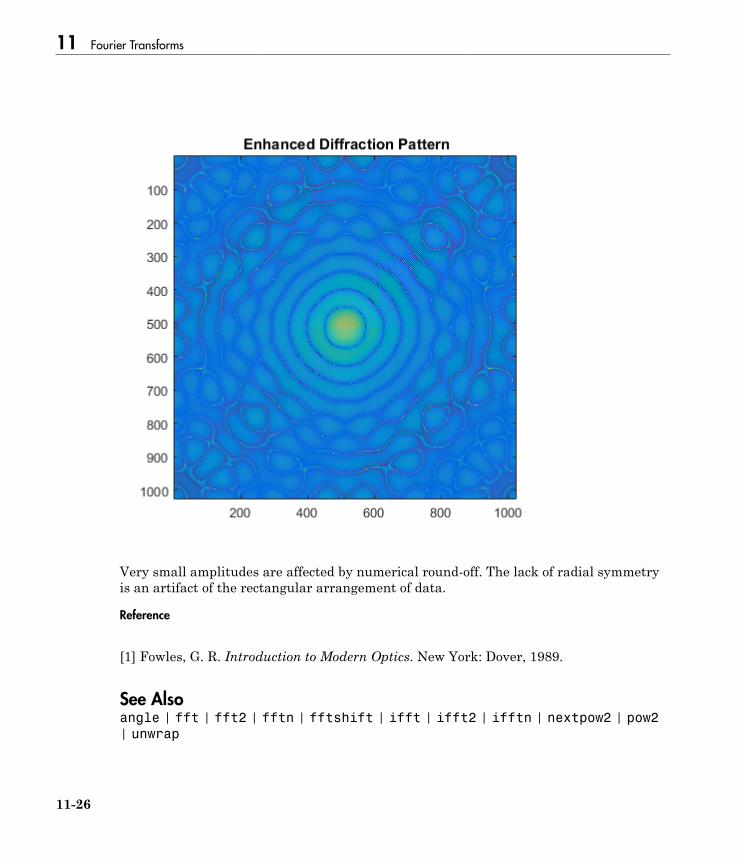
11 Fourier Transforms
11-26
Very small amplitudes are affected by numerical round-off. The lack of radial symmetryis an artifact of the rectangular arrangement of data.
Reference
[1] Fowles, G. R. Introduction to Modern Optics. New York: Dover, 1989.
See Alsoangle | fft | fft2 | fftn | fftshift | ifft | ifft2 | ifftn | nextpow2 | pow2| unwrap

Fast Fourier Transform (FFT)
11-27
More About• “Discrete Fourier Transform (DFT)” on page 11-2

11 Fourier Transforms
11-28
Function Summary
MATLAB functions related to Fourier transforms include:
Function Description
fft One-dimensional fast Fourier transformifft One-dimensional inverse fast Fourier transformfft2 Two-dimensional fast Fourier transformifft2 Two-dimensional inverse fast Fourier transformfftn N-dimensional fast Fourier transformifftn N-dimensional inverse fast Fourier transformfftshift Rearrange DFT data to center zero-frequency componentfftw Interface to FFTW run-time algorithmabs Amplitude of the DFTangle Phase of the DFTunwrap Correct phase angles with jumps greater than or equal to pinextpow2 Next power of two greater than or equal to a given lengthpow2 Compute powers of two
The MATLAB software also includes demos that use these functions in combination forFourier analysis:
• FFT for Spectral Analysis — Reviews basic spectral analysis with the FFT• Using FFT in MATLAB — Example of time series analysis with the FFT that looks
for periodicity in historical data on sunspot activity