بسم اهلل الرحمن الرحيمSudan University of Science and

Technology

STUDY THE EFFECT OF AUTOTHROTTLE ON

FUEL CONSUMPTION RATE ON TURBOJET

ENGINE USING MATLAB

Thesis submitted in Partial Fulfillment of the Requirements for the

Degree of Bachelor of Science. (B.sc Honor)

In the

Department of Aeronautical Engineering

Faculty of Engineering

By:

1. Mohamed Omer Abd AL Hameed Ali.

2. Rana Izzeldin Babekir Ibrahim.

Supervised By:

Ms. Raheeg Osama wahbi Alamin

October, 2015

i

اآلية

قال تعالى :

(79سورة النحل. اآلية )

ii

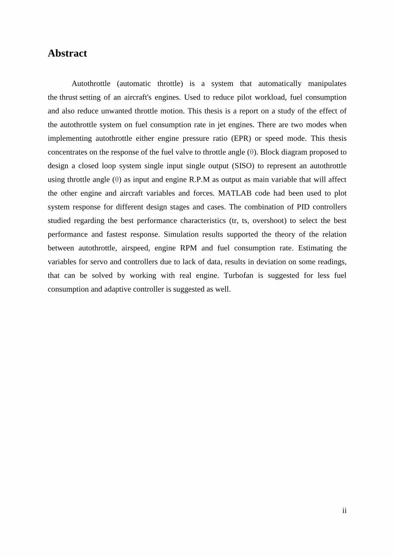
Abstract

Autothrottle (automatic throttle) is a system that automatically manipulates

the thrust setting of an aircraft's engines. Used to reduce pilot workload, fuel consumption

and also reduce unwanted throttle motion. This thesis is a report on a study of the effect of

the autothrottle system on fuel consumption rate in jet engines. There are two modes when

implementing autothrottle either engine pressure ratio (EPR) or speed mode. This thesis

concentrates on the response of the fuel valve to throttle angle (θ). Block diagram proposed to

design a closed loop system single input single output (SISO) to represent an autothrottle

using throttle angle (θ) as input and engine R.P.M as output as main variable that will affect

the other engine and aircraft variables and forces. MATLAB code had been used to plot

system response for different design stages and cases. The combination of PID controllers

studied regarding the best performance characteristics (tr, ts, overshoot) to select the best

performance and fastest response. Simulation results supported the theory of the relation

between autothrottle, airspeed, engine RPM and fuel consumption rate. Estimating the

variables for servo and controllers due to lack of data, results in deviation on some readings,

that can be solved by working with real engine. Turbofan is suggested for less fuel

consumption and adaptive controller is suggested as well.

iii

Acknowledgment

Verily all praise is for Allah, we praise him, seek his help and guidance.

We are deeply grateful to many. To our supervisor Raheeg Alamin, and another special

thanks to Dr. Osman Emam for his guidance and support all through this year.

To Mohamed Taha for his great help and concern.

To Support Team/ fourth year Aeronautical Department Batch 15.

To our parents and family, whose support is abundant, and whose love is nourishing.

Our colleagues, we express appreciation for creativity, discipline, competence and friendship.

iv

Symbols

𝐾 Gain

𝜃 The throttle position

𝑉𝑖 Input speed

𝑉𝑜 Output speed

VS0 Stall speed in the landing configuration

𝑇 Thrust

𝑡𝑑 Delay time

𝑡𝑟 Rise time

𝑡𝑠 Settling time

𝑀𝑝 Maximum overshoot

𝑡𝑝 Peak time

v

Abbreviation

ATC Air traffic control

ECU Engine Control Unit

EPR Engine pressure ratio

FADEC Full authority digital engine control

FMC Flight management computer

HMU Hydro-mechanical Unit

MCP Mode control panel

MIMO Multi input multi output

SISO Single input single output

TQA Throttle Quadrant Assembly

TECS Total energy control system

TMC Thrust management computer

vi

Contents

i ............................................................................................................................................... اآلية

Abstract ...................................................................................................................................... ii

Acknowledgment ..................................................................................................................... iii

Symbols..................................................................................................................................... iv

Abbreviation .............................................................................................................................. v

Contents .................................................................................................................................... vi

Table of Figures ........................................................................................................................ ix

List of Tables ............................................................................................................................. x

Chapter 1: Introduction .............................................................................................................. 1

1.1 Overview .......................................................................................................................... 1

1.2 Aim and objectives ........................................................................................................... 1

1.2.1 Aim ............................................................................................................................. 1

1.2.2 Objectives ................................................................................................................... 1

1.3 Problem Statement ............................................................................................................ 2

1.4 Proposed Solution ............................................................................................................. 2

1.5 Motivation ........................................................................................................................ 2

1.6 Contribution ...................................................................................................................... 3

1.7 Methodology ..................................................................................................................... 3

1.8 Outline .............................................................................................................................. 3

Chapter 2: Literature Review ..................................................................................................... 5

2.1 Engine Types and Applications ........................................................................................ 5

2.1.1 Turbo Jet Engine ........................................................................................................ 6

2.1.2 Turbofan Engine ......................................................................................................... 6

2.1.3 Turbo-shaft Engine ..................................................................................................... 7

2.1.4 Turbo-prop Engine ..................................................................................................... 7

vii

2.2 Jet Engine Theory ............................................................................................................. 8

2.2.1 Principle of Operation ................................................................................................ 8

2.3 Jet Engine Equation .......................................................................................................... 9

2.4 Factors Affecting Thrust ................................................................................................... 9

2.5 Summary ......................................................................................................................... 10

Chapter 3: Aircraft Fuel System .............................................................................................. 11

3.1 Fuel System General Requirement ............................................................................ 11

3.2 Fuel Flow Rate .......................................................................................................... 12

3.3 Aircraft Engine Control Concept .............................................................................. 14

3.4 Control Theory .......................................................................................................... 15

3.4.1 Classical Control Theory ................................................................................... 15

3.4.2 Modern Control Theory ..................................................................................... 16

3.4.3 Optimal Control Theory ..................................................................................... 16

3.5 Control Design Objectives ........................................................................................ 16

3.6 Types of Controllers .................................................................................................. 17

3.6.1 Proportional Controllers..................................................................................... 17

3.6.2 Integral Controllers ............................................................................................ 18

3.6.3 Derivative Controllers ........................................................................................ 18

3.6.4 PID Controller .................................................................................................... 19

3.6.5 Proportional and Integral Controller .................................................................. 20

3.6.6 Proportional and Derivative Controller ............................................................. 20

3.7 Full Authority Digital Engine Control (FADEC) ..................................................... 23

3.7.1 FADEC Components ......................................................................................... 23

Chapter 4: Autothrottle system ................................................................................................ 24

4.1 Background and Operation ............................................................................................. 24

4.1.1 Operation............................................................................................................ 26

4.2 Air Traffic Control .......................................................................................................... 28

viii

4.3 Autothrottle System Design ............................................................................................ 29

4.4 Summary ................................................................................................................... 30

Chapter 5: Simulation of Autothrottle using MATLAB .......................................................... 31

5.1 Relation between Thrust, Aircraft Speed and Engine RPM ........................................... 31

5.2 Results ............................................................................................................................ 34

5.2.2 PID Tool ................................................................................................................... 35

Chapter 6: Conclusion and Recommendation .......................................................................... 40

6.1 Conclusion ................................................................................................................. 40

6.2 Future work ............................................................................................................... 40

Appendix .................................................................................................................................. 42

ix

Table of Figures

Figure 1: Turbo Jet Engine Sections .......................................................................................... 6

Figure 2: Turbofan Engine Sections .......................................................................................... 6

Figure 3: Turbo-Shaft Engine Sections...................................................................................... 7

Figure 4: Turbo-Prop Engine Sections ...................................................................................... 7

Figure 5: Maximum Thrust (lbs) at each Altitude. .................................................................. 14

Figure 6: PID Controller Block Diagram................................................................................. 21

Figure 7: Transient and Steady-State Response Analyses source [9] ...................................... 22

Figure 8: FADEC Control Philosophy ..................................................................................... 23

Figure 9: Autothrottle Unit ..................................................................................................... 26

Figure 10: Block Diagram of Typical Modern Engine Control Logic (image courtesy of

NASA). Source [4]................................................................................................................... 27

Figure 11: Proposed Block Diagram by Rebecca .................................................................... 29

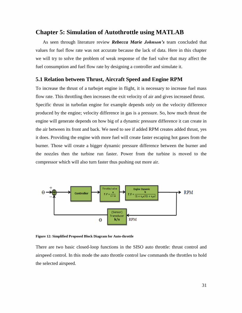
Figure 12: Simplified Proposed Block Diagram for Auto-throttle .......................................... 31

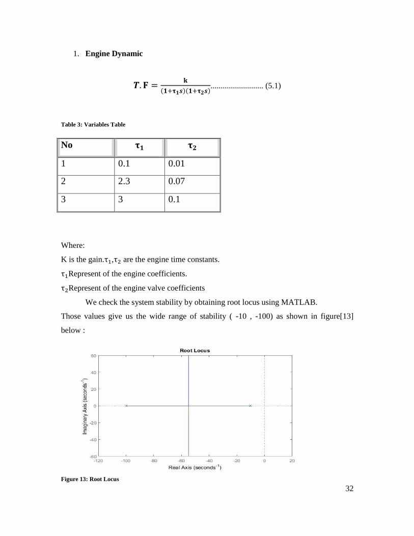
Figure 13: Root Locus ............................................................................................................. 32

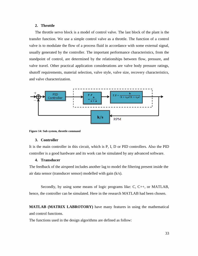
Figure 14: Sub system, throttle command ............................................................................... 33

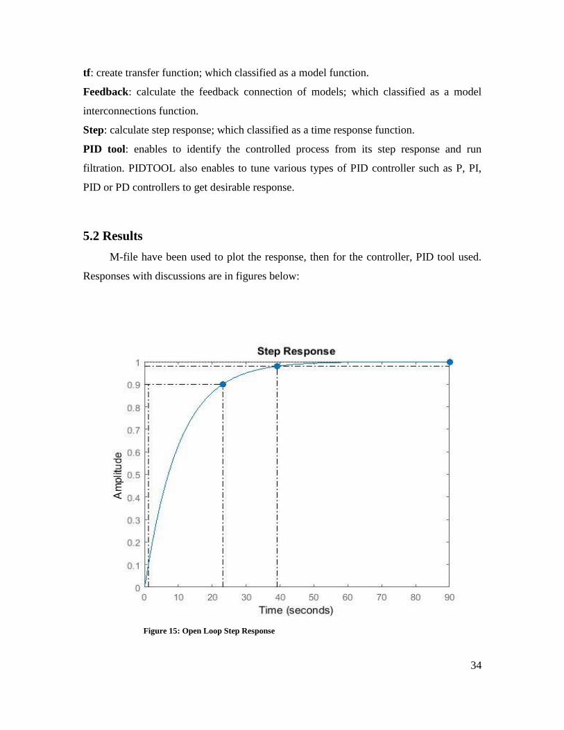
Figure 15: Open Loop Step Response ..................................................................................... 34

x

List of Tables

Table 1: Effects of each of controller Kp, Kd, and Ki on a closed-loop system ..................... 21

Table 2: Basic Auto throttle Functions over the Flight Profile. ............................................... 25

Table 3: Variables Table .......................................................................................................... 32

1

Chapter 1: Introduction

1.1 Overview

Aircraft engine performance parameters, such as thrust, provide crucial

information for operating an aircraft engine in a safe and efficient manner, but they

cannot be directly measured during flight. A technique to accurately estimate these

parameters is, therefore, essential for further enhancement and control of engine

operation.

The basic engine control concept is to provide smooth, stable, and stall free operation

of the engine via single input with no throttle restrictions and to have a reliable and

predictable throttle movement to thrust response.

A primitive auto throttle was first fitted to later versions of the Messerschmitt Me 262

jet fighter late in World War II. Today it is often linked to a Flight Management

System, and FADEC is an extension of the concept to control many other parameters

besides fuel flow.

An autothrottle (automatic throttle) control the power setting of an aircraft's engines

by specifying a desired flight characteristic, rather than manually controlling the fuel

flow. These systems can conserve fuel and extend engine life by metering the precise

amount of fuel required to attain a specific target indicated air speed, or the assigned

power for different phases of flight.

1.2 Aim and objectives

1.2.1 Aim

To study the effect of autothrottle on reducing pilot workload and fuel

consumption, what claimed to increase the range of the aircraft and reduce flight cost,

by design and control a simple autothrottle.

1.2.2 Objectives

Study how autothrottle control the speed of the aircraft by adjusting the position

of the throttles and ensures that the maximum fuel efficiency is obtained by the

engines during all stages of flight, by:

Study the theory of throttling system.

2

Propose a simple loop for design using engine RPM instead of aircraft

airspeed.

Make the throttle work automatically.

Build a control loop. Using PID controller and MATLAB

Analyse the responses in relation to theory.

1.3 Problem Statement

Due to the increase of the demand for using aircraft as a safe and practical

transportation media for the growing business worldwide , it become very important

to start looking for improving their engine's performance in term of fuel consumption.

Thus there will be efficient, reliable, competent and cost effective mean of

transportation to play the main rule in the business world. Even small changes

in aircraft performance and fuel efficiency can have a cumulative large impact on

operating costs. So in improving the aircraft engine performance, fuel consumption

should be considered as the main factor of improvement.

1.4 Proposed Solution

Applying a PID controller to simple autotrottle closed loop circuit using throttle

angle (θ) as input and engine R.P.M as output, in order to improve and to accelerate

throttle valve response to optimize the fuel consumption.

1.5 Motivation

The engine performance stability is a main thing to look for to decide if the

controller implemented to it is good enough to operate. We need the aircraft engine to

deliver forward/reverse and positive/negative torque to drag the control surfaces after

moving the throttle with seamless fuel losses. Quality control imposes further

requirements for stable system, smooth torque, fast dynamic response, and ability to

operate at zero speed.[1]

The great challenge is come with taking variables as functions on others when

dealing with aircraft engines.

To consider as good operation for the autothrottle system the response should be

fast and smooth (minimum settling and rise time) with minimum overshoot.

Controlling the throttle is depends on the engine pressure or aircraft speed which is a

3

function of engine rpm. These constraints have to be managed very tightly in order to

implement autothrottle in aircraft especially during take-off and landing.

1.6 Contribution

This project is a great chance to apply most of the theories about the aircraft

engine controlling by taking the throttle system and control it by building a control

loop and simulate it by using MATLAB. Aircraft engine rpm had been chosen to be

the controlling variable, all other variables, inputs and outputs from the system is been

connected to the engine rpm. The objective of the project is to make the throttle

system run under the software control then study its effect of the fuel consumption

rate will be fulfilled by designing and simulating the control loop circuit including the

indication of (throttle angle ϴ) and rpm.

1.7 Methodology

Simulation and analytical methodology have been used to go through this study.

From previous research it was clear that it is not easy to design a control law for a

throttle system, that’s why simulation was the best way to go with. RPM of the engine

was related to the thrust, speed fuel flow rate, then represented as the output of the

proposed block diagram while throttle angle was the input. MATLAB with M file and

PID tool used to simulate the system and discussion made regarding the response

characteristics.

1.8 Outline

The thesis is organised as follow:

Chapter one as a general introduction about the aircraft engine: its history and

applications. The inherent control problems rising with the fuel flow and thrust are

briefly discussed. Then the objectives of the project, the motivation and contribution

of this thesis are given.

In Chapter two, the principle of the thrust is discussed from both a physical and

mathematical point of view. The controlling problem and some researches discussed

briefly in this chapter.

Chapter three, for detailed study in the control issues with auto throttle and looks

at the speed and thrust as the modes to be controlled this done by choosing the fuel

flow rate to be observed and the speed to sensed and controlled by a feedback system.

4

The preparation for the project and things that needed to set all placed by their

calculation and specification in brief in the fourth chapter.

All the graphs to be needed to monitor the engine and the result are captured and

putted with a detailed discussion in chapter five.

Chapter six concluded the entire project and proposes for further research,

then the appendices.

5

Chapter 2: Literature Review

Aircraft jet turbine engine were used at the end of World War II. Before that,

engines were piston has identified the aircraft speed were replaced by turbine engines,

which was the most efficient and all the faces compared with these engines where it

was possible to get the momentum and thrust of the largest of turbo engines, the mass

of relatively less engine and the qualitative (the engine percentage-dimensional

volumetric to the thrust power of that engine) for at least several times that figure at

best piston engines. As well as increased dramatically aircraft turbine engines which

were used jet speed, reaching the speed of the aircraft for the first generation of turbo-

engines to the limit (950 km / h), while aircraft piston engines speed did not exceed

(750 km / h).

After that many types of jet turbine engines appeared and those types can be divided

into two groups (turbo jet engines, turbo prop engines). And between these two

groups there are (turbo fan or By-pass engines) such as these engines to get take-off

and flight highs speeds outweigh significantly the speed of sound, high efficiency and

a relatively large flight range.[2]

2.1 Engine Types and Applications

Most of modern passenger and military aircraft are powered by gas turbine

engines, which are also called jet engines. There are several types of jet engines, but

all jet engines have some parts in common.

Aircraft gas turbine engines can be classified according to the type of compressor

used or power produced by the engine.

Compressor types are as follow:

1. Centrifugal flow.

2. Axial flow.

3. Centrifugal-Axial flow.

Power produced is as follow:

1. Turbojet engines.

2. Turbofan engines.

3. Turbo-shaft engines.

4. Turboprop engines.

5. Piston engine.

6

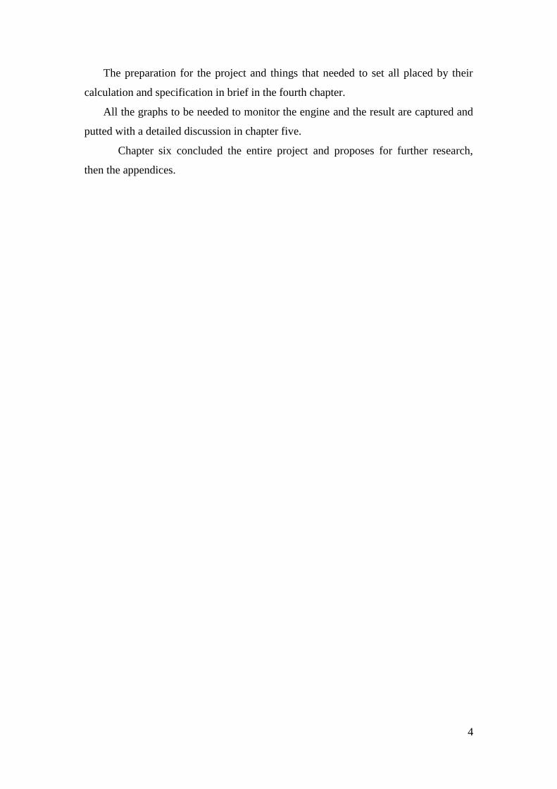
2.1.1 Turbo Jet Engine

Turbojet engine derives its thrust by highly accelerating a mass of air, all of

which goes through the engine. Since a high “jet” velocity is required to obtain an

acceptable of thrust, the turbine of turbojet is designed to extract only enough power

from the hot gas stream to drive the compressor and accessories. All of the propulsive

force (100% of thrust) produced by a jet engine derived from exhaust gas.

Figure 1: Turbo Jet Engine Sections

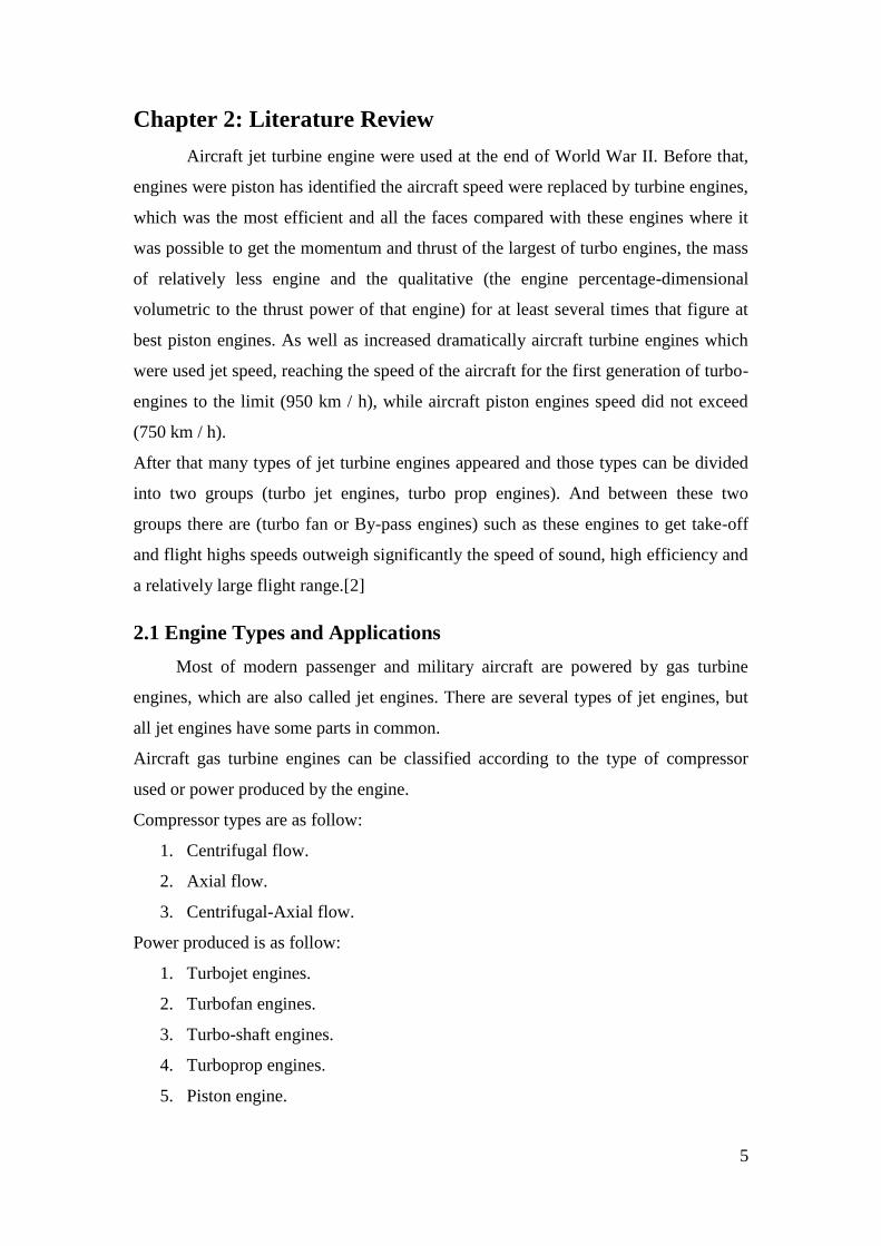
2.1.2 Turbofan Engine

Turbofan engine has a duct enclosed fan mounted at the front of the engine

and driven either mechanically at the same speed as the compressor, or by an

independent turbine located to the rear of the compressor drive turbine. The fan air

can exit separately from the primary engine air, or it can be ducted back to mix with

the primary’s air at the rear. Approximately more than 75% than thrust comes from

fan and less than 25% comes from exhaust gas.[3]

Figure 2: Turbofan Engine Sections

7

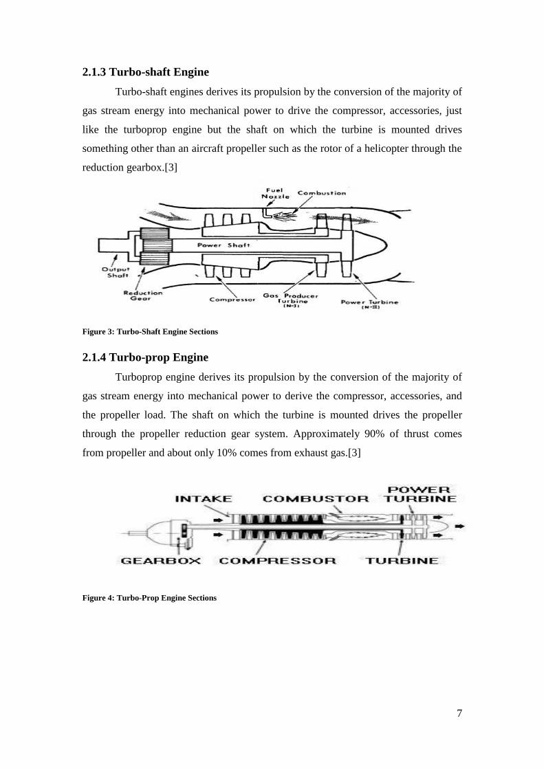
2.1.3 Turbo-shaft Engine

Turbo-shaft engines derives its propulsion by the conversion of the majority of

gas stream energy into mechanical power to drive the compressor, accessories, just

like the turboprop engine but the shaft on which the turbine is mounted drives

something other than an aircraft propeller such as the rotor of a helicopter through the

reduction gearbox.[3]

Figure 3: Turbo-Shaft Engine Sections

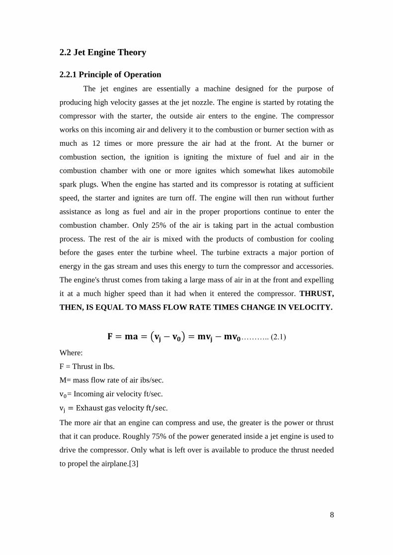
2.1.4 Turbo-prop Engine

Turboprop engine derives its propulsion by the conversion of the majority of

gas stream energy into mechanical power to derive the compressor, accessories, and

the propeller load. The shaft on which the turbine is mounted drives the propeller

through the propeller reduction gear system. Approximately 90% of thrust comes

from propeller and about only 10% comes from exhaust gas.[3]

Figure 4: Turbo-Prop Engine Sections

8

2.2 Jet Engine Theory

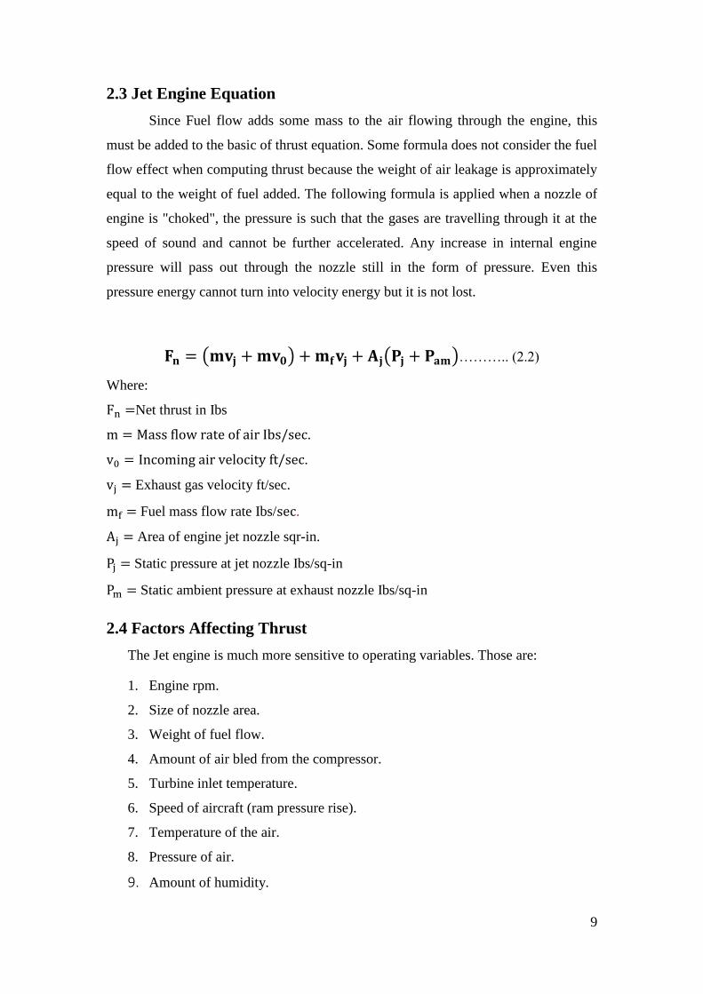
2.2.1 Principle of Operation

The jet engines are essentially a machine designed for the purpose of

producing high velocity gasses at the jet nozzle. The engine is started by rotating the

compressor with the starter, the outside air enters to the engine. The compressor

works on this incoming air and delivery it to the combustion or burner section with as

much as 12 times or more pressure the air had at the front. At the burner or

combustion section, the ignition is igniting the mixture of fuel and air in the

combustion chamber with one or more ignites which somewhat likes automobile

spark plugs. When the engine has started and its compressor is rotating at sufficient

speed, the starter and ignites are turn off. The engine will then run without further

assistance as long as fuel and air in the proper proportions continue to enter the

combustion chamber. Only 25% of the air is taking part in the actual combustion

process. The rest of the air is mixed with the products of combustion for cooling

before the gases enter the turbine wheel. The turbine extracts a major portion of

energy in the gas stream and uses this energy to turn the compressor and accessories.

The engine's thrust comes from taking a large mass of air in at the front and expelling

it at a much higher speed than it had when it entered the compressor. THRUST,

THEN, IS EQUAL TO MASS FLOW RATE TIMES CHANGE IN VELOCITY.

𝐅 = 𝐦𝐚 = (𝐯𝐣 − 𝐯𝟎) = 𝐦𝐯𝐣 − 𝐦𝐯𝟎……….. (2.1)

Where:

F = Thrust in Ibs.

M= mass flow rate of air ibs/sec.

v0= Incoming air velocity ft/sec.

vj = Exhaust gas velocity ft/sec.

The more air that an engine can compress and use, the greater is the power or thrust

that it can produce. Roughly 75% of the power generated inside a jet engine is used to

drive the compressor. Only what is left over is available to produce the thrust needed

to propel the airplane.[3]

9

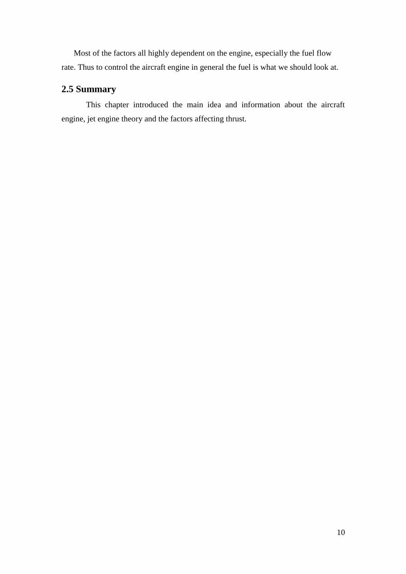
2.3 Jet Engine Equation

Since Fuel flow adds some mass to the air flowing through the engine, this

must be added to the basic of thrust equation. Some formula does not consider the fuel

flow effect when computing thrust because the weight of air leakage is approximately

equal to the weight of fuel added. The following formula is applied when a nozzle of

engine is "choked", the pressure is such that the gases are travelling through it at the

speed of sound and cannot be further accelerated. Any increase in internal engine

pressure will pass out through the nozzle still in the form of pressure. Even this

pressure energy cannot turn into velocity energy but it is not lost.

𝐅𝐧 = (𝐦𝐯𝐣 + 𝐦𝐯𝟎) + 𝐦𝐟𝐯𝐣 + 𝐀𝐣(𝐏𝐣 + 𝐏𝐚𝐦)……….. (2.2)

Where:

Fn =Net thrust in Ibs

m = Mass flow rate of air Ibs/sec.

v0 = Incoming air velocity ft/sec.

vj = Exhaust gas velocity ft/sec.

mf = Fuel mass flow rate Ibs/sec.

Aj = Area of engine jet nozzle sqr-in.

Pj = Static pressure at jet nozzle Ibs/sq-in

Pm = Static ambient pressure at exhaust nozzle Ibs/sq-in

2.4 Factors Affecting Thrust

The Jet engine is much more sensitive to operating variables. Those are:

1. Engine rpm.

2. Size of nozzle area.

3. Weight of fuel flow.

4. Amount of air bled from the compressor.

5. Turbine inlet temperature.

6. Speed of aircraft (ram pressure rise).

7. Temperature of the air.

8. Pressure of air.

9. Amount of humidity.

10

Most of the factors all highly dependent on the engine, especially the fuel flow

rate. Thus to control the aircraft engine in general the fuel is what we should look at.

2.5 Summary

This chapter introduced the main idea and information about the aircraft

engine, jet engine theory and the factors affecting thrust.

11

Chapter 3: Aircraft Fuel System

The aircraft fuel system serves for storing the required amount of fuel used by engines

operation under all flight conditions. The purpose of an aircraft fuel system is to store and

deliver the proper amount of clean fuel at the correct pressure to the engine. Also fuel

systems should provide positive and reliable fuel flow through all phases of flight

including:

1. Changes in altitude.

2. Violent manoeuvres.

3. Sudden acceleration and deceleration.

The fuel system is one of the more complex aspects of the gas turbine engine. The

variety of methods used to meet turbine engine fuel requirements makes reciprocating

engine carburetion seem a simple study by comparison.

Turbine-powered aircraft this control is provided by varying the flow of fuel to the

combustion chambers. However, turboprop aircraft also use variable-pitch propellers;

thus, the selection of thrust is shared by two controllable variables, fuel flow and

propeller blade angle. If the quantity of fuel becomes excessive in relation to mass air

flow throw the engine, the limiting temperature of the turbine blades can be exceeded, or

it will produce compressor stall and a condition referred to as "rich blowout".

3.1 Fuel System General Requirement

1. It must be possible to increase or decrease the power at will to obtain the thrust

required for any operating condition.

2. The quantity of fuel supplied must be adjusted automatically to correct for

changes in ambient temperature or pressure.

3. The fuel system must deliver fuel to the combustion chamber not only in the right

quantity but also in the right condition to satisfactory combustion.

4. The fuel system must also supply fuel so that the engine can be easily started on

the ground and in the air. This means that the fuel must be injected into the

combustion chamber in a combustible condition when the engine is being turned

12

over slowly by the starting system and the combustion must be sustained while

the engine is accelerating to its normal running speed.

5. A critical condition to which the fuel system must be respond occurs during slam

acceleration. When the engine is accelerated, energy must be furnished to the

turbine in excess of that necessary to maintain a constant rpm. However, if the

fuel flow increases too rapidly, an over rich mixture can be produced, with the

possibility of a rich blowout.[3]

3.2 Fuel Flow Rate

The ability of the fuel system to provide fuel at a rate of flow and pressure sufficient

for proper engine operation is vital in aircraft. Moreover, the fuel system must deliver the

fuel at the aircraft attitude that is most critical with respect to fuel feed and quantity of

unusable fuel. Tests are performed to demonstrate this performance. Fuel flow-meters are

installed on most aircraft. During testing, the flow-meter is blocked and fuel must flow

through or bypass the meter and still supply the engine at sufficient rate and pressure. For

gravity-flow fuel systems, the fuel flow rate must be 150 percent of the take-off fuel

consumption of the engine. For fuel pump systems, the fuel flow rate for each pump

system (main and reserve supply) for each reciprocating engine must be 125 percent of

the fuel flow required by the engine at the maximum take-off power. However, the fuel

pressure, with main and emergency pumps operating simultaneously, must not exceed the

fuel inlet pressure limits of the engine. Auxiliary fuel systems and fuel transfer systems

may operate under slightly different parameters. Turbine engine fuel systems must

provide at least 100 percent required by the engine under each intended operating

condition and manoeuvre. On aircraft with multiple fuel tanks, performance is monitored

when switching to a new tank once fuel has been depleted from a tank. For reciprocating,

naturally aspirated, single-engine aircraft in level flight, 75 percent maximum continuous

power must be obtainable in not more than 10seconds. For turbocharged aircraft, 20

seconds is allowed. Twenty seconds is also allowed on multiengine aircraft flow between

Interconnected Tanks.

In gravity feed fuel system with interconnected tank outlets, it must be impossible

for enough fuel to flow between the tanks to cause an overflow of fuel from any tank vent

13

under the conditions in 14 CFR parts 23, section 23.959. If fuel can be pumped from one

tank to another in flight, the fuel tank vents and the fuel transfer system must be designed

so that no structural damage to any airplane component can occur because of overfilling

of any tank.

��𝐚𝐜 = −��𝐟………................. (3.1)

��𝐟 = ��𝐓. 𝐅𝐓……..............….. (3.2)

Where:

��𝑎𝑐 = Change of mass of the aircraft.

mf= Fuel mass flow rate.

T= Thrust.

F= force.

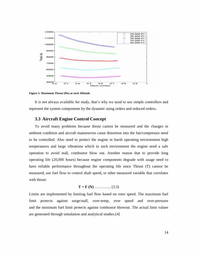
According to previous research altitude increasing leads to thrust decreasing. This

decrease in thrust is shown in Figure [5] below. By taking in account the consideration

average throttle lever angle; At low thrust settings the engine takes longer to respond to

thrust settings, so to help prevent excessive movement, lower gains are used at low

throttle angles. Another compensation that is used in this control law is pitch angle.

While tracking altitude, the pitch angle is not used because the changes in pitch angle are

small. However, during other phases of flight, initial changes in pitch angle should be

accounted for when controlling speed, because the angle of the force of thrust is

changing. Once an initial compensation for pitch angle has 25 been added, it is washed

out, so pitch angle does not create an unnecessary long term bias in the command. Thrust

in different altitude is shown in figure [5] below for the case of study.

14

Figure 5: Maximum Thrust (lbs) at each Altitude.

It is not always available for study, that’s why we need to use simple controllers and

represent the system components by the dynamic using orders and reduced orders.

3.3 Aircraft Engine Control Concept

To avoid many problems because thrust cannot be measured and the changes in

ambient condition and aircraft manoeuvres cause distortion into the fan/compressor need

to be controlled. Also need to protect the engine in harsh operating environment high

temperatures and large vibrations which in such environment the engine need a safe

operation to avoid stall, combustor blow out. Another reason that to provide long

operating life (20,000 hours) because engine components degrade with usage need to

have reliable performance throughout the operating life since Thrust (T) cannot be

measured, use fuel flow to control shaft speed, or other measured variable that correlates

with thrust:

T = F (N) ……….. (3.3)

Limits are implemented by limiting fuel flow based on rotor speed. The maximum fuel

limit protects against surge/stall, over-temp, over speed and over-pressure

and the minimum fuel limit protects against combustor blowout. The actual limit values

are generated through simulation and analytical studies.[4]

15

3.4 Control Theory

Is an interdisciplinary branch of engineering and mathematics that deals with the

behaviour of dynamical with inputs, and how their behaviour is modified by feedback.

The usual objective of control theory is to control a system, often called the plant, so its

output follows a desired control signal, called the reference, which may be a fixed or

changing value. To do this a controller is designed, which monitors the output and

compares it with the reference. The difference between actual and desired output, called

the error signal, is applied as feedback to the input of the system, to bring the actual

output closer to the reference. Some topics studied in control theory are stability (whether

the output will converge to the reference value or oscillate about

it), controllability and observability.[5]

3.4.1 Classical Control Theory

To overcome the limitations of the open-loop controller, control theory

introduces feedback. Closed-loop controller uses feedback to control states or outputs of

a dynamical system. Its name comes from the information path in the system: process

inputs (e.g., voltage applied to an electric motor) have an effect on the process outputs

(e.g., speed or torque of the motor), which is measured with sensors and processed by the

controller; the result (the control signal) is "fed back" as input to the process, closing the

loop.

Closed-loop controllers have the following advantages over open-loop controllers:

1. Disturbance rejection (such as hills in the cruise control example above).

2. Guaranteed performance even with model uncertainties, when the model structure

does not match perfectly the real process and the model parameters are not exact.

3. Unstable processes can be stabilized.

4. Reduced sensitivity to parameter variations.

5. Improved reference tracking performance.

In some systems, closed-loop and open-loop control are used simultaneously. In such

systems, the open-loop control is termed feed forward and serves to further improve

16

reference tracking performance. Common closed-loop controller architecture is the PID

controller.[6]

3.4.2 Modern Control Theory

In contrast to the frequency domain analysis of the classical control theory,

modern control theory utilizes the time-domain state space representation, a mathematical

model of a physical system as a set of input, output and state variables related by first-

order differential equations. To abstract from the number of inputs, outputs and states, the

variables are expressed as vectors and the differential and algebraic equations are written

in matrix form (the latter only being possible when the dynamical system is linear).[7]

The state space representation (also known as the "time-domain approach") provides a

convenient and compact way to model and analyse systems with multiple inputs and

outputs. With inputs and outputs, we would otherwise have to write down Laplace

transforms to encode all the information about a system.

Unlike the frequency domain approach, the use of the state-space representation is not

limited to systems with linear components and zero initial conditions. "State space" refers

to the space whose axes are the state variables. The state of the system can be represented

as a vector within that space.

3.4.3 Optimal Control Theory

Optimal control deals with the problem of finding a control law for a given system

such that a certain optimality criterion is achieved. A control problem includes

a functional that is a function of state and control variables. An optimal control is a set

of differential equations describing the paths of the control variables that minimize the

cost functional. The optimal control can be derived using Pontryagin's maximum

principle (a necessary condition also known as Pontryagin's minimum principle or simply

Pontryagin's Principle),or by solving the Hamilton–Jacobi–Bellman equation (a sufficient

condition).

3.5 Control Design Objectives

1. Regulation: keep controlled variable near a constant target value (e.g. process

control: pressure, concentration etc.).

17

2. Tracking: keep controlled variable near a time-varying target value (e.g. antenna

positioning, robotic manipulator point-to point manoeuvre, motor speed/position

control).

3. Stability, roughly means bounded output for bounded input,

4. Accuracy means minimum steady state error.

5. Satisfactory transient behaviour means minimum or zero overshoot, fast

response(less rise and settling times).

6. Robustness means less sensitivity to real operating conditions abrupt changes.

3.6 Types of Controllers

Most control systems in the past were implemented using mechanical systems or solid

state electronics. Pneumatics was often utilized to transmit information and control using

pressure. However, most modern control systems in industrial settings now rely on

computers for the controller. Obviously it is much easier to implement complex control

algorithms on a computer than using a mechanical system.

3.6.1 Proportional Controllers

We cannot use types of controllers at anywhere, with each type controller; there are

certain conditions that must be fulfilled. With proportional controllers there are two

conditions and these are written below:

1- Deviation should not be large; it means there should be less deviation

between the input and output.

2- Deviation should not be sudden.

Now we are in a condition to discuss proportional controllers, as the name

suggests in a proportional controller the output (also called the actuating signal) is

directly proportional to the error signal. Now let us analyse proportional controller

mathematically. As we know in proportional controller output is directly proportional to

error signal, writing this mathematically we have,

𝐴(𝑡) ∝ 𝑒(𝑡)………........ (3.4)

18

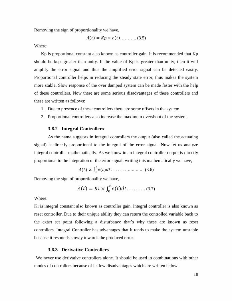
Removing the sign of proportionality we have,

𝐴(𝑡) = 𝐾𝑝 × 𝑒(𝑡)……….. (3.5)

Where:

Kp is proportional constant also known as controller gain. It is recommended that Kp

should be kept greater than unity. If the value of Kp is greater than unity, then it will

amplify the error signal and thus the amplified error signal can be detected easily.

Proportional controller helps in reducing the steady state error, thus makes the system

more stable. Slow response of the over damped system can be made faster with the help

of these controllers. Now there are some serious disadvantages of these controllers and

these are written as follows:

1. Due to presence of these controllers there are some offsets in the system.

2. Proportional controllers also increase the maximum overshoot of the system.

3.6.2 Integral Controllers

As the name suggests in integral controllers the output (also called the actuating

signal) is directly proportional to the integral of the error signal. Now let us analyze

integral controller mathematically. As we know in an integral controller output is directly

proportional to the integration of the error signal, writing this mathematically we have,

𝐴(𝑡) ∝ ∫ 𝑒(𝑡)𝑑𝑡𝑡

0………............. (3.6)

Removing the sign of proportionality we have,

𝐴(𝑡) = 𝐾𝑖 × ∫ 𝑒(𝑡)𝑑𝑡𝑡

0……….. (3.7)

Where:

Ki is integral constant also known as controller gain. Integral controller is also known as

reset controller. Due to their unique ability they can return the controlled variable back to

the exact set point following a disturbance that’s why these are known as reset

controllers. Integral Controller has advantages that it tends to make the system unstable

because it responds slowly towards the produced error.

3.6.3 Derivative Controllers

We never use derivative controllers alone. It should be used in combinations with other

modes of controllers because of its few disadvantages which are written below:

19

1. It never improves the steady state error.

2. It produces saturation effects and also amplifies the noise signals produced in the

system.

Now, as the name suggests in a derivative controller the output (also called the

actuating signal) is directly proportional to the derivative of the error signal. Now let us

analyze derivative controller mathematically. As we know in a derivative controller

output is directly proportional to the derivative of the error signal, writing this

mathematically we have,

𝐴(𝑡) ∝𝑑𝑒(𝑡)

𝑑𝑡……………… (3.8)

Removing the sign of proportionality we have,

𝐴(𝑡) = 𝐾𝑑 × 𝑑𝑒(𝑡)

𝑑𝑡……….. (3.9)

Where:

Kd is proportional constant also known as controller gain. Derivative controller is

also known as rate controller. The major advantage of derivative controller is that it

improves the transient response of the system.[8]

3.6.4 PID Controller

The PID controller calculation (algorithm) involves three separate parameters; the

Proportional, the Integral and Derivative values. The Proportional value determines the

reaction to the current error, the Integral determines the reaction based on the sum of

recent errors and the Derivative determines the reaction to the rate at which the error has

been changing. The weighted sum of these three actions is used to adjust the process via a

control element such as the position of a control valve or the power supply of a heating

element.

Some applications may require using only one or two modes to provide the appropriate

system control. This is achieved by setting the gain of undesired control outputs to zero.

A PID controller will be called a PI, PD, P or I controller in the absence of the respective

control actions. PI controllers are particularly common, since derivative action is very

20

sensitive to measurement noise, and the absence of an integral value may prevent the

system from reaching its target value due to the control action.

3.6.5 Proportional and Integral Controller

As the name suggests it is a combination of proportional and an integral controller

the output (also called the actuating signal) is equal to the summation of proportional and

integral of the error signal. Now let us analyse proportional and integral controller

mathematically. As we know in a proportional and integral controller output is directly

proportional to the summation of proportional of error and integration of the error signal,

writing this mathematically we have,

𝐴(𝑡) ∝ ∫ 𝑒(𝑡) + 𝐴(𝑡) ∝ 𝑒(𝑡)𝑡

0……….. (3.10)

Removing the sign of proportionality we have,

𝐴(𝑡) = 𝐾𝑖 ∫ 𝑒(𝑡)𝑑𝑡 + 𝐾𝑝 𝑒(𝑡)𝑡

0……….. (3.11)

Where:

Ki and Kp are proportional constant and integral constant respectively.

Advantages and disadvantages are the combinations of the advantages and disadvantages

of proportional and integral controllers.

3.6.6 Proportional and Derivative Controller

As the name suggests it is a combination of proportional and a derivative

controller the output (also called the actuating signal) is equals to the summation of

proportional and derivative of the error signal. Now let us analyse proportional and

derivative controller mathematically. As we know in a proportional and derivative

controller output is directly proportional to summation of proportional of error and

differentiation of the error signal, writing this mathematically we have,

𝐴(𝑡) ∝𝑑𝑒(𝑡)

𝑑𝑡+ 𝐴(𝑡) ∝ 𝑒(𝑡)……….. (3.12)

Removing the sign of proportionality we have,

𝐴(𝑡) = 𝐾𝑑𝑑𝑒(𝑡)

𝑑𝑡+ 𝐾𝑝𝑒(𝑡)……….. (3.13)

Where:

21

Kd and Kp are proportional constant and derivative constant respectively.

Advantages and disadvantages are the combinations of advantages and disadvantages of

proportional and derivative controllers. By "tuning" the three constants in the PID

controller algorithm the PID can provide control action designed for specific process

requirements. The response of the controller can be described in terms of the

responsiveness of the controller to an error, the degree to which the controller overshoots

the set point and the degree of system oscillation. Note that the use of the PID algorithm

for control does not guarantee optimal control of the system or system stability.

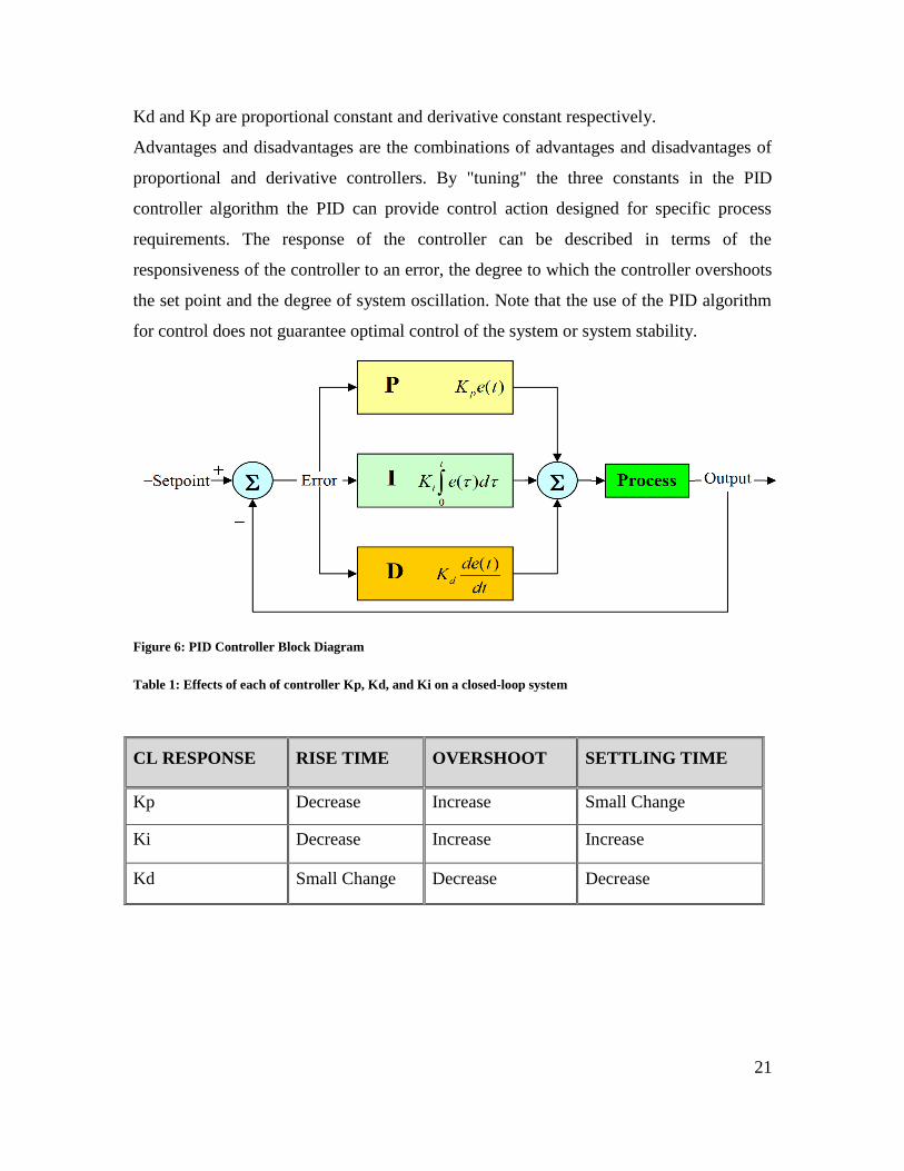
Figure 6: PID Controller Block Diagram

Table 1: Effects of each of controller Kp, Kd, and Ki on a closed-loop system

CL RESPONSE RISE TIME OVERSHOOT SETTLING TIME

Kp Decrease Increase Small Change

Ki Decrease Increase Increase

Kd Small Change Decrease Decrease

22

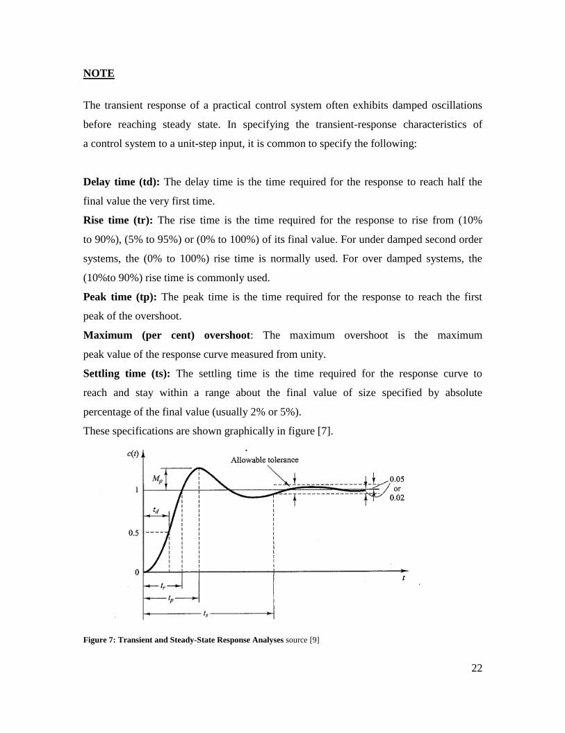
NOTE

The transient response of a practical control system often exhibits damped oscillations

before reaching steady state. In specifying the transient-response characteristics of

a control system to a unit-step input, it is common to specify the following:

Delay time (td): The delay time is the time required for the response to reach half the

final value the very first time.

Rise time (tr): The rise time is the time required for the response to rise from (10%

to 90%), (5% to 95%) or (0% to 100%) of its final value. For under damped second order

systems, the (0% to 100%) rise time is normally used. For over damped systems, the

(10%to 90%) rise time is commonly used.

Peak time (tp): The peak time is the time required for the response to reach the first

peak of the overshoot.

Maximum (per cent) overshoot: The maximum overshoot is the maximum

peak value of the response curve measured from unity.

Settling time (ts): The settling time is the time required for the response curve to

reach and stay within a range about the final value of size specified by absolute

percentage of the final value (usually 2% or 5%).

These specifications are shown graphically in figure [7].

Figure 7: Transient and Steady-State Response Analyses source [9]

23

Implementing control theories and tools in aircraft engines is one of the most

interesting fields of engineering. It is not always valuable to use same controller, it is

highly dependent on the states of the system and dynamics.

Aircraft engine automatisation gone through many stages and have different concepts, but

they all sub into maintaining stability and reducing cost. Autothrottle is a main topic to

look at while reaching FADEC (Full Authority Digital Engine Control).[9]

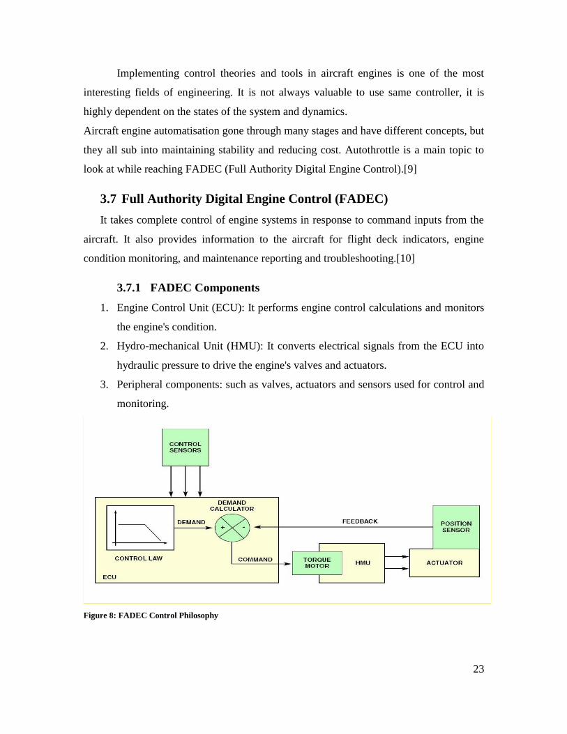
3.7 Full Authority Digital Engine Control (FADEC)

It takes complete control of engine systems in response to command inputs from the

aircraft. It also provides information to the aircraft for flight deck indicators, engine

condition monitoring, and maintenance reporting and troubleshooting.[10]

3.7.1 FADEC Components

1. Engine Control Unit (ECU): It performs engine control calculations and monitors

the engine's condition.

2. Hydro-mechanical Unit (HMU): It converts electrical signals from the ECU into

hydraulic pressure to drive the engine's valves and actuators.

3. Peripheral components: such as valves, actuators and sensors used for control and

monitoring.

Figure 8: FADEC Control Philosophy

24

Chapter 4: Autothrottle system

4.1 Background and Operation

The first-ever auto throttle was a primitive system in the World War II-era German

Me-262 jet fighter. The first viable commercial system was installed in a DC-3 in 1956

(two years before the speedostat cruise control was introduced in the Chrysler Imperial).

That first system was called Auto Power. The inventor was Leonard Greene, who

founded Safe Flight Instrument Corp. and was a pioneer in stall warning and angle-of-

attack equipment.

Greene's speed control device connected servos to the throttles that automatically

adjusted to maintain a given angle of attack not an air speed. When the pilots turned the

system on to fly an approach, it commanded the power levers to maintain a speed

corresponding with 1.3 times of stall speed in the landing configuration (VS0). It worked,

but the concept didn't really catch on until Safe Flight linked it to airspeed and not just

angle of attack. The modern auto throttle was born.

An unusual element of Safe Flight's auto throttles is a patented safety feature called the

"voter." It allows the auto throttle system to compare the speed selected by the pilots with

1.3 VS0 and automatically chooses the higher of the two. This prevents an airplane from

stalling with the autothrottle engaged if the pilot dials in a speed below reference speed

VR, even at steep bank angles with high load factors or at heavy weights. Safe flight’s

entire auto throttles to this day, including the systems the company designed for the

Gulfstream GII and GIII and in the Challenger 604 and 605 business jets (as well as

military aircraft including the F-117 stealth fighter) employ the voter concept.

It wasn't long before competitors got into the auto throttle game as Sperry (now part of

Honeywell) and Collins began developing auto throttle systems for a growing number of

airliners and bizjets. Today auto throttle is standard on most large-cabin bizjets and

airliners, and it's coming to more midsize jets as well. On these auto throttle equipped

airplanes, the system can automatically fly the glide slope and maintain speed to within a

hair's breadth of the target, leading to predictably safe and stable approaches (and

landings).[11]

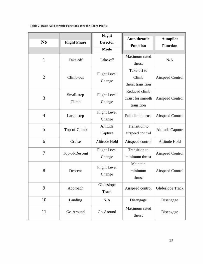
25

Table 2: Basic Auto throttle Functions over the Flight Profile.

No Flight Phase

Flight

Director

Mode

Auto throttle

Function

Autopilot

Function

1 Take-off Take-off Maximum rated

thrust N/A

2 Climb-out Flight Level

Change

Take-off to

Climb

thrust transition

Airspeed Control

3 Small-step

Climb

Flight Level

Change

Reduced climb

thrust for smooth

transition

Airspeed Control

4 Large-step Flight Level

Change Full climb thrust Airspeed Control

5 Top-of-Climb Altitude

Capture

Transition to

airspeed control Altitude Capture

6 Cruise Altitude Hold Airspeed control Altitude Hold

7 Top-of-Descent Flight Level

Change

Transition to

minimum thrust Airspeed Control

8 Descent Flight Level

Change

Maintain

minimum

thrust

Airspeed Control

9 Approach Glideslope

Track Airspeed control Glideslope Track

10 Landing N/A Disengage Disengage

11 Go-Around Go-Around Maximum rated

thrust Disengage

26

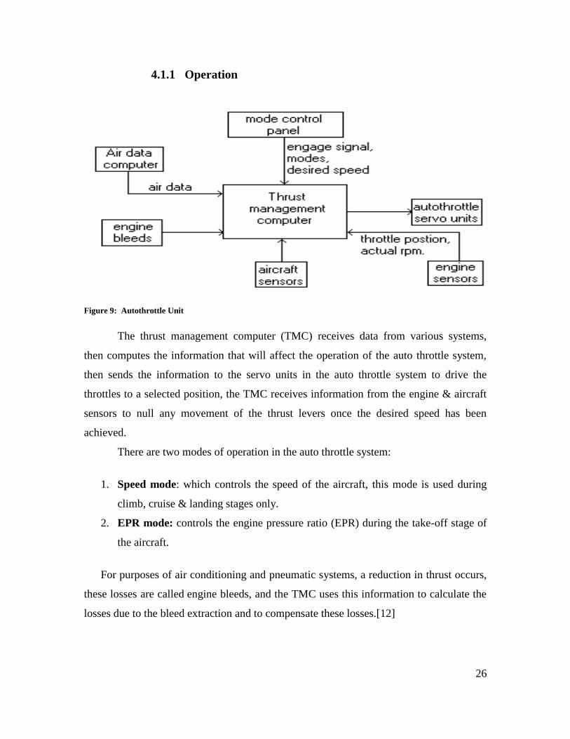
4.1.1 Operation

Figure 9: Autothrottle Unit

The thrust management computer (TMC) receives data from various systems,

then computes the information that will affect the operation of the auto throttle system,

then sends the information to the servo units in the auto throttle system to drive the

throttles to a selected position, the TMC receives information from the engine & aircraft

sensors to null any movement of the thrust levers once the desired speed has been

achieved.

There are two modes of operation in the auto throttle system:

1. Speed mode: which controls the speed of the aircraft, this mode is used during

climb, cruise & landing stages only.

2. EPR mode: controls the engine pressure ratio (EPR) during the take-off stage of

the aircraft.

For purposes of air conditioning and pneumatic systems, a reduction in thrust occurs,

these losses are called engine bleeds, and the TMC uses this information to calculate the

losses due to the bleed extraction and to compensate these losses.[12]

27

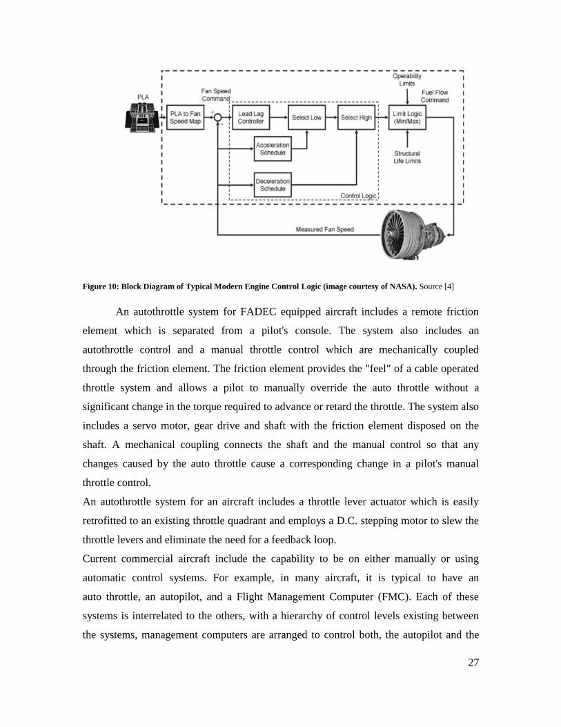
Figure 10: Block Diagram of Typical Modern Engine Control Logic (image courtesy of NASA). Source [4]

An autothrottle system for FADEC equipped aircraft includes a remote friction

element which is separated from a pilot's console. The system also includes an

autothrottle control and a manual throttle control which are mechanically coupled

through the friction element. The friction element provides the "feel" of a cable operated

throttle system and allows a pilot to manually override the auto throttle without a

significant change in the torque required to advance or retard the throttle. The system also

includes a servo motor, gear drive and shaft with the friction element disposed on the

shaft. A mechanical coupling connects the shaft and the manual control so that any

changes caused by the auto throttle cause a corresponding change in a pilot's manual

throttle control.

An autothrottle system for an aircraft includes a throttle lever actuator which is easily

retrofitted to an existing throttle quadrant and employs a D.C. stepping motor to slew the

throttle levers and eliminate the need for a feedback loop.

Current commercial aircraft include the capability to be on either manually or using

automatic control systems. For example, in many aircraft, it is typical to have an

auto throttle, an autopilot, and a Flight Management Computer (FMC). Each of these

systems is interrelated to the others, with a hierarchy of control levels existing between

the systems, management computers are arranged to control both, the autopilot and the

28

auto throttle, autopilots are arranged to control the auto throttle, etc. By adding a Mode

Control Panel (MCP), a Wide range of flight modes become available for use by the

pilot. When landing an aircraft (either manually or using an automatic mode), it is typical

to use the auto throttle to reduce the engine thrust to idle When the aircraft reaches a

certain altitude. For example during an automatic landing, upon reaching 24 feet, the auto

throttle will move the engine control lever to idle. The rate at which the lever is moved

depends on the existing lever position, e.g., a lever position that is already close to idle

will move slower than a lever position that is farther from idle. Typical throttle lever rate

movements are between about 2.2 degrees per second to about 1.7 degrees per second. A

negative sign refers to a resulting reduction in engine throttle setting. The vertical rate at

which the aircraft actually lands on the runway (referred to as the vertical speed or sink

rate at touchdown) is often influenced by current Wind and Weather conditions, and is

quite dependent upon the reduction of throttle to idle. During the aircraft landing

manoeuvre, Wind changes that reduce the airplane airspeed (referred to as an under speed

condition) may result in a reduction of airplane elevator effectiveness and in a high sink

rate at touchdown. This maybe felt as a hard bump at touchdown, which can cause

discomfort to some passengers and can cause wear to the landing gear. Under speed

conditions are also associated with short landing distances.

Autothrottle is used to maintain a specific airspeed or thrust automatically, without the

pilot having to constantly adjust the throttles by hand. This allows the pilot to, say, climbs

or descends in the airplane without having to touch the throttles the auto throttle adjusts

the engines as required to maintain the desired thrust or airspeed. It can be used in many

other phases of flight, too. The main idea is just to lighten the workload on the

pilot(s).[13]

4.2 Air Traffic Control

It is the responsibility of ATC to provide clearances to the crew based on known

traffic and physical airport conditions. States that ATC may clear an aircraft to a different

altitude or route due to traffic conditions.

While complying with a speed adjustment from ATC, the crew must maintain a speed

within plus or minus 0.02 Mach number of the speed specified, unless this is outside the

29

safe operating speed of the aircraft. Changes to this policy could improve fuel efficiency.

Approximately 6-12 percent of fuel burned could be saved by more efficient flight plans

and decreasing holding patterns.

In the impact on fuel consumption when a faster airplane follows a slower airplane is

analysed for a range of 100 nautical miles and three different altitudes. This research

showed that an aircraft’s performance can be reduced by up to 11 percent when forced to

follow a slower airplane.

There are two types of throttle control proposed in literature. First is a total energy

control system (TECS) that combines pitch and throttle control into one multi-input

multi-output (MIMO) control law. The second is a single-input single-output (SISO)

architecture that has two separate control laws for pitch and throttle. The thrust output of

these control laws is a throttle rate command. This gives the pilot visibility as to what the

auto throttle is commanding. This visual feedback was not provided on the A320, a

survey of the pilots of this aircraft was conducted, while not having back driving the

throttles had some advantages, it was concluded that providing movement of the throttles

was preferred.[11]

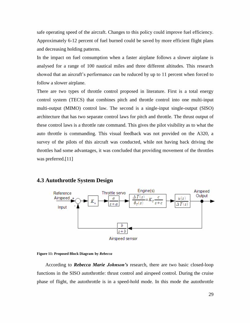
4.3 Autothrottle System Design

Figure 11: Proposed Block Diagram by Rebecca

According to Rebecca Marie Johnson’s research, there are two basic closed-loop

functions in the SISO autothrottle: thrust control and airspeed control. During the cruise

phase of flight, the autothrottle is in a speed-hold mode. In this mode the autothrottle

30

control law commands the throttles to hold the selected airspeed. Figure [11] shows a

simple autothrottle airspeed loop. In figure [11] Ku represents the autothrottle control

law. The throttle servo block is a model of the mechanical servo inside the TQA. The

engines are modelled with a gain, KT, of throttle position to thrust 15 (lbs/degree) and a

lag. The last block of the plant is the transfer function of thrust to airspeed, which is a

simplified model of the airplane dynamics. The feedback of the airspeed

includes another lag to model the filtering present inside the air data sensor a major

design compromise is represented by balancing control accuracy and dynamic response

with throttle activity. A typical flight crew makes steady and infrequent movements of

the throttles, and the autothrottle is expected to mimic this behaviour. Passenger comfort

is also taken into consideration, since they are able to hear adjustments to the engines and

feel changes to aircraft accelerations. Since high-altitude cruise can be the longest phase

of flight, passenger comfort and minimal throttle activity was considered to be the top

priority. While controlling airspeed, a wind gust can create a speed error equal in

magnitude to that of the gust. However, given the bandwidth of this loop, adjusting

throttles to compensate for winds, especially turbulence, could cause continuous cycling

of the throttles. In this situation the crew would set the throttle to a nominal position.

4.4 Summary

Results are not accurate due to losses in fuel every time fuel valve adjusted with each

throttle position is change. This may not be accurately modelled in this simulation,

because the lack of data. As such, they are still not quite matched to the generic

simulation.

Next in chapter five a simple design will be simulated in MATLAB, using the throttle as

servo and engine dynamic as a second order transfer function for a general jet engine.

31

Chapter 5: Simulation of Autothrottle using MATLAB

As seen through literature review Rebecca Marie Johnson’s team concluded that

values for fuel flow rate was not accurate because the lack of data. Here in this chapter

we will try to solve the problem of weak response of the fuel valve that may affect the

fuel consumption and fuel flow rate by designing a controller and simulate it.

5.1 Relation between Thrust, Aircraft Speed and Engine RPM

To increase the thrust of a turbojet engine in flight, it is necessary to increase fuel mass

flow rate. This throttling then increases the exit velocity of air and gives increased thrust.

Specific thrust in turbofan engine for example depends only on the velocity difference

produced by the engine; velocity difference in gas is a pressure. So, how much thrust the

engine will generate depends on how big of a dynamic pressure difference it can create in

the air between its front and back. We need to see if added RPM creates added thrust, yes

it does. Providing the engine with more fuel will create faster escaping hot gases from the

burner. Those will create a bigger dynamic pressure difference between the burner and

the nozzles then the turbine run faster. Power from the turbine is moved to the

compressor which will also turn faster thus pushing out more air.

Figure 12: Simplified Proposed Block Diagram for Auto-throttle

There are two basic closed-loop functions in the SISO auto throttle: thrust control and

airspeed control. In this mode the auto throttle control law commands the throttles to hold

the selected airspeed.

32

1. Engine Dynamic

𝑻. 𝐅 =𝐤

(𝟏+𝛕𝟏𝒔)(𝟏+𝛕𝟐𝒔).......................... (5.1)

Table 3: Variables Table

No 𝛕𝟏 𝛕𝟐

1 0.1 0.01

2 2.3 0.07

3 3 0.1

Where:

K is the gain.τ1,τ2 are the engine time constants.

τ1Represent of the engine coefficients.

τ2Represent of the engine valve coefficients

We check the system stability by obtaining root locus using MATLAB.

Those values give us the wide range of stability ( -10 , -100) as shown in figure[13]

below :

Figure 13: Root Locus

33

2. Throttle

The throttle servo block is a model of control valve. The last block of the plant is the

transfer function. We use a simple control valve as a throttle. The function of a control

valve is to modulate the flow of a process fluid in accordance with some external signal,

usually generated by the controller. The important performance characteristics, from the

standpoint of control, are determined by the relationships between flow, pressure, and

valve travel. Other practical application considerations are valve body pressure ratings,

shutoff requirements, material selection, valve style, valve size, recovery characteristics,

and valve characterization.

Figure 14: Sub system, throttle command

3. Controller

It is the main controller in this circuit, which is P, I, D or PID controllers. Also the PID

controller is a good hardware and its work can be simulated by any advanced software.

4. Transducer

The feedback of the airspeed includes another lag to model the filtering present inside the

air data sensor (transducer sensor) modelled with gain (k/s).

Secondly, by using some means of logic programs like: C, C++, or MATLAB,

hence, the controller can be simulated. Here in the research MATLAB had been chosen.

MATLAB (MATRIX LABROTORY) have many features in using the mathematical

and control functions.

The functions used in the design algorithms are defined as follow:

34

tf: create transfer function; which classified as a model function.

Feedback: calculate the feedback connection of models; which classified as a model

interconnections function.

Step: calculate step response; which classified as a time response function.

PID tool: enables to identify the controlled process from its step response and run

filtration. PIDTOOL also enables to tune various types of PID controller such as P, PI,

PID or PD controllers to get desirable response.

5.2 Results

M-file have been used to plot the response, then for the controller, PID tool used.

Responses with discussions are in figures below:

Figure 15: Open Loop Step Response

35

Steady state (final value) = 1

Rise time (sec) =22

Settling time (sec) =39.2

Figure [15] above shows the response for the subsystem in figure [14], clearly the system

will stay too long in the transient response with almost no transient error. It is a common

case for open loop systems and can be enhanced by closing the loop using a transducer

with integration.

5.2.2 PID Tool

Conditions:

Response time (second) = 0.27

Transient behaviour (second) = 0.6

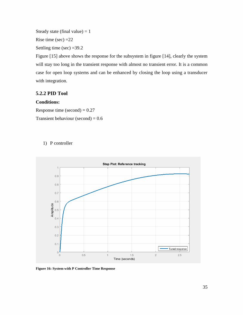
1) P controller

Figure 16: System with P Controller Time Response

36

Rise time (sec) = 1.75

Settling time (sec) =48.5

Over shoot=INF.

In figure [16] above, when a proportional controller added both settling time and

overshoot increased while rise time decreased.

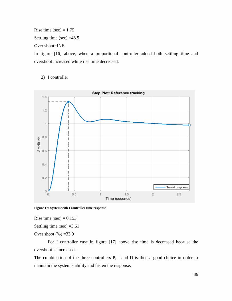
2) I controller

Figure 17: System with I controller time response

Rise time (sec) = 0.153

Settling time (sec) =3.61

Over shoot (%) =33.9

For I controller case in figure [17] above rise time is decreased because the

overshoot is increased.

The combination of the three controllers P, I and D is then a good choice in order to

maintain the system stability and fasten the response.

37

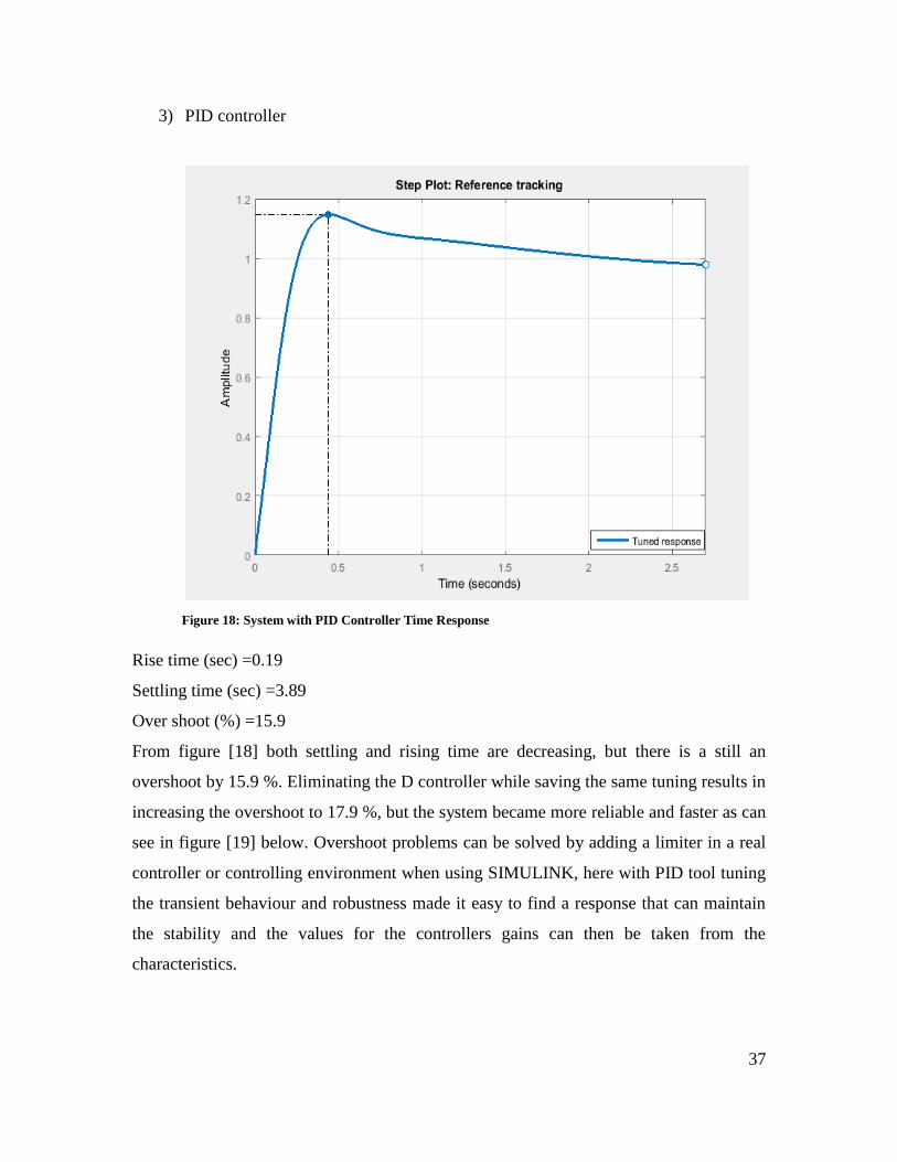
3) PID controller

Figure 18: System with PID Controller Time Response

Rise time (sec) =0.19

Settling time (sec) =3.89

Over shoot (%) =15.9

From figure [18] both settling and rising time are decreasing, but there is a still an

overshoot by 15.9 %. Eliminating the D controller while saving the same tuning results in

increasing the overshoot to 17.9 %, but the system became more reliable and faster as can

see in figure [19] below. Overshoot problems can be solved by adding a limiter in a real

controller or controlling environment when using SIMULINK, here with PID tool tuning

the transient behaviour and robustness made it easy to find a response that can maintain

the stability and the values for the controllers gains can then be taken from the

characteristics.

38

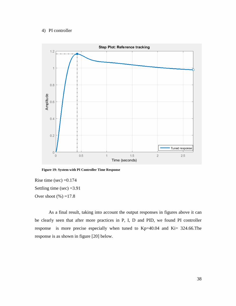
4) PI controller

Figure 19: System with PI Controller Time Response

Rise time (sec) =0.174

Settling time (sec) =3.91

Over shoot (%) =17.8

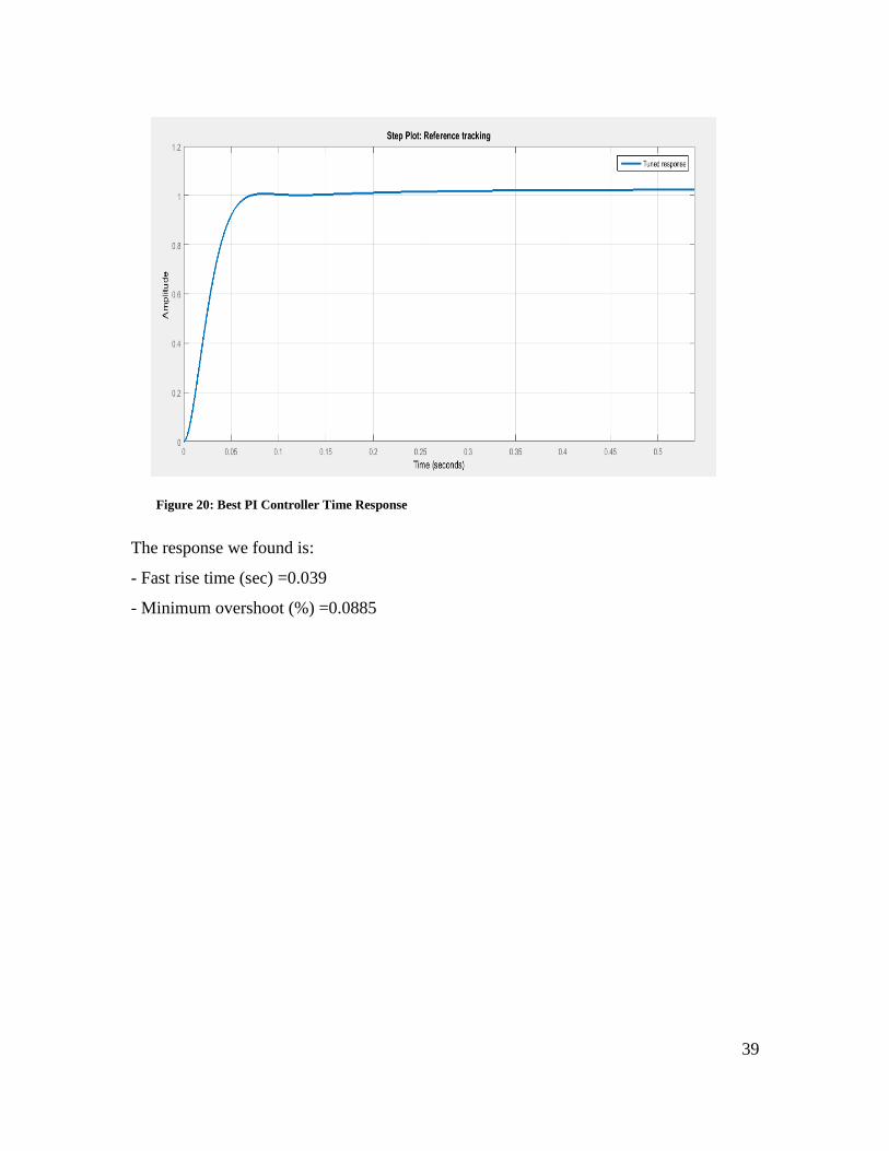
As a final result, taking into account the output responses in figures above it can

be clearly seen that after more practices in P, I, D and PID, we found PI controller

response is more precise especially when tuned to Kp=40.04 and Ki= 324.66.The

response is as shown in figure [20] below.

39

The response we found is:

- Fast rise time (sec) =0.039

- Minimum overshoot (%) =0.0885

Figure 20: Best PI Controller Time Response

40

Chapter 6: Conclusion and Recommendation

By the end of this project a lot of skills have been earned and important knowledge

acquired. The overlapping between the electrical, electronics and programming makes it

deserves to spend the time on it to apply and manage the engineering work.

6.1 Conclusion

Generally the project was capable to meet up the objectives of it. The aim of the

project was to study the effect of implementing autothrottle on reducing pilot workload

and fuel consumption, what claimed to increase the range of the aircraft and reduce flight

cost, by design and control a simple auto-throttle. The design proposed was able to do

this job and the response from the system supported the theory.

Most of the objectives of this project had been met and the overall performance of the

system was good but still having problems with the equations that relating airspeed and

range to rate of fuel consumption.

Generally, using PI controller gave a faster response to open and close the valve of the

fuel injection, but at the expense of requiring more electronics with which to operate the

throttle. There is a lot that can be done for the engine itself, controlling circuit and the

software in order to enhance the performance.

6.2 Future work

Here are some suggestions for further work:

1. The speed equation:

2. Use fuel flow rate equation: ��𝐟 = ��𝐓. 𝐅 to drive a control law while considering

ϴ as input and engine RPM as output.

3. Hardware design microcontroller using one of the available PIKT, ϴ as input,

engine coefficients as interrupts.

4. Another interrupt can be added or can use the switches in the PIKT to do this. To

simulate different flight stages.

5. Taking the study to higher levels, by applying the theory to turbofan engine as the

most fuel efficient engine, adaptive controller will be needed in order to do so.

41

Reference

[1] I. Husain and S. A. Hossain, "Modeling, simulation, and control of switched

reluctance motor drives," Industrial Electronics, IEEE Transactions on, vol. 52,

pp. 1625-1634, 2005.

".د. إ. ع. ا. م. خطاب, "بناء وتصميم المحركات التوربينية للطائرات [2][3] R. Stone, Introduction to internal combustion engines: Palgrave Macmillan,

2012.

[4] S. G. a. N. G. R. Center, "Aircraft Turbine Engine Control Research ".

[5] G. Pahl and W. Beitz, Engineering design: a systematic approach: Springer

Science & Business Media, 2013.

[6] K. J. Åström and B. Wittenmark, Adaptive control: Courier Corporation, 2013.

[7] E. D. Sontag, Mathematical control theory: deterministic finite dimensional

systems vol. 6: Springer Science & Business Media, 2013.

[8] N. S. Nise, CONTROL SYSTEMS ENGINEERING, (With CD): John Wiley & Sons,

2007.

[9] K. Ogata and U. o. Minnesota, Modern Control Engineering 4th Ed

[10] E. L. Wiener and R. E. Curry, "Flight-deck automation: Promises and

problems," Ergonomics, vol. 23, pp. 995-1011, 1980.

[11] R. M. Johnson and I. S. University, "Using an autothrottle to compare

techniques for saving fuel

".

[12] A. Ahmoudy, "aircraft autothrottle system S.P."

[13] D. S. Garg and C. a. D. B.-G. R. C. Chief, "Fundamentals of Aircraft Turbine

Engine Control."

42

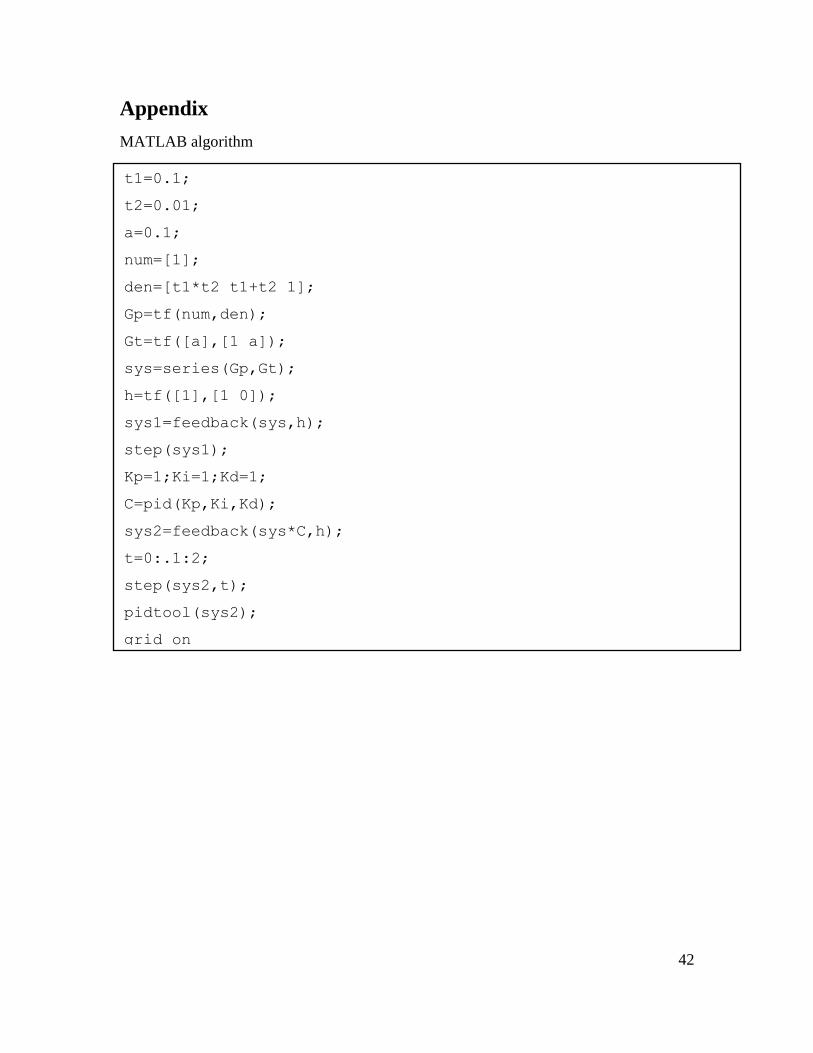
Appendix

MATLAB algorithm

t1=0.1;

t2=0.01;

a=0.1;

num=[1];

den=[t1*t2 t1+t2 1];

Gp=tf(num,den);

Gt=tf([a],[1 a]);

sys=series(Gp,Gt);

h=tf([1],[1 0]);

sys1=feedback(sys,h);

step(sys1);

Kp=1;Ki=1;Kd=1;

C=pid(Kp,Ki,Kd);

sys2=feedback(sys*C,h);

t=0:.1:2;

step(sys2,t);

pidtool(sys2);

grid on