CHAPTER ONE INTERODUCTION - SUST Repository

1

CHAPTER ONE

INTERODUCTION

2

CHAPTER ONE

INTERODUCTION

1.1 Background

Calculations of losses in power systems have been paid attention by many researchers.

Earlier efforts concentrated on energy loss estimation on a yearly basis and power loss

estimations for maximum load situations. The estimated losses were important data when

calculating the energy losses and planning grids. After the global deregulation of electricity

markets, the situation has completely changed. Knowledge of the magnitude of losses with

high accuracy is crucial for fair competition in deregulated markets. Correct value of losses is

necessary for correct evaluation of loss cost.

To be able to calculate losses with high accuracy, accurate data on power input and

output is required. There are several ongoing projects dedicated to improve the data

accuracy. One example is to install meters at the incomers on substations and feeders.

Recently, in 2010SEDC started to install energy meters. This work will be completed in

2014.

There are certain losses which affect the economy of the power system. It is a well-

known fact that all energy supplied to a distribution utility does not reach the end consumer.

The term “distribution losses” refers to the difference between the amount of energy

delivered to the distribution system and the amount of energy customers is billed.

In SEDC Sudan distribution network the percentage distribution losses has been quite

high, from table table.1.1[9]losses percentage is (16.61%) for year 2013.

Table.1.1: SEDC losses report 2013

. Month Losses %

1 JAN 16.7

2 FEB 16.2

3 MAR 19.7

4 APR 17.7

3

5 MAY 22.3

6 JUN 19.9

7 JUL 19.6

8 AUG 12.4

9 SEB 19.4

10 OCT 12.9

11 NOV 8.7

12 DEC 13.9

Average 16.61

Electric power transmission and distribution losses (% of output) in Sudan was last

measured at year 2012, according to the World Bank. Electric power transmission and

distribution losses include losses in transmission between sources of supply and points of

distribution and the distribution to consumers, including pilferage. From (fig 1.1) illustrate

losses for Electric power transmission and distribution losses (% of output) in Sudan since 1998

according to world bank [9].

Fig.1.1 :World Bank Indicators - Sudan - Energy losses

SEDC desires to improve its knowledge on the level of reasonable losses to obtain better

reference values to the results of grid settlement. Since losses vary, knowledge on how losses

vary within SEDC network during different times of the year, different load conditions etc.,

4

would be valuable. If the normal loss variations were known, errors in the metering, reporting

and grid settlement would be much easier to detect.

The Transmission and Distribution losses in the advanced Countries of the world ranging

from (4-12) %. However, the transmission and distribution losses in Sudan are not comparable

with advanced countries as the system operating conditions are. Table 1.2 shows the losses

percentage in selected countries [2].

Table.1.2: Transmission and distribution losses in selected countries

1.2 Objective The aim of this thesis is to investigate and analysis the technical losses of Distribution

grid by using simulation tools known NEPLAN , used extensively for the Power Systems

the main capabilities, features and benefits of using this professional software for planning .

Country 1980 1990 1999 2000 Finland 6.2 4.8 3.6 3.7 Netherlands 4.7 4.2 4.2 4.2 Belgium 6.5 6 5.5 4.8 Germany 5.3 5.2 5 5.1 Italy 10.4 7.5 7.1 5.1 Denmark 9.3 8.8 59 7.1 United States 10.5 10.5 5.7 17.1 Switzerland 9.1 7 7.5 7.4 France 6.9 9 8 7.8 Austria 7.9 6.9 7.9 7.8 Sweden 9.8 7.6 8.4 9.1 Australia 11.6 8.4 9.2 9.1 United Kingdom 9.2 8.9 9.2 9.4 Portugal 13.3 9.8 10 9.4 Norway 9.5 7.1 8.2 9.8 Ireland 12.8 10.9 9.6 9.9 Canada 10.6 8.2 9.2 9.9 Spain 11.1 11.1 11.2 10.6 New Zealand 14.4 13.3 13.1 11.5

5

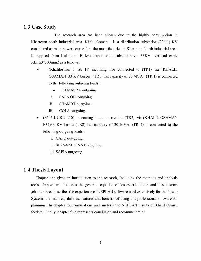
1.3 Case Study

The research area has been chosen due to the highly consumption in

Khartoum north industrial area. Khalil Osman is a distribution substation (33/11) KV

considered as main power source for the most factories in Khartoum North industrial area.

It supplied from Kuku and El-Izba transmission substation via 33KV overhead cable

XLPE3*300mm2 as a follows:

(Khalilosman 1 izb l4) incoming line connected to (TR1) via (KHALIL

OSAMAN) 33 KV busbar. (TR1) has capacity of 20 MVA. (TR 1) is connected

to the following outgoing loads :

ELMASRA outgoing.

i. SAFA OIL outgoing.

ii. SHAMBT outgoing.

iii. COLA outgoing.

(Z605 KUKU L10) incoming line connected to (TR2) via (KHALIL OSAMAN

B32)33 KV busbar.(TR2) has capacity of 20 MVA. (TR 2) is connected to the

following outgoing loads :

i. CAPO out-going.

ii. SIGA/SAIFONAT outgoing.

iii. SAFIA outgoing.

1.4 Thesis Layout Chapter one gives an introduction to the research, Including the methods and analysis

tools, chapter two discusses the general equation of losses calculation and losses terms

,chapter three describes the experience of NEPLAN software used extensively for the Power

Systems the main capabilities, features and benefits of using this professional software for

planning . In chapter four simulations and analysis the NEPLAN results of Khalil Osman

feeders. Finally, chapter five represents conclusion and recommendation.

6

CHAPTER TWO ELECTRICAL LOSSES LITERATURE

7

CHAPTER TWO ELECTRICAL LOSSES LITERATURE

2.1 INTRODUCTION

Due to the expansion in Sudanese national grid, limitation of generation and continuous

increasing in demand. As results the network becomes overloaded, energy transmission and

distribution is accompanied with losses, It is very important for electric power utility to

consider these losses and reduce them wherever practical. Cost of procedures to improve and

reduce the loss is less than the cost of the establishment of a new distribution substations and

consuming time as well.

This chapter is intended to discuss the losses terms and general equation of losses

calculation.

2.2 Electrical system loss Total electric energy losses in the electric system, consists of transmission , transformer ,

and distribution losses between the supply and receiving points.

The average power loss can be expressed as

P loss = P source– P load---------------------------------------------------------------------------------(2.1)

where P source means the average power that the source is injecting into the transmission line

and P load is the power consumed by the load at the end. This is a simple enough calculation,

except that power and current are both time dependent functions and that energy .Energy is

power accumulated over time, or

Wloss = ∫ P loss(t)dt----------------------------------------------------------------- (2.2) with and bas the starting and ending points of the time interval being evaluated.

2.3 The allowable volt drop The acceptable percentage volt drop ± 6% , is international standard for distribution grid.

2.4 Losses study

8

It is common practice to divide losses into categories:

Technical losses:

Technical losses are losses that occur in electrical equipment, especially cables, overhead

lines and power transformers.

Non-technical losses:

consists of losses not related to the physical power system but rather to loss sources like

electricity thefts and errors in billing and meter reading.

2.5 Technical Losses Technical losses in power system are caused by the physical properties components of the

power system. The most obvious example the power dissipation in transmission lines and

transformers due to internal electrical resistance .Following table showing reason of losses at

the transmission and distribution grid

Table.2.1:losses factors in grid of transmission and distribution network

Grid Resistance

loss

Corona loss

Dielectric loss

Copper & iron loss

transformer

Transmission √ √ √ √

Distribution √ × √ √

Technical losses are possible to compute and control , its occur during transmission and

distribution and involve substation, transformer, and line. These include resistive losses of the

primary feeders, the distribution transformer losses (resistive loses in windings and the core

losses), resistive losses in secondary network, resistive losses in service drops and losses in

meter. Losses are inherent to the distribution of electricity and cannot be eliminated.

Technical losses can classify into two type:

1. Load losses: include I2R load in the winding due to load and eddy current , stray

loss due to leaking fluxes in the winding , core clamps , and other parts.load losses

are caused primarily by resistance of the winding conducting to the current that

flows through them.

2. No- load losses : No load losses include core losses and dielectric losses

.Transformer losses are generally no load losses .

9

2.6 Transformer Losses Transformer losses are generally classified into no load or core losses and load losses ,

Fig.2.1 showing the total transformer losses , [2]

Fig.2.1: Transformer losses

Transformer components definitions

Core Losses :Losses that are mainly caused by the resistance of the iron core to

the magnetic flux magnetizing it .

Eddy current losses : are losses caused by the current induced in the iron by

the alternating magnetic field . As the magnetic flux changes with the

alternating current in the coil , a current is induced in the iron that flows at right

angles or cross - sectionally to the magnetic flux .[2]

푃푒 = 퐾푒 ( )² --------------------------------- (2.3)

where :

F : frequency

Bm: maximum magnetic flux density

Pe : Eddy current losses

휌 : Resistivity magnetic material

t : Thickness off iron plate

Ke : Proportional constant

10

Stray Load loss ( synchronous machines ) : The losses due to eddy currents in

copper and additional core losses in the iron, produced by distortion of the magnetic

flux by the load current, and including that portion the core loss associated with

the resistance drop.

Hysteresis loss ( power and distribution transformers): The energy loss in magnetic

material that results from an alternating magnetic field as the elementary magnets

within the material seek to align themselves with the reversing magnetic field..

푃 = 퐾 푓퐵 . ---------------------------------------(2.4) where

fh : Hysteresis Loss

F : Frequency

Bm : Maximum Magnetic Flux Density

Kh : Proportional Constant

Auxiliary losses : are losses caused by the use of cooling equipment such as fans and

pumps to increase the loading capability of substation transformers.

2.7 Reasons of technical losses: They are major reasons in transmission and distribution grid can cause obvious losses ,

due to material parameters of power system component quality and right network planning.

Following are some of the major reasons of power system grid:

1. The volt drops.

2. Low load power factor

3. Improper earthing at consumer end.

4. Long single phase lines.

5. Unbalanced loading.

6. Losses due to overloading.

7. Losses due to poor standard of equipments.

8. Harmonics distortion.

2.8 Non-Technical Losses (Commercial Losses)

Non-technical losses, sometimes called “commercial losses”, are very important

because they often contribute to a large extent to the power that the utility is not paid for.

11

it's related to metering errors, inaccurate meters, improperly read meters and estimated

consumption due to lack of meters. Unauthorized connections as well as administrative

errors are other possible sources of non-technical losses. From the examples above it is

clear that most non-technical losses are associated with low voltage distribution

networks. At medium voltage distribution level, non-technical losses are primarily caused

by inaccurate meters and tampering with measurement transformers .At transmission

voltage level non-technical losses are often related to metering errors at nodes. On

transmission level, nontechnical losses are rare and can be neglected .

2.9 Line Losses and Voltage Drop Relationship

Line losses are from the line current flowing through the resistance of the conductors. After

distribution transformer losses, primary line losses are the largest cause of losses on the

distribution system. Like any resistive losses, line losses are a function of the current squared

multiplied by the resistance (I2R).

Because losses are a function of the current squared, most losses occur on the primary near

the substation. Losses occur regardless of the power factor of the circuit

Approximations method are the common way for calculate drop. A uniformly distributed load

along a circuit of length (L) has the same losses as a single lumped load placed at a length of

(l/3) from the source end. For voltage drop, the equivalent circuits are different: a uniformly

distributed load along a circuit of length(L ) has the same voltage drop as a single lumped load

placed at a length of (l/2) from the source end. This (1/2) rule for voltage drop and the (1/3) rule

for losses are helpful approximations when doing hand calculations or when making

simplifications to enter in a load-flow program.

Losses, voltage drop, and capacity are all interrelated. Three-phase circuits have the highest

power transfer capacity, the lowest voltage drop, and the lowest losses.

Equivalent voltage drop Equivalent voltage drop

L L

I I

12

Equivalent voltage drop Equivalent voltage drop

L L

I I

fig.2.2: Load Distribution and Dispersal Loss Factor

Table 2.2 Load Distribution and Dispersal Loss Factor

2.10 Losses factors

Utilities consider both peak losses and energy losses. Peak losses are important because they

compose a portion of the peak demand; energy losses are the total kilowatt-hours wasted as heat

in the conductors. The peak losses are more easily estimated from measurements and models.

The average losses can be found from the peak losses using the loss factor Fl:

퐹l = Average

----------------------------------------------(2.5)

Losses factor use to measure energy losses if the value of losses is known.

13

Load factor is the ratio between average load and maximum load through cretin period , and

calculated from the following equations

Averageload =

----------------------(2.6),

loadfactor =

=

--------------(2.7)

Normally there is no enough information to directly measure the loss factor. For find the load

factor (the average demand over the peak demand). The loss factor is some function of the load

factor squared. The most common approximation is this is often used for evaluating line losses

and transformer load losses (which are also a function of I2R). Load factors closer to one result

in loss factors closer to one.

fig.2.3 : Relation between load and loss factor

14

CHAPTRE THREE METHODOLOGY AND MODELING BY NEPLAN

15

CHAPTRE THREE

METHODOLOGY AND MODELING BY NEPLAN

3.1 INTRODUCTION Many of electrical and power systems engineering laboratories must be realistic because

cannot be performed practical experiences on a HV transmission system and some of

equipments is often expensive. This chapter describes the experience of NEPLAN software

used extensively for the Power Systems the main capabilities, features and benefits of using

this professional software for planning .

The importance of simulation in power system engineering can be seen in the variety of

simulation tools there are available in various forms and brands around the power engineering

academic/research centers, electrical utilities, industries and companies. Software packages

for power system analysis can be divided into two classes of tools:

Commercial software. These tools represent a conventional and an attractive option for

education process due the many advantages of using. These software packages are created

and developed by important research or electric utilities companies, are well-known in a

concurrent market, typically well-tested and computationally efficient. For students,

represents a favorable opportunity to meet and use these well-known packages. there is an

extended presentation of most illustrative power engineering software (EDSA,

EUROSTAG, CYME, ETAP, NEPLAN).

Educational/research software are created and used mainly in universities or research

institutions. For educational activities, the flexibility and open-source characteristics are

more important aspects than computational efficiency. These aspects corresponds to the

main advantages of these tools which can be a valid alternative to commercial software for

power engineering education. In the last decade, several high-scientific languages, such as

MATLAB, have become very popular for research and educational purpose. At this aim,

there is a variety of open source educational tools. Most of them are oriented to a specific

aspect (application) of power system analysis .

16

3.2 DEFENTION NEPLAN is a power system software applied worldwide for network planning, modeling

and analysis. NEPLAN is used in more than 80 countries by more than 600 companies, such as

small and large electrical utilities, industries and universities. NEPLAN focuses on modeling

and simulation an analysis on computers, which represent a very efficient method for obtaining

experience and enhance skills with power system. The software has plenty possibilities to

entered graphically all the power systems elements, various analysis tools and flexibility.

Fig. 3.1 NEPLAN Graphic User Interface

NEPLAN is a very user friendly planning and information system for electrical-,gas- and

water- networks and one of the most complete planning, optimization and simulation tool for

transmission, distribution, generation and industrial networks. The power system analysis

software NEPLAN consists of several modules, The modules can be grouped as follows:

I. General :

• Load Flow .

• Short Circuit Analysis.

• Reliability Analysis.

17

II. Distribution

• Load Flow with Load profiles .

• Optimization of Distribution Network .

• Optimal separation point .

• Optimal Feeder Reinforcement .

• Low-voltage calculation .

• Capacitor Placement.

III. Transmission

• Contingency Analysis .

• Optimal power flow .

• Voltage stability .

• Small signal stability.

• Transient stability .

• Dynamic Transient stability.

• Net transfer capacity.

IV. Industrial

• Harmonic Analysis .

• Motor starting..

• Cable dimensioning.

V. Protection

• Fault finding analysis.

• Over current protection .

• Distance protection .

• Investment analysis.

3.3 Design in NEPLAN NEPLAN permits to define, develop and manage the power systems elements, data,

library and graphics. The main elements used for network design and applications are:

Transmission network elements: AC and DC transmission lines, two, three

or four windings transformers, buses

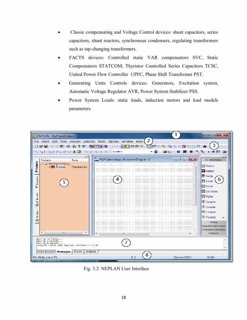
18

Classic compensating and Voltage Control devices: shunt capacitors, series

capacitors, shunt reactors, synchronous condensers, regulating transformers

such as tap-changing transformers.

FACTS devices: Controlled static VAR compensators SVC, Static

Compensators STATCOM, Thyristor Controlled Series Capacitors TCSC,

United Power Flow Controller UPFC, Phase Shift Transformer PST.

Generating Units Controls devices: Generators, Excitation system,

Automatic Voltage Regulator AVR, Power System Stabilizer PSS.

Power System Loads: static loads, induction motors and load models

parameters.

Fig. 3.2 NEPLAN User Interface

19

From fig .3.2 ,numbers indicate the following window features:

1. Title bar .

2. Menu option bar

3. Toolbar .

4. Workspace with diagrams and data tables.

5. Variant Manager .

6. Symbol Window.

7. Message Window .

8. Status bar.

3.4 The Basic Elements of NEPLAN To understand the NEPLAN environment, it is essential that certain concepts used

in the system are described

fig.3.3 :One line diagram with network components

The following are Elements of NEPLAN :

1. Notes : A node is the connection point of two elements or a location, where

electrical energy will be produced or consumed (generator, load). A node is

described by:

Name,

nominal system voltage in kV,

20

zone and area,

type of node (main bus bar, bus bar, sleeve, special node),

description,

2. Elements: An element corresponds to a network component, like e.g. line,

transformer or electrical machine. An element is described topological by a

starting and an ending node. The elements will be described electrical by the

rated current, rated power and rated voltage and its parameters, such as losses,

reactance,

3.5 Procedure of NEPLAN implementation in this thesis

For study and analysis any cases, all elements parameters and data sheets of lines

and transformers must be known and Inserting into the software .see fig.3.4 , for this

thesis information's have been taken from SEDC distribution Control Center.

fig.3.4 :Element parameters Data insertion

21

fig.3.5 :Creation grid

3.6 Input data all element have data and its import to fill all items for items:

3.6.1 network feeder Table 3. 1:network parameters

Name

SK max

IK max

R(1)/X(1) max

Z(0)/Z(1) max

R(0)/X(0) max

C1

SK min

IK min

R(1)/X(1)min

Z(0)/Z(1) min

R(0)/X(0) min

LF-

type

U oper %

sd 1250

3.28

0.1 1.667 0 0 1250

3.28

0 0 0 SL 100

3.6.2 loads Table 3. 2:loads parameters

Name LF Type P Q Units IZB PQ 34.85 12.3 HV

3.6.3 lines Table 3. 3:loads parameters

Name Length Number Units R(1) X(1) C(1) B(1) R(0) X(0) C(0) B(0) G(0) I max

KU 12 1 km 0.067 0.302 0.013 4.103 0.262 1.2 0.005 1.50 0 1250

22

3.6.4 transformers Table 3. 4:transformer parameters

Name Conn 1 Con 2 Conn 3 Vector group Sr MVA

V 1 KV V 2 KV

IZ KU MAN PA YNyn0d11 100 33 11

3.7 MODELING

3.7.1 Introduction

Sudanese Distribution Electricity Company (SEDC) for last years has experienced a

significant increase in the loads. This results in heavily loaded lines in distribution network due to

the limited capacity of substations. Distribution of electric power is accompanied with losses, it is

very important for electric power suppliers to consider these losses and reduce them wherever

practical .Cost of procedures to improve and reduce the loss is less than the cost of the

establishment of a new distribution substations and consuming time as well.

This thesis, represent investigation and analysis the technical losses which occurs in

numerous small components in the distribution system, such as transformers and distribution lines.

While each of these components may have relatively small losses, the large number of components

involved makes it important to examine the losses in the distribution system.

3.7.2 Case study The research area has been chosen due to the highly consumption in Khartoum north

industrial area.

Khalil Osman is a distribution substation (33/11) KV considered as main power source for

the most factories in Khartoum North industrial area. It supplied from Kuku and El-Izba

transmission substation via 33KV overhead cable XLPE3*300mm2 as a follows:

(Khalilosman 1 izb l4) incoming line connected to (TR1) via (KHALIL

OSAMAN) 33 KV busbar. (TR1) has capacity of 20 MVA. (TR 1) is connected

to the following outgoing loads :

ELMASRA outgoing.

23

SAFA OIL outgoing.

SHAMBT outgoing.

COLA outgoing.

(Z605 KUKU L10) incoming line connected to (TR2) via (KHALIL OSAMAN

B32)33 KV busbar.(TR2) has capacity of 20 MVA. (TR 2) is connected to the

following outgoing loads :

CAPO out-going.

SIGA/SAIFONAT outgoing.

SAFIA outgoing.

Table 4.1 illustrate the total actual load by transformer, meanwhile the capacities of

the substation are 40 MVA.

Table 3.5: distribution by transformer

Description TR 1 TR 2

Number of feeder 4 3

Number of customer 50 33

Total capacity (KVA) 27900 21450

24

Fig 3.6: Khalil Osman distribution substation Single line diagram

25

Khalil Osman area contains a large number of factories and loads of different capacities

distributed unevenly on different distribution lines putting strain resulting in losses power.

Following tables gives an idea of transformer capacities. The total real demand is 49.35MVA

while the capacities of two substation transformer are 40 MVA.

Table 3.6: Transformers (1) loads capacities

Transformer Outgoing name Load capacity KVA

TR (1)

ELMASRA 4350 SAFA OIL 16350

COLA 7000

SHAMBAT 200

TAOTAL 27900

Table 3.7 : Transformers (2) loads capacities

Transformer Outgoing name Load capacity KVA

TR (2) CAPO 5500

SIGA/SAIFONAT 8750 SAFIA 7200

TOTAL 21450

3.7.3 Modeling and simulation

The link between substation and customers is made up of several cable sections and

transformer. The information of component, such as cable, cable length and transformer data is

typically stored in a Geographic Information System (GIS).for this research data was collected in

Khartoum grid control center.

When building a network model, the first step is to extract the information for Simulation by

NEPLAN software. Second step is to simulate the area. Then All actual data of network

component (line and transformer parameters) implemented into the simulation, fig (3.7 , 3.8 , 3.9

) : illustrates Single line diagram of case area) the load flow run to determine the following items:

1. Line voltage drop.

26

2. Line and transformer loss.

3. Load power factor.

4. Line loading.

5. Phase angle.

6. P & Q for grid elements.

7. Losses.

27

fig3.7 :Single line diagram for CAPO, SIGA/ SAIFONAT and SAFIA

28

fig3.8 :Single line diagram for ELMASRA

fig 3.9 :Single line diagram for COLA and SHMABT and SAFA oil

29

3.7.3.1 SIGA/SAIFONAT outgoing losses detail

The feeder length is 9.271 Km connecting with five customers with overhead line

XLPE3*185mm2 .The voltage drop is acceptable and within the standard, maximum percentage

voltage drop value is 1.4 %. Table 3.8 :illustrate Voltage drop of SIGA/SAIFONAT feeder

Table 3.8 :Voltage drop of SIGA/SAIFONAT feeder

Load Name nominal voltage KV

calculated voltage

D V % Distance from substation (Km)

1 ALSARF ALSHEE

11 10.912 0.8 2.365

2 SIGA1 11 10.866 1.218182 4.753 3 SIGA2 11 10.847 1.390909 6.683 4 SIGA5 11 10.854 1.327273 7.522 5 SIGA6 11 10.852 1.345455 9.655

fig3.10 : voltage drop of SIGA/SAIFONAT feeder at the customer transformer

Analysis software display a values of line losses for each items in the

SIGA/SAIFONAT feeder ,the highest losses value at Node 3275 (marked in red color)

item name SIGA/SAIFONAT KHO L4,Table 3.9 : illustrates line losses of

30

SIGA/SAIFONAT feeder, the conductor size of this line is (35 mm2) with length 1.344

km , this feeder feeds two loads with capacity of 4000 KVA. The standard request for all

medium voltage line to use 185 mm2.

Table 3.9: line losses of SIGA/SAIFONAT feeder

ID Node Element name Losses P % P

Losses

Q

Losses

3259

KHALIL

OSMAN

B12

SIGA/SAIFONAT KHO L1 4.15% 0.096 -7.79

3220 N3204 SIGA/SAIFONAT KHO L2 12.58% 0.291 0.212

3228 N3225 L1229799101 0.91% 0.021 -15.11


3275 N3272 SIGA/SAIFONAT KHO L4 44.64% 1.033 -12.79


3296 N3293 L1229799126 0.22% 0.005 -0.28


3374 N3332 L1229799136 7.00% 0.162 -8.9



3410 N3407 L1229799156 0.00% 0 -0.24


3450 N3447 L1229799166 0.04% 0.001 -9.86

31

Table 3.10 :Transformer Losses of SIGA/SAIFONAT feeder

ID Node Element name Losses P % P Losses Q Losses

3236 N3225 TR2-3236 17.66% 0.101 0.375

3304 N3293 TR2-3304 40.73% 0.233 1.268

3382 N3332 TR2-3382 40.91% 0.234 1.272

3418 N3407 TR2-3418 0.35% 0.002 0.012

3458 N3447 TR2-3458 0.35% 0.002 0.012

Total feeder losses is 2.886 KW

fig 3.11 :line loss condition of SIGA/SAIFONAT

32

fig3.12 :Transformer loss condition of SIGA/SAIFONAT

3.7.3.2 SAFIA outgoing losses detail

Safia feeder consider as main problem with length 23.8684 Km connecting with 24

customers by overhead line XLPE3*185mm2 , all customer connect from main to

transformer by cable size 35 mm2.Element (ID: 4355) has conductor size 35mm2this

element connect 6 transformer with 3450 KVA capacity . The voltage drop is out of

distribution standard (6 %) in the end of feeder , maximum percentage voltage drop

value is 6.36% (marked in red) . Table 3.11: illustrate Voltage drop of Safia feeder

Table 3.11: Voltage drop of Safia feeder


calculated voltage

D V % Distance from substation (Km)

1 SPESTIAL 11 10.752 2.25 8.364 2 KHAS 11 10.64 3.27 9.916 3 ALSHRG ALAWST

LLTAGLIF 11 10.593 3.70 11.028

4 DAR ALADOWA LLNSHER

11 10.581 3.81 11.708

5 DUBI 2 11 10.572 3.89 11.706 6 SAEED LLMOAD

ALGZAYA 11 10.564 3.96 12.709

7 DUBI 11 10.544 4.15 13.741

33

8 SELIDOR 11 10.556 4.04 14.811 9 DANFODEW 11 10.563 3.97 14.642 10 ZEWT ALWAHA 11 10.562 3.98 12.825 11 SABOON SATEE 11 10.561 3.99 14.879 12 SAEED ALGZAEAA 11 10.563 3.97 16.496 13 CRYSTAL 11 10.479 4.74 12.131 14 CRYSTAL 2 11 10.479 4.74 15.173 15 CRYSTAL 3 11 10.479 4.74 15.173 16 PEPSI 2 11 10.465 4.86 15.173 17 PEPSI 1 11 10.465 4.86 15.545 18 Load 11 10.44 5.09 15.545 19 PEPSI 4 11 10.429 5.19 18.3116 20 KELOBATRA 11 10.425 5.23 16.7766 21 ALHYAH ALGOMEA

LLABHATH ALGELOGY 11 10.409 5.37 17.9286

22 ALBALAT ALMZAYKO 11 10.411 5.35 20.3936 23 ALKEBREET

ALHADETH 11 10.3 6.36 20.6316

24 ALADADAT 11 10.3 6.36 20.7166

fig3.13 :voltage drop of Safia feeder at the customer transformer

34

Neplan analysis software display a values of line losses for each items in the Safia

feeder . This feeder has highest losses in the whole area . The highest losses value at

element NO : 4518,item name L1229799633(marked in red) (Table 3.12: illustrates line

losses of Safia feeder, the length of this line is (0.529) km with cable size 35 mm2this

represent30.02 % of this feeder losses. The second lower losses value at element NO

3840 the length of this line is (0.052) km losses of this line 18.15% . with cable size 35

mm2, element NO 4549,length (0.497)km ,losses of this line 18.15%.

Table 3.12: line losses of Safia feeder

ID Node Element name Losses P % P Losses Q Losses

3627 N3616 SAFIA KHO L1 0.80% 9.232 -70.81

3622 N3619 L..1229800340 3.36% 5.581 10.528

3692 N3619 L1229797068 0.74% 2.753 5.197

3656 N3632 L1229797269 0.02% 0 -10.85

3661 N3640 L1229799284 0.73% 0 -0.34

3723 N3720 L1229799273 0.53% 3.384 6.386

3754 N3720 L1229797078 0.00% 0.179 0.096

3762 N3751 L1229797083 0.01% 0.038 -7.79

3793 N3751 L1229797088 0.00% 0.167 -0.07

3832 N3790 L1229797098 0.00% 0.113 -0.34

3801 N3798 L1229797093 0.00% 0.023 -4.68

3871 N3829 L1229797108 30.02% 0.026 -0.36

3840 N3837 L1229797103 18.15% 0.002 -0.47

3921 N3868 L1229797118 8.95% 0.011 -0.34

3882 N3876 L1229797113 0.00% 0.158 -0.38

3952 N3949 L1229800119 0.00% 1.36 2.378

4133 N3957 L1229800151 11.00% 0 -0.31

35

3965 N3957 L..1229800014 0.58% 0.162 0.275

4000 N3970 L1229799986 0.12% 0 -0.36

3973 N3986 L1229800367 0.54% 0.011 -0.37

4044 N4041 L..1229799999 0.37% 0.005 -0.31

4052 N4049 L1229800141 0.07% 0.001 -0.94

4169 N4080 L1229800354 0.08% 0 -0.31

4094 N4088 L1229800146 0.01% 0.002 -7.13

4164 N4161 L..1229800017 0.04% 0.047 0.078

4188 N4177 L1229797173 0.51% 2.2 3.65

4180 N4177 L1229800008 4.42% 1.412 -9.15

4196 N4185 L1229799735 0.00% 0.424 -8.77

4282 N4185 L1229799718 0.53% 0.401 0.472

4290 N4279 L1229799740 0.00% 0.091 -4.27

4344 N4279 L1229799723 0.80% 0.196 0

4355 N4341 L1229797228 3.36% 0.453 -6.62

4366 N4352 L1229797233 0.74% 0 -0.53

4405 N4352 L1229799550 0.02% 0.147 -0.02

4374 N4363 L1229800302 0.73% 0.001 -8.64

4444 N4402 L1229799555 0.53% 0.076 -0.17

4452 N4441 L1229797259 0.00% 0.004 -0.41

4486 N4441 L1229797243 0.01% 0.053 -0.25

4494 N4483 L1229799617 0.00% 0.043 -0.2

4502 N4491 L1229799622 0.00% 0.038 -0.18

4510 N4499 L1229797338 0.00% 0.008 -0.22

36

4518 N4507 L1229799633 30.02% 0.014 -4.67

4549 N4507 L1229797348 18.15% 0 -0.18

4580 N4577 L1229797294 8.95% 0.007 -0.17

4588 N4698 L1229797299 0.00% 0.023 -4.32

Table 3.13: Transformer losses of Safia feeder

ID Node Element name Losses % P Losses Q Losses

3236 N3225 TR2-3236 4.60% 0.101 0.375

3304 N3293 TR2-3304 10.62% 0.233 1.268

3382 N3332 TR2-3382 10.67% 0.234 1.272

3418 N3407 TR2-3418 0.09% 0.002 0.012

3458 N3447 TR2-3458 0.09% 0.002 0.012

3669 N3643 TR2-3669 0.87% 0.019 0.04

3700 N3689 TR2-3700 0.87% 0.019 0.041

3731 N3720 TR2-3731 1.64% 0.036 0.081

3770 N3759 TR2-3770 5.79% 0.127 0.531

3809 N3798 TR2-3809 5.83% 0.128 0.532

3848 N3837 TR2-3848 5.83% 0.128 0.532

3898 N3879 TR2-3898 5.83% 0.128 0.535

3932 N3918 TR2-3932 2.19% 0.048 0.119

4021 N3994 TR2-4021 1.64% 0.036 0.081

4060 N4049 TR2-4060 3.10% 0.068 0.209

4102 N4088 TR2-4102 2.19% 0.048 0.118

4141 N4130 TR2-4141 3.10% 0.068 0.209

4235 N4193 TR2-4235 5.93% 0.13 0.543

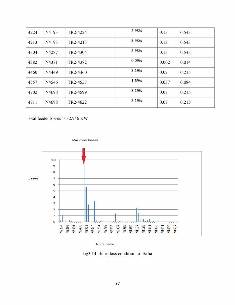
37

4224 N4193 TR2-4224 5.93% 0.13 0.543

4213 N4193 TR2-4213 5.93% 0.13 0.543

4304 N4287 TR2-4304 5.93% 0.13 0.543

4382 N4371 TR2-4382 0.09% 0.002 0.014

4460 N4449 TR2-4460 3.19% 0.07 0.215

4557 N4546 TR2-4557 1.69% 0.037 0.084

4702 N4698 TR2-4599 3.19% 0.07 0.215

4711 N4698 TR2-4622 3.19% 0.07 0.215


fig3.14 :lines loss condition of Safia

38

fig3.15 :Transformer loss condition of Safia

3.7.3.3 SHAMBT outgoing losses detail

Shambat feeder is short line with length 0.977Km connecting with one customer

by overhead line XLPE3*185mm2 , this feeder connected as standby with other feeder

from OLD FADUL substation to serving that loads . The voltage drop is acceptable and

within the standard the maximum percentage voltage drop value is 0.7 %. Table

3.14:illustrateVoltage drop of Shambat feeder.

Table 3.14:Voltage drop of Shambat feeder


calculated voltage

V D % Distance from substation (Km)

1 Load 11 10.922 0.7 0.977

Analysis software display losses values of each item , loses in this feeder is

neglected, illustration from table 3.15 : line losses and table 3.15 :transformer losses .

when connect this feeder with OLD FADUL substation loads losses calculation results

will be change .

39

Table 3.14: line losses of Shambat feeder

ID Node Element name Line

losses P Losses Q Losses

1292 KHALIL

OSMAN B11 SHAMBT KHO --- 0 -0.18

1300 N1289 SHAMBT KHO L3 --- 0 -0.04

1316 N1308 SHAMBT KHO L2 --- 0 -8.26

Table 3.16: transformer losses of Shambat feeder

ID

Node Element name Losses P Losses Q Losses

1324 N1308

ELHUSAYNI

SHAMBT TR 100 % 0.034 0.076

Total losses is 0.034 KW

fig 3.16 :Transformer loss condition of shambat

40

3.7.3.4 COLA outgoing losses detail

The feeder length is 2.535Km connecting with four customers by overhead line

XLPE3*185mm2 .The voltage drop is acceptable and within the standard the

maximum percentage voltage drop value is 0.9727 % . Table 3.17:illustrateVoltage

drop of COLA feeder.

Table 3.17:Voltage drop of COLA feeder


calculated voltage

V D % Distance from substation (Km)

1 ALCOLA1 11 10.893 0.9727 2.365 2 ALCOLA2 11 10.893 0.9727 4.753 3 ALCOLA3 11 10.893 0.9727 6.683 4 ALCOLA4 11 10.893 0.9727 7.522

fig3.17 :voltage drop of COLA feeder at the customer transformer

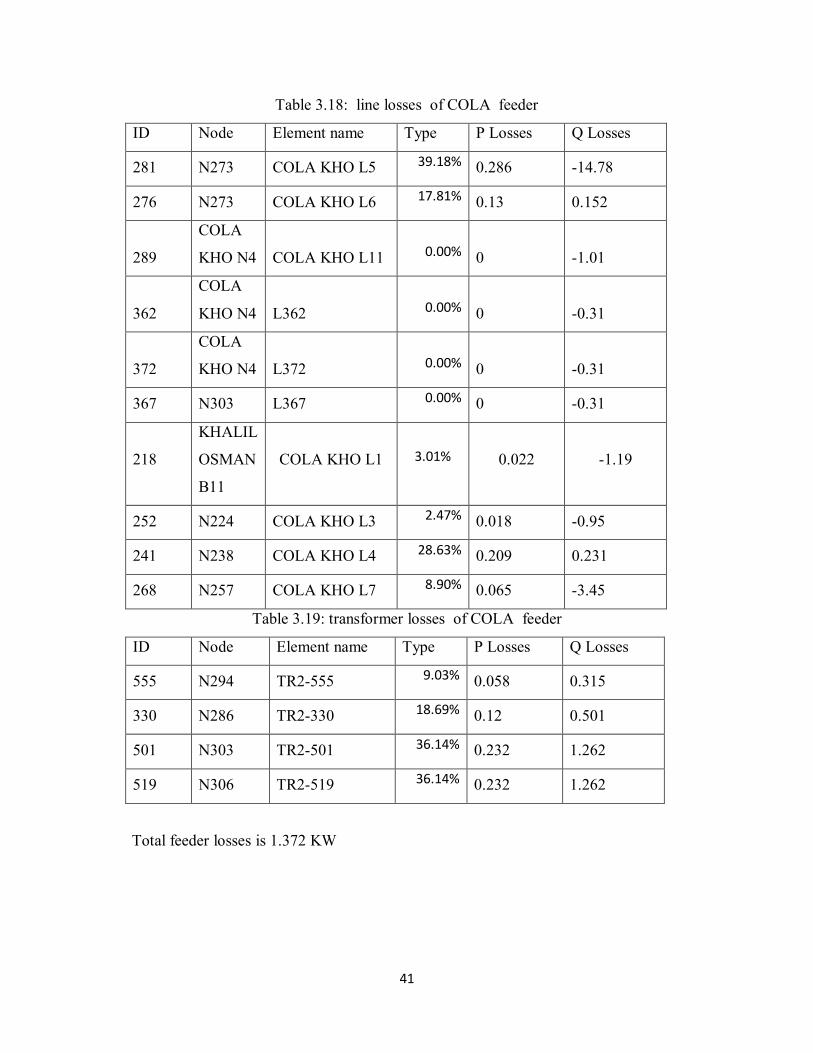
Neplan analysis software display losses for each items in the COLA feeder,

illustration from table (3.18 ) ,this feeder has the lowest losses value in the case area .

41

Table 3.18: line losses of COLA feeder

ID Node Element name Type P Losses Q Losses

281 N273 COLA KHO L5 39.18% 0.286 -14.78

276 N273 COLA KHO L6 17.81% 0.13 0.152

289

COLA

KHO N4 COLA KHO L11 0.00% 0 -1.01

362

COLA

KHO N4 L362 0.00% 0 -0.31

372

COLA

KHO N4 L372 0.00% 0 -0.31

367 N303 L367 0.00% 0 -0.31

218

KHALIL

OSMAN

B11

COLA KHO L1 3.01% 0.022 -1.19

252 N224 COLA KHO L3 2.47% 0.018 -0.95

241 N238 COLA KHO L4 28.63% 0.209 0.231

268 N257 COLA KHO L7 8.90% 0.065 -3.45

Table 3.19: transformer losses of COLA feeder

ID Node Element name Type P Losses Q Losses

555 N294 TR2-555 9.03% 0.058 0.315

330 N286 TR2-330 18.69% 0.12 0.501

501 N303 TR2-501 36.14% 0.232 1.262

519 N306 TR2-519 36.14% 0.232 1.262


42

fig ( 3.18 ) : line condition COLA outgoing

fig ( 3.19 ) : Transformer condition COLA outgoing

43

3.7.3.5 CAPO OUTGOING losses detail

The feeder length is 7.686 Km connecting with four customers by overhead line

XLPE3*185mm2 .The voltage drop is acceptable and within the standard the

maximum percentage voltage drop value is 0.9364% . Table 3.20 :illustrate Voltage

drop of COLA feeder.

Table 3.20:Voltage drop of CAPO feeder


calculated voltage

VD % Distance from substation

(Km) 1 CAPO 11 10.901 0.9000 5.216 2 CAPO 11 10.899 0.9182 5.514 3 CAPO 11 10.896 0.9455 5.613 4 CAPO 11 10.897 0.9364 5.413

fig3.20 :voltage drop of CAPO feeder at the customer transformer

44

Neplan analysis software display losses of each items in the CAPO feeder . The

highest losses value at element NO 3515 which is represent item name CAPO KHO

L1(marked in red)Table 3.21 illustrate line losses of CAPO feeder) the length of this

line is (4.69)km with cable size 185 mm2.

Table 3.21: line losses of CAPO feeder


3539 N3536

CAPO KHO

L5 5.27% 0.065 0.025

3515

KHALIL

OSMAN

B12

CAPO KHO

L1 86.62% 1.068 -72.78

3510 N3493

CAPO KHO

L2 0.16% 0.002 -5.69

3531 N3528

CAPO KHO

L4 6.57% 0.081 -9.95

3523 N3520

CAPO KHO

L3 1.38% 0.017 -8.91

Table 3.22:Transformer losses of CAPO feeder


3547 N3520 TR2-3547 18.58% 0.12 0.5

3579 N3528 TR2-3579 35.76% 0.231 1.261

3599 N3536 TR2-3599 35.76% 0.231 1.261

3487 N3493 TR2-3487 9.91% 0.064 0.196


45

fig ( 3.21 ) : line loss condition CAPO outgoing

fig ( 3.22 ) : Transformer loss condition CAPO outgoing

46

3.7.3.6 ELMASRA losses detail

The feeder length 18.549 Km connecting with 16 customers by overhead line

XLPE3*185mm2 , The voltage drop is acceptable and within the standard the

maximum percentage voltage drop value is 1.72% . Table 3.23 :illustrate Voltage

drop of ELMASRA feeder, this line not short but the voltage drop in the range of

the standard.

Table 3.23:Voltage drop of ELMASRA feeder


calculated voltage

VD % Distance from

substation (Km)

1 TLMAS TARK 11 10.867 1.21 5.469 2 ALCOLA 11 10.865 1.23 5.966 3 TRANS50 11 10.859 1.28 6.095 4 TRANCE200 11 10.858 1.29 6.177 5 TRANSE200 1 11 10.856 1.31 6.959 6 TRANSE 200 2 11 10.846 1.40 7.801 7 TESHOP 11 10.84 1.45 8.284 8 BIZYANOSE 11 10.836 1.49 8.317 9 ALSAFEEH 11 10.821 1.63 8.724 10 AAM 11 10.82 1.64 9.541

11

MKHAZEN ALCOLA 11 10.819 1.65 10.465

12 NASEG BAHRI 11 10.819 1.65 10.543

13 ZEOWT THANI 11 10.819 1.65 11.306

14

ALEZDEHAR LLAHZA 11 10.816 1.67 12.275

15

HANA LLIBASKAWE

T 11 10.811 1.72 11.202

16 DAL 11 10.811 1.72 12.04

47

fig ( 3.23 ) : voltage drop of ELMASRA feeder at the customer transformer

Neplan analysis software display a values of line losses for each items in

the ELMASRA feeder .The highest losses value at element NO : 680 ,item name

ELMASRA KHO L7 (marked in red) Table 4.20: illustrate line losses of ELMASRA

feeder) the length of this line is (0.94 ) km with cable size 185mm2this represent

13. 25 % of this feeder losses see Table 3.24

Table 3.24: line losses of ELMASRA feeder


1094 N1060 L1229798094 0.00% 0 -0.39

3832 N3790 L1229797098 5.13% 0.113 -0.34

606 N603 ELMASRA KHO L2 9.89% 0.218 0.135

595

KHALIL

OSMAN

B11 ELMASRA KHO L1 7.03% 0.155 -13.65

3871 N3829 L1229797108 1.18% 0.026 -0.36

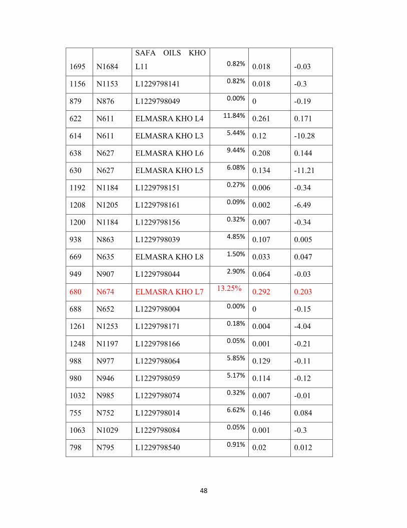
48

1695 N1684

SAFA OILS KHO

L11 0.82% 0.018 -0.03

1156 N1153 L1229798141 0.82% 0.018 -0.3

879 N876 L1229798049 0.00% 0 -0.19

622 N611 ELMASRA KHO L4 11.84% 0.261 0.171

614 N611 ELMASRA KHO L3 5.44% 0.12 -10.28

638 N627 ELMASRA KHO L6 9.44% 0.208 0.144

630 N627 ELMASRA KHO L5 6.08% 0.134 -11.21

1192 N1184 L1229798151 0.27% 0.006 -0.34

1208 N1205 L1229798161 0.09% 0.002 -6.49

1200 N1184 L1229798156 0.32% 0.007 -0.34

938 N863 L1229798039 4.85% 0.107 0.005

669 N635 ELMASRA KHO L8 1.50% 0.033 0.047

949 N907 L1229798044 2.90% 0.064 -0.03

680 N674 ELMASRA KHO L7 13.25% 0.292 0.203

688 N652 L1229798004 0.00% 0 -0.15

1261 N1253 L1229798171 0.18% 0.004 -4.04

1248 N1197 L1229798166 0.05% 0.001 -0.21

988 N977 L1229798064 5.85% 0.129 -0.11

980 N946 L1229798059 5.17% 0.114 -0.12

1032 N985 L1229798074 0.32% 0.007 -0.01

755 N752 L1229798014 6.62% 0.146 0.084

1063 N1029 L1229798084 0.05% 0.001 -0.3

798 N795 L1229798540 0.91% 0.02 0.012

49

Table 3.25: transformer losses of ELMASRA feeder


840 N829

TRANSE200 1 KHO

TR 5.11% 0.034 0.077

1133 N1122

ZEOWT THANI

KHO TR 9.76% 0.065 0.199

1164 N1153

ALEZDEHAR

LLAHZA KHO TR 9.76% 0.065 0.199

887 N876

TRANSE 200 2 KHO

TR 5.11% 0.034 0.077

646 N635

TLMAS TARK KHO

TR 2.70% 0.018 0.039

918 N907 TESHOP KHO TR 9.76% 0.065 0.198

1219 N1205

HANA

LLIBASKAWET

HKO TR 6.76% 0.045 0.113

957 N946 BAHRI 11 KV 5.11% 0.034 0.077

997 N985

MKHAZEN

ALCOLA KHO TR 9.76% 0.065 0.199

763 N752 TRANS50 KHO 1.35% 0.009 0.018

1040 N1029

NASEG BAHRI

KHO TR 9.76% 0.065 0.199

1071 N1060

ALSAFEEH KHO

TR 5.11% 0.034 0.077

806 N795

TRANCE200 KHO

TR 5.11% 0.034 0.077

1102 N1091 AAM KHO TR 5.11% 0.034 0.077

1269 N1253 DAL KHO TR 9.76% 0.065 0.199

50


fig ( 3.24 ) : line loss condition ELMASRA outgoing

fig ( 3.25 ) : Transformer loss condition ELMASRA outgoing

51

3.7.3.7 SAFA OIL

The feeder length is 24.08 Km connecting with 28 customers by overhead line

XLPE3*185mm2 and XLPE 70 mm2. The voltage drop is acceptable and within the

standard the maximum voltage drop value is 1.3 % Table 3.25: display Voltage drop

SAFA OIL feeder

Table 3.25 Voltage drop of SAFA OIL feeder


calculated voltage

VD % Distance from substation

(Km) 1 Load 11 10.899 0.92 1.326 2 Load 11 10.898 0.93 1.361 3 Load 11 10.898 0.93 1.627 4 Load 11 10.898 0.93 1.442 5 Load 11 10.897 0.94 1.655 6 Load 11 10.897 0.94 1.747 7 Load 11 10.897 0.94 1.844 8 Load 11 10.896 0.95 2.301 9 Load 11 10.895 0.95 1.893 10 Load 11 10.895 0.95 2.06 11 Load 11 10.895 0.95 2.198 12 Load 11 10.895 0.95 2.405 13 Load 11 10.892 0.98 2.495 14 Load 11 10.885 1.05 2.523 15 Load 11 10.878 1.11 2.776 16 Load 11 10.866 1.22 1.499 17 Load 11 10.857 1.30 1.709 18 Load 11 10.861 1.26 2.113 19 Load 11 10.86 1.27 2.548 20 Load 11 10.857 1.30 2.588 21 Load 11 10.857 1.30 2.623 22 Load 11 10.857 1.30 2.609 23 Load 11 10.86 1.27 2.648 24 Load 11 10.86 1.27 2.693 25 Load 11 10.86 1.27 2.806 26 Load 11 10.86 1.27 2.786 27 Load 11 10.86 1.27 2.905 28 Load 11 10.86 1.27 2.917

52

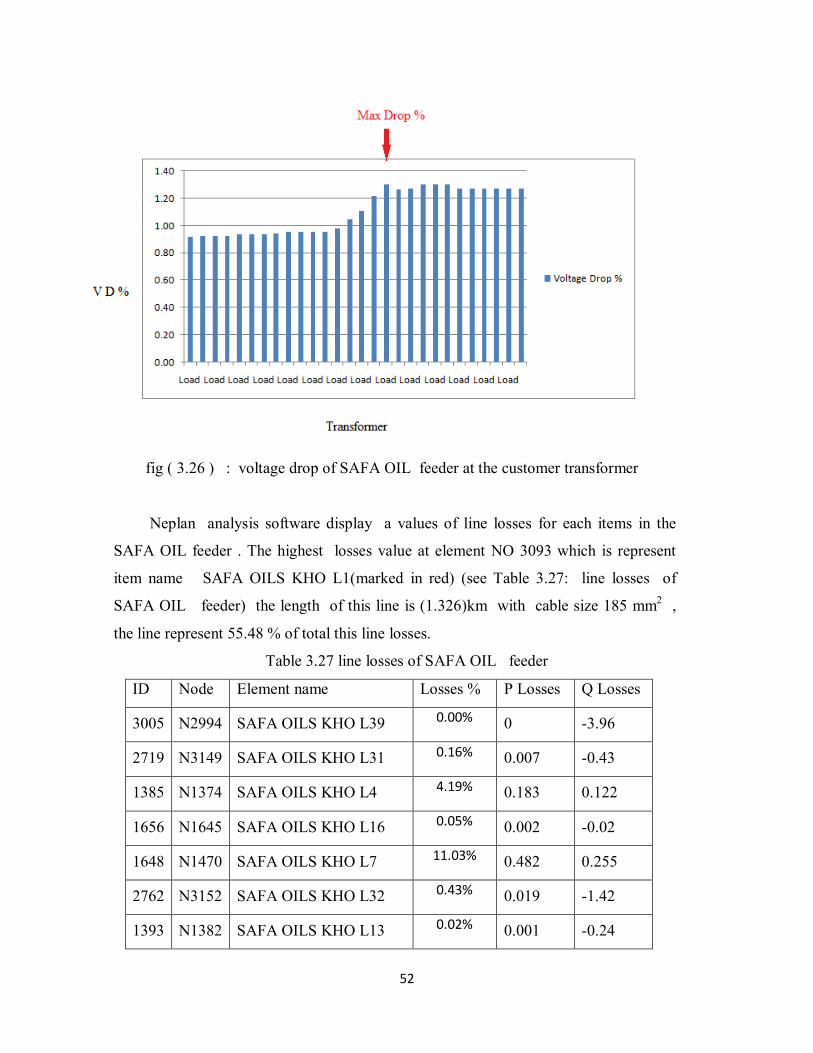
fig ( 3.26 ) : voltage drop of SAFA OIL feeder at the customer transformer

Neplan analysis software display a values of line losses for each items in the

SAFA OIL feeder . The highest losses value at element NO 3093 which is represent

item name SAFA OILS KHO L1(marked in red) (see Table 3.27: line losses of

SAFA OIL feeder) the length of this line is (1.326)km with cable size 185 mm2 ,

the line represent 55.48 % of total this line losses.

Table 3.27 line losses of SAFA OIL feeder


3005 N2994 SAFA OILS KHO L39 0.00% 0 -3.96

2719 N3149 SAFA OILS KHO L31 0.16% 0.007 -0.43

1385 N1374 SAFA OILS KHO L4 4.19% 0.183 0.122

1656 N1645 SAFA OILS KHO L16 0.05% 0.002 -0.02

1648 N1470 SAFA OILS KHO L7 11.03% 0.482 0.255

2762 N3152 SAFA OILS KHO L32 0.43% 0.019 -1.42

1393 N1382 SAFA OILS KHO L13 0.02% 0.001 -0.24

53

1687 N1645 SAFA OILS KHO L6 3.25% 0.142 0.056

3059 N3164 SAFA OILS KHO L42 0.00% 0 -0.43

1424 N1382 SAFA OILS KHO L3 8.38% 0.366 0.227

1703 N1692 SAFA OILS KHO L24 0.00% 0 -0.43

1695 N1684 SAFA OILS KHO L11 0.41% 0.018 -0.03

2799 N3155 SAFA OILS KHO L35 0.00% 0 -1.51

1996 N1848 SAFA OILS KHO L19 0.00% 0 -0.01

1442 N1421 SAFA OILS KHO L14 0.00% 0 -0.24

362

COLA

KHO L362 0.00% 0 -0.31

3098 N3087 SAFA OILS KHO L2 0.27% 0.012 -0.53

3093 N3087 SAFA OILS KHO L1 55.48% 2.424 -18.67

2553 N1684 SAFA OILS KHO L20 2.47% 0.108 -0.03

2004 N1993 SAFA OILS KHO L28 0.00% 0 -0.38

1742 N1731 SAFA OILS KHO L25 0.00% 0 -0.33

1734 N1692 SAFA OILS KHO L10 0.11% 0.005 -0.01

2836 N3161 SAFA OILS KHO L33 0.00% 0 -97.14

3103 N3087 SAFA OILS KHO L5 4.19% 0.183 0.122

2831 N3158 SAFA OILS KHO L34 0.00% 0 0

1473 N1421 SAFA OILS KHO L8 7.80% 0.341 0.195

3130 N3119 SAFA OILS KHO L22 0.02% 0.001 -0.62

3125 N3122 SAFA OILS KHO L21 0.00% 0 -0.54

1773 N1731 SAFA OILS KHO L9 0.07% 0.003 -0.01

3135 N2499 SAFA OILS KHO L23 0.05% 0.002 -0.46

2867 N3155 L2867SAFA OILS KHO 0.32% 0.014 -2.27

54

3179 N4674 SAFA OILS KHO L29 0.00% 0 -2.89

2898 N2864 SAFA OILS KHO L37 0.32% 0.014 -2.6

1812 N1770 SAFA OILS KHO L18 0.00% 0 -0.01

2640 N3146 SAFA OILS KHO L30 0.64% 0.028 -1.24

2929 N2895 SAFA OILS KHO L38 0.14% 0.006 -2.15

1851 N1809 SAFA OILS KHO L17 0.00% 0 -0.03

1862 N1848 SAFA OILS KHO L27 0.00% 0 -0.01

2960 N2926 SAFA OILS KHO L41 0.18% 0.008 -3.23

table 3.28transformer losses of SAFA OIL


2727 N3152 TR2-2727 3.68% 0.064 0.196

3013 N2997 TR2-3013 3.68% 0.064 0.196

3036 N2994 TR2-3036 3.68% 0.064 0.196

1945 N1939 TR2-1945 1.96% 0.034 0.077

2690 N4674 TR2-2690 3.68% 0.064 0.196

3067 N3164 TR2-3067 1.96% 0.034 0.076

1976 N1809 TR2-1976 1.04% 0.018 0.039

1711 N1700 TR2-1711 1.96% 0.034 0.077

2574 N3087 TR2-2574 1.04% 0.018 0.039

2012 N2001 TR2-2012 0.52% 0.009 0.018

2492 N3108 TR2-2492 6.96% 0.121 0.504

2844 N3161 TR2-2844 6.90% 0.12 0.5

1750 N1739 TR2-1750 1.96% 0.034 0.077

2480 N3122 TR2-2480 6.96% 0.121 0.504

2468 N3119 TR2-2468 6.96% 0.121 0.504

55

2875 N2864 TR2-2875 2.59% 0.045 0.111

1512 N1390 MTBA KHAR. UNIV. 6.90% 0.12 0.501

2611 N3146 TR2-2611 1.04% 0.018 0.039

1524 N1429 TOMAS 5.87% 0.102 0.377

2906 N2895 TR2-2906 5.87% 0.102 0.376

2770 N3155 TR2-2770 6.90% 0.12 0.5

2937 N2926 TR2-2937 2.59% 0.045 0.111

1870 N1859 TR2-1870 1.04% 0.018 0.039

1625 N1478 TR2-1625 3.68% 0.064 0.197

1789 N1778 TR2-1789 6.96% 0.121 0.504

2648 N3149 TR2-2648 3.68% 0.064 0.196


fig. 3.27 Line condition SAFA OIL outgoing

56

fig. 3.28 Transformer losses condition

57

CHAPTER FOUR

RESULTS AND DISCUSSION

58

CHAPTER FOUR

RESULTS AND DISCUSSION

4.1 INTRODUCTION Through the extracted results mentioned in the third chapter turned out that there is a

clear defect in multiple parts of the substation feeders . Results will be discussed extensively

in this chapter and puts up solutions to minimized losses in the region.

After reviewing the table results of each component of grid elements , problem

found in one feeder (Safia feeder) consist of 24 customers with 23.8684 Km length and the

majority of transformer feed residential costumer not connected with capacitor bank as the

rest of substation feeder feed industrial customers with capacitor bank in their location.

Fig.4.1 : illustrate the losses per feeders , it's clearly Safia outgoing has the biggest losses

value .

fig.4.1 : losses per feeder

From The data in the tables.4.1 , represent the whole details losses in lines and

transformer which shows the contrast of the line loss associated with each feeder pair line

2.87

6.108 0.034

1.372

1.897

2.886

32.946

ELMASRA

SAFA OIL

SHAMBT

COLA

CAPO

SIGA/SAIFONAT

SAFIA

59

and transformer loss. From fig 3. XX It can be concluded that the lines is significantly

greater than the transformer loss

Table . 4.1 losses precentage per feeder

Feeder name Losses %

1 ELMASRA 5.97%

2 SAFA OIL 12.70%

3 SHAMBT 0.07%

4 COLA 2.85%

5 CAPO 3.94%

6 SIGA/SAIFONAT 6.00%

7 SAFIA 68.48%

F.4.2: Loss distribution between lines and transformers.

60

Table .4.18 , illustrate the total losses found by NEPLAN software for the feeders include transformer is 0.053 MW

Table 4.2: Total losses

P :Losses MW Q : losses Mvar

0.053 -0.422

4.2 Annual Technical Losses Percentage For determination losses percentage , Annual energy sent must be known .khalil Osman

annually deliver 126099975.9 KWH for 2013 , Table 4.3 shows the feeder energy sent by detail and month .

Table 4.3: Khalil Osman total energy 2013 profile

Month CAPO COLA ELMASRA SAFA OIL SAFIA SIGA

/SAIFONAT SHAMBT

JAN 834806 2226637 1542382 1299440 2090524 3345608.7 804139.5 FEB 769254 1856749 1409859 1217577 1865111 3273919.7 836061.1

MAR 812563 1549390 1185897 887901 1391167 3057445.9 589453.7 APR 886618 1754937 1421345 1252709 1583650 3342843.8 697328 MAY 798131 1942213 1310197 1040861 1445408 3430255.2 380665.1 JUN 770042 1580170 1287296 939534 1337475 3270365.4 349881.2 JUL 753234 1379254 1285335 1075082 755961 3245173.3 420658.4

AUG 742405 1151629 1183714 1139566 1009546 3068616.9 446761.2 SEB 390850 1290741 1416910 1003853 1133374 2988348 430382.8 OCT 389711 1848548 2135067 1277797 1609113 3585994.1 674150.2 NOV 415358 2004177 2127219 1345182 1896368 3591849.9 733910.2 DEC 398594 2022799 2300018 1318774 1891178 3848841.5 706124.1

F.4.3:: Khalil Osman total energy 2013 profile

61

The loaded feeder SIGA/SAIFONAT with 40049262 KWH demand for 2013 is not the

highest losses value due to the capacitor bank in factories and the line length is 9.27 Km

connected with 5 transformers by over head line 185mm2 .

By multiplying the losses of each feeder by 8760 , the annual losses can be determine which

already found by NEPLAN . Table 4.4 illustrate all feeders annual losses

Table 4.4 : Khalil Osman feeders annual losses

Feeder name Annual losses Losses %

SIGA/SAIFONAT 25281.36 0.06

SAFIA 288606.96 1.6

CAPO 16460.04 0.2

COLA 12018.72 0.06

SHAMBT 297.84 0.004

SAFA OIL 53506.08 0.4

ELMASRA 25141.2 0.14 Total 421312.2

4.3 Problems and Solutions To reduce the feeders losses there many solution depend on the feeder situation , next table show action for weak point in the grid and correction action

Table 4.5 : Problems and Solutions losses

NO Feeder Name Component ID Problem Correction Action

1 SIGA/SAIFONAT 3275

Component has conductor cross 35mm

and feed 4000 KVA with 0.529 m length with

losses : P Loss = 1.033 KWH

Q Losses = -12.79 KVAR

Change the cross section from 35mm2 to 185 mm2 will reduce the losses to P Losses=0.327 KWH QLosses=0.104 KVAR for this element

2 SAFIA 4355

Component has conductor cross 35mm and feed 6 transformers

with 0.754 m length with losses :

P Loss = 0.453 KWH Q Losses = -6.62 KVAR

Change the cross section from 35mm2

to 185 mm2 will reduce the losses to P Losses=0.142KWH

Q Losses=-0.001 KVAR for this

element

62

Danfodu low power factor Alwaha oil low power factor Sati factory low power factor Dubai low power factor

Install Capacitor bank

4.4 Customer Transformer Reactive Power

Customer load nature may cause reactive energy , that reflect as drop voltage and

reduce the grid capacity . regarding to the thesis consideration of reactive must studied.

following tables display in detail the 2013 load profile , clearly the low power factor and

reactive energy transformer need to connect with shunt capacitors

Table 4.6 : Danfodu2013 load profile

Month KWH KVAR KVA P.F

Dec 1434 1434 2027.982248 0.7071

Nov 1878 1878 2655.89307 0.7071

Oct 2040 2040 2884.995667 0.7071

Sep 2348 2348 3320.573444 0.7071

Aug 2166 2166 3063.186576 0.7071

Jul 2752 2752 3891.915724 0.7071

Jun 2302 2302 3255.519621 0.7071

May 2391 2391 3381.384628 0.7071

Apr 1944 1944 2749.231165 0.7071

Mar 1795 3271 3731.148081 0.4811

Feb 1476 2190 2640.961189 0.5589

Jan 1565 2190 2691.714138 0.5814

63

Table 4.7: Alwaha oil factory2013 load profile


Dec 15948 19375 25094.40832 0.6355

Nov 14301 17668 22730.52628 0.6292

Oct 5103 7770 9295.886671 0.5490

Sep 3042 5025 5874.043667 0.5179

Aug 508 714 876.2762122 0.5797

Jul 3277 3389 4714.239069 0.6951

Jun 5768 6932 9017.895985 0.6396

May 5693 7060 9069.390773 0.6277

Apr 6402 7448 9821.319056 0.6518

Mar 6886 7270 10013.48571 0.6877

Feb 8096 10018 12880.43245 0.6286

Jan 5622 6474 8574.354786 0.6557

Table 4.8 : Sati factory2013 load profile


Dec 1443 468 1516.994726 0.9512

Nov 793 404 889.9803369 0.8910

Oct 3037 2433 3891.382531 0.7804

Sep 7067 7011 9954.728022 0.7099

Aug 1088 750 1321.455258 0.8233

Jul 1588 1145 1957.745898 0.8111

Jun 1516 1567 2180.308464 0.6953

May 836 887 1218.878583 0.6859

Apr 432 435 613.0652494 0.7047

Mar 403 331 521.5074304 0.7728

64

Feb 526 422 674.3589549 0.7800

Jan 5622 6474 8574.354786 0.6557

Table 4.9 : Dubai factory2013 load profile


Dec 1870 1376 2321.696793 0.8054

Nov 3299 1868 3791.150881 0.8702

Oct 4412 2029 4856.190379 0.9085

Sep 12201 10300 15967.2916 0.7641

Aug 5057 3241 6006.44071 0.8419

Jul 5405 1759 5684.021992 0.9509

Jun 6289 2106 6632.251277 0.9482

May 10356 7381 12717.14972 0.8143

Apr 7069 4258 8252.352695 0.8566

Mar 3574 1059 3727.593996 0.9588

Feb 7004 4046 8088.64216 0.8659

Jan 5188 3569 6297.071145 0.8239

65

CHAPTER FIVE

RESULTS AND RECOMONDATION

66

CHAPTER FIVE

RESULTS AND RECOMONDATION

Results of NEPLAN software is use for investigation and analysis Khalil Osman substation

feeders, The weak elements displayed and voltage drop as well. To reach the optimum losses, the

following proposed corrective action must follow. By using a network software simulator, losses can

be calculated rapidly. By trial and error, it is possible to quickly find the best solution by comparing

simulated scenarios against actual situations.

5.1 Conclusions Khalil Osman outgoings have many factors can raise the losses and voltage drop , First

factor if the length of the 11 KV from this expressed in ELMASRA,SAFA OIL and SAFIA feeders.

The second factor is the conductor size of 11 KV specially, SAFIA has size in many parts

35mm2. Third factor is load are concentrated in three feeders (ELMASRA, SAFA OIL and SAFIA ),

while four feeders connected with a few loads.

5.2 Recommendations For optimization technical losses for Khalil Osman outgoing , the recommendations corrective

action must followed:

1. Load Transfer

Load transfer can provide a fast long-term and generally low-cost solution to

overload and under voltage problems. ELMASRA, SAFA OIL and SAFIA

loads can distributed in CAPO , COLA , SHAMBAT and SIGA/SAIFONAT

with consideration the following account constraints:

Capacity of the receiving feeder or substation

Localization of the load breaker and switch

Limitations and risks associated with the network protection.

67

load transfer can also affect other measures such as load unbalance

correction or adding shunt capacitors.

2. Line conductor replacement

Conductor overloads appear when the current in a conductor exceeds the

conductor's allowable limit. SAFIA feeder has many conductor size 35mm2

need to replace with 185 mm2 size.

3. Shunt capacitor installation

Customer transformer due to the nature of their loads need to use shunt capacitors ,

for example danfodu transformer, alwaha oil factory, sati factory and Dubai

factory.

4. Use of custom power device such as D-statcom.

68

Appendix A

Khalil Osman outgoing transformer capacities details

Outgoing name Load name Load capacity KVA

ELMASRA TLMAS TARK 100

ALCOLA 100

TRANS50 50

TRANCE200 200

TRANSE200 1 200

TRANSE 200 2 200

TESHOP 500

BIZYANOSE 200

ALSAFEEH 200

AAM 200

MKHAZEN ALCOLA 500

NASEG BAHRI 500

ZEOWT THANI 500

ALEZDEHAR LLAHZA 500

HANA LLIBASKAWET 300

DAL 100

SAFA OIL Public transformer 100

Public transformer 100









69




















SHAMBT Public transformer 200

COLA Alcola1 1000

Alcola2 2000

Alcola3 2000

Alcola4 2000

Total Capacity 27900

70

Outgoing name Load name Load capacity KVA

CAPO Capo 500

Capo 1000

Capo 2000

Capo 2000

SIGA/SAIFONAT ALSARF ALSHEE1 750

SIGA1 2000

SIGA2 2000

SIGA5 2000

SIGA6 2000

SAFIA SPESTIAL 100

KHAS 100

ALSHRGALAWST

LLTAGLIF 200

DAR ALADOWA

LLNSHER 1000

DUBI 2 1000

SAEED LLMOAD

ALGZAYA 1000

DUBI 1000

SELIDOR 300

DANFODEW 200

ZEWT ALWAHA 500

SABOON SATEE 300

SAEED ALGZAEAA 500

CRYSTAL 1000

CRYSTAL 2 1000

CRYSTAL 3 1000

PEPSI 2 1000

PEPSI 1 1000

71

Load 2000

PEPSI 4 1000

KELOBATRA 500

ALHYAH ALGOMEA

LLABHATH ALGELOGY 750

ALBALAT W

ALMZAYKO 300

ALKEBREET

ALHADETH 500

ALADADAT 500

Total Capacity 27400

72

Appendix B

Data Parameters

COLA Line

From NODE

To NODE

Line Size Length R(1) X(1) C(1) R(0) X(0) C(0) Ir max mm² km ohm/km ohm/km uf/km ohm/km ohm/km uf/km Amp

108 238 185 0.077 0.0991 0.08783 0.42 0.2973 0.35168 0.168 315 238 224 185 0.435 0.0991 0.08783 0.42 0.2973 0.35168 0.168 315 224 246 185 0.62 0.0991 0.08783 0.42 0.2973 0.35168 0.168 315 246 257 185 0.269 0.164 0.330604 0.01108 0.367 1.46 0.01108 400 257 165 185 0.224 0.0991 0.08783 0.42 0.2973 0.35168 0.168 315 265 273 185 0.269 0.164 0.330604 0.01108 0.367 1.46 0.01108 400 273 210 185 0.69 0.0991 0.08783 0.42 0.2973 0.35168 0.168 315 210 265 185 0.065 0.0991 0.08783 0.42 0.2973 0.35168 0.168 315 210 294 185 0.02 0.0991 0.08783 0.42 0.2973 0.35168 0.168 315 210 303 185 0.02 0.0991 0.08783 0.42 0.2973 0.35168 0.168 315 210 306 185 0.02 0.0991 0.08783 0.42 0.2973 0.35168 0.168 315

SAFA OILS Line

From NODE

To NODE


108 3087 185 1.326 0.0991 0.08783 0.42 0.2973 0.35168 0.168 315 3087 3146 185 0.035 0.0991 0.08783 0.42 0.2973 0.35168 0.168 315 3146 3149 185 0.081 0.0991 0.08783 0.42 0.2973 0.35168 0.168 315 3149 4674 185 0.081 0.0991 0.08783 0.42 0.2973 0.35168 0.168 315 3149 3152 185 0.028 0.0991 0.08783 0.42 0.2973 0.35168 0.168 315 3152 3155 185 0.92 0.0991 0.08783 0.42 0.2973 0.35168 0.168 315 3155 3158 185 0.097 0.0991 0.08783 0.42 0.2973 0.35168 0.168 315 3158 3161 185 0.457 0.0991 0.08783 0.42 0.2973 0.35168 0.168 315 3161 3155 185 0.062 0.0991 0.08783 0.42 0.2973 0.35168 0.168 315 3155 2864 185 0.146 0.0991 0.08783 0.42 0.2973 0.35168 0.168 315 2864 2895 185 0.167 0.0991 0.08783 0.42 0.2973 0.35168 0.168 315 2864 2926 185 0.138 0.0991 0.08783 0.42 0.2973 0.35168 0.168 315 2926 2957 185 0.207 0.0991 0.08783 0.42 0.2973 0.35168 0.168 315 2957 2994 185 0.09 0.0991 0.08783 0.42 0.2973 0.35168 0.168 315 2994 3164 185 0.028 0.0991 0.08783 0.42 0.2973 0.35168 0.168 315 2994 2997 185 0.253 0.0991 0.08783 0.42 0.2973 0.35168 0.168 315 3087 1374 70 0.074 0.443 0.362291 0.010065 1.329 1.449162 0.168 315 1374 1382 70 0.074 0.443 0.362291 0.010065 1.329 1.449162 0.168 315

73

SHAMBAT Line

From NODE

To NODE


108 1289 185 0.446 0.164 0.330604 0.01108 0.367 1.46 0.01108 400 1289 1297 95 0.117 0.32 0.35261 0.010356 0.7168 1.41044 0.004142 400 1297 1308 185 0.525 0.0991 0.08783 0.42 0.2973 0.35168 0.168 315

ELMASRA Line

From NODE

To NODE


108 592 185 0.877 0.0991 0.08783 0.42 0.2973 0.35168 0.168 315

592 603 185 0.735 0.164 0.330604 0.01108 0.367 1.46 0.01108 400

603 611 185 0.662 0.0991 0.08783 0.42 0.2973 0.35168 0.168 315

1382 1390 35 0.025 0.524 0.11618 0.259999 1.572 0.46472 0.104 145 1382 1421 70 0.192 0.443 0.362291 0.010065 1.329 1.449162 0.168 315 1421 1429 35 0.025 0.524 0.11618 0.259999 1.572 0.46472 0.104 145 1421 1470 70 0.224 0.443 0.362291 0.010065 1.329 1.449162 0.168 315 1470 1478 35 0.43 0.524 0.11618 0.259999 1.572 0.46472 0.104 145 1470 1645 70 376 0.443 0.362291 0.010065 1.329 1.449162 0.168 315 1645 1653 70 0.075 0.44 0.362291 0.010066 1.329 1.449162 0.004027 270 1645 1684 70 0.16 0.44 0.362291 0.010066 1.329 1.449162 0.004027 270 1684 2499 70 0.32 0.443 0.362291 0.010065 1.329 1.449162 0.168 315 2499 3119 185 0.03 0.0991 0.08783 0.42 0.2973 0.35168 0.168 315 3119 3122 185 0.02 0.0991 0.08783 0.42 0.2973 0.35168 0.168 315 3122 3108 185 0.035 0.0991 0.08783 0.42 0.2973 0.35168 0.168 315 1684 1692 70 0.142 0.44 0.362291 0.010066 1.329 1.449162 0.004027 270 1692 1700 35 0.045 0.524 0.11618 0.259999 1.572 0.46472 0.104 145 1692 1731 70 0.049 0.44 0.362291 0.010066 1.329 1.449162 0.004027 270 1731 1739 35 0.035 0.524 0.11618 0.259999 1.572 0.46472 0.104 145 1731 1939 70 0.045 0.44 0.362291 0.010066 1.329 1.449162 0.004027 270 1939 1770 70 0.063 0.44 0.362291 0.010066 1.329 1.449162 0.004027 270 1770 1778 35 0.05 0.524 0.11618 0.259999 1.572 0.46472 0.104 145 1770 1809 70 0.03 0.44 0.362291 0.010066 1.329 1.449162 0.004027 270 1809 1848 70 0.088 0.44 0.362291 0.010066 1.329 1.449162 0.004027 270 1848 1859 70 0.031 0.44 0.362291 0.010066 1.329 1.449162 0.004027 270 1848 1993 70 0.043 0.44 0.362291 0.010066 1.329 1.449162 0.004027 270 1993 2001 35 0.04 0.524 0.11618 0.259999 1.572 0.46472 0.104 145

74

611 619 185 0.862 0.164 0.330604 0.01108 0.367 1.46 0.01108 400

619 627 185 0.724 0.0991 0.08783 0.42 0.2973 0.35168 0.168 315

627 674 185 69 0.164 0.330604 0.01108 0.367 1.46 0.01108 400

674 635 185 0.94 0.164 0.330604 0.01108 0.367 1.46 0.01108 400

635 652 185 0.111 0.164 0.330604 0.01108 0.367 1.46 0.01108 400

652 685 185 0.385 0.164 0.330604 0.01108 0.367 1.46 0.01108 400

625 752 185 0.515 0.164 0.330604 0.01108 0.367 1.46 0.01108 400

752 795 185 0.082 0.164 0.330604 0.01108 0.367 1.46 0.01108 400

795 829 185 0.182 0.164 0.330604 0.01108 0.367 1.46 0.01108 400

829 863 185 0.842 0.164 0.330604 0.01108 0.367 1.46 0.01108 400

863 876 185 0.48 0.164 0.330604 0.01108 0.367 1.46 0.01108 400

863 907 185 0.516 0.164 0.330604 0.01108 0.367 1.46 0.01108 400

907 946 185 0.407 0.164 0.330604 0.01108 0.367 1.46 0.01108 400

946 977 185 0.817 0.164 0.330604 0.01108 0.367 1.46 0.01108 400

977 985 185 0.924 0.164 0.330604 0.01108 0.367 1.46 0.01108 400

985 1029 185 0.078 0.164 0.330604 0.01108 0.367 1.46 0.01108 400

1029 1060 185 0.763 0.164 0.330604 0.01108 0.367 1.46 0.01108 400

1060 1091 185 0.969 0.164 0.330604 0.01108 0.367 1.46 0.01108 400

1029 1122 185 0.659 0.164 0.330604 0.01108 0.367 1.46 0.01108 400

1122 1153 185 0.838 0.164 0.330604 0.01108 0.367 1.46 0.01108 400

1153 1184 185 0.889 0.164 0.330604 0.01108 0.367 1.46 0.01108 400

1184 1197 185 0.889 0.164 0.330604 0.01108 0.367 1.46 0.01108 400

1197 1245 185 0.538 0.164 0.330604 0.01108 0.367 1.46 0.01108 400

1245 1353 35 0.424 0.524 0.11618 0.259999 1.572 0.46472 0.104 145

75

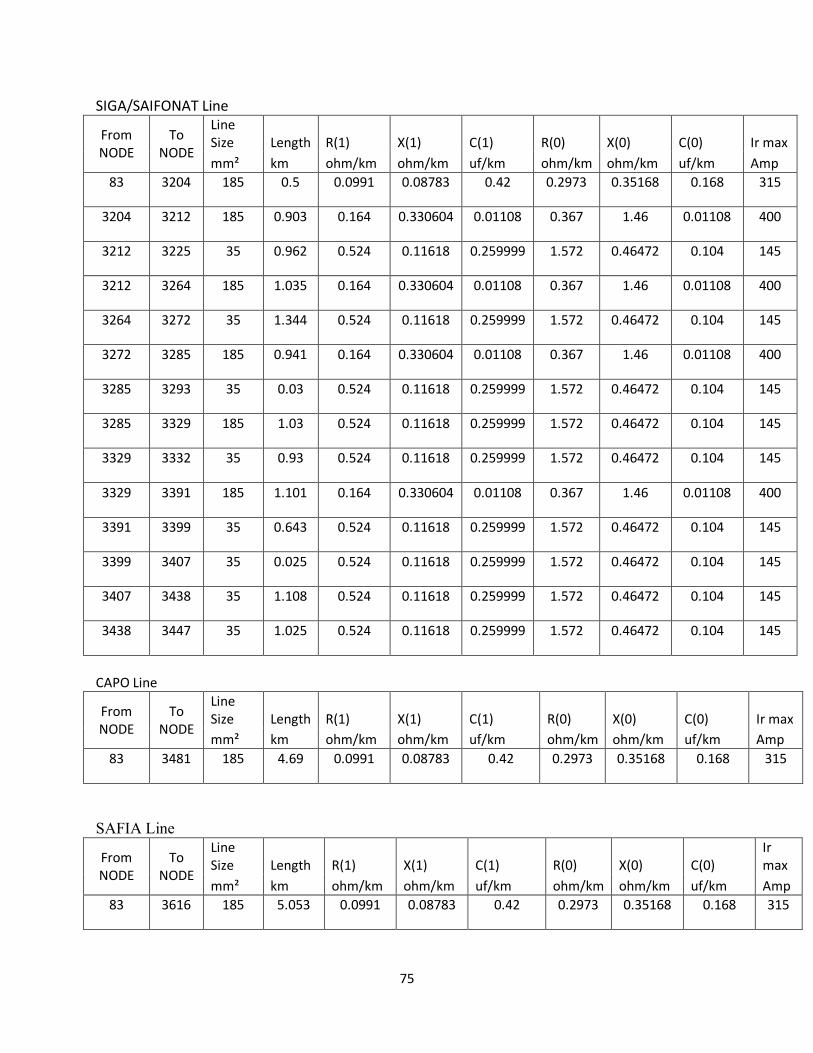
SIGA/SAIFONAT Line

From NODE

To NODE


83 3204 185 0.5 0.0991 0.08783 0.42 0.2973 0.35168 0.168 315

3204 3212 185 0.903 0.164 0.330604 0.01108 0.367 1.46 0.01108 400

3212 3225 35 0.962 0.524 0.11618 0.259999 1.572 0.46472 0.104 145

3212 3264 185 1.035 0.164 0.330604 0.01108 0.367 1.46 0.01108 400

3264 3272 35 1.344 0.524 0.11618 0.259999 1.572 0.46472 0.104 145

3272 3285 185 0.941 0.164 0.330604 0.01108 0.367 1.46 0.01108 400

3285 3293 35 0.03 0.524 0.11618 0.259999 1.572 0.46472 0.104 145

3285 3329 185 1.03 0.524 0.11618 0.259999 1.572 0.46472 0.104 145

3329 3332 35 0.93 0.524 0.11618 0.259999 1.572 0.46472 0.104 145

3329 3391 185 1.101 0.164 0.330604 0.01108 0.367 1.46 0.01108 400

3391 3399 35 0.643 0.524 0.11618 0.259999 1.572 0.46472 0.104 145

3399 3407 35 0.025 0.524 0.11618 0.259999 1.572 0.46472 0.104 145

3407 3438 35 1.108 0.524 0.11618 0.259999 1.572 0.46472 0.104 145

3438 3447 35 1.025 0.524 0.11618 0.259999 1.572 0.46472 0.104 145

CAPO Line

From NODE

To NODE


83 3481 185 4.69 0.0991 0.08783 0.42 0.2973 0.35168 0.168 315

SAFIA Line

From NODE

To NODE

Line Size Length R(1) X(1) C(1) R(0) X(0) C(0)

Ir max

mm² km ohm/km ohm/km uf/km ohm/km ohm/km uf/km Amp 83 3616 185 5.053 0.0991 0.08783 0.42 0.2973 0.35168 0.168 315

76

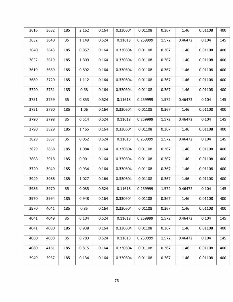
3616 3632 185 2.162 0.164 0.330604 0.01108 0.367 1.46 0.01108 400

3632 3640 35 1.149 0.524 0.11618 0.259999 1.572 0.46472 0.104 145

3640 3643 185 0.857 0.164 0.330604 0.01108 0.367 1.46 0.01108 400

3632 3619 185 1.809 0.164 0.330604 0.01108 0.367 1.46 0.01108 400

3619 3689 185 0.892 0.164 0.330604 0.01108 0.367 1.46 0.01108 400

3689 3720 185 1.112 0.164 0.330604 0.01108 0.367 1.46 0.01108 400

3720 3751 185 0.68 0.164 0.330604 0.01108 0.367 1.46 0.01108 400

3751 3759 35 0.853 0.524 0.11618 0.259999 1.572 0.46472 0.104 145

3751 3790 185 1.06 0.164 0.330604 0.01108 0.367 1.46 0.01108 400

3790 3798 35 0.514 0.524 0.11618 0.259999 1.572 0.46472 0.104 145

3790 3829 185 1.465 0.164 0.330604 0.01108 0.367 1.46 0.01108 400

3829 3837 35 0.052 0.524 0.11618 0.259999 1.572 0.46472 0.104 145

3829 3868 185 1.084 0.164 0.330604 0.01108 0.367 1.46 0.01108 400

3868 3918 185 0.901 0.164 0.330604 0.01108 0.367 1.46 0.01108 400

3720 3949 185 0.934 0.164 0.330604 0.01108 0.367 1.46 0.01108 400

3949 3986 185 1.027 0.164 0.330604 0.01108 0.367 1.46 0.01108 400

3986 3970 35 0.035 0.524 0.11618 0.259999 1.572 0.46472 0.104 145

3970 3994 185 0.948 0.164 0.330604 0.01108 0.367 1.46 0.01108 400

3970 4041 185 0.85 0.164 0.330604 0.01108 0.367 1.46 0.01108 400

4041 4049 35 0.104 0.524 0.11618 0.259999 1.572 0.46472 0.104 145

4041 4080 185 0.938 0.164 0.330604 0.01108 0.367 1.46 0.01108 400

4080 4088 35 0.783 0.524 0.11618 0.259999 1.572 0.46472 0.104 145

4080 4161 185 0.815 0.164 0.330604 0.01108 0.367 1.46 0.01108 400

3949 3957 185 0.134 0.164 0.330604 0.01108 0.367 1.46 0.01108 400

77

3957 4130 35 0.035 0.524 0.11618 0.259999 1.572 0.46472 0.104 145

3957 4161 185 0.044 0.164 0.330604 0.01108 0.367 1.46 0.01108 400

4161 4177 185 1.321 0.164 0.330604 0.01108 0.367 1.46 0.01108 400

4177 4185 185 2.034 0.164 0.330604 0.01108 0.367 1.46 0.01108 400

4185 4193 35 0.99 0.524 0.11618 0.259999 1.572 0.46472 0.104 145

4185 4279 185 0.882 0.164 0.330604 0.01108 0.367 1.46 0.01108 400

4279 4287 35 0.48 0.524 0.11618 0.259999 1.572 0.46472 0.104 145

4279 4341 185 1.056 0.164 0.330604 0.01108 0.367 1.46 0.01108 400

4341 4352 35 0.754 0.524 0.11618 0.259999 1.572 0.46472 0.104 145

4352 4363 185 1.416 0.164 0.330604 0.01108 0.367 1.46 0.01108 400

4163 4371 35 0.971 0.524 0.11618 0.259999 1.572 0.46472 0.104 145

4352 4402 185 0.852 0.164 0.330604 0.01108 0.367 1.46 0.01108 400

4402 4410 35 0.752 0.524 0.11618 0.259999 1.572 0.46472 0.104 145

4402 4441 185 0.871 0.164 0.330604 0.01108 0.367 1.46 0.01108 400

4441 4449 185 1.133 0.164 0.330604 0.01108 0.367 1.46 0.01108 400

4441 4483 185 0.964 0.164 0.330604 0.01108 0.367 1.46 0.01108 400

4483 4491 185 0.776 0.164 0.330604 0.01108 0.367 1.46 0.01108 400

4491 4499 185 0.696 0.164 0.330604 0.01108 0.367 1.46 0.01108 400

4499 4507 185 0.633 0.164 0.330604 0.01108 0.367 1.46 0.01108 400

4507 4515 35 0.529 0.524 0.11618 0.259999 1.572 0.46472 0.104 145

4507 4546 185 0.497 0.164 0.330604 0.01108 0.367 1.46 0.01108 400

4499 4477 185 0.499 0.164 0.330604 0.01108 0.367 1.46 0.01108 400

4477 4698 35 0.489 0.524 0.11618 0.259999 1.572 0.46472 0.104 145

78

SAFIA Transformer Voltage

1(KV) Voltage

2(KV) S(MVA) UrRr(1)% uKr(1)% UrRr(0)% uKr(0)% Vector group

11 0.433 1 1.17 5 1.17 5 Dyn11

11 0.433 0.5 1.25 4 1.25 4 Dyn11

11 0.433 0.5 1.25 4 1.25 4 Dyn11

11 0.433 0.5 1.25 4 1.25 4 Dyn11

11 0.433 1 1.17 5 1.17 5 Dyn11

11 0.433 1 1.17 5 1.17 5 Dyn11

11 0.433 0.3 1.5 4 1.5 4 Dyn11

11 0.433 0.3 1.5 5 1.5 5 Dyn11

11 0.433 1 1.17 5 1.17 5 Dyn11

11 0.433 0.2 1.63 4 1.63 4 Dyn11

11 0.433 0.5 1.25 4 1.25 4 Dyn11

11 0.433 1 1.17 5 1.17 5 Dyn11

11 0.433 0.75 1.31 5 1.31 5 Dyn11

11 0.433 0.5 1.25 4 1.25 4 Dyn11

11 0.433 1 1.17 5 1.17 5 Dyn11

11 0.433 1 1.17 5 1.17 5 Dyn11

11 0.433 1 1.17 5 1.17 5 Dyn11

11 0.433 1 1.17 5 1.17 5 Dyn11

11 0.433 0.2 1.63 4 1.63 4 Dyn11

11 0.433 0.2 1.63 4 1.63 4 Dyn11

11 0.433 0.2 1.63 4 1.63 4 Dyn11

11 0.433 1 1.17 5 1.17 5 Dyn11

11 0.433 0.1 1.173 4 1.73 4 Dyn11

79

11 0.433 0.1 1.173 4 1.73 4 Dyn11

11 0.433 2 1.13 6.25 1.13 6.25 Dyn11

SAFA OILS Transformer

Voltage 1(KV)

Voltage 2(KV) S(MVA) UrRr(1)% uKr(1)% UrRr(0)% uKr(0)% Vector group

11 0.433 0.1 1.173 4 1.73 4 Dyn11 11 0.433 0.1 1.173 4 1.73 4 Dyn11 11 0.433 0.5 1.25 4 1.25 4 Dyn11 11 0.433 0.5 1.25 4 1.25 4 Dyn11 11 0.433 0.5 1.25 4 1.25 4 Dyn11 11 0.433 1 1.17 5 1.17 5 Dyn11 11 0.433 1 1.17 5 1.17 5 Dyn11 11 0.433 0.3 1.5 4 1.5 4 Dyn11 11 0.433 0.75 1.31 5 1.31 5 Dyn11 11 0.433 0.3 1.5 5 1.5 5 Dyn11 11 0.433 1 1.17 5 1.17 5 Dyn11 11 0.433 0.2 1.63 4 1.63 4 Dyn11 11 0.433 0.5 1.25 4 1.25 4 Dyn11 11 0.433 1 1.17 5 1.17 5 Dyn11 11 0.433 0.75 1.31 5 1.31 5 Dyn11 11 0.433 0.5 1.25 4 1.25 4 Dyn11 11 0.433 1 1.17 5 1.17 5 Dyn11 11 0.433 1 1.17 5 1.17 5 Dyn11 11 0.433 1 1.17 5 1.17 5 Dyn11 11 0.433 1 1.17 5 1.17 5 Dyn11 11 0.433 0.2 1.63 4 1.63 4 Dyn11 11 0.433 0.2 1.63 4 1.63 4 Dyn11 11 0.433 0.2 1.63 4 1.63 4 Dyn11 11 0.433 1 1.17 5 1.17 5 Dyn11 11 0.433 0.1 1.173 4 1.73 4 Dyn11 11 0.433 0.1 1.173 4 1.73 4 Dyn11 11 0.433 0.05 1.81 4 1.81 4 Dyn11

SHAMBAT Transformer

Voltage 1(KV) Voltage 2(KV) S(MVA) UrRr(1)% uKr(1)% UrRr(0)% uKr(0)% Vector group

11 0.433 0.2 1.63 4 1.63 4 Dyn11 ELMASRA Transformer

Voltage Voltage S(MVA) UrRr(1)% uKr(1)% UrRr(0)% uKr(0)% Vector group

80

1(KV) 2(KV) 11 0.433 0.1 1.173 4 1.73 4 Dyn11

11 0.433 0.1 1.173 4 1.73 4 Dyn11

11 0.433 0.5 1.25 4 1.25 4 Dyn11

11 0.433 0.5 1.25 4 1.25 4 Dyn11

11 0.433 0.5 1.25 4 1.25 4 Dyn11

11 0.433 0.5 1.25 4 1.25 4 Dyn11

11 0.433 0.3 1.5 4 1.5 4 Dyn11

11 0.433 0.2 1.63 4 1.63 4 Dyn11

11 0.433 0.5 1.25 4 1.25 4 Dyn11

11 0.433 0.2 1.63 4 1.63 4 Dyn11

11 0.433 0.5 1.25 4 1.25 4 Dyn11

11 0.433 0.2 1.63 4 1.63 4 Dyn11

11 0.433 0.2 1.63 4 1.63 4 Dyn11

11 0.433 0.2 1.63 4 1.63 4 Dyn11

11 0.433 0.2 1.63 4 1.63 4 Dyn11

11 0.433 0.05 1.81 4 1.81 4 Dyn11

11 0.433 0.5 1.25 4 1.25 4 Dyn11

11 0.433 0.5 1.25 4 1.25 4 Dyn11

11 0.433 0.5 1.25 4 1.25 4 Dyn11

11 0.433 0.5 1.25 4 1.25 4 Dyn11

11 0.433 0.3 1.5 4 1.5 4 Dyn11

11 0.433 0.2 1.63 4 1.63 4 Dyn11

11 0.433 0.5 1.25 4 1.25 4 Dyn11

11 0.433 0.2 1.63 4 1.63 4 Dyn11

81

11 0.433 0.5 1.25 4 1.25 4 Dyn11

SIGA/SAIFONAT Transformer

Voltage 1(KV)


11 0.433 2 1.13 6.25 1.13 6.25 Dyn11

11 0.433 2 1.13 6.25 1.13 6.25 Dyn11

11 0.433 2 1.13 6.25 1.13 6.25 Dyn11

11 0.433 2 1.13 6.25 1.13 6.25 Dyn11

11 0.433 0.75 1.31 5 1.31 5 Dyn11

CAPO Transformer

Voltage 1(KV)


11 0.433 2 1.13 6.25 1.13 6.25 Dyn11

11 0.433 2 1.13 6.25 1.13 6.25 Dyn11

11 0.433 1 1.17 5 1.17 5 Dyn11

11 0.433 0.5 1.25 4 1.25 4 Dyn11

COLA Transformer

Voltage 1(KV)


11 0.433 2 1.13 6.25 1.13 6.25 Dyn11 11 0.433 2 1.13 6.25 1.13 6.25 Dyn11 11 0.433 2 1.13 6.25 1.13 6.25 Dyn11 11 0.433 1 1.17 5 1.17 5 Dyn11

82

REFERENCES 1) Tom Short , " ElECTRIC POWER distribution handbook" , CRC PRESS, Newyork ,2004.

2) Dr, Kamalia Yousif ,"Losses in Electrical Energy",.Alexandria Electricity Distribution Company

,Alexandria , 2004.

3) TaranGonen ," Electric power Distribution System Engineering" , Taylor Francis Group, New York ,

2008.

4) Dan Suruiyamongkol ," non technical losses in electrical power systems" , Dean

College of Engineering and Technology , Thailand , 2009 5) NEPLAN Manual .

6) Jiansong Ding, K.R.W.Bell, S.M.Strachan," Study of Low Voltage System Losses", University of

Strathclyde,Glasgow ,

7) SEDC Meter Management 2013 energy report.

8) SEDC Annual losses 2013 report.

9) http://www.tradingeconomics.com/sudan/electric-power-transmission-and-distribution-losses-percent-

of-output-wb-data.html

CHAPTER ONE INTERODUCTION - SUST Repository

Documents

Transcript of CHAPTER ONE INTERODUCTION - SUST Repository