1

Sudan University of Science and Technology

College of Petroleum Engineering and

Technology

Petroleum Engineering Department

Project Title

Water Flooding Analysis

(Simber West Field Case Study)

تحليل عملية الغمر المائي

) Simber West دراسة الحالة في حقل)

Submitted in partial Fulfillment of the Requirements

Of the Degree OfB.tech in Petroleum Engineering

Prepared By:

Mahir Abdallah Elmajoup

Musaab Ibrahim Elhassan

Ahmed Fayad Ahmed

Mulham Abdalla Mohammed

Supervisor:

Sami Mohamed Elamin

i

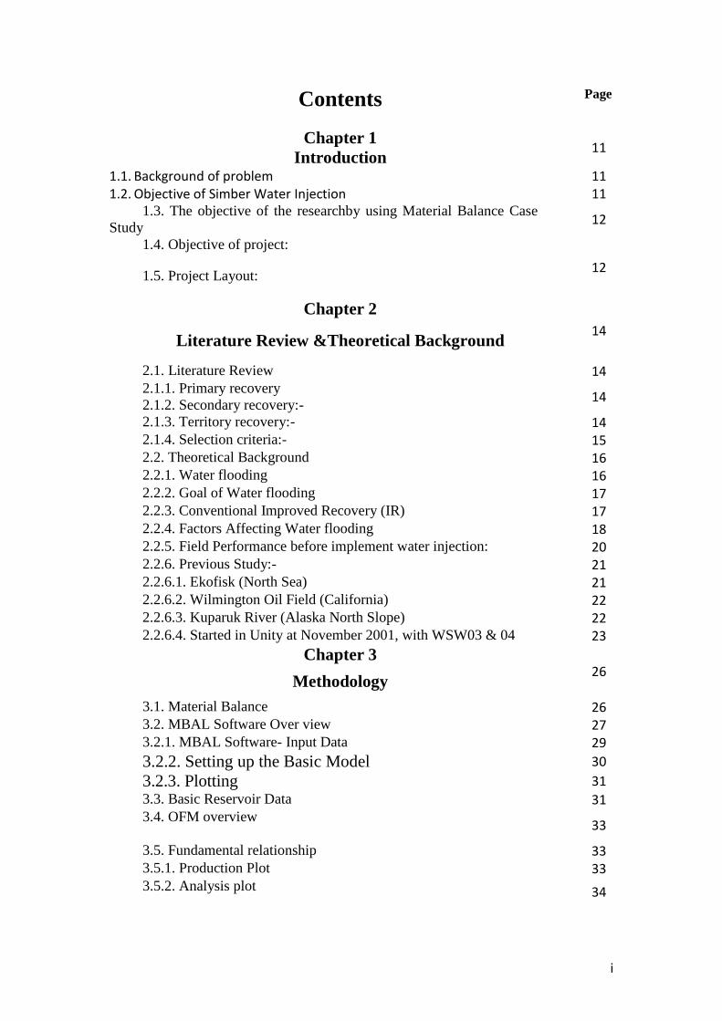
Contents

Page

Chapter 1

Introduction 11

1.1. Background of problem 11 1.2. Objective of Simber Water Injection 11

1.3. The objective of the researchby using Material Balance Case

Study 12

1.4. Objective of project:

1.5. Project Layout: 12

Chapter 2

Literature Review &Theoretical Background 14

2.1. Literature Review 14 2.1.1. Primary recovery

2.1.2. Secondary recovery:- 14

2.1.3. Territory recovery:- 14 2.1.4. Selection criteria:- 15 2.2. Theoretical Background 16 2.2.1. Water flooding 16 2.2.2. Goal of Water flooding 17 2.2.3. Conventional Improved Recovery (IR) 17 2.2.4. Factors Affecting Water flooding 18 2.2.5. Field Performance before implement water injection: 20 2.2.6. Previous Study:- 21 2.2.6.1. Ekofisk (North Sea) 21 2.2.6.2. Wilmington Oil Field (California) 22 2.2.6.3. Kuparuk River (Alaska North Slope) 22 2.2.6.4. Started in Unity at November 2001, with WSW03 & 04 23

Chapter 3

Methodology 26

3.1. Material Balance 26 3.2. MBAL Software Over view 27 3.2.1. MBAL Software- Input Data 29

3.2.2. Setting up the Basic Model 30

3.2.3. Plotting 31 3.3. Basic Reservoir Data 31 3.4. OFM overview

33

3.5. Fundamental relationship 33 3.5.1. Production Plot 33 3.5.2. Analysis plot 34

ii

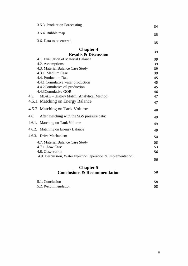
3.5.3. Production Forecasting 34

3.5.4. Bubble map 35

3.6. Data to be entered 35

Chapter 4

Results & Discussion 39

4.1. Evaluation of Material Balance 39 4.2. Assumptions 39 4.3. Material Balance Case Study 39 4.3.1. Medium Case 39 4.4. Production Data 45 4.4.1.Comulative water production 45 4.4.2Comulative oil production 45 4.4.3Comulative GOR 46

4.5. MBAL – History Match (Analytical Method) 47

4.5.1. Matching on Energy Balance 47

4.5.2. Matching on Tank Volume 48

4.6. After matching with the SGS pressure data: 49

4.6.1. Matching on Tank Volume 49

4.6.2. Matching on Energy Balance 49

4.6.3. Drive Mechanism 50

4.7. Material Balance Case Study 53 4.7.1. Low Case 53 4.8. Observation 56 4.9. Descussion, Water Injection Operation & Implementation:

56

Chapter 5

Conclusions & Recommendation

58

5.1. Conclusion 58 5.2. Recommendation 58

iii

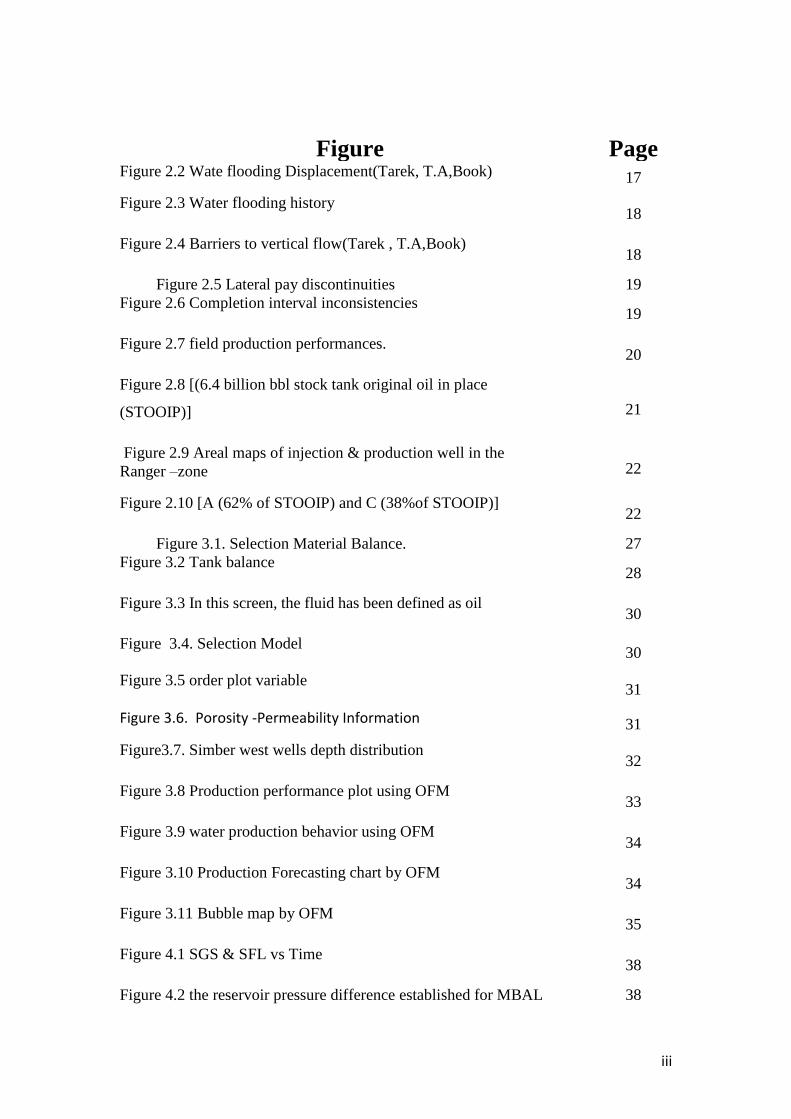
Figure Page Figure 2.2 Wate flooding Displacement(Tarek, T.A,Book) 17

Figure 2.3 Water flooding history 18

Figure 2.4 Barriers to vertical flow(Tarek , T.A,Book) 18

Figure 2.5 Lateral pay discontinuities 19

Figure 2.6 Completion interval inconsistencies 19

Figure 2.7 field production performances. 20

Figure 2.8 [(6.4 billion bbl stock tank original oil in place

(STOOIP)] 21

Figure 2.9 Areal maps of injection & production well in the

Ranger –zone 22

Figure 2.10 [A (62% of STOOIP) and C (38%of STOOIP)] 22

Figure 3.1. Selection Material Balance. 27

Figure 3.2 Tank balance 28

Figure 3.3 In this screen, the fluid has been defined as oil 30

Figure 3.4. Selection Model

30

Figure 3.5 order plot variable

31

Figure 3.6. Porosity -Permeability Information 31

Figure3.7. Simber west wells depth distribution 32

Figure 3.8 Production performance plot using OFM 33

Figure 3.9 water production behavior using OFM 34

Figure 3.10 Production Forecasting chart by OFM 34

Figure 3.11 Bubble map by OFM 35

Figure 4.1 SGS & SFL vs Time 38

Figure 4.2 the reservoir pressure difference established for MBAL 38

iv

analysis

Figure 4.3 Due to Limit fluid data available, correlation was used

to generate the PVT data 39

Figure 4.4 Black Oil Input Data 39

Figure 4.5 Pressure vs Oil viscosity 40

Figure 4.6 Pressure vs oil FVF 40

Figure 4.7 pressure vs Gas viscosity 41

Figure 4.8 pressure vs GOR 41

Figure 4.9 pressure vs Gas FVF 42

Figure 4.10. No aquifer attach as understood from reservoir pressure

and water cut behavior

43

Figure 4.11. Tank Input Data – Water Influx

43

Figure 4.12 Tank Input Data – Rermeabilities.

44

Figure 4.13Pressure&Cumulative water production 45

Figure 4.14 Pressure & Cumulative oil production 45

Figure 4.15 Pressure & cumulative GOR production 46

Figure 4.16 calculated oil production by MBAL 47

Figure 4.17 Matching on Tank Volume (calculated oil in place by

MBAL) 48

Figure 4.18 Matching on Tank Volume (actual Oil in place by

MBAL) 49

Figure 4.19 Tank Pressure vs Calculated oil production 49

Figure 4.20 Drive Mechanism identifying 50

Figure 4.21 Oil productions (Stimulated pressure vs actual

pressure) 50

Figure 4.22 cumulative oil production vs time 51

Figure 4.23 cumulative oil prod vs time (avg oil & tank pressure) 51

v

Figure 4.24.Average water Inj vs Time (tank pressure & Time) 52

Figure 4.25.calculated oil production vs tan pressure 53

Figure 4.26.actual oil in place vs calculated from MBAL 53

Figure 4.27 data matching 54

Figure 4.28 pressure vs calculated oil 54

Figure 4.29 Average oil actual pressure& estimated pressure 55

Figure 4.30 Average Water Injection vs tank pressure

55

Tables

Table2. .1 Selection criteria 15

MBAL Software- Input Data Table 3.1 29

Table 4.1. Basic Data 37

vi

بسم اهلل الرمحن الرحيم

( 1)اقزأ باسم ربك الذي خلق )قال تعاىل

( 3)اقزا وربك االكزم (2)خلق االنسان من علق

( 5)علم االنسان ما مل يعلم (4)الذي علم بالقلم

((.6)كال إن االنسان ليطغى

صدق اهلل العظيم

(سورة العلق)

vii

Abstract

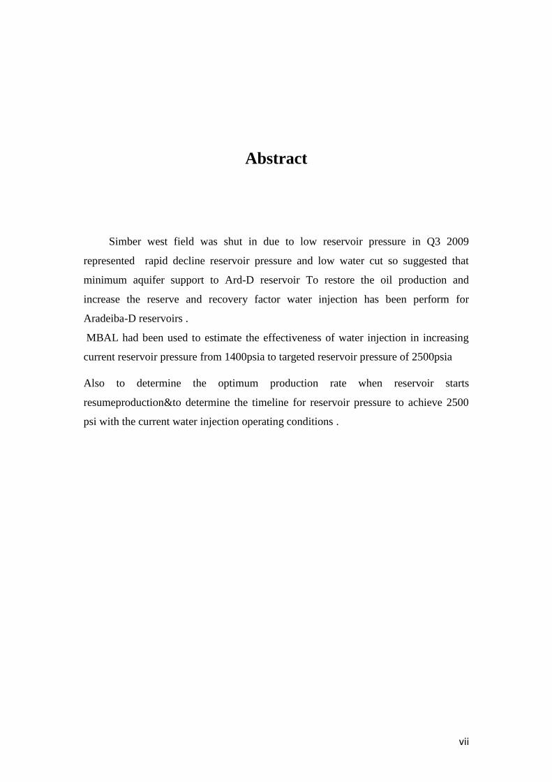
Simber west field was shut in due to low reservoir pressure in Q3 2009

represented rapid decline reservoir pressure and low water cut so suggested that

minimum aquifer support to Ard-D reservoir To restore the oil production and

increase the reserve and recovery factor water injection has been perform for

Aradeiba-D reservoirs .

MBAL had been used to estimate the effectiveness of water injection in increasing

current reservoir pressure from 1400psia to targeted reservoir pressure of 2500psia

Also to determine the optimum production rate when reservoir starts

resumeproduction&to determine the timeline for reservoir pressure to achieve 2500

psi with the current water injection operating conditions .

viii

تجريد

ورنك نالنخفاض انسريع في ضغط انًًكن في انربع انثانث ين سنت (Simber west)توقف االنتاج في حقم

الستعادة االنتاج (Aradeiba-D)تًاقتراح يعانجت قوة انذفع نهًكًن باستخذاو انغًر انًائي نهطبقت , 2009

وزيادة يعذل االستخالص

ويعرفت (psi 1400-2500) نحساب تاثير انغًر انًائي نرفع يستوى ضغط انًكًن ين (MBAL)تى استخذاو

.انسين انالزو نهوصول نهضغط انًحذد وانتنبؤ باالنتاج االيثم

1

Chapter One

Introduction

2

Chapter 1

Introduction

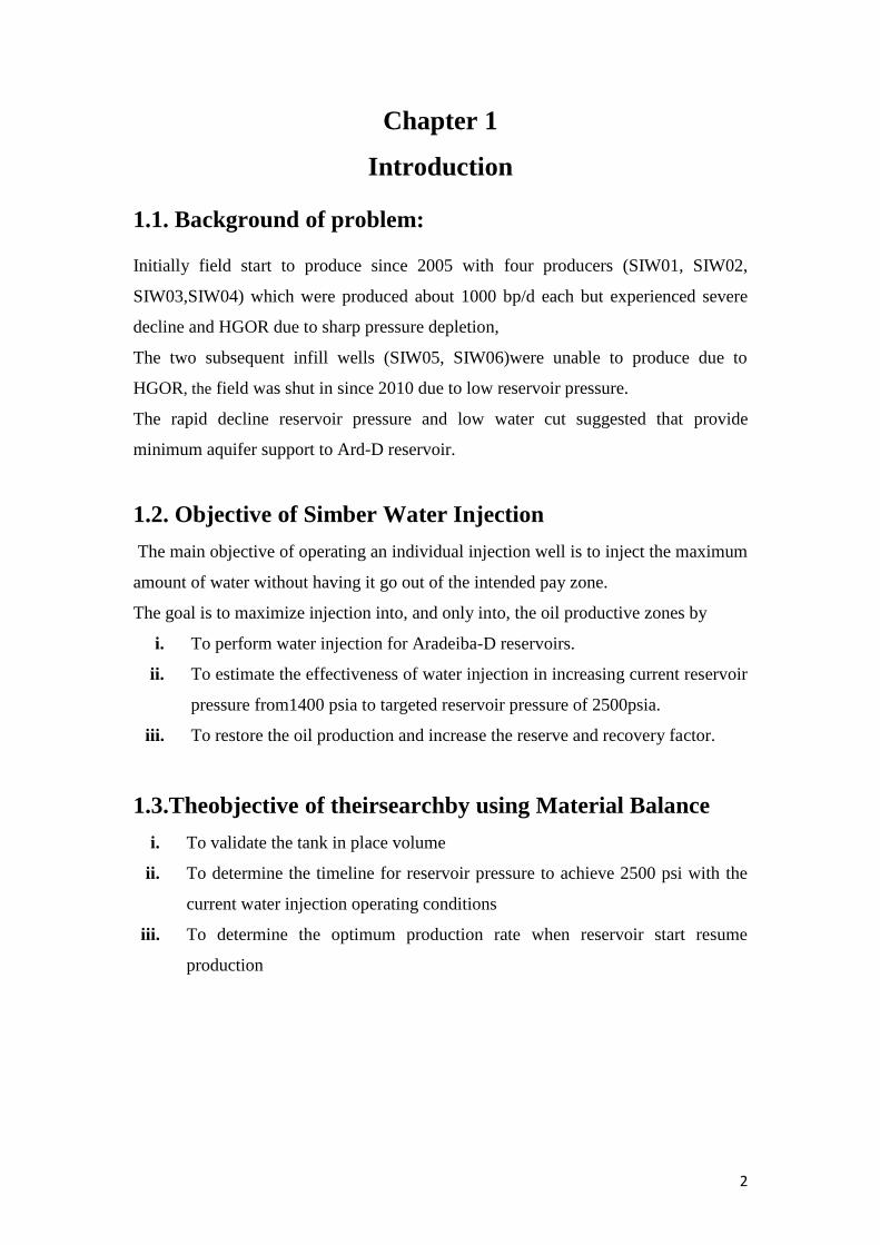
1.1. Background of problem:

Initially field start to produce since 2005 with four producers (SIW01, SIW02,

SIW03,SIW04) which were produced about 1000 bp/d each but experienced severe

decline and HGOR due to sharp pressure depletion,

The two subsequent infill wells (SIW05, SIW06)were unable to produce due to

HGOR, the field was shut in since 2010 due to low reservoir pressure.

The rapid decline reservoir pressure and low water cut suggested that provide

minimum aquifer support to Ard-D reservoir.

1.2. Objective of Simber Water Injection

The main objective of operating an individual injection well is to inject the maximum

amount of water without having it go out of the intended pay zone.

The goal is to maximize injection into, and only into, the oil productive zones by

i. To perform water injection for Aradeiba-D reservoirs.

ii. To estimate the effectiveness of water injection in increasing current reservoir

pressure from1400 psia to targeted reservoir pressure of 2500psia.

iii. To restore the oil production and increase the reserve and recovery factor.

1.3.Theobjective of theirsearchby using Material Balance

i. To validate the tank in place volume

ii. To determine the timeline for reservoir pressure to achieve 2500 psi with the

current water injection operating conditions

iii. To determine the optimum production rate when reservoir start resume

production

3

1.4. Objective of project:

The scope of our project is use tank model to validate the water injection project

and back the wells to production by maintain pressure by using,

i. Material balance model.

ii. OFM software (production data).

1.5. Project Layout:

This project report has been divided into five chapters:-Chapter one represents a

brief introduction related to our project. Chapter two explains the literature review&

Theoretical Backgrounds related towater injection project. Chapter three customized

represent Basic reservoir data Field Performance before implement water injection.&

introduction to software use in research (MBAL and OFM overview). In Chapter four

we enter all require data to software and analyze the output data calculations of. Also

we make software by visual Basic language to predict liquid loading. In chapter five

we show our resultsandlastlywe put our future Recommendation.

4

Chapter Two

Literature Review

&TheoreticalBackg

round

5

Chapter 2

Literature Review&Theoretical Background

2.1. Literature Review

The recovery of oil by any of the natural drive mechanisms is calledprimary

recovery. The term refers to the production of hydrocarbonsfrom a reservoir without

the use of any process (such as fluid injection)to supplement the natural energy of the

reservoir.

Performance of oil reservoirs is largely determined by the nature of theenergy,

(driving mechanism, available for moving the oil to the wellbore).

2.1.1. Primary recovery

There are basically six driving mechanisms that provide the natural energy necessary

for oil recovery:

i. Rock and liquid expansion drive

ii. Depletion drive

iii. Gas cap drive

iv. Water drive

v. Gravity drainage drive

vi. Combination drive

2.1.2. Secondary recovery:-

Its process of produce oil out from reservoir by use using outside energy

i. Water flooding

ii. Gas injection

2.1.3. Territory recovery:-

Its boost energy in reservoir to increase oil production and reduce residual oil

i. Thermal

ii. Chemical

iii. Miscible

iv. Microbial

6

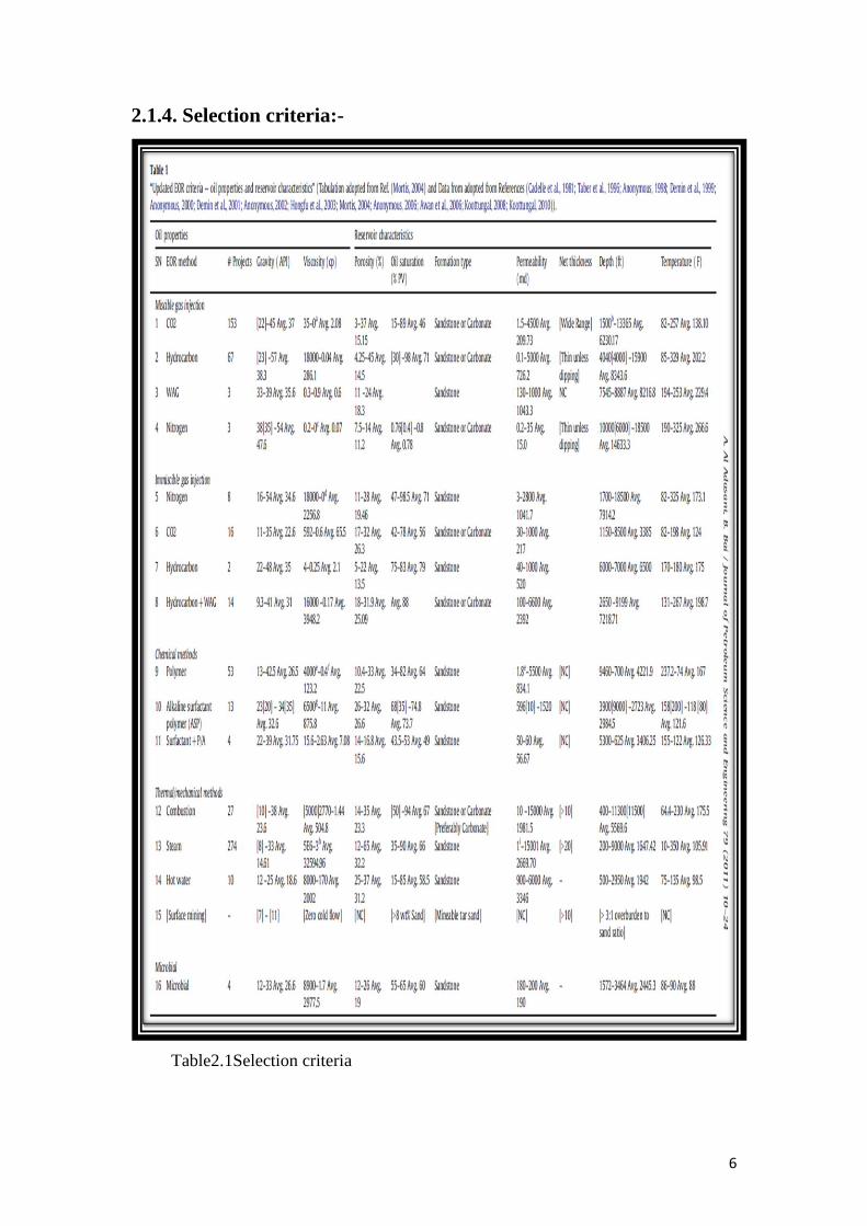
2.1.4. Selection criteria:-

Table2.1Selection criteria

7

2.2. Theoretical Background

2.2.1. Water flooding

Why is water flood the most popular Enhance Oil Recovery Scheme?

From screening criteria found that

i. Water is the cheapest flooding agent for Enhance Oil RecoveryThe need to

dispose of produced water

ii. Easy and safe to inject

iii. Proven technology

Planning a water flood scheme:

i. Ensure good understanding of fluid properties (PVT, water

chemicalanalysis...etc.)

ii. Establish good record of reservoir pressure history &productionbehavior

iii. Establish rock and mineral properties (relative perm., clay contents,

Compressibility...etc.)

iv. Establish geological maps (structure, net pay, cross-section)

Plan well spacing and pattern

i. Lease geometry & ownership

ii. Formation continuity

iii. Fracture system or permeability orientation

Stages of water flooding,

i. Interference Stage

ii. Fill-up

iii. Break-through

iv. Flood-out (after break-through)

8

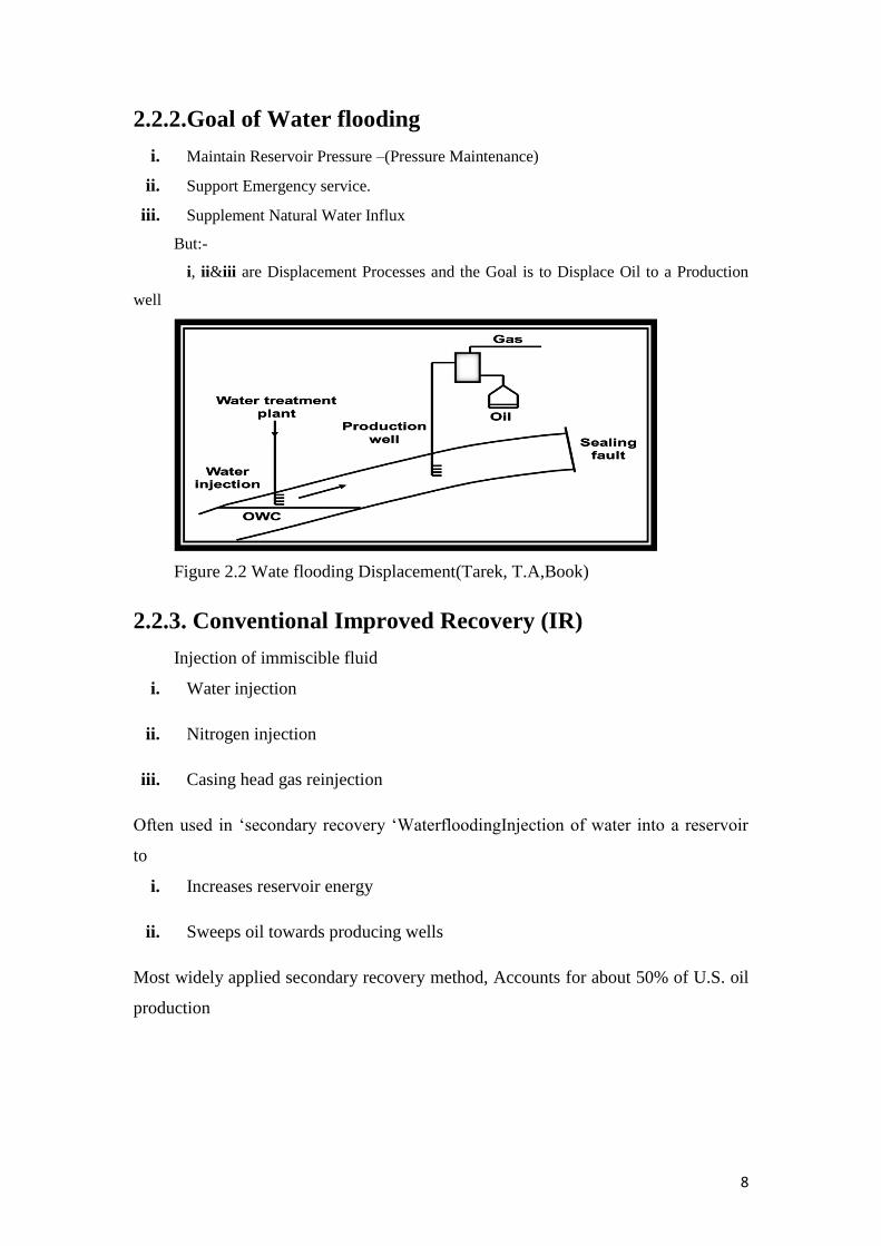
2.2.2.Goal of Water flooding

i. Maintain Reservoir Pressure –(Pressure Maintenance)

ii. Support Emergency service.

iii. Supplement Natural Water Influx

But:-

i, ii&iii are Displacement Processes and the Goal is to Displace Oil to a Production

well

Figure 2.2 Wate flooding Displacement(Tarek, T.A,Book)

2.2.3. Conventional Improved Recovery (IR)

Injection of immiscible fluid

i. Water injection

ii. Nitrogen injection

iii. Casing head gas reinjection

Often used in ‘secondary recovery ‘WaterfloodingInjection of water into a reservoir

to

i. Increases reservoir energy

ii. Sweeps oil towards producing wells

Most widely applied secondary recovery method, Accounts for about 50% of U.S. oil

production

9

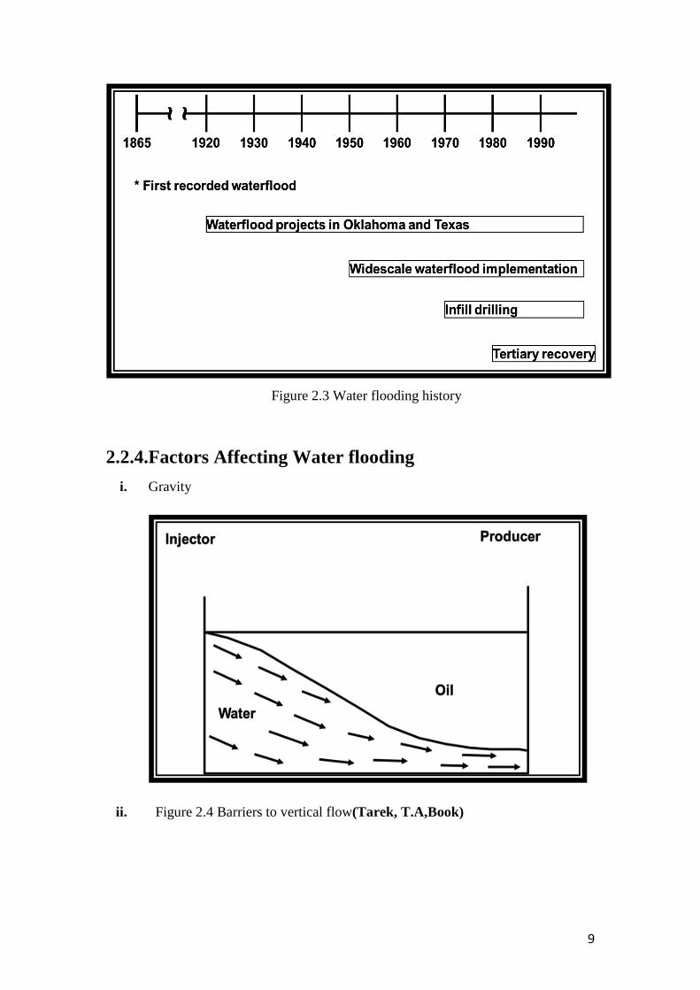
Figure 2.3 Water flooding history

2.2.4.Factors Affecting Water flooding

i. Gravity

ii. Figure 2.4 Barriers to vertical flow(Tarek, T.A,Book)

10

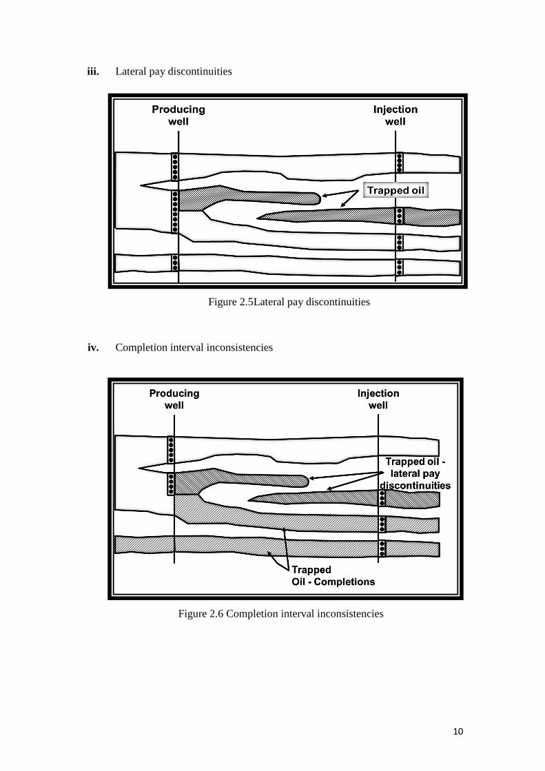
iii. Lateral pay discontinuities

Figure 2.5Lateral pay discontinuities

iv. Completion interval inconsistencies

Figure 2.6 Completion interval inconsistencies

11

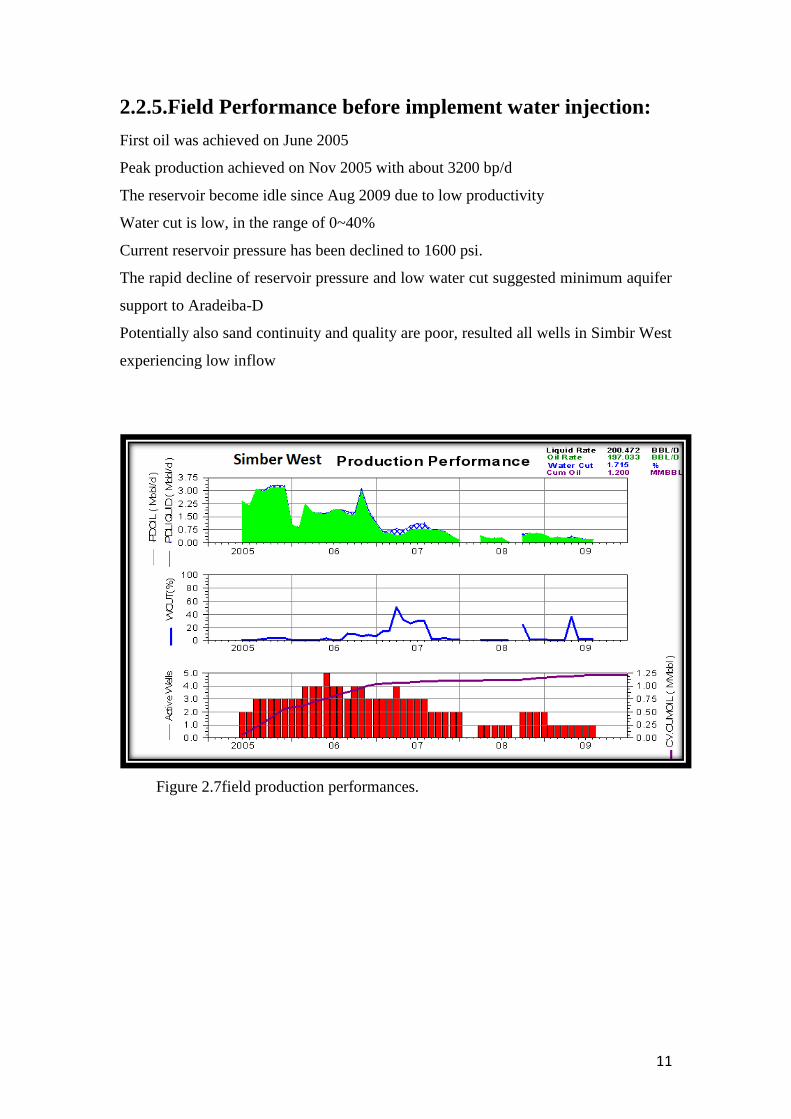
2.2.5.Field Performance before implement water injection:

First oil was achieved on June 2005

Peak production achieved on Nov 2005 with about 3200 bp/d

The reservoir become idle since Aug 2009 due to low productivity

Water cut is low, in the range of 0~40%

Current reservoir pressure has been declined to 1600 psi.

The rapid decline of reservoir pressure and low water cut suggested minimum aquifer

support to Aradeiba-D

Potentially also sand continuity and quality are poor, resulted all wells in Simbir West

experiencing low inflow

Figure 2.7field production performances.

12

2.2.6.Previous Study:-

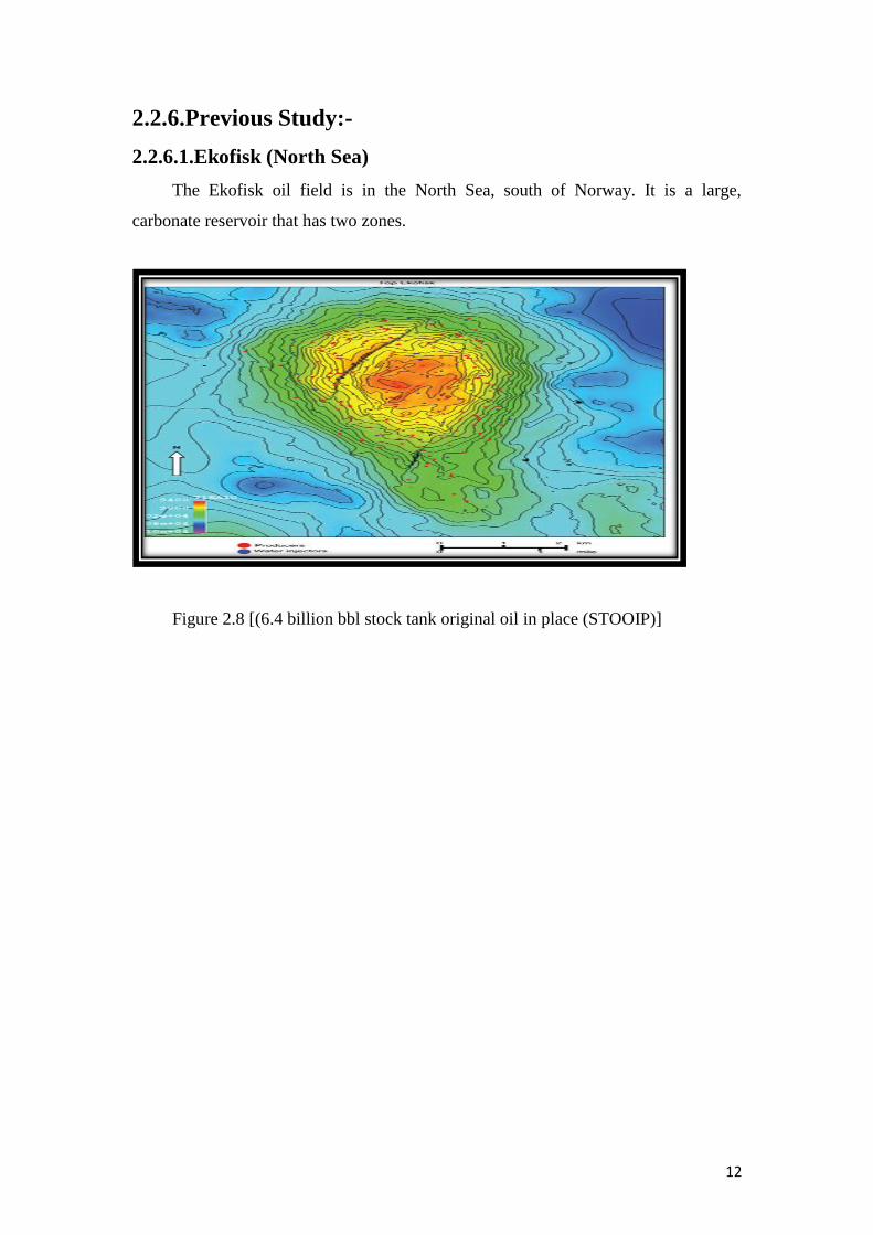
2.2.6.1.Ekofisk (North Sea)

The Ekofisk oil field is in the North Sea, south of Norway. It is a large,

carbonate reservoir that has two zones.

Figure 2.8 [(6.4 billion bbl stock tank original oil in place (STOOIP)]

13

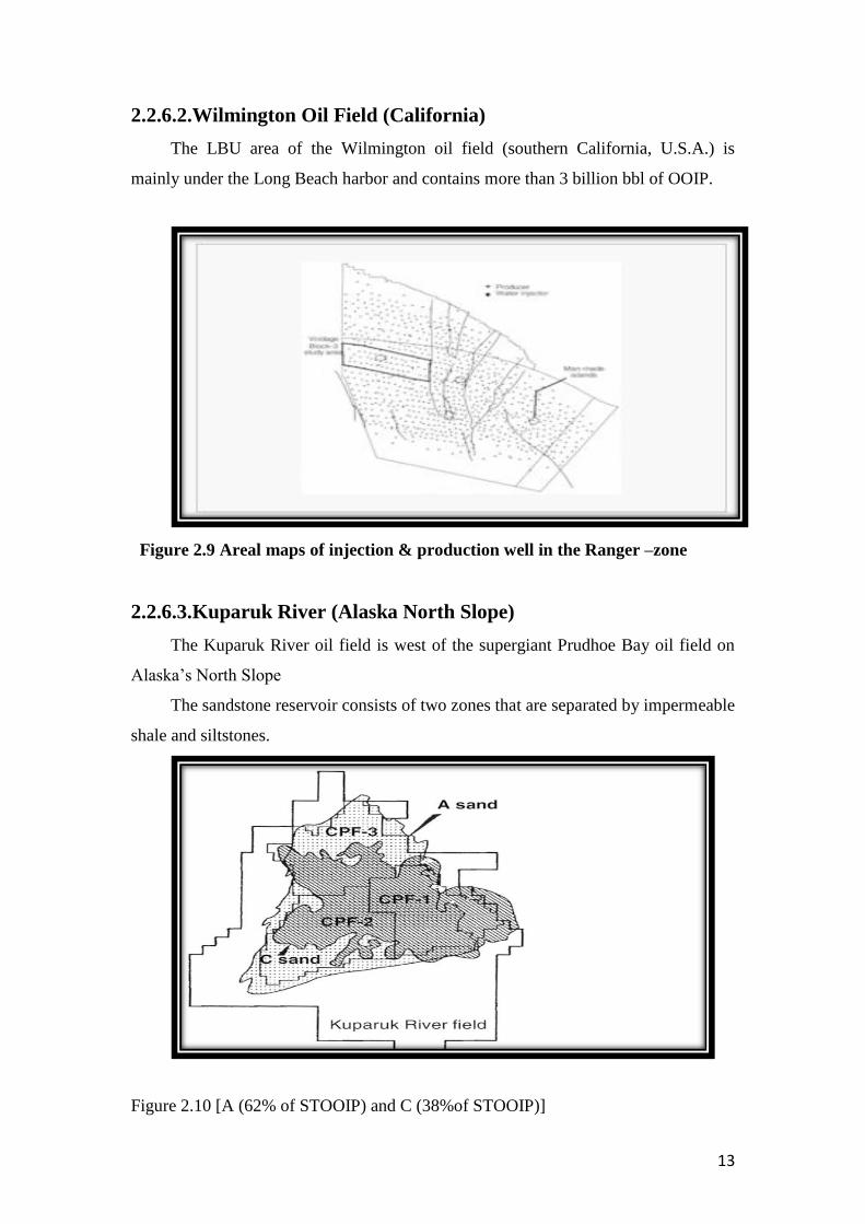
2.2.6.2.Wilmington Oil Field (California)

The LBU area of the Wilmington oil field (southern California, U.S.A.) is

mainly under the Long Beach harbor and contains more than 3 billion bbl of OOIP.

Figure 2.9 Areal maps of injection & production well in the Ranger –zone

2.2.6.3.Kuparuk River (Alaska North Slope)

The Kuparuk River oil field is west of the supergiant Prudhoe Bay oil field on

Alaska’s North Slope

The sandstone reservoir consists of two zones that are separated by impermeable

shale and siltstones.

Figure 2.10 [A (62% of STOOIP) and C (38%of STOOIP)]

14

2.2.6.4.Started in Unity at November 2001, with WSW03 & 04

1-To Provide artificial aquifer support to Ghazal, Zarga and Aradeiba Reservoirs.

2-To improve the areal and vertical sweep efficiency moving the oil to the producers.

3-To raise the depleted reservoir pressure at the desired reservoirs pressure and

sustain void age replacement ratio.

4-To improve the Recovery factor

15

Chapter Three

Methodology

16

Chapter 3

Methodology

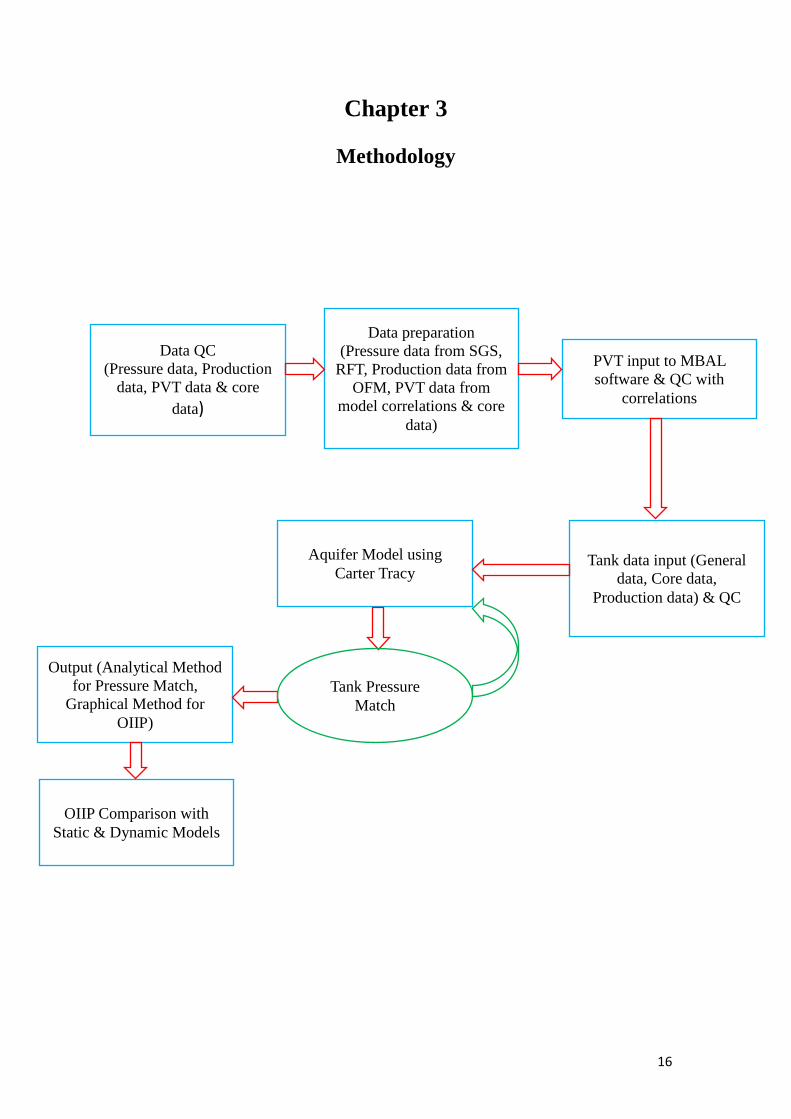
Data QC

(Pressure data, Production

data, PVT data & core

data)

Data preparation

(Pressure data from SGS,

RFT, Production data from

OFM, PVT data from

model correlations & core

data)

PVT input to MBAL

software & QC with

correlations

Tank data input (General

data, Core data,

Production data) & QC

Aquifer Model using

Carter Tracy

Output (Analytical Method

for Pressure Match,

Graphical Method for

OIIP)

OIIP Comparison with

Static & Dynamic Models

Tank Pressure

Match

17

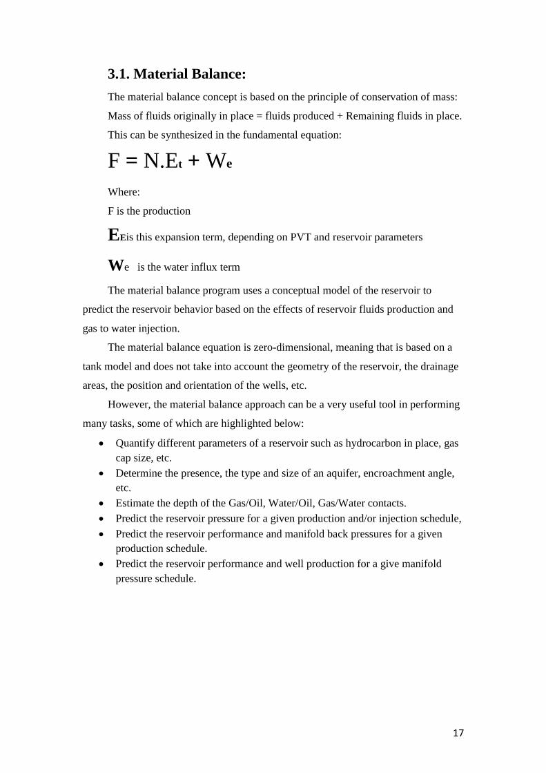
3.1. Material Balance:

The material balance concept is based on the principle of conservation of mass:

Mass of fluids originally in place = fluids produced + Remaining fluids in place.

This can be synthesized in the fundamental equation:

F = N.Et + We

Where:

F is the production

EEis this expansion term, depending on PVT and reservoir parameters

We is the water influx term

The material balance program uses a conceptual model of the reservoir to

predict the reservoir behavior based on the effects of reservoir fluids production and

gas to water injection.

The material balance equation is zero-dimensional, meaning that is based on a

tank model and does not take into account the geometry of the reservoir, the drainage

areas, the position and orientation of the wells, etc.

However, the material balance approach can be a very useful tool in performing

many tasks, some of which are highlighted below:

Quantify different parameters of a reservoir such as hydrocarbon in place, gas

cap size, etc.

Determine the presence, the type and size of an aquifer, encroachment angle,

etc.

Estimate the depth of the Gas/Oil, Water/Oil, Gas/Water contacts.

Predict the reservoir pressure for a given production and/or injection schedule,

Predict the reservoir performance and manifold back pressures for a given

production schedule.

Predict the reservoir performance and well production for a give manifold

pressure schedule.

18

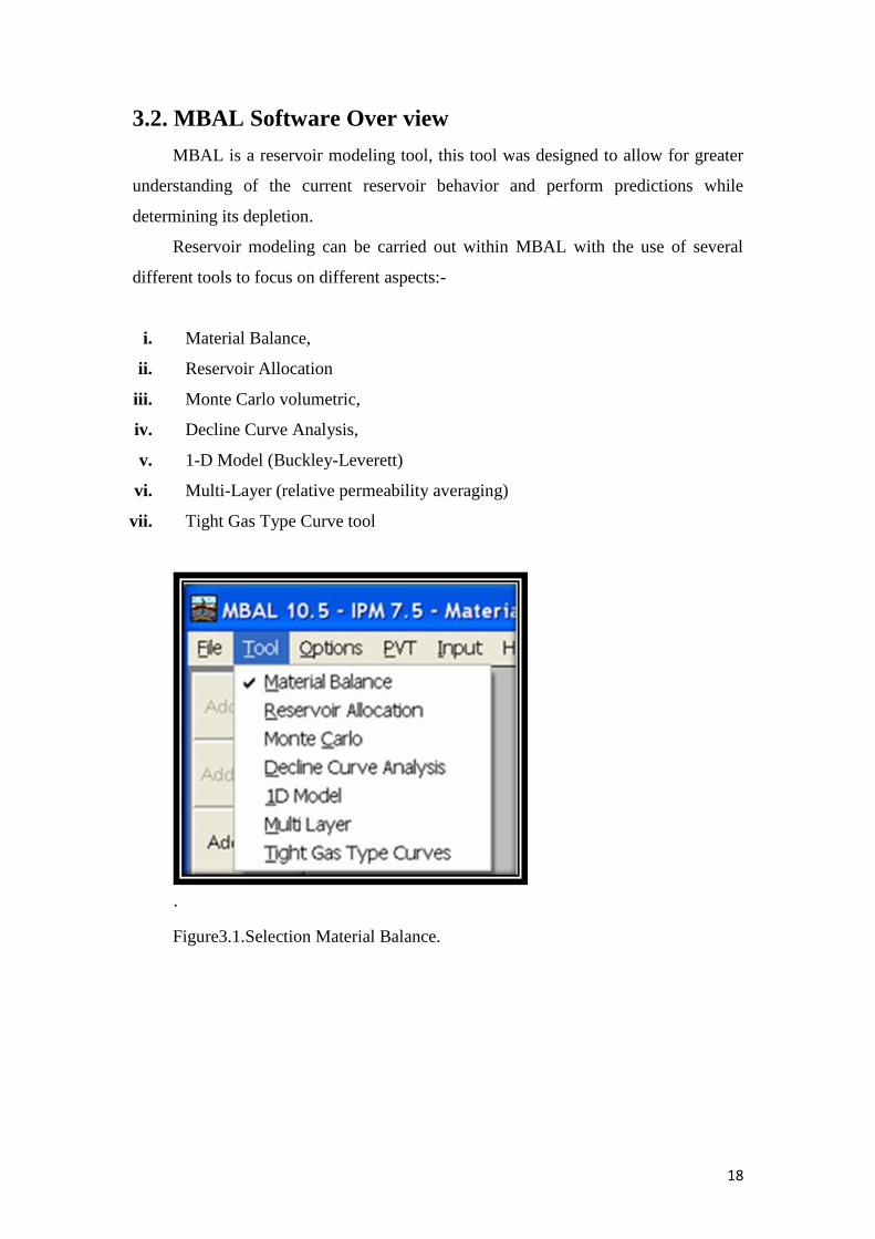
3.2. MBAL Software Over view

MBAL is a reservoir modeling tool, this tool was designed to allow for greater

understanding of the current reservoir behavior and perform predictions while

determining its depletion.

Reservoir modeling can be carried out within MBAL with the use of several

different tools to focus on different aspects:-

i. Material Balance,

ii. Reservoir Allocation

iii. Monte Carlo volumetric,

iv. Decline Curve Analysis,

v. 1-D Model (Buckley-Leverett)

vi. Multi-Layer (relative permeability averaging)

vii. Tight Gas Type Curve tool

·

Figure3.1.Selection Material Balance.

19

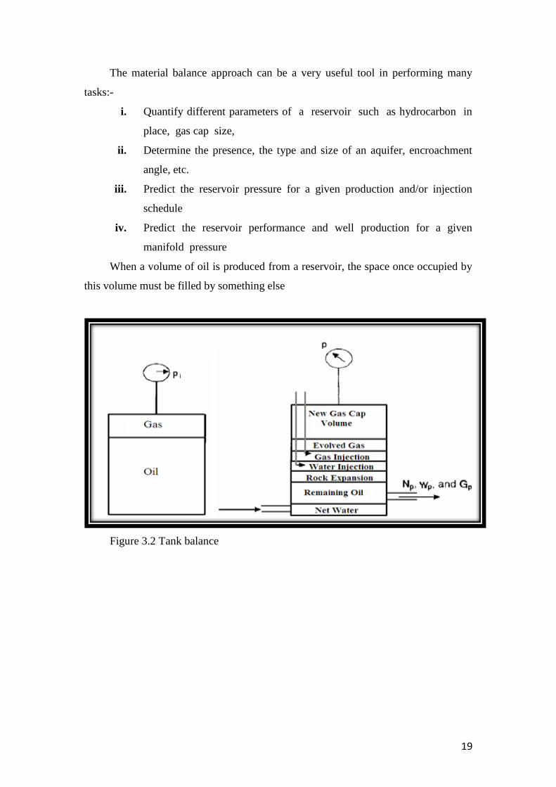
The material balance approach can be a very useful tool in performing many

tasks:-

i. Quantify different parameters of a reservoir such as hydrocarbon in

place, gas cap size,

ii. Determine the presence, the type and size of an aquifer, encroachment

angle, etc.

iii. Predict the reservoir pressure for a given production and/or injection

schedule

iv. Predict the reservoir performance and well production for a given

manifold pressure

When a volume of oil is produced from a reservoir, the space once occupied by

this volume must be filled by something else

Figure 3.2 Tank balance

20

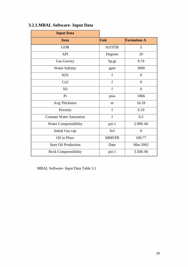
3.2.1.MBAL Software- Input Data

Input Data

Item Unit Formation A

GOR Scf/STB 5

API Degrees 20

Gas Gravity Sp.gr 0.74

Water Salinity ppm 3000

H2S f 0

Co2 f 0

N2 f 0

Pi psia 1866

Avg Thickness m 16.18

Porosity f 0.19

Connate Water Saturation f 0.2

Water Compressibility psi-1 2.99E-06

Initial Gas cap Scf 0

Oil in Place MMSTB 100.77

Start Oil Production Date Mar-2002

Rock Compressibility psi-1 3.50E-06

MBAL Software- Input Data Table 3.1

21

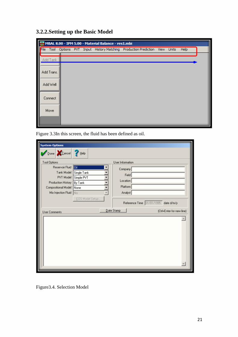
3.2.2.Setting up the Basic Model

Figure 3.3In this screen, the fluid has been defined as oil.

Figure3.4. Selection Model

22

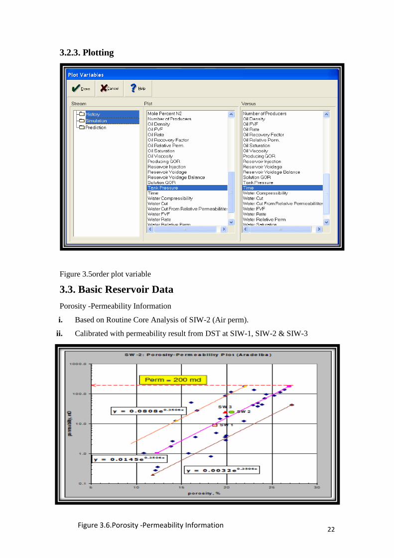
3.2.3. Plotting

Figure 3.5order plot variable

3.3. Basic Reservoir Data

Porosity -Permeability Information

i. Based on Routine Core Analysis of SIW-2 (Air perm).

ii. Calibrated with permeability result from DST at SIW-1, SIW-2 & SIW-3

Figure 3.6.Porosity -Permeability Information

23

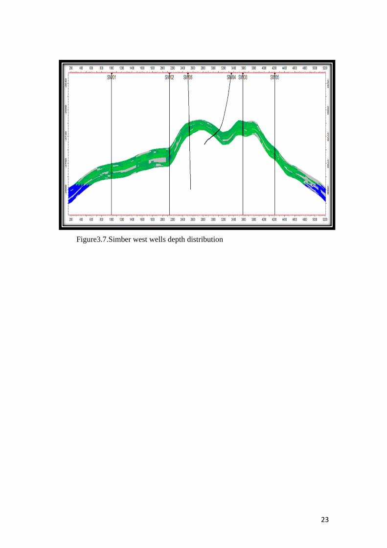
Figure3.7.Simber west wells depth distribution

24

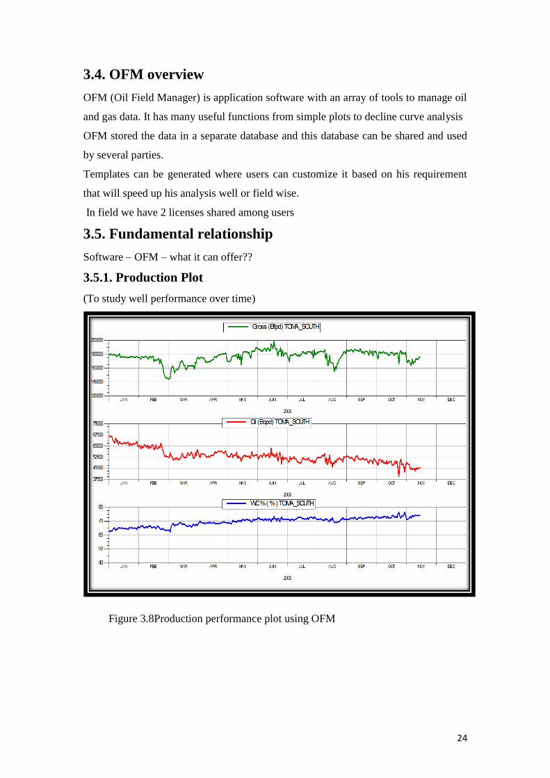
3.4. OFM overview

OFM (Oil Field Manager) is application software with an array of tools to manage oil

and gas data. It has many useful functions from simple plots to decline curve analysis

OFM stored the data in a separate database and this database can be shared and used

by several parties.

Templates can be generated where users can customize it based on his requirement

that will speed up his analysis well or field wise.

In field we have 2 licenses shared among users

3.5. Fundamental relationship

Software – OFM – what it can offer??

3.5.1. Production Plot

(To study well performance over time)

Figure 3.8Production performance plot using OFM

25

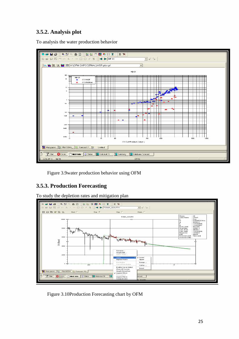
3.5.2. Analysis plot

To analysis the water production behavior

Figure 3.9water production behavior using OFM

3.5.3. Production Forecasting

To study the depletion rates and mitigation plan

Figure 3.10Production Forecasting chart by OFM

26

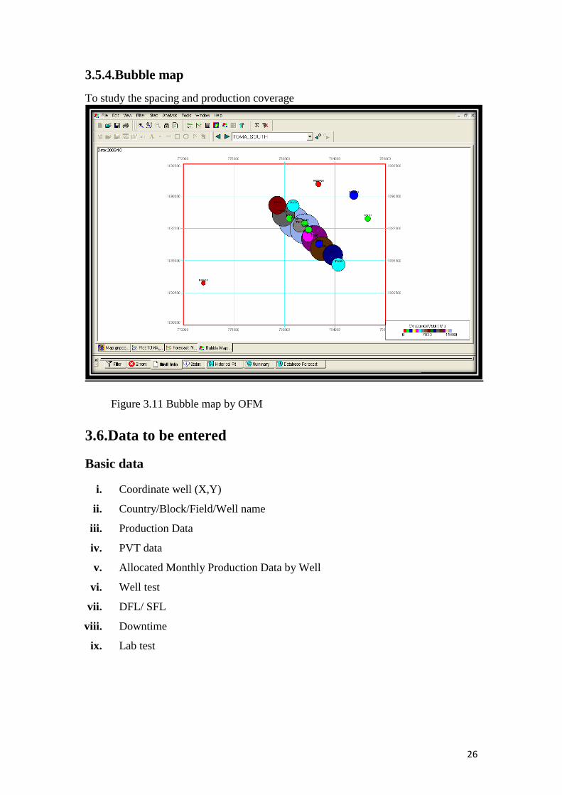
3.5.4.Bubble map

To study the spacing and production coverage

Figure 3.11 Bubble map by OFM

3.6.Data to be entered

Basic data

i. Coordinate well (X,Y)

ii. Country/Block/Field/Well name

iii. Production Data

iv. PVT data

v. Allocated Monthly Production Data by Well

vi. Well test

vii. DFL/ SFL

viii. Downtime

ix. Lab test

27

Chapter Four

Results &

Discussion

28

Chapter 4

Results & Discussion

4.1. Evaluation of Material Balance

1. To validate the tank in place volume

2. To determine the timeline for reservoir pressure to achieve 2500 psi with the

current water injection operating conditions

3. To determine the optimum production rate when reservoir start resume production

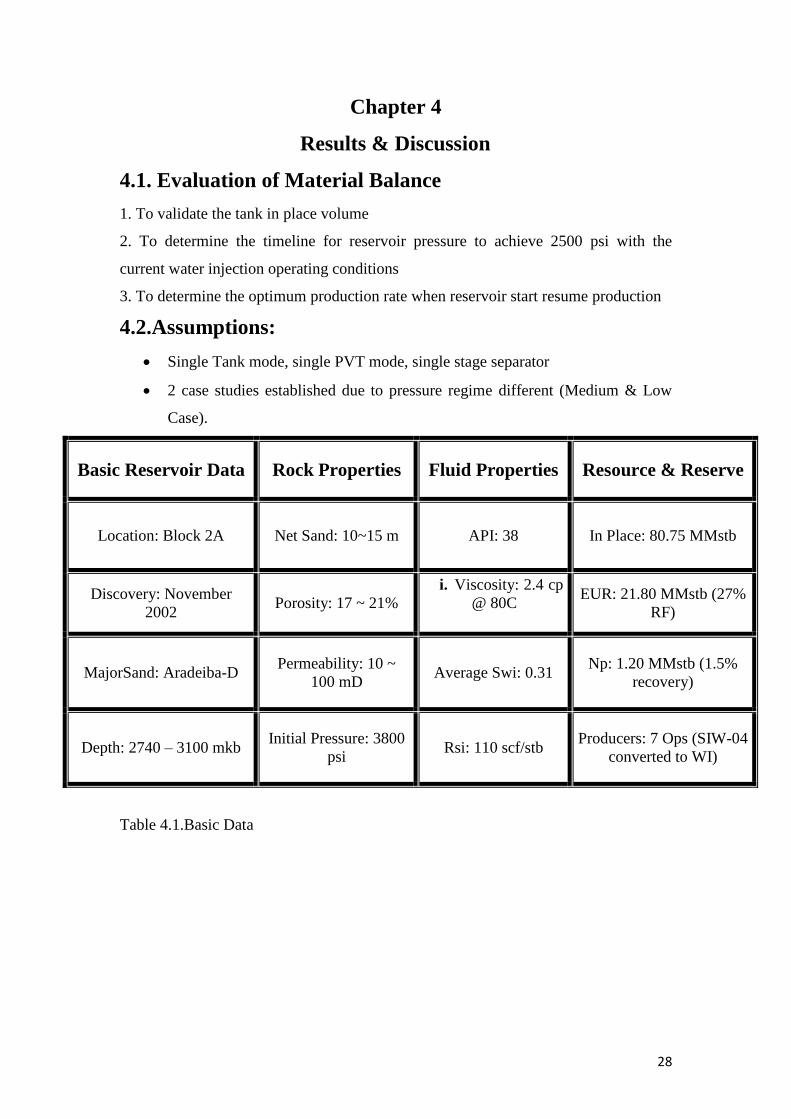
4.2.Assumptions:

Single Tank mode, single PVT mode, single stage separator

2 case studies established due to pressure regime different (Medium & Low

Case).

Basic Reservoir Data Rock Properties Fluid Properties Resource & Reserve

Location: Block 2A Net Sand: 10~15 m API: 38 In Place: 80.75 MMstb

Discovery: November

2002 Porosity: 17 ~ 21%

i. Viscosity: 2.4 cp

@ 80C

EUR: 21.80 MMstb (27%

RF)

MajorSand: Aradeiba-D Permeability: 10 ~

100 mD Average Swi: 0.31

Np: 1.20 MMstb (1.5%

recovery)

Depth: 2740 – 3100 mkb Initial Pressure: 3800

psi Rsi: 110 scf/stb

Producers: 7 Ops (SIW-04

converted to WI)

Table 4.1.Basic Data

29

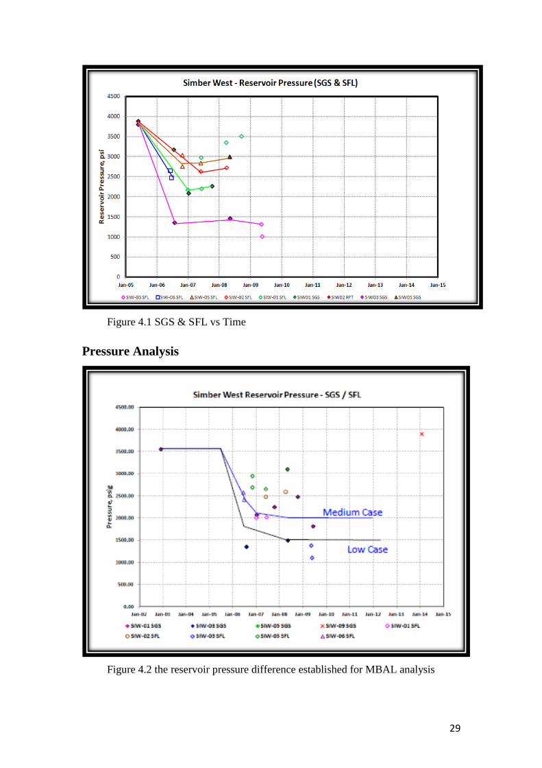
Figure 4.1 SGS & SFL vs Time

Pressure Analysis

Figure 4.2 the reservoir pressure difference established for MBAL analysis

30

The reservoir pressure range is quite significant difference, 2 cases (medium & low)

established for MBAL analysis.

4.3. Material Balance Case Study

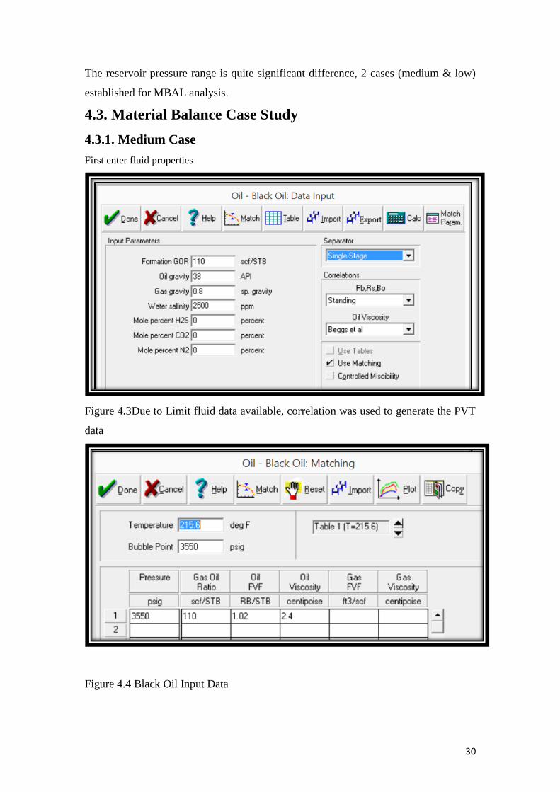
4.3.1. Medium Case

First enter fluid properties

Figure 4.3Due to Limit fluid data available, correlation was used to generate the PVT

data

Figure 4.4 Black Oil Input Data

31

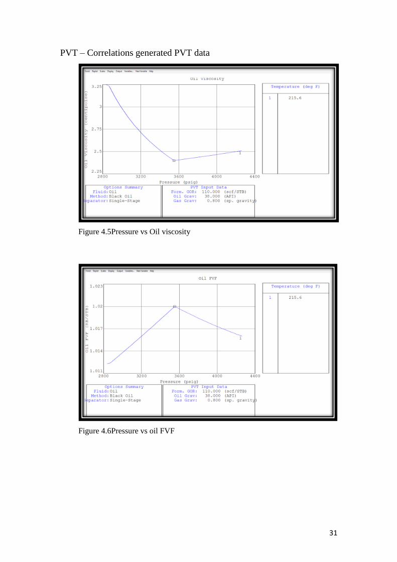
PVT – Correlations generated PVT data

Figure 4.5Pressure vs Oil viscosity

Figure 4.6Pressure vs oil FVF

32

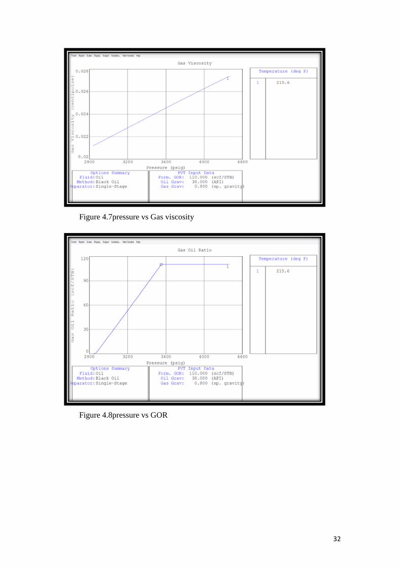
Figure 4.7pressure vs Gas viscosity

Figure 4.8pressure vs GOR

33

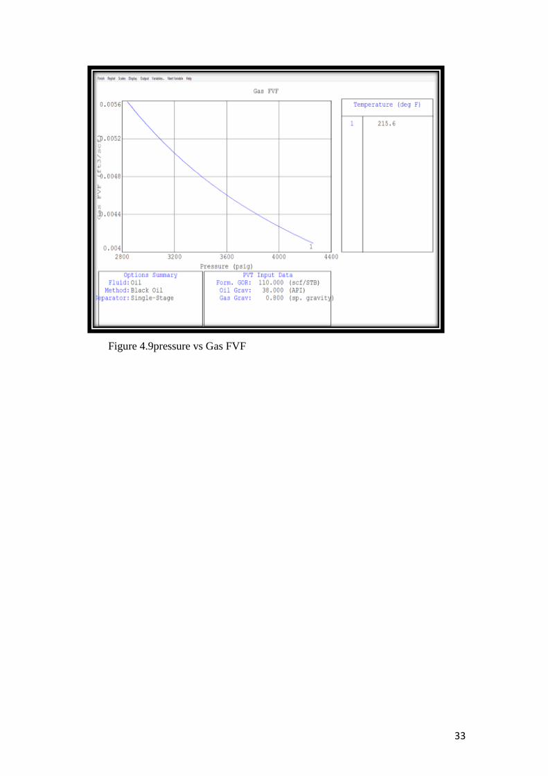
Figure 4.9pressure vs Gas FVF

34

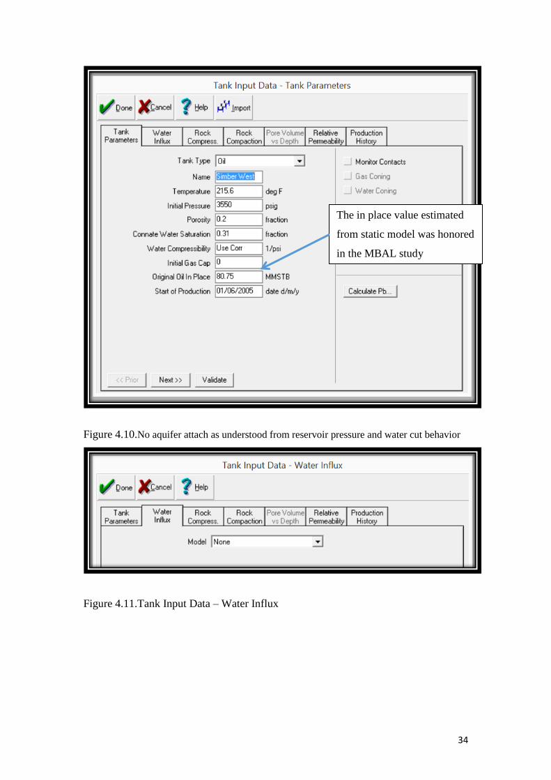
Figure 4.10.No aquifer attach as understood from reservoir pressure and water cut behavior

Figure 4.11.Tank Input Data – Water Influx

The in place value estimated

from static model was honored

in the MBAL study

35

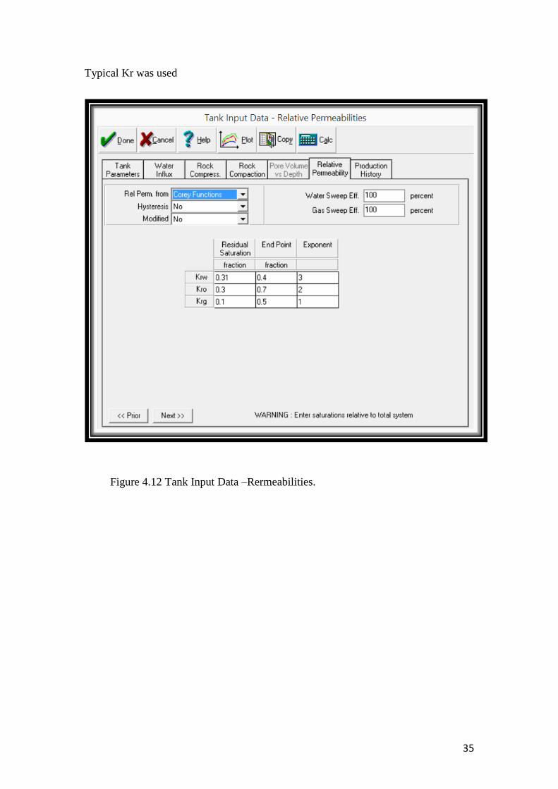
Typical Kr was used

Figure 4.12 Tank Input Data –Rermeabilities.

36

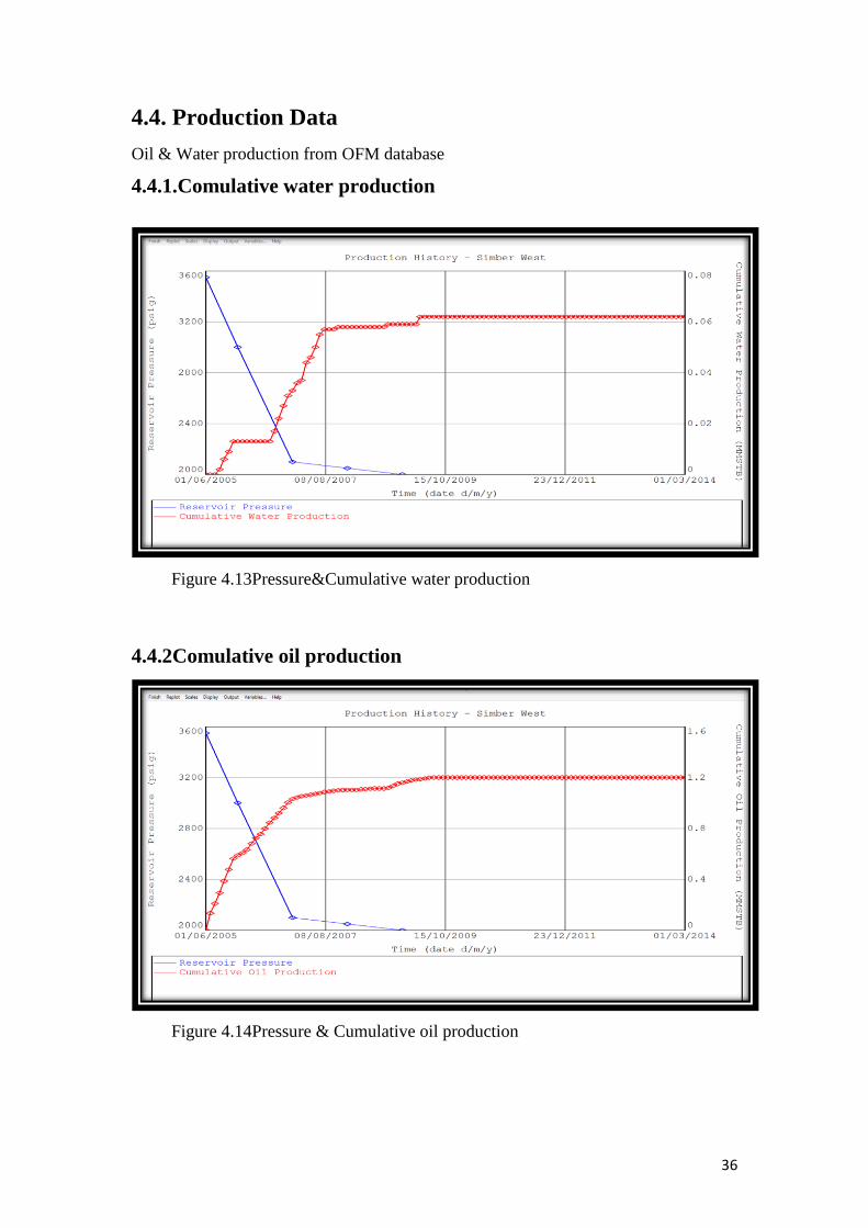
4.4. Production Data

Oil & Water production from OFM database

4.4.1.Comulative water production

Figure 4.13Pressure&Cumulative water production

4.4.2Comulative oil production

Figure 4.14Pressure & Cumulative oil production

37

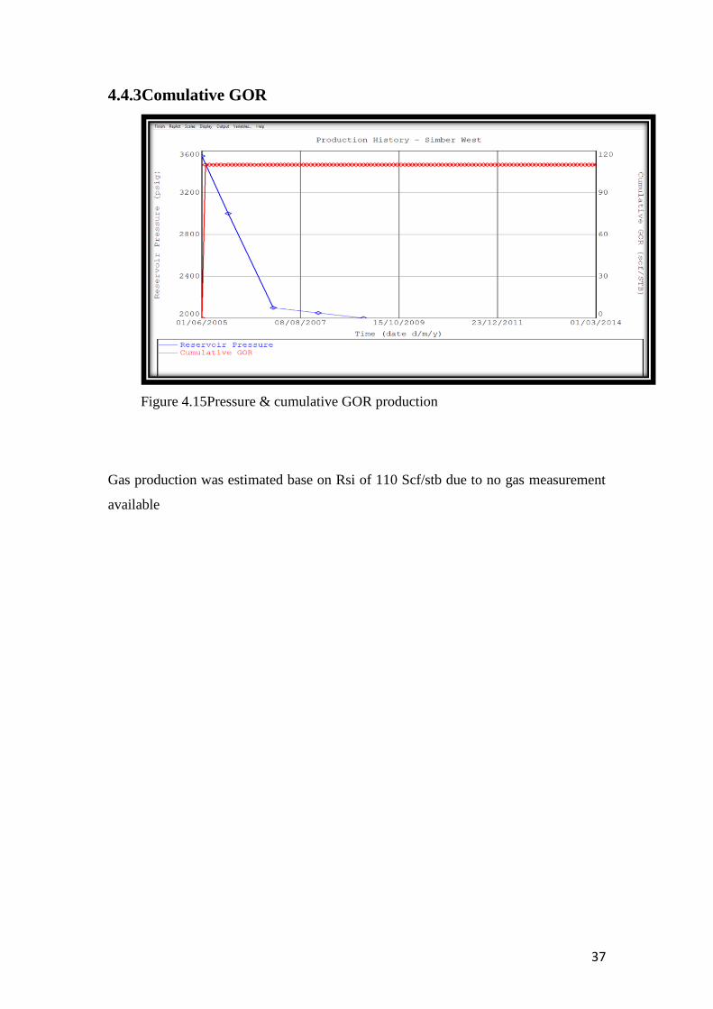
4.4.3Comulative GOR

Figure 4.15Pressure & cumulative GOR production

Gas production was estimated base on Rsi of 110 Scf/stb due to no gas measurement

available

38

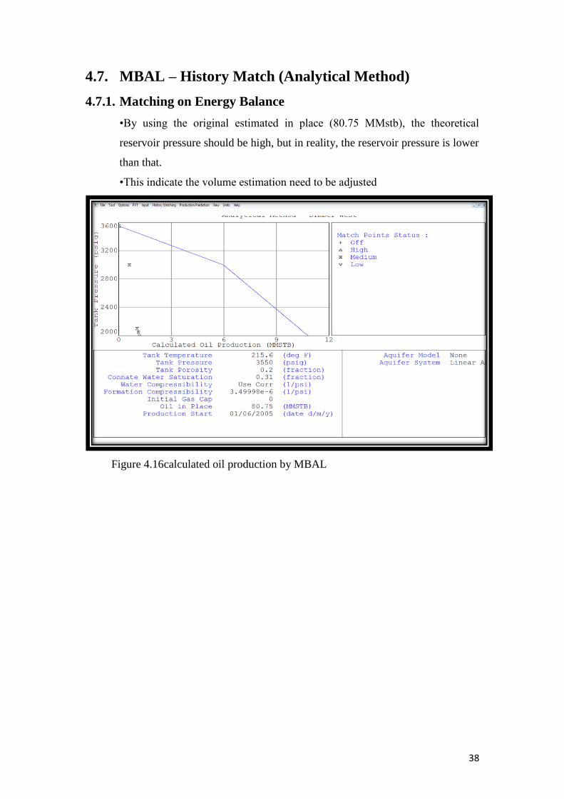
4.7. MBAL – History Match (Analytical Method)

4.7.1. Matching on Energy Balance

•By using the original estimated in place (80.75 MMstb), the theoretical

reservoir pressure should be high, but in reality, the reservoir pressure is lower

than that.

•This indicate the volume estimation need to be adjusted

Figure 4.16calculated oil production by MBAL

39

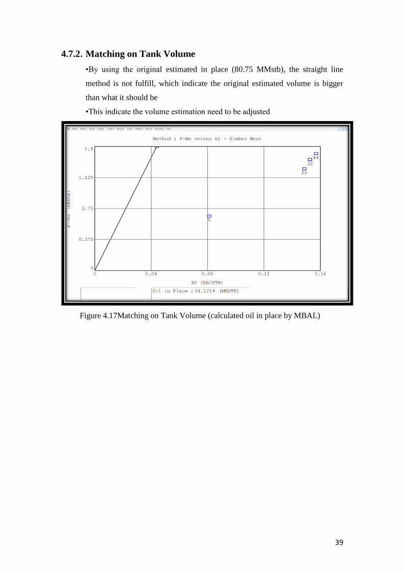
4.7.2. Matching on Tank Volume

•By using the original estimated in place (80.75 MMstb), the straight line

method is not fulfill, which indicate the original estimated volume is bigger

than what it should be

•This indicate the volume estimation need to be adjusted

Figure 4.17Matching on Tank Volume (calculated oil in place by MBAL)

40

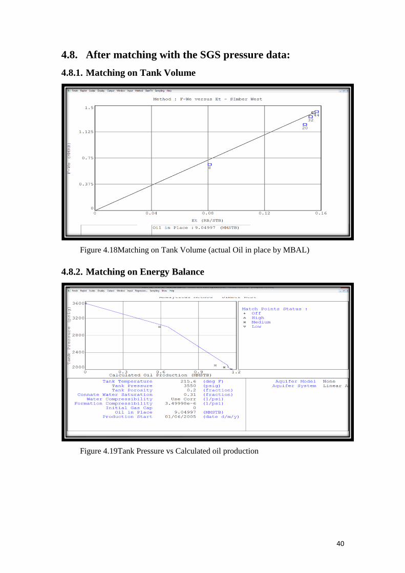
4.8. After matching with the SGS pressure data:

4.8.1. Matching on Tank Volume

Figure 4.18Matching on Tank Volume (actual Oil in place by MBAL)

4.8.2. Matching on Energy Balance

Figure 4.19Tank Pressure vs Calculated oil production

41

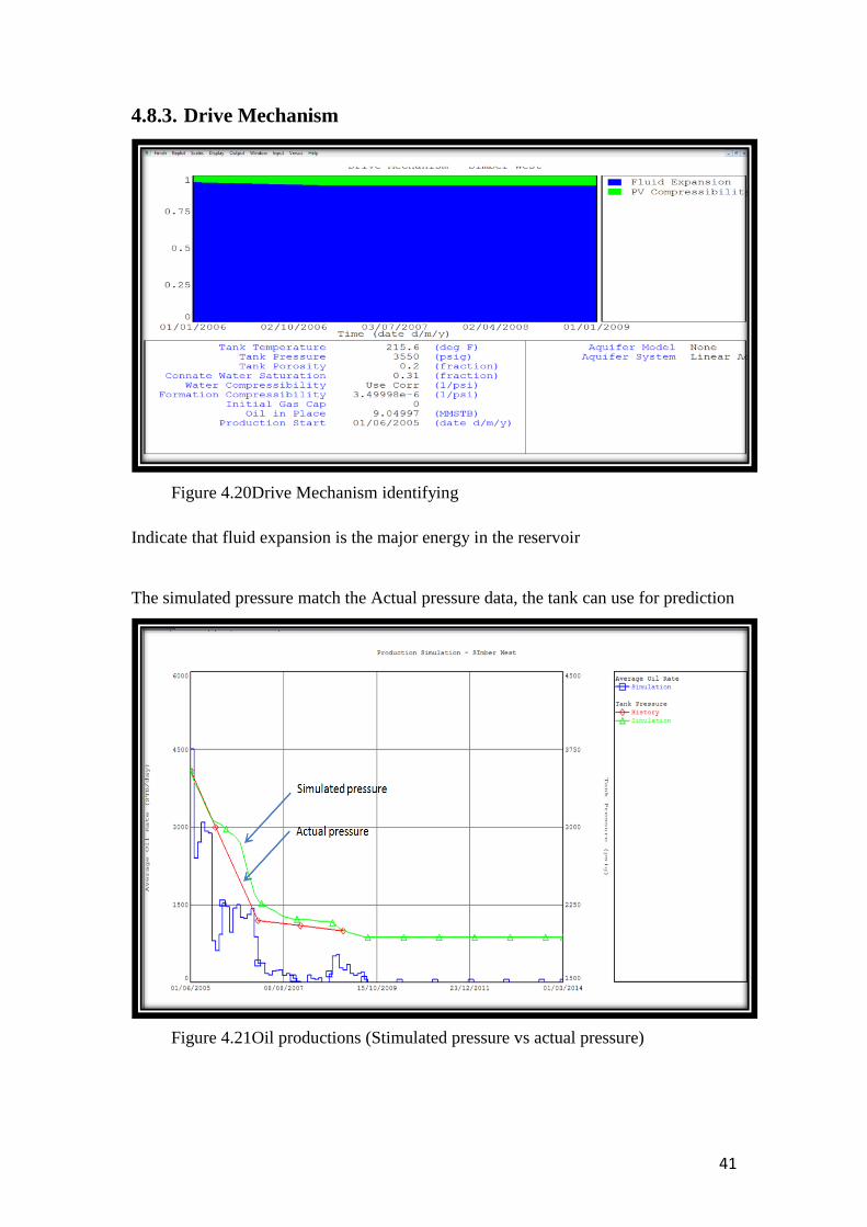
4.8.3. Drive Mechanism

Figure 4.20Drive Mechanism identifying

Indicate that fluid expansion is the major energy in the reservoir

The simulated pressure match the Actual pressure data, the tank can use for prediction

Figure 4.21Oil productions (Stimulated pressure vs actual pressure)

42

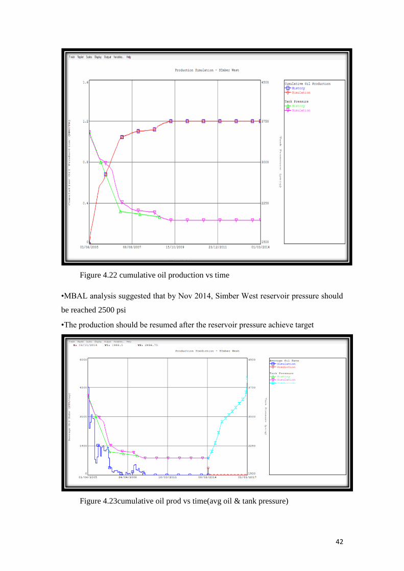
Figure 4.22 cumulative oil production vs time

•MBAL analysis suggested that by Nov 2014, Simber West reservoir pressure should

be reached 2500 psi

•The production should be resumed after the reservoir pressure achieve target

Figure 4.23cumulative oil prod vs time(avg oil & tank pressure)

43

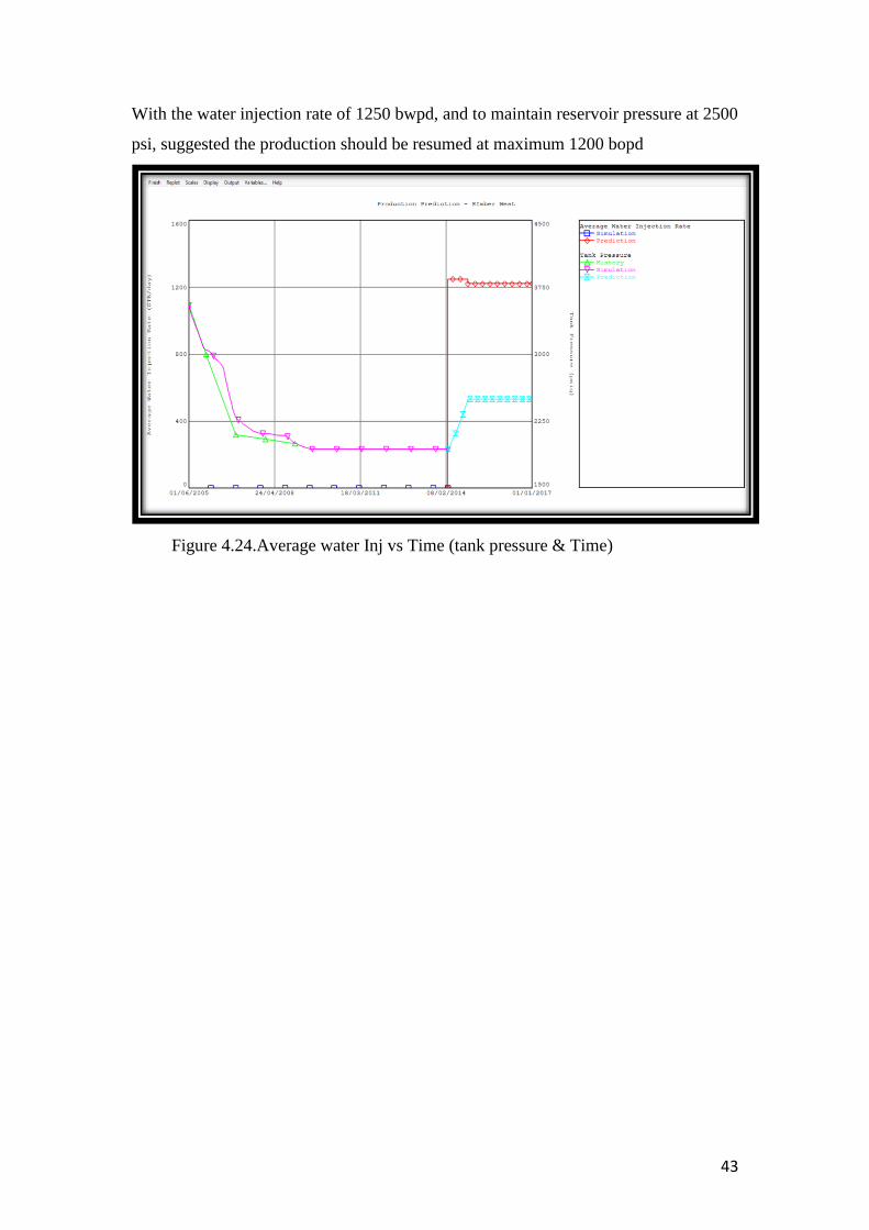
With the water injection rate of 1250 bwpd, and to maintain reservoir pressure at 2500

psi, suggested the production should be resumed at maximum 1200 bopd

Figure 4.24.Average water Inj vs Time (tank pressure & Time)

44

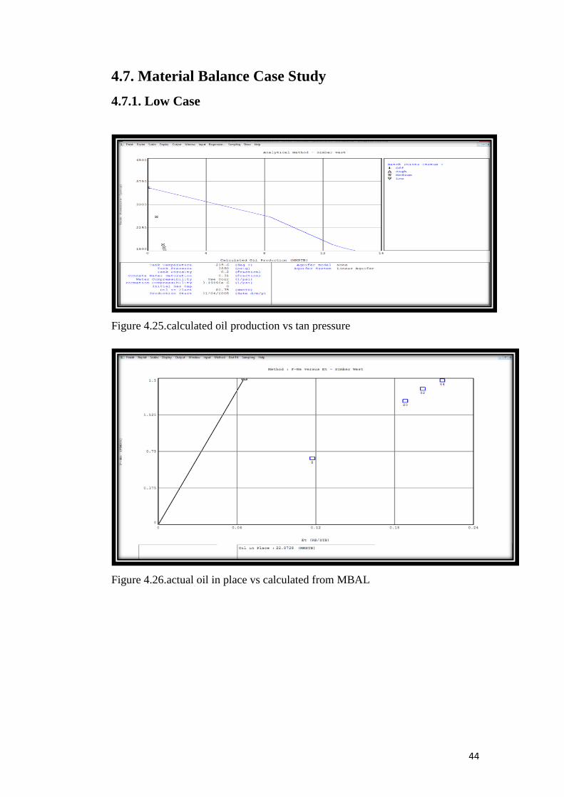
4.7. Material Balance Case Study

4.7.1. Low Case

Figure 4.25.calculated oil production vs tan pressure

Figure 4.26.actual oil in place vs calculated from MBAL

45

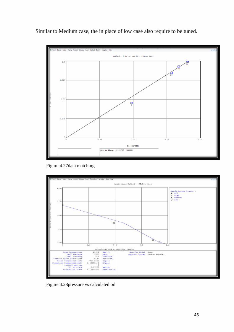
Similar to Medium case, the in place of low case also require to be tuned.

Figure 4.27data matching

Figure 4.28pressure vs calculated oil

46

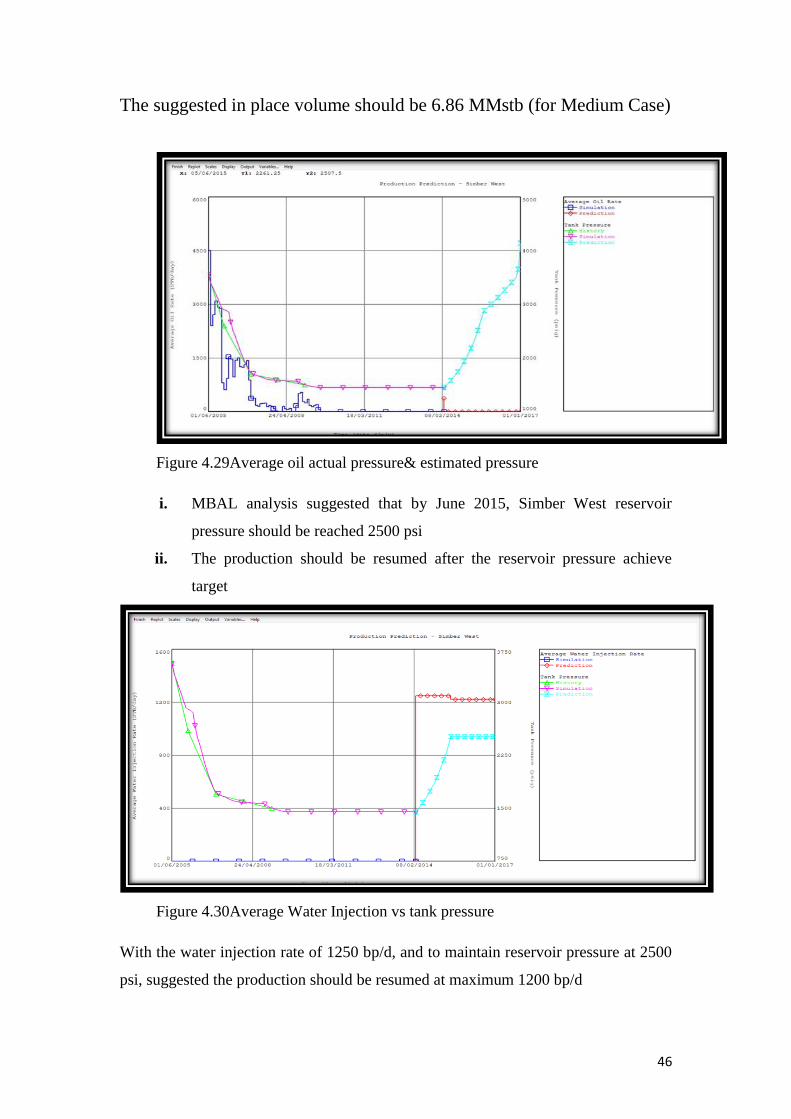
The suggested in place volume should be 6.86 MMstb (for Medium Case)

Figure 4.29Average oil actual pressure& estimated pressure

i. MBAL analysis suggested that by June 2015, Simber West reservoir

pressure should be reached 2500 psi

ii. The production should be resumed after the reservoir pressure achieve

target

Figure 4.30Average Water Injection vs tank pressure

With the water injection rate of 1250 bp/d, and to maintain reservoir pressure at 2500

psi, suggested the production should be resumed at maximum 1200 bp/d

47

4.8 Observation

i. MBAL analysis suggested that the reservoir should achieve pressure of 2500

psi by Nov 2014 (medium case) or June 2015 (low case) with production rate

of about 1100 bopd. However, close monitoring require to enhance the

understanding of subsurface to achieve optimize production.

ii. Fluid properties (PVT data) data quality may detriment the quality of the

analysis because the main drive mechanism is fluid expansion

iii. The reservoir pressure range indicate that the sand continuity is uncertain,

Geophysicist’s seismic input are essential to further understand the sand

continuity

4.9. Discussion, Water Injection Operation & Implementation:

i. Water injection metering performance is dissatisfactory

ii. Untreated injection water probably caused the scale / skin formation

iii. Water injection parameters established through injectivity test

iv. SIW01, SIW03 not really supported by water injection

v. SIW05 supported by water injection, but experiencing +ve skin

problems probably due to untreated injection water.

48

Chapter Five

Conclusions &

Recommendations

49

Chapter 5

Conclusions & Recommendation

5.1. Conclusion

i. Simber West oil properties is suitable for water injection scheme

ii. Geological understanding is dissatisfactory (unknown sand continuity)

iii. STOIIP probably less than expectation (Based on MBAL analysis)

iv. Weak and moderate aquifer available, but due to geological structure,

only support to SIW01 relatively

v. SIW01, SIW03, SIW05 are probably are located at different sand body

(Based on reservoir pressure respond)

vi. SIW03 production is fluctuating probably due to small volume of

connected sand body

5.2. Recommendation

i. The first part requires that water be injected at the highest pressure possible

ii. The second part limits the injection pressure to just below formation fracture

pressure.

iii. In practice, operators commonly use a surface injection pressure of 50 psig

below formation parting pressure minus the static pressure of a column of

injection fluid.

iv. More SGS pressure to ensure the analysis are properly calibrated

v. Gas measurement are recommended to avoid lost count of energy

50

References:-

-Tarek, T.A,Paul,D. McKinney,(2005) Advanced_Reservoir_Engineering, Senior

Staff Advisor, V.P. Reservoir Engineering, Anadarko Petroleum Corporation,

Anadarko Canada Corporation.

-Bose,R.B. (2007) Unloading Using Auger Tool and Foam and Experimental

Identification of Liquid Loading of Low Rate Natural Gas Wells, MSc Thesis, Texas

A&M University.

-Binli,O. (2009) Overview Of Solution To Prevent Liquid-Loading Problems In

Gas Wells, MSc Thesis, Middle East Technical University.

-AGARWAL, R.G. (1980). A new method to account for producing time effects

when drawdown type curves are used to analyze pressure buildup and other test data.

SPE Paper

9289, Presented at SPE–AIME 55th Annual Technical

Conference, Dallas, Texas, Sept. 21–24

-CARTER, R. and TRACY, G. (1960). An improved method for calculations of

water influx.Trans. AIME, 152

- CRAFT, B. and HAWKINS, M. (1959). Applied Petroleum Reservoir

Engineering (Englewood Cliffs, NJ: Prentice Hall)

-HAWKINS, M. (1955). Material Balances in Expansion TypeReservoirsAbove

Bubble-Point. SPE Transactions Reprint

Series No. 3, pp. 36–40