1 Chapter 1: Introduction

The terms primary oil recovery, secondary oil recovery, and tertiary (enhanced) oil

recovery are traditionally used to describe hydrocarbons recovery according to the

method of production or the time at which they are obtained.

1.1 Primary Oil Recovery

(Muskat) defines primary recovery as the production period beginning with the initial

field discovery and continuing until the original energy sources for oil expulsion (the

natural drive mechanism) are no longer alone able to sustain profitable producing rates.

The natural energy responsible for recovering the oil under primary recovery is:

I. Depletion drive.II. Water drive.

III. Gas cap drive.IV. Gravity drainage drive.V. Rock and liquid expansion drive.

VI. Combination drive.

1.2 Secondary Oil Recovery

(James Sheng 2010) Secondary recovery is recovery by injection of external fluids, such

as water and/or gas, mainly for the purpose of pressure maintenance and volumetric

sweep efficiency.

1.3 Enhanced Oil Recovery (EOR) Processes

9

Enhanced oil recovery (EOR) processes include all methods that use external sources of

energy and/or materials to recover oil that cannot be produced, economically by

conventional means.

1.4 The Difference between IOR/EOR

IOR is an acronym for Improved Oil Recovery that is commonly used to describe any

process, or combination of processes, that may be applied to economically increase the

cumulative volume of oil that is ultimately recovered from the reservoir at an accelerated

rate. IOR may include EOR, new well drilling, workover jobs, and production

enhancement. (Sunil.k and Abdulaziz. A)

10

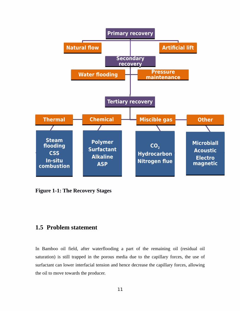
Figure 1-1: The Recovery Stages

1.5 Problem statement

In Bamboo oil field, after waterflooding a part of the remaining oil (residual oil

saturation) is still trapped in the porous media due to the capillary forces, the use of

surfactant can lower interfacial tension and hence decrease the capillary forces, allowing

the oil to move towards the producer.

11

Primary recoveryPrimary recovery

Natural flowNatural flow

Secondary recovery

Secondary recovery

Tertiary recoveryTertiary recovery

ChemicalChemical

PolymerSurfactant

AlkalineASP

PolymerSurfactant

AlkalineASP

Miscible gasMiscible gas

CO2

HydrocarbonNitrogen flue

CO2

HydrocarbonNitrogen flue

ThermalThermal

Steam flooding

CSSIn-situ

combustion

Steam flooding

CSSIn-situ

combustion

OtherOther

MicrobiallAcousticElectro

magnetic

MicrobiallAcousticElectro

magnetic

Water floodingWater flooding Pressure maintenance

Pressure maintenance

Artificial liftArtificial lift

1.6 Objectives

General objectives:

Study the possibility of surfactant flooding as good EOR method for Bamboo

main oil field based on screening criteria and simulation results. Build a model that resembles the actual bamboo main field conditions, based on

the available fluid and rock properties.

Specific objectives:

Design optimum surfactant concentration. Design optimum injection rate for bamboo main oil field.

Introduction to the Case Study

Greater Bamboo Field is located in block 2A Muglad Basin consist of four structures,

Bamboo west, main, east and south and covers an area of about 144 km as shown in

figures (1-2). It involves of multi-layered under-saturated sandstone reservoir of late

cretaceous ages buried at depth ranging from 1000 m to 1500 m. The total field STOIIP

and Recovery Factor (RF) is currently estimated at around 509 MMSTB, 16%

respectively. To date the field had recovered more than 69% of the Ultimate Recovery

(EUR).

12

Figure 1-2: location of bamboo field

The field initially produced around 20,000 STB/D with early water breakthrough and

very minimal gas production rate until today. However, the production rate declined

rapidly when the water production rate increased. Major factors that contributed to this

problem are possibly due to the fingering and water conning. Currently the field is

producing around 9000 STB/D with water cut around 75% and keeps increasing (Elamin

S.Mohmmed & Husham A.Ali, 2014).

13

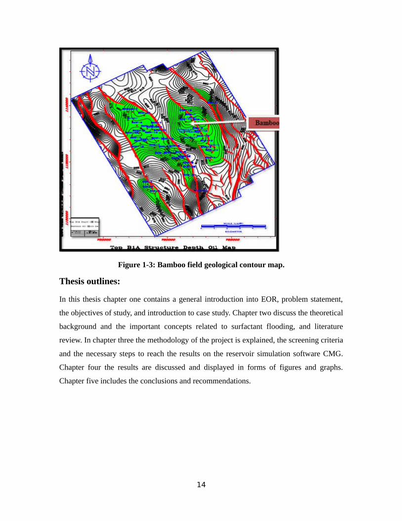
Figure 1-3: Bamboo field geological contour map.

Thesis outlines:

In this thesis chapter one contains a general introduction into EOR, problem statement,

the objectives of study, and introduction to case study. Chapter two discuss the theoretical

background and the important concepts related to surfactant flooding, and literature

review. In chapter three the methodology of the project is explained, the screening criteria

and the necessary steps to reach the results on the reservoir simulation software CMG.

Chapter four the results are discussed and displayed in forms of figures and graphs.

Chapter five includes the conclusions and recommendations.

14

2 Chapter 2: Literature Review & Background

2.1 General Background

2.1.1 Introduction

Oil production in many fields has reached the mark of residual oil saturation. This in turn

has forced the oil industry to recover oil from more complicated areas, where the oil is

less accessible, by means of advanced recovery techniques. The reserves and production

ratios in sandstone fields have around 20 years of production time left. The proven and

probable reserves in carbonate fields have around 80 years of production time left (Mon-

taron, 2008). With global energy demand and consumption forecast to grow rapidly

during the next 20 years, a more realistic solution to meet this need lies in sustaining

production from existing fields by means of EOR (James Sheng2010).

After primary and secondary methods, two-thirds of the original oil in place (OOIP) in a

reservoir is not produced and still pending for recovery by efficient enhanced oil recovery

(EOR) methods. EOR methods can be categorized into three main processes such as

thermal oil recovery, miscible flooding, and chemical flooding (Taber et al. 1979;

Shandrygin and Lutfullin 2008).

15

2.1.2 When to start EOR (Tarek ahmed, 2001):

A common procedure for determining the optimum time to start EOR process after water

flooding depends on:

i. Anticipated oil recovery.ii. Fluid production rates.

iii. Monetary investment.iv. Costs of water treatment and pumping equipment.v. Costs of maintenance and operation of the water installation facilities.

vi. Costs of drilling new injection wells or converting existing production wells into

injectors.

Basic concepts:1. Interfacial tension :

The surface tension is defined as the force exerted on the boundary layer between

a liquid phase and a vapor phase per unit length. This force is caused by

differences between the molecular forces in the vapor phase and those in the

liquid phase, and also by the imbalance of these forces at the interface. The

surface can be measured in the laboratory and is unusually expressed in dynes per

centimeter (Tarek ahmed, 2010).

¿¿¿

σ ow=r h g ( ρw−ρo )

2cosθ……… …(STYLEREF 1 2SEQ Equation 1)

Where:

r = pore radius cm

h = hight cm

ρo = density of oil, gm/cm.

16

ρw = density of water, gm/cm.

σ ow = interfacial tension between the oil and the water, dynes/cm.

2. Wettability:

Wettability is the preference of one fluid to spread on or adhere to a solid surface in the

presence of other immiscible fluids (Craig, 1971).

Figure 2-4: illustration of wettability

Wettability depends on the mineral ingredients of the rock, the composition of the oil and

water, the initial water saturation, and the temperature.

The wettability of reservoir rocks to the fluids is important in that the distribution of the

fluids in the porous media is a function of wettability.

Because of the attractive forces, the wetting phase tends to occupy the smaller pores of

the rock and the nonwetting phase occupies the more open channels (Tarek ahmed, 2010).

Wettability can be quantified by measuring the contact angle of oil and water on silica or

calcite surface or by measuring the characteristics of core plugs with either an Amott

imbibition test or a USBM test.

17

3. Capillary pressure

Capillary pressure is the most basic rock-fluid characteristic in multiphase flows. It is

defined as the difference between the pressures in the non-wetting and wetting phases

(Shunhua Liu, 2007).

Pc = Pnw – Pw

The capillary forces in a petroleum reservoir are the result of the combined effect of the

surface and interfacial tensions of the rock and fluids, the pore size and geometry, and the

wetting characteristics of the system.

The displacement of one fluid by another in the pores of a porous medium is either aided

or opposed by the surface forces of capillary pressure (Tarek ahmed, 2010).

¿¿¿¿

pc=2σ cosθ

R……… ..(STYLEREF 1 2STYLEREF 1 2SEQ Equation 2)

Where:

pc : Capillary pressure.

Pnw: pressure in the nonwetting phase.

Pw: pressure in the wetting phase.

σ : Interfacial tension between two fluid phases.

θ : Contact angle, measured in wetting phase.

R: radius of the tube.

18

3. Mobility ratio:

Tarek Ahmed (2000) states that The mobility is defined as the ratio of the permeamibiliy

to the viscosity and the Mobility ratio (M) is defined as the mobility of displacing phase

to mobility of displaced phase, and can be given by:

¿¿¿

M=ʎ displacingʎ displaced

……… (STYLEREF 1 2SEQ Equation 3)

M=

KrwKro

∗μo

μw……….. (2-1)

Where:

Kro, Krw = relative permeability to oil and water, respectively.

μo ,μw = viscosity of oil and water, respectively.

If a mobility ratio greater than unity, it is called an unfavorable ratio because the

Invading fluid will tend to bypass the displaced fluid. It is called favorable if less than

unity and called unit mobility ratio when equal to unity.

4. Capillary Number

Capillary Number is defined as the ratio of the viscous forces and local capillary forces.

This can be calculated from the formula in equation below (Moore and Slobod 1955):

NC=u μw

σ cosϕ ………… ( 2-2 )

19

u= Effective flow rate

μ = Viscosity of displacing fluid

σ = Interfacial Tension

Ø = Contact angle measured through the fluid with highest density.

An increase in capillary number implies a decrease in residual oil saturation and thus an

increase in oil recovery.

20

Capillary Desaturation Curve which relates the capillary Number Nc to the residual oil

saturation.

In order to achieve an increase in the capillary number, an increase in the viscosity of the

displacement fluid or an increase in the velocity of displacement may not be effective on

a field scale. However, a high Nc can be achieved by reducing the interfacial tension

between water and oil by the use of surfactant.

Also as can be seen from the capillary pressure relationship.

¿¿¿

pc=2 γ cos θ

rSTYLEREF 1 2−SEQ Equation 6 ¿

A very low oil-water interfacial tension reduces the capillary pressure and thus facilitates

oil mobilization allowing water to displace additional oil.

The residual oil can even be reduced to zero if the interfacial tension can be successfully

reduced to a zero-value.

5. Phase behavior

The phase behavior of surfactant/oil/water mixtures is the single most critical factor

determining the success of a chemical flood. The desired ultralow IFT in surfactant

systems is usually measured by examining the phase behavior of the microemulsion

system, where the regions with high solubilization are located.

Phase behavior is dependent on the type and concentration of surfactant, and brine.

Other important parameters are the effect of high temperature and pressure on the

microemulsion properties (at typical reservoir conditions). Predictive models, such as

21

equations of state, cannot describe the phase behavior of surfactant systems adequately,

due to the presence of both surfactants and salts, which are not, included in the available

prediction tools. Therefore phase behavior of a particular system has to be measured

experimentally.

6. Recovery factor

The overall recovery factor (efficiency) RF of any secondary or tertiary oil recovery

method is the product of a combination of three individual efficiency factors as given by

the following generalized expression:

RF=ED EA EV

Where RF = overall recovery factor

ED = displacement efficiency

EA = areal sweep efficiency

EV = vertical sweep efficiency

6. Displacement efficiency ED

22

Displacement efficiency is the fraction of movable oil that has been recovered from the

swept zone at any given time or pore volume injected (Tarek Ahmed, 2010).

Mathematically, the displacement efficiency is expressed as:

ED=Volume of oil at start of flood−Remainingoil volume

Volume of oil at start of flood

ED=

( pore volume )( soi

Boi)−( pore volume)(

ŝo

Bo

)

( pore volume )(soi

Boi

)

ED=ŝ w−swi

1−swi

Soi = initial oil saturation at start of flood

Boi = oil FVF at start of flood, bbl/STB

Sw DASH = average water saturation in the swept area

Swi = initial water saturation at the start of the flood.

Because an immiscible gas injection or waterflood will always leave behind some

residual oil, ED will always be less than 1.

7. Areal sweep efficiency EA

23

Is the fractional area of the pattern thatis swept by the displacing fluid (Tarek Ahmed,

2000).

8. Vertical sweep efficiency EV

Is the fraction of the vertical section of the pay zone that is contacted by injected fluids

(Tarek Ahmed, 2000). The vertical sweep efficiency is primarily a function of:

9. Volumetric Sweep Efficiency

Note that the product of EA EV is called the volumetric sweep efficiency. and represents

the overall fraction of the flood pattern that is contacted by the injected fluid(Tarek

Ahmed, 2000).

9. Screening Criteria:

A large number of variables are associated with a given oil reservoir for instance,

pressure, temperature, crude oil type and viscosity and the nature of the rock matrix and

connate water.

Because of these variables not every type of EOR process can be applied to every

reservoir. An initial screening procedure would quickly eliminate some EOR processes

from consideration in particular reservoir application.

Factors used in the screening are:• Reservoir conditions - temperature and pressure.• Reservoir fluid properties – oil viscosity and density and formation water salinity.• Reservoir geology – rock type and depth and permeability and porosity.(Teknika ,

2000).

24

Table 2-1: screening criteria (Green and Willhite).

2.1.3 Methods of EOR

The EOR methods work under the following principles (Latil et al., 1980):

Improve sweep efficiency be reducing the mobility ratio between injected and in-

place fluids. Eliminate or reduce the capillary and interfacial forces and thus improve

displacement efficiency. Act on both phenomena simultaneously.

2.1.3.1 Miscible Displacement

25

Miscible oil displacement is the displacement of oil by fluids with which it mixes in all

proportions without the presence of an interface, all mixtures remaining single phase.

This is possible only by injecting a miscible agent which reduces the retaining forces to

zero is nearly total displacement possible in the pores contacted by miscible agent.

Example of fluids injected to achieve miscible displacement (CO2, hydrocarbon solvents,

nitrogen and H2).

2.1.3.2 Thermal Methods

Thermal methods have been used since 1950s, primary and secondary production from

reservoirs containing heavy, low gravity oil is usually a small fraction of the initial oil in

place. This is due to the fact that these types of oils are very thick and viscous and as a

result does not migrate readily to producing wells. If the temperature of crude oil in

reservoir can be raised by 100 -200 F over the normal reservoir temperature, the oil

viscosity will be reduced significantly and will flow much more easily to a producing

well. The temperature of a reservoir can be raised by injecting a hot fluid or by generating

thermal energy in-situ by combusting the oil (Ronal E, 2001).

Thermal Processes Include:I. Steam injection

II. Cyclic steam stimulation (CSS)III. In-situ combustion (ISC)IV. Steam assisted gravity drainage (SAGD)

2.1.3.3 Chemical Methods

26

Chemical flooding methods are considered as a special branch of EOR processes to

produce residual oil after water flooding.

In chemical EOR or chemical flooding, the primary goal is to recover more oil by either

one or a combination of the following processes (Teknika, 2001):

Mobility control by adding polymers to reduce the mobility of the injected water,

and to increase sweep efficiency. Interfacial tension (IFT) reduction by using surfactants, and/or alkalis, to improve

the displacement efficiency.

I. Polymer Flooding

Polymer flooding is the process of adding small amount of polymers to thickening brine

water to reduce water mobility. In which a large macromolecule is used to increase the

displacing fluid viscosity, this leads to improve sweep efficiency in the reservoir.

There two main types of polymers:

1. XC-biopolymer:

It is a natural polysaccharide produced by microbial fermentation process. This type

reduces mobility ratio by increasing water viscosity. It increases mobility ratio by

decreases water viscosity

2. Polyacrylamides:

They are synthetic chemical products which reduce water mobility by reducing formation

permeability to water. (Aurel carcoana,1992).

Polymer Flooding Processes:

27

Firstly low salinity brine (freshwater) slug is injected to the reservoir followed by

injection of a slug of 0.3 or higher PV of polymer solution. The polymer slug is followed

by another freshwater and then followed by continuous drive water injection.

Polymers are usually added to water in concentrations ranging from 250 – 2000 parts per

million (ppm).

Limitations(Aurel carcoana, 1992):

a. High oil viscosity requires higher polymer concentration.b. Results can be better if polymer flood is started before the water oil ratio become

excessively high.c. Clays increase polymer adsorption.d. Some heterogeneity is acceptable but the extensive fractures must be avoided.

II. Alkaline Flooding

The alkaline flooding method relies on a chemical reaction between chemicals such as

bbsodium carbonate and sodium hydroxide (most common alkali agents) and organic

acids (saponifable components) in crude oil to produce in situ surfactants (soaps) that can

lower interfacial tension. Another very important mechanism is emulsification. The

addition of the alkali increases pH and lowers the surfactant adsorption so that very low

surfactant concentrations can be used to reduce cost (James Sheng, 2010).

Alkaline substances that have been used include “sodium hydroxide, sodium orthosilicat,

sodum metasilicate, sodium carbonate, ammonia ammonium hydroxide”.The most

popular one is sodium hydroxide. Sodium orthosilicate has some advantages in brines

with high divalent ion content (Ronald E, 2001).

III. Surfactant Flooding:

The term surfactant is a blend of surface acting agents. Surfactants are usually organic

compounds that are amphiphilic, meaning they are composed of a hydrocarbon chain

28

(hydrophobic group, the “tail”) and a polar hydrophilic group (the “head”). Therefore,

they are soluble in both organic solvents and water. They adsorb on or concentrate at a

surface or fluid/fluid interface to alter the surface properties significantly; in particular,

they reduce surface tension or interfacial tension (IFT).

Figure 2-5: surfactant structure

In EOR with surfactant flooding the hydrophilic head interacts with water molecules and

the hydrophobic tail interacts with the residual oil. Thus, surfactants can form water-in-

oil or oil-in-water emulsions. Surfactant molecules are amphiphilic, as they have both

hydrophilic and hydrophobic moieties. Amphiphiles adsorb effectively to interfaces and

typically contribute to significant reductions of the interfacial energy, [Pashley and

Karaman, 2004, p. 62].

Types of Surfactants:   

Surfactants may be classified according to the ionic nature of the head group as anionic,

cationic, nonionic, and zwitterionic (Ottewill, 1984):

1. Anionic Surfactants

Anionic surfactants are negatively charged. They are commonly used for various

industrial applications, such as detergents (alkyl benzene sulfonates), soaps (fatty acids),

29

foaming agents (lauryl sulfate), and wetting agents (di-alkyl sulfosuccinate). Anionic

surfactants are also the most commonly used in EOR. They display good surfactant

properties, such as lowering the IFT, their ability to create self-assembled structures, are

relatively stable, exhibit relatively low adsorption on reservoir rock and can be

manufactured economically [Green & Willhite, 1998, p. 241]. Anionic surfactants

dissociate in water to form an amphiphilic anion (negatively charged) and a cation

(positively charged), which would typically be an alkaline metal such as sodium (Na+) or

potassium (K+).

2. Nonionic Surfactants

Nonionic surfactants have no charged head group. They are also identified for use in

EOR, [Gupta and Mohanty, 2007], mainly as co-surfactants to promote the surfactant

process. Their hydrophilic group is of a non-dissociating type, not ionizing in aqueous

solutions. Examples of nonionic surfactants include alcohols, phenols, ethers, esters or

amides.

3. Cationic Surfactants

Cationic surfactants have a positively charged head group. Cationic surfactants dissociate

in water, forming an amphiphilic cation and anion, typically a halide (Br-, Cl- etc.).

During the synthesis to produce cationic surfactants, they undergo a high pressure

hydrogenation reaction, which is in general more expensive compared to anionic

surfactants. As a direct consequence cationic surfactants are not as widely used as anionic

and nonionic surfactants [Standnes & Austad, 2002].

Anionic

Sodium dodecyl sulfate (SDS)Sodium dodecyl benzene sulfonate

CH3 (CH)11 SO4̄ Na+

CH3 (CH2) C6 H4 SO3̄ Na+

Cationic

Cetyltrimethy lammonium bromide (CTAB)Dodecylamine hydrochloride

CH3 (CH2)15 N (CH3)+3 Br+

CH3 (CH2)11 NH3+ Cl ̄

Non-ionic

30

Polyethylene oxides CH3 (CH2)7 (O.CH2 CH2)8 OH

Table 2-2: Anionic and Nonionic Surfactants

4. zwitterionic surfactants :

The types of zwitterionic surfactants can be nonionic-anionic, nonionic-cationic, or

anionic-cationic. Such surfactants are temperature and salinity-tolerant, but they are

expensive. A term amphoteric is also used elsewhere for such surfactants (Lake, 1989).

Surfactant flooding process

After the surfactant solution has been injected into the formation targeting the surface

between oil/water to break the attractive forces between them IFT by producing soaps at

the contact reducing residual oil saturation in addition wettability change from oil wet to

water wet followed by polymer injection to enhance the sweep efficiency and control the

mobility as well as to stabilize the flow pattern.

By designing and selecting series of specialty surfactants to lower the interfacial tension

to the range of 10 – 3 dynes/cm a recovery of 10 – 20 % of the OIIP will not be

producible by other technologies is technically and economically feasible by surfactant

flooding (akzonobe, 2006).

31

Figure 2-6: Mechanism of chemical flooding (Abdulbasit, 2013).

Effect of salinity on surfactant flooding (Teknika, 2001):

A specific surfactant concentration and salinity is required for the formation of ultra-low

IFT. As the salt concentration varies in aqueous phase, the partition coefficient of the

surfactant between oil and water is altered which seems to be responsible for achieving

ultra-low IFT. The surfactant concentration in the oil phase increases with increasing salt

concentration in the aqueous phase and vice versa. Select optimal salinity in such a way

that surfactant concentration is highest at the oil-water interface which produces the

lowest IFT.

The success of surfactant flooding EOR depends on:1. Formulation.2. Cost of surfactant.3. Availability of chemicals.4. Environmental impact.5. Oil price.

Advantages:1. Reduce IFT and work as emulsifier between oil and water.2. Sour reduction to a very minimum value which immediately leads to increase in

recovery factor.3. Wettability change from oil to water wet .4. Trapped oil is produced5. Injection of polymer leads to pattern flow stabilization and mobility control.

Disadvantages and limitations :1. Complex process2. Expensive compared to alkaline and polymer.3. Incompatibility between surfactant polymers in case of no co-solvent is used.4. Degradation of surfactant and polymer in case of high reservoir temperature.5. Strong aquifer leads to both surfactant and polymer adsorption.

32

2.2 Literature review

Adding surfactant to injected water to reduce oil/water IFT and/or change wettability and

thereby increase recovery [Uren and Fahmy (1927)]. A few early field experiments where

small amounts of surfactant were injected did produce small increases in oil recovery.

The increases were probably caused mainly by wettability changes. The results were not

sufficiently promising to stimulate use of surfactants on a larger scale. A related concept

for improving recovery is to generate surfactant in-situ by injecting an alkaline solution

(Atkinson 1927), which is less expensive than synthetic surfactants and converts

naphthenic acids in the crude oil to soaps.

Dimensionless capillary number (Nc=µν/σ) control the amount of residual oil remaining

after flooding. A Core containing oil at velocity v with an aqueous solution having a

viscosity µ and IFT σ between the oil and the displacing fluid (Taber 1969).

Several researchers found that ultralow IFTs in the required range could be achieved by

using petroleum-sulfonate/alcohol mixtures. They also found systematic variations of IFT

when changing such variables as salinity, oil composition, and temperature (Hill et al.

1973; Foster 1973; Cayias et al. 1977).

Microemulsions are oil-swollen micelles in water at under optimum conditions and water

micelles in oil at optimum conditions. It was once thought that it is necessary to have a

cosolvent (alcohol) to have a microemulsion with an anionic surfactant. However, it is

now recognized that it is possible to have microemulsions without alcohol at room

temperature by using branched surfactants (Abe et al. 1986).

(Sume Sarkar, 2012) he investigated the effect of chemical flooding which is ASP (alkali,

surfactant and polymer) flooding in the Norne E-segment for various scenarios by using

33

applied reservoir simulation software (Eclipse). Though the results were good but not as

expected, he found out that shorter time periods, and also cyclic injection were much

more profitable than continuous and long period injections, a five years injection period

prove more profitable than 7 years period. He also injected different concentrations from

two types of surfactants and it turned out that increasing the amount of chemicals did not

necessarily give an increase in oil production. Higher concentrations gave higher oil

production rate and higher cumulative oil production, but it did not prove to be profitable

due to the cost of chemicals, applying a concentration between 0.5–10 kg/m3 of ASP

chemicals gave the best result.

(Yongwei Li & Lizhong Yin, 2013) They did a new surfactant flooding model for Low

Permeability Reservoirs, in Chao 522 Block of “Chaoyanggou” low permeability oilfield

which was already going under pilot testing. They presented a three-dimensional, two

phases, three component surfactant simulator. They also introduced new equation for the

calculation of surfactant adsorption, which can increase the matching degree between the

mathematical model and data from field. The goal of this new simulator is to help the

decision-making in surfactant EOR projects, and to find the best methods of field

development.

There were 4 injectors and 10 production wells in the pilot area. Four injection wells

started injecting water from January 2002. To January of 2005, just before the start of

pilot test, the designed water injection rate was 122.5 m3/d, the actual water injection was

98.3m3/d.

The injection method in the pilot testing was as the following; Main surfactant slug,

Water slug, secondary surfactant slug, and then water drive. They founded that the most

favorable surfactant concentration was 1.0%. Volume of each and every slug was 0.10

PV.

They found out from laboratory experiments that surfactant flooding lowered the

injection pressure by more than 40%, and increased the oil recovery efficiency of low

permeability reservoir by 5.0% of OOIP at Chao-522 reservoir conditions. The pilot tests

also showed that surfactant flooding can increase the water infectivity in low permeable

34

layers, and increase number of displaced zones; increase the oil production rate to

maximum of 3%.

(Farid Abadli, 2012) he did a simulation study to improve total oil production using

different chemical flooding methods such as:(surfactant flooding, polymer flooding,

Alkaline flooding, SP, ASP flooding) under many different scenarios and factors, based

on model of Norne field C-segment using Eclipse software. The black oil model was used

for simulations. He did sensitivity analyses especially focusing on chemical

concentration, injection rate and duration of injection time, our main focus here is going

to be on the results of the surfactant flooding study.

The simulated Norne C-segment field has 13 active wells including 9 producers and 4

injectors.

He chose three different surfactant concentrations at 15kg/m3, 25kg/m3, 40kg/m3. And

injection was set starting from 2013 to the end of 2016.

The results of simulations showed that surfactant flooding increased oil production

compared with water flooding. With the increase of surfactant concentration water

production is reduced. The study also showed that with small effect on recovery between

three concentrations, makes it possible that 15kg/m3 could be better choice considering

economic side. Also higher amount of chemicals is produced in higher concentration.

From the final results of his research (Farid Abadli, 2012 ) recommended surfactant

flooding for the Norne C-Segment especially when the concentration is low and injection

occurs in the early years. Injection of surfactant at a later time might not be profitable.

Also longer injection period in early life of simulation leads to higher oil production.

(Sumit Kumar Rai, Achinta Bera & Ajay Mandal, 2014) They made a research to

investigate the surfactant solution in terms of its ability to reduce the surface tension and

the interaction between surfactant and polymer in its aqueous solution. A series of

flooding experiments have been carried out to find the additional recovery using

surfactant and surfactant–polymer slug. Approximately 0.5 pore volume (PV) surfactant

(sodium dodecylsulfate) slug was injected in surfactant flooding, while 0.3 PV surfactant

35

slug and 0.2 PV polymer (partially hydrolyzed polyacrylamide) slug were injected for

surfactant–polymer flooding. In each case, water injection was used to maintain the

pressure gradient. Their objective is to determine whether or not a commercially available

simulator (CMG-STARS) could accurately simulate results from core flooding

experiments.

Two sets of experimental data have been modeled and matched using physically realistic

input parameters. The first experiment consisted of a surfactant injection which was

carried out after water flooding in a sand pack. According to surfactant flooding

simulation, the additional recovery after water flooding was found to be 17.65 % which is

comparable with the experimental results (18%).

The second experiment was conducted on a different sand pack. It consisted of surfactant

polymer flooding. According to chemical flooding simulation, the additional recovery

after water flooding was found to be 24 % which compares to the experimental result of

(23.45%).

Flooding agents Additional oil recovery, %OOIPExperimental results Simulated results

Surfactant 18 17.65Surfactant-polymer 23.45 24

Table 2-3 shows comparison between experimental and simulator results (SumitKumar Rai, Achinta Bera & Ajay Mandal, 2014).

Also, it was observed that the additional oil recovery in case of surfactant–polymer

flooding was greater than when only surfactant was used. This is because of the

contribution of IFT reduction using surfactant and mobility ratio reduction by polymer,

thus improving the overall sweep efficiency more than with surfactant flooding where

only IFT reduction is available.

(Rabia Mohammed Hunky & etl, 2010) They did an experimental study of alkaline-

surfactant flooding in ultra-shallow heavy oil reservoirs (<500 ft). The study was done on

Pennsylvanian warner sand in western Missouri, they tested more than 30 commercial

surfactants, and using sands saturated with heavy oil (API 17).

36

It has been found that a few surfactants can make stable emulsion with the warner heavy

oil and the formation brine. In all cases examined the highest recovery is from water wet

sands. The study founded that using these surfactants is better than using the commonly

used surfactants. The study also showed that the viscosity of Missouri heavy oil can be

reduced from 18518 cp to 2.5 cp at 25 C , through emulsion of a certain surfactants. The

emulsions were stable after weeks at 25 C . Alkaline-surfactant (AS) system can change

wettability from oil wet to water-wet.

By using Alkaline-surfactant (AS) system, the tertiary heavy oil recovery from water-wet

sand pack can reach up to 12% of remaining oil in place.

(George J. Hirasaki & et al, 2008) They presented a paper at the SPE Annual Technical

Conference and Exhibition, Denver, September 2008. They found out that Surfactant

adsorption can be reduced in by big difference sandstone and carbonate formations by

injection of an alkali such as sodium carbonate. The reduced adsorption allows lower

surfactant concentrations. Also they found out that Anionic surfactants and sodium

carbonate can make changes on wettability for either sandstone or carbonate formations.

oil displacement can happen just by the effect gravity drainage.

EOR in Sudan

(Wang Qiang, Mohamad Abu Bakar, el al, and 2013) they did a study about the ability of

chemical EOR in both GNPOC and PDOC fields in Sudan, from the initial EOR

screening, the best EOR processes that can be chosen in both GNPOC and PDOC are

mainly chemical and thermal EOR. Chemical EOR is the most widely used EOR process

in GNPOC fields, but thermal EOR is the most commonly used EOR process in PDOC

fields.

They did Chemical EOR evaluation using Eclipse EOR black oil simulator. Simulations

were done on sector models taken from full field models, which made to look like the

reservoir condition now. The chemical input data was taken from Qing Hai oil field lab

data which its oil properties are similar to that of Sudan's. The chemical EOR methods

are:

37

Polymer flooding. Surfactant-Polymer (Sp) Flooding. Alkaline-surfactant-polymer (asp) flooding.

They found out that chemical EOR can possibly increase field recovery factor between 4-

18% depending on the type of chemical EOR method. ASP flooding gives the highest

increase in oil recovery after waterflood ranging between 12%-18%, then SP flooding

and after that polymer flooding.

3 Chapter 3: Methodology

3.1 Introduction

In this chapter the procedure followed to get the results will be discussed, the main stages of the project can be stated as the following:

Collecting all data required. Technical Screening criteria to evaluate the initial amenability of the EOR

process. Building the model. Running the chemical EOR process, (surfactant flooding one component). Displaying the results in forms of graphs and tables. Discussing the results and forming the conclusions.

3.2 Screening criteria:EOR screening is the first step to do EOR project implementation in the field SPE

(Society of Petroleum Engineers) has established technical EOR screening concepts

using certain format, This format is based on field experience, project implementation

around the world, this method was the start point of all EOR screening softwares, the

objective is to select the suitable EOR method to be implemented in the future.

38

The procedure contains five plots:

Permeability Vs. EOR methods Viscosity Vs. EOR methods Depth Vs. EOR methods Reservoir Depth Vs. Oil Viscosity Reservoir Pressure Vs. Viscosity

The final screening result based on the combination between the five plots. It is not

necessary to use all the plots to take the decision in the selection of the suitable EOR

method.

Screening Properties:

Layer Sw So=1-SwLayer 1 0.239 0.761Layer 2 0.239 0.761Layer 3 0.239 0.761Layer 5 0.549 0.451Layer 7 0.582 0.418

Table 3-4saturations of layers

K=2500 md

Depth =1290 m=4232 ft

Oil API = 39

PRESSURE=1873 psi

Viscosity = 76 cp

1. Permeability (k=2500md) Vs EOR methods

39

Figure 3-7: Permeability (k=2500md) Vs EOR method

2. Viscosity (µ=76 cp) Vs EOR methods

Figure 3-8: Viscosity (µ=76 cp) Vs EOR methods

3. Depth (4232 ft) Vs. EOR methods

40

Figure 3-9: Depth (4232 ft) Vs. EOR method

4. Reservoir Pressure (1873 psi) Vs. Viscosity (76 cp)

Figure 3-10: Reservoir Depth (4232 ft) Vs. Oil Viscosity (µ=76 cp)

5. Reservoir Depth (4232 ft) Vs. Oil Viscosity (µ=76 cp)

41

Figure 3-11: Reservoir Depth (4232 ft) Vs. Oil Viscosity (µ=76 cp)

As we can see from the results of the SPE screening criteria formats, most of the

screening variables agree with the surfactant flooding process, even though the viscosity

is not on the optimum range for this method but it is still feasible, we can refer here to a

research done in screening and modeling in Sudanese oil fields by Eng. Khalil Ishag

Abdallah 2011 he stated in his M.Sc. research results that “Chemical flooding can be

considered feasible for areas of viscosity less than 125 cp. However, it is important to

take into consideration factors that can reduce its effectiveness such as: reservoir

heterogeneity”.

3.3 Simulation and modeling

Before discussing the steps of building the model and getting the results we ought to give

first a brief introduction about the software we used in this process which is CMG.

CMG

Computer Modeling Group Ltd., abbreviated as CMG, is a software company that

produces reservoir simulation software for the oil and gas industry. It is based in Calgary,

Alberta, Canada with branches over the world. The company offers three reservoir

42

simulation applications. IMEX, a conventional black oil simulator used for primary,

secondary and enhanced or improved oil recovery processes; GEM, an advanced

Equation-of-State (EoS) compositional and unconventional simulator; and STARS a

thermal an advanced chemical processes simulator. In addition, CMG offers CMOST, a

reservoir engineering tool that conducts automated history matching, sensitivity analysis

and optimization of reservoir models.

Stars

STARS is CMG's new generation advanced processes reservoir simulator which includes

options such as chemical/polymer flooding, thermal applications, steam injection,

horizontal wells, dual porosity/permeability, directional permeabilities, flexible grids,

fireflood, and many more. STARS was developed to simulate steam flood, steam cycling,

steam-with additives, dry and wet combustion, along with many types of chemical

additive processes, using a wide range of grid and porosity models in both field and

laboratory scale.

3.3.1 Building the model: Step 1: Open Builder

Figure 3-12: Open Builder

Step 2: Create grids (using quick pattern)

43

Figure 3-13:create grids.

Step 3: Enter reservoir general specifications (specify property)

Figure 3-14: : Enter reservoir generalspecifications (specify property)

Step 4: Create fluid model data (generate PVT data using correlations)

Figure 3-15: Create fluid model data(generate PVT data using correlations)

Step 5: Create relative permeability data

Figure 3-16: : Create relative permeability data

Step 6: Create the initial conditions

44

Figure 3-17: Create the initial conditions.

Step 7: Choose numerical controls (timestep)

Figure 3-18: Choose numerical controls(timestep).

Step 8: Create wells (define wells specifications)

Figure 3-19: Create wells (define wellsspecifications).

45

Step 9 : Select range of dates for running the model (start-end dates)

Figure 3-20: Select range of dates for running the model (start-end dates).

Now all the ticks next to the model tree components should turn green (model can berun)

46

Figure 3-21:model ready to run.

47

3.3.2 Steps for implementing the process (in our case surfactant flooding):

Step 1: On the component section of model tree open process wizard

Step 2: Choose the process you want to run.

Figure 3-22:choose process.

Step 3: Select number of components for the chemical flooding (In our case one component surfactant only).

Figure 3-23:Number of components.

Step 4: Fill the surfactant concentrations VS IFT table and the adsorption values table.

Figure 3-24:Surfactant data.

Step 5: Changing surfactant concentration (mole fraction %)

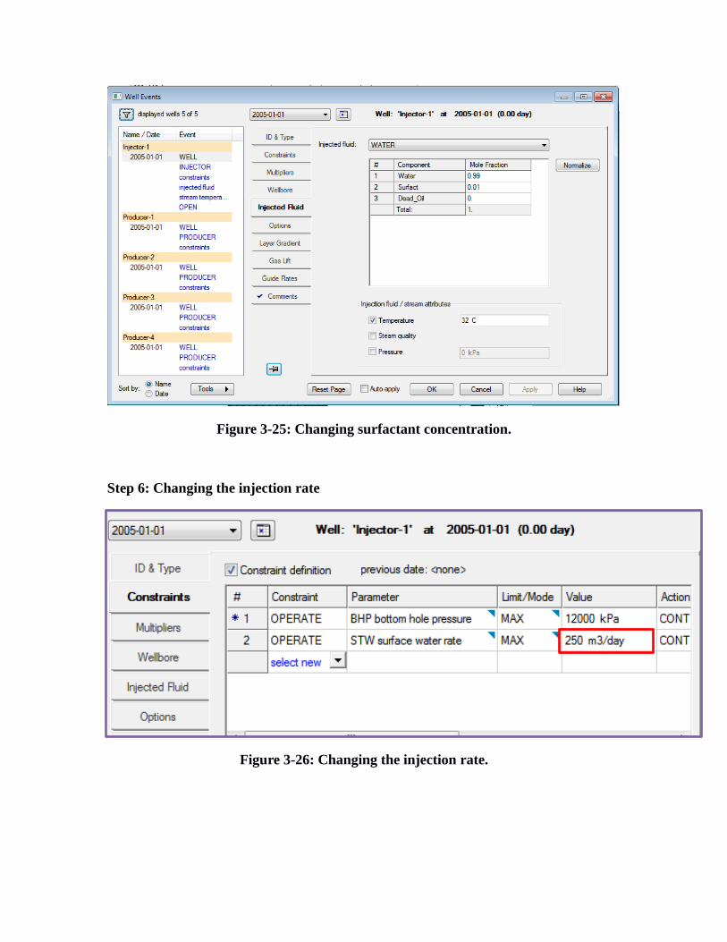
Figure 3-25: Changing surfactant concentration.

Step 6: Changing the injection rate

Figure 3-26: Changing the injection rate.

3.3.3 Displaying the results

Figure 3-27: Displaying the results.

Choosing graph variables on X-axis and Y-axis

Figure 3-28: Choosing graph variables.

4 Chapter 4: Result and discussion

4.1 IntroductionIn this chapter the results of the simulations will be displayed in form of tables and

graphs, the discussed results will include surfactant concentrations (mole fraction) against

cumulative oil production (bbl), and water cut percentage, also injection rates (m3/day)

against cumulative oil production (bbl) and water cut percentage, in addition different

surfactant injection periods will be investigated, every parameter will be studied at five

different values in a duration from Jan 2005 to Jan 2020, based on these results a

comparison will be made and decision will be made on the optimum variables for the best

surfactant flooding scenario.

It’s important to state that this model we have built to acquire the results in this chapter is

not the actual field model with the real data, since the real model is still under

development in china as we have been informed by the reservoir engineers in the oil

ministry of Sudan. This model is built to resemble the actual reservoir behavior and

conditions, by entering the reservoir and fluid properties we had access to, and in the

process some assumptions were made such as: homogenous porous media, and five spot

pattern, and default CMG data for surfactant.

4.2 Input data to CMG

Here the data entered to CMG from rock to fluid properties to surfactant properties is

specified in the form of tables below:

1. Rock Properties

Grid top (m)

Grid thickness(m)

Porosity PermeabilityI

PermeabilityJ

Permeabilityk

Water saturation

Layer1 1289.49

0.54 0.256 2500 2500 1250 0.239

Layer2 1290 7 0.256 2500 2500 1250 0.239

Layer3 1297 1.3 0.256 2500 2500 1250 0.239

Layer4 1298.3 7.84 0.256 100 100 50 0.239

Layer5 1306.14

5.41 0.268 2500 2500 1250 0.549

Layer6 1314.6 3.05 0.268 100 100 50 0.549

Layer7 1319.63

5.03 0.258 2500 2500 1250 0.582

Layer8 1319.63

45.72 0.258 5 5 2.5 0.582

Table 4-5: Rock Properties for BB-21 Well

2. Fluid properties

We have only two phases (water & oil) and their properties are illustrated below in the

following two tables, see table (4-2) and table (4-3).

For water phase

Property Water Phase

FVF (bbl./STB) 1

density (g/cm3) 1

viscosity (cp) 0.449

Table 4-6: Property of Water Phase

For oil phase

Property Oil phase

FVF (bbl/STB) @10×106 Pa 0.866

density (g/cm3)@ 10×106 Pa 0.826

viscosity (cp) 76

gas oil ratio 0

Table 4-7: Property of Oil Phase

3. Initial conditions

The initial condition of the reservoir is shown below in table (4-4 )

reference depth 1290 m

reference pressure 12911 KPa

water oil contact 1365 m

Table 4-8 Initial Conditions of Reservoir

4. Surfactant data

Table 4-9: Surfactantdata.

Surfactant adsorption

Porosity of laboratory sample data 0.2494

Weight % surfactant Surfactant adsorption mg/(100mg rock)

0 0

0.1 27.5

Table 4-10: Surfactantadsorption

4.3 Result and discussion

Comparison between primary recovery and water flooding and surfactant was made, to

identify the extent of production increment, which justifies the use of this EOR method as

a good option for recovery increase.

For this purpose the software was run three times, first run was used to simulate the

primary recovery, in the second run the injector was introduced to simulate the case of

water flooding, in the third run surfactant was introduced and injected with water with a

Weight % surfactant Interfacial tension, (dyne/cm)

0 18.2

0.05 0.5

0.1 0.028

0.2 0.028

0.4 0.0057

0.6 0.00121

0.8 0.00037

1 0.5

concentration of (0.01 mole fraction), the duration of each case was set equal to 15 years

starting from Jan 2005 to Jan 2020.

The simulations were run on a five spot model with 4 producers in the corners and 1

injector in the middle.

Figure 4-29: Five spot model.

Figure 4-30: Cumulative oil SC (bbl) Vs. Time (Yrs).

Table 4-11:

Cumulative oil SC for each recovery case.

Case Cumulative oil Sc at the endof simulation date in (bbl)

Primary recovery 762,561

Waterflooding 944,154

Surfactant flooding 1,217,070

Analyzing the figure above and table, it is clear that surfactant flooding has achieved a

great increase in cumulative oil recovery over primary and waterflooding cases, which

confirms the positive indicators obtained from the screening criteria performed in the

previous chapter.

4.3.1 Surfactant concentrations

After we confirmed that surfactant flooding can increase recovery over that of water

flooding (by 272,916 bbl), the objective now is to estimate the optimum surfactant

concentration, for this purpose five concentrations were chosen to perform the sensitivity

analysis, which are (0.20 – 0.15 – 0.10 – 0.05 – 0.01)mole fraction. The decision will be

made based on two technical considerations which are, Cumulative oil obtained under

each concentration, and the resulted water cut %.

Surfactant concentration (mole fraction)

Cumulative oil SC (bbl) Cumulative water SC

Water cut %

0.20 1,223,870 8,309,010 95.94

0.15 1,221,350 8,299,560 95.94

0.10 1,217,070 8,292,360 95.93

0.05 1,211,900 8,284,770 95.93

0.01 1,203,510 8,283,000 95.93

Table 4-12: Cumulative production for different concentrations.

Figure 4-31: Cumulative oil SC (bbl) Vs. Time (Yrs).

Figure 4-32: water cut% Vs. Time (Yrs).

By observing the above graphs and table we can see that all the surfactant concentration

gives a close results specially in the case of water cut and , it is noticed that a surfactant

concentration of 0.05 gives the minimum water cut and its cumulative oil increment is

also close the highest value which achieved by surfactant concentration of 0.2, based on

these observations and also considering the fact of cost of chemicals, a surfactant

concentration of 0.05 can be considered the optimum concentration for this case study.

4.3.2 Injection rateAfter determining the optimum surfactant concentration (0.05 in mole fraction), now we

need to estimate the optimum injection rate for the injection of surfactant, for this

objective 5 different injection rates were studied (250 m3/day – 200 m3/day - 150 m3/day -

100 m3/day – 50 m3/day) all of these injection rates were run with 0.05 surfactant

concentrations. The results obtained are showed below:

injection rate (m3/day)

Cumulative oil SC (bbl)

Cumulative water SC (bb)

Water cut %

250 1,211,900 8,299,560 95.93

200 1,181,260 6,620,560 95.03

150 1,143,170 4,951,300 93.61

100 1,090,160 3,297,120 90.98

50 1,009,520 1,676,120 84.16

Table 4-13: Cumulative production for different concentrations.

Figure 4-33: Cumulative oil SC (bbl) Vs. Time (Yrs).

Figure 4-34: Cumulative water SC (bbl) Vs. Time (Yrs).

Figure 4-35: water cut% Vs. Time (Yrs).

From above graphs and table it can be seen that as injection rate increases the cumulative

oil production increases but the cumulative water production also increases with

increasing injection rate, so the choice must be made in balance between these two

factors. An injection rate in the range of (200-100 m3/day) can be considered since it

provides good levels of oil production though its water cut is high as well, the final

decision must be made based on the economical analysis.

5 Chapter 5: Conclusions & Recommendations

5.1 Conclusions

Screening criteria for Bamboo main field showed a positive indicator in regard to

surfactant flooding. As surfactant concentration is increased the cumulative oil produced also

increases but the increase becomes insignificant after a certain concentrations. Increasing Surfactant concentration will increase the cost of process. Surfactant flooding can increase cumulative oil production in Bamboo Main Oil

Field by (28.9 %) in compare with the base case of water flooding. The optimum surfactant concentration was found to be 5%. The optimum injection rate was found to be in the range of 200-100 (m3/day).

5.2 Recommendations

One of the negatives surfactant flooding is the increased water production, a study

of the use of polymer with surfactant in this field is much recommended. It’s recommended to do study on the effect of the volume of surfactant slug, and

different injection techniques. It’s recommended to apply this work on the actual field model. An economic analysis should be made to evaluate the feasibility of the project in

profitable terms, since this research evaluate the process on technical point of

view.

6 References1. Ahmed, T., (2010) Reservoir engineering handbook. 4 edition. Huston : Gulf

Professional Publishing.

2. Eldias Anjar Perdana et.all (2011) Case Study : Cyclic Steam Stimulation in Sihapas

Formation. in SPE Asia Pacific Oil and Gas Conference and Exhibition, 20-22

September, Jakarta, Indonesia : SPE 147811.

3. Green, D.W., and Willhite, G.P. (1998) Enhanced Oil Recovery. Texas: Society of

Petroleum Engineers.

4. Husham and ELamin (2014) Design and Implementation of Enhanced Oil Recovery

Cyclic Steam Stimulation (CSS) Program in Bamboo West Field-Sudan, Case Study.

in SPE International Heavy Oil Conference and Exhibition, 8-10 December, Mangaf,

Kuwait: SPE 172892.

5. Interpretation Report of High Temperature Testing of BB-22-For OEPA

6. Jelmert,T,N,L,S,C,O,M .et.all (2010) Comparative Study of Different EOR Methods.

Norne Village : NTNU

7. M.L. Mao (2000) Evaluation of Cyclic Steam Injectors in China . in SPE Asia Pacific

Conference on Integrated Modelling for Asset Management, 25-26 April, Yokohama,

Japan : SPE-59463-MS.

8. Raj Deo et.all (2011) Successful Cyclic Steam Stimulation Pilot in Heavy Oilfield of

Sudan . in SPE Enhanced Oil Recovery Conference, 19-21 July, Kuala Lumpur,

Malaysia : SPE-144638-MS.

9. Romero-Zerón, Laura (ed.) (2012) Introduction to Enhanced Oil Recovery (EOR)

Processes and Bioremediation of Oil-Contaminated Sites. Croatia : InTech.

10. S Thomas, (2008) Enhanced Oil Recovery – An Overview, Oil & Gas Science and

Technology – Rev. IFP, Vol. No. 1.

11. Suranto AM, et.all (2014) Smart Completion Design for Managing Steam Injection in

CSS Process . in SPE Saudi Arabia Section Technical Symposium and Exhibition, 21-

24 April, Al-Khobar, Saudi Arabia : SPE 172212.