CHAPTER ONE INTRODUTORY BACKGROUND - SUST ...

1

CHAPTER ONE

INTRODUTORY BACKGROUND

1.1 INTRODUCTION: An important part of the total responsibility of the structural

engineer is to select, from many alternatives, the best structural system for

the given conditions. The wise choice of structural system is far more

important, in its effect on overall economy and serviceability, than

refinements in proportioning the individual members. Close cooperation

with the architect in the early stages of a project is essential in developing a

structure that not only meets functional and esthetic requirements but

exploits to the fullest the special advantages of reinforced concrete, which

include; versatility of form, durability, fire resistance, speed of construction,

cost and availability of labor and material.

Slab is a structural system consisting of a deck supported on columns

which is used to transfer dead and live loads to the supporting vertical

members through bending, shearing and torsion. They are used in various

places like buildings, bridges, and parking areas. As these places require

large column free area with conventional flat slabs it is a major challenge.

Since concreting larger area means increased dead weight of the slab

thereby resulting to simultaneous heavy structures which in-turn leads to a

costly construction practice. Development in this field can be observed

with the usage of waffle slabs which meets the requirement of reduction in

dead weight. As the weight of slab decreases, slab moments get reduced

and simultaneously material gets reduced, they also exhibit relatively less

deformation and possess higher stiffness under heavy loads.

2

Waffle slabs as a structural system comprise of a flat plate or topping

slab and a system of equally spaced parallel ribs running in both directions.

The ribs are designed in such a way that the slab does not require any shear

reinforcement. Waffle slab are economic in medium size floors ranging

from span length of five to ten meters as further increasing their size

increases the slab thickness and slab weight is increased. Services can also

be easily incorporated without any complications due to uniform soffit, as

thin topping within the ribs can be easily cut without the risk of cutting

main reinforcement. The various factors which influence the functionality

of waffle slabs are rib width, rib depth, rib spacing, distance of ribs from

supports, column size and shape, drop panels and column capital, type of

beam and rib stiffness

1.2 OBJECTIVES OF STUDY: 1. Identification of the types of reinforced concrete slab.

2. Analysis of waffle and flat slab using computer program (SAFE) and manual method (Direct method).

3. Design a waffle slab and a flat slab according to BS-8110.

4. Carry out a comparison between the analysis results.

5. Carry out a comparison between quantities of the waffle and flat slab.

6. Demonstrate that waffle slab with can be used to reduce the dead load on slab concrete structure.

3

1.3 METHODOLOGY OF STUDY: 1. Viewing the published literatures about reinforced concrete slabs, types

of slabs and methods of analysis and design of slabs.

2. Apply analysis and design operation using the British standards (BS-

8110)

3. Using SAFE program for analysis.

4. Comparison of results and then get recommendations.

1.4 CONTENTS: The study is consisting of five chapters as following:

Chapter one: includes a general introduction about study, the importance of

the choice of the structural system, the basic concept of waffle slab, aims

and methodology of study.

Chapter two: includes a general definition, classification, common types

and structural behavior of reinforced concrete slabs.

Chapter three: includes an explanation of the direct analysis and design

method according to BS-8110. And also includes a brief identification of

the basic concepts of finite element method of slab analysis.

Chapter four: includes analysis of slabs using program and manual method,

manual design, quantities computation, and results comparison.

Chapter five: includes conclusion and recommendations.

4

CHAPTER TWO

LITERATURE REVIEW

2.1 General: Reinforced concrete has long been one of the most widely used

materials in construction applications. It has numerous material advantages,

but one of its most significant benefits is the ability to be cast into a wide

variety of shapes. In fact, reinforced concrete is only geometrically limited

by the complexities or cost of the construction of formwork. As such, the

behavior of concrete structures easily constructed in the field often falls

beyond the scope of common frame analysis programs and conventional

design methods. This is certainly true for the analysis of reinforced

concrete systems where slabs, shear walls, shells, tanks, deep beams, and

coupling beams must be modeled. If the structural element contains holes

or is subjected to concentrated or otherwise irregular loadings, the analysis

is further complicated.

Structure is a system formed from the interconnection structural

members or the shape or form that prevents buildings from being collapsed.

A structure supports the building by using a framed arrangement known as

Structure

2.2 Slab definition: A slab is a flat two dimensional planar structural element having

thickness small compared to its other two dimensions. It provides a

working flat surface or a covering shelter in buildings. It primarily transfers

the load by bending in one or two directions.

5

Reinforced concrete slabs behave primarily as flexural members and

the design is similar to that of beams.

Reinforced concrete slabs are used in floors, roofs and walls of

buildings and as the decks of bridges. The floor system of a structure can

take many forms such as in situ solid slab, ribbed slab or pre-cast units.

Slabs may be supported on monolithic concrete beam, steel beams, walls or

directly over the columns.

2.3 Classification of slabs: Slabs are classified based on many aspects

1) Based of shape: Square, rectangular, circular and polygonal in shape.

2) Based on type of support: Slab supported on walls, Slab supported on

beams, Slab supported on columns (Flat slabs).

3) Based on support or boundary condition: Simply supported, Cantilever

slab, Overhanging slab, Fixed or Continues slab.

4) Based on use: Roof slab, Floor slab, Foundation slab, Water tank slab.

5) Basis of cross section or sectional configuration: Ribbed slab /Grid slab,

Solid slab, filler slab, folded plate

6) Basis of spanning directions:

One way slab – spanning in one direction.

Two way slab _ spanning in two directions.

6

2.4 Common types of slabs:

2.4.1 Solid slab: A slab supported on beams on two opposite sides or on

all sides of each panel, and a typical floor is shown in Fig.2.1. This system

is a development from beam-and-girder systems by removal of the beams,

except those on the column lines. As shown in Fig.2.2. Beam-and-girder

system is still used with heavy timber and steel frame construction,

especially when the column spacing becomes large.

Figure 2.1 Solid slab

Figure 2.2 plane view of Beam-and-Girder system

7

2.4.2. Beamless slabs: are described by the generic terms flat plates and

flat slabs.

Flat plate: is an extremely simple structure in concept and construction,

consisting of a slab of uniform thickness supported directly on columns,

as shown in Fig. 2.3. Flat plate floors have been found to be economical

and otherwise advantageous for such uses as apartment buildings where

the spans are moderate (up to about 9 m) and loads relatively light.

o Advantages of Flat Plate Floors :

The construction depth for each floor is held to the absolute

minimum, with resultant savings in the overall height of the

building. The smooth underside of the slab can be painted directly and left

exposed for ceiling, or plaster can be applied to the concrete. Minimum construction time and low labor costs result from the very

simple formwork.

o Disadvantages of Flat Plate Floors :

Shear stresses near the columns may be very high, requiring the use

of special types of slab reinforcement there. The transfer of moments from slab to columns may further increase

shear stresses and requires concentration of negative flexural steel in

the region close to the columns. At the exterior columns, where such shear and moment transfer may

cause particular difficulty, the design is much improved by extending

the slab past the column in a short cantilever.

8

Flat slab: A beamless systems with drop panels or column capitals or

both are termed flat slab systems. The basic form of the flat slab is

shown in Fig. 2.4 and the most common subtypes are flat slab with

column capitals which shown in Fig. 2.5.

Both of drop panels or column capitals serve a double purpose:

a) They increase the shear strength of the floor system in the critical

region around the column,

b) And they provide increased effective depth for the flexural steel in

the region of high negative bending moment over the support.

Figure 2.3 Flat Plate

Figure 2.4 Flat Slab with drop panel and column capitals

9

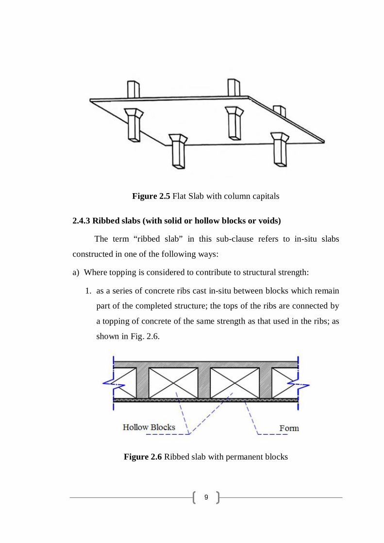
Figure 2.5 Flat Slab with column capitals

2.4.3 Ribbed slabs (with solid or hollow blocks or voids)

The term “ribbed slab” in this sub-clause refers to in-situ slabs

constructed in one of the following ways:

a) Where topping is considered to contribute to structural strength:

1. as a series of concrete ribs cast in-situ between blocks which remain

part of the completed structure; the tops of the ribs are connected by

a topping of concrete of the same strength as that used in the ribs; as

shown in Fig. 2.6.

Figure 2.6 Ribbed slab with permanent blocks

10

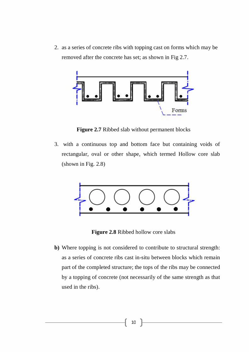
2. as a series of concrete ribs with topping cast on forms which may be

removed after the concrete has set; as shown in Fig 2.7.

Figure 2.7 Ribbed slab without permanent blocks

3. with a continuous top and bottom face but containing voids of

rectangular, oval or other shape, which termed Hollow core slab

(shown in Fig. 2.8)

Figure 2.8 Ribbed hollow core slabs

b) Where topping is not considered to contribute to structural strength:

as a series of concrete ribs cast in-situ between blocks which remain

part of the completed structure; the tops of the ribs may be connected

by a topping of concrete (not necessarily of the same strength as that

used in the ribs).

11

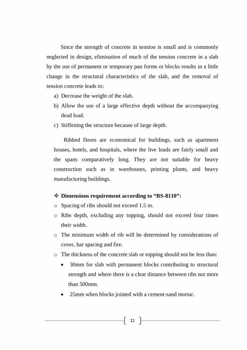
Since the strength of concrete in tension is small and is commonly

neglected in design, elimination of much of the tension concrete in a slab

by the use of permanent or temporary pan forms or blocks results in a little

change in the structural characteristics of the slab, and the removal of

tension concrete leads to:

a) Decrease the weight of the slab.

b) Allow the use of a large effective depth without the accompanying

dead load.

c) Stiffening the structure because of large depth.

Ribbed floors are economical for buildings, such as apartment

houses, hotels, and hospitals, where the live loads are fairly small and

the spans comparatively long. They are not suitable for heavy

construction such as in warehouses, printing plants, and heavy

manufacturing buildings.

Dimensions requirement according to “BS-8110”:

o Spacing of ribs should not exceed 1.5 m.

o Ribs depth, excluding any topping, should not exceed four times

their width.

o The minimum width of rib will be determined by considerations of

cover, bar spacing and fire.

o The thickness of the concrete slab or topping should not be less than:

30mm for slab with permanent blocks contributing to structural

strength and where there is a clear distance between ribs not more

than 500mm.

25mm when blocks jointed with a cement-sand mortar.

12

40mm or 1/10th of the clear distance between ribs, whichever is

greater, for all other slabs with permanent blocks.

50mm or 1/10th of the clear distance between ribs, whichever is

greater, for slabs without permanent blocks.

2.4.3.1 One-Way Ribbed Slab: consists of a series of small, closely

spaced reinforced concrete T beams, framing into monolithically cast

concrete girders, which are in turn carried by the building columns. The T

beams, called ribs, are formed by creating void spaces in what otherwise

would be a solid slab. Usually these voids are formed using special steel

pans, or hollow blocks as shown in Fig 2.9. When permanent hollow

blocks are used ribbed slab is termed Hollow Block Slab. Concrete is cast

between the forms to create ribs, and placed to a depth over the top of the

forms so as to create a thin monolithic slab that becomes the T beam

flange. Fig 2.10 shows the arrangement of blocks in One-Way hollow

block slab.

Figure 2.9 One-Way ribbed slab formed using blocks

13

Figure 2.10 Arrangement of block in One-Way hollow blocks

The joists and the supporting girders are placed monolithically. Like

the joists, the girders are designed as T beams. The shape of the girder

cross section depends on the shape of the end pans that form the joists, as

shown in Fig. 2.11.

Figure 2.11 One-Way hollow block slab cross section

2.4.3.2 Two-Way Ribbed Slab “Waffle”: is a variant of the solid slab,

may be visualized as a set of crossing ribs, set at small spacings relative to

the span, which support a thin top slab. Waffle slab may be designed as a

14

flat slab or a solid slab depending on the arrangement of voids. Fig. 2.12

shows the possible arrangements of Waffle slab.

Figure 2.12 Arrangements of waffle slab (a) as a flat slab (b) as a solid slab

The bottom voids are usually formed using dome-shaped steel pans or

hollow blocks that are placed on a plywood platform as shown in Fig. 2.13

and Fig. 2.14.

15

Figure 2.13 waffle slab formed using steel pans

Figure 2.14 waffle slab formed using hollow blocks

Domes are omitted near the columns to obtain a solid slab in the region

of negative bending moment and high shear. The lower flange of each

dome contacts that of the adjacent dome, so that the concrete is cast

entirely against a metal surface, resulting in an excellent finished

appearance of the slab “A waffle-like appearance” as shown in Fig. 2.15.

16

Figure 2.15 waffle slab appearance

2.5 Structural behavior of slabs:

2.5.1 Behavior of one –way slab:

The structural action of a one-way slab may be visualized in terms of

the deformed shape of the loaded surface. Fig. 2.16 shows a rectangular

slab, simply supported along its two opposite long edges and free of any

support along the two opposite short edges. If a uniformly distributed load

is applied to the surface, the deflected shape will be as shown by the solid

lines. Curvatures, and consequently bending moments, are the same in all

strips 푠 spanning in the short direction between supported edges, whereas

there is no curvature, hence no bending moment, in the long strips l parallel to the supported edges. The surface is approximately cylindrical.

For purposes of analysis and design, a unit strip of such a slab cut out

at right angles to the supporting beams, as shown in Fig. 2.17, may be

17

considered as a rectangular beam of unit width, with a depth h equal to the

thickness of the slab and a span 푙 equal to the distance between supported

edges. This strip can then be analyzed by the methods that were used for

rectangular beams, the bending moment being computed for the strip of

unit width. The load per unit area on the slab becomes the load per unit

length on the slab strip. Since all of the load on the slab must be transmitted

to the two supporting beams, it follows that all of the reinforcement should

be placed at right angles to these beams, with the exception of any bars that

may be placed in the other direction to control shrinkage and temperature

cracking. A one-way slab, thus, consists of a set of rectangular beams side

by side. This simplified analysis, which assumes Poisson’s ratio to be zero,

is slightly conservative. Actually, flexural compression in the concrete in

the direction of 푙 will result in lateral expansion in the direction of 푙

unless the compressed concrete is restrained. In a one-way slab, this lateral

expansion is resisted by adjacent slab strips, which tend to expand also.

The result is a slight strengthening and stiffening in the span direction, but

this effect is small and can be disregarded.

Figure 2.16 Deflected shape of uniformly loaded one-way slab

18

Figure 2.17 Unit strip basis for flexural design

2.5.2 Behavior of two-way slabs:

2.5.2.1 Two-way edge supported slabs:

In many cases, however, rectangular slabs are of such proportions and

are supported in such a way that two-way action results. When loaded, such

slabs bend into a dished surface rather than a cylindrical one. This means

that at any point the slab is curved in both principal directions, and since

bending moments are proportional to curvatures, moments also exist in

both directions. To resist these moments, the slab must be reinforced in

both directions, by at least two layers of bars perpendicular, respectively, to

two pairs of edges. The slab must be designed to take a proportionate share

of the load in each direction.

Types of reinforced concrete construction that are characterized by

two-way action include slabs supported by walls or beams on all sides (Fig.

2.1), flat plates (Fig. 2.3), flat slabs (Fig. 2.5), and waffle slabs (Fig. 2.15).

19

The simplest type of two-way slab action is that represented by Fig.

2.1, where the slab, or slab panel, is supported along its four edges by

relatively deep, stiff, monolithic concrete beams or by walls or steel

girders. If the concrete edge beams are shallow or are omitted altogether as

they are for flat plates and flat slabs, deformation of the floor system along

the column lines significantly alters the distribution of moments in the slab

panel itself such a slab is shown in Fig. 2.18a.

Figure 2.18 Two-way slab on simple edge supports: (a) bending of center

strips of Slab (b) grid model of slab

To visualize the flexural performance, it is convenient to think of it as

consisting of two sets of parallel strips, in each of the two directions,

intersecting each other. Evidently, part of the load is carried by one set and

transmitted to one pair of edge supports, and the remainder by the other.

Fig. 2.18a shows the two center strips of a rectangular plate with short

span 푙 and long span 푙 if the uniform load is q per square foot of slab,

20

each of the two strips acts approximately as a simple beam, uniformly

loaded by its share of q. Because these imaginary strips actually are part of

the same monolithic slab, their deflections at the intersection point must be

the same. Equating the center deflections of the short and long strips gives

5푞 푙384퐸퐼

=5푞 푙384퐸퐼

(2.1)

Where 푞 is the share of the load q carried in the short direction and 푞

is the share of the load q carried in the long direction. Consequently,

푞푞

=푙푙

(2.2)

One sees that the larger share of the load is carried in the short

direction, the ratio of the two portions of the total load being inversely

proportional to the fourth power of the ratio of the spans.

This result is approximate because the actual behavior of a slab is

more complex than that of the two intersecting strips. An understanding of

the behavior of the slab itself can be gained from Fig. 2.18b, which shows a

slab model consisting of two sets of three strips each. It is seen that the two

central strips 푠 and 푙 bend in a manner similar to that shown in Fig.

2.18a. The outer strips 푠 and 푙 however, are not only bent but also

twisted. Consider, for instance, one of the intersections of 푠 with 푙 . It is

seen that at the intersection the exterior edge of strip 푙 is at a higher

elevation than the interior edge, while at the nearby end of strip 푙 both

edges are at the same elevation; the strip is twisted. These twisting results

21

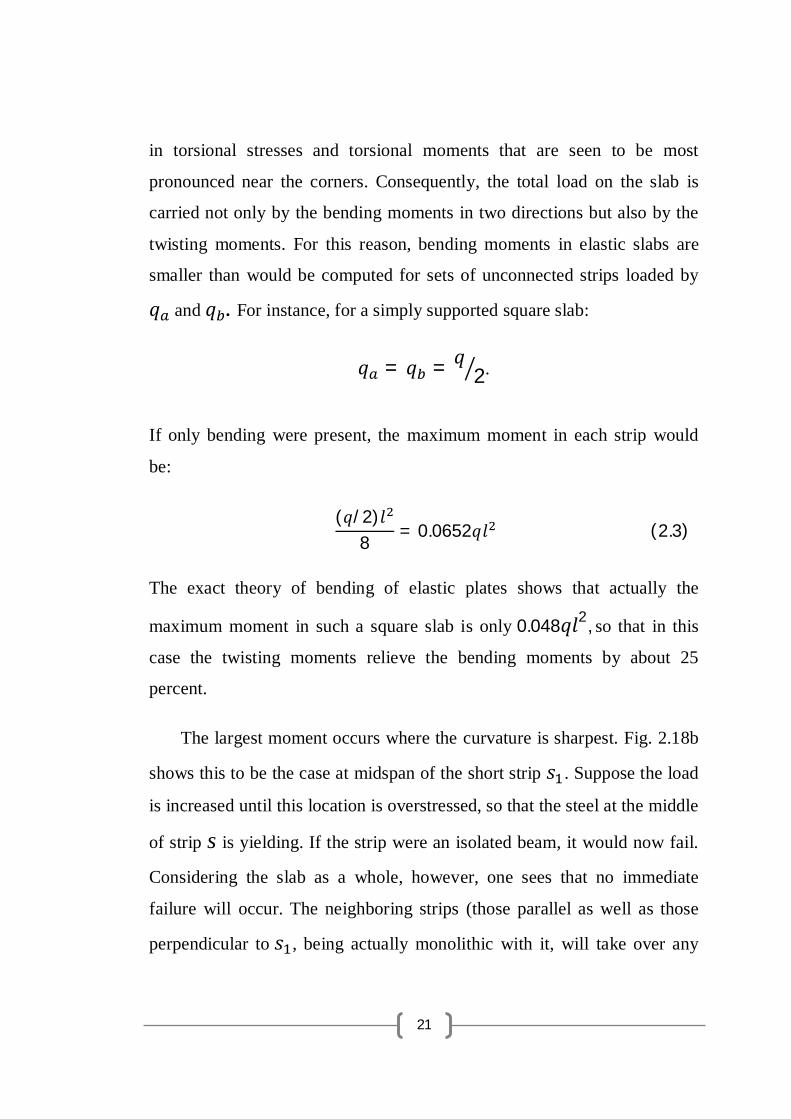
in torsional stresses and torsional moments that are seen to be most

pronounced near the corners. Consequently, the total load on the slab is

carried not only by the bending moments in two directions but also by the

twisting moments. For this reason, bending moments in elastic slabs are

smaller than would be computed for sets of unconnected strips loaded by

푞 and 푞 . For instance, for a simply supported square slab:

푞 = 푞 = 푞2.

If only bending were present, the maximum moment in each strip would

be:

(푞/2)푙8

= 0.0652푞푙 (2.3)

The exact theory of bending of elastic plates shows that actually the

maximum moment in such a square slab is only 0.048푞푙2, so that in this

case the twisting moments relieve the bending moments by about 25

percent.

The largest moment occurs where the curvature is sharpest. Fig. 2.18b

shows this to be the case at midspan of the short strip 푠 . Suppose the load

is increased until this location is overstressed, so that the steel at the middle

of strip s is yielding. If the strip were an isolated beam, it would now fail.

Considering the slab as a whole, however, one sees that no immediate

failure will occur. The neighboring strips (those parallel as well as those

perpendicular to 푠 , being actually monolithic with it, will take over any

22

additional load that strip 푠 can no longer carry until they, in turn, start

yielding. This inelastic redistribution will continue until in a rather large

area in the central portion of the slab all the steel in both directions is

yielding. Only then will the entire slab fail. From this reasoning, which is

confirmed by tests, it follows that slabs need not be designed for the

absolute maximum moment in each of the two directions (such as

0.048푞푙2in the example given in the previous paragraph), but only for a

smaller average moment in each of the two directions in the central portion

of the slab. For instance, one of the several analytical methods in general

use permits a square slab to be designed for a moment of 0.036푞푙2. By

comparison with the actual elastic maximum moment 0.048푞푙2, it is seen

that, owing to inelastic redistribution, a moment reduction of 25 percent is

provided.

The largest moment in the slab occurs at midspan of the short strip 푠

of Fig. 2.18b. It is evident that the curvature, and hence the moment, in the

short strip 푠 is less than at the corresponding location of strip 푠 .

Consequently, a variation of short-span moment occurs in the long

direction of the span. This variation is shown qualitatively in Fig. 2.19. The

short-span moment diagram in Fig. 2.19a is valid only along the center

strip at 1-1. Elsewhere, the maximum-moment value is less, as shown.

Other moment ordinates are reduced proportionately. Similarly, the long-

span moment diagram in Fig. 2.19 applies only at the longitudinal

centerline of the slab; elsewhere, ordinates are reduced according to the

variation shown. These variations in maximum moment across the width

and length of a rectangular slab are accounted for in an approximate way in

23

most practical design methods by designing for a reduced moment in the

outer quarters of the slab span in each direction.

It should be noted that only slabs with side ratios less than about 2 need

be treated as two-way slabs. From Eq. (b) above, it is seen that for a slab of

this proportion, the share of the load carried in the long direction is only on

the order of one-sixteenth of that in the short direction. Such a slab acts

almost as if it were spanning in the short direction only. Consequently,

rectangular slab panels with an aspect ratio of 2 or more may be reinforced

for one-way action, with the main steel perpendicular to the long edges.

Figure 2.19 moments and moment variation in a uniformly loaded slab

with simple supports on four sides

Consistent with the assumptions of the analysis of two-way edge-

supported slabs, the main flexural reinforcement is placed in an orthogonal

pattern, with reinforcing bars parallel and perpendicular to the supported

edges. As the positive steel is placed in two layers, the effective depth d for

the upper layer is smaller than that for the lower layer by one bar diameter.

24

Because the moments in the long direction are the smaller ones, it is

economical to place the steel in that direction on top of the bars in the short

direction. The stacking problem does not exist for negative reinforcement

perpendicular to the supporting edge beams except at the corners, where

moments are small.

Either straight bars, cut off where they are no longer required, or bent

bars may be used for two-way slabs, but economy of bar fabrication and

placement will generally favor all straight bars. The precise locations of

inflection points (or lines of inflection) are not easily determined, because

they depend upon the side ratio, the ratio of live to dead load, and

continuity conditions at the edges.

2.5.2.2 Two-way column-supported slabs:

When two-way slabs are supported by relatively shallow, flexible

beams, or if column-line beams are omitted altogether, as for flat plates,

flat slabs, or waffle system, then a number of new considerations are

introduced. Fig. 2.20a shows a portion of a floor system in which a

rectangular slab panel is supported by relatively shallow beams on four

sides. The beams, in turn, are carried by columns at the intersection of their

centerlines. If a surface load q is applied, that load is shared between

imaginary slab strips 푙푎 in the short direction and 푙 in the long direction.

The portion of the load that is carried by the long strips 푙 is delivered to

the beams 퐵 spanning in the short direction of the panel. The portion

carried by the beams 퐵 plus that carried directly in the short direction by

the slab strips 푙푎 sums up to 100 percent of the load applied to the panel.

25

Similarly, the short-direction slab strips 푙푎 deliver a part of the load to

long-direction beams 퐵2. That load, plus the load carried directly in the

long direction by the slab, includes 100 percent of the applied load. It is

clearly a requirement of statics that, for column-supported construction,

100 percent of the applied load must be carried in each direction, jointly by

the slab and its supporting beams.

A similar situation is obtained in the flat plate floor shown in Fig. 2.3.

In this case beams are omitted. However, broad strips of the slab centered

on the column lines in each direction serve the same function as the beams

of Fig. 2.19a; for this case, also, the full load must be carried in each

direction. The presence of drop panels or column capitals (Fig. 2.4) in the

double-hatched zone near the columns does not modify this requirement of

statics.

Fig. 2.20a shows a flat plate floor supported by columns at A, B, C,

and D. Fig. 2.20b shows the moment diagram for the direction of span 푙1.

In this direction, the slab may be considered as a broad, flat beam of width

푙2 . Accordingly, the load per meter of span is 푞푙2 . In any span of a

continuous beam, the sum of the midspan positive moment and the average

of the negative moments at adjacent supports is equal to the midspan

positive moment of a corresponding simply supported beam. In terms of

the slab, this requirement of statics may be written:

12

(푀 + 푀 ) + 푀 =18푞푙 푙 (2.4)

A similar requirement exists in the perpendicular direction, leading to the

relation:

26

12

(푀 + 푀 ) + 푀 =18푞푙 푙 (2.5)

Figure 2.20 column supported two-way slabs (a) two-way slab with beam

(b) two-way slab without beams

These results disclose nothing about the relative magnitudes of the

support moments and span moments. The proportion of the total static

moment that exists at each critical section can be found from an elastic

analysis that considers the relative span lengths in adjacent panels, the

loading pattern, and the relative stiffness of the supporting beams, if any,

and that of the columns.

Alternatively, empirical methods that have been found to be reliable under

restricted conditions may be adopted.

27

Figure 2.21 Moment variation in column supported two-way slab;

(a) Critical moment section (b) moment variation along a span

(c) moment variation across the width of critical section

The moments across the width of critical sections such as AB or EF are

not constant but vary as shown qualitatively in Fig. 2.21c. The exact

variation depends on the presence or absence of beams on the column lines,

the existence of drop panels and column capitals, as well as on the intensity

of the load. For design purposes, it is convenient to divide each panel as

shown in Fig. 2.21c into column strips, having a width of one-fourth the

panel width, on each side of the column centerlines, and middle strips in

the one-half panel width between two column strips. Moments may be

28

considered constant within the bounds of a middle strip or column strip, as

shown, unless beams are present on the column lines. In the latter case,

while the beam must have the same curvature as the adjacent slab strip, the

beam moment will be larger in proportion to its greater stiffness, producing

a discontinuity in the moment-variation curve at the lateral face of the

beam. Since the total moment must be the same as before, according to

statics, the slab moments must be correspondingly less.

While permitting design “by any procedure satisfying the

conditions of equilibrium and geometrical compatibility,” specific

reference is made to two alternative approaches: a semi empirical direct

design method and an approximate elastic analysis known as the equivalent

frame method.

In either case, a typical panel is divided, for purposes of design, into

column strips and middle strips. A column strip is defined as a strip of slab

having a width on each side of the column centerline equal to one-fourth

the smaller of the panel dimensions l1 and l2. Such a strip includes

column-line beams, if present. A middle strip is a design strip bounded by

two column strips. In all cases, l1 is defined as the span in the direction of

the moment analysis and l2 as the span in the lateral direction measured

center to center of the support. In the case of monolithic construction,

beams are defined to include that part of the slab on each side of the beam

extending a distance equal to the projection of the beam above or below the

slab h (whichever is greater) but not greater than 4 times the slab thickness

(see Fig. 2.18).

29

Figure 2.22 Portion of slab to be included with beam (a) symmetric slab

(b) single side slab

30

CHAPTER THREE

METHODS OF ANALYSIS

3.1 Introduction: The structural engineering community responded to this challenge

with numerous approximate techniques that attempt to simplify the design

of these reinforced concrete components.

For flat plates, these methods include the direct design, equivalent

frame, yield line, and strip design techniques, all of which approximate the

results of classical plate theory. These methods have gained wide

acceptance among engineers because of their simplicity.

However, these approximate techniques have significant limitations. Direct

design and equivalent frame methods are both limited to structures with

very regular geometry.

3.2 The direct Method: BS 8110 gives two principal methods for designing flat slabs which are

supported on columns positioned at the intersection of rectangular grid

lines for slabs where the aspect ratio is not greater than 2.

The first method is based on simple moment coefficients at critical

sections. This can be used where the lateral stability is not dependent on the

slab-column connections and is subject to the following provisions:

(a) the single load case is considered on all spans; and

(b) there are at least three rows of panels of approximately equal

spans in the direction being considered.

31

The second approach is the equivalent frame method. which as the

name suggests, involves subdividing the structure into sub frames and the

use of moment distribution or similar analysis techniques to obtain the

forces and moments at critical sections.

Other methods for designing flat slabs are again also acceptable, such

as on yield-line analysis, Hillerborg's 'advanced' strip method and finite

element analysis.

The simplified method of design is given by the following steps:

3.2.1 Division of flat slab structures into frames:

The structures may be divided longitudinally and transversely into

frames consisting of columns and strips of slab. The width of slab used to

define the effective stiffness of the slab will depend upon the aspect ratio of

the panels and type of loading. In the case of vertical loading, the stiffness

of rectangular panels may be calculated taking into account the full width

of the panel. For horizontal loading, it will be more appropriate to take half

this value.

The moments, loads and shear forces to be used in the design of

individual columns and beams of a frame supporting vertical loads only

may be derived from an elastic analysis of a series of sub-frames. Each

sub-frame may be taken to consist of the beams at one level together with

the columns above and below. The ends of the columns remote from the

beams may generally be assumed to be fixed unless the assumption of a

pinned end is clearly more reasonable (for example, where a foundation

detail is considered unable to develop moment restraint).

32

The second moment of area of any section of slab or column used in

calculating the relative stiffness of members may be assumed to be that of

the cross-section of the concrete alone.

3.2.2 Load arrangement

While, in principle, a flat slab should be analyzed to obtain at each

section the moments and shears resulting from the most unfavorable

arrangement of the design loads, it will normally be satisfactory to obtain

the moments and forces within a system of flat slab panels from analysis of

the structure under the single load case of maximum design load on all

spans or panels simultaneously, provided the following conditions are met:

a) In a one-way spanning slab the area of each bay exceeds 30 m2.

In this context, a bay means a strip across the full width of a structure

bounded on the other two sides by lines of support (see Figure 3.1).

b) The ratio of the characteristic imposed load to the characteristic dead

load does not exceed 1.25.

c) The characteristic imposed load does not exceed 5 kN/m2 excluding

partitions.

Where analysis is carried out for the single load case of all spans

loaded, the resulting support moments except those at the supports of

cantilevers should be reduced by 20 %, with a consequential increase in the

span moments.

33

Figure 3.1 Definition of panels and bays

If the conditions of the single load case are not met, it is not

appropriate to analyze for the single load case of maximum design load on

all spans, and it will normally be sufficient to consider the following

arrangements of vertical load:

a) All spans loaded with the maximum design ultimate load

(1.4Gk + 1.6Qk);

b) Alternate spans loaded with the maximum design ultimate load

(1.4Gk + 1.6Qk) and all other spans loaded with the minimum

design ultimate load (1.0Gk).

3.2.3 Moments determination:

For flat-slab structures whose lateral stability is not dependent on slab-

column connections, Table 3.1 may be used subject to the following

provisions:

a) design is based on the single load case of all spans loaded with the

maximum design ultimate load

34

b) there are at least three rows of panels of approximately equal span in

the direction being considered;

c) moments at supports taken from Table 3.1 may be reduced by

0.15Fhc; and

Allowance has been made to the coefficients of Table 3.1 for 20 %

redistribution of moments.

Table 3.1 Ultimate bending moment and shear forces

End support/slab connection

At first interior support

Middle interior spans

Interior supports

Simple Continuous

At outer support

Near middle of end span

At outer

support

Near middle of end span

Moment Shear

0 0.4F

0.086Fl ----

-0.04Fl 0.4F

0.075Fl ----

-0.086Fl 0.6F

0.063Fl

----

-0.063Fl 0.5F

NOTE F is the total design ultimate load (1.4Gk + 1.6Qk); l is the effective span.

3.2.4 Division of panels:

Flat slab panels should be assumed to be divided into column strips and middle strips (see Fig. 3.2).

In the assessment of the widths of the column and middle strips, drops should be ignored if their smaller dimension is less than one-third of the smaller dimension of the panel.

35

Figure 3.2 Division of panels in flat slabs

36

3.2.5 Division of moments between column and middle strips:

The design moments obtained from analysis of the continuous frames

or from Table 3.1 should be divided between the column and middle strips

in the proportions given in Table 3.2.

Table 3.2 Distribution of design moments in panels of flat slabs

Design

moment

Apportionment between column and middle strip

Column strip

%

Middle strip

%

Negative

Positive

75

55

25

45

For the case where the width of the column strip is taken as equal to

that of the drop, and the middle strip is thereby increased in width, the

design moments to be resisted by the middle strip should be increased in

proportion to its increased width. The design moments to be resisted by the

column strip may be decreased by an amount such that the total positive

and the total negative design moments resisted by the column strip and

middle strip together are unchanged.

37

3.3 Finite Element Method:

Slabs are most widely used structural elements of modern structural

complexes and the reinforced concrete slab is the most useful discovery for

supporting lateral loads in buildings. Slabs may be viewed as moderately

thick plates that transmit load to the supporting walls and beams and

sometimes directly to the columns by flexure, shear and torsion. It is

because of this complex behavior that is difficult to decide whether the slab

is a structural element or structural system in itself. Slabs are viewed in this

paper as a structural element.

The greatest volume of concrete that goes into a structure is in the

form of slabs, floors and footings. Since slabs have a relatively large

surface area compared with their volume, they are affected by temperature

and shrinkage slabs may be visualized as intersecting, closely spaced, grid-

beams and hence they are seen to be highly indeterminate. This high degree

of indeterminacy is directly helpful to designer, since multiple load-flow

paths are available and approximations in analysis and design are

compensated by heavy cracking and large deflections, without significantly

affecting the load carrying capacity. Slabs, being highly indeterminate, are

difficult to analyze by elastic theories. Since slabs are sensitivity support

restraints fixate, rigorous elastic solutions are not available for many

practically important boundary conditions.

More recently, finite difference and finite element methods have

been introduced and this is extremely useful. Methods have also been

innovated to find the collapse loads of various types of slabs through the

yield line theory and strip methods. In addition to supporting lateral loads

38

(perpendicular to the horizontal plane), slabs act as deep horizontal girders

to resist wind and earthquake forces that act on a multi-storied frame. Their

action as girder diaphragms of great stiffness is important in restricting the

lateral deformations of a multi-storied frame. However, it must be

remembered that the very large volume and hence the mass of these slabs

are sources of enormous lateral forces due to earthquake induced

accelerations.

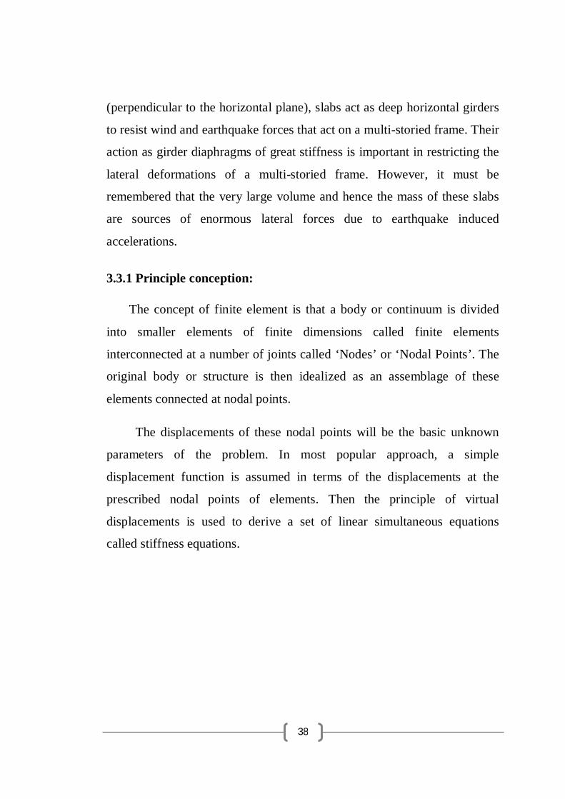
3.3.1 Principle conception:

The concept of finite element is that a body or continuum is divided

into smaller elements of finite dimensions called finite elements

interconnected at a number of joints called ‘Nodes’ or ‘Nodal Points’. The

original body or structure is then idealized as an assemblage of these

elements connected at nodal points.

The displacements of these nodal points will be the basic unknown

parameters of the problem. In most popular approach, a simple

displacement function is assumed in terms of the displacements at the

prescribed nodal points of elements. Then the principle of virtual

displacements is used to derive a set of linear simultaneous equations

called stiffness equations.

39

3.3.2 Formulation of the problem:

Finite Element Procedure:

The finite element method can be considered as a generalized

displacement method for two and three dimensional continuum problems.

It is necessary to discrete the continuum into a system with a finite number

of unknowns so that the problems can be solved numerically. The finite

element procedure can be divided into the following steps:

1. Idealization of the continuous surface as an assembling of discrete

elements.

2. Selection of displacement models.

3. Derivation of the element stiffness matrix.

4. Assembly of element stiffness matrix into an overall structure stiffness

matrix.

5. Solution of the system of linear equations relating nodal points loads and

unknown nodal displacements.

6. Computation of internal stress resultants by use of the nodal point

displacements already found.

Displacement Function:

In order to assure convergence to a valid result by mesh

reinforcement, the following three sacred rules have emerged for the

assumed displacement functions:

1. The displacement must be continuous within the element and the

displacements must be compatible between adjacent elements. For plane

stress and plane strain elements, continuity of the displacement functions

40

along is sufficient, whereas for bending elements, continuity of both the

displacement and slope is needed.

2. The displacement function must include the states of constant strain of

the element. This seems to be the most sacred of all the rules, since

eventually, by mesh reduction, one is evitable going to reach small

region where the strains are constant.

3. The displacement function must allow the element to undergo rigid body

motion without any internal strain. For plane stress and plate bending

elements, it is easy to establish displacement functions satisfying all

these three requirements.

The displacement functions used in deriving the 20 × 20 stiffness

matrix are:

푢 (푥,푦) = 푎1푥푦 + 푎2푥 + 푎3푦 + 푎4 (3.1)

푣 (푥,푦) = 푎5푥푦 + 푎6푥 + 푎7푦 + 푎8 (3.2)

푤 (푥, 푦) = 푎9푥3푦 + 푎10푥3 + 푎11푥2푦 + 푎12푥2 + 푎13푥푦3 + 푎14푥푦2

+ 푎15푥푦 + 푎16푥 + 푎17푦3 + 푎18푦2 + 푎19푦 + 푎20 (3.3)

Alternatively, in matrix form we can write this symbolically as follows:

{ū} = [푃]{푎푖} (3.4)

Where {ū} is vector of slab displacement and [P] is matrix of displacement

functions. Here the rectangular co-ordinate system is considered. The

degree of freedom considered at each node (corner) of the element is

푢, 푣,푤,푤푥 and 푤푦.

41

Element Stiffness Matrix:

To simplify the derivation of the element stiffness matrix, a more

convenient form of nodal displacement parameters with five degrees of

freedom per node is listed as follows:

[푢푖] = 푢1, 푣1,푤1,푤1푥,푤1푦, 푢2,푣2,푤2,푤2푥,푤2푦 푢3,푣3,푤3,푤3푥,

푤3푦, 푢4, 푣4,푤4,푤4푥,푤4푥 (3.5)

Where, 푤푖푥 = (훿푤/훿푥)푖 , = (훿푤/훿푦)푖 ; 푖 = 1 푡표 4 stands for the node

number of the node of an element.

Substituting the values of co-ordinates of four nodes in the three

displacement function and two derivatives of w stated above, we get the 20

nodal displacements of an element as follows:

{푢푖} = [퐻] {푎푖} (3.6)

Where, {ui} is vector of nodal displacement co-ordinates and [H] is called

transformation matrix.

The strain displacement relationships used in the analysis of this of

slab element may be expressed as:

{푒} = [훿] {ū} (3.7)

Therefore substituting Eq.(3.6) into Eq.(3.7) we get the strain expressed in

terms of displacement parameters as follows:

{푒} = [훿] {ū} = [훿] [푃] {푎푖} = [퐵] {푎푖} (3.8)

Where [B] is called strain matrix is a function of x and y co-ordinates.

The stress matrix can be expressed as follows:

42

{퐴푁} = [퐷] {푒} (3.9)

The strain energy developed in the element is expressed by

푈푡 = ½ × ∫ ∫ [퐴푁] {푒}푑푥 푑푦 (3.10)

Substituting the expression for [퐴푁] and {푒} in the 퐸푞. 6 we get the strain

energy

푈푡 = ½ × {푎푖} ∫ ∫ [퐵] [퐷][퐵]푑푥푑푦] {푎푖 = ½ {푎푖} [푈]{푎푖} (3.11)

Where [푈] = ∫ ∫ [퐵] [퐷] [퐵] 푑푥 푑푦

Now substituting {푎푖} from 퐸푞. 3.8 into 퐸푞. 3.11 and finally making

derivatives of strain energy 푈푡 with respect to the nodal displacement

parameters, we get the required element stiffness matrix [S] and are given

by

[푆] = [퐻 ] [푈][퐻] (3.12)

Overall Stiffness Matrix:

The element stiffness matrix relates quantities defined on the surface.

Therefore, co-ordinate transformations are completely avoided and the

overall stiffness matrix SFF of the slab structure is assembled by direct

summation of the stiffness contributions from the individual elements. The

degree of freedom for the overall stiffness matrix is obtained by

substituting joint restraint form, the total number of displacement co-

ordinates.

The overall stiffness matrix is first partitioned so that the terms

pertaining to the degrees of freedom are separated from those for the joint

43

restraints. Then the matrix is rearranged by interchanging rows and

columns in such a manner that stiffness corresponding to the degrees of

freedom is listed first and those corresponding to joint restraints are listed

second. Such a matrix is always symmetric. To computer time and storage,

only the upper band of the stiffness matrix 푆 (for free joint

displacements) is constructed.

Load Matrix:

The vertical gravity load (mainly self-weight) is the major load for roof

slab. The load intensity ′푄퐿′ is uniform over the area of a slab of uniform

thickness. This load intensity ′푄퐿′ can be resolved into three components at

a point in the three directions 푥,푦 푎푛푑 푧 as follows in a matrix.

The above-distributed load is replaced by an equivalent nodal load

matrix {AQ} for each element. This load matrix {퐴푄} is obtained by

equating virtual work done by the uniform load {푄} and the nodal loads

{퐴푄}. According to the standard formulae from texts:

{퐴푄} = ∫ ∫ [퐻 ] [푃] [푄] 푑푥 푑푦//

// (3.13)

Such a consistent load matrix will truly represent the distributed gravity

load ‘푄퐿’. But the laborious process of 퐸푞. 9 can be avoided by using

approximate overall nodal matrix {퐴푄}.

This can be worked out as follows:

The total vertical load on an element is assumed to be equally shared

by its four nodes. The z components of this vertical load are the element

nodal loads corresponding to displacements 푤 . Contributions from all

44

elements connected at a node together form the final values of nodal loads

for that node. Hence in the overall load matrix, out of five load values for

each node, only the third will be non-zero.

Expression for Stresses / Moments:

From Equation 2 the expression for {푎푖} is found as follows:

{푎푖} = [퐻] {푢푖} (3.14)

Using these values of {푎푖} and combining Eq.3.8 with Eq.3.14, we get the

matrix of resultant stresses / moments at any point (푥,푦) in terms of nodal

displacements as follows:

{퐴푁} = [퐷]{푒} = [퐷][퐵]{푎푖} = [퐷][퐵][퐻] {푢푖} (3.15)

45

CHAPTER FOUR

ANALYSIS, DESIGN, QUANTITIES

AND RESULTS COMPARISON

4.1. ANALYSIS:

4.1.1. Manual analysis:

Flat slab manual analysis:

Table 4.1: Flat slab information

Standards BS 8110 : 1997

Structure type Flat slab

Structure using Residential building floor

Material Concrete

fcu = 30 N/mm²

γc = 24 N/m³

Steel fy = 460 N/mm²

Loading D.L

self weight=5.5 kN/m²

partitions=3.6 kN/m²

finishing=1.5 kN/m²

Total=10.6 kN/m²

L.L live load=3 kN/m²

Concrete cover 20 mm

Bracing system Shear walls

Column Dim.

C1 (0.4×0.4) & 3m height

C2 (0.4×0.6) & 3m height

Capital (1.5×1.5) & 0.6m depth

46

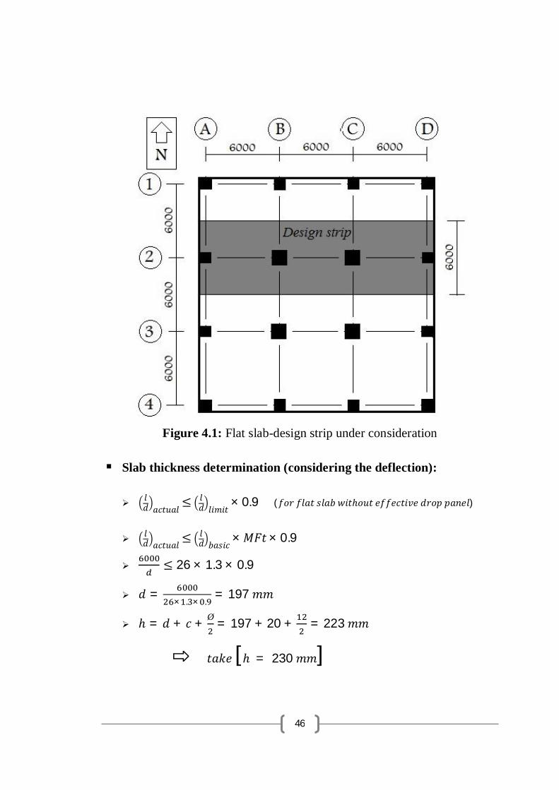
Figure 4.1: Flat slab-design strip under consideration

Slab thickness determination (considering the deflection):

푙푑 푎푐푡푢푎푙

≤ 푙푑 푙푖푚푖푡

× 0.9 (푓표푟 푓푙푎푡 푠푙푎푏 푤푖푡ℎ표푢푡 푒푓푓푒푐푡푖푣푒 푑푟표푝 푝푎푛푒푙)


≤ 푙푑 푏푎푠푖푐

×푀퐹푡× 0.9

≤ 26 × 1.3 × 0.9

푑 =× . × .

= 197 푚푚

ℎ = 푑 + 푐 + Ø = 197 + 20 + = 223 푚푚

⇨ 푡푎푘푒 [ℎ = 230 푚푚]

47

Load arrangement:

The conditions of Clause 3.5.2.3:

The ratio

=.

= 0.28 < 1.25

푐ℎ푎푟푎푐푡푎푟푖푠푡푖푐 푖푚푝표푠푒푑 푙표푎푑 = 3 푘푁/푚2 < 5 푘푁/푚2

are satisfied. So that;

1. It will be satisfactory to analyze for the single load case of maximum

design load on all panels simultaneously.

2. The moments and shears will be calculated using the code coefficients

given in table 3.12

→ [ 푛 = 1.4(10.6) + 1.6(3) = 19.64 푘푁/푚2 ]

Since the slab span are symmetric in both directions, so we will

consider an internal line of columns in one direction (E-W).

The lateral load is resisted by shear walls and thereby the

equivalent frame method will be used.

Total design ultimate load & span length considered (F&l ):

→ 퐹 = 푛 × (푝푎푛푒푙 푎푟푒푎) = 19.64 × (6 × 6) = 707 푘푁

→ 푙 = 6 푚

48

Figure 4.2: Ultimate load and span length

Design moment & shear:

Table 4.2: Flat slab-design strip moments and shear forces

Position At support

(A&D)

At mid span

(Panel 1)

At support

(B&C)

At mid span

Panel 2

Moment "-0.04Fl" "0.075Fl" "-0.086Fl" "0.063Fl"

169.68 318.15 364.81 267.25

Shear "0.46F" ---- "0.6F" ----

325.22

424.2

49

Figure 4.3: Ultimate moments in the design strip

Division of panels (into column & middle strips):

Figure 4.4: Division of panels into column & middle strips

50

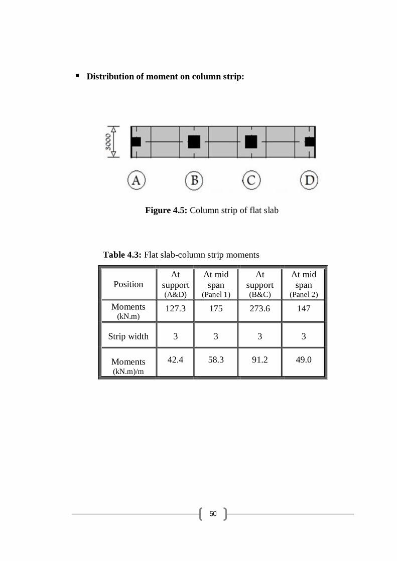
Distribution of moment on column strip:

Figure 4.5: Column strip of flat slab

Table 4.3: Flat slab-column strip moments

Position At

support (A&D)

At mid span

(Panel 1)

At support (B&C)

At mid span

(Panel 2) Moments

(kN.m) 127.3 175 273.6 147

Strip width 3 3 3 3

Moments (kN.m)/m

42.4 58.3 91.2 49.0

51

Distribution of moment on middle strip:

Figure 4.6: Middle strip of the flat slab

Table 4.4: Flat slab-middle strip moments

Position At

support (A&D)

At mid

span (Panel 1)

At

support (B&C)

At mid

span

(Panel 2)

Moment (kN.m)

42.4 143.2 91.2 120.3

Strip width 3 3 3 3

Moment (kN.m)/m

14.1 47.7 30.4 40.1

52

Waffle slab:

Table 4.5: Waffle slab information

Standards BS 8110 : 1997

Structure type Waffle slab

Structure using Residential building floor

Material Concrete

fcu=30 N/mm²

γc=24 N/m³

Steel fy=460 N/mm²

Loading D.L

self weight=4.5 kN/m²

partitions=3.6 kN/m²

blocks=0.6 kN/m²

finishing=1.5 kN/m²

Total=10.2 kN/m²

L.L live load=3 kN/m²

Concrete cover 20 mm

Bracing system Shear walls

Solid part (2×2) m (over columns)

Columns Dim (0.4×0.4) & 3m height

Capital (1.2×1.2) & 0.6m depth

53

Figure 4.7: Waffle slab-design strip under consideration

Slab thickness determination (considering the deflection):


≤ 푙푑 푙푖푚푖푡


≤ 푙푑 푏푎푠푖푐

×푀퐹푡

≤ 20.8 × 1.3

푑 =. × .

= 222 푚푚

ℎ = 푑 + 푐 + ∅ + Ø = 222 + 20 + 6 + = 254 푚푚

⇨ 푡푎푘푒 [ℎ = 260 푚푚]

54

Total design ultimate load & span length considered (F&l):

→ 푛 = 1.4(10.2) + 1.6(3) = 19.1 푘푁/푚2

→ 퐹 = 푛 × (푝푎푛푒푙 푎푟푒푎) = 19.1 × (6 × 6) = 686 푘푁

→ 푙 = 6 푚

Figure 4.8: Ultimate load and span length

Design moment & shear:

Table 4.6: Waffle slab-design strip moments and shear forces

Position At support

(A&D)

At mid span

(Panel 1)

At support

(B&C)

At mid span

Panel 2

Moment "-0.04Fl" "0.075Fl" "-0.086Fl" "0.063Fl"

164.6 308.7 354.0 259.3

Shear "0.46F" ---- "0.6F" ----

315.56

411.6

55

Figure 4.9: Ultimate moments in the design strip

Division of panels (into column & middle strips):

Figure 4.10: Division of panels into column & middle strips

The solid parts over the columns (which have dimensions more than

one-third of span) will act as drop panels and there by:

The column strip width will be equals to the drop panel width.

56

The coefficients of moments distribution between column & middle

strip will be modified by multiplying in:

o = 0.67 → 푓표푟 푐표푙푢푚푛 푠푡푟푖푝 푚표푚푒푛푡푠

o = 1.33 → 푓표푟 푚푖푑푑푙푒 푠푡푟푖푝 푚표푚푒푛푡푠

Distribution of moment on column strip:

Figure 4.11: Column strip of waffle slab

Table 4.7: Waffle slab-column strip moments

Position At

support (A&D)

At mid

span (Panel 1)

At

support (B&C)

At mid

span (Panel 2)

Moments (kN.m)

82.7 113.8 177.9 95.6

Strip width 2 2 2 2

Number of

ribs/strip 4 4 4 4

Moments (kN.m)/rib

20.7 28.4 44.5 23.9

57

Distribution of moment on middle strip:

Figure 4.12: Middle strip of waffle slab

Table 4.8: Waffle slab-middle strip moments

Position At

support (A&D)

At mid

span (Panel 1)

At

support (B&C)

At mid

span (Panel 2)

Moments (kN.m) 54.7 184.8 117.7 155.2

Strip width 4 4 4 4

Number of

ribs/strip 8 8 8 8

Moments (kN.m)/rib

6.8 23.1 14.7 19.4

58

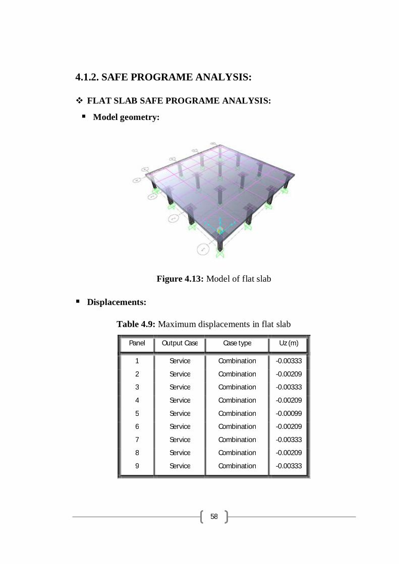
4.1.2. SAFE PROGRAME ANALYSIS:

FLAT SLAB SAFE PROGRAME ANALYSIS:

Model geometry:

Figure 4.13: Model of flat slab

Displacements:

Table 4.9: Maximum displacements in flat slab

Panel Output Case Case type Uz (m)

1 Service Combination -0.00333









59

Reactions:

Table 4.10: Reactions of flat slab

Point Output Case Case type Fz (KN)

5 Ultimate Combination 217.71
















60

Moments:

Table 4.11: Forces of the flat slab-design strip

Strip Span Location Max V2 Max M3 Min M3

SA2 Span 1 Start 28.647 80.047 3.24

SA2 Span 1 Middle 45.988 34.3744 -22.421

SA2 Span 1 End -28.647 80.047 3.24

SA3 Span 1 Start 45.988 78.4603 1.151

SA3 Span 1 Middle 45.988 44.9291 -30.942

SA3 Span 1 End -45.988 78.4603 1.1651

SA4 Span 1 Start -213.383 -2.949 -75.533

SA4 Span 1 Middle 168.535 85.777 -10.662

SA4 Span 1 End 269.415 -11.449 -176.01

SA4 Span 2 Start -250.377 -13.1062 -172.06

SA4 Span 2 Middle -150.335 41.7933 -23.891

SA4 Span 2 End 250.377 -13.1062 -172.66

SA4 Span 3 Start -269.415 -11.449 -176.01

SA4 Span 3 Middle -168.535 85.777 -10.662

SA4 Span 3 End 213.383 -2.949 -75.533

61

WAFFLE SLAB SAFE PROGRAME ANALYSIS:

Model geometry:

Figure 4.14: Model of the waffle slab

Displacements:

Table 4.12: Maximum displacements in waffle slab

Point Output Case Case type Uz (m)










62

Reactions:

Table 4.13: Reactions of waffle slab

Point Output Case Case type Fz (KN)

















63

Moments:

Table 4.14: Forces of waffle slab-design strip

Strip Span Location Max P Max V2 Max M3 Min M3

CSA2 Span 1 Start -52.646 -151.04 1.6469 -43.2405

CSA2 Span 1 Middle -42.793 95.234 72.989 14.931

CSA2 Span 1 End -32.447 213.342 -6.8997 -147.0571

CSA2 Span 2 Start -17.876 -192.94 -6.8559 -133.9212

CSA2 Span 2 Middle -19.222 -79.739 46.4045 5.4304

CSA2 Span 2 End -17.876 192.942 -6.8559 -133.9212

CSA2 Span 3 Start -32.447 -213.34 -6.8997 -147.0571

CSA2 Span 3 Middle -42.793 -95.234 72.989 14.931

CSA2 Span 3 End -52.646 151.045 1.6469 -43.2405

64

4.2. DESIGN:

4.2.1. Flat slab design:

REF. CALCULATIONS OUTPUT

BS-8110

Part1

Clause

3.4.4

Column strip:

Table 4.15: Flat slab-column strip design moments

Position At mid span (Panel 1)

At support (B&C)

Moments (kN.m)

Strip width

Moments (kN.m)/m

88.8

3

29.6

172.0

3

57.3

At mid span :

푀 = 29.6 푘푁.푚/푚

퐾 = = . ∗∗ ∗

= 0.024

= 0.5 + 0.25 −.

= 0.5 + 0.25 −0.024

0.9= 0.97

푧 = ∗ 푑 = 0.95 ∗ 204 = 194 푚푚

퐴푠 =. ∗ ∗

= . ∗. ∗ ∗

= 350푚푚

65

퐴푠 = . ∗ = . ∗ ∗ = 299 푚푚

As > As

푆 = ∗ = ∗ = 323 푚푚 푈푠푒 ∅ 12 @ 300 푚푚 푐/푐 푏표푡푡표푚

퐴푠 = 452 푚푚 /푚

At support :

푀 = −57.3 푘푁.푚/푚

퐾 = . ∗∗ ∗

= 0.046

= 0.5 + 0.25 − ..

= 0.95

푧 = 0.95 ∗ 204 = 194 푚푚

퐴푠 = . ∗. ∗ ∗

= 680 푚푚 As > (퐴푠 = 299 푚푚 )

푆 = ∗ = 296 푚푚

푈푠푒 ∅ 16 @ 250 푚푚 푐/푐

퐴푠 = 802 푚푚 /푚

452mm2

802 푚푚

66

Middle strip moments:

Table 4.16: Flat slab-middle strip design moments

Position At mid span (Panel 1)

At support (B&C)

Moments (kN.m) 71.3 42.3

Strip width 3 3

Moments (kN.m)/m 23.8 14.1

At mid span :

푀 = 23.8 kN. m/m

퐾 = . ∗∗ ∗

= 0.019

= 0.5 + 0.25 − ..

= 0.99

푧 = 0.95 ∗ 204 = 194 푚푚

퐴푠 = . ∗. ∗ ∗

= 281 푚푚

As > (퐴푠 = 299 푚푚 )

푆 = ∗ = 378 푚푚

67

푈푠푒 ∅ 12 @ 350 푚푚 푐/푐

퐴푠 = 339 푚푚 /푚

At support :

푀 = −14.1 푘푁.푚/푚

푘 = . ∗∗ ∗

= 0.011

= 0.5 + 0.25 − ..

= 0.99

= 0.95

푧 = 0.95 ∗ 204 = 194 푚푚

퐴푠 = . ∗. ∗ ∗

= 166 푚푚 < 퐴푠 =

299 푚푚

푆 = ∗ = 672 푚푚

푈푠푒 ∅ 16 @ 650 푚푚 푐/푐 푇표푝

퐴푠 = 402 푚푚 /푚

339mm2

402mm2

68

Clause

3.7.6

Clause

3.5.5

Clause

3.7.6.4

Check for shear :

(considering the critical internal column B2 )

The force at the center of column :

(force value is same in both direction)

Reaction = 770 푘푁

The effective depth for shear :

The average effective depth of the two directions :

푑 =192 + 204

2= 198 푚푚

At the face of column head :

o Applied shear stress:

V = 1.15V

V = R = 770 kN

V = 1.15 × 770 = 885.5 KN

69

Clause

3.7.7.1

푣 =푉푢푑

V = V = 885.5 KN

푢 = 4(ℎ ) = 4 × 1.5 = 6 푚

푣 = . ××

= 0.75 푁/푚푚

o Resistance :

푣 = 0.8 푓 = 0.8√30 = 4.38 < 5 푁/푚푚

[푣 = 0.75 푁/푚푚^2 < 4.38 푁/푚푚^2 ] __ OK

Punching shear:

(at 1.5d from the face of column head)


V = V = 885.5 KN

푢 = 4(ℎ + 3푑) = 4 1500 + 3(198) =

8376 푚푚

0.75

N/mm2

4.38

N/mm2

70

푣 = . ××

= 0.53 푁/푚푚

o Resistance :

푣 =0.79훾

100퐴푠푏푑

400푑

푓25

= ( )( )( )( ) = 0.41 < 3 ______푂퐾

= = 1.19 > 0.67 ______푂퐾

= = 1.06

푣 = (0.79/1.25)(0.41) (1.19)(1.06) =

0.59 푁/푚푚²

[ 푣 < 푣 ] _______ OK

Check for deflection :

o Actual span/effective depth ratio :

= = 29.4

o Limited span/effective depth ratio :

푙푑

=푙푑

× 푀퐹푡 × 0.9

0.53

N/mm2

0.59 N/mm2

29.4

71

Table 3.9

Table

3.10

= 26

푀퐹푡 = 0.55 +(477 − 푓 )

120 0.9 + 푀푏푑²

≤ 2.0

푓 =

= ( )( )

( ) = 270.5 푁/푚푚²

²

= . ×× ²

= 0.57

푀퐹푡 = 0.55 + ( . )( . . ) = 1.72 < 2.0

= 26 × 1.72 = 44.7

< _______ OK

44.7

72

4.2.2. Waffle slab design:

REF. CALCULATIONS OUTPUT

Column strip moments:

Table 4.17: Waffle slab-column strip design moments

Position Near middle (Panel 1)

At support (B&C)

Moments (kN.m) 72.3 76.4

Strip width 2 2

Number of ribs 4 4 Moments (kN.m)/rib 18.1 19.1

At support :

M = 19.1 kN. m/rib

퐾 = . ∗∗ ∗

= 0.023

= 0.5 + 0.25 − ..

= 0.97 > 0.95

푧 = 0.95 ∗ 228 = 217 푚푚

퐴푠 = . ∗. ∗ ∗

= 202 푚푚

퐹푙푎푛푔푒 푀 = 0.45푓 푏 ℎ 푑 −

73

= 0.45 ∗ 30 ∗ 525 ∗ 60 ∗ 228 −602

∗ 10

= 84.2 푘푁.푚 > 푀 = 19.1 푘푁.푚

푇ℎ푖푠 푖푚푝푙푖푒푠 푡ℎ푒 푛푒푢푡푟푎푙 푎푥푖푠 푙푖푒푠 푤푖푡ℎ푖푛 푡ℎ푒

푓푙푎푛푔푒 (푇ℎ푒 푠푒푐푡푖표푛 푖푠 푡표 푏푒 푑푒푠푖푔푛푒푑 푎푠 푟푒푐푡푎푛푔푢푙푎푟

퐴푠 = . ∗ ∗ = . ∗ ∗ = 58.5 푚푚

[ As > As ]

푁푢푚푏푒푟 표푓 푏푎푟푠 = = = 1.8 푏푎푟푠

푃푟표푣푖푑푒 2 푇 12 푏표푡푡표푚

퐴푠 = 226 푚푚 /푟푖푏

At Support : (rectangular section)

푀풂풑풑풍풊풆풅 = −18.1 푘푁.푚/푟푖푏

푘 = . ∗∗ ∗

= 0.022

226mm2

74

= 0.5 + 0.25 − ..

= 0.97

푧 = 0.95 ∗ 228 = 217 푚푚

퐴푠 = . ∗. ∗ ∗

= 191 푚푚

퐴푠 = . ∗ ∗ = 178 푚푚

[ As > As ]

푁푢푚푏푒푟 표푓 푏푎푟푠 = = 1.7 푏푎푟푠

푃푟표푣푖푑푒 2 푇 12 푇표푝

퐴푠 = 226 푚푚

Solid part :

푀풂풑풑풍풊풆풅 = −146

2= 73 푘푁.푚/푚

푘 = ∗∗ ∗

= 0.047

226mm2

75

= 0.5 + 0.25 − ..

= 0.94

푧 = 0.94 ∗ 228 = 214 푚푚

퐴푠 = ∗. ∗ ∗

= 775 푚푚

퐴푠 = . ∗ ∗ = 338 푚푚

[ As > As ]

푆 = ∗ = 259 푚푚

푃푟표푣푖푑푒 Ø 16 @ 250 푇표푝

퐴푠 = 804 푚푚 /푚

Middle strip moments:

Table 4.18: Waffle slab-middle strip design

moments

Position Near middle (Panel 1)

At support (B&C)

Moments (kN.m) 110.6 77.4 Strip width 4 4

Number of ribs 8 8 Moments (kN.m) / rib

13.8 9.7

804mm2

76

Middle Strip ribs :

At Mid Span :

M = 13.8 kN. m/rib

퐾 = . ∗∗ ∗

= 0.017

= 0.5 + 0.25 − ..

= 0.98 > 0.95

푧 = 0.95 ∗ 228 = 217 푚푚

퐴푠 = . ∗. ∗ ∗

= 146 푚푚

퐹푙푎푛푔푒 푀

= 0.45 ∗ 30 ∗ 525 ∗ 60 ∗ 228−602 ∗ 10

= 84.2 푘푁.푚 > 푀 = 13.8 푘푁.푚

푇ℎ푖푠 푖푚푝푙푖푒푠 푡ℎ푒 푛푒푢푡푟푎푙 푎푥푖푠 푙푖푒푠 푤푖푡ℎ푖푛 푡ℎ푒

푓푙푎푛푔푒 (푇ℎ푒 푠푒푐푡푖표푛 푖푠 푡표 푏푒 푑푒푠푖푔푛푒푑 푎푠 푟푒푐푡푎푛푔푢푙푎푟

퐴푠 = . ∗ ∗ = 58.5 푚푚

[ As > As ]

77

푁푢푚푏푒푟 표푓 푏푎푟푠 = = = 1.2푏푎푟푠

푃푟표푣푖푑푒 2 푇 12 푏표푡푡표푚

퐴푠 = 226 푚푚

At Support :

푀풂풑풑풍풊풆풅 = −9.7 푘푁.푚/푟푖푏

푘 = . ∗∗ ∗

= 0.023

= 0.5 + 0.25 − ..

= 0.97

푧 = 0.95 ∗ 228 = 217 푚푚

퐴푠 = . ∗. ∗ ∗

= 102 푚푚

퐴푠 = . ∗ ∗ = 84.5 푚푚

[ As > As ]

푁푢푚푏푒푟 표푓 푏푎푟푠 = = 1.3 푏푎푟푠

푃푟표푣푖푑푒 2 푇 10 푇표푝

퐴푠 = 158 푚푚

226mm2

158mm2

78

Clause 3.6.6.2

Clause 3.7.7.1

Topping reinforcement :

As = 0.12%(sectional area of topping)

As = . (100 × 1000) = 120 mm²/m

Provide A142 mesh (퐴 = 142 푚푚 /푚)

Punching shear:

at 1.5d from the face of column head :


푣 =푉푢푑

V = 1.15V Clause 3.7.6.2

V = R = 771 kN

V = 1.15 × 771 = 887 KN

V = V = 887 KN

푢 = 4(ℎ + 3푑) = 4 1500 + 3(228) =8736 푚푚

푣 = ××

= 0.45 푁/푚푚

142mm2

0.45 N/mm2

79

Table 3.9

Table 3.10

o Resistance :

푣 =0.79훾

100퐴푠푏푑

400푑

푓25

= ( )( )( )( )

= 0.35 < 3 ______푂퐾

= = 1.15 > 0.67 ______푂퐾

= = 1.06

푣 = ..

(0.35) (1.15)(1.06) = 0.54푁/푚푚2

[ 푣 < 푣 ] _______ OK

Check for deflection : Clause3.6.5

o Actual span/effective depth ratio :

푙푑

=6000228

= 26.3

o Limited span/effective depth ratio :

푙푑

=푙푑

× 푀퐹푡

= 20.8

푀퐹푡 = 0.55 +(477 − 푓 )

120 0.9 + 푀푏푑²

≤ 2.0

0.54 N/mm2

26.3

80

푓 =

= ( )( )

( )= 198 N/푚푚²

²

= . ×× ²

= 2.12

푀퐹푡 = 0.55 + ( )( . . ) = 1.32 < 2.0

= 20.8 × 1.32 = 27.5

< _______ OK

27.5

81

4.3. QUANTITIES:

4.3.1 Concrete quantities:

Waffle slab quantities:

For the solid part = 2 × 2 × 0.26 = 1.04 m3 per panel

For the waffle part = (2/3)(6×6×0.26-2×2×0.26) = 5.55 m3 per panel

Total concrete quantity in one panel = 6.6 m3

Total waffle slab concrete quantity = 6.6 × 9 = 59.3 m3

Flat slab quantities:

For one panel = 6 × 6 × 0.23 = 8.28 m3

Total flat slab concrete quantity = 8.28 × 9 = 74.5 m3

82

4.3.2. Reinforcing steel quantities:

푆푡푒푒푙 푣푎푙푢푒 = 퐴푠 푝푟표푣 × 푁표. 표푓 푟푖푏푠 × 푟푖푏 푙푒푛푔푡ℎ × 2 (푏표푡ℎ 푠푖푑푒푠)

Waffle slab steel quantities:

Column strip:

Top: 226 × 10-6 × 4 × 4 × 2 = 7232 × 10-6 m3

Bottom: 226 × 10-6 × 4 × 4 × 2 = 7232 × 10-6 m3

Middle strip:

Top: 158 × 10-6 × 8 × 6 × 2 = 15168 × 10-6 m3

Bottom: 226 × 10-6 × 8 × 6 × 2 = 21696 × 10-6 m3

Solid part: 802 × 10-6 × 2 × 2 × 2 = 6328 × 10-6 m3

Topping: 142 × 10-6 × 6 × 6 × 2 = 5112 × 10-6 m3

퐋퐢퐧퐤퐬:

× × 570 × 5 × (8 × 6 + 4 × 4) × 2 × 10 = 0.01 m3

Total value of steel: = 0.073 m3

Weight = value × density = 0.073 × 7.85 = 0.57 Ton per panel

Total steel weight in the waffle slab = 0.57 × 9 = 5.1 Ton

83

Flat slab steel quantities:

푆푡푒푒푙 푣푎푙푢푒 = 퐴푠 푝푟표푣 × 퐴푟푒푎 × 2 (푏표푡ℎ 푠푖푑푒푠)

Bottom: 4 × 113× 10-6 × 6 × 6 × 2 = 0.032 m3

Top:

Figure 4.15: Flat slab top reinforcement

A = 4 × 201× 10-6 × 3 × 3 × 2 = 0.0145 m3

B = 3 × 201× 10-6 × 3 × 3 × 2 × 2 = 0.022 m3

C = 2 × 201× 10-6 × 3 × 3 × 2 = 0.0145 m3

Total value of steel: = 0.076 m3

Weight = value × density = 0.076 × 7.85 = 0.60 Ton

Considering over lapping: 1.15 × 0.60 = 0.69 Ton per panel

Total steel weight in the flat slab = 0.69 × 9 = 6.2 Ton

84

4.4. Comparison of results:

4.4.1 Analysis results:

Flat slab:

o Bending moments in column strip:

Table 4.19: Flat slab-column strip moment comparison

Position At support

(B&C) At mid span

(Panel 2)

Manual 273.6 147

Program 172.0 41.8

Error 37% 71%

o Bending moments in middle strip:

Table 4.20: Flat slab-middle strip moment comparison

Position At support

(B&C) At mid span

(Panel 2)

Manual 91.2 120.3

Program 42.3 42.1

Error 53% 65%

85

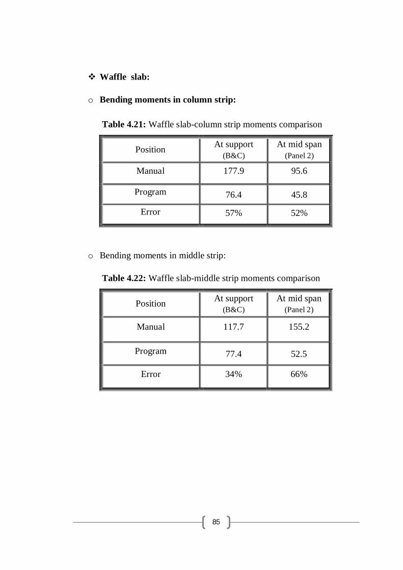
Waffle slab:

o Bending moments in column strip:

Table 4.21: Waffle slab-column strip moments comparison

Position At support (B&C)

At mid span (Panel 2)

Manual 177.9 95.6

Program 76.4 45.8

Error 57% 52%

o Bending moments in middle strip:

Table 4.22: Waffle slab-middle strip moments comparison

Position At support (B&C)

At mid span (Panel 2)

Manual 117.7 155.2

Program 77.4 52.5

Error 34% 66%

86

4.4.2. Quantities results:

Concrete quantities:

Table 4.23: Concrete quantities comparison

Slab Flat Waffle Difference

Concrete

quantity 74.5 m3 59.3 m3 20%

Reinforcing steel quantities:

Table 4.24: Reinforcing steel quantities comparison

Slab Flat Waffle Difference

Reinforcing

Steel quantity 6.2 Ton 5.1 Ton 18%

87

CHAPTER FIVE

CONCLUSION, RECOMMENDATIONS

5.1 Conclusion:

1. From the study results it is found that there is a large difference between

the values of the manual and program analysis.

2. From the study results it is found that in waffle slabs concrete quantity is

reduced up to 20% and the reduction of steel is 18%.

3. Economic aspect is an important parameter governing the superiority of

waffle slab over flat slab which can be inferred from the study results.

88

5.2 Recommendations:

From the study results we recommend to:

1. Repetition of analysis operation in order to treat the large differences

between the computer and manual analysis values.

2. Using the waffle slab as an economic alternative for flat slab.

For future studies we recommend to:

1. A comprehensive study of cost saving in buildings by considering all

factors, such as cost of two way slabs, frames (beams and columns),

foundations and the effect of time saving on the construction of such type

of slab shall be done.

2. Studying the behavior of an edge and a corner panel of waffle slabs.

3. Studying another system of waffle slabs (beams zones between

columns).

89

5.3 REFERENCES:

[1] Ahmed A.M. Civil Engineering, Zagazig University,2000 “Analysis of waffle slabs with openings” [2] Arthur H.Nilson , George Winter,(1986),”Design of Concrete Structures”McGraw-Hill 10th edition

[3] BS6399 (1996). Loading for buildings: Part1 - Code of practice for dead and imposed loads. British Standards Institution, London, UK.

[4] BS8110 (1997). Structural use of concrete: Part1 - Code of practice for design and construction. British Standards Institution, London, UK.

[5] Park ,R, and Gamble , W.L., (1980),“Reinforced Concrete Slabs”,Willy

Intersience , New York

[6] T.J.MacGinley, B. S. Choo, (1990), Reinforced Concrete: Design theory and examples 2nd Edition, London, UK

[7] W. H. Mosley. J. H. Bungey & R. Hulse, (1980) ,“Reinforced Concrete Design” 5th Edition

90

APPENDIX A: Flat slab analysis using SAFE program

Coordinate system:

91

Columns Properties:

Column 1:

92

Column 2:

93

Flat slab properties:

Load pattern:

94

Load Combinations:

95

Dead & Live Load

96

Deformed Shape:

Joint Reactions:

97

Strip Moment:

Punching Shear Capacity Ratios:

98

APPENDIX B: Waffle slab analysis using SAFE program

Coordinate System:

99

Waffle Slab Properties:

Load Pattern:

100

Load Combinations:

101

Dead & Live Load:

102

Deformed Shape:

Reactions:

103

Strip Moment:

Punching Shear Ratios:

CHAPTER ONE INTRODUTORY BACKGROUND - SUST ...

Documents

Transcript of CHAPTER ONE INTRODUTORY BACKGROUND - SUST ...