Investigation of Ultimate... .pdf - SUST Repository
100
Sudan University of Science and Technology College of Graduate Studies Investigation of Ultimate Resisting Moments of R.C. Slabs systems using Yield Line Theory, BS8110 and Computer Software Programs تقطات نظمة الب أ ل ق أوم القا العزم امرسانية ا طانيةدونة ال نظرية خط امضوع ، اتخداملحة بإسس اBS8110 لاسوب وبرامج اBy: Izeldein Jadalla Izeldein Ahmed Thesis Supervisor: Dr.Fathelrahaman Mohammed Adam A thesis submitted in partial fulfillment of the requirement for the degree of master of sciences in civil engineering (structures) to Civil Engineering Department, College of engineering December 2015
-
Upload
khangminh22 -
Category
Documents
-
view
1 -
download
0
Transcript of Investigation of Ultimate... .pdf - SUST Repository

Sudan University of Science and Technology
College of Graduate Studies
Investigation of Ultimate Resisting Moments of R.C.
Slabs systems using Yield Line Theory, BS8110 and
Computer Software Programs
اخلرسانية العزم املقاوم الأقىص لأنظمة البالطات تقيص
س تخدام نظرية خط اخلضوع ، املدونة الربطانية املسلحة بإ
BS8110 وبرامج احلاسوب
By:
Izeldein Jadalla Izeldein Ahmed
Thesis Supervisor:
Dr.Fathelrahaman Mohammed Adam
A thesis submitted in partial fulfillment of the requirement for the degree
of master of sciences in civil engineering (structures) to Civil
Engineering Department, College of engineering
December 2015

I
ACKNOWLEDGEMENTS
First and foremost, I would like to thank God.
Secondly, I would like to express my utmost gratitude and thanks to my thesis
supervisor, Dr. Fathelrahaman, who gives me support, guidance, continuous
encouragement throughout my project thesis, with his patience.
Finally, I would like to give a special thanks to my parent, my family, my wife,
and my friends for their care, love, encouragement and support during my study
and given me hope that Nothing is impossible, everything can be achieved by
perseverance .

II
الخالصة
، بحاالث حثبيج هخخلفت وهن البالطاث الخشسانيت الوسلحت لعذة أنظوتإنشائي عول ححليل في هزه الذاسست حن
هن بالبالطاث ، العزوم الوخحصل عليها هقاوهتىع إليجاد أقصى عزوم بإسخخذام نظشيت خظ الخض ورلك
هج ابإسخخذام بشهن الخحليل حن الحصىل عليها الخي نخائج الحوج هقاسنخها ببنظشيت خظ الخضىع الخحليل
بذسجاث هخخلفت يخشاوح وأظهشث الوقاسنت حطابق ( ، الوذونت البشيطانيت ، بشوكن -إسخاد بشوالحاسىب )
%109719% إلى 090.0ن هابي

III
ABSTRACT
In this study, different types of reinforced concrete slabs system of different
support conditions have been analyzed using yield line theory to determine the
maximum resisting moment, the result of resisting moments obtained, were
compared with others those obtained by using software program (STAAD-
PRO,PROKON) and BS8110. The comparison revealed different conforming by
percentage range by 0.097 % and 17.81%.
IV
Table of Contents
CHAPTER ONE GENRAL INTRODUCTION 1
1.1 Introduction: 1
1.2 Objectives of the Research 2
1.3 Methodology of Research 2
1.4 Outlines of Research 3
CHAPTER TWO LITERATURE REVIE 4
2.1 Introduction 4
2.2 Historical back ground about yield line theory 7
2.3 Yield lines theory 10
2.4 The advantages and disadvantages of yield line theory 11
2.5 prediction of yield line pattern 13
CHAPTER THREE Methodology 19
3.1 Introduction 19
3.2 Method of solution by using yield line theory 19
3.3 The 10% rule 26
3.4 Serviceability and deflections 26
3.5. Analysis and design of R.C. slabs using BS8110 27
3.6 Software program 29

V
CHAPTER FOUR 30
Investigation of Ultimate Resisting Moment for the Reinforced Concrete
Slabs
4.1 Introduction 30
4.2 4.2 Analysis of flat Slab system 31
4.3. Analysis of beam Slab system 49
4.4 Special Beam slab system of different support conditions 67
4.5 Discussion of the results 75
CHAPTER FIVE 76
CONCLUSIONS AND RECOMMENDATION 76
5.1 Conclusions 76
5.2 Recommendations 77
REFERENCES 78
APPENDIX A 80
APPENDIX B 82

VI
LIST OF FIGURES
Figure NO. TITLE PAGE
Fig.2.1 Yield Line Pattern for the Two-Way Slab 13
Fig.2.2 Consisting of Yield Line Pattern 13
Fig.2.3 Yield line pattern for square slab 16
Fig.2.4 Notation used for yield line theory 16
Fig.2.5 Yield line pattern for the different slabs shape 18
Fig.3.1 Simply supported one-way slab 21
Fig.3.2 Deformed shape at failure 23
Fig.3.3 Principles of expenditure of external loads 24
Fig.3.4 Principles of dissipation of internal energy 25
Fig.4. 1 Plan of Flat Slab with the Expected Yield Line Pattern 31

VII
Fig.4.2 Expected yield line Pattern of external Corner Panel S1 33
Fig.4.3 Yield Pattern of Panel S1 36
Fig.4.4 Expected yield line Pattern of the Panel S2 37
Fig.4.5 Yield Pattern of Panel S2 40
Fig.4.6 Expected yield line Pattern of edge Panel S3 41
Fig.4.7 Yield Pattern of Panel S3 44
Fig.4.8 Expected yield line Pattern of interior Panel S4 45
Fig.4.9 Yield Pattern of Panel S4 48
Fig.4.1 Plan of beam Slab system with the Expected Yield Line Pattern 49
Fig.4.11 Expected yield line Pattern of the Corner Panel S5 50
Fig.4.12 Yield Pattern of Panel S5 53
Fig.4.13 Expected yield line Pattern of the edge Panel S6 54
Fig.4.14 Yield line Pattern of Panel S6 57

VIII
Fig.4.15 Expected Yield line Pattern of the edge Panel S7 58
Fig.4.16 Yield line Pattern of Panel S7 61
Fig.4.17 Expected Yield line Pattern of the interior Panel S8 62
Fig.4.18 Yield line Pattern of Panel S8 65
Fig.4.19 Expected Yield line Pattern of Corner Panel S9 67
Fig.4.20 Yield line Pattern of Panel S9 70
Fig.4.21 Expected Yield line Pattern of Corner Panel S10 71
Fig.4.22 Yield line Pattern of Panel S4 74

IX
LIST OF TABLES
TABLE NO. TITLE PAGE
Table.3.1 Bending moment coefficients for rectangular panels 28
Table.4.1 Analysis of Panel S1 by yield line theory 33
Table.4.2 Analysis of Panel S2 by yield line theory 38
Table.4.3 Analysis of Panel S3 by yield line theory 42
Table.4.4 Analysis of Panel S4 by yield line theory 46
Table.4.5 The Ultimate Resisting Moment for flat slab system 48
Table.4.6 Analysis of Panel S5 by yield line theory 51
Table.4.7 Analysis of Panel S6 by yield line theory 55
Table.4.8 Analysis of Panel S7 by yield line theory 59
Table.4.9 Analysis of Panel S8 by yield line theory 63
Table.4.10 The Ultimate Resisting Moments for beam slab system 66

X
Table.4.11 Analysis of Panel S9 by yield line theory 68
Table.4.12 Analysis of Panel S10 by yield line theory 72
Table.4.13 The Ultimate Resisting Moments for Panels S9 &S10 76

XI
List of Symbols
Symbol Description Units
A Area cross-section m2
A, b, c Plan dimensions of slab supported on several sides m
D Dissipation of internal energy kNm
E Expenditure of energy by external loads kNm
g Ultimate distributed dead load kN/m
l Length of a yield line (projected onto a region’s axis of rotation) m
L Span (commonly edge to edge), distance m
m Positive moment, i.e the ultimate moment along the yield line kNm/m
m` Negative moment, i.e the ultimate moment along the yield line KNm/m
w Ultimate distributed load kN/m
x Distance to section of max. Positive moment from support m
∆δ max Deflection, maximum deflection (usually taken as unity) m
θ Angle of rotation …

CHAPTER ONE
GENRAL INTRODUCTION

1
CHAPTER ONE
GENRAL INTRODUCTION
1.1 Introduction
Reinforcement concrete slabs are among the most common structural element,
but despite the large number of slabs designer and built, the details of the elastic
and plastic behavior of slab are not always appreciated or properly taken into
account, this occurs at least partially because of the mathematical complexities
of dealing with elastic plate equation, especially for support condition, which
realistically approximate those in multi-panel building floor slabs.
Because the theoretical analysis of slab and plates is much less widely known
and practiced than is the analysis of element such as beam, the provisions in
building codes generally provide both design criteria and method of analysis for
slabs, whereas only criteria are provided for most other element, for example,
chapter 13 of the 1995 edition of the American Concrete Institute (ACI)
Building Code Requirements for structural Concrete one of the most widely
used codes for concrete design, is devoted largely to the determination of
moment in the slab structures, once the moments, shears, and torques are found,
section are proportioned to resist them using the criteria specified in other
sections of the same code.
Although the ACI code approach to slab design is basically one of using elastic
moment distributions, it is also possible to design slab using plastic analysis
(limit analysis) to provide the required moment.
Yield lines analysis is an analysis approach for determining the ultimate load
capacity of reinforced concrete slab and was pioneered by K.W.Johansen in the

2
1940s. It is closely related to the plastic collapse or limit analysis of steel frame,
and is an upper bound or mechanism approach.
Yield lines design is well founded method of designing reinforced concrete slabs
, and similar types of element , it uses the yield line theory to investigate failure
mechanism at limit state , the theory is based on the principle that :
Work done in yield line rotating = work done in load moving
Two of the most popular methods of application are working method and the
use of stander formula. Working method proposed to use in this research to
analysis and assessment different models of slabs (slab with beam and flat slab).
The proposed models consist of slab with beams with different edges conditions
and flat slab with different support conditions.
The suggested tools should be used is spread sheets and STAAD-Pro – Prokon
software and BS8110.
This research explains the use of practical and economic design of reinforced
concrete slabs.
1.2 Objectives of the Research
The objectives of this study are:
1- To identify yield line theory of reinforced concrete slabs.
2- To apply the yield line theory to obtain the ultimate resistance moments of
different types of slabs.
3- To compare the results obtained by yield line theory with that obtained by
software program STAAD-PRO, PROKON, and BS8110.
1.3 Methodology of Research
To achieve the objectives of this research; the following methods can be used:
1- A comprehensive reading and collecting data about yield line method must be
carried out.

3
2- Using three system of slabs (beam slab system flat slab system and special case
of support) with different of boundary condition as mathematical models in
order to apply the yield line theory for analysis.
3- Manual calculation is used for analyzing the different cases of slabs.
4- Structural Analysis Program STAAD-Pro, PROKON and BS8110 is used to
verify the results.
1.4 Outlines of Research
Chapter One contains general introduction.
Chapter Two contains literature review.
Chapter Three describes the methodology of analysis of reinforced concrete
slabs by using yield line theory.
Chapter Four (models) contains Analysis of the three systems of Slabs using
virtual work method.
Chapter Five contains conclusion and recommendation.

CHAPTER TWO
LITERATURE REVIEW

4
CHAPTER TWO
LITERATURE REVIEW
2.1 Introduction
There are a number of possible approaches to the analysis and design of the
reinforced concrete slab. The various approaches available are elastic theory,
limit analysis theory, and modifications to elastic theory and limit analysis
theory as in the ACI Code. Such methods can be used to analyze a given slab
system to determine rather the stresses in the slabs and the supporting system or
the load-carrying capacity. Alternatively, the methods can be used to determine
the distribution of moments and shears to allow the reinforcing steel and
concrete sections to be designed.
The bending and torsional moments, shear forces, and deflections of slab
systems, with given dimensions, steel content, and material properties, at any
stage of loading from zero to ultimate load, can be determined analytically using
conditions of static equilibrium and geometrical compatibility if the moment-
deformation relationships of the slab elements, and yield criteria for bending
and torsional moments and shear force when the strength of slab elements is
reached, are known. In such analysis of the complete behavior of slab system,
difficulties are caused by nonlinearity of the moment deformation relationships
of the slab elements at high levels of stress, and a step-by-step procedure with
load increased increment in generally necessary.
At low levels of load the slab elements are uncracked and the actions and
deformations can be computed from elastic theory using the uncracked flexural
rigidity of the slab elements. The slab elements are searched at each load
increment to ascertain whether cracking of the concrete has taken place. When
it is found that the cracking moment has been reached, the flexural rigidity of

5
the element is recomputed on the basis of cracked section value and the section
and deformations of the slab are recomputed. This procedure is repeated at the
same load level unit all the flexural rigidity values are correct. At higher load
increments, when the stresses in one or more elements begin to enter the
inelastic range, the flexural rigidities of those elements are reduced to that
corresponding to the particular point on the moment-deformation relationship
of the element. This requires the computation to be repeated at the load level
until the flexural rigidity of each element is correct. Eventually, with further
load increments, the strength of one or more elements is reached and if the
elements are sufficiently ductile, plasticity will spread through the slab system
with further loading. The ultimate load is reached when deflections occur
without further increase in load and hence further load cannot be carried.
Many finite element programs have been developed for the analysis of slabs,
and these programs have become more capable as computers have become more
powerful. The earlier efforts which included nonlinear effects generally were
for simple cases with idealized boundary conditions and were essentially
research tools.
Current commercial and semi commercial programs that can deal with slabs
with fairly general support conditions include the following non exhaustive list:
FIFNTE, SAP2000 , SAFE, RISA-3D, Lake Forest, ABAQUS, STAAD-Pro
and PCA-Mats is a specialized program adapted to the analysis of mat
foundations and slabs on grade. Some of these programs include nonlinear
effects such as cracking and yielding, and some include section of
reinforcement.
Code design procedures are usually based on elastic theory moments modified
in the light of some moment redistribution, which has been shown by tests to be
possible without excessive cracking or deflections at service loads.

6
Elastic theory moments without modification, and moments obtained from
methods of limit analysis, form alternative design approaches that are
recommended by some codes of practice.
Limit analysis recognizes that because of plasticity, redistribution of moments
and shears away from the elastic theory distribution can occur before the
ultimate load is reached. Such redistribution of moments occurs because for
typical reinforced concrete sections there is little change in moment with
curvature once the tension steel has reached the yield strength. Thus, when the
most highly stressed sections of slab reach the yield moment they tend to
maintain a moment capacity that is close to flexural strength with further
increase in curvature, while yielding of the slab reinforced spreads to other
sections of the slab with further increase in load. Limit analysis computes the
ultimate load of the slab, and the distribution of moments and shear at the
ultimate load, or the distribution of moments and shear at that load, of a given
slab system, either a lower bound or an upper bound method may be used.
The ultimate load is calculated from the equilibrium equation and the postulated
distribution of moments. For a given slab system the lower bound method gives
an ultimate load that is either correct or too low; that i.e., the ultimate load is
never overestimated.
The upper bound method postulates a collapse mechanism for the slab system
at the ultimate load
A collapse mechanism is composed of portions of the slab separated by lines of
plastic hinging, and the ultimate load is calculated from the postulated collapse
mechanism. The most commonly used lower bound approach is Hillerborgs
strip method. This method obtains the distribution of moments and shears by
replacing the slab by system of strip running in two directions. Which share the
load strip action is a valid lower bound procedure because if the loading is
carried entirely by flexure, and therefore satisfies the requirements of statics no

7
assistance from torsion is necessary .Wood has shown that alternative lower
bound solution, including torsion, are difficult to obtain in many cases, the upper
bound methods for slab is yield line theory, which was due primarily to
Johansen. If yield line theory is used, the designer must examine all possible
collapse mechanisms to ensure that the load-carrying capacity of the slab is not
overestimate, the correct collapse mechanisms in nearly all cases are well
known, however and therefore the designer is not often faced with the
uncertainty of whether further alternatives exist.
2.2 Historical back ground about yield line theory
The term "yield line" literally meaning is line of rupture was coined in 1921 by
Ingerslev [1] to describe lines in the slab along which the bending moment is
constant. In 1931 K W Johansen [2] gave the concept a geometrical meaning as
lines of relative rotation of rigid slab parts.
In 1938 Gvozdev [3] had already formulated the limit analysis theorems, but his
work was not widely known in the West until it was translated to English in
1960. Whereas the Pager school of plasticity was mainly concerned with
metallic structures, Gvozdev’s point of departure was reinforced concrete, in
particular slabs, [4].
Yield line analysis was adopted by the Danish concrete code [5], and introduced
into the curriculum at the Technical University of Denmark. There is anecdotic
evidence to the effect that the success of Danish engineers worldwide in the
decades immediately following the Second World War owed no small part to
their mastery of yield line analysis, allowing them to produce efficient designs
of reinforced concrete slabs of any shape and loading, [5].
In the 1960s yield line theory was the subject of considerable interest in the UK,
as evidenced by a flurry of papers and monographs, including a special
publication issued by Magazine of Concrete Research [6], including
contributions by L L Jones, K O Kemp, C T Morley, M P Nielsen and R H

8
Wood. A particular subject under debate was whether Johansen’s yield criterion
was compatible with limit analysis. Jones & Wood went so far as to state in 1967
[7] that such a criterion is useless within the strict framework of limit analysis,
which must develop its own idealized criteria of yield.
In 1970, however, Braestrup [9] showed that not only is the Johansen criterion
consistent with limit analysis, as evidenced by the work of Nielsen, it is indeed
the only possible yield condition for a slab that allows complete solutions
(coinciding upper and lower bounds) to be derived by yield line analysis. The
message was brought home in 1974 when Fox [10] determined the exact yield
load for the clamped, isotropic slab under uniform loading. This fairly simple
case had long defied attempts of solution, and this fact had been cited as
evidence of the incompatibility of yield line theory and limit analysis. Fox’s
analysis of the square, clamped slab is not a proper yield line solution, because
it includes finite regions with a negative Gaussian curvature [10]. However,
yield line analysis provides a close estimate, and by successively refining the
yield line pattern, the exact solution can be approximated to any desired degree,
which is the point. Slabs or plates obeying other yield conditions (egTresca or
v. Mises) can also be analyzed by yield lines, but except for trivial cases the
resulting upper bound will never approach the exact solution, however detailed
the yield line pattern. It is interesting to note that, unbeknownst to most
participants in the debate 40 years ago, limit analysis and yield line theory had
for many years peacefully coexisted in the Soviet Union.
In 1995 Gerg.E.Mertz mentions that: Yield line theory offers a simplified
nonlinear analytical method that can determine the ultimate bending capacity of
flat reinforced concrete plates subject to distributed and concentrated loads.
Alternately, yield line theory, combined with hinge rotation limits can determine
the energy absorption capacity of plates subject to impulsive and impact loads.
This method is especially useful in evaluating existing structures that cannot be
qualified using conservative simplifying analytical assumptions. Typical

9
components analyzed by yield line theory are basements, floor and roof slabs
subject to vertical loads along with walls subject to out of plane wall loads.
One practical limitation of yield line theory is that it is computationally difficult
to evaluate some mechanisms. This problem is aggravated by the complex
geometry and reinforcing layouts commonly found in practice. A yield line
evaluation methodology is proposed to solve computationally tedious yield line
mechanisms. This methodology is implemented in a small, PC based computer
program, which allows the engineer to quickly evaluate multiple yield line
mechanisms [11].
GregE.Mertz obtains, Yield line theory is capable of determining the ultimate
bending capacity of complex slabs, and when combined with rotation limits,
yield line theory can also be used to evaluate slabs for impact loads. [11]
In 2003 Tim Gudman-Hoyer papers treats the subject Yield line Theory for
Concrete Slabs Subjected to Axial Force. In order to calculate the load-carrying
capacity from an upper bound solution the dissipation has to be known.
For a slab without axial force the usual way of calculating this dissipation is by
using the normality condition of the theory of plasticity together with the yield
condition. This method is equivalent to the original proposal by K. W. Johansen.
This method has shown good agreement with experiments and has won general
acceptance.
The dissipation in a yield line is calculated on the basis of the Coulomb yield
condition for concrete in order to verify K. W. Johansen’s method. It is found
that the calculations lead to the same results if the axes of rotation are the same
for adjacent slab parts. However, this is only true if the slab is isotropic and not
subjected to axial load.

11
An evaluation of the error made using K. W. Johansen’s proposal for orthotropic
rectangular slabs is made and it is found that the method is sufficiently correct
for practical purposes.
For deflected slabs it is known that the load-carrying capacity is higher. If it is
assumed that the axis of rotation corresponds to the neutral axis of a slab part
and the dissipation is found from the moment capacities about these axes K. W.
Johansen’s proposal may be used to find the load- carrying capacity in these
cases too. In this paper this is verified by comparing the results with numerical
calculations of the dissipation. Also for deflected slabs it is found that the
simplified method is sufficiently correct for practical purposes.
The same assumptions are also used for rectangular slabs loaded with axial force
in both one and two directions and sufficiently good agreement is found by
comparing the methods.
Interaction diagrams between the axial load and the transverse load are
developed at the end of the paper for both methods. Different approaches are
discussed.
Only a few comparisons between experiments and theory are made. These
indicate that the theory may be used if a proper effectiveness factor is introduced
and the deflection at failure is known.
If the deflection is unknown an estimate of the deflection based on the yield
strains of the concrete and the reinforcement seems to lead to acceptable results
[12].
In this research an analysis of reinforced concrete slab was done by applying
yield line method with depending on virtual work method.
2.3 Yield lines theory
Yield lines analysis is an analysis approach for determining the ultimate load
capacity of reinforced concrete slab and was pioneered by K. W. Johansen in

11
the 1940s. It is closely related to the plastic collapse or limits analysis of steel
frame, and is an upper bound or mechanism approach.
Yield lines design is well-founded method of designing reinforcement concrete
slabs, and similar types of element. It uses the yield line theory to investigate
failure mechanism at limit state, the theory is based on the principle of virtual
work which state that:
Work done in yield lines rotating = work done in load moving (2.1)
One of the most popular method of applications is work method, this research
will explains how it may use in the practical of reinforced concrete slabs such
as flat slabs and slab with beam.
2.4 The advantages and disadvantages of yield line theory
Advantages of yield line theory over liner elastic analysis were summarized as
follows:
1. It is Simpler to use (computer not necessary).
2. Linear elastic only tell about slab first yield occurs, yield line theory give the
ultimate capacity of the slab what it takes to cause collapse.
3. It helps in understanding the ultimate behavior of the slabs.
4. Good for awkward shapes.
5. It more economical method.
6. It more Versatility.
Yield line design leads to slabs that are quick and easy to design , and are quick
and easy to construct , there is no need to resort to computer for analysis or
design , the resulting slab are thin and have very low amounts of reinforcement
in very regular arrangement .
The reinforcement therefore easy to detail and easy to fix and the slabs are very
quick to construct. Above all, yield line design generates very economic
concrete slabs, because it considers features at the ultimate limit state.

12
Disadvantages of yield line theory were summarized as follows:
1- Requires experience to know likely failure mechanism.
2- Dangerous design is possible with checking or experience.
3- Does not give an idea of slab behavior.
The yield line theory based on the following process:
1- Assume collapse mechanism by choosing a pattern of yield line.
2- Calculate the load factor corresponding the yield lines pattern.
3- Repeat for arrange of yield line pattern.
4- Actual failure occurs at the lowest collapse factor.
The yield line theory is based on the following assumptions and rules:
1- Yield line divides the slab in to rigid regions which remain plane through the
collapses.
2- Yield lines are straight.
3- Axes of rotation generally lie along line of support and pass over any columns.
4- Yield lines between adjacent regions must pass through the point of intersection
of the axes of rotation of these regions.
5- Yield lines must end at slab boundary.
6- Continuous supports repel and a simple attract a yield lines.
The mentioned above rules all are illustrated in Fig.2.1

13
Fig.2.1. Yield Line Pattern for the Two-Way Slab.
2.5 prediction of yield line pattern
When a simply supported, isotropically reinforced square slab is subjected to
uniformly distributed load of increasing intensity, initially it was observed that
the slab behaves elastically. As the load is gradually increased, cracking of
concrete on the tension side of the slab will cause the stiffness of the cracked
section to be reduced, and the distribution of moments in the slab to change
slightly.
Owing to this redistribution for equal increments of load, the increase in moment
at an un cracked section will be greater than before cracking occurred.
As the load is increased further the reinforcement will yield in the central area
of the slab, which is the region of highest moment.
Fig.2.2. Consisting of Yield Line Pattern.

14
Once the steel in an under-reinforced section has yielded, although the section
will continue to deform, its resistance moment will not increase by any
appreciable amount, and consequently an even greater redistribution of
moments takes place.
When even more load is applied, since an increased proportion of moment has
to be carried by the sections adjacent to the central area, this will cause the steel
in these sections to yield as well. In this manner, lines along which the steel has
yielded are propagated from the point at which yielding originally occurred. At
this stage of loading the yield lines might be as shown in Fig.2.2a. The
application of more load will cause the reinforcement in even more sections to
yield and further propagation of the yield lines, until eventually all the yield
lines reach the boundary of the slab. This is shown in Fig.2.2b. At this stage,
since the resistance moments along the yield lines are almost at their ultimate
values, and since the yield lines cannot propagate further, the slab is carrying
the maximum load possible.
Any slight increase in load will now cause a state of unstable equilibrium, and
the slab will continue to deflect under this load until the curvature at some
section along the yield lines is so great that the concrete will crush. This section
will then lose its capacity to carry any moment and this will increase the state of
unstable equilibrium yield lines. Thus the condition when the yield lines have
just reached the boundary may be regarded as the collapse criterion of the slab.
The system of yield lines or fracture lines such as that in Fig.2.2b is called a
yield-line pattern. From the description of the process of failure it will be
apparent how essential it is that the slab should have a long horizontal potion to
its moment-rotation curve, otherwise a section might fail and lose its moment
carrying capacity before the yield-line pattern reached the boundary of the slab.
If this occurred, it was not assume that the ultimate resistance moment of the

15
slab acted along the whole length of the yield line and analysis would be almost
impossible.
The first stage of the ultimate load analysis of any slab is to predict the yield-
line pattern at failure. For a given amount of reinforcement the ultimate
resistance moment along the yield lines can be calculated and hence by analysis
the slab at the failure condition, the value of the load which is in equilibrium
with these moments can be found.
As with most methods of analysis certain assumptions are made, which from
tests are known to be reasonably true. Since the steel has yielded along the yield
lines, the curvature of the slab in this region is larger than the curvature of the
parts of the slab between the yield lines, which are still behaving elastically.
Consequently it is quite reasonable to assume that the elastic deformations are
negligible in comparison with the plastic deformations, in other words the
assumption is made that the slab elements between the yield lines remain plane
and that all the deformations take place in the yield lines.
Thus in the deflected state, the plane elements of a slab such as A, B, C and D
in Fig.2.3 are inclined planes. Since the intersections between inclined planes
are straight lines, it follows that the yield lines, which are the intersection
between the planes elements, are also straight.
In order that the slab may deflect, the plane elements must rotate about certain
axes. Element A rotates about ab, and the element about bc, and it is a necessary
condition of deformation that the yield line, or intersection line between two
adjacent elements, passes through the inter section of the axes of rotation of
these

16
Fig.2.3.Yield line pattern for square slab.
Generally the axes of rotation will lie along the lines of support and pass over
any columns.
In order to represent in diagrammatic form the boundary conditions of any slab
and the sign of the yield lines, the notation given in Fig.2.4 will always be
adopted.
Column
Simple support
Continuous over support
Beam
Positive yield line
( tension in bottom face )
Negative yield line
Point load
Axis of rotation
Fig.2.4. Notation used for yield line theory.
17
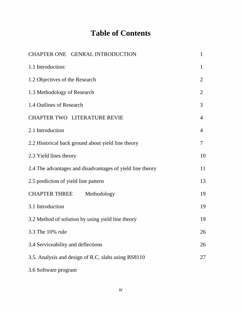
Since the first step in any analysis is to postulate a failure mechanism or yield-
line pattern, the yield-line patterns of various slabs are shown in Fig.2.5(a-k) to
show how the confirm to the four conditions that have been given. Fig.2.5a
shows a possible yield-line pattern for a square slab subjected to uniformly
distributed load. The axes of rotation of element A is ab, the line of support,
while that of B is bc. The yield line between these element passes through the
point of intersection of these axes, which is the corner b. similarly yield lines
pass through the other corners. Since yielding starts in the center of the slab,
then the yield lines are straight lines between the center and the corners. Fig.2.5b
shows a yield-line pattern for the rectangular slab under uniform load. The yield
lines pass through the corner for the reasons given previously and yield line ef
is parallel to the longer sides- it intersects the parallel axes of rotation of adjacent
elements A and C at infinity. Initially it is only necessary to draw the general
yield-line pattern, the exact position of e and f can be found in the process of the
analysis.
For the continuous rectangular slab shown in Fig.2.5c, negative yield lines must
also form along the lines of support before they can become axes of rotation, in
Fig.2.5b which represents a trapezoidal slab, the yield line ef produced passes
through the point of intersection of the axes of rotation along the longer sides.

18
Fig.2.5. yield line pattern for the different slabs shape with different
support conditions.
The patterns other than those shown in Fig 3.5(e)-3.5(j) may be found by similar
reasoning.
(a) (b) (c)
(d) (e) (f)
(g) (h) (i)
(j)

CHAPTER THREE
Methodology

19
CHAPTER THREE
Methodology
3.1 Introduction
According to Euro code 2, Yield Line Design is a perfectly valid method of
design. Section 5.6 of Euro code 2 states that plastic methods of analysis shall
only be used to check the ultimate limit state. Ductility is critical and sufficient
rotation capacity may be assumed provided x/d ≤ 0.25 for C50/60. Euro code 2
goes on to say that the method may be extended to flat slabs, ribbed, hollow or
waffle slabs and that corner tie down forces and torsion at free edges need to be
accounted for.
Section 5.11.1.1 of EC2 includes Yield Line as a valid method of analysis for
flat slabs. It is recommended that a variety of possible mechanisms are examined
and the ratios of the moments at support to the moment in the spans should lie
between 0.5 and 2.
3.2 Method of solution by using yield line theory
Once a failure pattern has been postulated two methods of solution are available
in order to find the relation between the ultimate resistance moments in the slab
and the ultimate load. Since the moment and the load are equilibrium when the
yield line pattern has formed, the slightest increment in load will cause the
structure to deflect. When this increase in load is infinitesimal, the work done
on the slab while the yield lines are rotating must be equal to the loss of work
due to the load deflecting. Thus, if a point on the slab is given a virtual deflection
take place along the yield lines. The internal work done on the slab will be the
sum of the rotations in the yield lines multiplied by the resisting ultimate
moments, while the external loss of work will be the sum of the loads multiplied
by their respective deflections. When the internal and external work is equated,
we have the relations between the ultimate resistance moments in the slab and

21
the ultimate load will be obtained. This method of solution is the well-known
principle of virtual work.
The second method of solution has been called the equilibrium method. When
using this method it is usually necessary to study the equilibrium of each of the
elements into which the slab is divided by the yield lines. Equilibrium equations
are obtained from each element, by equating internal and external moments and
by resolving vertical forces, and to find the desired solution the resulting
equations are solved simultaneously.
Both methods of the solution which are presented are upper bound solutions, to
find the most critical collapse mechanism several alternative yield-line patterns
may have to be studied.
Usually ultimate load solutions are obtained for slabs in which the percentage
of steel along any given line is constant. This implies that the same mesh is used
all over the slab. If the ultimate flexural strength along two orthogonal lines on
the slab surface is the same, the slab is called an isotropically reinforced slab; if
however the ultimate strength is different in the two directions the slab is called
an orthotropically reinforced slab.
The virtual work method of analysis is one-way, probably the most popular way
of applying yield line analysis to analyze slabs from first principles. It is
considered to be the quickest way of analyzing a slab using manual calculations
only. It can be applied and used on slabs of any configuration and loading
arrangement .
The only prerequisite is that the designer has a reasonably good idea of the
modes of failure and the likely shape of the crack pattern that will develop at
failure. This is not as difficult as it sounds. Having studied the basic failure
patterns that are formed by the majority of slab shapes encountered in practice,
the designer soon develops a feel for the way a slab is likely to fail and the
confidence to turn this feel into safe and practical designs. Provided the numeric

21
methods shown below are used, and, if necessary, iterations made, the virtual
work method gives solutions that are, almost always, within 10% of that attained
by an exact algebraic approach using a differentiation process. In recognition of
this possible inexactness, it is recommended that ‘the 10% rule.’
Before explaining how to apply the virtual work method of analysis it may help
to review the stages involved in the failure of a slab :
•Collapse occurs when yield lines form a mechanism .
•This mechanism divides the slab into rigid regions .
•Since elastic deformations are neglected these rigid regions remain as plane
areas .
•These plane areas rotate about their axes of rotation located at their supports.
•All deformation is concentrated within the yield lines: the yield lines act as
elongated plastic hinges.as shown in Fig.3.1.
Fig.3.1. Simply Supported One-way Slab.

22
The basis of the Work Method is simply that at failure the potential energy
expended by loads moving must equal the energy dissipated (or work done) in
yield lines rotating.
In other words:
External energy = Internal energy (3.1)
Expended by the displacement of loads = Dissipated by the yield lines rotating
Σ (Ν x δ) for all regions = Σ (m x l x θ) (3.2)
Where;
N : is the Load(s) acting within a particular region [kN].
δ : is the vertical displacement of the load(s) N on each region expressed as a
fraction of unity [m].
m : is the moment or moment of resistance of the slab per meter run represented
by the reinforcement crossing the yield line [kNm/m].
l : is the length of yield line or its projected length onto the axis of rotation for
that region [m].
θ : is the rotation of the region about its axis of rotation [m/m] for all regions.
Once a valid failure pattern (or mechanism) has been postulated, either the
moment, m, along the yield lines or the failure load of a slab, N (or indeed n
kN/m2), can be established by applying the above equation .
This, fundamentally, is the Work Method of analysis: it is a kinematic (or
energy) method of analysis. The deformed shape of slab at failure was shown in
Fig.3.2.

23
Fig.3.2. Deformed shape at failure.
Fig.3.3 shown the Principles of expenditure of external loads, The external
energy expended, E, is calculated by taking, in turn, the resultant of each load
type (i.e. uniformly distributed load, line load or point load) acting on a region
and multiplying it by its vertical displacement measured as a proportion of the
maximum deflection implicit in the proposed yield line pattern. For simplicity,
the maximum deflection is taken as unity, and the vertical displacement of each
load is usually expressed as a fraction of unity. The total energy expended for
the whole slab is the sum of the expended energies for all the regions.

24
Fig.3.3. Principles of expenditure of external loads.
Fig.3.4 shown the Principles of dissipation of internal energy, The internal
energy dissipated, D, is calculated by taking the projected length of each yield
line around a region onto the axis of rotation of that region, multiplying it by the
moment acting on it and by the angle of rotation attributable to that region. The
total energy dissipated for the whole slab is the sum of the dissipated energies
of all the regions.
Diagonal yield lines are assumed to be made up of small steps with sides parallel
to the axes of rotation of the two regions it divides. The 'length' of a diagonal or
inclined yield line is taken as the summation of the projected lengths of these
individual steps onto the relevant axes of rotation.

25
The angle of rotation of a region is assumed to be small and is expressed as
being δmax/length. The length is measured perpendicular to the axis of rotation
to the point of maximum deflection of that region.
Fig.3.4. Principles of dissipation of internal energy.
A fundamental principle of physics is that energy cannot be created or destroyed.
So in the yield line mechanism, External energy = Internal energy. By equating
these two energies the value of the unknown i.e. either the moment, m, or the
load, N, can then be established.

26
If deemed necessary, several iterations may be required to find the maximum
value of m (or the minimum value of load capacity) for each chosen failure
pattern.
3.3 The 10% rule
A 10% margin on the design moments should be added when using the virtual
work method or formulae for two-way slabs to allow for the method being upper
bound and to allow for the effects of corner levers [13].
The addition of 10% to the design moment in two-way slabs provides some
leeway where inexact yield line solutions have been used and some reassurance
against the effects of ignoring corner levers. At the relatively low stress levels
in slabs, a 10% increase in moment equates to a 10% increase in the
reinforcement design.
The designer may of course chase in search of a more exact solution but most
pragmatists are satisfied to know that by applying the 10% rule to a simple
analysis their design will be on the safe side without being unduly conservative
or uneconomic. The 10% rule can and usually is applied in other circumstances
where the designer wants to apply engineering judgment and err on the side of
caution.
The only situations where allowances under this ‘10% rule’ may be inadequate
relate to slabs with acute corners and certain configuration of slabs with
substantial point loads or line loads. In these cases guidance should be sought
from specialist literature.
3.4 Serviceability and deflections
Yield Line Theory concerns itself only with the ultimate limit state. The
designer must ensure that relevant serviceability requirements, particularly the
limit state of deflection, are satisfied.
Deflection of slabs should be considered on the basis of elastic design. This may
call for separate analysis but, more usually, deflection may be checked by using

27
span/effective depth ratios with ultimate (i.e. yield line) moments as the basis.
Such checks will be adequate in the vast majority of cases.
3.4.1 Deflection according to BS 8110
Deflection is usually checked by ensuring that the allowable span/effective
depth ratio is greater than the actual span/ effective depth ratio (or by checking
allowable span is greater than actual span). The basic span/depth ratio is
modified by factors for compression reinforcement (if any) and service stress in
the tension reinforcement. The latter can have a large effect when determining
the service stress, fs, to use in equation 8 in Table 3.10 of BS 8110. When
calculations are based on the ultimate yield line moments, one can,
conservatively, use βb values of 1.1 for end spans and 1.2 for internal spans.
Where estimates of actual deflections are required, other approaches, such as the
rigorous methods in BS 8110 Part 2, simplified analysis methods or finite
element methods should be investigated. These should be carried out as a
secondary check after the flexural design based on ultimate limit state principles
has been carried out.
In order to keep cracking to an acceptable level it is normal to comply (sensibly)
with the bar spacing requirements of BS 8110 Clauses 3.12.11.2.7 and 2.8.
3.4.2 Deflection according to Euro code 2
Euro code 2 treats deflection in a similar manner to BS 8110. Deemed-to-satisfy
span to depth ratios may be used to check deflection. Otherwise calculations,
which recognize that sections exist in a state between un cracked and fully
cracked, should be undertaken.
3.5. Analysis and design of R.C. slabs using BS8110
Any design process is governed by the recommendations of a specific code of
practice. In the UK, BS 8110 clause 3.5.2.1 says Alternatively Johansen’s Yield
Line method may be used for solid slabs. The proviso is that to provide against
serviceability requirements, the ratio of support and span moments should be
similar to those obtained by elastic theory. This sub-clause is referred to in

28
clauses 3.6.2 and 3.7.1.2 making the approach also acceptable for ribbed slabs
and flat slabs.
In slabs where the corners are prevented from lifting, and provision for torsion
is made, the maximum design moments per unit width are given by equations
3.3 and 3.4.
msx= βsxnlx2 (3.3)
msy= βsynlx2 (3.4)
Where design ultimate support moments are used which differ substantially
from those that would be assessed from Table 3.1.
Table 3.1. Bending moment coefficients for rectangular panels supported
on four sides with provision for torsion at corners.

29
3.6 Software program
3.6.1 STAAD-Pro
General purpose software suite for structural engineers involved in analysis and
design of structures. The structural analysis and design software, STAAD-Pro
was developed for practicing engineers. For static, pushover, dynamic, P-delta,
buckling or cable analysis, STAAD-Pro is the industry standard.
STAAD-Pro has design codes for most countries including US, BS, Canada,
Russia, Aus, France, India, China, Euro, Japan
3.6.2 PROKON
PROKON provides engineers with tools to streamline their Workflow in the
structural and geotechnical spheres. The tools are modular, but all are launched
from the Prokon Calcpad.
Analysis of Continuous Beam & Slab Design
The Continuous Beam and Slab Design module is used to design and detail
reinforced concrete beams and slabs as encountered in typical building projects.
The design incorporates automated pattern loading and moment redistribution.
Cross-sections can include a mixture of rectangular, I, T and L-sections. Spans
can have constant or tapered sections. Entered dead and live loads are
automatically applied as pattern loads during the analysis. At ultimate limit
state, moments and shears are redistributed to a user specified percentage. Both
short-term and long-term deflections are calculated. Complete bending
schedules can be generated for editing and printing using Pads. The
reinforcement details may be graphically edited by the designer, and is
presented in user friendly pages depicting entered, required and minimum
reinforcement (as specified by the applicable code of practice.

CHAPTER FOUR
Investigation of Ultimate
Resisting Moment for the
Reinforced Concrete Slabs

31
CHAPTER FOUR
Investigation of Ultimate Resisting Moment for the
Reinforced Concrete Slabs
4.1 Introduction
In this chapter, different types of reinforced concrete slab systems were analyzed
using yield line theory to determine ultimate resisting moment. Three systems
of reinforced concrete slabs were chosen. They were flat slab, beam slab
systems, have three panel in each direction. And special types of support of slabs
systems.

31
4.2 Analysis of flat Slab system
The Fig.4.1 shown below is the plan of flat slab have three equal spans at
direction X of 6 m length and three spans at direction Y of length 6 m for the
edges spans and 4 m length for middle span. , The slab is subjected to uniformly
distributed load of 20 kN/m2. By considering a reasonable pattern of positive
and negative yield lines is that shown in Fig.4.1, and with following the
procedure explained at previous Chapter, the ultimate resisting moment (MP)
can be obtained for each panel as named in Fig.4.1.
Fig.4.1. Plan of Flat Slab System with Expected of Yield Line Pattern.

32
4.2.1. Analysis of External Corner Panel S1
Panel S1 is the square panel have length of 6 m each with two adjacent edges
discontinuous and continuous in other tow edges, by considering a reasonable
pattern of positive and negative yield lines is that shown in Fig.4.2, we will
determine the Mp using work method.
Fig.4.2. Expected yield line Pattern of External Corner Panel S1.
For External work as explained in (3.2). = ∑N × δ
N = w x A, where A is the total area of panel
= ∑w × A × δ
= w (6*6) * 1
2
= 18w (4.1)
For Internal work =∑𝑚 × 𝑙 × 𝜃
Wint (total) = wint (A) +wint (B) +wint(C)+wint (D)

33
Table.4.1. Analysis of Panel S1 by yield line theory
Segment (A):
Length of (m) = √𝑥2 + 𝑦2
θB = 1
2𝑥 sin 𝛼
wint (A) = 𝑚 ∗ √𝑥2 + 𝑦2 ∗1
2𝑥 sin 𝛼
but ; sin 𝛼 = 𝑦
√𝑥2 + 𝑦2
wint (A) = (𝑚 ∗ √(6 − 𝑥)2 + 𝑦2 ∗ √(6−𝑥)2+𝑦2
2𝑦(6−𝑥)+ m` ∗
𝑦
2(6−𝑥))
= (𝑚 ∗(6−𝑥)2+𝑦2
2𝑦(6−𝑥)+ m` ∗
𝑦
2(6−𝑥))
Segment (B):
Length of (m) = √(6 − 𝑥)2 + 𝑦2
Length of (m`) = y ∗ sin 𝛽
Segment Length for
moment
Length for
moment
Component of
Rotation
Wint
Segment
(A)
but ; sin 𝛼 = 𝑦
√𝑥2 + 𝑦2
Segment
(B)
√(6 − 𝑥)2 + 𝑦2 y ∗ sin 𝛽 1
2(6 − 𝑥) sin 𝛽
but ; sin 𝛽
=𝑦
√(6 − 𝑥)2 + 𝑦2
𝑚 ∗(6 − 𝑥)2 + 𝑦2
2𝑦(6 − 𝑥)+ m`
∗𝑦
2(6 − 𝑥)
Segment
(C)
√(6 − 𝑥)2 + (6 − 𝑦)2 √(6 − 𝑥)2 + (6 − 𝑦)2
1
2(6 − 𝑦) sin 𝛾
but ; sin 𝛾
=6 − 𝑥
√(6 − 𝑥)2 + (6 − 𝑦)2
(𝑚 + m`) ∗(6 − 𝑥)2 + (6 − 𝑦)2
2(6 − 𝑦) (6 − 𝑥)
Segment
(D):
√(6 − 𝑦)2 + 𝑥2 x ∗ sin θ 1
2(6 − 𝑦) sin θ
but ; sin 𝛽
= 𝑥
√(6 − 𝑦)2 + 𝑥2
(𝑚 ∗(6 − 𝑦)2 + 𝑥2
2𝑥(6 − 𝑦)+ m`
∗𝑥
2(6 − 𝑦))
Total
wint 𝒎 ∗
(𝒙𝟐+𝒚𝟐)
𝟐𝒙𝒚+ (𝒎 ∗
(𝟔−𝒙)𝟐+𝒚𝟐
𝟐𝒚(𝟔−𝒙)+ 𝐦` ∗
𝒚
𝟐(𝟔−𝒙)) + (𝒎 + 𝐦`) ∗
(𝟔−𝒙)𝟐+(𝟔−𝒚)𝟐
𝟐(𝟔−𝒚) (𝟔−𝒙) + (𝒎 ∗
(𝟔−𝒚)𝟐+𝒙𝟐
𝟐𝒙(𝟔−𝒚)+ 𝐦` ∗
𝒙
𝟐(𝟔−𝒚))
√𝑥2 + 𝑦2 1
2𝑥 sin 𝛼 𝑚 ∗
(𝑥2 + 𝑦2)
2𝑥𝑦

34
θB = 1
2(6−𝑥) sin 𝛽
wint (B) = (𝑚 ∗ √(6 − 𝑥)2 + 𝑦2 + m` ∗ y ∗ sin 𝛽) ∗1
2(6−𝑥) sin 𝛽
but ; sin 𝛽 = 𝑦
√(6 − 𝑥)2 + 𝑦2
wint (B) = (𝑚 ∗ √(6 − 𝑥)2 + 𝑦2 ∗ √(6−𝑥)2+𝑦2
2𝑦(6−𝑥)+ m` ∗
𝑦
2(6−𝑥))
= (𝑚 ∗(6−𝑥)2+𝑦2
2𝑦(6−𝑥)+ m` ∗
𝑦
2(6−𝑥))
Segment (C):
Length of (m) = √(6 − 𝑥)2 + (6 − 𝑦)2
Length of (m`) = √(6 − 𝑥)2 + (6 − 𝑦)2
θC = 1
2(6−𝑦) sin 𝛾
wint (C) = (𝑚 + m`) ∗ √(6 − 𝑥)2 + (6 − 𝑦)2 ∗1
2(6−𝑦) sin 𝛾
but ; sin 𝛾 = 6 − 𝑥
√(6 − 𝑥)2 + (6 − 𝑦)2
wint (C) = (𝑚 + m`) ∗ √(6 − 𝑥)2 + (6 − 𝑦)2 ∗√(6−𝑥)2+(6−𝑦)2
2(6−𝑦) (6−𝑥)
= (𝑚 + m`) ∗(6−𝑥)2+(6−𝑦)2
2(6−𝑦) (6−𝑥)
Segment (D):
Length of (m) = √(6 − 𝑦)2 + 𝑥2
Length of (m`) = x ∗ sin θ
θD = 1
2(6−𝑦) sin θ
wint (D) = (𝑚 ∗ √(6 − 𝑦)2 + 𝑥2 + m` ∗ x ∗ sin θ) ∗1
2(6−𝑦) sin θ
but ; sin 𝛽 = 𝑥
√(6 − 𝑦)2 + 𝑥2
wint (D) = (𝑚 ∗ √(6 − 𝑦)2 + 𝑥2 ∗ √(6−𝑦)2+𝑥2
2𝑥(6−𝑦)+ m` ∗
𝑥
2(6−𝑥))
= (𝑚 ∗(6−𝑦)2+𝑥2
2𝑥(6−𝑥)+ m` ∗
𝑥
2(6−𝑥))
Total Internal work =

35
= 𝑚 ∗ (𝑥2+𝑦2)
2𝑥𝑦+ (𝑚 ∗
(6−𝑥)2+𝑦2
2𝑦(6−𝑥)+ m` ∗
𝑦
2(6−𝑥)) + (𝑚 + m`) ∗
(6−𝑥)2+(6−𝑦)2
2(6−𝑦) (6−𝑥) + (𝑚 ∗
(6−𝑦)2+𝑥2
2𝑥(6−𝑦)+ m` ∗
𝑥
2(6−𝑦)) (4.2)
Let m=m`
=3m [1
𝑥+
1
𝑦 +
2
(6−𝑥) +
2
(6−𝑦)] (4.3)
External work = Internal work
=3m [1
𝑥+
1
𝑦 +
2
(6−𝑥) +
2
(6−𝑦)] = 18 w (4.4)
𝑤
𝑚 = [
1
𝑥+
1
𝑦 +
2
(6−𝑥) +
2
(6−𝑦)]/ 6 (4.5)
Using the expression:
𝑑(𝑤
𝑚)
𝑑y = 0 ; when
𝑑
𝑑y[
1
𝑥+
1
𝑦 +
2
(6−𝑥) +
2
(6−𝑦)] = 0
i.e.
1
𝑦2 +
(−2)
(6−𝑦)2= 0
By using excel; substituting a range of values of (y) in the above equation
and solve the equation for (y),
Given; y = 2.485 m
That is (w/m) maximum when y = 2.485
For y = 2.485, the Eqn (4.1.5) reduces to
1
x +
2
(6−x)= 𝑚/𝑤 (4.6)
𝑑(𝑤
𝑚)
𝑑x = 0
i.e.
1
𝑥2 +
(−2)
(6−𝑥)2= 0
By using excel; substituting a range of values of (x) in the above equation
and solve the equation for (x),
gives x = 2.485 m
Substituting; x = 2.485 and y = 2.485 into Equ(4.1.5)
m = 3.09 w (4.7)
36
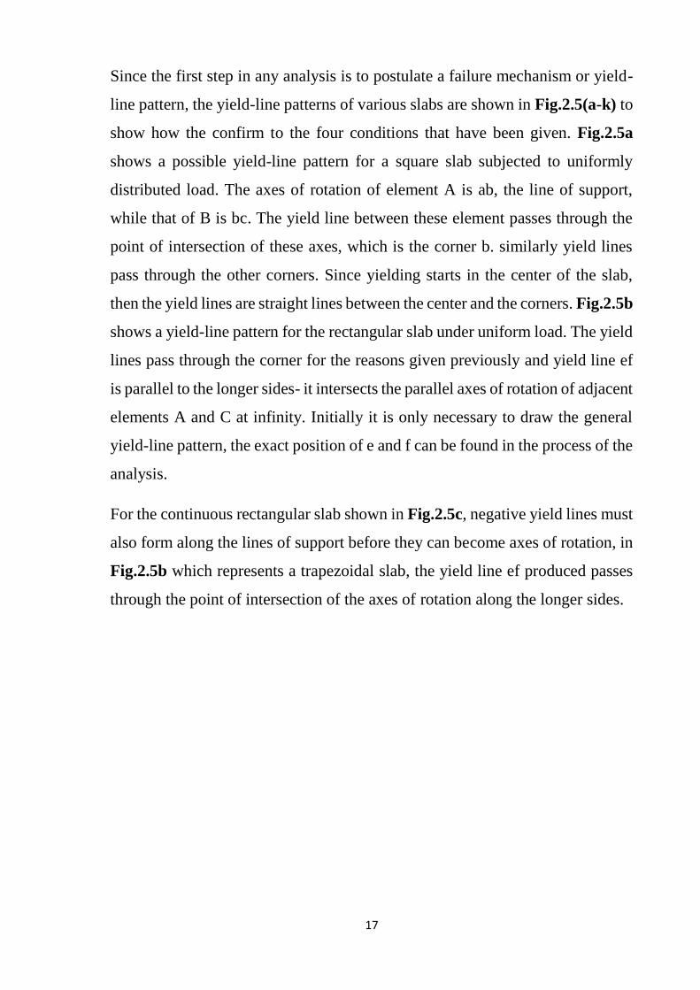
When; w = 20 kN.m2
Mmax =61.8 kN.m/m
By using “10% rule”; Mmax = 67.98kN.m/m
So; the actual yield lines pattern as per the calculation will be as shown in
figure below:
Fig.4.3.Yield Line Pattern of Panel S1.

37
4.2.2. Analysis of Edge Panel S2
Panel S2 is the square panel have length of 6m with one edge discontinuous and
three edges continuous, by considering a reasonable pattern of positive and
negative yield lines is that shown in Fig.4.4, we will determine the Mmax using
work method.
Fig.4.4.Expected yield line Pattern of the edge Panel S2.
Solution by using method work:
External work = Internal work
For External work = ∑N × δ
= ∑w × a × δ
= w (6*6) * 1
2
= 18w (4.8)
For Internal work =∑𝑚 × 𝑙 × 𝜃
Wint (total) = wint (A) +wint (B) +wint(C)+wint (D)

38
Table.4.3.Analysis of Panel S2 by yield line theory.
Segment (A):
Length of (m) = √9 + 𝑦2
Length of (m`) = y ∗ sin 𝛼
θA = 1
6 sin 𝛼
wint (A) =(𝑚 ∗ √9 + 𝑦2 + m` ∗ y ∗ sin 𝛼) ∗1
6 sin 𝛼
but ; sin 𝛼 = 𝑦
√9 + 𝑦2
wint (A) = (𝑚 ∗ √9 + 𝑦2 + m` ∗ y ∗ 𝑦
√9+𝑦2) ∗
√9+𝑦2
6𝑦
=(𝑚 ∗ (9 + 𝑦2) + m` ∗𝑦
6)
Segment (B):
Length of (m) = √9 + 𝑦2
Length of (m`) = y ∗ sin 𝛽
θB = 1
6 sin 𝛽
Segment Length for
moment
Length for
moment
Component of
Rotation
Wint
Segment
(A)
√9 + 𝑦2 y ∗ sin 𝛼 1
6 sin 𝛼 but ; sin 𝛼 =
𝑦
√9 + 𝑦2
𝑚 ∗ (9 + 𝑦2) + m` ∗𝑦
6
Segment
(B)
√9 + 𝑦2 y ∗ sin 𝛽 1
6 sin 𝛽
but ; sin 𝛽
=𝑦
√(6 − 𝑥)2 + 𝑦2
𝑚 ∗(9 + 𝑦2)
6𝑦+ m` ∗
𝑦
6
Segment
(C)
√9 + (6 − 𝑦)2 √9 + (6 − 𝑦)2 1
2(6 − 𝑦) sin 𝛾
𝑏𝑢𝑡 ; 𝑠𝑖𝑛 𝛾
= 3
√9 + (6 − 𝑦)2
(𝑚 + 𝑚`) ∗(9 + (6 − 𝑦)2)
6(6 − 𝑦)
Segment
(D):
√(6 − 𝑦)2 + 9 √(6 − 𝑦)2 + 9 1
2(6 − 𝑦) sin θ
𝑏𝑢𝑡 ; 𝑠𝑖𝑛 𝜃
= 3
√9 + (6 − 𝑦)2
(𝑚 + m`) ∗(9 + (6 − 𝑦)2)
6(6 − 𝑦)
Total wint 𝟐 (𝒎(𝟗+𝒚𝟐)
𝟔𝒚+ 𝒎`
𝒚
𝟔)+𝟐(𝒎 + 𝒎`)
(𝟗+(𝟔−𝒚)𝟐)
𝟔(𝟔−𝒚)

39
wint (B) = (𝑚 ∗ √9 + 𝑦2 + m` ∗ y ∗ sin 𝛽) ∗1
6 sin 𝛽
but ; sin 𝛽 = 𝑦
√9 + 𝑦2
wint (B) =(𝑚 ∗ √9 + 𝑦2 + m` ∗ y ∗ 𝑦
√9+𝑦2) ∗
√9+𝑦2
6𝑦
=(𝑚 ∗(9+𝑦2)
6𝑦+ m` ∗
𝑦
6)
Segment (C):
Length of (m) = √9 + (6 − 𝑦)2
Length of (m`) = √9 + (6 − 𝑦)2
θC = 1
2(6−𝑦) sin 𝛾
wint (C) = (𝑚 + m`) ∗ √9 + (6 − 𝑦)2 ∗1
2(6−𝑦) sin 𝛾
but ; sin 𝛾 = 3
√9 + (6 − 𝑦)2
wint (C) = (𝑚 + m`) ∗ √9 + (6 − 𝑦)2 ∗√9+(6−𝑦)2
6(6−𝑦)
= (𝑚 + m`) ∗(9+(6−𝑦)2)
6(6−𝑦)
Segment (D):
Length of (m) = √(6 − 𝑦)2 + 9
Length of (m`) = √(6 − 𝑦)2 + 9
θD = 1
2(6−𝑦) sin θ
wint (D) = (𝑚 + m`) ∗ √(6 − 𝑦)2 + 9 ∗1
2(6−𝑦) sin θ
but ; sin θ = 3
√9 + (6 − 𝑦)2
wint (D) = (𝑚 + m`) ∗ √9 + (6 − 𝑦)2 ∗√9+(6−𝑦)2
6(6−𝑦)
= (𝑚 + m`) ∗(9+(6−𝑦)2)
6(6−𝑦)
Total Internal work =
=𝟐 (𝑚(9+𝑦2)
6𝑦+ m`
𝑦
6)+2(𝑚 + m`)
(9+(6−𝑦)2)
6(6−𝑦) (4.9)

41
let m=m`
=𝑚 ((9+𝑦2)
3𝑦+
𝑦
3)+
2(9+(6−𝑦)2)
3(6−𝑦) ) (4.10)
= m [ 3
𝑦+
2𝑦
3 +
6
(6−𝑦) +
2(6−𝑦)
3] (4.11)
External work = Internal work
=m [ 3
𝑦+
2𝑦
3 +
6
(6−𝑦) +
2(6−𝑦)
3]= 18 w (4.12)
m = 18 w /[ 3
𝑦+
2𝑦
3 +
6
(6−𝑦) +
2(6−𝑦)
3] (4.13)
By using excel; substituting a range of values of (y) in the above equation
and finding the maximum Values of (m),
We find maximum values of (m) = 2.6w, coincide with y = 2.49m
That is (m) maximum when y = 2.49m
Substituting; x = 2.49m into Equ (4.13)
m = 2.6 w (4.14)
When; w = 20 kN.m2
Mmax =52.0kN.m/m
By using " 10% rule " ; Mmax = 57.2 kN.m/m
So; the actual yield lines pattern as per the calculation will be as shown in
figure below:
Fig.4.5 Yield line Pattern of Panel S2.

41
4.2.3. Analysis of edge Panel S3
Panel S3 is the rectangular panel have length of 6m and 4m width with one edge
discontinuous and three edges continuous, by considering a reasonable pattern
of positive and negative yield lines is that shown in Fig.4.6, we will determine
the Mp using work method.
Fig.4.6.Expected yield line Pattern of the edge Panel S3.
Solution by using virtual work method:
External work = Internal work from Equ (3.1)
For External work = ∑N × δ
= ∑w × a × δ
= w (6*4) * 1
2
= 12w (4.15)
For Internal work =∑𝑚 × 𝑙 × 𝜃
Wint (total) = wint (A) +wint (B) +wint(C)+wint (D)

42
Table.4.3. Analysis of Panel S3 by yield line theory.
Segment (A):
Length of (m) = √𝑥2 + 4
Length of (m`) =2 sin 𝛼
θA = 1
2𝑥 sin 𝛼
wint (A) = 𝑚 ∗ √𝑥2 + 4 ∗1
2𝑥 sin 𝛼+ m` ∗ 2 sin 𝛼 ∗
1
2𝑥 sin 𝛼
but ; sin 𝛼 = 2
√𝑥2 + 4
wint (A) = 𝑚(𝑥2+4)
4𝑥+
m`
𝑥
Segment (B):
Length of (m) = √(6 − 𝑥)2 + 4
Length of (m`) =√(6 − 𝑥)2 + 4
θB = 1
2(6−𝑥) sin 𝛽
Segment Length for
moment
Length
for
moment
Component
of Rotation
Wint
Segment
(A)
2 sin 𝛼 but ; sin 𝛼 =
2
√𝑥2 + 4
Segment
(B)
√(6 − 𝑥)2 + 4 √(6 − 𝑥)2 + 4 1
2(6 − 𝑥) 𝑠𝑖𝑛 𝛽
𝑏𝑢𝑡 ; 𝑠𝑖𝑛 𝛽
= 2
√(6 − 𝑥)2 + 4
(𝑚 + m`) ∗((6 − 𝑥)2 + 4)
4(6 − 𝑥)
Segment
(C)
√(6 − 𝑥)2 + 4 √(6 − 𝑥)2 + 4 1
2(6 − 𝑥) 𝑠𝑖𝑛 𝛽
𝑏𝑢𝑡 ; 𝑠𝑖𝑛 𝛽
= 2
√(6 − 𝑥)2 + 4
(𝑚 + m`) ∗((6 − 𝑥)2 + 4)
4(6 − 𝑥)
Segment
(D):
√4 + 𝑥2 𝑥 ∗ 𝑠𝑖𝑛 𝜃 1
4 𝑠𝑖𝑛 𝜃 𝑏𝑢𝑡 ; 𝑠𝑖𝑛 𝛽 =
𝑥
√4 + 𝑥2
𝑚 ∗(4 + 𝑥2)
4𝑥+ m` ∗
𝑥
4
Total wint 𝐦(𝐱𝟐+𝟒)
𝟒𝐱+
𝐦`
𝐱+ 𝟐 ∗ (𝐦 + 𝐦`) ∗
((𝟔−𝐱)𝟐+𝟒)
𝟒(𝟔−𝐱) + (𝐦 ∗
(𝟒+𝐱𝟐)
𝟒𝐱+ 𝐦` ∗
𝐱
𝟒)
√𝑥2 + 4 1
2𝑥 sin 𝛼 𝑚
(𝑥2 + 4)
4𝑥+
𝑚`
𝑥

43
wint (B) = (𝑚 + m`) ∗ √(6 − 𝑥)2 + 4 ∗1
2(6−𝑥) sin 𝛽
but ; sin 𝛽 = 2
√(6 − 𝑥)2 + 4
wint (B) = (𝑚 + m`) ∗ √(6 − 𝑥)2 + 4 ∗√(6−𝑥)2+4
4(6−𝑥)
= (𝑚 + m`) ∗((6−𝑥)2+4)
4(6−𝑥)
Segment (C):
Length of (m) = √(6 − 𝑥)2 + 4
Length of (m`) =√(6 − 𝑥)2 + 4
θC = 1
2(6−𝑥) sin 𝛽
wint (C) = (𝑚 + m`) ∗ √(6 − 𝑥)2 + 4 ∗1
2(6−𝑥) sin 𝛽
but ; sin 𝛽 = 2
√(6 − 𝑥)2 + 4
wint (C) = (𝑚 + m`) ∗ √(6 − 𝑥)2 + 4 ∗√(6−𝑥)2+4
4(6−𝑥)
= (𝑚 + m`) ∗((6−𝑥)2+4)
4(6−𝑥)
Segment (D):
Length of (m) = √4 + 𝑥2
Length of (m`) = x ∗ sin θ
θD = 1
4 sin θ
wint (D) = (𝑚 ∗ √4 + 𝑥2 + m` ∗ x ∗ sin θ) ∗1
4 sin θ
but ; sin 𝛽 = 𝑥
√4 + 𝑥2
wint (D) = (𝑚 ∗ √4 + 𝑥2 ∗ √4+𝑥2
4𝑥+ m` ∗
𝑥
4)
= (𝑚 ∗(4+𝑥2)
4𝑥+ m` ∗
𝑥
4)
Total Internal work =
=𝑚(𝑥2+4)
4𝑥+
m`
𝑥+ 2 (𝑚 + m`) ∗
((6−𝑥)2+4)
4(6−𝑥) + (𝑚 ∗
(4+𝑥2)
4𝑥+ m` ∗
𝑥
4)
let m=m`

44
= m [ 2
𝑥+
3
4𝑥 +
(6−𝑥)
2 +
2
(6−𝑥)] (4.16)
External work = Internal work
= m [ 2
𝑥+
3
4𝑥 +
(6−𝑥)
2 +
2
(6−𝑥)]=12 w (4.17)
m = 12 w/ [ 2
𝑥+
3
4𝑥 +
(6−𝑥)
2 +
2
(6−𝑥)] (4.18)
By using excel; substituting a range of values of (x) in the above equation
and finding the maximum Values of (m),
We find maximum values of (m) = 2.41w , coincide with x = 2.257 m
That is (m) maximum when x = 2.257 m
Substituting; x = 2.257 m into Equ (4.18)
m = 2.41w (4.19)
when;
w = 20 kN.m2
Mmax =48.2kN.m/m
By using " 10% rule " ; Mmax = 53.02 kN.m/m
So; the actual yield lines pattern as per the calculation will be as shown in
figure below:
Fig.4.7.Yield Line Pattern of Panel S3.

45
4.2.4. Analysis of Interior panel S4
Panel S4 is the rectangular panel have length of 6m and width 4m with four
edges continuous, by considering a reasonable pattern of positive and negative
yield lines is that shown in Fig.4.8, we will determine the Mp using virtual work
method.
Fig.4.8.Expected yield line Pattern for the interior Panel S4.
Solution by using method work:
External work = Internal work
For External work = ∑N × δ
= ∑w × a × δ
= w (6*4) * 1
2
= 12w (4.20)
For Internal work =∑𝑚 × 𝑙 × 𝜃
Wint (total) = wint (A) +wint (B) +wint(C)+wint (D)

46
Table.4.4. Analysis of panel S4 by yield line theory.
Segment (A):
Length of (m) = √4 + 9 = 3.61 𝑚
Length of (m`) =√4 + 9 = 3.61 𝑚
θA = 1
6 sin 𝛼
wint (A) = (𝑚 + 𝑚`) ∗ 3.61 ∗1
6 sin 𝛼
but ; sin 𝛼 = 2
3.61
wint (A) = (𝑚 + 𝑚`) ∗ 3.61 ∗3.61
6𝑥2
=(𝑚 + 𝑚`) ∗ 1.09
Segment (B):
Length of (m) = √4 + 9 = 3.61 𝑚
Length of (m`) =√4 + 9 = 3.61 𝑚
θB = 1
6 sin 𝛽
wint (B) = (𝑚 + 𝑚`) ∗ 3.61 ∗1
6 sin 𝛽
Segment Length for +ve
moment
Length for
–ve
moment
Component
of Rotation
Wint
Segment
(A)
3.61 𝑚 but ; sin 𝛼 =
2
3.61
Segment
(B)
3.61 𝑚
3.61 𝑚 1
6 𝑠𝑖𝑛 𝛽 𝑏𝑢𝑡 ; 𝑠𝑖𝑛 𝛽 =
2
3.61
(𝑚 + 𝑚`) ∗ 1.09
Segment
(C)
3.61 𝑚 1
4 𝑠𝑖𝑛 𝛾 𝑏𝑢𝑡 ; 𝑠𝑖𝑛 𝛽 =
2
3.61
(𝑚 + 𝑚`) ∗ 1.09
Segment
(D):
3.61 𝑚
3.61 𝑚 1
4 𝑠𝑖𝑛 𝜃 𝑏𝑢𝑡 ; 𝑠𝑖𝑛 𝜃 =
3
3.61
(𝑚 + 𝑚`) ∗ 1.09
Total wint 𝟒 ∗ (𝒎 + 𝒎`) ∗ 𝟏. 𝟎𝟗
3.61 𝑚 1
6 sin 𝛼
(𝑚 + 𝑚`) ∗ 1.09
3.61 𝑚

47
but ; sin 𝛽 = 2
3.61
wint (B) = (𝑚 + 𝑚`) ∗ 3.61 ∗3.61
6𝑥2
=(𝑚 + 𝑚`) ∗ 1.09
Segment (C):
Length of (m) = √4 + 9 = 3.61 𝑚
Length of (m`) =√4 + 9 = 3.61 𝑚
θC = 1
4 sin 𝛾
wint (C) = (𝑚 + 𝑚`) ∗ 3.61 ∗1
4 sin 𝛾
but ; sin 𝛾 = 3
3.61
wint (C) = (𝑚 + 𝑚`) ∗ 3.61 ∗3.61
4𝑥3
=(𝑚 + 𝑚`) ∗ 1.09
Segment (D):
Length of (m) = √4 + 9 = 3.61 𝑚
Length of (m`) =√4 + 9 = 3.61 𝑚
θD = 1
4 sin θ
wint (D) = (𝑚 + 𝑚`) ∗ 3.61 ∗1
4 sin θ
but ; sin θ = 3
3.61
wint (D) = (𝑚 + 𝑚`) ∗ 3.61 ∗3.61
4𝑥3
=(𝑚 + 𝑚`) ∗ 1.09
Total Internal work =
=4 ∗ (𝑚 + 𝑚`) ∗ 1.09 (4.21)
let m=m`
=8.72 m
External work = Internal work
=8.72 m = 12 w (4.22)
m = 12w/ 8.72 (4.23)

48
m = 1.38 w (4.24)
When; w = 20 kN.m2
Mmax =27.6kN.m/m
By using " 10% rule " ; Mmax = 30.36 kN.m/m
So; the actual yield lines pattern as per the calculation will be as shown in
figure below:
Fig.4.9. Yield Pattern of Panel S4.
The results obtained for the ultimate resisting moments for each panel of
reinforced concrete flat slabs were summarized at Table (4.5) and were
compared with value obtained by using STAAD-Pro Software.
Table .4.5. The Ultimate Resisting Moments for Flat Slab.
Panel Value of (MP) by
yield line theory
kN.m/m
Value of (MP) by
STAAD-pro
kN.m/m
Difference %
S1 61.80 61.74 0.097%
S2 52.00 52.96 -1.85%
S3 48.02 47.22 1.67%
S4 27.6 26.09 5.47%

49
4.3. Analysis of beam Slab system
The Fig.4.10. below is the plan of slab with beam have three equal spans at X
direction of 6 m length and three spans at Y direction of length 6 m for the edges
spans and 4 m length for middle span. , The slab is subjected to uniformly
distributed load of 20 kN/m2. By considering a reasonable pattern of positive
and negative yield lines is that shown in Fig.4.10, and with following the
procedure explained at previous Chapter, the ultimate moment (MP) can be
obtained for each panel as named in Fig.4.10.
Fig.4.10. Plan of beam Slab System with Expected of Yield Line Pattern.

51
4.3.1. Analysis of External Corner slab S5
Panel S5 is the square panel have length of 6 m each with two adjacent edges
discontinuous and continuous in other two sides, by considering a reasonable
pattern of positive and negative yield lines is that shown in Fig.4.11, we will
determine the MP using work method.
Fig.4.11. Expected Yield line Pattern of External Corner Panel S5.
Solution by using method work:
External work = Internal work
For External work = ∑N × δ
= ∑w × a × δ
= w (6*6) * 1
3
= 12w (4.25)
For Internal work =∑𝑚 × 𝑙 × 𝜃
Wint (total)= wint (A) +wint (B) +wint (D) +wint(C)

51
Table.4.6. Analysis of Panel S5 by yield line theory.
Segment (A):
Length of (m) = 6m
θA =1
𝑥
wint (A) = 𝟔𝒎
𝒙
Segment (B):
Length of (m) = 6m
θB = 1
𝑦
wint (B) = 𝟔𝒎
𝒚
Segment (C):
Length of (m) = 6m
Length of (m`) = 6m
θC = 1
(6−𝑥)
Segment Length for
moment
Length for
moment
Compone
nt of
Rotation
Wint
Segment
(A)
𝟔𝒎
𝒚
Segment
(B)
6m 1
𝑦
𝟔𝒎
𝒚
Segment
(C)
6m 6m 1
(6 − 𝑥)
𝟏𝟐𝒎
(𝟔 − 𝒙)
Segment
(D):
6m 6m 1
(6 − 𝑦)
𝟏𝟐𝒎
(𝟔 − 𝒚)
Total wint 𝟔𝐦
𝐱+
𝟔𝐦
𝐲 +
𝟏𝟐𝐦
(𝟔−𝐱) +
𝟏𝟐𝐦
(𝟔−𝐲)
6m 1
𝑥

52
wint (c) = 𝟔∗(𝒎+𝐦`)
(𝟔−𝒙)
Let; m`=m
wint (c) = 𝟔∗(𝒎+𝐦)
(𝟔−𝒙)=
𝟏𝟐𝒎
(𝟔−𝒙)
Segment (D):
Length of (m) = 6m
Length of (m`) = 6m
θC = 1
(6−𝑦)
wint (D) = 𝟔∗(𝒎+𝐦`)
(𝟔−𝒚)
Let; m`=m
wint (D) = 𝟔∗(𝒎+𝐦)
(𝟔−𝒚) =
𝟏𝟐𝒎
(𝟔−𝒚)
Total Internal work =
= 𝟔𝒎
𝒙+
𝟔𝒎
𝒚 +
𝟏𝟐𝒎
(𝟔−𝒙) +
𝟏𝟐𝒎
(𝟔−𝒚)
=6m [1
𝑥+
1
𝑦 +
2.33
(6−𝑥) +
2.33
(6−𝑦)] (4.26)
External work = Internal work
=6m [1
𝑥+
1
𝑦 +
2
(6−𝑥) +
2
(6−𝑦)]= 12w (4.27)
𝑤
𝑚 = [
1
𝑥+
1
𝑦 +
2
(6−𝑥) +
2
(6−𝑦)] / 2 (4.28)
Using the expression:
𝑑(𝑤
𝑚)
𝑑y = 0 ; when
𝑑
𝑑y[
1
𝑥+
1
𝑦 +
2
(6−𝑥) +
2
(6−𝑦)] = 0
i.e.
1
𝑦2 +
(−2)
(6−𝑦)2= 0
By using excel; substituting a range of values of (y) in the above equation
to solve it for (y)
Given; y = 2.485 m
That is w/m maximum when y = 2.485
For y = 2.485, the Eqn (4.28) reduces to

53
1
x +
2
(6−x)= 𝑚/𝑤 (4.29)
𝑑(𝑤
𝑚)
𝑑x = 0 ; gives x = 2.485 m
Substituting; x = 2.485 and y = 2.485 into Equ (4.28)
m = 1. 03 w (4.30)
When; w = 20 kN.m2
Mmax =20.6 kN.m/m
By using “10% rule”; Mmax = 22.66 kN.m/m
From BS8110:
msx= βsxnlx2
0.034*20*36=24.48 kN.m/m
So; the actual yield lines pattern as per the calculation will be as shown in
figure below:
Fig.4.12. Yield Pattern of Panel S5.
54
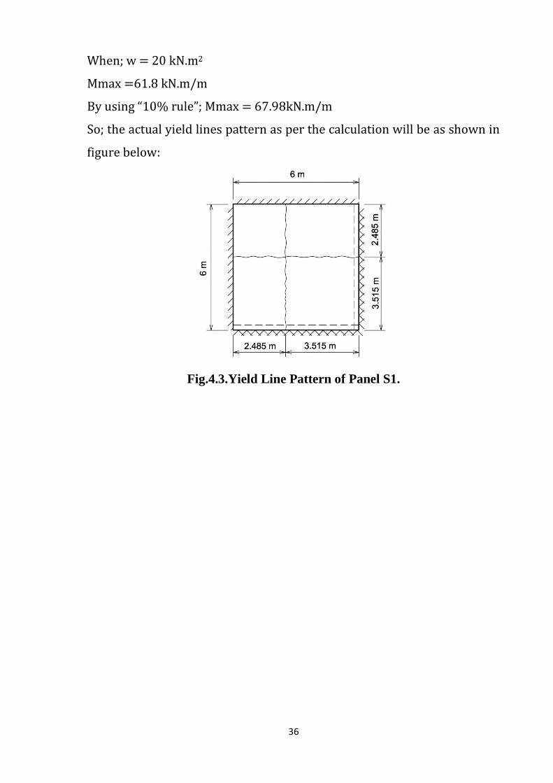
4.3.2. Analysis of Edge Slab S6
Panel S6 is the square panel have length of 6m with one edge discontinuous and
three edges continuous, by considering a reasonable pattern of positive and
negative yield lines is that shown in Fig.4.13, we will determine the Mp using
work method.
Fig.4.13. Expected Yield Line Pattern of edge Panel S6.
Solution by using virtual method work:
External work = Internal work
For External work = ∑N × δ
= ∑w × a × δ
= w (6*6) * 1
3
= 12w (4.31)
For Internal work =∑𝑚 × 𝑙 × 𝜃
Wint (total) = wint (A) +wint (B) +wint (D) +wint(C)
55
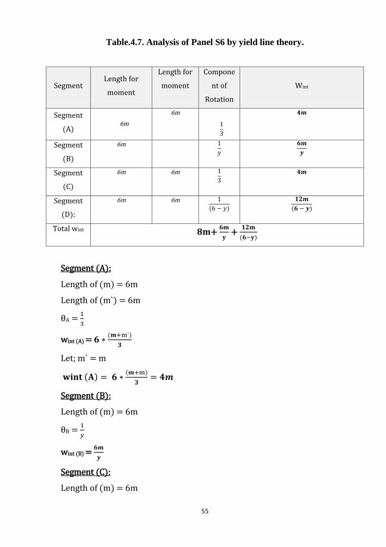
Table.4.7. Analysis of Panel S6 by yield line theory.
Segment (A):
Length of (m) = 6m
Length of (m`) = 6m
θA = 1
3
wint (A) = 𝟔 ∗(𝒎+m`)
𝟑
Let; m` = m
𝐰𝐢𝐧𝐭 (𝐀) = 𝟔 ∗(𝒎+m)
𝟑= 𝟒𝒎
Segment (B):
Length of (m) = 6m
θB = 1
𝑦
wint (B) = 𝟔𝒎
𝒚
Segment (C):
Length of (m) = 6m
Segment Length for
moment
Length for
moment
Compone
nt of
Rotation
Wint
Segment
(A)
6m
𝟒𝒎
Segment
(B)
6m 1
𝑦
𝟔𝒎
𝒚
Segment
(C)
6m 6m 1
3
𝟒𝒎
Segment
(D):
6m 6m 1
(6 − 𝑦)
𝟏𝟐𝒎
(𝟔 − 𝒚)
Total wint 𝟖𝐦+ 𝟔𝐦
𝐲 +
𝟏𝟐𝐦
(𝟔−𝐲)
6m 1
3
56
Length of (m`) = 6m
θc = 1
3
wint (c) = 𝟔 ∗(𝒎+m`)
𝟑
Let; m` = m
wint (c) = 𝟔 ∗(𝒎+m)
𝟑= 𝟒𝒎
Segment (D):
Length of (m) = 6m
Length of (m`) = 6m
θC = 1
(6−𝑦)
wint (D) = 𝟔∗(𝒎+𝐦`)
(𝟔−𝒚)
Let; m` = m
wint (D) = 𝟔∗(𝒎+𝐦)
(𝟔−𝒚)=
𝟏𝟐𝒎
(𝟔−𝒚)
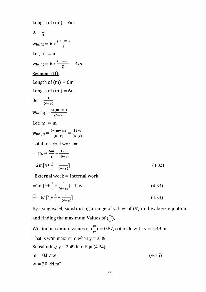
Total Internal work =
= 8𝑚+ 𝟔𝒎
𝒚 +
𝟏𝟐𝒎
(𝟔−𝒚)
=2m[4+ 3
𝑦 +
6
(6−𝑦)] (4.32)
External work = Internal work
=2m[4+ 3
𝑦 +
6
(6−𝑦)]= 12w (4.33)
𝑚
𝑤 = 6/ [4+
3
𝑦 +
6
(6−𝑦)] (4.34)
By using excel; substituting a range of values of (y) in the above equation
and finding the maximum Values of (𝑚
𝑤),
We find maximum values of (𝑚
𝑤) = 0.87, coincide with y = 2.49 m
That is w/m maximum when y = 2.49
Substituting; y = 2.49 into Equ (4.34)
m = 0.87 w (4.35)
w = 20 kN.m2
57
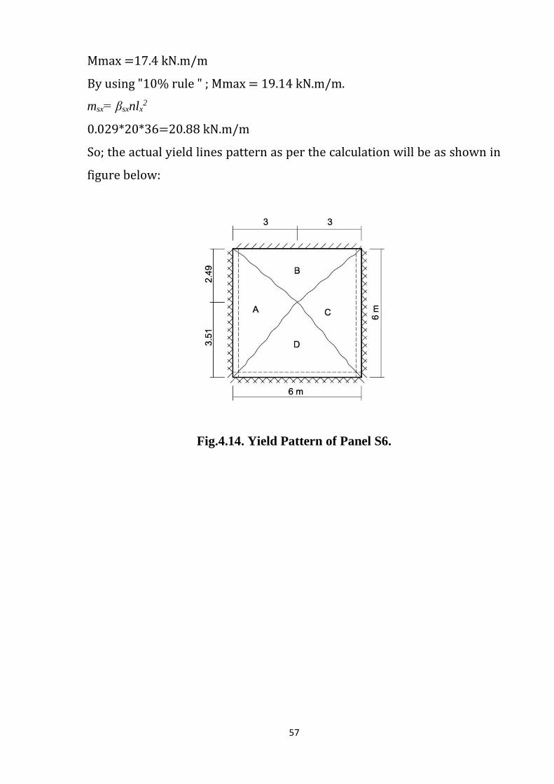
Mmax =17.4 kN.m/m
By using "10% rule " ; Mmax = 19.14 kN.m/m.
msx= βsxnlx2
0.029*20*36=20.88 kN.m/m
So; the actual yield lines pattern as per the calculation will be as shown in
figure below:
Fig.4.14. Yield Pattern of Panel S6.

58
4.3.3. Analysis of Edge Slab S7
Panel S7 is the rectangular panel have length of 6m and width 4m with one edge
discontinuous and three edges continuous, by considering a reasonable pattern
of positive and negative yield lines is that shown in Fig.4.15, we will determine
the Mp using work method.
Fig.4.15. Expected yield line Pattern of edge Panel S7.
Solution by using virtual method work:
External work = Internal work
For External work = ∑N × δ
= ∑w × a × δ
= w [(4x+4y) * 1/3 +(6-x-y) (4) *1/2]
= 2
3w (18-x-y) (4.36)
For Internal work =∑𝑚 × 𝑙 × 𝜃
Wint (total) = wint (A) +wint (B) +wint (D) +wint(C)
59
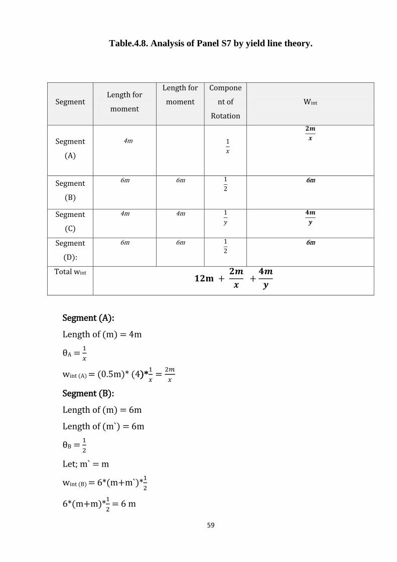
Table.4.8. Analysis of Panel S7 by yield line theory.
Segment (A):
Length of (m) = 4m
θA = 1
𝑥
wint (A) = (0.5m)* (4)*1
𝑥=
2𝑚
𝑥
Segment (B):
Length of (m) = 6m
Length of (m`) = 6m
θB = 1
2
Let; m` = m
wint (B) = 6*(m+m`)*1
2
6*(m+m)*1
2 = 6 m
Segment Length for
moment
Length for
moment
Compone
nt of
Rotation
Wint
Segment
(A)
𝟐𝒎
𝒙
Segment
(B)
6m 6m 1
2
6m
Segment
(C)
4m 4m 1
𝑦
𝟒𝒎
𝒚
Segment
(D):
6m 6m 1
2
6m
Total wint 𝟏𝟐𝐦 +
𝟐𝒎
𝒙 +
𝟒𝒎
𝒚
4m 1
𝑥

61
Segment (C):
Length of (m) = 4m
Length of (m`) = 4m
θc = 1
𝑦
wint (c) = (0.5m+0.5m`) *4
𝑦
Let; m` = m
= (0.5m+0.5*m) *4
𝑦=
4𝑚
𝑦
Segment (D):
Length of (m) = 6m
Length of (m`) = 6m
θD = 1
2
wint (B) = 6*(m+m`)*1
2
Let; m` = m
6*(m+m)*1
2= 6m
Total Internal work =
=12m + 2𝑚
𝑥 +
4𝑚
𝑦
=2m(6 + 1
𝑥 +
2
𝑦 ) (4.37)
External work = Internal work
=2m(6 + 1
𝑥 +
2
𝑦 )=
2
3w (18-x-y) (4.38)
𝑤
𝑚 =
3 (6+ 1
𝑥 +
2
𝑦 )
(18−x−y) (4.39)
Using the expression:
f1( 𝑥1, 𝑥2)
f2 ( 𝑥1, 𝑥2)=
𝑑
𝑑𝑥1f1( 𝑥1, 𝑥2)
𝑑
𝑑𝑥1f2 ( 𝑥1, 𝑥2)
By differentiate to x :

61
3 (6 + 1
𝑥 +
2
𝑦 )
(18 − x − y)=
3 ( − 1
𝑥2 )
−1
18-x-y = 6x2+2x +2𝑥2
y
(6 + 2
𝑦) 𝑥2+ 2x +(𝑦 − 18)= 0 (4.40)
Solve for "x" ;
x =
−2±√22−4(6+ 2
𝑦)(𝑦−18)
2∗(6+ 2
𝑦)
(4.41)
By using excel; substituting a range of values of (y) in the above equation
and finding the maximum Values of (x),
we find maximum values of (x) = 1.38 m , coincide with y = 1.95 m
m = 0.63 w (4.42)
w = 20 kN.m2
Mmax =12.6 kN.m/m
By using "10% rule " ; Mmax = 13.86kN.m/m
msx= βsxnlx2
0.043*20*16=13.76 kN.m/m
So; the actual yield lines pattern as per the calculation will be as shown in
figure below:
Fig.4.16. Yield line Pattern of Panel S7.

62
4.3.4. Analysis of Interior Slab S8
Panel S8 is the rectangular panel have length of 6m and width 4m with four
edges continuous, by considering a reasonable pattern of positive and negative
yield lines is that shown in Fig.4.17, we will determine the Mp using work
method.
Fig4.17. Expected Yield Line Pattern of Interior Panel S8.
Solution by using method work:
External work = Internal work
For External work = ∑N × δ
= ∑w × a × δ
= w [(4x+4y) *1
3+ (6-x-y) (4) *
1
2]
= 2
3w (18-x-y) (4.43)
For Internal work =∑𝑚 × 𝑙 × 𝜃
Wint (total) = wint (A) +wint (B) +wint (D) +wint(C)

63
Table.4.9. Analysis of Panel S8 by yield line theory.
Segment (A):
Length of (m) = 4m
Length of (m`) = 4m
θA = 1
𝑥
wint (A) = (0.5m+0.5m`)* 4
𝑥
Let; m` = m
wint (A) =(0.5m+0.5*m)* 4
𝑥 =
4𝑚
𝑥
Segment (B):
Length of (m) = 6m
Length of (m`) = 6m
θB = 1
2
wint (B) = 6*(m+m`)*1
2
Segment Length for
moment
Length for
moment
Compone
nt of
Rotation
Wint
Segment
(A)
4m
𝟒𝒎
𝒙
Segment
(B)
6m 6m 1
2
6m
Segment
(C)
4m 4m 1
𝑦
𝟒𝒎
𝒚
Segment
(D):
6m 6m 1
2
6m
Total wint 12m + 𝟒𝒎
𝒙 +
𝟒𝒎
𝒚
4m 1
𝑥

64
Let; m` = m
wint (B) =6*(m+m)*1
2 = 6m
Segment (C):
Length of (m) = 4m
Length of (m`) = 4m
θc = 1
𝑌
wint (c) = (0.5m+0.5m`) ∗ 4
𝑌
Let; m` = m
wint (c) = (0.5m+0.5*m) ∗ 4
𝑌=
4𝑚
𝑌
Segment (D):
Length of (m) = 6m
Length of (m`) = 6m
θD = 1
2
wint (D) = 6*(m+m`)*1
2
Let; m` = m
wint (D) = 6*(m+1.33m)*1
2= 6.99m
Total Internal work =
= 12m +4𝑚
𝑋 +
4𝑚
𝑌
= 4m (3 +1
𝑋+
1
𝑌) (4.44)
External work = Internal work
= 4m (3 +1
𝑋+
1
𝑌) =
2
3w (18-x-y) (4.45)
𝑤
𝑚=
6 (3 +1
𝑋+
1
𝑌 )
(18−x−y)
Using the expression:
f1( 𝑥1, 𝑥2)
f2 ( 𝑥1, 𝑥2)=
𝑑
𝑑𝑥1f1( 𝑥1, 𝑥2)
𝑑
𝑑𝑥1f2 ( 𝑥1, 𝑥2)
By differentiate to x:

65
6(3 + 1
𝑥 +
1
𝑦 )
(18−x−y)=
6( − 1
𝑥2 )
−1 (4.46)
18-x-y = 3x2+x +𝑥2
y
(3 + 1
𝑦) 𝑥2+ 2x +(𝑦 − 18)= 0
Solve for x;
x = −2+√22−4(3+
1 𝑦
)(𝑦−18)
2(3+ 1 𝑦
) (4.47)
By using excel; substituting a range of values of (y) in the above equation
and finding the maximum Values of (x),
we find maximum values of (x) = 1.87 m , coincide with y = 1.87 m
m = 0.584 w (4.48)
w = 20 kN.m2
Mmax =11.68kN.m/m
By using " 10% rule " ; Mmax = 12.85kN.m/m
msx= βsxnlx2
0.04*20*16=12.8 kN.m/m
So; the actual yield lines pattern as per the calculation will be as shown in
figure below:
Fig.4.18 Yield line Pattern of Panel S8.

66
The results obtained for the ultimate moments for each panel of reinforced
concrete slabs with beams are summarized as shown in Table. 4.10. and
compared with others obtained by using STAAD-Pro Software, and BS8110.
Table.4.10.The Ultimate Resisting Moments for Beam slab System.
Panel Value of
(MP) by
yield line
theory
KN.m/m
Value of
(MP) by BS
8110
KN.m/m
Difference
%
Value of (MP)
by STAAD-pro
KN.m/m
Difference
%
S5 22.65
24.48
8.08% 25.8 13.91%
S6 19.14
20.88
9.09% 20.02 4.6%
S7 13.86
13.76
0.72% 14.95 7.86%
S8 12.85
12.8
0.39% 12.76 0.70%

67
4.4 Special Beam slab system of different support conditions
4.4.1 Analysis of corner square slab S9
Panel S9 square slab length of 5m with edges continuous in two sides and simply
supported in other two sides, by considering a reasonable pattern of positive and
negative yield lines is that shown in Fig.4.19, the ultimate resisting moment Mp
can be determine using virtual work method
Fig.4.19. Expected yield line Pattern for the Corner Panel S9.
Solution by using virtual work method:
External work = Internal work
For External work = ∑N × δ
= ∑w × a × δ
=2 [(w*10∗(10−𝑥)
2*
1
3 )-(w* 5 *
5∗5(10−𝑥)
2𝑥 *
1
3 )]
5
𝑥+2 [(w *
(√2 ∗5)∗(√2 ∗(𝑥−5))
2∗
1
3 )] −(w*
((√2 ∗5))
2 *
(10𝑥−50)
(√2 ∗𝑥) ) ∗
(10𝑥−50)
√2 ∗√2 ∗(𝑥−5)
= 5𝑤
3 (10-x)
(2𝑥2−25)
𝑥2+
10𝑤
3 (x-5)
(𝑥2−25)
𝑥2
= 5𝑤
3𝑥2∗ {(10 − 𝑥)(2𝑥2 − 25) + 2 (𝑥 − 5)(𝑥2 − 25)}
=5𝑤
3𝑥 (10𝑥 − 25)(4.49)

68
Table.4.11 Analysis of Panel S9 by yield line theory.
For Internal work =∑𝑚 × 𝑙 × 𝜃
Wint (total) = wint (A) +wint (B) +wint(C)
Segment (A):
Length of (m) =5m
Length of (m`) = 5m
θA = 1
(10−𝑥)
wint (A) = (m +m`)* (5)*1
(10−𝑥)
Let; m = m`
=10𝑚
(10 − 𝑥)
Segment (B):
Length of (m) = 5m
Length of (m`) = 5m
θB = 1
(10−𝑥)
wint (B) = (m +m`)* (5)*1
(10−𝑥)
let; m = m`
Segment Length for
moment
Length for
moment
Component
of Rotation Wint
Segment
(A)
5m 𝟏𝟎𝒎
(𝟏𝟎 − 𝒙)
Segment
(B)
6m 6m 1
2
𝟏𝟎𝒎
(𝟏𝟎 − 𝒙)
Segment
(C)
(10𝑥 − 50)
(√2 ∗ 𝑥)
1
√2(𝑥 − 5) 2𝑚
(10𝑥 − 50)
(√2 ∗ 𝑥)√2(𝑥 − 5)
Total wint 𝟏𝟎𝐦{
𝟐
(𝟏𝟎 − 𝒙) +
𝟏
𝒙}
5m 1
(10 − 𝑥)

69
=10𝑚
(10 − 𝑥)
Segment (C):
Length of (m) = (10𝑥−50)
(√2 ∗𝑥)m
θc = 1
√2(𝑥−5)
wint (c) = 2(m) *(10𝑥−50)
(√2 ∗𝑥)∗
1
√2(𝑥−5)
= 2𝑚(10𝑥 − 50)
(√2 ∗ 𝑥)√2(𝑥 − 5)
Total Internal work =
=10𝑚
(10−𝑥)+
10𝑚
(10−𝑥) + 2𝑚
(10𝑥−50)
(√2 ∗𝑥)√2(𝑥−5)
= 20𝑚
(10−𝑥) +
(10𝑥−50) 𝑚
𝑥(𝑥−5)
= 10m{ 2
(10−𝑥) +
1
𝑥} (4.50)
External work = Internal work
= 10𝑚 ( 2
(10−𝑥) +
1
𝑥 ) =
5𝑤
3𝑥 (10𝑥 − 25) (4.51)
= 2𝑚 ( 2
(10−𝑥) +
1
𝑥 ) =
(10𝑥−25) 𝑤
3𝑥
m = w(10𝑥−25)
3𝑥 ÷ (
4
(10−𝑥) +
2
𝑥 )(4.52)
Solve for m;
By using excel; substituting a range of values of (x) in the above equation
and finding the maximum Values of (m),
We find maximum values of (m) = 1.462w, coincide with x = 5.81 m
m = 1.462 w (4.53)
w = 19.9 kN.m2
Mmax =29.10kN.m/m
By using “10% rule”; Mmax = 32.00kN.m/m
By using prokon program = Mmax= 37.70kN.m/m
msx= βsxnlx2

71
0.062*20*25=31 kN.m/m
So; the actual yield lines pattern as per the calculation will be as shown in
figure below:
Fig.4.20 Yield Pattern of Panel S9.
The results obtained for the ultimate moments for the panel S9 are summarized
at Table.4.12 and compared with others obtained by using Prokon Software,
and BS8110.

71
4.4.2 Analysis of rectangular slab S10
A rectangular slab of length 6m and width 4m with continuance edge in one side
and simply supported in two sides, and free edge in one, by considering a
reasonable pattern of positive and negative yield lines is that shown in Fig.4.12,
we will determine the Mmax using work method
Fig.4.21 Expected yield line Pattern of Corner Panel S10.
Solution by using method work:
External work = Internal work
For External work = ∑N × δ
= ∑w × a × δ
=w[2*1
2 (x*y)*
1
3+2*
1
2 (x*(4-y))*
1
3+(6-x)*y)*
1
2+ (6 − x) ∗ (6 − y) ∗
1
2]
= w (12+4
3 x-2x) (4.54)
= w (12-2
3 x)
For Internal work =∑𝑚 × 𝑙 × 𝜃
Wint (total) = wint (A) +wint (B) +wint (D) +wint(C)
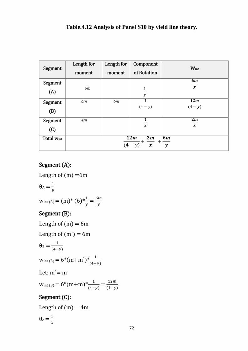
72
Table.4.12 Analysis of Panel S10 by yield line theory.
Segment (A):
Length of (m) =6m
θA = 1
𝑦
wint (A) = (m)* (6)*1
𝑦=
6𝑚
𝑦
Segment (B):
Length of (m) = 6m
Length of (m`) = 6m
θB = 1
(4−𝑦)
wint (B) = 6*(m+m`)*1
(4−𝑦)
Let; m`= m
wint (B) = 6*(m+m)*1
(4−𝑦) =
12𝑚
(4−𝑦)
Segment (C):
Length of (m) = 4m
θc = 1
𝑥
Segment Length for
moment
Length for
moment
Component
of Rotation Wint
Segment
(A)
𝟔𝒎
𝒚
Segment
(B)
6m 6m 1
(4 − 𝑦)
𝟏𝟐𝒎
(𝟒 − 𝒚)
Segment
(C)
4m 1
𝑥
𝟐𝒎
𝒙
Total wint 𝟏𝟐𝒎
(𝟒 − 𝒚)+
𝟐𝒎
𝒙 +
𝟔𝒎
𝒚
6m 1
𝑦

73
wint (c) = (0.5m) *4
𝑥=
2𝑚
𝑥
Total Internal work =
=12𝑚
(4−𝑦)+
2𝑚
𝑥 +
6𝑚
𝑦
= 2m (6
(4−𝑦)+
1
𝑥 +
3
𝑦 )
External work = Internal work
= 2m (6
(4−𝑦)+
1
𝑥 +
3
𝑦 )= w (12-
2
3 x)
= m (6
(4−𝑦)+
1
𝑥 +
3
𝑦 )=w (6-
x
3) (4.55)
𝑤
𝑚 =
(6
(4−𝑦)+
1
𝑥 +
3
𝑦 )
(6−x
3 )
(4.56)
Using the expression:
f1( 𝑥1, 𝑥2)
f2 ( 𝑥1, 𝑥2)=
𝑑
𝑑𝑥1f1( 𝑥1, 𝑥2)
𝑑
𝑑𝑥1f2 ( 𝑥1, 𝑥2)
By differentiate to x:
(6
(4−𝑦)+
1
𝑥 +
3
𝑦 )
(6−x
3 )
= 3( −
1
𝑥2 )
−1 (4.57)
18-x = (6
(4−𝑦)+
3
𝑦 ) x2+x
(6
(4−𝑦)+
3
𝑦) 𝑥2+ 2x - (18)= 0 (4.58)
Solve for x;
x = −2±√22−4(
6(4−𝑦)
+3𝑦
)∗18
2(6
(4−𝑦)+
3𝑦
) (4.59)
By using excel; substituting a range of values of (y) in the above equation
and finding the maximum Values of (x),
we find maximum values of (x) = 1.8 m, coincide with y = 1.66 m
m = 1.1 w (4.60)
w = 20 kN.m2
Mmax =22kN.m/m
By using "10% rule"; Mmax = 24.2kN.m/m

74
By using prokon program, Mmax= 22.9kN.m/m.
msx= βsxnlx2
0.063*20*16=20.16 kN.m/m
So; the actual yield lines pattern as per the calculation will be as shown in
figure below:
Fig.4.22 Yield Line Pattern for Panel S10.
The results obtained for the ultimate moments for the panel S10 are summarized
at Table (4.14) and compared with others obtained by using Prokon Software,
and BS8110.
Table.4.13 the Ultimate Resisting Moments for Panels S10.
panel Value of
(MP) by yield
line theory
kN.m/m
Value of
(MP) by
BS8110
Table 3.14
kN.m/m
Different
%
Value of
(MP) by
Prokon
kN.m/m
Different
%
S9 32.00 31.00 3.125% 37.7 17.%
S10 22.00 20.16 8.36% 22.9 4.09%

75
4.5 Discussion of the results
The discussion of the results may be summarized as follows:
1. From results of ultimate resisting moments for R.C. flat slab system it was
appeared that the difference about 0.097% to 5.47% in comparison of with yield
line theory.
2. The results of ultimate resisting moments obtained were shown in table (4.10)
for the R.C. beam slab system that were compared with others those obtained
by using STAAD-Pro software and BS8110. The comparison revealed different
conforming by percentages range by 0.70 % to 13.91% when comparing with
STAAD-PRO and range by 0.39 % to 9.09 % when comparing to BS8110.
3. The results of ultimate resisting moments obtained from table (4.13) for the R.C.
slabs that have special condition of supports that were compared with others
those obtained by using PROKON software and BS8110. The comparison
revealed different conforming by percentages range by 4.09 % to 17.81% when
comparing with PROKON and range by 3.125 % to 8.36 % when comparing
with BS8110.

CHAPTER FIVE
CONCLUSIONS AND
RECOMMENDATION

76
CHAPTER FIVE
CONCLUSIONS AND RECOMMENDATION
5.1 Conclusions
On Basis of this study, Conclusions that can be drawn are as follows:
1. By using yield line theory, different types of reinforced concrete slabs are used
to determine the ultimate resisting moments and their locations.
2. One of the most popular methods of application in yield line theory is the virtual
work method that was used in this research to analysis and assessment different
models of reinforced concrete slabs (beam slab and flat slab system) of different
shapes and different support conditions, In addition to slabs that have special
condition of supports.
3. The percentages range between 0.097 % to 5.47 % of the results of bending
moments for the reinforced concrete flat slab system that were compared with
others those obtained by using STAAD-Pro software. This results confirm to
the software program STAAD-Pro with manual calculations, the results were
classified as very good once.
4. The percentages range between 0.70 % and 13.91% of the results of bending
moments for the reinforced concrete beam slab system that were compared with
others those obtained by using STAAD-Pro software. This results confirm to
the software program STAAD-Pro with hand calculations, the results were
classified as good once. The same results from manual calculations were
compared with others those obtained by using BS8110 the percentages range of
difference between 0.39 %and 9.09 %. This results obtained by BS8110 and
manual calculations were closer than obtained by STAAD-Pro, the results were
classified good.
5. The percentages range between 4.09 % and 17.81% of the results of bending
moments for the reinforced concrete slabs that have special condition of
supports were compared with others those obtained by using PROKON

77
software. This results related to the software program PROKON with hand
calculations, the results were classified very good results. The same results from
hand calculations were compared with others those obtained by using BS8110
the percentages range of difference between 3.125 %and 8.36 %. This results
confirm to the BS8110 with hand calculations and it was closer than results from
PROKON, the results were classified very good results.
6. As the general, the results of this study were clearly demonstrate that acceptable
and close results can be achieved with analysis by using yield line theory.
5.2 Recommendations
Recommendations were summarized as follows:
1. Study the analysis by assuming the pattern of yield line bisecting the corners at
45 degrees "simple layout". It will make the calculations very quick and easy.
2. Check the analysis by assuming percentage for the distance between the yield
line and the edges of slab depend on support condition.
3. Irregular reinforced concrete slabs, raft foundations can be check by using yield
line theory.

78
REFERENCES
[1] Ingerslev A., (On a Simple Analysis of Two-Way Slabs)”, Ingeniren, 30,
69, 1921, pp 507-515. (See also: The Strength of Rectangular Slabs, Struct.
Eng., 1, 1, 1923, pp. 3-14.)
[2] Johansen, K.W. 3, 1, 1931, pp. 1-18 (German version, Memo. Int. Ass.
Bridge Struct. Eng. 1, 1932, pp. 277-296.).
[3] Gvozdev, A.A., (English translation: “The Determination of the Value of
the Collapse Load for Statically Indeterminate Systems Undergoing Plastic
Deformation”, International Journal of Mechanical Sciences, 1, 1960, pp. 322-
333.)
[4] Gvozdev, A.A, (Comments of the design standard for reinforced concrete
structures)”, 17, 3, 1939, pp. 51-58.
[5] Morley symposium on concrete plasticity and its application, university of
Cambridge 23th July, 2007, pp. 43.
[6] Recent Developments in Yield-Line Theory, MCR Special Publication,
Cement and Concrete Association, London, 1965.
[7] Jones, L.L. and Wood, R. H., Yield-Line Analysis for Slabs, Thames &
Hudson and Chatto & Windus, London, 1967, 405 pp.
[8] Wood, R. H., “A Partial Failure of Limit Analysis of Slabs”, Magazine of
Concrete Research, 21, 67, 1969, pp. 79-80 (Discussion, 22, 21, 1970, pp. 112-
113.).

79
[9] Braestrup, M.W., “Yield Line Theory and Limit Analysis of Plates and
Slabs”, Magazine of Concrete Research, 22, 71, 1970, pp. 99-106.
[10] Fox, E.N., “Limit Analysis for Plates: The Exact Solution for a Clamped
Square Plate of Isotropic Homogeneous Material Obeying the Square Yield
Criterion and Loaded by Uniformly Pressure”, Philosophical Transactions of
the Royal Society, London, 277, 1265, 1974, pp 121155.
[11] Ultimate capacity evaluation of reinforced concrete slabs using yield line
analyses, by GregE.Mertz, Structural Mechanics Section, Westinghouse
Savannah River Company, Aiken, South Carolina 29808, 1995 pp. 5.
[12] Yield line Theory for Concrete Slabs Subjected to Axial Force, by Tim
Gudmand-Høyer, Denmark's Tekniske University, December 2003, pp. 3.
[13] Practical yield line design, by Gerard Kennedy and Chales Good child,
Published by the British Cement Association, 2003 pp. 15.
[14] Reinforced Concrete Design, W.H.Mosley, J.H.Bungey&R.Hulse, Fifth
Edition.
[15] The plastic behavior and the calculation of plates subjected to bending, by
Prof. A.C.W.M. Vrouwenvelder, Prof. J. Witteveen, March 2003.
[16] Civil Engineering Design (1) Analysis and Design of Slabs, Dr. Colin
Caprani, Chartered Engineer, 2006.

81
APPENDIX A
The results of ultimate resisting moment for reinforced concrete flat slab system
by using STAAD-PRO.
The result of resisting moment at x direction.

81
The result of resisting moment at y direction.
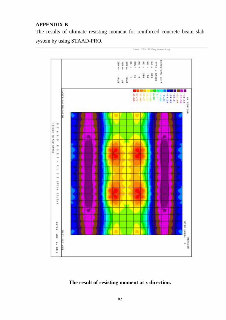
82
APPENDIX B
The results of ultimate resisting moment for reinforced concrete beam slab
system by using STAAD-PRO.
The result of resisting moment at x direction.

83
The result of resisting moment at y direction.