ENSC 383- Feedback ControlSummer 2010

TAs:Kaveh Kianfar, Esmaeil Tafazzoli

G(s)

U(s) input

Y(s) output

MATLAB Tutorial

1

Outline• Starting Matlab• Basics• Modeling• Control toolbox

2

Outline

M-file• When writing a program in matlab save it as m-file

( filename.m)

• 2 types of M-file 1- script (has no input and output,

simply execute commands) 2- function (need input, starts with

keyword “function”)function [y z]=mfunc(x)y=(x*x')^.5; % norm of xz=sum(x)/length(x); %%% using 'sum' functionend

m file

3

• Present polynomial with coefficients

vector123 34 sss x = [1 3 0 -2 1];

P3=poly([-2 -5 -6]))6)(5)(2( sss

rootsP3=roots(P3)6,5,2

)5)(2( ss P5=conv([1 2],[1 5])

Poly converts roots to coefficients of a polynomial:

4

Polynomials

• p=poly([-2 1 5])• R=roots(p)• x=-3:0.1:6;• y=p(1)*x.^3+p(2)*x.^2+p(3)*x+p(4);• plot(x,y)• grid

p =

1 -4 -7 10

R =

5.0000 -2.0000 1.0000

5

-3 -2 -1 0 1 2 3 4 5 6-40

-30

-20

-10

0

10

20

30

40

Polynomials

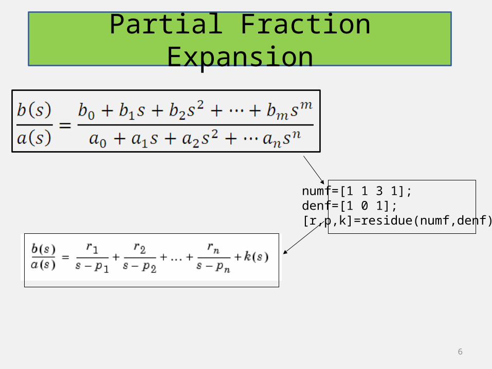
numf=[1 1 3 1]; denf=[1 0 1];[r,p,k]=residue(numf,denf)

Partial Fraction Expansion

6

•Roots of numerators are “zeros” of a

system,

•Roots of denominators are

“poles” of a system.

G(s)

U(s) input

Y(s) output

Dynamic system Representation

usingTransfer Function

7

Im

ReS-plane

zero

pole

Command “tf” by defining the

Command “zpk”

Using s=tf(‘s’), then for example:

Transfer Function in MATLAB

8

tf2zp: converts the numerator, denominator from coefficient to roots.[Z,P,K] = TF2ZP(NUM,DEN)

Ex.:

[z,p,k]=tf2zp([1 1],[1 2 1])

z=-1, p=-1;-1, k=1

zp2tf: converts the numerator, denominator from roots to coefficient. [NUM,DEN] = ZP2TF(Z,P,K)

Transfer Function in MATLAB

9

• G=series(G1,G2) or alternatively:

• G=parallel (G1,G2) or alternatively:

Interconnection between blocks

G1(s) G2(s)

G1(s)

G2(s)

u y

u y

10

• Feedback:

or alternatively for Negative feedback:

Interconnection between blocks

G1(s)

H(s)

-u y

11

• Syms s t :defines s, and t as symbolic variablesyms s a t1)G4=laplace(exp(t)): G4 =1/(s - 1)2)G5=laplace(exp(-t)): G5 =1/(s + 1)3)G6=laplace(sin(a*t)): G6 =a/(a^2 + s^2)

Hint:ilaplace(F,s,t): computes Inverse Laplace transform of F on the complex variable s and returns it as a function of the time, t.

ilaplace(a/(s^2+a^2),s,t)=(a*sin(t*(a^2)^(1/2)))/(a^2)^(1/2)

Symbolic computation in MATLAB

12

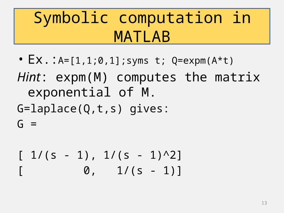
• Ex.:A=[1,1;0,1];syms t; Q=expm(A*t)Hint: expm(M) computes the matrix exponential of M.

G=laplace(Q,t,s) gives:G = [ 1/(s - 1), 1/(s - 1)^2][ 0, 1/(s - 1)]

Symbolic computation in MATLAB

13

• SystemStep, impulse, other inputs

•Matlab commands: lsim Simulate LTI model response to arbitrary inputs

sys=tf(num,den); t=0:dt:final_t; u=f(t); [y t]=lsim(sys,u,t) step Simulate LTI model response to step input

step(sys) special case of lsim• response

14

System Response

• Transient response: x(t)=x0*exp(a*t) “if a<0,it’s stable”.

First order systems

15

Im

Re

s-plane

s=-a

• When “a” is a complex number:t=0:0.1:5;a=-1+4*i; % a is complex with negative real partf=exp(a*t);X=real(f);Y=imag(f);plot(X,Y)xlabel('Re')ylabel('Im')axis('square')Plot(t,f)

Exp(a*t)

16

First order systems(cont’d)

•When “a” is complex, with Negative real partin polar coordinates:

Rho=sqrt(X.^2+Y.^2);Theta=atan2(Y,X);polar(Theta,Rho)

17

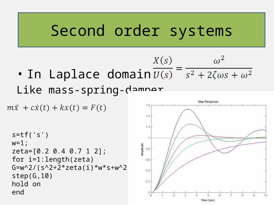
Second order System

• In Laplace domain:Like mass-spring-damper

18

s=tf('s')w=1;zeta=[0.2 0.4 0.7 1 2];for i=1:length(zeta)G=w^2/(s^2+2*zeta(i)*w*s+w^2)step(G,10)hold onend

Second order systems

19

0 0.5 1 1.5 2 2.5 30

0.2

0.4

0.6

0.8

1

1.2

1.4Step Response

Time (sec)

Amplitude

Dam ping ratio is 0.5:O vershoots are equal.

Second order systems

s-plane

Im

Re

Damping ratio is constant, wn changes.

s=tf('s')zeta=0.5w=[sqrt(12) 4 sqrt(20)];for i=1:length(w)G=(w(i))^2/(s^2+2*zeta*w(i)*s+(w(i))^2)step(G,3)hold onend

• Undamped system(mass-spring)Damping ratio is zero:

20

Second order systems

w=[1 2];for i=1:length(w)G=tf(w(i)^2,[1 0 w(i)^2]);step(G,20)hold onend

0 2 4 6 8 10 12 14 16 18 20-0.5

0

0.5

1

1.5

2

2.5

Step Response

Time (sec)

Amplitud

e

w =1w =2

21

Dynamic system representation

0]01[

)(/10

//10

2

11

2

1

2

1

122

21

2

1

xx

xy

tumx

xmbmkx

x

DUCXYBUAXX

kxbxuxmxx

yxyx

ybkyuymFma

C

BA

yb

ky)(tum

kbsmssUsY

2

1)()( System Transfer Function

22

MATLAB code• k=.2; % spring stiffness

coefficient• b=.5; % damping coefficient• m=1; % mass• A=[0 1;-k/m -b/m]; % Represent A.• B=[0;1/m]; % Represent column

vector B.• C=[1 0]; % Represent row vector

C.• D=0; % Represent D.• F=ss(A,B,C,D) % Create an LTI object and

display.• step(F)• [num den]=ss2tf(A,B,C,D)• Gs=tf(num,den) % system transfer function

Step Response

23

0 5 10 15 20 25 300

1

2

3

4

5

6Step Response

Time (sec)

Amplitude

Step Response

24

Ordinary differential equations

function dx=lin1(t,x)dx=zeros(2,1);dx(1)=-x(1);dx(2)=-2*x(2);A=[-1 0;0 -2];[u,v]=eig(A)In workspace:[T,X]=ode23(@lin1,[0 10], [a(i) b(j)]);plot(X(:,1),X(:,2))[u.v]=eig(A)u = 0 1 1 0

-3 -2 -1 0 1 2 3-3

-2

-1

0

1

2

3

x1

x2

Hint:For using ode command, the diff. equations should be written in the first order format,i.e. a second order diff. eq. should be written as two first order diff. equations.

25

function dx=pendulum(t,x)dx=zeros(2,1)dx(1)=x(2);dx(2)=-0.5*x(2)-sin(x(1));

[T,X]=ode23(@pendulum,[0 10], [a(i) 0]);plot(X(:,1),X(:,2))

-2 -1.5 -1 -0.5 0 0.5 1 1.5 2-1.5

-1

-0.5

0

0.5

1

1.5

x1

x2

0 2 4 6 8 10 12 14 16 18 20-2

-1.5

-1

-0.5

0

0.5

1

Nonlinear Differential eq. of a pendulum

g

Viscose Damping term

Gravity term

Angle

Angular velocity