INTERNATIONAL CONFERENCE ON EMERGING TRENDS IN COMPUTATIONAL AND APPLIED MATHEMATICS(Conference...
366
-
Upload
independent -
Category
Documents
-
view
0 -
download
0
Transcript of INTERNATIONAL CONFERENCE ON EMERGING TRENDS IN COMPUTATIONAL AND APPLIED MATHEMATICS(Conference...


International Conferenceon
Emerging Trends in Computationaland Applied Mathematics
(ICCAM-2014)
PROCEEDINGS
Department of Applied ScienceITM University, Gurgaon (India)

Editors : A.K. YadavPhool SinghGaurav Gupta
Department of Applied ScienceITM University, Gurgaon (India)
Sponsored by : NBHM, DST, CSIR, Govt. of India
No part of this publication may be reproduced or transmitted in any form by any means, electronicor mechanical, including photocoping, recording, or any information storage and retrieval system,without permission in writing from copyright owners.
D I S C L A I M E R
The authors are solely responsible for the contents of the papers compiled in this volume. Thepublisher or editors do not take any responsibility for the same in any manner. Errors, if any, arepurely unintentional and readers are requested to communicate such errors to the editors orpublishers to avoid discrepancies in future.
Published by :BHARTI PUBLICATIONS
4819/24, 3rd Floor, Ansari Road, Darya GanjNew Delhi-110002
Mobile : 09210047042E-mail : [email protected]
[email protected] : www.bhartipublications.com
Typeset by : Kumud Printographics, K-36/1, Street No. 12, Brahmpuri, Delhi-53 • Ph : 9811960476Printed at : Design Prints-Delhi
First Published, 2014ISBN : 978-93-81212-76-9
Copyright © Editors
All rights reserved. No part of this publication may be reproduced or transmitted, in any form orby any means, without permission. Any person who does any unauthorised act in relation to this
publication may be liable to criminal prosecution and civil claims for damages.

CONTENTS
M ATHEMA TICAL M ODELLING
1 Productivity Shocks, Sectoral Shifts and Unemployment in a Two Sector Search FrameworkArindam Mandal
2 Mathematical Modeling of Human Postural Sway in the Frontal PlaneKizilova N., Karpinsky M.
3 Mathematical Formulations for Multiscale Modeling of Cardiovascular DynamicsKizilova N., Philippova H.
4 Changes in diurnal temperature range over Western Himalayan Region in Indian climatescenarioNaresh Kumar, B. P. Yadav
5 Modeling the Survivor functions of Lithium-Ion Batteries Designed for Mobile PhonesChetna Dabas
6 Simulation of VSCS Phailin using WRF modelPratap Kumar Mohanty, Biranchi Kumar Mahala, Birendra Kumar Nayak
7 Application of Mathematics in Economics An Examination for Selected ConceptsD. R. Agarwal, Sanjay Kumar Mangla
FL U I D M E C H A N I C S
8 Application of the Optimal Homotopy Asymptotic Method for the solution of the BurgersequationRozaini Roslan, Mohammed Abdulhameed, Ishak Hashim, Habibis Saleh
9 On a Successive Linearization Solution of an Eigen BVP due to Magnetoconvection in a 2-Dimensional Rectangular BoxMahesha Narayana, S. S. Motsa, P. Sibanda
10 Buoyancy and thermocapillary Driven Convection Flow of Nanofluids in a CavityIshak Hashim
, Habibis Saleh
11 Effect of variable heat flux and constant suction of a viscous and incompressible MHD fluidflow on a stretching sheetAryan Kaushik, Anoop Kumar Vashisth, N. S. Tomer, Shri Dhar Kaushik
12 Effect of Geometrical Configuration on Temperature Distribution in FinSurjan Singh, Dinesh Kumar, K. N. Rai
13 Two Phase Model on Unsteady Heat Transfer on a Str etching Sheet in a Rotating Nanofluidwith Heat Source/SinkMeenakshi Khurana, Sangeet Srivastava, Puneet Rana

14 Influence of Chemical Reaction on MHD Free Convective Flow Past an Infinite VerticalOscillating PlateHemant Poonia, R. C. Chaudhary
15 Natural Convective Flow Around a Heated Cylinder Inside a Porous Enclosure Filled withNanoliquidsHabibis Saleh, Ishak Hashim
16 The Effects of Variable Fluid Properties on the Hydro- Magnetic Flow and Heat Transfer overa Non-Linearly Str etching Sheet with Free Str eam VelocityVikas Poply
17 Heat Generation effect on Unsteady Porous Stretching Sheet in Presence of Variable Viscosityand Thermal DiffusivityParveen Kumar, Phool Singh
18 Steady State Temperature Distribution in Biological Tissue Using Wavelet CollocationMethodDinesh Kumar, Surjan Singh , K. N. Rai
SO L I D M ECHANICS
19 Reflection and Transmission of Elastic Waves in the Nematic Elastomer half-spacesS. S. Singh
20 Thermo Elastic-Plastic Analysis of Rotating Disk Made of Non-homogeneous Material underInternal Pr essure with Variable Thickness and Variable DensitySanehlata Yadav, Sanjeev Sharma
21 Variation of Amplitude Ratios at the free Surface of Couple Stress Generalized ThermoelsticSolid Half-spaceKrishan Kumar,, Ravendra Nautiyal, Rajneesh Kumar, Rachna Khurana
OP T I M I Z A T I O N
22 Implementation and Analysis of Linear Electrical Networks using Interval Arithmetic onFPGA’sSoumya S Patil, Rajashekar. B.Shettar
23 Structural Design Optimization of T- Stif fened Panel of a Composite WingNithin Kumar K C, Sachin Rastogi, Naman Kumar Chandna, Md Mushfique Alam
24 Bilevel Programming application to Midterm Production-Distribution Planning ProblemAkhilesh Kumar, Neha
SOFT COMPUTING
25 Comparative Analysis of Real and Binary Coded GA for Fuzzy Time Series PredictionShilpa Jain, Prakash C. Mathpal, Dinesh Bisht
26 Human Activity Recognition Using Smartphone SensorsAishwarya Jain, Surbhi Jain
27 A Review Paper on Medical Science and Soft Computing TechniquesAkanksha Kaushik, Prakash C. Mathpal, Vandini Sharma
28 Scalable Spatially and Socially Aware Collaborative FilteringSurajit Halder, Prosenjit Gupta
29 Graphical User Interface for solving the Travelling Salesman Problem using GeneticAlgorithmSatyam Saravgi, Chander Verma, Sudhir Kumar Sharma

30 Fuzzy ‘SET’: A Quantitative, Reliable and Comparative Measure to Students’ Evaluation ofTeachingAkhilesh Kumar, Neha
31 Genetic Algorithm Approach for Solving Coupled Differential EquationDeshraj, Sangeeta Rani, Indu Saini
CRYPT OGRAPHY AND NETWORKS
32 Encryption of Time and DateAyush Jain
33 Mobile number encryption using “K-matrix algorithm”Karan Kumar Singh
34 RSA Cryptosystem: A ReviewSeema Verma, Deepak Garg
35 Electro Magnetic Analysis Attack and Countermeasures – The Latest VogueAditya Bhattacharyya, Sanjit Kumar Setua
36 A Secure Routing Scheme for Wireless Mesh NetworksPushpender, Sohan Garg
37 Wireless Communication to Monitor Air Pollution Sonal Omprakash Taloakr, Jagdish W. Bakal
I MAGE PROCESSING
38 Fully-phase image encryption with random phase mask and devil’s vortex Fresnel lens usinggyrator transformHukum Singh, A. K. Yadav, Sunanda Vashisth, Kehar Singh
39 A Novel Approach for Automated Early Detection of Glaucoma Using Image ProcessingPreeti, Jyotika Pruthi
40 A Novel Approach for Automatic Detection of Tumor in Human Brain Using Image ProcessingTechniquesPoonam, Jyotika Pruthi
41 Automatic License Plate Recognition: A ReviewVandini Sharma, Prakash C. Mathpal, Akanksha Kaushik
42 An Effective Approach of Noise Analysis on ImagesGourav Kumar Javeriya
43 A watermarking scheme for phase images using random phase masks in fractional Fourierand gyrator domainSunanda Vashisth, A. K. Yadav, Hukum Singh, Kehar Singh
44 Automated urban area building extraction from high resolution satellite imagerySidharth Bhatia, Gaurav Gupta
COMPLEX ANAL YSIS
45 On The Maximum Modulus of Polynomials Whose Zeros are Outside a Circle - IIArty Ahuja
46 On Inequality for a Class of Self Inverse PolynomialsVijay Dahiya, Harish Singh, Sushil Saini, Anil Saini, Seema Devi

I NVENT ORY AND QUEUING M ODELS
47 An Inventory Model for Deteriorating Items with Stock Dependent Demand ConsideringShortages and Life TimeKumar Sanjay, Aggarwal Naresh Kumar
48 Transient Solution of a Two-State Multiple Vacation Queueing Model with Arrivals andDepartur es in Batches of Variable SizeVijay Kumar, Vijay Dahiya, Kumar Rahul
49 Stochastic Model to Study Two-unit Standby System Working with Varying DemandRachna Khurana, A. K. Lal, S. S. Bhatia, Krishan Kumar
M ISCELLANEOUS
50 Integral Quaternions and Four-Square TheoremParvinder Singh
51 A Brief Survey of Stability of Functional Equations in Various SpacesSushma
52 Mathematics – A study begins with Minuteness but Ends in MagnificenceVijay Dahiya, Harish Singh, Alka Mittal, Preeti Malik, Rajeev Dahiya
53 An Efficient Zero Knowledge Identification Protocol Based on Weil Pairing on EllipticCurvesManoj Kumar
54 Academic Achievement in Relation to Achievement Motivation, Gender and Locale inMathematicsChanchal Sharma, Suman Lata
55 Inequalities for the Polar Derivative of PolynomialsJagjeet Kaur, D. Tripathi, S.Hans
56 Central M- Armendariz RingsAmit Bhooshan Singh
57 LIE Ideals & Generalized Dervations in σ -Prime RingsDeepa Arora
58 Negation-Switching Invariant t-Path Signed Graphs, t < 3*Deepa Sinha, Ayushi Dhama
59 Power Series Solution of Newell-Whitehead-Segel Equation with a Time Periodic CoefficientP. G. Siddheshwar, C. Kanchana
60 Performance Optimization of Levenberg-Marquardt Algorithm with ParallelizationNirmal Lourdh Rayan S., K. Balachandran
61 Primality Testing of Gaussian IntegersAakash Paul, Saransh Sharma, Subhashis Majumder, Somjit Datta
62 A New Algorithm Based on the Successive Linearization Method to find the Critical Eigenvaluein the Rayleigh-Bénard-Brinkman Convection Problem with General Boundary ConditionsP. G. Siddheshwar, S. B. Ashoka, Mahesha Narayana
63 Hydromagnetic Forced Flow of a Newtonian, Electrically Conducting Fluid due to a CurvedStr etching SurfaceP. G. Siddheshwar, N. Meenakshi
64 Suffciency and Duality in Nonsmooth Optimization Under Generalized FunctionsPallavi Kharbanda, Divya Agarwal
65 Lightning Arr ester Fault Detection through Digital Thermovision Image ProcessingTechniqueIshita Sharma, Shabana Urooj
66 An Application of Intuitionistic Fuzzy sets in Bi-matrix Game with Intuitionistic Fuzzy GoalsI. Khan, A. Aggarwal

MATHEMATICAL MODELLING

Introduction
The purpose of this paper is to develop a twosector search model to explain the relationship betweenvacancies, unemployment, labor productivity andsectoral shifts in the economy. Unlike one sector searchmodels, in a two sector model we have two separatefinal goods producing sectors. As a result, the model isable to capture effects on vacancies and due to sectoralshifts in an economy.
The model is based on Mortensen-Pissarides [1].The standard Mortensen-Pissarides search model is onesector search framework. Though one sector searchframework can explain labor market frictions as a resultof informational disadvantage, but it cannot explain theexistence of unemployment as a result of sectoraladjustments in an economy. Economies are multi-sectorand often changes in one sector spillover to othersectors.
The first major work to account for impact ofsectoral changes on the unemployment started withLilien [2], who by using sectoral data showed that periodswhere changes in employment differ more across sectorstend to be periods of aggregate downturns. With state-level data, Davis et al. [3] find that a reallocation of
military expenditures across states, holding aggregateexpenditures fixed, causes a temporary increase inunemployment, which they interpret as consistent withthe view that reallocation costs matter. Phelan andTrejos[4] showed that sectoral reallocations generateresponses that are qualitatively similar to productivityshocks.
The paper is structured as follows: section 2describes the model environment. In Section 3, formaltheoretical model is developed and in section 4 we willdiscuss comparative statics results using calibrationand numerical analysis. Final conclusions are presentedin section 5.
Model Environment
Preferences and Technology: Model frameworkis continuous time and infinite horizon. There are twosectors of production with a large number of firmsassociated with each sector. Firms create as manyvacancies as they like subject to a zero ex-ante profitcondition. The (endogenous) mass of vacancies is
, where i represents the sector. Firm incurs
an exogenous flow cost , in units of its own output, to
1Productivity Shocks, Sectoral Shifts and Unemployment
in a Two Sector Search Framework
Arindam MandalAssistant Professor of Economics, Department of Economics, Siena College, Loudonville, NY-12211, USA
Abstract:The paper develops a two sector search model to analyze the effects on unemployment and vacancies asa result of sector specific productivity and preference shocks.Unlike in one sector search models, in a two sectormodel, we have two separate finalgoods producing sectors. As a result, the model is able to capture effects onvacanciesand unemployment due tosectoral shifts due to productivity and preference shocks. The paper finds thatthe two sector model generates relatively more fluctuations in vacancies and unemployment as a result of productivitychange, compared to one sector search framework.Keywords: Sectoral shifts, two sector search, matching
Emerging Trends in Computational and Applied Mathematics 3

4 Emerging Trends in Computational and Applied Mathematics
maintain a vacancy throughout its life. Filled jobs breakup at the exogenous Poisson arrival rate ?
Capital adjusted labor is used to produce twononstorable final goods that are then sold in acompetitive market. An employed worker in sector iproduce units of good i, where can be interpretedas per unit labor productivity.
The model economy is populated by an infinitelylived continuum of workers with mass one, whereworkers are ex-ante identical. They derive utility fromconsumption of final goods and maximize the presentdiscounted value of their utility. Workers have a utilityfunction over consumption , where y
i is
consumption of good produced in sector i. Both workersand firms are risk neutral with a common discount rate r.
Matching Technology: Unemployed workers andvacancies are assumed to meet each other randomlyaccording to a matching function M(u,v), where u is thenumber of unemployed and v is the measure ofvacancies. Both types of vacancies have the sameprobability of meeting workers, and it is the total numberof vacancies and unemployment that enters thematching function. Matching function is characterizedby constant returns to scale so that
where
The contact rate of vacancies by a worker searching for
employment is and the rate at which
vacancies meet workers is where �
denotes labor market tightness.Institutions: In equilibrium, because of the
existence of entry/exit externality, any realized matchgenerates surpluses. I am assuming match surplusesare divided by Nash bargaining. Exogenous bargainingpower of the worker is � and that of the firm is (1-�).
Workers get paid in the good they help produce.Employed workers exchange a part of their earnings forthe good produced in the other sector. Exchange takesplace in a centralized competitive market in which therelative price p of good 2 in terms of good 1 is taken asgiven by all the participants (Good 1 is the numerairegood). Unemployed workers get nothing and spend alltheir time looking for work.
Model Analysis
The model economy consists of employed andunemployed workers, where total number of workersemployed in each sector is denoted by e
i and the pool
of unemployed workers looking for a job is denoted byu. Since the number of workers is normalized to one,therefore . The sector specific wage rateis denoted by w
i. Matches are formed between
unemployed workers and vacancies whenever the jointsurplus that would be realized by the match isnonnegative. I will solve the model via series of Bellmanequations and steady state equilibrium conditions.
Labor Market - Firm Side
For sector i, is present discounted value ofexpected profit from an occupied job and is presentdiscounted value of expected profit from a vacant job.
Therefore satisfies the Bellman equation
ci where i = 1,2
Free entry condition drives the profits from additionalvacancies to zero. Therefore, the equilibrium conditionfor supply of a vacant job is . Hence from equation(1)
Flow equation for occupied job is, where i = 1,2
Wage rate is determined by a bargaining processbetween the meeting firm and the worker. Therefore, byusing equations (2) and (3) we derive the equation
Above equation corresponds to marginal condition for
the demand for labor. is output per person employed
and is expected capitalized value of the
firm’s hiring cost.
Goods Market
There is a perfectly competitive goods market
where each workersmaximize utility subject to sector specific budget constraints. The sectorspecific budget constraints are y11 + py12 = w1 for sector1 and y21 + py22= pw2 for sector 2, where y
ij is

Emerging Trends in Computational and Applied Mathematics 5
consumption by sector i worker of output of sector jand w
i is the wage. The market clearing conditions are
e1w1 = e1y11+e2y21
e2w2 = e1y12+e2y22
where eiw
i is total amount of goods received by workers
in sector i as wage, and ei y
ij is total consumption by
sector i worker of output of sector j. The market clearingconditions apply to goods market alone. Only workersbring goods to market to trade for output of other sectorwhich has been paid to workers of other sector. Firmsdo not participate in that market. When r > 0, firms domake profits ex post in their own sector output whichgoes to compensate them for their vacancy costs. Hence,in equilibrium
The indirect utility derived by workers from consumptionis denoted by
Indirect utility of employed workers not only dependsupon the wage of the sector in which the worker isemployed, but also on the wage in the other sector.
Labor Market - Worker Side
Let and denote the present discountedvalue of expected income stream of an unemployed andan employed worker in sector i. The unemployed workercan become employed with probability �(�). Hence wehave
where � denotes proportion of total vacancies in sector1. Similarly, for employed workers, the flow equationsare
The above equation states that the flow value of
being employed is equal to value derived from the wagewhich is given by indirect utility z(w
i) and the net value
derived from being unemployed if the current job breakup.
By solving equations and then by substitutingequation, we get
Wage Determination
In equilibrium, realized job match yields pureeconomic rent. Wage levels need to share this economicrent, in addition to compensating each side for its costsfrom forming the job. We assume that the monopolyrent is shared according to the Nash solution to abargaining problem. Nash bargaining implies that w
i be
chosen so that
We can derive the wage equations in implicit form
by solving equations (<ref>Equ3</ref>), (<ref>Equ6</ref>) and (<ref>Equ11</ref>)
Steady State
In steady state, flows out of unemploymentequals flows into unemployment. Therefore
On the same note, in steady state, flows in and out ofjobs should be same. Therefore in steady state
Taking the ratio of the above two equations weget in steady state
We get the wage equations

6 Emerging Trends in Computational and Applied Mathematics
Equilibrium
Definition: An equilibrium is defined as labormarket tightness �, wages w
i and the proportion � of
vacancies in each sector,such that equations (4), (15)and (16) are satisfied for both the sectors.
Calibration and Numerical Analysis
This section analyzes the numerical simulationsof the model. The model parameters are based onMortensen and Pissarides [1], Shimer [5] and JobOpening and Labor Turnover Survey (JOLTS) data.Labor productivity has been normalized to one.According to JOLTS, between 2001 and 2007, separationrate averaged around 0.033 every month. This meansthat on an average a job lasted for 2.5 years before itbroke up. The model is solved assuming a yearly timeperiod, hence we set the job breakup rate � as 0.4 peryear. The discount rate r is assumed to be 5 percent peryear. The literature assumes a Cobb-Douglas matchingfunction of the form , where L is thematching intensity and the elasticity parameter is �. Weset the elasticity parameter ��as 0.5. Hosios [6] showedthat if ��= �, then the decentralized equilibrium maximizesa well posed social planner's problem. Therefore,bargaining power of the workers � is set to 0.5. Thematching intensity L is 7.2.
Permanent Productivity Change
Shimer [5] showed that standard one sector searchand matching model cannot generate the observedbusiness-cycle-frequency fluctuations in unemploymentand job vacancies in response to productivity shocksof plausible magnitude. In one sector model, higherwages absorb a part of the positive productivity gainsand hence eliminate the incentive for vacancy creation.Therefore, the basic issue in the literature is the lack ofpropagation of the productivity shocks in the models.In the two sector model, an increase in labor productivityin one of the sectors propagate to the other sectorthrough change in the demand for goods produced bythe other sector. Therefore, firms tend to produce morein the other sector too because of increased demand.
This leads to creation of more vacancies across theeconomy.
Effects of productivity shocks on the one sectorand two sector model is shown in Table 1(a) and 1 (b)respectively. One percent shock in two sector model isequivalent to 0.5 percent shock in one sector model. Allthe models are simulated using the same parametervalues. Changes in � as a result of productivity shocksare comparatively less in case of one sector model thanin two sector models. For example, a 0.5 percent shockto productivity in one sector model, changes � by only0.55 percent, whereas in case of two sector models, anone percent productivity shock changes � by 0.61percent.
Preference Change or Sectoral Shifts
What happens if there is change in consumerpreferences or sectoral shifts in the economy� In themodel, it is possible to introduce effects of consumerpreferences across sectors, which is not possible instandard one sector search models. Change in consumerpreferences can be introduced through changes inparameter � in the utility function. Details of thepreference changes are shown in Table 2.
In the model, increase in the relative share of thedemand for sector 1 good cause a fall in �, which impliesfalling vacancies and rising unemployment. Though inaggregate vacancies has fallen and unemployment hasgone up, but dynamics are very different across thesectors. In sector 1 vacancies increased, whereas insector 2 it declined. The decrease in sector 2 vacanciesare not offset by the increase in sector 1 vacancies.Because of the shift in preference towards sector 1goods, employment increased in sector 1, whereas fallingrelative demand for sector 2 goods caused decrease inemployment in sector 2. Increased employment is sector1 cannot offset falling employment in sector 2 and hencetotal employment in the economy declined. As a resulttotal unemployment in the economy increased. Thoughwages remained same across sector but the real wagesin sector 2 defined as p*w
2 decreased relative to wage
in sector 1. This decline in wages is due to fall in price ofgood 2 as a result of preference shift to good 1.
Conclusion
In this contribution, I have shown that the twosector search model is more robust in accommodatingnot only productivity changes but also to account for

Emerging Trends in Computational and Applied Mathematics 7
sectoral reallocation of labor. The model can generatesubstantially more fluctuations in vacancies andunemployment as a result of change in productivity,compare to one sector model. Also, the model showsthat unemployment can be caused because of sectoralreallocation of labor as a result of sectoral shifts in theeconomy. For future study, it would be interesting toexplore the off-steady state dynamics of the model.
REFERENCES
[1] Dale T. Mortensen and Christopher A. Pissarides. "Jobcreation and job destruction in the theory ofunemployment." The review of economic studies 61,
no. 3, 397-415 (1994).[2] David M. Lilien, "Sectoral shifts and cyclical
unemployment." Journal of political economy 90, no.4, 777 (1982).
[3] Steven J.Davis, Prakash Loungani, and RamamohanMahidhara. "Regional unemployment cycles." InFebruary 1995 BER Economic Fluctuations Conference(1995).
[4] ChristopherPhelan and Alberto Trejos. "The aggregateeffects of sectoral reallocations." Journal of MonetaryEconomics 45, no. 2, 249-268 (2000).
[5] Robert Shimer, "The cyclical behavior of equilibriumunemployment and vacancies." American economicreview, 25-49 (2005).
[6] Arthur J.Hosios, "On the efficiency of matching andrelated models of search and unemployment." TheReview of Economic Studies 57, no. 2, 279-298 (1990).
TABLE 1 A: One Sector Search Model with Productivity Change
� � w v e u
1 0.5053 0.9252 0.0366 0.9275 0.07251.005 0.5081 0.93 0.0367 0.9277 0.07231.015 0.5135 0.9396 0.0369 0.9281 0.07191.025 0.519 0.9492 0.0372 0.9284 0.0716
TABLE 1 B: Two Sector Search Model with Productivity Change
�1
� w1
w2
v1
v2
e1
e2
u
1 1 0.8948 0.8948 0.0263 0.0263 0.4737 0.4737 0.05261.01 1.0061 0.9045 0.8945 0.02641 0.02638 0.4739 0.4736 0.05251.03 1.0168 0.9239 0.8939 0.02657 0.02652 0.4744 0.4734 0.05221.05 1.0272 0.9434 0.8934 0.02674 0.02665 0.4748 0.4732 0.052
TABLE 2 : Search Model with Preference Change
� � w1
w2
v1
v2
e1
e2
u
0.5 1 0.8948 0.8948 0.0263 0.0263 0.4737 0.4737 0.05260.6 0.9633 0.8968 0.8968 0.0307 0.0209 0.5623 0.3841 0.05360.65 0.9203 0.8991 0.8991 0.0323 0.018 0.6067 0.3386 0.0547

8 Emerging Trends in Computational and Applied Mathematics
2Mathematical Modeling of Human Postural
Sway in the Frontal Plane
Kizilova N., Karpinsky M.Kharkov National University, Kharkov, Ukraine
[email protected], [email protected]
Abstract: Mathematical model of human body as an inverted multi-link pendulum, that is able to describe andexplain the postural sway in the frontal plane at different postures is developed. The model is nonlinear unlike thecorresponding model for the sway in the sagittal plane. The trajectories of the centre of mass (COM) of the humanbody have been computed on the measurement data and used for validation of the model and computations of thecontrol function supporting the postural stability.Keywords: Biomechanics, force platform, postural sway, diagnostic analysis, mathematical modeling.
Introduction
Parameters of human postural sway are importantdeterminant of human locomotor, balance and nervoussystems [1]. Body sway in the sagittal plane (forward-
to-backward) is studied at assumption of the small bodyoscillations around the vertical line that leads to thesystem of linear ODE [1,2], while the case of the frontal
plane (side-to-side) is not sufficiently studied.
Experimental measurements
Posturographic measurements have been done
on young healthy volunteers (37 men, 38 women; mean± SD: age = 20±2, height = 175±7 cm, body weight =75.4±15.1 kg) and a group of patients with different spine
and joint diseases (40 men, 42 women; age=54±21, height= 169±11 cm, body weight = 75.0±10.5 kg) using theforce platform (Statograph-M05/28). The set of tests on
2- and 1-leg postures with open and closed eyes [2] hasbeen carried out. The trajectories of the COM Y(X) havebeen computed. The lengths of the body segments have
been measured; masses, moments of inertia andpositions of the centre of mass of the segments have
been computed.
Mathematical model
Human body is modelled as an inverted 4-link
pendulum (fig.1). Position of the pendulum is determinedby the angles 1 4� � (fig.1). Oscillations of the pendulumare described by Lagrange equations. Supposing small
values of 1 4� � ( j j jsin( ) ~ , cos( ) ~ 1� � � ) and neglecting theterms 2
j~ ( )� one can obtain the governing system ofnonlinear ODE in the form
// / /M K( , ) N u( , )� � � � � �� � � � �
where T1 2 3 4( , , , )� � � � �� , T is transpose sign, M is the
mass-inertia matrix, K is centrifugal matrix, N is gravity
matrix, is the control function supporting the posturalstability. Components of the matrices M, K, N are basedon individual body parameters. Nonlinear system (1)
has been solved using MatLab7 software. Amplitudesand frequencies of body oscillations have beencomputed and analyzed.

Emerging Trends in Computational and Applied Mathematics 9
a bFig. 1. Multilink models of the human body for the 2-leg (a)
and 1-leg (b) postures.
Results and discussions
Good agreement of the computed and measuredfrequencies has been obtained. It was found the young
healthy volunteers exhibit good approximation of thecomputed results to the measured data by the control
function j j ju (t) a (t) bd (t) / dt� �� � , while for the elderly
patients with spine and joint problems
j j ju (t) a (t ) bd (t ) / dt� � � �� � � � and time delay
� correlates with both age and pathology level.Mathematical modeling provides good approach forearly differential diagnostics of combined pathology.
REFERENCES
[1] V. M. Zatsiorsky, A. C. Aruin and V. N. Selujanov,Biomechanics of human locomotor system (Nauka,1981).
[2] N. Kizilova, M.Yu. Karpinsky, J. Griskevicius andK. Daunoraviciene “Posturographic study of the humanbody vibrations for clinical diagnostics of the spine andjoint pathology,” Mechanika, 6, 37–41 (2009).

10 Emerging Trends in Computational and Applied Mathematics
Introduction to the style guide, formatting of main text,and page layout
Blood flow in the vessels exhibit different flowregimes, namely vortical and transitional flows at highReynolds numbers Re=1200-5800 in the large vessels;pulsatile flows at intermediate Reynolds numbersRe=100-1000 in the medium vessels; low amplitudepulsatile and quasi-steady flows at Re=0.1-10 with non-Newtonian properties produced by deformation,aggregation and microstructure formation of the redblood cells in the small vessels; quasi-steady flows withvarying viscosity at low Reynolds numbers Re<0.1 inthe capillaries. Blood vessel walls demonstrate passivedeformations for the low-amplitude blood flow and pulsewave propagation and active reaction to the highhydrostatic pressure (Bayliss effect) and wall shear rate.
Due to the complex structure of thecardiovascular system direct 3D computations arepossible in separate arteries only, provided othercompartments of the system are modeled by simplified1D and 0D models. It poses a problem of boundaryconditions at the interfaces of the models of differentdimensions as well as coupling the Newtonian and non-Newtonian flows. Here a review of the coupled modelsdeveloped for the cardiovascular system is given and
the correct mathematical formulations for the boundaryconditions at the interfaces are derived from theconservation laws.
Mathematical formulations for different flow regimesand scales
Blood flows in larger arteries can be studied onthe 3D incompressible Navier-Stokes equations andmodified Kelvin-Voight rheological model for the vesselwall
1
ˆ ˆ ˆˆˆsp I I E B
t t
� �� � � �
� �
�� � � �� � � � � �� � � �� � � �
where�̂ and �̂ are stress and strain tensors, sp is thehydrostatic pressure in the wall, E are elasticcoefficients,� and� are the relaxation and retardationtimes, I and / t� � are unit operator and invariant timederivative, B is the tensor of active stresses.
Flows in the medium vessels can be describedby the simplified 1D Euler-type equations in the nonlinearelastic boundaries [1]
� �
2
0 0 0
, ( )
( ) /
��
�
�
��� � � � �� � � � � � ���� � � � �� �
� � �
A Q Q Q A P Qq k
t x t x A x A
P A P A A A
3Mathematical Formulations for Multiscale
Modeling of Cardiovascular Dynamics
Kizilova N., Philippova H.Kharkov National University, Kharkov, Ukraine
[email protected], [email protected]
Abstract: Mathematical formulations for the blood flows in large, small and medium arteries, veins and lymphaticvessels as well as microcirculation in the capillary system are presented. Rheological models for the vessel walls aspassive and active soft materials are given. Solution to the problem of the boundary conditions at the interfaces ofthe models of different time and space scales and dimensions is proposed.Keywords: blood circulation system, active biological media, multiscale modeling.

Emerging Trends in Computational and Applied Mathematics 11
where A and Q are the lumen area and flow rate, � and �are fluid density and viscosity, q is the outflow in theside branches,� is the correcting coefficient for the
realistic non-parabolic flow profile, 0P is the external
pressure outside the vessel, 0A is the lumen area at
0P P� , � is the wall rigidity.. Blood flows in the smaller vessels and capillaries
can be successfully modeled as complex viscoelasticchambers (Windkesel model) [2]
outin out out out
dQdPC Q Q , L P P ZQ
dt dt� � � � �
where P is the hydrostatic pressure, Q is the flow rate, Cis the wall compliance, L is the blood inertia, Z is theresistivity to the outlet flow.
Boundary conditions
Direct coupling between the models (1)-(3) ismathematically incorrect due to different number of the
variables and types of the systems. Application of themass, momentum and energy balance equations at theinterfaces of the (1) and (2), (2) and (3), (1) and (3) modelsgives the missing boundary conditions for the fluidvelocity and wall displacement components. For thenon-Newtonian flows in the smaller vessels or areas ofblood clot formation, the corresponding balanceequations for mixtures can be successfully applied. Theresulting mathematical formulation is presented.
REFERENCES
[1] C. C.H. Smit, “On the modeling of the distributedoutflow in one-dimensional models of arterial bloodflow,” Zeitschr. Angew. Mathem. Physik. 32, 408-420(1981).
[2] N. Kizilova, “Viscoelastic windkessel in mathematicalmodeling of blood circulation system,” Math. Modeling,33, 9–12 (2013).

12 Emerging Trends in Computational and Applied Mathematics
Introduction
Many studies have been carried out globallyindicate the significant increase in global surfacetemperatures during last century [1]. According tostudies, the most rapid warming occurred mainly during1920–44 and after 1975 [2, 3]. In India, studies show thatannual mean temperature has risen by 0.56°C during theperiod 1901-2009 and are primarily due to increase inmaximum temperature [4]. Himalayas plays significantrole for climate of Indian subcontinents. A small rise intemperature largely affects the climate of the Indiansubcontinents, as it is the origin of the many glaciersand its main rivers. Therefore, an effort is made to studythe temperature changes in WHR by analysing theanomalies of T
max, T
min & DTR for the period 1901-2007.
Further detailed analysis of the data has been carriedout by dividing it into 30 years periods viz: 1918-1947,1948-1977 & 1978-2007 and 10 year period.
Data and Methodology
Source of the monthly Tmax
, Tmin
data for the
period 1901-2007 is from IITM, Pune (http://www.tropmet.res.in/). Details of data is available inKothawale et al. [5, 6]. T
max, T
min & DTR anomalies
(monthly Value of the year - series mean) series areconstructed for all the seasons namely: winter (January& February), pre-monsoon (March to May), monsoon(June to September), post-monsoon (October toDecember) and annual (January to December) basis.Further, data is analysed by taking 11 year running mean,Mann- Kendall test [7-10] and linear regression method.In present study, trend is considered to be significant, ifthe confidence level is more than 95%.
Result and Discussions
Annual and seasonal trends along with 11 yearrunning mean for the period 1901-2007 are shown in Fig.1. Mann Kendall ‘Z’ values for annual & seasonal andmonthly temperatures are given in Table 1 and Table 2respectively. Significant increasing trends are observedin annual as well as seasonal T
max with increase at higher
rate is observed in winter season during the period 1901-
4Changes in diurnal temperature range over Western
Himalayan Region in Indian climate scenario
Naresh Kumar, B. P. YadavIndia Metrological Department, Lodi Road, New Delhi-110003
Abstract: Temperature changes in Western Himalayan Region (WHR) has been studied by analysing the anomaliesof mean maximum temperature (T
max), minimum temperature (T
min) & diurnal temperature range (DTR; T
max - T
min)
for the period 1901-2007. Data has been analysed on monthly, seasonal and annual basis by using parametric &non-parametric techniques like Mann- Kendall test & linear regression method. Further detailed analysis of thedata has been carried out by dividing data into 30 years periods viz: 1918-1947, 1948-1977 & 1978-2007 and 10year period. Study shows a significant (confidence level more than 95%) increase in seasonal as well as annual T
max
during the period 1901-2007 with increase at higher rate (1.3°C from its mean) in winter season. Significantincreasing trends are also observed in seasonal as well as annual T
min except monsoon season, in which no trend is
observed. In sub-periods analysis, increase in seasonal as well as annual Tmax
and Tmin
observed at higher rate in1978-2007 as compare two other two sub-periods namely 1918-1947, 1948-1977.Keywords: Himalayas, temperature, trends

Emerging Trends in Computational and Applied Mathematics 13
2007 (Table 1). In winter season, an increase by 1.3° C isobserved from its mean T
max between 1901-2007.
Analysis of 11 year running mean for winter Tmax
seriesindicate that the probable change in the temperaturetrends occurs mainly after 1964 (Fig.1). because till 1963no trend in winter T
max is observed thereafter significant
increasing trend is observed between 1964 to 2007. Insub-periods analysis, significant increasing trends areobserved in the period 1978-2007 (Table 1). During thisperiod, rise in post-monsoon T
max is at higher rate as
compare to other season. In Tmin
series analysis for theperiod 1901-2007, significant increasing trends areobserved in annual as well as in all the seasons exceptmonsoon, in which no significant trend is observed.During this period, post-monsoon T
min trend shows rise
at higher rate as compare to other seasons. In sub-periods analysis, significant increasing trends areobserved in the period 1978-2007 (Table 1).
In DTR analysis, significant increasing trends areobserved in annual and winter & pre-monsoon seasonsduring the period 1901-2007. In sub-period analysis,significant increase in DTR observed in annual trendsfor all the three sub-periods namely: 1918-1947, 1948-1977 and 178-2007.
In monthly trend analysis, significant increasingtrends are observed in T
max from January to April,
September and October months for the period 1901-
2007. Comparing all the monthly trends, rise in Februarymonth observed at higher rate as compare to othermonths. In February, an increase by 1.6° C is observedfrom its mean T
max between 1901-2007. Thus highly
significant rise in winter Tmax
is mainly due to rise inhigher rate in February month. In sub-period analysis,mainly significant monthly rising trends are observedduring the period 1978-2007, in this period, significantrising trends are observed for February to April andOctober to December. The maximum rise is observed inNovember month. In T
min analysis for the period 1901-
2007, significant rising trends are observed in February,March and October to December months. Significantdecreasing trend is observed during August month.Comparing all monthly trends, November monthtemperature rose at higher rate as compare to othermonths. In DTR analysis for the period 1901-2007,significant rising trends are observed for January,February & April months and significant decreasingtrend is observed for November month. Significantdecreasing trend in November is attributed to NovemberT
min , which increased at much higher rate as compare to
Tmax
. Significant changes in DTR is mainly observedduring the period 1978-2007. During this period,significant rising trends are observed for February toApril, November and December month.
Table 1. Mann Kendall ‘Z’ values for annual & seasonal temperatures
Winter Pre-monsoon Monsoon Post-monsoon Annual
1901-2007 Tmax
4.0*** 2.6* 2.3* 2.0* 4.1***
Tmin
2.7** 2.0* 0.8 4.0*** 3.9***
DTR 3.4*** 2.7** 0.8 0.7 2.2*
1918-1947 Tmax
1.0 1.6 2.8** 2.0* 3.7***
Tmin
0.2 0.4 1.1 1.3 0.7
DTR 2.2* 2.0* 1.9 0.5 3.5***
1948-1977 Tmax
1.3 0.8 0.0 0.5 0.9
Tmin
-1.7 -1.9 -3.1** -0.4 -2.4*
DTR 1.9 3.1** 2.7** 0.4 3.0**
1978-2007 Tmax
3.6*** 3.0** 2.0* 4.1*** 3.8***
Tmin
2.8** 2.5* 3.5*** 0.9 3.7***
DTR 1.0 2.9** 1.6 2.9** 2.6**

14 Emerging Trends in Computational and Applied Mathematics
Table 2. Mann Kendall test ‘Z’ values for monthly temperatures
Jan Feb March April May June July Aug Sept Oct Nov Dec
1901-2007 Tmax
3.1*** 3.7*** 2.1* 3.5*** 0.5 1.0 -0.6 1.1 2.7* 2.3* 0.9 1.6
Tmin
1.4 3.1** 2.4* 1.9 -0.6 1.2 0.9 -2.0* 1.2 2.4* 4.0*** 2.9**
DTR 2.2* 3.2** 1.1 3.6*** 1.3 0.5 -1.1 1.8 1.0 1.2 -2.0* -0.5
1918-1947 Tmax
0.1 1.8 0.4 1.4 1.7 1.7 1.2 1.7 2.4* 2.7** 1.9 0.4
Tmin
-0.8 0.5 -0.6 0.4 1.0 0.7 0.2 -0.4 1.4 1.7 1.6 0.3
DTR 0.9 2.1* 1.1 1.7 1.5 1.7 0.8 1.7 1.5 1.4 0.4 0.0
1948- 1977 Tmax
2.0* 0.1 1.6 0.6 -0.3 0.8 -0.1 -0.4 -1.2 0.1 1.4 0.0
Tmin
-1.2 -0.4 -1.4 -1.0 -3.0** -1.4 -1.9 -2.8** -1.8 -0.6 0.3 -0.8
DTR 2.7** 0.8 3.1** 1.4 1.8 2.6** 2.4* 2.0* 0.9 1.2 0.4 -0.1
1978-2007 Tmax
1.3 3.9*** 3.6*** 2.2* 1.6 0.4 1.7 1.5 1.5 2.1* 4.2*** 3.1**
Tmin
1.7 3.7*** 1.7 1.3 1.3 2.3* 1.9 1.9 2.8** 0.8 1.0 0.3DTR -1.1 2.5* 3.6*** 3.1** 1.7 -1.3 0.0 0.0 -1.6 1.6 2.3* 2.1*
‘*’ indicate significant at 95%, ‘**’ at 99% and ‘***’ at 99.9% confidence level
In decadal analysis of data, positive anomaly in monthly, seasonal & annual Tmax
observed in last two
Fig.1. Annual and seasonal trends along with 11 year moving average from 1901-2007

Emerging Trends in Computational and Applied Mathematics 15
decades. It indicates that most abrupt changes in Tmax
occur mainly after 1991. In Tmin
decadal analysis also,more abrupt changes observed mainly after 1991 exceptpost-monsoon season, which shows positive anomalymainly after 1971.
Conclusions
The broad conclusions of the study are:
(a) Analysis of data shows a significantincreasing trend in seasonal as well asannual T
max during study period (1901-2007)
with increase at higher rate (1.3°C from itsmean) in winter season. Increase with higherrate mainly attributed to February monthT
max. 11 year running mean indicate that the
probable change in the Tmax
occurs mainlyafter 1964.
(b) Significant increasing trends are alsoobserved during study period in seasonalas well as annual T
min except monsoon
season.(c) In sub-periods analysis, increase in monthly,
seasonal and annual Tmax
& Tmin
mainlyobserved at higher rate in 1978-2007 ascompare two other two sub-periods.However, increase in T
max is observed at
higher rate as compare to Tmin
in seasonal aswell as annual basis. Which is the conformitywith the earlier findings [4] over Indianregion.
(d) In decadal analysis, abrupt rise in monthly,seasonal and annual T
max & T
min are
observed mainly in last two decades 1991-2000 and 2001-2007.
REFERENCES
[1] Intergovernmental Panel on Climate Change (IPCC),“Climate Change 2007,” Fourth Assessment Report ofIntergovernmental Panel on Climate Change, CambridgeUniv. Press, Cambridge, U. K (2007).
[2] Jones, P.D. and Moberg, A., “Hemispheric and largescale surface air temperature variations; An extensiverevision and an update to 2001,”, J. Climate, 16, 206–223 (2003).
[3] Luterbacher, J., Dietrich, D., Xoplaki, E., Grosjean, M.and Wanner, H., “European seasonal and annualtemperature variability, trends, and extremes since 1500”,Science, 303, 1499–1503 (2004).
[4] Attri, S.D. and Tyagi, Ajit, “Climate Profile of India”,India Meteorological Department, Met Monograph No.Environment Meteorology-01/2010.
[5] Kothawale, D. R. and Rupa Kumar K., “On the recentchanges in surface temperature trends over India”,Geophys. Res. Lett. 32 L18714, doi:10.1029/2005GL023528 (2005).
[6] Kothawale, D.R., Munot, A.A. and Krishna Kumar K.,“Surface air temperature variability over India during1901-2007, and its association with ENSO”, ClimateResearch, 42, 89-104 (2010).
[7] Kendall M., “Time series” (Griffin, Londan, 1976).[8] Bhutiyani M.R., Kale V.S. and Pawar N.J., “Climate
change and the precipitation variations in thenorthwestern Himalaya: 1866–2006. Int. J. Climatol.30(4): 535–548(2009).
[9] Kumar V. and Jain S.K., “Trends in seasonal and annualrainfall and rainy days in Kashmir Valley in the lastcentury. Quaternary International 212, 64–69(2010).
[10] Subash N, Sikka A.K. and Ram Mohan H.S., “Aninvestigation into observational characteristics of rainfalland temperature in Central Northeast India—a historicalperspective 1889–2008” Theor. Appl. Climatol. 103,305-319(2011).

16 Emerging Trends in Computational and Applied Mathematics
Introduction
The Survival analysis is an upcoming trend in theareas of both applied mathematics or in mathematicalcomputing. It is mostly applied and carried out forsystems and therefore a direct area for the field ofcomputer science as well.
The survival analysis is all about modeling thelifetime analysis of diverse systems.
Survival analysis is meant for analyzing data inwhich the time until event is of concern. The responsehere is referred to as a survival time, failure time or eventtime. For example, time until a machine part fails, timeuntil tumor occurrence, time until a battery of mobilephone is totally discharged etc. The survival timeresponse is primarily continuous, may be incompletelydetermined for some specific objects (incompletelyobserved responses are censored) and is always greaterthan or equal to zero.
In the similar context as above, if there is nocensoring, standard regression procedures could beused. But, on the other hand, these may fall inadequatedue to some reasons. These reasons include, firstly, theprobability of surviving past a particular point in time
bears more importance and interest capturing than theexpected time of event. Secondly, time to event isrestricted to be positive and bears a skewed distribution.Lastly, the hazard function, used for regression insurvival analysis, can provide a deeper insight into thefailure mechanism than linear regression.
Censoring is an important aspect while carryingout survival analysis, although censoring mechanismmust be independent of the survival mechanism.Censoring exists when, there exists some informationabout a subject’s event time, but the exact event time isnot known.
There may be three crucial reasons as to whycensoring might occur. Firstly, when a subject does notexperience the event before the study occur. Secondly,a person is lost to follow-up during the study period.Thirdly, a person withdraws from the study. All the abovespecified examples come under right-censoring.Regardless the type of censoring, it must be assumedthat it is non-informative about the event, or in otherwords, the censoring is caused by other than impendingfailure [1,2,3].
The systems that are taken into consideration thisresearch paper are a specific type of embedded systems
5Modeling the Survivor functions of Lithium-Ion Batteries
Designed for Mobile Phones
Chetna DabasJaypee Institute of Information Technology, Noida, India.
Abstract: Survival analysis is one the emerging trends in the area of mathematical computing. This paper proposesthe modeling, analysis and creation of survivor functions and their resultant plots for two types of light weightedbatteries for mobile phones heavily used in the present scenario. These types of batteries are Lithium-Ion andLithium-Ion Polymer batteries and are chosen due to the positive characteristics associated with them like highenergy density and low price. The work carried out in this paper contains the survival plots of Lithium-Ion andLithium-Ion Polymer batteries and the results are drawn in mat lab version R2013. The results obtained in thispaper are directly applicable with certain limitations.Keywords: Survival Functions, Mobile Phones, Batteries

Emerging Trends in Computational and Applied Mathematics 17
called mobile phones. Since these mobile phones belongto a class of embedded systems, cater to some wellknown constraints of embedded systems like limitedpower, limited computational capacity and limitedmemory on chip.
Due to the limited power reason in the so calledmobile phones, it has been an incremental trend to adoptlightweight batteries with comparatively low price (inorder to accelerate exponential adoption in industry,since economy drives the industry) and which havehigh energy densities (for performance reasons).
Keeping the above perspective and trends in viewtwo special types of mobile phone batteries have beenchosen for the study carried out in this paper. Thesebatteries which are very much popular in industry (duetothe possession of the above mentioned and well desiredfeatures) are Lithium-Ion and Lithium-Ion Polymerbatteries.
The study, modeling, analysis is carried out andrevolves around these two batteries of mobile phoneswhich are in heavy use in the present scenario.
The results for the survival analysis are carriedout in the mathematical math-works software Matlabversion R2013. The proposed work is done for 2G talktime and 3G talk time in concern with the mobile phonebatteries.
Figures and Results
The figures and tables are all in context with theresults drawn in Matlab R2013 depicting thesurvivability analysis of the Lithium-Ion and Lithium-Ion Polymer batteries for mobile phones.
Figure 1 reflects the plot of Survival probabilityversus mobile phone battery lifetime in minutes. Thisfigure indicates the performance comparison of theheavily used Lithium-ion Polymer and Lithium-ionbatteries for mobile phones.
Further, the performance comparison is broughtout in terms of the 2G talk time for both theabovementioned kinds of batteries. 2G talk time is a timeperiod during which battery charge will last, if oneisconstantly talking on the phone in a 2G cellularnetwork.
Figure 2 presents the survival probability versusmobile phone battery lifetime in minutes for the lithium-ion and lithium–ion polymer batteries. Here, infigure 2,the performance comparison for both kinds of batteriesis carried out taking 3G talk time as aparameter. 3G talktime is the longest time a battery charge will last, if themobile phone is not used but is constantly connectedto a 3G network.
The data file created as a part of this work in Matlabconsisted up of three attributes. The first attribute wasthe lifetime (in minutes) of the two types of batteries formobile phone under consideration.
The second attribute was the information aboutthe specific type of battery i.e. Lithium-ion Polymer orLithium-ion. Here, a value 0 indicated a Lithium-ionbattery and a value 1 indicated a Lithium-ion Polymerbattery.
The third attribute in this data file was created forcensoring information. A value 0 here in this columndepicted the exact failure time and a value 1 depictedthe censored data.
Then a variable was created for each respectivetype of Lithium-ion battery under consideration. Thecensorship information was also incorporated here. Thenusing the created code snippets (as a part of theproposed work) for the survival analysis for the Lithium-ion Polymer and Lithium-ion batteries, the estimatedsurvival analysis was carried out.
It is clear from the proposed results depicted infigure 1, that the survival probability of Lithium-ionPolymer batteries used for mobile phones is much greaterthan the survival probability of Lithium-ion batteriesfor mobile phones taking the 2G talk time as a parameter.
Figure 2 clearly indicates that in case of 3G talktime as well the survival probability of the Lithium-ionPolymer battery is much greater than the survivalprobability of the Lithium–ion battery for mobilephones.
Equations
Equation corresponding to the survival functionis mentioned below as equation 1:
S (t ) ��1 – F (t )In equation 1, S depicts the survivor function and
it gives the probability that the survival time of anindividual exceeds a certain value. It is also related tothe hazard function.
The survival function should be non-increasingwhich reflects the notion (in the proposed context) thatif and only if the younger mobile phone battery ages areattained, then only the survival to a later age (of themobile phone battery) would be feasible.
The survival function is normally assumed toapproach zero as mobile phone battery age increaseswithout bound, although the limit may assume a valuegreater than zero if eternal life is possible [4,5].
The survival functions when expressed in termsof probability distribution and probability densityfunctions are expressed by the following equation 2

18 Emerging Trends in Computational and Applied Mathematics
below:
( ) ( ) ( ) ( )t
S t P T t f u du F t�
� � � ��Similarly, the survival event density function can
be expressed by equation 3:
( ) ( ) ( ) ( ( ) ) [1 ( ) ( )t
t
d d dS t S t S t f u du F t f t
dt dt dt
�� � � � � � ��
Conclusions and Limitations
The results carried out in the proposed work(carried out in Matlab version R2013) and as depicted infigure 1 and figure 2 respectively shows that the survivalprobability of Lithium-ion Polymer batteries (used formobile phones) is much greater than the survivalprobability of Lithium-ion batteries (used for mobilephones). The limitations of the proposed work are thatthe results may vary for the wide spectrum of models ofmobile phones available in the market.
Future Scope
The proposed work is being carried out for 2Gtalk time and 3G talk time at present, whereas the Lithium-ion Polymer and Lithium-ion batteries for mobile phonesmay be evaluated for other parameters associated withthe mobile phones. Such as, music playback time andstandby time etc.
REFERENCES
[1] Machin D, Cheung YB, Parmar MK. 2nd ed. WestSussex: John Wiley and Sons Ltd; 2006. Survivalanalysis: a practical approach.
[2] Kaplan EL, Meier P. Non-parametric estimation fromincomplete observations. J Am Stat Assoc. 1958;53:457–81.
[3] Survival Analysis: Models and Applications,(Xian Liu,July 2012), Chap-2.
[4] Cox DR. Regression models with life-tables (withdiscussion) J R Stat Soc Series B Stat Methodol.1972;34:269–76.
[5] Batteries & Supercapacitors in Consumer Electronics2013-2023:Forecasts, Opportunities, Innovation(Franco Gonzalez and Dr Peter Harrop, 2014)

Emerging Trends in Computational and Applied Mathematics 19
Introduction
Very Severe Cyclonic Storm (VSCS) PHAILINoriginated over Tenasserim coast on 6th October 2013 asa remnant cyclonic circulation over the South ChinaSea. The cyclonic circulation then developed as a lowpressure centre and subsequently developed into a wellmarked low pressure area on 7th October and a depressionover the same region on 8th October near latitude 12.00Nand longitude 96.00E. Moving west-northwestwards, itfurther intensified into a deep depression on 9th morningand into cyclonic storm (CS), ‘PHAILIN’ in the sameday evening. Moving northwestwards, it furtherintensified into a severe cyclonic storm (SCS) in themorning and into a VSCS in the forenoon of 10th October,2013 over east central Bay of Bengal. The VSCS,PHAILIN crossed Odisha & adjoining north AndhraPradesh coast near Gopalpur (Odisha) around 2230 hrsIST of 12th October 2013 with a sustained maximum
surface wind speed of 115knots(215kmph) and centralpressure of 940hPa with pressure drop of 66hPa [1].India Meteorological Department (IMD) predicted thegenesis, intensity, track, point and time of landfall andthe associated storm surge and adverse weather veryaccurately 4 to 5 days in advance. IMD forecast wasdifferent from the forecast issued by the Joint TyphoonWarning Centre (JTWC), USA. JTWC forecast of 11October 0600hrs indicated maximum sustained wind of140 knots and gust of 170 knots on 12 October 1130 hrswith landfall position at 18.2o N and 85.7o E. However,PHAILIN crossed the coast at 2230 hrs on 12 Octobernear 19.2o N and 84.9o E. The difference in forecast madeby IMD and JTWC was more apparent after the systemunderwent an eyewall replacement cycle on 12 Octoberat 1130 hrs. Thus, it is pertinent to further examine thedetailed synoptic features of the cyclone with differentphysics and dynamical schemes using AdvancedResearch Weather Research Forecasting (ARW-WRF,
6Simulation of VSCS Phailin using WRF model
Pratap Kumar Mohanty1, Biranchi Kumar Mahala2, Birendra Kumar Nayak 3
1 Department of Marine Sciences, Berhampur University, Berhampur-760007, Odisha, India2 Department of Mathematics, KIIT Polytechnic, Bhubaneswar-751024, Odisha, India3Department of Mathematics, Utkal University, Vani Vihar, Bhubaneswar-751004, Odisha, India
[email protected], [email protected], [email protected]
Abstract: More cyclones occur in the Bay of Bengal than in the Arabian Sea. Tropical Cyclones (TCs) whichoriginate in the Bay of Bengal generally move in a west–north-westerly direction. The accurate forecast of track,intensity and landfall in case of Very Severe Cyclonic Storm (VSCS) “PHAILIN” which crossed Andhra Pradesh& Odisha coast near Gopalpur around 2230 hrs IST of 12th Oct. 2013 helped immensely in disaster mitigation andmanagement. Results from an explicit simulation of tropical cyclone “PHAILIN” are presented in this study. Thenumerical model used in the study is the WRF using two domains with a horizontal resolution of 30km for domain1and 10km for domain2. We conducted three simulation experiments on various features of the “PHAILIN” withsame cumulus parameterization and time integration schemes but with different microphysics. The model wasintegrated for 102 hours starting from 9th October, 2013 to 13th October, 2013. Simulated features include track,intensity, rainfall and other synoptic conditions. As a test of the model performance, some observed features (track, maximum sustained wind and sea level pressure) were compared with simulations and it was observed thatsimulations with WRF Single-Moment 3-class microphysics scheme (Test 1) compare well with observations.Other synoptic features simulated are also discussed in relation to model performance.Keywords: Tropical cyclones, track, intensity, time integration, microphysics

20 Emerging Trends in Computational and Applied Mathematics
hereafter WRF) mesoscale model developed at NationalCenter for Atmospheric Research (NCAR) because of itssuperior performance in generating fine-scale atmosphericstructures as well as its better forecast skill [2-4].
Model Description
In the present study, WRF (version 3.4.1) modeldeveloped by the Mesoscale and MicroscaleMeteorology (MMM) Division of NCAR, USA has beenused to simulate the VSCS “PHAILIN”. WRF model is anumerical weather prediction (NWP) and atmosphericsimulation system designed for both research andoperational applications. WRF reflects flexible, state-of-the-art, portable code that is efficient in computingenvironments ranging from massively-parallelsupercomputers to laptops. Its modular, single-sourcecode can be configured for both research and operationalapplications. WRF is fully compressible, non-hydrostatic system of equations with complete Coriolisand curvature terms. A detailed description of the modelequations, physics, and dynamics are available in [5, 6].
Numerical Experiments and data used
The location and dimensions of the modeldomains are detailed in Table 1. The domains were setup with a Mercator projection and parent grid and timestep ratios of 1:3. The model is run at the horizontalresolution of 30 km and 10 km with 51 Eta levels in thevertical and the integration is carried up to 102 hours(from 09th October 2013 06UTC and to 13th October 2013
12UTC) over two domains covering the area betweenlat. 0.5o N to 26o N and long 79.5o E to 108o E. Modelequations are in the terrain following hydrostatic-pressure vertical coordinate system and solved inArakawa-C grid. Runge–Kutta third-order timeintegration technique [7] is used for model integration.
Initial and boundary conditions are obtained fromthe http://rda.ucar.edu/datasets/ds083.2/. These NCEPFNL (Final) Operational Global Analysis data are on 1-degree by 1-degree grids prepared operationally everysix hours. Details of the simulation experiments aredepicted in Table 2.
The physics package parameters used for thesimulation of PHAILIN included: the microphysicsscheme (MP) which explicitly resolves water vapor,cloud, and precipitation processes. It also affects andgoverns the physical processes; cumulus parameteriza-tion (CU), which represents and defines atmosphericheat and moisture, cloud tendencies and surface rainfall;the planetary boundary layer (PBL) which representsboundary layer fluxes and exchanges such as heat,moisture and momentum and governs vertical diffusionand mixing. All other physics options including Kain–Fritsch CU parameterization [8] were kept constantthroughout the model runs. The Kain–Fritsch schemeis an updated version of the Fritsch Chappell scheme[9]. Here, the activation of convection is defined bylow-level forcing, and is also a function of the ConvectiveAvailable Potential Energy (CAPE) at a grid point. So itis both a low level- and deep-layer-control scheme. WRFoutputs were analyzed, interpreted and displayed byGrid Analysis and Display System (GrADS).
Table 1: Details on model set-up and model domain
Domain Centered Centered Grid Map HorizontalLatitude Longitude Nx Ny Space Dynamics projection grid
system
1 13 93 111 104 30km Non hydrostatic Mercator Arakawa-C grid2 16.27545 88.80152 184 163 10km Non hydrostatic Mercator Arakawa-C grid
TABLE 2: Details on model physics and time integration schemes
Test CU MP PBL Time-integration scheme
1 1: Kain Fritsch new Eta WRF Single-Moment 3-class (WSM3) Yonsei Runge–Kuttascheme: A simple, efficient scheme with University third-orderice and snow processes suitable for (YSU)[13]mesoscale grid sizes[10, Appendix I]

Emerging Trends in Computational and Applied Mathematics 21
Results and discussion
a. Track and Central pressure: Figure 1 depictsthe tracks simulated by the three test runs and the IMDobserved track. It is apparent that in all the three testruns tracks are very close to observed track till the periodof landfall. In the Test 1 (Figure 2) the central pressureon 09UTC of 9th October 2013 is simulated as 996hPaand further it drops to 992hPa as the storm changes itsintensity level from DD to CS.
Fig. 1. Track of PHAILIN in different tests
Again, at 03UTC of 10th October 2013 the centralpressure is 970hPa and drops to 965hPa at 06UTC of thesame day when the transition level of intensity is fromCS into VSCS. IMD observed central pressure is 940hPaat 03UTC of 11th October 2013 whereas the WRF modelsimulates it as 950hPa, and it simulates a fixed centralpressure of 940hPa from 09UTC of 11th October 2013which is same as the observed data by IMD. Furtherpressure increases (intensity weakens) as it progressesto make landfall. The model simulates the landfall point(84.9E, 19.2N) on 12th October, 2013 at 15UTC which istwo hours prior to the observed landfall (84.9E, 19.2Non 17UTC of 12th October 2013).The intensity (in termsof maximum sustained wind at 10m) of PHAILIN on 00UTC of 10th October 2013 is simulated as 68knots whichfurther increased to 97knots on 06 UTC of 11th October2013 and it continues upto 06UTC of 12th October 2013.The model underestimates the values of maximumsustained wind speed. Comparison of results from thethree experiments shows that CU1 with WSM3 produces
more accurate pressure, intensity evolution and accuratetrack for PHAILIN.
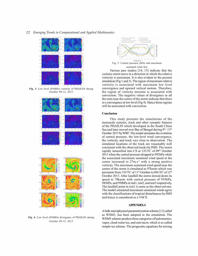
b. Low level Wind Convergence and Vorticity:During the formation of a cyclone the wind convergenceis supposed to take place near the cyclone center wherethe pressure is the least. Cyclonic flow around the centerof a low pressure area at 10-meter height (Fig 3) stronglysupported the existence of the active CS with maximumwind speed (Fig 5) of 24, 27, 35, 40, 50, and 45 m/s nearits centers at 09UTC, 12UTC of 9th, 03UTC, 06UTC of10th, 00UTC of 11th and 15UTC of 12th October 2013.Positive vorticity indicates anti-clockwise or cyclonicflow in the northern hemisphere. Vorticity of thePHAILIN are illustrated in Figure 3. The vorticity ofPHAILIN was found to be 0.0012s-1
at 09UTC on October09, 2013. The storm vorticity increased as the stormintensified to CS and the center extended wider with thevorticity of 0.0014s-1 at 12UTC of the same day. Thestorm gained the maximum vorticity of 0.0027s-1 at 06UTCof 10th October 2013 when its level of intensity waschanging from CS to VSCS.
Fig. 2. Simulated central pressure (hPa).
2 1: Kain Fritsch new Eta WSM 6-class Graupel[11] do do
3 1: Kain Fritsch new Eta Purdue Lin scheme: A sophisticatedscheme that has ice, snow and graupelprocesses, suitable for real-data high-resolution simulations[12] do do
22 Emerging Trends in Computational and Applied Mathematics
Fig. 3. Low level (850hPa) vorticity of PHAILIN duringOctober 09-12, 2013
Fig. 4. Low level (850hPa) divergence of PHAILIN during
October 09-12, 2013
Fig. 5. Central pressure (hPa) and maximum
sustained wind (kt).
Various past studies [14, 15] indicate that thecyclonic storm move in a direction in which the relativevorticity is maximum. It is also evident in the presentsimulation (Fig 1 and 3). The region of maximum relativevorticity is associated with maximum low levelconvergence and upward vertical motion. Therefore,the region of vorticity maxima is associated withconvection. The negative values of divergence in allthe tests near the centre of the storm indicate that thereis a convergence at low level (Fig 4). Hence these regionswill be associated with convection.
Conclusion
This study presents the simulations of themesoscale systems, track and other synoptic featuresof the PHAILIN which developed in the South ChinaSea and later moved over Bay of Bengal during 9th -13th
October 2013 by WRF. The model simulates the evolutionof central pressure, the low-level wind convergence,the vorticity, and track very close to observation. Thesimulated locations of the track are reasonably wellconsistent with the observed tracks by IMD. The stormrapidly intensified into CS at 12UTC of 09th October2013 when the central pressure dropped to 992hPa whilethe associated maximum sustained wind speed at thecenter increased to 27m.s-1 with a strong positivevorticity. The maximum sustained wind speed near thecenter of the storm is simulated as 97knots which waspersistent from 15UTC of 11th October to 06UTC of 12th
October 2013. After landfall the storm slowed down itsspeed to 78knots with central pressure of 955hPa,945hPa, and 950hPa in test1, test2, and test3 respectively.The landfall point in test1 is same as the observed one.The model simulated maximum sustained winds agreewith the classifications of tropical disturbances by IMDand hence is considered as a VSCS.
APPENDIX-I
A bulk microphysical parameterization scheme [11] calledas WSM3, has been adopted in the simulation. TheWSM3 scheme predicts three categories of hydrometers:vapor, cloud water/ice, and rain/snow, which is so-calledsimple-ice scheme. The prognostic equations for mixing

Emerging Trends in Computational and Applied Mathematics 23
ratios of water substances � �rqcqvq ,, and potentialtemperature (� ) are as follows:
Pw_cnd_v
Pi_nud_vPs_dep_v
Pi_dep_vPv_evp_r
)(DIF)(ADV
�
��
�
����
�vqvq
t
vq
δPw_mlt_iPs_ac_s_w
Pi_frz_wPw_cnd_v
Pr_ac_r_wPr_aut_w
)(DIF)(ADV
��
��
��
����
�cqcq
t
cq
δPr_mlt_sPs_ac_s_r
Pv_evp_rPr_aut_w
Pr_ac_r_wP_prc_r
)(DIF)(ADV
��
��
��
����
�rqrq
trq
� �
� �
� �
� �δPr_mlt_sδPw_mlt_i
Ps_ac_s_rPi_frz_wPs_ac_s_w
Ps_dep_vPi_nud_vPi_dep_v
Pw_cnd_vPv_evp_r
)(DIF)(ADV
��
���
���
��
����
�
�
�
�
�
���
pc
fL
pc
fL
pcsL
pcvL
t
Where t is time, )(ADV x is the advection term of x
and )(DIF x is the diffusion term of x. The symbols Lv, L
S
and Lf are latent heat of vaporization, sublimation and
fusion, respectively; cp the specific heat of dry air at
constant pressure, � the non-dimensional pressure(Exner function), and
��� ��
�otherwise0,
C0etemperaturtheif1,δ
The symbol Px_proc_y denotes the production rateof water substance x (v: water vapor, w: cloud water, r:rain, i: cloud ice, s: snow) through the process; ac:accretion, aut: autoconversion, cn: conversion such asriming, cnd: condensation, dep: depositional growth orevaporation, evp: evaporation, frz: freezing, mlt: melting,nud: nucleation by deposition. Concerning watersubstance y, zPx_proc_y_ denotes the production rate ofwater substance x through the process proc concerningwater substances y and z, and P_prc_x denotes
precipitation of x.
REFERENCES
[1] Very Severe Cyclonic Storm, PHAILIN over the Bay ofBengal (08-14 October 2013), “A Report,” (IndiaMeteorological Department, Cyclone Warning Division,New Delhi, 2013).
[2] J. A. Otkin, E. R. Olson, and A. Huang, “Comparison ofMM5 and WRF model data ingested into a forwardradiative transfer model,” In WRF/MM5 User’sWorkshop, June 2005.
[3] W. Y. Y. Cheng, and W. J. Steenburgh, “Evaluation ofsurface sensible weather forecasts by the WRF and theEta models over the western United States,” WeatherForecast, 20, 812–821 (2005).
[4] S. Pattanayak, and U. C. Mohanty, “A comparativestudy on performance of MM5 and WRF models insimulation of tropical cyclones over Indian seas,” CurrentScience, Vol. 95(7) 923-936 (2008).
[5] J. Dudhia, “The weather research and forecasting model(Version 2.0). 2nd International Workshop on NextGeneration NWP Model,” Seoul, Korea, Yonsei Univ.,19–23 (2004).
[6] W. C. Skamarock, J. B. Klemp, J. Dudhia, D. O. Gill, &D. M. Barker, Coauthors, 2008, “A description of theAdvanced Research WRF version 3,” NCAR Tech. NoteNCAR/TN-475+ STR, 113 (2005).
[7] L. J. Wicker, and W. C. Skamarock, “Time splittingmethods for elastic models using forward time schemes,”Mon. Wea. Rev., 130, 2088–2097 (2002).
[8] J. S. Kain, J. M. Fritsch, “Convective parameterizationfor meso scale models: The Kain-Fritsch scheme. InThe Representation of Cumulus Convection inNumerical Models,” Meteorological Monograph, No.46 (American Meteorological Society, Boston, USA,1993), pp. 165-170.
[9] J. M. Fritsch, C. F. Chappell, “Numerical prediction ofconvectively driven mesoscale pressure systems. PartI : Convective parameterization,” J. Atmos. Sci.,37,1722-1733 (1980).
[10] S.-Y. Hong, J. Dudhia, and S.-H. Chen, “A RevisedApproach to Ice Microphysical Processes for the BulkParameterization of Clouds and Precipitation,” Mon.Wea. Rev., 132, 103–120 (2004).
[11] S.-Y. Hong, and J.-O. J. Lim, “The WRF Single-Moment6-Class Microphysics Scheme (WSM6),” J. KoreanMeteor. Soc., 42, 129–151 (2006).
[12] Y.-L. Lin, R. D. Farley, and H. D. Orville, “Bulkparameterization of the snow field in a cloud model,” J.Climate Appl. Meteor., 22, 1065–1092 (1983).
[13] S. –Y., Hong, and J.-O. J. Lim, “The WRF Single-Moment 6-Class Microphysics Scheme (WSM6),” J.Korean Meteor. Soc., 42, 129–151 (2006).
[14] J. R. Holton, “An introduction to dynamic meteorology,”New York: Academic Press (1979).
[15] A. V. R. Krishna Rao, “Tropical cyclones-synopticmethods of forecasting,” Mausam 48, 239–256 (1997).

24 Emerging Trends in Computational and Applied Mathematics
Introduction:
Economics originated as a separate subject withthe advent of famous work “An Inquiry into the Natureand Causes of Wealth of Nations” by Adam Smith in1776 and since then there have been different schoolsof thoughts propounded various economic theories andmodels. Today’s modern economic analysis has beenbroadly divided into ‘Micro Economics’ and ‘Macroeconomics’ for convenient understanding. These termswere coined by Prof. Ragner Frisch of Oslo Universityin 1933 and since then they have been adopted amongthe economists worldwide.
Micro economics is defined as that branch ofeconomic analysis which studies the economicbehaviour of individual units such as people,companies, and industries within an economy that howthey allocate limited resource to get maximum gain. Themain areas of microeconomic study are consumerbehaviour, theories of cost and production,determination of product and factor prices withequilibrium output in various market structures etc.While macro economics is the study of economic
behaviour of an economy as a whole. It deals with theproblems and decision making process of the entireeconomy. The main areas of macroeconomic study aredetermination of income and employment, aggregatedemand and supply, consumption, saving andinvestment, inflation etc. Although microeconomics andmacroeconomics are the two main primary branches ofeconomics but, today economics has developed as amulti branch subject and has been studied asinternational economics, public finance, agricultureeconomic, population studies, labour economics andmany more.
In earlier times, economics was studied and taughtwith a very less application of mathematics but now aday, mathematical tools have become an integral part ofthe economic theories and models. Diagram analysis ofany model is limited to only two variables and solutionof any problem is much difficult and time taking. Whilemathematical application in economic theories helps inanalysing the economic problems in a better way andcontributes significantly in generating completesolutions. The development of economics during
7Application of Mathematics in Economics
An Examination for Selected Concepts
D. R. Agarwal, Sanjay Kumar ManglaSchool of Management, ITM University, Gurgaon, India
[email protected], [email protected]
Abstract: Economics has emerged as a very important field of study helping individuals, firms, industry, Govt.,nations etc. in allocating scarce resources to their alternative uses to satisfy maximum needs. Traditionally, all thesocial science subjects including economics were studied without or with a very less application of mathematicsbut nowadays mathematics has become an essential and integral part of economics theories and models; andmathematical economics has become a very popular subject worldwide. Thus mathematics and economics arecomplementary disciplines today. Mathematical approach to economic theories gives more precise and completesolution to economic problem but mathematical economic models have also been criticised. This paper attempts tocritically establish the application of mathematics in economics using selected theories and models frommicroeconomics and macroeconomics.Keywords: mathematics, economics, theories and models, application

Emerging Trends in Computational and Applied Mathematics 25
second quarter of 20th Century is named as the age ofmathematization of economics and today Starting fromthe microeconomics theory, macroeconomics,international trade, economic development, publicfinance and all the other branches of economics havebeen changed into a number of equation.
The development of mathematical economics toits present stage took several centuries. Sir William Petty(1623-1687) is believed to be the first participant in thisfield. He used but unsuccessfully the terms of symbolsin his studies. The first successful attempt was made byan Italian, named Giovanni Ceva (1647—1734). Afterthese earlier attempts, Antoine Augustin Cournot (1801-1877) made use of symbols in his theory of wealth. ThenAlfred Marshall in his “Principles of Economics” (1890)and Irving Fisher in his Ph.D. thesis “MathematicalInvestigations in the Theory of Value and Prices”showed a great interest in mathematical formulation ofthe economic theories. Then such a race had begunthat use of mathematics in economics became verycommon and essential and all the later theories andmodels had mathematical approach.
Objective:
In recent times, mathematical tools have beenwidely used in formulating economic theories andmodels. This paper aims at establishing the use ofmathematics and its importance in economics takingselected concepts of microeconomics andmacroeconomics.
Application in Selected Concepts:
This section shows the application of mathematicsin selected microeconomics and macroeconomicsconcepts.
Production Possibility Curve:
Production Possibility Curve (PPC) is defined aslocus of various combinations of two goods which canbe produced with available inputs and technology withtheir full utilization. PPC is concave to origin becauseMarginal Rate of Product Transformation (quantity ofY-good scarified / quantity of X-good obtains) isincreasing.
Let ),( yxfCPPC �� where C represents thegiven inputs employed to produce different
combinations of goods x and y . The problem ofoptimal resource allocation is one of the maximisationof Total Revenue (TR ) under production possibilities
as given ),( yxfC � . Thus the objective is to maximise
PyyPxxTR .. �� subject to ),( yxfC � . This isconstrained maximisation problem which is solved byLagrangian Multiplier.
The composite function is )),([ CyxfTR ��� �� .Differentiation of the composite function w.r.t.
,, yx and� gives:
-0)(
���
��
��
��
x
f
x
TR
x�
�
-0)(
���
��
��
��
y
f
y
TR
y�
�
-0),( �����
Cyxf��
fy
fx
Py
Px
fy
Py
fx
Pxλ ��� Hence
The slope of revenue line must be equal to theslope of PPC as a necessary condition for maximisationof revenue generated through given input constraint.The sufficient condition for the purpose
is 0 and 02
2
2
2
���
���
yx
��
0. and22
2
2
2
2
����
����
���
��
��
��
yxyx
���
TR is total revenue, x and y are units ofcommodities X and Y, and Px and Py are prices of
commodities X and Y. In ),( yxfC � , C represents givenresources employed to produce commodities X and Y.�
is Lagrenge’s multiplier and� is composite function.
Indifference Curve:
Indifference curve is the locus of all combinationsof two commodities yielding same level of satisfactionto a consumer. Higher indifference curve shows higherlevel of utility and a set of indifference curves is calledindifference map. Indifference curve is convex to originwhich means that marginal rate of substitution (MRS) isdiminishing. MRS shows the number of units of onecommodity sacrificed for an additional unit of another

26 Emerging Trends in Computational and Applied Mathematics
commodity. Suppose there are two commodities YX and ,then utility function is ),( yxfU � and budget constraint
is yx PyPxM .. �� . The objective of a consumer is tomaximise his total utility within given budget constraintwhich is a constraint maximisation problem and can besolved by Lagrangian multiplier. The objective function
becomes: )..(),( MPyPxyxf yx ���� �� Foroptimisation, first order partial derivatives are zero.
-----0..
----------0
----------0
������
����
���
����
���
MPyPx
Py
f
y
Px
f
x
yx
y
x
��
��
��
If equation (4) is divided by (5) then it is obtained
y
x
P
P
yf
xf�
����
/
/ or
y
x
y
x
P
P
MU
MU� which is condition for
equilibrium for a consumer. For a particular indifferencecurve total utility is constant i.e. ),( yxfU � , then
dyy
fdx
x
fdu ..
��
���
� and 0�du hence
y
x
MU
MU
dx
dy �� (which means that slope of indifference
curve is negative).
Elasticity of Demand and its relationship with AR andMR:
Elasticity of demand is the responsive change inquantity demanded for a particular product (other thingsbeing equal) corresponding to a change in price of thatproduct. Elasticity of demand (price elasticity) isnegative because there is a negative relationshipbetween price and quantity demanded of normal
commodities. Slope of demand curve is equal to dq
dp
because price is represented on Y-axis and quantitydemanded in X-axis. If demand is taken as a singlevariable function, elasticity of demand is equal to
��
���
������
q
p
q
p
dp
dq
function demand of slope
1. If demand
function is parallel to X-axis, slope is zero and if the
demand function is parallel to Y-axis, slope is infinity,hence elasticity of demand in these two cases are zeroand infinity respectively. There is an inverse relationshipbetween elasticity and slope of demand function. AsTR = p×q and MR is slope of TR function i.e.
)(TRdq
dand AR = p. If TR is differentiated w.r.t. q, it is
obtained that
��
���
�����
dq
dp
p
qp
dq
dpqpMR .1.
���
��� �
����
��� ��
e
eARMR
eARMR
1or
11
If 0�e , then MR = 0 and naturally TR ismaximum because demand function is a decreasingfunction. If demand function is a rectangular hyperbola,then pq = const. if it is differentiated w.r.t. q,
then 0. ��dq
dpqp and dq
dpqp �� or 1���
q
p
dp
dq, i .e.
Elasticity of demand is one at each point of this function.TR is total revenue, MR marginal revenue, AR
average revenue or price, e elasticity of demand, and dp
dq
inverse of the slope of the demand curve.
Consumer Surplus:
Consumer surplus is a conjectual gain, when aconsumer is willing to pay more for a commodity and inreality he pays a lesser amount [Consumer Surplus =Total Utility-Total Amount of Money Paid].Consumer ’s equilibrium is established at a point
where price�MU . MU is a decreasing function dueto law of diminishing marginal utility. In economic theory,when this concept is explained with an example, adiscontinuous series is taken but it has been assumedthat units of the commodity are divisible. This is amismatch between theory and real situation.
)(qfTU �
)(TUdq
dMU � is derivative of total utility or
called marginal utility or )(TUdMUdq � if it is
integrated both sides then, � �TUMUdq
Consumer surplus = Total amount of moneywilling to pay – Total money actually paid

Emerging Trends in Computational and Applied Mathematics 27
qpMUq
��� �0
function SurplusConsumer
Relationship between AC and MC:
Total cost (TC) of production is the total paymentsmade to all the factors used in the production process.Factors mean both primary factors (which do not changetheir identity during the production process) andsecondary factors (which change their identity duringthe production process). Total fixed cost (TFC) is thepayment to the factors which remain fixed in short periodtherefore fixed cost does response to change in output.Total variable cost (TVC) is the total payment made tothe variable inputs which response to change in output.Average fixed cost (AFC) is fixed cost per unit of output,average variable cost (AVC) is variable cost per unit ofoutput, average cost (AC) is total cost per unit of output,and marginal cost (MC) is total cost of producing anadditional unit of output.
TVCTFCTC ��AVCAFCATC ��
output of untis
TCATC �
hyperbola a isfunction ,output of units
TFCAFC �
output of units
TVCAVC �
ATCATC of Derivative of Slope �When ATC decreases, its slope is negative, when
ATC is constant, its slope is zero and when ATCincreases, its slope positive.
q
TCATC � of Slope
2
1
q
TCqMC ����
2q
TC
q
MC��
q
TCAC
q
AC
q
MC��� as
� �ACMCq
��1
Thus (i) when AC decreases, its
ACMCslope �� and 0 , (ii) when AC is constant, slope= 0 and MC = AC, and (iii) when AC increases, slope <0 and MC > AC.
Equilibrium of a firm and profit maximisation:
Equilibrium of a firm is established at a point whereits profits are maximised. There are two conditions ofprofit maximisation (i) first derivative of profit functionw.r.t. output should be zero which is a necessarycondition and (ii) second derivative of profit functionw.r.t. output should be negative which is a sufficientcondition.
TCTR ��)(Profit � or CR ���
MCMRdq
dC
dq
dR
dq
d���� Hence 0
�
02
2
2
2
2
2
���dq
Cd
dq
Rd
dq
d �
Hence slope of MR should be less than MC
Cobweb Model:
Let us consider a situation where the producertakes output decisions in one period advance of theactual sale such as agricultural production whereplanting must precede by an appreciable length of timebetween the harvesting and sale of output. Let usassume that the output decision in period t is based onthen prevailing price P
t. This output will not be available
for sale before the period t +1, however, Pt will determine
QSt+1
not QSt. Thus a lagged supply function is obtained
as QSt+1
= S(Pt) [it shows that quantity supplied is a
function of price prevailed in previous period] orequivalently, by shifting backs the time subscripts byone period as QS
t = S(P
t+1). Supply function interacts
with a demand function as )( tt PDQd � meaning thatcurrent quantity demanded is a function of current price.
Taking the linear versions of these (lagged) supplyand un-lagged demand functions, and assuming that ineach time period, the market price is always set a levelwhich clears the market, a market model is obtained withthe following equations:
tt QsQd �
)0,( where ��� ���� tt PQd

28 Emerging Trends in Computational and Applied Mathematics
)0,( where1 ���� � ���� tt PQs
���� ��� �1 tt PP ���� ��� �1 tt PP
By substituting the equation for tQd and tQs inthe market equilibrium model, a single first orderdifference equation is obtained as
Or ���
�� �
��� tt PP 1
[Difference equation with lagged variable].On solving this difference equation, it is obtained
that
0 ����
��
����
��
����
����
����
����
���
��t
t PP
price initial is where 0P
Formal model of Income, Output, and EmploymentDetermination:
According to the Keynesian theory of incomedetermination, the equilibrium level of national incomeis determined at a level where demand aggregate[ ICAD �� ] equals to aggregate supply ( AS ) of income
[ SCY �� ]. Keynes argued that there is no reason forthe aggregated demand to be always equal toaggregated supply. According to him, aggregate demanddepends on households’ plan to produce goods andservices. To present entire growth model, following setof variables are employed:
Z= aggregate supply price/function representingmust expectations when a volume of employment isoffered to workers by the entrepreneurs.
O= outputN= level of employmentD= aggregate demand/function representing real
expectations of the entrepreneurs from the sale of output,produced by a given a number of persons (volume ofemployment offered to workers)
D1= demand for consumer goods
D3= demand for investment goods
Aggregate supply price depends on level ofemployment i.e. )(NfZ � and similarly, demand forconsumer goods depends on real income or output whichin turn depends in the level of employment i.e.
)(1 NfD � . Thus if the level of full employment is to beachieved or cost of output is to be covered by the sale
proceeds of the output, aggregate demand must equateaggregate supply price, as
ZDDD ��� 21 (Effective demand)
)()(2 NfND ���)()(2 NNfD ���
D2 is a function of many autonomous factors such
as changes in technology and population. It will bewrong to say that aggregate demand is determined bythe level of employment. Autonomous investment (D
2)
may be regarded as a function of income.Let us assume that C = a + bY [where consumption
is a linear function of income] and I (investment) isconstant, thus
IbYaY ���
IabYY ���
IabY ��� )1(
b
IaY
��
�1
Where a is autonomous consumption,
I autonomous investment, and b is dY
CMPC
�� or
derivation/slope of consumption function.
Multiplier Analysis, Stability and IS-LM model:
In Keynesian economic theory, multiplier isdefined as a factor that quantifies the change in totalincome due to the injection of capital deposits orinvestments. It is usually used as a measurement of theeffects of government spending, investment orconsumption on income, and is calculated as onedivided by the marginal propensity to save or onedivided by the one minus marginal propensity toconsume.
)10( where)(1 ��� MPCYfC , consumption isa function of income.
)0,0( where),(2 ��� iy IIiYfI , investment is a
function of marginal efficiency of capital and rate ofinterest. Investment (private or induced) is a positivefunction of income and negative that of rate of interest.
0GG � (Autonomous Govt. expenditure)
0
0
P
Ms
P
Ms� ( M
S= supply of money which is
normally perfectly elastic)

Emerging Trends in Computational and Applied Mathematics 29
)0,0( where),( ��� iy LLiYLP
Md(M
d= demand
for money in an economy which is a liquidity functionof income and rate of interest, M
d includes transaction
demand function of income, precautionary demandfunction of income, and speculative demand functionof rate of interest).
SGI ��
In equilibrium position P
Md
P
Ms� and rate of
interest is determined by the interaction of demand andsupply of money. According to Keynes, rate of interestis purely a monetary phenomenon. Keynesian theoryof interest is known as Liquidity Preference Theory.
To derive the Govt. purchases multiplier, thebehavioural equations are:
)(),( 102 YfYGiYf ���[Investment + Govt. Ex. = Income – Consumption
= Savings]
),(0
0 iYLP
Ms�
[Real money supply = Demand for money that is aliquidity function of income and interest]
Now equations (7) and (8) are differentiated w.r.t.
Govt. purchases ( G )
dG
dYf
dG
dY
dG
dif
dG
dYf yiy 122 1 ����
0��dG
diL
dG
dYL iy
� � - 11 22 ����dG
dif
dG
dYff iyiy
- 0��dG
diL
dG
dYL iy
dG
dYis total derivative w.r.t. G, f
2y partial derivative
of f2 w.r.t. income, f
2i partial derivative of f
2 w.r.t. interest
rate, f1y
partial derivative of f1 w.r.t. income, L
Y partial
derivative of liquidity function w.r.t. income, and Lipartial
derivative of liquidity function w.r.t. interest rate.The Govt. purchases multiplier is represented
bydG
dY and may be determined by solving equations (9)
and (10) simultaneously, if Cramer’s rule is applied
� � yiyyi
i
iy
iyy
i
y
LfffL
L
LL
fff
L
f
dG
dY
.1
1
0
1
221221
2
����
���
�
�
Thus the Govt. purchases multiplier is
� �� �yiyyi
i
LfffL
L
.1 221 ��� .
dG
dYsuggests that multiplier may be either positive
or negative. In the multiplier, Li is negative, since an
increase in interest rate is assumed to reduce the amountof money demanded, where as L
yis positive, since an
increase in income is assumed to increase the amountof money demanded. Since f
1yis marginal propensity to
consume and it lies between 0 to 1, 1–f1y
is marginalpropensity to save which also lies between 0 to 1. Themarginal propensity to invest is positive. f
2i is negative,
since an increase in interest rate is assumed to reduce
investment. Since Li is negative, the numerator of
dG
dYis
negative. For dG
dYto be positive, the denominator should
also be negative. It means f2i, L
y exceeds L
i (–f
1y – f
2y) in
absolute terms. The denominator is negative, providedthat the stability condition is met.
Conclusion:
Economics has been proved a very importantsubject helping in allocation of resources to unlimitedrequirements and plays a significant role in decisionmaking by an individual, society, firms and industry,and the whole economy. Application of mathematicshas become an essential and widely adoptedphenomenon in formulation of economic theories andmodels. “The emergence and expansion of mathematicalformulation of economic theories and models began atthe end of Second World War and this so-calledmathematical revolution was noticed because of (1) shiftof emphasis from partial to a general equilibrium analysis(2) interest in theories of growth, technical progressand other economic dynamics, and (3) a revolution inthe techniques of applied economics” (Paul, 1974)
The mathematical formulation of economictheories and models is also subject some limitation suchas (1) “mathematical language describes what has been

observed not what will be observed, so it lacks predictivepower, which is the core of positive economics. Theultimate goal of positive economics is the developmentof a theory or hypothesis that yields and valid andmeaningful predictions about the phenomenon not yetobserved” (Friedman, 1953), (2) mathematical modelsare characteristically abstract and general, but it doesnot make them universally valid, (3) the main objectiveof economic theories is to make empirical studies usingactual world data but mathematical economics is non-empirical in nature which does not support the actualbehaviour of empirical nature of economics, (4)mathematical models can be fitted more suitably in largeand homogeneous collection of variables but are rarelybe used in single variable model whereas theoreticalmodels are more suitable in single variable model.
Despite of the above mentioned criticisms ofmathematical application in formulating economictheories and models, mathematics is highly used informulating economic theories and models. But it shouldbe remembered that mathematical economics is just anapproach to economic analysis and therefore, it shouldnot differ in conclusions arrived by using literaryeconomics. However, the choice between mathematicaland theoretical approaches in formulating economictheories depends upon the personal preference of theresearcher.
REFERENCES
[1] Allen R.G.D., Mathematical Analysis for Economists,
London Macmillan and Co, Ltd, (1962).[2] Bell, John Fred, A History of Economic Thought, N.Y.
Ronald Press Company, (1967), PP. 681-685.[3] Blaine, Roberts and Schultz, David L., Modern
Mathematics and Economic Analysis, N.Y, W.W. Nortonand Co, Inc., (1973).
[4] Chiang, Alpha C., Fundamental Methods ofMathematical Economics, 3rd ed., N.Y., Mcgraw HillCo,. (1984).
[5] Eichner, A,. “Why Economics is not yet a Science”’Journal of Economic Issues, June 1983, PP, 973-82.
[6] Friedman, Milton, Essays in Positive Economics,Chicago, University of Chicago Press, (1953).
[7] Galtung, Johan, Theory and Methods of Social Research,N.Y,. Columbia University Press, (1967).
[8] Hayes, Patrick, Mathematical Methods in the Socialand Managerial Sciences, N.Y., John Wiley and Sons,(1975).
[9] Katouzian, H., “Ideology and Methods in Economics”.Economica, August, 1978, PP. 369-382.
[10] Lazarsfeld, Paul F. and Henry, Neil W., Readings inMathematical Social Science, Chicago, Science ResearchAssociates, Inc, (1966) PP. 1-2.
[11] Leontief, W., “Academic Economics”. Letters, Science,Feb 25, 1983 PP. 904-5.
[12] Nemchinov, V.S., The Use of Mathematics in Economics,Massachusetts M.I.T., Press, (1964).
[13] Olinick, Michael, An Introduction to MathematicalModels in the Social and Life Sciences, Massachusetts,Addison-Wesley Publishing Company, (1978).
[14] Samuelson, Paul A., The Collected Scientific Papers ofPaul A. Samuelson, Vol.—II, Massachusetts, M.I.T.Press, (1966).
[15] Zarembka, Pual, Frontiers in Econometrics, N.Y.,Academic Press, (1974).
30 Emerging Trends in Computational and Applied Mathematics

FLUID MECHANICS


Introduction
Burgers equation is an important model in fluidmechanics; it can be used in various flow problems forexamples in modelling of gas dynamics and traffic flow[1,2]. The investigation for analytical solution isimportant not only because of the conceptualunderstanding of physical flow situations, but it can beused in assessing the accuracy of numerical methodsand experimental practices. Some important studiesdealing with Burgers equation are [3-5]. [6] introduced anew method known as the Optimal HomotopyAsymptotic Method (OHAM). OHAM provide a simpleway to control and adjust optimally the convergence ofthe solution series and give good approximation in fewterms. [6] obtained approximate analytical solution is invery good agreement with the numerical simulationresults, which proves the validity of the method. [7-11]have applied this method successfully to obtain thesolution of steady state heat problems and have alsoshown its effectiveness, generalization and reliability.Recently, [12] studied the symmetry reduction and exactsolution of a coupled KdV-Burgers equation by usingthe classical Lie group method, while [13] investigatedthe solution of (2+1)-dimensional Burgers equation by
using modified simple equation and exp-functionmethod.
In the present investigation, we consider theBurgers equation [3]
� � � � � �, ,0
,,,2
2
����
��
��
��
�x
x
txu
x
txuu
t
txu
subject to the initial condition
� � ,4
tanh2
1
2
10, �
��
�����
xxu
and the exact solution of (1) subject to (2) is given asfollows
� � .2
1
4
1tanh
2
1
2
1, ��
�
����
����
��� ��� txtxu
The aim of the present investigation is to applythe OHAM in order to obtain the solution of Burgersequation.
Mathematical technique of OHAM
Consider the partial differential equation of theform:
� �� � � �� � � � , ,0,,, ����� xtxgtxuNtxuL . ..(4)
8Application of the Optimal Homotopy Asymptotic Method
for the solution of the Burgers equation
Rozaini Roslan1, Mohammed Abdulhameed1, Ishak Hashim2, Habibis Saleh2
1Centre for Research in Computational Mathematics Faculty of Science, Technology and Human DevelopmentUniversiti Tun Hussein Onn Malaysia 86400 Batu Pahat, Johor Malaysia,
2School of Mathematical Sciences & Solar Energy Research Institute Faculty of Science & TechnologyUniversiti Kebangsaan Malaysia43600 UKM Bangi, Selangor, Malaysia
[email protected], [email protected], [email protected], [email protected]
Abstract: The optimal homotopy asymptotic method (OHAM) is applied to obtain the approximate analyticalsolution of the Burgers equation. We found that the OHAM solution is in very good agreement with the exactsolution, which prove the reliability of the method.Keywords: Burgers equation, Optimal Homotopy Asymptotic Method, Nonlinear partial differential equation.
Emerging Trends in Computational and Applied Mathematics 33

34 Emerging Trends in Computational and Applied Mathematics
.0, ���
���
���
t
uuB
where L is a linear operator, N is a non-linear
operator, � �txu , is an unknown function, � �txg , is a
known function, B is boundary condition and� is theproblem domain. By using OHAM, one can construct
the optimal homotopy � � � � Rqtx ��� 1,0:;,� whichsatisfies:
� � � �� � � �� �
� � � �� � � �� � � �� �txgqtxNqtxLqH
txgqtxLq
,;,;,
,;,1
���
��
��
�
,
� � � �,0
;,,;, ��
��
���
��
t
qtxqtxB
��
where � �1,0�q is an embedding parameter,, � �qtx ;,� is an
unknown function and � �qH is a nonzero auxiliary
function for .0�q Here, � � 00 �H . Equation � �6 is called
the optimal homotopy equation. Clearly, when
0�q and 1�q it holds that � � � �txutx ,0;, 0��
and � � � �txutx ,1;, �� respectively. Thus, as q varies
from 0 to1 the solution � �qtx ;,� approaches from
� �txu ,0 to � �,, txu where � �txu ,0 is obtained from
equation � �6 for :0�q
� �� � � �
.0,
,0,,
00
0
���
���
���
��
t
uuB
txgtxuL
Choose the auxiliary function � �qxH , in the form
� � � �,..., 22
1 xCqCqqCqxH mm����
where ,1C ,2C ..., mC are constants to be determined.
Let us consider the solution of equation � �6 in the form
� � � � � � ,...2,1 ,;,,,;,1
0 ��� ��
�
iqCtxutxuCqtx kik
k
i�
Now substituting equation � �9 into equation � �6 and
equating the coefficients of like powers of q , we obtain
zeroth order problem given by equation � �7 and the
general governing equations for � �txuk , ,
� �� � � �� � .0, ,,, 110011 ��
��
���
��
�t
uuBtxuNCtxuL
� �� � � �� � � �� �txuNCtxuLtxuL kkk ,,, 001 �� �
� �� �� � � � � �� ���
���
��
��
��
��
��
txutxutxuN
txuLC
ikik
iki
k
i ,,...,,,
,
10
1
1
.0, ,...,3,2 ����
����
���
�t
uuBk k
k
where � � � � � �� �txutxutxuN ikik ,,...,,, 10 �� is the
coefficient of ,ikq � obtained by expanding
� �� �ptxN ;,� in series with respect to the embedding
parameter .q
� �� � � �� � � � � �� �txutxuqNtxuNCqtxN i ,,,,,;, 10100 ���
� � � � � �� � � �12......,,,,, 21022 txutxutxuNq�
� �� �txuN ,00�
� � � � � � � �� �txutxutxutxuNq kkk
k,,...,,,,, 210
1��
�� ,
where � �� �iCqtx ,;,� is given by equation � �.9
It should be recognized that � �txuk , for 0�k is
govern by the linear equations � � � �10,7 and � �11 with
the linear boundary conditions that come from originalproblem.
The convergence of series of equation � �9 depend
upon the auxiliary constants ,...., 21 CC If it is convergent
at ,1�q we have
� � � � � �ik
m
ki CtxutxuCtxu ,,,;,
10 �
���
The solution of the nonlinear partial differential
equation � �4 subject to the boundary condition � �5 can
be determined approximately in the form
� � � � � � ,,,,;,~1
0 ik
m
ki CtxutxuCtxu �
���
.,...,2,1 mi �Substituting expression � �14 into equation � �4 subject
to boundary condition � �5 results in the following
residual expression R
� � � �� � � � � �� � ,;,~,;,~;, iii CtxuNtxgCtxuLCtxR ���

Emerging Trends in Computational and Applied Mathematics 35
.,...,2,1 mi �
If � � 0;, �iCtxR , then � �iCtxu ;,~ will be the exact
solution. Generally such a case will not happen fornonlinear problems, but we can minimize the functionby the method of least squares
� � � �dxdtCtxRCJ i
t
i ;,2
0 �� ��
The unknown constants � �miCi ,...,2,1� can beoptimally identified from the conditions
� � � � � �.0...
21
���
���
��
�
m
iii
C
CJ
C
CJ
C
CJ
With these known values of � �miCi ,...,2,1� , the
approximate solution of equation � �14 is well determined.
Alternatively, the constants � �miCi ,...,2,1� can also
be determined by another method as follows
� � � � � � .0;...;; 21 ���� imii CkRCkRCkR
where ,��ik mi ,...,2,1� at any time .t
3. Application of OHAM to the Burgers equation
In this section, we apply OHAM to solve the
Burgers equation � �1 subject to the initial condition � �.2
The linear and nonlinear operators are chosen asfollows
� �� � � �,
;,;,
t
qtxqtxL
��
��
�
� �� � � � � � � �,
;,;,;,;,
2
2
x
qtx
x
qtxqtxqtxN
��
��
��
����
subject to the initial condition
� �� � .4
tanh2
1
2
1;0, �
��
�����
xqxL �
According to equation � �6 , a family of equations is
constructed as follows
� � � � � � � �
� � � � � �2
2 ;,;,;,
;,;,1
x
qtx
x
qtxqtx
t
qtxqH
t
qtxq
�
��
��
�
��
��
��
��
�
���
��
� � .4
tanh2
1
2
1;0, �
��
����� x
qx�
From equation � �,7 we obtained the zeroth-order
problem:
� � � � ,4
tanh2
1
2
10, ,0
,0
0 ���
������
�� x
xut
txu
in which the solution is as follows
� � .4
tanh2
1
2
1,0 �
��
�����
xtxu
Substituting equation � �25 into equation � �10 , we
obtained the first-order problem:
� � � � � � � � � � � �
� � )27.......(.00,
,1,,
1
20
20
010
111
�
���
����
�
�
��
��
��
���
��
xu
x
xu
x
xuxuC
t
xuC
t
Ctxu
in which the solution is as follows
� �2
111 4
sec16
;, ���
�����
xht
CCtxu
For 2�k into equation � �,11 we obtained the second-
order problem:
� � � � � � � �
� � � � � � � �
� � � � � �
� � )29...(,00,
,
;,;,
;,1
,;,
2
20
20
02
211
20
111
01
02
111
212
�
���
����
�
�
��
��
�
���
����
�
�
��
��
��
��
��
��
���
��
xu
x
xu
x
xuxuC
x
Ctxu
x
xuu
x
CtxuxuC
t
xuC
t
CtxuC
t
CCtxu
in which the solution is as follows
� �
���
���
���
�����
��
����
���
�����
��
�����
4tanh
4sec
1284sec
16
4sec
164sec
16,,,
22
21
221
22
21
212
xxht
Cxht
C
xht
Cxht
CCCtxu
The approximate solution of this second-order is
obtained by adding equation � � � �27,25 and � � :29

36 Emerging Trends in Computational and Applied Mathematics
� �
4tanh
4sec
1284sec
16
4sec
84tanh
2
1
2
1,;,~
2
22
21
21
21
21
���
���
���
�����
��
����
���
�����
��
�����
xxht
Cxht
C
xht
CxCCtxu
....(,4
sec16
22 �
��
����
xht
C
where
� � � � � � � �21211021 ,,,,,,,;,~ CCtxuCtxutxuCCtxu ���
Substituting equation � �30 in equation � �,1 we obtain
the residual as
� � � � � � � �2
2
21,~,~,~
,;,x
txu
x
txuu
t
txuCCtxR
�
��
��
��
�� .
For the calculations of the constants 1C and 2C using
equation � �,18 For ,0.0�x 8.0 and 1�t , we
obtain 201 1083254.9 ���C and 11208.02 �C .
� �
2
2241
40
220
21
4sec79328.1
4tanh
4sec1055303.7
4sec1004242.6
4sec102290675.1
4tanh
2
1
2
1,;,
���
����
���
���
���
�����
���
�����
���
�����
���
�����
�
�
�
xht
xxht
xht
xht
xCCtxu
The series (33) is our OHAM solution.
Graphical result
Fig. 1. Comparison between the OHAM and exactsolution for values 05.0�t and 1.0�t .
To show the effectiveness of the OHAM solution,some numerical results are displayed between an exact
solution � �3 and the OHAM solution (33). Fig. 1 shows
the comparison between the OHAM solution and theexact solution for � �,1.0,05.0�t in this figure, we can see
that for small values of the time ,t the OHAM solutionis nearly identical with that given by the exact solution.This property holds for all values of time t , in theinterval 05.00 �� t and 1.005.0 �� t .
Fig. 2. Comparison between the OHAM and exactsolution for values 5.0�t and 0.1�t .

Emerging Trends in Computational and Applied Mathematics 37
Fig. 2 is plotted for � �,0.1,5.0�t in this figure, we
can see that when t increases, the OHAM and exactsolution tend to diverge.
5. Conclusion remark
In the present study, we have solved the Burgersequation by using the OHAM. OHAM gives accuratesolution to the Burgers equation with only few orderterms in the series. The obtained approximate analyticalsolution is in very good agreement with the exactsolution for small values of time .t
6. Acknowledgement
The author would like to acknowledge thefinancial support received from the Grant FRGS/1/2009/SG/UTHM/02/4/0734.
REFERENCES
[1] M.McAsey and L.A.Rubel, “Some closed-formsolutions of Burgers equation”, Stu Appl Math 88 173-190 (1993).
[2] A.M.Wazwaz, “Partial differential equations andsolitary wave’s theory (Nonlinear Physical Science)”.(Springer, 2009).
[3] P.G.Drazin and R.S.Jonson, “Soliton: an Introduction”.(Cambridge University Press, New York, 1993).
[4] C.A.J. Fletcher. “Burger’s equation: a model for allreason. Numerical solutions of partial differentialequations”. (North-Holland Publication Company,Amsterdam, 1982).
[5] M.M.Rashidi, G.Domairry and S.Dinarvand,“Approximate Solutions for the Burger and regularized
long wave equations by means of the homotopy analysismethod”, Communication in Nonlinear Science andNumerical Simulation 14, 708-717 (2009).
[6] N.Herisama, V.Marinca and T.Dordea, “A NewAnalytical Approach to Nonlinear Vibration of anElectrical Machine”, Proceedings of the RomanianAcademy, Series A 9(3) 229-236 (2008).
[7] V.Marinca, and N.Herisanu, “Application of OptimalHomotopy Asymptotic Method for Solving NonlinearEquations Arising in Heat Transfer”, InternationalCommunications in Heat and Mass Transfer 35 710-715 (2008).
[8] M.Idrees, S.Islam, H.Sirajul and S.Islam, “Applicationof the Optimal Homotopy Asymptotic Method toSqueezing Flow”. Computers and Mathematics withApplications, 59 3858-3866 (2010).
[9] M.Idrees, S.Islam, Haq,Sirajul and S.Islam, “Applicationof the Optimal Homotopy Asymptotic Method for thesolution of the Korteweg-de Varies equation”,Mathematical and Computer Modelling 55 1324-1333(2012).
[10] F.E.Mabood, A.Izani Md Ismail and I.Hashim. “TheApplication of Optimal Homotopy AsymptoticMethod for the Approximate Solution of RiccatiEquation”. Sains Malaysiana 42(6) 863-867 (2013).
[11] M.Sheikholeslami, H.R.Ashorynejad, D.Domairry andI.Hashim. “Investigation of the laminar viscous flow ina semi-porous channel in the presence of uniformmagnetic field using Optimal Homotopy AsymptoticMethod”. Sains Malaysiana 41 1281-1285 (2012).
[12] S.Yang and C.Hua. “Lie symmetry reductions and exactsolutions of a coupled KdV-Burgers equation”,AppliedMathematics and Computation 234, 579-583 (2014).
[13] K.Khan and M.A.Akbar. “Traveling wave solutions ofthe (2+1)-dimensional Zoomeron equation and theBurgers equations via the MSE method and the Exp-function method”. Ain Shams Engineering Journal 5,247-256 (2014).

38 Emerging Trends in Computational and Applied Mathematics
Introduction
Convection in fluids is one of the most widelystudied engineering problems of the recent era. It occursin many situations in nature as well as in industry.Atmospheric circulation, the formation of clouds,oceanic circulation, convection in planetary mantles,stellar convection are the most commonly observedforms of convection in nature. We encounter convectionin many industrial applications such as in the formationof micro-structures, crystal growth and so on. In alaboratory setup we observe convection in the form ofthe spectacular Bénard cells due to thermal convection.
The instabilities due to thermal convection in afluid layer have been studied extensively boththeoretically and experimentally over last century (seeChandrasekhar [1], Drazin and Reid [2], Platten andLegros [3] and the references there in). A theoreticalstudy of convective instability in a fluid layer can becarried out using linear or the weak nonlinear stabilitytheories. The linear stability theory that predicts theonset of convection usually leads to an eigen boundary
value problem (EBVP) with the Rayleigh number as theeigen value while the weakly non-linear theory whichcan predict both the onset and the aftermath ofconvection yields a chaotic system, the Lorenz system.There are several numerical and semi-analytical methodsavailable to solve EBVP arising from the linear stabilityanalysis of convection in a fluid layer.
Literature survey reveals that most of the boundaryvalue problems arising in fluid mechanics are usuallysolved numerically using either a shooting method orthe implicit finite difference scheme in combination witha linearization technique. These methods can be suitablyupgraded to solve EBVPs (see, Rees [4], Barletta andRees [5] and references therein). Other popular methodsfor EBVPs are variational methods such as the Rayleigh-Ritz method, the Galerkin method and spectral methods.There are several analytical/semi-analytical methods forsolving nonlinear boundary value problems, amongthem, the variational iteration method [6], the homotopyperturbation method [7, 8], the Adomian decompositionmethod [9, 10], homotopy analysis method [11, 12] and
9On a Successive Linearization Solution of an Eigen BVP due to
Magnetoconvection in a 2-Dimensional Rectangular Box
Mahesha Narayana1, S. S. Motsa2, P. Sibanda2
1 School of Advanced Sciences, VIT University, Vellore – 632 014, Tamilnadu, INDIA2 School of Mathematics, Statistics and Computer Science, University of KwaZulu-Natal,
Private Bag X01, Scottsville 3209, Pietermaritzburg, SOUTH [email protected] , [email protected], [email protected], [email protected]
Abstract: The paper describes the solution of an eigen boundary value problem (EBVP), arising from the linearstability analysis of magnetoconvection in a two dimensional rectangular box using the successive linearizationmethod (SLM). Normal mode analysis from linear theory leads to the eigen boundary value problem with Rayleighnumber as the eigen value. The numerical results obtained, using the linearization method, for the EBVP werevalidated by comparison with exact analytical results. The two methods gave nearly identical results. The comparativeanalysis of the performance of the SLM showed that this recent method is sufficiently accurate and robust for useas an alternative numerical method for eigen boundary value problems.Keywords: Eigen boundary value problem, Rayleigh number, convection, linear stability, successive linearizationmethod

Emerging Trends in Computational and Applied Mathematics 39
the spectral-homotopy analysis methods [13, 14]. Thesemethods pose various challenges and restrictionsrelating to their use such as lack of precision, poorconvergence, and inefficiency. These limitationsnecessitate the development of computationallyimproved semi-analytical methods for solving stronglynonlinear problem. It is important to note at this juncturethat the linear stability theory yields a linear EBVP.However, by regarding the eigen value as an unknownvariable, one can view the EBVP as a nonlinear BVPwith an additional normalization condition. Thus inprinciple, the solution of EBVP by linearization methodis equivalent to the solution of the nonlinear BVPassociated with a normalization condition.
In this paper we demonstrate the use of thesuccessive linearization method in finding solutions ofthe EBVP arising from magnetoconvection in a 2-dimensional rectangular box. The method iterativelylinearizes the nonlinear equations to obtain a system ofhigher order deformation equations that are solved usingthe Chebyshev spectral collocation method.
Mathematical Formulation
We consider magnetoconvection in a viscousfluid in a rectangular box of height d as shown in Figure1. A temperature difference of T� is maintained betweenthe layers z = 0 and z = d. The side walls are assumed toadiabatic, i.e., exchange no heat with the surroundings.
The gravity ˆg gk� �� is assumed act vertically
downwards. A uniform transverse magnetic field ofstrength 0H is applied along the positive z-direction. Itis assumed that working medium possesses weakelectrical conductivity so that the induced magnetic fieldis negligible, i.e., the magnetic Reynolds number isnegligibly small.
Fig. 1. Schematic diagram of the physicalconfiguration
We assume that the Boussinesq approximation is validand the state equation for density has the form
� �0 01 T T� � �� �� � �� � ,
where 0� is the reference density,,� is the coefficient
of thermal expansion, T is the temperature of the fluid
and 0T is the reference temperature. The equations
governing the magnetoconvection in a viscous fluidenclosed in a rectangular box can be written as:
0,� � ��q
20
qq q q g J B
tp� � �
�� �� � � � � �� ��� �� � �� �
� � �� � � �,
2.T
q T Tt
��
� � � ��
�,
� �J q B�� �� ��
,
mB H��� �
,
where, � �,q u w��
is the velocity vector, t is time, p is the
pressure, � is the density,, � is the fluid viscosity,, J�
is
the current density, B�
is the magnetic inductionvector,� is the thermal diffusivity, � is the electrical
conductivity, m� is the magnetic permeability,,0
ˆH H k��
is the magnetic field vector. For weak electricallyconducting fluids, the Lorentz force, on using equations(5) and (6), can be written as
2 20mJ B H q��� � �
� � �.
In the quiescent state, the temperature, pressure anddensity are functions of z alone and the following hold:
� � � �
� � � �
0
0 0
0,0 , 1 ,
1 , 0.
b b
bb b b
zq T z T T
d
dpz T T g
dz� � � �
� �� � � � �� �� �
� �� � � � �� �
�
To determine the stability of the system we disturb thebasic state by an infinitesimal amplitude perturbation, sothat
, , , .b b b bq q q T T T p p p� � �� � � �� � � � � � � �� � �
Here, � �,q u w� � ���
and the primes indicate that the
quantities are infinitesimal perturbations. Substitutingequation (7) in the momentum equation (3) and immediateuse of equation (9) yields the following equations forthe perturbations
0 T� � �� �� � ,
0,q�� � ��

40 Emerging Trends in Computational and Applied Mathematics
20
qq q q g
tp� � �
��� �� � � �� � � �� ��� ��� � �� �
�� � � �
2 20m H q�� ���
,
2. bdTTq T w T
t dz�
�� � � � �� � � � ��
�.
The problem defined through equations (10) to (13) isnon-dimensionalized using the following new variables
� � � �* * *2
2* * *
1, , , ,
, , .
x z x z t td d
d d Tq q p p T
T
�
� ��
�� � ���� �� �� � ��� �
� �
Here, � �* * *,q u w��
. Substituting (10) in (12) and
making use of new variables defined through equation(14) along with basic state equations (8) yields thefollowing governing equations:
0,� � ��q
21 ˆPr
qq q q RaTk Qq
tp
�� �� � � � �� ��� �� � �� �
�� � � �
,
2.T
q T w Tt
�� � � ��
��
.
Here, the asterisks have been dropped for clarity. Thenondimensional quantities in the above equations arethe Prandtl number Pr, the Rayleigh number Ra and theChandrasekhar number Q respectively defined as
Pr��
� , 3gd T
Ra�
���
� , 2 2 2
0m H dQ
���
� .
Here, 0� � �� is the kinematic viscosity. In the presentstudy the boundaries are assumed to be impermeableand stress-free, i.e.,
ˆ. 0nq e ��
, ˆ. 0te� � on x = 0, a and z = 0, 1,
where ˆne and ˆ
te are respectively the unit normal and
unit tangent vectors and � is the stress-tensor. Thehorizontal walls are isothermal while the side walls areadiabatic, i.e.,
0T � on z = 0, 1,
ˆ. 0nT e� � on x = 0, a.
The boundary conditions, in the component form are:
0w T
ux x
� �� � �
� � on x = 0, a,
0u
w Tz
�� � �
� on z = 0, 1.
We restrict ourselves to two-dimensional rolls, so thatall the physical quantities are independent of y. Withrespect to three-dimensional convection rolls where theaxes are parallel to the y-direction and the variables areindependent of y, we may assume the existence of astream function defined by
, .u wz x
� �� �� � �
� �Equation (20) satisfies the continuity equation (15)identically. Substituting equation (20) in equations (16)and (17), eliminating the pressure term from themomentum equation (16) and dropping nonlinear termsgives the following equations:
� � � �2 2 21
Pr
TRa
t xQ� �
� �� �
� �� � � � ,
2TT
t x
�� �� ��
� �.
The boundary conditions (18) and (19) take the form:2
20
T
xx
��
� �� � �
�� on x = 0, a,
2
20T
z
��
�� � �
� on z = 0, 1.
The solutions of equations (21) and (22) are assumed tobe of the periodic waves form given by
� �� �
� � � �� � � �
* sin, ,
, , cos
xat
xa
zx z te
T x z t z
��
�
�
�
� ��� �� � �� �
� � � �� � � �,
The quantity *� is a complex quantity given
by *r i� � �� � where r� , the growth rate and � , the
frequency of oscillations are real. In this short paper weassume that the principal of exchange of stabilities holds
and hence set * 0� � . Substituting equation (25) into(21) - (24), we get
� � � �2 2 2 2 0D k Q D k Rak�� �� � � �� �� � ,
� �2 2 0D k k�� � � � ,2 0D �� � � � � on z = 0, 1,
where k = � / a represents the wave number and Dstands for the derivative with respect to z.
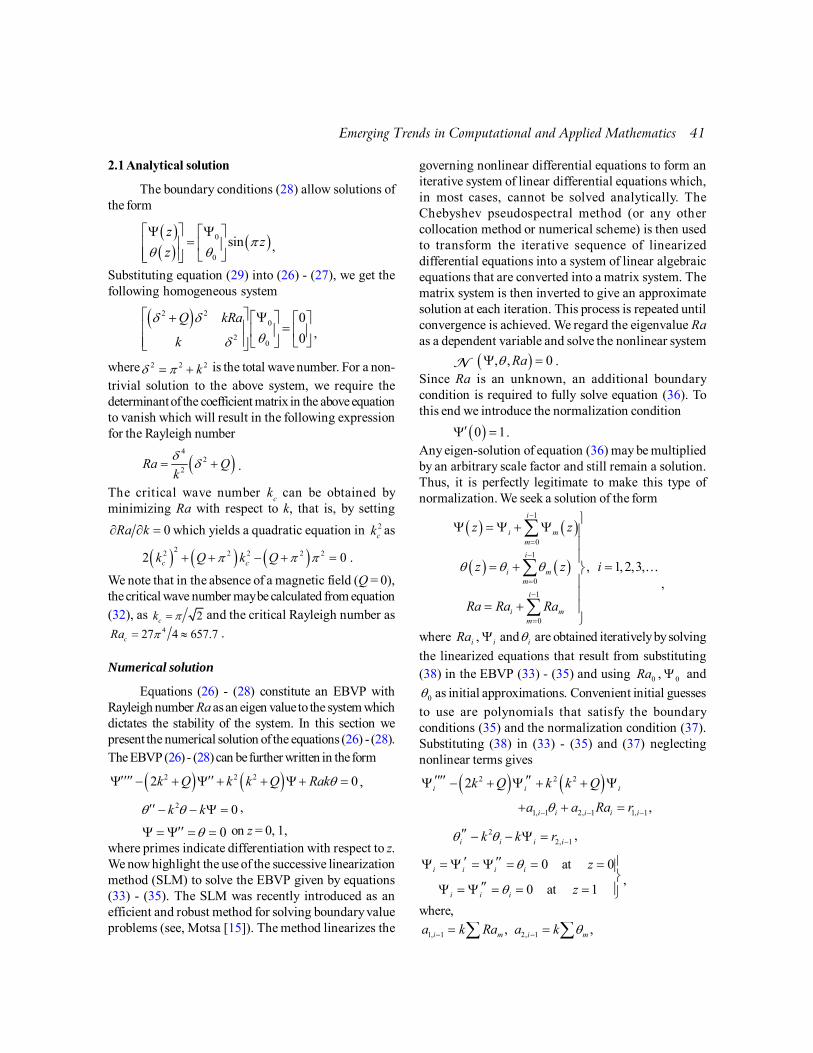
Emerging Trends in Computational and Applied Mathematics 41
2.1 Analytical solution
The boundary conditions (28) allow solutions ofthe form
� �� � � �0
0
sinz
zz
�� �
� �� �� ��� � � �
� � � �� �,
Substituting equation (29) into (26) - (27), we get thefollowing homogeneous system
� �2 20
20
0
0
Q kRa
k
� ���
� � �� � � � ��� � � � � �
� � � �� �� �,
where 2 2 2k� �� � is the total wave number. For a non-trivial solution to the above system, we require thedeterminant of the coefficient matrix in the above equationto vanish which will result in the following expressionfor the Rayleigh number
� �4
22
Ra Qk
��� � .
The critical wave number kc can be obtained by
minimizing Ra with respect to k, that is, by setting
0Ra k� � � which yields a quadratic equation in 2ck as
� � � � � �22 2 2 2 22 0c ck Q k Q� � �� � � � � .
We note that in the absence of a magnetic field (Q = 0),the critical wave number may be calculated from equation(32), as 2ck �� and the critical Rayleigh number as
427 4 657.7cRa �� � .
Numerical solution
Equations (26) - (28) constitute an EBVP withRayleigh number Ra as an eigen value to the system whichdictates the stability of the system. In this section wepresent the numerical solution of the equations (26) - (28).The EBVP (26) - (28) can be further written in the form
� � � �2 2 22 0k Q k k Q Rak����� ��� � � � � � �� � ,
2 0k k� ��� � � � � ,
0���� � � � � on z = 0, 1,where primes indicate differentiation with respect to z.We now highlight the use of the successive linearizationmethod (SLM) to solve the EBVP given by equations(33) - (35). The SLM was recently introduced as anefficient and robust method for solving boundary valueproblems (see, Motsa [15]). The method linearizes the
governing nonlinear differential equations to form aniterative system of linear differential equations which,in most cases, cannot be solved analytically. TheChebyshev pseudospectral method (or any othercollocation method or numerical scheme) is then usedto transform the iterative sequence of linearizeddifferential equations into a system of linear algebraicequations that are converted into a matrix system. Thematrix system is then inverted to give an approximatesolution at each iteration. This process is repeated untilconvergence is achieved. We regard the eigenvalue Raas a dependent variable and solve the nonlinear system
N � �, , 0Ra�� � .Since Ra is an unknown, an additional boundarycondition is required to fully solve equation (36). Tothis end we introduce the normalization condition
� �0 1�� � .Any eigen-solution of equation (36) may be multipliedby an arbitrary scale factor and still remain a solution.Thus, it is perfectly legitimate to make this type ofnormalization. We seek a solution of the form
� � � �
� � � �
1
0
1
0
1
0
, 1,2,3,
i
i mm
i
i mm
i
i mm
z z
z z i
Ra Ra Ra
� � �
�
�
�
�
�
�
�� � � � � �
��
� � ����
� � ��
�
�
�
�,
where iRa , i� and i� are obtained iteratively by solving
the linearized equations that result from substituting(38) in the EBVP (33) - (35) and using 0Ra , 0� and
0� as initial approximations. Convenient initial guesses
to use are polynomials that satisfy the boundaryconditions (35) and the normalization condition (37).Substituting (38) in (33) - (35) and (37) neglectingnonlinear terms gives
� � � �2 2 2
1, 1 2, 1 1, 1
2
,
i i i
i i i i i
k Q k k Q
a a Ra r�� � �
���� ��� � � � � � �
� � �
22, 1i i i ik k r� � �
�� � � � � ,
0 at 0
0 at 1
i i i i
i i i
z
z
�
�
�� ��� � � � � � � � ��
��� � � � � � ��,
where,
1, 1 2, 1, , i m i ma k Ra a k �� �� �� �

42 Emerging Trends in Computational and Applied Mathematics
� �� �
21, 1
2 2
2
,
i m m
m m m
r k Q
k k Q k Ra �
�� ���� ��� � � � � ���
�� � � � �
� �
� � �2
2, 1i m m mr k k� ��� ���� � � � �� �� �� � � .
To solve the linearized system (39) - (41) we usethe Chebyshev collocation spectral method in whichthe solution space is discretized using the Chebyshev-Gauss-Lobatto collocation points
� �cos , 0,1, , ,j j N j N� �� � �
which are the extrema of Nth order Chebyshev polynomial
� � � �1cos cosNT N� ��� .
Before applying the spectral method, it is convenient totransform the governing physical region [0, 1] for theproblem to the interval [-1, 1] on which the spectralmethod is defined. This can be achieved by using the
linear transformation � �1 2z �� � .
The Chebyshev spectral collocation method (seefor example [16, 17]) is based on the idea of introducing
a differentiation matrixD which is used to approximate
the derivatives of the unknown variables i� and i� at
the collocation points as the matrix vector product as
� �
� �0
0
, 0,1, 2, , ,
Ni
jk i kk
Ni
jk i kk
dD
dzj N
dD
dz
�
�� �
�
�
� �� � � �� ��
�� � ��
�
�
D
DΘ
�
where and D = 2D , withD being the Chebyshevderivative matrix and , Θ are the vector functions
of i� and i� respectively, at the collocation points j� .
The entries of D can be computed in different ways. Inthis work we use the method proposed by Trefethen[17] in the cheb.m MATLAB m-file. Substituting (42) -(44) in equations (39) - (41) we obtain the followinglinear matrix system
where Dij denote entries of matrix D. The above matrix
system can be put in a compact form as
1 1i i i� ��A Y R
where 1 1, 1 2, 1= , ,0T
i i iR R� � �� �� �R with , 1s iR � being the vectors
of , 1s ir � for s = 1, 2 at the collocation points. It must be
noted that the boundary conditions (41) have beenimposed on the aforementioned matrix system. Thus,
starting from the initial approximations 0Ra , 0� and
0� the subsequent solutions for iRa , i� and i� (i = 1, 2,
3,…) can be obtained by solving the iterative matrixsystem as
11 1i i i
�� ��Y A R .
Results and discussion
The successive linearization method has beenapplied to solve the EBVP arising due tomagnetoconvection in a two dimensional rectangularbox. Normal modes based linear stability theory wasused to obtain the EBVP. The numerical solutions of theEBVP were validated by comparison with analyticalresults. As indicated earlier, the linear EBVP obtainedthrough linear stability analysis can be regarded as anonlinear BVP with the eigen value Ra as an unknownvariable and thus requiring an extra normalizationcondition. The solution of the EBVP by the SLM isidentical to the solution of a nonlinear BVP by SLM.Figure 2 shows the neutral stability curves for differentvalues of Q. The solid lines represent the curvesobtained through the SLM and the circles representanalytical results. It is evident that the SLM and the
Fig. 2. Neutral stability curves for differentvalues of Q.

Emerging Trends in Computational and Applied Mathematics 43
analytical results are in excellent agreement. Animportant advantage of SLM over other direct spectralmethods is that it yields the exact eigen value of theproblem. It is not always the case for other direct spectralmethods as there is a possibility of spurious eigen valuesinstead of the one sought for.
Figure 2 also highlight the effect of the magneticfield on the onset of convection. Increasing the valuesof Chandrasekhar number Q increases the critical valueof Ra which delays the onset of convection. Thus, themagnetic field has a stabilizing effect on the systemconsidered. The results reported here qualitatively agreewith those reported by Chandrasekhar [1].
Conclusions
In this paper we presented a solution of the EBVParising from magnetoconvection in a two dimensionalrectangular box. The system of equations was solvedusing the successive linearization method. Thenumerical solution of the EBVP was validated bycomparison with the closed form solution obtainedthrough normal mode analysis. The successivelinearization method gave the exact eigen value of theproblem, which is a distinct advantage of this methodover other direct spectral methods.
REFERENCES
[1] S. Chandrasekhar, Hydrodynamic and hydromagneticstability (Clarendon, Oxford, 1961).
[2] P.G. Drazin and W.H. Reid, Hydrodynamic stability(Cambridge University Press, Cambridge, 1981).
[3] J.K. Platten, J.C. Legros, Convection in Liquids(Springer-Verlag, Berlin, 1984).
[4] D.A.S. Rees, “The onset of Darcy-Brinkman convectionin a porous layer: an asymptotic analysis”, InternationalJournal of Heat Mass Transfer 45, 2213-2220 (2002).
[5] A. Barletta and D.A.S. Rees, “Local thermal non-equilibrium effects in the Darcy-Bénard instability withisoflux boundary conditions”, International Journal ofHeat Mass Transfer 55, 384-394 (2012).
[6] J.H. He and X.H. Hu, “Variational iteration method:New development and applications”, Computers andMathematics with Application 54, 115-123 (2007).
[7] J.H. He, “A coupling method for homotopy techniqueand perturbation technique for non-linear problem”,International Journal of Non-Linear Mechanics 35, 37-43 (2000).
[8] J.H. He, “Homotopy perturbation method for solvingboundary value problems”, Physics Letters A 350, 87-88 (2006).
[9] G. Adomian, “Nonlinear stochastic differentialequations”, Journal of Mathematical Analysis andApplication 55, 441-452 (1976).
[10] G. Adomian, “A review of the decomposition methodand some recent results for nonlinear equations”,Computers and Mathematics with Application 21, 101-127 (1991).
[11] S.J. Liao, Beyond perturbation: Introduction to homotopyanalysis method (Chapman & Hall/CRC Press, 2003).
[12] S.J. Liao, Homotopy analysis method in nonlineardifferential equations (Springer, Berlin, 2012)
[13] S.S. Motsa, P. Sibanda and S. Shateyi, “A new spectral-homotopy analysis method for solving a nonlinearsecond order BVP”, Communications in NonlinearScience and Numerical Simulation 15, 2293-2302 (2010).
[14] S.S. Motsa, P. Sibanda, F.G. Awad and S. Shateyi, “Anew spectral-homotopy analysis method for the MHDJeffery-Hamel problem”, Computers and Fluids 39,1219-1225 (2010).
[15] S.S. Motsa, “New algorithm for solving non-linear BVPsin heat transfer”, International Journal of Modeling,Simulation and Scientific Computing 2, 355-373 (2011).
[16] C. Canuto, M.Y. Hussaini, A. Quarteroni, and T.A. Zang,Spectral Methods in Fluid Dynamics (Springer-Verlag,Berlin, 1988).
[17] L.N. Trefethen, Spectral Methods in MATLAB (SIAM,2000).

44 Emerging Trends in Computational and Applied Mathematics
Introduction
The beautiful hexagonal patterns can be obtainedby a simple experiment first conducted by Henri Benard,a French physicist, in 1900. Later, Pearson in (1958)identified that the Benard cells were driven by theimbalance of the tangential stress on the interfacecaused by temperature dependence of surface tension.The fluid motion along a free surface due to surfacetension effect is a common phenomenon in many materialprocessing such as crystal growth, vaporizing dropletand electron beam melting of metals. Such flow is knowneither as thermocapillary flow or Marangoni convection.
Most of the studies on the buoyant Marangoniconvection in cavities have considered the pure fluid.The material fabrication, cooking and transportationutilizing internal combustion and jet engines,unintentionally release nanoparticles into theatmosphere. These nanoparticles dispersed in the purefluid such as water known as nanofluids. In recent yearsa new type of source of nanoparticles has beenintroduced, and followed by an engineered nanofluids,product of [1]. Nanofluids water-Cu and water-Al2O3were utilitized by [2] and [3] to increase the heat transfer
performance of natural convection withoutthermocapillary effect. The heat transfer is reported todecrease by adding the nanoparticles for a particularRayleigh number [4]. In the present study, buoyantthermocapillary convection of nanofluids (water-Cu)with different nanoparticles concentrations areconsidered.
Mathematical formulation and method
Figure 1 shows a physical model of a squarecavity. The left wall is kept at low temperature, the rightwall at high temperature and the bottom and top wallsare adiabatic. The top free surface is assumed to be flatand non—deformable. The surface tension on the upperboundary is assumed to vary linearly with temperature.The fluid in the cavity is a water-based nanofluidscontaining Cu nanoparticles. It is presumed that thebase fluid (i.e. water) and the nanoparticles are in thermalequilibrium and no slip occurs between them. No-slipvelocity conditions imposed on all boundaries, exceptthe case where the top wall is considered as slip orsymmetric condition.
10Buoyancy and thermocapillary Driven Convection
Flow of Nanofluids in a Cavity
Ishak Hashim,, Habibis Saleh
School of Mathematical Sciences & Solar Energy Research Institute Faculty of Science & TechnologyUniversiti Kebangsaan Malaysia43600 UKM Bangi, Selangor, Malaysia
[email protected], [email protected]
Abstract: Buoyancy and thermocapillary driven convection flow of nanofluids in a cavity is studied numericallyusing Finite Difference Method (FDM). We found that a critical Marangoni number is exist, below which theincreasing the Marangoni number decreases the average Nusselt number and above which the increasing theMarangoni number increases the average Nusselt number. The nanoparticles play a crucial role on the criticalMarangoni number.Keywords: Natural convection, Thermocapillary convection, Finite Difference Method.

Emerging Trends in Computational and Applied Mathematics 45
Fig. 1. Schematic representation of the model.
Under the above assumptions, the dimensionlessgoverning equations in stream function, vorticity andtemperature formulation are:
2 2
2 2X Y
� � � �� � ��
� �
Y X X Y
�� �� �� ��� �
� � � �
2 2
2 2
0.25(1 ) (1 )
bf
sp
bf
Pr
X Y�� � �
�
� �� �
� �� � � �� � �� �� � � �� � � �� �� � �� �� �� �� �� �
(1 ) spbf bf
bf
Ra PrX
�� �
�
� � ��� �� � �� � � ��� �� �� �
Y X X Y��� �� �� �� ��
� � �� � � � �
2 2
2 2( )(1 )
( )
nf
bf
sp
bf
k
k
Cp X Y
Cp
�� �
�
� �� � � �� � � �� � �� �� � � �� �� �� �� �� �
The dimensionless boundary conditions are:
2
2 and 0 at 0X
X
� �� � � � � �
�
2
2and 1 at 1X
X
� �� � � � � �
�
2
2and 0 at 0Y
YY
� � ��� � � � �
��
2
2and 0bfMa
X YY
� � �� ��� � � � � �
� ��
at 1 Y �Once we know the temperature we can measure
the heat transfer performance. The total heat transferrate across the cavity in terms of the average Nusseltnumber are defined as
1
0
0
d at cold wallnfc
bf X
kNu Y
k X�
� �� � ��� � �� �� � �� �� �� ��
1
0
1
d at hot wallnfh
bf X
kNu Y
k X�
� �� � ��� � �� �� � �� �� �� ��
An iterative finite difference procedure will beapplied to solve the governing equations (1)–(3) subjectto the boundary conditions (4)–(7). Central differencemethod is applied for discretizing the equations. For theboundary conditions, backward and forward differentschemes are applied. An accurate representation ofvorticity at the surface is the most critical step in thestream function–vorticity formulation. A second-orderaccurate formula is used for the vorticity boundarycondition. Next, the solutions of the algebraic equations

46 Emerging Trends in Computational and Applied Mathematics
are performed using Gaussian SOR iteration. Theunknowns variables are calculated until the criterion ofconvergence is fulfilled. Finally, the integration of (8)and (9) is done by using the second-order Simpsonmethod
Fig. 2. Streamlines and isotherms [nanofluids (solidlines) with and pure-fluid (dashed lines)]
for different Marangoni numbers.
Result and discussion
The fluid motion as shown in the Figure 2 isdescribed as follows. Since the temperature of the rightwall is higher than that of the nanofluids or base fluidsinside the cavity, the wall transmits heat to the fluid andraises the temperature of fluid particles adjoining theright wall. When the temperature rises, the fluid startsmoving from the right (hot) wall to the left (cold) walland falling along the cold wall, then rising again at thehot wall, creating a counter, single clockwise rotatingcells in the cavity as shown in the streamlines patterns.We observed that nanofluids cells circulation are smallerthan the water cells circulation. The relative small stressat the top surface do not influence to the flow andtemperature characteristics in the cavity. When the shearstress increases at the free surface, the intensity of the
main flow at the bottom portion due to gravity forceweakens significantly. A secondary flow develops atthe top portion of the cavity which rotates in a clockwisedirection. The strength of the flow circulations of thenanofluids slightly weaker than the base fluid. Thenanofluids main cells are smaller than the water cells.The water main cells are more suppressed to the bottomcompare to the nanofluids cells. We note that thenegative signs in the streamlines label in this work refersto the clockwise in the flow direction and represent thestrength of the surface tension effect and the positivesigns refers to the anti clockwise flow and represent thenatural convection effect.
Fig. 3. Average Nusselt number along the cold andhot walls against the Marangoni
number for different Cu concentrations.

Emerging Trends in Computational and Applied Mathematics 47
Figure 3 shows the average Nusselt number alongthe cold (top) and hot (bottom) walls against theMarangoni number for different nanoparticlesconcentrations. In general, increasing the nanoparticlesconcentration increases the average number along thecold and hot walls. It observed that the insignificanteffect of adding the nanoparticles were obtained aboutMarangoni number equal 250. Figure 3 also shows thatboth Nusselt number shows a minimum at Marangoninumber of roughly 500 for the pure water(concentration=0.0). The location of the minimum movesto the left or toward low surface tension effect at a higherconcentration
Conclusion remark
The present numerical simulation study the effectsof the nanoparticles concentration on buoyantMarangoni convection in a differentially heated squarecavity. The dimensionless forms of the governingequations are solved using the FDM. We found that acritical Marangoni number is exist, below which the
increasing the Marangoni number decreases the averageNusselt number and above which the increasing theMarangoni number increases the average Nusseltnumber. The nanoparticles play a crucial role on thecritical Marangoni number.
REFERENCES
[1] S.U.S. Choi. “Enhancing thermal conductivity of fluidswith nanoparticles”, ASME Fluids Engineering Division231, 99-105 ( 1995).
[2] K. Khanafer, K. Vafai and M. Lightstone. “Buoyancy-driven heat transfer enhancement in a two-dimensionalenclosure utilizing nanofluids”, International Journal ofHeat and Mass Transfer 46, 3639-3653 (2003).
[3] E.B. Ogut. “Natural convection of water-basednanofluids in an inclined enclosure with a heat source”,International Journal of Thermal Science 48, 2063-2073(2009).
[4] W. Rashmi, A.F. Ismail, M. Khalid and Y. Faridah. “Cfdstudies on natural convection heat transfer of Al2O3-water nanofluids”, Heat Mass Transfer 47, 1301-1310(2011).

48 Emerging Trends in Computational and Applied Mathematics
Introduction
Production of polymers of fixed cross-sectionalprofiles, cooling of metallic and glass plates, theproduction of sheeting material (which includes bothmetals and polymers), the drawing of strips which areextruded from a die (with some prescribed velocity) aresometime stretched. The stretching surfaces undergocooling or heating which causes variations in surfacevelocities and temperatures.
Aforementioned issue has attracted the attentionof many researchers in recent years due to itsapplications in a variety of situations. Sakiadis [1]initiated the study of the boundary layer flow over acontinuous solid surface moving with constant speed.He assumed inextensible surface whereas most of thephysical situations concern with extensible surfacesmoving in a cooling liquid. Crane [2] reported an exactsolution for the steady two-dimensional flow of viscousand incompressible fluid induced in the stretching of an
elastic flat sheet. He reported that the uniform stresscauses the stretching of sheet in its own plane withlinear velocity variation along the distance from a fixedpoint. The pioneering works of Crane are subsequentlyextended by many authors to explore various aspectsof the flow and heat transfer occurring in an infinitedomain of the fluid surrounding the stretching sheet.
Most of the work reported in the literature is forthe case when fluid at rest but, in some practicalapplications fluid can have some prescribed velocity.Mahapatra and Gupta [3] analyzed stagnation-pointflow towards a stretching surface in presence of freestream velocity. They have reported that a boundarylayer is formed when stretching velocity is less than thefree stream velocity. As the stretching velocity exceedsthe free stream velocity then, an inverted boundary layeris formed. Singh et al. [4], [5], [6], [7] reported effect ofstretching parameter for orthogonal flow and obliqueflow under different conditions. Bachok et al. [8] studiedthe boundary layer stagnation point flow towards a
11Effect of variable heat flux and constant suction of a viscous
and incompressible MHD fluid flow on a stretching sheet
Aryan Kaushik1, Anoop Kumar Vashisth2, N. S. Tomer3, Shri Dhar Kaushik1
1ITM University, Gurgaon, Haryana, India-1220172GITM, Gurgaon, Haryana, India-1220173 F. G. M. F. C., Adampur, Hisar, Haryana, India-122017
Abstract : This paper deals with steady two-dimensional MHD flow of a viscous and incompressible fluid pasta stretching sheet. The flow carries a free stream velocity. Effect of variable heat flux and constant suction has beenaddressed in this paper. The influence of transverse magnetic field is considered for the fluid flow. The streamfunction splits into a Hiemenz and a tangential component. Using similarity variables, the governing partialdifferential equations are transformed into a set of two non-dimensional ordinary differential equations. Runge-Kutta Fehlberg method with shooting technique provides the numerical solutions for these equations. Moreover,the effect of magnetic parameter, suction parameter, heat generation parameter and heat flux parameter on flow andheat transfer characteristics has been discussed and their variations with the stretching sheet parameter have beengraphically presented. The results are in good agreement with the previous published work of the researchersworking in the same field.Keywords: MHD flow, Stream function, Stretching sheet, Heat flux, Constant suction

Emerging Trends in Computational and Applied Mathematics 49
stretching/ shrinking sheet in a nanofluid.The study of magneto hydrodynamic flow of an
electrically conducting fluid is of considerable interestin a modern metallurgical and metal-working process.Magneto hydrodynamic flow is caused by thedeformation of the wall of a vessel containing a fluid.The boundary layer flow passing a stretching planesurface in presence of a uniform magnetic field haspractical relevance in polymer processes. Attia [9], Al-Harbi [10], Jat and Chaudhary [11], Sharma and Singh[12] investigated effect of magnetic field on velocityboundary layer on stretching surface. RecentlyMukhopadhayay [13] studied MHD boundary layer andheat transfer over an expontial stretching sheetembedded in a thermal stratified medium. The effects ofvariable surface temperature and variable surface heatflux over the heat transfer characteristics of a continuouslinear stretching surface has been reported by Chenand Char [14]. Elbashbeshy [15] examined heat transferover a stretching surface with variable surface heat flux.The problem of magneto-hydrodynamic flow and heattransfer with surface heat flux has been studied by Chen[16].
In this paper, our concern is to investigate twodimensional steady flow of a viscous incompressiblefluid about stagnation point on permeable stretchingsheet in presence of free stream velocity. The mechanicaland thermal characteristics of such process have beeninvestigated in the boundary layer approximation. Thisproblem arises in a large class of industrial manufacturingprocesses as polymer extrusion, wire drawing, drawingof plastic sheet, coloring of fabrics etc. The reportedresults have been found to be in good agreement withthe available published work in the literature.
Mathematical Formulation of the Problem
The mathematical model presently considered,consists of a steady two-dimensional flow of a viscousand incompressible fluid having free stream velocitypast a permeable stretching sheet prescribed withvariable heat flux in the presence of heat source andconstant suction. Working fluid has been consideredhaving the influence of transverse magnetic field.Cartesian coordinate system has been chosen. The xaxis represents the direction of the main flow along thedirection of stretching sheet and y axis is in the directionnormal to the stretching sheet with velocity componentsu and v in these directions respectively (as in Fig. 1). A
magnetic field of strength B0 is applied normal to the
boundary. The fluid has constant physical properties.Laminar flow has been considered on the sheetstretching with a linear velocity. The magnetic Reynoldsnumber has been assumed to be so small such that theinduced magnetic field is negligible.
The energy equation involves the heat sourceterm and variable heat flux has been prescribed at thestretching surface. The effect of viscous and Joulesdissipation are assumed to be negligible in the energyequation. Under these assumptions, the governingequations of the problem are as follows:
Fig. 1 Physical picture of the problem
where k represents the thermal conductivity, is the
kinematic viscosity, is the density, p is the pressure,
is the electrical conductivity of the fluid. Cp represents
the specific heat at constant pressure, Q is the volumetricrate of heat generation and T
? is the free stream
temperature.Boundary conditions pertaining to velocity are
where a and b are positive constant with (time)–1
dimensions. Introducing the stream function (x, y) whichis as follows:

50 Emerging Trends in Computational and Applied Mathematics
In addition, a dimensionless stream function f ( )
has been defined as follows:
where the similarity variable depends solely on y. Usingabove equations , the velocity components become:
The wall mass transfer velocity becomes
. Substituting for u and v, equation(2) becomes:
where the prime denotes derivative with respect to �and M= ��� is the magnetic parameter and ��= b/arepresents the ratio of free stream velocity to thestretching stream velocity.
Boundary conditions become:
f(0) =S, (0) 1f � � and ( )f �� � �
where 0 0/ ( )S v av v� � is the suction parameter..
For practical applications, the major physicalquantity of our interest lies in the investigation of theflow behavior by analyzing the non-dimensional skinfriction C
f and its non-dimensional parameters. The shear
stress at the wall is given by:2( ) /((1/ 2)( ))fC w U� � ��
where 0( / )w yt u y �� � � is the local wall shear stress,
U � is the free-stream velocity and � is the dynamic
viscosity of the fluid. Therefore Cf is directly
proportional to f �� (0). The thermal boundary conditions
depend on the type of heating process underconsideration. Herein, the variable heat flux q
w prescribed
on the stretching surface is considered.The boundary conditions are:
-k( / ) nwT y q Dx� � � � at y = 0
T T�� as y ��
where D is some positive constant and n is heat fluxparameter. The following similarity transformation hasbeen introduced to solve the energy equation.
/ /( / ) ( ))nwT T T T Dx k v a � �� �� � �
where � is dimensionless temperature.Substituting these
Pr Pr Pr 0f n f B� � � ��� � �� � � �where Pr = ��cp/k is Prandtl number and B = Q/a �cp is
heat generation parameter. Corresponding boundaryconditions are:
(0) –1 ( ) 0� �� � � �
Results and Discussion
The governing boundary layer and thermalboundary layer equations (9) and (14) with boundaryconditions (10) and (15) are solved using Runge-KuttaFehlberg method with shooting technique. Differentvalues of suction parameter s, heat flux parameter n andratio of free stream velocity parameter to stretchingvelocity parameter, taking step size 0.001, have beenused for numerical simulation. While numericalsimulation, step size 0.002 and 0.003 were also checked
and values of (0)f �� and (0)� were found correct ineach case up to six decimal places.
Fig. 2 Effect of suction parameter s on transversevelocity taking � = 0.1, M = 2, B = 0.05,
Pr = 0.71 and n = 2
Fig. 3 Effect of suction parameter s on transversevelocity taking �= 2, M = 2, B = 0.05,
Pr = 0.71 and n = 2

Emerging Trends in Computational and Applied Mathematics 51
Fig. 4 Effect of suction parameter s on longitudinalvelocity taking � = 0.1, M = 2, B = 0.05,
Pr = 0.71 and n = 2
Fig. 5 Effect of suction parameter s on longitudinalvelocity taking � = 2, M = 2, B = 0.05,
Pr = 0.71 and n = 2
Fig. 6 Effect of suction parameter s on walltemperature � = 0.1, M = 2, B = 0.05,
Pr = 0.71 and n =2
Fig. 7 Effect of suction parameter s on wall takingtemperature taking � = 2, M = 2, B = 0.05,
Pr = 0.71 and n = 2
Fig. 8 Effect of suction parameter s on walltemperature gradient taking � = 0.1, M = 2,
B = 0.05, Pr = 0.71 and n = 2
Fig. 9 Effect of suction parameter s on walltemperature gradient taking �= 2, M = 2, B = 0.05,
Pr = 0.71 and n = 2

52 Emerging Trends in Computational and Applied Mathematics
From Table 1, it is clear that when s is increasing,the skin friction and wall temperature are decreasing for��< 1.
Table 1 Effect of suction parameter s on skin frictioncoefficient and wall temperature taking
Pr = 0.71 and n = 2.
Value of � Value of S (0)SF �� ��(0)
1 –2.1135753 0.7277424
2 –2.7394190 0.5243793
0.1 3 –3.4480306 0.3990225
4 –4.2130851 0.3181819
1 3.0465203 0.4896182
2 2 3.7190316 0.3933535
3 4.4615411 0.3238861
4 5.2588388 0.2726525
For � > 1, skin friction increases whereas walltemperature decreases as s increases. Further, Figs. 2and 3 depict the effect of suction parameter over thenon-dimensional transverse velocity for � < 1 and � >1, respectively. The effect of porosity is to enhance thetransverse velocity. The effect of suction parameter foreach value of s remains uniform as we move away fromthe wall. Fig. 4 demonstrates the non-dimensionallongitudinal velocity for different values of s when � <1. It is observed that there is a steady decrease inlongitudinal velocity as s increases with all profiles whichare tending asymptotically to the horizontal axis. Thiseffect acts to decrease the wall shear stress. Increase insuction causes progressive thinning of the boundarylayer.
For � > 1, it is observed from Fig. 5 that withincrease in s, fluid velocity increases, which is due to thefact that an inverted boundary is formed. Figs. 6 and 7exhibits that the wall temperature �(�) in boundary layeralso decreases with the increase in s. The thermalboundary layer thickness decreases with suctionparameter s, which causes an increase in the rate of heattransfer as shown in Figs. 8 and 9 with any value ofstretching parameter.
Fig. 10 Effect of parameter n on wall temperaturegradient taking � = 0.1Pr = 0.71 and s = 3
The graphical representation of the dimensionlesswall temperature due to variation of heat flux parametern is seen in Fig. 10. It shows the dimensionless walltemperature of the fluid decreases as n increases.
REFERENCES
[1] B.C. Sakiadis, Boundary layer behaviour on continuoussolid surface: I boundary layer equation for twodimensional and axisymmetric flow , American Instituteof Chemical Engineer J., 7 , 221-225 (1961).
[2] L.J. Crane, Flow past a stretching plate, J. Appl. Math.Phys. (ZAMP), 21 , 645-647 (1970).
[3] T.R. Mahapatra and A.S. Gupta, Stagnation-point flowtowards a stretching surface, The Canadian Journal ofChemical Engineering, 81 , 258-263 (2003).
[4] P. Singh, N.S. Tomer, S. Kumar and D. Sinha, MHDoblique stagnation-point flow towards a stretching sheetwith heat transfer , International Journal of AppliedMathematics and Mechanics , 6, 13 , 94-111 (2010).
[5] P. Singh, N.S. Tomer, S. Kumar and D. Sinha, Effect ofradiation and porosity parameter onmagnetohydrodynamic flow due to stretching sheet inporous media , Thermal Sciences, 15, 2 , 517-526 (2011).
[6] P. Singh, N.S. Tomer, A. Jangid and D. Sinha, Effects ofthermal radiation and magnetic field on unsteadystretching permeable sheet in presence of free streamvelocity , International Journal of Information andMathematical Sciences, 6, 3 , 63-69 (2011).
[7] P. Singh, N.S. Tomer and D. Sinha, Oblique stagnation-

Emerging Trends in Computational and Applied Mathematics 53
point Darcy flow towards a stretching sheet, Journal ofApplied Fluid Mechanics, 5, 3 , 29-37 (2012).
[8] N. Bachok, A. Ishak and I. Pop, Boundary layerstagnation-point flow towards a stretching/ shrinkingsheet in a nanofluid, ASME Journal of Heat Transfer,135 , 1-5 (2013).
[9] H.A. Attia, Hydromagnetic stagnation point flow withheat transfer over a permeable surface, The ArabianJournal for Science and Engineering, 28, 18 , 107-112(2003).
[10] S.M. Al-Harbi, Numerical study of heat transfer overpermeable stretching surface with variable viscosity andthermal diffusivity in uniform magnetic field, SoochowJournal of Mathematics, 33, 2 , 229-240 (2007).
[11] R.N. Jat and S. Chaudhary, MHD flow and heat transferover a stretching sheet, Applied Mathematical Sciences,3, 26 , 1285-1294 (2009).
[12] P.R. Sharma and G. Singh, Effects of Ohmic heating andviscous dissipation on steady MHD flow near astagnation point on an isothermal stretching sheet,Thermal Sciences, 13, 1 , 5-12 (2009).
[13] S. Mukhopadhyay, MHD boundary layer slip flowalong a stretching cylinder, Ain Shams Eng Je, 4, 2 ,317-324 (2013).
[14] C. Chen and M. Char, Heat transfer of a continuousstretching surface with suction or blowing, Journal ofMathematical Analysis and Applications, 135, 2 , 568-580 (1988).
[15] E.M.A. Elbashbeshy, Heat transfer over a stretchingsurface with variable surface heat flux, J. Phys. D: Appl.Phys., 31,7 , 1951-1954 (1998).
[16] C.H. Chen, Effects of magnetic field and suction/ injectionon convection heat transfer of non-Newtonian powerlaw stretched sheet with surface heat flux, InternationalJournal of Thermal Sciences, 47, 954-961 (2008).
[17] Y.Y. Lok, N. Amin and I. Pop, Effects of magnetic fieldand suction/injection on convection heat transfer of non-Newtonian power-law fluids past a power-law stretchedsheet with surface heat flux, International Journal ofThermal Sciences, 41 ,622-627 (2006),.
[18] I. Pop, S.R. Pop and T. Grosan, Radiation effects on theflow near the stagnation point, Technische Mechanik,25, 100-106 (2004).
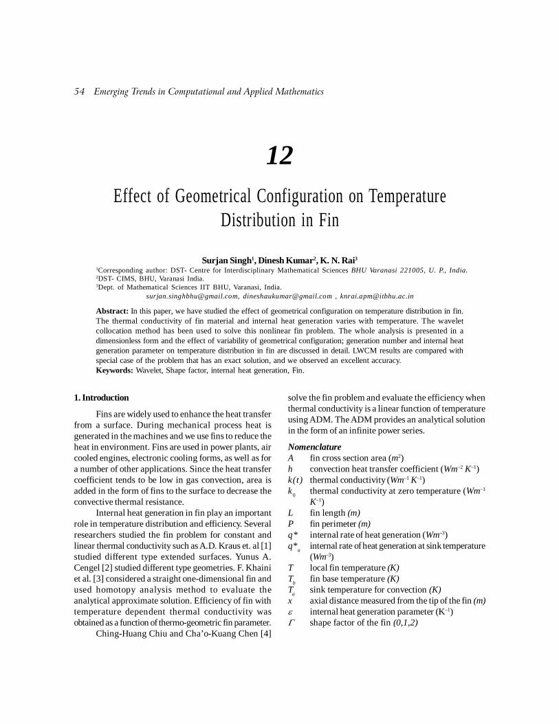
54 Emerging Trends in Computational and Applied Mathematics
1. Introduction
Fins are widely used to enhance the heat transferfrom a surface. During mechanical process heat isgenerated in the machines and we use fins to reduce theheat in environment. Fins are used in power plants, aircooled engines, electronic cooling forms, as well as fora number of other applications. Since the heat transfercoefficient tends to be low in gas convection, area isadded in the form of fins to the surface to decrease theconvective thermal resistance.
Internal heat generation in fin play an importantrole in temperature distribution and efficiency. Severalresearchers studied the fin problem for constant andlinear thermal conductivity such as A.D. Kraus et. al [1]studied different type extended surfaces. Yunus A.Cengel [2] studied different type geometries. F. Khainiet al. [3] considered a straight one-dimensional fin andused homotopy analysis method to evaluate theanalytical approximate solution. Efficiency of fin withtemperature dependent thermal conductivity wasobtained as a function of thermo-geometric fin parameter.
Ching-Huang Chiu and Cha’o-Kuang Chen [4]
solve the fin problem and evaluate the efficiency whenthermal conductivity is a linear function of temperatureusing ADM. The ADM provides an analytical solutionin the form of an infinite power series.
NomenclatureA fin cross section area (m2)h convection heat transfer coefficient (Wm–2 K–1)k(t) thermal conductivity (Wm–1 K–1)k
0thermal conductivity at zero temperature (Wm–1
K–1)L fin length (m)P fin perimeter (m)q* internal rate of heat generation (Wm–3)q*
ainternal rate of heat generation at sink temperature(Wm–3)
T local fin temperature (K)T
bfin base temperature (K)
Ta
sink temperature for convection (K)x axial distance measured from the tip of the fin (m)� internal heat generation parameter (K–1)� shape factor of the fin (0,1,2)
12Effect of Geometrical Configuration on Temperature
Distribution in Fin
Surjan Singh1, Dinesh Kumar2, K. N. Rai3
1Corresponding author: DST- Centre for Interdisciplinary Mathematical Sciences BHU Varanasi 221005, U. P., India.2DST- CIMS, BHU, Varanasi India.3Dept. of Mathematical Sciences IIT BHU, Varanasi, India.
[email protected], [email protected] , [email protected]
Abstract: In this paper, we have studied the effect of geometrical configuration on temperature distribution in fin.The thermal conductivity of fin material and internal heat generation varies with temperature. The waveletcollocation method has been used to solve this nonlinear fin problem. The whole analysis is presented in adimensionless form and the effect of variability of geometrical configuration; generation number and internal heatgeneration parameter on temperature distribution in fin are discussed in detail. LWCM results are compared withspecial case of the problem that has an exact solution, and we observed an excellent accuracy.Keywords: Wavelet, Shape factor, internal heat generation, Fin.

Emerging Trends in Computational and Applied Mathematics 55
Dimensionless parametersG Generation number� thermal conductivity parameterN fin parameterX axial distance measured from the tip of the fin�
Ginternal heat generation parameter
� dimensionless temperature
They compare results with numerical solution,perturbation solution and Galerkin solution andconclude that the decomposition method gives fasterconvergence and higher accuracy in comparison to othermethods. The accuracy of the ADM varying with thenumber of terms in the series is used in solution. CihatArslanturk [5] used ADM to evaluate the efficiency offins with temperature-dependent thermal conductivityand to determine the temperature distribution in fin.ADM provides solution in the form of an infinite powerseries. The efficiency of the straight fins withtemperature-dependent thermal conductivity has beenobtained as a function of thermo-geometric fin parameterand the thermal conductivity parameter describing thevariation of the thermal conductivity. Sin Kim and Cheng-Hung [6] obtained series solution for non-linear finproblem and assumed that the thermal conductivity isthe linear function of temperature and heat transfercoefficient is considered as power Law type form A.Aziz and M. N. Bouaziz [7] solved longitudinal finproblem with temperature dependent internal heatgeneration and thermal conductivity by using theOptimal Linearization Method. They consider thermalconductivity and internal heat generation as a linearfunction of temperature and studied the effect ofdifferent parameters on temperature distribution in finand its efficiency. K. Hosseini et. al [8] solved the finproblem with temperature dependent internal heatgeneration and constant thermal conductivity, usingHomotopy Analysis Method (HAM). The resultsobtained by HAM and numerical procedure are in goodagreement. In available literature, the variation of internalheat generation in general with temperature in fin is notstudied. Mohammadi et. al [9] used Legendre waveletsGalerkin method for solving ordinary differentialequations with non-analytic solution. M. Razzaghi andS. yousefi [10] presented an operational matrix ofintegration based on Legendre wavelets and solvedinitial value problem.
In this study, an attempt has been made to solvea boundary value problem governing the process ofheat transfer in plate fin, cylindrical fin and spherical fin
with temperature dependent internal heat generationand variable thermal conductivity.
Mathematical Formulation
We consider a fin of simple geometricalconfiguration like slab of thickness 2R, circular cylinder
or a sphere of radius R. The density of fin material is ,
specific heat c, area of the fin is A, perimeter is P, thethermal conductivity of fin material is k(T) and theconvection heat transfer coefficient is h(T). The fin isattached to the surface at the fixed temperature T
b and
loses heat by convection to the surrounding medium.The steady state energy balance equation for thetemperature distribution in fin in presence of internalheat generation can be put in the form
The boundary conditions associated with (1) are asfollows:
x = 0,
x = L,
where � is the shape factor (� = 0 for slab, � =1 forcircular cylinder and � = 2 for sphere).The internal heat generation is assumed to be a functionof temperature as follows:
and is the internal heatgeneration at temperature T
a,
We consider the thermal conductivity and heattransfer coefficient as a general function of temperaturei.e.
where and are the thermal conductivity and heat transfercoefficient at ambient temperature.
Introducing dimensionless variables and similaritycriteria.
, ,
, ,
The system of equations (1) to (3) reduce to

56 Emerging Trends in Computational and Applied Mathematics
X = 0,
X=1 ,
Preliminary Concepts
We are presenting certain powerful tools asconcepts properties and description of wavelets,Legendre wavelets and operational matrix of integrationas follows:
(i) Wavelets: Continuous wavelets are definedby the following formula:
a � 0
where a is dilation parameter and b is a translationparameter.
The Legendre wavelets are defined as
,
where =2n-1, n = 1, 2,… ,2k-1, k is any positive integer,,
m is the order of Legendre polynomials and x is thenormalized time.
The Legendre wavelets on the interval (0, 1) aredefined by
where m = 0, 1, …, M-1 and n = 1, 2, …, 2k-1. Here Pm( )
is the well known Legendre polynomials of order m.
m =1, 2, 3, …, M-1A function f(x) defined in domain [0, 1) can be expressedas
where in which < . , . >
denotes the inner product.If we take some terms of infinite series, then (12)
can be written as
Where C and are Matrices given by
(ii) Operational matrix of integration: The
integration of the wavelets which has been definedin (10) can be obtained as [8].
where P is M , k = 1, operational matrixof integration given by
P =
Wavelet Collocation Solution
Let
Integrating equation (25) with respect to x from 0 to x,we have
Again Integrating equation (26) with respect to x from 0to x, we have
At point x = 1 we get
using in equation (27) we
have
Substituting and in (22), (23) and (24), we get
As ( ) is an approximate solution of system (4)to (6). Choosing n collocation points in the interval (0, 1), at which residual equal to zero. The number of such points must be equalto the number of coefficients . Thus,
we get .Solving system of equations separately (29), (30)
and (31) for plate, cylindrical and spherical finrespectively.

Emerging Trends in Computational and Applied Mathematics 57
Exact Solution: In case of a slab fin whose thermalconductivity and heat transfer coefficient is temperature
independent, i.e. , and n = 0, the exact solutionof equations (6) to (8) come out to be
where
Result and discussion
The numerical computation has been made byusing MATLAB software and results are presented intwo tables and eleven figures. In table 1 we compareexact and LWCM results obtained by using nineLegendre Wavelet basis functions, we observe that aswe value of N increases error increases. In table 2 wecompute error for three, five and nine wavelet basisfunctions, we observe that as we increase number ofLegendre Wavelet basis functions error decreases.
The selected reference values are taken as and n =1/4. Figures
presented in this study, only the parameter whosevalues different from reference value are indicated.
For constant thermal conductivity and constantheat transfer, temperature in fin is presented in Figures1 to 4.
In Fig.1 effect of N on temperature distribution infin is presented for plate, cylinder and spherical fin. Inthis figure we observe that as we increase value of ‘N’temperature in fin decreases rapidly. Due to higher heattransfer coefficient, and lower thermal conductivityvalue, fin parameter ‘N’ increases. For higher value of‘N’ heat releases fast in environment, consequentlycooling becomes more effective. From this figure weobserve that temperature in plat fin is lowest for N = 2.For � = 0, 1 and 2, effect of ‘G’ on temperature distributionin fin is presented in Fig.2. As value of G increasestemperature distribution in fin also increases. When �increases from 0 to 1 temperature in fin increases rapidly,but � increase from 1 to 2 temperature increases slowly.Generation number ‘G’ decreases as value of ‘P’ and ‘h’increases. We conclude that decreasing value of G ismore effective for cooling process. Effect of internalheat generation parameter and shape factor ontemperature distribution in fin is presented in Fig.3. Herewe observe that as value of increases temperature in finincreases slowly. As internal heat generation parameterincreases from 0.4 to 0.6, temperature in fin increasesvary slowly for � = 0, but for � = 1 temperature increases
rapidly. temperature difference is small for cylindricalfin and spherical fin. Effect of ambient ‘�
a’ temperature
and shape factor on temperature distribution in fin ispresented in Fig.4. We observe that as value of ‘�
a’
increases temperature in fin increases rapidly. As ambienttemperature ‘�
a’ increases from 0.4 to 0.6, temperature in
fin increases rapidly for � = 0 but slowly for � = 1 and 2.The temperature in fin increases as � increases.
The Fig.5 shows the variation in temperature in afin of constant thermal conductivity and temperaturedependent convection heat transfer coefficient. As valueof increases, temperature in fin decreases while as Nincreases, temperature in fin also increases. Effect of‘�
G’ on temperature distribution in fin for different type
fins is presented in Fig.6. As value of ‘�G’ and � increases,
temperature in fin increases Temperature difference issmall for � = 2, and increases from 0.4 to 0.6, Temperaturedifference in fin is high for �= 0 and increases from 0.4to 0.6. Plat fin is very effective for cooling process.
Effect of on temperature distribution in fin for plat,cylindrical and spherical fins is presented in Fig.7. Asvalue of increases, temperature in fin decreases whileas � increases, temperature in fin also increases.Temperature difference is small for � = 1 and 2, and Nincreases from 1 to 2. Temperature difference in fin islarge for N = 0 and � increases from 0 to 1, but low when� increases from 1 to 2. We conclude that temperaturein fin increases rapidly when plat fin replaced bycylindrical fin. Effect of on temperature distribution ispresented in Fig.8, as we increase value of ‘n’temperature distribution in fin increases with increasingvalue of �.
In Fig.9 the effect of ‘G’ on temperature in fin fortemperature dependent thermal conductivity and heattransfer coefficient, is presented. As value of G increasetemperature distribution in fin also increases. When �increases from 0 to 1, temperature in fin increases rapidly,but ‘�
G’ increase from 1 to 2 temperature increase slowly.
Generation number ‘G’ decreases as value of ‘P’ and ‘h’increases. We conclude that decreasing value of G ismore effective for cooling process. Effect of ‘�
G’ on
temperature distribution when thermal conductivity andheat transfer coefficient is a function of temperature ispresented in Fig.10. As the value of ‘�
G’ increases,
temperature in fin also increases. Variation in temperatureis very small for � = 0, 1, 2 and �
G varies from 0.4 to 0.6.
Effect of ambient temperature ‘�a’ and different
type shape factor on temperature distribution in fin ispresented in Fig.11, here we observe that as ambient

58 Emerging Trends in Computational and Applied Mathematics
temperature ‘�a’ increases from 0.4 to 0.6, temperature in
fin increases rapidly for � = 0 but slowly for � = 1 and 2.Temperature difference in fin increases for � = 0, 1 and2.
In Fig. 12 we observe that as we increase value ofthermal conductivity, temperature in fin increases fortemperature dependent thermal conductivity and heat
transfer coefficient.In Fig 13 we observe that in absence of internal
heat general temperature in fin is decreases, but increasesas � increase form 0 to 1 and 1 to 2 . As value of Gincreases, temperature in fin also increase in absence ofinternal heat generation
Table 1: Comparison of Exact and WCM for ConstantThermal Conductivity and
Values Exact LWCM
N = 1.0, G = 0.2, = 0.2, 0.7976773474 0.7976773475X = 0 G = 0.2, = 0.4, 0.8730832025 0.8730832025
G = 0.4, = 0.4, 0.9615624794 0.9615624794
N = 2.0, G = 0.2, = 0.2, 0.5718371092 0.5718371151
X = 0 G = 0.2, = 0.4, 0.7273924963 0.7273924995
G = 0.4, = 0.4, 0.9148041237 0.9148041245
Table 2: Absolute error in LWCM for different basis function
when G = 0.2, = 0.2, , X= 0.
Parameter Absolute error
M = 3 M = 5 M = 7 M = 9
N=1 2.646E-3 9.9575E-06 1.67E-08 1E-10N=2 1.6605E-2 2.4063E-4 1.59E-06 5.9E-09
0 0.2 0.4 0.6 0.8 10.55
0.6
0.65
0.7
0.75
0.8
0.85
0.9
0.95
1
X
�
�G=0.2, G= 0.2, n=0, �a=0, �=0
N=1,�=0
N=1,�=1
N=1,�=2
N=2,�=0
N=2,�=1
N=2,�=2
0 0.2 0.4 0.6 0.8 10.86
0.88
0.9
0.92
0.94
0.96
0.98
1
X
�
N=1, �G=0.2, n=0,�a = 0, � = 0
G=0.4,�=0
G=0.4,�=1
G=0.4,�=2G=0.6,�=0
G=0.6,�=1
G=0.6,�=2
Fig. 1. Effect of N and geometries on Fig. 2. Effect of G and geometries on temperaturetemperature distribution in fin. distribution in fin.

Emerging Trends in Computational and Applied Mathematics 59
�
0 0.2 0.4 0.6 0.8 10.8
0.82
0.84
0.86
0.88
0.9
0.92
0.94
0.96
0.98
1
X
�
N=1, G=0.2, n=0, �a=0,�=0
�G=0.4,�=0
�G=0.4,�=1
�G=0.4,�=2
�G=0.6,�=0
�G=0.6,�=1
�G=0.6,�=2
0 0.2 0.4 0.6 0.8 10.86
0.88
0.9
0.92
0.94
0.96
0.98
1
X
�
N=1, �G=0.2,G=0.2, n=0, � =0
�a=0.4,�=0
�a=0.4,�=1
�a=0.4,�=2
�a=0.6,�=0
�a=0.6,�=1
�a=0.6,�=2
Fig 3. Effect of �G and geometries on Fig 4. Effect of �
a and geometries on temperature
temperature distribution in fin. distribution in fin
0 0.2 0.4 0.6 0.8 1
0.65
0.7
0.75
0.8
0.85
0.9
0.95
1
X
�
�G=0.2,G=0.2, n=1/4 , �a=0.2,�=0
N=1,�=0
N=1,�=1
N=1,�=2
N=2,�=0
N=2,�=1
N=2,�=2
0 0.2 0.4 0.6 0.8 10.8
0.82
0.84
0.86
0.88
0.9
0.92
0.94
0.96
0.98
1
X
�
N=1, G=0.2, n=1/4,�a=0.2,�=0.0
�G=0.4,�=0
�G=0.4,�=1
�G=0.4,�=2
�G=0.6,�=0
�G=0.6,�=1
�G=0.6,�=2
Fig 5. Effect of N and geometries on Fig 6. Effect of �G and geometries on
temperature distribution in fin. temperature distribution in fin.
0 0.2 0.4 0.6 0.8 1
0.65
0.7
0.75
0.8
0.85
0.9
0.95
1
X
�
n=1/4, �G=0.2, G=0.2, �=0.2, �a=0.2
N=1.0,�=0
N=1.0,�=1
N=1.0,�=2
N=2.0,�=0
N=2.0,�=1
N=2.0,�=2
0 0.2 0.4 0.6 0.8 10.82
0.84
0.86
0.88
0.9
0.92
0.94
0.96
0.98
1
X
�
N =1, �G = 0.2, G=0.2, � = 0.2, �a = 0.2
n=1/4,�=0
n=1/4,�=1
n=1/4,�=2n=2,�=0
n=2,�=1
n=2,�=2
Fig. 7. Effect of N and geometries on temperature Fig 8. Effect of n and geometries on temperaturedistribution in fin, when thermal conductivity distribution in fin, when thermal conductivity andand heat transfer is temperature dependent heat transfer is temperature dependent

60 Emerging Trends in Computational and Applied Mathematics
0 0 .2 0 .4 0 .6 0. 8 10 .9
0 . 9 1
0 . 9 2
0 . 9 3
0 . 9 4
0 . 9 5
0 . 9 6
0 . 9 7
0 . 9 8
0 . 9 9
1
X
�
N = 1 , n= 1 /4 , �G= 0 .2 ,� a= 0 .2 , � = 0 .2
G = 0 .4 ,�= 0
G = 0 .4 ,�= 1
G = 0 .4 ,�= 2G = 0 .6 ,�= 0
G = 0 .6 ,�= 1
G = 0 .6 ,�= 2
0 0 . 2 0 . 4 0 .6 0 .8 10 . 82
0 . 84
0 . 86
0 . 88
0 .9
0 . 92
0 . 94
0 . 96
0 . 98
1
X
�
N = 1 , G = 0 . 2 , n = 1 / 4 ,� a = 0 .2 , � = 0 .2
� G = 0 .4 , � = 0
� G = 0 .4 , � = 1
� G = 0 .4 , � = 2
� G = 0 .6 , � = 0
� G = 0 .6 , � = 1
� G = 0 .6 , � = 2
Fig 9. Effect of G and � on temperature distribution Fig 10. Effect of �G and � on temperature distribution
in fin, when � and h is temperature dependent. in fin, when � and h is temperature dependent.
0 0.2 0.4 0.6 0.8 10. 88
0.9
0. 92
0. 94
0. 96
0. 98
1
X
�
N = 1.0, n= 1/4, �G =0. 2, G = 0.2, �= 0.2
�a= 0.4,�= 0
�a= 0.4,�= 1
�a= 0.4,�= 2
�a= 0.6,�= 0
�a= 0.6,�= 1
�a= 0.6,�= 2
0 0.2 0.4 0.6 0.8 10.84
0.86
0.88
0.9
0.92
0.94
0.96
0.98
1
X
�
N = 1.0, n = 1/4, �G = 0.0, G = 0.2, �a = 0.2
�= 0.4,�= 0
�= 0.4,�= 1
�= 0.4,�= 2
�= 0.6,�= 0
�= 0.6,�= 1
�= 0.6,�= 2
Fig. 11. Effect of G and � on temperature distribution Fig 12. Effect of � and � on temperature distributionin fin, when � and h is temperature dependent. in fin, when � and h is temperature dependent.
0 0.2 0.4 0.6 0.8 10.82
0.84
0.86
0.88
0.9
0.92
0.94
0.96
0.98
1
X
�
N=1.0, n=1/4, �G=0.0, �=0.2, �=0.2
G=0.2,�=0
G=0.2,�=1
G=0.2,�=2G=0.4,�=0
G=0.4,�=1
G=0.4,�=2
Fig13. Effect of G and � on temperature distribution in fin, when no internal heat generation in fin

Emerging Trends in Computational and Applied Mathematics 61
Conclusion
Effect of geometries such as plate, cylinder andsphere on temperature in fin is studied, WaveletCollocation Method has been used in the solution.Cooling is more effective when fin parameter increases.It has been observed that the dimensionless temperatureincreases as shape factor, generation number and internalheat generation parameter, increases or N decreases.Temperature in fin increases for plat cylinder and sphereas value of all the parameters increases except N. Inspecial case exact result and our result are same uptonine decimal places for N = 1. Absolute error decreasesas we increase number of Legendre Wavelet basisfunctions. Temperature in fin is decreases when nointernal heat generation in fin.
Acknowledgement
Authors are grateful to Prof. Umesh Singh Co-ordinator DST- Centre for interdisciplinary MathematicalSciences Banaras Hindu University Varanasi, India forproviding necessary facilities.
REFERENCES
[1] A.D. Kraus, A. Aziz and J. Welty, Extended surfaceheat transfer, John Wiley & sons, INC. 2001.
[2] Yunus A. Cengel, Heat and Mass Transfer: A PracticalApproach, Third Edition, Tata McGraw-Hill NewDelhi, 2007.
[3] F. Khani, M. Ahmadzadeh Raji, H. Hamedi Nejad,Analytical solution and efficiency of the nonlinear finproblem with temperature-dependent thermalconductivity and heat transfer coefficient, CommunNolinear Sci Numer Simulat ,14 (2009) 3327-3338.
[4] Ching-Huang Chiu, Cha’o-Kuang Chen, A decompositionmethod for solving the convective longitudinal fins withvariable thermal conductivity, Int. J. of heat and masstransfer 45 (2002) 2067-2075.
[5] Cihat Arslanturk, A decomposition method for finefficiency of convective straight fins with temperature-dependent thermal conductivity, Int. comm. in Heatand Mass Transfer, 32 (2005) 831-841.
[6] Sin Kim and Cheng-Hung Huang, A series solution ofthe non-linear fin problem with temperature - dependentthermal conductivity and heat transfer coefficient, J.Phys. D: Appl. Phys. 40 (2007) 2979-2987.
[7] A. Aziz, M.N. Bouaziz, A least square method for alongitudinal fin with temperature dependent internalheat generation and thermal conductivity, EnergyConversion and Management 52 (2011) 2876-2882.
[8] K. Hosseini, B. Daneshian1, N. Amanifard, R. Ansari,Homotopy Analysis Method for a Fin with TemperatureDependent Internal Heat Generation and ThermalConductivity, International Journal of Nonlinear ScienceVol.14 (2012) No.2,pp.201-210.
[9 F. Mohammadi, M.M. Hosseini and Syed TauseefMohyud-Din, Legendre Wavelet Galerkin method forsolving ordinary differential equations with non-analyticsolution, Int. J. of Sys. Sci. Vol. 42, No. 4, (2011) 579-585.
[10] M. Razzaghi and S. Yousefi, the Legendre waveletsoperational matrix of integration, Int. J. of SystemsScience, Vol.32, No.4, (2001) 495-502.

62 Emerging Trends in Computational and Applied Mathematics
Introduction
The term ‘nanofluid’ coined by Choi [1] thatdescribes a solid-liquid mixture which consists of fluidsuspension containing tiny particles (1-100nm) andwhich is one of the new challenges for thermal scienceprovided by nanotechnology. The nanoparticles areboth metallic oxide and metal based such as Al
2O
3, CuO,
TiO2, Cu, ZnO and SiO
2. The small insertion of these
nanoparticles enhances the thermal conductivity andhence, heat transfer significantly. The enhancement canbe attributed to the added nanoparticles. As perliterature survey, two different types of mathematicalmodels have been developed; one is single phase modelwhere the thermophysical properties of base fluid areenhanced with the influence of small sized nanoparticles;other is two phase non-homogeneous model with sevenslip mechanisms. Out of these mechanisms, onlyBrownian diffusion and thermophoresis have beenfound to be significant in the absence of turbulenteffects.
The computational model with differentassumptions has been reported for the simulation ofnanofluid convection in thermal boundary-layer flows.
The rotating stretching sheet flows have beenaddressed by a number of authors. Newtonian viscousstudies of stretching sheet flows in a rotating regularfluid have been presented by Wang [2], Lakshmisha etal. [3], Nazar et al. [4] and Javed et al. [5]. Bachok et al.[6] studied the steady flow of an incompressible viscousfluid over a rotating disk in a nanofluid and solvedthe boundary conditions by Keller- Box method. Non-Newtonian viscoelastic rotating stretching sheet hasbeen studied by Sajid et al. [7]. Several studies ofrotating nanofluid flows have been conducted in thepresence or absence of magneto-hydrodynamic effects.Sheikholeslami et al. [8] investigated using homotopyanalysis methods, the convection flow of a nanofluidbetween a stationary surface and a stretching sheet in arotating system, showing that the reduction of heattransfer with the power of rotation parameter. Hamadand Pop [9] studied the transient rotating magneto-hydrodynamic flow of a nanofluid past an oscillatorymoving vertical permeable surface using perturbationmethod. In case of thermal stability, Agarwal andBhadauria [10] studied the effect of rotation on thethermal instability in a horizontal layer of aNewtonian nanofluid. They considered steady weakly
13
Two Phase Model on Unsteady Heat Transfer on a StretchingSheet in a Rotating Nanofluid with Heat Source/Sink
Meenakshi Khurana1, Sangeet Srivastava1*, Puneet Rana2
1*Department of Applied Science, ITM University, Gurgaon2Department of Mathematics, Jaypee Institute of Information Technology, Noida
Abstract: The present investigation focuses to study computationally, the effect of heat source/sink on thetransport behaviour of three dimensional transient rotating boundary layer flow regime over a stretching continuoussheet. The consideration of heat source/sink strongly influences the heat transfer characteristics. The multipleregression estimations for heat transfer analysis have also been conducted for the feasible range of all the significantparameters.Keywords: Nanofluid, boundary layer, Stretching sheet, Rotation, FEM, Brownian motion, Heat source/sink.

Emerging Trends in Computational and Applied Mathematics 63
nonlinear stability analysis in a horizontal rotating layerof a nanofluid using a minimal representation of truncatedfourier series involving only two terms and analyzedthat the rates of heat and mass transfer oscillatevigorously with time initially.
Heat source/sink is basically used to cool a deviceby dissipating heat into the surrounding medium. It hasgreat importance in many physical phenomena. Chamkhaand Aly [11] used FDM to study heat source/sink effectson hydro-magnetic nanofluid boundary layer flow. Abeland Mahesha[12] also studied the magneto-hydrodynamic boundary layer flow and heat transfercharacteristics of a non-Newtonian viscoelastic fluidover a flat sheet with a linear velocity with effect ofthermal radiation and non-uniform heat source/sink andfound that their combined effect have a large impact onrate of heat transfer in boundary layer region. Recently,Rana et al. [13] studied the effect of Heat source /sinkon a steady, mixed convective boundary layer laminarflow and heat transfer along with the vertical plate inincompressible nanofluids and examined the influenceof different types of nanoparticles on heat transfer andflow. Very Recently, Rana et al. [14] studied the behaviourof transient boundary layer MHD over a continuousstretching sheet along with a transverse magnetic fieldand solved 2-D dimensionless boundary layer problemby finite element method. They examined the effect ofboth Brownian motion and thermophoresis on Nusseltnumber and also found that Nusselt number andSherwood number decrease with the increase inrotational parameter.
In this present study, a numerical solution hasbeen developed using a variational finite element methodin which the influence of Heat source/sink parameter isdiscussed and presented graphically. The meshindependent results of present FEM code have alsobeen widely validated with previous published data.
Mathematical Model
Consider 3D magneto-hydrodynamic boundarylayer flow of an incompressible viscous and rotatingnanofluid on a continuous stretching sheet with heatsource/sink effect on it . A uniform magnetic field B
0 is
applied in the transverse direction of the flow. Theboundary layer and Boussinesq approximations areassumed to be valid. The governing equations ofcontinuity, momentum, thermal energy with heat source/sink effect are given by ,
= 0u v w
x y z
� � �� �
� � �
2
20
12 =
nf
nfnf
puu u u u
xu v w vt x y z
B u
�
� �
�� �� � �� � � � � ��� � � � � � �� � � � �� �� �
2
20
12 =
nf
nfnf
pvv v v v yu v w u
t x y zB v
�
��
�� �� � �� � � � � ��� � � � � � �� � � � � ��� �
21= nf
nf
w w w w pu v w w
t x y z z�
�� � � � �� �� � � � � �� �� � � � �� �
� � � �
2
0
=
( ). .
( )
nf
TB
p
T T T Tu v w T
t x y z
Q T TDD C T T T
T c
�
��
� �
�
� � � �� � � �
� � � �
� �� � �� �� � � � � � �� �� �� �� �� �
2 2= TB
DC C C Cu v w D C T
t x y z T�
� �� � � �� � � � � �� �� � � � � �
where u , v and w are the velocity components in thex, y and z directions, respectively, � is the angularvelocity about z-direction, nf� is the effective densityof the nanofluid, nf� is the dynamic viscosity of thenanofluid, nf� is the thermal diffusivity of the nanofluid,T is the nanofluid temperature, nf� is electrical
conductivity of the magnetic nanofluid, 0B is appliedmagnetic field, BD is Brownian diffusion coefficient,
TD signifies thermophoretic diffusion coefficient, � � isratio between the effective heat capacity of thenanoparticle material and heat capacity of the fluid,
2� denotes the three-dimensional Laplacian operator,,C is nanoparticle volume concentration, 0Q is the
volumetric rate of heat generation/absoption, pc� is theheat capacity of the nanofluid, t is time and T� is freestream temperature. For the present physical problem,the relevant boundary conditions are :
< 0: = = = 0, = , = ,
0 : = , = = 0, = , = at = 0,
0 : 0, 0, , as ,w w
t u v w T T C C
t u ax v w T T C C z
t u v T T C C z
� �
� �
�� � � � � ��
Introducing the set of transformation variables,
= , = ( , ), = ( , ),
= , = ( , ), = 1 ,
( , ) = , ( , ) = ,w w
az u axf v axh
at w a f e
T T T T
T T T T
�
� � � � ���
� �� � � �
� � � � �
�
� �
� �
�
� �
� ��
� �

64 Emerging Trends in Computational and Applied Mathematics
Using the above transformations, the continuityequation (1) is satisfied identically by virtue of theCauchy-Riemann equations, and equations (2)-(6)reduce to the following quartet of coupled, nonlinear,partial differential equations in the transformedcoordinate system (�, �) ,
� �
� �
21(1 ) 2
2
= 1
h h fh f h f M h
h
� � � �
� ��
�� � � � �� � � � � �
��
�
� �
(1 )2
1
Le NtLef
Nb
Le
� � �� � � �
�� �
�
�� � � ��� � � �
�� �
�
� �
� �
2Pr(1 ) Pr Pr Pr
2
1 Pr
f Nb Nt
Q
� � �� � � � � �
�� � � �
�
�� � � � � �� � � � �
�� � �
�
� �
(1 )2
1
Le NtLef
Nb
Le
� � �� � � �
�� �
�
�� � � ��� � � �
�� �
�The transformed boundary conditions are:
( ,0) = 0, ( ,0) = 0, ( , 0) = 0,
( ,0) = 1, ( ,0) = 1, ( , ) = 0,
( , ) = 0, ( , ) = 0, ( , ) = 0,
f f h
f
h
� � �� � � � �� � � � �
�� �
� � �
where ( )� denotes prime differentiation with respect to�
and the key thermophysical parameters dictating theflow dynamics are defined by,
� �� �
� �� � � �
20
0
( )= , = , = ,
( )= , ,
Pr = ,
B wp
f
T wp
f p
m
B
c D C CBM Nb
a a c
c D T T QNt Q
c T c a
LeD
���
� � �
�
� � �
���
�
�
�
��
��
�
where � is the rotating parameter , M is the magneticparameter, Pr is the Prandtl number, Nb is Brownianmotion parameter, Nt is the thermophoresis parameter,Q is Heat source/sink parameter, Le is Lewis number.
The reduced Nusselt number and the reducedSherwood number which are defined respectively, asfollows:
=0
=0
= ,( ) ( )
=( ) ( )
w zx
w w
m zx
B w w
Tx
q zNu
T T T T
Cx
q zSh
D C C C C
� � �
� �
�� �� ��� �� � �
� �
�� �� ��� �� � �
� �Using the transformation variables (8), we obtain
1/ 21/2
1/ 21/2
= ( ,0),R
= ( ,0)R
xx
xx
Nu e
Sh e
� � �
� � �
�
�
��
��
where 2= /xRe ax � . is the local Reynolds number..
Numerical FEM Solutions
The nonlinear differential equations (9) to (12)under boundary conditions (13) has been solved usinga variational finite element code [13-14]. In FEM, thediscretization of the domain, element equationsgeneration and assembly have been conducted. Afterimposing the boundary conditions, assembled systemof equations have been obtained which is solved bythe Gauss elimination method supporting throughoutthe computational process an accuracy of 10-4. Theiterative process is terminated when the followingcondition is satisfied:
1 4, ,
,
10m mi j i j
i j
� � � �� ��
where, � stands for either , ,f h � or � , and m denotes
the iterative step. To validate the present FEM code,extensive benchmarking has also been conducted, aspresented in Tables 1, where FEM results have beencompared with solutions obtained by Abbas et al. [15].
The integrations of FEM interpolation functionshas been solved with Gaussian Quadrature.
Results and Discussion
The effect of heat source/sink parameter Q
ranging in the interval � �0.2,0.2� has been plotted formin and max value of other controlling parameter
[0.1,0.5], [0.1,0.5], , [1,5]Nb Nt M�� � � in theFigures1-6. Moreover, both linear and Quadraticregression analysis for heat transfer have beenconducted for the above mentioned range of ,Nb Nt andQ by fixing Pr 5.0, 10.0Le� � for 125 set of results
(i) Linear Regrssion Analysis with adjusted

Emerging Trends in Computational and Applied Mathematics 65
2 0.9295R � and . . 0.0831( 1, 1)S E M�� � �0.9200 1.1954 0.6429 1.32478Nur Nb Nt Q� � � �
(ii) Linear Regression Analysis with adjusted2 0.9295R � and . . 0.1063( 5, 5)S E M�� � �
0.5488 0.7089 0.5055 2.1611Nur Nb Nt Q� � � �(iii) Quadratic Regression Analysis with adjusted
2 0.9978R � and . . 0.0152( 1, 1)S E M�� � �2
2 2
1.2726 2.8460 1.6056 1.7428 1.7767
0.6301 0.9271 1.9487 0.04386
1.4374
Nur Nb Nt Q Nb
Nt Q NbNt NtQ
NbQ
� � � � �
� � � ��
(iv) Quadratic Regression Analysis with adjusted2 0.9955R � and . . 0.0268( 5, 5)S E M�� � �
2
2 2
0.8436 1.8721 1.0901 2.7809 1.2369
0.2725 2.7299 1.4036 0.4265
2.4925
Nur Nb Nt Q Nb
Nt Q NbNt NtQ
NbQ
� � � � �
� � � ��
Reduced Nusselt number is decreasing functionof Nb, and Q both for extreme value of , [1,5]M� �This expressions clarify the behavior of parameters forheat transfer. Moreover, the heat transfer varies quadrati-
cally with the impact of nanoparticles.In Figs. 1-3, the temperature distribution, reduced
Nusselt number and Sherwood number for heat source/sink parameter has been plotted for low values ofrotational and magnetic field. The inclusion of heatsource boost up the temperature in the boundary layerfor given parameter which justifies the decrease of heattransfer. But, the mass transfer increase due to highmovement of nanoparticle with the temperatureenhancement.
The behaviour of heat source/sink parameter forhigh values of rotational and magnetic field is reportedin Figs. 4-6. The negative value of reduced Nusseltnumber for Q = 2.0 shows that nanoparticle can alsoincrease the boundary layer temperature for high valuesof Nb and Nt. But similar behaviour can be depicted forthe case of heat sink which is found to importantparameter in cooling processes in various industries.Thus, heat sink with nanofluid can comparitively amplifythe cooling as compared to regular fluid.
Table 1:Comparitive values of (0)� � for 1� � for different values of ,M� with Pr 7.0� .
Abbas et al.[15] Present Results
M=0.5 M=1.0 M=2.0 M=0.5 M=1.0 M=2.0
0 -1.870 -1.805 -1.626 -1.8696 -1.8047 -1.62620.5 -1.840 -1.787 -1.621 -1.8357 -1.7867 -1.62121.0 -1.778 -1.746 -1.607 -1.7784 -1.7459 -1.60702.0 -1.661 1.646 -1.558 -1.6609 1.6463 -1.55825.0 -1.363 -1.367 -1.359 -1.3627 -1.3668 -1.3586
Fig. 1: Temperature profile ( , )� � � showing Fig. 2. Reduced Nusselt number, 1/ 2Rex xNu
effect of Heat source/sink parameter showing effect of Heat source/sinkfor 0 .1, 1 .0N b N t M �� � � � parameter for 0.5, 5.0Nb Nt M �� � � �

66 Emerging Trends in Computational and Applied Mathematics
Fig. 3. Effect of Heat source/sink parameter ReducedSherwood number, 1/ 2Rex xSh showing for
0.1, 1.0Nb Nt M �� � � �
Fig. 4.Temperature profile ( , )� � � showing effect of
Heat source/sink parameter for
0.5, 5.0Nb Nt M �� � � �
Fig. 5. Reduced Nusselt number, 1 / 2R ex xN u showingeffect of Heat source/sink parameterfor 0 .5 , 5 .0N b N t M �� � � �
Fig. 6. Reduced Sherwood number, 1 / 2R ex xS h showingeffect of Heat source/sink parameter
for 0 .5 , 5 .0N b N t M �� � � �
Conclusions
The paper deals with the numerical study of heatsource/sink parameter for rotating stretching sheetproblem with finite element method. For the fixed valueof rotation and magnetic parameter, the correlation
showing the effect of ,Nb Nt and Q have been
calculated for feasible set of parameter which justifiesthe importance of heat source/sink parameter. In orderto control the heat transfer, we can modulate the valueof heat source/sink parameter. But the limitation of thismodel is to actively control the value of nanoparticlevolume fraction at the boundaries. We are updating thepresent model for the case of zero nanoparticle flux [16]which will be discussed in future communications.
REFERENCES
[1] S. U. S. Choi, “ Enhancing thermal conductivity of fluidswith nanoparticles in developments and applications ofnon-Newtonian flows,” ASME J. Fluids Engineering66, 99–105 (1995).
[2] C. Y. Wang, “Stretching a surface in a rotating fluid”,ZAMP- J. Applied Mathematics and Physics 39, 177-185 (1988).
[3] K.N.Lakshmisha, S.Venkateswaran and G.Nath, “Three-dimensional unsteady flow with heat and mass transferover a continuous stretching surface,” ASME J. HeatTransfer 110, 590-595 (1988).
[4] R. Nazar, N. Amin and I. Pop, “Unsteady boundarylayer flow due to a stretching surface in a rotating fluid,”Mechanics Research Communications 31, 121-128(2004).
[5] T. Javed, M. Sajid, Z. Abbas and N. Ali,” Non-similar

Emerging Trends in Computational and Applied Mathematics 67
solution for rotating flow over an exponentiallystretching surface,” Int. J. Numerical Methods HeatFluid Flow 21, 903-908 (2011).
[6] Norfifah Bachok, Anuar Ishak, Loan Pop,”Flow andheat transfer over a rotating porous disk in a nanofluid,”Physica B 406,1767–1772 (2011)
[7] M. Sajid, Z. Iqbal, T. Hayat and S. Obaidat, “Seriessolution for rotating flow of an upper convectedMaxwell fluid over a stretching sheet,” Commun. Theor.Phys. 56, 740 (2011).
[8] M.Sheikholeslami, H.R.Ashorynejad, G. Domairry andI. Hashim, “Flow and heat transfer of Cu-water nanofluidbetween a stretching sheet and a porous surface in arotating system,” J.Applied Mathematics 2012, 1-18(2012).
[9] M. A. A. Hamad and I. Pop, “Unsteady MHD freeconvection flow past a vertical permeable flat plate in arotating frame of reference with constant heat source ina nanofluid,” Heat Mass Transfer 47, 1517–1524 (2011).
[10] Shilpi Agarwal ,B. S. Bhadauria,“Unsteady heat andmass transfer in a rotating nanofluid layer,” ContinuumMech. Thermodyn,doi: 10.1007/s00161-013-0309-6.
[11] A. J. Chamkha and A. M. Aly, “MHD free convectionflow of a nanofluid past a vertical plate in the presenceof heat generation or absorption effects,” Chemical
Engineering Communications 198, 425-441 (2011).[12] M. Subhas Abel ,N. Mahesha, ”Heat transfer in MHD
viscoelastic fluid flow over a stretching sheet withvariable thermal conductivity,non-uniform heat sourceand radiation,” Applied Mathematical Modelling 32,1965–1983 (2008)
[13] P.Rana and R.Bhargava, ”Numerical study of heattransfer enhancement in mixed convection flow along avertical plate with heat source/sink utilizing nanofluids,”Commun Nonlinear Sci Numer Simulat 16, 4318–4334(2011).
[14] P.Rana and R.Bhargava, ”Finite element simulation ofunsteady magneto-hydrodynamic transport phenomenaon a stretching sheet in a rotating nanofluid,” Journal ofNanoengineering and Nanosystems 227, 77-19 (2013).
[15] Z. Abbas, T. Javed, M. Sajid and N. Ali, “UnsteadyMHD flow and heat transfer on a stretching sheet in arotating fluid,” J. Taiwan Institute of Chemical Engineers41, 644-650 (2010).
[16] A.V. Kuznetsov , D.A. Nield ,”The Cheng–Minkowyczproblem for natural convective boundary layer flow in aporous medium saturated by a nanofluid: A revisedmodel”, International Journal of Heat and Mass Transfer65 (2013) 682–685.

68 Emerging Trends in Computational and Applied Mathematics
Introduction
Diffusion rates can be tremendously altered bychemical reactions. Chemical reactions can be codifiedas either heterogeneous or homogeneous processes.This depends on whether they occur at an interface oras a single phase volume reaction. In well-mixed systems,the reaction is heterogeneous, if it takes place at aninterface and homogeneous, if it takes place in solution.In most cases of chemical reactions, the reactions ratedepends on the concentration of the species itself. Areaction is said to be of first order, if the rate of reactionis directly proportional concentration (Cussler [1]). Inmany chemical engineering processes, there is thechemical reaction between a foreign mass and the fluidin which the plate is moving. These processes take placein numerous industrial applications such asmanufacturing of ceramics, food processing andpolymer production. Bourne and Dixon [2] analyzed thecooling of fibers in the formation process. Thermalboundary layer growth on continuously movinghorizontal belts studied by Griffin and Throne [3].
Soundalgekar [4] presented an exact solution tothe flow of a viscous fluid past an impulsively startedinfinite isothermal vertical plate with mass transfer.Chemical reaction effects on heat and mass transfer onlaminar boundary layer flow have been discussed invarious situations by Apelblat [5]. Das et al. [6] studiedeffects of mass transfer and chemical reaction onimpulsively started infinite vertical plate with constantheat flux. The effect of temperature-dependent viscosityon the mixed convection flow from vertical plate isinvestigated by Kafoussias and Williams [7] andMuthucumaraswamy and Ganesan [8]. The study ofheat and mass transfer with magnetic effect is ofconsiderable importance in chemical and hydro-metallurgical industries. Effect of heat and mass transferon non linear MHD boundary layer flow have beendiscussed by Gupta and Gupta [9], Brady and Acrivos[10] in various situations. Revankar [12] pioneered innatural convection effects on flow past a moving plate.In industrial applications, it is quite often that the platetemperature starts to oscillate about a non-zero mean
14Influence of Chemical Reaction on MHD Free Convective Flow
Past an Infinite Vertical Oscillating Plate
Hemant Poonia1, R. C. Chaudhary2
1Deptt. of Math & Stat, CCSHAU, Hisar-125004.2Deptt. of Maths, Univ. of Rajasthan, Jaipur-302022.
[email protected], [email protected]
Abstract: An exact solution to the problem of a viscous incompressible MHD free convective flow past an infinitevertical oscillating plate with variable temperature and uniform mass diffusion is presented here, taking intoaccount of the homogeneous chemical reaction of first-order. The plate temperature is raised linearly with respectto time and the concentration level near the plate is raised to wC� . The dimensionless governing equations are solvedby using the Laplace-transform technique. The velocity and concentration are studied for different parameters likechemical reaction parameter, Schmidt number and time. Temperature profile, skin-friction, Nusselt number andSherwood number are also studied and depicted graphically. It is observed that the velocity decreases withincreasing magnetic parameter, whereas, increases with increasing chemical reaction parameter.Keywords: Chemical reaction, MHD, Oscillating vertical plate, Heat and Mass transfer.

Emerging Trends in Computational and Applied Mathematics 69
temperature. The flow past a surface with oscillatingtemperature was elucidated by Takhar et al. [11], Li et al.[13] and saeid [14]. Muthucumaraswamy [15] studiedeffects of chemical reaction on moving isothermalvertical plate with variable mass diffusion. Kandasamyet al. [16] discussed on effects of chemical reaction,heat and mass transfer along a wedge with heat source.Oscillating flow and heat transfer in a rigid tube ofvarying cross-section with permeable wall analyzed byMakinde [17]. Muthucumaraswamy [18] analyzedchemical reaction effects on vertical oscillating platewith variable temperature and uniform mass diffusion.
In this paper we have generalizedMuthucumaraswamy [18] by considering the effects ofhomogeneous chemical reaction of first order and freeconvection on the oscillating infinite vertical plate withvariable temperature and uniform mass diffusion in thepresence of uniform magnetic field. It is noted that ourpresent solution reduces to Muthucumaraswamy [18]results by taking the magnetic parameter equal to zerowhich provides a useful mathematical check. Thedimensionless governing equations are solved usingthe Laplace-transform technique. The solutions are interms of exponential and complementary error function.
Mathematical Analysis
First order chemical reaction effects on unsteadyflow of a viscous incompressible fluid past an infinitevertical oscillating plate with variable temperature anduniform mass diffusion in the presence of uniformmagnetic field is studied. It is assumed that the effect ofviscous dissipation is negligible in the energy equationand there is a first order chemical reaction between the
diffusing species and the fluid. The x� - axis is takenalong the plate in the vertically upward direction and
the y� - axis is taken normal to the plate. Initially, the
plate and the fluid are at the same temperature T�� and
concentration C�� . At time t�> 0, the plate starts
oscillating in its own plane with frequency �� and thetemperature of the plate is raised linearly with respect totime and concentration level near the plate is raised
to wC� . Then by usual Boussinesqs’ approximation, theunsteady flow is governed by the following equations:
� � � �*ug T T g C C
t� �� �
�� � � � �� � � ���
220
2
Buu
y
��
��� �� ���
2
2p
T TC k
t y�
� �� ��
� �� �2
2
C CD K C
t y
� �� � � �� �� �� �
With the following initial and boundary conditions:
� � � �0
0, 0, ,
cos , ,
0, 0
0, ,
w
w
t u T T C C for all y
u u t T T T T At
t C C at y
u T T C C as y
�� �
� �
� �
� � � � � � �� � � � ��� � � � � � � �� � � �� ��
� ��� � � �� � �� ��� ��� � � � � �� � � ��� ��
Where,
20u
A�
�
On introducing the following non-dimensionalquantities:
� �
� �
20 0
0
30
*
30
20
2 2 20 0 0
, , , ,
,
, , ,
, ,
w
wr
w
pwc r c
t u y u T Tuu t y
u T T
g T TC CC G
C C u
Cg C CG P S
u k D
BKK M
u u u
�� �
��
�� � �
� �� � ��
�
�
�
��
�
�
� � � �� ��� � � � �� �� �
�� ��� ��� � �
� �� ��
� �� �� � � ��
� � �� � � �
�
Using (5) in equations (1) to (4), leads to
2
2r c
u uG G C Mu
t y�
� �� � � �
� �
2
2
1
rt P y
� �� ��
� �
2
2
1
c
C CKC
t S y
� �� �
� �The initial and boundary conditions in non-
dimensional form are:

70 Emerging Trends in Computational and Applied Mathematics
� �0, 0, 0, 0
cos , , 1 00,
0, 0, 0
t u C for all y
u t t C at yt
u C as y
�
� �
�
� � � � ��
� � � �� ��� � ��� � � ��� ��All the physical variables are defined in the
nomenclature. The solutions are obtained forhydrodynamic flow field in the presence of first orderchemical reaction.
The dimensionless governing equations (6) to (8),subject to the boundary conditions (9), are solved bythe Laplace-transform technique and the solutions arederived as follows:
� �2
2
,2 2
exp4
r r
r r
P y Pyy t t erfc
t
Pt P yy
t
�
�
� �� �� � � �� � � �� � � �
� �� �� �
� �
� �� �
� �
exp21
,2
exp2
cc
cc
Syy KS erfc Kt
tC y t
Syy KS erfc Kt
t
� �� ��� �� �� �� �� �� � �
� �� �� � �� �� �� �� �� �
� � � � � �� � � �
� �
1, exp exp
4
exp2
2
u y t i t y M i
yerfc M i t y M i
t
yerfc M i t
t
� �
� �
�
�� � ��
� �� � � �� �� �
�� �� � �� �� ��
� �� � � �
� � � �
exp21
exp4
exp2
yy M i erfc M i t
ti t
yy M i erfc M i t
t
� �
�
� �
� �� �� � � �� �� �� �� ��
� �� �� � � �� �� �
� �� �
� �
� �
1 5 exp2 2
exp2
t ya a y M erfc Mt
t
yy M erfc Mt
t
� � � �� ��� � �
� ����� �� � � �� �
� ��
� �exp4 2
y yy M erfc Mt
M t
� � �� � �� � �
� ��
� �exp2
yy M erfc Mt
t
��� �� � ��� �� ���
� � � �
� �
26 7 1 5
1exp
2 2
exp2
ya a a a y M erfc Mt
t
yy M erfc Mt
t
� � �� � �� � �
� ���� �
� � � �� �� ��
� �� �
� �
� �
21 5
2
2 2
2 2
exp2
exp2
exp2
r
r r
r r
a aa P M t
yy a P erfc a P t
t
yy a P erfc a P t
t
� �
� � ��� � �� ��
�� �� � � �� �� ��
� �� � � �
� �
6 73 3 3
3 3
exp exp2 2
exp2
a a ya M t y a erfc a t
t
yy a erfc a t
t
� � �� � �� � �
� ���� �� � � �� �
� ��
� � � �
� �
12 2 22
2
2 2
exp exp2 2
exp2
rr
rr
a Pya t y a P erfc a t
a t
Pyy a P erfc a t
t
� � �� �� � �� �� � ��
�� �� � � �� �� ��� ��
21 122 2
2
2 2 2
exp4
r r r
r r
a P a y P Py yerfc t erfc
a t a t
Pt y Py
t�
�� � � �� �� � ��� � � �� �� � � �� ��� � � ��
�� �� � �� �
� ��
� �
� �
� �
4
4
exp2
2exp
2
exp2
cc
cc
c
Syy KS erfc Kt
ta
K Syy KS erfc Kt
t
Sa yerfc Kt
K t
� �� ��� �� �� �� �� �� � �
� �� �� � �� �� �� �� �� �� �
� �� �� �� �

Emerging Trends in Computational and Applied Mathematics 71
Where,
� �1 2 3 4, , , ,
1 1 1c cr
r r c c
M K S GG Ma a a a
P P S S K M
�� � � �
� � � � �
5 6 72 3
1 1, ,
1c
r c
Ga a a
M a P S M a� � �
� � �In order to get the physical insight into the
problem, the numerical values of u have been computedfrom (12).
� �erfc x being the complementary error functiondefined by
� � � � � � � �2
0
21 , exp
x
erfc x erf x erf x d� ��
� � � ��and � �1 1erfc X iY� is the complementary errorfunction of the complex argument which can becalculated in terms of tabulated numerical values of the
auxiliary function � �1W z , 1 1z X iY� � [19]. The table
given in [19] does not give � �1 1erfc X iY� directly but
an auxiliary function � �1 1 1W X iY� that is defined as:
� � � � � �� �2
1 1 1 1 1 1 1experfc X iY W Y iX X iY� � � � � �
Some properties of � �1 1 1W X iY� are
� � � �1 1 1 2 1 1W X iY W X iY� � � �
� � � �� � � �2
1 1 1 1 1 2 1 12expW X iY X iY W X iY� � � � � �
Where, � �2 1 1W X iY� is complex conjugate of
� �1 1 1W X iY� .
Nusselt number
0y
Nuy
�
�
� ��� �� ��� �
2 rP tNu
��
Sherwood number
0y
CSh
y �
� ��� �� ��� �
� � � �expcc
SSh KS erf Kt Kt
t�� � �
Skin-friction
0y
u
y�
�
� ��� �� ��� �
� � � �� �� � � �� �
1exp
21
exp2
i t M i erf M i t
i t M i erf M i t
� � � �
� � �
� � �
� � � �
� � � �
� � � � � �
1 5
26 7 1 5
exp 1
2
exp
Mta a t M erf Mt
t M
tMt a a a a M erf Mt
�
�
� �� �� � ��� �� ��
�� � � ��
�
� �� � � �21 5 2 2 2exp r r ra a a P M t a P erf a P t� �
� �� � � �� � � �
6 7 3 3 3
12 2 22
2
exp
exp r
a a a M t a erf a t
aa t a P erf a t
a
� �
�
� �1 4
2 2
2 1rc
a P at KS erf Kt
a Ka t�
� �� � �� �� �
� � ... (15)
Result and Discussion
In order to get a physical view of the problemnumerical calculations are carried out for different valuesof the magnetic parameter, chemical reaction parameter,Schmidt number and time. The purpose of thecalculations given here is to asses the effect of differentM, K, Sc and t upon the nature of the flow and transport.The Laplace-transform solutions are in terms ofexponential and complementary error function.
Fig. 1. Velocity distribution for various values of K

72 Emerging Trends in Computational and Applied Mathematics
Fig. 2. Velocity distribution for various values of Sc
In figure 1, 2 and 3, we depict the effects ofchemical reaction parameter (K), the Schmidt number(Sc) and the magnetic parameter (M) on the velocityprofile. We see that the velocity profile rises rapidly atthe plate from zero, attains a maximum before decreasingexponentially far away from the plate as increasing y. Itis also observed that the velocity profile decreases withincreasing chemical reaction parameter, the Schmidtnumber and the magnetic. This is because of the factthat the application of the transverse magnetic field toan electrically conducting fluid gives rise to a respectivetype of a force known as Lorentz force. This force hasthe tendency to slowdown the motion of the fluid in theboundary layer.
Fig. 3. Velocity distribution for various values of M
Fig. 4. Velocity distribution for various values of �t
Fig. 5. Velocity distribution for various values of Gc
Figure 4, shows the effects of the phase angle(�t) on velocity profile against y. It is concluded thatthe velocity profile increases as decreasing phase angle(�t). In figure 5 and 6, we depict the effects of the solutalGrashof number (Gc) and the thermal Grashof number(Gr) on velocity profile against y. The behaviour of thevelocity profiles is same as discussed in figure 1. It isalso observed that an increase Gc and Gr leads to increasein the velocity profile.

Emerging Trends in Computational and Applied Mathematics 73
Fig. 6. Velocity distribution for various values of Gr
Fig. 7. Velocity distribution for various values of t
Figure 7, represents the effects of the effects ofthe time on the velocity profile against y. The velocityprofile moves as figure 1 against y. It is also examinedthat the velocity profile decreases between 0 ? y ? 0.6,and then increases with increasing the time.
Result and Discussion
In order to get a physical view of the problemnumerical calculations are carried out for different valuesof the magnetic parameter, chemical reaction parameter,Schmidt number and time. The purpose of thecalculations given here is to asses the effect of differentM, K, Sc and t upon the nature of the flow and transport.The Laplace-transform solutions are in terms ofexponential and complementary error function.
Figure 8, 9 and 10, represent the effects of chemicalreaction parameter, the Schmidt number and time on theconcentration profile against y. The concentrationprofile decreases exponentially as increasing y. It is alsoconcluded that the concentration profile decrease as
increasing K and Sc as shown in figure 8 and 9, whereas, in figure 10, the concentration profile increases asincreasing the time.
Fig. 8. Concentration dist. for various values of K
Fig. 9. Concentration dist. for various values of Sc
Fig. 10. Concentration dist. for various values of t
Figure 11, shows the effects of the time on thetemperature profile against y. The temperature profiledecreases exponentially as increasing y. It is also

74 Emerging Trends in Computational and Applied Mathematics
concluded that an increase in the time results in thetemperature profile. In figure 12, the Nusselt number(Nu) increases rapidly as increasing time.
Figure 13, show the effects of chemical reactionparameter and the Schmidt number on the Sherwoodnumber (Sh) against time. In both figures, the Sherwoodnumber decreases steadily between 0 < t ? 0.2, afterthen decreases very slightly. It is also concluded thatan increase in K and Sc leads to increase in the Sherwoodnumber.
Fig. 11. Temperature dist. for various values of t
Fig. 12. Nusselt number against t
In figure 14, we depict the effects of the chemicalreaction parameter, the Schmidt number and themagnetic parameter on the skin-friction against time. Itis examined that the skin-friction increases as increasingK, Sc and M.
Fig. 13 .Sherwood number for variousvalues of K & Sc
Figure 15, represents the effects of the thermalGrashof number, the solutal Grashof number and the phaseangle on the skin-friction against t. It is observed that theskin-friction decreases as increasing Gr, Gc and �t.
Fig. 14. Skin-friction for various values of K, Sc, M
Fig. 15. Skin-friction for various values of Gr, Gc & �t

Emerging Trends in Computational and Applied Mathematics 75
Conclusions
First order chemical reaction effects on unsteadyMHD flow past an infinite vertical oscillating plate inthe presence of variable temperature and constant massdiffusion is studied. The dimensionless equations aresolved using Laplace-transform technique. The effectsof velocity, temperature and concentration profile fordifferent physical parameters like M, K, Sc, Gc, Gr and�t are studied. Skin-friction, Nusselt number andSherwood number are also displayed through graphs.From results we concluded that
1. The velocity profile decreases as increasingK, Sc, M and �t, whereas, increases asincreasing Gc and Gr.
2. An increase in time leads to increase intemperature profile and Nusselt numberincreases with time.
3. The concentration profile increases withtime, whereas, decreases as increasingchemical reaction parameter and the Schmidtnumber.
4. Skin-friction increases as increasing thechemical reaction parameter, the Schmidtnumber and the magnetic parameter, whereas, decreases as increasing the thermalGrashof number, the solutal Grashof numberand the phase angle.
5. An increase in K and Sc results to increasein the Sherwood number.
Nomenclature
C� - Concentration in the fluid, 3.mol m�
C - Dimensionless concentration
pC - Specific heat at constant
pressure, 1 1. .J Kg K� �
D - Mass diffusion coefficient, 2 1.m s�
cG - The solutal Grashof number
rG - The thermal Grashof number
g - Acceleration due to gravity,, 1.m s�
k - Thermal conductivity,, 1 1Wm K� �
K � -Chemical reaction parameter, J
K - Dimensionless chemical reaction parameter
M - The magnetic parameter
rP - Prandtl number
cS - Schmidt number
T � - Temperature of the fluid near the plate, K
t� - Time, st - Dimensionless time
u� - Velocity of the fluid in the x� - direction,1.m s�
0u - Velocity of the plate, 1.m s�
u - Dimensionless velocity
y� - Coordinate axis normal to the plate, my - Dimensionless coordinate axis normal to the
plate
Greek symbols
� - Thermal diffusivity,, 2 1.m s�
� - Volumetric coefficient of thermal
expansion, 1K �
*� - Volumetric coefficient of expansion with
concentration, 1K �
� - Coefficient of viscosity, Pa.s
� - Kinematic viscosity,, 2 1.m s�
� - Density of the fluid, 3.Kg m�
� - Dimensionless skin-friction
� - Dimensionless temperature
erfc - Complementary error function
erf - Error function
REFERENCES
[1] Cussler E. L., “Diffusion mass transfer in fluid systems.”Cambridge Univ. Press, London (1988).
[2] Bourne, D. E. and Dixon, H., “The cooling of fibres inthe formation process.” Int. J. Heat and Mass Transfer,34, 1323-1332 (1971).
[3] James, F. Griffin and James, L. Throne, “On thermalboundary layer growth on continuous moving belts.”AICHE J., 13, 1210-1211 (1967).
[4] Soundalgekar, V. M., “Effects of mass transfer and freeconvection on the flow past an impusively started verticalplate.” ASME Journal of Applied Mechanics, 46, 757-760 (1979).

76 Emerging Trends in Computational and Applied Mathematics
[5] Apelblat, A., “Mass transfer with a chemical reactionof the first order effects of axial diffusion.” The ChemicalEngineering Journal, vol. 23, 193-201 (1982).
[6] Das, U. N.; Deka, R. K. and Soundalgekar, V. M., “Effectsof mass transfer on flow past an impulsively startedinfinite vertical plate with constant heat flux and chemicalreaction.” Forschung im Ingenieurwesen, 60, 284-287(1994).
[7] Kafoussias, N. G. and Williams, E. W., “Effects oftemperature dependent viscosity on free-forcedconvective laminar boundary layer flow past a verticalisothermal flat plate.” Acta Mech., 110, 123 (1995).
[8] Muthucumaraswamy, R. and Ganesan, P., “Effects ofthe chemical reaction and injection on flowcharacteristics in an unsteady upward motion of anisothermal plate.” J. Appl. Mech. Tech. Phys., 42, 665(2001).
[9] Gupta, P. S. and Gupta, A. S., “Heat and mass transferon a stretching sheet with suction and blowing.” CanadianJ. of Chemical Engineering, 55, 744-746 (1977).
[10] Brady, J. F. and Acrivos, A., “Steady flow in a channelor tube with accelerating surface velocity, an exactsolution to the Navier-stokes equations with reverseflow.” Journal of Fluid Mechanics, 112, 127-150 (1981).
[11] Takhar, H. S. and Soundalgekar, V. M., “Heat transfer inflow past a semi-infinite plate with oscillating plate.”Flow. Turbul. Combust., 46, 159-164 (1989).
[12] Revankar, S. T., “Free convection effect on a flow past
an impusively started or oscillating infinite verticalplate.” Mech. Res. Commun., 27, 241-246 (2000).
[13] Li, Jain; Ingham, D. B. and Pop, I., “Natural convectionfrom a vertical flat plate with a surface temperatureoscillation.” Int. J. Heat Mass Transfer, 44, 2311-2322(2001).
[14] Saeid, Nawaf H. (2003): “Transient free convection fromvertical wall with oscillating surface temperature.”AJSTD, vol. 20, 261-269.
[15] Muthucumaraswamy, R., “Effects of chemical reactionon moving isothermal vertical plate with variable massdiffusion.” Theoret. Appl. Mech., 30, 209-220 (2003).
[16] Kandasamy, R.; Periasamy, K. and Sivagnana Prabhu,K. K., “Effects of chemical reaction, heat and masstransfer along a wedge with heat source andconcentration in the presence of suction or injection.”Int. J. Heat mass Transfer, 48, 1388-1394 (2005).
[17] Makinde, O. D., “Asymptotic approximations foroscillating flow in a tube of varing cross-section withpermeable isothermal wall.” Rom. Journ. Phys., 52, 61-72 (2007).
[18] Muthucumaraswamy, R., “Chemical reaction effects onvertical oscillating plate with variable temperature.”Chemical Industry and Chemical Engineering Quarterly,16, 167-173 (2010).
[19] Abramowitz, B. M. and Stegun, I. A., Handbook ofMathematical Functions, Dover Publication, Inc., NewYork (1972).

Emerging Trends in Computational and Applied Mathematics 77
Introduction
Natural convection in enclosures is encounteredin many engineering systems such as convection inbuildings, fluid movement in solar energy collectors,cooling of electronic equipments, etc. Natural convectionbetween a cylinder and its surrounding medium hasbeen a problem of considerable importance. This problemhas a wide range of applications, such as crude oilstorage tanks, heat exchangers, flooding protection forburied pipes and solidification processes.
Most of the studies on the natural convectionfrom a heated cylinder embedded in the cold enclosurethat have not been filled by anything. In some buildingservice situations, a pipe carrying hot water passesthrough an enclosure formed by structural componentsof the building such as filled with insulation to reducethe heat transfer rate from the pipe. The insulation couldbe made from a porous medium [1]. Rotating cylinderplaced in the center of the enclosure filled with porousmedium was studied by [2]. The active cylinder wasfound to enhance the heat transfer rate. Passive effortsto enhance the heat transfer of porous media are byfilling the enclosure by nanoliquids [3].
In engineering, nanoliquids [4] refer to nanometer-
sized metallic or non-metallic particles dispersed in abase liquid having relatively low thermal conductivitylike water and ethylene glycol in order to obtain a liquidwith improved thermo-physical properties. In the presentstudy, Al2O3 nanometer-sized with variousconcentrations dispersed in water are considered. Theporous enclosure having an inner hot circular cylinderis embedded in the center. The main objective is toexamine the implications of the rheological behavior onthe convective flow distribution and the heat transfer.
Fig. 1. Schematic representation of the model.
15Natural Convective Flow Around a Heated Cylinder Inside a
Porous Enclosure Filled with Nanoliquids
Habibis Saleh, Ishak HashimSchool of Mathematical Sciences & Solar Energy Research Institute Faculty of Science & Technology
Universiti Kebangsaan Malaysia43600 UKM Bangi, Selangor, [email protected], [email protected]
Abstract: Natural convective heat transfer and fluid flow around a heated cylinder inside a porous enclosure filledwith nanoliquids is studied numerically. We found that an optimum cylinder radius is exist, below which theincreasing cylinder radius increases the strength of flow circulation and above which the cylinder radius decreasesthe strength of flow circulation. The optimum values change by varying the nanoparticles concentration. The heattransfer rate was found to increase linearly by increasing the nanoparticles concentration for all cylinder radius.Keywords: Natural convection, Porous media, Nanoliquids

78 Emerging Trends in Computational and Applied Mathematics
Mathematical formulation and method
A schematic diagram of a square porous enclosurehaving an inner hot circular cylinder is shown in Figure1. Walls of the enclosure were kept at a cold temperature.The cylinder with radius r is located in the center of theenclosure. The liquid in the enclosure is a water-basednanofluids containing Al2O3 nanoparticles. In this study,the nanoliquids flow is set to be incompressible andlaminar. It is presumed that the water and thenanoparticles are in thermal equilibrium and no slipoccurs between them. Meanwhile, the Boussinesqapproximation is employed and homogeneity and localthermal equilibrium in the porous medium is assumed. Itis also assumed that nanoparticles are suspended inthe nanoliquids using either surfactant or surface chargetechnology. As a result, in keeping with the Darcy’s lawand adopting the nanoliquids model proposed by [5],Under the above assumptions, the dimensionlessgoverning equations are:
2 2
2.5 2 2
1[(1 )
(1 )Ra
X Y
� �� � � �� � � �� �� � �� �
��
��
] ...( / )( / ) sp bf sp bf X
Y X X Y
���
��� �� �� ��
� �� � � �
� � � � �
�2 2
2 2 nf
bf X Y
� �� � � ��� �� �� �
�
�
Streamfunction are zero on the walls and cylindersurface, the dimensionless boundary conditions fortemperature are:
0 on walls � �� �1 on cylinder surface � �
Once we know the temperature we can measurethe heat transfer performance. The total heat transferrate across the cavity in terms of the average Nusseltnumber are defined as
1
0
0
1
0
1
d at cold wall
d ....(at hot wall
nfc
bfX
nfh
bfX
kNu Y
k X
kNu Y
k X
�
�
� �� � ��� � �� �� � �� �� �� �
� �� � ��� � �� �� � �� �� �� �
�
�
The governing equations along with theboundary conditions are solved numerically by the CFDsoftware package COMSOL Multiphysics. COMSOLMultiphysics (formerly FEMLAB) is a finite elementanalysis, solver and simulation software package forvarious physics and engineering applications. Weconsider the following application modes in COMSOLMultiphysics. The Poisson Equations mode (poeq) forEq. (1), the Heat Transfer Equations mode (ht) for Eq.(2). In this study, mesh generation on square enclosurehaving an inner circular cylinder is made by usingtriangles. The triangular mesh distribution calibrates forfluid dynamics condition.
Result and discussion
Figure 2 presents Streamlines and isothermsevolutions of nanoliquids (solid lines) and pure-liquid(dashed lines) by varying the cylinder radius. The flowcirculates and temperature distributes near the relativesmall cylinder and upper region of the enclosure. Pair ofsecondary vortices are formed above the cylinder forbase liquid. The streamlines and isotherms structure ofpure- liquid has a mirror symmetric pattern about thevertical center line of the enclosure. Multi upwellingplume with asymmetrically shape are observed at thesufficiently large cylinder. The strength of nanofluidsflow circulation are weaker than base liquid flowcirculation at all cylinder size.
Fig. 2. Streamlines and isotherms evolutions ofnanoliquids (solid lines) and pure-
liquid (dashed lines) by varying the cylinder radius.

Emerging Trends in Computational and Applied Mathematics 79
Fig. 3. Maximum streamfunction against cylinderradius for different concentrations
Figure 3 shows the maximum streamfunctionvalues against cylinder radius for differentconcentrations. Initially, the maximum streamfunctionincreases by increasing the cylinder size, but later itdecreases by increasing the radius. The optimum valueof the streamfunction is observed about radius equal to0.17. The optimum values change by varying theconcentration. Much significant effect by varying theconcentration is observed at bigger cylinder radius.
Figure 4 depicts the average Nusselt numberagainst concentration for different cylinder radius. Theaverage Nusselt number increases linearly by increasingthe concentration for the considered cylinder radius.Obviously, bigger cylinder size has higher averageNusselt number for the all concentration. The heattransfer rate increases about 13% by increasing 5%nanoparticles concentration.
Fig. 4. Average Nusselt number against concentrationfor different cylinder radius.
4. Conclusion remark
The present numerical simulations study deal withbuoyancy-driven flows induced by a temperaturedifference between a cold outer square enclosure and ahot inner circular cylinder. The dimensionless forms ofthe governing equations are modeled and solved byusing the COMSOL package. Detailed computationalresults for flow and temperature fields and the heattransfer have been presented in graphical forms. Wefound that an optimum cylinder radius is exist, belowwhich the increasing cylinder radius increases thestrength of flow circulation and above which the cylinderradius decreases the strength of flow circulation. Theoptimum values change by varying the nanoparticlesconcentration. The heat transfer rate was found toincrease linearly by increasing the nanoparticlesconcentration for all cylinder radius.
REFERENCES
[1] P. Oosthuizen and D. Naylor. “Natural convective heattransfer from a cylinder in an enclosure partly filledwith a porous medium”, International Journal ofNumerical Method Heat Fluid Flow 6, 51-63 (2006).
[2] A. Misirlioglu. “The effect of rotating cylinder on theheat transfer in a square cavity filled with porousmedium”, International Journal of Engineering Science44, 1173-1187 (2006).
[3] A.J. Chamkha and M.A. Ismael. “Conjugate heattransfer in a porous cavity filled with nanofluids andheated by a triangular thick wall”, International Journalof Thermal Science 67, 135-151 (2013).
[4] S.U.S. Choi. “Enhancing thermal conductivity of fluidswith nanoparticles”, ASME Fluids Engineering Division231, 99-105 ( 1995).
[5] R.K. Tiwari and M.K. Das. “Heat transfer augmentationin a two-sided lid-driven differentially heated squarecavity utilizing nanofluids”, International Journal ofHeat and Mass Transfer 50, 2002-2018 (2007).

80 Emerging Trends in Computational and Applied Mathematics
Introduction
16The Effects of Variable Fluid Properties on the Hydro-Magnetic Flow and Heat Transfer over a Non-Linearly
Stretching Sheet with Free Stream Velocity
Vikas PoplyDeptt. of Applied Sciences, ITM University - Gurgaon
Abstract: The aim of this paper is to investigate the influence of temperature-dependent fluid properties on thehydro-magnetic flow and heat transfer with free stream velocity over a non-linearly stretching sheet. The stretchingvelocity and the transverse magnetic field are assumed to vary as a power of the distance from the origin. It isassumed that the fluid viscosity and the thermal conductivity vary as an inverse function and linear function oftemperature respectively. Using the similarity transformation, the governing coupled non-linear partial differentialequations are transformed into coupled non-linear ordinary differential equations. These equations are solvednumerically using Runge-Kutta Fehlberg method with the help of shooting technique. The numerical valuesobtained for the velocity, temperature, skin friction and the Nusselt number are presented through graphs andtables for several parameters, namely stretching parameter, viscosity parameter, magnetic parameter, variablethermal conductivity parameter and the Prandtl number. The effects of these different parameters on the flow andheat transfer characteristics are discussed.Keywords: Stretching sheet, free stream velocity, MHD flow.

Emerging Trends in Computational and Applied Mathematics 81
2. Mathematical Formulation
mw bxuu ��
0���
���
y
u
x
u
uxB
y
u
yy
uv
x
uu
��
����
����
���
��
���
���
��
��
)(1 2
���
����
���
��
����
����
���
���
� y
Tk
yy
Tv
x
Tuc p�
u v
�� �
� �� ���
��� TT���
111
)(1
rTTa ���
�
���
a�1
�� �TTr
�

82 Emerging Trends in Computational and Applied Mathematics
�T
��TTw
�)(2 xB
2/)1(0)( �� mxBxB
)(Tk
� ����
��� �
��� �� TT
TkTk
�1)(
���� TTT w � � ���� kkkw /�
wk �k
� � .()(
1
1 2
uxB
y
u
TTyy
uv
x
uu
��
�
�
����
����
���
����
���
���
��
��
�
� � .........................1 2
2
y
TTT
Tk
y
T
y
T
T
kvc
x
Tuc pp
��
���
����
����
��� �
��
���
���
����
���
���
��
��
�
�
���
mw bxuu �� 0�v wTT � 0�y
,)( maxxUu �� ,��TT ��yb
x
m
x
yRe
21�
�� xxuw
x�
��
)(Re
),( yx�)(��
)(})(Re{2
1),( 2
11
nfxum
yx xw
��
���
��� ���
)()()( �� ��� TTTT w��
)1(
yu
��
��
xv
��
���
� � � �����
��
���� ����
���
��
��
���� ''''
'''1
1'' 222 fM
fffff n
r
r
� � 'Pr'''1 2 ������ f����
.1)(' ��f ,0)( ��f 1)( ��� 0��
,)(' �� �f 0)( ��� ���
,� ,r� ,Mn � Pr
,1
2
��
m
m�
,1
2
)(
1
mTTTT
TT
ww
rr ��
���
���
�
��
,)1(
2 20
��
� mb
BMn
��
�
��k
cp�Pr
)10( )11(
),(xuw
wumbx

Emerging Trends in Computational and Applied Mathematics 83
fC
uN
,)(2
2w
wfx u
xC
��
�)( �� �
�TTk
xqNu
w
wx
0)()( ���
�� yatww y
uux�
0)()( �� ��
�� yatw y
Tkxq
),0('')1(
)1(2Re r
r
rxf f
mC �
��
��
��
),0(2
)1(Re/ rxu
mN ��
���
Numerical Solution
�����
)0(''f )0('���
���
Results and Discussion
0�r�
)0(''f )0('�� �;0�Mn ;0�� ;1Pr � ;0�� 5��r�
� )0(''f )0(''f )0('�� )0('��
)0(''f )0('��;0�� ;0�� ;1Pr � 01 ��
r�
Mn )0(''f )0('��
0��
5.0��
)(' �f �Mn ;0�� ;0�� ;1Pr � ;0��
01 ��r�
)(' �f

84 Emerging Trends in Computational and Applied Mathematics
)(' �f �Mn
;0�� ;0�� ;1Pr � ;5.0�� 01 ��r�
)(�� �Mn
;0�� ;0�� ;1Pr � ;0�� 01 ��r�
)0(''f )0('��
� ;1�Mn ;0�� ;1Pr �;5.0�� 01 ��
r�
� )0(''f )0('��
)(' �f �� ;1�Mn ;0�� ;1Pr � ;5.0�� 01 ��
r�
)(�� ��
;1�Mn ;0�� ;1Pr � ;5.0�� 01 ��r�

Emerging Trends in Computational and Applied Mathematics 85
)0(''f )0('��Pr ;0�� ;0�� ;0�Mn 01 ��
r�
Pr )0(''f )0('��
0��
1��
�
)(�� �Pr ;0�� ;0��
;0�Mn 01 ��r�
)0(''f )0('��� ;0�Mn ;0�� ;1Pr � 5��r�
� )0(''f )0('��
5.0��
)(�� ��
;0�Mn ;0�� ;1Pr � 5��r�
)0(''f )0('��r�
;0�Mn ;0�� ;10Pr � 0��
r� )0(''f )0('��
0��
5.0��

86 Emerging Trends in Computational and Applied Mathematics
)(' �f �
r� ;0�Mn ;0�� ;10Pr �
)(�� �
r� ;0�Mn ;0��;10Pr � 0��
REFERENCES
[1] B.C. Sakiadis, “Boundary layer behaviour on continuoussolid surfaces. I. Boundary layer equations for twodimensional and axisymmetric flow.” AIChE J. 7, 26–28 (1961).
[2] F.K. Tsou, E.M. Sparrow, R.J. Goldstein, “Flow andheat transfer in the boundary layer on a continuousmoving surface.” Int. J. Heat and Mass Transf.10, 219–235 (1967).
[3] L.J. Crane, “Flow past a stretching plate.” Z. Angew.Math. Phys. 21, 645–647 (1970).
[4] L.J. Grubka, K.M. Bobba, “Heat transfer characteristicsof a continuous stretching surface with variable
temperature.” ASME J. Heat Transf. 107, 248–250,(1985).
[5] V.M. Soundalgekar, T.V. Ramana Murthy, “Heat transferin the flow past a continuous moving plate with variabletemperature.” Warme Stoffubert. 14, 91–93 (1980).
[6] P.S. Gupta, A.S. Gupta, “Heat and mass transfer on astretching sheet with suction or blowing.” Can. J. Chem.Eng. 55, 744–746 (1977).
[7] C.K. Chen, M.I. Char, “Heat transfer of a continuousstretching surface with suction or blowing.” J. Math.Anal. Appl. 135, 568–580 (1988).
[8] P. Singh, N.S. Tomer, S. Kumar, D. Sinha, “Effect ofradiation and porosity parameter onMagnetohydrodynamic flow due to stretching sheet inporous media” Thermal Sciences, 15(2), 517-525, (2011).
[9] Phool Singh, Ashok Jangid, N.S. Tomer, Deepa Sinha,“Effects of thermal radiation and magnetic field onunsteady stretching permeable sheet in presence of freestream velocity.” International Journal of Informationand Mathematical Sciences 6 (2010).
[10] H.I. Andersson, “MHD flow of a visco-elastic fluidpast a stretching surface.” Acta Mech. 95, 227–230(1992).
[11] T.C. Chiam, “Hydro magnetic flow over a surfacestretching with a Power-law velocity.” Int. J. Eng. Sci.33, 429–435 (1995)
[12] A.J. Chamkha, ‘Hydro magnetic three dimensional freeconvection on a vertical stretching surface with heatgeneration or absorption.” Int. J. Heat Fluid Flow 20,84–92 (1992).
[13] E.M. Abo-Eldahab, “Hydro magnetic three-dimensionalflow over a stretching surface with heat and masstransfer.” Heat Mass Transf. 41, 734–743 (2005).
[14] A. Ishak, R. Nazar, I. Pop, “Magnetohydrodynamicstagnation point flow towards a stretching verticalsheet.” Magnetohydrodynamics 42, 17–30 (2006).
[15] M.E. Ali, “Heat Transfer characteristics of a continuousstretching surface.” Warme Stoffubert. 29, 227–234(1994).
[16] S. Naura Al-sudals, “Thermal radiation effects on MHDfluid flow near stagnation point of linear stretching sheetwith variable thermal conductivity.” InternationalMathematical Forum, 7(5`), 2525 – 2544 (1012).
[17] M. Subhas Abel, S.K. Khan, K.V. Prasad, “Study ofvisco-elastic fluid flow and heat transfer over a stretchingsheet with variable fluid viscosity.” Int. J. Non-LinearMech. 37, 81–88 (2002).
[18] M.E. Ali, “The effect of variable viscosity on mixedconvection heat transfer along a vertical moving surface.”Int. J. Thermal Sci. 45, 60–69 (2006).
[19] K.V. Prasad, K. Vajravelu, P.S. Datti, “The effects ofvariable fluid properties on the hydro-magnetic flowand heat transfer over a non-linearly stretching sheet.”Int. J. Thermal Sci. 49, 603–610 (2010).

Emerging Trends in Computational and Applied Mathematics 87
Introduction
The study of an incompressible viscous fluid flowover a stretching surface through porous media is aclassical problem in fluid dynamics. It has receivedenormous research interest over the last few decadesdue to its extensive and important applications in variousgeophysical and industrial processes. Some of itsremarkable applications include creation of polymers offixed cross-sectional profiles, aerodynamics shaping ofplastic sheet by forcing through die and cooling ofmetallic and glass plates. Other applications can be inmovement of biological fluids and in food processingindustry. Due to its applications in lots of areas it hasattracted many researchers towards it in recent years.
The steady, viscous and incompressible two-dimensional flow of a Newtonian fluid was first of allstudied by Crane [1] where he has applied uniform stresson an elastic flat sheet with velocity varying linearlywith the distance from a fixed point in its own plane.The commendable work of Crane was later extended byvarious researchers to explore various aspects of theflow and heat transfer occurring in an infinite domain of
the fluid surrounding the stretching sheet. The workcarried out on fluid includes both at rest and movingwith some velocity. Mahapatra and Gupta [2] reportedthat a boundary layer is formed when the free streamvelocity exceeds stretching velocity while studyingeffect of free stream velocity on stagnation-point flowtowards a stretching surface. The orthogonal andoblique flow along with porosity and radiation effect ona stretching sheet was studied by Singh et al. [3, 4]respectively.
There are many situations when due to suddenstretching of a sheet the flow and heat transfer becomeunsteady. Pop and Na [5] investigated the unsteadyflow past a wall and found that in due course of time theunsteady flow would approach the steady flow.Elbashbeshy and Bazid [6] reported similarity solutionfor the heat transfer of an unsteady boundary layerflow over stretching sheet and concluded thatunsteadiness parameter is inversely proportional tothermal boundary layer thickness and momentumboundary layer thickness. Ishak et al. [7] investigatedboundary layer flow over a continuous stretchingpermeable surface and reported that unsteadiness
17Heat Generation effect on Unsteady Porous Stretching Sheet in
Presence of Variable Viscosity and Thermal Diffusivity
Parveen Kumar1, Phool Singh2
1JJTU, Rajasthan, India2ITM University- Gurgaon, India
Abstract: The present communication explores the effect of heat generation and absorption on unsteady boundarylayer flow on a porous stretching sheet. The thermal diffusivity and viscosity are assumed to vary as linearfunction of temperature. Using the stream function, the governing partial differential equations are converted intoordinary differential equations. The obtained boundary value problem is converted into equivalent initial valueproblem using continuous genetic algorithm and solved by Runge-Kutta Fehlberg method. To carry out analysisthe results are depicted in the form of figures.Keywords: Unsteady flow, Variable Thermal diffusivity, Variable viscosity, Permeable stretching sheet

88 Emerging Trends in Computational and Applied Mathematics
parameter is directly proportional to the heat transferrate at the surface.
Gary et. al [8] and Mehta AND sood [9] explainedthat with variation in temperature, the physical propertiesof fluid changes. The decrease in temperature will makea local decrease in the transport phenomena byincreasing the viscosity across the momentum boundarylayer and as a result the rate of heat transfer at the wallis also affected. So the viscosity variation forincompressible fluids must be necessarily taken intoconsideration. The variable viscosity along with theapplication of MHD on boundary layer was explainedby Mukhopadhyay et al [10].
The present work deals with unsteady fluid flowand heat transfer over a stretching sheet in presence ofwall suction. Fluid viscosity and thermal diffusivity aretaken as a linear function of temperature. Using theSimilarity variable and similarity solutions ordinarydifferential equations corresponding to momentum andenergy equations are derived. These equations arefurther solved numerically using shooting method. Theeffects of various parameters (viz. variable thermaldiffusivity, temperature dependent fluid viscosity,unsteadiness and suction) on velocity and temperaturefields are explored and analysed with the help of graphs.
Formulation of Problem
The mathematical model considered here consistsof a viscous, incompressible, unsteady flow of a fluidflowing past a heated stretching sheet. Fluid isconsidered in the presence of thermal radiation effect.The fluid occupies the upper half plane i.e. 0�y . Thesheet has uniform temperature �T and moving with non-
uniform velocity ,1
),(t
cxtxU
��� where c and� are
positive constants with dimension (time)-1, c is the
initial stretching rate and t
c
��1 is the effective stretching
rate which is increasing with time. The temperature ofthe sheet is different from that of the ambient medium.The fluid viscosity is assumed to vary with temperaturewhile the other fluid properties are assumed constants.
The governing equations of continuity,momentum and energy under above assumptions are
,0��
��
�
�
y
v
x
u
2
21)(
1
y
u
y
u
y
T
Ty
u
yy
uv
x
uu
t
u
�
��
�
�
�
�
�
��
�
�
�
��
�
��
�
��
�
�
�
��
��
�
and
)()(1
����
�
�
��
�
��
�
��
�
�TTQ
y
T
ypcy
Tv
x
Tu
t
T�
�
where u and v are velocity components along x and yaxis respectively, T is the temperature, k is the coefficientof thermal diffusivity (dependent on temperature),c
p is
the specific heat, � is the fluid density (assumedconstant), � is the coefficient of fluid viscosity(dependent on temperature), k is the permeability of theporous medium.
Boundary conditions for the given model are:)(),,( twvvtxUu �� and
0),( �� yattxwTT
0�u and ���� yasTT
where t
ovtwv��
��1
1)( is the velocity of
suction )0( �ov at the wall, of the fluid,
2
2/1)1(Re),(
txoTTtxwT
����� is the wall
temperature, where�
uxx �Re is the local Reynolds
number based on the stretching velocity oTU , is a
reference temperature such that wToT ��0 and� is
the kinematic viscosity of the ambient fluid. Theexpression for ),(twv ),(),,( txUtxwT and )(tov are
valid only for time 1�� �t unless � become zero.
Introducing the stream function ),( yx� as
defined by xv
yu
��
����
���
, , the dimensionless
temperature�
�
��
�TT
TT
w
� and the similarity
variable )()1(
,)1(
��
��
��� xf
t
cy
t
c
��
�� and
)()1(2
2/32
����
�� �
���
�
���
��� t
xcTTT o .
The temperature dependant fluid viscosity isgiven by-

Emerging Trends in Computational and Applied Mathematics 89
)([* TTba w ��� �� ]
where *� is the constant value of the coefficient of
viscosity far away from the sheet and a, b are constantswith
We have used viscosity temperature
relation bTa ��� which is in perfect harmony with
the relation aTe��� when second and higher order
terms neglected in the expansions.The variation of thermal diffusivity with the
dimensionless temperature is written as
]1[* ���� ��
where � is a thermal diffusivity parameter which
depends on the nature of the fluid, *� is the value ofthermal diffusivity at the temperature T
w.
With the help of above relations the governingequations (2) and (3) finally reduces to
'''''')('''''2')'''2
( fAfAafAfffffM ���
��������
������������ W
rPffM
M������� )''''2'(
1''2
2
3'
2
where )(c
M �� is the unsteadiness parameter,,
)( ��� TTbA w ] is the temperature dependent viscosity
parameter.The corresponding boundary conditions then
reduces to:
1)0(',)0( �� fsf and 01)0( �� �� at
,0)(' ��f and ���� �� as0)(
where is rP Prandtl number = )( *
��
pc and S
corresponds to the suction.
Results and Discussion
The governing boundary layer equations (8) and(9) subjected to the boundary conditions (10) weresolved numerically by Runge-Kutta Fehlberg with thehelp of genetic algorithm. Different values of thermal
diffusivity parameter � , unsteadiness parameter M ,
viscosity variation parameter A , internal heatgeneration and absorption parameter W were taken fornumerical simulation. Numerical results were depictedgraphically.
0 1 2 3 4 50
0.2
0.4
0.6
0.8
1
W=0.1W=0.2W=0.3
�
f '
Fig. 1: Variation of heat generation parameter withon fluid velocity.
0 1 2 3 4 50
0.2
0.4
0.6
0.8
1
W=0.1W=0.2W=0.3
� '
�
Fig. 2: Variation of heat generation parameter withon dimensionless temperature.
Figure 1 and 2 shows the velocity and temperatureprofiles with the variation of heat generation parameter.From Figure 1, we interpreted that fluid velocitydecreases as heat generation parameter increases.Increase in heat generation parameter leads to more interparticle collision which results in decrease in fluidvelocity. Figure 2 reveals that dimensionless temperatureincrease with heat generation parameter.

90 Emerging Trends in Computational and Applied Mathematics
0 1 2 3 4 50
0.2
0.4
0.6
0.8
1
M=0.1M=0.2M=0.4
f '
�
Fig. 3: Variation of unsteadiness parameter with onfluid velocity.
0 1 2 3 4 50
0.2
0.4
0.6
0.8
1
M=0.1M=0.2M=0.4
�
�Fig. 4: Variation of unsteadiness parameter with on
dimensionless temperature.
Figure 3 represents variation of velocity profile ofthe fluid with unsteadiness parameter It is observed
that with the increase in unsteadiness parameter thefluid velocity first decreases and then after certain valueof it starts increasing. We notice that a crossing overpoint appears in the figure. This is a special point, whereall the velocity curves cross each other i.e., velocityprofile exhibit different behavior before and after thispoint. This is contrary to the result from the paper El-Aziz (2009), where the flow is without any such pointfor all values of considered. Temperature is found todecrease with increasing unsteadiness parameter asshown in Figure 4. We also notice that impact ofunsteadiness parameter on temperature profile is morepronounced than on the velocity profile.
0 1 2 3 4 50
0.2
0.4
0.6
0.8
1
A=1A=2A=3
�
f '
Fig. 5: Variation of viscosity variation parameterwith on fluid velocity..
0 1 2 3 4 50
0.2
0.4
0.6
0.8
1
A = 1A = 2A = 3
�
� '
Fig. 6: Variation of viscosity variation parameter with on dimesionless temperature.
Figure 5 and 6 shows variation of viscosityvariation parameter. They show that as the fluid viscosityvariation parameter increases, the fluid velocity goeson increasing. This happens at all the places exceptnear the wall. As the value of A increases the temperaturedecreases so as a result the thermal boundary layerdecreases as well as the boundary layer thicknessincreases.
From the above discussion we see that bothunsteadiness parameter and viscosity variationparameter affects the velocity and temperatureprofiles. The fluid velocity is inversely proportionalto unsteadiness parameter and directly proportionalto viscosity variation parameter. These two opposingeffects will shows that as M increases the fluid

Emerging Trends in Computational and Applied Mathematics 91
velocity decreases and as A increases the fluidvelocity decreases. From the graphs of velocity andtemperature profile one can conclude that up to thecrossing over point the unsteadiness parameterdominates and after crossing over point viscosityvariation parameter dominates.
From figure 7 and 8 show one can see that as thevalue of Prandtl number increases the fluid velocity goeson increasing and the temperature decreases.
0 1 2 3 4 50
0.2
0.4
0.6
0.8
1
Pr=0.3Pr=0.5Pr=0.71
f '
�
Fig. 7: Variation of Prandtl number parameter with on fluid velocity.
0 1 2 3 4 50
0.2
0.4
0.6
0.8
1
Pr=0.3Pr=0.5Pr=0.71
�
�
Fig. 8: Variation of Prandtl number parameter with on dimesionless temperature.
REFERENCES
[1] L.J. Crane, “Flow past a stretching plate,” The Journalof Applied Mathematics and Physics (ZAMP), vol. 21,pp 645–647, 1970.
[2] T.R. Mahapatra and A.S. Gupta, “Stagnation-point flowtowards a stretching surface,” The Canadian Journal ofChemical Engineering, vol. 81, pp 258-263, 2003.
[3] P. Singh, N.S. Tomer and D. Sinha, “Numerical study ofheat transfer over stretching surface in porous mediawith transverse magnetic field,” Proceed ing ofInternational Conference on Challenges and applicationof Mathematics in Sciences and Technology 2010, ISBN023- 032-875-X, pp 422-430.
[4] P. Singh, N.S. Tomer, S. Kumar and D. Sinha, “MHDoblique stagnation-point flow towards a stretching sheetwith heat transfer,”International Journal of AppliedMathematics and Mechanics, vol. 6, no. 13, pp 94-111,2010.
[5] I. Pop and T. Na, “Unsteady flow past a stretchingsheet,” Mechanics Research Communications, vol. 23,no. 4, pp 413-422, 1996.
[6] Elbashbeshy EMA, Bazid MAA. Heat transfer over anunsteady stretching surface. Heat and Mass Transfer2004; 41: 1-4.
[7] A. Ishak, R. Nazar and I. Pop, “Heat transfer over anunsteady stretching permeable surface with prescribedwall temperature,” Nonlinear Analysis: Real WorldApplications, vol. 10, pp 2909-2913, 2009.
[8] J. Gary, D.R. Kassoy, H. Tadjeran, A. Zebib, The effectsof significant viscosity variation on convective heattransport in water saturated porous medium, J. FluidMech. 117 (1982) 233–249.
[9] K.N. Mehta, S. Sood, Transient free convection flowwith temperature dependent viscosity in a fluid saturatedporous medium, Int. J. Eng. Sci. 30 (1992) 1083–1087.
[10] S. Mukhopadhyay, G.C. Layek, S.A. Samad, Study ofMHD boundary layer flow over a heated stretchingsheet with variable viscosity, Int. J. Heat Mass Transfer48 (2005) 4460–4466.
[11] El-Aziz M.A., Radiation effect on the flow and heattransfer over an unsteady stretching sheet. InternationalCommunications in Heat and Mass Transfer, vol. 36,(2009), 521-524.

92 Emerging Trends in Computational and Applied Mathematics
Introduction
Before 3000 BC human being used hyperthermiafor treatment purpose. Temperature above 37oC forhumans could be considered excessive, however,hyperthermia refers to body temperatures above 41oCused in therapy but this is different to fever. Fever isinternally induced temperature elevation resulting froman increase in the thermoregulatory set point of thewhole body, while hyperthermia is externally induced,locally or systemically, in spite of normalthermoregulatory set points operating. In other words,hyperthermia occurs when body metabolic heatproduction or environmental heat load exceeds normalheat loss capacity or when there is impaired heat loss.Hyperthermia is used for treatment of cancer in whichtissue temperature of the body is increased upto thelevel, so that cancer tissue will be dead.
Temperature dependent function for metabolicheat source is studied by J.W. Mitchell et al. [1]. M. W.Dewhirst and T.V. Samulski et al. [3] studied to raise thetemperature of pathological tissues above cytotoxictemperatures (41–46oC) without overexposing healthy
tissues. Gupta et al. [5] consider a mathematical model,describing the process of heat transfer in biologicaltissues with blood perfusion having different valuesfor various coordinate system and different boundaryconditions during thermal therapy by electromagneticradiation is studied. Finite difference–decompositionmethod is used in solution. They discussed the effectof variability of different parameter during thermaltherapy. F. Mohammadi et al. [7] used Legendre waveletsGalerkin method to solve ordinary differential equationwhich is non-analytic. M. W. Frazier [8] used WaveletGalerkin method in order to solve two point boundaryvalue problem of ordinary differential equation.
Nomenclature
Local tissue temperature (oC)
Initial temperature of the body (oC)
Temperature on the surface (oC)
Arterial blood temperature (oC)
Spatial coordinate (m)
Depth of the biological tissue (m)
18Steady State Temperature Distribution in Biological Tissue
Using Wavelet Collocation Method
Dinesh Kumar1, Surjan Singh 1, K. N. Rai2
1Centre for Interdisciplinary Mathematical Sciences, Banaras Hindu University, Varanasi 221005, U. P., India.2 Dept. of Mathematical Sciences IIT BHU, Varanasi, India.
[email protected], [email protected], [email protected]
Abstract: In this paper, a mathematical model describing the process of steady state heat transfer in biologicaltissue for different coordinate system during thermal therapy by electromagnetic radiation is studied. The boundaryvalue problem governing this process has been solved using Wavelet Collocation method taking Legendre polynomialas basis function. Whole analysis is given in dimensionless form. We consider thermal conductivity as a linearfunction of temperature. The effect of variability of thermal conductivity, antenna power, surface temperature, andblood perfusion rate on temperature distribution for different coordinate system is discussed in detail. It has beenobserved that the process is faster in spherical symmetric coordinates in comparison to axis symmetric coordinateand faster in axis symmetric in comparison to Cartesian coordinate.Keywords: Steady state, wavelet, Heat transfer, thermal conductivity, bioheat, geometry, Tissues.

Emerging Trends in Computational and Applied Mathematics 93
Thermal conductivity of tissue (W m-1 K-1)
Tissue density (kg m-3)
Specific heat of tissue (J kg-1 K-1)
Specific heat of blood (J kg-1 K-1)
Mass of flow rate the blood per unit volume ofthe tissue (kg m-3 s-1)Heat source due to blood circulation (W m-3)
Basal metabolic heat generation rate (W m-3)
Heat source due to absorbed electro-magneticradiation (W m-3)Antenna power (W)
Antenna constant (m-1)
Antenna constant (m-1)
The number to classify coordinates
Dimensionless parameters
Radial coordinate
Local tissue temperature
Arterial coefficient
Perfusion coefficient (j = 1, 2, 3)
Metabolic coefficient
External heat source coefficient
Temperature on surface
Thermal conductivity parameter of tissue
Mathematical formulations:
In hyperthermia treatment, the body tissue, whichis initially at a constant temperature T
0 (= 37oC) is heated
by electromagnetic radiation using a 432 MHz antenna.During heating process the surface of the tissue isalways maintained at a temperature Ts by some artificialmeans.
Fig.1: Models for bioheat transfer analysesat the each coordinate
Three kinds of coordinate system are consideredto study the temperature distribution in the tissue. Thecartesian coordinate corresponds to surface heating,the axisymmetric coordinates is suitable for treatmentusing a heating source while the spherical symmetriccoordinate is very effectively approximated if heatingsection is small. In this study, we used steady state ofmodified Penne’s bioheat transfer equation. Under theabove assumptions, the differential equation governingthe process of heat transfer in the tissue can beexpressed as
with conditions
where T is the local tissue temperature; r, the spacecoordinate; t, the time; , the density; c, the speci?cheat; the number to classify coordinates i.e., to indicate cartesian, axisymmetric and sphericalsymmetric coordinates, respectively [4].
Temperature of the body has variation, due tothis variation thermal conductivity of the tissuesincreases. Hence, we consider thermal conductivity ofthe tissue as a general function of temperature, which isas follows:
.
The term represents a heat source due to bloodcirculation. According to the Pennes’ bio-heat transferequation it may be expressed as [4]
,
where stands for the arterial blood temperature whichis taken as constant. In hyperthermia applications (Thigher than ), the term containing the blood perfusioncoefficient represents the heat removal producedby the ?ow of blood; it is a convection term in thedifferential equation whose effect is homogeneouslydistributed along the domain.
According to Sekins et al. [2], the blood perfusion remains near the basal level until the local tissue
temperature exceeds a critical temperature , which isapproximately 42.5oC. Above , the local perfusion rateincreases with local temperature in a roughly linearmanner i.e.,

94 Emerging Trends in Computational and Applied Mathematics
,
where is the maximum perfusion to the tissueand is ?xed at 45oC. For all simulations, the ratio of
to is assumed to 25. Thus the differential Eq.(1) which governs the temperature distribution withinthe tissue becomes nonlinear, which cannot be solvedexactly.
Mitchell et al. [1] observed that the metabolic heatgeneration is a function of local tissue temperature whichis as follows
.
For all practical purposes, the dependence ofmetabolic heat generation can be approximated as alinear function of local tissue temperature as follows
,
where .
The term represents heat generated per unitvolume of tissue due to the electromagnetic radiationabsorbed. In the present case it is in the form [4]
,where and a are the antenna constants; , thetransmitted power, which may be varied according tothe requirements and is the distance of tissuefrom the outer surface.
Let us consider, at some arbitrary radius R thetissue is kept at a constant temperature , by someunspecifed physiological processes occurring in therest of the body. The geometry of the model is given inFig. 1.
Solution of the problem
Introducing the dimensionless variable andsimilarity criteria
.
The system of Eqs. (1) - (3) reduce to the followingform
3.1 Wavelet Collocation Method:
Let
where and
C and are Matrices given by
and
The Legendre wavelets ,, n = 1, 2, …, 2k-1 , k is any positive integer, m is
the order of Legendre polynomials and ‘X’ is defined onthe interval [0, 1] by
where m = 0, 1, …, M-1 and n = 1, 2,…, 2k-1.Here Pm ( ) is
the well known Legendre polynomials of order m.
m =1, 2, 3, …, M-1Integrating equation (14) with respect to X from 0
to X, we have
, since
where P is M , k = 1, operational matrix ofintegration given in [6]

Emerging Trends in Computational and Applied Mathematics 95
P =
Again integrating equation (2 0) with respect to Xfrom 0 to X, we have
.at X=1, we have
= .From Eqns. (22) and (23), the required solution of
Eqn.(11) is.
Substituting , and in Eqn.(11), weget
As ) is an approximate solution of (11).Choosing n collocation points in theinterval [0, 1], at which residual equalto zero. The number of such points must be equal to thenumber of coefficients
Thus, we get.
In Eqn.(25) , is a generalized function oftemperature. In our study, it’s a linear function oftemperature i.e. , then the Eqn. (25) reduces to
Solving Eqn. (27) by Newton-Raphson Method,
we obtain value of C. And then substituting the valuesof C in equation (24), we obtain required tissuetemperature.
Result and discussion
In this work, the temperature distribution inbiological tissues obtained from steady state model isstudied under temperature dependent thermalconductivity. We are also taking temperature dependentmetabolic heat and blood perfusion in tissues. Thecomputation has been made using MATLAB-2011software and results are presented. Only the parameterswhose values different from reference value areindicated. The selected reference values for temperaturedistribution in living biological tissue in finite domainare as follows
,, , , ,
, , , , .
The steady state temperature distribution in tissueduring thermal therapy for the different mass flow rateof the blood per unit volume in different temperaturerange is evaluated and shown graphically. Figs. 2 and 3shows that the dimensionless temperature distributedin all type tissues. As value of � increases, temperaturein biological tissue increases as shown in Fig.2a, for �=2 process of thermal therapy in tissue is faster incomparison to � = 0 and 1. In Fig. 2(b), 2(c) and 2(d),temperature distribution in tissue is presented for b
1: T
< 42.5, b2: 42.5 � T � 45, and b
3 : 45 > T. It shows that
the dimensionless temperature distribution is reachingthe hyperthermia temperature in the small region fromthe centre for given boundary condition. For bloodperfusion, temperature range in tissue is 41.44 to 54.76.Figs.2 (e), 2 (f) and 2 (g) show the effect of surfacetemperature (TW) on tissues temperature for thermalconductivity parameter . We observe that as the valueof TW increases, temperature distribution in tissue issame for X = 0 to 0.6 while increases from X = 0.6 to 1and also found that the temperature distribution in tissueis more effective for which is shown in Fig.2 (g). For ,effect of antenna power (P) for is shown in Figs 2(h), 2(i)and 2(j) respectively. We observe that as the value of Pincreases, temperature distribution in tissue increaseswith increasing value of .
In Fig. 3(a) effect of on temperature distributionin tissue is presented at � = 0.5. We observe that as
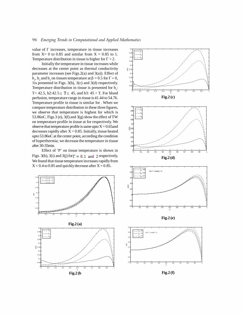
96 Emerging Trends in Computational and Applied Mathematics
value of � increases, temperature in tissue increasesfrom X= 0 to 0.85 and similar from X = 0.85 to 1.Temperature distribution in tissue is higher for ��= 2.
Initially the temperature in tissue increases whiledecreases at the center point as thermal conductivityparameter increases (see Figs.2(a) and 3(a)). Effect ofb
1, b
2 and b
3 on tissues temperature at � = 0.5 for ����0,
1is presented in Figs. 3(b), 3(c) and 3(d) respectively.Temperature distribution in tissue is presented for b
1:
T< 42.5, b2:42.5 � TT � 45, and b3: 45 > T. For bloodperfusion, temperature range in tissue is 41.44 to 54.76.Temperature profile in tissue is similar for . When wecompare temperature distribution in these three figures,we observe that temperature is highest for which is53.86oC. Figs.3 (e), 3(f) and 3(g) show the effect of TWon temperature profile in tissue at for respectively. Weobserve that temperature profile is same upto X = 0.65anddecreases rapidly after X = 0.85. Initially, tissue heatedupto 53.86oC at the center point, according the conditionof hyperthermia; we decrease the temperature in tissueafter 30-35min.
Effect of ‘P’ on tissue temperature is shown inFigs. 3(h), 3(i) and 3(j) for respectively..We found that tissue temperature increases rapidly fromX = 0.4 to 0.85 and quickly decrease after X = 0.85.
0 0.1 0.2 0.3 0. 4 0.5 0.6 0.7 0.8 0. 9 10
0.05
0.1
0.15
0.2
0.25
0.3
0.35
X
�(X
)
�=0 (� = 0)
�=0 (� = 1)
�=0 (� = 2)
Fig.2 (a)
0 0.1 0.2 0.3 0.4 0.5 0.6 0.7 0.8 0.9 10
0.05
0.1
0.15
0.2
0.25
0.3
0.35
0.4
0.45
0.5
X
�(X
)
b1
b2
b3
Fig.2 (b
0 0.1 0.2 0.3 0.4 0.5 0.6 0.7 0.8 0.9 10
0.05
0.1
0.15
0.2
0.25
0.3
0.35
0.4
0.45
0.5
X
�(X
)
b1
b2
b3
Fig.2 (c)
0 0.1 0.2 0.3 0.4 0.5 0.6 0.7 0.8 0.9 10
0.05
0.1
0.15
0.2
0.25
0.3
0.35
0.4
0.45
0.5
X
�(X
)
b1
b2
b3
Fig.2 (d)
0 0.1 0.2 0.3 0.4 0.5 0.6 0.7 0.8 0.9 1-0.2
-0.1
0
0.1
0.2
0.3
0.4
0.5
X
�(X
)
For � = 0 and � = 0
TW = 30
TW = 33
TW = 37
Fig.2 (e)
0 0.1 0.2 0.3 0.4 0.5 0.6 0.7 0.8 0.9 1-0.2
-0.1
0
0.1
0.2
0.3
0.4
0.5
X
� (X
)
For � = 1 and � = 0
TW = 30
TW = 33
TW = 37
Fig.2 (f)

Emerging Trends in Computational and Applied Mathematics 97
0 0.1 0.2 0.3 0.4 0.5 0.6 0.7 0.8 0.9 1-0.2
-0.1
0
0.1
0.2
0.3
0.4
0.5
X
�(X
)
For � = 2 and �=0
TW = 30
TW = 33
TW = 37
Fig.2 (g)
0 0.1 0.2 0.3 0.4 0.5 0.6 0.7 0.8 0.9 10
0.05
0.1
0.15
0.2
0.25
0.3
0.35
0.4
X
�(X
)
For � = 0 and � = 0
P=10
P=15P=20
Fig.2 (h)
0 0.1 0.2 0.3 0.4 0.5 0.6 0.7 0.8 0.9 10
0.05
0.1
0.15
0.2
0.25
0.3
0.35
0.4
0.45
0.5
X
�(X
)
For � = 1 and � = 0
P=10
P=15P=20
Fig.2 (i)
0 0.1 0.2 0.3 0.4 0.5 0.6 0.7 0.8 0.9 10
0.1
0.2
0.3
0.4
0.5
X
�(X
)
For � = 2 and � = 0
P=10P=15P=20
Fig.2 (j)
Figs.2 For , the effect of 2(a) the geometry,,2(b) b
1, b
2 and b
3, when , 2(c) b
1, b
2 and b
3, when
, 2(d) b1, b
2 and b
3, when , 2(e) surface
temperature for , 2(f) surface temperaturefor , 2(g) surface temperature for , 2(h)antenna power (P) for , 2(i) antenna power (P) for
, 2(j) antenna power (P) on temperaturedistribution on tissue
0 0.1 0.2 0.3 0.4 0.5 0.6 0.7 0.8 0.9 10
0.05
0.1
0.15
0.2
0.25
0.3
0.35
X
�(X
)
�=0.5 (� = 0)
�=0.5 (� = 1)
�=0.5 (� = 2)
Fig.3 (a)
0 0.1 0.2 0.3 0.4 0.5 0.6 0.7 0.8 0.9 10
0.05
0.1
0.15
0.2
0.25
0.3
0.35
0.4
0.45
0.5
X
�(X
)
For � = 0 and � = 0.5
b1
b2
b3
Fig.3 (b)
0 0.1 0.2 0.3 0.4 0.5 0.6 0.7 0.8 0.9 10
0.05
0.1
0.15
0.2
0.25
0.3
0.35
0.4
0.45
0.5
X
�(X
)
For � = 1 and � = 0.5
b1
b2
b3
Fig.3 (c)
0 0.1 0.2 0.3 0.4 0.5 0.6 0.7 0.8 0.9 10
0.05
0.1
0.15
0.2
0.25
0.3
0.35
0.4
0.45
0.5
X
�(X
)
For � = 2 and � = 0.5
b1
b2
b3
Fig.3(d)

98 Emerging Trends in Computational and Applied Mathematics
0 0.1 0.2 0.3 0.4 0.5 0.6 0.7 0.8 0.9 1-0.2
-0.1
0
0.1
0.2
0.3
0.4
0.5
X
�(X
)
For � = 0 and � = 0.5
TW = 30
TW = 33
TW = 37
Fig.3 (e)
0 0.1 0.2 0.3 0.4 0.5 0.6 0.7 0.8 0.9 1-0.2
-0.1
0
0.1
0.2
0.3
0.4
0.5
X
�(X
)
For � = 1 and � = 0.5
TW
= 30
TW = 33
TW = 37
Fig.3 (f)
0 0.1 0.2 0.3 0.4 0.5 0.6 0.7 0.8 0.9 1-0.2
-0.1
0
0.1
0.2
0.3
0.4
0.5
X
�(X
)
For � = 2 and � = 0.5
TW = 30
TW = 33
TW = 37
Fig3(g)
0 0.1 0.2 0.3 0.4 0.5 0.6 0.7 0.8 0.9 10
0.05
0.1
0.15
0.2
0.25
0.3
0.35
X
�(X
)
For � =1 � = 0.5
P = 10P = 15
P = 20
Fig3(h)
0 0.1 0.2 0.3 0.4 0.5 0.6 0.7 0.8 0.9 10
0.05
0.1
0.15
0.2
0.25
0.3
0.35
X
�(X
)
For � =1 � = 0.5
P = 10P = 15
P = 20
Fig3(i)
0 0.1 0.2 0.3 0.4 0.5 0.6 0.7 0.8 0.9 10
0.05
0.1
0.15
0.2
0.25
0.3
0.35
X
�(X
)
For � = 2 and � = 0.5
P = 10
P = 15
P = 20
Fig3(j)
Figs.3 For , the effect of 3(a) the geometry,,3(b) b
1, b
2 and b
3, when , 3(c) b
1, b
2 and b
3, when
, 3(d) b1, b
2 and b
3, when , 3(e) surface
temperature for , 3(f) surface temperaturefor , 3(g) surface temperature for , 3(h)antenna power (P) for , 3(i) antenna power (P) for
, 3(j) antenna power (P) on temperaturedistribution on tissue
Conclusions
We have presented an approximate solution ofthe nonlinear steady state model using Waveletcollocation method. The present method has been usedto analyze temperature distribution in tissue with thermalconductivity varying as linear function of temperature.The aim of this study is to get a temperature distributionwhich nearly avoids ‘‘hot spots’’ in healthy tissue. Thetemperature distribution in tissues studied, which is asfollow:
(i) Temperature distribution is faster in sphericalcoordinate system than other two systems.So spherical coordinate system is moreeffective for thermal therapy than othergeometries.
(ii) For the three different type blood perfusion,the range of temperature distribution intissue is 41.44 to 54.76 in case of linear

Emerging Trends in Computational and Applied Mathematics 99
thermal conductivity.(iii) As the value of antenna power (P) increases
temperature in tissue also increases in caseof linear thermal conductivity.
(iv) Temperature in tissue increases as value ofsurface temperature (T
W) increases.
Present work demonstrate the steady state modelto predict a quantative analysis of the temperaturedistribution in tissue can be very beneficial in wideningthe idea of clinical thermal technology and thermalmedical practice.
Acknowledgements
Authors are grateful to Professor Umesh Singh,Coordinator of DST- Centre for interdisciplinaryMathematical Sciences, Banaras Hindu University, andVaranasi, India for providing necessary facilities.
REFERENCES
[1] J.W. Mitchell, T.L. Galvez, J. Hangle, G.E. Myers, K.L.“Siebecker, Thermal response of human legs duringcooling”, J. Appl. Physiol. 29 (1970) 859–865.
[2] K. M. Sekins, J.F. Lehmann, P. Esselman, D. Dundore,A.F. Emery, B.J. Lateur, W. B. Nelp, “Local muscleblood ?ow and temperature responses to 915 MHzdiathermy as simultaneously measured and numericallypredicted”, Arch. Med. Rehab. 65 (1984) 1–7.
[3 M.W. Dewhirst, T.V. Samulski, “Hyperthermia in theTreatment for Cancer”, Upjohn, Kalamazoo, MI, 1988.
[4] P.K. Gupta, J. Singh, K.N. Rai, S.K. Rai, “Solution ofthe heat transfer problem in tissues during hyperthermiaby ?nite difference - decomposition method”, J. ofApplied Mathematics and Computation, 219 (2013)6882–6892.
[5] P.K. Gupta, J. Singh, K.N. Rai, “Numerical simulationfor heat transfer in tissues during thermal therapy”, J.Therm. Biol 35 (6) (2010) 295–301.
[6] M. Razzaghi, S. Yosefi, “Legendre wavelet operationmatrix of integration”, Int. J. of System Science, (2001),Vol. 32, No. 4, pp: 495-585
[7] F. Mohammadi, M.M. Hosseini and syed TauseefMohyud-Din, “Legendre Wavelet Galerkin method forsolving ordinary differential equations with non-analyticsolution”, Int. J. of Sys. Sci. Vol. 42, No. 4, (2011) 579-585.
[8] M.W. Frazier, “An Introduction to Wavelets ThroughLinear Algebra”, Springer-Verlag New York BerlinHeidelberg SPIN 10557627, 1999.

SOLID MECHANICS

Introduction
Nematic elastomers are materials of thesimultaneous combination of the elastic properties ofrubbers with the anisotropy of liquid crystals. Theyconsist of networks of elastic solid chains formed bythe cross linking of nematic crystalline molecules calledmesogens as the elements of their main-chains andpendant side-groups. Due to this structure, any stresson the polymer network influences the nematic orderand any change in the orientational order will affect themechanical shape of the elastomer. The interplaybetween elastic and orientational changes is responsiblefor many fascinating properties of such materials thatare different from the classical elastic solids and liquidcrystals. Liquid crystalline elastomers (LCE) have anumber of applications in the fields of mechanicalactuators (artificial muscles), optics and coatings ofmaterials, which can dissipate mechanical energy [5, 8,12]. Alexe-Ionescu et al. [2], Bladon et al. [4], Kupfer andFinkelmann [26], Long and Morse [28], Mitchell et al.[29], Verwey et al. [40], Warner et al. [42] and Weileppand Brand [43] discussed different problems in liquidnematic elastomers.
The electroclinic (EC) effect is an electro-opticalcoupling observed in liquid crystals, which consists in
the rotation of the optical axis about an electric field,perpendicular to the optical axis itself. The tilt is linearin the electric field and the proportionality coefficient,the EC coefficient, is a property of the material. Grecoand Ferrarini [24] derived the molecular expressions forthe EC coefficient and a computational methodologythat had allowed its calculations on the basis of themolecular structure. Finkelmann et al. [16] synthesizedside chain nematic polymer networks, performeddifferential scanning calorimetry (DSC), X-ray,birefringence, and thermo-mechanical characterization-ns. Selinger et al. [31] developed a phenomenologicaltheory for the isotropic-nematic transition in liquid-crystalline elastomers through a variation on Landautheory. DeSimone and Dolzmann [13] analyzed the softdeformation paths and domain patterns in nematicelastomers through the minimization of a nonconvexfree-energy. Anderson et al. [3] developed a continuumtheory for the mechanical behavior of rubber materials.Conti et al. [9, 10] showed that the effective energyresults from an instability toward formation of fine-scaleoscillations, for deformation gradients in part of thephase space, leading to two distinct macroscopic modesof response, called soft and hard. Clarke et al. [7] reportedthe theoretical and experimental study of linear
19Reflection and Transmission of Elastic Waves in
the Nematic Elastomer half-spaces
S. S. SinghDepartment of Mathematics & Computer Science, Mizoram University, Aizawl - 796 004, Mizoram, India
Abstract: The problem of the reflection and transmission of elastic waves due to incident longitudinal wave (qP-wave) at a plane interface between two dissimilar nematic elastomer half-spaces has been studied. The expressionsof the phase velocities corresponding to qP, qSV and qSH-waves are obtained. It is observed that these phasevelocities depend on the angle of propagation of the elastic waves. The reflection and transmission coefficientscorresponding to the reflected and refracted waves are derived by using appropriate boundary conditions.Keywords : Nematic elastomers, qP-wave, qSV -wave, Reflection, Refraction, Phase velocity
Emerging Trends in Computational and Applied Mathematics 103

104 Emerging Trends in Computational and Applied Mathematics
viscoelastic response in oriented monodomain nematicelastomers. Nematic elastomers [36] exhibits theremarkable phenomenon of soft or semisoft elasticity inwhich the effective shear modulus for shears in planescontaining the anisotropic axis, respectively, vanishesor is very small. Teixeira and Warner [37] discussedanalytically and numerically the dynamics of how anematic elastomer anisotropic rubber-respondselastically and orientationally to an imposed strain.Uchida [39] investigated the properties of disorderednematic elastomers and gels with emphasis on the rolesof nonlocal elastic interactions and crosslinkingconditions.
Fradkin et al. [18] studied the viscoelatic theoryof nematic elastomers in the low-frequency limit is usedto investigate the spectral and polarization propertiesof acoustic waves propagating in nematic liquid-crystalline nematic elastomers. Gebretsadkan and Kalra[22] investigated the propagation of linear waves inrelativistic anisotropic magnetohydrodynamics andploted a Fresnal ray surface. Singh [33] discussed theproblem of elastic waves propagation in the nematicelastomer and obtained the reflection coefficients usingthe linear viscoelastic theory of nematic elastomers.Terentjev et al. [38] developed a theory of elastic wavesin oriented monodomain nematic elastomers anddiscussed the effect of soft elasticity, combined withthe
Leslie-Ericksen version of dissipation function,results in an unusual dispersion and anomalousanisotropy of shear acoustic waves. Notable researcherswho contributed in solving problems in nematicelastomers are Carcione [6], Deeg et al. [11], DeSimoneand Teresi [14], Finkelmann et al. [17], Fried and Co-workers [19-21], Golubovic and Lubensky [23], Hottaand Terentjev [25], Rey [30], Selinger et al. [32], Stenulland Lubensky [34, 35] and Warner [41].
In this paper, we have attempted a problem ofreflection and refraction of elastic waves due to incidentqP-wave at a plane interface between two dissimilarnematic elastomers. The reflection and refractioncoefficients corresponding to the reflected and refractedelastic waves are obtained analytically and numerically.
Basic Equations
The elastic potential energy density in nematicsolid takes the form [12, 38] as
,
where the Frank elastic energy describes the non-uniform directors is not included due to the assumptionof uniform director rotations in nematic elastomers,
is an independent rotational variable,�n is a small variation in the undistorted nematic director,
is the local rotation vector, (n × �n)
are director rotations, is the
traceless part of linear symmetric strain,, C
i are elastic constants and D
1,
D2 are coupling constants.
Using the Leslie-Ericksen theory [15, 27] of anisotropicviscous dissipation in nematic liquid, the Rayleighdissipation function (entropy production density) canbe written in the quadratic form of correspondingvelocities [38] as
+ , .where A
i are viscous coefficients. This equation
describes two types of dissipation, by shear flow andby rotation of the director, and vanishes for rigidrotations.The equations of motion of viscous nematic solid afterneglecting the effects of Frank elasticity on the directorgradient are given as [18]
,
. .The components of the viscoelastic symmetric stresstensors with the choice of the coordinate axis (x
3) to lie
in the direction of the undistorted director, n are,
,
,
where the Frank elastic energy describes the non-uniform directors is not included due to the assumptionof uniform director rotations in nematic elastomers,
is an independent rotational variable,�n is a small variation in the undistorted nematic director,
is the local rotation vector, (n × �n)

Emerging Trends in Computational and Applied Mathematics 105
are director rotations, is the traceless
part of linear symmetric strain, , Ci
are elastic constants and D1, D
2 are coupling constants.
Using the Leslie-Ericksen theory [15, 27] ofanisotropic viscous dissipation in nematic liquid, theRayleigh dissipation function (entropy productiondensity) can be written in the quadratic form ofcorresponding velocities [38] as
where �R is the characteristic time of rubber
relaxation and �1, �
2 are director rotation times.
We have the following relations [33]We have the following relations [33]
, , . (6)The Rayleigh dissipation function is positive if
where C5 is the shear modulus.
Using Equations (5) and (4), the components ofrotational variable are given by [33]
,
where � is angular velocity.
Problem Formulation
Let us consider two dimensional wave propagation inx
1x
3-plane with x
1-axis lying horizontally and x
3 -axis
vertically downward. The dissimilar anisotropic nematicelastomer half-spaces, M : 0 ? x
3 < ? and M? : ?? < x
3 ? 0,
are separated by x3 = 0. It may be noted that the
corresponding parameters in M? will denote by insertinga (?) to that of M.The equations of motion in the nematic elastomer, Mafter neglecting the effects of Frank elasticity on thedirector gradient may be written as
, ... (7)
, ... (8)where
Similarly, the equations of motion in the nematicelastomer, M? can be written as
, .
, .where
Suppose a plane wave propagating in the half-space, Mbe incident at the plane interface x
3 = 0, in which a part
of the incident energy is reflected to the half-space Mand another part is refracted to the half-space M?. Thedisplacement of the elastic waves may be representedas
},
},
where A(3) is the amplitude constant, d1
(�) is componentof unit displacement vector, � is angular frequency, k
1(�)
and k3
(�) are corresponding wavenumbers with � = 0 forincident wave, � = 1 for the reflected qSP-wave, � = 2 forthe reflected qSV -wave, � = 3 for the refracted qP-wave,& � = 4 for the refracted qSV -wave.
The Snell’s law which gives the relation of theangles of incident, reflected as well as refracted wavesis given by
where ca is the apparent velocity, c
0(�) is the phase
velocity of incident wave, c1(�
1) is the phase velocity of
reflected qP-wave, c2(�
2) is the phase velocity of the
reflected qSV -wave, c’1(��) is the phase velocity ofrefracted qP-wave and c’
2(�
4) is the phase velocity of
the refracted qSV -wave.The phase velocity of the incident qP-wave is given by
where p = (p1, p
2, p
3),
The expressions of phase velocity correspondingto the reflected and refracted waves may be written as

106 Emerging Trends in Computational and Applied Mathematics
wherep(�) = (p
1(�), p
2(�), p
3(�) ), for ��=1, 2
again for � = 3 & 4
Thus, we have seen that the phase velocity of theelastic waves in the nematic elastomers depend on theangle of propagation. Consequently, the elastic wavesin anisotropic nematic elastomers are quasi nature.
Boundary conditions
The boundary conditions of the problem are thecontinuity of displacement and stress tractions at x
3 = 0.
Mathematically, these conditions may be written as(a) Continuity of displacements at the x
3 = 0
= and =
(b) Continuity of stress tractions at the x3 = 0
and With the help of Equations (11)-(13) and stress
tractions into (15) & (16), we get,
where A is a matrix of order 4 × 4 with the followingelements
X and B are column matrices given by
This equation will help to find out the reflectionand refraction coefficients of the reflected and refractedqP and qSV -waves.
Reflection and Refraction Coefficients
Solving the equations in the matrix form (17), we get thefollowing reflection and refraction coefficients of thereflected and refracted waves as
,
,
where
and the expressions of , , and can be writtenby replacing first, second, third and fourth columns of
the determinant, with the column matrix, B. Thecoefficient, corresponds to the reflection coefficient
of the reflected qP-wave and corresponds to thereflection coefficient of the reflected qSV -wave, while
corresponds to the refraction coefficient of the
refracted qP-wave and corresponds to the refractioncoefficient of the refracted qSV -wave.
Special Case
In the absence of the upper half-space (M?), theproblem reduces to the reflection of elastic waves dueto free surface. We consider the boundary condition(16) and the reflection coefficients are given by

Emerging Trends in Computational and Applied Mathematics 107
... (20)
These results are similar results as obtained bySingh [33] for the relevant problem.
6. Numerical Results & Discussion
In order to compute the reflection & refractioncoefficients of the reflected and refracted waves, thefollowing nematic elastomers are considered.
For the half-space, MC
1 = 1.42 × 10⁵ N/m2, C
2 = 2.25 × 10⁵N/m2, C
3 = 4.88
× 105N/m2, C4 = 2.15 × 10⁵ N/m2, C
5 = 1.06 × 10⁵N/m2, D
1=
0.12, D2 = 0.05, � = 1.66 × 10³kg/m3;
For the half-space, M’C’
1= 3.52 × 10⁵N/m2, C’
2 = 2.28 × 10⁵N/m2, C
3 = 1.65
× 105 N/m2, C4 = 1.60 × 10⁵ N/m2, C
5= 4.34 × 10⁵N/m2, D
1=
0.15, D2= 0.17, � = 1.26 × 10
3kg/m
3.
Using Equation (13) and (14), we obtained theangles corresponding to the reflected and refractedwaves. The variation of these angles with the angle ofincidence is depicted in Figure 1. Curve I correspondsto the angle of reflected qP-wave, Curve II correspondsto the angle of reflected qSV -wave, Curve IIIcorresponds to angle of refracted qP-wave and CurveIV corresponds to the angle of refracted qSV -wave. Allthese angles increase with the increase of angle ofincidence, ��
0 10 20 30 40 50 60 70 80 90Angle of Incidence
0.00
0.40
0.80
1.20
1.60
Ref
lect
ed a
nd
Ref
ract
ed
Ang
les
I
III
IV
II
Fig. 1: Variation of reflected and refracted angles withangle of incidence.
The variation of reflection and refraction coefficients
with angle of incidence for different values of��’
1, ��’
2, ��’
R and ��’
1, ��’
2, ��’
R are shown in
Figures 2-5. In all the figures, we takeCurve I: ��
1 = 0.10, ��
2 = 0.15, ��
R = 0.20 and
��’1= 0.05, ��’
2 = 0.14, ��’
R= 0.10
Curve II: ��1 = 0.30, ��
2 = 0.35, ��
R = 0.30 and
��’1= 0.25, ��’
2= 0.34, ��’
R= 0.20
Curve III: ��1 = 0.50, ��
2 = 0.55, ��
R = 0.40 and
��’1= 0.55, ��’
2= 0.54, ��’
R= 0.30.
0 10 20 30 40 50 60 70 80 90Angle of incidence
0.20
0.30
0.40
0.50
0.60
0.70
Re
flect
ion
coe
ffici
ent
I
IIIII
Fig. 2: Variation of reflection coefficient of thereflected qP-wave with angle of incidence.
0 10 20 30 40 50 60 70 80 90Angle of incidence
0.40
0.50
0.60
0.70
0.80
0.90
1.00
1.10
Ref
ratio
n co
effic
ien
t
I
II
III
Fig. 3: Variation of reflection coefficient of thereflected qSV-wave with angle of incidence.

108 Emerging Trends in Computational and Applied Mathematics
0 10 20 30 40 50 60 70 80 90Angle of incidence
0.00
0.20
0.40
0.60
0.80
1.00
Ref
ratio
n co
effic
ien
t
I
III
II
Fig. 4: Variation of refraction coefficient of therefracted qP-wave with angle of incidence.
0 10 20 30 40 50 60 70 80 90Angle of incidence
0.10
0.20
0.30
0.40
0.50
Ref
ratio
n co
effic
ient
IIII II
Fig. 5: Variation of refraction coefficient of therefracted qSV-wave with angle of incidence.In Figure 2, the reflection coefficient, r(1)
corresponding to reflected qP-wave starts from certainvalue at the normal incidence and increases upto � =140 which decreases thereafter with the increase of theangle of incidence. We have observed that the directorrotation time parameters (��
1, ��
2, ��
R) and (��’
1, ��’
2,
��’R) affected much near the glazing angle of incidence.
Figure 3 shows that r(2) of the reflected qSV -wavestarts from certain value which decrease upto � = 90,thereafter it increases upto � = 300 and then decreasesagain with the increase of�. In Figure 4, the refraction
coefficient, r(2) of the refracted qP-wave decreases withthe increase of angle of incidence upto � = 670 whichincreases thereafter. Figure 5 shows that the values ofr(4) decreases with the increase of angle of incidenceupto � = 300 and then it increases with �. We haveobserved that the values of r(4) increase with the increaseof director rotation time parameters.
Conclusion
Using appropriate boundary conditions, thereflection and refraction of elastic waves due to incidentqP-wave at a plane interface between two dissimilarnematic elastomer half-space has been investigated. Thereflection and refraction coefficients corresponding tothe reflected and refracted waves are obtainedanalytically and numerically for a particular model. Wemay conclude the following points
(i) The phase velocities of the elastic wavesdepend on the angle of incidence,
(ii) The reflection and refraction coefficients arefunctions of elastic constants, the couplingconstants, the characteristic time of rubberrelaxation, director rotation times elasticparameter and angle of incidence,
(iii) The angles corresponding to the reflectedand refracted waves increase with theincrease of angle of incidence,
(iv) The effect of director rotation timeparameters to the reflection coefficient, r(1)
is prominent near the glazing angle ofincidence and
(v) The values of the refraction coefficient,r(4)
increase with the increase of director rotationtime parameters.
Acknowledgement
Author acknowledges the Department of Science\& Technology (DST), New Delhi, India for financialsupport through Grant No. SR/FTP/MS-017/2010.
REFERENCES
[1] J. D. Achenbach, “Wave Propagation in Elastic Solids”,North Holland, Amsterdam, 1973.
[2] A. L. Alexe-Ionescu, R. Barberi, G. Barbero, M.Giocondo, “Anchoring energy for nematic liquidcrystals: contribution from the spatial variation of theelastic constants”, Phys. Rev. E 42(1994) 5378-88.
[3] D. R. Anderson, D. E. Carlson, E. Fried, “A continuum-mechanical theory of nematic elastomers”, J. Elast.56(1999) 33-58.
[4] P. Bladon, E. M. Terentjev, M. Warner, “Transitions
Emerging Trends in Computational and Applied Mathematics 109
and instabilities in liquid crystal elastomers”, Phys. Rev.E 47(1993) R3838-40.
[5] H. R. Brand, H. Pleiner, “Electrohydrodynamics ofnematic liquid crystalline elastomers”, Physica A208(1994) 359-72.
[6] J. M. Carcione, “Constitutive model and wave-equationsfor linear, viscoelastic, anisotropic media”, Geophysics60(1994) 537-48.
[7] S. M. Clarke, A. R. Tajbakhsh, E. M. Terentjev, M.Warner, “Anomalous viscoelastic response of nematicelastomers”, Phys. Rev. Lett. 81(2001) 4436-9.
[8] S. M. Clarke, E. M. Terentjev, “Slow stress relaxationin Randomly disordered nematic elastomers and gels”,Phys. Rev. Lett. 81(1998) 4436-4439.
[9] S. Conti, A. DeSimone, G. Dolzmann, “Soft elasticresponse of stretched sheets of nematic elastomers: anumerical study”, J. Mech. Phys. Solids 50(2002) 1431-51.
[10] S. Conti, A. DeSimone, G. Dolzmann, “Semisoftelasticity and director reorientation in stretched sheetsof nematic elastomers”, Phys. Rev. E 66(2002) 061710-8.
[11] F. W. Deeg, K. Diercksen, G. Schwalb, C. Brauchle, H.Reinecke, “Ultrasonic measurements of the anisotropicviscoelastic properties of nematic elastomers”, Phys.Rev. B 44(1991) 2830-3.
[12] P. G. de Gennes, “Liquid Crystals of One and TwoDimensional order edited by W. Helfrich and G. Heppke”,Springer, Berlin, 1980.
[13] A. DeSimone, G. Dolzmann, “Material instabilities innematic elastomers”, Physica D: Nonlin. Phenom.136(2000) 175-91.
[14] A. DeSimone, T. Teresi, “Elastic energies for nematicelastomers”, Eur. Phys. J. E 29(2009) 191-204.
[15] J. L. Ericksen, “Anisotropic fluids”, Arch. Ration. Mech.Anal. 4(1960) 231-237; “Conservation laws for liquidcrystals”, Trans. Soc. Rheol. 5(1961) 23-34.
[16] H. Finkelmann, A. Greve, M. Warner, “The elasticansiotropy of nematic elastomers”, Eur. Phys. J. E5(2001) 281-93.
[17] H. Finkelmann, I. Kundler, E. Terentjev, M. Warner,“Critical stripe domain instability of nematicelastomers”, J. Physique II 7(1997) 105969.
[18] L. J. Fradkin, I. V. Kamotski, E. M. Terentjev, D. D.Zakharov, “Low-frequency acoustic waves in nematicelastomers”, Proc. R. Soc. Lond. A 459(2003) 2627-42.
[19] E. Fried, V. Korchagin, “Striping of nematic elastomers”,Int. J. Solids Struct. 39(2002) 3451-67.
[20] E. Fried, S. Sellers, “Soft elasticity is not necessary forstriping in nematic elastomers”, J. Appl. Phys.100(2006) 043521.
[21] E. Fried, R. E. Tordes, “Disclinated states in nematicelastomers”, J. Mech. Phys. Solids 50(2002) 2691-716.
[22] W. B. Gebretsadkan, G. L. Kalra, “Propagation of linearwaves in relativistic anisotropicmagnetohydrodynamics”, Phys. Rev. E 66(2002)057401-4.
[23] L. Golubovic, T. C. Lubensky, “Nonlinear elasticity ofamorphous solids”, Phys. Rev. Lett. 63(1989) 1082-5.
[24] C. Greco, A. Ferrarini, “Electroclinic effect in nematic
liquid crystals: The role of molecular and environmentalchirality”, Phys. Rev. E 87(2013) 060501-4.
[25] A. Hotta, E. M. Terentjev, “Dynamics of soft elasticityin monodomain nematic elastomers”, Eur. Phys. J. E10(2003) 291-301.
[26] J. Kupfer, H. Finkelmann, “Nematic liquid single-crystalelastomers”, Makromol. Chem. Rapid Commun.12(1991) 717-26.
[27] F. M. Leslie, “Some constitutive equations foranisotropic fluids”, Q. J. Mech. Appl. Math.19(3)(1966) 357-370; “Some constitutive equations forliquid crystals”, Arch. Ration. Mech. Anal. 28(1968)265-283.
[28] D. Long, D. C. Morse, “Linear viscoelasticity anddirector dynamics of nematic liquid crystalline polymermelts”, Europhys. Lett. 49(2000) 25561.
[29] G. R. Mitchell, F. J. Davis, W. Guo, “Strain-inducedtransitions in liquid-crystal elastomers”, Phys. Rev.Lett. 71(1993) 2947-50.
[30] A. D. Rey, “Viscoelastic theory for nematic interfaces”,Phys. Rev. E 61(2000) 1540-9.
[31] J. V. Sellinger, H. G. Jeon, B. R. Ratna, “Isotropic-nematic transition in liquid-crystalline elastomers”,Phys. Rev. Lett. 89(2002)225701-4.
[32] J. V. Selinger, M. S. Spector, V. A. Greanya, B. T.Weslowski, D. K. Shenoy, R. Shashidhar, “Acousticrealignment of nematic liquid crystal”, Phys. Rev. E66(2002)051708-7.
[33] B. Singh, “Reflection of homogeneous elastic waves fromfree surface of nematic elastomer half-space”, J. Phys.D: Appl. Phys. 40(2007)584-592.
[34] O. Stenull, T. C. Lubensky, “Dynamics of nematicelastomers”, Phys. Rev. E 69 (2004) 051801-13.
[35] O. Stenull, T. C. Lubensky, “Anomalous elasticity ofnematic elastomers”, Europhys. Lett. 61(2003) 776-82.
[36] O. Stenull, T. C. Lubensky, “Dynamics of nematicelastomers “, Phys. Rev. E 69(2004) 051801.
[37] P. L. C. Teixeira, M. Warner, “Dynamics of soft andsemisoft nematic elastomers”, Phys. Rev. E 42(1999)603-9.
[38] E. M. Terentjev, I. V. Kamotski, D. D. Zakharov, L. J.Fradkin, “Propagation of acoustic waves in nematicelastomers”, Phys. Rev. E 66(2002) 052701.
[39] N. Uchida, “Soft and nonsoft structural transitions indisordered nematic networks”, Phys. Rev. E 62(2000)5119-36.
[40] G. C. Verwey, M. Warner, E. M. Terentjev, “Elasticinstability and stripe domains in liquid crystallineelastomers”, J. Physique II 6(1996) 1273-90.
[41] M. Warner, “New elastic behaviour arising from theunusual constitutive relation of nematic solids”, J. Mech.Phys. Solids 47(1999) 1355-77.
[42] M. Warner, E. M. Terentjev, R. B. Meyer, Y. Mao,“Untwisting of a cholesteric elastomer by mechanicalfield”, Phys. Rev. Lett. 85(2000) 2320-3.
[43] J. Weilepp, H. R. Brand, “Director reorientation innematic-liquid single crystal elastomers by externalmechanical stress”, Europhys. Lett. 34(1996) 495-500.

110 Emerging Trends in Computational and Applied Mathematics
Introduction
Functionally graded materials (FGMs) are thosematerials in which the volume fraction of two or morematerials is varied, as a power law, sigmoid or exponentialdistribution, continuously as a function of positionalong certain dimension(s) of the structure [1-2]. Thesedays the demands of non-homogeneous materials areincreasing because in many engineering as comparedto highly compressible homogeneous cylinder while forcylinder made of non-homogeneous materialapplications. a material undergoes high rotations andthermal loading. The non-homogeneous materials findstheir applications in many areas include coating forprotection of metallic or ceramic substrates against heatpenetration, wear, corrosion and oxidation [3], aerospace,nuclear reactors, flywheels are few to mention. Theproblems of rotating annular disk and cylinder can befound in many books of elasticity [4-5]. Tuntuncu et al.[6] used infinitesimal theory of elasticity to find theclosed form solution for stresses and displacement infunctionally graded cylindrical and spherical vessels
subjected to internal pressure. They compared stressdistributions depending on an inhomogeneity constantwith homogeneous case with the help of graph.
Sharma [7] studied elastic-plastic transitionalstresses in non-homogeneous thick-walled cylinderunder internal pressure using transition theory andobserved that a non-homogeneous cylinder with non-homogeneity increasing radially requires higherpercentage increase in pressure to become fully plasticthan to its initial yielding as compared to a homogeneouscylinder and is on the safer side of the design. Further,Sharma et al. [8] studied elastic-plastic transitionalstresses in non-homogeneous thick-walled cylinderunder external pressure. They concluded that lesscompressible homogeneous cylinder is on the safer sideof design, highly compressible cylinder is on the saferside of the design as compared to less compressiblecylinder. Changing the material model from linear strainhardening to non linear strain hardening, a perturbation[9] and an approximate power series solution [10] havebeen presented to determine the elastic- plastic stressin a rotating solid with constant thickness. You et al.
20Thermo Elastic-Plastic Analysis of Rotating Disk Made of Non-
homogeneous Material under Internal Pressure withVariable Thickness and Variable Density
Sanehlata Yadav, Sanjeev SharmaDepartment of Mathematics, Jaypee Institute of Information Technology, Noida (UP) - 201307, INDIA.
Abstract: Elastic-plastic thermal stresses have been obtained for a rotating disk made of non-homogeneousmaterial with non-linear strain hardening under internal pressure by using finite difference method with Von-Mises’ yield criterion. Results have been computed numerically and depicted graphically. The stresses obtained byfinite difference are compared with shooting method and a very good agreement has been found between both theapproaches. From the numerical results, it can be concluded that non-homogeneous disk with variable thicknessare safer side of the design as compared to homogeneous disk because the circumferential stress is less for nonhomogeneous disk whose thickness varying radially as compared to homogeneous disk.Keywords: Rotating, Strain-hardening, Non-homogeneous material, Elastic, Plastic.

Emerging Trends in Computational and Applied Mathematics 111
[11-12] extended this work to elastic- plastic analysis ofrotating disk with arbitrary variable thickness anddensity and rotating solid shafts respectively. Eraslanet al. [13] calculated the numerical solution for elastic-plastic stresses in a rotating with Von-Mises’ yieldcriterion using general non-linear strain hardening rule.
In this paper, a numerical solution for a rotatingdisk made of non-homogeneous material with non-linearstrain hardening and Von-Mises’ criterion under thermalloading subjected to internal pressure has beendeveloped using finite difference method. Finally,thermal radial and circumferential stresses are calculatedin elastic–plastic region. Results have been discussednumerically with the help of graphs.
Mathematical Formulation
Distribution of material properties and thicknessprofile
A rotating disk with an inner radius a and an
outer radius b is studied. The disk is made of non-homogeneous material in radial direction i.e. the Young’smodulus of the material is expressed by power functionof the radius r and density of the material is alsoexpresses by power function of the radius r . Thethickness profile of the disk is varying parabolically inradial direction. The coefficients of the Young’s modulus,thermal expansion, and density, temperature distributionof the material and thickness profile of the rotating areexpressed as:
� � � � � �
� �
1 1
0 0 0
0
; ; ;
1
e m
n
r r rE r E r r
b b b
rh r h k
b
�
� � � �� �
� � � � � �� � �� � � � � �� � � � � �� �� �� �� �� �
� �� �� �
where r is the radial coordinate , 0E , 0� , 0� are thematerial coefficients and 1e , 1� , m are geometricparameters and h
0 is the thickness of the disk and n
and k are geometric constants of thickness.
Basic equations
For rotating disk with constant angular velocity, thegoverning equilibrium equation is
� � 2 2 – 0rr
dhrT hT h r
dr �� ��� � .
The relation between strains and radialdisplacements are
rdu
e dre u
r�
� �� � � ��� � � �� � � �,
where u is the radial displacement.The equation of compatibility can be derived as
follows from eq. (3) is
0 r
der e e
dr�
�� � � .
The total radial and circumferential strains inrotating disk are
; ;e p e p e pr r r z z ze e e T e e e T e e e T� � �� � �� � � � � � � � �
The relationship between stresses and strainsaccording to Hooke’s Law in theory elasticity can bewritten as
� �11
1rr
ere
e T
TE re ���
��
� � � � �� �� � � � �� �� � �� � � �� �,
where ere and ee� are the elastic radial and circumferential
strains, � �E r is the Young’s modulus and rrT and
T�� are radial and circumferential stresses respectively..We defined a stress function � �r� which is related
to radial and circumferential stresses and can beexpressed as
2 2
1rrT h r
T dr
h dr��
�
���
� �� �� �
� � �� �� �� � �� �� �
.
Eq. (2) is satisfied after the substitution of eq. (7).Substituting eq. (7) into eq. (6) and expressing strain
components of eq. (5) in terms of the stress function
� � 2 211
1
1r
pr
p
e
e
ehr
E
Td Ter
h drr� �
���
� ����
� �� �� � � �
� �� ���� � � �
�� � � ��� �� � �
� � � ��� � � ��
� ��
Substituting eq. (8) into eq. (4), we obtain a basicgoverning equation of thermo elastic-plastic strainhardening rotating disk

112 Emerging Trends in Computational and Applied Mathematics
� � � �
' ' ' '2 '' ' ' 2 4
''2 3 2
1 1
3 ' 0,p p pr
h E h Er r r r h r
h E h E
Er h r Ehr e T Ehr e e
E � �
� � � � � �
� �� �
� � � �� � � �� � � � � � �� � � �� � � �
� � � �� � � �� � � �� � � �� � � � � � � �� � � �� �� �
where
" ' ' ' ' ' '; ; ; ; ; ; .p
p ded d dE d dh dE e h
dr dr dr dr dr dr dr�
�
� � � �� � � �� � � � � � �
In the elastic region of rotating 0p pre e�� � . Therefore,
eq. (9) reduces to
' ' ' '2 '' '
'' 2 4 2 3 2 '
1 1
3 0
h E h Er r r r
h E h E
Eh r r h r Ehr T
E
� � � �
� � � �� �
� � � �� � � �� � � � � �� � � �� � � �
� � � �� � � �� � � �� �
� � � � � �� �� �
The relations between the stresses and plasticstrains can be determined according to deformationtheory in plasticity as
11 21 12
p pr rrep ee
e Te
TTe ���
� �� � � � �� �� � � � �� �� � � � �� � � �,
where pre and pe� are the plastic radial and
circumferential strains, pee is the equivalent plastic strain
which depends on the material model used and eeT is
the equivalent stress which is defined as
2 2rr rreeT T T T T�� ��� � � .
The non-linear strain hardening model proposedby You et al. (1997) and used for modeling the stress-strain curve of the material beyond the yield point canbe written as
3 51 20 0, , ; pee
e e e ee ee ee T
e e e e a T a T e eE
� � � � �
where 11
152
17.956 10 , 1.551 10a a� �� � � � � are materialconstants, ee is the equivalent total strain and 0e is the yieldstrain.
Substituing pee from eq. (13) into eq. (11) results in
� �2 41 2
11 21 12
ee
pr rrp ee
e T
Ta T a T
e ���
� �� � � � �� �� � � � �� �� � �� � �
�� ��
where eeT is equivalent stress which is obtained from
eq. (12) and eq. (7). Substituting eq. (14) into eq. (9)gives eq. (15). Eq. (15) is the differential equation of thenonlinear strain hardening rotating disk with non–uniform thickness and material properties subjected tothermal loading in the plastic region in terms of stressesand stress function as follows
� �
' ' ' '2 '' ' ' 2 4
'2 42 3
1 2
1 1
3 ee ee
h E h Er r r r h r
h E h E
Er h r E a T a T
E
� � � � � �
� ��
� � � �� � � �� � � � � � � �� � � �� � � �
� � � �� � � �� � � �� �
� � � � �� �� �
� � � �
� � � �� �
2 21 2
'2 '' 2 '
'2 '' 2 ' '
' 2 4 2 3
'
2' 2 4 2 3
1 2
''
2 2
1 1
2 21
12
21 1
2 22 2
22
1 1 1
2 2 2
rr ee
rr rr
ee
T T a a T
hr r
hh
r r rh r h rh
hr E T T T T
ha a Th r h r
hr r
h
��
�� ��
� �
� � � � � ��
� �
� � ��
� � �
� � ���� �� �� ��� �� � �� � � �� � � ��� �� � � ��� � �� � � � � � ��� ��� �
��� ���� �� �� � � ��
� �� ��� �
�
���������������
� �� �� ��
� � � � � �2 4 2 '1 2
30
2 rr ee eeEhr T T a T a T Ehr T�� �� � � � � �
Eq. (15) is an implicit form of stress function which canbe expressed into the general form as
� � '' , , 'f r� � � �
subject to the boundary condition
, 0,rr rrT p r a T r b� � � � � ,
where p is the internal pressure.The second order differential eq. (16) with the
given boundary conditions in eq. (17) can be solved byusing finite difference method.
Using the finite difference approximation eq. (16)reduces into the following system of equations
1 1 1 12
2 , , , 2, 3,...
2i i i i i
if r i nhh
� � � �� � �� � �� �� � �� �
� �� �
.
After simplifying and collecting coefficients
of 1 i�� , i� and 1i�� , the boundary value problem results
in system of non-linear equations.

Emerging Trends in Computational and Applied Mathematics 113
Results and Numerical Discussion
In order to explain the effect of pressure androtation on rotating disk made up of non-homogeneousmaterial curve have been drawn between radii andstresses. The material properties of the rotating diskwith angular velocity 300,500 rad/s� � under internalpressure 100,150 MPap � are defined as: materialdensity 0 7800� � kg/m3, Young’s modulus
0 210E � GPa, Thermal expansion 60 14 10� �� � oC-1,
Poisson’s ratio 0.3� � .
0.1 0.2 0.3 0.4 0.5 0.6-2
-1
0
1
2
3
4x 10
8
Radius (m)
Str
esse
s (P
a)
p = 100 M Pa, e1 = 0, � 1= 0,
T = 0, m = 0, k = 0.7, n = 0.2
0.1 0.2 0.3 0.4 0.5 0.6-3
-2
-1
0
1
2
3
4x 10
8
Radius (m)
Str
esse
s (P
a)
p = 150 MPa, e1 = 0, � 1= 0,
T = 0, m = 0, k = 0.7, n = 0.2
Fig. 1. Elastic-Plastic stresses in a homogeneousrotating disk under internal pressure
(a) 100p � MPa (b) 150p � MPa.
It has been observed from fig. 1 that circumferentialstresses are tensile in nature under internal pressure. Ithas also been observed that with increase in angularspeed circumferential stress increases. It has been alsoobserved that with increase in internal pressure
circumferential stress increases and maximum near thecentre surface of the disk.
0.1 0.2 0.3 0.4 0.5 0.6-2
-1
0
1
2
3
4x 10
8
Radius (m)
Str
esse
s (P
a)
p = 100 MPa, e1 = 0, �1= 0,
T =400, m = 0, k = 0.7, n = 0.2
0.1 0.2 0.3 0.4 0.5 0.6-3
-2
-1
0
1
2
3
4x 10
8
Radius (m)
Str
esse
s (P
a)
p = 150 MPa, e1 = 0, �1= 0,
T =400, m = 0, k = 0.7, n = 0.2
Fig. 2. Thermal elastic-Plastic stresses in ahomogeneous rotating disk under internal pressure
(a) 100p � MPa (b) 150p � MPa.
It has been observed from fig. 2 that the effect oftemperature on homogeneous disk is negligible and withthe increase in rotation circumferential increases. It hasalso been observed that with increase in internalpressure circumferential stresses also increases.
0.1 0.2 0.3 0.4 0.5 0.6-3
-2
-1
0
1
2
3
4x 10
8
Radius (m)
Stre
sses
(P
a)
p = 150 MPa, e1 = 1, � 1= 0,
T = 0, m = 0.5, k = 0.7, n = 0.2

114 Emerging Trends in Computational and Applied Mathematics
0.1 0.2 0.3 0.4 0.5 0.6-2
-1
0
1
2
3x 10
8
Radius (m)
Stre
sses
(P
a)
p = 100 MPa, e1 = 2, �1= 0,
T = 0, m = 0.5, k = 0.7, n = 0.2
0.1 0.2 0.3 0.4 0.5 0.6-3
-2
-1
0
1
2
3
4x 10
8
Radius (m)
Stre
sses
(P
a)
p = 150 MPa, e1 = 2, �1= 0,
T = 0, m = 0.5, k = 0.7, n = 0.2
Fig. 3. Elastic-Plastic stresses in a rotating disk underinternal pressure (a) 1 1, 100e p� � MPa
(b) 1 1, 150e p� � MPa (c) 1 2, 100e p� � MPa
(d) 1 2, 150e p� � MPa.
It has been observed from fig. 3 that circumferentialstresses are tensile in nature for non-homogeneousrotating disk whose thickness varying parabolicallyunder internal pressure. It has been observed that withcircumferential stress increases with the increase indensity parameter from 0m � to 0.5m � with 1 1, 2e � fornon-homogeneous disk. It has also been observed thatwith increase in angular speed circumferential stressincreases. It has also been observed that with increasein internal pressure circumferential stress increases andmaximum near the centre surface of the disk.
0.1 0.2 0.3 0.4 0.5 0.6-2
-1
0
1
2
3x 10
8
Radius (m)
Str
esse
s (P
a)
p = 100 MPa, e1 = 1, �1= 0,
T = 0, m = 0.5, k = 0.7, n = 0.2
0.1 0.2 0.3 0.4 0.5 0.6-2
-1
0
1
2
3x 10
8
Radius (m)
Str
esse
s (P
a)
p = 100 MPa, e1 = 1, �1= 0,
T = 400, m = 0.5, k = 0.7, n = 0.2
0.1 0.2 0.3 0.4 0.5 0.6-3
-2
-1
0
1
2
3
4x 10
8
Radius (m)
Str
esse
s (P
a)p = 150 MPa, e1 = 1, �1= 0,
T = 400, m = 0.5, k = 0.7, n = 0.2
0.1 0.2 0.3 0.4 0.5 0.6-2
-1
0
1
2
3x 10
8
Radius (m)
Str
esse
s (P
a)
p = 100 MPa, e1 = 2, �1= 0,
T = 400, m = 0.5, k = 0.7, n = 0.2
0.1 0.2 0.3 0.4 0.5 0.6-3
-2
-1
0
1
2
3
4x 10
8
Radius (m)
Stre
sses
(P
a)
p = 150 MPa, e1 = 2, �1= 0,
T = 400, m = 0.5, k = 0.7, n = 0.2
Fig. 4. Thermal elastic-plastic stresses in a rotatingdisk under internal pressure (a) 1 1, 100e p� � MPa
(b) 1 1, 150e p� � MPa (c) 1 2, 100e p� � MPa (d)
1 2, 150e p� � MPa.

Emerging Trends in Computational and Applied Mathematics 115
It has been observed from fig. 4 that the effect ofconstant temperature on non-homogeneous disk isnegligible and circumferential stress increases withincrease in parameter from 1 1e � to 1 2e � .With theincrease in internal pressure circumferential stressdecrease and moreover with increase in rotationcircumferential stress also increases.
Conclusion
From the above analysis, it has been observedthat disk made of non-homogeneous material underinternal pressure with variable thickness is better choicefor the designers as compared to homogeneous diskbecause circumferential stress is less for non-homogeneous disk with variable thickness as comparedto homogeneous disk with variable thickness
REFERENCES
[1] Reddy J. N., “Analysis of Functionally Graded Plates,”Int. J. of Numerical Method in Engineering, 47, 663-684 (2000).
[2] S. Mortensen A, “Fundamentals of functionally gradedmaterials,” IOM Communications Limited, London,(1998).
[3] Schulz U., Peters M., Bach F. W. and Tegeder, G.,“Graded Coatings for Thermal, Wear and CorrosionBarriers,” Mater. Sci. Eng. A, 362, 61–80 (2003).
[4] Timoshenko S.P. and Goodier, J .N, “Theory ofElasticity. Third ed., McGraw-Hill, New York, (1970).
[5] Hill R., “The Mathematical Theory of Plasticity,”Oxford University Press, U.K, (1998).
[6] Tutuncu N. and Ozturk M., “Exact Solutions for Stressesin Functionally Graded Pressure Vessels,” Comp. Pt. BEng., 32, 683–686 (2001).
[7] Sharma, S, “Elastic-plastic Transition of a Non-homogeneous Thick-walled Circular Cylinder underInternal Pressure,” Defence Science Journal, 54(2), 135-141 (2004).
[8] Sharma S., Sahni M., and Sanehlata, “Elastic-PlasticTransition of Non-Homogeneous Thick-walled Cylinderunder External Pressure,” Applied MathematicalSciences, 6(122), 6069-6074 (2012).
[9] You L.H., Long S.Y. and Zhang J. J., “PerturbationSolution of Rotating Solid Disks with Non-Linear Strain-Hardening,” Mechanics Research Communications, 24,649-658, (1997).
[10] You L.H. and Zhang J. J, “Elastic-Plastic Stresses in aRotating Solid Disk, ” International Journal ofMechanical Sciences, 41, 269-282 (1999).
[11] You L.H., Tang Y.Y. Zhang, J. J. and Zheng, C.Y.,“Numerical Analysis of Elastic-Plastic Rotating s withArbitrary Variable Thickness and Density,” InternationalJournal of solids and Structures, 37, pp. 7809-7820(2000).
[12] You X.Y., You L.H. and Zhang J. J., “A Simple andEfficient Numerical Method for Determination ofDeformations and Stresses in Rotating Solid Shafts withNon-Linear Strain-Hardening,” Communications inNumerical methods in Engineering, 20, 689–697 (2004).
[13] Eraslan A.N. and Akgul F, “Yielding and Elasto-plasticDeformation of Annular Disk of a Parabolic SectionSubject to External Compression,” Turkish J. Eng. Env.Sci., 29, 51-60 (2005).

116 Emerging Trends in Computational and Applied Mathematics
Introduction
The theory of thermoelasticity deals with the effectof mechanical and thermal disturbances on an elasticbody. The theory of uncoupled thermoelasticityconsists of the heat equation, which is independent ofmechanical effects, and the equation of motion, whichcontains the temperature as a known function. Thereare two defects in this theory. First is that the mechanicalstate of the body has no effect on the temperature.Second, the heat equation, which is parabolic, impliesthat the speed of propagation of the temperature isinfinite, which contradicts physical experiments. Biot[1] introduced the theory of coupled thermoelasticity toovercome the first shortcoming. The governingequations for this theory are coupled, eliminating thefirst paradox of the classical theory. However, boththeories share the second shortcoming since the heatequation for the coupled theory is also parabolic. Toovercome this drawback, two generalizations to thecoupled theory were introduced. The first is due to Lordand Shulman [2], who obtained a wave-type heatequation by postulating a new law of heat conductionto replace the classical Fourier’s law. This new law
contains the heat flux vector as well as its time derivative.It contains also a new constant that act as a relaxationtime. Since the heat equation of this theory is of thewave-type, it automatically ensures finite speeds ofpropagation for heat and elastic waves. The remaininggoverning equations for this theory, namely, theequations of motion and constitutive relations, remainthe same as those for the coupled and uncoupledtheories.
The second generalization to the coupled theoryof elasticity is what is known as the theory ofthermoelasticity with two relaxation times or the theoryof temperature-rate-dependent thermoelasticity. Müllar[3], in a review of the thermodynamics of thermoelasticsolids, proposed an entropy production inequality, withthe help of which he considered restrictions on a classof constitutive equations. A generalization of thisinequality was proposed by Green and Laws [4]. Greenand Lindsay obtained another version of theconstitutive equations in [5]. These equations were alsoobtained independently and more explicitly by Suhubi[6]. This theory contains two constants that act asrelaxation times and modify all the equations of the
21Variation of Amplitude Ratios at the free Surface of Couple
Stress Generalized Thermoelstic Solid Half-space
Krishan Kumar1,2, Ravendra Nautiyal2, Rajneesh Kumar3, Rachna Khurana4
1,2Department of Mathematics, DeenBandhu Chhotu Ram University of Science and Technology, Sonipat,Haryana, India3Department of Mathematics,Kurukshetra University, Kurukshetra,Haryana, India-136119.1,4N.C. College of Engineering,Israna, Panipat,Haryana(India)-132107.
Abstract: The problem of reflection due to longitudinal and transverse wave incident obliquely at a free surface ofthe uniform couple stress generalized thermoelastic solid half-spaces in context to Lord-Shulman (LS) and Green-Lindsay (GL) has been studied. It is found that the amplitude ratios of various reflected waves are functions ofangle of incidence, frequency of incident wave and are influenced by the couple stress properties of media. Theexpressions of amplitude ratios are obtained. The amplitude ratios has been computed numericall. Some specialcases of interest are also derived.Keywords: couple stress thermoelastic solid, longitudinal wave, transverse wave, reflection, amplitude ratios.

Emerging Trends in Computational and Applied Mathematics 117
coupled theory, not only the heat equation. The classicalFourier’s law of heat conduction is not violated if themedium under consideration has a center of symmetry.
The existence of couple-stress in materials wasoriginally investigated by Voigt [7]. However, Cosseratand Cosserat [8] were the first to develop a mathematicalmodel to analyze materials with couple stresses. Theidea was revived and generalized much later by Toupin[9], Mindlin and Tiersten [10], Green and Rivlin [11]Mindlin [12], and others. Kumar and Singh [13] studiedthe reflection of plane waves from the flat boundary ofa micropolar generalized thermoelastic half space withstretch. Kumar and Singh [14] presented the reflectionof plane waves from flat boundary of a micropolargeneralized thermoelastic half-space. Reflection of planewaves in a heat flux dependent microstretchthermoelastic solid half space was discussed by Kumarand Partap [15].
Basic Equations:
Following Mindlin-Terstein [10], Green-Lindsay[5] and Loard-Shulman [2] the governing equations forcouple-stress generalized thermoelastic elastic solid aregiven by:
Constitutive relations are
ijji ut ����, ,
0, �� jkijkjji tem ,
���
����
�
�
��
�
����
�
����
���
���
��2
,2
0,
2
2
02*
t
un
t
uT
t
T
t
TcTK ii
oii
oe ����
ijllkijkijijkkij Tt
met �������� ���
���
��
����� 1, 12
12
ijjiij kkm �� ��� 44,
ijijk ,��
pqipqi ue ,2
1��
where
ijt is the stress components, ij� is the straincomponents, iu
is displacement components, ijm is the
couple-stress components, ij� is Kronecker’s delta, ijke is
alternate tensor, ijk is curvature tensor,,� is the Laplacianoperator, � is the density, i�
is rotational vector, , 10 ,��are thermal relaxation times with 001 ���� .
Here ,0,1 1 �� �on for L-S theory and 0�on for G-Ltheory.
With the help of equations (2), (4)-(7) and withoutloss of generality assuming that
,0, �� pklqijklpq uee� equation (1) takes the form
� �
� � illpiqkpqijk
iijji
Tt
uee
uuu
,1, 1,
2,
���
���
��
���
����
���
���� ��
Formulation of the problem:
We consider a homogenous isotropic couplestress generalized thermoelastic solid half space mediumM � ���� 30 x . Let 03 �x be the free surface of therectangular Cartesian coordinate system ),,( 321 xxx
with an origin on the surface 03 �x and 3x axis
pointing vertically downwards into the medium M . Thecomplete geometry of the problem is shown in Fig.1.For two dimensional problems, we assume thedisplacement vector as
),0,( 31 uuui �
We introduce the potential functions � and
� through the relation:
311 xx
u��
���
���
, 13
3 xxu
��
���
���
,
where � and � are the displacement potentials of
longitudinal and transverse waves.We define the dimensionless quantities as
*,*,*,*
,,*
,*
,*,2
,*
,,*,*
,*
1000011
03
131
11
222
1
0103
131
11
��������
�����
����
�
�
��
��
hchtt
T
TTu
cuu
cuc
Tc
mm
T
ttttx
cxx
cx ij
ijij
ij
��������
��������
�
����������
Upon introducing the quantities (11) in equation(8) and with the aid of (4)-(7), (9)and (10) aftersuppressing the primes, we obtain
��� ������
���
��
��� Tt
a 1132 1 ,

118 Emerging Trends in Computational and Applied Mathematics
��� ��22
214
122
c
ca ���� ,
���
����
�
�
��
�
����
�
����
���
���
��2
,2
0
,
72
2
062
t
un
t
ua
t
T
t
TaT
ji
o
ji
ij ���
� �
ijpllqkpqijk
ijjiijij
Tt
ueea
uuaeat
���
�
���
���
��
���
���
1,3
,,21
1 ,
piqjpqpjqipqij ueaueam ,5,4 �� ,
where
.1
,,,,)(
*
,,*
,*
,*2
,*2
,*
,,
8
1013
8
912
21
110
1021
2
9
8*
21
2*
21
1
021
2
5
021
2
4
021
2
30
20
1
a
aa
a
aa
ca
Ta
ca
aK
cb
K
ccb
Tca
Tca
Tca
Ta
Ta
e
��
��
��
��
�
����
��
����
���
���
����
���
��
��
���
���
���
��
��
The equation (13) corresponds to purelytransverse wave mode that decouples from rest of themotion and is not affected by the thermal effect butaffected by couple stress effect.
We assume the solution of the form
� � � � � �� �� �txxkieTT ������� ��� cossin111
31,,,, ,
where k is the wave number and � is the complex
circular frequency.Substituting the expressions of ��, and T from
equation (14) in equations (12)-(14), we obtained
024 ��� CBVAV ,
024 ��� FEVDV ,
where k
V�
� is the velocity of waves, 1V and 2V are
the velocities of reflected P-and T-waves and 3V , 4V are
the velocities of reflected SV1 and SV2 waves given byequations(15) and (16) respectively
and
,1,1, 32851771 ������ CllaailaBalA �
2
6226
21 ,
1, ������ F
aE
ca
cD .
Reflection
We consider a longitudinal wave in solid (P)/thermal wave (T) in solid transverse wave in solid (SV1or SV2) propagation through the medium M which istaken as the region 03 �x and incident at the freesurface 03 �x , with direction of propagation with angle
0� normal to the surface. Corresponding to each incidentwave, we get reflected P, T, SV1 and SV2 waves.
Boundary Conditions:
(a) Mechanical Conditions: The boundaryconditions are the vanishing of normal stress, tangentialstress, tangential couple stress at the freesurface 03 �x . Mathematically, these can be writtenas
��
��
�
��
�
0
0
0
32
31
33
m
t
t
at 03 �x .
(b)Thermal Condition: The thermal conditioncorresponding to insulated boundary is given by
���
3x
T at 03 �x .
In view of (14) we assume the solutions for
��, and T as:
� � � � � �� �� �� �itxxki
ii
i PeAbT ii �� ��
�� ���� 0301 cossin
0
2
1
,1,
� �� �� �� ���
�� ��4
3
cossin0
0301
jj
txxki
j PeB jj ���� ,
where� �� �� �txxki
iiieAP ��� ��� cossin 311
, � �� �� �txxkij
jjeP��� ��� cossin 31 ,
� �� �1
25
22
1
1
�i
ii
ikVa
kVb
���
� ,.
iA0 are the amplitudes of incident P- and T- waves,

Emerging Trends in Computational and Applied Mathematics 119
jB0 are the amplitudes of incident SV1- and SV2-waves,
iA are the amplitudes of reflected P- and T-waves,
jB are the amplitudes of reflected SV1- and SV2-wavesrespectively.
In order to satisfy the boundary conditions, theextension of Snell’s law is given by
4
4
3
3
2
2
1
1
0
0 sinsinsinsinsin
VVVVV
��������� ,
where VVVVV ���� 4321 at 03 �x .
Making use of potentials given by equations (19)-(20) in boundary conditions given by equations(17) and(18), we obtained a system of four non-homogeneousequations which can be written as:
��
�4
1, jiijij YZd ,
where
,sinsin1
,sin1
2
1
02
2
02
010
21
102
2
02
010
29
21
jj
j
ii
i
V
V
Vakd
bV
V
Vakakd
��
��
��
�
�
��
�
���
��
����
���
����
�
���
����
�
����
����
4110
2
2
02
0
2102
2
1
02
2
02
0
2102
sin1
,sinsin1
2
kaV
V
Vkad
V
V
Vkad
jj
ii
i
���
�
�
��
�
���
��
����
��
���
�
���
����
�
����
���
�
��
2
1
02
2
02
0
123 sin1
��
�
�
��
�
���
��
����
��� �
jj V
V
Vad ,
,sin1
2
1
02
2
02
0
*8
���
�
���
����
�
����
�� �
iii V
V
VbKd
.4,3,2,1 �� ji ,
*2
4*1
3*2
2*1
1 ,,,A
BZ
A
BZ
A
AZ
A
AZ ���� ,
and
�
}2
1
4
3
2
10
WaveSVincidentforV
waveSVincidentforV
WaveTincidentforV
WavePincidentforVV
��
���
.
For incident P-Wave:
0, 02010201* ���� BBAAA ,
414313212111 ,,, dYdYdYdY ����� .
For incident T-Wave:
0, 02010102* ���� BBAAA ,
424323222121 ,,, dYdYdYdY ����� .
For incident SV1- wave:
0, 02020101* ���� BAABA ,
434333232131 ,,, dYdYdYdY ����� .
For incident SV1- wave:
0, 01020102* ���� BAABA ,
444343242141 ,,, dYdYdYdY ����� .
Conclusions:
From above theoretical as well as numericalanalysis it is observed that the presence of couple stressand thermal disturbances half space play an importantrole in reflection phenomenon. Due to the presence ofcouple stress, the values of amplitude ratios
4,3,2,1�iZi oscillate with the increase in values ofangle of emergence when P-wave is incident, mixedbehavior is observed for incident of T- and SV1- waves.The behavior is similar of amplitude ratios
3,2,1�iZi but the change can be seen in the amplitude
ratio 4Z when SV2- is incident.The model studied in the present paper may be
helpful to experimental scientists/seismologists working

in various fields such as oil exploration, earthquakeestimation, and exploration of mineral ores present inthe earth’s crust.
REFERENCES
[1] M. Biot, “Thermoelasticity and irreversiblethermodynamics”, J. Appl. Phys. 27, 240–253 (1956).
[2] H. Lord and Y. Shulman, “A generalized dynamicaltheory of thermo-elasticity”, J. Mech. Phys. Solid 15,299–309 (1967).
[3] I.M. Müller, “The coldness, a universal function inthermoe- lastic bodies”, Arch. Rat. Mech. Analysis. 41,319–332 (1971).
[4] A.E. Green and N. Laws, “On the entropy productioninequality”, Arch. Rat. Mech. Analysis. 45, 47–53(1972).
[5] A.E. Green and K.A. Lindsay, “Thermoelasticity”, J.Elasticity 2, 1–7 (1972).
[6] E.S. Suhubi, “Thermoelastic solids”, in: ed. A.C. Eringen,Continuum Physics, Academic Press, London, 1975.
[7] W. Voigt, “Theoretische studien uber dieelastizitastsverhaltnisse der kristalle” 34, Abh. Ges.
Wiss. Gottingen 34 (1887).[8] E. Cosserat and F.Cosserat, “Theory des corps
deformables”, A. Herman Et. Fils, Paris, 1909.[9] R. A. Toupin, “Elastic materials with couple-stresses”,
Arch. Rat. Mech. Analysis 11, 385-413(1962).[10] R. D. Mendlin and Tiersten, “Effects of couple stresses
in linear elasticity”, Arch. Rat. Mech. Analysis 11, 415-448 (1962).
[11] A.E. Green and R. S. Rivlin, “Simple force and stressmultiples”, Arch. Rat. Mech. Analysis 16, 325-354(1964).
[12] R. D. Mindlin, “Micro-structure in linear elasticity”,Arch. Rat. Mech. Analysis 15, 51-78 (1964).
[13] R. Kumar and B. Singh, “Reflection of plane wavesfrom the flat boundary of a micropolar generalizedthermoelastic half-space with stretch”, Indian J. of PureAppl. Math. 29(6), 657-669(1998).
[14] R. Kumar and B. Singh, “Reflection of plane wavesfrom the flat boundary of a micropolar generalizedthermoelastic half-space”, Internat. J. of Engrg. Sci 36(7-8), 865-890(1998).
[15] R. Kumar and G. Partap, “Reflection of plane waves ina heat flux dependent microstretch thermoelastic solidhalf space”Internat. J. of Appl. Mech. and Engrg. 10(20),253-266(2005).
120 Emerging Trends in Computational and Applied Mathematics

OPTIMIZATION

Introduction
For linear time invariant electrical networks, thenetwork function of a large class of lumped linear time-invariant electrical networks can be written in a multilinear form
H(s, x) =
Where ‘s ‘is the complex frequency.Some of the network elements are assigned
numerical values, whereas the remaining elements arecharacterized by the variables x
1, x
2, …., x
m. The function
(1) is bilinear in each of the variables x, when theycharacterize network elements of the type impedance,admittance or controlled source [1].
If the variables x1, x
2…, x
m are confined to the
intervals [� x1, � x
1] [� x
2, � x
2]….. [� x
m, � x
m]
(where‘� xi’
represents the lower bound and ‘� x
i’
represents the upper bound values) the worst-casecharacteristics of the network can be computed fromthe network function (1) by global optimization over them-dimensional box defined by the intervals.
A number of computer programs are available forcomputation of network functions of the form (1). Thesurvey [1] contains several references, and among morerecent contributions the interpolative approach in [2-6]can be mentioned.
The global optimization can be performed invarious ways [3]. A popular approach to worst-caseanalysis is to assume that |H(s,x)| is monotone in thevariables x
i and then compute |H(s,x)| for parameters � x
and � x in the appropriate corners of the m-dimensionalbox. This method, however, fails to provide the worst-case values when the assumption of monotonicity isviolated. The extremes can be located by computing thezeros of the partial derivatives of |H(s,x)| with respect tox
1, x
2. . . x
m and in this way a computation can be
performed. Other methods for global optimization aredescribed in [4]. In [5] nonlinear programming is used inworst-case analysis.
In the mean value form, first-order intervalderivatives of the function are evaluated and make itpossible to detect regions where the function ismonotonic. Combined with a partitioning technique[6].This method is capable of providing arbitrarily sharp
22Implementation and Analysis of Linear Electrical Networks
using Interval Arithmetic on FPGA’s
Soumya S Patil, Rajashekar. B.ShettarElectronics and Communication Department BVB College of Engineering and Technology Hubli, Karnataka, India
[email protected], [email protected]
Abstract : Interval arithmetic provides better method for monitoring and controlling errors in scientific calculations.Interval arithmetic can be used to obtain an analysis of linear electrical networks using HDL (Hardware DescriptionLanguage). In this paper the mean value theorem is used to analyze the circuits and implemented on hardware. Themean value theorem is applied for three different circuits i.e. for first order, second order and third order analogcircuits. The experimental result confirms that using HDL performance is better as compared to software tools. Itrequires more than 106 times less delay time as compared to other available software tools. Using our proposedapproach, a significant performance improvement over software implementation methods is achieved.Keywords: linear equations with dependent elements, mean value forms, linear electrical networks, globaloptimization, HDL-VHDL, FPGA, Interval Analysis
Emerging Trends in Computational and Applied Mathematics 123

124 Emerging Trends in Computational and Applied Mathematics
bounds on the range. Unfortunately, the amount of workinvolved tends to grow rapidly with the dimensionalityof the problem. In order to overcome to an extent thisdrawback of the interval analysis approach, many mean-value forms of multivariate real functions are introduced[7].
In the following it will be discussed how intervalarithmetic can be used for worst-case analysis [8-11].Interval methods for determination of extreme values ofrational functions are described in [11] and [12]. In [13]these methods are further developed. Interval arithmeticis particularly powerful in worst-case analysis wherethe intervals are relatively narrow.
This paper shows the use of Interval Arithmeticis used to calculate system accuracy of analog circuits.An introduction to mean value theorem is given insection III. Hardware implementation of mean value formis given in section IV. Circuit examples illustrating thehardware implementation using VHDL is given insection V. Improvement as regards to delay timerequirements and area estimation are given in SectionVI.
The Interval Arithmatic
Real-valued intervals A Є R are defined by thebounds, A = [� a, � a] where ↑a ≥ ↓a . The value ‘� a’denote the lower bound and the ‘� a ‘denotes the upperbound of an interval. An interval A is called degenerateif �a, = �a and real numbers can be treated asdegenerate intervals. If * denotes +, -, ×, or / an arithmeticoperation on two intervals is defined by
A*B= {a*b | a Є A, b Є B}. The interval operation can be performed by
arithmetic operations of the type * on the bounds of theintervals. For A = [�a, = �a] and B = [�b, = �b] sumsand differences are calculated as follows:
A + B = [�a + �b, �a+�b] andA - B=[�a-�b, �a-�b]Multiplication and division are calculated as
follows.A × B = [min S, max S]Where S = {�a�b, �a�b, �a�b,�a �b}A/B is not defined if 0 Є B.
A 1=A •
B B ... (5)
The mean of the intervals is found by
a+ a
2A
� ��
A rational interval function F(A1,A
2, .......... ,Am)
can be derived from the rational function f(a1,a
2, …….
am) by replacing the real variables x1,x
2, ……. x
m by the
intervals A1,A
2,..…...,A
m and by replacing the arithmetic
operations by the equivalent interval operations, F iscalled the interval extension of ‘f’.
The distance between two intervals A and B isdefined by,
d(A,B)=max (|↓a -↓b | , |↑a -↑b |).The width of an interval A is defined by,
w (A) =(↑a -↓a) Interval vectors are composed of interval elements
A = (A1,A
2, .......... , A
m) and the width of an interval
vectors is defined byw(A)= ||(w(A
1),w(A
2)……,w(A
m)|| where || . ||is a
vector norm.
Mean Value Interval Forms
Let f: A Є Rn � R be a multivariate function withcontinuous first-order derivatives (f Є C1) defined in
the interval vector (box) X. Let f� (A0) be the range of a
function f: A0 Є Rn � R when the argumentsa=(a
1,a
2……..a
n) are allowed to vary in a box A0. Let
0( )f A� be the range of f in AA0 , that is
f� (A0) = {f(a) | aЄ A0}.
Let denote the interval extension of f (a) in Ao. Itis well known in [14] that
f� (A0) Є F (A0) .
Thus the problem of bounding reduces to that of
computing an interval extension f� (A0) with possiblynarrower width w(F(A0))[17]. If the function f underconsideration is assumed to be continuouslydifferentiable in A0 the most commonly used intervalextension of f is some mean-value form. In [15] and [16]the following interval extension is proposed:
Fmv
(A) = f(m) + 11( )( )
n
i iiG A A m
��� .
where A Є AAo is an n-dimensional vector of intervals A
i
= a, a� �� �� � , i = l,……. n, m = ( m1……… mn) is the
midpoint of A and Gi(A) is the interval extension of the

Emerging Trends in Computational and Applied Mathematics 125
derivative ( ) /if A ai� � of ‘f’. It is well known that the
mean-value form (2) is inclusion monotonic if all thefunctions G
i(A) are inclusion monotonic, i.e.,
Fmv
( X ) Є Fmv
( Y ) if X Є Y.Y.A better mean-value interval extension called the
monotonicity test form, Improved MT-form andimproved MV form is suggested in [17]
Implementation of Mean Value Theorem
This section demonstrates the implementation ofmean value theorem to analyze the circuit performance.
Fig. 1. Block Diagram to Implement the MeanValue of Transfer function H(s,x)
The overall block diagram to calculate the meanvalue of a transfer function H(s,x) using equation (7) isshown in Figure 1. The logic blocks are described inVHDL, and simulated to guarantee a correct behavior.Then a single VHDL file is written, hierarchicallyconnecting all the blocks. The important blocks are the
‘mean value calculator ( )iA ’, ‘partial differentiator
( ( ) / )i if A A� � ,‘Interval adder/subtractor’ and the ‘interval
multiplier’.
The inputs Xi= i i( x , x )� � where i=1,2….n and
the outputs Fmv = ( Fmv, Fmv)� � are in the form ofintervals and are represented using IEEE standardfloating point 754 single precision format. The input‘s’
is chosen to vary the frequency of transfer function.The mean value is evaluated from equation (6).Theoutput ‘m
i‘is given to calculate f(s,m
i).The difference
(Ai-m
i) is calculated using interval adder/subtractor
block. It is required to check the monotonicity of thetransfer function H(s,x). It is done by calculating thepartial derivative of the transfer function. The partialderivative, G
i(A) is calculated using equation (8).
The rate of change of f with respect to x (holdingy constant) is called the partial derivative of ‘f ‘withrespect to x, and is denoted by F
x(x,y). Similarly, the rate
of change of f with respect to y is called the partialderivative of f with respect to y, and is denoted byF
y(x,y).The value of ‘h’ is suitably selected and should
be near to ‘0’.Based on the value of ‘h’ the accuracy isdecided. If the partial derivative is positive then thetransfer function is said to be monotone. Then we canapply the mean value theorem to find the lower andupper bounds of a transfer function H(s,x).In theproposed paper the value of ‘h’ is taken as 0.1.Furtherthe partially differentiated output and the difference (A
i-
mi) are multiplied using interval multiplier. Then all the
results are added to get fmvl and fmv
u values. The interval
multiplier block functions according to equation (4).Itconsists of the four floating point multipliers to calculatethe vector ‘S’ shown in equation (4). To find the maximumand minimum values the four floating point comparatorsare used. The steps involved are as shown below
Algorithm:
Step1: Calculate mean of the inputs mi where i=1....n
using equation (6)Step2: Evaluate f(m) using the mean values from
step1.Step3: Calculate the partial derivatives of the inputs
Ai i.e.
( )i
i
f A
A
�� Using equation (8)
Step 4: Find the difference (Ai-m
i) using interval
subtractor Block.Step 5: Multiply the partial derivatives with the
difference (Ai-m
i) with the Interval Multiplier
Step 6: Add the above result with the f (m) to calculatethe final mean value of the transfer functionH(s, x).

126 Emerging Trends in Computational and Applied Mathematics
Illustrative Example
This section demonstrates worst-case analysisof the amplitude transfer function of a first order, secondorder and third order systems. The interval function iscomputed from the mean-value form as shown inequation (7) and the derivatives thus computed are usedfor detection of monotone intervals. The computationis performed on Intel core 2 deo CPU, 2.93GHz machine.For hardware implementation the Xilinx 13.1 version withmodelsim 6.6f is used. The values obtained are verifiedwith MATLAB-INTLAB tool. INTerval LABoratory isthe Matlab toolbox for self-validating algorithms,developed by the Hamburg University of Technology,Germany [18].
A) First Order System
The first-order electronic high-pass filter isimplemented by placing an input voltage across theseries combination of a capacitor and a resistor andusing the voltage across the resistor as an output.
Fig. 3. Circuit diagram of High Pass Filter
The product of the resistance and capacitance(R×C) is the time constant (�); it is inversely proportionalto the cutoff frequency f
c, at which the output power is
half the input power. Figure.3 shows the circuit diagramof High Pass Filter (HPF). The HPF was designed for�=1 Hz. The resistors were assigned numerical intervalsR= [99.9,100.1] � and the capacitors is varying betweenthe intervals C=[0.9,1.1] mF. The transfer function ofhigh pass filter is as shown in equation (9).
H(s) = 1
SRG
SRG�.
Fig. 4: Frequency response of High Pass Filter.
The plot of frequency response of first order highpass filter is shown in Figure.4. The frequencies arevaried from 0 to 10 Hz.The bounds of |H(j�)| werecalculated with the parameters in the corners of thetolerance box are plotted. The ‘fmv_l_HDL’ and‘fmv_u_HDL’ are the lower and upper bound valuestaken from the hardware implementation. The‘Fmv_l_intlab’ and ‘Fmv_u_intlab’ are the lower andupper bound values taken from MATLAB-INTLAB tool.In the graph plotted, it is observed that there is no muchvariation of the values. The small variation is becauseof the partial differentiation algorithm shown in equation(8).
b) Second Order System.
Fig. 6. Circuit diagram of Second-order band passactive RC filter

Emerging Trends in Computational and Applied Mathematics 127
A band-pass filter is a circuit that passesfrequencies within a certain range and rejects(attenuates) frequencies outside that range. The circuitdiagram of the band pass filter is shown in Figure. 6. Asonly one operational amplifier is used in the filter circuit,the gain should be limited to five or less, and the Q toless than ten. In order to improve the shape factor of theoperational amplifier filter one or more stages can becascaded. The nominal design has center frequency �=1 Hz and Q = 10. The corresponding resistor values areshown in the circuit diagram. The remaining componentvariations are taken as �=[2.871,2.929] and C=[0.98,1.02]uF
The voltage transfer function of second orderband pass filter is shown in the equation (10)
H(s) = 2 2
2
2 (6 2 ) 2
cs
c s C uC s
�� � � .
Fig. 7. Frequency response second orderof band pass filter
The frequency response of second order bandpass filter is shown in Figure.7. The frequencies arevaried from 0 to 10 Hz. The bounds of |H(j�)| werecalculated with the parameters in the corners of thetolerance box are plotted. The ‘fmv_l_HDL’ and‘fmv_u_HDL’ are the lower and upper bound valuestaken from the hardware implementation. The‘fmv_l_INTLAB and ‘fmv_u_INTLAB are the lower andupper bound values taken from MATLAB-INTLAB tool.In the graph plotted, it is observed that there is no muchvariation of the values. The small variation is becauseof the partial differentiation algorithm shown in equation(8).
c) Third Order System
The Butterworth filter is a type of signal processingfilter designed to have as flat a frequency response aspossible in the pass band so that it is also termed amaximally flat magnitude filter. The frequency responseof the Butterworth filter is maximally flat (has no ripples)in the pass band and rolls off towards zero in the stopband
Fig. 9. The circuit diagram of third orderButterworth low pass filter
The circuit diagram of third order Butterworth lowpass filter is shown in Figure.9. The filter is designed for�=1Hz. R and C are kept as constant. The values ofL
1=[1.4, 1.6] mH , L
2=[0.4,0.6] mH , R=1 �, C=1.333 F are
considered.The voltage transfer function of third order
Butterworth low pass filter is given by equation (11)
H(s) = 2 21 2 1 ( 1 2)
R
s L L C S L CR L L S R� � � � ...
Fig. 10: Frequency response of third orderButterworth low pass filter
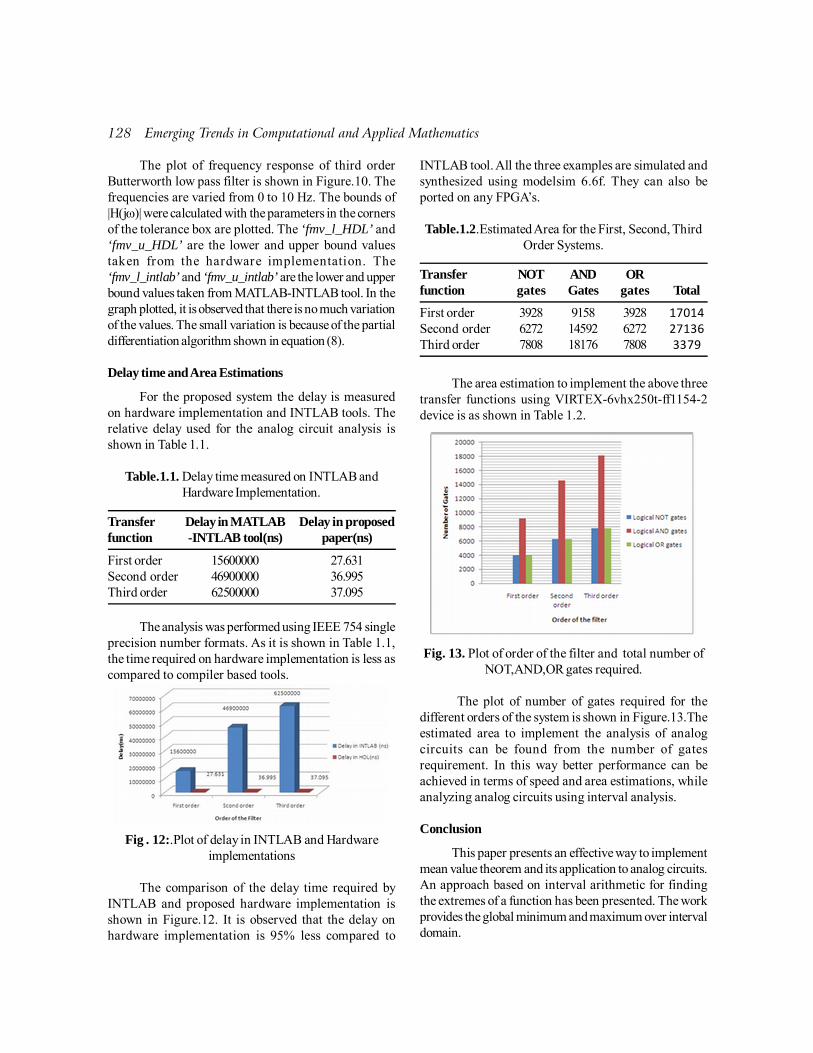
128 Emerging Trends in Computational and Applied Mathematics
The plot of frequency response of third orderButterworth low pass filter is shown in Figure.10. Thefrequencies are varied from 0 to 10 Hz. The bounds of|H(j�)| were calculated with the parameters in the cornersof the tolerance box are plotted. The ‘fmv_l_HDL’ and‘fmv_u_HDL’ are the lower and upper bound valuestaken from the hardware implementation. The‘fmv_l_intlab’ and ‘fmv_u_intlab’ are the lower and upperbound values taken from MATLAB-INTLAB tool. In thegraph plotted, it is observed that there is no much variationof the values. The small variation is because of the partialdifferentiation algorithm shown in equation (8).
Delay time and Area Estimations
For the proposed system the delay is measuredon hardware implementation and INTLAB tools. Therelative delay used for the analog circuit analysis isshown in Table 1.1.
Table.1.1. Delay time measured on INTLAB andHardware Implementation.
Transfer Delay in MATLAB Delay in proposedfunction -INTLAB tool(ns) paper(ns)
First order 15600000 27.631Second order 46900000 36.995Third order 62500000 37.095
The analysis was performed using IEEE 754 singleprecision number formats. As it is shown in Table 1.1,the time required on hardware implementation is less ascompared to compiler based tools.
Fig . 12:.Plot of delay in INTLAB and Hardwareimplementations
The comparison of the delay time required byINTLAB and proposed hardware implementation isshown in Figure.12. It is observed that the delay onhardware implementation is 95% less compared to
INTLAB tool. All the three examples are simulated andsynthesized using modelsim 6.6f. They can also beported on any FPGA’s.
Table.1.2.Estimated Area for the First, Second, ThirdOrder Systems.
Transfer NOT AND ORfunction gates Gates gates Total
First order 3928 9158 3928 17014
Second order 6272 14592 6272 27136
Third order 7808 18176 7808 3379
The area estimation to implement the above threetransfer functions using VIRTEX-6vhx250t-ff1154-2device is as shown in Table 1.2.
Fig. 13. Plot of order of the filter and total number ofNOT,AND,OR gates required.
The plot of number of gates required for thedifferent orders of the system is shown in Figure.13.Theestimated area to implement the analysis of analogcircuits can be found from the number of gatesrequirement. In this way better performance can beachieved in terms of speed and area estimations, whileanalyzing analog circuits using interval analysis.
Conclusion
This paper presents an effective way to implementmean value theorem and its application to analog circuits.An approach based on interval arithmetic for findingthe extremes of a function has been presented. The workprovides the global minimum and maximum over intervaldomain.

Emerging Trends in Computational and Applied Mathematics 129
The experimental evidence for the analysis ofanalog circuits shows that the hardware implementationusing mean value algorithm has a speed up of 106 timesas compared to software packages. So enhancement inperformance can be seen in many folds. On the similarbasis, the algorithm can be applied to analyze any linearelectrical networks. From the author’s best knowledge theanalysis of interval arithmetic are done using C and INTLAB.In this paper the concept is brought on hardware.
In the future work the concentrate is on implementingmore effective algorithm of differentiation which can beimplemented on hardware. By this we can reduce the error.
REFERENCES
[1] P. M. Lin, “A survey of applications of symbolicnetwork functions,” IEEE Trans. Circuit Theory, vol.CT-20, pp. 732-737, Nov. 1973.
[2] K. Singhal and J. Vlach, “Symbolic analysis of analogand digital Circuits,” Proc. 1976 IEEE Int. Symp.Circuits Syst., pp. 41-44, 1976.
[3] E. R. Hansen, “The centered form,” in Topics in IntervalAnalysis,E. R. Hansen, Ed. Oxford University Press,1969, pp. 102-106.
[4] L. C. W. Dixon and G. P. Szegii, Ed. towards GlobalOptimization. North-Holland, 1975.
[5] Fabian Bause, Andrea Walther, Jens Rautenberg, andBernd Henning Reliable Computation of Roots inAnalytical Waveguide Modeling Using an Interval–Newton Approach and Algorithmic Differentiation IEEETransactions on Ultrasonics, Ferroelectrics, andFrequency Control, vol. 60, no. 12, December 20132597 0885–3010/$25.00 c 2013
[5] M. Glesner and A. Blum, “Worst-case error analysis ofelectrical networks with the aid of nonlinear programmingmethods,” in 1974 European Conf. Circuit Theory andDesign, pp. 312-318, 1974.
[6] J. Rautenberg, F. Bause, and B. Henning, “Guidedacoustic waves for liquid property measurement,” Tech.Mess., vol. 79, no. 3, pp. 135–142, 2012.
[7] E. R.Hansen, Global optimization using interval analysisThe Multidimensional case,” Numer. Math ., vo!. 34,pp. 247-270,1980.
[8] Lubomir. V. Kolev, Valeri. M. Mladenov, Simeon. S. Vladov“Interval Mathematics Algorithms for ToleranceAnalysis” IEEE TRANSACTIONS ON CIRCUITSAND SYSEMS, VOL. 35, NO. 8, AUGUST 1988
[9] K. Reinschke, “Numerische Verfahren zur Analyse passiverlinearer Netzwerke unter Beriicksichtigung des EinfluDesder Toleranzen der Schaltelemente,” dissertation Fakultatfk Electrotechnik, ‘Tech. Univ. Dresden, 1966.
[11] K. Madsen and H. Jacobsen, “Algorithm for worst-case tolerance optimization,” IEEE Trans. Circuits Syst.,vol. CAS-26, pp. 775-783,1979.
[12] R. E. Moore, Interval Analysis. Englewood Cliffs, NJ:Prentice-Hall, 1996
[13] L. V. Kolev, “Global constrained optimization viainterval analysis technique,” in Proc. Int., AMSE Conf.Modelling and Simulation, Athens, Greece:‘vol. 1.2, pp.175-188, 1985.
[13] R. E. Moore, Interval Analysis. (Prentice-Hall Series inAutomatic Computation). Englewood Cliffs, NJ:Prentice-Hal& 1966.
[14] “On computing the range of a rational function of nvariables Over a bounded region”, Computing, vol. 16,pp. 1-15, 1976.
[15] S. Skelboe, “Computation of rational interval functions,”BIT, vol.14, no. 1, pp. 87;95,1974,
[16] R. E. Moore, Interval Analysis. Englewood Cliffs, NJ:Prentice-Hall, 1996
[17] S. Skelboe, “Computation of rational interval functions,”BIT, vol.14, no. 1, pp. 87;95,1974,
[18] Lubomir. V. Kolev, Valeri. M. Mladenov, Simeon. S.Vladov “Interval Mathematics Algorithms for ToleranceAnalysis” IEEE Transactions on circuits and systems,VOL. 35, No. 8, August 1988
[19] M. Rump, INTLAB - INTerval LABoratory,Developments in Reliable Computing, T. Csendes (ed.),Dordrecht, The Netherlands:Kluwer Academic, 1999,pp. 77–104.
[20] C . G. Lai, Ed., Surface Waves in Geomechanics: Directand Inverse Modeling for Soils and Rocks. Udine, Italy:Springer, 2005.
[21] N. H. Fletcher and T. D. Rossing, the Physics of MusicalInstruments, 2nd ed., New York, NY: Springer, 2008.
[22] D. S. Ballantine, S. J. Martin, A. J. Ricco, G. C. Frye, H.Wohltjen, R. M. White, and E. T. Zellers, Acoustic WaveSensors: Theory, Design, and Physico-ChemicalApplications. New York, NY: Academic, 1996.
[23] M . Sale, P. Rizzo, and A. Marzani, “Semi-analyticalformulation for the guided waves-based reconstructionof elastic module,” Mech. Syst. Signal Process. vol. 25,no. 6, pp. 2241–2256, 2011.
[24] A . Marzani and L. De Marchi, “Characterization of theelastic module in composite plates via dispersive guidedwaves data and genetic algorithms,” J. Intell. Mater. Syst.Struct., vol. 24, no. 17, pp. 2135–2147, 2013.
[25] J. Rautenberg and B. Henning, “Simultaneous direct andindirect measurement of sound velocities,” Proc. Eurosensors, vol. XXII, pp. 148–151, 2008.
[26] B. Henning and J. Rautenberg, “Process monitoring usingultrasonic Sensor systems,” Ultrasonics, vol. 44, suppl.1, pp. e1395–e1399, 2006.
[27] J. Rautenberg, F. Bause, and B. Henning, “Guidedacoustic waves for liquid property measurement,” Tech.Mess., vol. 79, no. 3, pp. 135–142, 2012.

130 Emerging Trends in Computational and Applied Mathematics
Introduction
Composites are used extensively in aerospace,automobile and civil engineering structures because oftheir high strength-to-weight ratios. Skin stiffenedconstructions are common in aircraft structuralcomponents that are subjected to compressive loads.The skin is so thin that it provides very little resistanceto buckling against in-plane compressive loads. Theobjective of the design optimization is to obtain theminimum structural weight of the stiffened panel. TheMSC/NASTRAN is used for design optimizer, YSFC andPBF criteria are incorporated in an automatic way byexploiting the secondary response constraint feature ofdesign optimizer. The optimizer allows calculating thesecondary response quantities at any stage of designoptimization, using the primary response quantities likestress values and design variables values are as input;and the secondary response constraint is used indefining the design constraints. The structural designoptimization is a gradient-based tool, we need to
construct a mathematical idealization of an physicalstructural component, select appropriate structuralresponses, which are provides an optimum sizing forthe minimum-weight design of a panel of a compositewing. Various components of stiffened panel is to bedetermined based on structural response constraints,subject to satisfaction of strength and buckling to findan optimum feasible solution. In the present study, uni-axial unit loads are considered for different sets ofstringers spacings of a stiffened panel. “Optimizationtechniques plays an important role in structural design,the very purpose of which is to find the best solutionsfrom which a designer or a decision maker can derive amaximum benefit from the available resources”[1]. Thestructural design optimization is a gradient-based tool,we need to construct a mathematical idealization of anphysical structural component, select appropriatestructural responses, which are provides an optimumsizing for the minimum-weight design of a wing. Variouscomponents of structural sizes of spars, stringers, skin-
23Structural Design Optimization of T- Stiffened
Panel of a Composite Wing
Nithin Kumar K C, Sachin Rastogi, Naman Kumar Chandna, Md Mushfique AlamDepartment of Mechanical Engineering, Graphic Era University, Dehradun-248002
[email protected];[email protected]
Abstract: Structural design optimization of a T-stiffened plate of a composite wing for typical transport aircraftis carried out for minimum weight meeting all the structural design constraints. The design variables are skinthickness and stringer cross section for different sets of stringer spacings. The Yamuda-Sun Failure Criterion(YSFC) for strength and Eigen value approach for buckling criteria are used of optimization. Buckling criteria usingPanel buckling Factor (PBF) criteria for buckling of panels and Euler buckling load criteria for stringers are also beattempted for optimization. The final configuration of stiffened plate gives the optimum stringer spacing, whichgives the minimum weight of stiffened plate for satisfying the strength and buckling constraints. Optimization deckfor the above mentioned strength and buckling criteria is developed using the equation input (DEQATN) optionand design response level 2 cards (DRESP2) for the MSC/NASTRAN optimization solver (SOL 200) to carry outthe optimization.Keywords: Composite Material, T-stiffened plate, YSFI, PBF, Eigen Value approach, Optimization.

Emerging Trends in Computational and Applied Mathematics 131
panels, ribs etc. have to be determined based onstructural response constraints, subject to satisfactionof strength and stiffness. To find an optimum feasiblesolution, i.e. a structural design has to satisfying all theresponse constraints by the optimization algorithm [2].
Optimization Problem
A composite panel with T-type stiffener as shownin Figure 1 is adopted as the target structureoptimization. The length of the panel is a=750 mm andthe width is b=500 mm. The width and length of thepanel are fixed and stringer spacings are varied from 50to 250 mm with an increment of 25 mm in the presentstudy. The design variables are thickness of the paneland stiffeners kept constant.
Fig. 1.T-Stiffened Panel
Geometry of the Stiffened Composite Panel
Composite stiffened panels are modeled with hatstiffeners having different stringer spacings. Thestiffened panel length 750mm and 500mm breadth is keptconstant for different stringer spacings. The stringerspacings are varied from 50 to 250 mm with an incrementof 25 mm. The initial thickness configuration of stiffenedpanel is 2.72 mm with basic four orientations of asymmetric balanced laminate. The stiffeners arepositioned along the length and parallel to the loadingdirection, the end panels are taken care of preventingfrom buckling to avoid spurious results. The dimensionsof a stiffened panel are chosen in such way that theyrepresent aircraft fuselage / wing structural componentpanels. The hat section stringers are used in compressivebehavior composite structures, since they are easy formanufacturing and effective in buckling phenomenon.The height of stringers is varied from 20 mm to 25 mmand neglecting the stringer trim corners. The materialproperties (Stiffness and Strength Properties) of carbonfibre composite (CFRP), (Fiber-Unidirectional Carbon
Fiber and Resin-RTM 120/HY 2954) used are listed inTable1 and Table 2. The laminate orientation of carbonfibers: the 0 degree plies are running parallel to theloading direction and laminate stacking is as shown inTable 3.
Table1: Stiffness properties of CFRP
E11
= 120 GPa E22
= 8 GPa v12
= 0.32
�=1.5 gm/cc G12
= 3.0 GPa
Table 2: Strength properties of CFRP
Strength Xt (Mpa) Xc (Mpa) S (Mpa) ILS (Mpa)
Ultimate 585 494 46.0 40.00
Limit 390 329 30.6 26.67
Where, Xt= Tensile Strength in Fiber Direction. Xc= Compressive Strength in Fiber Direction. S= In-plane shear Strength. ILS= Inter Laminar Strength.
Table 3: Stacking sequence of stiffened panel
Component Thk. No.of Stacking(mm) Layers sequence Material
Panel 2.72/ 3.0 8 [45/-45/0/90/90/0/-45/45] CFRP
Loads
The in-plane compressive (uni-axial) unit load perlength is applied along the stiffeners of the stiffenedplate that is parallel to the length direction. Themagnitude of load 150KN. The simply supportedboundary conditions are considered all along thestiffened panels. Since in literature uniaxial loading ispreferred due to Stiffened panels are stiffer along Stingerdirection and in this study loading places important role,loads are chosen carefully with trial and error method.
Structural optimization of stiffened panel
A stiffened panel of 750mm x 500mm in size withdifferent stringer spacings is considered along with asimply supported boundary conditions. A carbon fiber

132 Emerging Trends in Computational and Applied Mathematics
composite material is used with ply thickness of 0.34mmof balanced laminate of a stiffened panel. The Yamuda-Sun failure theory [Eq. (1)] is used as the strengthcriterion for unidirectional fibre carbon composite, theequation is used as the strength criterion. Eigen valueapproach is based on the lowest eigenvalue obtainedfrom the global analysis [4].The Panel buckling equations[5, [Eqs. (2-4)], which are used in DEQATN option inMSC/NASTRAN for the buckling constraint. Theconstraints are not violated if the value is less than orequal to unity.
Where,
Where,
Where,
Where,
i� = Applied Fiber direction stress, 1t� = Applied
in-plane shear stress, Fl= Fiber direction strength, S=In-plane shear strength, D11, D22, D66 are elements oflaminate D-matrix, a= Length along larger side of thePanel, b= Length along smaller side of the Panel, TS=Thickness of the laminates, K = Panel buckling
coefficients, PBF is the panel Buckling Factor, Nx, Nyand Nxy are computed stress results, NXCR, NYCR andNXYCR are computed Panel buckling strengths.
Results and Discussions
The optimization of stiffened panel with differentstinger spacing has been carried out; buckling is a criticalphenomenon in aircraft structures. With bucklingconstraints and strength constraints optimization iscarried out to meet all the design requirements. In thesetwo plots we found stinger spacing 125 mm is seems tobe optimum compared with 75 and 175 mm [Figure 2]. Asthe number of stiffener decreases the weight of the panelincreases or else we can say number of stiffenersdecreases with increasing stinger spacing (50 to 250mm),Figure 3 shows optimum weight versus stingers spacingfor only basic skin weight is considered by neglectingstingers effect/ weight. Here we observed that weightof the panel increases with increasing stinger spacing.
Fig. 2. Optimum Weight Vs Stinger spacing
Fig. 3. Optimum Weight Vs Stinger spacing(Basic Skin weight)

Emerging Trends in Computational and Applied Mathematics 133
Conclusions
Stiffened panels are widely used for aerospaceapplications due to their high stiffness to weight andstrength to weight ratios. However in this study,Structural design optimization of a stiffened panel of acomposite wing for typical transport aircraft is carriedout for minimum weight meeting all the structural designconstraints for different stinger spacings. Here twotypes of configurations are used for different stingersspacings, but in both configurations yield same resultswith little variation in the trends. In this optimization wefound that stinger spacing of 125 mm is optimum ascompared with 75 and 175 mm stinger spacing.
REFERENCES
[1] N. G. R. Iyengar. Department of Aerospace Engineering.“Optimization in Structural design”. Struct MultidiscOptim (2010) 50; pp. 277–298.
[2] E.Barkanov, S. Gluhih, O. Ozolins, E. Eglitis, F. Almeida,M.C. Bowering and G. Watson, “Optimal weight Designof Laminated Composite panels with different stiffenersunder Buckling Loads”.27th International Congress ofthe Aeronautical Sciences, 2010. 1-9.
[3] Ine-Wei Liu & Chien-Chang Lin, 1991, Optimum Designof Composite Wing Structures by a Refined OptimalityCriterion, Composite Structures, 17(1), 51-65.
[4] MSC/NASTRAN Reference Guide 2010: PrescribedConditions, Constraints & Interactions.

134 Emerging Trends in Computational and Applied Mathematics
Introduction
Supply chain planning plays a crucial in managingday to day operations and functions of a business. Theprimary objective of supply chain planning is to integratethe activities such as marketing, planning, purchasing,distribution and manufacturing so as to achieve desiredgoals and objectives of the enterprise.
Supply chain operations can, in general, beclassified into three categories of networks, namely,procurement of raw material from its suppliers,production at production centres and distribution ofthe final product to the customer. One of the mostimportant objectives of supply chain planning is todeliver optimal financial results for the business. Thedecision making process in these highly complex andinteracting networks can be decomposed into threemodels according to time horizon: (1) Strategic planning
models, (2) Tactical planning models and (3) Operational/Midterm-tactical models. Strategic planning is the long-term process of defining its strategy or direction of anorganization and making decisions on allocation ofresources to pursue this strategy. The time horizon ofthis strategy is 5 to 10 years. These are also called longterm planning models. Tactical planning focuses on whatto do in the short-term to help the organization to achievethe long-term objectives. This basically deals with dayto day functioning of an organization such as exactsequencing of the manufacturing tasks while accountingfor the various resource and timing constraints. Thesemodels are characterized by very short-time frames, suchas 1 to 2 weeks. Mid-term tactical models are intermediatein nature. These models address planning horizon of 1to 2 years and incorporate some of the considerationsfrom both the strategic and tactical models. Some
24Bilevel Programming application to Midterm Production-
Distribution Planning Problem
Akhilesh Kumar,1 Neha2
1Department of Operational Research, University of Delhi, Delhi, India2O.P. Shastri Institute of Excellence, Gurgaon, India
[email protected], [email protected]
Abstract: A mid-term production distribution planning problem is addressed in this paper. The situation underconsideration is of a decentralized company with its production and distribution departments having their ownoptimization strategies. Two departments of this kind of company do not cooperate. The company manufacturesmultiple products at its production centers at multiple locations. The distribution department anticipates demandsof its products from various customers and accordingly plans optimal transportation and inventory strategies andhence accordingly identifies the amounts of products that should be available at various production sites in eachperiod. It is to be planned so that all deliveries at customers are made on-time.The production department accordingly prepares its plan for production and inter-site shipment quantities. Amodel addressing this mid-term production distribution planning problem is considered as bilevel program. TheBilevel programming problem (BPP) being an NP-hard problem is suggested to be solved using heuristics. Thesolution of the problem will attempt to minimize the cost of production, inventory and distribution with demandbeing fulfilled and with-in-time delivery be deciding on the amounts of production on various production sites,amounts to be transported from there to various customers and those to hold as inventory in a coordinated manner.Keywords: Mid-term production planning; Supply chain; Delivery time; Bilevel programming

Emerging Trends in Computational and Applied Mathematics 135
considerations in these models include carryover ofinventory and backorders, if any, from previous periodand resource limitations like inventory space, labourcapacity and machine capacity affecting productionvolume. Because of this nature of these models whichconsiders both strategic and tactical planningconsiderations up to some extent and that over a periodof planning which is neither too short nor too long.
Maintaining an efficient supply chain is criticalfor every business enterprise in today’s changingmarket, especially with the increasing customerexpectations. An efficient supply chain aims towardsthe fulfilment of demand as far as possible and that toowithin the stipulated time.
In this paper we consider the mid-term supplychain planning model proposed in [9] and incorporatedelivery time constraints into it. The problem henceobtained is then formulated as a BPP which representsthe hierarchical decision making and informationexchange between production and distributiondepartments.
Literature Review
Supply chain planning models
Supply chain planning models have an extensiveliterature. This can be reviewed by considering each ofthe strategic, tactical and operational planning modelsone by one. Among long-term planning models with theaim of identifying the optimal timing, location and extentof additional investments in processing networks overa relatively long-time horizon, some are [12, 14, 15].Sahinidis et al. [14] considered and solved a multi-periodmixed integer linear programming (MILP) model foroptimal selection and expansion of processes in a giventime varying forecast for demand and prices of chemicalsin the chemical industry over a long range planninghorizon. Among short-term planning models some are[11, 16, 20]. Shah et al. (1993) short term operationalscheduling models constitute the other extreme of thespectrum planning models. Mid-term tactical planningmodels have been worked on by [6–8, 10].
Gupta and Maranas [7] developed an efficientprocedure for solving midterm planning problems. Thissolution strategy is more effective in terms of qualityand computational requirements. Gupta and Maranas[9] solve mid-term multisite supply chain planningproblem with uncertain demand using a stochasticprogramming approach.
Bilevel Programming Problem (BPP)
In some business planning situations there aredifferent decision makers trying to realize best decisionson the market with respect to their own, generallydifferent objectives and that they are often not able torealize their decisions independently but are forced toact according to a certain hierarchy. The mathematicalprogramming problem thus formulated to solve this kindof situation is termed as multilevel programming problem.A particular case of such situation is where there areonly two decision makers. Such a problem is called bi-level programming. As per the hierarchy the decisionmaker who takes decision first or is able to take on anindependent position in the sense of observing andutilizing the reactions of the dependent decision makeron his decisions is termed as leader and hence the otheras follower. Some examples of the situation are case ofproduction – distribution, producing – dealingcoordination. Thomas [17] reviewed the coordinatedplanning between two or more stages of the supplychain, placing particular emphasis on models that wouldlend themselves to a total supply chain model. Thetheoretical development, algorithms for solution andapplications of bi-level programming are well describedin monographs by [2, 5].
In production–distribution problems of supplychain planning dependency of Production andDistribution was advocated in [1]. Authors placeddistribution decision in top level and productiondecision in lower level, so that the production decisionsare revised to satisfy the top–down instructions of thedistribution sub-problem as far as feasibility permits.Roghanian [13] applied bilevel programming frameworkto enterprise-wide supply chain planning problem withprobabilistic market demand, production capacity ofmultiple plants and resource available to all plants foreach product by keeping the production decisions tofollow warehousing and distribution decisions. But thisproblem considers the decision of single period only,thereby not considering any safety-stocks andbackorders of previous and current periods. Hence theconsidered problem cannot be regarded as a mid-termproduction planning problem.
Mid-term planning model
Model Considered
The model developed by Gupta and Maranas [9]is aimed at determining the optimal sourcing and

136 Emerging Trends in Computational and Applied Mathematics
allocation of an enterprise’s limited resources to itsmanufacturing assets so as to satisfy the marketdemands, in the most cost-effective way. The supplychain network considered in the model consists ofmultiple production sites, which are potentially locatedglobally, and manufacture multiple products. Thedemand for these products exists at a set of customerlocations. The planning horizon, in keeping with themid-term nature of the model, ranges from around 1 to 2years. Each production site is characterized by one ormore single stage semi-continuous processing unitshaving limited capacity. The various products, whichare grouped into product families, compete for the limitedcapacity of these processing units. The decision makingprocess at the tactical level can be decomposed intotwo distinct phases: the manufacturing phase and thelogistics phase [7, 8, 10]. The manufacturing phasefocuses on the efficient allocation of the productioncapacity at the various production sites with an aim todetermine the optimal operating policies. Subsequently,in the logistics phase, the post-production activitiessuch as demand satisfaction and inventory managementare considered for effectively meeting the customerdemand. This classification of supply chain activitiestranslates into the following model formulation [9].
Table 1. Some Notations
Sets{i} Set of products{f} Set of product families{j} Set of processing units{s} Set of production sites{t} Set of time periodsParametersFC
fjsFixed production cost for family f on unit j at site s
vijs
Variable production cost for product i on unit jat site s
pis
Price of raw material i at site s
Transportation cost from site s to site Transportation cost from site s to site c
hist
Inventory holding cost for product i at site s inperiod tSafety stock violation penalty for product i atsite sRevenue per unit of product i sold to customer c
Rijst
Rate of production of product i on unit j at site sin period t
Yield adjusted amount of product i consumedto produce product at site s
0–1 parameter indicating whether product ibelongs to family f
Hjst
Production capacity of unit j at site s in period t
MRLfjs
Minimum run length for family f on unit j at site sd
ictDemand for product i at customer c in period tSafety stock for product i at site s in period t
Variables
Yfjst
Binary variable indicating whether product family fis manufactured on unit j at site s in period t
Pijst
Production amount of product i on unit j at sites in period t
RLijst
Run-length of product i on unit j at site s inperiod t
FRLfjst
Run-length of product f on unit j at site s inperiod t
Cist
Consumption of product i at site s in period t
Inter-site shipment of product i from site s tosite in period t
Aist
Amount of product i available for supply at sites in period t
Iist
Inventory of product i at site s in period tS
isctSupply of product i from site s to customer c inperiod tShortage of product i at customer c in period t
Deviation below safety stock of product i at sites in period t
The model can now be formulated as:
subject to

Emerging Trends in Computational and Applied Mathematics 137
The objective function of the deterministicmidterm planning model, equation (1), captures thecombined costs incurred in the manufacturing andlogistics phases. The manufacturing phase costs includefixed and variable production charges, cost of rawmaterial purchase and transportation charges incurredfor the inter-site shipment of intermediate products. Thelogistics phase costs are comprised of the chargesincurred for shipping the final product to customer,inventory holding charges, safety stock penalties andpenalties for lost sales. The decision made in themanufacturing phase establish the location and timingof production runs, length of campaigns, productionamounts and consumption of raw materials. P
ijst, RL
ijst,
FRLfjst
, Aist
, Cist
, Wiss’t
and Yfjst
constitute the manufacturingvariables, and uniquely define the production levels and
resource utilization in the supply chain. Thesemanufacturing variables are limited by themanufacturing constraints given by (2) to (8). Theproduction amount of a particular product is defined interms of the rate of production and the campaign runlength by Eq. (2). The input-output relationshipsbetween raw materials and final products, accountingfor the bill-of-materials, are given through constraint(3). Redundancy in the intersite shipment of intermediateproducts is eliminated by constraint (4), which forcesthe products shipped to a particular site in a particularperiod to be consumed in the same period.
The allocation of products to product families isachieved through constraint (5). Grouping of productsinto product families is typically done to account forthe relatively small transition times and costs betweensimilar products. Constraint (6) models the capacityrestrictions while constraint (7) provides upper andlower bounds for the family run lengths. The amountavailable for supply in the logistics phase following themanufacturing phase is defined through constraint (8).The decisions made in the logistics phase, termed thelogistics variables, are S
isct, I
ist, and . The
corresponding logistics constraints are given byconstraint (9) to (12). The linking between themanufacturing and logistics phases is captured byconstraint (9). The inventory level, which is determinedby the amount available for supply and the actualsupplies to the various customers, is defined byconstraint (9). No overstocking is permitted at thecustomer constraint (10) and the customer shortagesare carried over time constraint (11). Constraint (12)models the violation of the safety stock levels.Establishing of safety stock targets for the inventorylevel can be viewed as an aggregate deterministicattempt to buffer against unpredicted contingencies suchas demand variations and production rate fluctuations.
Lead-time constraint
Agility and accuracy in delivery time is one of thefundamental characteristics of competitiveness. Anenterprise has to be able to satisfy the consumers’demand within the stipulated time, with desired qualityand at a reasonable price. The time related strategies insupply chain planning aim towards restricting thedelivery time uncertainty to a fixed lowest level. As aresult of delay in the delivery time enterprise has to facebacklogs, delay in demand delivery, demurrages and
138 Emerging Trends in Computational and Applied Mathematics
increase in product total prices.At the time when the actual demand is realized,
customer usually associates a delivery time deadline.The producer has to satisfy the customers demand,partially or fully by volume, by meeting this deliverytime deadline. The time elapsed to deliver theconsignment measured from the time when the order isplaced is termed as lead-time. The aim of a supply chainmanager is to plan the outbound logistic operations insuch a manner that lead-time to each customer’s demanddoes not exceed its delivery time deadline. Weincorporate this condition as a constraint. Some authorsin the literature consider the aspect of lead-time as anobjective to be minimized. But time-minimization problemin distribution planning problems is considered in caseof perishable items or in case of emergency/ calamity.As we consider a general case of non-perishableconsumer product, therefore, once lead-time is less thanor equal to the delivery-time deadline, there is no needto further reduce the lead-time by paying an extra costfor a faster conveyance. Further, we assume here that atleast one arrangement of distribution of product fromvarious production/ distribution sites to variouscustomer sites is available.
Let be the binary variable indicatingwhether product i is transported from site s to customer
c in the period t. be the lead-time of transportingthe product i from site s to customer c in period t, and
be the delivery-time deadline of delivering theproduct i at customer c in period t. Then, the lead-timeconstraints over each period can be expressed asfollows.
This can be rewritten as a set of followingconstraints.
This set of constraints can be categorized intologistic constraints.
Proposed Approach
Formulating the problem as a BPP
As in a midterm production planning problemdecision on production quantities and inter-siteshipment volumes in a period not only depend uponthe forecasted demand on that period but also on the
decision on the inventory level to be maintained in thatperiod. Therefore, we pose this problem as a bilevelprogramming problem which considers the productioncost optimization problem as (follower’s) inner problemand the optimization of inventory and distribution costas the (leader’s) outer problem.
Let us consider
and . Then vectors X andY represent sets of follower’s and leader’s variables.
Then the corresponding bilevel programmingproblem can be written as following.
subject to
where are
obtained by solving
subject to

Emerging Trends in Computational and Applied Mathematics 139
Solving the BPP
The above bilevel programming problem is of theform:
subject towhere Y solves
subject to
Using the Penalty Function approach [19] theabove bilevel programming problem can be expressedas following optimization problem with non-linearobjective function involved in the penalty function.
subject to
Solution Strategy
As the midterm planning problem even over aplanning horizon of one year and BPP even with simplemost linear case are NP-hard [3], hence is the problem(P2). Therefore the problem (P2) can be solved usingheuristic algorithms like Genetic Algorithm.
Conclusion
The proposed work first presents an overview ofwork addressing the problem of midterm supply chains(production - distribution) planning. The deterministicmodel originally proposed by McDonald and Karimi [11]and then considered by Gupta and Maranas [9] was
adopted. Secondly, the aspect of delivery-times wasincorporated in the model as a step towards the resiliencewith a minimum service-level maintained.
Specifically, the supply chain networks consideredwere multi-product, multisite and multi-period in nature.It was shown that, in case of a decentralized firm, theproblem under consideration can be modelled as abilevel programming problem. The bilevel programmingproblem hence obtained can be dealt by followingPenalty function approach and then solved by heuristicalgorithms.
To summarize, it was shown that by utilizing thebilevel programming framework, for a company havingdecentralized production and distribution departmentsa more coordinated decision on production, inventoryand distribution variables can be taken. Consequently,the demand of various customers can be fulfilled in amore efficient way and well on time, thereby enhancingthe reliability of supply chain.
Acknowledgement
First author gratefully acknowledges the financialsupport of the Council of Scientific and IndustrialResearch, New Delhi, India through his Junior ResearchFellowship (JRF) scheme CSIR Award no.: 09/045(1257)/2012-EMR-I for his research work.
REFERENCES
[1] Barbarosoglu G. and Ozgur D. Hierarchical design of anintegrated production and 2-echelon distribution system.European Journal of Operational Research, 118, 464-84 (1999).
[2] Bard J.F., Practical Bilevel Optimization: Algorithms andApplications, (Springer Science Business Media Dordecht1998).
[3] Ben-Ayed, O., and Blair, E. Computational difficultiesof bilevel linear programming. Operations Research, 38,556-560 (1990).
[4] Calvete H. I., Gale C., Mateo P.M. A new approach forsolving linear bilevel problems using genetic algorithms.European Journal of Operational Research, 188, 14-28(2008).
[5] Dempe Stephan, Foundations of Bilevel Programming,(Kluwer academic publishers 2002).
[6] Dimitriadis, A.D., Shah, N., & Pantelides, C.C.,. RTN-based rolling horizon algorithms for medium termscheduling of multipurpose plants. Computers andChemical Engineering S21, S1061 (1997).

140 Emerging Trends in Computational and Applied Mathematics
[7] Gupta, A., & Maranas, C. D., A hierarchical Lagrangeanrelaxation procedure for solving midterm planningproblems. Industrial and Engineering ChemistryResearch 38, 1937-1947 (1999).
[8] Gupta, A. Maranas, C. D. A Two-Stage Modeling andSolution Framework for Multisite Midterm Planningunder Demand Uncertainty. Ind. Eng. Chem. Res., 39,3799 (2000).
[9] Gupta, A.; Maranas, C. D. Managing DemandUncertainty in Supply Chain Planning. Comput. Chem.Eng., 27, 1219–1227 (2003).
[10] McDonald, C. M., & Karimi, I. A. Planning andscheduling of parallel semicontinuous processes. 1.Production planning. Industrial and EngineeringChemistry Research 36, 2691 (1997).
[11] Karimi, I.A., & McDonald, C.M. Planning andscheduling of parallel semicontinuous processes. 2. Short-term scheduling. Industrial and Engineering ChemistryResearch 36, 2701 (1997).
[12] Norton, L. C., & Grossmann, I. E. Strategic planningmodel for complete process flexibility. Industrial andEngineering Chemistry Research 33-69 (1994).
[13] Roghanian E., Sadjadi S.J., Aryanezhad M.B. Aprobabilistic bi-level linear multi-objective programmingproblem to supply chain planning. Applied Mathematicsand Computation 188 (2007) 786-800 (2007).
[14] Sahinidis, N. V., Grossmann, I. E., Fornari, R. E., &Chathrathi, M. Optimisation model for long rangeplanning in the chemical industry. Computers andChemical Engineering 13, 1049 (1989).
[15] Sahinidis, N. V., and Grossmann, I. E. Multiperiodinvestment model for processing networks withdedicated and flexible plants. Industrial and EngineeringChemistry Research 30, 1165 (1991).
[16] Shah, N., Pantelides, C. C., and Sargent, R. W. H. Ageneral algorithm for short-term scheduling of batchoperations. Computational issues. Computers andChemical Engineering 17,229 (1993).
[17] Thomas D.J. and Griffin P.M. Coordinated supply chainmanagement. Europian J. of Operational Research 94, 1– 15 (1996).
[18] Verderame Peter M. and Floudas C.A. (2011) MultisitePlanning under Demand and Transportation TimeUncertainty: Robust Optimization and ConditionalValue-at-Risk Frameworks. Industrial & EngineeringChemistry Research, 50(9), 4959–4982.
[19] White, D.J. and Anandalingam, G. A Penalty Functionfor Solving Bi-Level Linear Programs. Journal of GlobalOptimization, 3, 397-419 (1993).
[20] Xueya, Z., and Sargent, R.W.H. Optimal operation ofmixed production facilities/extensions andimprovements. Computers and Chemical Engineering20, S1287 (1996).

SOFT COMPUTING

Introduction
Genetic Algorithm (GA):- was invented by JohnHolland[1] at University of Michigan in 1975, GA ispopulation based, probabilistic search and optimizationtechnique that works on mechanism of natural geneticsand Darwin’s principle of natural selection (i.e. survivalof the fittest).
GA maintains the population of individuals thatevolves according to rules of selection and manipulatesby genetic operators - crossover and mutation. GA cansearch irregular space and hence are applied to a varietyof function optimization, parameter estimation andmachine learning applications.
Working principle[2] can be explained briefly usingthe flowchart.
The primary difference between binary and realcoded GA is that in binary coded GA variables arerepresented by bits of zeros and ones while GAs basedon real number representation are called real coded GAs(RCGAs).
GA originated with a binary representation of thevariables. Until 1991 no specific theoretical studies weredone for RCGAs so its use was controversial. RCGAs
25Comparative Analysis of Real and Binary Coded GA
for Fuzzy Time Series Prediction
Shilpa Jain1, Prakash C. Mathpal2, Dinesh Bisht3
1,2School of Engineering and Technology, ITM University, Gurgaon, 122017, INDIA3Department of Mathematics, Jaypee Institute of Information Technology, Noida, 201304, INDIA
[email protected], [email protected], [email protected]
Abstract: GA is a robust optimization and search technique. It can be applied to optimizing many domains likedata mining, time series prediction, machine learning, routing, etc. Variants of GA are binary coded GA, real codedGA, micro GA, messy GA. Here, in this research article we present a comparative analysis of real coded and binarycoded GA for forecasting of enrollments of University of Alabama. Results clearly states that real coded GA arefaster & more accurate. Results are stated after testing on 100 generationsKeywords: Genetic Algorithms, Fuzzy Time Series, Data Mining, Machine Learning, Time Series Prediction,Routing.
Fig. 1: Working cycle of a GA
are mainly used for numerical optimization oncontinuous domains (Wright[4]; Davis[5];Mchalewicz[6]; Muhlenbein et al.[8]; Herrera et al.[9]).Goldberg[10], Deb[11][12][13] are also eminent
Emerging Trends in Computational and Applied Mathematics 143

144 Emerging Trends in Computational and Applied Mathematics
researchers who contributed in development ofcrossover and mutation operators of RCGAs
In this research article we compare real coded GAwith binary coded GA implemented on data set ofUniversity of Alabama which is a fuzzy time series. Timeseries is a sequence of data points recorded regularly.Fuzzy Time Series is used which differs from traditionaltime series as values of Fuzzy Time Series are representedby Fuzzy sets rather than real values. Song and Chissomproposed definitions of Fuzzy Time Series [14][15][16].Fuzzy time series has been developing for three decadesto improve forecasting accuracy of enrollments,economy, stock market, weather, population growth etc.
Methodology
Proposed method for Real and binary coded GAfuzzy time series forecasting:-
Step 1:- Define the universe of discourse.Step 2:- Partition into intervals using G.A (For
binary coded GA variables are population strings ofzeros and ones and for real coded GA population stringsare real number representations).
Step 3:- Construct Fuzzy sets.Step 4:- Fuzzify the data.Step 5:- Established Fuzzy rules.Step 6:- Forecast.Step 7:- Forecasting accuracy is measured using
MSE. The lower the MSE, the better is forecastingmethod. MSE is defined by the expression
Implementation of Proposed Method toEnrollments forecast
Step 1:- Define the Universe of discourse, U basedon range of available historical time series data, by ruleU=[Dmin - D1, Dmax + D2] Where, D1 and D2 are twoproper positive numbers. Table 1 shows historical dataof enrollments for University of Alabama. From table 1,we can see Dmin =13055 and Dmax=19337. Let D1=55and D2=663, therefore the universe of discourse U =[13000, 20000]
Step 2:- Divide universe of discourse U into 21intervals using X
1 to X
19. u
1 ......u
7
Table 1: Data of Enrollments from University ofAlabama.
Year Actual Enrollments
1971 130551972 135631973 138671974 146961975 154601976 153111977 156031978 158611979 168071980 169191981 163881982 154331983 154971984 151451985 151631986 159841987 168591988 181501989 189701990 193281991 193371992 18876
Step 3:- Define each chromosome consisting of19 genes as shown below :-
Table 2: Chromosome consisting of 19 genes
X1
X2
X3
.... .... .... .... X19
Where X1, X
2, X
3.... are integer variables. These
values of X1, X
2, X
3.... X
19 are generated randomly by GA.
GA generates 30 chromosomes as initialpopulation in form of binary strings for binary codedGA and in form of real number representation for RCGAs.Fuzzify the historical enrolments shown in Table 1 withthe chromosomes in the population. Let the Fuzzy setsconstructed can be realized as

Emerging Trends in Computational and Applied Mathematics 145
Fig. 2 Fuzzy Sets
Let the Fuzzy set A1, A
2.... A
7 be linguistic values
of the linguistic variable enrollments shown as below:
A1 = EL (Extremely Low)
A2 = VL (Very Low)
A3 = L (Low)
A4 = M (Medium)
A5 = H (High)
A6 = VH (Very High)
A7 = EH (Extremely High)
Step 4:- Rules for forecasting
,
,
,
, ,
Fig. 3: Rule Base
The rules stated in Figure 3 are the standard rulesgiven by Chen [17].
Step 5:- In this research article we have used
Matlab 7.6.0 to code Fuzzy and GA techniques of softcomputing. Code is generated for Fuzzy using FIS andcommand that is used for the same is EVALFIS(). Y =EVALFIS(U,FIS) simulates the Fuzzy Inference SystemFIS for the input data U and returns the output data Y.For a system with N input variables and L outputvariables,
* U is a M-by-N matrix, each row being a particularinput vector
* Y is M-by-L matrix, each row being a particularoutput vector.
Step 6:- MSE for each model of each generation iscalculated which becomes the objective function forGA.
Step 7:- Selection rate is 50 percentage. So thatmeans rest 50 percentage of the chromosomes arediscarded and new chromosomes after performing crossover and mutation operations are added to thepopulation. This continues for hundred generations.
Results & Conclusion
In this research article we have proposed acomparative analysis of binary and real coded GA. Themethod was implemented on the historical time seriesdata of student enrollment at the University of Alabamato provide comparative study. When the mutation rateis 0.05,the crossover is 1,the number of intervals in theuniverse of discourse is 19,the population size=30,andthe number of generations evolving is 100 for both binaryand real coded GA.GA originated with a binaryrepresentation of the variables. When variables arequantized naturally, the binary GA can be applied.However, when the variables are continuous, Its morelogical to represent them by floating point numbers. Inaddition, since the binary GA has its precision limited tobinary representation of variables using floating pointnumbers that allows representation to machine precision.Thus continuous GA or real coded GA also hasadvantage of requiring less storage than binary GAbecause a single floating point number represents thevariable instead of Nbits integers.
Moreover the continuous GA is inherently fasterthan the binary GA because the chromosome don’t haveto be decoded prior to evaluation of objective function.

146 Emerging Trends in Computational and Applied Mathematics
Table 3: Shows a Comparison of the MSE of theForecasting Enrollments of the Binary and
Real Coded GA.
Model Real coded GA Binary Coded GA
MSE 395420 275900
With the above specifications it was observedthat Real coded GA program ran much faster incomparison to Binary coded GAs although accuracy interms of MSE is better for binary coded GA although assuggested by Herrera, Lozano & Verdegay [18] resultscan be further improved by using non-uniform mutationand BLX-�, logical FCB and linear crossover operators.
REFERENCES
[1] J. H. Holland, Adaptation in Natural and ArtificialSystems. Ann Arbor, MI, USA: The University ofMichigan Press, 1975.
[2] D. K. Pratihar, Soft Computing, New Delhi: NarosaPublication, 2009.
[3] L. Randy Haupt and Sue Ellen Haupt, Practical Aspectsof Genetic Algorithms. New Jersey: John Wiley & Sons,2004.
[4] A. Wright, “Genetic Algorithms for Real ParameterOptimization” in Foundations of Genetic Algorithms 1,G. J. E. Rawlin, ed. (Morgan Kaufmann, Sun Mateo,1991).
[5] L Davis, Handbook of Genetic Algorithms, New York:Van Nostrand Reinhold, 1991.
[6] Z. Michalewicz, Genetic Algorithms + Data Structures= Evolution Programs, New York: Springer-Verlag, 1992.
[7] H. Michlenbein and D. Schlierkamp Voosen. “Predictivemodels for the breeder genetic algorithm I. continuousparameter optimization”, Evolutionary Computation1, 25-49 (1993).
[8] F. Herrera, E. Heera-Vieddma, M. Lozano, J. L.Verdegay, “Fuzzy Tools to Improve GeneticAlgorithms,” in Second European Congress on IntelligentTechniques and Soft Computing, 1994, pp. 1532-1539.
[9] D. E. Goldberg, Genetic Algorithms in Search,Optimization and Machine Learning, MA : Addison-Wesley, 1989.
[10] D. E. Goldberg, K. Deb, “A comparison of selectionschemes used in genetic algorithms”, In Proceedings ofFoundation of Genetic Algorithms-I, G. Rawlins ed.,San Mateo: Morgan Kaufmann, 1991, pp. 69-93.
[11] K. Deb, R. B. Agarwal, “Simulated binary crossover forcontinuous search space”, Complex Systems 9(2), 115-148 (1995)
[12] K. Deb, M. Goyal, “A combined genetic adaptive search(GeneAS) for Engineering design”, Computer Scienceand Informatics 26(4), 30-45 (1996)
[13] Q. Song and B. S. Chissom, “Forecasting enrollmentswith fuzzy time series - Part 1”, Fuzzy Sets and Systems54(1), 1-9 ( 1993)
[14] Q. Song and B. S. Chissom, “Fuzzy time series and itsmodels”, Fuzzy Sets and Systems 54(3), 269-277(1993)
[15] Q. Song and B. S. Chissom, “Forecasting enrollmentswith fuzzy time series- Part II”, Fuzzy Sets and Systems62(1), 1-8 (1994)
[16] S. M. Chen and N. Y. Chung. “Forecasting enrollmentsof students by using fuzzy time series and geneticalgorithms”, Information and Management Sciences17(3), 1-17 (2006)
[17] F. Herrera ,M. Lozano and J. L. Verdegay, “TracklingReal-Coded Genetic Algorithms: Operators and toolsfor behavior Analysis,” Artificial Intelligence Review12, 265-319 (1998)

Emerging Trends in Computational and Applied Mathematics 147
INTRODUCTION
With high technology developing in recent years,smart phones have become the new generation of cellphones. It penetrates in the market very rapidlyworldwide. Almost everybody has a smart-phone andcarries this device as a major part of daily life. Thus, inway of exploring the world of smart-phones, HumanActivity Recognition gains the most attention. It hasbecome very popular in a small fraction of time becauseof its numerous real time applications. After seeing thepresent scenario, we present a demo application whichcan turn mobile devices into a constantly monitoringdevice. This method can send the information related tophysical activity of the user to a connected server formonitoring purposes. Then on the server side, desktopcan be used as a monitoring agent to analyze the datasent to the server. This application can be very usefulfor the people who need constant assistance andmonitoring, such as elderly or physically unfit people.
Also, healthy people also can use this type ofapplication for monitoring their daily activity and energyconsumption.
Even though there exist many studies related tothe Activity Recognition via 3-axial accelerometer, butthere still exist some unobserved aspects which need tobe highlighted. The first aspect is the positioning ofthe phones that varies with the different persons, forexample some people may carry the phone in their handsor some may put it in their chest pocket or some mayeven keep in pants’ pocket. Here, we consider basicallythree positions namely Phone in hand, Phone inHandbags or Purse and in pants pocket. Beside thisthere can be many more possibilities of change inposition of placing the phones with the different people.This may recognize the activities incorrectly as theorientation of the phone will differ. The second aspectis the fact that different people may exhibit differentpattern of doing same activities. For eg. If a personwalks with fast pace then this would get mismatch with
26Human Activity Recognition Using Smartphone Sensors
Aishwarya Jain, Surbhi JainJaypee Institute of Information Technology Noida, Uttar Pradesh 201309, India
Abstract: In Recent times, with the explosion of smartphone devices, Human Activity Recognition has gained amassive attention as it enables a wide variety of applications in many areas. This work focuses on to explore theuse of smartphone technology to perform activity recognition without interfering in user’s daily lives. The systemrelies on device’s sensing and processing capabilities to recognize the various indoor and outdoor activities that aperson does in daily life i.e. Running, Sitting, Walking, Climbing Upstairs, Climbing Downstairs. In order toevaluate the system, the data has been gathered by the use of 6 built in sensors like linear acceleration, magneticfield, tri-axial accelerometer, gyroscope, gravity, orientation on as many as 5 different individuals, notably bypositioning the device at three different locations mainly in hand, jeans front pocket and in purse/bag and also byusing different mobile devices matching with the user’s lifestyle. A set of 3 machine learning algorithms (i.e., J48Decision Tree, Naïve-Bayes and Random Forest) that are working on sensor’s data have been evaluated andoptimized in terms of accuracy. Results show that Random Forest classifier give us accuracy upto 99.9% taking1.42 seconds to build the model when evaluated on the data set obtained from a set of 5 sensors namely tri-axialaccelerometer, gravity, orientation, linear acceleration and magnetic field sensor at a sampling rate of 100Hz.Keywords: Human Activity Recognition; Classifiers; Machine Learning Tool; Feature Extraction; Mobile Sensors

148 Emerging Trends in Computational and Applied Mathematics
running. To overcome this solution a strong approachshould be made to understand the various subjects andtheir way of responding towards any activity. In thiswork approach have been take to analyze the mostappropriate activity from the vast dataset by consideringdifferent human behavior.
In this work firstly, we collected the accelerometerdata sensor by taking 5 different individuals havingdifferent habits of doing activities to identify and trackthe physical activities that a user is performing such aswalking, running, sitting, standing, traveling on avehicle. This can be achieved by analyzing the datacoming from the accelerometer and GPS since eachdifferent activity results in different accelerometer andGPS data series. Then the data is preprocessed usingsome machine learning algorithm. This work is importantas the activity recognition model lets us extract usefulinformation about the daily routines of millions of usersjust by their habit of regularly carrying their smart phoneswith them. This can also serve as a base for severalother useful applications. For example, we can createdaily physical activity report for a user which showshow active he is during the day. It can show if the useris doing enough exercise or not so that the user can beencouraged to do more exercise. Another example couldbe Calorie Burnt Calculation by recording PhysicalActivities of user.
RELATED WORK
In [3], activity recognition has been investigatedby using a dataset of 4 subjects performing 7 activitiesby varying sensor placement positions. With the helpof decision tree classifier, precision and recall scores of0.75 and 0.73 respectively. A combination ofaccelerometer and gyroscope sensors has been used.The main problem that arises in [3, 5] is accuracy inactivity classification. This means that the user isexpected to get wrong predictions at many times.
In [6], 14 physical activities have been classifiedby using 14 triaxial accelerometers making a body sensornetwork. A tree based classifier and a set of 31 featureshas been used to classify the relevant activities.Accuracy measure has been reached upto 96% which isquite good. While in [7], a set of 20 features and RandomForest classifier have been implemented on the datagathered from wearable sensing devices to classify theactivities with 94% accuracy. It can be seen that [6, 7, 9]have proved to be very effective for the activityrecognition but the main lack in these work is that
subjects are bounded to wear the sensing devicesthroughout which is practically always not possible.
In spite of this, there have been many other studieson activity recognition like in [4], a person’s dailyphysical activities have been monitored by using asingle motion sensor device and by placing it on 6different pocket positions according to the user’s dailylifestyle. SVM based classifier has been developed torecognize 7 common physical activities. A data set of48.2 hours long duration has been collected from 7subjects and thus overall F-score comes out to be94%. While on the other side [12] has monitored thephysical activities by making the application orientationindependent for the user. But the main drawbacks of [4,8, 12] is that they are considering only single motionsensor and we are known with the fact that an androiddevice contains several other sensors too that mightprovide us better results. Also the device positions thatthey considered are very less. This means that user ofthe system are forced to use the device in such a waythat it should not be unfriendly for the device.
In this work, we work upon the combination ofdifferent sensors embedded in the smartphone toachieve maximum accuracy. Also we have consideredthe effects of different placements and orientations ofthe device on the accuracy.
EXPERIMENTAL SETUP
In this section we have described the setup ofour experiments that have been performed to recognizethe activities accurately. We begin with data acquisitionprocess that describes how the data has been gatheredfor our experiment and the set of activities considered.Then set of feature extracted from the data gathered hasbeen described followed by machine learning algorithmthat is used for classification.
DATA ACQUISITION
In this work a set of 6 activities namely sitting,standing, walking, running, climbing upstairs andclimbing downstairs are identified on the basis of users’daily life activities. In order to have more accurateresults subjects were asked to place the smartphonesat mainly 3 positions. These include phone in handposition, phone in front pocket near to the thighs andphone in bag or ladies purse. Notably, purse can be inhand or on the shoulders.
The data was gathered using an Android 2.3.6

Emerging Trends in Computational and Applied Mathematics 149
operating system based Samsung S Advance smartphone that contained MPL linear acceleration sensor,gravity sensor, gyroscope sensor, triaxial accelerometersensor, magnetic field sensor, orientation sensor andseveral others. These smartphone sensors were usedto collect the activity data set.
Data gathering was done by performingexperiments on four subjects. Each of the four subjectswere asked to collect the data activity one by one byplacing smartphone at the positions mentioned above.Each subject performed the set of 6 activities one byone for the duration of two minutes and the respectivedata was recorded in a .csv file in the external storage ofthe smartphone. The location and orientation of thephone was not standardized and was left to theconvenience of the subject. In all the cases we collectedthe sensors data every 50ms, i.e. 20 samples per second.
DATA PREPROCESSING
The raw data usually needs to be pre-processedin order to be supplied to the Weka toolkit. Wekaoperates in ARFF format files, so every data file has to
be converted into ARFF. Sensors raw data needs to bedivided in windows, sequentially, to be pre-processed.One should choose the window approach based onwhether the recognition is intended to be done in realtime (or “online”) or not . For online applications thewindow has to be defined in parallel with data collection,and for offline applications the window is defined priorto data collection. As we are working in offline mode,therefore we predefined the window size and thus restrictthe writing of data to 20 readings per second and thensend that data for applying sliding windows technique,where the signal is divided in equal windows with nogaps. We have taken a window of 100 samples(corresponding to 5 seconds).
The above file then send to the weka for furtherpreprocessing of data. Raw data needs to be split intotraining and test set. The training set will be used to trainthe recognition algorithm and the test set will then beused to evaluate the algorithm after training. Weka toolkithas some split data strategies, such as cross-validation,where a portionof the dataset is used for training and therest for testing (avoiding a partitioning with classesoverrepresented in the training set)and percentage split,where usually a third of the data is held out for testing,so the “train/test percentage split” is 66%.
FEATURE EXTRACTION
For each window, some features are extracted tocharacterize the signal. These features are then used asinput for the recognition algorithms, to associate eachwindow with an activity. We have used here some Time-domain features to extract basic signal information fromraw data. It could also be calculated as data is being read.
Table 1: Accuracy Comparison
Paper # of Sampling # of # of # of Accuracyactivities rate (Hz) classifiers inbuilt device
sensors position
[4] 7 10 1 1 1 94.8%
[7] 5 1 1 1 1 94%
[3] 7 20 5 2 - 75%
[12] 5 100 1 3 1 97%
[5] 4 50 3 5 1 88%
Ours 6 100 3 6 3 99.9%

150 Emerging Trends in Computational and Applied Mathematics
Usually, these features are simple to compute. Tablesummarizes time-domain features that we have used.
Table 2. TIME-DOMAIN FEATURE SUMMARY
FeaturesMean of x, y, z values
Standard Deviation of mean and x,y, z values
Magnitude of x, y, z valuesMin, Max Range of Values
CLASSIFICATION
After extracting signal features, we have appliedvarious machine learning techniques in order toconstruct a classifier. It is possible to use Wekaworkbench to implement these recognition algorithms.
We have classified our data on the basis of 3various machine learning algorithms. These are J48Classifier tree, Random Forest Tree and Naïve Bayesalgorithm. Among all the classifiers used the RandomForest provides us the most convincing results.
Fig. 1: Accuracies(in %) of the three classifiers used
Fig. 2: Time taken(in s) by the classifiers to build the model
RESULTS
When Random Forest classifier is applied on data
set obtained from a combination of 5 sensors mainlylinear acceleration, gravity, magnetic field, tri-axialaccelerometer and orientation sensor, an accuracy of99.9% is obtained which is very good.
Table 3: Confusion Matrix for Naïve Bayes
Classified as A B C d e f
A 1343 0 265 0 2 0B 0 1569 35 0 0 0C 201 0 1342 0 0 0D 94 0 1 1909 39 0E 59 0 1 17 2944 0F 21 0 42 0 0 2122
Table 4: Confusion Matrix for J48 Classifier
Classified as A B C d e F
A 1609 0 0 0 1 0B 0 1604 0 0 0 0C 7 0 1536 0 0 0D 0 0 1 2041 1 0E 1 0 1 1 3018 0F 0 0 0 0 0 2185
Table 5: Confusion Matrix for Random Forest
Classified as A b C D E f
A 1596 0 14 0 0 0B 0 1603 1 0 0 0C 19 1 1523 0 2 0D 0 0 1 2037 5 0E 2 0 3 3 3013 0F 0 0 0 0 0 2185
CONCLUSION AND FUTURE WORK
To provide mobility for tracking the daily lifeactivities, smartphone is a convenient and suitabledevice due to its rich functionalities. In this paper, wehave utilized various smartphone sensors data which isevaluated using 3 machine learning algorithms toimprove the accuracy of detecting a person’s activity.In contrast to the previous work of assuming that thephone is placed in a known position or fixed orientation,this paper intends to recognize the physical activities inthe natural setting where the phone is placed at threedifferent locations(in jeans front pocket, in hand and in
Emerging Trends in Computational and Applied Mathematics 151
purse/bag). For the varying orientation issue,acceleration magnitude is added as a new sensor readingdimension, which can relieve the effect of the orientationchange on the performance of activity classi?cation.Future work will involve increasing the number ofsubjects on which the experiments are performed andthe number of activities classified. As the data set isobtained at a sampling rate of 100Hz which increasesthe battery consumption of the smart phone, therefore,future work will also involve developing an applicationwhich helps in optimizing the battery usage so thatactivities can be identified accurately but not consumingmuch battery of the phone.
ACKNOWLEDGMENTS
The authors would like to thank Riti Kumari,Apoorva Jain and Nancy Jain for helping us collectour experimental data set. Also, authors are thankful toMs. Sangeeta Mittal for her continuous support andguidance throughout the experiment.
REFERENCES
[1] Al-Bashayreh, M.G. Hashim, N.L. AND Khorma, O.T.Towards Successful Design of Context-Aware ApplicationFrameworks to Develop Mobile Patient MonitoringSystems Using Wireless Sensors. Open Systems (ICOS),2012 IEEE Conference, Page(s):1 – 6.
[2] Das, B., Krishnan, Narayanan C., Thomas, B.L. ANDCook, D.J. Simple and Complex Activity RecognitionThrough SmartPhones. 2012 Eighth InternationalConference on Intelligent Environments © IEEE
[3] Daniel Kelly AND Brian Caulfield. An Investigationinto Non-Invasive Physical Activity Recognition usingSmartphones. 34th Annual International Conference ofthe IEEE EMBS San Diego, California USA, 28 August- 1September, 2012.
[4] Lin.Sun, Daqing Zhang, Bin.Li, Bin.Guo AND ShijianLi. Activity Recognition on an Accelerometer EmbeddedMobile Phone with Varying Positions and Orientations.UIC’10 Proceedings of the 7th international conferenceon Ubiquitous intelligence and computing.
[5] Henar Marti´n, Ana M. Bernardos, Josue ́Iglesias, Jose´R. Casar. Activity logging using lightweight classificationtechniques in mobile devices. 5 April 2012 Springer-Verlag London Limited 2012.
[6] Khan, A., Chehade, N.H., Chieh Chien AND Pottie, G.
Feature selection based on mutual information forhuman activity recognition. Acoustics, Speech and SignalProcessing (ICASSP), 2012 IEEE InternationalConference, Page(s): 1729 – 1732.
[7] Pierluigi Casale, Oriol Pujol, AND Petia Radeva. HumanActivity Recognition from Accelerometer Data Using aWearable Device. IbPRIA 2011, Proceedings of the 5th
Iberian conference on Pattern recognition and imageanalysis.
[8] Matti Lyra AND Hamed Ketabdar. ActivityMonitor:Assisted Life Using Mobile Phones. IUI’10, February7–10, 2010, Hong Kong, China. ACM 978-1-60558-515-4/10/02.
[9] Yi He, Ye Li AND Shu-Oi Bao. Fall Detection by Built-In Tri- Accelerometer of Smartphone. Proceedings ofthe IEEE-EMBS International Conference on Biomedicaland Health Informatics (BHI 2012) Hong Kong andShenzhen, China, 2-7 Jan 2012.
[10] Gueesang Lee AND Deokjai Choi. Fall Detection basedon movement in smartphone technology. Computing andCommunication Technologies, Research, Innovation, andVision for the Future (RIVF), 2012 IEEE RIVFInternational Conference, Page(s):1 – 4.
[11] Jeffrey W. Lockhart, Tony Pulickal AND Gary M.Weiss. Applications of mobile activity recognitionUbiComp’12, September 5-8, 2012, Pittsburgh. ACM978-1-4503-1224-0/12/09.
[12] Yunus Emre Ustey, Ozlem Durmaz Incel AND CemErsoy. User, device and orientation independent humanactivity recognition on mobile phones: challenges and aproposal. UbiComp’13, September 8–12, 2013, Zurich,Switzerland, ACM 978-1-4503-2215-7/13/09.
[13] Joshi, A., Finin, T. AND Jagtap, P. Privacy control insmart phones using semantically rich reasoning andcontext modeling. IEEE Symposium on Security andPrivacy Workshops © 2012.
[14] Kazushige Ouchi AND Miwako Doi. Smartphone-based monitoring system for activities of daily living forelderly people and their relatives etc. UbiComp’13Adjunct, September 8–12, 2013, Zurich,Switzerland.ACM 978-1-4503-2215-7/13/09.
[15] Matti Lyra AND Hamed Ketabdar. ActivityMonitor:Assisted Life Using Mobile Phones. IUI’10, February7–10, 2010, Hong Kong, China. ACM 978-1-60558-515-4/10/02.
[16] Troped, P.J., Evans,J.J. AND Pour,G.M. EnvironmentFeature Extraction and Classification for Context AwarePhysical Activity Monitoring. Sensors ApplicationsSymposium (SAS), 2013 IEEE, Page(s):123-128.

152 Emerging Trends in Computational and Applied Mathematics
Fig. 3. Gyroscope sensor plot
Fig. 4. Gravity sensor plot
Fig.5: Magnetic Field sensor plot
Fig.6: Tri-axial accelerometer plot
Fig.7: Linear acceleration sensor plot
Fig.8: Orientation sensor plot

Emerging Trends in Computational and Applied Mathematics 153
Introduction
Artificial neural network or simply a neuralnetwork is a powerful MATLAB tool that is inspired bybiological neurons in which each neuron is connectedand passes some information to another neuron. Neuralnetworks are used for modeling complex relationshipsbetween inputs and outputs. It involves a network ofsimple processing elements exhibiting complex globalbehavior determined by the connections between theprocessing elements and element parameters.
Artificial neural networks are used with algorithmsdesigned to alter the strength of the connections in thenetwork to produce a desired signal flow. The output ofeach neuron is calculated using an activation functionmay be Sigmoid or Step Function. Generally, we usenon-linear activation function as it is not mandatorythat the output generated will be linear. To train a neuralnetwork, some inputs and targets are given to it. Afterthat, when an unknown input is given, it produces some
result based on the past experience.A basic type of ANN is feed forward networks,
capable of approximating generic classes of functionthat includes continuous and integration function. Animportant feed-forward neural network is MLPNN,capable of learning and generalizing with small trainingsets with better and faster implementation results.Therefore, MLPNN’s are the most commonly used NNarchitecture.
BPN is another most popular and efficient trainingalgorithm for MLP, but it has some limitations like slowrate of convergence and in the search of local minimum.However, several modifications have already beensuggested to improve the performance but none of themproduces satisfactory results.
Image processing techniques are applied onmedical images so as to improve the quality of image.Image processing tools are very powerful tools that areapplied on images to perform many tasks such as Image
27A Review Paper on Medical Science and
Soft Computing Techniques
Akanksha Kaushik, Prakash C. Mathpal, Vandini Sharma1School of Engineering & Technology ITM University Sector-23A, Gurgaon 122017, Haryana
[email protected], [email protected], [email protected]
Abstract: Digital Image Processing played a vital role in locating an object or a region in the form of an image. Animage is represented in the form of pixels, grouped together based on some classifications. An image can beclassified according to its properties like color, texture, intensity etc. In this paper, we have discussed some of theimage processing techniques that can be applied on images so as to make them more precise and meaningful toperform further computations. The techniques that are used in this are image segmentation and feature extractionfrom medical images like X-ray image, CT image and MRI images. With the help of X-ray images, it becomes easyfor a doctor to analyse the portion that can be found defected/fractured. MRI images are used to locate the region/organ in human body like Brain MRI locates the Brain portion. A very successful and widely used soft computingtechnique that is used for the prediction of disease is Artificial Neural Network. A neural network is a set ofinterconnected components/attributes or we can say that it is a network of interconnected neurons to process someinformation. This paper discusses some of the soft computing approaches that are applied for the prediction/diagnosis of diseases like cancer tumor, fatigue, mammography, blood pressure and many more.Keywords: Medical Imaging, Image Segmentation, Artificial Neural Network, Disease Prediction.

154 Emerging Trends in Computational and Applied Mathematics
Enhancement, Image Segmentation, Features extractionand many more. Image enhancement is a process ofenhancing or improving the quality of image like noiseremoval, zooming, filtering etc. Image segmentation is aprocess of splitting an image into multiple segmentsknown as set of pixels, based on some homogeneitycriter ion. Features extraction is a process ofdistinguishing image into a number of features like color,intensity, texture etc.
Literature Review
For the Prediction of Diseases
In medical science, the exact prediction of diseaseis very difficult as there are a number of factors that mayeffect during the identification of the disease. There area number of disease like blood pressure, fatigue, cancertumor and many more, those which are predicted withthe help of Artificial Neural Network. Some of thosemethods are discussed in this section:
Rocha et al. [1] proposed an application of NeuralNetwork along with multi models structure for theprediction of adverse acute hypotensive episodes. Itsmethodology consists of two phases: First is thecorrelation analysis in which current blood pressuretime signals are analyzed with a collection of previousblood pressure templates. With this phase, the mostsimilar signals are determined and used to train the NeuralNetwork. In the second stage, the multi model structureis used to predict the future status of current bloodpressure signal.
Anastassopoulos et al [2] proposed a
combinational algorithm consisting of Artificial NeuralNetwork and a Genetic Algorithm procedure for theselection of diagnostic risk factors. Medical diseaseprediction can be considered as a pattern classificationproblem. This method consists of a set of clinical andlaboratory parameters and Genetic Algorithm is appliedon these parameters so as to get the appropriate andoptimal parameters required for diagnosing the disease.These optimal parameters now acts as input to theProbabilistic Neural Network during the training phaseand further it minimizes the number of nodes in the inputand hidden layer of Probabilistic Neural Network. Thesquare error is also minimized at the testing phase.
Patel et al. [3] presented a methodology ofdetecting early onset of fatigue in drivers using HeartRate Variability Concept. Fatigue is a problem that isgenerally found in drivers, those who are driving motorvehicles continuously for long hours. Fatigue is asignificant cause for severe road accidents. Heart RateVariability is defined as a measure of variation in heartbeats and is calculated by timely analyzing the beat tobeat intervals. The detection process consists of a testdataset of ECG record and fed into Artificial NeuralNetwork.
Cedeno et al. [4] presented a new algorithm namedas Neural Network Pruning. This paper aimed at theextraction of rules from a Pruned Neural Network forbreast cancer diagnoses. The network consists of a verysmall number of connections and a high accuracy isobtained. The rules can be extracted by consideringonly a finite number of hidden unit activation values.The accuracy rate of rule extracted from the Neural
Table 1: Accuracy of the Methods Used
Method used Type of disease Accuracy
Neural Network Multi models Blood Pressure Prediction The proposed method gives a globalsensitivity of 82.8% and globalspecificity of 78.4%
Genetic Algorithm + Probabilistic Medical Disease The proposed method gives accuraciesNeural Network Estimation of 82.1% with training sets, 89.7% with
test sets and 85.5 % with pathologicalcases.
Neural Network Analysis for Fatigue Detection of Fatigue The proposed methodology of Neuralin drivers network gives an accuracy of 90%
Artificial Metaplasticity Breast Cancer The proposed method provides anNeural Network Prediction accuracy of 99.26%

Emerging Trends in Computational and Applied Mathematics 155
Network is as high as the accuracy of Pruned NeuralNetwork.
Image segmentation
Image Segmentation is a very powerful techniqueused widely in many application areas such as medicalimaging (X-Ray imaging, MRI, CT scan, Ultrasound etc),pattern/object/face recognition, Object detection, trafficcontrol system and many more. Image segmentation isrequired on those areas where there is a need of only asmall portion of image rather than the whole image. Sofor this purpose, image is segmented in such a mannerthat it gives only the required information (image) alongwith the quality of the image is also maintained. Thereare a number of segmentation algorithms, capable ofproducing efficient results. Some of the researches thathave been done on image segmentation are discussedbelow:
Kim et al. in 2002 [5] proposed a methodology ofextracting video objects from a video sequence. Themethod is a combination of two approaches i.e. Multi-resolution application of a wavelet and a watershedtransform followed by wavelet co-efficient based regionmerging. The complete segmentation is carried out infour steps. First is Pyramid Representation (createsMultiresolution images using Wavelet Transforms).Second is Region Segmentation (segments the lowestresolution image created after pyramid representation).Third is Region Merging (merges the segmented regionsusing third order central moment values of the waveletco-efficient). Last is the Region Projection (used torecover the full resolution image by inverse wavelettransform).
Later on, in 2005, Liu et al. [6] presented asegmentation algorithm i.e. is a combination of pyramidalimage segmentation and Hierarchical Watershedsegmentation algorithm. The process segmentation iscarried out in four steps i.e. firstly, the image isrepresented in the form of pyramid (PyramidRepresentation), and then Image is segmented. Afterthat, Region Merging is carried out and finally RegionProjection is done. Each layer of pyramid is split into anumber of regions and the regions are projected to nexthigher resolution, using Reverse Wavelet Transform.The segmentation is ended when the projection achieveonto full resolution layers.
In 2008, Wang et al. [7] presented a segmentationalgorithm based on fractural dimension calculated
through differential box counting so as to find out thedefects in the gray-level images. Defect segmentationis very important and tough aspect for defect recognitionin X-Ray images because it not easy, every time, to findout the defect in X-Ray images because of its in-homogeneity.
In 2010, Zhou et al. [8] proposed a method thatused discrete time recurrent Neural Network with LTneuron and it is based on Competitive Layer model.This Neural Network is applied to medical images tosegment the portion, using the global gray-levelinformation and contextual information of pixels. Thistechnique resulted in fine results but due to its time andstorage consuming limitation, a technique of Divide-and-merge is used.
In 2011, Mahendran et al. [9] discusses X-Rayimage analysis techniques and the aim of imagesegmentation. Image Segmentation aimed at sub-dividing various portions of an image so as to helpmedical practitioners in various areas like study of bonestructures, identification of bone fractures, measurementof fracture treatment, treatment planning prior to surgery.X-Ray images are very complex in nature because therecan be over-lapping bones structures, partial volume atvarious places, closeness in gray-level of different softtissues and many more.
In 2012, Umadevi et al. [10] proposed veryimportant image segmentation and Features Extractionalgorithm and a two step model is implemented for thefeatures extraction. Step 1 consists of multiresolutionwavelet decomposition, region growing and activecontour model for the segmentation. Step 2 consists ofa fast Haugh Transform used to extract the diaphysis(required) region of the segmented image.
In 2012, Zhang et al. [11] proposed a frameworkfor automatic and rapid segmentation of lungs from 2Dchest X-Ray images. The complete framework comprisesof two main steps. In first step, a set of manuallysegmented training dataset is taken so as to obtain somelandmarks using learning techniques. Now, theseobtained landmarks are used as boundary indicatorsand a statistical shape inference is applied to fit thecontours and get a rough segmentation. The lungdetection method is carried out in two ways: Haar+Boostmethod and Gabor+SVM method.
Senthilkumaran [12] proposed a theoretical studyof edge detection for dental X-Ray Image Segmentationusing Artificial Neural Network. In image processing,edge detection has a significant role. An edge is a

156 Emerging Trends in Computational and Applied Mathematics
boundary that separates an object from background.This paper studies an application of Artificial NeuralNetwork in the Edge Detection of these images. Theresults prove the efficiency of the proposed algorithmin comparison with the methods used for edge detectionlike Roberts Operator, Prewitt Operators, Sobel Operator,Canny Operator.
Recently, Hassan et al. [13] proposed a
combinational approach of Iterative WatershedAlgorithm and Artificial Neural Network for thesegmentation of liver from an MR Image. The wholesystem comprises of several successive steps: First,preprocessing techniques are applied to enhance thequality of image like edge preserved noise reductionusing mathematical morphology. The next step is liverregion extraction in which two algorithms are used i.e.
Table 2: Efficiency of the algorithms used for the segmentation
Method Used Type of images Number ofused test images Efficiency
VOP Captured Images 2 The proposed method is effifrom Video cient in the manner of speed of
segmentation.
Multiresolution and Wavelet Transform CT Images 3 The proposed method producesefficient results for medical imageanalysis.
Fractural Dimension X-Ray Images 2 The proposed method usingfractural dimension work efficientlyto detect the defects in X-RayImages.
Discrete Time Recurrent Neural Network CT Images 1 The proposed method runsefficiently with medical images andgives 96.21% accurate results.
Wavelet and morphological Operators 256 x 256 X-Ray 4 Algorithm runs fast and producesresults in seconds than the basetime.
Bone Structure Extraction X-Ray Images 3 The proposed method worksefficiently both in the manner ofsegmentation and speed ofsegmentation.
Automatic Rapid Segmentation 2D chest X-Ray Images 1 The proposed method i.e. HAAR+ BOOST method runs efficientlyin comparison with Gabor + SVMmethod and produces results in 0.3seconds.
Edge Detection using Neural X-Ray Images 6 The proposed method worksNetwork approach efficiently for the detection of
edges.
Multi-Layer Neural Network + MR Image 115 The proposed method givesWatershed algorithm 94% accuracy and runs faster than
the active contour model.

Emerging Trends in Computational and Applied Mathematics 157
Multi-Layer Perceptron Neural Network and watershedalgorithm. The traditional watershed algorithm generally,produces over segmentation when directly applied tomedical images. Therefore, to reduce that we use trainedneural network to extract features from the requiredregion. The extracted region is then used to monitor thequality of segmentation using watershed algorithm andthe required parameters are adjusted automatically. Theprocess of adjustment of parameters is attainedsequentially in several iterations.
Conclusion
This paper presents a number of methodologieswith which an image can be segmented and a portion ofthe image can be extracted from the image. Thesesegmentation algorithms can be applied on medicalimages so as to get the required information/portionfrom the image. This paper also presents a number ofNeural Network methodologies for the prediction ofdiseases like cancer, tumor, blood pressure, fatigue etc.The accuracy rates shown in table1 and table 2 provethe efficiency of the algorithms.
REFERENCES
[1] Rocha Teresa, Paredes Sim~ao, Carvalho Paulode,Henriques Jorge, “Prediction of acute hypotensiveepisodes by means of neural network multi-models”,(ELSEVIER) Computers in Biology and Medicine 41,pp 881-890 (2011).
[2] Mantzaris Dimitrios, Anastassopoulos George,Adamopoulos Adam, “Genetic algorithm pruning ofprobabilistic neural networks in medical diseaseestimation”, (ELSEVIER) Neural Networks 24, pp 831-835 (2011).
[3] Patel M, Lal S.K.L, Kavanagh D, Rossiter P, “Applyingneural network analysis on heart rate variability data toassess driver fatigue”, (ELSEVIER) Expert Systemswith Applications 38, pp 7235–7242 (2011).
[4] Marcano-Cedeño A,Quintanilla-Domínguez J, Andina
D, “WBCD breast cancer database classificationapplying artificial metaplasticity neural network”,(ELSEVIER) Expert Systems with Applications 38, pp9573–9579 (2011).
[5] JB Kim, HJ Kim, “A Wavelet-Based Watershed ImageSegmentation for VOP Generation”, InternationalConference on Pattern Recognition (IEEE), Volume:3,PP 505 – 508, (2002).
[6] Liu Haihua, Chen Zhouhui, Chen Xinhao, Chen Yaguang,“Multiresolution Medical Image Segmentation Basedon Wavelet Transform”, Engineering in Medicine andBiology Society (IEEE-EMBS ), pp 3418 – 3421 (2005)
[7] WANG Jue, HOU Xiaoqin , CAI Yufang, “Segmentationof Casting Defects in X-Ray Images Based on FractalDimension”, Nondestructive Testing (2008)
[8] Zhou Wei, Zurada M. Jacek, “Discrete-time RecurrentNeural Networks for Medical Image Segmentation basedon Competitive Layer Model with LT neurons”,Biomedical Engineering and Computer Science(ICBECS), pp 1 – 4 (2010)
[9] Mahendran S.K, Baboo S.Santhosh, “EnhancedAutomatic X-Ray Bone Image Segmentation usingWavelets and Morphological Operators”, Informationand Electronics Engineering IPCSIT vol.6, pp 125-129(2011)
[10] Umadevi N, Geethalakshmi S.N, “Bone Structure andDiaphysis Extraction Algorithm for X-Ray Images”,International Journal of Advanced Research in ComputerScience and Software Engineering (IJARCSSE), Volume2, Issue 2, ISSN: 2277 128X (2012)
[11] Zhang J. Yan, Zhang S, Metaxas D. N, “AutomaticRapid Segmentation of Human Lung from 2D Chest X-Ray Images”, MICCAI workshop on SparsityTechniques in Medical Imaging, 2012.
[12] Senthilkumaran N, “Edge Detection for Dental X-rayImage Segmentation using Neural Network approach”,The International Journal of Computer Science &Applications (TIJCSA), Volume 1, No. 7, pp 8-13 ISSN– 2278-1080 (2012)
[13] Masoumi Hassan, Behrad Alireza, PourminaMohammad Ali, Roosta Alireza, “Automatic liversegmentation in MRI images using an iterative watershedalgorithm and artificial neural network”, (ELSEVIER)Biomedical Signal Processing and Control, volume 7,pp 429-437 (2012)

158 Emerging Trends in Computational and Applied Mathematics
Introduction
In our day to day life, we often take suggestionsfrom our friends, relatives, colleagues before taking anydecision in which we are confused amongst the numberof choices available. Suppose, a user wants to buy amusic CD, he may get confused by the large number ofCD’s available. He may narrow down his search byfiltering by artist, genre, year etc but is a time consumingprocess. Using a recommender system is appropriate inthis scenario, allowing the user to systematically chooseamongst the available alternatives. The Prime objectiveof a recommender system is to provide goodrecommendations to the user with a notion that the userwill like the recommended item. Collaborative filtering isone of the most widely used recommendation algorithms.It tries to recommend items to users based on user-useror item-item similarities computed from existinginformation. Working with the total dataset iscomputationally expensive in terms of both space andtime. So, we need some other mechanism to solve theproblem. In this paper, we propose a variant ofcollaborative filtering approach which will take the user’s
location and social graph into account and find a set ofsimilar users i.e. it will find a set of users who are closerto the user in a combined similarity measure of socialgraph and his geographical location. This reduces thesize of the neighbour set of the query user to a largeextent and thus it speeds up the recommendationalgorithm which will now run on a relatively small set ofneighbouring users rather than the whole data set. Thisallows us to solve larger problem instances using thesame resources.
Preliminaries
Collaborative Filtering
Collaborative Filtering is a technique used in somerecommender systems. It is a method of makingautomatic predictions (filtering) about the interest ofthe user by collecting preference or taste informationfrom many users (collaborating).
If two person x and y has similar opinion on anitem then it is more likely that they will have similaropinion on other items also. So, the idea is that given aquery user u, compute a set of similar users s (whose
28Scalable Spatially and Socially Aware Collaborative Filtering
Surajit Halder, Prosenjit GuptaDepartment of Computer Sc. & Engg, Heritage Institute of Technology, Kolkata, India
[email protected], [email protected]
Abstract: The explosive growth of e-commerce has made the issue of information search very crucial and lots ofresearch works are being carried out how to make the search algorithms run faster and also augment the searchprocedures. Today, when a user wants to buy something or search for information, he is overloaded by options toconsider and he may not have the time or knowledge to personally evaluate those options. Recommender systemshave proven to be a valuable alternative for online users to cope with the information overload and have become oneof the popular and powerful tools in e-commerce. In this paper, we propose a Spatially and Socially aware variantof Collaborative filtering which will take the user’s location and social graph into account and find a set of similarusers with a notion that it would provide a good recommendation to the query user. We partition the user spaceusing the location and social graph information and apply the recommendation algorithm independently in eachpartition. This allows us to process even larger datasets than what would otherwise be possible.Keywords: Recommender systems, Collaborative Filtering, Recommendation, Social Networks

Emerging Trends in Computational and Applied Mathematics 159
similarity value with the query user is above thesimilarity threshold) and then predict u’s preferencebased on the preferences of set s. Similarity thresholdshould be chosen carefully as too low threshold willgenerate poor recommendation and too high thresholdmay lead too few users in set s or even set s may becomenull leading to a poor or no recommendation at all. Manyapplications have a few number of users, collaborativefiltering may suffer from scarcity issue in those cases.So, to avoid it, the dataset should be sufficiently largeenough.
Pearson Correlation coefficient
For two users a and b, Pearson correlationcoefficient is the ratio of the covariance of user a and bto that of the product of standard deviation of users aand b. Mathematically
Simc(a,b) =
� �� �
� � � �� �� �
�
��
�
��
m
i
m
i
m
i
bibaia
bibaia
rrrr
rrrr1
2
1
2
1,,
,,
Where ri,j
is the user i’s rating for product j; m is
the total number of items or products, xr is the average
rating for user x on all the m items, and -1 < Simc(a, b) <1.
The correlation value of 1 (and -1) is treated aspositive (and negative) preferences between users. Avalue of 0 means that the users have no common set ofpreferences.
Spatial Auto correlation
The first law of geography [2] according to WaldoTobler (1970) states that “Everything is related toeverything else, but near things are more related thandistant things.” Experiments have shown that nearbyregions have similar climatic conditions, soil type,vegetation etc. Not only geographical features but alsothe social, cultural, political and economic aspects ofnearby locations are highly similar. Example: The folkmusic of a region, Languages spoken by people etc.Spatial autocorrelation is a statistical measure whichexamines the spatial ordering of geographic data. It dealsboth with the location and attribute’s information. Spatialautocorrelation compares the two sets of similarities.Features for which locational similarity implies similarityin the chosen attribute the spatial autocorrelation is
positive. Features for which locational similarity impliesmore dissimilarity in the chosen attribute then the spatialautocorrelation is negative. Features for which no suchimplication can be derived is deemed to have zero spatialautocorrelation. Spatial autocorrelation can measuredthrough Geary’s index and Moran’s index. In this work,we are using Geary’s index to find the spatialautocorrelation.
Geary’s Index
Geary’s index is a measure of spatial auto-correlation. Where c
ij is the similarity of i’s and j’s
attributes, which can be calculated as follows:
cij = ( z
i – z
j )2
Where zi and z
j are the values of the attribute of
interest for object i and j. A locational similarity wij was
used by Geary, and wij = 1 if i and j shared a common
boundary and wij = 0 if not. Geary’s index is expressed
as follows:
����
�
i jij
i jijij
w
cw
c22 �
Where,
n
zz
n
ii�
�
2� =
1
)( 2
1
�
���
n
zzn
i
i
If c = 1, the attr ibutes are distr ibutedindependently of location. If c < 1, similar attributescoincide with similar locations and if c > 1, attributesand locations are dissimilar.
Related Past work
Levandoski, Sarwat, Eldawy and Mokbel [6]proposed a Location aware recommendation system thatuses location-based ratings to producerecommendations. Das, Majumder and Gupta [7]proposed a Location aware collaborative filtering whichpartitions the data based on a Voronoi diagram andprovides recommendation to the user. Movie

160 Emerging Trends in Computational and Applied Mathematics
recommendation systems like Jinni[8], MovieCritic [9],MovieLens [10] have been developed whichrecommended movies according to user preferences.Netflix [11] used collaborative filtering approach torecommend movies. Jamali and Ester [12] suggested arandom walk model for combining proroposed a randomwalk model combining the trust-based and thecollaborative filtering approach for recommendation.Silva, Tsang, Cavalcanti and Tsang [13] proposed a graphbased friend recommendation system using geneticalgorithm. The algorithm uses the patterns defined bytheir connections to find those users who have similarbehavior as the root user. The recommendationmechanism was developed based on thecharacterization and analyses of the network formed bythe user’s friends and friends-of-friends. Li, Mi, Zhangand Wu [14], integrated GPS into recommender systemto create a location-aware recommender system whichrecommends attractions to the customer with thecustomer ’s rating of attractions and customer’ssensitivity to location. Hang and Singh [15] proposed atrust-based recommendation approach, which canrecommend trustworthy agents to a requester in a trustnetwork. Yang, Cheng, and Dia [16] proposed a location-aware recommender system for mobile shopping. Thesystem identified the customer’s shopping needs andsuggested vendors Webpages which includes offersand promotions depending on the location of thecustomer. Goldberg, Roederm, Gupta and Perkins [17]suggested a constant time collaborative filteringalgorithm that uses universal queries to elicit real-valueduser ratings on a common set of items and appliesprincipal component analysis (PCA) to the resultingdense subset of the ratings matrix. Condiff, Lewis andposse [18] proposed a Bayesian model forrecommendation. Schafer, Konstan, Borchers, Sarwar,Herlocker and Rield [19] combined collaborative filteringwith personal agents for recommendation. Park, Hongand Cho [20] proposed a location basedrecommendation system using Bayesian’s network. Thesystem collects context informations, time, weather,location and finds the item which would probably bepreferred by the user.
Summary of Contributions
In this paper, we propose a spatially and sociallyaware variant of collaborative filtering which will takethe user’s location and social graph into account and
find a set of similar users to provide goodrecommendation to the query user. Past works showsthat geographical neighbours are highly similar. But theproblems which would still arise are:
� A friend staying far away from the usergeographically but very close to the user onhis/her social network. Staying close insocial network intuitively implies that theymay be similar i.e. Users may be highlysimilar although they are not geographicalneighbours.
� A person staying nearer to the usergeographically but very far from the user inhis/her social network, the situation implyingthat they may be dissimilar.
Thus, Spatial Autocorrelation or Location Awarerecommendations are not enough alone to provide goodrecommendation.
In this work, we propose a recommendationalgorithm that takes the user’s location and social graphinto account. We have tried to solve the abovementioned problems and generate a new similaritymeasure which would find a set of similar users. So, auser is similar to the querying user if he is nearer to himbased on the new similarity metric.
We have tested our ideas on the MovieLens [8]dataset. MovieLens is a collaborative filter ingrecommender system developed by GroupLensResearch Group. The dataset contains 1,000,209anonymous ratings of approximately 3,900 movies madeby 6,040 MovieLens users who joined MovieLens in2000. The proposed work will use this dataset torecommend movies to users that are likely to be preferredby them, but as only 6018 user’s location can be traced,we have carried out our experiments on 6018 users. Aswe do not have a real social networking graph alongwith ratings and location, We use the Barabasi Albertmodel to simulate the social networking graph for 6018users. We use zip-code (city) to identify the user’slocation.
The Social Decomposition Algorithm
We use Kernighan–Lin min cut algorithm [4] tocut the social graph into two partitions such that userswho are more close to each other stays in the samepartition. Let G(V,E) be a graph, and let V be the set ofnodes and E the set of edges. The algorithm attempts to

Emerging Trends in Computational and Applied Mathematics 161
find a partition of G into two disjoint subsets A and B ofequal size, such that the sum T of the weights of theedges between nodes in A and B is minimized. Let I
a be
the internal cost of a, i.e sum of the costs of edgesbetween a and other nodes in A, and let E
a be the
external cost of a, that is, the sum of the costs of edgesbetween a and nodes in B. Let, D
a be the difference
between the external and internal costs of a. where,D
a=E
a-I
a
If a and b are interchanged, then the reduction incost is
�T=Da+D
b-2C
a,b
Where Ca,b
is the cost of the possible edgebetween a and b.
The algorithm finds an optimal series ofinterchange operations between elements of A and Bwhich maximizes �T and then executes the operations,producing a partition of the graph G to A and B.
Algorithm Social decomposition
Step 1: Bipartition G into A and B such that |VA|=|V
B|,
VA�V
B= Ø and VV
A�V
B=V
Step 2: Compute Dv, v V� �
Step 3: Find a pair of unlocked vertices vai�V
A
and vbi�V
B whose exchange makes the largest decrease
or smallest increase in the cut cost.Step 4: Mark v
ai and v
bi as locked, store the gain g
i
and compute the new Dv for all unlocked v?V
Step 5: Repeat from step 3 until i>n
Step 5: Find k, such that Gk=
i is maximized
Step 6: If Gk>0 then Step 7 else Step 8
Step 7: Move va1
…vak
from VA to V
B and v
b1….v
bk
from VB to V
A
Step 8: Unlock v, v V� �Step 9: Repeat from Step 2 Until G
k<=0
The Spatial Decomposition Algorithm
Partitioning algorithm decomposes the entire userspace into some smaller polygons. Space partitioning isdone on the basis of zipcodes (cities). User data file inthe MovieLens dataset has information about the userand their locations. Location is represented by zip-codes. Longitudinal and Latitudinal data are generatedfrom their zip-codes. Our algorithm finds two zip codesthat have a maximum number of users. These zip-codesbecomes the centroids (C
1 & C
2). Those regions whose
distance from C1 is less compared to distance from C2
lies in region cell1 and those regions whose distance
from C2 is less compared to distance from C
1 lies in cell
2.
Distances are measured using Haversine formula, whichcomputes great-circle distances between two point ona sphere from their longitudes and latitudes. (Theshortest distance over the earth’s surface –giving an‘as-the-crow-flies’ distance between the points)Continuing this way we map every point onto somecells.
Partitioning algorithm
a = sin²( �� /2) + cos(� 1).cos(� 2).sin²( �� /2)
c = 2.atan2( a , (1 )a� )
d = R.cWhere,� 1 = latitude of user 1� 2 = latitude of user 2�1 = longitude of user 1�2 = longitude of user 2�� = � 2 - � 1�� = �2 - �1atan2(x) = arctangent function with two arguments.R = earth’s radius (mean radius = 6,371km)
Algorithm Spatial decomposition
Step 1: Find two zip-codes (longitude-latitude)having maximum no. of users. They arethe centroids C
1 & C
2 respectively.
Step 2: Calculate Haversine’s distance betweenuser’s location with C
1 & C
2.
Step 3: Move user to Celli = mini (C1,C
2) [ users
close to C1 moves to cell1 & users close
to C2 moves to cell
2]
Step 4: Repeat steps 1 to 3 for all Users.
Combining Spatial and Social Decomposition
We alternatively apply spatial and social cuts forL levels. Then we measure the spatial auto-correlationin each of the polygons. We have used 1 level look-ahead i.e. If we cut the polygons further will it improvethe spatial auto-correlation. If improvement occurs andno. of users in the polygon after the cut is greater thanthe user threshold then we apply the cut else the cut isnot applied.

162 Emerging Trends in Computational and Applied Mathematics
7.1. Algorithm Spatial Social decomposition
Step 1: Algorithm Spatial DecompositionStep 2: Algorithm Social DecompositionStep 3: Repeat from step 1 for L levelsStep 4: corr1=Algorithm Find correlationStep 5: Repeat Step 1 and Step 2 (1 Level Look-
ahead)Step 6: corr2=Algorithm Find correlationStep 7: If corr2<corr1 and no. of users in the
polygon >= user threshold, Apply thecut else Step 8
Step 8: Repeat Step 4 to Step 7 for each polygon.
Finding Spatial Auto-Correlation
To find out the spatial autocorrelation betweenthe users of each polygon we use the Geary’s index. Foreach polygon, our algorithm finds the movie rated bymaximum number of users in that polygon.
Mp = Set of Movies rated by maximum number ofusers in a polygon
Up = Set of Users who have rated at least one ofthe movies in the set Mp.
Geographical similarity (geo_sim) is calculated bythe inverse of the distance between each pair of usersin the set Up. Social similarity (soc_sim) is 1 if the pair ofuser are friends i.e. an edge exist between them in thesocial graph and if the pair of users are not friends i.e.no edge between the pair of users then it is 0. We havechosen two parameters � and � to set the weightage ofgeographical and social similarity.
�+�=1As of now we consider � and � both to be 0.5. We
are choosing the Ratings of the user to find out attributesimilarity between the users where Zi is the Ratings ofuser i and Zj is the Ratings of user j. We calculate theAverage_geary from the geary index of each movie inthe set {Mp}.
Algorithm Find_correlation
Step 1: Find movies {Mp} which are rated bymaximum no. of users in the polygon.
Step 2: Find users {Up} who have rated at leastone of the most popular movies.
Step 3: Set parameters �=0.5 and �=0.5Step 4: Find geo_sim, soc_sim.Step 5: Wij = �*geo_sim + �*soc_simStep 6: Repeat steps 4 to 6 for each popular movie
in the set {Mp}.Step 7: Return the average geary index value.
The Recommendation Algorithm
After the decomposition is done, the wholedataset is partitioned and mapped to different Polygons.Then, we calculate similarity between every pair of usersin the polygon using Pearson’s correlation coefficient.
When the query user enters the site identifywhether the user is an existing user or a new user. If theuser is a new user then we select 5 random movies fromthe set Mt. If the user is an existing user then we find setSu, then we take 5 top rated movies from each of theusers from the set Su and from this we choose 5 moviesrandomly. Where,
Mt = Set of 50 top rated movies.Su = Top 5 users with whom the query user shares
maximum similarity.
Algorithm Recommendation
Step 1: If query user is existing then Step 2 elseStep 4
Step 2: Find a subset of users from the samepolygon in which the query user lies
Step 3: Recommend top 5 movies based on thepreferences of the above subset of users(Collaborative Filtering).
Step 4: Randomly Select 5 movies from the setMt
Experiment and Results
We have partitioned the dataset first using onlythe spatial aspect and then with both the spatial andsocial aspects. We have found that spatialautocorrelation improves if we combine both the spatialand social aspects. We have performed the experimentas a proof of concept. Results are summarized below.

Emerging Trends in Computational and Applied Mathematics 163
Table 1. Correlation Results ignoring the Social aspect
Correlation Number of % ofRange Polygons Polygons
0 - 0.25 1 1.56%0.25 – 0.50 5 7.81%0.50 – 0.75 11 17.18%
0.75 - 1 34 53.12%>=1 13 20.31%
Table 2: Correlation Results combining Spatialand Social aspects
Correlation Number of % ofRange Polygons Polygons
0 - 0.25 1 1.56%0.25 – 0.50 3 4.68%0.50 – 0.75 14 21.87%
0.75 - 1 37 57.18%>=1 9 14%
Directions for Future Research
To evaluate our work we need a dataset with userlocation, ratings and their social graph. We used theMovieLens dataset which has user ratings and locationsand defined a Barabasi-Albert graph over a randompermutation of the users to mimic a social networkconnecting them. We will try to gather real social networkgraphs and apply our algorithm’s on it. We will applyour Recommendation algorithm on other datasets otherthan MovieLens to check the quality of recommendationin various context. Experiments will be carried out to getthe optimal values of and parameters described toget better solution.
REFERENCES
[1] B. Bhasker, K. Srikumar, Recommender Systems in e-Commerce, Tata McGraw Hill,(2010)
[2] J.L. Herlocker, J.A. Konstan, J. Riedl, ExplainingCollaborative Filtering Recommendations. CSCW ’00Proceedings of the 2000 ACM Conference on ComputerSupported Cooperative Work, (2000).
[3] W. Tobler , A computer movie simulating urban growthin the Detroit region. Economic Geography, 46(2) p234-240 (1970)
[4] B.W. Kernighan, S. Lin, An efficient heuristic procedurefor partitioning graphs, The Bell system technical
journal,p.291-307,(1970)[5] S. Alag, Collective Intelligence in Action, Manning,
(2009)[6] J. J. Levandoski, M. Sarwat, A. Eldawy, M. F. Mokbel,
LARS: A Location-Aware Recommender System ICDE’12 Proceedings of the 2012 IEEE 28th InternationalConference on Data Engineering, p. 450-461,(2012)
[7] J. Das, S. Majumder, P. Gupta, Location AwareCollaborative Filtering Using Voronoi Diagrams, ACMCompute, (2012)
[8] Jinni, URL : http://www.jinni.com/[9] Moviecritic, URL : http://www.moviecritic.com/
[10] MovieLens, URL : http://www.movielens.org/[11] Netflix, URL : http://www.netflix.com/[12] M. Jamali, M.Ester, Trustwalker: A random walk model
for combining trust-based and item-basedrecommendation, KDD ‘09 Proceedings of the 15thACM SIGKDD international conference on Knowledgediscovery and data mining, p. 397-406,(2009)
[13] N.B. Silva, I.R.Tsang, G. D.C. Cavalcanti, I. J. Tsang, AGraph-Based Friend Recommendation System UsingGenetic Algorithm, IEEE Congress on EvolutionaryComputation, p. 1-7, (2007)
[14] X. Li, Z. Mi, Z. Zhang, J. Wu, A Location-AwareRecommender System for Tourism Mobile Commerce,p.1709-1711,(2012) Systems, Volume 25 Issue 3, p.475-498, (November 2012)
[15] C.W. Hang, M. P. Singh, Generalized framework forpersonalized recommendations in agent networks,Autonomous Agents and Multi-Agent systems 25(3),p.475-498, (2012)
[16] W. Yang, H. Cheng, J. Dia, A Location-AwareRecommender System for Mobile ShoppingEnvironments. Expert Systems with Application, (2008)
[17] K. Goldberg , T. Roeder , D. Gupta, C. Perkins,Eigentaste: A Constant Time Collaborative FilteringAlgorithm, Information Retrieval 4(2), p.133-151,(2001)
[18] M. Condliff, D.Lewis, D.Madigan, C. posse, “Bayesianmixed-effects models for recommender systems.”, InProceedings of the ACM SIGIR Workshop onRecommender Systems: Algorithms and Evaluation,22nd International Conference on Research andDevelopment in Information Retrieval, (August 1999)
[19] N. Good, J.B. Schafer, J.A. Konstan, A. Borchers, B.Sarwar, J.L. Herlocker, and J. Riedl, “CombiningCollaborative Filtering with Personal Agents for BetterRecommendations, WWW ‘09 Proceedings of the 18thinternational conference on World wide web, p. 691-700 , (2009)
[20] M.H. Park, J.H. Hong, S.B.Cho, Location-basedrecommendation system using Bayesian user’spreference model in mobile devices, UIC’07 Proceedingsof the 4th International Conference on UbiquitousIntelligence and Computing , p.1130-1139, (2007)

164 Emerging Trends in Computational and Applied Mathematics
Introduction
The Travelling Salesman Problem (TSP) is therepresentative of many combinatorial optimizationproblem. The TSP can be stated as: “Given a list ofcities and the distances between each pair of cities,what is the shortest possible route that visits each cityexactly once and returns to the origin city?”
This problem seems to be very easy as for a humanbut as the number of cities increases the complexity ofsolutions also increases exponentially.
TSP has a worst-case complexity of O�n �� . If wehave five cities than the total possible solutions are �n �1� � 2 � 12 . If we have a set of 30 cities than approximatelyit will take 1012 years to find a shortest path [1]. It alsoconsidered as NP complete problem. Due to theimportance of TSP, may variants have been emerged inthe last two decades for e.g., Travelling Salesman SubTour Problems, Postman Problems, Time Dependent TSPand Travelling Salesman Problem with Time Windows[1]. TSP is very easy to understand but still no solutionhas been given that could solve this problem inpolynomial time.
Various solutions have been proposed to solveTSP, Genetic Algorithm (GA) is one of them. GA is aglobal optimization method derived from the Darwin’s
theory of “survival of the fittest” [2]. In general, GAconsists of the following four steps:
1. Randomly producing an original populationwhose number of individuals is a constantN.
2. Producing next generation by crossing overand mutation functions among individuals.
3. Forming the new population of N individualsfrom the generation of 2.
4. Producing the next population by repeatingthe step 2 and 3 until obtaining the individualwhich satisfies conditions [3].
In this paper, we propose a solution of TSP usingGA with scaled map. We propose an interface that willhelp the user to mark the cities on a scaled map and itwill return the two-dimensional coordinates of all themarked points (cities). These coordinates of the citieswill be used in the GA as input. GA calculates the shortestpath of TSP. The user will not have to input the individualdistance between all the cities instead the applicationitself calculates the distance using the coordinates. Theproposed package can be used in many applicationslike, supply chain management systems, productdelivery planner, and other transport managementsoftware. The graphical user interface of the package
29Graphical User Interface for solving the Travelling Salesman
Problem using Genetic Algorithm
Satyam Saravgi, Chander Verma , Sudhir Kumar SharmaAnsal Institute of Technology, Gurgaon
[email protected], [email protected], [email protected]
Abstract:Travelling Salesman problem (TSP) is a popular and important combinatorial optimization problem.TSP has various applications e.g., supply chain management systems, product delivery planner, and other transportand travel planning software. In this paper, we propose a solution for TSP using Genetic Algorithm and providea graphical user interface that can be used in many applications. Genetic Algorithm is a global search algorithm,which is inspired by the Darwin’s Theory of Evolution.Keywords: Travelling Salesman Problem, Genetic Algorithm, Scaled Map.

Emerging Trends in Computational and Applied Mathematics 165
is designed in such a way that it can be easily usedwithout any technical details of GA.
Proposed Approach
In general TSP uses the number of cities andindividual distance between them and return the shortestpath. We propose an alternate approach for taking theinput for solving TSP using GA. In this approach, theuser will mark the points on a scaled map using mouseclicks. Using the features of the programming language,the coordinates of the selected points (cities) are retrievedand stored in a data structure. This information is thenpassed to the GA, which uses these coordinates as a setof cities. The standard Genetic Algorithm [4-5] appliesthe following operations on the given set of cities:
1. Create a random initial state: The set ofcities is combined in a random order to createan initial tour and this tour is encoded so asto be able to calculate the fitness.
2. Evaluate Fitness: The fitness of the encodedtour is calculated by reciprocating thedistance of the tour.
3. Create a population: Now we hold thepopulation of all the candidate tours forfuture generation of the off springs.
4. Evolve population of solutions: Evolving ageneration involves the natural process ofcrossover and mutation. We used orderedcrossover and swap mutation. Because theyenable us to avoid duplication of cities in atour as it would violate the statement of theproblem of visiting each city ones. We couldalso control the mutation rate andtournament size.
5. Next Generation: Using the evolvedpopulation will produce the next generation.The number of generations can also be setas per the accuracy required more the numberof generation more is the time required.
This algorithm gives the approximate minimumdistance as per the parameter set. We also get a full tourthat involves the cities in an appropriate order to achievethat minimum distance. The obtained results can be usedin many applications of TSP.
Experimental Setup
In this paper, we used JAVA eclipse IDE for the
implementation. The graphical user interface has beendesigned using swing features of Java i.e., JFrames andJPanels. Swing was used for designing an interface, asit is easy to use by the user for giving the input (selectingthe points on scaled map) and viewing the result interms of the shortest path and the order in which thesecities are visited.
The designed graphical user interface shows ascaled map of India and buttons in the lower portion.The scaled map is used to mark the position of cities. Asthe user is marking the cities, their coordinates areinternally stored in an array. After marking the cities, theuser has to click on the Start Button, which calls GAthat finds the shortest distance of Hamiltonian cycleand displays the shortest distance as well as the orderin which cities are traversed on the screen.
For implementing GA and designing the graphicaluser interface, various classes are implemented
� City: encodes the tour cities� TourManager: Holds all of our destination
cities for our tour� Tour: to encode out routes� Population: hold the population of
candidate tours� GA: to evolve our population of solutions
using crossover and mutation� TSP_GA: receive values from the interface
and evolve a route for our TSP.� MAIN, DistMatrix, glob, SupplyChain:
these classes are used for designing anddeveloping interface.
Other features that are provided by the interface are:
� Refresh button: reset all inputs� Distance Matrix button: allows the user to
view the matrix containing distancesbetween corresponding cities and also thepath to be followed.
� Transport Management button: providesadditional features for transportmanagement system usage.
Results and Discussions
The screen shot of the designed graphical userinterface with 20 selected cities as marked on the scaledmap is given in the Fig 1.

166 Emerging Trends in Computational and Applied Mathematics
Fig 1: Screen Shot of the Application with 20 cities
Fig 2: Screen Shot of Distance Matrix for 5 cities
Fig 2 shows the template considering the inputfor 5 cities.
Table 1 shows the empirical results of TSP usingGA. For analyzing, we are considering a set of 20 citiesand we vary the values of parameters of GA as shown intable 1.
� Second column shows the mutation rate� Third column shows the tournament size� Forth column shows the Elitism (if it is true
the fittest would be placed on the firstposition else all will be given equal priorityfor the production of next generation)
� Fifth column shows number of generation(which is the terminating criterion)
� Sixth column shows initial distance (distanceof the first initial random tour)
Best results have been obtained in Sr #3 as theshortest path is 873. In Table 1, we have not consideredall possible values of variables due to the extensivecomputation. As we can notice from the Table 1 thatdetermining a trend for finding the shortest distance isvery difficult because every time a new initial populationis generated randomly.
Table 1 shows that when we increase the numberof generation keeping other parameters constant thanthe shortest distance decreases.
Conclusion
In this paper, we have successfully solved theTravelling salesman problem (TSP) using GeneticAlgorithm with the help of scaled map. The proposed
Table 1. Effect of different parameters on solution
Sr # Mutation Rate Tournament Size Elitism Generation Initial Distance Final Distance
1 0.015 5 TRUE 100 1899 9762 0.015 5 TRUE 1000 2006 9783 0.015 5 TRUE 10000 1669 8734 0.2 5 TRUE 100 1809 13015 0.2 5 TRUE 500 1879 10596 0.2 10 TRUE 100 1944 12657 0.2 10 TRUE 500 1848 9828 0.015 5 FALSE 100 1822 10519 0.015 10 FALSE 100 1858 942
10 0.2 10 FALSE 500 1937 164011 0.2 10 FALSE 10000 1957 1532

Emerging Trends in Computational and Applied Mathematics 167
package can be utilized for many applications of TSP.The main contribution of this paper is designing thegraphical user interface that is used by the user withoutany technical expertise on GA. This paper proposed aprototype that can be modified easily by changing thescaled map of India by any other scaled map. Analternate method can be used by incorporating thefeatures of Google Maps to inherit the distance betweencities and provide it as input to the GA. To achievebetter results, we have to select the optimal value ofparameters of GA experimentally.
REFERENCES
[1] Affenzeller, Michael, et al. Genetic algorithms and
genetic programming: modern concepts and practicalapplications. Crc Press, 2009.
[2] Sivanandam, S. N., and S. N. Deepa. Genetic AlgorithmOptimization Problems. Springer Berlin Heidelberg,2008.
[3] Cheng Guo and XiaoyongYang ,“A Programming ofGenetic Algorithm in Matlab7.0”.Published by CanadianCenter of Science and Education
[4] Philip, Adewole, AkinwaleAdioTaofiki, andOtunbanowoKehinde. “A Genetic Algorithm for SolvingTravelling Salesman Problem.” International Journal ofAdvanced Computer Science and Applications 2.1(2011).
[5] Larranaga, Pedro, et al. “Genetic algorithms for thetravelling salesman problem: A review of representationsand operators.” Artificial Intelligence Review 13.2(1999): 129-170.

168 Emerging Trends in Computational and Applied Mathematics
Introduction
The ‘Students Evaluation of Teaching’ (SET) is aregular practice which is uses to identify theeffectiveness and/ or quality of teaching as per theobservation and hence evaluation by students. This isdone semester wise or annually. Some educationalinstitutions do it in two stages. One is done post-commencement of semester or academic year and theother is pre-exam. The former, which is formative, is aimedat eliciting comments from students so that the professorcan make in-course corrections in teaching pattern forthe things that are not working. The second one issummative and is mainly used for appraisals and otheraspects of academic administration.
The Protocol of SET is started by conductingsurvey which is done by providing students of eachclass with a pre-designed questionnaire, one to be filledfor each of the teacher. Respondent’s name is keptanonymous. The questionnaire is designed to obtain
student’s affective component of attitude about thosebroad aspects of teaching of the teacher underdiscussion which indicate quality. This is obtained interms of marks (also called as scores) or interval scales.After collecting this data from all students of the class,it is tabulated and then mean score is calculated foreach of the question [1]. Not to mention this is done bysumming up responses for that question by allrespondents and then dividing it by number ofrespondents.
SETs play a central role in taking decision ontenure, promotion, teaching improvement and manyother important aspects in academia. These daysperformance based appraisals are into practice for annualincrements in compensation of teachers. The SETincludes getting an idea about the teacher concernedfor: (1) course content (2) course delivery (3) fieldconnectivity and relevance (4) continuous evaluation/internal evaluation (5) personality and behaviour.
30Fuzzy ‘SET’: A Quantitative, Reliable and Comparative
Measure to Students’ Evaluation of Teaching
Akhilesh Kumar,1 Neha2
1Department of Operational Research, University of Delhi, Delhi, India1 O.P. Shastri Institute of Excellence, Gurgaon, India
[email protected], [email protected]
Abstract: Student’s Evaluation of Teaching (SET) is a significant component of evaluating the performance of themost basic and major responsibility of a teacher. Due to non availability of a comparative measure for SET, it is notused for computing the quantity of increments or promotions. Another concern in SETs is that students giving theratings may be biased against the instructor and unable to maintain objectivity in their reviews (Brent and Felder[4]). These days, because of IT revolution, many educational institutions obtain inputs for SET with the help ofprofessionally designed and maintained web portals due to its all time availability, non-requirement of dedicatingmanpower required for collecting data. Harnessing this, a method is proposed for obtaining a comparative measurefor SET which is practically easier, reliable and being self administered does not consume time.Keywords: fuzzy, grades attendance, teaching, students

Emerging Trends in Computational and Applied Mathematics 169
Concern due to current scenario
According to Arum and Roksa [2], the surveysand transcript analysis show that many college studentshave minimal class work expectations, they devote aboutonly 16 percent of the time in a day for studying andattending classes. Further, they lack rigor which isevident from their survey showing 32 percent ofstudents each semester do not take any courses withmore than 40 pages of reading assigned a week, andthat half don’t take a single course in which they mustwrite more than 20 pages over the course of a semester.This results in their poor performance and no significantimprovement in learning.
As per Brent and Felder [4], it is possible for agood teacher to get a poor evaluation or vice versabecause the protocol includes responses of all studentsof the class which are on rolls, even those who lackrigour and should not deserve to evaluate the teacher.From the above said reports it is clear that the proportionof this set of students is increasing. Therefore, thereliability of the SET score, which includes inputs bythis set of students also, is suspected to be a reliablefigure of quality teaching, especially when it is to bequantitatively and comparatively used as a significantcomponent of performance appraisals.
To overcome this, administrations of manycolleges have modified the practice by taking feedbackonly from those students who could achieve above say80 or 90 percent attendance for the concerned coursewhose teacher is being evaluated. Some have made theeligibility criteria as students who have obtained above75 percent marks grade in their previous semester.According to study of (Arum and Roksa [2]), there isdirect relationship between rigor and gains in learning.Therefore, both above said practices remove thecontribution into SET by those students who do nothave rigor of studies.
At the same time there are following two concerns.First that those students who due to some inevitablereasons couldn’t cross the attendance eligibility markby small margins in percentage might not necessarilylack rigor. Similarly, the second that those students whoare really serious about studies and have rigor forlearning, but due to some unforeseen circumstancescouldn’t achieve the mark of grades in their previoussemester by small margin might not necessarily lackrigor. So, not including these students to participate inthe SET cannot be totally justified. Also, consequences
of this practice can be that (1) it will create a divideamong the students and (2) those students who are notincluded to contribute to SET ratings, there rigor aboutclass participation will again be affected adversely.
Proposed solution of the problem
We propose a method of calculation of SET score,which will take into account the extent of sincerity ofstudents who evaluate the teaching of their professors.This can be done using the properties of fuzzy sets.
Steps involved are detailed below.
1. We define variables: attendance andcumulative grade point average score(CGPA) of each student as ‘X’ and ‘Y’.
2. For each student let us normalize the valuesof these variables and define correspondingnormalized variables as ‘x’ and ‘y’.
3. Let us define the variable for extent of rigoras ‘z’. We define ‘z’ as “weighted aggregate”of student’s attendance and CGPA score asz = w
1 x + w
2 y ������
Here, w1 and w
2 are the weights to attendance
and CGPA of students, which can be decidedby the college administration depending onto which among these two they give morepriority. For example, if a college decides togive equal weight age to both, then z = 0.5 x+ 0.5 y.
4. Now from the set of students of the class,we define a fuzzy set of students of thatclass who are having good rigor for learning.
5. The membership function of this set isproposed to be defined as
2, 0.6
( ) 0.25 0.6 0.75
1 0.75
z if z
f z z if z
if z
� ��� � � ��� ��
...(2)
The diagram corresponding to thismembership function is shown below. Thelogic behind this is that those students whohave neither attended 60% of the classes ofthe subject concerned nor the CGPA scoreachieved by him/ her in the previoussemester is 6.0, the contribution by him/ hertowards SET, in terms of significance, willbe accordingly very less. At the same timethe contribution by a student towards SET

170 Emerging Trends in Computational and Applied Mathematics
will increase linearly from 85% to 100%, asthe z score of him/ her increases from 0.6 to0.75. The contribution for the same will be100% by those students whose z score ismore than or equal to 0.75.
6. The fuzzy SET score will be calculated asweighted mean of SET scores given bystudents with weights as values of theirmembership function.Thus the fuzzy SET score hence calculatedtakes into consideration the rigor of learningof students, in comparison with traditionalSET score which is simply the arithmeticmean of SET scores of all students. “Fig. 1”demonstrates the graph of Membershipfunction of f (z).Values corresponding to themembership function f(z) are shown on y-axis. Value of f(z) for z score less than 0.6 isvery less, for z score between 0.6 and 0.75 iscomparatively high and for z score more than0.75 is highest, that is 1.
0.0 0.1 0.2 0.3 0.4 0.5 0.6 0.7 0.8 0.9 1.00.0
0.1
0.2
0.3
0.4
0.5
0.6
0.7
0.8
0.9
1.0
z
y
Graph of Membership function f (z).
Practical implementation of the proposed solution
These days, because of IT revolution, manyeducational institutions obtain inputs for SET with thehelp of their own web portals due to its all timeavailability, non-requirement of dedicating manpowerrequired for collecting data. The data of SET for themultidimensional aspects of teaching by their facultymembers is required to be filled in by students by logginginto their personal accounts already provided by theinstitutes. Once all students of the class concerned giveSET score for teachers who are teaching them or wereteaching them in the completing semester, the aggregateof their scores gets automatically calculated by the
algorithm of web portal. This aggregate score for eachfaculty member gets displayed against their names. Also,the list comprising of these aggregate scores for facultymembers of each department are available to their headsfor ready use.
These web portals also maintain data base ofattendance and grades of students. This setup, wherethe data of SETs for faculty members as well as therecords of students’ attendance and performance (CGPAscore) is maintained, can be very useful in getting inputsfor the proposed formula that too without loss ofanonymity of the student. An example of this kind ofweb portal is ‘Amizone’ which has been developed by‘AKC data systems’ and is being successfully used byall Amity Universities and Schools for collection andregular updating of academic inputs like dailyattendance, lesson plan and study material uploads byfaculty and feedback of professors, registration andexamination forms by students through their personallogin accounts. Once students have updated thefeedback of professors along with comments, no onecan have rights to access it, hence maintaining theanonymity. At the same time their attendance and results(grades) are available on the portal, making proposedcalculations possible.
Conclusion
The proposed formula for calculating SET scoresuses the very basic concept of fuzzy sets for taking intoconsideration the rigor of students who are giving inputsfor SET, thereby making it much reliable, quantitativeand hence comparative measure. This implementationis much appropriate and possible with the availabilityand trend of using web portals for obtaining feedbackfrom students by educational institutions.
Acknowledgement
First author gratefully acknowledges the financialsupport of the Council of Scientific and IndustrialResearch, New Delhi, India through his Junior ResearchFellowship (JRF) scheme CSIR Award no.: 09/045(1257)/2012-EMR-I for his research work.
REFERENCES
1 P.C. Abrami, “How Should We use Student Ratings toEvaluate Teaching?,” in Research in Higher Education.

Emerging Trends in Computational and Applied Mathematics 171
vol. 30 (2), pp. 361 – 365, 1989.2 R. Arum, J. Roksa, “Academically Adrift: Limited
Learning on College Campuses,” The University ofChicago Press, USA, 2010.
3 C.R. Bector, S. Chandra, Fuzzy MathematicalProgramming and Fuzzy Matrix Games. Springer BerlinHeidelberg, New York, 2005.
4 R. Brent, M. Felder Richard, A Protocol for Peer Reviewof Teaching. Proceedings of the American Society forEngineering Education Annual Conference & Exposition,2004.
5 P.A. Cohen, “Student Ratings of Instruction and StudentAchievement: A Meta-Analysis of Multisection Validity
Studies,” American Educational Research Association.vol. 51 (3), 281 – 309, 1981.
6 N.L. Gage, “The Appraisal of College Teaching,” inProceedings of the Conference on Appraisal on Teachingin Large Universities at University of Michigan, 1958.
7 A. G. Greenwald, “Validity Concerns and Usefulnessof Student Ratings of Instruction,” in AmericanPsychological Association. vol. 52 (11), 1997, pp. 1182– 1186.
8 S. Obeidat, A. Bashir, W.A. Jadayil, “The Importanceof Class Attendance and Cumulative GPA for AcademicSuccess in Industrial Engineering Classes, in InternationalJournal of Social and Human Sciences. vol. 6, pp. 139 –142, 2012.

172 Emerging Trends in Computational and Applied Mathematics
Introduction
Many physical problems linear or nonlinear inscience and engineering are usually modeled to coupledboundary value problems. Saini et al. (2013) haddiscussed the algorithm to solve a boundary valueproblem using genetic algorithms. In continuation ofthat, we extend her algorithm for the system of coupleddifferential equation. To demonstrate our algorithm, wehave considered Falkner-Skan equation with heattransfer having free stream velocity.
Falkner–Skan equation is a nonlinear two-pointboundary value problem for which no closed formsolutions are available. Falkner and Skan (1931) studiedthe flow over a static wedge which is immersed in aviscous fluid and introduced the Falkner –Skan equation.They used similarity transformations to reduce theboundary layer equations with the associated boundaryconditions to a nonlinear third-order ordinary differentialequation with corresponding boundary conditions. Themathematical treatments of this problem by Rosenhead(1963) and Weyl (1942) have mainly focused on obtainingexistence and uniqueness results. The numericaltreatment of this problem was presented by many
authors Cebeci and Keller (1971), Na (1979), Elgazery(2008) and many more. These approaches have mainlyused shooting or invariant imbedding method.
In the past few years some researchersinvestigated Falkner-Skan flow considering differentboundary conditions by applying the Lie-groupshooting method on the Blasius and Falkner-Skanequations. Flow past a wedge with different angles hasbeen studied by the Adomain decomposition method.Afzal (2010) discussed the effects of the suction andinjuctionon the laminar boundary layer flow of a viscousand incompressible fluid. Bachok and Ishak (2011)presented a numerical solution for a stagnation-pointflow towards a stretching/shrinking sheet.
In this chapter, our main concern is to develop anefficient algorithm based on genetic algorithms to solveFalkner–Skan equation with heat transfer which is muchmore straightforward and simpler than the other existingalgorithms.
Formulation of Problem
When an incompressible fluid passes in thevicinity of solid boundaries, the Navier Stokes equations
31Genetic Algorithm Approach for Solving Coupled
Differential Equation
Deshraj1, Sangeeta Rani2, Indu Saini1
1 ITM University, Gurgaon, 2 CDLU Sirsae-mail address: [email protected]
Abstract: In this paper, we solve the coupled differential equation through genetic algorithm. To demonstrate weuse Falkner-Skan equation with heat transfer. The governing partial differential equations for the physical situationare converted into a set of ordinary differential equations using similarity transformation. These equations are thennumerically solved using Runge Kutta Fehlberg fourth fifth method with the help of genetic algorithm. Thesimplicity of the present method arises from the fact that it does not require to guess the first value near thesolution and need not worry about singular points. Results show a very good accuracy and rapid convergence whenit is compared with other method of solution found in the literature as finite difference and shooting method.Keywords: Genetic algorithm, Falkner-Skan equation, heat transfer

Emerging Trends in Computational and Applied Mathematics 173
may be reduced drastically in to the boundary layerequations,
where T is the temperature of the, a is the thermaldiffusivity, U
e (x) is the free stream velocity, u and v are
the velocity components in x and y directionsrespectively and v is the kinematic viscosity. In theparticular case of the two-dimensional, incompressibleboundary-layer flow over a wedge, when the free streamvelocity is of the form U
e (x) = kx, is possible the
following similarity transformation:
which leads equations (1) and (2) to the well knowFalkner-Skan equation.
With boundary conditions
The equation (3) is transformed into
With boundary conditions
The Falkner-Skan equation constitutes a third-order, nonlinear two-point boundary-value problem, noexact analytical solution is known. In the case of � = 0,the Blasius equation is obtained. This equation isperhaps one of the most famous equations of fluiddynamics and represents the problem of anincompressible fluid that passes on a semi-infinity flatplate. In the case of accelerating flows (���� �), thevelocity profiles have no prints of inflection, whereas inthe case of decelerated flows (�����) Physically relevantsolution exist only for 0.19884 2�� �
Method of Solution
The non-linear coupled differential equation (4)and (6) subject to the boundary conditions (5) and (7)constitute a two-point boundary value problem. In orderto solve this equation numerically, we follow Runge–Kutta method with Genetic algorithm. In this method, itis most important to choose the appropriate finite valuesof � �� . The solution process is repeated with anotherlarge value of �� until two successive values of
(0)f �� differ only after a desired digit signifying the limitof the boundary along �. The last value of �� is chosenas appropriate value of the limit � �� for that particularset of parameters. The ordinary differential equation (4)and (6) was first converted into a set of five first-ordersimultaneous equations. To solve this system we requirefive initial conditions but we have only three initialconditions, namely f(0), (0)f � and ����� Still there aretwo initial conditions (0)f �� and (0)� � which is not
prescribed. However the values of ( )f �� and ( )� � isknown at � �� .
Thus these two end conditions are utilized toproduce two initial conditions at � = 0 by using geneticalgorithm. Equation (4) and (6) can be expressed as
Defining new variables as
Using these, we can write the initial value problemas follows:
=
and initial condition as follows:
(0) =
We use genetic algorithm to find the values of a and yso that the end boundary conditions of f and ��satisfies.Here we define intervals where we can find the valuesof a and y in place of a point as in the case of shootingmethod. We also define the objective functions of

174 Emerging Trends in Computational and Applied Mathematics
genetic algorithm as
We are given the values of ( as the endconditions and can be calculated usingRunge-Kutta Fehlberg method. We require to minimizingthis objective function. We use MATLAB 7.4 to optimizethis problem with the accuracy of . We have used50 as initial population size and algorithm carried for 100generation to meet our convergence criteria. Here theboundary value problem is transformed into the initialvalue problem. The missing initial conditions areobtained by continuous genetic algorithm.
Results and Discussion
In the absence of an analytical solution of aproblem, a numerical solution is indeed an obvious anda natural choice. Thus, the nonlinear third-order Falkner–Skan equation (4) and heat equation (6) with theboundary conditions in (5) and (7) have been solvednumerically using the Runge-Kutta –Fehlberg methodwith the help of genetic algorithm. Runge-Kutta –Fehlberg method is a well established adaptive numericalmethod for solving scalar or system of ordinarydifferential equations with associated initial conditions.To assess the accuracy of the present method,comparison with previously reported data available inthe literature has been made in Table 1.
Table 1: Comparison of the value for and from different authors.
Authors Values of
Asaithambi (1998, 1997) 0.33205
Zhang and Chen (2009) 0.33206
Present Result 0.332436
The Falkner–Skan equation has coefficient �.Physical relevant solutions exist onlyfor (Figure 2, 3 and.4).
Table 2. Comparison of the value for different from different authors.
Values of Zhang and Zhu et al. PresentChen (2009) (2009) Results
40 7.314785 7.314785 7.31852530 6.338208 6.338208 6.33805120 5.180718 5.180718 5.18059915 4.491486 4.491487 4.49167710 3.675234 3.675234 3.677009
1 1.1 1.2 1.3 1.4 1.5 1.6 1.7 1.8 1.90
0.1
0.2
0.3
0.4
0.5
0.6
0.7
0.8
0.9
1
��������������������
�
f'
Fig. 1: The velocity profiles corresponding todifferent when
1 1.5 2 2.5 3 3.5 4 4.5 50
0.2
0.4
0.6
0.8
1
��������������
�
f'
Fig. 2: The velocity profiles corresponding todifferent when
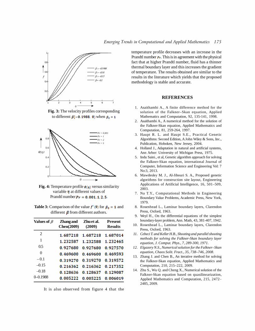
Emerging Trends in Computational and Applied Mathematics 175
1 2 3 4 5 6 70
0.2
0.4
0.6
0.8
1
������������������������������������
f'
�
Fig. 3: The velocity profiles correspondingto different when
0
0.2
0.4
0.6
0.8
1
Pr = 0.001
Pr = 1
Pr = 2
Pr = 5
�
����
Fig. 4: Temperature profile versus similarityvariable at different values of
Prandtl number .
Table 3: Comparison of the value for anddifferent from different authors.
Values of Zhang and Zhu et al. PresentChen(2009) (2009) Results
2
1
0.5
0
– 0.1
–0.15
–0.18
0–0.1988
It is also observed from figure 4 that the
temperature profile decreases with an increase in thePrandtl number . This is in agreement with the physicalfact that at higher Prandtl number, fluid has a thinnerthermal boundary layer and this increases the gradientof temperature. The results obtained are similar to theresults in the literature which yields that the proposedmethodology is stable and accurate.
REFERENCES
1. Asaithambi A., A finite difference method for thesolution of the Falkner–Skan equation, AppliedMathematics and Computation, 92, 135-141, 1998.
2. Asaithambi A., A numerical method for the solution ofthe Falkner-Skan equation, Applied Mathematics andComputation, 81, 259-264, 1997.
3. Haupt R. L. and Haupt S.E., Practical GeneticAlgorithms: Second Edition, A John Wiley & Sons, Inc.,Publication, Hoboken, New Jersey, 2004.
4. Holland J., Adaptation in natural and artificial systems,Ann Arbor: University of Michigan Press, 1975.
5. Indu Saini., et al, Genetic algorithm approach for solvingthe Falkner-Skan equation, international Journal ofComputer, Information Science and Engineering Vol: 7No:3, 2013.
6. Mawdesley M. J., Al-Jibouri S. A., Proposed geneticalgorithms for construction site layout, EngineeringApplications of Artificial Intelligence, 16, 501–509,2003.
7. Na T.Y., Computational Methods in EngineeringBoundary Value Problems, Academic Press, New York,1979.
8. Rosenhead L., Laminar boundary layers, ClarendonPress, Oxford, 1963.
9. Weyl H., On the differential equations of the simplestboundary-layer problem, Ann. Math, 43, 381-407, 1942.
10. Rosenhead L., Laminar boundary layers, ClarendonPress, Oxford, 1963.
11. Cebeci T. and Keller H.B., Shooting and parallel shootingmethods for solving the Falkner-Skan boundary layerequation, J. Comput. Phys., 7, 289-300, 1971.
12. Elgazery N.S., Numerical solution for the Falkner–Skanequation, Chaos Solit. Fract., 35, 738–746, 2008.
13. Zhang J. and Chen B., An iterative method for solvingthe Falkner-Skan equation, Applied Mathematics andComputation, 210, 215–222, 2009.
14. Zhu S., Wu Q. and Cheng X., Numerical solution of theFalkner-Skan equation based on quasilinearization,Applied Mathematics and Computation, 215, 2472–2485, 2009.

CRYPTOGRAPHY AND NETWORKS

Introduction
The encryption has been used by humans toprotect the secret information. It has been used in warssince early times to transmit information from onelocation to another without being getting into the handof enemies.
However in the era of information technology thescenario has changed because encryption has becomevital for the common man also. For eg- Withoutencryption we can’t think of protecting our bankaccounts.
For the army it is essential to keep the informationsecret. The secret information in the war can make ahuge difference and can be a reason for the victory.Hence for army encryption plays an important role.
The strength of any encryption depends on howwell it is able to keep the information safe and protectedfrom any undesired party. There are several encryptionalgorithms which are available but are cumbersome.
However we can develop some of the simpleralgorithms which can protect our information in a muchsimpler way. One such algorithm has been provided inthis paper to encrypt the time and date. The encryptionof time and date can be used for missile launches andattacks. These algorithms although being simple but atthe same time can be effective too.
Encryption of Time
The encryption of time is an important aspectduring the wars because by doing so we can protectour information related to when we are going to attackand when we will launch a missile. Hence if we are ableto protect the information about launching time we cansimply be the side in advantage. This paper also providesone such simple and effective algorithm to encrypt thetime.
Algorithm
Consider that we have been given the correct timeof the form H: M a.m. which we want to encrypt. Thebelow steps can be used to encrypt it.
1) Take the difference between minute and hourrecursively i.e. keep taking M-H until we get0<|M-H|< 12.
2) Count the number of steps taken to bringthe difference within the given range. Wecan also calculate the number of steps byusing the equation, 0< M-H*n < 12, wheren= number of steps. Also note that thedifference has to be taken atleast once.
3) Now divide H by |M-H| and represent it inthe form q r/|M-H| where, q= quotient and r=remainder. Hence H= (|M-H|*q) + r.
32Encryption of Time and Date
Ayush JainDayalbagh Educational Institute (Deemed University), Agra, India.
Abstract: In the era of information technology, in order, to protect our information from the hackers, terrorists orany other unauthorised party the encryption has become most important part for any organisation. By doing theencryption we converts our information in some absurd form which can be decrypted back later on by theauthorised party. This paper contains an algorithm to encrypt the given time and date. By using these algorithmswe can convert the time and date into some absurd form which cannot be traced by the hackers.Keywords : Encryption, circular table arrangement, light wave pattern.
Emerging Trends in Computational and Applied Mathematics 179

180 Emerging Trends in Computational and Applied Mathematics
4) Note the sign of M-H. We can get negativevalue if M<H. In the encrypted code we willbe required to know the sign of M-H for itsdecryption. In the encrypted code we canrepresent it by G.M.T+. If negative thanG.M.T- else G.M.T+.
5) Also note the sign of remainder ‘r’. In theencrypted code we will place ‘~’ at start ofcode if it is negative else simply avoid it.
6) The sign of M-H will also be used to decidewhether a.m. or p.m. In case if we get positiveM-H then invert the a.m. to p.m. and viceversa. If it comes out to be negative thenkeep them same. Also instead of using a.m./p.m. we will use a/p.
7) Finally we will use |M-H| as the hour and q ras minute while steps as the second. Hencewe can write the final encrypted code in theform as –~[G.M.T+ |M-H|: q r: steps a.m. / p.m.]
8) In order to make the encryption more strongwe can represent the digits in the lettersform. For this we can use the letters of lightwaves arranged in increasing order ofwavelength as given in the table below-
Table 1
Digit Letter Significance
0 X X-ray1 U Ultraviolet2 V Violet3 I Indigo4 B Blue5 G Green6 Y Yellow7 O Orange8 R Red9 M Microwave
Hence by using these letters in place of digits wecan obtain an encrypted code which is even muchstronger.
Fig. 1: Flowchart for time encryption
2.2 Illustrations
In this section the above algorithm has beenillustrated.
I. 11:35 a.m.
1) M-H => 35-11=2424-11=1313-11=2
2) Number of steps=33) H/|M-H| => 11/2=5 ½. Hence q=5 and r=1.4) Since M-H is positive so G.M.T+ is used.5) Also r is positive so no’~’.6) Since M-H is positive hence a.m. will
convert to p.m. and in code we will use‘p’.
7) The final encrypted code will become-G.M.T+ 2:51:3 p
8) Finally to make it even stronger we willuse the letters of table. Hence encryptionbecomes- G.M.T+ V: GU: I p.
II. 11:9 a.m.
1) M-H=> 9-11=-22) Number of steps=13) H/|M-H|=> 11/2=5 ½ q=5, r=1.

Emerging Trends in Computational and Applied Mathematics 181
4) Since M-H is negative hence G.M.T-5) Also r is positive so no ‘~’.6) Since M-H is negative so a.m. will remain
same and we will use ‘a’.7) Final encrypted code will be- G.M.T- 2:51:1 a.8) Finally replace digits by letters so code
will become-G.M.T- V: GU: U a.
III. 11:55 a.m.
1) M-H=> 55-11=4444-11=3333-11=2222-11=11
2) Number of steps=43) 11/11=1 0/11. Hence q= 1 and r=0.4) Sign of M-H is positive so will use
G.M.T+5) Also since r=0 hence we will avoid ‘~’.6) Since M-H is positive so a.m. will be
converted to p.m. represented by ’p’.7) The encrypted code will become
G.M.T+11:10:4 p.8) Convert digits to letter so code becomes
G.M.T+ UU: UX: B p.
IV. 7:53 a.m.
1) On doing M-H recursively we will obtain- 46, 39, 32, 25, 18,11. So we have M-H=11.
2) Number of steps = 6.3) 7/11=1(-4/11). Hence q=1 and r= -4.4) Sign of M-H is positive so we will use
G.M.T+5) Also the sign of r is negative hence we
will use ‘~’.6) Since M-H is positive so a.m. will change
to p.m.7) Finally the encrypted code becomes
~[G.M.T+11:14:6 p]8) Finally convert digits to letters we will
get following result ~ [G.M.T+UU: UB: Yp].
During decrypting the codes, sometimes theconfusion can occur between q and r, in case, if theycome out to be double digit, for example, UXV (102) it isdifficult to identify what is q and r. To avoid suchproblems put a dash (-) between q and r while encrypting
i.e. UX-V (10-2) it becomes clear q=10 and r=2.
Strength
The following reasons show the strength of thisencryption algorithm-
� The encrypted code also comes out to be inthe form of time, if not converted to letters,by which unauthorised party will think thatthey had obtained the correct time and willnot try to decrypt it further.
� The correct time was precise in minute whilethe encrypted time has been made precise inthe second which, can help to prevent thehackers or unauthorised person from furtherdecrypting it.
� The conversion of digits to letters usingthe letters from the table of wavelength oflight rays is also an interesting feature ofthis algorithm because mostly the letters aretaken from the alphabetical order of Englishwhich has become common now.
� The algorithm consists of simple steps whichtogether develops an effective cipher.
� The large range of hour, minute and secondmakes it stronger.
Limitation
This algorithm also has a limitation. In case, if weobtains M-H = 0 then this algorithm will not work as canbe seen H/0 will not exist. Eg- 7:7, 11:11etc.
Encryption of Date
The encryption of date will help us to keep theinformation about an event to be held on that particulardate to be secret. So the encryption of date alongwiththe time will help us to make a strong encryption whichwill keep our information about an event to be held atparticular time and date as a secret.
Even if the enemy is able to decrypt anyone ofthem then also it will become difficult for them to knowexact information.
Algorithm
Consider that we have been given the date D/M/Y which we want to encrypt. The steps below can be

182 Emerging Trends in Computational and Applied Mathematics
used to encrypt it.
1) Arrange the months in the tabular form inthree groups of 31, 30, 28 days. In each grouparrange the months in alphabetical order.
Table 2
31 August
December
January
July
March
May
October
30 April
June
November
September
29 February
This table can then be written in the circular tableform as shown.
Fig 2: Circular table arrangement
1) Now note the original date (D) and month(M).
2) Now keep on doing D-11 till we obtain 0<D-11< 11.
3) Now from the circular table start countingfrom the month next to the given month Mtill D-11.
4) The month which we obtained above willused as our encrypted month M’. So we arenow left with date and year.
5) For the encryption of Date we have to checkwhether leap year or non-leap year. This isdone in order to not violate the number ofdays in February by encrypting.
6) If leap year, then D’=D-M’ because therewill be no conflict between month ofFebruary and date i.e. if we gets M’ to beFebruary then the maximum date will be 31-2=29 which can be possible in February.
7) If non-leap year, then D’=D-M’-1. Becauseif we had calculated the D’ using above stepthen we will obtain D’=29 in maximum casewhich will conflict with calendar. So to avoidconfliction we can simply subtract 1 also.
8) There will be no need to encrypt the year.If we do so by some algorithm then the resultcan vary too much for example, if we encrypt2014 by some way to 1980/ 2030 then it willmake no sense as it has led to great variationfrom original year of event. So encryptingthe year will give the enemy clue that thedate has been encoded. Hence in thisalgorithm Y remains same.
9) So the final encoded date comes out to beD’/M’/Y.
Fig 3: Flowchart of Date encryption

Emerging Trends in Computational and Applied Mathematics 183
Illustrations
In this section the above algorithm has beenillustrated
I. 21/March/2014
1) D=21 and M=March (3)2) Now keep doing D-11. 21-11=10<11.3) Now look into the circular table.
Start counting from the next month of theMarch till 10 hence we will get M’=Jan.
4) Check if leap or non- leap year.5) Since 2014 is not leap year hence D’=D-
M’-1. So we get D’=21-1-1=196) So the final date becomes 20/Jan/2014
which is totally different from the originaland not even seems to be encrypted.
II. 28/May/2012
1) D=28 and M= May2) Now keep doing D-11. So we will obtain
28-11=17, 17-11=6 D-11=6.3) Now look in the circular table to know the
M’=Feb.4) Check for leap or non-leap year.5) Since 2012 is leap year. So we will get D’=D-
M’=28-2=266) So the final code becomes 26/Feb/2014
III. 31/Jan/2013
1) D=31 and M=Jan2) Keep doing D-11 we will get 20, 9. D-11=9.3) Now look into circular table to know the
M’ we will get M’= Feb.4) Check if leap or non-leap year.5) Since 2013 is non-leap year hence we get
D’=D-M’-1. So we get D’=31-2-1=286) So final date becomes 28/Feb/2013
IV. 30/Mar/2012
1) D=30 and M=March2) D-11=83) From circular table M’=Aug4) 2012 is leap year5) D’=D-M’=30-8=226) Encrypted date 22/Aug/2012
Using this algorithm we are able to encrypt thedate in a simple manner and also to note date will seemto be true to the enemy and he will not try further todecrypt it.
Strength
This algorithm has the following strengths-
� The encrypted form seems to be true andhence the unauthorised person will not tryfurther to decrypt it.
� The large range of dates and months makesit strong.
� The simple nature of algorithm.� The use of circular table arrangement of
month makes it unpredictable.
Limitation
� Using this method can take the event inthe past which makes easy for the enemy todetect that it is encrypted. Eg- 28/May/2012to 26/Feb/2012.
� Large variation in months can also causeproblem. However we can come across theabove limitations and can extend thisalgorithm by making some additional steps.
Conclusion
The above method shows that we can use thesimpler steps to build an effective encrypted code. Theimprovement of the limitations of above algorithm couldmake them much strong encryption which we can use inencryption of missile launches, hidden projects etc. tosurprise the enemy. The simple steps involved in theseencryption makes the algorithm more flexible. The mostimportant part of these algorithms is that the resultsdoesn’t seem to be encrypted by which we can makethe enemy satisfy that it is not encrypted and he will nottry to encrypt it.
REFERENCES
[1] wikipedia.org/Encryption
184 Emerging Trends in Computational and Applied Mathematics
Introduction
The use of encryption/decryption is as old as theart of communication. In wartime, a cipher, oftenincorrectly called a code, can be employed to keep theenemy from obtaining the contents of transmissions.(Technically, a code is a means of representing a signalwithout the intent of keeping it secret; examples areMorse code and ASCII.) Simple ciphers include thesubstitution of letters for numbers, the rotation of lettersin the alphabet etc. More complex ciphers workaccording to sophisticated computer algorithms thatrearrange the data bits in digital signals.
In order to easily recover the contents of anencrypted code, the correct decryption key is required.The key is an algorithm that undoes the work of theencryption algorithm. Alternatively, a computer can beused in an attempt to break the cipher. The more complexthe encryption algorithm, the more difficult it becomesto eavesdrop on the communications without access tothe key. From a defense perspective, nowadaysencryption algorithms are being replaced with open,standards- based algorithms that are less cumbersometo manage in terms of physical controls. We need more
advanced encryption techniques so that out data andsecurity are guarded.
As with any fairly new technology, there areadvantages and disadvantages that must be weighed.Less privacy, in the case of the defense Carnivore, is inthe interest of increased national security. No data isone hundred percent safe, a reality we must accept.
Mobile Number Encryption
The mobile number refers to the N-digit uniquenumber that is used to identify a mobile phone. In ageneralized mobile number first 3 digits identify thecountry code of the country. If a country has countrycode in one digit, the first two digits are replaced by 0number.
In the proposed algorithm, 8X8 matrix or a chessboard is used for the development of matrix code. Thecenter square is used for country code up to four digits.The second square from the center as shown in Fig. 1is used for the mobile numbers up to twelve digits. Theother squares are used to fill up the symmetry elements.p: mobile number ; c: country code
33Mobile number encryption using “K-matrix algorithm”
Karan Kumar SinghVIT University Chennai Campus, Vandalur-Kelambakkam road, Chennai-600048, India
Abstract: In cryptography, encryption is the process of encoding messages in such a way that eavesdroppers orhackers cannot read it, but that authorized parties can. In an encryption scheme, the message or information isencrypted using an encryption algorithm, turning it into an unreadable cipher text. This is usually done with the useof an encryption key, which specifies how the message is to be encoded. Any adversary that can see the cipher textshould not be able to determine anything about the original message. An authorized party, however, is able todecode the cipher text using a decryption algorithm that usually requires a secret decryption key. This papercontains an algorithm to encode mobile number of any country into a encrypted code named as “Matrix Code”. Thematrix code uses various techniques like fibonacci series, perfect number sequence and cumulation. It also uses anewly developed technique called “matrix symmetry” for development of matrix code. And this whole algorithmis known as “K-matrix algorithm”.Keywords : Encryption, Fibonacci series, Symmetry, Perfect numbers, Cumulative frequency, Aufbau’s Principle.

Emerging Trends in Computational and Applied Mathematics 185
Perfect Number
In number theory, a perfect number is a positiveinteger that is equal to the sum of its proper positivedivisors, that is, the sum of its positive divisorsexcluding the number itself.
General solution: 2n *(2n+1 – 1); 1<n<infinity
Energy sequence in sub-shells of atom
Fig. 2 shows the energy sequence in increasingorder, from 1s then 2s,2p,3s,3p,4s,3d,4p,5s and so on. Inthe algorithm proposed in this paper, numbers areassigned to the squares of the chess board in the energysequence order. This sequence is also called aufbau’sprinciple.
Fibonacci Series
The first two numbers in the Fibonacci sequenceis 0 and 1, depending on the chosen starting point ofthe sequence, and each subsequent number is the sumof the previous two. The series is:
0 1 1 2 3 5 8 13 21 34 55 89 144………
Cumulative frequency
Cumulative frequency can also defined as the sumof all previous frequencies up to the current point.
Matrix Symmetry
The matrix symmetry is new concept developedfor the distribution of numbers on a chess board.
It is categorized into three types as �, � and �symmetry. This type of symmetry mechanism is onlyvalid for the elements of second square lying on the
boundary of the square as shown in fig. 1.
-symmetry
This type of symmetry divides the element in thevertical direction. If the number n is even it is divided as(n/2, n/2) else it will be divided as ((n+1)/2, (n-1)/2). Thissymmetry will not work for corner elements.
It is denoted as �RN or CN which means �-symmetry of Nth row or Nth column.
-symmetry
This type of symmetry divides the element in thehorizontal direction. If the number n is even it is dividedas (n/2, n/2) else it will be divided as ((n+1)/2, (n-1)/2).This symmetry will not work for corner elements.
It is denoted as �RN or CN which means �-symmetry of Nth row or Nth column.
�-symmetry
This type of symmetry divides the elementdiagonally. If the number n is even it is divided as (n/2,n/2) else it will be divided as ((n+1)/2, (n-1)/2). Thissymmetry only works for corner elements.
It is denoted as � which means �-symmetry of thecorner elements.
This type of division of numbers throughsymmetry is done in the order of increasing energysequence arrangement of numbers in the second square.Only one type of code can be developed at a particularinstant i.e. if code is based on row transition, the wholecode should be based on row, similarly for the columntransition.
For example: if the matrix code isM-C: ��R1 �R2 �R3 �R4
In fig. 3 the digits of the mobile number arearranged in the increasing sequence analogous to fig.2. As in the matrix code the corner elements are divideddiagonally into equal parts as per even or odd number.Example the number N1 in the first box is divideddiagonally to the first adjacent empty diagonal boxes.Similarly the numbers in the other boxes except cornerelements are divided into two equal parts and placedhorizontally and vertically to the first adjacent emptyboxes according to � and � symmetry respectively. Ifthere is only one empty box in a particular direction theone half of the number will remain inside the box and ifthere is no empty box then the whole number will remain

186 Emerging Trends in Computational and Applied Mathematics
as it is.
Algorithm
The encryption of mobile using K-matrix algorithmis done as follows:
Step 1: First, the country code is encrypted in thecenter square of the chess board. Therefore take thecenter square and insert the country code in the orderof increasing energy sequence as shown in fig. 4.
Step 2: Sum up all the digits of country code.This will give a new number say ‘x’. Search for the nearestperfect square to x say ‘p’.
Step 3: Now do |p-x| which will give a new numbersay ‘q’. Check for (c1 + c2 + c3+ c4) % 2 = 0.
Step 4: If the x is divisible by 2 then, rotate thecenter square ‘q’ times in the clockwise direction. If notthen rotate the center square ‘q’ times in theanticlockwise direction. If x is itself a perfect squarethen q=0 i.e. no rotation.
Step 5: Now, form the matrix code using theinstruction given in section 2.5.
Step 6: Now, the values which were up to 2ndsquare will now extend up to 3rd and 4th square. Namethem analogous to the energy sequence. And writethem in the straight order.
Step 7: Write the first 10 perfect numbers usinggeneral solution of perfect number.
Step 8: The numbers from matrix code from step 6will be converted into the form of AB AB AB AB ABAB AB…….where repetition of AB is equal to the digits
in a matrix code.A= which number of perfect number among 10
perfect numbersB= which digit place has the same value as the
digit of mobile numberHere digit 10 is assigned to be ‘0’. In this type of
AB combination “ P ” is put at the starting to signify theuse of perfect numbers and it’s value is 0.
Step 9: After forming this code use cumulationmethod and add up the adjacent digits and add theresult with the other adjacent digit. This will give a codeconsisting of single, double and triple digits.
Step 10: Replace the first digit of a two digitnumber or first two digits of the numbers having threedigits with the alphabets assigned according toFibonacci series as follows.
0 1 1 2 3 5 8 13 21……P Q Q R S T U V WFor non-Fibonacci series4 6 7 9 10 11 12E F G H I J KStep 11: The resulting code is the encryption code
for mobile numbers.
Illustration
Suppose the mobile number required to beencrypted is 91- 9781217235
Step 1: Take the center square and insert thecountry code in the order of increasing energy sequenceas shown in fig. 5(a).
Step 2: Sum up all the digits of country code.This will give a new number say ‘x=10’. Search for thenearest perfect square to x say ‘p = 9’.
Step 3: Now do |p-x| which will give a new numbersay ‘q = 1’. Check for (c1 + c2 + c3+ c4) % 2 = 0. Here x is10 so remainder is 0 hence the center square will be rotatedone time in the clockwise direction. This will give a neworientation of center square as shown in fig. 5(b).

Emerging Trends in Computational and Applied Mathematics 187
Step 4: Suppose the matrix code is
M-C: ��R1 �R2 �R3 �R4
First write the mobile number in the second squarein the order of the energy sequence as shown in fig.6(a).
Now, from section 2.5 the numbers in the secondsquare will divided according to matrix code as shownin the fig. 6(b).
Step 5: Now, write the code in the increasingenergy sequence from fig. 6(b). Here code will be:
024330405200011090001040004110040100131Step 6: Now replace every digit with the AB
combination formed from first ten perfect numbers.
1. 62. 283. 1204. 4965. 20166. 81287. 326408. 1308169. 52377610. 2096128The combination will be:75 32 74 71 93 33 41 52 91 21 33 52 75 31 53 5203 83 02 75 62 52 41 52 33 75 74 53 85 33 75 4133 53 75 83 62 93 85Step 7: Now do the cumulation
7 12 15 17 24 28 35 36 45 48 51 54 58 59 64 66 75 7678 79 82 85 90 92 99 104 107 108 113 116 121 123 123126 134 137 137 139 146 151 157 159 162 165 172 177184 188 193 196 204 209 212 215 222 227 231 232 235238 243 246 253 258 266 269 275 277 286 289 297 302
Step 8: Replace the first digit of a two digit numberor first two digits of the numbers having three digitswith the alphabets assigned according to Fibonacciseries and non-Fibonacci series:P’7Q2Q5Q7R4R8S5S6E5E8T1T4T8T9F4F6G5G6G8G9U2U5H0H2H9I4I7I8J6K1K3K3K6V4V7V7V9L6QT1QT7QF2QF5O2O7QU4QU8QH3QH6RP4RP9W2W5RR2RR7RS1RS2RS5RS8RE3RE6RT3RT8RF6RF9RG5RG7RU6RU9RH7SP2
Step 9: Finally the mobile number 91- 9781217235got encrypted to:M-C: R1 R2 R3 R4P’7Q2Q5Q7R4R8S5S6E5E8T1T4T8T9F4F6G5G6G8G9U2U5H0H2H9I4I7I8J6K1K3K3K6V4V7V7V9L6QT1QT7QF2QF5O2O7QU4QU8QH3QH6RP4RP9W2W5RR2RR7RS1RS2RS5RS8RE3RE6RT3RT8RF6RF9RG5RG7RU6RU9RH7SP2
Step 10: The whole process can be reversed backto get the actual mobile number.
Strength of encryption
The strength of encryption lies in the randomnessof the concepts used. The algorithm proposed here linksconcepts from chemistry with mathematics which makesit formidable to determine the pattern. Also theincreasing energy subshell pattern does not have anymathematical equation derived for it making theencryption more powerful and undetectable.
The algorithm uses absolutely new kind of

188 Emerging Trends in Computational and Applied Mathematics
concept which cannot be detected by running computersimulation of already developed ciphers which makes itmore powerful.
Weakness of encryption
The main weakness of the algorithm is that it lacksa disguise feature. The eavesdroppers can figure outthat it is some kind of code and it is needed to be broken.But the concept used and the algorithm design is suchthat it is not easily breakable which eliminates this
weakness.
REFERENCE
[1] wikipedia.org/Encryption[2] http://chem-guide.blogspot.in/2010/04/aufbau-principle-
and-bohr- bury-rule.html[3] http://searchsecurity.techtarget.com/definition/encryp-
tion

Emerging Trends in Computational and Applied Mathematics 189
Introduction
Since the origin of RSA [1] in 1977, it was the mostpopular public key algorithm. The security lies oncomputing the factors of a large composite integer.Currently factoring 1024 bits integer is assumed to beas complex as workload of 280 which is the currentbenchmark used in cryptography. Simplicity makes thisalgorithm more attractive. The dark side of the algorithmis its high computation cost and large memoryconsumption. RSA algorithm is widely studied forreducing the computation cost. Computation involvedin finding the exponentiation modulo a large compositeinteger is very high. Researchers have done a lot ofwork to reduce the decryption cost. These improvementsare given in [2, 3, 4, 5, 6,7]. Performance comparison ofthe RSA variants is given in [8, 9, 10,11]. As the publicand private keys are inverse of each other, one sidealways have to compromise for the speed loss. So, needto balance both the sides originated many RSA variants.The work done to balance the encryption anddecryption sides are given in [12, 13, 14, 15, 16,17]. Thesize of the keys are very large and it further increases asthe security level. The big size of the key pairs lead tothe need of big storage requirement. The work relatedto reduction in memory consumption is shown in [18,19].
For effectively using RSA, its performance needsto be enhanced. This study provides the completedetails of the work done in RSA performance since itsorigin. The researchers will get the current scenario inRSA cryptography, which will help to design a betteralgorithm.
The paper is structured as follows. In Section 2,basic RSA and related security aspects are studied. InSection 3, the RSA variants based on the improvementin computation cost are studied. Comparison of differentRSA variants is given in is given in Section 4.
Basic RSA
The RSA algorithm [1] was publicly described in1977 by Ron Rivest, Adi Shamir and Leonard Adlemanat MIT. Each user of the system makes two numbers, eand N public and keeps a number d secret. In order for Ato send a message to B, A looks up B’s public valuesand, if the message is M (written as a number), then Ablocks the message into pieces of size less than N.
Key Generation Method
The following steps are performed to calculatethe public and private exponents:
34RSA Cryptosystem: A Review
Seema Verma, Deepak GargComputer Science Department, Thapar University, Patiala, India
[email protected], deepak [email protected]
Abstract: RSA is the most popular public key cryptographic algorithm. Since its origin in 1977, researchers havedone a lot to improve its performance. As it is widely used in electronic commerce, there is the need to study itmore and more. Many variants are designed to improve the performance of RSA. This paper concentrates on thestudy of the performance of RSA since its origin. The literature related to the speed and memory consumption ofRSA algorithm is presented with their related work. For better analysis the RSA variants are compared accordingto the complexities of their performance. This study is mainly done to help and motivate researchers to do morestudy in RSA to get better performance.Keywords: Cryptography; encryption; public key

190 Emerging Trends in Computational and Applied Mathematics
1. Choose two random primes of size n/2 bitseach (p and q, approximately equal size), such
that modulus qpN �� is of the required
length, say 1024 bits.2. Compute )1()1()( ���� qpN�
3. Choose an integer e , )(1 Ne ��� e, such
that 1))(,gcd( �Ne �
4. Compute the secret exponent d ,
)(1 Nd ��� , such that )(mod1 Ned ��
Public key= ),( eN , Private key= ),( dN template is used
Encryption Method
The plaintext M can be encrypted to get ciphertext C by calculating the exponentiation of the messagewith public exponent.
C=MemodN.
Decryption Method
The message can again be retrieved by calculatingthe exponentiation of the cipher text with the privateexponent.
M = Cd mod NRSA security is dependent upon RSA problem
and factoring a large integer. RSA problem is computingthe eth root modulo a large composite integer. RSAproblem is assumed to be hard in current state of art ofcomputing. It is also assumed that finding private RSAexponent d is equivalent to factoring N. Currentlyfactoring a large composite integer is considered as thehard problem. One can recover the private exponentonce the prime factors are known. Till now, without anyproof, no polynomial-time method for factoring largeintegers with current resources has yet been designed.The largest number which was factored in 2010 [6] wasof 768bits by number field sieve factoring method. PeterShor gave an algorithm [20] in 1994 which is based uponquantum computer can do the factorization inpolynomial time. But no practical evidence has beenfound till now.
RSA decryption is very costly as decryptionexponent is nearly having the same size as that of �(N).If private exponent is taken small, then public exponentis nearly having the same size as that of �(N). Onecannot chose very small value for decryption exponent.According to Boneh and Durfee [26, 27], 1999, onecannot use d < N0.292.
Improvement in Computational Cost
As the drawback of RSA is slow computationsinvolved, work is done to improve the speed of RSAencryption and decryption operations. In this section,the study is related to the work done to improve theperformance of RSA cryptosystem, i.e., to improvedecryption operation, balancing the encryption anddecryption operation.
RSA with CRT
In 1982, Quisquater and Couvreur [2] introducedthis technique to increase the speed of decryptionalgorithm of RSA cryptosystem. In this technique twosmaller secret keys (dp,dq) are calculated from theoriginal secret key(d), decryption is done with thesetwo keys and the result is combined with the help ofChinese Remainder Theorem(CRT). It improves theperformance of the basic RSA decryption algorithm by 4.
Key Generation Algorithm
The following calculations are done in additionto the steps taken in basic RSA
dp = d mod p-1dq = d mod q-1Public key = <N, e>, Private key = <N, dp, dq>
Encryption Algorithm
Same as in basic RSA
Decryption Algorithm
1. Calculate Mp=Cdp(mod p)2. Calculate Mq=Cdq (mod q)3. Calculate M from Mp & Mq using Chinese
Remainder Theorem(CRT)
The private exponent d is same as that used inbasic RSA, therefore the same security constraints applywith this variant. Also, the security of CRT RSA can bebroken if CRT exponents dp, dq are known.
Batch RSA
Fiat introduced Batch RSA [3] in 1989, the workwas done to improve the decryption time by taking morethan one job at a time. By this approach if small publicexponents are used for the same modulus N, thedecryption of the two ciphertext can be done at the costof one. Suppose C1 and C2 are the two ciphertext from

Emerging Trends in Computational and Applied Mathematics 191
message M1 and M2 respectively. There public keysare <N, 3> and <N, 5> respectively. To decrypt, C11/3modN and C21/5modN are calculated. According tothis variant both decryption processes can be mergedto enhance the speed of the decryption algorithm. Thescheme can be understood by setting A= (C15.C23)1/15
Then, C11/3= A10/ [C1
3.C22]
And C21/5= A6/ [C1
2.C2]Hence we are able to decrypt both C1 and C2 at
the cost of computing 15th root (takes the same time asa single RSA decryption) and some additional arithmetic.But this technique is only valuable when the publicexponents’ e1 and e2 are small. Otherwise it will notincrease the decryption speed; rather it will be moreexpensive. Also the modulus must be the same and publicexponents must be distinct for both the messages.Decryption of b messages in Batch RSA is done withthe cost of single exponentiation of the order of N.According to Fiat [3], for N=1024 bits, decryption speedis increased by 2.6 with batch size 4 and 3.5 with batchsize 8.
The constraint of small public key exponent anddelay introduced by waiting for the decryption requestsmake Batch RSA less attractive. According to Shachamand Boneh [63] in 2001, Batch size of more than eight isnot suitable for common applications, because of thedelay inroduced.
MultiPrime RSA
Collin et al introduced this variant [4] in 1997.MultiPrime RSA was designed to enhance the decryptionspeed of RSA cryptosystem by taking more than twoprime modulus. It consists of k primes p1, p2… pk insteadof using only two as in standard RSA. MultiPrime RSAis supported by PKCS#v2 [ ].
Key Generation Algorithm
1. Compute k distinct primes p1... pk each one[logN/k] bits in length and N=�i=1
k pi.2. The exponents e and d are taken such that d
= e-1 mod �(N), and gcd(e, �(N)) = 1, where�(N)=�i=1
k (pi-1)
3. For 1� i� k, compute di = d mod (pi - 1).
Public key = <N, e>, Private key = <N, d1, d2 ...dk>
Encryption Algorithm
Same as in basic RSA
Decryption Algorithm
1. For i= 1 to k, calculate di=d mod pi-12. For i=1 to k, Mi = Cdi(mod pi)3. Calculate M from Mi (i=1 to k) using Chi-
nese Remainder Theorem(CRT)
The security of MultiPrime RSA can be broken byknowing the value of private exponent or the multiple of?(N). One can not chose the number of primes by herown choice due to the security constraint. The numberof primes can be taken 3,3,4,5 as safe for modulus size1024, 2048, 4096, 8192 bits respectively [72].
MultiPower RSA
Takagi introduced MultiPower RSA [5] in 1998.The purpose of this variant was also to improve thedecryption time of RSA algorithm. In the algorithm N=pb-1q where p and q are n/b bits.
Key Generation Method
1. Generate two primes p and q of [n/b]-bitseach and compute N= pb-1.q
2. Compute d=e-1mod �(N)3. Compute d1=d mod (p-1) and d2=d mod (q-
1).
Public key= <N, e>, private key= <p, q, d1, d2>
Encryption Algorithm
Same as in basic RSA
Decryption Algorithm
1. Calculate M1=Cd1mod p, M2=Cd2 mod q sothat M1
e = C mod p and M2e = C mod q.
2. Calculate (M1')e = C mod pb-1 using Hensal
lifting.3. Calculate the message M such that
M=M1'mod pb-1 and M=M2 mod q usingChinese Remainder Theorem(CRT).
Once the private exponent d or multiples of �(N)is known, MultiPower RSA can be broken. Also, theexponents e and d are computed modulo �(N) insteadof �(N) due to avoid many of the attacks. The value ofb can be taken as 3, 3, 4, 5 for 1024, 4038, 4096, 8192respectively [72] to thwart the factoring attack of ECM.

192 Emerging Trends in Computational and Applied Mathematics
Rebalanced RSA
Rebalanced RSA [6] was introduced by Wiener in1990. This variant increases the decryption speed at thecost of slow encryption speed. Some applications like,signature generation on smartphones and verificationon large server, require this property of the variant.Rebalanced RSA improves the performance of thedecryption/signing algorithm by displacing the work tothe encryption/verification algorithm.
Key Generation Method
(x<=n/2 bits)1. Generate two random primes (p and q) of
size n/2-bit with gcd(p-1,q-1)=2, and N=pq.2. Generate two x-bits random numbers dp and
dq, such that gcd (dp, p-1) = gcd (dq,q-1) = 1and dp=dq mod 2.
3. Calculate d such that d= dp mod p-1 andd=dq mod q-1. Calculate e=d-1 mod �(N)
Public key =<N,e>, Private key=<p,q,dp,dq>
Encryption Algorithm
Same as in basic RSA
Decryption Algorithm
Same as in CRT RSAIf private exponent d or multiple of The security
of CRT RSA can be broken if dp, dq are known. Accordingto Baby-Step Giant-Step attack the CRT exponents dp,dq must be greater than 160bits. According to Jochemszand May [51] in 2007, the modulus can be factored inpolynomial time if dp, dq are smaller than N0.073 (For1024bit modulus, CRT exponents less than 75 bits areprone to cryptanalysis).
R Prime RSA
This variant [11] further improves thecomputational cost at the decryption side. In 2002 CesarAlison [13] combined the two RSA variants RebalancedRSA and Mprime RSA methods to further enhance thedecryption speed. The general idea of this scheme is touse the key generation algorithm of Rebalanced RSA(modified for k primes) together with the decryptionalgorithm of Mprime RSA. The key generation,encryption and decryption algorithms are as follows:
Key Generation Algorithm
Take s, an integer, s?n/k and executes the followingsteps:
1. Generate k distinct random primes of n/k bitsp
1, p
2..., p
k, with gcd (p
1 - 1, p
2 - 1, ..., p
k - 1) =
2; and calculate N=p1p
2...p
k.
2. Generate k random numbers of s-bits dp1, dp2
..., dpk, such that gcd (dp1, p1 - 1) = 1, gcd (dp2,p2 - 1) = 1, ..., gcd(dpk , pk - 1) = 1 and dp1 = dp2
= ... = dpk mod 2.3. Find d such that d = dp1 mod (p1 – 1), d = dp2
mod (p2 -1)…d = dpk mod (pk – 1)4. Calculate e =d-1 mod �(N).
Public key = <N, e> and Private key = <p1, p2... pk,dp1, dp2 ...dpk>
Encryption Algorithm
Same as in basic RSA
Decryption Algorithm
Same as in MultiPrime RSAFor 2048 bit moduli the decryption speed
increases by a factor of about 8 as compared to RSACRT and about 27 as compared to original RSA. Herethe security constraints are both from MultiPrime RSAand Rebalanced RSA. The number of primes for 1024bits modulus should be 3 and the CRT componentsmust be greater than 160 bits.
Generalized Rebalanced CRT RSA
As rebalanced RSA is having less computationcost on decryption side and more computation cost onencryption side. This variant[12] is the improvement ofRebalanced RSA, so that the increased encryption costbe lowered to balance both encryption and decryptioncost.
Here are the algorithms for key generation,encryption and decryption.
Key Generation Algorithm:
(e < n/2)
1. Randomly select an odd number e of 512bits.
2. Randomly select an odd number x of 198bits, such that gcd(x, e) = 1.

Emerging Trends in Computational and Applied Mathematics 193
3. We can uniquely determine two numbers dp,
x < dp< 2x, and p’, e < p’ < 2e, satisfying ed
p
? xp’ = 1.4. If p = p’ + 1 is not a prime number, then go to
Step 2.5. Randomly select an odd number y of 198
bits, such that gcd(y, e) = 1.6. We can uniquely determine two numbers d
q,
y < dq < 2y, and q’, e < q’< 2e, satisfying ed
q
– yq’ = 1.7. If q = q’+ 1 is not a prime number, then go to
Step 5.
Public key is= <N, e>, Private key=<dp, dq, p, q>
Encryption Algorithm
Same as in basic RSA
Decryption Algorithm
Same as in CRT RSAAll the constraints from Rebalanced CRT RSA are
applicable to this variant also. Many security parametersare discussed in [12]. For an example, this variant issecure for 170 bit public exponent and 358 bit privateexponent.
Tunable Balancing of RSA
In this variant [13] also, the work was done tobalance the encryption and decryption cost ofRebalanced RSA according to the applicationrequirements. This method is a generalization of usingsmall public exponents and small Chinese remainder(CRT) private exponents.
Key generation algorithm
1. Choose an odd ne-bit integer e2. Choose random n
k-bit integers k
1 coprime to
e and odd nd-bit integers d
p such that d
p � e–
1 (mod k1)3. If p = 1 + (ed
p – 1)/k1 is not prime, go to step
2.4. Choose random nk-bit integers k
2 coprime
to e and odd nd-bit integers d
q such that d
q
� e–1 (mod k2)
5. If q = 1 + (edq – 1)/k
2 is not prime, go to step
4.
Public key is= <N, e>, Private key=<dp, dq, p, q>
Encryption Algorithm
Same as in basic RSA
Decryption Algorithm
Same as in CRT RSAMany security constraints are discussed in [13].
Two prime and MultiPrime Tunable balancing arediscussed. For an example, for 2-prime Tunable balancingof RSA 176-bit public exponent and 338-bit privateexponent is secure.
Comparison And Summary
Some important RSA variants are analysed tocompare the time complexity of the encryption anddecryption performance. As the encryption anddecryption operations are based on calculating theexponentiation. Computation of RSA exponentiation isbased on square and multiply method. As we know thecomplexity of multiplying two n bit numbers is O(n2).For random exponent of size k bit, k times square and k/2 times multiply is assumed. Hence for Cdmod N, it isassumed that (k+k/2)n2 , i.e. 1.5kn2, here n is bit size ofN. Encryption exponent is small in case of basic RSA,RSA CRT, MultiPrime RSA, MultiPower RSA. One canchose the public exponent of the special form 216+1.This value results in 16 squares and only onemultiplication, hence the complexity is only (16+1)n2. Inbatch RSA, the public exponent must be very small,e.g., 3,5,7 etc., i.e, bit size e.g., 4. In these variants privateexponent d is very large and random. In RebalancedRSA, Generalized Rebalanced CRT RSA, TunableBalancing RSA, the encryption and decryptioncomplexities are computed for random exponents.Except basic RSA, Batch RSA, MultiPower RSA, thedecryption complexity of all the variants are calculatedon the basis of CRT exponents. In MultiPower RSA,exponentiation is done modulo 2n/3, which results inmore complexity than RSA CRT, as it computesexponentiation modulo n/2. For the calculation ofexponentiation in MultiPower RSA, Hensel lifting is usedwhich results in only two computations ofexponentiation modulo n/3, which results in lowcomplexity as compared to MultiPrime RSA.

194 Emerging Trends in Computational and Applied Mathematics
Table 1: Complexity Comparison Of RSA Variants
RSA Variants ne Enc Cost nd Dec Cost
RSA 16 17n2 1024 1536n2
RSA CRT 16 17n2 512 384n2
Batch RSA 4 6n2 1024 (1536/b)n2
(approx.)MultiPrime RSA 16 17n2 341 170n2
MultiPower RSA 16 17n2 341 114n2
Rebalanced RSA 1024 1536n2 160 120n2
RPrime RSA 1024 1536n2 160 80n2
Generalized RebalancedCRT RSA 170 255n2 358 268n2
Tuanable Balancing RSA 176 264n2 338 252n2
One can get the idea of performance of thedifferent RSA variants from table 1. Figure 1 shows theencryption and decryption complexity variation betweendifferent variants of RSA.
Fig. 1: Complexity Comparison Of RSA Variants
RSA is the first public key cryptosystem which isused the most in maximum applications of electroniccommerce. This survey gives the complete walk throughof performance of RSA cryptosystem since its origin.The important variants are compared for better analysis.As there are many loop holes in this cryptosystem, butwith the use of restricted parameters any of the RSAvariant can be used . Hence RSA will remain the popularpublic key cryptosystem for many years to come.
REFERENCES
[1] R. Rivest, A. Shamir, and L. Adleman, “A Method forObtaining Digital Signatures and Public Key
Cryptosystems”, Communications of the ACM Vol.21, No. 2, pp. 120 - 126, 1978
[2] J.-J. Quisquater and C. Couvreur, “Fast deciphermentalgorithm for RSA public key cryptosystem”, Electron-ics Letters, 18(21):905–907, October 1982
[3] A. Fiat, “Batch RSA”, Advances in Cryptology, Crypto’89, Vol. 435, 1989, pp.175–185
[4] T. Collins, D. Hopkins, S. Langford, and M. Sabin,“Public Key Cryptographic Apparatus and Method”,US Patent #5,848,159. Jan. 1997
[5] T. Takagi, “Fast RSA-Type Cryptosystem Modulopkq”, Crypto’98, 1462 of LNCS. 1998, pp. 318–326.
[6] M. J. Wiener, “Cryptanalysis of short RSA secret ex-ponents”, IEEE Transactions on Information Theory,36(3):553–558, May 1990
[7] CAM Paixao, “An Efficient Variant of the RSACryptosystem”, eprint Archieve/2003
[8] D. Boneh and H. Shacham, “Fast variants of RSA”,CryptoBytes, 5(1):1–9,2002
[9] Md Ali-Al-Mamun, Md Motaharul Islam, S.M.Mashihure Romman and A.H. Salah Uddin Ahmad,“Performance Evaluation of Several Efficient RSA Vari-ants”, International Journal of Computer Science andNetwork Security, IJCSNS, Vol. 8, 2008 pp. 7-11.
[10] Klaus Hansen, Troels Larsen and Kim Olsen, “On theEfficiency of Fast RSA Variants in Modern MobilePhones”, International Journal of Computer Science andInformation Security, IJCSIS, Vol.6(3), 2009, pp. 136-140
[11] C. Vuillaume, “Efficiency comparison of several RSAvariants”, Master’s thesis, Darmstadt University ofTechnology, 2003
[12] Sun HM., Hinek MJ. and Wu ME., “Trading Decryptionfor Speeding Encryption in Rebalanced-RSA”, Journalof Systems and Software, vol. 829 (9), pp. 1503-1512,2009
[13] S. D. Galbraith, C. Heneghan, and J. F. McKee, “Tun-able Balancing of RSA”, in C. Boyd and J. M. G. Nieto,editors, ACISP, volume 3574 of Lecture Notes in Com-puter Science, pages 280–292. Springer, 2005.
[14] H.-M. Sun and M.-E.Wu, “An approach towards Re-balanced RSA-CRT with short public exponent”,Cryptology ePrint Archive, Report 2005/053, 2005[Online]. Available: http://eprint.iacr.org/2005/053
[15] H.-M. Sun and M.-E. Wu, “Design of Rebalanced RSA-CRT for Fast Encryption” Information Security Con-ference 2005. pp. 16-27, June, 2005
[16] H.-M. Sun, M. J. Hinek, and M.-E. Wu, “On the designof Rebalanced-RSA”, revised version of [90,91] Centrefor Applied Cryptographic Research,Technical ReportCACR 2005-35, 2005 [Online]. Available:http://www.cacr.math.uwaterloo.ca/techreports/2005/cacr2005-35.pdf
[17] H.-M. Sun and C.-T. Yang, “RSA with balanced short

Emerging Trends in Computational and Applied Mathematics 195
exponents and its application to entity authentication”,in S. Vaudenay, editor, PublicKey Cryptography, vol-ume 3386 of Lecture Notes in Computer Science, pages199–215. Springer, 2005.
[18] K. Lenstra and B. M. M. de Weger, “Twin RSA”, in E.Dawson and S. Vaudenay, editors, Mycrypt, volume
3715 of Lecture Notes in Computer Science, pages 222–228. Springer, 2005.
[19] H.-M. Sun, M.-E. Wu, W.-C. Ting, and M. J. Hinek,“Dual RSA and its security analysis”, IEEE Transac-tions on Information Theory, 53(8):2922–2933, 2007.In-troduction to the style guide, formatting of main text,and page layout

196 Emerging Trends in Computational and Applied Mathematics
INTRODUCTION
Cryptographic algorithms are theoretically orcomputationally secure but their implementation maybe vulnerable. A ‘Side Channel’ is a source ofinformation that is inherent to the physicalimplementation of a primitive i.e, light, sound etc.[1, 2]and the analysis which is related to the attacker who areresponsible for retrieving the secret data is Side ChannelAttack. This physical attack can be categorized intotwo orthogonal axis- One is Non-Invasive vs. Invasiveand other is Active vs. Passive [3]. Our discussion isbased on Non-Invasive attack. Invasive attack meansthe unwrapping of chip to get direct access to its internalcomponents whereas Non –Invasive attack exploits onlyexternal information (Emission). It is impossible to givean exact definition of the electromagnetic emissionsgenerated by a cryptographic device. In Simple PowerAnalysis, the electrons are flown through the siliconmade semiconductor. It consumes the power and the
processor leaks the information of the data (HammingWeight). Similarly, when the current is passed throughCMOS devices, Electromagnetic Emission can track thebit transmission so as to reveal the Hamming Weight.The terms related to electromagnetic emissions arecurrent, voltage, electric field, and magnetic fields. Thereare two types of EMA- Simple EMA(SEMA) &Differential EMA(DEMA) as in[4]. In SEMA attack, ifthe data(secret program code) is represented byconditional branches, adversary can easily extract theinformation i.e., conditional statements in a codesegment is very helpful for SEMA attack. On the otherhand in case of DEMA attack, the attacker monitors theelectromagnetic emanations emitted from thecryptographic devices & trace out the secret parametersextracted from electromagnetic data through somestatistical analysis. Though Electro Magnetic Analysisare resembled same to the Power Analysis, there arevast differences in terms of expressing these two attacks.Power analysis can be measured by plotting the
35Electro Magnetic Analysis Attack and Countermeasures –
The Latest Vogue
Aditya Bhattacharyya1, Sanjit Kumar Setua2
1 Dept. of Computer Science,Vidyasagar University, West Bengal, India2 Dept. of Computer Science & Engineering , University of Calcutta, West Bengal, India
[email protected], [email protected]
Abstract: Cryptanalysis was extended from the theoretical work to its practical implementation over a decade. Asthe new attacks and new meddling methodologies are proposed more frequently, to make a secure cryptosystemhas become a challenge to the designers. A designer should concern about the attack as well as the correspondingcountermeasure also as because of a newly proposed countermeasure may also the target of a newly proposedattack. The idea of Side Channel Attack (SCA) was introduced over a decade ago. Power consumption, Timing,Electromagnetic radiation play the important role in SCA. Beside these light, heat, acoustic are also exploredrecently. This paper gives an overview on Electromagnetic Radiation (Emanation) which is out of an IntegratedCircuit. Different types of countermeasures related to SEMA (Simple Electro Magnetic Analysis) and DEMA(Differential Electro Magnetic Analysis) have been considered. Also some attacks have been considered againstthose countermeasures.Keywords: Electromagnetic Analysis (EMA), Elliptic Curve Cryptography, Countermeasures

Emerging Trends in Computational and Applied Mathematics 197
amplitude of wavelength with the time. On the otherhand, the electromagnetic analysis can be measured byconsidering three dimensional vector fields which isdependent on time [19].
Fig. 1: Basic structure of Electromagnetic Analysis
Here is the block diagram which can easily describethat how the electromagnetic emission can be captured.
In 1985, Victor Miller & Neal Kolbitz proposedECC independently. For its higher speed, lower powerconsumption, smaller certificates etc, it plays a majorrole in the research area of cryptography. Multiplyingthe point P on the curve with an integer k (secret key),we get an another point Q on the curve (i.e., Q=kP) - thisprocess is called Scalar Multiplication. IN the algorithms,for symbolic representation ki, ‘i’ is the bit-index of thenumber.
In section 2 , the history of EMA is considered.The evolution of EMA is described in this section yearwise. Different types of EMA are described in the section3. Mathematical background of EMA and Elliptic Curvehas been considered in section 4. In section 5, bothSEMA and DEMA countermeasures are also considered.Also the attacks, applied in those countermeasures havebeen considered in a tabular format. At last conclusionis kept.
SIMILAR WORK OF EMA
In the year 2001, two research groups publishedthe first paper on EMA independently. Using anoscilloscope, faraday cage and a flat coil (Sensor) [8],they measured the electromagnetic radiation from a SmartCard. The rest of the section the summary of the previousworks done by the researchers (year wise).
Quisquater&Samyde [4]
This paper describes the EMA attack, differentmeasurement strategies related to EMA andcountermeasures for Smart Cards. Smart card processoremit a lot of information (hamming Weight) when it is inworking condition. To build a set up , a sensor (flat coil)is placed under the smart card. The two fields – electricand magnetic can be measured by the coil. The paperconsiders countermeasures like Reduction ofElectromagnetic field which plays an important role inthe field of countermeasures. Their consideration forimplementing Faraday Cage to reduce noise may be aneffective mechanism to reduce the noise (by blockingthe electromagnetic field). Reduction of powerconsumption in the field of electromagnetic emanationmay be an important direction to the research field ofEMA. Another important countermeasure is Dual linelogic which has been considered in this paper.
They also suggested that the modification of chipcan reduce the field emanation i.e., if a chip is equiva-lent to two chips and the bigger one is replaced by two,the power radiation reduces and henceforth electromag-netic emanation.
Agrawal et.al [9]
They introduce the concept of multichannelattacks which is the simultaneous operation of differentside channels like Electro Magnetic and Power etc. ACMOS leakage adversarial model has been proposed inthe paper. The maximum likelihood principle has beenapplied to design this adversary.
To construct an adversarial model for elementaryleakage , two phases have been considered-the profilingphase and the hypothesis testing phase [10]. First phaseis a training phase for an adversary who can take atraining device and experiment on target device to makea clear concept about attack and in second, theadversary is given the target device and a set of sensorsto make the elementary operation on target deviceaccordingly to exact one of the two distributions B0and B1. The adversary has to select the correcthypothesis (H0 for B0 and H1 for B1). They alsooptimized the sophisticated attack strategies byassuming maximum likelihood hypothesis test. Themodel may be stronger than classical DPA/DEMA styleattack adversary.

198 Emerging Trends in Computational and Applied Mathematics
De Mulder et.al [18]
A differential EMA attack on FPGA implementa-tion of ECC over GF(p) has been considered in thispaper. They considered Distance of Mean Test forcalculate the signal emitted from FPGA . The significantnumber of measurements (only 2000) have been used toguess the correct key. They considered two types ofEMA- SEMA and DEMA. The measurement set up wasdeveloped with Xilinx Virtex 800 FPGA board, a TektronixTDS714L Oscilloscope, an antenna, a function generatorand power supply. The current flows through an FPGAforms a loop. These current could be modeled with amagnetic dipole as elementary building block where theonly factor is magnetic field. The circular loop antennahas been used to receive the signal.
The experimental DEMA attack has beenimplemented on Elliptic Curve Point Multiplicationalgorithm where the 2nd MSB of key is considered forattack. The electromagnetic radiation is measured whenFPGA computes 2400 clock cycles. This result has beenplotted graphically. After calculating the mean valueand the bias signal, guessing of correct key can be doneefficiently.
Real et.al. [19]
The overall performance of electromagneticanalysis depends on the positioning of probe into thefield where the device’s radiation can capture efficiently.They termed this spot as Hot Spot. An accurate methodby which hot spot onto the device can be detected hasbeen illustrated in this paper. The strategy is totallybased on an indicator. To find out the hot spot theyused 3 indicators – Signal to Noise indicator (SNI), SboxMaximal Difference Indicator(MDI) & CEMA indicator.At the last part , they compared each indicator’s resultwith the CEMA using Cartography. The MDI’s resultsare more accurate than SNI.
Homma et.al [20]
According to them the Electro Magnetic radiationbecomes an important source of leakage as it can beconducted without tampering the paper. They madeexperiments based on common mode current which iscomposed of SASEBO (2 FPGA), a digital oscilloscopeand a PC. Also experiments have been performed onSEMA on RSA implementation where a 1024 bit RSAcircuit is implemented on FPGA. They consider high
radix Montgomery multiplication algorithm using a 32bit multiplier. Attack at distance is their proposed work- which is based on the Correlation based EMA on ahardware based high performance AES module which iskept 50cm at a distance from EMA probe. Their methodprovides exploitable results & allows to retrieve theleakage information/ frequencies for unintentionalemanations.
TYPES AND TECHNIQUES
When a source or emitting device generatesemissions (information) and passes through anelectromagnetic environment , an attacker can ‘tap’ theinformation using proper measurement. According toAgrawal et.al [9,10], there are two types of emanations-Intentional and Un-intentional. Intentionalelectromagnetic fields are directly generated by a currentcarrying element . On the other hand Un-intentionalfield are originating from modulation effects (AM &FM), various coupling in the cryptographic chip.
Quisquater introduced the term Simple EMA &Differential EMA (SEMA & DEMA) .. The secret keycan be revealed by some statistical test like T-Test,Variance Test, Pearson Correlation, Spearman’s RankCorrelation etc [18].
MATHEMATICAL BACKGROUND
A. EMA ATTACK
CMOS is used to implement digital IC. The mostsimple logic gate is inverter, gives a general image of thepower consumption in CMOS circuit. There are 2 typesof power consumption distinguished.
a) The leakage current – the current flows fromthe power source to ground during shortcircuit(Switching from 0 to 1).
b) Charging and Discharging Current used inthe different capacitors.
The sudden current pulse that occurs during thetransition of the output of a CMOS gate causes avariation of the Electromagnetic field surrounding thechip. Electromagnetic waves are guided by antennaswhich are made of wires. These waves can travel freelyand unbounded. Using a loop antenna the voltageinduced by the current equals:
V=-d�/dt& � = ff B .dA where V be the probe’soutput voltage, � be the magnetic flux sensed by probe,

Emerging Trends in Computational and Applied Mathematics 199
t be the time, B be the magnetic field, A be the area thatit penetrates. Hence it can convey information outputbased on Induction, here a magnetic probe can directlyoutput V. While a current probe produce the valueproportional to I, the current . From both of these, anattacker can retrieve secret information (collection ofbit string) by using proper device setup (may beOscilloscope or Voltage probe or current probe orPreamplifier. ).
B . Elliptic Curve over Galois Field(p)
An Elliptic curve E over GF(p) is expressed interms of Weirstras � equation : y2=x3+ax+b, a & b areconstants, where 4a3+27b2 ? 0, each value of a & b willgive different curves.Consider two distinct points P andQ such that P = (x1, y2) and Q = (x2, y2) .
Let L = P + Q where L = (x3, y3), thenx3= s2 – x1 – x2 , y3 = s (x1– x3) – y1 and s = (y2 – y1)/
(x2 – x1), s is the slope of the line through P and Q. Againwhen P=Q, i.e L=2P, then ‘Doubling’ formula will beapplied. x3 = s2 – 2x1, y3 = s(x1 – x3) –y1, s = (3x1
2 + a) /(2y1), s is the tangent at point P. The basic operation ofECC is the point multiplication. The operation consistsof many number of Point addition and Doubling methodsin GF(p) [5].
Algorithm 1. Left to Right Double-and add Elliptic CurvePoint Multiplication
Input: The point given P, k= (kl-1, kl-2 …………k0)2, Here kl-1=1 and 0<k<M.
Output: kP
1. Q=P2. for i= l – 2 down to 0
2.1 Q=2Q2.2 If ki=1 then Q=Q+P2.3 End If
3. End for4. Return(Q)
The intruder’s target is to find out the key bits ki. If he/she finds those bits, the algorithm will be broken.In the above algorithm in the step 2.2, there is a keydependent conditional statement which may bevulnerable towards SEMA. We can solve the problemby executing a point addition and doubling for each keybit.
5 DIFFERENT EMA COUNTERMEASURES
EMA emanation is considered as an extension ofthe power consumption leakage & the countermeasuresare probably same as of Simple Power Analysis (SPA)and Differential Power Analysis (DPA) [13] .In the nextpart we will consider the countermeasures of SEMAand DEMA.
A .Countermeasures of SEMA
A.1. Left to Right always Double-and Add Elliptic CurvePoint Multiplication Algorithm
Cryptographic implementations are vulnerable toSEMA . The Left to Right always Double-and add EllipticCurve Point Multiplication in [14] is independent of thevalue of the secret scalar if we insert a dummy point
Algorithm 2.
Input: The point given P, k= (kl-1, kl-2 …………k0)2, Herekl-1=1 and 0<k<M.
Output: kP
1. Q=P2. for i= down to 0
2.1 Q1=2Q2.2 Q2 = Q1+P2.3 If ki = 0 then Q = Q1
2.4 Else Q = Q2
2.5 End If3. End for4. Return(Q)
A.2 Indistinguishable Point Addition and Doubling
Again from [15] by making Point addition & Pointdoubling indistinguishable, it prevents SEMA. Here thedummy operations can be added at the field arithmeticlevel. Though operational overhead become less, theHamming weight may leak .
A.3 Montgomery’s Powering Ladder
The Hamming Weight of the scalar is independentof the value of ki in Montgomery’s Ladder ScalarMultiplication Algorithm [16]. So this method ofrepresenting a scalar can be free from SEMA.

200 Emerging Trends in Computational and Applied Mathematics
Algorithm 3.Montgomery Scalar Multiplication
Input: k = 1
02
i i
iki
�
�� , P ? E(Fq) Output: Q= [k] P
1. Q0 = P and Q1= 2P
2. for i = l = 2 to 03. Q –ki � Q0 + Q1 , Qki� 2Qki
4. End for5. Return Q0
B. Countermeasures of DEMA
The first three countermeasures were proposedby Coron, Joye and Tymen and Ciet&Joye alsosuggested the next isomorphism methods. Let us collectbrief description about these mechanisms.
B.1 Scalar Randomization
In case of Passive SCA, the Scalar Randomizationmay be a countermeasure to DEMA. The randomizationcan be followed by following steps.
1. Let # E be the order of the curve & r be arandom number of size n bits. [bit length ofsize 20 bits.]
2. A new scalar k´ can be get by adding a mul-tiple of # E i.e., k´= k+ r # E . Now we have k´P= kP ,as (r # E ) P = 0 . This makes the attackinfeasible as the exponent k´ in Q=k´Pchanges at each new execution.
B .2 Base point Blinding [14]
We will blind the point P in such a way that kPbecomes k(P+R), 3where S= kR. At the end of thecomputation kR will be deducted from the value. Thepoints R and S = kR are initially stored inside the card &refreshed at each new execution by computing R= (-1)b
2R and S= (-1)b 2S, where b is a random bit generated ateach new execution. This attack is infeasible since thepoint P´=P+ R; multiplied by k is not known to attacker.
B.3 Random Projective Coordinate [14]
A point (x,y) on an Elliptic Curve is representedas (X,Y,Z) in projective coordinate system where x=X/Z, y=Y/Z. The homogeneous projectivecoordinates(X,Y,Z) with a random � � 0 , to (�X, �Y, �Z). After eachexecution of Point addition or Point Doubling, the valueof � will be updated. So the attack is infeasible as theattacker cannot predict any specific bit of the binary
representation of P in Projective Coordinate.
B.4 Random Scalar Splitting
A potential DEMA countermeasure is known askey splitting . The key is split into two parts such thateach part is different in every execution. Additivesplitting using subtraction is considered in [17]. HerekP=(k-r)P + rP , r is a random integer of size n bit [ sameof k].Again, additive splitting using division isconsidered in [4] which is k= ∟ k/r ∟ + k mod r (6) Letk1= k mod r & k2 = ∟ k/r∟, then (5) can be rewritten askP= k1P + k2P where r is size of n/2. Furthermore,Trichinna& Belleza has proposed multiplicative splitting,where kP can be compared as kP= [kr-1 (mod u)] (rP),where r is a random integer invertible modulo u. Here weneed two Scalar multiplication – one is R=rP and theother is kr-1R.
B.5 Randomized field Isomorphism [13]
An efficient countermeasures can be consideredby randomizing both the x & y – coordinates of point P, which is independent of characteristic of the field ofElliptic Curve. Here � be the irreducible monicpolynomial of degree n , p be the characteristic of curvehaving finite field L. For � (X) , any element of L can berepresented as k=Fp[X] / ( � ). Similarly, for anotherpolynomial �´(Y), L can be represented as k´=Fp [Y] /(�´). Now the fields k & k´ will be isomorphic for anisomorphism � from k to k´.
The map � extends to k x k where �(x,y) = (�(x),�(y) ).In particular the � transforms the equation of anElliptic Curve over k ,i.e., E/k :y2+a1xy + a3y = x3 + a2x
2 +a4x + a6 will be transformed into
E /́k : y2+�(a1)xy + �(a3)y = x3 + �(a2)x2 + �(a4)x
+ �(a6).Similar to compute Q=kP, we choose a field
randomly k´ which is isomorphic to k throughisomorphism �, Hence � = �-1(k (�(P ))).
In short we can say
1. Represent P´�E(k´) as a point P´� E´ (k´)2. Compute Q´= kP ́inE ́(k )́3. Finally go back to the original representation
by representing Q´as a point i.e.,Q´� E (k) .
The table-I describes the Countermeasuresagainst the different electromagnetic analysis attacksand also the corresponding attacks against thosecountermeasures.

Emerging Trends in Computational and Applied Mathematics 201
Table 1: Attack, Countermeasures and the attacksAgainst those countermeasures
COUNTER— ATTACK ATTACK
MEASURES SEMA DEMA againstCOUNTER-MEASURES
Always Add & Double � X Doublingattack ,C –Safe Error
Indistinguishable PointAddition and Doubling � X RPA / ZPA [7]
Montgomery’s Powering Twist CurveLadder � X Attack [6]
Scalar Randomization X � Safe error,Sign [11,12]
Change attack,Carry Based
attack
Base point Blinding X � Doubling attack
Random Projective RPA, as 0Coordinate X � can not be
efficientlyrandomized
Random Scalar Splitting X � Carry basedattack for
choosing r <#E [12]
Randomized field No suitableIsomorphism X � attack has
been found
CONCLUSION
The paper has presented a brief description ofECC along with SEMA and DEMA .We give asystematic review of the existing EMA attack and theircountermeasures. Again we have tabulated attackversus countermeasures also. We think that this paperwill be a credential to the researcher in the field ofEMA. We did not develop any new countermeasuresor any new attack, but the fact is that after reviewingthe table 1, any researcher can set his goal (from manyfields - attacks, countermeasures and attacks againstcountermeasures) towards the field of EMA.
REFERENCES
[1] P. Kocher, J. Jaffe, B. Jun, “Differential Power Analy-sis”, in the proceedings of Crypto 1999, LNCS, vol1666, pp 398-412, California, USA, August 1999.
[2] P. Kocher, “Timing Attacks on Implementations of Diffie-Hellman, RSA, DSS and Other Systems”, in the pro-ceedings of Crypto 1996, LNCS, vol 1109, pp 104-113, California, USA, August 1996.
[3] Francois- Xavier Standaert , Introduction to Side –Chan-nel Attacks, LNCS, 2003
[4] J.J. Quisquater and D. Samyde. Electro Magnetic Analy-sis (EMA) : Measures and Countermeasures for smartcards. Volume 2140 of LNCS, pages 200-210, Springer-Verlag, 2001.
[5] R.M.Avanzi, H.Cohen, C.Doche, G.Frey, T.Lange,K.Nguyen, F. Vercauteren, Handbook of Elliptic andHyper Elliptic Curve Cryptography.CRC, 2005.
[6] R.Avanzi, “ Side Channel Attacks on Implementationsof Curved -Based Cryptographic Primitives.” , 2005,Available from http://eprint.iacr.org/
[7] L.Goubin, “ A Refined Power Analysis Attack on EllipticCurve Cryptosystems”, Springer, 2003, pp 199-210.
[8] N.M.Ebeid, “Key Randomization Counter Measures toPower Analysis Attack on Elliptic Curve Cryptosystems”University of Waterloo, Canada, 2007 .
[9] D. Agrawal, B. Archambeault, J. R. Rao, and P. Rohatgi.The EM Side-Channel(s): Attacks and Assessment Meth-odologies .http://www.research.ibm.com/intsec/emf-paper.ps, 2003.
[10] D. Agrawal, J. R. Rao, and P. Rohatgi. Multi-channelAttacks. In Walter et al., pages 2–16.
[11] S. Chari, J.R. Rao, and P. Rohatgi. Template Attacks. InKaliski et al. ,pages 15–29.
[12] P.Fouque, D. Real, F.Valette , M Drissi, “ The Carryleakage on the Randomized Exponent Countermea-sures.” in CHES, LNCS,vol 5154, Springer 2008, 198-213 .
[13] M.Joye and C. Tymen, “Protections against Differen-tial Analysis for Elliptic Curve Cryptography,” in CHES,LNCS, vol. 2162.Springer, 2001, pp. 377–390.
[14] J. Coron, “Resistance against Differential Power Analy-sis for Elliptic Curve Cryptosystems,” in CryptographicHardware and Embedded Systems, CHES, LNCS, vol.1717. Springer, 1999, pp. 292–302.
[15] B. Chevallier-Mames, M. Ciet, and M. Joye, “Low-Cost Solutions for Preventing Simple Side-ChannelAnalysis: Side- Channel Atomicity,” IEEE Trans. Com-puters, vol. 53, no. 6, pp. 760–768, 2004.
[16] P. Montgomery, “Speeding the Pollard and elliptic curvemethods of factorization,” Mathematics of Computa-

202 Emerging Trends in Computational and Applied Mathematics
tion, vol. 48, no. 177, pp. 243–264, 1987. [17] M. Ciet, and M. Joye, Virtually free randomization tech-
niques for elliptic curve cryptography,” In-formationand Communications Security - ICICS’ 03, LNCS 2836,pp. 348-359, Springer- 2003
[18] Elke De Mulder , Electromagnetic Techniques and Probesfor Sid e-Channel Analysis on CryptographicDevices,Thesis paper , 2010
[19] D. Real, F. Valette, and M. Drissi. Enhancing Correla-tion Electro Magnetic Attack Using Planar Near-FieldCartography.In DATE 2009, France, April 20-24, 2009,pages 628–633.
[20] N.Homma, etal. “High-resolution side-channel attackusing phase-based waveform matching” Proceedingsof CHES 2006,

Emerging Trends in Computational and Applied Mathematics 203
Introduction
The Wireless mesh networks (WMNs) are self-configurable and, self-healing wireless networks. Accesspoint (AP), gateways, mesh clients, mobile nodes, meshrouters are the main components of a wireless meshnetworks. In WMNs data is transferred hop by hop.And to forward a packet from source to destination, anumber of hops may have to be visited. As the smallnetwork is extended to a large network, the chances ofdegradation of performance and reliability of routingprocess are more. Mostly several routing protocols usedfor MANETs are also used for WMNs. But when thesize of a WMN is extended to a large, the performancein such a network is going to through poor. In the lastfew years, a number of routing algorithms for wirelessmesh networks has been proposed. But most of thealgorithms are designed taking into consideration thatall the nodes into network will take full cooperation inrouting the packets form source to destination. Also
some traditional already existing protocols such as DSRand AODV only takes one parameter ‘minimum hopcount’ for routing decisions. Also there are severallimitations in the existing protocols. But several otherparameters must have to be considered such as signalpower, mobility of the node, buffer occupancy, trustlevel, and maliciously and selfishly of a node on awireless network. But, the fact that all the nodes in thewireless network will not compulsory full cooperates inrouting the packets from source to destination. Somenodes may refuse to forward packets as expected anddue to this reason the reliability and performance of thenetwork may be degraded. To enhance a secure andreliable routing, a new enhanced routing protocol musthave to be designed for wireless mesh networks. Due tothe selfishly and maliciously behavior of the nodes inthe WMNs, a new trust level based routing algorithm toeliminate the effects of such nodes in the network haveto be required. Utilizing the fuzzy inference system, ascheme to establish trust relationship between nodes is
36A Secure Routing Scheme for Wireless Mesh Networks
Pushpender1, Sohan Garg2
1Shri Venkateshwara University Gajraula(UP),2C.C.S. University,Meerut(UP),India
[email protected], [email protected]
Abstract: In this paper, we propose a secure and reliable routing technique based on fuzzy logic (SRRT) forfinding a secure and reliable path in wireless mesh networks. In this technique for each node we find out twovariables, trust value and hop count value, to determine the lifetime of the routes. The trust level that is used tochoose a reliable and secure route between the communicating nodes is not a predefined value. Therefore tofacilitate the evaluation of trust levels, a fuzzy logic based approach has been also implemented. To assign trustlevels to nodes of wireless mesh networks, a fuzzy trust evaluation mechanism receives information about thebehavior history of wireless mesh network nodes. Three types of misbehaving nodes are considered in this paper.These include dropping the packets by the node, packets forwarding in a wrong direction and delay the packetregularly. Every node along route discovery records the trust value and hop count value in RREQ packet. In thedestination with the aid of fuzzy logic, a new parameter is generated from inputs trust value and hop count valueof each route which is called “Route”. The path with more route value is selected as a secure and reliable route fromsource to destination. Simulation results show that SRRT has significant performance and reliability enhancementin comparison with other traditional existing on-demand routing algorithms.Keywords: Wireless Mesh Networks, Reliability, Trust value,Packet dropped,Fuzzy logic, SRRT

204 Emerging Trends in Computational and Applied Mathematics
proposed. The proposed scheme uses the trust level ofthe route and number of hops form source to destinationin routing decision purposes. In this proposed researchwork, trust level of each node is calculated based onmultiple parameters in a fuzzy trust evaluation techniqueis developed using fuzzy logic toolbox of MATLab 7.0.This technique takes into account the information aboutthe behavior history of the WMN node. The trust levelsand number of hop counts are then used by the routingprotocol in an attempt to select the most secure andreliable route between source and the destination.
To achieve a more reliable and secure route, theremainder of this paper is partitioned into five sections.The related work of fuzzy based routing protocols ispresented in section 2. In section3, a detailed descriptionof the proposed fuzzy model based on trust level andhop count is illustrated. The simulation work and resultdiscussion with various scenarios used in this researchwork are presented in section 4. And the section 5concludes this research article.
Literature Survey
In[1] H.Hallani et al proposed an reliable routingprotocol based on trust level between nodes. A trustevaluation model is proposed in this work. This modeluses four variables packet-dropping, wrong-forwarding,fabrication, and replay-attack for evaluation of trustlevel. Each route has a trust level. The proposed FuzzyTrust Algorithm (FTA) is compared with AODV routingprotocol. MATLab and OPNET simulators have beenused for simulation purposes.
H.Hallani and S.A. Shahrestani proposed anapproach for wireless ad-hoc networks [2]. Thisapproach is based on fuzzy logic to enhance theperformance of security and reliability for wireless ad-hoc networks. The trust level of node is calculated usingseveral parameters i.e. percentage of wrong forwardingmessages, percentage of dropped packets, andpercentage of replay attacks generated by a particularnode. This is mainly centralized to achieve a reliableand secure routing path. Throughput, round trip delay,and packet loss route are the three parameters used foranalyzing the effect of presence of a malicious node inthe network.
Houssein et al proposed a routing algorithmbased on fuzzy logic and trust level. This algorithm worksas other on-demand routing protocols such as AODVand DSR. Packet dropped, wrong forwarding, fabrication,
replay attack are the fuzzy inputs and trust level is theoutput variable for the proposed fuzzy rule basedalgorithm [3].
In [4] Paratha Sarathi Banarjee et al proposed atrust based AODV for mobile ad-hoc network. In thiswork, trust level is evaluated using five input parametersi.e. reliability, residual energy, buffer occupancy andpacket generation rate. And one output parameter ‘trustlevel’ is used. Gaussian and Pi Membership functionshave been used by fuzzy system.
K.Sasikala et al represent a routing protocol forwireless mesh network [5]. In this research work severalparameters are considered such as buffer residency, nodeenergy and hop count to calculate a reliable route onthe network. The proposed work is based on treeconstruction scheme which manages to decreases dataoverhead-compared to customary ad-hoc routingprotocols. Also an auto-configuration protocol is usedto provide nodes with topologically correct IPaddresses.
Mamam Hussein Mamaum presented a routingtechnique for MANET. A productive decision is appliedby using three input variables link strength (LS), nodeenergy (NE), and number of hopes (NH). Using a fuzzysystem, a network broadcast will be continue or notcontinue is decided. GloMoSim simulator have used forsimulation purposes and the proposed work is comparedwith DSR protocol using the performance metrics routerequest overhead, packet delivery ratio, average end-to-end delay[6].
Mehdi Karger presented a routing mechanism forad-hoc networks based on malicious and selfish nodes[7]. The proposed work is designed with LCP (LeastCost Path). It is a reactive routing scheme. After startingof a session, the computation of routing path is takenplace only. Route discovery, detecting malicious nodes,data transmission and route discovery are four mainparts of the proposed protocol.
Jing Nie et al presented a fuzzy logic based securityrouting protocol (FLSL) for mobile ad-hoc networks.This work is designed on the basic idea of “localmulticast” and security level. In this proposed protocol,security level of each node on the network is evaluated.To evaluate the security level, three parameters lengthof the security key(l), number of neighbor hosts (n),and the frequency of changing keys (f) are used asinput for fuzzy system and one parameter ‘security level’is used as output. Here fuzzy sets for output parameterare taken as lowest, low, normal, high, and highest[8].

Emerging Trends in Computational and Applied Mathematics 205
3. Proposed Mechanism
In this section we propose our secure and reliablerouting technique SRRT which is improved version ofour previous work [9].
A.SRRT Mechanism
Trust value and hop count are the two mainvariables in this technique that make the routingtechnique more secure and reliable. Before explainingthe scheme, trust value estimation mechanism isdescribed below.
Trust Evaluation: The trust level that is used tochoose a reliable and secure route between thecommunicating nodes is not a predefined value.Therefore to facilitate the evaluation of trust levels, afuzzy logic approach has been implemented here. Toassign trust levels to nodes of wireless mesh networks,a fuzzy trust evaluation approach receives informationabout the behavior history of wireless mesh networknodes. Three types of misbehaving nodes areconsidered in this paper. These include dropping thepackets by the node, packets forwarding in a wrongdirection and delay the packet regularly. Trust value ofeach node is calculated based on the various parameterslike packet dropped by node, packet forwarding to thewrong destination. Based on the above parameters trustlevel of a node i to its neighbor node j can be calculated.
Trust calculation: To calculate the trust value ofeach node in the network, Fuzzy Logic has been used.This trust of a node is based on Dropping of packets,delay of packets, and wrong forwarding of messageson the network. The absolute value of each of thesevariables can take a large range at different points onthe wireless mesh network. We have considered thenormalized values for each variable.
‘Crisp’ normalized values have been convertedinto fuzzy variables. For this, three fuzzy sets have beendefined for each variable. The fuzzy sets, Low, Mediumand High have been used for the input variables.
The normalized value of each parameter is mappedinto the fuzzy sets. Each value will have some grade ofmembership function for each set.
Fig.1: Fuzzy system for trust value evaluation
� In the fuzzy trust evaluation, the trust levelof a node is calculated by determining thenumber of packets dropped, the number ofpackets delayed, and the number of packetsforwarded to the wrong destination. Theseinput variables DR (Dropped packets), DE(Delayed packets), and WF (Wrongforwarding) are characterized by Gaussianmembership function.
� The output parameter that indicates the trustlevel of the node is termed as ‘Trust Value’.This parameter has seven fuzzy sets very-very low, very low, medium, high, very high,and very- very high.
Fig.2: Membership function for output parameter‘Trust Value’
� The trust evaluation system is a ‘Mamdani’type with three input variables and one outputparameter trust value into the interval (0, 1).
� Fuzzy inputs can then be processed usingfuzzy rules in the fuzzy trust value evaluation,

206 Emerging Trends in Computational and Applied Mathematics
a number of rules are derived, but one ofthem is explained as below:“If (DR is LOW) and (DE is MEDIUM) and(WF is LOW) then (TRUST_VALUE isVERY_HIGH)”.
Fig.3 : ‘Trust Value’ O/P w.r.t. ‘WF’ and ‘DE’
Fig.4 : ‘Trust Value’ O/P w.r.t. ‘DR’ and ‘DE’
The variation in the trust value of a node , as thedropped of packets, wrong forwarding packets, anddelay of packets variables are updated from low to high;is represented in figures. It is clear from these 3D graphsthat trust value increases when the values of thesevariables decreases.
��The Proposed fuzzy rule based SRRT protocol
FuzzyLogic Controller: A useful tool for solvinghard optimization problems with potentially conflictingobjectives is fuzzy logic. In fuzzy logic, values ofdifferent criteria are mapped into linguistic values thatcharacterize the level of satisfaction with the numericalvalue of the objectives. The numerical values are chosentypically to operate in the interval [0, 1] according to themembership function of each objective.
Fig.5: Fuzzy mechanism for SRRTThe proposed fuzzy logic based routing protocol
SRRT takes into account of two input parameters, trustvalue and hop count. For fuzzification process, bothinput parameters and one output parameter have beenassigned three fuzzy sets.
� The input fuzzy parameter “Trust Value” hasthree fuzzy sets-low, medium, and high. Themembership function for trust value is illustratedin fig.
� Low (from 0.0 to 0.4).� Medium (from 0.2 to 0.8).� High (from 0.6 to 1.0).
� The input fuzzy parameter “Hop Count” has threefuzzy sets-low, medium, and high. Themembership function for trust value is illustratedin fig.
� Low (from 0.0 to 0.4).� Medium (from 0.2 to 0.8).� High (from 0.6 to 1.0).
� The output fuzzy parameter “Route” has fivefuzzy sets- very low, low, medium, high, and veryhigh. The membership function for trust value isillustrated in fig.
Fig.6: Membership function for inputvariable ‘Trust_Value’

Emerging Trends in Computational and Applied Mathematics 207
Fig.7: Membership function for input variable ‘HopCount’
Fig.8: Membership function for ‘Route’
Route Evaluation: Route parameter take differentvalues based on nine fuzzy inference rules thatdependent upon varied input variable values i.e. hopcount and trust values .A fuzzy logic system calculatesfor each two input values which values appear in output.The fuzzy logic system with product inference engine,singleton fuzzifier and center average defuzzifier are ofthe following form:
In Eq.1 , represents crisp input ith (hop countor trust values), represents fuzzy membership
function for input ith , and is center average of output
fuzzy set Ith . The fuzzy rules are as follows:Rule1: If (Trust_ Value is Low) and (Hop Count
value is Low) then (Route is Medium).
Rule2: If (Trust_ Value is Medium) and (HopCount value is Low) then (Route is Low).
Rule3: If (Trust_ Value is High) and (Hop Countvalue is Low) then (Route is Very Low).
Rule4: If (Trust_ Value is Low) and (Hop Countvalue is Medium) then (Route is Very High).
Rule5: If (Trust_ Value is Medium) and (HopCount value is Medium) then (Route is Medium).
Rule6: If (Trust_ Value is High) and (Hop Countvalue is Medium) then (Route is Low).
Rule7: If (Trust_ Value is Low) and (Hop Countvalue is High) then (Route is Very High).
Rule8: If (Trust_ Value is Medium) and (HopCount value is High) then (Route is High).
Rule9: If (Trust_ Value is High) and (Hop Countvalue is High) then (Route is Medium).
A. Route discovery procedure
Step1: A source node starts to flood RREQpackets to its neighboring nodes in a wireless meshnetwork until they arrive at their destination node. EachRREQ consists of source id, destination id, hop countvalue and trust value of nodes along the path.
Step2: If the intermediate node M receives a RREQpacket and it is not the destination, then the informationof node
M is added to the RREQ packet which is appendedto packet fields. After that, node M re-forwards thepacket to all the neighboring nodes of itself.
Step 3: If node M receives a RREQ packet andnode M is the destination, it waits a period of time.Therefore, the destination node may receive manydifferent RREQ packets from the source. Then itcalculates the value of ‘Route’ for each path from sourceto the destination using the information in each RREQpacket. Finally, destination node sends a route reply(RREP) packet along the path which has a maximum‘Route’ value.
Simulation and result discussion
A detailed analysis of wireless mesh networksimulation results after applying the SRRT approach arepresented in this section. For simulation purposes, we haveused fuzzy logic toolkit of MATLab 7.0.The rule viewer forthe SRRT has been shown in figure 9 and figure 10.

208 Emerging Trends in Computational and Applied Mathematics
Fig.9: Fuzzy Rule viewer for the Routevalue calculation
The figure 9 illustrates that when hop count is 0.546,trust value is 0.486 then in this condition the route is 0.5.
Fig.10: Fuzzy Rule viewer for the Route calculation
The figure 10 indicates that when hop count islow 0.124, trust value is high (0.877) and bandwidth isthen in this condition the route is reliable (0.852).
Fig.11 : ‘Route’ O/P w.r.t. ‘Trust Value’
and ‘Hop Count’
Fig.12: ‘Route’ O/P w.r.t. ‘Hop Count’and ‘Trust Value’
In figure 11 the inputs of the protocol (hop countand trust value) are on the horizontal axes and theoutput (route) is on the vertical axis. In figure 12 hop -count and trust value are the fuzzy input parameter forthe proposed routing protocol which lies on thehorizontal axes and route is the output parameter whichhas been shown on the vertical axis.
A number of test cases have been conducted forthe proposed routing protocol SRRT. Some of them havebeen explained in the table 1. The table represents severalinput values of hop count and trust value and also theirrespected outputs.
Table 1: Test Cases
Test Case No. Hop Count Trust Value Route
Test case no.1 0.83 0.914(high) (high) 0.545
Test case no.2 0.0688 0.0682(high) (low) 0.5
Test case no.3 0.243 0.277(low) (low) 0.528
Test case no.4 0.546 0.489(medium) (medium) 0.5
Test case no.5 0.683 0.614(high) (high) 0.455
Test case no.6 0.794 0.759(high) (high) 0.473
Test case no.7 0.894 0.841(high) (high) 0.47
Test case no.8 0.977 0.941

Emerging Trends in Computational and Applied Mathematics 209
(high) (high) 0.5Test case no.9 0.702 0.877
(high) (high) 0.845Test case no.10 0.28 0.877 0.755
(low) (high)Test case no.11 0.124 0.877
(low) (high) 0.852Test case no.12 0.0413 0.95
(low) (high) 0.934Test case no.13 0.0413 0.659
(low) (high) 0.931Test case no.14 0.0413 0.477
(low) (medium) 0.934Test case no.15 0.0413 0.332
(low) (low) 0.777Test case no.16 0.0413 0.186
(low) (low) 0.568Test case no.17 0.0229 0.986
(low) (high) 0.934
� The simulation results indicates that at lowhop count and when value of trust is low,route is medium i.e. reliability and securityof route is medium. But at constant trustvalue, when increasing the value of hopcount from low to medium and then high,the reliability of the route is go to very -verypoor stage.
� At medium trust value, but lowest numberof hop count, at this condition, the routewill be at highest reliability point. But atconstant trust value, when increasing thehop count, again the route goes to at lowestreliability point.
� At high trust value and low hop count, theroute is at highest point of security andreliability, but when increasing the value ofhop count, the reliability of route goes tomedium stage.
� At last, the simulation results indicate thatproposed SRRT routing protocol works wellat high number of hop counts even thoughwhen trust value must be high. Also theproposed SRRT protocol works well at lowtrust value even though when hop countmust be very low.
A. Simulation setup for performance comparison
The main technique of evaluating the performanceof WMNs is simulation. The simulation work for
comparison of proposed protocol SRRT with AODVrouting protocol is done in MATLAB 7.0. The networkis taken as 100X100 square kilometers. The performanceis recorded taking different number of nodes. The nodesare placed randomly in the network. The packet size istaken as 512 bytes and the traffic type is Constant bitrate (CBR). The parameters taken for simulation are listedbelow in the Table 2. Here, we designed and implementedour test bed using MATLAB 7.0 to test the performanceof both Routing protocols. The data transmission rateis 4packets/sec. The total simulation time is 100 second.
Table 2: Simulation Parameters
Parameter Value
Simulator MATLAB (R2008b)Area 100 Km X 100 KmNo. of Nodes 20, 40, 60, 80 and so on
up to 300Packet Size 512 bytesTraffic Type CBRSimulation Duration 100sMobility Speed 10(m/s)Mobility Model RandomlyTransmission Range 250mPacket rate 4 packets/sNumber of CBR connections 8
B. Performance Measuring matrices
The performance is measured on the basis of somematrices which are described as follows:
Packet Delivery Ratio (PDR) - Packet deliveryratio is defined as the number of packets actuallydelivered to the destination to the number of datapackets supposed to be received. The better the packetdelivery ratio, the more complete and correct is therouting protocol.
PDR=No. of packets delivered/No. of packetsreceived
End-to-end delay (EED)- Average end-to-end delaysignifies how long it will take a packet to travel fromsource to destination node. It includes delays due toroute discovery, queuing, propagation delay andtransfer time. This metric is useful in understanding thedelay caused while discovering path from source todestination.
Throughput- Throughput is the ratio of numberof packets sent and total number of packets. It describesthe average rate of successful message delivery over acommunication channel. Throughput measures the

210 Emerging Trends in Computational and Applied Mathematics
efficiency of the system.Throughput= No. of packets sent/Total no. of
packets
C. Results and Analysis
The simulation results indicate the characteristicsof SRRT and AODV routing protocols. The analysis of thesimulation of SRRT and AODV routing protocol is doneon the basis of performance matrices which is as following:
Fig.13: End-to-End Delay v/s No. of Nodes
Fig. 13 shows that as the number of node increasesend to end delay in AODV increases rapidly as comparedwith SRRT. Reason behind the reduction in end to enddelay is because of the selective processing of packets.
Fig.14: Packet Delivery Ratio v/s No. of Nodes
Fig. 14 shows that as the number of nodesincreases routing overhead also increases, SRRT avoidunreliable and unsecure nodes from the route, it requiresless rerouting and leads to less control overhead so inlarge network SRRT perform better than AODV.
Fig.15: Throughput v/s Number of Nodes
Fig. 15 SRRT selects the most reliable and securepath so number of packet drop is also low as compare toAODV. So the packet delivery ratio is also better thanAODV in multi-hop WMNs.
The simulation results of comparison presentsthat SRRT perform better than AODV as the number ofnodes increases.
5.Conclusion
Wireless mesh networks are self-configurable,self-healing and data is transferred from source todestination hop by hop. In such an environment,cooperation of each node in the network is mostimportant. If any node behaves like a selfishly or amaliciously node, then performance degradation andsecurity attack of the network is taken place. Hence it isnecessary to find a more secure and reliable route thatendures a long time. To enhance the performance andreliability of wireless mesh networks in the presence ofmalicious and selfishly nodes, two fuzzy logic basedapproaches have been proposed in this paper. In oneapproach, we find out three variables: trust value, hopcount value and route value that are used for finding asecure and stable route from source to destination. Atthe time of discovery process in the network, everynode adds its trust value and hop count value in RREQpacket. At the destination, based on route value, isdecided which path or route have to be followed for

Emerging Trends in Computational and Applied Mathematics 211
data communication purposes. The route with moreroute value is selected to route data packets from sourceto destination. The simulation results indicate that theproposed routing technique has significant performanceand reliability enhancement in comparison with otherexisting on-demand routing protocols such as AODV.
REFERENCES
[1] H.Hallali and S.A. Shahrestani, “Enhancing the Reli-ability of Ad-hoc Networks through Fuzzy TrustEvaluation”,In 8th International Conference on AP-PLIED COMPUTER SCIENCE (ACSOP),pp. 93-98.
[2] H.Hallali, S.A. Shahrestani, “Fuzzy Trust Approachfor wireless Ad-hoc Networks” ,Communications ofthe IBIMA,volume 1, 2008,pp. 212-218.
[3] Houssein Hallali and Seyed A. Shahrestani, “Mitigationof the Effects of selfish and Malicious Nodes in Ad-hocNetworks”, WSEAS transactions on Computers, issue2, volume 8, February 2009, pp. 205-221.
[4] Parta Sarathi Banerjee, J.Paulchoudhry, S.R. BhadraChoudhuri, “Fuzzy Membership Function in a Trust
Based AODV for MANET”, I.J. Computer Networkand Information Security, 2013, pp. 27-34.
[5] K.Sasikala, V.Rajamani, “A Modified Fuzzy logic Rout-ing for Wireless Mesh Network”, International Journalof Computer Applications, volume 60-No.2, December2012, pp. 28-34.
[6] Mamoun Hussein Mamoun, “A proposed Route Selec-tion Technique in DSR Routing Protocol for MANET”,International Journal of Engineering &Technology IJET-IJENS vol: 11 No: 02, April, 2011, pp.10-13.
[7] Mehdi Kargar, “Trustful and Secure Routing in Ad-HocNetworks with Malicious and Selfish Nodes”, Interna-tional Journal of Security and its Applications, vol.3,No.1, January, 2009, pp. 117-128.
[8] Jing Nie, Jiangchua Wen, Ji Luo, Xin He, Zheng Zhou,“An adaptive fuzzy logic based secure routing protocolin mobile ad-hoc networks”, Fuzzy sets and Systems157(2006), pp. 1704-1712.
[9] Er. Pushpender Sarao, Prof.(Dr.) Sohan Garg, “LSA-AODV: A link stability based algorithm using fuzzylogic for multi-hop wireless mesh networks”, SHIVSHAKTI International Journal in Multidisciplinary andAcademic Research (SSIJMAR) Vol. 2, No. 6, Novem-ber- December (ISSN 2278 – 5973),Dec,2013,pp. 1-12.

212 Emerging Trends in Computational and Applied Mathematics
Introduction
The word “Tense” in English Grammar stood upand draws the comparison of every element in respectivedomain. For say, Developed (Past Tense) – Developing(Present Tense) – Developed (Future Tense). Thisexample relates to three states. Now when it comes totopic of any System then, Each System grows from scrapto form an appropriate accomplished and complete one.But as it rightly said Change Is Constant, therefore everyDeveloped System again goes through many Changes.This is what termed as Escalation or Extension. Thisaction leads to planning what may come in future. Forexample, Windows XP upgraded to Windows Vista laterchanged to Windows 7 enhanced to Windows 8.
The system’s amplification is reflection ofnecessity of the later requirement. The same goes withthe User need and tries to be for the same cause. TheSensor came in being to work in Wired System. Later,due to some drawback Wired System was replaced byWireless System. Though Wireless System wasappreciated by many but, few disagreed because of someof Cons were encapsulated with it. Well, the WirelessSystem proved a boon to Sensor Network Technology.One could easily plant the Sensor anywhere, anytime to
37Wireless Communication to Monitor Air Pollution
Sonal Omprakash Taloakr1, Jagdish W. Bakal2
1PIIT College Mumbai, 2Principal SSJCOE [email protected], [email protected]
Abstract: The advent of exact data to be known lead foundation to invent the term “Sensor”. The evolution of thenthe Wired Sensor Network came into being followed by Wireless Sensor Network in the present date. TheEnvironmental conditions face peril. Hence, the physical data needs to be tracked on. The input of the Real Worlddata is obtained by Sensor and further processed to acquire appropriate Information. The research lights on PowerConsumption and Time Consumption in WSN by implementation of Duplicate Elimination Method and RecursiveQuartile Method using the Matlab Tool.Keywords: Sensor Node, The Cluster Head, Matlab Simulation tool.
get the data from the Real World.
Recital of The Cluster Head.
The Wireless Sensor System to Monitor AirPollution consists of five components as Sensor Node,Cluster Head, Sink / Gateway, Database and Application.Of these Sensor Node and Cluster Head works inWireless Environment and Sink, Database, Applicationperform their task through Wired Mode.
The Sensor Node works to sense, store, transmitand receive data. The Cluster Head performsfunctionality not only Router but also of Sensor Node.The Cluster Head is a Multi-task Unit. The ResearchWork in this paper works to show one more entity basedon Operation carried out in the Cluster Head. The Cluster
Head performs task as, Sensing, Receiving,Storing, Processing and Transmitting. The Cluster Headis head of all the Sensor Nodes deployed in the Area.The Sensor Nodes sends data from the PhysicalEnvironment to the Cluster Head. The Cluster Headreceives the data. The data is then processed in theCluster Head and further send to Sink then to Databaseand then to Application.
The Process on the data in the Cluster Head intwo parts as,

Emerging Trends in Computational and Applied Mathematics 213
i) Duplicate Elimination Method.ii) Recursive Converging Quartile Method.
The Operation performed in the Cluster Head isas shown below in Daigram1.
�Deployment Strategy:
Area5
A rea4A rea1
Area2
Area3 Area6
NodeCluster Head
Operatio n Performed on the Cluster Head:1. Dup licate Elimination2. Recursive Q uarti le
Cluster HeadP roces sed Data in Cluster H ead
Daigram1: Operation performed in the Cluster Head.
The above diagram consists of Six Area namelyArea1 to Area6. Each Area consists of Sensor Nodes(Red Color) and the Cluster Head (Magenta Color).TheFunnel shows the Operation Performed in the ClusterHead and lastly the Processed Data is obtained .
The Data obtained by the Cluster Head was inraw structure. By applying the above i) and ii) on thedata, it turns into Processed Data or Information. Nowthe very Processed Data is transmitted to Sink. TheSink sends the same to Database which sends toApplication. This is what the Proposed System ruleson. Now, the Existing System acts simple way ascollecting data from Sensor Node and sending to ClusterHead, which sends same data further in similar formattill Application. Due to the Existing System the EnergyConsumption, Data Storage and Time requiredincreases. The Proposed System removes all threedisadvantages.
Simulation Results using Matlab Tool.
The implementation goes with deployment ofthree areas consisting of 25 sensor nodes each andother three areas consisting of 35 sensor nodes each.
The following picture1 shows three areas with 25nodes. Since the all three areas have same number ofnodes the energy consumption is same and recorded as59.7 Amp.. The picture2 and picture3 below showsgraphical view of the above state values, 210Amp/720sec. and 180.5/21.6sec. of the Proposed and Existingsystem
Picture1. 25: Sensor Nodes deployed inThree Areas each.
Picture2: The Existing System showing 210Amp/720sec. for 25nodes/3area
Picture3. The Proposed System showing 180Amp/21.6sec. for 25nodes/3area
The next picture3 shows the difference in powerconsumption of both the existing and proposed system.
Picture3. The Proposed System (Magenta Line) andThe Existing System (Yellow Line) for 25nodes/3area
Similarly, the deployment of 35 sensor nodes inanother three areas each respectively calculates energyconsumption reading as 83.58Amp. Also calculated

214 Emerging Trends in Computational and Applied Mathematics
values without RCQ and with RCQ are 293.5Amp./720sec. and 252.1/ 21.6sec.
The following picture4 shows 35 sensor nodeseach in three areas. Also picture5 shows powerconsumption with time the existing system and picture5shows proposed system with power and timeconsumption. Picture6 compares graphically the existingand the proposed system.
Picture1. 25 Sensor Nodes deployed inThree Areas each.
Picture2. The Existing System showing 293.5Amp/720sec. for 35nodes/3area
Picture3. The Proposed System showing 252.1Amp/21.6sec. for 35nodes/3area
Picture 4. The Proposed System (Magenta Line) andThe Existing System (Yellow Line) for 35nodes/3area
Conclusion
One of the major disadvantage of sensor node isthe battery life which enhances by construction of theproposed system. The implemented work proves ben-eficial and claims to increase the LifeTime of the Wire-less System which monitors air pollution system. Thecontent emphasis positive results by the deploymentof both Duplicate Elimination Method and RCQ Method.
The studied Matlab Tool Simulation results pointsout the following:
i) Deployment of number of Sensor Nodes isdirectly proportional to energy consumptionby itself.
ii) The Existing System consumes more energyand time.
iii) The Proposed System increases the Lifetimeof the monitoring application.
iv) The Transmission Time remains constant ir-respective of number of Sensor Nodes de-ployed.
REFERENCES
[1] Kavi K Khedo, Rajiv Perseedos and Avinash Mungur,“A Wireless Sensor Network Air Pollution MonitoringSystem,” IJWMN, Vol.2, No.2, May2010
[2] Sonal Omprakash Talokar, Manjusha Deshmukh , “WSNfor Air Pollution Monitoring system ” , ICEECMPE,Dec 2013, ISBN 978-93-82702-42-9.
[3] Sonal Omprakash Talokar, Dr. Jagdish W. Bakal, “AirPollution Monitoring System”, ICEEE, May 2014

IMAGE PROCESSING

Introduction
Optical/hybrid techniques for document securityhave generated considerable interest in the last fewyears as alternatives to conventional cryptographictechniques[1-5]. Optical techniques have advantagesover their digital counterparts because optics providesmany degrees of freedom in the form of parameters suchas amplitude, phase, wavelength, polarization, and orbitalangular momentum. One of the most familiar of thesemethods, double random phase encoding(DRPE), is anoptical symmetric-key technique that encrypts a givenimage by multiplying two random phase masks, one inthe spatial plane and other in the frequency plane. DRPEmay be implemented digitally or optically and haspotential applications in many areas such as securityverification systems, watermaking, information hiding,and multiple-image encryption. A number of differentDRPE architectures have been used, including severvalbased on Fourier transform, fractional (FrFT) Fouriertransform, Fresnel transform, Mellin transform [6] aswell as several phase-only architectures.
It is known that the conventional DRPE techniquesuffers from the problem of optical axis alignment. Somestudies have used structured phase mask, instead ofrandom, to overcome the problem of axis alignment andto enlarge the key space for enhanced security. Thestructured phase mask is, generally, made from a Fresnelzone plate and a spiral phase plate.We have considereda fully-phase image which is more secure and has certainadvantages[7]. When the fully-phase image encryptionis implemented optically, it is difficult to replicate thesystem. The scheme is also resistant to additive andmultiplicative noise. Towghi et al. [7] compared theperformance of encryption methods based on the twoapproaches in a DRPE setup. It was shown that thedecrypted images from fully-phase encryption are morerobust to additive noise than those from amplitude basedencryption.
One of the canonical transforms, the gyratortransform was introduced in the field of optics and imageprocessing by Rodrigo et al [8-10]. Further discussionon applications and digital implementation is contained
38Fully-phase image encryption with random phase mask and
devil’s vortex Fresnel lens using gyrator transform
Hukum Singh, A. K. Yadav, Sunanda Vashisth, Kehar SinghDepartment of Applied Science ITM University, Sector 23-A, Gurgaon-122 017, (Haryana) INDIA
Abstract: We propose a method for fully-phase image encryption based on gyrator transform (GT). The inputimage is encrypted using double random and structured phase mask encoding in the GT domain. The security of thesystem is strengthened by parameters used in the construction of structured phase mask(SPM) based on devil’svortex Fresnel lens (DVFL). The input image is recovered by using the correct parameters of SPM and transformorder of GT. The use of a DVFL-based SPM increases the key space for encryption and also overcomes theproblem of axis alignment associated with an optical set-up. The proposed scheme can also be implementedopticaly. The computed values of mean-squared-error (MSE) between the retrieved and the original image showefficacy of the proposed scheme. We have also investigated the scheme’s sensitivity to the encryption parameters,Keywords: Gyrator transform, Structured phase mask, Random phase mask, Mean-squared-error
Emerging Trends in Computational and Applied Mathematics 217

in the study by Pei and Ding [11]. Cryptosystems forsecuring the color images have also been proposed inGT domain [12-14]. Numerous other papers [15-23]dealing with different aspects of GT and its applicationsmay also be noted.
The gyrator transform
The gyrator transform is similar to the fractionalFourier transform (FrFT). It is also a linear canonicalintegral transform which produces the rotation in thetwisted position spatial frequency planes [8]. FrFT andGT have some similarities but kernels functions used inthem are different. FrFT uses a kernel function which isthe product of spherical and plane waves whereas GTuses kernel function which is the product of hyperbolicand plane waves. The GT of a two-dimensionalfunction can be written as, [9]
The kernel of the GT is defined as
…(2)where � is the transform angle and G(u,v) is the outputof gyrator transform. When � =0, it corresponds to the
identity transform. For , the GT reduces to a
Fourier transform/inverse Fourier transform with therotation of the coordinates . The inverse transformof is expressed as or . The GT is periodicand additive with respect to rotation angle, .
DVFL Phase Mask
The security of an optical encryption methoddepends on several factors including the size ofencryption key used. Devil’s lens is a rotationallysymmetric diffractive lens whose phase profile isdesigned from a devil’s staircase function [24]. Astandard devil’s lens is based on the one-dimensionalCantor function (CF) in [0, 1] domain. The first step inthe CF construction procedure, consists in defining astraight-line segment of unit length called initiator (S =0). Next, at S = 1, the generator of the set is constructedby dividing the segment into m equal parts of length
1/m removing some of them. Then, this procedure iscontinued at the subsequent stages, S = 2, 3 and so on.Based on the fractal structure, the devil’s staircaseCantor function can be defined as [25-32]
From a particular Cantor function a devil’sslens (DL) is defined as a circularly symmetric pure phasediffractive optical element and is expressed as
where is the normalised quadratic radial
variable and is the lens radius. Thus, the phase variationalong the radial coordinate is quadratic in each zone ofthe lens. The phase shift at the gap regions defined bythe Cantor set is –l2�, with = l = 1,..… 2S – 1. The fractalzone plate for S=2,3 is shown in Figs.1(a, b).
The radial Hilbert transform mask (RHM) isanother structured phase mask which can serve to makean image edge-enhanced relative to the input image inaddition to increasing the key space. The radial Hilberttransform is expressed in terms of a vortex function as
where P denotes the order of transformation, also calledas topological charge. It is apparent that the oppositehalves of any radial line of the mask have a relativephase difference of P� radian. Therefore, for each radialline we have the equivalent of a one-dimensional Hilberttransform of order P. The radial Hilbert transform can behelpful in aligning the axis of the optical setup. Phasedistribution in the RHM corresponding to the order P =5 has been displayed in Fig. 1(c).
A conventional kinoform (Fresnel lens), shown inFig. 1(d), is based on quadratic phase change and isgiven by
where is the focal length and is the wavelength ofincident light. Now, a DVFL phase mask shown in Fig.1(e, f) is obtained by taking the product of the threefunctions as
=
The phase of the DVFL can be expressed as
218 Emerging Trends in Computational and Applied Mathematics


(EURASIP, 2009), Glasgow, Scotland, August 24-28,2009, pp 441-445.
[12] Abuturab, M. R. “Color image security system usingdouble random-structured phase encoding in gyratordomain” Appl.Opt. 51 (2012) 3006-3016.
[13] Abuturab, M. R. “Securing color image using discretecosine transform in gyrator transform domain structured-phase encoding” Opt. Lasers Eng. 50 (2012) 1383-1390.
[14] Abuturab, M. R. “Color information security systemusing discrete cosine transform in gyrator transformdomain radial phase encoding,” Opt. Lasers Eng. 50(2012) 1209-1216.
[15] Liu, Z-j., Zhang, Y., Li, She., Liu, W., Liu, W., Wang,Y.Liu, S-t. “Double image encryption scheme by usingrandom phase encoding and pixel exchanging in thegyrator transform domains,” Opt. Laser Technol.47(2013)152-158.
[16] Chen, Hu., Du, X-p ., Liu, Z-j., Yang, C-w., “Colorimage encryption based on the affine transform andgyrator transform,” Opt. Lasers Engg. 51(2013)768-775.
[17] Abuturab M.R. “Color information verification systembased on singular value decomposition in gyratortransform domains,” Opt. Lasers Engg. 57(2014)13-19.
[18] Abuturab M.R., “Securing multiple color informationby optical coherent superposition based spiral phaseencoding,” Opt. Lasers Engg. 56(2014)152-163.
[19] Abuturab M.R., “An asymmetric color imagecryptosystem based on Schur decomposition in gyratordomain,” Opt. Lasers Engg. 58(2014)39-47.
[20] Chen J-x., Zhu Z-l., Liu Z-j., Fu C., Zhang L-b, and YuH., “A novel double-image encryption scheme based oncross-image pixel scrambling in gyrator domain,” Opt.Express 22(2014)7349-7361.
[21] Shao, Z-h., Shu, H-h, Wu, J-s., Dong, Z-f., Coatrieux G.and Coatrieux, J. L., “Double color image encryptionusing iterative phase retrieval algorithm in quaterniongyrator domain,” Opt. Express 22(2014)4932-4942.
[22] Wang Qu, Guo Qing, Lei Liang, “Multiple-image
encryption system using cascaded phase mask encodingand a modified Gerchberg-Saxton algorithm in gyratordomain,” Opt. Commun. 320(2014)12-21.
[23] Zhu K-c., Tang H-q., Tang Y., Xia H. “ Gyratortransform of generalized sine-Gaussian beams andconversion an edge-dislocation into a vortex,” Opt. LaserTechnol., 64(2014)11-16.
[24] Chalice, DR “A characterization of the Cantor function,”Am. Math. Mon. 98(1991)255-258.
[25] Davis JA,Ramirez L,M-JA, AlievaT, Calvo ML,“Focusing properties of fractal zone plates: experimentalimplementation with a liquid-crystal display,” Opt. Lett.29(2004)1321-1323.
[26] Monsoriu JA, Furlan WD, Saavedra G, Gimenez F,“Devil’s lenses” Opt. Express 15(2007)13858-13864.
[27] Wu D, NiuLi-G, Chen Q-D, Wang R,Sun H-B, “Highefficiency multilevel phase-type fractal zone plates,”Opt. Lett. 33(2008)2913-2915.
[28] Calatayud A, Rodrigo JA, Tremon L, Furlan WD,“Experimental generation and characterization of Devil’svortex-lenses,” Appl. Phys. 106 B(2012) 915-919.
[29] Mitry M, Doughty DC, Chaloupka JL, Anderson ME,“Experimental realization of the vortex Fresnel lens witha programmable spatial light modulator” Appl. Opt.51(2012)4103-4108.
[30] Barrera JF,Tebaldi M, Ammaya D, Furlan WD,Monsoriu JA, Bolognini N, Torroba R, “Multiplexingof encrypted data using fractal masks,” Opt. Lett. 37(2012) 2895-2897.
[31] Calabuig A,Sanchez-Ruiz S, Martinez-Leon L,Tajahuerce E, Fernandez-Alonso M, Furlan WD,Monsoriu JA, Pons-Marti A, “Generation ofprogrammable 3D optical vortex structures throughdevil’s vortex-lens arrays,”.Appl. Opt. 52(2013) 5822-5829.
[32] Vashisth S, Singh H, Yadav AK, Singh K, Devil’s vortexphase structure as frequency plane mask for encryptionusing the fractional Mellin transform, International JOpt Vol 2014, Art ID 728056, 9 pages.
222 Emerging Trends in Computational and Applied Mathematics

Introduction
Research in medical field suggest that abnormalpressure in eye can lead to eye disease like glaucoma[1],causing damage to optic nerve[2], and it can also damageother organs. Early detection of such complication isnecessary for diagnosis and treatment. For automaticearly detection of glaucoma, various image processingtechnique has been used. . The task of Retinal Diseasedetection is seemingly trivial for the human brain, yet itstill remains a challenging and difficult problem to enablea computer /mobile phone/PDA to do Retinal Diseasedetection. In this paper, we place emphasis on automaticdiagnosis of eye abnormalities like glaucoma whereinimage is firstly preprocessed and segmented to findregion of interest and then images are classified as eithernormal or glaucomatous.
Problem Statement
An early automated detection of glaucoma issignificant as it allows earlier treatment to prevent major
visual field loss. One of the parameter for diagnosis ofglaucoma is the measurement of CDR. This paperproposes an efficient method for automaticallyclassifying digital fundus images into either normal orglaucomatous types, thus, helping the ophthalmolo-gists. The purpose is to combine K-means clusteringapproach along with optimization i.e curvic analysis sothat effective segmentation will be done.
Objectives
This paper will represent a system that will coverthe following research objectives:
� To Design and implement new ContentBased Medical Image Retrieval frameworkfor Medical Images using K-meansclustering and Curvic Analysis approach.
� The aim is to predict the chances ofglaucoma disease in retinal images.
� To compare proposed model with the stateof art techniques.
39 A Novel Approach for Automated Early Detection of Glaucoma
Using Image Processing
Preeti, Jyotika PruthiComputer Science and Engineering, ITM University, Gurgaon, India
[email protected], [email protected]
Abstract: Glaucoma is a disease caused by damage to optic nerve caused by improper functioning of drainagesystem of eye leading to increased intra-occular pressure. It also results in change in shape of optic disk leading toincreased cup to disk ratio. Detection of disease through OCT and HRT is very expensive. Also, it has been a highlyresource intensive task to detect disease at an early stage. Hence, automatic early detection would be of great helpin treatment of the disease. In this paper, a novel approach using image processing technique is proposed. Theproposed methodology consist of following stages: preprocessing for converting image to normalized image,adaptive k means clustering for extracting region of interest(ROI), detection of glaucoma by performing curvatureanalysis using 8-fill model and performance analysis by calculating the parameters like entropy, visibility, standarddeviation, mean etc. The results in this paper indicate the glaucoma is detected accuratelyKeywords : Classification, Clustering, Feature Selection, Segmentation, Statistical Measures
Emerging Trends in Computational and Applied Mathematics 223

Proposed Methodology
Automatic early detection of the alarming retinaldiseases like glaucoma is necessary to aid ophthalmolo-gists in treating the disease[10]. The proposed frameworkis presented in Fig .1. The computational approach isdesigned to comprise of two stages : in the first stage,the disease area identification and localizaiton will bedone and in second stage, the exact extraction of opticdisc will be done. Then cup-to disc ratio is determinedto determine the extent of glaucoma.
Start
Read the Input Image
Converting an image into Grayscale image
Enhance the Image by adjusting the
intensity
Inputing Intensity adjusted image to
segmentation technique
Preprocessing
Image Segmentation using KMeans
clustering
Applying morphological operators
Optimize the Region Detection using
Curve Based Analysis
C/D calculation and Performance Analysis
Detection
Processing
Stop
Fig 1: Proposed Methodology
Loading Retinal Images
The data consists of 30 images. The databasecontains15 images of healthy patients and 15 images ofglaucomatous patients taken from the publicly availableHigh-Resolution Fundus (HRF) Image Database[11].
Fig:2 A sample of image taken from High ResolutionFundus image dataset.
Pre-Processing
The proposed approach which is appearancebased, analyzes the entire input image data to capturethe glaucoma characteristics[12].The preprocessingwork includes the conversion of image to the grayscaleand then to the normalized image by adjusting theintensity.
Fig:3 Original Adjusted Image
Segmentation
Image segmentation is one of the most importantsteps leading to the analysis of processed image data.The main goal is to divide an image in parts that have astrong correlation with objects or areas of the real worldcontained in the image. In the proposed system, a hybridmodel of adaptive k-means clustering along with curvicanalysis is used to extract the ROI[8]. In this, the imageis first clustered based on the intensities of pixels andthen distance is used as a measure.
Modified Clustering Algorithm
ImprovedClustering(Img)
1. Filter the retinal image in terms of brightness,contrast and image size.
2. Define the Number of clusters over the Imagecalled N clusters
3. Implement Min Max analysis over image toidentify frequency range.
224 Emerging Trends in Computational and Applied Mathematics

4. Identify Intensity Variation=Range/N[The intensity of pixels that will change betweencluster pixels]
5. .For i=1 to N[Process all clusters]
6. Obtain Center for Cluster(i) called Center(i) andthe relative cluster variation.
7. Set AvgChange=MinThreshold.8. While (AvgChange<> ActualMod)
[Repeat The cluster formation till the variationover the cluster pixel is obtained]
9. Obtain the Segment Distance between pixelintensity and the cluster center.
10. Update Variation min with minimum distancechange.
11. Include the pixels in differnt cluster based onintensity change.
12. Take the Mean values to update the clustercentroids.
13. Return ClusterList;
Distance Variation Analysis
1. Obtain intensity variation over regions.2. Analyze this variation over the image row wise
and column wise.3. Identify the average change over the image
pixels under the intensity value analysis.4. Identify the Average distance variation so that
the pixel distance analysis will be performed.5. Repeat from step 2 till the variation is not zero.
Fig: 4(a) shows the result of first step in which imageis clustered based on the variation in intensity using
min-max analysis
Fig: 4(b) Extracted ROI after processing thesegmented area using distance variation analysis.
Finally, optic disc detection is done in thesegmented image. Some morphological operations likedilation and erosion are applied on the image thusobtained to fill the holes and remove the noise andunconnected regions. The curvic analysis is performedto identify the bounds of the regions over the retinalimage. Different adaptive regions obtained fromclustering process are taken as input. In each areasegment, a 8 direction search is performed to identifythe curves over the image and to find some closed area.
CurvicAnalysis(Img)
1. Setup the clusters centers based on clusteringprocess.
2. Convert the input clustered image to index image.3. Perform the center oriented intensity variation
over the pixel under maximum intensity threshold.4. While i<MAX_ITERATIONS
[Process for all iterations].5. Set limit on edge limit with variation analysis.6. Identify the pixel points closer to the edge points.7. Move outward from center point in all direction
for the pixel variation analysis.8. Find the distance analysis between the center
and the curve points.9. Identify the curvature analysis respective to change.
10. If Change(CurvatureDistance)=0.11. Colorize the region.
Emerging Trends in Computational and Applied Mathematics 225

Fig: 5 Dark red region showing the optic disc .
Detection
Next, the area with high pixel intensity is identifiedas cup and the larger region with slightly lesser intensityis identified as optic disc. Cup-to-disc ratio, primaryindicator of glaucoma is calculated using these twoareas. For normal case, cup-to-disc ratio is 0.3 to 0.5, incase of glaucoma this ratio increases to 0.8.
Fig 6: Calculated CDR
Performance Analysis
The performance analysis is used for evaluatingthe accuracy of the proposed system [14]. Variousperformance measures are true positive, true negative,false positive and false negative. Based on theseparameters sensitivity, specificity and accuracy arecalculated.
The proposed system provides sensitivity of91%, sensitivity of 83% and accuracy of 87.8%.
Sensitivity- It is the measure of number ofSensitivity is the proportion of patients with diseasewho test positive.
Sensitivity = TP/(TP+FN)Specificity –It is the proportion of
patients without disease who test negative. Specificity = TN / (TN + FP) Accuracy- Accuracy of a measurement system is
the degree of closeness of measurements ofa quantity to that quantity’s actual (true) value.
Accuracy= (TP+ TN) / (TP+TN+FN+FP)
Table 1: Results of Cup-to-disc ratio determination
IMAGES CUP DISC C/D Clinical ClinicalAREA AREA CDR CDR
C D HRT OCT
1 6562 11865 0.55 0.46 0.492 5980 9047 0.65 0.67 0.653 6572 9026 0.72 0.8 0.794 6249 21365 0.29 0.33 0.27
Fig 7: Line curve showing the cup to discratio from various techniques
Conclusion
One of the critical area of image processing andimage segmentation is medical image processing. Thisresearch is also focused in same area. In proposed work,aim has been to identify the glaucoma in retinal images.To identify the glaucoma, a hybrid algorithm is presentedusing K Means Clustering and Curvic Analysis. At theearlier stage, the preprocessing is performed to improvethe image features and to convert it to an effectivenormalized image. After this preprocessing stage, thesegmentation is performed over the image. The regionlevel clustering is performed at higher level to obtainthe ROI over the image. This region level clustering isfollowed by K Means clustering to improve the imagefeatures. At the final stage, curvic analysis is performed
226 Emerging Trends in Computational and Applied Mathematics

to identify the region bounds and to separate theregions over the image. After exploration of regionseparation, the colorization is performed to show theseregions separately. At the final stage, the region analysisis performed to identify the estimate size of disc cupratio and glaucoma region. Based on this size estimation,the identification of glaucoma disease is performed. Theobtained result shows the successful detection ofglaucoma disease over the retinal images.
Future Scope
In this present work, a K-Means improved curvicanalysis approach is defined to identify the glaucomain retinal images. The work can be improved in futureunder different aspects. One of these aspects is the useof some other clustering approach to detect glaucomawith better efficiency.
REFERENCES
[1] “Eye Diseases and Conditions “ Available at: http://www.geteyesmart.org/eyesmart/diseases/index.cfm
[2] “Glaucoma symptoms, Treatment options, surgery,causes and medications” http://www.medicinenet.com/glaucoma/article.htm
[3] Jagadish Nayak, Rajendra Acharya U. P. Subbanna Bhat,Nakul Shetty and Teik-Cheng Lim, “AutomatedDiagnosis of Glaucoma Using DigitalFundus Images”,Journal of Medical Systems, vol.33, no. 5, 337-346,2009
[4] U. Rajendra Acharya, Sumeet Dua, Xian Du, VinithaSree S, and Chua Kuang Chua, “Automated Diagnosisof Glaucoma Using Texture and Higher Order SpectraFeatures”, IEEE Transactions on InformationTechnology in Biomedicine, vol. 15, no. 3, 2011.
[5] T. R. Ganesh Babu and S. Shenbagadevi, “AutomaticDetection of Glaucoma Using Fundus Image”, EuropeanJournal of Scientific Research, vol. 59, no.1, pp. 22-32,2011
[6] Chih-Yin Ho et.al, “An Atomatic Fundus Image AnalysisSystem for Clinical Diagnosis of Glaucoma”,International Conference on Complex, Intelligent andSoftware Intensive Systems, 2011, pp. 359-364.
[7] Naoto Inoue, et.al, “Development of a simple diagnosticmethod for the glaucoma using ocular Fundus pictures”,Proc. of the 2005 IEEE Engineering in Medicine andBiology, 2005, vol. 4, pp.3355-3358.
[8] K.Narasimhan and K.Vijayarekha, “An EfficientAutomated System For Glaucoma Detection UsingFundus Image”, Journal of Theoretical and AppliedInformation Technology, vol. 33, no. 1, pp. 104-110,2011.
[9] Wisam Shehadeh, Mohammad Rousan and AhmedGhorab, “Automated Diagnosis of Glaucoma usingArtificial Intelligent Techniques”, Journal ofCommunications and Computer Engineering, vol. 2, no.1, pp. 35-40, 2012.
[10] R. Bock et al.,” Glaucoma risk index:Automatedglaucoma detection from color fundus images”, MedicalImage Analysis 14 (2010) 471–481
[11] “High-Resolution Fundus (HRF) ImageDatabase”athttp://www5.cs.fau.de/research/data/fundus-images/
[12] R. Chrastek a, M. Wolf a, K. Donath, “Automatedsegmentation of the optic nerve head for diagnosis ofglaucoma”, Journal of Medical Image Analysis in Elsevier,Functional Imaging and Modeling of the Heart, August2005, pp 297-314.
[13] Jacob S.G, R.G, Ramani, “Discovery of KnowledgePatterns in Clinical Data through Data miningAlgorithms: Multi-Class categorization of Breast TissueData”, International Journal of Computer Applications,Vol.32, No. 7, pp.48-53, 2011
Emerging Trends in Computational and Applied Mathematics 227

Introduction
Medical image processing is a technique andscience that detect the degenerated tissue innoninvasive way. MRI technique is more effective thanCT scan in brain and cancer imaging because it providesgreater contrast between different soft tissues of humanbody [1] Brain tumor that is abnormal growth orpathological change of tissues in brain is spreading atalarming rate [2]. It may cause diminished speech andmemory difficulty, problem in talking, understanding andmany more others symptoms. Early and accuratedetection of tumor is very difficult task due to verycomplicated structure of brain.
In this paper, we put emphasis on automaticdiagnosis of tumor in brain where image is firstlypreprocessed and segmented to find region ofinterest(tumor) and then images are classified on basisof size of tumor that tumor is in critical state or not.
Problem Statement
An early automated detection of degeneratedtissue in human brain is significant as it detect tissue innoninvasive approach [3,4]. The problem that isaddressed is to perform the brain tumor detection usingmathematical operators and the adaptive thresholdingsegmentation approach. The main difficulty that isencountered is about information retrieval from medicalimages. The present research has been carried out todesign an algorithm for medical ROI detection in MRImedical images using Adaptive thresholding approach.Here the adaptive thresholding segmentation is used inthe initial phase and later on the optimization to theapproach is done using morphological operators.
Objective
The presented work will cover the following
40 A Novel Approach for Automatic Detection of Tumor in Human
Brain Using Image Processing Techniques
Poonam, Jyotika PruthiComputer Science and Engineering, ITM University, Gurgaon, India
[email protected], [email protected]
Abstract: due to several reasons, the neurological disorder in human brain is increasing day-by-day. One of suchknown neurological disorder is Tumor in human brain. Tumor is pathological change or abnormal growth of tissuein the brain that cause problem in speech learning, loss in memories, hearing problem, problems in talking andunderstanding etc. It has been a highly resource intensive task to detect disease at an early stage because of verycomplicated structure of brain. Hence, automatic early detection would be of great help in treatment of the disease.In this paper image processing techniques for automatic detection of brain tumor in non-invasive way are discussed.The proposed methodology includes the image acquisition, preprocessing and enhancement, image segmentation,calculation of size of tumor. Preprocessing and enhancement of initial brain MRI image is done to convert it intonormalized form. After preprocessing step segmentation is done in order to build object of interest (tumor). Aftergetting object of interest (tumor) size of tumor is calculated in order to classify that it is in critical state or not. Thenperformance analysis is performed. The results in this paper indicate that tumor in human brain is detectedaccurately.Keywords: Image Preprocessing and Enhancement, MRI, Segmentation, Statistical analysis.
228 Emerging Trends in Computational and Applied Mathematics

research objectives:
� The main objective of the work is toautomatic detection of degenerated tissues(tumor) in noninvasive way.
� The objective of work is to design asegmentation based algorithm to performtissue identification.
� The objective of work is to define thestatistical analysis over the tissues toidentify the abnormal tissues.
� Perform the analysis under differentparameters
Proposed methodology
The presented work is about to identify theabnormal brain tissues over the brain MRI images. Theresearch design of the presented work is given as figure1.
Proposed Algorithm
Algorithm(Img)
/*Img is the input medical brain image to extracttumor over image*/
1. Img=MedianFilter(Img)[Remove Noise over image]
2. Img=Watershed(Img)[Apply Structure Extraction from Image]
3. Img=Normalize(Img)[Adjust Brightness Contrast Over Image]
4. Apply MinMax Algorithm to perform IntensityAnalysis
5. Perform Statistical Analysis for Mean ValueAnalsis
6. Apply Adaptive Thresholding for High levelsegmenation
7. Apply Morphological Operator to fill smaller chunks8. Apply Directional Convolutional Filter for Tumor
Bound Identification9. Apply Morphological Operators to Improve
Segmented Area10. Return Segmented Tumor Image
Preprocessing and Enhancement
� Perform Transformation
� Apply median filter
Start
High level Segmentation
� Perform Edge Detection
� Apply watershed segmentation
� Apply morphological operators
Low Level segmentation
� Identify centroids on sliding window
� Perform distance analysis to highlight feature points
� Perform ROI selection
Performance analysis
Input Brain MRI Image
Calculation of size of tumor
Stop
Fig 1: Proposed Methodology
Emerging Trends in Computational and Applied Mathematics 229

Collecting brain MRI images
In this present work the required data is collectedfrom the secondary sources. The brain images areavailable online in UCI respiratory. Many of the earlierresearchers also used the same image set to presenttheir work.
Fig: A sample of brain MRI image.
Image Preprocessing and Enhancement
The initial Brain MRI image that is collected ispreprocessed in order to get the necessary information.The initial image contains many variations like presenceof noise, high frequency components, film artifacts etc.In presented work first image is negative adjusted to bedriven to find the segmented area then median filter isapplied to remove noise from it. After this step the MRIimage is converted into standard image without noise,film artifacts and labels [5, 6].
Fig: Negative adjusted image of original image.
Image segmentation
Image segmentation is one of the most importantsteps leading to the analysis of processed image data.
Segmentation is the process of partitioning an imageinto regions i.e. group of connected pixels with similarproperties such as gray levels, colors, textures, motioncharacteristics (motion vectors), edge continuity [7]. Inthis paper work is divided in two main stages. In firststage, the edge detection over the image is applied toenhance the image features. Once the image featuresare explored the next work is to apply the morphologicaloperator over it to find the adaptive segments over theimage. Along with this water shed algorithm isimplemented to separate the segmented areas. After thisstage, the distribution areas over the image are identified.The next work is to perform the intensity based analysisover the image. For this the min-max intensity analysisapproach is used. According to this the pixel intensityover the brain image is compared with mean adaptiveimage so that effective detection points will be obtained.Once the intensity based comparison is performed, thenext work is to perform the segmentation process underdistance analysis. For this adaptive distance measuremechanism is used.
In this stage, the adaptive threshold value isobtained from the brain image. This adaptive thresholdvalue is applied along with morphological operators sothat effective area will be identified and the small holewill be eliminated. Now at second stage, directionalconvolution filter based analysis is performed over theimage. These filters are performed in four directions toenhance the tumor area. After this stage, the tumor areawill be explored. At the final stage, the obtained valuesare compared with min max adaptive threshold valuesso that the higher intensity areas will be explored. Thisstage will identify the tumor area over the image.
a) Cover image (showing internal structure of image)
230 Emerging Trends in Computational and Applied Mathematics

b) image after segmentation
c) Image showing detected tumor
Area calculation of tumor
In this step size or area of tumor is calculated inorder to classify that tumor is in critical state or not [8].If the size of tumor is greater than 6 mm2 then tumor is incritical stage. In this work this area is 19.5930mm2 so thetumor is very critical. The area calculation formula is:
WhereP= no-of white pixels; 1 Pixel = 0.264 mm
Performance Analysis
The performance analysis is used for evaluating
the accuracy of the proposed system [9]. Variousstatistical measures like mean, standard deviation areapplied on number of images to evaluate the accuracy.
The proposed system provides accuracy of 87.5%,sensitivity of 90% and specificity of 83%.
Accuracy- is the measurement that a diagnostictest is correctly classified.
Accuracy= (TP+ TN) / (TP+TN+FN+FP)Sensitivity -is the measurement that a diagnostic
test is positive (abnormal) when patient has tumor. Sensitivity = TP/(TP+FN)Specificity- is the measurement that a diagnostic
test is negative (normal) when patient does not havetumor.
WhereTrue Positive (TP): abnormal cases are correctly
classified.True Negative (TN): normal cases are correctly
classified.False Positive (FP): abnormal cases are incorrectly
classified.False Negative (FN): normal cases are incorrectly
classified.
Conclusion
The aim of this paper is to present a novelapproach for early detection of tumor in human brain innoninvasive technique. In proposed work, aim has beento identify brain tumor as soon as possible in non-invasive way. For this purpose, right from the imageacquisition to the detection of tumor, an effective workis defined enough to detect brain tumor. In this work,the tumor detection has been performed using themathematical operator and adaptive thresholdingapproach. The adaptive thresholding segmentationtechnique detects the effected tumor area. The obtainedresult shows the successful detection of brain tumorover the MRI images.
Future Scope
In this work the soft computing approach hasbeen implemented to detect the tumor from the medicalbrain image. The wok can be extended in different ways.
1. In this work, the tumor detection is performedon 2 D images; the work can be extended for the 3Dimages.
2. The work can be performed on some other imageformats
Emerging Trends in Computational and Applied Mathematics 231

REFERENCES
[1] Dipali M. Joshi, Dr.N. K. Rana, V. M. Misra,”Classification of Brain Cancer Using Artificial NeuralNetwork” 2010 2nd International
[2] K.Elavarasi, A.K.Jayanthy.” Soft sensor based braintumor detection using CT-MRI” International Journalof Science, Engineering and Technology Research(IJSETR) Volume 2, Issue 10, October 2013Conference on Electronic Computer Technology (ICECT2010)
[3] Dr.N. NandhaGopal,” Automatic Detection Of BrainTumor Through Magnetic Resonance Image”International Journal of Advanced Research in Computerand Communication Engineering Vol. 2, Issue 4, April2013
[4] Kimmi Verma1, Aru Mehrotra2, Vijayeta Pandey3,Shardendu Singh4,” Image Processing Techniques Forthe Enhancement of Brain Tumor Patterns” InternationalJournal of Advanced Research in Electrical, Electronicsand Instrumentation Engineering Vol. 2, Issue 4, April2013
[5] R. Manikandan, G.S. Monolisa and K. Saranya,” ACluster Based Segmentation of Magnetic Resonance
Images for Brain Tumor Detection” Middle-East Journalof Scientific Research 14 (5): 669-672, 2013 ISSN 1990-9233 © IDOSI Publications, 2013DOI: 10.5829/idosi.mejsr.2013.14.5.73122
[6] K.Selvanayaki*, Dr. M. Karnan.” CAD System forAutomatic Detection of Brain Tumor through MagneticResonance Image-A Review” K.Selvanayaki et. al. /International journal of Engineering Science andTechnology Vol. 2(10), Publication year 2010, 5890-5901
[7] Ehab F. Badran, Esraa Galal Mahmoud, and NadderHamdy,” An Algorithm for Detecting Brain Tumors inMRI Images” IEEE Conference Publication AnnualIEEE,Publication year 2010
[8] J.selvakumar A.Lakshmi T.Arivoli,” Brain TumorSegmentation and Its Area Calculation in Brain MRImages using K-Mean Clustering and Fuzzy C-MeanAlgorithm” IEEE-International Conference On AdvancesIn Engineering, Science And Management (ICAESM -2012) March 30, 31, 2012
[9] Ms.Suchita Goswami,Mr.Lalit Kumar P.Bhaiya,”BrainTumour Detection using Unsupervised Learning basedNeural Network” 2013 International Conference onCommunication Systems and Network Technologies
232 Emerging Trends in Computational and Applied Mathematics

Introduction
Automatic license plate recognition (ALPR) playsimportant role in intelligent transportation system (ITS).It provides remedial solution to real life applicationssuch as road traffic monitoring, tollbooth, parking andtraffic management, stolen cars. The ALPR is sometimesknown by various terms: automatic license plate reader,automatic vehicle identification, car plate recognition,license plate recognition and automatic number platerecognition. The primary and vital technique requiredfor Automatic license plate recognition (ALPR) is theunderstanding of image processing to identify vehicles(car) by their license plates. Automatic license platerecognition (ALPR) consists of three main modules:License Plate Extraction, Segmentation of License Plateand Recognition of Characters as shown in fig. 1.
The ALPR extracts the license plate from the givenimage. First, the input image is captured using camera;the parameters of camera are such as the type of camera,optical zoom, shutter speed, resolution and light. Thenapply pre-processing techniques to improve the licenseplate recognition performance by removing noise frominput image. In [1] Binarization is applied to eliminate
the noise from the input image and characters arehighlighted and background is suppressed. Thisprovides high performance .In [2] standard median filteris used to de-noise., first sort all pixel values in scanwindow and find the mid value and change into thestandard median. This is time saving and high precisiontechnique. In third step extract the license plate frominput image. Extraction of license plate is difficult taskdue to environmental variations such as textured floors,bumper with vertical patterns, vehicle headlights, or platevariations such as different locations of an image,different notations, or plates may be tilted, and obscuredby dirt. The license plate can be anywhere in the image.The rectangular license plate is found based on featuresor techniques such as Hough transform [5], Ada-boostalgorithm. Next step is character segmentation; it extractsthe each character from extracted license plate based onconnected components [4]. Finally recognize thecharacters using neural network [19], fuzzy logics andetc.
The motivation of this paper is to discuss thevarious existing ALPR techniques and analyzing thepros and cons of these techniques and comparing them
41Automatic License Plate Recognition: A Review
Vandini Sharma, Prakash C. Mathpal, Akanksha Kaushik1School of Engineering & Technology ITM University Sector-23A, Gurgaon 122017, Haryana
[email protected], [email protected], [email protected]
Abstract: Automatic license plate recognition (ALPR) is an intelligent mass-surveillance method and used toextract the vehicle license plate number from an image or a series of images. The major element of success of theautomatic license plate is the quality of images obtained by the camera (black and white, color or infrared).Extracted information can be used in many applications for example electronic toll collection, traffic monitoringsystems etc. The automatic license plate recognition must operate license plate number under different conditionslike, environment such as non-uniform indoor, non-uniform outdoor & plate variation such as inclination andocclusion. It should process different styles, colors languages and fonts available of license plate number indifferent countries. In this paper, we present a detailed survey of ALPR techniques and compared them in termsof merits, demerits, accuracy and processing.Keywords: Automatic License Plate Recognition (ALPR), License Plate (LP) & Genetic Algorithm (GA).
Emerging Trends in Computational and Applied Mathematics 233

in terms of speed and performance. The pattern of thispaper is organized as follows: in section II review ofliterature. It contains methods of extracting the licenseplate of vehicle, character segmentation of license plateand recognizing the characters. Section III summarizedwith the conclusion.
Literature Review
The license plate is categorized on the basis offeatures. The features are obtained from the license platedesign and characters represented on it. In the followinglicense plate is classified on the basis of features.
The literature on ALPR techniques is divided into three categories based on the vehicle license platedetection, vehicle license plate segmentation andcharacter recognition and discussed on the basis ofadvantages, disadvantages and processing speed.
Vehicle License Plate Detection
��Edge detection and morphology based
In [3] the license plate is extracted using edgestatistics. The shape of LP is considered as rectangle.Edge statistics is applied to find the lines by combiningpoints. These lines are combined to form rectangles.The noise is removed using vertical edge and filtrationis done to smooth the image and light intensity is reducedby applying normalization. In [4] to find the license platea powerful tool morphology is applied . To remove theirrelevant parts from binary image vertical edge detectionis combined with morphology. Two operations areperformed of morphology closing and opening. Closingoperation is performed to eliminate black holes on whiteblocks. Opening is performed to eliminate the regionwhose height is maximum or minimum than the characterheight.
��Hough and Contour based
Modified Sobel operator is used for edgedetection. It uses neighboring pixels for computing thegray level in the image. Hough transform [5] is used to
detect the lines from this image. Peaks are searched andthere information is used to extract the exact line positionand required license plate is detected. The Houghtransform is time consuming algorithm. In [6] Hough iscombined with Contour algorithm to produce fasterspeed for detecting real time applications LP accurately.It finds the closed boundaries of objects and these arefed into Hough transform to find the interacted parallellines. Black pixels in Contour lines are less socomputation time is minimized.
��Connected Component based
Required license plate is found from all thecandidate regions of LP [4]. It eliminates the unwantedcandidate regions from the image. The number, widthand height are determined for all candidate regions. LPhas its defined dimensions and match with candidateregion and which match correctly is considered therequired license plate.
���Texture based
LP is considered in image where drastic changesoccur in the local characteristics of image because LPhas non-uniformity in the texture of the image. SlidingConcentric Windows (SCWs) is used to find the localnon-uniformity from the image using standard deviationand mean. Threshold is defined by the user and ratio isdetermined between two concentric windows if ratioexceeds threshold, then centre pixel of windows is regionof interest [7]. By locating the corners of license plateregion helps to find the location of license plate from animage. To find the corners improved Smallest Univaluesegment Assimilating Nucleus (SUSAN) is used. It usessquare mask over the circular mask used in classicalSUSAN because images are digitized so it cannot berealized [8].
��Genetic Algorithm and Color collocation
In [9] GA is used to find the region of licenseplate. First average brightness is calculated of specifiedimage. The GA determines the upper and lower boundsfor the image. Threshold function is defined by using
Vehicle License Plate
Extraction
Vehicle License Plate
Segmentation
Character Recognition
Fig 1:.Steps for Automatic License Plate Extraction
234 Emerging Trends in Computational and Applied Mathematics

average brightness and upper and lower bounds. Pixelsare considered if it lies between these thresholds. Whenrectangle is formed by these pixels the region isconsidered as license plate. in [10] every pixel is scannedin image to find the color edge. Horizontal and verticaledge point is found if plate background or charactercolor is same as pixel color then it will find the otherpixels with same color either horizontally or vertically.
��Combination of two or more characteristics
In [11] Hough transform is used to find therectangles shape by detecting horizontal and verticallines. Then texture feature is applied on LP and RGBimage is converted to HIS values by using colorcharacteristics. It reduces computational time.
Vehicle License Plate Segmentation
��Pixel Connectivity
In binary image of LP segmentation is done bylabeling the connected pixels. These pixels are processedin terms of size and aspect ratio. The pixels which havesame as the characters are finalized as the characters ofLP [12].
��Projection profiles
In [13] vertical concentration of colors is used todetect top and bottom positions of characters. Thenhorizontal concentration colors are applied to extractthe each character alone. After vertical projection peakto valley technique is used to find the valleys in theprojection as in [14]. Horizontal projection is done toscan the white pixels continuously. Vertical edgedetection is used to find the segmentation pointsfollowed by threshold values to remove the unwantedparts from the LP [15].
��Prior knowledge
In [16] Characters prior knowledge is used tosegment the characters. Dimensions such as characterwidth, fixed number of characters, and the ratio of heightto width of a character and soon are determined and
help to extract each character separately.
��Two- stage approach
Character coarse segmentation is used to removeupper and lower plate border then left and right bordersare removed to meet the size of license plate. To removethe unwanted blocks character precision segmentationprocess is used. This technique enhances the speed[17].
Character Recognition
��Template Matching
It is done to recognize the characters written onLP. First white spaces are removed by normalization inall the borders of characters. The image is resized to38*20 blocks because template database size is 38*20block for each character. Then correlation is applied tomatch the similar template from input image and templatedatabase as in [18]. In [17] improved template matchingis used because large calculation is not done easily inclassical template matching.
��Artificial Neural Network
It constructs four three-layer Back Propagationneural networks. It recognizes the Chinese, Englishletters and alphabets. Input 63 layers are required forChinese and others 13 are required. Hidden layer iscomputed by empirical formula and 10 output layers areused. Then it is trained in MATLAB by using toolboxANN [19].
Conclusion
The main idea of this paper is to provide reviewabout different methods used for automatic license platerecognition system. From above discussion the bestmethod for extraction is when two or more features arecombined. For segmentation two-stage approach isgood for English alphabets and number and forrecognition ANN is promising technique. Comparisonsof methods are done on basis of merits and demerits,processing speed and extraction, segmented andrecognition rate as shown in Table I and Table II.
Emerging Trends in Computational and Applied Mathematics 235

Table 1 Merits and Demerits of ALPR Methods
Methods Merits Demerits
Boundary basedi. Edge Detection Robust to variations of Not applied on complex images
lightning conditions. because of irrelevant edges.i. Morphology Analysis It is applied on any license plate. It is sensitive for unwanted edges in
And helpful in non-uniform an image.illumination conditions.
ii. Hough Transform Reduced some amount of time For larger image it is time andin computation. memory consuming.
iii. Contour and Hough Less time and memory consuming It fails dealing with bad qualityTransform and more accurate. It deals with plates.
multiple plates in the image.
Global basedi. Connected components License plate is found using
analysis connected components andindependent of its location. It may find broken objects.
Texture basedi. Sliding Concentric It is able to detect the LP region Less compatible with variations in
Windows even if their boundary lines environment such as weather andare disfigured. illumination conditions.
ii. SUSAN It is robust method because it uses Its performance is low to detect LP.corner and edge information. It findsLP in complicated background.
Color basedi. Genetic Algorithm It supports illumination conditions. It fails when extreme difference of
brightness between plate and car.ii. Color collocation Decreases edge points and fake Fails when advertisement or poster
plates region. has same color collocation.
Two or more characteristicsi. Boundary, Texture and
color based Reliable technique. Increases computational time.
Pixel Connectivity Simple, efficient and robust It fails when characters are brokentechnique. or joined.
Projection Profiles Independent of characters position. Performance is degraded due to poorquality of image.
Prior Knowledge Reduces error rate and Few errors are found when badconsumes less time. quality pates are dealt.
Two- Stage Approach Improve recognition efficiencyand reduce time of comparisons. Little bit complex.
Template Matching Highly accurate and robust method. Errors in recognition rate dueto similarities of some characters.
ANN Recognition accuracy and runspeed has greatly improved. Less suitable for Chinese network.
236 Emerging Trends in Computational and Applied Mathematics

REFERENCES
[1] Sneha G. Patel “VEHICLE LICENSE PLATERECOGNITION USING MORPHOLOGY ANDNEURAL NETWORK,”International Journal OnCybernetics & Informatics ( IJCI), February 2013,vol2.
[2] Lisheng Jin 1,*, Huacai Xian 1, Jing Bie 2, Yuqin Sun 1,Haijing Hou 1 and Qingning Niu “License PlateRecognition Algorithm for Passenger Cars in ChineseResidential Areas,” Sensors 2012, pp. 8355-8370.
[3] B. Hongliang and L. Changping, “A hybrid license plateextraction method based on edge statistics andmorphology”, IEEE Pattern Recognition ProceedingsOf 17th International Conference, 2004 vol. 2, pp. 831-834.
[4] P.V. Suryanarayan, Suman K. Mitra, er. Al. “AMorphology Based Approach for Car License PlateExtraction”, IEEE Indicon Conference, 2005, pp. 24-27.
[5] V. Kamat and S. Ganesan, “An efficient implementationof the Hough transform for detecting vehicle licenseplates using DSPs,” in Proc.Real-Time Tech. Applicat.Symp., 1995, pp. 58–59.
[6] T. D. Duan, T. L. H. Du, T. V. Phuoc, and N. V. Hoang,“Building an automatic vehicle license-plate recognitionsystem,” in Proc. Int. Conf. Comput. Sci. RIVF, 2005,pp. 59–63.
[7] C.-N. E. Anagnostopoulos, I. E. Anagnostopoulos, V.Loumos, and E. Kayafas, “A license plate-recognitionalgorithm for intelligent transportation systemapplications,” IEEE Trans. Intell. Trans. Syst., vol. 7,no. 3, pp. 377–392, Sep. 2006.
[8] Zhingang Xu, Honglei Zhu, “An Efficient Method ofLocating Vehicle License Plate”, IEEE Third InternationalConference On Natural Computation, 2007 vol. 2, pp.180-183.
[9] S. Yohimori, Y. Mitsukura, M. Fukumi, N. Akamatsu,and N. Pedrycz,“License plate detection system byusing threshold function and improved template matching
Table 2: Comparison table of License Plate Extraction (LPE), License Plate Segmentation (LPS),and License Character Recognition (LCR)
Ref. Methods Database LPE LPS LCR Processing Size PlateNo. Rate Rate Rate Time (ms) Layout
[3] Edge Statistics 9786 99.6% - - 100 768*534 Chinese Plate
[4] Morphology and Vertical Edge 342 95% - - - - Any Plate
[5] Hough Transform - - - - - 512*480 Any Plate
[6] Contour and Hough Transform 805 98.76% - - - 800*600 Any Plate
[7] SCW 1334 96.5% - - 111 90*28, Greek102*32, Plate61*19 to153*48,
138*29 to255*37
[8] SUSAN 169 95.9% - - - 701*533 Chinese Plate
[9] Genetic Algorithm - 95.0% - - - 340*240 -
[10] Color Collocation 150 95.3% - - - 1024*768 Chinese Plate
[11] Combination of three features 1176 97.3% - - - 640*480 Chinese Plate
[14] Projection Profiles - - - - 5 to 100 - Alberta Plate
[16] Prior Knowledge - - 96% - - - Chinese Plate
[17] Two-Stage Approach 500 - - 93.6% - - Chinese Plate
[18] Template matching 150 - - 92% - 640*480 Iranian Plate
[19] ANN 120 - - 94.1% - - Chinese Plate
Emerging Trends in Computational and Applied Mathematics 237

method,” in Proc. IEEE Annu. Meeting Fuzzy Inform.,vol. 1. Jun. 2004, pp. 357–362.
[10] Yao- Quang Yang, et. al. “A vehicle license platerecognition system based on fixed color collocation”,IEEE International On Conference Machine LearningAnd Cybernetics, 2005 vol. 2, 5394-5397.
[11] Z. Chen, C. Liu, F. Chang, and G. Wang, “Automaticlicense plate location and recognition based on featuresalience,” IEEE Trans. Veh.., vol. 58, no. 7, pp. 3781–3785, 2009.
[12] T. Nukano, M. Fukumi, and M. Khalid, “Vehicle licenseplate character recognition by neural networks,” in Proc.Int. Symp. Intell.Signal Process. Commun. Syst., 2004,pp. 771–775.
[13] C. A. Rahman, W. Badawy, and A. Radmanesh, “A realtime vehicle’s license plate recognition system,” in Proc.IEEE Conf. Adv. Video Signal Based Surveillance, Jul.2003, pp. 163–166.
[14] J. Barroso, E. Dagless, A. Rafael, and J. Bulas-Cruz,“Number plate reading using computer vision,” in Proc.IEEE Int. Symp. Ind. Electron., Jul. 1997, pp. 761–766.
[15] J. Jagannathan, et. al. , “License plate Character
Segmentation using horizontal and vertical projectionwith dynamic thresholding” IEEE InternationalConference on Emerging Trends In Computing ,Communication And Nanotechnology, 2013 pg 700-705.
[16] Q. Gao, X. Wang, and G. Xie, “License plate recognitionbased on prior knowledge,” in Proc. IEEE Int. Conf.Automat. Logistics, Aug.2007, pp. 2964–2968.
[17] Jian-xia wang, et. al., “The research and realization ofvehicle license plate character segmentation andrecognition technology”, IEEE International Conferenceon Wavelet Analysis And Pattern Recognition, 2010,pp. 101- 104.
[18] Seyed Hamidreza Mohades Kasaei, et. al.,” Extractionand Recognition of the Vehicle License Plate for Passingunder Outside Environment”, IEEE EuropeanConference on Intelligence & Security Informatics, 2011,pp. 234- 237.
[19] Jialan Feng, et. al. , “The research of vehicle licenseplate character recognition method based on artificialneural network”, IEEE International Asia ConferenceOn Informatics In Control, Automation And Robotics,2010 ,pp. 317-320.
238 Emerging Trends in Computational and Applied Mathematics

42An Effective Approach of Noise Analysis on Images
Gourav Kumar JaveriyaGovt. Engineering College, Ajmer, Rajasthan, India
Abstract: Here it is represented an image analysis technique using both noising &de-noising process.By taking asimple image of different formats we added a noise i.e. Gaussian noise to the particular image and then thecalculation of SNR(SIGNAL-TO-NOISE RATIO) and PSNR(PEAK SIGNAL-TO-NOISE RATIO) is performedbased on the image formats such as jpeg,png,etc.Although there are various types of noise but we considered herethe Gaussian noise only. The calculation done is also according to the different functions(blocking, nlfilter, etc.) andthe related categories applied on the simple images.After then the image de-noising is performed on the obtainednoised image and the image without any applied function in order to check the comparative analysis of the imagecontaining noise and the de-noised image. The image observed is not as an exact replica of the previous imagewithout noise. Also, there is a vast difference between the SNR and PSNR values of the noised and de-noisedimage. An image transferred by the sender, if get some distortion like Gaussian noise, then after de-noising processthe image observed on the receiver side may be not real and exact, but have less distortion which is a greatadvantage. It is a concept of image processing given by Gonzalez and Woods [1].The principle is to add noise toan image and to calculate the PSNR and SNR values of the noised image. These values are calculated on differenttypes of images. Although, there are various categories of noise present and discussed in this paper, but, we can useany type of noise depending on our choice. Here, in this paper we have taken Gaussian Noise in order to calculatethe required values. Gaussian noise is added to an image. Consider the figure 1 in which we have taken a simpleimage and figure 2 in which Gaussian noise is added to it. Here, in the figure 2, the noisy image has white coloreddots in each and every pixels because the standard model of this noise is additive, independent at each pixel andindependent of the signal intensity, caused primarily by thermal noise. Now, De-noising of a noisy image obtained,is performed. Calculation of the PSNR and SNR values of the de-noised image is done in order to do comparativeanalysis of the values obtained with noise and image obtained after de-noising. An excellent de-noising concept isgiven by A. Buades and S.B. Chang [2][3]. Again, consider figure 2 in which the Gaussian Noise is added to an imageand figure 3 in which the de-noising of an obtained noisy image is done.Results &Conclusions:As per the noising and de-noising algorithm applied on various image formats, there weresome of the results and conclusions which were analyzed during the proposed work. After calculations of PSNRand SNR values of the noised and de-noised image there was a vast difference between the observations. The mainreason was due to the addition of noise which created a difference. But, after de-noising the noised image andcalculating the required values, again a vast difference was observed. Also, the quality of an image after removingnoise was not an exact replica of the real image. Finally, the most important thing observed was the dimensions, ifan image must be same in order to observe exact value, else it may give garbage value.As per the calculations we conclude that an image transferred by the sender, if get some distortion like Gaussiannoise, then after de-noising process the image observed on the receiver side may be not real and exact, but have lessdistortion which is one of the requirement and also a great advantage.
Emerging Trends in Computational and Applied Mathematics 239

Introduction
Image Noise is random(not present in the objectimaged) variation of brightness or color information inimages, and is usually an aspect of electric noise. It canbe produced by the sensor and circuitry of a scanner ordigital camera. Image noise can also originate in filmgrain and in the unavoidable shot noise of an idealphoton detector. Image noise is an undesirable by-product of image capture that spurious and extraneousinformation.The original meaning of “noise” was andremains unwanted signal: unwanted electr icalfluctuations in signals by AM radios caused audibleacoustic noise (“static”). By analogy unwanted electricalfluctuations themselves came to be known as “noise”.Image noise is, of course, inaudible.The magnitude ofimage noise can range from almost imperceptible speckson a digital photograph taken in good light, to opticaland radio-astronomical images that are almost entirelynoise, from which a small amount of information can bederived by sophisticated processing(a noise level thatwould be totally unacceptable in a
photograph since it would be impossible todetermine even what the subject was). Also, there arevarious categories of noise. Principle sources ofGaussian noise in images arise during acquisition e.g.sensor noise caused by poor illumination and/or hightemperature, and or transmission e.g. electronic circuitnoise. The standard model of this noise is additive,independent at each pixel and independent of the signalintensity, caused primarily by thermal noise, includingthat which comes from the reset noise of capacitors.Another noise is Impulsive noise which is sometimescalled as salt-and-pepper noise or spike noise. An image
containing salt-and-pepper noise will have dark pixelsin bright regions and bright pixels in dark regions. Thenext is the shot noise, which is the dominant noise inthe lighter parts of an image from an image sensor istypically that caused by statistical quantum fluctuations,that is, variation in the number of photons sensed at agiven exposure level. Also, the QuantizationNoise i.e.uniform noise is the noise caused by quantizing thepixels of a sensed image to a number of discrete levels isknown as quantization noise. Some noise sources showup with a significant orientation of images. Such noiseis called as Anisotropic Noise. The last one is the Filmgrain, which is usually regarded as a nearly isotropic(non-oriented) noise source. Its effect is made worse bythe distribution of silver halide grains in the film alsobeing random. Here, in the above figure 3, the de-noisedimage shown is not represented in the form of an exactreplica of the real image.It is having some deformitieswhich is discussed in this paper.To analyze furtherdescriptive statistics of an image, various categories offunctions are applied on both the noised and de-noisedimage.Now, the next step is the calculation of PSNR andSNR values of both the noised image. After that theimage deniosing is done in order to observe the qualityof an image. As per calculations obtained, there is avast difference in the PSNR and SNR values obtainedfor the simple image(which is the original imagewithoutany added noise and function) and for the de-noised image.Also, the quality of an image observedafter de-noising was not an exact as compared to thesimple image. Another thing which must be kept in mindis that the dimensions of all the images must be same forthe calculations of PSNR and SNR values.
Fig.1.Adding Gaussian Fig.2.Removing Gaussian Fig. 3.Blocking function Fig. 4. De-noisingFig.3. Noise Noisefrom Fig. 1.applied on Fig. 1withimage (SNR= 115.3467,
(SNR= 200.9385,(SNR= 170.7442,dct value,(SNR= 205.8156,, PSNR= 6.3731) PSNR= 23.1266)PSNR= 11.5309)PSNR= 7.6782)
240 Emerging Trends in Computational and Applied Mathematics

2. Figures and Tables:
Fig.5. Simple image. Fig.6. Noisy image.
Fig.7. De-Noised Image
EFFECT OF GAUSSIAN NOISE ON VARIOUSIMAGES FOR SNR. The calculation is based on P.J.Ready theory [5]. D. S. Turaga also proposedPSNRestimation [6]. Gaussian Noise is added to variousimageformatsfor the SNR values and the representation is asfollows:
TABLE 1. SNR values of different image formats
VALUE\IMAGES JPEG BMP PNG GIF TIFF
SNR 200. 242. 203. 214. 198.9385 9319 0065 3502 0954
Fig. 8. SNR Graph
BLOCKING EFFECT ON NOISED(GAUSSIAN)IMAGE.Blocking function divides the image intoblocks.Therefore, the blocking of a noisy image is performedand the presentation is as follows:
TABLE 2. SNR with Blocking function values ofdifferent image formats
FUNCTINS/IMAGES JPEG BMP PNG GIF TIFF
dct 205. 200. 235. 152. 222.8156 8372 1334 1132 3122
std 251. 211. 254. 160. 253.3406 2933 5732 0854 6032
inline 251. 211. 222. 160. 253.4170 4049 3121 6146 6040
mean 202. 231. 222. 148. 203.6681 5706 0391 3010 2777
Fig. 9. SNR with blocking function Graph
DE-NOISING THE NOISED IMAGE. The noisedimage is de-noised for the SNR values and presentationis as follows:
TABLE 3. SNR values of de-noised image formats
VALUE\IMAGES JPEG BMP PNG GIF TIFF
SNR 177. 170. 172. 209. 139.7442 6795 3145 9615 0670
Emerging Trends in Computational and Applied Mathematics 241

Fig. 10. SNR de-noised image Graph
DE-NOISING THE NOISY BLOCKED IMAGE.The noisy blocked image is de-noised for SNR valuesand the presentation is as follows:
TABLE 4. SNR with Blocking function values ofde-noised image formats
FUNCTINS/IMAGES JPEG BMP PNG GIF TIFF
dct 115. 236. 99. 110. 113.3467 7438 7786 9409 7365
std 84. 153. 183. 96. 175.9414 3467 3529 5611 5630
inline 84. 126. 224. 96. 199.9470 8365 8107 5551 4001
mean 100. 112. 101. 147. 189.8533 4702 4572 8883 0286
Fig. 11. SNR with blocking function of de-noisedimage Graph
EFFECT OF GAUSSIAN NOISE ON VARIOUSIMAGE FORMATS FOR PSNR.Linfeng Guo proposedan algorithm for PSNR estimation [7]. Same is the casehere, Gaussian Noise is added to various image formatsfor the PSNR values and the representation is as follows:
TABLE 5. PSNR values of different image formats
VALUE\IMAGES JPEG BMP PNG GIF TIFF
PSNR 23. 12. 23. 22. 23.1266 4374 7296 4323 6447
Fig. 12. PSNR Graph
BLOCKING EFFECT ON NOISED(GAUSSIAN)IMAGE. Blocking function divides the image into blocks.Therefore, the blocking of a noisy image is performedand the presentation is as follows:
TABLE 6. PSNR with Blocking function valuesof different image formats
FUNCTION/
FUNCTINS/IMAGES JPEG BMP PNG GIF TIFF
dct 7. 6. 9. 7. 25.6782 1387 7671 6829 2341
std 21. 5. 24. 11. 25.9755 4833 9972 3029 4261
inline 21. 5. 5. 11. 25.9799 4887 7088 3122 4104
mean 23. 11. 23. 23. 23.2483 9171 8939 8842 7505
242 Emerging Trends in Computational and Applied Mathematics

Fig. 13. PSNR with blocking function Graph
DE-NOISING THE NOISED IMAGE. The noisedimage is de-noised for the PSNR values and presentationis as follows:
TABLE 7. SNR values of de-noised image formats
VALUE\IMAGES JPEG BMP PNG GIF TIFF
PSNR 11. 8. 11. 12. 7.5309 5675 5441 2341 3033
Fig. 14. PSNR de-noised image Graph
DE-NOISING THE NOISY BLOCKED IMAGE.The noisy blocked image is de-noised for PSNR valuesand the presentation is as follows:
TABLE 8. PSNR with Blocking function valuesof de-noised image formats
FUNCTINS/IMAGES JPEG BMP PNG GIF TIFF
dct 6. 8. 5. 6. 5.3731 7589 0719 3891 9814
std 4. 6. 8. 5. 7.6700 8499 1739 6117 7605
inline 4. 4. 7. 5. 9.6648 8464 5224 6112 5099
mean 7. 5. 6. 7. 13.6621 8414 2244 9001 3240
Fig. 15. PSNR with blocking function ofde-noised image Graph
REFERENCES
[1] Gonzalez and Woods, Digital Image Processing,2ndedition, Prentice Hall, 2002. Sec.8.5.2.
[2] A. Buades, B.Coll, and J.M. Morel, A review ofImagedenoising algorithms, with a new one, MultiscaleModeling and Simulation, 4(2): 490-530, 2005.
[3] S.G. Chang, B. Yu, and M.Vetterli, AdaptiveWaveletthresholding for image denoising andcompression, IEEETrans. on Image Processing, 9(9):1532-1546, 2000.
[4] M. Gharavi-Alkhansari and T.S. Huang, A Fractal-BasedImage Block-Coding Algorithm,ProceedingsICASSP 93, V pp. 345-348.
[5] P. J. Ready and P. A. Wintz, “Information ectraction,SNRimprovement, and data compression inmultispectalimagery” IEEE Trans. Commun., vol. 21,pp. 1123-1130, 1973.
[6] D.S. Turaga, C. Yingwei and J. Caviedes, “NoreferencePSNR estimation for compressedpictures,”Proc. IEEE International Conference on \ ImageProcessing, vol.3, pp. 61-64, June 2002.
[7] PSNR- BASED OPTIMIZATION OF JPEG-BASELINECOMPRESSION ON COLOR \ IMAGES,Linfeng Guo,BrainMedia LLC, New York, New York10016, USA.
[8] http://www.math.ust.hk/~masyleung/Teaching/CAS/MATLAB/image/images/cameraman.jpg
Emerging Trends in Computational and Applied Mathematics 243

Introduction
Watermarking is one such technique in which apiece of information can be hidden within another pieceof information [1-2]. Optical methods for data securityapplication have attracted many researchers in variousfields as it offers many advantages over digitaltechniques [3-5]. The information can be hidden in severaldimensions such asphase, wavelength, polarization etc.which makes it possible to encode data more securely.It is known that optical systems offer more difficultenvironment to intruders and are more resistant to attacksin comparison to digital methods. A large number ofpapers have been published based on the doublerandom phase encoding (DRPE). DRPE basedencryption schemes have been devised using variousintegral transforms and their fractionalized versions suchas Fourier transform, gyrator transform, Hartleytransform, Arnold transform, Mellin transform and affinetransform.
The FrFT technique is widely used in image
encryption as it is a generalized Fourier transformtechnique, providing additional encryption parameters.Watermarking using fractional Fourier transform (FrFT)technique has been reported by few researchers[6-10].Nishchal [6] has proposed an optical image watermarkembedding scheme employing the conventional DRPEin FrFT domain.
Gyrator transform is a relatively new tool for signalprocessing and image encryption [11-13]. Gyratortransform can be performed in paraxial optics and itcould find possible applications in image processing,holography, beam characterization, mode conversionand quantum information [11]. Rodrigo et al [14] havepresented properties and some applications of GT forimage processing. Some other applications in samplingtheory, filter design and analysis of wave propagationphenomena were discussed by Pei and Ding [15]. Theypresented two methods of digital implementation, onebased on discrete Fourier transform and the other onchirp convolution. To compute gyrator transform usingconvolution option, a discrete fast algorithm has been
43A watermarking scheme for phase images using random phase
masks in fractional Fourier and gyrator domain
Sunanda Vashisth, A. K. Yadav, Hukum Singh, Kehar SinghDepartment of Applied Sciences ITM University, Sector 23-A, Gurgaon-122 017, (Haryana) INDIA
Abstract: We propose a watermarking scheme, for input binary and grayscale phase images obtained fromamplitude images, based on the fractional Fourier transform (FrFT) and gyrator transform (GT). The two randomphase masks are used, one in the input plane and other in the frequency plane to convert the input image into astationary white noise. The resulting encrypted image is attenuated by a factor and embedded into a host image toprovide a watermarked image. The invisible watermark is recovered by using correct random phase masks alongwith the correct fractional Fourier orders and gyrator order. Peak signal-to-noise ratio (PSNR) which indicates thedegree of transparency between the original and retrieved image has also been calculated. The efficacy of thescheme has been evaluated by computing the mean-squared-error (MSE) between the retrieved and originalwatermark image. The effect of occlusion of watermarked image on the recovered image has also been investigated.The performance of the scheme has been validated by simulation results using MATLAB 7.6 platform.Keywords:Phase image, watermarking, fractional Fourier transform, gyrator transform, peak signal-to-noise ratio
244 Emerging Trends in Computational and Applied Mathematics

presented by Liu et al [16].In general, the images to be encrypted are intensity
representations. In the present study, we have takenphase images. If the input image is phase encoded andencrypted, then it is difficult to extract the informationof encrypted phase image even using the correct keysfor decryption. So, the full phase encryption is moresecure than amplitude encryption. Encryption basedon phase image has been reported in many studies [17-24]. The difficulty with the phase image encryptionsystem arises during the decryption. To retrieve theamplitude image from a phase image, a special techniqueis used.
The watermarking scheme
In the proposed scheme, we use DRPE to encryptthe watermark image and embed it into a host image.The two random phase masks, one in input plane andthe other in frequency plane have been used to convertthe input image into a stationary white noise. The inputimage is a phase image and subjected to two linearcanonical transforms, FrFT in the input planeand GT inthe frequency plane. It is known that the FrFT is ageneralization of Fourier transform in fractional orderand the GT is similar to FrFT. Both can be implementedoptically.
Fractional Fourier transform (FrFT)
The FrFT of order p of an input function f(x) canbe defined in terms of kernel as follows:
where, the kernel is expressed
and . When-
ever p is an integer multiple of �, the kernel is expressedin terms of Dirac delta function �(). In the particularcase of transform order p=1, FrFT reduces to theconventional full Fourier transform. The FrFT is a linearintegral transform and its optical implementation can beachieved by using Lohmann’s Type I and Type II setups[25-28].
Gyrator transform (GT)
The gyrator transform has a two-dimensional
format only. The GT of a two-dimensional function can be given as
. (3)
where � is the transform angle and is the output
of gyrator transform. For the transform reduces
to a Fourier transform with the rotation of the coordinates. The inverse transform of is expressed as
or .
Steps of watermarking scheme
The steps of the proposed watermarking schemecan be described as follows:
(i) Convert the input amplitude image f(x,y) intoa phase watermark image as .
(ii) The phase watermark image is multiplied bya random phase mask RPM1, defined as
.(iii) Apply FrFT, to give an intermediate
encrypted image.(iv) Multiply the intermediate image by the
second random phase mask RPM2, definedas in the frequency domain.
(v) Apply GT to give encrypted image E which is attenuated by a factor �, chosenarbitrarily.
(vi) Finally, the attenuated watermark is addedto a host image H to give watermarkedimage W . Mathematically, it can beexpressed as W = H . Theattenuation factor has been chosen toensure the invisibility of the hidden imageand the robustness of the hidden imageagainst distortions.
Flow chart of the encryption scheme is shown inFig. 1(a). The proposed scheme depends on encryptionparameters including the orders of FrFT and GT.
Decryption process
Generally, the decryption process isstraightforward and reverse of encryption. Unlike theamplitude image encryption method, the square modulus
Emerging Trends in Computational and Applied Mathematics 245

of decrypted image at output does not give anyinformation about the input image. Therefore, to converta phase image into intensity image a different procedureis required. The flow chart of decryption process isshown in Fig. 1(b).
RPM1 RPM2
exp{if(x, y)} FrFT (p1,p2)
Watermarked image
GT(a) +Host image
Encrypted image
f(x y)
Fig.1(a).Schematic diagram of the proposed watermarking encryption.
GT( -a ) FrFT
(-p1 ,-p2)
RP M1*RPM2*
Watermarked image
exp{if(x,y)} f (x y)
Fig.1(b).Schematic diagram of the proposed watermarking decryption.
Numerical simulations and discussion
The performance of the proposed scheme hasbeen validated by simulation results obtained usingMATLAB 7.6 platform. The entire process of embeddingand extracting of a watermark is accomplished in fewseconds, which demonstrates that the proposedwatermarking scheme is simple and quick. The inputimage is amplitude image f(x,y), and then converted intophase image . Simulations have been doneon binary and grayscale phase images (256×256 pixels).The phase images (binary and grayscale) are consideredas watermarks (Fig. 2(a), (b)). The watermark images areencrypted using two independent RPMs placed in theinput and frequency planes. The fractional orders,chosen arbitrarily, for the present encryption were p1 =0.7 and p2 = 0.7 (taken same for simplicity). The rotationangle (order) of GT was taken as �=0.4�. The encryptedwatermark for binary and grayscale are shown in Figs.2(c-d).A host grayscale image (256×256 pixels) ofcameraman is shown in Fig. 2(e).The attenuation factor�, for multiplication with encrypted watermark has alsobeen chosen arbitrarily as �=0.1. The watermarkedimages embedding the input binary and grayscalewatermark in the host image are shown in Figs. 2(f-g).The recovered watermark image using correct orders ofFrFT and GT are shown in Figs. 2(h-i).
(a) (b)
(c) (d)
(e)
(f) (g)
(h) (i)
Fig.2.The results of proposed watermarking scheme for (a) binary image (b)grayscale image (c-d) corresponding encrypted images (e) host image (f-g)
corresponding watermarked images and (h-i) recovered images.
In order to assess efficiency of the proposedscheme, mean-squared-error (MSE) between the inputwatermark and the recovered image has been computed.If Iw(x,y) and Ir(x,y) denote the pixel values of the inputwatermark and the recovered image, the MSE can bewritten as
The computed value of the MSE for thebinarywatermark is 6.8955 ×10⁻³⁰ and for grayscalewatermark is 7.0997×10⁻³⁰. It may be noted that a smallervalue of MSE means greater similarity between theoriginal and extracted watermarks, resulting in validationof the proposed scheme. We have also studied thesensitivity of the proposed scheme against the fractionalFourier order and transform order � of GT through aplot of MSE shown in Figs. 3(a-b). We can observe fromMSE plot, that MSE value is close to zero, only forcorrect value of transform order used in decryption,and shows very high MSE values for deviations from
246 Emerging Trends in Computational and Applied Mathematics

the correct transform order.
0 0.2 0.4 0.6 0.8 110
-25
10-20
10-15
10-10
10-5
100
105
Fractional order
MS
E
Grayscale Image
B ina ry mage
Fig.3. (a) MSE as a function of fractional order
0 0.2 0.4 0.6 0.8 110
-30
10-25
10-20
10-15
10-10
10-5
100
105
GT order
MS
E
Gra yscale Image
Bin ary Image
Fig.3.(b) MSE as a function of transform angle .
The degree of transparency of watermark in thewatermarked image has estimated by computing PSNRbetween the input image Iwand watermarked image Iwm
by the following expression
(5)
The plot of PSNR as a function of attenuationcoefficient for binary and grayscale images is shown inFigure 4. In order to study the robustness of theproposed scheme against occlusion attack, thewatermarked image was occluded and its effect onrecovery was investigated. Figs. 5(a-c) show thewatermarked image with 10%, 25% and 50% occlusions,respectively.Figs. 5(d-f) and Figs. 5(g-i) show theircorresponding recovered watermark images for binaryand grayscale images, respectively. It was observed thateven with 50% occlusion the watermark is recoveredalthough with significant drop in quality. However, it
can be inferred that the proposed scheme is robust upto nearly 50% of data loss. The results show thescheme’s resistance against occlusion attack.
0 0.02 0.04 0.06 0.08 0.1 0.12 0.14 0.16 0.18 0.2700
710
720
730
740
750
760
770
780
790
800
Attenuator factor
PS
NR
0 0.02 0.04 0.06 0.08 0.1 0.12 0.14 0.16 0.18 0.20
100
200
0 0.02 0.04 0.06 0.08 0.1 0.12 0.14 0.16 0.18 0.230
40
50
60
70
80
90
100
110
120
130
Input-recovered (grayscale)
Input- recovered (binary)
Input- host (grayscale)
Input- host (binary)
Fig.4.PSNR as a function of attenuator factor �.
(a) (b) (c)
(d) (e) (f)
(g) (h) (i)
Fig.5.Effect of occlusion of watermarked image with (a) 10%, (b)25% (c)50%occlusion and their corresponding recovered binary watermark images in
(d-f) and grayscale watermark images in (g-i), respectively.
4. Conclusions
We have proposed a watermarking scheme usingrandom phase masks in the fractional Fourier and gyratordomain. The scheme has been validated by performingnumerical simulations on binary and grayscale images.The watermark is recovered by applying phase keysalong with the correct fractional Fourier orders and
Emerging Trends in Computational and Applied Mathematics 247

gyrator order. The MSE and PSNR values are calculatedto judge the recovered hidden image quality. The effectsof distortions such as occlusion have also investigated.
The scheme performs reasonably well as seen fromthe retrieved watermark and corresponding MSE andPSNR values. However, with the rapid increase incomputational capability and emergence of newtechniques, one can expect to break security of thesystem in future. In this context, it is proposed to carryout a cryptanalysis of the proposed scheme with a viewto investigating the endurance of the scheme againstvarious types of attacks.
REFERENCES
[1] S. Kishk, B. Javidi, Information hiding technique withdouble phase encoding, Appl. Opt. 41,5462-5470(2002).
[2] S. Kishk, B. Javidi, 3D object watermarking by a 3Dhidden object, Opt. Express 11, 6211-6219 (2003).
[3] B. Javidi (Ed.), Optical and Digital Techniques forInformation Security (Springer-Verlag, New York 2005).
[4] K. Singh, G. Unnikrishnan, N. K. Nishchal,Photorefractive optical processing for data security,Proc. SPIE 4803, 205-219 (2002).
[5 A. Kumar, M. Singh, K. Singh, Speckle Coding forOptical and Digital Data Security ApplicationsinAdvanced in Speckle Metrology and RelatedTechniques, (Wiley-VCH Verlag GmbH & Co. KGaA.Weinheim, 2011) Ed. G. H. Kaufmann.
[6] N. K. Nishchal, Optical image watermarking usingfractional Fourier transform, J. Opt.(Springer) 38, 22-28(2009).
[7] N. K. Nishchal, Hierarchical image watermarking usingfractional Fourier domain random phase encoding, Opt.Engg. 50, 097003-1/7(2011).
[8] Q. Guo, Z. Liu andS. Liucora, Image watermarkingalgorithm based on fractional fourier transform andrandom phase encoding, Opt. Commun. 284, 3918-3923(2011).
[9] Q. Guo, J. Guo, Z-j. Liu and S-t. Liu, “An adaptivewatermarking using fractal dimension based on randomfractional Fourier transform,” Opt. Laser Technol. 44 ,124-129 (2012).
[10 J. Lang and Z-g. Zhang, Bind digital watermarkingmethod in the fractional Fourier transform domain, Opt.Lasers Engg. 53, 112-121 (2014).
[11] J. A. Rodrigo,T. Alieva and M L. Calvo, Gyratortransform: properties and applications, Opt. Express15, 2190-2203(2007).
[12] Q.Wang, Q.Guo and L.Lei, Double image encryptionbased on phase-amplitude mixed encoding and multistagephase encoding in gyrator transform domains. Opt. Laser
Technol. 48, 267-279 (2013).[13] H. Chen, X-p Du, Z-j Liu, and C. Yang, Color image
encryption based on the affine transform and gyratortransform. Opt. Lasers Eng.51,768-775 (2013).
[14] J.A. Rodrigo, T. Alieva, and M.L. Calvo, Applicationsof gyrator transform for image processing, Opt. Commun.278, 279-284 (2007).
[15 S-C Pei, and J-j Ding,Properties, digital implementation,applications and self-image phenomena of the gyratortransform, in 17th European signal processing conference(EUSIPCO 2009).
[16] Z-j Liu, L. Xu, C. Lin, Jingmin Dai, and S. Liu, Imageencryption scheme by using iterative random phaseencoding in gyrator transform domains,Opt. LasersEng.49, 542-546(2011) .
[17] B. Javidi, and A. Sergent,Fully phase encoded key andbiometrics for security verification, Opt. Eng. 36 (1997)935-942.
[18] N. Towghi, B. Javidi and Z. Luo, Fully phase encryptedimage processor, J. Opt. Soc. Am. A. 161915-1927 (1999).
[19] B. Javidi, N. Towghi, N. Maghzi ans S. C. Verrall, Error-reduction techniques and error analysis for fully phase-and amplitude-based encryption, Appl. Opt., 39, 4117-4130 (2000).
[20] X. Tan, O. Matoba, T. Shimura, K. Kuroda and B. Javidi,Secure optical storage that uses fully phase encryption,Appl. Opt., 39, 6689-6694 (2000).
[21] N. K. Nishchal, J. Joseph, and K. Singh,Fully phaseencryption using fractional Fourier transform, Opt. Eng.42 1583-1588 (2003) .
[22 N. K. Nishchal, J. Joseph, and K. Singh,Fully phase-based encryption memory using cascaded extendedfractional Fourier transform, Opt. Lasers Eng. 42 141-151 (2004).
[23] N. K. Nishchal, J. Joseph, and K. Singh,Fully phase–based encryption using fractional order Fourier domainrandom phase encoding: error analysis, Opt. Eng. 432266-2273 (2004).
[24] M. Singh,A. Kumar, and K. Singh,Secure optical systemthat uses fully phase-based encryption and lithiumniobate crystal as phase contrast filter fordecryption,Opt. Laser Technol. 40 619–624 (2008a).
[25] A.W. Lohmann, Image rotation, Wigner rotation, andthe fractional Fourier transform, J. Opt. Soc. Am. A102181-2186 (1993).
[26] D. Mendlovic, H. M. Ozaktas, Fractional Fouriertransforms and their optical implementation: I, J. Opt.Soc. Am. A 10 1875-81 (1993) .
[27] H. M. Ozaktas, D. Mendlovic, Fractional Fouriertransforms and their optical implementation: II, J. Opt.Soc. Am. A10 2522-31(1993) .
[28] G. Unnikrishnan, K. Singh, Double random fractionalFourier-domain encoding for optical security. Opt. Eng.39 2853-2859 (2000) .
248 Emerging Trends in Computational and Applied Mathematics

Introduction
From the last few decades, the automatic 3Dreconstruction of urban areas has become a constanttopic of research for several researchers due to greatdemand for 3D city models in commercial applications.A three-dimensional (3D) city model presents all cityfeatures such as buildings, bridges, roads, parking areasetc. on a computer platform. The manual digitization ofthe buildings is time consuming. Establishing anautomatic or semi-automatic technique for the buildingextraction is required.
The main goal of this paper is to establish a newautomatic technique for extraction of 2D vectorrepresentation of the buildings footprints from high-resolution satellite images. The proposed approach isapplied to IKONOS satellite images for tall buildings ina city area. This study shows that the automatic buildingextraction modules represent the buildings’ footprintsin an appropriate manner.
Proposed Approach
The first step in the proposed method is Otsu’s
thresholding [1]. Otsu’s threshold is a method ofthresholding which is used very widely when there is avery clear distinction between the intensity values ofthe foreground and the background or, more technicallyput, when the histogram is bimodal where one moderepresents the foreground intensities and the other modeconforming to the background intensities (Fig.1).
0
100
200
300
0 100 200 300
Fig. 1. The bimodlity can be seen easily.The Otsu’s method finds the optimal threshold
value for separating these bimaodalities. It can be clearlyseen from our input image (Fig. 2) that the buildings’“roofs” are having intensity values significantly higherthan the rest of the area surrounding them.
44Automated urban area building extraction from high resolution
satellite imagery
Sidharth Bhatia, Gaurav GuptaSchool of Engineering and Technology, ITM University, Gurgaon, INDIA
sidharthbhatia, [email protected]
Abstract: One of the most challenging application of image processing and computer vision, 3D city models haverecently received significant attention for the past few years. High resolution IKONOS stereo imagery provides animportant data source for three- dimensional scene extraction. In urban areas, it has long been a challenging topic toautomatically extract urban objects such as building footprints, trees, roads, parking areas etc. from images due tothe high object density and scene complexity. The problem of automated detection of buildings has been reportedby various researchers [7-9]. To overcome this problem, an approach for increasing the degree of automation inextraction of building rooftops using multiple cues from high resolution satellite images is presented. The proposedapproach focuses on the outline of the building structure, excluding the inner structure of roof surface.Keywords: Building extraction, Satellite Images, segmentation
Emerging Trends in Computational and Applied Mathematics 249

Fig. 2. The input image
The thresholded image after applying Otsu’smethod on the input image is shown in Fig. 3.
Fig. 3. The result after Otsu’s thresholding
The above image is giving the roof areas but thisis still far from ideal as an input to the final step thatwould find the number and location of the buildings.Further the unwanted information from the image needsto be removed. For this the first step is to fill theunwanted ‘holes’ so that the information in the imagebecomes understandable to the computer. This is
accomplished by using the Flood-Fill algorithm [2][3],which labels the connected components using 8-neighborhood and gives the information about thevarious sets of connected components available, thepixels that the region within the set of connectedcomponents contains and the number of pixels in theregion. The pixels are labeled as one of either kind, a‘boundary pixel’ ‘B’ or a ‘hole’ ‘h’ [4].
Fig. 4(a). Original Object
This resultant image is used to form the mask forfinal segmentation. This is done by first forming aconsolidated image from the ‘B’ and ‘h’ image foundabove. That is, all the regions of connected componentsthat are found are given the value ‘1’ and the pixels notcontained in any of the connected components aregiven a value ‘0’. The output from this step, which isthe initial mask for segmentation, is shown in Fig. 5.
B
BB
B
B
B
B
B
BB
B
B
BB
B
B
B
B
BB B
h h
h
h
hh
h
hh
h
h h h h h
h h h h h
hh h h h
h h
Fig. 4(b). Object converted to B and h: Boundarypixels and holes respectively.
250 Emerging Trends in Computational and Applied Mathematics

Fig. 5. White pixels are the regions ofconnected components.
After getting the initial, coarse, mask we improveits accuracy further by using the erosion operation doneusing flat diamond-shaped elements [5][6]. The resultantmask appears as in Fig. 6.
Fig. 6. Mask formed after erosion
The final step in terms of improving the mask’squality is to remove the regions of white pixels found inFig. 6 that are formed due to noise in the original image,for e.g. the reflections from the road’s surface, traffic on
the road, etc. This is done by using the informationwhich was gained about the regions of connectedcomponents when they were being labeled. Thisinformation includes, as given above, the informationabout the various sets of connected componentsavailable, the pixels that the regions within the sets ofconnected components contain and the number ofpixels in the corresponding region. The regions ofconnected components that contain a pixel count ofless than an empirically chosen optimal threshold value,TC, are removed by replacing these region’s pixels by‘0’s. The value of TC is chosen to be 100. After this stepthe mask looks as in Fig. 7.
Fig. 7. The final appearance of the mask
The last step of extracting the buildings from theoriginal image using the mask is then carried out byusing the boundary pixels for the connected componentregions which remain after executing the previous step.As explained before, and as can be seen in Fig. 4(b), foreach region of connected components we get theinformation in terms of boundary pixels ‘B’ and holes‘h’. So the ‘B’ pixels for Fig. 7 are used as the outlinesfor the buildings to be extracted and the pixels in theoriginal image that correspond to the holes in the Fig. 7are kept as those belonging to a building. The rest ofthe pixels are replaced with ‘0’s. The final result is shownin Fig. 8. By counting the number of sets of connectedcomponents we get the number of buildings. For thegiven image the number that was obtained was ‘8’. Theeight buildings found are shown in Fig. 9.
Emerging Trends in Computational and Applied Mathematics 251

Fig. 8. The final result
Fig. 9. The number of buildings found
Conclusions:
Performance evaluation of the building extractionon an urban test site using IKONOS satellite imagery is
reported. The experimental result indicated that theproposed procedure was able to reconstruct the outlineof buildings. The building extraction results arecompared with manually delineated ones. Thereconstruction results of eight buildings showed thatthis procedure was quite reasonable.
REFERENCES
[1] N. Otsu, “A threshold selection method from gray-levelhistograms,” IEEE Trans on SMC, vol. 9, pp. 62–66,1979.
[2] Soille, P., Morphological Image Analysis: Principles andApplications, Springer-Verlag, 1999, pp. 173-174.
[3] Marc Levoy, Area Flooding Algorithms, June 1991.[4] Suzuki, S. and Abe, K., Topological Structural Analysis
of Digitized Binary Images by Border Following.CVGIP 30 1, pg 32-46 (1985)
[5] Van Den Boomgard, R, and R. Van Balen, “Methods forFast Morphological Image Transforms Using BitmappedImages,” Computer Vision, Graphics, and ImageProcessing: Graphical Models and Image Processing,Vol. 54, Number 3, pp. 252–254, May 1992.
[6] Adams, R., “Radial Decomposition of Discs andSpheres,” Computer Vision, Graphics, and ImageProcessing: Graphical Models and Image Processing,Vol. 55, Number 5, pp. 325–332, September 1993.
[7] M. Awrangjeb, M. Ravanbakhsh, and C. S. Fraser.Automatic detection of residential buildings using lidardata and multispectral imagery. ISPRS Journal ofPhotogrammetry and Remote Sensing, 2010.
[8] N. Demir, D. Poli, and E. Baltsavias. Extraction ofbuildings using images & lidar data and a combination ofvarious methods. Int. Archives of the Photogrammetry,Remote Sensing and Spatial Information Sciences,38(part 3/W4):71-76, 2009.
[9] N. Demir, D. Poli, and E. Baltsavias. Extraction ofbuildings using images & lidar data and a combination ofvarious methods. Int. Archives of the Photogrammetry,Remote Sensing and Spatial Information Sciences,38(part 3/W4):71-76, 2009.
252 Emerging Trends in Computational and Applied Mathematics

COMPLEX ANALYSIS

INTRODUCTION AND STATEMENT OF RESULTS
Let p(z) be a polynomial of degree n and let
max ( )1
p p zz
�� ,
( , ) max ( ) and ( , ) min ( )M p r p z m p k p zz r z k
� �� � .
Concerning the estimate of maximum modulus of
p(z) on larger circle 1z R� � , we have the following
result which is a simple consequence of MaximumModulus Principle (for reference see [4,Vol. I,p.137, prob.III, 269]).
Theorem A. If � �0
n vp z a zvv
� ��
is a polynomial
of degree n, then
( , ) ( ,1), for 1nM p R R M p R� � .
The result is best possible and equality holds
for ( ) , where 1np z z� �� � .
If we restrict ourselves to the class of polynomials
having no zero in 1z � , then inequality (1.1) can be
sharpened. As a refinement of Theorem A, Ankeny andRivlin [1] proved the following result.
Theorem B. If � �0
n vp z a zvv
� ��
is a
polynomial of degree n having no zero in 1z � , then
1( , ) ( ,1), for 1
2
nRM p R M p R
�� �� �� �� �
The result is sharp and equality is (1.2) holds
for � � np z z� �� � , where � �� .
If we extend the class of polynomials p(z) not
vanishing in 1z � to the class of polynomials not
vanishing in the disk , 1z k k� � , then Shah [5]
proved the following:
45On The Maximum Modulus of Polynomials Whose Zeros are
Outside a Circle - II
Arty AhujaGGSSS, Vivek Vihar, New Delhi, India.
Abstract. In this paper, we study the growth of polynomials of degree n having no zeros in |z| < k, k � 1 for the
lacunary type of polynomial � � , 1n n jnp z a z a z nn n jj
��
�� � � �� �� . Using the notation ( , ) max ( )M p t p z
z t�
�, we
measure the growth of p by estimating ( , )
( ,1)
sM p t
M p
� �� �� �
from above for any 1t � and s any positive integer..
AMS Mathematics Subject Classification (2010): 30A10, 30C10, 30C15.
Keywords : Polynomials, Derivative, Maximum Modulus. �
Emerging Trends in Computational and Applied Mathematics 255

Theorem C. If � �0
n vp z a zvv
� ��
is a
polynomial of degree n having no zero in
, 1z k k� � , then for every real number R k�
1( , ) ( ,1) ( , )
1 1
n nR k RM p R M p m p k
k k
� �� �
� �
� � � �� � � �� � � �
.
The result is best possible in case k = 1 and
equality holds for the polynomial ( ) 1np z z� � .
While trying to obtain inequality analogous to
(1.3) for polynomials not vanishing in z k� where
1k � , Dewan and Ahuja [ 2] obtained the following
result :
Theorem D. Let � �0
n jp z a zjj
� �� be a
polynomial of degree n, having no zero in
, 1z k k� � . If � �'p z and � �'q z attains
maximum at the same point on the circle 1z � , then
for every positive integer s
� � � �
� �
( , ) ( ,1)1
1 1 ( ,1) , 1. (1.
1
ns nR ks sM p R M pnk
nsR sM p m Rnk
��
�
� �� �
�
� �� �� �� �� �� �
In this paper, we consider the class of polynomials
� � , 1n n jnp z a z a z nn n jj
��
�� � � �� �� , not
vanishing in the disk z k� , where 1k � and prove
the following new and interesting best possible result :Theorem 1. Let
� � , 1n n jnp z a z a z nn n jj
��
�� � � �� �� , be a polyno-
mial of degree n having no zero in , 1z k k� � .
If � �'p z and � �'q z attain maximum at the same point
on the circle 1z � , then for every positive integer s
� �� � � �� �1
, ,1 , 1 (111
nnss sR kM p R M p Rn
k
�
�
� ��� �� ��
The result is best possible in the case 1s � and
extremal polynomial is � � 1n np z z k �� �� � .
The following corollary immediately follows by
choosing 1s � in Theorem 1.
Corollary 1. Let
� � , 1n n jnp z a z a z nn n jj
��
�� � � �� �� ,
be a polynomial of degree n having no zero in
, 1z k k� � . If � �'p z and � �'q z attain
maximum at the same point on the circle 1z � , then
� � � �1
, ,1 , 1 (111
nnR kM pR M p Rn
k
�
�
� ��� �� ��
The above result is sharp and equality holds for
� � 1nnp z z k�� �� � .
If we choose µ = 1 in Theorem 1, we get thefollowing result due to Dewan and Ahuja [2].
Corollary 2. Let � �0
n jp z a zjj
� �� be a
polynomial of degree n having no zero in
, 1z k k� � . If � �'p z and � �'q z attain
maximum at the same point on the circle 1z �
� � � �( , ) ( ,1) , 1. (1.71
ns ns R k sMpR Mp Rnk
�� �
�
� �� �� �
256 Emerging Trends in Computational and Applied Mathematics

The result is best possible in the case 1s � and
extremal polynomial is ( ) n np z z k� � .
Our next result is an interesting refinement of
Theorem 1 by involving min ( )m p zz k
�� .
Theorem 2. Let
� � , 1n n jnp z a z a z nn n jj
��
�� � � �� �� , be a
polynomial of degree n having no zero in
, 1z k k� � . If � �'p z and � �'q z attain
maximum at the same point on the circle 1z � , then
for every positive integer s
� �� � � �� �
� � � �� � � �
1, ,111
11 1
,1 , , 1. (1.911
nnss sR kM p R M pn
knsR k s
M p m p k Rnk
�
�
�
�
� ��� � ��
�� �� �� ��
For 1� � , the above theorem reduces toTheorem D due to Dewan and Ahuja [2].
2. LEMMAS
These two lemmas are due to Dewan and Hans[3].
Lemma 1. Let
� � , 1n n jnp z a z a z nn n jj
��
�� � � �� �� ,
be a polynomial of degree n having no zero in
, 1z k k� � . If � �'p z and � �'q z attain
maximum at the same point on the circle 1z � , then
max '( ) max ( )11 11
np z p znz zk
�� � �� ��. (2.1)
Lemma 2. Let
� � , 1n n jnp z a z a z nn n jj
��
�� � � �� �� ,
be a polynomial of degree n having no zero in
, 1z k k� � . If � �'p z and � �'q z attain
maximum at the same point on the circle 1z � , then
� �1max '( ) max ( ) min '( )11 11
np z p z k p znz z z kk
��
�� �� �� � ��(2.2)
PROOF OF THE THEOREM
Proof of Theorem 1. Let
� � � �,1 max1
M p p zz
�� . For each � , 0 2� �� � and
1R � , we have
� �� � � �� � � �� �� �� � � �
1
1' .1
s s sdRi i ip Re p e p te dtdt
sR i i is p te p te e dt
� � �
� � �
� ��
���
This implies
� �� � � �� � � � � �1
'1
s s sRi i i ip Re p e s p te p te dt� � � ��
� � �
� � � � � � � �1'1
s s sRi i i ip Re p e s p te p te dt� � � ��
� � � . (3.1)
Since � �p z is a polynomial of degree n having
no zero in , 1z k k� � , therefore by Lemma 2.1, we
have
� � � �' ,111
np z M pn
k�� � ��
for 1z � .
Now '( )p z is a polynomial of degree ( 1n � ),
therefore, it follows by (1.1) thatfor all 1r � and
0 2� �� �
Emerging Trends in Computational and Applied Mathematics 257

� � � �1
' ,111
nnrip re M pnk
��
�� � ��
.
The above inequality in conjunction withinequalities (1.1) and (3.1) gives
� � � � � �� �
� �� �
11 1
1
,1 ,1
1,1 ,
1
s s Rsi i nsn
nss
n
nsp Re p e M p t dt
k
RM p
k
� ��
�
�� �
� �
� ��� ���� ��� �
�
which implies
� � � � � �� �
� �� � � �� �
1
1
1,1
1
1,1 ,1 ,
1
nss s si in
nss s
n
Rp Re p e M p
k
RM p M p
k
� ��
�
� �
� �
� ��� �� ��� �
� ��� �� ��� �
from which we get the desired result.Proof of Theorem 2. The proof of Theorem 2
follows on the same lines as that of Theorem 1 by usingLemma 2.2 instead of Lemma 2.1.
REFERENCES
1. N.C. Ankeny and T.J. Rivlin, On a Theorem of S.Bernstein, Pacific J. Math., 5(1955), pp.249-252.
2. K.K.Dewan and A. Ahuja, On the maximum modulus ofpolynomials whose zeros are outside a circle, AntarcticaJ. Math. , 11 (1) (2014), pp.1-6.
3. K.K.Dewan and Sunil Hans, On extremal properties forthe derivative of polynomials, Mathematica Balkanica,23 (2009), Fasc. 1-2, pp.27-36.
4. G. Pólya and G. Szegö, Aufgaben and Lehrsatze aus derAnalysis, Springer-Verlag, Berlin, (1925).
5. W.M.Shah, Extremal properties and bounds for the zerosof polynomials, Ph.D Thesis submitted to Univ. ofKashmir, (1998).
258 Emerging Trends in Computational and Applied Mathematics

Introduction:
let ( )p z be a polynomial of degree n,
( , ) max ( ) ,z R
M p r p z�
�1
( ,1) max ( )z
p M p p z�
� �
and let ( )p z� be the derivative of ( )p z . Then it is well
known [5]
p n p� �Besides, for R>1, we have the following result
which is a simple consequence of maximum modulusprinciples:
( , ) nM p R R p�And for r<1, the result is due to Zarantonello and
verga [6], which is also well known
( , ) nM p r r p�All the above inequalities are sharp and equality
holds for the polynomials ( ) ,np z z� �� being a
constant. For the class of polynomial of degree n having
no zeroes in 1,z � the sharp inequality analogous to
equation (1) was obtained by Lax [3], analogous toequation (2) by Ankeny and Rivilin [1] and analogous
to equation (3) by Rivilin [4]. Frappier et al. [6]generalized the result of Lax [3] by obtaining aninequality analogous to equation (1). In this paper wehave consider the class of polynomials ( )p z of degree
n satisfying 1
( ) np z z pz
� �� � �� �
. The result is best possible
and equality holds for ( ) 1 np z z� � .In this paper we have been able to obtain the
following best possible inequality analogous toequation (3), more precisely, we prove
Theorem: If ( )p z is a polynomial of degree n
satisfying1
( ) np z z pz
� �� � �� �
, then for r <1,
1( , ) .
2
nrM p r p
��
The result is best possible and equality holdsfor ( ) 1 np z z� � .
The following result due to [4] is needed for theproof of the Theorem.
Lemma: If ( )p z is a polynomial of degree n
satisfying1
( ) np z z pz
� �� � �� �
, then
46On Inequality for a Class of Self Inverse Polynomials
Vijay Dahiya1, Harish Singh*, Sushil Saini2, Anil Saini3, Seema Devi4
1*Department of Business Administration,Maharaja Surajmal Institute, C-4 Janakpuri, New Delhi.2Department of Mathematics, Dronacharya Govt. College, Gurgaon3Department of Mathematics, S.U.S Govt. College, matakmajri (indri)4Green Valley College Of Education, Shahpur (Jind)
[email protected], [email protected], [email protected], [email protected]
Abstract: In this paper, we consider the class of polynomials satisfying 1
( ) np z z pz
� �� � �� �
, where ( )p z is a polynomial
of degree n, then for 1r � ,1
( , ) .2
nrM p r p
�� The result is best possible and equality holds for ( ) 1 np z z� � .
Keywords: polynomials, self-inverse polynomials.
Emerging Trends in Computational and Applied Mathematics 259

.2
np p� �
The result is best possible and equality holds
for ( ) 1 np z z� � .
Proof: Since ( )p z is a polynomial of degree n,
applying inequality (3) to the polynomial ( )p z� which
is of degree n -1, we get
( , ) for 1nM p p� � �� �� �which on using the Lemma, gives
1( , ) for 12
n nM p p� � ��� � �
Now for each , 0 2� � �� � and for 1r � , we have1
( ) ( ) ( )i i i i
r
p e p re e p te dt� � � ��� � �Whichimplies
1
( ) ( ) ( )i i i
r
p e p re p te dt� � ��� � �
or
1
( ) ( ) ( , )i i
r
p e p re M p t dt� � �� � �which is equivalent to
1
( ) ( ) ( , )r
i ip e p re M p t dt� � �� � ��or
1
( ) ( , ) ( )r
i ip re M p t dt p e� ��� ��the above inequality when combined with (7), gives
1
1
( ) ( )2
ri n in
p re p t dt p e� ��� ��Or
1( ) ( )
2
ni ir
p re p p e� ��� �
Let 1
max ( ) ( ) ,i
zp z p e �
�� then from the above
inequality we get:
1
1( ) max ( )
2
ni
z
rp re p p z�
�
�� �
Or
1
1max ( )
2
n
z r
rp z p
� �
�� .
which proves the desired result.
REFERENCES
1. N.C. Ankeny and T.J. Rivilin, on a theorem of S.Bernstein. Pacific J. Math., 5 (1985), pp. 849-852.
2. C. Frappier, Q.I. Rahman and St. Ruscheweyh, Newinequalities for polynomial, Trans. Amer. Math. Soc.288 (1985), pp. 69-99.
3. P.D. Lax, Proof of a conjunction of P. Erdos on thederivative of a polynomial, Bull. Amer. Math. Soc.,50(1994), pp. 509-513.
4. T.J. Rivilin, On the maximum modulus of a polynomial,Jour. London Math. Soc., 1 (1969), pp. 57-60.
5. A.C. Schaeffer, Inequalities of A. Markoff and S.Bernstein for polynomials and related functions, Bull.Amer. Math. Soc., 47 (1941), pp. 565-579.
6. R.S. Varga, A comparison of the successive over relaxationmethod and semi-iterative methods using chebyshevpolynomials, J. Soc. Indus. Appl. Math., 5(1957). Pp.44.
260 Emerging Trends in Computational and Applied Mathematics

INVENTORY AND QUEUING MODELS

Introduction
Recently perishable inventor becomes theinteresting feature for its practical importance asinventory is depleted not only by demand but also bydeterioration. In real life deterioration occur in almost allproducts such as fruits, vegetables, drugs, chemicals,electronic components and radio active elements etc.
In most of the inventory models the demand rateis considered to be either constant or time dependentbut independent of the stock status. However, it hasbeen observed in supermarkets that the demand rate isusually inflexed by the amount of the stock level, that isthe demand rate may go up or down with the one handstock level. In today’s competitive market situationcustomers are influenced by the marketing policies suchas altercative display of units in the market or thebusiness place in fruits vegetables or fashionablecommodities etc. display of units in large number has amotivational effect on the people and altercates thepeople to by more. As pointed out by Levin etal (7)“attimes, the presence of inventory has a motivational effecton the people around it. It is common belief that largepiles of goods displayed in a super market will lead thecustomers to by more”. Hence the demand is influencedby stock status. This behaviour is termed as stock
dependent demand.Sliver and Peterson (3) also noted that sales at
the retail level tends to be proportional to the amount ofinventory displayed.
Gupta and Vrat (8) harei introduced the stockdependent phenomena in modeling inventory systemsassuming the consumption rates to be a function oforder quantity. After this a number of another developedinventory models under different assumptions.
Mandal and Phaujdar (6) developed a productioninventory model for deteriorating items with uniformsrate of production and linearly stock dependent demand.
Baker and Urban (11) Datta and Pal (10)concentrated on the situation that defined the demandrate as a polynomial function, dependent on theinstantaneous stock level. Some of the recent work inthis area may refer to Padmanabhan and Vrat (4), Mandaland Maiti (5), Subbaiah etal (2). Su etal. (1) and Dye (9).
On the other hand in many developedmathematical models, many researches assumed thatthe shortage are either completely backlogged orcompletely lost. Many other researches haves assumedthat the demand during shortage period is partiallycaptive. i. e. a fraction of the demand will be lost whilethe remaining fraction is backlogged. However in some
47An Inventory Model for Deteriorating Items with Stock
Dependent Demand Considering Shortages and Life Time
Kumar Sanjay,1 Aggarwal Naresh Kumar2
1Dept. of Mathematics K .L.P.College Rewari, Rewari2Dept. of Mathematics G.S.S.School Bikaner, Rewari
Abstract : In this paper an inventory model is developed considering demand dependent on stock level and lifetimetogether with partial backlogging. Backlogging rate has been assumed to be inversely proportional to the length ofthe waiting time for the next replenishment. There are many items in which deterioration starts after some time.This time is known as lifetime of that item. It is different for different items. The rate of deterioration may berandom function of time i.e. deterioration depends on two factors one is time and other may be temperaturehumidity etc. so it mould by more reasonable to consider such type of deterioration.
Emerging Trends in Computational and Applied Mathematics 263

inventory systems in case of some items such asfashionable commodities the length of the waiting timefor the next replenishment becomes the main factor fordetermining whether the backlogging will be acceptedor not. The longer the waiting time, the smaller is theback logging rate. Hence the back logging rate is variableand is dependent on the waiting time for the nextreplenishment. A model in the field of deteriorating itemswith time varying demand and shortage has recentlybeen developed by change and Dye (9) in which theback logging rate is assumed to be inversely proportionalto the waiting time for the next replenishment.
In this paper, a deterministic inventory model hasbeen formulated for deteriorating items taking demanddependent on instantaneous stock level with theassumption of random deterioration function and partialbacklogging. There are certain food items orpharmaceuticals in which deterioration depends uponthe fluctuation of humidity temperature etc. but it startsafter a certain period called the lifetime of the times.This life time differ from items to item. Hence is wouldbe more reasonable, if we assume the deteriorationfunction to depend upon a parameter ‘�’ in addition totime ‘t’ which ranges over a space ‘�’ and in which aprobability density function p(�) is defined and it startsafter a certain time. The model is solved by minimizingthe total mean average cost.
ASSUMPTIONS AND NOTATIONS:
1. Inventory involves only a single item.2. Replenishment occurs instant me our at an
infinite rate.3. There is no repair or replenishment of
deteriorated items.4. Lead time is zero.5. The demand rate D(t) is deterministic and is
the function of instantaneous stock levelI(t)
D(t) = � + �I(t) 10 Tt ��
= � TtT ��1
Where ������ and 0 <?<< 16. Shortages are allowed and backlogging rate
is
� �tT �� ��
1 when inventory is in shortage.
The backlogging parameter is a positiveconstant and Ttt ��1 .
7. CKh ,,,, �� inventory holding cost per unit,per unit time, set up cost per cycle, shortages
cost, opportunity cost due to lost sales perunit, cost of each unit respectively.
8. � � � �tIQSSQ �,, represents total amount ofinventory produced or purchased at the beginning of each of each production cycle,initial inventory after fulfilling back ordersand inventory at time ‘t’ respectively .
9. T, T1, � denotes cycle length, time at whichshortage starts and lifetime respectively.
10. A variable function � ��� ,t of the on handinventory deteriorates per unit time.
In the present model, the deterioration function isassumed in the form �(t, �) = �0(�)t � � 10 0 ��� �� , 0�twhich is a special form of two parameter weibull functionconsidered by Covert and Philip (28) the function issome functions of the random variable � which lungesover a space � and in which a probability density
function p��� is defined such that � ���
�1�� dp .
MATHEMATICAL MODEL AND ANALYSIS FOR THESYSTEM:
Let Q be the total amount of inventory producedor purchased at the banging of each production cycle.Let (S < Q) by the initial inventory after fulfillment backorder. During the period (0,�) inventory level graduallydecreases due to the effect of market demand only. Afterthat during (�, T1) the inventory level further decreasesdue to demand and deterioration both. At time T1, theinventory level reaches to zero and then shortage start.
Demand’s partially backlogged in the interval (T1,T). The differential equations describing the system inthe interval (0,T) are given by.
� � � �� �tIIdt
tdI���� ��� tO
� � � � � �� �tItdt
tdI���� ���� 0 1Tt ���
� �
� �tTdt
tdI
����
��
1 TtT ��1
Boundary Condition are
� � stI � at 0�t
� � � ��ItI � at ��t
� � 0�tI at 1Tt �Solutions of differential equation (1), (2) and (3)
using boundary conditions are given by:-
264 Emerging Trends in Computational and Applied Mathematics

� ���
��
�
����
��� ��
� te
StI ��� t0
� � � � � � � ���
���
���������
�
26232
20
30
20
2 tttttI
���������
����
� � � � � ���
���
���
��
��� �����
��
��� �� 220
211 �
�����
��
��
ttS
1Tt ���from (5) the value of S is given by
S = � � � � � �
���
�
���
�������
�
����
��
326221
30
2310
2
1
20 �����������
�Tt
T
From equation (5) and (4)
� � � � � �� � � � � ����
�
���
��������� 1
21
310
1
21
10
30
261
23T
TTtT
TT
ttI
�������
���
1Tt ���
Holding cost is given by
= � � � � ���
��� �� �
�
�o
TdttIdttIh
1
= � � � � � �
��
���
������ 3
401
3
0
21
31
410
3
2
432612��
������
����
TTTTh
Deteriorated units are :
� � � �� �� ��1T
dttII�
���
Cost of deteriorated units is given by
=� � � � � �
���
�
���
���
326
301
20
310 ��������
�TT
C
Shortages cost is given by:
= � ���T
T
dttIs1
= � � � �� �� �1121log TTTTs ����� ��
��
Lost sale is given by
= � � dttT
T
T� ��
�
����
���
�1
1 ��
��
= � � � �� �� �11
1
1log TTTt ���� ����
�
Amount of back orders
� �dttT
ST
T� ��
��11 �
�� � �� �11log TT ��� �
��
Total average cost is given by
� � � � � � � ����
�
���
�������� 3
4010
21
31
410
1 3
2
432612, ��
���������� TTTT
T
h
T
KTTC
� � � � � � � � � �� �� �112
301
20
310 1log
326TTTT
T
sTT
T
C������
�
���
���� ��
�����������
� � � �� �� �11 1log TTTTT
����� �����
Hence Mean cost � ��,,1 TTC is given by the integral
� � � � � ���
� �� pTTCTTC ,,, 11
Let A = � � � ���
���� dp0
� � ��
���
�������� 3
41
21
31
41
1 3
2
432612, ��
���� ATATTAT
T
h
T
KTTC
� � � �� �� �112
31
231 1log
326TTTT
T
sATAAT
T
C������
�
���
���� ��
�����
� � � �� �� �11 1log TTTTT
����� �����
for minimizing total average cost the equations forobtaining optimal value of T1 = T1
* and T = T* are givenby:-
� �0
,
1
1 ��
�T
TTC
and � �0
,1 ��
�T
TTC
Provided they satisfy the sufficient conditions
and � �
21
12 ,
T
TTC
�
�.
� �2
12 ,
T
TTC
�
�-
� �0
,2
1
12
����
����
�
��
TT
TTC
(14) and (15), we have
� � � �� � 0
122323 1
122
13
1
21
31 �
��
��
���
���
����
�
���
����
TT
TTsAATC
AT
TATCh
�����
���
�
and
���
�
���
����
����
�������� 3
41
321
31
41
3
2
432612
1��
����
ATATTAThK
T
� � � � � �� �� �������
����
����
���� 112
31
231 1log
326TTTT
sATAATC ��
������
�
� �� �� � 0
1 1
1 �����
TT
TTs
����
Emerging Trends in Computational and Applied Mathematics 265

Optimal values T1 = T1* and T = T* obtained from equate
(14) and (15) gives the minimum total mean average costwhen substituted in equation when substituted in otheroptimal quantities S = S* and Q = Q* Can also be obtainedfrom (5) and (11).
FASTER METHOD
Put T = �T1 in (12)
Then � �1,TTC
� � � � � ���
���
��������� 3
4010
21
31
410
11 3
2
432612��
�����������
�TTTT
T
h
T
K
� � � � � ���
���
����
326
301
20
310
1
���������� TT
T
C
��
���
����
����
� �� 11
12
TT
T
s ��
���
� �� �111log TT ��� ��
� � � �� �� �11111
1log TTTTT
����� ��������
Differentiating with respect to T1, we get
� � � ����
�
���
�����
����
��������
21
3
21
401
210
211 3
21
42
1
34 TT
TTh
T
K
dT
dC ����������
�
� � � � � �� � � ����
��
���
������
���
���
11
1111log
1
33 11222
1
3010
����
���������
��
TT
s
T
TC
� �� � � � � ���
���
��
������ 1
11
1111log
1
1112
1
����
������
TTT
T
Again differentiating with respect to T1, we get
� � � ���
���
������ 3
1
3
31
4010
31
21
2
3
4
232
2
TT
Th
T
K
dT
Cd ����������
�
� � � ���
���
��� 3
1
300
3
2
3 T
C �������
� �� � � � � �
� �� �� �
� �� � �
����
�
�
�����
�
�
����
����
���
����
�
12
12
11
22
12
1
131
2
11
11
11
11
111
1111log
2
TTTT
TTT
Ts
����
����
����
��
���
� �� � � �� �
� �� �
� �� �� � ��
���
�
���
����
����
����� 211
22
12
112
1
131 11
11111
1111
11log2
TTTTTTT
T ����
����
����
������
CONCLUSION:
In this Paper an inventory model for deterioratingitems has been developed tacking demand an a functionof instantaneous stock level. Shortages are allowed andare partially backlogged. Deterioration over time is aninherent property of the most of the items of daily life.
Many items like fruits, vegetables pulses, drugs, bloodcells etc. deteriorate with time together with temperatureor humidity etc. but at starting when item is produced orpurchased it is fresh and new and deterioration startsafter a certain period. This certain period is called lifetime of that particular item. It is different for differentitems. Fruits have life time while drugs have large lifetime. Keeping these realistic assumption, the model issold by minimizing the average mean cost.
REFRENCES
1. Su, C.T. Tong, L. I and Liao, H.C. (1996), An inventorymodel under inflation for stock dependent consumptionrate and exponential decay. Opsearch; Vol. 36(2), 71-82.
2. Prastacos, G.P. (1984) Blood inventory management.An overview of theory and practice. Mgmt. Science,Vol. 30(7), 777-800.
3. Peterson,R and Silver E.A (1979) Decision systems forinventory management and production planning. Wiley,New York.
4. Padmanabhan, G and Vrat, P. (1988) An inventory modelunder inflation and quantity discounts for stockdependent consumption rate. Proc. XXXth AnnualConvention of IIIE, India.
5. Mandal, M and Maiti, M (1997) Inventory model fordamageable items with stock dependent demand andshortages. Opsearch, Vol. 34(3), 155-166.
6. Mandal, B.N. and Phaujdar, S (1989) An inventorymodel for deteriorating items and stock- dependentconsumption rate. J. Opl. Res. Soc.,Vol. 40(5), 483-488.
7. Levin, R.I., Mclaughlin, C.P., Lamone, R.P. and Koltas,J.F. (1972) “Productions Operations Management;Contemporary policy for managing operating systems.”MC Graw-Hill, New-York. 373
8. Gupta, R, and Vrat. P. (1986) Inventory model for stockdependent consumption rate. Opsearch, Vol. 26(1), 19-24.
9. Dye, Chung-Yuan (2002) A deteriorating inventory modelwith stock-dependent dedmand and Partial backloggingunder conditions of permissible delay in payments.Opsearch, Vol. 39(3&4), 189-201.
10. Datta, T.K. and Pal, A.K. (1990) Deterministic inventorysystems for deteriorating items with inventory level-dependent demand rate and shortages. Opsearch, Vol.27(4), 213-224.
11. Baker, R.C. and Urban, T.L. (1988) A deterministicinventory system with an inventory level dependentdemand rate. J.Opl. Res. Soc. Vol. 39(9), 823-831.
266 Emerging Trends in Computational and Applied Mathematics
Introduction
In a pioneering paper, Bhat [1] analyzed singleserver bulk queues. After that, bulk arrival and bulkdeparture queues were studied by many researcher.Sharda [2] has studied the queuing system by assumingthat arrivals and departures occur in batches of variablesize. Vijay [3] presents a survey on bulk queues.Recently, Murthy et. al.[4], Gupta and Banerjee [5-6]study bulk service queues.
The classical transient results for the M/M/1queue provide little insight into the behavior of aqueueing system through a fixed operation time t. Thefunction give the distribution for the number in thesystem at time t, but provide no information on how thesystem has operated up until time t. The practitionerneeds to know what will happen up to time t. Typicalquestions include
• How many customers will be processed bytime‘t’?
• What fraction of time will the server be busyduring the first‘t’ time units of operation?
Furthermore, if the system begins operation empty, the
fraction of time the server is busy, the expected queuelength, and the initial state of output from the systemwill be below the steady-state values so that the use ofsteady-state results to obtain these measures is notappropriate. Thus, the investigation of the transientbehavior of queueing processes is also important fromthe point of view of the theory and its applications.
Pegden and Rosenshine[7] have given theprobability of exact number of arrivals and departuresby a given time for the classical queueing model M/M/1/ ? .This measure supplies better insight into thebehavior of a queuing system than the probability ofthe exact number of units in the system at a given time,studied in early literature on queues, in many practicalsituations and therefore more justified.
Also, in recent studies server’s idle time is utilizedfor the purpose of performing some other jobs. Thesestudies, however, do not consider the case when theserver has to go for performing other important jobs orfor its own maintenance even when the queue length isnot zero and these queuing systems correspond to thosepractical situations where the server is supposed tohandle other jobs in addition to the primary jobsrequiring attention and the period during which the
48Transient Solution of a Two-State Multiple Vacation Queueing
Model with Arrivals and Departures in Batches of Variable Size
Vijay Kumar1, Vijay Dahiya2, Kumar Rahul3
1,3Department of Basic and applied Science, National Institute of Food Technology Entrepreneurshipand Management (NIFTEM), Kundli, Sonepat, Haryana.
2Department of Business Administration, Maharaja Surjamal Institute, New [email protected], [email protected]
Abstract: Present paper studies the transient behavior of a first-come-first-served, single server multiple vacationqueueing system with arrivals and departures in batches of variable size. Inter-arrival time, service time andvacation time of the server are exponentially distributed. Probabilities of exact number of arrivals and departuresare obtained by solving the difference-differential equations recursively. Finally some particular cases are derivedtherefrom.Keywords: two-state, multiple vacations, batch arrival and batch departure.
Emerging Trends in Computational and Applied Mathematics 267

server attends the other jobs, starting from the timepoint when there are no primary jobs, up to the timepoint of its return for again performing the primary jobs,is called the vacation period in present day literature.The interest in such queuing systems further enhancedby its applications in computer, communication,production and other stochastic systems.
The concept of vacation time was introduced byCooper[8] in 1970 and studied by many researchersHowever, many of the researchers study only thesteady-state aspect of the queuing problems dealingwith vacation times. Keilson and Servi[9] seems to bethe first to talk about transient aspect of the queuingproblems related with vacation times.
Following [1], Sharda and Indra[10-12] obtainedthe transient solution of two-state (i) multiple vacationqueuing systems and (ii) multiple vacation queuingsystems with intermittent available server. Ayyappanand Sridevi[13] study bulk service queues withvacations. Vijay Kumar [14,15] also obtained transientsolution of two-state bulk queueing systems withvacations.
In the present work, a two-state multiple vacationqueueing system is studied where arrivals anddepartures occur in batches of variable size. There aremany physical situations where the server has to takevacations to complete some other important work or forits own maintenance after completing the service in handand when there is no customer waiting in the queue.
An example corresponds to the present situationcan be found in a bakery. The products (bread) are madein batches in oven. When raw mixture (yeast) for breadsis not available then the baker will do maintenance orcleaning. Here raw mixture corresponds to the arrivaland baking of bread as service. The maintenance andcleaning represents vacations.
The Model
The queueing system investigated here isdescribed by the following assumptions.
� The queue discipline is first-come-first-served.
� The arrivals follow a Poisson distributionwith parameter λ .
� Service time distribution is exponential withparameterμ.
� The various stochastic processes involvedin the system are statistically independent.
� The capacity of the service channel is arandom variable. The size of the batch isdetermined at the beginning of each serviceand is either equal to the total number ofunits waiting or to the capacity of the servicechannel determined afresh before eachservice whichever is less. The probabilitythat the service channel can serve 2k units
is2kd , where 1d
Y
1kk
2
2��
�, Y is the maximum
capacity of the server.
� )....1,2,3,(kΔt λa 1k1� is the first order
probability of 1k arrivals in the short interval
of time Δt , where1k1 a)kP(X �� ,� �1a
1k
and 0λ � is the mean arrival rate. The batchesare pre-ordered for service purpose.
Definitions & Notations
(t)P1Vj,i, = Probability that there are exactly i arrivals
and j departures by time t and the server is on vacation1;
0ji �� .
(t)P Bj,i, = Probability that there are exactly i arrivals
and j departures by time t and the server is busy inrelation to the queue; 0ji �� .
(t)P ji, = Probability that there are exactly i arrivals
and j departures by time t; 0ji �� .Notations:
1.
���
�u
1tt nr
1
, The summation over all those
permutations of n objects taken u (=1, 2…n) at a
time, such that , nru
1tt ��
� , 0rt � .
For example, when n=3
���
�u
1tt 3r
1
, The summation over all those
permutations of 3 is the sum of permutation of 3taken one (u=1) at a time i.e., 3r1 � ; permutations
of 3 taken two (u=2) at a time i.e., 3rr 21 �� andpermutations of 3 taken (u=3) at a time, i.e.
268 Emerging Trends in Computational and Applied Mathematics

3rrr 321 ��� .
2. The Laplace inverse-transform of P(p)
Q(p) is
kifor αα P(p)
)αQ(p)(p
pdd
1)!()!(met
ki
m
k
1
1n
1k
m
1 k
tαm
kαp
kk kk
���
�� ��
�
� �
�
�� �
�
�
�
��
where,n321 m
n
m
3
m
2
m
1 )α.....(p)α(p)α(p)α(pP(p) �����and Q(p) is polynomial of degree
1m.......mmm n321 ������
3. If � � � � G(t)g(s)L and F(t)f(s)L 11 �� �� , then
� � � ����t
0
1 G,*F u)du G(t F(u) f(s)g(s)L G*F is
called the convolution of F and G4. The Laplace inverse of
b)(sa)(s
1(s)B
βα
ba,α,β ��
�
����
���
� using 2 is
�����
�
�
���
���
�
���
���
�
�����
�
�
�����
�
����
����
� ��
���
����
��
��
�����
�
�
�
��
�
��
�
�
��
�
��
�
�
�����
�
�
�����
�
�
�
���
����
���
����
����
���
�
��
��
��
�
��
��
��
��
���
β
1g1g
2α
0gβ
1gα
bt
α
1g1g
)δ(11g
1gα
β
atba,βα,
b)-(a
)(g1)!(α
1
g)!(β
t1)(
b)(a
e
a)(b
1)(β1)!(g
1
g)!(α
t
a)(b
e(t)B
g,1
�
�
�
�
5. The Laplace inverse of ���
����
����
�βα
ba,
βα,1,
b)(sa)λ)(s(s
1(s)B
using 2 is
�����
�
�
���
���
�
���
���
�
����
�
�
����
�
�
��
���
��� �
����
����
��
���
�
�����
�
�
���
���
�
���
���
�
�����
�
�
�����
�
�
��
���
��� �
���
����
��
���
���
�
��
�
��
�
�
�
���
�
��
�
��
���
�
���
β
1p-1-p
1α
1gpβ1p
0
1p
α
bt
α
1p-1-p
)δ(11
0gpα1p
0
1p
β
at
βα
λtba,
βα,1,
b)(λb)(a
)(g 1)!(α
1
p)!(β
t1)(
b)b)(a(λ
e
a)(λa)(b
g)(β!
1
p)!(α
t1)(
a)a)(b(λ
e
λ)(bλ)(a
e(t)B
,0
���
��
�
�
�
�
�
6. αβfor 0 and 1β
α
β
α
��� ��
Initially,
���
�
�
0(0)P
1(0)P
B0,0,
V0,0, 1
(1)
The difference-differential equations governingthe system are
Yi0 ; )δ(1(t)Pμd(t)λP(t)Pdt
di,0
i
1
Y
gB,ii,gVi,i,Vi,i, 11
������ ��� �
�� �
�
Yi ; (t)Pμd(t)λP(t)Pdt
d Y
1
Y
gB,ii,gVi,i,Vi,i, 11
���� ��� �
�� �
�
0ji ; (t)λP(t))Pv(λ(t)Pdt
d111 Vj,1,iVj,i,1Vj,i, ������ �
����� ��� (t)Pdμ(t)μ)P(λ(t)P
dt
dB,ji,
j
1Bj,i,Bj,i, �
��
ji Y,j0 (t);Pv)δ-(t)(1λP1Vj,i,1j1,-iBj,1,i �����
����� ��� (t)Pdμ(t)μ)P(λ(t)P
dt
dB,ji,
Y
1Bj,i,Bj,i, �
��
ji Y,j ; (t)Pv)δ-(t)(1λP1Vj,i,1j1,-iBj,1,i ����
)δ-(t)(1P(t)P(t)P ji,Bj,i,Vj,i,ji, 1��
Solution of the problem
Taking the Laplace transform of equations (2) to(6) along with (1) and solving recursively, we have
���
����
�λs
1(s)P 1V0,0,
� � 0i ; (s)B λ(s)P )v(λλ,
i1,
iVi,0,
11 �
���
���
� �
1iY ; (s)P λs
μd(s)P B,ii,
i
1
Y
g
gVi,i, 1 ����
�
����
��
� �� ��� �
� �
Yi ; (s)P λs
μd(s)P B,ii,
Y
1
Y
g
gVi,i, 1 ���
�
����
��
� �� ��� �
� �
� � ; (s)P (s) B )μ(dλ(s)P B,jj,
j
1
)v(λλ,ji1,
)δ(1jiVj,i,
1,11 �
��
��
�
��
������
�
���
��
Yj 0,ji ���
� � ; (s)P (s) B )μ(dλ(s)P B,jj,
Y
1
)v(λλ,ji1,
)δ(1jiVj,i,
1,1
1 �
��
��
�
��
������
�
���
��
Yj j,i ��
� ���
�
���� �
���
���
�1i
0h
)v(λμ),(λ
1hh,i1,1
iBi,0, 0i ; (s)B vλ(s)P
1
� ���� �
�
�
��
�
��
�
�
��
���
��
�
�
��
�
�
��
���
��
���
���
i
jh
j
1
)δ(11
)δ(1
h1i
hiBj,i,
j
,1
j,jh
j
j )(d vμ)λ(s
d μλ(s)P
��
� �
Emerging Trends in Computational and Applied Mathematics 269

��
�
�
��
������
����
���
�
�����
j,jhj
1
j
δhi
1
)v(λμ),(λ,h1i1, (s) B
���
; (s)P B,j,h j �� Yj 0,ji ��� (14)
� ���� �
�
��
�
��
�
�
��
���
��
���
���
i
jh
Y
1
)δ(1
h1i
hiBj,i,
j
j,jh
j
j
μ)λ(s
d μλ(s)P
�
�
��
�
�
��
���
��
���
���
����
�����
�� �
�
�
�����
�
j,jhj
1
j
,1
δhi
1
)v(λμ),(λ,h1i1,
)δ(11 (s) B )(d v
����
�
Yj j,i ; (s)P Bg,j,h j ���
Taking the Laplace inverse transforms of equations(7) to (15), we have
λtV0,0, e(t)P
1
��
� � 0i ; (t)B λ(t)P )v(λλ,
i1,
i
Vi,0,1
1�
���
���
� �
1i ; (t)P*e μd(t)P B,ii,
i
1
Y
g
λt
gVi,i, 1��
�
���
�� �
� �
��� �� �
Yi ; (t)P*e μd(t)P B,ii,
Y
1
Y
g
λt
gVi,i, 1��
�
���
�� �
� �
��� �� �
� ���
��
��
���
�
���
��
j
1
)v(λλ,ji1,
)δ(1jiVj,i, (t)B )μ(dλ(t)P 1,1
1�
��
Yj 0,ji ; (t)P* B,jj, �����
� ���
��
��
���
�
���
��
Y
1
)v(λλ,ji1,
)δ(1jiVj,i, (t)B )μ(dλ(t)P 1,1
1�
��
Yj j,i ; (t)P* B,jj, ����
� � 0i ; (t)B vλ(t)P )v(λμ),(λ1hh,i1,
1i
0h1
iBi,0,
1 ����
���
� ����
�
��
� ���� �
����
�
��
�
�
��
���
��
���
���
����
�
��
i
jh
j
1
)δ(1
j
hiμ)t(λhi
Bj,i,
j
j,jhj
j
)!h(i
ted μλ(t)P
��
��
�
�
��
���
��
���
���
����
�����
�� �
�
�
�����
�
j,jhj
1
j
,1
δhi
1
)v(λμ),(λ,h1i1,
)δ(11 (t)B )(d v
����
�
Yj 0,ji ; (t)P* B,j,h j�����
� ���� �
����
�
��
�
�
��
���
��
���
���
����
�
��
i
jh
Y
1
)δ(1
j
hiμ)t(λhi
Bj,i,
j
j,jhj
j
)!h(i
ted μλ(t)P
��
��
�
�
��
���
��
���
���
����
�����
�� �
�
�
�����
�
j,jhj
1
j
,1
δhi
1
)v(λμ),(λ,h1i1,
)δ(11 (t)B )(d v
����
�
Yj j,i ; (t)P* Bg,j,h j���
From the equations (7) to (15), it is seen that
� �� ��
� �
��0i
i
0jji,Bj,i,Vj,i,
s
1)δ-(s)(1P(s)P 1 and hence
� ����
� �
��0i
i
0jji,Bj,i,Vj,i, 1)δ-(t)(1P(t)P
1 a verification.
1. The Laplace transform (s)P i, � of the
probability (t)P i, � that exactly i units arrive by
time t can be obtained by using the equations (7)to (15), and is given by
� ���� ��
�
i
0jji,Bj,i,Vj,i,i, )δ-(s)(1P(s)P (s)P 1
= 0i ; λ)(s
λ1i
i
����
���
� �
and hence‘the probability of the total number ofarrivals is not affected by the vacation1 time ofthe server.
2. The Laplace transform of the mean number ofarrivals is
��
� ���
����
0i2
i,.
s
λ(s)Pi
and the Laplace inverse of the mean number ofarrivals by time t is
��
�
�0i
i,. λt(t)iP
Particular cases
1. Results for the case, when departures areoccurring one by one, are obtained by substituting
1Yfor 0,d 1;Yfor 1,d YY ���� in equations (16) to (24).The results agree with the results (1.2.15) to (1.2.20) ofIndra[16].
270 Emerging Trends in Computational and Applied Mathematics

Particular case of case-1
1. (a) When the server is instantaneouslyavailable, i.e. the mean vacation1 time is zero.
Letting ��1v in the results of particular
case-1, we obtain results which coincide withthe results of Pegden and Rosenshine [7].
2. When the mean vacation1 time is zero, i.e.
by letting ��1v in equations (16) to (24),
the obtain results coincide with the results(1.3A.13) to (1.3A.15) of Prem Chand [17]
REFERENCES
[1] Bhat U.N., “Imbedded Markov chain analysis of singleserver bulk queues”. J. Aust. Math. Soc., Vol. 4, 1964.
[2] Sharda, “ A queueing problem with batch arrivals andcorrelated departures”. Metrika, 20, 81-92, 1973.
[3] Vijay Kumar, “Bulk Queueing Models”, ACCMANJournal of Management, Vol. 2, Issue No. 2, June 2010.
[4] Murthy, T.S.R., Rama Krishna, D. Siva, & Raju, D.V.S.,“M / M (k) /1 Queuing model with varying bulk ser-vice”, International Journal of Mathematics and SoftComputing, Vol.2, No.1, 109 – 117, 2012.
[5] Gupta, U.C. and Banerjee, A., “New results on bulkservice queue with finite-buffer: M/G(a,b)/1/N”,OPSEARCH, Vol.48, pp. 279-296, 2011.
[6] Banerjee, A. and Gupta, U.C., “ Reducing congestion inbulk service queueing system using batch dependentservice”, Performance Evaluation, Vol.69, pp. 53-70,2012.
[7] Pegden and Rosenshine, “Some new results for the M/M/1 queue”, Mgt Sci 28, 821-828 (1982).
[8] Cooper, R. B., “Queues served in cyclic order; waitingtimes, Bell systems Tech. J. ,Vol.49, pp. 339 - 413,1970.
[9] Keilson,J. and Servi,L.D., “Dynamics of the M/G/1vacation model, Opns. Res., Vol.35, No.4, pp. 575-582,1987.
[10] Sharda and Indra, “Utilizing the intermittently availabletime and the vacation time”,International journal of In-formation and Management Sciences,Vol.10, No.2, pp.1-11,1999.
[11] Sharda and Indra, “Utilization of an intermittently avail-able time and vacation time of a two-state model”, In-ternational journal of Information and ManagementSciences,Vol.7, No.1, pp.13-26,1996.
[12] Sharda and Indra, “Explicit transient and steady-statequeue length probabilities of a queuing model with serveron vacation providing service intermittently”,Microelectron. Reliab. Vol.35, No.1,pp. 117-129,1995.
[13] Ayyappan, S., Sridevi, S., “Bulk service Markovianqueue with service batch size dependent and accessibleand non accessible service batches and with vacation”,Journal of Computations & Modeling, vol.2, no.1, 2012,123-135, 2012.
[14] Vijay Kumar, “Two-state bulk queueing models withmultiple vacations”, LAP Lambert Academic Publish-ing, 2012.
[15] Vijay Kumar and Indra, “ Some new results for a two-state batch departure multiple vacation queueing modelwith” , American Journal of Operational Research 2013,3(2A): 26-33.
[16] Indra, “Transient solution of a two-state multiple vaca-tion queuing system”, ISIAM’92, , Deptt. of Math-ematics, University of Roorkee, Feb. 4-7, 1993.
[17] Premchand, “A measure of some time dependent queue-ing systems without/with feedback”, Ph.D. thesis,Kurukshetra University, Kurukshetra, March 1988.
Emerging Trends in Computational and Applied Mathematics 271

Introduction
The reliability of the system is an importantparameter which measures the quality of its consistenceperformance over its expected life span. With thedevelopment of modern technology and the worldeconomy, the reliability problem of a system attractsimperative attentions. As the systems are becoming morecomplex and the corrosion over a period of time is anatural phenomenon, the maintenance of system interms of periodic inspection, repairs and replacementsplay an important role in keeping their performancesatisfactory. The effectiveness of the system dependson its reliability indices, such as mean time to systemfailure (MTSF), availability and busy period of repairman.The research as a result lacks a balance betweenmodeling and its practical application to industries. Sincethe reliability is the mathematical representation of failuremechanism for the systems in terms of differentialequations, therefore the model embedded with realfailures of the industry is quite helpful from applicationpoint of view.
Several research works on various types ofsystems such as standby, redundant etc. have beencarried out in literature but the standby systems haveattracted the imperative attention of many scholars andreliability engineers for their applicability in theirrespective fields. In the era of emerging newtechnologies, competition and complexity, the conceptof reliability and availability significantly affect theoutput that a manufacturer gets from his industry. Onecan easily achieve maximum reliability of the system byusing standby component. For this purpose, one shouldhave the knowledge which component of the system ismore sensitive, depending on that one can mend thesystem or that particular component. Modelling andanalysis of these interesting areas need to be exploredfurther in terms of real industrial applications.
Standby systems have been widely studied inliterature of reliability due to their frequent use in modernbusiness and industries. Several authors such as Osakiand Nakagawa [6], Kumar and Agarwal [4]. Sridharanand Mohanavadivu [8] studied the stochastic
49Stochastic Model to Study Two-unit Standby System Working
with Varying Demand
Rachna Khurana1, A. K. Lal1, S. S. Bhatia1, Krishan Kumar2
1 School of Mathematics and Computer Applications, Thapar University, Patiala, Punjab - 147004, India.2. N.C.College of Engineering, Israna - 132107, Panipat, Haryana, India.
[email protected], [email protected], [email protected]
Abstract: In this paper we develop a stochastic model for two-unit standby system by making one or both theunits operative depending upon the load/demand. The system under consideration is assumed to have two shiftsof working and whole system undergoes for scheduled preventive/corrective maintenance before starting thesecond shift. Mathematical formulation of the problem determining the transition probabilities of various statesare developed considering two types of failure for each unit (Type -I which has no standby and the Type - II whichhas standby).This paper derive various reliability metrics such as MTSF, availability, busy period and profit formeasuring the system effectiveness by making use of semi-Markov process and regenerative point technique. Theproposed model is finally applied to rice manufacturing plant as a case study. .Keywords: Availability, Busy Period, MTSF, Regenerative point technique, Semi-Markov Process
272 Emerging Trends in Computational and Applied Mathematics

behaviour of a two-unit cold standby redundant system.Goyal et al. [2] and Khaled et al. [3] also studied two unitstandby systems. Goel et al. [1] discussed the reliabilityanalysis of a system with preventive maintenance andtwo types of repair. Rander et al. [7] studied a systemwith two types of repairmen with imperfect assistantrepairman and perfect master repairman. Taneja et al.[10] collected the real data on failure and repair rates of232 programmable logic controllers (PLC) and discussedreliability and profit analysis of a system which consistsof one main unit (used for manufacturing) and two PLCs(used for controlling). Initially, one of the PLCs isoperative and the other is hot standby. Tuteja et al. [11]discussed the cost benefit analysis of two server twounit warm standby system with different types of failure.The cost analysis of a two-unit cold standby systemsubject to degradation, inspection and priority has beenanalyzed by Kumar et al. [5]. Shakuntla et al. [8] discussedthe availability of a rice industryWang Z et al. [12]analyzed the reliability of systems with common causefailure under random load. Recently, Wu and Wu [13]studied reliability analysis of two-unit cold standbyrepairable systems under Poisson shocks.
In the research mentioned above on standbysystems, it was found that their analysis for systemreliability are based on the various hypothetical failureand repair situations and assumed numerical values.However, no satisfactory work has been carried out forvarying demand of system in the field of reliability. Theremay be different situations depending upon demand/load. Incorporating this situation in the present paper,we present a new contribution and motivation to thereliability literature in terms of real case study of anindustry in which a two-unit stand by system withvarying demand has been analyzed. We proposed amodel which analyzes mean time to system failure,availability of the system and cost benefit. This type ofmodel can be applied to any industries where standbysystems are used. We have applied this model to a ricemanufacturing plant which converts paddy into rice.
This paper has been organised as follows: InSection 2 a brief description of a rice manufacturingsystem is presented. The various notations andassumptions of two-unit standby system are alsodiscussed in this section. The mathematical formulationfor stochastic model determining, transition probabilitiesand mean sojourn times, are developed in Section 3.This section also deals with the formulation of Mean
Time to System Failure, busy period analysis. In Section4, we discuss methodologies to compute variousreliability metrics. Certain conclusions based on thepresent study are finally drawn in Section 5.
System descriptions and notations
In this system, it is assumed that one or both theunits are made operative depending on the demand.Each unit has two types of failures-one due to failure ofthe component having no standby which is referred asType –I failure and the second due to failure of anyother component having its standby referred as Type –II failure. The processing done on each of thecomponents of the unit before the component with nostandby is transferable to the corresponding componentof the other unit. But the processing in pending due tofailure is completed only on the concerned unit afterthat component is repaired. Various measures for theeffectiveness of the system such as mean time to systemfailure (MTSF) and availability are obtained assumingexponential distribution for failure time and takingarbitrary distribution for repair times. The model thusdeveloped will be applied to a rice manufacturing plantas a good example of the present system model. Theprocess flow chart of the rice manufacturing is shownin Fig. 1.
This plant has two units which are made operativedepending upon demand. Both the systems are of eightton capacity. The system under investigation considersthe situation where the system has two shifts of workingand before starting the second shift the whole systemundergoes for scheduled preventive/correctivemaintenance. Either one or both the units of this systemis made operative depending on the demand. Asmentioned above each unit maintains two types offailures, Type-I failure is due to the component colorsorter and Type-II failure is due to failure of any of thefollowing components of unit i.e. paddy separator,husker, destoner, polisher. The processing done on eachof the components of the unit before the componentcolour sorter is transferable to the correspondingcomponent of the other unit but the processing pendingdue to failure of colour sorter is completed only on theconcerned unit after it is repaired. The system isobserved at suitable regenerative epochs by usingregenerative point technique. As shown in Fig.1, thestates occurring in this bracket
Emerging Trends in Computational and Applied Mathematics 273

� � � � � �� � � � � �
0 0 0 1 0 2
3 0 4 0 5 01 2
, , , , , ,
, , , , ,
s r r
r r o p
S B B S B B S B B
S B F B S B F B S B B
� �� �� �� �� �are regenerative states. However, the states which arefailed and non-regenerative are presented in this bracket
� � � �� � � �
6 71 1 1 1
8 92 2 2 1
, , , ,
, , ,
R WR R W r
R W r R W r
S BF BF S BF BF
S BF BF S BF BF
� �� �� �� �� �
.
Following notations are used through the paper:
0 : Operative unit ,s : Standby unit
1rF : Unit is under repair which fails due to Type -I failure
1wrF :Unit is under waiting for repair which failsdue to Type -I failure
1RF : Repair is continuing from previous state ofType – I failure
2rF : Unit is under repair which fails due to Type -II failure
2wrF : Unit is under waiting for repair which failsdue to Type -I failure
2RF : Repair is continuing from previous state ofType - II failure
1� : Type - I failure rate , 2� : Type -II failure rate
1� : Rate at which system is made operative from
rest
2� : Rate at which system is made at rest from
operative state
� �i t : p.d.f of time to complete pending process of
material at colour sorter.p : Probability that after repair unit needs not to
be made operative depending upon demandq : Probability that after repair unit is made
operative depending upon demand
� � � �,i j i jq t Q t : Probability density function (p.d.f.),
cumulative distribution function (c.d.f) of firstpassage time from a regenerative state i to aregenerative state j or to a failed state j withoutvisiting any other regenerative state in (0, t].
� � � �1 1,G t g t : c.d.f. and p.d.f. of the repair time of unit forType - I failure
� � � �2 2,G t g t : c. d. f. and p.d.f. of the repair time of
unit for Type -II failure
� � � �1 1,H t h t : c.d.f. and p.d.f. of time to make operative
state stand by (as per demand)
� � � �2 2,H t h t : c.d.f. And p.d.f of time to make stand
by state operative (as per demand)
i jp : Transition probability from state ‘i’ to state
‘j’( )k
i jp : Transition probability from state ‘i’ to state ‘j’
via state ‘k’ © : Symbol for Laplace convolution
Statistical model of two – unit systems
Transition Probabilities
A transition diagram shown in Fig. 2 exhibits thevarious states of the system. The epochs of entry intostates 0, 1, 2, 3, 4 and 5 are regenerative points. Followingthe approach of [2, 4, 9, 10] the transitionprobabilities i jp can be obtained using the followingformula.
*
0 00
lim ( ) lim ( )
where , ( )
sti j i j i j
s s
i j i j
p q s e q t dt
dQ t q
dt
��
� �� �
�
�
From the transition diagram, the assumptionsdiscussed in preceding section and using equation (1),transition probabilities can be obtained as follows. Thefollowing particular cases are considered:
1- α t- γ t - α t -β t1 2 1 1 2g (t) = γe ; g (t) = α e ; h (t) = αe ; h (t) = βe
*01 1 1 1 2( 2 2 )p h � � �� � �
� �*102 1 1 1 2
1 1 2
1 ( 2 2 )2 2
p h�
� � �� � �
� � � �� �
� �*103 1 1 1 2
1 1 2
21 ( 2 2 )
2 2p h
�� � �
� � �� � � �
� �
274 Emerging Trends in Computational and Applied Mathematics

� �*204 1 1 1 2
1 1 2
21 ( 2 2 )
2 2p h
�� � �
� � �� � � �
� �
*10 2 1 1 2( )p h � � �� � �
� �*112 2 1 1 2
1 1 2
1 ( )p h�
� � �� � �
� � � �� �
� �*113 2 1 1 2
1 1 2
1 ( )p h�
� � �� � �
� � � �� �
� �*214 2 1 1 2
1 1 2
1 ( )p h�
� � �� � �
� � � �� �
20 1p �*
30 1 1 2( )p q g � �� �*
35 1 1 2( )p p g � �� �
*1
36 1 1 21 2
( )p g�
� �� �
� ��
*237 1 1 2
1 2
( )p g�
� �� �
� ��
(6) *33 1 11 ( )p g �� �
(7) *34 1 21 ( )p g �� �
*40 2 1 2( )p q g � �� �
*41 2 1 2( )p p g � �� �
� �*248 2 1 2
1 2
1 ( )p g�
� �� �
� � ��
� �*149 2 1 2
1 2
1 ( )p g�
� �� �
� � ��
(8) *44 2 21 ( )p g �� �
(3) *49 2 11 ( )p g �� �
51 1p �By using equations (2 - 22), it can be verified that
01 02 03 04 1p p p p� � � � (24)
10 12 13 14 1p p p p� � � � (25)
20 1p �
30 35 36 37 1p p p p� � � �
40 41 48 49 1p p p p� � � �
51 1p �(6) (7)
30 35 33 34 1p p p p� � � �(8) (9)
40 41 44 43 1p p p p� � � �The mean sojourn time i� in the thi regenerative
state is defined as the time to stay in that state beforetransition to any other state. If T denotes the sojourn
time in the regenerative state ‘ i ’, then
0
( ) ( ) ( ( ))i r i jE t P T t d Q t��
� � � � �
� �*0 1 1 1 2
1 1 2
11 ( 2 2 )
2 2h� � � �
� � �� � � �
� �
22
1�
��
� �*1 2 1 1 2
1 1 2
11 ( )h� � � �
� � �� � � �
� �
� �*3 1 1
1
11 ( )g� �
�� �
� �*4 2 2
2
11 ( )g� �
�� �
*5 (0) 1i� �� � �
The unconditional mean time taken by the systemto transit for any regenerative state ' 'j , when it iscounted from the epoch of entrance into state ' 'i ismathematically stated as
*
0 0
( ) ( ) (0)i j i j i j i jm t dQ t t q t dt q� �
� � � �� �Thus, we get
01 02 03 04 0m m m m �� � � �
10 12 13 14 1m m m m �� � � �
20 2m ��
30 35 36 37 3m m m m �� � � �
Emerging Trends in Computational and Applied Mathematics 275

40 41 48 49 4m m m m �� � � �
51 5m ��(6) (7)
30 35 33 34 3 ( )m m m m k say� � � �(8) (9)
40 41 44 43 4m m m m k� � � �
Mean Time to System Failure (MTSF)
Let � �i t� be the c.d.f. of the first passage time fromregenerative state i to a failed state. In order to determinethe mean time to system failure (MTSF) of the system,considering the failed state as absorbing states.Following the approach of [2, 4, 9, 10], we obtain the
following recursive relation for � �i t� :
0 01 1 02 2 03 3
04 4
( ) ( ) © ( ) ( )© ( ) ( )© ( )
( )© ( )
t Q t t Q t t Q t t
Q t t
� � � �
�
� � �
�
1 10 1 12 2
13 3 14 4
( ) ( ) © ( ) ( )© ( )
( )© ( ) ( )© ( )
t Q t t Q t t
Q t t Q t t
� � �
� �
� �
� �
2 20 0( ) ( )© ( )t Q t t� ��
3 30 0 35 5 36 37( ) ( )© ( ) ( ) © ( ) ( ) ( )t Q t t Q t t Q t Q t� � �� � � �
4 41 1 42 2 48 49( ) ( )© ( ) ( )© ( ) ( ) ( )t Q t t Q t t Q t Q t� � �� � � �
5 51 1( ) ( )© ( )t Q t t� ��
Availability
Let � �iA t be the probability that the system is inup state at instant t given that the system enteredregenerative state i at t = 0. Following the method usedin section 3.2, the availability Ai (t) is expressed as thefollowing recursive relations:
0 0 01 1 02 2
03 3 04 4
( ) ( ) ( )© ( ) ( )© ( )
( )© ( ) ( )© ( )
A t M t q t A t q t A t
q t A t q t A t
� � �
� �
1 1 10 1 12 2
13 3 14 4
( ) ( ) ( ) © ( ) ( )© ( )
( )© ( ) ( )© ( )
A t M t q t A t q t A t
q t A t q t A t
� � �
� �
2 20 0( ) ( )© ( )A t q t A t�
( 7)
3 3 30 0 35 5
(6)33 3 34 4
( ) ( ) ( )© ( ) ( )© ( )
( )© ( ) ( )© ( )
A t M t q t A t q t A t
q t A t q t A t
� � �
� �
4 41 1 42 2
(8) (9)44 4 43 3
( ) ( )© ( ) ( )© ( )
( )© ( ) ( )© ( )
A t q t A t q t A t
q t A t q t A t
� �
� �
5 5 51 1( ) ( ) ( )© ( )A t M t q t A t� �where ( )iM t is the probability that the system is up attime t without any transition through/to any otherregenerative state or returning to itself through one ormore non-regenerative states. Thus,
� �1 22 20 1( ) ( )tM t e H t� �� ��
� �1 1 2
1 2( ) ( )tM t e H t� � �� � ��
� �1 2
3 2( ) ( )tM t e G t� �� ��� �1 2
4 1( ) ( )tM t e G t� �� ��
5 ( ) ( )M t I t�
Busy period of repairman
Let � �iB t be the probability that a system, having
started from regenerative state ( 0,1....9)iS i� at t = 0, isunder the services of repairman. Following the methodused in section 3.2, we have
0 01 1 02 2
03 3 04 4
( ) ( )© ( ) ( )© ( )
( )© ( ) ( )© ( )
B t q t B t q t B t
q t B t q t B t
� �� �
1 10 1 12 2
13 3 14 4
( ) ( ) © ( ) ( )© ( )
( )© ( ) ( )© ( )
B t q t B t q t B t
q t B t q t B t
� �
� �
2 20 0( ) ( )© ( )B t q t B t�
(7 )
3 3 30 0 35 5
(6)33 3 34 4
( ) ( ) ( )© ( ) ( )© ( )
( )© ( ) ( )© ( )
B t W t q t B t q t B t
q t B t q t B t
� � �
� �
4 4 41 1 42 2
(8) (9)44 4 43 3
( ) ( ) ( )( ) ( ) ( )( ) ( )
( )( ) ( ) ( )( ) ( )
B t W t q t s B t q t s B t
q t s B t q t s B t
� � �
� �
5 51 1( ) ( )( ) ( )B t q t s B t�
Computation of reliability indices
In order to obtain MTSF, we first take Laplacetransforms of equations (46-51) and then solve them for
0 ( )s� �� . Thus, we get
276 Emerging Trends in Computational and Applied Mathematics

0
0
1 **( )lims
s NMTSF
s D
��
�� �
Where
� � � �0 14 41 13 35 1 01 04 41 03 35
2 02 12 04 12 41 12 03 35 02 02 14 41
3 03 03 14 41 01 13 04 13 41
4 04 04 13 35 01 14 03 14 35
5 03 35 01 13 35 13 35 04 41 03 35
1
( )
( )
( )
(
N p p p p p p p p p
p p p p p p p p p p p p
p p p p p p p p p
p p p p p p p p p
p p p p p p p p p p p
� �
�
��
�
� � � � � � � �
� � � � � �
� � � � �� � � � �
� � � � � 14 41p p
14 41 13 35 04 40 02 02 14 41
02 13 35 01 12 04 40 13 35 03 30
03 30 14 41 01 10 01 14 40 01 13 30
04 41 12 04 41 10 04 13 41 30
12 03 35 03 35 10 03 35 14 40
1D p p p p p p p p p p
p p p p p p p p p p p
p p p p p p p p p p p p
p p p p p p p p p p
p p p p p p p p p p
� � � � � �
� � � �� � � �
� � �� � �
Next, taking Laplace transforms of equations (52-
57) and solving them for *0 ( )A s we get
10 0
0 1
lim * ( )s
NA s A s
D�� �
Where
� �� �
(8)1 0 30 44 35 40 13 10 12
(9) (7) (7)35 41 35 43 34 41 30 14 41 34 40
(8)1 01 30 44 04 30 41 35 40 01 03
(7) (9) (7)01 40 34 02 35 41 35 43 41 34
3 03 40 03 4
{ 1 (1 ) ( )
}
{ (1 ) ( )
(1 )( )}
{
D p p p p p p p
p p p p p p p p p p p
p p p p p p p p p p
p p p p p p p p p p
k p p p p
�
�
� � � � � �
� � � �
� � � � �
� � � � �� � 1 03 14 41 01 40 13 02 03 13 41
(9) (9)01 10 12 43 02 43 4 35 14 01 03
(7) (7)01 10 12 34 02 34 35 04 13 30 04
(7) (9)01 14 30 2 01 12 30 35 34 40 41 43
(1 )
( ) (1 ) } { ( )
( ) (1 ) (1 )
} { ( )(
p p p p p p p p p p
p p p p p p k p p p p
p p p p p p p p p p p
p p p p p p p p p p p p�
� � � � �
� � � � � �
� � � � � � �
� � � � � � � 14 41
(7) (9) (7) (9)01 12 34 43 01 12 13 41 34 01 12 43 14 35
(9)01 12 13 35 40 41 43
)
( )
p
p p p p p p p p p p p p p p
p p p p p p p
� � �
� � �
(8) (6) (6) (8)1 0 01 1 44 14 41 33 33 44
(6) (8)33 14 41 13 35 13 35 44 13 35 14 41 4 41 1
(7) (6) (8)03 34 03 14 35 04 04 33 13 35 04 3 03 44 03
(9)03 14 41 04 43 04 13 41
( )(1
) ( )
( ) (
N M p M p p p p p p
p p p p p p p p p p p p M p M
p p p p p p p p p p p M p p p
p p p p p p p p
� � � � � �
� � � � � �
� � � � � � �
� � � (8)03 35 03 35 44
(9)03 35 14 41 04 35 43 13 35 04 41
) p p p p p
p p p p p p p p p p p
� �
� � �
(9)03 01 13 12 35 40 12 35 41 12 35 43
(7) (9)12 34 41 04 01 14 12 35 43
(7)12 30 41 12 35 41 12 34 41
(9)5 02 01 10 12 14 35 13 41 14 35 43
13 35 40 13 35 41 13 35 4
( )(
) ( )(
)}
{(1 ( ))(
p p p p p p p p p p p p
p p p p p p p p p
p p p p p p p p p
p p p p p p p p p p p
p p p p p p p p p
�
� � � �
� � �
� � �
� � � � �
� � � (9)3
03 01 13 10 12 35 40 10 12 35 41
(9)10 12 35 43 14 35 40
(9) (9)04 01 14 10 35 43 12 35 43 13 35 40
)
( )(( ) ( )
( ) )
( )( )}
p p p p p p p p p p p
p p p p p p p
p p p p p p p p p p p p
� � � � �
� � �
� � � �
Finally, again taking Laplace transforms of
equations (63-68) and solving them for *0 ( )B s we get
* 30
1
( )( )
( )
N sB s
D s�
In steady-state, the total fraction of time for whichthe system is under the service of assistant repairman isgiven by
� � 3
0 1
limo os
NB B s
D�
�� �
Where
48 49 4 41 14 483 03 04
49 4 13 35 48 48 4
03 04 13 14 04 41 03 35
36 37 3
(( )
) ( )
( )
( )
p p W p p pN p p
p W p p p p W
p p p p p p p p
p p W
� � �� �� � � �� � � � �� �� � � � � �
� �
and D1 is already specified.One of the objectives of reliability analysis is to
optimize the profit incurred to the system. To achievethis, profit model is defined by subtracting all expectedmaintenance liabilities from the total revenue. Usingequations (70) and (72), we get
Emerging Trends in Computational and Applied Mathematics 277

0 0 1 0P C A C B� �where
0 Total evenue per unit timeC r� and
1 cost of busyperiod of repairman.C �
Conclusions and discussions
In this study data for all types of failures andrepairs of the concerned industry was collected in theunits of per hour. On the basis of these data, we havecomputed the following rates: g1 (t) = 0.01, g2 (t) = 0.0123,
1γ = 0.01736 2and γ = 0.0987. Assuming 1h (t) = 0.01,
2h (t) = 0.01 and p= 0.8 , we have computed thefollowing results of important reliability indices usingthe software ‘MATLAB’. By varying 2� for different
values of 1� , the values of MTSF and availability arecomputed and shown in Table – I and Table –II,respectively. Similarly, the profit is also computed byvarying 0C for different choices of 1C and results arepresented in Table – III. Their behaviors are alsoexhibited in figures.
Fig. 3 shows the behavior of MTSF with respectto Type-II failure rate � �2� for different values of Type-I
failure rate� �1� . The graph shows that MTSF decreases
with increase in the Type - II failure rate � �2� keepingType - I failure rate constant and has higher values forlower values of Type - I failure rate � �1� . Fig.4 shows thebehavior of availability with respect to Type II failure
rate� �2� for different values of Type - I failure rate� �1� .This graph indicates that availability of the systemdecreases with increase in the Type - II failure rate� �2�
keeping Type - I failure rate constant and has higher
values for lower values of Type - I failure rate � �1� . So,the management of the manufacturing plant should paymore attention on the working of colour sorter part forincreasing the MTSF as well as availability.
The behavior of profit with respect to revenue� �0C for different values of cost of repairman � �1C isshown in Fig. 5. It is observed from this graph thatprofit decreases with the increase in revenue per unittime 0C and has higher values for lower values of cost of
repairman 1C .On comparing tables and graphs, it reveals that
(i) for 1C = 850, the profit is negative or zero or positive
according as 0C � or� 1425. Hence, revenue per unit
time should be fixed greater than 1449.63 and (ii) for 1C =900, the profit is positive or zero or negative according
as 0C � or� 1512. Hence, revenue per unit time shouldbe fixed greater than 1534.901 (iii) For C1 = 950, theprofit is positive or zero or negative according as 0C �or � 1648.5. Hence, revenue per unit time should befixed greater than 1620.174.
The present analysis provides importantinformation about the sensitivity of the particularcomponents of the standby systems which need morecare to achieve the maximum profit.
REFERENCES
[1] L.R. Goel, R. Gupta, G.C. Sharma, Reliability analysisof a system with preventive maintenance and two typesof repair. Microelectron Reliability 26 (1986) 429–433.
[2] V. Goel, K. Murray, Profit consideration of a 2-unitstandby system with a regular repairman and 2-foldpatience time. IEEE Transactions Reliability 34 (1981)544.
[3] M.E.S. Khaled, S.E.S .Mohammed, Profit evaluation oftwo unit cold standby system with preventive and ran-dom changes in units. Journal of Mathematics and Sta-tistics 1 (2005) 71-77.
[4] A. Kumar, M. Agawam, A review of standby redundantsystems. IEEE Trans. Reliability. R-29(4) (1980) 290-294.
[5] J. Kumar, S.M. Kandy, S.C. Malik, Cost analysis of atwo-unit cold standby system subject to degradation,inspection and priority. Eksploatacja i Niezawodnosc –Maintenance and Reliability 14 (4) (2012) 278–283.
[6] S. Osaki, T. Nakagawa, Bibliography of reliability andavailability of stochastic system redundant system.IEEE Trans. Reliability R-25(4) (1976) 284-287.
[7] M. Rander, A. Kumar, R.K. Tuteja, Analysis of a twounit cold standby system with imperfect assistant re-pairman and perfect master repairman. MicroelectronReliability 32 (1992) 497-501.
[8] Shakuntla, A.K. Lal A, S.S. Bhatia, Computational analy-sis of availability of process industry for high perfor-mance. Communication in Computer and InformationScience 169 (2011) 263-274.
[9] V. Sridharan, P. Mohanavadivu, Stochastic behaviour ofa two-unit standby system with two types of repair-men and patience time. Math. Comput. Modelling 28(1998) 63-71.
[10] G. Taneja, V. Naveen, D.K. Madan et al. Reliability andprofit analysis of a system with an ordinary and anexpert repairman wherein the latter may not always be
278 Emerging Trends in Computational and Applied Mathematics

available. Pure and Applied Mathematika Sciences 54(2001) 1-2.
[11] Tuteja R.K. and Taneja G, Cost analysis of two-server-two unit warm stansby ystem with different type offailure. Microelectron Reliability 32 (1992) 1353-1359.
[12] Wang Z, Kang R, Xie L. Dynamic reliability modelingof systems with common cause failure under random
load. Eksploatacja i Niezawodnosc– Maintenance andReliability 3(43) (2009) 47–54.
[13] Wu Qingtai and Wu Shaomin, Reliability analysis oftwo – unit cold standby repairable systems under Pois-son shocks, Applied Mathematics and Computation,218 (2011) 171-182.
Fig. 2 – Transition diagram of the two – unit system
0.010 0.012 0.014 0.016 0.018 0.020 0.022 0.024 0.026 0.028
100
120
140
160
180
200
220
240
260
280
300
MT
SF
�1=0.001
�1=0.002
�1=0.003
��
0.008 0.010 0.012 0.014 0.016 0.018 0.020 0.022 0.024 0.026
0.15
0.20
0.25
0.30
0.35
0.40
0.45
0.50
0.55
0.60
Ava
ilab
ility �1=0.001
�1=0.002
�1=0.003
�2
Fig. 3: Effect of Type-II failure rate on Mean Fig. 4 : Effect of Type-II failure rate ontime to system failure for different values of Availability for different values of Type-I failure rate
Type-I failure rate.
1100 1200 1300 1400 1500 1600 1700 1800 1900
-120
-90
-60
-30
0
30
60
90
120
* *
Pro
fit
C0
C1=850
C1=900
C1=950
*
Fig. 5 : Effect of cost of revenue per unit time on Profit achieved by the system for different values of costof busy period of repairman.
Emerging Trends in Computational and Applied Mathematics 279

MISCELLANEOUS

Introduction
Pierre de Fermat’s theorem on sums of two squaresstates that a prime p of the form 4n+1 is expressibleas with x and y integers.
For example, the primes 5, 13, 17, 29, 37 and 41 areall congruent to 1 modulo 4, and they can be expressedas sums of two squares in the following ways: Forexample 5=12+22, 13=22+32,17=12+42, 29=22+52,37=12+62,41=42+52.
Now we have to prove the interesting theoremthat theorem that every positive integer is a sum of foursquares. For which first we have to do some preparatorywork as under.Quaternion: On October 16th, 1843, while walking withhis wife to a meeting of the royal society of Dublin,Hamilton discovered a 4-dimensional division algebracalled Quaternion.The quaternionsare H
= s. t.i ,j , k ,aresquare roots of -1.
Implies thati j = k = - ji ,jk=i= - k j , k i =j = -i kOr can
be defined that = = = i j k = - 1
Quaternion H is equal to , a four dimensionalvector space over reals and has three operationsi.e.Addition, Scalar multiplication and Quaternionsmultiplication. The basis element 1 will be the identityelement of H.Elements of H are usually written as a+ bi+ cj +dk, suppressing the basis element 1.
Let Q be the division ring of real quaternions.Then we define adjoint of x as:
Adjoint of x: For x= in Q.
The ad joint of x denoted by , is defined by
50Integral Quaternions and Four-Square Theorem
Parvinder SinghS.G.G.S.Khalsa College,Mahilpur(Hoshiarpur).Punjab.(India).
Abstract: In the ring of Gaussian integers Fermat proves that every prime number of the form 4n+1 is the sum oftwo squares. But in a particular sub ring of Quaternions which in always except for its lack of commutatively willlook like a Euclidean ring. Because of this it will be possible to explicitly characterize all its left ideals. Thischaracterization of the left ideals will lead us to prove the classic theorem, that every positive integer is a sum offour squares.Key words: Ring of Gaussians Integers, Quaternion, Commutatively, left ideal.
Emerging Trends in Computational and Applied Mathematics 283

284 Emerging Trends in Computational and Applied Mathematics
= j - .
Lemma I: The adjoint of x for x , where Q is aQuaternion satisfies the following:
1.
2.
3. for all x , y in Qand , in R
Proof: If x= then =
j - , hence = ( )*=
which proves part 1.Let x= and y =
be in Q and , be realnumbers. Then
therefore by definition of the Adjoint we have
In view of part 2, to prove part 3 it is suffices toprove it for basis vectors of Q over reals. We prove it for
the basis elements 1, i, j, k. As ij=k then = = -k = j i
= (-j)(-i)= . Similarly = and
. Also = , andsimilarly for j and k. As part 3 is true for basis elementsthen in the light of part 2, part 3 is true for all linearcombinations of the basis elements with real coefficients;hence part 3 is true for all x and y in Q.
Definition: Let x then the Norm of x, denoted
by N(x), and is defined by N(x) = . That is if x= then N(x) = =
( ) = +
. From the above definition we have N(0)=0and N(x) isa positive number for x
Lemma II: For x and y in Q, N (x y) =N(x) N(y).Proof:From the above definition of norm of x, we
have N (x y) = (x y) and by part 3 of lemmaI
We have N (x y) =x y . But = N(y) which
is a real number it must commute with . Consequently
N (x y) = = =N(x) N(y).
Lemma III: (Lagrange’s Identity): If
and are real numbers then
Proof:As in Lemma II we prove that N (xy) =N(x)
N(y) where x= and
be in Q and �, � be real numbers.The proof is obvious by multiplying and comparing therespective terms. InfectLagrange’sidentity saysthat thesumoffour squarestimesthe sum of four squaresisa-gainin a very specific waythe sum of four squares .
Now we define Hurwitz ring of integral quaternion.
Let �� = and let H=
Lemma IV: Let H be a sub ring of Q where Q is aQuaternion, and ifthen and N(i.e.Norm of x is a positiveinteger for every non- zero .
Proof.The proof of the lemma is obvious.Lemma V: Let H be a sub ring over Q, and if a and
b with b 0. Then thre exit two elements c and d inH such that a= cb+ d and N (d) < N (b).
Proof: In order to prove this lemma we first proveIt for a special casesuch that let a is an arbitrary elementof H and b is a positive integer. Suppose thata= andb = n where n is a positive integer. Let c=
yet to be determined.
We want to choose them in such a manner as to force N(a-cn) <N (n) = n2. But a-cn =
( ( ) + ) - -
= ( + (
( + ( ( + (
( .

Emerging Trends in Computational and Applied Mathematics 285
If we could choose the integers in
such a way as to make |
( | ( |(
Then we have
N(a-cn)= + +….
+ +
Now further we have to say that
1. There is an integer such that
where ; for this |
2. There is an integer k such that =kn + r
and 0 If k- is even , put = k- then
= ( -
( If on the other hand k- is odd =
k- +1; thus = ( ( +
r-n, whence - ( = |r-n| since 0<r<n.
Therefore we can find an integer satisfing -
(3. As in part 2 we can find an integer
which satisfy - ( -
(Now let a is an arbitrary element of H and b be a
positive integer then by lemma IV b b*= n (say) bepositive integer, then there exist ac H such that ab*=c n+ d1 where N(d1) <N(n). Thus (ab* -cn) <N(n),but b b*= n hence we get N( ab*- cbb*)< N(n) and soN(( a-cb )b*)< N(n)=N(bb*).By lemma II it reduces toN(a-cb)N(b*) <N(b) N(b*). Since N(b*) > 0 we get N(a-cb)<N(b). By putting d= a-cb we have a=cb+d whereN(d)<N(b).Which proves the lemma?
Lemma VI ::IfL be a left ideal of H where H beasub ring of Q . Then there exist an element u suchthat every element in L is a left- multiple of u i.e. ifthen is of the form x = r u where
Proof: If L= (0) there is nothing to prove only wecan take u=0.
Let L be a non-zero space.By lemma IV we knowthat norm of a non- zero element is a positive integer.
Let u be in L whose norm is minimal over non zero
elements of L. Let x then by lemma V x=cu+d whereN(d)< N(u). However d is in L because both x and utherefore cu is also in L which is the left ideal of H.ThusN(d)=0 if d=0andwe prove that x=cuthe required result.
Lemma VII: If , where H be a sub ring of
Quaternion Q. Then iff N(a) = 1.
Proof:If and both are in H then by lemma IVboth N(a)and N(a-1) are positive integers. Howeverweknow that aa-1=1 Hence b ylemma II we have N(a) N(a-
1)=N(aa-1)=N(1)= 1. Which proves the result?
Otherwiseif a and N(a)=1then aa*= N(a)=1then a-
1= a*. Then by lemma IV we have and a* , sothat a-1 =a* is also in H.
Main Theorem: Every positive integer can beexpressed as the sum of squares of four integers.
Proof: Let n be a positive integer we have to prove
that n= for
. As every integeris the
product of prime numbers, if every prime number wererealizable as a sum of four squares , then in the light ofLagrange’sidentity every integer will be expressible asa sum of four squares .Thus we have reduced theproblem to prime numbers only. As the prime number 2can be written as 12+12+02+02 as the sum of four squares.
Let n be a prime number and denote it by p asusual.Consider the quaternion W
p over J
p, the integers
mod p; I.e. Wp= .
Then Wp is a finite ring, moreover since p it is not
commutative for ij=-ji ji. Thus by Wedderburn’sstheorem it cannot be a division ring and it must have aleft ideal which is neither (0) nor W
p.
Now we define two sided ideal V in H as
V= cannot be a
maximal left-ideal of H, since H/V the quotient space ofH in V is isomorphic to W
p . (Because of the fact thatif V
is amaximal left ideal of H ,H/V and so Wp, wouldhave
no left idealother than (0) and H/V.)Thus there is another left ideal L of H such that
L H and L V and L . Then by lemma VI there is an
element u .Such that every element in L is a left
multiple of u . Since p V and p hence p=cu for
some c H.Since u V, c cannot have an inverse in H,otherwise u=c-1p would be in V. Thus N(c)> 1 by lemma
VII.Since L H, u cannot have an inverse in H, whenceN (u)>1 . As p=cu, p2 = N(p) = N(cu) = N(c) N(u). ButN(c) and N(u) are integers and both c and uarein H ,

286 Emerging Trends in Computational and Applied Mathematics
then both are larger than1and both divide p2. The onlyway this is possible is that N(c) = N(u) =p.
Since ,
where ; thus
=
= ) ) .
Therefore N(2u)= + +. But N(2u) = N(2)N(u) = 4p since
N(2) = 4 and N(u) =p. We have shown that 4p=
+ + .To complete the proof we have to use Euler’s trick
that if 2a= + where
a, + for
some integers . To see this note that as 2a iseven all the x’s are even or all are odd, or two are evenand two are odd. At any rate in all three cases we can
renumber the x’s and pair them such a way that ,
are all integers. But
+ = ( ( (
( = + =
Since 4p is a sum of four squares, then 2p is alsoso, As 2p is the sum of four squares so is p. Thus p=
+ for some integers so is the proofof the theorem.
Express an integer as sum of four squares:BelievethatLagrange’sfour squaretheorem holds
thenhow doyou find thesaid integers . As earlier wegive lemma III (Lagrange’s Identity): If and
are real numbers then
= +
+
+ .Here we put some examples as under:
1. 11=32+12+12+02
2. 67=82+12+12+12
3. 751=252+112+22+12
4. 2176=27.17=26.34=64.34=(42+42+42+42)(52+32+02+02)=(20-12-0-0)2+(12+20+0-0)2+(0-0+20+12)2+(0+0-12+20)2 =82+(32)2+(32)2+82.
5. 1638=2.32.7.13=(12+12+02+02)(12+12+12+0)2
(22+12+12+12)(32+22+02+02)
= {(12+12+02+02) (12+12+12+02)}(12+12+12+02) (22+12+12+12) (32+22+02+02)= {(02+22+12+12)} (12+12+12+02)(22+12+12+12) (32+22+02+02)= {(02+22+12+12) (12+12+12+02)}(22+12+12+12) (32+22+02+02)= {((-3)2+12+22+22)} (22+12+12+12)(32+22+02+02)= {((-3)2+12+22+22) (22+12+12+12)}(32+22+02+02)= ((-11)2+ (-1)2+22+02) (32+22+02+02)= ((-31)2+ (-25)2+62+42
=312+252+62+42
Also1638=2.9.7.13= (12+12+02+02)(22+22+12+02). (22+12+12+12). (32+22+02+02)= {(12+12+02+02)(22+22+12+02)}(22+12+12+12). (32+22+02+02)= (02+42+12+12) (22+12+12+12) (32+22+02+02)= {(02+42+12+12) (22+12+12+12)}(32+22+02+02)= ((-6)2+82+ (-1)2+52) (32+22+02+02)= (-34)2+122+72+172
=342+122+72+172
In general there are many representations of anumber as a sum of 4 squares as the case for 1638.There is a theorem known as Jacobi’s four squaretheorem which states that:
The number of representations of an integer asthe sum of four squares is equal to eight times the sumof all its divisors that are not divisible by 4.
References
[1] Hardy,G.H., and Wright,E.M., An introduction to thetheory of numbers, 4thed. New-York: Oxford Univer-sity Press. 1960.
[2] J. H. Conway and D. A. Smith, On quaternions andoctonions, A. K. Peters,Massachusetts (2003).
[3] Tsit-Yuen Lam, A first course in non-commutative rings,2nd. ed., Graduate texts in math.,vol. 131, Springer-Verlag, New York, 2001.
[4] W. B. V. Kandasamy, On Finite Quaternion Rings andSkew Fields, Acta Ciencia Indica, Vol. XXVI , No 2.(2000), 133–135.
[5] P Erdos, J Suranyi. Topics in the Theory of Numbers(2nd Ed). Springer-Verlag New YorkInc. 2003.
[6] I Niven, H S Zuckerman. Introduction to the Theory ofNumbers (2nd Ed). John Wiley Sons, Inc. 1966.
[7] Weisstein, Eric W. “Waring’s Problem.” FromMathWorld Web Resource. http://mathworld.wolfram.com/WaringsProblem.html..

Emerging Trends in Computational and Applied Mathematics 287
Introduction
The concept of linear 2-normed spaces has beeninvestigated by S.Gahler [3] in 1964 and has beendeveloped extensively in different subjects by manyauthors.
Definition . Let X be a linear space of dimensiongreater than 1. Suppose ||� ,� || is a real-valued functionon X × X satisfying the following conditions:
1. ||x,y|| = 0 if any only if x, y are linearly depen-dent vectors,
2. ||x,y||= ||y,x|| for all x, y �X,
3. ||� x,y||=|� | ||x,y|| for all � �R and for all x,
y �X,4. ||x+y,z||? ||x,z||+ ||z,y|| for all x, y, z �X.
Then ||� ,� || is called a 2-norm on X and the pair(X, ||� ,� ||) is called 2-normed linear space. Some of thebasic properties of 2-norm are that they are non-negative
and ||x,y+� x||= ||x,y|| for all � �R and for all x, y �X.
Examples of 2-normed linear spaces:
�Vector space R2 is a 2-normed space with
respect to the following 2-norm ||x,z||={((x
1)2+(x
2)2)((z
1)2+(z
2)2)- (x
1z
1+x
2z
2)2}.
� Vector space R3 is a 2-normed space withrespect to the following 2-norms
(1) ||x,y||1= max{|x
1y
2 - x
2y
1| + |x
1y
3 - x
3y
1|, |x
1y
2-x
2y
1|
+|x2y
3 - x
3y
2|}, where x,y� R3
(2) ||x,y||2= max{|x
1y
2 - x
2y
1|,|x
1y
3 - x
3y
1|, |x
2y
3 - x
3y
2|},
where x,y� R3
(3) ||x,y||3=
2
1{max{|x
1y
2 - x
2y
1|, |x
1y
3 - x
3y
1|, |x
2y
3 -
x3y
2|}, where x,y� R3
In mathematics and particularly in functionalanalysis, a functional is traditionally a map from a vectorsto the field underlying the vector space, which is usuallythe real numbers. In other words, it is a function whichtakes for its input-argument a vector and returns a scalar.Commonly the vector space is a space of functions,thus the functional takes a function for its input-argument, and then it is sometimes considered a functionof a function. Its use originates in the calculus ofvariations where one searches for a function whichminimizes a certain functional. A particularly important
51A Brief Survey of Stability of Functional Equations
in Various Spaces
SushmaKanya Mahavidayalaya Kharkhoda, Sonepat.
Abstract: In this paper we prove the stability of Cauchy functional equations in 2-normed linear spaces and alsodeal with Jensen type function equations and their stability in 2-normed linear spaces and a study of brief surveyof functional equations in various spaces.Keywords: Cauchy functional equation, Jensen functional equation, stability, 2-norm linear space.

288 Emerging Trends in Computational and Applied Mathematics
application in physics is searching for a state of a systemwhich minimizes the energy functional. The traditionalusage also applies when one talks about a functionalequation meaning an equation between functionals: anequation F = G between functional can be read as an‘equation to solve’, with solutions being themselvesfunctions. In such equations there may be several setsof variable unknowns, like when it is said that an additivefunction f is one satisfying the functional equation
f(x+y)=f(x)+f(y)In other words, a functional equation is an
equation whose variables are ranging over functions.Functional equations arose from applications in severaldisciplines like Physics, biology, economics, statistics,information theory, taxation and geometry. Hence, weare seeking all possible functions satisfying theequation.
Examples of functional equations:
f(x+y)=f(x)f(y) satisfied by all exponentialfunctions
f(xy)=f(x)+f(y), satisfied by all logarithmicfunctions
f(x+y)=f(x)+f(y), (Cauchy functional equation)f(x+y)+f(x-y)=2[f(x)+f(y)] (quadratic equation)f((x+y)/2)=(f(x)+f(y))/2 (Jensen) g(x+y)+g(x-y)=2[g(x)g(y)](d’Alembert).These three functional equations are satisfied by
the gamma function
x
xfxf
)1()(
�� ,
)2(2
)2
1()(
12yfyfyf
y���
�,
)sin()1()(
zzfzf
��
�� (Euler’s reflection formula)
2
)()(
2
yfxfyxf
���
��
��� �
and
f(x+y) + f(x-y) =2 f(x) (Jensen functional equations ) f(x+y)+f(x-y)=2f(x)+2f(y)f(x+y+z)+f(x)+f(y)+f(z)=f(x+y)+f(y+z)+f(z+x),f(x-y-z)+f(x)+f(y)+f(z)= f(x-y)+f(y+z) +f(z-x),f(x+y+z)+f(x-y+z)+f(x+y-z)+f(-x+y+z)=
4f(x)+4f(y)+4f(z). (Quadratic functional equations)f(x+y)+g(x-y)-2h(x)-2k(y)=0 (Pexiderized quadratic
functional equation) f(2x + y) + f(2x � y) = 2f(x +y) +2 f(x �y) + 12f(x),
A question in the theory of functional equationsis the following “When is it true that a function whichapproximately satisfies a functional equation�must beclose to an exact solution� If the problem accepts asolution, we say that the equation� is stable. In 1940,S.M.Ulam [16] gave a wide ranging talk before theMathematics Club of the University of Wisconsin inwhich he discussed a number of important unsolvedproblems. Among those was the following questionconcerning the stability of homomorphism:
Let (G1, *) be a group and (G
2, � ,d) be a metric
group with the metric d. Given �>0, does there exists a
�� >0 such that if a mapping h:G1 � G
2 satisfies the
inequality d(h(x*y),h(x) � h(y))< �� � x,y�G1, then
there is a mapping H:G1 � G
2 such that for each x,y
�G1 H(x*y)=H(x) �H(y) and d(h(x),H(x))< �?In the next year, D.H.Hyers [16], gave answer to
the above question for additive groups under theassumption that groups are Banach spaces.Theorem 1.3. Let E
1 be a normed space, E
2 a Banach
space and suppose that the mapping T:E1 �E
2 satisfies
the inequality
����� )()()( yfxfyxf x, y�E1.
Where �>0 is a constant. Then the limit T(x)=lim 2-
nf(2nx) exists for each x�E1 and T is unique additive
mapping satisfying
��� )()( xTxfx�E
1.
Also, if for each x the function t � f(tx) from R to E2 is
continuous at a single point of E1, then T is continuous
everywhere in E1.
It is possible to prove a stability result similar to Hyersfunctions that do not have bounded Cauchy difference.In [1] Aoki (1950) first proved such a result. The sameresult was rediscovered by Rassias. In 1978, T.M.Rassias[11] proved a generalization of Hyer’s theorem foradditive mapping as a special case in the form offollowingTheorem 1.4. Suppose that E and F are real normedspaces with F a complete normed space, f: E�F is amapping such that for each fixed x�E the mapping t�f(tx) is continuous on R, and let there exist 0�� andp�[0,1) s.t
)()()()(pp
yxyfxfyxf ����� � x,y�E.
Then there exists a unique linear mapping T:E�F s.t

Emerging Trends in Computational and Applied Mathematics 289
)21()()(
1����
p
px
xTxf �
x�EThe case of the existence of unique additive mappinghad been obtained by T.Aoki[1].In 1982 J.M.Rassias [9], followed the innovativeapproach of Rassias, theorem in which he replaced the
factor pp
yx � byqp
yx with p+q � 1.
Remark. 1.5.If p=0, then Theorem 1.4 implies Theorem1.3.In 1990, Th.M.Rassias [13] during the 27th InternationalSymposium on Functional Equations asked thequestion whether such a theorem can also be provedfor value of p greater or equal to 1. In 1991, Gajda [2]provided an affirmative solution to Th.M.Rassias’ [13]question for p strictly greater than one. However, Gajda[2] and Th.M.Rassias and P.Semrl [10] independentlyshowed that a similar result can not obtained for p=1.Remark 1.6. Theorem 1.4 holds for all p �R\{1}. Gajdain 1991 gave an example to show that the Theorem.1.4fails if p=1. Gajda succeeded in constructing an exampleof a bounded continuous function g: R�R satisfying|g(x+y)-g(x)-g(y)|� |x|+|y| for all x,y�R, with
��� x
xgx
)(lim
0.
Gajda’s function g behaves badly near 0.The function g which Gajda [2] constructed is thefollowing. For a fixed � >0, let g: R�R be defined
by ��
�
��0
)2(2)(n
nn xxg � , x�R,
Where the function � : R � R is given by
���
�
���
�
�
������
���
���
�
.16
1
116
1
16
1
)(
xif
xifx
xif
x
�
�
�
�
This construction shows that Theorem1.5 is false forp=1, as we see in the following result:Theorem 1.7. The function f defined above satisfiesthe inequality
|g(x+y)-g(x)-g(y)|�� (|x|+|y|)
for all x,y�R. But there is no constant ),0[ ��� and noadditive function a: R� R satisfying the inequality
|g(x)-a(x)| �� |x| for all x,y�R.
Similarly, Th.M.Rassias and P.Semrl [10] constructed asimple counterexample to the Theorem1..3 for p=1 asfollowsTheorem1.8. The continuous real-valued mappingdefined by
���
��
���
0|1|log
,0)1(log)(
2
2
xforxx
xforxxxf
satisfies the inequality
|f(x+y)-f(x)-f(y)|� (|x|+|y|) with � =1
for all x,y�R, and |f(x)-cx|/|x| �� as x �� for anyreal number cIn 1988, Z.Gajda proved that Hyer’s theorem holds forthe class of all complex-valued functions defined on asemi-group (S,+) (not necessarily commutative) if forany f: S� C such that the set {f(x+y)-f(x)-f(y): x,y�S}is bounded, there exists an additive function a:S�C for which the function f-a is bounded. In 1986,L.Szekelyhidi [14] has proved that the validity of Hyer’stheorem for the class of complex-valued functions on Simplies its validity for the functions mapping S into asemi-reflexive locally convex linear topological spaceX. Gajda improved this result by assuming sequentialcompleteness of the space X instead of its semi-reflexiveness. His assumption on X is essentially weakerthan that of Szekelyhidi and the result is as follows.Theorem 1.9. Suppose that Hyer’s theorem holds forthe class of all complex-valued functions on a semi-group (S,+) and let X be a sequentially complete locallyconvex linear topological (Hausdroff) space. If F: S �Xis a function for which the mapping (x,y) �F(x+y)-F(x)-F(y) is bounded, then there exists an additivefunction A:S�X such that F-A is bounded.In 1994, P. Gauruta [4] provided a further generalizationof T.M.Rassias’ theorem [8] in which he replaced the
bound )(pp
yx �� by a general control
function ),( yx� for the existence of a unique linearmapping in the following wayTheorem 1.10. Let E be a vector space, E be a Banachspace and let
� : ),0[ ���� EE be a function satisfying

290 Emerging Trends in Computational and Applied Mathematics
���� ���
��
01
)2,2(2
1),(
k
kkk
yxyx ��
for all x,y�E. If a function f: E� F satisfies thefunctional inequality
���� )()()( yfxfyxf ),( yx�for all x,y�E. Then there exists a unique additivemapping T:E�F which satisfies
),()()( yxxTxf ��� for all x�E.
J.M.Rassias [8] solved the Ulam’s problem for differentmappings, in the following wayTheorem 1.11. Let X be a real normed linear space andlet Y be a real normed linear space. Assume in additionthat if f: X�Y is a mapping for which there exist constant
� >0 and p,q �R such that r=p+q � 1 and f satisfiesthe inequality
���� )()()( yfxfyxf � qp yx ||||||||for all x,y�X. Then there exist a unique additive mappingL: X�Y satisfying
r
rxxLxf ||||
||12||)()(
���
�
for all x�X.3.Main results. We generalize the result of Rassias in 2-normed linear spaces as follows:Theorem 3.1. Suppose f: X�Y is a mapping where Xis 2-normed spaces and Y a complete normed space and
for some 0�� and p�[0,1) such that
),,()()()(pp
zyzxyfxfyxf ����� �
� x,y,z�X.Then there exists a unique linear mapping A: X�Ysuch that
)21(
,)()(
1����
p
pzx
xTxf �
for all x,z�X.Proof: If we put y=x in (3.1), we get the followinginequality
pzxxfxf ,2)(2)2( ���
For all x,z�X. we replace x by 2k-1x (for k�N), we obtain
ppkpkk zxxfxf ,2)2(2)2( 11 ���� ��Multiplying both sides of the above inequality by
k2
1and then adding the resulting n inequalities, we get
�
�
�
��
�
�
�
�
n
kk
pkp
n
k
kkk
zx
xfxf
1
12
1
1
2
2,
)2(2)2(2
1
�.
Using the triangle inequality | |||||||||||| baba ���And simplifying the left side of the inequality, we get
��
����n
k
ppkpnn
zxxfxf1
1)1( 2.2,)()2(2
1� .
Since
���
�
�
�
� �1
)1(
1
)1( 22k
pkn
k
pk.
The inequality (2) yields
��
�
����1
)1(1 22,)()2(2
1
k
pkppnn
zxxfxf � .
which is
p
pn
nzxxfxf ,
22
2)()2(
2
1
���
�.
For all x,z�X. By induction it can be shown that (3.4) isvalid for all natural numbers. If m > n > 0, then m-n is anatural number and replacing n by m-n in (3.4), we get
p
pnm
nmzxxfxf ,
22
2)()2(
2
1
����
�
�
which is
p
pnnnm
mzxxfxf ,
22
2
2
1)(
2
1)2(
2
1
����� �
For all x,z�X. Replacing x by 2nx in (3.5), we obtain
p
pn
npn
nm
mzxxfxf ,
22
2
2
2)2(
2
1)2(
2
1
����
�
Since 10 �� p ,
02lim )1( ��
��
pn
n

Emerging Trends in Computational and Applied Mathematics 291
And hence from (3.6), we obtain
0)2(2
1)2(
2
1lim ��
��xfxf n
nm
mn.
Therefore
�
����
���
12
)2(
n
n
n xfis a Cauchy sequence. This
Cauchy sequence has a limit in Y. we define
A(x) = n
n
n
xf
2
)2(lim
��for all x�X (3.7)
First we claim that A: X�Y is additive mapping. Now,,we consider
||A(x + y) � A(x) � A(y)||= nn 2
1lim
��|| f (2nx+2ny) � f (2nx) �
f (2ny)||
� �n
nppp
n
zyzx
2
2,,lim
���
�(by (3.6))
= 0, since p�[0, 1)Hence A(x + y) = A(x) + A(y), for all x, y�X. Now againconsider
||A(x) � f (x)|| = )(2
)2(lim xf
xfn
n
n�
�� =
)(2
)2(lim xf
xfn
n
n�
��
p
pnzx,
22
2lim
��
��
�.
Hence we get
||A(x) � f (x)|| p
pzx,
22
2
��
�for all x,z �X.
Now, we show that A is unique.Suppose A is not unique. Then there exists another
additive mapping B: X�Y such that |B(x) � f (x)|
p
pzx,
22
2
��
�
Henc ||B(x) � A(x)|| ? ||B(x) – f (x)|| + ||A(x)� f (x)||
p
pzx,
22
2
��
� p
pzx,
22
2
��
�
= p
pzx,
22
4
��
.
Further, since A and B are additive, we have
||A(x) � B(x)|| = n
1|A(nx) � B(nx)|
p
ppzx
n,
22
411 �
� �
�
Hence taking limit as n � ? on both sides, we get from(3.8)
��n
lim ||A(x) � B(x)|| ?��n
lim p
ppzx
n,
22
411 ��
�
Hence||A(x) � B(x)|| ? 0Therefore A(x) = B(x), for all x�R. Hence A is unique.6.4 Stability of Jensen functional equations. Thefunctional equation
2
)()(
2
yfxfyxf
���
��
��� �
is known as Jensen’s equation.. By replacing x and y byx+y and x-y respectively, Jensen equation can be writtenasf(x+y) + f(x-y) =2 f(x).The first result on the stability of Jensen’s equation.wasobtained by Z. Kominek [8] in 1989. He proved thefollowing result:Theorem 4.1 [8]. Let D be a subset of Rn with non-empty interior. Assume that there exists an x
0 in the
interior of D such that D0 =D-x
0 satisfies the condition
(1/2)D0 �D
0 . Let a mapping f:D � Y satisfy the
inequality
�������
��� �
)()(2
2 yfxfyx
f ,
for some 0�� and for all x,y �D. then there exist amapping F: Rn � Y and a constant K>0 such that
)()(2
2 yFxFyx
F �����
��� �
for all x,y�Rn, and

292 Emerging Trends in Computational and Applied Mathematics
||f(x)-F(x)||�Kfor all x�D.
In 1998, S.M.Jung [7] generalized the Hyers-Ulam-Rassias stability of Jensen’s equation and itsapplications. He proved the stability of Jensen’sfunctional equation by using the concepts of Th. M.Rassias [11] and D. H. Hyers [6], i.e. the stability of thefunctional inequality
)()(2
2 yfxfyx
f �����
��� �
� � + � )(pp
yx �
for the case p � 0 (p � 1).Now, we generalized the above result in 2-normed linearspaces as follows.The Jensen’s functional inequality
)()(2
2 yfxfyx
f �����
��� �
� �+� ),,(pp
zyzx �
(4.1)For the case p � 0 (p � 1).Theorem 6.4.2. Let p > 0 be given with p � 1. Suppose
a mapping f : X � Y, where X is a 2-normed linear space
and Y is a Banach space, satisfies the inequality (1) for
all x, y,z�X. Further assume f (0) = 0 and � = 0 in (1) for
the case of p > 1. Further suppose that z is not in linearspan of x. Then there exists a unique additive mapping
F: X � Y such that )()( xFxf � � � + )0(f
+p
pzx,
121 ��
�,(forp<1)(4.2)
Or )()( xFxf � �p
p
p
zx,12
21
1
��
� �,(for p>1)
for all x,z�X.Proof: - If we puty = 0 in (4.1), then we get the followinginequality,
)(2
2 xfx
f ����
���
� � + )0(f +
pzx,�
(4.3)
for all x,z�X. By taking induction on n, we show that
)()2(2 xfxf nn �� � (� + )0(f )�
�
�n
k
k
1
2 +
pzx,� �
�
��n
k
kp
1
)1(2
for the case when 0 < p < 1. By substituting 2x for x in(4.3) and dividing by 2 both sides of (4.3) we see thevalidity of (4.4) for n = 1. Now, we consider that theinequality (4.4) holds for n �N. Now replace x in (4.3) by2n+1 x and dividing both sides of (4.3) by 2, then it followsfrom (4.4) that
)()2(2 1)1( xfxf nn ����� )2()2(22 11 xfxf nnn ���� +
)()2(2 xfxf nn ��� ( � + )0(f ) �
�
�
�1
1
2n
k
k +
pzx,� �
�
�
��1
1
)1(2n
k
kp
This completes the proof of inequality (4.4).
Now we define F(x) = )2(2lim xf nn
n
�
��. (4.5)
for all x�X.we now prove that the sequence
{ )2(2 xf nn� } is a Cauchy sequence for all x�X.For n
> m we use (4.4) to get
)2(2)2(2 xfxf mmnn �� �
= )2()22(22 )( xfxf mmmnmnm �����
� 2-m (� + )0(f + p
p
mp
zx,12
21 ��
�) � 0 as m � �
Let x, z�X be arbitrary. It follows from (4.5) and (4.1)
that � � )()( yFxFyxF ��� = ��nlim
)2()2(2
)(222 11
1)1( yfxf
yxf nn
nn ��
��� ����
�
����
� �
� ��n
lim )1(2 �� n [�+ 2(n+1)p� ),,(pp
zyzx � ]= 0
Hence, F is an additive mapping and the inequality (4.4)and the definition (4.5) imply the validity of (4.2).Now, let G: X � Y be another additive mapping whichsatisfies the inequality (4.2). Then, it follows from (2)that
)()( xGxF � = 2-n )2()2( xGxF nn �
� 2-n( )2()2( xfxF nn � + )2()2( xGxf nn � )
� 2-n (2� +2 )0(f +p
p
np
zx,12
21
1
��
� �),(4.6)
for all x�X and for any n�N. Since the right hand sideof (4.6) tends to 0 as n � ?, we conclude that F(x) = G(x),for all x�X, which proves the uniqueness of F. For thecase p>1 and � = 0 in the functional inequality (4.1) we

Emerging Trends in Computational and Applied Mathematics 293
can analogously prove the inequality
)()2(2 xfxf nn �� �
��
�
��1
0
)1(2,n
k
kppzx�
instead of (4.4). The rest of the proof for this case goesthrough in the similar way.Remark 4.3. Let p�[0, 1) be given. By substituting x +y for x and putting y = 0 in (6.4.1), we get
)(2
2 yxfyx
f �����
��� �
� �+ )0(f + � ),,(
ppzyzx �
This inequality, together with (4.1), gives
)()()( yfxfyxf ��� � 2�+ )0(f + 2�
),,(pp
zyzx � ,
for all x, y,z�X. then there exists a unique additivemapping F: X � Y such that
)()( xFxf � � 2�+ )0(f + p
pzx,
21
21��
�, x,z�X.
Theorem 4.4. Let d > 0 and � ? 0 be given. Assume that
a mapping f : X � Y satisfies the functional inequality
)()(2
2 yfxfyx
f �����
��� �
� �� ,
for all x, y�X with zyzx ,, � � d. Then there
exists a unique additive mapping F:X�Y such that
)()( xFxf � � 5� + )0(f , for all x�X.
Proof: - Suppose zyzx ,, � < d. If x = y = 0, we
can choose a w�X such that w =d. Otherwise, let w
=(1 + d/ zx, ) x for zx, � zy, or w = (1 + d/
zy, ) y for zx, < zy, . It is then obvious
that zwyzwx ,, ��� �
d; zwxzw ,,2 �� � d; zwzy ,2, � � d;
zzy �� � d; zx � � d.
form (4.7) and (4.9) and the relation
2 f ���
��� �
2
yx � f (x) � f (y) = 2 f �
��
��� �
2
yx � f (x
� z) � f (y + z)s
� [2 f ���
��� �
2
zx � f (2z) � f (x � z)]
+ [2 f ���
��� �
2
2zy � f (y) � f (2z)]�[2 f �
��
��� �
2
2zy
� f (y + z) � f (z)]+ [2 f ���
��� �
2
zx � f (x)�
f (z)] )()(2
2 yfxfyx
f �����
��� �
� 5�
Thusmapping f satisfies the inequality (4.7) for all x,
y,z �X. Therefore, there exists a unique additive mappingF: X � Y which satisfies the inequality (4.8) for allx� X.
Corollary 4.5- Suppose a mapping f : X� Y satisfies
the condition f (0) = 0 (X having 2-norm structure).
Also f satisfies the following asymptotic condition
)()(2
2 yfxfyx
f �����
��� �
� 0 as zyzx ,, � � � ,
for a fixed z in X, with z not being in the linear span of xand y, then f is an additive mappings and converse ofthis proposition holds.Proof: - On account of (4.11), there exists a sequence(�
n), monotonically decreasing to 0, such that
)()(2
2 yfxfyx
f �����
��� �
� �n
for all x, y�X with zyzx ,, � � n. It then follows
from (4.12) and by above Theorem 4.4 there exists aunique additive mapping F
n: X � Y such that
)()( xFxf n� �
5�n ,
for all x� X. Let l, m�N satisfying m � l. obviously, itfollows from (6.4.13) that
)()( xFxf m� � 5�
m � 5�l ,
for all x�X, since (�n) is a monotonically decreasing
sequence. The uniqueness of Fn implies F
m = F
l. Hence,
by letting n � � in (4.13). We conclude that f is
additive. The reverse assertion is trivial. Hence proved.

294 Emerging Trends in Computational and Applied Mathematics
REFERENCES
[1] Aoki, T., On the Stability of the Linear Transformationin Banach spaces, J. Math. Soc. Japan 2(1950)64-66.
[2] Gajda, Z., On the stability of additive mappings, Inter.J. Math. Math. Sci., 14 (1991) 431-434.
[3] Gahler, S., 2 Metrische Raume und ihre TopologischeStruktur, Math. Nachr., 26(1963), 115-148.
[4] Gavruta, P., A generalization of the Hyers-Ulam-Rassiasstability of approximately additive mappings, J.Math.Anal. Appl., 184(1994), 431-436.
[5] Hyers, D.H. and Rassias, Th. M., Approximate Homo-morphisms, Aequationes Math., 44 (1992), 125–153.
[6] Hyers, D.H., On the stability of the linear functionalequation, Proc. Nat. Acad. Sci. U.S.A., 27(1941) 222-224.
[7] Jung, S.M., On the Hyers-Ulam stability of functionalequation that has the quadratic property, J.Math. Anal.Appl., 222(1998)126-137.
[8] Kominek, Z. On a Local Stability of the Jensen Func-tional Equation, Demonstration Math. 22(1989), 499-507.
[9] Rassias, J.M., On Approximation of ApproximatelyLinear Mappings by Linear Mappings, J. Funct. Anal.46 (1982), 126–130.
[10] Rassias, T.M. and Semrl, P., On the behavior mappingwhich do not satisfy Hyer’s Ulam stability, Proc. Amer.Math. Soc. 114(1992) 989-993.
[11] Rassias, T.M., On stability of linear mapping in Banachspaces, Proc. Amer. Math. Soc. 72(1978)297-300.
[12] Rassias, T.M., On the Stability of Functional Equa-tions in Banach spaces, J. Math. Anal. Appl., 251(2000), 264–284.
[13] Rassias, T.M., Problem 16; 2, Report of the 27th Inter-national Symp. on Functional Equations, AequationesMath., 39 (1990), 292–293; 309.
[14] Szekelyhidi, L., Note on Hyers’ theorem,C.R.Math.Rep.Sci. Canada 8 (1986), 127-129.
[15] Ulam, S.M., A collection of Mathematical Problems,Interscience tracts in Pure and Applied Mathematics,U.S.A 16(1960).
[16] Ulam, S.M., A Collection of the Mathematical Prob-lems, Interscience Publ. New York, 1960.
[17] Ulam, S.M., Problems in Modern Mathematics, JohnWiley s& Sons, New York, USA, 1964.

Emerging Trends in Computational and Applied Mathematics 295
52Mathematics – A study begins with Minuteness
but Ends in Magnificence
Vijay Dahiya, Harish Singh, Alka Mittal, Preeti Malik, Rajeev DahiyaDepartment of Business Administration, Maharaja Surajmal Institute, C-4 Janakpuri, New Delhi.
[email protected] , [email protected]
Abstract: Mathematics is a great motivator for all humans because its career starts with “Zero” but it never ends(Infinity). Mathematics is generally regarded as the driest subject at school, made up of routine, difficult, boring,arcane and irrelevant calculations which have nothing to do with discovery and imagination. Whether we realize itor not, mathematics is around us, in our everyday life, and we are using the subject. Mathematics exists in nature.Mathematics is used in the kitchen; when we do our shopping, build a house, travel on the highway, and inwhatever things that we do. Even then, whenever we talk about mathematics, many fear the subject. The fact isthat, mathematics is a part of our life. We have to make the public aware of this. This is the duty of mathematiciansor mathematical scientists. Popularization of mathematics could be done at various levels in the society, young andold, and wherever we are; at home, nurseries, schools, universities, offices, supermarkets, and on the highways. Inthis paper, we will discuss how this could be achieved. Mathematical activity has changed a lot in the last 50 years.Some of these changes, like the use of computers, are very visible and are being implemented in mathematicaleducation quite extensively. There are other, more subtle trends that may not be so obvious. We will discuss someof these trends and how they could, or should, influence the future of mathematical education. The truly outstandingwork of this research paper is a collection of review papers / articles investigating the open problems. Our paperwill discuss recent advances, problems and their current status as well as historical background of the subjects suchas:
1. The influence of technology on school mathematics education
2. The turning point of mathematics / engineering mathematics in the 21st Century
3. Mathematics education towards vocationalisation
4. Industrial mathematics – A key technology for the future
5. Learning through distance education
6. Mathematics and the digital economy
7. Curriculum, methodologies and role of a mathematics teacher
8. Some question about mathematics of the 21st Century
It will help the students in pursuing higher education in their respective fields.
Keywords: Mathematics, Turning point.
Introduction
The rising demand for higher education isrepresented by an increase from 100.8 million tertiary
students worldwide in 2000 to 152.5 million in 2007. Thehigher education sector has undergone major changesthroughout the world which led to increased competition
296 Emerging Trends in Computational and Applied Mathematics
for institutions in this sector. According to UNESCO,“higher education is no longer a luxury; it is essentialto national, social and economic development”. Thequest to achieve Education for All (EFA) isfundamentally about assuring that children, youth andadults gain the knowledge and skills they need to bettertheir lives and to play a role in building more peacefuland equitable societies. This is why focusing on qualityis an imperative for achieving EFA. As many societiesstrive to universalize basic education, they face themomentous challenge of providing conditions wheregenuine learning can take place for each and everylearner. Quality must be seen in light of how societiesdefine the purpose of education (EFA Global MonitoringReport, 2005). Quality improves the value of education.So there is a lot of importance nowadays to increase thevalue of education. Pupil/teacher ratios remain higherthan is desirable in many countries of sub-Saharan Africa(regional median: 44:1) and South and West Asia (40:1).In many low-income countries, teachers do not meeteven the minimum standards for entry into teachingand many have not fully mastered the curriculum. TheHIV/AIDS pandemic is severely undermining theprovision of good education and contributingsignificantly to teacher absenteeism. This results inimprovement of the value of education. The centralplanks of most education systems are expected toensure that all pupils acquire the knowledge, skills andvalues necessary for the exercise of responsiblecitizenship.
The broad objective of education is to create asizeable population of such educated men and womenwho could understand the world well enough and areable to bring about a change leading to adequate healthand education services, a better environment, andelimination of ignorance and deprivation (limitations),which continue to strangulate the developingsocieties.The policy, therefore adhering to the principlesof equity, quality and efficiency place added emphasison the education of the people, who are under-privileged and live in misery.
In the next few decades, India will probably havethe world’s largest set of young people. Even as othercountries begin to age, India will remain a country ofyoung people. If the proportion of working populationto total population increases, that should be reflectedin a sharp increase in the country’s savings rate. And ifIndia can find productive job opportunities for workingpopulation, that would give India a big opportunity to
leapfrog in the race for social and economicdevelopment and as a result growth rates would goup. China and other countries of South East Asia facethe phenomenon of ageing population and India is anexception to this rule. Therefore, it might be India’sopportunity to leapfrog in the race for social andeconomic development. India’s youth can be an assetonly if there is an investment in their capabilities. Aknowledge-driven generation will be an asset. If deniedthis investment, it will become a social and economicliability must be able to attract global investment intoR&D activity at home and should put in place therequired legal and physical infrastructure that can attractmore foreign investment in R&D activity.
The National Knowledge Commission’s (NKC)recommendations have been crafted to achieve theobjective of tapping into India’s enormous reservoirof knowledge, to mobilise national talent and create anempowered generation with access to tremendouspossibilities. With 550 million below the age of 25,India’s demographic dividend is a greatest asset. Byrecommending reforms in the education and associatedsectors, NKC aim has been to provide a platform toharness this human capital, which has the ability tochange the course of development in the country.Recommendations have also been suggested in otherkey areas, because to adequately tap this potential, theright development paradigm has to be created byinvesting in intellectual capital, developing the skill setof the population, strengthening research, encouraginginnovation and entrepreneurship and creating effectivesystems of e-governance.
Objectives of the Study
To analyse the Higher Education Scenarioin IndiaTo know the need for popularization ofMathematicsTo find out the ways for popularization ofMathematicsTo understand the influence of technologyon school mathematics educationTo analyse Industrial mathematics as a keytechnology for the future
Research Methodology
The study is explorative cum descriptive in nature.It is an empirical research based upon secondary data.

Emerging Trends in Computational and Applied Mathematics 297
The theory is basically developed from secondarysources of information and a thorough study of variousacademic works in the relevant field has been attempted.
Indian Higher Education Scenario
In the socio-economic development of a nation,human capital has a very crucial role. So, there is a needof investment in education In India, education,particularly higher education, is mostly owned by thepublic sector. Hence, the role of the State is veryimportant in making literacy levels high. Private sector
role is also increasingly becoming important because ofwrong kind of state intervention or too little stateintervention. About 0.37% of GDP is spent on highereducation in India and this is also falling in recent years.Therefore, education in developed countries, have beenable to have “market complementary arrangements”ratherthan“marketexcluding arrangements” which willresultinto widespread literacy levels (Government ofIndia, 2007).Thegovernment of India has pursue dafive-fold strategy following there commendations of the NPEconsisting of the following:
Figure 1. Growth of higher education system. Source: University Grant Commission.
Figure 2: Growth of student enrolment in higher education in India (1950-51 to 2005-06).
Source: University Grant Commission.

298 Emerging Trends in Computational and Applied Mathematics
1. Improvement of infrastructural provisionand human resources for education.
2. Provision of improved curriculum and teach-ing-learning material.
3. Improve the quality of teaching – learningprocess through the introduction of child-centered pedagogy.
4. Attention to teacher capacity building.5. Increased focus on specification and mea-
surement of learner achievement levels.
Table 1: Gross enrolment ratio (GER) for 18-24years (in percentage).
Year Higher Education
2001-02 8.07 2002-03 8.97 2003-04 9.21 2004-05 9.97
Source: Ministry of Human Resource Development.
The present scenario in India has recommendedan increase in the GER to at least 20%. If India has toachieve the target soon, it would imply more thandoubling the scale and size of the higher educationsystem within the next 5 to 7 years. Table 2 shows theGER for 18 to 24 years in percentage. According to Table3, the percentage of GER shows increase every yearfrom 2001 to 2005. In 2002 to 2003, the percentageincrease was 0.90 from the last year, which showed themaximum increase during 2001 to 2005. The lowestincrease was 0.24 in 2003 to 2004 in comparison to thelast year.
Mathematics is generally regarded as the mostdry subject at school, made up of routine, boring, arcaneand irrelevant calculation which have nothing to dowith discovery and imagination. You may have noticedhow terms in mathematics have an unnerving effect onmost students as well as the public. “Dull” and “Urgh”are the most common epithets often used to describethe subject. Whether we realise it or not, mathematicsis around us, in our everyday life, and we are using thesubject. Mathematics exists in nature. Mathematics isused in the kitchen; when we prepare our food, we mustput in enough amounts of salt and spices in the curry,otherwise it will be too hot, tasteless, or very salty. Tobuild a house we need mathematics for its shapes andto estimate the cost needed. We need mathematics when
we go shopping, and when we are on the highway.Even then, whenever we talk about mathematics, manyfear the subject; they have the mathematicophobia, andtry to avoid it. The fact is that, mathematics forms partof our life. We have to make the public aware of this.This is the duty of mathematicians or mathematicalscientists. Popularisation of mathematics could be doneat various levels in the society, at home, nurseries,schools, universities, offices, supermarkets, highwaysand elsewhere. In this paper we will discuss how thiscould be achieved.
The role of mathematics in society is subtle andnot generally recognised in the needs of people ineveryday life and most often it remains totally hiddenin scientific and technological advancements. The oldsaying: “The one who lives hidden lives best” is nottrue in present day society. If a subject becomes invisible,it may soon be forgotten and eventually it may evendisappear. Mathematics has such a prominent place inschool curricula all over the world that probablynobody can imagine such a fate for this subject. But ifwe do not constantly care about the image ofmathematics, we will see continuing pressure to lowerthe amount of mathematics at primary schools,secondary schools and at the university level.Mathematics is exciting to many people but at the sametime is considered difficult and somewhat inaccessibleby many more. Since mathematics is the fundamentalcornerstone in many diverse areas of society, it isimportant for civilisation as a whole that mathematiciansdo their utmost to help explaining and clarifying the roleof mathematics.”
Conclusions
The purpose of University Education is only toopen the minds and enable one to perceive new problemsand seek solutions. Education is only a ladder to gatherfruits and not the fruits itself. It is up to the people tokeep pace with advances in science and technologyand adapt them to the constantly changing environment.Learning is a lifelong process. One has to evolve ownindividual programs to keep one well informed to be anefficient citizen of the country. University education isnot the end of learning; it is only the end of thebeginning. Learning is a perishable commodity thatneeds vigilant updating. Further learning is a mentalactivity, which keeps one young.

Emerging Trends in Computational and Applied Mathematics 299
REFERENCES
[1] Agarwal (2006). “HIGHER EDUCATION IN INDIA-The Need for Change”, Working Paper No: 180, IndianCouncil for Research on International Economic Rela-tion (ICRIER), India.
[2] Agarwal (2007). “Higher Education Services in Indiaand Trade Liberalisation”, Rupa Chanda (Editor), Tradein Services and India Prospects and Strategies.
[3] Abdul Razak Salleh. 2007. Memeriahkan PengajaranMatematik. A presentation to the Principals and Math-ematics
4] Teachers of Kabupaten Pasaman, Lubuk Sikaping,Sumatera Barat, Indonesia, 19 February.
[5] Abdul Razak Salleh. 2009a. How to make the teachingof Abstract Algebra interesting? Paper presented at The5th IMT-GT International Conference on Mathematics,Statistics and Their Applications. The Hills, Bukittinggi,Sumatera Barat, Indonesia, 9-11 June.
[6] Abdul Razak Salleh.2009b. MatematikdalambudayaMelayu (MathematicsinMalay culture).Professorial
[7] Inaugural Lecture. Bangi: Penerbit UniversitiKebangsaan Malaysia.
[8] Abdul Razak Salleh & Faridah Mohd Yusof. 1999.Transformation of a doughnut into a teacup Ceramic.
[9] Al-Attas Syed Muhammad Naquib. 1988. The OldestKnown MalayManuscript:A16th CenturyMalay
[10] Translation of the ‘Aqa’id of Al-Nasafi. Kuala Lumpur:Department of Publications, Universiti Malaya. AlirezaNoruzi. 2008. Science Popularization. Webology 5(1):1-2.
[11] Brown R. 2007. Promoting Mathematics. MSOR Con-nections 7(2): 24-28.
[12] Brown R. & Porter T. 2008. Making a MathematicalExhibition: Mathematics and Knots. http://www.bangor.ac.uk
[13] Brown R. & Robinson J. 1989. Symbolism: Sculpturesand Tapestries by John Robinson. Bangor: Mathemat-ics and Knots, University of Wales.
[14] Butler L.M. 2002. A beautiful mind. Notices Amer.Math. Soc. 49(4): 455-457.
[15] Cordier J.-M. & Porter T. 2008. Shape Theory: Cat-egorical Methods of Approximation. Mineola, N.Y.:Dover Publications, Inc.
[16] EFA Global Monitoring Report (2005). UNESCO.[17] Ellers E.W., Grunbaum B., McMullen P. & Weiss A.I.
2003. H.S.M. Coxeter (1907-2003). Notices Amer.Math. Soc. 50(10): 1234-1240.
[18] Gallop A.T. 1994. Warisan Warkah Melayu. London:The British Library.
[19] Hanapi Dollah & Shaharir Mohamad Zain. 2000. Ceritajenaka Melayu dan minda matematik pengaryanya.Kesturi 10(1 & 2): 41-51.
[20] Hofmann K.H. 2002. Commutative diagram in the finearts. Notices Amer. Math. Soc. 49(6): 663-668.Humphreys J.F. & Prest M.Y. 1991. Numbers, groupsand codes. Cambridge: Cambridge University Press.
[21] Jackson A. 2002. QED. Notices Amer. Math. Soc.49(6):679-680.teln & Dundes A. 2005. Foolproof: a samplingmathematical folk humour. Notices Amer. Math.Soc.52(1): 24-34.

300 Emerging Trends in Computational and Applied Mathematics
INTRODUCTION
An identification protocol (also known asauthentication scheme) is an interactive protocolbetween a prover and a verifier by which a prover mayprove his/her identity to a verifier without revealingessential knowledge. Identity based protocol is a newdevelopment of public key cryptography. Nowadaysidentity based cryptography has become a very activefield of research. The concept of identity based protocolwas first proposed by Shamir [15]. Identity basedschemes have been extensively studied for last threedecades and a lot of literature exist on the topic [1, 2, 3,4, 5, 8, 10, 11, 14, 15, 16].
In the world of elliptic curve cryptography, thepairing was initially considered as negative property.This is because it reduces the discrete logarithm problemon some elliptic curves (e.g. super singular curves) tothe discrete logarithm problem in a finite field, thusdiminishing the strength and practicability of supersingular curves in cryptography. Until a tripartite keyagreement protocol proposed by Joux in ANTS 2000[7], the pairing for the first time became beneficial andfavorable to cryptographic research and applications.
Later Boneh and Franklin [1] proposed an identity basedencryption scheme based on the modified weil-pairingand gave thorough analysis about its properties,security and performance. In the present paper weproposed a new zero knowledge identification schemebased on weil pairing on an elliptic curve, and prove itssecurity given certain computational assumptions.
NOTATIONS AND BASIC DEFINITIONS
1.Zero-knowledge proofs: Zero-knowledgeproofs were invented by Goldwasser, Micali and Rackoffin 1982[6]. A zero knowledge protocol must satisfy thefollowing properties [3]:
(i) Completeness: If the statement is true, theverifier will be convinced of this fact by anhonest prover.
(ii) Soundness: If the statement is false, nocheating prover can convince the verifierthat it is true.
(iii) Zero-knowledge: If the statement is true, nocheating verifier learns anything than thisfact.
2. Elliptic Curve Cryptography: The use of elliptic
53An Efficient Zero Knowledge Identification Protocol Based on
Weil Pairing on Elliptic Curves
Manoj KumarDepartment of Mathematics and Statistics, Gurukul Kangri Vishwavidyalaya, Haridwar (Uttrakhand) 249404, INDIA
Abstract: In cryptography, zero-knowledge proofs were first conceived in 1985 by Shafi Golwasser, SilvioMicalli and Charles Rackoff in a draft of the knowledge complexity of interactive proof systems. The goal of thepresent paper is to introduce a new identity based scheme which is a combination of zero-knowledge interactiveproof and weil pairing on elliptic curves. The concept of weil pairing was first introduced by Andre Weil in 1940.It plays an important role in the theoretical study of the arithmetic of elliptic curves and Abelian varieties. It hasalso recently become extremely useful in cryptologic constructions related to these objects. Being zero knowledgeour proposed protocol is more secure and efficient compared with any other pairing based authentication schemes.Keywords and phrases: Elliptic Curves, Identification, Zero Knowledge Proofs, Weil Pairing.
Emerging Trends in Computational and Applied Mathematics 301
curve cryptography was initially suggested by NealKoblitz [9] and Vivtor S. Miller [13]. For 1�n and aprime p let qF be a finite field with npq � elements. AnAn
elliptic curve E over qF can be given by the Weierstrassequation of the form
642
23
312 axaxaxyaxyay ������ , qi Fa � ,
6...,,2,1�i together with the condition that curve hasno singular points.
If 3,2�q then an easier representation of ellipticcurve E is given by baxxy ��� 32 (1)
where qa=0 qFa��0 and the discriminant
)(mod0274 23 qba ���� .
Thus an elliptic curve E is defined as the set of
points ),( yx satisfying the equation (1) and including
a pointO called point at infinity..The following properties hold on an elliptic curve
E :
(i) If ),( yxP is a point on an elliptic
curve E then inverse (reciprocal or opposite)
point of P is ),( yxP �� .
(ii) IF ),( 11 yxP and ),( 22 yxQ are two
different points on the curve E , then their
sum ),( 33 yxR is given by
212
3 xxx ��� �
and 1313 )( yxxy ��� � ,
where )/()( 2121 xxyy ���� .
(iii) If QP � then PyxR 2),( 33 � is given
by
12
3 2xx �� � , 1313 )( yxxy ��� �
where 1
21 2/)3( yax ��� .
3. Torsion points of an elliptic curve E : As we
know that every point on an elliptic curve E is one oftwo types (i) a point of finite order i.e. there exists a
positive integer n such that OnP � (ii) a point of
infinite order i.e. there exist no such n . The points offirst type are known as torsion points. Thus the set of
torsion points P on an elliptic curve E denotedby ][nE is defined as
}:{][ OnPEPnE ��� .
It can be easily verified that ][nE is a finite
subgroup of E i .e. ][)( 21 nEPP �� for all
][, 21 nEPP � .
4.Weil Pairing[12]: Let n belongs to the set of
positive integers N and nG be a multiplicative group
of nth roots of unity. Then weil pairing on an elliptic
curve E over the field qF , is family of maps
nn GnEnEw �� ][][: having the following
properties:
(i) Bilinearity: If ][,, nERQP � then
),().,(),( RQwRPwRQPw nnn ��and
),().,(),( RPwQPwRQPw nnn �� .
(ii) Alternating: If ][nEP� then 1),( �PPwn .Consequently using bilinearity we get
1)],([),( �� QPwPQw nn for all ][, nEQP �which is known as skew-symmetry or anti-symmetry.
(iii) Non-degeneracy: If ][nEP� with
OP � then there exists ][nEQ� such that
1),( �QPwn .
(iv) Compatibility: If ][nkEP� and ][nEQ�
then ),(),( QkPwQPw nnk � .
(v) Galoic Invariance: If ][, nEQP � and
)/( qq FFGalk�
then kn
kkn QPwQPw )],([),( � .
Besides the above definitions we will also use thefollowing notations:
� TEC-MUL
:Time complexity for execution of anelliptic curve multiplication.
� TEX
: Time complexity for execution of anexponentiation.
� TMUL
: Time complexity for execution of amodular multiplication.

302 Emerging Trends in Computational and Applied Mathematics
� TSM
: Time complexity for execution of ascalar multiplication.
� TGw: Time complexity for execution of a
bilinear pairing.
OUR SCHEME
In this section we propose a secure zeroknowledge identification protocol based on torsionpoints of an elliptic curve. Applying this technique thememory and the power consumption are lower for theproposed protocol.
Initial Setup: To implement the proposed protocolwe have to make some assumptions first as:
1. To select field size q ,we choose a prime
number 3�p such that pq � if p is an odd
prime otherwise kq 2� where 2�k .It is obvious that 3�q .
2. Choose two parameters a and b in qF to
define the Weierstrass equation of an elliptic
curve E over qF as
))(mod( 32 qbaxxy ���3. Select a very large prime n and two base
points P andQ in ][nE .
4. Define a multiplicative group nG of nth rootsof unity then a weil pairing is given by
nn GnEnEw �� ][][: .
5. Choose a security parameter s such that
ns �2 .Protocol Description: The different phases of
proposed protocol are described below
1. Commitment: Prover selects two random
numbers a and b between 1 and )1( �n ,
calculates bQaPR �� and sends R to theverifier.
2. Challenge: Verifier selects a random number
r from the set }2...,,2,1{ s and sends it to
the prover.
3. Response: Prover calculates bray �� andsends it to the verifier.
4. Verification: Verifier accepts prover ’s
identity if and only ifr
nnn QRwPRwyQPw )],().[,(),( � .
Verification of zero knowledge properties: Thecorrectness of our scheme can be shown by provingthe following zero knowledge properties namelycompleteness and soundness properties:
1. Completeness: We haver
nn QRwPRw )],().[,(
rnn QbQaPwPbQaPw )],().[,( ���
),().,( PbQwPaPw nn�r
nr
n QbQwQaPw )],(.[)],([� (using bilinearity property)
rnn QaPwPbQw )],().[,(� (using alternating,
compatibility and Galoic invar. property)ar
nb
n QPwPQw )],(.[)],([�(using compatibility
and Galoic invariance property)ar
nb
n QPwQPw )],(.[)],([ ��
(using antisymmetric property)
barn QPw �� )],([
yn QPw )],([�
)],([ yQPwn�Thus completeness property holds in our
proposed scheme.2. Soundness: By completeness property, for two
integers 1y and 2y , we have
11 )],().[,()],([ rnn
yn QRwPRwQPw �
and 22 )],().[,()],([ rnn
yn QRwPRwQPw �
Dividing above relations, we get
2121 )],([)],([ rrn
yyn QRwQPw �� �
21)],([ rrn QbQaPw ���
)( 21)],([ rran QPw ��
(using bilinearity, alternating, compatibilty and GaloicInvariance property)
which implies that ))(mod( 2121 nrrayy ��� .

Emerging Trends in Computational and Applied Mathematics 303
If )( 21 rr � and n are relatively prime then private
keya can be computed as
)(mod)).(( 12121 nrryya ����
If )( 21 rr � and n are not relatively prime then
knrr �� ),gcd( 21 i.e. 1,gcd 21 ����
��� �
k
n
k
rr.
SECURITY OF THE SCHEME
We shall explain the security facts in three steps.First we shall show that if we are able to represent a
point R on an elliptic curve E as nQmPR �� where
P andQ are basis points of E and qFnm �, , then we
can easily solve ECDLP. This is a one way implicationresult and its converse is not true. As we know that anECDLP is said to be solvable for R on an elliptic
curve E , whenever S is a multiple of R , we can always
find a positive integer k such that kRS � . If S is any
point on E then we can write S as a linear combination
of basis points P and Q i.e. QnPmS 11 �� . Since
R is on E therefore we can write QnPmR 22 �� .
But P and Q are independent and kRS � therefore
we get
)mod(21 orderPkmm �and )mod(21 orderQknn �These two relations together with help us to find
k modulo the order of R . Conversely suppose we areable to solve ECDLP. Solving our protocol means thatfor given basis points P , Q and a torsion point R on
E , we are able to find two positive
integers m and n such that nQmPR �� . Since
P and Q are independent therefore we cannot represent
R as a scalar multiple P of as well as scalar multiple of
Q .This implies that R cannot be represented as a linear
combination of P and Q i.e. we are unable to
find m and n such that nQmPR �� . This proves thecorrectness of the above result. Second fact related tothe security of our scheme is private key for provercould be revealed by the verifier if a is constant in thecommitment phase. To find the prover’s private key
verifier could calculate the difference of integers
1y and 2y i.e. abraabrayy ������ )(21 .This
implies that zero knowledge property of our scheme willbe vanished in obtaining prover’s private key by theverifier. The third fact about the security of our schemeis that even cheater guesses the accurate value of r inchallenge phase, he/she cannot introduce himself/herself as prover to the verifier. Suppose cheater couldguess the accurate value of r to impersonate prover,,
then he/she should compute the value of y from
YQRwPRwyQPwX rnnn
y ��� )],().[,(),( ,
where YX y � is called discrete logarithm problem (DLP).Thus our proposed protocol provides higher level ofsecurity.
COMPARISION
Most of the identification schemes have beenproposed in which security are based on intractabilityof factoring or DLP. In this section we compare theefficiency of our protocol with Massoud [11]identification scheme whose security was based onsolving ECDLP. The following table (5.1) comprises theefficiency of our scheme with Massoud et al scheme.
Table 5.1
Stages Our Scheme Massoud etal Scheme
Key generation 0 TEC-MUL
1 TEC-MUL
Commitment 1 TSM
1 TEC-MUL
Response 1 TMUL
1 TMUL
Verification 1 TEX
1 TEX
+1TEC-MUL
+1TEC-MUL
+3TGw
+3TGw
It is obvious from the above table that the securityof our scheme is improved in order to propose a moresecure and efficient scheme.
CONCLUSION
In the present paper we presented a relativelymore secure and efficient protocol which is based onexpressing torsion point on an elliptic curve as a linearcombination of basis points. The protocol has lowcomplexity because identification is made through zeroknowledge property. Using the concept of weil pairing

304 Emerging Trends in Computational and Applied Mathematics
on elliptic curve it provides a methodology for obtaininghigh speed implementation of authentication protocolas it requires minimal operations in encryption/decryption algorithms.
REFERENCES
[1] Boneh D. and Franklin M., Identity-based Encryptionfrom the weil-pairing, SIAM J. of Computing, Vol. 3,No. 3, 586-615, 2003.
[2] Cha J. C. and Cheon J. H., An identity based signaturefrom gap Diffie-Hellman groups, in Proceedings of In-ternational workshop on Practice and teory in PublicKey Cryptography-PKC, Springer-verlag, 18-30, 2003.
[3] Constantinescu N., Authentication protocol based onelliptic curve cryptography, Anals of the University ofCraiova, Mathematics and Computer Science Series,Vol. 37(2), 83-91, 2010.
[4] Fiat A. and Shamir A., How to prove yourself: practicalsolutions to identification and signature problems. pro-ceedings of crypto 86, Santa Barbara 181-187, 1986.
[5] Fiege U., Fiat A. andShamir A.,Zero knowledge proofsof identity. Proc. of STOC, 1987.
[6] Goldwasser S., Micali S. and Rackoff C., The Knowl-edge Complexity of Interactive Proofs Systems. SIAMJournal on Computing, Vol. 18, pages 186-208, 1989.Pre-liminary version in 17th ACM Symposium on the theoryof computing, 1985. Earlier version date to 1982.
[7] Joux A., A one round protocol for tripartite Diffie-Hellman, In springer-verlag, Algorithm Number TheorySymposium, ANTS-IV, Vol. 1838, Lecture notes in com-puter science, 385-394, 2000.
[8] Joye M. and Neven G., Identity based cryptography,IOS Press, 2009.
[9] Koblitz N., Elliptic curve cryptosystems. Mathemat-ics of Computation 48, 203-209, 1987.
[10] Kumar M., A secure and efficient authentication proto-col based on elliptic curve diffie-hellman algorithm andzero knowledge property, I. J. S. C. E., Vol. 3, Issue-5,137-142, 2013.
[11] Massoud H. D. and Reza A., Zero-Knowledge Identifi-cation Scheme Based on Weil Pairing. ISSN 1995-0802,Lobachevskii Journal of Mathematics, Vol. 30, No. 3,pp. 203-207, 2007.
[12] Miller V. S., The weil pairing and its efficient calcula-tion, J. Cryptography, 17:235-261, 2004.
[13] Miller V. S., Uses of elliptic curves in cryptography. in:Advances in Cryptology- Crypto’85, Lecture Notes inComputer Science, 218, Springer-Verlag, Berlin, pp. 417-426, 1986.
[14] Paterson K. G., ID based signature from pairings onelliptice curves, Electron Lett. 38(18), 1025-1026, 2002.
[15] Shamir A., Identity based cryptosystems and signatureschemes, in CRYPTO , 47-53, 1984.
[16] Zhang F. and Kim K., ID based blind signature and ringsignature from pairings, in Advances in Cryptology-ASIACRYPT, springer-verlag, 533-547, 2002.

Emerging Trends in Computational and Applied Mathematics 305
Introduction
Mathematics is one of the compulsory subjectsof senior secondary education. The main aim of teachingmathematics at senior secondary school level is to trainthe mind, develop the power of understanding andcritical thinking among pupils. Mathematics isessentially a program of education which fosters higherorder mental processes such as questioning, reasoning,analyzing, inducing and logical thinking. To learn sucha dynamic subject like
Mathematics, the students need achievementmotivation to acquire all the values and uses. Not onlyto learn mathematics but also to learn any subject,achievement motivation is the main factor. Motivationin its psychological sense is considered with theinculcation and stimulation of the learner’s interest inlearning activities.
Need of the study
Low achievement is a significant problem inmathematics education. It has been an ongoing causefor concerns and a major factor in mathematics educationboth nationally and internationally. There is a strong
belief that when it comes to learning, the cognitive andemotional domains are interconnected. Achievement oractual mental accomplishment, which belongs tocognitive domain, depends strongly on emotionally –driven endeavors such as motivation, efforts andperseverance. Hence, the present study investigatesthe academic achievement in relation to achievementmotivation, gender, locale in mathematics.
Statement of the problem
“Academic achievement in relation toachievement motivation, gender and locale inmathematics among senior secondary schoolstudents in Karnal district.”
Objectives of the study
The objectives of the study will be:-� To study the impact of motivation on
academic performance of male and femalestudents in mathematics.
� To compare the academic performance ofhighly motivated and lowly motivatedstudents in mathematics achievement.
54Academic Achievement in Relation to Achievement Motivation,
Gender and Locale in Mathematics
Chanchal Sharma, Suman LataKurukshetra University, Haryana
Abstract: In the present study, the impact of achievement motivation on gender, locale and mathematics achievementwas studied. Academic Achievement Motivation Test (AAMT) standardized tool was used and three hypotheseswere for significance at .05 and .01 margin of error using t-test and ANOVA. Result showed the gender differencewas not significant when impact of motivation on academic achievement was compared in male and femalestudents. The test of second mathematics indicates based on the degree of their motivation. The test of thirdhypothesis indicates that there is no significant difference of achievement motivation in academic achievement ofrural and urban students.Keywords: Academic Achievement, Achievement Motivation

306 Emerging Trends in Computational and Applied Mathematics
� To study the impact of motivation onacademic performance of rural and urbanstudents in mathematics.
Hypotheses
� There will be no significant difference in theimpact of motivation on academic performanceof male and female students in mathematics.
� There will be no significant difference in theacademic performance of highly motivatedand lowly motivated students in mathema-tics achievement.
� There will be no significant difference in theimpact of motivation on academic performanceof rural and urban students in mathematics.
Research tool used
Academic Achievement Motivation Test(AAMT) standardized and constructed by T.R. Sharma,prof. and Dean (retd.), faculty of education, Panjabiuniversity, Patiala.
Statistical techniques used
Descriptive statistics: Mean and StandardDeviation.
Inferential statistics: t – test, ANOVA
Data collection Procedure
Academic Achievement Motivation questionnairewas administered on all hundred students of KarnalDistrict. The mathematics teachers in the participatingschools assisted during the administration of theinstrument. Instructions on how to respond toquestionnaire was read to the participants. This ensuredthe proper filling. Data collection was done immediatelyafter the administration and all the response sheets wereretrieved from the students.
Analysis and interpretation
Result of hypothesis 1
H1: There will be no significant difference in the
impact of motivation on academic performance of maleand female students in mathematics.
The result is not significant. Consequently, nullhypothesis is accepted.
Table-1: ANOVA source table of Summary of GenderDifference and Academic Achievement
in Mathematics
Source of variance SS df Mean F - Ratiosquare
variance
Between Groups 184.96 1 184.96 3.56Within Groups 5041.04 98 51.43
F-critical value at .05 level = 3.95 and at .01 level = 6.90
Result of hypothesis 2
H2: There will be no significant difference in the
academic performance of highly motivated and slowlymotivated students in mathematics achievement.The result is significant. Consequently, null hypothesisis not accepted
Table-2: ANOVA source table of Summary of GenderDifference and Academic Achievement of Highly
Motivated and Lowly Motivated Students
Source of variance SS df Mean F - Ratiosquare
variance
Between Groups 30183.97 1 30183.97 17.914Within Groups 52232.52 31 1684.92
F-critical value at .05 level = 40.12 and at .01 level = 7.42
The result is significant. Consequently, null hypothesisis not accepted.
Table – 2(a): t-test showing Mean DifferenceSummary of Academic Achievement of Highly
Motivated and Lowly Motivated Students
Variable N Mean S.D. df t
Highly motivated students 25 34.12 1.032 31 4.864Lowly motivated students 8 21.38 5.180
t- Critical at .05 level = 2.03 and at .01 = 2.72.

Emerging Trends in Computational and Applied Mathematics 307
Table – 2(b): t-test showing mean Difference Summaryof Academic Achievement of Highly Motivated
Boys and Lowly Motivated Girls
Variable N Mean S.D. df t
Highly motivated boys 15 33.86 1.125 21 54.375Lowly motivated girls 8 21.38 5.180
t- Critical at .05 level = 2.57 and at .01 = 4.03 at df = 21
Table – 2(c): t-test showing Mean Difference Sum-mary of Academic Achievement of Highly Motivated
Urban Boys and Lowly Motivated Urban Boys
Variable N Mean S.D. df t
Highly motivatedurban boys 5 33.60 0.8616 5 3.919Lowly motivatedurban boys 2 16 9.899
t- Critical at .05 level = 2.57 and at .01 = 4.03 at df = 5
Result of hypothesis 3
H3: There will be no significant difference in the
impact of motivation on academic performance of rural
and urban students in mathematics.The result is not significant; consequently, null
hypothesis is accepted
Table 3: t-test showing Mean Difference Summary ofAcademic Achievement and Local Difference
Variable N Mean S.D. df t
Rural boys 50 30.72 3.137 98 0.85Urban boys 50 30.08 4.298
t- Critical at .05 level = 1.98 and at .01 = 2.63 at df = 98
REFERENCES
[1] Ball S. (1984). Student motivation: Some reflections andprojections. In Ames R.,Ames C. (Eds.), Research onmotivation in education (pp. 313-326). New York,NY:Academic.
[2] David C. McClelland (1965), “Achievement Motiva-tion Can Be Developed,” Harvard Business Review 43
[3] Dewl ,O.S. (1991), a handbook on educational research, NCTE, new Delhi.
[4] Dutt, N.K. (2009), Psychological Foundation of Edu-cation, Doaba House, New Delhi.

308 Emerging Trends in Computational and Applied Mathematics
55Inequalities for the Polar Derivative of Polynomials
Jagjeet Kaur1, D. Tripathi2, S.Hans3
1Department of Mathematics S.G.N.D. Khalsa College, University Of Delhi Dev Nagar, New Delhi, India2Department of Mathematics Manav Rachna College of Engineering Faridabad, India3Department of Mathematics and Statistics Banasthali University Banasthali Niwai, India3Department of Applied Science ITM University Gurgaon, India
[email protected], [email protected]
Abstract: If is a polynomial of degree n, then Aziz [Journal of Mathematical Analysis and
Applications, Vol. 142, No. 1, 1989, pp. 226-235.] proved that for every real
where
In this paper, we consider a class of polynomial Pn of degree n, with restricted zeros and present certain generalizations
of above inequality in terms of polar derivatives and some other well known results.Keywords: Polynomials, Polar Derivatives, Zeros.
Introduction
Let nP denote the space of all complex polynomials
of degree n, defined as
|)(|max|)('|max
,)(
1||1||
0
zpnzp
thenzazp
zz
vn
vv
��
�
�
��
Inequalities (1) is well known result of S.Bernstein
(see[6]) and the equality in above holds if p(z) = a .
It was shown by Frappier, Rahman and
Ruscheweyh [2, Theorem 8] that if p “ , then
.|)(|max|)('|max1||1||
n
ik
zzepnzp
�
���
Clearly (2) presents a reûnement of (1), since themaximum of |p(z)| on |z| = 1 may be larger than maximum
of |p(z)| taken over roots of unity, as one can
show by taking a simple example p(z) = + .
In this connection, A. Aziz [1] improved theinequality (2) by showing that
Theorem A: If
�realeveryforthenPp n ,�
|)(|max
,)(2
|)('|max
)2(
1
1||
n
ki
nk
z
epM
whereMMn
zp
��
�
���
�
��
��
�
��

Emerging Trends in Computational and Applied Mathematics 309
The result is best possible and equality in above
holds for p(z) = + .
In the same paper Aziz [1] consider the class of
polynomial p “ having no zero in |z| < 1 and prove
that
Theorem B : If p “ and having no zero in |z| < 1,
then for every real á
)(2
|)('|max 2
122
1||��� �
��� MM
nzp
z
where is deûned in (4). The result is best
possible and equality in above holds for p(z) = +
.Recently, Rather and Shah [5] improved the
inequality (5) of Aziz [1] by including m = |p(z)|
and prove the following result.
Theorem C: If p “ , p(z) 0 in |z| < 1 and m =
|p(z)|, then for every real á
)2(2
|)('|max 2
1222
1||mMM
nzp
z��� �
����
where is deûned in (4).
Let p(z) denote the polar derivative of
polynomials p(z) of degree n with respect to ä, then
p(z) = np(z) + (ä “ z)p’(z)
The polynomial p(z) is of degree n “ 1 and it
generalize the ordinary derivative in terms that
)('])(
[lim zpzpD
��� �
�
�
In this paper, we shall obtain several inequalitiesconcerning the polar derivative of a polynomial andpresent certain generalization of inequality (3), (5) and
(6) in terms of polar derivative of polynomials p(z) “ .
First we consider the class of polynomial p “
having all its zeros in |z| < 1 and prove following results.
Theorem: If and having all its zeros in
|z| , then for every
})(2
1|)(|max){1|(||)(|max 2
122
1||1||���� � ���
���� MMzpnzpDzz
where is deûned in (4).
On dividing inequality (7) by and taking | | | | ,we have
Corollary 1: If p “ and having all its zero in |z| d”
1, then for every real á
2
122
1||1||)(
2|)(|max|)('|max ��� ���
��� MMn
zpnzpzz
where �M is deûned in (4).
Instead of proving Theorem 1 we try to prove moregeneral result by including
m = 1||min �z |p(z)|.
Theorem 2: If p “ nP and having all its zeros in |z|
d” 1, then for every á and |ä| > 1
}}2{2
1|)(|max){1|(||)(| 2
1222
1||mMMzpnzpD
z����� �� ���� �
Where �M is deûne in (4) and m = 1||min �z |p(z)|.
If we divide inequality (9) of Theorem 2 by ä andtaking |ä| ’! “, then following result has been obtained.
Corollary 2: If p “ nP and having all its zeros in |z|
d” 1, then for every real á
and m = 1||min �z |p(z)|
}2{2
|)(|max|)('|max 2
1222
1||1||mMM
nzpnzp
zz���� ��� ���
Where �M is deûne in (4).
Now we consider the class of polynomial p “ nPhaving all the zeros in |z| e” 1 and present followingresults.
Theorem 3: If p “ nP and having no zero in |z| < 1,
then for every real á and |ä| > 1
})(2
)1|(||)(|max{|)(| 2
122
1||����
���
��
�� MMzpnzpDz
Where �M is deûne in (4).
Remark 1: If we divide inequality (11) by ä and taking|ä| ’! “, we have inequality (5) due to Aziz [1].
Inequality (11) of Theorem 3 can be improved by

310 Emerging Trends in Computational and Applied Mathematics
including m = 1||min �z |p(z)|. In this connection, we
prove following more general result instead of Theorem3.
Theorem 4: If p nP and having no zero in |z| < 1,
then for every real and | | > 1
})2(2
)1|(||)(|max{|)(| 2
1222
1||mMMzpnzpD
z��
��� �� ����
�
Where �M is deûne in (4) and m = 1||min �z |p(z)|.
Remark 2: We have inequality (6) of Theorem C bydividing inequality (12) of Theorem 4 to ä and making ä’! “.
Lemma For proving the above results the following lemmas
are required, the very ûrst lemma is due to Malik [4].
Lemma 1: If p “ �nP is a polynomial of degree n,
having all it’s zeros in |z| d” k , k d” 1 , then
|)('||)('| zpkzq �
where .)1
()(z
pzzq n� The following lemma
is due to Govil and Rahman [3]
Lemma 2: If p “ nP , then for 1 d” s < n and |z| = 1
|)(|max )1)......(1(|)(||)(|1||
zpsnnnzqzpz
ss
������
where )1
()(z
pzzq n� .
Proof of the Theorems
proof of Theorem 2: Let p(z) “ nP have all its zeros
in |z| d” 1 and )1
()(z
pzzq n� .Since
|)('||)('|||
|)(')()(||)(|
zqzp
zpzznpzpD
�����
���
Using Lemma (1) for k=1 in inequality (15) , we have
|)('|)1|(||)(| zpzpD �� ��
From inequality (9) of Corollary 2 , inequality (16)become
}}2{2
1|)(|max){1|(||)(| 2
1222
1||mMMzpnzpD
z����� �� ���� �
which complete the proof of theorem 2.
Proof of theorem 4: Let p(z) nP having no zero in
|z|<1 and )1
()(z
pzzq n� , therefore from inequality
(6)
}2{2
|)('|max 2
1222
1||mMM
nzp
z��� �
����
Since
|)('||)('||)('|)1|(|
|)('||)('|||
|)(')()(||)(|
zqzpzp
zqzp
zpzznpzpD
������
���
��
��
Using Lemma 2 due to Govil and Rahman [3] for s =1, that is |p’(z)| + |q’(z)| d” n|p(z)|, we have for |z| = 1
|)('|)1|(||)(||)(| zpzpnzpD ��� ��
on combining (18) and (20) , we obtained
})2(2
)1|(||)(|max{|)(| 2
1222
1||mMMzpnzpD
z��
��� �� ����
�
Theorem 4 is completed.
References
[1] A.Aziz, A Reûnement of an Inequality of S. Bernstein,J. Math. Analy. and Appl. Vol. 142, No. 1, 1989, pp.226-235.
[2] C. Frappier, Q. I. Rahmanand, St. Ruscheweyh, NewInequalities for Polynomials,Trans. Amer. Math. Soc.,Vol. 288, 1985, pp. 69-99.
[3] N. K. Govil and Q. I. Rahman, Functions of exponentialtype not van- ishing in a half plane and related polyno-mials , ”On the Derivative of a Polynomial ”Trans. Amer.Math. Soc., Vol. 137, 1969, pp.501-517.
[4] M. A. Malik, ”On The Derivative of Polynomial”,J.London Math. Soc., Vol. 40, 1916, pp. 337-347.
[5] N. A. Rather, M. A. Shah, On the Derivative of a Poly-nomial, Applied Mathematics, Vol. 3, 2012, pp. 746-749.
[6] A. C. Schaûer, ”Inequalities of A. Markoû and S.Bernstein polynomial and related function”,Bull. Amer.Math. Soc., Vol. 47, 1941, pp.565-579.

Emerging Trends in Computational and Applied Mathematics 311
56Central M- Armendariz Rings
Amit Bhooshan SinghDepartment of Mathematics, Manav Rachana College of Engineering, Faridabad, Haryana, India
[email protected], [email protected]
Abstract. In this article we prove that the class of central M-Armendariz rings lies strictly between the classes ofM-Armendariz rings and abelian rings, where M is monoid. Moreover, we show that an abelian ring, M-Armendarizring, central M-Armendariz ring, M N-Armendariz ring and central M N-Armendariz ring are equivalent, when Mand N be u.p.-monoids and R a right PP-ring.
Key words . Monoid ring, M-Armendariz ring, Central M-Armendariz.

312 Emerging Trends in Computational and Applied Mathematics

Emerging Trends in Computational and Applied Mathematics 313

314 Emerging Trends in Computational and Applied Mathematics

Emerging Trends in Computational and Applied Mathematics 315

316 Emerging Trends in Computational and Applied Mathematics


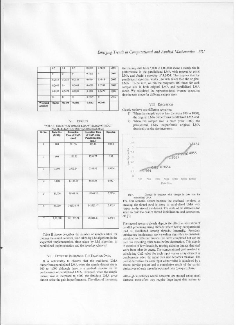


354 Emerging Trends in Computational and Applied Mathematics
65Lightning Arrester Fault Detection through Digital
Thermovision Image Processing Technique
Ishita Sharma, Shabana UroojElectrical Engineering Department, School of Engineering Gautam Buddha University, Greater Noida
[email protected], [email protected]
Abstract: Infrared Thermography has emerged as an important tool in predicting and preventing failure in anyelectrical equipment. All objects emit energy proportional to their surface temperature and the Infrared Energyradiated depends upon the emissivity coefficient of the surface under measurement. Lightning Arrester faultdetection and diagnosis through Digital Image Processing technique is discussed in this paper. The two approachesinvolved are Bottom-Up Approach and Top-Down Approach, in which the segmentation of Lightning Arresterusing Top-Down Approach is performed using Marker-Controlled Watershed Segmentation.Keywords: Infrared Thermography; Fault Detection; Digital Image Processing; Watershed Transformation; Neuro-Fuzzy Topology
Introduction
Image processing is any form of signal processingfor which the input is an image, such asa photograph or video frame; the output of imageprocessing may be either an image or a set ofcharacteristics or parameters related to the image [1].Image processing can be widely utilized in detectionof faults in power system. Faults in electrical powersystems can be classified into a few categories such aspoor connection, short circuit, overloading, loadimbalance and improper component installation. Inmost cases, poor connections are among the morecommon problems in transmission and distribution linesof electrical power systems. Infrared thermography iswell known as one of the effective tools in monitoringthe condition of electrical equipments. It has thecapability to detect the thermal abnormality in electricalequipments. The recent research in this field has shownthe interest on an automatic diagnosis system. This isdue to fast analysis and robustness compared to manualinspection. Various techniques have been used toidentify and classify the thermal anomalies in theinfrared thermographic image of electrical equipments.The common method that is normally used in analyzing
infrared thermogram can be divided into four steps:image preprocessing, segmentation, classification anddecision making [2].
Amongst many faults in electrical power system, thispaper mainly discusses the Lightning Arrester faultsand describes a methodology that aims to detect anddiagnose faults in lightning arresters, using the non-destructive thermovision technique. This techniquedoes not demand the disconnection of the equipmentunder inspection. It uses a set of neuro-fuzzy networksto achieve the lightning arresters fault classification.The methodology also uses digital image processingbased on the Watershed Transformation in order toperform the segmentation of the lightning arrester image[2, 3].
Image Processing MethodsIn evaluating the condition of electrical equipment,
Image Processing methods are of two types, Bottom-Up Approach and Top-Down Approach. InfraredThermogram involves the following steps in ImageProcessing methods:
1. Image Pre-processing2. Image Extraction3. Feature Extraction

Emerging Trends in Computational and Applied Mathematics 355
4. Classification5. Decision
The straight-forward approach is by following thesteps one by one in Bottom-Up order. On the other hand,Top-Down Approach involves identifying theinteresting image region. [2, 4].
A. Bottom-Up Approach
Based on the Gray-Level Histogram of an Image, thetarget object is separated from the background at aspecific threshold T.A, the thresholding image g(x,y)of an image f(x,y) is defined as
g(x,y) ={1, if f(x,y) < T 0, if f(x,y) > T}
The hotspot region can be segmented throughselecting a suitable threshold value. Morphologicalimage processing was used to extract the hotspot wherethe maximum gray pixel value determines the maximumtemperature of the hotspot region. Watershedtransformation algorithm was successfully used forsegmenting the thermogram of lightning arrester [3, 4and 11].
B. Top-Down Approach
The common steps used in evaluating the thermalanomaly of electrical equipments based on Top-Downoriented approach can be summarized by a flowchartas shown in Figure 1.
START
Finding Region of
Repeated Structure
Segmentation Process
Relevant Information
Decision Making
RESULT
Figure 1: Flowchart
Fault Detection In Lightning Arrester
A. Protection against Surges
As the use of products and equipment withcomponents and insulation systems vulnerable tovoltage surges and spikes continues to increase, therequirement for Lightning Arresters to protect againstthe effects due to lightning str ikes, switchingphenomenon, etc., continues to increase as well.Lightning Arresters protect equipment against impactsdue to strokes and guarantee reliability, economy andcontinuity of power systems operation. Protectionsystem control is needed to check if the systemoperation shows any kind of anomaly. This control isperformed by measurement and assessment of variablessuch as leakage current, radio interference and othervariables that may give indication about lightningArresters operational condition [10].
B. Methodology
The main step in order to achieve fault detection anddiagnosis is to select a set of inputs whose informationis capable to allow the fault detection. This paper usesdigital image processing techniques to extract somevariables from the thermogram. Besides usingthermographic variables, the diagnosis tool developeduses identification variables to generate the diagnosis.Once all data is collected, it’s necessary to apply digitalimage processing techniques. This procedure enablesthe extraction of some thermographic variables fromthe thermogram (eg. maximum and minimumtemperatures). These variables are used by the diagnosistool developed. The diagnosis tool uses a set of neuro-fuzzy networks to generate a thermovision diagnosis.This strategy is known as Bagging and is applied hereto improve the power of generalization of the faultdetection system. The methodology applied is shownin Figure 2 [3, 7].
Figure 2: Methodology applied [2]

356 Emerging Trends in Computational and Applied Mathematics
C. Description of Variables
The variables used in the diagnosis can be subdividedinto two groups [11]:
1. Identification Variables:• Material: can be SiC (porcelain) or ZnO
without spark gaps (porcelain or polymeric).• Surge arresters Rated Voltage.• Manufacturer: refers to the company that
designed and manufactured the surge arrest-ers.
• Pollution Index: This variable characterizesthe substation and is obtained by measure-ment of pollution particles in the air. Table Ipresents four pollution levels defined. Thisvariable is important to enable an efficientanalysis and treatment of a thermogram. Insome cases, the thermogram can change itsmain characteristics (maximum temperature)under high pollution levels.
TABLE IFOUR LEVELS DEFINED FOR POLLUTION INDEX AS A VARIABLE
(SOURCE: INTERNATIONAL ELECTROTECHNICAL COMMISSION IEC
REPORT—PUBLICATION 815—FIRST EDITION—1986)
Range (mg/cm2) Class
< 0.06 Light
0.06 – 0.1 Medium
0.1 – 0.2 Heavy
> 0.2 Very Heavy
2. Thermographic Variables:This group comprehends the four variables needed toenable an efficient analysis and treatment of athermogram:
• Distance: distance from the thermoviewerand the object being examined also calledtarget distance,
• Emissivity: emissivity is the measure of anobject’s ability to emit infrared energy. Theemissivity is estimated using the tapemethod. This method requires the usage ofa PVC tape (emissivity value 0.97) orequivalent.
• Ambient temperature: the imager’s operat-ing temperature range is 0 °C to 50 °C. Itscalibration is maintained within this range.
Figure 3: Thermovision photo of a real Surge Arrester
(Source: Electric Energy Research Center-2003)
Digital Thermogram ProcessingThe Digital Thermogram Processing may be divided
into the following steps [5, 12]:1) Image Processing: This article uses infra-
red cameras, known as Thermovisors to al-low image acquisition.
2) Preprocessing: The pre-processing consistsof the image transformation obtained by thethermovisor at a gray level image, whichallows the utilization of the traditional seg-mentation techniques.
3) Segmentation: The segmentation objectiveis the division of an image into set of partsand objects. It’s necessary to use the wholeinformation available related to the problemin order to have a successful segmentation.Important information at the lightning ar-rester image is its position, which is alwaysat the centre of the picture. It’s evident thatthe person who acquires the image, fits theimage centre with the lightning arrester cen-tre to identify it after the acquisition Themost common segmentation tools are: Pointor Line Detection, Edge Detection, Gradi-ent Operators, Laplacian, Hough Transfor-mation, Simple or Adaptive Threshold, Re-gion Growing and Watershed Transforma-tion [6].
1. Watershed Transformation: WatershedTransformation used for Image Segmentation is basedon Topographic Interpretation of a Gray Scale Image.

Emerging Trends in Computational and Applied Mathematics 357
An image can be regarded as a topographic relief onwhich the elevation of a point is represented by thegradient of a pixel. Assuming there is a hole that ispunched in each regional minimum and water is risingthrough these holes, in order to prevent the merging ofwater, dams are built to separate adjacent regions. Theprocess of water flooding and dams building willcontinue until the highest elevation level of the wholerelief is reached. At the end of the flooding, watershedlines are formed to surround each local minimum andthe segmentation of an image can be achieved. Theimplementation of above process in an image usuallystarts with detecting and labelling regional minima. Itcontinues until a completely labelled image is generatedwith each labelled region representing an imagesegment.
(a) (b)Figure 4: (a) Gray level image with two different sources of
water, catchment basins, meet each other and generate awatershed line and (b) it’s representation as a surface [5]
The Marker-Controlled Watershed Segmentation isa robust and flexible method for segmentation of objectswith closed contours, where the boundaries areexpressed as ridges [9]. Each initial marker has a one-to-one relationship to a specific watershed region, thusthe number of markers will be equal to the final numberof watershed regions. After segmentation, theboundaries of the watershed regions are arranged onthe desired ridges, thus separating each object from itsneighbours. The markers can be manually orautomatically selected, but high throughput experimentsoften employ automatically generated markers to savehuman time and resources. Thus we require to “mark”foreground objects and background locations in orderto make segmentation effective.Supposing a solid object, its picture morphologicalgradient produces a set of minima inside its surfaceand strong values at its edges, making the process to
“flood” a region possible. The original image istransformed into a gradient image, which representsthe edge strength of each pixel [16, 17].The thermographic image of the Lightning Arrester usedfor segmentation is shown in Figure 3. The Marker-Controlled Watershed Segmentation follows this basicprocedure [15]:Step 1: Converting the Coloured Image to Gray ScaleImage, as shown below:
Figure 5: Gray-Scale Image
Step 2: Using the Gradient magnitude as thesegmentation function, as shown below:
Figure 6: Gradient magnitude
Step 3: Marking the foreground objects, as shownbelow:
Figure 7: Opening- Closing with reconstruction

358 Emerging Trends in Computational and Applied Mathematics
Step 4: Computing the background markers, asshown below:
Figure 8: Watershed ridge lines
Step 5: Computing the Watershed Transformationof the segmentation.
Step 6: Visualizing the results. One visualizationtechnique is to superimpose the foreground markers,background markers, and segmented object boundarieson the original image. We can use dilation as needed tomake certain aspects, such as the object boundaries,more visible, as shown below:
Figure 9: Markers and object boundaries superimposed onoriginal image
Another useful visualization technique is to displaythe label matrix as a coloured image, as shown below:
Figure 10: Coloured Watershed label matrix
2. Fault Diagnosis using Neuro-Fuzzy Topology: TheThermovision diagnosis presented here uses a neuro-fuzzy network to process the input variables. Eachneuro-fuzzy network has the three layer structure shownin Figure 11 [14].
The neuro-fuzzy inputs are the Thermographicvariables (Emissivity, Ambient Temperature, AirRelative Humidity, Minimum and MaximumTemperature and Temperature variation) and theIdentification variables (Pollution Index, Rated Voltage,Material and Manufacturer). The thermovision neuro-fuzzy networks ensemble will yield the output variable.
Figure 11: Structure of networks used to implement thediagnosis method.
A brief description of each layer is presented:
Layer 1: Input Layer: This layer uses a node for eachinput variable x
i. Figure 12 shows N input nodes. The
network uses P triangular membership functions equallyspaced to represent if-then rules. Each membershipfunction has a weight w
ij, associated. The index i
identifies the input number and j the membershipfunction number. These weights are adjusted during thetraining phase.
Figure 12: Membership function model used

Emerging Trends in Computational and Applied Mathematics 359
Layer 2: Aggregation layer: This layer aggregates allthe activated rules by adding using the Max-Mininference system:
ai= �
�
p
j
f1
i, j (x
i) w
i,j
Layer 3: Output layer: This layer is only one node whose
value indicates the operational condition as follows:
- Lightning arrester in normal condition(NORMAL),
- Lightning arrester in suspicious condition(SUSPICIOUS),
- Lightning arrester in faulty condition(FAULTY).
3. Bagging Topology: The thermovision diagnosis isimplemented by a set of neuro-fuzzy networks havingthe structure detailed in Figure 11. The diagnosis isobtained by the majority voting of all neuro-fuzzynetworks. If parity occurs, the worst diagnosis isselected. This strategy is known as bagging and isapplied here to improve the power of generalization ofthe fault detection system [13, 14].
Conclusion
The paper presents a technique for fault detection anddiagnostics in Lightning Arresters using DigitalThermogram Processing without requir ing thedisconnection of the equipment under inspection andwith faster response time. The Bagging topologyimplemented by this system is based uponThermographic Image Processing techniques.The diagnostics tool implemented showed itself as anextremely efficient tool, being presently used byElectric Energy Research Center as an auxiliary systemto generate lightning arresters diagnosis.Some future work can be performed regarding theimprovement in thermogram parameters. If they changesignificantly, the tool might not present correct results,although this is not a common situation. For this case,the system must have the knowledge to compensate fordifferent environmental conditions. Also thethermogram comparative approach can be applied,using the size of the surge arrester hot spot and itsevolution during time.
REFERENCES
[1] [Online].Available: http://en.wikipedia.org/wiki/Image_processing
[2] Soib Taib, Mohd Shawal Jadin and Shahid Kabir, “Ther-mal Imaging for Enhancing Inspection Reliability: De-tection and Characterization”, Infrared Thermography,Dr. Raghu V Prakash (Ed.), InTech Publication, (2012),ISBN: 978-953-51-0242-7.
[3] Carlos A. Laurentys Almeida, Antonio. P. Braga, SinvalNascimento, Vinicius Paiva, Helvio J. A. Martins,Rodolfo Torres and Walmir M. Caminhas, “IntelligentThermographic Diagnostic Applied to Surge Arresters:A New Approach” in IEEE Transactions On PowerDelivery, Vol.24, No.2, (April, 2009), pp. 0885-8977.
[4] Mohd. Shawal Jadin, Soib Taib, Shahid Kabir andMohd. Ansor Bin Yusof, “Image Processing Methodsfor Evaluating Infrared Thermographic Image of Elec-trical Equipments”, Progress In Electromagnetics Re-search Symposium Proceedings, (Marrakesh, Morocco,March 20-23, 2011).
[5] Carlos A. Laurentys Almeida, Walmir M. Caminhas,Antônio P. Braga, Vinicius Paiva, Hélvio Martins,Rodolfo Torres, “ Intelligent Detection and Diagnosisof Lightning Arresters Faults Using DigitalThermovision Image Processing Techniques”, Proceed-ings of SPIE, Vol. 5782, (Bellingham, WA, 2005), pp.0277-786.
[6] Kregg, M.A., “Benefits of using infrared thermogra-phy in utility substations”, Proceedings of SPIE, (2004),pp. 249-257.
[7] Haralick, Robert M. Shanmugam, K., & Dinstein, I,“Textural Features for Image Classification”, IEEETransactions on Systems, Man and Cybernetics, (1973),Vol. 3, No. 6, pp. 610-621.
[8] Sukhjinder Singh, R. K. Bansal, Savina Bansal, “Com-parative Study and Implementation of Image Process-ing Techniques Using MATLAB”, International Jour-nal of Advanced Research in Computer Science andSoftware Engineering, Vol. 2, Issue 3, (March 2012),ISSN: 2277 128X.
[9] L. Vincent and P. Soille, “Watersheds in digital spaces:an efficient algorithm based on immersion simulations”,IEEE Transactions on Pattern Analysis and Mechani-cal Intelligence, (1991), pp. 583–598.
[10] Hernandez, “Lightning Arrester Selection and Appli-cation Guide”, GE.
[11] Shafi’i, M.A. and N. Hamzah, “Internal Fault Classifi-cation using Artificial Neural Network”, Proceedingsof 4th International Power Engineering and Optimiza-tion Conference, (Shah Alam, June, 2010), pp. 352-357.
[12] Wretman D, “Finding Regions of interest in a DecisionSupport System for Analysis of Infrared Images”, Mas-ter of Science Thesis, (Royal Institute of Technology,

360 Emerging Trends in Computational and Applied Mathematics
School of Computer Science and Communication,Stockholm, Sweden, 2006).
[13] Rafael C. Gonzalez, Richard E. Woods and Steven L.Eddins, “Digital Image Processing using MATLAB”,2nd ed., Gatesmark Publication, (2009), ISBN- 978-0-9820854-0-0.
[14] L.K. Hansen & P. Salamon, “Neural Network En-sembles”, IEEE Transactions on Pattern Analysis adMachine Intelligence, (1990), pp. 993-1001.
[15] [Online].Available:www.mathworks.in/help/images/ex-
a m p l e s / m a r k e r - c o n t r o l l e d - w a t e r s h e d -segmentation.html
[16] K. Parvati, B.S. Prakasa Rao & M. Mariya Das, “Im-age Segmentation Using Gray-Scale Morphology andMarker-Controlled Watershed Transformation”, Dis-crete Dynamics in Nature and Society, Hindawi Corpo-ration Publication, (Vol. 2008).
[17] Wiley Encyclopedia of Computer Science and Engi-neering: Image Segmentation by Region based and Wa-tershed Algorithms, John Wiley and Sons, (2008), pp.1543- 1552.

Emerging Trends in Computational and Applied Mathematics 361
66An Application of Intuitionistic Fuzzy sets in Bi-matrix Game
with Intuitionistic Fuzzy Goals
I. Khan, A. AggarwalUniversity School of Basic and Applied Sciences, Guru Gobind Singh Indraprastha University, Delhi, India
Abstract: Abstract: In this paper, we make an attempt to study bi-matrix game with intutionistic fuzzy goals.This study is the generalization of earlier work of Vidyottama etal.[18] in this regard. This model provides thedegree of acceptance as well as the degree of rejection to the aspiration levels for both the players. Further it isshown that two person zero sum matrix game with intuitionistic fuzzy goals [1] is the special case of this study.Further we point out certain shortcomings in the recent study of Nayak and Pal [16]. A numerical example is alsoincluded in the support of the theory.Keywords: Intuitionistic fuzzy sets · intuitionistic fuzzy inequlities · intuitionistic fuzzy goals · intuitionisticfuzzy bi-matrix game.

362 Emerging Trends in Computational and Applied Mathematics

Emerging Trends in Computational and Applied Mathematics 363

364 Emerging Trends in Computational and Applied Mathematics

Emerging Trends in Computational and Applied Mathematics 365

366 Emerging Trends in Computational and Applied Mathematics

Emerging Trends in Computational and Applied Mathematics 367

368 Emerging Trends in Computational and Applied Mathematics

Emerging Trends in Computational and Applied Mathematics 369

370 Emerging Trends in Computational and Applied Mathematics

Emerging Trends in Computational and Applied Mathematics 371


![[ CONFERENCE TENTATIVE ]](https://static.fdokumen.com/doc/165x107/6332727f3108fad7760ea090/-conference-tentative-.jpg)