CoNLL-2011 Fifteenth Conference on Computational Natural ...

CoNLL-2011

Fifteenth Conference onComputational Natural Language Learning

Proceedings of the Conference

23-24 June, 2011Portland, Oregon, USA

Production and Manufacturing by

CoNLL 2011 Best Paper sponsor:

c©2011 The Association for Computational Linguistics

Order copies of this and other ACL proceedings from:

Association for Computational Linguistics (ACL)209 N. Eighth StreetStroudsburg, PA 18360USATel: +1-570-476-8006Fax: [email protected]

ISBN 978-1-932432-92-3

ii

Omnipress, Inc.2600 Anderson StreetMadison, WI 53704 USA

Preface

The 2011 Conference on Computational Natural Language Learning is the fifteenth in the series ofannual meetings organized by SIGNLL, the ACL special interest group on natural language learning.CONLL-2011 will be held in Portland, Oregon, USA, June 23-24 2011, in conjunction with ACL-HLT.

For our special focus this year in the main session of CoNLL, we invited papers relating to massive,linked text data. We received 82 submissions on these and other relevant topics, of which 4 wereeventually withdrawn. Of the remaining 78 papers, 13 were selected to appear in the conferenceprogram as oral presentations, and 14 were chosen as posters. All accepted papers appear here in theproceedings. Each accepted paper was allowed eight content pages plus any number of pages containingonly bibliographic references.

As in previous years, CoNLL-2011 has a shared task, Modeling unrestricted coreference in OntoNotes.The Shared Task papers are collected in a companion volume of CoNLL-2011.

We begin by thanking all of the authors who submitted their work to CoNLL-2011, as well as theprogram committee for helping us select from among the many strong submissions. We are also gratefulto our invited speakers, Bruce Hayes and Yee Whye Teh, who graciously agreed to give talks at CoNLL.Special thanks to the SIGNLL board members, Lluıs Marquez and Joakim Nivre, for their valuableadvice and assistance in putting together this year’s program, and to the SIGNLL information officer,Erik Tjong Kim Sang, for publicity and maintaining the CoNLL-2011 web page. We also appreciatethe additional help we received from the ACL program chairs, workshop chairs, and publication chairs.

Finally, many thanks to Google for sponsoring the best paper award at CoNLL-2011.

We hope you enjoy the conference!

Sharon Goldwater and Christopher Manning

CoNLL 2011 Conference Chairs

iii

Program Chairs:

Sharon Goldwater (University of Edinburgh, United Kingdom)Christopher Manning (Stanford University, United States)

Program Committee:

Steven Abney (University of Michigan, United States)Eneko Agirre (University of the Basque Country, Spain)Afra Alishahi (Saarland University, Germany)Lourdes Araujo (Universidad Nacional de Educacion a Distancia, Spain)Jason Baldridge (University of Texas at Austin, United States)Steven Bethard (Katholieke Universiteit Leuven, Belgium)Steven Bird (University of Melbourne, Australia)Phil Blunsom (University of Oxford, United Kingdom)Thorsten Brants (Google Inc., United States)Chris Brew (Ohio State University, United States)David Burkett (University of California at Berkeley, United States)Yunbo Cao (Microsoft Research Asia, China)Xavier Carreras (Technical University of Catalonia, Spain)Nathanael Chambers (Stanford University, United States)Ming-Wei Chang (University of Illinois at Urbana-Champaign, United States)Colin Cherry (National Research Council, Canada)Massimiliano Ciaramita (Google Research, Switzerland)Alexander Clark (Royal Holloway, University of London, United Kingdom)Stephen Clark (University of Cambridge, United Kingdom)Shay Cohen (Carnegie Mellon University, United States)Trevor Cohn (University of Sheffield, United Kingdom)James Curran (University of Sydney, Australia)Walter Daelemans (University of Antwerp, Belgium)Mark Dras (Macquarie University, Australia)Amit Dubey (University of Edinburgh, United Kingdom)Chris Dyer (Carnegie Mellon University, United States)Jacob Eisenstein (Carnegie Mellon University, United States)Micha Elsner (University of Edinburgh, United Kingdom)Jenny Finkel (Columbia University, United States)Radu Florian (IBM Watson Research Center, United States)Robert Frank (Yale University, United States)Stella Frank (University of Edinburgh, United Kingdom)Michel Galley (Microsoft Research, United States)Kevin Gimpel (Carnegie Mellon University, United States)Yoav Goldberg (Ben Gurion University of the Negev, Israel)Cyril Goutte (National Research Council, Canada)

v

Spence Green (Stanford University, United States)Gholamreza Haffari (BC Cancer Research Center, Canada)Keith Hall (Google Research, Switzerland)James Henderson (University of Geneva, Switzerland)Julia Hockenmaier (University of Illinois at Urbana-Champaign, United States)Fei Huang (IBM Research, United States)Rebecca Hwa (University of Pittsburgh, United States)Richard Johansson (University of Trento, Italy)Mark Johnson (Macquarie University, Australia)Rohit Kate (University of Wisconsin at Milwaukee, United States)Philipp Koehn (University of Edinburgh, United Kingdom)Mamoru Komachi (Nara Institute of Science and Technology, Japan)Terry Koo (Google Inc., United States)Shankar Kumar (Google Inc., United States)Tom Kwiatkowski (University of Edinburgh, United Kingdom)Mirella Lapata (University of Edinburgh, United Kingdom)Shalom Lappin (Kings College London, United Kingdom)Lillian Lee (Cornell Universiy, United States)Percy Liang (University of California at Berkeley, United States)Adam Lopez (Johns Hopkins University, United States)Rob Malouf (San Diego State University, United States)Andre Martins (Carnegie Mellon University, United States)Yuji Matsumoto (Nara Institute of Science and Technology, Japan)Takuya Matsuzaki (University of Tokyo, Japan)David McClosky (Stanford University, United States)Ryan McDonald (Google Inc., United States)Paola Merlo (University of Geneva, Switzerland)Haitao Mi (Institute of Computing Technology, Chinese Academy of Sciences, China)Yusuke Miyao (University of Tokyo, Japan)Alessandro Moschitti (University of Trento, Italy)Lluıs Marquez (Technical University of Catalonia, Spain)Tahira Naseem (Massachusetts Institute of Technology, United States)Mark-Jan Nederhof (University of St. Andrews, United Kingdom)Hwee Tou Ng (National University of Singapore, Singapore)Vincent Ng (University of Texas at Dallas, United States)Joakim Nivre (Uppsala University, Sweden)Miles Osborne (University of Edinburgh, United Kingdom)Christopher Parisien (University of Toronto, Canada)Amy Perfors (University of Adelaide, Australia)Slav Petrov (Google Research, United States)Hoifung Poon (University of Washington, United States)Vasin Punyakanok (BBN Technologies, United States)Chris Quirk (Microsoft Research, United States)Ari Rappoport (The Hebrew University, Israel)Lev Ratinov (University of Illinois at Urbana-Champaign, United States)Roi Reichart (Massachusetts Institute of Technology, United States)

vi

Joseph Reisinger (University of Texas at Austin, United States)Sebastian Riedel (University of Massachusetts, United States)Dan Roth (University of Illinois at Urbana-Champaign, United States)William Sakas (Hunter College, United States)Anoop Sarkar (Simon Fraser University, Canada)William Schuler (The Ohio State University, United States)Libin Shen (Akamai, United States)Khalil Sima’an (University of Amsterdam, Netherlands)Noah Smith (Carnegie Mellon University, United States)Benjamin Snyder (University of Wisconsin-Madison, United States Richard Socher (StanfordUniversity, United States)Valentin Spitkovsky (Stanford University, United States)Mark Steedman (University of Edinburgh, United Kingdom)Mihai Surdeanu (Stanford University, United States)Jun Suzuki (NTT Communication Science Laboratories, Japan)Hiroya Takamura (Tokyo Institute of Technology, Japan)Ivan Titov (Saarland University, Germany)Kristina Toutanova (Microsoft Research, United States)Antal van den Bosch (Tilburg University, Netherlands)Theresa Wilson (Johns Hopkins University, United States)Peng Xu (Google Inc., United States)Charles Yang (University of Pennsylvania, United States)Chen Yu (Indiana University, United States)Daniel Zeman (Charles University in Prague, Czech Republic)Luke Zettlemoyer (University of Washington at Seattle, United States)

Invited Speakers:

Bruce Hayes (University of California, Los Angeles, United States)Yee Whye Teh (Gatsby Unit, University College London, United Kingdom)

vii

Table of Contents

Modeling Syntactic Context Improves Morphological SegmentationYoong Keok Lee, Aria Haghighi and Regina Barzilay . . . . . . . . . . . . . . . . . . . . . . . . . . . . . . . . . . . . . . 1

The Effect of Automatic Tokenization, Vocalization, Stemming, and POS Tagging on Arabic DependencyParsing

Emad Mohamed . . . . . . . . . . . . . . . . . . . . . . . . . . . . . . . . . . . . . . . . . . . . . . . . . . . . . . . . . . . . . . . . . . . . . . . 10

Punctuation: Making a Point in Unsupervised Dependency ParsingValentin I. Spitkovsky, Hiyan Alshawi and Daniel Jurafsky . . . . . . . . . . . . . . . . . . . . . . . . . . . . . . . . 19

Modeling Infant Word SegmentationConstantine Lignos . . . . . . . . . . . . . . . . . . . . . . . . . . . . . . . . . . . . . . . . . . . . . . . . . . . . . . . . . . . . . . . . . . . . 29

Word Segmentation as General ChunkingDaniel Hewlett and Paul Cohen . . . . . . . . . . . . . . . . . . . . . . . . . . . . . . . . . . . . . . . . . . . . . . . . . . . . . . . . . 39

(Invited talk) Computational Linguistics for Studying Language in People: Principles, Applications andResearch Problems

Bruce Hayes . . . . . . . . . . . . . . . . . . . . . . . . . . . . . . . . . . . . . . . . . . . . . . . . . . . . . . . . . . . . . . . . . . . . . . . . . . 48

Search-based Structured Prediction applied to Biomedical Event ExtractionAndreas Vlachos and Mark Craven . . . . . . . . . . . . . . . . . . . . . . . . . . . . . . . . . . . . . . . . . . . . . . . . . . . . . . 49

Using Sequence Kernels to Identify Opinion Entities in UrduSmruthi Mukund, Debanjan Ghosh and Rohini Srihari . . . . . . . . . . . . . . . . . . . . . . . . . . . . . . . . . . . . .58

Subword and Spatiotemporal Models for Identifying Actionable Information in Haitian KreyolRobert Munro . . . . . . . . . . . . . . . . . . . . . . . . . . . . . . . . . . . . . . . . . . . . . . . . . . . . . . . . . . . . . . . . . . . . . . . . . 68

Gender Attribution: Tracing Stylometric Evidence Beyond Topic and GenreRuchita Sarawgi, Kailash Gajulapalli and Yejin Choi . . . . . . . . . . . . . . . . . . . . . . . . . . . . . . . . . . . . . . 78

Improving the Impact of Subjectivity Word Sense Disambiguation on Contextual Opinion AnalysisCem Akkaya, Janyce Wiebe, Alexander Conrad and Rada Mihalcea . . . . . . . . . . . . . . . . . . . . . . . . 87

Effects of Meaning-Preserving Corrections on Language LearningDana Angluin and Leonor Becerra-Bonache . . . . . . . . . . . . . . . . . . . . . . . . . . . . . . . . . . . . . . . . . . . . . . 97

Assessing Benefit from Feature Feedback in Active Learning for Text ClassificationShilpa Arora and Eric Nyberg . . . . . . . . . . . . . . . . . . . . . . . . . . . . . . . . . . . . . . . . . . . . . . . . . . . . . . . . . 106

ULISSE: an Unsupervised Algorithm for Detecting Reliable Dependency ParsesFelice Dell’Orletta, Giulia Venturi and Simonetta Montemagni . . . . . . . . . . . . . . . . . . . . . . . . . . . . 115

Language Models as Representations for Weakly Supervised NLP TasksFei Huang, Alexander Yates, Arun Ahuja and Doug Downey. . . . . . . . . . . . . . . . . . . . . . . . . . . . . .125

ix

Automatic Keyphrase Extraction by Bridging Vocabulary GapZhiyuan Liu, Xinxiong Chen, Yabin Zheng and Maosong Sun . . . . . . . . . . . . . . . . . . . . . . . . . . . . 135

Using Second-order Vectors in a Knowledge-based Method for Acronym DisambiguationBridget T. McInnes, Ted Pedersen, Ying Liu, Serguei V. Pakhomov and Genevieve B. Melton 145

Using the Mutual k-Nearest Neighbor Graphs for Semi-supervised Classification on Natural LanguageData

Kohei Ozaki, Masashi Shimbo, Mamoru Komachi and Yuji Matsumoto . . . . . . . . . . . . . . . . . . . . 154

Automatically Building Training Examples for Entity ExtractionMarco Pennacchiotti and Patrick Pantel . . . . . . . . . . . . . . . . . . . . . . . . . . . . . . . . . . . . . . . . . . . . . . . . . 163

Probabilistic Word Alignment under the L0-normThomas Schoenemann . . . . . . . . . . . . . . . . . . . . . . . . . . . . . . . . . . . . . . . . . . . . . . . . . . . . . . . . . . . . . . . . 172

Authorship Attribution with Latent Dirichlet AllocationYanir Seroussi, Ingrid Zukerman and Fabian Bohnert . . . . . . . . . . . . . . . . . . . . . . . . . . . . . . . . . . . . 181

Evaluating a Semantic Network Automatically Constructed from Lexical Co-occurrence on a WordSense Disambiguation Task

Sean Szumlanski and Fernando Gomez . . . . . . . . . . . . . . . . . . . . . . . . . . . . . . . . . . . . . . . . . . . . . . . . . 190

Filling the Gap: Semi-Supervised Learning for Opinion Detection Across DomainsNing Yu and Sandra Kubler . . . . . . . . . . . . . . . . . . . . . . . . . . . . . . . . . . . . . . . . . . . . . . . . . . . . . . . . . . . 200

A Normalized-Cut Alignment Model for Mapping Hierarchical Semantic Structures onto Spoken Doc-uments

Xiaodan Zhu . . . . . . . . . . . . . . . . . . . . . . . . . . . . . . . . . . . . . . . . . . . . . . . . . . . . . . . . . . . . . . . . . . . . . . . . . 210

(Invited talk) Bayesian Tools for Natural Language LearningYee Whye Teh . . . . . . . . . . . . . . . . . . . . . . . . . . . . . . . . . . . . . . . . . . . . . . . . . . . . . . . . . . . . . . . . . . . . . . . 219

Composing Simple Image Descriptions using Web-scale N-gramsSiming Li, Girish Kulkarni, Tamara L. Berg, Alexander C. Berg and Yejin Choi . . . . . . . . . . . . 220

Adapting Text instead of the Model: An Open Domain ApproachGourab Kundu and Dan Roth . . . . . . . . . . . . . . . . . . . . . . . . . . . . . . . . . . . . . . . . . . . . . . . . . . . . . . . . . . 229

Learning with Lookahead: Can History-Based Models Rival Globally Optimized Models?Yoshimasa Tsuruoka, Yusuke Miyao and Jun’ichi Kazama . . . . . . . . . . . . . . . . . . . . . . . . . . . . . . . . 238

Learning Discriminative Projections for Text Similarity MeasuresWen-tau Yih, Kristina Toutanova, John C. Platt and Christopher Meek . . . . . . . . . . . . . . . . . . . . . 247

x

Conference Program

Thursday, June 23, 2011

9:00–9:05 Opening Remarks

Session 1

9:05–9:30 Modeling Syntactic Context Improves Morphological SegmentationYoong Keok Lee, Aria Haghighi and Regina Barzilay

9:30–9:55 The Effect of Automatic Tokenization, Vocalization, Stemming, and POS Tagging onArabic Dependency ParsingEmad Mohamed

9:55–10:20 Punctuation: Making a Point in Unsupervised Dependency ParsingValentin I. Spitkovsky, Hiyan Alshawi and Daniel Jurafsky

10:20–10:50 Coffee Break

Session 2

10:50–11:15 Modeling Infant Word SegmentationConstantine Lignos

11:15–11:40 Word Segmentation as General ChunkingDaniel Hewlett and Paul Cohen

11:40–12:40 (Invited talk) Computational Linguistics for Studying Language in People: Princi-ples, Applications and Research ProblemsBruce Hayes

12:40–14:00 Lunch Break

xi

Thursday, June 23, 2011 (continued)

Session 3

14:00–14:25 Search-based Structured Prediction applied to Biomedical Event ExtractionAndreas Vlachos and Mark Craven

14:25–14:50 Using Sequence Kernels to Identify Opinion Entities in UrduSmruthi Mukund, Debanjan Ghosh and Rohini Srihari

14:50–15:15 Subword and Spatiotemporal Models for Identifying Actionable Information in HaitianKreyolRobert Munro

15:15–15:40 Gender Attribution: Tracing Stylometric Evidence Beyond Topic and GenreRuchita Sarawgi, Kailash Gajulapalli and Yejin Choi


16:10–17:45 Main Session Posters

Improving the Impact of Subjectivity Word Sense Disambiguation on Contextual OpinionAnalysisCem Akkaya, Janyce Wiebe, Alexander Conrad and Rada Mihalcea

Effects of Meaning-Preserving Corrections on Language LearningDana Angluin and Leonor Becerra-Bonache

Assessing Benefit from Feature Feedback in Active Learning for Text ClassificationShilpa Arora and Eric Nyberg

ULISSE: an Unsupervised Algorithm for Detecting Reliable Dependency ParsesFelice Dell’Orletta, Giulia Venturi and Simonetta Montemagni

Language Models as Representations for Weakly Supervised NLP TasksFei Huang, Alexander Yates, Arun Ahuja and Doug Downey

Automatic Keyphrase Extraction by Bridging Vocabulary GapZhiyuan Liu, Xinxiong Chen, Yabin Zheng and Maosong Sun

xii

Thursday, June 23, 2011 (continued)

Using Second-order Vectors in a Knowledge-based Method for Acronym DisambiguationBridget T. McInnes, Ted Pedersen, Ying Liu, Serguei V. Pakhomov and Genevieve B.Melton

Using the Mutual k-Nearest Neighbor Graphs for Semi-supervised Classification on Nat-ural Language DataKohei Ozaki, Masashi Shimbo, Mamoru Komachi and Yuji Matsumoto

Automatically Building Training Examples for Entity ExtractionMarco Pennacchiotti and Patrick Pantel

Probabilistic Word Alignment under the L0-normThomas Schoenemann

Authorship Attribution with Latent Dirichlet AllocationYanir Seroussi, Ingrid Zukerman and Fabian Bohnert

Evaluating a Semantic Network Automatically Constructed from Lexical Co-occurrenceon a Word Sense Disambiguation TaskSean Szumlanski and Fernando Gomez

Filling the Gap: Semi-Supervised Learning for Opinion Detection Across DomainsNing Yu and Sandra Kubler

A Normalized-Cut Alignment Model for Mapping Hierarchical Semantic Structures ontoSpoken DocumentsXiaodan Zhu

xiii

Friday, June 24, 2011

Shared Task on Modeling Unrestricted Coreference in OntoNotes

9:00–10:30 Shared Task Overview and Oral Presentations


11:00–12:30 Shared Task Posters

12:30–14:00 Lunch Break

14:00–15:00 (Invited talk) Bayesian Tools for Natural Language LearningYee Whye Teh

15:00–15:30 SIGNLL Business Meeting


Session 4

16:00–16:25 Composing Simple Image Descriptions using Web-scale N-gramsSiming Li, Girish Kulkarni, Tamara L. Berg, Alexander C. Berg and Yejin Choi

16:25–16:50 Adapting Text instead of the Model: An Open Domain ApproachGourab Kundu and Dan Roth

16:50–17:15 Learning with Lookahead: Can History-Based Models Rival Globally Optimized Models?Yoshimasa Tsuruoka, Yusuke Miyao and Jun’ichi Kazama

17:15–17:40 Learning Discriminative Projections for Text Similarity MeasuresWen-tau Yih, Kristina Toutanova, John C. Platt and Christopher Meek

17:40–17:45 Best Paper Award and Closing

xiv

Proceedings of the Fifteenth Conference on Computational Natural Language Learning, pages 1–9,Portland, Oregon, USA, 23–24 June 2011. c©2011 Association for Computational Linguistics

Modeling Syntactic Context Improves Morphological Segmentation

Yoong Keok Lee Aria Haghighi Regina BarzilayComputer Science and Artificial Intelligence Laboratory

Massachusetts Institute of Technology{yklee, aria42, regina}@csail.mit.edu

Abstract

The connection between part-of-speech (POS)categories and morphological properties iswell-documented in linguistics but underuti-lized in text processing systems. This pa-per proposes a novel model for morphologi-cal segmentation that is driven by this connec-tion. Our model learns that words with com-mon affixes are likely to be in the same syn-tactic category and uses learned syntactic cat-egories to refine the segmentation boundariesof words. Our results demonstrate that incor-porating POS categorization yields substantialperformance gains on morphological segmen-tation of Arabic. 1

1 Introduction

A tight connection between morphology and syntaxis well-documented in linguistic literature. In manylanguages, morphology plays a central role in mark-ing syntactic structure, while syntactic relationshelp to reduce morphological ambiguity (Harley andPhillips, 1994). Therefore, in an unsupervised lin-guistic setting which is rife with ambiguity, model-ing this connection can be particularly beneficial.

However, existing unsupervised morphologicalanalyzers take little advantage of this linguisticproperty. In fact, most of them operate at the vo-cabulary level, completely ignoring sentence con-text. This design is not surprising: a typical mor-phological analyzer does not have access to syntac-

1The source code for the work presented in this paper isavailable at http://groups.csail.mit.edu/rbg/code/morphsyn/.

tic information, because morphological segmenta-tion precedes other forms of sentence analysis.

In this paper, we demonstrate that morphologicalanalysis can utilize this connection without assum-ing access to full-fledged syntactic information. Inparticular, we focus on two aspects of the morpho-syntactic connection:

• Morphological consistency within POS cat-egories. Words within the same syntactic cat-egory tend to select similar affixes. This lin-guistic property significantly reduces the spaceof possible morphological analyses, ruling outassignments that are incompatible with a syn-tactic category.

• Morphological realization of grammaticalagreement. In many morphologically rich lan-guages, agreement between syntactic depen-dents is expressed via correlated morphologicalmarkers. For instance, in Semitic languages,gender and number agreement between nounsand adjectives is expressed using matching suf-fixes. Enforcing mutually consistent segmen-tations can greatly reduce ambiguity of word-level analysis.

In both cases, we do not assume that the relevantsyntactic information is provided, but instead jointlyinduce it as part of morphological analysis.

We capture morpho-syntactic relations in aBayesian model that grounds intra-word decisionsin sentence-level context. Like traditional unsuper-vised models, we generate morphological structurefrom a latent lexicon of prefixes, stems, and suffixes.

1

In addition, morphological analysis is guided by alatent variable that clusters together words with sim-ilar affixes, acting as a proxy for POS tags. More-over, a sequence-level component further refines theanalysis by correlating segmentation decisions be-tween adjacent words that exhibit morphologicalagreement. We encourage this behavior by encodinga transition distribution over adjacent words, usingstring match cues as a proxy for grammatical agree-ment.

We evaluate our model on the standard Arabictreebank. Our full model yields 86.2% accuracy,outperforming the best published results (Poon etal., 2009) by 8.5%. We also found that modelingmorphological agreement between adjacent wordsyields greater improvement than modeling syntac-tic categories. Overall, our results demonstrate thatincorporating syntactic information is a promisingdirection for improving morphological analysis.

2 Related Work

Research in unsupervised morphological segmenta-tion has gained momentum in recent years bring-ing about significant developments to the area.These advances include novel Bayesian formula-tions (Goldwater et al., 2006; Creutz and Lagus,2007; Johnson, 2008), methods for incorporat-ing rich features in unsupervised log-linear models(Poon et al., 2009) and the development of multilin-gual morphological segmenters (Snyder and Barzi-lay, 2008a).

Our work most closely relates to approaches thataim to incorporate syntactic information into mor-phological analysis. Surprisingly, the research inthis area is relatively sparse, despite multiple resultsthat demonstrate the connection between morphol-ogy and syntax in the context of part-of-speech tag-ging (Toutanova and Johnson, 2008; Habash andRambow, 2005; Dasgupta and Ng, 2007; Adlerand Elhadad, 2006). Toutanova and Cherry (2009)were the first to systematically study how to in-corporate part-of-speech information into lemmati-zation and empirically demonstrate the benefits ofthis combination. While our high-level goal is simi-lar, our respective problem formulations are distinct.Toutanova and Cherry (2009) have considered asemi-supervised setting where an initial morpholog-

ical dictionary and tagging lexicon are provided butthe model also has access to unlabeled data. Since alemmatizer and tagger trained in isolation may pro-duce mutually inconsistent assignments, and theirmethod employs a log-linear reranker to reconcilethese decisions. This reranking method is not suit-able for the unsupervised scenario considered in ourpaper.

Our work is most closely related to the approachof Can and Manandhar (2009). Their method alsoincorporates POS-based clustering into morpholog-ical analysis. These clusters, however, are learnedas a separate preprocessing step using distributionalsimilarity. For each of the clusters, the model se-lects a set of affixes, driven by the frequency of theiroccurrences in the cluster. In contrast, we modelmorpho-syntactic decisions jointly, thereby enablingtighter integration between the two. This designalso enables us to capture additional linguistic phe-nomena such as agreement. While this techniqueyields performance improvement in the context oftheir system, the final results does not exceed state-of-the-art systems that do not exploit this informa-tion (for e.g., (Creutz and Lagus, 2007)).

3 Model

Given a corpus of unannotated and unsegmentedsentences, our goal is to infer the segmentationboundaries of all words. We represent segmen-tations and syntactic categories as latent variableswith a directed graphical model, and we performBayesian inference to recover the latent variables ofinterest. Apart from learning a compact morphemelexicon that explains the corpus well, we also modelmorpho-syntactic relations both within each wordand between adjacent words to improve segmenta-tion performance. In the remaining section, we firstprovide the key linguistic intuitions on which ourmodel is based before describing the complete gen-erative process.

3.1 Linguistic Intuition

While morpho-syntactic interface spans a range oflinguistic phenomena, we focus on two facets of thisconnection. Both of them provide powerful con-straints on morphological analysis and can be mod-eled without explicit access to syntactic annotations.

2

Morphological consistency within syntactic cate-gory. Words that belong to the same syntactic cat-egory tend to select similar affixes. In fact, the powerof affix-related features has been empirically shownin the task of POS tag prediction (Habash and Ram-bow, 2005). We hypothesize that this regularity canalso benefit morphological analyzers by eliminat-ing assignments with incompatible prefixes and suf-fixes. For instance, a state-of-the-art segmenter er-roneously divides the word “Al{ntxAbAt” into fourmorphemes “Al-{ntxAb-A-t” instead of three “Al-{ntxAb-At” (translated as “the-election-s”.) The af-fix assignment here is clearly incompatible — de-terminer “Al” is commonly associated with nouns,while suffix “A” mostly occurs with verbs.

Since POS information is not available to themodel, we introduce a latent variable that encodesaffix-based clustering. In addition, we consider avariant of the model that captures dependencies be-tween latent variables of adjacent words (analogousto POS transitions).

Morphological realization of grammatical agree-ment. In morphologically rich languages, agree-ment is commonly realized using matching suffices.In many cases, members of a dependent pair suchas adjective and noun have the exact same suf-fix. A common example in the Arabic Treebankis the bigram “Al-Df-p Al-grby-p” (which is trans-lated word-for-word as “the-bank the-west”) wherethe last morpheme “p” is a feminine singular nounsuffix.

Fully incorporating agreement constraints in themodel is difficult, since we do not have access tosyntactic dependencies. Therefore, we limit our at-tention to adjacent words which end with similarstrings – for e.g., “p” in the example above. Themodel encourages consistent segmentation of suchpairs. While our string-based cue is a simple proxyfor agreement relation, it turns to be highly effectivein practice. On the Penn Arabic treebank corpus, ourcue has a precision of around 94% at the token-level.

3.2 Generative ProcessThe high-level generative process proceeds in fourphases:

(a) Lexicon Model: We begin by generating mor-pheme lexicons L using parameters γ. This set

of lexicons consists of separate lexicons for pre-fixes, stems, and suffixes generated in a hierar-chical fashion.

(b) Segmentation Model: Conditioned on L, wedraw word types, their segmentations, and alsotheir syntactic categories (W ,S,T ).

(c) Token-POS Model: Next, we generate the un-segmented tokens in the corpus and their syn-tactic classes (w, t) from a standard first-orderHMM which has dependencies between adja-cent syntactic categories.

(d) Token-Seg Model: Lastly, we generate tokensegmentations s from a first-order Markov chainthat has dependencies between adjacent seg-mentations.

The complete generative story can be summarizedby the following equation:

P (w,s, t,W ,S,T ,L,Θ,θ|γ,α,β) =P (L|γ) (a)

P (W ,S,T ,Θ|L,γ,α) (b)

Ppos(w, t,θ|W ,S,T ,L,α) (c)

Pseg(s|W ,S,T ,L,β,α) (d)

where γ,α,Θ,θ,β are hyperparameters and pa-rameters whose roles we shall detail shortly.

Our lexicon model captures the desirability ofcompact lexicon representation proposed by priorwork by using parameters γ that favors small lexi-cons. Furthermore, if we set the number of syntac-tic categories in the segmentation model to one andexclude the token-based models, we recover a seg-menter that is very similar to the unigram DirichletProcess model (Goldwater et al., 2006; Snyder andBarzilay, 2008a; Snyder and Barzilay, 2008b). Weshall elaborate on this point in Section 4.

The segmentation model captures morphologicalconsistency within syntactic categories (POS tag),whereas the Token-POS model captures POS tagdependencies between adjacent tokens. Lastly, theToken-Seg model encourages consistent segmenta-tions between adjacent tokens that exhibit morpho-logical agreement.

3

Lexicon Model The design goal is to encouragemorpheme types to be short and the set of affixes(i.e. prefixes and suffixes) to be much smaller thanthe set of stems. To achieve this, we first draw eachmorpheme σ in the master lexicon L∗ according to ageometric distribution which assigns monotonicallysmaller probability to longer morpheme lengths:

|σ| ∼ Geometric(γl)

The parameter γl for the geometric distribution isfixed and specified beforehand. We then draw theprefix, the stem, and suffix lexicons (denoted byL−, L0, L+ respectively) from morphemes in L∗.Generating the lexicons in such a hierarchical fash-ion allows morphemes to be shared among thelower-level lexicons. For instance, once determiner“Al” is generated in the master lexicon, it can beused to generate prefixes or stems later on. To fa-vor compact lexicons, we again make use of a ge-ometric distribution that assigns smaller probabilityto lexicons that contain more morphemes:

prefix: |L−| ∼ Geometric(γ−)stem: |L0| ∼ Geometric(γ0)

suffix: |L+| ∼ Geometric(γ+)

By separating morphemes into affixes and stems, wecan control the relative sizes of their lexicons withdifferent parameters.

Segmentation Model The model independentlygenerates each word type using only morphemes inthe affix and stem lexicons, such that each wordhas exactly one stem and is encouraged to have fewmorphemes. We fix the number of syntactic cate-gories (tags) to K and begin the process by generat-ing multinomial distribution parameters for the POStag prior from a Dirichlet prior:

ΘT ∼ Dirichlet(αT , {1, . . . ,K})

Next, for each possible value of the tag T ∈{1, . . . ,K}, we generate parameters for a multino-mial distribution (again from a Dirichlet prior) foreach of the prefix and the suffix lexicons:

Θ−|T ∼ Dirichlet(α−, L−)

Θ0 ∼ Dirichlet(α0, L0)Θ+|T ∼ Dirichlet(α+, L+)

By generating parameters in this manner, we allowthe multinomial distributions to generate only mor-phemes that are present in the lexicon. Also, at infer-ence time, only morphemes in the lexicons receivepseudo-counts. Note that the affixes are generatedconditioned on the tag; But the stem are not.2

Now, we are ready to generate each word typeW , its segmentation S, and its syntactic category T .First, we draw the number of morpheme segments|S| from a geometric distribution truncated to gener-ate at most five morphemes:

|S| ∼ Truncated-Geometric(γ|S|)

Next, we pick one of the morphemes to be the stemuniformly at random, and thus determine the numberof prefixes and suffixes. Then, we draw the syntacticcategory T for the word. (Note that T is a latentvariable which we recover during inference.)

T ∼ Multinomial(ΘT )

After that, we generate each stem σ0, prefix σ−, andsuffix σ+ independently:

σ0 ∼ Multinomial(Θ0)σ−|T ∼ Multinomial(Θ−|T )

σ+|T ∼ Multinomial(Θ+|T )

Token-POS Model This model captures the de-pendencies between the syntactic categories of ad-jacent tokens with a first-order HMM. Conditionedon the type-level assignments, we generate (unseg-mented) tokens w and their POS tags t:

Ppos(w, t|W ,T ,θ)

=∏wi,ti

P (ti−1|ti, θt|t)P (wi|ti, θw|t)

where the parameters of the multinomial distribu-tions are generated by Dirichlet priors:

θt|t ∼ Dirichlet(αt|t, {1, . . . ,K})θw|t ∼ Dirichlet(αw|t,W t)

2We design the model as such since the dependencies be-tween affixes and the POS tag are much stronger than those be-tween the stems and tags. In our preliminary experiments, whenstems are also generated conditioned on the tag, spurious stemsare easily created and associated with garbage-collecting tags.

4

Here, W t refers to the set of word types that aregenerated by tag t. In other words, conditioned ontag t, we can only generate word w from the set ofword types inW t which is generated earlier (Lee etal., 2010).

Token-Seg Model The model captures the mor-phological agreement between adjacent segmenta-tions using a first-order Markov chain. The proba-bility of drawing a sequence of segmentations s isgiven by

Pseg(s|W ,S,T ,L,β,α) =∏

(si−1,si)

p(si|si−1)

For each pair of segmentations si−1 and si, we de-termine: (1) if they should exhibit morpho-syntacticagreement, and (2) if their morphological segmenta-tions are consistent. To answer the first question, wefirst obtain the final suffix for each of them. Next,we obtain n, the length of the longer suffix. Foreach segmentation, we define the ending to be thelast n characters of the word. We then use matchingendings as a proxy for morpho-syntactic agreementbetween the two words. To answer the second ques-tion, we use matching final suffixes as a cue for con-sistent morphological segmentations. To encode thelinguistic intuition that words that exhibit morpho-syntactic agreement are likely to be morphologicalconsistent, we define the above probability distribu-tion to be:

p(si|si−1)

=

β1 if same endings and same final suffixβ2 if same endings but different final suffixesβ3 otherwise (e.g. no suffix)

where β1 + β2 + β3 = 1, with β1 > β3 > β2. Bysetting β1 to a high value, we encourage adjacenttokens that are likely to exhibit morpho-syntacticagreement to have the same final suffix. And by set-ting β3 > β2, we also discourage adjacent tokenswith the same endings to be segmented differently. 3

4 Inference

Given a corpus of unsegmented and unannotatedword tokens w, the objective is to recover values of

3Although p sums to one, it makes the model deficient since,conditioned everything already generated, it places some prob-ability mass on invalid segmentation sequences.

all latent variables, including the segmentations s.

P (s, t,S,T ,L|w,W ,γ,α,β)

∝∫P (w, s, t,W ,S,T ,L,Θ,θ|γ,α,β)dΘdθ

We want to sample from the above distribution us-ing collapsed Gibbs sampling (Θ and θ integratedout.) In each iteration, we loop over each word typeWi and sample the following latent variables: its tagTi, its segmentation Si, the segmentations and tagsfor all of its token occurrences (si, ti), and also themorpheme lexicons L:

P (L, Ti, Si, si, ti|s−i, t−i,S−i,T−i,w−i,W−i,γ,α,β) (1)

such that the type and token-level assignments areconsistent, i.e. for all t ∈ ti we have t = Ti, and forall s ∈ si we have s = Si.

4.1 Approximate Inference

Naively sampling the lexicons L is computationallyinfeasible since their sizes are unbounded. There-fore, we employ an approximation which turns issimilar to performing inference with a Dirichlet Pro-cess segmentation model. In our approximationscheme, for each possible segmentation and tag hy-pothesis (Ti, Si, si, ti), we only consider one possi-ble value for L, which we denote the minimal lexi-cons. Hence, the total number of hypothesis that wehave to consider is only as large as the number ofpossibilities for (Ti, Si, si, ti).

Specifically, we recover the minimal lexicons asfollows: for each segmentation and tag hypothesis,we determine the set of distinct affix and stem typesin the whole corpus, including the morphemes intro-duced by segmentation hypothesis under considera-tion. This set of lexicons, which we call the minimallexicons, is the most compact ones that are neededto generate all morphemes proposed by the currenthypothesis.

Furthermore, we set the number of possible POStags K = 5. 4 For each possible value of the tag,we consider all possible segmentations with at mostfive segments. We further restrict the stem to have no

4We find that increasing K to 10 does not yield improve-ment.

5

more than two prefixes or suffixes and also that thestem cannot be shorter than the affixes. This furtherrestricts the space of segmentation and tag hypothe-ses, and hence makes the inference tractable.

4.2 Sampling equationsSuppose we are considering the hypothesis with seg-mentation S and POS tag T for word type Wi. LetL = (L∗, L−, L0, L+) be the minimal lexicons forthis hypothesis (S, T ). We sample the hypothesis(S, T, s = S, t = T,L) proportional to the productof the following four equations.

Lexicon Model∏σ∈L∗

γl(1− γl)|σ| ×

γ−(1− γ−)|L−| ×γ0(1− γ0)|L0| ×γ+(1− γ+)|L+| (2)

This is a product of geometric distributions involv-ing the length of each morpheme σ and the sizeof each of the prefix, the stem, and the suffix lexi-cons (denoted as |L−|, |L0|, |L+| respectively.) Sup-pose, a new morpheme type σ0 is introduced as astem. Relative to a hypothesis that introduces none,this one incurs an additional cost of (1 − γ0) andγl(1 − γl)|σ0|. In other words, the hypothesis is pe-nalized for increasing the stem lexicon size and gen-erating a new morpheme of length |σ0|. In this way,the first and second terms play a role similar to theconcentration parameter and base distribution in aDP-based model.

Segmentation Model

γ|S|(1− γ|S|)|S|∑5j=0 γ|S|(1− γ|S|)j

×

n−iT + α

N−i + αK×

n−iσ0+ α0

N−i0 + α0|L0|×

n−iσ−|T + α−

N−i−|T + α−|L−|×

n−iσ+|T + α+

N−i+|T + α+|L+|(3)

The first factor is the truncated geometric distribu-tion of the number of segmentations |S|, and thesecond factor is the probability of generate the tagT . The rest are the probabilities of generating thestem σ0, the prefix σ−, and the suffix σ+ (where theparameters of the multinomial distribution collapsedout). n−1

T is the number of word types with tag Tand N−i is the total number of word types. n−iσ−|Trefers to the number of times prefix σ− is seen in allword types that are tagged with T , and N−i−|T is thetotal number of prefixes in all word types that has tagT . All counts exclude the word type Wi whose seg-mentation we are sampling. If there is another pre-fix, N−i−|T is incremented (and also n−iσ−|T if the sec-ond prefix is the same as the first one.) Integratingout the parameters introduces dependencies betweenprefixes. The rest of the notations read analogously.

Token-POS Model

αw|t(mi)

(M−it + αw|t|W t|)(mi)×

K∏t=1

K∏t′=1

(m−it′|t + αt|t)(mi

t′|t)

(M−it + αt|t)(mi

t′|t)(4)

The two terms are the token-level emission and tran-sition probabilities with parameters integrated out.The integration induces dependences between alltoken occurrences of word type W which resultsin ascending factorials defined as α(m) = α(α +1) · · · (α + m − 1) (Liang et al., 2010). M−it isthe number of tokens that have POS tag t, mi is thenumber of tokens wi, and m−it′|t is the number of to-kens t-to-t′ transitions. (Both exclude counts con-tributed by tokens belong to word type Wi.) |W t| isthe number of word types with tag t.

Token-Seg Model

βmiβ11 β

miβ22 β

miβ33 (5)

Here,miβ1

refers to the number of transitions involv-ing token occurrences of word type Wi that exhibitmorphological agreement. This does not result inascending factorials since the parameters of transi-tion probabilities are fixed and not generated fromDirichlet priors, and so are not integrated out.

6

4.3 Staged Training

Although the Gibbs sampler mixes regardless of theinitial state in theory, good initialization heuristicsoften speed up convergence in practice. We there-fore train a series of models of increasing complex-ity (see section 6 for more details), each with 50 iter-ations of Gibbs sampling, and use the output of thepreceding model to initialize the subsequent model.The initial model is initialized such that all words arenot segmented. When POS tags are first introduced,they are initialized uniformly at random.

5 Experimental Setup

Performance metrics To enable comparison withprevious approaches, we adopt the evaluation set-upof Poon et al. (2009). They evaluate segmentationaccuracy on a per token basis, using recall, precisionand F1-score computed on segmentation points. Wealso follow a transductive testing scenario where thesame (unlabeled) data is used for both training andtesting the model.

Data set We evaluate segmentation performanceon the Penn Arabic Treebank (ATB).5 It consists ofabout 4,500 sentences of modern Arabic obtainedfrom newswire articles. Following the preprocessingprocedures of Poon et al. (2009) that exclude certainword types (such as abbreviations and digits), weobtain a corpus of 120,000 tokens and 20,000 wordtypes. Since our full model operates over sentences,we train the model on the entire ATB, but evaluateon the exact portion used by Poon et al. (2009).

Pre-defined tunable parameters and testingregime In all our experiments, we set γl = 1

2 (forlength of morpheme types) and γ|S| = 1

2 (for num-ber of morpheme segments of each word.) To en-courage a small set of affix types relative to stemtypes, we set γ− = γ+ = 1

1.1 (for sizes of the af-fix lexicons) and γ0 = 1

10,000 (for size of the stemlexicon.) We employ a sparse Dirichlet prior for thetype-level models (for morphemes and POS tag) bysetting α = 0.1. For the token-level models, we sethyperparameters for Dirichlet priors αw|t = 10−5

5Our evaluation does not include the Hebrew and ArabicBible datasets (Snyder and Barzilay, 2008a; Poon et al., 2009)since these corpora consists of short phrases that omit sentencecontext.

Model R P F1 t-testPCT 09 69.2 88.5 77.7 -Morfessor 72.6 77.4 74.9 -BASIC 71.4 86.7 78.3 (2.9) -+POS 75.4 87.4 81.0 (1.5) ++TOKEN-POS 75.7 88.5 81.6 (0.7) ∼+TOKEN-SEG 82.1 90.8 86.2 (0.4) ++

Table 1: Results on the Arabic Treebank (ATB) dataset: We compare our models against Poon et al. (2009)(PCT09) and the Morfessor system (Morfessor-CAT).For our full model (+TOKEN-SEG) and its simplifica-tions (BASIC, +POS, +TOKEN-POS), we perform fiverandom restarts and show the mean scores. The samplestandard deviations are shown in brackets. The last col-umn shows results of a paired t-test against the precedingmodel: ++ (significant at 1%), + (significant at 5%), ∼(not significant), - (test not applicable).

(for unsegmented tokens) and αt|t = 1.0 (for POStags transition.) To encourage adjacent words thatexhibit morphological agreement to have the samefinal suffix, we set β1 = 0.6, β2 = 0.1, β1 = 0.3.

In all the experiments, we perform five runs us-ing different random seeds and report the mean scoreand the standard deviation.

Baselines Our primary comparison is against themorphological segmenter of Poon et al. (2009)which yields the best published results on the ATBcorpus. In addition, we compare against the Mor-fessor Categories-MAP system (Creutz and Lagus,2007). Similar to our model, their system uses latentvariables to induce clustering over morphemes. Thedifference is in the nature of the clustering: the Mor-fessor algorithm associates a latent variable for eachmorpheme, grouping morphemes into four broadcategories (prefix, stem, suffix, and non-morpheme)but not introducing dependencies between affixes di-rectly. For both systems, we quote their performancereported by Poon et al. (2009).

6 Results

Comparison with the baselines Table 1 shows thatour full model (denoted +TOKEN-SEG) yields amean F1-score of 86.2, compared to 77.7 and 74.9obtained by the baselines. This performance gapcorresponds to an error reduction of 38.1% over thebest published results.

7

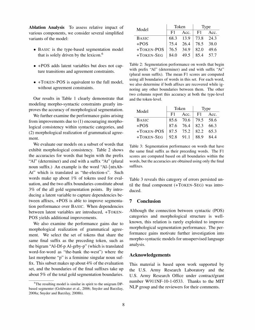
Ablation Analysis To assess relative impact ofvarious components, we consider several simplifiedvariants of the model:

• BASIC is the type-based segmentation modelthat is solely driven by the lexicon.6

• +POS adds latent variables but does not cap-ture transitions and agreement constraints.

• +TOKEN-POS is equivalent to the full model,without agreement constraints.

Our results in Table 1 clearly demonstrate thatmodeling morpho-syntactic constraints greatly im-proves the accuracy of morphological segmentation.

We further examine the performance gains arisingfrom improvements due to (1) encouraging morpho-logical consistency within syntactic categories, and(2) morphological realization of grammatical agree-ment.

We evaluate our models on a subset of words thatexhibit morphological consistency. Table 2 showsthe accuracies for words that begin with the prefix“Al” (determiner) and end with a suffix “At” (pluralnoun suffix.) An example is the word “Al-{ntxAb-At” which is translated as “the-election-s”. Suchwords make up about 1% of tokens used for eval-uation, and the two affix boundaries constitute about3% of the all gold segmentation points. By intro-ducing a latent variable to capture dependencies be-tween affixes, +POS is able to improve segmenta-tion performance over BASIC. When dependenciesbetween latent variables are introduced, +TOKEN-POS yields additional improvements.

We also examine the performance gains due tomorphological realization of grammatical agree-ment. We select the set of tokens that share thesame final suffix as the preceding token, such asthe bigram “Al-Df-p Al-grby-p” (which is translatedword-for-word as “the-bank the-west”) where thelast morpheme “p” is a feminine singular noun suf-fix. This subset makes up about 4% of the evaluationset, and the boundaries of the final suffixes take upabout 5% of the total gold segmentation boundaries.

6The resulting model is similar in spirit to the unigram DP-based segmenter (Goldwater et al., 2006; Snyder and Barzilay,2008a; Snyder and Barzilay, 2008b).

ModelToken Type

F1 Acc. F1 Acc.BASIC 68.3 13.9 73.8 24.3+POS 75.4 26.4 78.5 38.0+TOKEN-POS 76.5 34.9 82.0 49.6+TOKEN-SEG 84.0 49.5 85.4 57.7

Table 2: Segmentation performance on words that beginwith prefix “Al” (determiner) and end with suffix “At”(plural noun suffix). The mean F1 scores are computedusing all boundaries of words in this set. For each word,we also determine if both affixes are recovered while ig-noring any other boundaries between them. The othertwo columns report this accuracy at both the type-leveland the token-level.

ModelToken Type

F1 Acc. F1 Acc.BASIC 85.6 70.6 79.5 58.6+POS 87.6 76.4 82.3 66.3+TOKEN-POS 87.5 75.2 82.2 65.3+TOKEN-SEG 92.8 91.1 88.9 84.4

Table 3: Segmentation performance on words that havethe same final suffix as their preceding words. The F1scores are computed based on all boundaries within thewords, but the accuracies are obtained using only the finalsuffixes.

Table 3 reveals this category of errors persisted un-til the final component (+TOKEN-SEG) was intro-duced.

7 Conclusion

Although the connection between syntactic (POS)categories and morphological structure is well-known, this relation is rarely exploited to improvemorphological segmentation performance. The per-formance gains motivate further investigation intomorpho-syntactic models for unsupervised languageanalysis.

Acknowledgements

This material is based upon work supported bythe U.S. Army Research Laboratory and theU.S. Army Research Office under contract/grantnumber W911NF-10-1-0533. Thanks to the MITNLP group and the reviewers for their comments.

8

ReferencesMeni Adler and Michael Elhadad. 2006. An un-

supervised morpheme-based hmm for hebrew mor-phological disambiguation. In Proceedings of theACL/CONLL, pages 665–672.

Burcu. Can and Suresh Manandhar. 2009. Unsupervisedlearning of morphology by using syntactic categories.In Working Notes, CLEF 2009 Workshop.

Mathias Creutz and Krista Lagus. 2007. Unsupervisedmodels for morpheme segmentation and morphologylearning. ACM Transactions on Speech and LanguageProcessing, 4(1).

Sajib Dasgupta and Vincent Ng. 2007. Unsuper-vised part-of-speech acquisition for resource-scarcelanguages. In Proceedings of the EMNLP-CoNLL,pages 218–227.

Sharon Goldwater, Thomas L. Griffiths, and Mark John-son. 2006. Contextual dependencies in unsupervisedword segmentation. In Proceedings of the ACL, pages673–680.

Nizar Habash and Owen Rambow. 2005. Arabic tok-enization, part-of-speech tagging and morphologicaldisambiguation in one fell swoop. In Proceedings ofthe 43rd Annual Meeting of the Association for Com-putational Linguistics (ACL’05), pages 573–580, AnnArbor, Michigan, June. Association for ComputationalLinguistics.

Heidi Harley and Colin Phillips, editors. 1994. TheMorphology-Syntax Connection. Number 22 in MITWorking Papers in Linguistics. MIT Press.

Mark Johnson. 2008. Unsupervised word segmentationfor Sesotho using adaptor grammars. In Proceedingsof the Tenth Meeting of ACL Special Interest Groupon Computational Morphology and Phonology, pages20–27, Columbus, Ohio, June. Association for Com-putational Linguistics.

Yoong Keok Lee, Aria Haghighi, and Regina Barzilay.2010. Simple type-level unsupervised POS tagging.In Proceedings of the 2010 Conference on EmpiricalMethods in Natural Language Processing, pages 853–861, Cambridge, MA, October. Association for Com-putational Linguistics.

Percy Liang, Michael I. Jordan, and Dan Klein. 2010.Type-based mcmc. In Human Language Technolo-gies: The 2010 Annual Conference of the North Amer-ican Chapter of the Association for ComputationalLinguistics, pages 573–581, Los Angeles, California,June. Association for Computational Linguistics.

Hoifung Poon, Colin Cherry, and Kristina Toutanova.2009. Unsupervised morphological segmentation withlog-linear models. In Proceedings of HLT-NAACL2009, pages 209–217, Boulder, Colorado, June. As-sociation for Computational Linguistics.

Benjamin Snyder and Regina Barzilay. 2008a. Crosslin-gual propagation for morphological analysis. In Pro-ceedings of the AAAI, pages 848–854.

Benjamin Snyder and Regina Barzilay. 2008b. Unsuper-vised multilingual learning for morphological segmen-tation. In Proceedings of ACL-08: HLT, pages 737–745, Columbus, Ohio, June. Association for Computa-tional Linguistics.

Kristina Toutanova and Colin Cherry. 2009. A globalmodel for joint lemmatization and part-of-speech pre-diction. In Proceedings of the Joint Conference of the47th Annual Meeting of the ACL and the 4th Interna-tional Joint Conference on Natural Language Process-ing of the AFNLP, pages 486–494, Suntec, Singapore,August. Association for Computational Linguistics.

Kristina Toutanova and Mark Johnson. 2008. A bayesianlda-based model for semi-supervised part-of-speechtagging. In J.C. Platt, D. Koller, Y. Singer, andS. Roweis, editors, Advances in Neural InformationProcessing Systems 20, pages 1521–1528. MIT Press,Cambridge, MA.

9


The Effect of Automatic Tokenization, Vocalization, Stemming, and POS Tagging on Arabic Dependency Parsing

Emad Mohamed

Suez Canal University Suez, Egypt

[email protected]

Abstract We use an automatic pipeline of word tokenization, stemming, POS tagging, and vocalization to perform real-world Arabic dependency parsing. In spite of the high accuracy on the modules, the very few errors in tokenization, which reaches an accuracy of 99.34%, lead to a drop of more than 10% in parsing, indicating that no high quality dependency parsing of Arabic, and possibly other morphologically rich languages, can be reached without (semi-)perfect tokenization. The other module components, stemming, vocalization, and part of speech tagging, do not have the same profound effect on the dependency parsing process.

1. Introduction

Arabic is a morphologically rich language in which words may be composed of several tokens and hold several syntactic relations. We define word to be a whitespace delimited unit and token to be (part of) a word that has a syntactic function. For example, the word wsytzwjhA (!"#$%&'($)(English: And he will marry her) consists of 4 tokens: a conjunction w, a future marker s, a verb inflected for the singular masculine in the perfective form ytzwj, and a feminine singular 3rd person object pronoun. Parsing such a word requires tokenization, and performing dependency parsing in the tradition of the CoNLL-X (Buchholz and Marsi, 2006) and CoNLL 2007 shared task (Nivre et al, 2007) also requires part of speech tagging, lemmatization, linguistic features, and vocalization, all of which were in the human annotated gold standard form in the shared task.

The current study aims at measuring the effect of a pipeline of non gold standard tokenization, lemmatization, vocalization, linguistic features and POS tagging on the quality of Arabic dependency parsing. We only assume

that we have gold standard sentence boundaries since we do not agree with the sentence boundaries in the data, and introducing our own will have a complicating effect on evaluation. The CoNLL shared tasks of 2006 and 2007 used gold standard components in all fields, which is not realistic for Arabic, or for any other language. For Arabic and other morphologically rich languages, it may be more unrealistic than it is for English, for example, since the CoNLL 2007 Arabic dataset has tokens, rather than white space delimited words, as entries. A single word may have more than one syntactically functional token. Dependency parsing has been selected in belief that it is more suitable for Arabic than constituent-based parsing. All grammatical relations in Arabic are binary asymmetrical relations that exist between the tokens of a sentence. According to Jonathan Owens (1997: 52): “In general the Arabic notion of dependency and that defined in certain modern versions e.g. Tesniere (1959) rest on common principles”.

With a tokenization accuracy of 99.34%, a POS tagging accuracy of 96.39%, and with the absence of linguistic features and the use of word stems instead of lemmas, the Labeled Attachment Score drops from 74.75% in the gold standard experiment to 63.10% in the completely automatic experiment. Most errors are a direct result of tokenization errors, which indicates that despite the high accuracy on tokenization, it is still not enough to produce satisfactory parsing numbers.

2. Related Studies

The bulk of literature on Arabic Dependency Parsing stems from the two CoNLL shared tasks of 2006 and 2007. In CoNLL-X (Buchholz and

10

Marsi, 2006), the average Labeled Attachment Score on Arabic across all results presented by the 19 participating teams was 59.9% with a standard deviation of 6.5. The best results were obtained by McDonald et al (2006) with a score of 66.9% followed by Nivre et al (2006) with 66.7%.

The best results on Arabic in the CoNLL 2007 shared task were obtained by Hall et al (2007) as they obtained a Labeled Attachment Score of 76.52%, 9.6 percentage points above the highest score of the 2006 shared task. Hall et al used an ensemble system, based on the MaltParser dependency parser that extrapolates from a single MaltParser system. The settings with the Single MaltParser led to a Labeled Accuracy Score of 74.75% on Arabic. The Single MaltParser is the one used in the current paper. All the papers in both shared tasks used gold standard tokenization, vocalization, lemmatization, POS tags, and linguistic features.

A more recent study is that by Marton et al (2010). Although Marton et al varied the POS distribution and linguistic features, they still used gold standard tokenization. They also used the Columbia Arabic Treebank, which makes both the methods and data different from those presented here.

3. Data, Methods, and Evaluation 3.1.Data

The data used for the current study is the same data set used for the CoNLL (2007) shared task, with the same division into training set, and test set. This design helps in comparing results in a way that enables us to measure the effect of automatic pre-processing on parsing accuracy. The data is in the CoNLL column format. In this format, each token is represented through columns each of which has some specific information. The first column is the ID, the second the token, the third the lemma, the fourth the coarse-grained POS tag, the fifth the POS tag, and the sixth column is a list of linguistic features. The last two columns of the vector include the head of the token and the dependency relation between the token and its

head. Linguistic features are an unordered set of syntactic and/or morphological features, separated by a vertical bar (|), or an underscore if not available. The features in the CoNLL 2007 Arabic dataset represent case, mood, definiteness, voice, number, gender and person.

The data used for training the stemmer/tokenizer is taken from the Arabic Treebank (Maamouri and Bies, 2004). Care has been taken not to use the parts of the ATB that are also used in the Prague Arabic Dependency Treebank (Haijc et al 2004) since the PADT and the ATB share material.

3.2. Methods We implement a pipeline as follows

(1) We build a memory-based word segmenter using TIMBL (Daelemans et al, 2007) which treats segmentation as a per letter classification in which each word segment is delimited by a + sign whether it is syntactic or inflectional. A set of hand-written rules then produces tokens and stems based on this. Tokens are syntactically functional units, and stems are the tokens without the inflectional segments, For example, the word wsytzwjhA above is segmented as w+s+y+tzwj+hA. The tokenizer splits this into four tokens w, s, ytzwj, and hA, and the stemmer strips the inflectional prefix from ytzwj to produce tzwj. In the segmentation experiments, the best results were obtained with the IB1 algorithm with similarity computed as weighted overlap, relevance weights computed with gain ratio, and the number of k nearest distances equal to 1.

(2) The tokens are passed to the part of speech tagger. We use the Memory-based Tagger, MBT, (Daelemans et al: 2007). The MBT features for known words include the two context words to the left along with their disambiguated POS tags, the focus word itself, and one word to the right along with its ambitag (the set of all possible tags it can take). For unknown words, the features include the first five letters and the last three letters of the word, the, the left context tag, the right context

11

ambitag, one word to the left, the focus word itself, one ambitag to the right, and one word to the right.

(3) The column containing the linguistic features in the real world dependency experiment will have to remain vacant due to the fact that it is hard to produce these features automatically given only naturally occurring text.

(4) The dependency parser (MaltParser 1.3.1) takes all the information above and produces the data with head and dependency annotations.

Although the purpose of this experiment is to perform dependency parsing of Arabic without any assumptions, one assumption we cannot avoid is that the input text should be divided into sentences. For this purpose, we use the gold standard division of text into sentences without trying to detect the sentence boundaries, although this would be necessary in actual real-world use of dependency parsing. The reason for this is that it is not clear how sentence boundaries are marked in the data as there are sentences whose length exceeds 300 tokens. If we detected the boundaries automatically, then we would face the problem of aligning our sentences with those of the test set for evaluation, and many of the dependencies would not still hold.

In the parsing experiments below, we will use the dependency parser MaltParser (Nivre et al., 2006). We will use Single MaltParser, as used by Hall et al (2007), with the same settings for Arabic that were used in the CoNLL 2007 shared task on the same data to be as close as possible to the original results in order to be able to compare the effect of non gold standard elements in the parsing process.

3.3.Evaluation The official evaluation metric in the CoNLL 2007 shared task on dependency parsing was the labeled attachment score (LAS), i.e., the percentage of tokens for which a system has predicted the correct HEAD and DEPREL, but results reported also included unlabeled attachment score (UAS), i.e., the percentage of tokens with correct HEAD, and the label accuracy (LA), i.e., the percentage of tokens with correct DEPREL. We will use the same metrics here.

One major difference between the parsing experiments which were performed in the 2007 shared task and the ones performed here is vocalization. The data set which was used in the shared task was completely vocalized with both word-internal short vowels and case markings. Since vocalization in such a perfect form is almost impossible to produce automatically, we have decided to primarily use unvocalized data instead. We have removed the word internal short vowels as well as the case markings from both the training set and the test set. This has the advantage of representing naturally occurring Arabic more closely, and the disadvantage of losing information that is only available through vocalization. We will, however, report on the effect of vocalization on dependency parsing in the discussion.

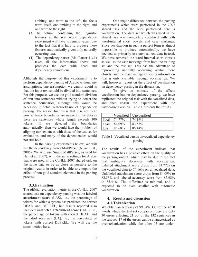
To give an estimate of the effects vocalization has on dependency parsing, we have replicated the original task with the vocalized data, and then re-run the experiment with the unvocalized version. Table 1 presents the results: Vocalized Unvocalized LAS 74.77% 74.16% UAS 84.09% 83.53% LA 85.68% 85.44%

Table 1: Vocalized versus unvocalized dependency

parsing The results of the experiment indicate that vocalization has a positive effect on the quality of the parsing output, which may be due to the fact that ambiguity decreases with vocalization. Labeled attachment score drops from 74.77% on the vocalized data to 74.16% on unvocalized data. Unlabeled attachment score drops from 84.09% to 83.53% and labeled accuracy score from 85.68% to 85.44%. The difference is minimal, and is expected to be even smaller with automatic vocalization

4. Results and discussion 4.1.Tokenization

We obtain an accuracy of 99.34%. Out of the 4550 words which the test set comprises, there are only 30 errors affecting 21 out of the 132 sentences in the test set. 17 of the errors can be characterized as over-tokenization while the other 13 are under-

12

tokenization. 13 of the over- tokenization cases are different tokens of the word blywn (Eng. billion) as the initial b in the words was treated as a preposition while it is an original part of the word.

A closer examination of the errors in the tokenization process reveals that most of the words which are incorrectly tokenized do not occur in the training set, or occur there only in the form produced by the tokenizer. For example, the word blywn does not occur in the training set, but the form b+lywn+p occurs in the training set, and this is the reason the word is tokenized erroneously. Another example is the word bAsm, which is ambiguous between a one-token word bAsm (Eng. smiling), and a two-token word, b+Asm (Eng. in the name of). Although the word should be tokenized as b+Asm, the word occurs in the training set as bAsm, which is a personal name.

In fact, only five words in the 30 mis-tokenized words are available in the training set, which means that the tokenizer has a very high accuracy on known words. There are yet two examples that are worthy of discussion. The first one involves suboptimal orthography. The word r>smAl (Eng. capital in the financial sense) is in the training set but is nonetheless incorrectly tokenized in our experiments because it is written as brAsmAl (with the preposition b) but with an alif instead of the hamza. The word was thus not tokenized correctly. The other example involves an error in the tokenization in the Prague Arabic Dependency Treebank. The word >wjh (Eng. I give/address) has been tokenized in the Prague Arabic dependency treebank as >wj+h (Eng. its utmost/prime), which is not the correct tokenization in this context as the h is part of the word and is not a different token. The classifier did nonetheless tokenize it correctly but it was counted as wrong in the evaluation since it does not agree with the PADT gold standard.

4.2.Stemming Since stemming involves removing all the inflectional prefixes and suffixes from the words, and since inflectional affixes are not demarcated in the PADT data set used in the CoNLL shared tasks, there is no way to know the exact accuracy of the stemming process in that specific experiment, but since stemming is a by-product of segmentation, and since segmentation in general

reaches an accuracy in excess of 98%, stemming should be trusted as an accurate process.

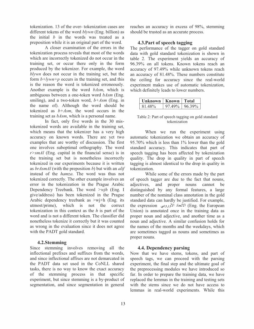
4.3.Part of speech tagging The performance of the tagger on gold standard data with gold standard tokenization is shown in table 2. The experiment yields an accuracy of 96.39% on all tokens. Known tokens reach an accuracy of 97.49% while unknown tokens reach an accuracy of 81.48%. These numbers constitute the ceiling for accuracy since the real-world experiment makes use of automatic tokenization, which definitely leads to lower numbers.

Unknown Known Total 81.48% 97.49% 96.39%

Table 2: Part of speech tagging on gold standard

tokenization

When we run the experiment using automatic tokenization we obtain an accuracy of 95.70% which is less than 1% lower than the gold standard accuracy. This indicates that part of speech tagging has been affected by tokenization quality. The drop in quality in part of speech tagging is almost identical to the drop in quality in tokenization.

While some of the errors made by the part of speech tagger are due to the fact that nouns, adjectives, and proper nouns cannot be distinguished by any formal features, a large number of the nominal class annotation in the gold standard data can hardly be justified. For example, the expression )*$+$,- .!/01- (Eng. the European Union) is annotated once in the training data as proper noun and adjective, and another time as a noun and adjective. A similar confusion holds for the names of the months and the weekdays, which are sometimes tagged as nouns and sometimes as proper nouns.

4.4. Dependency parsing Now that we have stems, tokens, and part of speech tags, we can proceed with the parsing experiment, the final step and the ultimate goal of the preprocessing modules we have introduced so far. In order to prepare the training data, we have replaced the lemmas in the training and testing sets with the stems since we do not have access to lemmas in real-world experiments. While this

13

introduces an automatic element in the training set, it guarantees the similarity between the features in the training set and those in the test set.

In order to discover whether the fine-grained POS tagset is necessary, we have run two parsing experiments using gold standard parts of speech with stems instead of lemmas, but without any of the linguistic features included in the gold standard: the first experiment has the two distinct part of speech tags and the other one has only the coarse-grained part of speech tags. Table 3 outlines the results.

LAS UAS LA CPOS+POS 72.54% 82.92% 84.04% CPOS 73.11% 83.31% 84.39% CoNLL2007 74.75% 84.21% 84.21%

Table 3: effect of fine-grained POS

As can be seen from table 3, using two part

of speech tagsets harms the performance of the dependency parser. While the one-tag dependency parser obtains a Labeled Accuracy Score of 73.11%, the number goes down to 72.54% when we used the fine-grained part of speech set. In Unlabeled Attachment Score, the one tag parser achieves an accuracy of 83.31% compared to 82.92% on two tag parser. The same is also true for Label Accuracy Score as the numbers go down from 84.39% when using only one tagset compared to 84.04% when using two tagsets. This means that the fine-grained tagset is not needed to perform real world parsing. We have thus decided to use the coarse-grained tagset in the two positions of the part of speech tags. We can also see that this setting produces results that are 1.64% lower than those of the Single MaltParser results reported in the CoNLL 2007 shared task in terms of Labeled Accuracy Score. The difference can be attributed to the lack of linguistic features, vocalization, and the use of stems instead of lemmas. The LAS of 73.11% now constitutes the upper bound for real world experiments where also parts of speech and tokens have to be obtained automatically (since vocalization has been removed, linguistic features have been removed, and lemmas have been replaced with automatic stems). It should be noted that our experiments, with the complete set of gold standard features, achieve higher results than those reported in the CoNLL 2007 shared task: a LAS of

74.77 (here) versus a LAS of 74.75 (CoNLL, 2007). This may be attributed to the change of the parser since we use the 1.3.1 version whereas the parser used in the 2007 shared task was the 0.4 version.

Using the settings above, we have run an experiment to parse the test set, which is now automatic in terms of tokenization, lemmatization, and part of speech tags, and in the absence of the linguistic features that enrich the gold standard training and test sets. Table 4 presents the results of this experiment.

Automatic Gold Standard LAS 63.10% 73.11% UAS 72.19% 83.31% LA 82.61% 84.39%

Table 4: Automatic dependency parsing experiment

The LAS drops more than 10 percentage

points from 73.11 to 63.10. This considerable drop in accuracy is expected since there is a mismatch in the tokenization which leads to mismatch in the sentences. The 30 errors in tokenization affect 21 sentences out of a total of 129 in the test set. When we evaluate the dependency parsing output on the correctly tokenized sentences only, we obtain much better results (shown in Table 5). Labeled Attachment Score on correctly tokenized sentences is 71.56%, Unlabeled Attachment Score 81.91%, and Label Accuracy Score is 83.22%. This indicates that no good quality parsing can be obtained if there are problems in the tokenization. A drop of a half percent in the quality of tokenization causes a drop of ten percentage points in the quality of parsing, whereas automatic POS tags and stemming, and the lack of linguistic features do not cause the same negative effect. Correctly-

tokenized Sentences

Incorrectly-Tokenized Sentences

LAS 71.56% 33.60% UAS 81.91% 38.32% LA 83.22% 80.49%

Table 5: Dependency parsing Evaluation on Correctly

vs. Incorrectly Tokenized Sentences

14

While correctly tokenized sentences yield results that are not extremely different from those using gold standard information, and the drop in accuracy in them can be attributed to the differences introduced through stemming and automatic parts of speech as well as the absence of the linguistic features, incorrectly tokenized sentences show a completely different picture as the Labeled Attachment Score now plummets to 33.6%, which is 37.96 percentage points below that on correctly tokenized sentences. The Unlabeled Attachment Score also drops from 81.91% in correctly tokenized sentences to 38.32% on incorrectly tokenized sentences with a difference of 43.59 percentage points. Error Analysis Considering the total number of errors, out of the 5124 tokens in the test set, there are 1425 head errors (28%), and 891 dependency errors (17%). In addition, there are 8% of the tokens in which both the dependency and the head are incorrectly assigned by the parser. The POS tag with the largest percentage of head errors is the Adverb (D) with an error rate of 57%, followed by Preposition

(P) at 34%, and Conjunctions at 34%. The preposition and conjunction errors are common among all experiments: those with gold standard and those with automatic information. These results also show that assigning the correct head is more difficult than assigning the correct dependency. This is reasonable since some tokens will have specific dependency types. Also, while there are a limited number of dependency relations, the number of potential heads is much larger.

If we look at the lexicon and examine the tokens in which most errors occur, we can see one conjunction and five prepositions. The conjunction w (Eng. and) tops the list, followed by the preposition l (Eng. for, to), followed by the preposition fy (Eng. in), then the preposition b (Eng. with), then the preposition ElY (Eng. on), and finally the preposition mn (Eng. from, of). We conclude this section by examining a very short sentence in which we can see the effect of tokenization on dependency parsing. Table 6 is a sentence that has an instance of incorrect tokenization.

Arabic 2+!3 4&5 +1$. 67'8* 9:;< ='>!?@&(1- ='AB93,- C-DE!F;<-English The American exceptional aid to Egypt is a billion dollars

until March. Buckwalter (Gold Standard Tokenization)

AlmsAEdAt Al>mrykyp AlAstvnA}yp l mSr blywn dwlAr HtY |*Ar

Buckwalter (Automatic Tokenization) AlmsAEdAt Al>mrykyp AlAstvnA}yp l mSr b lywn dwlAr HtY |*Ar

Table 6: A sentence showing the effect of tokenization

The sentence has 8 words one of which

comprises two tokens. The word lmSr comprises a preposition l, and the proper noun mSr (Eng. Egypt). The tokenizer succeeds in splitting the word into two tokens, but it fails on the one-token word blywn (Eng. billion) and splits it into two tokens b and lywn. The word is ambiguous between blywn (Eng. one billion) and b+lywn (Eng. in the city of Lyon), and since the second solution is much more frequent in the training set, it is the one incorrectly selected by the tokenizer.

This tokenization decision leads to an ill-alignment between the gold standard sentence and the automatic one as the gold standard has 8 tokens while the automatically produced one has 9. This thus affects the POS tagging decisions as blywn,

which in the gold standard is a NOUN, has been now tagged as b/PREPOSITION and lywn/PROPER_NOUN. This has also affected the assignment of heads and dependency relations. While blywn is a predicate dependent on the root of the sentence, it has been annotated as two tokens: b is a preposition dependent on the subject, and lywn is an attribute dependent on b. Using the Penn Tags So far, we have used only the POS tags of the PADT, and have not discussed the possibility of using the Penn Arabic Treebank. The difference is that the PADT tags are basic while the ATB ones have detailed representations of inflections. While

15

the word AlmtHdp is given the tag ADJ in the PADT, it is tagged as DET+ADJ+FEMININE_SINGULAR_MARKER in the ATB. Table 7 shows the effect of using the Penn tagset with the gold standard full-featured dataset in three different experiments as compared with the PADT tagset:

(1) The original Unvocalized Experiment with the full set of features and gold standard components. The Penn tagset is not used in this experiment, and it is provided for reference purposes only.

(2) Unvocalized experiment with Penn tags as CPOS tags. In this experiment, the Penn tagset is used instead of the coarse grained POS tagset, while the fine-grained pos tagset remains unchanged.

(3) Using Penn tags as fine grained POS tags, while the CPOS tags remain unchanged.

(4) Using the Penn POS tags in both positions.

In the four experiments, the only features

that change are the POS and CPOS features.

Experiment LAS UAS Unvocalized Original 74.16% 83.53

% Using Penn Tags as CPOS tags

74.12% 83.43%

Using Penn tags as POS 72.40% 81.79%

Using Penn tags in both positions

69.63% 79.33%

Table 7: Using the ATB tagset with the PADT dataset

As can be seen from Table 7, in all three

cases the Penn tagset produces lower results than the PADT tagset. The reason for this may be that the tagset is automatic in both cases, and the perfect accuracy of the PADT tags helps the classifier embedded in the MaltParser parser to choose the correct label and head. The results also show that when we use the Penn tagset as the CPOS tagset, the results are almost no different from the gold standard PADT tagset (74.12% vs. 74.16%). The fact that the Penn tagset does not harm the results encourages the inclusion of the Penn tags as CPOS tags in the automatic

experiments that have been used throughout this chapter. The worst results are those obtained by using the Penn tags in both positions (POS and CPOS).

Using the Penn tagset with the reduced experiments, those without the linguistic features, gives a different picture from that in the full standard experiments, as detailed in table 8.

Experiment LAS UAS Reduced with both PADT tags

72.54% 82.92%

Reduced with Penn tags as CPOS

73.09% 83.16%

Reduced with Penn tags as CPOS and automatic tokenization

63.11% 72.38%

Table 8: Including the Penn full tagset in the reduced

experiments

While the Penn tagset does not help improve parsing accuracy with the full-featured parsing experiments, it helps with the reduced experiments. While the experiment without the Penn tags score an LAS of 72.54%, replacing the CPOS tags in this experiment with the Penn tagset raises the accuracy to 73.09%, with an increase of 0.55%. This may be due to the fact that the full tagset gives more information that helps the parser. The increase is not as noticeable in the automatic tokenization experiment where the accuracy minimally changes from 63.10% to 63.11%. Effect of Vocalization We have stated in the methodology section that we use unvocalized data since naturally occurring Arabic is hardly vocalized. While this is a reasonable approach, it is worth checking the effect of vocalization on dependency parsing. Table 9 presents the results of vocalization effect in three experiments: (a) All the gold standard features with vocalization. This is the experiment reported in the literature on Arabic dependency parsing in CoNLL (2007), (b) All the gold standard features without the vocalization, (c) All gold standard features except for vocalization which is automatic, and (d) the automatic experiment with automatic vocalization. The vocalizer in the latter 2

16

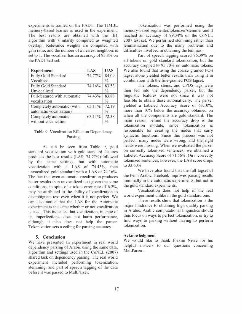
experiments is trained on the PADT. The TIMBL memory-based learner is used in the experiment. The best results are obtained with the IB1 algorithm with similarity computed as weighted overlap,. Relevance weights are computed with gain ratio, and the number of k nearest neighbors is set to 1. The vocalizer has an accuracy of 93.8% on the PADT test set.

Experiment LAS UAS Fully Gold Standard Vocalized

74.77% 84.09%

Fully Gold Standard Unvocalized

74.16% 83.53%

Full-featured with automatic vocalization

74.43% 83.88%

Completely automatic (with automatic vocalization)

63.11% 72.19%

Completely automatic without vocalization

63.11% 72.38%

Table 9: Vocalization Effect on Dependency

Parsing

As can be seen from Table 9, gold standard vocalization with gold standard features produces the best results (LAS: 74.77%) followed by the same settings, but with automatic vocalization with a LAS of 74.43%, then unvocalized gold standard with a LAS of 74.16%. The fact that even automatic vocalization produces better results than unvocalized text given the same conditions, in spite of a token error rate of 6.2%, may be attributed to the ability of vocalization to disambiguate text even when it is not perfect. We can also notice that the LAS for the Automatic experiment is the same whether or not vocalization is used. This indicates that vocalization, in spite of its imperfections, does not harm performance, although it also does not help the parser. Tokenization sets a ceiling for parsing accuracy.

5. Conclusion We have presented an experiment in real world dependency parsing of Arabic using the same data, algorithm and settings used in the CoNLL (2007) shared task on dependency parsing. The real world experiment included performing tokenization, stemming, and part of speech tagging of the data before it was passed to MaltParser.

Tokenization was performed using the memory-based segmenter/tokenizer/stemmer and it reached an accuracy of 99.34% on the CoNLL 2007 test set. We performed stemming rather than lemmatization due to the many problems and difficulties involved in obtaining the lemmas.

Part of speech tagging scored 96.39% on all tokens on gold standard tokenization, but the accuracy dropped to 95.70% on automatic tokens. We also found that using the coarse grained POS tagset alone yielded better results than using it in combination with the fine-grained POS tagset.

The tokens, stems, and CPOS tags were then fed into the dependency parser, but the linguistic features were not since it was not feasible to obtain these automatically. The parser yielded a Labeled Accuracy Score of 63.10%, more than 10% below the accuracy obtained on when all the components are gold standard. The main reason behind the accuracy drop is the tokenization module, since tokenization is responsible for creating the nodes that carry syntactic functions. Since this process was not perfect, many nodes were wrong, and the right heads were missing. When we evaluated the parser on correctly tokenized sentences, we obtained a Labeled Accuracy Score of 71.56%. On incorrectly tokenized sentences, however, the LAS score drops to 33.60%.

We have also found that the full tagset of the Penn Arabic Treebank improves parsing results minimally in the automatic experiments, but not in the gold standard experiments.

Vocalization does not help in the real world experiment unlike in the gold standard one.

These results show that tokenization is the major hindrance to obtaining high quality parsing in Arabic. Arabic computational linguistics should thus focus on ways to perfect tokenization, or try to find ways to parsing without having to perform tokenization. Acknowledgment We would like to thank Joakim Nivre for his helpful answers to our questions concerning MaltParser.

17

References Buchholz, Sabine and Marsi, Erwin (2006). CoNLL-X shared task on multilingual dependency parsing. In Proceedings of the 10th Conference on Computational Natural Language Learning (CoNLL), pages 149–164. Daelemans, Walter; Zavrel, Jakub; van der Sloot, Ko and van den Bosch, Antal (2007). TiMBL: Tilburg memory based learner – version 6.1 – reference guide. Technical Report ILK 07-09, Induction of Linguistic Knowledge, Computational Linguistics, Tilburg University. Daelemans, Walter,; Zavrel, Jakub; an den Bosch, Antal, and van der Sloot, Ko (2007). MBT: Memory-Based Tagger- Version 3.1. Reference Guide. Technical Report ILK 07-09, Induction of Linguistic Knowledge, Computational Linguistics, Tilburg University. HajiG, Jan; SmrH, Otakar; Zemánek, Petr; Inaidauf, Jan, and BeJka, Emanuel (2004). Prague Arabic Dependency Treebank: Development in Data and Tools. In Proceedings of the EMLAR International Conference on Arabic Language Resources and Tools, pages 110-117, Cairo, Egypt, September 2004. Hall, Johan; Nilsson, Jens; Nivre, Joakim; Eryigit, Gülsen; Megyesi, Beáta; Nilsson, Mattias and Saers, Markus (2007). Single Malt or Blended? A Study in Multilingual Parser Optimization. In Proceedings of the CoNLL Shared Task Session of EMNLP-CoNLL 2007, 933-939. Maamouri, Mohamed and Bies, Ann (2004) Developing an Arabic Treebank: Methods, Guidelines, Procedures, and Tools. In Proceedings of the Workshop on Computational Approaches to Arabic Script-based Languages, COLING 2004, Geneva, August 28, 2004. Marton, Yuval; Habash, Nizar; and Rambow, Owen (2010). Improving Arabic Dependency Parsing with Lexical and Inflectional Morphological Features. In Proceddings of The FirstWorkshop on Statistical Parsing of Morphologically Rich Languages (SPMRL 2010), LA, California. McDonald, Ryan; Lerman, Kevin and Pereira, Fernando (2006). Multilingual dependency analysis with a two-stage discriminative parser. CoNLLX shared task on multilingual dependency parsing. In Proceedings of the 10th Conference on Computational Natural Language Learning Nivre, Joakim; Hall, Jonathan; Nilsson, Jens; Eryigit, Gülsen and Marinov, Svetsolav (2006). Labeled Pseudo-Projective Dependency Parsing with Support

Vector Machines. In Proceedings of the Tenth Conference on Computational Natural Language Learning (CoNLL) Nivre, Joakim; Hall, Johan; Kübler, Sandra; McDonald, Ryan; Nilsson, Jens; Riedel, Sebastian, and Yuret, Deniz. (2007). The CoNLL 2007 shared task on dependency parsing. In Proceedings of the CoNLL Shared Task of EMNLP-CoNLL 2007, pages 915–932 Owen, Jonathan. The Arabic Grammatical Tradition. In Hetzron, Robert (ed.) (1997). The Semitic Languages. Routledge, London.

18


Punctuation: Making a Point in Unsupervised Dependency Parsing

Valentin I. SpitkovskyComputer Science Department

Stanford University and Google [email protected]

Hiyan AlshawiGoogle Inc.

Mountain View, CA, 94043, [email protected]

Daniel JurafskyDepartments of Linguistics and Computer ScienceStanford University, Stanford, CA, 94305, USA

[email protected]

Abstract

We show how punctuation can be used to im-prove unsupervised dependency parsing. Ourlinguistic analysis confirms the strong connec-tion between English punctuation and phraseboundaries in the Penn Treebank. However,approaches that naively include punctuationmarks in the grammar (as if they were words)do not perform well with Klein and Manning’sDependency Model with Valence (DMV). In-stead, we split a sentence at punctuation andimpose parsing restrictions over its fragments.Our grammar inducer is trained on the WallStreet Journal (WSJ) and achieves 59.5% ac-curacy out-of-domain (Brown sentences with100 or fewer words), more than 6% higherthan the previous best results. Further evalu-ation, using the 2006/7 CoNLL sets, revealsthat punctuation aids grammar induction in17 of 18 languages, for an overall averagenet gain of 1.3%. Some of this improvementis from training, but more than half is fromparsing with induced constraints, in inference.Punctuation-aware decoding works with exist-ing (even already-trained) parsing models andalways increased accuracy in our experiments.

1 Introduction

Unsupervised dependency parsing is a type of gram-mar induction — a central problem in computationallinguistics. It aims to uncover hidden relations be-tween head words and their dependents in free-formtext. Despite decades of significant research efforts,the task still poses a challenge, as sentence structureis underdetermined by only raw, unannotated words.

Structure can be clearer informattedtext, whichtypically includes proper capitalization and punctua-tion (Gravano et al., 2009). Raw word streams, such

as utterances transcribed by speech recognizers, areoften difficult even for humans (Kim and Woodland,2002). Therefore, one would expect grammar induc-ers to exploit any available linguistic meta-data. Andyet in unsupervised dependency parsing, sentence-internal punctuation has long been ignored (Carrolland Charniak, 1992; Paskin, 2001; Klein and Man-ning, 2004; Blunsom and Cohn, 2010,inter alia).

HTML is another kind of meta-data that is ordi-narily stripped out in pre-processing. However, re-cently Spitkovsky et al. (2010b) demonstrated thatweb markup can successfully guide hierarchicalsyntactic structure discovery, observing, for exam-ple, that anchors often match linguistic constituents:

..., whereas McCain is secure on the topic, Obama<a>[VP worries about winning the pro-Israel vote]</a>.

We propose exploring punctuation’s potential toaid grammar induction. Consider a motivating ex-ample (all of our examples are from WSJ), in whichall (six) marks align with constituent boundaries:

[SBAR Although it probably has reduced the level ofexpenditures for some purchasers], [NP utilization man-agement] — [PP like most other cost containment strate-gies] — [VP doesn’t appear to have altered the long-termrate of increase in health-care costs], [NP the Institute ofMedicine], [NP an affiliate of the National Academy ofSciences], [VP concluded after a two-year study].

This link between punctuation and constituentboundaries suggests that we could approximateparsing by treating inter-punctuation fragments in-dependently. In training, our algorithm first parseseach fragment separately, then parses the sequenceof the resulting head words. In inference, we use abetter approximation that allows heads of fragmentsto be attached by arbitrary external words, e.g.:

The Soviets complicated the issue by offering to[VP include light tanks], [SBAR which are as light as ...].

19

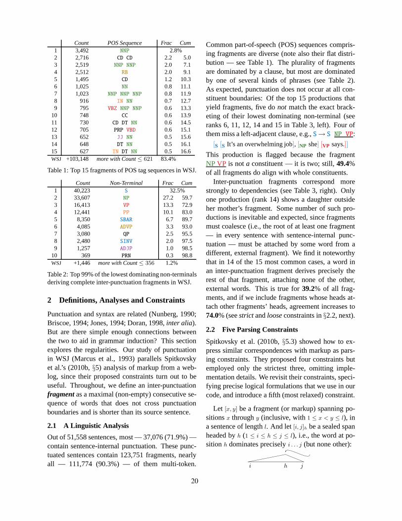
Count POS Sequence Frac Cum1 3,492 NNP 2.8%2 2,716 CD CD 2.2 5.03 2,519 NNP NNP 2.0 7.14 2,512 RB 2.0 9.15 1,495 CD 1.2 10.36 1,025 NN 0.8 11.17 1,023 NNP NNP NNP 0.8 11.98 916 IN NN 0.7 12.79 795 VBZ NNP NNP 0.6 13.3

10 748 CC 0.6 13.911 730 CD DT NN 0.6 14.512 705 PRP VBD 0.6 15.113 652 JJ NN 0.5 15.614 648 DT NN 0.5 16.115 627 IN DT NN 0.5 16.6WSJ +103,148 more with Count≤ 621 83.4%

Table 1: Top 15 fragments of POS tag sequences in WSJ.

Count Non-Terminal Frac Cum1 40,223 S 32.5%2 33,607 NP 27.2 59.73 16,413 VP 13.3 72.94 12,441 PP 10.1 83.05 8,350 SBAR 6.7 89.76 4,085 ADVP 3.3 93.07 3,080 QP 2.5 95.58 2,480 SINV 2.0 97.59 1,257 ADJP 1.0 98.5

10 369 PRN 0.3 98.8WSJ +1,446 more with Count≤ 356 1.2%

Table 2: Top 99% of the lowest dominating non-terminalsderiving complete inter-punctuation fragments in WSJ.

2 Definitions, Analyses and Constraints

Punctuation and syntax are related (Nunberg, 1990;Briscoe, 1994; Jones, 1994; Doran, 1998,inter alia).But are there simple enough connections betweenthe two to aid in grammar induction? This sectionexplores the regularities. Our study of punctuationin WSJ (Marcus et al., 1993) parallels Spitkovskyet al.’s (2010b,§5) analysis of markup from a web-log, since their proposed constraints turn out to beuseful. Throughout, we define an inter-punctuationfragment as a maximal (non-empty) consecutive se-quence of words that does not cross punctuationboundaries and is shorter than its source sentence.

2.1 A Linguistic Analysis

Out of 51,558 sentences, most — 37,076 (71.9%) —contain sentence-internal punctuation. These punc-tuated sentences contain 123,751 fragments, nearlyall — 111,774 (90.3%) — of them multi-token.

Common part-of-speech (POS) sequences compris-ing fragments are diverse (note also their flat distri-bution — see Table 1). The plurality of fragmentsare dominated by a clause, but most are dominatedby one of several kinds of phrases (see Table 2).As expected, punctuation does not occur at all con-stituent boundaries: Of the top 15 productions thatyield fragments, five donot match the exact brack-eting of their lowest dominating non-terminal (seeranks 6, 11, 12, 14 and 15 in Table 3, left). Four ofthem miss a left-adjacent clause, e.g.,S→ S NP VP:

[S [S It’s an overwhelming job], [NP she] [VP says.]]

This production is flagged because the fragmentNPVP is nota constituent — it is two; still,49.4%of all fragments do align with whole constituents.

Inter-punctuation fragments correspond morestrongly to dependencies (see Table 3, right). Onlyone production (rank 14) shows a daughter outsideher mother’s fragment. Some number of such pro-ductions is inevitable and expected, since fragmentsmust coalesce (i.e., the root of at least one fragment— in every sentence with sentence-internal punc-tuation — must be attached by some word from adifferent, external fragment). We find it noteworthythat in 14 of the 15 most common cases, a word inan inter-punctuation fragment derives precisely therest of that fragment, attaching none of the other,external words. This is true for39.2% of all frag-ments, and if we include fragments whose heads at-tach other fragments’ heads, agreement increases to74.0% (seestrict andlooseconstraints in§2.2, next).

2.2 Five Parsing Constraints

Spitkovsky et al. (2010b,§5.3) showed how to ex-press similar correspondences with markup as pars-ing constraints. They proposed four constraints butemployed only the strictest three, omitting imple-mentation details. We revisit their constraints, speci-fying precise logical formulations that we use in ourcode, and introduce a fifth (most relaxed) constraint.

Let [x, y] be a fragment (or markup) spanning po-sitionsx throughy (inclusive, with1 ≤ x < y ≤ l), ina sentence of lengthl. And let [i, j]h be a sealed spanheaded byh (1 ≤ i ≤ h ≤ j ≤ l), i.e., the word at po-sition h dominates preciselyi . . . j (but none other):

i h j

20

Count Constituent Production Frac Cum1 7,115 PP→ IN NP 5.7%2 5,950 S→ NP VP 4.8 10.63 3,450 NP→ NP PP 2.8 13.34 2,799 SBAR→ WHNP S 2.3 15.65 2,695 NP→ NNP 2.2 17.86 2,615 S→ S NP VP 2.1 19.97 2,480 SBAR→ IN S 2.0 21.98 2,392 NP→ NNP NNP 1.9 23.89 2,354 ADVP→ RB 1.9 25.7

10 2,334 QP→ CD CD 1.9 27.611 2,213 S→ PP NP VP 1.8 29.412 1,441 S→ S CC S 1.2 30.613 1,317 NP→ NP NP 1.1 31.614 1,314 S→ SBAR NP VP 1.1 32.715 1,172 SINV→ S VP NP NP 0.9 33.6WSJ +82,110 more with Count≤ 976 66.4%

Count Head-Outward Spawn Frac Cum1 11,928 IN 9.6%2 8,852 NN 7.2 16.83 7,802 NNP 6.3 23.14 4,750 CD 3.8 26.95 3,914 VBD 3.2 30.16 3,672 VBZ 3.0 33.17 3,436 RB 2.8 35.88 2,691 VBG 2.2 38.09 2,304 VBP 1.9 39.9

10 2,251 NNS 1.8 41.711 1,955 WDT 1.6 43.312 1,409 MD 1.1 44.413 1,377 VBN 1.1 45.514 1,204 IN VBD 1.0 46.515 927 JJ 0.7 47.3WSJ +65,279 more with Count≤ 846 52.8%

Table 3: Top 15 productions yielding punctuation-induced fragments in WSJ, viewed as constituents (left) and as de-pendencies (right). For constituents, we recursively expanded any internal nodes that did not align with the associatedfragmentation (underlined). For dependencies we dropped all daughters that fell entirely in the same region as theirmother (i.e., both inside a fragment, both to its left or bothto its right), keeping only crossing attachments (just one).

Define inside(h, x, y) as true iffx ≤ h ≤ y; and letcross(i, j, x, y) be true iff (i < x ∧ j ≥ x ∧ j < y) ∨

(i > x ∧ i ≤ y ∧ j > y). The three tightest constraintsimpose conditions which, when satisfied, disallowsealing[i, j]h in the presence of an annotation[x, y]:

strict — requires[x, y] itself to be sealed in theparse tree, voiding all seals that straddle exactly oneof {x, y} or protrude beyond[x, y] if their head is in-side. This constraint holds for39.2% of fragments.By contrast, only 35.6% of HTML annotations, suchas anchor texts and italics, agree with it (Spitkovskyet al., 2010b). This necessarily fails in every sen-tence with internal punctuation (since there,somefragment must take charge and attach another), whencross(i, j, x, y) ∨ (inside(h, x, y) ∧ (i < x ∨ j > y)).

... the British daily newspaper, The FinancialTimes .x = i h = j = y

loose — if h ∈ [x, y], requires that everything inx . . . y fall underh, with only h allowed external at-tachments. This holds for74.0% of fragments —87.5% of markup, failing whencross(i, j, x, y).

... arrests followed a“ Snake Day ” at Utrecht ...i x h = j = y

sprawl — still requires thath derive x . . . y butlifts restrictions on external attachments. Holdingfor 92.9% of fragments (95.1% of markup), it fails

whencross(i, j, x, y) ∧ ¬inside(h, x, y).

Maryland Club also distributes tea, which ...x = i h y j

These three strictest constraints lend themselves to astraight-forward implementation as anO(l5) chart-based decoder. Ordinarily, the probability of[i, j]his computed by multiplying the probability of the as-sociatedunsealed span by two stopping probabilities— that of the word ath on the left (adjacent ifi = h;non-adjacent ifi < h) and on the right (adjacent ifh = j; non-adjacent ifh < j). To impose a con-straint, we ran through all of the annotations[x, y]associated with a sentence and zeroed out this prob-ability if any of them satisfied disallowed conditions.

There are faster — e.g.,O(l4), and evenO(l3) —recognizers for split head automaton grammars (Eis-ner and Satta, 1999). Perhaps a more practical, butstill clear, approach would be to generaten-best listsusing a more efficient unconstrained algorithm, thenapply the constraints as a post-filtering step.

Relaxed constraints disallow joining adjacentsubtrees, e.g., preventing the seal[i, j]h from merg-ing below theunsealed span[j +1, J ]H , on the left:

i h j j + 1 H J

21

tear — preventsx . . . y from being torn apart byexternal heads fromoppositesides. It holds for94.7% of fragments (97.9% of markup), and is vi-olated when(x ≤ j ∧ y > j ∧ h < x), in this case.

... they “were not consulted about the [Ridley decision]

in advance and were surprised at the action taken.

thread — requires only that no path from the rootto a leaf enter[x, y] twice. This holds for95.0% ofall fragments (98.5% of markup); it is violated when(x ≤ j ∧ y > j ∧ h < x) ∧ (H ≤ y), again, in thiscase. Example that satisfiesthreadbut violatestear:

The ... changes“all make a lot of sense to me,” he added.

The case when[i, j]h is to the right is entirely sym-metric, and these constraints could be incorporatedin a more sophisticated decoder (sincei andJ donot appear in the formulae, above). We implementedthem by zeroing out the probability of the word atHattaching that ath (to its left), in case of a violation.

Note that all five constraints are nested. In partic-ular, this means that it does not make sense to com-bine them, for a given annotation[x, y], since the re-sult would just match the strictest one. Our markupnumber fortear is lower (97.9 versus 98.9%) thanSpitkovsky et al.’s (2010b), because theirs allowedcases where markup wasneither torn nor threaded.

Common structures that violatethread(and, con-sequently, all five of the constraints) include, e.g.,“seamless” quotations and even ordinary lists:

Her recent report classifies the stock as a“hold.”

The company said its directors, management andsubsidiaries will remain long-term investors and ...

2.3 Comparison with Markup

Most punctuation-induced constraints are less ac-curate than the corresponding markup-induced con-straints (e.g.,sprawl: 92.9 vs. 95.1%;loose: 74.0vs. 87.5%; but notstrict: 39.2 vs. 35.6%). However,markup is rare: Spitkovsky et al. (2010b,§5.1) ob-served that only 10% of the sentences in their blogwere annotated; in contrast, over 70% of the sen-tences in WSJ are fragmented by punctuation.

Fragments are more than 40% likely to be dom-inated by a clause; for markup, this number is be-low 10% — nearly 75% of it covered by noun

phrases. Further, inter-punctuation fragments arespread more evenly under noun, verb, prepositional,adverbial and adjectival phrases (approximately27:13:10:3:1 versus75:13:2:1:1) than markup.1

3 The Model, Methods and Metrics

We model grammar via Klein and Manning’s (2004)Dependency Model with Valence (DMV), whichordinarily strips out punctuation. Since this stepalready requires identification of marks, our tech-niques are just as “unsupervised.” We would havepreferred to test punctuation in their original set-up,but this approach wasn’t optimal, for several rea-sons. First, Klein and Manning (2004) trained withshort sentences (up to only ten words, on WSJ10),whereas most punctuation appears in longer sen-tences. And second, although we could augmentthe training data (say, to WSJ45), Spitkovsky etal. (2010a) showed that classic EM struggles withlonger sentences. For this reason, we use ViterbiEM and the scaffolding suggested by Spitkovsky etal. (2010a) — also the setting in which Spitkovsky etal. (2010b) tested their markup-induced constraints.

3.1 A Basic System

Our system is based on Laplace-smoothed ViterbiEM, following Spitkovsky et al.’s (2010a) two-stagescaffolding: the first stage trains with just the sen-tences up to length 15; the second stage then retrainson nearly all sentences — those with up to 45 words.

InitializationKlein and Manning’s (2004) “ad-hoc harmonic” ini-tializer does not work very well for longer sentences,particularly with Viterbi training (Spitkovsky et al.,2010a, Figure 3). Instead, we use an improved ini-tializer that approximates the attachment probabilitybetween two words as an average, over all sentences,of their normalized aggregateweighteddistances.Our weighting function isw(d) = 1+1/ lg(1+d).2

TerminationSpitkovsky et al. (2010a) iterated until successivechanges in overall (best parse) per-token cross-entropy dropped below2−20 bits. Since smoothingcan (and does, at times) increase the objective, wefound it more efficient to terminate early, after ten

1Markup and fragments are as likely to be in verb phrases.2Integerd ≥ 1 is a distance between two tokens;lg is log

2.

22

steps of suboptimal models. We used the lowest-perplexity (not necessarily the last) model found, asmeasured by the cross-entropy of the training data.

Constrained TrainingTraining with punctuation replaces ordinary Viterbiparse trees, at every iteration of EM, with the out-put of a constrained decoder. In all experimentsother than #2 (§5) we train with thelooseconstraint.Spitkovsky et al. (2010b) found this setting to bebest for markup-induced constraints. We apply it toconstraints induced by inter-punctuation fragments.

Constrained InferenceSpitkovsky et al. (2010b) recommended using thesprawlconstraint in inference. Once again, we fol-low their advice in all experiments except #2 (§5).

3.2 Data Sets and Scoring

We trained on the Penn English Treebank’s WallStreet Journal portion (Marcus et al., 1993). To eval-uate, we automatically converted its labeled con-stituents into unlabeled dependencies, using deter-ministic “head-percolation” rules (Collins, 1999),discarding punctuation, any empty nodes, etc., as isstandard practice (Paskin, 2001; Klein and Manning,2004). We also evaluated against the parsed portionof the Brown corpus (Francis and Kucera, 1979),used as a blind, out-of-domain evaluation set,3 sim-ilarly derived from labeled constituent parse trees.

We report directed accuracies — fractions of cor-rectly guessed arcs, including the root, in unlabeledreference dependency parse trees, as is also standardpractice (Paskin, 2001; Klein and Manning, 2004).One of our baseline systems (§3.3) produces depen-dency trees containing punctuation. In this case wedo not score the heads assigned to punctuation anduse forgiving scoring for regular words: creditingcorrect heads separated from their children by punc-tuation alone (from the point of view of the child,looking up to the nearest non-punctuation ancestor).

3.3 Baseline Systems

Our primary baseline is the basic system withoutconstraints (standard training). It ignores punctu-ation, as is standard, scoring 52.0% against WSJ45.

A secondary (punctuation as words) baseline in-

3Note that WSJ{15, 45} overlap with Section 23 — trainingon the test set is standard practice in unsupervised learning.

corporates punctuation into the grammar as if it werewords, as insuperviseddependency parsing (Nivreet al., 2007b; Lin, 1998; Sleator and Temperley,1993,inter alia). It is worse, scoring only 41.0%.4,5

4 Experiment #1: Default Constraints

Our first experiment compares “punctuation as con-straints” to the baseline systems. We use default set-tings, as recommended by Spitkovsky et al. (2010b):loosein training; andsprawl in inference. Evalua-tion is on Section 23 of WSJ (all sentence lengths).To facilitate comparison with prior work, we also re-port accuracies against shorter sentences, with up toten non-punctuation tokens (WSJ10 — see Table 4).

We find that both constrained regimes improveperformance. Constrained decoding alone increasesthe accuracy of a standardly-trained system from52.0% to 54.0%. And constrained training yields55.6% — 57.4% in combination with inference.

4We were careful to use exactly the same data sets in bothcases, not counting punctuation towards sentence lengths.Andwe used forgiving scoring (§3.2) when evaluating these trees.

5To get this particular number we forced punctuation to betacked on, as a layer below the tree of words, to fairly comparesystems (using the same initializer). Since improved initializa-tion strategies — both ours and Klein and Manning’s (2004)“ad-hoc harmonic” initializer — rely on distances between to-kens, they could be unfairly biased towards one approach or theother, if punctuation counted towards length. We also trainedsimilar baselines without restrictions, allowing punctuation toappear anywhere in the tree (still with forgiving scoring — see§3.2), using the uninformed uniform initializer (Spitkovsky etal., 2010a). Disallowing punctuation as a parent of a real wordmade things worse, suggesting that not all marks belong nearthe leaves (sentence stops, semicolons, colons, etc. make moresense as roots and heads). We tried the weighted initializeralsowithout restrictions and repeated all experiments withoutscaf-folding, on WSJ15 and WSJ45 alone, but treating punctuationas words never came within even 5% of (comparable) standardtraining. Punctuation, as words, reliably disrupted learning.

WSJ∞ WSJ10Supervised DMV 69.8 83.6

w/Constrained Inference 73.0 84.3

Punctuation as Words 41.7 54.8Standard Training 52.0 63.2

w/Constrained Inference 54.0 63.6Constrained Training 55.6 67.0

w/Constrained Inference 57.4 67.5

Table 4: Directed accuracies on Section 23 of WSJ∞ andWSJ10 for the supervised DMV, our baseline systems andthe punctuation runs (all using the weighted initializer).

23

These are multi-point increases, but they could dis-appear in a more accurate state-of-the-art system.

To test this hypothesis, we applied constrained de-coding to asupervisedsystem. We found that this(ideal) instantiation of the DMV benefits as much ormore than the unsupervised systems: accuracy in-creases from 69.8% to 73.0%. Punctuation seemsto capture the kinds of, perhaps long-distance, regu-larities that are not accessible to the model, possiblybecause of its unrealistic independence assumptions.

5 Experiment #2: Optimal Settings

Spitkovsky et al. (2010b) recommended trainingwith looseand decoding withsprawlbased on theirexperiments with markup. But are these the rightsettings for punctuation? Inter-punctuation frag-ments are quite different from markup — they aremore prevalent but less accurate. Furthermore, weintroduced a new constraint,thread, that Spitkovskyet al. (2010b) had not considered (along withtear).

We next re-examined the choices of constraints.Our full factorial analysis was similar, but signifi-cantly smaller, than Spitkovsky et al.’s (2010b): weexcluded their larger-scale news and web data setsthat are not publicly available. Nevertheless, westill tried every meaningful combination of settings,testing boththreadandtear (instead ofstrict, sinceit can’t work with sentences containing sentence-internal punctuation), in both training and inference.We did not find better settings thanloosefor train-ing, andsprawl for decoding, among our options.

A full analysis is omitted due to space constraints.Our first observation is that constrained inference,using punctuation, is helpful and robust. It boostedaccuracy (on WSJ45) by approximately 1.5%, onaverage, with all settings. Indeed,sprawl was con-sistently (but only slightly, at 1.6%, on average) bet-ter than the rest. Second, constrained training hurtmore often than it helped. It degraded accuracy in allbut one case,loose, where it gained approximately0.4%, on average. Both improvements are statisti-cally significant:p ≈ 0.036 for training with loose;andp ≈ 5.6× 10−12 for decoding withsprawl.

6 More Advanced Methods

So far, punctuation has improved grammar inductionin a toy setting. But would it help a modern system?

Our next two experiments employ a slightly morecomplicated set-up, compared with the one used upuntil now (§3.1). The key difference is that this sys-tem is lexicalized, as is standard among the more ac-curate grammar inducers (Blunsom and Cohn, 2010;Gillenwater et al., 2010; Headden et al., 2009).

LexicalizationWe lexicalize only in the second (full data) stage, us-ing the method of Headden et al. (2009). For wordsseen at least 100 times in the training corpus, weaugment their gold POS tag with the lexical item.The first (data poor) stage remains entirely unlexi-calized, with gold POS tags for word classes, as inthe earlier systems (Klein and Manning, 2004).

SmoothingWe do not use smoothing in the second stage exceptat the end, for the final lexicalized model. Stage onestill applies “add-one” smoothing at every iteration.

7 Experiment #3: State-of-the-Art

The purpose of these experiments is to compare thepunctuation-enhanced DMV with other, recent state-of-the-art systems. We find that, lexicalized (§6), ourapproach performs better, by a wide margin; withoutlexicalization (§3.1), it was already better for longer,but not for shorter, sentences (see Tables 5 and 4).

We trained a variant of our systemwithout goldpart-of-speech tags, using the unsupervised wordclusters (Clark, 2000) computed by Finkel and Man-ning (2009).6 Accuracy decreased slightly, to 58.2%on Section 23 of WSJ (down only 0.2%). This resultimproves over substantial performance degradationspreviously observed for unsupervised dependencyparsing with induced word categories (Klein andManning, 2004; Headden et al., 2008,inter alia).

6Available fromhttp://nlp.stanford.edu/software/stanford-postagger-2008-09-28.tar.gz:models/egw.bnc.200

Brown WSJ∞ WSJ10(Headden et al., 2009) — — 68.8

(Spitkovsky et al., 2010b) 53.3 50.4 69.3(Gillenwater et al., 2010) — 53.3 64.3

(Blunsom and Cohn, 2010) — 55.7 67.7Constrained Training 58.4 58.0 69.3

w/Constrained Inference 59.5 58.4 69.5

Table 5: Accuracies on the out-of-domain Brown100 setand Section 23 of WSJ∞ and WSJ10, for the lexicalizedpunctuation run and other recent state-of-the-art systems.

24

Unlexicalized, Unpunctuated Lexicalized ...and PunctuatedCoNLL Year Initialization @15 Training @15 Retraining @45 Retraining @45 Net& Language 1. w/Inference 2. w/Inference 3. w/Inference 3′. w/Inference Gain

Arabic 2006 23.3 23.6 (+0.3) 32.8 33.1 (+0.4) 31.5 31.6 (+0.1) 32.1 32.6 (+0.5) +1.1’7 25.6 26.4 (+0.8) 33.7 34.2 (+0.5) 32.7 33.6 (+0.9) 34.9 35.3 (+0.4) +2.6

Basque ’7 19.3 20.8 (+1.5) 29.9 30.9 (+1.0) 29.3 30.1 (+0.8) 29.3 29.9 (+0.6) +0.6Bulgarian ’6 23.7 24.7 (+1.0) 39.3 40.7 (+1.4) 38.8 39.9 (+1.1) 39.9 40.5 (+0.6) +1.6Catalan ’7 33.2 34.1 (+0.8) 54.8 55.5 (+0.7) 54.3 55.1 (+0.8) 54.3 55.2 (+0.9) +0.9Czech ’6 18.6 19.6 (+1.0) 34.6 35.8 (+1.2) 34.8 35.7 (+0.9) 37.0 37.8 (+0.8) +3.0

’7 17.6 18.4 (+0.8) 33.5 35.4 (+1.9) 33.4 34.4 (+1.0) 35.2 36.2 (+1.0) +2.7Danish ’6 22.9 24.0 (+1.1) 35.6 36.7 (+1.2) 36.9 37.8 (+0.9) 36.5 37.1 (+0.6) +0.2Dutch ’6 15.8 16.5 (+0.7) 11.2 12.5 (+1.3) 11.0 11.9 (+1.0) 13.7 14.0 (+0.3) +3.0English ’7 25.0 25.4 (+0.5) 47.2 49.5 (+2.3) 47.5 48.8 (+1.3) 49.3 50.3 (+0.9) +2.8German ’6 19.2 19.6 (+0.4) 27.4 28.0 (+0.7) 27.0 27.8 (+0.8) 28.2 28.6 (+0.4) +1.6Greek ’7 18.5 18.8 (+0.3) 20.7 21.4 (+0.7) 20.5 21.0 (+0.5) 20.9 21.2 (+0.3) +0.7Hungarian ’7 17.4 17.7 (+0.3) 6.7 7.2 (+0.5) 6.6 7.0 (+0.4) 7.8 8.0 (+0.2) +1.4Italian ’7 25.0 26.3 (+1.2) 29.6 29.9 (+0.3) 29.7 29.7 (+0.1) 28.3 28.8 (+0.5) -0.8Japanese ’6 30.0 30.0 (+0.0) 27.3 27.3 (+0.0) 27.4 27.4 (+0.0) 27.5 27.5 (+0.0) +0.1Portuguese ’6 27.3 27.5 (+0.2) 32.8 33.7 (+0.9) 32.7 33.4 (+0.7) 33.3 33.5 (+0.3) +0.8Slovenian ’6 21.8 21.9 (+0.2) 28.3 30.4 (+2.1) 28.4 30.4 (+2.0) 29.8 31.2 (+1.4) +2.8Spanish ’6 25.3 26.2 (+0.9) 31.7 32.4 (+0.7) 31.6 32.3 (+0.8) 31.9 32.3 (+0.5) +0.8Swedish ’6 31.0 31.5 (+0.6) 44.1 45.2 (+1.1) 45.6 46.1 (+0.5) 46.1 46.4 (+0.3) +0.8Turkish ’6 22.3 22.9 (+0.6) 39.1 39.5 (+0.4) 39.9 39.9 (+0.1) 40.6 40.9 (+0.3) +1.0

’7 22.7 23.3 (+0.6) 41.7 42.3 (+0.6) 41.9 42.1 (+0.2) 41.6 42.0 (+0.4) +0.1Average: 23.4 24.0 (+0.7) 31.9 32.9 (+1.0) 31.9 32.6 (+0.7) 32.6 33.2 (+0.5) +1.3

Table 6: Multi-lingual evaluation for CoNLL sets, measuredat all three stages of training, with and without constraints.

8 Experiment #4: Multi-Lingual Testing

This final batch of experiments probes the general-ization of our approach (§6) across languages. Thedata are from 2006/7 CoNLL shared tasks (Buch-holz and Marsi, 2006; Nivre et al., 2007a), wherepunctuation was identified by the organizers, whoalso furnished disjoint train/test splits. We testedagainst all sentences in their evaluation sets.7,8

The gains arenot English-specific (see Table 6).Every language improves with constrained decod-ing (more so without constrained training); and allbut Italian benefit in combination. Averaged acrossall eighteen languages, the net change in accuracy is1.3%. After standard training, constrained decodingalone delivers a 0.7% gain, on average, never caus-ing harm in any of our experiments. These gains arestatistically significant:p ≈ 1.59 × 10−5 for con-strained training; andp ≈ 4.27×10−7 for inference.

7With the exception of Arabic ’07, from which we discardedone sentence with 145 tokens. We down-weighed languagesappearing in both years by 50% in our analyses, and excludedChinese entirely, since it had already been cut up at punctuation.

8Note that punctuation was treated differently in the twoyears: in ’06, it was always at the leaves of the dependencytrees; in ’07, it matched original annotations of the sourcetree-banks. For both, we used punctuation-insensitive scoring (§3.2).

We did not detect synergy between the two im-provements. However, note that without constrainedtraining, “full” data sets do not help, on average, de-spite having more data and lexicalization. Further-more,after constrained training, we detected no ev-idence of benefits to additional retraining: not withthe relaxedsprawlconstraint, nor unconstrained.

9 Related Work

Punctuation has been used to improve parsing sincerule-based systems (Jones, 1994). Statistical parsersreap dramatic gains from punctuation (Engel et al.,2002; Roark, 2001; Charniak, 2000; Johnson, 1998;Collins, 1997,inter alia). And it is even known tohelp in unsupervisedconstituent parsing (Seginer,2007). But fordependencygrammar induction, untilnow, punctuation remained unexploited.

Parsing Techniques Most-Similar to ConstraintsA “divide-and-rule” strategy that relies on punctua-tion has been used in supervised constituent parsingof long Chinese sentences (Li et al., 2005). For En-glish, there has been interest inbalancedpunctua-tion (Briscoe, 1994), more recently using rule-basedfilters (White and Rajkumar, 2008) in a combinatorycategorial grammar (CCG). Our focus is specifically

25

on unsupervisedlearning ofdependencygrammarsand is similar, in spirit, to Eisner and Smith’s (2005)“vine grammar” formalism. An important differenceis that instead of imposing static limits on alloweddependency lengths, our restrictions are dynamic —they disallow some long (and some short) arcs thatwould have otherwise crossed nearby punctuation.

Incorporating partial bracketings into grammarinduction is an idea tracing back to Pereira and Sch-abes (1992). It inspired Spitkovsky et al. (2010b) tomine parsing constraints from the web. In that samevein, we prospected a more abundant and naturallanguage-resource — punctuation, using constraint-based techniques they developed for web markup.

Modern Unsupervised Dependency Parsing

State-of-the-art in unsupervised dependency pars-ing (Blunsom and Cohn, 2010) uses tree substitu-tion grammars. These are powerful models, capa-ble of learning large dependency fragments. To helpprevent overfitting, a non-parametric Bayesian prior,defined by a hierarchical Pitman-Yor process (Pit-man and Yor, 1997), is trusted to nudge training to-wards fewer and smaller grammatical productions.

We pursued a complementary strategy: usingKlein and Manning’s (2004) much simpler Depen-dency Model with Valence (DMV), but persistentlysteering training away from certain constructions, asguided by punctuation, to help preventunderfitting.

Various Other Uses of Punctuation in NLP

Punctuation is hard to predict,9 partly because itcan signal long-range dependences (Lu and Ng,2010). It often provides valuable cues to NLP taskssuch as part-of-speech tagging and named-entityrecognition (Hillard et al., 2006), information ex-traction (Favre et al., 2008) and machine transla-tion (Lee et al., 2006; Matusov et al., 2006). Otherapplications have included Japanese sentence anal-ysis (Ohyama et al., 1986), genre detection (Sta-matatos et al., 2000), bilingual sentence align-ment (Yeh, 2003), semantic role labeling (Pradhan etal., 2005), Chinese creation-title recognition (Chenand Chen, 2005) and word segmentation (Li andSun, 2009), plus, recently, automatic vandalism de-

9Punctuation has high semantic entropy (Melamed, 1997);for an analysis of the many roles played in the WSJ by thecomma — the most frequent and unpredictable punctuationmark in that data set — see Beeferman et al. (1998, Table 2).

tection in Wikipedia (Wang and McKeown, 2010).

10 Conclusions and Future Work

Punctuation improves dependency grammar induc-tion. Many unsupervised (and supervised) parserscould be easily modified to usesprawl-constraineddecoding in inference. It applies to pre-trained mod-els and, so far, helped every data set and language.

Tightly interwoven into the fabric of writing sys-tems, punctuation frames most unannotated plain-text. We showed that rules for converting markupinto accurate parsing constraints are still optimal forinter-punctuation fragments. Punctuation marks aremore ubiquitous and natural than web markup: whatlittle punctuation-induced constraints lack in preci-sion, they more than make up in recall — perhapsboth types of constraints would work better yet intandem. For language acquisition, a natural ques-tion is whether prosody could similarly aid grammarinduction from speech (Kahn et al., 2005).

Our results underscore the power of simple mod-els and algorithms, combined with common-senseconstraints. They reinforce insights fromjoint mod-eling in supervisedlearning, where simplified, in-dependent models, Viterbi decoding and expressiveconstraints excel at sequence labeling tasks (Rothand Yih, 2005). Such evidence is particularly wel-come inunsupervisedsettings (Punyakanok et al.,2005), where it is crucial that systems scale grace-fully to volumes of data, on top of the usual desider-ata — ease of implementation, extension, under-standing and debugging. Future work could exploresoftening constraints (Hayes and Mouradian, 1980;Chang et al., 2007), perhaps using features (Eisnerand Smith, 2005; Berg-Kirkpatrick et al., 2010) orby learning to associate different settings with var-ious marks: Simply adding a hidden tag for “ordi-nary” versus “divide” types of punctuation (Li et al.,2005) may already usefully extend our model.

Acknowledgments

Partially funded by the Air Force Research Laboratory (AFRL),under prime contract no. FA8750-09-C-0181, and by NSF, viaaward #IIS-0811974. We thank Omri Abend, Slav Petrov andanonymous reviewers for many helpful suggestions, and we areespecially grateful to Jenny R. Finkel for shaming us into usingpunctuation, to Christopher D. Manning for reminding us to ex-plore “punctuation as words” baselines, and to Noah A. Smithfor encouraging us to test against languages other than English.

26

References

D. Beeferman, A. Berger, and J. Lafferty. 1998.CYBERPUNC: A lightweight punctuation annotationsystem for speech. InICASSP.

T. Berg-Kirkpatrick, A. Bouchard-Cote, J. DeNero, andD. Klein. 2010. Painless unsupervised learning withfeatures. InNAACL-HLT.

P. Blunsom and T. Cohn. 2010. Unsupervised inductionof tree substitution grammars for dependency parsing.In EMNLP.

E. J. Briscoe. 1994. Parsing (with) punctuation, etc.Technical report, Xerox European Research Labora-tory.

S. Buchholz and E. Marsi. 2006. CoNLL-X shared taskon multilingual dependency parsing. InCoNLL.

G. Carroll and E. Charniak. 1992. Two experiments onlearning probabilistic dependency grammars from cor-pora. Technical report, Brown University.

M.-W. Chang, L. Ratinov, and D. Roth. 2007. Guidingsemi-supervision with constraint-driven learning. InACL.

E. Charniak. 2000. A maximum-entropy-inspired parser.In NAACL.

C. Chen and H.-H. Chen. 2005. Integrating punctuationrules and naıve Bayesian model for Chinese creationtitle recognition. InIJCNLP.

A. Clark. 2000. Inducing syntactic categories by contextdistribution clustering. InCoNLL-LLL.

M. Collins. 1997. Three generative, lexicalised modelsfor statistical parsing. InACL.

M. Collins. 1999. Head-Driven Statistical Models forNatural Language Parsing. Ph.D. thesis, Universityof Pennsylvania.

C. D. Doran. 1998. Incorporating Punctuation intothe Sentence Grammar: A Lexicalized Tree Adjoin-ing Grammar Perspective. Ph.D. thesis, University ofPennsylvania.

J. Eisner and G. Satta. 1999. Efficient parsing for bilexi-cal context-free grammars and head-automaton gram-mars. InACL.

J. Eisner and N. A. Smith. 2005. Parsing with soft andhard constraints on dependency length. InIWPT.

D. Engel, E. Charniak, and M. Johnson. 2002. Parsingand disfluency placement. InEMNLP.

B. Favre, R. Grishman, D. Hillard, H. Ji, D. Hakkani-Tur, and M. Ostendorf. 2008. Punctuating speech forinformation extraction. InICASSP.

J. R. Finkel and C. D. Manning. 2009. Joint parsing andnamed entity recognition. InNAACL-HLT.

W. N. Francis and H. Kucera, 1979.Manual of Informa-tion to Accompany a Standard Corpus of Present-DayEdited American English, for use with Digital Com-puters. Department of Linguistics, Brown University.

J. Gillenwater, K. Ganchev, J. Graca, F. Pereira, andB. Taskar. 2010. Posterior sparsity in unsuperviseddependency parsing. Technical report, University ofPennsylvania.

A. Gravano, M. Jansche, and M. Bacchiani. 2009.Restoring punctuation and capitalization in transcribedspeech. InICASSP.

P. J. Hayes and G. V. Mouradian. 1980. Flexible parsing.In ACL.

W. P. Headden, III, D. McClosky, and E. Charniak.2008. Evaluating unsupervised part-of-speech taggingfor grammar induction. InCOLING.

W. P. Headden, III, M. Johnson, and D. McClosky.2009. Improving unsupervised dependency parsingwith richer contexts and smoothing. InNAACL-HLT.

D. Hillard, Z. Huang, H. Ji, R. Grishman, D. Hakkani-Tur, M. Harper, M. Ostendorf, and W. Wang. 2006.Impact of automatic comma prediction on POS/nametagging of speech. InIEEE/ACL: SLT.

M. Johnson. 1998. PCFG models of linguistic tree rep-resentations.Computational Linguistics, 24.

B. E. M. Jones. 1994. Exploring the role of punctuationin parsing natural text.COLING.

J. G. Kahn, M. Lease, E. Charniak, M. Johnson, andM. Ostendorf. 2005. Effective use of prosody in pars-ing conversational speech. InHLT-EMNLP.

J.-H. Kim and P. C. Woodland. 2002. Implementation ofautomatic capitalisation generation systems for speechinput. In ICASSP.

D. Klein and C. D. Manning. 2004. Corpus-based induc-tion of syntactic structure: Models of dependency andconstituency. InACL.

Y.-S. Lee, S. Roukos, Y. Al-Onaizan, and K. Papineni.2006. IBM spoken language translation system. InTC-STAR: Speech-to-Speech Translation.

Z. Li and M. Sun. 2009. Punctuation as implicit annota-tions for Chinese word segmentation.ComputationalLinguistics, 35.

X. Li, C. Zong, and R. Hu. 2005. A hierarchical parsingapproach with punctuation processing for long Chi-nese sentences. InIJCNLP.

D. Lin. 1998. Dependency-based evaluation of MINI-PAR. InEvaluation of Parsing Systems.

W. Lu and H. T. Ng. 2010. Better punctuation predictionwith dynamic conditional random fields. InEMNLP.

M. P. Marcus, B. Santorini, and M. A. Marcinkiewicz.1993. Building a large annotated corpus of English:The Penn Treebank.Computational Linguistics, 19.

E. Matusov, A. Mauser, and H. Ney. 2006. Automaticsentence segmentation and punctuation prediction forspoken language translation. InIWSLT.

I. D. Melamed. 1997. Measuring semantic entropy. InACL-SIGLEX: Tagging Text with Lexical Semantics.

27

J. Nivre, J. Hall, S. Kubler, R. McDonald, J. Nils-son, S. Riedel, and D. Yuret. 2007a. The CoNLL2007 shared task on dependency parsing. InEMNLP-CoNLL.

J. Nivre, J. Hall, J. Nilsson, A. Chanev, G. Eryigit,S. Kubler, S. Marinov, and E. Marsi. 2007b. Malt-Parser: A language-independent system for data-driven dependency parsing.Natural Language Engi-neering, 13.

G. Nunberg. 1990. The Linguistics of Punctuation.CSLI Publications.

Y. Ohyama, T. Fukushima, T. Shutoh, and M. Shutoh.1986. A sentence analysis method for a Japanese bookreading machine for the blind. InACL.

M. A. Paskin. 2001. Grammatical bigrams. InNIPS.F. Pereira and Y. Schabes. 1992. Inside-outside reesti-

mation from partially bracketed corpora. InACL.J. Pitman and M. Yor. 1997. The two-parameter Poisson-

Dirichlet distribution derived from a stable subordina-tor. Annals of Probability, 25.

S. Pradhan, K. Hacioglu, W. Ward, J. H. Martin, andD. Jurafsky. 2005. Semantic role chunking combin-ing complementary syntactic views. InCoNLL.

V. Punyakanok, D. Roth, W.-t. Yih, and D. Zimak. 2005.Learning and inference over constrained output. InIJ-CAI.

B. E. Roark. 2001.Robust Probabilistic Predictive Syn-tactic Processing: Motivations, Models, and Applica-tions. Ph.D. thesis, Brown University.

D. Roth and W.-t. Yih. 2005. Integer linear programminginference for conditional random fields. InICML.

Y. Seginer. 2007. Fast unsupervised incremental parsing.In ACL.

D. D. Sleator and D. Temperley. 1993. Parsing Englishwith a link grammar. InIWPT.

V. I. Spitkovsky, H. Alshawi, D. Jurafsky, and C. D. Man-ning. 2010a. Viterbi training improves unsuperviseddependency parsing. InCoNLL.

V. I. Spitkovsky, D. Jurafsky, and H. Alshawi. 2010b.Profiting from mark-up: Hyper-text annotations forguided parsing. InACL.

E. Stamatatos, N. Fakotakis, and G. Kokkinakis. 2000.Text genre detection using common word frequencies.In COLING.

W. Y. Wang and K. R. McKeown. 2010. “Got you!”: Au-tomatic vandalism detection in Wikipedia with web-based shallow syntactic-semantic modeling. InCOL-ING.

M. White and R. Rajkumar. 2008. A more precise analy-sis of punctuation for broad-coverage surface realiza-tion with CCG. InGEAF.

K. C. Yeh. 2003. Bilingual sentence alignment based onpunctuation marks. InROCLING: Student.

28


Modeling Infant Word Segmentation

Constantine LignosDepartment of Computer and Information Science

University of [email protected]

Abstract

While many computational models have beencreated to explore how children might learnto segment words, the focus has largely beenon achieving higher levels of performance andexploring cues suggested by artificial learningexperiments. We propose a broader focus thatincludes designing models that display prop-erties of infants’ performance as they beginto segment words. We develop an efficientbootstrapping online learner with this focus inmind, and evaluate it on child-directed speech.In addition to attaining a high level of perfor-mance, this model predicts the error patternsseen in infants learning to segment words.

1 Introduction

The last fifteen years have seen an increased inter-est in the problem of how infants learn to segmenta continuous stream of speech into words. Much ofthis work has been inspired by experiments with in-fants focusing on what capabilities infants have andwhich cues they attend to. While experimental workprovides insight into the types of cues infants may beusing, computational modeling of the task providesa unique opportunity to test proposed cues on rep-resentative data and validate potential approaches tousing them.

While there are many potential approaches to theproblem, a desirable solution to the problem shoulddemonstrate acceptable performance in a simula-tion of the task, rely on cues in the input that aninfant learner is able to detect at the relevant age,and exhibit learning patterns similar to those of in-

fant learners. Most work in computational model-ing of language acquisition has primarily focusedon achieving acceptable performance using a sin-gle cue, transitional probabilities, but little effort hasbeen made in that work to try to connect these learn-ing solutions to the actual learning patterns observedin children outside of performance on short artificiallanguage learning experiments.

In this work we present a simple, easily extendedalgorithm for unsupervised word segmentation that,in addition to achieving a high level of performancein the task, correlates with the developmental pat-terns observed in infants. We discuss the connec-tions between the design and behavior of our algo-rithm and the cognitive capabilities of infants at theage at which they appear to begin segmenting words.We also discuss how our technique can easily be ex-tended to accept additional cues to word segmenta-tion beyond those implemented in our learner.

2 Related Work

As this paper examines the intersection of infants’capabilities and computational modeling, we discusswork in both domains, beginning with experimentalapproaches to understanding how infants may per-form the task of word segmentation.

2.1 Infant Word Segmentation

A potential account of how infants learn to iden-tify words in fluent speech is that they learn wordsin isolation and then use those words to segmentlonger utterances (Peters, 1983; Pinker et al., 1984).It is not clear, however, that infant-directed speechprovides enough detectable words in isolation for

29

such a strategy (Aslin et al., 1996). Whatever iso-lated words children do hear, they appear to attend tothem; whether a word is heard in isolation is a betterpredictor of whether a child has learned a word thanthe word’s frequency (Brent and Siskind, 2001).

A more plausible alternative account to assumechildren attend to patterns in the input, using them toidentify likely word units. Much experimental workhas followed from the finding that in artificial learn-ing tasks, infants and adults appear to prefer word-like units that match statistical patterns in the input(Saffran et al., 1996b; Saffran et al., 1996a). Saffranet al. and the authors of following studies (Aslin etal., 1998; Saffran, 2001, among many others) sug-gest that participants used transitional probabilitiesto succeed in these experiments, but the actual strat-egy used is unclear and may even be an artifact ofthe perceptual system (Perruchet and Vinter, 1998;Hewlett and Cohen, 2009).

More recent work using real language data hasnot shown transitional probabilities to be as usefula cue as originally suggested. Lew-Williams et al.(2011) found that 9-month-old English-learning in-fants were not able to learn high-transitional prob-ability words in fluent Italian speech unless thosewords were also presented in isolation. Given thisfinding and the extensive exisiting modeling workfocusing on the used of transitional probabilities, webelieve it is crucial to additionally explore segmen-tation strategies that rely on other cues in the input.

2.2 Modeling Word SegmentationWhile experimental work has posited simple algo-rithms that infants might use to accomplish the taskof word segmentation, when applied to real languagedata these techniques have yielded very poor results(Yang, 2004). This problem has created a chal-lenge for researchers modeling language acquisitionto suggest more sophisticated strategies that infantsmight use. These approaches have fallen into twoprimary categories: optimization-based and boot-strapping algorithm strategies.

Optimization-based strategies have focused ontechniques that a learner might use to arrive at anoptimal segmentation, either through a dynamic pro-gramming approach (Brent, 1999), online learning(Venkataraman, 2001), or nonparametric Bayesianinference (Goldwater et al., 2009; Johnson and

Goldwater, 2009). These approaches fit within stan-dard statistical approaches to natural language pro-cessing, defining statistical objectives and inferencestrategies, with the learners trying to optimize somecombination of the quality of its lexicon and repre-sentations of the corpus.

In contrast, bootstrapping approaches (Gambelland Yang, 2004; Lignos and Yang, 2010) to wordsegmentation have focused on simple heuristics forpopulating a lexicon and strategies for using the con-tents of the lexicon to segment utterances. These ap-proaches have focused on a procedure for segmen-tation rather than defining an optimal segmentationexplicitly, and do not define a formal objective thatis to be optimized.

While bootstrapping approaches have generallymade stronger attempts to align with infants abili-ties to process the speech signal (Gambell and Yang,2004) than other approaches, little effort has beenmade to connect the details of an implemented seg-mentation strategy with children’s learning patternssince the earliest computational models of the task(Olivier, 1968). It is important to draw a con-trast here between attempts to match patterns of hu-man development with regard to word segmentationwith attempts to model performance in artificial lan-guage learning experiments whose goal is to probeword segmentation abilities in humans (Frank et al.,2010). In this paper we are focused on matching theprogression of development and performance in nat-uralistic experiments to characteristics of a segmen-tation strategy, an approach similar to that employedin English past tense learning (Rumelhart and Mc-Clelland, 1986; Pinker, 2000; Yang, 2002).

We will now discuss the patterns of developmentfor children learning to segment English words,which form the motivation for the design of our seg-menter.

3 Infant Performance in WordSegmentation

While the developmental patterns of English-learning infants have been broadly studied, it hasbeen difficult to identify errors that must be causedby failures to correctly segment words and not othercognitive limitations, issues of morphological pro-ductivity, or syntactic competency issues.

30

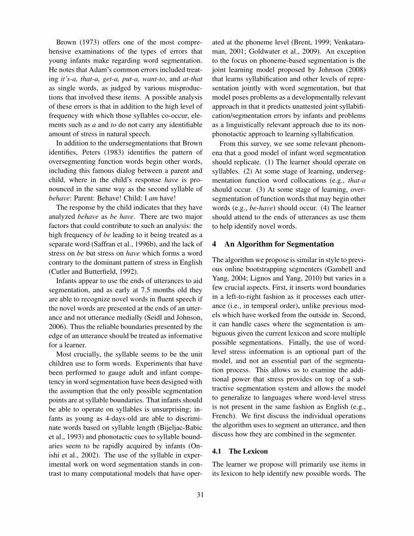
Brown (1973) offers one of the most compre-hensive examinations of the types of errors thatyoung infants make regarding word segmentation.He notes that Adam’s common errors included treat-ing it’s-a, that-a, get-a, put-a, want-to, and at-thatas single words, as judged by various misproduc-tions that involved these items. A possible analysisof these errors is that in addition to the high level offrequency with which those syllables co-occur, ele-ments such as a and to do not carry any identifiableamount of stress in natural speech.

In addition to the undersegmentations that Brownidentifies, Peters (1983) identifies the pattern ofoversegmenting function words begin other words,including this famous dialog between a parent andchild, where in the child’s response have is pro-nounced in the same way as the second syllable ofbehave: Parent: Behave! Child: I am have!

The response by the child indicates that they haveanalyzed behave as be have. There are two majorfactors that could contribute to such an analysis: thehigh frequency of be leading to it being treated as aseparate word (Saffran et al., 1996b), and the lack ofstress on be but stress on have which forms a wordcontrary to the dominant pattern of stress in English(Cutler and Butterfield, 1992).

Infants appear to use the ends of utterances to aidsegmentation, and as early at 7.5 months old theyare able to recognize novel words in fluent speech ifthe novel words are presented at the ends of an utter-ance and not utterance medially (Seidl and Johnson,2006). Thus the reliable boundaries presented by theedge of an utterance should be treated as informativefor a learner.

Most crucially, the syllable seems to be the unitchildren use to form words. Experiments that havebeen performed to gauge adult and infant compe-tency in word segmentation have been designed withthe assumption that the only possible segmentationpoints are at syllable boundaries. That infants shouldbe able to operate on syllables is unsurprising; in-fants as young as 4-days-old are able to discrimi-nate words based on syllable length (Bijeljac-Babicet al., 1993) and phonotactic cues to syllable bound-aries seem to be rapidly acquired by infants (On-ishi et al., 2002). The use of the syllable in exper-imental work on word segmentation stands in con-trast to many computational models that have oper-

ated at the phoneme level (Brent, 1999; Venkatara-man, 2001; Goldwater et al., 2009). An exceptionto the focus on phoneme-based segmentation is thejoint learning model proposed by Johnson (2008)that learns syllabification and other levels of repre-sentation jointly with word segmentation, but thatmodel poses problems as a developmentally relevantapproach in that it predicts unattested joint syllabifi-cation/segmentation errors by infants and problemsas a linguistically relevant approach due to its non-phonotactic approach to learning syllabification.

From this survey, we see some relevant phenom-ena that a good model of infant word segmentationshould replicate. (1) The learner should operate onsyllables. (2) At some stage of learning, underseg-mentation function word collocations (e.g., that-ashould occur. (3) At some stage of learning, over-segmentation of function words that may begin otherwords (e.g., be-have) should occur. (4) The learnershould attend to the ends of utterances as use themto help identify novel words.

4 An Algorithm for Segmentation

The algorithm we propose is similar in style to previ-ous online bootstrapping segmenters (Gambell andYang, 2004; Lignos and Yang, 2010) but varies in afew crucial aspects. First, it inserts word boundariesin a left-to-right fashion as it processes each utter-ance (i.e., in temporal order), unlike previous mod-els which have worked from the outside in. Second,it can handle cases where the segmentation is am-biguous given the current lexicon and score multiplepossible segmentations. Finally, the use of word-level stress information is an optional part of themodel, and not an essential part of the segmenta-tion process. This allows us to examine the addi-tional power that stress provides on top of a sub-tractive segmentation system and allows the modelto generalize to languages where word-level stressis not present in the same fashion as English (e.g.,French). We first discuss the individual operationsthe algorithm uses to segment an utterance, and thendiscuss how they are combined in the segmenter.

4.1 The Lexicon

The learner we propose will primarily use items inits lexicon to help identify new possible words. The

31

structure of the lexicon is as follows:

Lexicon. The lexicon contains the phonological ma-terial of each word that the learner has previouslyhypothesized. The lexicon stores a score along witheach word, which the segmenter may increment ordecrement.

The score assigned to each entry in the lexiconrepresents the relative confidence that it is a trueword of the language. Each increment simply addsto the score of an individual word and each decre-ment subtracts from it.

4.2 Subtractive Segmentation

Subtractive segmentation is the process of usingknown words to segment the speech signal, whichinfants appear to be able to do as young as at sixmonths of age (Bortfeld et al., 2005).

Subtractive Segmentation. When possible, removea known word in the lexicon from the front of theutterance being segmented.

One way to apply subtractive segmentation is agreedy score-based heuristic for subtractive segmen-tation (Lignos and Yang, 2010), such that whenevermultiple words in the lexicon could be subtractedfrom an utterance, the entry with the highest scorewill deterministically be used. This greedy approachresults in a “rich get richer” effect of the sort seen inDirichlet processes (Goldwater et al., 2009). We willfirst discuss this approach and then later extend thisgreedy search to a beam search.

Figure 1 gives the implementation of subtractivesegmentation in our algorithm. This algorithm re-sults in the following properties:

Initially, utterances are treated as words in isola-tion. When the lexicon is empty, no word bound-aries will be inserted and the full contents of eachutterance will be added to the lexicon as a word.

High-frequency words are preferred. When pre-sented with a choice of multiple words to subtract,the highest scored word will be subtracted, whichwill prefer higher frequency words over lower fre-quency words in segmentation.

Syllables between words are not necessarily con-sidered words. Syllables that occur between sub-tractions are not added as words in the lexicon. For

example, if play and please are in the lexicon butcheckers is not, the utterance play checkers pleasewill be correctly segmented, but checkers will notbe added to the lexicon. Much like infants appearto do, the learner does not place as much weight onless reliable boundaries hypothesized in the middleof an utterance (Seidl and Johnson, 2006).

4.3 Incorporating Stress Information

A particularly useful constraint for defining a word,introduced to the problem of word segmentation byYang (2004) but previously discussed by Halle andVergnaud (1987), is as follows:

Unique Stress Constraint (USC): A word can bearat most one primary stress.

Yang (2004) evaluated the effectiveness of theUSC in conjunction with a simple approach to us-ing transitional probabilities, showing significantperformance improvements. The availability ofsuch stress cues is not, however, an uncontroversialassumption; there are no language-universal cuesto stress and even within a single language auto-matic detection of word-level stress is still unreli-able (Van Kuijk and Boves, 1999), making auto-matic capture of such data for simulation purposesdifficult.

Before taking advantage of word-level stress in-formation, the infant learner would need to iden-tify the acoustic correlates to word-level stress in herlanguage, and we will not address the specific mech-anisms that an infant learner may use to accomplishthe task of identifying word-level stress in this paper.Based on strong experimental evidence that infantsdiscriminate between weakly and strongly stressedsyllables and use it to group syllables into word-likeunits (Jusczyk et al., 1999), we assume that an infantmay attend to this cue and we evaluate our modelwith and without it.

We adopt the USC for segmentation in the follow-ing fashion:

Unique Stress Segmentation (USS). Insert wordboundaries such that no word contains two strongstresses. Do so in a lazy fashion, inserting bound-aries as a last resort just before adding another syl-lable to the current would cause it to contain twostrong stresses.

32

u← the syllables of the utterance, initially with no word boundariesi← 0while i < len(u) do

if u starts with one or more words in the lexicon thenChoose the highest scoring word w and remove it from the front of u by inserting a word boundary before and after it.Increment the score of wAdvance i to the last word boundary inserted

elseAdvance i by one syllable

end ifend whileAdd the syllables between the last boundary inserted (or the beginning of the utterance if no boundaries were inserted) and theend of the utterance as a word in the lexicon with a score of 1

Figure 1: Subtractive segmentation procedure

u← the syllables of the utterance, initally with no word boundariesi← 0seenStress← Falsewhile i < len(u)− 1 do

if u[i] is stressed thenseenStress← True

end ifif seenStress and u[i + 1] is stressed then

Insert a word boundary between u[i] and u[i + 1]w ← the syllables between the previous boundary inserted (or the beginning of the utterance if no boundaries were inserted)and the boundary just insertedIncrement w’s score in the lexicon, adding it to the lexicon if neededseenStress← False

end ifi← i + 1

end whilew ← the syllables between the last boundary inserted (or the beginning of the utterance if no boundaries were inserted) and theend of the utteranceIncrement w’s score in the lexicon, adding it to the lexicon if needed

Figure 2: A Unique Stress Segmentation Algorithm

This strategy is expressed in an algorithmic formin Figure 2. The learner uses USS as a last resortto prevent creating a segmentation with an impossi-ble amount of stress in a single word. For exampleconsider an unsegmented English utterance with thestressed syllables underlined: Givemetheball. Ap-plying USS would create the following segmenta-tion: Givemethe ball.

A USS-based algorithm would note the stress onthe first syllable, then keep scanning until anotherstress is located on the fourth syllable, inserting abreak between the two. Givemethe and ball wouldbe added to the lexicon. While this is not a per-fect segmentation, it can be used to aid subtractivesegmentation by seeding the lexicon, even if not allentries added to the lexicon are not correct.

4.4 Combining Subtraction and StressInformation

Given our bootstrapping methodology, it is highlydesirable to be able to integrate USS along with sub-tractive segmentation. An algorithm that combinesboth is shown in Figure 3.

4.5 Extending to Beam Search

The greedy segmentation proposed is limited in itsability to find a good segmentation by its reliance onlocal decisions. A frequent undersegmentation errorof the greedy segmenter is of this type: partof anapple. Because partof has a higher score than partat the point in learning where this utterance is en-countered, the greedy segmenter will always choosepartof.

An alternative approach is to let the segmenter

33

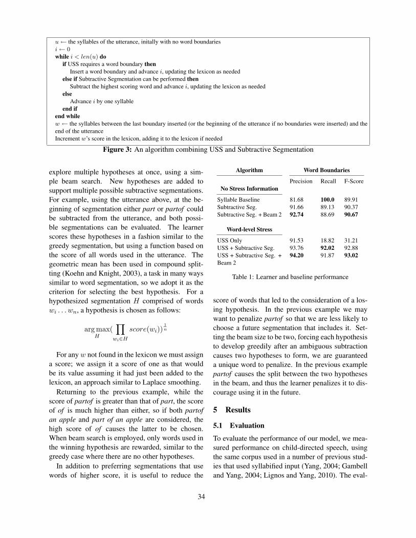
u← the syllables of the utterance, initally with no word boundariesi← 0while i < len(u) do

if USS requires a word boundary thenInsert a word boundary and advance i, updating the lexicon as needed

else if Subtractive Segmentation can be performed thenSubtract the highest scoring word and advance i, updating the lexicon as needed

elseAdvance i by one syllable

end ifend whilew ← the syllables between the last boundary inserted (or the beginning of the utterance if no boundaries were inserted) and theend of the utteranceIncrement w’s score in the lexicon, adding it to the lexicon if needed

Figure 3: An algorithm combining USS and Subtractive Segmentation

explore multiple hypotheses at once, using a sim-ple beam search. New hypotheses are added tosupport multiple possible subtractive segmentations.For example, using the utterance above, at the be-ginning of segmentation either part or partof couldbe subtracted from the utterance, and both possi-ble segmentations can be evaluated. The learnerscores these hypotheses in a fashion similar to thegreedy segmentation, but using a function based onthe score of all words used in the utterance. Thegeometric mean has been used in compound split-ting (Koehn and Knight, 2003), a task in many wayssimilar to word segmentation, so we adopt it as thecriterion for selecting the best hypothesis. For ahypothesized segmentation H comprised of wordswi . . . wn, a hypothesis is chosen as follows:

arg maxH

(∏

wi∈H

score(wi))1n

For any w not found in the lexicon we must assigna score; we assign it a score of one as that wouldbe its value assuming it had just been added to thelexicon, an approach similar to Laplace smoothing.

Returning to the previous example, while thescore of partof is greater than that of part, the scoreof of is much higher than either, so if both partofan apple and part of an apple are considered, thehigh score of of causes the latter to be chosen.When beam search is employed, only words used inthe winning hypothesis are rewarded, similar to thegreedy case where there are no other hypotheses.

In addition to preferring segmentations that usewords of higher score, it is useful to reduce the

Algorithm Word Boundaries

Precision Recall F-ScoreNo Stress Information

Syllable Baseline 81.68 100.0 89.91Subtractive Seg. 91.66 89.13 90.37Subtractive Seg. + Beam 2 92.74 88.69 90.67

Word-level Stress

USS Only 91.53 18.82 31.21USS + Subtractive Seg. 93.76 92.02 92.88USS + Subtractive Seg. +Beam 2

94.20 91.87 93.02

Table 1: Learner and baseline performance

score of words that led to the consideration of a los-ing hypothesis. In the previous example we maywant to penalize partof so that we are less likely tochoose a future segmentation that includes it. Set-ting the beam size to be two, forcing each hypothesisto develop greedily after an ambiguous subtractioncauses two hypotheses to form, we are guaranteeda unique word to penalize. In the previous examplepartof causes the split between the two hypothesesin the beam, and thus the learner penalizes it to dis-courage using it in the future.

5 Results

5.1 Evaluation

To evaluate the performance of our model, we mea-sured performance on child-directed speech, usingthe same corpus used in a number of previous stud-ies that used syllabified input (Yang, 2004; Gambelland Yang, 2004; Lignos and Yang, 2010). The eval-

34

uation set was comprised of adult utterances fromthe Brown (1973) data of the CHILDES database(MacWhinney, 2000).1 Phonemic transcriptions ofwords from the Carnegie Mellon Pronouncing Dic-tionary (CMUdict) Version 0.7 (Weide, 1998), us-ing the first pronunciation for each word and mark-ing syllables with level 1 stress as strong syllables.The corpus was syllabified using onset maximiza-tion. Any utterance in which a word could not betranscribed using CMUDICT was excluded, leaving55,840 utterances. We applied a probabilistic re-call function to the lexicon to simulate the fact thata child learner will not perfectly recall all hypothe-sized words either due to memory limitations, vari-ability in the input, or any other possible source offailure. We used the same function and constant asused by Lignos and Yang (2010).

To adjust the word-level stress information to bet-ter reflect natural speech, the stress information ob-tained from CMUdict was post-processed in the con-text of each utterance using the technique of Lig-nos and Yang (2010). For any n adjacent primary-stress syllables, only the nth syllable retains primarystress; all others are made into weak syllables. Thisreflects the fact that stress clash is avoided in Englishand that infants may not reliably detect acoustic cor-relates of stress in the input.

In addition to variations of our algorithm, we eval-uated a baseline segmenter which marks every syl-lable boundary as a word boundary, treating eachsyllable as a word. We tested five variants of ouralgorithm, adding combinations of USS, subtractivesegmentation, and adding beam search with a beamsize of two2 to subtractive segmentation.

Precision and recall metrics were calculated overall word boundaries over all utterances in the cor-pus. The segmenter’s task is effectively to classifyeach syllable boundary as a word boundary or not.As single-syllable utterances are unambiguously asingle word with no possible boundaries, they are

1A separate set of previous studies have used a corpus se-lected by Brent (1999) for evaluation. Due to length limitationsand the fact that the results presented here cannot be meaning-fully compared to those studies, we only present results on theBrown (1973) data here.

2As larger beam sizes did not lead to any benefits, partlybecause they do not straightforwardly allow for penalization,we do not report results for larger beam sizes.

excluded from evaluation but still given as input.Evaluation was performed by giving each algo-

rithm a single pass over the data set, with the perfor-mance on every utterance included in the total score.This is the most challenging metric for an onlinesegmenter, as early mistakes made when the learnerhas been exposed to no data still count against it.

5.2 PerformanceThe performance of several variations of our algo-rithm is given in Table 1. The most surprising re-sult is the high performance provided by the sylla-ble baseline. This good performance is both an arti-fact of English and the metrics used to evaluate thesegmenters. In English, there are larger number ofmonosyllabic words than in other languages, result-ing in high precision in addition to the guaranteed100% recall because it predicts every possible wordboundary. The standard metric of evaluating pre-cision and recall over word boundaries rather thanwords identified in each utterance also contributesto this performance; when this baseline is evaluatedwith a word-level precision and recall it does notperform as well (Lignos and Yang, 2010).

Subtractive Segmentation provides an improve-ment in utterance evaluation over the Syllable Base-line, and adding beam search to it slightly improvesF-score, sacrificing precision for recall. This is to beexpected from the penalization step in beam search;as the penalization penalizes some good words in ad-dition to undesirable ones, the purification of the ut-terance segmentation and the lexicon comes at thecost of recall from over-penalization.

While USS alone is clearly not a sufficiently richsegmentation technique, it is important to note thatit is a high precision indicator of word boundaries,suggesting that stress information can be useful tothe learner even when used in this simple way. Moreimportantly, USS contributes unique information tosubtractive segmentation, as the utterance F-scoreof subtractive segmentation improves from 90.37 to92.88.

While the performance numbers show that thesegmenter performs competently at the task, themore significant question at hand is whether the er-rors committed by the learner match developmentalpatterns of infants. As the design of the segmenterpredicts, the main error types of the Subtractive Seg-

35

mentation + USS algorithm fall into two classes:

Function word collocations. For example, thethird highest-scored non-word in the lexicon isthat’sa, congruent with observations of functionword collocations seen in children (Brown, 1973).

Oversegmentation of function words. Thegreedy approach used for segmenting the wordsof highest score results in function words beingaggressively segmented off the front of words, forexample a nother. The highest scored non-word inthe lexicon is nother as a result.

Adding beam search reduces the number of func-tion word collocations in the segmenter’s output; thelearner’s most commonly penalized lexicon entry isisthat. However, beam search also penalizes a lot ofwords, such as another. Thus the strategy used inbeam search predicts an early use of function wordcollocations, followed by later oversegmentation.

6 Discussion

In the discussion of related work, we identified twomajor paradigms in modeling word segmentation:optimization and bootstrapping approaches. The al-gorithm presented here combines elements of both.Its behavior over time and across utterances is that ofa bootstrapping learner, but when processing eachutterance it selects a segmentation based on a sim-ple, cognitively plausible beam search.

By using a beam search of the kind suggested, itis easy to see how a variety of other cues could beintegrated into the learning process. We have given asimple function for selecting the best hypothesis thatonly relies on lexicon scores, but more sophisticatedfunctions could take multiple cues into account. Forexample it has been observed that 7-month-olds at-tend more to distributional cues while 9-month-oldsattend more to stress cues (Thiessen and Saffran,2003). A learner in which the weight placed onstress cues increases as the learner receives moredata would match this pattern. Other research hassuggested a more complex hierarchy of cues (Mat-tys et al., 2005), but how the weighting of the vari-ous cues can be adjusted with more input remains anopen question.

A crucial frontier in word segmentation is the ex-pansion of evaluation to include other languages. As

with many other tasks, creating solutions that per-form well in a broad variety of languages is im-portant but has not yet been pursued. Future workshould attempt to match developmental patterns inother languages, which will require adding morpho-logical complexity to the system; the techniquesdeveloped for English are unlikely to succeed un-changed in other languages.

Comparing with other algorithms’ published re-sults is difficult because of varying choices of datasets and metrics. For example, other syllable-basedalgorithms have evaluated their performance usingword-level, as opposed to boundary-level, precisionand recall (Gambell and Yang, 2004; Lignos andYang, 2010). We have adopted the more popularboundary-based metric here, but there is no way todirectly compare with work that does not use syllab-ified input. The variety of possible evaluation met-rics obviates the need for a longer-form explorationof how existing approaches perform when evaluatedagainst varying metrics. Additionally, a more stan-dard set of evaluation data in many languages wouldgreatly improve the ability to compare different ap-proaches to this task.

7 Conclusion

The work presented here represents a step towardbringing together developmental knowledge regard-ing word segmentation and computational model-ing. Rather than focusing on cues in artificial learn-ing experiments which may or may not generalizeto the natural development of word segmentation inchildren, we have shown how a simple algorithmfor segmentation mimics many of the patterns seenin infants’ developing competence. We believe thiswork opens the door to a promising line of researchthat will make a stronger effort to see simulationsof language acquisition as not just an unsupervisedlearning task but rather a modeling task that musttake into account a broad variety of phenomena.

8 Acknowledgments

I would like to thank Charles Yang and Mitch Mar-cus for many enlightening discussions regarding thiswork. The author was supported by an NSF IGERTgrant to the University of Pennsylvania Institute forResearch in Cognitive Science.

36

References

R.N. Aslin, J.Z. Woodward, N.P. LaMendola, and T.G.Bever. 1996. Models of word segmentation in fluentmaternal speech to infants. Signal to syntax: Boot-strapping from speech to grammar in early acquisi-tion, pages 117–134.

R.N. Aslin, J.R. Saffran, and E.L. Newport. 1998.Computation of conditional probability statistics by 8-month-old infants. Psychological Science, 9(4):321.

R. Bijeljac-Babic, J. Bertoncini, and J. Mehler. 1993.How do 4-day-old infants categorize multisyllabic ut-terances? Developmental Psychology, 29:711–711.

H. Bortfeld, J.L. Morgan, R.M. Golinkoff, and K. Rath-bun. 2005. Mommy and me. Psychological Science,16(4):298.

M.R. Brent and J.M. Siskind. 2001. The role of ex-posure to isolated words in early vocabulary develop-ment. Cognition, 81(2):B33–B44.

M.R. Brent. 1999. An efficient, probabilistically soundalgorithm for segmentation and word discovery. Ma-chine Learning, 34(1):71–105.

R. Brown. 1973. A First Language: The EarlyStages. Harvard Univ. Press, Cambridge, Mas-sachusetts 02138.

A. Cutler and S. Butterfield. 1992. Rhythmic cuesto speech segmentation: Evidence from juncturemisperception. Journal of Memory and Language,31(2):218–236.

M.C. Frank, S. Goldwater, T.L. Griffiths, and J.B. Tenen-baum. 2010. Modeling human performance in statis-tical word segmentation. Cognition.

T. Gambell and C. Yang. 2004. Statistics learning anduniversal grammar: Modeling word segmentation. InFirst Workshop on Psycho-computational Models ofHuman Language Acquisition, page 49.

S. Goldwater, T.L. Griffiths, and M. Johnson. 2009. ABayesian framework for word segmentation: Explor-ing the effects of context. Cognition.

M. Halle and J.R. Vergnaud. 1987. An essay on stress.MIT Press.

D. Hewlett and P. Cohen. 2009. Word segmentationas general chunking. In Psychocomputational Modelsof Language Acquisition Workshop (PsychoCompLA),July 29, 2009.

M. Johnson and S. Goldwater. 2009. Improving non-parameteric Bayesian inference: experiments on unsu-pervised word segmentation with adaptor grammars.In Proceedings of Human Language Technologies:The 2009 Annual Conference of the North AmericanChapter of the Association for Computational Linguis-tics, pages 317–325. Association for ComputationalLinguistics.

M. Johnson. 2008. Using adaptor grammars to identifysynergies in the unsupervised acquisition of linguisticstructure. In 46th Annual Meeting of the ACL, pages398–406. Citeseer.

P.W. Jusczyk, D.M. Houston, and M. Newsome. 1999.The Beginnings of Word Segmentation in English-Learning Infants. Cognitive Psychology, 39(3-4):159–207.

P. Koehn and K. Knight. 2003. Empirical methods forcompound splitting. In Proceedings of the tenth con-ference on European chapter of the Association forComputational Linguistics-Volume 1, pages 187–193.Association for Computational Linguistics.

C. Lew-Williams, B. Pelucchi, and J. Saffran. 2011. Iso-lated words enhance statistical learning by 9-month-old infants. In Budapest CEU Conference on Cogni-tive Development 2011.

C. Lignos and C. Yang. 2010. Recession Segmenta-tion: Simpler Online Word Segmentation Using Lim-ited Resources. In Proceedings of CoNLL-2010, pages88–97.

B. MacWhinney. 2000. The CHILDES Project: Toolsfor Analyzing Talk. Lawrence Erlbaum Associates.

S.L. Mattys, L. White, and J.F. Melhorn. 2005. In-tegration of multiple speech segmentation cues: Ahierarchical framework. Journal of ExperimentalPsychology-General, 134(4):477–500.

D.C. Olivier. 1968. Stochastic grammars and languageacquisition mechanisms: a thesis. Ph.D. thesis, Har-vard University.

K.H. Onishi, K.E. Chambers, and C. Fisher. 2002.Learning phonotactic constraints from brief auditoryexperience. Cognition, 83(1):B13–B23.

P. Perruchet and A. Vinter. 1998. PARSER: A modelfor word segmentation. Journal of Memory and Lan-guage, 39:246–263.

A.M. Peters. 1983. The units of language acquisition.CUP Archive.

S. Pinker, Harvard University. The President, and Fellowsof Harvard College. 1984. Language learnabilityand language development. Harvard University PressCambridge, MA.

S. Pinker. 2000. Words and rules: The ingredients oflanguage. Harper Perennial.

D.E. Rumelhart and J.L. McClelland. 1986. Parallel dis-tributed processing: Explorations in the microstruc-ture of cognition. MIT Press, Cambridge, MA.

J.R. Saffran, R.N. Aslin, and E.L. Newport. 1996a.Statistical Learning by 8-month-old Infants. Science,274(5294):1926.

J.R. Saffran, E.L. Newport, and R.N. Aslin. 1996b. WordSegmentation: The Role of Distributional Cues. Jour-nal of Memory and Language, 35(4):606–621.

37

J.R. Saffran. 2001. Words in a sea of sounds: The outputof infant statistical learning. Cognition, 81(2):149–169.

A. Seidl and E.K. Johnson. 2006. Infant word segmenta-tion revisited: edge alignment facilitates target extrac-tion. Developmental Science, 9(6):565–573.

E.D. Thiessen and J.R. Saffran. 2003. When cues col-lide: Use of stress and statistical cues to word bound-aries by 7-to 9-month-old infants. Developmental Psy-chology, 39(4):706–716.

D. Van Kuijk and L. Boves. 1999. Acoustic character-istics of lexical stress in continuous telephone speech.Speech Communication, 27(2):95–111.

A. Venkataraman. 2001. A statistical model for worddiscovery in transcribed speech. Computational Lin-guistics, 27(3):351–372.

R.L. Weide. 1998. The Carnegie Mellon PronouncingDictionary [cmudict. 0.6].

C.D. Yang. 2002. Knowledge and learning in naturallanguage. Oxford University Press, USA.

C.D. Yang. 2004. Universal Grammar, statistics or both?Trends in Cognitive Sciences, 8(10):451–456.

38


Word Segmentation as General Chunking

Daniel Hewlett and Paul CohenDepartment of Computer Science

University of ArizonaTucson, AZ 85721

{dhewlett,cohen}@cs.arizona.edu

Abstract

During language acquisition, children learnto segment speech into phonemes, syllables,morphemes, and words. We examine wordsegmentation specifically, and explore thepossibility that children might have general-purpose chunking mechanisms to performword segmentation. The Voting Experts (VE)and Bootstrapped Voting Experts (BVE) algo-rithms serve as computational models of thischunking ability. VE finds chunks by search-ing for a particular information-theoretic sig-nature: low internal entropy and high bound-ary entropy. BVE adds to VE the abil-ity to incorporate information about wordboundaries previously found by the algorithminto future segmentations. We evaluate thegeneral chunking model on phonemically-encoded corpora of child-directed speech, andshow that it is consistent with empirical resultsin the developmental literature. We argue thatit offers a parsimonious alternative to special-purpose linguistic models.

1 Introduction

The ability to extract words from fluent speech ap-pears as early as the seventh month in human de-velopment (Jusczyk et al., 1999). Models of thisability have emerged from such diverse fields as lin-guistics, psychology and computer science. Manyof these models make unrealistic assumptions aboutchild language learning, or rely on supervision, orare specific to speech or language. Here we presentan alternative: a general unsupervised model ofchunking that performs very well on word segmen-tation tasks. We will examine the Voting Experts,

Bootstrapped Voting Experts, and Phoneme to Mor-pheme algorithms in Section 2. Each searches for ageneral, information-theoretic signature of chunks.Each can operate in either a fully unsupervised set-ting, where the input is a single continuous se-quence of phonemes, or a semi-supervised setting,where the input is a sequence of sentences. In Sec-tion 4, we evaluate these general chunking methodson phonetically-encoded corpora of child-directedspeech, and compare them to a representative set ofcomputational models of early word segmentation.Section 4.4 presents evidence that words optimizethe information-theoretic signature of chunks. Sec-tion 5 discusses segmentation methods in light ofwhat is known about the segmentation abilities ofchildren.

2 General Chunking

The Voting Experts algorithm (Cohen and Adams,2001) defines the chunk operationally as a sequencewith the property that elements within the sequencepredict one another but do not predict elements out-side the sequence. In information-theoretic terms,chunks have low entropy internally and high entropyat their boundaries. Voting Experts (VE) is a lo-cal, greedy algorithm that works by sliding a rel-atively small window along a relatively long inputsequence, calculating the internal and boundary en-tropies of sequences within the window.

The name Voting Experts refers to the two “ex-perts” that vote on possible boundary locations:One expert votes to place boundaries after se-quences that have low internal entropy (also calledsurprisal), given by HI(seq) = − log P (seq).The other places votes after sequences that have

39

high branching entropy, given by HB(seq) =−

∑c∈S P (c|seq) log P (c|seq), where S is the set

of successors to seq. In a modified version of VE,a third expert “looks backward” and computes thebranching entropy at locations before, rather than af-ter, seq.

The statistics required to calculate HI and HB arestored efficiently using an n-gram trie, which is typ-ically constructed in a single pass over the corpus.The trie depth is 1 greater than the size of the slid-ing window. Importantly, all statistics in the trie arenormalized so as to be expressed in standard devia-tion units. This allows statistics from sequences ofdifferent lengths to be compared.

The sliding window is then passed over the cor-pus, and each expert votes once per window for theboundary location that best matches that expert’s cri-teria. After voting is complete, the algorithm yieldsan array of vote counts, each element of which isthe number of times some expert voted to segmentat that location. The result of voting on the stringthisisacat could be represented in the follow-ing way, where the number between each letter isthe number of votes that location received, as int0h0i1s3i1s4a4c1a0t.

With the final vote totals in place, the boundariesare placed at locations where the number of votesexceeds a chosen threshold. For further details of theVoting Experts algorithm see Cohen et al. (2007),and also Miller and Stoytchev (2008).

2.1 Generality of the Chunk SignatureThe information-theoretic properties of chunks uponwhich VE depends are present in every non-randomsequence, of which sequences of speech sounds areonly one example. Cohen et al. (2007) exploredword segmentation in a variety of languages, as wellas segmenting sequences of robot actions. Hewlettand Cohen (2010) demonstrated high performancefor a version of VE that segmented sequences of ut-terances between a human teacher and an AI stu-dent. Miller and Stoytchev (2008) applied VE in akind of bootstrapping procedure to perform a visiontask similar to OCR: first to chunk columns of pix-els into letters, then to chunk sequences of these dis-covered letters into words. Of particular relevance tothe present discussion are the results of Miller et al.(2009), who showed that VE was able to segment a

continuous audio speech stream into phonemes. Theinput in that experiment was generated to mimic theinput presented to infants by Saffran et al. (1996),and was discretized for VE with a Self-OrganizingMap (Kohonen, 1988).

2.2 Similar Chunk SignaturesHarris (1955) noticed that if one proceeds incremen-tally through a sequence of letters and asks speakersof the language to list all the letters that could ap-pear next in the sequence (today called the succes-sor count), the points where the number increasesoften correspond to morpheme boundaries. Tanaka-Ishii and Jin (2006) correctly recognized that thisidea was an early version of branching entropy, oneof the experts in VE, and they developed an algo-rithm called Phoneme to Morpheme (PtM) around it.PtM calculates branching entropy in both directions,but it does not use internal entropy, as VE does. Itdetects change-points in the absolute branching en-tropy rather than local maxima in the standardizedentropy. PtM achieved scores similar to those of VEon word segmentation in phonetically-encoded En-glish and Chinese.

Within the morphology domain, Johnson andMartin’s HubMorph algorithm (2003) constructs atrie from a set of words, and then converts it intoa DFA by the process of minimization. HubMorphsearches for stretched hubs in this DFA, which aresequences of states in the DFA that have a lowbranching factor internally, and high branching fac-tor at the edges (shown in Figure 1). This is a nearlyidentical chunk signature to that of VE, only withsuccessor/predecessor count approximating branch-ing entropy. The generality of this idea was not loston Johnson and Martin, either: Speaking with re-spect to the morphology problem, Johnson and Mar-tin close by saying “We believe that hub-automatawill be the basis of a general solution for Indo-European languages as well as for Inuktitut.” 1

2.3 Chunking and BootstrappingBootstrapped Voting Experts (BVE) is an exten-sion to VE that incorporates knowledge gained fromprior segmentation attempts when segmenting newinput, a process known as bootstrapping. This

1Inuktitut is a polysynthetic Inuit language known for itshighly complex morphology.

40

Figure 1: The DFA signature of a hub (top) and stretchedhub in the HubMorph algorithm. Figure from Johnsonand Martin (2003).

knowledge does not consist in the memorization ofwhole words (chunks), but rather in statistics de-scribing the beginnings and endings of chunks. Inthe word segmentation domain, these statistics ef-fectively correspond to phonotactic constraints thatare inferred from hypothesized segmentations. In-ferred boundaries are stored in a data structure calleda knowledge trie (shown in Figure 2), which is es-sentially a generalized prefix or suffix trie.

a

3

t

3

t

3

h

2

s

1

o

1

root

. . .

a

3

t

3

t

3

h

2

s

1

o

1

root

#

3

#

3

o

1

n

1

#

1

e

3

n

1

Figure 2: A portion of the knowledge trie built from#the#cat#sat#on#the#mat#. Numbers withineach node are frequency counts.

BVE was tested on a phonemically-encoded cor-pus of child-directed speech and achieved a higherlevel of performance than any other unsupervised al-gorithm (Hewlett and Cohen, 2009). We reproducethese results in Section 4.

3 Computational Models of WordSegmentation

While many algorithms exist for solving the wordsegmentation problem, few have been proposedspecifically as computational models of word seg-mentation in language acquisition. One of the mostwidely cited is MBDP-1 (Model-Based DynamicProgramming) by Brent (1999). Brent describesthree features that an algorithm should have to qual-

ify as an algorithm that “children could use for seg-mentation and word discovery during language ac-quisition.” Algorithms should learn in a completelyunsupervised fashion, should segment incrementally(i.e., segment each utterance before considering thenext one), and should not have any built-in knowl-edge about specific natural languages (Brent, 1999).

However, the word segmentation paradigm Brentdescribes as “completely unsupervised” is actuallysemi-supervised, because the boundaries at the be-ginning and end of each utterance are known tobe true boundaries. A fully unsupervised paradigmwould include no boundary information at all, mean-ing that the input is, or is treated as, a continuous se-quences of phonemes. The MBDP-1 algorithm wasnot designed for operation in this continuous condi-tion, as it relies on having at least some true bound-ary information to generalize.

MBDP-1 achieves a robust form of bootstrappingthrough the use of Bayesian maximum-likelihoodestimation of the parameters of a language model.More recent algorithms in the same tradition, includ-ing the refined MBDP-1 of Venkataraman (2001),the WordEnds algorithm of Fleck (2008), and theHierarchical Dirichlet Process (HDP) algorithm ofGoldwater (2007), share this limitation. However,infants are able to discover words in a single streamof continuous speech, as shown by the seminal seriesof studies by Saffran et al. (1996; 1998; 2003). Inthese studies, Saffran et al. show that both adults and8-month-old infants quickly learn to extract wordsof a simple artificial language from a continuousspeech stream containing no pauses.

The general chunking algorithms VE, BVE, andPtM work in either condition. The unsupervised,continuous condition is the norm (Cohen et al.,2007; Hewlett and Cohen, 2009; Tanaka-Ishii andJin, 2006) but these algorithms are easily adaptedto the semi-supervised, incremental condition. Re-call that these methods make one pass over the entirecorpus to gather statistics, and then make a secondpass to segment the corpus, thus violating Brent’s re-quirement of incremental segmentation. To adhereto the incremental requirement, the algorithms sim-ply must segment each sentence as it is seen, andthen update their trie(s) with statistics from that sen-tence. While VE and PtM have no natural way tostore true boundary information, and so cannot ben-

41

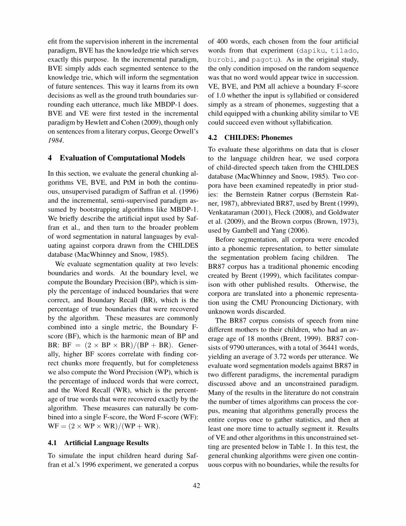
efit from the supervision inherent in the incrementalparadigm, BVE has the knowledge trie which servesexactly this purpose. In the incremental paradigm,BVE simply adds each segmented sentence to theknowledge trie, which will inform the segmentationof future sentences. This way it learns from its owndecisions as well as the ground truth boundaries sur-rounding each utterance, much like MBDP-1 does.BVE and VE were first tested in the incrementalparadigm by Hewlett and Cohen (2009), though onlyon sentences from a literary corpus, George Orwell’s1984.

4 Evaluation of Computational Models

In this section, we evaluate the general chunking al-gorithms VE, BVE, and PtM in both the continu-ous, unsupervised paradigm of Saffran et al. (1996)and the incremental, semi-supervised paradigm as-sumed by bootstrapping algorithms like MBDP-1.We briefly describe the artificial input used by Saf-fran et al., and then turn to the broader problemof word segmentation in natural languages by eval-uating against corpora drawn from the CHILDESdatabase (MacWhinney and Snow, 1985).

We evaluate segmentation quality at two levels:boundaries and words. At the boundary level, wecompute the Boundary Precision (BP), which is sim-ply the percentage of induced boundaries that werecorrect, and Boundary Recall (BR), which is thepercentage of true boundaries that were recoveredby the algorithm. These measures are commonlycombined into a single metric, the Boundary F-score (BF), which is the harmonic mean of BP andBR: BF = (2 × BP × BR)/(BP + BR). Gener-ally, higher BF scores correlate with finding cor-rect chunks more frequently, but for completenesswe also compute the Word Precision (WP), which isthe percentage of induced words that were correct,and the Word Recall (WR), which is the percent-age of true words that were recovered exactly by thealgorithm. These measures can naturally be com-bined into a single F-score, the Word F-score (WF):WF = (2×WP×WR)/(WP + WR).

4.1 Artificial Language Results

To simulate the input children heard during Saf-fran et al.’s 1996 experiment, we generated a corpus

of 400 words, each chosen from the four artificialwords from that experiment (dapiku, tilado,burobi, and pagotu). As in the original study,the only condition imposed on the random sequencewas that no word would appear twice in succession.VE, BVE, and PtM all achieve a boundary F-scoreof 1.0 whether the input is syllabified or consideredsimply as a stream of phonemes, suggesting that achild equipped with a chunking ability similar to VEcould succeed even without syllabification.

4.2 CHILDES: Phonemes

To evaluate these algorithms on data that is closerto the language children hear, we used corporaof child-directed speech taken from the CHILDESdatabase (MacWhinney and Snow, 1985). Two cor-pora have been examined repeatedly in prior stud-ies: the Bernstein Ratner corpus (Bernstein Rat-ner, 1987), abbreviated BR87, used by Brent (1999),Venkataraman (2001), Fleck (2008), and Goldwateret al. (2009), and the Brown corpus (Brown, 1973),used by Gambell and Yang (2006).

Before segmentation, all corpora were encodedinto a phonemic representation, to better simulatethe segmentation problem facing children. TheBR87 corpus has a traditional phonemic encodingcreated by Brent (1999), which facilitates compar-ison with other published results. Otherwise, thecorpora are translated into a phonemic representa-tion using the CMU Pronouncing Dictionary, withunknown words discarded.

The BR87 corpus consists of speech from ninedifferent mothers to their children, who had an av-erage age of 18 months (Brent, 1999). BR87 con-sists of 9790 utterances, with a total of 36441 words,yielding an average of 3.72 words per utterance. Weevaluate word segmentation models against BR87 intwo different paradigms, the incremental paradigmdiscussed above and an unconstrained paradigm.Many of the results in the literature do not constrainthe number of times algorithms can process the cor-pus, meaning that algorithms generally process theentire corpus once to gather statistics, and then atleast one more time to actually segment it. Resultsof VE and other algorithms in this unconstrained set-ting are presented below in Table 1. In this test, thegeneral chunking algorithms were given one contin-uous corpus with no boundaries, while the results for

42

bootstrapping algorithms were reported in a semi-supervised condition.

Algorithm BP BR BF WP WR WFPtM 0.861 0.897 0.879 0.676 0.704 0.690VE 0.875 0.803 0.838 0.614 0.563 0.587BVE 0.949 0.879 0.913 0.793 0.734 0.762MBDP-1 0.803 0.843 0.823 0.670 0.694 0.682HDP 0.903 0.808 0.852 0.752 0.696 0.723WordEnds 0.946 0.737 0.829 NR NR 0.707

Table 1: Results for the BR87 corpus with unconstrainedprocessing of the corpus. Algorithms in italics are semi-supervised.

In the incremental setting, the corpus is treated asa series of utterances and the algorithm must seg-ment each one before moving on to the next. This isdesigned to better simulate the learning process, as achild would normally listen to a series of utterancesproduced by adults, analyzing each one in turn. Toperform this test, we used the incremental versionsof PtM, VE, and BVE described in Section 3, andcompared them with MBDP-1 on the BR87 corpus.Each point in Figure 3 shows the boundary F-scoreof each algorithm on the last 500 utterances. Notethat VE and PtM do not benefit from the informa-tion about boundaries at the beginnings and endingsof utterances, yet they achieve levels of performancenot very inferior to MBDP-1 and BVE, which doleverage true boundary information.

0.50

0.55

0.60

0.65

0.70

0.75

0.80

0.85

0.90

0.5 1.5 2.5 3.5 4.5 5.5 6.5 7.5 8.5 9.5

Bo

un

dar

y F-

Sco

re (

BF)

Thousands of Utterances

VE

MBDP-1

BVE

PtM

Figure 3: Results for three chunking algorithms andMBDP-1 on BR87 in the incremental paradigm.

We also produced a phonemic encoding of theBR87 and Bloom73 (Bloom, 1973) corpora fromCHILDES with the CMU pronouncing dictionary,which encodes stress information (primary, sec-ondary, or unstressed) on phonemes that serve assyllable nuclei. Stress information is known to be

a useful factor in word segmentation, and infantsappear to be sensitive to stress patterns by as earlyas 8 months of age (Jusczyk et al., 1999). Resultswith these corpora are shown below in Figures 4 and5. For each of the general chunking algorithms, awindow size of 4 was used, meaning decisions weremade in a highly local manner. Even so, BVE out-performs MBDP-1 in this arguably more realisticsetting, while VE and PtM rival it or even surpassit. Note that the quite different results shown in Fig-ure 3 and Figure 4 are for the same corpus, undertwo different phonemic encodings, illustrating theimportance of accurately representing the input chil-dren receive.

0.50

0.55

0.60

0.65

0.70

0.75

0.80

0.85

0.90

0.95

0.5 1.5 2.5 3.5 4.5 5.5 6.5 7.5 8.5 9.5

Bo

un

dar

y F-

Sco

re (

BF)


VE

MBDP-1

BVE

PtM

Figure 4: Results for chunking algorithms and MBDP-1on BR87 (CMU) in the incremental paradigm.

0.60

0.65

0.70

0.75

0.80

0.85

0.90

0.95

0.5 1 1.5 2 2.5

Bo

un

dar

y F-

Sco

re (

BF)


VE

MBDP-1

BVE

PtM

Figure 5: Results for chunking algorithms and MBDP-1on Bloom73 (CMU) in the incremental paradigm.

4.3 CHILDES: Syllables

In many empirical studies of word segmentation inchildren, especially after Saffran et al. (1996), theproblem is treated as though syllables were the ba-sic units of the stream to be segmented, rather thanphonemes. If we assume children can syllabify their

43

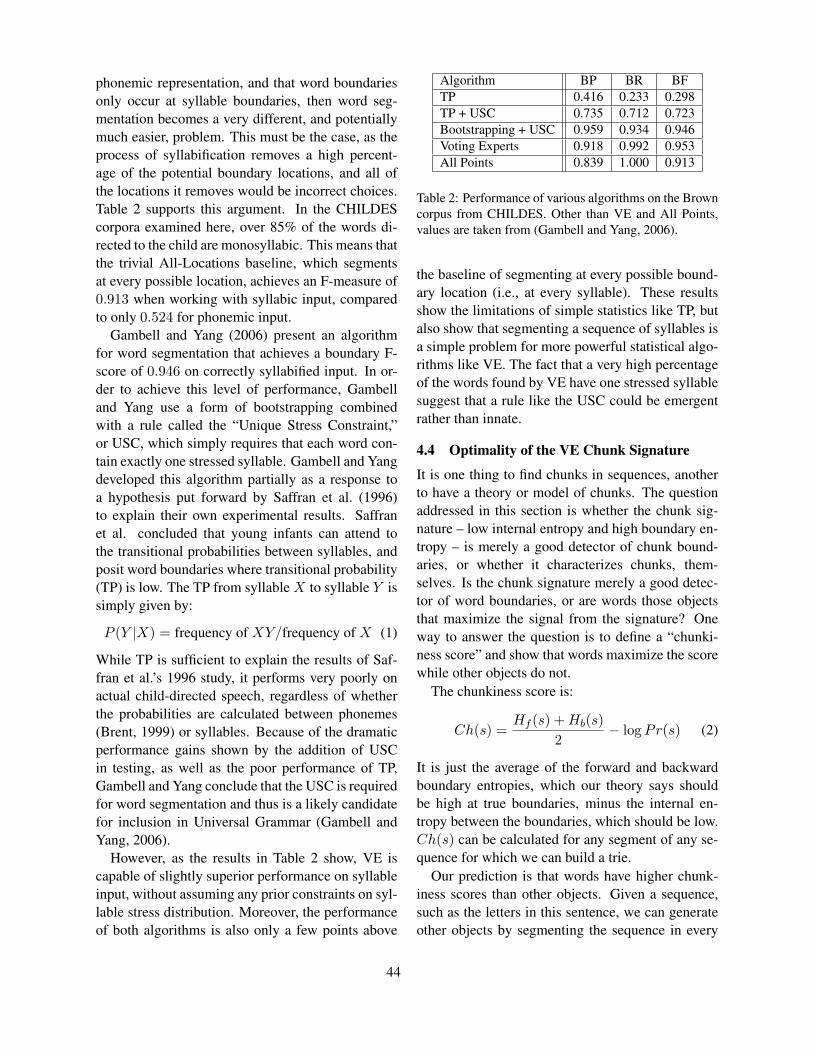
phonemic representation, and that word boundariesonly occur at syllable boundaries, then word seg-mentation becomes a very different, and potentiallymuch easier, problem. This must be the case, as theprocess of syllabification removes a high percent-age of the potential boundary locations, and all ofthe locations it removes would be incorrect choices.Table 2 supports this argument. In the CHILDEScorpora examined here, over 85% of the words di-rected to the child are monosyllabic. This means thatthe trivial All-Locations baseline, which segmentsat every possible location, achieves an F-measure of0.913 when working with syllabic input, comparedto only 0.524 for phonemic input.

Gambell and Yang (2006) present an algorithmfor word segmentation that achieves a boundary F-score of 0.946 on correctly syllabified input. In or-der to achieve this level of performance, Gambelland Yang use a form of bootstrapping combinedwith a rule called the “Unique Stress Constraint,”or USC, which simply requires that each word con-tain exactly one stressed syllable. Gambell and Yangdeveloped this algorithm partially as a response toa hypothesis put forward by Saffran et al. (1996)to explain their own experimental results. Saffranet al. concluded that young infants can attend tothe transitional probabilities between syllables, andposit word boundaries where transitional probability(TP) is low. The TP from syllable X to syllable Y issimply given by:

P (Y |X) = frequency of XY/frequency of X (1)

While TP is sufficient to explain the results of Saf-fran et al.’s 1996 study, it performs very poorly onactual child-directed speech, regardless of whetherthe probabilities are calculated between phonemes(Brent, 1999) or syllables. Because of the dramaticperformance gains shown by the addition of USCin testing, as well as the poor performance of TP,Gambell and Yang conclude that the USC is requiredfor word segmentation and thus is a likely candidatefor inclusion in Universal Grammar (Gambell andYang, 2006).

However, as the results in Table 2 show, VE iscapable of slightly superior performance on syllableinput, without assuming any prior constraints on syl-lable stress distribution. Moreover, the performanceof both algorithms is also only a few points above

Algorithm BP BR BFTP 0.416 0.233 0.298TP + USC 0.735 0.712 0.723Bootstrapping + USC 0.959 0.934 0.946Voting Experts 0.918 0.992 0.953All Points 0.839 1.000 0.913

Table 2: Performance of various algorithms on the Browncorpus from CHILDES. Other than VE and All Points,values are taken from (Gambell and Yang, 2006).

the baseline of segmenting at every possible bound-ary location (i.e., at every syllable). These resultsshow the limitations of simple statistics like TP, butalso show that segmenting a sequence of syllables isa simple problem for more powerful statistical algo-rithms like VE. The fact that a very high percentageof the words found by VE have one stressed syllablesuggest that a rule like the USC could be emergentrather than innate.

4.4 Optimality of the VE Chunk Signature

It is one thing to find chunks in sequences, anotherto have a theory or model of chunks. The questionaddressed in this section is whether the chunk sig-nature – low internal entropy and high boundary en-tropy – is merely a good detector of chunk bound-aries, or whether it characterizes chunks, them-selves. Is the chunk signature merely a good detec-tor of word boundaries, or are words those objectsthat maximize the signal from the signature? Oneway to answer the question is to define a “chunki-ness score” and show that words maximize the scorewhile other objects do not.

The chunkiness score is:

Ch(s) =Hf (s) + Hb(s)

2− log Pr(s) (2)

It is just the average of the forward and backwardboundary entropies, which our theory says shouldbe high at true boundaries, minus the internal en-tropy between the boundaries, which should be low.Ch(s) can be calculated for any segment of any se-quence for which we can build a trie.

Our prediction is that words have higher chunk-iness scores than other objects. Given a sequence,such as the letters in this sentence, we can generateother objects by segmenting the sequence in every

44

possible way (there are 2n−1 of these for a sequenceof length n). Every segmentation will produce somechunks, each of which will have a chunkiness score.

For each 5-word sequence (usually between 18and 27 characters long) in the Bloom73 corpus fromCHILDES, we generated all possible chunks andranked them by their chunkiness. The average rankof true words was the 98.7th percentile of the distri-bution of chunkiness. It appears that syntax is theprimary reason that true chunks do not rank higher:When the word-order in the training corpus is scram-bled, the rank of true words is the 99.6th percentileof the chunkiness distribution. These early results,based on a corpus of child-directed speech, stronglysuggest that words are objects that maximize chunk-iness. Keep in mind that the chunkiness score knowsnothing of words: The probabilities and entropies onwhich it is based are estimated from continuous se-quences that contain no boundaries. It is thereforenot obvious or necessary that the objects that maxi-mize chunkiness scores should be words. It might bethat letters, or phones, or morphemes, or syllables,or something altogether novel maximize chunkinessscores. However, empirically, the chunkiest objectsin the corpus are words.

5 Discussion

Whether segmentation is performed on phonemic orsyllabic sequences, and whether it is unsupervised orprovided information such as utterance boundariesand pauses, information-theoretic algorithms suchas VE, PtM and especially BVE perform segmen-tation very well. The performance of VE on BR87is on par with other state-of-the-art semi-supervisedsegmentation algorithms such as WordEnds (Fleck,2008) and HDP (Goldwater et al., 2009). Theperformance of BVE on corpora of child-directedspeech is unmatched in the unconstrained case, tothe best of our knowledge.

These results suggest that BVE provides a sin-gle, general chunking ability that that accounts forword segmentation in both scenarios, and potentiallya wide variety of other cognitive tasks as well. Wenow consider other properties of BVE that are es-pecially relevant to natural language learning. Overtime, BVE’s knowledge trie comes to represent thedistribution of phoneme sequences that begin and

end words it has found. We now discuss how thisknowledge trie models phonotactic constraints, andultimately becomes an emergent lexicon.

5.1 Phonotactic ConstraintsEvery language has a set of constraints on howphonemes can combine together into syllables,called phonotactic constraints. These constraints af-fect the distribution of phonemes found at the be-ginnings and ends of words. For example, wordsin English never begin with /ts/, because it is not avalid syllable onset in English. Knowledge of theseconstraints allows a language learner to simplify thesegmentation problem by eliminating many possi-ble segmentations, as demonstrated in Section 4.3.This approach has inspired algorithms in the litera-ture, such as WordEnds (Fleck, 2008), which buildsa statistical model of phoneme distributions at thebeginnings and ends of words. BVE also learns amodel of phonotactics at word boundaries by keep-ing similar statistics in its knowledge trie, but cando so in a fully unsupervised setting by inferring itsown set of high-precision word boundaries with thechunk signature.

5.2 An Emergent LexiconVE does not represent explicitly a “lexicon” ofchunks that it has discovered. VE produces chunkswhen applied to a sequence, but its internal datastructures do not represent the chunks it has dis-covered explicitly. By contrast, BVE stores bound-ary information in the knowledge trie and refines itover time. Simply by storing the beginnings andendings of segments, the knowledge trie comes tostore sequences like #cat#, where # represents aword boundary. The set of such bounded sequencesconstitutes an emergent lexicon. After segmentinga corpus of child-directed speech, the ten most fre-quent words of this lexicon are you, the, that, what,is, it, this, what’s, to, and look. Of the 100 mostfrequent words, 93 are correct. The 7 errors includesplitting off morphemes such as ing, and mergingfrequently co-occurring word pairs such as do you.

6 Implications for Cognitive Science

Recently, researchers have begun to empirically as-sess the degree to which segmentation algorithmsaccurately model human performance. In particular,

45

Frank et al. (2010) compared the segmentation pre-dictions made by TP and a Bayesian Lexical modelagainst the segmentation performance of adults, andfound that the predictions of the Bayesian modelwere a better match for the human data. As men-tioned in Section 4.3, computational evaluation hasdemonstrated repeatedly that TP provides a poormodel of segmentation ability in natural language.Any of the entropic chunking methods investigatedhere can explain the artificial language results moti-vating TP, as well as the segmentation of natural lan-guage, which argues for their inclusion in future em-pirical investigations of human segmentation ability.

6.1 Innate Knowledge

The word segmentation problem provides a reveal-ing case study of the relationship between nativismand statistical learning. The initial statistical pro-posals, such as TP, were too simple to explain thephenomenon. However, robust statistical methodswere eventually developed that perform the linguis-tic task successfully. With statistical learning mod-els in place that perform as well as (or better than)models based on innate knowledge, the argument foran impoverished stimulus becomes difficult to main-tain, and thus the need for a nativist explanation isremoved.

Importantly, it should be noted that the successof a statistical learning method is not an argumentthat nothing is innate in the domain of word segmen-tation, but simply that it is the learning procedure,rather than any specific linguistic knowledge, that isinnate. The position that a statistical segmentationability is innate is bolstered by speech segmentationexperiments with cotton-top tamarins (Hauser et al.,2001) that have yielded similar results to Saffran’sexperiments with human infants, suggesting that theability may be present in the common ancestor ofhumans and cotton-top tamarins.

Further evidence for a domain-general chunkingability can be found in experiments where humansubjects proved capable of discovering chunks ina single continuous sequence of non-linguistic in-puts. Saffran et al. (1999) found that adults and 8-month-old infants were able to segment sequencesof tones at the level of performance previously estab-lished for syllable sequences (Saffran et al., 1996).Hunt and Aslin (1998) measured the reaction time

of adults when responding to a single continuoussequence of light patterns, and found that subjectsquickly learned to exploit predictive subsequenceswith quicker reactions, while delaying reaction atsubsequence boundaries where prediction was un-certain. In both of these results, as well as the wordsegmentation experiments of Saffran et al., humanslearned to segment the sequences quickly, usuallywithin minutes, just as general chunking algorithmsquickly reach high levels of performance.

7 Conclusion

We have shown that a domain-independent theory ofchunking can be applied effectively to the problemof word segmentation, and can explain the ability ofchildren to segment a continuous sequence, whichother computational models examined here do notattempt to explain. The human ability to segmentcontinuous sequences extends to non-linguistic do-mains as well, which further strengthens the gen-eral chunking account, as these chunking algorithmshave been successfully applied to a diverse array ofnon-linguistic sequences. In particular, BVE com-bines the power of the information-theoretic chunksignature with a bootstrapping capability to achievehigh levels of performance in both the continuousand incremental paradigms.

8 Future Work

Within the CHILDES corpus, our results have onlybeen demonstrated for English, which leaves openthe possibility that other languages may presenta more serious segmentation problem. In En-glish, where many words in child-directed speechare mono-morphemic, the difference between find-ing words and finding morphs is small. In somelanguages, ignoring the word/morph distinction islikely to be a more costly assumption, especiallyfor highly agglutinative or even polysynthetic lan-guages. One possibility that merits further explo-ration is that, in such languages, morphs rather thanwords are the units that optimize chunkiness.

AcknowledgementsThis work was supported by the Office of Naval Re-search under contract ONR N00141010117. Any viewsexpressed in this publication are solely those of the au-thors and do not necessarily reflect the views of the ONR.

46

References

Richard N. Aslin, Jenny R. Saffran, and Elissa L. New-port. 1998. Computation of Conditional ProbabilityStatistics by 8-Month-Old Infants. Psychological Sci-ence, 9(4):321–324.

Nan Bernstein Ratner, 1987. The phonology of parent-child speech, pages 159–174. Erlbaum, Hillsdale, NJ.

Lois Bloom. 1973. One Word at a Time. Mouton, Paris.Michael R. Brent. 1999. An Efficient, Probabilistically

Sound Algorithm for Segmentation and Word Discov-ery. Machine Learning, (34):71–105.

Roger Brown. 1973. A first language: The early stages.Harvard University, Cambridge, MA.

Paul Cohen and Niall Adams. 2001. An algorithmfor segmenting categorical time series into meaning-ful episodes. In Proceedings of the Fourth Symposiumon Intelligent Data Analysis.

Paul Cohen, Niall Adams, and Brent Heeringa. 2007.Voting Experts: An Unsupervised Algorithm forSegmenting Sequences. Intelligent Data Analysis,11(6):607–625.

Margaret M. Fleck. 2008. Lexicalized phonotactic wordsegmentation. In Proceedings of The 49th AnnualMeeting of the Association for Computational Linguis-tics: Human Language Technologies, pages 130–138,Columbus, Ohio, USA. Association for ComputationalLinguistics.

Michael C Frank, Harry Tily, Inbal Arnon, and SharonGoldwater. 2010. Beyond Transitional Probabilities :Human Learners Impose a Parsimony Bias in Statisti-cal Word Segmentation. In Proceedings of the 32ndAnnual Meeting of the Cognitive Science Society.

Timothy Gambell and Charles Yang. 2006. StatisticsLearning and Universal Grammar: Modeling WordSegmentation. In Workshop on Psycho-computationalModels of Human Language.

Sharon Goldwater, Thomas L Griffiths, and Mark John-son. 2009. A Bayesian Framework for Word Segmen-tation: Exploring the Effects of Context. Cognition,112(1):21–54.

Sharon Goldwater. 2007. Nonparametric Bayesian mod-els of lexical acquisition. Ph.D. dissertation, BrownUniversity.

Zellig S. Harris. 1955. From Phoneme to Morpheme.Language, 31(2):190–222.

Marc D. Hauser, Elissa L. Newport, and Richard N.Aslin. 2001. Segmentation of the speech stream in anon-human primate: statistical learning in cotton-toptamarins. Cognition, 78(3):B53–64.

Daniel Hewlett and Paul Cohen. 2009. Bootstrap VotingExperts. In Proceedings of the Twenty-first Interna-tional Joint Conference on Artificial Intelligence.

Daniel Hewlett and Paul Cohen. 2010. Artificial GeneralSegmentation. In The Third Conference on ArtificialGeneral Intelligence.

Ruskin H. Hunt and Richard N. Aslin. 1998. Statisti-cal learning of visuomotor sequences: Implicit acqui-sition of sub-patterns. In Proceedings of the TwentiethAnnual Conference of the Cognitive Science Society,Mahwah, NJ. Lawrence Erlbaum Associates.

Howard Johnson and Joel Martin. 2003. Unsupervisedlearning of morphology for English and Inuktitut. Pro-ceedings of the 2003 Conference of the North Amer-ican Chapter of the Association for ComputationalLinguistics on Human Language Technology (HLT-NAACL 2003), pages 43–45.

Peter W. Jusczyk, Derek M. Houston, and Mary New-some. 1999. The Beginnings of Word Segmentationin English-Learning Infants. Cognitive Psychology,39(3-4):159–207.

Teuvo Kohonen. 1988. Self-organized formation of topo-logically correct feature maps.

Brian MacWhinney and Catherine E Snow. 1985. Thechild language data exchange system (CHILDES).Journal of Child Language.

Matthew Miller and Alexander Stoytchev. 2008. Hierar-chical Voting Experts: An Unsupervised Algorithm forHierarchical Sequence Segmentation. In Proceedingsof the 7th IEEE International Conference on Develop-ment and Learning, pages 186–191.

Matthew Miller, Peter Wong, and Alexander Stoytchev.2009. Unsupervised Segmentation of Audio SpeechUsing the Voting Experts Algorithm. Proceedings ofthe 2nd Conference on Artificial General Intelligence(AGI 2009).

Jenny R. Saffran and Erik D. Thiessen. 2003. Patterninduction by infant language learners. DevelopmentalPsychology, 39(3):484–494.

Jenny R. Saffran, Richard N. Aslin, and Elissa L. New-port. 1996. Statistical Learning by 8-Month-Old In-fants. Science, 274(December):926–928.

Jenny R. Saffran, Elizabeth K Johnson, Richard N. Aslin,and Elissa L. Newport. 1999. Statistical learning oftone sequences by human infants and adults. Cogni-tion, 70(1):27–52.

Kumiko Tanaka-Ishii and Zhihui Jin. 2006. FromPhoneme to Morpheme: Another Verification Usinga Corpus. In Proceedings of the 21st InternationalConference on Computer Processing of Oriental Lan-guages, pages 234–244.

Anand Venkataraman. 2001. A procedure for unsuper-vised lexicon learning. In Proceedings of the Eigh-teenth International Conference on Machine Learning.

47

Proceedings of the Fifteenth Conference on Computational Natural Language Learning, page 48,Portland, Oregon, USA, 23–24 June 2011. c©2011 Association for Computational Linguistics

Computational Linguistics for Studying Language in People:Principles, Applications and Research Problems

Invited talk

Bruce HayesDepartment of Linguistics, [email protected]

One of the goals of computational linguistics is to create automated systems that can learn, generate, andunderstand language at all levels of structure (semantics, syntax, morphology, phonology, phonetics). Thisis a very demanding task whose complete fulfillment lies far in the future. Human beings can learn, gen-erate, and understand language at all levels of structure, and the study of how they do it can be pursued bycomputational modeling. Indeed, one sort of “acid test” for theories in linguistics is whether they can serveas the basis for successful models of this kind. A research strategy for theoretical linguistics based on mod-eling thus invites close collaboration between “mainstream” linguists and their computational colleagues.

Such collaborations make the job of the computationalists, already very demanding, even harder. The col-lision between a computational model and human data arises when we apply the Turing test: the model oughtto behave like a human, not just in generating a correct output, but in every conceivable sense: generatingalternative outputs for a single input, (often with a nuanced sense of preferences among them), generatinghuman-like mistakes, generating child-like mistakes when given incomplete information, and so on. I sug-gest that linguists could serve as good Turing testers, because it is their daily practice in professional life tointerrogate their models in the most ingenious ways they can find, probing for deficiencies though compari-son to complex human intuitions and behavior.

With this as backdrop, I offers a series of case studies, of three different kinds: (1) Turing tests: caseswhere interrogation by linguists revealed non-humanlike traits in computational models that performed wellby traditional computational criteria (precision, recall, etc.); (2) Success stories: particular results of com-putational linguistics that have proven useful so far in modeling language in humans; (3) Suggestions forfuture work: proposals in linguistic theory that look promising and would benefit from computationalanalysis.

48


Search-based Structured Prediction applied to Biomedical Event Extraction

Andreas Vlachos and Mark CravenDepartment of Biostatistics and Medical Informatics

University of Wisconsin-Madison{vlachos,craven}@biostat.wisc.edu

Abstract

We develop an approach to biomedical eventextraction using a search-based structured pre-diction framework, SEARN, which convertsthe task into cost-sensitive classification taskswhose models are learned jointly. We showthat SEARN improves on a simple yet strongpipeline by 8.6 points in F-score on theBioNLP 2009 shared task, while achieving thebest reported performance by a joint inferencemethod. Additionally, we consider the issue ofcost estimation during learning and present anapproach called focused costing that improvesimproves efficiency and predictive accuracy.

1 Introduction

The term biomedical event extraction is used to re-fer to the task of extracting descriptions of actionsand relations involving one or more entities fromthe biomedical literature. The recent BioNLP 2009shared task (BioNLP09ST) on event extraction (Kimet al., 2009) focused on event types of varying com-plexity. Each event consists of a trigger and one ormore arguments, the latter being proteins or otherevents. Any token in a sentence can be a trigger forone of the nine event types and, depending on theirassociated event types, triggers are assigned appro-priate arguments. Thus, the task can be viewed asa structured prediction problem in which the outputfor a given instance is a (possibly disconnected) di-rected acyclic graph (not necessarily a tree) in whichvertices correspond to triggers or protein arguments,and edges represent relations between them.

Despite being a structured prediction task, most ofthe systems that have been applied to BioNLP09ST

to date are pipelines that decompose event extrac-tion into a set of simpler classification tasks. Clas-sifiers for these tasks are typically learned indepen-dently, thereby ignoring event structure during train-ing. Typically in such systems, the relationshipsamong these tasks are taken into account by incor-porating post-processing rules that enforce certainconstraints when combining their predictions, andby tuning classification thresholds to improve the ac-curacy of joint predictions. Pipelines are appealingas they are relatively easy to implement and they of-ten achieve state-of-the-art performance (Bjorne etal., 2009; Miwa et al., 2010).

Because of the nature of the output space, the taskis not amenable to sequential or grammar-based ap-proaches (e.g. linear CRFs, HMMs, PCFGs) whichemploy dynamic programming in order to do ef-ficient inference. The only joint inference frame-work that has been applied to BioNLP09ST to dateis Markov Logic Networks (MLNs) (Riedel et al.,2009; Poon and Vanderwende, 2010). However,MLNs require task-dependent approximate infer-ence and substantial computational resources in or-der to achieve state-of-the-art performance.

In this work we explore an alternative joint in-ference approach to biomedical event extraction us-ing a search-based structured prediction framework,SEARN (Daume III et al., 2009). SEARN is analgorithm that converts the problem of learning amodel for structured prediction into learning a setof models for cost-sensitive classification (CSC).CSC is a task in which each training instance hasa vector of misclassification costs associated with it,thus rendering some mistakes on some instances tobe more expensive than others (Domingos, 1999).Compared to a standard pipeline, SEARN is able to

49

achieve better performance because its models arelearned jointly. Thus, each of them is able to use fea-tures representing the predictions made by the oth-ers, while taking into account possible mistakes.

In this paper, we make the following contribu-tions. Using the SEARN framework, we develop ajoint inference approach to biomedical event extrac-tion. We evaluate our approach on the BioNLP09STdataset and show that SEARN improves on a simpleyet strong pipeline by 8.6 points in F-score, whileachieving the best reported performance on the taskby a joint inference method. Additionally, we con-sider the issue of cost estimation and present an ap-proach called focused costing that improves perfor-mance. We believe that these contributions are likelyto be relevant to applications of SEARN to othernatural language processing tasks that involve struc-tured prediction in complex output spaces.

2 BioNLP 2009 shared task description

BioNLP09ST focused on the extraction of eventsinvolving proteins whose names are annotated inadvance. Each event has two types of arguments,Theme and Cause, which correspond respectively tothe Agent and Patient roles in semantic role label-ing (Gildea and Jurafsky, 2002). Nine event typesare defined which can be broadly classified in threecategories, namely Simple, Binding and Regulation.Simple events include Gene expression, Transcrip-tion, Protein catabolism, Phosphorylation, and Lo-calization events. These have only one Theme ar-gument which is a protein. Binding events haveone or more protein Themes. Finally, Regulationevents, which include Positive regulation, Nega-tive regulation and Regulation, have one obligatoryTheme and one optional Cause, each of which canbe either a protein or another event. Each event hasa trigger which is a contiguous string that can spanover one or more tokens. Triggers and argumentscan be shared across events. In an example demon-strating the complexity of the task, given the passage“. . . SQ 22536 suppressed gp41-induced IL-10 pro-duction in monocytes”, systems should extract thethree appropriately nested events listed in Fig. 1d.

Performance is measured using Recall, Precisionand F-score over complete events, i.e. the trigger,the event type and the arguments all must be correct

in order to obtain a true positive. It is important tonote that if either the trigger, the type, or an argu-ment of a predicted event is incorrect then this eventwill result in one false positive and one false nega-tive. In the example of Fig. 1, if “suppressed” is rec-ognized incorrectly as a Regulation trigger then it isbetter to not assign a Theme to it so that we avoida false positive due to extracting an event with in-correct type. Finally, the evaluation ignores triggersthat do not form events.

3 Event extraction decomposition

Figure 1 describes the event extraction decomposi-tion that we use throughout the paper. We assumethat the sentences to be processed are parsed intosyntactic dependencies and lemmatized. Each stagehas its own module, which is either a learned classi-fier (trigger recognition, Theme/Cause assignment)or a rule-based component (event construction).

3.1 Trigger recognitionIn trigger recognition the system decides whether atoken acts as a trigger for one of the nine event typesor not. Thus it is a 10-way classification task. Weonly consider tokens that are tagged as nouns, verbsor adjectives by the parser, as they cover the majorityof the triggers in the BioNLP09ST data. The mainfeatures used in the classifier represent the lemmaof the token which is sufficient to predict the eventtype correctly in most cases. In addition, we includefeatures that conjoin each lemma with its part-of-speech tag. This allows us to handle words withthe same nominal and verbal form that have differ-ent meanings, such as “lead”. While the domainrestricts most lemmas to one event type, there aresome whose event type is determined by the context,e.g. “regulation” on its own denotes a Regulationevent but in “positive regulation” it denotes a Posi-tive regulation event instead. In order to capture thisphenomenon, we add as features the conjunction ofeach lemma with the lemma of the tokens immedi-ately surrounding it, as well as with the lemmas ofthe tokens with which it has syntactic dependencies.

3.2 Theme and Cause assignmentIn Theme assignment, we form an agenda of can-didate trigger-argument pairs for all trigger-proteincombinations in the sentence and classify them as

50

SQ 22536 suppressedNeg reg

gp41-inducedPos reg

IL-10 productionGene exp

(a) Trigger recognition


gp41-inducedPos reg


Theme

ThemeTheme

(b) Theme assignment


gp41-inducedPos reg


Theme

Theme

Cause

Theme

(c) Cause assignment

ID type Trigger Theme CauseE1 Neg reg suppressed E2E2 Pos reg induced E3 gp41E3 Gene exp production IL-10

(d) Event construction

Figure 1: The stages of our event extraction decomposition. Protein names are shown in bold.

Themes or not. Whenever a trigger is predicted to beassociated with a Theme, we form candidate pairsbetween all the Regulation triggers in the sentenceand that trigger as the argument, thus allowing theprediction of nested events. Also, we remove candi-date pairs that could result in directed cycles, as theyare not allowed by the task.

The features used to predict whether a trigger-argument pair should be classified as a Theme areextracted from the syntactic dependency path andthe textual string between them. In particular, weextract the shortest unlexicalized dependency pathconnecting each trigger-argument pair, allowing thepaths to follow either dependency direction. One setof features represents these paths, and in addition,we have sets of features representing each path con-joined with the lemma, the PoS tag and the eventtype of the trigger, the type of the argument andthe first and last lemmas in the dependency path.The latter help by providing some mild lexicaliza-tion. We also add features representing the textualstring between the trigger and the argument, com-bined with the event type of the trigger. While not asinformative as dependency paths, such features helpin sentences where the parse is incorrect, as triggersand their arguments tend to appear near each other.

In Cause assignment, we form an agenda of can-didate trigger-argument pairs using only the Regu-lation class triggers that were assigned at least oneTheme. These are combined with protein names andother triggers that were assigned a Theme. We ex-

tract features as in Theme assignment, further fea-tures representing the conjunction of the dependencypath of the candidate pair with the path(s) from thetrigger to its Theme(s).

3.3 Event construction

In event construction, we convert the predictions ofthe previous stages into a set of legal events. Ifa Binding trigger is assigned multiple Themes, wechoose to form either one event per Theme or oneevent with multiple Themes. Following Bjorne etal. (2009), we group the arguments of each Bindingtrigger according to the first label in their syntac-tic dependency path and generate events using thecross-product of these groups. For example, assum-ing the parse was correct and all the Themes recog-nized, “interactions of A and B with C” results intwo Binding events with two Themes each, A withC, and B with C respectively. We add the exceptionthat if two Themes are in the same token (e.g. “A/Binteractions”) or the lemma of the trigger is “bind”then they form one Binding event with two Themes.

4 Structured prediction with SEARN

SEARN (Daume III et al., 2009) forms the struc-tured output prediction for an instance s as a se-quence of T multiclass predictions y1:T made by ahypothesis h. The latter consists of a set of classi-fiers that are learned jointly. Each prediction yt canuse features from s as well as from all the previouspredictions y1:t−1. These predictions are referred to

51

as actions and we adopt this term in order to distin-guish them from the structured output predictions.

The SEARN algorithm is presented in Alg. 1. Itinitializes hypothesis h to the optimal policy π (step2) which predicts the optimal action in each stept according to the gold standard. The optimal ac-tion at step t is the one that minimizes the overallloss over s assuming that all future actions yt+1:T

are also made optimally. The loss function ` is de-fined by the structured prediction task considered.Each iteration begins by making predictions for allinstances s in the training data S (step 6). For eachs and each action yt, a cost-sensitive classification(CSC) example is generated (steps 8-12). The fea-tures are extracted from s and the previous actionsy1:t−1 (step 8). The cost for each possible actionyi

t is estimated by predicting the remaining actionsy′t+1:T in s using h (step 10) and evaluating the costincurred given that action (step 11). Using a CSClearning algorithm, a new hypothesis is learned (step13) which is combined with the current one accord-ing to the interpolation parameter β.

Algorithm 1 SEARN1: Input: labeled instances S , optimal policy π, CSC

learning algorithm CSCL, loss function `2: current policy h = π3: while h depends significantly on π do4: Examples E = ∅5: for s in S do6: Predict h(s) = y1:T7: for yt in h(s) do8: Extract features Φt = f(s, y1:t−1)9: for each possible action yi

t do10: Predict y′t+1:T = h(s|y1:t−1, y

it)

11: Estimate cit = `(y1:t−1, yit, y′t+1:T )

12: Add (Φt, ct) to E13: Learn a hypothesis hnew = CSCL(E)14: h = βhnew + (1− β)h15: Output: policy h without π

In each iteration, SEARN moves away from theoptimal policy and uses the learned hypotheses in-stead when predicting (steps 6 and 10). Thus, eachhnew is adapted to the actions chosen by h insteadof those of the optimal policy. When the depen-dence on the latter becomes insignificant, the algo-rithm terminates and returns the weighted ensembleof learned hypotheses without the optimal policy.

Note though that the estimation of the costs in step11 is always performed using the gold standard.

The interpolation parameter β determines howfast SEARN moves away from the optimal policyand as a result how many iterations will be needed tominimize the dependence on it. Dependence in thiscontext refers to the probability of using the optimalpolicy instead of the learned hypothesis in choos-ing an action during prediction. In each iteration,the features extracted Φt are progressively corruptedwith the actions chosen by the learned hypothesesinstead of those of the optimal policy.

Structural information under SEARN is incorpo-rated in two ways. First, via the costs that are es-timated using the loss over the instance rather thanisolated actions (e.g. in PoS tagging, the loss wouldbe the number of incorrect PoS tags predicted ina sentence if a token is tagged as noun). Second,via the features extracted from the previous actions(y1:t−1) (e.g. the PoS tag predicted for the previ-ous token can be a feature). These types of featuresare possible in a standard pipeline as well, but dur-ing training they would have to be extracted usingthe gold standard instead of the actual predictionsmade by the learned hypotheses, as during testing.Since the prediction for each instance (y1:T in step6) changes in every iteration, the structure featuresused to predict the actions have to be extracted anew.

The extraction of features from previous actionsimplies a search order. For some tasks, such as PoStagging, there is a natural left-to-right order in whichthe tokens are treated, however for many tasks thisis not the case.

Finally, SEARN can be used to learn a pipeline ofindependently trained classifiers. This is achievedusing only one iteration in which the cost for eachaction is set to 0 if it follows from the gold standardand to 1 otherwise. This adaptation allows for a faircomparison between SEARN and a pipeline.

5 SEARN for biomedical event extraction

In this section we discuss how we learn the eventextraction decomposition described in Sec. 3 underSEARN. Each instance is a sentence consisting ofthe tokens, the protein names and the syntactic pars-ing output. The hypothesis learned in each iterationconsists of a classifier for each stage of the pipeline,

52

excluding event construction which is rule-based.Unlike PoS tagging, there is no natural ordering

of the actions in event extraction. Ideally, the ac-tions predicted earlier should be less dependent onstructural features and/or easier so that they can in-form the more structure dependent/harder ones. Intrigger recognition, we process the tokens from leftto right since modifiers appearing before nouns tendto affect the meaning of the latter, e.g. “binding ac-tivity”. In Theme and Cause assignment, we predicttrigger-argument pairs in order of increasing depen-dency path length, assuming that since dependencypaths are the main source of features at this stage andshorter paths are less sparse, pairs containing shorterones should be more reliable to predict.

In addition to the features mentioned in Sec. 3,SEARN allows us to extract and learn weights forstructural features for each action from the previousones. During trigger recognition, we add as featuresthe combination of the lemma of the current tokencombined with the event type (if any) assigned tothe previous and the next token, as well as to the to-kens that have syntactic dependencies with it. Dur-ing Theme assignment, when considering a trigger-argument pair, we add features based on whether itforms an undirected cycle with previously predictedThemes, whether the trigger has been assigned a pro-tein as a Theme and the candidate Theme is an eventtrigger (and the reverse) and whether the argumenthas become the Theme of a trigger with the sameevent type. We also add a feature indicating whetherthe trigger has three Themes predicted already. Dur-ing Cause assignment, we add features representingwhether the trigger has been assigned a protein as aCause and the candidate Cause is an event trigger.

The loss function ` sums the number of false pos-itive and false negative events, which is the evalua-tion measure of BioNLP09ST. The optimal policy isderived from the gold standard and returns the ac-tion that minimizes this loss over the sentence giventhe previous actions and assuming that all future ac-tions are optimal. In trigger recognition, it returnseither the event type for tokens that are triggers or a“notrigger” label otherwise. In Theme assignment,for a given trigger-argument pair the optimal policyreturns Theme only if the trigger is recognized cor-rectly and the argument is indeed a Theme for thattrigger according to the gold standard. In case the ar-

gument is another event, we require that at least oneof its Themes to be recognized correctly as well. InCause assignment, the requirements are the same asthose for the Themes, but we also require that at leastone Theme of the trigger in the trigger-argument pairto be considered correct. These additional checksfollow from the task definition, under which eventsmust have all their elements identified correctly.

5.1 Cost estimationCost estimation (steps 5-12 in Alg. 1) is crucial tothe successful application of SEARN. In order tohighlight its importance, consider the example ofFig. 2 focusing on trigger recognition.

In the first iteration (Fig. 2a), the actions for thesentence will be made using the optimal policy only,thus replicating the gold standard. During costing,if a token is not a trigger according to the gold stan-dard (e.g. “SQ”), then the cost for incorrectly pre-dicting that it is a trigger is 0, as the optimal policywill not assign Themes to a trigger with incorrectevent type. Such instances are ignored by the cost-sensitive learner. If a token is a trigger according tothe gold standard, then the cost for not predicting itas such or predicting its type incorrectly is equal tothe number of the events that are dependent on it, asthey will become false negatives. False positives areavoided as we are using the optimal policy in thisiteration.

In the second iteration (Fig. 2b), the optimal pol-icy is interpolated with the learned hypothesis, thussome of the actions are likely to be incorrect. As-sume that “SQ” is incorrectly predicted to be aNeg reg trigger and assigned a Theme. During cost-ing, the action of labeling “SQ” as Neg reg has acost of 1, as it would result in a false positive event.Thus the learned hypothesis will be informed that itshould not label “SQ” as a trigger as it would assignThemes to it incorrectly and it is adapted to handleits own mistakes. Similarly, the action of labeling“production” as Neg reg in this iteration would in-cur a cost of 6, as the learned hypothesis would as-sign a Theme incorrectly, thus resulting in 3 falsenegative and 3 false positive events. Therefore, thelearned hypothesis will be informed that assigningthe wrong event type to “production” is worse thannot predicting a trigger.

By evaluating the cost of each action according to

53


gp41-inducedPos reg


Theme

Theme

Cause

Theme

token No Gene exp Pos reg Neg regSQ 0 0 0 0suppressed 1 1 1 0-induced 2 2 0 2production 3 0 3 3

(a) First iteration (optimal policy only)

SQNeg reg

22536 suppressedNeg reg

gp41-inducedPos reg

IL-10 productionNeg reg

Theme

Theme

Cause

ThemeTheme

token No Gene exp Pos reg Neg regSQ 0 0 0 1suppressed 1 1 1 0-induced 2 2 0 2production 3 0 3 6

(b) Second iteration (interpolation)

Figure 2: Prediction (top) and CSC examples for trigger recognition actions (bottom) in the first two SEARNiterations. Each CSC example has its own vector of misclassification costs.

its effect on the prediction for the whole sentence,we are able to take into account steps in the pre-diction process that are not learned as actions. Forexample, if the Binding event construction heuris-tic described in Sec. 3.3 cannot produce the correctevents for a token that is a Binding trigger despitethe Themes being assigned correctly, then this willincrease the cost for tagging that trigger as Binding.

The interpolation between the optimal policy andthe learned hypothesis is stochastic, thus affectingthe cost estimates obtained. In order to obtain morereliable estimates, one can average multiple sam-ples for each action by repeating steps 10 and 11of Alg. 1. However, the computational cost is effec-tively multiplied by the number of samples.

In step 11 of Alg. 1, the cost of each action is esti-mated over the whole sentence. While this allows usto take structure into account, it can result in costsbeing affected by a part of the output that is not re-lated to that action. This is likely to occur in eventextraction, as sentences can often be long and con-tain disconnected event components in their outputgraphs. For this reason, we refine the cost estimationof each action to take into account only the eventsthat are connected to it through either gold standardor predicted events. For example, in Fig. 2 the costestimation for “SQ” will ignore the predicted eventsin the first iteration and the gold standard, while itwill take them into account in the second one. Werefer to this refinement as focused costing.

A different approach proposed by Daume III etal. (2009) is to assume that all actions following the

one we are costing are going to be optimal and usethe optimal policy to approximate the prediction ofthe learned hypothesis in step 10 of Alg. 1. In taskswhere the learned hypothesis is accurate enough,this has no performance loss and it is computation-ally efficient as the optimal policy is deterministic.However, in event extraction the learned hypothesisis likely to make mistakes, thus the optimal policydoes not provide a good approximation for it.

5.2 CSC learning with passive-aggressivealgorithms

The SEARN framework requires a multiclass CSCalgorithm to learn how to predict actions. This algo-rithm must be computationally fast during parameterlearning and prediction, as in every iteration we needto learn a new hypothesis and to consider each pos-sible action for each instance in order to constructthe cost-sensitive examples. Daume III et al. (2009)showed that any binary classification algorithm canbe used to perform multiclass CSC by employing anappropriate conversion between the tasks. The maindrawback of this approach is its reliance on multi-ple subsamplings of the training data, which can beinefficient for large datasets and many classes.

With these considerations in mind, we implementa multiclass CSC learning algorithm using the gen-eralization of the online passive-aggressive (PA) al-gorithm for binary classification proposed by Cram-mer et al. (2006). For each training example xt,the K-class linear classifier with K weight vectorsw

(k)t makes a prediction yt and suffers a loss `t. In

54

the case of multiclass CSC learning, each examplehas its own cost vector ct. If the loss is 0 then theweight vectors of the classifier are not updated (pas-sive). Otherwise, the weight vectors are updatedminimally so that the prediction on example xt iscorrected (aggressive). The update takes into ac-count the loss and the aggressiveness parameter C.Crammer et al. (2006) describe three variants to per-form the updates which differ in how the learningrate τt is set. In our experiments we use the variantnamed PA-II with prediction-based updates (Alg. 2).Since we are operating in a batch learning setting(i.e. we have access to all the training examples andtheir order is not meaningful), we perform multiplerounds over the training examples shuffling their or-der, and average the weight vectors obtained.

Algorithm 2 Passive-aggressive CSC learning1: Input: training examples X = x1 . . . xT , cost vec-

tors c1 . . . cT ≥ 0, rounds R, aggressiveness C2: Initialize weights w(k)

0 = (0, ..., 0)3: for r = 1, ..., R do4: Shuffle X5: for xt ∈ X do6: Predict yt = argmaxk(w

(k)t · xt)

7: Receive cost vector ct ≥ 08: if c(yt)

t > 0 then

9: Suffer loss `t = w(yt)t ·xt−w(yt)

t ·xt+

√c(yt)t

10: Set learning rate τt = `t

||xt||2+ 12C

11: Update w(yt)t+1 = wt + τtxt

12: Update w(yt)t+1 = wt − τtxt

13: Average wavg = 1T×R

∑T×Ri=0 wi

6 Experiments

BioNLP09ST comprises three datasets – training,development and test – which consist of 800, 150and 260 abstracts respectively. After the endof the shared task, an on-line evaluation serverwas activated in order to allow the evaluation onthe test data once per day, without allowing ac-cess to the data itself. We report results usingRecall/Precision/F-score over complete events usingthe approximate span matching/approximate recur-sive matching variant which was the primary perfor-mance criterion in BioNLP09ST. This variant countsa predicted event as a true positive if its trigger is

extracted within a one-token extension of the gold-standard trigger. Also, in the case of nested events,those events below the top-level need their trigger,event type and Theme but not their Cause to be cor-rectly identified for the top-level event to be consid-ered correct. The same event matching variant wasused in defining the loss as described in Sec. 5.

A pre-processing step we perform on the train-ing data is to reduce the multi-token triggers in thegold standard to their syntactic heads. This proce-dure simplifies the task of assigning arguments totriggers and, as the evaluation variant used allowsapproximate trigger matching, it does not result ina performance loss. For syntactic parsing, we usethe output of the BLLIP re-ranking parser adapted tothe biomedical domain by McClosky and Charniak(2008), as provided by the shared task organizersin the Stanford collapsed dependency format withconjunct dependency propagation. Lemmatizationis performed using morpha (Minnen et al., 2001).

In all our experiments, for CSC learning with PA,the C parameter is set by tuning on 10% of the train-ing data and the number of rounds is fixed to 10. ForSEARN, we set the interpolation parameter β to 0.3and the number of iterations to 12. The costs foreach action are obtained by averaging three samplesas described in Sec. 5.1. β and the number of sam-ples are the only parameters that need tuning and weuse the development data for this purpose.

First we compare against a pipeline of indepen-dently learned classifiers obtained as described inSec. 4 in order to assess the benefits of joint learningunder SEARN using focused costing. The resultsshown in Table 1 demonstrate that SEARN obtainsbetter event extraction performance on both the de-velopment and test sets by 7.7 and 8.6 F-score pointsrespectively. The pipeline baseline employed in ourexperiments is a strong one: it would have rankedfifth in BioNLP09ST and it is 20 F-score points bet-ter than the baseline MLN employed by Poon andVanderwende (2010). Nevertheless, the indepen-dently learned classifier for triggers misses almosthalf of the event triggers, from which the subsequentstages cannot recover. On the other hand, the trig-ger classifier learned with SEARN overpredicts, butsince the Theme and Cause classifiers are learnedjointly with it they maintain relatively high precisionwith substantially higher recall compared to their in-

55

pipeline SEARN focus SEARN defaultR P F R P F R P F

triggerdev 53.0 61.1 56.8 81.8 34.2 48.2 84.9 12.0 21.0Themedev 44.2 79.6 56.9 62.0 69.1 65.4 59.0 65.1 61.9Causedev 18.1 59.2 27.8 30.6 45.0 36.4 31.9 45.5 37.5Eventdev 35.8 68.9 47.1 50.8 59.5 54.8 47.4 54.3 50.6Eventtest 30.8 67.4 42.2 44.5 59.1 50.8 41.3 53.6 46.6

Table 1: Recall / Precision / F-score on BioNLP09ST development and test data. Left-to-right: pipeline ofindependently learned classifiers, SEARN with focused costing, SEARN with default costing.

dependently learned counterparts. The benefits ofSEARN are more pronounced in Regulation eventswhich are more complex. For these events, it im-proves on the pipeline on both the development andtest sets by 11 and 14.2 F-score points respectively.

The focused costing approach we proposed con-tributes to the success of SEARN. If we replace itwith the default costing approach which uses thewhole sentence, the F-score drops by 4.2 points onboth development and test datasets. The defaultcosting approach mainly affects the trigger recog-nition stage, which takes place first. Trigger over-prediction is more extreme in this case and rendersthe Theme assignment stage harder to learn. Whilethe joint learning of the classifiers ameliorates thisissue and the event extraction performance is even-tually higher than that of the pipeline, the use of fo-cused costing improves the performance even fur-ther. Note that trigger overprediction also makestraining slower, as it results in evaluating more ac-tions for each sentence. Finally, using one insteadof three samples per action decreases the F-score by1.3 points on the development data.

Compared with the MLN approaches applied toBioNLP09ST, our predictive accuracy is better thanthat of Poon and Vanderwende (2010) which is thebest joint inference performance to date and substan-tially better than that of Riedel et al. (2009) (50 and44.4 in F-score respectively). Recently, McCloskyet al. (2011) combined multiple decoders for a de-pendency parser with a reranker, achieving 48.6 inF-score. While they also extracted structure fea-tures for Theme and Cause assignment, their modelis restricted to trees (ours can output directed acyclicgraphs) and their trigger recognizer is learned inde-pendently.

When we train SEARN combining the training

and the development sets, we reach 52.3 in F-score,which is better than the performance of the topsystem in BioNLP09ST (51.95) by Bjorne et al.(2009) which was trained in the same way. Thebest performance to date is reported by Miwa et al.(2010) (56.3 in F-score), who experimented with sixparsers, three dependency representations and vari-ous combinations of these. They found that differentparser/dependency combinations provided the bestresults on the development and test sets.

A direct comparison between learning frame-works is difficult due to the differences in task de-composition and feature extraction. In particular,event extraction results depend substantially on thequality of the syntactic parsing. For example, Poonand Vanderwende (2010) heuristically correct thesyntactic parsing used and report that this improvedtheir performance by four F-score points.

7 Conclusions

We developed a joint inference approach to biomed-ical event extraction using the SEARN frameworkwhich converts a structured prediction task into a setof CSC tasks whose models are learned jointly. Ourapproach employs the PA algorithm for CSC learn-ing and a focused cost estimation procedure whichimproves the efficiency and accuracy of the standardcost estimation method. Our approach provides thebest reported results for a joint inference method onthe BioNLP09ST task. With respect to the experi-ments presented by Daume III et al. (2009), we em-pirically demonstrate the gains of using SEARN ona problem harder than sequential tagging.

AcknowledgmentsThe authors were funded by NIH/NLM grant R01 /LM07050.

56

ReferencesJari Bjorne, Juho Heimonen, Filip Ginter, Antti Airola,

Tapio Pahikkala, and Tapio Salakoski. 2009. Extract-ing complex biological events with rich graph-basedfeature sets. In Proceedings of the BioNLP 2009 Work-shop Companion Volume for Shared Task, pages 10–18.

Koby Crammer, Ofer Dekel, Joseph Keshet, Shai Shalev-Shwartz, and Yoram Singer. 2006. Online passive-aggressive algorithms. Journal of Machine LearningResearch, 7:551–585.

Hal Daume III, John Langford, and Daniel Marcu. 2009.Search-based structured prediction. Machine Learn-ing, 75:297–325.

Pedro Domingos. 1999. Metacost: a general method formaking classifiers cost-sensitive. In Proceedings ofthe 5th International Conference on Knowledge Dis-covery and Data Mining, pages 155–164.

Daniel Gildea and Daniel Jurafsky. 2002. Automatic la-beling of semantic roles. Computational Linguistics,28:245–288.

Jin-Dong Kim, Tomoko Ohta, Sampo Pyysalo, Yoshi-nobu Kano, and Jun’ichi Tsujii. 2009. Overview ofBioNLP’09 shared task on event extraction. In Pro-ceedings of the BioNLP 2009 Workshop CompanionVolume for Shared Task, pages 1–9.

David McClosky and Eugene Charniak. 2008. Self-training for biomedical parsing. In Proceedings ofthe 46th Annual Meeting of the Association of Compu-tational Linguistics: Human Language Technologies,pages 101–104.

David McClosky, Mihai Surdeanu, and Christopher D.Manning. 2011. Event extraction as dependency pars-ing. In Proceedings of the 49th Annual Meeting ofthe Association for Computational Linguistics: Hu-man Language Technologies.

Guido Minnen, John Carroll, and Darren Pearce. 2001.Applied morphological processing of English. Natu-ral Language Engineering, 7(3):207–223.

Makoto Miwa, Sampo Pyysalo, Tadayoshi Hara, andJun’ichi Tsujii. 2010. Evaluating dependency repre-sentation for event extraction. In Proceedings of the23rd International Conference on Computational Lin-guistics, pages 779–787.

Hoifung Poon and Lucy Vanderwende. 2010. Joint in-ference for knowledge extraction from biomedical lit-erature. In Proceedings of the Human Language Tech-nologies: The 2010 Annual Conference of the NorthAmerican Chapter of the Association for Computa-tional Linguistics, pages 813–821.

Sebastian Riedel, Hong-Woo Chun, Toshihisa Takagi,and Jun’ichi Tsujii. 2009. A Markov logic approachto bio-molecular event extraction. In Proceedings of

the BioNLP 2009 Workshop Companion Volume forShared Task, pages 41–49.

57


Using Sequence Kernels to identify Opinion Entities in Urdu

Smruthi Mukund† and Debanjan Ghosh

* Rohini K Srihari

†SUNY at Buffalo, NY

[email protected] *

Thomson Reuters Corporate R&D

[email protected]

SUNY at Buffalo, NY

[email protected]

Abstract

Automatic extraction of opinion holders

and targets (together referred to as opinion

entities) is an important subtask of senti-

ment analysis. In this work, we attempt to

accurately extract opinion entities from

Urdu newswire. Due to the lack of re-

sources required for training role labelers

and dependency parsers (as in English) for

Urdu, a more robust approach based on (i)

generating candidate word sequences

corresponding to opinion entities, and (ii)

subsequently disambiguating these se-

quences as opinion holders or targets is

presented. Detecting the boundaries of such

candidate sequences in Urdu is very differ-

ent than in English since in Urdu,

grammatical categories such as tense,

gender and case are captured in word

inflections. In this work, we exploit the

morphological inflections associated with

nouns and verbs to correctly identify

sequence boundaries. Different levels of

information that capture context are

encoded to train standard linear and se-

quence kernels. To this end the best per-

formance obtained for opinion entity

detection for Urdu sentiment analysis is

58.06% F-Score using sequence kernels

and 61.55% F-Score using a combination

of sequence and linear kernels.

1 Introduction

Performing sentiment analysis on newswire da-

ta facilitates the development of systems capable

of answering perspective questions like “How did

people react to the latest presidential speech?” and

“Does General Musharraf support the Indo-Pak

peace treaty?”. The components involved in de-

veloping such systems require accurate identifica-

tion of opinion expressions and opinion entities.

Several of the approaches proposed in the literature

to automatically extract the opinion entities rely on

the use of thematic role labels and dependency

parsers to provide new lexical features for opinion

words (Bethard et al., 2004). Semantic roles (SRL)

also help to mark the semantic constituents (agent,

theme, proposition) of a sentence. Such features

are extremely valuable for a task like opinion en-

tity detection.

English is a privileged language when it comes

to the availability of resources needed to contribute

features for opinion entity detection. There are

other widely spoken, resource poor languages,

which are still in the infantile stage of automatic

natural language processing (NLP). Urdu is one

such language. The main objective of our research

is to provide a solution for opinion entity detection

in the Urdu language. Despite Urdu lacking NLP

resources required to contribute features similar to

what works for the English language, the perform-

ance of our approach is comparable with English

for this task (compared with the work of Weigand

and Klalow, 2010 ~ 62.61% F1). The morphologi-

cal richness of the Urdu language enables us to

extract features based on noun and verb inflections

that effectively contribute to the opinion entity ex-

traction task. Most importantly, these features can

be generalized to other Indic languages (Hindi,

Bengali etc.) owing to the grammatical similarity

between the languages.

58

English has seen extensive use of sequence ker-

nels (string and tree kernels) for tasks such as rela-

tion extraction (Culotta and Sorensen, 2004) and

semantic role labeling (Moschitti et al., 2008). But,

the application of these kernels to a task like opin-

ion entity detection is scarcely explored (Weigand

and Klalow, 2010). Moreover, existing works in

English perform only opinion holder identification

using these kernels. What makes our approach

unique is that we use the power of sequence ker-

nels to simultaneously identify opinion holders and

targets in the Urdu language.

Sequence kernels allow efficient use of the

learning algorithm exploiting massive number of

features without the traditional explicit feature rep-

resentation (such as, Bag of Words). Often, in case

of sequence kernels, the challenge lies in choosing

meaningful subsequences as training samples in-

stead of utilizing the whole sequence. In Urdu

newswire data, generating candidate sequences

usable for training is complicated. Not only are the

opinion entities diverse in that they can be con-

tained within noun phrases or clauses, the clues

that help to identify these components can be con-

tained within any word group - speech events,

opinion words, predicates and connectors.

1 Pakistan ke swaat sarhad ke janoobi shahar Banno

ka havayi adda zarayye ablaagk tavvju ka markaz

ban gaya hai.

[Pakistan’s provincial border’s south city’s airbase

has become the center of attraction for all reporters.]

Here, the opinion target spans across four noun

chunks, “Pakistan’s | provincial border’s | south

city’s | airbase”. The case markers (connectors)

“ke”and“ka” indicate the span.

2 Habib miyan ka ghussa bad gaya aur wo apne aurat

ko maara.

[Habib miya’s anger increased and he hit his own

wife.]

Here, the gender (Masculine) inflection of the verb

“maara” (hit) indicates that the agent performing

this action is “Habib miya” (Masculine)

3 Ansari ne kaha “mere rayee mein Aamir Sohail eek

badimaak aur Ziddi insaan hai”.

[Ansari said, “according to me Aamir Sohail is one

crazy and stubborn man”]

Here, cues similar to English such as “mere rayee

mein” (according to) indicate the opinion holder.

Another interesting behavior here is the presence of

nested opinion holders. “kaha” (said) indicates that

this statement was made by Ansari only.

4 Sutlan bahut khush tha, naseer key kaam se.

[Sultan was very happy with Naseer’s work]

Here, the target of the expression “khush” is after the

verb “khush tha”(was happy) – SVO structure

Table 1: Examples to outline the complexity of the task

Another contributing factor is the free word or-

der of the Urdu language. Although the accepted

form is SOV, there are several instances where the

object comes after the verb or the object is before

the subject. In Urdu newswire data, the average

number of words in a sentence is 42 (Table 3).

This generates a large number of candidate se-

quences that are not opinion entities, on account of

which the data used for training is highly unbal-

anced. The lack of tools such as dependency pars-

ers makes boundary detection for Urdu different

from English, which in turn makes opinion entity

extraction a much harder task. Examples shown in

table 1 illustrate the complexity of the task.

One safe assumption that can be made for opin-

ion entities is that they are always contained in a

phrase (or clause) that contains a noun (common

noun, proper noun or pronoun), which is either the

subject or the object of the predicate. Based on

this, we generate candidate sequences by consider-

ing contextual information around noun phrases. In

example 1 of Table 1, the subsequence that is gen-

erated will consider all four noun phrases “Paki-

stan’s | provincial border’s | south city’s |

airbase” as a single group for opinion entity.

We demonstrate that investigating postpositions

to capture semantic relations between nouns and

predicates is crucial in opinion entity identifica-

tion. Our approach shows encouraging perform-

ance.

2 Related Work

Choi et al., (2005) consider opinion entity iden-

tification as an information extraction task and the

opinion holders are identified using a conditional

random field (Lafferty et al., 2001) based se-

quence-labeling approach. Patterns are extracted

using AutoSlog (Riloff et al., 2003). Bloom et al.,

(2006) use hand built lexicons for opinion entity

identification. Their method is dependent on a

combination of heuristic shallow parsing and de-

pendency parsing information. Kim and Hovy

59

(2006) map the semantic frames of FrameNet

(Baker et al., 1998) into opinion holder and target

for adjectives and verbs to identify these compo-

nents. Stoyanov and Cardie (2008) treat the task of

identifying opinion holders and targets as a co-

reference resolution problem. Kim et al., (2008)

used a set of communication words, appraisal

words from Senti-WordNet (Esuli and Sebastiani,

2006) and NLP tools such as NE taggers and syn-

tactic parsers to identify opinion holders accu-

rately. Kim and Hovy (2006) use structural

features of the language to identify opinion enti-

ties. Their technique is based on syntactic path and

dependency features along with heuristic features

such as topic words and named entities. Weigand

and Klalow (2010) use convolution kernels that

use predicate argument structure and parse trees.

For Urdu specifically, work in the area of clas-

sifying subjective and objective sentences is at-

tempted by Mukund and Srihari, (2010) using a

vector space model. NLP tools that include POS

taggers, shallow parser, NE tagger and morpho-

logical analyzer for Urdu is provided by Mukund

et al., (2010). This is the only extensive work done

for automating Urdu NLP, although other efforts to

generate semantic role labels and dependency

parsers are underway.

3 Linguistic Analysis for Opinion Entities

In this section we introduce the different cues

used to capture the contextual information for cre-

ating candidate sequences in Urdu by exploiting

the morphological richness of the language.

Table 2: Case Inflections on Nouns

Urdu is a head final language with post-

positional case markers. Some post-positions are

associated with grammatical functions and some

with specific roles associated with the meaning of

verbs (Davison, 1999). Case markers play a very

important role in determining the case inflections

of nouns. The case inflections that are useful in the

context of opinion entity detection are “ergative”,

“dative”, “genitive”, “instrumental” and “loca-

tive”. Table 2 outlines the constructs.

Consider example 1 below. (a) is a case where

“Ali” is nominative. However, in (b) “Ali” is da-

tive. The case marker “ko” helps to identify sub-

jects of certain experiential and psychological

predicates: sensations, psychological or mental

states and obligation or compulsion. Such predi-

cates clearly require the subject to be sentient, and

further, indicate that they are a ected in some

manner, correlating with the semantic properties

ascribed to the dative’s primary use (Grimm,

2007).

Example (1):

(a) Ali khush hua (Ali became happy)

(b) Ali ko khushi hui (Ali became happy)

Example (2):

(a) Sadaf kaam karne ki koshish karti hai (Sadaf

tries to do work)

Semantic information in Urdu is encoded in a

way that is very different from English. Aspect,

tense and gender depend on the noun that a verb

governs. Example 2 shows the dependency that

verbs have on nouns without addressing the lin-

guistic details associated with complex predicates.

In example 2, the verb “karti”(do) is feminine

and the noun it governs ~Sadaf is also feminine.

The doer for the predicate “karti hai”(does) is

“Sadaf” and there exists a gender match. This

shows that we can obtain strong features if we are

able to accurately (i) identify the predicates, (ii)

find the governing noun, and (iii) determine the

gender.

In this work, for the purpose of generating can-

didate sequences, we encompass the post-position

responsible for case inflection in nouns, into the

noun phrase and group the entire chunk as one sin-

gle candidate. In example 1, the dative inflection

on ‘Ali’ is due to the case marker ‘ko’. Here, ‘Ali

ko’ will always be considered together in all candi-

date sequences that this sentence generates. This

Case Clitic

Form

Examples

Ergative (ne) Ali ne ghussa dikhaya ~

Ali showed anger

Accusa-

tive

(ko) Ali ko mainey maara ~

I hit Ali

Dative (ko,ke) Similar to accusative

Instru-

mental

(se) Yeh kaam Ali se hua ~

This work was done by

Ali

Genitive (ka, ke, ki) Ali ka ghussa, baap re

baap! ~ Ali’s anger, oh

my God!

Locative (mein, par,

tak, tale,

talak)

Ali mein ghussa zyaada

hai ~ there is a lot of

anger in Ali

60

behavior can also be observed in example 1 of ta-

ble 1.

We use SemantexTM

(Srihari et al., 2008) - an

end to end NLP framework for Urdu that provides

POS, NE, shallow parser and morphological ana-

lyzer, to mark tense, mood, aspect, gender and

number inflections of verbs and case inflections of

nouns. For ease of parsing, we enclose dative and

accusative inflected nouns and the respective case

markers in a tag called POSSESS. We also enclose

locative, genitive and ergative inflections and case

markers in a tag called DOER.

4 Methodology

Sequence boundaries are first constructed based

on the POSSESS, DOER and NP (noun chunk)

tags prioritized by the position of the tag while

parsing. We refer to these chunks as “candidates”

as they are the possible opinion entity candidates.

We generate candidate sequences by combining

these candidates with opinion expressions (Mu-

kund and Srihari, 2010) and the predicates that

contain or follow the expression words (~khushi in

(b) of example 1 above).

We evaluate our approach in two steps:

(i) Boundary Detection - detecting opinion

entities that contain both holders and tar-

gets

(ii) Entity Disambiguation - disambiguating

opinion holders from opinion targets

In the following sections, we briefly describe

our research methodology including sequence

creation, choice of kernels and the challenges thus

encountered.

4.1 Data Set

The data used for the experiments are newswire

articles from BBC Urdu1 that are manually anno-

tated to reflect opinion holders, targets, and ex-

pressions (emotion bearing words).

Number of subjective sentences 824

Average word length of each sentence 42

Number of opinion holders 974

Number of opinion targets 833

Number of opinion expressions 894

Table 3: Corpus Statistics

1 www.bbc.co.uk/urdu/

Table 3 summarizes the corpus statistics. The inter

annotator agreement established between two an-

notators over 30 documents was found to be 0.85

using Cohen’s Kappa score (averaged over all

tags). The agreement is acceptable as tagging emo-

tions is a difficult and a personalized task.

4.2 Support Vector Machines (SVM) and

Kernel Methods

SVMs belong to a class of supervised machine

learning techniques that merge the nuances of sta-

tistical learning theory, kernel mapping and opti-

mization techniques to discover separating

hyperplanes. Given a set of positive and negative

data points, based on structural risk minimization,

SVMs attempt to find not only a separating hyper-

plane that separates two categories (Vapnik and

Kotz, 2006) but also maximize the boundary be-

tween them (maximal margin separation tech-

nique). In this work, we propose to use a variation

of sequence kernels for opinion entity detection.

4.3 Sequence Kernels

The lack of parsers that capture dependencies in

Urdu sentences inhibit the use of ‘tree kernels’

(Weigand and Klalow, 2010). In this work, we ex-

ploit the power of a set of sequence kernels known

as ‘gap sequence string kernels’ (Lodhi et al.,

2002). These kernels provide numerical compari-

son of phrases as entire sequences rather than a

probability at the chunk level. Gap sequence ker-

nels measure the similarity between two sequences

(in this case a sequence of Urdu words) by count-

ing the number of common subsequences. Gaps

between words are penalized with suitable use of

decay factor to compensate for

matches between lengthy word sequences.

Formally, let be the feature space over

words. Consequently, we declare other disjoint

feature spaces (stem words, POS,

chunks, gender inflections, etc.)

and.For any two-feature

vectors let compute the number

of common features between s and t. Table 5 lists

the features used to compute .

Given two sequences, s and t and the kernel

function that calculates the number of

61

weighted sparse subsequences of length n (say,

n=2: bigram) common to both s and t, then

is as shown in eq 1 (Bunescu and

Mooney, 2005).

(i,j,k are dimensions) ------ Eq 1.

Generating correct sequences is a prior require-

ment for sequence kernels. For example, in the task

of relation extraction, features included in the

shortest path between the mentions of the two se-

quences (which hold the relation) play a decisive

role (Bunescu and Mooney, 2005). Similarly, in

the task of role labeling (SRL - Moschitti et al.,

2008), syntactic sub-trees containing the arguments

are crucial in finding the correct associations. Our

approach to create candidate sequences for opinion

entity detection in Urdu is explained in the next

section.

4.4 Candidate Sequence Generation

Each subjective sentence in Urdu contains sev-

eral noun phrases with one or more opinion ex-

pressions. The words that express opinions

(expression words) can be contained within a verb

predicate (if the predicate is complex) or precede

the verb predicate. These subjective sentences are

first pre-processed to mark the morphological in-

flections as mentioned in §3.

Table 4: Candidate Sequence Generation

We define training candidate sequences as the

shortest substring t which is a tuple that contains

the candidate noun phrase (POSSESS, DOER or

NP), an emotion expression and the closest predi-

cate. Table 4 outlines the steps taken to create the

candidate sequences and figure 1 illustrates the

different tuples for a sample sentence.

Experiments conducted by Weigand and

Klakow (2010) consider <candidate, predicate>

and <candidate, expression> tuples. However, in

Urdu the sense of expression and predicate are so

tightly coupled (in many examples they subsume

each other and hence inseparable), that specifically

trying to gauge the influence of predicate and

expression separately on candidates is impossible.

There are three advantages in our approach to

creating candidate sequences: (i) by pairing ex-

pressions with their nearest predicates, several un-

necessary candidate sequences are eliminated, (ii)

phrases that do not contain nouns are automatically

not considered (see RBP chunk in figure 1), and

(iii) by considering only one candidate chunk at a

time in generating the candidate sequence, we en-

sure that the sequence that is generated is short for

better sequence kernel performance.

4.4.1 Linear Kernel features

For linear kernels we define features explicitly

based on the lexical relationship between the can-

didate and its context. Table 5 outlines the features

used.

Feature Sets and Description

Set 1

Baseline 1. head word of candidate

2. case marker contained within candidate?

3. expression words

4. head word of predicate

5. POS sequence of predicate words

6. # of NPs between candidate and emotion

Set 2 7. the DOER

8. expression right after candidate?

Set 3 9. gender match between candidate and

predicate

10. predicate contains emotion words?

Set 4 11. POS sequence of candidate

Set 5 12. “kah” feature in the predicate

13. locative feature?

14. genitive feature on noun?

Table 5: Linear Kernel Features

1 A sentence is parsed to extract all likely candi-

date chunks – POSSESS, DOER, NP in that

order.

2 <expression, predicate> tuples are first selected

based on nearest neighbor rule :

1. Predicates that are paired with the expres-

sion words either contain the expressions or

follow the expressions.

2. Stand alone predicates are simply ignored as

they do not contribute to the holder identifi-

cation task (they contribute to either the sen-

tence topic or the reason for the emotion).

3 For each candidate,

<candidate, expression, predicate> tuples are

generated without changing the word order.

(Fig. 1 – example candidates maintain the same

word order)

62

Figure 1: Illustration of candidate sequences

4.4.1 Sequence Kernel features

Features commonly used for sequence kernels

are based on words (such as character-based or

word-based sequence kernels). In this work, we

consider to be a feature space over Urdu words

along with other disjoint features such as POS,

gender, case inflections. In the kernel, however, for

each combination (see table 6) the similarity

matching function that computes the num-

ber of similar features remains the same.

Table 6: Disjoint feature set for sequence kernels

Sequence kernels are robust and can deal with

complex structures. There are several overlapping

features between the feature sets used for linear

kernel and sequence kernel. Consider the POS

path information feature. This is an important fea-

ture for the linear kernel. However this feature

need not be explicitly mentioned for the sequence

kernel as the model internally learns the path in-

formation. In addition, several Boolean features

explicitly described for the linear kernel (2 and 13

in table 5) are also learned automatically in the

sequence kernel by matching subsequences.

5 Experiments

The data used for our experiments is explained

in §4.1. Figure 2 gives a flow diagram of the entire

process. LIBSVM’s (Chang and Lin, 2001) linear

kernel is trained using the manually coded features

mentioned in table 5. We integrated our proposed

sequence kernel with the same toolkit. This se-

quence kernel uses the features mentioned in table

6 and the decay factor is set to 0.5.

Figure 2: Overall Process

KID Kernel Type

1 word based kernel (baseline)

2 word + POS (parts of speech)

3 word + POS + chunk

4 word + POS + chunk + gender inflection

63

The candidate sequence generation algorithm gen-

erated 8,329 candidate sequences (contains all opi-

nion holders and targets – table 3) that are used for

training both the kernels. The data is parsed using

SemantexTM

to apply POS, chunk and morphology

information. Our evaluation is based on the exact

candidate boundary (whether the candidate is en-

closed in a POSSESS, DOER or NP chunk).All

scores are averaged over a 5-fold cross validation

set.

5.1 Comparison of Kernels

We apply both linear kernels (LK) and se-

quence kernels (SK) to identify the entities as well

as disambiguate between the opinion holders and

targets. Table 7 illustrates the baselines and the

best results for boundary detection of opinion enti-

ties. ID 1 of table 7 represents the result of using

LK with feature set 1 (table 5). We interpret this as

our baseline result. The best F1 score for this clas-

sifier is 50.17%.

Table 7: Boundary detection of Opinion Entities

Table 8 compares various kernels and combina-

tions. Set 1 of table 8 shows the relative effect of

feature sets for LK and how each set contributes to

detecting opinion entity boundaries. Although sev-

eral features are inspired by similar classification

techniques (features used for SRL and opinion

mining by Choi et al., (2005) ~ set 1, table 5), the

free word nature of Urdu language renders these

features futile. Moreover, due to larger average

length of each sentence and high occurrences of

NPs (candidates) in each sentence, the number of

candidate instances (our algorithm creates 10 se-

quences per sentence on average) is also very high

as compared to any English corpus. This makes

the training corpus highly imbalanced. Interest-

ingly, when features like – occurrence of postposi-

tions, “kah” predicate, gender inflections etc. are

used, classification improves (set 1, Feature set

1,2,3,4,5, table 8).

Table 8: Kernel Performance

ID 3 of table 7 displays the baseline result for SK.

Interestingly enough, the baseline F1 for SK is

very close to the best LK performance. This shows

the robustness of SK and its capability to learn

complex substructures with only words. A se-

quence kernel considers all possible subsequence

matching and therefore implements a concept of

partial (fuzzy) matching. Because of its tendency

to learn all fuzzy matches while penalizing the

gaps between words intelligently, the performance

of SK in general has better recall (Wang, 2008). To

explain the recall situation, consider set 2 of table

8. This illustrates the effect of disjoint feature

scopes of each feature (POS, chunk, gender). Each

feature adds up and expands the feature space of

sequence kernel and allows fuzzy matching there-

by improving the recall. Hence KID 4 has almost

20% recall gain over the baseline (SK baseline).

However, in many cases, this fuzzy matching

accumulates in wrong classification and lowers

precision. A fairly straightforward approach to

overcome this problem is to employ a high preci-

sion kernel in addition to sequence kernel. Another

limitation of SK is its inability to capture complex

I

D Kernel

Features

(table

5/6)

Prec.

(%)

Rec.

(%)

F1

(%)

1 LK Baseline

(Set 1) 39.58 51.49 44.75

2 LK(best) Set 1, 2,

3, 4, 5 44.20 57.99 50.17

3 SK Baseline

(KID 1) 58.22 42.75 49.30

4 SK (best) KID 4 54.00 62.79 58.06

5

Best LK

+ best

SK

KID 4,

Set 1, 2,

3, 4, 5

58.43 65.04 61.55

Set Kernel KID Prec.

(%)

Rec.

(%)

F1

(%)

Baseline

(Set 1)

39.58 51.49 44.75

Set 1,2 39.91 52.57 45.38

Set 1, 2, 3 43.55 57.72 49.65

Set 1,2,3,4 44.10 56.90 49.68

1

LK

Feature set

1,2,3,4,5

44.20 57.99 50.17

Baseline -

KID 1

58.22 42.75 49.30

KID 2 58.98 47.55 52.65

KID 3 58.18 49.62 53.59

2

SK

KID 4 54.00 62.79 58.06

KID 1 +

best LK

51.44 68.89 58.90

KID 2 +

best LK

59.18 62.98 61.02

KID 3 +

best LK

55.18 68.38 61.07

3

SK +

LK

KID 4 +

best LK

58.43 65.04 61.55

64

grammatical structure and dependencies making it

highly dependent on only the order of the string

sequence that is supplied.

We also combine the similarity scores of SK

and LK to obtain the benefits of both kernels. This

permits SK to expand the feature space by natu-

rally adding structural features (POS, chunk) re-

sulting in high recall. At the same time, LK with

strict features (such as the use of “kah” verb) or

rigid word orders (several Boolean features) will

help maintain acceptable precision. By summing

the contribution of both kernels, we achieve an F1

of 61.55% (Set 3, table 8), which is 17.8%, more

(relative gain – around 40%) than the LK baseline

results (ID 1, table 7).

Table 9: Opinion entity disambiguation for best features

Our next sets of experiments are conducted to dis-

ambiguate opinion holders and targets. A large

number of candidate sequences that are created are

not candidates for opinion entities. This results in a

huge imbalance in the data set. Jointly classify

opinion holders, opinion targets and false candi-

dates with one model can be attempted if this im-

balance in the data set due to false candidates can

be reduced. However, this has not been attempted

in this work. In order to showcase the feasibility of

our method, we train our model only on the gold

standard candidate sequences that contain opinion

entities for entity disambiguation.

The two kernels are applied on just the two

classes (opinion holder vs. opinion target). Com-

bined kernels identify holders with a 65.26% F1

(table 9). However, LK performs best for target

identification (61.23%). We believe that this is due

to opinion holders and targets sharing similar syn-

tactic structures. Hence, the sequence information

that SK learns affects accuracy but improves recall.

6 Challenges

Based on the error analysis, we observe some

common mistakes and provide some examples.

1. Mistakes resulting due to POS tagger and shal-

low chunker errors.

2. Errors due to heuristic rules for morphological

analysis.

3. Mistakes due to inaccurate identification of ex-

pression words by the subjectivity classifier.

4. Errors due to complex and unusual sentence

structures which the kernels failed to capture.

Example (3):

Is na-insaafi ka badla hamein zaroor layna chahiye.

[we have to certainly take revenge for this injustice.]

Example (4):

Kya hum dayshadgardi ka shikar banna chahatein

hai?

[Do we want to become victims of terrorism?]

Example (5):

Jab secretary kisi aur say baat karke husthi hai, tho

Pinto ko ghussa aata hai.

[When the secretary talks to someone and laughs,

Pinto gets angry.]

Example 3 is a false positive. The emotion is “an-

ger”, indicated by “na-insaafi ka badla” (revenge

for injustice) and “zaroor” (certainly). But only

the second expression word is identified accu-

rately. The sequence kernel model determines na-

insaafi (injustice) to be the opinion holder when it

is actually the reason for the emotion. However, it

also identifies the correct opinion holder - hamein

(we). Emotions associated with interrogative sen-

tences are not marked (example 4) as there exists

no one word that captures the overall emotion.

However, the subjectivity classifier identifies such

sentences as subjective candidates. This results in

false negatives for opinion entity detection. The

target (secretary) in example 5, fails to be detected

as no candidate sequence that we generate indi-

cates the noun “secretary” to be the target. We

propose to address these issues in our future work.

7 Conclusion

We describe an approach to identify opinion en-

tities in Urdu using a combination of kernels. To

the best of our knowledge this is the first attempt

where such an approach is used to identify opinion

entities in a language lacking the availability of

resources for automatic text processing. The per-

formance for this task for Urdu is equivalent to the

state of the art performance for English (Weigand

and Klakow, 2010) on the same task.

Kernel Opinion

Entity

Prec.

(%)

Rec.

(%)

F1

(%)

Holder 58.71 66.67 62.44 LK

(best) Target 65.53 57.48 61.23

Holder 60.26 69.46 64.54 SK

Target 59.75 49.73 54.28

Holder 62.90 69.81 65.26 Both

kernels Target 60.71 55.44 57.96

65

References

Collin F. Baker, Charles J. Fillmore, John B. Lowe.

1998. The Berkeley FrameNet Project, Proceedings

of the 17th international conference on Computa-

tional linguistics, August 10-14. Montreal, Quebec,

Canada

Steven Bethard, Hong Yu, Ashley Thornton, Vasileios

Hatzivassiloglou, and Dan Jurafsky. 2004. Automatic

Extraction of Opinion Propositions and their Holders,

AAAI Spring Symposium on Exploring Attitude and

Affect in Text: Theories and Applications.

Kenneth Bloom, Sterling Stein, and Shlomo Argamon.

2007. Appraisal Extraction for News Opinion Analy-

sis at NTCIR-6. In Proceedings of NTCIR-6 Work-

shop Meeting, Tokyo, Japan.

R. C. Bunescu and R. J. Mooney. 2005. A shortest path

dependency kernel for relation extraction. In Pro-

ceedings of HLT/EMNLP.

R. C. Bunescu and R. J. Mooney. 2005. Subsequence

Kernels for Relation Extraction. NIPS. Vancouver.

December.

Chih-Chung Chang and Chih-Jen Lin. 2001. LIBSVM:

a library for support vector machines. Software

available at http://www.csie.ntu.edu.tw/~cjlin/libsvm

Yejin Choi, Claire Cardie, Ellen Riloff, and Siddharth

Patwardhan. 2005. Identifying Sources of Opinions

with Conditional Random Fields and Extraction Pat-

terns. In Proceedings of the Conference on Human

Language Technology and Empirical Methods in

Natural Language Processing (HLT/EMNLP), Van-

couver, Canada.

Aaron Culotta and Jeffery Sorensen. 2004. Dependency

tree kernels for relation extraction. In Proceedings of

the 42rd Annual Meeting of the Association for

Computational Linguistics. pp. 423-429.

Alice Davison. 1999. Syntax and Morphology in Hindi

and Urdu: A Lexical Resource. University of Iowa.

Andrea Esuli and Fabrizio Sebastiani. 2006. Sen-

tiWordNet: A publicly available lexical resource for

opinion mining. In Proc of LREC. Vol 6, pp 417-422.

Scott Gimm. 2007. Subject Marking in Hindi/Urdu: A

Study in Case and Agency. ESSLLI Student Session.

Malaga, Spain.

Youngho Kim, Seaongchan Kim and Sun-Hyon

Myaeng. 2008. Extracting Topic-related Opinions

and their Targets in NTCIR-7. In Proceedings of the

7th NTCIR Workshop Meeting. Tokyo. Japan.

John Lafferty, Andrew McCallum and F. Pereira. 2001.

Conditional random fields: Probabilistic models for

segmenting and labeling sequence data. In: Proc.

18th International Conf. on Machine Learning, Mor-

gan Kaufmann, San Francisco, CA . pp. 282–289

Huma Lodhi, Craig Saunders, John Shawe-Taylor,

Nello Cristianini, Chris Watkins. 2002. Text

classification using string kernels. J. Mach. Learn.

Res. 2 (March 2002), 419-44.

Kim, Soo-Min. and Eduard Hovy. 2006. Extracting

Opinions, Opinion Holders, and Topics Expressed in

Online News Media Text. In ACL Workshop on Sen-

timent and Subjectivity in Text.

Alessandro Moschitti, Daniele Pighin, Roberto Basili.

2008. Tree kernels for semantic role labeling. Com-

putational Linguistics. Vol 34, num 2, pp 193-224.

Smruthi Mukund and Rohini K. Srihari. 2010. A Vector

Space Model for Subjectivity Classification in Urdu

aided by Co-Training, In Proceedings of the 23rd In-

ternational Conference on Computational Linguistics,

Beijing, China.

Smruthi Mukund, Rohini K. Srihari and Erik Peterson.

2010. An Information Extraction System for Urdu –

A Resource Poor Language. Special Issue on Infor-

mation Retrieval for Indian Languages.

Ellen Riloff, Janyce Wiebe and Theresa Wilson. 2003.

Learning subjective nouns using extraction pattern

bootstrapping. In Proceedings of the Seventh Confer-

ence on Natural Language Learning (CoNLL-03).

Rohini K. Srihari, W. Li, C. Niu, and T. Cornell. 2008.

InfoXtract: A Customizable Intermediate Level In-

formation Extraction Engine, Journal of Natural Lan-

guage Engineering, Cambridge U. Press, 14(1), pp.

33-69.

Veselin Stoyanov and Claire Cardie. 2008. Annotating

Topic Opinions. In Proceedings of the Sixth Interna-

tional Conference on Language Resources and Eval-

uation (LREC 2008), Marrakech, Morocco.

John Shawe-Taylor and Nello Cristianni. 2004. Kernel

methods for pattern analysis. Cambridge University

Press.

Mengqiu Wang. 2008. A Re-examination of Depend-

ency Path Kernels for Relation Extraction, In

Proceedings of IJCNLP 2008.

Michael Wiegand and Dietrich Klalow. 2010. Convolu-

tion kernels for opinion holder extraction. In Proc. of

Human Language Technologies: The 2010 Annual

Conference of the North American Chapter of the

Association for Computational Linguistics. pp 795-

803, ACL

66

Vladimir Vapnik, S.Kotz. 2006. Estimation of De-

pendences Based on Empirical Data. Springer, 510

pages.

67


Subword and spatiotemporal models for identifying actionable informationin Haitian Kreyol

Robert MunroDepartment of Linguistics

Stanford UniversityStanford, CA, 94305

[email protected]

Abstract

Crisis-affected populations are often able tomaintain digital communications but in asudden-onset crisis any aid organizations willhave the least free resources to process suchcommunications. Information that aid agen-cies can actually act on, ‘actionable’ informa-tion, will be sparse so there is great poten-tial to (semi)automatically identify actionablecommunications. However, there are hurdlesas the languages spoken will often be under-resourced, have orthographic variation, andthe precise definition of ‘actionable’ will beresponse-specific and evolving. We presenta novel system that addresses this, drawingon 40,000 emergency text messages sent inHaiti following the January 12, 2010 earth-quake, predominantly in Haitian Kreyol. Weshow that keyword/ngram-based models us-ing streaming MaxEnt achieve up to F=0.21accuracy. Further, we find current state-of-the-art subword models increase this substan-tially to F=0.33 accuracy, while modeling thespatial, temporal, topic and source contexts ofthe messages can increase this to a very ac-curate F=0.86 over direct text messages andF=0.90-0.97 over social media, making it a vi-able strategy for message prioritization.

1 Introduction

The recent proliferation of cellphone technologieshas resulted in rapid increases in the volume of in-formation coming out of crisis-affected regions. Inthe wake of the January 12, 2010 earthquake inHaiti local emergency response services were inop-erable but 70-80% of cell-towers were quickly re-

stored. With 83%/67% of men/women possessinga cellphone, the nation remained largely connected.People within Haiti were texting, calling and inter-acting with social media, but aid agencies were notequipped to process so much information. This isbecause in any sudden onset crisis, this flood of in-formation out of the region coincides with crisis-response organizations already working at capacityas they move in. The problem definition is clear:how can we filter this information to identify action-able intelligence to support relief efforts?

The solution is complicated. There may befew resources for the language(s) of the crisis-affected population and the ratio of actionable tonon-actionable information will often be very large,especially when reported through social-media andother non-official channels. In the absence of ex-isting electronic resources models must be built on-the-fly and account for substantial spelling varia-tions. The definition of what constitutes action-able intelligence will often be context-specific andchanging, too. In the data used here ‘actionable’changed quickly from Search and Rescue to anymedical emergency and then to include clusters ofrequests for food and water. The models will there-fore need to be time-sensitive or otherwise adaptive.

The system presented here attempts to addressthese problems, finding that the accurate identifica-tion of actionable information can be achieved withsubword models, the automatic identification of top-ics (categories), and spatiotemporal clustering, allwithin a streaming architecture. It is evaluated us-ing 40,811 emergency text messages sent in Haitifollowing the January 12, 2010 earthquake.

68

2 Evaluation data

Three sets of short-messages are used, all from be-tween January 12 and May 12, 2010:

1. Mission 4636. 40,811 text-messages sent to afree number, ‘4636’, in Haiti.

2. Radio Station. 7,528 text-messages sent to aHaitian radio station.

3. Twitter. 63,195 Haiti-related tweets.

The Mission 4636messages were translated, ge-olocated and categorized by a volunteer onlinecrowdsourced workforce, predominantly from theHaitian diaspora, and by paid workers within Haiti(Munro, 2010). English-speaking crisis-mappersidentified actionable messages and refined the coor-dinates and categories. The categories are a standardset of UN-defined emergency categories with someadditions (48 total). The definition of an ‘actionable’message was defined by the main responders to themessages, the US Coast Guard and the US Marinesworking with Southern Command, and included anymessages with an identifiable location that containeda request for medical assistance, Search and Rescue,water-shortages, clusters of requests for food in ar-eas not known to aid workers, security, and reportsof unaccompanied minors.

The radio station and Twitter messages are notstructured or geolocated. They are used here as po-tential false-positives in a needle-in-a-haystack sce-nario where the majority of messages are irrelevant.A recent Red Cross survey (2010) found that nearlyhalf the respondents would use social media to re-port emergencies, so this is a realistic scenario.

3 Streaming models

Supervised streaming-models attempt to classify anincoming stream of unlabeled items by building uptraining-data on past items (Aggarwal, 2006; Hul-ten et al., 2001; Babcock et al., 2002). The mod-els are often time-sensitive with training data eitherweighted towards or exclusively consisting of morerecently seem items, especially in the context of con-cept drift or bounded memory (Zhang et al., 2008).

There is a penalty for applying GOLD labels topast items for training: either only a subset can belabeled or there is a time-delay. When only a subset

can be labeled the scenario is similar to that ofactivelearning(Cohn et al., 1996; Tong and Koller, 2002).When there is a delay not all past items are imme-diately available, meaning that short-term conceptdrifts might not be adapted to. In both cases, accu-racy is continually evaluated over incoming items.

Here, the time-delay penalty was used for all Mis-sion 4636 messages as it is closer to the actual sce-nario where each potential emergency message is ul-timately read by a person but with potential delaysfrom sudden bursts and backlogs.

The messages were divided into 100 temporallyordered sets. Each set belongs to one epochi inthe streaming architecture,R, such thatRi is eval-uated onR0, . . . , Ri−1 (R1 is evaluated on a modeltrained onR0; R2 is evaluated on a model trainedon{R0, R1}; R3 is evaluated on a model trained on{R0, R1, R2}, etc.). The accuracy is therefore cal-culated overR1, . . . , R99 (all but the first set).

The results here report a system using a MaxEntlearning algorithm with Quasi-Newton optimizationand a convergence tolerance of10−4. Changing pa-rameter settings or swapping out the learning algo-rithm with linear and quadratic kernel SVMs madelittle difference in accuracy (see discussion of othermodels below).

4 Features (F )

G : Words and ngrams.W : Subword patterns (extended definition below).P : Source of the message (phone number).T : Time received.C : Categories (c0,...,47).L : Location (longitude and latitude).L∃ : Has-location (there is an identifiable location

within the message).

G, W , P andT were calculated directly from themessages.C andL∃ were predicted using indepen-dent streaming models andL was clustered throughtiling (see below).

4.1 Hierarchical streaming models forhas-location (L∃) and category (C)

The SMS protocol does not encode locations or cate-gories. The streaming model was extended to a two-level hierarchical architecture so that we could use(predicted) locations and categories as features.

69

Nou tigwav,nou pa gen manje nou pa gen kay. m.‘We are Petit Goave, we don’t have food, we don’t have a house.Thanks.Actionable -72.86537, 18.43264 1/22/2010 16:59 2a. Food Shortage, 2b. Water shortage

Lopital Sacre-Coeur ki nan vil Milot, 14 km nan sid vil Okap, p re pou li resevwa moun malad e l’apmande pou moun ki malad yo ale la.‘Sacre-Coeur Hospital which located in this village Milot 14 km south of Oakp is ready to receive thosewho are injured. Therefore, we are asking those who are sick to report to that hospital.’Actionable -72.21272, 19.60869 2/13/2010 22:33 4a. Healthservices

Mwen se [FIRST NAME] [LAST NAME] depi jeremi mwen ta renmen jw enm travay.‘My name is [FIRST NAME] [LAST NAME], I’m in Jeremi and I wouldlike to find work.’Not Actionable -74.1179, 18.6423 1/22/2010 18:29 5. Other

Rue Casseus no 9 gen yon sant kap bay swen ak moun ki blese e mounki brile.‘Street Casseus no 9, there is a center that helps people thatare wounded or burnt.’Actionable -72.32857,18.53019 1/19/2010 11:21 4a. Healthservices

Paket moun delmas 32 ki forme organisation kap mache pran manje sou non pep yo ankesel lakay‘People in Delmas 32 formed an association that takes food inthe name of everyone in the neighborhood’Not Actionable -72.30815,18.54414 2/4/2010 1:21 5. Other

Table 1: Examples of messages, with translation, actionable flag, location, timestamp and categories. The final twowere a consistent false negative and false positive respectively. The former likely because of sparsity - places offeringservices were rare - and the latter because reports of possible corruption were not, unfortunately, considered actionable.

A set S, of 49 base streaming models predictedthe has-location,L∃, feature and categories,c0,...,47.That is, unlike the main model,R, which predictsthe ‘Actionable’/‘Not Actionable’ division, eachmodelS predicts either the existence of a locationwithin the text or binary per-category membership.The predictions for each message were added to thefinal model as feature confidence values per-label.This is richer than simply using the best-guess labelsfor each modelS and it was clear in early processingthat confidence features produced consistently moreaccurate final models than binary predicted labels.In fact, using model confidence features forL∃ ac-tually outperforms an oracle binary has-location fea-ture,O(L∃) (see results).

The sameG, W , P andT features were used fortheS andR models.

As the final modelR requires the outputs fromSfor training, andS are themselves predictive models,theL∃ andC features are not included until the sec-ond training epochR1. In the context of machine-learning for sudden onset humanitarian informationprocessing any delay could be significant. One sim-

ple solution is starting with smaller epoch sizes.

4.2 Subword features

A typical former creole, Haitian Kreyol has verysimple morphology but the text message-languageproduces many compounds and reductions (‘myfamily’: fanmi mwen, fanmwen, fanmi m, fanmi’m,fanmim’, fanmim), so it requires segmentation.There is also substantial variation due to lack ofspelling conventions, geographic variation, varyingliteracy, more-or-less French spellings for cognates,and character sets/accents (‘thank you’:mesi, mesi,meci meci, merci). See Table 2 for further examplesand common subword patterns that were discoveredacross very different surface forms.

The approach here builds on the earlier work ofMunro and Manning (2010), adapted from Gold-water et al. (2009), where unsupervised methodswere used to segment and phonologically normalizethe words. For example, the process might turn allvariants of ‘thank you’ into‘mesi’ and all variantsof ‘my family’ into ‘fan mwen’. This regulariza-tion allows a model to generalize over the different

70

Abbrev. Full Form Pattern Meaning

s’on se yon sVn is aaven aveknou VvVn with usrelem rele mwen relem call mewap ouap uVp you aremap mwen ap map I will bezanmim zanmi mwen zanmim my friendlavel lave li lavel to wash (it)

Table 2: Abbreviations and full forms of words, showingsubstantial variation but common subword patterns andcharacter alternations (V=any vowel).

forms even in the event of singleton word variants.Here we incorporated the segmentation into the su-pervised learning task rather than model the phono-logical/orthographic variation as a pre-learning nor-malization step, as in Munro and Manning. A setof candidate segmentations and normalizations wereadded to our final model as features representingboth the pre and post-normalization, allowing themodel to arrive at the optimal training weights be-tween the unnormalized/unsegmented and normal-ized/segmented variants.

This meant that rather than optimizing the sub-word segmentation according to a Gaussian priorover unlabeled data we optimized the segmentationaccording to the predictive ability of a given seg-mentationper model. This is further from the lin-guistic reality of the segments than our earlier ap-proach but the richer feature space led to an increasein accuracy in all test cases here.

The subword models were only applied to theoriginal messages. The English translations werenot included among the features as it is not realis-tic to assume manual translation of every messagebefore the less labor-intensive task of identifying ac-tionable items.

4.3 Oracle features

While the SMS protocol does not encode thegeographical origin of the message, other proto-cols/systems do, especially those used by smart-phones. Similarly, cell-tower granularity of loca-tions might be available, phone numbers might beapriori associated with locations, or locations couldbe formalized within the text using methods like

‘Tweak the Tweet’ (Starbird and Stamberger, 2010).Therefore, it is reasonable to also simulate a scenariowhere the messages come pre-geocoded. We com-pared our results to models also containing the ora-cle longitude and latitude of the messages,O(L) (noattempt was made to predictL, the precise longitudeand latitude - a challenging but interesting task) andthe oracle existence of a locationO(L∃).

It is less likely that messages come pre-categorized but oracle features for the categorieswere also evaluated to compare the performance formodels containing the predictive categories to onescontaining the actual categories,O(c0,...,47).

4.4 Spatial clustering

In addition to identifying locations, we also used thelatitude and longitude to geographically cluster mes-sages. This was to capture two phenomena:

1. Hot spots:some areas were in greater need ofaid than others.

2. Clustered food requests:the definition of ‘ac-tionable’ extended to clustered requests forfood, but not requests from lone individuals.

Figure 1 shows a Port-au-Prince (Potoprens)neighborhood with incident reports from the textmessages. Thex, y axes (latitude, longitude) showthe clusters given by the Ushahidi map and thez axisshows the temporal distribution of messages over atwo month period. Both the spatial and temporaldistributions clearly show a high frequency of bothclusters and outliers.

The most accurate clustering divided the mes-sages by longitude and latitude into tiles approxi-mating 100m2, 1km2 and 10km2. At each gran-ularity, tiling was repeated with an offset by halfon each dimension to partially smooth the arbitrari-ness of tile boundaries. This resulted in each geo-located messages being a member of 12 tiles in to-tal, which were included as 12 featuresL. We werenot able to find an unsupervised spatial clustering al-gorithm that improved the results beyond this brute-force method of multiple tiles at different granulari-ties (see discussion of other models tested below).

4.5 Temporal modeling and discounting

It is common to calculate a discounting functionover training epochs in streaming models (Aggar-

71

Figure 1: Map of a Port-au-Prince neighborhood with in-cident reports from text messages, with spatial clusters onthe latitudinal and longitudinal axes and temporal distri-butions on the time axis, showing both spatial and tem-poral clustering, with frequent outliers.

wal, 2006; Hulten et al., 2001; Babcock et al., 2002).We used a slightly different method here where

the time-stamp feature,T , performs this function,arriving at the relative probability for a given timeperiod t in the final model,R (Zhang et al., 2008).It has several advantages over a simple weighteddiscounting function. First,t is calculated incre-mentally, not per training epoch, meaning that theweight θ for t is calculated until the most recentlyseen items. Second, it freesT to cluster accord-ing to temporal divisions other than the (arbitrary)divisions of training epochs. Finally, it allows un-constrained weights for different temporal clusters,permitting the final distribution of weights over dif-ferentts to define complex and possibly nonmono-tonic discounting functions. Modeling time as a fea-ture rather than a discounting function also madeit simpler to combine temporal and spatial cluster-ing. The featureT consisted of multiple bucketsof time-stamps per message and also composite fea-tures with theO(L) tiles when present.

4.6 Other models tested

Several other machine-learning methods were testedbut ultimately not reported here.

Intuitively, SVMs with non-linear kernels couldmore accurately model geographic divisions inthe latitude and longitude dimensions and dis-cover different combinations of features likehas-location=true andcategory=emergency. However,we were not able to find a combination of kernels

and parameter settings that demonstrated this. It ispossible that we could not avoid over-fitting or thatthe composite features had already sufficiently cap-tured the combinations.

Munro and Manning (2010) also found gains us-ing supervised LDA (Ramage et al., 2009), whichhas also previously been used for disaster responseclustering (Kireyev et al., 2009). We implementedsupervised LDA and unsupervised LDA topic mod-els, but they showed modest improvements over thebaseline model only. We presume that this is be-cause when we add the predicted categories fromour (supervised) category learning task, they alreadycontained enough information about topic divisions.

We looked at several methods for spatio-temporalclustering including cliques (Zhang et al., 2004), k-means (Wagstaff et al., 2001), and targeted low fre-quency clusters (Huang et al., 2003). The change inaccuracy was negligible but the exploration of meth-ods was by no means exhaustive. One exceptionwas using nearest-neighbor spatiotemporal cluster-ing, however the gains were predominantly repeatedmessages from the same person and thus alreadycaptured by the source feature,P .

Several systems have been built by humanitar-ian organizations for filtering/prioritizing messages,mostly keyword and memory-based. All are cur-rently less accurate than the baseline system hereand their predicted outputs gave no gains as features.TheSwiftRiversystem built on NLTK library (Birdet al., 2009) was the most promising, only underper-forming the baseline by F=0.01.

5 Results

The results in Table 3 show that a combination ofstreaming models with subword models improvesthe accuracy of identifying actionable messages. Allincreases in accuracy are significant relative to thebaseline.

The temporal feature,T , alone gives F=0.045 in-crease in accuracy indicating that there is substantialconcept drift and an adaptive model is necessary foraccurate classification.

The subword models,W , increase the gain to0.119 showing that despite Kreyol being a morpho-logically simple language the variation in spellingsand compounds is significant.

72

Model Precision Recall F-value F-Gain

Words/Ngrams (G) 0.622 0.124 0.207 n/aTemporal feature (G,T ) 0.716 0.153 0.252 0.045Subwords and Source (G,T,W,P ) 0.548 0.233 0.326 0.119Categories (predicted:G,T,C, P ) 0.464 0.240 0.316 0.109Location (predicted:G,T,L∃, P ) 0.572 0.212 0.310 0.103Categories (oracle:G,T,O(C), P ) 0.565 0.225 0.322 0.115Location (oracle:G,T,O(L∃), P ) 0.746 0.168 0.274 0.067Spatial clusters (L) 0.896 0.653 0.756 0.549All non-oracle and spatial clusters 0.872 0.840 0.855 0.648

Pre-filtered spatial clusters 0.613 0.328 0.428 0.221

Radio station 0.961 0.854 0.904 n/aTwitter 0.950 0.989 0.969 n/a

Table 3: The final results for the different models. The first three andLocation (oracle)contain only single streamingmodels. The others use a hierarchical streaming model combining features with the outputs from the base streamingmodelsS. The model combining all features is the most accurate at F=0.855, 0.648 above the baseline model optimizedover words and word sequences (ngrams). ThePre-filtered spatial clusterscontains the same architecture/features asthe most accurate model, but with those messages not containing an identifiable location (and therefore automaticallynon-actionable) stripped from the training and test data. The finalRadio stationandTwitter models used the messagessent to a radio station and Twitter as the non-actionable items, using the same training model asAll non-oracle andspatial clusters.

5.1 Oracle vs predicted outputs

Comparing the oracle values and predicted outputsfrom the categories and the identification of mes-sages containing locations,O(C), O(L∃), C, L∃, wesee that the predictive model for categories onlyslightly underperforms the oracle, but the predictivemodel for locationsoutperforms the oracle model.We suspect that this is because the predictions areprobabilities, not binary indicators of the existenceof a location. Therefore, the richer real-valuedfeature space led to greater information for the fi-nal model despite any predictive errors in this basemodel. Another reason can be clearly seen in theprecision, 0.746 for theO(L) model, one of thehighest precision-to-recall ratios. The final modelis clearly giving too much weight to the existenceof a location as a predictor of an actionable la-bel. SmoothingO(L) makes little difference as itis a high-frequency binary feature, but the greaterrange of probability values inL are necessarily moresparse and therefore more de-weighted by smooth-ing.

Identifying locations is one area that could be ex-

panded on greatly. Initial experiments with named-entity recognition were abandoned when it was clearthat the data was too sparse and too different fromexisting data sets, but perhaps text-message-specificnamed-entity recognition methods could lead toeven more accurate results for identifying locations.

5.2 Spatial clustering

By adding spatial clusters we get the greatest leap inaccuracy: F=0.756, a substantial F=0.549 over thebaseline. This is strong evidence in favor of extend-ing text-only messaging to location-aware messag-ing. As with the prediction of locations, it is likelythat methods for spatial clustering other than brute-force bucketing could lead to more accurate results,but as stated earlier we were not able to identify any.

Combining the base streaming model outputswith all features leads to the most accurate model. Itis expected that this would produce the best results,but at F=0.855 we have averysignificant gain overany of the models implementing only single-streamlearning, or without the full feature space.

73

5.3 Pre-filtering

Somewhat counterintuitively, pre-filtering messageswithout known locations (in both training and testdata) decreased the accuracy to F=0.428. Oracle fil-tering of true-negative test items will not change re-call and can only increase precision, so clearly thereis ‘signal’ in the ‘noise’ here. Analysis of the mes-sages showed that many non-actionable messageswere not related to emergencies at all (general ques-tions, requests for work, etc), as were many mes-sages without identifiable locations. That is, peoplewho tended to not send actionable information alsotended to not include locations. Because of this cor-relation, the content of messages without locationsbecomes useful information for the model.

A careful analysis of the training models con-firms this: the word and subword features for non-actionable messages with no locations had non-zeroweights. Pre-filtering them therefore resulted in animpoverished training set.

It is standard practice in the humanitarian indus-try to pre-filter messages that are easily identifiedas non-actionable (for obvious reasons: it reducesthe manual processing), which is what occurred inHaiti - only about 5% of messages were treated as‘actionable’ candidates. The results here indicatethat if manual processing is extended to automatedor semi-automated processing this strategy needs tochange, with all potential training items included inthe models.

5.4 Comparison to non-emergency messages

For the social media scenarios where we combinedthe actionable test items with the messages sent toa radio station and Twitter the accuracy was highestof all. This is a promising result for seeking action-able information in non-traditional sources. The ra-dio station is particularly promising as almost all themessages where in Haitian Kreyol and spoke aboutthe same locations as the 4636 messages.

While the Twitter messages were extremely ac-curate at F=0.969, the majority of the tweets werein English or French from people outside of Haiti,so this model was at least in part about languageidentification, a much simpler task and less novelfrom a research perspective. Nonetheless, while atleast part of the accuracy is easily explained this was

the most sparse test set with only 0.025% actionableitems, so the application scenario is very promising.

5.5 Prioritization

Applying ROC analysis, the methods here couldspeed up the prioritization of actionable messagesby a factor of 10 to 1 based on content alone. Thatis, on average an actionable message falls within the90th percentile for probability of being actionable.By including spatial clustering this becomes the 98thpercentile. There is great potential for improvementsbut the methods reported here could already be usedto efficiently prioritize the triage of the most impor-tant messages within a semi-automated system.

6 Related Work

6.1 trillion text messages were sent in 2010 - morethan emails and social network communicationscombined (ITU, 2010), especially in areas of greatlinguistic diversity (Maffi, 2005). This easily makesit the leastwell-studied method for digital commu-nication relative to the amount digital informationbeing generated.

The lack of research is probably due to obstaclesin obtaining data. By contrast Twitter’s API has ledto much recent research, primarily in sentiment anal-ysis (O’Connor et al., 2010; Alexander Pak, 2010;Sriram et al., 2010) and unsupervised event detec-tion (Petrovic et al., 2010). The task of identifyingsentiment is different to filtering actionable intelli-gence, we were not training on tweets, and Twitter-language is reportedly different from text-message-language (Krishnamurthy et al., 2008). However,there are similarities relating to problems of mes-sage brevity and the ability to extend the feature-space. For example, Sriram et al. (2010) also foundthat modeling the source of a message improved ac-curacy. Eisenstein et al. (Eisenstein et al., 2010)show promising results in identifying an author’sgeographic location from micro-blogs, but the lo-cations are course-grained and rely on a substantialmessage history per-source.

In recent work with medical text messages in theChichewa language, we compared the accuracy ofrule-based and unsupervised phonological normal-ization and morphological segmentation when ap-plied to a classification task over medical labels,

74

showing substantial gains from subword models(Munro and Manning, 2010).

A cluster of earlier work looked at SMS-SPAM inEnglish (Healy et al., 2005; Hidalgo et al., 2006;Cormack et al., 2007) and Beaufort et al. (2010)used a similar preprocessing method for normaliz-ing text-messages in French, combining rule-basedmodels with a finite-state framework. The accuracywas calculated relative to BLEU scores for ‘correct’French, not as a classification task.

Machine-translation into a more well-spoken lan-guage can extend the potential workforce. Earlyresults are promising (Lewis, 2010) but still leavesome latency in deployment.

For streaming architectures, Zhang et al. (2008)proposed a similar method for calculating per epochweights as an alternative to a discounting functionwith significant gains. Wang et al. (2007) alsolooked at multiple parallel streams of text from dif-ferent newspapers reporting the same events but wecouldn’t apply their method here as there were fewinstances of the same pairs of people independentlyreporting two distinct events. The two-tiered archi-tecture used here is similar to a hierarchical model,the main difference being epoch-based retrainingand the temporal offset of the base models feed-ing into the final one. Joint learning over hierarchi-cal models has been successful in NLP (Finkel andManning, 2010) but to our best knowledge no onehas published work on joint learning over hierarchi-cal streaming models, in NLP or otherwise.

7 Conclusions

From models optimized over words and ngramsto one including temporal clustering and subwordmodels the accuracy rises from F=0.207 to F=0.326.Clearly, the words that someone has chosen to ex-press a message is just one small aspect of thecontext in which that message is understood andby combining different learning models with richerfeatures we can prioritize actionable reports withsome accuracy. With spatial clustering this rises toF=0.885, indicating that geographic location was thesingle most important factor for prioritizing action-able messages.

These results are only a first step as there is greatpotential for research identifying more accurate and

efficient learning paradigms. A growing number ofour communications are real-time text with frequentspelling variants and a spatial component (tweets,location-based ‘check-ins’, instant messaging, etc)so there will be increasingly more data available inan increasing variety of languages.

It is easy to imagine many humanitarian applica-tions for classifying text-messages with spatiotem-poral information. Social development organiza-tions are already using text messaging to supporthealth (Leach-Lemens, 2009), banking (Peevers etal., 2008), access to market information (Jagun et al.,2008), literacy (Isbrandt, 2009), and there is the po-tential to aid many of them. Even more importantly,this work can contribute to information processingstrategies in future crises. Had a system like the onepresented here been in place for Haiti then the iden-tification of actionable messages could have beenexpedited considerably and a greater volume pro-cessed. I coordinated the Mission 4636 volunteerswho were translating and mapping the messages inreal-time, so this research is partially motivated bythe need to see what I could have done better, with aview to being better prepared for future crises.

The results for social media are especially promis-ing. In total, the tweets contained 1,178,444 words- the size of approximately 10 novels - but if therewas just one real emergency among them, there wasa 97% chance it would rise to the top when orderedby actionable confidence.

Acknowledgments

With thanks to the volunteers of Mission 4636.Their work translating, categorizing and mappingcommunications showed the humanitarian commu-nity the benefits of crowdsourcing/microtasking andis now also helping us prepare for higher-volumesemi-automated systems. Thanks also to the volun-teers and workers of Samasource/FATEM in Haiti,Ushahidi Haiti in Boston, and to the engineers atCrowdFlower and Ushahidi who built the platformswe used for translation and mapping.

This work was supported by a Stanford Grad-uate Fellowship and owes thanks to collaborativework and conversations with Chris Manning andcolleagues in the Stanford NLP Research Group.

75

References

Charu C. Aggarwal. 2006. Data Streams: Mod-els and Algorithms (Advances in Database Systems).Springer-Verlag, New York.

Patrick Paroubek Alexander Pak. 2010. Twitter as a cor-pus for sentiment analysis and opinion mining. InPro-ceeding of the 2010 International Conference on Lan-guage Resources and Evaluation (LREC 2010).

Brian Babcock, Shivnath Babu, Mayur Datar, RajeevMotwani, and Jennifer Widom. 2002. Models andissues in data stream systems. InProceedings of thetwenty-first ACM SIGMOD-SIGACT-SIGART sympo-sium on Principles of database systems, pages 1–16.ACM.

Richard Beaufort, Sophie Roekhaut, Louise-AmelieCougnon, and Cedrick Fairon. 2010. A hybridrule/model-based finite-state framework for normaliz-ing sms messages. InProceedings of the 48th AnnualMeeting of the Association for Computational Linguis-tics ACL 2010.

BSteven Bird, Ewan Klein, and Edward Loper. 2009.Natural language processing with Python. Oreilly &Associates Inc.

David A. Cohn, Zoubin Ghahramani, and Michael Jor-dan. 1996. Active learning with statistical models.Arxiv preprint cs/9603104.

Gordon V. Cormack, Jose Mara Gomez Hidalgo, and En-rique Puertas Sanz. 2007. Feature engineering formobile (SMS) spam filtering. InThe 30th annual in-ternational ACM SIGIR conference on research anddevelopment in information retrieval.

The American Red Cross. 2010. Social media in disas-ters and emergencies. Presentation.

Jacob Eisenstein, Brendan O’Connor, Noah A. Smith,and Eric P. Xing. 2010. A latent variable model for ge-ographic lexical variation. InProceedings of the Con-ference on Empirical Methods in Natural LanguageProcessing (EMNLP 2010).

Jenny Rose Finkel and Christopher D. Manning. 2010.Hierarchical joint learning: Improving joint parsingand named entity recognition with non-jointly labeleddata. InAnnual Conference of the Association forComputational Linguistics (ACL 2010).

Sharon Goldwater, Thomas L. Griffiths, and Mark John-son. 2009. A bayesian framework for word segmen-tation: Exploring the effects of context.Cognition,112(1):21–54.

Matt Healy, Sarah Jane Delany, and Anton Zamolotskikh.2005. An assessment of case-based reasoning forShort Text Message Classification. InThe 16th IrishConference on Artificial Intelligence & Cognitive Sci-ence.

Jose Mara Gomez Hidalgo, Guillermo Cajigas Bringas,Enrique Puertas Sanz, and Francisco Carrero Garca.2006. Content based SMS spam filtering. InACMsymposium on Document engineering.

Yan Huang, Hui Xiong, Shashi Shekhar, and Jian Pei.2003. Mining confident co-location rules without asupport threshold. InProceedings of the 2003 ACMsymposium on Applied computing.

Geoff Hulten, Laurie Spencer, and Pedro Domingos.2001. Mining time-changing data streams. InPro-ceedings of the seventh ACM SIGKDD internationalconference on Knowledge discovery and data mining.ACM.

Scott Isbrandt. 2009. Cell Phones in West Africa: im-proving literacy and agricultural market informationsystems in Niger. White paper: Projet Alphabetisationde Base par Cellulaire.

ITU. 2010. The world in 2010: ICT facts and figures.International Telecommunication Union.

Abi Jagun, Richard Heeks, and Jason Whalley. 2008.The impact of mobile telephony on developing countrymicro-enterprise: A Nigerian case study.InformationTechnologies and International Development, 4.

Kirill Kireyev, Leysia Palen, and Kenneth M. Ander-son. 2009. Applications of topics models to analy-sis of disaster-related Twitter data. InProceedings ofthe NIPS Workshop on Applications for Topic Models:Text and Beyond.

Balachander Krishnamurthy, Phillipa Gill, and MartinArlitt. 2008. A few chirps about Twitter. InProceed-ings of the first workshop on Online social networks,New York.

Carole Leach-Lemens. 2009. Using mobile phones inHIV care and prevention.HIV and AIDS Treatment inPractice, 137.

Will Lewis. 2010. Haitian Creole: How to Build andShip an MT Engine from Scratch in 4 days, 17 hours,& 30 minutes. In14th Annual Conference of the Eu-ropean Association for Machine Translation.

Luisa Maffi. 2005. Linguistic, cultural, and biologicaldiversity. Annual Review of Anthropology, 34:599–617.

Robert Munro and Christopher D. Manning. 2010. Sub-word variation in text message classification. InPro-ceedings of the Annual Conference of the North Ameri-can Chapter of the Association for Computational Lin-guistics (NAACL 2010).

Robert Munro. 2010. Crowdsourced translation foremergency response in Haiti: the global collaborationof local knowledge. InAMTA Workshop on Collabo-rative Crowdsourcing for Translation.

Brendan O’Connor, Ramnath Balasubramanyan,Bryan R. Routledge, and Noah A. Smith. 2010.

76

From tweets to polls: Linking text sentiment to publicopinion time series. InProceedings of the FourthInternational AAAI Conference on Weblogs and SocialMedia.

Gareth Peevers, Gary Douglas, and Mervyn A. Jack.2008. A usability comparison of three alternative mes-sage formats for an SMS banking service.Interna-tional Journal of Human-Computer Studies, 66.

Sasa Petrovic, Miles Osborne, and Victor Lavrenko.2010. Streaming first story detection with applicationto twitter. In Proceedings of the Annual Conferenceof the North American Chapter of the Association forComputational Linguistics (NAACL 2010).

Daniel Ramage, David Hall, Ramesh Nallapati, andChristopher D. Manning. 2009. Labeled LDA: Asupervised topic model for credit attribution in multi-labeled corpora. InProceedings of the 2009 Confer-ence on Empirical Methods in Natural Language Pro-cessing, Singapore.

Bharath Sriram, Dave Fuhry, Engin Demir, Hakan Fer-hatosmanoglu, and Murat Demirbas. 2010. Short textclassification in twitter to improve information filter-ing. In Proceeding of the 33rd international ACM SI-GIR conference on research and development in infor-mation retrieval.

Kate Starbird and Jeannie Stamberger. 2010. Tweak theTweet: Leveraging Microblogging Proliferation with aPrescriptive Syntax to Support Citizen Reporting. InProceedings of the 7th International ISCRAM Confer-ence.

Simon Tong and Daphne Koller. 2002. Support vec-tor machine active learning with applications to textclassification. The Journal of Machine Learning Re-search, 2:45–66.

Kiri Wagstaff, Claire Cardie, Seth Rogers, and StefanSchr”odl. 2001. Constrained k-means clustering withbackground knowledge. InProceedings of the Eigh-teenth International Conference on Machine Learning,volume 577, page 584. Citeseer.

Xuanhui Wang, Cheng Xiang Zhai, Xiao Hu, and RichardSproat. 2007. Mining correlated bursty topic pat-terns from coordinated text streams. InProceedingsof the 13th ACM SIGKDD international conference onKnowledge discovery and data mining.

Xin Zhang, Nikos Mamoulis, David W. Cheung, and Yu-tao Shou. 2004. Fast mining of spatial collocations.In Proceedings of the tenth ACM SIGKDD interna-tional conference on Knowledge discovery and datamining, pages 384–393. ACM.

Peng Zhang, Xingquan Zhu, and Yong Shi. 2008. Cate-gorizing and mining concept drifting data streams. InProceedings of the 14th ACM SIGKDD internationalconference on Knowledge discovery and data mining.

77


Gender Attribution: Tracing Stylometric Evidence Beyond Topic and Genre

Ruchita Sarawgi, Kailash Gajulapalli, and Yejin ChoiDepartment of Computer Science

Stony Brook UniversityNY 11794, USA

{rsarawgi, kgajulapalli, ychoi}@cs.stonybrook.edu

Abstract

Sociolinguistic theories (e.g., Lakoff (1973))postulate that women’s language styles differfrom that of men. In this paper, we explorestatistical techniques that can learn to iden-tify the gender of authors in modern Englishtext, such as web blogs and scientific papers.Although recent work has shown the efficacyof statistical approaches to gender attribution,we conjecture that the reported performancemight be overly optimistic due to non-stylisticfactors such as topic bias in gender that canmake the gender detection task easier. Ourwork is the first that consciously avoids genderbias in topics, thereby providing stronger evi-dence to gender-specific styles in language be-yond topic. In addition, our comparative studyprovides new insights into robustness of var-ious stylometric techniques across topic andgenre.

1 Introduction

Sociolinguistic theories (e.g., Lakoff (1973)) postu-late that women’s language styles differ from thatof men with respect to various aspects of communi-cation, such as discourse behavior, body language,lexical choices, and linguistic cues (e.g., Crosbyand Nyquist (1977), Tannen (1991), Argamon et al.(2003), Eckert and McConnell-Ginet (2003), Arga-mon et al. (2007)). In this paper, we explore statis-tical techniques that can learn to identify the gen-der of authors in modern English text, such as webblogs and scientific papers, motivated by sociolin-guistic theories for gender attribution.

There is a broad range of potential applicationsacross computational linguistics and social sciencewhere statistical techniques for gender attributioncan be useful: e.g., they can help understanding de-mographic characteristics of user-created web texttoday, which can provide new insight to social sci-ence as well as intelligent marketing and opinionmining. Models for gender attribution can also helptracking changes to gender-specific styles in lan-guage over different domain and time. Gender de-tectors can be useful to guide the style of writing aswell, if one needs to assume the style of a specificgender for imaginative writing.

Although some recent work has shown the effi-cacy of machine learning techniques to gender at-tribution (e.g., Koppel et al. (2002), Mukherjee andLiu (2010)), we conjecture that the reported perfor-mance might be overly optimistic under scrutiny dueto non-stylistic factors such as topic bias in genderthat can make the gender detection task easier. In-deed, recent research on web blogs reports that thereis substantial gender bias in topics (e.g., Janssen andMurachver (2004), Argamon et al. (2007)) as wellas in genre (e.g., Herring and Paolillo (2006)).

In order to address this concern, we perform thefirst comparative study of machine learning tech-niques for gender attribution after deliberately re-moving gender bias in topics and genre. Further-more, making the task even more realistic (and chal-lenging), we experiment with cross-topic and cross-genre gender attribution, and provide statistical ev-idence to gender-specific styles in language beyondtopic and genre. Five specific questions we aim toinvestigate are:

78

Q1 Are there truly gender-specific characteristicsin language? or are they confused with genderpreferences in topics and genre?

Q2 Are there deep-syntactic patterns in women’slanguage beyond words and shallow patterns?

Q3 Which stylometric analysis techniques are ef-fective in detecting characteristics in women’slanguage?

Q4 Which stylometric analysis techniques are ro-bust against domain change with respect to top-ics and genre?

Q5 Are there gender-specific language characteris-tics even in modern scientific text?

From our comparative study of various techniquesfor gender attribution, including two publicly avail-able systems - Gender Genie1 and Gender Guesser2

we find that (1) despite strong evidence for deepsyntactic structure that characterizes gender-specificlanguage styles, such deep patterns are not as robustas shallow morphology-level patterns when facedwith topic and genre change, and that (2) there areindeed gender-specific linguistic signals that go be-yond topics and genre, even in modern and scientificliterature.

2 Related Work

The work of Lakoff (1973) initiated the research onwomen’s language, where ten basic characteristicsof women’s language were listed. Some exemplaryones are as follows:

1 Hedges: e.g., “kind of”, “it seems to be”

2 Empty adjectives: e.g., “lovely”, “adorable”,“gorgeous”

3 Hyper-polite: e.g., “would you mind ...”, “I’dmuch appreciate if ...”

4 Apologetic: e.g., “I am very sorry, but I thinkthat ...”

5 Tag questions: e.g., “you don’t mind, do you?”1http://bookblog.net/gender/genie.php2Available at http://www.hackerfactor.com/

GenderGuesser.php

Many sociolinguists and psychologists consequentlyinvestigated on the validity of each of the aboveassumptions and extended sociolinguistic theo-ries on women’s language based on various con-trolled experiments and psychological analysis (e.g.,Crosby and Nyquist (1977), McHugh and Ham-baugh (2010)).

While most theories in socioliguistics and psy-chology focus on a small set of cognitively identi-fiable patterns in women’s language (e.g., the use oftag questions), some recent studies in computer sci-ence focus on investigating the use of machine learn-ing techniques that can learn to identify women’slanguage from a bag of features (e.g., Koppel et al.(2002), Mukherjee and Liu (2010)).

Our work differs from most previous work inthat we consciously avoid gender bias in topics andgenre in order to provide more accurate analysisof statistically identifiable patterns in women’s lan-guage. Furthermore, we compare various techniquesin stylometric analysis within and beyond topics andgenre.

3 Dataset without Unwanted Gender Bias

In this section, we describe how we prepared ourdataset to avoid unwanted gender bias in topics andgenre. Much of previous work has focused on for-mal writings, such as English literature, newswirearticles and the British Natural Corpus(BNC) (e.g.,Argamon et al. (2003)), while recent studies ex-panded toward more informal writing such as webblogs (e.g., Mukherjee and Liu (2010)). In thiswork, we chose two very different and prominentgenre electronically available today: web blogs andscientific papers.

Blogs: We downloaded blogs from popular blogsites for 7 distinctive topics:3 education, travel, spir-ituality, entertainment, book reviews, history andpolitics. Within each topic, we find 20 articles writ-ten by male authors, and additional 20 articles writ-ten by female authors. We took the effort to matcharticles written by different gender even at the sub-topic level. For example, if we take a blog writtenabout the TV show “How I met your mother” by afemale author, then we also find a blog written by a

3wordpress.com, blogspot.com & nytimes.com/interactive/blogs/directory.html

79

male author on the same show. Note that previousresearch on web blogs does not purposefully main-tain balanced topics between gender, thereby bene-fiting from topic bias inadvertently. From each blog,we keep the first 450 (+/- 20) words preserving thesentence boundaries.4 We plan to make this datapublically available.

Scientific Papers: Scientific papers have not beenstudied in previous research on gender attribution.Scientific papers correspond to very formal writ-ing where gender-specific language styles are notlikely to be conspicuous (e.g., Janssen and Mu-rachver (2004)).

For this dataset, we collected papers from the re-searchers in our own Natural Language Processingcommunity. We randomly selected 5 female and 5male authors, and collected 20 papers from each au-thor. We tried to select these authors across a varietyof subtopics within NLP research, so as to reducepotential topic-bias in gender even in research. It isalso worthwhile to mention that authors in our selec-tion are highly established ones who have publishedover multiple subtopics in NLP.

Similarly as the blog dataset, we keep the first450 (+/- 20) words preserving the sentence bound-aries. Some papers are co-authored by researchersof mixed gender. In those cases, we rely on the gen-der of the advisory person as she or he is likely toinfluence on the abstract and intro the most.

4 Statistical Techniques

In this section, we describe three different types ofstatistical language models that learn patterns at dif-ferent depth. The first kind is based on probabilis-tic context-free grammars (PCFG) that learn deeplong-distance syntactic patterns (Section 4.1). Thesecond kind is based on token-level language mod-els that learn shallow lexico-syntactic patterns (Sec-tion 4.2). The last kind is based on character-levellanguage models that learn morphological patternson extremely short text spans (Section 4.3). Fi-nally, we describe the bag-of-word approach usingthe maximum entropy classifier (Section 4.4).

4Note that existing gender detection tools require a mini-mum 300 words for appropriate identification.

4.1 Deep Syntactic Patterns usingProbabilistic Context free Grammar

A probabilistic context-free grammar (PCFG) cap-tures syntactic regularities beyond shallow ngram-based lexico-syntactic patterns. Raghavan et al.(2010) recently introduced the use of PCFG for au-thorship attribution for the first time, and demon-strated that it is highly effective for learning stylisticpatterns for authorship attribution. We therefore ex-plore the use of PCFG for gender attribution. Wegive a very concise description here, referring toRaghavan et al. (2010) for more details.

(1) Train a generic PCFG parser Go on manuallytree-banked corpus such as WSJ or Brown.

(2) Given training corpus D for gender attribution,tree-bank each training document di ∈ D usingthe PCFG parser Go.

(3) For each gender γ, train a new gender-specificPCFG parser Gγ using only those tree-bankeddocuments in D that correspond to gender γ.

(4) For each test document, compare the likelihoodof the document determined by each gender-specific PCFG parser Gγ , and the gender cor-responding to the higher score.

Note that PCFG models can be considered as a kindof language models, where probabilistic context-free grammars are used to find the patterns in lan-guage, rather than n-grams. We use the implementa-tion of Klein and Manning (2003) for PCFG models.

4.2 Shallow Lexico-Syntactic Patterns usingToken-level Language Models

Token-based (i.e. word-based) language modelshave been employed in a wide variety of NLP ap-plications, including those that require stylometricanalysis, e.g., authorship attribution (e.g., Uzner andKatz (2005)), and Wikipedia vandalism detection(Wang and McKeown, 2010). We expect that token-based language models will be effective in learningshallow lexico-syntactic patterns of gender specificlanguage styles. We therefore experiment with un-igram, bigram, and trigram token-level models, andname them as TLM(n=1), TLM(n=2), TLM(n=3),respectively, where TLM stands for Token-based

80

lexicon based deep syntax morphology b.o.w. shallow lex-syntaxGender Gender PCFG CLM CLM CLM ME TLM TLM TLM

Data Type Genie Guesser n=1 n=2 n=3 n=1 n=2 n=3

Male Only 72.1 68.6 53.4 65.8 69.0 63.4 57.6 67.1 67.8 66.2Female Only 27.1 06.4 74.8 57.6 73.6 76.8 73.8 60.1 64.2 64.2

All 50.0 37.5 64.1 61.70 71.3 70.3 65.8 63.7 66.1 65.4

Table 1: Overall Accuracy of Topic-Balanced Gender Attribution on Blog Data (Experiment-I)

Language Models. We use the LingPipe package5

for experiments.

4.3 Shallow Morphological Patterns usingCharacter-level Language Models

Next we explore the use of character-level lan-guage models to investigate whether there are mor-phological patterns that characterize gender-specificstyles in language. Despite its simplicity, previ-ous research have reported that character-level lan-guage models are effective for authorship attribu-tion (e.g., Peng et al. (2003b)) as well as genreclassification (e.g., Peng et al. (2003a), Wu et al.(2010)). We experiment with unigram, bigram,and trigram character-level models, and name themas CLM(n=1), CLM(n=2), CLM(n=3), respectively,where CLM stands for Character-based LanguageModels. We again make use of the LingPipe pack-age for experiments.

Note that there has been no previous researchthat directly compares the performance of character-level language models to that of PCFG based modelsfor author attribution, not to mention for gender at-tribution.

4.4 Bag of Words usingMaximum Entropy (MaxEnt) Classifier

We include Maximum Entropy classifier using sim-ple unigram features (bag-of-words) for comparisonpurposes, and name it as ME. We use the MALLETpackage (McCallum, 2002) for experiments.

5 Experimental Results

Note that our two datasets are created to specificallyanswer the following question: are there gender-specific characteristics in language beyond gender

5Available at http://alias-i.com/lingpipe/

preferences in topics and genre? One way to answerthis question is to test whether statistical models candetect gender attribution on a dataset that is dras-tically different from the training data in topic andgenre. Of course, it is a known fact that machinelearning techniques do not transfer well across dif-ferent domains (e.g., Blitzer et al. (2006)). However,if they can still perform considerably better than ran-dom prediction, then it would prove that there is in-deed gender-specific stylometric characteristics be-yond topic and genre. In what follows, we presentfive different experimental settings across two differ-ent dataset to compare in-domain and cross-domainperformance of various techniques for gender attri-bution.

5.1 Experiments with Blog Dataset

First we conduct two different experiments using theblog data in the order of increasing difficulty.

[Experiment-I: Balanced Topic] Using the webblog dataset introduced in Section 3, we performgender attribution (classification) task on balancedtopics. For each topic, 80% of the documents areused for training and remaining ones are used fortesting, yielding 5-fold cross validation. Both train-ing and test data have balanced class distributionsso that random guess would yield 50% of accuracy.The results are given in Table 1. Note that the “over-all accuracy” corresponds to the average across thefive folds.

The PCFG model achieves prediction accuracy64.1%, demonstrating statistical evidence to gender-specific characteristics in syntactic structure. ThePCFG model outperforms two publicly availablesystems - Gender Genie and Gender Guesser, whichare based on a fixed list of indicator words. The dif-ference is statistically significant (p = 0.01 < 0.05)

81


Topic Genie Guesser n=1 n=2 n=3 n=1 n=2 n=3

Per Topic Accuracy (%) for All AuthorsEntertain 50.0 42.5 50.0 52.5 67.5 67.5 60.0 57.5 57.5 57.5

Book 50.0 42.5 65.0 57.5 67.5 72.5 55.0 60.0 67.5 67.5Politics 35.0 30.0 50.0 47.5 52.5 50.0 45.0 52.5 52.5 52.5History 40.0 35.0 77.5 65.0 80.0 80.0 55.0 65.0 65.0 65.0

Education 62.5 42.5 55.0 63.0 65.0 70.0 63.0 55.0 57.5 52.5Travel 62.5 37.5 63.0 65.0 63.0 63.0 63.0 62.5 65.0 65.0

Spirituality 50.0 32.5 53.0 78.0 78.0 78.0 50.0 65.0 70.0 72.5Avg 50.0 37.5 59.0 61.2 68.3 68.3 55.87 60.0 61.3 61.5

Per Topic Accuracy (%) for Female AuthorsEntertain 25.0 10.0 85.0 70.0 50.0 85.0 70.0 75.0 75.0 75.0




Per Topic Accuracy (%) for Male AuthorsEntertain 75.0 75.0 15.0 35.0 85.0 50.0 50.0 40.0 40.0 40.0




Table 2: Per-Topic & Per-Gender Accuracy of Cross-Topic Gender Attribution on Blog Data (Experiment-II)

using paired student’s t-test.6

Interestingly, the best performing approaches arecharacter-level language models, performing sub-stantially better (71.30% for n=2) than both thetoken-level language models (66.1% for n=2) andthe PCFG model (64.10%). The difference betweenCLM(n=2) and PCFG is statistically significant (p =0.015 < 0.05) using paired student’s t-test, while thedifference between TLM(n=2) and PCFG is not.

6We also experimented with the interpolated PCFG modelfollowing Raghavan et al. (2010) using various interpolationdataset, but we were not able to achieve a better result in ourexperiments. We omit the results of interpolated PCFG modelsfor brevity.

As will be seen in the following experiment(Experiment-II) using the Blog dataset as well, theperformance of PCFG models is very close to thatof unigram language models. As a result, one mightwonder whether PCFG models are learning any use-ful syntactic pattern beyond terminal productionsthat can help discriminating gender-specific styles inlanguage. This question will be partially answeredin the fourth experiment (Experiment-IV) usingthe Scientific Paper dataset, where PCFG modelsdemonstrate considerably better performance overthe unigram language models.

Following Raghavan et al. (2010), we also exper-

82




All 47.0 31.5 47.5 53.0 51.0 58.5 61.5 51.0 50.0 50.0

Table 3: Overall Accuracy of Cross-Topic /Cross-Genre Gender Attribution on Scientific Papers (Experiment-III)

imented with ensemble methods that linearly com-bine the output of different classifiers, but we omitthe results in Table 1, as we were not able to ob-tain consistently higher performance than the simplecharacter-level language models in our dataset.

[Experiment-II: Cross-Topic] Next we performcross-topic experiments using the same blog dataset,in order to quantify the robustness of different tech-niques against topic change. We train on 6 topics,and test on the remaining 1 topic, making 7-foldcross validation. The results are shown in Table 2,where the top one third shows the performance forall authors, the next one third shows the performancewith respect to only female authors, the bottom onethird shows the performance with respect to onlymale authors.

Again, the best performing approaches are basedon character-level language models, achieving upto68.3% in accuracy. PCFG models and token-levellanguage models achieve substantially lower accu-racy of 59.0% and 61.5% respectively. Per-genderanalysis in Table 1 reveals interesting insights intodifferent approaches. In particular, we find thatGender Genie and Gender Guesser are biased to-ward male authors, attributing the majority authorsas male. PCFG and ME on the other hand are bi-ased toward female authors. Both character-leveland token-level language models show balanced dis-tribution between gender. We also experimentedwith ensemble methods, but omit the results as wewere not able to obtain higher scores than simplecharacter-level language models.

From these two experiments so far, we find thatPCFG models and word-level language models areneither as effective, nor as robust as character-levellanguage models for gender attribution. Despiteoverall low performance of PCFG models, this re-

sult suggests that PCFG models are able to learngender-specific syntactic patterns, albeit the signalsfrom deep syntax seem much weaker than those ofvery shallow morphological patterns.

5.2 Experiments with Scientific PapersNext we present three different experiments usingthe scientific data, in the order of decreasing diffi-culty.

[Experiment-III: Cross-Topic & Cross-Genre]In this experiment, we challenge statistical tech-niques for gender attribution by changing both top-ics and genre across training and testing. To do so,we train models on the blog dataset and test on thescientific paper dataset. Notice that this is a dramati-cally harder task than the previous two experiments.

Note also that previous research thus far has notreported experiments such as this, or even like theprevious one. It is worthwhile to mention that ourgoal in this paper is not domain adaptation for gen-der attribution, but merely to quantify to what degreethe gender-specific language styles can be tracedacross different topics and genre, and which tech-niques are robust against domain change.

The results are shown in Table 5. Precisely as ex-pected, the performance of all models drop signif-icantly in this scenario. The two baseline systems– Gender Genie and Gender Guesser, which are notdesigned for formal scientific writings also performworse in this dataset. Table 4 discussed in the nextexperiment will provide more insight into this byproviding per-gender accuracy of these baseline sys-tems.

From this experiment, we find a rather surprisingmessage: although the performance of most statis-tical approaches decreases significantly, notice thatmost approaches perform still better than random(50%) prediction, achieving upto 61.5% accuracy.

83



Per Author Accuracy (%) for All AuthorsAll 47.0 31.5 76.0 73.0 72.0 76.0 70.50 63.5 62.5 62.5

Per Author Accuracy (%) for Male AuthorsA 80.0 55.0 75.0 100.0 100.0 100.0 45.0 45.0 40.0 40.0B 90.0 75.0 75.0 80.0 70.0 85.0 55.0 45.0 40.0 40.0C 95.0 55.0 85.0 85.0 90.0 95.0 90.0 90.0 90.0 90.0D 85.0 65.0 100.0 95.0 100.0 100.0 100.0 100.0 100.0 100.0E 75.0 65.0 90.0 70.0 85.0 80.0 70.0 70.0 70.0 60.0

Avg 85.0 63.0 85.0 86.0 89.0 92.0 72.0 70.0 68.0 66.0

Per Author Accuracy (%) for Female AuthorsF 15.0 0.0 95.0 05.0 30.0 75.0 100.0 85.0 85.0 85.0G 5.0 0.0 25.0 55.0 70.0 85.0 75.0 80.0 85.0 85.0H 10.0 0.0 65.0 70.0 45.0 35.0 40.0 35.0 30.0 30.0I 15.0 0.0 80.0 85.0 45.0 50.0 65.0 35.0 35.0 35.0J 0.0 0.0 70.0 85.0 85.0 85.0 65.0 50.0 50.0 60.0

Avg 9.0 0.0 67.0 60.0 55.0 66.0 69.0 57.0 57.0 59.0

Table 4: Per-Author Accuracy of Cross-Topic Gender Attribution for Scientific Papers (Experiment-IV)

Considering that the models are trained on dras-tically different topics and genre, this result sug-gests that there are indeed gender-specific linguis-tic signals beyond different topics and genre. Thisis particularly interesting given that scientific paperscorrespond to very formal writing where gender-specific language styles are not likely to be conspic-uous (e.g., Janssen and Murachver (2004)).

[Experiment-IV: Cross-Topic] Next we performcross-topic experiment, only using the scientific pa-per dataset. Because the stylistic difference in genreis significantly more prominent than the stylistic dif-ference in topics, this should be a substantially eas-ier task than the previous experiment. Nevertheless,previous research to date has not attempted to eval-uate gender attribution techniques across differenttopics. Here we train on 4 authors per gender (8 au-thors in total), and test on the remaining 2 authors,making 5-fold cross validation. As before, the classdistributions are balanced in both training and testdata.

The experimental results are shown in Table 4,where we report per-author, per-gender, and overallaverage accuracy. As expected, the overall perfor-

mance increase dramatically, as models are trainedon articles in the same genre. It is interesting tosee how Gender Genie and Gender Guesser are ex-tremely biased toward male authors, achieving al-most zero accuracy with respect to articles writtenby female authors. Here the best performing modelsare PCFG and CLM(n=3), both achieving 76.0% inaccuracy. Token-level language models on the otherhand achieve significantly lower performance.

Remind that in the first two experiments basedon the blog data, PCFG models and token-level lan-guage models performed similarly. Given that, it isvery interesting that PCFG models now perform justas good as character-level language models, whileoutperforming token-level language models signifi-cantly. We conjecture following two reasons to ex-plain this:

• First, scientific papers use very formal lan-guage, thereby suppressing gender-specific lex-ical cues that are easier to detect (e.g., emptywords such as “lovely”, “gorgeous” (Lakoff,1973)). In such data, deep syntactic patternsplay a much stronger role in detecting genderspecific language styles. This also indirectly

84




All 47.0 31.5 85.0 90.0 88.50 91.50 88.50 85.0 85.5 87.0

Table 5: Overall Accuracy of Topic-Balanced Gender Attribution on Scientific Papers (Experiment-V)

addresses the concern raised in Experiment-I& II as to whether the PCFG models are learn-ing any syntactic pattern beyond terminal pro-ductions that are similar to unigram languagemodels.

• Second, our dataset is constructed in such away that the training and test data do not sharearticles written by the same authors. Further-more, the authors are chosen so that the mainresearch topics are substantially different fromeach other. Therefore, token-based languagemodels are likely to learn topical words andphrases, and suffer when the topics change dra-matically between training and testing.

[Experiment-V: Balanced Topic] Finally, wepresent the conventional experimental set up, wheretopic distribution is balanced between training andtest dataset. This is not as interesting as the previoustwo scenarios, however, we include this experimentin order to provide a loose upper bound. Becausewe choose each different author from each differentsub-topic of research, we need to split articles by thesame author into training and testing to ensure bal-anced topic distribution. We select 80% of articlesfrom each author as training data, and use the re-maining 20% as test data, resulting in 5-fold crossvalidation.

This is the easiest task among the three exper-iments using the scientific paper data, hence theperformance increases substantially. As before,character-level language models perform the best,with CLM n=3 reaching extremely high accuracyof 91.50%. All other statistical approaches performvery well achieving at least 85% or higher accuracy.

Note that token-level language models performvery poorly in the previous experimental setting,while performing close to the top performer in this

experiment. We make the following two conclusionsbased on the last two experiments:

• Token-level language models have the ten-dency of learning topics words, rather than juststylometric cues.

• When performing cross-topic gender attribu-tion (as in Experiment-IV), PCFG models aremore robust than token-level language models.

6 Conclusions

We postulate that previous study in gender attribu-tion might have been overly optimistic due to gen-der specific preference on topics and genre. We per-form the first comparative study of machine learn-ing techniques for gender attribution consciously re-moving gender bias in topics. Rather unexpect-edly, we find that the most robust approach is basedon character-level language models that learn mor-phological patterns, rather than token-level languagemodels that learn shallow lexico-syntactic patterns,or PCFG models that learn deep syntactic patterns.Another surprising finding is that we can trace sta-tistical evidence of gender-specific language stylesbeyond topics and genre, and even in modern scien-tific papers.

Acknowledgments

We thank reviewers for giving us highly insightfuland valuable comments.

ReferencesShlomo Argamon, Moshe Koppel, Jonathan Fine, and

Anat Rachel Shimoni. 2003. Gender, genre, and writ-ing style in formal written texts. Text, 23.

Shlomo Argamon, Moshe Koppel, James W. Pennebaker,and Jonathan Schler. 2007. Mining the blogosphere:

85

Age, gender and the varieties of selfexpression. InFirst Monday, Vol. 12, No. 9.

John Blitzer, Ryan McDonald, and Fernando Pereira.2006. Domain adaptation with structural correspon-dence learning. In Conference on Empirical Methodsin Natural Language Processing, Sydney, Australia.

Faye Crosby and Linda Nyquist. 1977. The female reg-ister: an empirical study of lakoff’s hypotheses. InLanguage in Society, 6, pages 313 – 322.

Penelope Eckert and Sally McConnell-Ginet. 2003. Lan-guage and gender. Cambridge University Press.

Susan C. Herring and John C. Paolillo. 2006. Genderand genre variations in weblogs. In Journal of Soci-olinguistics, Vol. 10, No. 4., pages 439 –459.

Anna Janssen and Tamar Murachver. 2004. The relation-ship between gender and topic in gender-preferentiallanguage use. In Written Communication, 21, pages344– 367.

Dan Klein and Christopher D. Manning. 2003. Accurateunlexicalized parsing. In Proceedings of the 41st An-nual Meeting on Association for Computational Lin-guistics, pages 423–430. Association for Computa-tional Linguistics.

Moshe Koppel, Shlomo Argamon, and Anat Shimoni.2002. Automatically categorizing written texts byauthor gender. Literary and Linguistic Computing,17(4):401–412, June.

Robin T. Lakoff. 1973. Language and woman’s place. InLanguage in Society, Vol. 2, No. 1, pages 45 – 80.

Andrew Kachites McCallum. 2002. Mal-let: A machine learning for language toolkit.http://www.cs.umass.edu/ mccallum/mallet.

Maureen C. McHugh and Jennifer Hambaugh. 2010.She said, he said: Gender, language, and power. InHandbook of Gender Research in Psychology. Volume1: Gender Research in General and Experimental Psy-chology, pages 379 – 410.

Arjun Mukherjee and Bing Liu. 2010. Improving gen-der classification of blog authors. In Proceedings ofthe 2010 Conference on Empirical Methods in NaturalLanguage Processing, EMNLP ’10, pages 207–217,Stroudsburg, PA, USA. Association for ComputationalLinguistics.

Fuchun Peng, Dale Schuurmans, Vlado Keselj, and Shao-jun Wang. 2003a. Language independent authorshipattribution with character level n-grams. In EACL.

Funchun Peng, Dale Schuurmans, and Shaojun Wang.2003b. Language and task independent text catego-rization with simple language models. In Proceedingsof the 2003 Human Language Technology Conferenceof the North American Chapter of the Association forComputational Linguistics.

Sindhu Raghavan, Adriana Kovashka, and RaymondMooney. 2010. Authorship attribution using proba-bilistic context-free grammars. In Proceedings of theACL, pages 38–42, Uppsala, Sweden, July. Associa-tion for Computational Linguistics.

Deborah Tannen. 1991. You just don’t understand:Women and men in conversation. Ballantine Books.

Ozlem Uzner and Boris Katz. 2005. A Compara-tive Study of Language Models for Book And Au-thor Recognition. In Second International Joint Con-ference on Natural Language Processing:Full Papers,pages 1969–980. Association for Computational Lin-guistics.

William Yang Wang and Kathleen R. McKeown.2010. “got you!”: Automatic vandalism detec-tion in wikipedia with web-based shallow syntactic-semantic modeling. In 23rd International Conferenceon Computational Linguistics (Coling 2010), page1146?1154.

Zhili Wu, Katja Markert, and Serge Sharoff. 2010. Fine-grained genre classification using structural learningalgorithms. In Proceedings of the 48th Annual Meet-ing of the Association for Computational Linguistics,pages 749–759, Uppsala, Sweden, July. Associationfor Computational Linguistics.

86


Improving the Impact of Subjectivity Word Sense Disambiguation onContextual Opinion Analysis

Cem Akkaya, Janyce Wiebe, Alexander ConradUniversity of Pittsburgh

Pittsburgh PA, 15260, USA{cem,wiebe,conrada}@cs.pitt.edu

Rada MihalceaUniversity of North TexasDenton TX, 76207, [email protected]

Abstract

Subjectivity word sense disambiguation(SWSD) is automatically determining whichword instances in a corpus are being used withsubjective senses, and which are being usedwith objective senses. SWSD has been shownto improve the performance of contextualopinion analysis, but only on a small scale andusing manually developed integration rules.In this paper, we scale up the integration ofSWSD into contextual opinion analysis andstill obtain improvements in performance,by successfully gathering data annotated bynon-expert annotators. Further, by improvingthe method for integrating SWSD into con-textual opinion analysis, even greater benefitsfrom SWSD are achieved than in previouswork. We thus more firmly demonstrate thepotential of SWSD to improve contextualopinion analysis.

1 Introduction

Often, methods for opinion, sentiment, and sub-jectivity analysis rely on lexicons of subjective(opinion-carrying) words (e.g., (Turney, 2002;Whitelaw et al., 2005; Riloff and Wiebe, 2003; Yuand Hatzivassiloglou, 2003; Kim and Hovy, 2004;Bloom et al., 2007; Andreevskaia and Bergler, 2008;Agarwal et al., 2009)). Examples of such words arethe following (in bold):

(1) He is a disease to every team he has gone to.Converting to SMF is a headache.The concert left me cold.That guy is such a pain.

However, even manually developed subjectiv-ity lexicons have significant degrees of subjectivitysense ambiguity (Su and Markert, 2008; Gyamfi etal., 2009). That is, many clues in these lexicons haveboth subjective and objective senses. This ambiguityleads to errors in opinion and sentiment analysis, be-cause objective instances represent false hits of sub-jectivity clues. For example, the following sentencecontains the keywords from (1) used with objectivesenses:

(2) Early symptoms of the disease include severeheadaches, red eyes, fevers and cold chills, bodypain, and vomiting.

Recently, in (Akkaya et al., 2009), we introducedthe task of subjectivity word sense disambiguation(SWSD), which is to automatically determine whichword instances in a corpus are being used with sub-jective senses, and which are being used with objec-tive senses. We developed a supervised system forSWSD, and exploited the SWSD output to improvethe performance of multiple contextual opinion anal-ysis tasks.

Although the reported results are promising, thereare three obvious shortcomings. First, we were ableto apply SWSD to contextual opinion analysis onlyon a very small scale, due to a shortage of anno-tated data. While the experiments show that SWSDimproves contextual opinion analysis, this was onlyon the small amount of opinion-annotated data thatwas in the coverage of our system. Two questionsarise: is it feasible to obtain greater amounts ofthe needed data, and do SWSD performance im-provements on contextual opinion analysis hold on a

87

larger scale. Second, the annotations in (Akkaya etal., 2009) are piggy-backed on SENSEVAL sense-tagged data, which are fine-grained word sense an-notations created by trained annotators. A concernis that SWSD performance improvements on con-textual opinion analysis can only be achieved usingsuch fine-grained expert annotations, the availabilityof which is limited. Third, (Akkaya et al., 2009) usesmanual rules to apply SWSD to contextual opinionanalysis. Although these rules have the advantagethat they transparently show the effects of SWSD,they are somewhat ad hoc. Likely, they are not opti-mal and are holding back the potential of SWSD toimprove contextual opinion analysis.

To address these shortcomings, in this paper, weinvestigate (1) the feasibility of obtaining a substan-tial amount of annotated data, (2) whether perfor-mance improvements on contextual opinion analy-sis can be realized on a larger scale, and (3) whetherthose improvements can be realized with subjectiv-ity sense tagged data that is not built on expert full-inventory sense annotations. In addition, we explorebetter methods for applying SWSD to contextualopinion analysis.

2 Subjectivity Word Sense Disambiguation

2.1 Annotation Tasks

We adopt the definitions of subjective (S) and ob-jective (O) from (Wiebe et al., 2005; Wiebe and Mi-halcea, 2006; Wilson, 2007). Subjective expressionsare words and phrases being used to express mentaland emotional states, such as speculations, evalua-tions, sentiments, and beliefs. A general coveringterm for such states is private state (Quirk et al.,1985), an internal state that cannot be directly ob-served or verified by others. Objective expressionsinstead are words and phrases that lack subjectivity.

The contextual opinion analysis experiments de-scribed in Section 3 include both S/O and polar-ity (positive,negative, neutral) classifications. Theopinion-annotated data used in those experiments isfrom the MPQA Corpus (Wiebe et al., 2005; Wilson,2007),1 which consists of news articles annotated forsubjective expressions, including polarity.

1Available at http://www.cs.pitt.edu/mpqa

2.1.1 Subjectivity Sense LabelingFor SWSD, we need the notions of subjective

and objective senses of words in a dictionary. Weadopt the definitions from (Wiebe and Mihalcea,2006), who describe the annotation scheme as fol-lows. Classifying a sense as S means that, whenthe sense is used in a text or conversation, one ex-pects it to express subjectivity, and also that thephrase or sentence containing it expresses subjectiv-ity. As noted in (Wiebe and Mihalcea, 2006), sen-tences containing objective senses may not be objec-tive. Thus, objective senses are defined as follows:Classifying a sense as O means that, when the senseis used in a text or conversation, one does not expectit to express subjectivity and, if the phrase or sen-tence containing it is subjective, the subjectivity isdue to something else.

Both (Wiebe and Mihalcea, 2006) and (Su andMarkert, 2008) performed agreement studies of thescheme and report that good agreement can beachieved between human annotators labeling thesubjectivity of senses (κ values of 0.74 and 0.79, re-spectively).

(Akkaya et al., 2009) followed the same annota-tion scheme to annotate the senses of the words usedin the experiments. For this paper, we again usethe same scheme and annotate WordNet senses of90 new words (the process of selecting the words isdescribed in Section 2.4).

2.1.2 Subjectivity Sense TaggingThe training and test data for SWSD consists of

word instances in a corpus labeled as S or O, in-dicating whether they are used with a subjective orobjective sense.

Because there was no such tagged data at the time,(Akkaya et al., 2009) created a data set by com-bining two types of sense annotations: (1) labels ofsenses within a dictionary as S or O (i.e., the subjec-tivity sense labels of the previous section), and (2)sense tags of word instances in a corpus (i.e., SEN-SEVAL sense-tagged data).2 The subjectivity senselabels were used to collapse the sense labels in thesense-tagged data into the two new senses, S and O.The target words (Akkaya et al., 2009) chose are thewords tagged in SENSEVAL that are also members

2Please see the paper for details on the SENSEVAL dataused in the experiments.

88

Sense Set1 (Subjective){ attack, round, assail, lash out, snipe, assault } – attack inspeech or writing; ”The editors attacked the House Speaker”{ assail, assault, set on, attack } – attack someone emotionally;”Nightmares assailed him regularly”

Sense Set2 (Objective){ attack } – begin to injure; ”The cancer cells are attacking hisliver”; ”Rust is attacking the metal”{ attack, aggress } – take the initiative and go on the offensive;”The visiting team started to attack”

Figure 1: Sense sets for target word “attack” (abridged).

of the subjectivity lexicon of (Wilson et al., 2005;Wilson, 2007).3 There are 39 such words. (Akkayaet al., 2009) chose words from a subjectivity lexiconbecause such words are known to have subjectiveusages.

For this paper, subjectivity sense-tagged data wasobtained from the MTurk workers using the anno-tation scheme of (Akkaya et al., 2010). A goal is tokeep the annotation task as simple as possible. Thus,the workers are not directly asked if the instance ofa target word has a subjective or an objective sense,because the concept of subjectivity would be diffi-cult to explain in this setting. Instead the workersare shown two sets of senses – one subjective set andone objective set – for a specific target word and atext passage in which the target word appears. Theirjob is to select the set that best reflects the meaningof the target word in the text passage. The set theychoose gives us the subjectivity label of the instance.

A sample annotation task is shown below. AnMTurk worker has access to two sense sets of thetarget word “attack” as seen in Figure 1. The S andO labels appear here only for the purpose of this pa-per; the workers do not see them. The worker is pre-sented with the following text passage holding thetarget word “attack”:

Ivkovic had been a target of intra-partyfeuding that has shaken the party. He wasattacked by Milosevic for attempting tocarve out a new party from the Socialists.

In this passage, the use of “attack” is most similarto the first entry in sense set one; thus, the correctanswer for this problem is Sense Set-1.

3Available at http://www.cs.pitt.edu/mpqa

(Akkaya et al., 2010) carried out a pilot studywhere a subjectivity sense-tagged dataset was cre-ated for eight SENSEVAL words through MTurk.(Akkaya et al., 2010) evaluated the non-expert la-bel quality against gold-standard expert labels whichwere obtained from (Akkaya et al., 2009) relyingon SENSEVAL. The non-expert annotations are reli-able, achieving κ scores around 0.74 with the expertannotations.

For some words, there may not be a clean split be-tween the subjective and objective senses. For these,we opted for another strategy for obtaining MTurkannotations. Rather than presenting the workerswith WordNet senses, we show them a set of objec-tive usages, a set of subjective usages, and a text pas-sage in which the target word appears. The workers’job is to judge which set of usages the target instanceis most similar to.

2.2 SWSD System

We follow the same approach as in (Akkaya et al.,2009) to build our SWSD system. We train a differ-ent supervised SWSD classifier for each target wordseparately. This means the overall SWSD systemconsists of as many SWSD classifiers as there aretarget words. We utilize the same machine learningfeatures as in (Akkaya et al., 2009), which are com-monly used in Word Sense Disambiguation (WSD).

2.3 Expert SWSD vs. Non-expert SWSD

Before creating a large subjectivity sense-taggedcorpus via MTurk, we want to make sure that non-expert annotations are good enough to train reliableSWSD classifiers. Thus, we decided to comparethe performance of a SWSD system trained on non-expert annotations and on expert annotations. Forthis purpose, we need a subjectivity sense-taggedcorpus where word instances are tagged both by ex-pert and non-expert annotations. Fortunately, wehave such a corpus. As discussed in Section 3,(Akkaya et al., 2009) created a subjecvitivity sense-tagged corpus piggybacked on SENSEVAL. Thisgives us a gold-standard corpus tagged by experts.There is also a small subjectivity sense-tagged cor-pus consisting of eight target words obtained fromnon-expert annotators in (Akkaya et al., 2010). Thiscorpus is a subset of the gold-standard corpus from(Akkaya et al., 2009) and it consists of 60 tagged

89

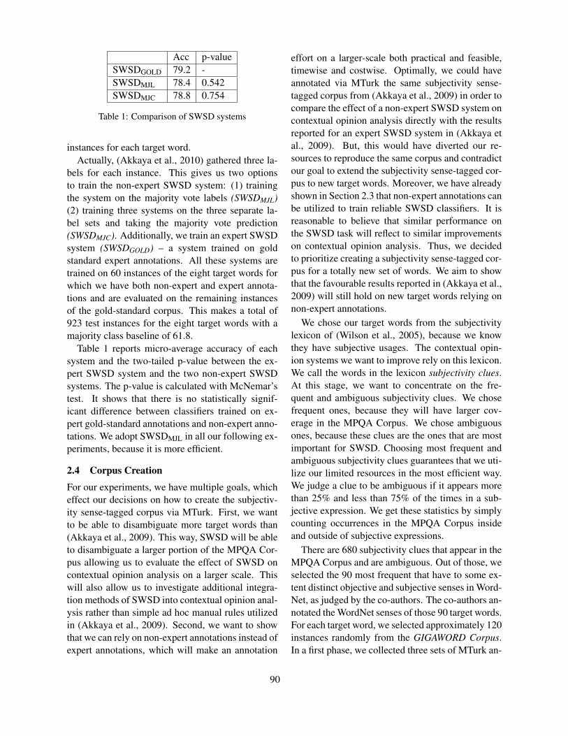
Acc p-valueSWSDGOLD 79.2 -SWSDMJL 78.4 0.542SWSDMJC 78.8 0.754

Table 1: Comparison of SWSD systems

instances for each target word.Actually, (Akkaya et al., 2010) gathered three la-

bels for each instance. This gives us two optionsto train the non-expert SWSD system: (1) trainingthe system on the majority vote labels (SWSDMJL)(2) training three systems on the three separate la-bel sets and taking the majority vote prediction(SWSDMJC). Additionally, we train an expert SWSDsystem (SWSDGOLD) – a system trained on goldstandard expert annotations. All these systems aretrained on 60 instances of the eight target words forwhich we have both non-expert and expert annota-tions and are evaluated on the remaining instancesof the gold-standard corpus. This makes a total of923 test instances for the eight target words with amajority class baseline of 61.8.

Table 1 reports micro-average accuracy of eachsystem and the two-tailed p-value between the ex-pert SWSD system and the two non-expert SWSDsystems. The p-value is calculated with McNemar’stest. It shows that there is no statistically signif-icant difference between classifiers trained on ex-pert gold-standard annotations and non-expert anno-tations. We adopt SWSDMJL in all our following ex-periments, because it is more efficient.

2.4 Corpus Creation

For our experiments, we have multiple goals, whicheffect our decisions on how to create the subjectiv-ity sense-tagged corpus via MTurk. First, we wantto be able to disambiguate more target words than(Akkaya et al., 2009). This way, SWSD will be ableto disambiguate a larger portion of the MPQA Cor-pus allowing us to evaluate the effect of SWSD oncontextual opinion analysis on a larger scale. Thiswill also allow us to investigate additional integra-tion methods of SWSD into contextual opinion anal-ysis rather than simple ad hoc manual rules utilizedin (Akkaya et al., 2009). Second, we want to showthat we can rely on non-expert annotations instead ofexpert annotations, which will make an annotation

effort on a larger-scale both practical and feasible,timewise and costwise. Optimally, we could haveannotated via MTurk the same subjectivity sense-tagged corpus from (Akkaya et al., 2009) in order tocompare the effect of a non-expert SWSD system oncontextual opinion analysis directly with the resultsreported for an expert SWSD system in (Akkaya etal., 2009). But, this would have diverted our re-sources to reproduce the same corpus and contradictour goal to extend the subjectivity sense-tagged cor-pus to new target words. Moreover, we have alreadyshown in Section 2.3 that non-expert annotations canbe utilized to train reliable SWSD classifiers. It isreasonable to believe that similar performance onthe SWSD task will reflect to similar improvementson contextual opinion analysis. Thus, we decidedto prioritize creating a subjectivity sense-tagged cor-pus for a totally new set of words. We aim to showthat the favourable results reported in (Akkaya et al.,2009) will still hold on new target words relying onnon-expert annotations.

We chose our target words from the subjectivitylexicon of (Wilson et al., 2005), because we knowthey have subjective usages. The contextual opin-ion systems we want to improve rely on this lexicon.We call the words in the lexicon subjectivity clues.At this stage, we want to concentrate on the fre-quent and ambiguous subjectivity clues. We chosefrequent ones, because they will have larger cov-erage in the MPQA Corpus. We chose ambiguousones, because these clues are the ones that are mostimportant for SWSD. Choosing most frequent andambiguous subjectivity clues guarantees that we uti-lize our limited resources in the most efficient way.We judge a clue to be ambiguous if it appears morethan 25% and less than 75% of the times in a sub-jective expression. We get these statistics by simplycounting occurrences in the MPQA Corpus insideand outside of subjective expressions.

There are 680 subjectivity clues that appear in theMPQA Corpus and are ambiguous. Out of those, weselected the 90 most frequent that have to some ex-tent distinct objective and subjective senses in Word-Net, as judged by the co-authors. The co-authors an-notated the WordNet senses of those 90 target words.For each target word, we selected approximately 120instances randomly from the GIGAWORD Corpus.In a first phase, we collected three sets of MTurk an-

90

notations for the selected instances. In this phase,MTurk workers base their judgements on two sensesets they observe. This way, we get training data tobuild SWSD classifiers for these 90 target words.

The quality of these classifiers is important, be-cause we will exploit them for contextual opinionanalysis. Thus, we evaluate them by 10-fold cross-validation. We split the target words into threegroups. If the majority class baseline of a word ishigher than 90%, it is considered as skewed (skewedwords have a performance at least as good as the ma-jority class baseline). If a target word improves overits majority class baseline by 25% in accuracy, it isconsidered as good. Otherwise, it is considered asmediocre. This way, we end up with 24 skewed, 35good, and 31 mediocre words. There are many pos-sible reasons for the less reliable performance forthe mediocre group. We hypothesize that a majorproblem is the similarity between the objective andsubjective sense sets of a word, thus leading to poorannotation quality. To check this, we calculate theagreement between three annotation sets and reportaverages. The agreement in the mediocre group is78.68%, with a κ value of 0.57, whereas the aver-age agreement in the good group is 87.51%, witha κ value of 0.75. These findings support our hy-pothesis. Thus, the co-authors created usage inven-tories for the words in the mediocre group as de-scribed in Section 2.1.1. We initiated a second phaseof MTurk annotations. We collect for the mediocregroup another three sets of MTurk annotations for120 instances, this time utilizing usage inventories.The 10-fold cross-validation experiments show thatnine of the 31 words in the mediocre group shift tothe good group. Only for these nine words, we ac-cept the annotations collected via usage inventories.For all other words, we use the annotations collectedvia sense inventories. From now on, we will referto this non-expert subjectivity sense-tagged corpusconsisting of the tagged data for all 90 target wordsas the MTurkSWSD Corpus (agreement on the entireMTurkSWSD corpus is 85.54%, κ:0.71).

3 SWSD Integration

Now that we have the MTurkSWSD Corpus, weare ready to evaluate the effect of SWSD on con-textual opinion analysis. In this section, we ap-ply our SWSD system trained on MTurkSWSD to

both expression-level classifiers from (Akkaya et al.,2009): (1) the subjective/objective (S/O) classifierand (2) the contextual polarity classifier. Both clas-sifiers are introduced in Section 3.1

Our SWSD system can disambiguate 90 targetwords, which have 3737 instances in the MPQACorpus. We refer to this subset of the MPQA Corpusas MTurkMPQA. This subset makes up the cover-age of our SWSD system. Note that MTurkMPQAis 5.2 times larger than the covered MPQA subsetin (Akkaya et al., 2009) referred as senMPQA. Wetry different strategies to integrate SWSD into thecontextual classifiers. In Section 3.2, we follow thesame rule-based strategy as in (Akkaya et al., 2009)for completeness. In Section 3.3, we introduce twonew learning strategies for SWSD integration out-performing existing rule-based strategy. We evalu-ate the improvement gained by SWSD on MTurkM-PQA.

3.1 Contextual Classifiers

The original contextual polarity classifier is intro-duced in (Wilson et al., 2005). We use the same im-plementation as in (Akkaya et al., 2009). This classi-fier labels clue instances in text as contextually neg-ative/positive/neutral. The gold standard is definedon the MPQA Corpus as follows. If a clue instanceappears in a positive expression, it is contextuallypositive (Ps). If it appears in a negative expression,it is contextually negative (Ng). If it is in an objec-tive expression or in a neutral subjective expression,it is contextually neutral (N). The contextual polar-ity classifier consists of two separate steps. The firststep is an expression-level neutral/polar (N/P) clas-sifier. The second step classifies only polar instancesfurther into positive and negative classes. This way,the overall system performs a three-way classifica-tion (Ng/Ps/N).

The subjective/objective classifier is introduced in(Akkaya et al., 2009). It relies on the same machinelearning features as the N/P classifier (i.e. the firststep of the contextual polarity classifier). The onlydifference is that the classes are S/O instead of N/P.The gold standard is defined on the MPQA Corpusin the following way. If a clue instance appears ina subjective expression, it is contextually S. If it ap-pears in an objective expression, it is contextually O.Both contextual classifiers are supervised.

91

Baseline Acc OF SF

MTurkMPQA 52.4% (O)OS/O 67.1 68.9 65.0R1R2 71.1 72.7 69.2

senMPQA 63.1% (O)OS/O 75.4 65.4 80.9R1R2 81.3 75.9 84.8

Table 2: S/O classifier with and without SWSD.

3.2 Rule-Based SWSD Integration

(Akkaya et al., 2009) integrates SWSD into a con-textual classifier by simple rules. The rules flip theoutput of the contextual classifier if some conditionshold. They make use of following information: (1)SWSD output, (2) the contextual classifier’s confi-dence and (3) the presence of another subjectivityclue – any clue from the subjectivity lexicon – in thesame expression.

For the contextual S/O classifier, (Akkaya et al.,2009) defines two rules: one flipping the S/O classi-fier’s output from O to S (R1) and one flipping fromS to O (R2). R1 is defined as follows : if the contex-tual classifier decides a target word instance is con-textually O and SWSD decides that it is used in a Ssense, then SWSD overrules the contextual S/O clas-sifier’s output and flips it from O to S, because aninstance in a S sense will make the surrounding ex-pression subjective. R2 is a little bit more complex.It is defined as follows: If the contextual classifier la-bels a clue instance as S but (1) SWSD decides thatit is used in an O sense, (2) the contextual classifier’sconfidence is low, and (3) there is no other subjec-tivity clue in the same expression, then R2 flips thecontextual classifier’s output from S to O. The ra-tionale behind R2 is that even if the target word in-stance has an O sense, there might be another reason(e.g. the presence of another subjectivity clue in thesame expression) for the expression enclosing it tobe subjective.

We use the exact same rules and adopt the sameconfidence threshold. Table 2 holds the comparisonof the original contextual classifier and the classi-fier with SWSD support on senMPQA as reported in(Akkaya et al., 2009) and on MTurkMPQA. OS/O isthe original S/O classifier; R1R2 is the system withSWSD support utilizing both rules. We report onlyR1R2, since (Akkaya et al., 2009) gets highest im-provement utilizing both rules.

Baseline Acc NF PF

MTurkMPQA 70.6% (P)ON/P 72.3 82.0 39.8R4 74.5 84.0 37.8

senMPQA 73.9% (P)ON/P 79.0 86.7 50.3R4 81.6 88.6 52.3

Table 3: N/P classifier with and without SWSD

In Table 2 we see that R1R2 achieves 4% percent-age points improvement in accuracy over OS/O onMTurkMPQA. The improvement is statistically sig-nificant at the p < .01 level with McNemar’s test. Itis accompanied with improvements both in subjec-tive F-measure (SF) and objective F-measure (OF).It is not possible to directly compare improvementson senMPQA and MTurkMPQA since they are dif-ferent subsets of the MPQA Corpus. SWSD supportbrings 24% error reduction on senMPQA over theoriginal S/O classifier. In comparison, on MTurkM-PQA, the error reduction is 12%. We see that the im-provements on the large MTurkMPQA set still hold,but not as strong as in (Akkaya et al., 2009).

(Akkaya et al., 2009) uses a similar rule tomake the contextual polarity classifier sense-aware.Specifically, the rule is applied to the output of thefirst step (N/P classifier). The rule, R4, flips P to Nand is analogous to R2. If the contextual classifierlabels a clue instance as P but (1) SWSD decidesthat it is used in an O sense, (2) the contextual clas-sifier’s confidence is low, and (3) there is no otherclue instance in the same expression, then R4 flipsthe contextual classifier’s output from P to N.

Table 3 holds the comparison of the original N/Pclassifier with and without SWSD support on sen-MPQA as reported in (Akkaya et al., 2009) and onMTurkMPQA. ON/P is the original N/P classifier; R4is the system with SWSD support utilizing rule R4.Since our main focus is not rule-based integration,we did not run the second step of the polarity classi-fier. We report the second step result below for thelearning-based SWSD integration in section 3.4.

In Table 3, we see that R4 achieves 2.2 percent-age points improvement in accuracy over ON/P onMTurkMPQA. The improvement is statistically sig-nificant at the p < .01 level with McNemar’s test.It is accompanied with improvement only in objec-tive F-measure (OF). SWSD support brings 12.4%error reduction on senMPQA (Akkaya et al., 2009).

92

On MTurkMPQA, the error reduction is 8%. We seethat the rule-based SWSD integration still improvesboth contextual classifiers on MTurkMPQA, but thegain is not as large as on senMPQA. This might bedue to the brittleness of the rule-based integration.

3.3 Learning SWSD IntegrationNow that we can disambiguate a larger portion ofthe MPQA Corpus than in (Akkaya et al., 2009),we can investigate machine learning methods forSWSD integration to deal with the brittleness of therule-based integration. In this section, we introducetwo learning methods to apply SWSD to the contex-tual classifiers. For the learning methods, we rely onexactly the same information as the rule-based inte-gration: (1) SWSD output, (2) the contextual clas-sifier’s output, (3) the contextual classifier’s confi-dence, and (4) the presence of another clue instancein the same expression. The rationale is the same asfor the rule-based integration, namely to relate sensesubjectivity and contextual subjectivity.

3.3.1 Method1In the first method, we extend the machine learn-

ing features of the underlying contextual classifiersby adding (1) and (4) from above. We evaluate theextended contextual classifiers on MTurkMPQA via10-fold cross-validation. Tables 4 and 5 hold thecomparison of Method1 (EXTS/O, EXTN/P) to theoriginal contextual classifiers (OS/O, ON/P) and to therule-based SWSD integration (R1R2, R4). We seesubstantial improvement for Method1. It achieves39% error reduction over OS/O and 25% error reduc-tion over ON/P. For both classifiers, the improvementin accuracy over the rule-based integration is statisti-cally significant at the p< .01 level with McNemar’stest.

3.3.2 Method2This method defines a third classifier that accepts

as input the contextual classifier’s output and theSWSD output and predicts what the contextual clas-sifier’s output should have been. We can think ofthis third classifier as the learning counterpart ofthe manual rules from Section 3.2, since it actu-ally learns when to flip the contextual classifier’soutput considering SWSD evidence. Specifically,this merger classifier relies on four machine learn-ing features (1), (2), (3), (4) from above (the ex-

Acc OF SFOS/O 67.1 68.9 65.0R1R2 71.1 72.7 69.2EXTS/O 80.0 81.4 78.3MERGERS/O 78.2 80.3 75.5

Table 4: S/O classifier with learned SWSD integration

Acc NF PFON/P 72.3 82.0 39.8R4 74.5 84.0 37.8EXTN/P 79.1 85.7 61.1MERGERN/P 80.4 86.7 62.8

Table 5: N/P classifier with learned SWSD integration

act same information used in rule-based integration).Because it is a supervised classifier, we need train-ing data where we have clue instances with cor-responding contextual classifier and SWSD predic-tions. Fortunately, we can use senMPQA for thispurpose. We train our merger classifier on senM-PQA (we get contextual classifier predictions via 10-fold cross-validation on the MPQA Corpus) and ap-ply it to MTurkMPQA. We use SVM classifier fromthe Weka package (Witten and Frank., 2005) withits default settings. Tables 4 and 5 hold the com-parison of Method2 (MERGERS/O, MERGERN/P) tothe original contextual classifiers (Oo/s, ON/P) andthe rule-based SWSD integration (R1R2, R4). Itachieves 29% error reduction over OS/O and 29% er-ror reduction over ON/P. The improvement on therule-based integration is statistically significant atthe p < .01 level with McNemar’s test. Method2performs better (statistically significant at the p <.05 level) than Method1 for the N/P classifier butworse (statistically significant at the p < .01 level)for the S/O classifier.

3.4 Improving Contextual PolarityClassification

We have seen that Method2 is the best method toimprove the N/P classifier, which is the first stepof the contextual polarity classifier. To assess theoverall improvement in polarity classification, werun the second step of the contextual polarity clas-sifier after correcting the first step with Method2.Table 6 summarizes the improvement propagated to

93

Acc NF NgF PsF

MTurkMPQAOPs/Ng/N 72.1 83.0 34.2 15.0MERGERN/P 77.8 87.4 53.0 27.7

senMPQAOPs/Ng/N 77.6 87.2 39.5 40.0R4 80.6 89.1 43.2 44.0

Table 6: Polarity classifier with and without SWSD.

Ps/Ng/N classification. For comparison, we alsoinclude results from (Akkaya et al., 2009) on sen-MPQA. Method2 results in 20% error reduction inaccuracy over OPs/Ng/N (R4 achieves 13.4% errorreduction on senMPQA). The improvement on therule-based integration is statistically significant atthe p < .01 level with McNemar’s test. More im-portantly, the F-measure for all the labels improves.This indicates that non-expert MTurk annotationscan replace expert annotations for our end-goal – im-proving contextual opinion analysis – while reduc-ing time and cost requirements by a large margin.Moreover, we see that the improvements in (Akkayaet al., 2009) scale up to new subjectivity clues.

4 Related Work

One related line of research is to automaticallyassign subjectivity and/or polarity labels to wordsenses in a dictionary (Valitutti et al., 2004; An-dreevskaia and Bergler, 2006; Wiebe and Mihalcea,2006; Esuli and Sebastiani, 2007; Su and Markert,2009). In contrast, the task in our paper is to auto-matically assign labels to word instances in a corpus.

Recently, some researchers have exploited fullword sense disambiguation in methods for opinion-related tasks. For example, (Martın-Wanton et al.,2010) exploit WSD for recognizing quotation polar-ities, and (Rentoumi et al., 2009; Martın-Wanton etal., 2010) exploit WSD for recognizing headline po-larities. None of this previous work investigates per-forming a coarse-grained variation of WSD such asSWSD to improve their application results, as we doin this work.

A notable exception is (Su and Markert, 2010),who exploit SWSD to improve the performance ona contextual NLP task, as we do. While the taskin our paper is subjectivity and sentiment analy-sis, their task is English-Chinese lexical substitu-tion. As (Akkaya et al., 2009) did, they anno-

tated word senses, and exploited SENSEVAL dataas training data for SWSD. They did not directly an-notate words in context with S/O labels, as we do inour work. Further, they did not separately evaluate aSWSD system component.

Many researchers work on reducing the granular-ity of sense inventories for WSD (e.g., (Palmer et al.,2004; Navigli, 2006; Snow et al., 2007; Hovy et al.,2006)). Their criteria for grouping senses are syn-tactic and semantic similarities, while the groupingsin work on SWSD are driven by the goals to improvecontextual subjectivity and sentiment analysis.


In this paper, we utilized a large pool of non-expertannotators (MTurk) to collect subjectivity sense-tagged data for SWSD. We showed that non-expertannotations are as good as expert annotations fortraining SWSD classifiers. Moreover, we demon-strated that SWSD classifiers trained on non-expertannotations can be exploited to improve contextualopinion analysis.

The additional subjectivity sense-tagged data en-abled us to evaluate the benefits of SWSD on con-textual opinion analysis on a corpus of opinion-annotated data that is five times larger. Using thesame rule-based integration strategies as in (Akkayaet al., 2009), we found that contextual opinion anal-ysis is improved by SWSD on the larger datasets.We also experimented with new learning strategiesfor integrating SWSD into contextual opinion analy-sis. With the learning strategies, we achieved greaterbenefits from SWSD than the rule-based integrationstrategies on all of the contextual opinion analysistasks.

Overall, we more firmly demonstrated the poten-tial of SWSD to improve contextual opinion analy-sis. We will continue to gather subjectivity sense-tagged data, using sense inventories for words thatare well represented in WordNet for our purposes,and with usage inventories for those that are not.

6 Acknowledgments

This material is based in part upon work supportedby National Science Foundation awards #0917170and #0916046.

94

ReferencesApoorv Agarwal, Fadi Biadsy, and Kathleen Mckeown.

2009. Contextual phrase-level polarity analysis us-ing lexical affect scoring and syntactic N-grams. InProceedings of the 12th Conference of the EuropeanChapter of the ACL (EACL 2009), pages 24–32. Asso-ciation for Computational Linguistics.

Cem Akkaya, Janyce Wiebe, and Rada Mihalcea. 2009.Subjectivity word sense disambiguation. In Proceed-ings of the 2009 Conference on Empirical Methods inNatural Language Processing, pages 190–199, Singa-pore, August. Association for Computational Linguis-tics.

Cem Akkaya, Alexander Conrad, Janyce Wiebe, andRada Mihalcea. 2010. Amazon mechanical turk forsubjectivity word sense disambiguation. In Proceed-ings of the NAACL HLT 2010 Workshop on CreatingSpeech and Language Data with Amazon’s Mechani-cal Turk, pages 195–203, Los Angeles, June. Associa-tion for Computational Linguistics.

Alina Andreevskaia and Sabine Bergler. 2006. Miningwordnet for a fuzzy sentiment: Sentiment tag extrac-tion from wordnet glosses. In Proceedings of the 11rdConference of the European Chapter of the Associa-tion for Computational Linguistics (EACL-2006).

Alina Andreevskaia and Sabine Bergler. 2008. Whenspecialists and generalists work together: Overcom-ing domain dependence in sentiment tagging. In Pro-ceedings of ACL-08: HLT, pages 290–298, Columbus,Ohio, June. Association for Computational Linguis-tics.

Kenneth Bloom, Navendu Garg, and Shlomo Argamon.2007. Extracting appraisal expressions. In HLT-NAACL 2007, pages 308–315, Rochester, NY.

Andrea Esuli and Fabrizio Sebastiani. 2007. Pagerank-ing wordnet synsets: An application to opinion min-ing. In Proceedings of the 45th Annual Meeting ofthe Association of Computational Linguistics, pages424–431, Prague, Czech Republic, June. Associationfor Computational Linguistics.

Yaw Gyamfi, Janyce Wiebe, Rada Mihalcea, and CemAkkaya. 2009. Integrating knowledge for subjectiv-ity sense labeling. In Proceedings of Human Lan-guage Technologies: The 2009 Annual Conference ofthe North American Chapter of the Association forComputational Linguistics (NAACL-HLT 2009), pages10–18, Boulder, Colorado, June. Association for Com-putational Linguistics.

E. Hovy, M. Marcus, M. Palmer, L. Ramshaw, andR. Weischedel. 2006. Ontonotes: The 90% solution.In Proceedings of the Human Language TechnologyConference of the NAACL, Companion Volume: ShortPapers, New York City.

Soo-Min Kim and Eduard Hovy. 2004. Determining thesentiment of opinions. In Proceedings of the Twen-tieth International Conference on Computational Lin-guistics (COLING 2004), pages 1267–1373, Geneva,Switzerland.

Tamara Martın-Wanton, Aurora Pons-Porrata, AndresMontoyo-Guijarro, and Alexandra Balahur. 2010.Opinion polarity detection - using word sense disam-biguation to determine the polarity of opinions. InICAART 2010 - Proceedings of the International Con-ference on Agents and Artificial Intelligence, Volume1, pages 483–486.

R. Navigli. 2006. Meaningful clustering of senses helpsboost word sense disambiguation performance. InProceedings of the Annual Meeting of the Associationfor Computational Linguistics, Sydney, Australia.

M. Palmer, O. Babko-Malaya, and H. T. Dang. 2004.Different sense granularities for different applications.In HLT-NAACL 2004 Workshop: 2nd Workshop onScalable Natural Language Understanding, Boston,Massachusetts.

Randolph Quirk, Sidney Greenbaum, Geoffry Leech, andJan Svartvik. 1985. A Comprehensive Grammar of theEnglish Language. Longman, New York.

Vassiliki Rentoumi, George Giannakopoulos, VangelisKarkaletsis, and George A. Vouros. 2009. Sentimentanalysis of figurative language using a word sensedisambiguation approach. In Proceedings of the In-ternational Conference RANLP-2009, pages 370–375,Borovets, Bulgaria, September. Association for Com-putational Linguistics.

Ellen Riloff and Janyce Wiebe. 2003. Learning extrac-tion patterns for subjective expressions. In Proceed-ings of the Conference on Empirical Methods in Natu-ral Language Processing (EMNLP-2003), pages 105–112, Sapporo, Japan.

R. Snow, S. Prakash, D. Jurafsky, and A. Ng. 2007.Learning to merge word senses. In Proceedings ofthe Joint Conference on Empirical Methods in Natu-ral Language Processing and Computational NaturalLanguage Learning (EMNLP-CoNLL), Prague, CzechRepublic.

Fangzhong Su and Katja Markert. 2008. From wordto sense: a case study of subjectivity recognition. InProceedings of the 22nd International Conference onComputational Linguistics (COLING-2008), Manch-ester.

Fangzhong Su and Katja Markert. 2009. Subjectivityrecognition on word senses via semi-supervised min-cuts. In Proceedings of Human Language Technolo-gies: The 2009 Annual Conference of the North Ameri-can Chapter of the Association for Computational Lin-guistics, pages 1–9, Boulder, Colorado, June. Associ-ation for Computational Linguistics.

95

Fangzhong Su and Katja Markert. 2010. Word sensesubjectivity for cross-lingual lexical substitution. InHuman Language Technologies: The 2010 AnnualConference of the North American Chapter of the As-sociation for Computational Linguistics, pages 357–360, Los Angeles, California, June. Association forComputational Linguistics.

Peter Turney. 2002. Thumbs up or thumbs down? Se-mantic orientation applied to unsupervised classifica-tion of reviews. In Proceedings of the 40th AnnualMeeting of the Association for Computational Linguis-tics (ACL-02), pages 417–424, Philadelphia, Pennsyl-vania.

Alessandro Valitutti, Carlo Strapparava, and OlivieroStock. 2004. Developing affective lexical resources.PsychNology, 2(1):61–83.

Casey Whitelaw, Navendu Garg, and Shlomo Argamon.2005. Using appraisal taxonomies for sentiment anal-ysis. In Proceedings of CIKM-05, the ACM SIGIRConference on Information and Knowledge Manage-ment, Bremen, DE.

Janyce Wiebe and Rada Mihalcea. 2006. Word senseand subjectivity. In Proceedings of the 21st Interna-tional Conference on Computational Linguistics and44th Annual Meeting of the Association for Compu-tational Linguistics, pages 1065–1072, Sydney, Aus-tralia, July. Association for Computational Linguistics.

Janyce Wiebe, Theresa Wilson, and Claire Cardie. 2005.Annotating expressions of opinions and emotionsin language. Language Resources and Evaluation,39(2/3):164–210.

Theresa Wilson, Janyce Wiebe, and Paul Hoffmann.2005. Recognizing contextual polarity in phrase-level sentiment analysis. In Proceedings of the Hu-man Language Technologies Conference/Conferenceon Empirical Methods in Natural Language Process-ing (HLT/EMNLP-2005), pages 347–354, Vancouver,Canada.

Theresa Wilson. 2007. Fine-grained Subjectivity andSentiment Analysis: Recognizing the Intensity, Polar-ity, and Attitudes of private states. Ph.D. thesis, Intel-ligent Systems Program, University of Pittsburgh.

I. Witten and E. Frank. 2005. Data Mining: PracticalMachine Learning Tools and Techniques, Second Edi-tion. Morgan Kaufmann, June.

Hong Yu and Vasileios Hatzivassiloglou. 2003. Towardsanswering opinion questions: Separating facts fromopinions and identifying the polarity of opinion sen-tences. In Proceedings of the Conference on EmpiricalMethods in Natural Language Processing (EMNLP-2003), pages 129–136, Sapporo, Japan.

96


Effects of Meaning-Preserving Corrections on Language Learning

Dana Angluin ∗

Department of Computer ScienceYale University, USA

[email protected]

Leonor Becerra-BonacheLaboratoire Hubert Curien

Universite de Saint-Etienne, [email protected]

Abstract

We present a computational model of lan-guage learning via a sequence of interactionsbetween a teacher and a learner. Experimentslearning limited sublanguages of 10 naturallanguages show that the learner achieves ahigh level of performance after a reasonablenumber of interactions, the teacher can pro-duce meaning-preserving corrections of thelearner’s utterances, and the learner can de-tect them. The learner does not treat correc-tions specially; nonetheless in several cases,significantly fewer interactions are needed bya learner interacting with a correcting teacherthan with a non-correcting teacher.

1 Introduction

A child learning his or her native language typicallydoes so while interacting with other people who areusing the language to communicate in shared situ-ations. The correspondence between situations andutterances seems likely to be a very important sourceof information for the language learner. Once achild begins to produce his or her own utterances,other people’s responses to them (or lack thereof)are another source of information about the lan-guage. When the child’s utterances fall short ofadult-level competence, sometimes the other personin the conversation will repeat the child’s utterancein a more correct form. A number of studies havefocused on the phenomenon of such corrections andquestions of their frequency in child-directed speech

∗Research supported by the National Science Foundation,Grant CCF-0916389.

and whether children can and do make use of them;some of these studies are discussed in the next sec-tion.

In this paper we construct a computational modelwith a learner and a teacher who interact in a se-quence of shared situations. In each situation theteacher and learner interact as follows. First thelearner uses what it has learned about the languageto (attempt to) generate an utterance appropriate tothe situation. The teacher then analyzes the correct-ness of the learner’s utterance and either generatesan utterance intended as a correction of the learner’sutterance, or generates another utterance of its ownappropriate to the situation. Finally, the learner usesinformation given by its own utterance, the teacher’sutterance and the situation to update its knowledgeof the language. At the conclusion of this interac-tion, a new interaction is begun with the next situa-tion in the sequence.

Both the learner and the teacher engage in com-prehension and production of utterances which areintended to be appropriate to their shared situation.This setting allows us to study several questions:whether the teacher can offer meaningful correc-tions to the learner, whether the learner can detectintended corrections by the teacher, and whether thepresence of corrections by the teacher has an ef-fect on language acquisition by the learner. For ourmodel, the answer to each of these questions is yes,and while the model is in many respects artificial andsimplified, we believe it sheds new light on these is-sues. Additional details are available (Angluin andBecerra-Bonache, 2010).

97

2 Meaning-preserving corrections

Formal models of language acquisition have mainlyfocused on learning from positive data, that is, utter-ances that are grammatically correct. But a questionthat remains open is: Do children receive negativedata and can they make use of it?

Chomsky’s poverty of stimulus argument hasbeen used to support the idea of human innate lin-guistic capacity. It is claimed that there are princi-ples of grammar that cannot be learned from positivedata only, and negative evidence is not available tochildren. Hence, since children do not have enoughevidence to induce the grammar of their native lan-guage, the additional knowledge language learnersneed is provided by some form of innate linguisticcapacity.

E. M. Gold’s negative results in the frameworkof formal language learning have also been used tosupport the innateness of language. Gold provedthat superfinite classes of languages are not learn-able from positive data only, which implies thannone of the language classes defined by Chomskyto model natural language is learnable from positivedata only (Gold, 1967).

Brown and Hanlon (Brown and Hanlon, 1970)studied negative evidence understood as explicitapprovals or disapprovals of a child’s utterance(e.g.,“That’s right” or “That’s wrong.”) Theyshowed that there is no dependence between thesekinds of answers and the grammaticality of chil-dren’s utterances. These results were taken as show-ing that children do not receive negative data. Butdo these results really show this? It seems evidentthat parents rarely address their children in that way.During the first stages of language acquisition chil-dren make a lot of errors, and parents are not con-stantly telling them that their sentences are wrong;rather the important thing is that they can communi-cate with each other. However, it is worth studyingwhether other sources of negative evidence are pro-vided to children. Is this the only form of negativedata? Do adults correct children in a different way?

Some researchers have studied other kinds ofnegative data based on reply-types (e.g., Hirsh-Pasek et al. (Hirsh-Pasek et al., 1984), Demetraset al. (Demetras et al., 1986) and Morgan andTravis (Morgan and Travis, 1989).) These studies

argue that parents provide negative evidence to theirchildren by using different types of reply to gram-matical versus ungrammatical sentences. Marcusanalyzed such studies and concluded that there isno evidence that this kind of feedback (he called itnoisy feedback) is required for language learning,or even that it exists (Marcus, 1993). He arguedfor the weakness, inconsistency and inherently ar-tificial nature of this kind of feedback. Moreover, hesuggested that even if such feedback exists, a childwould learn which forms are erroneous only aftercomplex statistical comparisons. Therefore, he con-cluded that internal mechanisms are necessary to ex-plain how children recover from errors in languageacquisition.

Since the publication of the work of Marcus, theconsensus seemed to be that children do not have ac-cess to negative data. However, a study carried outby Chouinard and Clark shows that this conclusionmay be wrong (Chouinard and Clark, 2003). First,they point out that the reply-type approach does notconsider whether the reply itself also contains cor-rective information, and consequently, replies thatare corrective are erroneously grouped with thosethat are not. Moreover, if we consider only reply-types, they may not help to identify the error made.Hence, Chouinard and Clark propose another viewof negative evidence that builds on Clark’s principleof contrast (Clark, 1987; Clark, 1993). Parents oftencheck up on a child’s erroneous utterances, to makesure they have understood them. They do this byreformulating what they think the child intended toexpress. Hence, the child’s utterance and the adult’sreformulation have the same meaning, but differentforms. Because children attend to contrasts in form,any change in form that does not mark a differentmeaning will signal to children that they may haveproduced an utterance that is not acceptable in thetarget language. In this way, reformulations iden-tify the locus of any error, and hence the existenceof an error. Chouinard and Clark analyze longitu-dinal data from five children between two and fouryears old, and show that adults reformulate erro-neous child utterances often enough to help learn-ing. Moreover, these results show that children notonly detect differences between their own utteranceand the adult reformulation, but that they make useof that information.

98

In this paper we explore this new view of nega-tive data proposed by Chouinard and Clark. Cor-rections (in form of reformulations) have a semanticcomponent that has not been taken into account inprevious studies. Hence, we propose a new com-putational model of language learning that gives anaccount of meaning-preserving corrections, and inwhich we can address questions such as: What arethe effects of corrections on learning syntax? Cancorrections facilitate the language learning process?

3 The Model

We describe the components of our model, and giveexamples drawn from the primary domain we haveused to guide the development of the model.

3.1 Situation, meanings and utterances.

A situation is composed of some objects and someof their properties and relations, which pick outsome aspects of the world of joint interest to theteacher and learner. A situation is represented as aset of ground atoms over some constants (denotingobjects) and predicates (giving properties of the ob-jects and relations between them.) For example, asituation s1 consisting of a big purple circle to theleft of a big red star is represented by the follow-ing set of ground atoms: s1 = {bi1 (t1), pu1 (t1),ci1 (t1), le2 (t1, t2), bi1 (t2), re1 (t2), st1 (t2)}.

Formally, we have a finite set P of predicatesymbols, each of a specific arity. We also have aset of constant symbols t1, t2, . . ., which are usedto represent distinct objects. A ground atom is anexpression formed by applying a predicate symbolto the correct number of constant symbols as argu-ments.

We also have a set of of variables x1, x2, . . .. Avariable atom is an expression formed by applyinga predicate symbol to the correct number of vari-ables as arguments. A meaning is a finite sequenceof variable atoms. Note that the atoms do not con-tain constants, and the order in which they appear issignificant. A meaning is supported in a situation ifthere exists a support witness, that is, a mapping ofits variables to distinct objects in the situation suchthat the image under the mapping of each atom inthe meaning appears in the situation. If a meaning issupported in a situation by a unique support witness

then it is denoting in the situation. We assume thatboth the teacher and learner can determine whethera meaning is denoting in a situation.

We also have a finite alphabet W of words. Anutterance is a finite sequence of words. The tar-get language is the set of utterances the teacher mayproduce in some situation; in our examples, this in-cludes utterances like the star or the star to the rightof the purple circle but not star of circle small thegreen. We assume each utterance in the target lan-guage is assigned a unique meaning. An utteranceis denoting in a situation if the meaning assignedto utterance is denoting in the situation. Intuitively,an utterance is denoting if it uniquely picks out theobjects it refers to in a situation.

In our model the goal of the learner is to be ableto produce every denoting utterance in any given sit-uation. Our model is probabilistic, and what we re-quire is that the probability of learner errors be re-duced to very low levels.

3.2 The target language and meaningtransducers.

We represent the linguistic competence of theteacher by a finite state transducer that both recog-nizes the utterances in the target language and trans-lates each correct utterance to its meaning. Let Adenote the set of all variable atoms over P . We de-fine a meaning transducer M with input symbolsW and output symbols A as follows. M has a fi-nite set Q of states, an initial state q0 ∈ Q, a finiteset F ⊆ Q of final states, a deterministic transitionfunction δ mappingQ×W toQ, and an output func-tion γ mapping Q×W to A∪ {ε}, where ε denotesthe empty sequence.

The transition function δ is extended in the usualway to δ(q, u). The language of M , denoted L(M)is the set of all utterances u ∈ W ∗ such thatδ(q0, u) ∈ F . For each utterance u, we defineM(u)to be the meaning of u, that is, the finite sequence ofnon-empty outputs produced by M in processing u.Fig. 1 shows a meaning transducer M1 for a limitedsublanguage of Spanish. M1 assigns the utterance eltriangulo rojo the meaning (tr1 (x1), re1 (x1)).

3.3 The learning task.Initially the teacher and learner know the predicatesP and are able to determine whether a meaning is

99

a / !

0 1 2

6

3 4

el / !

circulo / ci1(x1)

cuadrado / sq1(x1)

triangulo / tr1(x1)

encima / ab2(x1,x2)

a / ! la / !

5

izquierda / le2(x1,x2)

derecha / le2(x2,x1)

rojo / re1(x1)

verde / gr1(x1)

azul / bl1(x1)

encima / ab2(x1,x2)

7

del / !

8 9 circulo / ci1(x2)

cuadrado / sq1(x2)

triangulo / tr1(x2)

rojo / re1(x2)

verde / gr1(x2)

azul / bl1(x2)

Figure 1: Meaning transducer M1.

denoting in a situation. The learner and teacher bothalso know a shared set of categories that classify asubset of the predicates into similarity groups. Thecategories facilitate generalization by the learnerand analysis of incorrect learner utterances by theteacher. In our geometric shape domain the cate-gories are shape, size, and color; there is no categoryfor the positional relations. Initially the teacher alsohas the meaning transducer for the target language,but the learner has no language-specific knowledge.

4 The Interaction of Learner and Teacher

In one interaction of the learner and teacher, a newsituation is generated and presented to both of them.The learner attempts to produce a denoting utter-ance for the situation, and the teacher analyzes thelearner’s utterance and decides whether to producea correction of the learner’s utterance or a new de-noting utterance of its own. Finally, the learner usesthe situation and the teacher’s utterance to update itscurrent grammar for the language.

In this section we describe the algorithms used bythe learner and teacher to carry out the steps of thisprocess.

4.1 Comprehension and the co-occurrencegraph.

To process the teacher’s utterance, the learnerrecords the words in the utterance and the predi-cates in the situation in an undirected co-occurrencegraph. Each node is a word or predicate symbol andthere is an edge for each pair of nodes. Each node uhas an occurrence count, c(u), recording the numberof utterances or situations it has occurred in. Each

edge (u, v) also has an occurrence count, c(u, v),recording the number of utterance/situation pairs inwhich the endpoints of the edge have occurred to-gether. From the co-occurrence graph the learner de-rives a directed graph with the same nodes, the im-plication graph, parameterized by a noise thresholdθ (set at 0.95 in the experiments.) For each orderedpair of nodes u and v, the directed edge (u, v) is in-cluded in the implication graph if c(u, v)/c(u) ≥ θ.The learner then deletes edges from predicates towords and computes the transitively reduced im-plication graph.

The learner uses the transitively reduced implica-tion graph to try to find the meaning of the teacher’sutterance by translating the words of the utteranceinto a set of sequences of predicates, and determin-ing if there is a unique denoting meaning corre-sponding to one of the predicate sequences. If so, theunique meaning is generalized into a general formby replacing each predicate by its category gener-alization. For example, if the learner detects theunique meaning (tr1 (x1), re1 (x1)), it is general-ized to the general form (shape1 (x1), color1 (x1)).The learner’s set of general forms is the basis for itsproduction.

4.2 Production by the learner.

Each general form denotes the set of possible mean-ings obtained by substituting appropriate symbolsfrom P for the category symbols. To produce a de-noting utterance for a situation, the learner finds allthe meanings generated by its general forms usingpredicates from the situation and tests each meaningto see if it is denoting, producing a set of possible de-noting meanings. If the set is empty, the learner pro-duces no utterance. Otherwise, it attempts to trans-late each denoting meaning into an utterance.

The learner selects one of these utterances witha probability depending on a number stored withthe corresponding general form recording the lasttime a teacher utterance matched it. This ensuresthat repeatedly matched general forms are selectedwith asymptotically uniform probability, while gen-eral forms that are only matched a few times are se-lected with probability tending to zero.

100

4.3 From meaning to utterance.

The process the learner uses to produce an utter-ance from a denoting meaning is as follows. Fora meaning that is a sequence of k atoms, there aretwo related sequences of positions: the atom posi-tions 1, 2, . . . , k and the gap positions 0, 1, . . . , k.The atom positions refer to the corresponding atoms,and gap position i refers to the position to the rightof atom i, (where gap position 0 is to the left of atoma1.) The learner generates a sequence of zero ormore words for each position in left to right order:gap position 0, atom position 1, gap position 1, atomposition 2, and so on, until gap position k. The re-sulting sequences of words are concatenated to formthe final utterance.

The choice of what sequence of words to pro-duce for each position is represented by a decisiontree. For each variable atom the learner has en-countered, there is a decision tree that determineswhat sequence of words to produce for that atomin the context of the whole meaning. For exam-ple, in a sublanguage of Spanish in which there areboth masculine and feminine nouns for shapes, theatom re1 (x1) has a decision tree that branches onthe value of the shape predicate applied to x1 to se-lect either rojo or roja as appropriate. For the gappositions, there are decision trees indexed by thegeneralizations of all the variable atoms that haveoccurred; the variable atom at position i is general-ized, and the corresponding decision tree is used togenerate a sequence of words for gap position i. Gapposition 0 does not follow any atom position and hasa separate decision tree.

If there is no decision tree associated with a givenatom or gap position in a meaning, the learner fallsback on a “telegraphic speech” strategy. For a gapposition with no decision tree, no words are pro-duced. For an atom position whose atom has no as-sociated decision tree, the learner searches the tran-sitively reduced implication graph for words thatapproximately imply the predicate of the atom andchooses one of maximum observed frequency.

4.4 The teacher’s response.

If the learner produces an utterance, the teacher an-alyzes it and then chooses its own utterance for thesituation. The teacher may find the learner’s utter-

ance correct, incorrect but correctable, or incorrectand uncorrectable. If the learner’s utterance is in-correct but correctable, the teacher chooses a pos-sible correction for it. The teacher randomly de-cides whether or not to use the correction as its ut-terance according to the correction probability. Ifthe teacher does not use the correction, then its ownutterance is chosen uniformly at random from thedenoting utterances for the situation.

If the learner’s utterance is one of the correct de-noting utterances for the situation, the teacher clas-sifies it as correct. If the learner’s utterance isnot correct, the teacher “translates” the learner’s ut-terance into a sequence of predicates by using themeaning transducer for the language. If the result-ing sequence of predicates corresponds to a denot-ing meaning, the learner’s utterance is classified ashaving an error in form. The correction is cho-sen by considering the denoting utterances with thesame sequence of predicates as the learner’s utter-ance, and choosing one that is “most similar” to thelearner’s utterance. For example, if the learner’s ut-terance was el elipse pequeno and (el1 , sm1 ) cor-responds to a denoting utterance for the situation,the teacher chooses la elipse pequena as the cor-rection. If the learner’s utterance is neither correctnor an error in form, the teacher uses a measure ofsimilarity between the learner’s sequence of predi-cates and those of denoting utterances to determinewhether there is a “close enough” match. If so, theteacher classifies the learner’s utterance as havingan error in meaning and chooses as the possiblecorrection a denoting utterance whose predicate se-quence is “most similar” to the learner’s predicatesequence. If the learner produces an utterance andnone of these cases apply, then the teacher classifiesthe learner’s utterance as uninterpretable and doesnot offer a correction.

When the teacher has produced an utterance, thelearner analyzes it and updates its grammar of thelanguage as reflected in the co-occurrence graph,the general forms, and the decision trees for wordchoice. The decision trees are updated by comput-ing an alignment between the teacher’s utterance andthe learner’s understanding of the teacher’s meaning,which assigns a subsequence of words from the ut-terance to each atom or gap position in the meaning.Each subsequence of words is then added to the data

101

for the decision tree corresponding to the position ofthat subsequence.

If the learner has produced an utterance and findsthat the teacher’s utterance has the same meaning,but is expressed differently, then the learner classi-fies the teacher’s utterance as a correction. In thecurrent model, the learner reports this classification,but does not use it in any way.

5 Empirical Results

We have implemented and tested our learning andteaching procedures in order to explore questionsabout the roles of corrections in language learning.We have used a simplified version of the MiniatureLanguage Acquisition task proposed by Feldman etal. (Feldman et al., 1990). Although this task is notas complex as those faced by children, it involvesenough complexity to be compared to many real-word tasks.

The questions that we address in this section arethe following. (1) Can the learner accomplish thelearning task to a high level of correctness and cov-erage from a “reasonable” number of interactions(that is, well short of the number needed to memo-rize every legal situation/sentence pair)? (2) Whatare the effects of correction or non-correction bythe teacher on the learner’s accomplishment of thelearning tasks?

5.1 The specific learning tasks.

Each situation has two objects, each with three at-tributes (shape, color and size), and one binary rela-tion between the two objects (above or to the left of.)The attribute of shape has six possible values (cir-cle, square, triangle, star, ellipse, and hexagon), thatof color has six possible values (red, orange, yellow,green, blue, and purple), and that of size three possi-ble values (big, medium, and small.) There are 108distinct objects and 23,328 distinct situations. Situ-ations are generated uniformly at random.

For several natural languages we construct a lim-ited sublanguage of utterances related to these situ-ations. A typical utterance in English is the mediumpurple star below the small hexagon. There are 168meanings referring to a single object and 112,896meanings referring to two objects, for a total of113,064 possible meanings. The 113,064 possible

meanings are instances of 68 general forms: 4 refer-ring to a single object and 64 referring to two ob-jects. These languages are the 68-form languages.

We consulted at least one speaker of each lan-guage to help us construct a meaning transducer totranslate appropriate phrases in the language to all113,064 possible meanings. Each transducer wasconstructed to have exactly one accepted phrase foreach possible meaning. We also constructed trans-ducers for reduced sublanguages, consisting of thesubset of utterances that refer to a single object (168utterances) and those that refer to two objects, but in-clude all three attributes of both (46,656 utterances.)Each meaning in the reduced sublanguage is an in-stance of one of 8 general forms, while most of thelexical and syntactic complexity of the 68-form lan-guage is preserved. We refer to these reduced sub-languages as the 8-form languages.

5.2 How many interactions are needed tolearn?

The level of performance of a learner is measuredusing two quantities: the correctness and complete-ness of the learner’s utterances in a given situation.The learning procedure has a test mode in which thelearner receives a situation and responds with theset of U utterances it could produce in that situa-tion, with their corresponding production probabili-ties. The correctness of the learner is the sum of theproduction probabilities of the elements of U thatare in the correct denoting set. The completenessof the learner is the fraction of all correct denotingutterances that are in U . The averages of correct-ness and completeness of the learner for 200 ran-domly generated situations are used to estimate theoverall correctness and completeness of the learner.A learner reaches a level p of performance if bothcorrectness and completeness are at least p.

In the first set of trials the target level of per-formance is 0.99 and the learner and teacher en-gage in a sequence of interactions until the learnerfirst reaches this level of performance. The perfor-mance of the learner is tested at intervals of 100 in-teractions. Fig. 2 shows the number of interactionsneeded to reach the 0.99 level of performance foreach 68-form language with correction probabilitiesof 0.0 (i.e., the teacher never corrects the learner)and 1.0 (i.e., the teacher offers a correction to the

102

learner every time it classifies the learner’s utteranceas an error in form or an error in meaning.) Forcorrection probability 1.0, it also shows the numberof incorrect utterances by the learner, the number ofcorrections offered by the teacher, and the percent-age of teacher utterances that were corrections. Eachentry is the median value of 10 trials except those inthe last column. It is worth noting that the learnerdoes not treat corrections specially.

0.0 1.0 incorrect corrections c/u%English 700 750 25.0 11.5 1.5%German 800 750 71.5 52.5 7.0%Greek 3400 2600 344.0 319.0 12.3%Hebrew 900 900 89.5 62.5 6.9%Hungarian 750 800 76.5 58.5 7.3%Mandarin 700 800 50.0 31.5 3.9%Russian 3700 2900 380.0 357.0 12.3%Spanish 1000 850 86.0 68.0 8.0%Swedish 1000 900 54.0 43.5 4.8%Turkish 800 900 59.0 37.0 4.1%

Figure 2: Interactions, incorrect learner utterances andcorrections by the teacher to reach the 0.99 level of per-formance for 68-form languages.

In the column for correction probability 0.0 thereare two clear groups: Greek and Russian, each withat least 3400 interactions and the rest of the lan-guages, each with at most 1000 interactions. Thefirst observation is that the learner achieves correct-ness and completeness of 0.99 for each of these lan-guages after being exposed to a small fraction of allpossible situations and utterances. Even 3700 inter-actions involve at most 16.5% of all possible situa-tions and at most 3.5% of all possible utterances bythe teacher, while 1000 interactions involve fewerthan 4.3% of all situations and fewer than 1% of allpossible utterances.

5.3 How do corrections affect learning?

In the column for correction probability 1.0 we seethe same two groups of languages. For Greek, thenumber of interactions falls from 3400 to 2600, adecrease of about 24%. For Russian, the number ofinteractions falls from 3700 to 2900, a decrease ofabout 21%. Corrections have a clear positive effectin these trials for Greek and Russian, but not for therest of the languages.

Comparing the numbers of incorrect learner utter-ances and the number of corrections offered by the

teacher, we see that the teacher finds corrections fora substantial fraction of incorrect learner utterances.The last column of Fig. 2 shows the percentage ofthe total number of teacher utterances that were cor-rections, from a low of 1.5% to a high of 12.3%.

There are several processes at work in the im-provement of the learner’s performance. Compre-hension improves as more information accumulatesabout words and predicates. New correct generalforms are acquired, and unmatched incorrect gen-eral forms decrease in probability. More data im-proves the decision tree rules for choosing phrases.Attainment of the 0.99 level of performance may belimited by the need to acquire all the correct generalforms or by the need to improve the correctness ofthe phrase choices.

In the case of Greek and Russian, most of the tri-als had acquired their last general form by the timethe 0.90 level of performance was reached, but forthe other languages correct general forms were stillbeing acquired between the 0.95 and the 0.99 lev-els of performance. Thus the acquisition of gen-eral forms was not a bottleneck for Greek and Rus-sian, but was for the other languages. Because theteacher’s corrections generally do not help with theacquisition of new general forms (the general formin a correction is often the same one the learnerjust used), but do tend to improve the correctnessof phrase choice, we do not expect correction to re-duce the number of interactions to attain the 0.99level of performance when the bottleneck is the ac-quisition of general forms. This observation led usto construct reduced sublanguages with just 8 gen-eral forms to see if correction would have more ofan effect when the bottleneck of acquiring generalforms was removed.

The reduced sublanguages have just 8 generalforms, which are acquired relatively early. Fig. 3gives the numbers of interactions to reach the 0.99level of performance (except for Turkish, where thelevel is 0.95) for the 8-form sublanguages with cor-rection probability 0.0 and 1.0. These numbers arethe means of 100 trials (except for Greek and Rus-sian, which each had 20 trials); the performance ofthe learner was tested every 50 interactions.

Comparing the results for 8-form sublanguageswith corresponding 68-form languages, we see thatsome require notably fewer interactions for 8-form

103

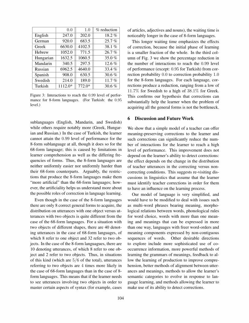
0.0 1.0 % reductionEnglish 247.0 202.0 18.2 %German 920.0 683.5 25.7 %Greek 6630.0 4102.5 38.1 %Hebrew 1052.0 771.5 26.7 %Hungarian 1632.5 1060.5 35.0 %Mandarin 340.5 297.5 12.6 %Russian 6962.5 4640.0 33.4 %Spanish 908.0 630.5 30.6 %Swedish 214.0 189.0 11.7 %Turkish 1112.0* 772.0* 30.6 %

Figure 3: Interactions to reach the 0.99 level of perfor-mance for 8-form languages. (For Turkish: the 0.95level.)

sublanguages (English, Mandarin, and Swedish)while others require notably more (Greek, Hungar-ian and Russian.) In the case of Turkish, the learnercannot attain the 0.99 level of performance for the8-form sublanguage at all, though it does so for the68-form language; this is caused by limitations inlearner comprehension as well as the differing fre-quencies of forms. Thus, the 8-form languages areneither uniformly easier nor uniformly harder thantheir 68-form counterparts. Arguably, the restric-tions that produce the 8-form languages make them“more artificial” than the 68-form languages; how-ever, the artificiality helps us understand more aboutthe possible roles of correction in language learning.

Even though in the case of the 8-form languagesthere are only 8 correct general forms to acquire, thedistribution on utterances with one object versus ut-terances with two objects is quite different from thecase of the 68-form languages. For a situation withtwo objects of different shapes, there are 40 denot-ing utterances in the case of 68-form languages, ofwhich 8 refer to one object and 32 refer to two ob-jects. In the case of the 8-form languagues, there are10 denoting utterances, of which 8 refer to one ob-ject and 2 refer to two objects. Thus, in situationsof this kind (which are 5/6 of the total), utterancesreferring to two objects are 4 times more likely inthe case of 68-form languages than in the case of 8-form languages. This means that if the learner needsto see utterances involving two objects in order tomaster certain aspects of syntax (for example, cases

of articles, adjectives and nouns), the waiting time isnoticeably longer in the case of 8-form languages.

This longer waiting time emphasizes the effectsof correction, because the initial phase of learningis a smaller fraction of the whole. In the third col-umn of Fig. 3 we show the percentage reduction inthe number of interactions to reach the 0.99 levelof performance (except: 0.95 for Turkish) from cor-rection probability 0.0 to correction probability 1.0for the 8-form languages. For each language, cor-rections produce a reduction, ranging from a low of11.7% for Swedish to a high of 38.1% for Greek.This confirms our hypothesis that corrections cansubstantially help the learner when the problem ofacquiring all the general forms is not the bottleneck.

6 Discussion and Future Work

We show that a simple model of a teacher can offermeaning-preserving corrections to the learner andsuch corrections can significantly reduce the num-ber of interactions for the learner to reach a highlevel of performance. This improvement does notdepend on the learner’s ability to detect corrections:the effect depends on the change in the distributionof teacher utterances in the correcting versus non-correcting conditions. This suggests re-visiting dis-cussions in linguistics that assume that the learnermust identify teacher corrections in order for themto have an influence on the learning process.

Our model of language is very simplified, andwould have to be modified to deal with issues suchas multi-word phrases bearing meaning, morpho-logical relations between words, phonological rulesfor word choice, words with more than one mean-ing and meanings that can be expressed in morethan one way, languages with freer word-orders andmeaning components expressed by non-contiguoussequences of words. Other desirable directionsto explore include more sophisticated use of co-occurrence information, more powerful methods oflearning the grammars of meanings, feedback to al-low the learning of production to improve compre-hension, better methods of alignment between utter-ances and meanings, methods to allow the learner’ssemantic categories to evolve in response to lan-guage learning, and methods allowing the learner tomake use of its ability to detect corrections.

104

ReferencesD. Angluin and L. Becerra-Bonache. 2010. A Model

of Semantics and Corrections in Language Learning.Technical Report, Yale University Department ofComputer Science, YALE/DCS/TR-1425.

R. Brown and C. Hanlon. 1970. Derivational complexityand the order of acquisition in child speech. In J.R.Hayes (ed.): Cognition and the Development of Lan-guage. Wiley, New York, NY.

M.M. Chouinard and E.V. Clark. 2003. Adult Reformu-lations of Child Errors as Negative Evidence. Journalof Child Language, 30:637–669.

E.V. Clark 1987. The principle of contrast: a constrainton language acquisition. In B. MacWhinney (ed.):Mechanisms of language acquisition. Erlbaum, Hills-dale, NJ.

E.V. Clark 1993. The Lexicon in Acquisition. CambridgeUniversity Press, Cambridge, UK.

M. J. Demetras, K. N. Post and C.E. Snow. 1986. Brownand Hanlon revisited: mothers’ sensitivity to ungram-matical forms. Journal of Child Language, 2:81–88.

J.A. Feldman, G. Lakoff, A. Stolcke and S. Weber 1990.Miniature Language Acquisition: A Touchstone forCognitive Science. Annual Conference of the Cogni-tive Science Society, 686–693.

E.M. Gold. 1967. Language identification in the limit.Information and Control, 10:447–474.

K. Hirsh-Pasek, R.A. Treiman M. and Schneiderman.1984. Brown and Hanlon revisited: mothers’ sensi-tivity to ungrammatical forms. Journal of Child Lan-guage, 2:81–88.

G.F. Marcus 1993. Negative evidence in language acqui-sition. Cognition, 46:53–95.

J.L. Morgan and L.L. Travis. 1989. Limits on negativeinformation in language input. Journal of Child Lan-guage, 16:531–552.

105


Assessing Benefit from Feature Feedback in Active Learningfor Text Classification

Shilpa AroraLanguage Technologies Institute

School of Computer ScienceCarnegie Mellon [email protected]

Eric NybergLanguage Technologies Institute

School of Computer ScienceCarnegie Mellon University

[email protected]

Abstract

Feature feedback is an alternative to instancelabeling when seeking supervision from hu-man experts. Combination of instance andfeature feedback has been shown to reduce thetotal annotation cost for supervised learning.However, learning problems may not benefitequally from feature feedback. It is well un-derstood that the benefit from feature feed-back reduces as the amount of training dataincreases. We show that other characteristicssuch as domain, instance granularity, featurespace, instance selection strategy and propor-tion of relevant text, have a significant effecton benefit from feature feedback. We estimatethe maximum benefit feature feedback mayprovide; our estimate does not depend on howthe feedback is solicited and incorporated intothe model. We extend the complexity mea-sures proposed in the literature and proposesome new ones to categorize learning prob-lems, and find that they are strong indicatorsof the benefit from feature feedback.

1 Introduction

Linear classifiers model the response as a weightedlinear combination of the features in input instances.A supervised approach to learning a linear classifierinvolves learning the weights for the features fromlabeled data. A large number of labeled instancesmay be needed to determine the class association ofthe features and learn accurate weights for them. Al-ternatively, the user may directly label the features.For example, for a sentiment classification task, theuser may label features, such as words or phrases,

as expressing positive or negative sentiment. Priorwork (Raghavan et al., 2006; Zaidan et al., 2007)has demonstrated that users are able to reliably pro-vide useful feedback on features.

Direct feedback on a list of features (Raghavan etal., 2006; Druck et al., 2008) is limited to simple fea-tures like unigrams. However, unigrams are limitedin the linguistic phenomena they can capture. Struc-tured features such as dependency relations, paths insyntactic parse trees, etc., are often needed for learn-ing the target concept (Pradhan et al., 2004; Joshiand Rose, 2009). It is not clear how direct featurefeedback can be extended straightforwardly to struc-tured features, as they are difficult to present visu-ally for feedback and may require special expertiseto comprehend. An alternative approach is to seekindirect feedback on structured features (Arora andNyberg, 2009) by asking the user to highlight spansof text, called rationales, that support the instancelabel (Zaidan et al., 2007). For example, when clas-sifying the sentiment of a movie review, rationalesare spans of text in the review that support the senti-ment label for the review.

Assuming a fixed cost per unit of work, it mightbe cheaper to ask the user to label a few features, i.e.identify relevant features and their class association,than to label several instances. Prior work (Ragha-van et al., 2006; Druck et al., 2008; Druck et al.,2009; Zaidan et al., 2007) has shown that a combi-nation of instance and feature labeling can be usedto reduce the total annotation cost required to learnthe target concept. However, the benefit from featurefeedback may vary across learning problems. If wecan estimate the benefit from feature feedback for a

106

given problem, we can minimize the total annotationcost for achieving the desired performance by select-ing the optimal annotation strategy (feature feedbackor not) at every stage in learning. In this paper, wepresent the ground work for this research problem byanalyzing how benefit from feature feedback variesacross different learning problems and what charac-teristics of a learning problem have a significant ef-fect on benefit from feature feedback.

We define a learning problem (P = {D, G, F , L,I , S}) as a tuple of the domain (D), instance gran-ularity (G), feature representation (F ), labeled dataunits (L), amount of irrelevant text (I) and instanceselection strategy (S).

With enough labeled data, we may not benefitfrom feature feedback. Benefit from feature feed-back also depends on the features used to representthe instances. If the feature space is large, we mayneed several labeled instances to identify the rele-vant features, while relatively fewer labeled featuresmay help us quickly find these relevant features.Apart from the feature space size, it also matterswhat types of features are used. When hand craftedfeatures from a domain expert are used (Pradhan etal., 2004) we expect to gain less from feature feed-back as most of the features will be relevant. Onthe other hand, when features are extracted automat-ically as patterns in annotation graphs (Arora et al.,2010) feature feedback can help to identify relevantfeatures from the large feature space.

In active learning, instances to be labeled are se-lectively sampled in each iteration. Benefit from fea-ture feedback will depend on the instances that wereused to train the model in each iteration. In the caseof indirect feature feedback through rationales or di-rect feature feedback in context, instances selectedwill also determine what features receive feedback.Hence, instance selection strategy should affect thebenefit from feature feedback.

In text classification, an instance may contain alarge amount of text, and even a simple unigramrepresentation will generate a lot of features. Oftenonly a part of the text is relevant for the classifica-tion task. For example, in movie reviews, often thereviewers talk about the plot and characters in addi-tion to providing their opinion about the movie. Of-ten this extra information is not relevant to the clas-sification task and bloats the feature space without

adding many useful features. With feature feedback,we hope to filter out some of this noise and improvethe model. Thus, the amount of irrelevant informa-tion in the instance should play an important role indetermining the benefit from feature feedback. Weexpect to see less of such noise when the text in-stance is more concise. For example, a movie reviewsnippet (about a sentence length) tends to have lessirrelevant text than a full movie review (several sen-tences). In addition to analyzing document instanceswith varying amount of noise, we also compare thebenefit from feature feedback for problems with dif-ferent granularity. Granularity for a learning prob-lem is defined based on the average amount of textin its instances.

Benefit from feature feedback will also depend onhow feedback is solicited from the user and how itis incorporated back into the model. Independentlyfrom these factors, we estimate the maximum pos-sible benefit and analyze how it varies across prob-lems. Next we describe measures proposed in theliterature and propose some new ones for categoriz-ing learning problems. We then discuss our experi-mental setup and analysis.

2 Related Work

There has been little work on categorizing learn-ing problems and how benefit from feature feedbackvaries with them. To the best of our knowledgethere is only one work in this area by Raghavan etal. (2007). They categorize problems in terms oftheir feature complexity. Feature complexity is de-fined in terms of the minimum number of featuresrequired to learn a good classifier (close to maxi-mum performance). If the concept can be describedby a weighted combination of a few well-selectedfeatures, it is considered to be of low complexity.

In this estimate of complexity, an assumption ismade that the best performance is achieved whenthe learner has access to all available features andnot for any subset of the features. This is a reason-able assumption for text classification problems withrobust learners like SVMs together with appropriateregularization and sufficient training data.

Instead of evaluating all possible combinations offeatures to determine the minimum number of fea-tures required to achieve close to the best perfor-

107

mance, feature complexity is estimated using an in-telligent ranking of the features. This ranking isbased on their discriminative ability determined us-ing a large amount of labeled data (referred to asoracle) and a feature selection criterion such as In-formation Gain (Rijsbergen, 1979). It is intuitivethat the rate of learning, i.e., the rate at which per-formance improves as we add more features to themodel, is also associated with problem complexity.Raghavan et al. (2007) define the feature learningconvergence profile (pfl) as the area under the fea-ture learning curve (performance vs. number of fea-tures used in training), given by:

pfl =∑log2N

t=1 F1(M, 2t)log2N × F1(M, N)

(1)

where F1(M, 2t) is the F1 score on the test datawhen using all M instances for training with topranked 2t features. The features are added at an ex-ponentially increasing interval to emphasize the rel-ative increase in feature space size. The three featurecomplexity measures proposed by Raghavan et al.(2007) are the following: 1) Feature size complex-ity (Nf ): Logarithm (base 2) of the number of fea-tures needed to achieve 95% of the best performance(when all instances are available), 2) Feature profilecomplexity (Fpc), given by Fpc = 1 − pfl, and 3)Combined feature complexity (Cf ) , Cf = Fpc ∗ nf ,incorporates both the learning profile and the num-ber of features required.

In order to evaluate the benefit from feature feed-back, Raghavan et al. (2007) use their tandem learn-ing approach of interleaving instance and featurefeedback (Raghavan et al., 2006), referred to asinteractive feature selection (ifs). The featuresare labeled as ‘relevant’ (feature discriminates wellamong the classes), or ‘non-relevant/don’t know’.The labeled features are incorporated into learningby scaling the value of the relevant features by a con-stant factor in all instances.

Raghavan et al. (2007) measure the benefit fromfeature feedback as the gain in the learning speedwith feature feedback. The learning speed measuresthe rate of performance improvement with increas-ing amount of supervision. It is defined in terms ofthe convergence profile similar to feature learningconvergence profile in Equation 1, except in terms

of the number of labeled units instead of the num-ber of features. A labeled unit is either a labeledinstance or an equivalent set of labeled features withthe same annotation time. The benefit from featurefeedback is then measured as the difference in theconvergence profile with interactive feature selec-tion (pifs) and with labeled instances only (pal).

Raghavan et al. (2007) analysed 9 corpora and358 binary classification tasks. Most of these cor-pora, such as Reuters (Lewis, 1995), 20-newsgroup(Lang, 1995), etc., have topic-based category la-bels. For all classification tasks, they used simpleand fixed feature space containing only unigram fea-tures (n-gram features were added where it seemedto improve performance). They observed a negativecorrelation (r = −0.65) between the benefit fromfeature feedback and combined feature complexity(Cf ), i.e., feature feedback accelerates active learn-ing by an amount that is inversely proportional tothe feature complexity of the problem. If a conceptcan be expressed using a few well-selected featuresfrom a large feature space, we stand to benefit fromfeature feedback as few labeled features can providethis information. On the other hand, if learning aconcept requires all or most of the features in thefeature space, there is little knowledge that featurefeedback can provide.

3 Estimating Maximum Benefit &Additional Measures

In this section, we highlight some limitations of theprior work that we address in this work.

Raghavan et al. (2007) only varied the domainamong different problems they analyzed, i.e, onlythe variable D in our problem definition (P ={D,G,F, L, I, S}). However, as motivated in theintroduction, other characteristics are also importantwhen categorizing learning problems and it is notclear if we will observe similar results on problemsthat differ in these additional characteristics. In thiswork, we apply their measures to problems that dif-fer in these characteristics in addition to the domain.

Analysis in Raghavan et al. (2007) is specific totheir approach for incorporating feature feedbackinto the model, which may not work well for all do-mains and datasets as also mentioned in their work(Section 6.1). It is not clear how their results can be

108

extended to alternate approaches for seeking and in-corporating feature feedback. Thus, in this work weanalyze the maximum benefit a given problem canget from feature feedback independent of the feed-back solicitation and incorporation approach.

Raghavan et al. (2007) analyze benefit from fea-ture feedback at a fixed training data size of 42 la-beled units. However, the difference between learn-ing problems may vary with the amount of labeleddata. Some problems may benefit significantly fromfeature feedback even at relatively larger amount oflabeled data. On the other hand, with very largetraining set, the benefit from feature feedback canbe expected to be small and not significant for allproblems and all problems will look similar. Thus,we evaluate the benefit from feature feedback at dif-ferent amount of labeled data.

Raghavan et al. (2007) evaluate benefit from fea-ture feedback in terms of the gain in learning speed.However, the learning rate does not tell us how muchimprovement we get in performance at a given stagein learning. In fact, even if at every point in thelearning curve performance with feature feedbackwas lower than performance without feature feed-back, the rate of convergence to the correspondingmaximum performance may still be higher when us-ing feature feedback. Thus, in this work, in addi-tion to evaluating the improvement in the learningspeed, we also evaluate the improvement in the ab-solute performance at a given stage in learning.

3.1 Determining the Maximum Benefit

Annotating instances with or without feature feed-back may require different annotation time. It isonly fair to compare different annotation strategiesat same annotation cost. Raghavan et al. (2006)found that on average labeling an instance takes thesame amount of time as direct feedback on 5 fea-tures. Zaidan et al. (2007) found that on averageit takes twice as much time to annotate an instancewith rationales than to annotate one without ratio-nales. In our analysis, we focus on feedback on fea-tures in context of the instance they occur in, i.e., in-direct feature feedback through rationales or directfeedback on features that occur in the instance be-ing labeled. Thus, based on the findings in Zaidan etal. (2007), we assume that on average annotating aninstance with feature feedback takes twice as much

time as annotating an instance without feature feed-back. We define a currency for annotation cost asAnnotation cost Units (AUs). For an annotation bud-get of a AUs, we compare two annotation strategiesof annotating a instances without feature feedbackor a

2 instances with feature feedback.In this work, we only focus on using feature feed-

back as an alternative to labeled data, i.e., to pro-vide evidence about features in terms of their rele-vance and class association. Thus, the best featurefeedback can do is provide as much evidence aboutfeatures as evidence from a large amount of labeleddata (oracle). Let F1(k,Nm) be the F1 score of amodel trained with features that occur in m train-ing instances (Nm) and evidence for these featuresfrom k instances (k ≥ m). For an annotation budgetof a AUs, we define the maximum improvement inperformance with feature feedback (IPa) as the dif-ference in performance with feature feedback fromoracle on a

2 training instances and performance witha training instances without feature feedback.

IPa = F1(o, Na2)− F1(a, Na) (2)

where o is the number of instances in the oracledataset (o >> a). We also compare annotationstrategies in terms of the learning rate similar toRaghavan et al. (2007), except that we estimate andcompare the maximum improvement in the learningrate. For an annotation budget of a AUs, we definethe maximum improvement in learning rate from 0to a AUs (ILR0−a) as follows.

ILR0−a = pcpwFF − pcp

woFF (3)

where pcpwFF and pcp

woFF are the convergenceprofiles with and without feature feedback at sameannotation cost, calculated as follows.

pcpwFF =

∑log2a2

t=1 F1(o, N2t)log2

a2 × F1(o, Na

2)

(4)

pcpwoFF =

∑log2at=2 F1(2t, N2t)

(log2a− 1)× F1(a, Na)(5)

where 2t denotes the training data size in iterationt. Like Raghavan et al. (2007), we use exponen-tially increasing intervals to emphasize the relativeincrease in the training data size, since adding a few

109

labeled instances earlier in learning will give us sig-nificantly more improvement in performance thanadding the same number of instances later on.

3.2 Additional Metrics

The feature complexity measures require an ‘ora-cle’, simulated using a large amount of labeled data,which is often not available. Thus, we need mea-sures that do not require an oracle.

Benefit from feature feedback will depend on theuncertainty of the model on its predictions, since itsuggests uncertainty on the features and hence scopefor benefit from feature feedback. We use the proba-bility of the predicted label from the model as an es-timate of the model’s uncertainty. We evaluate howbenefit from feature feedback varies with summarystatistics such as mean, median and maximum prob-ability from the model on labels for instances in aheld out dataset.

4 Experiments, Results and Observations

In this section, we describe the details of our exper-imental setup followed by the results.

4.1 Data

We analyzed three datasets: 1) Movie reviewswith rationale annotations by Zaidan et al. (2007),where the task is to classify the sentiment (posi-tive/negative) of a review, 2) Movie review snippetsfrom Rotten Tomatoes (Pang and Lee., 2005), and 3)WebKB dataset with the task of classifying whetheror not a webpage is a faculty member’s homepage.Raghavan et al. (2007) found that the webpage clas-sification task has low feature complexity and ben-efited the most from feature feedback. We compareour results on this task and the sentiment classifica-tion task on the movie review datasets.

4.2 Experimental Setup

Table 1 describes the different variables and theirpossible values in our experiments. We make a log-ical distinction for granularity based on whether aninstance in the problem is a document (several sen-tences) or a sentence. Labeled data is composed ofinstances and their class labels with or without fea-ture feedback. As discussed in Section 3.1, instanceswith feature feedback take on average twice as much

time to annotate as instances without feature feed-back. Thus, we measure the labeled data in terms ofthe number of annotation cost units which may meandifferent number of labeled instances based on theannotation strategy. We used two feature configura-tions of “unigram only” and “unigram+dependencytriples”. The unigram and dependency annotationsare derived from the Stanford Dependency Parser(Klein and Manning, 2003).

Rationales by definition are spans of text in a re-view that convey the sentiment of the reviewer andhence are the part of the document most relevant forthe classification task. In order to vary the amountof irrelevant text, we vary the amount of text (mea-sured in terms of the number of characters) aroundthe rationales that is included in the instance repre-sentation. We call this the slack around rationales.When using the rationales with or without the slack,only features that overlap with the rationales (andthe slack, if used) are used to represent the instance.Since we only have rationales for the movie reviewdocuments, we only studied the effect of varying theamount of irrelevant text on this dataset.

Variable Possible ValuesDomain (D) {Movie Review classifica-

tion (MR), Webpage classi-fication (WebKB)}

Instance Granu-larity (G)

{document (doc), sentence(sent)}

Feature Space (F ) {unigram only (u), uni-gram+dependency (u+d)}

Labeled Data(#AUs) (L)

{64, 128, 256, 512, 1024}

Irrelevant Text (I) {0, 200, 400, 600,∞ }Instance SelectionStrategy (S))

{deterministic (deter), un-certainty (uncert)}

Table 1: Experiment space for analysis of learning prob-lems (P = {D,G, F, L, I, S})

For all our experiments, we used Support Vec-tor Machines (SVMs) with linear kernel for learn-ing (libSVM (Chang and Lin, 2001) in Minorthird(Cohen, 2004)). For identifying the discrimina-tive features we used the information gain score.For all datasets we used 1800 total examples withequal number of positive and negative examples. We

110

held out 10% of the data for estimating model’s un-certainty as explained in Section 3.2. The resultswe present are averaged over 10 cross validationfolds on the remaining 90% of the data (1620 in-stances). In a cross validation fold, 10% data is usedfor testing (162 instances) and all of the remaining1458 instances are used as the ‘oracle’ for calculat-ing the feature complexity measures and estimatingthe maximum benefit from feature feedback as dis-cussed in Sections 2 and 3.1 respectively. The train-ing data size is varied from 64 to 1024 instances(from the total of 1458 instances for training in afold), based on the annotation cost budget. Instanceswith their label are added to the training set either inthe original order they existed in the dataset, i.e. noselective sampling (deterministic), or in the decreas-ing order of current model’s uncertainty on them.Uncertainty sampling in SVMs (Tong and Koller,2000) selects the instances closest to the decisionboundary since the model is expected to be most un-certain about these instances. In each slice of thedata, we ensured that there is equal distribution ofthe positive and negative class. SVMs do not yieldprobabilistic output but a decision boundary, a com-mon practice is to fit the decision values from SVMsto a sigmoid curve to estimate the probability of thepredicted class (Platt, 1999).

4.3 Results and Analysis

To determine the effect of various factors on benefitfrom feature feedback, we did an ANOVA analysiswith Generalized Linear Model using a 95% confi-dence interval. The top part of Table 2 shows theaverage F1 score for the two annotation strategiesat same annotation cost. As can be seen, with fea-ture feedback, we get a significant improvement inperformance.

Next we analyze the significance of the effect ofvarious problem characteristics discussed above onbenefit from feature feedback in terms of improve-ment in performance (IP ) at given annotation costand improvement in learning rate (ILR). Improve-ment in learning rate is calculated by comparingthe learning profile for the two annotation strategieswith increasing amount of labeled data, up to themaximum annotation cost of 1024 AUs.

As can be seen from the second part of Table 2,most of the factors have a significant effect on bene-

fit from feature feedback. The benefit is significantlyhigher for the webpage classification task than thesentiment classification task in the movie review do-main. We found that average feature complexity forthe webpage classification task (Nf = 3.07) to belower than average feature complexity for the senti-ment classification task (Nf = 5.18) for 1024 train-ing examples. Lower feature complexity suggeststhat the webpage classification concept can be ex-pressed with few keywords such as professor, fac-ulty, etc., and with feature feedback we can quicklyidentify these features. Sentiment on the other handcan be expressed in a variety of ways which explainsthe high feature complexity.

The benefit is more for document granularity thansentence granularity, which is intuitive as featurespace is substantially larger for documents and weexpect to gain more from the user’s feedback onwhich features are important. This difference is sig-nificant for improvement in the learning rate andmarginally significant for improvement in perfor-mance. Note that here we are comparing docu-ments (with or without rationale slack) and sen-tences. However, documents with low rationaleslack should have similar amount of noise as a sen-tence. Also, a significant difference between do-mains suggests that documents in WebKB domainmight be quite different from those in Movie Reviewdomain. This may explain the marginal significantdifference between benefit for documents and sen-tences. To understand the effect of granularity alone,we compared the benefit from feature feedback fordocuments (without removing any noise) and sen-tences in movie review domain only and we foundthat this difference in also not significant. Thus, con-trary to our intuition, sentences and documents seemto benefit equally from feature feedback.

The benefit is more when the feature space islarger and more diverse, i.e., when dependency fea-tures are used in addition to unigram features. Wefound that on average adding dependency featuresto unigram features increases the feature space bya factor of 10. With larger feature space, featurefeedback can help to identify a few relevant features.As can also be seen, feature feedback is more help-ful when there is more irrelevant text, i.e., there isnoise that feature feedback can help to filter out.Unlike improvement in performance, the improve-

111

ment in learning rate does not decrease monoton-ically as the amount of rationale slack decreases.This supports our belief that improvement in perfor-mance does not necessarily imply improvement inthe learning rate. We saw similar result when com-paring benefit from feature feedback at different in-stance granularity. Improvement in learning rate forproblems with different granularity was statisticallysignificant but improvement in performance was notsignificant. Thus, both metrics should be used whenevaluating the benefit from feature feedback.

We also observe that when training examples areselectively sampled as the most uncertain instances,we gain more from feature feedback than withoutselective sampling. This is intuitive as instancesthe model is uncertain about are likely to containfeatures it is uncertain about and hence the modelshould benefit from feedback on features in these in-stances. Next we evaluate how well the complexitymeasures proposed in Raghavan et al. (2007) corre-late with improvement in performance and improve-ment in learning rate.

V ar. V alues AvgF1 Group

Strat. wFF 78.2 AwoFF 68.2 B

V ar. V alues AvgIP GrpIP AvgILR GrpILR

D WebKB 11.9 A 0.32 AMR 8.0 B 0.20 B

G Doc 10.9 A 0.30 ASent 9.0 A 0.22 B

F u+d 12.1 A 0.30 Au 7.8 B 0.22 B

I

∞ 12.8 A 0.34 A600 11.2 A B 0.23 B400 11.1 A B 0.26 A B200 9.8 B 0.26 A B0 4.8 C 0.21 B

S Uncer. 12.7 A 0.32 ADeter. 7.1 B 0.20 B

Table 2: Effect of variables defined in Table 1 on benefitfrom feature feedback. AvgIP is the average increase inperformance (F1) and AvgILR is the average increase inthe learning rate. Different letters in GrpIP and GrpILR

indicate significantly different results.

For a given problem with an annotation cost bud-get of a AUs, we calculate the benefit from featurefeedback by comparing the performance with fea-

ture feedback on a2 instances and the performance

without feature feedback on a instances as describedin Section 3.1. The feature complexity measures arecalculated using a

2 instances, since it should be thecharacteristics of these a

2 training instances that de-termine whether we would benefit from feature feed-back on these a

2 instances or from labeling new a2

instances. As can be seen from Table 3, the correla-tion of feature complexity measures with both mea-sures of benefit from feature feedback is strong, neg-ative and significant. This suggests that problemswith low feature complexity, i.e. concepts that canbe expressed with few well-selected features, benefitmore from feature feedback.

It is intuitive that the benefit from feature feed-back decreases as amount of labeled data increases.We found a significant negative correlation (−0.574)between annotation budget (number of AUs) andimprovement in performance with feature feedback.However, note that this correlation is not verystrong, which supports our belief that factors otherthan the amount of labeled data affect benefit fromfeature feedback.

Measure R(IP ) R(ILR)Nf -0.625 -0.615Fpc -0.575 -0.735Cf -0.603 -0.629

Table 3: Correlation coefficient (R) for feature size com-plexity (Nf ), feature profile complexity (Fpc) and com-bined feature complexity (Cf ) with improvement in per-formance (IP ) and improvement in learning rate (ILR).All results are statistically significant (p < 0.05)

Feature complexity measures require an ‘oracle’simulated using a large amount of labeled datawhich is not available for real annotation tasks.In Section 3.2, we proposed measures based onmodel’s uncertainty that do not require an oracle.We calculate the mean, maximum and median ofthe probability scores from the learned model on in-stances in the held out dateset. We found a signifi-cant but low negative correlation of these measureswith improvement in performance with feature feed-back (maxProb = −0.384, meanProb = −0.256,medianProb = −0.242). This may seem counter-intuitive. However, note that when the training datais very small, the model might be quite certain about

112

its prediction even when it is wrong and feature feed-back may help by correcting the model’s beliefs. Weobserved that these probability measures have onlymedium and significant positive correlation (around0.5) with training datasize. Also, the held out datasetwe used may not be representative of the whole setand using a larger dataset may give us more accurateestimate of the model’s uncertainty. There are alsoother ways to measure the model’s uncertainty, forexample, in SVMs the distance of an instance fromthe decision boundary gives us an estimate of themodel’s uncertainty about that instance. We plan toexplore additional measures for model’s uncertaintyin the future.

5 Conclusion and Future Work

In this work, we analyze how the benefit from fea-ture feedback varies with different problem charac-teristics and how measures for categorizing learningproblems correlate with benefit from feature feed-back. We define a problem instance as a tuple ofdomain, instance granularity, feature representation,labeled data, amount of irrelevant text and selectivesampling strategy.

We compare the two annotation strategies, withand without feature feedback, in terms of both im-provement in performance at a given stage in learn-ing and improvement in learning rate. Instead ofevaluating the benefit from feature feedback us-ing a specific feedback incorporation approach, weestimate and compare how the maximum benefitfrom feature feedback varies across different learn-ing problems. This tells us what is the best featurefeedback can do for a given learning problem.

We find a strong and significant correlation be-tween feature complexity measures and the twomeasures of maximum benefit from feature feed-back. However, these measures require an ‘ora-cle’, simulated using a large amount of labeled datawhich is not available in real world annotation tasks.We present measures based on the uncertainty of themodel on its prediction that do not require an oracle.The proposed measures have a low but significantcorrelation with benefit from feature feedback. Inour current work, we are exploring other measuresof uncertainty of the model. It is intuitive that a met-ric that measures the uncertainty of the model on

parameter estimates should correlate strongly withbenefit from feature feedback. Variance in param-eter estimates is one measure of uncertainty. TheBootstrap or Jacknife method (Efron and Tibshirani,1994) of resampling from the training data is oneway of estimating variance in parameter estimatesthat we are exploring.

So far only a linear relationship of various mea-sures with benefit from feature feedback has beenconsidered. However, some of these relationshipsmay not be linear or a combination of several mea-sures together may be stronger indicators of the ben-efit from feature feedback. We plan to do furtheranalysis in this direction in the future.

We only considered one selective sampling strat-egy based on model’s uncertainty which we foundto provide more benefit from feature feedback. Inthe future, we plan to explore other selective sam-pling strategies. For example, density-based sam-pling (Donmez and Carbonell, 2008) selects the in-stances that are representative of clusters of simi-lar instances, and may facilitate more effective feed-back on a diverse set of features.

In this work, feature feedback was simulated us-ing an oracle. Feedback from the users, however,might be less accurate. Our next step will be to ana-lyze how the benefit from feature feedback varies asthe quality of feature feedback varies.

Our eventual goal is to estimate the benefit fromfeature feedback for a given problem so that the rightannotation strategy can be selected for a given learn-ing problem at a given stage in learning and the totalannotation cost for learning the target concept canbe minimized. Note that in addition to the charac-teristics of the labeled data analyzed so far, expectedbenefit from feature feedback will also depend onthe properties of the data to be labeled next for thetwo annotation strategies - with or without featurefeedback.

Acknowledgments

We thank Carolyn P. Rose, Omid Madani, HemaRaghavan, Jaime Carbonell, Pinar Donmez andChih-Jen Lin for helpful discussions, and the re-viewers for their feedback. This work is supportedby DARPA’s Machine Reading program under con-tract FA8750-09-C-0172.

113

ReferencesShilpa Arora and Eric Nyberg. 2009. Interactive annota-

tion learning with indirect feature voting. In Proceed-ings of NAACL-HLT 2009 (Student Research Work-shop).

Shilpa Arora, Elijah Mayfield, Carolyn Penstein Rose,and Eric Nyberg. 2010. Sentiment classificationusing automatically extracted subgraph features. InProceedings of the Workshop on Emotion in Text atNAACL.

Chih-Chung Chang and Chih-Jen Lin, 2001. LIB-SVM: a library for support vector machines. Soft-ware available at http://www.csie.ntu.edu.tw/˜cjlin/libsvm.

William W. Cohen. 2004. Minorthird: Methods for iden-tifying names and ontological relations in text usingheuristics for inducing regularities from data.

Pinar Donmez and Jaime G. Carbonell. 2008. PairedSampling in Density-Sensitive Active Learning. InProceedings of the International Symposium on Arti-ficial Intelligence and Mathematics.

Gregory Druck, Gideon Mann, and Andrew McCallum.2008. Learning from labeled features using general-ized expectation criteria. In SIGIR ’08: Proceedingsof the 31st annual international ACM SIGIR confer-ence on Research and development in information re-trieval, pages 595–602, New York, NY, USA. ACM.

Gregory Druck, Burr Settles, and Andrew McCallum.2009. Active learning by labeling features. In Pro-ceedings of the Conference on Empirical Methods inNatural Language Processing (EMNLP). Associationfor Computational Linguistics.

B. Efron and R.J. Tibshirani. 1994. An introduction tothe bootstrap. Monographs on Statistics and AppliedProbability. Chapman and Hall/CRC, New York.

Mahesh Joshi and Carolyn Penstein Rose. 2009. Gen-eralizing dependency features for opinion mining. InACL-IJCNLP ’09: Proceedings of the ACL-IJCNLP2009 Conference Short Papers, pages 313–316, Mor-ristown, NJ, USA. Association for Computational Lin-guistics.

Dan Klein and Christopher D. Manning. 2003. Accu-rate unlexicalized parsing. In ACL ’03: Proceedingsof the 41st Annual Meeting on Association for Compu-tational Linguistics, pages 423–430, Morristown, NJ,USA. Association for Computational Linguistics.

K. Lang. 1995. NewsWeeder: Learning to filter net-news. In 12th International Conference on MachineLearning (ICML95), pages 331–339.

D. Lewis. 1995. The reuters-21578 text categorizationtest collection.

Bo Pang and Lillian Lee. 2005. Seeing stars: Exploitingclass relationships for sentiment categorization withrespect to rating scales. In Proceedings of ACL.

John C. Platt. 1999. Probabilistic outputs for supportvector machines and comparisons to regularized like-lihood methods. In ADVANCES IN LARGE MARGINCLASSIFIERS, pages 61–74. MIT Press.

Sameer Pradhan, Wayne Ward, Kadri Hacioglu, James H.Martin, and Dan Jurafsky. 2004. Shallow seman-tic parsing using support vector machines. In Pro-ceedings of the Human Language Technology Con-ference/North American chapter of the Association ofComputational Linguistics (HLT/NAACL).

Hema Raghavan, Omid Madani, and Rosie Jones. 2006.Active learning with feedback on features and in-stances. Journal of Machine Learning Research,7:1655–1686.

Hema Raghavan, Omid Madani, and Rosie Jones. 2007.When will feature feedback help? quantifying thecomplexity of classification problems. In IJCAI Work-shop on Human in the Loop Computing.

C. J. Van Rijsbergen. 1979. Information Retrieval. But-terworths, London, 2 edition.

Simon Tong and Daphne Koller. 2000. Support vectormachine active learning with applications to text clas-sification. In JOURNAL OF MACHINE LEARNINGRESEARCH, pages 999–1006.

Omar Zaidan, Jason Eisner, and Christine Piatko. 2007.Using “annotator rationales” to improve machinelearning for text categorization. In Human LanguageTechnologies: Proceedings of the Annual Conferenceof the North American Chapter of the Association forComputational Linguistics (NAACL-HLT), pages 260–267, Rochester, NY, April.

114


ULISSE:an Unsupervised Algorithm for Detecting Reliable Dependency Parses

Felice Dell’Orletta, Giulia Venturi and Simonetta MontemagniIstituto di Linguistica Computazionale “Antonio Zampolli” (ILC–CNR)

via G. Moruzzi, 1 – Pisa (Italy){felice.dellorletta,giulia.venturi,simonetta.montemagni}@ilc.cnr.it

Abstract

In this paper we present ULISSE, an unsu-pervised linguistically–driven algorithm to se-lect reliable parses from the output of a de-pendency parser. Different experiments weredevised to show that the algorithm is robustenough to deal with the output of differentparsers and with different languages, as wellas to be used across different domains. Inall cases, ULISSE appears to outperform thebaseline algorithms.

1 Introduction

While the accuracy of state–of–the–art parsers is in-creasing more and more, this is still not enough fortheir output to be used in practical NLP–based ap-plications. In fact, when applied to real–world texts(e.g. the web or domain–specific corpora such asbio–medical literature, legal texts, etc.) their accu-racy decreases significantly. This is a real problemsince it is broadly acknowledged that applicationssuch as Information Extraction, Question Answer-ing, Machine Translation, and so on can benefit sig-nificantly from exploiting the output of a syntacticparser. To overcome this problem, over the last fewyears a growing interest has been shown in assessingthe reliability of automatically produced parses: theselection of high quality parses represents nowadaysa key and challenging issue. The number of stud-ies devoted to detecting reliable parses from the out-put of a syntactic parser is spreading. They mainlydiffer with respect to the kind of selection algo-rithm they exploit. Depending on whether trainingdata, machine learning classifiers or external parsers

are exploited, existing algorithms can be classifiedinto i) supervised–based, ii) ensemble–based and iii)unsupervised–based methods.

The first is the case of the construction of a ma-chine learning classifier to predict the reliability ofparses on the basis of different feature types. Yateset al. (2006) exploited semantic features derivedfrom the web to create a statistical model to de-tect unreliable parses produced by a constituencyparser. Kawahara and Uchimoto (2008) relied onfeatures derived from the output of a supervised de-pendency parser (e.g. dependency lengths, num-ber of unknown words, number of coordinated con-junctions, etc.), whereas Ravi et al. (2008) exploitedan external constituency parser to extract text–basedfeatures (e.g. sentence length, unknown words, etc.)as well as syntactic features to develop a super-vised predictor of the target parser accuracy. Theapproaches proposed by Reichart and Rappoport(2007a) and Sagae and Tsujii (2007) can be classi-fied as ensemble–based methods. Both select highquality parses by computing the level of agreementamong different parser outputs: wheras the formeruses several versions of a constituency parser, eachtrained on a different sample from the training data,the latter uses the parses produced by different de-pendency parsing algorithms trained on the samedata. However, a widely acknowledged problem ofboth supervised–based and ensemble–based meth-ods is that they are dramatically influenced by a) theselection of the training data and b) the accuracy andthe typology of errors of the used parser.

To our knowledge, Reichart and Rappoport(2009a) are the first to address the task of high qual-

115

ity parse selection by resorting to an unsupervised–based method. The underlying idea is that syntacticstructures that are frequently created by a parser aremore likely to be correct than structures producedless frequently. For this purpose, their PUPA (POS–based Unsupervised Parse Assessment Algorithm)uses statistics about POS tag sequences of parsedsentences produced by an unsupervised constituencyparser.

In this paper, we address this unsupervised sce-nario with two main novelties: unlike Reichart andRappoport (2009a), a) we address the reliable parsesselection task using an unsupervised method in asupervised parsing scenario, and b) we operate ondependency–based representations. Similarly to Re-ichart and Rappoport (2009a) we exploit text inter-nal statistics: but whereas they rely on features thatare closely related to constituency representations,we use linguistic features which are dependency–motivated. The proposed algorithm has been eval-uated for selecting reliable parses from English andItalian corpora; to our knowledge, this is the firsttime that such a task has been applied to a less re-sourced language such as Italian. The paper is or-ganised as follows: in Section 2 we illustrate theULISSE algorithm; sections 3 and 4 are devoted tothe used parsers and baselines. Section 5 describesthe experiments and discusses achieved results.

2 The ULISSE Algorithm

The ULISSE (Unsupervised LInguiStically–drivenSelection of dEpendency parses) algorithm takes asinput a set of parsed sentences and it assigns to eachdependency tree a score quantifying its reliability. Itoperates in two different steps: 1) it collects statis-tics about a set of linguistically–motivated featuresextracted from a corpus of parsed sentences; 2) itcalculates a quality (or reliability) score for each an-alyzed sentence using the feature statistics extractedfrom the whole corpus.

2.1 Selection of features

The features exploited by ULISSE are all linguis-tically motivated and rely on the dependency treestructure. Different criteria guided their selection.First, as pointed out in Roark et al. (2007), weneeded features which could be reliably identified

within the automatic output of a parser. Second,we focused on dependency structures that are widelyagreed in the literature a) to reflect sentences’ syn-tactic and thus parsing complexity and b) to imposea high cognitive load on the parsing of a completesentence.

Here follows the list of features used in the exper-iments reported in this paper, which turned out to bethe most effective ones for the task at hand.Parse tree depth: this feature is a reliable indicatorof sentence complexity due to the fact that, with sen-tences of approximately the same length, parse treedepth can be indicative of increased sentence com-plexity (Yngve, 1960; Frazier, 1985; Gibson, 1998;Nenkova, 2010).Depth of embedded complement ‘chains’: thisfeature is a subtype of the previous one, focusing onthe depth of chains of embedded complements, ei-ther prepositional complements or nominal and ad-jectival modifiers. Long chains of embedded com-plements make the syntactic structure more complexand their analysis much more difficult.Arity of verbal predicates: this feature refers to thenumber of dependency links sharing the same ver-bal head. Here, there is no obvious relation betweenthe number of dependents and sentence complexity:both a small number and a high number of depen-dents can make the sentence processing quite com-plex, although for different reasons (elliptical con-structions in the former case, a high number of mod-ifiers in the latter).Verbal roots: this feature counts the number of ver-bal roots with respect to number of all sentence rootsin the target corpus.Subordinate vs main clauses: subordination is gen-erally considered to be an index of structural com-plexity in language. Two distinct features are con-sidered for monitoring this aspect: one measuringthe ratio between main and subordinate clauses andthe other one focusing on the relative ordering ofsubordinate clauses with respect to the main clause.It is a widely acknowledged fact that highly com-plex sentences contain deeply embedded subordi-nate clauses; however, subordinate clauses are easierto process if they occur in post–verbal rather than inpre–verbal position (Miller, 1998).Length of dependency links: McDonald and Nivre(2007) report that statistical parsers have a drop in

116

accuracy when analysing long distance dependen-cies. This is in line with Lin (1996) and Gibson(1998) who claim that the syntactic complexity ofsentences can be predicted with measures based onthe length of dependency links, given the memoryoverhead of very long distance dependencies. Here,the dependency length is measured in terms of thewords occurring between the syntactic head and thedependent.Dependency link plausibility (henceforth, Arc-POSFeat): this feature is used to calculate the plausi-bility of a dependency link given the part–of–speechof the dependent and the head, by also consideringthe PoS of the head father and the dependency link-ing the two.

2.2 Computation ScoreThe quality score (henceforth, QS) of parsed sen-tences results from a combination of the weights as-sociated with the monitored features. ULISSE ismodular and can use several weights combinationstrategies, which may be customised with respect tothe specific task exploiting the output of ULISSE.

For this study, QS is computed as a simple prod-uct of the individual feature weights. This followsfrom the necessity to recognize high quality parseswithin the input set of parsed sentences: the prod-uct combination strategy is able to discard low qual-ity parse trees even in presence of just one lowweight feature. Therefore, QS for each sentence iin the set of input parsed sentences I is QS(Si) =∏n

y=1 Weight(Si, fy), where Si is the i–th sentenceof I , n is the total number of selected features andWeight(Si, fy) is the computed weight for the y–thfeature.

Selected features can be divided into two classes,depending on whether they are computed with re-spect to each sentence and averaged over all sen-tences in the target corpus (global features), or theyare computed with respect to individual dependencylinks and averaged over all of them (local features).The latter is the case of the ArcPOSFeat feature,whereas the all other ones represent global features.

For the global features, the Weight(Si, fy) is de-fined as:

Weight(Si, fy) =F (V (fy), range(L(Si), r))

|range(L(Si), r)| ,

(1)

where V (fy) is the value of the y–th feature (ex-tracted from Si), L(Si) is the length of the sen-tence Si, range(L(Si), r) defines a range cov-ering values from L(Si) − r and L(Si) + r,F (V (fy), range(L(Si), r)) is the frequency ofV (fy) in all sentences in I that has a value oflength in range(L(Si), r1) and |range(L(Si), r)|is the total number of sentences in I with lengthin range(L(Si), r). For what concerns the lo-cal feature ArcPOSFeat, ULISSE assigns a weightfor each arc in Si: in principle different strate-gies can be used to compute a unique weight forthis feature for Si. Here, the sentence weightfor the feature ArcPOSFeat is computed as theminimum weight among the weights of all arcsof Si. Therefore, Weight(Si, ArcPOSFeat) =min{weight((Pd, Ph, t)), ∀(Pd, Ph, t) ∈ Si},where the triple (Pd, Ph, t) is an arc in Si in whichPd is the POS of the dependent, Ph is the POSof the syntactic head and t is the type of the de-pendency relation and weight((Pd, Ph, t)) is theweight of the specific arc (Pd, Ph, t). The individ-ual arc weight is computed as follows:

weight((Pd, Ph, t)) =F ((Pd, Ph, t))F ((Pd, X, t))

·

· F ((Pd, Ph, t))F ((X, Ph, t))

·

· F (((Pd, Ph, t)(Ph, Ph2, t2)))F ((Pd, Ph, t))

·

· F (((Pd, Ph, t)(Ph, Ph2, t2)))F ((Ph, Ph2, t2))

·

· F (((Pd, Ph, t)(Ph, Ph2, t2)))F ((((Pd, X, t))(X,Ph2, t2)))

,

where F (x) is the frequency of x in I , X is a vari-able and (arc1 arc2) represent two consecutive arcsin the tree.

3 The Parsers

ULISSE was tested against the output of two reallydifferent data–driven parsers: the first–order Max-imum Spanning Tree (MST) parser (McDonald etal., 2006) and the DeSR parser (Attardi, 2006) usingSupport Vector Machine as learning algorithm. The

1We set r=0 in the in–domain experiments and r=2 in theout–of–domain experiment reported in Sec 5.3.

117

former is a graph–based parser (following the so–called “all–pairs” approach Buchholz et al. (2006))where every possible arc is considered in the con-struction of the optimal parse tree and where depen-dency parsing is represented as the search for a max-imum spanning tree in a directed graph. The latteris a Shift–Reduce parser (following a “stepwise” ap-proach, Buchholz et al. (2006)), where the parseris trained and learns the sequence of parsing actionsrequired to build the parse tree.

Although both parser models show a similar accu-racy, McDonald and Nivre (2007) demonstrate thatthe two types of models exhibit different behaviors.Their analysis exemplifies how different the twoparsers behave when their accuracies are comparedwith regard to some linguistic features of the ana-lyzed sentences. To mention only a few, the Shift–Reduce parser tends to perform better on shortersentences, while the MST parser guarantees a higheraccuracy in identifying long distance dependencies.As regards the identification of dependency types,the MST parser shows a better ability to identifythe dependents of the sentences’ roots whereas theShift–Reduce tends to better recognize specific rela-tions (e.g. Subject and Object).

McDonald and Nivre (2007) describe how thesystems’ behavioral differences are due to the dif-ferent parsing algorithms implemented by the Shift–Reduce and the MST parsing models. The ShiftReduce parser constructs a dependency tree by per-forming a sequence of parser actions or transitionsthrough a greedy parsing strategy. As a result ofthis parsing procedure, a Shift Reduce parser cre-ates shorter arcs before longer arcs. The latter couldbe the reason for the lower accuracy in identifyinglonger arcs when compared to the MST parser. Thisalso influences a lower level of accuracy in the anal-ysis of longer sentences that usually contain longerarcs than shorter sentences. The MST parser’s abil-ity to analyze both short and long arcs is invariantas it employs a graph-based parsing method whereevery possible arc is considered in the constructionof the dependency tree.

4 The Baselines

Three different increasingly complex baseline mod-els were used to evaluate the performance of

ULISSE.The first baseline is constituted by a Random Se-

lection (RS ) of sentences from the test sets. Thisbaseline is calculated in terms of the scores of theparser systems on the test set.

The second baseline is represented by the Sen-tence Length (SL ), starting from the assumption,demonstrated by McDonald and Nivre (2007), thatlong sentences are harder to analyse using statisticaldependency parsers than short ones. This is a strongunsupervised baseline based on raw text features,ranking the parser results from the shortest sentenceto the longest one.

The third and most advanced baseline, exploitingparse features, is the PUPA algorithm (Reichart andRappoport, 2007a). PUPA uses a set of parsed sen-tences to compute the statistics on which its scoresare based. The PUPA algorithm operates on a con-stituency based representation and collects statisticsabout the POS tags of the words in the yield of theconstituent and of the words in the yields of neigh-boring constituents. The sequences of POS tags thatare more frequent in target corpus receive higherscores after proper regularization is applied to pre-vent potential biases. Therefore, the final score as-signed to a constituency tree results from a combina-tion of the scores of its extracted sequences of POSs.

In order to use PUPA as a baseline, we imple-mented a dependency–based version, hencefoth re-ferred to as dPUPA. dPUPA uses the same scorecomputation of PUPA and collects statistics aboutsequences of POS tags: the difference lies in the factthat in this case the POS sequences are not extractedfrom constituency trees but rather from dependencytrees. To be more concrete, rather than represent-ing a sentence as a collection of constituency–basedsequences of POSs, dPUPA represents each sen-tence as a collection of sequences of POSs cov-ering all identified dependency subtrees. In par-ticular, each dependency tree is represented as theset of all subtrees rooted by non–terminal nodes.Each subtree is then represented as the sequenceof POS tags of the words in the subtree (reflect-ing the word order of the original sentence) inte-grated with the POS of the leftmost and rightmostin the sentence (NULL when there are no neigh-bors). Figure 1 shows the example of the depen-dency tree for the sentence I will give you the ball.

118

Figure 1: Example of dependency tree.

If we consider the subtree rooted by give (in thedotted circle), the resulting POS sequence is asfollows: POS2 POS3 POS4 POS5 POS6 NULL,where POS3 POS4 POS5 POS6 is the sequence ofPOS tags in the subtree, POS2 is the left neighborPOS tag and NULL marks the absence of a rightneighbor.

5 Experiments and Results

The experiments were organised as follows: a targetcorpus was automatically POS tagged (Dell’Orletta,2009) and dependency–parsed; the ULISSE andbaseline algorithms of reliable parse selection wererun on the POS–tagged and dependency–parsed tar-get corpus in order to identify high quality parses;results achieved by the selection algorithms wereevaluated with respect to a subset of the target cor-pus of about 5,000 word–tokens (henceforth referredto as “test set”) for which gold-standard annotationwas available. Different sets of experiments weredevised to test the robustness of our algorithm. Theywere performed with respect to i) the output of theparsers described in Section 3, ii) two different lan-guages, iii) different domains.

For what concerns the languages, we chose Italianand English for two main reasons. First of all, theypose different challenges to a parser since they arecharacterised by quite different syntactic features.For instance, Italian, as opposed to English, is char-acterised by a relatively free word order (especiallyfor what concerns subject and object relations withrespect to the verb) and by the possible absence ofan overt subject. Secondly, as it is shown in Section5.1, Italian is a less resourced language with respectto English. This is a key issue, since as demonstrated

by Reichart and Rappoport (2007b) and McCloskyet al. (2008), small and big treebanks pose differentproblems in the reliable parses selection.

Last but not least, we aimed at demonstrating thatULISSE can be successfully used not only with textsbelonging to the same domain as the parser train-ing corpus. For this purpose, ULISSE was testedon a target corpus of Italian legislative texts, whoseautomatic linguistic analysis poses domain–specificchallenges (Venturi, 2010). Out–of–domain experi-ments are being carried out also for English.

5.1 The Corpora

The Italian corpora Both parsers were trained onISST–TANL2, a dependency annotated corpus usedin Evalita’093, an evaluation campaign carried outfor Italian (Bosco et al., 2009). ISST–TANL in-cludes 3,109 sentences (71,285 tokens) and consistsof articles from newspapers and periodicals.

Two different target corpora were used for thein–domain and out–of–domain experiments. Forthe former, we used a corpus of 1,104,237 sen-tences (22,830,739 word–tokens) of newspaperstexts which was extracted from the CLIC-ILC Cor-pus (Marinelli et al., 2003); for the legal domain,we used a collection of Italian legal texts (2,697,262word–tokens; 97,564 sentences) regulating a vari-ety of domains, ranging from environment, humanrights, disability rights, freedom of expression to pri-vacy, age disclaimer, etc. In the two experiments,the test sets were represented respectively by: a) thetest set used in the Evalita’09 evaluation campaign,constituted by 260 sentences and 5,011 tokens fromnewpapers text; b) a set of 102 sentences (corre-sponding to 5,691 tokens) from legal texts.

The English corpora For the training of parserswe used the dependency–based version of Sections2–11 of the Wall Street Journal partition of thePenn Treebank (Marcus et al., 2003), which was de-veloped for the CoNLL 2007 Shared Task on De-pendency Parsing (Nivre et al., 2007): it includes447,000 word tokens and about 18,600 sentences.

As target data we took a corpus of news, specif-ically the whole Wall Street Journal Section of the

2http://medialab.di.unipi.it/wiki/SemaWiki3http://evalita.fbk.eu/index.html

119

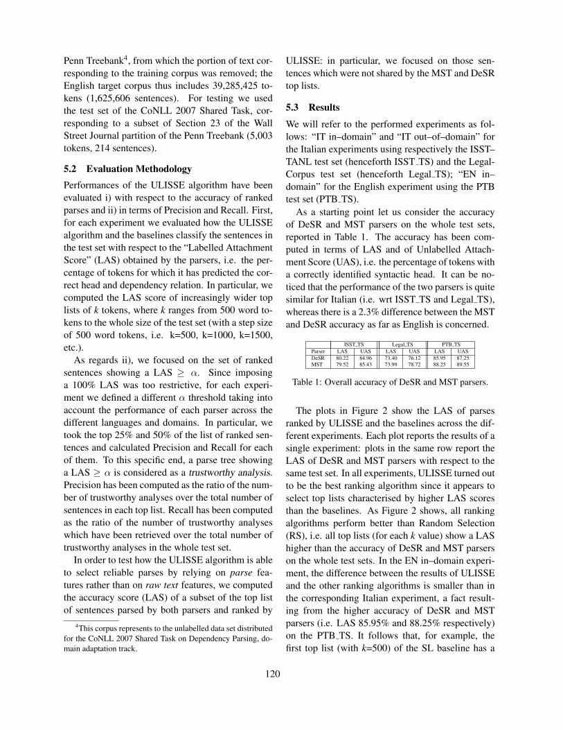
Penn Treebank4, from which the portion of text cor-responding to the training corpus was removed; theEnglish target corpus thus includes 39,285,425 to-kens (1,625,606 sentences). For testing we usedthe test set of the CoNLL 2007 Shared Task, cor-responding to a subset of Section 23 of the WallStreet Journal partition of the Penn Treebank (5,003tokens, 214 sentences).

5.2 Evaluation MethodologyPerformances of the ULISSE algorithm have beenevaluated i) with respect to the accuracy of rankedparses and ii) in terms of Precision and Recall. First,for each experiment we evaluated how the ULISSEalgorithm and the baselines classify the sentences inthe test set with respect to the “Labelled AttachmentScore” (LAS) obtained by the parsers, i.e. the per-centage of tokens for which it has predicted the cor-rect head and dependency relation. In particular, wecomputed the LAS score of increasingly wider toplists of k tokens, where k ranges from 500 word to-kens to the whole size of the test set (with a step sizeof 500 word tokens, i.e. k=500, k=1000, k=1500,etc.).

As regards ii), we focused on the set of rankedsentences showing a LAS ≥ α. Since imposinga 100% LAS was too restrictive, for each experi-ment we defined a different α threshold taking intoaccount the performance of each parser across thedifferent languages and domains. In particular, wetook the top 25% and 50% of the list of ranked sen-tences and calculated Precision and Recall for eachof them. To this specific end, a parse tree showinga LAS ≥ α is considered as a trustworthy analysis.Precision has been computed as the ratio of the num-ber of trustworthy analyses over the total number ofsentences in each top list. Recall has been computedas the ratio of the number of trustworthy analyseswhich have been retrieved over the total number oftrustworthy analyses in the whole test set.

In order to test how the ULISSE algorithm is ableto select reliable parses by relying on parse fea-tures rather than on raw text features, we computedthe accuracy score (LAS) of a subset of the top listof sentences parsed by both parsers and ranked by

4This corpus represents to the unlabelled data set distributedfor the CoNLL 2007 Shared Task on Dependency Parsing, do-main adaptation track.

ULISSE: in particular, we focused on those sen-tences which were not shared by the MST and DeSRtop lists.

5.3 Results

We will refer to the performed experiments as fol-lows: “IT in–domain” and “IT out–of–domain” forthe Italian experiments using respectively the ISST–TANL test set (henceforth ISST TS) and the Legal-Corpus test set (henceforth Legal TS); “EN in–domain” for the English experiment using the PTBtest set (PTB TS).

As a starting point let us consider the accuracyof DeSR and MST parsers on the whole test sets,reported in Table 1. The accuracy has been com-puted in terms of LAS and of Unlabelled Attach-ment Score (UAS), i.e. the percentage of tokens witha correctly identified syntactic head. It can be no-ticed that the performance of the two parsers is quitesimilar for Italian (i.e. wrt ISST TS and Legal TS),whereas there is a 2.3% difference between the MSTand DeSR accuracy as far as English is concerned.

ISST TS Legal TS PTB TSParser LAS UAS LAS UAS LAS UASDeSR 80.22 84.96 73.40 76.12 85.95 87.25MST 79.52 85.43 73.99 78.72 88.25 89.55

Table 1: Overall accuracy of DeSR and MST parsers.

The plots in Figure 2 show the LAS of parsesranked by ULISSE and the baselines across the dif-ferent experiments. Each plot reports the results of asingle experiment: plots in the same row report theLAS of DeSR and MST parsers with respect to thesame test set. In all experiments, ULISSE turned outto be the best ranking algorithm since it appears toselect top lists characterised by higher LAS scoresthan the baselines. As Figure 2 shows, all rankingalgorithms perform better than Random Selection(RS), i.e. all top lists (for each k value) show a LAShigher than the accuracy of DeSR and MST parserson the whole test sets. In the EN in–domain experi-ment, the difference between the results of ULISSEand the other ranking algorithms is smaller than inthe corresponding Italian experiment, a fact result-ing from the higher accuracy of DeSR and MSTparsers (i.e. LAS 85.95% and 88.25% respectively)on the PTB TS. It follows that, for example, thefirst top list (with k=500) of the SL baseline has a

120

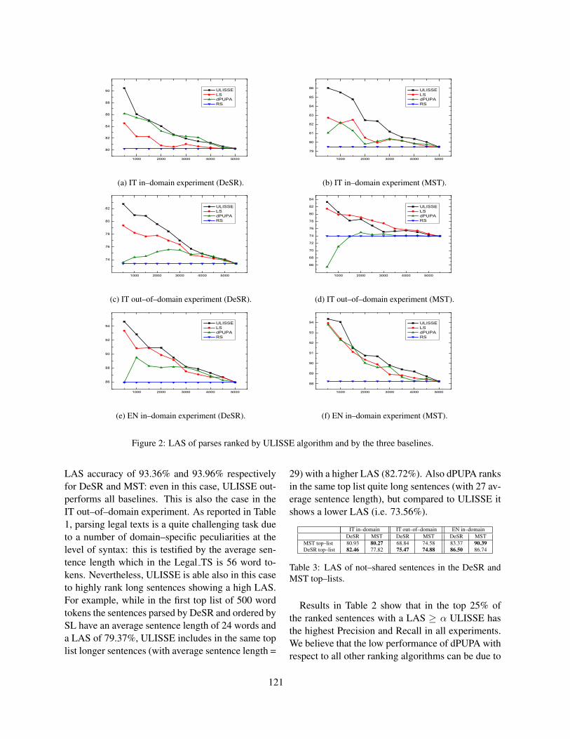
1000 2000 3000 4000 5000

80

82

84

86

88

90

ULISSE LS dPUPA RS

(a) IT in–domain experiment (DeSR).

1000 2000 3000 4000 5000

79

80

81

82

83

84

85

86

ULISSE LS dPUPA RS

(b) IT in–domain experiment (MST).

1000 2000 3000 4000 5000

74

76

78

80

82

ULISSE LS dPUPA RS

(c) IT out–of–domain experiment (DeSR).

1000 2000 3000 4000 5000

66

68

70

72

74

76

78

80

82

84

ULISSE LS dPUPA RS

(d) IT out–of–domain experiment (MST).

1000 2000 3000 4000 5000

86

88

90

92

94

ULISSE LS dPUPA RS

(e) EN in–domain experiment (DeSR).

1000 2000 3000 4000 5000

88

89

90

91

92

93

94

ULISSE LS dPUPA RS

(f) EN in–domain experiment (MST).

Figure 2: LAS of parses ranked by ULISSE algorithm and by the three baselines.

LAS accuracy of 93.36% and 93.96% respectivelyfor DeSR and MST: even in this case, ULISSE out-performs all baselines. This is also the case in theIT out–of–domain experiment. As reported in Table1, parsing legal texts is a quite challenging task dueto a number of domain–specific peculiarities at thelevel of syntax: this is testified by the average sen-tence length which in the Legal TS is 56 word to-kens. Nevertheless, ULISSE is able also in this caseto highly rank long sentences showing a high LAS.For example, while in the first top list of 500 wordtokens the sentences parsed by DeSR and ordered bySL have an average sentence length of 24 words anda LAS of 79.37%, ULISSE includes in the same toplist longer sentences (with average sentence length =

29) with a higher LAS (82.72%). Also dPUPA ranksin the same top list quite long sentences (with 27 av-erage sentence length), but compared to ULISSE itshows a lower LAS (i.e. 73.56%).

IT in–domain IT out–of–domain EN in–domainDeSR MST DeSR MST DeSR MST

MST top–list 80.93 80.27 68.84 74.58 83.37 90.39DeSR top–list 82.46 77.82 75.47 74.88 86.50 86.74

Table 3: LAS of not–shared sentences in the DeSR andMST top–lists.

Results in Table 2 show that in the top 25% ofthe ranked sentences with a LAS ≥ α ULISSE hasthe highest Precision and Recall in all experiments.We believe that the low performance of dPUPA withrespect to all other ranking algorithms can be due to

121

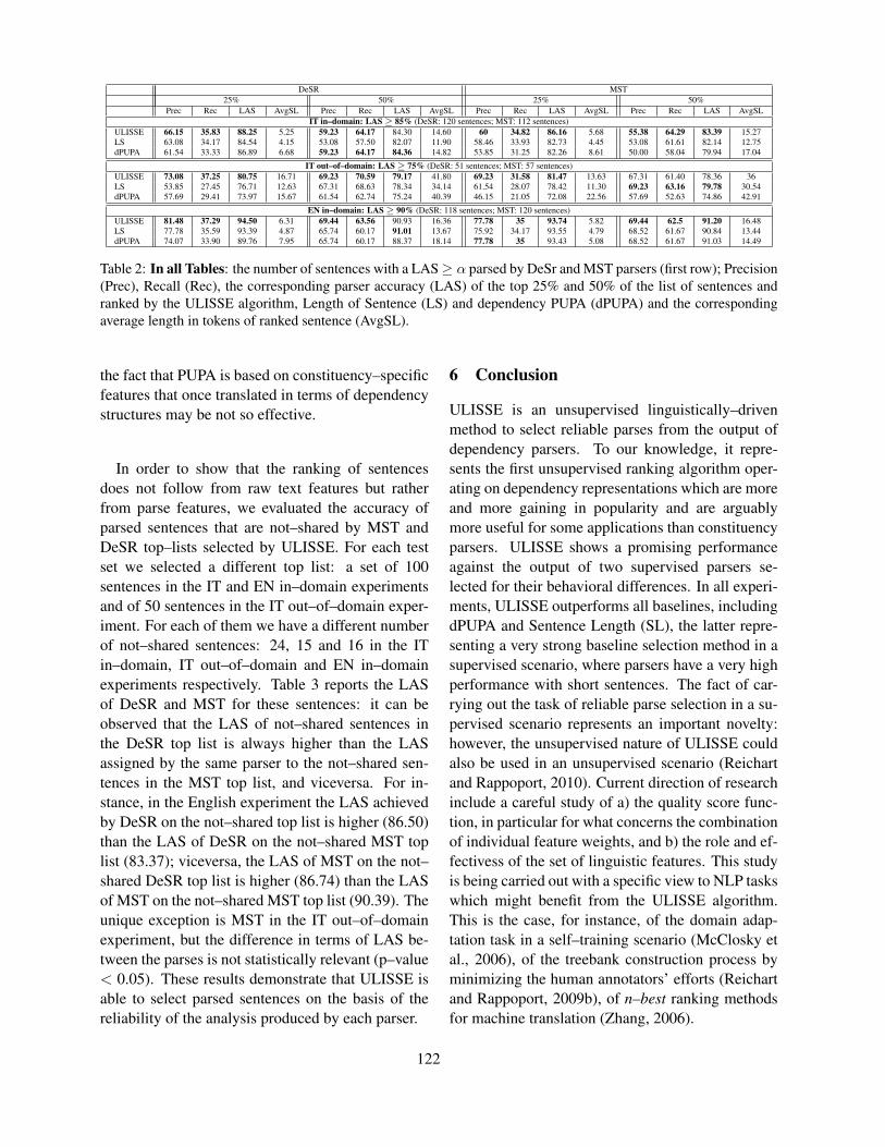
DeSR MST25% 50% 25% 50%

Prec Rec LAS AvgSL Prec Rec LAS AvgSL Prec Rec LAS AvgSL Prec Rec LAS AvgSLIT in–domain: LAS≥ 85% (DeSR: 120 sentences; MST: 112 sentences)

ULISSE 66.15 35.83 88.25 5.25 59.23 64.17 84.30 14.60 60 34.82 86.16 5.68 55.38 64.29 83.39 15.27LS 63.08 34.17 84.54 4.15 53.08 57.50 82.07 11.90 58.46 33.93 82.73 4.45 53.08 61.61 82.14 12.75dPUPA 61.54 33.33 86.89 6.68 59.23 64.17 84.36 14.82 53.85 31.25 82.26 8.61 50.00 58.04 79.94 17.04

IT out–of–domain: LAS≥ 75% (DeSR: 51 sentences; MST: 57 sentences)ULISSE 73.08 37.25 80.75 16.71 69.23 70.59 79.17 41.80 69.23 31.58 81.47 13.63 67.31 61.40 78.36 36LS 53.85 27.45 76.71 12.63 67.31 68.63 78.34 34.14 61.54 28.07 78.42 11.30 69.23 63.16 79.78 30.54dPUPA 57.69 29.41 73.97 15.67 61.54 62.74 75.24 40.39 46.15 21.05 72.08 22.56 57.69 52.63 74.86 42.91

EN in–domain: LAS≥ 90% (DeSR: 118 sentences; MST: 120 sentences)ULISSE 81.48 37.29 94.50 6.31 69.44 63.56 90.93 16.36 77.78 35 93.74 5.82 69.44 62.5 91.20 16.48LS 77.78 35.59 93.39 4.87 65.74 60.17 91.01 13.67 75.92 34.17 93.55 4.79 68.52 61.67 90.84 13.44dPUPA 74.07 33.90 89.76 7.95 65.74 60.17 88.37 18.14 77.78 35 93.43 5.08 68.52 61.67 91.03 14.49

Table 2: In all Tables: the number of sentences with a LAS≥ α parsed by DeSr and MST parsers (first row); Precision(Prec), Recall (Rec), the corresponding parser accuracy (LAS) of the top 25% and 50% of the list of sentences andranked by the ULISSE algorithm, Length of Sentence (LS) and dependency PUPA (dPUPA) and the correspondingaverage length in tokens of ranked sentence (AvgSL).

the fact that PUPA is based on constituency–specificfeatures that once translated in terms of dependencystructures may be not so effective.

In order to show that the ranking of sentencesdoes not follow from raw text features but ratherfrom parse features, we evaluated the accuracy ofparsed sentences that are not–shared by MST andDeSR top–lists selected by ULISSE. For each testset we selected a different top list: a set of 100sentences in the IT and EN in–domain experimentsand of 50 sentences in the IT out–of–domain exper-iment. For each of them we have a different numberof not–shared sentences: 24, 15 and 16 in the ITin–domain, IT out–of–domain and EN in–domainexperiments respectively. Table 3 reports the LASof DeSR and MST for these sentences: it can beobserved that the LAS of not–shared sentences inthe DeSR top list is always higher than the LASassigned by the same parser to the not–shared sen-tences in the MST top list, and viceversa. For in-stance, in the English experiment the LAS achievedby DeSR on the not–shared top list is higher (86.50)than the LAS of DeSR on the not–shared MST toplist (83.37); viceversa, the LAS of MST on the not–shared DeSR top list is higher (86.74) than the LASof MST on the not–shared MST top list (90.39). Theunique exception is MST in the IT out–of–domainexperiment, but the difference in terms of LAS be-tween the parses is not statistically relevant (p–value< 0.05). These results demonstrate that ULISSE isable to select parsed sentences on the basis of thereliability of the analysis produced by each parser.

6 Conclusion

ULISSE is an unsupervised linguistically–drivenmethod to select reliable parses from the output ofdependency parsers. To our knowledge, it repre-sents the first unsupervised ranking algorithm oper-ating on dependency representations which are moreand more gaining in popularity and are arguablymore useful for some applications than constituencyparsers. ULISSE shows a promising performanceagainst the output of two supervised parsers se-lected for their behavioral differences. In all experi-ments, ULISSE outperforms all baselines, includingdPUPA and Sentence Length (SL), the latter repre-senting a very strong baseline selection method in asupervised scenario, where parsers have a very highperformance with short sentences. The fact of car-rying out the task of reliable parse selection in a su-pervised scenario represents an important novelty:however, the unsupervised nature of ULISSE couldalso be used in an unsupervised scenario (Reichartand Rappoport, 2010). Current direction of researchinclude a careful study of a) the quality score func-tion, in particular for what concerns the combinationof individual feature weights, and b) the role and ef-fectivess of the set of linguistic features. This studyis being carried out with a specific view to NLP taskswhich might benefit from the ULISSE algorithm.This is the case, for instance, of the domain adap-tation task in a self–training scenario (McClosky etal., 2006), of the treebank construction process byminimizing the human annotators’ efforts (Reichartand Rappoport, 2009b), of n–best ranking methodsfor machine translation (Zhang, 2006).

122

References

Giuseppe Attardi. 2006. Experiments with a multilan-guage non-projective dependency parser. In Proceed-ings of the Tenth Conference on Computational Nat-ural Language Learning (CoNLL-X ’06), New YorkCity, New York, pp. 166–170.

Cristina Bosco, Simonetta Montemagni, AlessandroMazzei, Vincenzo Lombardo, Felice Dell’Orletta andAlessandro Lenci. 2009. Parsing Task: comparingdependency parsers and treebanks. In Proceedings ofEvalita’09, Reggio Emilia.

Sabine Buchholz and Erwin Marsi. 2006. CoNLL-Xshared task on multilingual dependency parsing. InProceedings of CoNLL.

Felice Dell’Orletta. 2009. Ensemble system for Part-of-Speech tagging. In Proceedings of Evalita’09, Eval-uation of NLP and Speech Tools for Italian, ReggioEmilia, December.

Lyn Frazier. 1985. Syntactic complexity. In D.R.Dowty, L. Karttunen and A.M. Zwicky (eds.), NaturalLanguage Parsing, Cambridge University Press, Cam-bridge, UK.

Edward Gibson. 1998. Linguistic complexity: Localityof syntactic dependencies. In Cognition, 68(1), pp. 1-76.

Daisuke Kawahara and Kiyotaka Uchimoto. 2008.Learning Reliability of Parses for Domain Adaptationof Dependency Parsing. In Proceedings of IJCNLP2008, pp. 709–714.

Dekan Lin. 1996. On the structural complexity of nat-ural language sentences. In Proceedings of COLING1996, pp. 729–733.

Ryan McDonald, Kevin Lerman, and Fernando Pereira.2006. Multilingual dependency analysis with a two-stage discriminative parser. In Proceedings of CoNLL2006.

Ryan McDonald and Joakim Nivre. 2007. Character-izing the Errors of Data-Driven Dependency ParsingModels. In Proceedings of EMNLP-CoNLL, 2007, pp.122-131.

Mitchell P. Marcus, Mary Ann Marcinkiewicz and Beat-rice Santorini. 1993. Building a large annotated cor-pus of English: the penn treebank. In Comput. Lin-guist.,vol. 19, issue 2, MIT Press, pp. 313–330.

Rita Marinelli, et al. 2003. The Italian PAROLE cor-pus: an overview. In A. Zampolli et al. (eds.), Compu-tational Linguistics in Pisa, XVI–XVII, Pisa–Roma,IEPI., I, 401–421.

David McClosky, Eugene Charniak and Mark Johnson.2006. Reranking and self–training for parser adap-tation. In Proceedings of ICCL–ACL 2006, pp. 337–344.

David McClosky, Eugene Charniak and Mark Johnson.2008. When is Self–Trainig Effective for parsing?. InProceedings of COLING 2008, pp. 561–568.

Jim Miller and Regina Weinert. 1998. Spontaneous spo-ken language. Syntax and discourse. Oxford, Claren-don Press.

Ani Nenkova, Jieun Chae, Annie Louis, and Emily Pitler.2010. Structural Features for Predicting the LinguisticQuality of Text Applications to Machine Translation,Automatic Summarization and Human–Authored Text.In E. Krahmer, M. Theune (eds.), Empirical Methodsin NLG, LNAI 5790, Springer-Verlag Berlin Heidel-berg, pp. 222241.

Joakim Nivre, Johan Hall, Sandra Kubler, Ryan Mc-Donald, Jens Nilsson, Sebastian Riedel, Deniz Yuret.2007. The CoNLL 2007 Shared Task on DependencyParsing. In Proceedings of the EMNLP-CoNLL, pp.915–932.

Sujith Ravi, Kevin Knight and Radu Soricut. 2008. Auto-matic Prediction of Parser Accuracy. In Proceedingsof the EMNLP 2008, pp. 887–896.

Roi Reichart and Ari Rappoport. 2007a. An ensemblemethod for selection of high quality parses. In Pro-ceedings of ACL 2007, pp. 408–415.

Roi Reichart and Ari Rappoport. 2007b. Self–Trainingfor Enhancement and Domain Adaptation of Statisti-cal Parsers Trained on Small Datasets. In Proceedingsof ACL 2007, pp. 616–623.

Roi Reichart and Ari Rappoport. 2009a. Automatic Se-lection of High Quality Parses Created By a Fully Un-supervised Parser. In Proceedings of CoNLL 2009,pp. 156–164.

Roi Reichart and Ari Rappoport. 2009b. Sample Selec-tion for Statistical Parsers: Cognitively Driven Algo-rithms and Evaluation Measures. In Proceedings ofCoNLL 2009, pp. 3–11.

Roi Reichart and Ari Rappoport. 2010. Improved FullyUnsupervised Parsing with Zoomed Learning. In Pro-ceedings of EMNLP 2010.

Brian Roark, Margaret Mitchell and Kristy Hollingshead.2007. Syntactic complexity measures for detectingMild Cognitive Impairment. In Proceedings of ACLWorkshop on Biological, Translational, and ClinicalLanguage Processing (BioNLP’07), pp. 1–8.

Kenji Sagae and Junichi Tsujii. 2007. DependencyParsing and Domain Adaptation with LR Models andParser Ensemble. In Proceedings of the EMNLP–CoNLL 2007, pp. 1044–1050.

Giulia Venturi. 2010. Legal Language and Legal Knowl-edge Management Applications. In E. Francesconi, S.Montemagni, W. Peters and D. Tiscornia (eds.), Se-mantic Processing of Legal Texts, Lecture Notes inComputer Science, Springer Berlin / Heidelberg, vol.6036, pp. 3-26.

123

Alexander Yates, Stefan Schoenmackers and Oren Et-zioni. 2006. Detecting Parser Errors Using Web–based Semantic Filters. In Proceedings of the EMNLP2006, pp. 27–34.

Victor H.A. Yngve. 1960. A model and an hypothesis forlanguage structure. In Proceedings of the AmericanPhilosophical Society, pp. 444-466.

Ying Zhang, Almut Hildebrand and Stephan Vogel.2006. Distributed language modeling for N-best listre-ranking. In Proceedings of the EMNLP 2006, pp.216–223.

124


Language Models as Representations for Weakly-Supervised NLP Tasks

Fei Huang and Alexander YatesTemple University

Broad St. and Montgomery Ave.Philadelphia, PA 19122

[email protected]@temple.edu

Arun Ahuja and Doug DowneyNorthwestern University

2133 Sheridan RoadEvanston, IL 60208

[email protected]@eecs.northwestern.edu

Abstract

Finding the right representation for words iscritical for building accurate NLP systemswhen domain-specific labeled data for thetask is scarce. This paper investigates lan-guage model representations, in which lan-guage models trained on unlabeled corporaare used to generate real-valued feature vec-tors for words. We investigate ngram mod-els and probabilistic graphical models, includ-ing a novel lattice-structured Markov RandomField. Experiments indicate that languagemodel representations outperform traditionalrepresentations, and that graphical model rep-resentations outperform ngram models, espe-cially on sparse and polysemous words.

1 Introduction

NLP systems often rely on hand-crafted, carefullyengineered sets of features to achieve strong perfor-mance. Thus, a part-of-speech (POS) tagger wouldtraditionally use a feature like, “the previous tokenis the” to help classify a given token as a noun oradjective. For supervised NLP tasks with sufficientdomain-specific training data, these traditional fea-tures yield state-of-the-art results. However, NLPsystems are increasingly being applied to texts likethe Web, scientific domains, and personal commu-nications like emails, all of which have very differ-ent characteristics from traditional training corpora.Collecting labeled training data for each new targetdomain is typically prohibitively expensive. We in-vestigate representations that can be applied whendomain-specific labeled training data is scarce.

An increasing body of theoretical and empiricalevidence suggests that traditional, manually-crafted

features limit systems’ performance in this settingfor two reasons. First, featuresparsityprevents sys-tems from generalizing accurately to words and fea-tures not seen during training. Because word fre-quencies are Zipf distributed, this often means thatthere is little relevant training data for a substantialfraction of parameters (Bikel, 2004), especially innew domains (Huang and Yates, 2009). For exam-ple, word-type features form the backbone of mostPOS-tagging systems, but types like “gene” and“pathway” show up frequently in biomedical liter-ature, and rarely in newswire text. Thus, a classifiertrained on newswire data and tested on biomedicaldata will have seen few training examples related tosentences with features “gene” and “pathway” (Ben-David et al., 2009; Blitzer et al., 2006).

Further, because words arepolysemous, word-type features prevent systems from generalizing tosituations in which words have different meanings.For instance, the word type “signaling” appears pri-marily as a present participle (VBG) in Wall StreetJournal (WSJ) text, as in, “Interest rates rose, sig-naling that . . . ” (Marcus et al., 1993). In biomedicaltext, however, “signaling” appears primarily in thephrase “signaling pathway,” where it is considereda noun (NN) (PennBioIE, 2005); this phrase neverappears in the WSJ portion of the Penn Treebank(Huang and Yates, 2010a).

Our response to these problems with traditionalNLP representations is to seek new representationsthat allow systems to generalize more accurately topreviously unseen examples. Our approach dependson the well-knowndistributional hypothesis, whichstates that a word’s meaning is identified with thecontexts in which it appears (Harris, 1954; Hin-dle, 1990). Our goal is to develop probabilistic lan-

125

guage models that describe the contexts of individ-ual words accurately. We then constructrepresen-tations, or mappings from word tokens and typesto real-valued vectors, from these language models.Since the language models are designed to modelwords’ contexts, the features they produce can beused to combat problems with polysemy. And bycareful design of the language models, we can limitthe number of features that they produce, controllinghow sparse those features are in training data.

In this paper, we analyze the performanceof language-model-based representations on taskswhere domain-specific training data is scarce. Ourcontributions are as follows:1. We introduce a novel factorial graphical modelrepresentation, a Partial-Lattice Markov RandomField (PL-MRF), which is a tractable variation ofa Factorial Hidden Markov Model (HMM) for lan-guage modeling.2. In experiments on POS tagging in a domain adap-tation setting and on weakly-supervised informa-tion extraction (IE), we quantify the performance ofrepresentations derived from language models. Weshow that graphical models outperform ngram rep-resentations. The PL-MRF representation achieves astate-of-the-art 93.8% accuracy on the POS taggingtask, while the HMM representation improves overthe ngram model by 10% on the IE task.3. We analyze how the performance of the differentrepresentations varies due to the fundamental chal-lenges of sparsity and polysemy.

The next section discusses previous work. Sec-tions 3 and 4 present the existing representations weinvestigate and the new PL-MRF, respectively. Sec-tions 5 and 6 describe our two tasks and the resultsof using our representations on each of them. Sec-tion 7 concludes.

2 Previous Work

There is a long tradition of NLP research on rep-resentations, mostly falling into one of four cate-gories: 1) vector space models of meaning basedon document-level lexical cooccurrence statistics(Salton and McGill, 1983; Turney and Pantel, 2010;Sahlgren, 2006); 2) dimensionality reduction tech-niques for vector space models (Deerwester et al.,1990; Honkela, 1997; Kaski, 1998; Sahlgren, 2005;Blei et al., 2003; Vayrynen et al., 2007); 3) usingclusters that are induced from distributional similar-ity (Brown et al., 1992; Pereira et al., 1993; Mar-

tin et al., 1998) as non-sparse features (Lin and Wu,2009; Candito and Crabbe, 2009; Koo et al., 2008;Zhao et al., 2009); 4) and recently, language models(Bengio, 2008; Mnih and Hinton, 2009) as represen-tations (Weston et al., 2008; Collobert and Weston,2008; Bengio et al., 2009), some of which have al-ready yielded state of the art performance on domainadaptation tasks (Huang and Yates, 2009; Huang andYates, 2010a; Huang and Yates, 2010b; Turian et al.,2010) and IE (Ahuja and Downey, 2010; Downey etal., 2007b). In contrast to this previous work, we de-velop a novel Partial Lattice MRF language modelthat incorporates a factorial representation of latentstates, and demonstrate that it outperforms the pre-vious state-of-the-art in POS tagging in a domainadaptation setting. We also analyze the novel PL-MRF representation on an IE task, and several repre-sentations along the key dimensions of sparsity andpolysemy.

Most previous work on domain adaptation has fo-cused on the case where some labeled data is avail-able in both the source and target domains (DaumeIII, 2007; Jiang and Zhai, 2007; Daume III andMarcu, 2006; Finkel and Manning, 2009; Dredzeet al., 2010; Dredze and Crammer, 2008). Learn-ing bounds are known (Blitzer et al., 2007; Man-sour et al., 2009). Daume III et al. (2010) use semi-supervised learning to incorporate labeled and unla-beled data from the target domain. In contrast, weinvestigate a domain adaptation setting where no la-beled data is available for the target domain.

3 Representations

A representationis a set of features that describeinstances for a classifier. Formally, letX be aninstance set, and letZ be the set of labels for aclassification task. A representation is a functionR : X → Y for some suitable feature spaceY (suchasR

d). We refer to dimensions ofY asfeatures, andfor an instancex ∈ X we refer to values for partic-ular dimensions ofR(x) as features ofx.

3.1 Traditional POS-Tagging Representations

As a baseline for POS tagging experiments and anexample of our terminology, we describe a repre-sentation used in traditional supervised POS taggers.The instance setX is the set of English sentences,andZ is the set of POS tag sequences. A traditionalrepresentation TRAD-R maps a sentencex ∈ X to asequence of boolean-valued vectors, one vector per

126

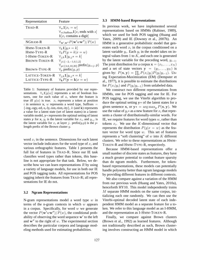
Representation Feature

TRAD-R ∀w1[xi = w]∀s∈Suffixes1[xi ends withs]1[xi contains a digit]

NGRAM-R ∀w′,w′′P (w′ww′′)/P (w)

HMM -TOKEN-R ∀k1[yi∗ = k]HMM -TYPE-R ∀kP (y = k|x = w)I-HMM -TOKEN-R ∀j,k1[yi,j∗ = k]BROWN-TOKEN-R ∀j∈{−2,−1,0,1,2}

∀p∈{4,6,10,20} prefix(yi+j , p)BROWN-TYPE-R ∀p prefix(y, p)

LATTICE-TOKEN-R ∀j,k1[yi,j∗ = k]LATTICE-TYPE-R ∀kP (y = k|x = w)

Table 1: Summary of features provided by our repre-sentations. ∀a1[g(a)] represents a set of boolean fea-tures, one for each value ofa, where the feature istrue iff g(a) is true. xi represents a token at positioni in sentencex, w represents a word type, Suffixes={-ing,-ogy,-ed,-s,-ly,-ion,-tion,-ity}, k (andk) representsa value for a latent state (set of latent states) in a latent-variable model,y∗ represents the optimal setting of latentstatesy for x, yi is the latent variable forxi, andyi,j isthe latent variable forxi at layerj. prefix(y,p) is thep-length prefix of the Brown clustery.

wordxi in the sentence. Dimensions for each latentvector include indicators for the word type ofxi andvarious orthographic features. Table 1 presents thefull list of features in TRAD-R. Since our IE taskclassifies word types rather than tokens, this base-line is not appropriate for that task. Below, we de-scribe how we can learn representationsR by usinga variety of language models, for use in both our IEand POS tagging tasks. All representations for POStagging inherit the features from TRAD-R; all repre-sentations for IE do not.

3.2 Ngram Representations

N-gram representations model a word typew interms of the n-gram contexts in whichw appearsin a corpus. Specifically, for wordw we generatethe vectorP (w′ww′′)/P (w), the conditional prob-ability of observing the word sequencew′ to the leftandw′′ to the right ofw. The experimental sectiondescribes the particular corpora and language mod-eling methods used for estimating probabilities.

3.3 HMM-based Representations

In previous work, we have implemented severalrepresentations based on HMMs (Rabiner, 1989),which we used for both POS tagging (Huang andYates, 2009) and IE (Downey et al., 2007b). AnHMM is a generative probabilistic model that gen-erates each wordxi in the corpus conditioned on alatent variableyi. Eachyi in the model takes on in-tegral values from1 to K, and each one is generatedby the latent variable for the preceding word,yi−1.The joint distribution for a corpusx = (x1, . . . , xN )and a set of state vectorsy = (y1, . . . , yN ) isgiven by: P (x,y) =

∏i P (xi|yi)P (yi|yi−1). Us-

ing Expectation-Maximization (EM) (Dempster etal., 1977), it is possible to estimate the distributionsfor P (xi|yi) andP (yi|yi−1) from unlabeled data.

We construct two different representations fromHMMs, one for POS tagging and one for IE. ForPOS tagging, we use the Viterbi algorithm to pro-duce the optimal settingy∗ of the latent states for agiven sentencex, or y∗ = arg maxy P (x,y). Weuse the value ofyi∗ as a new feature forxi that repre-sents a cluster of distributionally-similar words. ForIE, we require features for word typesw, rather thantokensxi. We use theK-dimensional vector thatrepresents the distributionP (y|x = w) as the fea-ture vector for word typew. This set of featuresrepresents a “soft clustering” ofw into K differentclusters. We refer to these representations as HMM -TOKEN-R and HMM -TYPE-R, respectively.

Because HMM-based representations offer asmall number of discrete states as features, they havea much greater potential to combat feature sparsitythan do ngram models. Furthermore, for token-based representations, these models can potentiallyhandle polysemy better than ngram language modelsby providing different features in different contexts.

We also compare against a variation of the HMMfrom our previous work (Huang and Yates, 2010a),henceforth HY10. This model independently trainsM separate HMM models on the same corpus, ini-tializing each one randomly. We can then use theViterbi-optimal decoded latent state of each inde-pendent HMM model as a separate feature for a to-ken. We refer to this language model as an I-HMM,and the representation as I-HMM -TOKEN-R.

Finally, we compare against Brown clusters(Brown et al., 1992) as learned features. Althoughnot traditionally described as such, Brown cluster-ing involves constructing an HMM model in which

127

each type is restricted to having exactly one latentstate that may generate it. Brownet al. describe agreedy agglomerative clustering algorithm for train-ing this model on unlabeled text. Following Turianet al. (2010), we use Percy Liang’s implementationof this algorithm for our comparison, and we testruns with 100, 320, and 1000 clusters. We use fea-tures from these clusters identical to Turianet al.’s.1

Turianet al. have shown that Brown clusters matchor exceed the performance of neural network-basedlanguage models in domain adaptation experimentsfor named-entity recognition, as well as in-domainexperiments for NER and chunking.

4 A Novel Lattice Language ModelRepresentation

Our final language model is a novel latent-variablelanguage model with rich latent structure, shown inFigure 1. The model contains a lattice ofM ×N la-tent states, whereN is the number of words in a sen-tence andM is the number of layers in the model.We can justify the choice of this model from a lin-guistic perspective as a way to capture the multi-dimensional nature of words. Linguists have longargued that words have many different features in ahigh dimensional space: they can be separately de-scribed by part of speech, gender, number, case, per-son, tense, voice, aspect, mass vs. count, and a hostof semantic categories (agency, animate vs. inani-mate, physical vs. abstract, etc.), to name a few (Saget al., 2003). Our model seeks to capture a multi-dimensional representation of words by creating aseparate layer of latent variables for each dimension.The values of theM layers of latent variables for asingle word can be used asM distinct features inour representation. The I-HMM attempts to modelthe same intuition, but unlike a lattice model the I-HMM layers are entirely independent, and as a re-sult there is no mechanism to enforce that the layersmodel different dimensions. Duh (2005) previouslyused a 2-layer lattice for tagging and chunking, butin a supervised setting rather than for representationlearning.

Let Cliq(x,y) represent the set of all maximalcliques in the graph of the MRF model forx andy.

1Percy Liang’s implementation is available athttp://metaoptimize.com/projects/wordreprs/. Turian et al.also tested a run with 3200 clusters in their experiments, whichwe have been training for months, but which has not finished intime for publication.

y4,1

y3,1

y

y4,2

y3,2

y

y4,3

y3,3

y

y4,4

y3,4

y

y4,5

y3,5

y

x1

y2,1

y1,1

x2

y2,2

y1,2

x3

y2,3

y1,3

x4

y2,4

y1,4

x5

y2,5

y1,5

Figure 1: The Partial Lattice MRF (PL-MRF) Model for a5-word sentence and a 4-layer lattice. Dashed gray edgesare part of a full lattice, but not the PL-MRF.

Expressing the lattice model in log-linear form, wecan write the marginal probabilityP (x) of a givensentencex as:

∑

y

∏c∈Cliq(x,y) score(c,x,y)

∑x′,y′

∏c∈Cliq(x′,y′) score(c,x′,y′)

where score(c,x,y) = exp(θc · fc(xc,yc)). Ourmodel includes parameters for transitions betweentwo adjacent latent variables on layerj: θtrans

i,s,i+1,s′,j

for yi,j = s andyi+1,j = s′. It also includes obser-vation parameters for latent variables and tokens, aswell as for pairs of adjacent latent variables in differ-ent layers and their tokens:θobs

i,j,s,w andθobsi,j,s,j+1,s′,w

for yi,j = s, yi,j+1 = s′, andxi = w.Computationally, the lattice MRF is preferable to

a naıve Factorial HMM (Ghahramani and Jordan,1997) representation, which would requireO(2M )parameters for anM -layer model. However, ex-act training and inference in supervised settings arestill intractable for this model (Sutton et al., 2007),and thus it has not yet been explored as a languagemodel, which requires even more difficult, unsuper-vised training. Training is intractable in part becauseof the difficulty in enumerating and summing overthe exponentially-many configurationsy for a givenx. We address this difficulty in two ways: by modi-fying the model, and by modifying the training pro-cedure.

4.1 Partial Lattice MRF

Instead of the full lattice model, we construct aPartial Lattice MRF (PL-MRF) model by deleting

128

certain edges between latent layers of the model(dashed gray edges in Figure 1). Letc = bN

2 c,whereN is the length of the sentence. Ifi < cand j is odd, or if j is even andi > c, we deleteedges betweenyi,j andyi,j+1. The same lattice ofnodes remains, but fewer edges and paths. A cen-tral “trunk” at i = c connects all layers of the lat-tice, and branches from this trunk connect either tothe branches in the layer above or the layer below(but not both). The result is a model that retainsmost2 of the edges of the full model. Additionally,the pruned model makes the branches conditionallyindependent from one another, except through thetrunk. For instance, the right branch at layers 1and 2 in Figure 1 (y1,4, y1,5, y2,4, andy2,5) are dis-connected from the right branch at layers 3 and 4(y3,4, y3,5, y4,4, andy4,5), except through the trunkand the observed nodes. As a result, excluding theobserved nodes, this model has a lowtree-widthof2 (excluding observed nodes), and a variety of ef-ficient dynamic programming and message-passingalgorithms for training and inference can be readilyapplied (Bodlaender, 1988).3 Our inference algo-rithm passes information from the branches inwardsto the trunk, and then upward along the trunk, intimeO(K4MN).

As with our HMM models, we create two repre-sentations from PL-MRFs, one for tokens and onefor types. For tokens, we decode the model to com-putey∗, the matrix of optimal latent state values forsentencex. For each layerj and and each possi-ble latent state valuek, we add a boolean featurefor tokenxi that is true iffy∗i,j = k. For types,we compute distributions over the latent state space.Let y be the column vector of latent variables forwordx. For each possible configuration of valuesk

of the latent variablesy, we add a real-valued fea-tures forx given byP (y = k|x = w). We referto these two representations as LATTICE-TOKEN-Rand LATTICE-TYPE-R, respectively.

4.2 Parameter Estimation

We train the PL-MRF using contrastive estimation,which iteratively optimizes the following objectivefunction on a corpusX:

∑

x∈X

log

∑y

∏c∈Cliq(x,y) score(c,x,y)

∑x′∈N (x),y′

∏c∈Cliq(x′,y′) score(c,x′,y′)

2As M, N →∞, 5 out of every 6 edges are kept.3c.f. a tree-width of min(M ,N ) for the unpruned model

whereN (x), the neighborhood ofx, indicates aset of perturbed variations of the original sentencex. Contrastive estimation seeks to move probabilitymass away from the perturbed neighborhood sen-tences and onto the original sentence. We use aneighborhood function that includes all sentenceswhich can be obtained from the original sentence byswapping the order of a consecutive pair of words.Training uses gradient descent over this non-convexobjective function with a standard software package(Liu and Nocedal, 1989) and converges to a localmaximum (Smith and Eisner, 2005).

For tractability, we modify the training procedureto train the PL-MRF one layer at a time. Letθi rep-resent the set of parameters relating to features oflayer i, and letθ¬i represent all other parameters.We fix θ¬0 = 0, and optimizeθ0 using contrastiveestimation. After convergence, we fixθ¬1, and opti-mizeθ1, and so on. We use a convergence thresholdof 10−6, and each layer typically converges in under100 iterations.

5 Domain Adaptation for a POS Tagger

We evaluate the representations described above ona POS tagging task in a domain adaptation setting.


We use the same experimental setup as in HY10:the Penn Treebank (Marcus et al., 1993) Wall StreetJournal portion for our labeled training data; 561MEDLINE sentences (9576 types, 14554 tokens,23% OOV tokens) from the Penn BioIE project(PennBioIE, 2005) for our labeled test set; and all ofthe unlabeled text from the Penn Treebank WSJ por-tion plus a MEDLINE corpus of 71,306 unlabeledsentences to train our language models. The twotexts come from two very different domains, mak-ing this data a tough test for domain adaptation.

We use an open source Conditional Random Field(CRF) (Lafferty et al., 2001) software package4 de-signed by Sunita Sarawagi and William W. Cohento implement our supervised models. LetX be atraining corpus,Z the corresponding labels, andRa representation function. For each tokenxi in X,we include a parameter in our CRF model for allfeaturesR(xi) and all possible labels inZ. Further-more, we include transition parameters for pairs ofconsecutive labelszi, zi+1.

4Available fromhttp://sourceforge.net/projects/crf/

129

For representations, we tested TRAD-R,NGRAM-R, HMM -TOKEN-R, I-HMM -TOKEN-R(between 2 and 8 layers), and LATTICE-TOKEN-R(8, 12, 16, and 20 layers). Following HY10, eachlatent node in the I-HMMs have 80 possible values,creating808 ≈ 1015 possible configurations of the8-layer I-HMM for a single word. Each node inthe PL-MRF is binary, creating a much smallernumber (220 ≈ 106) of possible configurations foreach word in a 20-layer representation. NGRAM-Rwas trained using an unsmoothed trigram model onthe Web 1Tgram corpus. To keep the feature setmanageable, we included the top 500 most commonngrams for each word type, and then used mutualinformation on the training data to select the top10,000 most relevant ngram features for all wordtypes. We incorporated ngram features as binaryvalues indicating whetherxi appeared with thengram or not. We also report on the performanceof Brown clusters and Blitzeret al.’s StructuralCorrespondence Learning (SCL) (2006) technique,which uses manually-selected “pivot” words (like“of”, “the”) to learn domain-independent features.Finally, we compare against the self-training CRFtechnique from HY10.

5.2 Results and Discussion

For each representation, we measured the accuracyof the POS tagger on the biomedical test text. Ta-ble 2 shows the results for the best variation of eachkind of model — 20 layers for the PL-MRF, 7 lay-ers for the I-HMM, and 1000 clusters for the Brownclustering. All language model representations sig-nificantly outperform the SCL model and the TRAD-R baseline. The novel PL-MRF model outperformsthe previous state of the art, the I-HMM model, andmuch of the performance increase comes from a11.3% relative reduction in error on words that ap-pear in biomedical texts but not in newswire texts.Both graphical model representations significantlyoutperform the ngram model, which is trained on farmore text. For comparison, our best model, the PL-MRF, achieved a 96.8% in-domain accuracy on sec-tions 22-24 of the Penn Treebank, about 0.5% shyof a state-of-the-art in-domain system (Shen et al.,2007) with more sophisticated supervised learning.

We expected that language model representationsperform well in part because they provide meaning-ful features for sparse and polysemous words. Totest this, we selected 109 polysemous word types

model % error OOV % error

TRAD-R 11.7 32.7TRAD-R+self-training 11.5 29.6SCL 11.1 -BROWN-TOKEN-R 10.8 25.4HMM -TOKEN-R 9.5 24.8NGRAM-R 6.9 24.4I-HMM -TOKEN-R 6.7 24LATTICE-TOKEN-R 6.2 21.3

SCL+500bio 3.9 -

Table 2: PL-MRF representations reduce error by 7.5%relative to the previous state-of-the-art I-HMM, and ap-proach within 2.3% absolute error a SCL+500bio modelwith access to 500 labeled sentences from the target do-main. 1.8% of the tags in the test set are new tags thatdo not occur in the WSJ training data, so an error rate of3.9+1.8 = 5.7% error is a reasonable bound for the bestpossible performance of a model that has seen no exam-ples from the target domain.

from our test data, along with 296 non-polysemousword types, chosen based on POS tags and manualinspection. We further define sparse word types asthose that appear 5 times or fewer in all of our unla-beled data, and non-sparse word types as those thatappear at least 50 times in our unlabeled data. Table3 shows results on these subsets of the data.

As expected, all of our language models outper-form the baseline by a larger margin on polysemouswords than on non-polysemous words. The mar-gin between graphical model representations and thengram model also increases on polysemous words,presumably because the Viterbi decoding of thesemodels takes into account the tokens in the sur-rounding sentence. The same behavior is evident forsparsity: all of the language model representationsoutperform the baseline by a larger margin on sparsewords than not-sparse words, and all of the graphicalmodels perform better relative to the ngram modelon sparse words as well. Thus representations basedon graphical models address two key issues in build-ing representations for POS tagging.

6 Information Extraction Experiments

In this section, we evaluate our learned representa-tions on a different task that investigates the abil-ity of each representation to capture semantic, ratherthan syntactic, information. Specifically, we inves-

130

POS Tagging Information Extractionpolys. not polys. sparse not sparse polys. not polys. sparse not sparse

tokens/types 159 4321 463 12194 222 210 266 166categories - - - - 12 4 13 3TRAD-R 59.5 78.5 52.5 89.6 - - - -Ngram 68.2 85.3 61.8 94.0 0.07 0.17 0.06 0.25HMM 67.9 83.4 60.2 91.6 0.14 0.26 0.15 0.32(-Ngram) (-0.3) (-1.9) (-1.6) (-2.4) (+0.07) (+0.09) (+0.09) (+0.07)

I-HMM 75.6 85.2 62.9 94.5 - - - -(-Ngram) (+7.4) (-0.1) (+1.1) (+0.5) - - - -

PL-MRF 70.5 86.9 65.2 94.6 0.09 0.15 0.1 0.19(-Ngram) (+2.3) (+1.6) (+3.4) (+0.6) (+0.02) (-0.02) (+0.04) (-0.06)

Table 3: Graphical models consistently outperform ngram models by a larger margin on sparse words than not-sparsewords. On polysemous words, the difference between graphical model performance and ngram performance growsfor POS tagging, where the context surrounding polysemous words is available to the language model, but not forinformation extraction. For tagging, we show number of tokens and accuracies. For IE, we show number of types,categories, and AUCs.

tigate aset-expansiontask in which we’re given acorpus and a few “seed” noun phrases from a se-mantic category (e.g. Superheroes), and our goal isto identify other examples of the category in the cor-pus. This is aweakly-supervisedtask because we aregiven only a handful of examples of the category,rather than a large sample of positively and nega-tively labeled training examples.

Existing set-expansion techniques utilize the dis-tributional hypothesis: candidate noun phrases for agiven semantic class are ranked based on how sim-ilar their contextual distributions are to those of theseeds. Here, we measure how performance on theset-expansion task varies when we employ differentrepresentations for the contextual distributions.

6.1 Methods

The set-expansion task we address is formalized asfollows: given a corpus, a set of seeds from somesemantic categoryC, and a separate set of candidatephrasesP , output a ranking of the phrases inP indecreasing order of likelihood of membership inC.

For any given representationR, the set-expansionalgorithm we investigate is straightforward: we cre-ate a prototypical “seed representation vector” equalto the mean of the representation vectors for eachof the seeds. Then, we rank candidate phrases inincreasing order of the distance between the candi-date phrase representation and the seed representa-tion vector. As a measure of distance between rep-resentations, we compute the average of five stan-

dard distance measures, including KL and Jensen-Shannon divergence, and cosine, Euclidean, and L1distance. In experiments, we found that improvingupon this simple averaging was not easy—in fact,tuning a weighted average of the distance measuresfor each representation did not improve results sig-nificantly on held-out data.

Because set expansion is performed at the levelof word types rather than tokens, it requires type-based representations. We compare HMM -TYPE-R, NGRAM-R, LATTICE-TYPE-R, and BROWN-TYPE-R in this experiment. We used a 25-stateHMM, and the same PL-MRF as in the previoussection. Following previous set-expansion experi-ments with n-grams (Ahuja and Downey, 2010), weemploy a trigram model with Kneser-Ney smooth-ing for NGRAM-R. For Brown clusters, instead ofdistance metrics like KL divergence (which assumedistributions), we rank extractions by the numberof matches between a word’s BROWN-TYPE-R fea-tures and seed features.

6.2 Data Sets

We utilized a set of approximately 100,000 sen-tences of Web text, joining multi-word named enti-ties in the corpus into single tokens using the Lexalgorithm (Downey et al., 2007a). This processenables each named entity (the focus of the set-expansion experiments) to be treated as a single to-ken, with a single representation vector for compar-ison. We developed all word type representations

131

model AUCHMM -TYPE-R 0.18BROWN-TYPE-R 0.16LATTICE-TYPE-R 0.11NGRAM-R 0.10Random baseline 0.10

Table 4: HMM -TYPE-R outperforms the other methods,improving performance by 12.5% over Brown clusters,and by 80% over the traditional NGRAM-R.

using this corpus.To obtain examples of multiple semantic cat-

egories, we utilized selected Wikipedia “listOf”pages from (Pantel et al., 2009) and augmented thesewith our own manually defined categories, such thateach list contained at least ten distinct examples oc-curring in our corpus. In all, we had 432 exam-ples across 16 distinct categories such as Countries,Greek Islands, and Police TV Dramas.

6.3 Results

For each semantic category, we tested five differ-ent random selections of five seed examples, treatingthe unselected members of the category as positiveexamples, and all other candidate phrases as nega-tive examples. We evaluate using the area under theprecision-recall curve (AUC) metric.

The results are shown in Table 4. All represen-tations improve performance over a random base-line, equal to the average AUC over five random or-derings for each category, and the graphical modelsoutperform the ngram representation. HMM -TYPE-R performs the best overall, and Brown clusteringwith 1000 clusters is comparable (320 and 100 clus-ter perform slightly worse).

As with POS tagging, we expect that languagemodel representations improve performance on theIE task by providing informative features for sparseword types. However, because the IE task classifiesword types rather than tokens, we expect the rep-resentations to provide less benefit for polysemousword types. To test these hypotheses, we measuredhow IE performance changed in sparse or polyse-mous settings. We identified polysemous categoriesas those for which fewer than 90% of the categorymembers had the category as a clear dominant sense(estimated manually); other categories were consid-ered non-polysemous. Categories whose members

had a median number of occurrences in the cor-pus less than 30 were deemed sparse, and othersnon-sparse. IE performance on these subsets of thedata are shown in Table 3. Both graphical modelrepresentations outperform the ngram representationmore on sparse words, as expected. For polysemy,the picture is mixed: the PL-MRF outperform n-grams on polysemous categories, whereas HMM’sperformance advantage over n-grams decreases.

One surprise on the IE task is that the LATTICE-TYPE-R performs significantly less well than theHMM -TYPE-R, whereas the reverse is true on POStagging. We suspect that the difference is due to theissue of classifying types vs. tokens. Because oftheir more complex structure, PL-MRFs tend to de-pend more on transition parameters than do HMMs.Furthermore, our decision to train the PL-MRFsusing contrastive estimation with a neighborhoodthat swaps consecutive pairs of words also tends toemphasize transition parameters. As a result, webelieve the posterior distribution over latent statesgiven a word type is more informative in our HMMmodel than the PL-MRF model. We measured theentropy of these distributions for the two models,and found thatH(PPL-MRF(y|x = w)) = 9.95 bits,compared withH(PHMM (y|x = w)) = 2.74 bits,which supports the hypothesis that the drop in thePL-MRF’s performance on IE is due to its depen-dence on transition parameters. Further experimentsare warranted to investigate this issue.


Our investigation into language models as represen-tations shows that graphical models can be used tocombat polysemy and, especially, sparsity in rep-resentations for weakly-supervised classifiers. Ournovel factorial graphical model yields a state-of-the-art POS tagger for domain adaptation, and HMMsimprove significantly over all other representationsin an information extraction task. Important direc-tions for future research include models for han-dling polysemy in IE, and richer language modelsthat incorporate more linguistic intuitions about howwords interact with their contexts.

Acknowledgments

This research was supported in part by NSF grantIIS-1065397 and a Microsoft New Faculty Fellow-ship.

132

References

Arun Ahuja and Doug Downey. 2010. Improved extrac-tion assessment through better language models. InProceedings of the Annual Meeting of the North Amer-ican Chapter of the Association of Computational Lin-guistics (NAACL-HLT).

Shai Ben-David, John Blitzer, Koby Crammer, AlexKulesza, Fernando Pereira, and Jenn Wortman. 2009.A theory of learning from different domains.MachineLearning, (to appear).

Y. Bengio, J. Louradour, R. Collobert, and J. Weston.2009. Curriculum learning. InInternational Confer-ence on Machine Learning (ICML).

Yoshua Bengio. 2008. Neural net language models.Scholarpedia, 3(1):3881.

Daniel M. Bikel. 2004. Intricacies of Collins ParsingModel. Computational Linguistics, 30(4):479–511.

David M. Blei, Andrew Y. Ng, and Michael I. Jordan.2003. Latent dirichlet allocation.Journal of MachineLearning Research, 3:993–1022, January.

John Blitzer, Ryan McDonald, and Fernando Pereira.2006. Domain adaptation with structural correspon-dence learning. InEMNLP.

John Blitzer, Koby Crammer, Alex Kulesza, FernandoPereira, and Jenn Wortman. 2007. Learning boundsfor domain adaptation. InAdvances in Neural Infor-mation Processing Systems.

Hans L. Bodlaender. 1988. Dynamic programming ongraphs with bounded treewidth. InProc. 15th Interna-tional Colloquium on Automata, Languages and Pro-gramming, pages 105–118.

P. F. Brown, P. V. deSouza, R. L. Mercer, V. J. D. Pietra,and J. C. Lai. 1992. Class-based n-gram models ofnatural language.Computational Linguistics, pages467–479.

M. Candito and B. Crabbe. 2009. Improving generativestatistical parsing with semi-supervised word cluster-ing. In IWPT, pages 138–141.

R. Collobert and J. Weston. 2008. A unified architecturefor natural language processing: Deep neural networkswith multitask learning. InInternational Conferenceon Machine Learning (ICML).

Hal Daume III and Daniel Marcu. 2006. Domain adap-tation for statistical classifiers.Journal of ArtificialIntelligence Research, 26.

Hal Daume III, Abhishek Kumar, and Avishek Saha.2010. Frustratingly easy semi-supervised domainadaptation. InProceedings of the ACL Workshop onDomain Adaptation (DANLP).

Hal Daume III. 2007. Frustratingly easy domain adapta-tion. In ACL.

S. C. Deerwester, S. T. Dumais, T. K. Landauer, G. W.Furnas, and R. A. Harshman. 1990. Indexing by latentsemantic analysis.Journal of the American Society ofInformation Science, 41(6):391–407.

Arthur Dempster, Nan Laird, and Donald Rubin. 1977.Likelihood from incomplete data via the EM algo-rithm. Journal of the Royal Statistical Society, SeriesB, 39(1):1–38.

D. Downey, M. Broadhead, and O. Etzioni. 2007a. Lo-cating complex named entities in web text. InProcs.of the 20th International Joint Conference on ArtificialIntelligence (IJCAI 2007).

Doug Downey, Stefan Schoenmackers, and Oren Etzioni.2007b. Sparse information extraction: Unsupervisedlanguage models to the rescue. InACL.

Mark Dredze and Koby Crammer. 2008. Online methodsfor multi-domain learning and adaptation. InProceed-ings of EMNLP, pages 689–697.

Mark Dredze, Alex Kulesza, and Koby Crammer. 2010.Multi-domain learning by confidence weighted param-eter combination.Machine Learning, 79.

Kevin Duh. 2005. Jointly labeling multiple sequences: AFactorial HMM approach. In43rd Annual Meeting ofthe Assoc. for Computational Linguistics (ACL 2005),Student Research Workshop.

Jenny Rose Finkel and Christopher D. Manning. 2009.Hierarchical bayesian domain adaptation. InProceed-ings of HLT-NAACL, pages 602–610.

Zoubin Ghahramani and Michael I. Jordan. 1997. Facto-rial hidden markov models.Machine Learning, 29(2-3):245–273.

Z. Harris. 1954. Distributional structure. Word,10(23):146–162.

D. Hindle. 1990. Noun classification from predicage-argument structures. InACL.

T. Honkela. 1997. Self-organizing maps of words fornatural language processing applications. InProceed-ings of the International ICSC Symposium on SoftComputing.

Fei Huang and Alexander Yates. 2009. Distributionalrepresentations for handling sparsity in supervised se-quence labeling. InProceedings of the Annual Meet-ing of the Association for Computational Linguistics(ACL).

Fei Huang and Alexander Yates. 2010a. Exploringrepresentation-learning approaches to domain adapta-tion. In Proceedings of the ACL 2010 Workshop onDomain Adaptation for Natural Language Processing(DANLP).

Fei Huang and Alexander Yates. 2010b. Open-domainsemantic role labeling by modeling word spans. InProceedings of the Annual Meeting of the Associationfor Computational Linguistics (ACL).

133

Jing Jiang and ChengXiang Zhai. 2007. Instance weight-ing for domain adaptation in NLP. InACL.

S. Kaski. 1998. Dimensionality reduction by randommapping: Fast similarity computation for clustering.In IJCNN, pages 413–418.

T. Koo, X. Carreras, and M. Collins. 2008. Simple semi-supervised dependency parsing. InProceedings of theAnnual Meeting of the Association of ComputationalLinguistics (ACL), pages 595–603.

J. Lafferty, Andrew McCallum, and Fernando Pereira.2001. Conditional random fields: Probabilistic mod-els for segmenting and labeling sequence data. InPro-ceedings of the International Conference on MachineLearning.

D. Lin and X Wu. 2009. Phrase clustering for discrimi-native learning. InACL-IJCNLP, pages 1030–1038.

D.C. Liu and J. Nocedal. 1989. On the limited mem-ory method for large scale optimization.Mathemati-cal Programming B, 45(3):503–528.

Y. Mansour, M. Mohri, and A. Rostamizadeh. 2009. Do-main adaptation with multiple sources. InAdvances inNeural Information Processing Systems.

Mitchell P. Marcus, Mary Ann Marcinkiewicz, and Beat-rice Santorini. 1993. Building a large annotated cor-pus of English: the Penn Treebank.ComputationalLinguistics, 19(2):313–330.

S. Martin, J. Liermann, and H. Ney. 1998. Algorithmsfor bigram and trigram word clustering.Speech Com-munication, 24:19–37.

A. Mnih and G. E. Hinton. 2009. A scalable hierarchi-cal distributed language model. InNeural InformationProcessing Systems (NIPS), pages 1081–1088.

P. Pantel, E. Crestan, A. Borkovsky, A. M. Popescu, andV. Vyas. 2009. Web-scale distributional similarity andentity set expansion. InProc. of EMNLP.

PennBioIE. 2005. Mining the bibliome project.http://bioie.ldc.upenn.edu/.

F. Pereira, N. Tishby, and L. Lee. 1993. Distributionalclustering of English words. InProceedings of theAnnual Meeting of the Association for ComputationalLinguistics (ACL), pages 183–190.

Lawrence R. Rabiner. 1989. A tutorial on hiddenMarkov models and selected applications in speechrecognition.Proceedings of the IEEE, 77(2):257–285.

Ivan A. Sag, Thomas Wasow, and Emily M. Bender.2003.Synactic Theory: A Formal Introduction. CSLI,Stanford, CA, second edition.

M. Sahlgren. 2005. An introduction to random index-ing. In Methods and Applications of Semantic Index-ing Workshop at the 7th International Conference onTerminology and Knowledge Engineering (TKE).

M. Sahlgren. 2006. The word-space model: Us-ing distributional analysis to represent syntagmatic

and paradigmatic relations between words in high-dimensional vector spaces. Ph.D. thesis, StockholmUniversity.

G. Salton and M.J. McGill. 1983.Introduction to Mod-ern Information Retrieval. McGraw-Hill.

L. Shen, G. Satta, and A. Joshi. 2007. Guided learn-ing for bidirectional sequence classification. InPro-ceedings of the 45th Annual Meeting of the Associa-tion of Computational Linguistics (ACL 2007), pages760–767.

Noah A. Smith and Jason Eisner. 2005. Contrastive esti-mation: Training log-linear models on unlabeled data.In Proceedings of the 43rd Annual Meeting of the As-sociation for Computational Linguistics (ACL), pages354–362, Ann Arbor, Michigan, June.

Charles Sutton, Andrew McCallum, and Khashayar Ro-hanimanesh. 2007. Dynamic conditional randomfields: Factorized probabilistic models for labelingand segmenting sequence data.J. Mach. Learn. Res.,8:693–723.

Joseph Turian, Lev Ratinov, and Yoshua Bengio. 2010.Word representations: A simple and general methodfor semi-supervised learning. InProceedings of theAnnual Meeting of the Association for ComputationalLinguistics (ACL), pages 384–394.

P. D. Turney and P. Pantel. 2010. From frequency tomeaning: Vector space models of semantics.Journalof Artificial Intelligence Research, 37:141–188.

J. J. Vayrynen, T. Honkela, and L. Lindqvist. 2007.Towards explicit semantic features using independentcomponent analysis. InProceedings of the Work-shop Semantic Content Acquisition and Representa-tion (SCAR).

Jason Weston, Frederic Ratle, and Ronan Collobert.2008. Deep learning via semi-supervised embedding.In Proceedings of the 25th International Conferenceon Machine Learning.

Hai Zhao, Wenliang Chen, Chunyu Kit, and GuodongZhou. 2009. Multilingual dependency learning: Ahuge feature engineering method to semantic depen-dency parsing. InCoNLL 2009 Shared Task.

134


Automatic Keyphrase Extraction by Bridging Vocabulary Gap ∗

Zhiyuan Liu, Xinxiong Chen, Yabin Zheng, Maosong SunState Key Laboratory of Intelligent Technology and Systems

Tsinghua National Laboratory for Information Science and TechnologyDepartment of Computer Science and Technology

Tsinghua University, Beijing 100084, China{lzy.thu, cxx.thu, yabin.zheng}@gmail.com, [email protected]

Abstract

Keyphrase extraction aims to select a set ofterms from a document as a short summaryof the document. Most methods extractkeyphrases according to their statistical prop-erties in the given document. Appropriatekeyphrases, however, are not always statis-tically significant or even do not appear inthe given document. This makes a largevocabulary gap between a document and itskeyphrases. In this paper, we consider thata document and its keyphrases both describethe same object but are written in two differentlanguages. By regarding keyphrase extractionas a problem of translating from the languageof documents to the language of keyphrases,we use word alignment models in statisticalmachine translation to learn translation proba-bilities between the words in documents andthe words in keyphrases. According to thetranslation model, we suggest keyphrases giv-en a new document. The suggested keyphrasesare not necessarily statistically frequent in thedocument, which indicates that our methodis more flexible and reliable. Experimentson news articles demonstrate that our methodoutperforms existing unsupervised methodson precision, recall and F-measure.

1 Introduction

Information on the Web is emerging with thedevelopment of Internet. It is becoming more andmore important to effectively search and manageinformation. Keyphrases, as a brief summary of adocument, provide a solution to help organize and

∗Zhiyuan Liu and Xinxiong Chen have equal contributionto this work.

retrieve documents, which have been widely usedin digital libraries and information retrieval (Turney,2000; Nguyen and Kan, 2007). Due to the explosionof information, it is ineffective for professionalhuman indexers to manually annotate documentswith keyphrases. How to automatically extractkeyphrases from documents becomes an importantresearch problem, which is usually referred to askeyphrase extraction.

Most methods for keyphrase extraction try toextract keyphrases according to their statistical prop-erties. These methods are susceptible to low perfor-mance because many appropriate keyphrases maynot be statistically frequent or even not appear in thedocument, especially for short documents. We namethe phenomenon as the vocabulary gap betweendocuments and keyphrases. For example, a researchpaper talking about “machine transliteration” mayless or even not mention the phrase “machinetranslation”. However, since “machine transliter-ation” is a sub-field of “machine translation”, thephrase “machine translation” is also reasonable tobe suggested as a keyphrase to indicate the topicsof this paper. Let us take another example: in anews article talking about “iPad” and “iPhone”, theword “Apple” may rarely ever come up. However,it is known that both “iPad” and “iPhone” are theproducts of “Apple”, and the word “Apple” may thusbe a proper keyphrase of this article.

We can see that, the essential challenge ofkeyphrase extraction is the vocabulary gap betweendocuments and keyphrases. Therefore, the task ofkeyphrase extraction is how to capture the semanticrelations between the words in documents and inkeyphrases so as to bridge the vocabulary gap.In this paper, we provide a new perspective to

135

documents and their keyphrases: each documentand its keyphrases are descriptions to the sameobject, but the document is written using one lan-guage, while keyphrases are written using anotherlanguage. Therefore, keyphrase extraction can beregarded as a translation problem from the languageof documents into the language of keyphrases.

Based on the idea of translation, we use wordalignment models (WAM) (Brown et al., 1993) instatistical machine translation (SMT) (Koehn, 2010)and propose a unified framework for keyphraseextraction: (1) From a collection of translation pairsof two languages, WAM learns translation probabil-ities between the words in the two languages. (2)According to the translation model, we are able tobridge the vocabulary gap and succeed in suggestingappropriate keyphrases, which may not necessarilyfrequent in their corresponding documents.

As a promising approach to solve the problemof vocabulary gap, SMT has been widely ex-ploited in many applications such as informationretrieval (Berger and Lafferty, 1999; Karimzade-hgan and Zhai, 2010), image and video anno-tation (Duygulu et al., 2002), question answer-ing (Berger et al., 2000; Echihabi and Marcu, 2003;Murdock and Croft, 2004; Soricut and Brill, 2006;Xue et al., 2008), query expansion and rewrit-ing (Riezler et al., 2007; Riezler et al., 2008; Riezlerand Liu, 2010), summarization (Banko et al., 2000),collocation extraction (Liu et al., 2009b; Liu et al.,2010b) and paraphrasing (Quirk et al., 2004; Zhaoet al., 2010). Although SMT is a widely adoptedsolution to vocabulary gap, for various applicationsusing SMT, the crucial and non-trivial problem isto find appropriate and enough translation pairs forSMT.

The most straightforward translation pairs forkeyphrase extraction is document-keyphrase pairs.In practice, however, it is time-consuming to anno-tate a large collection of documents with keyphrasesfor sufficient WAM training. In order to solvethe problem, we use titles and summaries to buildtranslation pairs with documents. Titles and sum-maries are usually accompanying with the corre-sponding documents. In some special cases, titlesor summaries may be unavailable. We are also ableto extract one or more important sentences fromthe corresponding documents to construct sufficient

translation pairs.

2 State of the Art

Some researchers (Frank et al., 1999; Witten et al.,1999; Turney, 2000) regarded keyphrase extractionas a binary classification problem (is-keyphrase ornon-keyphrase) and learned models for classifica-tion using training data. These supervised methodsneed manually annotated training set, which is time-consuming. In this paper, we focus on unsupervisedmethods for keyphrase extraction.

The most simple unsupervised method forkeyphrase extraction is using TFIDF (Salton andBuckley, 1988) to rank the candidate keyphrases andselect the top-ranked ones as keyphrases. TFIDFranks candidate keyphrases only according to theirstatistical frequencies, which thus fails to suggestkeyphrases with low frequencies.

Starting with TextRank (Mihalcea and Tarau,2004), graph-based ranking methods are becomingthe state-of-the-art methods for keyphrase extrac-tion (Liu et al., 2009a; Liu et al., 2010a). Givena document, TextRank first builds a word graph,in which the links between words indicate theirsemantic relatedness, which are estimated by theword co-occurrences in the document. By executingPageRank (Page et al., 1998) on the graph, we obtainthe PageRank score for each word to rank candidatekeyphrases.

In TextRank, a low-frequency word will benefitfrom its high-frequency neighbor words and thus beranked higher as compared to using TFIDF. Thisalleviates the problem of vocabulary gap to someextent. TextRank, however, still tends to extracthigh-frequency words as keyphrases because thesewords have more opportunities to get linked withother words and obtain higher PageRank scores.Moreover, TextRank usually constructs a wordgraph simply according to word co-occurrences asan approximation of the semantic relations betweenwords. This will introduce much noise because ofconnecting semantically unrelated words and highlyinfluence extraction performance.

Some methods have been proposed to improveTextRank, of which ExpandRank (Wan and Xi-ao, 2008b; Wan and Xiao, 2008a) uses a smal-l number, namely k, of neighbor documents to

136

provide more information of word relatedness forthe construction of word graphs. Compared toTextRank, ExpandRank performs better when facingthe vocabulary gap by borrowing the information ondocument level. However, the finding of neighbordocuments are usually arbitrary. This process mayintroduce much noise and result in topic drift whenthe document and its so-called neighbor documentsare not exactly talking about the same topics.

Another potential approach to alleviate vocabu-lary gap is latent topic models (Landauer et al.,1998; Hofmann, 1999; Blei et al., 2003), of whichlatent Dirichlet allocation (LDA) (Blei et al., 2003)is most popular. Latent topic models learn topicsfrom a collection of documents. Using a topicmodel, we can represent both documents and wordsas the distributions over latent topics. The semanticrelatedness between a word and a document can becomputed using the cosine similarities of their topicdistributions. The similarity scores can be used asthe ranking criterion for keyphrase extraction (Hein-rich, 2005; Blei and Lafferty, 2009). On one hand,latent topic models use topics instead of statisticalproperties of words for ranking, which abates thevocabulary gap problem on topic level. On the otherhand, the learned topics are usually very coarse, andtopic models tend to suggest general words for agiven document. Therefore, the method usually failsto capture the specific topics of the document.

In contract to the above-mentioned methods, ourmethod addresses vocabulary gap on word level,which prevents from topic drift and works out betterperformance. In experiments, we will show ourmethod can better solve the problem of vocab-ulary gap by comparing with TFIDF, TextRank,ExpandRank and LDA.

3 Keyphrase Extraction by BridgingVocabulary Gap Using WAM

First, we give a formal definition of keyphraseextraction: given a collection of documents D, foreach document d ∈ D, keyphrase extraction aimsto rank candidate keyphrases according to theirlikelihood given the document d, i.e., Pr(p|d) for allp ∈ P, where P is the candidate keyphrase set. Thenwe select top-Md ones as keyphrases, where Md canbe fixed or automatically determined by the system.

The document d can be regarded as a sequence ofwords wd = {wi}Nd

1 , where Nd is the length of d.In Fig. 1, we demonstrate the framework of

keyphrase extraction using WAM. We divide thealgorithm into three steps: preparing translationpairs, training translation models and extractingkeyphrases for a given document. We will introducethe three steps in details from Section 3.1 toSection 3.3.

Input: A large collection of documents D for keyphraseextraction.Step 1: Prepare Translation Pairs. For each d ∈ D, wemay prepare two types of translation pairs:

• Title-based Pairs. Use the title td of each documentd and prepare translation pairs, denote as ⟨D,T ⟩.

• Summary-based Pairs. Use the summary sd ofeach document d and prepare translation pairs,denote as ⟨D,S⟩.

Step 2: Train Translation Model. Given translationpairs, e.g., ⟨D,T ⟩, train word-word translation modelPr⟨D,T ⟩(t|w) using WAM, where w is the word in docu-ment language and t is the word in title language.Step 3: Keyphrase Extraction. For a document d,extract keyphrases according to a trained translationmodel, e.g., Pr⟨D,T ⟩(t|w).

1. Measure the importance score Pr(w|d) of each wordw in document d.

2. Compute the ranking score of candidate keyphrasep by

Pr(p|d) = ∑t∈p ∑w∈d Pr⟨D,T ⟩(t|w)Pr(w|d) (1)

3. Select top-Md ranked candidate keyphrases accord-ing to Pr(p|d) as the keyphrases of document d.

Figure 1: WAM for keyphrase extraction.

3.1 Preparing Translation Pairs

Training dataset for WAM consists of a numberof translation pairs written in two languages. Inkeyphrase extraction task, we have to constructsufficient translation pairs to capture the semanticrelations between documents and keyphrases. Herewe propose to construct two types of translationpairs: title-based pairs and summary-based pairs.

137

3.1.1 Title-based PairsTitle is usually a short summary of the given doc-

ument. In most cases, documents such as researchpapers and news articles have corresponding titles.Therefore, we can use title to construct translationpairs for a document.

WAM assumes each translation pair should be ofcomparable length. However, a document is usuallymuch longer than title. It will hurt the performanceif we fill the length-unbalanced pairs for WAMtraining. We propose two methods to address theproblem: sampling method and split method.

In sampling method, we perform word samplingfor each document to make it comparable to thelength of its title. Suppose the lengths of a documentand its title are Nd and Nt , respectively. Fordocument d, we first build a bag of words bd ={(wi,ei)}Wd

i=1, where Wd is the number of uniquewords in d, and ei is the weights of word wi in d.

In this paper, we use TFIDF scores as the weightsof words. Using bd , we sample words for Nt

times with replacement according to the weights ofwords, and finally form a new bag with Nt wordsto represent document d. In the sampling result,we keep the most important words in document d.We can thus construct a document-title pair withbalanced length.

In split method, we split each document intosentences which are of comparable length to itstitle. For each sentence, we compute its semanticsimilarity with the title. There are various methodsto measure semantic similarities. In this paper, weuse vector space model to represent sentences andtitles, and use cosine scores to compute similarities.If the similarity is smaller than a threshold δ , wewill discard the sentence; otherwise, we will regardthe sentence and title as a translation pair.

Sampling method and split method have theirown characteristics. Compared to split method,sampling method loses the order information ofwords in documents. While split method generatesmuch more translation pairs, which leads to longertraining time of WAM. In experiment section, wewill investigate the performance of the two methods.

3.1.2 Summary-based PairsFor most research articles, authors usually pro-

vide abstracts to summarize the articles. Many news

articles also have short summaries. Suppose eachdocument itself has a short summary, we can usethe summary and document to construct translationpairs using either sampling method or split method.Because each summary usually consists of multiplesentences, split method for constructing summary-based pairs has to split both the document andsummary into sentences, and the sentence pairs withsimilarity scores above the threshold are filled intraining dataset for WAM.

3.2 Training Translation ModelsWithout loss of generality, we take title-based pairsas the example to introduce the training processof translation models, and suppose documents arewritten in one language and titles are written inanother language. In this paper, we use IBM Model-1 (Brown et al., 1993) for WAM training. IBMModel-1 is a widely used word alignment algorithmwhich does not require linguistic knowledge for twolanguages 1.

In IBM Model-1, for each translation pair⟨wd ,wt⟩, the relationship of the document languagewd = {wi}Ld

i=0 and the title language wt = {ti}Lti=0

is connected via a hidden variable a = {ai}Ldi=1

describing an alignment mapping from words ofdocuments to words of titles,

Pr(wd |wt) = ∑a Pr(wd ,a|wt) (2)

For example, a j = i indicates word w j in wd atposition j is aligned to word ti in wt at position i.The alignment a also contains empty-word align-ments a j = 0 which align words of documents toan empty word. IBM Model-1 can be trained usingExpectation-Maximization (EM) algorithm (Demp-ster et al., 1977) in an unsupervised fashion. UsingIBM Model-1, we can obtain the translation prob-abilities of two language-vocabularies, i.e., Pr(t|w)and Pr(w|t), where w is a word in documentvocabulary and t is a word in title vocabulary.

IBM Model-1 will produce one-to-many align-ments from one language to another language, andthe trained model is thus asymmetric. Hence, we can

1We have also employed more sophisticated WAM al-gorithms such as IBM Model-3 for keyphrase extraction.However, these methods did not achieve better performancethan the simple IBM Model-1. Therefore, in this paper we onlydemonstrate the experimental results using IBM Model-1.

138

train two different translation models by assigningtranslation pairs in two directions, i.e., (document→title) and (title → document). We denote the formermodel as Prd2t and the latter as Prt2d. We definePr⟨D,T ⟩(t|w) in Eq.(1) as the harmonic mean of thetwo models:

Pr⟨D,T ⟩(t|w) ∝(

λPrd2t(t|w) + (1−λ )

Prt2d(t|w)

)−1(3)

where λ is the harmonic factor to combine the twomodels. When λ = 1.0 or λ = 0.0, it simply usesmodel Prd2t or Prt2d, correspondingly. Using thetranslation probabilities Pr(t|w) we can bridge thevocabulary gap between documents and keyphrases.

3.3 Keyphrase ExtractionGiven a document d, we rank candidate keyphrasesby computing their likelihood Pr(p|d). Each can-didate keyphrase p may be composed of multiplewords. As shown in (Hulth, 2003), most keyphrasesare noun phrases. Following (Mihalcea and Tarau,2004; Wan and Xiao, 2008b), we simply selectnoun phrases from the given document as candidatekeyphrases with the help of POS tags. For eachword t, we compute its likelihood given d, Pr(t|d) =

∑w∈d Pr(t|w)Pr(w|d), where Pr(w|d) is the weightof the word w in d, which is measured usingnormalized TFIDF scores. Pr(t|w) is the translationprobabilities obtained from WAM training.

Using the scores of all words in candidatekeyphrases, we compute the ranking score of eachcandidate keyphrase by summing up the scoresof each word in the candidate keyphrase, i.e.,Pr(p|d) = ∑t∈p Pr(t|d). In all, the ranking scoresof candidate keyphrases is formalized in Eq. (1)of Fig. 1. According to the ranking scores, we cansuggest top-Md ranked candidates as the keyphrases,where Md is the number of suggested keyphrases tothe document d pre-specified by users or systems.We can also consider the number of words in thecandidate keyphrase as a normalization factor to Eq.(1), which will be our future work.

4 Experiments

To perform experiments, we crawled a collection of13,702 Chinese news articles 2 from www.163.

2The dataset can be obtained from http://nlp.csai.tsinghua.edu.cn/˜lzy/datasets/ke_wam.html.

com, one of the most popular news websites in Chi-na. The news articles are composed of various topicsincluding science, technology, politics, sports, arts,society and military. All news articles are manuallyannotated with keyphrases by website editors, andall these keyphrases come from the correspondingdocuments. Each news article is also provided witha title and a short summary.

In this dataset, there are 72,900 unique words indocuments, and 12,405 unique words in keyphrases.The average lengths of documents, titles and sum-maries are 971.7 words, 11.6 words, and 45.8 words,respectively. The average number of keyphrasesfor each document is 2.4. In experiments, weuse the annotated titles and summaries to constructtranslation pairs.

In experiments, we select GIZA++ 3 (Och andNey, 2003) to train IBM Model-1 using translationpairs. GIZA++, widely used in various applicationsof statistical machine translation, implements IBMModels 1-5 and an HMM word alignment model.

To evaluate methods, we use the annotatedkeyphrases by www.163.com as the standardkeyphrases. If one suggested keyphrase exact-ly matches one of the standard keyphrases, itis a correct keyphrase. We use precision p =ccorrect/cmethod , recall r = ccorrect/cstandard and F-measure f = 2pr/(p + r) for evaluation, whereccorrect is the number of keyphrases correctly sug-gested by the given method, cmethod is the numberof suggested keyphrases, and cstandard is the numberof standard keyphrases. The following experimentresults are obtained by 5-fold cross validation.

4.1 Evaluation on Keyphrase Extraction

4.1.1 Performance Comparison and AnalysisWe use four representative unsupervised methods

as baselines for comparison: TFIDF, TextRank (Mi-halcea and Tarau, 2004), ExpandRank (Wan andXiao, 2008b) and LDA (Blei et al., 2003). Wedenote our method as WAM for short.

In Fig. 2, we demonstrate the precision-recallcurves of various methods for keyphrase extractionincluding TFIDF, TextRank, ExpandRank, LDAand WAM with title-based pairs prepared using

3The website for GIZA++ package is http://code.google.com/p/giza-pp/.

139

sampling method (Title-Sa) and split method (Title-Sp), and WAM with summary-based pairs preparedusing sampling method (Summ-Sa) and split method(Summ-Sp). For WAM, we set the harmonic factorλ = 1.0 and threshold δ = 0.1, which is the optimalsetting as shown in the later analysis on parameterinfluence. For TextRank, LDA and ExpandRank, wereport their best results after parameter tuning, e.g.,the number of topics for LDA is set to 400, and thenumber of neighbor documents for ExpandRank isset to 5 .

The points on a precision-recall curve representdifferent numbers of suggested keyphrases fromMd = 1 (bottom right) to Md = 10 (upper left),respectively. The closer the curve is to the upperright, the better the overall performance of themethod is. In Table 1, we further demonstrate theprecision, recall and F-measure scores of variousmethods when Md = 2 4. In Table 1, we also showthe statistical variances after ±. From Fig. 2 andTable 1, we have the following observations:

0.1

0.2

0.3

0.4

0.5

0.6

0.7

0.05 0.1 0.15 0.2 0.25 0.3 0.35 0.4

Rec

all

Precision

TFIDFTextRank

LDAExpandRank

Title-SaTitle-Sp

Summ-SaSumm-Sp

Figure 2: The precision-recall curves of variousmethods for keyphrase extraction.

First, our method outperforms all baselines. Itindicates that the translation perspective is validfor keyphrase extraction. When facing vocabu-lary gap, TFIDF and TextRank have no solutions,ExpandRank adopts the external information ondocument level which may introduce noise, andLDA adopts the external information on topic levelwhich may be too coarse. In contrast to thesebaselines, WAM aims to bridge the vocabulary gapon word level, which avoids topic drift effectively.

4We select Md = 2 because WAM gains the best F-measurescore when Md = 2, which is close to the average number ofannotated keyphrases for each document 2.4.

Method Precision Recall F-measureTFIDF 0.187 0.256 0.208±0.005

TextRank 0.217 0.301 0.243±0.008LDA 0.181 0.253 0.203±0.002

ExpandRank 0.228 0.316 0.255±0.007Title-Sa 0.299 0.424 0.337±0.008Title-Sp 0.300 0.425 0.339±0.010

Summ-Sa 0.258 0.361 0.289±0.009Summ-Sp 0.273 0.384 0.307±0.008

Table 1: Precision, recall and F-measure of variousmethods for keyphrase extraction when Md = 2.

Therefore, our method can better solve the problemof vocabulary gap in keyphrase extraction.

Second, WAM with title-based pairs performsbetter than summary-based pairs consistently, nomatter prepared using sampling method or splitmethod. This indicates the titles are closer tothe keyphrase language as compared to summaries.This is also consistent with the intuition that titlesare more important than summaries. Meanwhile, wecan save training efforts using title-based pairs.

Last but not least, split method achieves better orcomparable performance as compared to samplingmethod on both title-based pairs and summary-based pairs. The reasons are: (1) the split methodgenerates more translation pairs for adequate train-ing than sampling method; and (2) split methodalso keeps the context of words, which helps toobtain better word alignment, unlike bag-of-wordsin sampling method.

4.1.2 Influence of ParametersWe also investigate the influence of parameters

to WAM with title-based pairs prepared using splitmethod, which achieves the best performance asshown in Fig. 2. The parameters include: harmonicfactor λ (described in Eq. 3) and threshold factorδ . Harmonic factor λ controls the weights of thetranslation models trained in two directions, i.e.,Prd2t(t|w) and Prt2d(t|w) as shown in Eq. (3). Asdescribed in Section 3.1.1, using threshold factor δwe filter out the pairs with similarities lower than δ .

In Fig. 3, we show the precision-recall curvesof WAM for keyphrase extraction when harmonicfactor λ ranges from 0.0 to 1.0 stepped by 0.2. Fromthe figure, we observe that the translation modelPrd2t(t|w) (i.e., when λ = 1.0) performs better than

140

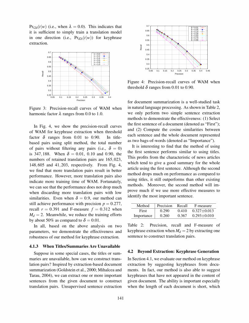
Prt2d(t|w) (i.e., when λ = 0.0). This indicates thatit is sufficient to simply train a translation modelin one direction (i.e., Prd2t(t|w)) for keyphraseextraction.

0.25

0.3

0.35

0.4

0.45

0.5

0.55

0.6

0.65

0.7

0.05 0.1 0.15 0.2 0.25 0.3 0.35 0.4

Rec

all

Precision

λ = 0.0λ = 0.2λ = 0.4λ = 0.6λ = 0.8λ = 1.0

Figure 3: Precision-recall curves of WAM whenharmonic factor λ ranges from 0.0 to 1.0.

In Fig. 4, we show the precision-recall curvesof WAM for keyphrase extraction when thresholdfactor δ ranges from 0.01 to 0.90. In title-based pairs using split method, the total numberof pairs without filtering any pairs (i.e., δ = 0)is 347,188. When δ = 0.01, 0.10 and 0.90, thenumbers of retained translation pairs are 165,023,148,605 and 41,203, respectively. From Fig. 4,we find that more translation pairs result in betterperformance. However, more translation pairs alsoindicate more training time of WAM. Fortunately,we can see that the performance does not drop muchwhen discarding more translation pairs with lowsimilarities. Even when δ = 0.9, our method canstill achieve performance with precision p = 0.277,recall r = 0.391 and F-measure f = 0.312 whenMd = 2. Meanwhile, we reduce the training effortsby about 50% as compared to δ = 0.01.

In all, based on the above analysis on twoparameters, we demonstrate the effectiveness androbustness of our method for keyphrase extraction.

4.1.3 When Titles/Summaries Are UnavailableSuppose in some special cases, the titles or sum-

maries are unavailable, how can we construct trans-lation pairs? Inspired by extraction-based documentsummarization (Goldstein et al., 2000; Mihalcea andTarau, 2004), we can extract one or more importantsentences from the given document to constructtranslation pairs. Unsupervised sentence extraction

0.25

0.3

0.35

0.4

0.45

0.5

0.55

0.6

0.65

0.7

0.05 0.1 0.15 0.2 0.25 0.3 0.35 0.4 0.45

Rec

all

Precision

δ = 0.01δ = 0.05δ = 0.10δ = 0.30δ = 0.50δ = 0.70δ = 0.90

Figure 4: Precision-recall curves of WAM whenthreshold δ ranges from 0.01 to 0.90.

for document summarization is a well-studied taskin natural language processing. As shown in Table 2,we only perform two simple sentence extractionmethods to demonstrate the effectiveness: (1) Selectthe first sentence of a document (denoted as “First”);and (2) Compute the cosine similarities betweeneach sentence and the whole document representedas two bags-of-words (denoted as “Importance”).

It is interesting to find that the method of usingthe first sentence performs similar to using titles.This profits from the characteristic of news articleswhich tend to give a good summary for the wholearticle using the first sentence. Although the secondmethod drops much on performance as compared tousing titles, it still outperforms than other existingmethods. Moreover, the second method will im-prove much if we use more effective measures toidentify the most important sentence.

Method Precision Recall F-measureFirst 0.290 0.410 0.327±0.013

Importance 0.260 0.367 0.293±0.010

Table 2: Precision, recall and F-measure ofkeyphrase extraction when Md = 2 by extracting onesentence to construct translation pairs.

4.2 Beyond Extraction: Keyphrase Generation

In Section 4.1, we evaluate our method on keyphraseextraction by suggesting keyphrases from docu-ments. In fact, our method is also able to suggestkeyphrases that have not appeared in the content ofgiven document. The ability is important especiallywhen the length of each document is short, which

141

itself may not contain appropriate keyphrases. Wename the new task keyphrase generation. Toevaluate these methods on keyphrase generation,we perform keyphrase generation for the titles ofdocuments, which are usually much shorter thantheir corresponding documents. The experimentsetting is as follows: the training phase is thesame to the previous experiment, but in the testphase we suggest keyphrases only using the titles.LDA and ExpandRank, similar to our method, arealso able to select candidate keyphrases beyond thetitles. We still use the annotated keyphrases of thecorresponding documents as standard answers. Inthis case, about 59% standard keyphrases do notappear in titles.

In Table 3 we show the evaluation results of vari-ous methods for keyphrase generation when Md = 2.For WAM, we only show the results using title-basedpairs prepared with split method. From the table,we have three observations: (1) WAM outperformsother methods on keyphrase generation. Moreover,there are about 10% correctly suggested keyphrasesby WAM do not appear in titles, which indicates theeffectiveness of WAM for keyphrase generation. (2)The performance of TFIDF and TextRank is muchlower as compared to Table 1, because the titles areso short that they do not provide enough candidatekeyphrases and even the statistical information torank candidate keyphrases. (3) LDA, ExpandRankand WAM roughly keep comparable performance asin Table 1 (The performance of ExpandRank dropsa bit). This indicates the three methods are able toperform keyphrase generation, and verifies again theeffectiveness of our method.

Method Precision Recall F-measureTFIDF 0.105 0.141 0.115±0.004

TextRank 0.107 0.144 0.118±0.005LDA 0.180 0.256 0.204±0.008

ExpandRank 0.194 0.268 0.216±0.012WAM 0.296 0.420 0.334±0.009

Table 3: Precision, recall and F-measure of variousmethods for keyphrase generation when Md = 2.

To demonstrate the features of our method forkeyphrase generation, in Table 4 we list top-5keyphrases suggested by LDA, ExpandRank andWAM for a news article entitled Israeli Military

Claims Iran Can Produce Nuclear Bombs andConsidering Military Action against Iran (We trans-late the original Chinese title and keyphrases intoEnglish for comprehension.). We have the followingobservations: (1) LDA suggests general words like“negotiation” and “sanction” as keyphrases becausethe coarse-granularity of topics. (2) ExpandRanksuggests some irrelevant words like “Lebanon” askeyphrases, which are introduced by neighbor doc-uments talking about other affairs related to Israel.(3) Our method can generate appropriate keyphraseswith less topic-drift. Moreover, our method can findgood keyphrases like “nuclear weapon” which evendo not appear in the title.

LDA: Iran, U.S.A., negotiation, Israel, sanctionExpandRank: Iran, Israel, Lebanon, U.S.A., IsraeliMilitaryWAM: Iran, military action, Israeli Military, Israel,nuclear weapon

Table 4: Top-5 keyphrases suggested by LDA,ExpandRank and WAM.


In this paper, we provide a new perspective tokeyphrase extraction: regarding a document and itskeyphrases as descriptions to the same object writtenin two languages. We use IBM Model-1 to bridgethe vocabulary gap between the two languages forkeyphrase generation. We explore various methodsto construct translation pairs. Experiments showthat our method can capture the semantic relationsbetween words in documents and keyphrases. Ourmethod is also language-independent, which can beperformed on documents in any languages.

We will explore the following two future work:(1) Explore our method on other types of articlesand on other languages. (2) Explore more com-plicated methods to extract important sentences forconstructing translation pairs.

Acknowledgments

This work is supported by the National NaturalScience Foundation of China (NSFC) under GrantNo. 60873174. The authors would like to thankPeng Li and Xiance Si for their suggestions.

142

References

M. Banko, V.O. Mittal, and M.J. Witbrock. 2000.Headline generation based on statistical translation. InProceedings of ACL, pages 318–325.

A. Berger and J. Lafferty. 1999. Information retrieval asstatistical translation. In Proceedings of SIGIR, pages222–229.

A. Berger, R. Caruana, D. Cohn, D. Freitag, andV. Mittal. 2000. Bridging the lexical chasm: statisticalapproaches to answer-finding. In Proceedings ofSIGIR, pages 192–199.

D.M. Blei and J.D. Lafferty, 2009. Text mining:Classification, Clustering, and Applications, chapterTopic models. Chapman & Hall.

D.M. Blei, A.Y. Ng, and M.I. Jordan. 2003. Latentdirichlet allocation. Journal of Machine LearningResearch, 3:993–1022, January.

P.F. Brown, V.J.D. Pietra, S.A.D. Pietra, and R.L.Mercer. 1993. The mathematics of statistical machinetranslation: Parameter estimation. Computationallinguistics, 19(2):263–311.

A.P. Dempster, N.M. Laird, D.B. Rubin, et al. 1977.Maximum likelihood from incomplete data via the emalgorithm. Journal of the Royal Statistical Society.Series B (Methodological), 39(1):1–38.

P. Duygulu, Kobus Barnard, J. F. G. de Freitas, andDavid A. Forsyth. 2002. Object recognition asmachine translation: Learning a lexicon for a fixedimage vocabulary. In Proceedings of ECCV, pages97–112.

A. Echihabi and D. Marcu. 2003. A noisy-channelapproach to question answering. In Proceedings ofACL, pages 16–23.

E. Frank, G.W. Paynter, I.H. Witten, C. Gutwin, and C.G.Nevill-Manning. 1999. Domain-specific keyphraseextraction. In Proceedings of IJCAI, pages 668–673.

J. Goldstein, V. Mittal, J. Carbonell, and M. Kantrowitz.2000. Multi-document summarization by sentenceextraction. In Proceedings of NAACL-ANLP 2000Workshop on Automatic summarization, pages 40–48.

G. Heinrich. 2005. Parameter estimation for text anal-ysis. Web: http://www. arbylon. net/publications/text-est.

T. Hofmann. 1999. Probabilistic latent semanticindexing. In Proceedings of SIGIR, pages 50–57.

A. Hulth. 2003. Improved automatic keyword extractiongiven more linguistic knowledge. In Proceedings ofEMNLP, pages 216–223.

M. Karimzadehgan and C.X. Zhai. 2010. Estimation ofstatistical translation models based on mutual informa-tion for ad hoc information retrieval. In Proceedingsof SIGIR, pages 323–330.

P. Koehn. 2010. Statistical Machine Translation.Cambridge University Press.

T.K. Landauer, P.W. Foltz, and D. Laham. 1998. Anintroduction to latent semantic analysis. DiscourseProcesses, 25:259–284.

Z. Liu, P. Li, Y. Zheng, and M. Sun. 2009a. Clusteringto find exemplar terms for keyphrase extraction. InProceedings of EMNLP, pages 257–266.

Z. Liu, H. Wang, H. Wu, and S. Li. 2009b. Collocationextraction using monolingual word alignment method.In Proceedings of EMNLP, pages 487–495.

Z. Liu, W. Huang, Y. Zheng, and M. Sun. 2010a. Au-tomatic keyphrase extraction via topic decomposition.In Proceedings of EMNLP, pages 366–376.

Z. Liu, H. Wang, H. Wu, and S. Li. 2010b. Improvingstatistical machine translation with monolingual collo-cation. In Proceedings of ACL, pages 825–833.

R. Mihalcea and P. Tarau. 2004. Textrank: Bringingorder into texts. In Proceedings of EMNLP, pages404–411.

V. Murdock and W.B. Croft. 2004. Simple translationmodels for sentence retrieval in factoid question an-swering. In Proceedings of SIGIR.

T. Nguyen and M.Y. Kan. 2007. Keyphrase extractionin scientific publications. In Proceedings of the 10thInternational Conference on Asian Digital Libraries,pages 317–326.

F.J. Och and H. Ney. 2003. A systematic comparison ofvarious statistical alignment models. Computationallinguistics, 29(1):19–51.

L. Page, S. Brin, R. Motwani, and T. Winograd. 1998.The pagerank citation ranking: Bringing order tothe web. Technical report, Stanford Digital LibraryTechnologies Project, 1998.

C. Quirk, C. Brockett, and W. Dolan. 2004. Monolingualmachine translation for paraphrase generation. InProceedings of EMNLP, volume 149.

S. Riezler and Y. Liu. 2010. Query rewriting usingmonolingual statistical machine translation. Compu-tational Linguistics, 36(3):569–582.

S. Riezler, A. Vasserman, I. Tsochantaridis, V. Mittal, andY. Liu. 2007. Statistical machine translation for queryexpansion in answer retrieval. In Proccedings of ACL,pages 464–471.

S. Riezler, Y. Liu, and A. Vasserman. 2008. Translatingqueries into snippets for improved query expansion. InProceedings of COLING, pages 737–744.

G. Salton and C. Buckley. 1988. Term-weightingapproaches in automatic text retrieval. Informationprocessing and management, 24(5):513–523.

R. Soricut and E. Brill. 2006. Automatic questionanswering using the web: Beyond the factoid. Infor-mation Retrieval, 9(2):191–206.

143

P.D. Turney. 2000. Learning algorithms for keyphraseextraction. Information Retrieval, 2(4):303–336.

X. Wan and J. Xiao. 2008a. Collabrank: towards acollaborative approach to single-document keyphraseextraction. In Proceedings of COLING, pages 969–976.

X. Wan and J. Xiao. 2008b. Single documentkeyphrase extraction using neighborhood knowledge.In Proceedings of AAAI, pages 855–860.

I.H. Witten, G.W. Paynter, E. Frank, C. Gutwin, andC.G. Nevill-Manning. 1999. Kea: Practical automatickeyphrase extraction. In Proceedings of DL, pages254–255.

X. Xue, J. Jeon, and W.B. Croft. 2008. Retrieval modelsfor question and answer archives. In Proceedings ofSIGIR, pages 475–482.

S. Zhao, H. Wang, and T. Liu. 2010. Paraphrasing withsearch engine query logs. In Proceedings of COLING,pages 1317–1325.

144


Using Second-order Vectors in aKnowledge-based Method for Acronym Disambiguation

Bridget T. McInnes∗

College of PharmacyUniversity of MinnesotaMinneapolis, MN 55455

Ted PedersenDepartment of Computer Science

University of MinnesotaDuluth, MN 55812

Ying LiuCollege of Pharmacy

University of MinnesotaMinneapolis, MN 55455

Serguei V. PakhomovCollege of Pharmacy


Genevieve B. MeltonInstitute for Health Informatics


Abstract

In this paper, we introduce a knowledge-basedmethod to disambiguate biomedical acronymsusing second-order co-occurrence vectors. Wecreate these vectors using information about along-form obtained from the Unified MedicalLanguage System and Medline. We evaluatethis method on a dataset of 18 acronyms foundin biomedical text. Our method achieves anoverall accuracy of 89%. The results showthat using second-order features provide a dis-tinct representation of the long-form and po-tentially enhances automated disambiguation.

1 Introduction

Word Sense Disambiguation (WSD) is the taskof automatically identifying the appropriate sense ofa word with multiple senses. For example, the wordculture could refer toanthropological culture

(e.g., the culture of the Mayan civilization), or alaboratory culture (e.g., cell culture).

Acronym disambiguation is the task of automat-ically identifying the contextually appropriate long-form of an ambiguous acronym. For example, theacronymMScould refer to the diseaseMultiple Scle-rosis, the drugMorphine Sulfate, or the stateMissis-sippi, among others. Acronym disambiguation canbe viewed as a special case of WSD, although, un-like terms, acronyms tend to be complete phrasesor expressions, therefore collocation features arenot as easily identified. For example, the featurerate when disambiguating the terminterest, as in

∗Contact author : [email protected].

interest rate, may not be available. Acronyms alsotend to be noun phrases, therefore syntactic featuresdo not provide relevant information for the purposesof disambiguation.

Identifying the correct long-form of an acronymis important not only for the retrieval of informationbut the understanding of the information by the re-cipient. In general English, Park and Byrd (2001)note that acronym disambiguation is not widelystudied because acronyms are not as prevalent in lit-erature and newspaper articles as they are in specificdomains such as government, law, and biomedicine.

In the biomedical sublanguage domain, acronymdisambiguation is an extensively studied problem.Pakhomov (2002) note acronyms in biomedical lit-erature tend to be used much more frequently than innews media or general English literature, and tendto be highly ambiguous. For example, the Uni-fied Medical Language System (UMLS), which in-cludes one of the largest terminology resources inthe biomedical domain, contains 11 possible long-forms of the acronymMS in addition to the fourexamples used above. Liu et al. (2001) show that33% of acronyms are ambiguous in the UMLS. In asubsequent study, Liu et al. (2002a) found that 80%of all acronyms found in Medline, a large repositoryof abstracts from biomedical journals, are ambigu-ous. Wren and Garner (2002) found that there exist174,000 unique acronyms in the Medline abstractsin which 36% of them are ambiguous. The authorsalso estimated that the number of unique acronymsis increasing at a rate of 11,000 per year.

Supervised and semi-supervised methods havebeen used successfully for acronym disambiguation

145

but are limited in scope due to the need for sufficienttraining data. Liu et al. (2004) state that an acronymcould have approximately 16 possible long-forms inMedline but could not obtain a sufficient number ofinstances for each of the acronym-long-form pairsfor their experiments. Stevenson et al. (2009) citea similar problem indicating that acronym disam-biguation methods that do not require training data,regardless if it is created manually or automatically,are needed.

In this paper, we introduce a novel knowledge-based method to disambiguate acronyms usingsecond-order co-occurrence vectors. This methoddoes not rely on training data, and therefore, is notlimited to disambiguating only commonly occurringpossible long-forms. These vectors are created us-ing the first-order features obtained from the UMLSabout the acronym’s long-forms and second-orderfeatures obtained from Medline. We show that us-ing second-order features provide a distinct repre-sentation of the long-form for the purposes of dis-ambiguation and obtains a significantly higher dis-ambiguation accuracy than using first order features.

2 Unified Medical Language System

The Unified Medical Language System (UMLS) isa data warehouse that stores a number of distinctbiomedical and clinical resources. One such re-source, used in this work, is the Metathesaurus.The Metathesaurus contains biomedical and clin-ical concepts from over 100 disparate terminol-ogy sources that have been semi-automatically in-tegrated into a single resource containing a widerange of biomedical and clinical information. Forexample, it contains the Systematized Nomencla-ture of Medicine–Clinical Terms (SNOMED CT),which is a comprehensive clinical terminology cre-ated for the electronic exchange of clinical healthinformation, the Foundational Model of Anatomy(FMA), which is an ontology of anatomical conceptscreated specifically for biomedical and clinical re-search, and MEDLINEPLUS, which is a terminol-ogy source containing health related concepts cre-ated specifically for consumers of health services.

The concepts in these sources can overlap. Forexample, the conceptAutonomic nerveexists in bothSNOMED CT and FMA. The Metathesaurus assigns

the synonymous concepts from the various sourcesa Concept Unique Identifiers (CUIs). Thus boththeAutonomic nerveconcepts in SNOMED CT andFMA are assigned the same CUI (C0206250). Thisallows multiple sources in the Metathesaurus to betreated as a single resource.

Some sources in the Metathesaurus contain ad-ditional information about the concept such as aconcept’s synonyms, its definition and its relatedconcepts. There are two main types of relationsin the Metathesaurus that we use: the parent/childand broader/narrower relations. A parent/child re-lation is a hierarchical relation between two con-cepts that has been explicitly defined in one of thesources. For example, the conceptSplanchnic nervehas anis-a relation with the conceptAutonomicnerve in FMA. This relation is carried forward tothe CUI level creating a parent/child relations be-tween the CUIs C0037991 (Splanchnic nerve) andC0206250 (Autonomic nerve) in the Metathesaurus.A broader/narrower relation is a hierarchical relationthat does not explicitly come from a source but iscreated by the UMLS editors. We use the entireUMLS including the RB/RN and PAR/CHD rela-tions in this work.

3 Medline

Medline (Medical Literature Analysis and RetrievalSystem Online) is a bibliographic database contain-ing over 18.5 million citations to journal articlesin the biomedical domain which is maintained bythe National Library of Medicine (NLM). The 2010Medline Baseline, used in this study, encompassesapproximately 5,200 journals starting from 1948 andis 73 Gigabytes; containing 2,612,767 unique uni-grams and 55,286,187 unique bigrams. The majorityof the publications are scholarly journals but a smallnumber of newspapers, and magazines are included.

4 Acronym Disambiguation

Existing acronym disambiguation methods can beclassified into two categories: form-based andcontext-based methods. Form-based methods, suchas the methods proposed by Taghva and Gilbreth(1999), Pustejovsky et al. (2001), Schwartz andHearst (2003) and Nadeau and Turney (2005), dis-ambiguate the acronym by comparing its letters di-

146

rectly to the initial letters in the possible long-formsand, therefore, would have difficulties in distin-guishing between acronyms with similar long-forms(e.g., RA referring to Refractory anemia or Rheuma-toid arthritis).

In contrast, context-based methods disambiguatebetween acronyms based on the context in which theacronym is used with the assumption that the contextsurrounding the acronym would be different for eachof the possible long-forms. In the remainder of thissection, we discuss these types of methods in moredetail.

4.1 Context-based Acronym DisambiguationMethods

Liu et al. (2001) and Liu et al. (2002b) introducea semi-supervised method in which training andtest data are automatically created by extracting ab-stracts from Medline that contain the acronym’slong-forms. The authors use collocations and a bag-of-words approach to train a Naive Bayes algorithmand report an accuracy of 97%. This method be-gins to treat acronym disambiguation as more of aWSD problem by looking at the context in whichthe acronym exists to determine its long-form, ratherthan the long-form itself. In a subsequent study, Liuet al. (2004) explore using additional features andmachine learning algorithms and report an accuracyof 99% using the Naive Bayes.

Joshi (2006) expands on Liu, et al’s work. Theyevaluate additional machine learning algorithms us-ing unigrams, bigrams and trigrams as features.They found that given their feature set, SVMs ob-tain the highest accuracy (97%).

Stevenson et al. (2009) re-recreate this dataset us-ing the method described in Liu et al. (2001) to auto-matically create training data for their method whichuses a mixture of linguistics features (e.g., colloca-tions, unigrams, bigrams and trigrams) in combina-tion with the biomedical features CUIs and Medi-cal Subject Headings, which are terms manually as-signed to Medline abstracts for indexing purposes.The authors evaluate the Naive Bayes, SVM andVector Space Model (VSM) described by Agirre andMartinez (2004), and report that VSM obtained thehighest accuracy (99%).

Pakhomov (2002) also developed a semi-supervised method in which training data was

automatically created by first identifying the long-form found in the text of clinical reports, replacingthe long-form with the acronym to use as trainingdata. A maximum entropy model trained and testedon a corpus of 10,000 clinical notes achieved anaccuracy of 89%. In a subsequent study, Pakhomovet al. (2005) evaluate obtaining training data fromthree sources: Medline, clinical records and theworld wide web finding using a combination ofinstances from clinical records and the web obtainedthe highest accuracy.

Joshi et al. (2006) compare using the NaiveBayes, Decision trees and SVM on ambiguousacronyms found in clinical reports. The authorsuse the part-of-speech, the unigrams and the bi-grams of the context surrounding the acronym asfeatures. They evaluate their method on 7,738manually disambiguated instances of 15 ambiguousacronyms obtaining an accuracy of over 90% foreach acronym.

5 Word Sense Disambiguation

Many knowledge-based WSD methods have beendeveloped to disambiguate terms which are closelyrelated to the work presented in this paper. Lesk(1986) proposes a definition overlap method inwhich the appropriate sense of an ambiguous termwas determined based on the overlap between itsdefinition in a machine readable dictionary (MRD).Ide and Veronis (1998) note that this work provideda basis for most future MRD disambiguation meth-ods; including the one presented in this paper.

Banerjee and Pedersen (2002) use the Lesk’soverlap method to determine the relatedness be-tween two concepts (synsets) in WordNet. They ex-tend the method to not only include the definition(gloss) of the two synsets in the overlap but also theglosses of related synsets.

Wilks et al. (1990) expand upon Lesk’s method bycalculating the number of times the words in the def-inition co-occur with the ambiguous words. In theirmethod, a vector is created using the co-occurrenceinformation for the ambiguous word and each of itspossible senses. The similarity is then calculated be-tween the ambiguous word’s vector and each of thesense vectors. The sense whose vector is most simi-lar is assigned to the ambiguous word.

147

0 .3

0 0 0 0 0 0 disphosphoric

glu

cose

fructo

se

ph

osp

ho

ric

esters

chan

ged

effect

0 0 0 0 0

glyco

lyte

enzym

es

com

bin

ed

decreases

inten

sity

acid

0

metab

olites

FEATURES

0 0 0 0 .2 0 acid 0 0 0 .1 0 0

0 0 0 0 .5 0 0 esters 0 0 0 0 0 0

0 .1 0 0 0 0 0 0 0 0 0 0 0

0 0 0 0 0 0 0

fructose

0 0 0 0 0 0

0 0 0 0 0 0 0

diphosphate

0 0 0 0 0 0 isomer

0 0 0 0 0 0 0 prevalent 0 0 0 0 0 0

0 .1 0 .3 .5 .2 0 2nd order vector for Fructose Diphosphate

0 0 0 .1 0 0

Ext

end

ed D

efin

itio

n

for

Fru

cto

se D

iph

osp

hat

e

Figure 1: 2nd Order Vector for Fructose Diphosphate (FDP)

Patwardhan and Pedersen (2006) introduce a vec-tor measure to determine the relatedness betweenpairs of concepts. In this measure, a second orderco-occurrence vector is created for each concept us-ing the words in each of the concepts definition andcalculating the cosine between the two vectors. Thismethod has been used in the task of WSD by calcu-lating the relatedness between each possible senseof the ambiguous word and its surrounding context.The context whose sum is the most similar is as-signed to the ambiguous word.

Second-order co-occurrence vectors were first in-troduced by Schutze (1992) for the task of wordsensediscrimination and later extended by Puran-dare and Pedersen (2004). As noted by Pedersen(2010), disambiguation requires a sense-inventoryin which the long-forms are known ahead of time,where as in discrimination this information is notknown a priori.

6 Method

In our method, a second-order co-occurrence vec-tor is created for each possible long-form of the

acronym, and the acronym itself. The appropriatelong-form of the acronym is then determined bycomputing a cosine between the vector represent-ing the ambiguous acronym and each of the vectorsrepresenting the long-forms. The long-form whosevector has the smallest angle between it and theacronym vector is chosen as the most likely long-form of the acronym.

To create a second-order vector for a long-form,we first obtain a textual description of the long-formin the UMLS, which we refer to as theextended defi-nition. Each long-form, from our evaluation set, wasmapped to a concept in the UMLS, therefore, we usethe long-form’s definition plus the definition of itsparent/children and narrow/broader relations and theterms in the long-form.

We include the definition of the related conceptsbecause not all concepts in the UMLS have a defini-tion. In our evaluation dataset, not a single acronymhas a definition for each possible long-form. Onaverage, each extended definition contains approx-imately 453 words. A short example of the extendeddefinition for the acronym FDP when referring to

148

fructose diphosphateis: “ Diphosphoric acid estersof fructose. The fructose diphosphate isomer is mostprevalent. fructose diphosphate.”

After the extended definition is obtained, we cre-ate the second-order vector by first creating a wordby word co-occurrence matrix in which the rowsrepresent the content words in the long-forms, ex-tended definition, and the columns represent wordsthat co-occur in Medline abstracts with the words inthe definition. Each cell in this matrix contains theLog Likelihood Ratio (Dunning (1993)) of the wordfound in the row and the word in the column. Sec-ond, each word in the long-forms, extended defini-tion is replaced by its corresponding vector, as givenin the co-occurrence matrix. The centroid of thesevectors constitutes the second order co-occurrencevector used to represent the long-form.

For example, given theexample corpuscontain-ing two instances: 1) The metabolites, glucose fruc-tose and their phosphoric acid esters are changeddue to the effect of glycolytic enzymes, and 2)The phosphoric acid combined with metabolites de-creases the intensity. Figure 1 shows how thesecond-order co-occurrence vector is created for thelong-form fructose diphosphateusing the extendeddefinition and features from our given corpus above.

The second-order co-occurrence vector for theambiguous acronym is created in a similar fashion,only rather than using words in the extended defini-tion, we use the words surrounding the acronym inthe instance.

Vector methods are subject to noise introduced byfeatures that do not distinguish between the differ-ent long-forms of the acronym. To reduce this typeof noise, we select the features to use in the secondorder co-occurrence vectors based on the followingcriteria: 1) second order feature cannot be a stop-word, and 2) second order feature must occur at leasttwice in the feature extraction dataset and not occurmore than 150 times. We also experiment with thelocation of the second-order feature with respect tothe first-order feature by varying the window size ofzero, four, six and ten words to the right and the leftof the first-order feature. The experiments in thispaper were conducted using CuiTools v0.15.1

Our method is different from other context-based

1http://cuitools.sourceforge.net

acronym disambiguation methods discussed in therelated work because it does not require annotatedtraining data for each acronym that needs to be dis-ambiguated. Our method differs from the methodproposed by Wilks et al. (1990) in two fundamen-tal aspects: 1) using theextended definition ofthe possible long-forms of an acronym, and 2) usingsecond-order vectors to represent the instance con-taining the acronym and each of the acronym’s pos-sible long-forms.

7 Data

7.1 Acronym Dataset

We evaluated our method on the “Abbrev” dataset2

made available by Stevenson et al. (2009). Theacronyms and long-forms in the data were initiallypresented by Liu et al. (2001). Stevenson et al.(2009) automatically re-created this dataset by iden-tifying the acronyms and long-forms in Medline ab-stracts and replacing the long-form in the abstractwith its acronym. Each abstract contains approxi-mately 216 words. The dataset consists of three sub-sets containing 100 instances, 200 instances and 300instances of the ambiguous acronym referred to asAbbrev.100, Abbrev.200, Abbrev.300, respectively.The acronyms long-forms were manually mapped toconcepts in the UMLS by Stevenson, et al.

A sufficient number of instances were not foundfor each of the 21 ambiguous acronyms by Steven-son et al. (2009). For example, “ASP” only con-tained 71 instances and therefore not included in anyof the subsets. “ANA” and “FDP” only containedjust over 100 instances and therefore, are only in-cluded in the Abbrev.100 subset. “ACE”, “ASP”and “CSF” were also excluded because several ofthe acronyms’ long-forms did not occur frequentlyenough in Medline to create a balanced dataset.

We evaluate our method on the same subsets thatStevenson et al. (2009) used to evaluate their super-vised method. The average number of long-formsper acronym is 2.6 and the average majority senseacross all subsets is 70%.

7.2 Feature Extraction Dataset

We use abstracts from Medline, containing ambigu-ous acronym or long-form, to create the second-

2http://nlp.shef.ac.uk/BioWSD/downloads/corpora

149

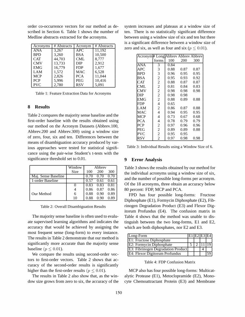
order co-occurrence vectors for our method as de-scribed in Section 6. Table 1 shows the number ofMedline abstracts extracted for the acronyms.

Acronyms # Abstracts Acronym # AbstractsANA 3,267 APC 11,192BPD 3,260 BSA 10,500CAT 44,703 CML 8,777CMV 13,733 DIP 2,912EMG 16,779 FDP 1,677LAM 1,572 MAC 6,528MCP 2,826 PCA 11,044PCP 5,996 PEG 10,416PVC 2,780 RSV 5,091

Table 1: Feature Extraction Data for Acronyms

8 Results

Table 2 compares the majority sense baseline and thefirst-order baseline with the results obtained usingour method on the Acronym Datasets (Abbrev.100,Abbrev.200 and Abbrev.300) using a window sizeof zero, four, six and ten. Differences between themeans of disambiguation accuracy produced by var-ious approaches were tested for statistical signifi-cance using the pair-wise Student’s t-tests with thesignificance threshold set to 0.01.

Window AbbrevSize 100 200 300

Maj. Sense Baseline 0.70 0.70 0.701-order Baseline 0.57 0.61 0.61

Our Method

0 0.83 0.83 0.814 0.86 0.87 0.866 0.88 0.90 0.8910 0.88 0.90 0.89

Table 2: Overall Disambiguation Results

The majority sense baseline is often used to evalu-ate supervised learning algorithms and indicates theaccuracy that would be achieved by assigning themost frequent sense (long-form) to every instance.The results in Table 2 demonstrate that our method issignificantly more accurate than the majority sensebaseline(p ≤ 0.01).

We compare the results using second-order vec-tors to first-order vectors. Table 2 shows that ac-curacy of the second-order results is significantlyhigher than the first-order results(p ≤ 0.01).

The results in Table 2 also show that, as the win-dow size grows from zero to six, the accuracy of the

system increases and plateaus at a window size often. There is no statistically significant differencebetween using a window size of six and ten but thereis a significant difference between a window size ofzero and six, as well as four and six (p ≤ 0.01).

Acronym# LongAbbrev Abbrev Abbrevforms 100 200 300

ANA 3 0.84APC 3 0.88 0.87 0.87BPD 3 0.96 0.95 0.95BSA 2 0.95 0.93 0.92CAT 2 0.88 0.87 0.87CML 2 0.81 0.84 0.83CMV 2 0.98 0.98 0.98DIP 2 0.98 0.98EMG 2 0.88 0.89 0.88FDP 4 0.65LAM 2 0.86 0.87 0.88MAC 4 0.94 0.95 0.95MCP 4 0.73 0.67 0.68PCA 4 0.78 0.79 0.79PCP 2 0.97 0.96 0.96PEG 2 0.89 0.89 0.88PVC 2 0.95 0.95RSV 2 0.97 0.98 0.98

Table 3: Individual Results using a Window Size of 6.

9 Error Analysis

Table 3 shows the results obtained by our method forthe individual acronyms using a window size of six,and the number of possible long-forms per acronym.Of the 18 acronyms, three obtain an accuracy below80 percent: FDP, MCP and PCA.

FPD has four possible long-forms: FructoseDiphosphate (E1), Formycin Diphosphate (E2), Fib-rinogen Degradation Product (E3) and Flexor Dig-itorum Profundus (E4). The confusion matrix inTable 4 shows that the method was unable to dis-tinguish between the two long-forms, E1 and E2,which are both diphosphates, nor E2 and E3.

Long-Form E1 E2 E3 E4E1: Fructose DiphosphateE2: Formycin Diphosphate 5 2 11 19E3: Fibrinogen Degradation Product 4E4: Flexor Digitorum Profundus 59

Table 4: FDP Confusion Matrix

MCP also has four possible long-forms: Multicat-alytic Protease (E1), Metoclopramide (E2), Mono-cyte Chemoattractant Protein (E3) and Membrane

150

Cofactor Protein (E4). The confusion matrix in Ta-ble 5 shows that the method was not able to distin-guish between E3 and E4, which are both proteins,and E1, which is a protease (an enzyme that breaksdown a protein).

Long-Form E1 E2 E3 E4E1: Multicatalytic Protease 1 5 6 1E2: Metoclopramide 15E3: Monocyte Chemoattractant Protein1 3 44 11E4: Membrane Cofactor Protein 13

Table 5: MCP Confusion Matrix

PCA has four possible long-forms: Passive Cu-taneous Anaphylaxis (E1), Patient Controlled Anal-gesia (E2), Principal Component Analysis (E3), andPosterior Cerebral Artery (E4). The confusion ma-trix in Table 6 shows that the method was not ableto distinguish between E2 and E3. Analyzing theextended definitions of the concepts showed that E2includes the definition to the concept Pain Manage-ment. The words in this definition overlap withmany of the words used in E3s extended definition.

Long-Form E1 E2 E3 E4E1:Passive Cutaneous Anaphylaxis18 6 1E2:Patient Controlled Analgesia 5 15E3:Principal Component Analysis 48E4:Posterior Cerebral Artery 7

Table 6: PCA Confusion Matrix

10 Comparison with Previous Work

Of the previously developed methods, Liu et al.(2004) and Stevenson et al. (2009) evaluated theirsemi-supervised methods on the same dataset as weused for the current study. A direct comparisoncan not be made between our method and Liu et al.(2004) because we do not have an exact duplicationof the dataset that they use. Their results are com-parable to Stevenson et al. (2009) with both report-ing results in the high 90s. Our results are directlycomparable to Stevenson et al. (2009) who reportan overall accuracy of 98%, 98% and 99% on theAbbrev.100, Abbrev.200 and Abbrev.300 datasetsrespectively. This is approximately 10 percentagepoints higher than our results.

The advantage of the methods proposed byStevenson et al. (2009) and Liu et al. (2004) is that

they are semi-supervised which have been shown toobtain higher accuracies than methods that do notuse statistical machine learning algorithms. The dis-advantage is that sufficient training data are requiredfor each possible acronym-long-form pair. Liu etal. (2004) state that an acronym could have approxi-mately 16 possible long-forms in Medline but a suf-ficient number of instances for each of the acronym-long-form pairs were not found in Medline and,therefore, evaluated their method on 15 out of theoriginal 34 acronyms. Stevenson et al. (2009) citea similar problem in re-creating this dataset. Thisshows the limitation to these methods is that a suffi-cient number of training examples can not be ob-tained for each acronym that needs to be disam-biguated. The method proposed in the paper doesnot have this limitation and can be used to disam-biguate any acronym in Medline.

11 Discussion

In this paper, we presented a novel method to disam-biguate acronyms in biomedical text using second-order features extracted from the UMLS and Med-line. The results show that using second-order fea-tures provide a distinct representation of the long-form that is useful for disambiguation.

We believe that this is because biomedical textcontains technical terminology that has a rich sourceof co-occurrence information associated with themdue to their compositionality. Using second-orderinformation works reasonably well because whenthe terms in the extended definition are broken upinto their individual words, information is not beinglost. For example, the term Patient Controlled Anal-gesia can be understood by taking the union of themeanings of the three terms and coming up with anappropriate definition of the term (patient has con-trol over their analgesia).

We evaluated various window sizes to extract thesecond-order co-occurrence information from, andfound using locally occurring words obtains a higheraccuracy. This is consistent with the finding reportedby Choueka and Lusignan (1985) who conducted anexperiment to determine what size window is neededfor humans to determine the appropriate sense of anambiguous word.

The amount of data used to extract the second-

151

order features for each ambiguous acronym varieddepending on its occurrence in Medline. Table 1 inSection 7.2 shows the number of abstracts in Med-line used for each acronym. We compared the accu-racy obtained by our method using a window size ofsix on the Abbrev.100 dataset with the number of ab-stracts in the feature extraction data. We found thatthe accuracy was not correlated with the amount ofdata used (r = 0.07). This confirms that it is not thequantity but the content of the contextual informa-tion that determines the accuracy of disambiguation.

We compared using second-order features andfirst-order features showing that the second-order re-sults obtained a significantly higher accuracy. Webelieve that this is because the definitions of the pos-sible concepts are too sparse to provide enough in-formation to distinguish between them. This find-ing coincides to that of Purandare and Pedersen(2004) and Pedersen (2010) who found that withlarge amounts of data, first-order vectors performbetter than second-order vectors, but second-ordervectors are a good option when large amounts ofdata are not available.

The results of the error analysis indicate thatfor some acronyms using the extended definitiondoes not provide sufficient information to makefiner grained distinctions between the long-forms.This result also indicates that, although many long-forms of acronyms can be considered coarse-grainedsenses, this is not always the case. For example, theanalysis ofMCP showed that two of its possiblelong-forms are proteins which are difficult to differ-entiate from given the context.

The results of the error analysis also show thatindicative collocation features for acronyms are noteasily identified because acronyms tend to be com-plete phrases. For example, two of the possiblelong-forms ofDF are Fructose DiphosphateandFormycin Diphosphate.

Two main limitations of this work must be men-tioned to facilitate the interpretation of the results.The first is the small number of acronyms and thesmall number of long-forms per acronym in thedataset; however, the acronyms in this dataset arerepresentative of the kinds of acronyms one wouldexpect to see in biomedical text. The second limita-tion is that the dataset contains only those acronymswhose long-forms were found in Medline abstracts.

The main goal of this paper was to determine if thecontext found in the long-forms, extended definitionwas distinct enough to distinguish between them us-ing second-order vectors. For this purpose, we feelthat the dataset was sufficient although a more ex-tensive dataset may be needed in the future for im-proved coverage.

12 Future Work

In the future, we plan to explore three differentavenues. The first avenue is to look at obtainingcontextual descriptions of the possible long-formsfrom resources other than the UMLS such as theMetaMapped Medline baseline and WordNet. Thesecond avenue is limiting the features that are usedin the instance vectors. The first-order features inthe instance vector contain the words from the entireabstract. As previously mentioned, vector methodsare subject to noise, therefore, in the future we planto explore using only those words that are co-locatednext to the ambiguous acronym. The third avenue isexpanding the vector to allow for terms. Currently,we use word vectors, in the future, we plan to extendthe method to use terms, as identified by the UMLS,as features rather than single words.

We also plan to test our approach in the clinicaldomain. We believe that acronym disambiguationmay be more difficult in this domain due to the in-crease amount of long-forms as seen in the datasetsused by Joshi et al. (2006) and Pakhomov (2002).

13 Conclusions

Our study constitutes a significant step forward inthe area of automatic acronym ambiguity resolu-tion, as it will enable the incorporation of scalableacronym disambiguation into NLP systems used forindexing and retrieval of documents in specializeddomains such as medicine. The advantage of ourmethod over previous methods is that it does not re-quire manually annotated training for each acronymto be disambiguated while still obtaining an overallaccuracy of 89%.

Acknowledgments

This work was supported by the National Insti-tute of Health, National Library of Medicine Grant#R01LM009623-01.

152

References

E. Agirre and D. Martinez. 2004. The Basque CountryUniversity system: English and Basque tasks. InPro-ceedings of the 3rd ACL workshop on the Evaluationof Systems for the Semantic Analysis of Text (SENSE-VAL), pages 44–48.

S. Banerjee and T. Pedersen. 2002. An adapted lesk al-gorithm for word sense disambiguation using Word-Net. In Proceedings of the 3rd International Confer-ence on Intelligent Text Processing and ComputationalLinguistics, pages 136–145.

Y. Choueka and S. Lusignan. 1985. Disambiguationby short contexts. Computers and the Humanities,19(3):147–157.

T. Dunning. 1993. Accurate methods for the statistics ofsurprise and coincidence.Computational Linguistics,19(1):61–74.

N. Ide and J. Veronis. 1998. Introduction to the specialissue on word sense disambiguation: the state of theart. Computational Linguistics, 24(1):2–40.

M. Joshi, S. Pakhomov, T. Pedersen, and C.G. Chute.2006. A comparative study of supervised learning asapplied to acronym expansion in clinical reports. InProceedings of the Annual Symposium of AMIA, pages399–403.

M. Joshi. 2006. Kernel Methods for Word Sense Disam-biguation and Abbreviation Expansion. Master’s the-sis, University of Minnesota.

M. Lesk. 1986. Automatic sense disambiguation usingmachine readable dictionaries: how to tell a pine conefrom an ice cream cone.Proceedings of the 5th AnnualInternational Conference on Systems Documentation,pages 24–26.

H. Liu, YA. Lussier, and C. Friedman. 2001. Disam-biguating ambiguous biomedical terms in biomedicalnarrative text: an unsupervised method.Journal ofBiomedical Informatics, 34(4):249–261.

H. Liu, A.R. Aronson, and C. Friedman. 2002a. A studyof abbreviations in MEDLINE abstracts. InProceed-ings of the Annual Symposium of AMIA, pages 464–468.

H. Liu, S.B. Johnson, and C. Friedman. 2002b. Au-tomatic resolution of ambiguous terms based on ma-chine learning and conceptual relations in the UMLS.JAMIA, 9(6):621–636.

H. Liu, V. Teller, and C. Friedman. 2004. A multi-aspect comparison study of supervised word sense dis-ambiguation.JAMIA, 11(4):320–331.

D. Nadeau and P. Turney. 2005. A supervised learningapproach to acronym identification. InProceedingsof the 18th Canadian Conference on Artificial Intelli-gence, pages 319–329.

S. Pakhomov, T. Pedersen, and C.G. Chute. 2005. Ab-breviation and acronym disambiguation in clinical dis-course. InProceedings of the Annual Symposium ofAMIA, pages 589–593.

S. Pakhomov. 2002. Semi-supervised maximum en-tropy based approach to acronym and abbreviationnormalization in medical texts. InProceedings ofthe 40th Annual Meeting on Association for Compu-tational Linguistics, pages 160–167.

Y. Park and R.J. Byrd. 2001. Hybrid text mining for find-ing abbreviations and their definitions. InProceedingsof the Conference on Empirical Methods in NaturalLanguage Processing, pages 126–133.

S. Patwardhan and T. Pedersen. 2006. Using WordNet-based context vectors to estimate the semantic related-ness of concepts. InProceedings of the EACL 2006Workshop Making Sense of Sense - Bringing Com-putational Linguistics and Psycholinguistics Together,pages 1–8.

T. Pedersen. 2010. The effect of different context repre-sentations on word sense discrimination in biomedicaltexts. InProceedings of the 1st ACM International IHISymposium, pages 56–65.

A. Purandare and T. Pedersen. 2004. Word sense dis-crimination by clustering contexts in vector and sim-ilarity spaces. InProceedings of the Conference onComputational Natural Language Learning (CoNLL),pages 41–48.

J. Pustejovsky, J. Castano, B. Cochran, M. Kotecki,M. Morrell, and A. Rumshisky. 2001. Extraction anddisambiguation of acronym-meaning pairs in medline.Unpublished manuscript.

H. Schutze. 1992. Dimensions of meaning. InProceed-ings of the 1992 ACM/IEEE Conference on Supercom-puting, pages 787–796.

A.S. Schwartz and M.A. Hearst. 2003. A simplealgorithm for identifying abbreviation definitions inbiomedical text. InProceedings of the Pacific Sym-posium on Biocomputing (PSB), pages 451–462.

M. Stevenson, Y. Guo, A. Al Amri, and R. Gaizauskas.2009. Disambiguation of biomedical abbreviations.In Proceedings of the ACL BioNLP Workshop, pages71–79.

K. Taghva and J. Gilbreth. 1999. Recognizing acronymsand their definitions.ISRI UNLV, 1:191–198.

Y. Wilks, D. Fass, C.M. Guo, J.E. McDonald, T. Plate,and B.M. Slator. 1990. Providing machine tractabledictionary tools.Machine Translation, 5(2):99–154.

J.D. Wren and H.R. Garner. 2002. Heuristics for iden-tification of acronym-definition patterns within text:towards an automated construction of comprehensiveacronym-definition dictionaries.Methods of Informa-tion in Medicine, 41(5):426–434.

153


Using the Mutual k-Nearest Neighbor Graphsfor Semi-supervised Classification of Natural Language Data

Kohei Ozaki and Masashi Shimbo and Mamoru Komachi and Yuji MatsumotoNara Institute of Science and Technology

8916-5 Takayama, Ikoma, Nara 630-0192, Japan{kohei-o,shimbo,komachi,matsu}@is.naist.jp

Abstract

The first step in graph-based semi-supervisedclassification is to construct a graph from in-put data. While the k-nearest neighbor graphshave been the de facto standard method ofgraph construction, this paper advocates usingthe less well-known mutual k-nearest neigh-bor graphs for high-dimensional natural lan-guage data. To compare the performanceof these two graph construction methods, werun semi-supervised classification methods onboth graphs in word sense disambiguation anddocument classification tasks. The experi-mental results show that the mutual k-nearestneighbor graphs, if combined with maximumspanning trees, consistently outperform the k-nearest neighbor graphs. We attribute betterperformance of the mutual k-nearest neigh-bor graph to its being more resistive to mak-ing hub vertices. The mutual k-nearest neigh-bor graphs also perform equally well or evenbetter in comparison to the state-of-the-artb-matching graph construction, despite theirlower computational complexity.

1 Introduction

Semi-supervised classification try to take advan-tage of a large amount of unlabeled data in addi-tion to a small amount of labeled data, in order toachieve good classification accuracy while reducingthe cost of manually annotating data. In particular,graph-based techniques for semi-supervised classi-fication (Zhou et al., 2004; Zhu et al., 2003; Cal-lut et al., 2008; Wang et al., 2008) are recognizedas a promising approach. Some of these techniques

have been successfully applied for NLP tasks: wordsense disambiguation (Alexandrescu and Kirchhoff,2007; Niu et al., 2005), sentiment analysis (Gold-berg and Zhu, 2006), and statistical machine trans-lation (Alexandrescu and Kirchhoff, 2009), to namebut a few.

However, the focus of these studies is how to as-sign accurate labels to vertices in a given graph. Bycontrast, there has not been much work on how sucha graph should be built, and graph construction re-mains “more of an art than a science” (Zhu, 2005).Yet, it is an essential step for graph-based semi-supervised classification and (unsupervised) cluster-ing, and the input graph affects the quality of finalclassification/clustering results.

Both for semi-supervised classification and forclustering, the k-nearest neighbor (k-NN) graphconstruction has been used almost exclusively in theliterature. However, k-NN graphs often producehubs, or vertices with extremely high degree (i.e.,the number of edges incident to a vertex). This ten-dency is obvious especially if the original data ishigh-dimensional—a characteristic typical of natu-ral language data. In a later section, we demonstratethat such hub vertices indeed deteriorate the accu-racy of semi-supervised classification.

While not in the context of graph construction,Radovanovic et al. (2010) made an insightful obser-vation into the nature of hubs in high-dimensionalspace; in their context, a hub is a sample close tomany other samples in the (high-dimensional) sam-ple space. They state that such hubs inherentlyemerge in high-dimensional data as a side effect ofthe “curse of dimensionality,” and argue that this is a

154

reason nearest neighbor classification does not workwell in high-dimensional space.

Their observation is insightful for graph con-struction as well. Most of the graph-based semi-supervised classification methods work by gradu-ally propagating label information of a vertex to-wards neighboring vertices in a graph, but the neigh-borhood structure in the graph is basically deter-mined by the proximity of data in the original high-dimensional sample space. Hence, it is very likelythat a hub in the sample space also makes a hubin the k-NN graph, since k-NN graph constructiongreedily connects a pair of vertices if the sample cor-responding to one vertex is among the k closest sam-ples of the other sample in the original space. It istherefore desirable to have an efficient graph con-struction method for high-dimensional data that canproduce a graph with reduced hub effects.

To this end, we propose to use the mutual k-nearest neighbor graphs (mutual k-NN graphs),a less well-known variant of the standard k-NNgraphs. All vertices in a mutual k-NN graph havea degree upper-bounded by k, which is not usuallythe case with standard k-NN graphs. This propertyhelps not to produce vertices with extremely highdegree (hub vertices) in the graph. A mutual k-NNgraph is easy to build, at a time complexity identicalto that of the k-NN graph construction.

We first evaluated the quality of the graphs apartfrom specific classification algorithms using the φ-edge ratio of graphs. Our experimental results showthat the mutual k-NN graphs have a smaller num-ber of edges connecting vertices with different la-bels than the k-NN graphs, thus reducing the possi-bility of wrong label information to be propagated.We also compare the classification accuracy of twostandard semi-supervised classification algorithmson the mutual k-NN graphs and the k-NN graphs.The results show that the mutual k-NN graphs con-sistently outperorm the k-NN graphs. Moreover, themutual k-NN graphs achieve equally well or bet-ter classification accuracy than the state-of-the-artgraph construction method called b-matching (Je-bara et al., 2009), while taking much less time toconstruct.

2 Problem Statement

2.1 Semi-supervised Classification

The problem of semi-supervised classification canbe stated as follows. We are given a set of n ex-amples, X = {x1, . . . ,xn}, but only the labelsof the first l examples are at hand; the remainingu = n − l examples are unlabeled examples. LetS = {1, . . . , c} be the set of possible labels, andyi ∈ S the label of xi, for i = 1, . . . , n. Sincewe only know the labels of the first l examples, wedo not have access to yl+1, . . . , yn. For later conve-nience, further let y = (y1, . . . , yn).

The goal of a semi-supervised classification al-gorithm is to predict the hidden labels yl+1, . . . , yn

of u unlabeled examples xl+1, . . . ,xn, giventhese unlabeled examples and l labeled data(x1, y1), . . . , (xl, yl). A measure of similarity be-tween examples is also provided to the algorithm.Stated differently, the classifier has access to an all-pair similarity matrix W ′ of size n × n, with its(i, j)-element W ′ij holding the similarity of exam-ples xi and xj . It is assumed that W ′ is a symmetricmatrix, and the more similar two examples are (withrespect to the similarity measure), more likely theyare to have the same label. This last assumption isthe premise of many semi-supervised classificationalgorithms and is often called the cluster assumption(Zhou et al., 2004).

2.2 Graph-based Semi-supervisedClassification

Graph-based approaches to semi-supervised classi-fication are applicable if examples X are graph ver-tices. Otherwise, X must first be converted into agraph. This latter case is the focus of this paper.That is, we are interested in how to construct a graphfrom the examples, so that the subsequent classifica-tion works well.

Let G denote the graph constructed from the ex-amples. Naturally, G has n vertices, since verticesare identified with examples. Instead of graph G it-self, let us consider its real-valued (weighted) adja-cency matrix W , of size n × n. The task of graphconstruction then reduces to computing W from all-pairs similarity matrix W ′.

The simplest way to compute W from W ′ is tolet W = W ′, which boils down to using a dense,

155

complete graph G with the unmodified all-pairs sim-ilarity as its edge weights. However, it has been ob-served that a sparseW not only save time needed forclassification, but also results in better classificationaccuracy1 than the full similarity matrix W ′ (Zhu,2008). Thus, we are concerned with how to sparsifyW ′ to obtain a sparseW ; i.e., the strategy of zeroingout some elements of W ′.

Let the set of binary values be B = {0, 1}. A spar-sification strategy can be represented by a binary-valued matrix P ∈ Bn×n, where Pij = 1 if W ′ijmust be retained as Wij , and Pij = 0 if Wij = 0.Then, the weighted adjacency matrix W of G isgiven by Wij = PijW

′ij . The n × n matrices W

and P are symmetric, reflecting the fact that mostgraph-based algorithms require the input graph to beundirected.

3 k-Nearest Neighbor Graphs and theEffect of Hubs

The standard approach to making a sparse graph G(or equivalently, matrix W ) is to construct a k-NNgraph from the data (Szummer and Jaakkola, 2002;Niu et al., 2005; Goldberg and Zhu, 2006).

3.1 The k-Nearest Neighbor Graphs

The k-NN graph is a weighted undirected graph con-necting each vertex to its k-nearest neighbors in theoriginal sample space. Building a k-NN graph is atwo step process. First we solve the following opti-mization problem.

maxP∈Bn×n

∑i,j

PijW′ij (1)

s.t.∑

j

Pij = k, Pii = 0, ∀i, j ∈ {1, . . . , n}

Note that we are trying to find P , and not P . Thisis an easy problem and we can solve it by greedilyassigning Pij = 1 only if W ′ij is among the top kelements in the ith row of W ′ (in terms of the mag-nitude of the elements). After P is determined, welet Pij = max(Pij , Pji). Thus P is a symmetricmatrix, i.e., Pij = Pji for all i and j, while P may

1See also the experimental results of Section 6.3.2 in whichthe full similarity matrix W ′ is used as the baseline.

d 1 2 ≥ 3 total

# of vertices 1610 1947 164 3721

original 65.9 65.7 69.8 66.0hub-removed 66.6 66.0 69.8 66.4

Table 1: Classification accuracy of vertices around hubsin a k-NN graph, before (“original”) and after (“hub-removed”) hubs are removed. The value d represents theshortest distance (number of hops) from a vertex to itsnearest hub vertex in the graph.

not. Finally, weighted adjacency matrix W is deter-mined byWij = PijW

′ij . MatrixW is also symmet-

ric since P and W ′ are symmetric.This process is equivalent to retaining all edges

from each vertex to its k-nearest neighbor vertices,and then making all edges undirected.

Note the above symmetrization step is necessarybecause the k-nearest neighbor relation is not sym-metric; even if a vertex vi is a k-nearest neighbor ofanother vertex vj , vj may or may not be a k-nearestneighbor of vi. Thus, symmetrizing P and W asabove makes the graph irregular; i.e., the degree ofsome vertices may be larger than k, which opens thepossibility of hubs to emerge.

3.2 Effect of Hubs on Classification

In this section, we demonstrate that hubs in k-NNgraphs are indeed harmful to semi-supervised clas-sification as we claimed earlier. To this end, weeliminate such high degree vertices from the graph,and compare the classification accuracy of other ver-tices before and after the elimination. For this pre-liminary experiment, we used the “line” dataset ofa word sense disambiguation task (Leacock et al.,1993). For details of the dataset and the task, seeSection 6.

In this experiment, we randomly selected 10 per-cent of examples as labeled examples. The remain-ing 90 percent makes the set of unlabeled examples,and the goal is to predict the label (word sense) ofthese unlabeled examples.

We first built a k-NN graph (with k = 3)from the dataset, and ran Gaussian Random Fields(GRF) (Zhu et al., 2003), one of the most widely-used graph-based semi-supervised classification al-gorithms. Then we removed vertices with degree

156

greater than or equal to 30 from the k-NN graph,and ran GRF again on this “hub-removed” graph.

Table 1 shows the classification accuracy of GRFon the two graphs. The table shows both the over-all classification accuracy, and the classification ac-curacy on the subsets of vertices, stratified by theirdistance d from the nearest hub vertices (which wereeliminated in the “hub-removed” graph). Obvi-ously, overall classification accuracy has improvedafter hub removal. Also notice that the increase inthe classification accuracy on the vertices nearest tohubs (d = 1, 2). These results suggest that the pres-ence of hubs in the graph is deteriorating classifica-tion accuracy.

4 Mutual k-Nearest Neighbor Graphs forSemi-supervised Classification

As demonstrated in Section 3.2, removing hub ver-tices in k-NN graphs is an easy way of improv-ing the accuracy of semi-supervised classification.However, this method adds another parameter to thegraph construction method, namely, the threshold onthe degree of vertices to be removed. The methodalso does not tell us how to assign labels to the re-moved (hub) vertices. Hence, it is more desirableto have a graph construction method which has onlyone parameter just like the k-NN graphs, but is at thesame time less prone to produce hub vertices.

In this section, we propose to use mutual k-NNgraphs for this purpose.

4.1 Mutual k-Nearest Neighbor Graphs

The mutual k-NN graph is not a new concept andit has been used sometimes in clustering. Even inclustering, however, they are not at all as popular asthe ordinary k-NN graphs. A mutual k-NN graphis defined as a graph in which there is an edge be-tween vertices vi and vj if each of them belongs tothe k-nearest neighbors (in terms of the original sim-ilarity metric W ) of the other vertex. By contrast, ak-NN graph has an edge between vertices vi and vj

if one of them belongs to the k-nearest neighbors ofthe other. Hence, the mutual k-NN graph is a sub-graph of the k-NN graph computed from the samedata with the same value of k. The mutual k-NNgraph first optimizes the same formula as (1), but inmutual k-NN graphs, the binary-valued symmetric

matrix P is defined as Pij = min(Pij , Pji). Sincemutual k-NN graph construction guarantees that allvertices in the resulting graph have degree at mostk, it is less likely to produce extremely high degreevertices in comparison with k-NN graphs, providedthat the value of k is kept adequately small.

4.2 Fixing Weak Connectivity

Because the mutual k-NN graph construction ismore selective of edges than the standard k-NNgraphs, the resulting graphs often contain manysmall disconnected components. Disconnectedcomponents are not much of a problem for clus-tering (since its objective is to divide a graph intodiscrete components eventually), but can be a prob-lem for semi-supervised classification algorithms; ifa connected component does not contain a labelednode, the algorithms cannot reliably predict the la-bels of the vertices in the component; recall thatthese algorithms infer labels by propagating label in-formation along edges in the graph.

As a simple method for overcoming this problem,we combine the mutual k-NN graph and the max-imum spanning tree. To be precise, the minimumnumber of edges from the maximum spanning treeare added to the mutual k-NN graph to ensure thatonly one connected component exists in a graph.

4.3 Computational Efficiency

Using a Fibonacci heap-based implementation(Fredman and Tarjan, 1987), one can constructthe standard k-NN graph in (amortized) O(n2 +kn log n) time. A mutual k-NN graph can also beconstructed in the same time complexity as the k-NN graphs. The procedure below transforms a stan-dard k-NN graph into a mutual k-NN graph. It usesFibonacci heaps once again and assumes that the in-put k-NN graph is represented as an adjacency ma-trix in sparse matrix representation.

1. Each vertex is associated with its own heap.For each edge e connecting vertices u and v,insert e to the heaps associated with u and v.

2. Fetch maximum weighted edges from eachheap k times, keeping globally the record ofthe number of times each edge is fetched. No-tice that an edge can be fetched at most twice,

157

once at an end vertex of the edge and once atthe other end.

3. A mutual k-NN graph can be constructed byonly keeping edges fetched twice in the previ-ous step.

The complexity of this procedure is O(kn). Hencethe overall complexity of building a mutual k-NNgraph is dominated by the time needed to buildthe standard k-NN graph input to the system; i.e.,O(n2 + kn log n).

If we call the above procedure on an approximatek-NN graph which can be computed more efficiently(Beygelzimer et al., 2006; Chen et al., 2009; Ramet al., 2010; Tabei et al., 2010), it yields an ap-proximate mutual k-NN graphs. In this case, theoverall complexity is identical to that of the ap-proximate k-NN graph construction algorithm, sincethese approximate algorithms have a complexity atleast O(kn).

5 Related Work

5.1 b-Matching Graphs

Recently, Jebara et al. (2009) proposed a newgraph construction method called b-matching. A b-matching graph is a b-regular graph, meaning thatevery vertex has the degree b uniformly. It can be ob-tained by solving the following optimization prob-lem.

maxP∈Bn×n

∑ij

PijW′ij

s.t.∑

j

Pij = b, ∀i ∈ {1, . . . , n} (2)

Pii = 0, ∀i ∈ {1, . . . , n} (3)

Pij = Pji, ∀i, j ∈ {1, . . . , n} (4)

After P is computed, the weighted adjacency matrixW is determined by Wij = PijW

′ij The constraint

(4) makes the binary matrix P symmetric, and (3) isto ignore self-similarity (loops). Also, the constraint(2) ensures that the graph is regular. Note that k-NNgraphs are in general not regular. The regularity re-quirement of the b-matching graphs can be regardedas an effort to avoid the hubness phenomenon dis-cussed by Radovanovic et al. (2010).

Figure 1: Two extreme cases of φ-edge ratio. Vertexshapes (and colors) denote the class labels. The φ-edgeratio of the graph on the left is 1, meaning that all edgesconnect vertices with different labels. The φ-edge ratioof the one on the right is 0, because all edges connectvertices of the same class.

Jebara et al. (2009) reported that b-matchinggraphs achieve semi-supervised classification accu-racy higher than k-NN graphs. However, with-out approximation, building a b-matching graphis prohibitive in terms of computational complex-ity. Huang and Jebara (2007) developed a fast im-plementation based on belief propagation, but theguaranteed running time of the implementation isO(bn3), which is still not practical for large scalegraphs. Notice that the k-NN graphs and mutual k-NN graphs can be constructed with much smallertime complexity, as we mentioned in Section 4.3.In Section exp, we empirically compare the per-formance of mutual k-NN graphs with that of b-matching graphs.

5.2 Mutual Nearest Neighbor in Clustering

In the clustering context, mutual k-NN graphs havebeen theoretically analyzed by Maier et al. (2009)with Random Geometric Graph Theory. Their studysuggests that if one is interested in identifying themost significant clusters only, the mutual k-NNgraphs give a better clustering result. However, it isnot clear what their results imply in semi-supervisedclassification settings.

6 Experiments

We compare the k-NN, mutual k-NN, and b-matching graphs in word sense disambiguation anddocument classification tasks. All of these tasks aremulti-class classification problems.

6.1 Datasets

We used two word sense disambiguation datasets inour experiment: “interest” and “line.” The “inter-est” data is originally taken from the POS-tagged

158

interest dataset

number of edges (x 103)

phi−

edge

rat

io

0.10

0.15

0.20

0.25

●●●●●

●●●

●●●●●●●●●●●●●●●●●●●●●

0 5 10 15 20 25 30 35

● bMGkNNGMkNNG

line dataset


phi−

edge

rat

io

0.15

0.20

0.25

0.30

0.35

●●●

●●●●●●●●●●●●●●●●●●●

0 10 20 30 40

● bMGkNNGMkNNG

Reuters dataset


phi−

edge

rat

io

0.100.120.140.160.180.200.220.24

●

●●●●●●

●●●●●●●●●●●●●●●●●●●●●

0 10 20 30 40 50

● bMGkNNGMkNNG

20 newsgroups dataset


phi−

edge

rat

io

0.15

0.20

0.25

0.30

0.35

0.40

0 50 100 150 200 250

kNNGMkNNG

Figure 2: φ-edge ratios of the k-NN graph, mutual k-NN graph, and b-matching graphs. The φ-edge ratio of a graphis a measure of how much the cluster assumption is violated; hence, smaller the φ-edge ratio, the better. The plot forb-matching graph is missing for the 20 newsgroups dataset, because its construction did not finish after one week forthis dataset.

dataset examples features labels

interest 2,368 3,689 6line 4,146 8,009 6

Reuters 4,028 17,143 420 newsgroups 19,928 62,061 20

Table 2: Datasets used in experiments.

portion of the Wall Street Journal Corpus. Each in-stance of the polysemous word “interest” has beentagged with one of the six senses in Longman Dic-tionary of Contemporary English. The details of thedataset are described in Bruce and Wiebe (1994).The “line” data is originally used in numerous com-parative studies of word sense disambiguation. Eachinstance of the word “line” has been tagged with oneof the six senses on the WordNet thesaurus. Furtherdetails can be found in the Leacock et al. (1993).Following Niu et al. (2005), we used the followingcontext features in the word sense disambiguationtasks: part-of-speech of neighboring words, singlewords in the surrounding context, and local colloca-tion. Details of these context features can be foundin Lee and Ng (2002).

The Reuters dataset is extracted from RCV1-v2/LYRL2004, a text categorization test collection(Lewis et al., 2004). In the same manner as Cram-mer et al. (2009), we produced the classificationdataset by selecting approximately 4,000 documentsfrom 4 general topics (corporate, economic, gov-ernment and markets) at random. The features de-scribed in Lewis et al. (2004) are used with thisdataset.

The 20 newsgroups dataset is a popular datasetfrequently used for document classification andclustering. The dataset consists of approximately20,000 messages on newsgroups and is originallydistributed by Lang (1995). Each message is as-signed one of the 20 possible labels indicating whichnewsgroup it has been posted to, and represented asbinary bag-of-words features as described in Rennie(2001).

Table 2 summarizes the characteristics of thedatasets used in our experiments.


Our focus in this paper is a semi-supervised classi-fication setting in which the dataset contains a smallamount of labeled examples and a large amount ofunlabeled examples. To simulate such settings, wecreate 10 sets of labeled examples, with each setconsisting of randomly selected l examples from theoriginal dataset, where l is 10 percent of the totalnumber of examples. For each set, the remaining90 percent constitute the unlabeled examples whoselabels must be inferred.

After we build a graph from the data using oneof the graph construction methods discussed earlier,a graph-based semi-supervised classification algo-rithm must be run on the resulting graph to infer la-bels to the unlabeled examples (vertices). We usetwo most frequently used classification algorithms:Gaussian Random Fields (GRF) (Zhu et al., 2003)and the Local/Global Consistency algorithm (LGC)(Zhou et al., 2004). Averaged classification accuracyis used as the evaluation metric. For all datasets, co-

159

interest dataset (GRF)


aver

aged

acc

urac

y

0.79

0.80

0.81

0.82

0.83●●

●●●●

●●●●

●●●●●●●

●●●

●

●●●●●

0 5 10 15 20 25 30 35

● bMG

kNNG

MkNNG

interest dataset (LGC)


aver

aged

acc

urac

y

0.79

0.80

0.81

0.82

0.83●●

●●●●●

●●●

●●●●●

●●●●●●

●

●●●●

●

0 5 10 15 20 25 30 35

● bMG

kNNG

MkNNG

line dataset (GRF)


aver

aged

acc

urac

y

0.62

0.64

0.66

0.68

0.70

●●

●●

●●

●●●

●●●

●

●

●●●●

●●

0 10 20 30 40

● bMG

kNNG

MkNNG

line dataset (LGC)


aver

aged

acc

urac

y

0.62

0.64

0.66

0.68

0.70

●●

●●

●●

●●

●●

●●

●

●

●●●●

●●

0 10 20 30 40

● bMG

kNNG

MkNNG

Figure 3: Averaged classification accuracies for k-NN graphs, b-matching graphs and mutual k-NN graphs (+ maxi-mum spanning trees) in the interest and line datasets.

sine similarity is used as the similarity measure be-tween examples.

In “interest” and “line” datasets, we compare theperformance of the graph construction methods overthe broad range of their parameters; i.e., b in b-matching graphs and k in (mutual) k-NN graphs.

In Reuters and the 20 newsgroups datasets, 2-foldcross validation is used to determine the hyperpa-rameters (k and b) of the graph construction meth-ods; i.e., we split the labeled data into two folds, andused one fold for training and the other for develop-ment, and then switch the folds in order to find theoptimal hyperparameter among k, b ∈ {2, . . . , 50}.The smoothing parameter µ of LGC is fixed at µ =0.9.

6.3 Results

6.3.1 Comparison of φ-Edge RatioWe first compared the φ-edge ratios of k-NN

graphs, mutual k-NN graphs, and b-matching graphsto evaluate the quality of the graphs apart from spe-cific classification algorithms.

For this purpose, we define the φ-edge ratio as theyardstick to measure the quality of a graph. Here, aφ-edge of a labeled graph (G,y) is any edge (vi, vj)for which yi 6= yj (Cesa-Bianchi et al., 2010), andwe define the φ-edge ratio of a graph as the numberof φ-edges divided by the total number of edges inthe graph. Since most graph-based semi-supervisedclassification methods propagate label informationalong edges, edges connecting vertices with differ-ent labels may lead to misclassification. Hence, agraph with a smaller φ-edge ratio is more desirable.Figure 1 illustrates two toy graphs with extreme val-

ues of φ-edge ratio.Figure 2 shows the plots of φ-edge ratios of the

compared graph construction methods when the val-ues of parameters k (for k-NN and mutual k-NNgraphs) and b (for b-matching graphs) are varied. Inthese plots, the y-axes denote the φ-edge ratio of theconstructed graphs. The x-axes denote the numberof edges in the constructed graphs, and not the val-ues of parameters k or b, because setting parametersb and k to an equal value does not achieve the samelevel of sparsity (number of edges) in the resultinggraphs.

As mentioned earlier, the smaller the φ-edge ra-tio, the more desirable. As the figure shows, mu-tual k-NN graphs achieve smaller φ-edge ratio thanother graphs if they are compared at the same levelof graph sparsity.

The plot for b-matching graph is missing for the20 newsgroups data, because we were unable tocomplete its construction in one week2. Meanwhile,a k-NN graph and a mutual k-NN graph for the samedataset can be constructed in less than 15 minutes onthe same computer.

6.3.2 Classification ResultsFigure 3 shows the classification accuracy of GRF

and LGC on the different types of graphs con-structed for the interest and line datasets. As in Fig-ure 2, the x-axes represent the sparsity of the con-structed graphs measured by the number of edges inthe graph, which can change as the hyperparameter(b or k) of the compared graph construction methods

2All experiments were run on a machine with 2.3 GHz AMDOpteron 8356 processors and 256 GB RAM.

160

kNN graph b-matching graph mutual kNN graph

dataset algorithm Dense MST original +MST original +MST original +MST

Reuters GRF 43.65 72.74 81.70 80.89 84.04 84.04 85.01 84.72Reuters LGC 43.66 71.78 82.60 82.60 84.42 84.42 84.81 84.85

20 newsgroups GRF 10.18 66.96 75.47 75.47 —– —– 76.31 76.4620 newsgroups LGC 14.51 65.82 75.19 75.19 —– —– 75.27 75.41

Table 3: Document classification accuracies for k-NN graphs, b-matching graphs, and mutual k-NN graphs. The col-umn for ’Dense’ is the result for the graph with the original similarity matrix W ′ as the adjacency matrix; i.e., withoutusing any graph construction (sparsification) methods. The column for ’MST’ is the result the for the maximum span-ning tree. b-matching graph construction did not complete after one week on the 20 newsgroups data, and hence noresults are shown.

vs. kNNG vs. bMG

dataset (algo) orig +MST orig +MST

Reuters (GRF) � � > ∼Reuters (LGC) � � ∼ ∼

20 newsgroups (GRF) � � —– —–20 newsgroups (LGC) ∼ > —– —–

Table 4: One-sided paired t-test results of averaged ac-curacies between using mutual k-NN graphs and othergraphs. “�”, “>”, and “∼” correspond to p-value <0.01, (0.01, 0.05], and > 0.05 respectively.

are varied.As shown in the figure, the combination of mu-

tual k-NN graphs and the maximum spanning treesachieves better accuracy than other graph construc-tion methods in most cases, when they are com-pared at the same levels of graph sparsity (numberof edges).

Table 3 summarizes the classification accuracy onthe document classification datasets. As a baseline,the table also shows the results (‘Dense’) on thedense complete graph with the original all-pairs sim-ilarity matrix W ′ as the adjacency matrix (i.e., nograph sparsification), as well as the results for us-ing the maximum spanning tree alone as the graphconstruction method.

In all cases, mutual k-NN graphs achieve betterclassification accuracy than other graphs.

Table 4 reports the one-sided paired t-test resultsof averaged accuracies with k-NN graphs and b-matching graphs against our proposed approach, thecombination of mutual k-NN graphs and maximumspanning trees. From Table 4, we see that mutual

k-NN graphs perform significantly better than k-NN graphs. On the other hand, theere is no signifi-cant difference in the accuracy of the mutual k-NNgraphs and b-matching graphs. However, mutualk-NN graphs achieves the same level of accuracywith b-matching graphs, at much less computationtime and are applicable to large datasets. As men-tioned earlier, mutual k-NN graphs can be computedwith less than 15 minutes in the 20 newsgroups data,while b-matching graphs cannot be computed in oneweek.

7 Conclusion

In this paper, we have proposed to use mutual k-NN graphs instead of the standard k-NN graphs forgraph-based semi-supervised learning. In mutual k-NN graphs, all vertices have degree upper boundedby k. We have demonstrated that this type ofgraph construction alleviates the hub effects statedin Radovanovic et al. (2010), which also makes thegraph more consistent with the cluster assumption.In addition, we have shown that the weak connectiv-ity of mutual k-NN graphs is not a serious problemif we augment the graph with maximum spanningtrees. Experimental results on various natural lan-guage processing datasets show that mutual k-NNgraphs lead to higher classification accuracy than thestandard k-NN graphs, when two popular label in-ference methods are run on these graphs.

ReferencesAndrei Alexandrescu and Katrin Kirchhoff. 2007. Data-

driven graph construction for semi-supervised graph-based learning in NLP. In Proc. of HLT-NAACL.

161

Andrei Alexandrescu and Katrin Kirchhoff. 2009.Graph-based learning for statistical machine transla-tion. In Proc. of NAACL-HLT.

Alina Beygelzimer, Sham Kakade, and John Langford.2006. Cover trees for nearest neighbor. In Proc. ofICML.

Rebecca Bruce and Janyce Wiebe. 1994. Word-sensedisambiguation using decomposable models. In Proc.of ACL.

Jerome Callut, Kevin Francoisse, Marco Saerens, andPierre Dupont. 2008. Semi-supervised classificationfrom discriminative random walks. In Proc. of ECML-PKDD.

Nicolo Cesa-Bianchi, Claudio Gentile, Fabio Vitale, andGiovanni Zappella. 2010. Random spanning trees andthe prediction of weighted graphs. In Proc. of ICML.

Jie Chen, Haw-ren Fang, and Yousef Saad. 2009. Fastapproximate kNN graph construction for high dimen-sional data via recursive lanczos bisection. Journal ofMachine Learning Research, 10.

Koby Crammer, Mark Dredze, and Alex Kulesza. 2009.Multi-class confidence weighted algorithms. In Proc.of EMNLP.

Michael L. Fredman and Robert Endre Tarjan. 1987. Fi-bonacci heaps and their uses in improved network op-timization algorithms. J. ACM, 34:596–615, July.

Andrew B. Goldberg and Xiaojin Zhu. 2006. Seeingstars when there aren’t many stars: graph-based semi-supervised learning for sentiment categorization. InProc. of TextGraphs Workshop on HLT-NAACL.

Bert Huang and Tony Jebara. 2007. Loopy belief prop-agation for bipartite maximum weight b-matching. InProc. of AISTATS.

Tony Jebara, Jun Wang, and Shih-Fu Chang. 2009.Graph construction and b-matching for semi-supervised learning. In Proc. of ICML.

Ken Lang. 1995. Newsweeder: Learning to filter net-news. In Proc. of ICML.

Claudia Leacock, Geoffrey Towell, and Ellen Voorhees.1993. Corpus-based statistical sense resolution. InProc. of ARPA Workshop on HLT.

Yoong Keok Lee and Hwee Tou Ng. 2002. An empir-ical evaluation of knowledge sources and learning al-gorithms for word sense disambiguation. In Proc. ofEMNLP.

David D. Lewis, Yiming Yang, Tony G. Rose, Fan Li,G. Dietterich, and Fan Li. 2004. RCV1: A new bench-mark collection for text categorization research. Jour-nal of Machine Learning Research, 5.

Markus Maier, Matthias Hein, and Ulrike von Luxburg.2009. Optimal construction of k-nearest-neighborgraphs for identifying noisy clusters. Journal of Theo-retical Computer Science, 410.

Zheng-Yu Niu, Dong-Hong Ji, and Chew Lim Tan. 2005.Word sense disambiguation using label propagationbased semi-supervised learning. In Proc. of ACL.

Milos Radovanovic, Alexandros Nanopoulos, and Mir-jana Ivanovic. 2010. Hub in space: popular nearestneighbors in high-dimensional data. Journal of Ma-chine Learning Research, 11.

Parikshit Ram, Dongryeol Lee, William March, andAlexander Gray. 2010. Linear-time algorithms forpairwise statistical problems. In Proc. of NIPS.

Jason D. M. Rennie. 2001. Improving multi-class textclassification with naive bayes. Master’s thesis, Mas-sachusetts Institute of Technology. AITR-2001-004.

Martin Szummer and Tommi Jaakkola. 2002. Partiallylabeled classification with markov random walks. InProc. of NIPS.

Yasuo Tabei, Takeaki Uno, Masashi Sugiyama, and KojiTsuda. 2010. Single versus multiple sorting in allpairs similarity search. In Proc. of ACML.

Jun Wang, Tony Jebara, and Shih-Fu. Chang. 2008.Graph transduction via alternating minimization. InProc. of ICML.

Dengyong Zhou, Olivier Bousquet, Thomas Navin Lal,Jason Weston, and Bernhard Scholkopf. 2004. Learn-ing with local and global consistency. In Proc. ofNIPS.

Xiaojin Zhu, Zoubin Ghahramani, and John D. Lafferty.2003. Semi-supervised learning using gaussian fieldsand harmonic functions. In Proc. of ICML.

Xiaojin Zhu. 2005. Semi-Supervised Learning withGraphs. Ph.D. thesis, Carnegie Mellon University.CMU-LTI-05-192.

Xiaojin Zhu. 2008. Semi-supervised learning literaturesurvey. Technical Report 1530, Computer Sciences,University of Wisconsin-Madison.

162


Automatically Building Training Examples for Entity Extraction

Marco PennacchiottiYahoo! Labs

Sunnyvale, CA, [email protected]

Patrick PantelMicrosoft Research

Redmond, WA, [email protected]

Abstract

In this paper we present methods for automat-ically acquiring training examples for the taskof entity extraction. Experimental evidenceshow that: (1) our methods compete with acurrent heavily supervised state-of-the-art sys-tem, within 0.04 absolute mean average pre-cision; and (2) our model significantly out-performs other supervised and unsupervisedbaselines by between 0.15 and 0.30 in abso-lute mean average precision.

1 Introduction

Entity extraction is a fundamental task in NLP andrelated applications. It is broadly defined as the taskof extracting entities of a given semantic class fromtexts (e.g., lists of actors, musicians, cities). Searchengines such as Bing, Yahoo, and Google collectlarge sets of entities to better interpret queries (Tanand Peng, 2006), to improve query suggestions (Caoet al., 2008) and to understand query intents (Hu etal., 2009). In response, automated techniques forentity extraction have been proposed (Pasca, 2007;Wang and Cohen, 2008; Chaudhuri et al., 2009; Pan-tel et al., 2009).

There is mounting evidence that combiningknowledge sources and information extraction sys-tems yield significant improvements over applyingeach in isolation (Pasca et al., 2006; Mirkin et al.,2006). This intuition is explored by the Ensem-ble Semantics (ES) framework proposed by Pennac-chiotti and Pantel (2009), which outperforms pre-vious state-of-the-art systems. A severe limitationof this type of extraction system is its reliance on

editorial judgments for building large training setsfor each semantic class to be extracted. This isparticularly troublesome for applications such asweb search that require large numbers of semanticclasses in order to have a sufficient coverage of factsand objects (Tan and Peng, 2006). Hand-craftingtraining sets across international markets is often in-feasible. In an exploratory study we estimated thata pool of editors would need roughly 300 workingdays to complete a basic set of 100 English classesusing the ES framework. Critically needed are meth-ods for automatically building training sets that pre-serve the extraction quality.

In this paper, we propose simple and intuitivelyappealing solutions to automatically build trainingsets. Positive and negative training sets for a tar-get semantic class are acquired by leveraging: i)‘trusted’ sources such as structured databases (e.g.,IMDB or Wikipedia for acquiring a list of Actors);ii) automatically constructed semantic lexicons; andiii) instances of semantic classes other than the tar-get class. Our models focus on extracting trainingsets that are large, balanced, and representative ofthe unlabeled data. These models can be used in anyextraction setting, where ‘trusted’ sources of knowl-edge are available: Today, the popularity of struc-tured and semi-structured sources such as Wikipediaand internet databases, makes this approach widelyapplicable. As an example, in this paper we showthat our methods can be successfully adapted andused in the ES framework. This gives us the possi-bility to test the methods on a large-scale entity ex-traction task. We replace the manually built trainingdata in the the ES model with the training data built

163

by our algorithms. We show by means of a large em-pirical study that our algorithms perform nearly asgood as the fully supervised ES model, within 4% inabsolute mean average precision. Further, we com-pare the performance of our method against bothPasca et al. (2006) and Mirkin et al. (2006), show-ing 17% and 15% improvements in absolute meanaverage precision, respectively.

The main contributions of this paper are:• We propose several general methods for

automatically acquiring labeled training data;we show that they can be used in a large-scaleextraction framework, namely ES; and• We show empirical evidence on a large-scale

entity extraction task that our system usingautomatically labeled training data performsnearly as well as the fully-supervised ESmodel, and that it significantly outperformsstate-of-the-art systems.

2 Automatic Acquisition of Training Data

Supervised machine learning algorithms requiretraining data that is: (1) balanced and large enoughto correctly model the problem at hand (Kubat andMatwin, 1997; Japkowicz and Stephen, 2002); and(2) representative of the unlabeled data to decode,i.e., training and unlabeled instances should be ide-ally drawn from the same distribution (Blumer et al.,1989; Blum and Langley, 1997). If these two prop-erties are not met, various learning problems, suchas overfitting, can drastically impair predictive ac-curacy. To address the above properties, a commonapproach is to select a subset of the unlabeled data(i.e., the instances to be decoded), and manually la-bel them to build the training set.

In this section we propose methods to automatethis task by leveraging the multitude of structuredknowledge bases available on the Web.

Formally, given a target class c, our goal isto implement methods to automatically build atraining set T (c), composed of both positive andnegative examples, respectively P (c) and N(c);and to apply T (c) to classify (or rank) a setof unlabeled data U(c), by using a learningalgorithm. For example, in entity extraction,given the class Actors, we might have P (c) ={Brad Pitt, Robert De Niro} and N(c) ={Serena Williams, Rome, Robert Demiro}.

Below, we define the components of a typicalknowledge acquisition system as in the ES frame-work, where our methods can be applied :

Sources. Textual repositories of information, ei-ther structured (e.g., Freebase), semi-structured(e.g., HTML tables) or unstructured (e.g., a we-bcrawl). Information sources serve as inputs to theextraction system, either for the Knowledge Extrac-tors to generate candidate instances, or for the Fea-ture Generators to generate features (see below).

Knowledge Extractors (KE). Algorithms re-sponsible for extracting candidate instances such asentities or facts. Extractors fall into two categories:trusted and untrusted. Trusted extractors execute onstructured sources where the contents are deemed tobe highly accurate. Untrusted extractors execute onunstructured or semi-structured sources and gener-ally generate high coverage but noisy knowledge.

Feature Generators. Methods that extract evi-dence (features) of knowledge in order to decidewhich extracted candidate instances are correct.

Ranker. A module for ranking the extracted in-stances using the features generated by the featuregenerators. In supervised ML-based rankers, labeledtraining instances are required to train the model.Our goal here is to automatically label training in-stances thus avoiding the editorial costs.

2.1 Acquiring Positive ExamplesTrusted positives: Candidate instances for a classc that are extracted by a trusted Knowledge Extrac-tor (e.g., a wrapper induction system over IMDB),tend to be mostly positive examples. A basic ap-proach to acquiring a set of positive examples is thento sample from the unlabeled set U(c) as follows:

P (c) = {i ∈ U(c) : (∃KEi|KEi is trusted} (1)

where KEi is a knowledge extractor that extractedinstance i.

The main advantage of this method is that P (c) isguaranteed to be highly accurate, i.e., most instancesare true positives. On the downside, instances inP (c) are not necessarily representative of the un-trusted KEs. This can highly impact the perfor-mance of the learning algorithm, which could over-fit the training data on properties that are specific to

164

the trusted KEs, but that are not representative of thetrue population to be decoded (which is largely com-ing from untrusted KEs).

We therefore enforce that the instances in P (c)are extracted not only from a trusted KE, but alsofrom any of the untrusted extractors:

P (c) = {i ∈ U(c) :∃KEi|KEi is trusted ∧∃KEj |KEj is untrusted}

(2)

External positives: This method selects the set ofpositive examples P (c) from an external repository,such as an ontology, a database, or an automati-cally harvested source. The main advantage of thismethod is that such resources are widely availablefor many knowledge extraction tasks. Yet, the riskis that P (c) is not representative of the unlabeled in-stances U(c), as they are drawn from different pop-ulations.

2.1.1 Acquiring Negative ExamplesAcquiring negative training examples is a much

more daunting task (Fagni and Sebastiani, 2007).The main challenge is to select a set which is a goodrepresentative of the unlabeled negatives in U(c).Various strategies can be adopted, ranging fromselecting near-miss examples to acquiring genericones, each having its own pros and cons. Belowwe propose our methods, some building on previouswork described in Section 5.

Near-class negatives: This method selects N(c)from the population U(C) of the set of classes Cwhich are semantically similar to c. For example, inentity extraction, the classes Athletes, Directorsand Musicians are semantically similar to the classActors, while Manufacturers and Products aredissimilar. Similar classes allow us to select negativeexamples that are semantic near-misses for the classc. The hypothesis is the following:

A positive instance extracted for a class similarto the target class c, is likely to be a near-missincorrect instance for c.

To model this hypothesis, we acquire N(c) fromthe set of instances having the following two restric-tions:

1. The instance is most likely correct for C

2. The instance is most likely incorrect for c

Note that restriction (1) alone is not sufficient, as aninstance of C can be at the same time also instanceof c. For example, given the target class Actors, theinstance ‘Woody Allen’ ∈ Directors, is not a goodnegative example for Actors, since Woody Allen isboth a director and an actor.

In order to enforce restriction (1), we select onlyinstances that have been extracted by a trusted KEof C, i.e., the confidence of them being positive isvery high. To enforce (2), we select instances thathave never been extracted by any KE of c. Moreformally, we define N(c) as follows:

N(c) =⋃

ci∈C

P (ci) \ U(c) (3)

The main advantage of this method is that it acquiresnegatives that are semantic near-misses of the tar-get class, thus allowing the learning algorithm to fo-cus on these borderline cases (Fagni and Sebastiani,2007). This is a very important property, as mostincorrect instances extracted by unsupervised KEsare indeed semantic near-misses. On the downside,the extracted examples are not representative of thenegative examples of the target class c, since theyare drawn from two different distributions.

Generic negatives: This method selects N(c)from the population U(C) of all classes C differentfrom the target class c, i.e., both classes semanticallysimilar and dissimilar to c. The method is very sim-ilar to the one above, apart from the selection of C,which now includes any class different from c. Theunderlying hypothesis is the following:

A positive instance extracted for a class differentfrom the target class c, is likely to be an incorrectinstance for c.

This method acquires negatives that are both seman-tic near-misses and far-misses of the target class.The learning algorithm is then able to focus both onborderline cases and on clear-cut incorrect cases, i.e.the hypothesis space is potentially larger than for thenear-class method. On the downside, the distribu-tion of c and C are very different. By enlarging thepotential hypothesis space, the risk is then again tocapture hypotheses that overfit the training data onproperties which are not representative of the truepopulation to be decoded.

165

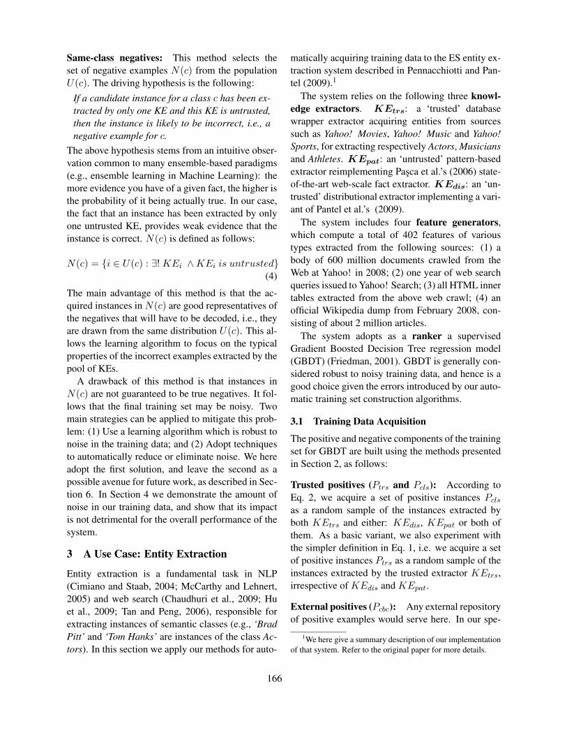
Same-class negatives: This method selects theset of negative examples N(c) from the populationU(c). The driving hypothesis is the following:

If a candidate instance for a class c has been ex-tracted by only one KE and this KE is untrusted,then the instance is likely to be incorrect, i.e., anegative example for c.

The above hypothesis stems from an intuitive obser-vation common to many ensemble-based paradigms(e.g., ensemble learning in Machine Learning): themore evidence you have of a given fact, the higher isthe probability of it being actually true. In our case,the fact that an instance has been extracted by onlyone untrusted KE, provides weak evidence that theinstance is correct. N(c) is defined as follows:

N(c) = {i ∈ U(c) : ∃! KEi ∧KEi is untrusted}(4)

The main advantage of this method is that the ac-quired instances in N(c) are good representatives ofthe negatives that will have to be decoded, i.e., theyare drawn from the same distribution U(c). This al-lows the learning algorithm to focus on the typicalproperties of the incorrect examples extracted by thepool of KEs.

A drawback of this method is that instances inN(c) are not guaranteed to be true negatives. It fol-lows that the final training set may be noisy. Twomain strategies can be applied to mitigate this prob-lem: (1) Use a learning algorithm which is robust tonoise in the training data; and (2) Adopt techniquesto automatically reduce or eliminate noise. We hereadopt the first solution, and leave the second as apossible avenue for future work, as described in Sec-tion 6. In Section 4 we demonstrate the amount ofnoise in our training data, and show that its impactis not detrimental for the overall performance of thesystem.

3 A Use Case: Entity Extraction

Entity extraction is a fundamental task in NLP(Cimiano and Staab, 2004; McCarthy and Lehnert,2005) and web search (Chaudhuri et al., 2009; Huet al., 2009; Tan and Peng, 2006), responsible forextracting instances of semantic classes (e.g., ‘BradPitt’ and ‘Tom Hanks’ are instances of the class Ac-tors). In this section we apply our methods for auto-

matically acquiring training data to the ES entity ex-traction system described in Pennacchiotti and Pan-tel (2009).1

The system relies on the following three knowl-edge extractors. KEtrs: a ‘trusted’ databasewrapper extractor acquiring entities from sourcessuch as Yahoo! Movies, Yahoo! Music and Yahoo!Sports, for extracting respectively Actors, Musiciansand Athletes. KEpat: an ‘untrusted’ pattern-basedextractor reimplementing Pasca et al.’s (2006) state-of-the-art web-scale fact extractor. KEdis: an ‘un-trusted’ distributional extractor implementing a vari-ant of Pantel et al.’s (2009).

The system includes four feature generators,which compute a total of 402 features of varioustypes extracted from the following sources: (1) abody of 600 million documents crawled from theWeb at Yahoo! in 2008; (2) one year of web searchqueries issued to Yahoo! Search; (3) all HTML innertables extracted from the above web crawl; (4) anofficial Wikipedia dump from February 2008, con-sisting of about 2 million articles.

The system adopts as a ranker a supervisedGradient Boosted Decision Tree regression model(GBDT) (Friedman, 2001). GBDT is generally con-sidered robust to noisy training data, and hence is agood choice given the errors introduced by our auto-matic training set construction algorithms.

3.1 Training Data Acquisition

The positive and negative components of the trainingset for GBDT are built using the methods presentedin Section 2, as follows:

Trusted positives (Ptrs and Pcls): According toEq. 2, we acquire a set of positive instances Pcls

as a random sample of the instances extracted byboth KEtrs and either: KEdis, KEpat or both ofthem. As a basic variant, we also experiment withthe simpler definition in Eq. 1, i.e. we acquire a setof positive instances Ptrs as a random sample of theinstances extracted by the trusted extractor KEtrs,irrespective of KEdis and KEpat.

External positives (Pcbc): Any external repositoryof positive examples would serve here. In our spe-

1We here give a summary description of our implementationof that system. Refer to the original paper for more details.

166

cific implementation, we select a set of positive ex-amples from the CBC repository (Pantel and Lin,2002). CBC is a word clustering algorithm thatgroups instances appearing in similar textual con-texts. By manually analyzing the cluster membersin the repository created by CBC, it is easy to pick-up the cluster(s) representing a target class.

Same-class negatives (Ncls): We select a set ofnegative instances as a random sample of the in-stances extracted by only one extractor, which canbe either of the two untrusted ones, KEdis orKEpat.

Near-class negatives (Noth): We select a set ofnegative instances, as a random sample of the in-stances extracted by any of our three extractors for aclass different than the one at hand. We also enforcethe condition that instances in Noth must not havebeen extracted for the class at hand.

Generic negatives (Ncbc): We automatically se-lect as generic negatives a random sample of in-stances appearing in any CBC cluster, except thosecontaining at least one member of the class at hand(i.e., containing at least one instance extracted byone of our KEs for the given class).

4 Experimental Evaluation

In this section, we report experiments comparingthe ranking performance of our different methodsfor acquiring training data presented in Section 3,to three different baselines and a fully supervisedupper-bound.

4.1 Experimental SetupWe evaluate over three semantic classes: Actors(movie, tv and stage actors); Athletes (profes-sional and amateur); Musicians (singers, musicians,composers, bands, and orchestras), so to comparewith (Pennacchiotti and Pantel, 2009). Ranking per-formance is tested over the test set described in theabove paper, composed of 500 instances, randomlyselected from the instances extracted by KEpat andKEdis for each of the classes2.

We experiment with various instantiations of theES system, each trained on a different training set

2We do not test over instances extracted by KEtrs, as theydo not go though the decoding phase

obtained from our methods. The different system in-stantiations (i.e., different training sets) are reportedin Table 1 (Columns 1-3). Each training set consistsof 500 positive examples, and 500 negative exam-ples.

As an upper bound, we use the ES system, wherethe training consists of 500 manually annotated in-stances (Pman and Nman), randomly selected fromthose extracted by the KEs. This allows us to di-rectly check if our automatically acquired trainingsets can compete to the human upper-bound. Wealso compare to the following baselines.

Baseline 1: An unsupervised rule-based ES sys-tem, assigning the lowest score to instances ex-tracted by only one KE, when the KE is untrusted;and assigning the highest score to any other instance.

Baseline 2: An unsupervised rule-based ES sys-tem, adopting as KEs the two untrusted extractorsKEpat and KEdis, and a rule-based Ranker that as-signs scores to instances according to the sum oftheir normalized confidence scores.

Baseline 3: An instantiation of our ES system,trained on Pman and Nman. The only differ-ence with the upper-bound is that it uses only twofeatures, namely the confidence score returned byKEdis and KEpat. This instantiation implementsthe system presented in (Mirkin et al., 2006).

For evaluation, we use average precision (AP), astandard information retrieval measure for evaluat-ing ranking algorithms:

AP (L) =

∑|L|i=1 P (i) · corr(i)∑|L|

i=1 corr(i)(5)

where L is a ranked list produced by a system, P (i)is the precision of L at rank i, and corr(i) is 1 if theinstance at rank i is correct, and 0 otherwise.

In order to accurately compute statistical signifi-cance, we divide the test set in 10-folds, and com-pute the AP mean and variance obtained over the10-folds. For each configuration, we perform therandom sampling of the training set five times, re-building the model each time, to estimate the vari-ance when varying the training sampling.

4.2 Experimental ResultsTable 1 reports average precision (AP) results fordifferent ES instantiations, separately on the three

167

System Training Set AP MAPPositives Negatives Actors Athletes Musicians

Baseline1 (unsup.) - - 0.562 0.535 0.437 0.511Baseline2 (unsup.) - - 0.676 0.664 0.576 0.639Baseline3 (sup.) Pman Nman 0.715 0.697 0.576 0.664Upper-bound (full-sup.) Pman Nman 0.860§ 0.901§ 0.786§ 0.849§

S1. Pcls Noth 0.751† 0.880§ 0.642 0.758§

S2. Pcls Ncbc 0.734† 0.854§ 0.644 0.744‡

S3. Pcls Ncls 0.842§ 0.806§ 0.770§ 0.806§

S4. Pcls Noth + Ncbc 0.756‡ 0.853§ 0.693‡ 0.767§

S5. Pcls Ncls + Noth 0.835§ 0.807§ 0.763§ 0.802§

S6. Pcls Ncls + Ncbc 0.838§ 0.822§ 0.768§ 0.809§S7. Pcls Ncls + Noth + Ncbc 0.838§ 0.818§ 0.764§ 0.807§

Table 1: Average precision (AP) results of systems using different training sets, compared to two usupervised Base-lines, a supervised Baseline, and a fully supervised upper-bound system. § indicates statistical significance at the 0.95level wrt all Baselines. ‡ indicates statistical significance at the 0.95 level wrt Baseline1 and Baseline 2. † indicatesstatistical significance at the 0.95 level wrt Baseline1.

classes; and the mean average precision (MAP)computed across the classes. We report results us-ing Pcls as positive training, and varying the neg-ative training composition3. Systems S1-S3 use asingle method to build the negatives. Systems S4-S6 combine two methods (250 examples from onemethod, 250 from the other), and S7 combines allthree methods. Table 3 reports additional basic re-sults when varying the positive training set compo-sition, and fixing the best performing negative set(namely Ncls).

Table 1 shows that all systems outperform thebaselines in MAP, with 0.95 statistical significance,but S2 which is not significant wrt Baseline 3. S6 isthe best performing system, achieving 0.809 MAP,only 4% below the supervised upper-bound (statis-tically insignificant at the 0.95 level). These resultsindicate that our methods for automatically acquir-ing training data are highly effective and competitivewith manually crafted training sets.

A class-by-class analysis reveals similar behav-ior for Actors and Musicians. For these two classes,the best negative set is Ncls (system S3), achievingalone the best AP (respectively 0.842 and 0.770 forActors and Musicians, 2.1% and 1.6% points belowthe upper-bound). Noth and Ncbc show a lower ac-curacy, more than 10% below Ncls. This suggestthat the most promising strategy for automatically

3For space limitation we cannot report exhaustively all com-binations.

Negative set False NegativesActors Athletes Musicians

Ncls 5% 45% 30%Noth 0% 10% 10%Ncbc 0% 0% 15%

Table 2: Percentage of false negatives in different types ofnegative sets, across the three experimented classes (esti-mations over a random sample of 20 examples per class).

acquiring negative training data is to collect exam-ples from the target class, as they guarantee to bedrawn from the same distribution as the instances tobe decoded. The use of near- and far-misses is stillvaluable (AP results are still better than the base-lines), but less effective.

Results for Athletes give different evidence: thebest performing negative set is Noth, performingsignificantly better than Ncls. To investigate thiscontrasting result, we manually picked 20 exam-ples from Ncls, Noth and Ncbc for each class, andchecked their degree of noise, i.e., how many falsenegatives they contain. Table 2 reports the results:these numbers indicate that the Ncls is very noisyfor the Athletes class, while it is more clean for theother two classes. This suggests that the learningalgorithm, while being robust enough to cope withthe small noise in Ncls for Actors and Musicians, itstarts to diverge when too many false negatives arepresented for training, as it happens for Athletes.

False negatives in Ncls are correct instances ex-tracted by one untrusted KE alone. The results in

168

Table 2 indicates that our untrusted KEs are moreaccurate in extracting instances for Athletes than forthe other classes: accurate enough to make our train-ing set too noisy, thus decreasing the performanceof S3 wrt S1 and S2. This indicates that the effec-tiveness of Ncls decreases when the accuracy of theuntrusted KEs is higher.

A good strategy to avoid the above problem is topair Ncls with another negative set, either Ncbc orNoth, as in S5 and S6, respectively. Then, whenthe above problem is presented, the learning algo-rithm can rely on the other negative set to com-pensate some for the noise. Indeed, when addingNcbc to Ncls (system S6) the accuracy over Athletesimproves, while the overall performance across allclasses (MAP) is kept constant wrt the system usingNcls (S3).

It is interesting that in Table 2, Ncbc and Noth alsohave a few false negatives. An intrinsic analysis re-veals that these are either: (1) Incorrect instancesof the other classes that are actual instances of thetarget class; (2) Correct instances of other classesthat are also instances of the target class. Case (1) iscaused by errors of KEs for the other classes (e.g.,erroneously extracting ‘Matthew Flynt’ as a Musi-cian). Case (2) covers cases in which instances areambiguous across classes, for example ‘Kerry Tay-lor’ is both an Actor and a Musician. This observa-tion is still surprising, since Eq. 3 explicitly removesfrom Ncbc and Noth any correct instance of the tar-get class extracted by the KEs. The presence of falsenegatives is then due to the low coverage of the KEsfor the target class, e.g. the KEs were not able to ex-tract ‘Matthew Flynt’ and ‘Kerry Taylor’ as actors.

Correlations. We computed the Spearman corre-lation coefficient r among the rankings producedby the different system instantiations, to verifyhow complementary the information enclosed in thetraining sets are for building the learning model.Among the basic systems S1− S3, the highest cor-relation is between S1 and S2 (r = 0.66 in aver-age across all classes), which is expected, since theyboth apply the principle of acquiring negative ex-amples from classes other than the target one. S3exhibits lower correlation with both S1 and S2, re-spectively r = 0.57 and r = 0.53, suggesting that itis complementary to them. Also, the best system S6

System Training Set AP MAPPos. Neg. Act. Ath. Mus.

S3. Pcls Ncls 0.842 0.806 0.770 0.806S8. Ptrs Ncls 0.556 0.779 0.557 0.631S9. Pcbc Ncls 0.633 0.521 0.561 0.571

Table 3: Comparative average precision (AP) results forsystems using different positive sets as training data.

Figure 1: Average precision of system S6 with differenttraining sizes.

has higher correlation with S3 (r = 0.94) than withS2 (r = 0.62), indicating that in the combination ofNcls and Ncbc, most of the model is built on Ncls.

Varying the positive training. Table 3 reports re-sults when fixing the negative set to the best per-forming Ncls, and exploring the use of other posi-tive sets. As expected Pcls largely outperforms Ptrs,confirming that removing the constraint in Eq. 2 andusing the simpler Eq. 1 makes the training set unrep-resentative of the unlabeled population. A similarobservation stands for Pcbc. These results indicatethat having a good trusted KE, or even an externalresource of positives, is effective only when select-ing from the training set examples that are also ex-tracted by the untrusted KEs.

Varying the training size. In Figure 1 we reportan analysis of the AP achieved by the best perform-ing System (S6), when varying the training size, i.e.,changing the cardinality of Pcls and Ncls + Ncbc.The results show that a relatively small-sized train-ing set offers good performance, the plateau beingreached already with 500 training examples. Thisis an encouraging result, showing that our methodscan potentially be applied also in cases where fewexamples are available, e.g., for rare or not well-represented classes.

169

5 Related Work

Most relevant are efforts in semi-supervised learn-ing. Semi-supervised systems use both labeled andunlabeled data to train a machine learning system.Most common techniques are based on co-trainingand self-training. Co-training uses a small set of la-beled examples to train two classifiers at the sametime. The classifiers use independent views (i.e.‘conditionally independent’ feature sets) to repre-sent the labeled examples. After the learning phase,the most confident predictions of each classifieron the unlabeled data are used to increase the la-beled set of the other. These two phases are re-peated until a stop condition is met. Co-traininghas been successfully applied to various applica-tions, such as statistical parsing (Sarkar, 2001) andweb pages classification (Yarowsky, 1998). Self-training techniques (or bootsrapping) (Yarowsky,1995) start with a small set of labeled data, and it-eratively classify unlabeled data, selecting the mostconfident predictions as additional training. Self-training has been applied in many NLP tasks, suchas word sense disambiguation (Yarowsky, 1995) andrelation extraction (Hearst, 1992). Unlike typicalsemi-supervised approaches, our approach reducesthe needed amount of labeled data not by acting onthe learning algorithm itself (any algorithm can beused in our approach), but on the method to acquirethe labeled training data.

Our work also relates to the automatic acquisi-tion of labeled negative training data. Yangarber etal. (2002) propose a pattern-based bootstrapping ap-proach for harvesting generalized names (e.g., dis-eases, locations), where labeled negative examplesfor a given class are taken from positive seed exam-ples of ‘competing’ classes (e.g. examples of dis-eases are used as negatives for locations). The ap-proach is semi-supervised, in that it requires somemanually annotated seeds. The study shows thatusing competing categories improves the accuracyof the system, by avoiding sematic drift, which isa common cause of divergence in boostrapping ap-proaches. Similar approaches are used among othersin (Thelen and Riloff, 2002) for learning semanticlexicons, in (Collins and Singer, 1999) for named-entity recognition, and in (Fagni and Sebastiani,2007) for hierarchical text categorization. Some of

our methods rely on the same intuition describedabove, i.e., using instances of other classes as nega-tive training examples. Yet, the ES framework al-lows us to add further restrictions to improve thequality of the data.

6 Conclusion

We presented simple and general techniques for au-tomatically acquiring training data, and then testedthem in the context of the Ensemble Semanticsframework. Experimental results show that ourmethods can compete with supervised systems us-ing manually crafted training data. It is our hope thatthese simple and easy-to-implement methods can al-leviate some of the cost of building machine learn-ing architectures for supporting open-domain infor-mation extraction, where the potentially very largenumber of classes to be extracted makes infeasiblethe use of manually labeled training data.

There are many avenues for future work. Al-though our reliance on high-quality knowledgesources is not an issue for many head classes, itposes a challenge for tail classes such as ‘wine con-noisseurs’, where finding alternative sources of highprecision samples is important. We also plan to ex-plore techniques to automatically identify and elim-inate mislabeled examples in the training data asin (Rebbapragada and Brodley, 2007), and relax theboolean assumption of trusted/untrusted extractorsinto a graded one. Another important issue regardsthe discovery of ‘near-classes’ for collecting near-classes negatives: we plan to automate this step byadapting existing techniques as in (McIntosh, 2010).Finally, we plan to experiment on a larger set ofclasses, to show the generalizability of the approach.

Our current work focuses on leveraging auto-learning to create an extensive taxonomy of classes,which will constitute the foundation of a very largeknowledge-base for supporting web search.

ReferencesAvrim L. Blum and Pat Langley. 1997. Selection of rel-

evant features and examples in machine learning. Ar-tificial Intelligence, 97:245–271.

A. Blumer, A. Ehrenfeucht, D. Haussler, and M.K. War-muth. 1989. Proceedings of ltc-07. Journal of ACM,36:929–965.

170

Huanhuan Cao, Daxin Jiang, Jian Pei, Qi He, Zhen Liao,Enhong Chen, and Hang Li. 2008. Context-awarequery suggestion by mining click-through and sessiondata. In Proceedings of KDD-08, pages 875–883.

Surajit Chaudhuri, Venkatesh Ganti, and Dong Xin.2009. Exploiting web search to generate synonyms forentities. In Proceedings of WWW-09, pages 151–160.

Philipp Cimiano and Steffen Staab. 2004. Learning bygoogling. SIGKDD Explorations, 6(2):24–34.

M. Collins and Y. Singer. 1999. Unsupervised mod-els for named entity classification. In Proceedings ofWVLC/EMNLP-99, pages 100–110.

Tiziano Fagni and Fabrizio Sebastiani. 2007. On the se-lection of negative examples for hierarchical text cate-gorization. In Proceedings of LTC-07, pages 24–28.

Jerome H. Friedman. 2001. Greedy function approxima-tion: A gradient boosting machine. Annals of Statis-tics, 29(5):1189–1232.

Marti A. Hearst. 1992. Automatic acquisition of hy-ponyms from large text corpora. In Proceedings ofCOLING-92, pages 539–545.

Jian Hu, Gang Wang, Fred Lochovsky, Jian tao Sun, andZheng Chen. 2009. Understanding user’s query intentwith Wikipedia. In Proceedings of WWW-09, pages471–480.

N. Japkowicz and S. Stephen. 2002. The class imbalanceproblem: A systematic study. Intelligent Data Analy-sis, 6(5).

M. Kubat and S. Matwin. 1997. Addressing the curseof inbalanced data sets: One-side sampleing. In Pro-ceedings of the ICML-1997, pages 179–186. MorganKaufmann.

Joseph F. McCarthy and Wendy G Lehnert. 2005. Usingdecision trees for coreference resolution. In Proceed-ings of IJCAI-1995, pages 1050–1055.

Tara McIntosh. 2010. Unsupervised discovery of nega-tive categories in lexicon bootstrapping. In Proceed-ings of the 2010 Conference on Empirical Methods inNatural Language Processing, pages 356–365, Mas-sachusetts, USA. Association for Computational Lin-guistics.

Shachar Mirkin, Ido Dagan, and Maayan Geffet. 2006.Integrating pattern-based and distributional similaritymethods for lexical entailment acquisition. In Pro-ceedings of ACL/COLING-06, pages 579–586.

Marius Pasca, Dekang Lin, Jeffrey Bigham, Andrei Lif-chits, and Alpa Jain. 2006. Organizing and search-ing the world wide web of facts - step one: The one-million fact extraction challenge. In Proceedings ofAAAI-06, pages 1400–1405.

Marius Pasca. 2007. Weakly-supervised discovery ofnamed entities using web search queries. In Proceed-ings of CIKM-07, pages 683–690, New York, NY,USA.

Patrick Pantel and Dekang Lin. 2002. Discovering wordsenses from text. In Proceedings of KDD-02, pages613–619.

Patrick Pantel, Eric Crestan, Arkady Borkovsky, Ana-Maria Popescu, and Vishnu Vyas. 2009. Web-scaledistributional similarity and entity set expansion. InProceedings of EMNLP-09.

Marco Pennacchiotti and Patrick Pantel. 2009. Entityextraction via ensemble semantics. In Proceedings ofthe 2009 Conference on Empirical Methods in Natu-ral Language Processing, pages 238–247, Singapore.Association for Computational Linguistics.

Umaa Rebbapragada and Carla E. Brodley. 2007. Classnoise mitigation through instance weighting. In Pro-ceedings of the 18th European Conference on MachineLearning.

Anoop Sarkar. 2001. Applying co-training methods tostatistical parsing. In NAACL-2001.

Bin Tan and Fuchun Peng. 2006. Unsupervised querysegmentation using generative language models andwikipedia. In Proceedings of WWW-06, pages 1400–1405.

Michael Thelen and Ellen Riloff. 2002. A bootstrappingmethod for learning semantic lexicons using extractionpattern contexts. In Proceedings of the 2002 Confer-ence on Empirical Methods in Natural Language Pro-cessing, pages 214–221, Philadelphia, PA, USA. As-sociation for Computational Linguistics.

Richard C. Wang and William W. Cohen. 2008. Itera-tive set expansion of named entities using the web. InICDM ’08: Proceedings of the 2008 Eighth IEEE In-ternational Conference on Data Mining, pages 1091–1096, Washington, DC, USA. IEEE Computer Society.

Roman Yangarber, Winston Lin, and Ralph Grishman.2002. Unsupervised learning of generalized names.In COLING-2002.

David Yarowsky. 1995. Unsupervised word sense dis-ambiguation rivaling supervised methods. In Proceed-ings of ACL-1996, pages 189–196.

David Yarowsky. 1998. Combining labeled and unla-beled data with co-training. In Proceedings of theWorkshop on Computational Learning Theory, pages92–100.

171


Probabilistic Word Alignment under the L0-norm

Thomas SchoenemannCenter for Mathematical Sciences

Lund University, Sweden

Abstract

This paper makes two contributions to thearea of single-word based word alignment forbilingual sentence pairs. Firstly, it integratesthe – seemingly rather different – works of(Bodrumlu et al., 2009) and the standard prob-abilistic ones into a single framework.

Secondly, we present two algorithms to opti-mize the arising task. The first is an iterativescheme similar to Viterbi training, able to han-dle large tasks. The second is based on the in-exact solution of an integer program. While itcan handle only small corpora, it allows moreinsight into the quality of the model and theperformance of the iterative scheme.

Finally, we present an alternative way tohandle prior dictionary knowledge and dis-cuss connections to computing IBM-3 Viterbialignments.

1 Introduction

The training of single word based translation mod-els (Brown et al., 1993b; Vogel et al., 1996) is an es-sential building block for most state-of-the-art trans-lation systems. Indeed, even more refined transla-tion models (Wang and Waibel, 1998; Sumita et al.,2004; Deng and Byrne, 2005; Fraser and Marcu,2007a) are initialized by the parameters of singleword based ones. The exception is here the jointapproach of Marcu and Wong (2002), but its refine-ment by Birch et al. (2006) again relies on the well-known IBM models.

Traditionally (Brown et al., 1993b; Al-Onaizanet al., 1999) single word based models are trained

by the EM-algorithm, which has the advantageousproperty that the collection of counts can be de-composed over the sentences. Refinements that alsoallow symmetrized models are based on bipartitegraph matching (Matusov et al., 2004; Taskar et al.,2005) or quadratic assignment problems (Lacoste-Julien et al., 2006). Recently, Bodrumlu et al.(2009) proposed the first method that treats a non-decomposable problem by handling all sentencepairs at once and via integer linear programming.Their (non-probabilistic) approach finds dictionarieswith a minimal number of entries. However, the ap-proach does not include a position model.

In this work we combine the two strategies intoa single framework. That is, the dictionary sparsityobjective of Bodrumlu et al. will become a regu-larity term in our framework. It is combined withthe maximal alignment probability of every sentencepair, where we consider the models IBM-1, IBM-2and HMM. This allows us to write dictionary spar-sity as the (non-convex) L0 norm of the dictionaryparameters of the respective models.

For supervised training, regularity terms are quitecommon, e.g. (Taskar et al., 2005; Lacoste-Julien etal., 2006). For the unsupervised problem addressedin this paper they have recently been introduced inthe form of posterior constraints (Ganchev et al.,2010). In related fields of NLP lately Dirichlet pri-ors have been investigated, e.g. (Johnson, 2007).

We present two strategies to handle the objec-tive function addressed in this paper. One of theseschemes relies, like (Germann et al., 2004; Lacoste-Julien et al., 2006; DeNero and Klein, 2008; Bo-drumlu et al., 2009), on integer linear programming

172

(see e.g. (Schrijver, 1986; Achterberg, 2007)), butdue to the large-scale nature of our problem wesolve only the LP-relaxation, followed by successivestrengthening. For the latter, we develop our own,exponentially large set of cuts and show that it canbe handled as a polynomially sized system, thoughin practice this is too inefficient.

2 The Models

Before we introduce our objective function we givea brief description of the (standard) models we con-sider. In all cases, one is given a set of bilin-gual sentence pairs containing a foreign languageand English. The models formalize the probabil-ity of obtaining the foreign sentence from a givenEnglish sentence, by considering hidden variablescalled alignments:

pd,l(fs|es) =∑as

pd,l(fs,as|es) .

Here, the subscripts d and l denote two sets of pa-rameters: whereas the set l defines the probability ofan alignment without knowing any of the sentences,d describes the translational probability given analignment and a source sentence.

For a source (English) sentence of length I and atarget (foreign) sentence of length J , the set of ad-missible alignments is generally the set of subsetsof {1, . . . , I} × {1, . . . , J}. However, for compu-tational reasons the considered models only allowrestricted alignments, where each target word mayalign to at most one source word. Any such align-ment is expressed as a vector aJ

1 ∈ {0, . . . , I}J .

2.1 Considered modelsFor a source sentence es = eI1 and a target sentencef s = fJ

1 , the considered models all factor as follows:

pd,l(f s,as|es) = (1)J∏

j=1

pd(fj |eaj ) · pl(aj |aj−1, j, I)

In all cases, the translational probability is non-parametric, i.e. d contains one parameter for everyco-occurring pair of source and target words. Sincethe model is probabilistic, the parameters of all f fora given e have to sum up to one.

With respect to the alignment probability, themodels differ. For the IBM-1 the set l is actuallyempty, so pl(aj |aj−1, j, I) = 1/(I+1). The IBM-2models1 p(aj |j, I), with a respective set of parame-ters. Finally, the HMM models p(aj |aj−1, I).

It is common to further reduce the alignment pa-rameters. In this paper we consider a nonparametricdistribution for the IBM-2, but both a nonparamet-ric and a parametric one for the HMM. In contrastto GIZA++, we have a parameter for every possibledifference, i.e. we do not group differences with ab-solutes greater than 5. Also, commonly one uses adistribution p(i|i′, I) = r(i− i′)/

∑Ii′′=1 r(i

′′ − i′),but for technical reasons, we drop the denominatorand instead constrain the r(·)-parameters to sum to1. In future work we hope to implement both thenormalization and the grouping of bins.

2.2 Word AlignmentOriginally the considered models were used for theactual translation problem. Hence, the parametersd and l had to be inferred from a training corpus,which was based on maximizing the probability

maxd,l

∏s

∑a

pd,l(f s,as|es) . (2)

Today the major application of the models lies inword alignment. Instead of estimating continuousparameters, one is now faced with the discrete opti-mization problem of assigning a single alignment toevery sentence pair in the corpus. This lead to therecent innovative work of (Bodrumlu et al., 2009)where the alignments are the only unknown quanti-ties.

Nevertheless, the use of probabilistic models re-mains attractive, in particular since they contributestatistics of likely alignments. In this work, we com-bine the two concepts into the criterion

mind,l− log

[∏s

maxas

pd,l(f s,as|es)

]+ λ ‖d‖0 ,

where λ ≥ 0 is a weighting parameter and we nowestimate a single alignment for every sentence.

The second term denotes the L0-norm of thetranslational parameters, i.e. the number of non-zero

1The original work considered a dependence on I and J , butit is common to drop J .

173

parameters. Since we only consider a single align-ment per sentence, this term is equivalent to Bo-drumlu et al.’s objective function. Minimizing thefirst term is closely related to the common criterion(2). For parameter estimation it is known as the max-imum approximation, but for word alignment it is aperfectly valid model.

For the IBM-1 model the first term alone results ina convex, but not strictly convex minimization prob-lem2. However, EM-like iterative methods generallydo not reach the minimum: they are doing block co-ordinate descent (Bertsekas, 1999, chap. 2.7) whichgenerally gives the optimum only for strictly convexfunctions. Indeed, our experiments showed a strongdependence on initialization and lead to heavily lo-cal solutions.

In the following we present two strategies to min-imize the new objective. We start with an iterativemethod that also handles the regularity term.

3 An Iterative Scheme

To derive our algorithms, we first switch the mini-mum and maximum in the objective and obtain

min{as}

mind,l−∑

s

log[pd,l(f s,as|es)

]+ λ ‖d‖0 ,

where the notation{as} denotes the alignments ofall sentence pairs. Ignoring the L0-term for the mo-ment, we now make use of a result of (Vicente et al.,2009) in their recent work on histogram-based im-age segmentation: for any given set of alignments,the inner minimization over the parameters is solvedby relative frequencies. When plugging this solutioninto the functional, one gets a model that does notdecompose over the sentences, but one that is stillreasonably easy to handle.

Before we get into details, we observe that thisminimizer is valid even when including the L0 term:if two words are never linked, both terms will set therespective parameter to 0. If they are linked, how-ever, then setting this parameter to 0 would makethe first term infinite. All non-zero parameters aretreated equally by the L0 term, so the restrictionto relative frequencies does not change the optimalvalue. In fact, this can be extended to weighted L0

2This is due to taking the maximizing alignment. Summingover all alignments is strictly convex.

terms, and later on we exploit this to derive an al-ternative way to handle a dictionary prior. Note thatthe same principle could also be applied to the workof (Bodrumlu et al., 2009).

3.1 Mathematical Formulation

We detail our scheme for the IBM-1 model, the ex-tension to other models is easy. For given align-ments we introduce the counts

Nf,e({as}) =∑

s

∑j

δ(f, fj) · δ(e, eaj )

Ne({as}) =∑

s

∑j

δ(e, eaj ) ,

where δ(·, ·) is the Kronecker-delta. The op-timal translation parameters are then given byNf,e({as})/Ne({as}), and plugging this into thefirst term in the objective gives (up to a constant)

min{as}

∑f,e

−Nf,e({as}) log(Nf,e({as})Ne({as})

).

The second term is simply λ∑

f,e ‖Nf,e({as})‖0,and since N(e) =

∑f N(f, e), in total we get

min{as}

∑f,e

−Nf,e({as}) log (Nf,e({as}))

+∑

e

Ne({as}) log (Ne({as})) .

+ λ∑f,e

‖Nf,e({as})‖0 (3)

In essence we are now dealing with the functionx log(x), where its value for 0 is defined as 0.

3.2 Algorithm

For the new objective, we were able to entirely getrid of the model parameters, leaving only alignmentvariables. Nevertheless, the algorithm we presentmaintains these parameters, and it requires an initialchoice. While we initialize the alignment parame-ters uniformly, for the translation parameters we useco-occurrence counts. This performed much betterthan a uniform initialization. The algorithm, calledAM (for alternating minimization), now iterates twosteps:

174

1. Starting from the current setting of d andl, derive Viterbi alignments for all sentencepairs. E.g. for the IBM-1 we set as

j =arg max

id(fj |ei). For the IBM-2 the term is

similar, while for the HMM one can use dy-namic programming.

Note that this step does not consider the L0-term. This term can however not increase.

2. Run the Iterated Conditional Modes (Besag,1986), i.e. go sequentially over all alignmentvariables and set them to their optimal valuewhen keeping the others fixed.

Here, we need to keep track of the currentalignment counts. In every step we need tocompute the objective cost associated to a countthat increases by 1, and (another) one thatdecreases by 1. For the IBM-2 we need toconsider the alignment counts, too, and forthe HMM usually two alignment terms are af-fected. In case of 0-alignments there can bemore than two. We presently do not considerthese cases and hence do not find the exact op-timum there.

Afterwards, reestimate the parameters d and lfrom the final counts.

4 Integer Linear Programming

The above algorithm is fast and can handle large cor-pora. However, it still gets stuck in local minima,and there is no way of telling how close to the opti-mum one got.

This motivates the second algorithm where wecast the objective function as an integer linear pro-gram (ILP). In practice it is too large to be solvedexactly, so we solve its linear programming relax-ation, followed by successive strengthening. Herewe derive our own set of cuts. Now we also get alower bound on the problem and obtain lower en-ergy solutions in practice. But we can handle onlysmall corpora.

We limit this method to the models IBM-1 andIBM-2. Handling an HMM would be possible,but its first order alignment model would introducemany more variables. Handling the IBM-3, based on(Ravi and Knight, 2010; Schoenemann, 2010) seemsa more promising direction.

4.1 An ILP for the Regularized IBM-1The basis of our ILP is the fact that the counts Nf,e

and Ne can only assume a finite, a-priori known setof integral values, including 0. We introduce a bi-nary variable nc

f,e ∈ {0, 1} for each possible valuec, where we want nc

f,e = 1 if Nf,e(as) = c, oth-erwise nc

f,e = 0. This is analogous for the vari-ables nc

e and Ne(as). Finally, since the counts de-pend on the alignments, we also need binary vari-ables xs

i,j ∈ {0, 1} that we want to be 1 if and onlyif as

j = i.The cost function of (3) can now be written as a

linear function in terms of the integer variables ncf,e

and nce, with coefficients

wce,f = −c log(c) + λ‖c‖0 , wc

e = c log(c) .

However, we need additional constraints. In particu-lar we need to ensure that for a given f and e exactlyone variable nc

f,e is 1. Equivalently we can postulatethat the sum of these variables is one. We proceedanalogous for each e and the variables nc

e.Then, we need to ensure that for each source word

in each sentence f s an alignment is specified, i.e.that for each given s and j the variables xs

i,j sumto 1. Finally, the count variables have to reflect thecounts induced by the alignment variables. For thecounts Nf,e this is expressed by∑

s,i,j:fsj =f,es

i =e

xsi,j =

∑c

c · ncf,e ∀f, e ,

and likewise for the counts Ne.Altogether, we arrive at the following system:

min{xs

i,j},{ncf,e},{nc

e}

∑e,c

wce n

ce +

∑f,e,c

wcf,e n

cf,e

s.t.∑

i

xsi,j = 1 ∀s, j∑

c

ncf,e = 1 ∀f, e∑

c

nce = 1 ∀e∑

s,i,j:fj=f,ei=e

xsi,j =

∑c

c · ncf,e ∀f, e∑

s,i,j:ei=e

xsi,j =

∑c

c · nce ∀e

xsi,j ∈ {0, 1}, nc

e ∈ {0, 1}, nce,f ∈ {0, 1} .

175

4.2 Handling the IBM-2

The above mentioned system can be easily adaptedto the IBM-2 model. To this end, we introduce vari-ables nc

i,j,I ∈ {0, 1} to express how often sourceword j is aligned to target word i given that thereare I words in the target sentence. Note that thenumber of times source word j is aligned given thatthe target sentence has I words is known a-prioriand does not depend on the alignment to be opti-mized. We denote it Cj,I . The cost function ofthe ILP is augmented by

∑i,j,I,cw

ci,j,I n

ci,j,I , with

wci,j,I = c log(c/Cj,I). In addition we add the fol-

lowing constraints to the system:∑s:Is=I

xsi,j =

∑c

c · nci,j,I ∀i, j, I .

5 Cutting Planes

Integer linear programming is an NP-hard problem(see e.g. (Schrijver, 1986)). While for problemswith a few thousand variables it can often be solvedexactly via the branch and cut method, in our settingnone of the solvers we tried terminated. Alreadysolving the linear programming relaxation requiresup to 4 GB of memory for corpora with roughly3000 sentence pairs.

So instead of looking for an exact solution, wemake use of a few iterations of the cutting planesmethod (Gomory, 1958), where repeatedly an LP-relaxation is solved, then additionally valid inequal-ities, called cuts, are added to the system. Everyround gives a tighter relaxation, i.e. a better lowerbound on the optimal integral value.

After solving each LP-relaxation we derive an in-tegral solution by starting the iterative method fromsection 3 from the fractional LP-solution. In the endwe output the best found integral solution.

For deriving cuts we tried all the methods imple-mented in the COIN Cut Generation Library CGL3,based on the solver Clp from the same project line.However, either the methods were very slow in pro-ducing cuts or they produced very few cuts only. Soeventually we derived our own set of cuts that willnow be presented. Note that they alone do not givean integral solution.

3http://www.coin-or.org/projects/Cgl.xml

5.1 A Set of Count-based Cuts

The derived ILP contains several constraints of theform ∑

i

yi =∑

c

c · zc , (4)

where all variables are binary. Expressions of thiskind arise wherever we need to ensure consistencybetween alignment variables and count variables.Our cuts aim at strengthening each of these equa-tions individually.

Assume that equation (4) involves the variablesy1, . . . , yK and hence also the variables z0, . . . , zK .The trouble with the equation is that even if theleft hand side is integral, the right-hand side is usu-ally not. As an example, consider the case where∑K

i=1 yi = 3. Then the fractional assignment z0 =1−3/K, zK = 3/K and zc = 0 for all other c satis-fies (4). Indeed, if the cost function for zc is concavein c, as is the function−c log(c) we use, this will bethe optimal solution for the given left hand side.

Hence we want to enforce that for an integralvalue k of the left hand side, all variables zc for0 ≤ c < k are zero. This is ensured by the fol-lowing system of inequalities that is exponentiallylarge in k: ∑

i∈Kyi +

k−1∑c=0

zc ≤ k (5)

∀K ⊆ {1, . . . ,K} : |K| = k .

It turns out that this system can be formulated quitecompactly.

5.2 Polynomial Formulation

We now formalize the result for the compact formu-lation of (5).

Proposition 1 The union of the systems (5) for all kcan be represented by polynomially many variablesand linear constraints.

Proof: we first observe that it suffices to enforce[maxK:|K|=k

∑i∈K

yi

]+

k−1∑c=0

zc ≤ k

for all k. These are polynomially many equations(one for each k), but each involves a maximization

176

over exponentially many sets. However, this maxi-mization can be expressed by the auxiliary variables

τkl := max

K⊆{1,...,l}:|K|≤k

∑i∈K

yi

= max{τk−1l−1 + yl , τ

kl−1}

Now we only have to maximize over two linear ex-pressions for each of the new, polynomially many,variables. We can enforce τk

l to be an upper boundon the maximum by postulating τk

l ≥ τk−1l−1 + yl and

τkl ≥ τk

l−1. Since the original maximum occurred onthe left hand side of a less-than constraint, this upperbound will be tight wherever this is necessary. 2

In practice the arising system is numerically hardto solve. Since usually only polynomially many cutsof the form (5) are actually violated during the cut-ting planes process, we add them in passes and getsignificantly lower running times. Moreover, eachround of cuts gives a new opportunity to derive aheuristic integral solution.

5.3 Backward Cuts

We call the cuts we have derived above forward cutsas they focus on variables that are smaller than k. Ifwe could be sure that the left-hand side of (4) wasalways integral, they should indeed suffice. In prac-tice this is not the case, so we now also derive back-ward cuts where we focus on all variables that arelarger than k, with the following reasoning: once weknow that at least K − k variables yi are inactive(i.e. yi = 0), we can conclude that all zc with c > kmust be zero, too. This can be expressed by the setof inequalities∑

i∈K(1− yi) +

K∑c=k+1

zc ≤ K − k

∀K ⊆ {1, . . . ,K} : |K| = K − k ,

or equivalently∑i∈K−yi +

K∑c=k+1

zc ≤ 0 ∀K : |K| = K − k .

5.4 Other Applications

A related constraint system arises in recent work(Ravi and Knight, 2010; Schoenemann, 2010) on

computing IBM-3 Viterbi alignments. We imple-mented4 the polynomial formulation of the aboveforward cuts for this system, and got mild speed-ups(224 instead of 237 minutes for the Hansards taskreported in the second paper). With an additionallyimproved fertility exclusion stage5 this is reduced to176 minutes.

6 Experiments

We evaluate the proposed strategies on both smallscale and (where applicable) large scale tasks. Wecompare to standard EM with sums over alignments,where for the IBM-1 and the HMM we use GIZA++.In addition, we evaluate several variants (our imple-mentations) of the HMM, with non-parametric andparametric alignment models. Note that for the non-parametric variant we estimate distributions for thefirst aligned position, for the parametric all initialpositions are equally likely. For the IBM-2 we con-sider the non-parametric variant and hence our im-plementation. We also evaluate our schemes on thetask without regularization.

All experiments in this work were executed on a3 GHz Core 2 Duo machine with 8 GB of memory,where up to 4 GB were actually used. The itera-tive scheme was run for 15 iterations, where it wasnearly converged. This setting was also used for ourown EM-implementations. Solely for GIZA++ weused the standard setting of 5 iterations, and the im-plemented smoothing process. For the IBM-2 andHMM we follow the standard strategy to first trainan IBM-1 with the same objective function.

6.1 Large Scale Tasks

We consider two well-known corpora with publiclyavailable gold alignments, and run both translationdirections for each of them. The first task is theCanadian Hansards task (French and English) withroughly 1 million sentences. The second task isEuroparl Spanish-English, where we take the first500000 sentences. Our iterative scheme runs in

4based on code available at www.maths.lth.se/matematiklth/personal/tosch/download.html.

5In (Schoenemann, 2010) we stated that the difference be-tween cy

if and the contribution of i to the bound has to exceedu − l3. This can be tightened if one additionally adds the costof the best f alignments to i to the cost cy

if .

177

Canadian HansardsFr→ En En→ Fr

HMM (Giza++) 0.918 0.918par. HMM (our EM) 0.887 0.896par. HMM (Viterbi) 0.873 0.897par. HMM + L0 0.891 0.907nonpar. HMM (our EM) 0.873 0.911nonpar. HMM (Viterbi) 0.881 0.909nonpar. HMM + L0 0.902 0.917

EuroparlEs→ En En→ Es

HMM (Giza++) 0.764 0.754nonpar. HMM (our EM) 0.738 0.733nonpar. HMM (Viterbi) 0.726 0.716nonpar. HMM + L0 0.729 0.73

Table 1: For large corpora, the proposed scheme outper-forms Viterbi training and sometimes even our EM.

roughly 5 hours (with room for improvements), us-ing 2.5 GB memory. We found that an L0-weight ofλ = 5.0 performs very well. Hence, we will use thisfor all our experiments.

We compare to the standard GIZA++ implemen-tation and our own HMM implementations with EM.Here we ran 15 iterations for IBM-1 and HMM each.

As shown in Table 1 adding the L0 term improvesthe standard Viterbi training. Our method also some-times beats the simple EM implementation but notGIZA++. This may be due to the special paramet-ric model of GIZA++, its smoothing process or thelower number of iterations. Our deficient paramet-ric model is inferior for the Hansards task, so we didnot run it for Europarl.

6.2 Small Scale Tasks

To evaluate the ILP strategy we consider four smallscale tasks released by the European Corpus Ini-tiative6. See (Schoenemann, 2010) for the corpusstatistics. We report weighted f-measures (Fraserand Marcu, 2007b) on gold alignments (sure andpossible) specified by one annotator, for 144 and 110sentences respectively. The number of cut roundswas selected so that the execution times remainedbelow 2 days for all tasks. This was 50 rounds forthe IBM-1 and 2 rounds for the IBM-2. In fact, with

6http://www.elsnet.org/eci.html

these numbers the Avalanche task is processed in lit-tle less than a day.

We tested a number of LP solvers and found thatmost of them need several hours to solve the root re-laxation. This is different for the commercial solverFICO Xpress, which only needs around 15 minutes.However, it is slower in processing the subsequentcut iterations. Hence, for the IBM-1 we use the opensource Clp7.

The resulting f-measures for the tested strategiesare given in Table 2. In all cases, adding the L0

term greatly improves the standard Viterbi training.Moreover, for the small scale tasks, the parametricHMM is clearly the best choice when using the L0

penalty. In the majority of cases the ILP strategyperforms better than the iterative scheme. In fact, italways found the lower energy solution. The mostextreme difference we observed for the IBM-2 onthe UBS English to German task: here AM finds anenergy of 318147, where the ILP gives 303674.

Finally, Table 3 evaluates the effectiveness ofthe cut strategy exemplarily on one of the tasks.Clearly, the gaps are reduced significantly comparedto the LP-relaxation. However, except for the IBM-1 (which is convex for λ = 0) the lower bounds arestill quite loose.

6.3 Handling Dictionary Knowledge

The presented L0 regularity is easily modified to in-clude dictionary knowledge8. To this end, we intro-duce a weighted L0-norm: whenever a pair of sourceand target words is listed in the dictionary, the entryis not penalized. All remaining entries are penalizedby λ.

Note that this is different from the standard way(Brown et al., 1993a) of handling dictionary knowl-edge, which appends the dictionary to the corpus(with a proper weighting factor). We tried bothschemes with several weighting factors, then chosethe best-performing for the UBS task. For the UBSGerman to English task we get an accuracy of 0.445,which beats GIZA++ both with (0.438) and without(0.398) dictionary knowledge. In the reverse direc-tion both schemes profit from the extra knowledge,

7http://www.coin-or.org/projects/Clp.xml8Our data are based on www.dict.info/uddl.php

and www.ilovelanguages.com/idp and the stemmingalgorithms at snowball.tartarus.org.

178

Avalanche French→ GermanModel EM AM ILPIBM-1 0.603 0.619 0.591IBM-1 + L0 – 0.64 0.625IBM-2 0.568 0.632 0.60IBM-2 + L0 – 0.680 0.636par. HMM 0.752 0.621 –par. HMM + L0 – 0.779 –nonpar. HMM 0.752 0.655 –nonpar. HMM + L0 – 0.714 –

Avalanche German→ FrenchModel EM AM ILPIBM-1 0.494 0.485 0.507IBM-1 + L0 – 0.497 0.488IBM-2 0.428 0.459 0.526IBM-2 + L0 – 0.483 0.55par. HMM 0.606 0.49 –par. HMM + L0 – 0.592 –nonpar. HMM 0.582 0.501 –nonpar. HMM + L0 – 0.537 –

UBS German→ EnglishModel EM AM ILPIBM-1 0.381 0.359 0.335IBM-1 + L0 – 0.350 0.442IBM-2 0.315 0.324 0.340IBM-2 + L0 – 0.383 0.462par. HMM 0.398 0.229 –par. HMM + L0 – 0.383 –nonpar. HMM 0.421 0.29 –nonpar. HMM + L0 – 0.371 –

UBS English→ GermanModel EM AM ILPIBM-1 0.515 0.435 0.489IBM-1 + L0 – 0.444 0.504IBM-2 0.417 0.40 0.435IBM-2 + L0 – 0.52 0.571par. HMM 0.625 0.404 –par. HMM + L0 – 0.537 –nonpar. HMM 0.623 0.436 –nonpar. HMM + L0 – 0.524 –

Table 2: Alignment accuracy (weighted f-measure) fordifferent algorithms. We use a dictionary penalty ofλ = 5 and the standard EM (GIZA++ for IBM-1 andparametric HMM, our implementation otherwise) train-ing scheme with 5 iterations for each model.

UBS English→ GermanL0-weight IBM-1 IBM-2

root relaxation 0.0 1.098 7.697after cut rounds 0.0 1.081 5.67root relaxation 5.0 1.16 2.76after cut rounds 5.0 1.107 2.36

Table 3: Ratios of the best known integer solution and thebest known lower bounds for all considered tasks.

but GIZA++ remains the clear winner. Applyingthe same weights to the above mentioned Hansardstask slightly improved GIZA++, whereas it slightlyworsened the performance of our scheme in the onedirection and slightly improved it in the other. Weintend to investigate this more thoroughly in the fu-ture.

7 Discussion

In this paper we have shown that an L0 prior onthe dictionary parameters greatly improves Viterbitraining. A simple iterative scheme often nearlymatches our EM-implementation of the HMM.

We have also derived two algorithms to deal withthe new objective. A simple iterative scheme givesquite accurate results on large scale tasks. On smallscale tasks our inexact ILP strategy shows that theiterative scheme does not find the optimum in prac-tice, a point that may well carry over to other mod-els trained with the maximum approximation. Thisstrategy also provides lower bounds, but at presentthey are quite loose.

Moreover, we have presented an alternative wayof handling dictionary knowledge. Finally, we havediscussed connections to computing IBM-3 Viterbialignments, where we got mild speed-ups.

In future work we intend to investigate the effectof the generated alignments on the translation qual-ity of phrase-based approaches. We also want to ex-plore strategies to determine the regularity weight.Finally, we want to handle a non-deficient paramet-ric HMM.

Acknowledgements. We thank Ben Taskar andJoao Graca for helpful discussions. This work wasfunded by the European Research Council (Glob-alVision grant no. 209480).

179

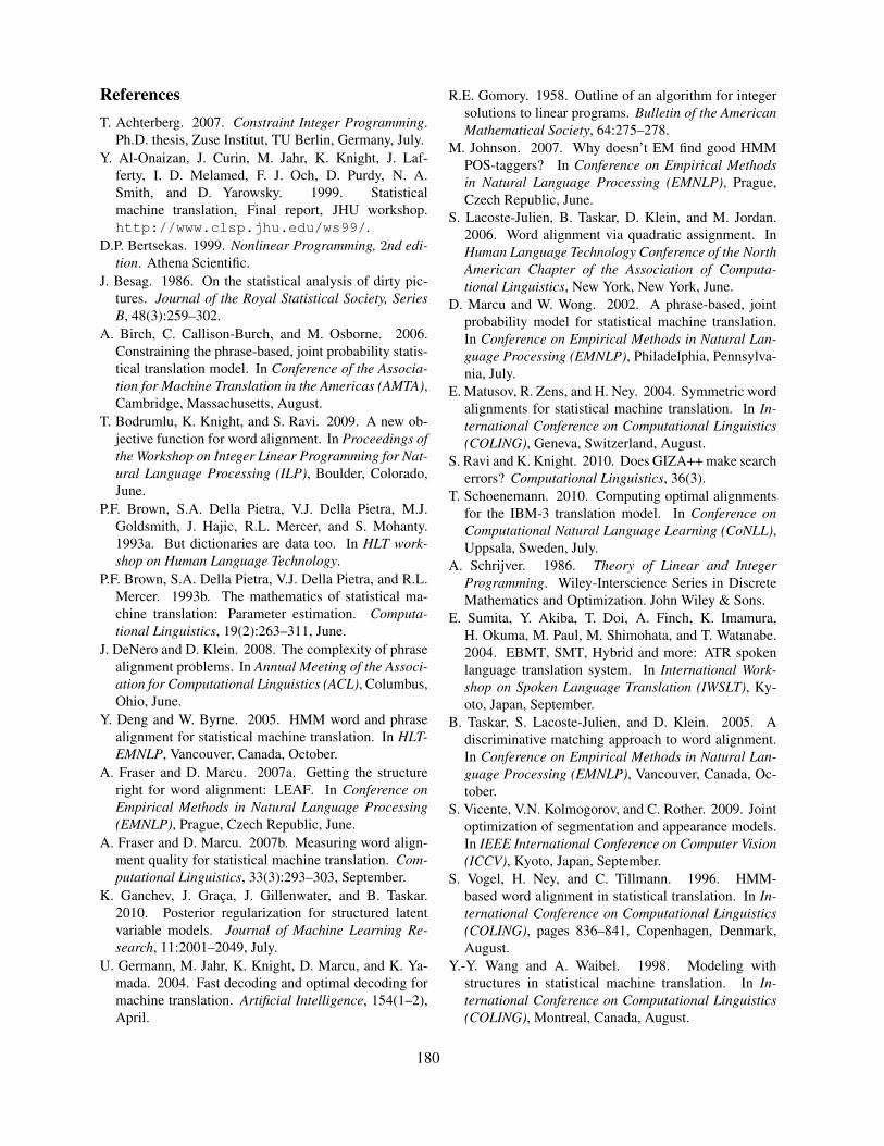
ReferencesT. Achterberg. 2007. Constraint Integer Programming.

Ph.D. thesis, Zuse Institut, TU Berlin, Germany, July.Y. Al-Onaizan, J. Curin, M. Jahr, K. Knight, J. Laf-

ferty, I. D. Melamed, F. J. Och, D. Purdy, N. A.Smith, and D. Yarowsky. 1999. Statisticalmachine translation, Final report, JHU workshop.http://www.clsp.jhu.edu/ws99/.

D.P. Bertsekas. 1999. Nonlinear Programming, 2nd edi-tion. Athena Scientific.

J. Besag. 1986. On the statistical analysis of dirty pic-tures. Journal of the Royal Statistical Society, SeriesB, 48(3):259–302.

A. Birch, C. Callison-Burch, and M. Osborne. 2006.Constraining the phrase-based, joint probability statis-tical translation model. In Conference of the Associa-tion for Machine Translation in the Americas (AMTA),Cambridge, Massachusetts, August.

T. Bodrumlu, K. Knight, and S. Ravi. 2009. A new ob-jective function for word alignment. In Proceedings ofthe Workshop on Integer Linear Programming for Nat-ural Language Processing (ILP), Boulder, Colorado,June.

P.F. Brown, S.A. Della Pietra, V.J. Della Pietra, M.J.Goldsmith, J. Hajic, R.L. Mercer, and S. Mohanty.1993a. But dictionaries are data too. In HLT work-shop on Human Language Technology.

P.F. Brown, S.A. Della Pietra, V.J. Della Pietra, and R.L.Mercer. 1993b. The mathematics of statistical ma-chine translation: Parameter estimation. Computa-tional Linguistics, 19(2):263–311, June.

J. DeNero and D. Klein. 2008. The complexity of phrasealignment problems. In Annual Meeting of the Associ-ation for Computational Linguistics (ACL), Columbus,Ohio, June.

Y. Deng and W. Byrne. 2005. HMM word and phrasealignment for statistical machine translation. In HLT-EMNLP, Vancouver, Canada, October.

A. Fraser and D. Marcu. 2007a. Getting the structureright for word alignment: LEAF. In Conference onEmpirical Methods in Natural Language Processing(EMNLP), Prague, Czech Republic, June.

A. Fraser and D. Marcu. 2007b. Measuring word align-ment quality for statistical machine translation. Com-putational Linguistics, 33(3):293–303, September.

K. Ganchev, J. Graca, J. Gillenwater, and B. Taskar.2010. Posterior regularization for structured latentvariable models. Journal of Machine Learning Re-search, 11:2001–2049, July.

U. Germann, M. Jahr, K. Knight, D. Marcu, and K. Ya-mada. 2004. Fast decoding and optimal decoding formachine translation. Artificial Intelligence, 154(1–2),April.

R.E. Gomory. 1958. Outline of an algorithm for integersolutions to linear programs. Bulletin of the AmericanMathematical Society, 64:275–278.

M. Johnson. 2007. Why doesn’t EM find good HMMPOS-taggers? In Conference on Empirical Methodsin Natural Language Processing (EMNLP), Prague,Czech Republic, June.

S. Lacoste-Julien, B. Taskar, D. Klein, and M. Jordan.2006. Word alignment via quadratic assignment. InHuman Language Technology Conference of the NorthAmerican Chapter of the Association of Computa-tional Linguistics, New York, New York, June.

D. Marcu and W. Wong. 2002. A phrase-based, jointprobability model for statistical machine translation.In Conference on Empirical Methods in Natural Lan-guage Processing (EMNLP), Philadelphia, Pennsylva-nia, July.

E. Matusov, R. Zens, and H. Ney. 2004. Symmetric wordalignments for statistical machine translation. In In-ternational Conference on Computational Linguistics(COLING), Geneva, Switzerland, August.

S. Ravi and K. Knight. 2010. Does GIZA++ make searcherrors? Computational Linguistics, 36(3).

T. Schoenemann. 2010. Computing optimal alignmentsfor the IBM-3 translation model. In Conference onComputational Natural Language Learning (CoNLL),Uppsala, Sweden, July.

A. Schrijver. 1986. Theory of Linear and IntegerProgramming. Wiley-Interscience Series in DiscreteMathematics and Optimization. John Wiley & Sons.

E. Sumita, Y. Akiba, T. Doi, A. Finch, K. Imamura,H. Okuma, M. Paul, M. Shimohata, and T. Watanabe.2004. EBMT, SMT, Hybrid and more: ATR spokenlanguage translation system. In International Work-shop on Spoken Language Translation (IWSLT), Ky-oto, Japan, September.

B. Taskar, S. Lacoste-Julien, and D. Klein. 2005. Adiscriminative matching approach to word alignment.In Conference on Empirical Methods in Natural Lan-guage Processing (EMNLP), Vancouver, Canada, Oc-tober.

S. Vicente, V.N. Kolmogorov, and C. Rother. 2009. Jointoptimization of segmentation and appearance models.In IEEE International Conference on Computer Vision(ICCV), Kyoto, Japan, September.

S. Vogel, H. Ney, and C. Tillmann. 1996. HMM-based word alignment in statistical translation. In In-ternational Conference on Computational Linguistics(COLING), pages 836–841, Copenhagen, Denmark,August.

Y.-Y. Wang and A. Waibel. 1998. Modeling withstructures in statistical machine translation. In In-ternational Conference on Computational Linguistics(COLING), Montreal, Canada, August.

180


Authorship Attribution with Latent Dirichlet Allocation

Yanir Seroussi Ingrid ZukermanFaculty of Information Technology, Monash University

Clayton, Victoria 3800, [email protected]

Fabian Bohnert

Abstract

The problem of authorship attribution – at-tributing texts to their original authors – hasbeen an active research area since the end ofthe 19th century, attracting increased interestin the last decade. Most of the work on au-thorship attribution focuses on scenarios withonly a few candidate authors, but recently con-sidered cases with tens to thousands of can-didate authors were found to be much morechallenging. In this paper, we propose waysof employing Latent Dirichlet Allocation inauthorship attribution. We show that our ap-proach yields state-of-the-art performance forboth a few and many candidate authors, incases where these authors wrote enough textsto be modelled effectively.

1 Introduction

The problem of authorship attribution – attributingtexts to their original authors – has received con-siderable attention in the last decade (Juola, 2006;Stamatatos, 2009). Most of the work in this field fo-cuses on cases where texts must be attributed to oneof a few candidate authors, e.g., (Mosteller and Wal-lace, 1964; Gamon, 2004). Recently, researchershave turned their attention to scenarios with tens tothousands of candidate authors (Koppel et al., 2011).In this paper, we study authorship attribution withfew to many candidate authors, and introduce a newmethod that achieves state-of-the-art performance inthe latter case.

Our approach to authorship attribution consists ofbuilding models of authors and their texts using La-tent Dirichlet Allocation (LDA) (Blei et al., 2003).We compare these models to models built from texts

with unknown authors to find the most likely authorsof these texts (Section 3.2). Our evaluation showsthat our approach yields a higher accuracy than themethod recently introduced by Koppel et al. (2011)in several cases where prolific authors are consid-ered, while requiring less runtime (Section 4).

This paper is structured as follows. Related workis surveyed in Section 2. Our LDA-based approachto authorship attribution is described in Section 3,together with the baselines we considered in ourevaluation. Section 4 presents and discusses the re-sults of our evaluation, and Section 5 discusses ourconclusions and plans for future work.

2 Related Work

The field of authorship attribution predates moderncomputing. For example, in the late 19th century,Mendenhall (1887) suggested that word length canbe used to distinguish works by different authors. Inrecent years, increased interest in authorship attribu-tion was fuelled by advances in machine learning,information retrieval, and natural language process-ing (Juola, 2006; Stamatatos, 2009).

Commonly used features in authorship attribu-tion range from “shallow” features, such as tokenand character n-gram frequencies, to features thatrequire deeper analysis, such as part-of-speech andrewrite rule frequencies (Stamatatos, 2009). As inother text classification tasks, Support Vector Ma-chines (SVMs) have delivered high accuracy, asthey are designed to handle feature vectors of highdimensionality (Juola, 2006). For example, one-vs.-all (OVA) is an effective approach to using bi-nary SVMs for multi-class (i.e., multi-author) prob-lems (Rifkin and Klautau, 2004). Given A authors,

181

OVA trains A binary classifiers, where each classi-fier is trained on texts by one author as positive ex-amples and all the other texts as negative examples.However, ifA is large, each classifier has many morenegative than positive examples, often yielding poorresults due to class imbalance (Raskutti and Kowal-czyk, 2004). Other setups, such as one-vs.-one ordirected acyclic graph, require training O(A2) clas-sifiers, making them impractical where thousands ofauthors exist. Multi-class SVMs have also been sug-gested, but they generally perform comparably toOVA while taking longer to train (Rifkin and Klau-tau, 2004). Hence, using SVMs for scenarios withmany candidate authors is problematic (Koppel etal., 2011). Recent approaches to employing binarySVMs consider class similarity to improve perfor-mance (Bickerstaffe and Zukerman, 2010; Chenget al., 2007). We leave experiments with such ap-proaches for future work (Section 5).

In this paper, we focus on authorship attributionwith many candidate authors. This problem was pre-viously addressed by Madigan et al. (2005) and Luy-ckx and Daelemans (2008), who worked on datasetswith texts by 114 and 145 authors respectively. Inboth cases, the reported results were much poorerthan those reported in the binary case. More re-cently, Koppel et al. (2011) considered author sim-ilarity to handle cases with thousands of candidateauthors. Their method, which we use as our base-line, is described in Section 3.1.

Our approach to authorship attribution utilises La-tent Dirichlet Allocation (LDA) (Blei et al., 2003)to build models of authors from their texts. LDAis a generative probabilistic model that is tradition-ally used to find topics in textual data. The mainidea behind LDA is that each document in a cor-pus is generated from a distribution of topics, andeach word in the document is generated accordingto the per-topic word distribution. Blei et al. (2003)showed that using LDA for dimensionality reductioncan improve performance for supervised text clas-sification. We know of only one case where LDAwas used in authorship attribution: Rajkumar et al.(2009) reported preliminary results on using LDAtopic distributions as feature vectors for SVMs, butthey did not compare the results obtained with LDA-based SVMs to those obtained with SVMs trainedon tokens directly. Our comparison shows that both

methods perform comparably (Section 4.3).Nonetheless, the main focus of our work is

on authorship attribution with many candidate au-thors, where it is problematic to use SVMs. OurLDA+Hellinger approach employs LDA withoutSVM training (Section 3.2), yielding state-of-the-artperformance in several scenarios (Section 4).

3 Authorship Attribution Methods

This section describes the authorship attributionmethods considered in this paper. While all thesemethods can employ various representations of doc-uments, e.g., token frequencies or part-of-speech n-gram frequencies, we only experimented with tokenfrequencies.1 This is because they are simple to ex-tract, and can achieve good performance (Section 4).Further, the focus of this paper is on comparing theperformance of our methods to that of the baselinemethods. Thus, we leave experiments on other fea-ture types for future work (Section 5).

3.1 Baselines

We consider two baseline methods, depending onwhether there are two or many candidate authors.If there are only two, we use Support Vector Ma-chines (SVMs), which have been shown to de-liver state-of-the-art performance on this task (Juola,2006). If there are many, we follow Koppel etal.’s (2011) approach, which we denote KOP.

The main idea behind KOP is that different pairsof authors may be distinguished by different sub-sets of the feature space. Hence, KOP randomlychooses k1 subsets of size k2F (k2 < 1) from a setof F features; for each of the k1 subsets, it calcu-lates the cosine similarity between a test documentand all the documents by one author (each author isrepresented by one feature vector); it then outputsthe author who had most of the top matches. KOPalso includes a threshold σ∗ to handle cases wherea higher level of precision is required, at the costof lower recall. If the top-matching author was thetop match less than σ∗ times, then KOP outputs “un-known author”. In our experiments we set σ∗ = 0 toobtain full coverage, as this makes it easier to inter-pret the results using a single measure of accuracy.

1Token frequency is the token count divided by the totalnumber of tokens.

182

3.2 Authorship Attribution with LDA

In this work, we follow the extended LDA model de-fined by Griffiths and Steyvers (2004). Under the as-sumptions of the extended model, given a corpus ofM documents, a document iwithN tokens is gener-ated by choosing a document topic distribution θi ∼Dir(α), where Dir(α) is a T -dimensional symmet-ric Dirichlet distribution, and α and T are parame-ters of the model. Then, each token in the documentwij is generated by choosing a topic from the docu-ment topic distribution zij ∼ Multinomial(θi), andchoosing a token from the token topic distributionwij ∼ Multinomial(φzij ), where φzij ∼ Dir(β), andβ is a parameter of the model. The model can beinferred from the data using Gibbs sampling, as out-lined in (Griffiths and Steyvers, 2004) – an approachwe follow in our experiments.

Note that the topics obtained by LDA do not haveto correspond to actual, human-interpretable topics.A more appropriate name may be “latent factors”,but we adopt the convention of calling these fac-tors “topics” throughout this paper. The meaning ofthe factors depends on the type of tokens that areused as input to the LDA inference process. Forexample, if stopwords are removed from the cor-pus, the resulting factors often, but not necessarily,correspond to topics. However, if only stopwordsare retained, as is commonly done in authorship at-tribution studies, the resulting factors lose their in-terpretability as topics; rather, they can be seen asstylistic markers. Note that even if stopwords arediscarded, nothing forces the factors to stand for ac-tual topics. Indeed, in a preliminary experiment on acorpus of movie reviews and message board posts,we found that some factors correspond to topics,with words such as “noir” and “detective” consid-ered to be highly probable for one topic. However,other factors seemed to correspond to authorshipstyle as reflected by authors’ vocabulary, with net-speak words such as “wanna”, “alot” and “haha” as-signed to one topic, and words such as “compelling”and “beautifully” assigned to a different topic.

We consider two ways of using LDA in authorshipattribution: (1) Topic SVM, and (2) LDA+Hellinger.The LDA part of both approaches consists of apply-ing a frequency filter to the features in the training

documents,2 and then using LDA to reduce the di-mensionality of each document to a topic distribu-tion of dimensionality T .

Topic SVM. The topic distributions are used asfeatures for a binary SVM classifier that discrimi-nates between authors. This approach has been em-ployed in the past for document classification, e.g.,in (Blei et al., 2003), but it has been applied to au-thorship attribution only in a limited study that con-sidered just stopwords (Rajkumar et al., 2009). InSection 4.3, we present the results of more thoroughexperiments in applying this approach to binary au-thorship attribution. Our results show that the per-formance of this approach is comparable to that ob-tained without using LDA. This indicates that wedo not lose authorship-related information when em-ploying LDA, even though the dimensionality of thedocument representations is greatly reduced.

LDA+Hellinger. This method is our main contri-bution, as it achieves state-of-the-art performance inauthorship attribution with many candidate authors,where it is problematic to use SVMs (Section 2).

The main idea of our approach is to use theHellinger distance between document topic distribu-tions to find the most likely author of a document:3

D(θ1, θ2) =

√12

∑Tt=1

(√θ1,t −

√θ2,t

)2 where θi

is a T -dimensional multinomial topic distribution,and θi,t is the probability of the t-th topic.

We propose two representations of an author’sdocuments: multi-document and single-document.

• Multi-document (LDAH-M). The LDA modelis built based on all the training documents.Given a test document, we measure theHellinger distance between its topic distribu-tion and the topic distributions of the trainingdocuments. The author with the lowest meandistance for all of his/her documents is returnedas the most likely author of the test document.

2We employed frequency filtering because it has been shownto be a scalable and effective feature selection method for au-thorship attribution tasks (Stamatatos, 2009). We leave experi-ments with other feature selection methods for future work.

3We considered other measures for comparing topic dis-tributions, including Kullback-Leibler divergence and Bhat-tacharyya distance. From these measures, only Hellinger dis-tance satisfies all required properties of a distance metric.Hence, we used Hellinger distance.

183

• Single-document (LDAH-S). Each author’sdocuments are concatenated into a single doc-ument (the profile document), and the LDAmodel is learned from the profile documents.4

Given a test document, the Hellinger distancebetween the topic distributions of the test docu-ment and all the profile documents is measured,and the author of the profile document with theshortest distance is returned.

The time it takes to learn the LDA model de-pends on the number of Gibbs samples S, the num-ber of tokens in the training corpusW , and the num-ber of topics T . For each Gibbs sample, the al-gorithm iterates through all the tokens in the cor-pus, and for each token it iterates through all thetopics. Thus, the time complexity of learning themodel is O(SWT ). Once the model is learned, in-ferring the topic distribution of a test document oflength N takes O(SNT ). Therefore, the time ittakes to classify a document when using LDAH-SisO(SNT+AT ), whereA is the number of authors,and O(T ) is the time complexity of calculating theHellinger distance between two T -dimensional dis-tributions. The time it takes to classify a docu-ment when using LDAH-M is O(SNT + MT ),where M is the total number of training documents,and M ≥ A, because every candidate author haswritten at least one document.

An advantage of LDAH-S over LDAH-M is thatLDAH-S requires much less time to classify a testdocument when many documents per author areavailable. However, this improvement in runtimemay come at the price of accuracy, as authorshipmarkers that are present only in a few short doc-uments by one author may lose their prominenceif these documents are concatenated to longer doc-uments. In our evaluation we found that LDAH-M outperforms LDAH-S when applied to one ofthe datasets (Section 4.3), while LDAH-S yieldsa higher accuracy when applied to the other twodatasets (Sections 4.4 and 4.5). Hence, we presentthe results obtained with both variants.

4Concatenating all the author documents into one documenthas been named the profile-based approach in previous studies,in contrast to the instance-based approach, where each docu-ment is considered separately (Stamatatos, 2009).

4 Evaluation

In this section, we describe the experimental setupand datasets used in our experiments, followedby the evaluation of our methods. We evaluateTopic SVM for binary authorship attribution, andLDA+Hellinger on a binary dataset, a dataset withtens of authors, and a dataset with thousands of au-thors. Our results show that LDA+Hellinger yieldsa higher accuracy than Koppel et al.’s (2011) base-line method in several cases where prolific authorsare considered, while requiring less runtime.

4.1 Experimental SetupIn all the experiments, we perform ten-fold crossvalidation, employing stratified sampling where pos-sible. The results are evaluated using classificationaccuracy, i.e., the percentage of test documents thatwere correctly assigned to their author. Note thatwe use different accuracy ranges in the figures thatpresent our results for clarity of presentation. Sta-tistically significant differences are reported whenp < 0.05 according to a paired two-tailed t-test.

We used the LDA implementation from Ling-Pipe (alias-i.com/lingpipe) and the SVM im-plementation from Weka (www.cs.waikato.ac.nz/ml/weka). Since our focus is on testing theimpact of LDA, we used a linear SVM kernel andthe default SVM settings. For the LDA param-eters, we followed Griffiths and Steyvers (2004)and the recommendations in LingPipe’s documenta-tion, and set the Dirichlet hyperparameters to α =min(0.1, 50/T ) and β = 0.01, varying only thenumber of topics T . We ran the Gibbs samplingprocess for S = 1000 iterations, and based the doc-ument representations on the last sample. Whiletaking more than one sample is generally consid-ered good practice (Steyvers and Griffiths, 2007),we found that the impact of taking several sampleson accuracy is minimal, but it substantially increasesthe runtime. Hence, we decided to use only one sam-ple in our experiments.

4.2 DatasetsWe considered three datasets that cover differentwriting styles and settings: Judgement, IMDb62 andBlog. Table 1 shows a summary of these datasets.

The Judgement dataset contains judgements bythree judges who served on the Australian High

184

Judgement IMDb62 Blog

Authors 3 62 19,320

Texts 1,342 62,000 678,161

Texts perAuthor

Dixon: 902McTiernan: 253

Rich: 1871,000 Mean: 35.10

Stddev.: 104.99

Table 1: Dataset Statistics

Court from 1913 to 1975: Dixon, McTiernan andRich (available for download from www.csse.

monash.edu.au/research/umnl/data). Inthis paper, we considered the Dixon/McTiernan andthe Dixon/Rich binary classification cases, usingjudgements from non-overlapping periods (Dixon’s1929–1964 judgements, McTiernan’s 1965–1975,and Rich’s 1913–1928). We removed numbers fromthe texts to ensure that dates could not be used to dis-criminate between judges. We also removed quotesto ensure that the classifiers take into account onlythe actual author’s language use.5 Employing thisdataset in our experiments allows us to test our meth-ods on formal texts with a minimal amount of noise.

The IMDb62 dataset contains 62,000 movie re-views by 62 prolific users of the Internet Moviedatabase (IMDb, www.imdb.com, available uponrequest from the authors of (Seroussi et al., 2010)).Each user wrote 1,000 reviews. This dataset is nois-ier than the Judgement dataset, since it may con-tain spelling and grammatical errors, and the reviewsare not as professionally edited as judgements. Thisdataset allows us to test our approach in a settingwhere all the texts have similar themes, and the num-ber of authors is relatively small, but is already muchlarger than the number of authors considered in tra-ditional authorship attribution settings.

The Blog dataset is the largest dataset we consid-ered, containing 678,161 blog posts by 19,320 au-thors (Schler et al., 2006) (available for downloadfrom u.cs.biu.ac.il/˜koppel). In contrast toIMDb reviews, blog posts can be about any topic,but the large number of authors ensures that everytopic is likely to interest at least some authors. Kop-pel et al. (2011) used a different blog dataset con-sisting of 10,240 authors in their work on authorship

5We removed numbers and quotes by matching regular ex-pressions for numbers and text in quotation marks, respectively.

attribution with many candidate authors. Unfortu-nately, their dataset is not publicly available. How-ever, authorship attribution is more challenging onthe dataset we used, because they imposed some re-strictions on their dataset, such as setting a minimalnumber of words per author, and truncating the train-ing and testing texts so that they all have the samelength. The dataset we use has no such restrictions.

4.3 LDA in Binary Authorship AttributionIn this section, we present the results of our experi-ments with the Judgement dataset (Section 4.2), test-ing the use of LDA in producing feature vectors forSVMs and the performance of our LDA+Hellingermethods (Section 3.2).

In all the experiments, we employed a classifierensemble to address the class imbalance problempresent in the Judgement dataset, which contains 5times more texts by Dixon than by Rich, and over 3times more texts by Dixon than by McTiernan (Ta-ble 1). Dixon’s texts are randomly split into 5 or3 subsets, depending on the other author (Rich orMcTiernan respectively), and the base classifiers aretrained on each subset of Dixon’s texts together withall the texts by the other judge. Given a text by anunknown author, the classifier outputs are combinedusing majority voting. We found that the accuraciesobtained with an ensemble are higher than those ob-tained with a single classifier. We did not requirethe vote to be unanimous, even though this increasesprecision, because we wanted to ensure full cover-age of the test dataset. This enables us to comparedifferent methods using only an accuracy measure.6

Experiment 1. Figure 1 shows the results of anexperiment that compares the accuracy obtained us-ing SVMs with token frequencies as features (TokenSVMs) with that obtained using LDA topic distribu-tions as features (Topic SVMs). We experimentedwith several filters on token frequency, and differ-ent numbers of LDA topics (5, 10, 25, 50, . . ., 250).The x-axis labels describe the frequency filters: theminimum and maximum token frequencies, and theapproximate number of unique tokens left after fil-tering (in thousands). We present only the resultsobtained with 10, 25, 100 and 200 topics, as the re-

6For all our experiments, the results for the Dixon/McTier-nan case are comparable to those for Dixon/Rich. Therefore,we omit the Dixon/McTiernan results to conserve space.

185

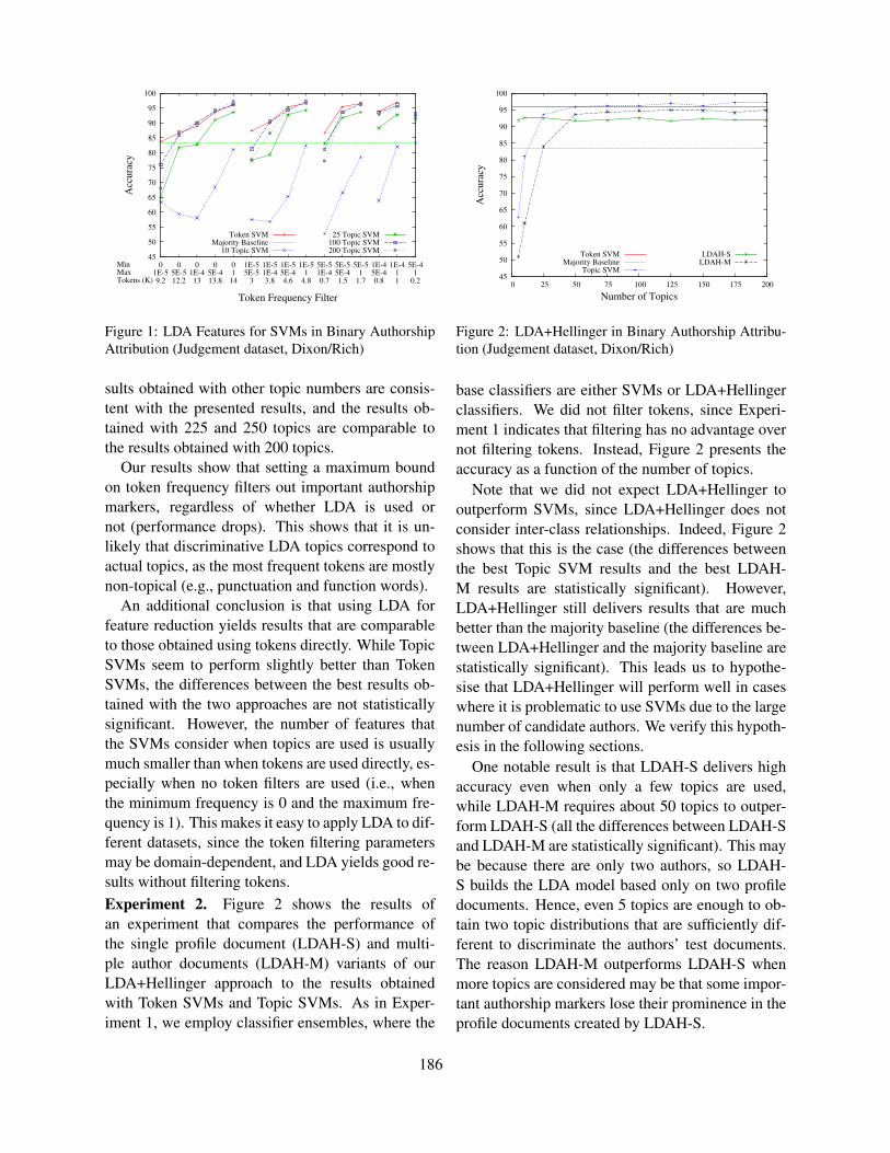
45

50

55

60

65

70

75

80

85

90

95

100

01E-59.2

05E-512.2

01E-413

05E-413.8

0114

1E-55E-5

3

1E-51E-43.8

1E-55E-44.6

1E-51

4.8

5E-51E-40.7

5E-55E-41.5

5E-51

1.7

1E-45E-40.8

1E-411

5E-41

0.2

Acc

ura

cy

Token Frequency Filter

MinMaxTokens (K)

Token SVMMajority Baseline

10 Topic SVM

25 Topic SVM100 Topic SVM200 Topic SVM

Figure 1: LDA Features for SVMs in Binary AuthorshipAttribution (Judgement dataset, Dixon/Rich)

sults obtained with other topic numbers are consis-tent with the presented results, and the results ob-tained with 225 and 250 topics are comparable tothe results obtained with 200 topics.

Our results show that setting a maximum boundon token frequency filters out important authorshipmarkers, regardless of whether LDA is used ornot (performance drops). This shows that it is un-likely that discriminative LDA topics correspond toactual topics, as the most frequent tokens are mostlynon-topical (e.g., punctuation and function words).

An additional conclusion is that using LDA forfeature reduction yields results that are comparableto those obtained using tokens directly. While TopicSVMs seem to perform slightly better than TokenSVMs, the differences between the best results ob-tained with the two approaches are not statisticallysignificant. However, the number of features thatthe SVMs consider when topics are used is usuallymuch smaller than when tokens are used directly, es-pecially when no token filters are used (i.e., whenthe minimum frequency is 0 and the maximum fre-quency is 1). This makes it easy to apply LDA to dif-ferent datasets, since the token filtering parametersmay be domain-dependent, and LDA yields good re-sults without filtering tokens.Experiment 2. Figure 2 shows the results ofan experiment that compares the performance ofthe single profile document (LDAH-S) and multi-ple author documents (LDAH-M) variants of ourLDA+Hellinger approach to the results obtainedwith Token SVMs and Topic SVMs. As in Exper-iment 1, we employ classifier ensembles, where the

45

50

55

60

65

70

75

80

85

90

95

100

0 25 50 75 100 125 150 175 200

Acc

ura

cy

Number of Topics

Token SVMMajority Baseline

Topic SVM

LDAH-SLDAH-M

Figure 2: LDA+Hellinger in Binary Authorship Attribu-tion (Judgement dataset, Dixon/Rich)

base classifiers are either SVMs or LDA+Hellingerclassifiers. We did not filter tokens, since Experi-ment 1 indicates that filtering has no advantage overnot filtering tokens. Instead, Figure 2 presents theaccuracy as a function of the number of topics.

Note that we did not expect LDA+Hellinger tooutperform SVMs, since LDA+Hellinger does notconsider inter-class relationships. Indeed, Figure 2shows that this is the case (the differences betweenthe best Topic SVM results and the best LDAH-M results are statistically significant). However,LDA+Hellinger still delivers results that are muchbetter than the majority baseline (the differences be-tween LDA+Hellinger and the majority baseline arestatistically significant). This leads us to hypothe-sise that LDA+Hellinger will perform well in caseswhere it is problematic to use SVMs due to the largenumber of candidate authors. We verify this hypoth-esis in the following sections.

One notable result is that LDAH-S delivers highaccuracy even when only a few topics are used,while LDAH-M requires about 50 topics to outper-form LDAH-S (all the differences between LDAH-Sand LDAH-M are statistically significant). This maybe because there are only two authors, so LDAH-S builds the LDA model based only on two profiledocuments. Hence, even 5 topics are enough to ob-tain two topic distributions that are sufficiently dif-ferent to discriminate the authors’ test documents.The reason LDAH-M outperforms LDAH-S whenmore topics are considered may be that some impor-tant authorship markers lose their prominence in theprofile documents created by LDAH-S.

186

0

10

20

30

40

50

60

70

80

90

100

0 50 100 150 200 250 300 350 400

Acc

ura

cy

Number of Topics

KOP: k1 = 400, k2 = 0.2LDAH-S

LDAH-M

Figure 3: LDA+Hellinger with Tens of Authors (IMDb62dataset)

4.4 LDA+Hellinger with Tens of Authors

In this section, we apply our LDA+Hellinger ap-proaches to the IMDb62 dataset (Section 4.2), andcompare the obtained results to those obtained withKoppel et al.’s (2011) method (KOP). To this effect,we first established a KOP best-performance base-line by performing parameter tuning experiments forKOP. Figure 3 shows the results of the comparisonof the accuracies obtained with our LDA+Hellingermethods to the best accuracy yielded by KOP (ob-tained in the parameter tuning experiment).

For this experiment, we ran our LDA+Hellingervariants with 5, 10, 25, 50, . . ., 300, 350 and 400topics. The highest LDAH-M accuracy was ob-tained with 300 topics (Figure 3). However, LDAH-S yielded a much higher accuracy than LDAH-M.This may be because the large number of trainingtexts per author (900) may be too noisy for LDAH-M. That is, the differences between individual textsby each author may be too large to yield a meaning-ful representation of the author if they are consideredseparately. Finally, LDAH-S requires only 50 topicsto outperform KOP, and outperforms KOP by about15% for 150 topics. All the differences between themethods are statistically significant.

This experiment shows that LDAH-S models theauthors in IMDb62 more accurately than KOP. Thelarge improvement in accuracy shows that the com-pact author representation employed by LDAH-S,which requires only 150 topics to obtain the highestaccuracy, has more power to discriminate betweenauthors than KOP’s much heavier representation, of

400 subsets with more than 30,000 features each. Inaddition, the per-fold runtime of the KOP baselinewas 93 hours, while LDAH-S required only 15 hoursper fold to obtain the highest accuracy.

4.5 LDA+Hellinger with Thousands of Authors

In this section, we compare the performance of ourLDA+Hellinger variants to the performance of KOPon several subsets of the Blog dataset (Section 4.2).For this purpose, we split the dataset according tothe prolificness of the authors, i.e., we ordered theauthors by the number of blog posts, and consideredsubsets that contain all the posts by the 1000, 2000,5000 and 19320 most prolific authors.7 Due to thelarge number of posts, we could not run KOP formore than k1 = 10 iterations on the smallest subsetof the dataset and 5 iterations on the other subsets,as the runtime was prohibitive for more iterations.For example, 10 iterations on the smallest subset re-quired about 90 hours per fold (the LDA+Hellingerruntimes were substantially shorter, with maximumruntimes of 56 hours for LDAH-S and 77 hours forLDAH-M, when 200 topics were considered). Inter-estingly, running KOP for 5 iterations on the largersubsets decreased performance compared to runningit for 1 iteration. Thus, on the larger subsets, themost accurate KOP results took less time to obtainthan those of our LDA+Hellinger variants.

Figure 4 shows the results of this experiment.For each author subset, it compares the results ob-tained by LDAH-S and LDAH-M to the best re-sult obtained by KOP. All the differences betweenthe methods are statistically significant. For up to2000 prolific authors (Figures 4(a), 4(b)), LDAH-Soutperforms KOP by up to 50%. For 5000 prolificusers (figure omitted due to space limitations), themethods perform comparably, and KOP outperformsLDAH-S by a small margin. However, with all theauthors (Figure 4(c)), KOP yields a higher accuracythan both LDA+Hellinger variants. This may bebecause considering non-prolific authors introducesnoise that results in an LDA model that does not cap-ture the differences between authors. However, it isencouraging that LDAH-S outperforms KOP whenless than 5000 prolific authors are considered.

7These authors make up about 5%, 10%, 25% and exactly100% of the authors, but they wrote about 50%, 65%, 80% andexactly 100% of the texts, respectively.

187

0

2

4

6

8

10

12

14

16

18

20

0 25 50 75 100 125 150 175 200

Acc

ura

cy

Number of Topics

KOP: k1 = 10, k2 = 0.6LDAH-S

LDAH-M

(a) 1,000 Prolific Authors

0

2

4

6

8

10

12

14

16

18

20

0 25 50 75 100 125 150 175 200

Acc

ura

cy

Number of Topics

KOP: k1 = 1, k2 = 1.0LDAH-S

LDAH-M

(b) 2,000 Prolific Authors

0

2

4

6

8

10

12

14

16

18

20

0 25 50 75 100 125 150 175 200

Acc

ura

cy

Number of Topics

KOP: k1 = 1, k2 = 1.0LDAH-S

LDAH-M

(c) 19,320 (all) Authors

Figure 4: LDA+Hellinger with Thousands of Authors (Blog dataset)

The accuracies obtained in this section are ratherlow compared to those obtained in the previoussections. This is not surprising, since the author-ship attribution problem is much more challengingwith thousands of candidate authors. This chal-lenge motivated the introduction of the σ∗ thresh-old in KOP (Section 3.1). Our LDA+Hellinger vari-ants can also be extended to include a threshold: ifthe Hellinger distance of the best-matching author isgreater than the threshold, the LDA+Hellinger algo-rithm would return “unknown author”. We leave ex-periments with this extension to future work, as ourfocus in this paper is on comparing LDA+Hellingerto KOP, and we believe that this comparison isclearer when no thresholds are used.


In this paper, we introduced an approach to author-ship attribution that models texts and authors usingLatent Dirichlet Allocation (LDA), and considersthe distance between the LDA-based representationsof the training and test texts when classifying testtexts. We showed that our approach yields state-of-the-art performance in terms of classification accu-racy when tens or a few thousand authors are consid-ered, and prolific authors exist in the training data.This accuracy improvement was achieved togetherwith a substantial reduction in runtime compared toKoppel et al.’s (2011) baseline method.

While we found that our approach performs wellon texts by prolific authors, there is still room forimprovement on authors who have not written manytexts – an issue that we will address in the future.One approach that may improve performance onsuch authors involves considering other types of fea-tures than tokens, such as parts of speech and char-

acter n-grams. Since our approach is based on LDA,it can easily employ different feature types, whichmakes this a straightforward extension to the workpresented in this paper.

In the future, we also plan to explore ways of ex-tending LDA to model authors directly, rather thanusing it as a black box. Authors were considered byRosen-Zvi et al. (2004; 2010), who extended LDAto form an author-topic model. However, this modelwas not used for authorship attribution, and wasmostly aimed at topic modelling of multi-authoredtexts, such as research papers.

Another possible research direction is to improvethe scalability of our methods. Our approach, likeKoppel et al.’s (2011) baseline, requires linear timein the number of possible authors to classify a singledocument. One possible way of reducing the timeneeded for prediction is by employing a hierarchi-cal approach that builds a tree of classifiers based onclass similarity, as done by Bickerstaffe and Zuker-man (2010) for the sentiment analysis task. Underthis framework, class similarity (in our case, authorsimilarity) can be measured using LDA, while smallgroups of classes can be discriminated using SVMs.

In addition to authorship attribution, we plan toemploy text-based author models in user modellingtasks such as rating prediction – a direction that wealready started working on by successfully applyingour LDA-based approach to model users for the rat-ing prediction task (Seroussi et al., 2011).

Acknowledgements

This research was supported in part by grantLP0883416 from the Australian Research Council.The authors thank Russell Smyth for the collabora-tion on initial results on the judgement dataset.

188

ReferencesAdrian Bickerstaffe and Ingrid Zukerman. 2010. A hier-

archical classifier applied to multi-way sentiment de-tection. In COLING 2010: Proceedings of the 23rdInternational Conference on Computational Linguis-tics, pages 62–70, Beijing, China.

David M. Blei, Andrew Y. Ng, and Michael I. Jordan.2003. Latent Dirichlet allocation. Journal of MachineLearning Research, 3(Jan):993–1022.

Haibin Cheng, Pang-Ning Tan, and Rong Jin. 2007. Lo-calized support vector machine and its efficient algo-rithm. In SDM 2007: Proceedings of the 7th SIAMInternational Conference on Data Mining, pages 461–466, Minneapolis, MN, USA.

Michael Gamon. 2004. Linguistic correlates of style:Authorship classification with deep linguistic analysisfeatures. In COLING 2004: Proceedings of the 20thInternational Conference on Computational Linguis-tics, pages 611–617, Geneva, Switzerland.

Thomas L. Griffiths and Mark Steyvers. 2004. Find-ing scientific topics. Proceedings of the NationalAcademy of Sciences, 101(Suppl. 1):5228–5235.

Patrick Juola. 2006. Authorship attribution. Founda-tions and Trends in Information Retrieval, 1(3):233–334.

Moshe Koppel, Jonathan Schler, and Shlomo Argamon.2011. Authorship attribution in the wild. LanguageResources and Evaluation, 45(1):83–94.

Kim Luyckx and Walter Daelemans. 2008. Authorshipattribution and verification with many authors and lim-ited data. In COLING 2008: Proceedings of the 22ndInternational Conference on Computational Linguis-tics, pages 513–520, Manchester, UK.

David Madigan, Alexander Genkin, David D. Lewis,Shlomo Argamon, Dmitriy Fradkin, and Li Ye. 2005.Author identification on the large scale. In Proceed-ings of the Joint Annual Meeting of the Interface andthe Classification Society of North America, St. Louis,MO, USA.

Thomas C. Mendenhall. 1887. The characteristic curvesof composition. Science, 9(214S):237–246.

Frederick Mosteller and David L. Wallace. 1964. In-ference and Disputed Authorship: The Federalist.Addison-Wesley.

Arun Rajkumar, Saradha Ravi, VenkatasubramanianSuresh, M. Narasimha Murthy, and C. E. Veni Mad-havan. 2009. Stopwords and stylometry: A latentDirichlet allocation approach. In Proceedings of theNIPS 2009 Workshop on Applications for Topic Mod-els: Text and Beyond (Poster Session), Whistler, BC,Canada.

Bhavani Raskutti and Adam Kowalczyk. 2004. Extremere-balancing for SVMs: A case study. ACM SIGKDDExplorations Newsletter, 6(1):60–69.

Ryan Rifkin and Aldebaro Klautau. 2004. In defense ofone-vs-all classification. Journal of Machine LearningResearch, 5(Jan):101–141.

Michal Rosen-Zvi, Thomas Griffiths, Mark Steyvers, andPadhraic Smyth. 2004. The author-topic model forauthors and documents. In UAI 2004: Proceedings ofthe 20th Conference on Uncertainty in Artificial Intel-ligence, pages 487–494, Banff, AB, Canada.

Michal Rosen-Zvi, Chaitanya Chemudugunta, ThomasGriffiths, Padhraic Smyth, and Mark Steyvers. 2010.Learning author-topic models from text corpora. ACMTransactions on Information Systems, 28(1):1–38.

Jonathan Schler, Moshe Koppel, Shlomo Argamon, andJames W. Pennebaker. 2006. Effects of age and gen-der on blogging. In Proceedings of AAAI Spring Sym-posium on Computational Approaches for AnalyzingWeblogs, pages 199–205, Stanford, CA, USA.

Yanir Seroussi, Ingrid Zukerman, and Fabian Bohnert.2010. Collaborative inference of sentiments fromtexts. In UMAP 2010: Proceedings of the 18th In-ternational Conference on User Modeling, Adaptationand Personalization, pages 195–206, Waikoloa, HI,USA.

Yanir Seroussi, Fabian Bohnert, and Ingrid Zukerman.2011. Personalised rating prediction for new users us-ing latent factor models. In Hypertext 2011: Proceed-ings of the 22nd ACM Conference on Hypertext andHypermedia, Eindhoven, The Netherlands.

Efstathios Stamatatos. 2009. A survey of modern au-thorship attribution methods. Journal of the Ameri-can Society for Information Science and Technology,60(3):538–556.

Mark Steyvers and Tom Griffiths. 2007. Probabilistictopic models. In Thomas K. Landauer, Danielle S.McNamara, Simon Dennis, and Walter Kintsch, ed-itors, Handbook of Latent Semantic Analysis, pages427–448. Lawrence Erlbaum Associates.

189


Evaluating a Semantic Network Automatically Constructed from Lexical

Co-occurrence on a Word Sense Disambiguation Task

Sean Szumlanski

Department of EECS

University of Central Florida

[email protected]

Fernando Gomez

Department of EECS

University of Central Florida

[email protected]

Abstract

We describe the extension and objective eval-

uation of a network1 of semantically related

noun senses (or concepts) that has been au-

tomatically acquired by analyzing lexical co-

occurrence in Wikipedia. The acquisition pro-

cess makes no use of the metadata or links

that have been manually built into the ency-

clopedia, and nouns in the network are auto-

matically disambiguated to their correspond-

ing noun senses without supervision. For

this task, we use the noun sense inventory of

WordNet 3.0. Thus, this work can be con-

ceived of as augmenting the WordNet noun

ontology with unweighted, undirected related-

to edges between synsets. Our network con-

tains 208,832 such edges.

We evaluate our network’s performance on a

word sense disambiguation (WSD) task and

show: a) the network is competitive with

WordNet when used as a stand-alone knowl-

edge source for two WSD algorithms; b) com-

bining our network with WordNet achieves

disambiguation results that exceed the perfor-

mance of either resource individually; and c)

our network outperforms a similar resource

that has been automatically derived from se-

mantic annotations in the Wikipedia corpus.

1 Introduction

A growing interest in using semantic relatedness in

word sense disambiguation (WSD) tasks has spurred

investigations into the limitations of the WordNet

ontology (Fellbaum, 1998) for this purpose. Al-

though WordNet comprises a rich set of semantic

1http://www.cs.ucf.edu/ seansz/sem

links between word senses (or concepts), indicat-

ing semantic similarity through subsumptive hyper-

nymic and hyponymic relations (among others), it

lacks a general indication of semantic relatedness.

We present a semantic network that is automat-

ically acquired from lexical co-occurrence in Wi-

kipedia, and indicates general semantic relatedness

between noun senses in WordNet 3.0. In this work,

the discovery of relatedness is a context-sparse affair

that takes place in absentia of the semantic annota-

tions of Wikipedia, such as inter-article links, entries

in disambiguation pages, the title of the article from

which a sentence is extracted, and so on.

We released an earlier version of such a network

that was limited by the fact that only relationships

involving at least one monosemous noun had been

included, and it was not evaluated on a WSD task

(Szumlanski and Gomez, 2010).

In contrast, the network we present here has relat-

edness data for over 4,500 polysemous noun targets

and 3,000 monosemous noun targets, each of which

are related to an average of 27.5 distinct noun senses.

It consists of 208,832 undirected edges – a 181% in-

crease in size over the previous network. The result

is a semantic network that has reached maturity and,

as we will show, can be successfully applied to a

WSD task.

This paper proceeds as follows. In the next sec-

tion (Section 2), we discuss related work. We then

give an overview of the method we use to con-

struct our network (Sections 3 and 4). The network

is evaluated through its application to a WSD task

(Sections 5–7), where we compare its performance

to WordNet and another automatically acquired se-

mantic network called WordNet++ (Ponzetto and

Navigli, 2010). A discussion follows (Section 8),

190

and we present our conclusions in Section 9.

2 Related Work

Our work bears strong relation to WordNet++

(henceforth WN++), which is constructed automat-

ically from the semantic annotations in Wikipedia

(Ponzetto and Navigli, 2010).2 Links in WN++ are

established between words whose articles link to one

another. For example, the article on astronomy in

Wikipedia links to the article on celestial naviga-

tion, so we find an edge from astronomy#n#1 to

celestial navigation#n#1 in WN++.3 The nouns re-

lated in WN++ are disambiguated automatically us-

ing further semantic annotation data from Wikipe-

dia, including sense labels, the titles of other pages

linked to by any two related nouns, and the folk-

sonomic categories to which articles belong. These

serve as context words that are compared with con-

text words from various WordNet relations in or-

der to map the nouns to their appropriate WordNet

senses. The resulting resource contains 1,902,859

unique edges between noun senses.

Augmenting the structure of Wikipedia itself has

been the subject of research as well, and involves

the discovery of relations between articles. Mihal-

cea and Csomai (2007), for example, added links

between Wikipedia pages after automatically iden-

tifying keywords in each article and disambiguating

those words to their appropriate Wikipedia concepts

(article titles), while Ponzetto and Navigli (2009)

used graph theoretic approaches to augment the tax-

onomic organization of Wikipedia articles.

In terms of automatically discovering semantic re-

lations, many pattern-based approaches have been

used to extract specific types of relations from large

corpora, e.g., hyponymy, meronymy, and synonymy

(Hearst, 1992; Pantel and Pennacchiotti, 2006).

Approaches based on distributional similarity have

been applied toward the same end (Harris, 1985;

Gorman and Curran, 2006), and there are sev-

eral approaches that rely on the underlying struc-

ture of WordNet or Wikipedia to measure the re-

latedness between two concepts or nouns quantita-

tively (Hughes and Ramage, 2007; Gabrilovich and

2http://lcl.uniroma1.it/wordnetplusplus

3The notation astronomy#n#1 refers to sense 1 (#1) of the

noun (#n) “astronomy” in WordNet. Other parts of speech are

denoted by #v (verbs), #a (adjectives), or #r (adverbs).

Markovitch, 2007; Zaragoza et al., 2007; Patward-

han and Pedersen, 2006; Strube and Ponzetto, 2006;

Budanitsky and Hirst, 2006; Resnik, 1995).

Other quantitative approaches have leveraged the

large amounts of data available on the Web to dis-

cover relatedness. Notably, Agirre and de Lacalle

(2004) employed web queries to associate WordNet

synsets with representative context words, known as

topic signatures. Cuadros and Rigau (2008) have

used these data to construct four KnowNets, seman-

tic knowledge bases derived by disambiguating the

top 5, 10, 15, and 20 nouns, respectively, from the

topic signatures of Agirre and de Lacalle.

3 Automatic Acquisition of the Semantic

Network

The semantic network is automatically acquired in

three distinct stages (Szumlanski and Gomez, 2010):

(1) quantitative measurement of relatedness between

nouns that co-occur in a large corpus; (2) categori-

cal determination of whether the quantitative mea-

sure indicates strong and mutual semantic related-

ness between a given pair of nouns; and (3) unsuper-

vised disambiguation of all the nouns that are found

to be semantically related. We provide an overview

of each of these steps below (Sections 3.1–3.3), and

then discuss how we have expanded this method-

ology to create a more complete semantic network

(Section 4).

3.1 Quantitatively measuring relatedness from

lexical co-occurrence

We first measure the semantic relatedness, or re-

lational strength, of a target, t, to one of its co-

occurring nouns, or co-targets, c, with the following

asymmetric function:

Srel(t, c) = P (t|c)P (c|t)logP (c|t)

P (c)

where P (c|t) is the relative frequency of c among all

nouns co-occurring with t, and vice versa for P (t|c).P (c) is the relative frequency of c among all nouns

occurring in the corpus. For these values, we rely on

lexical co-occurrence data extracted from Wikipe-

dia. Co-occurrence is considered intra-sententially

(as opposed to co-occurrence in entire articles or

paragraphs, or co-occurrence within variable-sized

windows of context).

191

This function essentially measures the degree to

which an occurrence of t in a sentence predicts the

co-occurrence of c. It is an adaptation of Resnik’s

(1999) selectional association measure.

Table 1 shows the results of applying this function

to the co-targets of “yoga” and “meditation.”

Target (t): yoga Target (t): meditation

Co-target (c) Srel Co-target (c) Srel

hatha yoga .1801 yoga .0707

asana .0761 mindfulness .0415

meditation .0673 contemplation .0165

bhakti .0508 prayer .0139

raja .0410 practice .0068

tantra .0148 technique .0060

yogi .0132 mantra .0053

karma .0125 relaxation .0048

posture .0104 retreat .0047

aerobics .0093 enlightenment .0031

tai chi .0089 monk .0025

exercise .0036 posture .0024

practice .0032 breathing .0017

instructor .0031 - - - - - - - - - - - - -

- - - - - - - - - - - - - exercise .0015

guru .0027 teaching .0014

massage .0026 practitioner .0014

exercise .0019 ascetic .0014...

......

...

Table 1: The most strongly related co-targets of “yoga”

and “meditation,” sorted by decreasing value of relational

strength (Srel). Nouns above dashed lines are the top 5%

of the target’s most strongly related co-targets.

3.2 Establishing categorical relatedness

We then use a mutual relatedness algorithm to as-

certain whether two nouns are semantically related

by determining whether the nouns under considera-

tion reciprocate a high degree of relatedness to one

another. It proceeds as follows:

For some target noun of interest, t, let Cx(t) be

the set of the top x% of t’s co-targets as sorted by

Srel(t, c). For each c ∈ Cx(t), if we have t ∈ Cx(c),then we say that t and c are categorically related and

add the noun pair (t, c) to our semantic network. We

then increment x by one and repeat the process: for

every c ∈ Cx+1(t) such that (t, c) is not already in

our network, we look for t in Cx+1(c), and add (t, c)

to our network if we find it. This process continues

until we have incremented x some number of times

without adding any new relations to the semantic

network. We then take the symmetric closure of the

network, so that if (t, c) is in the network, (c, t) is, as

well. (That is, the relation is considered undirected.)

Consider, for example, the nouns in Table 1.

Given the target “yoga,” we might first examine the

top 5% of its most strongly related co-targets (an ar-

bitrary initial threshold chosen simply for illustra-

tive purposes). In this case, we have all the nouns

above the dashed line: C5(yoga) = {hatha yoga,

asana, meditation, bhakti, raja, tantra, yogi, karma,

posture, aerobics, tai chi, exercise, practice, instruc-

tor}. The algorithm then searches C5(hatha yoga),

C5(asana), and so on, for “yoga,” adding a new re-

lation to the network every time “yoga” is found.

Thus, we can see by the inclusion of “yoga” in

C5(meditation) (all nouns above the dashed line in

the second column of Table 1), that the pair (yoga,

meditation) will be included in the network.

This reliance on mutual relatedness ensures that

only noun pairs exhibiting strong semantic related-

ness are admitted to the network.

3.3 Disambiguation

Disambiguation of the resulting noun-noun pairs is

the product of majority-rules voting by the following

three algorithms.

Subsumption. The most frequently occurring

immediate hypernyms of all nouns related to our

target are permitted to disambiguate the polyse-

mous nouns. This is useful because of the semantic

clustering that tends to occur among related nouns.

(E.g., “astronomer” is related to several terms cat-

egorized as celestial bodies in WordNet, such as

“planet,” “star,” “minor planet,” and “quasar.”)

Glosses. Senses of polysemous co-targets with

occurrences of monosemous co-targets in their

glosses are preferentially taken as the intended

meanings of the polysemous nouns. Monosemous

co-targets are matched directly, or by suffix replace-

ment. (E.g., “biology” can be matched by the oc-

currence of “biologist” in a gloss, “engineering” by

“engineers,” and so on.)

Selectional Preferences. This method associates

a numerical score with all superordinate synsets

from the WordNet noun ontology that categorize

192

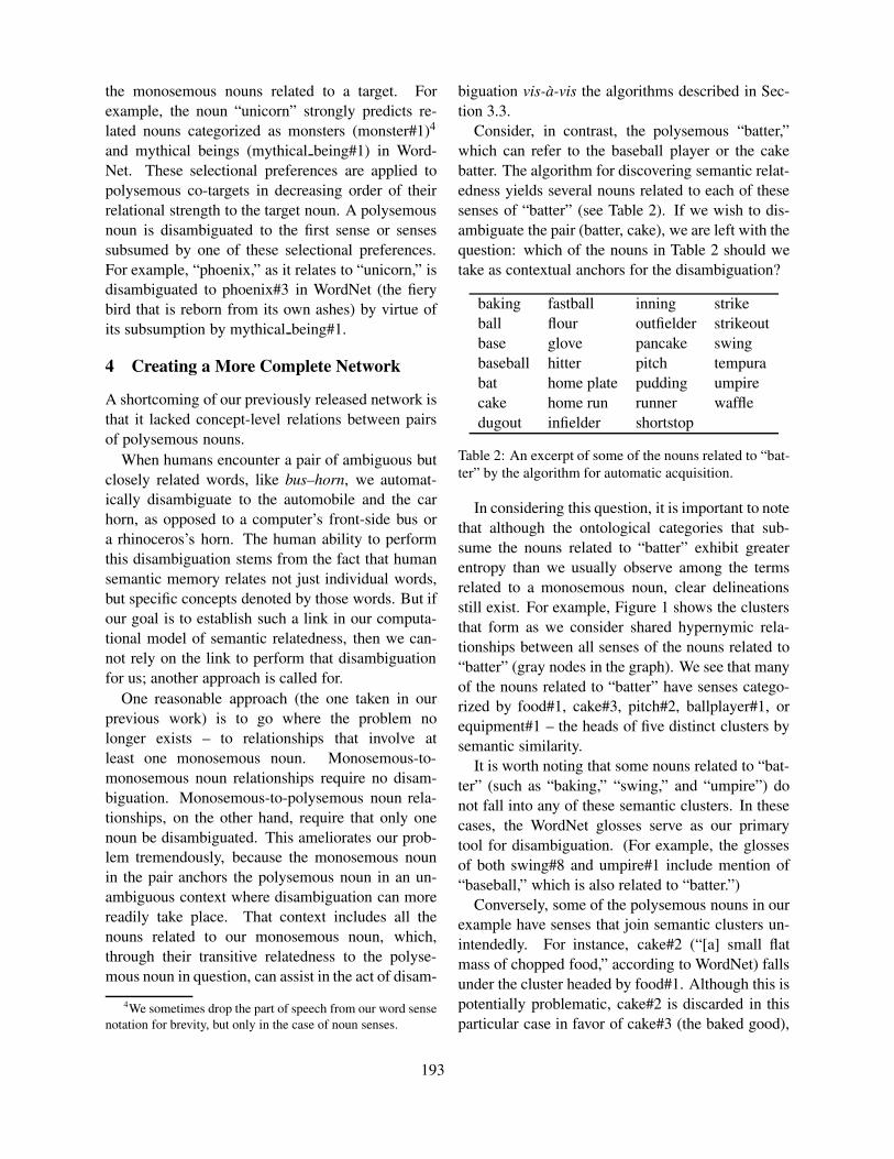
the monosemous nouns related to a target. For

example, the noun “unicorn” strongly predicts re-

lated nouns categorized as monsters (monster#1)4

and mythical beings (mythical being#1) in Word-

Net. These selectional preferences are applied to

polysemous co-targets in decreasing order of their

relational strength to the target noun. A polysemous

noun is disambiguated to the first sense or senses

subsumed by one of these selectional preferences.

For example, “phoenix,” as it relates to “unicorn,” is

disambiguated to phoenix#3 in WordNet (the fiery

bird that is reborn from its own ashes) by virtue of

its subsumption by mythical being#1.

4 Creating a More Complete Network

A shortcoming of our previously released network is

that it lacked concept-level relations between pairs

of polysemous nouns.

When humans encounter a pair of ambiguous but

closely related words, like bus–horn, we automat-

ically disambiguate to the automobile and the car

horn, as opposed to a computer’s front-side bus or

a rhinoceros’s horn. The human ability to perform

this disambiguation stems from the fact that human

semantic memory relates not just individual words,

but specific concepts denoted by those words. But if

our goal is to establish such a link in our computa-

tional model of semantic relatedness, then we can-

not rely on the link to perform that disambiguation

for us; another approach is called for.

One reasonable approach (the one taken in our

previous work) is to go where the problem no

longer exists – to relationships that involve at

least one monosemous noun. Monosemous-to-

monosemous noun relationships require no disam-

biguation. Monosemous-to-polysemous noun rela-

tionships, on the other hand, require that only one

noun be disambiguated. This ameliorates our prob-

lem tremendously, because the monosemous noun

in the pair anchors the polysemous noun in an un-

ambiguous context where disambiguation can more

readily take place. That context includes all the

nouns related to our monosemous noun, which,

through their transitive relatedness to the polyse-

mous noun in question, can assist in the act of disam-

4We sometimes drop the part of speech from our word sense

notation for brevity, but only in the case of noun senses.

biguation vis-a-vis the algorithms described in Sec-

tion 3.3.

Consider, in contrast, the polysemous “batter,”

which can refer to the baseball player or the cake

batter. The algorithm for discovering semantic relat-

edness yields several nouns related to each of these

senses of “batter” (see Table 2). If we wish to dis-

ambiguate the pair (batter, cake), we are left with the

question: which of the nouns in Table 2 should we

take as contextual anchors for the disambiguation?

baking fastball inning strike

ball flour outfielder strikeout

base glove pancake swing

baseball hitter pitch tempura

bat home plate pudding umpire

cake home run runner waffle

dugout infielder shortstop

Table 2: An excerpt of some of the nouns related to “bat-

ter” by the algorithm for automatic acquisition.

In considering this question, it is important to note

that although the ontological categories that sub-

sume the nouns related to “batter” exhibit greater

entropy than we usually observe among the terms

related to a monosemous noun, clear delineations

still exist. For example, Figure 1 shows the clusters

that form as we consider shared hypernymic rela-

tionships between all senses of the nouns related to

“batter” (gray nodes in the graph). We see that many

of the nouns related to “batter” have senses catego-

rized by food#1, cake#3, pitch#2, ballplayer#1, or

equipment#1 – the heads of five distinct clusters by

semantic similarity.

It is worth noting that some nouns related to “bat-

ter” (such as “baking,” “swing,” and “umpire”) do

not fall into any of these semantic clusters. In these

cases, the WordNet glosses serve as our primary

tool for disambiguation. (For example, the glosses

of both swing#8 and umpire#1 include mention of

“baseball,” which is also related to “batter.”)

Conversely, some of the polysemous nouns in our

example have senses that join semantic clusters un-

intendedly. For instance, cake#2 (“[a] small flat

mass of chopped food,” according to WordNet) falls

under the cluster headed by food#1. Although this is

potentially problematic, cake#2 is discarded in this

particular case in favor of cake#3 (the baked good),

193

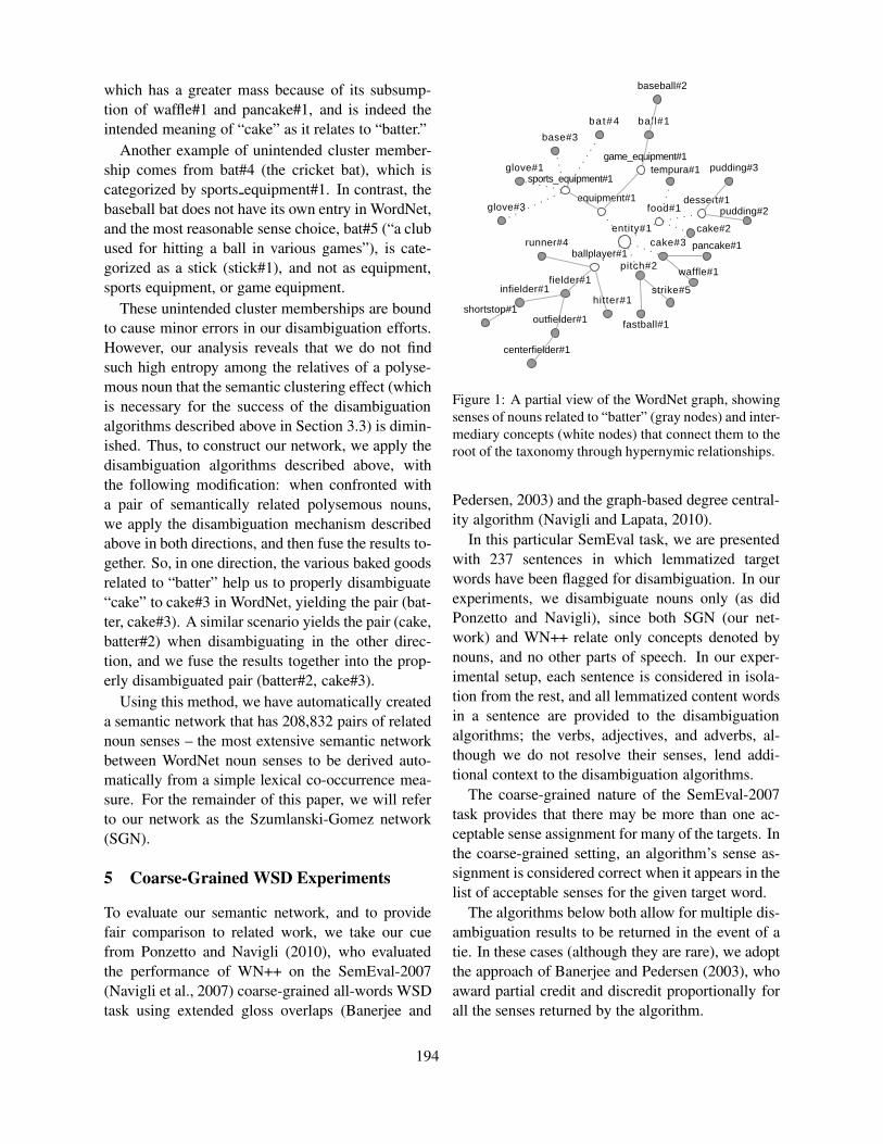
which has a greater mass because of its subsump-

tion of waffle#1 and pancake#1, and is indeed the

intended meaning of “cake” as it relates to “batter.”

Another example of unintended cluster member-

ship comes from bat#4 (the cricket bat), which is

categorized by sports equipment#1. In contrast, the

baseball bat does not have its own entry in WordNet,

and the most reasonable sense choice, bat#5 (“a club

used for hitting a ball in various games”), is cate-

gorized as a stick (stick#1), and not as equipment,

sports equipment, or game equipment.

These unintended cluster memberships are bound

to cause minor errors in our disambiguation efforts.

However, our analysis reveals that we do not find

such high entropy among the relatives of a polyse-

mous noun that the semantic clustering effect (which

is necessary for the success of the disambiguation

algorithms described above in Section 3.3) is dimin-

ished. Thus, to construct our network, we apply the

disambiguation algorithms described above, with

the following modification: when confronted with

a pair of semantically related polysemous nouns,

we apply the disambiguation mechanism described

above in both directions, and then fuse the results to-

gether. So, in one direction, the various baked goods

related to “batter” help us to properly disambiguate

“cake” to cake#3 in WordNet, yielding the pair (bat-

ter, cake#3). A similar scenario yields the pair (cake,

batter#2) when disambiguating in the other direc-

tion, and we fuse the results together into the prop-

erly disambiguated pair (batter#2, cake#3).

Using this method, we have automatically created

a semantic network that has 208,832 pairs of related

noun senses – the most extensive semantic network

between WordNet noun senses to be derived auto-

matically from a simple lexical co-occurrence mea-

sure. For the remainder of this paper, we will refer

to our network as the Szumlanski-Gomez network

(SGN).

5 Coarse-Grained WSD Experiments

To evaluate our semantic network, and to provide

fair comparison to related work, we take our cue

from Ponzetto and Navigli (2010), who evaluated

the performance of WN++ on the SemEval-2007

(Navigli et al., 2007) coarse-grained all-words WSD

task using extended gloss overlaps (Banerjee and

entity#1

food#1

cake#2

equipment#1

ballplayer#1pitch#2

cake#3

dessert#1

tempura#1game_equipment#1

sports_equipment#1

runner#4

fielder#1

hitter#1

fastball#1

strike#5

waffle#1

pancake#1

pudding#2

pudding#3

ball#1

infielder#1

outfielder#1

baseball#2

bat#4

base#3

glove#1

glove#3

shortstop#1

centerfielder#1

Figure 1: A partial view of the WordNet graph, showing

senses of nouns related to “batter” (gray nodes) and inter-

mediary concepts (white nodes) that connect them to the

root of the taxonomy through hypernymic relationships.

Pedersen, 2003) and the graph-based degree central-

ity algorithm (Navigli and Lapata, 2010).

In this particular SemEval task, we are presented

with 237 sentences in which lemmatized target

words have been flagged for disambiguation. In our

experiments, we disambiguate nouns only (as did

Ponzetto and Navigli), since both SGN (our net-

work) and WN++ relate only concepts denoted by

nouns, and no other parts of speech. In our exper-

imental setup, each sentence is considered in isola-

tion from the rest, and all lemmatized content words

in a sentence are provided to the disambiguation

algorithms; the verbs, adjectives, and adverbs, al-

though we do not resolve their senses, lend addi-

tional context to the disambiguation algorithms.

The coarse-grained nature of the SemEval-2007

task provides that there may be more than one ac-

ceptable sense assignment for many of the targets. In

the coarse-grained setting, an algorithm’s sense as-

signment is considered correct when it appears in the

list of acceptable senses for the given target word.

The algorithms below both allow for multiple dis-

ambiguation results to be returned in the event of a

tie. In these cases (although they are rare), we adopt

the approach of Banerjee and Pedersen (2003), who

award partial credit and discredit proportionally for

all the senses returned by the algorithm.

194

6 Extended Gloss Overlaps (ExtLesk)

The first disambiguation algorithm we employ is

the extended gloss overlaps measure (henceforth

ExtLesk) of Banerjee and Pedersen (2003), which

is an extension of the Lesk (1986) gloss overlap

measure. Loosely speaking, the algorithm disam-

biguates a target noun by maximizing the overlap

(number of words in common) between the glosses

of word senses related5 to the target’s noun senses

and those related to all context words (all lemma-

tized targets in the sentence under consideration

other than the target itself). The sense with the great-

est overlap is selected as the intended meaning of a

target noun.

In the event of a tie, multiple senses may be se-

lected. ExtLesk does not attempt to perform sense

assignment if the score for every sense of a target

noun is zero, except when dealing with a monose-

mous noun, in which case we default to the only

sense possible.

6.1 Results

We have run ExtLesk on the SemEval-2007 task us-

ing five combinations of semantic resources: Word-

Net only, SGN (our semantic network) only, SGN

and WordNet combined (that is, the union of all

links contained in both networks), WN++ only, and

WN++ combined with WordNet. We include the tra-

ditional baselines of most frequent sense (MFS) as-

signment and random sense assignment for compari-

son, and measure precision (number of correct sense

assignments divided by the number of attempted

sense assignments), recall (number of correct sense

assignments divided by the number of target nouns

to be disambiguated), and the harmonic mean of the

two, F1, defined as:

F1 =2 ∗ precision ∗ recall

precision + recall

We present our results in Table 3, and offer the

following observations. Firstly, SGN as a stand-

alone network rivals the performance of WordNet.

This is particularly impressive given the fact that

5We use all relations available in WordNet, as well as a

related-to relation derived from the links in our semantic net-

work.

Resource P R F1

WordNet 78.80 74.82 76.76

SGN 78.64 72.82 75.62

SGN and WordNet 82.35 78.11 80.18

WN++ 74.67 61.87 67.67

WN++ and WordNet 77.35 73.38 75.31

MFS Baseline 77.40 77.40 77.40

Random Baseline 63.50 63.50 63.50

Table 3: ExtLesk disambiguation results on the SemEval-

2007 all-words coarse-grained WSD task (nouns only).

the edges in SGN were derived automatically from

a simple lexical co-occurrence measure.

Equally impressive is the ability of SGN and

WordNet, when used in combination, to achieve re-

sults that exceed what either network is able to ac-

complish as a stand-alone knowledge source. When

combined, we see improvements of 3.42% and

4.56% over WordNet and SGN as stand-alone re-

sources, respectively. It is also only with these re-

sources combined that we are able to outperform the

MFS baseline, and we do so by 2.78%.6

In contrast, WN++ fails to perform as a stand-

alone resource, falling behind the MFS baseline by

9.73%.7 Of all the resources tested, WN++ yields

the lowest results. When combined with WordNet,

WN++ actually diminishes the ability of WordNet to

perform on this WSD task by 1.45%. We defer our

discussion of factors impacting the performance of

WN++ to Section 8 (Discussion).

7 WSD with Degree Centrality

Degree centrality is a graph-based measure of se-

mantic relatedness (Navigli and Lapata, 2010) in

which we search through a semantic network for

paths of length l ≤ maxLength between all sense

nodes for all lemmas in our context. The edges along

all such paths are added to a new graph, G′, and for

each target noun to be disambiguated, the sense node

with the greatest number of incident edges (highest

vertex degree) in G′ is taken as its intended sense.

6Other systems have obtained better results on the same

dataset, but we focus only on SGN and WN++ because our aim

is to compare the resources themselves.7Ponzetto and Navigli (2010) report results of F1 = 68.3 and

72.0 for WN and WN++ as stand-alone resources. Space con-

siderations prevent us from discussing this disparity in detail.

195

In these graphs, nodes represent synsets, as op-

posed to instantiating separate nodes for different

members of the same synset and allowing edges to

be constructed between them. We include all lem-

mas from a sentence in our context, but only return

disambiguation results for the nouns.

With SGN and WN++, the implementation of this

algorithm is straightforward. We initiate a breadth-

first search (BFS)8 at each target sense node in the

network, and proceed through ⌊maxLength+1

2⌋ itera-

tions of spreading activation. Whenever the tendrils

of this spreading activation from one target sense

node in the graph connect to those of another,9 we

add the path between the nodes to our new graph, G′,

potentially incrementing the degree of the involved

target sense nodes in G′ as we do so.

Because BFS is an admissible algorithm (guaran-

teed to find the shortest path from an initial state to

a goal), it provides a computationally efficient ap-

proach to finding all paths between all target nodes.

Also, because any node on a path of length l ≤maxLength between two target nodes is at most

⌊ l2⌋ nodes removed from at least one of those tar-

get sense nodes, we only need to perform a BFS of

depth ⌊maxLength+1

2⌋ from every target sense node

in order to guarantee that every such path between

them will be discovered. Since the time complexity

of BFS is exponential with respect to the depth of

the search, cutting this depth in half (in comparison

to performing a BFS of depth maxLength) greatly

reduces the running time of our algorithm.

We take the same approach in traversing the

WordNet noun graph, using all possible sense re-

lations as edges. In keeping with the approach of

Navigli and Lapata (2010), an edge is also induced

between synsets if the gloss of one synset contains a

monosemous content word. For example, the gloss

for leprechaun#n#1, “a mischievous elf in Irish folk-

lore,” contains the monosemous noun “folklore;”

thus, we have an edge between leprechaun#n#1 and

8This is in contrast to the DFS implementation of Navigli

and Lapata (2010), so for the sake of posterity, we expound

upon our approach in this section.9When maxLength is odd, this requires an additional

check to ensure that the intersection is not taking place at a node

that is exactly ⌊maxLength+1

2⌋ degrees removed from each of

the two target nodes it is connecting, as this would result in a

path with overall length maxLength + 1 between the target

nodes.

folklore#n#1 in the WordNet graph.

Once we have our new graph, G′, constructed in

this manner, the vertex degree is considered an in-

dication of the semantic relatedness of a particular

synset to all other lemmas in our context. For each

target noun, we use its sense node with the highest

degree in G′ for sense assignment.

7.1 Results

We have tested the degree centrality algorithm with

the following combinations of semantic resources:

WordNet, SGN, WN++, Refined WN++, SGN and

WordNet combined, and Refined WN++ and Word-

Net combined. (Refined WN++ consists of 79,422

of WN++’s strongest relations, and was created in an

unsupervised setting by Ponzetto and Navigli specif-

ically for use with degree centrality when they dis-

covered that WN++ had too many weak relations to

perform well with the algorithm.)

We have observed that the performance of de-

gree centrality rapidly levels off as maxLength

increases. Ponzetto and Lapata (2010) also re-

port this so-called “plateau” effect, and employ a

maxLength of 6 in their experiments, despite find-

ing that results level off around maxLength = 4.

We, too, find that performance levels off around

maxLength = 4 in almost all cases, and so only

continue up to maxLength = 5.

We find that, in all cases tested, degree centrality

is unable to outperform the MFS baseline (with re-

spect to F1) (see Table 4). SGN and WN++ exhibit

comparable performance with this algorithm, with

maximum F1 values of 68.4% (maxLength = 2)

and 67.3% (maxLength = 3–5), respectively. Nei-

ther achieves the performance of WordNet with de-

gree centrality (F1 = 74.0%), which underperforms

the MFS baseline (F1 = 77.4%) by 3.4%.10 Ponzetto

and Navigli (2010) reported that only performing

sense assignment when the max degree exceeded an

empirically derived but non-disclosed threshold im-

proved performance, but we have found that imple-

menting such a threshold universally lowers results

for all resources we tested with degree centrality.

10Although Ponzetto and Navigli (2010) reported similar re-

sults with WordNet (F1 = 74.5), we have been unable to repro-

duce their results using Refined WN++, either combined with

WordNet (F1 = 79.4) or as a stand-alone resource (F1 = 57.4).

196

The lowest performance using degree central-

ity comes from Refined WN++ as a stand-alone

resource. We attribute this to the fact that Re-

fined WN++ is so semantically sparse. On average,

noun senses in Refined WN++ are related to only

3.42 other noun senses, while those in WN++ and

SGN relate to an average of 44.59 and 10.92 noun

senses, respectively. Accordingly, the success of Re-

fined WN++ and WordNet combined is attributable

mostly to the success of WordNet as a stand-alone

resource; as maxLength increases, the contribu-

tions made by the sparse Refined WN++ network

rapidly become negligible in comparison to those

provided by the WordNet ontology.

l P R F1 P R F1

WordNet SGN

1 96.9 16.8 28.6 79.7 32.9 46.6

2 77.6 45.1 57.0 72.0 64.6 68.4

3 76.7 65.6 70.7 68.7 63.5 66.0

4 76.9 71.0 73.9 68.0 63.9 65.9

5 76.6 71.6 74.0 68.0 64.2 66.1

SGN & WN WN++

1 77.4 52.4 62.5 87.2 23.5 37.1

2 74.7 70.7 72.7 71.6 60.2 65.4

3 70.3 67.1 68.7 70.7 64.3 67.3

4 70.5 67.4 68.9 70.4 64.5 67.3

5 70.1 67.0 68.5 70.4 64.5 67.3

WN++

refinedWN

++

refined& WN

1 98.3 15.3 26.5 83.3 31.2 45.4

2 91.4 23.4 37.3 77.5 66.6 71.6

3 88.7 29.9 44.7 77.6 73.6 75.5

4 83.7 32.3 46.7 74.7 71.4 73.0

5 80.2 35.3 49.0 74.7 71.4 73.0

MFS Baseline Random Baseline

77.4 77.4 77.4 63.5 63.5 63.5

Table 4: Degree centrality disambiguation results on

the SemEval-2007 all-words coarse-grained WSD task

(nouns only). l is maximum path length.

8 Discussion

The fact that the performance of degree centrality

quickly plateaus hints at the root cause of its weak

performance compared to ExtLesk and the MFS

baseline. As the maximum path length is increased

in a dense semantic network, all possible edges from

our target sense nodes rapidly find themselves in-

volved with paths to other target sense nodes. This is

particularly true of WN++ (notice its rapid and sta-

ble convergence), where certain “sticky” nodes form

bridges between seemingly unrelated concepts. For

example, the frequent appearance of “United States”

in Wikipedia articles, and its tendency to be linked

to the United States Wikipage when it occurs, causes

the term to serve as a bridge between such diverse

concepts as automaton#2 and burrito#1, which one

would typically expect to be far removed from one

another in a model of semantic relatedness.

Nonetheless, the degree centrality algorithm has

no difficulty finding short paths between target sense

nodes when traversing any of the semantic networks

we tested. In fact, we have discovered that as the

results of degree centrality converge, they approach

the performance obtained by foregoing the algo-

rithm altogether and simply disambiguating each

noun to the sense with the most edges in the net-

work (regardless of whether those edges ultimately

connect two word senses from the disambiguation

context). The expected values of convergence at-

tained by defaulting to the most semantically well-

connected sense of each target noun in each network

are F1 = 66.3%, 67.5%, and 74.6% for SGN, WN++,

and WordNet, respectively – remarkably close to the

experimentally derived degree centrality results of

F1 = 66.1%, 67.3%, and 74.0%.

9 Conclusion

We have constructed a semantic network of related

noun senses automatically from intra-sentential lex-

ical co-occurrence data, and shown that on a WSD

task, it outperforms a similar resource, WN++,

which is derived from the rich set of semantic anno-

tations available in the Wikipedia corpus. Our net-

work has also shown competitive performance with

the WordNet ontology on WSD, and when combined

with WordNet, improves disambiguation results in

a coarse-grained setting using the ExtLesk disam-

biguation algorithm.

Acknowledgments

This research was supported in part by the

NASA Engineering and Safety Center under

Grant/Cooperative Agreement NNX08AJ98A.

197

References

Eneko Agirre and Oier Lopez de Lacalle. 2004. Pub-

licly available topic signatures for all WordNet nom-

inal senses. In Proceedings of the 4th International

Conference on Language Resources and Evaluations

(LREC ’04), pages 1123–1126, Lisbon, Portugal.

Satanjeev Banerjee and Ted Pedersen. 2003. Extended

gloss overlaps as a measure of semantic relatedness.

In Proceedings of the 18th International Joint Confer-

ence on Artificial Intelligence (IJCAI ’03), pages 805–

810, Acapulco, Mexico.

Alexander Budanitsky and Graeme Hirst. 2006. Evalu-

ating WordNet-based measures of lexical semantic re-

latedness. Computational Linguistics, 32(1):13–47.

Montse Cuadros and German Rigau. 2008. KnowNet:

building a large net of knowledge from the web. In

Proceedings of the 22nd International Conference on

Computational Linguistics (COLING ’08), pages 161–

168, Manchester, UK. Association for Computational

Linguistics.

Christiane Fellbaum, editor. 1998. WordNet: An Elec-

tronic Lexical Database. MIT Press.

Evgeniy Gabrilovich and Shaul Markovitch. 2007. Com-

puting semantic relatedness using Wikipedia-based ex-

plicit semantic analysis. In Proceedings of the 20th In-

ternational Joint Conference on Artificial Intelligence

(IJCAI ’07), pages 1606–1611, Hyderabad, India.

James Gorman and James R. Curran. 2006. Scaling dis-

tributional similarity to large corpora. In Proceedings

of the 21st International Conference on Computational

Linguistics and the 44th Annual Meeting of the Asso-

ciation for Computational Linguistics (COLING-ACL

’06), pages 361–368, Sydney, Australia. Association

for Computational Linguistics.

Zellig S. Harris. 1985. Distributional structure. In J. J.

Katz, editor, The Philosophy of Linguistics, pages 26–

47. Oxford University Press.

Marti A. Hearst. 1992. Automatic acquisition of hy-

ponyms from large text corpora. In Proceedings of

the 14th International Conference on Computational

Linguistics (COLING ’92), pages 539–545, Nantes,

France.

Thad Hughes and Daniel Ramage. 2007. Lexical se-

mantic relatedness with random graph walks. In Pro-

ceedings of the 2007 Joint Conference on Empirical

Methods in Natural Language Processing and Compu-

tational Natural Language Learning (EMNLP-CoNLL

’07), pages 581–589, Prague, Czech Republic. Asso-

ciation for Computational Linguistics.

Michael Lesk. 1986. Automatic sense disambiguation

using machine readable dictionaries: how to tell a pine

cone from an ice cream cone. In Proceedings of the

5th Annual International Conference on Systems Doc-

umentation (SIGDOC ’86), pages 24–26, Toronto, On-

tario, Canada. ACM.

Rada Mihalcea and Andras Csomai. 2007. Wikify!: link-

ing documents to encyclopedic knowledge. In Pro-

ceedings of the 16th ACM Conference on Information

and Knowledge Management (CIKM ’07), pages 233–

242, Lisbon, Portugal. ACM.

Roberto Navigli and Mirella Lapata. 2010. An exper-

imental study of graph connectivity for unsupervised

word sense disambiguation. IEEE Transactions on

Pattern Analysis and Machine Intelligence, 32(4):678–

692.

Roberto Navigli, Kenneth C. Litkowski, and Orin Har-

graves. 2007. SemEval-2007 Task 07: coarse-grained

English all-words task. In Proceedings of the 4th In-

ternational Workshop on Semantic Evaluations (Sem-

Eval ’07), pages 30–35, Prague, Czech Republic. As-

sociation for Computational Linguistics.

Patrick Pantel and Marco Pennacchiotti. 2006. Espresso:

leveraging generic patterns for automatically harvest-

ing semantic relations. In Proceedings of the 21st In-

ternational Conference on Computational Linguistics

and the 44th Annual Meeting of the Association for

Computational Linguistics (COLING-ACL ’06), pages

113–120, Sydney, Australia. Association for Compu-

tational Linguistics.

Siddharth Patwardhan and Ted Pedersen. 2006. Using

WordNet-based context vectors to estimate the seman-

tic relatedness of concepts. In Proceedings of the 11th

Conference of the European Chapter of the Associa-

tion for Computational Linguistics Workshop on Mak-

ing Sense of Sense, pages 1–8, Trento, Italy.

Simone Paolo Ponzetto and Roberto Navigli. 2009.

Large-scale taxonomy mapping for restructuring and

integrating Wikipedia. In Proceedings of the 21st In-

ternational Joint Conference on Artifical Intelligence

(IJCAI ’09), pages 2083–2088, Pasadena, CA.

Simone Paolo Ponzetto and Roberto Navigli. 2010.

Knowledge-rich word sense disambiguation rivaling

supervised systems. In Proceedings of the 48th Annual

Meeting of the Association for Computational Linguis-

tics (ACL ’10), pages 1522–1531, Uppsala, Sweden.

Association for Computational Linguistics.

Philip Resnik. 1995. Using information content to eval-

uate semantic similarity in a taxonomy. In Proceed-

ings of the 14th International Joint Conference on Ar-

tificial Intelligence (IJCAI ’95), pages 448–453, Mon-

treal, QC.

Philip Resnik. 1999. Semantic similarity in a taxonomy:

an information-based measure and its application to

problems of ambiguity in natural language. Journal

of Artificial Intelligence Research, 11:95–130.

198

Michael Strube and Simone Paolo Ponzetto. 2006.

Wikirelate! computing semantic relatedness using wi-

kipedia. In Proceedings of the 21st National Confer-

ence on Artificial Intelligence (AAAI ’06), pages 1419–

1424, Boston, MA. AAAI Press.

Sean Szumlanski and Fernando Gomez. 2010. Auto-

matically acquiring a semantic network of related con-

cepts. In Proceedings of the 19th ACM Conference on

Information and Knowledge Management (CIKM ’10),

pages 19–28, Toronto, Ontario, Canada. ACM.

Hugo Zaragoza, Henning Rode, Peter Mika, Jordi Atse-

rias, Massimiliano Ciaramita, and Giuseppe Attardi.

2007. Ranking very many typed entities on Wikipe-

dia. In Proceedings of the 16th ACM Conference on

Information and Knowledge Management (CIKM ’07),

pages 1015–1018, Lisbon, Portugal. ACM.

199


Filling the Gap:Semi-Supervised Learning for Opinion Detection Across Domains

Ning YuIndiana University

[email protected]

Sandra KublerIndiana University

[email protected]

Abstract

We investigate the use of Semi-SupervisedLearning (SSL) in opinion detection both insparse data situations and for domain adapta-tion. We show that co-training reaches the bestresults in an in-domain setting with small la-beled data sets, with a maximum absolute gainof 33.5%. For domain transfer, we show thatself-training gains an absolute improvement inlabeling accuracy for blog data of 16% overthe supervised approach with target domaintraining data.

1 Introduction

Rich and free opinions published electronically and,more recently, on the WWW offer ample opportuni-ties to discover individual’s attitudes towards certaintopics, products, or services. To capitalize on thisenormous body of opinions, researchers have beenworking in the area of opinion mining since the late1990s. Opinion detection seeks to automatically de-termine the presence or absence of opinions in a text,and it is therefore a fundamental task for opinionmining.

In order to capture subtle and creative opinions,opinion detection systems generally assume that alarge body of opinion-labeled data are available.However, collections of opinion-labeled data are of-ten limited, especially at the granularity level of sen-tences; and manual annotation is tedious, expensiveand error-prone. The shortage of opinion-labeleddata is less challenging in some data domains (e.g.,reviews) than in others (e.g., blog posts). A sim-ple method for improving accuracies in challengingdomains would be to borrow opinion-labeled data

from a non-target data domain; but this approachoften fails because opinion detection strategies de-signed for one data domain generally do not performwell in another domain. One reason for failure ofthe simple transfer approach is that the informationused for opinion detection is typically lexical, andlexical means of expressing opinions may vary notonly from domain to domain, but also from registerto register. For example, while the word ”awesome”is a good indicator of an opinion in blogs, it is lesslikely to occur in the same role in newspaper texts.

While it is difficult to obtain opinion-labeled data,one can easily collect almost infinite unlabeled user-generated data that contain opinions. The use ofSemi-Supervised Learning (SSL), motivated by lim-ited labeled data and plentiful unlabeled data in thereal world, has achieved promising results in vari-ous NLP studies (e.g., (Furstenau and Lapata, 2009;Talukdar and Pereira, 2010)), yet it has not beenfully investigated for use in opinion detection. Al-though studies have shown that simple SSL meth-ods are promising for extracting opinion featuresor patterns using limited opinion-labeled data (e.g.,(Wiebe and Riloff, 2005)), few efforts have beenmade either to apply SSL directly to opinion detec-tion or to examine more sophisticated SSL methods.This research is intended to fill the gap regarding ap-plication of SSL in opinion detection. We investi-gate a range of SSL algorithms with a focus on self-training and co-training in three types of electronicdocuments: edited news articles, semi-structuredmovie reviews, and the informal and unstructuredcontent of the blogosphere. We conclude that SSLis a successful method for handling the shortage ofopinion labeled data and the domain transfer prob-lem.

200

2 Background and Related Work

There is a wide range of literature on opinion detec-tion. We concentrate here on supervised and semi-supervised approaches.

2.1 Supervised Learning for Opinion DetectionSupervised learning algorithms that can automati-cally learn important opinion-bearing features froman annotated corpus have been adopted and inves-tigated for opinion detection and yielded satisfyingresults (Wiebe et al., 2004; Yu and Hatzivassiloglou,2003; Zhang and Yu, 2007). With no classifica-tion techniques developed specifically for opiniondetection, state-of-the-art topical supervised classifi-cation algorithms can achieve performance compa-rable to complex linguistic approaches when usingbinary values (i.e., presence or absence) and incor-porating different types of features. Commonly usedopinion-bearing features include bag-of-words, POStags, ngrams, low frequency words or unique words(Wiebe et al., 2004; Yang et al., 2007), semanticallyoriented adjectives (e.g., “great”, “poor”) and morecomplex linguistic patterns. Both the scale and qual-ity of the annotated corpus play an important role inthe supervised learning approach.

2.2 SSL for Opinion DetectionIn contrast to supervised learning, SSL learns fromboth labeled and unlabeled data. SSL assumes that,although unlabeled data hold no information aboutclasses (e.g., “opinion” or “non-opinion”), they docontain information about joint distribution overclassification features. Therefore, when a limited setof labeled data is available in the target domain, us-ing SSL with unlabeled data is expected to achievean improvement over supervised learning.

Self-training Self-training is the simplest andmost commonly adopted form of SSL for opiniondetection. Self-training was originally used to fa-cilitate automatic identification of opinion-bearingfeatures. For example, Riloff and Wiebe (2003) pro-posed a bootstrapping process to automatically iden-tify subjective patterns. Self-training has also beenapplied directly for identifying subjective sentencesby following a standard self-training procedure: (1)train an initial supervised classifier on the labeleddata; (2) apply this classifier to unlabeled data and

select the most confidently labeled data, as deter-mined by the classifier, to augment the labeled dataset; and (3) re-train the classifier by restarting thewhole process. Wiebe and Riloff (2005) used a self-trained Naıve Bayes classifier for classifying subjec-tive sentences and achieved better recall with modestprecision over several rule-based classifiers.

One shortcoming of self-training is that the result-ing data may be biased: That is, the final labeled datamay consist of examples that are easiest for this par-ticular opinion detector to identify.

Co-training The core idea of co-training is to usetwo classifiers and trade additional examples be-tween them, assuming that the resulting union ofclassified examples is more balanced than examplesresulting from using either classifier alone. Whenlabeling new examples, a final decision is made bycombining the predictions of the two updated learn-ers. The original co-training algorithm assumes re-dundancy in the training data and thus more thanone view can be used to represent and classify eachexample independently and successfully (Blum andMitchell, 1998). For example, an image can be nat-urally represented by its text description or by itsvisual attributes. Even when a natural split in thefeature set is not available, studies have shown thatthe key to co-training is the existence of two largelydifferent initial learners, regardless of whether theyare built by using two feature sets or two learningalgorithms (Wang and Zhou, 2007).

When there are different views for the target ex-amples, co-training is conceptually clearer than self-training, which simply mixes features. Since co-training uses each labeled example twice, it requiresless labeled data and converges faster than self-training. However, the lack of natural feature splitshas kept researchers from exploring co-training foropinion detection. To the best of our knowledge,the only co-training application for opinion detec-tion was reported by Jin et al. (2009), who createddisjoint training sets for building two initial classi-fiers and successfully identified opinion sentences incamera reviews by selecting auto-labeled sentencesagreed upon by both classifiers.

EM-Based SSL Expectation-Maximization (EM)refers to a class of iterative algorithms formaximum-likelihood estimation when dealing with

201

incomplete data. Nigam et al. (1999) combinedEM with a Naıve Bayes classifier to resolve theproblem of topical classification, where unlabeleddata were treated as incomplete data. The EM-NBSSL algorithm yielded better performance than ei-ther an unsupervised lexicon-based approach or asupervised approach for sentiment classification indifferent data domains, including blog data (Aue andGamon, 2005; Takamura et al., 2006). No opiniondetection applications of EM-based SSL have beenreported in the literature.

S3VMs Semi-Supervised Support Vector Ma-chines (S3VMs) are a natural extension of SVMs inthe semi-supervised spectrum. They are designed tofind the maximal margin decision boundary in a vec-tor space containing both labeled and unlabeled ex-amples. Although SVMs are the most favored super-vised learning method for opinion detection, S3VMshave not been used in opinion detection. Graph-based SSL learning has been successfully applied toopinion detection (Pang and Lee, 2004) but is notappropriate for dealing with large scale data sets.

2.3 Domain Adaptation for Opinion Detection

When there are few opinion-labeled data in thetarget domain and/or when the characteristics ofthe target domain make it challenging to detectopinions, opinion detection systems usually borrowopinion-labeled data from other data domains. Thisis especially common in opinion detection in the bl-ogosphere (Chesley et al., 2006). To evaluate thisshallow approach, Aue and Gamon (2005) com-pared four strategies for utilizing opinion-labeleddata from one or more non-target domains and con-cluded that using non-targeted labeled data withoutan adaptation strategy is less efficient than using la-beled data from the target domain, even when themajority of labels are assigned automatically by aself-training algorithm.

Blitzer et al. (2007) and Tan et al. (2009) imple-mented domain adaptation strategies for sentimentanalysis. Although promising, their domain adapta-tion strategies involved sophisticated and computa-tionally expensive methods for selecting general fea-tures to link target and non-target domains.

3 Motivation and Objective

While SSL is especially attractive for opinion de-tection because it only requires a small number oflabeled examples, the studies described in the previ-ous section have concentrated on simple SSL meth-ods. We intend to fill this research gap by comparingthe feasibility and effectiveness of a range of SSLapproaches for opinion detection. Specifically, weaim to achieve the following goals:

First, to gain a more comprehensive understand-ing of the utility of SSL in opinion detection. Weexamine four major SSL methods: self-training, co-training, EM-NB, and S3VM. We focus on self-training and co-training because they are both wrap-per approaches that can be easily adopted by any ex-isting opinion detection system.

Second, to design and evaluate co-training strate-gies for opinion detection. Since recent work hasshown that co-training is not restricted by the orig-inal multi-view assumption for target data and thatit is more robust than self-training, we evaluate newco-training strategies for opinion detection.

Third, to approach domain transfer using SSL,assuming that SSL can overcome the problem ofdomain-specific features by gradually introducingtargeted data and thus diminishing bias from thenon-target data set.

4 SSL Experiments

Our research treats opinion detection as a binaryclassification problem with two categories: subjec-tive sentences and objective sentences. It is evalu-ated in terms of classification accuracy.

Since a document is normally a mixture of factsand opinions (Wiebe et al., 2001), sub-documentlevel opinion detection is more useful and meaning-ful than document-level opinion detection. Thus, weconduct all experiments on the sentence level.

The remainder of this section explains the datasets and tools used in this study and presents the ex-perimental design and parameter settings.

4.1 Data Sets

Three types of data sets have been explored in opin-ion detection studies: news articles, online reviews,and online discourse in blogs or discussion forums.These three types of text differ from one another in

202

terms of structure, text genre (e.g., level of formal-ity), and proportion of opinions found therein. Weselected a data set from each type in order to inves-tigate the robustness and adaptability of SSL algo-rithms for opinion detection and to test the feasibil-ity of SSL for domain adaptation.

Movie Review One of the standard data sets inopinion detection is the movie review data set cre-ated by Pang and Lee (2004). It contains 5,000 sub-jective sentences or snippets from the Rotten Toma-toes pages and 5,000 objective sentences or snip-pets from IMDB plot summaries, all in lowercase.Sentences containing less than 10 tokens were ex-cluded and the data set was labeled automaticallyby assuming opinion inheritance: every sentence inan opinion-bearing document expresses an opinion,and every sentence in a factual document is factual.Although this assumption appears to be acceptablefor movie review data, it is generally unreliable forother domains.

News Article The Wall Street Journal part of thePenn Treebank III has been manually augmentedwith opinion related annotations. This set is widelyused as a gold-standard corpus in opinion detectionresearch. According to the coding manual (Wiebeet al., 1999), subjective sentences are those express-ing evaluations, opinions, emotions, and specula-tions. For our research, 5,174 objective sentencesand 5,297 subjective sentences were selected basedon the absence or presence of manually labeled sub-jective expressions.

JDPA Blog Post The JDPA corpus (Kessler et al.,2010) is a new opinion corpus released in 2010. Itconsists of blog posts that express opinions aboutautomobile and digital cameras with named entitiesand sentiments expressed about them manually an-notated. For our purpose, we extracted all sentencescontaining sentiment-bearing expressions as subjec-tive sentences and manually chose objective sen-tences from the rest by eliminating subjective sen-tences that were not targeted to any labeled entities.After this process, we had approximately 10,000subjective sentences and 4,348 objective sentences.To balance the number of subjective and objectivesentences, we used 4,348 sentences from each cate-gory.

4.2 Data PreparationWe removed a small number of stop words. Nostemming was conducted since the literature showsno clear gain from stemming in opinion detection.One reason for this may be that stemming actuallyerases subtle opinion cues such as past tense verbs.All words were converted to lowercase and numberswere replaced by a placeholder #. Both unigramsand bigrams were generated for each sentence.

Each data set was randomly split into three por-tions: 5% of the sentences were selected as the eval-uation set and were not available during SSL andsupervised learning (SL) runs; 90% were treated asunlabeled data (U) for SSL runs and i% (1 ≤ i ≤ 5)as labeled data (L) for both SL and SSL runs. Foreach SSL run, a baseline SL run was designed withthe same number of labeled sentences (i%) and afull SL run was designed with all available sentences(90% + i%). If effective, an SSL run would signifi-cantly outperform its corresponding baseline SL runand approach the performance of a full SL run.

4.3 Experimental DesignWe conducted three groups of experiments: 1) to in-vestigate the effectiveness of the SSL approach foropinion detection; 2) to explore different co-trainingstrategies; and 3) to evaluate the applicability of SSLfor domain adaptation.

4.3.1 General Settings for SSLThe Naıve Bayes classifier was selected as the

initial classifier for self-training because of its abil-ity to produce prediction scores and to work wellwith small labeled data sets. We used binary valuesfor unigram and bigram features, motivated by thebrevity of the text unit at the sentence level as wellas by the characteristics of opinion detection, whereoccurrence frequency has proven to be less influen-tial. We implemented two feature selection options:Chi square and Information Gain.

Parameters for SSL included: (1) Threshold k fornumber of iterations. If k is set to 0, the stoppingcriterion is convergence; (2) Number of unlabeledsentences available in each iteration u (u << U );(3) Number of opinion and non-opinion sentences,p and n, to augment L during each iteration; and (4)Weighting parameter λ for auto-labeled data. Whenλ is set to 0, auto-labeled and labeled data are treated

203

equally; when λ is set to 1, feature values in anauto-labeled sentence are multiplied by the predic-tion score assigned to the sentence.

We used the WEKA data mining software (Hallet al., 2009) for data processing and classifica-tion of the self-training and co-training experi-ments. EM implemented in LingPipe (Alias-i, 2008)was used for the EM-NB runs. S3VMs imple-mented in SVMlight (Joachims, 1999) and basedon local search were adopted for the S3VM runs.Since hyper-parameter optimization for EM-NB andS3VM is not the focus of this research and prelim-inary explorations on parameter settings suggestedno significant benefit, default settings were appliedfor EM-NB and S3VM.

4.3.2 Co-Training StrategiesFor co-training, we investigated five strategies for

creating two initial classifiers following the criteriathat these two classifiers either capture different fea-tures or based on different learning assumptions.

Two initial classifiers were generated: (1) Us-ing unigrams and bigrams respectively to create twoclassifiers based on the assumption that low-ordern-grams and high-order n-grams contain redundantinformation and represent different views of an ex-ample: content and context; (2) Randomly splittingfeature set into two; (3) Randomly splitting train-ing set into two; (4) Applying two different learn-ing algorithms (i.e., Naıve Bayes and SVM) withdifferent biases; and (5) Applying a character-basedlanguage model (CLM) and a bag-of-words (BOW)model where the former takes into consideration thesequence of words while the latter does not. In prac-tice, for strategy (1), bigrams were used in combina-tion with unigrams because bigrams alone are weakfeatures when extracted from limited labeled data atsentence level.

Auto-labeled sentences were selected if they wereassigned a label that both classifiers agreed on withhighest confidence. Because our initial classifiers vi-olated the original co-training assumptions, forcingagreement between confident predictions improvedthe maintenance of high precision.

4.3.3 Self-Training for Domain AdaptationBased on the literature and our preliminary re-

sults (Yu and Kubler, 2010), movie reviews achieve

# Labeled ExamplesType 100 200 300 400 500 allSelf-tr 85.2 86.6 87.0 87.2 86.6SL 63.8 73.6 77.2 79.4 80.2 89.4Co-tr. 92.2 93.8 92.6 93.2 91.4SL 75.8 80.8 82.6 85.2 84.8 95.2EM-NB 88.1 88.7 88.6 88.4 89.0SL 73.5 78.7 81.3 82.8 83.9 91.6S3VM 59.0 68.4 67.8 67.0 75.2SL 70.0 72.8 75.6 76.2 80.0 90.0

Table 1: Classification accuracy(%) of SSL and SL onmovie reviews

the highest accuracy while news articles and blogreviews are considerably more challenging. Thus,we decided to use movie reviews as source dataand news articles and blog posts as target data do-mains. While the data split for the target domain re-mains the same as in section 4.2, all sentences in thesource domain, except for the 5% evaluation data,were treated as labeled data. For example, in orderto identify opinion-bearing sentences from the blogdata set, all 9,500 movie review sentences and i%of blog sentences were used as labeled data, 90% ofblog sentences were used as unlabeled data, and 5%as evaluation data. We also applied a parameter togradually decrease the weight of the source domaindata, similar to the work done by Tan et al. (2009).

5 Results and Evaluation

Overall, our results suggest that SSL improves ac-curacy for opinion detection although the contribu-tion of SSL varies across data domains and differentstrategies need to be applied to achieve optimizedperformance. For the movie review data set, almostall SSL runs outperformed their corresponding base-line SL runs and approached full SL runs; for thenews article data set, SSL performance followed asimilar trend but with only a small rate of increase;for the blog post data set, SSL runs using only blogdata showed no benefits over the SL baseline, butwith labeled movie review data, SSL runs producedresults comparable with full SL result.

5.1 SSL vs. SLTable 1 reports the performance of SSL and SL runson movie review data based on different numbers

204

of initial labeled sentences. Both the self- and co-training runs reported here used the same parame-ter settings: k=0, u=20, p=2, n=2, λ =0, with nofeature selection. The co-training results in Table1 used a CLM and a BOW model (see section 5.2).SL runs for co-training classified sentences based onthe highest score generated by two classifiers; SLruns for S3VM applied the default SVM setting inSVMlight; and SL runs for EM-NB used the NaıveBayes classifier in the EM-NB implementation inLingPipe.

Table 1 shows that, except for S3VM, SSL al-ways outperforms the corresponding SL baseline onmovie reviews: When SSL converges, it achievesimprovement in the range of 8% to 34% over the SLbaseline. The fewer initial labeled data, the morebenefits an SSL run gained from using unlabeleddata. For example, using 100 labeled sentences, self-training achieved a classification accuracy of 85.2%and outperformed the baseline SL by 33.5%. Al-though this SSL run was surpassed by 4.9% by thefull SL run using all labeled data, a great amountof effort was saved by labeling only 100 sentencesrather than 9,500. Co-training produced the bestSSL results. For example, with only 200 labeledsentences, co-training yielded accuracy as high as93.8%. Overall, SSL for opinion detection on moviereviews shows similar trends to SSL for traditionaltopical classification (Nigam and Ghani, 2000).

However, the advantages of SSL were not as sig-nificant in other data domains. Figure 1 demon-strates the performance of four types of SSL runsrelative to corresponding baseline and full SL runsfor all three data sets. All SSL runs reported hereused 5% data as labeled data. Lines with differentpatterns indicate different data sets, green trianglesmark baseline SL runs, green dots mark full SL runs,and red crosses mark SSL runs. Numbers next tosymbols indicate classification accuracy. For eachline, if the red cross is located above the triangle,it indicates that the SSL run improved over the SLbaseline; and, the closer the red cross to the upperdot, the more effective was the SSL run. Figure 1shows that S3VM degrades in performance for allthree data sets and we exclude it from the follow-ing discussion. From movie reviews to news articlesto blog posts, the classification accuracy of baselineSL runs as well as the improvement gained by SSL

Figure 1: Classification accuracy(%) of SSL and SL onthree data sets (i=5)

runs decreased: With greater than 80% baseline ac-curacy on movie reviews, SSL runs were most effec-tive; with slightly above 70% baseline accuracy onnews articles, self-training actually decreased per-formance of the corresponding SL baseline whileco-training and EM-NB outperformed the SL base-line only slightly; and with 60% or so baseline accu-racy on blog posts, none of the SSL methods showedimprovement. We assume that the lower the baselineaccuracy, the worse the quality of auto-labeled data,and, therefore, the less advantages is application ofSSL. We also found that the average sentence lengthin blog posts (17 words) is shorter than the averagesentence length in either movie reviews (23.5 words)or news articles (22.5 words), which posed an addi-tional challenge because there is less information forthe classifier in terms of numbers of features.

Overall, for movie reviews and news articles, co-training proved to be most robust and effective andEM-NB showed consistent improvement over theSL baseline. For news articles, EM-NB increasedaccuracy from 63.5% to 68.8% with only 100 la-beled sentences. For movie reviews, a close look atEM-NB iterations shows that, with only 32 labeledsentences, EM-NB was able to achieve 88% clas-sification accuracy, which is close to the best per-formance of simple Naıve Bayes self-training using300 labeled sentences. This implies that the prob-

205

Figure 2: Performance of four co-training strategies on movie review data

lem space of opinion detection may be successfullydescribed by the mixture model assumption of EM.As for blog posts, since the performance of the base-line classifiers was only slightly better than chance(50%), we needed to improve the baseline accuracyin order for SSL to work. One solution was to intro-duce high quality features. We augmented featureset with domain independent opinion lexicons thathave been suggested as effective in creating highprecision opinion classifier, but improvement wasonly minimal. An alternative solution was to bor-row more labeled data from non-blog domains(s).Section 5.3 discusses dealing with a ‘difficult’ datadomain using data from an ‘easy’ domain.

The preliminary exploration of different parame-ter settings for both self- and co-training showed nosignificant benefit gained by setting the weight pa-rameter λ or applying feature selection; and usinga larger number of unlabeled sentences u availablefor each iteration did not improve results. Furtherinvestigation is needed for an in-depth explanation.

5.2 Co-training

The best co-training runs reported in Table 1 andFigure 1 used an 8-grams CLM to train one clas-sifier and a BOW model to train the other classifier.

These two classifiers differ both in feature represen-tation (i.e., character vs. word) and in learning al-gorithm (language model vs. pure statistical model).To investigate whether the two different classifiersimprove each other’s performance during iterations,we analyzed the CLM and BOW classifiers individ-ually. When comparing the BOW classifier duringco-training iterations to the performance of corre-sponding SL runs based on BOW, the former us-ing both CLM and BOW classifiers always outper-formed the latter, indicating that the BOW classi-fier learned from CLM. Similarly, the CLM classi-fier also gained from the BOW classifier during co-training.

Figure 2 shows that for the movie review do-main, other simple co-training configurations alsoproduced promising results by using different fea-ture sets (e.g., unigrams and the union of unigramsand bigrams, or randomly split feature sets) or differ-ent training sets. In the news domain, we observedsimilar trends. This shows the robustness and greatpotential of co-training. Because even with the lo-gistic model to output probabilistic scores for theSVM classifier, the difference in probabilities wastoo small to select a small number of top predic-tions, adding an SVM classifier for co-training did

206

not improve accuracy and is not discussed here.An observation of the performance of self-

training and co-training over iterations confirmedthat co-training used labeled data more effectivelyfor opinion detection than self-training, as sug-gested for traditional topical classification. Wefound that, overall, co-training produces better per-formance than self-training and reaches optimal per-formance faster. For instance, with 500 labeled sen-tences, a self-training run reached an optimal classi-fication accuracy of 88.2% after adding 4,828 auto-matically annotated sentences for training, while theco-training run reached an optimal performance of89.4% after adding only 2,588 sentences.

5.3 Domain TransferEven without any explicit domain adaptation meth-ods, results indicate that simple self-training aloneis promising for tackling domain transfer betweenthe source domain movie reviews and the target do-mains news articles and blog posts.

Target domain news articles We used 9,500 la-beled movie review sentences to train a Naıve Bayesclassifier for news articles. Although this classi-fier produced a fairly good classification accuracyof 89.2% on movie review data, its accuracy waspoor (64.1%) on news data (i.e., domain-transferSL), demonstrating the severity of the domain trans-fer problem. Self-training with Naıve Bayes usingunlabeled data from the news domain (i.e., domain-transfer SSL run) improved the situation somewhat:it achieved a classification accuracy of 75.1% sur-passing the domain-transfer SL run by more than17%. To finvestigate how well SSL handles the do-main transfer problem, a full in-domain SL run thatused all labeled news sentences was also performed.This full SL run achieved 76.9% classification accu-racy, only 1.8% higher than the domain-transfer SSLrun, which did not use any labeled news data.

Target domain blog posts Because blog data aremore challenging than news data, we kept 5% blogdata as labeled data. Both SSL runs with and withoutout-of-domain data are depicted in Figure 3. Self-training using only blog data decreases SL baselineperformance (dashed black line). Keeping the samesettings, we added additional labeled data from themovie reviews, and self-training (gray line) came

Figure 3: Self-training for domain transfer betweenmovie reviews (source domain) and blogs (target domain)

closer to the performance of the full SL run (redline), which used 90% of the labeled blog data. Wethen added a control factor that reduced the impactof movie review data gradually (i.e., a decrease of0.001 in each iteration). Using this control, the self-training run (solid black line) reached and occasion-ally exceeded the performance of the full SL run.


We investigated major SSL methods for identify-ing opinionated sentences in three domains. Formovie review data, SSL methods attained state-of-the-art results with a small number of labeled sen-tences. Even without a natural feature split, dif-ferent co-training strategies increased the baselineSL performance and outperformed other SSL meth-ods. Due to the nature of the movie review data, wesuspect that opinion detection on movie reviews isan ‘easy’ problem because it relies, strictly speak-ing, on distinguishing movie reviews from plot sum-maries, which also involves genre classification. Forother manually created data sets that are expectedto reflect real opinion characteristics, the SSL ap-proach was impeded by low baseline precision andshowed limited improvement. With the addition ofout-of-domain labeled data, however, self-trainingexceeded full SL. This constitutes a successful newapproach to domain adaptation.

Future work will include integrating opinion lex-icons to bootstrap baseline precision and exploringco-training for domain adaptation.

207

References

Alias-i. 2008. LingPipe (version 4.0.1). Available fromhttp://alias-i.com/lingpipe.

Anthony Aue and Michel Gamon. 2005. Customizingsentiment classifiers to new domains: A case study. InProceedings of the International Conference on RecentAdvances in Natural Language Processing (RANLP),Borovets, Bulgaria.

John Blitzer, Mark Dredze, and Fernando Pereira. 2007.Biographies, Bollywood, boom-boxes and blenders:Domain adaptation for sentiment classification. InProceedings of the 45th Annual Meeting of the Associ-ation of Computational Linguistics (ACL), pages 440–447, Prague, Czech Republic.

Avrim Blum and Tom Mitchell. 1998. Combining la-beled and unlabeled data with co-training. In Proceed-ings of the 11th Annual Conference on ComputationalLearning Theory, pages 92–100, Madison, WI.

Paula Chesley, Bruce Vincent, Li Xu, and Rohini K. Sri-hari. 2006. Using verbs and adjectives to automati-cally classify blog sentiment. In Proceedings of AAAI-CAAW-06, the Spring Symposia on Computational Ap-proaches to Analyzing Weblogs, Menlo Park, CA.

Hagen Furstenau and Mirella Lapata. 2009. Semi-supervised semantic role labeling. In Proceedings ofthe 12th Conference of the European Chapter of theACL (EACL), pages 220–228, Athens, Greece.

Mark Hall, Eibe Frank, Geoffrey Holmes, BernhardPfahringer, Peter Reutemann, and Ian H. Witten.2009. The WEKA data mining software: An update.SIGKDD Explorations, 11(1).

Wei Jin, Hung Hay Ho, and Rohini K. Srihari. 2009.OpinionMiner: A novel machine learning system forweb opinion mining. In Proceedings of the 15thACM SIGKDD International Conference on Knowl-edge Discovery and Data Mining, Paris, France.

Thorsten Joachims. 1999. Making large-scale SVMlearning practical. In B. Scholkopf, C. Burges, andA. Smola, editors, Advances in Kernel Methods - Sup-port Vector Learning. MIT-Press.

Jason S. Kessler, Miriam Eckert, Lyndsie Clark, andNicolas Nicolov. 2010. The ICWSM 2010 JDPA sen-timent corpus for the automotive domain. In 4th Inter-national AAAI Conference on Weblogs and Social Me-dia Data Workshop Challenge (ICWSM-DWC), Wash-ington, D.C.

Kamal Nigam and Rayid Ghani. 2000. Analyzing theeffectiveness and applicability of co-training. In Pro-ceedings of the Ninth International Conference on In-formation and Knowledge Management, McLean, VA.

Kamal Nigam, Andrew Kachites Mccallum, SebastianThrun, and Tom Mitchell. 1999. Text classification

from labeled and unlabeled documents using EM. Ma-chine Learning, 39:103–134.

Bo Pang and Lillian Lee. 2004. A sentimental edu-cation: Sentiment analysis using subjectivity summa-rization based on minimum cuts. In Proceedings ofthe 42nd Annual Meeting on Association for Compu-tational Linguistics, Barcelona, Spain.

Ellen Riloff and Janyce Wiebe. 2003. Learning extrac-tion patterns for subjective expressions. In Proceed-ings of the Conference on Empirical Methods in Natu-ral Language Processing (EMNLP), Sapporo, Japan.

Hiroya Takamura, Takashi Inui, and Manabu Okumura.2006. Latent variable models for semantic orientationsof phrases. In Proceedings of the 11th Conference ofthe European Chapter of the Association for Compu-tational Linguistics (EACL), Trento, Italy.

Partha Pratim Talukdar and Fernando Pereira. 2010.Experiments in graph-based semi-supervised learningmethods for class-instance acquisition. In Proceed-ings of the 48th Annual Meeting of the Association forComputational Linguistics (ACL), pages 1473–1481,Uppsala, Sweden.

Songbo Tan, Xueqi Cheng, Yufen Wang, and Hongbo Xu.2009. Adapting naive Bayes to domain adaptation forsentiment analysis. In Proceedings of the 31st Eu-ropean Conference on Information Retrieval (ECIR),Toulouse, France.

Wei Wang and Zhi-Hua Zhou. 2007. Analyzing co-training style algorithms. In Proceedings of the 18thEuropean Conference on Machine Learning, Warsaw,Poland.

Janyce Wiebe and Ellen Riloff. 2005. Creating sub-jective and objective sentence classifiers from unan-notated texts. In Proceedings of the 6th InternationalConference on Intelligent Text Processing and Compu-tational Linguistics (CICLing), Mexico City, Mexico.

Janyce Wiebe, Rebecca Bruce, and Thomas O’Hara.1999. Development and use of a gold standard dataset for subjectivity classifications. In Proceedings ofthe 37th Annual Meeting of the Association for Com-putational Linguistics (ACL), College Park, MD.

Janyce Wiebe, Rebecca Bruce, Matthew Bell, MelanieMartin, and Theresa Wilson. 2001. A corpus study ofevaluative and speculative language. In Proceedingsof the 2nd ACL SIGdial Workshop on Discourse andDialogue, Aalborg, Denmark.

Janyce Wiebe, Theresa Wilson, Rebecca Bruce, MatthewBell, and Melanie Martin. 2004. Learning subjectivelanguage. Computational Linguistics, 30(3):277–308.

Kiduk Yang, Ning Yu, and Hui Zhang. 2007. WIDITin TREC-2007 blog track: Combining lexicon-basedmethods to detect opinionated blogs. In Proceed-ings of the 16th Text Retrieval Conference (TREC),Gaithersburg, MD.

208

Hong Yu and Vasileios Hatzivassiloglou. 2003. Towardsanswering opinion questions: Separating facts fromopinions and identifying the polarity of opinion sen-tences. In Proceedings of the Conference on EmpiricalMethods in Natural Language Processing (EMNLP),Sapporo, Japan.

Ning Yu and Sandra Kubler. 2010. Semi-supervisedlearning for opinion detection. In Proceedings of theIEEE/WIC/ACM International Conference on Web In-telligence and Intelligent Agent Technology, volume 3,pages 249–252, Toronto, Canada.

Wei Zhang and Clement Yu. 2007. UIC at TREC 2007blog track. In Proceedings of the 16th Text RetrievalConference (TREC), Gaithersburg, MD.

209


A Normalized-Cut Alignment Model for Mapping Hierarchical SemanticStructures onto Spoken Documents

Xiaodan ZhuInstitute for Information TechnologyNational Research Council Canada

[email protected]

Abstract

We propose a normalized-cut model for theproblem of aligning a known hierarchicalbrowsing structure, e.g., electronic slides oflecture recordings, with the sequential tran-scripts of the corresponding spoken docu-ments, with the aim to help index and accessthe latter. This model optimizes a normalized-cut graph-partitioning criterion and considerslocal tree constraints at the same time. The ex-perimental results show the advantage of thismodel over Viterbi-like, sequential alignment,under typical speech recognition errors.

1 Introduction

Learning semantic structures of written text has beenstudied in a number of specific tasks, which include,but not limited to, those finding semantic represen-tations for individual sentences (Ge and Mooney,2005; Zettlemoyer and Collins, 2005; Lu et al.,2008), and those constructing hierarchical structuresamong sentences or larger text blocks (Marcu, 2000;Branavan et al., 2007). The inverse problem of thelatter kind, e.g., aligning certain form of already-existing semantic hierarchies with the correspondingtext sequence, is not so much a prominent problemfor written text as it is for spoken documents. In thispaper, we study a specific type of such a problem, inwhich a hierarchical browsing structure, i.e., elec-tronic slides of oral presentations, have already ex-isted, the goal being to impose such a structure ontothe transcripts of the corresponding speech, with theaim to help index and access spoken documents assuch.

Navigating audio documents is often inherentlymuch more difficult than browsing text; an obvi-ous solution, in relying on human beings’ ability toread text, is to conduct a speech-to-text conversionthrough automatic speech recognition (ASR). Im-plicitly, solutions as such change the conventionalspeaking-for-hearing construals: now speech can beread through its transcripts, though, in most cases,it was not intended for this purpose, which in turnraises a new set of problems.

The convenience and efficiency of reading tran-scripts (Stark et al., 2000; Munteanu et al., 2006)are first affected by errors produced in transcrip-tion channels for various reasons, though if the goalis only to browse salient excerpts, recognition er-rors on the extracts can be reduced by consider-ing ASR confidence scores (Xie and Liu, 2010;Hori and Furui, 2003; Zechner and Waibel, 2000):trading off the expected salience of excerpts withtheir recognition-error rate could actually result inthe improvement of excerpt quality in terms of theamount of important content being correctly pre-sented (Zechner and Waibel, 2000).

Even if transcription quality were not a problem,browsing transcripts is not straightforward. Whenintended to be read, written documents are almostalways presented as more than uninterrupted stringsof text. Consider that for many written docu-ments, e.g., books, indicative structures such as sec-tion/subsection headings and tables-of-contents arestandard constituents created manually to help read-ers. Structures of this kind, even when existing, arerarely aligned with spoken documents completely.

This paper studies the problem of imposing a

210

known hierarchical browsing structure, e.g., theelectronic slides of lecture recordings, onto the se-quential transcripts of the corresponding spokendocument, with the aim to help index and hence ac-cess the latter more effectively. Specifically, we pro-pose a graph-partitioning approach that optimizes anormalized-cut criterion globally, in traversing thegiven hierarchical semantic structures. The exper-imental results show the advantage of this modelover Viterbi-like, sequential alignment, under typi-cal speech recognition errors.

2 Related work

Flat structures of spoken documents Much pre-vious work, similar to its written-text counterpart,has attempted to find certainflat structures of spokendocuments, such as topic and slide boundaries. Forexample, the work of (Chen and Heng, 2003; Rud-darraju, 2006; Zhu et al., 2008) aims to find slideboundaries in the corresponding lecture transcripts.Malioutov et al. (2007) developed an approach todetecting topic boundaries of lecture recordings byfinding repeated acoustic patterns. None of thiswork, however, has involved hierarchical structuresof a spoken document. Research has also resortedto other multimedia channels, e.g., video (Liu et al.,2002; Wang et al., 2003; Fan et al., 2006), to detectslide transitions. This type of research, however, isunlikely to recover semantic structures in more de-tails than slide boundaries.

Hierarchical structures of spoken documentsRecently, research has started to align hierarchicalbrowsing structures with spoken documents, giventhat inferring such structures directly from spokendocuments is still too challenging. Zhu et al. (2010)investigates bullet-slide alignment by first sequen-tializing bullet trees with a pre-order walk beforeconducting alignment, through which the problemis reduced to a string-to-string alignment problemand an efficient Viterbi-like method can be naturallyapplied. In this paper, we use such a sequentialalignment as our baseline, which takes a standarddynamic-programming process to find the optimalpath on an M-by-N similarity matrix, whereM andN denote the number of bullets and utterances in alecture, respectively. Specifically, we chose the paththat maps each bullet to an utterance to achieve the

highest total bullet-utterance similarity score; thispath can be found within a standardO(MN2) timecomplexity.

A pre-order walk of the hierarchical tree is a natu-ral choice, since speakers of presentations often fol-low such a order in developing their talk; i.e., theyoften talk about a bullet first and then each of its chil-dren in sequence. A pre-order walk is also assumedby Branavan et al. (2007) in their table-of-contentgeneration task, a problem in which a hierarchicalstructure has already been assumed (aligned) with aspan of written text, but the title of each node needsto be generated.

In principle, such a sequential-alignment ap-proach allows a bullet to be only aligned to one ut-terance in the end, which does not model the basicproperties of the problem well, where the content ina bullet is often repeated not only when the speakertalks about it but also, very likely, when he discussesthe descendant bullets. Second, we suspect thatspeech recognition errors, when happening on thecritical anchoring words that bridging the alignment,would make a sequential-alignment algorithm muchless robust, compared with methods based on many-to-many alignment. This is very likely to happen,considering that domain-specific words are likely tobe the critical words in deciding the alignment, butthey are also very likely to be mis-recognized by anASR system at the same time, e.g., due to out-of-vocabulary issue or language-model sparseness. Wewill further discuss this in more details later in ourresult section. Third, the hierarchical structures arelost in the sequentialization of bullets, though someremedy could be applied, e.g., by propagating a par-ent bullet’s information onto its children (Zhu et al.,2010).

On the other hand, we should also note that thebenefit of formulating the problem as a sequentialalignment problem is its computational efficiency:the solution can be calculated with conventionalViterbi-like algorithms. This property is also impor-tant for the task, since the length of a spoken docu-ment, such as a lecture, is often long enough to makeinefficientalgorithms practically intractable.

An important question is therefore how to, in prin-ciple, model the problem better. The second is howtime efficient the model is. Malioutov and Barzi-lay (2006) describe a dynamic-programming version

211

of a normalized-cut-based model in solving a topicsegmentation problem for spoken documents. In-spired by their work, we will propose a model basedon graph partitioning in finding the correspondencebetween bullets and the regions of transcripts thatdiscuss them; the proposed model runs in polyno-mial time. We will empirically show its benefit onboth improving the alignment performance over asequential alignment and its robustness to speechrecognition errors.

3 Problem

We are given a speech sequenceU = u1, u2, ..., uN ,whereui is an utterance, and the corresponding hi-erarchical structure, which, in our work here, is asequence of lecture slides containing a set of slide ti-tles and bullets,B = {b1, b2, ..., bM}, organized in atree structureT (ℜ,ℵ,Ψ), whereℜ is the root of thetree that concatenates all slides of a lecture; i.e., eachslide is a child of the rootℜ and each slide’s bulletsform a subtree. In the rest of this paper, the wordbullet means both the title of a slide (if any) and anybullet in it, if not otherwise noted.ℵ is the set ofnodes of the tree (both terminal and non-terminals,excluding the rootℜ), each corresponding to a bulletbm in the slides.Ψ is the edge set. With the defini-tions, our task is herein to find the triple(bi, uj , uk),denoting that a bulletbi is mapped to a region of lec-ture transcripts that starts from thejth utteranceuj

and ends at thekth, inclusively. Constrained by thetree structure, the transcript region corresponding toan ancestor bullet contains those corresponding toits descendants; i.e., if a bulletbi is the ancestor ofanother bulletbn in the tree, the acquired boundarytriples(bi, uj1 , uk1) and(bi, uj2 , uk2) should satisfyj1 ≤ j2 andk1 ≥ k2. Figure 1 shows a slide, itsstructure, and the correspondence between one ofits bullets and a region of transcribed utterances (theroot that concatenates all such slides of a lecture to-gether is not shown here).

4 A graph-partitioning approach

The generative process of lecture speech, with re-gard to a hierarchical structure (here, bullet trees),is characterized in general by a speaker’s producingdetailed content for each bullet when discussing it,during which sub-bullets, if any, are talked about re-

Figure 1: A slide, its tree structure, and the correspon-dence between one of its bullets and a region of tran-scribed utterances (uj, uj+1..., uk).

cursively. By its nature of the problem, words in abullet could be repeated multiple times, even whenthe speaker traverses to talk about the descendantbullets in the depth of the sub-trees. In principle,a model would be desirable to consider such proper-ties between a slide bullet, including all its descen-dants, and utterance transcripts, as well as the con-straints of bullet trees. We formulate the problemof finding the correspondence between bullets andtranscripts as a graph-partitioning problem, as de-tailed below.

The correspondence between bullets and tran-scribed utterances is evidenced by the similaritiesbetween them. In a graph that contains a set of bul-lets and utterances as its vertices and similarities be-tween them as its edges, our aim is to place bound-aries to partition the graph into smaller ones in orderto obtain triples, e.g.,(bi, uj , uk), that optimize cer-tain criterion. Inspired by the work of (Malioutovand Barzilay, 2006; Shi and Malik, 2000), we op-timize a normalized-cut score, in which the totalweight of edges being cut by the boundaries is mini-mized, normalized by the similarity between the bul-let bi and the entire vertices, as well as between thetranscript regionuj , ..., uk and the entire vertices,respectively.

Consider a simple two-set case first, in which aboundary is placed on a graphG = (V,E) to sepa-rate its verticesV into two sets,A andB, with all theedges between these two sets being removed. Theobjective, as we have mentioned above, is to mini-mize the following normalized-cut score:

212

Ncut(A,B) =cut(A,B)

assoc(A,V )+

cut(A,B)

assoc(B,V )(1)

where,

cut(A,B) =∑

a∈A,b∈B

w(a, b)

assoc(A,V ) =∑

a∈A,v∈V

w(a, v)

assoc(B,V ) =∑

b∈B,v∈V

w(b, v)

In equation (1),cut(A,B) is the total weight ofthe edges being cut, i.e., those connectingA withB, whileassoc(A,V ) andassoc(B,V ) are the totalweights of the edges that connectA with all verticesV , andB with V , respectively;w(a, b) is an edgeweight between a vertexa andb.

In general, minimizing such a normalized-cutscore has been shown to be NP-complete. In ourproblem, however, the solution is constrained bythe linearity of segmentation on transcripts, simi-lar to that in (Malioutov and Barzilay, 2006). Insuch a situation, a polynomial-time algorithm exists.Malioutov and Barzilay (2006) describe a dynamic-programming algorithm to conduct topic segmenta-tion for spoken documents. We modify the methodto solve our alignment problem here, which, how-ever, needs to cope with the bipartite graphs betweenbullets and transcribed sentences rather than sym-metric similarity matrices among utterances them-selves. We also need to integrate this in consideringthe hierarchical structures of bullet trees.

We first consider a set of sibling bullets,b1, ..., bm,that appear on the same level of a bullet tree andshare the same parentbp. For the time being, weassume the corresponding region of transcripts hasalready been identified forbp, sayu1, ..., un. Weconnect each bullet inb1, ..., bm with utterances inu1, ..., un by their similarity, which results in a bi-partite graph. Our task here is to placem − 1boundaries onto the bipartite graph to partition thegraph intom bipartite graphs and obtain triples, e.g.,(bi, uj , uk), to align bi to uj, ..., uk , where bi ∈{b1, ..., bm} anduj, uk ∈ {u1, ..., bn} andj <= k.Since we have all descendant bullets to help the par-titioning, when constructing the bipartite graph, we

actually include also all descendant bullets of eachbullet bi, but ignoring their orders within eachbi.We will revisit this in more details later. We findoptimal normalized cuts in a dynamic-programmingprocess with the following recurrence relation:

C[i, k] = minj≤k

{C[i− 1, j] + D[i, j + 1, k]} (2)

B[i, k] = arg minj≤k

{C[i−1, j]+D[i, j +1, k]} (3)

In equation (2) and (3),C[i, k] is the opti-mal/minimal normalized-cut value of aligning thefirst i sibling bullets,b1, ..., bi, with the firstk ut-terances,u1, ..., bk, while B[i, k] records the back-tracking indices corresponding to the optimal pathyielding the currentC[i, k]. As shown in equation(2), C[i, k] is computed by updatingC[i− 1, j] withD[i, j + 1, k], for all possiblej s.t. j ≤ k, whereD[i, j + 1, k] is a normalized-cut score for the triple(bi, uj+1, uk) and is defined as follows:

D[i, j + 1, k] =cut(Ai,j+1,k, V \Ai,j+1,k)

assoc(Ai,j+1,k, V )(4)

where Ai,j+1,k is the vertex set that contains thebullet bi (including its descendant bullets, if any,as discussed above) and the utterancesuj+1, ..., uk ;V \ Ai,j+1,k is its complement set.

Different from the topic segmentation problem(Malioutov et al., 2007), we need to remember thenormalized-cut values between any regionuj , ..., uk

and any bulletbi in our task, so we need to usethe additional subscripti in Ai,j+1,k, while in topicsegmentation, the computation of bothcut(.) andassoc(.) is only dependant on the left boundaryj

and right boundaryk. Note that the similarity matrixhere is not symmetric as it is in topic segmentation,butm by n, wherem is the number of bullets, whilen is the number of utterances.

For any triple(bi, uj+1, uk), there are two differ-

ent types of edges being cut: those betweenBindef=

{bi} (again, includingbi and all its descendant bul-

lets) andUoutdef= {u1, ..., uj , uk+1, ..., um}, as well

as those betweenBoutdef= {b1, ..., bi−1, bi+1, ..., bm}

and Uindef= {uj+1, ..., uk}. We discriminate

these two types of edges. Accordingly,cut(.) and

213

assoc(.) in equation (4) are calculated with equation(5) and (6) below by linearly combining the weightsof these two types of edges withλ, whose value isdecided with a small held-out data.

cut(Ai,j+1,k, V \ Ai,j+1,k) =

λ∑

b∈Bin,u∈Uout

w(b, u)

+(1− λ)∑

b′∈Bout,u′∈Uin

w(b′, u′) (5)

assoc(Ai,j+1,k, V ) = λ∑

b∈Bin,u∈V

w(b, u)

+(1− λ)∑

b′∈Uin,u′∈V

w(b′, u′) (6)

In addition, different form that in topic segmen-tation, where a segment must not be empty, weshall allow a bulletbi to be aligned to an emptyregion, to model the situation that a bullet is notdiscussed by the speaker. To do so, we madej inequation (2) and (3) above to be able to equal tok in the subscript, i.e.,j ≤ k. Specifically, whenj = k, the setAi,j+1,k has no internal edges, andD[i, j + 1, k] is either equal to1, or often not de-fined if assoc(Ai,j+1,k, V ) = 0. For the latter, weresetD[i, j + 1, k] to be1.

A visual example of partitioning sibling bulletsb1, b2, and b3 is shown in Figure 2, in which thedescendant bullets of them (here,b4, b5, andb6) arealso considered. Note that we only show direct chil-dren of b1 here, while, as discussed above, all de-scendant bullets, if any, will be considered.

Figure 2: A visual example of partitioning sibling bulletsb1, b2, and b3.

Up to now, we have only considered partition-ing sibling bullets by assuming the boundaries of

their parent on lecture transcripts have already beengiven, where the sibling bullets and the correspond-ing transcripts form a bipartite graph. When parti-tioning the entire bullet trees and all utterances for alecture, the graph contains not only a bipartite graphbut also the hierarchical trees themselves. We de-couple this two parts of graph by a top-down traver-sal of the bullet trees: starting from the root, for eachnode on the bullet tree, we apply the normalized-cutalgorithm discussed above to find the correspondingregions of transcripts for all its direct children, andrepeat this process recursively. In each visit to parti-tion a group of sibling bullets, to allow the first childto have a different starting point from its parent bul-let (the speaker may spend some time on the parentbullet itself before talking about each child bullet),we inserted an extra child in front of the first childand copy the text of the parent bullet to it. Note thatin each visit to partition a group of sibling bullets,the solution found is optimal on that level, which,again, results in a powerful model since all descen-dant bullets, if any, are all considered. For exam-ple, processing high-level bullets first is expectedto benefit from the richer information of using alltheir descendants in helping find the boundaries ontranscripts accurately. Recall that we have discussedabove how to incorporate the descendant bullets intothis process. It would also dramatically reduce thesearching space of partitioning lower-level bullets.

As far as computational complexity is concerned,the graph-partitioning method discussed above ispolynomial, O(MN2), with M and N denotingthe number of bullets and utterances in a lecture,respectively. Note thatM is often much smallerthan N , M ≪ N . In more details, the loop ker-nel of the algorithm is computingD[i, j, k]. Thisin total needs to compute1

2(MN2) values, which

can be pre-calculated and stored before dynamic-programming decoding runs; the later, as normal, isO(MN2), too.

5 Experiment set-up

5.1 Corpus

Our experiment uses a corpus of four 50-minutethird-year university lectures taught by the same in-structor on the topics of human-computer interac-tion (HCI), which contain 119 slides composed of

214

921 bullets prepared by the lecturer himself. Theautomatic transcripts of the speech contain approxi-mately 30,000 word tokens, roughly equal to a 120-page double-spaced essay in length. The lecturer’svoice was recorded with a head-mounted micro-phone with a 16kHz sampling rate and 16-bit sam-ples, while students’ comments and questions werenot recorded. The speech is split into utterances bypauses longer than 200ms, resulting in around 4000utterances. The slides and automatic transcripts ofone lecture were held out to decide the value ofλ indifferentiating the two different types of edges be-ing cut, as discussed in Section 4. The boundariesbetween adjacent slides were marked manually dur-ing the lectures were recorded, by the person whooversaw the recording process, while the boundariesbetween bullets within a slide were annotated after-wards by another human annotator.

5.2 Building the graphs

The lecture speech was first transcribed into text au-tomatically with ASR models. The first ASR modelis a baseline with its acoustic model trained on theWSJ0 and WSJ1 subsets of the 1992 developmentset of the Wall Street Journal (WSJ) dictation cor-pus, which contains 30 hours of data spoken by283 speakers. The language model was trained onthe Switchboard corpus, which contains 2500 tele-phone conversations involving about 500 English-native speakers, which was suggested to be suit-able for the conversational style of lectures, e.g.,by (Munteanu et al., 2007; Park et al., 2005). Thewhole model yielded a word error rate (WER) at0.48. In the remainder of this paper, we call themodel as ASR Model 1.

The second model is an advanced one using thesame acoustic model. However, its language modelwas trained on domain-related documents obtainedfrom the Web through searching the words appear-ing on slides, as suggested by Munteanu et al.(2007). This yielded a WER of 0.43, which is atypical WER for lectures and conference presenta-tions (Leeuwis et al., 2003; Hsu and Glass, 2006;Munteanu et al., 2007), though a lower WER ispossible in a more ideal condition (Glass et al.,2007), e.g., when the same course from the previoussemester by the same instructor is available. The 3-gram language models were trained using the CMU-

CAM Language Modelling Toolkit (Clarkson andRosenfeld, 1997), and the transcripts were generatedwith the SONIC toolkit (Pellom, 2001). The out-of-vocabulary rates are 0.3% in the output of ASRModel 1 and 0.1% in that of Model 2, respectively.

Both bullets and automatic transcripts werestemmed and stop words in them were removed. Wethen calculated the similarity between a bullet andan utterance with the number of overlapping wordsshared, normalized by their lengths. Note that usingseveral other typical metrics, e.g., cosine, resultedin a similar trend of performance change—our con-clusions below are consistent under these situations,though the specific performance scores (i.e., wordoffsets) are different. Finally, the similarities be-tween bullets and utterances yielded a single M-by-N similarity matrix for each lecture to be aligned,with M and N denoting the number of bullets inslides and utterances in transcripts, respectively.

5.3 Evaluation metric

The metric used in our evaluation isstraightforward—automatically acquired bound-aries on transcripts for each slide bullet arecompared against the corresponding gold-standardboundaries to calculate offsets measured in numberof words. The offset scores are averaged over allboundaries to evaluate model performance. Thoughone may consider that different bullets may be ofdifferent importance, in this paper we do not useany heuristics to judge this and we treat all bulletsequally in our evaluation.

Note that topic segmentation research often usesmetrics such asPk and WindowDiff (Malioutovet al., 2007; Beeferman et al., 1999; Pevsner andHearst, 2002). Our problem here, as an alignmentproblem, has an exact 1-to-1 correspondence be-tween a gold and automatic boundary, in which wecan directly measure the exact offset of each bound-ary.

6 Experimental results

Table 1 presents the experimental results obtainedon the automatic transcripts generated by the ASRmodels discussed above, with WERs at 0.43 and0.48, respectively, which are typical WERs for lec-tures and conference presentations in realistic and

215

less controlled situations. SEQ-ALN in the tablestands for the Viterbi-like, sequential alignment dis-cussed above in section 2, while G-CUT is thegraph-partitioning approach proposed in this paper.The values in the table are the average word-offsetscores counted after stop-words having been re-moved.

WER=0.43 WER=0.48SEQ-ALN 15.22 20.38G-CUT 13.41 16.77Offs. Reduction 12% 18%

Table 1: The average word offsets of automatic bound-aries from the gold-standard.

Table 1 shows that comparing these twopolynomial-time models, G-CUT reduces the aver-age offsets of SEG-ALN under both WERs. On thetranscripts with 0.48 WER, the average word-offsetscore is reduced by approximately 18% from 20.38to 16.77, while for the transcripts with WER at 0.43,the offset reduction is 12%, from 15.22 to 13.41.Since both models use exactly the same input simi-larity matrices, the differences between their resultsconfirm the advantage of the modeling principle be-hind the proposed approach. Although the graph-partitioning model could be extended further, e.g.,with the approach in (Zhu et al., 2010), our primaryinterest here is the principle modeling advantage ofthis normalized-cut framework.

The results in Table 1 also suggest that the graph-partitioning model is more robust to speech recog-nition errors: when WERs increase from 0.43 to0.48, the error of G-CUT increases by 25%, from13.41 to 16.77, while that of SEQ-ALN increases by44%, from 15.22 to 20.38. We due this to the factthat the graph-partitioning model considers multiplealignments between bullets, including their descen-dants, and the transcribed utterances, where mis-matching between bullet and transcript words, e.g.,that caused by recognition errors, is less likely toimpact the graph-partitioning method, which basesits optimization criterion on multiple alignments,e.g., when calculatingcut(.) andassoc(.) in equa-tion (5) and (6). Recall that the ASR Model 2 in-cludes domain-specific Web data to train the lan-guage models, which were acquired by using bul-

let words to search the Web. It is expected to in-crease the recognition accuracy on domain words,particularly those appearing on the slides. There-fore, Model 2 is likely to particularly increase thecorrect matching between bullets and transcript.

The results in Table 1 also show the usefulnessof better ASR modeling on the structure-imposingtask here. As discussed in the introduction sec-tion earlier, browsing automatic transcripts of longspoken documents, such as lectures, is affected byboth speech recognition errors and lack of browsingstructures. Table 1 shows that the improvement insolving the first problem also helps the second.

Last, from a pragmatic viewpoint of system de-velopment, the graph-partitioning algorithm is sim-ple to implement: the essence of equation (2)-(6) isto find the optimal normalized-cut score character-ized by computingD[i, j + 1, k] and updating theformulae with it, which is not much more compli-cate to build than the baseline. Also, the practicalspeed difference between these two types of modelsis not obvious on our dataset.

7 Conclusion

This paper proposes a graph-partitioning approachfor aligning a known hierarchical structure with thetranscripts of the corresponding spoken documentthrough optimizing a normalized-cut criterion. Thisapproach models the basic properties of the prob-lem and is quadratic-time. Experimental resultsshow both its advantage on improving the alignmentperformance over a standard sequential-alignmentbaseline and its robustness to speech recognition er-rors, while both take as input exactly the same simi-larity matrices. From a pragmatic viewpoint of sys-tem development, this graph-partitioning-based al-gorithm is simple to implement. We believe immedi-ate further work such as combining the normalized-cut model with CYK-like dynamic programing totraverse the semantic trees in alignment could helpus further understand the problem, though suchmodels need much more memory in practice if notproperly optimized and have a higher time complex-ity. Also, topic-segmentation (cohesion) models canbe naturally combined with the alignment model dis-cussed here. We will study such problems as ourimmediate future work.

216

References

D. Beeferman, A. Berger, and J. Lafferty. 1999. Statisti-cal models for text segmentation.Machine Learning,34(1-3):177–210.

S. Branavan, Deshpande P., and Barzilay R. 2007. Gen-erating a table-of-contents: A hierarchical discrimina-tive approach. InProc. of Annual Meeting of the As-sociation for Computational Linguistics.

Y. Chen and W. J. Heng. 2003. Automatic synchroniza-tion of speech transcript and slides in presentation. InProc. International Symposium on Circuits and Sys-tems.

P. Clarkson and R. Rosenfeld. 1997. Statistical languagemodeling using the cmu-cambridge toolkit. InProc. ofISCA European Conf. on Speech Communication andTechnology, pages 2707–2710.

Q. Fan, K. Barnard, A. Amir, A. Efrat, and M. Lin. 2006.Matching slides to presentation videos using sift andscene background. InProc. of ACM InternationalWorkshop on Multimedia Information Retrieval, pages239–248.

R. Ge and R. J. Mooney. 2005. A statistical semanticparser that integrates syntax and semantics. InProc.of Computational Natural Language Learnine, pages9–16.

J. Glass, T. Hazen, S. Cyphers, I. Malioutov, D. Huynh,and R. Barzilay. 2007. Recent progress in the mitspoken lecture processing project.Proc. of AnnualConference of the International Speech Communica-tion Association, pages 2553–2556.

C. Hori and S. Furui. 2003. A new approach to auto-matic speech summarization.IEEE Transactions onMultimedia, 5(3):368–378.

B. Hsu and J. Glass. 2006. Style and topic languagemodel adaptation using hmm-lda. InProc. of Confer-ence on Empirical Methods in Natural Language Pro-cessing.

E. Leeuwis, M. Federico, and M. Cettolo. 2003. Lan-guage modeling and transcription of the ted corpus lec-tures. InProc. of IEEE International Conference onAcoustics, Speech and Signal Processing.

T. Liu, R. Hjelsvold, and J. R. Kender. 2002. Analysisand enhancement of videos of electronic slide presen-tations. InProc. IEEE International Conference onMultimedia and Expo.

W. Lu, H. T. Ng, W. S. Lee, and L. S. Zettlemoyer. 2008.A generative model for parsing natural language tomeaning representations. InProc. of Empirical Meth-ods in Natural Language Processing, pages 783–792.

I. Malioutov and R. Barzilay. 2006. Minimum cut modelfor spoken lecture segmentation. InProc. of Interna-tional Conference on Computational Linguistics and

Annual Meeting of the Association for ComputationalLinguistics.

I. Malioutov, A. Park, R. Barzilay, and J. Glass. 2007.Making sense of sound: Unsupervised topic segmen-tation over acoustic input. InProc. of Annual Meet-ing of the Association for Computational Linguistics,pages 504–511.

D. Marcu. 2000. The theory and practice of discourseparsing and summarization. The MIT Press.

C. Munteanu, R. Baecker, G. Penn, E. Toms, andE. James. 2006. Effect of speech recognition accu-racy rates on the usefulness and usability of webcastarchives. InProc. of ACM Conference on Human Fac-tors in Computing Systems, pages 493–502.

C. Munteanu, G. Penn, and R. Baecker. 2007. Web-based language modelling for automatic lecture tran-scription. InProc. of Annual Conference of the Inter-national Speech Communication Association.

A. Park, T. Hazen, and J. Glass. 2005. Automatic pro-cessing of audio lectures for information retrieval. InProc. of IEEE Conf. on Acoustics, Speech, and SignalProcessing, pages 497–500.

B. L. Pellom. 2001. Sonic: The university of coloradocontinuous speech recognizer.Tech. Rep. TR-CSLR-2001-01, University of Colorado.

L. Pevsner and M. Hearst. 2002. A critique and im-provement of an evaluation metric for text segmenta-tion. Computational Linguistics, 28:19–36.

R. Ruddarraju. 2006.Indexing Presentations Using Mul-tiple Media Streams. Ph.D. thesis, Georgia Institute ofTechnology. M.S. Thesis.

J. Shi and J. Malik. 2000. Normalized cuts and imagesegmentation.IEEE Trans. Pattern Anal. Mach. In-tell., 22.

L. Stark, S. Whittaker, and J. Hirschberg. 2000. Find-ing information in audio: A new paradigm for audiobrowsing and retrieval. InProc. of International Con-ference on Spoken Language Processing.

F. Wang, C. W. Ngo, and T. C. Pong. 2003. Synchroniza-tion of lecture videos and electronic slides by videotext analysis. InProc. of ACM International Confer-ence on Multimedia.

S. Xie and Y. Liu. 2010. Using confusion networks forspeech summarization. InProc. of International Con-ference on Human Language Technology and AnnualMeeting of North American Chapter of the Associationfor Computational Linguistics.

K. Zechner and A. Waibel. 2000. Minimizing word er-ror rate in textual summaries of spoken language. InProc. of Applied Natural Language Processing Con-ference and Meeting of the North American Chapter ofthe Association for Computational Linguistics, pages186–193.

217

L. S. Zettlemoyer and M. Collins. 2005. Learning tomap sentences to logical form: Structured classifica-tion with probabilistic categorial grammars. InProc.of Uncertainty in Artificial Intelligence, pages 658–666.

X. Zhu, X. He, C. Munteanu, and G. Penn. 2008. Us-ing latent dirichlet allocation to incorporate domainknowledge for topic transition detection. InProc. ofAnnual Conference of the International Speech Com-munication Association.

X. Zhu, C. Cherry, and G. Penn. 2010. Imposing hierar-chical browsing structures onto spoken documents. InProc. of International Conference on ComputationalLinguistics.

218

Proceedings of the Fifteenth Conference on Computational Natural Language Learning, page 219,Portland, Oregon, USA, 23–24 June 2011. c©2011 Association for Computational Linguistics

Bayesian Tools for Natural Language LearningInvited talk

Yee Whye TehGatsby Computational Neuroscience Unit, UCL

[email protected]

In recent years Bayesian techniques have made good inroads in computational linguistics, due to their pro-tection against overfitting and expressiveness of the Bayesian modeling language. However most Bayesianmodels proposed so far have used pretty simple prior distributions, chosen more for computational conve-nience than as reflections of real prior knowledge.

In this talk I will propose that prior distributions can be powerful ways to put computational linguis-tics knowledge into your models, and give two examples from my own work. Firstly, hierarchical priorscan allow you to specify relationships among different components of your model so that the informationlearned in one component can be shared with the rest, improving the estimation of parameters for all. Sec-ondly, newer distributions like Pitman-Yor processes have interesting power-law characteristics that if usedas prior distributions can allow your linguistic models to express Zipf’s Law and Heap’s Law.

I will round up the talk with a discussion of the viability of the Bayesian approach, in a future wherewe have too much data, making the natural language learning problem more a computational rather than astatistical one.

219


Composing Simple Image Descriptions using Web-scale N-grams

Siming Li, Girish Kulkarni, Tamara L Berg, Alexander C Berg, and Yejin ChoiDepartment of Computer Science

Stony Brook UniversityNY 11794, USA

{silli, gkulkarni, tlberg, aberg, ychoi}@cs.stonybrook.edu

Abstract

Studying natural language, and especially howpeople describe the world around them canhelp us better understand the visual world. Inturn, it can also help us in the quest to generatenatural language that describes this world in ahuman manner. We present a simple yet effec-tive approach to automatically compose im-age descriptions given computer vision basedinputs and using web-scale n-grams. Unlikemost previous work that summarizes or re-trieves pre-existing text relevant to an image,our method composes sentences entirely fromscratch. Experimental results indicate that it isviable to generate simple textual descriptionsthat are pertinent to the specific content of animage, while permitting creativity in the de-scription – making for more human-like anno-tations than previous approaches.

1 Introduction

Gaining a better understanding of natural language,and especially natural language associated with im-ages helps drive research in both computer visionand natural language processing (e.g., Barnard etal. (2003), Pastra et al. (2003), Feng and Lapata(2010b)). In this paper, we look at how to exploitthe enormous amount of textual data electronicallyavailable today, web-scale n-gram data in particular,in a simple yet highly effective approach to com-pose image descriptions in natural language. Auto-matic generation of image descriptions differs fromautomatic image tagging (e.g., Leong et al. (2010))in that we aim to generate complex phrases or sen-tences describing images rather than predicting in-

dividual words. These natural language descriptionscan be useful for a variety of applications, includ-ing image retrieval, automatic video surveillance,and providing image interpretations for visually im-paired people.

Our work contrasts to most previous approachesin four key aspects: first, we compose fresh sen-tences from scratch, instead of retrieving (Farhadi etal. (2010)), or summarizing existing text fragmentsassociated with an image (e.g., Aker and Gaizauskas(2010), Feng and Lapata (2010a)). Second, we aimto generate textual descriptions that are truthful tothe specific content of the image, whereas related(but subtly different) work in automatic caption gen-eration creates news-worthy text (Feng and Lapata(2010a)) or encyclopedic text (Aker and Gaizauskas(2010)) that is contextually relevant to the image, butnot closely pertinent to the specific content of theimage. Third, we aim to build a general image de-scription method as compared to work that requiresdomain specific hand-written grammar rules (Yao etal. (2010)). Last, we allow for some creativity inthe generation process which produces more human-like descriptions than a closely related, very recentapproach that drives annotation more directly fromcomputer vision inputs (Kulkarni et al., 2011).

In this work, we propose a novel surface realiza-tion technique based on web-scale n-gram data. Ourapproach consists of two steps: (n-gram) phrase se-lection and (n-gram) phrase fusion. The first step– phrase selection – collects candidate phrases thatmay be potentially useful for generating the descrip-tion of a given image. This step naturally accom-modates uncertainty in image recognition inputs as

220

Hairy goat under a tree Fluffy posturing sheep under a tree

<furry;gray;brown,sheep>,by;near,<rusty;gray;green,tree>

furry gray brown

rusty gray green

by near

Figure 1: The big picture of our task to automaticallygenerate image description.

well as synonymous words and word re-ordering toimprove fluency. The second step – phrase fusion– finds the optimal compatible set of phrases us-ing dynamic programming to compose a new (andmore complex) phrase that describes the image. Wecompare the performance of our proposed approachto three baselines based on conventional techniques:language models, parsers, and templates.

Despite its simplicity, our approach is highly ef-fective for composing image descriptions: it gen-erates mostly appealing and presentable language,while permitting creative writing at times (see Fig-ure 5 for example results). We conclude from ourexploration that (1) it is viable to generate simpletextual descriptions that are germane to the specificimage content, and that (2) world knowledge implic-itly encoded in natural language (e.g., web-scale n-gram data) can help enhance image content recogni-tion.

2 Image Recognition

Figure 1 depicts our system flow: a) an image is in-put into our system, b) image recognition techniquesare used to extract visual content information, c) vi-sual content is encoded as a set of triples, d) natural

language descriptions are generated.In this section, we briefly describe the image

recognition system that extracts visual informationand encodes it as a set of triples. For a given image,the image recognizer extracts objects, attributes andspatial relationships among objects as follows:

1. Objects: including things (e.g., bird, bus, car)and stuff (e.g., grass, water, sky, road) are de-tected.

2. Visual attributes (e.g., feathered, black) are pre-dicted for each object.

3. Spatial relationships (e.g., on, near, under) be-tween objects are estimated.

In particular, object detectors are trained using stateof the art mixtures of multi-scale deformable partsmodels (Felzenszwalb et al., 2010). Our set ofobjects encompasses the 20 PASCAL 2010 objectchallenge 1 categories as well as 4 additional cate-gories for flower, laptop, tiger, and window trainedon images with associated bounding boxes fromImagenet (Deng et al., 2009). Stuff detectors aretrained to detect regions corresponding to non-partbased object categories (sky, road, building, tree,water, and grass) using linear SVMs trained onthe low level region features of (Farhadi et al.,2009). These are also trained on images with la-beled bounding boxes from ImageNet and evaluatedat test time on a coarsely sampled grid of overlap-ping square regions over whole images. Pixels inany region with a classification probability above afixed threshold are treated as detections.

We select visual attribute characteristics that arerelevant to our object and stuff categories. Our at-tribute terms include 21 visual modifiers – adjec-tives – related to color (e.g. blue, gray), texture(e.g. striped, furry), material (e.g. wooden, feath-ered), general appearance (e.g. rusty, dirty, shiny),and shape (e.g. rectangular) characteristics. The at-tribute classifiers are trained on the low level fea-tures of (Farhadi et al., 2009) using RBF kernelSVMs. Preposition functions encoding spatial rela-tionships between objects are hand designed to eval-uate the spatial relationships between pairs of re-gions in an image and provide a score for 16 prepo-sitions (e.g., above, under, against, in etc).

1http://pascallin.ecs.soton.ac.uk/challenges/VOC/voc2010/

221

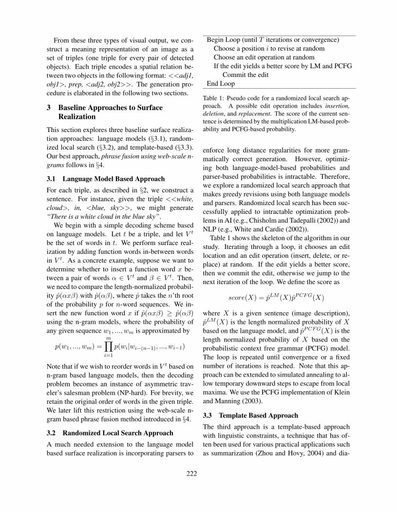
From these three types of visual output, we con-struct a meaning representation of an image as aset of triples (one triple for every pair of detectedobjects). Each triple encodes a spatial relation be-tween two objects in the following format: <<adj1,obj1>, prep, <adj2, obj2>>. The generation pro-cedure is elaborated in the following two sections.

3 Baseline Approaches to SurfaceRealization

This section explores three baseline surface realiza-tion approaches: language models (§3.1), random-ized local search (§3.2), and template-based (§3.3).Our best approach, phrase fusion using web-scale n-grams follows in §4.

3.1 Language Model Based ApproachFor each triple, as described in §2, we construct asentence. For instance, given the triple <<white,cloud>, in, <blue, sky>>, we might generate“There is a white cloud in the blue sky”.

We begin with a simple decoding scheme basedon language models. Let t be a triple, and let V t

be the set of words in t. We perform surface real-ization by adding function words in-between wordsin V t. As a concrete example, suppose we want todetermine whether to insert a function word x be-tween a pair of words α ∈ V t and β ∈ V t. Then,we need to compare the length-normalized probabil-ity p(αxβ) with p(αβ), where p takes the n’th rootof the probability p for n-word sequences. We in-sert the new function word x if p(αxβ) ≥ p(αβ)using the n-gram models, where the probability ofany given sequence w1, ..., wm is approximated by

p(w1, ..., wm) =m∏

i=1

p(wi|wi−(n−1), ..., wi−1)

Note that if we wish to reorder words in V t based onn-gram based language models, then the decodingproblem becomes an instance of asymmetric trav-eler’s salesman problem (NP-hard). For brevity, weretain the original order of words in the given triple.We later lift this restriction using the web-scale n-gram based phrase fusion method introduced in §4.

3.2 Randomized Local Search ApproachA much needed extension to the language modelbased surface realization is incorporating parsers to

Begin Loop (until T iterations or convergence)Choose a position i to revise at randomChoose an edit operation at randomIf the edit yields a better score by LM and PCFG

Commit the editEnd Loop

Table 1: Pseudo code for a randomized local search ap-proach. A possible edit operation includes insertion,deletion, and replacement. The score of the current sen-tence is determined by the multiplication LM-based prob-ability and PCFG-based probability.

enforce long distance regularities for more gram-matically correct generation. However, optimiz-ing both language-model-based probabilities andparser-based probabilities is intractable. Therefore,we explore a randomized local search approach thatmakes greedy revisions using both language modelsand parsers. Randomized local search has been suc-cessfully applied to intractable optimization prob-lems in AI (e.g., Chisholm and Tadepalli (2002)) andNLP (e.g., White and Cardie (2002)).

Table 1 shows the skeleton of the algorithm in ourstudy. Iterating through a loop, it chooses an editlocation and an edit operation (insert, delete, or re-place) at random. If the edit yields a better score,then we commit the edit, otherwise we jump to thenext iteration of the loop. We define the score as

score(X) = pLM (X)pPCFG(X)

where X is a given sentence (image description),pLM (X) is the length normalized probability of Xbased on the language model, and pPCFG(X) is thelength normalized probability of X based on theprobabilistic context free grammar (PCFG) model.The loop is repeated until convergence or a fixednumber of iterations is reached. Note that this ap-proach can be extended to simulated annealing to al-low temporary downward steps to escape from localmaxima. We use the PCFG implementation of Kleinand Manning (2003).

3.3 Template Based ApproachThe third approach is a template-based approachwith linguistic constraints, a technique that has of-ten been used for various practical applications suchas summarization (Zhou and Hovy, 2004) and dia-

222

blue, bike [2669] blue, bicycle [1365] bike, blue [1184] blue, cycle [324] cycle, of, the, blue [172] cycle, blue [158] bicycle, blue [154] bike, in, blue [98] cycle, of, blue [64] bike, with, blue [43]

< < blue , bicycle >, near, < shiny , person > >

bright, boy [8092] bright, child [7840] bright, girl [6191] bright, kid [5873] bright, person [5461] bright, man [4936] bright, woman [2726] bright, women [1684] lady, bright [1360] bright, men [1050]

person, operating, a, bicycle [3409] man, on, a, bicycle [2842] cycle, of, child [2507] bike, for, men [2485] person, riding, a, bicycle [2118] cycle, in, women [1853] bike, for, women [1442] boy, on, a, bicycle [1378] cycle, of, women [1288] man, on, a, bike [1283]

bright person operating a blue bicycle [25411589385] bright man on a blue bicycle [19148372880] bright man on a blue bike [16902478072] bright person riding a blue bicycle [15788133270] bright boy on a blue bicycle [15220809240] blue bike for bright men [6964088250] blue bike for bright women [6481207432] blue cycle of bright child [6368181120] blue cycle in bright women [1011026448]

Figure 2: Illustration of phrase fusion composition al-gorithm using web-scale n-grams. Numbers in squarebrackets are n-gram frequencies.

logue systems (Channarukul et al., 2003). Becausethe meaning representation produced by the imagerecognition system has a fixed pattern of <<adj1,obj1>, prep, <adj2, obj2>>, it can be templated as“There is a [adj1] [obj1] [prep] the [adj2] [obj2].”We also include templates that encode basic dis-course constraints. For instance, the template thatgenerated the first sentences in Figure 3 and 4 is:[PREFIX] [#(x1)] [x1], [#(x2)] [x2], ... and [#(xk)][xk], where xi is the name of an object (e.g. “cow”),#(xi) is the number of instances of xi (e.g. “one”),and PREFIX ∈ {”This picture shows”, ”This is a pic-ture of”, etc}.

Although this approach can produce good lookingsentences in a limited domain, there are many limita-tions. First, a template-based approach does not al-low creative writing and produces somewhat stiltedprose. In particular, it cannot add interesting newwords, or replace existing content words with betterones. In addition, such an approach does not allowany reordering of words which might be necessary tocreate a fluent sentence. Finally, hand-written rulesare domain-specific, and do not generalize well tonew domains.

4 Surface Realization by Phrase Fusionusing Web-scale N-gram

We now introduce an entirely different approachthat addresses the limitations of the conventional ap-

proaches discussed in §3. This approach is basedon web-scale n-gram, also known as Google Web1T data, which provides the frequency count of eachpossible n-gram sequence for 1 ≤ n ≤ 5.

4.1 [Step I] – Candidate Phrase SelectionWe first define three different sets of phrases for eachgiven triple <<adj1, obj1>, prep, <adj2, obj2>>:

• O1 = {(x, f) | x is an n-gram phrase describ-ing the first object using the words adj1 andobj1, and f is the frequency of x}

• O2 = {(x, f) | x is an n-gram phrase describ-ing the second object using the words adj2 andobj2, and f is the frequency of x}

• R = {(x, f) | x is an n-gram describing the re-lation between the two objects using the wordsobj1 and obj2, and f is the frequency of x}

We find n-gram phrases for O1, O2, andR from theGoogle Web 1T data. The search patterns for O1 is:

• [adj1] [♣]n−2 [obj1]

• [obj1] [♣]n−2 [adj1]

where [♣] is a wildcard word, and [♣]n−2 denotesa sequence of n-2 number of wildcard words in a n-gram sequence. For wildcards, we only allow a lim-ited set of function words, and verbs in the gerundform2 for reasons that will become clearer in thenext step – phrase fusion in §4.2.

Note that it is the second pattern that allowsinteresting re-ordering of words in the final sen-tence generation. For instance, suppose adj1=green,obj1=person. Then it is more natural to generatea phrase using the reverse pattern such as, “personin green” or “person wearing green” than simplyconcatenating adj1 and obj1 to generate “green per-son”. Similarly, given obj1=bicycle and obj2=man,generating a phrase using the reverse pattern, e.g.,“man with a bicycle” would be more natural than“bicycle with a man”. Our hypothesis is that suchordering preference is implicitly encoded in theweb-scale n-grams via frequencies.

It is worthwhile to note that our pattern matchingis case sensitive, and we only allow patterns that are

2We treat words with suffix “ing” as gerund for simplicity.

223

Phrase Fusion Black bull eating fluffy grass

Bright apartment in the blue sky Shaggy grass looking at the blue sky

Local Search the black cow or even by the furry grass. the shiny building up by the same blue sky. the furry grass be

below over one blue sky.

Template This picture shows one cow, one building, one grass and one sky. The black cow is by the shiny building, and by the furry grass, and by the blue sky. The

shiny building is by the furry grass, and by the blue sky. The furry

grass is below the blue sky.

Simple decoding the black cow or by the furry grass. the shiny building up by the blue sky. the furry grass be below one blue sky.

Image Recognition Output as Tripes: <black;yellow;rusty,cow>,by;near;by,<furry;green;brown,grass> <shiny;colorful;yellow,building>,by;near;by,<blue;clear;colorful,sky> <furry;green;brown,grass>,below;beneath;by,<blue;clear;colorful,sky>

Figure 3: Comparison of image descriptions

all lower-case. From our pilot study, we found thatn-grams with upper case characters are likely fromnamed entities, which distort the n-gram frequencydistribution that we rely on during the phrase fusionphase. To further reduce noise, we also discard anyn-gram that contains a character that is not an alpha-bet.

Accommodating Uncertainty We extend candi-date phrase selection in order to cope with uncer-tainty from the image recognition. In particular,for each object detection obji, we include its top 3predicted modifiers adji1, adji2, adji3 determinedby the attribute classifiers (see §2) to expand theset O1 and O2 accordingly. For instance, givenadji =(shiny or white) and obji = sheep, we canconsider both <shiny,sheep> and <white,sheep>pairs to predict more compatible pairs of words.

Accommodating Synonyms Additionally, weaugment each modifier adji and each object nameobji with synonyms to further expand our setsO1, O2, and R. These expanded sets of phrasesenable resulting generations that are more fluentand creative.

4.2 [Step II] – Phrase Fusion

Given the expanded sets of phrases O1, O2, and Rdescribed above, we perform phrase fusion to gen-erate simple image description. In this step, we findthe best combination of three phrases, (x1, f1) ∈

O1, (x2, f2) ∈ O2, and (xR, fR) ∈ R as follows:

(x1, x2, xR) = argmaxx1,x2,xRscore(x1, x2, xR) (1)

score(x1, x2, xR) = φ(x1)× φ(x2)× φ(xR) (2)

s.t. x1 and xR are compatible

& x2 and xR are compatible

Two phrases xi and xR are compatible if they sharethe same object noun obji. We define the phrase-level score function φ(·) as φ(xi) = fi using theGoogle n-gram frequencies. The equation (2) can bemaximized using dynamic programming, by align-ing the decision sequence as x1 − xR − x2.

Once the best combination – (x1, x2, xR) is de-termined, we fuse the phrases by replacing the wordobj1 in the phrase xR with the corresponding phrasex1. Similarly, we replace the word obj2 in the phrasexR with the other corresponding phrase x2. Becausethe wildcard words – [♣] in §4.1 allow only a lim-ited set of function words and gerund, the resultingphrase is highly likely to be grammatically correct.

Computational Efficiency One advantage of ourphrase fusion method is its efficiency. If we wereto attempt to re-order words with language mod-els in a naive way, we would need to consider allpossible permutations of words – an NP-hard prob-lem (§3.1). However, our phrase fusion method isclever in that it probes reordering only on selectedpairs of words, where reordering is likely to be use-ful. In other words, our approach naturally ignoresmost word pairs that do not require reordering andhas a time complexity of only O(K2n), where K isthe maximum number of candidate phrases of anyphrase type, and n is the number of phrase types ineach sentence. K can be kept as a small constant byselecting K-best candidate phrases of each phrasetype. We set K = 10 in this paper.

5 Experimental Results

To construct the training corpus for language mod-els, we crawled Wikipedia pages that describe ourobject set. For evaluation, we use the UIUC PAS-CAL sentence dataset3 which contains upto fivehuman-generated sentences that describing 1000 im-ages. Note that all of the approaches presented in

3http://vision.cs.uiuc.edu/pascal-sentences/

224

Phrase fusion shiny motorcycle nearby shiny motorcycle. black women operating a shiny motorcycle.

bright boy on a shiny motorcycle. girl showing pink on a shiny motorcycle.

Local search the shiny motorbike or

against the shiny motorbike. the shiny

motorbike or by the black person. the shiny motorbike or by the shiny person. the shiny motorbike or by the

pink person.

Simple Decoding the shiny motorbike or

against the shiny motorbike. the shiny

motorbike or by the black person. the shinny

motorbike or by the shiny boy. the shiny motorbike or

by the pink person.

Template This is a picture of two motorbikes, three persons, one building and one tree. The first shiny motorbike is against the second shiny motorbike, and by the first black person. The second shiny motorbike is by the first black person, and by

the second shiny person, and by the third pink person.

Image Recognition Output as Triples: < < shiny; black; rusty , motorbike >, against; by; in , < shiny; black; rusty , motorbike > > < < shiny; black; rusty , motorbike >, by; near; by , < black; shiny; rusty , person > > < < shiny; black; rusty , motorbike >, by; near; by , < pink; rusty; striped , person > >

Figure 4: Comparison of image descriptions

Section 3 and 4 attempt to insert function words forsurface realization. In this work, we limit the choiceof function words to only those words that are likelyto be necessary in the final output.4 For instance, wedisallow function words such as “who” or “or”.

Before presenting evaluation results, we presentsome samples of image descriptions generated by 4different approaches in Figure 3 and 4. Notice thatonly the PHRASE FUSION approach is able to in-clude interesting and adequate verbs, such as “eat-ing” or “looking” in Figure 3, and “operating” inFigure 4. Note that the choice of these action verbsis based only on the co-occurrence statistics encodedin n-grams, without relying on the vision compo-nent that specializes in action recognition. These ex-amples therefore demonstrate that world knowledgeimplicitly encoded in natural language can help en-hance image content recognition.

Automatic Evaluation: BLEU (Papineni et al.,2002) is a widely used metric for automatic eval-uation of machine translation that measures the n-gram precision of machine generated sentences withrespect to human generated sentences. Because ourtask can be viewed as machine translation from im-ages to text, BLEU (Papineni et al., 2002) may seem

4This limitation does not apply to TEMPLATE.

w/o w/ synLANGUAGE MODEL 0.094 0.106TEMPLATE 0.087 0.096LOCAL SEARCH 0.100 0.111PHRASE FUSION (any best) 0.149 0.153PHRASE FUSION (best w/ gerund) 0.146 0.149Human 0.500 0.510

Table 2: Automatic Evaluation: BLEU measured at 1

Creativ. Fluency Relevan.

LANGUAGE MODEL 2.12 1.96 2.09TEMPLATE 2.04 1.7 1.96LOCAL SEARCH 2.21 1.96 2.04PHRASE FUSION 1.86 1.97 2.11

Table 3: Human Evaluation: the scores range over 1 to 3,where 1 is very good, 2 is ok, 3 is bad.

like a reasonable choice. However, there is largerinherent variability in generating sentences from im-ages than translating a sentence from one languageto another. In fact two people viewing the same pic-ture may produce quite different descriptions. Thismeans BLEU could penalize many correctly gener-ated sentences, and be poorly correlated with humanjudgment of quality. Nevertheless we report BLEUscores in absence of any other automatic evaluationmethod that serves our needs perfectly.

The results are shown in Table 2 – first columnshows BLEU score considering exact matches, sec-ond column shows BLEU with full credit for syn-onyms. To give a sense of upper bound and to seesome limitations of the BLEU score, we also com-pute the BLEU score between human-generated sen-tences by computing the BLEU score of the first hu-man sentence with respect to the others.

There is one important factor to consider when in-terpreting Table 2. The four approaches exploredin this paper are purposefully prolific writers in thatthey generate many more sentences than the num-ber of sentences in the image descriptions written byhumans (available in the UIUC PASCAL dataset).In this work, we do not perform sentence selectionto reduce the number of sentences in the final out-put. Rather, we focus on the quality of each gener-ated sentence. The consequence of producing many

225

Way rusty the golden cow Golden cow in the golden sky

Tree snowing black train Black train under the tree Rusty girl sitting at a white table

White table in the clear sky Rusty girl living in the clear sky

Blue path up in the clear sky Blue path to colored fishing boat Blue path up in the clear morning sky

rusty chair for rusty dog. rusty dog under the rusty chair. rusty dog sitting in a rusty chair.

Gray cat from a burning gray building Gray building with a gray cat. Gray building in the white sky

Shaggy dog knotting hairy men Pink flowering plant the hairy dog Pink dog training shaggy dog Shaggy dog relaxing on a colored sofa

black women hanging from a black tree. colored man in the tree.

1 2 3 4

5

6 7

8

Figure 5: Sample image descriptions using PHRASE FUSION: some of the unexpected or poetic descriptions arehighlighted in boldface, and some of the interesting incorrect descriptions are underlined.

more sentences in our output is overall lower BLEUscores, because BLEU precision penalizes spuriousrepetitions of the same word, which necessarily oc-curs when generating more sentences. This is not anissue for comparing different approaches however,as we generate the same number of sentences foreach method.

From Table 2, we find that our final approach —PHRASE FUSION based on web-scale n-grams per-forms the best. Notice that there are two differentevaluations for PHRASE FUSION: the first one isevaluated for the best combination of phrases (Equa-tion (1)), while the second one is evaluated for thebest combination of phrases that contained at leastone gerund.

Human Evaluation: As mentioned earlier, BLEUscore has some drawbacks including obliviousnessto correctness of grammar and inability to evaluatethe creativity of a composition. To directly quantifythese aspects that could not be addressed by BLEU,we perform human judgments on 120 instances forthe four proposed methods. Evaluators do not haveany computer vision or natural language generationbackground.

We consider the following three aspects to eval-uate the our image descriptions: creativity, fluency,

and relevance. For simplicity, human evaluators as-sign one set of scores for each aspect per image. Thescores range from 1 to 3, where 1 is very good, 2 isok, and 3 is bad.5 The definition and guideline foreach aspect is:

[Creativity] How creative is the generated sen-tence?

1 There is creativity either based on unexpectedwords (in particular, verbs), or describingthings in a poetic way.

2 There is minor creativity based on re-orderingwords that appeared in the triple

3 None. Looks like a robot talking.

[Fluency] How grammatically correct is the gener-ated sentence?

1 Mostly perfect English phrase or sentence.2 There are some errors, but mostly comprehen-

sible.3 Terrible.

[Relevance] How relevant is the generated descrip-tion to the given image?

1 Very relevant.2 Reasonably relevant.3 Totally off.

5In our pilot study, human annotations on 160 instancesgiven by two evaluators were identical on 61% of the instances,and close (difference ≤ 1) on 92%.

226

Table 3 shows the human evaluation results. Interms of creativity, PHRASE FUSION achieves thebest score as expected. In terms of fluency andrelevance however, TEMPLATE achieves the bestscores, while PHRASE FUSION performs the secondbest. Remember that TEMPLATE is based on hand-engineered rules with discourse constraints, whichseems to appeal to evaluators more. It would bestraightforward to combine PHRASE FUSION withTEMPLATE to improve the output of PHRASE FU-SION with hand-engineered rules. However, ourgoal in this paper is to investigate statistically moti-vated approaches for generating image descriptionsthat can address inherent limitations of hand-writtenrules discussed in §3.3.

Notice that the relevance score of TEMPLATE isbetter than that of LANGUAGE MODEL, even thoughboth approaches generate descriptions that consist ofan almost identical set of words. This is presum-ably because the output from LANGUAGE MODEL

contains grammatically incorrect sentences that arenot comprehendable enough to the evaluators. Therelevance score of PHRASE FUSION is also slightlyworse than that of TEMPLATE, presumably becausePHRASE FUSION often generates poetic or creativeexpressions, as shown in Figure 5, which can be con-sidered a deviation from the image content.

Error Analysis There are different sources of er-rors. Some errors are due to mistakes in the origi-nal visual recognition input. For example, in the 3rdimage in Figure 5, the color of sky is predicted tobe “golden”. In the 4th image, the wall behind thetable is recognized as “sky”, and in the 6th image,the parrots are recognized as “person”.

Other errors are from surface realization. For in-stance, in the 8th image, PHRASE FUSION selectsthe preposition “under”, presumably because dogsare typically under the chair rather than on the chairaccording to Google n-gram statistics. In the 5thimage, an unexpected word “burning” is selected tomake the resulting output idiosyncratic. Word sensedisambiguation sometimes causes a problem in sur-face realization as well. In the 3rd image, the word“way” is chosen to represent “path” or “street” bythe image recognizer. However, a different sense ofway – “very” – is being used in the final output.

6 Related Work

There has been relatively limited work on automat-ically generating natural language image descrip-tions. Most work related to our study is discussedin §1, hence we highlight only those that are clos-est to our work here. Yao et al. (2010) present acomprehensive system that generates image descrip-tions using Head-driven phrase structure (HPSG)grammar, which requires carefully written domain-specific lexicalized grammar rules, and also de-mands a very specific and complex meaning rep-resentation scheme from the image processing. Incontrast, our approach handles images in the open-domain more naturally using much simpler tech-niques.

We use similar vision based inputs – object detec-tors, modifier classifiers, and prepositional functions– to some very recent work on generating simple de-scriptions for images (Kulkarni et al., 2011), but fo-cus on improving the sentence generation method-ology and produce descriptions that are more trueto human generated descriptions. Note that theBLEU scores reported in their work of Kulkarni etal. (2011) are not directly comparable to ours, as thescale of the scores differs depending on the numberof sentences generated per image.

7 Conclusion

In this paper, we presented a novel surface realiza-tion technique based on web-scale n-gram data toautomatically generate image description. Despiteits simplicity, our method is highly effective in gen-erating mostly appealing and presentable language,while permitting creative writing at times. We con-clude from our study that it is viable to generatesimple textual descriptions that are germane to thespecific image content while also sometimes pro-ducing almost poetic natural language. Furthermore,we demonstrate that world knowledge implicitly en-coded in natural language can help enhance imagecontent recognition.

Acknowledgments

This work is supported in part by NSF Faculty EarlyCareer Development (CAREER) Award #1054133.

227

ReferencesA. Aker and R. Gaizauskas. 2010. Generating image

descriptions using dependency relational patterns. InACL.

K. Barnard, P. Duygulu, N. de Freitas, D. Forsyth,D. Blei, and M. Jordan. 2003. Matching words andpictures. JMLR, 3:1107–1135.

Songsak Channarukul, Susan W. McRoy, and Syed S.Ali. 2003. Doghed: a template-based generator formultimodal dialog systems targeting heterogeneousdevices. In NAACL.

Michael Chisholm and Prasad Tadepalli. 2002. Learningdecision rules by randomized iterative local search. InICML, pages 75–82.

J. Deng, W. Dong, R. Socher, L.-J. Li, K. Li, and L. Fei-Fei. 2009. ImageNet: A Large-Scale Hierarchical Im-age Database. In CVPR.

A. Farhadi, I. Endres, D. Hoiem, and D. A. Forsyth.2009. Describing objects by their attributes. In CVPR.

A. Farhadi, M Hejrati, A. Sadeghi, P. Young,C. Rashtchian, J. Hockenmaier, and D. A. Forsyth.2010. Every picture tells a story: generating sentencesfor images. In ECCV.

P. Felzenszwalb, R. Girshick, D. McAllester, and D. Ra-manan. 2010. Object detection with discriminativelytrained part based models. tPAMI, Sept.

Y. Feng and M. Lapata. 2010a. How many words is apicture worth? automatic caption generation for newsimages. In ACL.

Yansong Feng and Mirella Lapata. 2010b. Topic modelsfor image annotation and text illustration. In HLT.

Dan Klein and Christopher D. Manning. 2003. Accurateunlexicalized parsing. In Proceedings of the 41st An-nual Meeting on Association for Computational Lin-guistics, pages 423–430. Association for Computa-tional Linguistics.

Girish Kulkarni, Visruth Premraj, Sagnik Dhar, SimingLi, Yejin Choi, Alexander C Berg, and Tamara L Berg.2011. Babytalk: Understanding and generating simpleimage descriptions. In CVPR.

Chee Wee Leong, Rada Mihalcea, and Samer Hassan.2010. Text mining for automatic image tagging. InCOLING.

Kishore Papineni, Salim Roukos, Todd Ward, and Weijing Zhu. 2002. Bleu: a method for automatic evalua-tion of machine translation.

Katerina Pastra, Horacio Saggion, and Yorick Wilks.2003. Nlp for indexing and retrieval of captioned pho-tographs. In EACL.

Michael White and Claire Cardie. 2002. Selecting sen-tences for multidocument summaries using random-ized local search. In ACL Workshop on AutomaticSummarization.

B.Z. Yao, Xiong Yang, Liang Lin, Mun Wai Lee, andSong-Chun Zhu. 2010. I2t: Image parsing to text de-scription. Proc. IEEE, 98(8).

Liang Zhou and Eduard Hovy. 2004. Template-filtered headline summarization. In Text Summariza-tion Branches Out: Pr ACL-04 Wkshp, July.

228


Adapting Text instead of the Model: An Open Domain Approach

Gourab Kundu, Dan RothUniversity of Illinois at Urbana Champaign

Urbana, IL 61801{kundu2,danr}@illinois.edu

Abstract

Natural language systems trained on labeleddata from one domain do not perform wellon other domains. Most adaptation algorithmsproposed in the literature train a new model forthe new domain using unlabeled data. How-ever, it is time consuming to retrain big mod-els or pipeline systems. Moreover, the domainof a new target sentence may not be known,and one may not have significant amount ofunlabeled data for every new domain.

To pursue the goal of an Open Domain NLP(train once, test anywhere), we propose ADUT(ADaptation Using label-preserving Transfor-mation), an approach that avoids the need forretraining and does not require knowledge ofthe new domain, or any data from it. Our ap-proach applies simple label-preserving trans-formations to the target text so that the trans-formed text is more similar to the training do-main; it then applies the existing model onthe transformed sentences and combines thepredictions to produce the desired predictionon the target text. We instantiate ADUT forthe case of Semantic Role Labeling (SRL)and show that it compares favorably with ap-proaches that retrain their model on the targetdomain. Specifically, this “on the fly” adapta-tion approach yields 13% error reduction fora single parse system when adapting from thenews wire text to fiction.

1 Introduction

In several NLP tasks, systems trained on annotateddata from one domain perform well when tested

on the same domain but adapt poorly to other do-mains. For example, all systems of CoNLL 2005shared task (Carreras and Màrquez, 2005) on Se-mantic Role Labeling showed a performance degra-dation of almost 10% or more when tested on a dif-ferent domain.

Most works in domain adaptation have focusedon learning a common representation across train-ing and test domains (Blitzer et al., 2006; DauméIII,2007; Huang and Yates, 2009). Using this represen-tation, they retrain the model for every new domain.But these are not Open Domain Systems since themodel needs to be retrained for every new domain.This is very difficult for pipeline systems like SRLwhere syntactic parser, shallow parser, POS taggerand then SRL need to be retrained. Moreover, thesemethods need to have a lot of unlabeled data that istaken from the same domain, in order to learn mean-ingful feature correspondences across training andtest domain. These approaches cannot work whenthey do not have a lot of unlabeled data from the testdomain or when the test domain in itself is very di-verse, e.g., the web.

The contribution of this paper is a new frame-work for adaptation. We propose ADUT (ADap-tation Using label-preserving Transformation) as aframework in which a previously learned model canbe used on an out-of-domain example without re-training and without looking at any labeled or unla-beled data for the domain of the new example. Theframework transforms the test sentence to generatesentences that have, in principle, identical labelingbut that are more like instances from the training do-main. Consequently, it is expected that the exist-

229

ing model will make better predictions on them. Allthese predictions are then combined to choose themost probable and consistent prediction for the testsentence.

ADUT is a general technique which can be ap-plied to any natural language task. In this paper, wedemonstrate its usefulness on the task of semanticrole labeling (Carreras and Màrquez, 2005). Start-ing with a system that was trained on the news textand does not perform well on fiction, we show thatADUT provides significant improvement on fiction,and is competitive with the performance of algo-rithms that were re-trained on the test domain.

The paper is organized as follows. Section 2 dis-cusses two motivating examples. Section 3 gives aformal definition of our adaptation framework. Sec-tion 4 describes the transformation operators that weapplied for this task. Section 5 presents our joint in-ference approach. Section 6 describes our semanticrole labeling system and our experimental results arein Section 7. Section 8 describes the related worksfor domain adaptation. Finally in Section 9 we con-clude the paper with a discussion.

2 Motivating Examples

One of the key reasons for performance degradationof an NLP tool is unseen features such as words inthe new domain that were not seen in the trainingdomain. But if an unknown word is replaced by aknown word without changing the labeling of thesentence, tools perform better. For example, in thetask of syntactic parsing, the unknown word checkupcauses the Charniak parser to make a wrong co-ordination decision on the sentence

He was discharged from the hospital af-ter a two-day checkup and he and his par-ents had what Mr. Mckinley described asa “celebration lunch” at the cafeteria onthe campus.

If we replace the word checkup with its hyper-nym examination which appears in training data, theparse gets corrected. Figure 1 shows both originaland corrected parse trees.

For the task of semantic role labeling, systems donot perform well on the predicates that are infre-quent in training domain. But if an infrequent predi-

cate is replaced with a frequent predicate from train-ing domain such that both predicates have similarsemantic argument structure, the system performsbetter. Consider the following sentence

Scotty gazed out at ugly gray slums.

The semantic role for the phrase at ugly gray slumswith respect to predicate gaze is A1. But the pred-icate gaze appears only once in training data andour model predicts at ugly gray slums as AM-LOCinstead of A1. But if gaze is replaced with lookwhich occurs 328 times in training data and has sim-ilar argument structure (in the same VerbNet class asgaze), the system makes the correct prediction.

3 Problem Formulation

Let the in-domain distribution be Di and out-of-domain distribution be Do. We have a model ftrained over a set of labeled examples drawn fromDi. If Di and Do are very dissimilar, f will not per-form well on examples drawn from Do. The prob-lem is to get good performance from f on Do with-out retraining f .

We define a Transformation g to be a function thatmaps an example e into a set of examples E. So g :X → 2X where X is the entire space of examples.In this paper, we only consider the Label-preservingTransformations which satisfy the property that alltransformed examples in E have the same label asinput example e, i.e., ∀x x ∈ Sk ⇒ g(x) ⊂ Skwhere Sk is the set of examples with label k . LetG be a set of label-preserving transformation func-tions. G = {g1, g2, . . ., gp}.

At evaluation time, for test example d, we willapply G to get a set of examples T1. Let T2 = {d′ ∈T1 : Di(d

′) > Di(d)}. So all examples in T2 havesame label as d but have a higher probability thand to be drawn from the in-domain distribution. Sof should perform better on examples in T2 than ond. For each d′ ∈ T2, f will produce scores for theoutput labels. The scores will be combined subjectto constraints to produce the final output.

4 Transformation Functions

After applying a transformation function to get anew sentence from an input sentence, we remem-ber the mapping of segments across the original

230

a. S1

S

NP

He

VP

was VP

discharged PP

from the hospital

PP

after NP

NP

a two-daycheckup

SBAR

NP

and he and his parents

VP

had . . . campus

.

b. S1

S

S

NP

He

VP

was VP

discharged PP

from the hospital

PP

after NP

a two-dayexamination

and S

NP

he and his parents

VP

had . . . campus

.

Figure 1: a. Original Parse tree b. Corrected Parse tree after replacement of unknown word checkup by examination

and transformed sentence. Thus, after annotatingthe transformed sentence with SRL, we can transferthe roles to the original sentence through this map-ping. Transformation functions can be divided intotwo categories. The first category is Transforma-tions From List which uses external resources likeWordNet, VerbNet and Word Clusters. The secondis Learned Transformations that uses transformationrules that have been learned from training data.

4.1 Transformation From ListI. Replacement of Predicate:

As noted in (Huang and Yates, 2010), 6.1% of thepredicates in the Brown test set do not appear in WSJtraining set and 11.8% appear at most twice. Sincethe semantic roles of a sentence depend on the pred-icate, these infrequent predicates hurt SRL perfor-mance on new domains. Note that since all predi-cates in PropBank are verbs, we will use the wordspredicate and verb interchangeably.

We count the frequency of each predicate and itsaccuracy in terms of F1 score over the training data.If the frequency or the F1 score of the predicate inthe test sentence is below a threshold, we perturbthat predicate. We take all the verbs in the same classof VerbNet1 as the original verb (in case the verb ispresent in multiple classes, we take all the classes).In case the verb is not present in VerbNet, we takeits synonyms from WordNet. If there is no synonymin WordNet, we take the hypernyms.

From this collection of new verbs, we select verbsthat have a high accuracy and a high frequency in

1http://verbs.colorado.edu/ mpalmer/projects/verbnet.html

training. We replace the original verb with each ofthese new verbs and generate one new sentence foreach new verb; the sentence is retained if the parsescore for the new sentence is higher than the parsescore for the original sentence.2 VerbNet has de-fined a set of verb-independent thematic roles andgrouped the verbs according to their usage in frameswith identical thematic roles. But PropBank anno-tation was with respect to each verb. So the samethematic role is labeled as different roles for dif-ferent verbs in PropBank. For example, both warnand advise belong to the same VerbNet class (37.9)and take thematic roles of Recipient (person beingwarned or advised) and Topic (topic of warning oradvising). But Recipient was marked as A2 for warnand A1 for advise and Topic was marked as A1 forwarn and A2 for advise in PropBank annotation.Semlink3 provides a mapping from the thematic roleto PropBank role for each verb. After the SRL anno-tates the new sentence with PropBank roles for thenew verb, we map the PropBank roles of the newverb to their corresponding thematic roles and thenmap the thematic roles to the corresponding Prop-Bank roles for the original verb.II. Replacement and Removal of Quoted Strings:

Quoted sentences can vary a lot from one domainto another. For example, in WSJ, quoted sentencesare like formal statements but in Brown, these arelike informal conversations. We generate the trans-formations in the following ways:

1) We use the content of the quoted string as one2

Parse score is the parse probability returned by Charniak or Stanford parser.3

http://verbs.colorado.edu/semlink/

231

sentence. 2) We replace each quoted string in turnwith a simple sentence (This is good) to generate anew sentence. 3) If a sentence has a quoted string inthe beginning, we move that quoted string after thefirst NP and VP that immediately follow the quotedstring. For example, from the input sentence, “Wejust sit quiet”, he said. we generate the sentences 1)We just sit quiet 2) “This is good”, he said. 3) Hesaid, “We just sit quiet”.III. Replacement of Unseen Words:

A major difficulty for domain adaptation is thatsome words in the new domain do not appear in thetraining domain. In the Brown test set, 5% of totalwords were never seen in the WSJ training set.

Given an unseen word which is not a verb, wereplace it with WordNet synonyms and hypernymsthat were seen in the training data. We used theclusters obtained in (Liang, 2005) from running theBrown algorithm (Brown et al., 1992) on Reuters1996 dataset. But since this cluster was generatedautomatically, it is noisy. So we chose replacementsfrom the Brown clusters selectively. We only replacethose words for which the POS tagger and the syn-tactic parser predicted different tags. For each suchword, we find its cluster and select the set of wordsfrom the cluster. We delete from this set all wordsthat do not take at least one part-of-speech tag thatthe original word can take (from WordNet). For eachcandidate synonym or hypernym or cluster member,we get a new sentence. Finally we only keep thosesentences that have higher parse scores than the orig-inal sentence.IV. Sentence Split based on Stop Symbols:

We split each sentence based on stop symbols like; and . . Each of the splitted sentences becomes onetransformation of the original sentence.V. Sentence Simplification:

We have a set of heuristics for simplifying theconstituents of the parse tree; for example, replac-ing an NP with its first and last word, removal ofPRN phrases etc. We apply these heuristics and gen-erate simpler sentences until no more simplificationis possible. Examples of our heuristics are given inTable 1.

Note that we can use composition of multipletransformation functions as one function. A compo-sition p1 � p2(s) = ∪a∈p1(s)p2(a). We apply II�I,III�I, IV�I and V�I.

Node Input Example Simplified Example Operation

NP He and she ran. He ran. replace

NP The big man ran. The man ran. replace

ADVP He ran fast. He ran. delete

PP He ran in the field. He ran. delete

PRN He – though sick – ran. He ran. delete

VP He walked and ran. He ran. delete

TO I want him to run. I want that he can ran. rewrite

Table 1: Examples of Simplifications (Predicate is run)

4.2 Learned Transformations

The learned model is inaccurate over verbs and rolesthat are infrequent in the training data. The purposeof the learned transformation is to transfer such aphrase in the test sentence in place of a phrase of asimpler sentence; this is done such that there existsa mapping from the role of the phrase in the newsentence to the role of the phrase in the original sen-tence.

Phrase Representation: A phrase tuple is a 3-tuple (t, i, h) where, t is the phrase type, i is the in-dex, and h is the headword of the phrase. We denoteby PR the Phrase Representation of a sentence – anordered list of phrase tuples. A phrase tuple corre-sponds to a node in the tree. We only consider phrasetuples that correspond to nodes that are (1) a siblingof the predicate node or (2) a sibling of an ancestorof the predicate node. Phrase tuples inPR are sortedbased on their position in the sentence. The index iof the phrase tuple containing the predicate is takento be zero with the indices of the phrase tuples onthe left (right) sequentially decreasing (increasing).

Transformation Rule: We denote by Label(n, s)the semantic role of nth phrase in the PR of thesentence s. Let Replace(ns, nt, ss, st) be a newsentence that results from inserting the phrase ns insentence ss instead of phrase nt in sentence st. Wewill refer to st as target sentence and to nt as thetarget phrase. Let sp be a sequence of phrase tuplesnamed as source pattern. If Label(ns, ss) = r1 andLabel(nt, Replace(ns, nt, ss, st)) = r2, then denotef(r2) = r1. In this case we call the 6-tuple (st, nt,p, sp, ns, f ) a transformation rule. We call f the

232

label correspondence function.Example: Consider the sentence st = “But it didnot sing." and the rule τ : (st, nt, p, sp, ns, f). Let:nt = −3, p = entitle,sp = [−2, NP, φ][−1, AUX, φ][0, V, entitle][1, φ, to]ns = −2, f = {<A0, A2>} ∪ {<Ai,Ai>|i 6= 0}.

The PR of τ.st is {[−4, CC, But] [−3, NP, it][−2, AUX, did] [−1, RB, not] [0, VB, sing] [1, ., .]}.Consider the input sentence ss: Mr. X was entitledto a discount . with PR of {[−2, NP, X] [−1, AUX,was] [0, V, entitle] [1, PP, to][2, ., .]}. Since τ.sp isa subsequence of the PR of ss, τ will apply to thepredicate entitle of ss. The transformed sentence is:str = Replace(τ.ns, τ.nt, ss, τ.st) = But Mr. X

did not sing. with PR of {[−4, CC, But] [−3, NP,X] [−2, AUX, did] [−1, RB, not] [0, VB, sing] [1,., .]}. If the SRL system assigns the semantic roleof A0 to the phrase Mr. X of str, the semantic roleof Mr. X in ss can be recovered through τ.f sinceτ.f(A0) = A2 = Label(−2, ss).

While checking if τ.sp is a subsequence of thePR of the input sentence, φ in each tuple of τ.sphas to be considered a trivial match. So τ willmatch the sentence He is entitled to a reward. withPR = {[−2, NP, He] [−1, AUX, is] [0, V, entitle][1, PP, to][2, ., .]} but will not match the sentenceThe conference was entitled a big success. withPR = {[−2, NP, conference] [−1, AUX, was] [0,V, entitle] [1, S, success][2, ., .]} (mismatch positionis bolded). The index of a phrase tuple cannot be φ,only the head word or type can be φ and the ruleswith more φ strings in the source pattern are moregeneral since they can match more sentences.

Algorithm 1 GenerateRules1: Input: predicate v, semantic role r, Training sentences D, SRL

Model M2: Output: set of rules R3: R⇐ GetInitialRules(v, r,D,M)4: repeat5: J ⇐ ExpandRules(R)6: K ⇐ R ∪ J7: sort K based on accuracy, support, size of source pattern8: select some rules R ⊂ K based on database coverage9: until all rules in R have been expanded before

10: return R

The algorithm for finding rules for a semantic roler of a predicate v is given in Algorithm 1. It is aspecific to general beam search procedure that startswith a set of initial rules (Line 3, detail in Algorithm

2) and finds new rules from these rules (Line 5, de-tail in Algorithm 3). In Line 7, the rules are sortedby decreasing order of accuracy, support and numberof φ strings in the source pattern. In Line 8, a set ofrules are selected to cover all occurrences of the se-mantic role r with the predicate v a specific numberof times. This process continues until no new rulesare found. Note that these rules need to be learnedonly once and can be used for every new domain.

Algorithm 2 GetInitialRules1: Input: predicate v, semantic role r, Training sentences D, SRL-

Model M2: Output: Set of initial rules I3: I ⇐ φ4: T ⇐ {s ∈ D : length(s) <= e}5: S ⇐ {s ∈ D : s has role r for predicate v}6: M ⇐ Set of all semantic roles7: for each phrase p1 in s1 ∈ S with gold label r for predicate v do8: for each phrase p2 in s2 ∈ T labeled as a core argument do9: if s1 6= s2 and p1 and p2 have same phrase types then

10: τ ⇐ empty rule11: τ.st ⇐ s2, τ.p⇐ v12: τ.nt ⇐ index of p2 in PR of s213: τ.ns ⇐ index of p1 in PR of s114: τ.sp ⇐ phrase tuples for phrases from p1 to v and two

phrases after v in PR of s115: L⇐ φ16: for each sentence s3 ∈D with predicate v do17: if τ.sp is a subsequence of PR of s3 then18: x⇐ replace(τ.ns, τ.nt, s3, τ.st)19: annotate x with SRL using M20: r1 ⇐ the gold standard semantic role of the

phrase with index τ.ns in PR of s321: r2 ⇐ Label(τ.nt, x)22: if r2 /∈ L then23: insert(r2, r1) in τ.f24: L = L ∪ {r2}25: end if26: end if27: end for28: for each role j ∈M − L do29: insert(j, j) in τ.f30: end for31: I ⇐ I∪ {τ}32: end if33: end for34: end for35: return I

The algorithm for generating initial rules for thesemantic role r of predicate v is given in Algorithm2. Shorter sentences are preferred to be target sen-tences(Line 4). A rule τ is created for every (p1,p2)pair where p1, p2 are phrases, p1 has the semanticrole r in some sentence s1, p2 is labeled as a coreargument(A0 − A5) in some sentence in T and thephrase types of p1 and p2 in their respective parsetrees are same(Lines 7 − 9). Every sentence s3 in

233

training corpus with predicate τ.p is a potential can-didate for applying τ (Line 16) if τ.sp is a subse-quence ofPR of s3(Line 17). After applying τ to s3,a transformed sentence x is created(Line 18). Lines20 − 26 find the semantic role r2 of the transferredphrase from SRL annotation of x using model Mand create a mapping from r2 to the gold standardrole r1 of the phrase in s3. L maintains the set of se-mantic roles for which mappings have been created.In lines 28 − 30, all unmapped roles are mapped tothemselves.

The algorithm for creating new rules from a setof existing rules is given in Algorithm 3. Lines 4 −13 generate all immediate more general neighbors ofthe current rule by nullifying the headword or phrasetype element in any of the phrase tuples in its sourcepattern.

Algorithm 3 ExpandRules1: Input: a set of rules R2: Output: a set of expanded rules E3: E ⇐ φ4: for each phrase tuple c in the source pattern of r ∈ R do5: if c is not the tuple for predicate then6: create a new rule r′ with all components of r7: mark the head word of c in the source pattern of r′ to φ8: add r′ to E9: create a new rule r′′ with all components of r

10: mark the phrase type of c in the source pattern of r′′ to φ11: add r′′ to E12: end if13: end for14: return E

5 Combination by Joint Inference

The transformation functions transform an inputsentence into a set of sentences T . From each trans-formed sentence ti, we get a set of argument can-didates Si. Let S =

⋃|T |i=1 Si be the set of all ar-

guments. Argument classifier assigns scores foreach argument over the output labels(roles) in Sthat is then converted into a probability distribu-tion over the possible labels using the softmax func-tion (Bishop, 1995). Note that multiple argumentswith the same span can be generated from multipletransformed sentences.

First, we take all arguments from S with distinctspan and put them in S′. For each argument arg inS′, we calculate scores over possible labels as thesum over the probability distribution (over output la-bels) of all arguments in S that have the same span

as arg divided by the number of sentences in T thatcontained arg. This results in a set of arguments withdistinct spans and for each argument, a set of scoresover possible labels. Following the joint inferenceprocedure in (Punyakanok et al., 2008), we want toselect a label for each argument such that the totalscore is maximized subject to some constraints. Letus index the set S′ as S′1:M where M = |S′|. Alsoassume that each argument can take a label from aset P . The set of arguments in S′1:M can take a setof labels c1:M ∈ P 1:M . Given some constraints, theresulting solution space is limited to a feasible set F;the inference task is: c1:M = arg maxc1:M∈F (P 1:M )∑M

i=1 score(S′i = ci).

The constraints used are: 1) No overlapping orembedding argument. 2) No duplicate argument forcore arguments A0-A5 and AA. 3) For C-arg, therehas to be an arg argument.

6 Experimental Setup

In this section, we discuss our experimental setupfor the semantic role labeling system. Similar to theCoNLL 2005 shared tasks, we train our system usingsections 02-21 of the Wall Street Journal portion ofPenn TreeBank labeled with PropBank. We test oursystem on an annotated Brown corpus consisting ofthree sections (ck01 - ck03).

Since we need to annotate new sentences withsyntactic parse, POS tags and shallow parses, we donot use annotations in the CoNLL distribution; in-stead, we re-annotate the data using publicly avail-able part of speech tagger and shallow parser1, Char-niak 2005 parser (Charniak and Johnson, 2005) andStanford parser (Klein and Manning, 2003).

Our baseline SRL model is an implementation of(Punyakanok et al., 2008) which was the top per-forming system in CoNLL 2005 shared task. Due tospace constraints, we omit the details of the systemand refer readers to (Punyakanok et al., 2008).

7 Results

Results for ADUT using only the top parse of Char-niak and Stanford are shown in Table 2. The Base-line model using top Charniak parse (BaseLine-Charniak) and top Stanford parse (BaseLine-Stanford) score respectively 76.4 and 73.3 on the

1http://cogcomp.cs.illinois.edu/page/software

234

WSJ test set. Since we are interested in adaptation,we report and compare results for Brown test setonly. On this set, both ADUT-Charniak and ADUT-Stanford significantly outperform their respectivebaselines. We compare with the state-of-the-art sys-tem of (Surdeanu et al., 2007). In (Surdeanu etal., 2007), the authors use three models: Model1 and 2 do sequential tagging of chunks obtainedfrom shallow parse and full parse. Model 3 assumeseach predicate argument maps to one syntactic con-stituent and classifies it individually. So Model 3matches our baseline model. ADUT-Charniak out-performs the best individual model (Model 2) of(Surdeanu et al., 2007) by 1.6% and Model 3 by3.9%. We also tested another system that used clus-ter features and word embedding features computedfollowing (Collobert and Weston, 2008). But wedid not see any performance improvement on Brownover baseline.

System P R F1

BaseLine-Charniak 69.6 61.8 65.5

ADUT-Charniak 72.75 66.1 69.3BaseLine-Stanford 70.8 56.5 62.9

ADUT-Stanford 72.5 60.0 65.7

(Surdeanu et al., 2007)(Model 2) 71.8 64.0 67.7

(Surdeanu et al., 2007)(Model 3) 72.4 59.7 65.4

Table 2: Comparing single parse system on Brown.

All state-of-the-art systems for SRL are a com-bination of multiple systems. So we combinedADUT-Stanford, ADUT-Charniak and another sys-tem ADUT-Charniak-2 based on 2nd best Charniakparse using joint inference. In Table 3, We com-pare with (Punyakanok et al., 2008) which was thetop performing system in CoNLL 2005 shared task.We also compare with the multi parse system of(Toutanova et al., 2008) which uses a global jointmodel using multiple parse trees. In (Surdeanu et al.,2007), the authors experimented with several com-bination strategies. Their first combination strategywas similar to ours where they directly combined theoutputs of different systems using constraints (de-noted as Cons in Table 3). But their best result onBrown set was obtained by treating the combina-tion of multiple systems as a meta-learning problem.

They trained a new model to score candidate argu-ments produced by individual systems before com-bining them through constraints (denoted as LBI inTable 3). We also compare with (Huang and Yates,2010) where the authors retrained a SRL model us-ing HMM features learned over unlabeled data ofWSJ and Brown.

System P R F1 Retrain

(Punyakanok et al., 2008) 73.4 62.9 67.8 ×(Toutanova et al., 2008) NR NR 68.8 ×

(Surdeanu et al., 2007) (Cons) 78.2 62.1 69.2 ×(Surdeanu et al., 2007) (LBI) 81.8 61.3 70.1 ×

ADUT-combined 74.3 67.0 70.5 ×(Huang and Yates, 2010) 77.0 70.9 73.8 X

Table 3: Comparison of the multi parse system on Brown.

Table 3 shows that ADUT-Combined performsbetter than (Surdeanu et al., 2007) (Cons) when in-dividual systems have been combined similarly. Webelieve that the techniques in (Surdeanu et al., 2007)of using multiple models of different kinds (twobased on sequential tagging of chunks to capture ar-guments whose boundaries do not match a syntac-tic constituent) and training an additional model tocombine the outputs of individual systems are or-thogonal to the performance improvement that wehave and applying these methods will further in-crease the performance of our final system which isa research direction we want to pursue in future.

We did an ablation study to determine whichtransformations help and by how much. Table 4presents results when only one transformation is ac-tive at a time. We see that each transformation im-proves over the baseline.

The effect of the transformation of Replacementof Predicate on infrequent verbs is shown in Table5. This transformation improves F1 as much as 6%on infrequent verbs.

The running time for ADUT-Charniak on Brownset is 8 hours compared to SRL training time of 20hours. Average number of transformed sentencesgenerated by ADUT-Charniak for every sentencefrom Brown is 36. The times are calculated basedon a machine with 2x 6-Core Xeon X5650 Proces-sor with 48G memory.

235

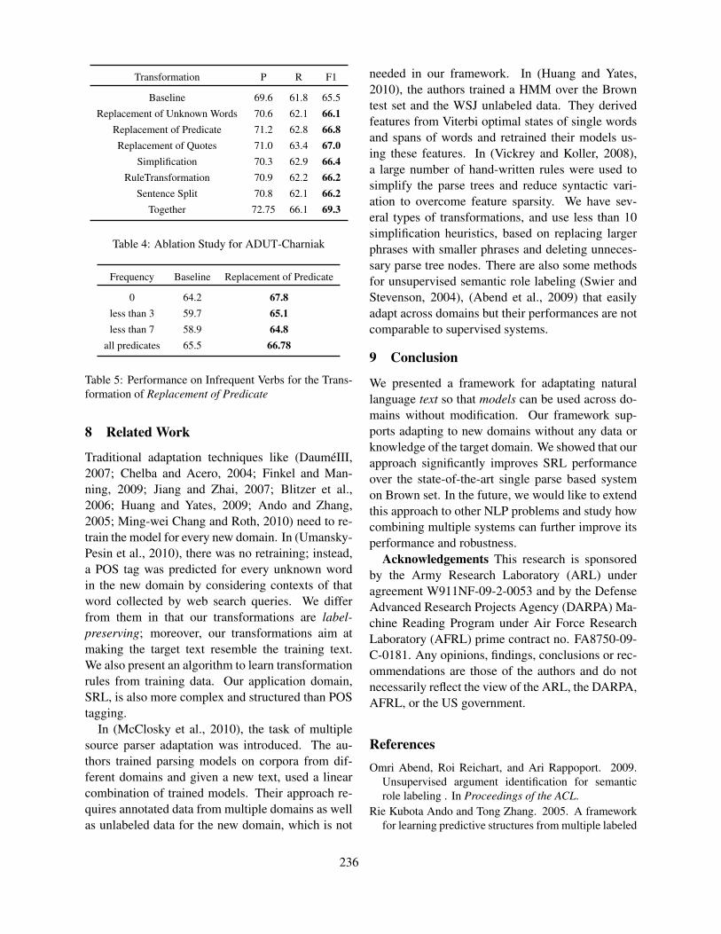
Transformation P R F1

Baseline 69.6 61.8 65.5

Replacement of Unknown Words 70.6 62.1 66.1Replacement of Predicate 71.2 62.8 66.8Replacement of Quotes 71.0 63.4 67.0

Simplification 70.3 62.9 66.4RuleTransformation 70.9 62.2 66.2

Sentence Split 70.8 62.1 66.2Together 72.75 66.1 69.3

Table 4: Ablation Study for ADUT-Charniak

Frequency Baseline Replacement of Predicate

0 64.2 67.8less than 3 59.7 65.1less than 7 58.9 64.8

all predicates 65.5 66.78

Table 5: Performance on Infrequent Verbs for the Trans-formation of Replacement of Predicate

8 Related Work

Traditional adaptation techniques like (DauméIII,2007; Chelba and Acero, 2004; Finkel and Man-ning, 2009; Jiang and Zhai, 2007; Blitzer et al.,2006; Huang and Yates, 2009; Ando and Zhang,2005; Ming-wei Chang and Roth, 2010) need to re-train the model for every new domain. In (Umansky-Pesin et al., 2010), there was no retraining; instead,a POS tag was predicted for every unknown wordin the new domain by considering contexts of thatword collected by web search queries. We differfrom them in that our transformations are label-preserving; moreover, our transformations aim atmaking the target text resemble the training text.We also present an algorithm to learn transformationrules from training data. Our application domain,SRL, is also more complex and structured than POStagging.

In (McClosky et al., 2010), the task of multiplesource parser adaptation was introduced. The au-thors trained parsing models on corpora from dif-ferent domains and given a new text, used a linearcombination of trained models. Their approach re-quires annotated data from multiple domains as wellas unlabeled data for the new domain, which is not

needed in our framework. In (Huang and Yates,2010), the authors trained a HMM over the Browntest set and the WSJ unlabeled data. They derivedfeatures from Viterbi optimal states of single wordsand spans of words and retrained their models us-ing these features. In (Vickrey and Koller, 2008),a large number of hand-written rules were used tosimplify the parse trees and reduce syntactic vari-ation to overcome feature sparsity. We have sev-eral types of transformations, and use less than 10simplification heuristics, based on replacing largerphrases with smaller phrases and deleting unneces-sary parse tree nodes. There are also some methodsfor unsupervised semantic role labeling (Swier andStevenson, 2004), (Abend et al., 2009) that easilyadapt across domains but their performances are notcomparable to supervised systems.

9 Conclusion

We presented a framework for adaptating naturallanguage text so that models can be used across do-mains without modification. Our framework sup-ports adapting to new domains without any data orknowledge of the target domain. We showed that ourapproach significantly improves SRL performanceover the state-of-the-art single parse based systemon Brown set. In the future, we would like to extendthis approach to other NLP problems and study howcombining multiple systems can further improve itsperformance and robustness.

Acknowledgements This research is sponsoredby the Army Research Laboratory (ARL) underagreement W911NF-09-2-0053 and by the DefenseAdvanced Research Projects Agency (DARPA) Ma-chine Reading Program under Air Force ResearchLaboratory (AFRL) prime contract no. FA8750-09-C-0181. Any opinions, findings, conclusions or rec-ommendations are those of the authors and do notnecessarily reflect the view of the ARL, the DARPA,AFRL, or the US government.

ReferencesOmri Abend, Roi Reichart, and Ari Rappoport. 2009.

Unsupervised argument identification for semanticrole labeling . In Proceedings of the ACL.

Rie Kubota Ando and Tong Zhang. 2005. A frameworkfor learning predictive structures from multiple labeled

236

and unlabeled data . Journal of Machine Learning Re-search.

Christopher Bishop. 1995. Neural Networks for Patternrecognition, chapter 6.4: Modelling conditional distri-butions. Oxford University Press.

John Blitzer, Ryan McDonald, and Fernando Pereira.2006. Domain adaptation with structural correspon-dence learning. In Proceedings of the Conference onEmpirical Methods in Natural Language Processing(EMNLP).

Peter F. Brown, Peter V. deSouza, Robert L. Mercer, Vin-cent J. D. Pietra, and Jenifer C. Lai. 1992. Class-basedn-gram models of natural language. ComputationalLinguistics, 18(4):467–479.

Xavier Carreras and Lluís Màrquez. 2005. Introductionto the conll-2005 shared task: Semantic role labeling .In Proceedings of CoNLL.

Eugene Charniak and Mark Johnson. 2005. Coarse-to-fine n-best parsing and maxent discriminative rerank-ing. In Proceedings of ACL.

Ciprian Chelba and Alex Acero. 2004. Little datacan help a lot. In Proceedings of the Conference onEmpirical Methods in Natural Language Processing(EMNLP).

Ronan Collobert and Jason Weston. 2008. A unified ar-chitecture for natural language processing: Deep neu-ral networks with multitask learning. In Proceedingsof ICML.

Hal DauméIII. 2007. Frustratingly easy domain adapta-tion. In Proceedings of the the Annual Meeting of theAssociation of Computational Linguistics (ACL).

Jenny R. Finkel and Christopher D. Manning. 2009. Hi-erarchical bayesian domain adaptation . In Proceed-ings of NAACL.

Fei Huang and Alexander Yates. 2009. Distributionalrepresentations for handling sparsity in supervisedsequence-labeling . In Proceedings of ACL.

Fei Huang and Alexander Yates. 2010. Open-domainsemantic role labeling by modeling word spans. InProceedings of ACL.

Jing Jiang and ChengXiang Zhai. 2007. Instance weight-ing for domain adaptation in nlp. In Proceedings ofACL.

Dan Klein and Christopher D. Manning. 2003. Fast exactinference with a factored model for natural languageparsing. In Proceedings of NIPS.

Percy Liang. 2005. Semi-supervised learning for naturallanguage. Masters thesis, Massachusetts Institute ofTechnology.

David McClosky, Eugene Charniak, and Mark Johnson.2010. Automatic domain adaptation for parsing. InProceedings of NAACL.

Michael Connor Ming-wei Chang and Dan Roth. 2010.The necessity of combining adaptation methods. InProceedings of the Conference on Empirical Meth-ods in Natural Language Processing (EMNLP), Mas-sachusetts, USA.

Vasin Punyakanok, Dan Roth, and Wen tau Yih. 2008.The importance of syntactic parsing and inference insemantic role labeling. Computational Linguistics,34(2).

Mihai Surdeanu, Lluís Màrquez, Xavier Carreras, andPere R. Comas. 2007. Combination strategies for se-mantic role labeling. Journal of Artificial IntelligenceResearch, 29:105–151.

Robert S. Swier and Suzanne Stevenson. 2004. Unsuper-vised semantic role labelling. In Proceedings of Em-pirical Methods in Natural Language Processing.

Kristina Toutanova, Aria Haghighi, and Christopher D.Manning. 2008. A global joint model for semanticrole labeling. Computational Linguistics, 34:161–191.

Shulamit Umansky-Pesin, Roi Reichart, and Ari Rap-poport. 2010. A multi-domain web-based algorithmfor pos tagging of unknown words . In Proceedings ofColing.

David Vickrey and Daphne Koller. 2008. Sentence sim-plification for semantic role labeling. In Proceedingsof the ACL-HLT.

237


Learning with Lookahead:Can History-Based Models Rival Globally Optimized Models?

Yoshimasa Tsuruoka†∗ Yusuke Miyao‡∗ Jun’ichi Kazama∗

† Japan Advanced Institute of Science and Technology (JAIST), Japan‡ National Institute of Informatics (NII), Japan

∗ National Institute of Information and Communications Technology (NICT), [email protected] [email protected] [email protected]

Abstract

This paper shows that the performance ofhistory-based models can be significantly im-proved by performing lookahead in the statespace when making each classification deci-sion. Instead of simply using the best ac-tion output by the classifier, we determinethe best action by looking into possible se-quences of future actions and evaluating thefinal states realized by those action sequences.We present a perceptron-based parameter op-timization method for this learning frame-work and show its convergence properties.The proposed framework is evaluated on part-of-speech tagging, chunking, named entityrecognition and dependency parsing, usingstandard data sets and features. Experimentalresults demonstrate that history-based modelswith lookahead are as competitive as globallyoptimized models including conditional ran-dom fields (CRFs) and structured perceptrons.

1 Introduction

History-based models have been a popular ap-proach in a variety of natural language process-ing (NLP) tasks including part-of-speech (POS) tag-ging, named entity recognition, and syntactic pars-ing (Ratnaparkhi, 1996; McCallum et al., 2000; Ya-mada and Matsumoto, 2003; Nivre et al., 2004).The idea is to decompose the complex structuredprediction problem into a series of simple classifi-cation problems and use a machine learning-basedclassifier to make each decision using the informa-tion about the past decisions and partially completedstructures as features.

Although history-based models have many prac-tical merits, their accuracy is often surpassed byglobally optimized models such as CRFs (Laffertyet al., 2001) and structured perceptrons (Collins,2002), mainly due to the label bias problem. To-day, vanilla history-based models such as maximumentropy Markov models (MEMMs) are probably notthe first choice for those who are looking for a ma-chine learning model that can deliver the state-of-the-art accuracy for their NLP task. Globally opti-mized models, by contrast, are gaining popularity inthe community despite their relatively high compu-tational cost.

In this paper, we argue that history-based mod-els are not something that should be left behindin research history, by demonstrating that their ac-curacy can be significantly improved by incorpo-rating a lookahead mechanism into their decision-making process. It should be emphasized that weuse the word “lookahead” differently from some lit-erature on syntactic parsing in which lookahead sim-ply means looking at the succeeding words to choosethe right parsing actions. In this paper, we use theword to refer to the process of choosing the best ac-tion by considering different sequences of future ac-tions and evaluating the structures realized by thosesequences. In other words, we introduce a looka-head mechanism that performs a search in the spaceof future actions.

We present a perceptron-based training algorithmthat can work with the lookahead process, togetherwith a proof of convergence. The algorithm enablesus to tune the weight of the perceptron in such a waythat we can correctly choose the right action for the

238

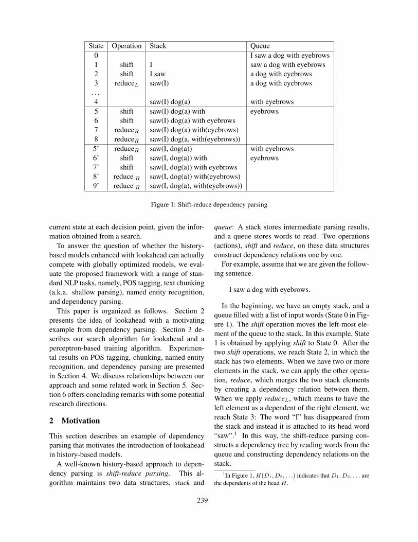
State Operation Stack Queue0 I saw a dog with eyebrows1 shift I saw a dog with eyebrows2 shift I saw a dog with eyebrows3 reduceL saw(I) a dog with eyebrows

. . .4 saw(I) dog(a) with eyebrows5 shift saw(I) dog(a) with eyebrows6 shift saw(I) dog(a) with eyebrows7 reduceR saw(I) dog(a) with(eyebrows)8 reduceR saw(I) dog(a, with(eyebrows))5’ reduceR saw(I, dog(a)) with eyebrows6’ shift saw(I, dog(a)) with eyebrows7’ shift saw(I, dog(a)) with eyebrows8’ reduce R saw(I, dog(a)) with(eyebrows)9’ reduce R saw(I, dog(a), with(eyebrows))

Figure 1: Shift-reduce dependency parsing

current state at each decision point, given the infor-mation obtained from a search.

To answer the question of whether the history-based models enhanced with lookahead can actuallycompete with globally optimized models, we eval-uate the proposed framework with a range of stan-dard NLP tasks, namely, POS tagging, text chunking(a.k.a. shallow parsing), named entity recognition,and dependency parsing.

This paper is organized as follows. Section 2presents the idea of lookahead with a motivatingexample from dependency parsing. Section 3 de-scribes our search algorithm for lookahead and aperceptron-based training algorithm. Experimen-tal results on POS tagging, chunking, named entityrecognition, and dependency parsing are presentedin Section 4. We discuss relationships between ourapproach and some related work in Section 5. Sec-tion 6 offers concluding remarks with some potentialresearch directions.

2 Motivation

This section describes an example of dependencyparsing that motivates the introduction of lookaheadin history-based models.

A well-known history-based approach to depen-dency parsing is shift-reduce parsing. This al-gorithm maintains two data structures, stack and

queue: A stack stores intermediate parsing results,and a queue stores words to read. Two operations(actions), shift and reduce, on these data structuresconstruct dependency relations one by one.

For example, assume that we are given the follow-ing sentence.

I saw a dog with eyebrows.

In the beginning, we have an empty stack, and aqueue filled with a list of input words (State 0 in Fig-ure 1). The shift operation moves the left-most ele-ment of the queue to the stack. In this example, State1 is obtained by applying shift to State 0. After thetwo shift operations, we reach State 2, in which thestack has two elements. When we have two or moreelements in the stack, we can apply the other opera-tion, reduce, which merges the two stack elementsby creating a dependency relation between them.When we apply reduceL, which means to have theleft element as a dependent of the right element, wereach State 3: The word “I” has disappeared fromthe stack and instead it is attached to its head word“saw”.1 In this way, the shift-reduce parsing con-structs a dependency tree by reading words from thequeue and constructing dependency relations on thestack.

1In Figure 1, H(D1, D2, . . .) indicates that D1, D2, . . . arethe dependents of the head H .

239

Let’s say we have now arrived at State 4 after sev-eral operations. At this state, we cannot simply de-termine whether we should shift or reduce. In suchcases, conventional methods rely on a multi-classclassifier to determine the next operation. That is,a classifier is used to select the most plausible oper-ation, by referring to the features about the currentstate, such as surface forms and POSs of words inthe stack and the queue.

In the lookahead strategy, we make this decisionby referring to future states. For example, if we ap-ply shift to State 4, we will reach State 8 in the end,which indicates that “with” attaches to “dog”. Theother way, i.e., applying reduceR to State 4, eventu-ally arrives at State 9’, indicating “with” attaches to“saw”. These future states indicate that we were im-plicitly resolving PP-attachment ambiguity at State4. While conventional methods attempt to resolvesuch ambiguity using surrounding features at State4, the lookahead approach resolves the same ambi-guity by referring to the future states, for example,State 8 and 9’. Because future states can provide ad-ditional and valuable information for ambiguity res-olution, improved accuracy is expected.

It should be noted that Figure 1 only shows onesequence of operations for each choice of operationat State 4. In general, however, the number of poten-tial sequences grows exponentially with the looka-head depth, so the lookahead approach requires us topay the price as the increase of computational cost.The primary goal of this paper is to demonstrate thatthe cost is actually worth it.

3 Learning with Lookahead

This section presents our framework for incorporat-ing lookahead in history-based models. In this pa-per, we focus on deterministic history-based modelsalthough our method could be generalized to non-deterministic cases.

We use the word “state” to refer to a partiallycompleted analysis as well as the collection of his-torical information available at each decision pointin deterministic history-based analysis. State transi-tions are made by “actions” that are defined at eachstate. In the example of dependency parsing pre-sented in Section 2, a state contains all the infor-mation about past operations, stacks, and queues as

1: Input2: d: remaining depth of search3: S0: current state4: Output5: S: state of highest score6: v: highest score7:8: function SEARCH(d, S0)9: if d = 0 then

10: return (S0, w · φ(S0))11: (S, v)← (null,−∞)12: for each a ∈ POSSIBLEACTIONS(S0)13: S1 ← UPDATESTATE(S0, a)14: (S′, v′)← SEARCH(d− 1, S1)15: if v′ > v then16: (S, v)← (S′, v′)17: return (S, v)

Figure 2: Search algorithm.

well as the observation (i.e. the words in the sen-tence). The possible actions are shift, reduceR, andreduceL. In the case of POS tagging, for example, astate is the words and the POS tags assigned to thewords on the left side of the current target word (ifthe tagging is conducted in the left-to-right manner),and the possible actions are simply defined by thePOS tags in the annotation tag set.

3.1 Search

With lookahead, we choose the best action at eachdecision point by considering possible sequences offuture actions and the states realized by those se-quences. In other words, we need to perform asearch for each possible action.

Figure 2 describes our search algorithm in pseudocode. The algorithm performs a depth-first search tofind the state of the highest score among the states inits search space, which is determined by the searchdepth d. This search process is implemented witha recursive function, which receives the remainingsearch depth and the current state as its input andreturns the state of the highest score together withits score.

We assume a linear scoring model, i.e., the scoreof each state S can be computed by taking the dotproduct of the current weight vector w and φ(S),the feature vector representation of the state. The

240

1: Input2: C: perceptron margin3: D: depth of lookahead search4: S0: current state5: ac: correct action6:7: procedure UPDATEWEIGHT(C, D, S0, ac)8: (a∗, S∗, v)← (null, null,−∞)9: for each a ∈ POSSIBLEACTIONS(S0)

10: S1 ← UPDATESTATE(S0, a)11: (S′, v′)←SEARCH(D,S1)12: if a = ac then13: v′ ← v′ − C14: S∗

c ← S′

15: if v′ > v then16: (a∗, S∗, v)← (a, S′, v′)17: if a∗ 6= ac then18: w ← w + φ(S∗

c )− φ(S∗)

Figure 3: Perceptron weight update

scores are computed at each leaf node of the searchtree and backed up to the root.2

Clearly, the time complexity of determinis-tic tagging/parsing with this search algorithm isO(nmD+1), where n is the number of actionsneeded to process the sentence, m is the (average)number of possible actions at each state, and D isthe search depth. It should be noted that the timecomplexity of k-th order CRFs is O(nmk+1), soa history-based model with k-depth lookahead iscomparable to k-th order CRFs in terms of train-ing/testing time.

Unlike CRFs, our framework does not require thelocality of features since it is history-based, i.e., thedecisions can be conditioned on arbitrary features.One interpretation of our learning framework is thatit trades off the global optimality of the learned pa-rameters against the flexibility of features.

3.2 Training a margin perceptron

We adapt a learning algorithm for margin percep-trons (Krauth and Mezard, 1987) to our purpose of

2In actual implementation, it is not efficient to compute thescore of a state from scratch at each leaf node. For most ofthe standard features used in tagging and parsing, it is usuallystraight-forward to compute the scores incrementally every timethe state is updated with an action.

optimizing the weight parameters for the lookaheadsearch. Like other large margin approaches suchas support vector machines, margin perceptrons areknown to produce accurate models compared to per-ceptrons without a margin (Li et al., 2002).

Figure 3 shows our learning algorithm in pseudocode. The algorithm is very similar to the standardtraining algorithm for margin perceptrons, i.e., weupdate the weight parameters with the difference oftwo feature vectors (one corresponding to the cor-rect action, and the other the action of the highestscore) when the perceptron makes a mistake. Thefeature vector for the second best action is also usedwhen the margin is not large enough. Notice that thefeature vector for the second best action is automat-ically selected by using a simple trick of subtractingthe margin parameter from the score for the correctaction (Line 13 in Figure 3).

The only difference between our algorithm andthe standard algorithm for margin perceptrons is thatwe use the states and their scores obtained fromlookahead searches (Line 11 in Figure 3), which arebacked up from the leaves of the search trees. In Ap-pendix A, we provide a proof of the convergence ofour training algorithm and show that the margin willapproach at least half the true margin (assuming thatthe training data are linearly separable).

As in many studies using perceptrons, we averagethe weight vector over the whole training iterationsat the end of the training (Collins, 2002).

4 Experiments

This section presents four sets of experimental re-sults to show how the lookahead process improvesthe accuracy of history-based models in commonNLP tasks.

4.1 Sequence prediction tasks

First, we evaluate our framework with three se-quence prediction tasks: POS tagging, chunking,and named entity recognition. We compare ourmethod with the CRF model, which is one of the defacto standard machine learning models for such se-quence prediction tasks. We trained L1-regularizedfirst-order CRF models using the efficient stochasticgradient descent (SGD)-based training method pre-sented in Tsuruoka et al. (2009). Since our main in-

241

terest is not in achieving the state-of-the-art resultsfor those tasks, we did not conduct feature engineer-ing to come up with elaborate features—we sim-ply adopted the feature sets described in their paper(with an exception being tag trigram features testedin the POS tagging experiments). The experimentsfor these sequence prediction tasks were carried outusing one core of a 3.33GHz Intel Xeon W5590 pro-cessor.

The first set of experiments is about POS tagging.The training and test data were created from the WallStreet Journal corpus of the Penn Treebank (Marcuset al., 1994). Sections 0-18 were used as the trainingdata. Sections 19-21 were used for tuning the metaparameters for learning (the number of iterations andthe margin C). Sections 22-24 were used for thefinal accuracy reports.

The experimental results are shown in Table 1.Note that the models in the top four rows use exactlythe same feature set. It is clearly seen that the looka-head improves tagging accuracy, and our history-based models with lookahead is as accurate as theCRF model. We also created another set of modelsby simply adding tag trigram features, which can-not be employed by first-order CRF models. Thesefeatures have slightly improved the tagging accu-racy, and the final accuracy achieved by a searchdepth of 3 was comparable to some of the best re-sults achieved by pure supervised learning in thistask (Shen et al., 2007; Lavergne et al., 2010).

The second set of experiments is about chunking.We used the data set for the CoNLL 2000 sharedtask, which contains 8,936 sentences where each to-ken is annotated with the “IOB” tags representingtext chunks. The experimental results are shownin Table 2. Again, our history-based models withlookahead were slightly more accurate than the CRFmodel using exactly the same set of features. Theaccuracy achieved by the lookahead model with asearch depth of 2 was comparable to the accuracyachieved by a computationally heavy combinationof max-margin classifiers (Kudo and Matsumoto,2001). We also tested the effectiveness of additionalfeatures of tag trigrams using the development data,but there was no improvement in the accuracy.

The third set of experiments is about named en-tity recognition. We used the data provided forthe BioNLP/NLPBA 2004 shared task (Kim et al.,

2004), which contains 18,546 sentences where eachtoken is annotated with the “IOB” tags representingbiomedical named entities. We performed the tag-ging in the right-to-left fashion because it is knownthat backward tagging is more accurate than forwardtagging on this data set (Yoshida and Tsujii, 2007).

Table 3 shows the experimental results, togetherwith some previous performance reports achievedby pure machine leaning methods (i.e. without rule-based post processing or external resources such asgazetteers). Our history-based model with no looka-head was considerably worse than the CRF modelusing the same set of features, but it was signifi-cantly improved by the introduction of lookaheadand resulted in accuracy figures better than that ofthe CRF model.

4.2 Dependency parsing

We also evaluate our method in dependency parsing.We follow the most standard experimental settingfor English dependency parsing: The Wall StreetJournal portion of Penn Treebank is converted to de-pendency trees by using the head rules of Yamadaand Matsumoto (2003).3 The data is split into train-ing (section 02-21), development (section 22), andtest (section 23) sets. The parsing accuracy was eval-uated with auto-POS data, i.e., we used our looka-head POS tagger (depth = 2) presented in the previ-ous subsection to assign the POS tags for the devel-opment and test data. Unlabeled attachment scoresfor all words excluding punctuations are reported.The development set is used for tuning the meta pa-rameters, while the test set is used for evaluating thefinal accuracy.

The parsing algorithm is the “arc-standard”method (Nivre, 2004), which is briefly described inSection 2. With this algorithm, state S correspondsto a parser configuration, i.e., the stack and thequeue, and action a corresponds to shift, reduceL,and reduceR. In this experiment, we use the sameset of feature templates as Huang and Sagae (2010).

Table 4 shows training time, test time, and parsingaccuracy. In this table, “No lookahead (depth = 0)”corresponds to a conventional shift-reduce parsingmethod without any lookahead search. The results

3Penn2Malt is applied for this conversion, while depen-dency labels are removed.

242

Training Time (sec) Test Time (sec) AccuracyCRF (L1 regularization & SGD training) 847 3 97.11 %No lookahead (depth = 0) 85 5 97.00 %Lookahead (depth = 1) 294 9 97.19 %Lookahead (depth = 2) 8,688 173 97.19 %No lookahead (depth = 0) + tag trigram features 88 5 97.11 %Lookahead (depth = 1) + tag trigram features 313 10 97.22 %Lookahead (depth = 2) + tag trigram features 10,034 209 97.28 %Structured perceptron (Collins, 2002) n/a n/a 97.11 %Guided learning (Shen et al., 2007) n/a n/a 97.33 %CRF with 4 billion features (Lavergne et al., 2010) n/a n/a 97.22 %

Table 1: Performance of English POS tagging (training times and accuracy scores on test data)

Training time (sec) Test time (sec) F-measureCRF (L1 regularization & SGD training) 74 1 93.66No lookahead (depth = 0) 22 1 93.53Lookahead (depth = 1) 73 1 93.77Lookahead (depth = 2) 1,113 9 93.81Voting of 8 SVMs (Kudo and Matsumoto, 2001) n/a n/a 93.91

Table 2: Performance of text chunking (training times and accuracy scores on test data).

clearly demonstrate that the lookahead search boostsparsing accuracy. As expected, training and testspeed decreases, almost by a factor of three, whichis the branching factor of the dependency parser.

The table also lists accuracy figures reported inthe literature on shift-reduce dependency parsing.Most of the latest studies on shift-reduce depen-dency parsing employ dynamic programing or beamsearch, which implies that deterministic methodswere not as competitive as those methods. It shouldalso be noted that all of the listed studies learn struc-tured perceptrons (Collins and Roark, 2004), whileour parser learns locally optimized perceptrons. Inthis table, our parser without lookahead search (i.e.depth = 0) resulted in significantly lower accuracythan the previous studies. In fact, it is worse than thedeterministic parser of Huang et al. (2009), whichuses (almost) the same set of features. This is pre-sumably due to the difference between locally opti-mized perceptrons and globally optimized structuredperceptrons. However, our parser with lookaheadsearch is significantly better than their determinis-tic parser, and its accuracy is close to the levels ofthe parsers with beam search.

5 Discussion

The reason why we introduced a lookahead mech-anism into history-based models is that we wantedthe model to be able to avoid making such mistakesthat can be detected only in later stages. Probabilis-tic history-based models such as MEMMs should beable to avoid (at least some of) such mistakes by per-forming a Viterbi search to find the highest proba-bility path of the actions. However, as pointed outby Lafferty et al. (2001), the per-state normaliza-tion of probabilities makes it difficult to give enoughpenalty to such incorrect sequences of actions, andthat is primarily why MEMMs are outperformed byCRFs.

Perhaps the most relevant to our work in termsof learning is the general framework for search andlearning problems in history-based models proposedby Daume III and Marcu (2005). This framework,called LaSO (Learning as Search Optimization), caninclude many variations of search strategies such asbeam search and A* search as a special case. In-deed, our lookahead framework could be regardedas a special case in which each search node con-

243

Training time (sec) Test time (sec) F-measureCRF (L1 regularization & SGD training) 235 4 71.63No lookahead (depth = 0) 66 4 70.17Lookahead (depth = 1) 91 4 72.28Lookahead (depth = 2) 302 7 72.00Lookahead (depth = 3) 2,419 33 72.21Semi-Markov CRF (Okanohara et al., 2006) n/a n/a 71.48Reranking (Yoshida and Tsujii, 2007) n/a n/a 72.65

Table 3: Performance of biomedical named entity recognition (training times and accuracy scores on test data).

Training time (sec) Test time (sec) AccuracyNo lookahead (depth = 0) 1,937 4 89.73Lookahead (depth = 1) 4,907 13 91.00Lookahead (depth = 2) 12,800 31 91.10Lookahead (depth = 3) 31,684 79 91.24Beam search (k = 64) (Zhang and Clark, 2008) n/a n/a 91.4Deterministic (Huang et al., 2009) n/a n/a 90.2Beam search (k = 16) (Huang et al., 2009) n/a n/a 91.3Dynamic programming (Huang and Sagae, 2010) n/a n/a 92.1

Table 4: Performance of English dependency parsing (training times and accuracy scores on test data).

sists of the next and lookahead actions4, althoughthe weight updating procedure differs in several mi-nor points. Daume III and Marcu (2005) did not trya lookahead search strategy, and to the best of ourknowledge, this paper is the first that demonstratesthat lookahead actually works well for various NLPtasks.

Performing lookahead is a very common tech-nique for a variety of decision-making problemsin the field of artificial intelligence. In computerchess, for example, programs usually need to per-form a very deep search in the game tree to find agood move. Our decision-making problem is sim-ilar to that of computer Chess in many ways, al-though chess programs perform min-max searchesrather than the “max” searches performed in our al-gorithm. Automatic learning of evaluation functionsfor chess programs can be seen as the training ofa machine learning model. In particular, our learn-ing algorithm is similar to the supervised approach

4In addition, the size of the search queue is always truncatedto one for the deterministic decisions presented in this paper.Note, however, that our lookahead framework can also be com-bined with other search strategies such as beam search. In thatcase, the search queue is not necessarily truncated.

(Tesauro, 2001; Hoki, 2006) in that the parametersare optimized based on the differences of the featurevectors realized by the correct and incorrect actions.

In history-based models, the order of actions is of-ten very important. For example, backward taggingis considerably more accurate than forward taggingin biomedical named entity recognition. Our looka-head method is orthogonal to more elaborate tech-niques for determining the order of actions such aseasy-first tagging/parsing strategies (Tsuruoka andTsujii, 2005; Elhadad, 2010). We expect that incor-porating such elaborate techniques in our frameworkwill lead to improved accuracy, but we leave it forfuture work.

6 Conclusion

We have presented a simple and general frameworkfor incorporating a lookahead process in history-based models and a perceptron-based training algo-rithm for the framework. We have conducted ex-periments using standard data sets for POS tagging,chunking, named entity recognition and dependencyparsing, and obtained very promising results—theaccuracy achieved by the history-based models en-

244

hanced with lookahead was as competitive as glob-ally optimized models including CRFs.

In most of the experimental results, steady im-provement in accuracy has been observed as thedepth of the search is increased. Although it isnot very practical to perform deeper searches withour current implementation—we naively exploredall possible sequences of actions, future work shouldencompass extending the depths of search spaceby introducing elaborate pruning/search extensiontechniques.

In this work, we did not conduct extensive featureengineering for improving the accuracy of individ-ual tasks because our primary goal with this paper isto present the learning framework itself. However,one of the major merits of using history-based mod-els is that we are allowed to define arbitrary featureson the partially completed structure. Another inter-esting direction of future work is to see how muchwe could improve the accuracy by performing ex-tensive feature engineering in this particular learningframework.

Appendix A: Convergence of the LearningProcedure

Let {xi, aic}Ki=1 be the training examples where ai

c

is the correct first action for decision point xi, andlet Si be the set of all the states at the leaves ofthe search trees for xi generated by the lookaheadsearches and Si

c be the set of all the states at theleaves of the search tree for the correct action ai

c.We also define Si = Si \ Si

c. We write the weightvector before the k-th update as wk. We defineS∗

c = argmaxS∈Si

c

w·φ(S) and S∗ = argmaxS∈Si

w·φ(S)5.

Then the update rule can be interpreted as wk+1 =wk +(φ(S∗

c )−φ(S∗)). Note that this update is per-formed only when φ(Sc) ·wk−C < φ(S∗) ·wk forall Sc ∈ Sc since otherwise S∗ in the learning algo-rithm cannot be a state with an incorrect first action.In other words, φ(Sc) ·w − φ(S∗) ·w ≥ C for allSc ∈ Sc after convergence.

Given these definitions, we prove the convergencefor the separable case. That is, we assume the exis-tence of a weight vector u (with ||u|| = 1), δ (> 0),

5S∗c and S∗ depend on the weight vector at each point, but

we omit it from the notation for brevity.

and R (> 0) that satisfy:

∀i,∀Sc ∈ Sic,∀S ∈ Si φ(Sc) · u− φ(S) · u ≥ δ,

∀i,∀Sc ∈ Sic,∀S ∈ Si ||φ(Sc)− φ(S)|| ≤ R.

The proof is basically an adaptation of the proofsin Collins (2002) and Li et al. (2002). First, we ob-tain the following relation:

wk+1 · u = wk · u + (φ(S∗c ) · u− φ(S∗) · u)

= wk · u + δ ≥ w1 · u + kδ = kδ.

Therefore, ||wk+1 · u||2 = ||wk+1||2 ≤ (kδ)2 —(1). We assumed w1 = 0 but this is not an essentialassumption.

Next, we also obtain:

||wk+1||2 ≤ ||wk||2 + 2(φ(S∗c )− φ(S∗)) ·wk

+||φ(S∗c )− φ(S∗)||2

≤ ||wk||2 + 2C + R2

≤ ||w1||2 + k(R2 + 2C) = k(R2 + 2C)— (2)

Combining (1) and (2), we obtain k ≤ (R2 +2C)/δ2. That is, the number of updates is boundedfrom above, meaning that the learning procedureconverges after a finite number of updates. Substi-tuting this into (2) gives ||wk+1|| ≤ (R2 + 2C)/δ— (3).

Finally, we analyze the margin achieved by thelearning procedure after convergence. The margin,γ(w), is defined as follows in this case.

γ(w) = minxi

minSc∈Si

c,S∈Si

φ(Sc) ·w − φ(S) ·w||w||

= minxi

minSc∈Si

c

φ(Sc) ·w − φ(S∗) ·w||w||

After convergence (i.e., w = wk+1), φ(Sc) · w −φ(S∗)·w ≥ C for all Sc ∈ Sc as we noted. Togetherwith (3), we obtain the following bound:

γ(w) ≥ minxi

δC

2C + R2

=δC

2C + R2=

(δ

2

)(1− R2

2C + R2

)As can be seen, the margin approaches at least halfthe true margin, δ/2 as C → ∞ (at the cost of infi-nite number of updates).

245

References

Michael Collins and Brian Roark. 2004. Incrementalparsing with the perceptron algorithm. In Proceedingsof ACL, pages 111–118.

Michael Collins. 2002. Discriminative training meth-ods for hidden markov models: Theory and experi-ments with perceptron algorithms. In Proceedings ofEMNLP, pages 1–8.

Hal Daume III and Daniel Marcu. 2005. Learning assearch optimization: Approximate large margin meth-ods for structured prediction. In Proceedings of ICML,pages 169–176.

Yoav Goldbergand Michael Elhadad. 2010. An effi-cient algorithm for easy-first non-directional depen-dency parsing. In Proceedings of NAACL-HLT, pages742–750.

Kunihito Hoki. 2006. Optimal control of minimaxsearch results to learn positional evaluation. In Pro-ceedings of the 11th Game Programming Workshop(GPW), pages 78–83 (in Japanese).

Liang Huang and Kenji Sagae. 2010. Dynamic program-ming for linear-time incremental parsing. In Proceed-ings of ACL, pages 1077–1086.

Liang Huang, Wenbin Jiang, and Qun Liu. 2009.Bilingually-constrained (monolingual) shift-reduceparsing. In Proceedings of EMNLP, pages 1222–1231.

J.-D. Kim, T. Ohta, Y. Tsuruoka, Y. Tateisi, and N. Col-lier. 2004. Introduction to the bio-entity recogni-tion task at JNLPBA. In Proceedings of the Interna-tional Joint Workshop on Natural Language Process-ing in Biomedicine and its Applications (JNLPBA),pages 70–75.

W Krauth and M Mezard. 1987. Learning algorithmswith optimal stability in neural networks. Journal ofPhisics A, 20(11):L745–L752.

Taku Kudo and Yuji Matsumoto. 2001. Chunking withsupport vector machines. In Proceedings of NAACL.

John Lafferty, Andrew McCallum, and Fernando Pereira.2001. Conditional random fields: Probabilistic mod-els for segmenting and labeling sequence data. In Pro-ceedings of ICML, pages 282–289.

Thomas Lavergne, Olivier Cappe, and Francois Yvon.2010. Practical very large scale CRFs. In Proceed-ings of ACL, pages 504–513.

Yaoyong Li, Hugo Zaragoza, Ralf Herbrich, John Shawe-Taylor, and Jaz S. Kandola. 2002. The perceptronalgorithm with uneven margins. In Proceedings ofICML, pages 379–386.

Mitchell P. Marcus, Beatrice Santorini, and Mary AnnMarcinkiewicz. 1994. Building a large annotated cor-pus of English: The Penn Treebank. ComputationalLinguistics, 19(2):313–330.

Andrew McCallum, Dayne Freitag, and FernandoPereira. 2000. Maximum entropy markov models forinformation extraction and segmentation. In Proceed-ings of ICML, pages 591–598.

Joakim Nivre, Johan Hall, and Jens Nilsson. 2004.Memory-based dependency parsing. In Proceedingsof CoNLL, pages 49–56.

Joakim Nivre. 2004. Incrementality in deterministic de-pendency parsing. In ACL 2004 Workshop on Incre-mental Parsing: Bringing Engineering and CognitionTogether, pages 50–57.

Daisuke Okanohara, Yusuke Miyao, Yoshimasa Tsu-ruoka, and Jun’ichi Tsujii. 2006. Improving the scal-ability of semi-markov conditional random fields fornamed entity recognition. In Proceedings of COL-ING/ACL, pages 465–472.

Adwait Ratnaparkhi. 1996. A maximum entropy modelfor part-of-speech tagging. In Proceedings of EMNLP1996, pages 133–142.

Libin Shen, Giorgio Satta, and Aravind Joshi. 2007.Guided learning for bidirectional sequence classifica-tion. In Proceedings of ACL, pages 760–767.

Gerald Tesauro, 2001. Comparison training of chessevaluation functions, pages 117–130. Nova SciencePublishers, Inc.

Yoshimasa Tsuruoka and Jun’ichi Tsujii. 2005. Bidirec-tional inference with the easiest-first strategy for tag-ging sequence data. In Proceedings of HLT/EMNLP2005, pages 467–474.

Yoshimasa Tsuruoka, Jun’ichi Tsujii, and Sophia Ana-niadou. 2009. Stochastic gradient descent trainingfor l1-regularized log-linear models with cumulativepenalty. In Proceedings of ACL-IJCNLP, pages 477–485.

Hiroyasu Yamada and Yuji Matsumoto. 2003. Statisticaldependency analysis with support vector machines. InProceedings of IWPT, pages 195–206.

Kazuhiro Yoshida and Jun’ichi Tsujii. 2007. Rerankingfor biomedical named-entity recognition. In Proceed-ings of ACL Workshop on BioNLP, pages 209–216.

Yue Zhang and Stephen Clark. 2008. A tale oftwo parsers: investigating and combining graphbasedand transition-based dependency parsing using beam-search. In Proceedings of EMNLP, pages 562–571.

246


Learning Discriminative Projections for Text Similarity Measures

Wen-tau Yih Kristina Toutanova John C. Platt Christopher MeekMicrosoft ResearchOne Microsoft Way

Redmond, WA 98052, USA{scottyih,kristout,jplatt,meek}@microsoft.com

Abstract

Traditional text similarity measures considereach term similar only to itself and do notmodel semantic relatedness of terms. We pro-pose a novel discriminative training methodthat projects the raw term vectors into a com-mon, low-dimensional vector space. Our ap-proach operates by finding the optimal matrixto minimize the loss of the pre-selected sim-ilarity function (e.g., cosine) of the projectedvectors, and is able to efficiently handle alarge number of training examples in the high-dimensional space. Evaluated on two very dif-ferent tasks, cross-lingual document retrievaland ad relevance measure, our method notonly outperforms existing state-of-the-art ap-proaches, but also achieves high accuracy atlow dimensions and is thus more efficient.

1 Introduction

Measures of text similarity have many applicationsand have been studied extensively in both the NLPand IR communities. For example, a combinationof corpus and knowledge based methods have beeninvented for judging word similarity (Lin, 1998;Agirre et al., 2009). Similarity derived from a large-scale Web corpus has been used for automaticallyextending lists of typed entities (Vyas and Pantel,2009). Judging the degree of similarity betweendocuments is also fundamental to classical IR prob-lems such as document retrieval (Manning et al.,2008). In all these applications, the vector-basedsimilarity method is the most widely used. Termvectors are first constructed to represent the origi-nal text objects, where each term is associated with

a weight indicating its importance. A pre-selectedfunction operating on these vectors, such as cosine,is used to output the final similarity score. This ap-proach has not only proved to be effective, but is alsoefficient. For instance, only the term vectors ratherthan the raw data need to be stored. A pruned inverseindex can be built to support fast similarity search.

However, the main weakness of this term-vectorrepresentation is that different but semantically re-lated terms are not matched and cannot influencethe final similarity score. As an illustrative ex-ample, suppose the two compared term-vectorsare: {purchase:0.4, used:0.3, automobile:0.2} and{buy:0.3, pre-owned: 0.5, car: 0.4}. Even thoughthe two vectors represent very similar concepts, theirsimilarity score will be 0, for functions like cosine,overlap or Jaccard. Such an issue is more severein cross-lingual settings. Because language vocab-ularies typically have little overlap, term-vector rep-resentations are completely inapplicable to measur-ing similarity between documents in different lan-guages. The general strategy to handle this prob-lem is to map the raw representation to a commonconcept space, where extensive approaches havebeen proposed. Existing methods roughly fall intothree categories. Generative topic models like La-tent Dirichlet Allocation (LDA) (Blei et al., 2003)assume that the terms are sampled by probabil-ity distributions governed by hidden topics. Lin-ear projection methods like Latent Semantic Anal-ysis (LSA) (Deerwester et al., 1990) learn a projec-tion matrix and map the original term-vectors to thedense low-dimensional space. Finally, metric learn-ing approaches for high-dimensional spaces have

247

also been proposed (Davis and Dhillon, 2008).

In this paper, we propose a new projection learn-ing framework, Similarity Learning via SiameseNeural Network (S2Net), to discriminatively learnthe concept vector representations of input text ob-jects. Following the general Siamese neural networkarchitecture (Bromley et al., 1993), our approachtrains two identical networks concurrently. The in-put layer corresponds to the original term vectorand the output layer is the projected concept vector.Model parameters (i.e., the weights on the edges)are equivalently the projection matrix. Given pairsof raw term vectors and their labels (e.g., similar ornot), the model is trained by minimizing the loss ofthe similarity scores of the output vectors. S2Netis closely related to the linear projection and met-ric learning approaches, but enjoys additional ad-vantages over existing methods. While its modelform is identical to that of LSA, CCA and OPCA, itsobjective function can be easily designed to matchthe true evaluation metric of interest for the targettask, which leads to better performance. Comparedto existing high-dimensional metric learning meth-ods, S2Net can learn from a much larger numberof labeled examples. These two properties are cru-cial in helping S2Net outperform existing methods.For retrieving comparable cross-lingual documents,S2Net achieves higher accuracy than the best ap-proach (OPCA) at a much lower dimension of theconcept space (500 vs. 2,000). In a monolingualsetting, where the task is to judge the relevance ofan ad landing page to a query, S2Net also has thebest performance when compared to a number of ap-proaches, including the raw TFIDF cosine baseline.

In the rest of the paper, we first survey someexisting work in Sec. 2, with an emphasis on ap-proaches included in our experimental comparison.We present our method in Sec. 3 and report on anextensive experimental study in Sec. 4. Other re-lated work is discussed in Sec. 5 and finally Sec. 6concludes the paper.

2 Previous Work

In this section, we briefly review existing ap-proaches for mapping high-dimensional term-vectors to a low-dimensional concept space.

2.1 Generative Topic Models

Probabilistic Latent Semantic Analysis(PLSA) (Hofmann, 1999) assumes that eachdocument has a document-specific distribution θover some finite number K of topics, where eachtoken in a document is independently generatedby first selecting a topic z from a multinomialdistribution MULTI(θ), and then sampling a wordtoken from the topic-specific word distributionfor the chosen topic MULTI(φz). Latent DirichletAllocation (LDA) (Blei et al., 2003) generalizesPLSA to a proper generative model for documentsand places Dirichlet priors over the parametersθ and φ. In the experiments in this paper, ourimplementation of PLSA is LDA with maximum aposteriori (MAP) inference, which was shown to becomparable to the current best Bayesian inferencemethods for LDA (Asuncion et al., 2009).

Recently, these topic models have been general-ized to handle pairs or tuples of corresponding doc-uments, which could be translations in multiple lan-guages, or documents in the same language that areconsidered similar. For instance, the Poly-lingualTopic Model (PLTM) (Mimno et al., 2009) is anextension to LDA that views documents in a tu-ple as having a shared topic vector θ. Each of thedocuments in the tuple uses θ to select the topicsz of tokens, but could use a different (language-specific) word-topic-distribution MULTI(φLz ). Twoadditional models, Joint PLSA (JPLSA) and Cou-pled PLSA (CPLSA) were introduced in (Platt et al.,2010). JPLSA is a close variant of PLTM when doc-uments of all languages share the same word-topicdistribution parameters, and MAP inference is per-formed instead of Bayesian. CPLSA extends JPLSAby constraining paired documents to not only sharethe same prior topic distribution θ, but to also havesimilar fractions of tokens assigned to each topic.This constraint is enforced on expectation using pos-terior regularization (Ganchev et al., 2009).

2.2 Linear Projection Methods

The earliest method for projecting term vectors intoa low-dimensional concept space is Latent Seman-tic Analysis (LSA) (Deerwester et al., 1990). LSAmodels all documents in a corpus using a n ×d document-term matrix D and performs singular

248

value decomposition (SVD) on D. The k biggestsingular values are then used to find the d × k pro-jection matrix. Instead of SVD, LSA can be doneby applying eigen-decomposition on the correlationmatrix between terms C = DTD. This is very sim-ilar to principal component analysis (PCA), where acovariance matrix between terms is used. In prac-tice, term vectors are very sparse and their meansare close to 0. Therefore, the correlation matrix is infact close to the covariance matrix.

To model pairs of comparable documents,LSA/PCA has been extended in different ways. Forinstance, Cross-language Latent Semantic Indexing(CL-LSI) (Dumais et al., 1997) applies LSA to con-catenated comparable documents from different lan-guages. Oriented Principal Component Analysis(OPCA) (Diamantaras and Kung, 1996; Platt et al.,2010) solves a generalized eigen problem by intro-ducing a noise covariance matrix to ensure that com-parable documents can be projected closely. Canon-ical Correlation Analysis (CCA) (Vinokourov et al.,2003) finds projections that maximize the cross-covariance between the projected vectors.

2.3 Distance Metric Learning

Measuring the similarity between two vectors can beviewed as equivalent to measuring their distance, asthe cosine score has a bijection mapping to the Eu-clidean distance of unit vectors. Most work on met-ric learning learns a Mahalanobis distance, whichgeneralizes the standard squared Euclidean distanceby modeling the similarity of elements in differentdimensions using a positive semi-definite matrix A.Given two vectors x and y, their squared Maha-lanobis distance is: dA = (x − y)TA(x − y).However, the computational complexity of learn-ing a general Mahalanobis matrix is at least O(n2),where n is the dimensionality of the input vectors.Therefore, such methods are not practical for highdimensional problems in the text domain.

In order to tackle this issue, special metriclearning approaches for high-dimensional spaceshave been proposed. For example, high dimen-sion low-rank (HDLR) metric learning (Davis andDhillon, 2008) constrains the form of A = UUT ,where U is similar to the regular projection ma-trix, and adapts information-theoretic metric learn-ing (ITML) (Davis et al., 2007) to learn U.

sim(vp,vq)

1t dt

vp vq

it

1c kcjc'tw

tw

Figure 1: Learning concept vectors. The output layerconsists of a small number of concept nodes, where theweight of each node is a linear combination of all theoriginal term weights.

3 Similarity Learning via Siamese NeuralNetwork (S2Net)

Given pairs of documents with their labels, such asbinary or real-valued similarity scores, our goal isto construct a projection matrix that maps the corre-sponding term-vectors into a low-dimensional con-cept space such that similar documents are closewhen projected into this space. We propose a sim-ilarity learning framework via Siamese neural net-work (S2Net) to learn the projection matrix directlyfrom labeled data. In this section, we introduce itsmodel design and describe the training process.

3.1 Model Design

The network structure of S2Net consists of two lay-ers. The input layer corresponds to the raw term vec-tor, where each node represents a term in the originalvocabulary and its associated value is determined bya term-weighting function such as TFIDF. The out-put layer is the learned low-dimensional vector rep-resentation that captures relationships among terms.Similarly, each node of the output layer is an ele-ment in the new concept vector. In this work, thefinal similarity score is calculated using the cosinefunction, which is the standard choice for documentsimilarity (Manning et al., 2008). Our frameworkcan be easily extended to other similarity functionsas long as they are differentiable.

The output of each concept node is a linear com-

249

bination of the weights of all the terms in the orig-inal term vector. In other words, these two layersof nodes form a complete bipartite graph as shownin Fig. 1. The output of a concept node cj is thusdefined as:

tw′(cj) =∑ti∈V

αij · tw(ti) (1)

Notice that it is straightforward to add a non-linearactivation function (e.g., sigmoid) in Eq. (1), whichcan potentially lead to better results. However, inthe current design, the model form is exactly thesame as the low-rank projection matrix derived byPCA, OPCA or CCA, which facilitates comparisonto alternative projection methods. Using concisematrix notation, let f be a raw d-by-1 term vector,A = [αij ]d×k the projection matrix. g = AT f isthus the k-by-1 projected concept vector.

3.2 Loss Function and Training ProcedureFor a pair of term vectors fp and fq, their similar-ity score is defined by the cosine value of the corre-sponding concept vectors gp and gq according to theprojection matrix A.

simA(fp, fq) =gTp gq

||gp||||gq||,

where gp = AT fp and gq = AT fq. Let ypq bethe true label of this pair. The loss function canbe as simple as the mean-squared error 1

2(ypq −simA(fp, fq))

2. However, in many applications, thesimilarity scores are used to select the closest textobjects given the query. For example, given a querydocument, we only need to have the comparabledocument in the target language ranked higher thanany other documents. In this scenario, it is moreimportant for the similarity measure to yield a goodordering than to match the target similarity scores.Therefore, we use a pairwise learning setting by con-sidering a pair of similarity scores (i.e., from twovector pairs) in our learning objective.

Consider two pairs of term vectors (fp1 , fq1) and(fp2 , fq2), where the first pair has higher similarity.Let ∆ be the difference of their similarity scores.Namely, ∆ = simA(fp1 , fq1)− simA(fp2 , fq2). Weuse the following logistic loss over ∆, which upper-bounds the pairwise accuracy (i.e., 0-1 loss):

L(∆; A) = log(1 + exp(−γ∆)) (2)

Because of the cosine function, we add a scalingfactor γ that magnifies ∆ from [−2, 2] to a largerrange, which helps penalize more on the predictionerrors. Empirically, the value of γ makes no dif-ference as long as it is large enough1. In the ex-periments, we set the value of γ to 10. Optimizingthe model parameters A can be done using gradi-ent based methods. We derive the gradient of thewhole batch and apply the quasi-Newton optimiza-tion method L-BFGS (Nocedal and Wright, 2006)directly. For a cleaner presentation, we detail thegradient derivation in Appendix A. Given that theoptimization problem is not convex, initializing themodel from a good projection matrix often helps re-duce training time and may lead to convergence toa better local minimum. Regularization can be doneby adding a term β

2 ||A − A0||2 in Eq. (2), whichforces the learned model not to deviate too muchfrom the starting point (A0), or simply by early stop-ping. Empirically we found that the latter is moreeffective and it is used in the experiments.

4 Experiments

We compare S2Net experimentally with existing ap-proaches on two very different tasks: cross-lingualdocument retrieval and ad relevance measures.

4.1 Comparable Document RetrievalWith the growth of multiple languages on the Web,there is an increasing demand of processing cross-lingual documents. For instance, machine trans-lation (MT) systems can benefit from training onsentences extracted from parallel or comparabledocuments retrieved from the Web (Munteanu andMarcu, 2005). Word-level translation lexicons canalso be learned from comparable documents (Fungand Yee, 1998; Rapp, 1999). In this cross-lingualdocument retrieval task, given a query document inone language, the goal is to find the most similardocument from the corpus in another language.

4.1.1 Data & SettingWe followed the comparable document retrieval

setting described in (Platt et al., 2010) and evalu-ated S2Net on the Wikipedia dataset used in that pa-per. This data set consists of Wikipedia documents

1Without the γ parameter, the model still outperforms otherbaselines in our experiments, but with a much smaller gain.

250

in two languages, English and Spanish. An articlein English is paired with a Spanish article if theyare identified as comparable across languages by theWikipedia community. To conduct a fair compari-son, we use the same term vectors and data split as inthe previous study. The numbers of document pairsin the training/development/testing sets are 43,380,8,675 and 8,675, respectively. The dimensionalityof the raw term vectors is 20,000.

The models are evaluated by using each Englishdocument as query against all documents in Span-ish and vice versa; the results from the two direc-tions are averaged. Performance is evaluated by twometrics: the Top-1 accuracy, which tests whetherthe document with the highest similarity score is thetrue comparable document, and the Mean Recipro-cal Rank (MRR) of the true comparable.

When training the S2Net model, all the compara-ble document pairs are treated as positive examplesand all other pairs are used as negative examples.Naively treating these 1.8 billion pairs (i.e., 433802)as independent examples would make the trainingvery inefficient. Fortunately, most computation inderiving the batch gradient can be reused via com-pact matrix operations and training can still be doneefficiently. We initialized the S2Net model using thematrix learned by OPCA, which gave us the best per-formance on the development set2.

Our approach is compared with most methodsstudied in (Platt et al., 2010), including the best per-forming one. For CL-LSI, OPCA, and CCA, we in-clude results from that work directly. In addition, were-implemented and improved JPLSA and CPLSAby changing three settings: we used separate vocab-ularies for the two languages as in the Poly-lingualtopic model (Mimno et al., 2009), we performed 10EM iterations for folding-in instead of only one, andwe used the Jensen-Shannon distance instead of theL1 distance. We also attempted to apply the HDLRalgorithm. Because this algorithm does not scalewell as the number of training examples increases,we used 2,500 positive and 2,500 negative docu-ment pairs for training. Unfortunately, among all the

2S2Net outperforms OPCA when initialized from a randomor CL-LSI matrix, but with a smaller gain. For example, whenthe number of dimensions is 1000, the MRR score of OPCAis 0.7660. Starting from the CL-LSI and OPCA matrices, theMRR scores of S2Net are 0.7745 and 0.7855, respectively.

Figure 2: Mean reciprocal rank versus dimension forWikipedia. Results of OPCA, CCA and CL-LSI arefrom (Platt et al., 2010).

hyper-parameter settings we tested, HDLR could notoutperform its initial model, which was the OPCAmatrix. Therefore we omit these results.

4.1.2 ResultsFig. 2 shows the MRR performance of all meth-

ods on the development set, across different dimen-sionality settings of the concept space. As can beobserved from the figure, higher dimensions usuallylead to better results. In addition, S2Net consistentlyperforms better than all other methods across differ-ent dimensions. The gap is especially large whenprojecting input vectors to a low-dimensional space,which is preferable for efficiency. For instance, us-ing 500 dimensions, S2Net already performs as wellas OPCA with 2000 dimensions.

Table 1 shows the averaged Top-1 accuracy andMRR scores of all methods on the test set, wherethe dimensionality for each method is optimized onthe development set (Fig. 2). S2Net clearly outper-forms all other methods and the difference in termsof accuracy is statistically significant3.

4.2 Ad Relevance

Paid search advertising is the main revenue sourcethat supports modern commercial search engines.To ensure satisfactory user experience, it is impor-tant to provide both relevant ads and regular search

3We use the unpaired t-test with Bonferroni correction andthe difference is considered statistically significant when the p-value is less than 0.01.

251

Algorithm Dimension Accuracy MRRS2Net 2000 0.7447 0.7973OPCA 2000 0.7255 0.7734CCA 1500 0.6894 0.7378CPLSA 1000 0.6329 0.6842JPLSA 1000 0.6079 0.6604CL-LSI 5000 0.5302 0.6130

Table 1: Test results for comparable document retrievalin Wikipedia. Results of OPCA, CCA and CL-LSI arefrom (Platt et al., 2010).

results. Previous work on ad relevance focuses onconstructing appropriate term-vectors to representqueries and ad-text (Broder et al., 2008; Choi et al.,2010). In this section, we extend the work in (Yihand Jiang, 2010) and show how S2Net can exploitannotated query–ad pairs to improve the vector rep-resentation in this monolingual setting.

4.2.1 Data & TasksThe ad relevance dataset we used consists of

12,481 unique queries randomly sampled from thelogs of the Bing search engine. For each query, anumber of top ranked ads are selected, which resultsin a total number of 567,744 query-ad pairs in thedataset. Each query-ad pair is manually labeled assame, subset, superset or disjoint. In our experi-ment, when the task is a binary classification prob-lem, pairs labeled as same, subset, or superset areconsidered relevant, and pairs labeled as disjoint areconsidered irrelevant. When pairwise comparisonsare needed in either training or evaluation, the rele-vance order is same > subset = superset > disjoint.The dataset is split into training (40%), validation(30%) and test (30%) sets by queries.

Because a query string usually contains only a fewwords and thus provides very little content, we ap-plied the same web relevance feedback techniqueused in (Broder et al., 2008) to create “pseudo-documents” to represent queries. Each query in ourdata set was first issued to the search engine. Theresult page with up to 100 snippets was used as thepseudo-document to create the raw term vectors. Onthe ad side, we used the ad landing pages insteadof the short ad-text. Our vocabulary set contains29,854 words and is determined using a documentfrequency table derived from a large collection ofWeb documents. Only words with counts larger than

a pre-selected threshold are retained.How the data is used in training depends on the

model. For S2Net, we constructed preference pairsin the following way. For the same query, each rel-evant ad is paired with a less relevant ad. The lossfunction from Eq. (2) encourages achieving a highersimilarity score for the more relevant ad. For HDLR,we used a sample of 5,000 training pairs of queriesand ads, as it was not able to scale to more train-ing examples. For OPCA, CCA, PLSA and JPLSA,we constructed a parallel corpus using only rele-vant pairs of queries and ads, as the negative exam-ples (irrelevant pairs of queries and ads) cannot beused by these models. Finally, PCA and PLSA learnthe models from all training queries and documentswithout using any relevance information.

We tested S2Net and other methods in two differ-ent application scenarios. The first is to use the adrelevance measure as an ad filter. When the similar-ity score between a query and an ad is below a pre-selected decision threshold, this ad is considered ir-relevant to the query and will be filtered. Evaluationmetrics used for this scenario are the ROC analysisand the area under the curve (AUC). The second oneis the ranking scenario, where the ads are selectedand ranked by their relevance scores. In this sce-nario, the performance is evaluated by the standardranking metric, Normalized Discounted CumulativeGain (NDCG) (Jarvelin and Kekalainen, 2000).

4.2.2 ResultsWe first compare different methods in their AUC

and NDCG scores. TFIDF is the basic term vec-tor representation with the TFIDF weighting (tf ·log(N/df)). It is used as our baseline and also asthe raw input for S2Net, HDLR and other linear pro-jection methods. Based on the results on the devel-opment set, we found that PCA performs better thanOPCA and CCA. Therefore, we initialized the mod-els of S2Net and HDLR using the PCA matrix. Ta-ble 2 summarizes results on the test set. All models,except TFIDF, use 1000 dimensions and their bestconfiguration settings selected on the validation set.

TFIDF is a very strong baseline on this monolin-gual ad relevance dataset. Among all the methodswe tested, at dimension 1000, only S2Net outper-forms the raw TFIDF cosine measure in every eval-uation metric, and the difference is statistically sig-

252

AUC NDCG@1 NDCG@3 NDCG@5S2Net 0.892 0.855 0.883 0.901TFIDF 0.861 0.825 0.854 0.876HDLR 0.855 0.826 0.856 0.877CPLSA 0.853 0.845 0.872 0.890

PCA 0.848 0.815 0.847 0.870OPCA 0.844 0.817 0.850 0.872JPLSA 0.840 0.838 0.864 0.883CCA 0.836 0.820 0.852 0.874PLSA 0.835 0.831 0.860 0.879

Table 2: The AUC and NDCG scores of the cosine sim-ilarity scores on different vector representations. The di-mension for all models except TFIDF is 1000.

0.3

0.4

0.5

0.6

0.7

0.8

0.9

0.05 0.1 0.15 0.2 0.25

Tru

e-P

ositi

ve R

ate

False-Positive Rate

The ROC Curves

S2NetTFIDFHDLR

CPLSA

Figure 3: The ROC curves of S2Net, TFIDF, HDLR andCPLSA when the similarity scores are used as ad filters.

nificant4. In contrast, both CPLSA and HDLR havehigher NDCG scores but lower AUC values, andOPCA/CCA perform roughly the same as PCA.

When the cosine scores of these vector represen-tations are used as ad filters, their ROC curves (fo-cusing on the low false-positive region) are shownin Fig. 3. It can be clearly observed that the similar-ity score computed based on vectors derived fromS2Net indeed has better quality, compared to theraw TFIDF representation. Unfortunately, other ap-proaches perform worse than TFIDF and their per-formance in the low false-positive region is consis-tent with the AUC scores.

Although ideally we would like the dimensional-ity of the projected concept vectors to be as small

4For AUC, we randomly split the data into 50 subsets andran a paired-t test between the corresponding AUC scores. ForNDCG, we compared the DCG scores per query of the com-pared models using the paired-t test. The difference is consid-ered statistically significant when the p-value is less than 0.01.

as possible for efficient processing, the quality ofthe concept vector representation usually degradesas well. It is thus interesting to know the best trade-off point between these two variables. Table 3 showsthe AUC and NDCG scores of S2Net at different di-mensions, as well as the results achieved by TFIDFand PCA, HDLR and CPLSA at 1000 dimensions.As can be seen, S2Net surpasses TFIDF in AUC atdimension 300 and keeps improving as the dimen-sionality increases. Its NDCG scores are also con-sistently higher across all dimensions.

4.3 Discussion

It is encouraging to find that S2Net achieves strongperformance in two very different tasks, given thatit is a conceptually simple model. Its empirical suc-cess can be attributed to two factors. First, it is flex-ible in choosing the loss function and constructingtraining examples and is thus able to optimize themodel directly for the target task. Second, it canbe trained on a large number of examples. For ex-ample, HDLR can only use a few thousand exam-ples and is not able to learn a matrix better than itsinitial model for the task of cross-lingual documentretrieval. The fact that linear projection methodslike OPCA/CCA and generative topic models likeJPLSA/CPLSA cannot use negative examples moreeffectively also limits their potential.

In terms of scalability, we found that methodsbased on eigen decomposition, such as PCA, OPCAand CCA, take the least training time. The complex-ity is decided by the size of the covariance matrix,which is quadratic in the number of dimensions. Ona regular eight-core server, it takes roughly 2 to 3hours to train the projection matrix in both experi-ments. The training time of S2Net scales roughlylinearly to the number of dimensions and trainingexamples. In each iteration, performing the projec-tion takes the most time in gradient derivation, andthe complexity is O(mnk), where m is the num-ber of distinct term-vectors, n is the largest numberof non-zero elements in the sparse term-vectors andk is the dimensionality of the concept space. Forcross-lingual document retrieval, when k = 1000,each iteration takes roughly 48 minutes and about 80iterations are required to convergence. Fortunately,the gradient computation is easily parallelizable andfurther speed-up can be achieved using a cluster.

253

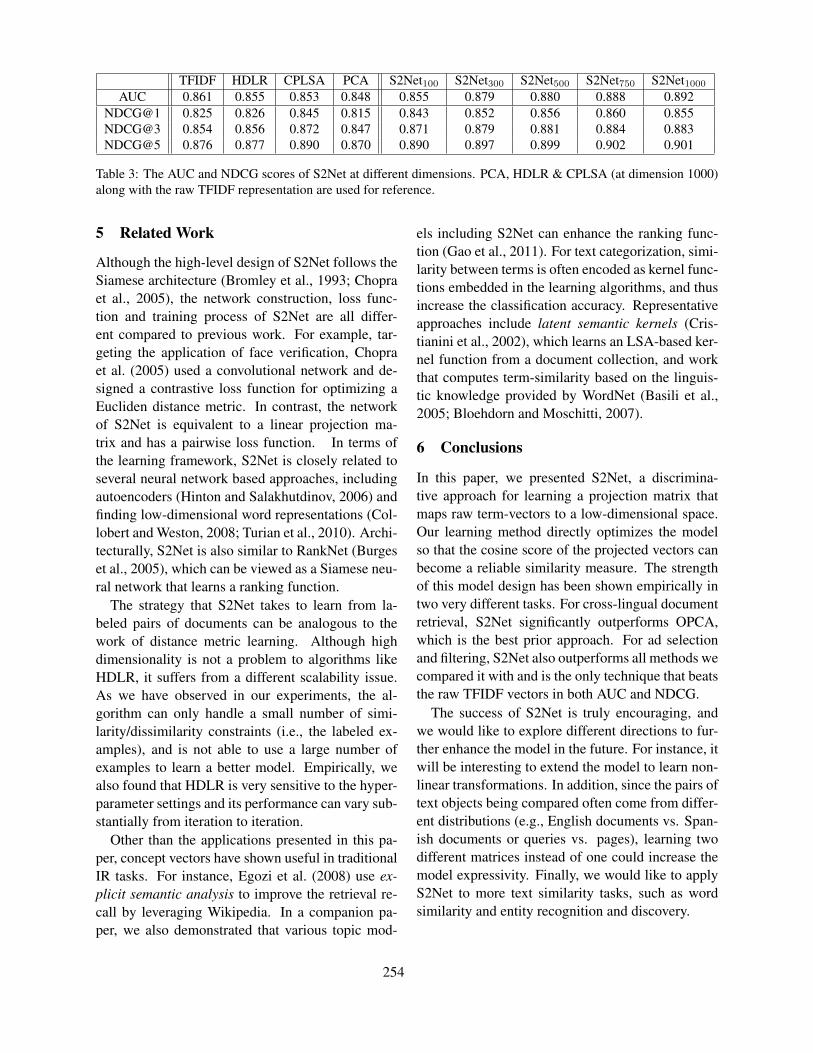
TFIDF HDLR CPLSA PCA S2Net100 S2Net300 S2Net500 S2Net750 S2Net1000AUC 0.861 0.855 0.853 0.848 0.855 0.879 0.880 0.888 0.892

NDCG@1 0.825 0.826 0.845 0.815 0.843 0.852 0.856 0.860 0.855NDCG@3 0.854 0.856 0.872 0.847 0.871 0.879 0.881 0.884 0.883NDCG@5 0.876 0.877 0.890 0.870 0.890 0.897 0.899 0.902 0.901

Table 3: The AUC and NDCG scores of S2Net at different dimensions. PCA, HDLR & CPLSA (at dimension 1000)along with the raw TFIDF representation are used for reference.

5 Related Work

Although the high-level design of S2Net follows theSiamese architecture (Bromley et al., 1993; Chopraet al., 2005), the network construction, loss func-tion and training process of S2Net are all differ-ent compared to previous work. For example, tar-geting the application of face verification, Chopraet al. (2005) used a convolutional network and de-signed a contrastive loss function for optimizing aEucliden distance metric. In contrast, the networkof S2Net is equivalent to a linear projection ma-trix and has a pairwise loss function. In terms ofthe learning framework, S2Net is closely related toseveral neural network based approaches, includingautoencoders (Hinton and Salakhutdinov, 2006) andfinding low-dimensional word representations (Col-lobert and Weston, 2008; Turian et al., 2010). Archi-tecturally, S2Net is also similar to RankNet (Burgeset al., 2005), which can be viewed as a Siamese neu-ral network that learns a ranking function.

The strategy that S2Net takes to learn from la-beled pairs of documents can be analogous to thework of distance metric learning. Although highdimensionality is not a problem to algorithms likeHDLR, it suffers from a different scalability issue.As we have observed in our experiments, the al-gorithm can only handle a small number of simi-larity/dissimilarity constraints (i.e., the labeled ex-amples), and is not able to use a large number ofexamples to learn a better model. Empirically, wealso found that HDLR is very sensitive to the hyper-parameter settings and its performance can vary sub-stantially from iteration to iteration.

Other than the applications presented in this pa-per, concept vectors have shown useful in traditionalIR tasks. For instance, Egozi et al. (2008) use ex-plicit semantic analysis to improve the retrieval re-call by leveraging Wikipedia. In a companion pa-per, we also demonstrated that various topic mod-

els including S2Net can enhance the ranking func-tion (Gao et al., 2011). For text categorization, simi-larity between terms is often encoded as kernel func-tions embedded in the learning algorithms, and thusincrease the classification accuracy. Representativeapproaches include latent semantic kernels (Cris-tianini et al., 2002), which learns an LSA-based ker-nel function from a document collection, and workthat computes term-similarity based on the linguis-tic knowledge provided by WordNet (Basili et al.,2005; Bloehdorn and Moschitti, 2007).

6 Conclusions

In this paper, we presented S2Net, a discrimina-tive approach for learning a projection matrix thatmaps raw term-vectors to a low-dimensional space.Our learning method directly optimizes the modelso that the cosine score of the projected vectors canbecome a reliable similarity measure. The strengthof this model design has been shown empirically intwo very different tasks. For cross-lingual documentretrieval, S2Net significantly outperforms OPCA,which is the best prior approach. For ad selectionand filtering, S2Net also outperforms all methods wecompared it with and is the only technique that beatsthe raw TFIDF vectors in both AUC and NDCG.

The success of S2Net is truly encouraging, andwe would like to explore different directions to fur-ther enhance the model in the future. For instance, itwill be interesting to extend the model to learn non-linear transformations. In addition, since the pairs oftext objects being compared often come from differ-ent distributions (e.g., English documents vs. Span-ish documents or queries vs. pages), learning twodifferent matrices instead of one could increase themodel expressivity. Finally, we would like to applyS2Net to more text similarity tasks, such as wordsimilarity and entity recognition and discovery.

254

References

Eneko Agirre, Enrique Alfonseca, Keith Hall, JanaKravalova, Marius Pasca, and Aitor Soroa. 2009. Astudy on similarity and relatedness using distributionaland WordNet-based approaches. In Proceedings ofHLT-NAACL, pages 19–27, June.

Arthur Asuncion, Max Welling, Padhraic Smyth, andYee Whye Teh. 2009. On smoothing and inferencefor topic models. In UAI.

Roberto Basili, Marco Cammisa, and Alessandro Mos-chitti. 2005. Effective use of WordNet semantics viakernel-based learning. In CoNLL.

David M. Blei, Andrew Y. Ng, Michael I. Jordan, andJohn Lafferty. 2003. Latent dirichlet allocation. Jour-nal of Machine Learning Research, 3:993–1022.

Stephan Bloehdorn and Alessandro Moschitti. 2007.Combined syntactic and semantic kernels for text clas-sification. In ECIR, pages 307–318.

Andrei Z. Broder, Peter Ciccolo, Marcus Fontoura,Evgeniy Gabrilovich, Vanja Josifovski, and LanceRiedel. 2008. Search advertising using web relevancefeedback. In CIKM, pages 1013–1022.

Jane Bromley, James W. Bentz, Leon Bottou, IsabelleGuyon, Yann LeCun, Cliff Moore, Eduard Sackinger,and Roopak Shah. 1993. Signature verification us-ing a “Siamese” time delay neural network. Interna-tional Journal Pattern Recognition and Artificial Intel-ligence, 7(4):669–688.

Chris Burges, Tal Shaked, Erin Renshaw, Ari Lazier,Matt Deeds, Nicole Hamilton, and Greg Hullender.2005. Learning to rank using gradient descent. InICML.

Y. Choi, M. Fontoura, E. Gabrilovich, V. Josifovski,M. Mediano, and B. Pang. 2010. Using landing pagesfor sponsored search ad selection. In WWW.

Sumit Chopra, Raia Hadsell, and Yann LeCun. 2005.Learning a similarity metric discriminatively, with ap-plication to face verification. In Proceedings of CVPR-2005, pages 539–546.

Ronan Collobert and Jason Weston. 2008. A unified ar-chitecture for natural language processing: deep neuralnetworks with multitask learning. In ICML.

Nello Cristianini, John Shawe-Taylor, and Huma Lodhi.2002. Latent semantic kernels. Journal of IntelligentInformation Systems, 18(2–3):127–152.

Jason V. Davis and Inderjit S. Dhillon. 2008. Struc-tured metric learning for high dimensional problems.In KDD, pages 195–203.

Jason V. Davis, Brian Kulis, Prateek Jain, Suvrit Sra, andInderjit S. Dhillon. 2007. Information-theoretic met-ric learning. In ICML.

Scott Deerwester, Susan Dumais, George Furnas,Thomas Landauer, and Richard Harshman. 1990. In-dexing by latent semantic analysis. Journal of theAmerican Society for Information Science, 41(6):391–407.

Konstantinos I. Diamantaras and S.Y. Kung. 1996. Prin-cipal Component Neural Networks: Theory and Appli-cations. Wiley-Interscience.

Susan T. Dumais, Todd A. Letsche, Michael L. Littman,and Thomas K. Landauer. 1997. Automatic cross-linguistic information retrieval using latent seman-tic indexing. In AAAI-97 Spring Symposium Series:Cross-Language Text and Speech Retrieval.

Ofer Egozi, Evgeniy Gabrilovich, and Shaul Markovitch.2008. Concept-based feature generation and selectionfor information retrieval. In AAAI.

Pascale Fung and Lo Yuen Yee. 1998. An IR approachfor translating new words from nonparallel, compara-ble texts. In Proceedings of COLING-ACL.

Kuzman Ganchev, Joao Graca, Jennifer Gillenwater, andBen Taskar. 2009. Posterior regularization for struc-tured latent variable models. Technical Report MS-CIS-09-16, University of Pennsylvania.

Jianfeng Gao, Kristina Toutanova, and Wen-tau Yih.2011. Clickthrough-based latent semantic models forweb search. In SIGIR.

G. E. Hinton and R. R. Salakhutdinov. 2006. Reducingthe dimensionality of data with neural networks. Sci-ence, 313(5786):504–507, July.

Thomas Hofmann. 1999. Probabilistic latent semanticindexing. In SIGIR ’99, pages 50–57.

K. Jarvelin and J. Kekalainen. 2000. Ir evaluation meth-ods for retrieving highly relevant documents. In SI-GIR, pages 41–48.

Dekang Lin. 1998. Automatic retrieval and clustering ofsimilar words. In Proc. of COLING-ACL 98.

Christopher D. Manning, Prabhakar Raghavan, and Hin-rich Schutze. 2008. Introduction to Information Re-trieval. Cambridge University Pres.

David Mimno, Hanna W. Wallach, Jason Naradowsky,David A. Smith, and Andrew McCallum. 2009.Polylingual topic models. In EMNLP.

Dragos Stefan Munteanu and Daniel Marcu. 2005. Im-proving machine translation performance by exploit-ing non-parallel corpora. Computational Linguistics,31:477–504.

Jorge Nocedal and Stephen Wright. 2006. NumericalOptimization. Springer, 2nd edition.

John Platt, Kristina Toutanova, and Wen-tau Yih. 2010.Translingual document representations from discrimi-native projections. In EMNLP.

Reinhard Rapp. 1999. Automatic identification of wordtranslations from unrelated English and German cor-pora. In Proceedings of the ACL, pages 519–526.

255

Joseph Turian, Lev Ratinov, and Yoshua Bengio. 2010.Word representations: a simple and general method forsemi-supervised learning. In ACL.

Alexei Vinokourov, John Shawe-taylor, and Nello Cris-tianini. 2003. Inferring a semantic representation oftext via cross-language correlation analysis. In NIPS-15.

Vishnu Vyas and Patrick Pantel. 2009. Semi-automaticentity set refinement. In NAACL ’09, pages 290–298.

Wen-tau Yih and Ning Jiang. 2010. Similarity modelsfor ad relevance measures. In MLOAD - NIPS 2010Workshop on online advertising.

Appendix A. Gradient DerivationThe gradient of the loss function in Eq. (2) can be

derived as follows.

∂L(∆,A)

∂A=

−γ1 + exp(−γ∆)

∂∆

∂A

∂∆

∂A=

∂

∂AsimA(fp1 , fq1)− ∂

∂AsimA(fp2 , fq2)

∂

∂AsimA(fp, fq) =

∂

∂Acos(gp,gq),

where gp = AT fp and gq = AT fq are the projectedconcept vectors of fq and fq. The gradient of thecosine score can be further derived in the followingsteps.

cos(gp,gq) =gTp gq

‖gp‖‖gq‖∇AgTp gq = (∇AAT fp)gq + (∇AAT fq)gp

= fpgTq + fqg

Tp

∇A1

‖gp‖= ∇A(gTp gp)

− 12

= −1

2(gTp gp)

− 32∇A(gTp gp)

= −(gTp gp)− 3

2 fpgTp

∇A1

‖gq‖= −(gTq gq)

− 32 fqg

Tq

Let a, b, c be gTp gq, 1/‖gp‖ and 1/‖gq‖, respec-tively.

∇A

gTp gq

‖gp‖‖gq‖= − abc3fqgTq − acb3fpgTp

+ bc(fpgTq + fqg

Tp )

256

Author Index

Ahuja, Arun, 125Akkaya, Cem, 87Alshawi, Hiyan, 19Angluin, Dana, 97Arora, Shilpa, 106

Barzilay, Regina, 1Becerra-Bonache, Leonor, 97Berg, Alexander C., 220Berg, Tamara L., 220Bohnert, Fabian, 181

Chen, Xinxiong, 135Choi, Yejin, 78, 220Cohen, Paul, 39Conrad, Alexander, 87Craven, Mark, 49

Dell’Orletta, Felice, 115Downey, Doug, 125

Gajulapalli, Kailash, 78Ghosh, Debanjan, 58Gomez, Fernando, 190

Haghighi, Aria, 1Hayes, Bruce, 48Hewlett, Daniel, 39Huang, Fei, 125

Jurafsky, Daniel, 19

Kazama, Jun’ichi, 238Komachi, Mamoru, 154Kubler, Sandra, 200Kulkarni, Girish, 220Kundu, Gourab, 229

Lee, Yoong Keok, 1Li, Siming, 220

Lignos, Constantine, 29Liu, Ying, 145Liu, Zhiyuan, 135

Matsumoto, Yuji, 154McInnes, Bridget T., 145Meek, Christopher, 247Melton, Genevieve B., 145Mihalcea, Rada, 87Miyao, Yusuke, 238Mohamed, Emad, 10Montemagni, Simonetta, 115Mukund, Smruthi, 58Munro, Robert, 68

Nyberg, Eric, 106

Ozaki, Kohei, 154

Pakhomov, Serguei V., 145Pantel, Patrick, 163Pedersen, Ted, 145Pennacchiotti, Marco, 163Platt, John C., 247

Roth, Dan, 229

Sarawgi, Ruchita, 78Schoenemann, Thomas, 172Seroussi, Yanir, 181Shimbo, Masashi, 154Spitkovsky, Valentin I., 19Srihari, Rohini, 58Sun, Maosong, 135Szumlanski, Sean, 190

Teh, Yee Whye, 219Toutanova, Kristina, 247Tsuruoka, Yoshimasa, 238

Venturi, Giulia, 115

257

Vlachos, Andreas, 49

Wiebe, Janyce, 87

Yates, Alexander, 125Yih, Wen-tau, 247Yu, Ning, 200

Zheng, Yabin, 135Zhu, Xiaodan, 210Zukerman, Ingrid, 181

CoNLL-2011 Fifteenth Conference on Computational Natural ...

Documents

Transcript of CoNLL-2011 Fifteenth Conference on Computational Natural ...