International Joint Conference on Neural Networks 2007

POST-CONFERENCE WORKSHOP ON COMPUTATIONAL INTELLIGENCE

APPROACHES FOR THE ANALYSIS OF BIOINFORMATICS DATA

CI-BIO 2007

http://ci-bio2007.disi.unige.it/

August 17th, 2007 Renaissance Orlando Resort at SeaWorld, Florida, USA

SPONSORED BY THE INNS BIOINFORMATICS SIG

EditorsFrancesco MasulliRoberto Tagliaferri

NOTES OF THE

Chairs

Francesco Masulli University of Genova (Italy)

Roberto Tagliaferri University of Salerno (Italy)

International Program Committee

Pierre Baldi, University of California, Irvine, CA, USAJake Chen, Purdue University Indianapolis, IN, USAAlexessander Couto Alves, University of Porto, PurtugalAlexandru Floares, Oncological Institute Cluj-Napoca, RomaniaJon Garibaldi, University of Nottingham, UKLuciano Milanesi, CNR-ITB, Milano, Italy David Alejandro Pelta, University of Granada, SpainLeif Peterson, The Methodist Hospital, Houston, TX, USAGiorgio Valentini, University of Milan, ItalyGennady M. Verkhivker, The University of Kansas, Lawrence, KS, USAJean-Philippe Vert, Ecole des Mines de Paris, France

i

Scope & Topics

Bioinformatics is a fast growing scientific area aimed at managing, analyzing and interpreting information from biological data, sequences and structures. In the past few years, many Computational Intelligence approaches have been successfully applied to the solution of complex problems typical of this field, including signal and image processing, clustering, feature selection,data visualization, and data mining.

CI-BIO 2007 will present surveys and contributed papers covering different areas where neural, fuzzy, and genetic approaches have been successfully applied to the analysis of Bioinformatics data.

ii

Index of contributions

"Machine Learning Methods for DNA Motif Finding" Mark Kon, Qi Ding, Dustin Holloway, Yue Fan, and Charles DeLis .................................................................................................................... 1

"Principal Direction Linear Oracle for Gene Expression Ensemble Classification", Leif E. Peterson, Matthew A. Coleman .......................................................................................................... 3

"Aggregating Memberships in Possibilistic Biclustering", Maurizio Filippone, Francesco Masulli, and Stefano Rovetta ............................................................................................................. 9

"A Review on clustering and visualization methodologies for Genomic data analysis", Roberto Tagliaferri, Alberto Bertoni, Francesco Iorio, Gennaro Miele, Francesco Napolitano, Giancarlo Raiconi and Giorgio Valentini ......................................................................................................... 10

"Topographic Map of Gammaproteobacteria using 16S rRNA gene sequence", M. La Rosa, G. Di Fatta, S. Gaglio, G.M. Giammanco, R. Rizzo, and A.M. Urso ................................................... 15

"Reverse Engineering Algorithm for Biological Networks Applied to Neural Networks and Transcription Networks", Alexandru George Floares .................................................................. 17

"Mathematical Modeling for Structure-Based Computational Drug Designing", K.I.Ramachandran, Deepa Gopakumar and Krishnan Namboori .................................................. 19

"PredLRC: Predicting Long-Range Contacts from Sequence Profile Centers and Neural Networks", Peng Chen and D.S. Huang ......................................................................................... 20

iii

Machine Learning Methods for DNA Motif Finding

Mark Kon, Qi Ding, Dustin Holloway, Yue Fan, and Charles DeLisiBoston University

We discuss some new and as well as recent neural network andmachine learning methods for gene classification and transcriptionfactor binding site (TFBS) identification based on DNA data. Theseinclude identification (from small sample sets) of human genes whicha given transcription factor (TF) controls, and also using DNAfeature data to predict specific TF binding sites. The methods haveall shown a high dimensional capacity. We consider radial basisfunction (RBF) networks, random projections, random forests,hidden Markov labeling of DNA strings, and Bayesian supportvector machines (SVM). We compare these with currentcomputational methods involving Gibbs sampling and relatedmethods (BioProspector, AlignACE, and MDSCAN), as well as toeach other. We show how SVM can assist in searching for subtlemotifs (binding DNA patterns) in humans, which can be achallenging task.

Biological motivation: In order for a TF in a cell to induceexpression of a gene, it must bind to a nearby location in the DNA.This starts reactions leading to attachment of an RNA polymerasecomplex at the beginning of the gene, which induces and controls thegene's transcription into pre-RNA. From here this process takes thegene's sequence to the ribosomes for protein production (see, e.g.,[12]). Discovering correspondence between TF's and their targets(genes they control), and more specifically identification of locationsof binding sites for TF's, has been a largely experimental process upto the last 15 years.

Figure: Biology of DNA transcription. CRM denotes cis-regulatory module, whichcan co-activate transcription with a TF (from [12])

Current algorithms: Recently a number of different algorithms forcomputational determination of binding sites have arisen ([6], [8],[7], [10]). These are largely optimization algorithms, which take aputative collection of genes thought to bind to a specific TF, andidentify DNA subsequences (sequential typicallystrings of base pairsof length 5 to 15) which are overrepresented in the potential bindingregions around these genes. This can involve a Gibbs samplingalgorithm in which an objective function measuring maximalalignment of sequences in the binding genes is gradually optimized.We will describe machine learning methods to do the same thing.

Use of string feature spaces: One way to do this is by mappingeach gene for which binding information exists (i.e. information as towhether a fixed TF binds it) into a large feature space based oncounts of substrings (short sequences of DNA bases) appearing nearthe gene in upstream, intron, intergenic, and untranslated regions.Such feature vectors have been used in a number of contexts forprotein analysis [5], TF binding prediction [2], [3], and motif finding[11]. One then finds the set of substrings which maximallydifferentiate binding and nonbinding genes (see below).

We note one way this method improves on Gibbs sampling is itsability use negative examples as well as positive ones. This creates achallenge as well as an opportunity, namely the challenge ofproviding negative examples as well as positive ones from existingdata sets. An opportunity in the case of is presented inS. cereviciaeChIP-chip data analyses [1], which provide values representingprobabilities that genes are targets of the given TF . These values, when large, provide an opportunity to label genes as "less likely" tobind . Even in genomes (like the human) where there are few (evenweakly) verified negatives, it is possible in lieu of this to deemrandomly chosen genes as negatives, since typically only 10% or lessof genes are positive targets of a given TF. In this case it is a goodidea to resample such random selections of negatives 50 to 100times, to homogenize the negative background from which positivegenes can stand out.

Motif finding algorithm: The algorithm for identifying specificbinding sites of a TF from the above information involves twosteps. The first (key) step is finding strings of length 4, 5, and 6 basepairs (bp) which are overrepresented in targets and underrepresentedin non-targets, i.e., strings that differentiate binding and nonbindinggenes. The second step involves clustering these strings together andon top of each other into representations of binding motifs. The

1

greedy clustering algorithm which we use is good but can also bereplaced by others, for example Clustal [9].

Machine learning methods can take their place in this stringdifferentiation process. The method of choice (e.g., SVM or RF) canbe used to determine which features in string space most differentiatethe positive and negative classes. We will discuss how differentmethods perform in this.

SVM results: For gene , the feature vector in the string feature space has in each position a count of the number of times agiven 4-, 5-, or 6-string (each permanently associated with a positionin the feature vector) occurs within potential binding regions near .An initial step eliminates "noisy" strings, i.e., those provingirrelevant to binding to . Examples are "AAAAAA" or "ATATAT",which are uninformative in general. The problem is they tend todilute the clusters useful to reconstructing motifs. Other sources ofconfusion include the fact that some sequences (e.g., the string"ACAC" in the sequence "ACACAC") can be counted twice becauseof overlaps. Similarly, in the string "AAAAAAA", the subsequence"AAAA" could be counted 4 times. We must dictate rules to avoidthis.

The choice of strings which best differentiate binding andnonbinding sequences is done by separation of feature vectors in (from training genes for which the binding variable is known up to an acceptable error) according to the value of .Using an SVM to classify genes according to the sign of w w , the vector points in a direction thatoptimally differentiates feature vectors for which from those with . Standard SVM methods for identification of significant components of for determining , selects for xwhich are largest in . w

A modification of this, recursive SVM (RSVM [13]) recursivelyreduces the coordinate set by reevaluating on successively smallerwsubspaces of The top 20 strings ( components) are kept, and a wgreedy algorithm is used to determine their overlaps (determiningwhen they belong to a larger motif). At this point we have not yetstudied gapped motifs (which come in two parts, separated by 5-15bp). These occur when TF's attach in pairs (dimers), and thus intotwo nearby DNA locations.

A clustering algorithm similar to the present one is discussedbriefly in [4]; the current clustering algorithm is done sequentially,with the top 20 strings presented from most to least important(according to weight) in . Successive strings either join an existingwcluster (so that all of its members overlap sufficiently), or start a newone. Once a cluster is formed from sufficiently many strings, aprobability weight matrix (PWM) is formed, based on thefrequencies of different bases in the (now fixed) positions determinedby the clusters.

A second algorithm (implemented in Matlab and soon to beavailable) involves clustering in which deletions from clusters as wellas additions to them are allowed. The pseudo-code for such an

algorithm starts by letting be the set of top (e.g., top 20) strings.Let be the current set of clusters.

Initial step: { , , }, ordered by weight in w emptyStep 0: Form a new cluster from . Delete from . Step 1: If empty, then quit. Otherwise, pick out the string with the highest weight.Step : Compute the scores of the string from Step 1 w.r.t. each of2 the current clusters in . If the highest score from is greater than theaddition threshold (threshold1 in the code), go to step 3 (additionstep). If the highest score is less than the new cluster threshold(threshold2 in the code), go to . Otherwise, go tostep step4 5Step (addition step): Add string into the cluster producing the3 highest score, and delete from . Let . Go to . step 3'Step 3' (deletion step): Examine each element in the cluster beingupdated in step 3 by computing the score of this element w.r.t. thePWM of this cluster. If the score is smaller than the deletingthreshold, move this string back into .Step : Form a new cluster in from string , and delete string4 from . Let . Go to step 1. Step : Move string into the Exceptional set . Go to step 1.5

References:[1] C. Harbison, D. Gordon, et al., "Transcriptional regulatory code of a eukaryotic

genome," pp. 99-104, 2004Nature 431,[2] D. Holloway, M. Kon and C. DeLisi, "Classifying Transcription Factor Targets

and Discovering Relevant Biological Features", preprint, 2007.[3] D. Holloway, M. Kon and C. DeLisi, "In Silico Regulatory Analysis for

Exploring Human Disease Progression," preprint, 2007.[4] M. Kon, D. Holloway, Y. Fan, S. Sai and C. DeLisi, "Learning Methods for

DNA Binding in Computational Biology," to appear, , 2007.Proc. IJCNN[5] C. Leslie, C., E. Eskin and W.S. Noble, "The Spectrum Kernel: A String Kernel

for SVM Protein Classification," Proceedings of the Pacific Symposium onBiocomputing, 2002.

[6] X. Liu, D. Brutlag, and J. Liu, "BioProspector: Discovering conserved DNAmotifs in upstream regulatory regions of co-expressed genes," Pac. Symp.Biocomputing, pp. 127–138, 2001.

[7] X. Liu, D. Brutlag, and J. Liu, "An algorithm for finding protein-DNAinteraction sites with applications to chromatin immunoprecipitationmicroarray experiments." 20, pp. 835-39, 2002.Nature Biotechnology

[8] F. Roth, J. Hughes, P. Estep, and G. Church, "Finding DNA regulatory motifswithin unaligned noncoding sequences clustered by whole-genome mRNAquantitation," , pp. 939-945, 1998.Nat. Biotechnol. 16

[9] J. Thompson, T. Gibson, F. Plewniak, F. Jeanmougin, and D. Higgins, "TheClustalX windows interface: flexible strategies for multiple sequencealignment aided by quality analysis tools," , , pp.Nucleic Acids Research 254876-4882, 1997.

[10] M. Tompa, et al., "Assessing computational tools for the discovery oftranscription factor binding sites," 23, pp. 137-144,Nature Biotechnology2005.

[11] J.-P. Vert, R. Thurman and W. S. Noble, "Kernels for gene regulatory regions,"NIPS, 2005.

[12] W. Wasserman, "Applied bioinformatics for the identification of regulatoryelements," Nature Reviews 5, pp. 276-287, 2004

[13] X. Zhang, X. Lu, Q. Shi, X. Xu, H. Leung, L. Harris, J. Iglehart, A Miron, J. Liuand W. Wong, "Recursive SVM Feature Selection and Sample Classificationfor Proteomics Mass-Spectrometry Data." , p. 197.BMC Bioinformatics 7

2

Principal Direction Linear Oracle for Gene

Expression Ensemble ClassificationLeif E. Peterson, Matthew A. Coleman

Abstract—A principal direction linear oracle (PDLO) en-semble classifier for DNA microarray gene expression datais proposed. The common fusion-selection ensemble based onweighted trust for a specifier classifier was replaced with pairsof subclassifiers of the same type using PDLO to perform alinear hyperplane split of training and testing samples. Thehyperplane split forming the oracle was based on rotations ofprincipal components extracted from sets of filtered features inorder to maximize the separation of samples between the pair ofminiclassifiers. Eleven classifiers were evaluated for performancewith and without PDLO implementation, which included knearest neighbor (kNN), naıve Bayes classifier (NBC), linear dis-criminant analysis (LDA), learning vector quantization (LVQ1),polytomous logistic regression (PLOG), artificial neural networks(ANN), constricted particle swarm optimization (CPSO), kernelregression (KREG), radial basis function networks (RBFN),gradient descent support vector machines (SVMGD), and leastsquares support vector machines (SVMLS). PLOG resultedin the best performance when used as a base classifier forPDLO. The greatest performance for PLOG implemented withPDLO occurred for tenfold CV and 100 rotations of PC scoreswith fixed angles for hyperplane splits. Random rotation anglesfor hyperplane splits resulted in reduced performance whencompared to rotations with fixed angles.

I. INTRODUCTION

Ensemble learning has proven to result in performance

levels which exceed average classifier performance[1-2]. The

history of improved ensemble learning performance is founded

on several premises. First, complexities inherent in data can

result in complex decision boundaries that are too difficult

for a single classifier to handle. The application of a given

classifier is commonly hinged to a variety of assumptions

surrounding a particular set of data and pattern recognition

functions, each of which effect scale, robustness, and com-

putational efficiency. Examples of classifier fusion techniques

include majority voting, mixture of experts, bagging, boost-

ing, and bootstrapping. Majority voting exploits a variety of

addition, product, and weighting rules for adjusting classifier

outcome to achieve better performance[3]. The mixture of

experts approach determines the particular area of the feature

space where each expert performs optimally, and assigns future

samples to the expert that is most capable of providing a

correct solution in the specific space[4-12]. Bagging ensembles

randomly select independent bootstrap samples of data and

build classifiers from the various sets of samples[13,14].

L.E. Peterson is with the Division of Biostatistics and Epidemiology, Dept.

of Public Health, The Methodist Hospital, 6550 Fannin Street, SM-1299,Houston, Texas 77030, USA. E-mail: peterson.leif@ieee.org.

M.A. Coleman is with the Biology and Biotechnology Research Program,

Lawrence Livermore National Laboratory, 7000 East Avenue, Livermore,California 94550, USA. E-mail: coleman16@llnl.gov.

Ensemble learning through boosting repeatedly runs a weak

classifier with sequentially derived weighted mixtures of the

training data to form a composite classifier[15-18].

A requirement for ensemble classifiers is that the individual

classifiers have diversity and are different from one another,

otherwise there will be no improvement in results when

compared with the individual classifiers. Hashem [19] has

reported varying degrees of diversity such as “good” and

“poor”, whose results directly translate into decreased and

increased performance based on the combination of classifiers

considered. Measurements made among classifiers employed

during bagging indicate a decrease in diversity with an increase

in the number of training instances, while for boosting the

diversity increases with increasing training sample sizes[20].

An alternative approach involves overproduce-and-select, in

which a pool of classifiers are spawned and then optimally

selected on-the-fly by monitoring accuracy and diversity pa-

rameters such as the double-fault measure[21], measure of

difficulty[22], Kohavi-Wolpert variance[23], kappa[24], and

generalized diversity[25]. Despite previous efforts to enhance

and refine ensemble methods, the majority of studies on

ensemble construction based on diversity have yielded unsatis-

factory results, since a universal theory for optimized ensemble

construction does not exist[26-28].

This investigation focuses on increasing ensemble diversity

through use of a principal direction linear oracle (PDLO).

Instead of using different classifiers in the ensemble, a single

classifier is replaced with a miniensemble of two subclassifiers

to which training and testing samples are assigned after

performing a linear hyperplane split on the principal directions

from principal component analysis (PCA). Empirical gene ex-

pression data are used for determining whether each classifier

considered resulted in better performance by itself or when

applied to PDLO. Other ensemble methods such as majority

voting, boosting, etc., were not employed since the goal of

this study was to determine which classifier resulted in the

greatest performance when used for the pair of subclassifiers

in miniensembles. The effect of the number of iterations and

the number of folds used in cross validation (CV) on PDLO

performance were also evaluated.

II. METHODS

A. DNA Microarray Data Sets Used

Data used for classification analysis were available in C4.5

format from the Kent Ridge Biomedical Data Set Repository

(http://sdmc.i2r.a-star.edu.sg/rp), see Table I. The 2-class adult

brain cancer data were comprised of 60 arrays (21 censored,

39 failures) with expression for 7,129 genes [29]. The 2-

class adult prostate cancer data set consisted of 102 training

3

2

TABLE I

DATA SETS USED FOR CLASSIFICATION ANALYSIS.

Cancer Classes-Genes-Samples Selected*

Brain[29] 2-7129-60 (21 censored, 39 failures) 16

Prostate[30] 2-12600-102 (52 tumor, 50 normal) 11

Breast[31] 2-3170-15 (8 BRCA1, 7 BRCA2) 6

Breast[32] 2-24481-78 (34 relapse, 44 non-relapse) 17

Colon[33] 2-2000-62 (40 negative, 22 positive) 5

Lung[34] 2-12533-32 (16 MPM, 16 ADCA) 29

Leukemia[35] 2-7129-38 (27 ALL, 11 AML) 9

Leukemia[36] 3-12582-57 (20 ALL, 17 MLL, 20 AML) 13

SRBCT[37] 4-2308-63 (23 EWS, 8 BL, 12 NB, 20 RMS) 20

* Genes selected using greedy PTA.

samples (52 tumor, and 50 normal) with 12,600 features. The

original report for the prostate data supplement was published

by Singh et al [30]. Two breast cancer data sets were used.

The first had 2 classes and consisted of 15 arrays for 8

BRCA1 positive women and 7 BRCA2 positive women with

expression profiles of 3,170 genes [31], and the second was

also a 2-class set including 78 patient samples and 24,481

features (genes) comprised of 34 cases with distant metastases

who relapsed (“relapse”) within 5 years after initial diagnosis

and 44 disease-free (“non-relapse”) for more than 5 years

after diagnosis [32]. Two-class expression data for adult colon

cancer were based on the paper published by Alon et al [33].

The data set contains 62 samples based on expression of

2000 genes in 40 tumor biopsies (“negative”) and 22 normal

(“positive”) biopsies from non-diseased colon biopsies from

the same patients. An adult 2-class lung cancer set including

32 samples (16 malignant pleural mesothelioma (MPM) and

16 adenocarcinoma (ADCA)) of the lung with expression val-

ues for 12,533 genes[34] was also considered. Two leukemia

data sets were evaluated: one 2-class data set with 38 arrays

(27 ALL, 11 AML) containing expression for 7,129 genes

[35], and the other consisting of 3 classes for 57 pediatric

samples for lymphoblastic and myelogenous leukemia (20

ALL, 17 MLL and 20 AML) with expression values for 12,582

genes [36]. The Khan et al [37] data set on pediatric small

round blue-cell tumors (SRBCT) had expression profiles for

2,308 genes and 63 arrays comprising 4 classes (23 arrays

for EWS-Ewing Sarcoma, 8 arrays for BL-Burkitt lymphoma,

12 arrays for NB-neuroblastoma, and 20 arrays for RMS-

rhabdomyosarcoma).

B. Gene Filtering and Selection

For each data set, input genes were ranked by the F-ratio

test statistic, and the top 150 were then used for gene selection.

Gene selection was based on a stepwise greedy plus-take-away

(PTA) method using a plus 1 take away 1 heuristic[38]. Gene-

specific expression on each array was standardized using the

mean and standard deviation over the 150 genes identified

by filtering. Forward stepping was carried out to add(delete)

the most(least) important genes for class separability based

on squared Mahalanobis distance and the F-to-enter and F-

remove statistics. Genes were entered into the model if their

standardized expression resulted in the greatest Mahalanobis

distance between the two closest classes and their F-to-enter

statistic exceeded the F-to-enter criterion. At any step, a gene

was removed if its F-to-enter statistic (F=3.84) was less than

the F-to-remove criterion (F=2.71). Table I lists the number

of genes selected using greedy PTA.

C. Principal Direction Linear Oracle

The Principal Direction Linear Oracle (PDLO) ensemble

classifier was used to invoke a linear hyperplane split of

training and testing samples into two miniclassifiers. Let xi D.xi1; xi2; : : : ; xip/ be the set of feature values for sample

xi , and zi D .zi1; zi2; : : : ; zip/ be the set of standardized

feature values for sample xi . Let R be the p�p (“gene by

gene”) correlation matrix based on n training samples. By the

principal axis theorem, there exists a rotation matrix E and

diagonal matrix ƒ such that ERE0 D ƒ. Pre-multiplying both

sides by E, and post-multiplying by E0, yields the principal

form (or spectral decomposition) of R given as

Rp�pD EƒE0

p�p(1)

where columns of E and E0 are the eigenvectors and diagonal

entries of ƒ are the eigenvalues.

The concept of principal directions relies on the eigenvec-

tors derived from PCA. Let e1; e2; : : : ; em represent the eigen-

vectors associated with the m greatest eigenvalues �1 � �2 �� � � � �m extracted from the correlation matrix R. A unique

characteristic of eigenvectors, i.e., principal components, de-

rived from PCA is they are all orthogonal (uncorrelated)

with one another. For each l th extracted principal component

(l D 1; 2; : : : ; m/ there exists a p-vector .j D 1; 2; : : : ; p/

of principal component score coefficients determined with the

relationship j l D ejl=p

�l . For each i th sample, the l th

principal component score (“PC score”) is calculated as

yi l D ˇ1lzi1 C ˇ2lzi2 C � � � C pl zip : (2)

The vector yl is distributed N.0; 1/ and serves as a new feature

representing each sample in score space. If a standardized

data set primarily consists of two largely separated clusters,

then by theory the first eigenvector e1 associated with the

largest eigenvalue �1 will form a straight line connecting the

centers of the two clusters, since the two clusters will define

the greatest amount of variation in the data. A reliable linear

hyperplane h.y/ split of the data can then be made where

yi2 D 0. Samples having positive values of yi2 lie above

h.y/ and are assigned to data set D1, whereas samples with

negative yi2 lie below h.y/ and are assigned to D2. The first

miniensemble is used for training and testing with D1 and the

second miniensemble used for training and testing with D1.

The predicted class membership of test samples in D1 and D2

are then used during construction of the confusion matrix used

in performance evaluation.

An iterative scheme was employed in which PC scores for

the first 3 PCs y1, y2, and y3 for each i th sample were rotated

around the axis of the first PC, i.e., y1 as follows0

B

B

@

y0

i1

y0

i2

y0

i3

1

1

C

C

A

D

0

B

B

@

1 0 0 0

0 cos.�/ � sin.�/ 0

0 sin.�/ cos.�/ 0

0 0 0 1

1

C

C

A

0

B

B

@

yi1

yi2

yi3

1

1

C

C

A

: (3)

4

3

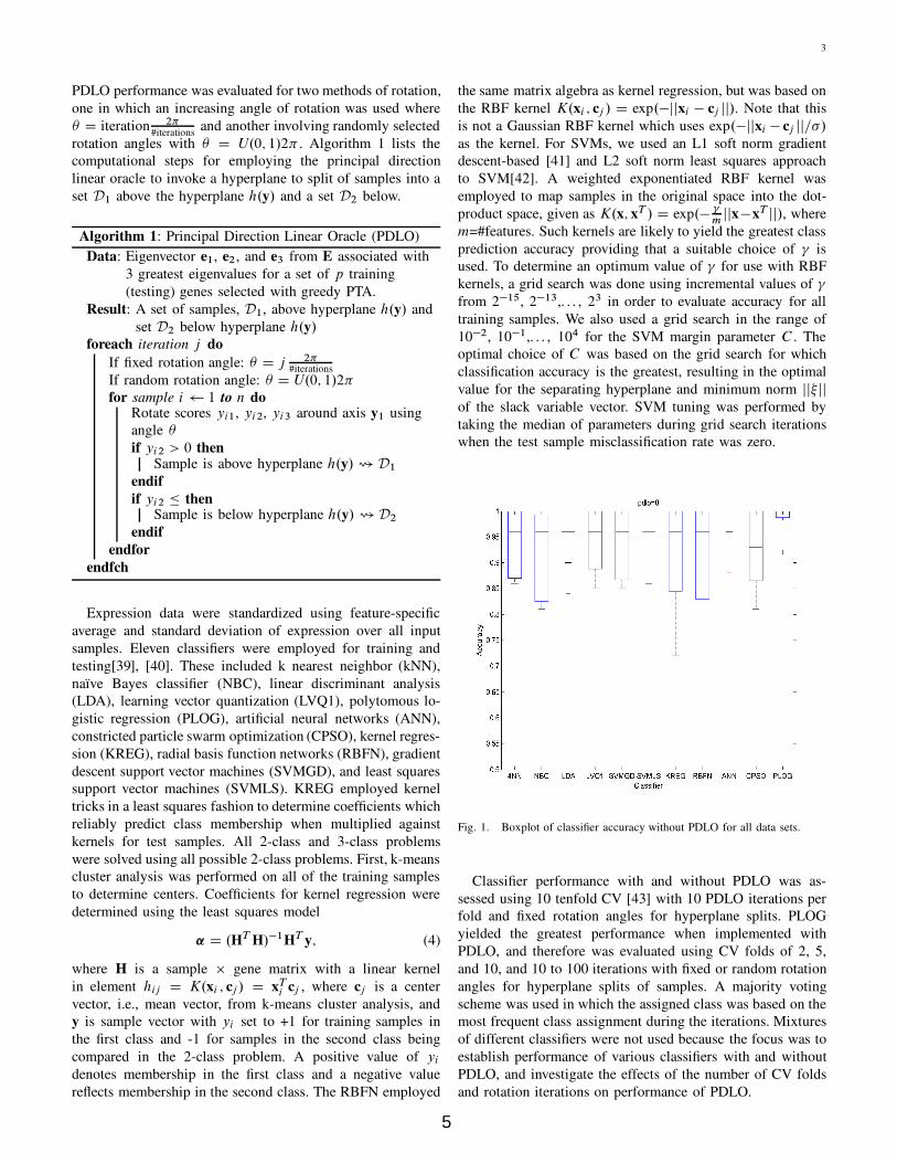
PDLO performance was evaluated for two methods of rotation,

one in which an increasing angle of rotation was used where

� D iteration 2�#iterations

and another involving randomly selected

rotation angles with � D U.0; 1/2� . Algorithm 1 lists the

computational steps for employing the principal direction

linear oracle to invoke a hyperplane to split of samples into a

set D1 above the hyperplane h.y/ and a set D2 below.

Algorithm 1: Principal Direction Linear Oracle (PDLO)

Data: Eigenvector e1, e2, and e3 from E associated with

3 greatest eigenvalues for a set of p training

(testing) genes selected with greedy PTA.

Result: A set of samples, D1, above hyperplane h.y/ and

set D2 below hyperplane h.y/

foreach iteration j do

If fixed rotation angle: � D j 2�#iterations

If random rotation angle: � D U.0; 1/2�

for sample i 1 to n doRotate scores yi1, yi2, yi3 around axis y1 using

angle �

if yi2 > 0 thenSample is above hyperplane h.y/ D1

endif

if yi2 � thenSample is below hyperplane h.y/ D2

endif

endfor

endfch

Expression data were standardized using feature-specific

average and standard deviation of expression over all input

samples. Eleven classifiers were employed for training and

testing[39], [40]. These included k nearest neighbor (kNN),

naıve Bayes classifier (NBC), linear discriminant analysis

(LDA), learning vector quantization (LVQ1), polytomous lo-

gistic regression (PLOG), artificial neural networks (ANN),

constricted particle swarm optimization (CPSO), kernel regres-

sion (KREG), radial basis function networks (RBFN), gradient

descent support vector machines (SVMGD), and least squares

support vector machines (SVMLS). KREG employed kernel

tricks in a least squares fashion to determine coefficients which

reliably predict class membership when multiplied against

kernels for test samples. All 2-class and 3-class problems

were solved using all possible 2-class problems. First, k-means

cluster analysis was performed on all of the training samples

to determine centers. Coefficients for kernel regression were

determined using the least squares model

˛ D .HT H/�1HT y; (4)

where H is a sample � gene matrix with a linear kernel

in element hij D K.xi ; cj / D xTi cj , where cj is a center

vector, i.e., mean vector, from k-means cluster analysis, and

y is sample vector with yi set to +1 for training samples in

the first class and -1 for samples in the second class being

compared in the 2-class problem. A positive value of yi

denotes membership in the first class and a negative value

reflects membership in the second class. The RBFN employed

the same matrix algebra as kernel regression, but was based on

the RBF kernel K.xi ; cj / D exp.�jjxi � cj jj/. Note that this

is not a Gaussian RBF kernel which uses exp.�jjxi � cj jj=�/

as the kernel. For SVMs, we used an L1 soft norm gradient

descent-based [41] and L2 soft norm least squares approach

to SVM[42]. A weighted exponentiated RBF kernel was

employed to map samples in the original space into the dot-

product space, given as K.x; xT / D exp.� mjjx�xT jj/, where

m=#features. Such kernels are likely to yield the greatest class

prediction accuracy providing that a suitable choice of is

used. To determine an optimum value of for use with RBF

kernels, a grid search was done using incremental values of

from 2�15, 2�13,. . . , 23 in order to evaluate accuracy for all

training samples. We also used a grid search in the range of

10�2, 10�1,. . . , 104 for the SVM margin parameter C . The

optimal choice of C was based on the grid search for which

classification accuracy is the greatest, resulting in the optimal

value for the separating hyperplane and minimum norm jj�jjof the slack variable vector. SVM tuning was performed by

taking the median of parameters during grid search iterations

when the test sample misclassification rate was zero.

Fig. 1. Boxplot of classifier accuracy without PDLO for all data sets.

Classifier performance with and without PDLO was as-

sessed using 10 tenfold CV [43] with 10 PDLO iterations per

fold and fixed rotation angles for hyperplane splits. PLOG

yielded the greatest performance when implemented with

PDLO, and therefore was evaluated using CV folds of 2, 5,

and 10, and 10 to 100 iterations with fixed or random rotation

angles for hyperplane splits of samples. A majority voting

scheme was used in which the assigned class was based on the

most frequent class assignment during the iterations. Mixtures

of different classifiers were not used because the focus was to

establish performance of various classifiers with and without

PDLO, and investigate the effects of the number of CV folds

and rotation iterations on performance of PDLO.

5

4

Fig. 2. Boxplot of classifier accuracy with PDLO for all data sets.

III. RESULTS

Figure 1 and Figure 2 show boxplots of classifier accuracy

without and with PDLO for 10 tenfold CV. In the absence of

PDLO (Figure 1), PLOG showed the greatest 25th percentile

of accuracy for all data sets, followed by ANN and LDA.

When PDLO was applied to the base classifiers, that is, use

of an oracle with two miniensembles within the classifier, the

same pattern emerged wherein PLOG had the greatest 25th

percentile followed again by LDA and ANN (Figure 2).

Fig. 3. PDLO accuracy as a function of CV folds and fixed rotation angles� used during rotation of PC scores. PLOG used as base classifier for PDLO.

Figure 3 illustrates PLOG performance with PDLO as

a function of CV folds and rotation iterations when fixed

rotation angles were used for rotating the PC scores prior

to sample hyperplane splits. Figure 4 shows that reduced

performance was obtained for PLOG implemented with PDLO

Fig. 4. PDLO accuracy as a function of CV folds and random rotation angles

� used during rotation of PC scores. PLOG used as base classifier for PDLO.

when random angles were employed for PC score rotations

before hyperplane splits of samples.

IV. DISCUSSION AND CONCLUSION

Linear oracles for classification are not a new concept. Their

use primarily originated in the development of decision tree

classifiers. Hyperplane splits first appeared in oblique decision

trees in the form of axis-parallel splits used in CART-LC

[44] and later OC1[45]. Random linear oracles were recently

applied by Kuncheva and Rodriguez to 35 UCI data sets using

a variety of classification methods including Adaboost, bag-

ging, multiboost, random subspace, and random forests[46]. In

their study of classifier ensembles, random hyperplane splits

were used in which 2 points were randomly selected and the

perpendicular vector at the midpoint between the 2 points was

used as a reference for the hyperplane. Superior results were

obtained for the random linear oracle when compared with the

routine uses of various bagging and boosting forms of decision

tree methods.

In the present study, our focus was to evaluate the effect of

PDLO on performance for 11 base classifiers, since to date this

has eluded systematic investigation. Principal directions were

used for the purpose of developing linear hyperplanes from

orthogonal eigenvectors describing the majority of variance in

the data. Thus far, we have observed that the greatest per-

formance of PDLO occurred when implemented with PLOG,

ANN, and LDA. Using PLOG as the base classifier, we

observed that tenfold CV and 100 rotations using fixed rotation

angles for hyperplane splits resulted in the greatest perfor-

mance. We are currently evaluating differences in diversity

among multiple classifiers used in ensembles vs. PDLO.

In conclusion, PLOG resulted in the best performance when

used as a base classifier for PDLO. The greatest performance

for PLOG when implemented with PDLO occurred for tenfold

CV and 100 rotations of PC scores with fixed angles for

hyperplane sample splits.

6

5

REFERENCES

[1] J. Kittler, M. Hatef, R.P.W. Duin, J. Matas. On combiningclassifiers. IEEE Transactions on Pattern Analysis and MachineIntelligence, IEEE Transactions, 20(3), 226-239. 1998

[2] L.I. Kuncheva. Combining Pattern Classifiers: Methods andAlgorithms. New York(NY): John Wiley, 2004.

[3] van Erp, M., Vuupijl, L., and Shomaker, L. An overview andcomparison of voting methods for pattern recognition. 1-6.2002. Hoboken(NJ), IEEE. Proceedings of the 8th InternationalWorkshop on Frontiers in Handwriting Recognition (WFHR02).

[4] M.I. Jordan, R.A. Jacobs. Hierarchical mixtures of experts andthe EM algorithm. Neural Computation, 6, 181-214, 1994.

[5] G.J. McLachlan, D. Peel. Finite Mixture Models. John Wiley,New York(NY), 2000.

[6] S. Gutta, J.R.J. Huang, P. Jonathon, H. Wechsler. Mixture ofexperts for classification of gender, ethnic origin, and pose ofhuman faces. IEEE Transactions on Neural Networks. 11(4),948-960, 2000.

[7] M. Szummer, C.M. Bishop. Discriminative writer adaptation.In 10th International Workshop on Frontiers in HandwritingRecognition (IWFHR), 2006.

[8] K. Rose, Deterministic annealing for clustering, compression,classification, regression, and related optimization problems.Proceedings of IEEE, 86(11), 2210-2239, 1998.

[9] K. Chen, L. Xu, H. Chi. Improved learning algorithms formixture of experts in multiclass classification. Neural Networks.12, 1229-1252 (1999).

[10] S-K. Ng, G.J. McLachlan. Using the EM algorithm to train neu-ral networks: misconceptions and a new algorithm for multiclassclassification.

[11] A. Rao, D. Miller, K. Rose, and A. Gersho. Mixture of expertsregression modeling by deterministic annealing. IEEE Transac-tions on Signal Processing. 45(11), 2811-2820, 1997.

[12] Bishop, C., and Tipping, M., A Hierarchical Latent VariableModel for Data Visualisation. IEEE Transactions on PatternAnalysis and Machine Intelligence. 20(3), 281-293, 1998.

[13] L. Breiman. Bagging predictors. Machine Learning. 24(2), 123-140, 1996.

[14] Efron, B. Estimating the error rate of a prediction rule: Im-provement on cross-validation. J. American Stat. Assoc. 1983.78:316-331.

[15] Y. Freund, R.E. Schapire. Experiments with a New BoostingAlgorithm, in Proceedings of the Thirteenth International Con-ference on Machine Learning, 148-156. San Francisco, MorganKaufmann, 1996.

[16] Y. Freund, R.E. Schapire. A short introduction to boosting. Jour-nal of Japanese Society for Artificial Intelligence, 14(5):771-780, 1999.

[17] Qu, Y, Adam, BH, Yasuo, Y, Ward, MD, Cazres, LH,Schellhammer, PF, Feng, Z., Semmes, O.J., Wright, GL.Boosted decision tree analysis of surface-enhanced laser des-orption/ionization mass spectral serum profiles discriminatesprostate cancer from noncancer patients. Clinical Chemistry2002. 48(10): 1835-1843.

[18] J. Lu, K.N. Plataniotis, A.N. Venetsanopoulos. Boosting lineardiscriminant analysis for face recognition. ICIP (1), 657-660,2003.

[19] S. Hashem. Trating harmful collinearity in neural network en-sembles. In: Combining Neural Networks (ed: A.J.C. Sharkey),pp. 101-125. London, Springer-Verlag, 1999.

[20] Skurichina M, Kuncheva LI, Duin RPW. Bagging and boostingfor the nearest mean classifier: effects of sample size on diversityand accuracy. Lecture Notes in Computer Science 2002;2364:62-71.

[21] G. Giacinto, F. Roli. Design of effective neural network en-sembles for image classification processes. Image Vision andComputing. 19(9-10), 699-707, 2001.

[22] L.K. Hansen, P. Solamon. Neural network ensembles. IEEETransactions on Pattern Analysis and Machine Intelligence.12(10), 993-1001, 1990.

[23] R. Kohavi, D.H. Wolpert. Bias plus variance decompositionfor zero-one loss functions. Proc. 13th Int. Conf. on MachineLearning, pp. 275-283. San Francisco, Margan Kaufman, 1996.

[24] D. Margineantu, T. Dietterich, T. Pruning adaptive boosting.In Proceedings of the Fourteenth International Conference onMachine Learning, Morgan Kaufmann, San Francisco, 1997.

[25] W.J. Krzanowski, D. Partridge. Software Diversity: practicalstatistics for its measurement and exploitation, Res. Report 324.Exeter(UK), Univ. of Exeter, 1995

[26] Kuncheva LI, Whitaker CJ. Measures of diversity in classifierensembles. Machine Learning 2003;51:181-207.

[27] Kuncheva LI. That Elusive Diversity in Classifier Ensembles.Lecture Notes in Computer Science 2003;2652:1126-38.

[28] Shipp CA, Kuncheva LI. Relationships between combinationmethods and measures of diversity in combining classifiers.Information Fusion 2002;3:135-48.

[29] S.L. Pomeroy, P. Tamayo, M. Gaasenbeek, L.M. Sturla, M.Angelo, M.E. McLaughlin, J-Y.H. Kim, L.C. Goumnerovak,P. M. Blackk, C. Lau, J.C. Allen, D. ZagzagI, J.M. Olson,T. Curran, C. Wetmore, J.A. Biegel, T. Poggio, S. Mukherjee,R. Rifkin, A. Califanokk, G. Stolovitzkykk, D.N. Louis, J.P.Mesirov, E.S. Lander, T.R. Golub, Prediction of central nervoussystem embryonal tumour outcome based on gene expression,Nature. 415(6870) (2002) 436-442.

[30] D. Singh, P.G. Febbo, K. Ross, D.G. Jackson, J. Manola, C.Ladd, P. Tamayo, A.A. Renshaw , A.V. D’Amico, J.P. Richie,E.S. Lander, M. Loda, P.W. Kantoff, T.R. Golub, W.R¿ Sellers,Gene expression correlates of clinical prostate cancer behavior,Cancer Cell. 1(2) (2002) 203-209.

[31] I. Hedenfalk, D. Duggan, Y. Chen et al, Gene-expressionprofiles in hereditary breast cancer, N. Engl. J. Med. 344 (2001)539-548.

[32] L.J. van ’t Veer, H. Dai, M.J. van de Vijver, Y.D. He, A.A.Hart, M. Mao, H.L. Peterse, K. van der Kooy, M.J. Marton,A.T. Witteveen, G.J. Schreiber, R.M. Kerkhoven, C. Roberts,P.S. Linsley, R. Bernards, S.H. Friend, Gene expression profilingpredicts clinical outcome of breast cancer, Nature. 415 (2002)530-536.

[33] U. Alon, N. Barkai, D.A. Notterman, K. Gish, S. Ybarra,D. Mack, and A.J. Levine, Broad patterns of gene expressionrevealed by clustering of tumor and normal colon tissues probedby oligonucleotide arrays, Proc. Natl. Acad. Sci. USA. 96(12)(1999) 6745-6750.

[34] G.J. Gordon, R.V. Jensen, L.L. Hsiao, S.R. Gullans, J.E. Blu-menstock, S. Ramaswamy, W.G. Richards, D.J. Sugarbaker, R.Bueno, Translation of microarray data into clinically relevantcancer diagnostic tests using gene expression ratios in lungcancer and mesothelioma, Cancer Res. 62(17) (2002) 4963-5967.

[35] T.R. Golub, D.K. Slonim, P. Tamayo, C. Huard, M. Gaasenbeek,J.P. Mesirov, H. Coller, M. Loh, J.R. Downing, M.A. Caligiuri,C.D. Bloomfield, E.S. Lander, Molecular Classification of Can-cer: Class Discovery and Class Prediction by Gene Expression,Science. 286 (1999) 531-537.

[36] S.A. Armstrong, J.E. Staunton, L.B. Silverman, R. Pieters, M.L.den Boer, M.D. Minden, S.E. Sallan, E.S. Lander, T.R. Golub,S.J. Korsmeyer, MLL translocations specify a distinct geneexpression profile that distinguishes a unique leukemia, NatureGenetics. 30(1) (2001) 41-47.

[37] J. Khan, J.S. Wei, M. Ringner, L.H. Saal, M. Ladanyi, F.Westermann, F. Berthold, M. Schwab, C.R. Antonescu CR, C.Peterson, R.S., Meltzer, Classification and diagnostic predictionof cancers using gene expression profiling and artificial neuralnetworks, Nature Med., 7 (2001) 673-679.

[38] Somol P., Pudil P., Nonovicova J., Paclik J. Adaptive floating

7

6

search methods in feature selection. Pattern Recognition Letters1999;20:1157-63.

[39] Peterson LE, Coleman MA. Machine learning-based receiveroperating characteristic (ROC) curves for crisp and fuzzy clas-sification of DNA microarrays in cancer research. Int. J. Approx.Reasoning, (in press).

[40] L.E. Peterson, R.C. Hoogeveen, H.J. Pownall, J.D. Mor-risett. Classification Analysis of Surface-enhanced Laser Des-orption/Ionization Mass Spectral Serum Profiles for ProstateCancer. Proceedings of the 2006 IEEE World Congress onComputational Intelligence (WCCI 2006).

[41] Christianini, N. and Shawe-Taylor, J. 2000. An Introductionto Support Vector Machines and Other Kernel-based LearningMethods. Cambridge Univ. Press, Cambridge.

[42] Abe, S. Support Vector Machines for Pattern Classification.Advances in Pattern Recognition Series. Springer, Berlin, 2005.

[43] Kohavi R. A Study of Cross-Validation and Bootstrap forAccuracy Estimation and Model Selection. International JointConference on Artificial Intelligence (IJCAI) 1995;1137-45.

[44] L. Breiman, J. Friedman, R. Olshen, C. Stone. Classificationand Regression Trees. Boca Raton(FL), Chapman & Hall/CRC,1984.

[45] Murthy, S.K., S. Kasif, and S. Salzberg. A system for induc-tion of oblique decision trees. Journal of Artificial IntelligenceResearch. 2, 1-33, 1994.

[46] L.I. Kuncheva, J.J. Rodriguez. Classifier Ensembles with aRandom Linear Oracle. IEEE Transactions on Knowledge andData Engineering. 19(4) 500-508, 2007.

8

Aggregating Memberships in Possibilistic Biclustering

Maurizio Filippone, Francesco Masulli, Stefano Rovetta

ABSTRACT

The analysis of genomic data from DNA microarray canproduce a valuable information on the biological relevanceof genes and on correlations among them. Starting fromthe seminal paper by Cheng and Church [1], in the lastfew years many biclustering algorithms have been proposedfor the analysis of Bioinformatics data sets (see, e.g., [4]).Biclustering is a learning task for finding clusters of sam-ples possessing similar characteristics together with featurescreating these similarities. When applied to genomic data itcan allow us to identify genes with similar behavior withrespect to different conditions. This paper presents a newdevelopment of a biclustering algorithm problem based onthe possibilistic clustering paradigm [3] named the Possi-bilistic BiClustering (PBC) algorithm [2]. The PossibilisticBiclustering algorithm finds one bicluster at a time, assigninga membership to the bicluster for each gene and for eachcondition and computing the membership of an element ofthe data matrix to the bicluster is obtained by aggregationof memberships of his gene and his condition with respectto bicluster.

M. Filippone, F. Masulli and S. Rovetta are with the CNISM, Via dellaVasca Navale 84, 00146 Roma, Italy and the Department of Computer andInformation Sciences, University of Genova, Via Dodecaneso 35, 16146Genova, Italy (email: {filippone|masulli|rovetta}@disi.unige.it).

Some results on oligonucleotide microarray data sets usingdifferent aggregation operators are presented and comparedwith those obtained using other biclustering methods. Theresults show the ability of the PBC algorithm to find biclus-ters with low residuals. The quality of the large biclustersobtained is better in comparison with other biclusteringmethods.

ACKNOWLEDGMENT

Work funded by a grant of the University of Genova.

REFERENCES

[1] Cheng, Y., Church, G.M.: Biclustering of expression data. In:Proceedings of the Eighth International Conference on IntelligentSystems for Molecular Biology, AAAI Press (2000) 93–103.

[2] Filippone, M., Masulli, F., Rovetta, S., Mitra, S., Banka, H.: “Possi-bilistic Approach to Biclustering: An Application to OligonucleotideMicroarray Data Analysis”, Computational Methods in Systems Biol-ogy, LNCS/LNBI4210 (2006) 312–322, Springer-Verlag, Heidelberg(Germany)

[3] Krishnapuram, R., Keller, J.M.: A possibilistic approach to clustering.Fuzzy Systems, IEEE Transactions on 1(2) (1993) 98–110.

[4] Madeira, S.C., Oliveira, A.L.: Biclustering algorithms for biologicaldata analysis: A survey. IEEE Transactions on Computational Biologyand Bioinformatics 1 (2004) 24–45.

9

A Review on clustering and visualizationmethodologies for Genomic data analysis

Roberto Tagliaferri1, Alberto Bertoni2, Francesco Iorio1,3, Gennaro Miele4,Francesco Napolitano1, Giancarlo Raiconi1 and Giorgio Valentini2

1 DMI, Universita degli Studi di Salerno - Fisciano (Sa), Italy2 DSI, Universita degli Studi di Milano - Milano, Italy

3 Telethon Institute of Genetics and Medicine - Napoli, Italy4 Dipartimento di Scienze Fisiche, Universita degli Studi di Napoli “Federico II” -

Napoli, Italy

This abstract presents a survey on the aims, the problems and the meth-ods concerning Cluster Analysis and its applications in genomic data analysis.With the term Cluster Analysis we refer to a data exploration tool whose goal isgrouping objects of similar kind into their respective categories without a prioriinformation on their classes. We can look at cluster analysis as a classificationproblem with no labeled samples, or without any a priori knowledge about theway the objects have to be put together. There are several and heterogeneousproblems linked to the cluster analysis and several times they are treated sepa-rately. In this work we examine these problems, and we illustrate the differentapproaches and their applications to Computational Biology and Bioinformat-ics. The problems related to Cluster Analysis in the context of high-dimensionalgenomic data analysis can be summarized as shown in figure 1 . In this figureeach node represents an item of the data exploration problem via cluster analysisor computational methods used in this kind of data analysis. The edges of thisgraph can be mono-directional or bi-directional and, following a path (accordingthe edge directions), one can see a sequence of steps toward the final goal ofcluster analysis and the relationships between different problems and computa-tional methods involved in unsupervised genomic data analysis.

As we can see in the figure, the problems tackled with cluster analysis areparticular cases of a more general class of problems: the partitioning problems.In this class of problems, given a set of objects N and a set of K functions f =(f1, . . . , fK) from the set N to the real numbers, the aim is to find a partition A =(A1, . . . , AK) of the set N that minimizes or maximizes an objective functiong(f1(A1), . . . , fK(AK)). In the case of cluster analysis the function defined onthe subsets Ai of N is the same for every i and usually it is the sum of thepairwise similarity between the elements of Ai (intra-cluster similarity) or theratio between intra-cluster similarity and this sum of the similarity betweenclusters (inter-cluster similarity).

The similarity can be seen as the inverse of the distance between objects.The function g is usually a sum and it should be minimized (if we use distances

10

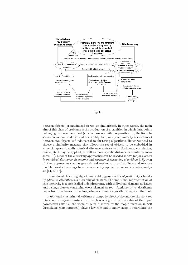
Fig. 1.

between objects) or maximized (if we use similarities). In other words, the mainaim of this class of problems is the production of a partition in which data pointsbelonging to the same subset (cluster) are as similar as possible. So, the first ob-servation we can make is that the ability to quantify a similarity (or distance)between two objects is fundamental to clustering algorithms. Hence we need tochoose a similarity measure that allows the set of objects to be embedded ina metric space. Usually classical distance metrics (e.g. Euclidean, correlation,cosine, etc.) may be applied, as well as more specific distance or similarity mea-sures [13]. Most of the clustering approaches can be divided in two major classes:hierarchical clustering algorithms and partitional clustering algorithms [13], evenif other approaches such as graph-based methods, or probabilistic and mixturemodels based clusterings have been recently applied to genomic cluster analy-sis [14, 17, 15].

Hierarchical clustering algorithms build (agglomerative algorithms), or breaksup (divisive algorithms), a hierarchy of clusters. The traditional representation ofthis hierarchy is a tree (called a dendrogram), with individual elements as leavesand a single cluster containing every element as root. Agglomerative algorithmsbegin from the leaves of the tree, whereas divisive algorithms begin at the root.

Partitional clustering algorithms attempt to directly decompose the data setinto a set of disjoint clusters. In this class of algorithms the value of the inputparameters (like i.e. the value of K in K-means or the map dimension in SelfOrganizing Map approach) plays a key role and in many cases it determines the

11

final number of clusters. In hierarchical clustering algorithms the same role isplayed by the choice of the dendrogram cutting threshold.

A major problem related to cluster analysis is the proper choice of the numberof clusters. To this end we may perform a preliminary statistical analysis on theset we want to cluster instead of blindly make clustering on it. Moreover, thisfirst analysis can check the “effective clusterizability” of a set, in other words,it checks the presence of well localized and well separable homogeneous (by thesimilarity point of view) object groups in the set. Several approaches have beenproposed in the literature: for a recent review in the context of genomic and post-genomic data analysis see, e.g. [12]. In this work we focus on methods based onthe concept of stability, as recently several works showed their effectiveness inthe analysis of genomic data [1][2][3][4][10].

In these methods many clusterings are obtained by introducing perturbationsinto the original set, and the candidate clustering is considered reliable if itsstructure is approximately reflected by the clusterings obtained on the perturbedinstances of the data. Informally, the stability of a given clustering is a measurethat quantifies the change the clustering is affected by, after a perturbation ofthe original data set. Different procedures have been introduced to randomlyperturb the data, ranging from bootstrapping techniques [1], to noise injectioninto the data [16] or random projections into lower dimensional subspaces [3].

The underlying idea of stability-based methods is described in the follow-ing. Cluster analysis is based on the (almost philosophical) assumption that thephenomenon that generated the data we want to analyze can be modeled by astatistical point of view. Can we say how much the statistical model underlyingdata has been discovered by a clustering? Can we say how much an assumptionon the artificial model (the clustering) is close to the real model? If we know theunderlying data statistical model then answers to these questions are obtainedin a quite simple way: we generate different data set samples from the same sta-tistical distribution and then we cluster each sample. If the clusterings obtainedare similar then we can look to each of them as a slightly modified version of ageneral stable clustering in which the statistical model underlying data is welldetected. So this approach is useful to test the correctness of some assumptionson the artificial model (for our purpose, the number of clusters, input valuesfor parametric clustering algorithms and so on). The “different samples” of thedata set can be obtained simulating the underlying statistical model via differentperturbation techniques.

We need similarity measures between clusterings to test how two differentclusterings are similar, and several classical measures can be applied [13][1]. Re-cently a novel measure to test similarity between partition on the same set hasbeen introduced [5][6]. It is based on the entropy of the confusion matrix betweenthe partitions and its parametric version quantifies also how much two partitionsare in conflict each other.Usually the objective functions that clustering algorithms tries to minimize hasmultiple local minima. It means that multiple and in some cases very differentsolutions grant very close optimal values for the objective function. This sug-

12

gests to analyze the whole solutions space before choose the optimal clustering.In some novel approaches multiple solutions are compared, by the objective func-tion value point of view and by the clusters composition point of view both, andembedded in a viewable map.Another important path in the graph of the figure 1 crosses the single solutionassessment node. In this case the main aim is providing reliability scores foreach cluster of a clustering and for the membership of each data point to eachcluster. In order to obtain these results, tools based on random projection tech-niques [7][8] have been modeled. Combining these tools with very simple fuzzylogic derived concepts [9], membership functions are provided for each data pointand interactive clustering is realized. These tools allow the user to consider onlythe sub set of points belonging to clusters (or sub-cluster) whose reliability isgreater than a fixed threshold value. Manually reassignments for a point whosemembership function distribution has a very high entropy are also possible.In an effective usable environment all the tools implementing these models shouldbe equipped with procedures that allow the user to easily visualize and manipu-late data and to this end dimensionality reduction techniques need to be applied.The integration of different tools that explicitly consider the problems of clustervalidity assessment, clustering reliability and robustness, discovery of multiplestructures underlying the data, as well as data and clustering results visualiza-tion, are of paramount importance in bioinformatics and bio-medical applica-tions [11][18].

In the full version of this paper each of the general arguments introduced herewill be discussed in detail, and relevant literature about them will be provided.

References

1. A. Ben-Hur, A. Elisseeff, I. Guyon. A stability based method for discovering structurein clustered data. Pacific Symposium on Biocomputing, 2002.

2. Shai Ben-David, Ulrike von Luxburg, David Pal. A Sober Look at Clustering Sta-bility. David R. Cheriton School of Computer Science, University of Waterloo, Wa-terloo, Ontario, Canada

3. A. Bertoni and G. Valentini. Discovering structures through the Bernstein inequality.In KES-WIRN 2007, Vietri sul Mare, Italy, 2007

4. M. Smolkin and D. Gosh. Cluster stability scores for microarray data in cancerstudies. BMC Bioinformatics, 36(4), 2003

5. R.J.J.H. van Son. A method to quantify the error distribution in confusion matrices.Institute of Phonetic Sciences, University of Amsterdam, Proceedings 18, 1994

6. F. Iorio and F. Napolitano. ITACA (Integrated tool for assessing clustering algo-rithm): un tool integrato per la valutazione del clustering. Degree thesis in ComputerScience. Universita degli studi di Salerno. 2007

7. B. Stein, S. M. zu Eissen, F. Wibrock. On Cluster Validity and the Information Needof Users. 3rd IASTED Int. Conference on Artificial Intelligence and Applications(AIA 03), 2003

8. A. Bertoni, G. Valentini. Random projections for assessing gene expression clusterstability. IJCNN 2005, The IEEE-INNS International Joint Conference on NeuralNetworks, Montreal, 2005

13

9. J. C. Dunn. Well separated clusters and fuzzy partitions. Journal on Cybernetics,1974

10. A. Bertoni and G. Valentini. Model order selection for bio-molecular data cluster-ing. BMC Bioinformatics, 8(Suppl.3), 2007.

11. N. Bolshakova, F. Azuaje, and P. Cunningham. An integrated tool for microarraydata clustering and cluster validity assessment. Bioinformatics, 21(4):451–455, 2005.

12. J. Handl, J. Knowles, and D. Kell. Computational cluster validation in post-genomic data analysis. Bioinformatics, 21(15):3201–3215, 2005.

13. A.K. Jain, M.N. Murty, and P.J. Flynn. Data Clustering: a Review. ACM Com-puting Surveys, 31(3):264–323, 1999.

14. H. Kawaji, Y. Takenaka, and H. Matsuda. Graph-based clustering for findingdistant relationships in a large set of protein sequences. Bioinformatics, 20(2):243–252, 2004.

15. X. Liu, S. Sivaganesan, K.Y. Yeung, J. Guo, R. E. Bumgarner, and M. Medvedovic.Context-specific infinite mixtures for clustering gene expression profiles across di-verse microarray dataset. Bioinformatics, 22(14):1737–1744, 2006.

16. L.M. McShane, D. Radmacher, B. Freidlin, R. Yu, M.C. Li, and R. Simon. Methodfor assessing reproducibility of clustering patterns observed in analyses of microarraydata. Bioinformatics, 18(11):1462–1469, 2002.

17. K.Y. Yeung, C. Fraley, A. Murua, A.E. Raftery, and W.L. Ruzzo. Model-basedclustering and data transformations for gene expression data. Bioinformatics,17(10):977–987, 2001.

18. R. Yoshida, T. Higuchi, S. Imoto, and S. Miyano. Arraycluster: an analytic toolfor clustering, data visualization and module finder on gene expression profiles.Bioinformatics, 22(12):1538–1539, 2006.

14

Topographic Map of Gammaproteobacteriausing 16S rRNA gene sequence

M. La Rosa, G. Di Fatta, S. Gaglio, G.M. Giammanco, R. Rizzo, and A.M. Urso

I. I NTRODUCTION

Microbial identification is crucial for the study of infec-tious diseases. The classical method to attribute a specificname to a bacterial isolate to be identified is based onthe comparison of morphologic and phenotypic charactersto those described for type or typical strains. Recently anew naming approach based on bacteria genotype has beenproposed and is currently under development. In this newapproach phylogenetic relationships of bacteria could bedetermined by comparing a stable part of the genetic code.The part of the DNA commonly used for taxonomic purposesfor bacteria is the 16S rRNA “housekeeping”gene. The 16SrRNA gene sequence analysis can be used to obtain aclassification for rare or poorly described bacteria, to classifyorganisms with an unusual phenotype in a well defined taxon,to find misclassification that can lead to the discovery anddescription of new pathogens.

The goal of this work is duo fold: the first one is to obtain atopographic representation of the bacteria clusters that allowsto understand the relationships among them, the second oneis to do that using genotype information without using afeature space. Many clustering works are conducted using afeature space where objects are represented. We did not usea vector space representation and we left the data in theiroriginal form.

II. M ETHODOLOGIES

A. Building Dataset

In order to test our system, we built a database of 16SrRNA gene sequences of bacteria. The choice of the set ofbacteria has been done according to the current taxonomy[1]. We focused on the bacteria belonging to Phylum BXII,Proteobacteria; Class III, Gammaproteobacteria: this classis interesting because it includes some of the most com-mon, and dangerous, bacteria related to human pathologies.Among Gammaproteobacteria class there are 14 orders, eachof them containing one or more family. Each family is alsodivided in genera; for each genus we selected the type strains(see fig. 1).

M. La Rosa, R. Rizzo and A.M. Urso are with ICAR-CNR, ConsiglioNazionale delle Ricerche, Italy.

S. Gaglio is with DINFO, University of Palermo, and with ICAR-CNR,Consiglio Nazionale delle Ricerche, Italy.

G. Di Fatta is with School of Systems Engineering, The University ofReading, United Kingdom.

G. M. Giammanco is with Dipartimento di Igiene e Microbiologia G.D’Alessandro, University of Palermo, Italy

B. Sequence Alignment

Sequence alignment allows to compare homologous sitesof the same gene between two different species. For thispurpose, we used two of the most popular alignment algo-rithms: ClustalW [2] for multiple-alignment; and Needleman-Wunsch [3] for pairwise alignment. The ClustalW algorithmaims to produce the best alignment configuration consideringall the sequences at the same time, whereas Needleman-Wunsch algorithm provides a global optimum alignmentbetween two sequences even of different length.

C. Evolutionary Distances

The evolutionary distance is a distance measure betweentwo homologous sequences, previously aligned. There areseveral kinds of evolutionary distances: the simplest one isthe number of nucleotide substitutions per site. In our study,we used the method proposed by Jukes and Cantor [4]. Wealso used the distance proposed by [5], called NormalizedCompressed Distance (NCD). This metric does not use anysequence alignment, and to compute the distance it uses anapproximation of the Kolmogorov complexity.

The above calculated distances constitute the elementsof the dissimilarity matrix that represents the input for thealgorithm described in the next sub-section.

D. Soft Topographic Map

In order to visualize the bacteria dataset we built a topo-graphic map. A widely used algorithm for topographic mapsis the Kohonen’s Self Organizing Map (SOM) algorithm [11],but it does not operate with dissimilarity data.

According to Luttrell’s works [6], the building of topo-graphic map can be interpreted as an optimization problembased on the minimization of a cost function, representingan energy function, and taking its minimum when each datapoint is mapped to the best matching neuron.

An algorithm that exploits this point of view is the onedeveloped by Graepel, Burger and Obermayer [7], [8], whichcan be seen as an extension of SOM to arbitrary distancemeasures. This algorithm is called the Soft TopographicMap (STM) and creates the map using a set of neuronsorganized in a rectangular lattice defining their neighborhoodrelationships. The cost function minimization has been doneusing the deterministic annealing [9], [10] technique.

III. E XPERIMENTAL RESULTS

We carried out many tests using the STM algorithm. Weapplied a slightly tuned version of Soft Topographic Map al-gorithm: in order to speed up processing time, neighborhood

15

functions associated to each neuron have been set to zero ifthey referred to neurons outside a previously chosen radiusin the grid.

In order to avoid the dependence from the initial conditionswe trained many maps having the same dimensions (10 foreach geometry) and we considered only the stable situations.Moreover we trained maps of different dimensions in order toconsider only stable configurations of the bacteria positions.

We also compared maps of the same dimensions obtainedfrom evolutionary distances computed starting from multiplealignment and pairwise alignment and from the NormalizedCompressed Distance; we saw that in all the above situationsthe results are quite similar. In figure 2, we show the resultsprovided by a30 × 30 map trained with the dissimilaritymatrix using the pairwise alignment. We can see that mostof the bacteria are classified according to their order in theactual taxonomy. We can also see that bacteria belonging toorder “Enterobacteriales” are split into a series of adjacentclusters in the central part of the map. This situation couldmean that order “Enterobacteriales” could be subdividedinto distinct families rather than the only one of the actualtaxonomy.

The most important result obtained from our trials isthat there are some anomalies that are constant for all theexperiments regardless to map dimensions and alignment.For example bacterium “Alterococcus agarolyticus”, of or-der “Enterobacteriales”, in small maps is wrongly clusteredtogether with bacteria of other orders, whereas in largermaps it is isolated in an individual cluster. In general, wenoticed that in the transition from smaller maps to largerones there is always a set of bacteria belonging to singleclusters and far from the other bacteria that are actuallyclassified as belonging to the same order. The explanationof this situation regards the possibility that these bacteriawere wrongly classified or that they could form brand neworders that have not discovered analyzing only phenotypicfeatures.

In conclusion, although the topographic map shows aclustering that generally reflects the existent taxonomy, thereare, however, some singular cases. The proposed system canbe a first attempt to provide an innovative instrument to bothcorrect the sequences submission system GenBank, and tobuild a genotypic features based taxonomy.

REFERENCES

[1] Garrity, G. M., Julia B. A. and Lilburn T. 2004. The revised road mapto the manual, p. 159-187.In G. M. Garrity (ed), Bergeys manual ofsystematic bacteriology. Springer-Verlag, New York, N.Y.

[2] J. D. Thompson, D. G. Higgins, and T. J. Gibson. CLUSTAL W:improving the sensitivity of progressive multiple sequence alignmentthrough sequence weighting, position specific gap penalties and weightmatrix choice. Nucleic Acids Research, 22:4673–4680, 1994.

[3] Needleman, S. B. and Wunsch, C. D. (1970) J. Mol. Biol. 48, 443-453.[4] T. H. Jukes and C. R. Cantor,Mammalian Protein Metabolism,H. N.

Munro, editors, Academic Press, New York, 1969, ch. Evolution ofProtein Molecules, pp. 21– 132.

[5] M. Li, X. Chen, X. Li, B. Ma, and P. M. B. Vitnyi,The similaritymetric, IEEE Trans. Inf. Theory, vol. 50, no. 12, pp. 32503264, Dec.2004.

Fig. 1. Actual taxonomy of our bacteria dataset

Fig. 2. 30× 30 topographic map of bacteria dataset

[6] S. P. Luttrell, “A Bayesian analysis of self-organizing maps,” NeuralComput., vol. 6, pp. 767–794, 1994.

[7] T. Graepel, M. Burger, and K. Obermayer.Self-organizing maps: gener-alizations and new optimization techniques.Neurocomputing, 21:173–190, 1998.

[8] Graepel, T. and Obermayer, K. (1999).A stochastic self organizing mapfor proximity data. Neural Computation, 11:139–155.

[9] T. Hofmann and J. M. Buhmann, “Pairwise data clustering by determin-istic annealing,” IEEE Transactions on Pattern Analysis and MachineIntelligence, vol. 19, pp. 1–14, 1997. 154

[10] Rose, K., “Deterministic Annealing for Clustering, Compression, Clas-sification, Regression, and Related Optimization Problems,” Proc. ofthe IEEE, Vol. 86:11, pp.2210-2239, 1998.

[11] Teuvo Kohonen.Self-organizing maps.Springer, Berlin; Heidelberg;New-York, 1995.

16

Reverse Engineering Algorithm for Biological Networks Applied to

Neural Networks and Transcription Networks

Alexandru George Floares

I. INTRODUCTION

Inferring networks models, like neural networks (NN) ortranscription networks (TN), from various high throughputtime-series data is a major topic in biomedical informatics.The ordinary differential equations (ODE) approach triesto get a deep understanding of the exact nature of thecircuits and their biochemical and biophysical mechanisms.This is also the most difficult approach; the models arenonlinear, high dimensional, stiff, and most of the parametersare unknown. We proposed a reverse engineering algorithmfor NN and TN based on linear genetic programming (GP)[1]. The algorithm automates the discovery of structure, andparameter estimation, and allows biochemical and biophys-ical mechanisms identification. It starts from experimentalor simulated time-series data and produces systems of ODE.To the best of author’s knowledge, this is the first realisticreverse engineering algorithm based on linear GP applied toNN and TN.

II. PROPOSED METHODS

The reversing ordinary differential equations systems(RODES) algorithm is based on a linear version of steadystate GP [1], and consists in the following steps:

1) Compute the time derivative of each variable, dXi/dt,at all discrete time points t:

a) differentiate each variable with respect to time forsimulated data;

b) fit first a function to smooth the data, and thendifferentiate it, for noisy experimental data.

2) Build input-output pairs, (Xi; dXi/dt), at the corre-sponding discrete time points t:

a) use all variables supposed to belong to the righthand side of the reconstructed ODE as inputs, and

b) use the time derivative of one of the variables asoutput, if the GP implementation accepts manyinputs but only one output, or

c) use the time derivatives of all variables as output,if the GP implementation accepts many inputsand many outputs.

3) Build training, validation (optional, to avoid overfit-ting), and testing sets from the input-output pairs.

Alexandru George Floares is with the Department of Artificial Intelli-gence, Oncological Institute Cluj-Napoca, 400015, Republicii, No 34-36,Cluj-Napoca, Transilvania, Romania (phone: +40 729 055 407; fax: +40264 591399; email: Alexandru.Floares@ieee.org).

4) Initialize a population of randomly generated pro-grams, coding mathematical models relating the inputsXi to the output(s) dXi/dt.

5) Tournament contest:

a) Randomly select four programs and evaluate theirfitness (mean squared error) - how well they mapthe input data Xi to the output data dXi/dt.

b) Select two programs as winners, and the othertwo as losers.

c) Copy the two winner programs and transformthem probabilistically by:

i) exchanging parts of the winner programswith each other to create two new programs(crossover), and/or

ii) randomly changing each of the tournamentwinners to create two new programs (muta-tion).

d) Replace the loser programs with the transformedwinner programs. The winners of the tournamentremain in the population unchanged.

6) Repeat steps 5.a through 5.d until a program is devel-oped that predicts the behavior sufficiently.

7) Extract the ODE model from the resulting program ordirectly use it.

Steps 1) to 3) transform the problem of reversing a systemof coupled ODE, in that of reversing individual, decoupled,algebraic equations. This drastically reduce the CPU time, byorders of magnitude, because in step 5.a fitness evaluationdoes not require integration of ODE systems. While the timeneeded to integrate a system of ODE seems negligible, duringfitness evaluation the integration has to be executed hundredor thousands of times per generation. These, and our previousresults [2], [3], suggest that RODES will scale up well, asrequired by the modern high throughputs biomedical tech-niques. Domain knowledge, as identified patterns in the ODEsystems modeling NN (e.g., Hodgkin-Huxley formalism) andTN, greatly reduce the structure search space of the GPcomponent of RODES. This can guide the selection of themost probable functions and input variables. Also, using theknown range of the constants involved could greatly reducethe parameters search space. GP evolves both the structureand the constants to the solution simultaneously. GP stronglydiscriminates between relevant input data and inputs thathave no bearing on a solution.

17

III. MAIN RESULTS

To illustrate the methods we used a NN and a TNmodel. The first is a conductance-based biophysical modelof cells from subthalamic nucleus and the external segmentof the globus pallidus [4]. The authors also built modelnetworks composed of synaptically coupled cells; the detailsof connections between cells are poorly understood. Thecoupling architecture of the networks and the associatedsynaptic conductances have important roles in modulatingthe activity patterns displayed by the networks. For TN, weused a model of corticoids pharmacogenomics [5].

The ODE reversing accuracy was maximal, R2 = 1, forthe NN model, and R2 = 0.99 for the TN model; the fitnessfunction was 0, the best for the NN model, and almost zerofor the TN model. The number of C programs evaluated wasof the order of 106, and the CPU time was of the orderof minutes [6]. Using domain knowledge - e.g., Hodgkin-Huxley formalism, and the known range of the parameters -drastically reduced the structural and parameters search spacefor finding the right ODE. This was done by: 1. selectingonly the functions known to belong to the right hand sideof the desired equations, 2. restricting the evolved programsto a maximal size of 128 ko, which proved sufficient for thecomplexity of the target model, and 3. restricting the range ofthe parameters. The very short CPU time is explained mainlyby the fact that fitness evaluation does not require integration.Other reverse engineering methods, based on evolutionaryalgorithms and applied to transcription or gene regulatingnetworks, require integration for fitness evaluation (e.g., [7]).Their CPU time for similar problems is of the order of hoursor even days, making their scalability problematic.

Neural networks connectivity is very important, leadingthrough dynamic interactions to different normal or patholog-ical activity patterns, like in Parkinson disease. We performedexperiments to see if RODES is able to discover from data:1. if neurons are connected, 2. which neurons are connectedwith which, 3. the inhibitory or activatory nature of the inter-actions, and 4. the values of the corresponding currents. Theexperiments belong to two extreme situations: 1. hypothesizeno connectivity, and 2. hypothesize full connectivity.

RODES is capable to discover if some information fromthe input set is either missing or not related to the output.The first situation is recognized by a performance lower thanusual, which is not increasing after reasonable long runs. Inthe second situation, RODES filters out the input variablesnot related to the target output. The final ODE does notcontain that input variables. The performance is either verygood if all the required input variables are present or is lowif some of them are missing.

For the first experiment, we simulated an equation withoutexisting synaptic connections. After 103,379,295 programsevaluated, the test R2 was 0.83974, (low value), and the testfitness function value was 256.48663, (high value; 0 is thebest). In the second experiment, we simulated an equationhaving the real synaptic connections but also some non-existing connections. The test R2 was 1, and the test fitness

function was 0, both maximal, after less than a minute. Thefinal formula given by RODES was identical with the realequation; the irrelevant synaptic connections were excluded.All experiments were performed on a PC Athlon64 x2,4800+, and 4Gb RAM.

IV. CONCLUSIONSThe ODE system approach to NN and TN modeling

is one of the most sensible but also difficult approaches.We proposed a reverse engineering algorithm for NN andTN, based on linear genetic programming - RODES. Thisalgorithm allows the investigators to automatically and si-multaneously discover the structure of NN and TN, estimatetheir parameters, and even identify the biophysical and bio-chemical mechanisms involved. It starts from experimentalor simulated time series data, and produces systems ofODE. We tested the algorithm on simulated data becausethe true structure of the network is known; this allows afaithful evaluation of the predicted models. The results werevery good in terms of accuracy, which was maximal foralmost all the experiments, and CPU time, which was ofthe order of minutes. Two factors have a major contributionto these performances: 1. The algorithm allows the use ofdomain knowledge, which drastically reduces the structuraland parameters search space, and 2. Fitness evaluation doesnot requires integration, which drastically reduces the CPUtime. These results suggest that the algorithm will scale upwell, as required by the modern high throughputs biomedicaltechniques, and can reverse engineer systems of ordinarydifferential equations in any scientific and engineering field,with a proper use of domain knowledge. To the best ofauthor’s knowledge, this is the first realistic reverse engi-neering algorithm, based on linear GP, applied to NN andTN networks.

REFERENCES

[1] M. Brameier and W. Banzhaf, Linear Genetic Programming, ser.Genetic and Evolutionary Series. Springer, 2007.

[2] A. G. Floares, “Genetic programming and neural networks feedbacklinearization for modeling and controlling complex pharmacogenomicsystems,” in Fuzzy Logic and Applications, 6th International Workshop,WILF 2005, Revised Selected Papers, ser. Lecture Notes in ComputerScience, I. Bloch, A. Petrosino, and A. Tettamanzi, Eds., vol. 3849.Crema, Italy: Springer, Sept. 15-17 2005, pp. 178–187.

[3] ——, “Computational intelligence tools for modeling and control-ling pharmacogenomic systems: Genetic programming and neural net-works,” in Proceedings of the 2006 IEEE World Cogress on Computa-tional Intelligence, G. C. Yen, L. Wang, P. Bonissone, and S. M. Lucas,Eds. Vancouver, CA: IEEE Press, 2006, pp. 7510–7517.

[4] D. Terman, J. E. Rubin, A. C. Yew, and C. J. Wilson, “Activity patternsin a model for the subthalamopallidal network of the basal ganglia,” TheJournal of Neuroscience, vol. 22, no. 7, pp. 2963–2976, April 2002.

[5] J. Y. Jin, R. R. Almon, D. C. Dubois, and W. J. Jusko, “Modeling ofcorticosteroid pharmacogenomics in rat liver using gene microarrays,”The Journal of Pharmacology and Experimental Therapeutics, vol. 307,no. 1, pp. 93–109, 2003.

[6] A. G. Floares, “Reverse engineering algorithm for neural networksapplied to the subthalamopallidal network of the basal ganglia,” inProceedings of the International Joint Confference on Neural Networks,Orlando, Florida, USA, August 2007, to appear.

[7] C. Spieth, R. Worzischek, and F. Streichert, “Comparing evolutionaryalgorithms on the problem of network inference,” in GECCO ’06:Proceedings of the 8th annual conference on Genetic and evolutionarycomputation. New York, NY, USA: ACM Press, 2006, pp. 305–306.

18

MATHEMATICAL MODELING FOR STRUCTURE-BASED COMPUTATIONALDRUG DESIGNING

Prof. K.I.Ramachandran, Dr.Deepa Gopakumar and Krishnan Namboori.P.K. Computational Engineering and Networking, Amrita Vishwa Vidyapeetham-

University, Ettimadai, Coimbatore-641 105 Tamilnadu, INDIA Email:n_krishnan@ettimadai.amrita.edu

Abstract The plasma membrane sodium-hydrogen exchanger (SHE) plays a patho-physiological role in such diverse conditions as renal acid-base disorders, essential hypertension, cancer, and tissue or organ hypertrophy. Thus, future research on plasma membrane sodium-hydrogen exchange will enhance our understanding of a great variety of physiological and Patho-physiological processes. N-(3-Oxo-3,4-dihydro-2H-benzo[1,4]oxazine-6-carbonyl) guanidines are known to be powerful sodium-hydrogen exchange inhibitors. Physicochemical descriptors of this inhibitor are determined through computational techniques. The biological activity (IC50) of these compounds is evaluated by their ability to inhibit platelet swelling induced by sodium propionate. This data was explored using data mining techniques like principal components analysis (PCA), multiple linear regression (MLR) partial least square (PLS), Support Vector Classification (SVC)etc. A comparison of result was made to identify the most helpful tool. The identified potential descriptors were correlated with biological activity through a mathematical model. This type of computational modeling helps in forecasting drug-likeness with Suitable descriptors.

19

PredLRC: Predicting Long-Range Contacts fromSequence Profile Centers and Neural Networks

Peng Chen1Department of Automation,

University of Science and Technology of China,Hefei Anhui, 230026, China2Intelligent Computing Lab,

Hefei Institute of Intelligent Machines,Chinese Academy of Sciences,

Hefei Anhui, 230031, ChinaE-mail: rochen.dragon@yahoo.com.cn

D.S. Huang∗Intelligent Computing Lab,

Hefei Institute of Intelligent Machines,Chinese Academy of Sciences,

Hefei Anhui, 230031, ChinaE-mail: dshuang@iim.ac.cn

∗Corresponding authorphone: 86-551-5591108

fax: 86-551-5592751

Abstract— Motivation: Although many developers have de-voted their efforts to improve the prediction of protein structuresusing different methods and tools, the prediction hasn’t seen itssatisfactory prediction accuracy level since the middle of thelast century due to the complexity of the problem and too manyabundant data to be processed. In order to simplify this problem,some developers studied the characteristics of protein structuresand therefore obtained higher prediction accuracy. Long-rangecontact actually is one of the important characteristics of proteinstructures.Results: This paper proposes a novel contact prediction methodby the adoption of a generalized regression neural network(GRNN) to classify the long-range contacts in protein structures.Our previous work have showed that sequence profiles of inter-residues are nearby their corresponding sequence profile center.Firstly, based on the investigation on sequence profile centers, weadopt the GRNN predictor to locate different types of sequenceprofile centers. Then, we may predict the long-range contacts bythe calculation of the distance between sequence profiles of inter-residues and their corresponding Sequence profile centers. As aresult, our predictor achieved higher prediction accuracy thanthat discussed in the previous works. Prediction results showedthat our contact prediction method outperforms other methodsproposed by previous works.

20