
European Journal of Applied Mathematics
40
European Journal of Applied Mathematics http://journals.cambridge.org/EJM Additional services for European Journal of Applied Mathematics: Email alerts: Click here Subscriptions: Click here Commercial reprints: Click here Terms of use : Click here A Survey in Mathematics for Industry An efficient method for the numerical simulation of magnetomechanical sensors and actuators M. SCHINNERL, M. KALTENBACHER, U. LANGER, R. LERCH and J. SCHÖBERL European Journal of Applied Mathematics / Volume 18 / Issue 02 / April 2007, pp 233 271 DOI: 10.1017/S0956792507006882, Published online: 29 March 2007 Link to this article: http://journals.cambridge.org/abstract_S0956792507006882 How to cite this article: M. SCHINNERL, M. KALTENBACHER, U. LANGER, R. LERCH and J. SCHÖBERL (2007). A Survey in Mathematics for Industry An efficient method for the numerical simulation of magneto mechanical sensors and actuators. European Journal of Applied Mathematics, 18, pp 233271 doi:10.1017/S0956792507006882 Request Permissions : Click here Downloaded from http://journals.cambridge.org/EJM, IP address: 131.188.201.33 on 25 Jan 2013
-
Upload
khangminh22 -
Category
Documents
-
view
0 -
download
0
Transcript of European Journal of Applied Mathematics

European Journal of Applied Mathematicshttp://journals.cambridge.org/EJM
Additional services for European Journal of Applied Mathematics:
Email alerts: Click hereSubscriptions: Click hereCommercial reprints: Click hereTerms of use : Click here
A Survey in Mathematics for Industry An efficient method for the numerical simulation of magnetomechanical sensors and actuators
M. SCHINNERL, M. KALTENBACHER, U. LANGER, R. LERCH and J. SCHÖBERL
European Journal of Applied Mathematics / Volume 18 / Issue 02 / April 2007, pp 233 271DOI: 10.1017/S0956792507006882, Published online: 29 March 2007
Link to this article: http://journals.cambridge.org/abstract_S0956792507006882
How to cite this article:M. SCHINNERL, M. KALTENBACHER, U. LANGER, R. LERCH and J. SCHÖBERL (2007). A Survey in Mathematics for Industry An efficient method for the numerical simulation of magnetomechanical sensors and actuators. European Journal of Applied Mathematics, 18, pp 233271 doi:10.1017/S0956792507006882
Request Permissions : Click here
Downloaded from http://journals.cambridge.org/EJM, IP address: 131.188.201.33 on 25 Jan 2013

Euro. Jnl of Applied Mathematics (2007), vol. 18, pp. 233–271. c© 2007 Cambridge University Press
doi:10.1017/S0956792507006882 Printed in the United Kingdom233
A Survey in Mathematics for IndustryAn efficient method for the numerical simulation
of magneto-mechanical sensors and actuators
M. SCHINNERL 1, M. KALTENBACHER 2, U. LANGER 1, R. LERCH 2
and J. SCHOBERL 1
1 Special Research Program “Numerical and Symbolic Scientific Computing”, SFB F013,
Johannes Kepler University Linz, Altenbergerstrasse 69, A-4040 Linz, Austria
email: [email protected] Department of Sensor Technology, Friedrich-Alexander-University Erlangen-Nuremberg,
Paul-Gordan-Strasse 3/5, D-91052 Erlangen, Germany
(Received 28 December 2005; revised 7 December 2006; first published online 29 March 2007)
The dynamic behaviour of magneto-mechanical sensors and actuators can be completely
described by Maxwell’s and Navier-Lame’s partial differential equations (PDEs) with appro-
priate coupling terms reflecting the interactions of these fields and with the corresponding
initial, boundary and interface conditions. Neglecting the displacement currents, which can be
done for the classes of problems considered in this paper, and introducing the vector potential
for the magnetic field, we arrive at a system of degenerate parabolic PDEs for the vector
potential coupled with the hyperbolic PDEs for the displacements. Usually the computational
domain, the finite element discretization, the time integration, and the solver are different
for the magnetic and mechanical parts. For instance, the vector potential is approximated by
edge elements whereas the finite element discretization of the displacements is based on nodal
elements on different meshes. The most time consuming modules in the solution procedure
are the solvers for both, the magnetical and the mechanical finite element equations arising at
each step of the time integration procedure. We use geometrical multigrid solvers which are
different for both parts. These multigrid solvers enable us to solve quite efficiently not only
academic test problems, but also transient 3D technical magneto-mechanical systems of high
complexity such as solenoid valves and electro-magnetic-acoustic transducers. The results of
the computer simulation are in very good agreement with the experimental data.
1 Introduction
Magneto-mechanical sensors and actuators are used in various technical devices, for
instance as force-sensors and valve-actuators in automatization-engineering, in injection-
valves for diesel engines or as actuators in loudspeakers. Numerical simulation is an
important tool for designing and optimizing these sensors and actuators.
The basis for the numerical simulation is a mathematical model that describes the dy-
namic behaviour of magneto-mechanical sensors and actuators. Such magneto-mechanical
systems can be modelled by Maxwell’s and Navier-Lame’s partial differential equations
(PDEs) describing the electromagnetic field and the mechanical field, respectively. The
interaction of these fields is taken into account by additional terms in the PDE systems.

234 M. Schinnerl et al.
The mathematical model is completed by appropriate initial, boundary and interface
conditions. Neglecting the displacement currents, which can be done for a wide range
of sensor and actuators, and introducing the vector potential for the magnetic field, we
arrive at a system of degenerate parabolic PDEs for the vector potential coupled with the
hyperbolic PDEs for the displacements.
The line variational formulations (called sometimes also weak formulations) of the
PDE systems are the starting point for the finite element discretization. The mechanical
displacements, which are in H1, are approximated by nodal tedrahedrial finite elements,
whereas the vector potential, which is in H(curl), is discretized by edge tedrahedrial finite
elements. We notice that the edge finite element discretization ensures the continuity of the
tangential component of vector potential. We use different meshes for approximating the
mechanical displacements and the magnetic vector potential. These meshes are obtained
from different refinement strategies of a common coarse mesh that represents the geometry.
Special transfer operators manage the transfer of magnetic quantities from the magnetic
grids to the mechanical grids and vice versa. These transfers are needed in the coupling
terms.
This finite element discretization results in a large-scale second-order ordinary differ-
ential equation (ODE) system for the nodal values of the displacements that is strongly
coupled with a large-scale first-order ODE system for the edge degrees of freedoms
(dofs) determining the finite element approximation to the magnetic vector potential. The
second-order ODE system is numerically integrated by a Newmark scheme, whereas the
first-order ODE system is solved by generalized trapezoidal rule. The time integration
is connected with some coupling iteration taking into account the coupling of the ODE
systems in a weak way. Since the time integration schemes are implicit, we have to solve a
large-scale linear mechanical system and a large-scale nonlinear magnetic system at each
step. The nonlinearity in the magnetic system is due to the dependence of the permeability
on the induction in ferromagnetic materials. The nonlinear magnetic system is solved by
a fixed point iteration combined with some line-search algorithm. Finally, in both cases
the arising linear systems are solved by special designed multigrid methods. The multigrid
method for the mechanical system uses a block Gauss-Seidel smoother that takes into
account the strong coupling of nodal displacements belonging to one node, whereas the
multigrid method for the magnetic systems uses the special block smoothers proposed
in [1]. An alternative multigrid technique for Maxwell’s equations was proposed in [14].
The solution of these linear systems of finite element equations is certainly the most
time-consuming part of the whole numerical algorithms. Thanks to the efficiency of these
multigrid methods we can successfully solve not only academic test problems, but also
transient 3D technical magneto-mechanical systems of high complexity such as magnetic
valves and electro-magnetic-acoustic transducers.
To the best knowledge of the authors, there is neither a complete mathematical analysis
of the coupled magneto-mechanical model discussed in this paper nor a complete numer-
ical analysis of the complicated numerical algorithm presented in this paper. Therefore, to
verify the mathematical model and the accuracy of the numerical algorithm proposed, we
perform a lot of numerical simulations for real-life problem containing all the difficulties
which are characteristic for industrial applications and compare the numerical results with
the measurements made along with the numerical simulations. The first test example is a

Numerical simulation of magneto-mechanical sensors and actuators 235
solenoid valve. We create a finite element model for the computer simulation and, at the
same time, we build the same solenoid valve for real experiments and measurements. Due
to the construction of the valve, a full 3-D simulation of the model must be performed.
Additionally, the used material is strongly nonlinear and the movement of the arma-
ture causes a displacement of the FE-mesh. Also the very low penetration-depth of the
magnetic-field is a challenge for the numerical simulation. An electro-magnetic-acoustic
transducer (EMAT) serves as a second example. The EMAT can be considered as a 3D
linear problem, because the used materials are linear and the mechanical displacements
are small. Nevertheless, the dimensions of the EMAT, which are very large in comparison
to the small penetration depth of the magnetic field, cause a very high number of 3D
finite elements. Therefore, only 2-D simulations of EMATs were performed in the past
[26].
The remaining part of the paper is organized as follows. In § 2, we present the PDEs
describing the transient behaviour of the mechanical and magnetical fields, together with
the appropriate initial, boundary, and interface conditions. Special emphasis is given to
the discussion of the influence of the coupling terms. Section 3 introduces the variational
line formulations of both field problems which are the starting point for the finite element
semidiscretization. The time integration, the iterative coupling, and the multigrid handling
are discussed in § 4. The coupling of the magnetic system to an electrical network with a
given voltage and its handling in our numerical scheme is also discussed in § 3 and § 4,
respectively. Section 5 deals with the computer simulation of two real-life applications
and their verification by experimental results. Finally, in the last section, we give some
concluding remarks.
2 PDEs for the magnetic and the mechanical fields
In this section, we briefly present the Navier-Lame and the Maxwell PDE systems describ-
ing the dynamic mechanical behaviour and the transient electromagnetic behaviour of
magneto-mechanical sensors and actuators, respectively. The eddy current approximation
to Maxwell’s equations is appropriate for our class of problems. We put special emphasis
on the terms modeling the coupling of mechanical and magnetical fields. The describing
equations are completed by appropriate initial, boundary and, interface conditions.
2.1 The mechanical system
If geometrically linear elasticity and isotropic linear material are assumed, the dynamical
behaviour of mechanical systems can be modelled by the Navier-Lame PDE system
ρ∂2d
∂t2+ c
∂d
∂t− E
2(1 + ν)
((∇ · ∇)d +
1
1 − 2ν∇(∇ ·d)
)= fV , (2.1)
where fV denotes the volume forces, E Young’s modulus, ν the Poisson ratio, ρ the specific
density and c a viscous damping of the material. On the boundary Γmech of the mechanical
computational domain Ωmech either the mechanical displacements d (Dirichlet boundary)
or the mechanical normal stresses σn (Neumann boundary) or a mechanical impedance
are given [38]. On interfaces, the continuity of the displacements and the normal stresses

236 M. Schinnerl et al.
is required. The initial conditions prescribed for the displacements d and the velocities
∂d/∂t complete the mechanical equations.
2.2 The magnetic system and the coupling terms
The transient electromagnetic behaviour of magneto-mechanical sensors and actuators is
described by Maxwell’s equations [37]. Neglecting high frequency displacement currents,
which can be always done without restrictions for the class of problems considered, we
can rewrite Maxwell’s equations in the form
∇ × H = J (Ampere’s law), (2.2)
∇ × Es = −∂B
∂t(Faraday’s law), (2.3)
∇ · B = 0 . (2.4)
In equations (2.2)–(2.4) H denotes the magnetic field strength, J the electric current
density, B the magnetic induction and Es the solenoidal part of the electric field E, which
can be written as
E = Ee + Es (2.5)
with Ee the irrotational part of E. These equations must be completed by the constitutive
relations
B = µH, (2.6)
J = Je + γ(Es +v × B
), (2.7)
where v is the velocity, γ the specific electrical conductivity and µ the permeability of
the material. Je = γEe denotes a given current density. We mention that in ferromagnetic
materials the permeability depends on the magnetic induction.
The physical quantities H , B and J have to satisfy not only equations (2.2)–(2.7) but
also certain interface- and boundary-conditions. In Fig. 1 an eddy-current problem is
shown. The regions Ω1 and Ω2 consist of materials with the conductivities γ1 and γ2. In
Ω1 and Ω2 eddy currents can arise. The region Ω3 has no conductivity but possibly an
impressed current Je. The boundary Γ = ∂Ω of the whole domain Ω = Ω1 ∪ Ω2 ∪ Ω3
usually consists of the parts ΓH and ΓB with the boundary conditions
B ·n = 0 on ΓB (2.8)
and
H ×n = K on ΓH. (2.9)
In equations (2.8) and (2.9) n denotes the outer normal unit vector to the boundary Γ . K
is a given surface current-density. On the interface Γ12 between Ω1 and Ω2 the interface
conditions
B1 ·n1 + B2 ·n2 = 0 and H1 ×n1 + H2 ×n2 = 0 (2.10)

Numerical simulation of magneto-mechanical sensors and actuators 237
eddy currents
no eddy currents
Figure 1. Model of an eddy-current problem.
must hold. The normal unit vectors are oriented in opposite directions which means that
n2 = −n1. (2.11)
Furthermore, since the the current J is divergence-free, the condition
J1 ·n1 + J2 ·n2 = 0 (2.12)
must hold on Γ12, too. On the boundaries Γ13 and Γ23, analogous conditions must be
valid.
Introducing a magnetic vector potential A
B = ∇ × A (2.13)
leads according to equation (2.3) to the relation
Es = −∂A
∂t, (2.14)
so that we can transfer equations (2.2)–(2.7) to the form
γ∂A
∂t+ ∇ ×
(1
µ∇ × A
)+ −γv × (∇ × A) = Je . (2.15)
For large Peclet-numbers
Pe =µγvh
2>> 1, (2.16)
the term γv× (∇ × A) becomes dominant and causes instabilities in the numerical solution
process [24]. In (2.16), h denotes the discretization parameter in direction of the velocity
v. However, if due to mechanical movements/deformations the overall magnetic field is
changed (e.g., movement of the armature in a magnetic valve), we have to consider the

238 M. Schinnerl et al.
Figure 2. Movement of a considered point P.
formulation of the magnetic problem on the deformed geometry [24]. Observing some
point P in a fixed reference frame Γ (x, y, z) (see Fig. 2), we can express the spatial and
temporal variation of the magnetic vector potential A at this point by the formula
∆A
∆t=
A(d + ∆d, t + ∆t) − A(d, t)
∆t
=A(d + ∆d, t + ∆t) − A(d, t + ∆t)
∆t+
A(d, t + ∆t) − A(d, t)
∆t.
For ∆t → 0, the expression (2.17) leads to the relation
dA
dt=
∂A
∂t+ (v · ∇)A. (2.17)
On the other hand, the electromotive force can be rewritten as1
v × (∇ × A) = ∇A(v · A) − (v · ∇)A. (2.18)
Using (2.17) and (2.18), we can transform the partial differential equation (2.15) into the
form
γdA
dt+ ∇ ×
(1
µ∇ × A
)− γ∇A(v · A) =Je . (2.19)
Equation (2.19) illustrates that the total differential dA/dt takes the induced current
caused by the electromotive force implicitly into account, but in return the term γ∇A(v · A)
must be considered additionally. Ifv and A are orthogonal, this term disappears, which is
the case for all 2D problems. Besides the electromotive force, magnetic forces also cause
a coupling between the magnetic and the mechanical field. The magnetic volume-force,
produced by the magnetic field, can be separated into two parts. The first effect is the
Lorentz force,
fV,L = J × B, (2.20)
1 ∇A(v · A) means, that the gradient is used only for the terms of the magnetic vector potential A.

Numerical simulation of magneto-mechanical sensors and actuators 239
Material 1 Material 2
Figure 3. Interface between two materials with different permeabilities.
which occurs when a magnetic induction B exists in a body with a current density J .
Using the magnetic vector potential A, (2.20) can be rewritten as
fV,L =
(Je − γ
dA
dt+ γ∇A(v · A)
)× (∇ × A). (2.21)
In the case of non-constant permeability, especially in the presence of ferromagnetic
materials, an additional force
fV,µ = −1
2
∣∣∣∣1µ∇ ×A
∣∣∣∣2
∇µ (2.22)
arises. At an interface between two materials with the permeabilities µ1 and µ2, the
volume-force formulation (2.22) can be transferred into Maxwell’s surface force-density
formulation [37]
fΓ = (n · H)B −n1
2B · H. (2.23)
This formulation can also be written with the help of a tensor [T ], which allows the
calculation of the magnetic force and moment acting to a body by the equations (see [36,
pp. 154–155] and [18])
f =
∮A
[T ] dA (2.24)
and
M =
∮A
r × ([T ] dA). (2.25)
We mention that (2.23) must not consider the jump of the magnetic permeability at the
interface of the ferromagnetic material. So it is sufficient to calculate (2.23) only at the
finite elements of the non-ferromagnetic domain which are connected to the interface.
For problems with permanent-magnetic materials the additional force term
fV3 = −H ∇ · M (2.26)
must be considered. M is the magnetization of the used permanent magnetic material.

240 M. Schinnerl et al.
Lastly the magnetostriction coupling effect is described by
fV4 =
H∫0
∇(
|H |2ρ∂µ
∂ρ
)dH, (2.27)
where ρ denotes the specific density. Magnetostrictive actuators are especially suited for
the generation of high forces, but this effect is not covered here.
3 Variational formulation and finite element discretization
This section provides the variational formulations of the mechanical and magnetic PDE
systems which are, of course, coupled. The coupled variational formulations are the
starting point for the finite element semi-discretization that results into a second-order
mechnical ODE system and a first-order magnetic ODE system which are again coupled.
Finally, we describe a magnetic system that is coupled to an electrical network with an
impressed voltage.
3.1 Mechanical system
By multiplying the mechanical differential equation (2.1) with a weighting function w and
integrating over the domain Ωmech, the mechanical problem is transferred to the weak
form
∫Ω
(ρ
∂2d
∂t2+ c
∂d
∂t− E
2(1 + ν)
((∇ · ∇)d +
1
1 − 2ν∇(∇ ·d)
))· w dΩ =
∫Ω
fV · w dΩ. (3.1)
Using Green’s first identity and the symmetry of the stress tensor, we obtain the variational
formulation or the so-called weak form [16]
∫Ωmech
ρ∂2di
∂t2widΩ +
∫Ωmech
ε(d)TDε(w)dΩ +
∫Ωmech
c∂di∂t
widΩ =
∫Ωmech
fiwidΩ +
∫Γni
σniwidΓ (3.2)
of (2.1), where Einstein’s summation convention is used. In (3.2), i denotes the spatial
direction (x, y, or z),ε the components of the mechanical strain tensor in Voigt notation,
D the tensor of the elastic coefficients, and Γni the boundary with given surface stress σni.
The mechanical domain is now discretized with the help of nodal finite elements.
Thereby, the mechanical displacements are approximated in the form
d ≈nn∑k=1
Nkdk, (3.3)
where Nk denotes the shape function of the k-th node, dk the displacement at the k-th node
and nn the number of nodes. By using (3.3) in (3.2) and applying Galerkin’s technique,

Numerical simulation of magneto-mechanical sensors and actuators 241
the system of second-order ordinary differential equations (ODE)
M
∂2d
∂t2
+ C
∂d
∂t
+ Kd = F (3.4)
is obtained, where the mass matrix M, the stiffness matrix K and the force vector Fhave the following form:
• Mass matrix:
M = [Mab], with Mab = δij
∫Ω
NaρNb dΩ, 1 a, b neq, 1 i, j nsd. (3.5)
• Stiffness matrix:
K = [Kab], with Kab =eTi
∫Ω
BTa DBb dΩej , 1 a, b neq, 1 i, j nsd. (3.6)
In the 3D case, we have
Ba =
⎛⎜⎜⎜⎜⎜⎜⎜⎜⎜⎜⎜⎜⎝
∂Na
∂x0 0
0 ∂Na
∂y0
0 0 ∂Na
∂z
0 ∂Na
∂z∂Na
∂y
∂Na
∂z0 ∂Na
∂x
∂Na
∂y∂Na
∂x0
⎞⎟⎟⎟⎟⎟⎟⎟⎟⎟⎟⎟⎟⎠
. (3.7)
• Force vector:
F = Fa, with Fa =
∫Ω
NafidΩ +
∫Γni
NaσnidΓ . (3.8)
In (3.5)–(3.8) neq denotes the number of unknowns, ei the unity vector in the spatial
direction i, δij Kronecker’s operator and nsd the spatial dimension of the mechanical field.
The damping matrix C is chosen as a linear combination of M and K [5], i.e.
C = αM + βK. (3.9)
The magnitudes of the Rayleigh coefficients α and β depend on the energy dissipation
characteristics of the modelled mechanical problem.
3.2 Magnetic system
By multiplying the magnetic system (2.19) with a weighting function W , integrating over
the domain Ωmag(d), which is deformed by the mechanical displacement d, and applying
the first Green’s identity, the magnetic field can be expressed in a weak sense by the

242 M. Schinnerl et al.
x
yz
interface Γ n
material 2 (µ2, γ2)
material 1 (µ1, γ1)
Figure 4. Interface between two materials.
variational formulation∫Ωmag
γdA
dt· W dΩ +
∫Ωmag
1
µ(∇ × A) · (∇ × W ) dΩ −
∫Ωmag
γ ∇A(v · A) · W dΩ
=
∫Ωmag
Je · W dΩ +
∫Γmag,H
(H ×n) · W dΓ , (3.10)
where Γmag,H denotes a boundary with specified H ×n. To achieve an appropriate FE-
discretization of the magnetic system, the properties of the magnetic field at an interface
must be analyzed in a more detailed way. In Fig. 4 an interface between two materials with
the permeabilities µ1 and µ2 and the conductivities γ1 and γ2 is displayed. For simplicity
and without loss of generality, the interface lies in the x-y plane and the normal-vector n
is exactly oriented in the z-direction. Using (2.13) and (2.10), the condition
Bn = Bz =∂Ay1
∂x− ∂Ax1
∂y=
∂Ay2
∂x− ∂Ax2
∂y(3.11)
must be satisfied. Equation (3.11) can be enforced explicitly, if the tangential component ofA is continuous at the interface. As mentioned in § 2.2 displacement currents are neglected,
which enables the reformulation of (2.12) on an interface between two eddy-current regions
as
n · γ1∂A1
∂t= n · γ2
∂A2
∂t. (3.12)
Therefore, in the z direction, the equation
∂
∂t[γ1Az1 − γ2Az2] = 0 (3.13)
must hold. Since the magnetic vector potential is not static, (3.13) requires a discontinuity
of Az if γ1 γ2. For nodal finite elements one needs a splitting of the magnetic vector
potential in a new vector, which has to be divergence free, and a gradient of a scalar
potential (corresponds to a decomposition of the space H(curl)). In addition, a weighted
regularization according to [7] has to be applied. For a detailed discussion we refer to [19].
The “natural” choice of the spatial discretization are edge-finite-elements [28]. Thereby,
the degrees of freedom are not attached to the element nodes, but to the element edges. In
Fig. 5 a linear edge-tetrahedron-element is shown. Using the edge element discretization,

Numerical simulation of magneto-mechanical sensors and actuators 243
4
A5
A3
A63
2
1
A
A
A
1
4
2
Figure 5. Linear edge tetrahedron.
the magnetic vector field A is approximated by
A ≈nk∑k=1
NkAk. (3.14)
In (3.14), Nk denotes the vectorial shape function, which is associated with the k-th edge
ek , nk the number of edges in the magnetic FE mesh, and
Ak =
∫ek
A · ds (3.15)
approximates the line integral over the projection of the magnetic vector potential A to
the k-th edge ek . Inserting (3.14) into the weak formulation (3.10) leads to the first-order
ODE system
L
dA
d t
+ PA + P2(v)A = Q. (3.16)
The conductivity matrix L, the permeability matrix P, the second permeability matrix P2
and the source vector Q have the forms:
• Conductivity matrix:
L = [Lab], with Lab =
∫Ωmag(d)
Na · γNbdΩ, 1 a, b nk. (3.17)
• Permeability matrix:
P = [Pab], with Pab =
∫Ωmag(d)
(1
µ∇ × Na
)· (∇ × Nb) dΩ, 1 a, b nk. (3.18)
• Permeability matrix 2:
P2 = [P2ab], with P2ab = −∫
Ωmag(d)
γ∇A(v · Na) · Nb dΩ, 1 a, b nk. (3.19)
244 M. Schinnerl et al.
U(t)
I(t) Rcoil
FE-model of thetransient magneto-mechanical problem
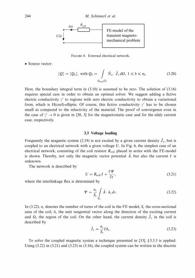
Figure 6. External electrical network.
• Source vector:
Q = Qb, with Qb =
∫Ωmag(d)
Na · Je dΩ, 1 b nk. (3.20)
Here, the boundary integral term in (3.10) is assumed to be zero. The solution of (3.16)
requires special care in order to obtain an optimal solver. We suggest adding a fictive
electric conductivity γ′ to regions with zero electric conductivity to obtain a variational
form, which is H(curl)-elliptic. Of course, this fictive conductivity γ′ has to be chosen
small as compared to the reluctivity of the material. The proof of convergence even in
the case of γ′ → 0 is given in [30, 3] for the magnetostatic case and for the eddy current
case, respectively.
3.3 Voltage loading
Frequently the magnetic system (2.19) is not excited by a given current density Je, but is
coupled to an electrical network with a given voltage U. In Fig. 6, the simplest case of an
electrical network, consisting of the coil resistor Rcoil placed in series with the FE-model
is shown. Thereby, not only the magnetic vector potential A, but also the current I is
unknown.
The network is described by
U = Rcoil I +∂Ψ
∂t, (3.21)
where the interlinkage flux is determined by
Ψ =nc
Sc
∫Ωj
A ·ns dν. (3.22)
In (3.22), nc denotes the number of turns of the coil in the FE model, Sc the cross-sectional
area of the coil, ns the unit tangential vector along the direction of the exciting current
and Ωj the region of the coil. On the other hand, the current density Je in the coil is
described by
Je =nc
ScIns. (3.23)
To solve the coupled magnetic system a technique presented in [33], § 5.3.3 is applied.
Using (3.22) in (3.21) and (3.23) in (3.16), the coupled system can be written in the discrete

Numerical simulation of magneto-mechanical sensors and actuators 245
form as
L
dA
d t
+ PA + P2(v)A = uI, (3.24)
Rcoil I + uTdA
d t
= U. (3.25)
Thereby, the coupling vector u has the form
u =nc
Sc
∫Ωj
Ni ·ns dν ∈ IRNe , (3.26)
where Ne denotes the number of edges in the considered FE mesh.
4 Time integration, iterative coupling and solution
A mathematically strong coupling of the mechanical and the magnetic system in one
large equation system is hard to realize, because the electromotive force is a nonlinear
term, i.e., both fields contribute directly to this effect. Additionally, the Lorentz force
and the interface force, caused by variations of the magnetic permeability, are quadratic
functions of the magnetic vector potential A. Therefore, an iterative coupling mechanism,
used for instance in [31, 20], is applied. Therewith, it is possible to consider variations of
the magnetic field, which are caused by the mechanical displacement d, easily. In order to
achieve a good adaptation of the FE meshes to the mechanical and magnetic fields, two
different grids are used for both physical fields. Therefore, it is necessary to transfer data,
like the mechanical displacement d or the magnetic volume-force fV , between the edge
element discretization of the magnetic field and the nodal element discretization of the
mechanical field. The time discretization of the mechanical and the magnetic system is
achieved by implicit time stepping algorithms. The large-scale systems of mechanical FE
equations are solved by a geometrical multigrid method whereas the nonlinear system of
magnetic FE equations are solved by multigrid combined with a fixed point iteration.
4.1 Time discretization of the mechanical and the magnetic systems
The time discretization of the second-order mechanical ODE system (3.4) is performed
by using Newmark’s technique [16]. To shorten the notation, the velocity ∂d/∂t and
the acceleration ∂2d/∂t2 at the nodes are abbreviated by v and a, respectively. In
addition to this, the curved brackets for the FE nodal and edge values are omitted. The
index n denotes the variable at the time moment n∆t, where ∆t denotes the used time
step. Applying Newmark’s technique gives the equations
Man+1 + Cvn+1 + Kdn+1 = Fn+1 (4.1)

246 M. Schinnerl et al.
for defining
dn+1 = dn + ∆tvn +∆t2
2[(1 − 2β)an + 2βan+1], (4.2)
vn+1 = vn + ∆t[(1 − γ)an + γan+1], (4.3)
where β and γ denote Newmark’s parameters which control the stability and accuracy of
the method.
The first-order magnetic ODE system (3.16) is numerically integrated by the use of the
generalized trapezoidal rule, giving the equations
LRn+1 + PAn+1 + P2(vn+1)An+1 = Qn+1 (4.4)
for defining
An+1 = An + ∆tRn+α, (4.5)
Rn+α = (1 − α)Rn + αRn+1, (4.6)
where the abbreviation R is used for the time derivation ∂A/∂t of the edge dofs [16].
4.2 Iterative coupling of the mechanical and magnetic systems
The time discretization methods of the mechanical and magnetic systems are coupled
by an iterative technique handling the coupling of the mechanical and magnetic parts
(k denotes the iteration counter and n the time step counter):
• Step 1: Calculation of a first approximation to the mechanical displacement and velocity
on the mechanical mesh Mmech:
dkn+1 = dn + ∆tvn +∆t2
2an, (4.7)
vkn+1 = vn + ∆tan. (4.8)
• Step 2: Projection of dkn+1 and vkn+1 from Mmech to the magnetic mesh Mmag .
• Step 3: Distortion of the magnetic mesh Mmag by dkn+1. Reassembling of the conducti-
vity-matrix L and the permeability matrix P at the deformed geometry. According to
(2.17), the total differential of the magnetic vector potential is calculated by this updating
and, thereby, the electromotive force is implicitly taken into account. Additionally, the
variation of the magnetic field, caused by the mechanical displacement, is considered
by the updating process.
• Step 4: Calculation of the magnetic system:
The matrix P2(v) is non-symmetric and depends on the velocity v, therefore, this term
is only approximated by a predictor value:
Aappn+1 =
An + ∆tRn k = 1
Akn+1 otherwise
(4.9)
Numerical simulation of magneto-mechanical sensors and actuators 247
P2(vn+1)An+1 := P2(vkn+1)Aappn+1. (4.10)
Solve the system
L∗Rk+1n+1 = Qn+1 − PAn − (1 − α)∆tPRn − P2(vkn+1)A
appn+1, (4.11)
with the system matrix
L∗ = L + α∆tP. (4.12)
Correct the vector potential:
Ak+1n+1 = An + (1 − α)∆tRn + α∆tRk+1
n+1 . (4.13)
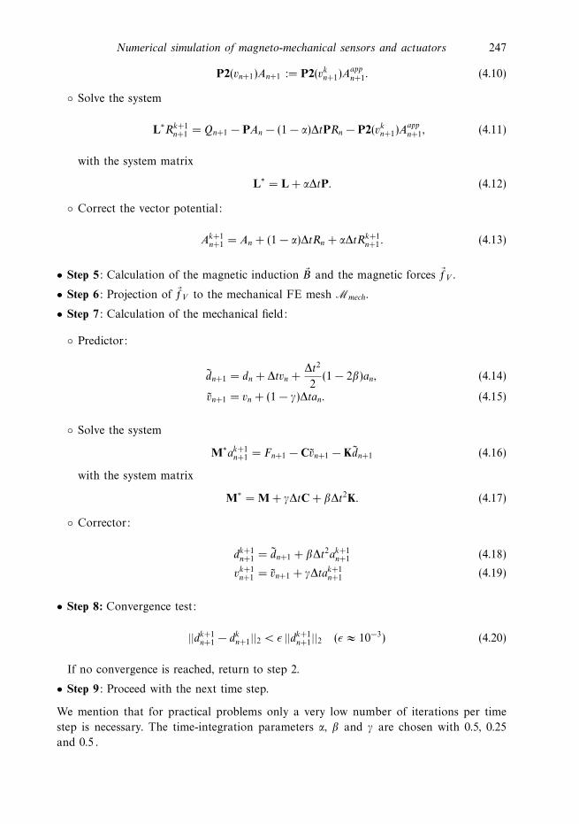
• Step 5: Calculation of the magnetic induction B and the magnetic forces fV .
• Step 6: Projection of fV to the mechanical FE mesh Mmech.
• Step 7: Calculation of the mechanical field:
Predictor:
dn+1 = dn + ∆tvn +∆t2
2(1 − 2β)an, (4.14)
vn+1 = vn + (1 − γ)∆tan. (4.15)
Solve the system
M∗ak+1n+1 = Fn+1 − Cvn+1 − Kdn+1 (4.16)
with the system matrix
M∗ = M + γ∆tC + β∆t2K. (4.17)
Corrector:
dk+1n+1 = dn+1 + β∆t2ak+1
n+1 (4.18)
vk+1n+1 = vn+1 + γ∆tak+1
n+1 (4.19)
• Step 8: Convergence test:
||dk+1n+1 − dkn+1||2 < ε ||dk+1
n+1||2 (ε ≈ 10−3) (4.20)
If no convergence is reached, return to step 2.
• Step 9: Proceed with the next time step.
We mention that for practical problems only a very low number of iterations per time
step is necessary. The time-integration parameters α, β and γ are chosen with 0.5, 0.25
and 0.5 .

248 M. Schinnerl et al.
4.3 Calculation of the magnetic field in the presence of ferromagnetic materials
Ferromagnetic materials have a non-constant magnetic permeability µ. Thereby, the
nonlinear relation
H =1
µ(B)B. (4.21)
holds. It is assumed, that the material is isotropic, i.e. that µ is equal in each direction,
and that no hysteresis effects arise. In the nonlinear case, system (4.11) has the form
L∗(A)Rn+1 = Qn+1 − P(A)An − (1 − α)∆tP(A)Rn − P2(vappn+1)Aappn+1. (4.22)
In (4.22), the modified conductivity matrix L∗ and the permeability matrix P depend on
the edge degrees of freedom. The nonlinear magnetic field is calculated by a fixed-point
method [35], which is described by the following algorithm:
• Step 1: Calculation of an initial guess Ain+1 by using the variables of the time step n:
i = 0, (4.23)
Ain+1 = An + ∆tRn, (4.24)
Rin+1 = 0. (4.25)
• Step 2: Reassembling of the matrices L∗ and P.
• Step 3: Calculation of improved guesses Ri+1n+1 and Ai+1
n+1:
L∗(Ain+1)R
i+1n+1 = Qn+1 − P(Ai
n+1)An − (1 − α)∆tP(Ain+1)Rn
− P2(vAn+1)Ain+1, (4.26)
Ai+1n+1 = An + (1 − α)∆tRn + α∆tRi+1
n+1. (4.27)
• Step 4: Convergence test:
IF
‖Ri+1n+1 − Ri
n+1‖ ε‖Rin+1‖ (4.28)
THEN i = i + 1 and return to Step 2
ELSE proceed with the next time step.
In many cases this algorithm is oscillating or only slowly convergent. However, the method
can be stabilized by a line-search algorithm [35]. Thereby, Step 3 of the iteration must be
modified as follows:
• Step 3.1: Calculation of improved guesses Rin+1 and Ai
n+1.
• Step 3.2: Calculation of a search direction
δRn+1 = Ri+1n+1 − Ri
n+1, (4.29)
δAn+1 = Ai+1n+1 − Ai
n+1. (4.30)

Numerical simulation of magneto-mechanical sensors and actuators 249
• Step 3.3: Choosing of a relaxation parameter τ and calculation of modified guesses
Rτn+1 = Ri
n+1 + τδRn+1, (4.31)
Aτn+1 = Ai
n+1 + τδAn+1. (4.32)
• Step 3.4: Reassembling of L∗ and P and calculation of the residual Ψ (τ) and the
projection of the residual to the search direction G(τ):
Ψ (τ) = L∗Rτn+1 − Qn+1 + PAτ
n+1 + P2(vappn+1)Aappn+1, (4.33)
G(τ) = δRn+1 · Ψ (τ). (4.34)
Now, the relaxation parameter τ is chosen in such a way that the projection of the residual
to the search direction is a minimum. Since even for strong nonlinear materials G(τ) is
approximately a linear function of τ, it is sufficient to calculate G(τ) for two different
values of τ and to determine the optimal τ with linear interpolation. This method leads
to a fast convergent and very stable solution process with comparatively low numerical
effort in the case of applying a full multigrid method.
4.4 Modifications in the case of voltage loading
One possibility to take into account the external network is the coupling of (3.24) and
(3.25) in one coupled system [31]. Thereby, the structure of the arising system matrix
is destroyed, which may lead to a slower convergence of the used iterative MG solvers.
Therefore, in this paper an alternative strong coupling method of the magnetic field and
the network is chosen, which preserves the structure of the system matrix. By multiplying
(3.24) with the inverse modified mass matrix (L∗)−1, we obtain
Rn+1 = (L∗)−1uIn+1 − (L∗)−1[PAn − (1 − α)∆tPRn − P2(vkn+1)A
appn+1
]. (4.35)
Using the abbreviation
An+1 = PAn − (1 − α)∆tPRn − P2(vappk )Aappn+1 (4.36)
and inserting (4.35) in the time discretized form of (3.25), we arrive at the relation
Un+1 = uT (L∗)−1uIn+1 + Rcoil In+1 − uT (L∗)−1An+1, (4.37)
which can be rewritten in the form
In+1 =Un+1 + uT (L∗)−1An+1
uT (L∗)−1u + Rcoil. (4.38)
Therefore, in the case of voltage loading, the calculation of the magnetic field at each
time step is modified as follows:
• Approximations:
Aappn+1 =
An + ∆tRn k = 1
Akn+1 else
(4.39)
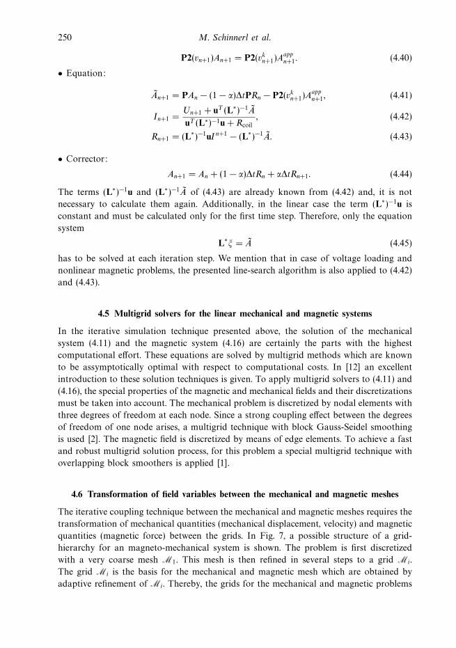
250 M. Schinnerl et al.
P2(vn+1)An+1 = P2(vkn+1)Aappn+1. (4.40)
• Equation:
An+1 = PAn − (1 − α)∆tPRn − P2(vkn+1)Aappn+1, (4.41)
In+1 =Un+1 + uT (L∗)−1A
uT (L∗)−1u + Rcoil, (4.42)
Rn+1 = (L∗)−1uIn+1 − (L∗)−1A. (4.43)
• Corrector:
An+1 = An + (1 − α)∆tRn + α∆tRn+1. (4.44)
The terms (L∗)−1u and (L∗)−1A of (4.43) are already known from (4.42) and, it is not
necessary to calculate them again. Additionally, in the linear case the term (L∗)−1u is
constant and must be calculated only for the first time step. Therefore, only the equation
system
L∗ξ = A (4.45)
has to be solved at each iteration step. We mention that in case of voltage loading and
nonlinear magnetic problems, the presented line-search algorithm is also applied to (4.42)
and (4.43).
4.5 Multigrid solvers for the linear mechanical and magnetic systems
In the iterative simulation technique presented above, the solution of the mechanical
system (4.11) and the magnetic system (4.16) are certainly the parts with the highest
computational effort. These equations are solved by multigrid methods which are known
to be assymptotically optimal with respect to computational costs. In [12] an excellent
introduction to these solution techniques is given. To apply multigrid solvers to (4.11) and
(4.16), the special properties of the magnetic and mechanical fields and their discretizations
must be taken into account. The mechanical problem is discretized by nodal elements with
three degrees of freedom at each node. Since a strong coupling effect between the degrees
of freedom of one node arises, a multigrid technique with block Gauss-Seidel smoothing
is used [2]. The magnetic field is discretized by means of edge elements. To achieve a fast
and robust multigrid solution process, for this problem a special multigrid technique with
overlapping block smoothers is applied [1].
4.6 Transformation of field variables between the mechanical and magnetic meshes
The iterative coupling technique between the mechanical and magnetic meshes requires the
transformation of mechanical quantities (mechanical displacement, velocity) and magnetic
quantities (magnetic force) between the grids. In Fig. 7, a possible structure of a grid-
hierarchy for an magneto-mechanical system is shown. The problem is first discretized
with a very coarse mesh M1. This mesh is then refined in several steps to a grid Mi.
The grid Mi is the basis for the mechanical and magnetic mesh which are obtained by
adaptive refinement of Mi. Thereby, the grids for the mechanical and magnetic problems

Numerical simulation of magneto-mechanical sensors and actuators 251
Figure 7. Possible grid-hierarchy of a coupled magneto-mechanical problem.
can be adapted to the special properties of the fields. For instance the magnetic mesh can
be very fine in eddy-current regions whereas the mechanical mesh remains coarse there.
The transformation of the mechanical and magnetic quantities between the different grids
is now realized by multigrid transfer operators. These operators are described for instance
in [12, 17, 33].
5 Application examples
It is not possible to verify the presented simulation technique for coupled magneto-
mechanical problems by a mathematical proof. Therefore, the technique was tested and
verified by modelling and measuring of two challenging magneto-mechanical devices.
The dynamical behaviour of the two models (a solenoid valve and an electro-magnetic-
acoustic-transducer) was measured and compared to the simulated results. Additionally,
the properties of the presented simulation technique with respect to the simulation time
were analyzed.
5.1 Solenoid valve
Electro-magnetic actuators are widely used for industrial purposes. Examples are the
application in clutches, brakes, relays, loudspeakers, printers and as solenoid valves for
pneumatic and hydraulic systems. The reasons for the success of these actuators are
• large magnetic forces,
• large and adjustable strokes, and
• a very robust and stable design.
The disadvantages of electro-magnetic actuators are
• the nonlinear behaviour of the magnetic materials,
• strong variations of the magnetic force depending on the position of the armature and
• the magnetic force acts only in one direction.

252 M. Schinnerl et al.
compression spring
distance boltarmature
plain bearing
pot-magnet
tappet
guiding plate
x
zcoil
Figure 8. Cross section of the solenoid valve.
5.1.1 Design of the solenoid valve
In Fig. 8, the principal setup of a solenoid valve is illustrated. The main parts are an
armature and a pot-magnet which are made of soft-magnetic material. A prestressed
pressure-spring holds the armature in its upper position. If the coil is excited by an
electric current, a magnetic force between the pot-magnet and the armature is generated
which causes a movement of the armature. The valve-tappet transfers the movement to
the mechanical acting mechanism. The outer diameter of the structure is 90mm, the height
145mm and the diameter of the tappet is 10mm. The armature and the pot-magnet consist
of unalloyed steel. For both, the guiding-plate and the distance-bolt, alloyed nonmagnetic
steel is used and the plain-bearings are made of brass [6]. The coil has 200 turns of copper
wire with 1mm diameter. In Fig. 9, the fully assembled solenoid valve is illustrated.
5.1.2 Simulation model
In Fig. 10, the pot-magnet is displayed. In order to reduce the eddy currents in the material,
cuts are milled into the magnet [34]. These cuts destroy the axi-symmetry of the solenoid
valve. Therefore, a 3D analysis of the problem must be performed. In Fig. 11, the coarse
grid of the pot-magnet is displayed. The radial component of the magnetic induction is
zero at the cuts. Therefore, only one eighth of the problem must be considered. At the
interface between the pot-magnet and the coil, eddy currents with a very low penetration
depth occur. Assuming a maximum relative permeability µr = 1200, a specific conductivity
γ = 5 · 106 S/m and a maximum frequency of 2000Hz, we can estimate a penetration
depth of [18]
δ =1√
πγµ0µrf= 103 µm. (5.1)

Numerical simulation of magneto-mechanical sensors and actuators 253
Figure 9. Solenoid valve with slotted pot-magnet and force sensor.
Figure 10. Pot-magnet with four slots which are situated in a relative angle of 90.
The penetration depth was discretized with the help of flat tetrahedron-elements (Fig. 11),
where 6 tetrahedron layers for δ were used at the finest discretization level. Therewith, a
magnetic edge element discretization with 75 · 103 degrees of freedom was necessary. The
mechanical mesh was much coarser and had 20 · 103 mechanical degrees of freedom.

254 M. Schinnerl et al.
slot
eddy-currentregions
Figure 11. Coarse grid of the pot magnet.
5.1.3 Frequency response of the solenoid valve (clamped armature)
To guarantee the suitability of the used magnetic FE simulation model, the frequency
response of the voltage-current transfer function (impedance) is analyzed. The impedance
of the solenoid valve is strongly affected by the eddy currents in the pot-magnet and the
armature. Therefore, the determination of the simulated frequency response allows us an
evaluation of the used simulation model. Only if the model takes into account the small
penetration depths at the surfaces of the magnetic materials, the simulated impedance
agrees with the measured impedance.
Let us consider the case of the frequency response for small excitations. With the
help of an impedance-analyzer [13], the frequency response of the solenoid valve was
measured in the frequency range of 100–750 Hz. Since the measurement causes a very
small induction in the magnetic circuit, a linear behaviour of the magnetic material can
be assumed. To determine the frequency response of the valve, a transient simulation is
performed. Thereby, the input voltage u(t) is quadratically integrable. Using the Fourier
analysis for the input signal u(t) and the calculated current i(t), the frequency response
Z(ω) can be determined by
Z(ω) =U(ω)
I(ω). (5.2)
U(ω) and I(ω) denote the input voltage and simulated current which are transferred
into the frequency domain. Figure 12 compares the measured and calculated impedance
of the solenoid valve. The air gap between armature and pot magnet is zero. Additionally,
the simulated impedance for the case of neglected eddy currents is depicted. In this case,
the impedance of the valve behaves like the impedance of an ideal inductance which
means that it increases linearly as a function of the frequency. The comparison of the

Numerical simulation of magneto-mechanical sensors and actuators 255
0 100 200 300 400 500 600 7000
0.5
1
1.5
2
2.5
3
3.5
4
4.5
5
simulation witheddy-currents
measurement
simulation withouteddy-currents
frequency (Hz)
impe
danc
e (O
hm)
Figure 12. Impedance of the magnetic valve.
Fmag
compression-tube force-sensor armature
Figure 13. Mechanical equivalent circuit in the case of a clamped armature.
curves with and without consideration of the eddy current shows that the eddy currents
have a significant influence on the dynamical behaviour of the solenoid valve and must
definitely be taken into account.
5.1.4 Simulated and measured dynamical magnetic force (clamped armature)
To measure the magnetic force to the armature, the compression spring (Fig. 8) is replaced
by a compression tube which suppresses the movement of the armature. Therefore, the vis
inertiae can be neglected. Nonlinear vibrations at the contact areas between the guiding
plate, the compression tube and the armature are prevented by a prestressing of the
mechanical circuit with the force Fv . If the magnetic force Fmag becomes larger than the
prestressing force Fv , the mechanical circuit is described by an equivalent network which is
displayed in Fig. 13. The same force acts at each element of the serial equivalent network,
because the vis inertiae is neglected. Therefore, the used force sensor directly measures
the magnetic force Fmag .
To produce a high magnetic force, the coil with 200 turns is loaded by a current pulse.
The air gap δ between the armature and the magnetic pot is 2 mm. Since the magnetic
circuit is strongly excited by the current pulse, the consideration of the nonlinearity of

256 M. Schinnerl et al.
Figure 14. Setup of the hysteresisgraph. Left: Power and measure electronic; right: Double
C-yoke with probe [4].
0 5 10 15 20 25 300
0.5
1
1.5
2
2.5
magnetic field-strength H (kA/m)
indu
ctio
nB
(T)
Figure 15. Measured virgin magnetization-curve of the used material St37.
the used ferromagnetic material is necessary. To measure the magnetization curve, a
rod-shaped probe of the used material is measured with the help of a hysteresisgraph
(Fig. 14).
The used frequency is approximately 0.1 Hz. Because of this low frequency the influence
of the eddy currents can be neglected. The magnetic pot, the armature, and the probe
were annealed in a nitrogen atmosphere. The annealing process reduces the stresses in
the material. The magnetization curve of the used steel St37 is displayed in Fig. 15. The
low amount of carbon and other admixtures as well as the annealing process result in
a steel with a soft magnetic behaviour. Therefore, hysteresis effects can be neglected. In
Fig. 16, the simulated and measured magnetic force of the solenoid valve is displayed.

Numerical simulation of magneto-mechanical sensors and actuators 257
-5 0 5 10 15 20 25 30 35 40
0
200
400
600
800
1000
1200
simulation
measurement
prestressing force
time (ms)
mag
neti
cfo
rce
(N)
Figure 16. Magnetic force Fz in the air gap (clamped armature).
laser vibrometer
force-sensor
capacitor
Shunt
switch
U
R
Figure 17. Measurement of the dynamical behaviour of the solenoid valve.
The inductance of the valve and the eddy currents in the magnetic circuit delay the rise
of the magnetic force. After a time of 4 ms, the maximum of the magnetic force (1200 N)
is reached. The maximum of the magnetic induction is 1.9 T. This value of the magnetic
induction causes a strong saturation of the material.
5.1.5 Simulated and measured movement of the armature
To measure the movement of the armature, the compression spring with a stiffness of
cSpring = 18.3 kN/m was loaded by a pre-stress force of F0 = 198 N.
Again, the current in the coil was produced by a capacitor discharge. The transient
current was measured with the help of a shunt and the movement of the armature

258 M. Schinnerl et al.
0 1 2 3 4 5 6 7 8 9 10
–1.0
–1.2
–0.8
–0.6
–0.4
–0.2
0
time (ms)
simulation
measurement
disp
lace
men
t(m
m)
Figure 18. Simulated and measured movement of the armature.
was measured with a Laser-Doppler-Vibrometer [29]. The advantages of the contactless
measurement with a vibrometer are the good and linear distance resolution, which is only
limited by noise, and a very good dynamic range.
In Fig. 18, the simulated and measured movement of the armature are compared.
During the first 1.2 ms after switching on the voltage the magnetic force is smaller than
the mechanical pre-stress which avoids a movement of the armature. After these first 1.2
ms the magnetic force is large enough to overpower the pre-stress and an acceleration of
the armature in the direction of the pot-magnet takes place. Due to the decreasing of the
gap between the armature and the pot-magnet the magnetic force is additionally increased.
To show the influence of the geometric variations, the magnetic force is simulated with
and without considering the geometrical effect of changing the magnetic computational
domain (see Fig. 19). At the beginning of the simulation the armature is in rest and
the magnetic force is the same for both simulations. After approximately 1.5 ms, the air
gap is decreased considerably, which causes a stronger raise of the magnetic force in the
geometrically nonlinear simulation. Therefore, it is necessary to consider the geometric
effect in the simulation of the solenoid valve.
5.1.6 Simulation times
Figure 18 shows, that the time between switching on the voltage and contact of the
armature and pot-magnet is 2.8 ms. The time step width for the simulation is chosen to
be 100 µs which means that 28 time steps are necessary to simulate the movement of the
armature. At each time step one nonlinear magnetic field problem must be solved. For
the solution of this nonlinear problem an average of 10 iterations was necessary. Each
iteration required the solution of the magnetic FE equation system (4.26). Therefore, the
solution of these systems is the most time-consuming part of the simulation process. The
considered simulation model with 75000 edge degrees of freedom could by solved with

Numerical simulation of magneto-mechanical sensors and actuators 259
consideration of thegeometrical effect
no movement ofthe armature
time (ms)
mag
neti
cfo
rce
(N)
0 0.5 1 1.5 2 2.5
1500
1000
500
0
Figure 19. Simulated magnetic force Fz with and without considering the movement of the
armature.
the presented multigrid technique in 21 seconds. The total calculation time for the whole
dynamical 3D simulation was 3.05 hours on the SGI Origin with 300 MHz RS12000
processors.
5.2 Electro-Magnetic-Acoustic-Transducer (EMAT)
Inspecting materials by utilizing ultrasonic waves is a widely used industrial technique
[23]. A transducer generates a sound wave which propagates in the material under test.
With the help of the position and the shape of reflected and transmitted acoustic waves
it is possible to find defects (e.g. cracks) in the material. Piezoelectric transducers are
frequently used for the generation and detection of sound waves. For a good transmission
of the wave a contact medium must be used between the piezoelectric transducer and the
material. Alternative transducer types, which allows a contactless material test, are Electro-
Magnetic-Acoustic-Transducers (EMATs) [26]. These are considered in this section.
5.2.1 Generation of acoustic bulk waves with an EMAT
In Fig. 20, the principal setup of an EMAT is shown. It consists of a permanent magnet
(magnetized in z-direction) and a meander coil.
The test specimen is situated below the EMAT. The specimen is made of a conductive
material. If the meander coil is fed by a transient current Idyn(t), a transient magnetic field
and eddy currents Jeddy(t) are induced in the specimen. Due to the Lorentz force
fdyn = Jeddy × (Bdyn + Bstat) (5.3)
a mechanical force is generated which leads to the transmission of a sound wave in the

260 M. Schinnerl et al.
Figure 20. Setup of an EMAT.
Figure 21. Magnetic field of a conductor near a conductive plate.
specimen. It must be taken into account that the magnetic field Bdyn and the force densityfdyn decrease with the distance to the surface of the specimen. The region with an effective
generation of a mechanical wave can be determined by the penetration depth (see Fig. 21)
δ =1√
πfγµ0µr. (5.4)
In equation (5.4), f denotes the frequency of the excitation current Idyn, γ the conductivity,
µ0 the permeability in vacuum and µr the relative permeability of the used material.

Numerical simulation of magneto-mechanical sensors and actuators 261
Figure 22. Phase velocity of existing modes in an aluminum-plate.
S0:
A0:
Figure 23. Lamb wave modes in a plate. Above: symmetrical plate wave with zero-order (S0),
Bottom: asymmetrical plate wave with zero-order (A0).
5.2.2 Using EMATs for the generation of Lamb waves
Let us assume that the specimen is a thin plate. That means that the thickness d of the
plate is small compared to the wavelength λ of the sound wave. If linear elasticity and a
plane strain situation is assumed, the existing plate waves can be described by a number
of nonlinear equations [22] which can be solved by numerical techniques. The results of
this calculation can be demonstrated by a mode dispersion diagram (see Fig. 22). On the
abscissa of Fig. 22, the product of excitation frequency and plate thickness, and on the
ordinate, the phase velocity are displayed. The abbreviations S0, A0, S1, A1, S2 and A2
refer to the different Lamb modes in the plate. The letter S is used for modes which are
symmetrically to the plane of symmetry of the plate, whereas A is used for modes which
are antisymmetric to the plane of symmetry. The used number describes the order of the
wave in the thickness of the plate. In Fig. 23, the S0 and A0 modes are displayed.

262 M. Schinnerl et al.
aluminum
1.5 mm
δ 1mm
eddy-current region
conductor
z
x
magnetizationpermanent-
magnet
Figure 24. Cross-section of the EMAT and the aluminum-plate in the x-z plane
(dimensions in mm).
To excite one of the plate waves with the help of an EMAT, the excitation-frequency
must be chosen in such a way that an additive superposition of the conductor forces
arise. The maximum excitation can be reached when the wave length of the chosen mode
is equal to two times the distance a between two conductors. Therewith, it is possible to
determine the optimal excitation frequency of the different plate modes by drawing the
straight line v = 2 a/d into the dispersion diagram (see Fig. 22).
5.2.3 Simulation model
In former publications, for instance, in [26, 9], a constant magnetic and mechanical
field in the y-dimension was assumed. In this case, only a 2D numerical simulation of
EMATs was considered. Since the length of the EMATs in y-direction is in the same
order of magnitude as the wave-length of the excited plate, diffraction effects occur. These
effects are not considered by the 2D models. In this work, a real 3D simulation of the
transmission behaviour of an EMAT is presented.
In Fig. 24, a cross-section of the EMAT and the specimen (aluminum-plate) in the x-z
plane is shown. The used material parameters of aluminum are the following [22]:
• Young’s modulus E = 7.0713 · 1010 N/m2,
• Poisson ratio ν = 0.3375,
• specific density ρ = 2.7 · 102 kg/m3, and
• specific electrical conductivity γ = 35.5 · 106 Sm.
The conductors of the meander coil are 1 mm thick and 0.1 mm high. The distance
between the permanent magnet and the meander coil is 0.3 mm. The static magnetic field
of 0.29 T in z-direction is produced by a Neodym-Iron permanent-magnet. By using the
phase velocity diagram (see Fig. 22), the optimal excitation frequency of the A0-mode is
fin = 650 kHz. This frequency results in a penetration depth into the plate which can be
approximated by δ = 104.7 µm.
This very small penetration depth requires a fine edge element discretization of the
aluminum plate under the EMAT. In Fig. 26, the coarse grid discretization of the meander
coil and the permanent magnet is shown. The model uses the symmetry of the problem

Numerical simulation of magneto-mechanical sensors and actuators 263
meander-coil
80
5014
11.5
permanent-magnet
aluminum-platex
y
Figure 25. EMAT and aluminum plate in the x-y plane (dimensions in mm).
permanent-magnet
meander-coil
symmetry-plane
Figure 26. Coarse grid mesh of the meander coil and the permanent magnet.
in the y-z plane. Since the gradient of the magnetic field in x- and y-direction is weak,
flat tetrahedral elements with a length to hight ratio of 15 are used. The number of
necessary finite elements could be reduced considerably by these flat elements. The height
of the coarse-grid elements in the area of the penetration depth is 150 µm. To achieve a
sufficiently fine resolution of the penetration depth, these elements must be refined twice.
This results in elements with a maximal hight of 37.5 µm. The final magnetic edge element
mesh has the following properties:
• 391.500 edge-tetrahedron-elements,
• 342.625 edges (degrees of freedom).
The wave length λ of the excited A0-mode is 3 mm. To describe the propagation of this
mode for the maximal side-length emax of the mechanical elements
emax =λ
k(5.5)

264 M. Schinnerl et al.
0 0.2 0.4 0.6 0.8 1 1.2 1.4 1.6 1.8 2
-250
-200
-150
-100
-50
0
50
100
150
200
250
time (s)
curr
ent (
A)
Figure 27. Excitation of a A0 Lamb wave by an current burst.
must hold. The so called locking-effect, which results in too stiff elements, is avoided
by the use of elements with quadratic basis functions [5]. For quadratic elements, it is
sufficient to choose k = 6 [21]. With this assumptions the final mechanical FE mesh has
the following properties:
• 191.000 quadratic tetrahedron-elements,
• 261.000 nodes,
• 783.000 degrees of freedom.
5.2.4 Simulation of the generation and the propagation of a Lamb wave
By loading the meander coil of the EMAT by a sine current burst, the A0-mode in the
plate is excited. The sine burst with a frequency of 650 kHz (see Fig. 27) is filtered by
a Kaiser-window which reduces the bandwidth of the burst considerably [25]. The time
step of the FE-simulation is chosen with 100 ns. In Fig. 28 and Fig. 29, the simulated
transversal components of the generated Lamb wave are shown for different time steps.
It can be seen that the main part of the wave propagates in normal direction to the
conductors. Nevertheless, also radiations in other spatial directions occur. After 4 µs
waves in positive and negative y-direction can be detected. These waves are reflected after
approximately 6 µs on the upper and lower boundary of the plate. The shape of the
reflected waves can be seen clearly after 8.5 µs. The main wave is reflected on the right
plate boundary after approximately 11 µs. The reflected wave can be seen after 15 µs.
The shape of the wave for a single point can be seen in Fig. 30. In this case the current
excitation burst had five sinus-periods. In Fig. 30, the shape of the radiated wave front
with its maximum after 11 µs can be seen clearly. The wave is reflected on the right
boundary and reaches the considered point after 21 µs again.

Numerical simulation of magneto-mechanical sensors and actuators 265
Figure 28. z-component (transversal component) of the Lamb wave at the surface of the
aluminum plate.
5.2.5 Measurement and simulation of the radiation pattern of the EMAT
To measure the radiation pattern of the EMAT, the experimental setup which is shown
in Fig. 31 is used. To excite the EMAT with sine burst of a frequency of 650 kHz, a
RITEC System is used [32]. This system allows the generation of pulses with very high
currents. In Fig. 32, the whole measurement setup is displayed. By use of the RITEC
system a current pulse in the meander coil is generated. The produced mechanical wave is
detected with the help of a laser-doppler vibrometer. The output signal of the vibrometer
is filtered by the RITEC system and is then displayed on an oscilloscope. By measuring

266 M. Schinnerl et al.
Figure 29. Transversal component of the Lamb wave at the surface of the aluminum plate.
0 5 10 15 20 25 30-0.5
-0.4
-0.3
-0.2
-0.1
0
0.1
0.2
0.3
0.4
0.5
time (s)
velo
city
(m
m/s
)
Figure 30. z-component of the surface velocity in a point with the coordinates x = 20 mm
and y = 0 mm.

Numerical simulation of magneto-mechanical sensors and actuators 267
shunt
holding device meander-coil
resonator permanent-magnet
Figure 31. Setup of the EMAT and the integrated amplifier circuit [15].
TransmitterLaser-Doppler-Vibrometer
Control
Data
Trigger HF-Signal
Personal Computer
Figure 32. Setup to measure the radiation pattern of a Lamb wave EMAT.
the maximum amplitude of the wave for different angles ϕ and constant distance r of the
vibrometer measurement point, the radiation characteristic can be obtained (see Fig. 33).
To avoid to big errors of the measurement, the distance r must be out of the nearfield of
the EMAT. The size of the nearfield can be estimated by the Fresnel distance [27]
rf = w2 k
10 π= 26.6mm, (5.6)
where w denotes the length of the meander coil in y-direction and k = 2 π/λ the wave

268 M. Schinnerl et al.
Figure 33. Measurement of the radiation pattern of the EMAT with the help of a
laser-doppler vibrometer.
–80 –60 –40 –20 0 20 40 60 800
0.2
0.4
0.6
0.8
1
norm
aliz
ed z
-dis
plac
emen
t
angle (degrees)
measurement3D simulation
Figure 34. Simulated and measured radiation pattern of a plate-wave EMAT (excitation
frequency 0.65 MHz).
number. In the simulation, the amplitude of the radiated wave for different angles ϕ and
the distance r was also used to determine the radiation pattern (see Fig. 33).
In Fig. 34, the measured and simulated radiation patterns are displayed. It can be seen
that the main radiation direction of the EMAT is in an angle of zero grad (y-direction), but
there is also a radiation in other directions. These components can only be calculated by
a full 3D simulation of the problem. The reason for the slight distortion of the symmetry
of the radiation pattern with respect to the x-axis is the asymmetry of the meander coil.
Numerical simulation of magneto-mechanical sensors and actuators 269
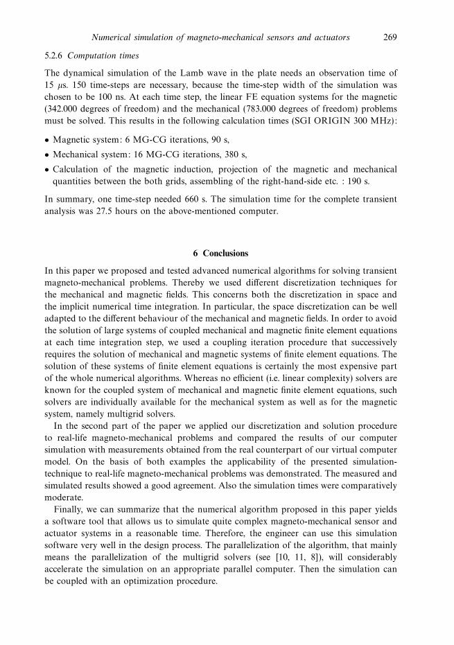
5.2.6 Computation times
The dynamical simulation of the Lamb wave in the plate needs an observation time of
15 µs. 150 time-steps are necessary, because the time-step width of the simulation was
chosen to be 100 ns. At each time step, the linear FE equation systems for the magnetic
(342.000 degrees of freedom) and the mechanical (783.000 degrees of freedom) problems
must be solved. This results in the following calculation times (SGI ORIGIN 300 MHz):
• Magnetic system: 6 MG-CG iterations, 90 s,
• Mechanical system: 16 MG-CG iterations, 380 s,
• Calculation of the magnetic induction, projection of the magnetic and mechanical
quantities between the both grids, assembling of the right-hand-side etc. : 190 s.
In summary, one time-step needed 660 s. The simulation time for the complete transient
analysis was 27.5 hours on the above-mentioned computer.
6 Conclusions
In this paper we proposed and tested advanced numerical algorithms for solving transient
magneto-mechanical problems. Thereby we used different discretization techniques for
the mechanical and magnetic fields. This concerns both the discretization in space and
the implicit numerical time integration. In particular, the space discretization can be well
adapted to the different behaviour of the mechanical and magnetic fields. In order to avoid
the solution of large systems of coupled mechanical and magnetic finite element equations
at each time integration step, we used a coupling iteration procedure that successively
requires the solution of mechanical and magnetic systems of finite element equations. The
solution of these systems of finite element equations is certainly the most expensive part
of the whole numerical algorithms. Whereas no efficient (i.e. linear complexity) solvers are
known for the coupled system of mechanical and magnetic finite element equations, such
solvers are individually available for the mechanical system as well as for the magnetic
system, namely multigrid solvers.
In the second part of the paper we applied our discretization and solution procedure
to real-life magneto-mechanical problems and compared the results of our computer
simulation with measurements obtained from the real counterpart of our virtual computer
model. On the basis of both examples the applicability of the presented simulation-
technique to real-life magneto-mechanical problems was demonstrated. The measured and
simulated results showed a good agreement. Also the simulation times were comparatively
moderate.
Finally, we can summarize that the numerical algorithm proposed in this paper yields
a software tool that allows us to simulate quite complex magneto-mechanical sensor and
actuator systems in a reasonable time. Therefore, the engineer can use this simulation
software very well in the design process. The parallelization of the algorithm, that mainly
means the parallelization of the multigrid solvers (see [10, 11, 8]), will considerably
accelerate the simulation on an appropriate parallel computer. Then the simulation can
be coupled with an optimization procedure.

270 M. Schinnerl et al.
Acknowledgements
This work has been supported by the Austrian Science Foundation - ‘Fonds zur Forderung
der wissenschaftlichen Forschung (FWF)’ under project F1306 of the SFB F013 ‘Numerical
and Symbolic Scientific Computing’. The third author and the fifth author would like to
thank the Johann Radon Institute for Computational and Applied Mathematics (RICAM)
of the Austrian Academy of Sciences for supporting the work on this article.
References
[1] Arnold, D. N., Falk, R. S. & Winther, R. (2000) Multigrid in H(div) and H(curl). Numerische
Mathematik 85, 197–218.
[2] Axelsson, O. (1996) Iterative solution methods (2nd edn). London. Cambridge University Press.
[3] Bachinger, F., Langer, U. & Schoberl, J. (2005) Numerical analysis of nonlinear multihar-
monic eddy current problems. Numerische Mathematik 100, 593–616.
[4] Ballanyi (2000) Handbuch Weicheisenprufer WP-Cs).
[5] Bathe, K. J. (1996) Finite element procedures. New Jersey. Prentice-Hall.
[6] Beitz, W. & Kuttner, K.-H. (1990) Dubbel, Taschenbuch fur den Maschinenbau (17th edn).
Berlin. Springer-Verlag.
[7] Costabel, M. & Dauge, M. (2002) Weighted regularization of Maxwell equations in polyhedral
domains. Numerische Mathematik 93, 239–278.
[8] Douglas, C., Haase, G. & Langer, U. (2003) A tutorial on elliptic PDE solvers and their
parallelization. Philadelphia. SIAM.
[9] Ettinger, K. (1998) Numerical simulation of electromagnetic acoustic transducers. Master thesis.
Linz. Johannes Kepler University Linz.
[10] Haase, G., Kuhn, M. & Langer, U. (2001) Parallel multigrid 3d Maxwell solvers. Parallel
Computing 27, 761–775.
[11] Haase, G. & Langer, U. (2002) Multigrid methods: From geometrical to algebraic versions.
In A. Bourlioux and M.J. Gander, editors, Modern Methods in Scientific Computing and Ap-
plications Volume 75 of NATO Science Ser. II, Mathematics, Physics and Chemistry. Pages
103–153. Dordrecht. Kluwer Academic.
[12] Hackbusch, W. (1985) Multi-grid methods and applications. Berlin. Springer-Verlag.
[13] Hewlett-Packard. Handbuch Impedance/Gain Phase Analyzer 4194 A.
[14] Hiptmair, R. (1999) Multigrid methods for Maxwell’s equations. SIAM Journal on Numerical
Analysis 36, 204–225.
[15] Hofer, M. (1999) Simulation und Messung der Abstrahleigenschaften von Elektromagnetisch –
Akustischen Transducern. Master thesis. Linz. Johannes Kepler University Linz.
[16] Hughes, T. J. R. (1987) Finite element method. New Jersey. Prentice-Hall.
[17] Jung, M. & Langer, U. (1991) Applications of multilevel methods to practical problems.
Surveys on Mathematics for Industry 1, 217–257.
[18] Kallenbach, E., Eick, R. & Quendt, P. (1994) Elektromagnete. Stuttgart. Teubner-Verlag.
[19] Kaltenbacher, M. (2004) Numerical simulation of mechatronic sensors and actuators. Berlin,
Heidelberg, New York. Springer-Verlag.
[20] Kaltenbacher, M., Landes, H. & Lerch, R. (1997) An efficient calculation scheme for
the numerical simulation of coupled magnetomechanical systems. IEEE Transactions on
Magnetics 33, 1646–1649.
[21] Kaltenbacher, M., Landes, H. & Lerch, R. (1999) CAPA Verification Manual, Release 3.
Linz. Johannes Kepler University Linz.
[22] Kino, G. S. (1987) Acoustic waves – devices, imaging & analog signal processing. New Jersey.
Prentice-Hall.
[23] Krautkramer, J. & Krautkramer, H. (1986) Werkstoffprufung mit Ultraschall (5th edn).
Berlin. Springer-Verlag.
Numerical simulation of magneto-mechanical sensors and actuators 271
[24] Kurz, S., Fetzer, J., Lehner, G. & Rucker, W. (1998) A novel formulation for 3d eddy current
problems with moving bodies using a Lagrangian description and bem-fem coupling. IEEE
Transactions on Magnetics 34, 3068–3073.
[25] Lerch, R. (2004) Elektrische Messtechnik. Berlin. Springer-Verlag.
[26] Ludwig, R. & Dai, X.-W. (1991) Numerical simulation of electromagnetic acoustic transducer
in the time domain. J. Appl. Phys. 69, 89–98.
[27] Morgan, D. P. (1991) SAW devices and signal processing. Amsterdam. Elsevier.
[28] Nedelec, J. (1980) Mixed finite elements in R3. Numerische Mathematik 35, 315–341.
[29] Polytec (1999) Handbuch Polytec Laser Doppler Vibrometer.
[30] Reitzinger, S. & Schoberl, J. (2002) An algebraic multigrid method for finite element
discretizations with edge elements. Numerical Linear Algebra with Applications 31, 223–238.
[31] Ren, Z. & Razek, A. (1994) A strong coupled model for analysing dynamic behaviours of
non-linear electromagnetic systems. IEEE Transactions on Magnetics 30, 3252–3255.
[32] RITEC (1997) Operation manual for advanced measurement system model RAM-0.25-17.5.
[33] Schinnerl, M. (2001) Numerische Berechnung magneto-mechanischer Systeme mit Mehrgitterver-
fahren. PhD thesis. Erlangen-Nurnberg. University of Erlangen-Nurnberg.
[34] Schmitz, K. P. (1988) Entwicklung und Untersuchung einer schnellschaltenden elektromagnet-
ischen Stelleinheit. PhD thesis. Aachen. RWTH Aachen.
[35] Silvester, P. S. & Ferrari, R. L. (1996) Finite elements for electrical engineers (3rd edn).
London. Cambridge University Press.
[36] Stratton, J. A. (1941) Electromagnetic theory. McGraw-Hill, Inc.
[37] Wunsch, G. & Schulz, H. (1996) Finite elements for electrical engineers (2nd edn). Berlin.
Verlag Technik.
[38] Ziegler, F. (1991) Mechanics of Solids and Fluids. Vienna, Springer-Verlag.