MODELING IN APPLIED MATHEMATICS
727
MODELING IN APPLIED MATHEMATICS Bengt Fornberg and Ben Herbst
-
Upload
khangminh22 -
Category
Documents
-
view
0 -
download
0
Transcript of MODELING IN APPLIED MATHEMATICS

MODELING IN APPLIED
MATHEMATICS
Bengt Fornberg and Ben Herbst

Department of Applied MathematicsUniversity of ColoradoBoulder, CO 80309
USA
Email : [email protected]
Applied Mathematics
University of StellenboschStellenbosch 7601South Africa
Email : [email protected]

Contents
Part 1. APPLICATIONS 11
Chapter 1. TOMOGRAPHIC IMAGE RECONSTRUCTION 121.1. Introduction. 121.2. Non-invasive medical imaging techniques. 13
1.3. Additional Background on Computerized Tomography. 181.4. Model Problem. 191.5. Least Squares Approach. 211.6. Back Projection method. 29
1.7. Fourier transform method. 351.8. Filtered BP method derived from the FT method. 421.9. Exercises. 45
Chapter 2. Facial Recognition 472.1. Introduction 472.2. An Overview of Eigenfaces. 512.3. Calculating the eigenfaces. 56
2.4. Using Eigenfaces 57
Chapter 3. Global Positioning Systems 613.1. Introduction. 61
3.2. A Brief History of Navigation. 613.3. Principles of GPS. 673.4. Test Problem with Numerical Solutions. 703.5. Error Analysis. 74
3.6. Pseudorandom Sequences. 79
Chapter 4. Radar Scattering from Aircraft 83
3

CONTENTS 4
4.1. Introduction. 83
Chapter 5. FREAK OCEAN WAVES 845.1. Introduction. 845.2. Mechanism for freak ocean waves. 85
5.3. Derivation of the governing equations. 895.4. Test problem - Circular current. 935.5. Atlas Pride incident revisited. 965.6. Creation of freak waves in an energy-rich ocean state. 98
Chapter 6. PATIENT POSITIONING 1026.1. Introduction. 102
6.2. Proton Therapy. 1036.3. Patient Positioning. 1066.4. Planar geometry and the 2D projective plane. 1096.5. Projective transformations. 117
6.6. The pinhole camera. 1316.7. Camera calibration. 1396.8. Triangulation. 145
Part 2. ANALYTICAL TECHNIQUES 148
Chapter 7. FOURIER SERIES/TRANSFORMS 1497.1. Introduction. 1497.2. Fourier series. 149
7.3. Fourier transform. 1547.4. Discrete Fourier transform (DFT). 1587.5. 2-D Fourier transform. 166
Chapter 8. DERIVATION AND ANALYSIS OF WAVE EQUATIONS 1688.1. Introduction. 168
8.2. Wave Function. 1698.3. Examples of Derivations of Wave Equations. 1718.4. Water Waves. 173

CONTENTS 5
8.5. First Order System Formulations for some Linear wave Equations. 1788.6. Analytic solutions of the acoustic wave equation. 189
8.7. Hamilton’s equations. 192
Chapter 9. DIMENSIONAL ANALYSIS 202
9.1. Introduction. 2029.2. Buckingham’s PI-Theorem. 2029.3. Simple Examples. 2069.4. Shock Waves. 211
9.5. Dimensionless Numbers. 216
Chapter 10. Asymptotics 223
10.1. Introduction. 22310.2. Algebraic Equations. 22710.3. Convergent vs. Asymptotic expansions 23010.4. An example of a perturbation expansion for an ODE 242
10.5. Asymptotic methods for integrals. 24610.6. Appendix 252
Part 3. NUMERICAL TECHNIQUES 254
Chapter 11. LINEAR SYSTEMS: LU, QR AND SVD FACTORIZATIONS 25511.1. Introduction. 25511.2. Gaussian elimination. 25711.3. QR factorization—Householder matrices. 268
11.4. Rotations. 27111.5. Singular Value Decomposition (SVD.) 27811.6. Overdetermined linear system and the generalized inverse. 29511.7. Vector and matrix norms. 302
11.8. Conditioning. 304
Chapter 12. POLYNOMIAL INTERPOLATION 30512.1. Introduction. 30512.2. The Lagrange interpolation polynomial. 307

CONTENTS 6
12.3. Newton’s form of the interpolation polynomial. 30812.4. Interpolation error and accuracy. 310
12.5. Finite difference formulas. 31812.6. Splines. 32812.7. Subdivision schemes for curve fitting. 341
Chapter 13. ZEROS OF FUNCTIONS 35913.1. Introduction. 35913.2. Four Iterative Methods for the Scalar Case. 36013.3. Nonlinear Systems. 366
Chapter 14. Radial Basis Functions 37014.1. Introduction. 370
14.2. Introduction to RBF via cubic splines. 37114.3. The shape parameter ε. 38114.4. Stable computations in the flat RBF limit. 39014.5. Brief overview of high order FD methods and PS methods. 395
14.6. RBF-generated finite differences. 39914.7. Some other related RBF topics. 402
Chapter 15. THE FFT ALGORITHM 41515.1. Introduction 41515.2. FFT implementations 41615.3. A selection of FFT applications 420
Chapter 16. NUMERICAL METHODS FOR ODE INITIAL VALUEPROBLEMS 428
16.1. Introduction. 42816.2. Forward Euler (FE) scheme. 43016.3. Examples of linear multistep (LM) methods. 43116.4. Key numerical ODE concepts. 435
16.5. Predictor-corrector methods. 44216.6. Runge-Kutta (RK) methods. 44416.7. Taylor series (TS) methods. 446

CONTENTS 7
16.8. Stiff ODEs. 450
Chapter 17. FINITE DIFFERENCE METHODS FOR PDE’s 45217.1. Introduction. 452
Chapter 18. OPTIMIZATION: LINE SEARCH TECHNIQUES 45318.1. Introduction. 45318.2. Lagrange Multipliers. 45418.3. Line Search Methods. 460
18.4. The conjugate gradient method 473
Chapter 19. GLOBAL OPTIMIZATION 48819.1. Introduction. 488
19.2. Simulated Annealing 49019.3. Genetic Algorithms. 499
Chapter 20. Quadrature 50720.1. Introduction. 50720.2. Trapezoidal Rule. 50720.3. Gaussian Quadrature. 513
20.4. Gregory’s Method. 519
Part 4. PROBABILISTIC MODELING 525
Chapter 21. BASIC PROBABILITY 52821.1. Introduction. 528
21.2. Discrete Probability. 52821.3. Probability Densities. 53921.4. Expectation and Covariances. 54221.5. Decision Theory. 544
Chapter 22. PROBABILITY DENSITY FUNCTIONS 54922.1. Introduction. 549
22.2. Binary Variables. 54922.3. Multinomial Variables. 55422.4. Model comparison. 556

CONTENTS 8
22.5. Gaussian Distribution. 56522.6. Linear Transformations of Gaussians and the central limit theorem. 579
Chapter 23. LINEAR MODELS FOR REGRESSION 58223.1. Introduction. 58223.2. Curve Fitting. 58223.3. Linear Models 588
23.4. Bayesian Linear Regression. 59023.5. Bayesian Model Comparison. 59523.6. Summary. 598
Chapter 24. LINEAR MODELS FOR CLASSIFICATION 599
24.1. Introduction. 59924.2. Linear Discriminant Analysis 60024.3. Probabilistic Generative Models. 61324.4. Probabilistic Discriminative Models. 619
Chapter 25. PRINCIPAL COMPONENT ANALYSIS 62425.1. Introduction. 62425.2. Principal Components . 62525.3. Numerical Calculation. 62725.4. Probabilistic PCA. 628
Chapter 26. PARTIALLY OBSERVED DATA AND THE EM ALGORITHM 63226.1. Introduction. 63226.2. K-Means Clustering. 63226.3. Gaussian Mixture Models. 634
26.4. The Expectation Maximization (EM) Algorithm for Gaussian MixtureModels. 638
Chapter 27. KALMAN FILTERS 64127.1. Introduction. 641
27.2. Kalman Filter Equations. 641
Chapter 28. Dynamic Programming. 647

CONTENTS 9
Chapter 29. HIDDEN MARKOV MODELS 65729.1. Introduction. 657
29.2. Basic concepts and notation 65729.3. Calculating p(xT1 |M) 66129.4. Calculating the most likely state sequence: The Viterbi algorithm 66429.5. Training/estimating HMM parameters 665
Part 5. MODELING PROJECTS 669
Chapter 30. DETERMINING THE STRUCTURES OF MOLECULES BYX-RAY DIFFRACTION 670
30.1. Introduction. 67030.2. Model Problem. 672
30.3. Analytical technique for finding atomic positions. 67330.4. Computer implementation. 676
Chapter 31. SIGNATURE VERIFICATION 68631.1. Introduction. 68631.2. Capturing the Signature. 68731.3. Pre-Processing. 689
31.4. Feature Extraction. 69031.5. Comparison of Features, Dijkstra’s Algorithms. 69231.6. Example. 701
Chapter 32. STRUCTURE-FROM-MOTION 70532.1. Introduction 70532.2. Orthographic camera model. 70632.3. Reconstructing 3D Images. 712
32.4. Rotation and Translation. 71532.5. Example. 717
Bibliography 720
Bibliography 721
Index 723

CONTENTS 10
Note. When this manuscript grows up it wants to be a book. In the mean timeyou will have to live with its growing pains. We do not take any responsibility for
any injury, real or imaginary, that may result from using it. If you like it, please letus know what you like about it. If you don’t like it, please tell us why, and whatwe can change to make it better. And if you know of good examples that might beuseful, tell us about it.
This manuscript is somewhat unusual in the sense that it might not be possible
to read it front-to-back. When we discuss the Applications in the first part forexample, we sometimes refer to material that is covered in detail in later parts ofthe manuscript. It means that the reader may find it necessary to return to topicsfor a full understanding, after excursions to other parts of the manuscript. We don’t
really want to apologize for this. It is how things work in practice, at least in ourexperience. When first presented with an interesting problem, most of the time wehave only a vague idea (or none at all) of how to solve it. It is only after repeatedlyreturning to the problem after numerous excursions, that we sometimes come up
with something useful.In earlier versions we had a section with Matlab code. It has been taken out of this
version but it still exists. If you want to play with the code (highly recommended),we plan to make it available on some or other website, probably close to where you
found this manuscript. Otherwise, please contact one of the authors for details.

Part 1
APPLICATIONS

CHAPTER 1
TOMOGRAPHIC IMAGE RECONSTRUCTION
1.1. Introduction.
In medicine as well as in many other situations, it is invaluable to be able tolook inside objects without actually needing to slice them open, or to do somethingelse that is grossly invasive (we regard here taking an X-ray image as ’non-invasive’).
The problem with conventional X-ray imaging is that all objects along the path ofthe X-rays appear to be superposed on top of each other (a bit like taking manyexposures without winding the film in a camera). A 3-D object has been projected to2-D (with a big loss of information content, especially since one is often interested in
localized and subtle changes in soft tissues that are near-transparent to X-rays). Themethods we will discuss in this chapter allow full spatial reconstruction throughout a3-D object or throughout a 2-D slice (in Greek τωµωσ—hence the name tomography)of the object.
In Section 1.2 we discuss very briefly six different approaches to non-invasiveimaging techniques. The remaining Sections 1.3—1.8 are focused on ComputationalTomography (CT)—a means of getting full reconstructions in one or—simultaneouslyor sequentially—many slices through the object. The input data is numerous X-rayimages captured on 2-D ‘film-like’ or 1-D line-type electronic detectors. This data is
then computationally processed to create the full, spatially true reconstruction. Ofthe several possible computational approaches to this reconstruction, we will focus onthree: least squares (LS), filtered back projection (FBP) and Fourier reconstruction(FR).
The applications of CT extend far beyond medicine. To mention one example:In the 1980s, Exxon developed micro-tomography, mainly in order to explore thedetailed pore structures of coal and of oil-saturated sand stones. One might thinkthat non-invasiveness would not be particularly important for such objects, but,
12

1.2. NON-INVASIVE MEDICAL IMAGING TECHNIQUES. 13
understanding for example how oil flows to wells requires knowledge about how mi-croscopic pores and channels in sand stone are connected. With the grains extremely
hard compared to the pores, invasive procedures would inevitably destroy the porestructures before they could be recorded (a little bit like trying to feel the fine struc-ture of a snow flake with bare fingers—the evidence would just ‘melt away’). Incontrast to medical tomography which achieves mm-size 2-D resolution across a sliceof body-sized objects, micro-tomography achieves µm size 3-D resolution throughout
cubic mm sized samples. The X-ray source is typically synchrotron radiation from anaccelerator. The 109pixel (1000× 1000× 1000) volume image sets require the fastestcomputational inversion (FR), whereas medical imaging traditionally is based on themuch slower FBP method. Here the data sets (typically 2-D) are much smaller, and
throughput is limited more by patient handling than by equipment speed.
1.2. Non-invasive medical imaging techniques.
In the last few decades, several non-invasive imaging techniques have been dis-covered which are capable of providing full 3-D information of an object. Earliermethods had either
• loss of spatial information (e.g. standard X-rays, failing to discriminatebetween overlapping structures), or• been highly invasive (for example ‘serial-section microscopy’, typically re-
quiring the object to be frozen and then sliced up).
Important non-invasive imaging methods include
(1) Ultrasound. Very high sound frequencies (several MHz) allow beams to re-main very narrow. These beams are typically sent / received by a smalltransducer which is held in contact with the body. It can rapidly change the
direction of the beam, making it ’sweep’ an angular domain. Echoes frominterfaces between different soft tissue types are recorded, with time delayscorresponding to depths. The technique is used for a large number of organs,including fetal monitoring during pregnancy. A potential future application
- still requiring further developments - is to replace X-rays for mammogra-phy. Strong sound absorption by bones somewhat limits its use, for ex. inbrain studies. The method gives images in real-time, and the equipment is

1.2. NON-INVASIVE MEDICAL IMAGING TECHNIQUES. 14
inexpensive. It used to be considered entirely safe, but some doubts aboutthis emerged after a recent Swedish study showed that, after two scans, the
likelihood of left handedness in babies increased by 32%. Although this issmall compared to the 5 times increase that has been reported in cases ofpremature birth, the fact that it has any effect at all gives rise to concerns.However, present opinion seems to be that the benefits well outweigh thepossible dangers.
(2) CT - Computerized Tomography. A parallel sheet of X-rays is sent throughthe object, and recorded by a 1-D row of detectors. From the accumulateddata when source and receiver (or object) are rotated 180◦, cross-sectionalimages can be computed. In medical application, the resolution is normally
about 0.3 mm. With the use of much more intense X-rays (which woulddestroy living tissues; such X-rays can be obtained from accelerators in theform of synchrotron radiation), resolutions around 0.001 mm (= 1 µm) areachieved. This is comparable to the best resolution that is possible with
optical microscopes, used on sliced samples. Some drawbacks with medicaluse of X-ray tomography include possible tissue damage from ionization (X-ray absorption depends on the target’s electron density), and low contrastsbetween different types of soft tissues, for example between malignant and
healthy tissues.Mathematical tools needed for successful CT imaging were discovered
more than once, not recognized for their potential and then forgotten beforesuccessful experimental realizations (employing less effective algorithms)
were achieved. For independent pioneering work in experimentally real-izing CT and bringing it to medical use, the 1979 Nobel Prize in Physiologyand Medicine was awarded jointly to G. Hounsfield and A.M. Cormack. Thehistory of CT and other applications of it are described in more detail in
Section 1.3.(3) MRI - Magnetic Resonance Imaging (earlier called NMR - Nuclear Magnetic
Resonance). The object that is to be imaged is placed in a very strong,highly uniform magnetic field (e.g. inside a large superconducting magnet).
Two different, relatively weak magnetic gradients are introduced — one

1.2. NON-INVASIVE MEDICAL IMAGING TECHNIQUES. 15
stationary and orthogonal to it, one that is stepped in time. When subjectedto accurately tuned high frequency radio pulses, many light nuclei (with an
odd number of nucleons, such as hydrogen) start to spin. While returning toa state of magnetic alignment, they re-radiate these waves. The frequencyis proportional to the local magnetic field, i.e. it carries information aboutthe positions of the different atoms. The numerical techniques needed tocreate images are similar to those used in CT. However, Fourier inversion is
nowadays preferred over back projection-type algorithms.Advantages of MRI over CT in medical applications include
• high contrast between many different soft tissues,– possibility (although little used) to ‘tune in’ on different atoms with
very distinct biological functions (e.g. H1, Na23, and P31 resonate at
42.57, 11.26 and 17.24 MHz respectively in a field of 1 Tesla), and∗ far safer radiation (the frequencies are about 11 orders of mag-
nitude lower than those of X-rays - the associated electromag-netic quanta carry correspondingly less energy, and cannot alter
molecules of living tissues). In spite of using wavelengths in the5—25 meter range, 1—2 mm resolution is obtained.
Disadvantages compared to CT include slightly less resolution and higher
cost of equipment. In practical usage, the big risk factor turns out to be thatinadvertently present metallic objects can become dangerous projectiles dueto the extreme magnetic fields.
The Nobel Prize in Physics for 1952 was awarded to E. Purcell and F.
Bloch (at Harvard and Stanford Universities) for their discovery of the NMRphenomenon. The problem of obtaining spatial information from NMR datawas considered already in the early 50’s and solved in different ways in themid-70’s. Routine medical use began in the mid-80’s. Technology improve-
ments have reduced recording times from hours to, in some cases, 30-100 msfor instance, when using echo-planar imaging (EPI)—a high-speed record-ing technique that permits a full image to be obtained in a single nuclear

1.2. NON-INVASIVE MEDICAL IMAGING TECHNIQUES. 16
excitation cycle, as opposed to a few hundred cycles; cf. [?]. A summary ofthe principles of MRI is given, for example, in [?].
(1) PET - Positron Emission Tomography. A radioactively labeled substanceis injected and follows the blood stream, while emitting positrons. After
traveling a very short distance, a positron will encounter an electron, andannihilate it. The energy gets transferred into two gamma rays that aresent off in nearly perfectly opposite directions of each other. When two de-tectors (out of a big array surrounding the body part—typically the head)
detect signals at the same instant, the emission is assumed to have occurredalong the straight line between them. This procedure generates data on theaccumulated concentrations of the tracer substance along a large numberof different lines through the body, thus allowing its distribution to be re-
constructed through 3-D generalizations of the 2-D CT algorithms that aredescribed in Sections 1.4—1.8.
When using radioactively labeled glucose, brain activities can be followedin ‘real time’, since the blood flow (and glucose usage) very quickly responds
to areas of activity (however, EPI-type MRI, in connection with the use ofcontrast agents in the blood, offer competition to PET in this field). Anotherusage is based on the fact that certain substances tend to concentrate indifferent tissues, e.g. Cu64 can be used to spot some brain abnormalities.
Disadvantages include quite low resolution, very high cost, and possiblydangerous radiation levels which are somewhat minimized by the use ofradio-isotopes with short half-times. However, this requires the availabilityof a nearby reactor or accelerator.
The last two methods to be mentioned here are entirely non-invasivealso as far as waves and radiation are concerned. However, their ability toprovide true imaging is very limited. Both can record brain signals in caseswhen thousands of neighboring neurons fire in a synchronized manner.
(2) EEG - Electroencephalography ; electric potentials on the scalp are recordedat tens (or more) locations with time resolutions in milliseconds. The lowspatial resolution and the mathematically ill-posed inversion problem makes

1.2. NON-INVASIVE MEDICAL IMAGING TECHNIQUES. 17
the technique more important in studying neural firing patterns than forimaging.
(3) MEG - Magnetoencephalography; the very weak magnetic fields from neu-ral activities are picked up outside the scull by SQUIDs (superconductingquantum interference devices), possibly the most sensitive recording devicesof any kind. Using low temperature, liquid helium cooled, superconductors,individual flux quanta can be recorded. This can in turn be utilized for a
variety of measurement tasks, giving astounding precisions, e.g.magnetic field 10−15T ( = 1 fT; femto-Tesla); signals from the brain reach
about 10-100 fT (measured outside the skull); fromthe heart 50,000 fT; the earth’s field is about1011fT = 10−4T.
voltage 10−14V about 5 orders of magnitude better than semiconductor
voltmeters,motion 10−18m about 1/1,000 of the diameter of an atomic nucleus;
1/1,000,000 of the typical diameter of an atom.‘High temperature’ (using liquid nitrogen at 77K) superconducting SQUIDs
are much cheaper than liquid He-ones; however their ability to detect detectfields of around 25 fT is only barely sufficient for brain studies.
Although SQUIDs operate much faster than neurons, acceptable signal-to-noise ratios when applied to brain imaging require recording times in tens
of seconds. Already in 1853, it was shown by Helmholtz that the inversionproblem, determining internal currents from external magnetic fields, wasnot uniquely solvable. Like for X-ray crystallography (Section 30.2), ad-ditional data needs to be supplied. Possibilities for MEG include the use
of
• simultaneous EEG-data for potentials. This offers the best signal whencurrents are orthogonal to the scull—the magnetically least visible case,
and– MRI-provided structural information. This will pinpoint folds in the
cortex. As it happens, primary sensor areas tend to be located in such

1.3. ADDITIONAL BACKGROUND ON COMPUTERIZED TOMOGRAPHY. 18
folds, with the consequence that the key currents become relativelyparallel to the skull, i.e. well oriented for a good magnetic signal.
MEG is described in Hämäläinen (1993). One of the inventors of MEG (D. Cohen,
MIT) has raised serious questions about the utility of the approach [?].
1.3. Additional Background on Computerized Tomography.
From a mathematical point of view, the main challenge in CT lies in the inversiontechnique. In a purely mathematical form (prompted by an issue relating to grav-itational field equations), this problem was solved by the Austrian mathematician
Johann Radon [?]. His solution assumes that all variables are continuous functionsdefined on an infinite domain. In practice, one has to work with a finite numberof rays at a finite number of angles to produce a reconstruction at a finite numberof grid points. In the exercise section of this book, we will see how Radon’s inver-
sion method connects to two of the presently most used techniques—filtered back
projection and Fourier inversion.The paper by Radon was just the first of several which gave solutions to the
inversion problem which were not noted by later pioneers. Another case is a paper
by R. Bracewell [?] (in the context of obtaining images of the sun from microwavedata) which describes a Fourier-based reconstruction method. With the use of theFFT (fast Fourier transform) algorithm, Fourier based reconstruction methods arenow the fastest ones available. Although surprisingly little used in medical contexts
(where filtered back projection dominates), they are preferred in the even more dataintensive application of micro-tomography.
Allan MacLeod Cormack (1924-1998) was working as a physicist (at Universityof Cape Town) and assisting a local hospital with routine radiological tasks, when it
occurred to him that if enough X-ray projections were taken in a variety of directions,there would be enough data for a full reconstruction. He realized that CT couldrevolutionize medical imaging and his tests on simple wood and aluminum objects inthe late 1950s and early 1960s, showed the concept to be practical. In two seminal
papers [?, ?], Cormack very clearly outlined the medical implications, and presentedstill another numerical procedure for the reconstruction. However, his efforts at thetime to interest the medical community were not successful.

1.4. MODEL PROBLEM. 19
About a decade after Cormack’s pioneering work, Goodfrey Hounsfield (1919-)independently developed the idea of medical tomography (while doing pattern recog-
nition studies at the electronics company EMI Ltd. in Britain). His first apparatuswas similar to Cormack’s, but used an americum radiation source and a crystaldetector. Following very successful preliminary tests, the radionuclide source wasreplaced with an X-ray tube, reducing data gathering times from well over a weekto about 9 hours. Following many further improvements, his work led to the first
clinical machine, installed in a hospital in Wimbledon in 1971. By this time thetechnique had advanced to the point that 180 projections (at 1◦ separation) could becollected in just under 5 minutes, followed by about 20 minutes for the image recon-struction. These specifications improved even more and current machines provide
about 0.3 mm resolution throughout full body slices. The major limiting factor infurther improvements comes from the need to keep X-ray doses within safety limits.
There are many applications other than medical ones, of tomography. Below arejust a few examples:
astronomy Marsh and Horne [1988] (binary stars),Gies et al [1994](ac-cretion discs)Hurlburt et.al.[1994] (coronal studies)
oceanography Worcester and Spindel [1990],Worchester et.al. [1991]
Munk et.al. [1995] (acoustic probing of ocean conditionsgeophysics Anderson and Dziewonski [1984] (mantle flows), Frey et al
[1996] (aurora)Gorbunow [1996] (atmosphere)
porous media Hal [1987]
1.4. Model Problem.
Figures 1.4.1 and 1.4.2 show a test object, defined on a 63×63 grid. This objectwas generated by the code logo.m. The X-ray absorption levels at different locationsare displayed as darkness and elevation respectively. Figure 1.4.3 shows how X-ray
data can be collected for a sequence of angles θi = π i64, i = 0, 1, ..., 63. Figure 1.4.4
shows what the scan data would look like in the case of the test object in Figures1.4.1 and 1.4.2. The scan lines are shown as successive lines (in the r-direction)

1.4. MODEL PROBLEM. 20
Figure 1.4.1. Test object.
from the front left, θ = 0, to the back right, θ = π; this last line being an up-down
reflection of the first one.Given the density function f(x, y) of the 2-D object, the scan data can be written
as
(1.1) g(r, θ) =
∫ ∞
−∞f(x, y) ds
where the coordinate axes are as defined in Figure 1.4.5. Since the (s, r) axes differfrom the (x, y) axes by a pure rotation, they are related by
(1.2)
{s = x cos θ + y sin θ
r = −x sin θ + y cos θ
{x = s cos θ − r sin θ
y = s sin θ + r cos θ.
This means that we sum all the contributions along lines parallel to the s axis inFigure 1.4.5.

1.5. LEAST SQUARES APPROACH. 21
Figure 1.4.2. Another view of test object.
Equation (1.1) is known as the Radon transform. The computational issue in CTis to invert this transform, i.e. to recover f(x, y) from g(r, θ).
1.5. Least Squares Approach.
To understand the idea behind the back projection method (how to achieve thereconstruction, how much data is needed etc.) we consider first a very small object—a
3×3 structure of 9 square elements, having unknown densities x1, x2, . . . , x9 respec-tively:
(1.1)x1 x4 x7
x2 x5 x8
x3 x6 x9
.
Suppose that we have knowledge only of the row sums r1, r2, r3 and of column sumss1, s2, s3 (like having done X-ray recordings only horizontally and vertically). This

1.5. LEAST SQUARES APPROACH. 22
Figure 1.4.3. Principle for generation of 1-D scan data from a 2-D object.
gives rise to the linear system of equations
(1.2)
1 1 1 0 0 0 0 0 0
0 0 0 1 1 1 0 0 0
0 0 0 0 0 0 1 1 1
1 0 0 1 0 0 1 0 0
0 1 0 0 1 0 0 1 0
0 0 1 0 0 1 0 0 1
x1
x2
x3
x4
x5
x6
x7
x8
x9
=
r1
r2
r3
s1
s2
s3
The first question that we need to ask ourself is whether it is possible to obtainthe densities x1, x2, . . . , x9 of the elements from these row- and column sums only.
Considering that all the six density patterns shown in Table 1 have the same row-and column sums, it is clear that the problem will not always have a unique answer.Next, we might ask if (1.2) will always have at least one solution, no matter what

1.5. LEAST SQUARES APPROACH. 23
Figure 1.4.4. Scan data of the CU-object.
the values are in the right hand side. It is easy to see this can’t be the case (in spite
of the fact that this system Ax = b has fewer equations than unknowns). If we addrows 1, 2, and 3, we get
x1 + x2 + x3 + x4 + x5 + x6 + x7 + x8 + x9 = r1 + r2 + r3
while adding rows 4, 5, and 6 gives
x1 + x2 + x3 + x4 + x5 + x6 + x7 + x8 + x9 = s1 + s2 + s3
Unless
(1.3) r1 + r2 + r3 = s1 + s2 + s3
holds, there is no possibility for a solution to exist. We might argue that (1.3) should
hold if our data came from any object, such as the one indicated in (1.1). However,all actual data contains errors of some size, and one can never rely on data havingto be completely error free. For much bigger linear systems than (1.2), there is no

1.5. LEAST SQUARES APPROACH. 24
Figure 1.4.5. Relation between the (x, y) and (s, r) coordinate systems.
1 0 00 1 00 0 1
1 0 00 0 10 1 0
0 1 01 0 00 0 1
0 1 00 0 11 0 0
0 0 11 0 00 1 0
0 0 10 1 01 0 0
Table 1. The six possible permutation matrices of size 3x3
chance to spot multiple solutions or situations with non-existence of solutions in theway we have just dome. What is needed are general results telling just when systems
have solutions (and, if so, how many) or do not have any. If there are solutions, howdoes one effectively find them? Maybe surprisingly, systems with more equationsthan unknowns—almost invariably lacking exact solutions altogether—is the mostimportant case in applications. And we will soon see that our first approach totomographic inversion is an illustration of this.

1.5. LEAST SQUARES APPROACH. 25
1.5.1. SVD analysis of (1.2). Usually the best way to explore the solvabilityof any specific linear system starts with performing an SVD factorization of the
coefficient matrix A (cf. Section ....; in particular note Figure .... illustrating howthe decomposition related to the four fundamental subspaces of a matrix) Writingthis decomposition as A = U Σ V ∗, we get in the particular case of the coefficientmatrix A in (1.2)
U =
−0.4082 0 0 0.8165 0 0.4082
−0.4082 0 −0.2599 −0.4083 0.6576 0.4082
−0.4082 0 0.2599 −0.4083 −0.6576 0.4082
−0.4082 0.5393 −0.5701 0 −0.2253 −0.4082
−0.4082 −0.8006 −0.1493 0 −0.0590 −0.4082
−0.4082 0.2612 0.7194 0 0.2843 −0.4082
,
Σ =
2.4495 0 0 0 0 0 0 0 0
0 1.7321 0 0 0 0 0 0 0
0 0 1.7321 0 0 0 0 0 0
0 0 0 1.7321 0 0 0 0 0
0 0 0 0 1.7321 0 0 0 0
0 0 0 0 0 0 0 0 0
,
V∗ =
2
6
6
6
6
6
6
6
6
6
6
6
6
6
6
6
6
4
−0.3333 0.3114 −0.3292 0.4714 −0.1301 0.6327 0.1464 0.1503 −0.0096
−0.3333 −0.4622 −0.0862 0.4714 −0.0341 −0.4331 0.2297 0.1479 0.4269
−0.3333 0.1508 0.4154 0.4714 0.1642 −0.1997 −0.3762 −0.2981 −0.4174
−0.3333 0.3114 −0.4792 −0.2357 0.2496 −0.2662 −0.5409 0.1831 0.2179
−0.3333 −0.4622 −0.2363 −0.2357 0.3456 0.3042 0.0479 −0.5903 −0.0332
−0.3333 0.1508 0.2653 −0.2357 0.5438 −0.0380 0.4930 0.4073 −0.1846
−0.3333 0.3114 −0.1791 −0.2357 −0.5098 −0.3665 0.3945 −0.3333 −0.2083
−0.3333 −0.4622 0.0638 −0.2357 −0.4137 0.1288 −0.2777 0.4425 −0.3937
−0.3333 0.1508 0.5654 −0.2357 −0.2155 0.2377 −0.1168 −0.1091 0.6020
3
7
7
7
7
7
7
7
7
7
7
7
7
7
7
7
7
5
.
The last entry (zero) in the main diagonal of Σ tells that the rank of the systemis 5 (rather then 6, as might have been expected). The first 5 columns of U form
then an orthogonal basis for the column space of A, i.e. the system (1.2) is solvableif and only if the right hand side b of (1.2) lies in this space. The columns of U areorthogonal - so another way to say this is that b needs to be orthogonal to the last

1.5. LEAST SQUARES APPROACH. 26
column of U , giving the condition for solvability
(1.4) r1 + r2 + r3 − s1 − s2 − s3 = 0 .
We arrived, mainly by chance, earlier at this very same requirement (1.3). Thebig difference is that we now have derived it in a manner that works for absolutelyany system. And we also now see that this is the only requirement that is needed
for solvability. Physically, this condition is natural: r1 + r2 + r3 and s1 + s2 + s3
both express the same quantity, viz. the sum of all the nine unknowns. If (1.4)holds, the general solution is any one particular solution to which we can add anycombination of vectors from the null space of A. By the same theory about SVD
and the fundamental subspaces, this space will be found in the last 4 rows of V ∗.Once we have the SVD of A, we can alternatively extract all the information above
- plus find a particular solution—without referring to the fundamental subspaces. Thesystem Ax = b can be written UΣV ∗x = b, i.e.
(1.5) Σy = U∗b
with
(1.6) x = V y.
In order for (7.1) not to contain a contradiction in the last row, we need the lastelement of U∗b to be zero, leading once again to the condition (1.4). With that beingthe case, (7.1) gives uniquely the first 5 entries of y, but leaves the last 4 free. The
most general solution then follows from (7.4). We note again that the solution isundetermined precisely with respect to any combination of the last 4 rows of V ∗.This last result is very much more complete than our earlier observation that the sixparticular solutions represented by the matrices in Table 1 all corresponded to the
same RHS for (1.2).
1.5.2. A least-square formulation of the CT inversion problem. Themost obvious shortcoming with using only row- and column sums for the model (1.1)
is that we do not get enough data for the number of unknowns. Increasing theresolution from 3 × 3 to n × n elements does not help; we will then only have 2n
equations for n2 unknowns. The ‘obvious’ remedy to this is to do the scans in many

1.5. LEAST SQUARES APPROACH. 27
more directions than just two. There is no limit to how many directions we canuse. With m directions and, for each of these, sending n side-by-side rays through
an object made up of n × n elements, we will instead of the n = 3, m = 2 caserepresented by (1.2), obtain a linear system of the type
(1.7)
· · ·· · ·· A ·· · ·· · ·· · ·
mn,n2
·x
·
n2
=
··b
···
mn
.
If we have more equations than unknowns, the system becomes overdetermined, inwhich case there is typically no exact solution. However, least squares solutions canbe readily found (cf. Section 11.4), making the difference between left hand– andright hand sides of the system as small as possible. Typically, using m >> n will not
be disadvantageous (as one might think, based on introducing more possibilities ofconflict) but instead advantageous (by making the solution more stable against datanoise). The entries in the coefficient matrix are now not only 0’s or 1’s (as in (1.2)),but instead real numbers which reflect how visible each element is to each ray. When
we only used horizontal and vertical rays, they either went through the full extentof an element, or they missed the element altogether. With rays going thorough theblock-structured object at arbitrary angles, the length of the intersection between anelement and a ray can take any value between zero and the length of its diagonal. The
coefficient matrix A will be quite sparse, and with a complicated sparsity structure.With the object consisting of n × n elements (whose densities are to be deter-
mined), the detailed structure of the system (1.7) becomes as shown in Figure 1.5.1.There are n2 densities that need to be calculated. We rearrange the n × n set of
unknowns as before into a column vector x of length n2. The first n equationscorrespond to the n rays when scanning at the first angle; the next n equationscorresponding to the second angle, etc. It is natural to think of A as made up ofan m × n layout of n× n-sized blocks, and x and b of n and m end-to-end vectors,

1.5. LEAST SQUARES APPROACH. 28
Figure 1.5.1. Structure of the overdetermined linear system of theleast-square method.
Figure 1.5.2. Illustration of how the A-matrix entries are formed.
respectively, each of length n. Figure 1.5.2 illustrates how the linear system is formed(with one block row of A for each scan angle).
1.5.3. Least square solution. We now need to solve the overdetermined sys-tem (1.7) in a least squares sense. The best approach will be to use an iterative
method that is capable of fully utilizing the sparsity structure of A. One such algo-rithm is Matlab’s lsqr—a conjugate gradient implementation of the normal equations.In Section 11.3 it is described how a direct solver can be implemented in a stable

1.6. BACK PROJECTION METHOD. 29
way using QR factorization. Codes for both of these methods are included in thecomputer code section .... For a simple operation count for a direct solver, we con-
sider the normal equation approach (roughly the same count as for the QR method,but less stable numerically, so not recommended). The normal equations of a linearmn× n2 system Ax = b is a square n2 × n2 system
ATAx = AT b .
Forming ATA will cost O(mn5) operations, AT b costs O(mn3); Cholesky decompo-sition of ATA into L LT will add another O(n6). The final step to get x through two
back substitutions, using L and LT respectively, adds a further O(n4) operations.Assuming m is just slightly larger than n, the total cost becomes O(n6) operations.
A very large saving can be realized by noting that the A-matrix is independentof the object we are studying—that will only affect the b- and x- vectors. The L-
matrix can therefore be determined once and for all. Each image will then cost ‘only’O(n4) operations. We will soon see that even this is not competitive—the next twomethods, filtered back projection and the Fourier method will cost only O(n3) andO(n2 log n) respectively. Table 2 compares the computational time needed by thedifferent approaches.
Hounsfield used the least squares approach in his first successful experimentalinversion. Already with a sample as coarse as 8 × 8, the necessary computing tookhours on EMI’s then state-of-the-art ICL machine. The code least_sq is a directimplementation of this approach. Figure 1.5.3 shows the result if our test object is
scanned with 31 rays and 40 angles, followed by reconstruction with this method toa 31× 31 grid. This level of resolution is too low for a good reconstruction, but wecan still see a rough version of the ring and the central lettering. With the iterativesolver least_sq_iter we can easily afford a 63× 63 inversion on a standard PC. The
result of this inversion is shown in Figure 1.5.3Current medical imaging uses the filtered BP-method, to be described next.
1.6. Back Projection method.
The idea of back projection is conceptually very straightforward, it is easy toimplement, and the computational cost is moderate. In its most direct form, the

1.6. BACK PROJECTION METHOD. 30
Comparisons of times for algorithms of different complexity on asystem performing 10 8 floating point operations per second
Size n× n n6 n4 n3 n2 log npixels (least squares) (least squares) (filtered BP) (Fourier)
n = 100 3 h 1 s 0.01 s 0.2 msn = 1000 320 y 3 h 10 s 0.03 s
Table 2. Comparison of computational efficiencies for some non-iterative inversion methods.
Figure 1.5.3. Reconstruction with the least squares method whenthe logo was scanned with 31 rays at 40 angles, followed by a recon-struction to a 30 × 30 grid.
reconstruction comes out ‘smeared’. However, the addition of a simple filter all but
resolves this. It is of little surprise that Filtered Back Projection (FBP) has becomethe most widely used reconstruction process in the medical community where it verywell meets the requirements placed on it.

1.6. BACK PROJECTION METHOD. 31
For an n× n image reconstruction, the FBP method will cost O(n3) operations.In many contexts, this cost is acceptable or rather, it became accepted at a time
when the major alternatives were even more costly. The computing time using FBPis quite fast in comparison to the other tasks involved such as patient handling etc.However, in an application such as micro-tomography, the situation is very different.There the resolution can be as high as 1000 simultaneously recorded slices, each tobe imaged on a 1000×1000 grid, giving a 3-D 1µm resolution throughout a cubic
millimeter sample. Each full inversion for such a cube of using back projectionswould cost on the order of 1012 operations. This is likely to become a slow processin comparison with the rapid one of automated sample handling where data for the1000 slices are collected simultaneously by using a 2-D rather that a 1-D array of
X-ray sensors. We describe in Section 1.7 an inversion algorithm which cuts this costby some orders of magnitude—in this case to about 1010 operations.
1.6.1. Immediate back projection. Figure 1.6.1(a) shows a point-type ob-ject, and 1.6.1(b) its scan data. Let us remind ourselves how the scan data is ob-tained. At each angle, the total absorption of each ray is recorded; we do not have
any information about the contribution from any specific location. The most obviousthing to do is to assume that all locations along the ray contributes an equal amount.As illustrated in Figure 1.6.2 the simplest form of back projection consists of drawingparallel bands across the image area, with the darkness of the band corresponding
to the absorption that was recorded for each ray. Mathematically back projection isdescribed by
(1.1) h(x, y) =
∫ π
0
g(r, θ)dθ.
The right part of Figure 1.6.1 shows the result of this process in this case of the pointobject. The only error is that the point has turned into a ‘smeared out’ cone-typemound. The sharp edge of the original point object has been lost, as areas near thepoint are also covered by some of the bands. However, the position of the recovered
mound is precisely the same as that of the original point-object. Also, the amplitudeand shape of the mound is position invariant—it takes the same values wherever theoriginal point object was located.

1.6. BACK PROJECTION METHOD. 32
Figure 1.6.1. Point-type object, its scan data, and the image recov-ered through immediate back projection.
Figure 1.6.2. Principle behind back projection (when applied imme-diately to scan data - no filtering) shown here in the case of a pointobject.
To appreciate the significance of this example with a point object, we need to
note that both the scanning and the back projection phases are linear. If there hadbeen two point objects, the scan data would just have been the sum of the scandata for the two objects if recorded independently. Similarly, the back projectionproduces in that case a result which is the sum of the back projections of the two
objects, if they were treated separately. Finally, the darkness of the back projectedresult of each object by itself is proportional to the original darkness. The processof scanning followed by back projection satisfies the two criteria for a function (here

1.6. BACK PROJECTION METHOD. 33
a matrix-valued function with a matrix input) to be linear :
f(x+ y) = f(x) + f(y)
f(αx) = α f(x).
From this linearity follows the important conclusion that the reconstruction mustalso work for full images and not just point objects.
In summary, wherever the imaged object x had a gray pixel, the image f willfeature a smeared one centered at the same location, and with a darkness proportionalto the darkness of the one in the original. From the linearity follows that if x wasa sum of two images with a different gray pixel in each, f will become the sum
of the two corresponding images. Continuing this observation: Since every imageis a combination of pixels, this linearity implies that f must become a (smeared)representation of the original object. Immediate back projection using the scan datashown in Figures 1.6.1 leads to the reconstruction seen in Figure 1.6.3. The original
object is recovered but smeared out. In the next section we discuss a simple methodof improving the situation.
1.6.2. Filtered back projection. Comparing the original object in Figure 1.6.1with Figure 1.6.3 (both featuring the same grid density of 63×63 points), we clearlysee a loss in sharpness. Hence, we look for some way to enhance the output fromdirect back projection in order to reduce the smearing. The step from original ob-ject to scan data is essentially outside our control (dictated by X-rays and physics).
Options remaining include
• Based on the smeared image, apply some filter which sharpens all gradients
(such filters can for example be based on FFTs), and• Since the cause of the smearing is understood (for the point image), try to
alter the scan data in a way that off-sets the back projection smearing.
Both options above are viable; filtered back projection pursues the second one. Twokey questions become:
(1) Does there exist any special type of (simulated) scan data for which the backprojection method will give a nearly point like result?

1.6. BACK PROJECTION METHOD. 34
Figure 1.6.3. Immediate back projection of the scan data for the test object.
(2) Is there any operator—linear, location preserving, and not altering the dark-ness at the point itself—that we can apply to turn the actual scan data for
the point-type test object into the form that we looked for in point 1 above?
Addressing the first issue, we note that we can replace the ‘single-hump’ data by a
‘hump’ at the same place, but with a bright band on each side of it. The contributionsfor all the angles will still superimpose to an equally dark spot at precisely the desiredlocation, but at nearby locations, the bright sidebands might just cancel some of theundesired darkness, as the contributions for different angles θ are superimposed.
To turn the scan data for a fixed angle, (0,0,...,0,1,0,...,0)T , into a vector witha bright (negative) entry on each side of the ‘one’—wherever it is located—can beachieved by multiplying the scan data from the left by a symmetric n×n tri-diagonal

1.7. FOURIER TRANSFORM METHOD. 35
Toeplitz band matrix
(1.2) E =
1 −β−β 1 −β
−β 1 −β. . . . . . . . .
. . . . . . . . .
−β 1 −β−β 1 −β
−β 1
Applying this idea to the test object, Figure 1.4.1, the results are shown in Fig-ure 1.6.4. To get these figures, we multiplied every single scan data vector with thismatrix E, before back projecting where of course, we exploit the sparse structure ofE.
This modification preserves
• location and strength of images of point objects—they will appear lesssmeared, and
• linearity, meaning that a general image will be as good as is the treatment ofpoint objects. Thus linearity also implies that an optimal value of β shouldbe obtainable from considering a point object, a question to be returned toin Section 1.8.
Choosing β= 0.3, 0.4, 0.5 and 0.6 respectively in (1.2) gives, with the scan dataof our test object, the reconstructions that are shown in Figures 1.6.4. In spite ofthe filter being narrow (tri-diagonal; wider filters could be ‘tuned’ better) and the
optimization of the filter coefficient being crude—we simply pick the best-looking ofthe four cases, we get excellent inversions.
1.7. Fourier transform method.
The Fourier transform (FT) method requires considerably more mathematical
background than did the previous two methods. Computationally, it is the fastestknown method. In the exercises we shall see how one can mathematically derive fromthis method both the filtered back projection method and Radon’s original inversion

1.7. FOURIER TRANSFORM METHOD. 36
Figure 1.6.4. Filtered back projection with some choices of simpletri-diagonal filters.
formula (which, as we noted before, is mathematically compact but numericallyimpractical).
1.7.1. Analytical description. We assume as before that the density of the
object is represented by a density function f(x, y) where x and y denote the twospatial directions. The 2-D Fourier transform of the density function is given by
(1.1) f(ωx, ωy) =1
(2π)2
∫ ∞
−∞
∫ ∞
−∞f(x, y) e−iωxx e−iωyy dx dy.
The density function f(x, y) can then be recovered by
(1.2) f(x, y) =
∫ ∞
−∞
∫ ∞
−∞f(ωx, ωy) e
iωxx eiωyy dωx dωy

1.7. FOURIER TRANSFORM METHOD. 37
We will give two descriptions of how one can arrive at the FT method. The mostheurisic one follows below. A more concise but less intuitive approach is given in the
exercise section.The key step is to turn the scan data into f(ωx, ωy). This rests on two observa-
tions:
• Noting what happens if we send in the X-rays in a direction parallel to the
x-axis: The left part of Figure 1.7.1 illustrates how we obtain the scan datag(y) =
∫∞−∞ f(x, y)dx. Its 1-D Fourier transform is
g(ωy) =1
2π
∫ ∞
−∞g(y) e−iωyydy
=1
2π
∫ ∞
−∞
[∫ ∞
−∞f(x, y)dx
]e−iωyydy
=1
2π
∫ ∞
−∞
∫ ∞
−∞f(x, y)e−i0xe−iωyydxdy
= 2πf(0, ωy),
i.e. we have obtained f(ωx, ωy) along a vertical line through origin in the(ωx, ωy)-plane (cf. Figure 1.7.1(b)).• Considering the difference if the X-rays would have entered from another
direction. If the X-rays had entered from an angle θ (Figure 1.7.3(a)), the
collected scan data will be exactly the same as if instead, the object hadbeen turned an angle of −θ (Figure 1.7.3(b)). As is shown in Section 7.3 onFourier transforms, turning an object turns its Fourier transform throughexactly the same angle. Therefore, we obtain in this case values for f(ωx, ωy)
along the line through the origin in the (ωx, ωy)-plane orthogonal to the X-ray direction in the physical plane (Figure 1.7.3(c), (d)). When we havetaken X-ray images for 0 ≤ θ < π (and applied the 1-D Fourier transformto them), we have actually obtained f(ωx, ωy) along all radial lines through
the origin, i.e. throughout the complete (ωx, ωy)-plane. Thus we find that
(1.3) f(ωr, θ) =1
(2π)2
∫ ∞
−∞g(r, θ)e−iωrrdr.

1.7. FOURIER TRANSFORM METHOD. 38
Figure 1.7.1. Recording with rays parallel to the x-axis, and thecorresponding data set in Fourier space.
Figure 1.7.2. Schematic illustration of the steps in the Fourier re-construction method.
The density function f(x, y) is then recovered by the 2-D Fourier transform(1.2).
1.7.2. Numerical results with FT method. Following the description abovegives a reconstruction as shown in Figure 1.7.4.
Although the details in the center is near-perfect, we see a quite disturbing wobblein the base level of the reconstruction. The FT method that is implemented in the
Matlab code therefore contains one more refinement. Each scan vector is ‘padded’ todouble length by just adding zeros at each end of it. Once brought to Fourier space,it is laid out on a correspondingly enlarged 2-D (ωx, ωy)-plane. After returning (by

1.7. FOURIER TRANSFORM METHOD. 39
a. Scan with incoming X-rays at an angle θ. Thedensity of the object is f(x, y).
b. Equivalent recording as in a. The image is nowrotated through an angle θ, and the X-rays enterhorizontally.
c. The 1D Fourier Transform of the recording ofpart b provides a line of data along the ω-axis ofthe 2D Fourier Transform.
d. Since the FT rotates through an angle θ whenthe image rotates through the sameangle, we have now obtained a function f(ωx, ωy)along a line in the (ωx, ωy) plane, sloping the sameway as the scan line of part a.
Figure 1.7.3. Fundamental principle behind the FT method for to-mographic reconstruction.

1.7. FOURIER TRANSFORM METHOD. 40
Figure 1.7.4. Reconstruction by direct FT method from 63 ray, 64angle scan data to a 64× 64 grid.
Figure 1.7.5. Same Fourier reconstruction as in the previous figure,but with the spatial domain ‘padded’ by a factor of two within the FTalgorithm.
the inverse 2-D FFT) to the (x,y)-plane, we keep only the central square; i.e. disre-gard the borders (containing 3/4 of the total reconstructed area—these borders onlycontain an image of the padding areas). The resulting picture is seen in Figure 1.7.5.
There are a couple of ways to understand why this padding idea helps:
• Very heuristically: We are using periodic FFTs instead of infinite-domaintransforms. Periodic images of the object are then present near the bound-aries of the shown domain. Discrepancies between the concept of periodic-
ity in polar- and in Cartesian coordinates cause a difficult-to-analyze errorpattern. From this loose argument, one might expect that padding wouldimprove the image by increasing the distances to unphysical ghost images.

1.7. FOURIER TRANSFORM METHOD. 41
• More theoretically: Extending the spatial domain by a factor of two meansthat in each direction a twice as dense set of Fourier modes become available.
For example, in a 1-D spatial domain of [-π, π], modes
. . . e−3ix, e−2ix, e−ix, e0ix, e1ix, e2ix, e3ix, . . .
are available. If the domain is extended to [−2π, 2π], also the intermediate
modes. . . e−
52ix, e−
32ix, e−
12ix, e
12ix, e
32ix, e
52ix . . .
become present. The interpolation from polar to Cartesian grids occurs in
Fourier space and with a denser grid in that space, interpolation becomesmore accurate.
It is important to use better than-linear-interpolation and our code uses cubic in-terpolation. We can illustrate this in 1-D by trying to represent a half-integer
mode ei(n+ 12)x on a grid in Fourier space that only has integer modes eikx, k =
. . . ,−3,−2,−1, 0, 1, 2, 3, . . . available. Linear (second order) interpolation gives
ei(n+ 12)x ≈ 1
2einx +
1
2ei(n+1)x = ei(n+ 1
2)x
(e−i
12x + ei
12x
2
)= ei(n+ 1
2)x cos
x
2
and fourth order interpolation (cf. Table 2 of Section 12.5)
ei(n+ 12)x ≈ − 1
16ei(n−1)x+
9
16einx+
9
16ei(n+1)x− 1
16ei(n+2)x = ei(n+ 1
2)x (
9
8cos
x
2−1
8cos
3x
2)
The interpolation would have been perfect, had the factors (referred to as the damp-ing factors) multiplying ei(n+ 1
2)x in the RHSs in the two equations above been equal
to one. Figure 1.7.6 displays the actual factor for interpolation of different orders.Note that this factor depends on x only, i.e. not on n. Interpolation by order 4 andabove achieves excellent results in the center of the domain. Hence, we can expectgood reconstruction where, in the padded case, the object is located.
Although a factor two padding leads internally to a larger grid, the opera-tion count still remains O(n2 log n), only the proportionality constant has increasedaround a factor of four.

1.8. FILTERED BP METHOD DERIVED FROM THE FT METHOD. 42
Figure 1.7.6. The damping factor at different physical locationsacross the domain when a half-integer Fourier mode is interpolatedin Fourier space to integer frequencies.
1.8. Filtered BP method derived from the FT method.
The Fourier inversion method is exact—assuming continuous functions and adoubly infinite domain. The ‘raw’ BP method gave a quite smeared reconstruction,
but it became very good after applying an empirically found filter to each of thescan data vectors. Although we arrived at the two methods—BP and FT—by quitedifferent arguments, they ought to be somehow related.
A little bit of notation to start with: With the coordinate axes as shown in
Figure 1.4.5, we can write the scan data function as
(1.1) g(r, θ) =
∫ ∞
−∞f(x, y)ds
where x = x(s, r, θ), y = y(s, r, θ). Immediate back projection, as shown in Fig-
ure 1.6.2, gives a reconstruction
(1.2) h(x, y) =
∫ π
0
g(r, θ) dθ
with r = r(x, y, θ). The result of the immediate back projection was shown in
Figure 1.6.3. Although it is a reasonably good recovery, it is clear that h(x, y) 6=f(x, y). In the next section, we will show that if we replace g(r, θ), as produced by(1.1), with

1.8. FILTERED BP METHOD DERIVED FROM THE FT METHOD. 43
g(r, θ) → 1
(2π)2
∫ ∞
−∞
[∫ ∞
−∞g(ρ, θ) e−iωrρdρ
]|ωr| eiωrrdωr(1.3)
=1
2π
∫ ∞
−∞g(ωr, θ)|ωr|eiωrrdr(1.4)
before substituting into (1.2), we get h(x, y) = f(x, y)—i.e. exact reconstruction.Note that (1.4) is the Fourier transform of the product g(ωr, θ)|ωr|eiωrr. Writing
|ωr| as the Fourier transform of a function that is to be determined at the end of thissection, we can interpret (1.4) as a particular filter applied to the function g(r, θ).
There is another way to express (1.4) that is mathematically equiva-lent:
(1.5) g(r, θ) → 1
2π2
∫ ∞
−∞
∂g(ρ, θ)/∂ρ
r − ρ dρ.
This expression was found by J. Radon in 1917. It is mathematicallyvery elegant, shorter than (1.4), and superficially looks simpler (just asingle integral), but turns out to be far less practical for computational
use. Derivatives are usually more difficult to approximate well thanintegrals. Also, the integral has a ‘principal value’ singularity at ρ = r
which adds computational difficulty.
1.8.1. Derivation of replacement formula for g(r, θ). Both the FT method
as well as (1.4) are exact. It is therefore natural to suppose that (1.4) can be derivedfrom the FT method. Starting from
f(x, y) =
∫ ∞
−∞
∫ ∞
−∞f(ωx, ωy)e
iωxx+iωyydωxdωy
we change to the scan data coordinates (1.2) (see also Figure 1.4.5),
ωx = −ωr sin θ, ωy = ωr cos θ,d(ωx, ωy)
d(ωr, θ)= ωr,
to obtain
f(x, y) =
∫ 2π
0
∫ ∞
0
f(ωr, θ)e−iωr sin θx+iωr cos θ yωr dωrdθ.

1.8. FILTERED BP METHOD DERIVED FROM THE FT METHOD. 44
If we now alter the description of the standard polar domain 0 ≤ ωr <∞, 0 ≤ θ ≤2π to − ∞ < ωr < ∞, 0 ≤ θ ≤ π and recalling from Section 1.4 that −x sin θ +
y cos θ = r, it follows that,
f(x, y) =
∫ π
0
∫ ∞
−∞f(ωr, θ) e
iωrr |ωr| dωrdθ.
Finally, the key result of the FT method (1.3) gives
f(x, y) =1
(2π)2
∫ π
0
{∫ ∞
−∞
[∫ ∞
−∞g(r, θ)e−iωrrdr
]|ωr| eiωrrdωr
}dθ.
Comparing this with (1.2) and (1.4), we see that (1.4) is established.
1.8.2. Interpretation of the replacement formula as a filter. We havejust shown that the back projection method would be exact if each scan vector was
modified according to (1.4) before being actually used for back projecting. Theformula (1.4) amounts, independently for each θ, to a convolution of g with some yetundetermined function whose Fourier transform in the r-direction is |ωr|. Simplifyingour notation a bit (r → x, ωr → ω), we need to ask ourselves what function e(x)
has the Fourier transform |ω|, i.e.
|ω| = 1
2π
∫ ∞
−∞e(x) e−iωx dx
or
(1.6) e(x) =
∫ ∞
−∞|ω| eiωx dω
This first attempt runs into a roadblock—the integral (1.6) is divergent.
The integral is divergent because it is defined on an infinite interval. In practicalwork, we only consider finite intervals. So one way to gain insight into what (1.6) is‘trying to tell us’ is to discretize it and look at the DFT of the function |ω|. We canthen see if there is any clear pattern emerging as N →∞. We choose N even and
for frequency: −N2
+ 1 −N2
+ 2 · · · −2 −1 0 1 2 · · · N2− 2 N
2− 1 ±N
2
enter value: N2− 1 N
2− 2 · · · 2 1 0 1 2 · · · N
2− 2 N
2− 1 N
2

1.9. EXERCISES. 45
After having normalized the FFT output by multiplying it with 4N2 we get
N = 32 . . . −.0176 0.0 −.0464 0.0 −.4066 1.0000 −.4066 0.0 −.0464 0.0 −.0176 . . .
N = 64 . . . −.0165 0.0 −.0454 0.0 −.4056 1.0000 −.4056 0.0 −.0454 0.0 −.0165 . . .
N = 128 . . . −.0163 0.0 −.0451 0.0 −.4054 1.0000 −.4054 0.0 −.0451 0.0 −.0163 . . .
. . . . . .
limN→∞ . . . −.0162 0.0 −.0450 0.0 −.4053 1.0000 −.4053 0.0 −.0450 0.0 −.0162 . . .
= . . . −`
25π
´20 −
`
23π
´20 −
`
21π
´21 −
`
21π
´20.0 −
`
23π
´20.0 −
`
25π
´2. . .
The three entries
−0.4053 1.0000 −0.4053
very much dominate the other entries. We have arrived theoretically at just the sametype of filter as was empirically proposed in Section 1.6. The value β ≈ 0.4 we usedthere is indeed nearly optimal.
1.9. Exercises.
We recall from Section 1.4 that given the density function f(x, y) of a 2-D object,the scan data can be written
(1.1) g(r, θ) =
∫ ∞
−∞f(x, y) ds
where the rotated coordinate axes are as defined through{s = x cos θ + y sin θ
r = −x sin θ + y cos θ
{x = s cos θ − r sin θ
y = s sin θ + r cos θ. . .
• Determine the scan data produced by the function f(x, y) =
{1 x2 + y2 ≤ 1
0 otherwise
Answer: g(r, θ) =
{2√
1− r2 |r| ≤ 1
0 otherwise.
• Determine the scan data produced by the function f(x, y) =
{1 max(x, y) ≤ 1
0 otherwiseAnswer: Define φ = mod(θ+ π
4, π
2)− π
4(suffices to solve for 0 ≤ θ ≤ π
4;
remaining θ-intervals reflections of this one). Then

1.9. EXERCISES. 46
g(r, θ) =
2cos φ
|r| ≤ cos φ− sinφcos φ+sinφ−r
cos φ sinφcos φ− sin φ < |r| ≤ cos φ+ sin φ
0 otherwise
.
• Verify from the definition (1.1) that g(r, θ) is a linear function of f(x, y).
Hint: Write down the two requirements for linearity, and test these ong(r, θ).
• We let R denote the Radon transform operator, i.e. Rf(x, y) = g(r, θ).
a. Show that R f(αx, αy) = |α| g(αr, θ).
b. Show that if we change independent variable
(ξ
η
)= A
(x
y
)
where A is a 2× 2 matrix; B = A−1, then R f(ξ, η) = |detB| g(..., ...).
• Show that for g(r, θ) =
{1 |r| ≤ 1
1− |r|√r2−1
otherwiseimmediate back projec-
tion leads to a reconstruction h(x, y) =
{1 x2 + y2 ≤ 1
0 otherwise.

CHAPTER 2
Facial Recognition
2.1. Introduction
How can one tell whether the criminal who has just been convicted of a crime,is a first– or a habitual offender? This is a most serious question since the sentencedepends on the answer. The habitual offender can of course expect a harsher sen-
tence and will do everything possible to hide his/her real identity. This was exactlythe situation in Europe during the second half of the nineteenth century. There wasno reliable system in place to identify individuals and the police had to rely almostentirely on personal recognition. People were often misidentified—with sometimes
disastrous consequences. A case in point, as late as 1896, Adolf Beck was misidenti-fied as John Smith, a conman and repeat offender, and sentenced to seven years inprison. The fact that according to descriptions, John Smith had brown eyes whileBeck had blue eyes, that Smith was circumcised and Beck not, made no difference—it
was ascribed to administrative error. Just too many witnesses were willing to swearthat Beck was indeed the perpetrator. It was only after Beck’s release that JohnSmith was arrested on a charge of hoaxing two actresses out of their rings that thefull sorry tale was revealed, see [?].
A reliable personal identification system was clearly long overdue.
At that time two rival personal identification systems were being developed.William James Herschel, not to be confused with his grandfather, the eminent as-tronomer, also William Herschel, was experimenting with hand prints, and a littlelater with fingerprints in India. But the most influential individual in the devel-
opment of fingerprints as a personal identification system was Henry Faulds. Hisdiscovery was accidental. Because of his anthropological interests, he was in thehabit of collecting fingerprints of his students and friends, his collection soon num-bered in the thousands. At about this time he noticed that the supply of medical
47

2.1. INTRODUCTION 48
alcohol at his hospital started to run inexplicably low. When he then discovereda cocktail glass in the form of a laboratory beaker with an almost complete set of
fingerprints, the culprit was promptly identified. This was exactly the spark that wasneeded, although it took at least another 20 years before fingerprints were widelyaccepted as forensic evidence.
The second system was developed in France during the 1870’s by one AlphonseBertillon. His system was the result of frustration and bitterness over a mindlessly
boring and futile job. He was required to write police descriptions into the fivemillion police files gathering dust in their massive archive. A typical descriptionwould say, ‘Stature: average’, ‘Face: ordinary’. These descriptions were obviouslytotally useless. He then hit on the idea of measuring an individual. Maybe if one
takes enough measurements that total set would be unique for an individual. Hissystem employed eleven separate measurements: height, length and breadth of head,length and breadth of ear, length form elbow to end of middle finger, lengths ofmiddle and ring fingers, length of left foot, length of the trunk, and length of out-
stretched arms from middle fingertip to middle fingertip. Apart from being to abledistinguish between different individuals, it also allowed a classification system thatenabled Bertillion to quickly locate the file of a criminal, given only the measure-ments. The system was so successful that France was one of the last countries to
adopt fingerprints for personal identification, see [?].Our modern technological society relies heavily on personal identity verification,
be it to gain access to bank accounts or secure areas, or just to login on a computer.Automated identity verification is a complex problem and many different options
have been pursued. Some old favorites, including
• Personal Identification Numbers (PIN)• Passwords• Identity documents, etc
are easy to copy and encourage fraud. The problem is that these systems do not
contain any personal information about the individual. Passwords and PIN’s are ofcourse totally divorced from the individual using it—it is impossible to verify that theperson offering the password is in fact authorized to use it. It is not surprising that

2.1. INTRODUCTION 49
fraudulent transactions based on the misuse of identification systems have become amost serious problem.
In recent years one therefore finds an increasing move away from systems relyingon something the individual own or know as a means of identification, to systemsrecognizing something the individual is. Thus much effort has gone into the de-velopment of automated personal identification/verification systems based on thecharacteristics unique to each individual, the so-called Biometric Personal Identifi-
cation Systems. Ideally these system are based on personal characteristics that eventhe individual is not able to alter (disguise). A number of biometric identificationsystems are already commercially available. It is possible to login onto your computerusing your fingerprint or go through immigration after a retina scan has establish you
identity. Dynamic signature verification is totally dependent on the participation ofthe individual and is ideal in situations where one has to endorse a transaction; moreof this in Chapter 22.
Facial recognition on the other hand, is a passive system requiring no partici-
pation from the individual. No wonder that it is becoming increasingly popular forsurveillance systems. For humans it is also the most natural identification systemavailable. It is indeed difficult to imagine a world without the human face as we knowit: flat (i.e. no muzzle), hairless and with its characteristic features, eyes, protruding
nose, mouth and chin. Yet the true human face appeared only about 180 000 yearsago with Homo sapiens in Africa. The human face is a most remarkable object. Ithouses four of the five senses (sight, smell, taste and touch) and we learn from theearliest infancy to rely on it for identifying each other. Equally important is its use
for communication. It might be argued that the human face has evolved to its presentform for no other reason than to improve communication. Indeed, facial hair hidesexpression and the fact that the facial muscles are directly attached to skin, allowsfor an infinity of facial expressions, reflecting an infinitude of emotional subtleties.
No wonder that the human face has held such a fascination for artists through allthe centuries. Some of the greatest works of art convey such a complex of emotionsthat it defies description. For some the smile of the Mona Lisa by Leonardo da Vinciis ‘divinely pleasing’, someone else believes she is flirting and yet another senses a
‘hateful haughtiness’. See [?] for a fascinating discussion of the human face.

2.1. INTRODUCTION 50
Serious scientific studies of the visual qualities of the human face date back atleast to the same Leonardo da Vinci who made detailed studies of the interaction of
light and face and recently of course, it has become the object of intensive scientificstudy. Although the scientist may have very different goals, its fascination withthe geometric structure, the interaction of this structure with light, its moods andexpressions, is no less keen than that of the artist. For it is exactly these very humancharacteristics that provide a person his/her visual individuality—one of the major
concerns of the biometric scientist.A number of different ideas have been developed for automated facial recognition
, see for example [?]. In this chapter we concentrate on systems based on the so-called eigenface technique. The basic idea, first introduced by Sirovich and Kirby
[?], has subsequently been developed into some of the most reliable facial recognitionsystems available. In particular, the eigenface-based system developed at the MediaLaboratory at MIT ([?],[?] and [?]) has consistently performed among the best inthe comprehensive FERET tests [?].
Eigenfaces are derived from a carefully constructed set of facial images, the train-ing set. The training set is a substitute for all the facial images the system is expectedto encounter and should therefore represent the characteristics of all relevant facialimages. The aim of the eigenface approach is to distill these characteristics in the
form of the eigenfaces. The idea is simple: find an orthonormal basis for the sub-space spanned by the images in the training set, easily achieved through the SingularValue Decomposition (SVD). The power of this approach lies in the fact that thefacial images in the training set lie inside a low dimensional subspace of the general
image space. This subspace is identified through the nonzero, or very small, singu-lar values. The eigenfaces are the orthonormal basis elements associated with theremaining nonzero singular values. Assuming that the training set is really represen-tative of all faces, the eigenfaces therefore form a low dimensional, orthonormal basis
for the linear subspace containing all facial images (note that we try to formulate thisvery carefully—faces themselves do not form a linear subspace). Any facial imagecan be orthogonally projected onto the eigenfaces with the result that any particularface is represented by its projection coefficients. In a facial recognition system the

2.2. AN OVERVIEW OF EIGENFACES. 51
similarity of the projection coefficients of different faces is used to decide whethertwo images are from the same individual or not.
In this very basic description of a facial recognition system based on eigenfacesimportant practical issues have been ignored. For example, experiments by Pent-land and co-workers, see [?, ?], show that the efficiency of the system is improvedsignificantly if a comparison of global, eigenface expansions is augmented by a localeigenfeature expansion, consisting for example of the eyes, noses and mouths. Since
these ‘local’ features are also compared by expanding in their ‘eigenfeatures’, theideas described in this chapter also apply to these situations.
2.2. An Overview of Eigenfaces.
The idea behind the eigenface technique is to extract the relevant information
contained in a facial image and represent it as efficiently as possible. Rather thanmanipulating and comparing faces directly, one manipulates and compares their rep-resentations.
Assume that the facial images are represented as 2D arrays of size m = p × q.Obviously, m can be quite large, even for a coarse resolution such as 100 × 100,m = 10, 000. By ‘stacking’ the columns, we can rewrite any m = p × q image asa vector of length m. Thus, we need to specify m values in order to describe theimage completely. Therefore, all p × q sized images can be viewed as occupying an
m = pq-dimensional vector space. Do facial images occupy some lower dimensionalsubspace? If so, how is this subspace calculated?
Consider n vectors with m components, each constructed from a facial image bystacking the columns. This is the training set and the individual vectors are denoted
by fj where j = 1, . . . , n. Obviously, it is impossible to study every single face onearth, so the training set is chosen to be representative of all the faces our systemmight encounter. This does not mean that all faces one might encounter are includedin the training set, we merely require that all faces are adequately represented by
the faces in the training set. For example, it is necessary to restrict the deviation ofany individual face from the average face. Some individuals may be so unique thatour system simply cannot cope. See [?, ?] for a detailed analysis of issues relating

2.2. AN OVERVIEW OF EIGENFACES. 52
to training sets. Obviously, the training set must be developed with care. Also,typically n≪ m.
As mentioned above, one should ensure that the faces are normalized with respectto position, size, orientation and intensity. All faces must have the same size, be atthe same angle (upright is most appropriate) and have the same lighting intensity,etc, requiring some nontrivial image processing (see [?]). Assume it is all done.
Since all the values for the faces are nonnegative and the facial images are well
removed from the origin, the average face can be treated as a uniform bias of all thefaces. Thus we subtract it from the images as will be explained in more detail inSection 11.4. The average and the deviations, also referred as the caricatures, are
(2.1) a =1
n
n∑
j=1
fj,
(2.2) xj = fj − a.
We illustrate the procedure using the Surrey database [?]. This consists of alarge number of RGB color images taken against a blue background. Using colorseparation it is easy to remove the background and the images were then convertedto gray-scale by averaging the RGB values. A training set consisting of 600 images
(3 images of each of 200 individuals) was constructed according to the LausuanneProtocol Configuration 1 [?]. We should point out that the normalization was doneby hand and is not particularly accurate as will become evident in the experiments.Figure 2.2.1 shows three different images of two different persons—the first twoimages are of the same person where the first image is part of the training set.
The second image is not inside the training set, taken on a different day and oneshould note the different in pose as well as facial expression. The third image is of aperson not in the training set.
We need a basis for the space spanned by the xj . These basis vectors will become
the building blocks for reconstructing any face in the future, whether or not theface is in training set. In order to construct an orthonormal basis for the subspacespanned by the faces in the training set, we define the m×n matrix X with columns

2.2. AN OVERVIEW OF EIGENFACES. 53
Figure 2.2.1. Sample faces in the database.
corresponding to the faces in the training set,
(2.3) X =1√n
[x1 x2 . . . xn
],
where the constant 1√n
is introduced for convenience. The easiest way of finding an
orthonormal basis for X is to calculate its Singular Value Decomposition (SVD), asexplained in detail in Section ??. Thus we write
X = UΣV T .
For an m×n dimensional matrix X, U and V orthonormal matrices with dimensionsm×m and n×n, respectively. Σ is an m×n diagonal matrix with the non-negativesingular values, σj , j = 1, . . . ,min(m,n) arranged in non-decreasing order on itsdiagonal. If there are r nonzero singular values then the first r columns of U form an
orthonormal basis for the column space of X. In practice one can also discard thosecolumns associated with very small singular values. Let us say we keep the first νcolumns of U where ν ≤ r and σν+1 is regarded to be sufficiency small so that it canbe discarded.
In Figure 2.2.2, we plot the normalized singular values—normalized so that thelargest singular value is one—for our training set of facial images. Typically theseeigenvalues decrease rapidly. In this case the 150th singular values is already quitesmall. One would therefore expect a rather good representation using the first 150
columns of U , i.e. ν ≈ 150. These basis vectors, uj, j = 1, . . . , ν, are the eigenfaces.Some of them are shown in Figure 2.2.3. Note how the higher eigenfaces have moredetail added to them. This is in general the case—the lowest eigenfaces contain

2.2. AN OVERVIEW OF EIGENFACES. 54
0 100 200 300 400 500 6000
0.1
0.2
0.3
0.4
0.5
0.6
0.7
0.8
0.9
1
n
The
n−
th n
orm
aliz
ed s
ingu
lar
valu
e
Figure 2.2.2. The normalized singular values.
general face-like information with the detail required to distinguish an individual
provided by the higher order eigenfaces. For a more detailed explanation see [?, ?].In this case one should point out that the almost complete lack of structure of thefirst eigenface is an indication that our training set is not well normalized.
If our training set were representative, all facial images are in a 150 dimensional
linear subspace. However, the faces in our training set were selected arbitrarilyand not optimized to be as widely representative as possible. More importantly,our normalization is crude and we’ll describe a simple experiment indicating justhow sensitive the system is to the normalization. One should also realize that for a
automated facial recognition system, visually perfect reconstruction is not required.Reconstructions that include sufficient information to distinguish between differentindividuals suffice. Estimates in the literature range from 40 to about 100 eigenfacesbased on experiments with a heterogeneous population (see [?]), indicating that faces
are described very efficiently in terms of eigenfaces—the effective dimension of thelinear vector space containing the facial images is of order 100 (rather than m = pq)for a general p× q image.
One might ask how important it is to subtract the average a. Imagine that the
facial images are clustered around the average face, far from the origin. The firsteigenface indeed points in the direction of the average face. The problem is thatthe rest of the eigenfaces are constrained to be orthogonal to this rather arbitrary

2.2. AN OVERVIEW OF EIGENFACES. 55
(a) Eigenface 1 (b) Eigenface 10
(c) Eigenface 50 (d) Eigenface 100
Figure 2.2.3. Eigenfaces number 1, 10, 50, and 100.

2.3. CALCULATING THE EIGENFACES. 56
direction, reducing their ability to describe the distribution of the faces clusteredaround the average face. Experiments show that if the average is not removed, the
first eigenface is indeed closely related to the average, but the singular values decreaseslightly slower.
2.3. Calculating the eigenfaces.
One striking feature of the calculation of the SVD is the relative sizes of m andn. Because m = pq it can easily become very large, the number n of images in thetraining set is typically one or two orders of magnitude smaller. The question arises
whether one can exploit this fact for numerical purposes. This turns out to be alittle tricky. The main problem is that one has to be very careful to ensure thatnumerical errors do not destroy the orthogonality of the orthogonal matrices. Forexample one might be tempted to follow the procedure prescribed by Fukunaga [?,
p39] and first calculate the reduced V+ from the n×n symmetric eigenvalue problem(11.2), using any of the efficient methods available for calculating the eigensystem ofsymmetric matrices, including the QR algorithm, Rayleigh quotient iteration, divideand conquer methods, etc. See [?, ?] for more details. Although there is already a
loss in accuracy by computing XTX (see Section 11.4 for more detail), it is the nextstep where one can go seriously wrong. For example, it is tempting to calculate U+
from
(2.1) XV+ = U+Σ+,
i.e. U+ = XV+Σ−1+ . This is not a good idea. Note, for example that round-off error
destroys the orthogonality of the columns of U+.
In order to exploit the fact the n << m in a numerically stable way, we suggest thefollowing procedure. Given anm×n matrixX with n << m, we use of another of thegreat matrix factorizations, namely the QR factorization with column permutations(the basis of the QR algorithm mentioned above), to calculate XP = QR where Q
is an m×m matrix with orthonormal columns and R is an m× n upper triangularmatrix. P is a permutation matrix rearranging the columns of X such that thediagonal entries of R are in non-increasing order of magnitude. Since the last m− n

2.4. USING EIGENFACES 57
rows of R consist of zeroes, we can form the reduced QR factorization by keepingthe first n columns of Q and the first n rows of R. Thus we obtain X = Q+R+
where R+ is an n×n upper triangular matrix. The next step is to calculate the SVDof R+ = URΣV T . Thus we get, XP = (Q+UR)ΣV T , or XP = UΣV T with U theproduct of two orthonormal matrices, U = Q+UR.
2.4. Using Eigenfaces
In the previous section we discussed the reasons why faces can be efficientlyrepresented in terms of eigenfaces. To obtain the actual representation is quitestraightforward. The idea is to project any given face orthogonally onto the space
spanned by the eigenfaces. More precisely, given an face f we need to project f − a
onto the column space of Uν := [u1 · · ·uν ]. This means that we wish to solve
(2.1) Uνy = f − a
in a least squares sense. Since the columns of Uν are orthonormal, it follows that theeigenface representation is given by
(2.2) y = UTν (f − a).
This representation captures all the features associated with the face f and instead
of comparing faces directly, we rather compare features.The eigenface reconstruction of f is given by
(2.3) f = Uνy + a.
The eigenface reconstruction of the first face in Figure 2.2.1 (the face in thetraining set) is shown in Figure 2.4.1, using 40, 100 and 450 eigenfaces. The rootmean square (rms) errors of the three reconstructions—the 2-norm of the difference
between the original and the reconstruction, or equivalently, the magnitude of thefirst neglected singular value—are given by 6742, 4979 and 753. Certainly up to 100eigenfaces, the reconstruction is visually not particularly good, despite the fact the

2.4. USING EIGENFACES 58
(a) 40 Eigenfaces (b) 100 Eigenfaces (c) 450 Eigenfaces
Figure 2.4.1. The reconstruction of a face in the training set.
the singular values (rms values) are already relatively small. The 2-norm is clearlynot a good norm in which to measure visual correspondence. It is only for rms valuesless than about 1000 that one finds good visual reconstruction.
We do the same for the second image of the first person, not in the training set (the
second image of Figure 2.2.1), and the results are shown in Figure 2.4.2. Although theresult is not visually pleasing, the important question is whether enough informationis available to recognize the individual.
In Figure 2.4.3 we show the reconstruction of the third face of Figure 2.2.1, the
face not in the training set, again using 40, 100 and 450 eigenfaces. Although thereconstruction is visually not particularly good, the individual is already recognizableusing 100 eigenfaces. In fact this reconstruction is better than that of Figure 2.4.2.The reason is that most of the images in the training set are facing the camera
directly. Thus, although not in the training set, the individual with a similar poseare better reconstructed in Figure 2.4.3 than the individual in the training set butwith a pose not represented in the training set.

2.4. USING EIGENFACES 59
(a) 40 Eigenfaces (b) 100 Eigenfaces (c) 450 Eigenfaces
Figure 2.4.2. The reconstruction of a face not in the training set.
(a) 40 Eigenfaces (b) 100 Eigenfaces (c) 450 Eigenfaces
Figure 2.4.3. The reconstruction of a person not in the training set.
The final experiment demonstrates the sensitivity of the system to the normal-ization. In this experiment we shifted the first image of Figure 2.2.1 two pixels down
from its original position. Figure 2.4.4 shows its reconstruction using 450 eigenfaces.The result is clearly a significant deterioration of the visually good reconstructionwe obtained in Figure 2.4.1.

2.4. USING EIGENFACES 60
Figure 2.4.4. Reconstruction of a non-normalized face.
Up to this point the gray-scale images have been 2D representations of the in-teraction of light with a 3D structure. This poses several difficulties. For example,since no 3D information is available it is hard to correct for essentially 3D distortionssuch as out-of-plane rotations. We had more problems reconstructing the image with
out-of-plane rotation of a person inside the training set, than of a person not in thetraining set, but directly facing the camera. Of course facial expression also playsa important role and is not easily corrected for. Gray-scale images are also heavilydependent on the strength and direction of the light source and it is not easy to com-
pensate for different lighting conditions [?]. Working with gray-scale images wherethe different shades of gray represent 3D structure directly remove these problems.This idea is pursued in Chapter 32. Provided a simple camera model is used, thereconstruction again relies on the SVD.

CHAPTER 3
Global Positioning Systems
3.1. Introduction.
The history of navigation is one of the longest and most important quests in theevolution of civilization. With GPS, technology has at last provided a near-perfectsolution, now freely available for everybody to use. GPS receivers have quickly
become indispensable, not only by professionals such as seamen or pilots, but alsoto hikers and basically to anybody enjoying the outdoors. The accuracy of presentsmall hand-held units is of the order of 10—15 meters after selective availability —degrading the precision for non-military users—was eliminated in 2000. One can the
for example use these to record the position where one leaves a car in a big outdoor carpark. Used simply as clocks, they providing local time to better than 10−6 seconds—far higher accuracy of course than is ever needed in everyday life. Together withdifferential correction and a phase locking technique, accuracies can be as high as
one millimeter, potentially making all other surveying techniques obsolete, both forglobal (e.g. piloting) and local (e.g. construction site) usage.
Section 3.2 recalls very briefly the history of navigational devices, from ancientdays until the breakthrough of GPS. Section 3.3 summarizes the principles of GPS.We formulate in Section 3.4 a test problem and then solve it in two different ways.
This is followed by some error analysis in Section 3.5 and a discussion of pseudo-
random sequences in Section 3.6.
3.2. A Brief History of Navigation.
Early man observed the sun and the stars, and presumably used these for nav-
igation long before leaving any written records about it. As late as the Viking age(800-1100 AD), little further help was available for navigation on open seas. Roughestimates of the Polar star’s height over the horizon, together with ‘dead reckoning’
61

3.2. A BRIEF HISTORY OF NAVIGATION. 62
(a phrase originating from ‘deduced reckoning’; estimating distances based on course,currents, winds and speeds), did not always suffice to find the intended destinations.
Innumerable marine disasters have been caused by navigational errors.
One particularly gruesome incident occurred on a foggy night in Oc-tober, 1707 when a group of four British warships with about 2,000men on board ran aground just off the English SW coast. Only two
men reached shore. One happened to be the fleet commander, whowas promptly murdered upon reaching shore by a local woman fora ring he was wearing. Maybe there was some justice in this. Thefleet officers knew full well before the accident that their navigation
had been faulty; nevertheless, a seaman who had kept a perfectlog, and dared to very carefully and respectfully offer this to anofficer the day before—knowing the risk but hoping to help avoida disaster—was immediately hanged for insubordination. This par-
ticular incident was a contributing factor to a British competitionthat about half a century later finally led to a successful means todetermine longitude at sea—latitude is much easier—and hence tomuch safer sea travels.
The concept of longitudes and latitudes goes back at least to Ptolemy. All 27 sheetsof his world atlas from 150 AD have such lines drawn, together with a separate list ofcoordinates for all its named locations. The equator was on his atlas marked as thezeroth parallel (latitude) and the Canary Islands defined the zero meridian (longi-
tude). This latter choice was quite arbitrary, and indicative of the coming difficultiesin determining the longitude at sea. Before settling at Greenwich, ‘prime meridi-ans’ were at times placed at the Azores, Cape Verde Islands, Rome, Copenhagen,Jerusalem, St. Petersburg, Pisa, Paris, Philadelphia and many other places as well.
The big advances in navigation from the days of the Vikings have been
• discovery of the compass,• finding the longitude,
(latitude can be read off easily from the height of stars—e.g. the pole star—over
the horizon),
• navigation by radio beacons (LORAN), and

3.2. A BRIEF HISTORY OF NAVIGATION. 63
• GPS.
The first compasses were simple chunks of loadstone (magnetite, a common iron ore)
which tend to orient themselves in a fixed direction, when suspended freely (by astring, or floated in a container of water). Their first documented use for navigationoccurred in the Mediterranean during the 12th century. Magnetic compasses remainto this date indispensable on all ships, at the very least as a navigational back-
up device. Gyro-compasses work by a completely different principle—a suitablysuspended rapidly rotating disc will keep its axis aligned with that of the earth.These compasses will always point to true north, and are insensitive to variationsin the magnetic field (which can be due to geological anomalies or electrical storms
on the sun). Although far more complicated than magnetic compasses, they arenowadays used in most larger ships and aircraft, often in connection with ‘inertialguidance’ devices that compute changes in positions from sensed accelerations.
The lack of any reliable means for determining the longitude at sea caused great
hazards for sea travels until the chronometer was developed in the second half ofthe 18th century. If it was not possible to simply follow coastlines which can bedangerous, especially at night and in bad weather, it was common practice to tryto reach ports by first finding the appropriate latitude, and then follow it until thedestination appeared in sight. This procedure was not very satisfactory for several
reasons
• it works less well for coastlines facing north or south, as opposed to east orwest,
• when aiming for a small island, the approach to the desired latitude had tobe quite far off to the east or to the west in order to leave no ambiguityabout the direction to finally proceed in,• it forced sailing ships to follow paths that might not be suitable with regard
to shoals, winds and currents, and• it offered opportunities for pirates to lie in wait out at sea at the latitudes
of main harbors.

3.2. A BRIEF HISTORY OF NAVIGATION. 64
The main competing approaches for finding the longitude all required that the localtime which is easily available by the position of the sun, be compared to the simul-
taneous time at some fixed reference location such as Greenwich. Ideas to determinethis reference time included
• Observing the position of our moon relative to the sun and the stars. New-ton’s law of gravity was discovered first in 1684, and the complicated orbitof the moon—a quite non-circular path influenced by both the earth and
the sun—could not be predicted with enough precision until well after thewhole approach had been made obsolete by the chronometer.• Observations of Jupiter’s moons. Since their orbits could be tabulated ac-
curately, the moons can serve as an accurate clock in the sky. Eclipses when
a moon disappears in the shadow of the planet, happens roughly every twodays for each of the inner moons and are near-instantaneous events, allow-ing very accurate time readings. Although this worked very well on land(for example to determine the location of islands), even in good weather it
proved to be utterly impractical at sea.• The chronometer—basically an accurate clock, designed to be insensitive
to motions and changes in temperature, humidity and gravity. This be-came the winner in the longitude competition. John Harrison’s produced a
series of increasingly accurate chronometers, culminating in 1760 with thepocket-sized ‘H-4’. On its first sea trial—UK to Jamaica, arriving in Jan-uary 1762—it lost only 5 seconds. This corresponds to an error of only 2km after 81 days at sea. However, this was somewhat lucky—an error ofabout one minute or 24 km could have been expected; even that a vast
improvement over other methods. By 1780, chronometers were starting tocome in wide use throughout the British and other navies. These were oftenprivately purchased by the Captains, as official navy channels still were slowin providing them.
More exotic ideas at the time included
• Placing light-ships at known strategic locations. These would then every-so-often send up a rocket that exploded brightly—deemed to be visible at

3.2. A BRIEF HISTORY OF NAVIGATION. 65
night for up to 60 to 100 miles, providing travelers within that range witha time signal, and
• Mapping the vertical inclination of the earth’s magnetic field. Lines of equalinclination would generally intersect the lines of constant latitude (or theangle could be mapped), thus together with the latitude providing completepositional information. However, not only does the earth’s magnetic fieldchange slowly with time, it can also fluctuate dramatically with solar activ-
ities, up to about 10 degrees—enough to cause positional uncertainties aswide as an ocean.
The history of how the longitude problem got resolved though the chronome-
ter recounted in many books; a recent one being ‘Longitude’ by Sobel [?].
Even then, navigation was not always easy. After the loss of his ship, the En-
durance, in the pack-ice of the Antarctic, the famous British explorer, Ernst
Shackleton, and his whole crew ended up on Elephant island, one of the most
remote spots on earth. This was April 1916, Europe was at war and no one
in any case had the faintest idea of the critical situation of the Shackleton
expedition. The nearest help was at the South Georgia islands, about 800
miles across some of the stormiest oceans imaginable. Their most seaworthy
vessel was the James Caird, an open lifeboat, totally unsuitable for the task
ahead. With no other options left, Shackleton and a small crew, including
the navigator and captain of the Endurance, Frank Worseley, sailed from
Elephant island on April 24, 1916 on their 800 mile journey. Due to bad
weather Worseley was forced to navigate mainly through dead-reconing. As
they approached the South Georgia islands, the situation became critical.
In the words of Worseley [?]:
On the thirteenth day we were getting nearer to our destination. If we
made the tragic mistake of passing it we could never retrace our way on
account of the winds and the currents, it therefore became essential that I
should get observations. But the morning was foggy, and if you cannot see
the horizon it is impossible to measure the altitude of the sun to establish
your position. Now, the nearer your eye is to the surface of the sea, the
nearer is the horizon. So I adopted the expedient of kneeling on the stones
in the bottom of the boat, and by this means succeeded in taking a rough

3.2. A BRIEF HISTORY OF NAVIGATION. 66
observation. It would have been a bold assumption to say that it was a
correct one; but is was the best I could do, and we had to trust it. Two
observations are necessary, however, to fix your position, and my troubles
were far from over; for at noon, when I wanted to observe our latitude,
I found conditions equally difficult. The fog, which before had been on a
level with us and therefore did not altogether obscure the sun, had now risen
above us and was hovering between the sun and ourselves, so that all I could
see was a dim blur. I measured to the centre of this ten times, using the
mean of these observations as the sun’s altitude.
With serious misgiving I worked out our position and set my course by
it to sight South Georgia, near King Haakon Sound, the next day.
Thus, against all odds, the whole expedition was saves without theloss of a single man.
The first radio-based navigation technique amounted to determining the direction toa known transmitter by rotating a direction-sensitive antenna. Much higher precisionwas offered by a series of systems known as OMEGA, DECCA, GEE and LORAN(long range navigation). These were developed around the time of World War II.
By the timing difference in arrivals of radio signals from a ‘master’ and a ‘slave’transmitter which re-transmitted the master signal the moment it received it, a shipcould locate itself along a specific curve, In the 2-D plane case, it is a hyperbola whichis the curve with constant difference from two points. By also receiving signals from
another transmitter pair, the ship could determine its location from the intersectionsof the two curves. This system gave a typical accuracy of around 1 km and a usefulrange of about 1000 km at daytime, and about double that at night time. Radionavigation systems were the first ones that could give positional fixes in any weather
conditions.The GPS idea is to have a number of satellites in orbit, each transmitting both its
orbital data and very accurate time pulses. A receiver can then time the arrivals ofthe incoming time pulses. Knowing the speed of light, the distances to the satellites
can be found (c = 299,792,458 m/s in vacuum). This is exact and serves since 1983as the definition of the meter based on an existing definition of the second. Fromknowing their orbits, the receiver’s position can be found. With the high velocity

3.3. PRINCIPLES OF GPS. 67
of the satellites (and the high speed of light!), the demands on the precision of theequipment are extreme.
The cesium or rubidium clocks in the GPS satellites operate at 10.22999999545MHz rather than the nominal 10.23 MHz to compensate for both thespecial relativity effect of a moving source and the general relativity
effect of operating from a point of higher gravitational potential. Themaster clock at the GPS control center near Colorado Springs is set torun 16 ns a day fast to compensate for its location 1830 m above sealevel.
The military’s need for the system was also extreme—it was developed towards theend of the cold war as a means of accurately guiding ICBMs. Hence, it is hardlysurprising that there are today two parallel fully operational systems in place, onecreated by the US Department of Defense and one by its Soviet counterpart. The cost
for getting the GPS systems operational was staggering—at least 12 B$ (i.e. 12·109$)for the US system. The fact that both systems now are available to the general public,without any charge, is almost as impressive as their technical capabilities. With lowcost handheld receivers (around 100 dollars), anyone can now determine his/her
position to better than 100 meters at any time, in any weather, at any point onearth. With the best, and much more expensive, receiving equipment available, thatcan be improved to an amazing 1 mm in both horizontal and vertical coordinates.Surprisingly, GPS is still not used routinely in aviation (in 2000)—possibly because
neither of the two signal providers is officially committed to providing uninterruptedpublic service. For most civil and private usage, this concern is far outweighed byits practical advantages.
3.3. Principles of GPS.
Table 1 summarizes some technical specifications for GPS and GLONASS. TheseAmerican and Russian systems are very similar in most respects. Before concentrat-ing on GPS, let us note one difference: All the GPS satellites broadcast on exactly
the same frequency (in order to save bandwidth); their transmission of separatepseudo-random (PR) sequences—described in Section 3.6—allows this without caus-ing any signal confusion. Two GLONASS satellites exactly opposite each other use

3.3. PRINCIPLES OF GPS. 68
GPS GLONASS
Operated by US DOD (Department of Defense) Russia
Control center Falcon Air Force Base ?(near Colorado Springs, CO)
First satellite launched 1978 1982
System operational 1993 1993
Satellite constellation
Number of satellites 24 + 3 spares 24 + 2or 3 spares
Satellite distribution 4 spaced 90o apart in 6 planes 8 spaced 45oapart in 3 planes
Orbital inclination to 55o(limited by possible orbits of the 64.8o
equatorial plane space shuttle for launching and servicing)
Average elevation (from center 27,560 km 25,510 km
of earth) (about 3.0 earth radii above its surface—at the outer edge of upper van Allen belt)
Orbital period 11 h 58 min (one half sidereal day) 11 h 15 m 45 s
Frequency of orbital information every hour every half hour
update from ground
Radio frequencies (civilian) 1575.42 MHz (Navigational information) 1602 + n · 0.5625MHz, n = 0, 1, . . . , 12
Length of pseudo-random code 1023 = 210 − 1 bits 511 = 29 − 1 bits
Chip rate; repeat time of pseudor. code 1.023 MHz; 1.0 ms 0.511 MHz; 1.0 Ms
Data package; rate, length 50 bits/s; 30 s 50 bits/s ; 30 s
Table 1. Some technical specifications of GPS and GLONASS
the same frequency—the 24 satellites require therefore 12 separate frequencies. TheGLONASS satellites also use a PR sequence, but the same sequence is used by allthe satellites.
In this section, we will briefly describe how a position is determined and why weneed to receive signals from four satellites for this.
We start with the simplest possible situation, assuming that
(1) The satellites and the receiver are constrained to lie in a 2-D plane, and(2) Both the satellites and the receiver have perfect clocks.

3.3. PRINCIPLES OF GPS. 69
S1
S2
S1
S2
S3
S1
S2
S3a. Two satellites; accurate clock in receiver. Ambiguity in receiver position easily resolved.
b. Three satellites; accurate clock in receiver. Its position uniquely determined.
c. Three satellites; clock in receiver running too fast (increasing the size of all circles). Clock can be corrected so all circles intersect in one point - then position and time determined.
Figure 3.3.1. Principle behind how receiver position is calculated incase of 2-D satellite and receiver configuration.
The satellites send out a data package that tells their precise orbits, so their positionat any time can be assumed to be perfectly known. They send out their time pulses
at exactly known times, and the receiver records accurately when these arrive. Alsoknowing the speed of light, the receiver can therefore calculate how far it is awayfrom the (known positions) of the satellites. In a 2-D model world, we get a pictureas shown in Figure 3.3.1 where we listen in to two satellites. The receiver can be
at either of the two places where the circles intersect. In Figure 3.3.1(b), a thirdsatellite is added, and the position becomes uniquely determined.
The assumption of perfect clocks is quite true for the satellites; although theircesium or rubidium clocks have the phenomenal accuracy of up to one part in 1013,
they are still corrected from the ground several times a day. The cost and bulk ofsimilar clocks in the receivers would be prohibitive. In reality, the receivers havebuilt-in clocks not much better than a typical wrist watch—the errors can be in the

3.4. TEST PROBLEM WITH NUMERICAL SOLUTIONS. 70
order of seconds or even minutes. Figure 3.3.1(c) shows what happens if the receiverclock has gone a bit too fast—the receiver would think that all signals had been
traveling for a longer time than the actually have. Hence, all the circles will havetheir radii too large, but all are increased with the same amount. The three circlesthat should have intersected in one point don’t do that any longer. The receiver usesthis to calculate a clock correction—it determines how much its clock needs to becorrected so the three circles again intersect in one point. After that, it is accurate
both in position and in time.In 3-D, the situation is very similar—only that we need four satellites to determine
both position and time, using exactly the same ideas. Two spheres intersect along acircle; a third sphere selects out two possible positions. It takes a fourth satellite to
get us a discrepancy allowing the clock to be corrected. So when receiving from foursatellites, we can determine both position and time in a 3-D space.
3.4. Test Problem with Numerical Solutions.
With 24 GPS satellites in the sky (not counting spares), as many as 10-12 might
be above the horizon at the same time. The orbits are designed so that at least 4 willbe in fairly good positions at all times and from any point on earth. Therefore, oneis always assured of being able to get a GPS positional fix. To get the best accuracy,it makes sense to utilize information from all satellites that are available. Finding
a position usually becomes an over-determined problem ; we have more data thatwhat is minimally needed to get a unique solution.
We will next formulate a numerical test problem, and then discuss two differentmethods of solving it.
3.4.1. Test problem. We assume that we have six satellites (S1 - S6) and areceiver (R) located as seen in Figure 3.4.1 and described in Table 2.
This data set is ‘rigged’ so that our answer, receiver position and clock error, all
will be integers. This has no significance for any of the algorithms—it just makes theequations shorter to write, and also makes it easier to follow how the convergence inthe algorithms is progressing.

3.4. TEST PROBLEM WITH NUMERICAL SOLUTIONS. 71
0 1 2 3 4 5 6 7 80
5
100
1
2
3
4
5
6
7
8
S5
R
S3
E−W positions
S1
S2
S6
S4
N−S positions
Hei
ght
Figure 3.4.1. Location of satellites and receiver in the test problem(distance units 1,000 km).
Satellite and receiver position in test problem
GIVEN DATATransmitters (satellites) Recorded delay (ms) between accurate
transmission time and the receive timeNr x,y,z - locations according to inaccurate receiver clock
(in units of 1,000 km)
S1 3, 2, 3 10010.00692286S2 1, 3, 1 10013.34256381S3 5, 7, 4 10016.67820476S4 1, 7, 3 10020.01384571S5 7, 6, 7 10023.34948666S6 1, 4, 9 10030.02076857TO BE DETERMINED (4 quantities)Receiver location Clock errorR 5, 3, 1 t = 10,000
Table 2. Satellite and receiver locations in test problem
3.4.2. Numerical Solutions. With (x, y, z, t) denoting the unknowns, receiverposition and clock error, the nonlinear system to be solved can be written as

3.4. TEST PROBLEM WITH NUMERICAL SOLUTIONS. 72
(3.1)
(x− 3)2 + (y − 2)2 + (z − 3)2 − [(10010.00692286− t) · c]2 = 0
(x− 1)2 + (y − 3)2 + (z − 1)2 − [(10013.34256381− t) · c]2 = 0
(x− 5)2 + (y − 7)2 + (z − 4)2 − [(10016.67820476− t) · c]2 = 0
(x− 1)2 + (y − 7)2 + (z − 3)2 − [(10020.01384571− t) · c]2 = 0
(x− 7)2 + (y − 6)2 + (z − 7)2 − [(10023.34948666− t) · c]2 = 0
(x− 1)2 + (y − 4)2 + (z − 9)2 − [(10030.02076857− t) · c]2 = 0
where c = 0.299792458 (in the unit of 1,000 km/ms). The two numerical methodswe will describe below are linearization and Newton’s method.
Linearization
The equations (3.1) are nonlinear, but if we expand all the squares, each equationwill take the form x2 + y2 + z2 + t2c2 + {linear terms} = 0, i.e. if we subtract oneof the equations say, the last one, from the rest, all nonlinearities vanish, and we are
left with the linear system
4 −4 −12 3.59751
0 −2 −16 2.99792
8 6 −10 2.39834
0 6 −12 1.79875
12 4 −4 1.19917
x
y
z
t
=
35971.1
29957.2
24031.4
17993.5
12059.7
This overdetermined system can be solved in the least square sense with the methodsin Section 11.5, giving
x = 5.0000, y = 3.0000, z = 1.0000, t = 10, 000 .
If we have only four satellites visible, the elimination of the nonlinear terms wouldgive us three linear equations in four unknowns. The echelon form (Section ??) allowsus to express three of the unknowns in terms of the fourth one. Substituting theseexpressions into the last one would give us a quadratic equation in the remaining
unknown. This quadratic will typically have two solutions, only one of which willcorrespond to a ‘reasonable’ position. We can then immediately find the remainingunknowns.

3.4. TEST PROBLEM WITH NUMERICAL SOLUTIONS. 73
Newton’s method
It was a very unusual circumstance that allowed the nonlinear terms in all but
one of the equations (3.1) to be eliminated. Linearization—as it occurs in Newton’smethod—is much more general. It does not rely on any particular coincidences inthe structure of the equations, nor do we end up with one equation less to work with.With numerical linearization, the solution process becomes iterative, and we need toprovide a starting guess. How close such a guess has to be varies from problem to
problem. As we shall see, this is not a difficulty in the present case.Applying Newton’s method, as described in (to be written) to (3.1) gives the
iteration
xn+1 = xn + ∆xn, yn+1 = yn + ∆yn, zn+1 = zn + ∆zn, tn+1 = tn + ∆tn,
where the updates are obtained from solving the (overdetermined) linear system
2(xn−3) 2(yn−2) 2(zn−3) 2c2(10010.00692286− tn)2(xn−1) 2(yn−3) 2(zn−1) 2c2(10013.34256381− tn)2(xn−5) 2(yn−7) 2(zn−4) 2c2(10016.67820476− tn)2(xn−1) 2(yn−7) 2(zn−3) 2c2(10020.01384571− tn)2(xn−7) 2(yn−6) 2(zn−7) 2c2(10023.34948666− tn)2(xn−1) 2(yn−4) 2(zn−9) 2c2(10030.02076857− tn)
∆xn
∆yn∆zn
∆tn
=
= −
(xn−3)2+(yn−2)2+(zn−3)2−[(10010.00692286− tn) · c]2(xn−1)2+(yn−3)2+(zn−1)2−[(10013.34256381− tn) · c]2(xn−5)2+(yn−7)2+(zn−4)2−[(10016.67820476− tn) · c]
2
(xn−1)2+(yn−7)2+(zn−3)2−[(10020.01384571− tn) · c]2
(xn−7)2+(yn−6)2+(zn−7)2−[(10023.34948666− tn) · c]2(xn−1)2+(yn−4)2+(zn−9)2−[(10030.02076857− tn) · c]2
The next issue is to find a start guess (x0, y0, z0, t0). Knowing that the travel timesfor signals cannot be negative, one can for example choose t0 as the shortest timerecorded, i.e. t0 = 10010.00692286. Let us also guess that we are at the location
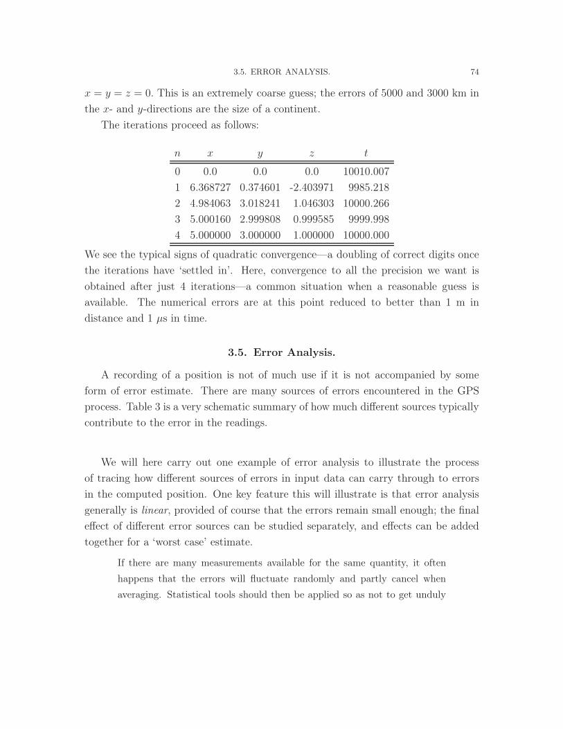
3.5. ERROR ANALYSIS. 74
x = y = z = 0. This is an extremely coarse guess; the errors of 5000 and 3000 km inthe x- and y-directions are the size of a continent.
The iterations proceed as follows:
n x y z t
0 0.0 0.0 0.0 10010.0071 6.368727 0.374601 -2.403971 9985.2182 4.984063 3.018241 1.046303 10000.2663 5.000160 2.999808 0.999585 9999.9984 5.000000 3.000000 1.000000 10000.000
We see the typical signs of quadratic convergence—a doubling of correct digits oncethe iterations have ‘settled in’. Here, convergence to all the precision we want is
obtained after just 4 iterations—a common situation when a reasonable guess isavailable. The numerical errors are at this point reduced to better than 1 m indistance and 1 µs in time.
3.5. Error Analysis.
A recording of a position is not of much use if it is not accompanied by someform of error estimate. There are many sources of errors encountered in the GPSprocess. Table 3 is a very schematic summary of how much different sources typicallycontribute to the error in the readings.
We will here carry out one example of error analysis to illustrate the processof tracing how different sources of errors in input data can carry through to errorsin the computed position. One key feature this will illustrate is that error analysis
generally is linear, provided of course that the errors remain small enough; the finaleffect of different error sources can be studied separately, and effects can be addedtogether for a ‘worst case’ estimate.
If there are many measurements available for the same quantity, it often
happens that the errors will fluctuate randomly and partly cancel when
averaging. Statistical tools should then be applied so as not to get unduly

3.5. ERROR ANALYSIS. 75
Typical errors (in meters) in computed distance to eachsatellite due to different error sources
Source Standard GPSSatellite clocks1 1.5Orbit errors 2.5Ionospheric delays2 5.0Tropospheric delays 0.5Receiver noise 0.3Multipath 0.6Typical resulting positional accuracyHorizontal 10Vertical 401 Clock stability: Rubidium 10−11–10−12, cesium 10−12 −−10−13.
(Cf. hydrogen maser 10−16 and typical watch 10−6)2 Can be reduced to 0.5 - 1.0 m if receiving on two frequencies; delay
proportional to (number of electrons)/f 2where f is the signal frequency.Table 3. Summary of error sources
pessimistic ‘worst case’ errors only. For example, with n estimates, the
expected error often decreases like 1/√n.
We suppose here that we have only the top four equations of the set (3.1) available.We write these in the form
(3.1)
f1 ≡ (x− 3)2 + (y − 2)2 + (z − 3)2 − [(T1 + t1 − t) · c]2 = 0
f2 ≡ (x− 1)2 + (y − 3)2 + (z − 1)2 − [(T2 + t2 − t) · c]2 = 0
f3 ≡ (x− 5)2 + (y − 7)2 + (z − 4)2 − [(T3 + t3 − t) · c]2 = 0
f4 ≡ (x− 1)2 + (y − 7)2 + (z − 3)2 − [(T4 + t4 − t) · c]2 = 0
where the recorded time delays according to the receiver’s very inaccurate clock are
T1 = 10010.00692286
T2 = 10013.34256381
T3 = 10016.67820476
T4 = 10020.01384571

3.5. ERROR ANALYSIS. 76
We have also introduced additional variables t1, t2, t3, t4 which represent furthererrors in the timing signals from each of the four satellites. Causes for these errors
could for example be ionospheric delays. We want to estimate the uncertainty is inthe position x, y, z and corrected time t, as functions of variations in t1, t2, t3, and t4.
Simplified one variable / one equation situation:
Had our system of equations been just one scalar equation in one variable
(3.2) f1 ≡ (x− 3)2 − [(T1 + t1 − t) · c]2 = 0
we would first set t1 = 0 i.e. assume this extra error was not there, and solve forx. Next, we would re-introduce t1 and ask how the variations in t1 will influence x.Hence, we view x as a function of t1 : x = x(t1). Differentiating (13.1) with respect
to t1 givesdf1
dt1= 2(x− 3)
dx
dt1− 2c2(T1 + t1) = 0.
Now we again set t1 = 0 and solve for dxdt1
. That derivative is precisely what wewant—a measure of how much x will change for small changes in t1.
Original four variable / four equation situation:
In (3.1), we similarly have x = x(t1, t2, t3, t4), y = y(t1, t2, t3, t4), z = z(t1, t2, t3, t4),
t = t(t1, t2, t3, t4). Differentiating fi with respect to tj becomes an exercise in usingthe chain rule:
dfidtj
=∂fi∂x
∂x
∂tj+∂fi∂y
∂y
∂tj+∂fi∂z
∂z
∂tj+∂fi∂t
∂t
∂tj+∂fi∂tj
= 0, i, j = 1, ..., 4.
This is most clearly written in matrix form
∂f1∂x
∂f1∂y
∂f1∂z
∂f1∂t
∂f2∂x
∂f2∂y
∂f2∂z
∂f2∂t
∂f3∂x
∂f3∂y
∂f3∂z
∂f3∂t
∂f4∂x
∂f4∂y
∂f4∂z
∂f4∂t
∂x∂t1
∂x∂t2
∂x∂t3
∂x∂t4
∂y∂t1
∂y∂t2
∂y∂t3
∂y∂t4
∂z∂t1
∂z∂t2
∂z∂t3
∂z∂t4
∂t∂t1
∂t∂t2
∂t∂t3
∂t∂t4
= −
∂f1∂t1
∂f1∂t2
∂f1∂t3
∂f1∂t4
∂f2∂t1
∂f2∂t2
∂f2∂t3
∂f2∂t4
∂f3∂t1
∂f3∂t2
∂f3∂t3
∂f3∂t4
∂f4∂t1
∂f4∂t2
∂f4∂t3
∂f4∂t4

3.5. ERROR ANALYSIS. 77
Taking partial derivatives of (3.1) gives all the entries of the first and last matricesabove
2
x− 3 y − 2 z − 3 c2(T1 + t1 − t)x− 1 y − 3 z − 1 c2(T2 + t2 − t)x− 5 y − 7 z − 4 c2(T3 + t3 − t)x− 1 y − 7 z − 3 c2(T4 + t4 − t)
∂x∂t1
∂x∂t2
∂x∂t3
∂x∂t4
∂y∂t1
∂y∂t2
∂y∂t3
∂y∂t4
∂z∂t1
∂z∂t2
∂z∂t3
∂z∂t4
∂t∂t1
∂t∂t2
∂t∂t3
∂t∂t4
=
= 2
c2(T1 + t1 − t) 0 0 0
0 c2(T2 + t2 − t) 0 0
0 0 c2(T3 + t3 − t) 0
0 0 0 c2(T4 + t4 − t)
.
Writing this as A X = B, we can solve for X by simply multiplying by A−1 fromthe left, or better still—view this as a linear system of equations with four RHSs and
four side-by-side solution vectors. Using the known values for Ti, setting ti = 0 andusing our numerical solution x = 5, y = 3, z = 1 and t = 10, 000 gives(3.3)
∂x∂t1
∂x∂t2
∂x∂t3
∂x∂t4
∂y∂t1
∂y∂t2
∂y∂t3
∂y∂t4
∂z∂t1
∂z∂t2
∂z∂t3
∂z∂t4
∂t∂t1
∂t∂t2
∂t∂t3
∂t∂t4
=
0.149896 −0.349758 −0.624568 0.824429
0.149896 0.249827 0.124914 −0.524637
−0.449689 0.749481 0.374741 −0.674533
−0.500000 2.166667 2.083333 −2.750000
This tells how sensitive each variable x, y, z, t is to the small errors in the timingst1, t2, t3, t4 for the signals from the four satellites.
If the timings are all accurate to within 0.1 µs = 0.0001 ms, the worst case errorsin the results can be calculated using the formula,
∆x ≈ ∂x
∂t1∆t1 +
∂x
∂t2∆t2 +
∂x
∂t3∆t3 +
∂x
∂t4∆t4,
to obtain

3.5. ERROR ANALYSIS. 78
x-dir (0.1499 + 0.3498 + 0.6246 + 0.8244) · 0.1 km ≈ 195 m
y-dir (0.1499 + 0.2498 + 0.1249 + 0.5246) · 0.1 km ≈ 105 mz-dir (0.4497 + 0.7495 + 0.3747 + 0.6745) · 0.1 km ≈ 225 mt-err (0.5000 + 2.5000 + 2.0833 + 2.7500) · 0.1 µs ≈ 0.75 µs
In this case, the positional error turns out to be largest in the z-direction. The besttime the receiver can calculate is about 7.5 times less accurate than the precision ofthe incoming signals.
The analysis above was based on reception from only the first four of our six
satellites, giving us a 4× 4 matrix in (3.3) with sensitivity information. In a similarway, we could have analyzed the full 6-satellite case to arrive at
∂x∂t1
∂x∂t2
∂x∂t3
∂x∂t4
∂x∂t5
∂x∂t6
∂y∂t1
∂y∂t2
∂y∂t3
∂y∂t4
∂y∂t5
∂y∂t6
∂z∂t1
∂z∂t2
∂z∂t3
∂z∂t4
∂z∂t5
∂z∂t6
∂t∂t1
∂t∂t2
∂t∂t3
∂t∂t4
∂t∂t5
∂t∂t6
=
=
−0.0362 −0.1061 −0.0267 0.2221 −0.4185 0.3655
0.1240 0.2097 −0.1619 −0.3125 0.2007 −0.0602
−0.0643 0.3353 0.0169 −0.0456 0.2505 −0.6213
−0.3616 1.1765 0.0047 −0.5127 1.4550 −1.4852
This time, the worst-case errors are notably smaller even though none of the inputsare any more accurate:
x-dir ≈ 118 my-dir ≈ 107 mz-dir ≈ 133 mt-err ≈ 0.50µs
The improvement in expected errors is better still—the probability that the signand size of all errors conspire to create a maximum error situation is far less likelythe more independent input variables that enter, i.e. cancellation of errors becomes
increasingly likely.

3.6. PSEUDORANDOM SEQUENCES. 79
3.6. Pseudorandom Sequences.
Two of the problems that arise in connection with transmitting timing pulses
from the satellites are
(1) how to send a very sharp pulse, so that its arrival can be very accuratelytimed, without needing to use a wide bandwidth (this will be explained inmore detail in a moment), and
(2) how to allow all the satellites to transmit on exactly the same frequencywithout their signals interfering with each other.
One mathematical construct—pseudo-random (PR) sequences—resolves both theseproblems very nicely. Once we have seen how they resolve the first problem, it willbe clear how the solution to the second one follows.
To appreciate the dilemma posed in point 1, we recall the function-Fourier trans-form pair f(x) = e−αx
2, f(ω) = 1√
4παe−ω
2/(4α)(c.f. Table 2 in Section 9.3). If theparameter α is large, the function f(x) will be a sharp spike, allowing its positionto be accurately pinpointed (think here of x as time). However, f(ω) will then have
a very broad maximum, i.e. occupy a lot of frequency space (bandwidth). On theother hand, making the parameter α small will make the pulse broad and difficultto accurately determine its position (e.g. center of its peak).
The answer to this dilemma turns out to be that after all one does not need a
sharp pulse in order to achieve a fine time resolution—a suitably structured signalof long duration can also achieve a fine time resolution. Each satellite sends its ownPR signal as illustrated in Figure 3.6.1; very small up/down-variations in frequencyaccording to a pattern that looks random, but is fixed for each satellite, and repeats
periodically after 1023 chip times of 1 µs each. Thus, the whole pattern repeatsroughly each ms. During each 1 µs chip time, the carrier (at 1575.42 MHz) goesthrough about 1,500 cycles—enough to detect which one of the two very nearbyfrequency levels that is used. A receiver knows the pseudo-random sequence (for
each satellite), and slides its copies relative to the received signal until the matchgets perfect (c.f. again Figure 3.6.1).
The correlation function f(x) of two functions, g(x) and h(x), is defined as,

3.6. PSEUDORANDOM SEQUENCES. 80
Figure 3.6.1. Pseudo-random (PR) received code compared with acopy stored in the receiver (in this picture shifted one chip time).
f(x) =
∫g(s)h(s+ x)ds,
i.e. it measures the ‘similarity’ between two functions as they are shifted aver eachother. Figure 3.6.2 shows the correlation function of the two sequences of Figure 3.6.1(where summation replaces the integral), displayed as a function of the sideways shift
in a case of a periodic PR sequence of length 128.Whenever the shift is a multiple of 128, we get here a very sharp spike of perfectly
triangular shape with a base width of 2 chip times. Even a small misalignment intime—a fraction of the chip time—will notably bring down the correlation. A timing
error of about 1/20th of a chip time would lead to a distance error of about 15 m;typical of the hardware capabilities of present low cost GPS receivers.
Of course, with 24 satellites in orbit, each receiver has to test the received signalagainst 24 copies.
The whole PR sequence repeats about each 1 ms. Given the speed of light,this corresponds to about 300 km. All distances to satellites become undeterminedwith respect to multiples of this distance. The easiest way to avoid this ambiguity

3.6. PSEUDORANDOM SEQUENCES. 81
Figure 3.6.2. Correlation between a periodic PR code of length 128and a translated copy of itself. The sharp spikes appear here every 128chip times.
is to require that the receiver has to be initialized—the user has first to enter an
approximate position that is accurate to better than 150 km, thus removing thearbitrariness. There are (at least) two other ways to resolve this problem:
i.: Guessing wrong by 300 km (when receiving signals from the minimal num-
ber of satellites required to get a position) is very likely to produce a positionhundreds of kilometers under ground or above ground—easily rejected forall receivers not used in space crafts, and
ii.: When receiving signals from more satellites, a wrong guess will quite cer-
tainly produce a contradiction—no single point will satisfy all the distancerequirements.
This second observation allows us to state the problem of finding our position as
one of locating a point so that the distance to every observed satellite is equal to anunknown integer plus a known (measured) fractional part of this 300 km distance.Determining these integers would be an example of integer programming—the task of

3.6. PSEUDORANDOM SEQUENCES. 82
finding best approximations to a problem for which several unknowns are constrainedto integer values only.
Integer programming is actually of great importance for GPS, but in a
slightly different way. To get the highest possible accuracy, we apply the
idea not to the 300 km PR sequence repeat distance, but to the approxi-
mately 0.2 m wavelength of the 1745.42 MHz carrier wave. Trying to lock
on to the phase angle of the carrier oscillations, we get distances to within
an unknown multiple of 0.2 m. With a good positional guess, say from dif-
ferentially corrected GPS, we may have only about 50—100 multiples to be
concerned with. Finding a position that gives a correct carrier phase for
all available satellites can pinpoint just which carrier multiple we are locked
onto for each of the satellites in view, i.e. an error better than 0.2 m. Finally,
being locked onto exactly the right integer multiple of the carrier oscillation,
the phase angle can be reconciled to maybe one part in 200. The accuracy
is now down to about 1 mm—not bad considering that the radio signals
are of quite narrow bandwidth and how fast these satellites fly far out in
space! For more discussion on this issue of locking onto an individual carrier
wave and its phase angle—and on integer programming in the context of
GPS—see Strang and Borre [?].

CHAPTER 4
Radar Scattering from Aircraft
4.1. Introduction.
Chapter to be written. Another suggestion: A chapter on Climate Modeling?
83

CHAPTER 5
FREAK OCEAN WAVES
5.1. Introduction.
Large waves on the oceans usually appear as the result of storms, and they tendto arrive in lengthy wave trains. However, numerous marine disasters are also causedby more sporadically appearing isolated giant waves. For example Bascom (1980)
tells about ships being lost and of survivors describing the cause as a huge solitarywave. He also recounts that both the liners Queen Mary and Queen Elizabeth werefortunate to survive dramatic freak wave encounters in the North Atlantic (at onepoint causing the former to roll to within two degrees of its point of no-return while
carrying 15,000 US troops to the UK in World War II).Although freak waves can arise in all oceans, one particular stretch of one of the
major shipping routes is particularly prone to these. This is within the AgulhasCurrent off the SE coast of South Africa, approximately between Durnford Point
(shortly north of Durban) and Port Elizabeth—see Figure 5.1.1. Table 1 lists somelarge ships which have been severely damaged by freak waves within this area duringthe 11 years 1981-1991 (not including minor ships such as fishing vessels etc.).
Incidents in the Agulhas Current before this time period include
• Passenger liner Waratah, lost in 1909 while carrying 211 crew and passengersby the end of the homeward leg of her maiden voyage (to Australia). Notrace of the ship was ever recovered.• Supertanker World Glory, sunk in 1968 after being broken in two by a single
freak wave,• Supertanker Neptune Saphire in 1973 lost its front 60 m bow section.
Figure 5.1.2 shows the cargo liner Bencruchan with its front quarter bent down aftera freak wave incident off the SA coast (also in 1973). Figure 5.1.3 shows a giant wavebreaking over the front deck of the super-tanker Esso Nederland in 1978 (with no
84

5.2. MECHANISM FOR FREAK OCEAN WAVES. 85
DATE VESSEL TYPE DWT DATE VESSEL TYPE DWT
81 4 Energy Endurance T 205,807 87 7 Goldstar OBO 145,057
8 Schelderin T 230,679 10 Bocita B
8 Rimula OBO 227,412 88 11 Atlantic Emperor T 292,641
82 4 Alva Sea OBO 89 7 Arabian Sea T 315,695
7 Marofa T 135,000 11 Paaficos T 268,467
7 Antonios T 290,558 90 1 Rokko San OBO 200,000
7 Theodora B 137,519 9 Dorado Star T
7 Victoria T 236,810 11 Samjohn Captain B 65,051
9 Torvanger CH-T 17,057 91 4 Vasso B 51,181
84 7 Merity CH-T 5 Alborz T 230,673
11 Alva Sea OBO 225,010 8 World Renown T 262,267
85 2 Musashi B 8 Mimosa T 357,647
86 6 World Scholar T 268,000 8 Novelty T 233,399
8 Formosa Fortune OBO 8 Settebello T 317,354
9 Atlas Pride T 248,602
Table 1. Major ships severely damaged in the Agulhas Current 1981-1991. Ship types: T - Tanker, OBO - Oil/Bulk ore, B - Bulk, CH-TChemical tanker. Source: Pentow Marine Salvaging Co, S.A.
damage suffered to the vessel). Figures 5.1.4 and 5.1.5 show the damages sufferedby the first and the last ships that were listed in Table 1.
Ships tend to travel in the direction of a current (to gain speed), and freak waves
tend to move against a current, causing frontal damage to ships to be predominant.A freak wave is often preceded by a long sloping trough, in which the ship acceleratesdownward before being hit by the wave. The frontal damage can arise either when thebow gets buried into the freak wave, or when the high pressure is suddenly released
as the ship emerges out of it. Many questions relating to freak waves remain open.For example, little is known about their typical sideways extent and the distancethey can travel before dissipating or otherwise breaking up.
5.2. Mechanism for freak ocean waves.
Different explanations have been proposed for freak waves. For example, Dawson(1977) suggests they can be attributed quite directly to the bottom topography, anidea ”found to be fallacious” according to Shillington and Schumann (1993). The

5.2. MECHANISM FOR FREAK OCEAN WAVES. 86
Figure 5.1.1. Schematic view of the southern part of Agulhas current.
Figure 5.1.2. Cargo liner Benchruchan—with front quarter of theship bent down after a freak wave incident.
most plausible mechanism is a focusing process, described by Crapper (1984) andfurther studied by in Gerber (1993), (1996).
Empirical statistics on ocean waves tell that, on the average, one wave in 23 isover twice the mean wave height, one in 1,175 over three times it, and one in 300,000
over four times the average height. Although rough weather appears to favor theemergence of freak waves—their energy has to come from somewhere—they do notseem to simply represent the top end of this distribution.

5.2. MECHANISM FOR FREAK OCEAN WAVES. 87
Figure 5.1.3. Large wave in the Agulhas current breaking over thefront deck of the supertanker Esso Nederland.
Figure 5.1.4. Bow damage to Energy Endurance.
Figure 5.1.5. Bow damage to Atlas Pride.

5.2. MECHANISM FOR FREAK OCEAN WAVES. 88
Regarding the SE coast of South Africa (known as the “Wild Coast”), there arehowever several special circumstances that should be noted:
• One of the fastest and largest ocean currents in the world flows along the
coast (cf. Figure 5.1.1). The Agulhas Current can reach around 2-3 m/s (4-6knots) and transports about 70 · 106 m3/second (250 km3/hour) of water.It follows very closely the edge of the continental shelf, and it is fairly freeof side-eddies while it makes a slow turn in the area which is most prone to
the freak wave phenomenon.• This current meets nearly head-on a steadily incoming near-monochromatic
wave swell, constantly generated in the ’roaring forties’, see Figure 5.2.1.
Waves can travel very long distances before loosing energy due to internal viscosity.Crapper (1984) notes that a wave with time period T = 9 s (average for ocean
swell; wavelength λ ≈ 126 m) looses only about 1/10th of its height in a distancecorresponding to three times around the earth. For a short T = 2 s - wave (λ ≈ 6.2m), the distance is much smaller - about 62 km.
• Freak waves have been found to occur particularly frequent during weathersituations such as the one shown in Figure 5.2.2. This supports the notion
of the incoming swell as a major factor.
Waves meeting a current not only get their wave length reduced (coming closer tobreaking) - their directions also change. This will turn out to be the key effect inmodeling the freak wave phenomenon.
Figure 5.2.1. Typical swell paths. In the shaded area - part of the’roaring forties’ - average wave heights exceed 4.5 m. (Data from Chel-ton, Hussey and Parke, 1981).

5.3. DERIVATION OF THE GOVERNING EQUATIONS. 89
Figure 5.2.2. Weather situation most likely to generate freak waves(long ’fetch’ strengthening the incoming swell; illustration from Mal-lory, 1974).
5.3. Derivation of the governing equations.
We start by assuming that the incoming wave amplitudes are low enough thattheir propagation can be approximated as linear - different waves will then mainly
superpose on each other. This simplification will quite certainly not hold for 30meter high giant waves near breaking, but we are here primarily interested in themechanism that can lead to such waves rather than in their dynamics once they havebuilt up to giant size. Let the wave (for now in 1-D) have the form
(5.1) η(x, t) = a cos(k x− ωt) = fRe a ei (k x−ω t)
For simplicity in writing, we will follow the convention of omitting ”Re” in most ofwhat follows, i.e. we will be working with
(5.2) η(x, t) = a ei (k x−ω t)
For deep water, we note in Section 8.2 the dispersion relation
(5.3) ω =√gk.

5.3. DERIVATION OF THE GOVERNING EQUATIONS. 90
Here, g is the acceleration of gravity, approximately 9.8 m/s2. It follows from (5.2)that the wave length λ satisfies
(5.4) λ =2π
k
and also that the phase speed cp =√
gk
=√
gλ2π
and the time period T = 2πω.
A typical wave swell might have T ≈ 10 s, and hence λ ≈ 160 m (swells of upto λ ≈ 800 m have been recorded). The highest possible steady waves can be shownto have h/λ ≈ 0.142 (with h being the vertical distance between crest and trough).For λ = 160 m, the maximal steady height would thus be about 23 meters. That is
about 5 times the height that is typical in the ocean south of South Africa. Wavesthat are so much lower than the steady ones of maximal height behave reasonablylinearly, and (5.2) is a good enough wave model for studying the onset of focusing.
A usual way to derive governing equations is to look at the mechanics of a phe-
nomenon in detail—see what happens on local time and space scales of ∆t and ∆x
and, in the limit of these getting smaller, obtain some governing ODEs or PDEs(as we did in the case of a string under tension in Section 8.3). The approach weused in that section for obtaining Maxwell’s equations was somewhat different in
that we started out with some laws in terms of integrals along arbitrary contours,and we then applied techniques of calculus to modify these into volume integrals,again giving governing PDEs as the volumes were decreased to zero. For the presentproblem, a third approach is needed. The first of the approaches above is clearly
impossible; there is far too much data and complexity involved in modeling oceandynamics all the way down to its individual waves. This would require discretizationinto trillions of mesh points, and totally astronomical computer resources (for bothoperation count and memory).
The totally different approach needed here is described in detail in Section 8.7.
The key observation is that the phase of the wave field is sufficiently well-behavedto allow one to identify local frequency ω and wave number k. In addition one notesthat the frequency and wave numbers are related through a dispersion relation,
ω = W (x,k,t).

5.3. DERIVATION OF THE GOVERNING EQUATIONS. 91
Using these two ideas it is rather straightforward to derive a Hamiltonian system forthe characteristic curves for x and k
dxjdt
=∂W
∂kj,
dkjdt
= −∂W∂xj
,(5.5)
where j = 1, . . . , n and n is the spatial dimension of the problem. Thus the maintask therefore has to be to identify the dispersion relation. Very surprisingly, thisgeneral observation, together with Hamilton’s equations contain all the physics thatis needed for modeling wave focusing in the presence of arbitrary currents.
5.3.1. The Hamilton equations for a 2-D wave field. In Section 8.4, itwas shown that the dispersion relation for deep water waves in the absence of anycurrent, is given by
ω =√g |k|.
Since it does not depend on x, Hamilton’s equations show that the characteristiccurves are straight lines which does not allow any interesting phenomena. The situa-
tion changes significantly if one introduces a current moving with velocity U(x). Thetime frequency, as seen by a stationary observer, would include a Doppler correction,and the dispersion relation becomes,
ω = W (x,k) =√g |k|+ k ·U.
According to Hamilton’s equations, the quantity remain constant along the charac-teristic curves. will hold at all spatial locations.
In 2-D, x = [x1, x2] and k = [k1, k2] and the plane wave
ψ(x, t) = ei(k·x−ωt)
travels in the direction of the k-vector. The dispersion relation takes the form
(5.6) ω = W (x1, x2, k1, k2) =√g (k2
1 + k22)
1/4 + k1 U1(x1, x2) + k2U2(x1, x2)

5.3. DERIVATION OF THE GOVERNING EQUATIONS. 92
Hamilton’s equations (5.5) are now explicitly written
(5.7)
{dx1
dt= ∂W
∂k1dx2
dt= ∂W
∂k2{dk1dt
= − ∂H∂x1
dk2dt
= − ∂W∂x2
will hold. Next step is to use (5.6) to calculate the partial derivatives that appear in
the RHSs of (5.7). Straightforward algebra gives
∂W∂k1
= α k1 + U1
∂W∂k2
= α k2 + U2
∂W∂x1
= k1∂U1
∂x1+ k2
∂U2
∂x1∂W∂x2
= k1∂U1
∂x2+ k2
∂U2
∂x2
where α =√g
2|k|3/2 . Therefore, the coupled system of ODEs which needs to be solvedin order to find k(x)—describing the wave field everywhere—becomes
(5.8)
With nocurrent
Terms dueto current
dx1
dt= αk1 + U1
dx2
dt= αk2 + U2
dk1dt
= −(k1
∂U1
∂x1+ k2
∂U2
∂x1
)
dk2dt
= −(k1
∂U1
∂x2+ k2
∂U2
∂x2
)
.
What this tells is that, if the current U(x) is given, and we at some locationx = [x1, x2] specify an initial wave (by giving k = [k1, k2] there), solving the fourcoupled ODEs (5.8) forward in the parameter t will trace out a path in the (x1, x2)-plane along which we at the same time obtain k1 and k2. Starting from many places
along a (spatial) domain boundary, we can trace out a dense set of paths in the x-plane—hence obtain k1 and k2 throughout a domain. Each such path represents howa ray progresses. Rays are a natural concept in case of light, but for water a moreabstract concept; a path that is orthogonal to the wave fronts. Wave energy can be
shown to follow these rays—if rays cross each other, wave energy has focused. Solvingthis coupled system of ODEs will therefore produce paths in the x-plane along which

5.4. TEST PROBLEM - CIRCULAR CURRENT. 93
energy travels. The independent variable t is for the moment just a path parameter,although it actually turns out to correspond to physical time describing the speed
by which energy propagates along the paths.Note:
• Well hidden in the interpretation of the rays are a few physical assumptions
than have not yet been pointed out. A notable one is that the wavelength λmust be small in comparison with any objects or flow features (such as cur-rents). This tends to be the case for light, making rays then a particularlyclear concept. It is much less clear in the case of sound—such waves travelseasily around everyday objects. Another key difference between the linear
propagation of light and the non-linear case of water waves is that the formercan cross each other without any interference. Large water waves comingtogether are likely to break, and therefore change their character. The raymodel is mainly useful to highlight areas with potentially high wave ener-
gies, but it can not be expected to give any details after waves have passedthrough focusing areas.
5.4. Test problem - Circular current.
Figure 5.4.1 shows a test problem for ray tracing that has been used by someinvestigators (Gerber, 1993, White and Fornberg, 1997)—a circular current U(x, y)
with inner radius 40 km and outer radius 160 km.Between these boundaries, the velocity profile (a function of radius r only) is
parabolic, with a maximal velocity of 2 m/s.We now denote the spatial directions x and y (rather than x1 and x2), and
the velocity components in these directions u(x, y) and v(x, y) respectively. Theeasiest way to specify a current field u(x, y) and v(x, y), which needs to satisfy the
incompressibility requirement
(5.1)∂u
∂x+∂v
∂y= 0

5.4. TEST PROBLEM - CIRCULAR CURRENT. 94
Figure 5.4.1. Test example of circular current. Parabolic velocityprofile with maximum velocity of 2 m/s.
may be to note that (5.1) is equivalent to the existence of a stream function ψ(x, y)
such that
(5.2)
{u = ψy
v = −ψx.
Given any (reasonably smooth) function ψ(x, y), the velocities u(x, y) and v(x, y)
it produces through (5.2) will automatically satisfy (5.1). Figure 5.4.2 shows theψ(x, y) function (undetermined with respect to an additive constant) correspondingto a circular current.
Looking along the x-axis, we have
v(x, 0) =
0 0 < x < 40e3(x−40e3)(x−160e3)
1.8e940e3 < x < 160e3
0 x > 160e3
.
Hence, from (5.2) and noting that ψ(x, y) becomes a function of r only (r =√x2 + y2),
we obtain
ψ(r) =
− 1.76e627
0 < r < 40e3
− 32r9
+ r2
1.8e4− r3
5.4e940e3 < r < 160e3
0 r > 160e3
.

5.4. TEST PROBLEM - CIRCULAR CURRENT. 95
Figure 5.4.2. Stream function ψ(x, y) for the annular current (withhorizontal scale in kilometers, vertical in 1000m2s−1
Figure 5.4.3. Velocity component in x-direction of circular current.
Figure 5.4.3 shows the resulting u−field (as to be expected with its largest valueat (0,100) (when measured in km), most negative at (0,-100), and zero along y = 0).
In the wave ray field shown in Figure 5.4.4, each wave has a time period T = 10
s, i.e. according to (5.3) ω = 5/π.From (5.3) follows then |k| = 25/(9.8 · π2). At equi-spaced positions x along the
left and bottom edges of the domain, we start all the rays with k = (1, 1) · |k| /√
2
(a vector of the length corresponding to T = 10 s, and pointing towards NE). The
computation of the paths involves the following steps:
• Generate the u− and v−fields for the circular current, and

5.5. ATLAS PRIDE INCIDENT REVISITED. 96
Figure 5.4.4. Ray pattern for circular current in case of incomingmonochromatic waves from SW with a time period T = 10 s (corre-sponding to a wavelength λ ≈ 160 m.
• For each ray, solve the four coupled ODEs (5.8) for as long time as is neededuntil the ray exits the domain.
In our code a second order, 2-stage Runge-Kutta method is used as the ODE solver.Many other choices would have worked equally well (cf. the discussion of ODEsolvers in Chapter 16). The other main numerical issues are interpolation and finite
difference approximations. At every (discrete) (x, y)−position that we reach alonga ray path, the values for u, v, ux, uy, vx, vy must all be obtained by interpolationfrom adjacent (x, y)−grid positions.
A ray path picture like Figure 5.4.4 is very effective in illustrating focus spots
of wave energy. In other cases, it might be more useful to display the wave energy(roughly corresponding to the ray density) as a function of spatial position as inFigure 5.4.5 - generated from the rays in Figure 5.4.4.
5.5. Atlas Pride incident revisited.
To apply the numerical ray tracing technique to the region SW of South Africa,we need data on the current and the incoming wave swell. The current can be seen
quite well in infrared images from weather satellites. Figure 5.5.1 is a black-and-whitereproduction of a false-color high resolution original which shows warmer water inbrighter colors. Small eddies can readily be identified, and their motions tracked on

5.5. ATLAS PRIDE INCIDENT REVISITED. 97
Figure 5.4.5. Ray pattern translated into a surface display of raydensity - an approximate measure of wave energy.
Figure 5.5.1. Infra-red weather satellite picture of southernmost partof the Agulhas current, as it breaks up into eddies just south of themain danger zone. (The sloping line drawn in the rectangular boxshows the path of space shuttle Challenger during an unsuccessful at-tempt to record freak wave patterns from space by radar).
a sufficiently frequent basis for providing all the needed current velocity data. Since
the incoming wave swell can be approximated well by a monochromatic wave train,wave number (a 2-vector) and amplitude (a scalar number) suffice as input wavedata. Buoys in the ocean record this.

5.6. CREATION OF FREAK WAVES IN AN ENERGY-RICH OCEAN STATE. 98
Figure 5.5.2. Calculation of wave (ray) paths based on data for cur-rent and incoming swell on 4/7/91. A primary focus is clearly visiblenear the inner edge of the current, which further north acts like a waveguide.
Figure 5.5.2 shows the result of a ray tracing based on data for 4/7/91. A verystrong focus can be seen shortly south of Durban. North of that, we can see howwaves have got trapped within the current, acting like a wave guide. The ray picturechanges on a time scale of several hours, and is significantly different on the date
of the Atlas Pride accident later that year (9/8/91), cf. Figure 5.5.3 (showing alarger scale detail of the area south of Port Elizabeth). The small arrow points atthe position of Atlas Pride at the time of the accident, again seen in different typesof displays in Figures 5.5.4 and 5.5.5 (both generated from this same simulation).
The calculation highlights as a danger area maybe 1/1000th of the total area offthe SE coastline. In a second case (the Alborz, 1991), the agreement between com-puted danger area and site of actual incident proved equally good. The probabilityfor a 2-out-of-2 score having occurred purely by chance is small.
5.6. Creation of freak waves in an energy-rich ocean state.
The focusing mechanism, described in the previous sections, show how dangerareas can arise and their position be computed. Since these areas are considerablysmaller in extent than the width of the current, shipping (if receiving proper forecasts)

5.6. CREATION OF FREAK WAVES IN AN ENERGY-RICH OCEAN STATE. 99
Figure 5.5.3. Ray picture for the Atlas Pride accident. Small arrowmarks the position of the ship.
Figure 5.5.4. Ray intensity represented as surface elevations.
can still safely utilize the 4-5 knots extra speed it offers on travels along its path.However, an energy rich sea state does not imply that freak waves need to arise.Even under such circumstances, freak waves is a relatively rare phenomenon. Inparticular, our analysis has so far given no indications about issues like
• Onset mechanism for freak wave from an energy-rich sea state,• General characteristics of freak waves. These are often, by eye witnesses,
described as a slowly sloping long trough followed by one or two giant waves,

5.6. CREATION OF FREAK WAVES IN AN ENERGY-RICH OCEAN STATE. 100
Figure 5.5.5. Contour plot of the ray intensity.
appearing as near-vertical walls of water, as schematically indicated in Fig-
ure 5.6.1)• Sideways extent of freak waves,• Duration in time and distance traveled by freak waves before disintegrating
back to regular waves.
Figure 5.6.1. Schematic illustration of a freak wave preceeded by atrough, moving against a current.
The onset process is clearly a highly nonlinear process. A recent numerical studyby V.E. Zakharov et.al. (2002) may provide some insights in this. Their numericalcalculation is in 1-D (meaning one horizontal space dimension together with a ver-
tical one plus time). This work incorporates a number of analytical and numericaltechniques (conformal mapping, Hamiltonian equations, FFT treatment of a Hilberttransform, etc.) and produces time simulations of highly nonlinear wave evolution.
While the ’classical’ Benjamin-Feir instability demonstrates how a uniform 1-
D wave train on deep water will develop instabilities over time, it deals only withrelatively weak nonlinearities. Over longer periods in time, it models recurrenciesof regular and less regular states - but it does not address what happens in case of

5.6. CREATION OF FREAK WAVES IN AN ENERGY-RICH OCEAN STATE. 101
Figure 5.6.2. Emergence of freak waves in a 1-D simulation, startingfrom a uniform wave train.
very high waves. So far, only numerical computations can give insights in such flowregimes (since experimentally realizing a true 1-D wave appears to be exceedinglydifficult). Figure 5.6.2 (from [..]) shows how the fully nonlinear mechanisms inlarge waves indeed can produce a dramatic energy concentration into single waves.
Regarding freak waves in the ocean, one possibility is that the process illustrated inFigure 5.6.2 ’kicks in’ only when the original wave state happens to be locally bevery nearly one-dimensional. If so, this could explain why energy-rich sea states (aswe computed by the ray tracing method) are necessary but not at all sufficient for
freak waves to be generated.

CHAPTER 6
PATIENT POSITIONING
6.1. Introduction.
The human stereo vision system consists of two basic components—the retinas(hardware) that record the images, and the brain (hardware) that process the imagesand do the three dimensional reconstruction. Studies (cite Stephen Pinker) indicate
that we are not born with this ability, but that it is acquired shortly after birth—thesoftware requires a training process. It is this 3D ability that allows us to become soproficient in different ball games, to judge the distance to the threat, to accuratelynavigate at high speed, and so on. There is little mystery behind the reconstruction
process, the brain has to identify corresponding points on the two retinal images, andfrom their offset estimates the depth. The reader will be familiar with the followingexperiment: Hold you finger in front of you, alternatively close first the one eye andthen the other and observe how the position of your finger changes with respect to
the background. Now move your finger closer to your eyes and note how its positionsagainst the background change from the previous experiment. It is this offset betweenthe relative positions that allows the brain to estimate depth. You may also want toclose one eye and look around. Do you note how different the world looks.
Incidentally, if you ever find yourself in a situation where you see double (such as
after partying to much), it is an indication that your brain is malfunctioning—thetwo images from your retinas are no longer combined into a single 3D view.
This 3D stereo reconstruction is so useful that it is no wonder that we want todo the same on a computer. Again the challenge can be described quite easily, given
two images of an object recorded at different angles, find the offset of the featuresand use that to do a 3D reconstruction of the features. In case it is not clear, by‘feature’ we simply mean a point that is present in the image. If it is identifiable onboth images, it is called a corresponding feature. It is the 3D coordinates of these
102

6.2. PROTON THERAPY. 103
features that we are after. The 3D coordinates of the corresponding features frompart of the structure we want to reconstruct, the more features the more accurate
the reconstruction.As pointed out above, 3D reconstruction from stereo images (there is a number
of other ways of estimating 3D structures including X-ray tomography discussed inChapter 1), find various applications. In this chapter we want to discuss a some-what unusual, but important application of stereo reconstruction, namely its use
to position patients undergoing proton therapy. In the next section we give somebackground information of the problem before we proceed to discuss the solution.Apart from the mainstream mathematics such as the Singular Value Decompositiondiscussed in detail in Section 11.5, stereo reconstruction relies heavily on an un-
fortunately much neglected, but very elegant geometric framework called projectivegeometry. Although we are not in a position to treat the subject in any depth, wewill give you a flavor of it. And we trust that you will be able to put it to good use,not only for stereo reconstruction.
6.2. Proton Therapy.
Proton therapy is fast becoming one of the most significant modes of treatment ofmalignant tumours. In order to understand why it is so successful we really only needto know that an atom consists of a nucleus made up of positively charged protons, andneutrons, and surrounded by a cloud of negatively charged electrons. Assume that we
are somehow able to get hold of a free proton and have a mechanism to send it throughliving tissue. Since the proton is positively charged, it attracts the negatively chargedelectrons surrounding the atoms as it passes through the tissue. As it it attracts theelectron it transfers some of its momentum to the electron, slowing it down. As
it slows down, the interaction with the nearby electrons increases, slowing it downeven more, increasing its pull on the electrons. At some point the pull becomesstrong enough to knock the electron out of its orbit, a process known as ionization.The effect this has on living tissue is to mess up the DNA thereby destroying the
living cells. This is exactly what we need to destroy cancerous cells, but it is badfor healthy tissue. Whatever we do, including proton therapy, healthy cells aregoing to be destroyed in the process. All cancer treatment today is based on a single

6.2. PROTON THERAPY. 104
principle: Healthy tissue recovers faster than the malignant tumors. Therefore, if oneadminister the treatment sessions over a period of time, the tumors are completely
destroyed while the healthy tissue has time to recover between sessions.What makes proton therapy so special is that one can localize the ionization
much better than in other treatment procedures, thereby confining the damage tothe tumor with little damage to the nearby healthy tissue. The basic idea wasalready conceived by Robert R Wilson in 1946 and illustrated in Figure 6.2.1 Note
how sharply the relative dosage increases with depth in the tissue as described above,an effect known as the Bragg peak. Also note how well the proton dosage is localizedin comparison with other treatments. In sense it is too localized, one wants todestroy the whole tumor not only a small part of it. For that reason the Bragg peak
is modulated. First the energy with which the protons inter the body is calculated(it depends on the distance the protons need to travel through the healthy tissuein order to reach the tumor) so that the Bragg peak occurs inside the tumor. Theproton beam is then modulated by placing a spinning disc of variable thickness in
front of the beam. Some of the protons pass through thicker regions of the discslowing then down. If the variation in thickness is just right, the Bragg peaks of theprotons with different energies cover the total depth of the tumor. The proton beamobviously also has to be shaped in the form of the profile of the tumor. This can be
done by placing a thick lead disc with a cut-out in the shape of profile of the tumorin front of the beam.
Although already proposed by Wilson in 1946, the first treatment on a regularbasis only started in 1990 at Loma Linda University Medical Center. One of the
reasons for the delay was due to the inability of doing 3D imaging; it was just notpossible to determine the exact position and extent of the tumor. This changed whenCT scans, based on the X-ray tomography discussed in Chapter 1 became available.At the moment (2007) some 26 facilities are in operation world wide, with many
more under construction.Of course there is the matter of getting hold of protons with sufficient energy to
penetrate to the tumor. Since protons are positively charged they can be acceleratedin a cyclotron. Proton therapy therefore requires a cyclotron, not exactly standard
hospital equipment, at least not yet. Modern facilities newly constructed are in

6.2. PROTON THERAPY. 105
Figure 6.2.1. Bragg peak.
a position to design their cyclotrons specifically to treat malignant tumors. Thedesigners however, face a formidable problem—the protons need to be acceleratedto energies of the order of 250MeV. If this does not mean much to you, the electrons
do about 5 million trips around the accelerator at about 600 000 000 rpm’s. In theprocess the protons reach speeds about half that of light—they go fast. All our talkabout the Bragg peak and precise localization of the ionization is in vain unless oneis able to align the tumor exactly with the proton beam. Again the positive charge
of the proton is useful, using giant magnets the protons can be deflected from theirpath. Since the protons move so fast these magnets are truly gigantic. A typicalgantry system used to precisely align the proton beam to within a fraction of amillimeter is a 200 ton, three-story high construction. It will utilize several 2000kg
magnets consuming 3000 ampere each. It is not energy efficient, the whole systemmay consume a million watts to deliver 1
5watt for 1
3s to the tumor.
6.3. PATIENT POSITIONING. 106
Although this is a solution that is common with modern treatment centers, thereare a number of cyclotrons all over the world that are no longer powerful enough to
do any useful physics that can be and are converted for medical purposes, includingproton therapy. The proton beams from these cyclotrons are fixed and constructionof a gantry system is in many instances prohibitively expensive. There has to be acheaper solution.
The cases in point are the cyclotrons at iThemba laboratories near Cape Town
in South Africa (see Figure 6.2.2) , and the original cyclotron (dating from verylate 1940’s) at the Joint Institute for Nuclear Research in Dubna, north of Moscow.Instead of aligning the proton beam, both these facilities position the patient, usingcompletely different methods. The Dubna facility basically position the patient by
taking a CT scan of the patient strapped to a maneuverable chair in treatment vault.The iThemba Lab solution employs stereo vision, described in the next section.
6.3. Patient Positioning.
The IThemba proton therapy procedure at the time of writing only treats tumorsin the brain. Since the patient is manipulated into position internal organs shift andit is hard to determine the precise 3D location of the tumor with respect to the protonbeam. The brain encased in the skull van be treated as a rigid object with no or
minimal shift of the internal structures. This is can be exploited by first determiningthe position of the tumor in relation to external markers. For this purpose a tight-fitting mask is constructed for each patient. On the mask is a number of reflectivemarkers as shown in Figure 6.3.1
This mask is then fitted on the patient and a CT scan is taken of the head with themask in position. The CT scan shows the position of the tumor in relation to the CTscanner coordinate system. At the same time the 3D coordinates of the markers inthe CT coordinate system are also determined using a stereo camera setup as shown
in Figure6.3.2 (a). Figure 6.3.2(b) is an image of the CT scanner with cameras inposition. Don’t get too concerned at this stage, the rest of the chapter explains howto calculate the 3D coordinates using stereo vision.

6.3. PATIENT POSITIONING. 107
Figure 6.2.2. The exit of the proton beam from the cyclotron atIThemba Labs.
With the position of the tumor known relative to the markers, the patient isthen immobilized on a mechanical chair, or a robot arm. Figure 6.3.3 shows themechanical chair used before it was replaced with a mechanical robot arm.
The treatment vault is equipped with a number of cameras (9 at the time ofwriting). The reflective markers are automatically detected by at least 3 cameras(otherwise the marker is rejected) and it 3D position calculated with respect to theworld coordinate system of the proton beam. Thus the 3D position of the markers,
hence the 3D location of the tumor is known with respect to the proton beam co-ordinate system. Since the desired position is known—as determined by the clinicalprofessionals—the patient is moved into position by manipulating the chair or the

6.3. PATIENT POSITIONING. 108
Figure 6.3.1. Patient mask with reflective markers.
CT Scannercoordinatesystem CC
CCD Cameras ofStereo rig
ZC
YC
XC
(a) (b)
Figure 6.3.2. CT scanner. (a) Coordinate system. (b) Actual scan-ner with cameras in position.
robot arm. A final X-ray is then taken to confirm that the patient is in position
before the proton beam is activated.Just to complete the picture, the cameras are also used to monitor the motion of
the patient as it is moved into position. It also monitors the patient during treatment.If any motion id detected the beam is immediately shut down.
From the discussion above it should be clear that the heart of the system consistsof a multiple camera setup that is used to calculate the 3D position of the. In thenext sections we explain how that is done for stereo camera pairs.

6.4. PLANAR GEOMETRY AND THE 2D PROJECTIVE PLANE. 109
Figure 6.3.3. Mechanical chair.
6.4. Planar geometry and the 2D projective plane.
We usually represent a point in the plane by a pair of coordinates x =
[x1
x2
],
thus we often identify the plane with R2. In this lecture we introduce homogeneous
coordinates as a representation of points in a plane. This unifies the concept ofthe intersection of two lines (even parallel lines will be shown to intersect in a well-defined point), and leads us straight into the projective plane P
2, the computationof intersection points of two lines and other useful concepts.
6.4.1. Homogeneous representation of lines. A line in the plane is repre-sented by an equation of the form
(6.1) ax+ by + c = 0,
with different choices of a, b and c yielding different lines. The lines
(6.2) 2x+ y − 1 = 0,

6.4. PLANAR GEOMETRY AND THE 2D PROJECTIVE PLANE. 110
with a = 2, b = 1 and c = −1, and
x− 1 = 0,
with a = 1, b = 0 and c = −1, are illustrated in Figure 6.4.1 below.
-0.5 0.0 0.5 1.0 1.5
x axis
-2.0
-1.5
-1.0
-0.5
0.0
0.5
1.0
1.5
2.0
y a
xis
x = 1y = 1-2x
Figure 6.4.1. Two lines in the plane R2.
We now make an important observation: A line can either be specified by its
coefficients l =
a
b
c
or the set of points x =
[x
y
]satisfying(6.1) ax+ by + c = 0.
Note for instance that the lines Figure are uniquely determined by l =
2
1
−1
and l′ =
1
0
−1
respectively. But we now note an awkward asymmetry: it does
not change the line if we multiply its coefficients with a non-zero constant, i.e. kl =ka
kb
kc
, with k 6= 0 is exactly the same line as l =
a
b
c
, since x and y satisfy (6.1)
if and only if they satisfy
kax+ kby + kc = 0, k 6= 0.

6.4. PLANAR GEOMETRY AND THE 2D PROJECTIVE PLANE. 111
For this reason we consider the vectors
a
b
c
and k
a
b
c
(k 6= 0) to be equivalent.
This however is not the case with the point representation of a line, kx is not thesame point in the plane as x. A complete symmetry is obtained if we note that the
line (6.1) can be written as the inner product,
(6.3)[x y 1
]a
b
c
= 0.
Here the point
[x
y
]in R
2 is represented by a 3-vector by adding a third coordinate
of 1. The important observation is that, for any k 6= 0, we have
[kx ky k
]a
b
c
= 0
if and only if (6.3) holds. It is therefore natural to consider the vector
kx
ky
k
k 6= 0
equivalent to
x
y
1
.
An equivalence class of vectors under this equivalence relationship is known as
a homogeneous vector, where any particular vector
a
b
c
is a representative of a
whole class of equivalent vectors. The set of equivalence classes in R3 \ {0} (the
vector space R3 with the zero vector
0
0
0
removed) forms the projective space P
2.

6.4. PLANAR GEOMETRY AND THE 2D PROJECTIVE PLANE. 112
6.4.2. Homogeneous representation of points. A point
[x
y
]lies on the
line l =
a
b
c
if and only if
ax+ by + c = 0,
which can be written as the inner product (6.3) where the point
[x
y
]∈ R
2 is repre-
sented by a 3-vector by adding a third coordinate of 1 and an arbitrary homogeneous
vector
x1
x2
x3
∈ P
2 represents the point
[x1/x3
x2/x3
]in R
2.
Theorem 1. The point
x =
x1
x2
x3
lies on the line
l =
a
b
c
if and only if
(6.4) lTx = 0.
In order to unique specify a point in R2, we need to specify two ratios (x1/x3 and
x1/x3) in P2or two values (an x-coordinate and an y-coordinate) in R
2. In a similar
manner, a line is specified by two parameters and so has two degrees of freedom. For
example, in an inhomogeneous representation of a line, we could uniquely specify a
line by its gradient and y-intercept.
Homogeneous vector representations of lines and points allow us to express some
previously clumsy concepts, for example the intersection of two lines, in an elegantway.

6.4. PLANAR GEOMETRY AND THE 2D PROJECTIVE PLANE. 113
-1.5 -1.0 -0.5 0.0 0.5 1.0 1.5 2.0
x axis
-2
-1
0
1
2
3
4
y a
xis
x = 1y = x+1
Figure 6.4.2. Two intersecting lines in the plane R2.
Theorem 2. The intersection of two lines l and l′ is given by the point
x = l× l′
where × denotes the vector cross product.
Exercise 3. Prove Theorem 2.
Example 4. Determine the intersection point of the lines x = 1 and y = x+ 1.
The line x = 1 is written as −x + 0y + 1 = 0, and thus has the homogeneous
representation l =
−1
0
1
, while the line y = x + 1 is written as−x + y − 1, and
thus has the homogeneous representation l′ =
−1
1
−1
. Then, from Theorem 2, we
calculate the intersection point as
x = l× l′ =
∣∣∣∣∣∣∣
i j k
−1 0 1
−1 1 −1
∣∣∣∣∣∣∣=
−1
−2
−1
,
which is the homogeneous representation of the point
[1
2
], consistent with the
intersection obtained in Figure 6.4.1}.

6.4. PLANAR GEOMETRY AND THE 2D PROJECTIVE PLANE. 114
−1.5 −1 −0.5 0 0.5 1 1.5 2−2
−1
0
1
2
3
4
x axisy
axis
The line y = −x+1
x′
x
Figure 6.4.3. A line joining two points in the plane R2.
Theorem 5. The line l joining two points x and x′ is given by the cross product
l = x× x′.
Exercise 6. Prove Theorem 5.
Example 7. Determine the line joining the points x =[0, 1]T and x′ = [1, 0]T .
The homogeneous representation of x and x′ are[
0 1 1]T
and[
1 0 1]T
respectively. The homogeneous representation of the line joining the two points istherefore given by
l = x× x′ =
∣∣∣∣∣∣∣
i j k
0 1 1
1 0 −1
∣∣∣∣∣∣∣=
1
1
−1
,
or equivalently, x1+x2−x3 = 0. The inhomogeneous representation is then x+y−1 =
0, or equivalently, y = −x+ 1, see Figure 6.4.3.
The homogeneous presentation of a line allows a particularly elegant expressionfor the intersection of parallel lines,
ax+ by + c = 0 and ax+ by + c′ = 0.
These two lines are represented by the vectors l =[a b c
]Tand l′ =
[a b c′
]T
for which the first two coordinates are the same. Although these lines are parallel,

6.4. PLANAR GEOMETRY AND THE 2D PROJECTIVE PLANE. 115
we can compute their intersection x using Theorem 2,
x = l× l′ =
∣∣∣∣∣∣∣
i j k
a b c
a b c′
∣∣∣∣∣∣∣=
bc′ − bcac− ac′
0
= (c′ − c)
b
−a0
.
Since we are working in homogeneous coordinates, we consider any nonzero multipleof a vector to be equivalent to the original vector, i.e. the point of intersection is
x =
b
−a0
.
This is a perfectly well-defined point in the projective plane. If however, we try
to find its Euclidean equivalent we get
[b0
−a0
]. This is not defined, however, it
does suggest that two parallel lines intersect at infinity. In addition, the coordinates[a b
]Tpoint in the direction of the parallel lines, i.e. in the direction of the point
of intersection at infinity.
Example 8. Consider the parallel lines x = 1 and x = 2 with homogeneous
representations l =[−1 0 1
]Tand l′ =
[−1 0 2
]T. These two lines intersect
at
x = l× l′ =
∣∣∣∣∣∣∣
i j k
−1 0 1
−1 0 1
∣∣∣∣∣∣∣=
0
1
0
,
which is the point at infinity in the direction of the y-axis.
6.4.3. Ideal points and the line at infinity. The projective space P2 consists
of all homogeneous vectors x =
x1
x2
x3
, where x represents a finite point in R
2 if
x3 6= 0. If x3 = 0 we say x is an ideal point. These points have no equivalent inEuclidean space, although it is useful to think of them as points at infinity.

6.4. PLANAR GEOMETRY AND THE 2D PROJECTIVE PLANE. 116
Since the set of all ideal points consists of all points of the form
x1
x2
0
it follows
that this set lies on the line lT =[
0 0 1], since
[x1 x2 0
]
0
0
1
= 0.
We call this line the line at infinity and denote it by l∞ =
0
0
1
.
Example 9. The line at lT =[a b c
]intersects the line at infinity lT∞ =
[1 0 0
]at
x = l× l∞ =
∣∣∣∣∣∣∣
i j k
a b c
0 0 1
∣∣∣∣∣∣∣=
b
−a0
,
which is an ideal point. The line l′T =[a b c′
], parallel to l intersects l∞ at the
same point.
In Euclidean coordinates, the vector
[b
−a
]is tangent to the line ax+by+c = 0
or, equivalently, orthogonal to its normal, and so represents the line’s direction. If
we were to vary the line’s direction, the ideal point
b
−a0
would also vary over I∞.
Thus the line at infinity can be thought of as a set of directions of lines in theplane.
6.4.4. Duality. The reader might have observed that there is a close connection
between points and lines in P2—one either think of a line as a collection of points or in
terms of its coefficients. In fact a much stronger statement is possible as formulatedin the following duality theorem (stated without proof):

6.5. PROJECTIVE TRANSFORMATIONS. 117
Theorem 10. For any theorem of 2-dimensional projective geometry there is a
dual theorem, which may be derived by interchanging the roles of points and lines in
the original theorem.
This theorem ensures that for every statement involving points and lines, thereis a dual statement where lines and points are interchanged.
6.4.5. A useful way to think of P2. The study of the geometry of P
2 is knownas projective geometry. A useful way of thinking of P
2 is as a set of rays in R3, see
Figure 6.4.4. The set of vectors k
x1
x2
x3
(as k varies) forms a ray through the origin.
Such a ray can be thought of representing a single point in P2.
The corresponding point in R2 may be obtained by intersecting a particular ray
with the plane x3 = 1, i.e., there is a one-to-one correspondence between R2 \[
0
0
]
and P2:
if
[x1
x2
]∈ R
2 ⇒
x1
x2
1
∈ P
2
and
if
x1
x2
x3
∈ P
2 ⇒[
x1
x3x2
x3
]∈ R
2.
6.5. Projective transformations.
6.5.1. Projectivities. The most useful transformation h : P2 −→ P
2of theprojective plane to itself is one that is invertible and maps straight lines to straightlines. More specifically, if the three points u, v and w lie on a straight line then we
require that h(u), h(v) and h(w) also lie on a straight line. Such a transformationis known as a projective transformation or a projectivity, also sometimes referred asa collineation or homography.

6.5. PROJECTIVE TRANSFORMATIONS. 118
Ideal point
x1
x2
x3O
X
x
Figure 6.4.4. A model of the projective plane.
In the statement above we have emphasized that straight lines go to straightlines. Since we almost exclusively work with straight lines, we use the conventionthat when we say lines we mean straight lines, unless otherwise stated.
Fortunately there is a particularly simple representation of projective transfor-
mations, as the following theorem states:
Theorem 11. A mapping h : P2 −→ P
2 is a projectivity if and only if there exists
a non-singular, homogeneous 3× 3 matrix H such that, for any point in x ∈ P2it is
true that
h(x) = Hx.
Exercise 12. Show that if H is a 3×3, non-singular, homogeneous matrix, thenthe map y = Hx is a projectivity. The converse of the theorem is harder and can beaccepted without proof.
This theorem enables to give an alternative definition of a projectivity:
Definition 13. A projective transformation is a linear transformation h : P2 −→
P2 defined by a non-singular, homogeneous, 3× 3 matrix
(6.1)
x′1x′2x′3
=
h11 h12 h13
h21 h22 h23
h31 h32 h33
x1
x2
x3
,
or more briefly, x′ = Hx.

6.5. PROJECTIVE TRANSFORMATIONS. 119
Note that, since the vectors x and x′ are homogeneous, the projective transforma-tions x′ = kHx, k 6= 0, and x′ = Hx, are equivalent. Thus our emphasis throughout
that H is a homogeneous matrix—any non-zero multiple of H is equivalent to H .There are 8 independent elements in the homogeneous matrix H , implying that
there are 8 degrees of freedom in a projective transformation. This means that wewe need 4 point correspondences to calculate H , as explained in the next section.
6.5.2. A Hierarchy of transformations. In this subsection, we consider spe-cial cases of the projective transformation, starting with the most restricted case, anisometry and ending with the most general projective transformation.
6.5.2.1. Isometric transformations. An isometric transformation (or isometry) of
the plane R2 preserves Euclidean distance (iso = same, metric = measure), e.g. a
rotation. The most general isometry is represented by the matrix equationx′1x′21
=
ǫ cos θ − sin θ tx
ǫ sin θ cos θ ty
0 0 1
x1
x2
1
.
where ǫ = ±1. If ǫ = 1, then the isometry is orientation-preserving and is a Eu-
clidean transformation (a composition of a rotation and a translation). If ǫ = −1
the isometry reverses orientation, for example, a composition of a reflection and atranslation. Here we focus on Euclidean transformations, as they are predominantin the applications.
We can write a Euclidean transformation in block form
x′ = HEx =
[R t
0T 1
]x,
where R is a 2 × 2 rotation matrix (an unitary matrix; a matrix satisfying RTR =
RRT = I), t is a translation 2-vector and 0 =[
0 0]T
.Degrees of freedom. A Euclidean transformation has 3 degrees of freedom:
1 for rotation and 2 for translation. Thus 3 parameters must be specified to define
the transformation. Accordingly, we can compute the transformation from 2 pointcorrespondences.
Invariants

6.5. PROJECTIVE TRANSFORMATIONS. 120
• length• angles
• area• parallel lines
Example. For the Euclidean transformation where the matrix R is a anticlockwise
rotation through π3
and a translation t =
[−1
2
1
], the transformation matrix HE is
given by
HE =
cos(π3) − sin(π
3) −1
2
sin(π3) cos(π
3) 1
0 0 1
.
Below is the Python code used to apply this transformation to the unit square andunit circle. Note that we need to convert the xy-coordinates of both objects intohomogeneous coordinates by adding a row of ones.
import pylab as P
import numpy as N
t = N.linspace(-N.pi,N.pi,200)
x = N.cos(t)
y = N.sin(t)
circle = N.vstack((x,y,N.ones(N.shape(x)))) # make homogeneous coordinates
P.plot(circle[0],circle[1],’b-’)

6.5. PROJECTIVE TRANSFORMATIONS. 121
a = N.array([1.0, 1.0, -1.0, -1.0, 1.0])
b = N.array([-1.0, 1.0, 1.0, -1.0, -1.0])
square = N.vstack((a,b,N.ones(N.shape(a)))) # make homogeneous coordinates
P.plot(square[0],square[1],’r-’)
t = N.array([-0.5, 1],ndmin=2).transpose()
R = N.array([N.cos(N.pi/3), -N.sin(N.pi/3), N.sin(N.pi/3), N.cos(N.pi/3)])
R = R.reshape(2,2)
H = N.hstack((R,t))
H = N.vstack((H,[0,0,1.0]))
Hcircle = N.dot(H,circle)
Hsquare = N.dot(H,square)
Hcircle = Hcircle/Hcircle[2] # transform from homogeneous coords

6.5. PROJECTIVE TRANSFORMATIONS. 122
-2 -1 0 1
x axis
-1.0
-0.5
0.0
0.5
1.0
1.5
2.0
2.5
y a
xis
Figure 6.5.1. Example of a Euclidean transformation.
Hsquare = Hsquare/Hsquare[2] # transform from homogeneous coords
P.plot(Hcircle[0],Hcircle[1],’b--’)
P.plot(Hsquare[0],Hsquare[1],’r--’)
P.show()
above commands, to convince yourself of the invariants of the Euclidean transforma-tion.
6.5.2.2. Similarity transformations. A similarity transformation (or a similarity)is an isometry together with an isotropic scaling. In the case of a Euclidean trans-
formation composed with an isotropic scaling, the form of the similarity is givenby
x′1x′21
=
s cos θ −s sin θ tx
s sin θ s cos θ ty
0 0 1
x1
x2
1
.

6.5. PROJECTIVE TRANSFORMATIONS. 123
This can be written more concisely in block form as
x′ = HSx =
[sR t
0T 1
]x,
where s is a scalar that represents the scaling and the other symbols are the sameas for an isometry.
Degrees of freedom The similarity transformation has four degrees of free-
dom: the same three as the isometry plus one for the scaling. We can thereforecompute a similarity from two point correspondences.
Invariants
• ratio of two lengths• angles• ratio of areas• parallel lines
Example. For the similarity transformation with scaling factor s = 12, and where the
matrix R and the translation vector t are the same as the Euclidean transformationexample, we have the transformation matrix HS given by
HS =
12cos(π
3) −1
2sin(π
3) −1
212sin(π
3) 1
2cos(π
3) 1
0 0 1
.
Below is the Matlab code used to generate the transformation matrix HS and toapply this transformation to the unit square and unit circle.
>> H = [0.5*R t; 0 0 1]
H =
0.2500 -0.4330 -0.5000
0.4330 0.2500 1.0000
0 0 1.0000
>> Hcircle = H*circle; Hsquare = H*square
Hsquare =
0.1830 -0.6830 -1.1830 -0.3170 0.1830

6.5. PROJECTIVE TRANSFORMATIONS. 124
−2 −1 0 1 2−2.5
−2
−1.5
−1
−0.5
0
0.5
1
1.5
2
2.5
x axis
y ax
is
Figure 6.5.2. Example of a similarity transformation.
1.1830 1.6830 0.8170 0.3170 1.1830
1.0000 1.0000 1.0000 1.0000 1.0000
>> plot(Hcircle(1,:),Hcircle(2,:),’b--’);plot(Hsquare(1,:),Hsquare(2,:),’r--’)
>> axis([-2.5 2.5 -2.5 2.5]);axis square
transformation given in this example, to convince yourself of the invariants of thesimilarity transformation.
6.5.2.3. Affine transformations. An affine transformation (or an affinity) is anon-singular linear transformation followed by a translation. It is represented, inmatrix form, by
x′1x′21
=
a11 a12 tx
a21 a22 ty
0 0 1
x1
x2
1
,
or more compactly in block form, by
x′ = HAx =
[A t
0T 1
]x,
where A is a non-singular 2× 2, and the other symbols are as before.Degrees of freedom An affinity has six degrees of freedom, and so we need
three point correspondences to compute HA, the matrix of the affinity.

6.5. PROJECTIVE TRANSFORMATIONS. 125
Invariants
• ratio of areasArea is scaled by det A = σ1σ2, i.e. the ratios of areas is preserved.
• parallel lines
Two parallel lines intersect at[x1 x2 0
]T(an ideal point). Under an
affinity this ideal point is mapped to
x′ =
[A t
0T 1
]x1
x2
0
=
[Ay
0
],
where y =
[x1
x2
]. Since the last element of x′ is zero, it is also an ideal
point. Said differently, an affinity maps parallel lines to parallel lines. Notethat the transformed parallel lines do not necessarily have the same directionas the original parallel lines.
• ratio of lengths of parallel lines
Example. For the affinity with matrix A =
[1 2
−1 12
]and translation
vector t the same as the previous two examples, the transformation matrixis given by
HA =
1 2 −12
−1 12
1
0 0 1
.
Below is the Matlab code used to apply this transformation to the unit
square and unit circle.
>> A = [1 2; -1 .5];
>> H = [A t; 0 0 1];
>> Hcircle = H*circle; Hsquare = H*square
Hsquare =
-1.5000 2.5000 0.5000 -3.5000 -1.5000
-0.5000 0.5000 2.5000 1.5000 -0.5000
1.0000 1.0000 1.0000 1.0000 1.0000

6.5. PROJECTIVE TRANSFORMATIONS. 126
−4 −2 0 2 4−4
−3
−2
−1
0
1
2
3
4
x axis
y ax
is
Figure 6.5.3. Example of a affinity transformation.
>> plot(Hcircle(1,:),Hcircle(2,:),’b--’);plot(Hsquare(1,:),Hsquare(2,:),’r--’)
>> axis([-4 4 -4 4]);axis square
transformation given in this example, to convince yourself of its invariants.6.5.2.4. Projective transformations. A projective transformation (or pro-
jectivity) as defined in (6.1), is a general non-singular linear transformationof homogeneous coordinates, and generalizes an affinity, which is a non-
singular linear transformation of inhomogeneous coordinates and a transla-tion. Given in block form as
x′ = HPx =
[A t
vT v
]x,
where both v and v are not necessarily nonzero, and the other symbols are
as before. Note that since v could be zero, we cannot always scale the matrixHA in such a way that v = 1.
Degrees of freedom The matrix HA has nine elements, but since itis a homogeneous matrix, any nonzero multiple of HA, say kHA is equivalent
to HA, we therefore only have eight degrees of freedom. We can computethe matrix HA from a four point correspondence (with no three points beingcollinear).

6.5. PROJECTIVE TRANSFORMATIONS. 127
Invariants
– cross ratio of four points (ratio of ratios of lengths on a line)
Example. Consider the projective transformation with matrix
HP =
−1 2 1
1 −1 12
−12
2 −3
.
Below is the Matlab code used to apply this transformation to the unit
square and unit circle.
>> H = [-1 2 1; 1 -1 .5; -.5 2 -3]
H =
-1.0000 2.0000 1.0000
1.0000 -1.0000 0.5000
-0.5000 2.0000 -3.0000
>> Hcircle = H*circle; Hsquare = H*square
Hsquare =
-2.0000 2.0000 4.0000 0 -2.0000
2.5000 0.5000 -1.5000 0.5000 2.5000
-5.5000 -1.5000 -0.5000 -4.5000 -5.5000
>> Hcircle(1,:) = Hcircle(1,:)./Hcircle(3,:);
>> Hcircle(2,:) = Hcircle(2,:)./Hcircle(3,:);
>> Hcircle(3,:) = Hcircle(3,:)./Hcircle(3,:);
>> Hsquare(1,:) = Hsquare(1,:)./Hsquare(3,:);
>> Hsquare(2,:) = Hsquare(2,:)./Hsquare(3,:);
>> Hsquare(3,:) = Hsquare(3,:)./Hsquare(3,:)
Hsquare =
0.3636 -1.3333 -8.0000 0 0.3636
-0.4545 -0.3333 3.0000 -0.1111 -0.4545
1.0000 1.0000 1.0000 1.0000 1.0000

6.5. PROJECTIVE TRANSFORMATIONS. 128
−8 −6 −4 −2 0
−2
−1
0
1
2
3
4
x axisy
axis
Figure 6.5.4. Example of a projective transformation.
>> plot(Hcircle(1,:),Hcircle(2,:),’b--’);plot(Hsquare(1,:),Hsquare(2,:),’r--’)
Hcircle and Hsquare in order to plot the transformed objects in the plane.This rescaling was not necessary in the previous example since the last rowof the transformed objects’ consisted of ones.
Use Figure 6.5.4, an illustration of the projective transformation givenin this example, to convince yourself of that the invariants listed for theprevious transformations (for example parallel lines) are not invariants forthis transformation.
Remark. If a projective transformation preserves parallel lines, it is an
affinity. To prove this, suppose a projective transformation is such thatparallel lines are mapped to parallel lines, then
[A t
vT v
][x
0
]=
[Ax
vTx
]=
x′1x′20
.
Then it must hold that vTx = 0 for all x, so that v must necessarily be
equal to the zero vector. Since the matrix must be non-singular, it mustthen also hold that v 6= 0, so that the transformation matrix is of the form
[A t
vT v
]
for a nonzero constant v. The transformation is therefore an affinity.

6.5. PROJECTIVE TRANSFORMATIONS. 129
O
Image plane
World plane
x1
x2
x3
x
xy
x′
x′y′
Figure 6.5.5. Transform from world plane to image plane.
6.5.3. Removing perspective distortion from a plane. Considerthe central projection in Figure 6.5.5. Projection along rays though a com-mon point (the center of the projection) defines a mapping from one plane toanother, say the world plane to the image plane. It maps lines to lines, and
so is a projective transformation. If a coordinate system is defined in eachof the planes, say world coordinates and image coordinates, and points arerepresented in homogeneous coordinates, then the central projection map-ping may be expressed as x′ = Hx, where H is a non-singular 3× 3 matrix.
This transformation is called a perspective transformation and is actuallymore restricted than a general projective transformation, in that it only hassix degrees of freedom.
Shape is distorted under such a perspective transformation, but since the
image plane is related to the world plane via a projective transformation, wecan undo this distortion. This is done by computing the inverse projectivetransformation and applying it to the image, resulting in an image wherethe objects have their correct geometric shape.
In order to compute this inverse transformation, we choose local inho-mogeneous coordinates x = (x, y) and x′ = (x′, y′)—both measured directlyfrom the world and the image plane, respectively. Then, the projective

6.5. PROJECTIVE TRANSFORMATIONS. 130
transformationx′1x′2x′3
=
h11 h12 h13
h21 h22 h23
h31 h32 h33
x1
x2
x3
,
can be written in inhomogeneous form as
x′ =x′1x′3
=h11x+ h12y + h13
h31x+ h32y + h33, y′ =
x′2x′3
=h21x+ h22y + h23
h31x+ h32y + h33.
Each point correspondence leads to two linear equations of the form
x′(h31x+ h32y + h33
)= h11x+ h12y + h13
y′(h31x+ h32y + h33
)= h21x+ h22y + h23
or equivalently,
[x y 1 0 0 0 −x′x −x′y −x′0 0 0 x y 1 −y′x −y′y −y′
]
h11
h12
...h33
=
[0
0
].
Since H has eight degrees of freedom and each point correspondence results
in two linear equations, we need four point correspondences to solve for H .Of course, if one has more than four point correspondences it is even better.The resulting overdetermined system for the null space can then be solvedin a least-squares sense. Since measurement errors corrupt the system, therank of the coefficient matrix will now be 9, but with a small 9th singular
value. The 9th singular vector is therefore used as an approximation for thenull space.
For four point correspondences, we get the system of equations Ah =
0, where A is an 8 × 9 matrix and hT =[h11 h12 · · · h33
]. Choose
points so that A has full rank, i.e. A is of rank 8, this means that the pointcorrespondences should be chosen such that no three points are collinear.
The vector h is then a vector in the null space of the matrix A, or anynonzero multiple of it. One way of obtaining h is to compute the SVD of

6.6. THE PINHOLE CAMERA. 131
(a) Distorted image. (b) Corrected image.
Figure 6.5.6. Removal of perspective distortion.
the matrix A, i.e. A = UΣV T . Then the last column of V will be a basis for
the null space of A, so that we can choose h as the last column of V .Applying this to a perspective distorted image, we can correct the dis-
tortion, for example in Figure 6.5.6(a) we recognize that the wall of theruin forms a rectangle in world coordinates. We then choose the points
xi =[xi yi, i = 1, . . . , 4
]as four points on the ruin and map them to
the four corners of a rectangle to get the projective transformation H . Oncewe have H , we apply its inverse to the entire distorted image, to obtain therectified image Figure 6.5.6(b).
Remark. The computation of the matrix H does not require any knowledge ofthe camera’s parameters, for example the focal length, or the orientation of the plane
6.6. The pinhole camera.
6.6.1. Basic pinhole model. Here we consider the central projection of a point
X =[X Y Z
]Tin the camera coordinate system, with origin at the camera center
C, onto the image plane. The image plane is located at Z = f in the cameracoordinate system where f is known as the focal length of the camera. The point
where the Z-axis pierces the image plane is known as the principal point and theZ-axis as the principal axis. The origin of the image coordinate system is for now,chosen as the principal point and its x- and y axes are aligned with the X- and Y axes

6.6. THE PINHOLE CAMERA. 132
of the camera coordinate system. All of this is illustrated in Figure 6.6.1. If a point
X ∈ R3 has coordinates
[X Y Z
]Trelative to the camera coordinate system, X
projects onto the point x on the image plane, with C the center of the projection,see Figure 6.6.1. Using homogeneous coordinates this projection is described by amatrix P . We’ll variously refer to this matrix as the camera matrix or the projectionmatrix, depending on which aspect we wish to emphasize.
image plane
principleaxis
cameracentre
X
Y
Z
X
x
pC
xy
Figure 6.6.1. Pinhole camera geometry.
Using similar triangles, it follows immediately that x =[f XZ
f YZ
]T(in Eu-
clidean coordinates). This is a nonlinear map, however, that becomes linear if ho-mogeneous coordinates are used.
6.6.2. Central projection using homogeneous coordinates. Realising that[f XZ
f YZ
]
is written in homogeneous coordinates asfX
fY
Z

6.6. THE PINHOLE CAMERA. 133
the map from homogeneous camera coordinates to homogeneous image coordinatesis given by
x
y
z
=
f 0 0 0
0 f 0 0
0 0 1 0
X
Y
Z
1
.
The matrix in this expression can be written as diag(f, f, 1)[I | 0
]where
diag(f, f, 1) =
f 0 0
0 f 0
0 0 1
,
i.e. the diagonal matrix with (f, f, 1) on the diagonal and
[I | 0] =
1 0 0 0
0 1 0 0
0 0 1 0
.
Using this notation, we can describe the central projection from X to x as
x = PX
where P is the 3×4 homogeneous camera projection matrix. This defines the camera
matrix for the central projection as
P = diag(f, f, 1) [I | 0] .
6.6.3. Principal point offset. The camera matrix derived above assumes that
the origin of the image coordinate system is at the principal point p, however, thisis not usually the case in practice. If the coordinates of the principal point p are(px, py) in the image coordinate system, see Figure 6.6.2, then the mapping of X tox is given by
P :
X
Y
Z
−→
[f XZ
+ px
f YZ
+ py
],

6.6. THE PINHOLE CAMERA. 134
image plane
principleaxis
cameracentre
X
Y
Z
X
x
p
px
pyC
xy
Figure 6.6.2. Pinhole camera geometry with offset image coordinates.
or equivalently in homogeneous coordinates by
x
y
z
=
f X + Zpx
f Y + Zpy
Z
=
f 0 px 0
0 f py 0
0 0 1 0
X
Y
Z
1
.
Introducing the calibration matrix
K =
f 0 px
0 f py
0 0 1
the camera matrix P is given by
P = K [I | 0] .
Emphasizing the fact that we are projecting features described in terms of thecamera coordinate system, we rewrite the projection as
(6.1) x = K [I | 0]Xcam.
The next step is to introduce the world coordinate system and relate it to thecamera coordinate system.

6.6. THE PINHOLE CAMERA. 135
image plane
principleaxis
camera coordinate
frame
world coordinate
frame
rotation and
translation Xcam
Ycam
Zcam
X
x
pC
O
X
Y
Z
Figure 6.6.3. Pinhole camera with general geometry.
6.6.4. The world coordinate system. In general, 3D objects are describedin terms of coordinate systems fixed to the objects as shown in Figure 6.6.3. In
homogeneous coordinates it is given by
X =
X
Y
Z
1
.
Since we already know how to project a feature in the camera coordinate system
onto the image coordinate system, we only need to relate the world– and cameracoordinate systems, i.e. X and Xcam. Since the two coordinate systems are relatedby a rotation and a translation, see Figure 6.6.3 we may write Xcam = R
(X − C
)=
RX − t, where the tilde denotes Euclidean coordinates, X =
[X
1
]for example, C
is the coordinates of the camera center in the world coordinate system, and R is a3× 3 rotation matrix describing the rotation of the world coordinate system relative
to the camera coordinate system. Also note that Xcam = 0 if X = C, i.e. thecamera coordinate is zero at the camera center, as expected. If we use Xcam andX to denote the homogeneous representations of Xcam and X respectively, then we

6.6. THE PINHOLE CAMERA. 136
have
(6.2) Xcam =
[R −RC
0T 1
]
X
Y
Z
1
=
[R −RC
0T 1
]X.
Combining this with (6.1), we get
x = KR[I | − C
]X,
where X is now given in the world coordinate system.Degrees of freedom. We note that the general pinhole camera has nine degrees
of freedom:
• three for the calibration matrix K (the elements f, px and py);• three for the rotation matrix R and• three for the camera center C.
Note that all the parameters that refer to the specific type of camera are contained
in K; these parameters are referred to as the intrinsic parameters, and K is referredto as the calibration matrix. R and C describe the external orientation of the worldcoordinate system to the camera coordinate system and are therefore referred to asthe extrinsic parameters.
6.6.5. CCD cameras. In the models above we assume that the image coor-dinate frame is Euclidean with equal scales in both axial directions, which is notalways true. In the case of CCD cameras there is the additional possibility of hav-ing rectangular pixels. In particular, if the number of pixels per unit distance in
image coordinates are mx and my in the x and y directions, respectively, then thecalibration matrix becomes
K =
mx 0 0
0 my 0
0 0 1
f 0 px
0 f py
0 0 1
=
αx 0 x0
0 αy y0
0 0 1
where αx = fmx and αy = fmy represent the focal length of the camera in termsof pixel coordinates in the x and y directions, respectively. Similarly, (x0, y0) is the

6.6. THE PINHOLE CAMERA. 137
principal point in terms of pixel coordinates with x0 = mxpx and y0 = mypy. A CCDcamera thus has ten degrees of freedom.
6.6.6. Finite projective camera. For added generality, we use a calibrationmatrix of the form
K =
αx s x0
0 αy y0
0 0 1
,
where the added parameter s is referred to as the skew parameter. The skew param-
eter will be zero for most normal cameras, but has some important applications.With this calibration matrix K, we call the camera
P = KR[I | − C
]
a finite projective camera. A finite projective camera has eleven degrees of freedom:one more than the CCD camera to make provision for the skew parameter. This alsoreflects the fact that P is a 3× 4 homogeneous matrix.
Note that the 3 × 3 sub-matrix KR is non-singular (det P 6= 0). Conversely,
any 3× 4 matrix for which the left hand 3× 3 sub-matrix is non-singular, is a finitecamera matrix.
Exercise 14. Given a finite projective camera, i.e. a 3× 4 homogeneous matrixP =
[M t
]with non-singular 3×3sub-matrix M , find an algorithm based on the
QR factorization to compute the decomposition of P into K, R and C.
6.6.7. General projective camera. The final step in this hierarchy of pro-jective cameras is to remove the condition of non-singularity on the left hand 3× 3
sub-matrix. A general projective camera is one represented by an arbitrary homoge-
neous 3 × 4 matrix of rank 3. It has eleven degrees of freedom. We need a rank 3
matrix, since if the rank is 1 or 2, the range of the projective transformation is a lineor point and not the whole plane, i.e. a 3D scene will be projected onto a point or aline. The orthographic camera that will be encountered in Chapter 32 is an example
of an infinite camera. We now briefly discuss the difference.Since the camera matrix P has rank 3, it means that it has a one dimensional
null space spanned by y where

6.6. THE PINHOLE CAMERA. 138
image plane
A
x
C
X(λ)
Figure 6.6.4. The ray through A and the camera center.
Py = 0.
We can also say that the null space of P consists of a single homogeneous vector. It
turns out that this homogeneous vector has special meaning—it is the camera centerin the world coordinate system, expressed in homogeneous coordinates. To showthis, suppose that a is an arbitrary point in 3-space, and y is in the null space of P .Then the line in 3-space through a and y is given (in homogeneous coordinates) by
X(λ) = λa + (1− λ)y.
Each point X(λ) on this line maps to
x(λ) = PX(λ) = P (λa + (1− λ)y) = λPa + (1− λ)Py = λPa,
which is the same as Pa in homogeneous coordinates. Thus the whole ray throughy and a maps to a single point Pa. Thus X(λ) is a ray through the camera center
C. Since this holds for any choice of a, it follows that y = C the camera center, seeFigure 6.6.4.
Remarks:

6.7. CAMERA CALIBRATION. 139
(1) It is not surprising that a vector in the null space of P is the camera center
of P , since the image point
0
0
0
= PC is not defined, and the camera
center is the unique point for which the image is not defined.(2) For finite cameras one can calculate the null space of P directly. Moreover,
since the homogeneous representation of the camera center is C =
[C
1
]it
follows that
PC = KR[I | − C
] [ C
1
]= 0,
which shows that the camera center in homogeneous coordinates, is indeedthe null space of P .
(3) If P is not a finite camera we write it as P = [M | p4], where M is a singular3 × 3 matrix of rank 2, and p4 denotes the fourth column of P . Since M
is singular of rank 2, there exists a unique homogeneous vector d such that
Md = 0, and for C =[
dT 0]T
it follows that PC = 0. Thus
C =
[d
0
]
is the unique camera center of P , proving that if M is singular the cameracenter is at infinity.
6.7. Camera calibration.
In this section we discuss two aspects of calculating the camera matrix P : firstly,given a number of point correspondences, we use our linear model to derive a set ofequations that generate the matrix P , then we consider the nonlinear effect of radial
distortion.
6.7.1. Calibration objects. Suppose we have a real-life object and we knowthe 3D coordinates of n points on the object in some world coordinate system. Iffor example you are asked to reconstruct a big industrial plant, you may attach a

6.7. CAMERA CALIBRATION. 140
number of markers on the plant as shown in Figure 6.7.1, you might hire a surveyorto precisely measure the 3D coordinates of your markers.
Figure 6.7.1. Industrial plant with markers attached.
In other applications you may construct a calibration object to precise specifica-tions. Basically a calibration object is an object such as a cube with easily identifiablemarkers in known positions. The calibration object used for the patient positioningsystem is shown in Figure 6.7.2.
Apart from knowing the exact 3D positions of the markers, one also wants todetect them automatically and reliably. Very often calibration objects with a chessboard pattern is used in which case one has to automatically detect the corners onthe chess board for which something like the Harris corner detector is quite useful.
In case you need to build your own calibration object, we suggest you use Lego bricksas shown in Figure 6.7.3.
Lego bricks are made to precise specifications and measure 32×16×9.6mm. Theonly problem is that the corners get worn down with use and it becomes a bit more
of an issue to locate them accurately. Nevertheless, for most purposes it works fine.Note that the calibration object needs to span 3Dspace. A planar calibration
object causes leads to singularities since it does not contain sufficient information. Is it necessary togive more infor-mation?

6.7. CAMERA CALIBRATION. 141
Figure 6.7.2. Calibration object for patient positioning.
Figure 6.7.3. Lego calibration object.
6.7.2. Calculating the camera matrix. We can now assume that we haveavailable a calibration object and that we know the 3D coordinates Xj, j = 1, . . . , n
of n features in a world coordinate system. Note that the world coordinate system

6.7. CAMERA CALIBRATION. 142
is important. It is the coordinate system in which we eventually reconstruct our3D object. The camera matrix P is still unknown but it projects the calibration
features to images features xj , j = 1, . . . , n, that we can identify in the image. (Thecalibration object was constructed for exactly this purpose.) Thus we know that theknown calibration features and their known projections onto the image plane arerelated through,
(6.1) xj = PXj , j = 1, . . . , n,
where all the quantities are expressed in homogeneous coordinates. Since P is anhomogeneous matrix, defined only up to an arbitrary scale, it has only 11 degrees of
freedom. We’ll shortly find that each point correspondence gives us two equations.Thus at least 51
2point correspondences are needed to calculate P . Setting up the
necessary equations to solve for P is a little tricky only because we are working inhomogeneous coordinates. The correspondences given by (6.1) are not equalities inthe usual sense. Since we work with homogeneous coordinates they only mean that
xi and PXi point in the same direction. This fact can be simply expressed in termsof the vector cross product as xi×PXi = 0. This allows us to derive a simple linearsolution for the entries of the camera matrix P . 1
If we write the camera matrix in terms of its rows, as
P =
rT1rT2rT3
and xj =
xj
yj
1
,
then
PXi =
rT1rT2rT3
Xi =
rT1 Xi
rT2 Xi
rT3 Xi
,
1The similarity of this problem with that of computing the 2D projective transformation in Project3, is evident.

6.7. CAMERA CALIBRATION. 143
and the vector cross product becomes
(6.2)
0T −XTi yiX
Ti
X 0T −xiXTi
−yiXTi xiX
Ti 0T
r1
r2
r3
= 0.
This equation has the form Air = 0, where Ai is a 3×12 matrix, and r is a 12 vectormade up of the entries of the camera matrix P .
(1) The equation Air = 0 is a linear equation in the unknown r.
(2) Although there are three equation in (6.2), only the two of them are linearlyindependent, so that (6.2) reduces to
[0T −wiXT
i yiXTi
wiXTi 0T −xiXT
i
]
r1
r2
r3
= 0.
From a set of n correspondences we obtain 2n equations, and a 2n × 12
matrix A, by stacking up these 2n equations.
(3) The camera matrix P has 11 degrees of freedom, so that we need at leastfive and a half point correspondences to solve for r in Ar = 0.
(4) In practice, the rule of thumb for good estimation of a camera matrix is thatthe number of constraints should exceed the number of unknowns by a factor
5, so that in this case we would use 28 constraints (14 point correspondences)and use the SVD to find the best approximation to the null space of A.
Exercise 15. Show that the three equations of (6.2) are linearly dependent.
Problem 16. How would you go about solving for the null space if you use morethan the minimum number (51
2) of corresponding points? It is a really good idea to
use many more, well separated over the whole image.
6.7.3. Radial distortion. Until now, we have assumed that our cameras arelinear, i.e. that the relationship between world– and image coordinates satisfy thelinear relationship (32.4). For real lenses this is not true since the lenses introduce
nonlinear distortions. The most important nonlinear effect is that of radial distortion.This is where a camera lens looses accuracy towards its edges, which causes straightlines, especially close to the edges of the image, to bend. An example of severe radial

6.7. CAMERA CALIBRATION. 144
(a) Distorted image. (b) Corrected image.
Figure 6.7.4. Removal of radial distortion.
distortion is shown in the left hand image of Figure 6.7.4. Note for example, the
distortion of the line where the wall meets the ceiling. In the right hand image of theFigure the radial distorting has been corrected and the line now appears as beingstraight.
The idea is that one should first correct an image for radial distortion and then
apply the theory derived in the previous lectures.The correction for radial distortion takes place on the image plane. Suppose that
the corrected, undistorted coordinates are given in pixel coordinates by
[x
y
], and
the measured, distorted coordinates by
[x
y
]. Assuming only radial distortion, we
write the relationship between the distorted and undistorted coordinates as
(6.3)
[x
y
]=
[xc
yc
]+ L(r)
[x− xcy − yc
],
where r =√
(x− xc)2 + (y − yc)2 is the radial distance from the center
[xc
yc
]of the
radial distortion. Note that the distortion factor L(r) is a function of radius r only.Also note that if the aspect ratio (pixel size in x and y direction) is not unitary, ithas to be taken into account.

6.8. TRIANGULATION. 145
The distortion factor L(r) is only defined for positive values of r and satisfiesL(0) = 1. For an arbitrary function L(r), we may use a Taylor expansion
L(r) = 1 + κ1r + κ2r2 + κ3r
3 + · · · ,
to approximate the distortion factor. An optimization procedure is used to estimate
the distortion center
[xc
yc
]as well as the expansion coefficients. The distortion
parameters,
rp = {κ1, κ2, κ3, . . . , xc, yc}(6.4)
are then considered part of the internal calibration of the camera.In order to remove radial distortion in practice one has to identify one, preferably
more, straight lines in the scene. Or rather lines that are supposed to be straight
but are radially distorted. The radial distortion is corrected by the transformation
(6.3), and we need to calculate its parameters (6.4). Choose a point[x y
]Ton
the distorted curve in the image. Use an optimization procedure ones minimizes
the distance between[x y
]Tin (6.3) and the straight line connecting the end
points of the line. As initial guess set κj = 0 and the the distortion center equal tothe center of the image. How many distortion parameters one use depends on theaccuracy requirements of the application. Using only κ1 and setting the rest equal
to zero already gives pretty good results.
:
6.8. Triangulation.
Given two calibrated cameras P and P ′ as well as a pair of corresponding pointsx and x′ the idea is to calculate the 3D feature X where
x = PX,
x′ = P ′X.
As before these equations cannot be solved directly for X since we are working inhomogeneous coordinates, i.e. the equality signs merely indicate that the two sidesof the equality sign point in the same direction. Taking cross products as usual in

6.8. TRIANGULATION. 146
this situation, e.g. x× PX = 0, we get
ypT3 X− zpT
2 X = 0
zpT1 X− xpT
3 X = 0
xpT2 X− ypT
1 X = 0,
where the pTi are the rows of P . Taking the first two equations of each of the two
camera systems, we get a system of the form
(6.1) AX = 0,
where
A =
ypT3 − zpT2zpT1 − xpT3y′p′T
3 − z′p′T2
z′p′T1 − x′p′T
3
.
Note that we measure the image coordinates directly in Euclidean (pixel) coordinates.Converting to homogeneous coordinates simply means that z = 1 = z′.
Again we calculate the best approximation of the null space of A using the SVD.These are the basics for the reconstruction of 3D objects from stereo images. A
few remarks however, are in order.
(1) We have glossed over the problem of automatically identifying correspondingpoints in the stereo image pair. One possibility is to use something like the
Scale-invariant Feature Transform (SIFT) algorithm developed by DavidLowe in 1999. Another possibility is to use an elegant construction based onthe so-called epipolar geometry of the stereo setup that reduces the problemto searching for the corresponding point along a line, the epipolar line.
(2) Solving for the system (6.1) amounts to finding the intersection of the raysthrough the camera center and the image feature. Unfortunately, as Figure ?suggests, two lines in 3D space do not in general intersect. Because of mea-surement errors our system (6.1) has no solution! That is why we have been
rather careful to say we are looking for the best approximation to the nullspace as provided by the SVD. The problem is that there is not a naturalway to say what we mean by ‘best’ approximation. In projective geometry

6.8. TRIANGULATION. 147
Figure 6.8.1. Lines in 3D do not in general intersect.
distance is not an invariant and cannot be used to define ‘best’ approxima-
tions. Hartley and Zisserman uses something they call the geometric error.In short it amounts to minimizing the error in pixel coordinates. Since thisis measured in an Euclidean coordinate system, it is well defined. In orderto pull it off one has again to resort to epipolar geometry.
(3) Epipolar geometry is quite straightforward and the interested reader shouldhave no problem to learn it from Hartley and Zisserman (our personal fa-vorite reference on everything related to stereo vision).

Part 2
ANALYTICAL TECHNIQUES

CHAPTER 7
FOURIER SERIES/TRANSFORMS
7.1. Introduction.
We will discuss four main versions of Fourier series / transforms—all closelyrelated to each other. The four are sketched out in Figure 7.1.1:
Type Domain Description
i. Continuous [−∞,∞] Fourier transformii. Continuous [−π, π] Fourier seriesiii. Discrete [−π, π] DFT—discrete Fourier transformiv. Discrete [0, N ] DFT—case handled by FFT algorithm
Of these, we have used case i. in the theory for CT (computerized tomography).Effective numerical implementation required case iv and the FFT algorithm. The
order of the four cases in Figure 7.1.1 reflect that, in some sense, i. can be seen as themost fundamental situation, of which ii., iii., and iv. are successively more restrictedspecial cases. The conceptually simplest case is probably case ii.—the Fourier seriesof a continuous function. Hence, that case is described first, in Section 7.2. The
subsequent Sections 7.3 and 7.4 cover the remaining cases. Generalizations to 2-Dare discussed in Section 7.5.
7.2. Fourier series.
With very mild restrictions, any periodic function can be represented as a super-
position (sum) of sines and cosines. This result, due to Joseph Fourier (1768-1830) isone of the most fundamental in all of mathematics. In the case of [−π, π]-periodicity,the key result can be written as
149

7.2. FOURIER SERIES. 150
Figure 7.1.1. Comparisons between different types of Fourier expansions.

7.2. FOURIER SERIES. 151
(7.1) u(x) = a0 +∞∑
k=1
ak cos kx+∞∑
k=1
bk sin kx .
Supposing this result is true, it is easy to find the coefficients from the function
(7.2)
a0 = 12π
∫ π−π u(x) dx
ak = 1π
∫ π−π u(x) cos kx dx
bk = 1π
∫ π−π u(x) sin kx dx
}, k = 1, 2, ...
For example, to find bn for some integer n, we consider∫ π
−πu(x) sinnx dx = a0 sin nx dx +
∞∑
k=1
ak
∫ π
−πu(x) cos kx sin nx dx+(7.3)
+
∞∑
k=1
bk
∫ π
−πu(x) sin kx sinnx dx(7.4)
Because of
cos kx sinnx =1
2sin(k + n)x − 1
2sin(k − n)x , and
sin kx sinnx = −1
2cos(k + n)x+
1
2cos(k − n)x,
every term in the RHS of (7.4) integrates to zero apart from theone term which corresponds to 1
2cos(k − n)x ≡ 1
2if k = n. Hence∫ π
−π u(x) sinnx dx = bk · π, giving the value of bk.
It is often inconvenient to have three types of terms in (7.1), and with that, the threedifferent formulas (7.2) for the coefficients. Also, the function u(x) may be complexvalued. For these reasons, one often replaces (7.1) with a complex expansion
(7.5) u(x) =
∞∑
k=−∞uke
ikx
and (7.2) by the single formula
(7.6) uk =1
2π
∫ π
−πu(x)e−ikxdx , k = −∞, . . . ,−1, 0, 1, . . . ,+∞.

7.2. FOURIER SERIES. 152
Equations (7.5) and (7.6) correspond to the second case ‘CONTINUOUS, (−π, π)’in Figure 7.1.1. In the common situation that u(x) is real, u0 is real and it follows
directly from (7.6) that u−k = u∗k, k = 1, 2, . . . ,∞ (with ‘∗’ denoting complexconjugation).
If u(x) has a jump discontinuity, the Fourier series will at that location convergeto the average value from the two sides. Near the jump, there will be a Gibbs’
phenomenon. We wish to distinguish between two different version of Gibbs’ phe-
nomenon:
• Use the exact Fourier coefficients but truncate the Fourier expansion to afinite number of terms.• Use the Fourier polynomial that interpolates the discontinuous function atN points.
These two cases are discussed next.
(1) Truncated Fourier expansion. The partial sums∑N
k=−N ukeikx ‘over-
shoots’ the jump at each side by about 9%. As N →∞, the region in whichthis occurs gets narrower, but the height persists. In this case, the error in
the partial sum (in the maximum norm) will be O(1) near the jump andO(1/N) away from it.
(2) Fourier interpolation. Another version of Gibbs’ phenomenon occurs ifone performs equispaced interpolation with trigonometric functions (the in-
terpolation formula is given by equation (7.12) in Section 7.4). In this case,the overshoot approaches 14% of the height of the jump as the density ofthe interpolation points tend to infinity. Figure 7.2.1 illustrates Gibbs’ phe-nomenon for the Fourier interpolation formula. Note how the interpolationfunction passes through the interpolation points in the top part of the Fig-
ure. For comparison the overshoot in the case of a truncated Fourier seriesis also indicated.
If u(x) is smoother, the convergence rates become faster, and the Gibbs overshootdisappears:

7.2. FOURIER SERIES. 153
Order of max− norm errors in partial Fourier sums caused by
irregularities of a function
Max-norm of errors (order)Function Near irregularity Away from irregularity
f discont. 1 1/N
f ′ discont. 1/N 1/N 2
f ′′ discont. 1/N 2 1/N 3
......
...f analytic e −cN , c > 0
(periodic)
The condition that a Fourier series converges if u(x) is piecewise differentiablecan be weakened somewhat, but attempting to do this leads to surprisingly tricky
mathematics.
In spite of the fact that a truncated Fourier series∑N
k=−N ukeikx always
gives the best approximation to u(x) of all possible sums∑N
k=−N dkeikx
in the sense of least squares—(∫∞−∞(u(x)−∑N
k=−N dkeikx)2dx is minimized—
the Fourier series of a continuous function u(x) can still diverge to in-finity at one (or more) points as N →∞. However, such mathematical
subtleties play no role in the practical application of Fourier series.
It is always permissible to integrate term-by-term both sides of a Fourier expansion.
Taking derivatives also works, but on condition that the resulting series convergesuniformly and absolutely.
There are numerous uses of Fourier expansions in analysis/modeling/engineeringand it is impossible to provide a complete list. In this book, they enter in the
contexts of CT image reconstruction and the analytic solution of some wave- andheat equations. Other applications include,
• Signal and image processing (the widely used JPEG algorithm for imagecompression is Fourier based),

7.3. FOURIER TRANSFORM. 154
Figure 7.2.1. Gibbs’ phenomenon for trigonometric interpolationand for truncated Fourier series.
• Numerical algorithms (e.g. the fast multiplication of two very large num-bers),
• The Numerical solution of partial differential equations (e.g. the Fourierspectral or pseudospectral schemes), etc.
7.3. Fourier transform.
To keep the notation simple, we introduced in the last section Fourier seriesassuming [−π, π] periodicity. In case of a more general period of [−Lπ, Lπ] (L neednot be an integer), the equations (7.3) and (7.6) becomes

7.3. FOURIER TRANSFORM. 155
u(x) =∑∞
k=−∞ ukei k
Lx where uk = 1
2πL
∫ Lπ−Lπ u(x)e
−i kLxdx .
Writing uk = 1Lu( k
L) gives
u(x) = 1L
∑∞k=−∞ u
(kL
)ei
kLx and u
(kL
)= 1
2π
∫ Lπ−Lπ u(x)e
−i kLxdx .
We now call kL
= ω and let L→∞. In the limit, the sum above becomes an integral,and we get the Fourier transform, as listed on the top line of Figure 7.1.1:
(7.1) u(x) =∫∞−∞ u(ω)eiωxdω and u(ω) = 1
2π
∫∞−∞ u(x)e−iωxdx .
Explained in words:
• When making the period wider, we need to use an ever denser set of fre-quencies (no longer just eikx but, for [−Lπ, Lπ]-periodicity, ei
kLx where k
runs through all the integers),
• As L → ∞, a continuum of frequencies is needed. Instead of summing thefrequency components to represent our function, we need to integrate overthem.
Convergence of a Fourier transform is assured if∫∞−∞ |u(x)| dx < ∞. As in the
case of a Fourier series, many important uses of the Fourier transform follow from
differentiating or integrating (7.1). Table 1 summarizes a number of key propertiesof the Fourier transform. Table 2 gives some examples of the transforms of somesimple functions.
Unfortunately there is considerable confusion between different texts about how
to best define Fourier transforms. Our convention was stated in equation (7.1)—the function u(x) is a straightforward superposition of the basic modes eiωx. Thetransform using this choice is denoted u1(ω) below, and compared against two other

7.3. FOURIER TRANSFORM. 156
Function Transform Commentdudx
iωu(ω) Turns space derivatives into algebraic factors; keyto solving many ODEs and turning some PDEs
into ODEs. Derivation:(dudx
)= 1
2π
∫∞−∞
dudxe−iωxdx =[
u e−iωx
2π
]∞−∞
+ iω2π
∫∞−∞ u e−iωxdx = iωu
d2udx2 −ω2u(ω) Immediate from case abovex u(x) i du(ω)
dωCan for example be used to obtain integral represen-tations of variable coefficient ODEs - a key to gene-rating many asymptotic estimates. Ex: The Fouriertransform to Airy’s equation y′′ − xy = 0 satisfies−ω2y − iy′ = 0⇒ y = A e i ω
3/3; y(x) =
=∫∞−∞Ae i ω
3/3e i ω xdω = A∫∞−∞ cos
(ω3
3+ ωx
)dω
u(x− α) e−iωαu(ω) Translation of a function introduces an exponentialfactor in the transform
12π
∞∫−∞
f(ξ)g(x− ξ)dξ f(ω) · g(ω) Convolution theorem: Large number of applications -some described in connection with DFT-FFT.Derivation: Given f(x), g(x), then which functionh(x) has the transform h(ω) = f(ω) · g(ω)?h(x) =
∫∞−∞ f(ω) · g(ω) eiωxdω =
=∫∞−∞
[12π
∫∞−∞ f(ξ) e−iωξdξ
]g(ω)eiωxdω =
= 12π
∫∞−∞ f(ξ)
[∫∞−∞ g(ω) eiω(x−ξ)dω
]dξ =
= 12π
∫∞−∞ f(ξ)g(x− ξ)dξ
12π
∫∞−∞ |u(ξ)|
2 dξ =∫∞2
−∞ dω |u(ω)|2 Parseval′s relation: Setting x = 0 in the derivation ofthe convolution theorem above gives: h(0) =∫∞−∞ f(ω) · g(ω)dω = 1
2π
∫∞−∞ f(ξ)g(−ξ)dξ;
Result follows from setting f(x) = u(x), g(x) = u(−x)Table 1. Some properties of the Fourier transform.
versions:
Convention here u(x) =∫∞−∞ u1(ω)eiωxdω u1(ω) = 1
2π
∫∞−∞ u(x)e−iωxdx
Change of sign
in exponentsu(x) =
∫∞−∞ u2(ω)e−iωxdω u2(ω) = 1
2π
∫∞−∞ u(x)eiωxdx
Scaling of frequen-cies by factor 2π
u(x) =∫∞−∞ u3(ω)e2πiωxdω u3(ω) =
∫∞−∞ u(x)e−2πiωxdx

7.3. FOURIER TRANSFORM. 157
Some examples of Fourier transformsFunction Transform Comment (in all cases Reα > 0)δ(x− x0)
12πe−iωx0 Transform of a delta function is a single trig. mode
eiω0x δ(ω − ω0) Transform of a single trig. mode is a delta functione−αx
2 1√4πα
e−ω2/(4α) Some functions have transforms which are simply
scaled copies of themselves. The transform of a realand even function is again real and even.√
παe−x
2/(4α) e−αω2
Different scaling of case above1
coshαx1
2α cosh(πω2α )
1cosh2 αx
ω
2α2 sinh(πω2α )
1√|x|
1√2π|ω|
Note: singular at the origin
x e−αx2
- iω4α
√παe−ω
2/(4α) Derivative of Gaussian - transform of a real oddfunction is again odd, but purely imaginary{
0 |x| > α1 |x| ≤ α
1π
sinαωω
Transform of a step function decays for large ω likeO(1/ω)
e−α|x| απ(ω2+α2)
If the derivative is discontinuous, the decay ratebecomes O(1/ω2) (like for a Fourier series)
Table 2. Some examples of Fourier transforms
TO
u1 u2 u3
u1 - ω → −ω ω → 2πωMultiply by 2π
FROM u2 ω → −ω -ω → −2πωMultiply by 2π
u3ω → ω/(2π)Divide by 2π
ω → ω/(2π)Divide by 2π
-
Table 3. Conversions between the different definitions of the Fourier transform.
If we know a Fourier transform in one of these systems, we can quickly convert toany of the other as illustrated in Table 3.

7.4. DISCRETE FOURIER TRANSFORM (DFT). 158
7.4. Discrete Fourier transform (DFT).
For the discrete case, we consider first a function u(x) which is 2π-periodic, and
defined only at the N equispaced node points xj = j 2πN, j = 0, 1, . . . , N − 1. The
modes are then limited to
eikx , k = 0, 1, . . . , N − 1.
This can be contrasted to {eiωx, ω real} for the Fourier transform, and {eikx, kany integer} for the Fourier series of a 2π-periodic function.
Both the input data and the output results for the DFT consists of N complexnumbers. It is natural to index both of these sets by the integers 0, 1, . . . , N − 1. We
then write the discrete transform pair as follows:
(7.1) uj =∑N−1
k=0 uke2πikj/N , j = 0, 1, . . . , N − 1
and
(7.2) uk = 1N
∑N−1j=0 uje
−2πikj/N , k = 0, 1, . . . , N − 1.
These transforms are often best expressed in matrix form; among other things itwill tell us that these two equations are equivalent—one follows from the other. The
matrix form of (7.1) is given by,
(7.3)
1 1 1 1 . . . 1
1 ω ω2 ω3 . . . ωN−1
1 ω2 ω4 ω6 . . . ω2N−2
......
......
......
1 ωN−1 . . . . . . . . . ω(N−1)2
u0
u1
u2
...
...uN−1
=
u0
u1
u2
...
...uN−1
where ω is the N -th root of unity, i.e. ω = e2πi/N . Similarly for the inverse transform(7.2):

7.4. DISCRETE FOURIER TRANSFORM (DFT). 159
(7.4)1
N
1 1 1 1 . . . 1
1 ω−1 ω−2 ω−3 . . . ω−N+1
1 ω−2 ω−4 ω−6 . . . ω−2N+2
......
......
......
1 ω−N+1 . . . . . . . . . ω−(N−1)2
u0
u1
u2
...
...uN−1
=
u0
u1
u2
...
...uN−1
We now verify that the product of the two matrices above is N times the
identity matrix. It should be clear that all the diagonal elements of the
product equal N , it remains to show that all the off-diagonal elements vanish.
A little thought (and a small specific example is always helpful) should
convince the reader that the off-diagonal elements are all of the form
N−1∑
j=0
ωkj
where k is an integer with 1 ≤ k ≤ N − 1. This sums to (1 − ωkN )/(1 − ωk). Since ω
is the Nth root of unity, the numerator is zero and because of the restrictions on k the
denominator is not zero. This confirms that (7.1), (7.2) indeed constitutes a transform and
its inverse.
In Section not written, we find that the fast Fourier transform (FFT) amounts toexploiting the matrix in (7.3) (or similarly in (7.4)) can be factored into a productof very sparse matrices. The matrix×vector product in (7.3) can then instead beperformed by multiplying the vector in turn with these sparse matrices.
7.4.1. Discrete convolution theorem. One of the most important applica-tions of the FFT algorithm is that it allows periodic discrete convolutions to becalculated rapidly. If three vectors
(7.5) [x0, x1, . . . , xN−1] , [y0, y1, . . . , yN−1] , [z0, z1, . . . , zN−1]

7.4. DISCRETE FOURIER TRANSFORM (DFT). 160
satisfy
(7.6)
z0 zN−1 zN−2. . . z1
z1 z0 zN−1. . . z2
. . . . . . . . . . . . . . .
. . . . . . . . . . . . . . .
zN−1 zN−2. . . z1 z0
x0
x1
...
...
xN−1
=
y0
y1
...
...
yN−1
,
then their DFT coefficients satisfy
(7.7)
z0
z1. . .
. . .
zN−1
x0
x1
...
...xN−1
=1
N
y0
y1
...
...yN−1
.
Since this equation amounts to a simple multiplication of the DFT coefficients,
znxn = yn,
this result, together with the FFT algorithm, offers a very fast way to calculate any
one of the vectors in (7.5) if the other two are provided.
The following is an illustration of how the discrete convolution theorem can
be derived in the case of N = 4 generalizes immediately to any size. We
multiply (7.7) from the left by the matrix in (7.3) and in-between the matrix
and vector in (7.7), we insert the matrices from (7.4) and (7.3):
2
6
6
6
6
4
1 1 1 1
1 ω ω2 ω3
1 ω2 ω4 ω6
1 ω3 ω6 ω9
3
7
7
7
7
5
2
6
6
6
6
4
z0
z1
z2
z3
3
7
7
7
7
5
1
N
2
6
6
6
6
4
1 1 1 1
1 ω−1 ω−2 ω−3
1 ω−2 ω−4 ω−6
1 ω−3 ω−6 ω−9
3
7
7
7
7
5
2
6
6
6
6
4
1 1 1 1
1 ω ω2 ω3
1 ω2 ω4 ω6
1 ω3 ω6 ω9
3
7
7
7
7
5
2
6
6
6
6
4
x0
x1
x2
x3
3
7
7
7
7
5
=
=1
N
2
6
6
6
6
4
1 1 1 1
1 ω ω2 ω3
1 ω2 ω4 ω6
1 ω3 ω6 ω9
3
7
7
7
7
5
2
6
6
6
6
4
y0
y1
y2
y3
3
7
7
7
7
5

7.4. DISCRETE FOURIER TRANSFORM (DFT). 161
We now cancel the 1/N , multiply together the three leftmost matrices, and apply (7.1)to the two matrix×vector products:2
6
6
6
6
4
z0 + z1 + z2 + z3 z0 + z1ω3 + z2ω6 + z3ω9 z0 + z1ω2 + z2ω4 + z3ω6 z0 + z1ω1 + z2ω2 + z3ω3
z0 + z1ω1 + z2ω2 + z3ω3 z0 + z1 + z2 + z3 z0 + z1ω3 + z2ω6 + z3ω9 z0 + z1ω2 + z2ω4 + z3ω6
z0 + z1ω2 + z2ω4 + z3ω6 z0 + z1ω1 + z2ω2 + z3ω3 z0 + z1 + z2 + z3 z0 + z1ω3 + z2ω6 + z3ω9
z0 + z1ω3 + z2ω6 + z3ω9 z0 + z1ω2 + z2ω4 + z3ω6 z0 + z1ω1 + z2ω2 + z3ω3 z0 + z1 + z2 + z3
3
7
7
7
7
5
×
×
2
6
6
6
6
4
x0
x1
x2
x3
3
7
7
7
7
5
=
2
6
6
6
6
4
y0
y1
y2
y3
3
7
7
7
7
5
From (7.3) follows that the elements in the matrix above agree with the ones in the
matrix (7.6).
It is sometimes useful to write the convolution as
yn = (z ∗ x)n :=N−1∑
s=0
zn−sxs
The convolution now follows by a direct application of the DFT pair, (7.1) and 7.2.
7.4.2. Aliasing. It follows directly from (7.2) that
uk+pN =1
N
N−1∑
j=0
uje−2πi(k+pN)j/N = uk
for any integer p. Thus, modes for which k-values differ by N (or by any multiple of
N) become indistinguishable at the node points, as seen in Figure 7.11. Consequently,consider a [−π, π]-periodic function u(x), with the Fourier series
(7.8) u(x) =∞∑
k=−∞uke
ikx.
Sampling this function at the discrete points xj = j 2πN
, the DFT coefficients (heredenoted by Uk, to distinguish from the Fourier series coefficients above) can be calcu-lated from (7.2). Substituting (7.8) into the expression for Uk we obtain the following,

7.4. DISCRETE FOURIER TRANSFORM (DFT). 162
Figure 7.4.1. The functions sin x and − sin 9x are indistinguishableon the grid xj = 2πj
10, j = 0, 1, . . . , 10.
Uk =1
N
N−1∑
j=0
uje−2πikj/N(7.9)
=1
N
∞∑
s=−∞
N−1∑
j=0
use2πij(s−k)/N(7.10)
=∞∑
n=−∞uk+nN .(7.11)
The effect of sampling u(x) at discrete points therefore leads to an aliasing error—allthe modes that cannot be resolved by the grid are folded back (aliased) onto those
that are resolved by the grid.
7.4.3. Numbering of modes and trigonometric interpolation. Let us fornow assume that N is odd (this is not important, but it slightly simplifies the al-gebra). Suppose we are given u0, u1, . . . , uN−1, all real numbers, and that we have

7.4. DISCRETE FOURIER TRANSFORM (DFT). 163
calculated the complex DFT coefficients u0, u1, . . . , uN−1 using (7.2). Then one canform the Fourier interpolant,
U(x) :=
N−1∑
k=0
ukeikx.
One would expect this to give interpolated values of u(x) in-between the originaldata points. However, this leads to a nasty surprise: Even when all the originaldata is real, the interpolant becomes complex-valued between the node points (j =
0, 1, . . . , N − 1). To resolve this, we need to make use of aliasing:
Fouriermodes
u0 u1 . . . uN−12
uN+12
. . . uN−2 uN−1
Corresponding towave numbers
0 1 . . . N−12
N+12
. . . N -2 N -1
By aliasing, caninstead be viewedas wave numbers
0 1 . . . N−12
−N−12
. . . −2 −1
This is of course exactly the aliasing result derived in the previous section,
u−k = u−k+N .
Thus the discrete transform (7.1) can be written as
uj =
12(N−1)∑
k=− 12(N−1)
uke2πijk/N .
This suggests the following definition for the Fourier interpolant,
(7.12) U(x) =
12(N−1)∑
k=− 12(N−1)
ukeikx.
If the original function uj is real then u0 is real and u−k = u∗kt with the result thatU(x) = U(x)∗, i.e. U(x) is a real function as it should be.

7.4. DISCRETE FOURIER TRANSFORM (DFT). 164
If N is even, an additional slight complication arises. From the aliasing result(7.11) follows that
u− 12N = u 1
2N .
This is known as the reflection or Nyquist frequency and requires the following mod-
ification in the interpolation formula,
U(x) =
12N−1∑
k=− 12N+1
ukeikx + u± 1
2N cos(
1
2Nx),
where u± 12N := u+ 1
2N = u− 1
2N . In many cases, we can simply set u± 1
2N to zero (or
just ignore its presence, depending on the application).
7.4.4. Character of transform for different cases of input data. If theN input numbers to a DFT are complex, so are the output ones. This is seenillustrated as the top case in Figure 7.4.2. If the input is a real vector (next case inFigure 7.4.2), the output will have the particular structure illustrated to the right.
To avoid unnecessary computations, specialized codes for this case use as input anddeliver as output only the entries inside the boxes shown with thick boundary lines.The last two cases—cosine and sine transforms—arise also often in applications. Thereal input data is here itself symmetric or anti-symmetric, and the transforms take on
a similar structure. These examples illustrate again that it is necessary to interpretthe modes in the order [0, 1, 2, ....., -2, -1], as just described (rather than [0, 1, 2,......, N -2, N -1]).
In this Figure 7.4.2, N has been assumed to be even. This is the most common
case in computations because the FFT algorithm is particularly simple and effectivefor sizes—values of N—that are powers of two. One therefore has to keep in mindthat the mode N/2 then does not quite ‘fit the pattern’, as pointed out above.

7.4. DISCRETE FOURIER TRANSFORM (DFT). 165
Figure 7.4.2. Comparison between a general complex DFT and somespecial cases of it. The heavy lines surround the data vectors whichspecialized routines for the cases typically use as input and output(other table entries are superfluous).

7.5. 2-D FOURIER TRANSFORM. 166
7.5. 2-D Fourier transform.
We can graphically display the paths (both ways) between u(x) and its 1-D
Fourier transform u(ω) as
ր 12π
∫∞−∞ u(x)e−iωxdx ց
u(x) u(ω)
տ∫∞−∞ u(ω)eiωxdω ւ
In 2-D, the Fourier transform pair is defined as
(7.1) u(x, y) =
∞∫
−∞
∞∫
−∞
u(ωx, ωy)ei(ωxx+ωyy)dωx dωy
where
(7.2) u(ωx, ωy) =1
(2π)2
∞∫
−∞
∞∫
−∞
u(x, y)e−i(ωxx+ωyy)dx dy
This can be graphically displayed as a 2-step process using only 1-D Fourier trans-
forms:
ր 12π
∫∞
−∞u(x, y)e−iωxxdx ց ր 1
2π
∫∞
−∞u(ωx, y)e−iωyydy ց
u(x, y) u(ωx, ωy) u(ωx, ωy)
տ∫∞
−∞u(ωx, y)eiωxxdωx ւ տ
∫∞
−∞u(ωx, ωy)e
iωyydωy ւ
The path left-to-right clearly illustrates (7.2) and the return path (7.1).We cannote
• It is of no consequence that we carried out the integrations x first, then y;reversed order gives the same result,• The fact that the equations (7.1), (7.2) form a transform pair (one inverse
of the other) follows from this same property of the 1-D transforms,
• There is no need to have special 2-D transform codes - successive 1-D trans-forms can be used instead.
One of the most noteworthy (and, for the FT method for tomography, criticallyimportant) properties of the 2-D Fourier transform is the following:

7.5. 2-D FOURIER TRANSFORM. 167
Theorem: If a function is rotated around the origin in (x, y)-space, its Fouriertransform becomes rotated the same angle in (ωx, ωy)-space (and undergoes otherwise
no change).
Proof: If the original function u(x, y) has the Fourier transform
u(ωx, ωy) =1
(2π)2
∞∫
−∞
∞∫
−∞
u(x, y)e−i(ωxx+ωyy)dx dy ,
then the rotated function u(x cos θ + y sin θ,−x sin θ + y cos θ) has the transform
1(2π)2
∞∫−∞
∞∫−∞
u(x cos θ + y sin θ,−x sin θ + y cos θ)e−i(ωxx+ωyy)dxdy =
call
{x′ = x cos θ + y sin θ
y′ = −x sin θ + y cos θ
}, then
{x = x′ cos θ − y′ sin θ
y = x′ sin θ + y′ cos θ
}
= 1(2π)2
∞∫−∞
∞∫−∞
u(x′, y′)e−i[ωx(x′ cos θ−y′ sin θ)+ωy(x′ sin θ+y′ cos θ)]dxdy =
reorder terms in exponent; change integration variables from
x, y to x′, y′ (no extra factor since Jacobian = 1)
= 1(2π)2
∞∫−∞
∞∫−∞
u(x′, y′)e−i[(ωx cos θ−ωy sin θ)x′+(−ωx sin θ+ωy cos θ)y′]dx′dy′ =
irrelevant what the dummy integration variable is called, so
= u(ωx cos θ + ωy sin θ,−ωx sin θ + ωy cos θ) .
Hence, the Fourier transform has become rotated the same angle around the originin (ωx, ωy)-space as the function was in (x, y)-space.
The result generalizes immediately to 3-D. For an easy proof in this case, it suffices
to note that any rotation in 3-space can be carried out as successive rotations aroundthe three axes. For each of these cases, the proof above applies.

CHAPTER 8
DERIVATION AND ANALYSIS OF WAVE EQUATIONS
8.1. Introduction.
Wave phenomena are ubiquitous in nature. Examples include water waves, soundwaves, electromagnetic waves (radio waves, light, X-rays, gamma rays etc.), the wavesthat in quantum mechanics are found to be an alternative (and often better) descrip-
tion of particles, etc. Some features are common for most waves, e.g. that they incases of small amplitude can usually be well approximated by a simple trigonometricwave function (Section 8.2) Other features differ. In some cases, all waves travel withthe same speed (e.g. sound waves, or light in vacuum) whereas in other cases, the
speed depends strongly on the wave length (e.g. water waves, or quantum mechan-ical particle waves). In most cases, one can start from basic physical principles andfrom these derive partial differential equations (PDEs) that govern the waves. InSection 8.3 we will do this for transverse waves on a tight string, and for Maxwell’s
equations describing electromagnetic waves in 3-D. In both of these cases, we obtainlinear PDEs that are quite easy to solve numerically. In other cases, such as waterwaves, discussed in Section 8.4, the full governing equations are too complex to givehere, and we need to restrict ourselves to a number of general observations. In stillother cases, such as the Schrödinger equation for quantum wave functions, the set
of PDEs are well known and extremely accurate (often said to describe all of chem-istry!) but these equations are prohibitively difficult to solve in all but the simplestspecial cases. We note in Section 8.5 that some important nonlinear wave equationscan be formulated as systems of first order PDEs. Not only are these systems usu-
ally very well suited for numerical solution, they also allow a quite simple analysisregarding various features, such as types of waves they support, and their speeds(also when spatial derivatives have been replaced by finite differences). In the case
168

8.2. WAVE FUNCTION. 169
of the acoustic wave equation, discussed further in Section 8.6, we note some closed-form analytic solutions. We arrive in Section 8.7 at Hamilton’s equations. These are
fundamental in many applications, such as mechanical and dynamical systems, andthe study of chaotic motions. In the context of this book, their key application is toprovide the governing equations for the freak wave phenomenon that is discussed inChapter 5.
8.2. Wave Function.
A progressive wave may at some instant in time look like what is shown in Fig-ure 8.2.1
Figure 8.2.1. Snapshot of a progressive sinusoidal wave.
The variable that is displayed here need however not correspond to sidewaysdeflections. For sound waves, it can represent pressure, for light it can represent thestrength of electric or magnetic fields, etc. At least when the amplitude is small,such a progressive wave can be well approximated by a single trigonometric mode
(8.1) φ(x, t) = φ0 cos(k x− ω t) .
In terms of the wave number k and angular time frequency ω, we find
wave length λ = 2π/k
frequency ν = ω/(2π)
If the time t is increased by one and the spatial position x by ω/k, the argumentof the cosine in (8.1) is unchanged. Hence, the wave in (8.1) travels with
(8.2) phase speed cp = ω/k .
We will later come across another speed, group speed, cg. If only ’wave speed’ ismentioned, or no subscript for c is given, the phase speed cp is assumed.

8.2. WAVE FUNCTION. 170
For almost all waves, ω is not a constant quantity, but a function of k. In somecases, this relation takes the form ω = c · k, e.g. for sound waves and for light in
vacuum. In such cases the wave speed (according to (8.2)), becomes independent ofthe wave number. In other cases, the dispersion relation ω = ω(k) takes differentforms. For waves on deep water, the leading order approximation (when the waveamplitude is small) can be shown [??] to be
(8.3) ω =√gk
where g denotes the acceleration of gravity.It is often very convenient to write the wave function as
φ(x, t) = φ0 Re ei (k x− ω t),
which is mathematically equivalent to (8.1). Many trigonometric manipulations be-come very much easier if one uses the complex exponential function rather than
manipulate sines and cosines directly. It is even more convenient not to write ”Re”all the time, but instead let that be implicitly understood. Hence, we will in thefollowing usually write the 1-D wave function simply as
(8.4) φ(x, t) = φ0 ei (k x− ω t).
Not all wave forms are sinusoidal. However, by Fourier analysis (cf. Chapter 7),any other shape can be viewed as a superposition of sinusoidal waves of differentwave numbers k. Together with knowledge of the dispersion relation ω = ω(k), we
can then (for a linear wave equation) analyze how an initial wave form evolves intime.
The 2-D counterpart to (8.4) is
(8.5) φ(x, t) = φ0 ei (k·x− ω t)
where x = (x1, x2) and k = (k1, k2) are two-component vectors.The wave φ(x, t) given by (8.5) clearly reduces to (8.4) in case we introduce
a (scalar) x-direction parallel to the k-vector. We can also note that φ(x, t) is un-
changed if x moves along any direction orthogonal to k. From the fist observationfollows that the wave length λ = 2π/ |k| and the phase speed cp = ω/ |k| ; from

8.3. EXAMPLES OF DERIVATIONS OF WAVE EQUATIONS. 171
Figure 8.2.2. 2-D progressing wave. Wave crests are marked withdotted lines; waves progress in the direction of the k-vector.
the second observation follows that wave fronts are orthogonal to their direction oftravel.
8.3. Examples of Derivations of Wave Equations.
The two cases we will consider are waves traveling along a string under tension,and Maxwell’s equations for electromagnetic waves in 3-D. The methods of deriva-tion that we will employ are rather different, and they illustrate two of the main
approaches for obtaining governing equations in many other situations as well. InSection 8.7, we will come across a third approach via Hamilton’s equations.
8.3.1. Transverse waves in a string under tension. Two kinds of waves
will travel along a string under tension - transverse and longitudinal. Their speedsare typically very different. Transverse (sideways) oscillations are usually fairly slow(and visible), whereas longitudinal (lengthwise) waves causing no visible deflectionswhile traveling with the speed of sound in the material (maybe of the order of 1
km/s). In a loosely stretched ’slinky’, both wave types can be seen traveling atabout 10 m/s. The transverse waves in a string is the simplest case to obtain anequation for, and we will do that next.
A string, with density ρ per unit length, is stretched in the x-direction with a
tension force T (cf. Figure 8.3.1).At any time, the vertical forces on the small string segment must balance. They
are

8.3. EXAMPLES OF DERIVATIONS OF WAVE EQUATIONS. 172
Figure 8.3.1. Illustration of an infinitesimal section of a transverselyvibrating string.
ρ ·∆x︸ ︷︷ ︸ ×∂2u
∂ t2︸︷︷︸= T (x+ ∆x, t) sin θ(x+ ∆x, t)− T (x, t) sin θ(x, t)︸ ︷︷ ︸
mass × acceleration = difference between vertical tension forces at the two ends
Assuming the deflection angles θ(x, t) are small, sin θ ≈ tan θ = ∂u∂x. Dividing both
sides by ∆x and letting ∆x→ 0 then gives
ρ(x)∂2u
∂t2=
∂
∂x
(T∂u
∂x
).
Still assuming that the deflection is small, the tension T is approximately a constant,and can be factored out. Introducing c2 = T/ρ, we arrive at the 1-D wave equationin its standard form
(8.1)∂2u
∂t2= c2
∂2u
∂x2
We will soon see that this equation supports waves traveling with the velocity c to
either left or right.
8.3.2. Maxwell’s equations in 3-D. ******.. To be filled in ....Will start bybasic laws of electromagnetics, and then use vector calculus ****** to obtain:
(8.2)
∂Ex
∂t= 1
ε
(∂Hz
∂y− ∂Hy
∂z
)
∂Ey
∂t= 1
ε
(∂Hx
∂z− ∂Hz
∂x
)
∂Ez
∂t= 1
ε
(∂Hy
∂x− ∂Hx
∂y
) ,
∂Hx
∂t= − 1
µ
(∂Ez
∂y− ∂Ey
∂z
)
∂Hy
∂t= − 1
µ
(∂Ex
∂z− ∂Ez
∂x
)
∂Hz
∂t= − 1
µ
(∂Ey
∂x− ∂Ex
∂y
)

8.4. WATER WAVES. 173
HereEx, Ey, Ez the components of the electric field
Hx, Hy, Hz the components of the magnetic fieldµ permeabilityε permettivity
For lossy media, we need to subtract σEx, σEy, σEz, ρHx, ρHy, ρHz, resp. fromthe six RHSs (with σ and ρ denoting conductivity and magnetic resistivity respec-tively).
8.4. Water Waves.
A great variety of different wave phenomena occur in and on bodies of water.
Table 1 summarizes some that can be found in lakes and oceans.
Wave type Cause Period VelocitySound Sea life, ships 10−1 − 10−5 s 1.52 km/sCapillary ripples Wind < 10−1s 0.2 - 0.5 m/sGravity waves Wind 1 - 25 s 2 - 40 m/sSieches Earthquakes, storms minutes to hours standing wavesStorm surges Low pressure areas 1 - 10 h ∼ 100 m/sTsunami Earthquakes, slides 10 min - 2 h < 800 km/hInternal waves Stratification instabilities, tides 2 min - 10 h < 5 m/sTides Moon and sun 12 - 24 h < 1700 km/hPlanetary waves Earth rotation ∼ 100 days 1 - 10 km/h
Table 1. Types of water waves in lakes and oceans
We will here describe only the most obvious case - gravity waves (so called becausegravity is the restoring force which strives to keep the surface level). To get started
with some analysis of steady translating waves, we make a number of simplifyingassumptions:
• no surface tension or wind forces,• infinitely deep water,• very small wave amplitude a.

8.4. WATER WAVES. 174
Figure 8.4.1. Physical and Fourier space representation of a uniformwave train and of a wave packet.
For waves on a string, we could write down a PDE which describes how any initialstate evolves forward in time. In contrast to this, for deep water gravity waves, thereis no single PDE which describes the evolution of a surface disturbance.
8.4.1. Dispersion relation for deep water. To make some progress, we needto make still one more simplifying assumption, namely that the surface elevation
φ(x, t) for small amplitude becomes approximately sinusoidal:
(8.1) φ(x, t) = a cos(kx− ωt)
As noted earlier (8.3), the dispersion relation then becomes
(8.2) ω =√gk,
where the acceleration of gravity g ≈ 9.8 m/s2. Denoting the wave length by λ =
2π/k, the velocity of this wave (cf. (??)) becomes
(8.3) cp =ω
k=
√g
k=
√gλ
2π,
and the time period T = 2π/ω. The fact that cp grows proportionally with√λ
leads to many notable features of water waves (such as the extremely high speed oftsunamis). Some of these are mentioned in Section ....
8.4.2. Group speed vs. phase speed. The upper part of Figure 8.4.1 illus-trates a wave train, described by (8.1), when just one single frequency k is present.

8.4. WATER WAVES. 175
In Fourier space, the wave becomes a delta function. In many situations, wavesinstead travel in the form of wave packets, as sketched in the lower part of the
figure. In Fourier space, the wave packet is a superposition of waves with very similarfrequencies. If the peak (in Fourier space) is getting narrower, the packet becomeswider in physical space. We can clearly see two different velocities associated withthe wave packet, both of which can be expressed in terms of the dispersion relation:
phase speed speed of individual crests cp = ω(k)k
group speed speed of the whole group cg = dω(k)dk
Derivation of the formula for cg : The wave function for a single wave
number k0 can be written
(8.4) φ(x, t) = φ0 ei(k0x−ω(k0) t)
A wave packet with the same main wave number is similarly a super-
position of different waves
φ(x, t) =
∫ ∞
−∞φ0 e
i(k x−ω(k) t) dk
where φ(k) is very nearly zero everywhere but has a sharp peak at k =
k0. In that small neighborhood of k0 we have (by Taylor expansion)
ω(k) = ω(k0) + (k − k0) α where α =dω
dk
∣∣∣∣k=k0
.
Hence
φ(x, t) ≈
∫ ∞
−∞φ(k) ei(k x−(ω(k0)+(k−k0)α) t) dk
= ei(k0 x−ω(k0)t)︸ ︷︷ ︸×∫ ∞
−∞φ(k) ei(k−k0)(x−αt) dk
︸ ︷︷ ︸Pure harmonic of Factor providing the envelopewave number k0 of the wave packet
We notice that in the second factor, the variables x and t appearonly in the combination x−αt, showing that this expression translates

8.4. WATER WAVES. 176
Type of wave Dispersion cp = ω/k cg = ∂ω/∂k cg/cp Comment
relation ω =
Gravity wave,√
gk√
g
k12
√g
k12 g = gravitational
deep water acceleration
Gravity wave,√
gk tanh kh√
g
ktanh kh cp · (cg/cp)
12 + kh
sinh(2hk) h = water depth
shallow water
Capillary wave√
Tk3√
Tk 3√
Tk2
32 T = surface tension
Quantum mechanical hk2
4πmhk
4πmhk
2πm2 h = Planck’s
particle wave constant
m = particle mass
cg = particle velocity
Light in vacuum ck c c 1 c = 299,792,458 m/s
Light in a ckn(k)
cn(k) cp
(1− kn′(k)
n(k)
)1− kn′(k)
n(k) n(k) = index of
transparent medium refraction
Table 2. Dispersion relations and wave speeds for some differenttypes of waves.
with the speed α = dωdk
∣∣k=k0
, i.e. this quantity is equal to the groupspeed.
Table 2 summarizes the dispersion relations and the two speeds cp and cg for somedifferent types of waves (in the case of surface waves, the liquid is assumed to bewater, with density ρ = 1).
The results in this table have some notable implications:
• Since cp > cg for gravity waves, a surfer gets the longest ride is he/she cancatch a wave at the end of a wave packet• Compared to the wave lengths of tsunami waves (hundreds of kilometers),
all oceans are shallow. Measurements of the travel times for such wavesoffered the first means (in the 19th century) of estimating average oceandepths.• If a twig sticks up in a stream, the phase angle of waves gets locked at it.
Since capillary waves have cg > cp, they can be observed as small stationaryripples upstream of the twig. Gravity waves will instead appear in somerelatively narrow sector downstream of the twig.

8.4. WATER WAVES. 177
• The ratio cg/cp = 12
for gravity waves can be shown to imply that the distinctV-shaped wake left behind a ship will always form the angle arcsin 1
3≈ 19.5o
to each side of the center line of he wake independently of the speed of the
ship (intuition might wrongly suggest that the wake should get narrowerwith increased speeds, like the case is for shocks generated by a fast-movingobject).• In quantum mechanics, a particle’s position is undetermined within the
width ∆x of its wave packet. Fourier analysis will show that ∆x and itsspread in Fourier space are related by ∆x ·∆k > 1 (or ∆x ·∆k > constant;there is some arbitrariness in how wide one regards a Gaussian pulse tobe). De Broglie’s relation k = 2πmν/h relates wave number k to Planck’s
constant h; here m is the particle mass and ν (= cg) its velocity. From this,we obtain Heisenberg’s uncertainty relation ∆x · ∆ν > h/(2πm). In otherwords, the product of the uncertainties in a particle’s position and velocitymust always exceed h/(2πm).
8.4.3. Stokes’ waves. These are periodic translating solutions η(x, t) = η(x−ct) for the surface elevation in the case of infinite depth and no surface tension;
gravity is assumed to be the only restoring force. However, we no longer consideronly infinitesimal amplitudes, so the approximation (8.1) amounts only to the firstterm in an expansion for small a. Including terms up to a3 can be shown to give
(8.5) η(x, t) = a cos(kx− ωt) +1
2ka2 cos 2(kx− ωt) +
3
8k2a3 cos 3(kx− ωt) + . . .
where ω ≈(1 + 1
2k2a2
)√gk is the next order approximation beyond (8.2) for the
dispersion relation. Some observations:
• The governing equations for surface water waves turn out to be nonlinear.Apart for infinitesimal waves, solutions can therefore not be linearly super-posed (or multiplied by scalars) to give other solutions.• In the limit of large amplitude, already Stokes (in 1880) showed that the
wave would approach a top angle of 120o. However, it was noted laterthat the local wave structure near the top will feature a complicated finestructure.

8.5. FIRST ORDER SYSTEM FORMULATIONS FOR SOME LINEAR WAVE EQUATIONS. 178
• The expansion (8.5), if continued to more terms, will diverge before thehighest Stokes’ wave is reached. This is related to the fact that a Taylor
expansion will fail to converge at a radius determined by the nearest singu-larity. In this case, there will arise unphysical complex singularity points forthe real variable a.• When including further terms in (8.5), the coefficients for the individual
modes will no longer be pure powers of a, but will turn into power series
expansions in a.• In real water, high Stokes’ waves are never seen. Such a wave is (near the top)
unstable to oscillatory disturbances. Another (physically more significant)instability arises already at low amplitudes. The Benjamin-Feir instability
causes uniform periodic wave trains to loose their periodicity. As a result,wave trains (on deep water) will always exhibit irregularities in amplitudebetween the individual waves.
8.5. First Order System Formulations for some Linear wave Equations.
It is often practical to rewrite higher order ODEs into systems of first order ones.The main theme of this section is to extend that idea to linear PDEs which describedifferent types of waves. These first order formulations are usually very well suitedfor numerical calculations. We will here also use them to analytically determine the
different types of translating waves that the equations can feature.
8.5.1. High order ODEs as first order systems. One example suffices toillustrate the general procedure. If we, for example, consider the ODE
(8.1) y′′′ +y′′ sin y′
1 + t2y′− t y + 11 arctan
y
1 + t= 0
we can introduce the new variables
u1 = y
u2 = y′
u3 = y′′.

8.5. FIRST ORDER SYSTEM FORMULATIONS FOR SOME LINEAR WAVE EQUATIONS. 179
The ODE then becomes
u′1 = u2
u′2 = u3
u′3 = − u3 sin u2
1+t2u1+ tu1 − 11 arctan u1
1+t
The initial conditions for y, y′ and y′′ become the initial values for the three variablesu1, u2 and u3. This system, like the more general first order system
u′1 = f1(u1, . . . , un, t)
u′2 = f2(u1, . . . , un, t)
· · ·u′n = fn(u1, . . . , un, t)
,
can be solved accurately with almost any of the standard numerical techniques forODEs (such as Runge-Kutta or linear multistep methods).
Analytical solutions of systems of ODEs are rarely available. However, linearsystems
d
dt
u1
...un
=
[
A
]u1
...un
+
f1(t)...fn(t)
where A is a matrix with constant coefficients, form a notable exception. If the
f -vector is absent, and A has distinct eigenvalues λ1, . . . , λn with correspondingeigenvectors v1, . . . , vn, the general solution becomes
(8.2)
u
= c1e
λ1t
v1
+ c2e
λ2t
v2
+ . . .+ cne
λnt
vn
.
The coefficients c1, c2, . . . , cn will follow from the initial conditions. Standard ODEtext books will discuss the minor modifications that will need to be done to the form
of (8.2) in the (usually rare) cases of multiple eigenvalues or missing eigenvectors.If the f -vector is present, variation of parameters can be used to obtain a generalsolution.
8.5.2. High order PDEs as first order systems. A similar approach to theone for ODEs can be used to transform higher order PDEs into lower order ones.

8.5. FIRST ORDER SYSTEM FORMULATIONS FOR SOME LINEAR WAVE EQUATIONS. 180
This time, success is not guaranteed, but it still works out in the constant coefficientcases that are of most interest in our present context.
8.5.2.1. 1-D acoustic wave equation. This equation describes for example the vi-brations of a string (8.1) or acoustic waves in 1-D
∂2u
∂t2= c2
∂2u
∂x2
While keeping u, we can introduce an additional variable v defined by vt = c ux. Itthen follows that
(8.3)∂
∂t
[u
v
]= c
[0 1
1 0
]∂
∂x
[u
v
].
8.5.2.2. 2-D acoustic wave equation. The governing equation in this case is
∂2u
∂t2= c2
(∂2u
∂x2+∂2u
∂y2
).
This time, we similarly introduce v and w by vt = c ux and wt = c uy, and obtain
(8.4)∂
∂t
u
v
w
= c
0 1 0
1 0 0
0 0 0
∂
∂x
u
v
w
+ c
0 0 1
0 0 0
1 0 0
∂
∂y
u
v
w
.
8.5.2.3. 2-D elastic wave equation. If a 2-D sheet also possesses elastic properties,the most straightforward derivation of the governing equations (for motions withinthe x, y−plane) leaves them in the form
(8.5)
∂u∂t
=(∂f∂x
+ ∂g∂y
)/ρ
∂v∂t
=(∂g∂x
+ ∂h∂y
)/ρ
∂f∂t
= (λ+ 2µ)∂u∂x
+ λ∂v∂y
∂g∂t
= µ ∂v∂x
+ µ∂u∂y
∂h∂t
= λ∂u∂x
+ (λ+ 2µ)∂v∂y
.
Here,
u, v local displacements in x-and y-directionsf, g, h local x-compression, shear, and y-compression respectively
ρ, λ, µ density, and elastic constants (wrt. compression and shear)

8.5. FIRST ORDER SYSTEM FORMULATIONS FOR SOME LINEAR WAVE EQUATIONS. 181
Since the equations (8.5) were directly obtained in first order system form, they areimmediately expressible in terms of matrices
∂
∂t
u
v
f
g
h
=
0 0 1/ρ 0 0
0 0 0 1/ρ 0
λ+ 2µ 0 0 0 0
0 µ 0 0 0
λ 0 0 0 0
∂
∂x
u
v
f
g
h
+
0 0 0 1/ρ 0
0 0 0 0 1/ρ
0 λ 0 0 0
µ 0 0 0 0
0 λ+ 2µ 0 0 0
∂
∂y
u
v
f
g
h
.
8.5.2.4. 3-D Maxwell’s equations. We obtained also these equations directly in
the form of a first order system (8.2). In the case that ε and µ are constants, we canre-arrange the equations into higher order ones for each individual field component(However, this might not be a useful thing to do, since material interfaces, conductors,etc. are often present, in which case the first order formulation is usually preferable.
Mainly out of mathematical interest, we will do this re-arrangement in two differentways.
Differentiation of the governing equations. Differentiation of the first andthe two last equations in (8.2) with respect to t , z and y respectively gives (Ex)tt =1ε((Hz)ty − (Hy)tz) = 1
εµ((Ex)yy + (Ex)zz)− 1
µε((Ey)yx + (Ez)zx) . Since the electrical
field is divergence free 0 = div E = (Ex)x+(Ey)y+(Ez)z, we also have 0 = ∂∂xdiv E =
(Ex)xx + (Ey)yx + (Ez)zx. With the last result, the expression for (Ex)tt simplifies to
(Ex)tt =1
µε((Ex)xx + (Ex)yy + (Ex)zz) .
Similarly, all the other components of the electric and magnetic fields will eachsatisfy the 3-D acoustic wave equation (to repeat ourselves, on the very restrictiveassumption that ε and µ are constants).
By vector algebra. Writing (8.2) as
(8.6)∂
∂tE =
1
ε(∇×H) ,
∂
∂tH = − 1
µ(∇× E)
we get

8.5. FIRST ORDER SYSTEM FORMULATIONS FOR SOME LINEAR WAVE EQUATIONS. 182
∂2E
∂t2=
1
ε
(∇× ∂H
∂t
)by (8.6)
= − 1
εµ(∇× (∇× E)) again by (8.6)
= − 1
εµ(∇ (∇E)−∇2E) vector identity
=1
εµ∇2E since ∇E = 0
Similarly,∂2H
∂t2= − 1
εµ∇2H,
implying again that each component of both fields will satisfy the 3-D acoustic wave
equation.
8.5.3. Determination of wave types and speeds. First order formulationsof PDEs are often particularly well suited for numerical solution methods. They
also often provide a good starting point for analytical work. We next re-visit theexamples in the previous section, in order to determine what kinds of waves theysupport.
8.5.3.1. 1-D acoustic wave equation. We look for a translating solution to (8.3)
of the form [u
v
]=
[u(t− αx)v(t− αx)
],
i.e. for waves with the speed σ = 1/α. Then∂
∂t
[u
v
]=
[u
v
]′and
∂
∂x
[u
v
]=
−α[u
v
]′. Substitution into (8.3) gives
(8.7)
[u
v
]′= −cα
[0 1
1 0
][u
v
]′,
which we can write as
(8.8)
[0 1
1 0
][u
v
]′=−1
cα
[u
v
]′.

8.5. FIRST ORDER SYSTEM FORMULATIONS FOR SOME LINEAR WAVE EQUATIONS. 183
We recognize this as an eigenvalue problem. Since the matrix has eigenvalues ±1,
we get α = ±1c, and we can conclude that (8.3) admits translating solutions with
speeds σ = 1/α1,2 = ±cWhen we next turn to more space dimensions, (8.8) will generalize in a way
that no longer allows this immediate interpretation as an eigenvalue problem. Thatdifficulty can be avoided in a couple of ways:
1. Analysis via the determinant,2. Analysis based on the (complex) wave function.
In this case of equation (8.3):1. Analysis via the determinant: We can write (8.7) as
{[1 0
0 1
]+ cα
[0 1
1 0
]}[u
v
]′=
[0
0
].
This system has a non-trivial (non-zero) solution if and only if the matrix
[1 cα
cα 1
]
is singular. From
0 = det
[1 cα
cα 1
]= 1− c2α2
follows again α1,2 = ±1/c, etc.
2. Analysis based on the wave function: Let the wave be
(8.9)
[u(x, t)
v(x, t)
]= ei(kx−ωt)
[u0
v0
],
traveling with the velocity σ = ωk. Substituting (8.9) into (8.3) gives, after some
simplifications [0 1
1 0
][u0
v0
]= − ω
ck
[u0
v0
].
From this eigenvalue problem follows − ωck
= ±1, and therefore wave velocitiesσ = ± c.We have again found that the waves travel in either direction, with thevelocity c.

8.5. FIRST ORDER SYSTEM FORMULATIONS FOR SOME LINEAR WAVE EQUATIONS. 184
8.5.3.2. 2-D acoustic wave equation. 1. Analysis via the determinant: Weagain to look for translating solutions, now of the form
u(x, y, t)
v(x, y, t)
w(x, y, t)
=
u(t− αx− βy)v(t− αx− βy)w(t− αx− βy)
.
This solution moves in the (α, β)−direction with the velocity σ = 1√α2+β2
. From
∂
∂t
u
v
w
=
u
v
w
′
,∂
∂x
u
v
w
= −cα
u
v
w
′
,∂
∂y
u
v
w
= −cβ
u
v
w
′
followsu
v
w
′
= −cα
0 1 0
1 0 0
0 0 0
u
v
w
′
− cβ
0 0 1
0 0 0
1 0 0
u
v
w
′
.
This is no longer in the form of a regular eigenvalue problem, but we can still concludethat it will possess non-trivial solutions if and only if
0 = det
1 cα cβ
cα 1 0
cβ 0 1
= 1− c2(α2 + β2).
This shows that there is no ’preferred direction’ in the (x, y)−plane. There aresolutions which translate with speed σ = c in any direction.
2. Analysis based on the wave function: Let the wave beu(x, t)
v(x, t)
w(x, t)
= ei(kxx+kyy−ωt)
u0
v0
w0
,

8.5. FIRST ORDER SYSTEM FORMULATIONS FOR SOME LINEAR WAVE EQUATIONS. 185
traveling with velocity σ = ω√k2
x+k2y
. Substitution into (8.4) gives
(8.10)
0 kx ky
kx 0 0
ky 0 0
u0
v0
w0
= −ω
c
u0
v0
w0
with eigenvalues −ωc
= { 0,√k2x + k2
y,−√k2x + k2
y }, showing that the possible ve-locities are direction independent: σ = 0, +c, or −c. The two choices +c and −ccorrespond again to the fact that waves can travel in either direction. The zero ve-locity solution is more surprising. It tells that there, apart from the waves that we
are looking for, exists some quantity that does not travel at all. EXPLAIN THESPURIOUSVELOCITYFURTHER !!!!
8.5.3.3. 2-D elastic wave equation. 1. Analysis via the determinant: Analo-gously to the previous case, looking for translating solutions leads us to consider
0 = det
1 0 α/ρ β/ρ 0
0 1 0 α/ρ β/ρ
(λ+ 2µ)α λβ 1 0 0
µβ µα 0 1 0
λα (λ+ 2µ)β 0 0 1
=[µ(α2 + β2)− ρ
]·[(λ+ 2µ)(α2 + β2)− ρ
]/ρ2 .
There are now two types of possible waves, both with velocities that are direction
independent:
P (pressure or primary) wave: cp = [(λ+ 2µ)/ρ]1/2
S (shear or secondary) wave: cs = [µ/ρ]1/2.
In many materials (such as for seismic waves in the earth), the two material constantsλ and µ are of similar size. It then follows that cp/cs ≈
√3.
2. Analysis based on the wave function: We are led to the eigenvalue problem
0 0 kx/ρ ky/ρ 0
0 0 0 kx/ρ ky/ρ
(λ+ 2µ)kx λky 0 0 0
µky µkx 0 0 0
λkx (λ+ 2µ)ky 0 0 0
u0
v0
f0
g0
h0
= −ω
u0
v0
f0
g0
h0
,

8.5. FIRST ORDER SYSTEM FORMULATIONS FOR SOME LINEAR WAVE EQUATIONS. 186
and therefore −ω = { 0, ±√
µρ
√k2x + k2
y, ±√
λ+2µρ
√k2x + k2
y} , representing the
same waves as above.8.5.3.4. 3-D Maxwell’s equations. Omitting the details, the same approaches as
above show that there is exactly one type of wave - again direction independent - and
that it travels with the velocity c = 1/√εµ. Since ε and µ can be found independently
by experiments, this relation offers one possibility for determining the speed of light.
8.5.4. Dispersion analysis for FD approximations to wave equations.
The first step in finite difference (FD) solutions of wave equations is to replace space
derivatives with FD approximations. The velocities of wave propagation will thencome to depend on the frequency, the space step, and furthermore, it will no longerbe isotropic (same in all directions). Of the two approaches above to determine wavespeeds, the second one carries immediately over to the discrete case, and becomes
an essential tool for such dispersion analysis of FD schemes. We give examples ofthis analysis below for when space derivatives are replaced by centered second orderfinite differences (FD2) in the cases of the equations (8.3), (8.4), and (8.2).
8.5.4.1. Dispersion analysis for the FD2 approximation to the 1-D wave equation.
Let the grid spacing be h, and approximate ∂∂xu(x, t) by u(x+h,t)−u(x−h,t)
2h(and similarly
for v(x, t)). Then
∂
∂xei(kx−ωt) ≈ eikh − e−ikh
2hei(kx−ωt) = i
sin kh
hei(kx−ωt).
Substituting [u(x, t)
v(x, t)
]= ei(kx−ωt)
[u0
v0
]
into the spatially discretized version of (8.3) will therefore lead to
−iω[u0
v0
]= c
[0 i sin kh
h
i sin khh
0
][u0
v0
],
i.e. [0 1
1 0
][u0
v0
]= − ωh
c sin kh
[u0
v0
].

8.5. FIRST ORDER SYSTEM FORMULATIONS FOR SOME LINEAR WAVE EQUATIONS. 187
−3 −2 −1 0 1 2 3−0.2
0
0.2
0.4
0.6
0.8
1
kh
σ/c
IdealFD2FD4
Figure 8.5.1. Plot of σ/c (numerical wave velocity relative to itsideal value) displayed as a function of kh for second and fourth ordercentered finite differences (denoted FD2 and FD4 respectively).
Since the eigenvalues to the matrix are ±1, it follows that the wave velocities are
(8.11) σ =ω
k= ± c
sin kh
kh.
Fora fixed value of k and letting h → 0 (i.e. letting the spatial grid become in-creasingly refined), we recover the exact result σ = ±c. Choosing the plus sign,Figure 8.5.1 shows σ/c as a function of kh, according to (8.11) (labeled FD2), and
also the corresponding result for fourth order centered differences (labeled FD4). In-stead of the ideal result (σ/c ≡ 1), we see a reasonable accuracy in the wave velocityonly for very small values of |kh|. Since the highest mode k that can be representedon a grid with spacing h satisfies k = ±π
h, the domain for kh in the figure is chosen as
[−π, π]. The highest modes (with kh = ±π) are the ’saw-tooth modes’ e± iπhx, which
swap sign each time x is incremented by h. For these modes, the FD approximationsreturn a zero value for the derivative at each grid point, in agreement with the factthat the FD curves in Figure 8.5.1 go to zero when kh = ±π.
8.5.4.2. Dispersion analysis for the FD2 approximation to the 2-D wave equation.
The additional effect that now needs to be included is that the computed wavevelocities will also depend on their direction of travel in the x, y−plane. Let the grid

8.5. FIRST ORDER SYSTEM FORMULATIONS FOR SOME LINEAR WAVE EQUATIONS. 188
spacing be h in both the x and y grid directions. We approximate ∂∂xu(x, y, t) by
u(x+h,y,t)−u(x−h,y,t)2h
and similarly for ∂∂yu(x, y, t), i.e. the multiplicative factor caused
by the ∂∂x
and ∂∂y
- operators, when applied to ei(kxx+kyy−ωt), become no longer ikxand iky but instead eikxh−e−ikxh
2h= i sin kxh
hand eikyh−e−ikyh
2h= i sin kyh
h, respectively. In
place of (8.10), we get
0 sin kxhh
sin kyhh
sin kxhh
0 0sin kyh
h0 0
u0
v0
w0
= −ω
c
u0
v0
w0
and −ωc
= { 0, ± 1h
√(sin kxh)
2 + (sin kyh)2}. Again, waves can travel in any direc-
tion, but with velocities
σ =ω√
k2x + k2
y
= ± ch
√(sin kxh)
2 + (sin kyh)2
√k2x + k2
y
.
For a wave with wave number k that propagates with the angle θ relative to the
x−axis, we have kx = k cos θ, ky = k sin θ, and therefore
σ =c
kh
√(sin (kh cos θ))2 + (sin (kh sin θ))2.
andσ
c=
1
kh
√(sin (kh cos θ))2 + (sin (kh sin θ))2
≈ 1− (kh)2
24(3 + cos 4θ) +
(kh)4
11520(65 + 36 cos 4θ − 5 cos 8θ) + . . .
Figure 8.5.2 illustrates this relationship, i.e. how the wave velocity in the discretescheme varies with the wave direction relative to the grid for different values of kh.
8.5.4.3. Dispersion analysis for the FD2 approximation to the 3-D Maxwell’s
equations. ...... TO BE WRITTEN !!! .....

8.6. ANALYTIC SOLUTIONS OF THE ACOUSTIC WAVE EQUATION. 189
−0.8 −0.6 −0.4 −0.2 0 0.2 0.4 0.6 0.8
−0.8
−0.6
−0.4
−0.2
0
0.2
0.4
0.6
0.8
x
y
Idealkh = 0.5kh = 1.0kh = 2.0
Figure 8.5.2. Values of σ/c (numerical wave velocity relative to isideal value), displayed as radial distance from the origin for differentvalues of kh.
8.6. Analytic solutions of the acoustic wave equation.
We have already come across the acoustic wave equation in 1-D, 2-D and 3-D. Inn-D it takes the form
(8.1)∂2u
∂t2= c2
(∂2u
∂x21
+∂2u
∂x22
+ ... +∂2u
∂x2n
).
This can be written more compactly as ∂2u∂t2
= c2∇2u where u(x, t) is a scalarfunction of x = (x1, x2, ..., xn) and, as before, ∇ = ( ∂
∂x1, ∂∂x2, ..., ∂
∂xn) i.e. ∇2 =
∂2
∂x21
+ ∂2
∂x22
+ ...+ ∂2
∂x2n.
Since (8.1) has a second derivative in time, we will need two initial conditions toget a solution started:
(8.2)
{u(x, 0) = f(x)
ut(x, 0) = g(x).
In the three subsections below, we discuss briefly the general solution to (8.1), (8.2) in
1-D, in n-D, and finally, we show how (8.1) simplifies in the case of radial symmetry.The analytic solutions all assume constant material properties, and they cannoteasily be extended to irregular domains. They can still be useful for obtaining general

8.6. ANALYTIC SOLUTIONS OF THE ACOUSTIC WAVE EQUATION. 190
insights about the character of wave equations. However, in most practical situations,numerical solutions are needed.
8.6.1. Acoustic wave equation in 1-D; d’Alembert’s solution. The gen-eral solution to
(8.3)∂2u
∂t2= c2
∂2u
∂x2
can be written down as
(8.4) u(x, t) = F (x− ct) +G(x+ ct)
where F and G are completely arbitrary functions. Verification that (8.4) satisfies(8.3) is straightforward:
uxx = F ′′(x− ct) + G′′(x− ct)
andutt = c2F ′′(x− ct) + c2G′′(x− ct) = c2 uxx
Hence (8.3) holds. An easy way to arrive at (8.4) (rather than just verifying it) is byFourier analysis - cf. the exercises in Part V.
For the common situation when
(8.5)
{u(x, 0) = f(x)
ut(x, 0) = g(x)
are given as initial conditions (rather than F (x) and G(x)), we need a way to’translate’ f(x), g(x) over into the functions F (x) and G(x). This is achieved byd’Alembert’s formula, stating that the unique solution to (8.3), (8.5) is
(8.6) u(x, t) =1
2
[f(x− ct) + f(x+ ct) +
1
c
∫ x+ct
x−ctg(ξ) dξ
].
Derivation of (8.6): As just indicated, the idea for the proof is toconvert f(x) and g(x) into F (x) and G(x). From (8.5) and (8.4) follow
(8.7)
{u(x, 0) = f(x) = F (x) + G(x)
ut(x, 0) = g(x) = −cF ′(x) + c G′(x)

8.6. ANALYTIC SOLUTIONS OF THE ACOUSTIC WAVE EQUATION. 191
After differentiating the top equation (8.7), we can solve the systemfor F ′(x) and G′(x) in terms of f(x) and g(x):
{F ′(x) = 1
2
[f ′(x)− 1
cg(x)
]
G′(x) = 12
[f ′(x) + 1
cg(x)
]
Integrating these give F (x) and G(x){F (x) = 1
2
[f ′(x)− 1
c
∫ x0g(ξ)dξ
]+ c1
G(x) = 12
[f ′(x) + 1
c
∫ x0g(ξ)dξ
]+ c2
and by (8.4)
u(x, t) = F (x− ct) +G(x+ ct) =
= 12
[f(x− ct)− 1
c
∫ x−ct0
g(ξ) dξ]
+ 12
[f(x− ct) + 1
c
∫ x+ct0
g(ξ) dξ]
+ c3 =
= 12
[f(x− ct) + f(x+ ct) + 1
c
∫ x+ctx−ct g(ξ) dξ
]+ c3
It remains only to note that setting t = 0 shows that the constant
c3 = 0.
8.6.2. Acoustic wave equation in n-D.. One can write down formulas inn-D that, completely analogously to d’Alembert’s formula in 1-D, give the u(x, t)
which satisfies (8.1) in terms of the initial conditions (8.2). Rather than doing that,we will here just summarize a few things that these formulas tell us:
1-D: The solution at a point u(x, t) depends on f(x − ct), f(x + ct) and on allthe g-values in-between x − ct and x + ct. As a consequence, the general solutiondescribes two very different kinds of outgoing wave motions:
(1) Cleanly translating pulses (if started by f(x) 6= 0 within some small areaonly, and g(x) = 0 everywhere). Such waves leave a zone of perfect silencebehind them,
(2) Disturbances which spread out throughout a complete interval (wheneverg(x) 6= 0 initially).
Both of these situations can arise on a tight string: Case 1 if the string is locallydeformed to feature a small ’hump’ but is otherwise straight, and is then released,and Case 2 if a straight string is lightly hit at one point.

8.7. HAMILTON’S EQUATIONS. 192
2-D: (and also higher even dimensions): The solution u(x, t) depends both on f
and g everywhere within a distance ct from the point x. Both solution types (with
f(x) 6= 0, g(x) = 0 and f(x) = 0, g(x) 6= 0 resp.) fall in the second category above,i.e. outgoing signals never leave any zone of silence behind.
3-D: (and also higher odd dimensions): The solution u(x, t) at the point x depends
on the values of f and g only on the surface of a sphere centered at x and with radiusct. As a consequence, however we initiate a sound signal at a point in 3-D, it will leaveperfect silence behind itself as it travels out. This very remarkable property makesspeech possible in 3-D. These outgoing sound signals attenuate with the distance
traveled, but undergo no other changes. The conclusion is that ’clean speech’ ispossible only in odd dimensions from three and up.
8.6.3. Form of the wave equation in radial symmetry. In the special caseof signals emerging from one point and propagating out with equal strength in all
directions, the wave equation can be simplified from (8.1) to a form that depends ont and r =
√x2
1 + x22 + ...+ x2
n only:
(8.8)∂2u
∂t2= c2
(∂2u
∂r2+n− 1
r
∂u
∂r
)
Derivation of (8.8): The chain rule gives
∂u∂xi
= ∂u∂r
∂r∂xi
= ∂u∂rxi
1r
(noting that r2 = x21 + x2
2 + ... + x2n implies 2 r ∂r
∂xi= 2xi ),
∂2u∂x2
i= ∂
∂xi
(∂u∂xi
)= ∂
∂r
(∂u∂r
xi
r
)xi
r= ∂2u
∂r2
(xi
r
)2+ ∂u
∂r1r− ∂u
∂r
x2i
r3
Summation over i now gives∑n
i=1∂2u∂x2
i= ∂2u
∂r2+ n−1
r∂u∂r
, from which (8.8)
follows.
8.7. Hamilton’s equations.
8.7.1. Hamiltonian systems from conservation laws. In nature systems
often evolve according to some fundamental conservation law such as conservationof energy, momentum, etc. Such a fundamental conservation law clearly poses limi-tations on the ways in which the system are allowed to evolve. Suppose we have a

8.7. HAMILTON’S EQUATIONS. 193
system with an even number of degrees of freedom denoted by z.In mechanical sys-tems z can for instance consist of generalized position and momentum coordinates.
Since there is a momentum coordinate for each position coordinate, it follows that z
consists of the 2n coordinates,
z =
q1...
qn
p1
...pn
,
where the q’s denote the n position coordinates and p the n corresponding momentumcoordinates. Suppose further that the system (it does not need to be a mechanicalsystem) evolves evolves in such a way that a quantity, H(z), remains constant,
(8.1) H(z(t)) = constant, t ≥ 0,
where we have now explicitly indicated the time dependence of the variables z. Theexact value of the constant is determined by its value at any fixed time, more often
than not by its initial value. One can think of this conserved quantity as imposinga restriction on the 2n coordinates z. In the absence of any conserved quantities,the system is free to evolve in all of the 2n dimensional space determined by its2n coordinates. The restriction imposed by the conserved quantity has the effect of
limiting the space in which the system is allowed to evolve—instead of having thefull 2n dimensional space available, motion is now restricted to an 2n−1 dimensional‘surface’. Let us consider how one might describe the motion on this surface.
From (8.1) it follows that
dH
dt=
2n∑
j=1
∂H
∂zjzj = 0,
which can be more conveniently written as
∇H · z =0.

8.7. HAMILTON’S EQUATIONS. 194
This expression simply says that the motion is tangent to the normal ∇H of thesurface. Unfortunately this this not provide sufficient constraints to determine the
motion uniquely—all we really know is that z should always point in the directionof the tangent to the surface, i.e. orthogonal to ∇H . The most general solution tothis problem—motivated more fully in the exercises— is therefore,
(8.2) z =J∇H
where J is any non-singular 2n dimensional antisymmetric matrix, J = −JT . Therequirement for J to be non-singular has the effect that the tangent z is well-definedfor any nonzero ∇H. Of course there are many matrices meeting these requirements;
each choice is a perfectly good candidate to describe the motion on the 2n − 1
dimensional surface. In order to pin this down further and specify J uniquely, onehas to know more about the particular system. Systems of this type are knownas Hamiltonian systems and they have many remarkable properties that we cannotinvestigate in full in this book. We’ll come back to some of them. For the time
being note that one has to specify two things in order to define a Hamiltonian systemuniquely—one has to specify the Hamiltonian H and the so-called symplectic matrixJ . Appropriate choices for Jhave to come from the applications. For the time beingwe note that arguably the most common choice for J turns out to be
J =
[0 I
−I 0
],
where I is the n-dimensional identity matrix. With this choice of J, Hamilton’sequations assume their so-called canonical form. In the next section we see how
additional assumptions lead to an appropriate choice of H. Before we proceed, wegive a simple example from mechanics.
Example: The figure shows a mass m attached to one end of a light,rigid rod of length ℓ. The other end of the rod is attached to a smooth
hinge so that it can swing freely. The total energy of the mass isthe sum of its kinetic and potential energies, given by 1
2mℓ2θ2 and
−mgℓ cos θ, respectively. Since the total energy is conserved a good

8.7. HAMILTON’S EQUATIONS. 195
choice of the Hamiltonian H is
H(q, p) =1
2mℓ2p2 −mgℓ cos q,
where the generalized position and momentum coordinates are givenby
p = mℓ2θ
q = θ
With the canonical choice of symplectic matrix, Hamilton’s equationsbecome,
q =∂H
∂p=
1
mℓ2p,
p = −∂H∂q
= −mgℓ sin θ.
In the original variables this becomes
θ = θ
θ = −gℓ
sin θ.
Note how the conservation of energy constrains the system to movealong the curves described by,
H(q, p) =1
2mℓ2p2 −mgℓ cos q = E,
where E is the total energy of the system determined by the initialvalues of q and p. Figure8.7.1 shows the curves for different values ofE; solutions depicted in this way ware known as phase-space solutions.
Phase space is therefore just the coordinate space describing the motionof the system. The only essential information that one cannot deducedirectly from this Figure, is the exact position and momentum of thependulum at a given time.
Apart from that, the phase space solution gives us complete qualitative informationof the motion of the system. The most prominent feature of the Figure 8.7.1 is thatit is divided into two distinct parts. For small enough energies (values of E) the

8.7. HAMILTON’S EQUATIONS. 196
ut
u
Rotation
Oscillation
Figure 8.7.1. The phase space curves of the pendulum.
orbits form closed loops. This means that the systems periodically returns to itsstarting position—it oscillates with a fixed period. If, on the other hand, the initialenergy is large enough, the pendulum goes ‘over the top’ and starts rotating. Theorbit separating these two motions, the separatrix, is clearly a delicate structure—it
is neither oscillating nor rotating. It means that we have to launch the pendulumwith the exact amount of energy for it to swing up to the top where it has to come torest. Just slightly less energy and it performs large amplitude oscillations. A fractiontoo much energy and it rotates very slowly, each rotation barely making it over the
top.Come to think of it, the representation of Figure 8.7.1 is not entirely satisfactory.
We do not really want to make any distinction between angles 2π apart—physicallyit amounts to the same position. One way of identifying angles 2π apart is to roll up
Figure 8.7.1 into a cylinder. As the systems goes round the cylinder it ends up whereit started. Thus, even rotation become periodic motion. The situation is illustratedin Figure .

8.7. HAMILTON’S EQUATIONS. 197
Figure 8.7.2. The cylindrical phase space of the pendulum.
Exercise: Let J be any anti-symmetric matrix, JT = −J . Show that uTJu = 0
for any vector u.
Exercise: Let J be any odd dimensional, anti-symmetric matrix, JT = −J. Showthat J is singular.
Exercise: Let u = Sa for any matrix a. Show that u is orthogonal to a if andonly if S is an anti-symmetric matrix. Is it possible to determine J uniquely? Why?
8.7.2. Hamilton’s equations for a potential system. In this section weshow how additional assumptions lead to natural choices for the Hamiltonian H andsymplectic matrix J . Let us assume that we are given a real potential function θ(q, t)

8.7. HAMILTON’S EQUATIONS. 198
where q ∈ Rn. Computing the gradient of θ, we define the following quantities,
(8.3) ω = −∂θ∂t, pj =
∂θ
∂qj, j = 1, . . . , n.
The only additional assumption is that these quantities are related by an functionH,
(8.4) ω = H(q,p,t).
Let us now investigate the consequences of our assumptions. From (8.3) follows that
∂pj∂t
+∂ω
∂qj= 0, j = 1, . . . , n(8.5)
∂pi∂qj− ∂pj∂qi
= 0, i, j = 1, . . . , n.(8.6)
Using the chain rule, the relation (8.4) gives us
∂ω
∂qj=∂H
∂qj+
n∑
i=1
∂H
∂pi
∂pi∂qj
, j = 1, . . . , n.
Substituting this into (8.5), gives
(8.7)∂pj∂t
+∂H
∂qj+
n∑
i=1
∂H
∂pi
∂pi∂qj
= 0, j = 1, . . . , n,
and using (8.6) gives us
∂pj∂t
+
n∑
i=1
∂H
∂pi
∂pj∂qi
= −∂H∂qj
, j = 1, . . . , n.
The total change in p with time is given by
dpjdt
=∂pj∂t
+n∑
i=1
∂pj∂qi
dqidt, j = 1, . . . , n,

8.7. HAMILTON’S EQUATIONS. 199
or, making use of (8.7),
dpjdt
= −∂H∂qj−
n∑
i=1
∂H
∂pi
∂pj∂qi
+
n∑
i=1
∂pj∂qi
dqidt,
= −∂H∂qj
+
n∑
i=1
[−∂H∂pi
+dqidt
]∂pj∂qi
, j = 1, . . . , n.
Thus, along the characteristic curves,
(8.8)dqjdt
=∂H
∂pj,
we have
(8.9)dpjdt
= −∂H∂qj
,
for j = 1, . . . , n. Thus we have arrived at Hamilton’s equations in canonical form. Itis worth calculating the total time variation of H(x,k,t),
dH
dt=
n∑
j=1
[∂H
∂qj
dqjdt
+∂H
∂pj
dpjdt
]+∂H
∂t,
making use of Hamilton’s equations (8.8) and (8.9) it follows that
dH
dt=∂H
∂t.
If H does not depend explicitly on time, i.e. ∂H∂t
= 0, then it does not change withtime.
From two assumptions, the existence of a potential function and a relationshipbetween its partial derivatives, we were naturally led to Hamilton’s equations in
canonical form. These assumptions specified both the Hamiltonian function as well asthe symplectic structure J. In the following example we show how these assumptionscan be realized in practice.
Example: Imagine a complex wave field where the frequency andwave numbers can change in time and from one location to another.
If this happens very abruptly and in a completely arbitrary way, itmay not possible to identify any specific pattern. Somehow we needto identify, at least locally, a specific frequency and wave number. A

8.7. HAMILTON’S EQUATIONS. 200
very general description of a wave is given by
(8.10) ψ(x,t) = A(x,t) exp iθ(x,t)
where x ∈ R2, A(x,t) is a complex amplitude and θ(x,t) real, repre-
sents the phase. We again use the convention that the waves we areinterested in are given by the real part of (??), without indicating it in
our notation. Also note that we can safely assume that θ(0,0) = 0; ifnot we subtract the constant value from the phase and absorb it intothe amplitude. This is a very general description and if θ(x,t) variestoo much, it will not be possible to identify anything that we can as-
sociate with a wave. We therefore need to put some restrictions onθ(x,t). Accordingly we assume that its Taylor expansion is dominatedby its first order terms. In that case it is natural to define the localfrequency and wave number by,
(8.11) ω = −∂θ∂t, kj =
∂θ
∂xj, j = 1, . . . , n.
We know that the frequency and wave numbers are related through adispersion relation,
(8.12) ω = W (x,k,t),
which means that the wave numbers evolve along the characteristiccurves according to Hamilton’s equations,
dxjdt
=∂W
∂kj,
dkjdt
= −∂W∂xj
,(8.13)
for j = 1, . . . , n with the dispersion relation acting as the Hamiltonianfunction.
The next example investigates a specific choice for the dispersion relation.

8.7. HAMILTON’S EQUATIONS. 201
Example: For deep-water wave, we know that the dispersion relationin the absence of a current is given by
W (x,k,t) =√g |k|.
Since W does not depend on t, it remains constant along the char-acteristic curves. Since it does not depend on x, the wave number
k also remain constant along the characteristics. The characteristicsthemselves are straight lines, given by
dxjdt
=∂W
∂kj
=12
√gkj
|k|3/2.
Since k remains constant along these curves, this integrates to
xj =∂W
∂kjt+ const.
In this example, the dispersion relation W does not depend on x. Therefore the
frequency ω is the same everywhere, i.e. for all values of x. Moreover, Hamilton’sequations then imply that the wave numbers are constant in time. Thus, if onedrives a wave field for which the dispersion relation depends on k but not on x, witha single frequency and wave number, this frequency will be propagated throughout
the domain—one observes a monochromatic wave with a single frequency and wavenumber provided by the forcing.

CHAPTER 9
DIMENSIONAL ANALYSIS
9.1. Introduction.
How does one approach the question as to how dinosaurs ran? Did they stumbleabout clumsily, or were they agile like monkeys? The problem is that no one hasever seen a live dinosaur, and the exact way they moved cannot be studied by direct
observation. On the other hand, it is safe to assume that dinosaurs were subjectto the same physical laws as you and I, and all animals moving about today. Itis probably for that reason that one already has an intuition that their movementshould depend on their size (dinosaurs came in all different shapes and sizes). The
bigger the animal, the more clumsy they are. Or is that true? An elephant can easilyout-sprint a tortoise and the relatively small cheetah is fastest of them all.
The more general question that we address in this chapter, is to investigate howbasic physical laws determine what is possible and what is not. By a careful analysis a
seemingly intractable problem may yield surprisingly accurate numerical answers anda complicated problem may become tractable if one can identify the small quantitiesthat can be neglected.
The main physical principle that will be exploited in this chapter is the fact thatthe laws of nature should not depend on the units that we use to express them in.
This is a good thing too, otherwise the physics conducted in the USA where the USCustomary Units (slightly different from the old Imperial Units) are still commonlyused, might have been different than in countries where the SI units (m, kg, s, A, K,etc) are the units of choice.
9.2. Buckingham’s PI-Theorem.
For the discussion in this section we have benefitted from the notes by HaraldHanche-Olsen (2004).
202

9.2. BUCKINGHAM’S PI-THEOREM. 203
Consider a physical equation in the form
(9.1) A1 + A2 + · · ·+ As = 0
where each Aj is a separate term in the equation. As an example a famous equation1
can be written as
(9.2) E −mc2 = 0.
Let us see what happens if we decide to change the units of one of the physicalquantities. Let us for example decide to measure the speed of light in km/h insteadof m/s. Since E has exactly the same units as mc2 the fact that we change the units
of any physical quantity does not change the physics. The value of the energy E maychange, but not the physics. This is a very general observation: the behavior of aphysical system should not depend on the chooice of units. If we therefore scale anyof the quantities in (9.1) by a factor of say, λ, every term in the equation should scale
by the same power of λ so that it can factor out of the equation, leaving the physicsintact. By exploiting this simple idea, we’ll arrive at the celebrated Buckingham’sTheorem.
The physical quantities we are interested in are denoted by R1, . . . , Rn, measured
in a fixed system of units such as the SI system whose basic units are the meter,kilogram, second, ampere and kelvin (m, kg, s, A, K). In general we denote the basicunits of our system by F1, . . . , Fmand we write
(9.3) Rj = ρj [Rj ]
where ρj is the value of the physical quantity and [Rj] denotes the units of Rj . Thuswe can write
(9.4) [Rj ] =m∏
i=1
Faij
i , j = 1, . . . , n.
1It even has its own biography.

9.2. BUCKINGHAM’S PI-THEOREM. 204
It is important to note that the fundamental units are independent, i.e. one unitcannot be expressed in terms of the others. Thus if
m∏
i=1
F xii = 1
it follows thatx1 = x2 = · · · = xm = 0.
Let us now change our units to (converting from meter to foot, for example)
Fi = x−1i Fi, i = 1, . . . , m
where the xi are positive numbers that depend on the units. The physical quantitiesRj can now be expressed in terms of the new units as
Rj = ρj
[Rj
].
We can compute the relationship between the new and old system of units,
Rj = ρj
m∏
i=1
Faij
i
= ρjxa1j
1 · · ·xamjm︸ ︷︷ ︸
bρj
Fa1j
1 · · · F amjm .
Thus we find that
(9.5) ρj = ρj
m∏
i=1
xaij
i .
Example. Let us use this formalism to convert speed measured in m/s to speedmeasured in km/h. The fundamental units are F1 = m and F2 = s and the units of
speed, R1, is given by [R1] = F 11F
−12 so that a11 = 1 and a12 = −1. With F1 = km
and F2 = h, it follows that x−11 = 1000 and x−1
2 = 3600. Thus ρ = ρx11x
−12 = 3.6ρ,
and 1m/s becomes 3.6km/h.

9.2. BUCKINGHAM’S PI-THEOREM. 205
The dimension matrix
(9.6) A =
a11 · · · a1n
.... . .
...am1 · · · amn
of the physical quantities R1, . . . , Rn play an important role because it describes howthe quantities transform under a change of units.
In physics the so-called dimensionless numbers, i.e. those quantities that do notnot change under changes of units, play a particularly important role. Since theirmagnitudes do not change under changes of units, one might expect that their mag-nitudes have physical meaning, i.e. the physics changes if a dimensionless quantity
changes value. These dimensionless numbers appear as a combination of our physicalquantities Rj in the following way,
[Rλ1
1 · · ·Rλnn
]=
m∏
i=1
F ai1λ1+···+ainλni .
This combination can only be dimensionless if the right hand side equals one, i.e. if
Aλ = 0.
This means that every element in the null space of the dimension matrix defines a
dimensionless quantity. The maximum number of independent dimensionless quan-tities therefore equals the dimension of the null space of A. If the rank of A is r, thenthe dimension of its null space is n− r (at this point you may want to consult Sec-tion 11.5). There is a large number of physically important dimensionless numbers.
Table 1 lists just a few.
Exercise 17. The value of a dimensionless quantity is given by∏n
j=1 ρλj
j . Make
use of (9.5) and show that the value of a dimensionless quantity does not changeunder a change of units.
We are now in a position to state the main result of this section.
Theorem 18. (Buckingham’s pi-theorem). Any meaningful relation Φ(R1, . . . , Rn) =
0 with Rj 6= 0, is equivalent to a relation of the form Ψ(π1, . . . , πn−r) = 0, involving
a maximal set of independent dimensionless combinations.

9.3. SIMPLE EXAMPLES. 206
Dimensionless number Typical form Description
Bond number, Bo Bo =ρgL2
τExpresses the ratio between grav-itational forces and surface ten-sion.
Courant number, C C =u∆t
∆xLimits the time step, solving ad-vection equations numerically.
Froude number, F F =v√gh
Describes the resistance of float-ing bodies.
Mach number, M M =v0
vsRelative speed of an object in amedium to the speed of soundthat medium.
Prandl number, Pr Pr =ν
αRation of viscosity to thermal dif-fusivity.
Rayleigh number, Ra Describes heat transfer in fluids.
Reynolds number, Re Re =vsL
νThe ratio of inertial and viscousforces in fluids.
Richardson number, Ri Ri =gh
v2Ratio of potential and kinetic en-ergies.
Table 1. Dimensionless numbers.
From our previous discussion this theorem should be intuitively true. The only
remaining issue is what we mean by ‘meaningful relation’. In short this means thatthe relation needs to change according to a law similar to (9.5) if we change units.For a more detailed discussion, see Hanche-Olsen (2004).
The power of Buckingham’s theorem lies in the fact that the number of physical
quantities are reduced by r, where r is the rank of the dimension matrix (9.6).
9.3. Simple Examples.
In this section we apply Buckingham’s theorem to a few simple examples as awarm-up to the more interesting examples of the remainder of this chapter.
Example. Let us see how one can get an estimate of how long it takes to travel
from point A to point B. The physical quantities are, distance d between A and B,the time T , and the average speed, v. The basic units are m and s. According toBuckingham’s Theorem (Theorem 18), there is 3 − 2 = 1 dimensionless quantity.

9.3. SIMPLE EXAMPLES. 207
Since the units of the physical quantities are [d] = m, [T ] = t and [v] = ms−1 thedimension matrix becomes
A =
[1 0 1
0 1 −1
].
The one dimensional null space is spanned by[−1 1 1
]which means means that
the dimensionless number is given by
π = d−1Tv.
This can be rewritten asT = πd/v
giving us the time in terms of the average speed and the distance between the two
points. Of course we don’t know the value of the dimensionless number π but atleast we have reduced to problem to a simple experiment to determine π.
We now decide that the time may also depend on the acceleration a. Let ussee how that affects our calculations. It may be convenient to become a little more
systematic and order the physical quantities and the units in a table,
Physical quantities d T v aUnits m s ms−1 ms−2
Table 2. Physical quantities and their units.
The dimension matrix therefore becomes
A =
[1 0 1 1
0 1 −1 −2
].
In this case we have four physical quantities and two units, Buckingham’s theoremtherefore gives us two dimensionless numbers that get from calculating the two-dimensional null space of A. Since it is in echelon form, one easily finds the following
basis elements,[−1 1 1 0
]and
[−1 2 0 1
]. The two dimensionless quan-
tities therefore are
π1 = d−1Tv
π2 = d−1T 2a.

9.3. SIMPLE EXAMPLES. 208
Also according to Buckingham’s theorem, the physical equation relating all the vari-ables now takes the form, Ψ(π1, π2) = 0. This is not uniquely defined and in or-
der to proceed one has to rely on physical intuition. When a is zero we are backat the previous case and we know that Ψ(π1, 0) = π1 − 1. At least for smalla, it is not unreasonable to assume an additive correction, i.e. to assume thatΨ(π1, π2) = κ1π1 + κ2π2 − 1 = 0, where κ1 and κ2 are dimensionless constantsproviding the necessary generality. Thus we end up with
d = κ1vT + κ2aT2
and it remains to determine the two dimensionless numbers κ1 and κ2.
Example. In this example we want to calculate the period of a simple linearoscillator swinging in a gravitational field. Let us first set up our physical quantities.We expect that the period T depends on the mass M , the length of the pendulum
L, and gravitational acceleration g. The basic units are s, kg and m. Setting up thetable of quantities and units we get,
Physical quantities T M L gUnits s kg m ms−2
Table 3. Physical quantities and their units.
, and the dimension matrix becomes,
A =
1 0 0 −2
0 1 0 0
0 0 1 1
.
The null space is one dimensional and is spanned by[
2 0 −1 1]
, and the onlydimensionless quantity is given by
π = T 2L−1g.
The model therefore becomes Ψ(π) = 0. We cannot get much further than this.Assuming however that Ψ has a single zero, denoted by π, we get that
T = κ√L/g

9.3. SIMPLE EXAMPLES. 209
where κ is a dimensionless constant that has to be determined. Interestingly we findthat the period does not depend on the mass of the particle.
Example. Let us now consider a related problem, but his time we want tocalculate the period T of a particle of mass M that is attached to a linear springwith modulus k. Since, from the previous example we might expect the period todepend on gravitational acceleration as well, we set up the following table,
Physical quantities T M k gUnits s kg kg s−2 ms−2
Table 4. Physical quantities and their units.
with corresponding dimension matrix
A =
1 0 −2 −2
0 1 1 0
0 0 0 1
.
Since the one dimensional null space is spanned by[
2 −1 1 0]
the dimensionlessquantity is
π = T 2M−1k.
Reasoning as before we get the following expression for the period
T = κ√M/k,
where again we need to determine the value of the dimensionless number κ. Notethat the period does not depend on gravity—the period of the oscillator is the same
on the moon and on earth.
Example. For our final example we return to water waves, discussed in theprevious chapter. As we saw, surface waves are characterized by a wave numberk = 2π/λ where λis the wave length, and an angular frequency ω. The dispersion
relation expresses the frequency in terms of the wave number, and our goal is toderive it from the general considerations of this chapter. Our first goal is to list thephysical quantities that are involved. The depth d of the water should play a role, as

9.3. SIMPLE EXAMPLES. 210
well as the height h of the wave, and gravitational acceleration g. The fluid propertiesthat play a role are the density ρ, and the surface tension τ , for very small waves.
We therefore set up our customary table
Physical quantities ω k h d ρ τ gUnits s−1 m−1 m m kgm−3 kg s−2 ms−2
Table 5. Physical quantities and their units.
from which we obtain the dimension matrix
A =
−1 0 0 0 0 −2 −2
0 −1 1 1 −3 0 1
0 0 0 0 1 1 0
.
In this case we expect to find four dimensionless constants, and indeed the null space
of A is spanned by the following
0
1
1
0
0
0
0
,
0
1
0
1
0
0
0
,
−2
3
0
0
−1
1
0
,
−2
1
0
0
0
0
1
.
The dimensionless numbers are therefore,
π1 = kh, π2 = kd, π3 =k3τ
ω2ρ, π4 =
gk
ω2.
Rearranging for convenience, we end up with the following,
π1 = kh, π2 = kd, π3 =ρg
τk2, π4 =
ω2
gk.
Note that π3 is written in this way so that it becomes the Bond number, relatinggravitational force to surface tension. Since there is now only one term containingthe frequency, the relationship involving all these numbers can be written as
(9.1) ω2 = gkΨ(π1, π2, π3).

9.4. SHOCK WAVES. 211
In order to simplify further we need to take more physics into account. If the wavesare long, i.e. k << 1, then the Bond number π3 is large and one can ignore the
surface tension. If in addition, the water is deep with respect to the wave length,then dk → ∞, and if the wave height is small as compared to the wave length,kh ≈ 0. If all these approximations hold, then Ψ is approximately constant and wefind that ω2 is proportional to gk, and in fact we know from the previous chapterthat in this limit
ω2 = gk.
There is one more result that one can derive from this. For very short waves, it
seems natural to assume that gravity plays no role and that only surface tensionis responsible for the wave motion. In order for gravity to cancel from (9.1) it isnecessary for Ψ to be inversely proportional to π3.. Still assuming that dk >> 1 andkh << 1, we end up with a dispersion relation of the form
ω2 =τk3
ρ.
The dimensionless constant that is ignored in this expression is in fact equal to 1.
9.4. Shock Waves.
The first atomic bomb was exploded on 16 July 1945 on the barren planes ofthe Alamogordo Bombing Range, some 210 miles south of Los Alamos where it was
developed. One question very much on the minds of the scientists involved was theyield of the gadget, i.e. how much energy it would release. Estimates varied sharply,from the low estimate of 3 000 ton TNT by Oppenheimer to the 30 000 ton TNT ofEdward Teller, who always liked big explosions. Waiting for the explosion that was
scheduled for 5:30 am was tense with no one really knowing what to expect. Therest is history.
In this section we described the ingeneous argument of GI Taylor, leading to a rel-atively simple expression that we will use to estimate the yield using the photographs
taken of the original explosion.The energy release by massive explosions drive a shock front that with speed of
propagation depending on the amount of energy. The full mathematical model is

9.4. SHOCK WAVES. 212
truly complicated, and we only give the equations in order to impress the reader—we have no intention of solving them. Assuming that the propagation of the shock
front is spherically symmetric, i.e. it only depends on the radius from the explosioncenter, one can write down the necessary equations: Need a figure?
(1) Conservation of mass, in spherical coordinates
∂tρ+1
r2∂rr
2ρu = 0,
where ρ is the mass density, u the gas velocity, t the time and r the radialdistance from the explosion center.
(2) Conservation of momentum
∂tu+ u∂ru+1
ρ∂rp = 0
where p is the gas pressure.(3) Conservation of energy
∂t
(p
ργ
)+ u∂r
(p
ργ
)= 0,
where γ is the adiabatic index, a constant property of the gas; for air γ = 1.4.
These are the basic equations and should be supplemented by the boundary condi-tions at the shock front:
(1) Conservation of mass,
ρf (uf −D) = −ρ0D
where ρf , uf are the density and velocity respectively just behind the shock
front, D =drfdt
is the shock speed, rf is the shock radius, and ρ0 is the
initial gas density of ambient quiescent air.(2) Conservation of momentum,
ρf(uf −D)2 + pf = p0 + ρ0D2
where pf is the gas pressure just behind the shock front and p0 is the gaspressure of ambient quiescent air.

9.4. SHOCK WAVES. 213
(3) Conservation of energy,
ρf(uf −D)
[γ
γ − 1
pfρf
+(uf −D)2
2
]= −ρ0D
[γ
γ − 1
p0
ρ0
+D2
2
].
Initial conditions at the beginning of the shock wave propagation should also beprovided,
ρ(r, 0) = ρ0; p(r, 0) = p0; u(r, 0) = 0 (r ≥ r0),
ρ(r, 0) = ρi(r); p(r, 0) = pi(r); u(r, 0) = ui(r) (r < r0),
4π
∫ r0
0
ρi
[u2i
2+
1
γ − 1
piρi
]r2dr = E.
Here r0 is the initial radius of the shock wave, p0 and ρ0 are constants denoting theinitial pressure and density respectively of ambient air. E is the energy, concentrated
initially in a sphere of radius r0. The functions ρi(r), pi(r) and ui(r) give the initialdistribution of the density, pressure and velocity inside the shock, respectively.
These equations are complicated, and it is hard to draw any conclusions fromthem. It was this situation that GI Taylor faced in 1941 when he was studying the
blast effects of intense explosions. Let us again write down the physical quantitiesinvolved in the propagation of the shock front rf . In the formulation above they are
E, ρ0, t, r0, p0, γ
where γ is a dimensionless number (the adiabatic index of a gas). Let us tabulatetheir units.
Physical quantities rf E ρ0 t r0 p0
Units m kgm2 s−2 kg m−3 s m kgm−1 s−2
Table 6. Physical quantities and their units.
Here we have six physical quantities and three basic units. According to Buck-ingham’s theorem this gives us three dimensionless quantities; and expressions thatare still hard to make sense of. Taylor therefore needed to simply further. The cru-
cial assumption is that the initial radius r0 = 0. This assumption means that theenergy is suddenly released from an infinitely concentrated source. In practice this isreasonable if it is assumed that the shock front rf is much larger than r0. Neglecting

9.4. SHOCK WAVES. 214
r0 we set up the following dimension matrix
A =
1 2 −3 0 −1
0 1 1 0 1
0 −2 0 1 −2
with null space spanned by[−5 1 −1 2 0
]Tand
[3 −1 0 0 1
]T. This
leads to two dimensionless constants,
π1 = rf
( ρ0
Et2
)1/5
and
π2 = r3fE
−1p0.
If we clear rf from the second equation, using the first, we can write the seconddimensionless constant in the form
π2 = p0
(t6
E2ρ30
)1/5
.
We have now simplified a seemingly intractable problem to an equation of the form,
Ψ(π1, π2) = 0. Taylor then made another crucial observation, namely that if onecan assumes a massive release of energy, it is possible to set π2 = 0, or equivalently,neglect the initial pressure p0 in the ambient gas. Thus we are left with Taylor’scelebrated expression for the propagation of a shock front,
(9.1) rf = κ
(Et2
ρ0
)1/5
,
where κ is a dimensionless constant. Further analysis indicates that κ ≈ 1. Thishas been achieved without having to resort to the problem of solving a complicatedsystem of partial differential equation, incorporating moving boundary conditions.All one now needs to do is to study photographs of the progress of the shock front, in
order to estimate the amount of energy released E. Figure 9.4.1 shows the progressof the shock front of the first nuclear explosion mentioned above. These images,together with independent measurements of the strength of the blast, confirmed theaccuracy of (9.1).

9.4. SHOCK WAVES. 215
(a) After 0.006 s. (b) After 0.016 s.
(c) After 0.025 s. (d) After 15.0 s.
Figure 9.4.1. Shock wave of the first atomic bomb.
Problem 19. Use the photographs to estimate the yield of the explosion. Assumethat the images are calibrated so that the distance scale reflects the true distances at
the site of the explosion. The average ambient density of air is about ρ0 = 1kg m−3
and one ton of TNT has the energy equivalent of 4184 megajoule. Compare youranswer with the best official estimate of 19~000 ton TNT. Taylor used Figure 9.4.1(c)and measured the radius of the shock front to be 140m. How does your measure-
ment compare with his? (Actually he combined the information from all availablephotographs in order to reduce the measurement error.)
(Reference:http://www.answers.com/topic/nuclear-weapon-yield).
Problem 20. The famous Italian physicist, Enrico Fermi, was also present at thetest, situated in an observation post 10 000 yards from the explosion. Not preparedto wait for the official estimates obtained from direct pressure measurements, he

9.5. DIMENSIONLESS NUMBERS. 216
devised his own experiment. In his own words (R Rhodes. The making of the atomicbomb. Simon and Schuster, New York (1986), p674.),
About 40 seconds after the explosion the air blast reached me. Itried to estimate its strength by dropping from about six feet smallpieces of paper before, during, and after the passage of the blastwave. Since, at the time, there was no wind, I could observe verydistinctly and actually measure the displacement of the pieces of
paper that were in the process of falling while the blast was passing.The shift was about 21
2meters, which at the time, I estimated to
correspond to the blast that would be produced by ten thousandtons of TNT.
It is not unreasonable to assume that Fermi was aware of the Taylor formula. Whydid he not use it? Try it! What is the reason for the disappointing estimate? Doesthis explain why Fermi designed his own experiment?
9.5. Dimensionless Numbers.
Since the dimensionless numbers do not depend on the units in which physicalquantities are expressed they often convey universal truths. In this section we explore
the truths captured by some of the numbers.We start with a very simple example and investigate the distance an object might
travel in the presence of a gravitation. Let us list the physical quantities that mightbe involved: distance (height) traveled h, time T, gravitational acceleration g, take-
off speed v, and the mass m of the object. Table 7 lists the physical quantities andtheir units.
Physical quantities h T v g mUnits m s ms−1 ms−2 kg
Table 7. Physical quantities and their units.

9.5. DIMENSIONLESS NUMBERS. 217
The dimension matrix, with units m, s, and kg, is given by
A =
1 0 1 1 0
0 1 −1 −2 0
0 0 0 0 1
.
Calculating the 3D null space shows that the height is independent of the mass (if ourphysical intuition were stronger we could have omitted it right from the beginning),and the two dimensionless quantities are given by
π1 =Tv
h, π2 =
g
hT 2.
Solving for T gives us the dimensionless quantity we are after, namely the Froudenumber, or rather, the square of the Froude number,
(9.1) Fr =v2
hg.
The important thing to notice is that it relates the kinetic– and potential energiesof a particle moving in a gravitational field. Once a measurement has revealed that
Fr = 2 for a particle launched in a gravitational field we can confidently use (9.1) tocalculate the height obtained by a particle if it is launched with an initial (vertical)velocity v, without knowing any more about the physics.
Noting that the Froude number relates the conversion of kinetic– into potential
energy, and back, one might be led to investigate whether it is informative in othersituations where there is a transfer between kinetic– and potential energies.
Water waves. In the case of surface waves, gravitation would like to flatten thewaves while it kinetic energy is what keeps it moving. The Froude number therefore
tells us that waves with higher wavelengths h move faster than waves with shorterwavelengths. Experiments reveal the magic wave number to be about Fr = 0.16.
Surface vessels. Let us now consider an ordinary vessel with a water replacinghull. These vessels generate a bow wave and additional waves along its length and
its stern. Figure clearly shows the bow wave of a typical surface vessel.This wave has a characteristic wavelength of about the length of the vessel. As
long as the duck of Figure 9.5.1 moves at the characteristic speed of the wave its

9.5. DIMENSIONLESS NUMBERS. 218
Figure 9.5.1. Bow wave created by a duck.
creates, it is quite efficient. Should it however try and swim faster, it has to overtakethe bow wave in front of it, and that takes a large amount of energy. Ship designersknow this too, and if you design a boat for racing it should take the familiar form
shown in Figure 9.5.2. Boat design is largely about bringing the Froude numberdown as much as possible.
Animals are short by nature and therefore quite inefficient surface vessels. Theydo however, have a few clever design principles up their sleeves. Penguins are re-
markable. Unable to fly, clumsy on land, they have evolved into very efficient seacreatures. When efficiency is important they swim submerged. This enables themto neatly circumvent the limitations placed by the Froude number, see Figure 9.5.3.
Instead of dealing with the physical limitations of surface swimming, Emperorpenguins shown in Figure 9.5.3 have evolved amazing lung capacities and can stay
submerged for up to 18 minutes, reaching depths of over 200m.
How Dinosaurs ran. No one has seen a dinosaur, much less one in action.
We return to the question stated in the Introduction to this chapter. How canone tell how fast dinosaurs moved? R. McNeill Alexander studied the movement ofmodern animals in detail and came to the conclusion that the Froude number again

9.5. DIMENSIONLESS NUMBERS. 219
Figure 9.5.2. K2 racing canoe.
T
Figure 9.5.3. Penguins are more efficient swimming submerged.

9.5. DIMENSIONLESS NUMBERS. 220
Figure 9.5.4. Ratio of stride— and leg length against Froude num-ber.
determines the basic physics of animal motion. In this case the length parameter his the length of the leg. This makes sense since movement is based on the continuousexchange of kinetic— and gravitational potential energies. The elastic energy thatis stored in the tendons, ligaments and muscles that makes hopping such an efficientmeans of movement, is assumed to be similar for the animals under consideration.
The first observation is that a specific Froude number determines the gait ofthe animal; different animals change from walking to trotting at about the sameFroude number of 2.55. One can also plot the relative stride length to leg lengthagainst the Froude number for a number of animals, including humans, bipeds such
as Kangaroos, and various quadrupeds. They all fall roughly on the same curve asshown in reproduction from (Alexander) in Figure 9.5.4.
It so happens that dinosaurs left fossilized footprints in a number of places seeFigure 9.5.5. How does this help us to measure their speed? Since leg length can
be estimated from the size of the footprint—a footprint should be about one quarterof the leg length—and the stride length can be measured, the appropriate Froudenumber can be read from the graph. And from there the walking speed of thedinosaur can be estimated. It is estimated that the large sauropods walked at about
1m/s, painfully slow for animals with three meter long hind legs. You should haveno problem staying out of their way.
Bond number. We met the Bond number earlier when we derived the dispersionrelation for water waves. It describes the ration of the gravitational force to surface

9.5. DIMENSIONLESS NUMBERS. 221
Figure 9.5.5. Fossilized footprints.
tension force and can be written as
(9.2) Bo =mg
γl,
where γ is the surface tension and l is a length. Suppose you need to walk on watersupported by surface tension in which case l is the length of the leg-water contact.In order to be supported by surface tension we need Bo < 1. It should be clear thatyou need to be either extremely light, or the contact length l should be very long.
If you are a water strider weighing a tenth of a gram, your legs touching the waterneed not be extraordinary long, 1.3 mm should do, as shown in Figure 9.5.6. Notethe relatively long legs and the large contact region.

9.5. DIMENSIONLESS NUMBERS. 222
Figure 9.5.6. Surface tension supporting a water strider.
Exercise 21. Figure out how long your feet need to be in order to walk on
water. Surface tension depends on the water temperature but you can use a value of72× 10−3Nm−1. Surface tension increases a little for colder water, but not enoughto make a real difference. We are of course not talking about very low temperaturesas in ice, where the mechanism is completely different.

CHAPTER 10
Asymptotics
10.1. Introduction.
The governing equations for various phenomena in nature and in the sciencesoften take the form of ODEs, PDEs, integral equations, linear or nonlinear systemsof equations, or combinations of the above. The three most important methods to
gain information from such equations roughly fall in the categories of analytical,numerical, and asymptotic methods.
Analytical (exact) methods: For all but the very simplest model problems(the importance of which we however do not want to under estimate), this avenue
is rarely possible. A vast number of seemingly innocent looking integrals, ODEs,algebraic equations, etc., just do not have solutions that can be expressed in a finitenumber of terms of our standard elementary functions. Most variable coefficientsecond order ODEs fall in this category (even if they are linear), as does finding the
roots of a polynomial equation of degree 5, or finding a function whose derivative isex/x, etc. Although computer algebra systems (such as Mathematica and Maple) areincredibly competent in advanced calculus and can flawlessly carry out very lengthyalgebraic tasks, they still can not come up with closed form solutions when thesejust do not exist.
Numerical methods: As a general rule, if a set of equations is well posed,numerical methods will in theory be able to provide good approximations. However,numerical (or graphical) outputs may provide much less insights than either exactor approximate formulas. There are also many situations of interest when numerics
gets increasingly difficult and its cost becomes prohibitive. Examples include whenintegrands get extremely peaked or extremely oscillatory and, more generally, when
223

10.1. INTRODUCTION. 224
problems includes phenomena on vastly different space or time scales (such as large-scale flows with fine scale turbulence present). Any attempt to resolve the fine scale
by ‘brute force numerics’ becomes hopelessly expensive on the large scales.Asymptotic methods: This is the topic of the present chapter. It provides
analytic approximations that often get increasingly more accurate in situations sim-ilar to that where numerics gets increasingly difficult. In asymptotic methods, anunsolvable mathematical task is replaced by a sequence of solvable ones. Typically, a
rough approximation is first derived by hand, and symbolic algebra can then be usedvery effectively to generate expansions with many terms, increasing the accuracy ofthe approximation. This approach often complements regular numerical methods,being particularly strong when the other is particularly weak, and vice versa. Al-
though the two topics naturally belong together, modern texts very rarely touch onboth. Among many excellent texts on asymptotic methods, we want in particular tomention [9].
This chapter is only intended to give a very brief flavor of the rich topic of
asymptotic methods, which contains far more techniques and application areas thanwe can possibly touch on here. Significant omissions include singular perturbationsand boundary layer methods (essential to fluid mechanics), WBKBJ methods (whichplay a large role for example in quantum mechanics) and multiple scale analysis.
Before turning to actual asymptotic methods, let us consider two examples.
10.1.1. Example 1: The van der Pol oscillator. It is described by the ODE
(10.1)d2y
dt2+ k (y2 − 1)
dy
dt+ y = 0.
When k = 0, the general solution y(t) = c1 cos t+ c2 sin t has the period P (k = 0) =
2π, regardless of the choice of initial conditions. When k > 0, the ODE becomesnonlinear and can no longer be solved in closed form. It features negative damping
when |y| < 1 and positive damping when |y| > 1. To be more precise, if we definethe energy as E = 1
2(y2 + y2) then it follows readily that y
dE
dt= −k(y2 − 1)y2.

10.1. INTRODUCTION. 225
Figure 10.1.1. Solutions of the van der Pol oscillator for three dif-ferent k-values (when starting with y(0) = 1, y′(0) = 0).
Thus the energy steadily increases if |y| < 1, and steadily decreases if |y| < 1. Thisleads to solutions as seen in Figure 10.1.1.
For any non-zero initial condition, the solutions will settle into patterns for whichthe period P (k) depends only on k, giving the solid curve in Figure 10.1.2. Clearly,P (k) seems to increase with k, but just how fast when k →∞? Numerical solutionsthen become difficult. Matlab’s particularly robust ODE solver ode15s fails already
for k = 15 because of the sharp spikes in dydt
. With asymptotic analysis, one canhowever quite readily prove a result such as
(10.2) P (k) ≈{
2π(1 + 116k2 + . . .) as k → 0
1.6137 k + 7.0143 k−1/3 + . . . as k →∞ ,
where the two constants are 3− log 2 ≈ 1.6137 and 7.0143 is three times the first rootof the Bessel equation J1/3(x) + J−1/3(x) = 0. These two ‘leading order’ estimates
(10.2) are also shown in Figure 10.1.2.More terms can be worked out with symbolic algebra, providing still better ap-
proximations.
10.1.2. Example 2: Radial basis function coefficients on an infinite
unit-spaced grid in 1-D. Radial basis functions (RBFs) are discussed in Chap-ter 14. Their main use is for interpolation and for solving PDEs over scattered nodesets on bounded domains in two or more dimensions, combining excellent accuracy
with the ability to carry out local node refinement wherever the solutions need tobe particularly well resolved. However, analysis in much simpler settings can some-times give valuable insights. One such case is finding the RBF expansion coefficients

10.1. INTRODUCTION. 226
Figure 10.1.2. True value for the period P (k) compared to the lead-ing order approximations for k → 0 and k →∞.
λk, k ∈ Z (the set of all integers from −∞ to +∞) so that the RBF expansion
(10.3) s(x) =
∞∑
k=−∞λkφ(|x− xk|)
with xk = k reproduces cardinal data
s(xk) =
{1 k = 0
0 k 6= 0,
for integer k. Such cardinal interpolants s(x) play a similar role as the individual
terms in Lagrange’s interpolation formula (Section 12.2). As shown in [6] (we skipthe details here, but the tools are those of Fourier transforms, cf. Section 7.3), onecan find ‘closed form’ expressions for the λk coefficients. For example, in the case ofmultiquadric RBFs (φ(r) =
√1 + (εr)2) in the special case of ε = 1, one obtains
(10.4) λk = − 1
4π
2π∫
0
eikξ∑∞
j=0K1(2πj+ξ)
2πj+ξ+∑∞
j=1K1(2πj−ξ)
2πj−ξdξ ,
where K1 stands for the first order K-Bessel function. Technically, this is calleda closed form solution since it only involves sums and an integral, but it is very
unpractical to work with, and it does not offer good insights. However, the methodof steepest descent (Section 10.5.3) shows that there are two main components to thevalues for λk, and that each of these can be approximated as a rapidly converging

10.2. ALGEBRAIC EQUATIONS. 227
Figure 10.1.3. The magnitude of the RBF coefficients λk plottedagainst k. Dots: Exact values, Piecewise linear curve: Connecting thevalues for k = 1, 2, . . . that are given by the two-term approximation(10.5).
series. Keeping only the first term in each gives
(10.5)λk ≈ (−1)k+117.3 e−1.04k + . . .︸ ︷︷ ︸ −
3
k5+ . . .
︸ ︷︷ ︸exponential part algebraic part
.
This is a significant simplification of (10.4)—and is also extraordinary accurate, asseen in Figure 10.1.3.
10.2. Algebraic Equations.
Algebraic equations can be used to illustrate some approaches for generating ap-
proximate solutions of increasing accuracies. The task we set ourselves is to explorehow the roots of an algebraic (polynomial) equation change when a coefficient un-dergoes a small change. To be specific, let us investigate how the root near x = 1

10.2. ALGEBRAIC EQUATIONS. 228
for
(10.1) x2 + εx− 1 = 0 ,
varies as a function of ε where ε is assumed to be small, |ε| << 1. We consider threeapproaches of increasing generality. With the last of the approaches, we arrived at awidely applicable one.
10.2.1. Analytic solution. As it happens, this equation can be solved in closedform; x = − ε
2±√
1 + ( ε2)2. Using the binomial expansion
(10.2) (1 + z)α = 1 + αz +α(α− 1)
1 · 2 z2 +α(α− 1)(α− 2)
1 · 2 · 3 z3 + . . . ,
one immediately finds that the root near x = 1 is given by
(10.3) x = 1− 1
2ε+
1
8ε2 − 1
128ε4 +
1
1024ε6 −+ . . .
However, the whole point with perturbation expansions is to clarify cases withoutclosed form solutions. Let us therefore look at two possibilities that do not use theanalytic result for the root.
10.2.2. Direct iteration.
We can rewrite (10.1) as x2 = 1− εx, i.e. x =√
1− εx. It is now tempting to setx0 = 1 and then iterate
(10.4) xn+1 =√
1− εxn, n = 0, 1, 2, . . . ,
just as we do in Section 13.2, where we call it Fixed Point Iteration. Mathematicamakes the algebra simple. The statement
n = 6; x = 1; Do[x = Series[√
1− ǫ x, {ǫ, 0,n},Print[x],{k,1,n}]
produces the successive results
1− ǫ2− ǫ2
8− ǫ3
16− 5ǫ4
128− 7ǫ5
256− 21ǫ6
1024+O[ǫ]7
1− ǫ2
+ ǫ2
8+ ǫ3
8+ 11ǫ4
128+ 3ǫ5
64+ 19ǫ6
1024+O[ǫ]7
1− ǫ2
+ ǫ2
8+ 0ǫ3 − 9ǫ4
128− 5ǫ5
64− 55ǫ6
1024+O[ǫ]7
1− ǫ2
+ ǫ2
8+ 0ǫ3 − ǫ4
128+ ǫ5
32+ 57ǫ6
1024+O[ǫ]7
1− ǫ2
+ ǫ2
8+ 0ǫ3 − ǫ4
128+ 0ǫ5 − 15ǫ6
1024+O[ǫ]7

10.2. ALGEBRAIC EQUATIONS. 229
1− ǫ2
+ ǫ2
8+ 0ǫ3 − ǫ4
128+ 0ǫ5 + ǫ6
1024+O[ǫ]7
(where we have included also terms with zero coefficients; Mathematica wouldtypically not print these). With every iteration, one more coefficient becomescorrect. Having observed that, there is no need to carry the initial expansions anyfurther than to only include terms we know are correct. The Mathematica
statement can therefore be simplified to
n = 6; x = 1; Do[x = Series[√
1− ǫ x, {ǫ, 0,k},Print[x],{k,1,n}]
Although we do not use the analytic solution for the root, this method is alsounsatisfactory in that we utilize a simple way to write down the plausible iteration(10.4). For higher order equations, with more terms present and ε maybe entering
in more complex ways, that is unlikely to work. Hence, we need a still more generalidea.
10.2.3. Equating coefficients. The idea is to look for coefficients in an expan-sion
x = 1 + a1ε+ a2ε2 + a3ε
3 + . . .+ anεn +O(εn)
such that, when substituting this into the left hand side of (10.1), the coefficients forall powers of ε up through εn all vanish. The sequence of relations we obtain at the
different orders of ε, becomes
ε : 1 + 2a1 = 0
ε2 : a1 + a21 + 2a2 = 0
ε3 : a2 + 2a1a2 + 2a3 = 0
etc.
The essential point that emerges is that we can solve these equations in turn, at everystep obtaining a new coefficient in terms of already calculated ones: a1 = −1
2, a2 =
−12(a1 + a2
1) = 18, a3 = 0, . . .
Mathematica again allows this to be automated. If we want to display the resultsfor all the steps along the way, we execute in turn the lines
n = 6; x = 1 +n∑
i=1
ai ǫi+ O[ǫ]n+1

10.3. CONVERGENT VS. ASYMPTOTIC EXPANSIONS 230
x2 + ǫ x - 1 = = 0
LogicalExpand[%]
Solve[%]
with the last statement producing the output
{{a6 → 1
1024, a5 → 0, a4 → − 1
128, a3 → 0, a2 → 1
8, a1 → −1
2,}}
It can quite frequently happen (and most certainly will in the case of roots withmultiplicities higher than one) that the resulting expansion also includes fractionalpowers of ε. Insightful ‘trial and error’ is an invaluable tool in this field!
10.3. Convergent vs. Asymptotic expansions
The series expansion obtained in the previous section converges whenever |ε| < 2.It turns out that one often encounters expansions that are nowhere convergent. Ifour first instinct would be to reject all divergent expansions as nonsense, we wouldbe in excellent company. Niels Henrik Abel (1802-1829; arguably the greatest ever
Scandinavian mathematician) is quoted as saying “The divergent series are the inven-tion of the Devil, and it is a shame to base on them any demonstration whatsoever”.However, divergent expansions can be tremendously effective in many cases. We nextgive two illustrations of this. After that some discussion is needed in order to (i)
establish when divergent expansions can and cannot be used, and (ii) show how to‘accelerate’ them in order to obtain as much valuable information as possible fromonly a few leading terms.
10.3.1. Two examples of divergent expansions.
10.3.1.1. The error function. Most scientific computer systems have the errorfunction[15]
(10.1) Erf(z) =2√π
∫ z
0
e− t2dt
as a standard built-in function (although in case of Matlab at present limited to realvalues of z). Suppose we don’t have the function available, and need to approximateit at z = 6. Let us investigate two possible approaches.

10.3. CONVERGENT VS. ASYMPTOTIC EXPANSIONS 231
Figure 10.3.1. The sizes of the successive terms in the Taylor (top)and the asymptotics (bottom) expansions for evaluating Erf(6). Inboth cases, △ indicates a positive term and ▽ a negative term.
Taylor expansion. From the Taylor expansion of et follows,
et = 1 +1
1!t+
1
2!t2 +
1
3!t3 + . . .
⇒ e− t2 = 1− 1
1!t2 +
1
2!t4 − 1
3!t6 +− . . .
⇒ 2√π
∫ z
0
e− t2dt =2√π
(z − 1
3 · 1!z3 +
1
5 · 2!z5 − 1
7 · 3!z7 +− . . .
).(10.2)
The radius of convergence for all three expansions is Rc =∞ and a first inclination
might be to use (10.2) for numerically evaluating Erf(6).The sizes of the successive terms in (10.2) are shown in the top part of Fig-
ure 10.3.1. Although z = 6 still is quite close to the origin, the result is neverthelessa complete disaster. Since the series is oscillating, the error wherever we truncate
it, is less than the first omitted term. To get the terms to become of size 10−16, weneed to go well past 100 terms. Even if we do that, the numerically result is totallydestroyed by earlier terms in the expansion that reached sizes around 10+16. Cancel-lations between these massive terms would (in standard double precision) leave an
error of size O(1). Thus even after a lot of work we get an answer that is unlikely tohave even a single correct digit.
Asymptotic expansion. Since∫∞0e− t2dt =
√π/2, we can write Erf(z) as
(10.3) Erf(z) = 1− 2√π
∫ ∞
z
e− t2dt.

10.3. CONVERGENT VS. ASYMPTOTIC EXPANSIONS 232
This looks generally promising (if z is positive), since the integrand then becomesquite small, due to the rapid decay of the Gaussian e− t2 . Furthermore, we can inte-
grate by parts as many times as we like,∫ ∞
z
e− t2dt =e− z2
2z−∫ ∞
z
e− t2
2t2dt,
∫ ∞
z
e− t2
2t2dt =
e− z2
4z3−∫ ∞
z
3e− t2
4t4dt,
etc.
giving
(10.4) Erf(z) = 1− e− z2
z√π
(1− 1
2z2+
1 · 3(2z2)2
− 1 · 3 · 5(2z2)3
+− . . .),
again with the property that the error is always smaller than the first omitted term(as can be seen from the derivation process which, after each integration by parts,gives an integral with known sign as exact remainder). The size of the expansionterms for z = 6 now evolves as seen in the bottom part of Figure 10.3.1. After
only one term, the error is below 10−16, and it falls below 10−30 after about 30 terms.However, if we keep going further, the error eventually grows without bound. Viewedas an infinite series, (10.4) is always divergent (totally in contrast to (10.2) whichalways converges). Nevertheless, it is the latter expansion that is superior whenever
z is not very close to zero.We considered only positive z-values above. In the complex z-plane, the Erf
function grows to extremely large values within the two sectors π4< θ < 3π
4and
−π4> θ > −3π
4(measuring the angle θ from the real axis), as shown in Figure 10.3.2.
Without getting into any details, we point out that truncated versions of (10.4)work everywhere in the sector −3π
4< θ < +3π
4; the better the further z is away
from the origin. Swapping the leading “1” to “-1” gives an expansion valid outside−π
4< θ < π
4. In contrast to Taylor expansions that are valid within some circle in
the complex plane, asymptotic expansions are typically valid within angular sectors.It is common that one needs to use different expansions in different sectors, but itcan also happen that different expansions are valid within the same sectors—here

10.3. CONVERGENT VS. ASYMPTOTIC EXPANSIONS 233
Figure 10.3.2. The magnitude of Erf(z) in the complex z = x + iy-plane. The real axis extends to the right (and slightly down) and theimaginary axis backwards (and slightly to the right).
illustrated by the fact that both versions of (10.4), starting with either +1 or -1, are
valid in the sectors where Erf(z) ‘explodes’ in size.10.3.1.2. Euler-McLaurin’s formula. This formula is widely used for approxi-
mating slowly converging, non-oscillatory, infinite sums. There are several rigor-ous and very elegant derivations available in the literature. However, a mathe-
matical modeler often needs to work heuristically in order to come up with cus-tomized formulas. To illustrate such an approach, we first recall that the trapezoidalrule approximates an integral with a sum. If we apply it to a convergent integral∫∞Nf(x)dx, use a step size h = 1, and noting that f(x −→ ∞) = 0, it suggests
that∑∞
k=N f(k) ≈∫∞Nf(x)dx + 1
2f(N). We may also remember that the leading
error term in the trapezoidal rule contains a factor of h2 times the first derivative atthe end points. With h = 1, powers of h disappear, and one might guess that theremainder can be further refined by including more derivative terms,
(10.5)∞∑
k=N
f(k) =
∫ ∞
N
f(x)dx+α0f(N)+α1f′(N)+α2f
′′(N)+α3f′′′(N)+− . . . ,

10.3. CONVERGENT VS. ASYMPTOTIC EXPANSIONS 234
where the coefficients αn remain to be found. In Section 7.2 (on Fourier series andFourier transforms), we make good use of the fact that any periodic function over
[−π, π] can be written as a linear combination of eikx, k ∈ Z, and writing functionsthat decay fast enough over [−∞,∞] as combinations of eiωx, ω ∈ R (real). Onemight guess that decaying functions f(x) for increasing x can similarly be written ascombinations of e−zx where Rez > 0. Since the coefficients need to be the same forall decaying function, we substitute f(x) = e−zx into (10.5) giving, after a few quick
simplifications,
(10.6)1
1− e−z −1
z= α0 − α1z + α2z
2 − α3z3 +− . . . .
The unknown coefficients now follow uniquely from the Taylor expansion of the lefthand side, giving(10.7)∞∑
k=N
f(k) =
∫ ∞
N
f(x)dx+1
2f(N)− 1
12f ′(N) +
1
720f ′′′(N)− 1
30240f (5)(N) +− . . . .
The Taylor series (10.6) has a radius of convergence Rc = 2π (the distance to thenearest singularity, located at ±2πi). Had Rc been infinite, the right hand side of(10.7) might well have been convergent, but in general it diverges since increasing
order derivatives often grow in size like factorials. However, that does not stop (10.7)from being immensely useful as an asymptotic expansion—increasingly accurate thelarger N is—provided we only use a limited number of terms.
As a test problem, consider the task of numerically evaluating Euler’s constantγ, defined by
(10.8) γ = limN→∞
((N∑
k=1
1
k
)− logN
)≈ 0.57721 . . . .
Besides e and π, Euler’s constant is perhaps the one that most frequently appears inunexpected situations. In contrast to e and π, it is more ‘elusive’, both analyticallyand numerically. While it has been known for centuries that e and π are irrational(not the ratio of two integers; the tools of elementary Calculus suffice for short
proofs), the status of γ in this regard remains an open question (providing an oppor-tunity for everlasting fame for an interested student!). To evaluate γ numerically, we

10.3. CONVERGENT VS. ASYMPTOTIC EXPANSIONS 235
first rewrite (10.8) as
γ = 1 +
∞∑
k=2
(1
k+ log(k − 1)− log(k)
)(10.9)
= 1 +
∞∑
k=2
(1
k+ log(1− 1
k)
).(10.10)
The size of the kth term in the sum is approximately 1k+(− 1k
+ 12k2 − 1
3k3 + . . .)≈ 1
2k2 ,
and∫∞N
12k2dk = 1
N, so summing (10.10) directly until the error becomes less than
10−10 would require about 1010 terms. Maybe a really fast computer can do that inone second. But, say we want an error of 10−30. That would then take 1020 seconds—definitely impractical given that astronomers estimate the time since the big bangstart of the universe to be about 1017 seconds.
Using Euler-McLaurin’s formula instead with f(k) = 1k
+ log(1− 1
k
), we can for
example sum the first 9 terms directly and then apply it with N = 10,
1 +∑9
k=2 f(k) = +0.6317436767∫∞10f(k)dk = −0.0517553591
12f(10) = −0.0026802578
− 112f ′(10) = −0.0000925926
1720f ′′′(10) = +0.0000001993
− 130240
f (5)(10) = −0.0000000015
−−−−−− −−−−−−∑∞k=1 f(k) ≈ +0.5772156650
The result is wrong only by one unit in the last digit. The more terms we sumdirectly to start with, the faster the expansion will converge. This method quicklygives hundreds or thousands of digits, should that ever be needed.
10.3.2. Some properties of asymptotic expansions. The examples above
illustrate the usefulness of using only a finite number of terms of a divergent seriesto approximate a function. Let us now make it more precise what we mean by anasymptotic series. Accordingly consider the formal series, i.e. it may be convergent

10.3. CONVERGENT VS. ASYMPTOTIC EXPANSIONS 236
or divergent,∞∑
n=0
anεn
This series yields an asymptotic approximation of f(ε), written as
(10.11) f(ε) ∼M∑
n=0
anεn,
iff(ε)−∑M
n=0εn
εM→ 0 as ε→ 0,
for any fixed non-negative integer M . This means that even if the series diverges forfixed ε as the number of terms go to infinity, one obtains an approximation of f(ε)
for any fixed number of terms, if ε→ 0. It should be clear that any convergent seriesis also an asymptotic series. Note that there is no requirement that M need to belarge, in fact useful approximations might be obtained for a small numbers of terms.
It is however, not necessary for asymptotic expansions to take on the form of
a Taylor expansion around ε = 0 as in (10.11); they can also use other types ofexpansion functions. In the more general case we write
(10.12) f(ε) ∼M∑
n=0
anfn(ε)
iff(ε)−∑M
n=0anfn(ε)
fM(ε)→ 0 as ε→ 0,
where M is again any non-negative integer.It is possible that one function can have many asymptotic expansions, for exam-
ple,tan(ε) ∼ ε+ 1
3ε3 + 2
15ε5
∼ sin ε+ 12(sin ε)3 + 3
8(sin ε)5
∼ ε cosh(√
23ε) + 31
270
(ε cosh(
√23ε))5
.
However, once we have decided on the expansion functions fn(ε), then the coefficientsan are uniquely determined. If two functions have been expanded according to (10.12)

10.3. CONVERGENT VS. ASYMPTOTIC EXPANSIONS 237
using the same expansion functions, we can add and subtract the expansions term-by-term. Multiplication and division is trickier since we may end up with different
types of expansion functions, but works anyway in many cases (such as when weexpand in powers of ε). If so, the result will be asymptotic in the same sense asthe original functions. Term-by-term integration is always valid, but (in contrast toTaylor expansions), differentiation term-by-term may fail. It should also be notedthat different functions can have the same asymptotic expansion. For example, the
three functions tanh 1/ε1+ε
, 1+e−1/ε
1+ε, and 1
1+εshare for ε −→ 0+ the asymptotic expansion
1− ε+ ε2 − ε3 +− . . . , and are therefore described as ‘asymptotically equal’.
10.3.3. Convergence acceleration. With the asymptotic expansions consid-ered so far, it has been quite easy to generate any number of terms. In more com-plicated cases, it can require a lot of work to obtain just the few terms, making
it important to extract as much information as possible from just a few leadingterms. This is especially the case if the sequence of approximations diverges rightfrom the start, rather then first appearing to converge and only ultimately diverges.Padé approximations and Shanks’ method are two examples of powerful acceleration
methods.10.3.3.1. Padé approximation. The idea is to convert a truncated Taylor polyno-
mial
(10.13) TM+N(x) =
M+N∑
n=0
anxn
to rational form
(10.14) PNM (x) =
∑Nn=0Anx
n
∑Mn=0Bnxn
in such a way that as many derivatives as possible match at x = 0. After normaliza-tion through B0 = 1, the expressions TM+N(x) and PN
M (x) both contain M +N + 1
parameters. For example, if we are given T5(x), we can then compute P 23 as follows:
A0 + A1x+ A2x2
1 +B1x+B2x2 +B3x3= a0 + a1x+ +a2x
2 + a3x3 + a4x
4 + a5x5 +O(x6).

10.3. CONVERGENT VS. ASYMPTOTIC EXPANSIONS 238
N — order of numerator0 1 2 3 .
M — 0 1 1− x2
1− 12x+ 1
3x2 1− 1
2x+ 1
3x2 − 1
4x3 .
order of 1 11+ x
2
1+ x6
1+ 2x3
1+ x4−x2
24
1+ 3x4
1+ 3x10
−x2
15+ x3
60
1+ 4x5
.
denomi- 2 1
1+ x2−x2
2
1+ x2
1+x+ x2
6
1+ 7x10
+ x2
30
1+ 6x5
+ 3x2
10
1+ 5x6
+ x2
15− x3
180
1+ 4x3
+ 2x2
5
.
nator 3 1
1+ x2−x2
12+ x3
24
1+ 19x30
1+ 17x15
+ 7x2
30−x3
90
1+x+ 11x2
60
1+ 3x2
+ 3x2
5+ x3
20
1+ 17x14
+ x2
3+ x3
140
1+ 12x7
+ 6x2
7+ 4x3
35
.
......
......
...Table 1. Beginning of the Padé table for f(x) = 1−(1/2)x+(1/3)x2−(1/4)x3 +− · · ·
After multiplying both sides with the denominator and equating the coefficients of
the different powers of x, we obtain the two relationsa2 a1 a0
a3 a2 a1
a4 a3 a2
B1
B2
B3
= −
a3
a4
a5
and
A0
A1
A2
=
a0 0 0
a1 a0 0
a2 a1 a0
1
B1
B2
.
The first relation can be solved for B1, B2, B3 after which A0, A1, A2 follow from
the second one. The utility of this type of conversion is illustrated in the followingexample.
Example: Suppose we are given the Taylor expansion
(10.15) f(x) = 1− 1
2x+
1
3x2 − 1
4x3 +
1
5x4 − . . .
and wish to approximate f(2) (at which point the series (10.15) is rapidly diverging).The Padé table shown in Table 1 lists the corresponding rational functions PN
M (x)
for increasing M and N . The top row (denominators of degree zero) merely repeats
the successive truncations of (10.15). Especially the entries down the main diagonaltypically provide much improved functional approximations. If we numerically eval-uate these for x = 2, we get rapid geometric convergence to 1
2log 3, with the error
reaching 10−16 for M = N = 13. This amounts to an analytic continuation of (10.15)
since f(x) = 1x
log(1 + x) when |x| < 1).
�

10.3. CONVERGENT VS. ASYMPTOTIC EXPANSIONS 239
10.3.3.2. Shanks’ method. With this approach we typically do not accelerate asequence of functions, but instead a sequence sn of numerical values. We start by
the much oversimplified assumption that we are dealing with an approximation sn
of s, given by
(10.16) sn = s+ α qn,
where α and q are two unknown constants. Writing down (10.16) also for n− 1 andn+ 1 gives three equations from which we can eliminate α and q, giving the relation
s = sn −(sn+1 − sn)(sn − sn−1)
(sn+1 − sn)− (sn − sn−1).
Whenever we have three consecutive sn-values, we can thus obtain an approximationfor s. A convenient way to arrange the extrapolation work is to place the original sn-
values in a column, followed by another column (2 steps shorter) with extrapolatedresults, then another column 2 steps shorter again with a further extrapolation fromthe previous column, etc.
Example: We consider again the test case we used for the Padé method above,i.e. to approximate the function (10.15) at x = 2 based only on some leading entries
in the sequence of partial sums
sn = 1− 1
22 +
1
322 +− . . .+ (−1)n−1
n2n−1, n = 1, 2, . . . .
Noting that one can write sn = sn−1 + (−1)n−1
n2n−1 , one can calculate the table just
described,

10.3. CONVERGENT VS. ASYMPTOTIC EXPANSIONS 240
s1 → 1.0000s2 = s1 − 1
2× 2 → 0.0000
s3 = s2 + 13× 22 → 1.3333 0.5714
s4 = s3 − 14× 23 → -0.6667 0.5333
s5 = s4 + 15× 24 → 2.5333 0.5641 0.5504
s6 = s5 − 16× 25 → -2.8000 0.5333 0.5487
s7 = s6 + 17× 26 → 6.3429 0.5684 0.5497 0.5493
s8 = s7 − 18× 27 → -9.6571 0.5247 0.5490 0.5493
s9 = s8 + 19× 28 → 18.7873 0.5829 0.5496 0.5493 0.5493
......
......
......
.... . .
Despite the fact that the sequence sn is wildly oscillating, the top entries in
successive columns seem to converge. The error in the last entry in line 9 (ascompared to 1
2log 3, when using Matlab’s standard double precision arithmetic) has
in fact decreases to 3 · 10−16, after which it starts to slowly grow again.
�
As we saw in Section 10.3.1, direct summation of the leading terms of an as-ymptotic (divergent) series can work very well. However, in more difficult situations
(with expansions that diverge right from the start, or when only very few termsare available), acceleration methods are invaluable (although they are by no meansinfallible—use with care!). One benefit of having acceleration methods available isthat we only rarely need to be concerned about whether the expansions are conver-
gent or divergent, with the latter case probably being the more common one.
Exercise 22. Evaluate numerically to ten decimal places,∞∑
n=2
1
n (log n)2 . (answ: ≈ 2.1097428012)
How many terms would one need to include, if one sums directly, i.e. for which valueof N is ∞∑
n=N+1
1
n (log n)2 < 10−10?(answ: ≈ 10434 000 000
)
�

10.3. CONVERGENT VS. ASYMPTOTIC EXPANSIONS 241
Exercise 23. Calculate the Padé approximation of the function with Taylorexpansion
f(x) = x− x3 + x5 − x7 + · · · .First note that the radius if convergence of the series is R = 1. Use the Padéapproximation to find the poles of f(x) in the complex plane. Experiment with
different values of M and N .
�
Exercise 24. Find the Padé approximation of
f(x) = x+1
3x3 +
2
15x5 +
17
315x7 + · · · .
Use M = 2 and find the positions of the poles in the Padé approximation. Comparethese values with the value of ±π/2. Any idea what f(x) might be?
�
Exercise 25. Find the Padé approximation for f(2) where f(x) = 1 + x+ x2 +
x3 + x4 + x5 + · · · . Use M = 3, N = 2. Note that this series is also divergent butthe example above indicates that this needs not be a problem. Nevertheless for thisexample one can get into trouble trying to solve for the Padé coefficients. Since thematrix that appears in the equation for the Bn coefficients is singular, in this case
it allows an infinite number of different solutions for the Bn coefficients. Let us trya few solutions. For B1 = −1, B3 = 0 = B2, calculate the Am to find that the Padéapproximation is given by
1
1− x.
Another choice is B1 = −12
= B2, B3 = 0, and calculating the values of the An givesthe Padé approximation
1 + 12x
1− 12x− 1
2x2.

10.4. AN EXAMPLE OF A PERTURBATION EXPANSION FOR AN ODE 242
To see that this is also a valid Padé approximation, write
1 + 12x
1− 12x− 1
2x2
= 1 + x1 + 1
2x
1− 12x− 1
2x2
= 1 + x+ x2 1 + 12x
1− 12x− 1
2x2
= 1 + x+ x2 + x3 1 + 12x
1− 12x− 1
2x2
etc .
Now calculate f(2) using the Padé approximation for both cases. What do youobserve? Finally choose M = 1, N = 4, and calculate the Padé approximationfor f(2). Conclusion: Since f(x) = 1
1−x is already in Padé form, the singularityof the system is an indication that the choice of M and N allows a redundancy.
However, any consistent choice of coefficients provide a valid, albeit an unnecessarycomplicated approximation.
�
10.4. An example of a perturbation expansion for an ODE
The topic of asymptotic expansions for ordinary differential equations (ODEs)is immense, and can barely be touched upon here. We limit ourselves to a singleexample, indicating how an analytically unsolvable ODE can be approximated by a
sequence of solvable ones. In this case, the expansion approach aims at providingapproximations across a complete domain. In other often occurring situations, onewould instead be interested in how solutions behave near a singular point, as theindependent parameter goes towards infinity, or when a parameter ε causes the co-
efficient for the highest order derivative to vanish as ε → 0, frequently leading toboundary layers—thin transition regions with very sharp gradients.
Example: Projectile problem. Suppose a projectile (think canon ball) is shotstraight up, attaining height y(t) after time t. It starts at the earth’s surface (height
zero, y(0) = 0) with an initial velocity y′(0) = v0. With g denoting the accelerationof gravity, and R the radius of the earth, its height obeys the ODE d2y
dt2= − g R2
(y+R)2.
Several simplifications assumptions have already been made, such as no air resistance,

10.4. AN EXAMPLE OF A PERTURBATION EXPANSION FOR AN ODE 243
earth not rotating, but at least we have assumed the earth to be round and that theforce of gravity decays appropriately with height. Guided by non-dimensionalization
and scaling (Chapter 9), we change variables y =v20gy∗, t = v0
gt∗, and introduce a
small parameter ε =v20gR
. After dropping the stars for y∗ and t∗, the ODE takes thesimpler non-dimensional form
(10.1)d2y
dt2= − 1
(1 + ε y)2, y(0) = 0, y′(0) = 1.
The idea is to replace this analytically unsolvable ODE with a series of solvable ones.We do this in three different ways, all aiming towards determining the functions yk(t)in an asymptotic expansion
(10.2) y(t) = y0(t) + ε y1(t) + ε2 y2(t) + . . .
�
10.4.1. Equate powers.
Substituting (10.2) into (10.1) gives, after some expansions and simplifications, aseparate ODE for each power of ε:
ε0 : y′′0(t) = −1, y0(0) = 0, y′0(0) = 1,
ε1 : y′′1(t) = 2y0(t), y1(0) = 0, y′1(0) = 0,
ε2 : y′′2(t) = 2y1(t)− 3y20(t), y2(0) = 0, y′2(0) = 0,
......
Both the creation and the solution of these successive ODEs are greatly simplifiedby a symbolic algebra system. In Mathematica, the statements:
n = 2; y[t_]:=n∑k=0
yk[t] ǫk;
ODEs = LogicalExpand[Series[y′′[t]+1
(1 + ǫ y[t])2, {ǫ, 0,n}] == 0]
BC = Flatten[Table[{yk[0]==0,y′k[0]==0},{k,0,n}]];BC[[2]]=y′
0[0]==1;BC
unknowns =Table[yk[t],{k,0,n}]
DSolve[Prepend[BC,ODEs],unknowns,t]

10.4. AN EXAMPLE OF A PERTURBATION EXPANSION FOR AN ODE 244
produces the following four lines of output, describing in turn the sequence ofODEs, their boundary conditions, lists the unknown functions, and finally gives
their functional form
1 + (y0)′′[t]==0 && -2 y0[t] + (y1)
′′[t]==0 && 3 y0[t]2-2 y1[t] +
(y2)′′[t]==0
{y0[0]==0, (y0)′[0]==1, y1[0]==0, (y1)
′[0]==0, y2[0]==0, (y2)′[0]==0}
{y0[t], y1[t], y2[t]}
{{y0[t]→ 12(2t-t2), y1[t]→ 1
12(4t3-t4), y2[t]→ 1
360(−90t4+66t5-11t6)}}
10.4.2. Parametric differentiation.
The functions y0(t), y1(t), y2(t), . . . are the coefficients of the Taylor expansion of
y(t) = y(t, ε) in terms of ε (cf. equation (10.2)). So we can get them by setting
ε = 0 in y(t, ε),∂y(t, ε)
∂ε,
1
2!
∂y(t, ε)
∂ε, etc. In Mathematica, this can again be
implemented in just a few lines (for an arbitrary value of n):
n = 2; y[t_]:=n∑k=0
yk[t] ǫk;
Do[ode=If[k==0, y′′[t]+1
(1 + ǫ y[t])2,D[ode,ǫ]];
sol=DSolve[{ode==0/.ǫ → 0,yk[0]==0, y ′k[0]==If[k==0,1,0]},
yk[t],t];yk[t_]=yk[t]/.sol[[1]],{k,0,n}]; y[t]
producing the output
12(2t− t2) + 1
12(4t3 − t4)ε+ 1
360(−90t4 + 66t5 − 11t6)ε2.
10.4.3. Direct iteration. The first step this time is to rewrite the ODE so thatsetting the right hand side to zero provides the initial ε = 0 approximation. Since
the right hand side of (10.1) takes the value -1 for ε = 0, we add one to both sides,
d2y
dt2+ 1 = 1− 1
(1 + ε y)2= ε
2y + εy2
(1 + ε y)2, y(0) = 0, y′(0) = 1.
One can then iterate
d2yn+1
dt2+ 1 = ε
2yn + εy2n
(1 + ε yn)2, yn+1(0) = 0, y′n+1(0) = 1, n = 0, 1, 2, . . . ,

10.4. AN EXAMPLE OF A PERTURBATION EXPANSION FOR AN ODE 245
where y0(t) = −12t2 + t. Before we give a short Mathematica code that solves it
automatically, it may be of some value to derive some of the terms by hand.
Given y0(t) and anticipating an O(ε) correction, we keep only first order termson the right hand side,
d2y1
dt2+ 1 = ε2y0(t).
Since y0(t) is a solution for ε = 0, we need to calculate the O(ε) contribution to find,
y1(t) =
(−1
2t2 + t
)+ ε
(1
3t2 − 1
12t4).
In order to find y2(t) we only need to find the O(ε2)contribution from
d2y2
dt2+ 1 = ε
2y1 + εy21
(1 + εy1)2
= ε(2(y0(t) + 2εyε(t) + εy0(t)
2)(1− 2εy0(t)− 2εyε(t)) +O(ε3),
where we have written y1(t) = y0(t) + εyε(t). Simplifying, it follows that we need tosolve
d2y2
dt2+ 1 = 2εy0(t) + ε2
(−3y0(t)
2 + 2yε(t))
+O(ε3).
Since we only need the second order contribution, having already calculated up tofirst order contributions, we solve
d2y
dt2= ε2
(−3y0(t)
2 + 2yε(t))
= ε2
(−11
12t4 +
11
3t3 − 3t2
)
to find that
y2(t) =
(−1
2t2 + t
)+ ε
(1
3t2 − 1
12t4)
+ ε2
(− 11
360t6 +
11
60t5 − 1
4t4).
Again, it is much easier to let Mathematica do the algebra:
n = 2; LHS[y_]:=D[y,{t,2}]+1; RHS[y_]:=ε(2y+εy2)
(1+ε y)2; y−1[t_]:=0;
Do[sol=DSolve[{LHS[yk[t]]==Normal[Series[RHS[yk-1[t]],{ε,0,k}]],
yk[0]==0, y ′k[0]==1},yk[t],t]; yk[t]=yk[t]/.sol[[1]],{k,0,n}];
Collect[yn[t],ε]

10.5. ASYMPTOTIC METHODS FOR INTEGRALS. 246
Figure 10.4.1. Comparison between the exact solution to (10.1) andthe three leading approximations in case of ε = 0.3.
producing the output
y2(t) = 1360
(360t− 180t2) + 1360
(120t3 − 30t4)ε+ 1360
(−90t4 + 66t5 − 11t6)ε2.
Correct, but for some reason arranged with a common denominator of 360.
Figure 10.4.1 compares the exact solution against its three leading approximations
in the case of ε = 0.3. Not surprisingly, the accuracies are the best near t = 0, wherethe two initial conditions are specified. However, the approximations are also quiteaccurate across the full time span of the problem (and will become even more accuratefor smaller ε values).
10.5. Asymptotic methods for integrals.
This is again such an extensive topic that we can only give a brief flavor here,in particular since we cannot go deeply into analytic function theory. The types ofintegrals we consider and some appropriate methods for them are summarized inTable 2.
We have already come across integration by parts in connection with Erf(z) inSection 10.3.1.1. In the subsections below, we briefly describe some of the othertechniques.

10.5. ASYMPTOTIC METHODS FOR INTEGRALS. 247
Some classes of integrals Techniques for asymptotics
Variable domain Taylor or Laurent expansions∫ x0. . . ,
∫∞x. . . Integration by part
Expand and integrate term-by-termChange variable to Laplace integral
Laplace integral Integration by part∫ baf(t)exφ(t)dt, φ(t) real, x −→∞ Laplace method / Watson’s lemma
Steepest descentFourier integrals Integration by part∫ baf(t)eixφ(t)dt, φ(t) real, x− >∞ Stationary phase
Steepest descentContour integrals Steepest descent∫Cf(t)ezφ(t)dt; φ(t) may be complex
Includes Laplace and FourierTable 2. Brief summary of some classes of integrals and appropriateasymptotic techniques
10.5.1. Laplace method / Watson’s lemma. If one can bring an integral tothe form
(10.1) I(x) =
∫ b
0
f(t)e−xtdt (b > 0), with f(t) = tα∞∑
n=0
antβn (for t→ 0+)
then the complete asymptotic expansion for x→∞ is given by
(10.2) I(x) ∼∞∑
n=0
anΓ(α + βn + 1)
xα+βn+1,
where Γ(·) is the gamma function (see Appendix). The concept is simple. Forincreasing x, only the tiniest neighborhood of t = 0 matters for the function f(t). Soit makes no difference if we change b to ∞. All the integrals that arise when we usethe expansion for f(t) can then be evaluated exactly in terms of gamma functions,
giving the right hand side of (10.2).Example: We revisit the Erf(z) example from Section 10.3.1.1. Starting from
(10.3), we first change variables t = z+ τ in order to shift the integral to the interval

10.5. ASYMPTOTIC METHODS FOR INTEGRALS. 248
[0,∞]. After one more variable change, u = 2τ ,∫ ∞
z
e−t2
dt = e−z2
∫ ∞
0
e−τ2
e−2τ zdτ =1
2e−z
2
∫ ∞
0
e−(u/2)2e−zudu,
we arrive at an integral that is in exactly the form needed for Watson’s lemma. Using
e−(u/2)2 = 1− u2
1·22 + u4
2!·24 − . . ., (10.2) gives∫ ∞
z
e−t2
dt ∼ 1
2e−z
2
{1
1− 1
(2z2)1+
1 · 3(2z2)2
− 1 · 3 · 5(2z2)3
+− . . .}.
�
Another application of Laplace method / Watson’s lemma arises with integrals of
the form
I(x) =
∫ b
a
f(t)exφ(t)dt,
where φ(t) takes its maximum value at one of the end points a or b. One can thenchange variable to get the integral into the form (10.1). If the maximum valuehappens to occur at an interior point t = c, one can split the interval in two, and cbecomes an end point for both sub-intervals. If φ′′(c) < 0, there is an easy formula
for picking up the leading order asymptotic term,
(10.3) I(x) ∼√
2πf(c)exφ(c)
√−xφ′′(c)
.
Example: At first glance, it may look as if
I(x) =
∫ ∞
0
e−1t e−xtdt =
2√xK1(2
√x)
(with K1 denoting a first order Bessel function) is already in the desired form for
applying Watson’s lemma. However e−1t goes to zero too fast as t→ 0 for the
required type of expansion in (10.1) to exist. The next idea then is to consider thewhole exponent −xt − 1
tas a function of t, and note that it has a ‘movable’
maximum at t =√x. We therefore change variable t = s/
√x to make this
maximum point stationary. The integral now becomes I(x) = 1√x
∫∞0e−
√x(s+1/s)ds.
With f(s) = 1 and φ(s) = s+ 1/s (featuring a local maximum at s = 1), (10.3)applies directly, giving I(x) ∼
√πe−2
√x
x3/4 .

10.5. ASYMPTOTIC METHODS FOR INTEGRALS. 249
Figure 10.5.1. Schematic sketches of (a) φ(t) and (b) f(t) ei x φ(t)
(real or imaginary part) in cases for which the stationary phase ap-proach applies.
�
10.5.2. Stationary phase.
This method applies to integrals∫ baf(t)eixφ(t)dt, where φ(t) is real and takes its
maximum value at t = c inside [a, b].
Figure 10.5.1 sketches a typical situation. As x→∞, the contribution from thevicinity of t = c becomes increasingly dominant because of all the cancellations that
happen elsewhere. By local expansions around t = c, it is not hard to pick up theleading asymptotic term for large values of x,
(10.4) I(x) ∼√
2π
x|φ′′(c)|f(c) ei[xφ(c)±π4],
where the sign marked ± has to be chosen to match the sign of φ′′(c). Further termsare difficult to obtain by this approach (since they no longer depend only on whathappens near t = c). If one needs an extended (or complete) expansion, steepest
descent usually offers the best chance.
Example: We want to find the leading behavior of
(10.5) I(x) =
∫ π/2
0
eix cos tdt.
We can immediately apply (10.4) with φ(t) = cos t featuring a stationary point att = 0, at which φ′′(0) = −1. Since this point is at the domain boundary (rather

10.5. ASYMPTOTIC METHODS FOR INTEGRALS. 250
than inside the domain), we need to halve the result from (10.4), giving I(x) ∼√π2xei(x−π/4).
�
10.5.3. Steepest descent. This approach is by far the most powerful one forobtaining both leading terms and complete expansions of many integrals. Unfortu-nately, it is also the approach that requires the most theoretical background, placingit out of the scope of this book. Let it only be said here that, if the integrand in∫Cf(t)ezφ(t)dt is an analytic function of t, one is then free to change the contour C
along which one carries out the integration without this affecting the result (as longas the path, while it is being moved, does not cross any singularities). For example,one might want to change a path from a to b along the real axis into one that makes a
detour in the complex plane. A function like eixt that is very highly oscillatory alongthe real t-axis (with our usual assumption of x→∞), instead decays extremely fastif we move upwards in the complex plane, and Watson’s lemma may then providethe complete asymptotic expansion in cases for which stationary phase could only
give the leading term. One can often find a stationary point ts in the complex plane(characterized by φ′(ts) = 0) and an brief curve segment passing through it alongwhich Reφ(t) descends in value, such that the complete expansion follows from justlocal expansions at this ts-location. We cannot give any demonstration of the general
steepest descent approach here, but we can illustrate the idea of path change:Example: Find the next two terms in the expansion for (10.5). We can change
variable s = cos t to obtain
I(x) =
∫ 1
0
1√1− s2
eixsds.
Instead of integrating along the real axis from s = 0 to s = 1, we integrate straight
up the imaginary axis, then far up we go horizontally over to Re(s)= 1, and finallystraight down until we reach s = 1. The integrand is vanishingly small along thetop horizontal path. Along the imaginary axis, we change variable s = iσ to obtainI1(x) = i
∫∞0
1√1+σ2 e
−xσdσ, and along the other vertical path s = 1 + iσ to obtain
I2(x) = ieix∫∞0
1√σ(σ−2i)
e−xσdσ. Both of these integrals are exactly what is needed

10.5. ASYMPTOTIC METHODS FOR INTEGRALS. 251
Name of Special cases of more Example of a solution tofunction general families of ODEs the ODE listed to the left
AiryAi d2ydx2 − xy = 0
∫∞−∞ cos( t
3
3− tx)dt = 2π Ai(x)
BesselK d2ydx2 + 1
xdydx− (1 + 1
x2 ) y = 0∫∞0e−1/t e−xtdt = 2√
xK1(2
√x)
BesselJ d2ydx2 + 1
xdydx
+ y = 0∫ π/20
ei x cos tdt =
StruveH d2ydx2 + 1
xdydx
+ y − 2π x
= 0 = π2
(J0(x) + i H0(x))Table 3. Some examples we have come across of integral solutions tolinear variable coefficient ODEs
for Watson’s lemma. After a bit of algebra, we get
I(x) ∼√π
2
1
x1/2ei(x−π/4) +
i
x−√π
2
1
8x3/2ei(x+π/4) +O(x−5/2).
We recognize the first term from the stationary phase calculation. The change ofcontour approach opened up the possibility of calculating any number of terms.
�
The method in this last example is virtually identical to what was used in Sec-tion 10.1.2. Instead of evaluating (10.4) along the real axis from 0 to 2π, we follow
an equivalent path to the one in the example above. Then it turns out that only thelocal properties at three points in the complex plane matters for the result.
A footnote to the examples above of oscillatory integrals: We have just seenseveral such examples, summarized in Table 3. A good general reference is [15].
Not surprisingly, these are just glimpses of a systematic concept. There are directprocedures available to write down integral representations for all the independentsolutions to many linear variable coefficient ODEs. Important cases are listed inhandbooks of special functions, such as [15], mentioned above. Taylor (or Taylor-like)
expansions can normally also be found for the solutions (assume unknown coefficients,substitute into the ODE, and then equate coefficients). However, even when thesolutions are entire functions (with Taylor expansions converging everywhere; Rc =
∞), this approach quickly turns into a numerical disaster if we are interested in x
increasing, as we saw in Section 10.3.1.1 for the error function. In contrast, integralrepresentations can be approximated better and better in this same limit, and aretherefore very useful in many contexts.

10.6. APPENDIX 252
10.6. Appendix
10.6.1. The gamma function. The gamma function Γ(z) appears regularly in
asymptotic expansions of integrals, as encountered in Section 10.5, see for example,[2, 15]. There are three definitions of the gamma function that interest us. The firstis in terms of an infinite limit, named after Euler,
(10.1) Γ(z) = limn→∞
1 · 2 · · · nz(z + 1) · · · (z + n)
nz, z 6= 0,−1,−2, . . . ,
where z can be complex. From this definition immediately follows the importantrecursion relation,
(10.2) Γ(z + 1) = zΓ(z).
It also follows thatΓ(1) = lim
n→∞
1 · 2 · · · n1 · 2 · · · n · (n+ 1)
n = 1.
Using the recursion relation it now follows that
Γ(2) = 1 · Γ(1) = 1
Γ(3) = 2 · Γ(2) = 2,
and finally thatΓ(n) = (n− 1)!,
for n a positive integer.The second definition, also due to Euler, is in terms of a definite integral, the
Euler integral,
(10.3) Γ(z) =
∫ ∞
0
e−ttz−1dt, Rez > 0,
where the condition on z is to ensure convergence of the integral. This is of coursethe form that is most useful for asymptotic expansions.
By changing variables, t = s2 the gamma function can be written in another formthat occurs often in practice,
(10.4) Γ(z) =
∫ ∞
0
e−s2
s2z−1ds.

10.6. APPENDIX 253
Thus we note that the gamma function is also related to the Gauss error integral forz = 1
2, and
Γ
(1
2
)=√π.
The third definition is due to Weierstrass,
(10.5)1
Γ(z)= zeγz
∞∏
n=1
(1 +
z
n
)e−
zn ,
where γ is the Euler constant (10.8) encountered in Section 10.3.It is not particularly hard to show the equivalence of the three definitions, for the
details see Arfken [2].
10.6.2. Matlab code for van der Pol oscillator. We first rewrite (10.1) asa system of two first order ODEs. With y1(t) = y(t), y2(t) = y′(t), it becomes
d
dt
[y1
y2
]=
[y2
k(1− y21)y2 − y1
].
Matlab takes automatically care of issues such as dynamically varying the step size,
etc. Figure 10.1.1 was produces by the following Matlab code:
close all; clear all;
kv = [0 4 10];%Compute the van der Pol solution for three different
k-values
for n = 1:3
k = kv(n);
dy = @(t,y)[y(2);k*(1-y(1)^2)*y(2)-y(1)]; %ODE RHS to be used by ODE solver
[T,Y] = ode15s(dy,[0,40],[1,0]); %Use for ex. Matlab’s built-in ode15s
subplot(1,3,n); plot(T,Y(:,1),’.-’); %Plot the result
title ([’k = ’,num2str(k)]); xlabel(’t’); ylabel(’y’)
end

Part 3
NUMERICAL TECHNIQUES

CHAPTER 11
LINEAR SYSTEMS: LU, QR AND SVD FACTORIZATIONS
11.1. Introduction.
A general linear system Ax = b of m equations in n unknowns can be graphicallywritten as
(11.1)[A]m×n
[x]n
=[
b]m.
The main goal of this chapter is to solve any linear system of the form (11.1). Ifyou have had some exposure to the solution of linear systems you might be temptedto think that this is quite trivial. For a square system m = n you might know that
there is a unique solution provided the determinant is not zero, i.e. the system isnon-singular. If not, a solution does not exist. The fact that we emphasize ‘any
linear system’ of the form (11.1) makes life a little more interesting. A few examplesshould illustrate what we have in mind.
Example:: Solve for x = 1. This example is so trivial that it hardly warrants
comment. The point is that is of the form (11.1) with m = n = 1. Since thedeterminant is non-zero, the solution is trivial.
Example:: Let us now complicated things slightly and solve simultaneouslyfor
x = 1
x = 2.
At first glance this does not make sense, x cannot simultaneously equal 1
and 2. Yet, it is of the form (11.1) with A =
[1
1
], and b =
[1
2
]. The
best one can do in this case is to solve it as best we can, perhaps choosing
255

11.1. INTRODUCTION. 256
x = 1.5 as the best compromise. This turns out to be the least squaressolution.
Example:: At the other extreme we may also want to solve for x + y = 1.
Again this is of the form (11.1) with A =[
1 1]
and b = 1. Now theproblem is that we have an infinite number of solutions, and we have toselect one. The question is to identify a natural choice. Is there any obviousreason why you would choose x = 1
2= y? Towards the end of this chapter
you will realize that this is the so-called generalized solution.
In the process of learning how to solve general systems of the form (11.1) you will be
exposed to a number of key issues, issues of fundamental importance, theoreticallyand in practice.
A key issue is to determine whether systems such as (11.1) have zero, one orinfinitely many solutions (these turn out to be the only possibilities). Section ??
presents a (primarily theoretical) procedure to determine the solution set—reducingthe matrix to echelon form. The most important case of linear systems is proba-bly when there is exactly one solution. Gaussian elimination is then appropriate(Section 11.2. The case with no solution is also ubiquitous—it arises for example ifmore measurements are made in an experiment than there are free parameters to be
determined. The least-squares problem then amounts to finding the vector x thatminimizes the error ‖Ax− b‖ (where ‖z‖ = ‖z‖2 =
√Σni=1z
2i ). The case of infinitely
many solutions arises when we have more unknowns than equations. One can thinkof these equations as a constraint on the variables and then use the freedom provided
by the infinitely many solutions to select one that optimizes some desired quantity.This situation arises in filter design, for example.
Closely connected with solving linear systems is the task of factorizing a matrixA into a product of simpler matrices. Gaussian elimination is equivalent to the firstof the three factorizations below:
A = PLU P is a permutation matrix, L is a lower- and, U is an upper triangular matrix
A = QR Q is unitary and R is upper triangular
A = UΣV ∗ U, V are both unitary and Σ is diagonal with nonnegative elements on its diagonal
The three factorizations go under the names of LU, QR and SVD (singular valuedecomposition) respectively. We discuss them in Sections 11.2—11.5, and we willsee in Section 11.6 how they can be used to obtain solutions, in some sense, of any

11.2. GAUSSIAN ELIMINATION. 257
m × n system of equations. Thus you will be able to solve in a systematic way, allthe examples given above.
11.2. Gaussian elimination.
In its simplest form, Gaussian elimination proceeds just like the reduction toechelon form in the previous section—the main difference lies only in the fact thatthings now proceed in a very systematic manner. The procedure is best describedby means of an example.
Solve the system
x1 − 2x2 + 2x3 = 1
−x1 − x2 + 3x3 = 1
3x1 + x2 − 2x3 = 2
It is convenient to write down only the coefficients, and proceeding by removing theentries below the main diagonal in successive columns, gives,
1 −2 2 1
−1 −1 3 1
3 1 −2 2
⇒
Multiply the first row with -1 and subtract from row 2then
multiply the first row with 3 and subtract from row 3
⇒
1 −2 2 1
-1 −3 5 2
3 7 −8 −1
Before we proceed to the next and final step, note that instead of writing the zeroeswe have just created, we write the multipliers (the values inside the boxes) for future
use.The 7 in the last row is removed by multiplying the second row with -7/3 and
subtract it from the third row,

11.2. GAUSSIAN ELIMINATION. 258
1 −2 2 1
-1 −3 5 2
3 7 −8 −1
⇒
1 −2 2 1
-1 −3 5 2
3 -7/3 11/3 11/3
Backsubstitution now proceeds by noting that the last equation tells us that x3 = 1;knowing this, the middle equation tells us that x2 = 1, and from the top equation we
obtain x1 = 1. It is important to note that our ability to solve the system dependscrucially on the fact that none of the pivots indicated in boldface, is zero.
The basic elimination process is not quite satisfactory as it stands:
(1) If any of the pivots is zero, the elimination process breaks down. For exam-ple, if the first pivot, i.e. the (1,1) element, had been zero, the multiplierwould have been infinite with the result that no multiple of the first row can
eliminate any of the nonzero entries in the first column. Similar breakdownscan occur at any stage. If a pivot is very small, the corresponding row ismultiplied by a large multiplier, and this looses accuracy in floating pointarithmetic.
(2) It is quite common that one needs to solve a system with many right handsides (RHSs). If they are all known initially, we can just place them side-by-side when we eliminate as above. But it is also common that they becomeknown only one after another. We then do not want to repeat the work on
the coefficient part.(3) The coefficient matrix has often a lot of zero elements, or some other special
structure, e.g. it may be tri-diagonal or banded. Such structures can oftenbe exploited to greatly reduce both operations and storage.
We now address these issues in turn.
(1) Let us illustrate the problem of small pivots with a simple example,
[ǫ 1
1 1
][x
y
]=
[1
2
].
The exact solution is easily seen to be
x =1
1− ǫ , y =1− 2ǫ
1− ǫ .

11.2. GAUSSIAN ELIMINATION. 259
Assuming that ǫ is machine precision, i.e. 1 ± ǫ → 1 in floating pointarithmetic, the original system becomes
[ǫ 1
0 1− 1ǫ
][x
y
]=
[1
2− 1ǫ
].
Solving this in floating point arithmetic gives y = 1, x = 0. It is easy tosee where the problem occurs: had we been able to represent y as y = 1− ǫ(O(ǫ2) from its exact value), we get x = 1 (O(ǫ) from its exact value).
Thus an O(ǫ) approximation in our variables, leads to an O(1) change inthe solution—clearly an unstable situation. If, on the other hand, we firstexchange the two rows and then proceed as before we get (in floating pointarithmetic),
[1 1
0 1
][x
y
]=
[2
1
]
or x = 1, y = 1. Now an O(ǫ) approximation of our variables leads to anO(ǫ) approximation of the result—clearly a stable situation.
Since the solution of a linear system is totally independent of the order inwhich the equations are written down, one can therefore interchange rows inorder to ensure that the pivots are as large as possible. Thus at the k-th stagethe k-th row is interchanged with the row below it with the largest element
in the k-th first position. This of course implies that the magnitudes of themultipliers never exceed one—growth in intermediate quantities becomesless likely. In practice this partial pivoting procedure generally results in astable procedure.
Although row interchanges occur as part of the elimination process, con-ceptually one can imagine that all the necessary row interchanges are per-formed right at the start. This is achieved by multiplying the original arrayby an appropriate permutation matrix P . For example the first and second
rows of a 3× 3 matrix is interchanged by a multiplication (from the left) by

11.2. GAUSSIAN ELIMINATION. 260
P =
0 1 0
1 0 0
0 0 1
.
In general a permutation matrix is obtained by interchanging the rows of
the identity matrix. For example, the matrix P above is obtained by inter-changing the first and second rows of the identity matrix. It should thereforebe clear that that the determinant of a permutation matrix is ±1 where thesign is positive in case of an even number and negative in case of an odd
number of of row interchanges.(2) The multipliers that we conveniently kept in the example above, allows a
factorization of the original matrix,
A =
1 −2 2
−1 −1 3
3 1 −2
into a product A = LU where L is lower triangular and U upper triangular.In fact both matrices are already present in the final matrix of the exam-ple. The L matrix consists of the multipliers, and U is the result of theelimination process,
L =
1 0 0
-1 1 0
3 -7/3 1
, U =
1 −2 2
0 −3 5
0 0 11/3
.
The reader should verify that the product LU actually recovers A.The reason why this happens is best understood if we realize that each
elimination can be achieved by a matrix multiplication. Thus we find that
1 0 0
1 1 0
0 0 1
1 −2 2
−1 −1 3
3 1 −2
=
1 −2 2
0 −3 5
3 1 −2
and

11.2. GAUSSIAN ELIMINATION. 261
1 0 0
0 1 0
−3 0 1
1 −2 2
0 −3 5
3 1 −2
=
1 −2 2
0 −3 5
0 7 −8
.
Putting it all together we get
1 0 0
0 1 0
0 7/3 1
1 0 0
0 1 0
−3 0 1
1 0 0
1 1 0
0 0 1
1 −2 2
−1 −1 3
3 1 −2
=
1 −2 2
0 −3 5
0 0 11/3
.
The inverses of the matrices on the left hand side is immediate: one onlychanges the sign of the entry below the diagonal. Multiplying with theinverses from the left therefore gives,
1 −2 2
−1 −1 3
3 1 −2
=
1 0 0
−1 1 0
0 0 1
1 0 0
0 1 0
3 0 1
1 0 0
0 1 0
0 −7/3 1
1 −2 2
−1 −1 3
3 1 −2
=
1 0 0
−1 1 0
3 −7/3 1
1 −2 2
−1 −1 3
3 1 −2
Note how the first three matrices on the right hand side multiply together—their product is formed simply by putting the nonzero entries together in asingle matrix. Try it!
A few comments are in order.• In the form LUx = b, the linear system is quickly solved by two suc-
cessive back substitutions: First Lw = b and then Ux = w.• No additional storage is required for L and U . As we have seen in the
example both can be fitted back in the memory A used to occupy.• The LU factorization is the more expensive part of the process, re-
quiring O(n3) operations for an n × n matrix whereas the two back

11.2. GAUSSIAN ELIMINATION. 262
substitution steps require on O(n2) operations. Thus for multiple righthand sides, the expensive factorization is done only once.
• The determinant of A is given by the product of the diagonal elementsof U . Thus A is singular if and only if one of pivots is zero.
A slight complication is introduced if partial pivoting is incorporatedinto the LU factorization. Again it is useful to imagine that all the rowinterchanges are done beforehand, resulting in a new matrix PA. The LU
factorization therefore becomes PA = LU . Note the following:• In practice the row interchanges are performed during the factorization
process. Since this is done independently form the right hand side, itis necessary to keep a record of these interchanges in order to be able
to do the same interchanges during the back substitution steps.• It is not efficient to physically swap rows in computer memory. It turns
out that it can be simulated most efficiently, and at the same timekeeping track of the interchanges for use during the back substitution
steps.The key idea is to reference the appropriate rows through an indexvector, let us call it p. Initially the elements of p are set as p(i) =
i, i = 1, . . . , n. A record of a row interchange is kept by interchanging
the same rows of p. For example, if rows i and j are interchanged,we set p(i) = j and p(j) = i. The new i-th row of A is addressed asA(p(i), :). Since p(i) = j, this actually refers to the original row j. etc.
(3) The three sparsity patterns that arise most frequently are:
a.: tri-diagonalb.: banded, andc.: banded with some extra full rows and or columns (or corners), as
shown

11.2. GAUSSIAN ELIMINATION. 263
• •• • •• • •• • •• • •• • •• • •• •
• • •• • • •• • • •• • • •• • • •• • • •• • •• •
• • • • •• • • • • •• • • • • •• • • • • •• • • • •• • • •
• • • • • • • •• • • • • • • •
Although very complex sparsity patterns often arise in applications,
strategies for them fall well outside the scope of this summary. For thethree cases above:
(a): If the matrix is not diagonally dominant, i.e. if
|ai,i < |ai,i−1|+ |ai,i+1|we need to pivot. Tri-diagonal then becomes a special case of type
(b)—general banded matrix. If it happens to be diagonally dominant,pivoting can be shown to be unnecessary, and the very fast Thomas
algorithm can be used. This is equivalent to unpivoted Gaussian elimi-nation, but is usually described differently. We aim for a standard LUfactorization, which will be of the form,
a1 b1
c1 a2 b2
c2 a3 b3. . . . . . . . .
cn−2 an−1 bn−1
cn−1 an
=
1
ℓ1 1. . . . . .
ℓn−1 1
d1 u1
d2 u2
. . . . . .
dn−1 un−1
dn
.
For: the right hand side to equal the left hand side, we need

11.2. GAUSSIAN ELIMINATION. 264
row 1: d1 = a1, u1 = b1,row 2: ℓ1d1 = c1, ℓ1u1 + d2 = a2, u23 = a23,row 3: ℓ2d2 = c2, ℓ2u2 + d3 = a3, u3 = b3,
etcNote that the super-diagonal of A is copied into the super diagonal of U .The remaining equations give us recursively d1, ℓ1, d2, ℓ2, d3, etc.The two back substitutions become equally quick recursions.
One can obviously save a lot of storage by just storing the diagonalelements of A in a few vectors—the LU factorization then overwritesthese vectors, requiring no additional storage.
(b): In the banded case we basically have to use the same strategy as for
full matrices. The only difference is that L and U (even when partialpivoting is employed) will have nonzero entries only in some centraldiagonals. So again it is much better to only store these diagonals(in the columns of a matrix), and confine all the arithmetic to within
it. The following schematic illustrations show how the U matrix withthe fill-in is generated in a case where the band is equally wide onboth sides of the main diagonal, and partial (row–) pivoting is used.Removed entries are marked as “0”.

11.2. GAUSSIAN ELIMINATION. 265
• •• • •• • •• • •• • •• • •• • •• •
⇒
• • •0 • • •0 • • • •
• • • •• • • •• • • •• • • •• • •
⇒
• • • ·0 • • •0 0 • • •
0 • • • •• • • • •• • • • •• • • •• • •
⇒
• • •0 • • •0 0 • • •
0 0 • • •0 0 • • •
0 0 • • •0 0 • •
0 0 •
The U -part will not only fit back into the matrix that used to holdthe diagonals, it can directly overwrite in the space that the diagonalsof A used to occupy. Had the RHS been available initially—and been
manipulated with the matrix—we would now be ready for the back sub-stitution and no additional storage would be needed. If the RHS wasnot available we also need to store one integer vector of pivot informa-tion, exactly as in the case of the full LU decomposition. In additionwe need the L-matrix, which contains the multipliers as before. using
the same diagonal-based storage as before, the matrix structures wouldbe,

11.2. GAUSSIAN ELIMINATION. 266
A =
• •• • •• • •• • •• • •• • •• • •• •
, L =
1
• 1
• • 1
• • 1
• • 1
• • 1
• • 1
• • 1
,
U =
• • •• • •• • •• • •• • •• • •• ••
, P =
••••••••
With the information in L, U and P we can rapidly—and repeatedly—solve the linear system Ax = b whenever a RHS vector b becomesavailable.
(c): If one happens to have available solvers for general full and bandedlinear systems, one can solve this case of banded with extra rows/columnsquickly. Schematically we write the system to solve as (assuming forsimplicity that we have the RHS available from the start)
A B
C D
[X1
X2
]=
[b1
b2
]
First we solve (by a band solver) the many-RHS system

11.2. GAUSSIAN ELIMINATION. 267
[A] [
E b3
]=[B b1
].
The original system is now equivalent to
I E
C D
[X1
X2
]=
[b3
b2
]
where I is the identity matrix. This holds because we could haveachieved the same thing (more costly) by multiplying the original sys-
tem from the left by
A−1 0
0 I
.
Now we can easily—and explicitly—add multiples of the top rows toclear out C, while turning b2 into b4:
I E
0 D
[X1
X2
]=
[b3
b4
]
Next we solve the square system (with one RHS)
D
[
X2
]=
[
b4
]

11.3. QR FACTORIZATION—HOUSEHOLDER MATRICES. 268
which has separated out at the bottom, independently of the rest of theequations. Knowing X2, we find the remaining unknowns X1 through
[
X1
]=
[
b3
]−
E
[
X2
]
11.3. QR factorization—Householder matrices.
One way to interpret Gaussian elimination is to note that it can be used to splita matrix A into a product A = PLU . The system Ax = b then takes the formPLUx = b, which is quickly solvable in three steps: Px1 = b, Lx2 = x1, Ux = x2.
Another very useful factorization of A which not only also works for solvingAx = b, but has many other uses as well, is A = QR where Q is unitary and R isupper triangular. R has the same structure as U in the PLU -factorization; it justhappens to be traditional to call it R in the QR context.
Definition: Q is called unitary if it satisfies QQ∗ = Q∗Q = I (Here, I is the identitymatrix, and the star denotes transpose and conjugate). Q is called hermitian if itsatisfies Q = Q∗.
�
Some notable properties of unitary matrices are
(1) Q1 and Q2 unitary =⇒ Q1Q2 unitary.
(2) ‖Q x‖ = ‖x‖ for any vector x.(3) A unitary, hermitian matrix is its own inverse, i.e. if QQ∗I and Q = Q∗
then Q2 = I, or Q = Q−1.
The most effective way to achieve a QR factorization of a matrix A is by multiplyingA with a suitable series of Householder matrices H .
Definition: A Householder matrix H is a matrix of the form H = I − 2ωω∗.Here ω is a column vector satisfying ω∗ω = 1 (i.e. ω is of length one).
�

11.3. QR FACTORIZATION—HOUSEHOLDER MATRICES. 269
Figure 11.3.1. Illustration of how applying H to a vector x causesit to be reflected in the (hyper-) plane orthogonal to ω.
Notable properties of H-matrices include
(1) H is Hermitian, since H∗ = I∗ − 2(ωω∗)∗ = I − 2ωω∗ = H ;
(2) H is unitary, since H∗H = HH∗ = (I − 2ωω∗)(I − 2ωω∗) = I − 4ωω∗ +
4(ωω∗)(ωω∗) = I − 4ωω∗ + 4ω(ω∗ω)ω∗ = I;(3) H is its own inverse (H−1 = H), and it satisfies H2 = I;
(a) Hω = −ω, since Hω = (I − 2ωω∗)ω = ω − 2ω = −ω.
(b) Hv = v if v is orthogonal to ω, since Hv = (I−2ωω∗)v = v−0ω = v.
The last observations (under item 4) show that the effect of applying H to any vectorx is to change the sign of the component of x which falls in the same direction as
ω, but otherwise leave x unchanged, i.e. H reflects x about the plane orthogonal toω. Figure 11.3.1 illustrates this in a space of 3-D vectors. From this observation, wecan conclude that if we have any two vectors x and y of equal length, we can pick ωin the direction of x−y to get y = Hx. We will soon see that this ability to find an
H-matrix that takes any x into any y (with two restrictions noted below) is at thecore of almost all applications of H-matrices. We need to state this result in a waythat does not rely on just geometric intuition in 3-D:

11.3. QR FACTORIZATION—HOUSEHOLDER MATRICES. 270
Theorem: If two vectors x and y satisfy
(11.1)
{x∗x = y∗y
x∗y real (automatically satisfied if x and y are real
then we can find an ω and with it a corresponding H , such that Hx = y.
Proof: (outline): In order to find an expression for H , we first note, afterexpanding H as I − 2ωω∗, that Hx = y implies
ω =x− y
2ω∗x
Since the denominator is a scalar, ω must be a vector in the same direction as x−y.We also know that ω is a unit length vector. So the only two possible choices aretherefore
(11.2) ω = ± x− y
‖x− y‖Next step is to show that both of these choices indeed work. Using either of thesechoices for ω, we form H = I − 2ωω∗ and multiply out Hx. With help of both parts
of (11.1) this will in a few lines simplify down to y. (This sounds really simple, butthe algebra is a little bit tricky, so we leave it out here). �
We note that both conditions in (11.1) indeed are required. If Hx = y is to hold,then
(1) y∗y = (Hx)∗(Hx) = x∗H∗Hx = x∗x,
(2) x∗y = x∗Hx = x∗H∗x = y∗x = (x∗y)∗. The scalar quantity x∗y is thereforeunchanged when it is complex conjugated, i.e. it must be real.
Implementation of QR factorization: With these H-matrices, we have just thetool we need to factorize A into A = QR. Looking only at the first column of A, wecan find H1 so that
• • • · · · •• •• H1 •...
...• • • · · · •
• • • · · · •• •• A •...
...• • • · · · •
=
±‖a1‖ • • · · · •0 • •0 • A1 •...
......
0 • • · · · •

11.4. ROTATIONS. 271
where a1 is the first column of A. Note that it is best to choose the opposite sign tothat of a11—then no risk of cancellations in the denominator of (11.2). Next we find
H2 (of one dimension less) so that
1 0 0 · · · 0
0 • • •0 • H2 •...
......
0 • • · · · •
• • • · · · •0 • •0 • A1 •...
......
0 • • · · · •
=
• • • · · · •0 • • •0 0 • A2 •...
......
...0 0 • · · · •
etc. By multiplying A successively from the left with this sequence of unitary ma-
trices, the result has become upper triangular. Writing this as Q∗A = R, we getA = QR.
If A is an n × n matrix, the leading order operation count for factorizing A =
QR becomes 43N3 operations - twice as expensive as an A = PLU factorization by
Gaussian elimination. However the cost is only half of a QR factorization based onGivens rotations, and the same as fast Givens (the main alternatives—not discussedhere).
11.4. Rotations.
In this section we describe a very useful application of unitary matrices. Considerthe motion of a rigid object. It can really do only one, or both, of two things: it cantranslate and it can rotate. Translation of the object is describe by a simple positionvector. In order to describe its rotation we need to develop the necessary tools.
Let Q be a real 3 × 3 matrix (we are only interested in 3D rotations of realobjects). Since Q maps any vector x to a vector y = Qx, the question is when doesQ describe a rotation? It should be clear that a good way of characterizing a rotationis that the length of vectors should remain unchanged, i.e. we need xTx = yTy, for
all vectors x. This means that
xTx = yTy
= xTQTQx,

11.4. ROTATIONS. 272
for all x. It therefore follows that QTQ = I = QQT , i.e. that Q be orthogonal.Since det(QTQ) = det(Q)2 = det(I) = 1, it follows that general rotation matrices
have det(Q) = ±1. If we now think of a rotation matrix that depends on a parameter,the rotation angle θ, det(Q) cannot changes sign by a smooth change in the angleof rotation. Therefore det(Q) = ±1 really divides the rotation matrices into twoseparate classes. Let us look at an example.
Example: Let
Q =
cos θ − sin θ 0
sin θ cos θ 0
0 0 1
.
If x = [1 0 0]T then Qx = [cos θ sin θ 0], i.e. Q describes a rotation anti-clockwisearound the z-axis through an angle θ. A simple calculation shows that det(Q) = 1.
�
Let us look at another example.Example: Let Q be one of the Householder matrices of the previous section,
Q = I − 2ωωT
with ωTω = 1. Recall (or quickly verify again) that QTQ = I = QQT , i.e. Q isa rotation matrix in the sense of our earlier definition that it preserves lengths ofvectors. However, we saw that Householder matrices reflect vectors over the plane
orthogonal to ω. Moreover, in this case det(Q) = −1. (Why?) �
From these examples it should be clear that the lengths of vectors are also pre-served by reflections, characterized by det(Q) = −1. And our argument aboveshowed that one cannot produce a reflection by a pure rotation. Henceforth, purerotations with det(Q) = 1 will be referred to simply as ‘rotations’. The case
det(Q) = −1 is similarly referred to as ‘reflections’.Physically a pure rotation in 3D is described by an angle θ and an axis of rotation
a = [a1 a2 a3]T , normalized since we are only interested in the direction of a, i.e.
aTa = 1. Thus we effectively need three parameters in order to completely describe
a rotation, the angle, and two parameters describing the direction of the axis ofrotation. We need to know how to do two things: First, given an angle θ and axis ofrotation, a, construct Q. Secondly, given Q, extract θ and a.

11.4. ROTATIONS. 273
Instead of rotating a vector through an angle θ around an axis a, imagine that werotate the (Euclidean) coordinate axes around the same axis but through −θ. This
means that all vectors keep their length. More precisely, for any vector x dependingon θ we have that xT (θ)x(θ) = const. Differentiation gives
(11.1) xT (θ)x′(θ) = 0,
where ′ means the derivative with respect to θ. We leave it as an exercise to showthat this equation is satisfied for all vectors x if and only if
(11.2) x′ = Sx,
where S is an anti-symmetric matrix
S =
0 −a3 a2
a3 0 −a1
−a2 a1 0
,
with a21 + a2
2 + a23 = 1.
Note that, apart from the scaling, S is just the most general 3×3 anti-symmetricmatrix; its identification as the axis of rotation needs justification. Indeed, note that
the cross product a× x can be written as
a× x = Sx
with S given as above. This has a neat physical interpretation: x′ = a × x pointsin the direction orthogonal to both a and x. Since S, hence a remains constantduring the rotation, x(θ) rotates in a plane orthogonal to a which defines the axis ofrotation.
Solving (11.2) gives,
x(θ) = exp(Sθ)x(0).
Thus the rotation matrix Q is written as

11.4. ROTATIONS. 274
(11.3) Q = exp(Sθ),
and it only remains to find a closed-from expression for Q. A simple calculationshows that S3 = −S which enables us to write
Q = exp(Sθ)
= I + Sθ +1
2S2θ2 +
1
3!S3θ3 +
1
4!S4θ4 + · · ·
= I + Sθ +1
2S2θ2 − 1
3!Sθ3 − 1
4!S2θ4 + · · ·
= I + S(1− 1
3!θ3 + · · · ) + S2(
1
2θ2 − 1
4!θ4 + · · · ).
It therefore follows that
(11.4) Q = I + S sin θ + S2(1− cos θ).
Before we get to the meaning of a and θ in (11.3) and (11.4), let us look at theproperties of Q. From (11.3) it follows that Q is indeed a rotation matrix. We onlyneed to observe that
QT = exp(ST θ)
= exp(−Sθ).
Emphasizing Q’s dependence on θ by writing Q(θ) we also note that QT (θ) = Q(−θ)so that Q(θ)Q(−θ) = I. This means that any rotation of a vector by θ is undoneby a rotation in the opposite direction. In order to make this even clearer, supposea = [0 0 1]T . From (11.4) follows that,
Q =
cos θ − sin θ 0
sin θ cos θ 0
0 0 1
.

11.4. ROTATIONS. 275
Thus Q is a rotation anti-clockwise through θ degrees around the z-axis. We thereforemake the identification that θ is indeed the angle of rotation.
Note that the axis of rotation is the only vector that remains unchanged under arotation, i.e. the axis of rotation is the eigenvector of the eigenvalue 1. It is easy toverify that Sa = 0 so that Qa = a. We therefore identify a with the axis of rotation.
One of our two objectives has been achieved: Given the angle θ and axis a ofrotation, the corresponding rotation matrix is given by (11.4).
The remaining question, given Q find θ and a, can be answered by noting that
(11.5) Q−QT = 2 sin θS.
Since the left-hand side is known, the right-hand side gives the un-normalized a
with the normalization factor equal to 2 sin θ. Thus both a and θ are calculatedfrom (11.5). Note that there is no ambiguity regarding the sign of the normalizationconstant: a rotation clockwise through θ around a is the same as a rotation through
−θ around −a, and vise versa. There is however, an ambiguity between θ and π− θ.This is resolved by noting that
(11.6) trace(Q) = 1 + 2 cos θ.
Example: For
Q =
1√2
1√3− 1√
6
0 1√3
2√6
1√2− 1√
31√6
,
first check that QQT = 1 and det(Q) = 1. It now follows that
Q−QT =
0 1√3
− 1√6− 1√
2
− 1√3
0 2√6
+ 1√3
1√2
+ 1√6− 2√
6− 1√
30
= 2 sin θ
0 −a3 a2
a3 0 −a1
−a2 a1 0
.

11.4. ROTATIONS. 276
We therefore find that
2 sin θa =
− 2√
6− 1√
3
− 1√6− 1√
2
− 1√3
.
Since a is normalized, it follows that
4 sin2 θ =
(2√6
+1√3
)2
+
(1√6
+1√2
)2
+
(1√3
)2
so that sin θ = 0.9381. In addition,
trace(Q) = (√
3 +√
2 + 1)/√
6
= 1 + 2 cos θ.
so that cos θ = 0.3464 and θ = 1.2171. �
Example: Since the product of two orthogonal matrices is again orthogonal,
the result of two consecutive rotations can be written as a single rotation. Supposewe first rotate on object around the z-axis though 45◦ and then around the x-axisthrough 60◦. We want to write it as a single rotation, around a yet to be determinedaxis.
For the first rotation, a1 = [0 0 1]T with
S1 =
0 −1 0
1 0 0
0 0 0
, S2
1 =
−1 0 0
0 −1 0
0 0 0
so that
Q1 =
1 0 0
0 1 0
0 0 1
+ sin θ1
0 −1 0
1 0 0
0 0 0
+ (1− cos θ1)
−1 0 0
0 −1 0
0 0 0
=
cos θ1 − sin θ1 0
sin θ1 cos θ1 0
0 0 1
.

11.4. ROTATIONS. 277
For the second rotation it follows similarly that,
Q2 =
1 0 0
0 cos θ2 − sin θ2
0 sin θ2 cos θ2
.
The product of the two rotations (note the order!), is given by
Q = Q2Q1
=
cos θ1 − sin θ1 0
cos θ2 sin θ1 cos θ2 cos θ1 − sin θ2
sin θ1 sin θ2 cos θ1 sin θ2 cos θ2
.
We now extract the axis– and angle of rotation,
Q−QT =
0 − sin θ1(1 + cos θ2) − sin θ1 sin θ2
sin θ1(1 + cos θ2) 0 − sin θ2(1 + cos θ1)
sin θ1 sin θ2 sin θ2(1 + cos θ1) 0
.
Thus the new axis of rotation is,
2 sin θa =
sin θ2(1 + cos θ1)
− sin θ1 sin θ2
sin θ1(1 + cos θ2)
,
with
2 sin θ =
√(sin θ2(1 + cos θ1))
2 + (sin θ1 sin θ2)2 + (sin θ1(1 + cos θ2))
2.
For θ1 = π/4 and θ2 = π/3 it follows that sin θ = 0.9599 and
a =
0.7701
−0.3190
0.5525
.
Since
trace(Q) = cos θ1 + cos θ2 + cos θ1 cos θ2
= (3 +√
2)/2√
2,
and cos θ = 0.2803, it follows that θ = 1.2867. �

11.5. SINGULAR VALUE DECOMPOSITION (SVD.) 278
Following this example we note that any number of rotations can be written asa single rotation. Although a single reflection cannot be written as a rotation, any
even number of reflections can be written as a single rotation (why?).
11.5. Singular Value Decomposition (SVD.)
The Singular Value Decomposition (or SVD for short) extracts, in a remarkablyclear form, a lot of information about an arbitrary matrix A. In the context ofthe applications earlier in this book we needed, for the facial recognition problem
discussed in Chapter 2, to find an orthonormal basis for the subspace spanned bya set of vectors. Although this can also be achieved by the QR factorization—thecolumns of Q in the QR factorization provide an orthonormal basis for the columnspace of A— we will soon see that the SVD provides even more useful information
about A.
11.5.1. Definition of the SVD . The Singular Value Decomposition (SVD)of an m× n matrix A is given by
(11.1) A = UΣV ∗
where U and V are unitary matrices, of sizes m×m and n× n respectively. Σ is a
diagonal m× n matrix containing the singular values of A.For example, if m = 3 and n = 2 then
· ·· ·· ·
A
=
· · ·· · ·· · ·
U
σ1 0
0 σ2
0 0
Σ
[· ·· ·
]
V ∗.
The singular values are (by convention) ordered in non-increasing order of magnitude,so that σj ≤ σi if j > i. There are exactly s = min(m,n) singular values, σj , j =
1, . . . , s, some of which may be zero. The number r of nonzero singular values iscalled the rank of A (i.e. σj = 0, j = r + 1, . . . , s). If r = s then A is said to be of
full rank.

11.5. SINGULAR VALUE DECOMPOSITION (SVD.) 279
11.5.2. Computation of the SVD. Expressions for the different factors inthe SVD are easily obtained. Multiplying (11.1) from the right and left respectively
with A∗, we obtain,
(11.2) AA∗U = UΣΣ∗ and A∗AV = V Σ∗Σ.
Thus the columns of U are the eigenvectors of the symmetric matrix AA∗, andsimilarly for V . The singular values are the positive square roots of the eigenvaluesof AA∗ or A∗A (we’ll be more precise in a moment). Note that since both AA∗ andA∗A are symmetric, their eigenvalues are always real. We leave it as an exercise to
show that the eigenvalues are nonnegative.There is one slight complication however—one has to be careful in the choice of
the sign of the eigenfunctions. The relevant equation is straightforward to derive,
(11.3) Avj = σjuj , j = 1, . . . , s,
where we have written
U =[
u1 · · · um
]and V =
[v1 · · · vn
].
From (11.3) follows that one is free to choose the sign of either vj or uj but notboth. Once the sign of, say vj is chosen, the sign of uj is determined by (11.3).
Let us now consider the situation where n > m in more detail, leaving the casewhere m > n to the reader. Since n > m, A∗A has more eigenvalues than AA∗, n andm respectively. Since we have exactly m singular values, A∗A has more eigenvaluesthan singular values, and the statement above that the singular values are the positive
square roots of the eigenvalues of A∗A is therefore not strictly true. The remainingn−m eigenvalues are all zero, since A∗A is the product of two matrices of rank nolarger than m. The corresponding eigenvectors that go into the last m− n columnsof V , satisfy
Avj = 0, j = n+ 1, . . . , m,
and therefore form an orthogonal basis of the null space of A, as explained in moredetail below.

11.5. SINGULAR VALUE DECOMPOSITION (SVD.) 280
Although the formulas (11.2) allow us to calculate the SVD by calculating theeigenvalues and eigenvector of symmetric matrices, there is a loss of information
due to rounding errors when A∗A or A∗A is formed (see [?, ?, ?]). This is easilydemonstrated, using an example from [?].
Example: Consider
A =
[1 1
0√η
]
where η = ǫ/2 and ǫ denotes machine precision, i.e. 1 + η rounds to 1. Its singularvalues are close to
√2 and
√η/2. Since
ATA =
[1 1
1 1 + η
]
it rounds to [1 1
1 1
],
with singular values given by√
2 and 0. Thus, rounding 1 + η to 1, changes thesmaller singular value from
√η/2 =
√ǫ/2 to 0. This represents a considerable loss
in significant digits in the small singular value. Note that it is the smallest singular
values that are affected the most, therefore, for applications such as facial recognitionwhere we ignore small singular values, this usually does not cause any problems.
�
For more information how to overcome this problem and calculate the SVD nu-merically, the reader is referred to [?, ?]. We also provide a little more detail inSection 3.3 for situations where m >> n.
11.5.3. Reduced form of the SVD. Because of the many zeros in Σ, a number
of columns of U or rows in V ∗—depending on the shape of A—may be redundant.If for example m > n and A is of full rank, the areas inside the dashed lines inFigure 11.5.1(a) can always be removed without any loss of information. If r < s,

11.5. SINGULAR VALUE DECOMPOSITION (SVD.) 281
Figure 11.5.1. Regular and reduced forms of the SVD decompositionof a matrix. For the reduced form, omit areas inside the dashed boxes.
i.e. A is not of full rank, even more rows and columns can be removed, as illustratedin Figure 11.5.1(b). This gives the reduced form of the SVD.
We can formally state this as
(11.4) A = U Σ+V∗
where Σ+ = diag(σ1 · · ·σr), U is an m× r matrix consisting of the first r columns of
U and V is a n× r matrix consisting of the first r columns of V .From the reduced form follows that we can write A as a sum of r rank one
matrices
(11.5) A =r∑
j=1
σjujv∗j ,
where the uj and vj are the columns of U and V respectively. In many cases, theσj go to zero quickly. Truncating the sum in (11.5) by discarding terms with smallsingular values, offers an effective means of data compression.

11.5. SINGULAR VALUE DECOMPOSITION (SVD.) 282
Figure 11.5.2. Sample illustration of the range of Ax when A is a2× 2 matrix and x is a unit length vector.
11.5.4. Geometric interpretation of the SVD. The unit sphere x (all vec-
tors with ‖x‖ = 1) maps through y = Ax onto a hyper-ellipse . In particular, the
(orthogonal) unit vectors vj map into the (also orthogonal) semi-axes σjuj of this
hyper-ellipse.
The Figure 11.5.2 illustrates this in the case when A is a 2× 2 matrix.
A consequence of this result is that the largest singular value provides us withsome sort of measure of the ‘size’ of A. The L2 norm of the matrix A is defined as
(11.6) ‖A‖2 = sup‖x‖2=1
‖Ax‖2
where the L2 norm of the vector on the right hand side is the usual Euclideandistance, i.e.
‖x‖2 =√x2
1 + · · ·+ x2n.
It follows from the principle above that
(11.7) ‖A‖2 = σ1.
This can also be demonstrated algebraically as follows: Since A∗A is hermitian it can
be diagonalized by a matrix S, such that S∗A∗AS = Λ := diag(λj) where the λj arethe eigenvalues of A∗A. Since A∗A is a semi- positive definite matrix, its eigenvaluesare all non-negative. Thus we find that

11.5. SINGULAR VALUE DECOMPOSITION (SVD.) 283
‖A‖2 = sup‖x‖2=1
(x∗A∗Ax)1/2 = sup‖x‖2=1
(x∗S∗ΛSx)1/2
= sup‖x‖2=1
((Sx)∗Λ(Sx))1/2 = sup‖y‖2=1
(y∗Λy)1/2 = sup‖y‖2=1
√∑λj|yj|2
≤ sup‖y‖2=1
√λmax
∑|yj|2 =
√λmax = σ1,
which is attainable by choosing y to be the appropriate column of the identity matrix.
11.5.5. Some theoretical consequences of the SVD decomposition. Letus first recall the following fundamental subspaces related to a matrix A:
• The column space of A is spanned by its columns,• The row-space of A is spanned by its rows,
• The null-space of A is spanned by all vectors x such that Ax = 0,• The left null-space of A is spanned by all vectors y such that y∗A = 0.
(Note that y∗ is a row vector.)
We then have:
Theorem 26. If there are exactly r nonzero singular values with r ≤ s then the
first r columns of U form an orthonormal basis for the column space of A, the first
r columns of V form an orthonormal basis for the row space of A, the last m − rcolumns of U form an orthonormal basis for the left null space of A, the last n − rcolumns of V form an orthonormal basis for the null space of A.
Proof: From (11.4) follows that every column of A can be written as a linearcombination of the first r columns U , thus the column space of A is a subspace ofthe space spanned by the first r columns of U . Conversely, from (11.4) also followsthat every one of the first r columns of U is a linear combination of the columns
of A, implying that the first r columns of U lie in the column space of A. Thus(i) is established. A direct calculation shows that Av = 0 where v is any one ofthe last n − r columns of V . Thus they all lie in the null space of A. Conversely,

11.5. SINGULAR VALUE DECOMPOSITION (SVD.) 284
Figure 11.5.3. An illustration of the bases of the four fundamental subspaces
suppose Ax = 0. It follows from the SVD (11.1) that ΣV ∗x = 0, implying that x
is orthogonal to the first r columns of V . Thus x lies in the space spanned by the
last m − r columns of the unitary matrix V and (iv) is proved. (ii) and (iii) followby similar arguments (simply consider A∗ instead of A). �
This theorem is illustrated graphically in Figure 11.5.3.
An immediate and important consequence of this theorem is that the columnspace of A is orthogonal to its left null space, and the row space is orthogonal to the
null space. The orthogonality of the four spaces is illustrated in Figure 11.5.4. Notehow the matrix A always maps any vector x into its column space, Ax.
In practice experimental and numerical errors usually prevent the presence ofsingular values that are exactly zero. The following theorem states that a goodapproximation of A is obtained if the singular values close to zero are ignored. Thisturns out to be the best possible approximation. In fact, the best approximation of
the hyper-ellipse, mentioned at the beginning of this subsection, by a one-dimensionalellipse is the line with the longest axis. The best approximation by a two-dimensionalellipse is obtained by taking the ellipsoid spanned by the longest and second longestaxes, and so on. The following theorem makes this more precise.

11.5. SINGULAR VALUE DECOMPOSITION (SVD.) 285
row space ATy
nullspace Ax = 0
column space Ax
leftnullspace ATy = 0
A : x Ax
Figure 11.5.4. The orthogonality of the four fundamental subspaces
Theorem 27. If Aν is the approximation of A obtained by keeping the first ν
terms in (11.5),
(11.8) Aν =
ν∑
j=1
σjujv∗j .
then
(11.9) ‖A− Aν‖2 = infB∈Rm×n
rank(B)≤ν
‖A− B‖2 = σν+1
where we define σν+1 = 0 if ν = s.
Proof: (Following [?]). Suppose there is a B with rank(B) ≤ ν such that‖A − B‖2 < σν+1. The rank condition implies that the null space, W ⊆ Cn is of
dimension n− ν. Thus for any w ∈ W we have Aw = (A− B)w with
‖Aw‖2 = ‖(A− B)w‖2 ≤ ‖A−B‖2‖w‖2 < σν+1‖w‖2.
This implies that ‖Aw‖2 < σν+1‖w‖2 on the n − ν dimensional subspace W . Onthe other hand the space spanned by the first ν + 1 right singular vectors of A isan (ν + 1)-dimensional subspace where ‖Aw‖2 ≥ σν+1‖w‖2. Since the sum of the

11.5. SINGULAR VALUE DECOMPOSITION (SVD.) 286
dimensions of these spaces exceeds n, there must be a nonzero vector for whichboth ‖Aw‖2 < σν+1‖w‖2 and ‖Aw‖2 ≥ σν+1‖w‖2 is satisfied, which is clearly a
contradiction. �
Thus if σν+1 is sufficiently small it is safe to keep only ν singular values. The ideais illustrates in Figure 11.5.5. The upper left hand image is the original 256 × 256
image and the other three images show the reconstruction using 20, 50 and 75 singularvalues.
It is also interesting to look a the singular values themselves. Figure 11.5.6shows that they drop off rather rapidly, explaining why a reasonable reconstruction
is obtained using a relatively small number of terms in the approximation, (11.9).However, we should point out that singular value compression is not by any meansthe best way of compressing general images. The JPEG algorithm and especially themore recent wavelet-based algorithms are much better.
Example:: Let
A =
1 1 1 1
1 0 1 0
1 1 0 0
0 1 0 1
0 0.01 1 1
.
Calculating the SVD of A we find that
Σ =
2.83020006
1.41494759
1.409958
0.00306759
,
with U and V not written down (only showing the nonzero entries of Σ).From Σ it is clear that A is of rank 4. However, the fourth singular value
is small in comparison with the other three and it is therefore possible thatit is the result of some error that crept into the coefficients of A. Let ustherefore find the best rank 3 approximation of A. For that purpose we drop

11.5. SINGULAR VALUE DECOMPOSITION (SVD.) 287
(a) Original (b) 20 singular values
(c) 50 singular values (d) 75 singular values
Figure 11.5.5. Original image and reconstructions keeping differentnumbers of singular values.
the smallest singular value from Σ to form
Σ =
2.83020006
1.41494759
1.409958
0
.

11.5. SINGULAR VALUE DECOMPOSITION (SVD.) 288
0 50 100 150 200 250 3000
0.5
1
1.5
2
2.5
3x 10
4 The singular values.
Figure 11.5.6. The singular values in non-increasing order.
The best rank 3 approximation of A is then given by A = UΣV T with U
and V the left and right singular vector matrices of A respectively. Using
Python or Matlab to help with the calculations we find that
A =
0.999 1.001 1.001 0.999
1.000 0.000 1.000 0.000
1.001 0.999 −0.001 0.001
0.000 1.000 0.000 1.000
0.001 0.009 0.999 1.001
,
written to three decimal places.�Example:: In the previous example errors destroyed the null space of A, and
we noticed that it has rank 4. If we need an approximation of the null space
of A as it was prior to destruction, the best one can do is to calculate thenull space of the best rank-3 approximation of A, i.e. we calculate the nullspace of A. According to Theorem 26 it is one-dimensional and a basis is

11.5. SINGULAR VALUE DECOMPOSITION (SVD.) 289
given by the last column of V on the SVD of A, i.e.
n =
−0.499
0.501
0.498
−0.502
.
Assuming that the original matrix, before contamination, is given by
A =
1 1 1 1
1 0 1 0
1 1 0 0
0 1 0 1
0 0 1 1
,
we calculate its null space and find that it is given by
n =
−0.5
0.5
0.5
−0.5
.
Since both n and n are normalized, a useful comparison is to calculatethe angle between the two, cos θ = 0.999997, accurate to the number ofdigits given. This means that the two vectors very nearly point in thesame direction—a very good approximation of the null space of the original,
uncontaminated, matrix indeed.
�
11.5.6. The SVD and covariances. In this section we approach the SVD from
a slightly different point of view. Imagine that we are given m n-dimensional vectors,Xj, j = 1, . . . , m with a zero average, i.e. A = 1
m
∑mj=1 Xj = 0. If the average
is not zero, we can always form a new system with zero average by subtracting theaverage from the original system.
Previously we asked questions such as to find an orthonormal basis for the sub-space spanned by these vectors. Instead, let us now ask for the average direction inwhich the vectors are aligned. One can also think of it as the direction of maximum

11.5. SINGULAR VALUE DECOMPOSITION (SVD.) 290
deviation from the origin. In this sense we are looking for a correlation between thevectors. Mathematically, we are looking for the direction u that maximizes µ where
(11.10) µ = max‖u‖2=1
1
m
m∑
j=1
(u∗Xj)2
Introducing the covariance matrix
C =1
m
m∑
j=1
XjX∗j
it is possible to rewrite (11.10) as
(11.11) µ = max‖u‖2=1
(u∗Cu) .
Since C is symmetric, it can be diagonalized with a unitary matrix, U , i.e.
C = UΛU∗.
where Λ = diag(λ1, . . . , λn) and we again order the eigenvalues λj in decreasing orderof magnitude.
Exercise: Show that the eigenvalues of C are always non-negative. �
With the introduction of the covariance matrix C, (11.11) is rewritten as
µ = max‖u‖2=1
(u∗UΛU∗u)(11.12)
= max‖y‖2=1
(y∗Λy) .(11.13)
where
y = U∗u.
Also note that the fact that U is unitary ensures that ‖y‖2 = ‖u‖2 = 1. Thus weare required to calculate

11.5. SINGULAR VALUE DECOMPOSITION (SVD.) 291
(11.14) µ = max‖y‖2=1
n∑
j=1
λj|yj|2
subject to∑n
j=1 |yj|2 = 1. Hence it follows that µ = λ1 and y = e1 where ej has aone in its j-th entry, the rest are all zeros. Since u = Uy = Ue1, it follows that the
direction of maximum deviation, u, we were looking for, is exactly the eigenvector,u1, of the covariance matrix C, belonging to the largest eigenvalue λ1. Moreover, λ1
provides a measure for the deviation in the direction of u1.Let us now ask for the direction of maximum deviation orthogonal to u1. Thus
we are again required to calculate (11.14) but this time subject to∑n
j=1 |yj|2 = 1 and
e∗1y = 0. Since this implies that the first component of y equals zero, i.e. y1 = 0,
it follows that (11.14) is calculated subject to∑n
j=2 |yj|2 = 1. This is achieved byy = e2, or u = Ue2 = u2, the eigenvector of C belonging to the second largest
eigenvalue.Continuing in this fashion we arrive at the following result: The first eigenvector
of the covariance matrix C points in the direction of maximum variation and the cor-responding eigenvalue measures the variation in this direction, i.e. it is the variance
in this direction. The subsequent eigenvectors point in the directions of maximumvariation orthogonal to the previous directions with their associated eigenvalues againmeasuring the variations in these directions.
Finally notice that the same results are obtained by calculating the SVD of the
matrix
X =1√m
[X1 . . .Xm].
The directions of maximum variation are then given by the columns of U and thevariances by the squares of the singular values.
Let us now illustrate these ideas two examples.
Example: Let us consider the problem of finding a face in an image. One possible(rather naive) approach would be to identify a number of objects that might qualifyand measure their width and height. It is easy to imagine that the measurements

11.5. SINGULAR VALUE DECOMPOSITION (SVD.) 292
of any face should fall within a certain range. Anything outside the ‘typical’ rangecan be discarded. Anything inside the range can then be investigated in more detail
for further face-like characteristics. The problem is to find the ‘typical’ range ofmeasurements for faces.
Although this example is contrived—the number of features we measure is toolow—it is not entirely unrealistic. In fact, one of the earliest identification systems,and at the time a serious rival for fingerprints, was based on a comprehensive mea-
surements of individuals [?]. The system developed by Alphonse Bertillion in Franceduring the 1870’s employed eleven separate measurements of an individual: height,length and breadth of head, length and breadth of ear, length form elbow to end ofmiddle finger, lengths of middle and ring fingers, length of left foot, length of the
trunk, and length of outstretched arms from middle fingertip to middle fingertip.Apart from being to able distinguish between different individuals, it also allowed aclassification system that enabled Bertillion to quickly locate the file of a criminal,given just the measurements. The system was so successful that France was one of
the last countries to adopt fingerprints for personal identification, see [?].Figure 11.5.7 shows the actual measurements of a number of faces from a student
population. The width is measured from ear-to-ear and the height from the chinto between the eyes. Note the natural distribution of the sizes of the faces around
a certain mean value. Given a particular measurement, the question is whetherit belongs to this distribution. It should be clear that one cannot simply use thedistance from the mean—the ellipse clearly gives a better indication of the nature
of the distribution. It makes therefore more sense to classify measurements in the
vicinity of the ellipse as belonging to the distribution. Of course this does not meanthat it is actually a face, only that it is possibly a face and that a more detailedinvestigation is in order.
In this case the mean of the 48 facial measurements xj = [xj , yj]T is calculated,
a =∑48
j=1 xj and the matrix X is defined by
X =1√48
[x1 · · ·x48] .

11.5. SINGULAR VALUE DECOMPOSITION (SVD.) 293
0 5 10 15 20 25 30 35 400
5
10
15
20
Width of a face (cm)
Hei
ght o
f a fa
ce (
cm)
Figure 11.5.7. The distribution of the width and height measure-ments of a sample of faces.
The SVD of X now gives the 2 × 2 matrices U and Σ. The columns of U give theprinciple axes of the ellipse and in this case the size of the ellipse is two times thestandard deviation.
For this example we find that
(11.15) U =
[−0.9778 −0.2095
−0.2095 0.9778
]and Σ =
[2.43 0
0 0.91
].
Incidentally, what happens if the mean is not removed from the measurements?
�
Example: Figure 11.5.8(a) shows 262 different points in (x,y)-space representinga discretized a handwritten signature. Note that the mean of these points is at theorigin. Let X be the 2 × 262 matrix obtained when placing the (x,y)-values insuccessive columns, scaled by the factor 1√
262(scaling Σ with the number of point
samples). When calculating the SVD of X, the 2× 2 Uand Σ-matrices are obtainedfrom
XX∗U = UΣ2.
For this example we find that
U =
[−0.9851 0.1718
−0.1718 −0.9851
]and Σ =
[73.79 0
0 19.52
]

11.5. SINGULAR VALUE DECOMPOSITION (SVD.) 294
−100 −50 0 50 100
−60
−40
−20
0
20
40
60
80
100
(a)
−100 −50 0 50 100
−80
−60
−40
−20
0
20
40
60
80
(b)
Figure 11.5.8. (a) Data set in the form of a signature. (b) Theprinciple axes as well as the hyper-ellipse associated with the data set.
In Figure 11.5.8(b) we draw the columns of U together with the signature. Theeigenvector belonging to the larger singular value, 73.79, indicates the direction of
maximum variation between the vectors constituting the signature. The ellipse shownin the figure has principle semi-axes of lengths 73.79 and 19.52. Any automated sig-nature verification system should be invariant with respect to the size and rotation ofthe signature. This example suggests a way (by no means the only possibility) of nor-
malizing the orientation of the signatures—use the direction of maximum variationas the horizontal axis.
�
Let us now briefly consider what happens if the mean of the points is not
at the origin. In fact let us assume that the mean is very far from the
origin. If we now proceed as above by forming X from the different vectors
constituting the signature, without removing the mean, and calculating C =
XX∗, the first eigenvector still points in the direction of the maximum
variation. Since the origin is now very far from the mean, it simply points
in the direction of the mean and the second eigenvector is constrained to
be orthogonal to the first one. Thus in this case the two eigenvectors fail
to describe the variation between the data points themselves and become a
function of the choice of the origin. For this reason it is often appropriate
to subtract the mean from a data set.

11.6. OVERDETERMINED LINEAR SYSTEM AND THE GENERALIZED INVERSE. 295
11.6. Overdetermined linear system and the generalized inverse.
11.6.1. Solution by Normal Equations. An over-determined linear system
can graphically be written
(11.1)
A
m×n
[
x
]
n
=
b
m
where m > n. Typically, these systems lack a solution—there are too many con-straints imposed on the variables x1, x2, ..., xn. The question to ask is not what vectorx makes Ax− b = 0, but what vector x makes ‖Ax− b‖ as small as possible (unlessotherwise stated ‖ · ‖ refers to the L2-norm defined in the previous section; in the
next section more general norms will be discussed). If we multiply (11.1) from theleft with AT , we obtain a square linear system known as the normal equations.
Theorem 28. If A is of full rank, the solution to the normal equations
(11.2) ATAx = ATb
is unique and provides the least squares solution to Ax = b.
Proof: We prove this theorem in two different ways; the first is a geometric proof
and the second is purely algebraic.Geometric proof:
The situation we are looking at is illustrated in Figure 11.6.1: we need to solvethe system Ax = b where b is outside the column space of A. Therefore an exact
solution does not exist. The idea is to find the solution of an alternative systemAx = b where b is the vector in the column space of A as close as possible to b.This will of course be the case if e = b−Ax is orthogonal to the columns space of A.From Figure 11.5.4, this means that e is in the left nullspace of A, or ATe = 0, which
is exactly the normal equations (11.2).In order to show that ATA is non-singular,consider ATAx = 0. Therefore Ax lies in both the column– and left null-space of A.Since they are orthogonal it follows that Ax = 0. On the other hand, the fact that

11.6. OVERDETERMINED LINEAR SYSTEM AND THE GENERALIZED INVERSE. 296
b
Ax
e = b − Ax
column space
Figure 11.6.1. Orthogonal projection onto the column space.
A is of full rank implies that its null-space consists of only the zero element. Thus
from ATAx = 0 implies that x = 0, showing that ATA is non-singular.Algebraic proof:
Now the the idea is to demonstrate that if x satisfies ATAx = AT b, then ‖Ax− b‖ ≤‖Ay − b‖ for any vector y. We denote these two residuals by rx = Ax − b and
ry = Ay − b respectively. From the normal equations, we know that
(11.3) AT rx = 0, implying rTxA = 0
Then
ry = Ay − b = (Ax− b)− (Ay − Ax) = rx + A(y − x)and
‖ry‖2 = (rx + A(y − x))T (rx + A(y − x)) =
= ‖rx‖2 + rTxA(y − x) + [A(y − x)]T rx + ‖A(y − x)‖2 .Both the two middle terms in the line above vanish because of (11.3). The last termis non-negative. Hence ‖ry‖2 ≥ ‖rx‖2 .�
The coefficient matrix in the normal equations is of the form ATA. This is alwaysa symmetric matrix. Assuming A has rank n (we discuss the general case in the nextsection), it is furthermore positive definite since yT (ATA)y = ‖Ay‖2 > 0 whenever

11.6. OVERDETERMINED LINEAR SYSTEM AND THE GENERALIZED INVERSE. 297
y 6= 0. This makes a couple of very effective numerical methods available for solvingthe normal equation system:
• Cholesky’s method is conceptually similar to Gaussian elimination, but re-quires no pivoting and has about half the operation count.
• The conjugate gradient method is iterative, but often converges very fast. Inthis algorithm, one needs to repeatedly multiply the coefficient matrix withdifferent vectors—no other operations are performed with the matrix entries.This makes this method particularly attractive if the matrix is sparse—zero
entries can be fully utilized to save on arithmetic operations.
The big disadvantage with the normal equation approach is that, in some cases,
the resulting system can be very sensitive to small errors in A and b—the process offorming ATA can lead to an ill-conditioned linear system.
11.6.2. Solution by QR factorization. With A split as A = QR, we getAx− b = QRx− b and (since multiplying any vector by a unitary matrix leaves the
2-norm unchanged)‖Ax− b‖ = ‖Rx−Q∗b‖
At this point, a picture illustrating the ‘shape’ of Rx−Q∗b helps:
Regarding the components in the vector Rx − Q∗b : choosing different x doesnot change the last m− n rows and we can make the first n rows all zero by solvingRx = b1 where b1 is the first n rows of Q∗b. It should be clear that this minimizesthe norm of the residual.
We can formulate this observation in a convenient algorithm as follows:The cost in terms of arithmetic operations is somewhat larger than in the normal
equations approach, but the algorithm can be shown to be entirely numerically stable.
11.6.3. Solution by SVD factorization and the generalized inverse. The
procedure is almost identical to the one based on the QR factorization. After notingthat
‖Ax− b‖ = ‖ΣV ∗x− U∗b‖we ignore, as before, the last m−n rows and solve the resulting square n×n system.However, we can do even better. Let us now consider the completely general situation

11.6. OVERDETERMINED LINEAR SYSTEM AND THE GENERALIZED INVERSE. 298
Figure 11.6.2. Shape of the QR factors.
Figure 11.6.3. Solution by QR factorization.
shown in Figure 11.6.4. In this case we want to ‘solve’ the system Ax = b where b
does not necessarily lie the column space of A and/or the null-space is empty, i.e. Amay also be rank deficient.
We already know the answer to the problem of b not being in the column spaceof A: we project b orthogonally onto the column space, i.e. we write

11.6. OVERDETERMINED LINEAR SYSTEM AND THE GENERALIZED INVERSE. 299
row space AT y
nulllspace Ax = 0
column space Ax
leftnullspace AT y = 0
x = xr+x
n b = b
c + b
l
xr
xn
bc
bl
A
Figure 11.6.4. The generalized inverse.
b = bc + bl,
with bc and bl in the column– and left null-spaces of A, respectively. Solving Ax = bc
amounts to solving the normal equations (11.2). However, since A is rank deficient(its null-space is not the trivial one), there is not a unique solution for this system—
adding any element of the null-space to a solution gives another solution. For exam-ple, let xp be any solution of Axp = bc, clearly x = xp + xn for any xn ∈ null(A), isalso a solution. However, it is possible to identify among all these solutions a uniqueone with special properties. suppose we decompose xp and write it (uniquely) as thesum of its orthogonal parts in the row– and null-spaces of A,
xp = xr + xn.
Then Axr = bc, i.e. xr is also a solution. The point is, br is the unique solution inthe row space of A. Suppose there is another solution in row(A), Ayr = bc we findthat A(xr − yr) = 0, showing that xr − yr lies in both the row– and the null-spaceof A. Since these spaces are orthogonal, xr − yr is orthogonal to itself—it has to be
zero.We have now identified a candidate for a unique solution of the general system
Ax = b, namely the unique vector in the row space of A that solves the system

11.6. OVERDETERMINED LINEAR SYSTEM AND THE GENERALIZED INVERSE. 300
obtained from projecting b orthogonally onto the column space of A. Any othersolution of this system adds an orthogonal component from the null-space of A to
xr, i.e. any other solution has a larger L2 norm. Thus the unique element in row(A)
is also the solution with the smallest norm. It only remains to find a formula for xr;for this the SVD is particularly convenient.
Using the reduced form of the SVD, we substitute
A = UrΣrVTr
in the normal equations to obtain
V Tr x = Σ−1
r UTr b.
Since A is not necessarily of full rank this may be an under-determined system with
possibly an infinite number of solutions. As explained above, a unique solution existsif we restrict ourselves to the row space of A, i.e. if we let xr = ATy = V rΣrU
Tr y
for some y. Substitution into the expression above yields
ΣrUTr y = Σ−1
r UTr b.
Pre-multiplying with Vr yields the generalized inverse
(11.4) xr = VrΣ−1r UT
r b.
Note that in case A is (square and) non-singular, this solution simply becomes x =
A−1b. In case it is rectangular (m < n) and of full rank, it reduces to the standard
linear least squares solutions. And it also provides a unique solution in the generalcase when A is any m× n matrix.
Although the SVD provides the most general answer in terms of the generalizedinverse, it should be kept in mind that is is relatively expensive to compute. For
example, the operation count in computing the QR factorization (43n3 for a full n×n
matrix A) is significantly lower than for the SVD (4n3 for Σ only, 26n3 for U,Σ, V ;
these numbers are approximate since SVD procedures are iterative). For this reason,

11.6. OVERDETERMINED LINEAR SYSTEM AND THE GENERALIZED INVERSE. 301
QR factorization is usually the preferred approach for least squares problems whenA is of full rank.
Let us now return to the examples of the Introduction, Section 11.1.
Example 29. Returning to the example at the beginning of the section we find
the generalized solution of[
1 1] [ x
y
]= 1.
The null space is given by x + y = 0, and
[1
−1
]is a basis of the null space. We
are looking for a solution orthogonal to the null space or, equivalently, a solutionin the row space of A. A basis for the row space is
[1 1
]This implies that the
solution we are looking for should satisfy x = y, i.e. the generalized solution is[x
y
]= 1
2
[1
1
], see Figure 11.6.5.
�
Exercise 30. Consider the system
x+ y = 1
2x+ 2y = 1.
(1) Write the system in the form Ax = b.
(2) Calculate the four fundamental spaces of A, and draw them in a figure.(3) Can you calculate a least squares solution of the system? Why not?(4) Plot b in your figure, and note that it does not lie in the column space of
A. Find the orthogonal projection of b on the column space of A. Call it b.
(5) Find all the solutions of Ax = b, and draw them in your figure. Find thegeneralized solution and plot it in the figure.
(6) Write down the SVD of A without calculating any eigenvalues and eigen-vectors. Explain how you figure out the singular values of A.
�

11.7. VECTOR AND MATRIX NORMS. 302
Figure 11.6.5. The generalized solution.
11.7. Vector and matrix norms.
This section summarizes a few facts about norms —scalar quantities which in
some sense measure the ’size’ of a vector or a matrix. Norms are very widely usedin linear algebra to estimate things like errors and rates of convergence.
Definition 31. A vector norm associates with a vector x a scalar number thatwe denote ‖x‖ . To be called a norm, we furthermore require
‖x‖ ≥ 0, with equality if and only if x = 0.‖cx‖ = |c| ‖x‖ for any complex number c.‖x+ y‖ ≤ ‖x‖ + ‖y‖ (triangle inequality). �
These three requirements may appear somewhat arbitrary, but it turns out thatrequiring just them and nothing more makes norms a really useful concept. Manydifferent vector norms are possible, and it depends on the context which one is most

11.7. VECTOR AND MATRIX NORMS. 303
suitable. The following are examples of vector norms (xi denotes the components ofx):
Examples of vector norms:
‖x‖max = maxi |xi| max-norm; also called ’infinity norm’ and often denoted ‖x‖∞‖x‖1 =
∑ |xi| ‘one’-norm
‖x‖2 =√∑ |xi|2 Eucledian norm or ‘two’-norm
Most often, in this book, we assume the ‖·‖2 norm if nothing else is specified.
Definition 32. A matrix norm ‖A‖associates with a square matrix A a scalarnumber. To be called a matrix norm, we require‖A‖ ≥ 0, with equality if and only if A = 0.
‖cA‖ = |c| ‖A‖ for any complex number c.‖A +B‖ ≤ ‖A‖+ ‖B‖ (triangle inequality).‖AB‖ ≤ ‖A‖ ‖B‖ .�
The first three requirements correspond precisely to the three for vector norms -the fourth is additional.
Theorem 33. Given any vector norm, we can define an associated matrix norm
by means of
(11.1) ‖A‖ = max‖x‖=1
‖Ax‖
(note that both norms in the RHS are vector norms).
Proof: To prove this theorem, one needs to show that the quantity ‖A‖ intro-duced in this way actually satisfies the four requirements. A very useful consequence
turns out to be‖Ax‖ ≤ ‖A‖ ‖x‖
We must here use the same type of norm throughout the expression. �

11.8. CONDITIONING. 304
Theorem 34. The matrix norms associated with the different vector norms above
are:
‖A‖max = maxi
∑nj=1 |aij | max row sum (taking absolute values)
‖A‖1 = maxj
∑ni=1 |aij| max column sum (taking absolute values)
‖A‖2 = ρ(A∗A) max eigenvalue to the matrix A∗A
�
Although (11.1) shows how every vector norm leads to a matrix norm, not allmatrix norms can be generated in this way. A notable example is the Fröbenius norm
‖A‖E =√∑
i, j |aij |2. This can be shown to satisfy all matrix norm requirements.
However, the fact that ‖I‖E =√n rules out that it could have arisen from a vector
norm through (11.1).
Some useful results, holding for all matrix norms, are
Theorem 35. ρ(A) ≤ ‖A‖ (with ρ(A) denoting the spectral radius of A—the
largest eigenvalue in magnitude). �
Theorem 36. ‖A‖ < 1 implies that Ak → 0 for k →∞.�
11.8. Conditioning.
Section to be written.

CHAPTER 12
POLYNOMIAL INTERPOLATION
12.1. Introduction.
Figure 12.1.1 shows the coordinates of a signature recorded by a digitizing tablet.This representation is not quite convenient; it is more natural to connect the pointsand Figure 12.1.2 shows the same signature but this time connected with straight
lines. This is of course, an example of a piecewise linear interpolation—the pointsare connected by pieces of linear polynomials.
Even this signature may not be quite what we want. Since the points are con-
nected by straight lines the signature has a distinct jagged appearance. Althoughit is continuous, it does not have a continuous first derivative, and it shows in Fig-ure ??. A much smoother curve should be obtained if we connect the points withpieces with matching higher derivatives, typically first and second derivatives. An-
other, perhaps more subtle problem is that the original points are noisy to begin
Figure 12.1.1. Signature recorded by a digitizing tablet.
305

12.1. INTRODUCTION. 306
Figure 12.1.2. The same signature with the dots connected withstraight lines.
Figure 12.1.3. The same signature after smoothing.
with—because of the construction of the digitizing tablet, they are not in their cor-
rect positions. In many applications it is necessary to filter out the noise, i.e. tosmooth the original points in some way. The result of one such filtering process isshown in Figure 12.1.3. In this Figure the approximating polynomial is piecewisecubic and also has continuous second derivatives.
In general, if we are given a set of points (xj , f(xj)), j = 0, . . . , N , the interpola-tion polynomial pN(x) of degree at most N, satisfies pN(xj) = f(xj), j = 0, . . . , N .It is important to note that there is just one interpolation polynomial of degree at

12.2. THE LAGRANGE INTERPOLATION POLYNOMIAL. 307
most N satisfying the interpolation conditions at the N +1 interpolation points. Forsuppose there is a second one, qN (x), interpolating f(x) at the same N + 1 points.
The difference pN(x)− qN(x) is again a polynomial of degree at most N , but it hasN + 1 zeros, at the N + 1 interpolation points. Since a polynomial of degree Nhas at most N real zeros, the difference has to be identically zero. This means thatalthough one can write the interpolation polynomial in different ways, it remainsexactly the same polynomial.
In this chapter we address the problem of constructing the interpolation polyno-mial, we investigate its accuracy and we’ll discuss the problem of efficient implemen-tation as well as the removal of noise in the data points. The latter two questionswill lead us to subdivision schemes for curves.
12.2. The Lagrange interpolation polynomial.
Given the N + 1 interpolation points
(xj , f(xj)), j = 0, . . . , N,
we form the N + 1 polynomials of degree N , uniquely defined by,
(12.1) Lk(xj) = δjk, j, k = 0, . . . , N.
The Lagrange form of the interpolation polynomial is then given by
(12.2) pN (x) =
N∑
j=0
f(xj)Lj(x).
Note that the condition (12.1) ensures that pN(xj) = f(xj). An explicit expressionfor the Lj(x)’s is given by

12.3. NEWTON’S FORM OF THE INTERPOLATION POLYNOMIAL. 308
(12.3) Lj(x) =
N∏
k=0k 6=j
(x− xk)
N∏
k=0k 6=j
(xj − xk).
This formula is very useful for theoretical purposes; as it stands however, it is com-
putationally not very effective. A single evaluation of the Lagrange form of theinterpolation polynomial takes O(N2) operations. Although this count can be re-duced to O(N) operations using the so-called barycentric formula, we’ll reduce thecount by introducing Newton’s form of the interpolation polynomial.
12.3. Newton’s form of the interpolation polynomial.
Newton’s form of the interpolation polynomial is given by,
(12.1) pN(x) = a0 +a1(x−x0)+a2(x−x0)(x−x1)+ · · ·+aN(x−x0) · · · (x−xN−1)
where the aj ’s are constants to be determined such that pN(x) satisfies the interpo-lation condition pN(xj) = f(xj), j = 0, . . . , N . One of the advantages of Newton’sform is that it is built from lower order interpolation polynomials. Suppose that wehave somehow obtained the aj ’s such that pN(x) satisfies the interpolation condition.
Using just the first k of these coefficients, let
qk(x) = a0 + a1(x− x0) + a2(x− x0)(x− x1) + · · ·+ ak(x− x0) · · · (x− xk−1).
It follows that
pN(x) = qk(x) + (x− x0) · · · (x− xk)r(x)where r(x) is a polynomial of degree at most n−k−1. The first important observationis that

12.3. NEWTON’S FORM OF THE INTERPOLATION POLYNOMIAL. 309
f(xj) = pN(xj) = qk(xj), j = 1, . . . , k,
implying that qk(x) is the interpolation polynomial interpolating at the first k + 1
interpolation points. The second important observation is that ak is the leadingcoefficient of the interpolation polynomial, interpolating f(x) at x0, . . . , xk. We want
to emphasize this fact in our notation and therefore rewrite
ak = f [x0, . . . , xk],
so that Newton’s form of the interpolation polynomial can be written as
pN(x) = f [x0] + f [x0, x1](x− x0) + f [x0, x1, x2](x− x0)(x− x1) + · · ·(12.2)
+f [x0, . . . , xN ](x− x0) · · · (x− xN−1)(12.3)
Now we are ready to derive an expression for the coefficients. Consider thepolynomial,
(12.4) q(x) = r(x)x− x0
xk − x0
+ s(x)x− xkx0 − xk
where r(x) and s(x) are both interpolation polynomials of degree at most k−1 with
r(xj) = f(xj), j = 1, . . . , k and s(xj) = f(xj), j = 0, . . . , k − 1. Their leadingcoefficients are therefore given by f [x1, . . . , xk] and f [x0, . . . , xN−1], respectively. Itshould be easy to verify that q(x) is therefore the interpolation polynomial satisfying,q(xj) = f(xj), j = 0, . . . , k. Its leading coefficient is therefore given by f [x0, . . . , xk]
and comparing it with the leading coefficient of the right hand side of (12.4) gives,
(12.5) f [x0, . . . , xk] =f [x1, . . . , xk]− f [x0, . . . , xk−1]
xk − x0
With f [xj ] = f(xj), j = 0, . . . , N this is a recursive formula for the calculation ofthe coefficients of Newton’s form of the interpolation polynomial. The recursion isdisplayed in the following table,

12.4. INTERPOLATION ERROR AND ACCURACY. 310
x0 f [x0]
f [x0, x1]
x1 f [x1] f [x0, x1, x2]
f [x1, x2] f [x0, x1, x2, x3]
x2 f [x1] f [x1, x2, x3]
f [x2, x3]
x3 f [x3]
where
f [x2, x3] =f [x3]− f [x1]
x3 − x2
and
f [x0, x1, x2, x3] =f [x1, x2, x3]− f [x0, x1, x2]
x3 − x0,
for example.The calculation of the differences (12.5) is the most expensive part of the al-
gorithm, requiring 32N(N + 1) operations. After this initial investment, a single
polynomial evaluation is quite efficient if we rewrite the interpolation polynomial as,
pN(x) = a0 + (x− x0)[a1 + (x− x1)[a2 + (x− x2)[· · · [aN−1 + (x− xN−1)aN ] · · · ].
The evaluation starts at the innermost bracket, and the cost of a single evaluation
is 3N . In addition, should we decide to include additional interpolation points, it isnot necessary to recalculate the entire difference table. Assuming that we kept thepreviously calculated values, we simply add the new point to the bottom of the tableand calculate a single new diagonal.
12.4. Interpolation error and accuracy.
Given a smooth function f(x) (a function with infinitely many derivatives) andits interpolation polynomial pN(x) at the points xj , j = 0, . . . , N , i.e. pN(xj) =
f(xj), j = 0, . . . , N , the question is what is the error, e(x) = f(x) − pN(x)? We

12.4. INTERPOLATION ERROR AND ACCURACY. 311
obtain an expression for the error by means of an intuitive argument. There arethree basic considerations.
(1) Since the error is zero at the interpolation points, one can factor out a term
of the form w(x) = (x− x0) · · · (x− xN ).(2) Since we know that the interpolation polynomial is unique, it follows that
e(x) should be identically zero whenever f(x) is a polynomial of degree nohigher than N . One therefore expects the error to also contain a term of the
form f (N+1)(x). Since it is not clear where we need to evaluate f (N+1)(x) weexpress this uncertainty through an unknown function ξ(x). Thus we usef (N+1)(ξ(x)).
(3) If f(x) is a polynomial of degree N+1, say f(x) = xN+1, e(x) is a polynomialof degree N + 1 with leading coefficient 1.
Putting all of this together, with w(x) as given above, we find that
(12.1) e(x) = w(x)f (N+1)(ξ(x))
(N + 1)!,
where ξ(x) is unknown, except that it takes one some value inside the smallestinterval containing x and the interpolation points.
It should be clear that the error depends on the nature of f (N+1)(x) as well as the
interpolation points, through the factor w(x). Given a function f(x) there nothingone can do to control its derivatives. One can therefore try and reduce the error by ajudicious choice of the interpolation points when possible, and/or by increasing thenumber of interpolation points. Let us investigate these possibilities by means of an
example.
Example 37. The Runge phenomenon. Let us interpolate
(12.2) f(x) =1
1 + k2x2
over the interval [−1, 1] for different values of k using equispaced interpolation points,xj = −1 + j 2
N, j = 0, . . . , N . We fix N = 10 and calculate the interpolation

12.4. INTERPOLATION ERROR AND ACCURACY. 312
−1 −0.5 0 0.5 10.4
0.6
0.8
1N = 10, k = 1
−1 −0.5 0 0.5 10
0.2
0.4
0.6
0.8
1N = 10, k = 2
−1 −0.5 0 0.5 10
0.2
0.4
0.6
0.8
1N = 10, k = 3
−1 −0.5 0 0.5 1−0.5
0
0.5
1
1.5N = 10, k = 4
Figure 12.4.1. Equidistant interpolation.
polynomial for different values of k as shown in Figure 12.4.1. It is perhaps a littlesurprising that the interpolation deteriorates for increasing k. Let us try and reducethe error for k = 3 by increasing the number of interpolation points, as shown in
Figure 12.4.2. Rather unexpectedly, there is no improvement in the error. In factthe error close to the edges of the interval is worse than before. �
We cannot give a full explanation of what is going wrong here. Partly it is due tothe singularity at x = ±i
kin the complex plane, partly due to our choice of equidistant
interpolation points. As the singularity moves closer to the real axis by increasingk, it has a greater effect on the quality of the interpolation polynomial. In order to
illustrate the possible role of the choice of interpolation points, we develop a littlemore theory.
Suppose that among all the polynomials of degree not greater than N , interpo-lating at all possible choices of N+1 interpolation points, we choose the one with the
smallest maximum error. It can be shown that this polynomial exists and is unique;constructing it is a different matter altogether. We want to compare the error in anygiven interpolation polynomial with this optimal error.

12.4. INTERPOLATION ERROR AND ACCURACY. 313
−1 −0.8 −0.6 −0.4 −0.2 0 0.2 0.4 0.6 0.8 1−3
−2.5
−2
−1.5
−1
−0.5
0
0.5
1N = 20, k = 3
Figure 12.4.2. Increasing the number of interpolation points.
Let P denote the interpolation operator, i.e. P : f(x) −→ pN (x). Note that P
is a linear operator satisfying the projection property, P 2 = P which simply statesthat a polynomial interpolates itself. Denoting the optimal interpolation operatorby Poptf , we have
f − Pf = f − Poptf + Poptf − Pf= f − Poptf − P (f − Poptf).
Using the triangle inequality as well as the properties of the operator norm, it follows
that
(12.3) ‖f − Pf‖ ≤ (1 + ‖P‖)‖f − Poptf‖,
where ‖P‖ is known as the Lebesgue constant and it gives in idea of how well aparticular interpolation scheme performs in comparison with the best possible.

12.4. INTERPOLATION ERROR AND ACCURACY. 314
If we use the ∞-norm the Lebesgue constant of the Lagrange interpolation poly-nomial is given by
(12.4) ‖P‖∞ = maxa≤x≤b
N∑
k=0
|Lk(x)|.
This easily follows from the definition of an operator norm,
‖P‖∞ := sup‖f‖∞=1
‖Pf‖∞
= sup‖f‖∞=1
maxa≤x≤b
∣∣∣∣∣N∑
k=0
f(xk)Lk(x)
∣∣∣∣∣
= maxa≤x≤b
sup‖f‖∞=1
∣∣∣∣∣N∑
k=0
f(xk)Lk(x)
∣∣∣∣∣
= maxa≤x≤b
N∑
k=0
|Lk(x)|.
For equispaced points, it is possible to show that
(12.5) ‖P‖ = O
(2N
N ln(N)
),
clearly suggesting that equispaced points are far from optimal since the bound growsexponentially with increasing order of the interpolation polynomial.
These ideas can be illustrated by looking graphically at the functions Lk(x) in
Lagrange’s interpolation formula. In the top half of Figure 12.4.3, we see from front toback Lk(x), k = 0, 1, . . . , N (with N = 10) in the case that the interpolation pointsxk (k = 0, 1, . . . , N) are equispaced over [-1,1]. Apart from the little ‘hump’ of Lk(x)at x = xk, we notice very big edge oscillations for some of the functions. Linearly
combining these Lk(x) according to the Lagrange interpolation formula, is thereforelikely to leave pN(x) also badly oscillatory near the ends of the interval. We canmake this problem disappear by simply choosing our sampling points denser towardthe end of the interval. In Figure 12.4.3(bottom), we see that the use of Chebyshev

12.4. INTERPOLATION ERROR AND ACCURACY. 315
Figure 12.4.3. Basis functions Lk(x) in Lagrange’s interpolationpolynomial for two different node distributions, N = 10. (a) Equi-spaced nodes. (b) Chebyshev distributed nodes xk = − cos(πk/N), k =0, . . . , N .
nodes xk = − cos(πk/N) makes Lk(x) perfectly well behaved. In this case, pN (x)
converges to f(x) whenever this is a continuous function, and very rapidly if f(x) ismany times differentiable.
Adding the Lagrange functions shown in Figure 12.4.3,
(12.6) L(x) =
N∑
k=0
|Lk(x)|, x ∈ [−1, 1] ,

12.4. INTERPOLATION ERROR AND ACCURACY. 316
0 1 2 3 4 5 6 7 8 9 100
5
10
15
20
25
30
Figure 12.4.4. The Lebesgue function: equidistant points.
one obtains Figure 12.4.4 forN = 10 equidistant points, and Figure 12.4.5 forN = 10
Chebyshev points. It is straightforward to read the value of the Lebesgue constantfrom these graphs.
All of this suggest that Chebyshev points are really much better than equidistant
points. Indeed, if we use N = 10 Chebyshev points to interpolate the Runge exampleabove with k = 3, Figure 12.4.6 shows a significant improvement. In general, onecan show that the Lebesgue constant for Chebyshev points is given by,
(12.7) ‖P‖ = O(ln(N)).
The convergence rate is clearly x-dependent—even for equispaced in-
terpolation points the error in the Runge example is always well-behaved in the interior of the interval. One can show (see for exampleFornberg, 1996) that the error behaves like O(α(x)N) where
(12.8) α(x) = e12(1−x) ln(1−x)+ 1
2(1+x) ln(1+x) + C .

12.4. INTERPOLATION ERROR AND ACCURACY. 317
−1 −0.8 −0.6 −0.4 −0.2 0 0.2 0.4 0.6 0.8 10
5
10
15
20
25
30
Figure 12.4.5. The Lebesgue constant: Chebyshev points.
−1 −0.8 −0.6 −0.4 −0.2 0 0.2 0.4 0.6 0.8 10
0.1
0.2
0.3
0.4
0.5
0.6
0.7
0.8
0.9
1
Figure 12.4.6. Runge example: Chebyshev points.

12.5. FINITE DIFFERENCE FORMULAS. 318
The function f(x) affects only the value of the constant C. In thecase of the Runge example, f(x) = 1/(1 + x2), one can find that
C = −12ln 17
16− 14 arctan 4. It is then easy to verify that α(x) passes
the value one at x ≈ ±0.7942. We indeed notice in Figures 12.4.1 andFigure 12.4.2 a transition between convergence and divergence (as Nincreases) just at these locations.
In the Chebyshev case, the relation (12.8) simplifies all the waydown to
α(x) = eC
where C is a non-positive constant. Uniform convergence is now as-sured for all continuous functions f(x)—and is faster (C is more neg-
ative) the smoother f(x) is.
12.5. Finite difference formulas.
12.5.1. Some elementary ways to derive finite difference (FD) formulas.
An FD formula approximates a derivative as a linear combination of some neighboringfunction values. We consider first a specific case, and note a few ways one might useto obtain the weights (coefficients) that the function values need to be multipliedwith to make the derivative approximation exact for as high degree polynomials as
possible.
Example: Approximate f ′(x0) based on function values at the three points x0−h, x0 and x0 +h, i.e. determine the best weights c−1, c0 and c1 in the approximation
f ′(x0) ≈ c−1f(x0 − h) + c0f(x0) + c1f(x0 + h).
Solution 1: The value of x0 has no influence, so we set x0 = 0 in order tokeep the notation simple. The Lagrange polynomial that takes the desired values at
x = −h, 0, h becomes
p2(x) = f(−h) (x− 0)(x− h)(−h− 0)(−h− h) + f(0)
(x+ h)(x− h)(0 + h)(0− h) + f(h)
(x+ h)(x− 0)
(h+ h)(h− 0)

12.5. FINITE DIFFERENCE FORMULAS. 319
Differentiating with respect to x and then setting x = 0 gives
p′2(0) = − 1
2hf(−h) + 0 f(0) +
1
2hf(h) ,
i.e. the desired weights are c−1 = − 12h, c0 = 0, c1 = 1
2h.
Solution 2: We express f(−h), f(0) and f(h) by means of Taylor expansionsaround x = 0
f(−h) = f(0)− h1!f ′(0) + h2
2!f ′′(0)− . . .
f(0) = f(0)
f(h) = f(0) + h1!f ′(0) + h2
2!f ′′(0)− . . .
.
We want
c−1f(−h) + c0f(0) + c1f(h) = 0 f(0) + 1 f ′(0) + 0 f ′′(0) + . . .
Plugging in the expansions above and equating coefficients for f(0), f ′(0) and f ′′(0)
gives a linear system for the three unknowns
c−1 +c0 +c1 = 0
− h1!c−1 + h
1!c1 = 1
h2
2!c−1 +h2
2!c1 = 0
.
This has the same solution as before: c−1 = − 12h, c0 = 0, c1 = 1
2h.
Solution 3: We want the formula
f ′(0) ≈ c−1f(−h) + c0f(0) + c1f(h)
to be exact for as high degree polynomials as possible. We enforce it in turn forf = 1, f = x and f = x2 and obtain essentially the same system to solve as in the
previous solution.
f = 1 ⇒ c−1 + c0 +c1 = 0
f = x ⇒ c−1(−h) +c1(h) = 1
f = x2 ⇒ c−1(−h)2 +c1(h)2 = 0
.
�
Tediously, one can use either of the three approaches above to generate tables of
weights, such as seen in Table 12.5.2. In the first of these tables, we recognize theapproximation we have just derived as the top line of weights −1
20 1
2(a division by

12.5. FINITE DIFFERENCE FORMULAS. 320
Figure 12.5.1. Illustration of the notation used for the Pade weight algorithm.
hm is also assumed when calculating an mth derivative). A much more convenientprocedure is given next.
12.5.2. Padé-based routine for finding FD formulas on an equispaced
grid. Symbolic algebra packages such as Mathematica or Maple can be very con-venient for carrying out and simplifying many difficult or tedious tasks in calculusand algebra. In the case of finding weights for FD formulas, particular advantages
of such packages include the availability of
• exact arithmetic—here in the form of rational numbers, and• advanced commands, like analytical Taylor or Padé expansion of a function.
Table 1 gives five examples of equispaced FD approximations that are needed indifferent situations (to approximate PDEs in space, advance ODEs in time etc.)
We can illustrate the general form of stencils like these in the way that is shownin Figure 12.5.1. The four numbers d, s, n and m entirely describe the FD stencilwe are interested in. The five cases described in Table 1 amount to choosing thesenumbers as shown in Table 12.5.4. Given just these numbers, the task is to generate
all the weights needed for the corresponding FD formulas. The following very shortcodes achieve this (first presented in Fornberg [?]):
Mathematica:
t =Pade[xsLog[x]m, {x, 1, n, d}];{CoefficientList[Denominator[t],x],CoefficientList[Numerator[t],x]/hm}

12.5. FINITE DIFFERENCE FORMULAS. 321
Description Finite difference formula Errorcentered,regular grid
f ′′(x) ≈[− 1
12f(x− 2h) +
4
3f(x− h)− 5
2f(x)
+4
3f(x+ h)− 1
12f(x+ 2h)
]/h2
O(h4)
staggered,regular grid
f ′(x) ≈[
1
24f(x− 3
2h)− 9
8f(x− 1
2h)
+9
8f(x+
1
2h)− 1
24f(x+
3
2h)
]/h
O(h4)
one-sided,regular grid
f ′(x+ h) ≈[1
4f(x− 3h)− 4
3f(x− 2h) + 3f(x− h)
− 4f(x) +25
12f(x+ h)
]/h
O(h4)
implicit,regular grid 1
12f ′′(x− h) +
5
6f ′′(x) +
1
12f ′′(x+ h)
≈[1f(x− h)− 2f(x) + 1f(x+ h)] /h2
O(h4)
implicit,one-sided,regular grid −3
8f ′(x− 3h) +
37
24f ′(x− 2h) − 59
24f ′(x− h) +
55
24f ′(x)
≈[−f(x) + f(x+ h)]/h
O(h4)
Table 1. Some illustrative examples of FD formulas.
In the output, the variable h will denote the grid spacing—no explicitvalue needs to be entered for it in advance. This brief code uses Math-ematica’s routine Padé, which is not loaded automatically. So before

12.5. FINITE DIFFERENCE FORMULAS. 322
running the code, a package containing it must be loaded by the com-mand <<Calculus‘Pade‘ . In the case illustrated in Figure 12.5.1 and
choosing m = 1, the Mathematica output becomes
{{0, 49288, 95
144, 49
288},
{− 64925110592 h
, 64925110592 h
, 78841552960 h
,− 343110592 h
, 43430080 h
}}
It is interesting to note that best accuracy is achieved when the leftmostderivative entry is omitted (has weight zero).
Maple:
t :=pade(xˆs ∗ ln(x)ˆm, x = 1, [n, d]) :
coeff (expand (denom(t)), x, i) $i = 0..d;
coeff (expand (numer(t)), x, i)/hˆm $i = 0..n;
The package containing the routine pade needs again to be pre-loaded;the syntax now is with (numapprox): .
12.5.3. Derivation of Padé routine for FD weights. One example sufficesto illustrate why the Padé algorithm works. Consider for example case 4 from Ta-
bles 1 and 12.5.4. We want to find the coefficients which make a stencil
b0f′′(x− h) + b1f
′′(x) + b2f′′(x+ h) ≈ c0f(x− h) + c1f(x) + c2f(x+ h)
accurate for as high degree polynomials as possible. Substituting f(x) = eiωx gives
−ω2[b0e
−iωh + b1 + b2eiωh]eiωx ≈
[c0e
−iωh + c1 + c2eiωh]eiωx .
Case d s n m1 0 2 4 22 0 3/2 3 13 0 4 4 14 2 0 2 25 3 -3 1 1
Table 2. Input parameters required for the symbolic algebra algo-rithm to generate the FD formulas in Table 12.5.4

12.5. FINITE DIFFERENCE FORMULAS. 323
The goal is to make the approximation as accurate as possible, if expanded locallyaround ω = 0. Canceling the factors eiωx and substituting eiωh = ξ , i.e. iωh = ln ξ
gives {ln ξ
h
}2 [b0ξ
+ b1 + b2ξ
]≈[c0ξ
+ c1 + c2ξ
],
{ln ξ
h
}2
≈ c0 + c1ξ + c2ξ2
b0 + b1ξ + b2ξ2.
At this point, we want the best possible accuracy when expanded around ξ = 1.
Padé approximation of{
ln ξh
}2around ξ = 1 to order [2,2] will offer this:
{ln ξ
h
}2
≈ (ξ − 1)2
h2(1 + (ξ − 1) + 112
(ξ − 1)2)=
1− 2ξ + 1ξ2
h2( 112
+ 56ξ + 1
12ξ2)
.
The weights follow from just picking off the coefficients in the numerator and de-
nominator.
12.5.4. Some convenient tables of FD weights.
12.5.5. FD formulas on arbitrarily spaced grids. The three methods in
Subsection 12.5.4 to obtain FD weights generalize - tediously - to the case of non-equispaced grids, whereas the Padé method does not. A very simple algorithmfor arbitrarily-spaced 1-D grids was discovered in 1988 [??], [??]. Starting fromLagrange’s interpolation formula, it turns out that the weights can be calculated as
is implemented in the following Matlab code:
function c=weights(z,x,m) % Calculates FD weights. The parameters are:
% z location where approximations are to be accurate,
% x vector with x-coordinates for grid points,
% m highest derivative that we want to find weights for
% c array size m+1,length(x) containing (as output) in
% successive rows the weights for derivatives 0,1,...,m.
n=length(x); c=zeros(m+1,n); c1=1; c4=x(1)-z; c(1,1)=1; for i=2:n
mn=min(i,m+1); c2=1; c5=c4; c4=x(i)-z; for j=1:i-1 c3=x(i)-x(j); c2=c2{*}c3;
if j==i-1 c(2:mn,i)=c1{*}((1:mn-1)’.{*}c(1:mn-1,i-1)-c5{*}c(2:mn,i-1))/c2;
c(1,i)=-c1{*}c5{*}c(1,i-1)/c2; end c(2:mn,j)=(c4{*}c(2:mn,j)-(1:mn-1)’.{*}c(1:mn-1,j))/c3

12.5. FINITE DIFFERENCE FORMULAS. 324
Figure 12.5.2. FD weights.

12.5. FINITE DIFFERENCE FORMULAS. 325
Figure 12.5.3. FD weights.
c(1,j)=c4{*}c(1,j)/c3; end c1=c2; end
To reproduce for ex. the formulas that extend over the 9 points [-4:4] in Table 1in the previous section, we would call this routine weights as follows:
function c = weights(0,-4:4,4)
giving the output
c = 0 0 0 0 1.0000
0 0 0 0 0.0036 -0.0381 0.2000 -0.8000 -0.0000 0.8000 -0.2000 0.0381
-0.0036 -0.0018 0.0254 -0.2000 1.6000 -2.8472 1.6000 -0.2000 0.0254
-0.0018 -0.0292 0.3000 -1.4083 2.0333 -0.0000 -2.0333 1.4083 -0.3000

12.5. FINITE DIFFERENCE FORMULAS. 326
Figure 12.5.4. FD weights.

12.5. FINITE DIFFERENCE FORMULAS. 327
0.0292 0.0292 -0.4000 2.8167 -8.1333 11.3750 -8.1333 2.8167 -0.4000
0.0292
Although in this example, the grid was equi-spaced and the point of approxima-
tion (z = 0) happened to coincide with a grid point, neither of this was required.This algorithm is flexible, fast, and numerically stable. Especially when working inMatlab, it is generally the preferable one to use for calculating FD weights (includingweights to use for interpolation).
12.5.6. FD formulas in 2-D.. The two main tasks are
(1) approximate some derivative (say ∂3
∂x∂y2) at a grid point, or
(2) approximate some derivative but now also including interpolation which wecan see as ∂0
∂x0∂y0at arbitrary in-between grid point locations. This of course,
includes interpolation.
The procedure is essentially the same in both cases. Starting with the first case (justto keep the notation marginally simpler); let h and k be the grid spacings in the
x– and y–directions respectively. From the tables in the previous subsection, we seethat we can approximate to fourth order
∂
∂x≈[
1
12− 2
30
2
3− 1
12
]/h and
∂2
∂y2≈[− 1
12
4
3− 5
2
4
3− 1
12
]/k2
The corresponding 2-D stencil can then be represented by the matrix
∂3
∂x∂y2≈
− 11243
−52
43
− 112
[112−2
30 2
3− 1
12
]/(k2h) =
− 1144
118
0 − 118
1144
19
−89
0 89−1
9
− 524
53
0 −53
524
19
−89
0 89−1
9
− 1144
118
0 − 118
1144
/(k2h) .
This is best implemented without ever forming the product above (there is no needto spend n2 storage locations on keeping the elements of the rank 1 matrix). We can
just as well apply the two 1-D stencils in succession to the data. For example, we canapply the x-derivative stencil at five consecutive y-levels, and then weigh togetherthese results according to the weights in the y-stencil. Or reverse the order and

12.6. SPLINES. 328
Figure 12.5.5. Illustration of how to apply 1-D FD formulas to cal-culate a 2-D derivative at an in-between grid point location.
implement five y-derivatives first and conclude with the x-derivative on the results.
In either case, the result would be the same as if we had used the full n× n matrix.If we need to approximate a derivative in-between grid points, as shown in Fig-
ure 12.5.5, the procedure would be essentially identical. The Figure illustrates howone might approximate x-derivatives first at five grid lines and conclude with an
approximation in the y-direction. For this, we need to find the FD weights for ap-proximation at a location other than a grid point. The Padé algorithm does this justfine, but gets a bit slow if one needs to do this for a very large number of places. Acomputationally much faster method (which also works for non-equispaced grids) isgiven in the exercises.
12.6. Splines.
In a previous section we noted that one has to take care while increasing the degree
of the interpolation polynomial. There is however, a way of increasing the accuracyof the approximation without increasing the order of the interpolation polynomial.The idea is to use a low order interpolation polynomial and apply this polynomial

12.6. SPLINES. 329
over short intervals of the approximation range. Thus, if we choose piecewise linearinterpolation polynomials, we simply connect (interpolate) the interpolation points
with straight lines, as in our example of the Introduction. Since the error for piecewiselinear polynomials, interpolating f(x), x ∈ [xj , xj+1] is given by,
(12.1) e(x) =1
2(x− xj)(x− xj+1)f
(2)(ξ)
one finds that
(12.2) maxx∈[xj ,xj+1]
|e(x)| ≤ 1
8h2jMj
where hj = xj+1 − xj , and |f (2)(x)| ≤ Mj for x ∈ [xj , xj+1]. Thus provided that|f (2)(x)| is bounded, one can decrease the error by decreasing hj , perhaps by in-
creasing the number of interpolation points. On the other hand, since (12.2) showsthat the error is larger in areas where the second derivative is large one can also tryand reduce the overall error by using the same number of interpolation points, butplacing them according to
h2jMj ≈ constant, j = 0, . . . , N − 1,
i.e. by placing more interpolation points in areas where the ‘curvature’ is higher.
For one dimensional problems this strategy works really well. Unfortunately itsgeneralization to higher dimensions is not so easy. This topic is further explored inthe Chapter on Radial Basis Functions, Chapter 14.
The main problem with piecewise linear interpolation is that the interpolation
function is not smooth—it has jumps in its first derivative where the pieces join, andit shows. One can do better by using splines which are designed to have continuoushigher order derivatives at the joints.
12.6.1. Splines on uniformly spaced interpolation points. Anticipating
the development of subdivision schemes in the next section, we slightly change direc-tion. Instead of using different functions, like the Lagrange functions, to interpolatea given function f(x) at the equidistant points xj = j, j = 0, . . . N , we now use a

12.6. SPLINES. 330
single function, say B(x), to construct the interpolation polynomial p(x) as a linearcombination of shifted versions of B(x) itself,
p(x) =
N∑
j=0
cjB(x− j),
where the coefficients are again chosen to satisfy the interpolation condition, p(j) =
f(j), j = 0, . . .N .
It is necessary to point out two facts:
(1) The particular choice of equidistant points is not special. Any set of N + 1
equidistant points can be rescaled to the interval [0, N ]. Also we’ll shortlyremove the restriction to equidistant points.
(2) The coefficients cj are no longer necessarily equal to f(x) at the interpolationpoints x = j—the coefficients need to be chosen so that the interpolationcondition is satisfied.
Example 38. Piecewise linear interpolation is obtained by choosing,
B(x) =
1 + x, x ∈ [−1, 0]
1− x, x ∈ [0, 1]
0, x /∈ [−1, 1]
.
�
A particularly useful set of interpolation functions, the so-called B-splines (B forBell -shaped), are recursively constructed, starting with
(12.3) B1(x) =
{1, x ∈ [−1
2, 1
2)
0, x 6∈ [−12, 1
2).
Higher order B-splines are then defined as
(12.4) Bm(x) =
∫ 12
− 12
Bm−1(x− t)dt,
more conveniently written as the convolution

12.6. SPLINES. 331
(12.5) Bm(x) = Bm−1 ⋆ B1(x),
where the convolution between two functions, f(x) and g(x) is given by,
(12.6) f ⋆ g(x) =
∫ ∞
−∞f(t)g(x− t)dt.
We list the following important properties of B-splines; there is one more, refin-
ability, that we’ll get to in the next section:
(1) Over each interval [j, j + 1], Bm(x) is a polynomial of degree m− 1.(2) B-splines are positive and have finite support: Bm(x) > 0, x ∈ (−1
2m, 1
2m)
and Bm(x) = 0, x 6∈ (−12m, 1
2m).
(3) Symmetry: Bm(−x) = Bm(x).(4) Normalization:
∫∞−∞Bm(x)dx = 1.
(5) Partition of unity:∞∑
k=−∞Bm(x− k) = 1.
(6) Smoothness:
(12.7) B′m(x) = Bm−1(x+
1
2)−Bm−1(x−
1
2).
This tells us that Bm(x) has m− 2 continuous derivatives, and B(m−1)(x) ispiecewise continuous.
(7) Recurrence relation:
(12.8) Bm(x) =12m+ x
m− 1Bm−1(x+
1
2) +
12m− xm− 1
Bm−1(x−1
2).
With the exception of (12.8) these properties are more or less straightforwardlyderived from its definition (12.4).
Figure 12.6.1 shows the first fourB-splines. Incidentally, by looking at the graphs,can you guess what the limiting shape is if we continue the process to higher ordersplines? (See problem section.)

12.6. SPLINES. 332
−3 −2 −1 0 1 2 30
0.5
1
1.5
B1(x)
−3 −2 −1 0 1 2 30
0.5
1
1.5
B2(x)
−3 −2 −1 0 1 2 30
0.5
1
1.5
B3(x)
−3 −2 −1 0 1 2 30
0.5
1
1.5
B4(x)
Figure 12.6.1. The first four B-splines.
Example 39. Runge example (continued).
Let us return to the Runge example, f(x) = 1/(1 + 9x2), x ∈ [−1, 1] andapproximate it with piecewise cubic splines at uniformly spaced interpolation points.If we use N = 10 uniformly spaced points it is the easiest to map [−1, 1] to [0, 10]
using t = 5x+ 5. This amounts to interpolating the function
F (x) =25
9x2 − 90x+ 250,
at the integers, j = 0, . . . , 10. The cubic spline approximation is given by
S3(x) =
10∑
k=0
ckB4(x− k),
with S3(j) = F (j), j = 0, . . . , 10. Since B4(x) is supported in the interval (−2, 2),this gives rise to the following tri-diagonal system of equations for the ck’s,

12.6. SPLINES. 333
B1(0) = 1B2(0) = 0
B3(−1) = 18
B3(−12) = 1
2B3(0) = 3
4B3(
12) = 1
2B3(1) = 1
8B4(−1) = 1
6B4(0) = 2
3B4(1) = 1
6Table 3. Calculating the splines.
(12.9) F (j) =
j+1∑
k=j−1
ckB4(j − k).
Thus we need the values of B4(x) at the integers. From, B1(0) = 1 it is easy tocompute the following table recursively using (12.8),
The tri-diagonal system (12.9) now becomes,
F (0) =1
6c−1 +
2
3c0 +
1
6c1(12.10)
F (j) =1
6cj−1 +
2
3cj +
1
6cj+1, j = 1, . . . , N − 1 (= 9)(12.11)
F (N) =1
6cN−1 +
2
3cN +
1
6cN+1(12.12)
There is clearly a problem at the boundaries; we need two additional equations inorder to determine c−1 and c11. There are three popular choices, natural splines,clamped splines, and the preferred, not-a-knot choice.
Natural spline. For this choice one specifies, S ′′(0) = 0 = S ′′(N), to obtain
c−1B′′4 (1) + c0B
′′4 (0) + c1B
′′4 (−1) = 0 = cN−1B
′′4 (1) + cNB
′′4 (0) + cN+1B
′′4 (−1).
Repeated use of the smoothness condition (12.7) gives,
B′′4 (1) = B2(2)− 2B2(1) +B2(0) = 1
B′′4 (0) = B2(1)− 2B2(0) +B2(−1) = −2
B′′4 (−1) = B2(0)− 2B2(−1) +B2(−2) = 1,

12.6. SPLINES. 334
so thatc−1 − 2c0 + c1 = 0 = cN−1 − 2cN + cN+1.
Substituting this into the tri-diagonal system (12.12), we arrive at
1
6
6
1 4 1. . . . . . . . .
1 4 1
6
c0
c1...
cN−1
cN
=
F (0)
F (1)...
F (N − 1)
F (N)
.
This is efficiently solved for the coefficients cj using the specialized tri-diagonal solver
of the previous chapter. Since we know the B-splines, one can therefore evaluateS3(x) at any desired value.
Clamped Spline. For this choice the derivatives of the splines are specified atthe endpoints, i.e. B′(0) and B′(N) are specified. The detail are left as an exercise.
Not-a-knot. For this choice one demands that the third derivative is also con-tinuous at 1 and N −1. This means that the cubic splines over the first two intervalsare one and the same cubic polynomial, and the same for the last two intervals. Thusthe second and second last ‘knots’ have disappeared, hence the name, not-a-knot.
The result of using a natural spline is shown in Figure 12.6.2 where the cubicspline approximation as well as the original function is shown; the two are virtuallyindistinguishable. � Redo Figure!
12.6.2. Splines on non-uniformly spaced grids. If the node points are notuniformly spaced, there are two main options:
(1) Introduce a variable spacing hj = xj+1 − xj in the previous algorithm,(2) Use parametric splines.
In the case (1), very little changes from before. There will again exist cubic B-splines,again representing the most compact deviation from identical zero of any cubic spline(also now extending over four sub-intervals only). The equivalent linear system to
(12.12) will again be tri-diagonal and diagonally dominant. Instead of pursuing theminor differences the deviation from non-uniformity causes in the previous algebra(for references, see [??], [??]), we will instead follow the option (2) - Parametric

12.6. SPLINES. 335
−1 −0.8 −0.6 −0.4 −0.2 0 0.2 0.4 0.6 0.8 10.1
0.2
0.3
0.4
0.5
0.6
0.7
0.8
0.9
1
Figure 12.6.2. The Runge example using cubic splines.
splines in the next section. However, before doing so, we will show a remarkableresult which indicates that cubic splines indeed are very special in providing goodapproximations to data in 1-D.
Theorem 40. Given data ui at locations xi, i = 0, 1, 2, . . . , n, the natural cubic
spline u(x) (i.e. satisfying u′′ = 0 at both ends) minimizes∫ xn
x0(u′′(x))2dx over all
possible interpolants to the data.
Since u′′(x) roughly measures the local curvature, minimizing the integral of the square
of this quantity will lead to a smooth interpolant which feature the least possible
amount of spurious extra oscillations (such as the Gibbs’ phenomenon or the Runge
phenomenon).
Proof: Let u(x) be the natural cubic spline interpolant to the data. Supposes(x) = u(x) + q(x) is an interpolant which makes the integral even smaller (i.e.the only constraint on q(x) is that q(xi) = 0, i = 0, 1, 2, . . . , n). Consider f(ε) =

12.6. SPLINES. 336
∫ xn
x0(u′′(x) + ε q′′(x))2dx. This function f(ε) is a parabola in ε. If we can show that
f ′(0) = 0, then we are finished. A parabola with a positive coefficient for the
quadratic term can have only one minimum, and this result would show that this istaken when the spline interpolant u(x) is not modified in any way.
Differentiation gives
df
dε= 2
∫ xn
x0
(u′′(x) + ε q′′(x)) q′′(x) dx
and
df
dε
∣∣∣∣ε=0
= 2
∫ xn
x0
u′′(x)q′′(x)dx = 2 [u′′(x)q′(x)]|xn
x0− 2
∫ xn
x0
u′′′(x)q′(x)dx.
The term that came out of the integration by parts vanishes since u(x) was a naturalspline. Since it is a cubic spline, u′′′(x) is constant within each sub-interval. Factoring
out these different constants gives the result
df
dε
∣∣∣∣ε=0
= −2c0
∫ x1
x0
q′(x)dx− 2c1
∫ x2
x1
q′(x)dx− . . .− 2cn
∫ xn
xn−1
q′(x)dx.
Each of the integrals is of the form∫ xk+1
xkq′(x)dx = q(xk+1)− q(xk) = 0− 0 = 0.
Hence, the proof is finished. �
12.6.3. Parametric splines. Non-uniformly spaced interpolation points arealso easily accommodated by the development of the previous section. The idea is touse a parametric representation of the function or curve and to use uniformly spaced
interpolation points in the parameter.We are asked to interpolate a function y(x) at xj , j = 0 . . . , N . If we write
yj = y(xj), we form the vectors,
(12.13) aj =
[xj
yj
], j = 0 . . .
and form the vector interpolation polynomial
(12.14) S(t) :=
[Sx(t)
Sy(t)
]=
N∑
k=0
cjBm(t− k)

12.6. SPLINES. 337
Figure 12.6.3. Control points and quadratic splines.
Figure 12.6.4. Control points and quadratic splines.
where the cj are again obtained from the interpolating conditions, S(j) = aj , j =
0, . . . , N . Note that this is simply a parametric curve drawn in the x− y plane andis completely general.
There is another useful way of constructing a spline approximation. Thinking
about it, one realizes that in many situations it does not make much sense to insist onthe interpolatory condition. If the original values are for example, contaminated bymeasurement errors a curve that follows the data-points, without necessarily passingthrough them, may actually be more advisable. Let us therefore view the data-points
(12.13) as so-called control points that determine the shape of the approximatingspline without the necessity of being interpolatory. Thus, given the control points(12.13) we form the spline of order m,
(12.15)
[px(t)
py(t)
]=: p(t) =
N∑
j=0
ajBm(t− j).
Let us illustrate this using m = 3 (quadratic spline).

12.6. SPLINES. 338
Figure 12.6.5. The shark with blunt teeth.
Example 41. Figure 12.6.3 shows the control points, connected with straightline (second order splines). If we now form the quadratic spline according to (12.15)with the aj as the control points and m = 3, we obtain Figure 12.6.4.
Note that the spline follows, but does not pass through the control points. The
result is a much smoother curve, with continuous first derivative as shown in Fig-ure 12.6.5. Unfortunately this turned out to be quite disastrous for the shark. Al-though its body has been nicely streamlined, blunt teeth are no good to a sharkat all. One possibility is to insist that the spline passes through (interpolates) the
control points defining the teeth. Fortunately there is a very simple mechanism fordoing just that: one can force a quadratic spline m = 3 to pass through a controlpoint by simply doubling it. For example, if the sequence of control points are givenby
[x
y
]=
[1 1.5 3 4 4.5
0 3 1 3.5 0.5
]
we can force the curve through
[3
1
]by simply changing the sequence of control
points to
[x
y
]=
[1 1.5 3 3 4 4.5
0 3 1 1 3.5 0.5
].
Doing this for all the teeth, a much happier shark is the result, see Figure 12.6.6.
Note that the price we pay for forcing the quadratic spline through the control pointsis a loss of one order of smoothness. At these points we loose the continuity in thefirst derivative—exactly what is needed to sharpen the teeth. �

12.6. SPLINES. 339
Figure 12.6.6. The same shark with sharp teeth.
Figure 12.6.7. Example of a finite curve
In these examples the curve is closed and periodic boundary conditions are ap-propriate. If, however, we are given a control sequence as shown in Figure 12.6.7,
one has to do something about the endpoints.In this case it is natural to again force the spline to pass through the endpoints,
easily achieved by doubling them as before. The result, again for m = 3 is shown inFigure 12.6.8.
All that remains is to explain why the doubling of a control point forces thespline through them. Let us double up on any of the control points of (12.15), saythe second one,

12.6. SPLINES. 340
Figure 12.6.8. Finite curve and quadratic splines
[px(t)
py(t)
]=: p(t) = a0B3(t)+a1(B3(t−1)+B3(t−2))+
N+1∑
j=3
aj−1B3(t−j), 0 ≤ t ≤ N+1.
Since the support of B3(t) is inside the interval [−32, 3
2] it follows that
p(3
2) = a1(B3(−
1
2) +B3(
1
2)) = a1,
where the last step follows from the partition of unity. In order to see why we loose
the smoothness we take the derivative,
d
dtp(
3
2) = a1
d
dt(B3(−
1
2) +
d
dtB3(
1
2)) = 0,
where the last step follows from the symmetry of the B-splines. Thus we find that
the tangent of the curve is not defined at the double control points, indicating adiscontinuity of the first derivative.
These results depend on the partition of unity—only two shifted quadratic splinesare nonzero at t = 3
2— and for higher order splines more shifted splines are nonzero
at any given point. This means that one has to use multiple control points in orderto force the spline through it—three points for order 4 splines, etc. Interpolation isenforced at the cost of the smoothness of the curve.

12.7. SUBDIVISION SCHEMES FOR CURVE FITTING. 341
It is remarkable that these splines can be easily computed without any referenceto the B-splines. This is the topic of the next section.
12.7. Subdivision schemes for curve fitting.
The technical quality of the graphics in modern animated movies has shown
remarkable improvement over the older generations. Modern mathematical develop-ments, in particular the so-called subdivision schemes have played an important role.Let us say we want to do an animation of a person called Geri. At first Geri con-sists of only a number of control points that we possibly obtained by picking up the
coordinates of reflective markers on a body suit worn by a real person. From these3D coordinates we want to build a surface that is starting to resemble Geri. Amongother things the surface should be dense so that we can later on map some textureonto it. We also need the representation to be local. We’ll probably want to give
Geri its own identity and that means that we have to remodel the original surface.This has to be done locally—if we change the shape of Geri’s nose for example, theeyes should not be affected. Since we most likely will have to experiment a lot, thescheme has to be fast. Subdivision schemes do exactly this. Not only do companies
specializing in animation such as Pixar, use these schemes extensively, they are alsowidely used for modeling objects in engineering and construction. In this section weexplain the basic ideas of the subdivision of curves. We show that it is an efficientway of constructing some of the spline approximants of the previous section. The
same ideas are the ones used for modeling surfaces in 3D, there is just a little moretechnical detail to think about.
Suppose we are given the following bi-infinite sequence of points, c(0) = {cj}, j ∈Z where each point cj ∈ R
2. We are interested in approximating these points with
a smooth curve in R2. (Actually there is nothing that prevents us from considering
curves in Rn; curves in R
2 are just simpler to display.) Since we are not necessarilyinterested in curves passing through these points, we refer to them as control points
rather than interpolation points, exactly as we did in the previous section
The schemes described in the previous sections consisted of a two-step procedure.First the approximating polynomial was constructed and then evaluated at the de-sired values. The basic idea behind subdivision schemes is to do away with the first

12.7. SUBDIVISION SCHEMES FOR CURVE FITTING. 342
(a) (b)
Figure 12.7.1. (a) The original control points ⋆. The new controlpoints ◦ after one iteration.
step—we describe procedures for evaluating the approximation function without hav-ing to construct it first. Note the subtle change in wording: in the previous sectionwe already moved from an interpolation polynomial to an approximating polynomial.In this section we go one step further, we’ll need to consider approximating functions.
The main ideas are illustrated by an example.
Example 42. Suppose we are given the control points c(0) indicated by ⋆’s inFigure 12.7.1(a), conveniently connected by straight lines. The idea is to fill in thespace between the control points without having to explicitly construct an approxi-
mating function. We need a prescription to proceed from the given c(0) to a new setc(1) where c(1) start to fill in the space between the original control points. A verysimple rule is the following linear combination of the original control points,
(12.1) c(1)2j = c
(0)j and c(1)2j+1 =
1
2(c
(0)j + c
(0)j+1), j ∈ Z.
Note that the odd-indexed new points are generated halfway between the old oneswhile the even-indexed new points are simply the original points, indicated by ◦’s inFigure 12.7.1(b). This step can of course be repeated indefinitely, roughly doubling
the number of points at each step. In this case the points fill in or converge to thestraight lines connecting the initial control points. This simple rule provides us withthe familiar piecewise linear interpolation polynomial. The question is whether wecan construct higher order approximating functions. �
Both the existence and smoothness of this limit curve depend on the choice ofthe coefficients of the linear combination. In general, given a sequence of coefficients

12.7. SUBDIVISION SCHEMES FOR CURVE FITTING. 343
(only a finite number being nonzero) a = {aj}—the mask of the subdivision scheme—and an initial sequence of control points c, we define the corresponding subdivision
operator S by
(12.2) (Sc)j =∑
k∈Z
aj−2kck, j ∈ Z.
The resulting subdivision scheme is then defined, for a given initial sequence ofcontrol points c, by
(12.3) c(0) = c, c(r) = Sc(r−1), r = 1, . . . ,
or, equivalently,
(12.4) c(0) = c, c(r) = Src, r = 1, . . . .
Note that the even– and odd-indexed points decouple. When j is even we use
the even-indexed elements of the mask a, and when j is odd we use the odd-indexedelements of a. This means that we have two different maps combined into one.
Example 43. Let us illustrate the use of the mask by choosing a0 = 1, a1 = 12
=
a−1, and the rest all zeros. It is then straightforward to see that
c(1)2j = c
(0)j and c(1)2j+1 = 1
2
(c(0)j + c
(0)j+1
),
i.e. this is just the scheme discussed above. �
There is no unique or best way of obtaining a mask. Different choices lead to dif-ferent approximating functions, provided the resulting scheme converges. We inves-tigate two different types of schemes. The first one, the so-called Dubuc-Deslaurierssubdivision [?, ?], is an interpolatory scheme where the approximating function
interpolates the initial, and by implication, all subsequent, control points. The sec-ond scheme, the so-called Lane-Riesenfeld schemes, do not interpolate the controlpoints—they smooth the data.
The key therefore is to find an appropriate mask. The choice of the mask de-
termines (i) whether the subdivision scheme is interpolatory or smoothing (corner-cutting), (ii) the convergence of the scheme, and (iii) the smoothness of the finalcurve.

12.7. SUBDIVISION SCHEMES FOR CURVE FITTING. 344
These issues are closely related to the existence of a refinable function whichinterestingly, also provides a link with wavelets [?].
Below we discuss both interpolatory as well as corner-cutting subdivision schemes,for infinite as well as finite sequences of control points.
12.7.1. Interpolatory Subdivision . In this section we introduce Dubuc-Deslauriers subdivision as an iterative procedure that reproduces polynomials ofa given odd degree, i.e. if the original control points fall on any p(x) ∈ P2N+1,then all subsequent points also fall on p(x). We also indicate how the limit curve for
the Dubuc-Deslauriers scheme depends on the existence of an associated refinablefunction.
12.7.1.1. Construction of the mask. Suppose the original control points fall on apolynomial p ∈ P2N+1, i.e. c(0)j = p(j), p ∈ P2N+1, j ∈ Z. The idea is to find the
shortest possible mask a such that all the subsequent iterations c(r) also fall on p(x).This implies that
(12.5)∑
k∈Z
aj−2kp(k) = p
(j
2
), ∀p(x) ∈ P2N+1, j ∈ Z.
Since the interpolation polynomial is unique, it follows that
(12.6)N+1∑
k=−Np(k)Lk(x) = p(x), x ∈ R,
for any polynomial of degree not greater than 2N+1, where the Lagrange polynomialsLk(x) of degree 2N + 1, are uniquely defined by (see Section ??),
(12.7) Lk(j) = δk,j, k, j = −N, . . . , N + 1.
Suppose that j is even in (12.5), i.e. j = 2n implies that
∑
k∈Z
a2(n−k)p(k) = p (n) , ∀ p(x) ∈ P2N+1, j ∈ Z
leading to the choice
a2j = δj,0, j ∈ Z.

12.7. SUBDIVISION SCHEMES FOR CURVE FITTING. 345
The odd-indexed coefficients are obtained by choosing x = 12
in (12.6) and j = 1
in (12.5), so that
N+1∑
k=−Np(k)Lk(
1
2) = p(
1
2),
and ∑
k∈Z
a1−2kp(k) = p
(1
2
),
respectively. Comparing these two expressions give
(12.8) a1−2k = Lk(1
2) or a2j+1 = L−j(
1
2).
Thus we find that
(12.9) c(r+1)2j = c
(r)j , j ∈ Z, r = 0, 1, ....
and that the mask is symmetric,
(12.10) aj = a−j , j ∈ Z.
Note that the subdivision scheme can now be written as
c(r)2j = c
(r−1)j
c(r)2j+1 =
j+N+1∑
k=j−Na2j+1−2kc
(r−1)k .
Example 44. For N = 0, we have L0(x) = x−10−1
and L1(x) = x−01−0
. The mask is
therefore given by a =[
12
1 12
], and it simply connects the control points with
straight lines, as seen in Figure 12.7.1. �

12.7. SUBDIVISION SCHEMES FOR CURVE FITTING. 346
(a) (b)
Figure 12.7.2. (a) Original control points ⋆ and one step of subdivi-sion. (b) Original control points with limit curve.
Example 45. Example: For N = 1, (12.8) give
a2j+1 =
− 116, j = −2,
916, j = −1,
916, j = 0,
− 116, j = 1,
0, otherwise.
Our previous example showed that for N = 0, the scheme converges to a contin-uous, piecewise linear function, connecting the original control points. In contrast,subdivision with the mask for N = 1 in converges to a smoother function, while stillinterpolating the original control points, as shown in Figure 12.7.2. Incidentally, this
example is not completely arbitrary. In fact Knuth based his construction of TEXfonts on ideas remarkably similar to subdivision schemes [?, Chapter 2], more than10 years before the Dubuc-Deslauriers scheme was introduced in [?].
�
Figure 12.7.2 indicates that the Dubuc-Deslauriers subdivision converges to asmooth function. This limiting curve is described in terms of a refinable functionwhich we now proceed to discuss.

12.7. SUBDIVISION SCHEMES FOR CURVE FITTING. 347
12.7.1.2. Refinable functions. In general a refinable function is a function thatcan be written as a linear combination of squashed and shifted versions of itself.
The refinable functions φ(x) in which we are interested are the ones where the linearcombination is determined by the mask,
(12.11) φ(x) =∑
j∈Z
ajφ(2x− j), x ∈ R.
Let us fix the ideas with two examples.
Example 46. If
φ(x) =
{1 x ∈ [0, 1)
0 elsewhere,
then φ(x) = 12φ (2x) + φ(2x − 1
2) + 1
2φ(2x − 1). This function is also known as the
Haar wavelet. �
Example 47. If
φ(x) =
2x x ∈[0, 1
2
]
2(1− x) x ∈[
12, 1]
0 elsewhere
,
then φ(x) = 12φ (2x) + 1
2φ(2x− 1).�
These two examples provide a powerful hint—they are shifted versions of the firsttwo B-splines of Section 12.6. This is no accident. All the B-splines of Section 12.6has this property. It is also the only explicitly known examples of refinable functions.
In general, given a mask a, one has to prove that the refinable function φ(x) definedby (12.11) exists. This is often done by proving a contraction mapping based on(12.11). Although this can provide a way of actually constructing the refinablefunction, there is a better way, as well explain shortly.
We now pursue the hint provided by our two examples and show that all theB-splines of Section 12.6, or rather, shifted versions of them, are refinable.
First note that B1(x) satisfies,
B1(x) = B1(2x+1
2) +B1(2x−
1
2).

12.7. SUBDIVISION SCHEMES FOR CURVE FITTING. 348
Taking the Fourier transform,
B1(ω) =
∫ 12
− 12
exp(−iωx)dx(12.12)
=i
ω
(exp(−1
2iω)− exp(+
1
2iω)
)(12.13)
=1
2
(exp(−1
4iω) + exp(+
1
4iω)
)i
ω/2
(exp(−1
4iω)− exp(+
1
4iω)
)(12.14)
=1
2
(exp(−1
4iω) + exp(+
1
4iω)
)B1(ω/2).(12.15)
Higher order splines are defined in terms of convolutions (12.6),written as,
Bm(x) = B1 ⋆ · · · ⋆ B1(x) (m times),
or making use of the convolution theorem,
Bm(ω) =(B1(ω)
)m.
Combining this result with (12.15), we find that
Bm(ω) =
(exp(−1
4iω) + exp(+1
4iω)
2
)mBm(ω/2).
The inverse Fourier transform returns us to Bm(x),

12.7. SUBDIVISION SCHEMES FOR CURVE FITTING. 349
Bm(x) =1
2π
∫ ∞
−∞exp(ixω)Bm(ω)dω(12.16)
=1
2π
∫ ∞
−∞exp(ixω)
(exp(−1
4iω) + exp(+1
4iω)
2
)mBm(ω/2)dω(12.17)
=1
2m−1
1
2π
∫ ∞
−∞exp(i2xω)
(exp(−1
2iω) + exp(+
1
2iω)
)mBm(ω)dω(12.18)
=1
2m−1
m∑
k=0
(m
k
)1
2π
∫ ∞
−∞exp
(i(2x− k +
1
2m)ω
)Bm(ω)dω(12.19)
=1
2m−1
m∑
k=0
(m
k
)Bm(2x− k +
1
2m)(12.20)
This is close, but not quite what we want—we still have to shift the
B-splines through 12m. Therefore, if we define Bm(t) =: Bm(t+ 1
2m),
it follows that,
(12.21) Bm(x) =1
2m−1
m∑
k=0
(m
k
)Bm(2x− k).
This result will be significant when we discuss the convergence of the Lane-Riesenfeldsubdivision schemes.
12.7.1.3. Convergence of Dubuc-Deslauriers subdivision. For a given mask a, therefinable function is defined by (12.11). Micchelli proved, using concepts outside the
scope of this book, the existence of a refinable function for the Dubuc-Deslauriers

12.7. SUBDIVISION SCHEMES FOR CURVE FITTING. 350
mask. Moreover, it has the following properties,
(i) φ(j) = δj,0, j ∈ Z(12.22)
(12.23)
(ii) φ(x) = 0, x 6∈ (−2N − 1, 2N + 1)(12.24)
(12.25)
(iii)∑
j∈Z
p(j)φ(x− j) = p(x), p(x) ∈ P2N+1, x ∈ R(12.26)
(12.27)
(iv) φ(x) = φ(−x), x ∈ R(12.28)
(12.29)
(v) φ
(j
2
)= aj , j ∈ Z.(12.30)
Now we are finally in a position to describe the limiting curve for Dubuc-Deslaurierssubdivision: For the given initial control points c, the limiting curve f(x) of theDubuc-Deslauriers subdivision scheme is given by,
(12.31) f(x) =∑
j∈Z
cjφ(x− j), x ∈ R.
Can you see how this formula allows us to compute the refinable functions for the
Dubuc-Deslauriers subdivision? (Hint: If we want the limiting curve to be a shiftedversion of the refinable function φ(x), how do we choose the initial control points,c?)
12.7.2. A modified subdivision scheme for finite sequences. The algo-
rithms for bi-infinite sequences as described in the previous sections, are appliedmainly in the case of periodic sequences. For finitely supported sequences thesealgorithms must be modified to accommodate the boundaries; away from the bound-aries, we use the schemes as derived in Sub-section 12.7.1.1, of course. To be more
precise, let us say we have a finite initial sequence given by c = [c0, . . . , cK ] , and thatwe wish to apply a Dubuc-Deslauriers scheme of order N , i.e. we want to reproducepolynomials p(x) ∈ P2N+1. It is easy to understand the problem if we write out the

12.7. SUBDIVISION SCHEMES FOR CURVE FITTING. 351
subdivision scheme (12.2) for j = 1,
c(1)1 =
N+1∑
k=−Na−2k+1c
(0)k .
Since the formula requires the values c(0)−N , c(0)−N+1, . . . , c
(0)−1, it cannot be used. The
problem persists for all values near the boundary, up to
c(1)2N−1 =
2N∑
k=−1
a2(N−k)−1c(0)k
Concentrating just on the left-hand boundary—the right-hand boundary is treatedin exactly the same way—the problem is for j = 1, 3, . . . , 2N − 1. For j = 2N + 1,
and higher, things are fine until we run into the right-hand boundary. It is for theseN values (at each boundary) that we need an alternative formula.
The idea is very simple. We still want to reproduce polynomials of degree 2N +
1, and therefore simply base our formula on polynomials defined inside the finite
interval. Let ℓk(x), k = 0, . . . , 2N + 1 be the Lagrange polynomials of degree 2N +
1, uniquely defined by the 2N + 2 interpolation points adjacent to the left-handboundary,
(12.32) ℓk(j) = δk,j, k, j = 0, . . . , 2N + 1.
For any polynomial, p(x) ∈ P2N+1 we can again write
2N+1∑
k=0
p(k)ℓk(x) = p(x).
For our subdivision scheme to reproduce polynomials p(x) ∈ P2N+1 we choose p(k) =
ck and evaluate the polynomial at x = j + 12
for j = 0, . . . , N − 1,
p(j +1
2) =
2N+1∑
k=0
p(k)ℓk(j +1
2)(12.33)
=
2N+1∑
k=0
ckℓk(j +1
2) j = 0, . . . , N − 1.(12.34)

12.7. SUBDIVISION SCHEMES FOR CURVE FITTING. 352
Noting that the ℓk(x) are just shifted versions of the Lk(x) defined by (12.7),
ℓk(x) = Lk−N(x−N), k = 0, . . . , 2N + 1,
the modified scheme for the left hand boundary (j = 0, . . . , N − 1) becomes
c(r+1)2j = c
(r)j ,
c(r+1)2j+1 =
∑2N+1k=0 aj,kc
(r)k ,
where for j = 0, 1, . . . , N − 1,
(12.35) aj,k =
Lk−N(j + 1
2−N
), k = 0, . . . , 2N + 1,
0, otherwise.
For interior points j ≥ N (avoiding the right hand boundary) the scheme is the sameas the one we derived above. To wit, if we write
c(r+1)2j+1 =
j+N+1∑
k=j−Naj,kc
(r)k
then aj,k = a2(j−k)+1 so that
(12.36) aj,k =
Lk−j(12), k = −N + j, . . . , N + 1 + j,
0, otherwise.
Note that the subdivision coefficients for the boundary formulas (12.35) have twoindexes, j and k. Thus the mask changes for all the boundary points. This ismarked contrast with the interior scheme (12.36), which is identical to the scheme
for bi-infinite sequences (12.8).

12.7. SUBDIVISION SCHEMES FOR CURVE FITTING. 353
Example 48. For N = 1, (12.35) gives
a0,k =
516, k = 0,
1516, k = 1,
− 516, k = 2,
116, k = 3,
0, k = 4, . . . .
The basic procedure is exactly the same at the left and right hand boundaries.Given the modified mask for finite sequences, it can be shown that a set of refin-
able functions exist with respect to the modified mask (defined similarly to (12.11)).The boundary modifications of the refinable function is illustrated in Figure 12.7.3.
�
The existence of a refinable function for the boundary modified subdivisionscheme allows one to construct wavelets for finite intervals. It is remarkable thatthese wavelets have finite decomposition and reconstruction sequences [?].
Next we discuss the so-called corner-cutting subdivision schemes.
12.7.3. Corner-cutting Subdivision. The problem with interpolatory sub-division schemes is that the control points themselves may contain noise in which
case a certain amount of smoothing might be appropriate. We are for a subdivi-sion scheme where the limit curve remains close to the control points but does notnecessarily go through them. In this section we discuss one class of corner-cuttingsubdivision schemes, namely the de Rham-Chaikin scheme and its generalization,
the Lane-Riesenfeld scheme. The essential difference between the corner-cutting andinterpolatory schemes lies in the choice of the mask of equation (12.2).
Example 49. The de Rham-Chaikin mask is given by,

12.7. SUBDIVISION SCHEMES FOR CURVE FITTING. 354
φ0
φ1 φ
2φ
3
Figure 12.7.3. The refinable functions at the boundaries.
aj =1
4
(3
j
), j = 0, . . . , 3(12.37)
=1
4
[1 3 3 1
].(12.38)
Since this mask is not interpolatory, two new control points are created betweenany two given control points. According to prescription (12.38), the two pointsare inserted on the straight line connecting the two points, 1
4of the distance away
from the points, as illustrated in Figure 12.7.4(a). The original control points are
indicated by ⋆ and the new ones by ◦. This procedure is repeated iteratively, at eachstep two new points are inserted between two existing ones. The result is shown inFigure 12.7.4(b). Note the smoothness of the limit curve. �

12.7. SUBDIVISION SCHEMES FOR CURVE FITTING. 355
(a) (b)
Figure 12.7.4. De Rham-Chaikin corner cutting. (a) The original ⋆and new ◦ control points ofter one iteration. (b) The limit curve.
Lane-Riesenfeld subdivision is a straightforward generalization of the de Rham-
Chaikin scheme, with mask given by
(12.39) aj =1
2m−1
(m
j
), j = 0, . . . , m.
The Rham-Chaikin scheme is therefore a Lane-Riesenfeld scheme of order m = 3.The existence of a refinable function for Lane-Riesenfeld is straightforward; we
only need to recall from Section 12.6 that the B-splines satisfy a refinable equationwith coefficients given by (12.39). The limiting curve is therefore the spline,
p(x) =∑
j
c(0)j Bm(x− j).
Thus the limiting curve becomes smoother with increasing values of m. Also notethat it is precisely the parametric spline constructed in Section 12.6.
All that remains to be done is to modify the scheme in the presence of boundaries.
The problem is the same as before—we need to supply missing values at the boundary.A very simple procedure is to repeat the boundary values as many times as needed.This should remind the reader of the procedure used in a previous section of forcingthe parametric spline to pass through the control points. In fact, it is exactly the
same procedure. It turns out that this again leads to a refinable function. Thusthe boundary modified scheme again converges to a spline of the same degree asdefined by the interior mask. The de Rham-Chaikin boundary modified refinable

12.7. SUBDIVISION SCHEMES FOR CURVE FITTING. 356
φ1 φ
2
φ0
Figure 12.7.5. Boundary modifications of the de Rham-Chaikin re-finable function.
functions are shown in Figure 12.7.5. In this case we need a doubling of the boundarypoints, as explained in detail in Section 12.6.3spline. In fact, all the examples in
section 12.6.3spline were calculated using the de Rham-Chaikin subdivision scheme.The pointed out above, all the examples shown in Sub-section 12.6.3spline} were
computed using the de Rham-Chaikin subdivision scheme. In this section we comparethe interpolatory and corner-cutting subdivision schemes using two problems that
also occur in practical applications and both examples are defined on a finite interval,necessitating the boundary modifications.
Example 50. The first example is a signature which was obtained from a digitiz-
ing tablet as part of a signature verification system. This particular tablet is not ofthe highest quality (but cheap!) and the coarseness of the underlying grid is clearlyvisible as shown in Figure 12.7.6(a). In its present form the signature is not suitable

12.7. SUBDIVISION SCHEMES FOR CURVE FITTING. 357
(a) (b) (c)
Figure 12.7.6. Smoothing a signature. (a) Original. (b) Interpola-tory subdivision. (c) Corner cutting subdivision.
for verification purposes and needs to be smoothed. Figure 12.7.6(b) and (c) showthe limit curves of our two types of subdivision schemes—interpolatory and corner
cutting.Note that both schemes smooth the signature. Interpolatory subdivision keeps
the original points, although they are themselves inaccurate. The smoothing is there-fore limited to newly generated points. Since the corner cutting algorithms also
smooth the original points, for this application they appear to be more appropriate.�
Example 51. In our second example we illustrate the same properties on an
image. For these applications the subdivision is first applied the each row (or column)of the image and then on each column (or row) of the result. Figure 12.7.7(a) showssome detail of a larger image and the blockiness of the individual pixels is clearlyvisible. Again the two different types subdivision smooth the image and both images
shown in Figures 12.7.7(b) and (c) are significant improvements of the original. Weleave it to the reader to decide which is the more pleasing result. �

12.7. SUBDIVISION SCHEMES FOR CURVE FITTING. 358
(a) (b) (c)
Figure 12.7.7. Smoothing an image. (a) Original. (b) Interpolatorysubdivision. (c) Corner cutting subdivision.

CHAPTER 13
ZEROS OF FUNCTIONS
13.1. Introduction.
Many different numerical methods have been proposed for solving scalar equationsof the form
f(x) = 0.
In applications there is usually greater interest (and certainly a greater challenge) insolving nonlinear sytems of the form
f(x) = 0
where f : RN −→ R
N is a vector valued function of a vector variable. Written incomponent form it becomes,
f1(x1, . . . , xN ) = 0
...
fN (x1, . . . , xN ) = 0.
Closely related to the problem of solving nonlinear systems is that of finding the
optimum (maximum or minimum) of a real valued function of several variables.This is discussed in Chapter ?
The discussion of this chapter starts with the problem of finding the zeros ofa scalar equation. Four methods will be discussed in detail, the bisection method,
fixed-point interation, Newton’s method, and the secant method. Subsequently weturn to the problem of solving systems of nonlinear equations. Two methods will bediscussed, the always-important Newton’s method, and Broyden’s method.
359

13.2. FOUR ITERATIVE METHODS FOR THE SCALAR CASE. 360
13.2. Four Iterative Methods for the Scalar Case.
We illustrate the four methods on the following example,
(13.1) f(x) = 2− x− e−x,
see Figure ? Note the two distinct roots, x = −1.148193, and x = 1.841406.
13.2.1. Bisection. If we have two guesses xland xh of a root such that xl < xhsuch that f(xl)f(xh) < 0, we know (assuming that f(x) is continuous) that there isa root x⋆ somewhere in between, i.e. x⋆ ∈ (xl, xh). The simple idea of the bisectionmethod is to check the function value in the middle, xn = 1
2(xl+xh). If f(xn)f(xl) <
0, then xh is replaced with xn, and the procedure repeated. If, on the other hand,
f(xn)f(xh) < 0, then xl is replaced with xn, and the procedure repeated.Since we repeated half the interval in which the root is located, the error is halved
at each iteration. More precisely, if en+1 = xh − xlafter n iterations, then
en+1 =1
2en.
although convergence is guaranteed, it tends to be slow. If we write the iterates xnin binary format, we gain one binary digit of accuracy per iteration. It is possible todo much better. In practice however, it is standard practice to first apply a robust
algorithm like bisection until we get close enough to the root, in which case thealgorithms switches to one of the faster methods to be discussed below.
Table 1 shows the convergence of the bisection method on our example (13.1).
13.2.2. Fixed Point iteration. For this approach we rewrite the equation as
(13.2) x = F (x),
choose an initial guess x0 and iterate
(13.3) xn+1 = F (xn), n = 0, . . . .
In order to apply Fixed Point (FP) iteration to our example (13.1), we rewrite it as
x = 2− e−x.

13.2. FOUR ITERATIVE METHODS FOR THE SCALAR CASE. 361
Iteration number xl xh0 1.8000000000 2.00000000001 1.8000000000 1.85000000002 1.8250000000 1.85000000003 1.8375000000 1.85000000004 1.8375000000 1.8437500000...
......
10 1.8412109375 1.8414062500...
......
20 1.8414054871 1.8414056778Table 1. Convergence of the bisection method. The bold, italicizeddigits are correct.
Iteration Number xn+1 = 2− e−xn xn+1 = − ln (2− xn)0 2.000000000 1.84140000001 1.8646647168 1.84136996982 1.8450518473 1.84118064213 1.8419828721 1.8399878362...
......
10 1.8414056619 -1.0241369097...
......
20 1.8414056604 -1.1461918984Table 2. Fixed Point examples (13.4) and (13.5). The bold, italicizeddigits are correct.
Another possibility isx = − ln (2− x) .
Written in this form the iteration becomes
(13.4) xn+1 = 2− e−xn ,
and
(13.5) xn+1 = − ln (2− xn) .
The results for the two cases are shown in Table 2.

13.2. FOUR ITERATIVE METHODS FOR THE SCALAR CASE. 362
The table shows an interesting fact. The first iteration (13.4) converges steadilyto the solution. The second iteration however, although starting close to the solution,
strays away and eventually settles on the second root in the vicinity of −1.14619.This is something to be investigated in more detail.
Let us denote the root by α, i.e.
α = F (α).
If the error in the n-th iteration is given by en := xn − α it follows that
en+1 = xn+1 − α= F (xn)− F (α)
=[F (α) + F ′(α)(xn − α) +O
(|xn − α|2
)]− F (α)
= F ′(α)en +O(|en|2
)
To leading order we therefore have that the error at each iteration is reduced/amplified
by a factor of F ′(α). Clearly if we want the error to reduce during each iteration werequire
(13.6) |F ′(α)| < 1.
Let us return to our two examples. In the case of iteration (13.4),
F ′(α) = e−α,
therefore the scheme converges for the positive root, and should diverge for thenegative root (try it!).
In the case of iteration (13.5),
F ′(α) =1
2− α.
In this case it will clearly converges for the negative root, and diverges for the positiveroot. That is exactly the behavior observed in Table 2.
13.2.3. Newton’s method. One way of writing f(x) = 0 in Fixed Point form,is to write it as
x = x− βf(x) =: F (x)

13.2. FOUR ITERATIVE METHODS FOR THE SCALAR CASE. 363
Iteration number xn0 2.01 1.8434823572503343482 1.8414060661579264383 1.841405660436976121
Table 3. The convergence of Newton’s method. The bold, italicizeddigits are correct.
where β can be any constant. We have just seen that the convergence of fixed pointiterations depend on
F ′(α) = 1− βf ′(α).
Since β is an arbitrary parameter, we may be able to use it to get the best possiblerate of convergence. That happens if we choose
F ′(α) = 0 = 1− βf ′(α),
orβ =
1
f ′(α).
There is just one problem, we don’t know the value of α—it is the root that weare trying to estimate. So instead of using the unknown α, we use our best currentestimate of it, and choose
β =1
f ′(xn).
Newton’s method therefore becomes
(13.7) xn+1 = xn −f(xn)
f ′(xn).
Let us see how it behaves in practice. Table 3 show the results.After just three iterations, the result is correct to 14 digits. More significantly,
the number of correct digits seem to about double at each iteration. Let us confirm
this.Since Newton’s method is in the form of FP iteration (13.3) with
F (x) = x− f(x)
f ′(x),

13.2. FOUR ITERATIVE METHODS FOR THE SCALAR CASE. 364
Iteration Number xn0 1 .00000000000000000001 2.00000000000000000002 1.82365723756505020033 1.84155501830482185654 1.84140608211255988685 1.84140566042701820766 1.841405660436960637
Table 4. Convergence of the secant method. The bold, italicizeddigits are correct.
we can analyze its convergence as before. In this case however, we need to keep onemore term in the Taylor expansion. Therefore
en+1 = xn+1 − α= F (xn)− F (α)
= F ′(α)en +1
2F ′′(α)e2n +O(e3n).
We have derived Newton’s method so that F ′(α) = 0. To leading order we thereforehave second order convergence. In practice this means that the error is roughlysquared at each iteration, i.e. the number of accurate digits is roughly doubled at
each iteration, as observed in Table 3.
13.2.4. Secant method. The one drawback of Newton’s method is the factthat the derivative is required. Not only can it be complicated, but it increases thecomputational cost. This is significant, especially if one wants to solve systems ofnonlinear equations, as we’ll see below. The secant method replaces the derivative
f ′(xn) with f(xn)−f(xn−1)xn−xn−1
so that the secant method is given by
(13.8) xn+1 = xn − f(xn)xn − xn−1
f(xn)− f(xn−1).
In order to start the scheme two initial guesses are required. After that the methodcontinues with only one function evaluation per step; roughly of that of Newton. Itsconvergence properties are illustrated in Table 4

13.2. FOUR ITERATIVE METHODS FOR THE SCALAR CASE. 365
We have apparently sacrificed speed of convergence in favor of one less functionevaluation per iteration. But how much less? Before we analyze the secant method
in more detail, let us compute the rate of convergence numerically. Accordingly,assume that
en+1 = Keqn
where K and q are constants for sufficiently many iterations, with q the rate ofconvergence of course. If we also write
en = Keqn−1
we divide the two expressions to obtain
en+1
en=
(enen−1
)q
so that
q = ln
(en+1
en
)/ ln
(enen−1
)
Taking x6 in Table 4to be the exact solution, we find that q = . Although apparentlyslower that Newton’s method, it is still super linear.
Using the secant equation (13.8), it folows that
en+1 = xn+1 − α
= xn − α− f(xn)xn − α− (xn−1 − α)
f(xn)− f(xn−1)
=en (f(xn)− f(xn−1))− f(xn) (en − en−1)
f(xn)− f(xn−1)
=f(xn)en−1 − f(xn−1)en
f(xn)− f(xn−1).
If we now do a Taylor expansion
f(xn) = f(α) + f ′(α)en +1
2f ′′(α)e2n +O(e3n),

13.3. NONLINEAR SYSTEMS. 366
with f(α) = 0, and similarly for f(en−1), we find
en+1 =12f ′′(α)
(en−1e
2n − ene2n−1
)+O(e2ne
2n−1)
f ′(en) (en − en−1) +O(e2n + e2n−1)
=f ′′(α)
2f ′(α)enen−1 +O(e4).
The fact that en+1 is now proportional to the product of the error at the two preceed-
ing iterations reduces the convergence rate to something a little less than quadratic.In order to see what it is, assume en+1 = Keqn = K(Keqn−1)
q. Balancing the powerson the left– and right-hand sides give
q2 = q + 1
withq =
1
2
(1 +√
5).
13.3. Nonlinear Systems.
13.3.1. Newton’s method. We now turn to solving nonlinear sytems of theform
(13.1) f(x) = 0,
where f : RN −→ R
N is a vector valued function of a vector variable, as promised inthe Introduction. Written in component form it becomes,
f1(x1, . . . , xN ) = 0
...
fN (x1, . . . , xN ) = 0.(13.2)
The basic idea is the same as for a scalar equation. Assuming we have an approximatesolution xk, we are looking for a direction p such that xk+p is closer to the solution.Ons wayof finding p is to replace f(xk + p) with its linear approximation
(13.3) m(p) = fk + Jkp

13.3. NONLINEAR SYSTEMS. 367
where fk and Jk are hte function values and Jacobian matrix evaluated at xk. Incomponent form we have
Jk :=
∂f1∂x1
· · · ∂f1∂xN
.... . .
...∂fN
∂x1· · · ∂fN
∂xN
x=x0
.
Ideally we would like f(xk + p) = 0, since this is not possible, we set m(p) = 0
instead, to find
(13.4) Jkpk = −fk.
The update is then given byxk+1 = xk + pk.
Starting with an initial guess, x0 this procedure is then iterated to convergence.Using arguments along similar lines as the scalar equation, one can again show
that Newton’s method for systems is quadratically convergent.The main difficulty, even more so than in the scalas case is the requirement of
the Jacobian matrix.
13.3.2. Broyden’s method. In Broyden’s method the Jacobian Jk is replacedby an approximation Bk and the linearization (13.3) becomes,
m(p) = fk +Bkp.
If Bk is nonsingular, the iterations become
Bkpk = −fk.
We need Bk to mimic the behavior of the true Jacobian. The idea is if we are givenBk how can we update it in such a way that the behavior of the true Jacobian ismimicked. If we let sk := xk+1 − xk and yk := fk+1 − fk, it follows from Taylor’s
theorem that
yk =
∫ 1
0
J(xk + tsk)skdt+O(‖sk‖2
)
≈ Jk+1sk +O(‖sk‖2
).

13.3. NONLINEAR SYSTEMS. 368
This is the behavior we require from Bk+1, known as the secant condition
(13.5) yk = Bk+1sk.
Note that the secant condition only requires how Bk+1 should behave in the directionof sk. In fact an operations count shows considerable freedom in the choice of Bk+1.(Bk+1 has N2 degrees of freedom, and (13.5) provided N conditions.) If N = 1, Bk+1
is completely determined by (13.5), reducing it to the scalar secant method. ForN > 1, the most successful choice for updating Bk+1 is Broyden’s method,
(13.6) Bk+1 = Bk +(yk −Bksk)s
Tk
sTk s.
Exercise. Show that Bk+1 as defined by (13.6) satisfies the secant condition(13.5).
Broyden’s method has an attractive property: It makes the smallest possiblechange to the approximate Jacobian, as measured by the Euclidean norm ‖Bk+1 −Bk‖,consistent with the secant condition (13.5). This can be seen through a direct calcu-lation. Let B be any matrix satisfying the secant constraint, Bsk = yk, and consider
‖Bk+1 −Bk‖ =
∥∥∥∥(yk −Bksk)s
Tk
sTk s
∥∥∥∥
=
∥∥∥∥(B − Bk)sks
Tk
sTk s
∥∥∥∥
≤ ‖B −Bk‖∥∥∥∥ssTksTk s
∥∥∥∥= ‖B −Bk‖ ,
where the final step follows from the fact that the rank one matrix ssT/sT s hassingular value σN = 1. We therefore have that
‖Bk+1 − Bk‖ ≤ ‖B −Bk‖ ,
for any matrix B that satisfies the secant constraint.
Not all our problems have been resolved. There is still the matter of choosingthe initial B0. As the performance of Broyden’s method depends critically on thischoice, careful attention should be given to its choice. Since one should choose it to

13.3. NONLINEAR SYSTEMS. 369
mimic the behavior of J(x0), one possibility is to choose B0 = J0, if this feasible. Ifnot, one can try some finite difference approximation of J0.

CHAPTER 14
Radial Basis Functions
14.1. Introduction.
This chapter focuses on the application of RBF to the numerical solution of PDEs.The RBF methodology was originated by Rolland Hardy around 1970 in connectionwith a cartography application that required multivariate scattered-node interpola-
tion [?]. In a much noted 1982 survey [?], this approach, using a certain type ofbasis functions known as multiquadrics (MQ), was found to be the preferable one ofabout 30 then known methods (scoring the best in 13 of 18 tests, and second bestin 3 of the remaining 5 tests). Although unconditional non-singularity of the inter-
polation problem was known early in some special cases [?], it was the breakthroughdiscovery in 1986 of guaranteed non-singularity also for MQ [?] which propelled thedevelopment of RBF into one of the most promising areas in modern computationalmathematics.
In this chapter, we first introduce RBF as a generalization of standard cubicsplines to multiple dimensions, and then summarize some results concerning accuracyand non-singularity. We note that one of the most striking developments over thelast several decades regarding numerical solutions of PDEs has been the increaseduse of high-order methods. At the beginning of the era of digital computing, first or
second order of accuracy was the norm. Although this sufficed for many pioneeringcalculations, and is still sometimes used, higher order methods can be far moreefficient. Their primary limitation so far has been difficulties in cases with non-trivial domain shapes. The main aspect of RBF that we will focus on in this chapter
is how they are well on the way to become the long sought after tool for generalizinghigh-order finite difference (FD) and pseudospectral (PS) methods to such situations.For the first time, freedom from mesh generation, ability to do local refinements, andeasy handling of irregular geometries can all be combined with spectral accuracy.
370

14.2. INTRODUCTION TO RBF VIA CUBIC SPLINES. 371
After providing some general RBF background in Sections 14.2— 14.3, we discussin Section 14.4 a major major computational issues: Stable algorithms. Following
this, our attention will turn to RBF for PDEs, starting in Section 14.5 with a verybrief overview of pseudospectral (PS) methods. This is followed in Section 14.6 bya derivation of finite difference methods using RBFs. Section 14.7 addresses morebriefly a large number of additional RBF topics.
14.2. Introduction to RBF via cubic splines.
Figure 14.2.1(a) shows a function that is sampled at equispaced nodes over [−1, 1],and the interpolating cubic spline (using Matlab’s default not-a-knot end conditions).
Part (b) displays the error of this interpolation.
−1 −0.8 −0.6 −0.4 −0.2 0 0.2 0.4 0.6 0.8 1−1.5
−1
−0.5
0
0.5
1
1.5
arctan(10x)sampling pointsspline interpolant
−1 −0.8 −0.6 −0.4 −0.2 0 0.2 0.4 0.6 0.8 1−0.2
−0.1
0
0.1
0.2
O(h4)
h
interpolation error
Figure 14.2.1. (a) The function arctan(10x) and its cubic spline in-terpolant. (b) The interpolation error.
A standard cubic spline is made up of a different cubic polynomial between eachpair of adjacent node points, and it may at these points feature a jump in the third
derivative (the function, and its first two derivatives are continuous everywhere).The standard approach for computing the coefficients of the different cubics whichform the spline requires only the solution of a tridiagonal linear system [?]. If the
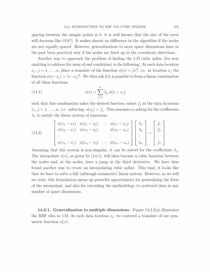
14.2. INTRODUCTION TO RBF VIA CUBIC SPLINES. 372
spacing between the sample points is h, it is well known that the size of the errorwill decrease like O(h4). It makes almost no difference in the algorithm if the nodes
are not equally spaced. However, generalizations to more space dimensions have inthe past been practical only if the nodes are lined up in the coordinate directions.
Another way to approach the problem of finding the 1-D cubic spline (for nowomitting to address the issue of end conditions) is the following: At each data locationxj , j = 1, . . . , n, place a translate of the function φ(x) = |x|3, i.e. at location xj the
function φ(x−xj) = |x−xj |3. We then ask if it is possible to form a linear combinationof all these functions
(14.1) s(x) =
n∑
j=1
λj φ(x− xj)
such that this combination takes the desired function values fj at the data locations
xj , j = 1, . . . , n., i.e. enforcing s(xj) = fj. This amounts to asking for the coefficientsλj to satisfy the linear system of equations
(14.2)
φ(x1 − x1) φ(x1 − x2) · · · φ(x1 − xn)φ(x2 − x1) φ(x2 − x2) φ(x2 − xn)...
...φ(xn − x1) φ(xn − x2) · · · φ(xn − xn)
λ1
λ2
...λn
=
f1
f2
...fn
.
Assuming that this system is non-singular, it can be solved for the coefficients λj .The interpolant s(x), as given by (14.1), will then become a cubic function betweenthe nodes and, at the nodes, have a jump in the third derivative. We have thusfound another way to create an interpolating cubic spline. This time, it looks like
that we have to solve a full (although symmetric) linear system. However, as we willsee next, this formulation opens up powerful opportunities for generalizing the formof the interpolant, and also for extending the methodology to scattered data in anynumber of space dimensions.
14.2.1. Generalization to multiple dimensions. Figure 14.2.2(a) illustratesthe RBF idea in 1-D. At each data location xj , we centered a translate of our sym-metric function φ(x).

14.2. INTRODUCTION TO RBF VIA CUBIC SPLINES. 373
Figure 14.2.2. Illustration of the RBF concept in 1-D and in 2-D.
In 2-D, as illustrated in Figure 14.2.2(b), we instead use a rotated version of thesame radial function. In d dimensions, we can write these rotated basis functions as
φ(||x− xj||), where ‖·‖ denotes the standard Euclidean norm. The form of the RBFinterpolant and of the linear system that is to be solved has hardly changed from the1-D case. Instead of (14.1) and (14.2), we now use as interpolant
(14.3) s(x) =
n∑
j=1
λj φ(∥∥x− xj
∥∥)

14.2. INTRODUCTION TO RBF VIA CUBIC SPLINES. 374
with the collocation conditions
(14.4)
φ(‖x1 − x1‖) φ(‖x1 − x2‖) · · · φ(‖x1 − xn‖)φ(‖x2 − x1‖) φ(‖x2 − x2‖) φ(‖x2 − xn‖)...
...
φ(‖xn − x1‖) φ(‖xn − x2‖) · · · φ(‖xn − xn‖)
λ1
λ2
...
λn
=
f1
f2
...
fn
.
In particular, we note that the algebraic complexity of the interpolation problem has
not increased with the number of dimensions - we will always end up with a squaresymmetric system of the same size as the number of data points. Cubic splines havethus been generalized to apply also to scattered data in any number of dimensions.
A generalized version of (14.3) will be introduced at the end of this chapter
(equations (14.9) and (14.10)).
14.2.2. Different types of radial functions. The error O(h4) for cubic splinesin 1-D will become O(h6) in the case of quintic splines. And it falls to O(h2) for linearsplines (corresponding to φ(x) = |x|). In general, if we take the RBF approach asoutlined above, and use φ(x) = |x|2m+1, the error will become O(h2m+2) (even powers
in φ(x) will not work; for ex. if φ(x) = x2, the interpolant (14.1) will reduce to asingle quadratic polynomial, no matter the value of n, and attempting to interpolatemore than three points will have to give rise to a singular system). The sizes ofthese errors correspond directly to which derivative of φ(x) it is that features a
jump. This leads to the ‘obvious’ question: why not choose a φ(x) which is infinitelydifferentiable everywhere, such as φ(x) =
√1 + x2 ? This idea is an excellent one,
which can be applied to good advantage in any number of dimensions. If we stillignore boundary issues (possibly leading to some counterpart for RBF of the Runge
phenomenon (RP) for polynomials, to be discussed in Section 14.7), the accuracywill become spectral: better than any polynomial order, and generally of the formO(e−c n), where c > 0 and n is the number of points. Some precise statements andproofs in this regard (however without describing in-between node point oscillations
as a manifestation of RP) have been given in [?], [?].Table 1 lists a number of possible choices of radial functions, with illustrations
shown in Figure 14.2.3.

14.2. INTRODUCTION TO RBF VIA CUBIC SPLINES. 375
0 0.5 1 1.5 20
5
10
MN φ(r)=r3
Piecewise smooth
0 0.5 1 1.5 2−1
0
1
2
3
TPS φ(r)=r2 log r
0 0.5 1 1.5 20
1
2
3
MQ φ(r)=(1+r2)1/2
Infinitely smooth
0 0.5 1 1.5 20
0.5
1
1.5
IMQ φ(r)=(1+r2)−1/2
0 0.5 1 1.5 20
0.5
1
1.5
IQ φ(r)=(1+r2)−1
0 0.5 1 1.5 20
0.5
1
1.5
GA φ(r)=e r 2
Figure 14.2.3. Illustrations of the eight different radial functions in Table 1.
In the piecewise smooth category (where we so far have discussed only MN:
φ(r) = |r|2m+1), other interesting choices include TPS φ(r) = |r|2m ln |r|, and alsothe WE and MT classes. The TPS RBF are commonly used in 2-D, especially thenwith m = 1. Just like how the natural cubic spline (obeying the end conditionss′′(a) = s′′(b) = 0) minimizes
∫ ba[s′′(x)]2dx over all possible interpolants [?], the
RBF interpolant using φ(r) = r2 log r achieves an equivalent minimization for 2-Dscattered data [?], [?]. The most notable feature of the Wendland functions is theircompact support, i.e. being nonzero only over a local region of radius 1/ε. Unless ε isvery small, the matrix in (14.4) will be sparse, and (14.3) will contain well less than
n terms. This can greatly speed up RBF calculations. However, as discussed furtherin Section 14.4, this advantage may be offset by a significant loss in accuracy. TheMT functions turn out to be of particular interest in many statistical applications[??].
The spectral accuracy noted above for smooth radial functions holds in any num-ber of spatial dimensions. For the non-smooth ones, the order accuracy curiouslyimproves with the number of dimensions. For example, for φ(r) = |r|2m+1 and for

14.2. INTRODUCTION TO RBF VIA CUBIC SPLINES. 376
φ(r) = |r|2m ln |r|, the order of accuracy (in the ...-norm) becomes ..... and .....respectively [?]. Intuitively, this can be understood from the fact that ...... (?). Check
For all the types of RBF, apart from MN and TPS, we have also introduced ashape parameter, which is commonly denoted by ε. For small values of ε, the basisfunctions become very flat and, for large values, they become sharply spiked (e.g.for IQ, IMQ, GA) or, in the case of MQ, it approaches the piecewise linear case.Although the extremes (ε very small, and ε very large) would at first both seem to
be unsuitable, we will soon see that the former case will be of particular interest inconnecting RBF with pseudospectral (PS) methods.
14.2.3. Fourier representation of radial functions. In some of the subse-quent analysis, the Fourier transforms of the RBF will be of interest. Table 1 also
shows these (or their generalized Fourier transform, if the integral that defines theregular version would be divergent, cf. [?], [?]). We use in this chapter the 1-D convention u(x) = 1√
2π
∫∞−∞ u(ω) eiωxdω; u(ω) = 1√
2π
∫∞−∞ u(x) e−iωxdx, and its
generalization to higher dimensions. When a function in d dimensions is radially
symmetric (i.e. depends on r =√x2
1 + x22 + . . .+ x2
d only), the Fourier transformwill similarly depend only on ρ =
√ω2
1 + ω22 + . . .+ ω2
d. The computation of the d-dimensional transforms is then known as a Hankel transform (identical to its owninverse):
φ(ρ) = 1(2π)d/2
∫∞−∞ . . .
∫∞−∞ φ(‖x‖) e−i ω · x dx
= 1ρ(d−2)/2
∫∞0φ(r) rd/2 J(d−2)/2(r ρ) dr
.
Alternatively, the Hankel transform can be computed by the formulas
d = 2m+ 1 odd: φ(ρ) = (−2)m√
2π
dm
d(ρ2)m
∫∞0φ(r) cos(rρ) dr
d = 2m+ 2 even: φ(ρ) = (−2)m dm
d(ρ2)m
∫∞0φ(r) r J0(rρ) dr
,
involving derivatives, but no Bessel functions of higher than zeroth order.
14.2.4. Non-singularity of the RBF system. We denote the coefficient ma-trix in (14.4) by A. The issue whether this matrix can ever become singular is ofcritical importance for the utility and robustness of RBF in approximations of the

14.2. INTRODUCTION TO RBF VIA CUBIC SPLINES. 377
Type of radial function Fourier transform φ(ρ) in d-DPiecewise smooth
MN monomial |r|2m+1 (−1)m+122m+ d2 +1Γ(m+ d+1
2)Γ(m+ 3
2)
π1
|ρ|2m+d+1
TPSthin platespline |r|2m ln |r| (−1)m+122m+ d
2−1m!Γ(m+ d
2) 1|ρ|2m+d
WE Wendland ...... ......MT Matérn ...... ......
Infinitely smooth
MQ multiquadric√
1 + (εr)2 ......
IQinversequadratic
1
1 + (εr)2......
IMQ inverse MQ1√
1 + (εr)2......
GA Gaussian e−(εr)2 e−ρ2/(4ε2)
(√
2ε)d
Table 1. Definition and Fourier transforms for some cases of radial functions.
form (14.3). We will show in Theorem 53 that a sufficient condition for uncondi-tional non-singularity (no matter how any number of points are distributed in any
number of dimensions) is that the radial function’s Fourier transform φ(ρ) is posi-tive. This result will immediately guarantee the non-singularity for the WE, MT,IQ, IMQ and GA cases. The result holds also for IQ, as was shown by Micchelli in1986 [?], with the first elementary proof only quite recent [..]. We will give the proof
of non-singularity for all cases with φ(ρ) positive in two stages. Lemma 52 carriesit out in the special case of GA, and we note in the proof of Theorem 53 that thechange is minor when generalizing to other cases with φ(ρ) > 0. These results wereobtained (although in a somewhat different context) already in the early 1930s ([?],see also [?]):
Theorem 52. The RBF matrix A is positive definite (in particular, nonsingular)
in the case of GA RBF.

14.2. INTRODUCTION TO RBF VIA CUBIC SPLINES. 378
Proof. The standard proof is carried out in two steps:1. Show that A is positive semidefinite, and
2. If a set of points xm are distinct, show that the function
(14.5) f(x) =
n∑
m=1
αm e−i x·xm
cannot be identically zero unless all the coefficients αm are all zero. Step 1: Every
entry of A is then of the form e−ε2‖ω‖2
for some vector ω (i.e. for Aj,k we chooseω = xj − xk). The exponent can be simplified to be just linear in ω if we note (cf.the Fourier transform of Gaussians, as listed in Table 1)
(14.6) e−ε2‖ω‖2
= 1(4π)d/2εd
∫
Rd
e−‖x‖2/4ε2 e−i x·ω dx
If α = (α1, α2, . . . , αn)T is an arbitrary column vector, we thus find that
(14.7)αT A α =
∑nj=1
∑nk=1 αjαk e
−ε2‖xj−xk‖2
=∑n
j=1
∑nk=1 αjαk
1(4π)d/2εd
∫Rd e
−‖x‖2/4ε2 e−i x· (xj−xk) dx
= 1(4π)d/2εd
∫Rd e
−‖x‖2/4ε2∑n
j=1
∑nk=1 αjαk e
−i x· (xj−xk) dx
The double sum in the integrand can be written as
(14.8)(∑n
j=1αj e
−i x· xj
)(∑n
k=1αk e
i x· xk
)=∣∣∣∑n
m=1αm e−i x· xm
∣∣∣2
≥ 0.
Since e−‖x‖2/4ε2 (in the integral) is everywhere positive, this shows that αTAα ≥ 0,i.e. A is a positive semidefinite matrix. It remains to show that we can’t have equalityif any component of α is non-zero. Step 2: Since the points xm are assumed to be
distinct, we can choose m∗ such that xm∗ · xm∗ > xm∗ · xk , k 6= m∗. Let x = σ xm∗ .Assuming further that f(x) ≡ 0 (cf. (14.5)), so is g(σ) =
∑nm=1 αm e−i σxm∗ ·xm ≡ 0.
If αm∗ 6= 0, the term αm∗ e−i σxm∗ ·xm∗ will outgrow all other terms if we differentiateg(σ) increasingly many times. This is impossible in view of g(σ) ≡ 0. Hence αm∗ = 0.
The argument can then be repeated to show that all coefficients αm are equal to zero.
�

14.2. INTRODUCTION TO RBF VIA CUBIC SPLINES. 379
Other proofs for the Step 2 can be found for ex. in [?], [..]. A slight modificationof Theorem 52 is particularly useful when considering RBF of compact support (such
as Wendland-type radial functions):
Theorem 53. The RBF matrix A is positive definite if∫Rd φ(‖x‖)2dx is finite
φ(ρ) is positive.
Proof. Instead of (14.6), we start with the relation
φ(‖ω‖) = 1(2π)d/2
∫
Rd
φ(‖x‖) ei x·ω dx ,
and proceed similarly. We will again arrive at (14.8); the only (insignificant) differ-ence being that the double sum within the integral in the last line of (14.7) will bepreceded by another positive function than e−‖x‖2/4ε2 . �
The two Theorems 52 and 53 rely on∫Rd φ(‖x‖)2dx to be finite, greatly limiting
the types of radial functions they can be applied to. The concept of completely
monotone (CM) functions leads to non-singularity proofs for many more types of
radial functions:
Definition 54. A C∞(0,∞) function ψ(r), which has a bounded first derivative
at the origin, is said to be completely monotone if (−1)k dk
drkψ(r)≥ 0 for r > 0 and
k = 0, 1, . . .
Lemma 55. A function ψ(r), r ≥ 0, is completely monotone if and only if its in-
verse Laplace transform γ(s) is nonnegative (i.e. γ(s) ≥ 0 when ψ(r) =∫∞0γ(s) e−srds)
Proofs of Lemma 55 and can be found for ex. in [..], [..].
Theorem 56. If ψ(r) is completely monotone (but not constant), then the RBF
matrix A using the radial function φ(r) = ψ(r2) will be positive definite.

14.2. INTRODUCTION TO RBF VIA CUBIC SPLINES. 380
Proof. Let again α = (α1, α2, . . . , αn)T is an arbitrary column vector. We then
obtainαT A α =
∑nj=1
∑nk=1 αjαk ψ(
∥∥xj − xk∥∥2
)
=∑n
j=1
∑nk=1 αjαk
∫∞0γ(s) e−s‖xj−xk‖2 ds
=∫∞0γ(s)
∑nj=1
∑nk=1 αjαk e
−s‖xj−xk‖2 ds .The double sum is positive according to Theorems 52 and γ(s) ≥ 0 (and not identi-cally zero). Hence αT A α > 0. �
Example. With φ(r) = 1(1+r2)β , i.e. ψ(r) = 1
(1+r)β , it will hold that (−1)k dk
drkψ(r) =(∑k−1i=0 (β + i)
)/ (1 + r)β+k, k = 0, 1, . . . Hence, by the Definition 54, ψ(r) is com-
pletely monotone if β > 0. Lemma 55 confirms this, since γ(s) ≡ e−ssβ−1/Γ(β),
which is positive for s positive, again when β > 0. Therefore, by Theorem 56, theA-matrix for φ(r) = 1
(1+r2)β is always positive definite (for any point distributions inany number of space dimensions) when β > 0. �
Example. In the case of φ(r) = sech εr, the closed-form expressions for φ(ρ)
become too difficult to work with if the dimension d is large, and Theorem 53 is there-fore not easily applicable. Nevertheless, Theorem 56 will readily show that we again
always get a positive definite A-matrix (for details, see [?]; another demonstrationof the result can be found in [..]). �
The implication in Theorem 56 goes both ways—ψ(r) being CM is in fact bothnecessary and sufficient for the A-matrix to be guaranteed positive definite for anynumber of space dimensions. From this follows immediately that the A-matrix cannotbe unconditionally positive definite if φ(r) has a zero for r ≥ 0. In particular, any
radial function with compact support (such as the Wendland functions) are alwayslimited to some certain number of dimensions.
The MQ case of φ(r) =√
1 + (ε r)2 is more difficult. In this case, the A-matrixis no longer positive definite. However, it is still non-singular, having one positive
and n− 1 negative eigenvalues. Micchelli’s celebrated proof of this result in 1986 [?]played a key role in confirming MQ RBF as a method of choice for multidimensionalinterpolation, and this formed the starting point for much of the recent interest in

14.3. THE SHAPE PARAMETER ε. 381
RBF. A very much simplified proof of this result was found only recently (see [..] fordetails).
In the (piecewise smooth) cases of MN and TPS (or just the m = 1 cases? ), checksingularities of the A-matrix can arise if we use (14.3), but not if we instead use thealmost equivalent form
(14.9) s(x) = λ0 +
n∑
j=1
λj φ(∥∥x− xj
∥∥),
together with the constraint∑n
j=1 λj = 0. This extension, allowing constants to beinterpolated exactly, can be advantageous also in cases smooth RBF. It can also be
extended further still by letting {pk(x)}mk=1 be a basis for the space of all d-variatepolynomials that have degree ≤ Q, and then use as interpolant
(14.10) s(x) =n∑
j=1
λj φ(∥∥x− xj
∥∥) +m∑
k=1
βkpk(x)
where the expansion coefficients λj and βk are determined by enforcing s(xj) =
fj , j = 1, . . . , n, together with the constraints∑n
j=1 λj pk(xj) = 0, k = 1, . . . , m (see
for example [?] and [??] for results regarding non-singularity).
14.3. The shape parameter ε.
The literature on selecting a good (single) value for ε is extensive, e.g. [?],[?], [?], [?], [?], [?], [?], [?]. Most of these works focus on finding the minimalerror in computations on various applications. For large values of ε, for ex. a GAinterpolant consists of a many narrow spikes, reaching up to each function value
that is to be interpolated, i.e. the interpolant in-between data points will be veryinaccurate. Hence, a decrease in ε is initially beneficial. Tests tend to show thatthese improvements will cease at some point, after which errors will tend to increaseagain as ε → 0. There are two main causes for this reversal in trend; numerical ill-
conditioning, and a Runge-type phenomenon. They will be discussed in the next twosubsections. We will find that both causes can be at least partly overcome, therebymaking the low ε-regime of great practical interest.

14.3. THE SHAPE PARAMETER ε. 382
14.3.1. Potential advantages of using near-flat basis functions. It wasdemonstrated in [?] that, in the limit of ε→ 0, the RBF interpolants in 1-D in gen-
eral converge to the Lagrange interpolating polynomial. Since these (lowest degree)interpolating polynomials in turn form the basis for all classical pseudospectral (PS)methods, this implies that PS methods alternatively can be viewed as special cases ofRBF methods [?]. Already in 1-D, this viewpoint can offer new opportunities becauseuse of RBF with ε > 0 can be both more accurate and more stable than the ‘clas-
sical’ PS methods (which correspond to the ε = 0 limit in conjunction with certainvery restricted types of node layouts, often based on zeros or extrema of orthogonalpolynomials). However, the most striking advantages come in 2-D (and higher) withthe new ability of then using scattered node layouts over irregularly shaped domains.
This allows PS methods to be generalized from very restrictive domain shapes andtensor-type grids only over to fully irregular domains with scattered nodes.
In the ε→ 0 limit, the conditioning of the linear system (14.4) degrades rapidly.For example, with 41 scattered nodes in 2-D, det(A) is proportional to ε416 as ε→ 0
for all the infinitely smooth radial functions listed in Table 1 [?]. The expansioncoefficients λi become oscillatory and grow rapidly in magnitude with decreasingε (proportionally to 1/ε16 in this example). The subsequent evaluation of the in-terpolant by means of (14.3) will then involve large amounts of numerical cancel-
lations. It was for some time believed that a trade-off between high accuracy andgood conditioning was inevitable (expressed in terms of an “uncertainty principle”[?], see also Section 5.3.4 in [?]). Utilizing contour integration in a complex ε-plane,the Contour-Padé algorithm [?] became the first method able to bypass this ill-
conditioning, thereby permitting stable computations of RBF interpolants all theway down to ε = 0. Maybe even more importantly, this algorithm demonstratedthat the previously feared ill-conditioning barrier against the use of small ε merelyamounted to equations (14.4) and (14.3) being an ill-conditioned approach for the
well-conditioned task of evaluating the RBF interpolant s(x) based on data values fiat locations xi, i = 1, 2, . . . , n. By means of the still more recent RBF-QR algorithm[?], [?], the Contour-Padé limitation on the number of nodes n (to be no more thanaround 100-200 nodes in 2-D) is essentially eliminated. Both of these methods will
be described further in Section 14.4.

14.3. THE SHAPE PARAMETER ε. 383
Figure 14.3.1. Three different node distributions, all with 16 nodeson the boundary and 48 nodes in the interior of the unit circle, used bythe FD2, PS, and RBF methods, respectively, in the Poisson equationtest case.
The potential benefits of computing in a very low ε-range were strikingly illus-trated in [?]. One of the test cases considered there was to solve Poisson’s equa-tion ∂2u
∂x2 + ∂2u∂x2 = f(x, y) over the unit circle using straightforward RBF colloca-
tion, with a right hand side f(x, y) and Dirichle boundary conditions chosen so thatu(x, y) = 65/(65 + (x − 0.2)2 + (y + 0.1)2) becomes the solution. With nodes for asecond order finite difference scheme (FD2), a Fourier-Chebyshev PS scheme, andRBF laid out as illustrated in parts a-c respectively of Figure 14.3.1, the max norm
errors become as seen in Figure 14.3.2(a) when calculated with the Contour-Padéalgorithm. Direct solution of the RBF collocation equations by Gaussian elimination(Figure 14.3.2(b)) gives the same results for large ε, but the accuracy is lost due toill-conditioning for low ε.
The RBF approach features much more flexibility than the FD2 and PS alter-natives in that the results depend very little on how the nodes are scattered overdomains, which furthermore need not be circular but can be arbitrarily shaped. TheRBF errors are seen to be many orders of magnitude smaller (than those of FD2
and PS) as soon as ε is chosen sufficiently small. For the FD2 scheme, halving thetypical space step will increase the accuracy by a factor of four - and (in 2-D) require4 times as many nodes. Increasing the accuracy by a factor of 106 (to make the FD2calculation as accurate as the RBF ones) would thus require approximately 64 · 106
rather than 64 node points.Figures 14.3.2(a) and (b) indicate that, even when ill-conditioning is eliminated
for low ε values, there still remains some additional effect that breaks the trend of

14.3. THE SHAPE PARAMETER ε. 384
Figure 14.3.2. The max norm errors in the Poisson equation testcase, as functions of ε when using MQ, IQ, and GA RBFs. The errors(not ε-dependent) for standard second order finite differences (FD2)and Fourier-Chebyshev pseudospectral (PS) method are also includedfor comparison: (a) Computation using Contour-Padé method, (b)Direct implementation via Gaussian elimination.
errors decreasing with decreasing ε. In the next subsection, we will focus on he cause
for this.
14.3.2. The Runge phenomenon (RP).
14.3.2.1. The RP for polynomials. The best-known case of the RP occurs forincreasing order polynomial interpolation on equispaced grids, and is illustrated inFigure 14.3.3. Convergence / divergence rates as the number of node points increaseswill depend on x-position, node distribution but only to a limited extent on prop-
erties of the interpolated function (the only relevant quantity being how far awayfrom [−1, 1] the function can be analytically continued without encountering anysingularities). The theory for this is well understood [?], [?].
For example, in the case shown in Figure 14.3.3, the envelope of the oscillatory
error varies proportionally to
(14.1) E(z, n) = en (ψ(z0)−ψ(z))
(both for z = x real, and for z complex), where the logarithmic potential function
(14.2) ψ(z) = − 1
2Re [(1− z) ln(1− z)− (−1− z) ln(−1− z)]

14.3. THE SHAPE PARAMETER ε. 385
−1 −0.5 0.5 1
−0.5
0.5
1
1.5
(a) n = 21
−1 −0.5 0.5 1
−0.5
0.5
1
1.5
(b) n = 41
Figure 14.3.3. Equispaced polynomial interpolation of f(x) =1
1+16x2 over [-1,1]. As n increases, there is spectral convergence for|x| < 0.7942 and exponential divergence otherwise. These transitionpoints are marked by solid dots.
is generic for equispaced polynomial interpolation over [-1,1]. The function f(x) thatis interpolated enters only by setting z0 = 0.25i in (14.1); a singularity in the complexplane of f(z) = 1/(1 + 16z2).
The standard remedy against the RP is Chebyshev-type clustering of nodes to-
wards the end of the interval, e.g.
(14.3) xj = − cos(π(j − 1)
n− 1), j = 1, 2, . . . , n.
In that case, one then obtains, in place of (14.2), ψ(z) = − ln |z+√z2 − 1|, which for
z = x real, −1 ≤ x ≤ 1, evaluates to zero. Because of (14.1), this corresponds to thewell-known uniform Chebyshev interpolation accuracy across [−1, 1] for all functionsf(x). However, while this particular node distribution resolves one difficulty (the
RP), it introduces others. For example, in the context of time stepping PDEs, theCFL stability condition can become very severe.
14.3.2.2. The RP for RBF approximations. Figure 14.3.4 illustrates how the RBFinterpolation error at first decreases and then increases when ε goes from very large
to very small. For ε large, each GA basis function consists of a sharp spike, with aheight such that it just reaches up to the corresponding function value. The errorsthis mechanism causes vanish quickly for decreasing ε, but another type of error is

14.3. THE SHAPE PARAMETER ε. 386
−1 1
−0.5
0.5
1
1.5
(a) ε = 30
−1 1
−0.5
0.5
1
1.5
(b) ε = 3.5
−1 1
−0.5
0.5
1
1.5
(c) ε = 0.5
Figure 14.3.4. GA interpolants of f(x) = 11+16x2 for a wide range of
ε-values: ε = 30, 3.5, and 0.5 respectively.
−1 1
−0.5
0.5
1
1.5 α = 0.1
fα(x)
x −1 1
−0.5
0.5
1
1.5 α = 1
x −1 1
−0.5
0.5
1
1.5 α = 16
x
10−1
100
101
10−16
10−12
10−8
10−4
100
GA
|Err
or|
ε 10−1
100
101
10−16
10−12
10−8
10−4
100
ε 10−1
100
101
10−16
10−12
10−8
10−4
100
ε
10−1
100
101
10−16
10−12
10−8
10−4
100
MQ
|Err
or|
ε 10−1
100
101
10−16
10−12
10−8
10−4
100
ε 10−1
100
101
10−16
10−12
10−8
10−4
100
ε
Figure 14.3.5. Top row: The function fα(x) =1
1 + αx2for three
values of α. Next two rows of subplots show how the error varies withε in the case of GA and MQ RBFs respectively.
seen to enter for very small ε - the RP, as an immediate consequence of the fact that
the interpolant then approaches the polynomial one.The six subplots in Figure 14.3.5 illustrate how the smoothness of the interpolant
influences when the trend reversal occurs, and how strong this reversal will be. The

14.3. THE SHAPE PARAMETER ε. 387
third case (α = 116
) uses the same test function as is shown in Figures 14.3.3 and14.3.4. The Runge phenomenon enters in all cases once ε is sufficiently small, and
its level at ε = 0, as obtained from the polynomial RP theory quoted in Section14.3.2.1, agrees completely with the lowest ε-results in Figure 14.3.5. Althoughhigher accuracy can be reached if the data is smoother, the RP still in all casesbreaks a very favorable improvement trend for decreasing ε.
The discussion above provides an understanding of the trend reversal that was
illustrated earlier (in a slightly different context) in Figure 14.3.2 a. Although thistrend reversal was described theoretically in [?], the present RP interpretation of it(first presented in [?]) is much more intuitive.
A few possible approaches for reducing the accuracy loss due to RP at boundaries
have already been suggested in the literature:
(1) Node clustering at edges (or wherever needed to improve accuracy),(2) Super Not-a-Knot (SNaK) generalization of cubic spline Not-a_Knot end
conditions,
(3) Spatially variable shape parameter; use εj at node location xj .
The first option is the only one available if one uses polynomial interpolants. Thediscussion in [?] suggests that SNaK is preferable to node clustering in the contextof RBF. The idea of suppressing RP by use of spatially variable shape parameters is
considered in [?], and is discussed briefly later in this chapter in Section 14.7.While boundaries are a common trigger of RP, it is not the only one. It can also
arise if one attempts to improve local accuracy by clustering nodes in select areas,as is a standard procedure with finite elements or splines.An extensive discussion of
this effect (and a possible remedy) can be found in [?]. This effect is illustrated inFigure 14.3.6. In part a, there is no RP visible, but the equispaced RBF approx-imation lacks sufficient resolution near the center, where the data features a verysharp gradient. In part b, we have inserted two extra nodes in the critical area and,
in part c, still two more points are inserted. The most striking result of this localrefinement is a seemingly disastrous RP. We will next see how this can be broughtunder control.

14.3. THE SHAPE PARAMETER ε. 388
−1 0 1−4
−2
0
2
4
(a) 14 nodes.−1 0 1
−4
−2
0
2
4
(b) 16 nodes.−1 0 1
−4
−2
0
2
4
(c) 18 nodes.
Figure 14.3.6. MQ RBF ε = 2 interpolants (dashed curves) off(x) = arctan(20x) (dotted curves) over [-1,1] (a) 14 equispaced points,(b) two extra points inserted near the center, and (c) still two morepoints inserted near the center.
−1 0 1−2
−1
0
1
2Interpolant
Equ
i−sp
aced
xk; O
ptim
ize
ε
x−1 0 1
−0.2
−0.1
0
0.1
0.2Error
x−1 0 10
5
10
15
20
x
ε values
−1 0 1−2
−1
0
1
2
Opt
imiz
e x k a
nd ε
x−1 0 1
−2
−1
0
1
2x 10
−3
x−1 0 10
5
10
15
20
x
−1 0 1−2
−1
0
1
2
Opt
imiz
e x k a
nd ε
k
x−1 0 1
−4
−2
0
2
4x 10
−5
x−1 0 10
5
10
15
20
x
Figure 14.3.7. Ten-node MQ interpolations of f(x) = arctan 20x.Top row: Equispaced nodes, ε (same at all nodes) optimized. Middlerow: Node locations xk and ε (same at all nodes) optimized. Bottomrow: Both xk and εk optimized.
14.3.2.3. Example of RP control. Figure 14.3.7 shows that one can obtain excel-lent accuracy in the f(x) = arctan 20x test case already with very few nodes if onejust uses good choices for their locations xj and, better still (bottom row of subplots),

14.3. THE SHAPE PARAMETER ε. 389
−1 −0.5 0 0.5 1−2
−1
0
1
2
n =
10
poin
ts
x
Interpolant
−1 −0.5 0 0.5 1−0.4
−0.2
0
0.2
0.4
x
Error
−1 −0.5 0 0.5 1−2
−1
0
1
2
n =
50
poin
ts
x−1 −0.5 0 0.5 1
−0.04
−0.02
0
0.02
0.04
x
−1 −0.5 0 0.5 1−2
−1
0
1
2
n =
170
poi
nts
x−1 −0.5 0 0.5 1
−3−2−1
0123
x 10−5
x
Figure 14.3.8. 10-point, 50-point and 170-point Chebyshev inter-polants for arctan(20x) over [-1,1]; display of the interpolants and theirerrors.
if one also makes the shape parameter spatially variable (now taking the value εjfor the RBF centered at the node xj ∈ [−1, 1]). We note that it is favorable to letthe εj-values be large where the nodes are dense, as will be discussed further in Sec-
tion 14.7. Although the multivariate optimizer (function ga from Matlab’s geneticalgorithm toolbox) used in obtaining Figure 14.3.7 probably found only local optima(in contrast to the global ones), the error level that is reached is nevertheless spec-tacular in comparison with what can be achieved with, say, polynomial interpolation
at the Chebyshev nodes (corresponding to a typical non-periodic PS method).As Figure 14.3.8 shows, n = 170 nodes are needed to match the max norm accu-
racy of 2.5·10−5 that RBF achieved using only n = 10 interpolation nodes. Hopefully,further numerical experiments in the style of Figure 14.3.7 will lead to fast and prac-
tical guidelines for effective choices for both nodes and shape parameter(s). Thechances are excellent that especially the idea of spatially variable shape parameterswill allow RBF interpolants to overcome the RP, as well as the Gibbs phenomenon as

14.4. STABLE COMPUTATIONS IN THE FLAT RBF LIMIT. 390
discussed further in Section 14.7. Spatially variable shape parameters are discussedfurther in Section 14.7.
14.4. Stable computations in the flat RBF limit.
As we noted above, direct calculation of RBF interpolants by means of (14.4)and (14.3) lead to extreme ill-conditioning when ε → 0. All the elements of the
A-matrix (the coefficient matrix in (14.4)) then approach one. For example in 1-D,with n points, the condition number of the system will approach infinity at the rateO(1/εn) if n is odd, and as O(1/εn−1) if n is even. High precision arithmetic (beyondthe standard 64 bit) can be used to ‘survive’ some of the ill-conditioning, but the
cost for this will increase without bound in the ε → 0 limit. Preconditioning forthe system (14.4) can be somewhat helpful [?], [?] but, once the coefficient matrixA has been formed numerically, irreversible conditioning damage has already beendone. The Contour-Padé algorithm provided the first clear demonstration that direct
use of (14.4), (14.3) merely amounts to an ill-conditioned numerical approach to agenuinely well-conditioned problem. More recently, a second algorithm, RBF-QR,has been developed which also entirely avoids the ill conditioning issue in the ε→ 0
limit. These two algorithms are briefly summarized next.
14.4.1. Contour-Padé method. In the discussion so far, the shape parame-ter ε has been a real-valued quantity. However, if one imagined solving (14.4) by
Cramer’s rule, followed by evaluating (14.3), it becomes clear that the resulting in-terpolant s(x, ε) (for fixed x and variable ε) is an analytic function of ε which, inthe vicinity of the origin, has no other singularities than possibly some poles. Sincelimε→0 s(x, ε) typically exists finite-valued [?], the origin (ε = 0) cannot even be a
pole, and a removable singularity remains therefore as the only option. Furthermore,we know that the value of an analytic function at any point is the average value ofthe function taken around any circle centered at the point (assuming there are nosingularities within the circles). In the simplest case, the Contour-Padé method will
work as illustrated in Figure 14.4.1. With ill conditioning not allowing us to evalu-ate s(x, ε) directly at or near ε = 0, we simply evaluate it instead around a circlesurrounding ε = 0, and then take the average.

14.4. STABLE COMPUTATIONS IN THE FLAT RBF LIMIT. 391
Figure 14.4.1. Schematic illustration of the Contour-Padé methodin the simplest case of no singularities of s(x, ε) near the origin.
We know from the non-singularity theory in Section 14.2 that s(x, ε) cannothave any singularities along the real axis in the ε-plane. The only complicationthat might arise is that it sometimes turns out to have a few poles within the ill-conditioned central region. Instead of just averaging the values around the circle,
the values are instead used as input to a complex FFT. This will produce (withexponentially increasing accuracy as the number of sample points are increased) theLaurent coefficients for an expansion of s(x, ε) that is valid in the largest singularity-free annulus that surround the contour. The terms with negative powers of ε originate
purely from the poles inside the contour (whether located inside the ill-conditionedregion, or outside it). Padé summation of these terms will convert them into arational function r(ε). Together with the remaining Laurent expansion terms (for

14.4. STABLE COMPUTATIONS IN THE FLAT RBF LIMIT. 392
non-negative powers of ε), the interpolant takes the form
s(x, ε) = {r(ε)}+{d0 + d1ε+ d2ε
2 + d3ε3 + . . .
},
which is well suited for numerical evaluation anywhere inside the evaluation path.Outside it, there are no ill-conditioning issues, and direct evaluation according to(14.4) and (14.3) work just fine. As n (the number of points in the data set) is
increased, the number of poles in the vicinity of origin tends to remain very low.However, the central region of ill-conditioning grows, and the Contour-Padé methodfails when this region becomes so large that it leaves no clear path between this regionand where the branch points start along the imaginary axis (in case of MQ, arising
from singularities of√
1 + (εr)2 in the ε-plane). In 2-D, this tend to happen whenn is greater than around 100-200; the situation improves significantly if the numberof dimensions increases. This causes no difficulties for the elliptic equation problemdiscussed in Section 14.3.1 or for generating scattered-node FD-type formulas as willbe described in Section 14.6, but it is nevertheless desirable to have available a stable
method which does not have this limitation on the number of points.
14.4.2. RBF-QR method. The key idea behind the RBF-QR method is to re-place, in the case of small ε, the extremely ill conditioned RBF basis with a well condi-tioned one that spans exactly the same space, and to do this exchange in a way which
does not at any stage involve any potentially dangerous numerical cancellations. Theconcept is somewhat reminiscent of how {1, x, x2, ..., xn} forms a very ill conditionedbasis over [-1,1], whereas the Chebyshev basis {T0(x), T1(x), T2(x), ..., Tn(x)} is a verywell conditioned one. Since the spaces they span are identical, the results of interpo-
lation using the two bases will also be identical, except for the fact that computationswith the latter basis are vastly more stable against influence of rounding errors. Thefirst implementation of RBF-QR was for the important special case of nodes on thesurface of a sphere [?], followed by an implementation for general node distributions
[?]. We limit the discussion here to the former case. The new equivalent bases thatwe introduce will be seen to converge to the spherical harmonics (SPH) basis asε→ 0.

14.4. STABLE COMPUTATIONS IN THE FLAT RBF LIMIT. 393
RBF Definition Expansion coefficients cµ,ε
MQ√
1 + (εr)2 −2π(2ε2+1+(µ+1/2)√
1+4ε2)(µ+3/2)(µ+1/2)(µ−1/2)
(2
1+√
4ε2+1
)2µ+1
IMQ1√
1 + (εr)2
4π(µ+1/2)
(2
1+√
4ε2+1
)2µ+1
IQ1
1 + (εr)24 π3/2 µ!
Γ(µ+ 32)(1+4ε2)µ+1 2F1(µ+ 1, µ+ 1; 2µ+ 2; 4ε2
1+4ε2)
GA e−(εr)2 4π3/2
ε2µ+1 e−2ε2Iµ+1/2(2ε
2)Table 2. SPH expansion coefficients corresponding to differentchoices of smooth RBFs.
14.4.2.1. Relations between RBF and SPH. A SPH expansion of a function de-fined over the surface of the unit sphere takes the form
s(x, y, z) =
∞∑
µ=0
µ∑
ν=−µcµ,ν Y
νµ (x).
Truncated SPH expansions (µ ≤ µmax) feature a completely uniform resolution overthe surface of the sphere. Based on the works of Freeden et.al. [?] and of Hubbertand Baxter [?] we can find explicit formulas for the coefficients cµ,ε when expanding
a RBF centered on the surface of the sphere:
(14.1) φ(‖x− xi‖) =∞∑
µ=0
µ∑
ν=−µ
′ {cµ,ε ε2µ Y νµ (xi)} Y ν
µ (x).
(where the symbol∑ ′ implies halving the ν = 0 term of the sum). The resulting
coefficients in the cases of MQ, IMQ, IQ, and GA are shown in Table 2.A key feature of these formulas is that, even for ε vanishingly small, all coefficients
can be calculated without any danger of loosing significant digits.14.4.2.2. Matrix representation and QR-factorization. The result when (14.1) is
applied in turn to the n RBF, all centered on the surface of the sphere, can be

14.4. STABLE COMPUTATIONS IN THE FLAT RBF LIMIT. 394
re-written in matrix×vector form:
φ(‖x− x1‖)φ(‖x− x2‖)...φ(‖x− xn‖)
=
=
c0,ε
2Y 0
0 (x1) ε2c1,εY−11 (x1) ε2 c1,ε
2Y 0
1 (x1) ε2c1,εY11 (x1) ε4{.} .
c0,ε
2Y 0
0 (x2) ε2c1,εY−11 (x2) ε2 c1,ε
2Y 0
1 (x2) ε2c1,εY11 (x2) ε4{.} .
. . . . . . . . . . . . . . . .c0,ε
2Y 0
0 (xn) ε2c1,εY−11 (xn) ε2 c1,ε
2Y 0
1 (xn) ε2c1,εY11 (xn) ε4{.} .
Y 00 (x)
Y −11 (x)
Y 01 (x)
Y 11 (x)
Y −22 (x)
Y −12 (x)
Y 02 (x)
Y 12 (x)
Y 22 (x)
. . .
= B · Y
A QR factorization of B combines its rows in such a way that the result becomesupper triangular. Since the powers of ε are the same within each column, elementswith different powers of ε do not mix in this process, and the upper triangular matrixis obtained stably, featuring the same pattern as for B in terms of the powers of ε.
Factoring out to the left the lowest power of ε for each row of R gives the result
φ(‖x− x1‖)φ(‖x− x2‖)φ(‖x− x3‖)...
φ(‖x− xn‖)
=
Q
1
ε2
ε2
ε2
. . .
×

14.5. BRIEF OVERVIEW OF HIGH ORDER FD METHODS AND PS METHODS. 395
×
∗ . . . . . . . ...
∗ ∗ ∗ . . . . ...
∗ ∗ . . . . ...
∗ . . . . ...
∗ ∗ ∗ ∗ .... . . ... ... ...
Y 00 (x)
Y −11 (x)
Y 01 (x)
Y 11 (x)
Y −22 (x)
Y −12 (x)
Y 02 (x)
Y 12 (x)
Y 22 (x)
...
(14.2)
= (Q · E · R) · Y (x)(14.3)
where Q is a unitary n× n matrix, E is a n× n diagonal matrix and R is an uppertriangular n × m matrix. The entries marked as “*” in the matrix R are of size
O(ε0). All the other non-zero entries of R are of size O(ε2) (or higher powers). Thenew basis is given by the elements of R · Y (x). It differs from the original basisonly by having omitted the non-singular matrix Q ·E from its left side, i.e. it formsa different basis for the same space. The key feature of the algorithm is that the
E-matrix, which contains all the ill-conditioning, disappeared analytically from theproblem, and has not in any way damaged the accuracy of the equivalent (but well-conditioned) base R ·Y (x). We can easily continue one step further and combine thenew basis functions so that each one becomes a single spherical harmonic function,
with a small perturbation. These perturbations fade away as ε → 0 because allthe entries denoted with “ ·” contain a positive power of ε. RBF interpolation onthe sphere in the ε → 0 limit will thus agree with SPH interpolation. However, aswe have seen already RBF are often more accurate for finite (or spatially variable)
ε-values, thereby providing a new perspective on SPH-based methods.
14.5. Brief overview of high order FD methods and PS methods.
14.5.1. High order FD methods. On an equispaced grid with nodes locatedat {. . .− 2h, −h, 0, h, 2h, . . .}, the simplest approximation for f ′(0) is Check FD section

14.5. BRIEF OVERVIEW OF HIGH ORDER FD METHODS AND PS METHODS. 396
(14.1) f ′(0) ≈ − 1
2hf(−h) + 0 f(0) +
1
2hf(h)
with an error of size O(h2). The coefficients in formulas such as this are uniquelydetermined by requiring that they be exact for polynomials of as high degree aspossible. Numerous methods are available to very effectively compute coefficients also
for formulas of higher orders of accuracy and which approximate higher derivatives,both on equispaced and nonuniform 1-D grids ([?], [..], [..]).
14.5.2. FD introduction to PS methods.
14.5.2.1. Periodic case. With any of the procedures to compute FD weights justmentioned, one readily determines the coefficients that are shown in Table 3. In this
special case, they are also available in closed form
cj,k =
{(−1)k+1(j!)2
i (j+k)! (j−k)! k = ±1, 2, . . . ,±j0 k = 0
for approximations of order 2j, j = 1, 2, . . . .
order weights2 −1
20 1
24 1
12−2
30 2
3− 1
126 − 1
60320−3
40 3
4− 3
20160
8 1280− 4
10515−4
50 4
5−1
54
105− 1
280... ↓ ↓ ↓ ↓ ... ↓ ↓ ↓ ↓limit · · · 1
4−1
312
-1 0 1 −12
13−1
4· · ·
Table 3. Weights for centered FD approximations of the first deriv-ative on an equispaced grid (omitting the factor 1/h).
We can note that there exists a very simple limit for the coefficients when theorder of the FD stencils go to infinity
limj→∞
cj,k =
{(−1)k+1 / k k = ±1, 2, . . .
0 k = 0.
This limit provides a fundamental connection between FD and Fourier PS methodsin the way that is illustrated in Figure 14.5.1.

14.5. BRIEF OVERVIEW OF HIGH ORDER FD METHODS AND PS METHODS. 397
Figure 14.5.1. Two different ways to wiev the approximation of afirst derivative by the Fourier PS method. Both give the same result.
Collocation of equispaced periodic data with trigonometric functions and thendifferentiating these functions analytically gives exactly the same derivative approxi-mations as one would get if the periodic data was extended to an infinite grid and the
infinite order FD stencil was applied. Needless to say, the latter is a computationallyless practical approach, but the equivalence is fundamental in connecting trigono-metric function collocation with increasing order FD methods. The equivalence canbe proved to hold for any order derivative [?], [?]. maybe clarify fur-
ther with somepicture of Fourieranalysis of FDschemes
14.5.2.2. Non-periodic case. If we consider non-periodic data, for example withdata points located at the Chebyshev nodes xk = − cos (k−1)π
n−1, k = 1, 2, . . . , n, we
have a very similar equivalence. For any node distribution, we can approximate thederivative at any node point (or at any in-between location) by easily obtained FD
weights in stencils that extend across the full grid [?], [Weideman]. The resultingderivative approximations will be exactly the same as if the data was collocated (i.e.fitted by a linear combination of Chebyshev polynomials) and the resulting function

14.5. BRIEF OVERVIEW OF HIGH ORDER FD METHODS AND PS METHODS. 398
differentiated analytically. The FD approach reduces to the Chebyshev PS methodif the node points happen to be located at Chebyshev node locations (14.3), but
works just as well however the points were distributed—i.e. there is no need to limitoneself to node distributions that are suggested by any classical polynomial set.
The collocation methods we have just described - based on Fourier and Chebyshevbasis functions - generalize in a completely straightforward manner to tensor-typegrids (i.e. rectangular domains in 2-D, etc.). By use of domain decomposition ideas,
single-domain PS methods lead to spectral element methods, gaining some level ofgeometric flexibility [??]. As we will see next, PS methods of the types describedso far (using any fixed set of basis functions) can never allow the data to lie atscattered locations. One key theme of this chapter is how the RBF approach entirely
overcomes this restriction.The efficiency of PS methods, periodic (Fourier) or non-periodic is thoroughly
documented in the literature. check
14.5.3. Possible singularity of scattered node PS collocation in more
than 1-D.. To show that no fixed set of expansion functions can ever guarantee anon-singular interpolation problem in more that 1-D, we follow [?] and consider a setof data points xk, k = 1, 2, . . . , n in more than 1-D, with associated function values
fk. Let ψk(x) be any fixed set of basis functions. The interpolant then takes the form
s(x) =
n∑
k=1
λkψk(x)
where the expansion coefficients are obtained by solving
ψ1(x1) ψ2(x1) · · · ψn(x1)
ψ1(x2) ψ2(x2) ψn(x2)...
...
ψ1(xn) ψ2(xn) · · · ψn(xn)
λ1
λ2
...
λn
=
f1
f2
...
fn
.
In more than 1-D, it is possible to continuously move two data locations so theybecome interchanged, without them having had to coincide at any time along theway. Doing this, two rows of the coefficient matrix above have swapped positions,

14.6. RBF-GENERATED FINITE DIFFERENCES. 399
i.e. the determinant has changed sign. Therefore, it must have been zero somewherealong that way.
In contrast, this particular exchange process will not lead to any difficulty inthe case of RBF interpolation. Considering the corresponding coefficient matrix in(14.4), both a row and a column will have changed places, i.e. there is no resultingsign change. To show that no other movement of nodes can lead to singularitiesrequire the more general arguments given in Section 14.2.
14.6. RBF-generated finite differences.
As we noted in Section 14.5, weights in 1-D FD formulas are typically obtainedby requiring them to be exact for polynomials of as high degree as possible. Thesame idea has been tried for scattered nodes in 2-D, with some success [?], [?], [?]. Asan alternative to basing FD-type formulas on local polynomial interpolants, one can
instead base them on local RBF interpolants. To illustrate this concept, as developedin [?], we first recall two classical FD stencils for the 2-D Laplacian ∆u = ∂2u
∂x2 + ∂2u∂y2
[?], [?], [?]
(14.1)
Explicit (2nd order) Compact (4th order)
1
1 −4 1
1
u
h2= ∆u ;
1 4 1
4 −20 4
1 4 1
u
6h2=
1
1 8 1
1
∆u
12
If one for example wants to solve Poisson’s equation ∆u = f , it is no disadvantage
that a linear combination of ∆u-values appear in the right hand side of the compactformula, as these would correspond to known f -values. The advantage is that wehave reached 4th order of accuracy, with the stencil for u still remaining small anddiagonally dominant.
Figure 14.6.1 illustrates a scattered set of nodes, and how some of these have
been selected out to form a similar stencil. To find weights cj, j = 1, . . . , n1 andbk, k = {some subset of 1, . . . , n1}, giving a formula accurate at location x1, wedemand it to be exact for the radial functions φ(
∥∥x− xj∥∥) and for ∆φ(
∥∥x− xj∥∥), j =

14.6. RBF-GENERATED FINITE DIFFERENCES. 400
Figure 14.6.1. RBF-HFD concept: To the left, an example of howstencil points may be selected near a location at which the Laplacianis to be approximated. To the right, a schematic representation of howu-values and ∆u-values (on a smaller subset still of the stencil points)will be linked through RBF-computed wights.

14.6. RBF-GENERATED FINITE DIFFERENCES. 401
−1 −0.5 0 0.5 1
−1
−0.5
0
0.5
1
Figure 14.6.2. Computational domain in RBF-HFD test example;shown together with the hybrid node layout used in the example.
1, . . . , {check}. Several issues relating to an efficient implementation are addressedin [?]. Key steps and issues include
• Form of the RBF interpolant (use of (14.9) turns out to be preferable to(14.3)),
• Given a center location x1, select nearby nodes so the stencils with cj -weights becomes diagonally dominant,• Decide what radial function and shape parameter ε to use
We will here limit ourselves to give an example from [?] which illustrates how theconcept may be used effectively in a case with irregular geometry:
Example: Numerically solve the nonlinear Poisson equation ∆u = e −2xu3 over thedomain between the large outer square and the inner circle as shown in Figure 14.6.2.
Dirichlet boundary conditions are chosen so that u(x, y) = ex tanh y√2
becomes anexact solution.
The hybrid node structure uses a regular grid with 4th order compact FD stencilsover a large part of the domain, and then adds scattered-node stencils only as neededto accommodate irregular boundaries. In this example, diagonal dominance and 4th
order accuracy could be achieved everywhere by using 9 c-weights with 5 b-weights
in the regular part (like in (14.1)) and 10 c-weights with 9 b-weights where nodes areirregular. Standard Newton-SOR iterations ([?], Section 7.4) converge very rapidly.The resulting error varies with ε as is shown in Figure 14.6.3. For low ε, the FD

14.7. SOME OTHER RELATED RBF TOPICS. 402
0 0.5 1 1.5 210
−8
10−7
10−6
10−5
10−4
ε||e
rror
|| ∞
Figure 14.6.3. Error in RBF-HFD solution to nonlinear Poisson testproblem; shown as function of ε.
weights were computed using the Contour-Padé method. In the ε → 0 limit, theytypically agreed with standard polynomial-based weights in cases of regular meshes.
14.7. Some other related RBF topics.
We have in this section collected a number of additional RBF topics that all areof importance when designing and analyzing RBF for PDEs.
14.7.1. Spatially variable shape parameters. We have already come acrossdemonstrations of spatially variable shape parameters in Section 14.3, Figure 14.3.7).Many aspects of this topic are discussed in [?]. Following a literature survey, we will
here focus on some surprisingly distinct patterns that arise in the eigenvalues of theA-matrix, as defined in (14.4), both when ε is the same at all nodes (denoted ”εconstant”) and when it varied from node point to node point (denoted ”εk variable”).Although much analysis remains to be done (in particular with respect to conditions
for non-singularity; the theorems in Section 14.2 assume the ”ε constant” case), ourobservations nevertheless strongly indicate that spatially variable shape parametersoffer major opportunities for improving both accuracy and conditioning of RBFinterpolation.
14.7.1.1. Some literature on choosing a good shape parameter values. The litera-ture on selecting a good (single) value for ε is extensive, as noted in the introductionto Section 14.3. The idea of using a spatially variable shape parameter in the RBF

14.7. SOME OTHER RELATED RBF TOPICS. 403
−1 −0.8 −0.6 −0.4 −0.2 0 0.2 0.4 0.6 0.8 1−1
−0.8
−0.6
−0.4
−0.2
0
0.2
0.4
0.6
0.8
1
x
y
Figure 14.7.1. Random distribution of n = 51 nodes used in theeigenvalue calculations.
expansion (14.3) has been proposed numerous times. A limited version of the con-cept was proposed by Kansa already in 1990 [?]. The idea was generalized shortlyafterwards by him and Carlson [?], using least squares optimization to find goodεk distributions for certain test functions. More recently, spatially variable εk MQ
interpolants in 1-D have been related to 1-D splines [?]. In [?], an adaptive algorithmis proposed in which node densities are varied according to a local error criterion,and variable εk-values are increased wherever the node layout has become denser.Numerical experiments reported in [?] led to a number of observations, several of
which agree well with results in this study (such as the benefit of reducing εk atboundaries and that introducing oscillations in εk might improve both conditioningand accuracy).
14.7.1.2. Eigenvalue analysis for the A-matrix. Results in [?] (page 308) can be
shown to imply that the eigenvalues of the A-matrix in the former case will scale withdifferent powers of ε. Numerical calculations provide a much more detailed picture.
For example, with n = 51 scattered nodes in 2-D, as shown in Figure 14.7.1,

14.7. SOME OTHER RELATED RBF TOPICS. 404
10−8
10−6
10−4
10−2
100
10−120
10−100
10−80
10−60
10−40
10−20
100 1 {
2 {
3 {
4 {
5 {
6 {
7 {
8 {
9 {
6 {
ε
|Eig
enva
lues
|
(a)
10−8
10−6
10−4
10−2
100
10−120
10−100
10−80
10−60
10−40
10−20
100 1 {
3 {
5 {
7 {
9 {
11 {
13 {
2 {
ε(b)
Figure 14.7.2. Eigenvalues of the MQ RBF A-matrix in the 2-Dn = 51 scattered node case, as functions of ε.The number of eigenvaluesin each of the different groups are also shown (easiest counted whenshown numerically rather than graphically); (a) ε constant, (b) εkvariable.
the eigenvalues vary with ε as seen in Figure 14.7.2 a (computed using Matlab’sVPA - variable precision arithmetic). Irrespective of the choice of RBF type (IQ,MQ, or GA), the eigenvalues form very clear groups, following the pattern
{O(1)}, {O(ε2), O(ε2)}, {O(ε4), O(ε4), O(ε4)}, {O(ε6), O(ε6), O(ε6), O(ε6)}, . . .
until the last eigenvalue is reached (causing the last group to possibly contain fewereigenvalues than the general pattern would suggest). Different choices of scattered
node locations xk make no difference in this regard. More concisely, we can writethis eigenvalue pattern as
(14.1) 1, 2, 3, 4, 5, 6, . . .
indicating how many eigenvalues there are of orders ε0, ε2, ε4, ε6, ε8, ε10, etc.Given such a pattern, one can immediately calculate the orders of both cond(A) and

14.7. SOME OTHER RELATED RBF TOPICS. 405
Power of ε =Geometry shape param. 0 2 4 6 8 10 12 14 ...1-D non-periodic ε constant 1 1 1 1 1 1 1 1 ...
εk variable 1 2 2 2 2 2 2 2 ...1-D on circle periph. ε constant 1 2 2 2 2 2 2 2 ...(embedded in 2-D) εk variable 1 2 2 2 2 2 2 2 ...2-D non-periodic ε constant 1 2 3 4 5 6 7 8 ...
εk variable 1 3 5 7 9 11 13 15 ...On spherical surface ε constant 1 3 5 7 9 11 13 15 ...(embedded in 3-D) εk variable 1 3 5 7 9 11 13 15 ...3-D non-periodic ε constant 1 3 6 10 15 21 28 36 ...
εk variable 1 4 9 16 25 36 49 64 ...Table 4. Numbers of eigenvalues of different sizes (powers of ε) fordifferent geometries and types of shape parameter.
det(A) =∏n
k=1 λk. Doing so confirms the special case noted in Section 14.4 of det(A)
being of size O(ε416) when n = 41 (obtained in [?] by an entirely different approachinvolving contour integration) and also shows that in this same case, cond(A) =
O(ε−16). Corresponding results for different geometry types are shown in Table 4 onthe lines labeled “ε constant”.
Figure 14.7.2 b shows that choosing εk = ε·{random numbers on [0,1]} and letting
ε→ 0 (for the figure using same random nodes in 2-D as seen in Figure 14.7.1) createsa different but equally distinct and clear eigenvalue pattern
(14.2) 1, 3, 5, 7, 9, 11, . . .
In the n = 41 -case discussed above, we get for the spatially variable εk det(A) =
O(ε310) and cond(A) = O(ε−12) (i.e. a clear improvement). These same types ofnumerical studies can easily be extended to all the cases shown in Table 4 as ”εkvariable”
. In all cases that are shown, the results are verified for IQ, MQ, and GA incalculations extending to still higher values of n and also for numerous cases ofdifferent scattered node sets and random εk distributions.

14.7. SOME OTHER RELATED RBF TOPICS. 406
Number of nodes n =Geometry shape param. 1 10 100 1000 10000 100000 ...1-D non-periodic ε constant 0 18 198 1998 19998 199998 ...
εk variable 0 10 100 1000 10000 100000 ...1-D on circle periph. ε constant 0 10 100 1000 10000 100000 ...(embedded in 2-D) εk variable 0 10 100 1000 10000 100000 ...2-D non-periodic ε constant 0 6 26 88 280 892 ...
εk variable 0 6 18 62 198 632 ...On spherical surface ε constant 0 6 18 62 198 632 ...(embedded in 3-D) εk variable 0 6 18 62 198 632 ...3-D non-periodic ε constant 0 4 14 34 76 166 ...
εk variable 0 4 12 26 60 132 ...Table 5. Condition number cond(A) = 1 / εα(n) with α(n) displayedfor various values of n in all the cases of Table 4.
The patterns seen in Table 4 show that “εk variable” in all the non-periodic casesis more favorable than “ε constant”. Because cond(A) = O(1/{smallest eigenvalue}),we can readily convert the information in Table 4 to obtain cond(A) as a function ofn, as shown in some typical cases in Table 5
. For fixed n, conditioning is also seen to improve rapidly with increasing numberof dimensions.
The data in Table 4 shows that, even with randomly scattered εk-values (orwhen the εk-values are chosen according to an ‘inversely proportional to nearest
neighbor’ strategy; found to give exactly the same eigenvalue results), extremelydistinct eigenvalue patterns hold. One might have expected that completely irregularvariations in the shape parameters εk might have led to irregular variations in theeigenvalues of the A-matrix (compared to the constant ε situation), and that therefore
some of the extremely small eigenvalues might have been perturbed enough to changesign (with the possibility of becoming zero). The fact that even the very smallesteigenvalues show no tendency whatsoever towards any irregularities suggests thatsingular systems are not likely to arise.
Still other eigenvalue patterns appear in ‘intermediate’ cases, such as all εk butone taking the same value, or the εkalternating between two values. For example, inthe case “2-D general” (cf. Table 4), the patterns become as seen in Table 6. These

14.7. SOME OTHER RELATED RBF TOPICS. 407
Power of ε =Geometry shape param. 0 2 4 6 8 10 12 14 16 18 ...2-D general one εk different 1 3 2 5 4 7 6 9 8 11 ...
εk alternating 1 3 4 5 7 8 9 11 12 13 ...Table 6. Eigenvalue patterns (for IQ, MQ and GA) in two additionalcases of scattered points in 2-D.
two cases are seen to feature conditionings that fall between the most favorable “εkvariable” and least favorable “ε constant” cases shown in Table 4.
.
14.7.2. Analysis of RBF on lattices. some results from[?]14.7.2.1. Accuracy of interpolation and derivative approximations.
14.7.2.2. Cardinal coefficient locality. Many types of RBF (such as MN, TPS,
MQ, etc.) are large across an entire domain. Yet, in contrast with expansionsin orthogonal polynomials, RBF expansions exhibit strong locality with regard totheir coefficients. That is, changing a single data value mainly affects coefficientsof RBF that are centered in the immediate vicinity of that data location. Thislocality feature is advantageous for the development of fast and well conditioned
iterative RBF algorithms. Although locality holds for scattered data in any numberof dimensions, it has so far been analyzed successfully only on periodic lattices, andmainly in 1-D. Following [?], we can for any radial functions introduce a 2π-periodicfunction
(14.3) Ξ(ξ) =
∞∑
k=−∞φ(k) ei k ξ =
∞∑
j=−∞φ(ξ + 2πj).
The second sum above, following from Poisson’s summation formula, will typicallyconverge also in the cases where the first one diverges. With cardinal data, defined
at the integer lattice points as f0 = 1 and fk = 0 at x = k non-zero integer, the RBFexpansion coefficients become [?], [?]
(14.4) λk =1
2π
∫ 2π
0
cos kξ
Ξ(ξ)dξ

14.7. SOME OTHER RELATED RBF TOPICS. 408
02
4
6
-5
0
5
0100200300400
02
4
6
Figure 14.7.3. Magnitude of h(ξ), as given by (14.6) over the domain0 ≤ Reξ ≤ 2π, −8 ≤ Imξ ≤ 8.
and the RBF cardinal interpolant becomes
(14.5) sC(x) =1
2π
∫ ∞
−∞
φ(ξ) cosxξ
Ξ(ξ)dξ.
By means of Cauchy’s theorem and the calculus of residues, one can obtain very
accurate approximations for the integral in (14.4). The case of MQ with ε = 1 isused below to illustrate this approach. The task then becomes to evaluate
λk = − 1
4π
∫ 2π
0
h(ξ) ei k ξdξ
whereh(ξ) =
1∑∞
j=−∞K1(|2πj+ξ|)
|2πj+ξ|.
The function h(ξ) is 2π-periodic, and can over ξ ∈ [0, 2π] (on the real axis) bewritten, without taking magnitudes, as
(14.6) h(ξ) =1
∑∞j=0
K1(2πj+ξ)2πj+ξ
+∑∞
j=1K1(2πj−ξ)
2πj−ξ.
In this latter form, h(ξ) can be extended as a single-valued analytic function through-
out the strip 0 ≤ Reξ ≤ 2π, −∞ < Imξ <∞.Figure 14.7.3 illustrates the magnitude of this function, and Figure 14.7.4 shows
its schematic character. Figure needs re-pair.

14.7. SOME OTHER RELATED RBF TOPICS. 409
Figure 14.7.4. Character of the function h(ξ) in the complex plane.The original and the modified integration paths are shown.
We change the integration path as is indicated in Figure 14.7.4, and note thatthe two leading contributions to the integral, when k increases, will come from (i)the first pole and (ii) from the (non-canceling) contributions from the vicinities ofthe branch points at ξ = 0 and ξ = 2π. Along the line ξ = π + i t, t real, the
function h(ξ) is purely real and 1/h(ξ) features decaying oscillations. The first poleof h(ξ) appears near π+1.056109 i and has a residue of approximately -34.866, thuscontributing a term of 17.433 (−1)k e−1.056 k to λk. The singularity of h(ξ) aroundthe origin (repeated at ξ = 2π) comes from only one term in the denominator of
(14.6), taking the form ξK1(ξ)
= ξ2 +(14− γ
2+ ln 2
2− ln ξ
2)ξ4 + . . . The branch singularity
is to leading order of the form −12ξ4 ln ξ = −1
2ξ4(ln |ξ|+i arg ξ) (and similarly around
ξ = 2π). What does not cancel between the two sides of the contour but instead addsup (hence the factor 2 below) amounts to 2(− 1
4π)∫ i·{some δ > 0}0
(− 12)ξ4i π
2e−ikξ dξ.
Letting ξ = it and noting that, as k → ∞, we can change the upper integrationlimit to infinity, this simplifies to − 1
8
∫∞0t4e−ktdt = − 3
k5 . For increasing k, we thusobtain
(14.7)λk ≈ 17.433 (−1)k e−1.056 k + . . .︸ ︷︷ ︸ −
3
k5+ . . .
︸ ︷︷ ︸exponential part algebraic part
Figures 14.7.5a,b compare, using log-linear and log-log scales respectively, the truevalues for |λk| against the 2-term approximation in (14.7).
The agreement is seen to be nearly perfect (when considering that only the firstterm of the exponential part and of the algebraic part were retained).
The same procedure as above can be carried through for any value of the shapeparameter ε and also for all other RBF types. There will in every case be an exponen-tial decay process, featuring oscillations in sign. It will depend on the regularity ofφ(ξ) at ξ = 0 (if this is a branch point or not when continued to complex ξ) whether
there will also be an algebraic non-oscillatory decay present. Given the expressionsfor φ(ξ) in Table 1, we can see that λk will decay exponentially for all k in thecases of MN (confirming what we obtained earlier when we considered MN splines

14.7. SOME OTHER RELATED RBF TOPICS. 410
0 20 40 60 80 10010
−10
10−8
10−6
10−4
10−2
100
102
k
|λk|
100
101
102
10−10
10−8
10−6
10−4
10−2
100
102
k
|λk|
Figure 14.7.5. Comparison between correct values of |λk| for MQin 1-D, ε = 1 (dots) and the 2-term asymptotic formula (14.7) (solidline). The subplot to the left is log-linear and the one to the right oftype log-log.
in Section 14.2), GA and SH, whereas there will be a transition from exponentialto algebraic decay in the cases of TPS, MQ, IQ and IMQ. Formulas correspond-
ing to (14.7) for large numbers of RBF cases (and for different ε) as well as somegeneralizations to 2-D lattices can be found in [?].
14.7.2.3. RBF and the Gibbs phenomenon. The best known version of the Gibbsphenomenon is the overshoot that arises when a discontinuous function is represented
by a truncated set of Fourier expansion terms. A similar situation arises if equispaceddata is interpolated for example by trigonometric functions or splines.
Figures 14.7.6(a)—(c) show more detailed pictures near a unit height jump inthese three cases. Exact formulas for the overshoots are available in these and other
cases, see for example [?], Section 2.4, also [?], [?] and [?]. The amplitudes ofsuccessive oscillations decay in inverse proportion with the distance from the jumpin the first two cases, but exponentially fast in case of splines. Following [?], we willnext see that RBF interpolants can feature a variety of decay patterns.
If we, in place of cardinal data (as in Section 14.7.2.2) consider step (Gibbs-)data (fk = 1 at x = k non-positive integer and fk = 0 at x = k positive integer),adding translates of (14.5) gives the Gibbs interpolant as
(14.8) sG(x) =
∞∑
j=0
sC(x+ j).

14.7. SOME OTHER RELATED RBF TOPICS. 411
−0.2
0
0.2
0.4
0.6
0.8
1
1.2
← 1.0895
← 1.0
0.0 →
a. Truncated Fourier series
−0.2
0
0.2
0.4
0.6
0.8
1
← 1.1411
← 1.0
0.0 →
b. Equispaced Fourier interpolation
−0.2
0
0.2
0.4
0.6
0.8
1
← 1.1078
← 1.0
0.0 →
c. Cubic spline interpolation
Figure 14.7.6. The Gibbs phenomenon for (a) truncated Fourier se-ries, (b) equispaced Fourier interpolation, and (c) cubic spline inter-polation. For (b) and (c), the nodes are located at the integers, withfunction value zero at positive integers, else one.
The similarity between the integrals (14.4) and (14.5) will permit the key observationsfor λk to be carried over, first to sC(x) and then by (14.8) to sG(x). The integralsdiffer only in a few respects:
• A trivial multiplicative factor,• The free parameter is called x instead of k (and we will consider it also for
non-integer values),• There is an extra factor φ(ξ) in the numerator of (14.5),• The integration interval is [−∞,∞] instead of [0, 2π].
In the same way as we deformed the contour for the integral (14.4), as was shownin Figure 14.7.4, and is again shown more schematically still in Figure 14.7.7(a), wenow deform the contour for (14.5) as is shown in Figure 14.7.7(b).
Since Ξ(ξ)is 2π-periodic, the poles will in the two cases have the same imaginaryparts, and therefore the exponential decay rates will be the same for sC(x) as wasfound for λk. The singularity at the origin will be canceled by the factor φ(ξ) in

14.7. SOME OTHER RELATED RBF TOPICS. 412
Figure 14.7.7. Original and modified integration contours for eval-uating (a) the integral (14.4) for λk and (b) the integral (14.5) forsC(x).
Figure 14.7.8. Cardinal interpolant sC(x) in the case of IQ, ε = 1,shown over the intervals (a) [0,4] and (b) [4,10].
the numerator of (14.5), but the contributions from other multiples of 2π will not becanceled, so algebraic decay rates (if at all present) will also be the same (to leadingorder) for λk and sC(x).
We illustrate the general observations above with the case of IQ. In this case, ittranspires that we can simplify (14.5) to
sC(x) =sinh 2π
εsin πx
πεx(cosh 2πε− cos 2πx)
∫ π
0
cosxξ
cosh2( ξε)dξ .
Figure 14.7.8 illustrates how this cardinal data interpolant at first decays in an oscil-latory manner at an exponential rate, followed by algebraic decay without changesof sign, entirely as predicted by the general argument above.
Considering the fast decay of cardinal RBF interpolants, it is clear that super-posing translates of these according to (14.8) will give results for sG(x) which arequalitatively the same as those for the cardinal interpolant sC(x). With help of the

14.7. SOME OTHER RELATED RBF TOPICS. 413
−5 0 5−0.5
0
0.5
1
1.5a. TPS
← 1.0805
4 6 8 10−2
−1
0
1
2x 10
−4
20 25 30−1.5
−1
−0.5
0x 10
−6
−5 0 5−0.5
0
0.5
1
1.5b. IQ, ε = 1
← 1.0836
4 6 8 10−2
−1
0
1
2x 10
−3
20 25 30−5
0
5
10x 10
−5
−5 0 5−0.5
0
0.5
1
1.5c. GA, ε = 1
← 1.1183
4 6 8 10−0.01
−0.005
0
0.005
0.01
20 25 30−5
0
5
10x 10
−10
Figure 14.7.9. The Gibbs oscillations around a jump, and furtherout to the right, in the cases of (a) TPS, (b) IQ, ε=1, and (c) GA,ε=1.
formulas (14.5) and (14.8), one can readily compute the Gibbs interpolants for anyradial function.
Figures 14.7.9(a)—(c) show the Gibbs oscillations in a number of cases. In ac-
cordance with the analysis, we can note that the oscillations decay exponentially forall distances in cases when 1
bφ(ξ)is analytic around the origin (here shown only in the
case of GA), but otherwise there will at some distance be a transition to one-sidedoscillations which decay at a slower algebraic rate. For the infinitely smooth RBF, it
is also of interest to see how the Gibbs phenomenon varies with the shape parameterε.
As ε → 0, the oscillations seen in Figure 14.7.10 c (MQ, ε = 0.1) increasinglyresemble the trigonometric interpolation case shown in Figure 14.7.6b. The transition
point between exponential and algebraic decay, visible around x = 4 in the case ofε = 10 (Figure 14.7.10(a)) and around x = 16 for ε = 1 (Figure 14.7.10(b)) hasin the ε = 0.1 case moved too far out to be visible in computations carried out in
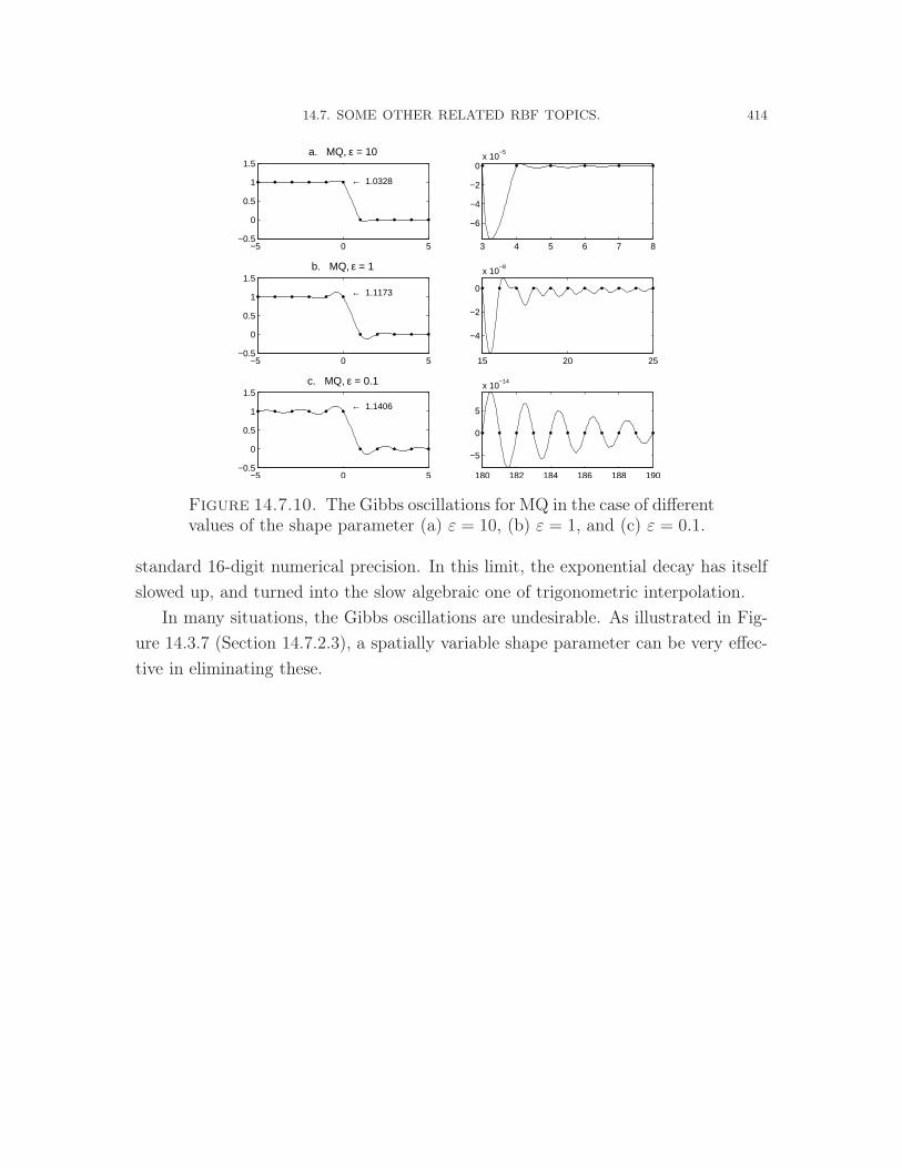
14.7. SOME OTHER RELATED RBF TOPICS. 414
−5 0 5−0.5
0
0.5
1
1.5a. MQ, ε = 10
← 1.0328
3 4 5 6 7 8
−6
−4
−2
0x 10
−5
−5 0 5−0.5
0
0.5
1
1.5b. MQ, ε = 1
← 1.1173
15 20 25
−4
−2
0
x 10−8
−5 0 5−0.5
0
0.5
1
1.5c. MQ, ε = 0.1
← 1.1406
180 182 184 186 188 190
−5
0
5
x 10−14
Figure 14.7.10. The Gibbs oscillations for MQ in the case of differentvalues of the shape parameter (a) ε = 10, (b) ε = 1, and (c) ε = 0.1.
standard 16-digit numerical precision. In this limit, the exponential decay has itselfslowed up, and turned into the slow algebraic one of trigonometric interpolation.
In many situations, the Gibbs oscillations are undesirable. As illustrated in Fig-ure 14.3.7 (Section 14.7.2.3), a spatially variable shape parameter can be very effec-
tive in eliminating these.

CHAPTER 15
THE FFT ALGORITHM
15.1. Introduction
The discovery by Cooley and Tukey (1965) of the FFT algorithm caused one ofthe greatest computational revolutions of all times. Applications of the FFT soonproved abundant in nearly all fields. Not only could many existing tasks be solved
orders of magnitude faster, computing could be brought to bear on new areas. TheFFT principle has since been found in several earlier works, e.g. by Gauss (1866)and Runge (1903, 1905). It is described in a numerical survey book by Runge andKönig (1924) and again in a book on trigonometric computations by Stumpff (1939).
X-ray crystallographers in Cambridge used the method in the 1930’s. It is describedin this context by Danielson and Lanczos (1942). Still, it remained on the fringesof numerical knowledge until its revolutionary potential became apparent to the re-discoverers James W. Cooley and John W. Tukey (Tukey was a professor of statistics
at Princeton University, and Cooley then a programmer at IBM’s Thomas J. WatsonResearch Center, Yorktown Heights, NY).
Part of the reason the FFT idea had not had much impac earlier was that elec-tronic computers were then not available. Clever symmetries had been found thatwere just as effective in speeding up the calculations for the small problem sizes
that were all that then could be handled. By the end of the 1960’s, big computersperformed Fourier transforms on data sets with thousands of points.
A dramatic example of the impact of the FFT is described by Cooley et.al. (1969)regarding the spectral analysis of a seismogram recording from the big Alaska earth-
quake of 1965. A 2048 point discretization of the seismic trace seen in Figure 15.1.1required 26 minutes to transform on a then state-of-the-art computer (producingthe spectrum seen in Figure 15.1.2. With the FFT algorithm, this same task took2.4 seconds (and the result also became more accurate). The difference between the
415

15.2. FFT IMPLEMENTATIONS 416
Figure 15.1.1. Strain seismograph recording of Rat Island earth-quake; N = 2048, T = 131
2hours.
Figure 15.1.2. Power spectrum of the recording in the previous Figure.
operation counts of O(n2) and O(n logn) become larger still when n is increased
further - as is very often the case in present applications.
15.2. FFT implementations
We noted in Section 7.4 that the discrete Fourier Transform (DFT), given by theequations
(15.1) uj =∑N−1
k=0 uke2πikj/N , j = 0, 1, . . . , N − 1
and
(15.2) uk = 1N
∑N−1j=0 uje
−2πikj/N , k = 0, 1, . . . , N − 1.

15.2. FFT IMPLEMENTATIONS 417
are often best expressed in matrix×vector form. For example, in the case of (15.1)we get
(15.3)
1 1 1 1 . . . 1
1 ω ω2 ω3 . . . ωN−1
1 ω2 ω4 ω6 . . . ω2N−2
......
......
......
1 ωN−1 . . . . . . . . . ω(N−1)2
u0
u1
u2
...
...
uN−1
=
u0
u1
u2
...
...
uN−1
where ω = e2πi/N is primary the N th root of unity.We note that the matrix is independent on the data (which appears only in the u
and u - vectors). It turns out that we can factorize the DFT matrix into a product
of a few very sparse matrices. That allows us to carry out what otherwise wouldbe a full matrix×vector multiplication instead as a sequence of a few very sparsematrix×vector multiplications. The FFT algorithm is an implementation of thatidea.
15.2.1. Cooley-Tukey factorization. Figure 15.2.1 shows in the case of N =
8 a factorization of the DFT matrix into a product of sparse matrices. From left toright, these factors are
• a very sparse matrix (two entries per each row only),• a 2× 2 block-diagonal matrix in which each diagonal block is again a DFT
matrix, but of half size, and
• a permutation matrix.
It is straightforward to verify that this factorization works whenever N is an even
number (remembering that ωk+N = ωk and ωk+N/2 = −ωk). In the N = 8 case, werepeat this splitting idea on the two 4×4 blocks, and then on the resulting four 2×2
blocks. That will generate (emerging at the left in the three steps) the first threematrices seen in the top display in Figure ??. The three permutation matrices that
emerged to the right in each of the steps can be combined into a single permutationmatrix. The full 8× 8 DFT matrix we started with is therefore equal to the Coley-Tukey product seen at the top of Figure 15.2.2. The generalization to a matrix of

15.2. FFT IMPLEMENTATIONS 418
Figure 15.2.1. One step in FFT factorization of the DFT matrix,shown for size N = 8.
size N = 2m is immediate. We get m = log2N sparse factors with only 2N non-zeroentries each (half of which are ones, thus costing no multiply operations) The totaloperation count for the matrix×vector multiplication has been reduced from O(N2)
to O(N logN).
A couple of observations:
(1) Vector overwriting: Usually when one performs a matrix×vector multi-plication, one needs to store two separate vectors. As the multiplication isin progress, it is not allowed to let the output vector overwrite the input
vector. This time, the matrix factors happen to have a structure that allowsthis (assuming new wntries are computed pairwise). Of course, no storage isneeded for the matrix factors—they are cheaply generated as the algorithmproceeds.
(2) Generation of permutation matrix: Table 1 illustrates the idea of bit
reversal in our 8 × 8 case; this generalizes directly to any size N = 2m.This principle can be shown for example by induction over m, together withnoting the structure of the individual permutation matrices that emerged
to the right. There are very quick ways available to implement this compu-tationally.

15.2. FFT IMPLEMENTATIONS 419
Figure 15.2.2. Cooley-Tukey and Glassman factorizations of theDFT matrix in case of N = 8.
15.2.2. Glassman factorization. An alternative to the Cooley-Tukey factor-ization was presented by Glassman (1970) - seen in the bottom part of Figure 15.2.2.
This can be derived by step-by-step incorporating the successive permutation matri-ces into the factors that emerged to the left. This factorization may be the easiestof all to implement in a computer code, and the absence of permutations can be

15.3. A SELECTION OF FFT APPLICATIONS 420
Illustration of bit reversal in case of N=8
succes- expres- binary beco- equal to posi-sive sed in digits mes tion of entry
integers binary reversed in column0 = 000 000 = 0 01 = 001 100 = 4 12 = 010 010 = 2 23 = 011 110 = 6 34 = 100 001 = 1 45 = 101 101 = 5 56 = 110 011 = 3 67 = 111 111 = 7 7
Table 1. Illustration of bit reversal. Note that we number the matrixrows and columns starting from zero.
particularly adventageous on vector- or parallel computers that are fast for arith-metic operations, but do ’data shuffling’ relatively slowly. However, no successive
overwriting of output vector on top of the input vector is allowed this time.There exists several other sparse factorizations of the DFT matrix than the two
we have described. For other algorithms (although usually not described in thelanguage of matrix factorizations), see for ex. [..], [..].
15.3. A selection of FFT applications
Applications of the FFT algorithm are ubiquitous in almost all areas that includecomputing. The few brief examples here barely start to scratch the surface. In mostproblems that feature some form of periodicity (e.g. PDEs on a spatially periodicdomain) very powerful numerical methods can be based on numerical transform
to Fourier space (in which the usually delicate task of taking derivatives reducesto regular multiplications). In this book, we have looked at the Fourier methodfor tomographic inversion Chapter 1 and later, in Chapter 30, for X-ray analysis ofcrystals. In this section, we will first mention how it can be used for image processing.This is then followed by a few uses in basic numerical algorithms.
15.3.1. Image enhancement. A common task is to sharpen an image thatis blurred, for example by camera motion or bad focusing. As an example, let us

15.3. A SELECTION OF FFT APPLICATIONS 421
consider the sharp image in Figure (15.3.1), and one of its horizontal scan lines. Ifthe camera was turned sideways during the exposure, the brightness trace would
be smeared just as if it had been convolved with a matrix whose rows are shiftedversions of a rectangular pulse, as shown in Figure (15.3.2). Comparing the sketchof this matrix×vector multiply with the discrete convolution theorem as written inequation ...., we can identify the vectors x, y, z as follows:
z rectangular pulse
x sharp tracey blurred trace
Given any two of these vectors, we quickly find the third by applying (...). Ourinterest is of course to recover x when y and z are given (or if the correct z is notknown, we can try with different z and see what works the best). The idea we havehere sketched in 1-D generalizes immediately to 2-D. For example, if the imaging
error was bad focusing, the equivalent z would be a 2-D matrix featuring a circularlysymmetric smooth hump.
Figure 15.3.1. Example of an image and the grey level of a scan linethrough it.

15.3. A SELECTION OF FFT APPLICATIONS 422
Matrix with sliding copy of a rectangular pulse
Trace of sharp image
Trace of blurred image
Figure 15.3.2. Schematic illustration of how the convolution theoremrelates sharp and blurred images.
15.3.2. Numerical Chebyshev expansion of a function. Any continuous
function on, say, [-1,1] can be approximated arbitrarily closely by a polynomial. Abad way to do this is to interpolate the function at increasingly many equispacedpoints - the polynomial will usually oscillate violently near the ends of the interval.We saw the cause of this Runge phenomenon in Section 12.4 on Lagrange’s interpo-lation formula. We saw also (cf. Figure 12.4.1 vs. Figure 12.4.6) that these spurious
oscillations could be suppressed by simply clustering the interpolation nodes densertowards the edges. The choice
xk = − cosπk
N, k = 0, 1, 2, . . . , N

15.3. A SELECTION OF FFT APPLICATIONS 423
is particularly effective. Convergence of the interpolating polynomial pN (x) to thefunction f(x) is then usually very rapid as N increases. For this particular set
of nodes, it turns out that pN(x) can be found much faster using the Fast CosineTransform (FCT; see Section 7.4) than by using Lagrange’s or Newton’s interpolationformulas. For this, we need first to introduce the Chebyshev polynomials
T0(x) = cos(0 arccosx) = 1 ,
T1(x) = cos(1 arccosx) = x ,
T2(x) = cos(2 arccosx) = 2x2 − 1 ,
T3(x) = cos(3 arccosx) = 4x3 − 3x ,...
......
Tn(x) = cos(n arccos x) = 2n−1xn − . . . .
Tn(x) is clearly a polynomial of degree n for n = 0 and for n = 1.
For higher n the result follows for ex. from the three-term recursionformula Tn+1(x) = 2x Tn(x) − Tn−1(x) (a consequence of the trigono-metric identity cos((n+1)α)+ cos((n− 1)α) = 2 cosα cosnα if we letα = arccosx, i.e. cosα = x).
Making the polynomial
pN(x) =
N∑
ν=0
ανTν(x)
agree with f(x) at the nodes xk = − cos πkN
amounts to finding values of αν such that
N∑
ν=0
ανTν(xk) = f(xk) .
With Tν(xk) = cos(ν arccos(− cos πkN
)) = cos ν πkN
, this becomes
N∑
ν=0
αν cos νπk
N= f(xk), k = 0, 1, 2, . . . , N
Therefore, the desired expansion coefficients are obtained as the output of an FCTapplied to the function values f(xk), k = 0, 1, 2, . . . , N.Also, given the coefficients,this allows a quick evaluation of the function values at the Chebyshev points.

15.3. A SELECTION OF FFT APPLICATIONS 424
If one wants, one can re-sort the expansion ΣNν=0ανTν(x) into the more
usual form for a polynomial ΣNν=0βνx
ν , but there is often little reason
to do this. Thanks to many formulas relating Chebyshev polynomialsof different orders, these are fast to evaluate and easy to manipulate (todifferentiate etc.). A notable advantage with them is that for any f(x)
continuous on [-1,1], there is a unique expansion f(x) = Σ∞ν=0ανTν(x).
Truncations of this series offer excellent approximations to f(x). The
situation for power series is much less attractive. For f(x) = Σ∞ν=0βνx
ν
to hold, it is not even sufficient that f(x) is infinitely many timesdifferentiable over [-1,1]. And even when there is a convergent powerseries expansion, truncations are usually accurate only near x = 0.
15.3.3. Numerical computation of Taylor coefficients. Although this is atask that is not particularly often needed, it is interesting to note that the DFTmakes it possible and the FFT makes it very fast. If a function f(x) can be numeri-cally computed only for real arguments x (the most common situation), we can not
do much better than applying some finite difference approximation from Section....Especially approximations for high derivatives become very sensitive to small errorsin function values.
For example, if we approximate a fourth derivative by(15.1)
f (4)(x) =f(x− 2h)− 4f(x− h) + 6f(x)− 4f(x+ h) + f(x+ 2h)
h4+O(h2) ,
we need h to be small so that the truncation error O(h2) is small. But
then, the h4 in the denominator is far smaller still, causing errors in theterms in the numerator to be greatly magnified. Another way to putit: The numerator must be small like the denominator to evaluate toan O(1) result. It must therefore involve serious cancellation of digits
- the ONLY way to loose large numbers of significant digits in floatingpoint arithmetic.
If f(x) is an analytic function, i.e. once differentiable in the sense that f ′(x) =
limh→0f(x+h)−f(x)
hexists for all complex h→ 0, it can then be shown to automatically

15.3. A SELECTION OF FFT APPLICATIONS 425
be infinitely many times differentiable (only one of very many remarkable theoremsregarding analytic functions).
then f(x) can be Taylor expanded around x:
(15.2) f(x+ h) = f(x) + hf ′(x)
1!+ h2 f
′′(x)
2!+ h3 f
′′′(x)
3!+ . . . .
If we sample f(x) not at equispaced points on the real axis in the neighborhood ofx (such as in (15.1)) but instead around a circle centered at x in the complex planez = x+ h with h = r eiθ, 0 ≤ θ ≤ 2π, then (15.2) becomes
f(x+ r eiθ) = f(x) + rf ′(x)
1!eiθ + r2f
′′(x)
2!e2iθ + r3f
′′′(x)
3!e3iθ + . . . .
The RHS is a Fourier series. Once we have computed the LHS for equispaced valuesof θ, a standard complex FFT will give approximations to the Fourier coefficients(which are rkf (k)(x)/k!− hence also to the derivatives f (k)(x)). In this procedure, the
variable r is a free parameter. Fornberg (1981 a,b) describe in some detail how resultsfor a few different values of r can be combined to get very accurate approximationsto the Taylor coefficients (or derivatives).
15.3.4. Multiplication of large polynomials. The product of
p1(x) = a0 + a1x+ a2x2 + · · ·+ aNx
N and
p2(x) = b0 + b1x+ b2x2 + · · ·+ bNx
N
is
p1(x) · p2(x) = 1 ·{a0b0}+x ·{a1b0 + a0b1}+x2 ·{a2b0 + a1b1 + a0b2}+...xN ·{aNb0 + aN−1b1 + aN−2b2 + . . .+ a1bN−1 + a0bN}+...x2N−1 ·{aNbN−1 + aN−1bN}+x2N ·{aNbN}
= c0 + c1x+ c2x2 + . . .+ c2Nx
2N .

15.3. A SELECTION OF FFT APPLICATIONS 426
This can be written in matrix×vector form as
a0 0 . . . . . . 0 aN . . . a2 a1
a1 a0 0 . . . . . . 0 aN . . . a2
a2 a1 a0 0 . . . . . . 0 aN . . .
. . . a2 a1 a0 0 . . . . . . 0 aN
aN . . . a2 a1 a0 0 . . . . . . 0
0 aN . . . a2 a1 a0 0 . . . . . .
. . . 0 aN . . . a2 a1 a0 0 . . .
. . . . . . 0 aN . . . a2 a1 a0 0
0 . . . . . . 0 aN . . . a2 a1 a0
b0
b1
b2
:
bN
0
:
:
0
=
c0
c1
c2
:
cN
:
:
:
c2N
where we have introduced N zeros following the N+1 elements of the a- and b-vectors(we can pad with additional zeros if we want to make the vector sizes a power of twoor something else that is particularly fast for the FFT). This matrix×vector productis of the form that was shown in equation .... to allow a fast evaluation by means ofthe discrete convolution theorem. The cost becomes O(N logN) operations rather
than O(N2) if computed directly.
15.3.5. Filtering. Basic application of the convolution theorem. To be written.
15.3.6. Sharpening blurred images. Suppose you are taking a picture of the
moon using a long exposure. Even if your camera is mounted on a very sturdy tripod,the motion of the moon across the sky during the exposure blurs your image. Sinceyou know exactly what caused the blur—it is just a convolution with an appropriateblurring function—there is the possibility that the blurring can be undone.
Figure 15.3.3 shows an image of the moon. Find an appropriate function tosimulate the motion of the moon, convolve that with the image to caused a blurredmoon. Now undo the effect. To be written

15.3. A SELECTION OF FFT APPLICATIONS 427
Figure 15.3.3. Original, unblurred image of the moon.

CHAPTER 16
NUMERICAL METHODS FOR ODE INITIAL VALUE
PROBLEMS
16.1. Introduction.
A scalar first order ordinary differential equation (ODE) takes the form
(16.1) y′ = f(t, y) ,
where y = y(t) is a function to be determined. It can be illustrated by a vector field,as shown in Figure 16.1.1 for the case of
(16.2) y′ = t2 + y2 .
At each location in a (t, y)-plane, equation (16.2) tells in which direction a solutioncurve should go. The analytic solution is a continuous function that everywhere
follows the required directions. Even for very simple-looking ODEs, it may be im-possible to find closed-form expressions for solutions. In the case of (16.2), togetherwith the initial condition (IC) y(0) = 0, it happens to be possible:
y(t) = − t(J−3/4(
12t2)− Y−3/4(
12t2))
J1/4(12t2)− Y1/4(
12t2)
,
but its complexity makes it of limited value (J and Y denote here Bessel functions
of fractional orders; this solution is shown as the smooth curve starting at the originin Figure 16.1.1).
In complete contrast to analytical methods, numerical techniques for ODEs donot get any more complicated if the ODE is nonlinear rather than linear, or if it is
428

16.1. INTRODUCTION. 429
−1.5 −1 −0.5 0 0.5 1 1.5−1.5
−1
−0.5
0
0.5
1
1.5
t
y
Figure 16.1.1. llustration of solutions to the ODE (16.2). The arrowsshow the direction field. The smooth and the piecewise linear curvesshow the analytic solution and the Euler approximation (with stepk = 0.5) in the case of the IC y(0) = 0. The dashed circles areexamples of isoclines - curves along which the slopes are constant.
generalized from one scalar ODE to a system of many coupled ODEs, for ex.
(16.3)
y′1 = f1(t, y1, y2, . . . , yn)
y′2 = f2(t, y1, y2, . . . , yn)...y′n = fn(t, y1, y2, . . . , yn)
with IC
y1(0) = a1
y2(0) = a2
...yn(0) = an
.
The ease with which we will soon see that first order systems can be handled numer-ically makes it attractive to turn higher order equations into coupled systems of firstorder ones. For example, instead of
y′′′ = f (t, y, y′, y′′) with IC y(0) = a0, y′(0) = a1, y
′′(0) = a2,

16.2. FORWARD EULER (FE) SCHEME. 430
we introduce extra dependent variables through y0(t) = y(t), y1(t) = y′(t), y2(t) =
y′′(t) and then solve
y′0 = y1
y′1 = y2
y′2 = f (t, y0, y1, y2)
with IC
y0(0) = a0
y1(0) = a1
y2(0) = a2
.
In Section 16.2, we introduce the simplest possible numerical ODE scheme, For-
ward Euler (FE). In its basic form, it is very inaccurate (as seen already in Fig-ure 16.1.1), and it is rarely used. We give in Section 16.3 numerous examples oflinear multistep (LM) methods, which represent one direction for generalizing FEtowards higher accuracy and efficiency. It will transpire that some of these schemes
that are described are very efficient while others, appearing equally plausible, infact are entirely useless. The analysis that is needed to address this involves fourkey concepts: accuracy, consistency, stability and stability domain, and is givenin Section 16.4. With the help of this additional background, we discuss in Sec-
tion 16.5 predictor-corrector methods, in Section 16.6 Runge-Kutta methods and inSection 16.7 Taylor series methods. In the concluding Section 16.8, we describe stiffODEs and how stability domains give insights into how to choose between differentODE methods.
16.2. Forward Euler (FE) scheme.
The numerical solution produced by this scheme is made up of piecewise straightline segments, each one with the slope of the direction field at its start location.A step from time t to time t + k amounts to using the first two terms of a Taylorexpansion of the solution at time t:
(16.1)y(t+ k) = y(t) + k y′(t)︸ ︷︷ ︸ +
k2
2y′′(t) + . . .
︸ ︷︷ ︸Use for Forward Euler Local error O(k2)
Substituting the ODE (16.1) for y′, we get the forward Euler method
(16.2) y(t+ k) = y(t) + k f(t, y) .

16.3. EXAMPLES OF LINEAR MULTISTEP (LM) METHODS. 431
A very convenient way to graphically illustrate the stencil of this scheme is as follows:
(16.3)
y f
time level ⇓ ⇓new: t+ k ⊡ ⊡/⊞ unknown/known values for y
− + − − ⊙/⊕ unknown/known values for fold: t ⊞ ⊕
or, more compactly,
[⊡
⊞ ⊕
].
Each time step, the local error is of size O(k2). In order to advance over a timeinterval of fixed duration, we need to take O(1/k) time steps. It is therefore notsurprising that the total error can be shown to become of the size O(k2) ·O(1/k) =
O(k1) as k → 0. The FE scheme is therefore known as a first order scheme.
16.3. Examples of linear multistep (LM) methods.
The general idea behind linear multistep (LM) methods is to extend the com-
putational stencil shown for forward Euler in (16.3) backwards to still earlier timelevels. In the examples below, we do this in various ways. In all the cases, once theshape of the stencil is decided on, we find the actual coefficients to use (giving thehighest local accuracy) most easily by means of the two-line Padé-based Mathematicaalgorithm described in Section 12.5:
t = Pade[xs*Log[x]m,{x,1,n,d}]; {CoefficientList[Numerator[t],x],CoefficientList[Denomina
The parameter m is here always one since we are approximating a first derivative;
the other three numbers s, n and d describe the ‘shape’ of the stencil, as is describedin Section 12.5. and is also illustrated in Figure 16.3.1.
Example 57.
⊡
⊞ ⊕⊕⊕
Scheme: y(t+ k) = y(t) + k[
2312y′(t)− 4
3y′(t− k) + 5
12y′(t− 2k)
]
Find coeff: m = 1, s = −2, n = 1, d = 2
Accuracy: 3rd order

16.3. EXAMPLES OF LINEAR MULTISTEP (LM) METHODS. 432
Figure 16.3.1. Illustration of how the shape of a linear multistepstencil is described by the parameters s, n and d. If the right column ofentries descends further down than the left column, s will be negative.While n and d need to be integers, we will in a later context considertime-staggared stencils for which s is a half-integer.
The output of the Mathematica algorithm is{{−1, 1}, { 5
12,−4
3, 23
12}}
which should
be interpreted as
−1 y(t) + 1 y(t+ k) = 512y′(t− 2k)− 4
3y′(t− k) + 23
12y′(t).
In this and the following examples, y′(·) should be replaced by f (·, y(·)), i.e. theright hand side of the ODE at time level ” · ”. In this scheme, the stencil is extendedbackwards two additional steps in the right column compared to the FE scheme.Schemes of this general type (extending backwards in the right column only) areknown as Adams-Bashforth schemes. Every step backwards relative to the FE scheme
increases the order by one. Due to its third order of accuracy, we denote the presentscheme as AB3. �

16.3. EXAMPLES OF LINEAR MULTISTEP (LM) METHODS. 433
Example 58.
⊡ ⊙⊞ ⊕⊕⊕
Scheme: y(t+ k) = y(t)+
+k[
38y′(t+ k) + 19
24y′(t)− 5
24y′(t− k) + 1
24y′(t− 2k)
]
Find coeff: m = 1, s = −2, n = 1, d = 3
Accuracy: 4th order
This is an example of an implicit scheme (as opposed to the AB-type schemes, whichare explicit). At each time step, both y(t + k) and y′(t + k) = f (t + k, y(t + k))
are unknown. However, the scheme provides a relation between these two quantities,
from which we can solve for y(t+k) (maybe requiring Newton’s method in case f(t, y)
is a nonlinear function of y). In the next Section 16.4, we will see that, dependingon the ODE, this inconvenience may be well worth it. Schemes of this type (twolevels for y, while implicit and extending different distances backwards for y′) are
known as Adams-Moulton schemes. If the right column contains only the entry ⊙,the resulting first order scheme AM1 is also known as Backward Euler (BE). Again,the accuracy increases by one for every further entry in the right column. �
Example 59.
⊡
⊞ ⊕⊞ ⊕⊞ ⊕
Scheme: y(t+ k) = [−18y(t) + 9y(t− k) + 10y(t− 2k)]−+k [9y′(t) + 18y′(t− k) + 3y′(t− 2k)]
Find coeff: m = 1, s = 0, n = 3, d = 2
Accuracy: 5th order
Here, we are attempting (and we indeed succeed) to reach a very high formal orderof accuracy by extending the stencil backwards in both of its columns. However,as we will see soon, the result is nevertheless a disaster. When letting k → 0, the
numerical solution will explode to infinity. Although the scheme is useless for allpractical work, it will serve as a good motivation for why we need the convergencetheory that is summarized in Section 16.4. �
Example 60.

16.3. EXAMPLES OF LINEAR MULTISTEP (LM) METHODS. 434
⊡ ⊙⊞
⊞
⊞
Scheme: y(t+ k) =[
1811y(t)− 18
22y(t− k) + 1
3y(t− 2k)
]+
− k 611y′(t+ k)
Find coeff: m = 1, s = 3, n = 3, d = 0
Accuracy: 3rd order
This scheme generalizes BE by extending two more levels backwards in the leftcolumn (and its accuracy is consequently two orders higher than that of BE). Schemesof this type are called Backward Differentiation (BD) methods, with this case beingabbreviated as BD3. Again, as the analysis in Section 16.4 will show, this class ofimplicit schemes can be very attractive in certain situations. Although AB and AM
schemes can be successfully brought to any order by just pushing increasingly farback in the second column, there will turn out to be a barrier against increasing BDschemes past order 6. If that is attempted, the same disaster will arise as in Example3. �
The four examples above have illustrated three important families of LM methods:AB, AM, and BD. In the Section 16.5, we will see how the AB and AM classes canbe combined in a particularly effective way.
We conclude this section by showing how one can determine the accuracy of a
LM scheme if its coefficients are given (and not necessarily are the optimal ones withregard to accuracy). One example suffices to illustrate the procedure.
Example 61.
⊡
⊞ ⊕⊞ ⊕
Scheme: y(t+ k) = [3y(t)− 2y(t− k)]++ k
[12y′(t)− 3
2y′(t− k)
]
Accuracy: To be determined
Since each LM formula is an example of a finite difference formula, relating y andy′-values, we can obtain the scheme’s order simply by checking for how high powersof t the formula is exact. We test the error E(t) = {LHS} − {RHS} of the present

16.4. KEY NUMERICAL ODE CONCEPTS. 435
scheme as follows:{y(t) = 1, y′(t) = 0
E(t) = {1} − {[3− 2] + k[120− 3
20]} = 0
{y(t) = t, y′(t) = 1
E(t) = {t+ k} − {[3t− 2(t− k)] + k[121− 3
21]} = 0
{y(t) = t2, y′(t) = 2t
E(t) = {(t+ k)2} − {[3t2 − 2(t− k)2] + k[122t− 3
22(t− k)]} = 0
{y(t) = t3, y′(t) = 3t2
E(t) = {(t+ k)3} − {[3t3 − 2(t− k)3] + k[123t2 − 3
23(t− k)2]} = 7
2k3 6= 0
Given that the scheme fails to be exact for y(t) = t3, it is a second order scheme.Since the result in this type of test will not depend on the value of k, one can simplify
the algebra by first setting k = 1. �
16.4. Key numerical ODE concepts.
16.4.1. Convergence. The key issues when using a numerical ODE solver are
(1) Will the numerical solution converge to the true solution when k → 0 and,if so,
(2) How fast is the rate of convergence?(3) How small does the time step k need to be for the scheme to give a qualita-
tively correct answer?
The first of these questions is answered by the following theorem
Theorem 62. A numerical ODE scheme converges to the true solution of an
ODE (linear or nonlinear) if and only if both consistency and stability hold.
Consistency is a very easy concept to check. A scheme is consistent if the local
error, when the true ODE solution is substituted into the scheme, goes to zero whenk → 0. In particular, any ODE scheme that is of at least of first order accuracyis automatically consistent. No scheme that we would ever consider would fail this

16.4. KEY NUMERICAL ODE CONCEPTS. 436
condition. Assuming from now on that consistency is satisfied, a scheme will thereforeconverge if and only if it is stable.
16.4.2. Stability. Another key result states that, in order to check stability,it suffices to test the scheme in case of the trivially simple ODE y′(t) = 0. To firstillustrate what can go wrong, let us consider the scheme in Example 5. When appliedto y′(t) = 0, it becomes
(16.1) y(t+ k)− 3y(t) + 2y(t− k) = 0.
This is a 3-term recursion relation, which is most easily solved by forming its char-acteristic equation
r2 − 3r + 2 = 0,
with roots r1 = 1 and r2 = 2. The general solution to (16.1) is therefore
y(t+ n k) = c1 · 1n + c2 · 2n
where c1 and c2 are some constants (c1 = 2y(t)−y(t+k) and c2 = y(t+k)−y(t)). Forevery time step forward, the term c2 · 2n doubles in size. The smaller k is made, themore steps need to be taken, and the numerical solution will thus diverge to infinity
(given that machine rounding errors are always present and that we simplified theODE by setting its RHS to zero, it will not happen in practice that c2 is exactly
equal to zero). The cause of the divergence is that the characteristic equation hasa root (here r2 = 2) outside the unit circle |r| = 1. Omitting a few further details,
this leads us to the root condition:
Theorem 63. A LM scheme is stable if and only if all the roots to its character-
istic equation lie inside or on the periphery of the unit circle. If any root is on the
periphery, it needs to be a simple root.
We can note that whenever a scheme is accurate to first order or better, it will
admit the exact solution y(t) ≡ 1 to the ODE y′(t) = 0. From this follows that r1 = 1
is always a root to the characteristic equation. All other roots are ‘spurious’, andwhat matters is that powers of these spurious roots must not grow. In the graphical

16.4. KEY NUMERICAL ODE CONCEPTS. 437
stencils we use to illustrate LM schemes, stability (as opposed to accuracy) dependsonly on the entries in the left column.
16.4.3. Stability domains. The concept of stability domain (or domain of ab-
solute stability) has very little to do with stability, as defined in the previous Sec-tion 16.4.2, so the traditional naming convention is unfortunate. To every ODE
method corresponds a stability domain (in a complex plane, which we will soon de-fine). For ODEs, this stability domain provides a guide to how small time step oneneed to take in order to get a ‘reasonable’ numerical solution. Stability domainsprovide often a good guide to what type of numerical method to choose for different
ODEs, as discussed in Section 16.8. A related application area of stability domainswill arise when we, in Chapter ??, apply ODE methods for numerically solving PDEs.In that context, the stability domain will tell whether schemes will converge or di-verge when both time and space steps are refined—much like how stability (as tested
by the root condition) is the key issue for convergence in the case of ODEs.We will start the discussion of stability domains by an example which illustrates
the need for a practical guide in choosing an appropriate time step:
Example 64. Determine how small we need to choose k in order to get a quali-tatively reasonable approximation when using forward Euler to solve the ODE
(16.2) y′(t) = −10y(t).
The analytic solution y(t) = e−10 ty(0) decays rapidly for increasing t. Supposewe try to solve (16.2) with forward Euler using the time step k = 1. The schemebecomes y(t + 1) = y(t) + 1 · (−10y(t)) = −9y(t). Obviously, stepping forward inthis way will lead to an oscillatory and rapidly divergent numerical solution, bearing
no relation to the analytical one. Since forward Euler is consistent and satisfies theroot condition (with r1 = 1 as the only root), we know that all will be well in thelimit of k → 0. However, in practice one needs to calculate with a finite value of k,so a natural question to ask is how small k need to be so that the numerical solution
will not grow in time. For a general value of k, the forward Euler scheme for (16.2)becomes y(t + k) = y(t) + k · (−10y(t)) = (1 − 10k) y(t), so the answer becomesk ≤ 1/5. �

16.4. KEY NUMERICAL ODE CONCEPTS. 438
16.4.3.1. Linearization of a general ODE.. The general ODE (16.1) can, locallyaround a point (t0, y0) = (t0, y(t0)), be linearized in both t and y:
y′ ≈ f(t0, y0) + ft(t0, y0)(t− t0)︸ ︷︷ ︸+ fy(t0, y0)︸ ︷︷ ︸ (y − y0)︸ ︷︷ ︸g(t) λ
; v(t)
i.e. v′(t) ≈ λ v(t) + g(t). In the present context, it turns out that we can furtherignore g(t), and only the value of λ = fy(t0, y0) will remain significant.
16.4.3.2. Stability domains for AB- and AM-type LM methods. In the case of FE
(AB1), we can compute the stability domain as follows:
Example 65. Calculate the stability domain for FE.For the ODE y′ = λy, FE becomes y(t+ k) = y(t)+λk y(t). For all ODE methods(not just as here for FE), the variables λ and k will at this point only enter in thecombination ξ = λk. Thus y(t+ k) = (1 + ξ)y(t), and y(t+ nk) = (1 + ξ)ny(t). The
condition for no growing solutions therefore becomes |1 + ξ| ≤ 1, i.e. a circle in acomplex ξ-plane centered at ξ = −1 and with radius 1, shown by the label ”1” inFigure 16.4.1(a). �
In the case of Example 65 , we have λ = −10. The stability domain for FE tellsthat we have no-growth if −2 ≤ ξ ≤ 0. Given that ξ = λk, we have thus again
arrived at the previous condition k ≤ 1/5.Even for real-valued ODEs, we are also interested in complex values of ξ. If we
for example want to solve a system of ODEs such as[y1
y2
]′=
[0 1
−1 0
][y1
y2
]
(which can arise directly in applications or as the result of rewriting a higher orderequation as a first order system; in this case y′′ + y = 0), a simple change of variabledecouples the two equations, and the eigenvalues to consider are λ1,2 = ±i.
Example 66. Calculate the stability domain for AB2.

16.4. KEY NUMERICAL ODE CONCEPTS. 439
Applying y(t+ k) = y(t) + k [32y′(t)− 1
2y′(t− k)] to y′ = λy and substituting ξ = λk
gives
(16.3) y(t+ k)− (1 + 32ξ) y(t) + 1
2ξ y(t− k) = 0.
This is a 3-term linear recursion relation, which is most easily solved via its charac-teristic equation
(16.4) r2 − (1 + 32ξ) r + 1
2ξ = 0.
We now want to plot, in the complex ξ-plane, the domain with the property thatboth roots r1 and r2 to (16.4) lie inside or on the unit circle - the condition for (16.3)
not to have growing solutions. Trying to solve the quadratic equation (16.4) for rturns out to be a bad idea. A much better one is to realize that the boundary of thestability domain (in the ξ-plane) must be characterized by one root r to (16.4) beingon the edge of the unit circle. Thus, we solve (16.4) for ξ
(16.5) ξ =2r (r − 1)
3r − 1
and obtain the stability domain by letting r = eiθ and plotting ξ as θ runs from 0 to2π. In Matlab, the complete code for this becomes
r = exp(i*linspace(0,2*pi)); plot(2*r.*(r-1)./(3*r-1));
The resulting domain is labeled ”2” Figure 16.4.1(a). �
The procedure in Example 66 for AB2 works for all LM methods. In case of AB3,we get in place of (16.5)
ξ =12r2 (r − 1)
23r2 − 16r + 5and for AB4
ξ =24r3 (r − 1)
55r3 − 59r2 + 37r − 9.
At this point (of AB4) enters a minor complication in that the curve that is traced out
in the ξ-plane intersects itself. The curve marks where one root to the characteristicequation changes from |r| < 1 to |r| > 1. It can happen that another root is largerthan one, so that both sides of the traced curve are outside the stability domain. In

16.4. KEY NUMERICAL ODE CONCEPTS. 440
−2.5 −2 −1.5 −1 −0.5 0 0.5−2
−1.5
−1
−0.5
0
0.5
1
1.5
2
12
34
56
Adams−Bashforth
−6 −4 −2 0 2−6
−4
−2
0
2
4
6
1
2
3
45 6
Adams−Moulton
Figure 16.4.1. Stability domains for (a) AB and (b) AM methodsof orders 1-6. The stability domains in all cases include the regionsimmediately to the left of the origin, i.e. for AB1 it is the domainoutside the circle |1− ξ| = 1, and for AB2 the left halfplane. In allother cases, the regions are bounded. Note that the scale differs by afactor of three between the two pictures.
such cases of intersecting loops, one simply chooses any ξ-value inside the loop, and
solves for all the roots - that will tell if the loop is part of the stability region or not.Figures 16.4.1(a) and (b) summarize the stability domains for AB and AM meth-
ods of increasing orders.In both cases, the stability domains get smaller when the order increases. For
each fixed order, the domain for the AM method is much larger than the one for theAB method. Dependent on the ODE that is solved, this advantage may outweighthe disadvantage of the AM methods being implicit.
In some important applications discussed in Chapter ??, all eigenvalues of the
ODE will be purely imaginary, and it is then essential to know if a method’s stabilitydomain will include an interval of the imaginary axis around the origin. For ABmethods, this turns out to happen if the order is {3,4}, {7,8}, {11,12}, etc. and theopposite holds for AM methods, i.e. there is some imaginary axis coverage for orders
{1,2}, {5,6}, {9,10}, etc. [..].16.4.3.3. Stability domains for BD methods. Example 4 in Section 16.3 provided
an example of a BD scheme. The schemes BD1-BD6 differ only in the number of

16.4. KEY NUMERICAL ODE CONCEPTS. 441
−10 0 10 20 30−25
−20
−15
−10
−5
0
5
10
15
20
25
1 2 34
56
BD method
−0.5 0 0.50
0.2
0.4
0.6
0.8
1
1.2
1
234
5
6
Detail near the origin
Figure 16.4.2. Stability domains of BD methods of orders 1-6. Thedomains are in all cases on the outside of the shown boundaries: (a)the complete boundaries (b) detailed boundary structures near theorigin.
back levels that are employed for y. Figure 16.4.2 a show their stability domains and
part b gives a more detailed picture near the origin.The stability domains are this time what falls outside (not inside) the closed
curves. For all these schemes, the whole negative real axis is included in the domains.For BD schemes of orders p = 7 and above, not only does this property get lost; the
schemes will also fail the root condition.
16.4.4. The Dahlquist barriers. The concepts of stability (root condition)and of stability domain are not entirely unrelated for LM methods, as shown by theDahlquist stability barriers.
First barrier: The order of accuracy p of a stable s-step LM formula satisfies
p ≤
s+ 2 if s is evens+ 1 if s is odds if the formula is explicit
.
For example, the AB3 scheme illustrated in Example 1 is explicit, and features
p = s = 3 (note that s here is not the same s as in the Mathematica code to generateLM schemes). From this first barrier follows that any attempt to increase the orderof accuracy by introducing further entries also down the left stencil column (as in

16.5. PREDICTOR-CORRECTOR METHODS. 442
Example 3) must cause the root condition to become violated. For explicit LMschemes, the AB class features as high orders of accuracy as is possible, given any
value of s.It is natural to want a method to include the whole negative half plane (Re ξ < 0)
in the domain, since the analytical solutions to y′ = λy decay when Re λ < 0. Sucha scheme is called A-stable.Second barrier: The following two results hold:
(1) An explicit LM method can never be A-stable, and(2) An implicit A-stable method can be at most second order accurate.
The AM1 (also described as BE and BD1), AM2 and BD2 methods are all examples ofA-stable schemes. In most applications, A-stability is a more restrictive requirementthan what is needed, cf. the discussion about stiff systems in Section 16.8.
16.5. Predictor-corrector methods.
An interesting idea for combining the key strength of AB methods (being explicit)with that of AM methods (having much larger stability domains) is to use them insuccession as a predictor-corrector pair. One of several possible strategies to obtainsuch a combined method of order p is the following:
(1) use AB of order p−1 to get a predicted value at the new time level: y(t+k),
(2) use y(t+ k) to calculate a predicted value f(t+ k, y(t+ k)),(3) use f(t + k, y(t + k)) in the RHS of an AM scheme of order p, to obtain
y(t+ k).
(4) calculate a corrected value of f(t+ k, y(t+ k)) (to use for subsequent time
steps).
This combined scheme can be shown to be accurate of order p, is entirely explicit,and will have considerably larger stability domain than corresponding AB methods,as seen by comparing Figure 16.4.1(a) with Figure 16.5.1(a).
It can be shown that all schemes of this type with p ≥ 3 will have some imaginaryaxis coverage near the origin. A disadvantage with the schemes is that they requiretwo (rather than one) function evaluations per time step.

16.5. PREDICTOR-CORRECTOR METHODS. 443
−3 −2 −1 0−3
−2
−1
0
1
2
3
65
43
2
AB(p−1) / AMp predictor / corrector
−6 −4 −2 0−6
−4
−2
0
2
4
6
12
34
56
78
910
Runge−Kutta / Taylor series
Figure 16.5.1. Stability domains for (a) AB(p-1)/AMp predic-tor/corrector methods for p = 2, 3, . . . , 6. (b) Solid curves: RK meth-ods with s = p = 1, 2, 3, 4; Solid and dash-dot curves: TS methods oforders p = 1, 2, . . . , 10. Note that the scale differs by a factor of twobetween the two plots.
The method to calculate a predictor/corrector scheme’s stability domain is verysimilar to that for a regular LM scheme:
Example 67. Calculate the stability domain for the AB2/AM3 scheme.
As always when calculating stability domains, we consider the ODE y′ = λy. Thetwo steps can be written
{y(t+ k) = y(t) + λk [3
2y(t)− 1
2y(t− k)]
y(t+ k) = y(t) + λk [ 512y(t+ k) + 2
3y(t)− 1
12y(t− k)] .
After the substitutions of λk = ξ and of y(t + k) from the first equation into thesecond one, we get a linear 3-term recursion relation with characteristic equation
(16.1) r2 −(1 + 13
12ξ + 5
8ξ2)r +
(112ξ + 5
24ξ2)
= 0 .
To trace out the edge of the stability domain, we again let r run around the peripheryof the unit circle, and follow how ξ then moves. Although we, for each r-value can

16.6. RUNGE-KUTTA (RK) METHODS. 444
do this by solving a quadratic equation for ξ, an easier strategy is to start by notingthat r = 1 always corresponds to ξ = 0. As we step along in r, we can use Newton’s
method to find the corresponding ξ-value (using the ξ-value from the last computedcase as the start approximation for the next one). �
16.6. Runge-Kutta (RK) methods.
Runge-Kutta methods are more convenient than LM methods in that one doesnot need any previous time levels to get started. The lowest order RK scheme is FE,
which we now write as
s = 1, p = 1 d(1) = k f(t, y(t))
−−−−−−−−y(t+ k) = y(t) + [d(1)]
For higher order RK methods, each time
step is split into s internal stages, requiring one function evaluation each. Thefollowing are examples of methods of increasing numbers of stages s and of corre-spondingly increasing accuracies p:
s = 2, p = 2 d(1) = k f(t, y(t))
d(2) = k f(t+ k2, y(t) + 1
2d(1))
−−−−−−−−y(t+ k) = y(t) + [d(2)]
s = 3, p = 3 d(1) = k f(t, y(t))
d(2) = k f(t+ k3, y(t) + 1
3d(1))
d(3) = k f(t+ 2k3, y(t) + 2
3d(2))
−−−−−−−−y(t+ k) = y(t) + [1
4d(1) + 3
4d(3)]
The best known of all RK schemes is probably

16.6. RUNGE-KUTTA (RK) METHODS. 445
s = 4, p = 4 d(1) = k f(t, y(t))
d(2) = k f(t+ k2, y(t) + 1
2d(1))
d(3) = k f(t+ k2, y(t) + 1
2d(2))
d(4) = k f(t+ k, y(t) + d(3))
−−−−−−−−y(t+ k) = y(t) + 1
6[d(1) + 2d(2) + 2d(3) + d(4)] .
Although there are many different RK schemes with the same values for s and p,it turns out that whenever s = p, the stability domains are described by the relation
(16.1) r =
p∑
n=0
ξn
n!,
giving the domains shown by solid lines (numbered 1-4) in Figure 16.5.1(b). Fors = p = 1, we recognize the domain for FE. In contrast to the AB and AM methods,the stability domains increase in size when the order increases. In particular, we can
note that the domains for RK3 and RK4 cover sizeable sections of the imaginaryaxis. For RK methods of higher orders than p = 4, a few complications arise:
(1) computation of coefficients within the stages becomes extremely complicated(however, schemes with orders up to around p = 10 have been tabulated inthe literature, and need not be re-derived by users),
(2) there are no longer any schemes with s = p, only with s > p,(3) the stability domains become dependent on the RK coefficients (i.e. no
longer dependent only on p = s), and(4) the accuracy may be lower for systems of PDEs than for scalar ODEs.
Numerical ODE packages that are based on RK methods usually employ RK varia-tions which provide not only a value at the new time level, but also an error estimatefor each step. The step lengths can then be adjusted automatically in order to meeta specified error tolerance.
Apart from explicit RK methods, there are also implicit RK methods. Thesecan reach order 2s with only s stages, and can also have perfect stability domains- precisely the left half plane (matching where the solutions to the ODE y′ = λy

16.7. TAYLOR SERIES (TS) METHODS. 446
feature no growth). However, the cost required for solving the systems of equationsthat arise often make them less practical.
16.7. Taylor series (TS) methods.
The TS approach is in some cases the most powerful technique available, but itis somewhat limited in that
• The right hand side of the ODE (16.1) must be composed only of analyticfunctions (e.g. of powers, fractions, exponentials, and trigonometric func-
tions), and• Quite advanced software is needed if one wants to automatically translate
(compile) an ODE into executable code. In contrast, for linear multistepand Runge-Kutta methods, the ODE solver itself does not need to be altered
between different ODEs.
Recalling from (16.1) that forward Euler corresponds to truncating after the secondterm in a Taylor series
(16.1) y(t+ k) = y(t) + k y′(t) +k2
2!y′′(t) +
k3
3!y′′′(t) +
k4
4!y′′′′(t) + . . . ,
the idea is simply to truncate at a much later level. That requires that we somehowcan determine higher derivatives of y. Surprisingly many numerical analysis textbooks mention and then dismiss this approach after considering only an inefficient
way to go about this - repeated differentiation. Given y′(t) = f(t, y(t)), differentia-tion (based on the chain rule) gives
y′′ = f ∂f∂y
+ ∂f∂t
y′′′ = f 2 ∂2f∂y2
+ f
{2 ∂2f∂t∂y
+(∂f∂y
)2}
+ ∂f∂t· ∂f∂y
+ ∂2f∂t2
y′′′′ = f 3 ∂3f∂y3
+ f 2{
3 ∂3f∂t∂y2
+ 4∂f∂y· ∂2f∂y2
}+ ∂f
∂t·(∂f∂y
)2
+ ∂3f∂t3
+ 3∂f∂t· ∂2f∂t∂y
+ ∂2f∂t2· ∂f∂y
+
+f
{(∂f∂y
)3
+ 5 ∂2f∂t∂y· ∂f∂y
+ 3 ∂3f∂t2∂y
+ 3∂f∂t· ∂2f∂y2
}
· · · etc.
Not only does the number of terms increase very rapidly, the individual derivativesalso get very complex quickly for all but the simplest functions f(t, y). It is much

16.7. TAYLOR SERIES (TS) METHODS. 447
more efficient to determine the expansion coefficients recursively. This is best ex-plained by means of an example. Repeating example (16.2) here for convenience,
(16.2) y′ = t2 + y2, y(0) = y0,
we substitute the Taylor series centered at t = 0,
(16.3) y(t) =N∑
n=0
antn
into (16.2),N−1∑
n=0
(n+ 1)an+1tn = t2 +
2N∑
n=0
n∑
s=0
asan−stn.
Matching the different powers of t we get the recursion relation
t0 : a1 = a20
t1 : a2 = a0a1
t2 : a3 =1
3
(1 +
2∑
j=0
aja2−j
)
...
tn : an+1 =1
n+ 1
n∑
j=0
ajan−j,
with a0 = y0, the initial value. Once the Taylor expansion coefficients are known,up to any desired order, an approximation of y(t) can now be calculated from (16.3)for any value of t, say t1, within the radius of convergence of the Taylor series. Once
an approximation of y(t1) is known, the process is repeated by Taylor expanding att = t1.
Of course it is not necessary to do the above by hand. The following brief Math-ematica script illustrates how, if given a value y at time t, one can generate thecoefficients a1, a2, ... in the expansion
(16.4) y(t+ k) = y(t) + a1k + a2k2 + a3k
3 + . . .
In the case of n = 8 and the ODE (16.2), the script would be

16.7. TAYLOR SERIES (TS) METHODS. 448
n=8;(* Specify number of coefficients *)y[k]:=y+Sum[a[i] ki,{i,1,n}]+O[k](n+1)
f[t,y]:=t^2+y^2(* Specify the RHS of the ODE *) LogicalExpand[y’[k]==f[t+k,y[k]]]
giving the output
t^2+y^2-a[1]==0 && 2t+2ya[1]-2a[2]==0 && 1+a[1]^2+2y a[2]-3a[3]==0 &&
2a[1]a[2]+2ya[3]-4a[4]==0 && a[2]^2+2a[1]a[3]+2ya[4]-5a[5]==0 &&
2a[2]a[3]+2a[1]a[4]+2ya[5]-6a[6]==0 &&
a[3]^2+2a[2]a[4]+2a[1]a[5]+2y a[6]-7a[7]==0 &&
2a[3]a[4]+2a[2]a[5]+2a[1]a[6]+2ya[7]-8a[8]==0
again become simple algebraic recursions that explicitly provide the successive coef-ficients. A similar approach to obtain the same recursions starts with considering
dy(t+ k)
dk= f(t+ k, y(t+ k)).
Every time a truncated version of (16.4) is substituted into the RHS f(t+k, y(t+k))
and is integrated with respect to k, we gain (at least) one more term in (16.4).By always truncating to no more terms than what are known to be correct, the
algebra remains moderate and is well suited for automation without the need ofgeneral symbolic packages such as Mathematica. In the TS method, the recursionrelations are generated as a preprocessing step, and are then compiled into the actualsolution algorithm. Like for the other numerical ODE approaches, it is usually most
convenient to rely on library software when using the TS approach.The stability domains for the TS methods are also described by (16.1). For RK
methods, this formula was valid only when s = p = 1, 2, 3, 4. The TS method con-tinues this same formula up to any value of p. The dashed curves in Figure 16.5.1(b)
show how the domains continue to grow as p increases.One intuitive way to understand why TS methods have so much larger stability
domains (and also are much more accurate) than AB or AM methods of correspond-ing orders is to note that the latter pick up their ‘extra’ information from very old
and ‘obsolete’ back values of y′, essentially relying on the notoriously ill-conditionedconcept of using one-sided high order polynomial approximations (cf. the discussionof the Runge phenomenon in Section 12.4). In contrast, a TS method increases the

16.7. TAYLOR SERIES (TS) METHODS. 449
order by means of extracting much more analytic information from the ODE itself,right at the most recent time position.
The following example illustrates a remarkable property of Taylor methods.
Example 68. Solve
y′ = y2, y(0) = 1.
The analytical solution is y(t) = 11−t , it therefore has a simple pole at t = 1 on the
real axis. Let us see how the TS methods deals with this singularity. Substituting
the Taylor expansion (16.3), we find the recursion relation,
a0 = 1
a1 = a20
...
an+1 =1
n+ 1
n∑
j=0
ajan−j.
It should not be hard to show that the solution is given by an = 1, for all n. Thisis a remarkable, as should become clear if we convert it to a Padé approximation,as investigated in Exercise 25. Thus remarkably, the TS method returns the exact
analytical solution, despite the presence of a pole. This is a point worth stressing:TS methods together with Padé approximations are eminently suitable for capturingpoles in the complex plane, a property not shared by any of the polynomial-basedmethods.
The next example is one of a family of six equations, the Painlevé equations, that
is all about the structure of their poles in the complex plane. It is not possible to gointo any details here but one of their distinguishing properties is that their solutionsall have only poles or essential singularities in the complex plane, no branch cutsare present. One of the main outstanding numerical issues was how to calculate
numerical solutions in the presence of these singularities. The previous examplesuggests that TS methods, together with Padé may be suitable. Let us thereforecalculate the Taylor expansion coefficients for the first Painlevé equation.

16.8. STIFF ODES. 450
n 0 1 2 3 4 5 6 7 8 9an 0.0000 0.5000 0.0000 0.1667 0.0000 0.1250 0.0000 0.0333 0.0000 0.0164
Table 1. Taylor expansion coefficients for Painlevé I.
Example 69. Solve the first Painlevé equation, PI,
(16.5) y′′ = 6y2 + t, y(0) = 0, y′(0) = 0.5,
numerically using Taylor’s method. Substituting (16.3), and matching different pow-ers of t, we find the recursion relations
t0 : a2 = 3a20
t1 : a3 = 2a0a1 +1
6...
tn : an+2 =6
(n + 2)(n+ 1)
n∑
j=0
ajan−j .
From the initial values a0 = 0, a1 = 0.5, the numerical values for the Taylorexpansion coefficients are given in Table 1.
We leave it as an exercise to convert this expansion into a Padé approximation,as explained in Section 10.3.
16.8. Stiff ODEs.
A stiff system of ODEs is one in which some processes happen extremely fastwhile others are much slower. A typical example could be a chemical process withdifferent coupled reactions. Generalizing the linearization procedure described in Sec-tion 16.4.3.1 to a system of ODEs leads us to consider
v′(t) ≈ A v(t) + b.
If the eigenvalues λ of A differ in size by several orders of magnitude, especially if
some are negative and very large in magnitude, we have a stiff system. In order notto be forced to use an extremely small time step (given that ξ = λk for all the λhave to fall within the stability domain of the ODE solver), it is essential that the

16.8. STIFF ODES. 451
stability domain extends far out to the left in the complex ξ-plane. Of the methodsthat we have discussed, the BD methods excel in this regard.
In the context of solving wave-type PDEs, we will come across cases where theλ’s will be lying far out along the imaginary axis. Once the eigenvalue character ofan ODE or (more commonly) of a system of ODEs has been assessed, comparisonswith different methods’ stability domains provide a very good guide for choosing asuitable method.

CHAPTER 17
FINITE DIFFERENCE METHODS FOR PDE’s
17.1. Introduction.
Chapter to be written.
452

CHAPTER 18
OPTIMIZATION: LINE SEARCH TECHNIQUES
18.1. Introduction.
If nature is left to run its course it tends to find the best or optimal solutionsfor its problems. In the Western Cape, South Africa, several Gladiolus species forexample, produce heavy scent in the evening but none during the day, so as not to
waste precious energy during day time when its pollinator moth is not active. Inphysics equilibrium solutions correspond to minimum energy solutions, and scientistsand engineers in general are constantly faced with find solutions that minimizes someobjective function. The generalized inverse of a general linear system of algebraic so-
lutions discussed in Section 11.5 will soon be interpreted as an optimization problemwith linear constraints, in which case it appears in the guise of Lagrange multipliers.
Optimization can be constrained or unconstrained. In the former it means thatadditional constraints are imposed that the solution has to satisfy. One popular
method for incorporating the constraints is Lagrange multipliers, discussed in thenext section. Our discussion differs from most other in that it is based on theSingular Value Decomposition (SVD), as alluded to above. From there we proceedto discuss the so-called line-search methods. These are all iterative methods; givenan estimate of the solution (minimizing the objective function), one systematically
improves on the estimate until convergence. In the case of line-search methods, theimprovement consists of two general steps. First an approximate direction from thecurrent estimate to the optimum is determined. One then moves in this directiontowards the optimum. The second step is to determine how far one has to move in
this direction, see for example [5, 14].The different line-search methods differ in the ways in which the directions and
distances are determined. It is important to note that the directions are, for thesemethods, always determined by local information. This leads to a major complication
453

18.2. LAGRANGE MULTIPLIERS. 454
with line-search methods— they tend to get stuck in local optima. Starting from aninitial guess the iterative improvements tend to proceed in directions of decreasing
objective function values. If a point is reached where all directions lead to an increasein the objective function, i.e. a local minimum, the solution is stuck at this localminimum. Since the line-search directions are determined by local properties of theobjective function, it is not possible to determine the position, or even the presence,of better (global) minima. These complications are addressed in the next chapter.
18.2. Lagrange Multipliers.
Suppose we are given a function, the objective function f(x) where x = [x1, x2, . . . , xn]T
and we want to find the minimum value of f . More precisely, we are interested infinding x⋆ that minimizes f(x), i.e.
(18.1) x⋆ = arg minxf(x).
The well-known necessary condition for the extreme values is given by (assuming ofcourse that the necessary partial derivatives are available),
∂f
∂xj
∣∣∣∣x=x⋆
= 0, j = 1, . . . , n.
This means that in general one has to solve a nonlinear system of algebraic equations.Assuming that problem is tractable, one finds all the extreme values, and then pick
the global optima.The problem becomes more complicated if we put constraints on the solution
space. Let us illustrate it with an example.
Example 70. Let f(x, y) := x2 + y2 and we are asked to find the minimum
of f subject to g(x, y) := x + y = 1. In this case the two independent variables areconnected through a constraint and it is no longer possible to find the extreme valuesby setting the partial derivatives of f equal to zero. We need to find the minimumof f on the line x+ y = 1. Since f(x, y) = x2 + y2 is just the square of the distance
from the origin, the minimum we are looking for is the point on the line closest tothe origin, i.e. x = 1
2= y, see Figure 18.2.1.
�

18.2. LAGRANGE MULTIPLIERS. 455
Figure 18.2.1. Minimizing x2 + y2 subject to x+ y = 1.
This does not easily generalize to higher dimensions and a different point of viewis required. Both f(x, y) = c and g(x, y) = 1 define curves in the plane. In fact
as we vary c a family of curves is defined by f where each member of the familyis uniquely associated with c. We need to find that member of the family with thesmallest value of c, subject to the constraint g(x, y) = 1. Imagine that we start witha very large value of c, corresponding to the circle with a very large radius in our
example, intersecting the curve g(x, y) = 1 in two points. As we decrease the value ofc, the circles start to shrink, and at some some stage we end up with a circle that justtouches the curve g(x, y) = 1. The corresponding value of c is the minimum value forf, subject to the constraint. Out goal therefore is to find where the circle and curve
touch. One way of doing this is to recognize that the two curves have a commontangent, where they touch, i.e. their gradients (perpendicular to the tangents) pointin the same direction,
(18.2) ∇f = −λ∇g,

18.2. LAGRANGE MULTIPLIERS. 456
where λ is a scalar known as the Lagrange multiplier (the minus sign is for laterconvenience). We now have three equations for three unknowns x, y and λ, two
equations from the Lagrange multiplier equation (18.2), and g(x, y) = 1. For ourexample these are
2x = −λ2y = −λ
x+ y = 1.
The first two equations tell us that x = y, and the third one that x = 12
= y. We arenot really interested in λ but we find that λ = −1.
There is only one more observation to be made in order to generalize these ideas,and that is that (18.2) is equivalent to finding the minimum of
f(x, y) + λ (g(x, y)− 1)
with respect to x, y and λ, where the constraint is recovered from minimizing withrespect to λ.
Example 71. For the problem in the previous Example 70, calculate the gener-alized solution of x+ y = 1 using the SVD of Section 11.5.
Writing this as a system of linear equations (a system consisting of a single
equation!),[
1 1] [ x
y
]= 1,
we note that it admits an infinite number of solutions. As explain in Section 11.5the SVD finds the solution that minimizes |x2| = x2 + y2. Thus the SVD gives thesame answer as the Lagrange multiplier problem. Is this a coincidence or is there
something more fundamental behind it?
�
A similar geometric argument that led to (18.2) can be used to generalize tohigher dimensions. We prefer an alternative approach. We first give the generalequations and then justify them using the Singular Value Decomposition (SVD). In

18.2. LAGRANGE MULTIPLIERS. 457
general the problem is, find We are looking for the minimum of
x⋆ = arg maxx
f(x), x = [x1, x2, . . . , xn]T ,
subject to m constraints
(18.3) gj(x) = 0, j = 1, . . . , m,
assuming that m < n. Introducing the m Lagrange multipliers λ = [λ1, . . . , λm]T weminimize
(18.4) L(x) = f(x) + λTg(x),
where g(x) = [g1(x), . . . , gm(x)]T . The necessary conditions for an extreme value,
∇xL(x) = 0
gives us n equations inm+n unknowns (the x’s and λ’s). The remaining m equationscome from the constraints (18.3). Before we justify these equations using the SVD,let us do another example.
Example 72. Find the minimum of
f(x, y, z) = x2 + y2 + z2
subject to
x+ y + z = 1
x− y − z = 1.(18.5)
According to (18.4) we minimize
L(x, y, z) = x2 + y2 + z2 + λ1 (x+ y + z − 1) + λ2 (x− y − z − 1)
subject to the constraints. From ∇L = 0 we find
2x+ λ1 + λ2 = 0
2y + λ1 − λ2 = 0
2z + λ2 − λ2 = 0.(18.6)

18.2. LAGRANGE MULTIPLIERS. 458
Solving for x, y and z and substituting into the equations for the constraints (18.5)we get
−3λ1 + λ2 = 2
λ1 − 3λ2 = 2,
or λ1 = −1 = λ2. Substituting back into (18.6) we find x = 1, y = 0 and z = 0. The
minimum value of f subject to the constraints is therefore f = 1.
�
Now for the justification, using the SVD. The constraints (18.3) form a n − mdimensional manifold in R
n. Suppose we have found the minimum of f(x⋆) on this
manifold. Let us move a small distance on the manifold, away from the minimum,i.e. let x = x⋆ + ∆x. Since we stay on the manifold it follows that g(x) = 0 = g(x⋆)
and from this follows thatJg(x
⋆)∆x = 0,
where Jg is the Jacobian matrix of g, i.e.
(18.7) Jg(xm) =
∂g1∂x1
∂g1∂x2
· · · ∂g1∂xn
∂g2∂x1
∂g2∂x2
· · · ∂g2∂xn
......
. . ....
∂gm
∂x1
∂gm
∂x2· · · ∂gm
∂xn
x=x⋆
=
∇g1(xm)T
∇g2(xm)T
...
∇gm(xm)T
.
This means that ∆x lies in the null space of the Jacobian matrix of g. Since x⋆ is alocal minimum of f(x) on the manifold, it follows that
∇f(x⋆)∆xT = 0.
This tells us that ∇f(x⋆) is orthogonal to the null space of Jg(x⋆), i.e. we canwrite ∇f(x⋆) as a linear combination of the rows of (18.7) which is equivalent to
minimizing (18.4).
Example 73. Entropy.
Suppose we have N symbols xi, i = 1, . . . , N that we want to send over acommunication channel. Each symbol occurs with a probability p(xi). The questionis how much information h(xi) do we receive if we receive a specific symbol xi. If

18.2. LAGRANGE MULTIPLIERS. 459
p(xi) = 1, then the symbol xi appears with absolute certainty and there is no surprise;the information it carries should be zero, thus we require that h(xi) = 0, whenever
p(xi) = 1. Now suppose we receive two unrelated symbols, xi, xj . The informationgained by observing both of them should be h(xi, xj) = h(xi) + h(xj). From theseconsiderations it follows that a reasonable definition of the information content isgiven by
(18.8) h(x) = − log2 p(x)
where the negative sign ensures that the information is non-negative.The average amount of information received is given by
(18.9) H(x) = −∑
j
p(xj) log2 p(xj)
and is known as the entropy. Calculating the maximum entropy is easy, using La-grange Multipliers. Thus we want to maximize (18.9) subject to
(18.10)∑
j
p(xj) = 1.
Using Lagrange multipliers we maximize
−∑
j
p(xj) log2 p(xj)− λ(∑
j
p(xj)− 1
)
subject to (18.10). Taking partial derivatives with respect to p(xj) we find
− log2 p(xj)− 1− λ = 0.
Since this expression is independent of j it means that p(xj) are the same for all j.From the constraint then follows that for maximum entropy,
p(xj) =1
N.
�
Example 74. Let A be a positive definite matrix. We are asking for the minimumof xTAx subject to xTx = 1. Note that without the constraint the minimum value

18.3. LINE SEARCH METHODS. 460
would trivially be zero. Using Lagrange multipliers we need to minimize
xTAx− λ(xTx− 1
)= 0.
Setting partial derivatives with respect to the xj equal to zero gives,
Ax = λx.
The minimum values is just xTAx = λ. Thus λ is the smallest eigenvalue of A.
�
Example 75. Sampson Correction.
18.3. Line Search Methods.
In practice one repeatedly encounters the situation where a real valued objectivefunction f(x) that depends on the real variables x ∈ R
n has to minimized withrespect to x. In mathematical terms, the problem becomes, find
(18.1) x⋆ := arg minxf(x),
which is of course the same as (18.1), but this time we are interested in the un-
constrained problem. This formulation implies that we are interested in a global
optimizer, i.e. we optimize over all values of x. In practice this is not easy as theobjective function may have several local minima in high dimensions in which caseit can be hard to find the global optimum. In this section we concentrate on finding
local optima, leaving the harder question of finding the global optimum for the nextchapter (Chapter 19).
Example 76. In order to fix the ideas, let us turn to an example discussed froma different point of view in Section 11.6. The linear least squares problem assumesthat we are given data pairs, (xi, ti), i = 1, . . . , N . The idea is to find a straight linet = ax + b that best fits the given data. Thus we need to find values for a and b
that are optimal in the sense that the straight line best fits the data. Accordingly
we need to specify an objective function, and in this case a natural choice is
f(a, b) =
N∑
i=1
(ti − axi − b)2.

18.3. LINE SEARCH METHODS. 461
The minimum is easily obtained by setting ∂f∂a
= 0 = ∂f∂b
, or
N∑
i=1
−2(ti − axi − b)xi = 0
N∑
i=1
−2(ti − axi − b) = 0.
Although this system can be easily solved, our real interest lies elsewhere.
�
18.3.1. Setting the scene. Let us state from the outset that in this chapterwe always assume that the second partial derivatives of f are continuous. The first
question we have to answer is how to recognize a local minimum. First we find thenecessary conditions from Taylor’s theorem in the form
f(x + p) = f(x) +∇f(x + tp)Tp
where ∇f is the gradient of f , defined by
∇f =
∂f∂x1...∂f∂xN
and t ∈ (0, 1). Now suppose that x⋆ is a local minimizer of f(x), i.e. f(x⋆) ≤ f(x)
for all x in a neighborhood of x⋆ and that ∇f(x⋆) 6= 0. Choosing p = −ǫ∇f(x⋆)
we conclude from the continuity of the gradient operator that if we choose ǫ small
enough, ∇f(x⋆ + tp)Tp > 0 in which case f(x⋆ + tp) < f(x⋆), contradicting theassumption that x⋆ is a local minimum.
A necessary condition for x⋆ to be a local minimum is therefore
∇f(x⋆) = 0.
In order to find sufficient condition we need one more term in the Taylor expansion
f(x + p) = f(x) +∇f(x)Tp +1
2pT∇2f(x + tp)p

18.3. LINE SEARCH METHODS. 462
where ∇2f is the Hessian matrix of f , given by
∇2f =
∂2f∂x1∂x1
· · · ∂2f∂xN∂x1
.... . .
...∂2f
∂x1∂xN· · · ∂2f
∂xN∂xN
,
and t ∈ (0, 1). Since ∇f(x⋆) = 0, it follows, using the continuity of the Hessianmatrix, that f(x⋆ + p) > f(x⋆) for all sufficiently small p if and only if the Hessian
matrix, ∇2f(x⋆) is positive definite, written as
∇2f(x⋆) > 0.
18.3.2. Line Search, the basic ideas. An iterative strategy will be followedin order to calculate the minimum x⋆. Accordingly we select an initial estimate x0
and the algorithm then calculates successive approximations, xi, i = 1, . . . Thereare several ways how to do this and in this section we concentrate on a specific class,known as Line Search methods.
Imagine that your are standing on the side of a valley in dense fog. You knowyour current position by consulting your GPS. Let us say that your position, insome coordinate system, is given by two coordinates, x0 ∈ R
2 that indicate your‘horizontal’ position, and and another coordinate f(x0), indicating your altitude.
Using your GPS, you want to get to the bottom (the lowest point) of the valley(assuming it has one; it might be the bottom of a lake in which case you will getwet, but mathematicians don’t care about that). What is a good strategy to getto the bottom? Since you can’t see your surroundings it may be a good idea to set
off in a downhill direction. You might decide to go straight down. In order to findthis direction of steepest descent you may have to experiment a little by stepping ashort way in different directions, but it should not be too hard to find it. In fact, itmay be easier on the legs if you don’t go straight down but at an angle. It should
not matter too much, as long as you keep on going downhill. The next question ishow far should you go in your chosen direction? Obviously you don’t want to goso far as to start going up again. The moment that happens, it is a good time tochange direction, and repeat the process all over again. If you have ever experienced
getting off a mountain, you know you should be concerned about the possibility of

18.3. LINE SEARCH METHODS. 463
wondering off into a side valley, which can be disastrous. Remember you are in densefog, and don’t have a global view of your surroundings.
Line search methods are very much the mathematical equivalent of what we havejust described.
Given an objective function f(x) that we can evaluate for any value of x and astarting value x0 we find a direction p0, as well as a step length α0. The new estimateestimate is then given by x1 = x0 + α0p0, and in general the iterates are given by
(18.2) xk+1 = xk + αkpk, k = 0, 1, . . . ,
with ‖pk‖ = 1. In order to move closer to the minimum, an obvious prerequisite for
the choices of pk and αk is that f(xk+1) < f(xk). This means that pk should bechosen in a descending direction. Once we have chosen the direction, the step lengthαk can be chosen by solving the one-dimensional minimization problem,
(18.3) αk = arg minαφ(α),
whereφ(α) := f(xk + αpk).
In practice this may be too expensive to solve exactly, and it may actually be betterto use approximations that are cheap to calculate. We discuss a few strategies shortly.
Three popular choices for the directions are, steepest descent, Newton’s method,
and conjugate gradients, to be discussed in more detail shortly. For now only notethat for pk to be in a descent direction we require
[∇fk]T pk < 0,
where we have introduced the notation
fk := f(xk)
Assuming we have identified a downhill search direction pk, we turn to addressingthe question of estimating the step size, αk.
18.3.3. Step size estimation. As alluded to above, solving equation (18.3)exactly may be too expensive, and an approximate strategy may be more appropriate.

18.3. LINE SEARCH METHODS. 464
In general the estimation proceeds in two steps. First an interval containingappropriate step sizes is determined. Secondly a good step size is selected from
within the interval. So what is an appropriate step size? Surely we need a step sizethat reduces the value of the objective function, i.e. φ(α) < f(xk). This in itselfhowever, is not sufficient, the value of the objective function should be sufficientlyreduced to ensure that the minimum is reached. Suppose, for example that thestep sizes are chosen so small that f(xk), k = 0, 1, . . . is reduced according to
f(xk) ∝ 1/k. In this case f(xk) −→ 0, no matter that the actual value might forinstance be f(x⋆) = −1. The first Wolfe condition ensures that there is a sufficientdecrease in the objective function,
(18.4) φ(α) ≤ fk + c1α [∇fk]T pk,
which can be rewritten as
φ(α) ≤ φ(0) + c1αφ′(0),
for some constant c1 ∈ (0, 1). In practice c1 is chosen to be quite small, say c1 = 10−4.
Since the right hand side is a linear function in α with a small, negative gradient, itdoes allow undesirably small step sizes. Another criterion is needed to rule out too
small step sizes,
(18.5) [∇f(xk + αkpk)]T pk ≥ c2 [∇fk]T pk,
for some c2 ∈ (c2, 1). This can be rewritten as
φ′(αk) ≥ c2φ′(0).
Thus the second Wolfe condition requires that the slope of φ at the chosen step sizeis c2 times greater than the initial slope. If the slope is strongly negative one would
like to move further in the chosen direction, so as to reduce the objective functionmore. On the other hand, if the slope is only slightly negative, it may be better notto continue to far in the chosen direction, but instead, terminate and start over in amore promising direction.

18.3. LINE SEARCH METHODS. 465
There is one more point that deserves attention. The second Wolfe condition(18.5) potentially allows the slope φ′(αk) to be strongly positive. This has the un-
desirable consequence that the step size may be chosen far from the optimal whereφ′(α) = 0. The strong Wolfe condition prevents this,
(18.6) |φ′(αk)| ≤ c2 |φ′(0)| ,
with c2 ∈ (c1, 1). Provided that the objective function is continuously differentiableand bounded from below, it is possible to show that there are step sizes satisfying theWolfe conditions, including the strong Wolfe condition. Let us proceed to calculatingappropriate step sizes.
Since the second Wolfe condition primarily prevents too small step sizes, onesimple strategy to satisfy it is to start with a large step size, here and below denotedα0, and then keep on reducing it until the first Wolfe condition is satisfied. If wereduce the step size with a constant factor ρ, the algorithm may look as follows,
Algorithm 1:
Choose α0, ρ ∈ (0, 1), c ∈ (0, 1)
Let α = α0
repeat until φ(α) < φ(0) + cαφ′(0)
set α = ρα
end (repeat)set αk = α
Note that this algorithm requires the gradient of the objective function. Fortu-nately it needs to be calculated only once per iteration in order to estimate the step
size.Let us consider a second algorithm based on interpolation. The idea is again to
pick a rather large initial step size and then reduce it by calculating the minimumof an interpolant of the objective function. The initial estimate is again denoted by
α0, and the improved value, α1. One then proceeds as follows.Given the initial guess α0, test to see whether it satisfies the first Wolfe condition,
φ(α0) ≤ φ(0) + c1α0φ′(0).

18.3. LINE SEARCH METHODS. 466
If it satisfies the condition the search is terminated and we set αk = α0. If not, weform the quadratic interpolant φ2(α) of φ(α) by interpolating the values, φ(α0), φ(0)
and φ′(0). Thus
φ2(α) =
(φ(α0)− φ(0)− α0φ
′(0)
α20
)α2 + φ′(0)α + φ(0).
The minimizer of φ2(α) is given by
α1 =φ′(0)α2
0
2 [φ(α0)− φ(0)− α0φ′(0)].
If α1 satisfies the second Wolfe condition, it is assigned to αk and the search is termi-nated. If not, we form a cubic interpolant φ3(α) from the four pieces of information,
φ(α1), φ(α0), φ(0), and φ′(0). Writing
φ3(α) = aα3 + bα2 + φ′(0)α+ φ(0)
we need to determine a and b from the conditions, φ3(α0) = φ(α0), and φ3(α1) =
φ(α1). This gives[a
b
]=
1
α20α
21(α1 − α0)
[α2
0 −α21
−α30 α3
1
][φ(α1)− φ(0)− φ′(0)α1
φ(α0)− φ(0)− φ′(0)α0
].
By setting the derivative equal to zero the minimizer of φ3(α) is given by the largerroot
α2 =−b+
√b2 − 3aφ′(0)
3a.
If α2 does not satisfy the Wolfe condition, the process can be repeated until a suitablevalue is obtained. Of course for higher order polynomials the polynomials and theminimizers should be calculated numerically. A useful safe-guard is to check whetherthe newly computed value αi is either too close, or too far from its predecessor. In
that case one can set αi = αi−1/2.
Algorithms also exist that use the strong Wolfe condition as termination condi-tion. For details see for example Nocedal and Wright [14].
18.3.4. The search directions. We shall discuss three different choices for thesearch directions. The first one is the simplest, the direction of steepest descent. The

18.3. LINE SEARCH METHODS. 467
second one should be familiar already, Newton’s method. The third one, conjugategradient, deserves special attention and is postponed to the next section.
18.3.4.1. Steepest descent. For this choice we descend straight down the side ofthe valley, in the direction of steepest descent, i.e. we choose
pk = −∇f(xk).
With this choice the optimization scheme becomes,
(18.7) xk+1 = xk − αk∇fkwhere the step size is chosen according to one of the strategies described above. There
is just one additional issue that is worth pointing out. Since we do not normalizethe search direction, one has to be careful how the step size is initialized at eachiteration (18.7). A useful strategy is to assume that the first order change at thek-th iteration will be the same as that of the previous iteration. One can therefore
initialize α0 according to α0 ‖∇fk‖2 = αk−1 ‖∇fk−1‖2, or
α0 =αk−1 ‖∇fk−1‖2
‖∇fk‖2.
Although following the direction of steepest descent is intuitively attractive, inpractice convergence tends to be slow. This is best illustrated by an example that isinteresting in its own right.
Example 77. For A a symmetric, positive definite matrix, an objective functionis given by,
f(x) =1
2xTAx− bTx
for a given vector b. The gradient of the objective function is given by
∇f(x) = Ax− b
and the minimizer is given by the unique solution of the linear system
Ax = b.

18.3. LINE SEARCH METHODS. 468
The optimal step size minimizes
φ(α) = f(xk − α∇fk),
=1
2(xk − α∇fk)TA(xk − α∇fk)− bT (xk − α∇fk).
From φ′(α) = 0 (and some manipulation), follows that
(18.8) αk =(∇fk)T ∇fk
(∇fk)T A∇fk.
The steepest descent iteration is therefore given by
xk+1 = xk −(
(∇fk)T ∇fk(∇fk)T A∇fk
)∇fk.
Since ∇fk = Axk − b we have easily calculate xk+1 in terms of xk.
In order to quantify the rate of convergence it is useful to introduce the weightednorm
‖x‖2A := xTAx.
Note that1
2‖x− x⋆‖2A =
1
2(x− x⋆)T A (x− x⋆)
= 12
(xTAx− x⋆TAx− xTAx⋆ + x⋆TAx⋆
)
=1
2
(xT (Ax− 2b) + x⋆Tb
)
=1
2xTAx− xTb− 1
2x⋆Tb + x⋆Tb
= f(x)− f(x⋆)
since Ax⋆ = b.In order to obtain the convergence result, we need to calculate ‖xk+1 − x⋆‖2A.
Making use of (18.7) and (18.8) a tedious calculation gives (see Nocedal and Wright)
‖xk+1 − x⋆‖2A = Kk ‖xk − x⋆‖2Awhere
Kk = 1−(∇fTk ∇fk
)2
(∇fTk A∇fk) (∇fTk A−1∇fk).

18.3. LINE SEARCH METHODS. 469
This expression suggests linear convergence, but it is not easy to interpret Kk. Abound in terms of the eigenvalues of A is given by Luenberger, in which case the
error satisfies,
‖xk+1 − x⋆‖2A ≤(λN − λ1
λN + λ1
)2
‖xk − x⋆‖2Awhere λ1 ≤ λ2 ≤ · · · ≤ λN , are the eigenvalues of A. Note in particular that whenall the eigenvalues are the same, i.e. λ1 = λN then convergence is in one step. If onthe other hand, the condition number of A is large, i.e. λN >> λ1, then convergencecan be excruciatingly slow.
�
For general nonlinear objective functions the result is essentially the same.18.3.4.2. Newton’s method. Since we are essentially finding the zeros of the gra-
dient of the objective function, Newton’s method is likely to be particularly useful.The system of equations to be solved are,
∇f(x) = 0
and a straightforward application of Newton’s method yields the iterative scheme
xk+1 = xk −(∇2fk
)−1∇fk.
This is a gradient method with search direction given by
pk = −(∇2fk
)−1∇fk.
That it is indeed a descent direction follows easily. Since
pTk∇fk = −∇fTk(∇2fk
)−1∇fk,
and (∇2fk) is positive definite, it follows that pTk∇fk < 0.
Note that there is a natural step size associated with Newton’s method, namelyαk = 1. If it happens that a Newton step does not give a sufficient reduction in thevalue of the objective function, it is of course possible to use different step sizes. To
get the full advantage of the second order convergence of Newton’s method, thatwe’ll describe below, it is a good idea to use a step size αk = 1 during the latter partof the iteration.

18.3. LINE SEARCH METHODS. 470
As in the case of one-dimensional problems, Newton’s method is locally secondorder convergent. Consider,
xk+1 − x⋆ = xk + pk − x⋆
= xk − x⋆ −(∇2fk
)−1∇fk=
∥∥(∇2fk)∥∥ (∇2fk (xk − x⋆)− (∇fk −∇f⋆)
).
Since
∇fk −∇f⋆ =
∫ 1
0
∇2f (xk + t(x⋆ − xk)) (x⋆ − xk)dt
it follows that∥∥∇2fk (xk − x⋆)− (∇fk −∇f⋆)
∥∥ =
∥∥∥∥∫ 1
0
[∇2fk −∇2f (xk + t(x⋆ − xk))
](x⋆ − xk)dt
∥∥∥∥
≤∫ 1
0
∥∥∇2f(xk)−∇2f (xk + t(x⋆ − xk))∥∥ ‖x⋆ − xk‖ dt
≤ ‖x⋆ − xk‖2∫ 1
0
Lt dt
=1
2L ‖x⋆ − xk‖2
where is a Lipschitz constant for the Hessian matrix,∥∥∇2f(xk)−∇2f (xk + t(x⋆ − xk))
∥∥ ≤ L ‖t(x⋆ − xk)‖ .
Since we assume that ∇2f(x⋆) is positive definite, hence non-singular, there is a
radius around x⋆ where ∇2f(x) is non-singular and can be bounded from above. Wetherefore have that
‖xk+1 − x⋆‖ ≤ 1
2L∥∥∥(∇2fk
)−1∥∥∥ ‖x⋆ − xk‖2
≤ L ‖x⋆ − xk‖2 .
Thus, if we choose the initial position x0 close enough to the solution x⋆, we havequadratic convergence for Newton’s method.
18.3.4.3. Quasi Newton methods. The main drawback of using Newton’s methodis the fact that it requires the Hessian matrix of the objective function. This can
be expensive to calculate, or not available at all. The idea is to replace the Hessian

18.3. LINE SEARCH METHODS. 471
matrix with some approximation that is also cheap to calculate. The search directionis therefore replaced by
pk = −B−1k ∇fk
where B is a symmetric positive definite replacement for the Hessian ∇2fk, and theoptimization iteration becomes,
xk+1 = xk + αkpk,
where the step size αk is required to satisfy the Wolfe condition (18.5) or the strongWolfe condition (18.6). The question is what is a suitable replacement for the Hessian
matrix? A Taylor expansion gives,
∇fk+1 = ∇fk +∇2fkαk (xk+1 − xk) +O(‖xk+1 − xk‖2
).
With xk+1 and xk sufficiently close to x⋆, the O(‖xk+1 − xk‖2
)term may be ignored,
and an approximation of the Hessian is given by
∇fk+1 ≈ ∇fk +∇2fk (xk+1 − xk) .
The idea is to choose Bk+1 such that it reflects this situation. We therefore impose
the secant condition and choose Bk+1 such that
Bk+1 (xk+1 − xk) = ∇fk+1 −∇fk.
Introducing the notation
sk = (xk+1 − xk) = αkpk and yk = ∇fk+1 −∇fk,
the secant condition is written as
(18.9) Bk+1sk = yk.
Note that this still requires the inversion of Bk+1 at each iteration. It would be auseful to work directly with its inverse, Hk+1, with corresponding secant conditiongiven by,
(18.10) Hk+1yk = sk.
Given sk and yk the problem is to find a suitable Bk+1or Hk+1. Let us do a parameter
count. An N×N symmetric matrix has 12N(N+1) parameters. Positive definiteness

18.3. LINE SEARCH METHODS. 472
imposes another N conditions—all N eigenvalues need to be positive so that we areleft with 1
2N(N−1) free parameters. The secant condition impose N more conditions
so that we are left with 12N(N − 3) free parameters. It is indeed the case that an
infinite number of suitable replacements for the Hessian matrix can be obtained.Many have been proposed but one reigns supreme—the BFGS formula, named afterits inventors, Broyden, Fletcher, Goldfarb and Shannon,
(18.11) Bk+1 = Bk −Bksks
TkBk
sTkBksk+
ykyTk
yTk sk.
The BFGS formula may come as a surprise—Bk+1 is in the form of a rank-twoupdate of Bk. It does make sense however—it is easy to compute. The original idea isdue to W.C. Davidon, an idea that eventually transformed optimization. Althoughalready proposed in 1959, his paper was not accepted for publication until 1991.
A derivation of the BFGS formula will take us outside the scope of this book.Note however the following:
(1) A necessary condition for satisfying the secant condition is given by
0 < sTkBk+1sk = sTk yk,
or
sTy > 0.
This automatically satisfied if we impose the Wolfe conditions (18.5) or(18.6) on the step size.
(2) The inverse Hk+1 = B−1k+1 is given by
Hk+1 =(I − ρkskyT
)Hk
(I − ρkyksTk
).
In this case the optimization iteration becomes,
xk+1 = xk − αkHk∇fk.
(3) Since both Bk and Hk are calculated using a recursion scheme, the initial
values B0 and H0 need to be provided. One obvious restriction is that bothshould be symmetric positive definite. Unfortunately there are no furtherguidelines and a popular choice is to choose them as a user defined multiple

18.4. THE CONJUGATE GRADIENT METHOD 473
of the identity matrix. Fortunately the BFGS formula has very effective self-correcting properties. Even if Hk is an inaccurate estimate of the inverse
Hessian, the step sizes tend to decrease while the Hessian approximationcorrects itself.
(4) As alluded to above the step size is chosen so that it satisfies either theWolfe condition (18.5) or the strong Wolfe condition (18.6). For the BFGSthe step size iteration always uses the initial estimate α0 = 1. In this way the
step sizes are forced to the ideal value αk = 1, as the optimization iterationapproaches convergence.
(5) Because of the the approximation of the Hessian, the quadratic convergenceof Newton’s method is lost. The rate of convergence however, remains super-
linear and therefore still significantly faster than say the steepest descentmethod.
Exercise 78. What is the geometric significance of the one-step convergence inExample 77, in case all the eigenvalues are equal?
Exercise 79. Assuming that Bk satisfies the secant condition, show that Bk+1
also satisfies the secant condition in (18.11).
18.4. The conjugate gradient method
When we discussed the solution of systems of linear equations of the form
(18.1) Ax = b
in Chapter 11 we concentrated on Gaussian elimination, one of the so-called directmethods. This means that the algorithm terminates after a finite, fixed number
of steps. In the case of Gaussian elimination the intermediate steps don’t tell usmuch about the information and we need to wait for the solution until the algorithmterminates. Although iterative methods can terminate after a finite number of steps,each iteration brings us closer to the solution and it is possible to terminate whenever
the desired accuracy is attained. The conjugate gradient method is the method ofchoice for large, positive definite systems. Since large, positive definite systems occurfrequently in practice it is a method of considerable interest in its own right. In this

18.4. THE CONJUGATE GRADIENT METHOD 474
section, we also use it to introduce the main ideas for solving nonlinear optimizationproblems.
18.4.1. The linear conjugate gradient method. If A is an n×n symmetricpositive definite in (18.1) its solution can be written as the equivalent optimization
problem
(18.2) x⋆ = arg minxφ(x) with φ(x) :=
1
2xTAx− bTx.
The solution of the optimization problem is obtained by setting the gradient of φ(x)
equal to zero, and since A is positive definite, it has a unique minimum. Accordingly,
if define the residual,
(18.3) r(x) := ∇φ(x) = Ax− b,
then solving,
r(x) = 0 = ∇φ(x),
is the same as solving (18.1).The basic strategy is a line-search technique, i.e. we solve (18.2) by iterating
(18.4) xk+1 = xk + αkpk,
which is of course identical to the general line-search formula (18.2). Moreover, givenxk and pk, the optimal step-size αk is given by
(18.5) αk = arg minαφ(xk + αpk).
Unlike the general problem, in this case it is straightforward to solve for αk,
(18.6) αk = − rTkpkpTkApk
.
The main difference with the general optimization problem, and the real magic, is inthe choice of the search direction pk. In order to set the scene, let us work througha simplest possible example—we solve a diagonal system.
Example 80. Solve [3 0
0 1
]x =
[3
1
],

18.4. THE CONJUGATE GRADIENT METHOD 475
using line-search, with the step-size given by (18.6), and for search directions wechoose the coordinate axes.
For this problem we minimize,
φ(x) =1
2
(3x2
1 + x22
)− (3x1 + x2)
with solution
x⋆ =
[1
1
].
Choosing
x0 =
[−0.5
−1
]
and the first search direction along the x1 axis,
p0 =
[1
0
],
it follows that α0 = 1.5 and
x1 =
[1
−1
].
With the second search direction along the x2 axis
p1 =
[0
1
],
it now follows that
r1 =
[0
−2
], and α1 = 2.
Thus we arrive at the solution after exactly two iterations,
x2 =
[1
1
]= x⋆.
The situation is illustrated in Figure 18.4.1.
We should note a few interesting features of this procedure, facts that will becomeeven more significant shortly. First we should note that no matter what the initialvalue, the exact solution is obtained in no more than two steps. For an n×n diagonal

18.4. THE CONJUGATE GRADIENT METHOD 476
Figure 18.4.1. Search directions along the coordinate axes. For adiagonal matrix the solution is reached after two iterations.
matrix, exact convergence is obtained in no more than n steps. Of course this does
not take roundoff errors into account. Secondly, after each step iteration one ofthe coordinates of the solution is obtained and it does not change with subsequentiterations. Finally, we note that the matrix A is not transformed during this process,unlike say. Gaussian elimination with pivoting. Therefore if A is sparse to begin
with, there is no fill-in with during the iteration process.Unfortunately it might appear that all these highly desirable features are lost for
more general matrices, as illustrated in the following example.
Example 81. Solve [2 1
1 2
]x =
[3
3
],
using line-search, with the step-size given by (18.6), and for search directions wechoose the coordinate axes.

18.4. THE CONJUGATE GRADIENT METHOD 477
For this problem we minimize,
φ(x) = x21 + x1x2 + x2
2 − 3 (x1 + x2)
with solution
x⋆ =
[1
1
].
Choosing
x0 =
[0
0
]
and the first search direction along the x1 axis,
r0 = −[
3
3
], p0 =
[1
0
],
and it follows that α0 = 1.5 with
x1 = 1.5
[1
0
].
With the second search direction along the x2 axis
p1 =
[0
1
],
it now follows that
r1 = −1.5
[0
1
], and α1 = 0.75.
Thus we arrive at,
x2 =
[1.5
0.75
].
The situation is illustrated in Figure 18.4.2.
The most striking difference between Examples 80 and 81 is that in the former
case, convergence is reached after no more than two iterations. The first questionis how to recover this desirable behavior for the general symmetric positive definitematrix in (18.2). Example 80 suggests a transformation to diagonalize A,
x = P x

18.4. THE CONJUGATE GRADIENT METHOD 478
Figure 18.4.2. Using search directions along the coordinate axes.For general positive definite matrices, he solution is reached after aninfinite number of iterations.
where P is invertible. Accordingly (18.2) becomes,
x⋆ = arg minbxφ(x), with φ(x) :=
1
2xTP TAP x− bTP x.
Thus we are looking for n directions, p0, . . . ,pn−1, conjugate to A such that
(18.7) pTj Apk = 0, j 6= k.
With P =[
p0 · · · pn−1
]can therefore write,
(18.8) STAS = Λ,
where Λ is a diagonal matrix.We shall address the question of finding a set of conjugate directions below; for the
moment note that one possibility is to choose the eigenvectors of A. This however, is

18.4. THE CONJUGATE GRADIENT METHOD 479
not computationally efficient and part of the magic of the conjugate gradient methodlies in its construction of a set of conjugate directions.
Now suppose that somehow we are given a set of n conjugate directions p0, . . . ,pn−1
and a starting value x0, then the line search optimization (18.4), using the conjugatedirections, becomes
xk+1 = xk + αkpk(18.9)
= x0 + α0p0 + · · ·+ αkpk,(18.10)
with the step sizes αk given by (18.6). We now show that using the conjugatedirections, the iteration terminates within at most n steps.
Since the conjugate directions are linearly independent it is possible to write theerror in the initial estimate as
x⋆ − x0 = σ0p0 + · · ·+ σn−1pn−1.
Premultiplying this expression by pTkA, and using the conjugacy condition, it followsimmediately that,
σk =pTkA (x⋆ − x0)
pTkApk
= − rT0 pkpTkApk
.
Noting that we have arrived at a conjugate gradient recursion of the form (18.9), allthat remains to be done is to show that σk = αk, and for that we have to show that
rT0 pk = rTkpk, orpTkA (x⋆ − x0) = pTkA (x⋆ − xk) .
Since (see (18.9)),
xk = x0 + α0p0 + · · ·+ αk−1pk−1,
the same argument as above shows that
pTkA (xk − x0) = 0.

18.4. THE CONJUGATE GRADIENT METHOD 480
Thus
pTkA (x⋆ − x0) = pTkA (x⋆ − xk + xk − x0)
= pTkA (x⋆ − xk) + pTkA (xk − x0)
= pTkA (x⋆ − xk) ,
as required.
A key result in the conjugate gradient method is that the conjugate directionscan be calculated recursively from the previous direction—it does not need all theprevious directions. If we write pk as a linear combination,
(18.11) pk = −rk + βkpk−1,
of the steepest descent direction rk of φ, and the previous direction, pk is conjugateto pk−1 provided,
βk =pTk−1Ark
pTk−1Apk−1.
An induction argument shows that this indeed guarantees that pk is conjugate to allprevious directions, provided that the first direction is chosen as the steepest descent
direction at the initial estimate x0, i.e. we choose p0 = −r0. Making use of theorthogonality conditions,
rTkpi = 0, i = 0, . . . , k − 1,
which follows using an induction argument, it is possible to simplify the equationsfor αk and βk,
αk =rTk rk
pTkApk, and βk+1 =
rTk+1rk+1
rTk rk.
From the definition of the residual (18.3) written as
rk = Axk − b,
and the conjugate iteration (18.9) it follows that the residual is also given by a simple
recursion,rk+1 = rk + αkApk.
Thus we arrive at the following standard form of the conjugate gradient algorithm:

18.4. THE CONJUGATE GRADIENT METHOD 481
Algorithm:
Set x0 = 0, r0 = −b, p0 = −r0, k = 0
while rk 6= 0
αk =rT
k rk
pTkApk
xk+1 = xk + αkpk
rk+1 = rk + αkApk
βk+1 =rT
k+1rk+1
rTk rk
pk+1 = −rk+1 + βk+1pk
k = k + 1
Several remarks are in order.
(1) The main cost at each iteration is a single matrix-vector multiplication Apk.
In addition a single inner product rTk+1rk+1 has to be calculated giving atotal of O(n2 + n) operations. Since the algorithm terminates after at mostn iterations (without taking roundoff error into account), we have O(n3+n2)
operations. This is a gross overestimate, as will soon become clear. In any
case, if n is large we would want to terminate early.(2) The matrix A is not changes in any way during any stage of the iteration.
This allows one to exploit any special structure of A to speed up the calcu-lation of the matrix-vector product. This is easily achieved if A is sparse,
for example.(3) Each iteration provides a more accurate approximation of x⋆. More explic-
itly, if we define the A-norm by ‖z‖2A := zTAz then xk is the unique pointthe Krylov subspace
Kk := span{b, Ab, · · · , Ak−1b
}
that minimizes ‖x⋆ − xk‖A. Moreover convergence is monotonic,
‖x⋆ − xk‖A ≤ ‖x⋆ − xk−1‖A .

18.4. THE CONJUGATE GRADIENT METHOD 482
(4) The general result describing the convergence of the conjugate gradientmethod is one of the truly beautiful theorems of numerical linear algebra,
(18.12) ‖x⋆ − xk‖A ≤ infp∈Pk
maxλ∈Λ(A)
|p(λ)| × ‖x⋆ − x0‖A ,
where Pk is the set of all polynomials p with degree ≤ k, and Λ(A) denotesthe spectrum of A. This means that we are looking for a polynomial p(λ)
whose maximum value over the eigenvalues of A, is as small as possible.
Instead of proving the convergence theorem (18.12), let us investigate some of itsconsequences. The first results follows directly from (18.12).
Suppose that A has only k < n distinct eigenvalues, λ1, . . . , λk then one can formthe polynomial of degree k,
p(λ) =k∏
j=1
(1− λ
λj
),
since p(λj) = 0 at all the eigenvalues λj the convergence result (18.12) tells us thatthe CG iteration terminates after k iterations.
This result is an extreme example of the clustering of eigenvalues of A—all theeigenvalues are clustered at the k distinct eigenvalues. In general one can show thatthe CG iteration can converge very fast if the eigenvalues are clustered around thesmallest. More precisely, if the eigenvalues of A are given by λ1 ≤ λ2 ≤ · · · ≤ λn
then
(18.13) ‖x⋆ − xk+1‖2A ≤(λn−k − λ1
λn−k + λ1
)2
‖x⋆ − x0‖2A .
Suppose that n−m eigenvalues are clustered around λ1 ≈ 1, such that λn−m−λ1 = ǫ,then (18.13) tells us that after m steps,
‖x⋆ − xm+1‖A ≈ ǫ ‖x⋆ − x0‖A .
If ǫ is small, one can get a really good estimate after only m steps.At the other extreme, if we know nothing about the clustering of the eigenvalues,
except the 2-norm condition number, κ = λmax/λmin, then it can be shown that
(18.14) ‖x⋆ − xk‖A ≤(√
κ− 1√κ+ 1
)k‖x⋆ − x0‖A .

18.4. THE CONJUGATE GRADIENT METHOD 483
Figure 18.4.3. Clustered eigenvalues.
For large κ but not too large (we need κ < n2), it follows that√κ− 1√κ+ 1
≈ 1− 2√κ
so that any prescribed tolerance can be expected after O(√κ) steps. This might be
a gross overestimate of the number of steps required.
Example 82. The CG algorithm is applied to two different problems of sizen = 500, illustrating the effect of the distribution of the eigenvalues on the conver-
gence. In the first problem 50 eigenvalues are uniformly distributed (drawn randomlyfrom a uniform distribution) between 2 and 3, with the rest uniformly distributedin the vicinity of 1, as illustrated in Figure 18.4.3. For the second problem all 500
eigenvalues are uniformly distributed over the interval (0, 3), as illustrated in Fig-
ure 18.4.4. For this example the condition number is κ = 400.The difference in convergence rates is shown in Figure 18.4.5. Clustered eigen-
values clearly have a huge effect on the convergence rate.

18.4. THE CONJUGATE GRADIENT METHOD 484
Figure 18.4.4. Uniformly distributed eigenvalues.
In practice a pre-conditioned conjugate gradient method is most often used. Thebasic idea is to multiply A and b with a matrix, say M , where the pre-conditionerM is chosen such that the eigenvalues of the product are more favorably clustered
for faster convergence. The choice of M is as much an art as science and the bestresults are often obtained by constructing an M based on the specific application,see for example [17], [14].
18.4.2. A nonlinear conjugate gradient method. The conjugate gradient
method as described above can be extended to nonlinear optimization problems indifferent ways. The Fletcher-Reeves method is a particularly simple extension. Itamounts to linearizing the nonlinear problem, and then apply the standard conjugategradient method. Two adjustments are required in order to solve the nonlinear
optimization problem, repeated here for convenience,
(18.15) x⋆ = arg minxφ(x).

18.4. THE CONJUGATE GRADIENT METHOD 485
Figure 18.4.5. Convergence rates.
First, since φ is no longer a quadratic function, it is not possible to solve (18.5) ana-lytically for the step length—an approximate minimum along the line in the directionof pk is required. Secondly, the residual is replaced by the gradient ∇φk := ∇φ(xk).With these two changes, the nonlinear conjugate gradient algorithm becomes:
Algorithm:
Given x0 = 0
Set p0 = −∇φ0, k = 0
while ∇φk 6= 0
Calculate αk by approximatelyminimizing φ(xk + αkpk)
xk+1 = xk + αkpk
βk+1 =∇φT
k+1∇φk+1
∇φTk ∇φk
pk+1 = −∇φk+1 + βk+1pk
k = k + 1

18.4. THE CONJUGATE GRADIENT METHOD 486
Since the line-search method used to estimate αk may not be exact, there is adanger that the search direction pk+1 is not a descent direction. Taking the inner
product of pk+1 = −∇φk+1 + βk+1pk with ∇φk+1 we find that
(18.16) ∇φk+1pk+1 = −∇φTk+1∇φk+1 + βk+1∇φTk+1pk.
If αk is an exact minimizer of φ(xk+1) = φ(xk + αkpk), i.e. if ddαk
φ(xk+1) = 0, then
∇φTk+1pk = 0, and ∇φk+1pk+1 < 0, showing that pk+1 is indeed a descent direction.On the other hand if ∇φTk+1pk 6= 0 then the second term on the right hand side of(18.16) may dominate, in which case pk+1 may not be a descent direction. It can beshown that pk+1 is a descent direction if the step length satisfies the strong Wolfe
conditions,
φ(xk + αkpk) ≤ φ(xk) + c1αk∇φTkpk,∣∣∇φT (xk + αkpk)pk∣∣ ≤ −c2∇φTkpk,
where 0 < c1 < c2 <12, and where the stronger condition on c2 should be noted.
Recall that the desirable properties of the linear conjugate gradient depends onthe fact that the first search direction is chosen as the steepest descent direction.For the nonlinear problem, the initial estimate is not necessarily inside the quadratic
region in the neighborhood of x⋆, but eventually it should enter this region. In orderto regain the desirable convergence properties of the linear problem, it is advisableto restart the iteration with a steepest descent direction. Since one does not knowwhen the quadratic region is entered the algorithm should incorporate regular restarts
setting βk+1 = 0.

18.4. THE CONJUGATE GRADIENT METHOD 487

CHAPTER 19
GLOBAL OPTIMIZATION
19.1. Introduction.
The strategies discussed in the previous chapter for finding minima of an objectivefunction f(x) suffer from two serious problems. In the first place, we need to assumethat the optimization surface f(x)is smooth, i.e. we need to calculate or approximate
the gradient of f . There are many problems that do not allow us to do this. In thesecond place, the algorithm tends to get stuck in local minima. Let us address thefirst problem first by changing strategies.
Instead of finding a new estimate xk+1, given xk by moving in a prescribed
direction—no longer available since we no longer assume the necessary smoothnessof f—let us select an x in the vicinity of xk through a probabilistic process. Thismeans that any x in a small neighborhood of xk can potentially be selected. Oncex is selected, calculate f(x). There is no guarantee that it is a better estimate than
xk, i.e. it is possible that f(x) ≥ f(xk). If this happens, we discard it and select anew random candidate. If, on the other hand, f(x) ≤ f(xk), we assign xk+1 = x.
It should be clear that following this probabilistic procedure, we again generate asequence x0, x1, . . . such that f(xk+1) ≤ f(xk), k = 0, 1, . . . .
Although we no longer require the gradient, it should be obvious that this pro-
cedure is also prone to get stuck in local minima as it moves down the slope ofdecreasing f(x) with no hope of getting out once it reaches a local minimum, seeFigure 19.1.1. It should also be clear that the local minimum reached by moving‘downhill’ all the time, depends on the starting value—the first local minimum that
is reached, is the one where it gets stuck.If we are interested in the global minimum, we need to find a way to avoid getting
stuck in local minima. This is the fundamental problem addressed in this chapter.
488

19.1. INTRODUCTION. 489
Figure 19.1.1. A function with many local minima.
One strategy for finding a global minimum readily presents itself. Since theminimum that gets selected depends on the starting value, one can chooseN different,randomly selected, starting values. If one has reason to favor a specific region of theoptimization space, it is always possible to reduce the number of required starting
values by choosing from that particular region. It should not be hard to convinceyourself that if N → ∞, the global minima (no reason why there should be onlyone), will be found. Of course in practice it may simply not be possible to cover thesolution space in any meaningful way, in which case there is a real danger of missing
the global minima.The two algorithms discussed in this chapter, Simulated Annealing (SA), and
Genetic Algorithms (GA) provide different strategies to cover the solution space.However it is important to bear the following in mind:
(1) Using N different starting values together with say, a line search method,
is often a viable approach, in particular if additional knowledge about thestructure of the solution space is available. Once a starting value is given,line-search methods tend to be fast.

19.2. SIMULATED ANNEALING 490
(2) Both SA and GA provide strategies for finding global optima. In practiceneither guarantees that a global optimum will be found given finite compu-
tational resources.(3) A consequence of the previous point is that in engineering one often has to
be satisfied with a good optimum, not necessarily the global or best opti-mum. This is not necessarily disastrous. An interesting example is providedby evolutionary biology. The eye of vertebrates (including humans) and the
octopus developed independently. From our point of view one can perhapsthink, different starting values, or different choices during the execution ofthe algorithms. Evolution has a strong stochastic character! Although thereare similarities between the structures of the eyes, two different solutions (lo-
cal minima) were reached as illustrated in Figure 19.1.2. Two different, butfunctional designs were obtained. The main difference is that in vertebratesthe nerve fibers lie in front of the retina whereas with the octopus the retinais in front of the nerve fibers. This means that in the case of vertebrates
light needs to pass through the nerve fibers in order to reach the retina.It also causes a blind spot where the nerve fibers pass through the retina.Thus the octopus has perhaps the better design!
The point is that in engineering one can sometimes live with a good local opti-mum, often the best one can do anyway, given limited computational power.
It is interesting that the two algorithms discussed in this chapter are based onconcepts from statistical physics and evolutionary biology, thus creating connections
between three different disciplines.
19.2. Simulated Annealing
In order to reflect the statistical physics origins of Simulated Annealing (SA), asexplained below, we now change notation. The objective function is now called the
energy E(·) and we are interested in finding the state x⋆ of lowest energy,
(19.1) x⋆ = arg maxx
E(x),
where the states can either be discrete, in which case we are dealing with a combina-torial optimization problem, or continuous. This is of course the same problem that

19.2. SIMULATED ANNEALING 491
Figure 19.1.2. The eye of vertebrates (left) and the octopus (right):1. Retina, 2. Nerve fibers, 3. Optical Nerve, 4. Blind spot, in verte-brates.
we solved in the previous chapter using line-search methods. Also note that we do
not make any assumptions on the smoothness of E(x).Good general references include, [18, 12]
19.2.1. Basic algorithm. Starting with the probabilistic algorithm describedin the Introduction (Section 19.1), we select a candidate x in the vicinity of the
current estimate xk according to some probability distribution centered at xk. If weproceed as described above, the iteration reaches a minimum, where it gets stuck.There are basically two ways out of a local minimum. The first is the one mentionedin Section 19.1, namely start from a different initial value. Alternatively, and this is
the choice explored in this section, it is necessary to sometimes accept selections x
that are worse than the current estimate in the sense that E(x) > E(xk). The onlyway out of the local minima shown in Figure 19.1.1, is to climb up and out of them.We first a general description of this can be achieved, filling in more details later.
(1) SA is an iterative procedure. From an initial value x0 SA generates a se-quence of estimates xk that hopefully converges to a global minimum.

19.2. SIMULATED ANNEALING 492
(2) Finding a new estimate xk+1 given xk involves a probabilistic process. Thisprobabilistic process needs to specified by the user. There is no best way of
generating new candidates that will work for all problems.(3) Since the generation of a nearby xk+1, given xk, involves a probabilistic
process, xk+1 is allowed to be ‘worse’ than xk in the sense that the energyat the new state may be higher than the current state, i.e. it is possiblethat E(xk+1) > E(xk). This is essentially the mechanism that allows one to
escape from a local minimum.(4) Once a candidate state x is selected by the probabilistic process, there is
a choice whether to accept or reject it. For ∆Ek = E(xk+1) − E(xk) it isaccepted with probability 1, if the energy is decreased, i.e. ∆E < 0 (this
means it is always accepted if ∆E < 0). Otherwise it is accepted withprobability given by the Metropolis criterion, exp
(−∆E
T
), where T is the
so-called temperature, more about it later. The selected state x is thereforeaccepted with a probability given by
(19.2) P (xk+1 = x|∆Ek, T ) = min
[1, exp
(−∆Ek
T
)].
The larger the temperature T , the higher the probability that x will be ac-
cepted, regardless of whether it is an ‘improvement’ on xk. There is however,no compelling reason to use the Metropolis acceptance criterion. In order toescape local minima we only need P (xk+1 = x|∆Ek, T ) > 0 if ∆Ek > 0 andT > 0, and if the temperature T goes to zero, then P (xk+1 = x|∆Ek, T )
must tend to zero if ∆Ek > 0, and to a positive value if ∆Ek < 0.
(5) The temperature T is gradually decreased during the process, accordingto a ‘cooling schedule’ that needs to be specified by the user. Thus fewercandidate states that lead to an increase in the energy are accepted as the
temperature cools down.
Before we provide further detail, let us outline a very basic SA algorithm. The basic
SA algorithm given in Table 1 assumes that the energy E(x), initial state estimatex0, a selection criterion, select(x), and a cooling schedule, temp(t), are available. Inaddition it also needs a random number generator, random(), that returns a random

19.2. SIMULATED ANNEALING 493
x← x0, e← E(x0) # Set initial state and energyk ← 0 # Set iteration counterwhile k < kmax # While there is time left
xnew ← select(x) # Find a new state in the vicinityenew ← E(xnew) # Calculate its energyif P
(xnew|(enew − e), temp( k
kmax))> random() # Should we accept?
x← xnew, e← enew # Yes, change to new statek ← k + 1 # One more iteration
return xnew, enew # Return the optimal state and its energyTable 1. The SA Algorithm.
number between 0 and 1, drawn from a uniform distribution, as well as a stopping
criterion. This algorithm terminates after kmax iterations.The performance of SA depends on the selections we make. As pointed out above,
there is no single choice that works for all problems. In fact, a small modificationto the algorithm described above, vastly increases its performancs. In order to un-
derstand the reasons for this, and to develop some intuition of how the differentchoices might affect the performance of the algorithm, we briefly recall its origins instatistical physics.
19.2.2. Origins in Statistical Physics. In condensed matter physics ‘anneal-ing’ refers to the process where a solid is heated in a heat bath to the point where
all the particles arrange themselves randomly in a liquid phase of the solid. If thisis followed by a cooling, the particles arrange themselves in the low-energy ground-state of a lattice, provided the cooling takes place sufficiently slowly. This coolingdown should be slow enough that at each temperature T the particles are allowed to
reach thermal equilibrium, characterized by the fact that the probability of being ina state i with energy Ei is given by the Boltzmann distribution,
(19.3) P (state = i) =1
Z(T )exp
(− EikBT
),

19.2. SIMULATED ANNEALING 494
where kB is the Boltzmann constant and Z(T ) a normalization depending on thetemperature T , also referred to as the partition function,
(19.4) Z(T ) =∑
i
exp
(− EikBT
).
Note that we assume that the states take on discrete values, in this description weare discussing a combinatorial optimization problem.
A simulation of this annealing process was provided by Metropolis et al. They
propose a Monte Carlo method very much along the lines of the SA algorithm de-scribed above. Given the current state i with energy Ei of the system characterizedby the position of its particles, they propose a small randomly generated perturba-tion in the position of a randomly chosen particle, changing the system into state
j with energy Ej . Assuming that the Boltzmann distribution is satisfied it followsthat
P (state j)P (state i)
=exp (−Ej/kBT )
exp (−Ei/kBT )
= exp (−(Ej −Ei)/kBT )
= exp (−∆E/kBT ) .
Thus, if the energy decreases, ∆E < 0, i.e. if the new state is in a more desirable
lower energy state, then the new state is accepted and the process continued. Ifhowever, ∆E ≥ 0, then the new state is accepted with probability given by theMetropolis criterion (recall (19.2)),
(19.5) exp
(−∆E
kBT
),
where-after the process is continued.Note that if we follow this procedure we sample all possible configurations con-
sistent with the Boltzmann distribution. This allows one to estimate averages bysumming over the path we follow through all allowable states. In general it is not
necessary to confine oneself to the Boltzmann distribution, any distribution will do,giving rise to the powerful Markov Chain Monte Carlo (MCMC) algorithm, widelyused to estimate quantities such as expected values (integrals) or histograms, see for

19.2. SIMULATED ANNEALING 495
example Bishop [4]. Note in particular that this procedure does not require knowl-edge about the partition function, a quantity that can be very difficult to estimate
in practice since we need to average over all the possible configurations.Some of the macroscopic quantities physicists are interested in include the ex-
pected energy
(19.6) 〈E(T )〉 =∑
i
EiQi(T )
where Qi(T ) is the probability of state i at temperature T , satisfying the Boltzmanndistribution,
Qi(T ) =1
Z(T )exp (−Ei/kBT ) ,
and the entropy ,
(19.7) S(T ) = −∑
i
Qi(T ) lnQi(T ).
It now follows directly from the definitions and the expression for the Boltzmanndistribution that
d
dT〈E(T )〉 =
σ2(T )
kBT 2,
andd
dTS(T ) =
1
kBT
d
dT〈E(T )〉 ,
where the variance σ2(T ) in the energy is given by,
σ2(T ) =∑
i
⟨(E(T )− 〈E(T )〉)2⟩
=⟨E2(T )
⟩− 〈E(T )〉2 .
These expressions describe the rate of change of the equilibrium quantities with tem-
perature. Thus, if the system is allowed to reach equilibrium before the temperatureis lowered, the average energy and entropy decrease during the annealing process.
If we now take the intuitive leap, and think of the objective function of theminimization problem as the energy of a system, and the independent variable as
describing the states of a system, then the simulated annealing algorithm models

19.2. SIMULATED ANNEALING 496
x← x0, e← E(x0) # Set initial state and energyk ← 0 # Set iteration counterT ← Tmax # Set initial temperaturewhile T > Tmin # While the temperature is high
while not in thermal equilibrium # While not yet in thermal equilibriumxnew ← select(x) # Find a new state in the vicinityenew ← E(xnew) # Calculate its energyif P (xnew|(enew − e), T ) > random() # Should we accept?
x← xnew, e← enew # Yes, change to new stateT ← temp(T ) # Cool down the temperature
return xnew, enew # Return the optimal state and its energyTable 2. The modified SA Algorithm.
the physical annealing process described above. It also suggests that both the av-erage energy (average value of the objective function), as well as the ‘entropy’ of
the simulated annealing process should decrease as we lower the temperature, pro-vided of course that the system is allowed to reach thermal equilibrium before thetemperature is lowered.
This realization suggests a modification of the algorithm of Table 1, where no al-
lowance is made for reaching thermal equilibrium before the temperature is decreased.This however, is easily done and the modified algorithm is shown in Table 2.
In practice the simplest way to approximate thermal equilibrium is to iterate afixed number of times at each temperature.
19.2.3. Cooling schedule. Strictly speaking it is not necessary to wait forthermal equilibrium before the temperature is decreased. Provided the cooling issufficiently slow, it can be shown that the original of Table 1 converges to a globaloptimum with probability 1. This cooling unfortunately has to be exceedingly slow,
of the order, Tk ∝ 1log k
, where Tk is the temperature at the k − th iteration. Thisis not realizable in practice. It is therefore more common to achieve approximate
equilibrium, and then use a cooling schedule of the form,
(19.8) Tk+1 = αTk, k = 0, 1, . . .

19.2. SIMULATED ANNEALING 497
where α is a fixed parameter, normally chosen just smaller than 1. This still requiresan initial temperature. While there are elaborate schemes to choose the initial value,
let it suffice to note it should be high.
19.2.4. Example. A well-known example of combinatorial optimization is theTraveling Salesperson (TS) problem. In this problem the traveler has to visit N citiesonce and only once, and returning home at the end of the journey. We also assumethat any city can be reached from all other cities. The problem is to calculate theoptimal route between the cities, where the optimal route is the one with the shortest
traveling distance.For a problem with N cities, there are N ! possible paths. Unless N is small, say
less than 20, it is just possible for a fast computer to investigate all the possibilities.There is no chance to solve the problem by brute force for N > 40 cities.
Let us solve this problem with SA for the twenty largest cities in the US. Table 3shows the cities with their latitudes and longitudes.
In order to simplify the equations let us label the twenty cities as ci, i = 1, . . . , 20.
The problem is to find an order in which the cities are visited so that the total
distance traveled is as small as possible. Each ordering therefore presents a differentstate (there are 20! of them), and the objective function for a given an ordering, is thetotal distance implied by that ordering. In order to specify the objective function,the distance between two cities, given their latitudes and longitudes, needs to be
calculated. Approximating the earth with a perfect sphere of radius R = 6371km,we need to find the great-circle distance DAB between cities A and B with coordinates(φA, λA) and (φB, λB) respectively, on the surface of the sphere. A numerically stableformula is the haversine formula,
DAB = 2R arcsin
(√sin2
(∆φ
2
)+ cos φA cosφB sin2
(∆λ
2
)),
where ∆φ = φB − φA and ∆λ = λB − λA. Here the latitudes and longitudes aremeasured in radians.
Making use of the code developed by Richard J. Wagner ([email protected]),the initial configuration is chosen as a random order, with New York as home city.A new configuration is generated from the present one by selecting two cities at

19.2. SIMULATED ANNEALING 498
City Latitude (φ) Longitude (λ)
New York City 40.72 74.00Los Angeles 34.05 118.25Chicago 41.88 87.63Houston 29.77 95.38Phoenix 33.45 112.07Philadelphia 39.95 75.17San Antonio 29.53 98.47Dallas 32.78 96.80San Diego 32.78 117.15San Jose 37.30 121.87Detroit 42.33 83.05San Francisco 37.78 122.42Jacksonville 30.32 81.70Indianapolis 39.78 86.15Austin 30.27 97.77Columbus 39.98 82.98Fort Worth 32.75 97.33Charlotte 35.23 80.85Memphis 35.12 89.97Baltimore 39.28 76.62
Table 3. Cities with latitudes and longitudes (degrees).
random and then swap their order. The acceptance of a new configuration happens
according to the Metropolis criterion (19.2). Thermal equilibrium is approximatedby iterating 500 times at each temperature. The temperature itself is exponentiallylowered from Tmax = 107to Tmin = 0.01, according to (19.8) with α = 0.99. The finalorder, with total distance 10935km, selects the route: New York City, Philadelphia,
Baltimore, Charlotte, Jacksonville, Memphis, Dallas, Fort Worth, Houston, Austin,San Antonio, Phoenix, San Diego, Los Angeles, San Jose, San Francisco, Chicago,Indianapolis, Columbus, Detroit, as illustrated in Figure 19.2.1.
Information about the way SA progresses is provided in Figure 19.2.2. First note
how the energy (total distance traveled) is decreased with decreasing temperature inFigure 19.2.2(a). Figure 19.2.2(b) shows that for high temperatures almost all thestates are accepted, regardless whether they improve on the energy or not. As the

19.3. GENETIC ALGORITHMS. 499
Figure 19.2.1. The optimal route visiting the twenty largest UScities, starting at New York city.
temperature cools down, fewer and fewer states are accepted, until eventually only
those states that lowers the temperature are accepted. Figure 19.2.2(c) shows thatfor high temperatures about half of the states lead to an improvement in the energy(contrast this with the fact that almost all states are accepted at these temperatures).For cooler temperatures, very few states lead to an improvement—when the global
minimum is reached, no selection of states improves the energy (but bear in mindthat there can be multiple global minima).
Exercise 83. Develop an SA program that solves the Sudoku problem.
19.3. Genetic Algorithms.
For Genetic Algorithms (GA) it is more natural to consider the maximizationproblem,

19.3. GENETIC ALGORITHMS. 500
(a) Energy at each temperature.
(b) Fraction of states accepted ateach temperature.
(c) Fraction of states leading to animprovement.
Figure 19.2.2. The traveling salesperson problem.
(19.1) x⋆ := arg maxx
f(x).
One can of course apply all the methods developed for the minimization problemto a maximization problem by replacing f(x) with −f(x). As in the case of sim-
ulated annealing, GAs also address the problem of finding global optima, withoutmaking any assumptions on the smoothness of the objective function. Unlike simu-lated annealing that originates from statistical physics, GAs draw their inspirationfrom evolutionary biology. Recalling Figure 19.1.2, it is appropriate the remind the
reader that evolutionary biology does not always find the global optimum (unless thereader wants to argue that both solutions shown in Figure 19.1.2 are different global
optima). Given finite resources there are certainly no guarantees that GAs will find

19.3. GENETIC ALGORITHMS. 501
the global optima. Also, evolutionary biology work over evolutionary time scales.In our experience, GAs tend to be slow. They are however powerful and cannot be
discarded. Among several good references, see for example [8, 13].Inspired by the mechanics of natural selection and natural genetics, GA’s have a
number of properties that distinguish it from the gradient-based methods of Chap-ter 18. These include
(1) Instead of working directly with the parameters, an encoding of the param-
eters is used. This can take many forms and need not even be numerical.We use a simple binary coding.
(2) Instead of starting with a single initial value, GA’s start with a large popu-lation of initial values, often chosen at random.
(3) GA’s only use information from the objective function, not its gradient.(4) The transition from one generation to the next (one iteration) is determined
by probabilistic, not deterministic rules.
The mechanics of a basic GA is quite simple, best illustrated by means of an example.
Suppose we want to maximize
f(x) = x2, x ∈ [0, 31],
i.e. we are looking for
x⋆ = arg maxx
f(x), x ∈ [0, 31].
Note that f ′(x⋆) 6= 0 and gradient information is not particularly helpful in this case(it may help to determine the direction is which to move, but not how far). Let ussystematically follow the basic steps of a GA in order to solve this problem.
Encoding:: GA’s require the natural parameter (x in this case) to be coded asa finite string. Different encodings are possible. For the crossover process tobe described below it is convenient to encode each member of the populationwith a string of the same length ℓ. In practice, it is common to use a binary
encoding scheme, allowing a population consisting of at most 2ℓ members.For our example the domain of the parameter is conveniently given as [0, 31],and it is natural to encode it as a five-bit binary string. This means that

19.3. GENETIC ALGORITHMS. 502
each member of the population is expressed as as a binary string of the form
a5a4a3a2a1,
where each ai can take on the values 0 or 1. If, in analogy to biologicalsystems, we refer to each ai as a single gene, then the full string representsa chromosome. It is important to note that one can assign a fitness value
through the objective function. More specifically, by converting each stringback to its decimal value
x = a1 + a22 + a322 + a42
3 + a524
we can evaluate f(x). Since we are looking to maximize f(x), chromosomeswith the highest values of f(x) are the most desirable. Out of the 32 chro-mosomes allowed by our encoding, the GA finds the ones with the highestfitness.
Initial population:: As initial population we now choose n random samplesfrom the 2ℓ strings allowed by our encoding. Since we use a binary encoding,we simply flip an unbiased coin n × ℓ times to find the n strings. If we wechoose n = 4 for example, the initial population might look something like
0 1 1 0 1
1 1 0 0 0
0 1 0 0 0
1 0 0 1 1
.
Of course if you again flip a coin 20 times, you should get different entries.It does not matter, the idea behind GA’s is to identify the most desirable
strings, somehow combine them to create even more desirable offspring.In practice n can be large, easily a number somewhere in the thousands.Instead of choosing the initial population completely randomly, it is of coursepossible to design schemes that will populate the most promising areas of
parameter space.Fitness:: We now determine the relative fitness of each string. For this each
string is converted to its decimal equivalent, and its fitness is the value ofthe objective function. This is illustrated in Table 4.

19.3. GENETIC ALGORITHMS. 503
No String x Fitness f(x) % of total1 0 1 1 0 1 13 169 14.42 1 1 0 0 0 24 576 49.23 0 1 0 0 1 8 64 5.54 1 0 0 1 1 19 361 30.9
Total 1179 100Average 293
Max 576Table 4. Initial population and fitness values.
Reproduction:: The idea is to multiply the fittest strings and discard theunfit. One popular scheme of doing this is known in the GA literature asthe roulette wheel reproduction. Imagine a roulette wheel with 100 equallyspaced slots. We divide the 100 slots between the strings according to their
fitness. For our example, we may award 14 slots to string 1, 49 slots to string2, 6 slots to string 3, and 31 slots to string 4. We now spin the roulette wheel4 times; each spin selects one of the current strings. Since string 2 has themost slots, it is to be expected that it will be selected more often than the
rest. Indeed, if we do this in a real experiment, we might find the followingselection after a total of 4 spins,
No. Times selected1 1
2 2
3 0
4 1
The new population therefore consists of
0 1 1 0 1
1 1 0 0 0
1 1 0 0 0
1 0 0 1 1
.
Note that it is important to maintain genetic diversity. It is therefore neces-sary to guard against discarding too many seemingly unfit members, as this

19.3. GENETIC ALGORITHMS. 504
may lead to premature convergence.So far we have improved the quality of the population in terms of fitness by
duplicating the fit and discard the unfit, but we have not introduced any newgenetic material. This is achieved through a process known as crossover.
Crossover:: Crossover generates a new generation of strings. Having dis-carded (most of) the unfit members we marry two parent strings at randomto produce two offspring. Note that this can already be done at the repro-
duction stage by simply spinning the roulette wheel twice to obtain the twoparents. It is possible that the two parents are identical, in which case nonew genetic material will be produced for these two individuals. This doesnot matter, since in general the parents will be different. At a specified
crossover rate pc the two parents will produce offspring through a crossoverprocess. A typical value might be pc = 0.7. This means that 30% of marriedparents produce no crossover, in which case the two offspring are identicalto the parents. For strings of length ℓ, an integer number k is drawn from
a uniform distribution between 1 and ℓ− 1 (inclusive). This value specifiesthe crossover position. (There are ℓ − 1 possible crossover positions for astring of length ℓ.) More specifically, say the two selected parent strings areA1 = 0 1 1 0 1 , and A2 = 1 1 0 0 1 , and that the crossover po-
sition turns out to be k = 4. Crossover means that the genes from positionsk+1 to ℓ are swapped between the parents. Thus in our example with k = 4
we have
A1 = 0110 | 1
A2 = 1100 | 0
where we have indicated the crossover position with a vertical line. Aftercrossover, the children are
A′1 = 0110 0
A′2 = 1100 1 .
This random selection of parents (with replacement) and producing offspringthrough crossover, are repeated until we have reached the desired number of

19.3. GENETIC ALGORITHMS. 505
String Population after Mate Cross site New population x f(x)No. reproduction (randomly (randomly
(Cross site shown) selected) selected)1 0 1 1 0 1 2 4 0 1 1 0 0 12 1442 1 1 0 0 0 1 4 1 1 0 0 1 25 6253 1 1 0 0 0 4 2 1 1 0 1 1 27 7294 1 0 0 1 1 3 2 1 0 0 0 0 16 256
Sum 1754Average 439
Max 729Table 5. New population generated after crossover.
strings in our population. This process is summarized in Table 5. If we com-pare the fitness values of the new generation (Table 4) with that of the par-ents (Table 5), we see that both the average as well as the maximum fitness
has improved.There is just one more step before we are done with a single iteration (gen-eration).
Mutation:: With GA’s, as in nature it is important to maintain genetic di-
versity. This is exactly what mutations aim to achieve. After creation of thenew population, each bit in the new population is inverted with a probabil-ity pm. The main reason for this is that it creates the opportunity to exploreparts of parameter space that might otherwise be unreachable. If we think
of reproduction and crossover as a means to exploit past experience, thenmutation allows us to explore beyond what is available to us through pastobservations of the fitness of our population. Exploitation and explorationsare also persistent themes in Machine Learning, and it is important to strike
a balance. A typical value for the mutation rate pm = 0.001. From the latterone can deduce that mutations in GA’s are rare, as in nature.
Termination:: We have now described the basic ingredients of a single iter-ation of a GA. This procedure is repeated until sufficiently high fitness lev-
els are reached, or a maximum number of iterations (generations) reached.Note that one might end up with a whole population consisting of different,equally fit members. Thus it is possible that a number of local maxima

19.3. GENETIC ALGORITHMS. 506
may be explored with a single GA. If the maximum number of iterations isreached the population may or may not contain sufficiently fit members.
It is not possible to explain the reason why GAs work, and we refer the interestedreader to the literature, for example [8, 13].

CHAPTER 20
Quadrature
20.1. Introduction.
One of the basic tasks in numerical analysis is to compute integrals of the form
(20.1) I =
∫ b
a
f(x)dx
where the limits a and b may be −∞ or ∞ respectively, in which case it is assumedthat the integral converges over the infinite interval. In this section we dicuss threeapproaches to the problem. Starting the with the simple trapeziodal rule, it used asa prototypical example of the polynomial-based approach where the idea is to derive
rules that integrate polynomial up to certain order exactly on a uniform grid. Thenext idea is to relax the requirement of a uniform grid in which case it is possibleto integrate higher order polynomials exactly, using the same number of grid points.Thus we arrive at the so-called Gaussian Quadrature (GQ) The final method is one
of the forgotten gems of numercical analysis, namely Gregory’s formula. For all thesemethods the integral (20.1) is replaced by the general quadrature formula,
(20.2) IN =
N∑
n=0
wnf(xn).
The different methods differ in their choice of the weights wn and abscissae xn.
20.2. Trapezoidal Rule.
Assuming a uniform grid with grid length
h =b− aN
507

20.2. TRAPEZOIDAL RULE. 508
the (composite) trapezoidal rule is given by
(20.1) IN =1
2hf(a) + h
N−1∑
n=1
f(xn) +1
2hf(b)
where xn = a + hn, n = 0, . . . , N. This formula is easily derived by requiring
that polynomials up to first degree (linear) are integrated exactly between xn andxn+1 = xn + h. More specifically, write the quadrature rule (20.2) as
∫ xn+1
xn
f(x)dx ≈ w0f(xn) + w1f(xn+1)
where the weights are determined from choosing f(x) = 1,
h =
∫ xn+h
xn
1dx = w0 + w1
and choosing f(x) = x,
1
2(xn + h)2 − 1
2x2n =
∫ xn+h
xn
xdx = w0xn + w1(xn + h).
This system is easily solved to give the trapezoidal rule,∫ xn+h
xn
f(x)dx ≈ 1
2h (f(xn) + f(xn+1)) .
The composite trapezoidal rule (20.1) is then obtained by writing∫ b
a
f(x)dx =N−1∑
n=0
∫ xn+1
xn
f(x)dx ≈N−1∑
n=0
1
2h (f(xn) + f(xn+1)) .
An alternative derivation is approximate f(x) by a linear polynomial over [xn, xn+1],
(20.2) f(x) = −f(xn)(x− xn+1)
h+ f(xn+1)
(x− xn)h
+O(h2),
and integrate the linear polynomial instead of f(x).

20.2. TRAPEZOIDAL RULE. 509
20.2.1. Error analysis. From (20.2) follows that the error in the trapezoidalrule is given by
∫ xn+1
xn
f(x)dx =1
2h (f(xn) + f(xn+1)) +
∫ xn+1
xn
O(h2)dx
=1
2h (f(xn) + f(xn+1)) + O(h3).
Thus for the composite rule we commit an error of O(h3) over each of the N = b−ah
intervals. The total error of the composite rule therefore becomes NO(h3) = O(h2).
Thus if we half h in the trapezoidal rule we expect the error to be reduced by aquarter. In general this is not sufficient and one would therefore consider higherorder methods.
This is estimate is rather pessimistic however and in specific situations one cando a whole lot better. Let us assume for instance that the integrand is periodic,f(x) = f(x+ 2π), and let us integrate over one period
I =
∫ 2π
0
f(x)dx
≈ 1
2f(0) +
N−1∑
n=1
f(xn) +1
2f(2π) =: IN ,
where xn = nh, n = 0, . . . , N with h = 2π/N . Since f(x) is periodic one can write
it in terms of its Fourier series (see Section 7.2),
f(x) =1
2π
∞∑
m=−∞ane
imx,
where
am =
∫ 2π
0
f(x)e−imxdx.
Obviously a0 = I, the value of the integral. Note that at the end points, x = 0 andx = 2π the Fourier series converges to 1
2(f(0) + f(2π)), in case of a discontinuity.
But this is exactly the way that the trapezoidal rule approximates the boundaryvalues. And this way of handling the end points has a remarkable effect on theaccuracy of the trapezoidal rule—handling the end points correctly turns out to bethe key. Let us compare the trapezoidal approximation IN with the exact value.

20.2. TRAPEZOIDAL RULE. 510
It is easy to evaluate IN , lumping together 12(f(0) + f(2π)) we find that
IN = hN−1∑
n=0
f(xn)
= h
N−1∑
n=0
1
2π
∞∑
m=−∞ame
imxn
=
∞∑
m=−∞am
1
N
N−1∑
n=0
ei2πmn/N .
This inner sum simplifies a lot since it is zero unless m is an integer multiple of N .Thus we get for integer s,
IN = a0 +∑
s 6=0
asN .
= a0 +
∞∑
s=1
(asN + a−sN).
For periodic functions the error in the trapezoidal rule is therefore given by∣∣∣∣∣EN := I − IN =
∞∑
s=1
(asN + a−sN)
∣∣∣∣∣
and the question becomes, how quickly decay the Fourier expansion coefficients of theperiodic function f(x)? It is not hard to derive the necessary estimates, integrationby parts is all that is required, but the key observation is that it depends on thesmoothness of f(x). If for example f(x) is ℓ times differentiable with f (ℓ)(x) piecewise
continuous with some jump discontinuities, then
asN = O
(1
(sN)ℓ+1
)
in which case the error becomes
EN = O(hℓ+1).
In the case that f(x) is analytic in a region that includes the real axis, ℓ goes toinfinity in which case the trapezoidal rule is of spectral accuracy, i.e. the Fourier

20.2. TRAPEZOIDAL RULE. 511
coefficients decay exponentially fast and the error becomes
EN ∝ e−γ/h,
where γ depends on the location of the nearest pole of f(x) in the complex plane.This unbeatable by any ‘higher order’ scheme.
This is an example of a rather common theme, how the location of the singularities
in the complex plane directly influences the behavior on the real axis.We are so close that we might as well derive a similar result for integrals over the
whole real line,
I =
∫ ∞
−∞f(x)dx,
where we again assume that the integrand decays sufficiently fast for the integral toconverge. In this case the trapezoidal rule takes the form
IN = h∞∑
n=−∞f(nh),
and we want to calculate the error
EN = |I − IN | .
This follows directly from the Poisson sum formula of Section 7.3, here written inthe form,
h∞∑
n=−∞f(nh) =
∞∑
k=−∞f
(k
h
),
where f(ω) is the Fourier transform of f(x) defined by (see Section 7.3),
f(ω) =
∫ ∞
−∞f(x)e−2πiωxdx.
Thus
I :=
∫ ∞
−∞f(x)dx = f(0),

20.2. TRAPEZOIDAL RULE. 512
so that the trapezoidal rule is related to the integral by
IN = h∞∑
n=−∞f(nh)
=∞∑
k=−∞f
(k
h
)
= f(0) +∑
k 6=0
f
(k
h
)
= I +∑
k 6=0
f
(k
h
).
The error in the trapezoidal rule is therefore again determined by the rate of decayof the Fourier terms,
EN ≤∑
k 6=0
∣∣∣∣f(k
h
)∣∣∣∣ .
If f(x) is analytic then the Fourier terms decay exponentially fast, again leading tospectral accuracy in the trapezoidal rule.
There is one other interesting situation. If we are dealing with a band limited
signal, i.e. a function f(x) for which the Fourier transform vanishes outside a bandlimited by |ω| < T , then the trapezoidal rule is exact, provided we choose h < 1/T.
This is an important result for engineers to decide how densely they need to samplea signal in order to capture it perfectly. If they want to reproduce all frequencies up
to T , they sample according to the Nyquist rate,
(20.3) h <1
T.
Example 84. Approximate∫ 1
−1exdx = e1 − e−1 using the trapeziodal rule. The
results are given in Table .
Note the typical quadratic convergence.
�
Example 85. Approximate∫∞−∞ e−
12x2dx =
√2π using the trapezoidal rule.
Inthis case we need to integrate far enough out so that the boundaries play no

20.3. GAUSSIAN QUADRATURE. 513
Number of nodes Error8 1.2e-0216 3.1e-0332 7.7e-0464 1.9-04
Table 1. Error in the trapezoidal approximation of∫ 1
−1exdx.
Number of nodes Error8 5.6e-0116 7.8e-0432 3.6e-15
Table 2. Error in the trapezoidal approximation of∫∞−∞ e−
12x2dx.
role in the accuracy. We therefore apply the trapezoidal rule to∫ 12
−12e−
12x2dx. The
results are summarized in Table 2.The spectral convergence is particularly noticeable.
20.3. Gaussian Quadrature.
In this section we consider integrals of the form
(20.1) I =
∫ b
a
w(x)f(x)dx,
where the limits a and b are allowed to be −∞ or ∞ respectively. The weight func-tion w(x) is non-negative, w(x) ≥ 0 and zero only at isolated points. In order toexplain Gaussian Quadrature (GQ), we first need to say something about orthogonal
polynomials, briefly encountered in Section 12.4 by way of the Chebyshev polynomi-als.
20.3.1. Orthogonal polynomials. Let us start with a specific example. Thefamily of Legendre polynomials can be defined recursively,
(20.2) (n+ 1)Pn+1(x) = (2n+ 1)xPn(x)− nPn−1(x),

20.3. GAUSSIAN QUADRATURE. 514
with P0(x) = 1, P1(x) = x. It should be easy to see that each Legendre polynomialPn(x) is a polynomial of degree n. We list the first few:
P0(x) = 1
P1(x) = x
P2(x) =1
2
(3x2 − 1
)
P3(x) =1
2x(5x2 − 3
)
P4(x) =1
8
(35x4 − 30x2 + 3
)
... .
The property that is most important for our purposes is their orthogonality,
(20.3)∫ 1
−1
Pm(x)Pn(x)dx =
{0 if m 6= n2
2n+1if m = n
.
Note that this means that Pn(x) is orthogonal to all polynomials of degree less than
n. The orthogonality ensures that Pn(x) has n distinct real roots, all lying in theinterval (−1, 1).
In general a family of polynomials Pn(x), n = 0, 1, . . . of degree n, is orthogonalwith respect to a weight function w(x) ≥ 0 (zero only at isolated points), and an
interval [a, b] if
(20.4)∫ b
a
w(x)Pn(x)Pm(x)dx = 0, if m 6= n.
The limits a and b are allowed to be −∞ or ∞ respectively. Also in the generalcase one can show that the polynomial Pn(x) of degree n has exactly n isolated realroots, lying in the interval (a, b). In Table 3we list some of the common families, see
[2, 15], for example for more detail.

20.3. GAUSSIAN QUADRATURE. 515
Family (a, b) w(x) Recursion
Legendre (−1, 1) 1 (n+ 1)Pn+1(x) = (2n+ 1)xPn(x)− nPn−1(x)
P0(x) = 1, P1(x) = x
Chebyshev (−1, 1) 1√1−x2
Tn+1(x) = 2xTn(x)− Tn−1(x)
T0(x) = 1, T1(x) = x
Hermite (−∞,∞) e−x2 Hn+1(x) = 2xHn(x)− 2nHn−1(x)
H0(x) = 1, H1(x) = 2x
Laguerre (0,∞) e−x (n+ 1)Ln+1(x) = (2n+ 1− x)Hn(x)− nLn−1(x)
L0(x) = 1, L1(x) = −x+ 1
Table 3. A few common orthogonal polynomial families.
20.3.2. Gaussian Quadrature. The idea is to approximate the integral (20.1)with a quadrature formula of the form,
(20.5)∫ b
a
w(x)f(x)dx ≈N∑
n=0
wnf(xn).
The question that we need to answer is how to choose the weights wn and nodes xn inorder to find the best approximation. Recall that in our discussion of the trapezoidalrule, we mentioned that a good criterion is to find the weights and nodes to exactlyintegrate polynomials up to a certain order. Also in that discussion we chose the
nodes to be equidistant, a choice common to all Newton-Cotes formulas. Since wechose N = 1 we could do not better than integrating a linear polynomial exactly.For the more general case of (20.5) it is straightforward to derive a scheme thatintegrates polynomials up to degree N exactly. Given the nodes xn, n = 0, 1, . . . , N
(at this point any choice of node distribution is acceptable), write down the Lagrangeinterpolation polynomial (see Section 12.2) of degree N,
f(x) ≈ LN (x) =
N∑
n=0
ℓn(x)f(xn).

20.3. GAUSSIAN QUADRATURE. 516
Integrating the Lagrange polynomial instead of f(x) gives,∫ b
a
w(x)LN(x)dx =
N∑
n=0
f(xn)
∫ b
a
w(x)ℓn(x)dx.
Comparing with the quadrature formula (20.5) gives us the weights,
(20.6) wn =
∫ b
a
w(x)ℓn(x)dx,
that ensures that the quadrature formula is exact for all polynomials up to degreeN, for a given node distribution xn. However, the number of free parameters in thequadrature formula is 2(N +1), indicating the possibility that, with a good choice ofall the parameters, polynomials up to degree 2N+1 might be integrated exactly. We
are happy with the choice (20.6) for the weights, the problem is to choose the nodes.The answer is both beautiful and simple. Recall that we mentioned that the Pn(x)the member of degree n of the family of orthogonal polynomials with respect to theweight function w(x) and interval [a, b], has exactly n isolated real roots inside the
interval (a, b). These roots are our choice of nodes xn. Let us see how these choicesof weights wn and nodes xn allow us to integrate polynomials up to degree 2N + 1
exactly.Let Q2N+1(x) be any polynomial of degree 2N+1. Next we divide this polynomial
by the orthogonal polynomial PN+1(x) of degree N + 1,
Q2N+1(x) = QN(x)PN+1(x) +RN (x),
where QN (x) is a polynomial of degree N , and RN (x) the remainder of degree less
or equal to N. Let us do the calculation,∫ b
a
w(x)Q2N+1(x)dx =
∫ b
a
w(x) [QN(x)PN+1(x) +RN (x)] dx
=
∫ b
a
w(x)RN(x)dx,
where the first integral on the right side vanishes because of the orthogonality ofPN+1(x). But we choose the weights to integrate polynomials of degree N exactly,

20.3. GAUSSIAN QUADRATURE. 517
±xk wk0.00000 00000 0.56888 888890.53846 93101 0.47862 867050.90617 98459 0.23692 68851
Table 4. The weights and nodes for the five point Gauss-Legendrerule.
consequently, ∫ b
a
w(x)RN (x)dx =
N∑
n=0
wnRN (xn).
Since the nodes xn are the zeros of PN+1(x), it follows that
Q2N+1(xn) = QN (xn)PN+1(xn) +RN(xn)
= RN (xn).
Putting all this together we find that∫ b
a
w(x)Q2N+1(x)dx =N∑
n=0
wnQ2N+1(xn).
This is exact, no approximations involved.
In order to apply the GQ rule one has to find the weights and nodes for theappropriate orthogonal polynomial (note that a transformation of variables is oftenrequired in order to get the integral in one of the standard forms). Although thiscan be done using the formulas above, e.g. using Matlab’s polynomial root-findingroutine. This however quickly becomes unstable. A numerical stable procedure is
obtained by relating the nodes to the eigenvalues of a tridiagonal matrix, which canbe stably computed. Fortunately this can be done once and for all and the valuestabulated for future use.
Example 86. Find an approximation for∫ 1
−1exdx = e1 − e−1, using the Gauss-
Legendre rule. In order to use the Gauss-Legendre rule, the necessary weights andnodes are required. A good electronic source is http://dlmf.nist.gov/3.5#v. Thedata for the five point formula is given in Table 4.

20.3. GAUSSIAN QUADRATURE. 518
The five point Gauss-Legendre approximation is therefore given by∫ 1
−1
exdx ≈ 0.23692 68851(e−0.90617 98459 + e0.90617 98459
)
+0.47862 86705(e−0.53846 93101 + e0.53846 93101
)
+0.56888 88889e0.0000000000
= 2.35040 23866.
Compare this with the analytical value, e1 − e−1 = 2.35040 23873.
�
Example 87. Approximate∫∞0e−xdx = 1 using the five point Gauss-Laguerre
rule. Since the weight function is w(x) = e−x the function f(x) = 1, and in this casethe formula becomes particularly simple. The necessary values are given in Table 5.The five point Gauss-Laguerre approximation is therefore given by
GL5 = w1 + w2 + w3 + w4 + w5
= 0.10000 00000× 101
which is exact to the number of decimal places used. This is to be expected, all
polynomials up to degree N = 9, should be integrated exactly.
�
Example 88. Approximate∫∞0e−
12x2dx =
√π/2 using the five point Gauss-
Laguerre rule. In this case the weight function is w(x) = e−x, we therefore integrate∫∞0e−xex−
12x2dx, with the result that f(x) = ex−
12x2. The necessary values are given
in Table 5.

20.4. GREGORY’S METHOD. 519
xk wk0.26356 03197 0.52175 56106
0.14134 03059×101 0.39866 681110.35964 25771×101 0.75942 44968×10−1
0.70858 10006×101 0.36117 58680×10−2
0.12640 80084×102 0.23369 97239×10−4
Table 5. The weights and nodes for the five point Gauss-Laguerre rule.
The five point Gauss-Laguerre approximations is therefore given by
GL5 = 0.5217556106× f(0.2635603197)
+0.3986668111× f(0.1413403059× 101)
+0.7594244968× 10⁻¹ × f(0.3596425771× 101)
+0.3611758680× 10⁻² × f(0.7085810006× 101)
+0.2336997239× 10⁻⁴ × f(0.1264080084× 10²)
= 1.2636725238561697,
which should be compared with the analytical value,√π/2 = 1.2533141373155001.
One should not expect too much using only five function evaluations. For the tenpoint scheme the approximation improves to GL10 = 1.2532905795030598, still re-quiring only ten function evaluations.
�
20.4. Gregory’s Method.
Gregory’s method is among the very first quadrature formulas ever described
in the literature, dating back to James Gregory (1638–1675). It seems to havebeen highly regarded for centuries, but is less often seen these days. Fröberg [7]offers an operator algebra type derivation but also made the puzzling comment,“Gregory’s formula, as a rule, is not used for numerical quadrature but sometimes
for summation”. Later authors usually ignore Gregory’s method. Nevertheless webelieve it is one of the real gems from long ago that should find its way back intotextbooks.

20.4. GREGORY’S METHOD. 520
For simplicity we start by considering the approximations of a convergent integral,
(20.1) I =
∫ ∞
0
f(x)dx,
based on the function values only at the integer locations, xn = n, n = 0, 1, . . .. Acrude approximations is
(20.2) I ≈∞∑
n=0
f(n) = f(0) + f(1) + · · · .
In the next four subsections, we will
(1) Develop a sequence of ‘end conditions’ at x = 0 for increasing the accuracy
of (20.2),(2) Generalize the node locations from xn = n to xn = nh, where h denotes an
arbitrary node spacing.(3) Change the integration interval from [0,∞] to an arbitrary finite interval
[a, b]. In that step the assumption of the integral converging over the infiniteinterval can be dropped.
(4) Discuss Gregory’s method and, in particular, compare it to Simpson’s method.
20.4.1. End corrections. We know from the trapezoidal rule discussed in Sec-tion 19.2 that the coefficient of f(0) should be 1
2instead of 1. If we use a node spacing
of h instead of h = 1 as we do above, then this simple change in the boundary co-efficient reduces the error from O(h) to O(h2). It is then natural to ask whether
additional end corrections can reduce the error, in some systematic way, to any de-sired order. This is not at all implausible, given that the trapezoidal rule is spectrallyaccurate over (−∞,∞) for analytic functions that decay sufficiently fast in both di-rections. The situation is similar to the one discussed in Section 19.2 where spectral
accuracy is achieved for periodic analytic functions. All algebraic error terms musttherefore come from what happens at the x = 0 boundary. These error terms oughtto be possible to identify and removed. Euler-Maclaurin, discussed in Section 10.5but requires us to know high derivatives at the end point. Gregory’s method is
conceptually similar but does not require any such extra information.Using the notation
∆f(xn) = f(xn+1)− f(xn)

20.4. GREGORY’S METHOD. 521
we obtain
∆0f(0) = f(0)
∆1f(0) = f(1)− f(0)
∆2f(0) = f(2)− 2f(1) + f(0)
∆3f(0) = f(3)− 3f(2) + 3f(1)− f(0)
...
where we recognize the coefficients as coming from the successive lines of Pascal’striangle. We next try to ‘correct’ (20.2) by adding yet unknown amounts of the termsabove,
(20.3) I ≈∞∑
n=0
f(n) +(b0∆
0 + b1∆1 + b2∆
2 + · · ·)f(0).
At this point we recall that an arbitrary periodic function over [0, 2π] can be writtenas a combination of eikx, k ∈ Z (Fourier series), and that functions that decay fastenough over (−∞,∞) similarly can be written as a combinations of eiωx, ω ∈ R
(Fourier transform). One might therefore guess that functions f(x) that decay forincreasing values x similarly can be written as combinations of e−zx where Rez > 0.
Substituting f(x) = e−zx into (20.3) gives, after a few straightforward simplifications,
1
z=
1
1− z +(b0 − b1(1− e−z) + b2(1− e−z)2 − b3(1− e−z)3 + · · ·
).
After changing variables w = 1− e−z, i.e. z = − log(1− w), we get
1
log(1− w)+
1
w= −b0 + b1w − b2w2 + b3w
3 − · · · .
Since the right hand side is of the form of the Taylor series expansion of the left handside, we can read off the coefficients from the Taylor expansion of 1
log(1−w)+ 1
waround
w = 0. Multiplying by the denominators, utilizing the well-known Taylor expansion
of log(1 − w), and equating coefficients lead to a simple recursion relation for thecoefficients bn. Expressed in matrix form, the coefficients are obtained by solving a

20.4. GREGORY’S METHOD. 522
triangular Toeplitz system
1
−12
113−1
21
−14
13−1
21
......
. . . . . .
b0
b1
b2
b3...
=
−1213
−1415...
from which follows,
b0 = −1
2, b1 =
1
12, b2 = − 1
24, b3 =
19
720, b4 = − 3
160, b5 =
863
60480, b6 = − 2751
24192, · · · .
Analysis, which we do not present here, shows that, for each extra coefficient that isincluded, the overall accuracy increases with one power of h (in the case of using aspacing h rather than just h = 1).
20.4.2. Change of grid spacing. Changing the grid spacing from h = 1 toarbitrary h, we first rewrite Gregory’s formula (20.3) as
∫ ∞
0
f(x)dx ≈∞∑
n=0
cnf(n)
where the ‘boundary’ cn’s are no longer equal to one. A change of variables n →nh =: xn inserts an h in front of the sum,
(20.4)∫ ∞
0
f(x)dx ≈ h∞∑
n=0
cnf(xn).
If we include k corrective boundary terms, the coefficients cn, n = 0, . . . , k − 1 aremodified while the rest remain ones, i.e. cn = 1, n = k, k + 1, . . ..
20.4.3. Using a finite interval. This change is also trivial. Instead of havingone boundary on the left, we have another one on the right. All that is required is toapply the same corrections to the right hand boundary as what we have just arrived
for the left hand boundary, except from symmetry, the order is reversed at the righthand boundary. When all is said and done, the first and last cncoefficients are thesame, the second and next-to-last are the same, etc.

20.4. GREGORY’S METHOD. 523
20.4.4. Brief discussion. Everyone knows that the trapezoidal rule is usuallypretty bad with an error of O(h2). However, important exceptions arise if the in-
tegrand is analytic, either or the infinite interval, or periodic, in which case theaccuracy becomes spectral. In the general case for fixed, bounded intervals, moderntext book typically advise the use of
(1) Newton-Cotes formulas (including Simpson’s rule), and(2) Gaussian Quadrature (GQ) formulas, discussed in Section 20.3.
If GQ formulas can be used, it is often the best option. Assuming however, as we dohere, that the function values are only available at equidistant node locations, GQis no longer an option.
Newton-Cotes formula, including Simpson’s rule have several shortcomings:
(1) The accuracy of Simpson’s rule is O(h4). Higher orders are sufficiently awk-ward to reach that they are seldom used.
(2) Recalling (the composite) Simpson’s rule,∫ b
a
f(x)dx ≈ h
3[f(x0) + 4f(x1) + 2f(x2) + 4f(x3) + · · ·+ 4f(xN−1) + f(xN )]
where xn = a+hn, n = 0, 1, . . . , N, with h = b−aN
, it is necessary to have anodd number of nodes. Higher order versions have even more awkward nodenumber restrictions—it is not trivial to just jack up the order step-by-step.
(3) The oscillating Simpson/Newton-Cotes weights across the whole interval is
a very clumsy way of handling errors that have their cause in what happensat the boundaries. Note for instance (explored further in the Exercises),that Simpson’s rule can be obtained on a grid with spacing h, by usingRichardson extrapolation on two trapezoidal approximations based on grids
2h and h. In the important cases where the trapezoidal rule is spectrallyaccurate, contaminating the 2h approximation with an h approximations,severely damages the accuracy. The Gregory approach involves no suchaccuracy destruction for smooth functions.
Example 89. Experiment approximating∫ 1
−1exdx = e1 − e−1, using Gregory’s
method for different number nodes and different orders of accuracy by including moreboundary correction terms. The results are summarized in Table 6

20.4. GREGORY’S METHOD. 524
order number of nodes=11 21 312 7.8e-03 2.0e-3 8.7e-043 9.7e-04 1.3e-04 3.7e-054 8.0e-05 5.6e-06 1.1e-065 1.6e-05 5.3e-07 7.2e-086 1.3e-06 2.7e-08 2.5e-097 3.4e-07 3.0e-09 1.8e-108 2.4e-08 1.5e-10 6.7e-12
Table 6. Error in Gregory’s method applied to∫ 1
−1exdx.
Example 90.∫∞0e−
12x2dx =
√π/2

Part 4
PROBABILISTIC MODELING

Uncertainties are part of life. Observations can never be perfect, and the processeswe need to investigate are often so complex that it is impossible to model it with any
accuracy. In this part we therefore change emphasis. Instead of modeling physicalprocesses using the fundamental laws of physics, we now build probabilistic modelsdirectly from data obtained from observations or measurements. Fundamentally weassume that the data is generated by a specific process, reflected by patterns andregularities that we are able to learn from the data. In order to illustrate this point,
let me share with you my personal discomfort in searching for patterns in stockmarket trends (bearing in mind that many, if not most researchers do not share thisdiscomfort with me). The process generating the stock market data is truely complexand there is no hope to do any detailed modeling, therefore a prime candidate for
the type of modeling we’ll be studying. So what is the problem? Let us supposethat we have been able to extract the patterns of market movements from the data,even if there is still significant uncertainty, and start to exploit this knowledge. It isinevitable that our exploitation has an effect on the mechanism that will eventually
break the process, in which case it is necessary to start learning the patterns allover again. If we don’t break the system, there is the potential of gaining umlimitedwealth, and that does not make sense to me. Said in a different way, what we reallyneed to do is to be able to predict the break-downs of the mechanism, i.e. when the
patterns we have learned are no longer of any use to us. In which case the sameobjection applies.
Be it as it may, it is important that the data we study is generated by someorderly process, producing patterns and regularities that we can identify.
In this manuscript the emphasis is on parametric modeling, where the data isused to estimate the model parameters. The model itself depends on the questionsone wants to ask, i.e. on the problem one has to solve. One may, for example, beinterested in knowing whether a given handwritten signature is a forgery or not, or
one may want to identify the person speaking on the other side of a telephone. In yetanother application you may want to identify the corresponding points in a stereovision pair. It is also possible to repair badly damaged images by estimating themost likely pixel values, based on the information conveyed by the undamaged part
of the image.

527
In all examples like these we proceed in the same basic way. First the probabilisticmodel is constructed based on all available data. This is the learning phase, and it
often boils down to estimating the parameters of a model using something calledmaximum likelihood. Note that finding the parameters is probably the easy part.The actual modeling process is much harder, and determines the efficacy of thesystem. In this part we’ll introduce powerful techniques, as well as a number ofreal-life examples, always with the understanding that proficiency in the modeling
process only comes with experience.The second part of the process is to address queries to the model. This is where we
actually find the answers to the questions we would like ask, such as those mentionedabove. If the modeling is done carefully, the main issue that remains is probably
computational speed. If it is our task to estimate the position and velocity of anaircraft during take-off and landing as part of an automated control system, we hadbetter get the results in real time.
As it stands the reader will not fail to recognize our debt to the book by Chris
Bishop [4], we have freely borrowed from his images that he has generously madeavailable on-line. Other useful references include [1, 3, 10, 11]

CHAPTER 21
BASIC PROBABILITY
21.1. Introduction.
One needs surprisingly little background in probability in order to follow thediscussion in this part of the manuscript. Everything we do is based on just twobasic rules: the sum rule, and the product rule. In this chapter we develop the
essential ideas.
21.2. Discrete Probability.
Everything we do derives from a few basic rules of probability. Assuming that youare at least familiar with the basic ideas we go straight to a more general discussion.
We need to specify a a triple (X,AX ,PX), the discrete random variable, X,the set of possible values, or outcomes, or realizations of X, AX = {a1, . . . , aI} ,and the relative frequencies with which we observe the different values of X, PX =
{p1, . . . , pI}, where P (X = ai) = pi, pi ≥ 0 and∑
ai∈AXP (X = ai) = 1. The two
conditions, pi ≥ 0, and∑I
i=1 pi = 1, ensure that that the pi are proper probabilities.Instead of P (X = ai) the shorthand P (ai) or P (X) will often be used but make
sure you understand the distinction between a random variable X, written in uppercase, and its value or realization, x or ai, written in lower case. ( Often we don’t
make the distinction, hoping it will be clear from the context.)If T is a subset of AX then, noting that the values are mutually exclusive,
P (T ) = p(X ∈ T ) =∑
ai∈TP (ai).
A joint ensembleXY is an ensemble in which each outcome is an ordered pair, (x, y)
with x ∈ AX and y ∈ AY . We call P (X, Y ) the joint probability of X and Y . Moreintuitively, P (X = x, Y = y) is the probability of observing the values x and y
simultaneously.
528

21.2. DISCRETE PROBABILITY. 529
The conditional probability is given by
P (X = ai|Y = bj) =P (X = ai, Y = bj)
P (Y = bj).
Note that the conditional probability is not defined if P (Y = bj) = 0. The conditional
probability P (X|Y ) is read as ‘the probability of X, given Y ’. It will be necessaryto discuss this in more depth in order to develop an intuition. Let it suffice for nowto point out that the conditional probability tells us what we can learn about theprobability of X, given information about Y. Also note that P (X|Y ) is a probability
distribution over X, and is therefore properly normalized, i.e.∑
X∈AX
P (X|Y ) = 1,
for any value of Y = y. This leads us to the product rule
(21.1) P (X, Y ) = P (X|Y )P (Y ) = P (Y |X)P (X),
where the second equality derives from the fact that the joint probability is symmetric(we make no distinction in the order when we observe X and Y simultaneously).Together the two factorizations lead to the important Bayes’ theorem
(21.2) P (Y |X) =P (X|Y )P (Y )
P (X).
Before we proceed with a detailed discussion of Bayes’ theorem, we derive an-
other useful result, the marginal probability, or the sum rule. Since the conditionalprobability is normalized,
1 =∑
Y ∈AY
P (Y |X) =1
P (X)
∑
Y ∈AY
P (X, Y )
it follows that the denominator P (X) is given by the marginal probability,
(21.3) P (X) =∑
Y ∈AY
P (X, Y ),
and,P (Y ) =
∑
X∈AX
P (X, Y ).

21.2. DISCRETE PROBABILITY. 530
It might be useful to note that the joint probability P (X, Y ) is the most fundamentalof the quantities mentioned above. Knowing the joint probability one derives the
marginals as well as the conditional probabilities.We alluded to the denominator as a normalization constant (as far as Y is con-
cerned), ensuring that the posterior probability is properly normalized. Using thesum and product rules one can also write the denominator as
(21.4) P (X) =∑
Y ∈AY
P (X|Y )P (Y ).
For reasons that will become clear later, it is also called the evidence.Note: If P (X|Y ) = P (X), i.e. if the conditional probability does not depend on
Y , the two variables are statistically independent . In particular this implies that forstatistically independent variables
P (X, Y ) = P (X)P (Y ).
In practice this means that any knowledge about Y has no effect on what we knowabout X.
It is important to note that dependencies do not imply any causal relationshipbetween the variables. Statistical dependence means that new information aboutone variable changes the state of our knowledge of the other. For example, if wehear a cock crow, there is a distinct probability that the sun is about to rise. It
does not however, imply that the rising of the sun is caused by the cock crowing1.Although we do not study causal relationships, it is of considerable interest. It is forexample, of extreme importance to discover if a desired effect is actually caused bythe medicine administered to the patient, or due to some other serendipitous effect.
Establishing causal effects is beyond the scope of this work, see [16].In the next example we use Bayes’ theorem to investigate the practical efficacy
of a signature verification system.
Example 91. Suppose you have developed a signature verification system witherror curves shown in Figure 21.2.1. For further background you may want to readChapter .
1Let us not blame the cock; politicians also believe they make the world go round.

21.2. DISCRETE PROBABILITY. 531
Figure 21.2.1. Error rates of a static signature verification system.

21.2. DISCRETE PROBABILITY. 532
It is clear from the error curves that your system is not perfect—there does notexist a perfect system. It will on occasion accepts a forgery, or reject a genuine
signature. Suppose you have installed your system in a bank and your system rejectsa signature. What is the probability that it is actually a forgery? This is an importantquestion. If your system rejects a large percentage of genuine signatures, it is basicallyuseless. From the Figure is is clear that you cannot expect any better than a 4%
equal error rate (when the false acceptance rate equals the false rejection rate).
Crime statistics are normally given as a number per one hundred thousand of thepopulation. We don’t have exact statistics of the number of forgers in a societybut in countries with high crime rates, a number of forty per hundred thousand istypical. Use these numbers to calculate the probability that a signature is a forgery
if rejected by the system. What should the error rate be before your system becomesuseful, if by ‘useful’ you mean that every second signature that is rejected is actuallya forgery? It is worth spending some time on this example.
First of all, let us introduce our random variables. Let S denote the signatures,
i.e. S can take on two values, S = t indicating a genuine signature, and S = f
a forgery. Similarly, let M indicates the measurement (the output of the system)so that M = t and M = f indicate a genuine signature and a forgery respectively,according to the system.
Let us start by considering what we can say about a signature without the benefitof our system, i.e. if we are presented with a signature how much confidence do wehave that it is genuine? The important thing to realize is that we actually havesome faith that it is genuine based on prior knowledge about the behavior of people
in our community. Using the crime statistics quoted above, let us suppose that theprobability that it is a forgery is 40
100 000, i.e. P (S = f) = 40
100 000= 0.0004 . Without
the benefit of the system we conclude that it is quite unlikely to encounter a forgery.Let us now consider how an actual measurement of the system affects this prior
belief. Suppose the system indicates a forgery, we are interested in the posteriorP (S = f |M = f). Using Bayes’ rule we write
P (S = f |M = f) =P (M = f |S = f)P (S = f)
P (M = f).

21.2. DISCRETE PROBABILITY. 533
The likelihood, P (M = f |S = f) is an indication of how well the system describesthe signatures, and is used as a correction of our prior assumption. According to
the error curves we have P (M = f |S = f) = 0.96, and the normalization constantP (M = f) = P (M = f |S = f)P (S = f) + P (M = f |S = t)P (S = t) = 0.96 ×0.0004 + 0.04× 0.9996 = 0.0404. The posterior is therefore given by P (S = f |M =
f) = 0.96×0.00040.0404
= 0.0095, or about 0.95%. Although the likelihood has changedour prior belief, we note that our system performs very poorly indeed—in the vast
majority of cases we simply cannot trust the system even if it does indicate a forgery.Can you think of the reason for this?
If one really does not have any prior idea of the prevalence of forgeries, one canuse an uninformative prior P (S = f) = 0.5. In this case the posterior becomes
P (S = f |M = f) =0.96× 0.5
0.96× 0.5 + 0.04× 0.5= 0.96
which is just the output from the system. Using this prior really means that in theabsence of any information from the system one believes that half the population
forge signatures. Hopefully this is not the case.If you find the next exercise somewhat vague, it is on purpose. We cannot do
any inference without making assumptions. In this exercise we want you to makewhat you think are reasonable assumptions, state your assumptions, and explore the
consequences of those assumptions. It will be even better if you explore the conse-quences of different sets of assumptions. There is always some subjective elementin the assumptions we make. If however, we agree on the assumptions, we shouldalways come to the same conclusion. Our conclusions should always be objective in
that sense.
Example 92. You have lost the last digit of the phone number of your friend.So you decide to try a number at random and see whether you get through to yourfriend. Since you have a random choice between 10 different digits, the chances thatyou get connected is 1
10. What are your chances if you allow yourself a second chance?
If you ever encounter a problem where you are not sure how to proceed it is agood idea to list all the possibilities. In this case you may want to first do it forfewer digits, say four. We go straight for ten digits.

21.2. DISCRETE PROBABILITY. 534
Since you are not going to repeat the number already dialed, you may dial any ofthe following combinations: (0, 1), (0, 2), . . . , (0, 9), (1, 2), . . . , (1, 9), . . . , (7, 8), (7, 9), (8, 9)
for a total of 9 + 8 + · · ·+ 1 = 45 combinations. Looking at this list we see that eachnumber appears in nine different combinations. Thus the probability of hitting theright number is 9
45= 1
5.
Let us now reason in a different way. Choosing the first number out of tenpossibilities gives us a probability of 1
10of being right. For the second number we
choose a different one, that is one out of nine possibilities. If we knew that thecorrect number is among those, it would have given a probability of 1
9. However, the
correct number might have been the first one (the mathematics doesn’t care whetherthe first number was the correct one), the probability that the correct number is
among the remaining nine is 910
. The total probability of dialing the correct numberis therefore 1
10+ 1
9910
= 15.
Note that you need to dial all ten numbers to ensure that you will get the rightone.
Exercise 93. We now want you to model the situation and think carefully about
your modeling assumptions by approaching the problem in the following systematicmanner. Introduce three binary random variables, S and X1, X2. S = 1 describesa successful connection with your friend. X1 and X2 describe the two trials. Forexample, P (S = 1|X1 = 1) = 1. From the joint probability P (S,X1, X2) you find
the total probability of success
P (S) =∑
X1,X2∈{0,1}P (S,X1, X2)
=∑
X1,X2∈{0,1}P (S|X1, X2)P (X2|X1)P (X1).
You are interested in P (S = 1). Assign values to the different terms on the righthand side, and note in particular how they derive from your modeling assumptions.
Let us think about specific assumptions. A very reasonable assumption is that you
are a rational person, and having discovered that the first number is not the correctone, choose another one among the remaining ones. A less reasonable assumptionbut perhaps not impossible, is that it simply does not occur to you to discard the

21.2. DISCRETE PROBABILITY. 535
(a) (b)
Figure 21.2.2. (a) a and b dependent (b) a and b independent, given c.
wrong number, and that you select the second number again from all ten possibilities.Finally, it might just be possible that your friend has a heavy cold and that you are
unable to tell, even if you have reached the right number.Maybe you can think of more scenarios. But once you have decided on a specific
scenario, you should be able to come to a definite conclusion.
21.2.1. Conditional independence. It is interesting, and important, to notethat additional knowledge may change dependencies into independencies and vice
versa. The main idea is that of conditional independence . Variables X and Y areconditionally independent given Z, if
(21.5) P (X, Y |Z) = P (X|Z)P (Y |Z),
or equivalently,
(21.6) P (X|Y, Z) = P (X|Z)
also written as
X ∐ Y |Z.
Exercise 94. Show that P (X, Y |Z) = P (X|Z)P (Y |Z)⇐⇒ P (X|Y, Z) = P (X|Z).
Let us look at few examples illustrating how knowledge about Z can influenceour knowledge about the dependencies between X and Y.
Example 95. Suppose we have a model where the joint distribution factorizesas
(21.7) P (A,B,C) = P (B|C)P (C|A)P (A).
One can illustrate these dependencies as in Figure 21.2.2.

21.2. DISCRETE PROBABILITY. 536
Assuming that C = c is observed, it follows from the standard factorizationsP (A,B,C = c) = P (A|B,C = c)P (B|C = c)P (C = c) and (21.7) that
P (A|B,C = c) =P (C = c|A)P (A)
P (C = c)
= P (A|C = c).
Thus the moment that C = c is observed in this particular model, A and B become
conditinally independent.A practical example of this scenario is, where your gnome depends on the gnomes
of your grand parents. Once you know the gnome of your parents, you have all theavailable knowledge of your own gnome and it becomes independent of that of your
grand parents.
Example 96. For this model the joint distribution factorizes as follows (seeFigure 21.2.3),
P (A,B,C) = P (C|A,B)P (A)P (B).
If C is unobserved we can marginalize and write
P (A,B) =∑
C
P (A,B,C)
=∑
C
P (C|A,B)P (A)P (B)
= P (A)P (B).
This means that as long as C is unobserved, A and B are statistically independent.
The moment C is observed we can no longer marginalize (C is locked to its observedvalue, C = c), and A and B have become conditionally dependent.
Again a practical situation is where the genomes of you and your husband areindependent. The moment you know the genome of your children, you can infer
something about your own genome from the genome of your husband—your genomehas become linked to your husband’s through knowledge of your children’s.
The last example is a particularly vivid illustration of the fact that there need notbe any causal relationship between statistically dependent variables. The fact that

21.2. DISCRETE PROBABILITY. 537
(a) (b)
Figure 21.2.3. (a) a and b independent. (b) a and b dependent, given c.
you know your children’s genome, does not alter the relationship between your or
your wife’s genome in any sense; physically they remain independent. In probabilitywe are talking about a logical relationship. You can infer something about yourown genome via the link through your children, by knowing your wife’s and yourchildren’s genome.
Example 97. Let us return to the signature verification example, Example 91,above. The question arises of what happens when your systems rejects a signatureas a forgery? Do you immediately call security? What if it is the system that
erroneously rejects the signature? In that case you have just lost what might havebeen a valued customer. Another approach is to verify your system by asking thecustomer to sign again. Let us analyze this situation.
In general if we have two signatures, we are interested in
P (S|M1,M2) =P (M1,M2|S)P (S = f)
P (M1,M2).
So far we have not made any assumptions; in order to make further progress we nowneed to make an assumption. We assume that the two measurements, M1 and M2
are conditionally independent, given S. This means that
P (M1,M2|S) = P (M1|S)P (M2|S)
in which case we have
P (S|M1,M2) =P (M1|S)P (M2|S)P (S = f)
P (M1,M2).
21.2. DISCRETE PROBABILITY. 538
Using the same numerical values as in Example 91, we can now calculate the prob-ability of the signature being a forgery, if the system indicates a forgery both time,
P (S = f |M1 = f,M2 = f) =P (M1 = f |S = f)P (M2 = f |S = f)P (S = f)
P (M1 = f,M2 = f).
Since
P (M1,M2) =∑
S
P (M1,M2, S)
=∑
S
P (M1,M2|S)P (S)
=∑
s
P (M1|S)P (M2|S)P (S),
we find that
P (S = f |M1 = f,M2 = f) =0.96× 0.96× 0.0004
0.96× 0.96× 0.0004 + 0.04× 0.04× 0.9996= 0.1873
which is about 19%. Although we still cannot be too sure, our confidence that it isa forgery has increased after the signature has been rejected twice.
This example is a useful illustration of the difference between independence andconditional independence. The fact that we assumed conditional independence
P (M1,M2|S) = P (M1|S)P (M2|S)
does not imply independence, i.e.
P (M1,M2) = P (M1)P (M2)
is not necessarily true.Let us first give the intuitive reason. If we know S, i.e. we know whether the
signature is a forgery or not, then there is no way that a second measurement can addto what we already know. It means the two measurements are conditionally indepen-
dent. On the other hand if we don’t know whether the signature is a forgery, thenour only information comes from the measurements. Thus if the first measurementindicates a forgery, we have a reasonable expectation that the second measurement

21.3. PROBABILITY DENSITIES. 539
(a) (b)
Figure 21.2.4. Conditional probability for Example 97.(a) S is notobserved. (b) S is observed.
will also indicate a forgery. If not, if the measurements are completely random with
no dependencies between the signatures, surely your system is utterly useless. Thus,in the absence of any knowledge about S the measurements are dependent, andP (M1,M2) 6= P (M1)P (M2).
Let us now discuss the formal explanation, illustrated by the appropriate graph-
ical model. Assuming conditional independence as above, the joint distribution fac-torizes as follows,
P (M1,M1, S) = P (M1|S)P (M2|S)P (S)
with the graphical model given by Figure 21.2.4.It is an easy exercise to show that, given this graphical model, M1 and M2 are
conditionally independent given S, and that M1and M2 are not independent.
21.3. Probability Densities.
In the previous section we looked at discrete random variables. In this sectionwe turn to continuous random variables. With this also comes a change in natation:continous random variables are denoted by lower case; leaving it to the context in todetermine whether we are working with a random variable or its realization.
Since the state space is now continous, i.e. the random variable x can now assumevalues drawn from the continuous set, we need to replace the idea of a probabilitydistribution. After all, the probability of drawing a specific number from a continuumis zero. Thus instead of a probability distribution over a discrete random variable,
P (X), we now introduce a continous random variable described by a probabilitydensity function p(x). If the probability of a real-valued variable x falling in theinterval (x, x+ δx) is given by p(x)δx for δx→ 0,then p(x) is called the probability

21.3. PROBABILITY DENSITIES. 540
density over x. The probability that x will lie in the interval (a, b) is therefore givenby
P (x ∈ (a, b)) =
∫ b
a
p(x)dx.
Note: p(x) satisfies
• p(x) ≥ 0
•∫∞−∞ p(x)dx = 1.
The sum (marginal)– and product rules become
p(x) =
∫p(x, y)dy
p(x, y) = p(x|y)p(y).
Change of variables: If x = g(y) we want to figure out how the density functionstransform, i.e. how px(x) is transformed to py(y). For simplicity we only consider thecase where g(y) is monotonic, either increasing or decreasing. First consider the case
where g(y) monotoninc increasing. The probability that x falls in the range (x, x+δx)
has to be the same as the probability that y falls in the range (y, y+ δy), where g(y)maps (y, y + δy) to (x, x+ δx). Accordingly we require that px(x)δx = py(y)δy, or
py(y) = px(x)dx
dy
= px(g(y))g′(y).
If g(y) is monotonic decreasing then (y, y + δy) is again mapped to (x, x + δx)
but in this case x + δx < x if δy > 0. In this case we therefore require that−px(x)δx = py(y)δy, or
py(y) = −px(x)dx
dy
= − px(g(y))g′(y).
Since g(y) is monotonic decreasing, dxdy< 0. Thus for monotonic functions is follows
that

21.3. PROBABILITY DENSITIES. 541
py(y) = px(x)
∣∣∣∣dx
dy
∣∣∣∣= px(g(y)) |g′(y)| .
Example 98. A transformation function of particular importance is given by
(21.1) x = g(y) =
∫ y
0
py(r)dr.
It now follows thatdx
dy=
dg
dy
= py(y).
Let us calculate the transformed density function,
px(x) = py(y)
∣∣∣∣dy
dx
∣∣∣∣
= py(y)
∣∣∣∣1
py(y)
∣∣∣∣= 1.
Let us say you have available to you a method that draws unbiased randomsamples from a uniform distribution, this transformation then allows you to draw
unbiased random samples from any other density function.In image processing this can be used to enhance the contrast in an image, through
histogram equilization. Given a histogram py(y) (normalized so that∑
y py(y) = 1)the idea is to transform it so that px(x) = 1. This just the transformation given
above. If the image has L gray levels, i.e. y is the discrete variable with valuesyk, k = 0, . . . , L− 1, and there are n pixels in the image, then py(yk) = nk
nwhere nk
is the number of pixels that have gray level yk. The discrete version of the transform

21.4. EXPECTATION AND COVARIANCES. 542
(a) (b)
Figure 21.3.1. (a) Original image. (b) After histogram equalization.
(21.1) is then given by
xk = g(yk)
=
k∑
r=0
py(r)
=
k∑
r=0
nrn, k = 0, . . . , L− 1.
The transformed image is obtained by mapping each pixel with gray level yk toa pixel with gray level xk. The result is shown in Figure 21.3.1. Notice how thecontrast is enhanced by the histogram equalization.
The histograms are given by the following Figure. Do you have any explanation
why the histogram after equalization does not show a flat curve?
21.4. Expectation and Covariances.
Discrete expectation:
E[f ] =∑
x
P (x)f(x).

21.4. EXPECTATION AND COVARIANCES. 543
(a) (b)
Figure 21.3.2. (a) Histogram of original image. (b) Histogram ofequalized image.
Continuous expectation:
E[f ] =
∫p(x)f(x)dx.
Note: If we have N points xn, n = 1, . . . , N drawn from the probability density p(x)
the expectation can be approximated by-
E[f ] ≈ 1
N
N∑
n=1
f(xn).
This approximation becomes exact for N →∞. Note that formally what we are do-ing is to approximate p(x) with samples drawn from it. There are different strategies
for doing this, see for example Chapter 11 of Bishop’s book.Conditional expectation:
E[f |y] =∑
x
P (x|y)f(x).
Variance:
var[f ] = E[(f(x)− E[f(x)])2].

21.5. DECISION THEORY. 544
Covariance:
cov[x, y] = Ex,y [{x− E[x]} {y − E[y]}]= Ex,y[xy]− E[x]E[y].
For vector variables this becomes
cov[x,y] = Ex,y
[{x− E[x]} {y− E[y]}T
]= Ex,y[xyT ]− E[x]E[yT ].
A particularly important case of the covariance matrix is cov [x,x]. If x is a d-
dimensional vector then cov [x,x] is a d×d, symmetric, positive semi-definite matrix.This implies that all its eigenvalues are real, moreover all its eigenvalues are non-negative.
The only ‘problem’ with this definition is that we seldom know the probability
density function p(x). In fact the learning part of machine learning is to estimateor approximate the pdf from data. In general we observe samples that we assumeare generated by the pdf, from these samples we have to estimate, ideally the pdf,or perhaps the mean and covariance. We have already given the expression for the
sample estimate for the mean. The (biased) sample estimate for the covariancematrix, given N samples xn, n = 1, . . . , N is
Σ =1
N
N∑
n=1
(xn − µ)(xn − µ)T ,
where µ is the mean.
Exercise 99. Show that the sample covariance matrix Σ is symmetric and pos-itive semi-definite, i.e. that it is symmetric and all its eigenvalues are non-negative.
21.5. Decision Theory.
In the signature verification example we referred to a decision boundary thatallows one to accept a signature, or reject it as a forgery. The question is how does
one find the optimal decision boundary. We classify a given signature x into one oftwo classes Ck, k = 0, 1 and we are interested in the probability of class Ck givena signature x, i.e. we are interested in P (Ck|x). Using Bayes theorem we can write

21.5. DECISION THEORY. 545
this as
P (Ck|x) =p(x|Ck)P (Ck)
p(x).
The prior probability P (Ck) tells us the probability of class Ck in the absence of anyfurther information. It simply tells us how likely it is that any given signature is
a forgery. This represents our (subjective) belief in the honesty of the populationand may for example be based on crime statistics. p(Ck|x) is the revised, posteriorestimate, based on the actual measurement x. The class-based likelihood p(x|Ck)requires knowledge about our system.
We want to minimize the chances of assigning x to the wrong class. Intuitively
we assign x to the class with the highest posterior probability. Let us make thisprecise.
21.5.1. Minimizing misclassification. Two types of errors are possible, ac-cepting a forgery, or rejecting a genuine signature. In general an input vector be-longing to C0 can be wrongly assigned to class C1, or vice versa. The probability ofa mistake is therefore given by
(21.1) P (mistake|x) =
P (C0|x) if we choose C1
P (C1|x) if we choose C0
.
It may be even better to minimize the probability of a mistake, averaged over allpossible input values, i.e. minimize the marginal probability,
P (mistake) =
∫P (mistake, x)dx
=
∫
R0
P (mistake, x)dx+
∫
R1
P (mistake, x)dx
=
∫
R0
P (mistake|x)p(x)dx+
∫
R1
P (mistake|x)p(x)dx

21.5. DECISION THEORY. 546
Figure 21.5.1. Optimal decision boundary.
where Rk is the region where all input vectors x are assigned to Ck, see Figure 21.5.1.Making use of (21.1) this can be written as
P (mistake) =
∫
R0
P (C1|x)p(x)dx+
∫
R1
P (C0|x)p(x)dx
=
∫
R0
p(x|C1)P (C1)dx+
∫
R1
p(x|C0)P (C0)dx
where the last line follows from Bayes’ theorem. This is minimized if x is assignedto the region for which the integrand is the smallest, as illustrated in Figure 21.5.1.
Note that it is not possible to make an informed decision in the absence of knowl-edge of our system. In fact, following this approach we need to know quite a lot:
essentially we need to know the joint densities p(x, Ck). The ‘learning’ part of ma-chine learning is about inferring joint densities or class conditional densities from thedata. Signature verification is hard because we do not have a model for forgeries—aforgery is everything that is not a genuine signature. The reason why it is at all
possible to design efficient systems is because we are able to design a good modelsfor the genuine signatures.
21.5.2. Minimizing expected loss. If there is a penalty involved in a par-ticular misclassification it can be modeled by a loss function. Commercial banksfor instance would rather accept more forgeries than alienating their customers by

21.5. DECISION THEORY. 547
rejecting genuine signatures—there is a heavy penalty for rejecting a genuine signa-ture.
Let us generalize a little and assume that there are N different classes (or statesof nature), and a different actions α1, . . . , αN every time we observe x. Action αj forexample, may indicate: put x in class Cj. The posterior is given as usual by
P (Cj|x) ∝ p(x|Cj)P (Cj).
Let λij expresses the penalty for taking action αi when the true state is Cj. The lossor penalty for taking action αi having observed x, is the average penalty
R(αi|x) =N∑
j=1
P (Cj|x)λij.
Our decision rule is a function α(x) that maps each x to an action αi. The averagepenalty is minimized if, for each x choose
α(x) = arg minαiR(αi|x).
Note that this also minimizes the overall risk, defined as the expected loss for a givendecision rule,
R = E [R(α(x)|x)] =
∫R(α(x)|x)p(x)dx.
21.5.3. Reject option. If it is essential that a correct classification be made,
one might consider a reject option for samples falling in the ambiguous region closeto the decision boundary.
21.5.4. Inference and decision. Instead of two different stages, inference anddecision, one might opt for a discriminant function. Three approaches
(1) Calculate the posterior density p(CK |x) from the class conditional densitiesp(x|Ck). Then use decision theory, i.e. incorporate the possible risk. This isa so-called generative model. The name stems from the fact that, since one
builds a probabilistic model of each class, it is possible to use the model togenerate data by drawing samples from the probability distributions. Themain drawback of this approach is the danger of overkill. We may not be

21.5. DECISION THEORY. 548
interested in a detailed model of each class, in which case it might be betterto use the available data to directly achieve your aim.
(2) Find p(Ck|x) directly, then use decision theory. This is a so-called discrim-
inative model. Instead of using the data to build a model of each class, theavailable data is used to estimate parameters that directly gives the prob-ability of class membership. Note that any penalty funtions are built intothe model.
(3) Find a function f(x) that maps x directly onto a class label. This is perhapsthe simplest approach. The main drawback is that one does not get aconfidence value with the estimate and therefore has no indication to whatextent the class assignment can be trusted.
Combining models. Suppose we have two independent test of a quantity, forexample using both a signature and fingerprint for personal identification. If the two
tests are (conditionally) independent we write
p(x1, x2|Ck) = p(x1|Ck)p(x2|Ck).
the posterior density is then given by
p(Ck|x1, x2) ∝ p(x1, x2|Ck)p(Ck)= p(x1|Ck)p(x2|Ck)p(Ck)
∝ p(Ck|x1)p(Ck|x2)
p(Ck).
It is always a good idea to use different, independent models. Note that this alsoworks if one obtains a second conditionally independent measurement using the samemodel.

CHAPTER 22
PROBABILITY DENSITY FUNCTIONS
22.1. Introduction.
We introduce various probability density functions, the most important one isthe Gaussian or normal density function. It does show up regularly in practicalsituations but its main attraction is its analytical properties. Operations that are
otherwise intractable can be evaluated analytically in case of Gaussian.
22.2. Binary Variables.
22.2.1. The Bernoulli distribution. If X ∈ {0, 1} is a discrete random vari-able such that P (X = 1) = µ, implying P (X = 0) = 1 − µ, then the probability
distribution P (X|µ) is given by the Bernoulli distribution,
(22.1) P (X|µ) = Bern(X|µ) = µX(1− µ)1−X .
Exercise 100. Show that E[X] = µ, and var[X] = µ(1− µ).
The goal is to estimate µ from data, D = {x1, . . . , xN} . If we draw the samplesindependently, the likelihood function of µ is given by
(22.2) P (D|µ) =N∏
n=1
P (xn|µ) =N∏
n=1
µxn(1− µ)1−xn.
If we observe X = 1, m times, then the likelihood becomes
P (D|µ) = µm(1− µ)N−m.
Maximizing the log-likelihood,
lnP (D|µ) = m lnµ+ (N −m) ln(1− µ),
gives
549

22.2. BINARY VARIABLES. 550
µML =m
N.
Note: If N = 3 and we observe x = 1 for all three samples, then the maximumlikelihood estimate gives µML = 1, which is nonsense. The problem is that we areworking with a point estimate of µ, and not a probability distribution over µ. We
return to this problem later when we introduce a prior distribution over µ.
22.2.2. The binomial distribution. If we observe x = 1, m times out of N
observations, it follows from (22.2) that the probability of m ones out of a sequence
of N trials is µm(1− µ)N−m. Since there are
(N
m
)= N !
(N−m)!m!ways of getting m
ones out of a sequence of N trials, the total total probability of getting m ones outof a sequence of N trials, is given by the binomial distribution
(22.3) Bin(m|N, µ) =
(N
m
)µm(1− µ)N−m.
Note that∑N
m=0 Bin(m|N, µ) = 1.
It can be shown that
E[m] = Nµ
var[m] = Nµ(1− µ).
The following example asks questions based directly on the data that is observed.The answers are therefore obtained directly from the data.
Example 101. An urn contains K balls, of which B are black and W = K −Bare white. You draw a ball at random, and replaces it, N times. Let us calculate
the probability distribution of the number of times a black ball is drawn nB, as wellas the expectation and variance of nB,
P (nB|D) =
(N
nB
)µnB(1− µ)N−nB
where µ = BK
,E [nB] = Nµ and var [nB] = Nµ(1− µ).

22.2. BINARY VARIABLES. 551
You might also, for example, be interested in the quantity
z =(nB −Nµ)2
Nµ (1− µ).
Since nB is a random variable, z is also a random variable and we can calculate itsexpected value,
E [z] =E[(nB −Nµ)2]
Nµ (1− µ)= 1
since the numerator is the variance of nB.
In the next example we are still using a generative model, i.e. we again use amodel that describes a process that generates data, but this time we ask questions
about latent quantities, i.e. quantities not directly observed. For this Bayes’ theoremis invariably required.
Example 102. We now have eleven urns Cj , j = 0, . . . , 10, each one containingten balls, either white or black. Suppose the jth urn contains j black balls, and10− j white balls. One urn is now selected at random and N balls are drawn from
it, with replacement. You don’t know which urn is selected but you know that nBblack balls, and N−nB white balls are drawn. What is the probability that the ballsare drawn from urn Cu?
Each urn can be modeled as,
P (nB|Cj) =
(N
nB
)µnBj (1− µj)N−nB , j = 0, . . . , 10,
where µj = j10. In this case however, the information we need is not directly accessible
from the data. The question is, given nB, what is the probability of Cu, i.e. what is
P (Cu|nB)? Using Bayes’ theorem we can invert the posterior to get
P (Cu|nB) =P (nB|Cu)P (Cu)
P (nB).
The prior probability P (Cu) = 111, and the marginal,
P (nB) =∑
j
P (nB|Cj)P (Cj).

22.2. BINARY VARIABLES. 552
Exercise 103. Assuming that in the previous problem N = 10 and nB = 3,
calculate P (Cu|nB) for u = 0, . . . , 10. Now you draw another ball from the same urn.
What is the probability that the next ball is black? Hint: You need to calculateP (ballN+1 is black|nB, N). Write this as the marginal
P (ballN+1 is black|nB, N) =∑
u
P (ballN+1 is black, u|nB, N).
Factorize this in the usual way and note that
P (ballN+1 is black|u, nB, N) = P (ballN+1 is black|u).
This means that ballN+1 is black is conditionally independent of nB and N , giventhat we know it is drawn from urn Cu.
Please note carefully the reasoning in this problem—by marginalizing you aretaking the average over all urns. Let us see how your answer differs if instead, you
simply use the fact that nB = 3, to determine the most likely urn, finding that itis urn u = 3. Drawing the next ball from urn u = 3, gives a probability of 0.3 ofdrawing a black ball. This answer is not as good as the one you calculated above,because it does not take the uncertainty of the urn into account.
22.2.3. The beta distribution. Given the data D in (22.2) we calculated themaximum likelihood estimate of µ using the likelihood p(D|µ). We noted that thiscan run into problems for a small number of samples. Let us therefore examine
the possibility of maximizing the posterior probability p(µ|D) instead. This alsohas a more philosophical interpretation. Instead of the point estimate we get frommaximizing the likelihood, we now end up with a probability distribution over µ,given the data. In order to do so a ‘subjective’ element is introduced in the form of
a prior over µ. To wit, according to Bayes’ theorem the posterior is proportional top(D|µ)p(µ), where p(µ)is the prior. The question is how to choose a suitable prior—the subjective element. In the absence of other considerations, it is convenient tochoose it in such a way so that the posterior distribution has the same functional
form as the prior, referred to as a conjugate prior. A suitable conjugate prior is thebeta distribution
(22.4) Beta(µ|a, b) =Γ(a+ b)
Γ(a)Γ(b)µa−1(1− µ)b−1

22.2. BINARY VARIABLES. 553
where the gamma function is defined as
Γ(x) =
∫ ∞
0
ux−1e−udu,
and
E[µ] =a
a + b
var[µ] =ab
(a + b)2(a + b+ 1).
Given that x = 1 is observed m times in a trial of N samples, and setting l = N −m(the number of times x = 0 is observed) the posterior is proportional to
p(µ|m, l, a, b) ∝ µm+a−1(1− µ)l+b−1.
This is another (unormalized) beta distribution and properly normalized (using(22.4)) the posterior becomes,
p(µ|m, l, a, b) =Γ(m+ a+ l + b)
Γ(m+ a)Γ(l + b)µm+a−1(1− µ)l+b−1.
Starting with the prior note how it is modified by the subsequent observations: ais increased by the number of times X = 1 is observed, and b is increased by thenumber of times X = 0 is observed. The effect of the prior is as if we had a certain
number of prior observations of X = 0 and X = 1. This prior ‘belief’ is then modifiedin view of the actual observations received.
Note (important): The posterior can be used as a prior if subsequent observationsare made. This allows for sequential estimates.
Let us be a little more precise and compute the probability of observing X = 1
in view of the data D, by marginalizing over the joint distribution P (X = 1, µ|D),
P (X = 1|D) =
∫ 1
0
P (X = 1|µ)p(µ|D)dµ =
∫ 1
0
µp(µ|D)dµ = E[µ|D].
Using the mean of the beta distribution, we get
P (X = 1|D) =m+ a
m+ a+ l + b.
The interpretation of the prior is now clear: one can think of a and b as fictitiousobservations prior to any actual observations (of X = 1, and X = 0 respectively).

22.3. MULTINOMIAL VARIABLES. 554
The probability of observing observing X = 1 is the fraction of the total numberof times m + a, including the prior ‘observations’, out of a total of m + a + l + b
observations, again including the prior ‘observations’.It is important to note the shift in point of view: when we wrote down the
Bernoulli distribution, all the way through to the maximum likelihood estimate ofµ from the binomial distribution, µ was just a parameter with P (X = 1|µ) = µ.
Having introduced the prior, we get a probability distribution over µ. µ has become
a random variable itself, and in order to find P (X = 1|D) it has become necessaryto marginalize over µ, as we did above.
Finally note that our estimate of P (X = 1|D) (using a prior) agrees with themaximum likelihood estimate as m, l→∞.
Exercise 104. Suppose that you observe X = 1 three times out of three trials.Using maximum likelihood, we find that µ = 1. Introducing a prior, investigatehow the estimate P (X = 1|D) is modified by the presence of data. Suppose youhave reason to believe that your coin is balanced, how do you assign values to the
parameters of the prior? Suppose this prior belief turns out to be wrong, how doessubsequent observations correct this mistaken prior belief? Any idea how manyobservations are required in order to correct a mistaken prior belief?
22.3. Multinomial Variables.
Variables that can take on one of K mutually exclusive states can be representedby a K-dimensional vector of the form,
x = [0 · · · 0 1 0 · · · 0]T
where the position of the 1 indicates the specific state. If P (xk = 1) = µk, then
P (x|µ) =K∏
k=1
µxkk
where µ = [µ1, . . . , µK]T , µk ≥ 0 and∑
k µk = 1.
Note:∑
x
P (x|µ) =
K∑
k=1
µk = 1

22.3. MULTINOMIAL VARIABLES. 555
andE[x|µ] =
∑
x
p(x|µ)x = [µ1, . . . , µK ]T .
For a data set D consisting of N independent observations, the likelihood is,
p(D|µ) =N∏
n=1
K∏
k=1
µxnkk =
K∏
k=1
µ(P
n xnk)k =
K∏
k=1
µmkk ,
where
mk =∑
n
xnk,
the number of observations of xk = 1. Maximizing the log-likelihood ln p(D|µ) sub-
ject to the constraint∑
k µk = 1, is achieved through a Lagrange multiplier, i.e. bymaximizing
K∑
k=1
mk lnµk + λ
(K∑
k=1
µk − 1
).
Setting the partial derivative with respect to µk equal to zero, gives
µk = −mk
λ,
and the constraint givesλ = −N.
ThusµMLk =
mk
N,
and the multinomial distribution is given by
Mult(m1, . . . , mK |µ, N) =
(N
m1 · · ·mK
)K∏
k=1
µmkk ,
whereK∑
k=1
mk = N.

22.4. MODEL COMPARISON. 556
22.3.1. Dirichlet distribution. The Dirichlet distribution is the conjugateprior for the multinomial distribution
Dir(µ|α) =Γ(α0)
Γ(α1) · · ·Γ(αK)
K∏
k=1
µαk−1k
where
α0 =
K∑
k=1
αk,
andK∑
k=1
µk = 1.
22.4. Model comparison.
It is not always clear what underlying process generates the observed data. Theremight be competing hypotheses and one would like a systematic procedures to makean informed decision.
Suppose we observe N trials of a binary process, i.e. we are given a sequence
s of N zero’s and ones. One hypothesis, let us call it H1, is that the sequence isgenerated by a biased coin. We are not given the bias and need to estimate it fromthe data. We also want to predict the outcome of the next trial. This is of coursethe problem already encountered in Section 22.2.
The probability of observing m ones and n = N −m zero’s is given by
P (s|µ,N,H1) = µm(1− µ)n,
where the dependence on our hypothesis is explicitly stated. Let us also assume
a uniform prior, p(µ|H1) = 1. There is nothing too special about this choice—the choice of prior is part of our assumptions and we cannot do inference withoutassumptions. Here we make this choice more as a matter of convenience; we mighthave chosen a conjugate prior, the beta distribution. We want to infer µ where
P (X = 1|µ,H1) = µ, and predict the outcome of the next trial. Again it might beuseful to note that, since predictions are never certainties, they are always expressedin terms of probabilities. Assuming that H1 is true, the posterior probability is given

22.4. MODEL COMPARISON. 557
by
p(µ|s, N,H1) =P (s|µ,N,H1)p(µ|H1)
P (s|N,H1)
=P (s|µ,N,H1)
P (s|N,H1),(22.1)
using the uniform prior. Since the likelihood of the parameter µ is known, theposterior is given by
p(µ|s, N,H1) =µm(1− µ)n
P (s|N,H1),
where the normalization constant (also called the evidence, for reasons that willbecome clear shortly) is given by
P (s|N,H1) =
∫ 1
0
µm(1− µ)ndµ
=Γ(m+ 1)Γ(n+ 1)
Γ(m+ n+ 2)
=m!n!
(m+ n+ 1)!.
Given our hypothesis and the observed data, the posterior probability distributionof µ is therefore given by
p(µ|s, N,H1) =(m+ n+ 1)!
m!n!µm(1− µ)n.
Exercise 105. Recall that the maximum likelihood estimate gives µ = mN. Cal-
culate the most probable value of µ from the posterior, i.e. calculate the value of µ
that maximizes the posterior (this is also called the maximum a posteriori (MAP)estimate). What is the mean of µ under this distribution? How does it compare withthe maximum likelihood estimate?
Turning to prediction, we now calculate the probability P (X = 1|s, N). The sumrule gives,
P (X = 1|s, N,H1) =
∫ 1
0
p(X = 1, µ|s, N,H1)dµ
=
∫ 1
0
P (X = 1|µ, s, N,H1)p(µ|s, N,H1)dµ.

22.4. MODEL COMPARISON. 558
Since the probability of observing X = 1 is µ, the prediction for observing X = 1 isgiven by
P (X = 1|s, N,H1) =
∫ 1
0
µ(m+ n+ 1)!
m!n!µm(1− µ)ndµ
=(m+ n+ 1)!
m!n!
∫ 1
0
µm+1(1− µ)ndµ
=(m+ n+ 1)!
m!n!
(m+ 1)!n!
(m+ n+ 2)!
=m+ 1
m+ n+ 2.
Now suppose we have a second hypothesis H0 of how the sequence s is generated.
Suppose this second hypothesis states that the sequence is generated by casting anormal, six-sided dice, with five sides painted ‘zero’ and one side painted ‘one’. Howdo we decide between these two alternative hypotheses, is H0 more probable thatH1?
Also note that H0 does not have any free parameters whereas H1 has one, namely
µ ∈ [0, 1] .
Using Bayes’ theorem again,
P (H1|s, N) =P (s|N,H1)P (H1)
P (s|N)
and
P (H0|s, N) =P (s|N,H0)P (H0)
P (s|N).
The normalization constant is the same for both models, and if we only considerthese two models it is given by
P (s|N) = P (s|N,H0)P (H0) + P (s|N,H1)P (H1).
In order to evaluate the posterior probabilities we need to assign the prior probabili-ties P (H0) and P (H1). Without any additional information we might set both to 1
2.
The two data dependent terms indicate how much the data favor the two hypotheses;this is also referred to as the evidence for the model. Note that it appeared as thenormalization constant in (22.1)when we inferred µ from the data.

22.4. MODEL COMPARISON. 559
The evidence for model H0 is very simple because it has no free parameters
P (s|N,H0) = µm0 (1− µ0)n
where µ0 = 16. The ratio of the two models becomes,
P (H1|s, N)
P (H0|s, N)=
P (s|N,H1)
P (s|N,H0)
=m!n!
(m+ n + 1)!/µm0 (1− µ0)
n.
Exercise 106. Suppose you observe the following sequence, which one of thetwo models is the more probable,
01110001010011100101011010010010010100110101101100010?
It should be no surprise that the model H1with the one free parameter is favoredover the model H0 with no free parameters. The reason is that free parameters canbe adjusted to favor the data at least to some extent. Such models are thereforeseldom totally unlikely.
Example 107. A tale of three prisoners.In a cruel, far-away country three prisoners find themselves in a cell awaiting
their lot. Two of them will be set free the next morning but the third one will gofree. The warden draws the name of the prisoner to be executed from a uniformdistribution, i.e. each prisoner has a 1
3chance of being selected for execution. The
warden draws the name but it will only be announced the next morning.
The first prisoner quite agitated, reasons that at least one of the other two pris-oners will be released, and he begs the warden to tell him the name of one of theothers that will be released. The warden gives him a name. Then the first prisonerrealizes that he might have made a mistake because, according to his reasoning rea-
soning, there are only two of them left, with equal probabilities of being executed.His chances of being executed has just gone up from 1
3to 1
2. Or is he wrong?
Let us introduce three different hypotheses, H1, H2 and H3 where Hi is thehypothesis that prisoner i, i = 1, 2 , 3 is executed. Let D denotes the available
data, i.e. the answer provided by the warden. The three hypotheses have the sameprior probabilities, P (Hi) = 1
3, i = 1, . . . , 3. Since prisoner one asked the question,

22.4. MODEL COMPARISON. 560
we are interested in P (H1|D). Again using Bayes’ theorem we find that
P (H1|D) =P (D|H1)P (H1)
P (D).
The response D from the warden is either D = 2 or D = 3. For hypothesis H1 (bothprisoners 2 and 3 are being released) the warden has a choice. Let us assume thathe chooses randomly between them (no bias). This means that P (D = 2|H1) = 1
2=
P (D = 3|H1). In the case of H2 or H3, the warden does not have a choice, and itfollows that
P (D = 2|H2) = 0 = P (D = 3|H3),
P (D = 3|H2) = 1 = P (D = 2|H3).
This allows us to compute
P (D) =
3∑
i=1
P (D|Hi)P (Hi)
=1
3
3∑
i=1
P (D|Hi).
Thus
P (D = 2) =1
3[P (D = 2|H1) + P (D = 2|H2) + P (D = 2|H3)]
=1
3
[1
2+ 0 + 1
]
=1
2,
similarly
P (D = 3) =1
2.
Thus we find that
P (H1|D) =12× 1
312
=1
3,

22.4. MODEL COMPARISON. 561
for either D = 2 or D = 3. Thus, perhaps surprisingly, the additional informationdoes not affect the chances of prisoner 1 to be released at all. This does not mean
that he slept any easier.
Exercise 108. Let us say the prisoners learn that prisoner 3 is being released.How does this affect the chances of prisoner 2?
Example 109. At a crime scene blood samples from two individuals are found.After testing, the samples turn out to be of type O, a relative common blood type
(about 60% of the population), and type AB, a rather rare blood type (about 1%of the population). A suspect is tested and his blood type is found to be of type O.What is the probability, based on blood types, that he was at the crime scene?
We are dealing with two different hypotheses. Let us denote the hypothesis,
‘the suspect and one other unknown person was at the crime scene’, by S, and thealternative, ‘two unknown people were present at the crime scene’, by S. In thiscase the priors are the prior probabilities of the two scenarios, of which we might notknow much. Let us therefore concentrate on what can be learned from the data or,
equivalently, assign the same prior probabilities to the two scenarios. Given S, i.e.the suspect was present at the crime scene, the probability of the data is
P (D|S) = pAB,
the probability of the blood type AB. (We are given that the suspect was present,thus the presence of blood type O is a given. ) The probability of the data given S,is
P (D|S) = 2pOpAB.
The presence of the factor 2 might cause some confusion. We need to take intoaccount all possible scenarios that explain the two different blood types, subject tothe hypothesis. Here the hypothesis is that two unknown individuals are present,
one with blood type O and one with blood type AB. There are two ways in whichthat can happen, given two individuals.
The likelihood ration is therefore
P (D|S)
P (D|S)=
1
2pO= 0.83.

22.4. MODEL COMPARISON. 562
This analysis provides weak evidence, against the suspect being present at the crimescene.
This result looks reasonable. If, for instance, the analysis provided evidence for
the suspect being present at the crime scene, the same analysis would then indicatethat all persons with blood type are suspect, 60% of the population.
Exercise 110. Suppose the suspect has blood type AB, what is the probability
that he was present at the crime scene.
Exercise 111. Consider the following (actual) statement:
When spun on edge 250 times, a Belgian one-euro coin came up
heads 140 times and tails 110. ‘It looks very suspicious to me’,said Barry Blight, a statistics lecturer at the London School ofEconomics. ‘If the coin were unbiased the chance of getting a resultas extreme as that would be less than 7%’.
What do you think, does this data provide evidence that the coin is biased ratherthan fair?
Exercise 112. You visit a family with three children, but you don’t know theirsexes. Each child has his/her own bedroom, and you stumble by chance into one of
the bedrooms. It is clear that it is the bedroom of a girl. Then you observe a letterfrom the school addressed to parents of the boys in the school.
Now you know that the family has at least one boy and one girl. What is morelikely, that the family has one boy and two girls, or one girl and two boys? State
your answer in terms of probabilities.
Exercise 113. The Monte Hall problem. (For this problem it is a good idea tostudy Example 107 first.)
The rules of a game show are as follows. The contestant is shown three door,
behind one door is a prize, behind the other two doors, nothing. The contestantchooses a door and indicate it to the game show host. At lease one of the tworemaining doors, is empty. The host, who knows where the prize is, chooses an

22.4. MODEL COMPARISON. 563
empty door between the other two, and open it. The contestant is now faced withtwo closed doors, his original choice and one other, and one open, empty door. The
contestant now gets the opportunity of changing his/her original choice.Calculate the probabilities of winning the prize when (a) the contestant changes
his/her original choice, (b) sticks with his/her original choice.If you know this problem, chances are that you know an easy argument to find
the probabilities. If you don’t know the argument, try and find it. What I want you
to do, is to argue systematically, based on conditional probabilities. In what waydoes the opening of an empty door, adds information to the system that you canexploit?
Exercise 114. This problem is exactly like the previous one. Except that afterthe contestant made his/her initial choice, there is a small earthquake, causing one
of the remaining empty doors to fly open. Assuming that earthquakes know nothingabout the game, how does this change the situation? What is the probabilities ofwinning the prize, using both strategies?
Exercise 115. You play a game with your friend consisting of three identicalcards, except that both sides of one card are painted black, both sides of the secondcard are painted red, and the two sides of the third card are painted red and black
respectively. Your friend picks a card at random, then show you, also randomly, oneof the sides. You therefore see either a red or black side. The game consists of youguessing the color of the other, unseen, side of the card. What is your best strategyto guess right as often as possible? How often do you expect to guess right?
You can again approach the problem by listing all possibilities. Alternatively,you can use Bayes’ theorem. Try comparing three hypotheses, you see the black-black card, you see the red-red card, you see the red-black card. If C is the randomvariable describing your observation, i.e. C ∈ {red, black}, you need to calculate the
posterior probabilities, P (H|C). Answer: P (H = red-red|C = red) = 23, P (H =
red-black|C = red) = 13.

22.4. MODEL COMPARISON. 564
Now that we have seen the examples, and you have worked through a few exer-cises, let us look at the general situation. Suppose have are observing a generative
process providing us with observations D, assumed to be statistically independent.We now model the process, resulting in a generative model. That is we hypothesizethat the observed data is generated by a pdf p(x|θa,Ha), where we now explicitlyindicate that the model is conditioned on our hypothesis Ha, and the model dependson parameters θa that can be adjusted to the data. Given the observations, we form
the likelihood p(D|θa,Ha). Because the observations are statistically independent,this joint distribution factorizes over the individual observations.
The posterior distribution over the parameters requires a prior p(θa|Ha) over theparameters, and is given by
(22.2) p(θa|D,Ha) =p(D|θa,Ha)p(θa|Ha)
p(Da|Ha),
where we recall that the denominator is also referred to as the evidence. Given theposterior of the parameters, we make predictions. For example, the probability ofmaking a specific observation x, is given by
p(x|D,Ha) =
∫p(x|θ,Ha)p(θ|D,Ha)dθ,
where we have made use of the conditional independence of x on the data D, given
the parameters θ.We can also ask how well the data supports the hypothesis. Introducing the prior
P (Ha), it follows that
P (Ha|D) =p(D|Ha)P (Ha)
p(D),
where p(D|Ha) is given by the evidence in (22.2). The normalization term p(D) posesa problem. In order to do the normalization we need an exhaustive set of hypotheses,
which may not be available. In practice however, a comparison of different hypothesesis often all that is required. Accordingly, suppose we have an alternative hypothesisHb with model parameters θb. Following the same reasoning as above, we find that
P (Ha|D)
P (Hb|D)=p(D|Ha)P (Ha)
p(D|Hb)P (Hb).

22.5. GAUSSIAN DISTRIBUTION. 565
Taking the log, gives
logP (Ha|D)
P (Hb|D)= log
p(D|Ha)
p(D|Hb)+ log
P (Ha)
P (Hb).
This nicely separates the contributions of two quantities. The odds in favor of hypoth-
esis Ha against hypothesis Hb is just the ratio P (Ha)P (Hb)
. Thus, the posterior log-oddsequals the prior log-odds plus the log-likelihood ratio.
If you are wondering about the meaning of the term ‘odds’, it derives from bettingwhere the odds in favor of an event E is given by
odds(E) =P (E)
1− P (E).
For example, if P (E) = 0.2, then the odds in favor of event E, is given by odds(E) =
0.25. In betting the bookmakers give their odds against the event taking place. Thus,if P (E) = 0.2, the odds against it taking place is 1/odds(E) = 4. This means thatbetting R1, you win R4 if the event realizes, against the bookie who wins your R1 if
the event does not take place.
22.5. Gaussian Distribution.
22.5.1. Univariate Gaussian Distributions. One of the most important dis-tributions is the Gaussian– or normal distribution
(22.1) N(x|µ, σ2) =1√
2πσ2exp
{− 1
2σ2(x− µ)2
}.
The Gaussian distribution is governed by exactly two parameters, the mean µ andthe variance σ2. The square root of the variance σ is called the standard deviation andthe reciprocal of the variance 1/σ2 is called the precision—the smaller the variance,
the greater the precision, see Figure 22.5.1.Note that
E[x] =
∫ ∞
−∞N(x|µ, σ2)xdx = µ
and
E[x2] =
∫ ∞
−∞N(x|µ, σ2)x2dx = µ2 + σ2.

22.5. GAUSSIAN DISTRIBUTION. 566
Figure 22.5.1. Gaussian density function.
Thus the variance is given by
var[x] = E[x2]− E[x]2 = σ2.
Suppose we have N independent observations x = [x1 · · · xN ]T all drawn fromthe same Gaussian distribution N(x|µ, σ2). Such data points are said to be indepen-
dent and identically distributed, or i.i.d. Furthermore, suppose that we do not know
the values of µ and σ2 and want to infer them from the observations. Because thedata set x is i.i.d. we can factorize the joint distribution as
p(x|µ, σ2) =
N∏
n=1
N(xn|µ, σ2).
Viewed as a function of µ and σ2 this is the likelihood function for the Gaussian
parameters, see Figure 22.5.2.In order to infer the values of µ and σ2 from the data, one might maximize the
likelihood function, or rather, the log likelihood,
ln p(x|µ, σ2) = − 1
2σ2
N∑
n=1
(xn − µ)2 − N
2ln σ2 − N
2ln(2π).
Maximizing with respect to µ gives the maximum likelihood solution,
µML =1
N
N∑
n=1
xn,

22.5. GAUSSIAN DISTRIBUTION. 567
Figure 22.5.2. Likelihood function.
which is the sample mean. The maximum likelihood solution of the variance issimilarly obtained as
σ2ML =
1
N
N∑
n=1
(xn − µML)2.
Exercise 116. The sample mean and sample variance are also random variablesand one can calculate their mean. Show that
• E[µML] = µ
• E[(µML − µ)2] = σ2
N. Hint: It is the simplest to write δn = µ − xn, so that
E[δ] = 0 and E[δ2] = σ2.
• E[σ2ML] = N−1
Nσ2. Hint: Write
N∑
n=1
(xn − µML)2 =
N∑
n=1
[(xn − µ)− (µML − µ)]2
=
N∑
n=1
(xn − µ)2 − 2(µML − µ)
N∑
n=1
(xn − µ) +N(µML − µ)2
=
N∑
n=1
(xn − µ)2 −N(µML − µ)2.
From Exercise 116 it is clear that a bias is introduced into the sample variance.This is due to the fact that the variance is calculated with respect to the sample meanand not the real mean. An unbiased estimate is easily obtained (show it yourself!)

22.5. GAUSSIAN DISTRIBUTION. 568
Figure 22.5.3. Illustration of how a bias arises. Averaged over threedata sets the mean is correct but the variance is under-estimated.
by
σ2UB =
1
N − 1
N∑
n=1
(xn − µML)2.
The bias can also be explained in the following way. First note that the data pointsare distributed around the true mean µ with mean squared error σ2. The samplemean µML minimizes the mean squared error of the data. Thus, unless µ and µML
coincide, the data has a larger sum-squared deviation from the the true mean µ than
from the sample mean µML. The expected mean squared deviation from the samplemean is therefore smaller than the mean squared deviation from the true mean. Thisis illustrated in Figure 22.5.3.
Exercise 117. Assume that you are observing a generative process that gener-ates observations from a univariate Gaussian distribution, N (x|0, σ2 = 1). You are
asked to write a computer program to generate samples from this distribution. Youmay assume that you have access to an algorithm that draws samples from a uniformdistribution. These are readily available and you may use whatever is available inyour favorite software library. Explain, based on the discussion of Section~30.3 how
you can use samples drawn from a uniform distribution to generate samples from aGaussian distribution. Use this to write a program that will generate an arbitrarynumber of data points from the Gaussian distribution. Plot the data together with

22.5. GAUSSIAN DISTRIBUTION. 569
the Gaussian distribution. How can you easily adapt your code in order to generatedata from a Gaussian distribution with arbitrary mean and covariance?
22.5.2. Multivariate Gaussian Distributions. In D dimensions the Gauss-
ian distribution is given by,
(22.2) N(x|µ,Σ) =1
|2πΣ| 12exp
{−1
2(x− µ)TΣ−1(x− µ)
},
where |·| denotes the determinant, and the covariance matrix Σ is anD×D symmetricmatrix.
Exercise 118. Show that there is no loss in generality to assume that the co-variance matrix is symmetric. Hint: Assume that Σ−1 is not symmetric and write it
as Σ−1 = Σ−1s + Σ−1
as , i.e. write it as the sum of a symmetric and an anti-symmetricmatrix. Now show that the anti-symmetric part cancels and draw the appropriateconclusion.
The Mahalanobis distance is defined as,
(22.3) ∆2 = (x− µ)TΣ−1(x− µ).
Note:
• ∆ = const defines the curves of constant probability.
If we write U = [u1 · · · uD]T and Λ = diag(λ1, . . . , λD) where the uj are the eigen-vectors, and the λj the corresponding eigenvalues of the covariance matrix, i.e.,
Σuj = λjuj , j = 1, . . . , D,
then we can write[
Σu1 . . . ΣuD
]=[λ1u1 . . . λDuD
]
orΣU = UΛ.
This means thatΣ = UΛUT

22.5. GAUSSIAN DISTRIBUTION. 570
Figure 22.5.4. Rotating the principle axes.
orΣ−1 = UΛ−1UT
assuming, of course, that the eigenvectors are normalized. Multiplying out this gives,
Σ =
D∑
i=1
λiuiuTi ,
and
Σ−1 =
D∑
i=1
1
λiuiu
Ti .
If we now change variables
(22.4) y = UT (x− µ)
in (22.3) we get
∆2 = yTUTΣ−1Uy
= yTΛ−1y
=
D∑
i=1
y2i
λi
The transformation (22.4) is simply a rotation so that the principle axes coincidewith the coordinate axes, see Figure 22.5.4.

22.5. GAUSSIAN DISTRIBUTION. 571
In these coordinates the Gaussian becomes
p(y) = N(y|0,Λ).
This is magical: The y coordinates, obtained by a rotation of the x coordinates, arestatistically independent since the covariance matrix is diagonal. Thus for normallydistributed variables one easily removes any statistical dependence through a simple
rotation around the mean.Note: For the normal distribution (22.2) the mean and covariance are given by
• E[x] = µ.
• cov[x] = E[(x− µ)(x− µ)T ] = Σ.
The following exercise prepares the way for what is to follow.
Exercise 119. Jointly Gaussian. Assume that two Gaussian variables x and y
are jointly Gaussian in the sense that
p(x, y) = N(x|µ,Σ),
where x = [x y]T and Σ =
[σ2x σxy
σxy σ2y
].
• Show that the marginal distributions p(x) and p(y) are Gaussian and calcu-late their mean and covariance.• Show that p(x|y) is Gaussian and calculate its mean and covariance.
• Now show that x and y are independent if and only if σxy = 0.
Although the next section might seem a little technical, the results discussed belowis one of the reasons why we use Gaussian distributions extensively.
Conditional Gaussian distribution. The following identity will be used ex-
tensively,
(22.5)
[A B
C D
]−1
=
[M −MBD−1
−D−1CM D−1 +D−1CMBD−1
]
whereM =
(A−BD−1C
)−1.

22.5. GAUSSIAN DISTRIBUTION. 572
Exercise 120. Verify the identity by showing that[A B
C D
]×[
M −MBD−1
−D−1CM D−1 +D−1CMBD−1
]= I.
Suppose that x ∈ RD is a Gaussian random variable x ∼ N(x|µ,Σ). Partition
x =
[xa
xb
]
where xa is the first M components of x. We also partition the mean and covariance
matrix,
µ =
[µa
µb
],
and
Σ =
[Σaa Σab
Σba Σbb
]
where Σaa = ΣTaa, Σbb = ΣT
bb, Σab = ΣTba. Also partition the precision matrix,
Λ = Σ−1,
as
Λ =
[Λaa Λab
Λba Λbb
].
We are looking for p(xa|xb). It turns out that it is again a Gaussian distribution inxa. Therefore we only need to find the mean and covariance of p(xa|xb). In principle
this is easy to calculate. All we need to do is to fix xb in the joint distribution,and to extract the quadratic form of the remaining xa. A tedious but essentiallystraightforward calculation gives,
Σa|b = Λ−1aa ,
andµa|b = µa − Λ−1
aaΛab(xb − µb).

22.5. GAUSSIAN DISTRIBUTION. 573
Making use of the matrix identity this can also be expressed in terms of the parti-tioned covariance matrix
(22.6) Σa|b = Σaa − ΣabΣ−1bb Σba
and
(22.7) µa|b = µa + ΣabΣ−1bb (xb − µb).
Note that the conditional mean takes the form
µa|b = Axb + b
and that the conditional covariance is independent of xa. This is an example of alinear Gaussian model.
22.5.3. Marginal Gaussian distribution. We want to compute the marginaldistribution
p(xa) =
∫p(xa,xb)dxb.
Again it turns out to be a Gaussian distribution,
p(xa) = N(xa|µa,Σaa).
This means that the marginal distribution can be simply read off the partitioned
mean and covariance. This illustrated in Figure 22.5.5
22.5.4. Bayes’ theorem for Gaussian variables. Assume we are given aGaussian marginal distribution p(x) and a Gaussian conditional distribution p(y|x)
that has a mean that is linear in x and a covariance independent of x. We wish tofind the marginal distribution p(y) and the conditional distribution p(x|y). Let
p(x) = N(x|µ,Λ−1)
p(y|x) = N(y|Ax + b, L−1).
If x ∈ RM and y ∈ R
D then A is an D ×M matrix. Note that we are essentiallygiven the joint distribution
p(x,y) = p(y|x)p(x).

22.5. GAUSSIAN DISTRIBUTION. 574
(a) (b)
Figure 22.5.5. (a) 2D Gaussian distribution. (b) Marginal and con-ditional distributions.
Since it is the product of Gaussian distributions, it is also a Gaussian distribution.Therefore the marginal p(y) can be obtained through marginalization. Again anessentially straightforward but tedious calculation gives the mean and covariance ofthe marginal,
E[y] = Aµ + b
cov[y] = L−1 + AΛ−1AT .
The posterior distribution is now obtained using Bayes’ theorem,
p(x|y) =p(y|x)p(x)
p(y).
Not surprisingly this is a Gaussian distribution with mean and covariance given by,
E[x|y] =(Λ + ATLA
)−1 (ATL(y − b) + Λµ
)
cov[x|y] =(Λ + ATLA
)−1.
Summary:

22.5. GAUSSIAN DISTRIBUTION. 575
Given a marginal distribution p(x) and a conditional distribution p(y|x) in theform
p(x) = N (x|µ,Λ−1)(22.8)
p(y|x) = N (y|Ax + b, L−1)(22.9)
the marginal p(y) and conditional p(x|y) distributions are given by
p(y) = N (y|Aµ + b, L−1 + AΛ−1AT )(22.10)
p(x|y) = N (x|Σ{ATL(y − b) + Λµ
},Σ)(22.11)
where
Σ = (Λ + ATLA)−1.
22.5.5. Maximum likelihood. Given an i.i.d. data set, X = [x1 . . .xN ] drawnfrom a multivariate Gaussian distribution, the log likelihood is given by
ln p(X|µ,Σ) = −ND2
ln(2π)− N
2ln |Σ| − 1
2
N∑
n=1
(xn − µ)TΣ−1(xn − µ).
The sufficient statistics are given by∑N
n=1 xn and∑N
n=1 xnxTn . Maximizing gives,
µML =1
N
N∑
n=1
xn
and
ΣML =1
N
N∑
n=1
(xn − µML)(xn − µML)T .
The unbiased estimate is given by
ΣML =1
N − 1
N∑
n=1
(xn − µML)(xn − µML)T .
22.5.6. Bayesian inference for the univariate Gaussian. Suppose that thevariance σ2 is known. We need to infer the mean µ given data D = {x1, . . . , xN}.The likelihood is given by
p(D|µ) =
N∏
n=1
p(xn|µ) =1
(2πσ2)N/2exp
{− 1
2σ2
N∑
n=1
(xn − µ)2
}.

22.5. GAUSSIAN DISTRIBUTION. 576
Maximizing the likelihood gives a point estimate of µ. A systematic Bayesian ap-proach treats µ like a random variable and looks for a pdf over µ, given the data.
This means that we we are after the posterior
p(µ|D) =p(D|µ)p(µ)
p(D).
Here one has to provide a suitable prior p(µ). Note that the likelihood as a functionof µ, assumes the form of a Gaussian distribution albeit not properly normalized.This however, allows us to choose a conjugate prior p(µ) in the form of a Gaussian,
p(µ) = N (µ|µ0, σ20)
so that the posterior distribution becomes
p(µ|D) ∝ p(D|µ)p(µ).
Completing the square it follows that
p(µ|D) = N (µ|µN , σ2N )
where
µN =σ2
Nσ20 + σ2
µ0 +Nσ2
0
Nσ20 + σ2
µML
1
σ2N
=1
σ20
+N
σ2
where µML is the sample mean.Note that the prior plays the role of a fictitious observation followed by N ‘real’
observations. The observations serve to ‘correct’ or modify the prior assumption,see Figure 22.5.6. Also note that one can manipulate the relative importance of
the prior by adjusting the prior variance σ20. A small value of σ2
0 indicates highconfidence in the prior. In fact σ2
0 = 0 shows absolute confidence with the result thatthe measurements have no effect. Small values means that its effect is persistent andonly disappears as the number of observations N −→∞.
Note that this leads naturally to a sequential view where is observation is used
to correct our current best estimate.

22.5. GAUSSIAN DISTRIBUTION. 577
Figure 22.5.6. Bayesian inference for the mean µ.
Figure 22.5.7. The gamma distribution.
Now suppose that the mean is known and we want to infer the variance, or moreconveniently the precision λ = 1
σ2 . The likelihood is given by
p(x|λ) =N∏
n=1
N (xn|µ, λ−1) ∝ λN/2 exp
{−λ
2
N∑
n=1
(xn − µ)2
}.
Following the same reasoning as above, the conjugate prior is a gamma distribution
Gam(λ|a, b) =1
Γ(a)baλa−1 exp(−bλ),
with mean and variance given by,
E[λ] =a
b
var[λ] =a
b2.
The gamma distribution is illustrated in Figure 22.5.7

22.5. GAUSSIAN DISTRIBUTION. 578
Using the prior p(λ) = Gam(λ|a0, b0) the posterior becomes
p(λ|D) ∝ λa0−1λN/2 exp
{−b0λ−
λ
2
N∑
n=1
(xn − µ)2
}
which is a Gamma distribution of the form Gam(λ|aN , bN) where
aN = a0 +N
2
bN = b0 +1
2
N∑
n=1
(xn − µ)2 = b0 +N
2σ2ML.
Note that N observations increase a0 by N2. One therefore interprets a0 as being
the equivalent of 2a0 prior observations. The N observations also increase the valueof b0 by Nσ2
ML/2. If we want to interpret b0 as being the result of the 2a0 prior
observations, we have to write b0 = a0b0a0
so that we conclude that the prior is theequivalent of 2a0observations with variance b0
a0.
If both the mean and precision are unknown, we are looking for an expression forthe posterior p(µ, λ|D) ∝ p(D|µ, λ)p(µ, λ). It is worth writing the likelihood again,
p(D|µ, λ) =N∏
n=1
(λ
2π
) 12
exp
{−λ
2(xn − µ)2
}
∝[λ
12 exp
(−λµ
2
2
)]Nexp
{λµ
N∑
n=1
xn −λ
2
N∑
n=1
x2n
}.
A conjugate prior takes the same functional form as the likelihood and should there-fore be of the form
p(µ, λ) ∝[λ
12 exp
(−λµ
2
2
)]βexp {cλµ− dλ}
= exp
(−βλµ
2
2+ cλµ
)[λ
β2 exp (−dλ)
]
= exp
{−βλ
2
(µ− c
β
)2}[
λβ2 exp
{−(d− c2
2β
)λ
}].

22.6. LINEAR TRANSFORMATIONS OF GAUSSIANS AND THE CENTRAL LIMIT THEOREM.579
Factorized the prior as p(µ, λ) = p(µ|λ)p(λ), and compare with the expression aboveto find that
p(µ, λ) = p(µ|λ)p(λ)
= N(µ|µ0, (βλ)−1)Gam(λ|a, b)
with
µ0 =c
β, a = 1 +
β
2, b = d− c2
2β.
This means that the posterior has a normal-gamma distribution.
Exercise 121. In Exercise 117 you developed a program that samples from aunivariate Gaussian pdf. Generalize your program to generate samples from a multi-variate Gaussian distribution. Plot your results for a 2D Gaussian distribution.
Plot the data points together with the contours of the pdf (this might require somethought). Choose covariance matrices so that the two components are (i) indepen-dent, (ii) dependent. Also use a covariance matrix that is a multiple of the identitymatrix. Note how the shape of the contours change. And of course your data should
be consistent with these curves.
22.6. Linear Transformations of Gaussians and the central limit theorem.
There is another important and useful property of Gaussian pdf’s namely that alinear transformation results in another Gaussian. Let
x = Ay
where A is an invertible matrix. Substituting into (22.2) gives,
N (y|µy,Σy) ∝ exp(−1
2(Ay − µ)TΣ−1(Ay − µ))
= exp(−1
2(y −A−1µ)TATΣ−1A(y − A−1µ)).
It now easily follows that µy = A−1µ and Σy = A−1ΣA−T . Although it is a lin-ear transformation, it is a very special kind of linear transformation. Consider forinstance the following transformation
z = x1 + x2

22.6. LINEAR TRANSFORMATIONS OF GAUSSIANS AND THE CENTRAL LIMIT THEOREM.580
where both x1 and x2 are Gaussian random variables, let us say with means µ1 andµ2 and variances σ2
1 and σ22 . This is also a linear transformation but in this case the
transformation matrix is not invertible. The previous derivation does not cover thisresult, and the question remains, is a linear transformation of a Gaussian again aGaussian? The next exercise guides you through a simple construction.
Exercise 122. Let z1 = x1 + x2 and define z2 = x2. Write down the linear
transformation z = Ax where z =
[z1
z2
]and x =
[x1
x2
]. Show that A is invertible.
Assume that x1 and x2 are jointly Gaussian and write down the joint distribution forx. From this you should be able to calculate the Gaussian for z from which you canobtain the distribution of z1 by marginalization. Consider the separate cases when
x1 and x2 are statistically independent, and when they are dependent.
What about random variables that are not Gaussian? The next exercise guides
you through an example.
Exercise 123. Let z = x1 +x2 and assume that x1 and x2 are statistically inde-
pendent random variables with, in this case, the pdf’s given by the general functionsp1(x1) and p2(x2) respectively. Try the same trick as in the previous exercise, i.e.write z1 = x1 + x2 and z2 = x2. If p(x1, x2) is the joint pdf we can now transform tothe z-coordinates, p(z1, z2) = p(x1(z1, z2), x2(z1, z2)) = p1(x1(z1, z2))p2(x2(z1, z2)) =
p1(z1 − z2)p2(z2) (noting that the determinant of the transformation matrix equals1). If we do the transformation, and marginalize, p(z1) =
∫p(z1, z2)dz2, we can write
the pdf of z in the form of a convolution.
Exercise 124. Given two statistically independent random variables x and y
with means x and y respectively, calculate the mean of z = x + y. Show that thevariance of z is the sum of the variances of x and y.
Exercise 125. This exercise, together with the next one should help you under-
stand the idea behind the central limit theorem.Assume that you throw two fair six-sided dice, i.e. assume that the six sides are
drawn from a uniform distribution every time you throw. Write down the probability

22.6. LINEAR TRANSFORMATIONS OF GAUSSIANS AND THE CENTRAL LIMIT THEOREM.581
distribution of the sum of the two dice. How does this relate to Exercise 123? Whatis the probability distribution of the sum of the numbers if you throw three dice?
Suppose that you throw 100 dice, what is the probability distribution of the sumof the numbers? Write a computer program that simulates this. Also describe howone can calculate the distribution theoretically, at least in principle (you may find ittedious to do it in practice).
Exercise 126. The central limit theorem states that if independent randomvariables x1, x2, . . . , xN have means µn and variances σ2
n, then, in the limit of large
N , the sum∑
n xn has a distribution that tends to a Gaussian distribution withmean
∑n µn and variance
∑n σ
2n.
Calculate the mean and variance of one die (assume a uniform distribution). Usethe results of the previous problems and calculate the mean and variance of the sum
one hundred dice. In the previous question you simulated the probability distributionof the sum of 100 dice. Compare your simulation with a Gaussian distribution withmean and variance you have just calculated. Do you find confirmation for the centrallimit theorem in the result?
Since you have shown that the probability distribution of the sum of two indepen-dent variables is given by a convolution, another way of approaching this problem isto calculate the convolution of two uniform distributions (giving the distribution oftwo dice). Show that by taking convolutions of the result with a uniform distribution
recursively, generates the probability distributions of more and more dice (you needto ensure that the probability distributions are properly normalized of course).

CHAPTER 23
LINEAR MODELS FOR REGRESSION
23.1. Introduction.
The regression problem is related to the interpolation problem we studied beforein Chapter 8. The main difference is that we no longer assume that the data isknown with infinite precision. This implies that it is no longer feasible to require
the approximant to pass through the data—the data itself is imprecisely known. Inaddition, we want to make use of all available knowledge in a principled way in orderto obtain the best possible estimates.
From a modeling point of view, whenever your model requires the output in terms
of a real number, you are probably dealing with a regression problem. The modelingprocess should become more familiar by now. Using a parametric generative model,training data is used to estimate the model parameters. Once the parameters areknown one can query the model, given input, the model provides a response in terms
of a continuous variable. We first start by finding point estimates for the parameters,moving to a more systematic Bayesian approach where the model parameters aretreated as random variables.
23.2. Curve Fitting.
Suppose we are given the data points, x = {x1, . . . , xN}, together with corre-sponding observations t = {t1, . . . , tN} . Think of the xn as different machine settingsand the tn as observations corresponding to the setting. Alternatively, one can thinkof x, t as a training set with x the observations and t the corresponding known pre-
diction values. The idea is to be able to predict a value for t, given a corresponding,previously unseen, value for x. One way of approaching this problem is to view it asan interpolation problem, i.e. we fit a polynomial t = PN(x) (here N refers to the
582

23.2. CURVE FITTING. 583
Figure 23.2.1. Noisy data.
order of the polynomial) of degree N − 1 through the N data points. The predictedvalue then becomes t = PN (x).
This is familiar but not very satisfactory. One reason is that it does not makemuch sense to force the model through the observations tn if these are contaminated
by noise, as shown in Figure 23.2.1 One can revert to a least squares approximationwhere the approximation polynomial is no longer required to pass through the datapoints. In particular one might want to fit a polynomial of the form
(23.1) y(x,w) =M∑
j=0
wjxj ,
where M is the degree of the polynomial (one less than the order of the polynomial).The question is how to determine the coefficients w in order to get a good approx-
imation. First note that if M ≥ N − 1 then we can fit y(x,w) exactly through thedata points, and we are back at the interpolation problem. Let us therefore assumethat M < N − 1 in which case we minimize the sum of the squares of the errorsbetween the predictions y(xi,w) for each data point xi and the corresponding target
values ti, i.e. we minimize
(23.2) E(w) =1
2
N∑
i=1
(y(xi,w)− ti)2 .

23.2. CURVE FITTING. 584
Figure 23.2.2. Approximating polynomial (red) of sin (2πx) (green)for various values of M .
Example 127. Let us generate data from the function sin (2πx) by first choosingrandom values of x ∈ [0, 1]. The t values are obtained by evaluating sin 2πx at these
random values, corrupted by Gaussian noise. The results are shown in Figure 23.2.2.The most important observation from this Figure is how bad the approximation
becomes for M = 9. If one investigates the values of w for M = 9 one finds that thevalues become very large and oscillatory. One idea therefore is to introduce a penalty
or regularization term to the error function in order to prevent large oscillatory valuesof w,
(23.3) E(w) =1
2
N∑
i=1
{y(xi,w)− ti}2 +λ
2‖w‖2
where λ governs the relative importance of the regularization term.
From Figure 23.2.3it is clear that the situation has improved dramatically.A number of question remain:
• How does one determine the value of λ?• How does one find the optimal value for M ?

23.2. CURVE FITTING. 585
Figure 23.2.3. Using M = 9 and different values of the regularization constant.
• Are polynomials really the best approximating functions?
23.2.1. A probabilistic view. Moving towards a probabilistic description, weassume that the process we need model is able to provide us with completely observed
training data in the form of N input values x = {x1 · · · xN} and correspondingtarget values t = {t1 · · · tN}. The model is generative and parametric where theparameters are inferred from the training data. The model can then be used topredict a target value t for a given input x. Assuming a Gaussian model,
p(t|x,w, β) = N(t|y(x,w), β−1),
where for the time being it is safe to think of y(x,w) as the polynomial (23.1); β isthe precision of the observation noise, see Figure 23.2.4. We’ll generalize y(x,w) in
a moment. For now, note how this model allows us to generate predictions for givenx, once the model parameters w and β are known.
Assuming the observations to be independent, the likelihood is given by
p(t|x,w, β) =N∏
n=1
N(tn|y(xn,w), β−1),
and the log-likelihood by
ln p(t|x,w, β) = −β2
N∑
n=1
{y(xn,w)− tn}2 +N
2ln β − N
2ln(2π).

23.2. CURVE FITTING. 586
Figure 23.2.4. Gaussian distribution for t given x.
The parameters are now obtained by maximizing the log-likelihood. Note that max-
imizing the log-likelihood with respect to w is the same as minimizing the sum-of-squares error function (23.2). This means that we get the same solution as (23.2).
Maximizing log-likelihood with respect to β, gives
1
βML
=1
N
N∑
n=1
{y(xn,wML)− tn}2 .
Having determined w and β we can now use these point-wise estimates for the pa-rameters to predict the output t for given input x, using the probability distributionover t,
p(t|x,wML, βML) = N(t|y(x,wML), β−1ML).
Thus for any given x we are able to generate samples of the target t.Changing views, the parameters are now treated as random variables, allowing
us to write down the posterior distribution over the parameters. Assuming that theobservation noise precision β is known, the posterior is given by
p(w|x, t, β) ∝ p(t|x,w, β)p(w),
where we note the prior over w. Since the likelihood as a function of w assumes theform of a Gaussian, a conjugate prior is given by the following simplified Gaussian

23.2. CURVE FITTING. 587
distribution,
p(w|α) = N(w|0, α−1I) =( α
2π
)(M+1)/2
exp{−α
2wTw
},
where α is the precision and M + 1 the order of the polynomial. Although we can
make predictions when the posterior is known, it is instructive to calculate a pointestimated for w. Taking negative log, the maximum posterior (MAP) estimate isthe minimum of
β
2
N∑
n=1
{y(xn,w)− tn}2 +α
2wTw.
This should look familiar—maximizing the posterior is the same as minimizing theregularized sum-of-squares error (23.3). Also note that it is not necessary to find a
point estimate for w—it may be better to use a softer approach and average overthe distribution of w, as shown in the next section.
23.2.2. Bayesian curve fitting. In a Bayesian approach we take the uncer-tainty in w into account by marginalizing over it. Given the data x, t and the testpoint x we want to predict t, i.e. we need p(t|x,x, t). Using the product and sum
rules, we get (omitting the α and β dependence for simplicity),
p(t|x,x, t) =
∫p(t,w|x,x, t)dw
=
∫p(t|x,w,x, t)p(w|x,x, t)dw
=
∫p(t|x,w)p(w|x, t)dw,
noting the conditional independence of p(t|x,w,x, t) on x and t, once w is known.It turns out (and it is not hard to show) that this is again a Gaussian of the form,
p(t|x,x, t) = N(t|m(x), s2(x))
with the mean and covariance given by
m(x) = βφ(x)TSN∑
n=1
φ(xn)tn
(23.4) s2(x) = β−1 + φ(x)TSφ(x).

23.3. LINEAR MODELS 588
Figure 23.2.5. Predictive distribution resulting from a Bayesian treatment.
Here the matrix S is given by
S−1 = αI + βN∑
n=1
φ(xn)φ(xn)T
where I is the identity matrix, and the vector φ is defined to have the componentsφi(x) = xi, i = 1, . . . ,M .
Note: The first term in (23.4) is the uncertainty in the predicted value of t dueto the noise on the target values. The second term is because of the uncertainty in
the parameters w and is a consequence of the Bayesian treatment, see Figure 23.2.5.Also note that in this formulation we bypass the parameters w and move straightto prediction, given the data. This is a consequence of the convenient mathematicalproperties of the Gaussian, in particular the fact that marginalizing a Gaussian,
produces another Gaussian.
23.3. Linear Models
Consider a linear combinations of fixed, nonlinear functions
y(x,w) = w0 +
M−1∑
j=1
wjφj(x)

23.3. LINEAR MODELS 589
where the φj are known as the basis functions. This is written in more compact formas
y(x,w) = wTφ(x).
23.3.1. Maximum likelihood and least squares. Assume that the targetvalue is given by a deterministic function plus noise,
t = y(x,w) + ǫ
where ǫ is a Gaussian random variable with zero mean and precision β, i.e.
p(t|x,w, β) = N (t|y(x,w), β−1).
Given data X = {x1, . . . ,xN} with corresponding target values t1, . . . , tN (drawn
independently from a Gaussian distribution), the likelihood is given by,
p(t|X,w, β) =N∏
n=1
N (tn|wTφ(xn), β−1)
and
ln p(t|X,w, β) =N∑
n=1
lnN (tn|wTφ(xn), β−1)
=N
2ln β − N
2ln(2π)− βED(w)(23.1)
where
ED(w) =1
2
N∑
n=1
{tn −wTφ(xn)
}2.
This can be rewritten as
ED(w) =1
2(t−Φw)T (t−Φw)
=1
2(tTt−wTΦT t− tTΦw + wTΦTΦw)
where Φ is the matrix
Φ =
φ0(x1) · · · φM−1(x1)...
. . ....
φ0(xN) · · · φM−1(xN)
.

23.4. BAYESIAN LINEAR REGRESSION. 590
Minimizing ED with respect to w gives the maximum log-likelihood
∇wED = −tTΦ + wTΦTΦ = 0,
so thatwML = (ΦTΦ)−1Φ
Tt.
We also find that1
βML=
1
N
N∑
n=1
{tn −wT
MLφ(xn)}2.
23.3.2. Regularized least squares. In order to control over-fitting one canadd a regularization term so that the total error term becomes,
ED(w) =1
2
N∑
n=1
{tn −wTφ(xn)
}2+λ
2wTw.
Minimizing the error with respect to w gives
(23.2) w =(λI + ΦTΦ
)−1ΦT t.
23.4. Bayesian Linear Regression.
Instead of the likelihood we now turn to the posterior, as ususal. This requires aprior over the parameters. Assuming the noise precision parameter β is known, theconjugate prior is a Gaussian,
p(w) = N (w|m0, S0).
Since the posterior is given by
p(w|t) ∝ p(t|w)p(w)
withp(t|w) = N (t|Φw, β−1),
it follows thatp(w|t) = N (w|mN , SN),

23.4. BAYESIAN LINEAR REGRESSION. 591
where
mN = SN(S−10 m0 + βΦT t)
S−1N = S−1
0 + βΦTΦ.
For simplicity consider the prior
p(w|α) = N (w|0, α−1I)
so that
mN = βSNΦT t
S−1N = αI + βΦTΦ.
This form of the prior simply adds a term to the posterior so that we have from(23.1)
ln p(w|t) = −β2
N∑
n=1
{tn −wTφ(xn)
}2 − α
2wTw + const.
Maximizing the posterior distribution with respect to w is therefore equivalent tothe minimization of the sum-of-squares error with a quadratic regularization. Note
that we have already obtained the solution that minimizes the regularized error termwith respect to w, namely (23.2) above.
Example. Let y(x,w) = w0 + w1x. Generate data from y = −0.3 + 0.5x byfirst choosing x from a uniform distribution and then adding Gaussian noise withstandard deviation 1√
β= 0.2 (β is the precision). We assume that this is known, i.e.
the value of β in the equations above is set to β = 10.22 = 25. The prior (over w)
has zero mean and is given the precision matrix 12.0I. The data points are obtained
sequentially with the posterior of the previous estimate acting as the prior for thenext estimate, illustrated in Figure 23.4.1.
23.4.1. Predictive distribution. In practice we are not interested in the valueof w itself but in predicting t for unseen values of x. Thus we marginalize over w, toget the predictive distribution,
p(t|t, α, β) =
∫p(t|w, β)p(w|t, α, β)dw

23.4. BAYESIAN LINEAR REGRESSION. 592
Figure 23.4.1. Sequential Bayesian learning.
where αis the precision of the prior over w and β is the precision of the noise in thedata. Note that
p(t|w, β) = N (t|ΦTw, β−1)

23.4. BAYESIAN LINEAR REGRESSION. 593
Figure 23.4.2. Predictive distribution.
andp(w|t, α, β) = N (w|mN , SN).
Since p(t|t, α, β) is the marginalization of two Gaussians we get
p(t|t, α, β) = N (t|mTNφ(x), σ2
N(x))
where the variance is given by
σ2N(x) =
1
β+ φ(x)TSNφ(x).
This illustrated in Figure 23.4.2The green curve shows the synthetic (sinusoidal) data set, using a linear com-
bination of Gaussian basis functions (details not specified). This Figure shows themean of the predictive distribution in red for N = 1, N = 2, N = 4 and N = 24
data points. The mean is of course the best estimate that we have for the givennumber of data points, at any given value of x. We also see (shaded) the standarddeviation around the mean as a function of the input value x. We can also look at

23.4. BAYESIAN LINEAR REGRESSION. 594
Figure 23.4.3. Samples from the posterior distribution of w.
the variations in the predictive function. In order to do this we draw samples of w
from its posterior distribution (for the given data points). For each sample we thendraw the predictive curve y(x,w). This is shown in Figure 23.4.3.
23.4.2. Equivalent kernel. There is a powerful alternative interpretation ofthe posterior mean. Writing the posterior mean as mN we get
y(x,mN) = mTNφ(x)
= βφ(x)TSNΦT t
=
N∑
n=1
βφ(x)TSNφ(xn)tn.
Defining the kernelk(x,xn) = βφ(x)TSNφ(xn)

23.5. BAYESIAN MODEL COMPARISON. 595
Figure 23.4.4. Linear smoother.
we get
y(x,mN) =N∑
n=1
k(x,xn)tn.
We can think of the kernel as a smoother of the data tn. Plotting the kernel as in
Figure 23.4.4 we see that it gives more weight to the data closest to x where we wantto estimate the value of t.
This provides a general procedure: In general one has to find an appropriatekernel.
Note thatN∑
n=1
k(x,xn) = 1.
This can be seen intuitively as follows. Let us say that all out input values tn = 1,
then we need the prediction to equal 1 as well for all input values x.
23.5. Bayesian Model Comparison.
Given observed data D we consider L different models Mi, i = 1, . . . , L, where
each model is a probability observation over the data D. The idea is to select the bestmodel. Our uncertainty in the exact nature of the model is expressed in the priorprobability, p(Mi). Given a training set we are looking for the posterior distribution
p(Mi|D) ∝ p(D|Mi)p(Mi).

23.5. BAYESIAN MODEL COMPARISON. 596
If we assume equal prior probabilities the interesting term is the model evidencep(D|Mi) which describes the preference shown by the data for different models.
Once we know the posterior distribution of the model, the predictive distribution isobtained from marginalizing over the different models,
p(t|x,D) =
L∑
i=1
p(t,Mi|x,D)
=L∑
i=1
p(t|x,Mi,D)p(Mi|x,D)
=
L∑
i=1
p(t|x,Mi,D)p(Mi|D),
since the model only depends on the data.Note that this is an example of how one can combine different models into a single
predictive model, hopefully more accurate than any of the individual models. An
approximation to this model averaging is to choose the single most probable modelalone to make predictions. This is known as model selection.
If the model is governed by a set of parameters w, as we have used up to now,the model evidence is obtained by marginalizing,
p(D|Mi) =
∫p(D,w|Mi)dw
=
∫p(D|w,Mi)p(w|Mi)dw.
We can try and understand the meaning by making a simple approximation. Assum-
ing a single parameter w, then the posterior distribution for a given model (omittedin the notation) is given by
p(w|D) ∝ p(D|w)p(w).
Assuming that the posterior distribution is sharply peaked around wMAP with width∆wposteriorwe approximate the integral by the maximum value of the integrandtimes the width of the integrand. Also assume that the prior is flat with width

23.5. BAYESIAN MODEL COMPARISON. 597
Figure 23.5.1. Approximation of the model evidence.
∆wprior so that p(w) = 1∆wprior
, we find that
p(D) =
∫p(D|w)p(w)dw
≈ p(D|wMAP)∆wposterior
∆wprior.
Taking logs
ln p(D) = ln p(D|wMAP) + ln
(∆wposterior
∆wprior
).
This approximation is illustrated in Figure 23.5.1.The first term represents the fit to the data given by the most probable pa-
rameter values. The second term penalizes the model according to its complexity.Since ∆wposterior < ∆wprior, it is negative and increases in magnitude as the ratio∆wposterior
∆wpriorgets smaller. Thus if the parameters are finely tuned to the data in the
posterior distribution, the penalty term is large.If we have M parameters, and assuming that all parameters have the same ratio
∆wposterior∆wprior
, we get
ln p(D) = ln p(D|wMAP) +M ln
(∆wposterior
∆wprior
).

23.6. SUMMARY. 598
Thus the size of the penalty increases linearly with the number of adaptive parametersin the model. If we increase the number of parameters in the model the first term
should decrease since we are better able to fit the data. The penalty term on theother hand increases. We need to find the trade-off between these two competingterms.
23.6. Summary.
(1) Want to build a probabilistic model
p(t|w, β) = N (t|wTφ(x), β−1)
by estimating the parameters w and β from data{
xn tn
}, n = 1, . . . , N .
(2) Calculating the parameters using least squares is the same as maximizingthe log-likelihood
ln p(t|w, β).
(3) Maximizing the posterior (assuming β to be known), p(w|t) ∝ p(t|w)p(w)
requires the prior distribution p(w). Assuming p(w) = N (w|0, α−1I), in-
troduces a hyper parameter α. Maximizing the posterior is the same as leastsquares with a regularization term.
(4) Since w is now a full-fledged random variable, one can adopt a full Bayesiantreatment and marginalizes over it.
(5) Similarly the hyper-parameters α and β can also be considered to be randomvariables in which case one can get rid of them by marginalizing over them.Alternatively one can go for a point-wise estimate of the hyper-parametersusing the data. A point-wise estimate is obtained from maximizing
p(t|α, β) =
∫p(t|w, β)p(w|α)dw.
This is knows as the evidence approximation.

CHAPTER 24
LINEAR MODELS FOR CLASSIFICATION
24.1. Introduction.
We are again observing a generative process. This process generates data of theform xn and our task is to assign a given sample xn to one of K classes Ck, k =
1, . . . , K, where K is fixed and generally assumed to be known. In the classification
problem, the training data comes with class labels, i.e. every observation xn belongsto a given class Ck. If the data does not come with class labels, we are faced withthe problem of identifying the different classes, in which case we face a clustering
problem. In this case it is still generally assumed that we at least know the number
of classes.Regardless of the training data our task is, given an input x, assign it to a
class. As always, the answer is in terms of a probability. Thus, given x we wantto calculate P (Ck|x) where Ck is one of the K classes. This probability distribution
can be obtained following a generative approach, or a discriminative approach, asindicated in the Introduction. Suppose we know to which class each observation xn
belongs. For the generative approach a generative model of each class, p(x|Ck), isdeveloped from the observations known to belong to that class. Introducing a classprior P (Ck), the posterior is then given by
P (Ck|x) ∝ p(x|Ck)P (Ck).
The alternative, discriminative approach dispenses with the class-conditional distri-bution p(x|Ck), and directly estimates the posterior P (Ck|x) from the data. This has
the advantage that the data is used to best effect to discriminate between the classes,and not ‘waste’ some to estimate class-conditional models that may not be neededanyway. Each approach has its own strengths and weaknesses.
599

24.2. LINEAR DISCRIMINANT ANALYSIS 600
Before we address this problem we discuss a closely related problem that is ofinterest in its own right.
24.2. Linear Discriminant Analysis
We start the discussion of this section by developing linear methods separatingdifferent classes. It culminated with a linear discriminant method that is widely used
to reduce the dimension of the problem.
24.2.1. Two Classes. To set the scene, we consider only two classes. The idea
is to find a linear function of the input vector x that maps x directly onto one ofthe two classes. This approach is not entirely satisfactory. For one thing, we haveno measure of the confidence in the assignment. However, this approach forms thebasis of truly useful methods and is therefore worth studying.
A simple example of a linear discriminant function is a linear function of theinput vector
y(x) = wTx + w0
where w is a weight vector, and w0 a bias. x is assigned to class C1 if y(x) ≥ 0 andto C2 otherwise. The decision boundary is therefore give by y(x) = 0, which is aD − 1 dimensional hyperplane in the D dimensional input space. One immediateinterpretation of w0 is that of a threshold, since y(x) ≥ 0 implies that wTx ≥ −w0.
Suppose xA and xB both lie on the decision boundary then wT (xA − xB) = 0 sothat w is orthogonal to the decision boundary.
Let x0 = α w‖w‖ be the point on the decision boundary closest to the origin, then
α is the distance of the decision boundary from the origin. Since 0 = y(x0) =
wT(α w
‖w‖
)+ w0, it follows that α = − w0
‖w‖ . The bias w0 determines the locationof the decision surface, whereas w determines its direction. More specifically, the
decision boundary is a line perpendicular to w.
From Figure 24.2.1 we note that y(x) gives a signed measure of the perpendiculardistance r of x from the decision surface. First write
x = x⊥ + rw
‖w‖ .

24.2. LINEAR DISCRIMINANT ANALYSIS 601
Figure 24.2.1. Geometry of the linear discriminant function.
Since y(x⊥) = 0, i.e. wTx⊥ + w0 = 0 it follows that
y(x) = y(x⊥ + rw
‖w‖)
= wTx⊥ + rwTw
‖w‖ + w0
= r ‖w‖ .
so that
r =y(x)
‖w‖ .
This is quite useful because it softens the hard classification somewhat as it gives us
a measure of how close the input vector is to the decision boundary. Note that thelinear classifier can also be written as
y(x) = wT x.
24.2.2. Multiple classes. It is not feasible to build an K−class system froma number of two-class systems. Better to use a single K-class system based on K
linear functions of the form
yk(x) = wTk x + wk0.

24.2. LINEAR DISCRIMINANT ANALYSIS 602
Figure 24.2.2. Decision regions for a multi-class linear discriminant function.
A point x is then assigned to class Ck if yk(x) > yj(x) for all j 6= k. The decisionboundary between Ck and Cj is therefore given by yk(x) = yj(x) and corresponds toa hyperplane defined by
(wk −wj)T x + (wk0 − wj0) = 0.
This has the same form as the decision surface for the two-class problem.It is important to note that the decision regions of such a discriminant function
are always singly connected and convex. Let xA and xB both lie inside decisionregion Rk as shown in Figure 24.2.2.
Any point x on the line connecting xA and xB satisfies
x = λxA + (1− λ)xB
where 0 ≤ λ ≤ 1. Then
yk(x) = λyk(xA) + (1− λ)yk(xB).
Since yk(xA) > yj(xA) ∀j 6= k and yk(xB) > yj(xB) ∀j 6= k it follows that yk(x) >
yj(x) ∀j 6= k. This means that x also lies inside Rk. Thus Rk is singly connectedand convex.
We still need to know how to learn the parameters w.
24.2.3. Least squares for classification. Each class Ck is described by itsown linear model
yk(x) = wTk x + wk0, k = 0, . . . , K

24.2. LINEAR DISCRIMINANT ANALYSIS 603
that can be combined into a single equation as,
y(x) = W T x
where
W =
w00 · · · wK0
.... . .
...
w0D · · · wKD
and x =[
1 xT]T
. An unseen x is assigned to the class for which the output
yk = wTk x is the largest and we determine the coefficients W using a least squares
technique. We use a 1-of-K coding scheme for the target vector which is far from
Gaussian, consequently the least-squares approach is inefficient. It is, among otherthings, sensitive to outliers. Nevertheless, it is straightforward to obtain the wksthrough least squares, amounting to an exercise in linear algebra.
We assume that we have a fully observable system, i.e. we observe a number offeatures xn, n = 1, . . . , N together with its class label, given by tn where tn is a K-
dimensional vector such that its j-th component is 1if xn belongs to class j, and therest of the components equal zero. Accordingly we observe {xn, tn} n = 1, . . . , N.
The trick is to write the equations in matrix form. First we writey1(xn)
...yK(xn)
=
xTn w1
...xTn wK
, n = 1, . . . , N.
Collecting all these equations into a single equation, we gety1(x1) · · · yK(x1)
.... . .
...
y1(xN) · · · yK(xN )
=
xT1 w1 · · · xT1 wK
.... . .
...
xTNw1 · · · xTNwK
=
xT1...
xTN
[
w1 · · · wK
].
This is rewritten as
Y = XW
where the meanings of W and X derive from the previous expression. The n-thcolumn of Y is matched to tn. If we now define a matrix T =
[t1 · · · tN
]we
need to find W that minimizes the Frobenius norm ‖Y − T‖F , i.e. we need to find

24.2. LINEAR DISCRIMINANT ANALYSIS 604
the least squares solution. Let us now stack the columns of T and W to obtain asystem of the form
t = Aw
where t and w consist of the columns of Y and W respectively, and A is a block-diagonal matrix. The least squares solution is then given by w =
(ATA
)−1AT t. If
we rearrange we get
W =(XT X
)−1
XTT T .
Note: As it is written this system is numerically unstable—it is not a good idea tosolve the normal equations directly. A numerical stable scheme is to first do a QRfactorization of A and then solve the normal equations.
24.2.4. Fisher’s linear discriminant. As it stands, Fisher’s linear discrimi-nant approach does not directly lead to a separation between classes. In fact, that is
probably not its primary use. It is however, invaluable as a dimension reduction tech-nique where the reduction aims to give maximum separability between classes. Oncethe dimension reduction has been achieved, some other classification technique canbe employed. First we consider only two classes, projected down to one dimension.
Given a D-dimensional vector x, project it down to one dimension using
y = wTx.
Note that the interpretation of w has changed. Before it pointed in a direction
orthogonal to the decision boundary. Now it points in the direction of the line ontowhich we orthogonally project the data points x. Also note that the magnitude ofw is not important, it only scales the data in the transformed space.
Placing a threshold on y and classifying y ≥ −w0 as class C1, and otherwise of
class C2, we again arrive at the linear classifier. The idea is to choose w in such a waythat maximum class separation is achieved in the one-dimensional projected space.One possibility is to maximize the separation between the projected class means.This idea is illustrated in Figure 24.2.3. Calculating the means of the two classes,
m1 =1
N1
∑
n∈C1
xn, m2 =1
N2
∑
n∈C2
xn,

24.2. LINEAR DISCRIMINANT ANALYSIS 605
(a) (b)
Figure 24.2.3. Projection onto the line joining the class means.
we want to maximally separate the projected class means, i.e. we want to choose w
so as to maximize
m2 −m1 = wT (m2 −m1),
where mk = wTmk. Constraining w by wTw = 1, a Lagrange multiplier λ is intro-duced so that we minimize
L(w) = wT (m2 −m1) + λ(wTw − 1)
subject to the constraint wTw = 1. From ∂L∂wn
= 0 follows
(m2n −m1n) + 2λwn = 0, n = 1, . . . , D.
subject to wTw = 1. In vector notation this looks even better,
m2 −m1 + 2λw = 0,
orw ∝m2 −m1.
This means that w points in the direction of the vector connecting the two classmeans, implying that the decision boundary is orthogonal to this direction, see Fig-ure 24.2.3(a).

24.2. LINEAR DISCRIMINANT ANALYSIS 606
This is not the best one can do, as seen in Figure 24.2.3(b). Not only do wewant to maximize the separation of the projected class means but, simultaneously,
we also want to minimize class overlap by minimizing the total projected within-classscatter. The within-class scatter for each of the two classes, is given by
s2k =
∑
n∈Ck
(yn −mk)2
where yn = wTxk, and the total within-class scatter by s21 + s2
2. The Fisher criterionis to maximize J(w) where
J(w) =(m2 −m1)
2
s21 + s2
2
.
=wTSBw
wTSWw,
whereSB = (m2 −m1)(m2 −m1)
T
andSW =
∑
n∈C1
(xn −m1)(xn −m1)T +
∑
n∈C2
(xn −m2)(xn −m2)T .
J(w) is maximized when
(wTSBw)SWw = (wTSWw)SBw.
Note that since we are only interested in the direction of w not its magnitude, wecan drop the scalar factors. Also SBw = (m2 − m1)(m2 − m1)
Tw points in the
direction of m2 −m1 and we get that
w ∝ S−1W (m2 −m1).
The attentive reader would have noted that the within-class scatter for each class is
not normalized by the number of points in that class. This means that less weightis attached to classes with fewer members.
24.2.5. Fisher’s discriminant for multiple classes. Moving on to multipleclasses, one can think of Fischer’s scheme as a way to do dimensionality reduction,

24.2. LINEAR DISCRIMINANT ANALYSIS 607
optimized for classification. The goal is to reduce the dimension to get maximal sepa-ration between the classes. There is another common type of (linear) dimensionality
reduction where the goal is to preserve the ‘geometric’ structure of the data space.More of that later, for now we concentrate on classification.
We are given a training set consisting of N data values, each of dimension D, andeach one with a class label indicating to which one of K classes the value belongs.We also assume that the dimensionality D ≥ K. Introduce D′ < D linear features
yk = wTk x, k = 1, . . . , D′ written in matrix form as
(24.1) y = W Tx
whereW =
[w1 · · · wD′
].
The D dimensional features x are therefore projected onto a lower dimensional space,
D′. Our task is to find the lower dimensional space with maximal class separation.This of course amounts to finding W . The main idea is to find a measure J(W ) ofthe class separation. Once J(W ) is fixed it becomes a matter of finding the optimalW ∗,
W ∗ = arg maxWJ(W ).
We start by defining total within— and between class scatter. The total within-class scatter is defined by
(24.2) Sw =
K∑
k=1
PkΣk
where Σk is the biased class covariance matrix and Pk is the class probability, Pk =Nk
N, where Nk is the number of data values belonging to class k, and N is the total
number of data values.If m is the mean of the total data set,
(24.3) m =1
N
N∑
n=1
xn =
K∑
n=1
Pkmk,

24.2. LINEAR DISCRIMINANT ANALYSIS 608
where mk is the class mean, the between-class scatter is given by
(24.4) Sb =K∑
k=1
Pk(mk −m)(mk −m)T .
We now define similar matrices on the D′-dimensional linear, projected spaces (using
y = W Tx),
sw =
K∑
k=1
PkΣyk,
where Σyk is the projected class covariance, and
sb =K∑
k=1
Pk(µk − µ)(µk − µ)T
where µk is the projected class mean, and µ is the projected total mean.Intuitively we again need to simultaneously maximize between-class scatter and
minimize within-class scatter. There are a number of suitable objective functionsone can use. The one we consider is given by
J(W ) = tr{s−1w sb
}.
Written in terms of the original, known quantities, it becomes
J(W ) = tr{(WSwW
T )−1(WSbWT )}.
Exercise 128. Show that sw = WSwWT and sb = WSbW
T .
Recall that the idea is to maximize J(W ) overW , i.e. we needW ∗ = arg maxW J(W )
such that W ∗ defines a projection from our original data space to a new data spacewith maximal class separability. The data points xn are projected to
yn = W ∗Txn.
Also note that this is not a classifier; all it does is to project the data onto a lowerdimensional space suitable for classification.
We now proceed to finding the optimal transformation.
24.2.6. Derivation of the optimal transformation. Conceptually, derivingthe optimal transform is quite simple. Since the trace of a matrix equals the sum of

24.2. LINEAR DISCRIMINANT ANALYSIS 609
its eigenvalues, it is immediately clear that we need to maximize the eigenvalues ofs−1w sb. Written in terms of the given data, it follows that
J(W ) = tr(s−1w sb
)
= tr((W TSwW
)−1 (W TSbW
)),
as noted above. As usual the optimum is obtained by setting ∂J(W )∂W
= 0. The onlyaspect that might be somewhat unusaul is taking the derivative of the trace of amatrix. However this is well-documented, see for example Fukanaga, and is given by,
(24.5)(S−1w Sb
)W = W
(s−1w sb
).
This is of the form of a similarity transformation, except for the fact that W isrectangular and does not have an inverse. It is a simple matter to show that the
eigenvalues of s−1w sb are also eigenvalues of S−1
w Sb, and if b is an eigenvector of s−1w sb
then Wb is an eigenvector of S−1w Sb. To wit, if B is the eigenvector matrix of s−1
w sb,
s−1w sbB = BΞ
where Ξ is the diagonal eigenvalue matrix, then
S−1w SbWB = WBΞ.
Note that the converse is not true. The eigenvalues of S−1w Sb are not (necessarily)
the eigenvalues of s−1w sb; since S−1
w Sb is of higher dimension it has more eigenvaluesthan s−1
w sb. More specifically, the D′ eigenvalues of s−1w sb form a subset of the D
eigenvalues of S−1w Sb. Now we get the the heart of the argument: The trace of
s−1w sb equals the sum of its eigenvalues. If we want to maximize its trace we need to
maximize the sum of its eigenvalues. Since its D′ eigenvalues are eigenvalues of S−1w Sb
we need to somehow ensure that W automatically selects the D′ largest eigenvaluesfrom among the D eigenvalues of S−1
w Sb. All we need to do is to choose for WB theeigenvectors of S−1
w Sb belonging to its D′ largest eigenvalues.
That’s it, except for a small subtlety.We calculate WB and since we don’t know B, we cannot find W by itself. The
good news is that it is not necessary to solve for W from the product WB. The differ-ence between the product WB and W is just multiplication by an invertible square

24.2. LINEAR DISCRIMINANT ANALYSIS 610
matrix B. This implies another coordinate transformation from the y coordinates tonew z coordinates through z = BTy. This transformation leaves the fundamental
quantity tr (s−1w sb) invariant. To see this, suppose that z = BTy transforms sw and
sb to zw and zb respectively. This means that zw = BT swB and zb = BT sbB. Aquick calculation shows that
tr(z−1w zb
)= tr
((BT swB
)−1 (BT sbB
))
= tr(B−1s−1
w sbB)
= tr(s−1w sb
).
In this case the eigenvalues of z−1w zb and s−1
w sb are identical. The conclusion is, thepresence of B does no harm, it does not change the value of the trace of s−1
w sb; wetherefore choose the matrix consisting of the D′ largest eigenvectors of S−1
w Sb as our
transformation matrix.Finally, a word on the calculation of the eigenvectors of S−1
w Sb. Although Sw andSb are both symmetric, the product S−1
w Sb is not necessarily symmetric. For this,and other reasons, we do not want to calculate the eigenvectors of S−1
w Sb directly.
It is better to calculate it indirectly by calculating the matrix that simultaneouslydiagonalizes Sw and Sb as explained below.
24.2.6.1. Simultaneous diagonalization of two symmetric matrices. Suppose weare given two symmetric matrices Sw and Sb and we are looking for a transformation
that will transform both of them to diagonal matrices. To be more specific, we arelooking for a matrix B such that BTSwB = I, and BTSbB = Λ, where I is theidentity matrix and Λ is a diagonal matrix.
Geometrically the idea is very simple. Let us assume that each covariance matrix
represents a Gaussian distribution centered at the origin. If we sample from eachdistribution the data will be scattered in the shape of two ellipsoids, both centered atthe origin. First we whiten the data generated by Sw by transforming it to an identitymatrix. We apply the same transformation to Sb, noting that the transformed Sb
is again a covariance matrix. At this stage we can think of the data generated by
Sw as being scattered in the spherical shape, while the data generated by Sb againscattered in an elliptical shape. All that now remains to be done is to rotate the data

24.2. LINEAR DISCRIMINANT ANALYSIS 611
associated with Sb so that its ellipsoid is aligned along the coordinate axes. Notingthat a rotation does not change the shape of a sphere, we apply the same rotation
to transformed Sw. We are done.
Exercise 129. Is it in general possible to simultaneously diagonalize more thantwo covariance matrices?
Let us now describe the procedure step-by-step:
(1) If Sw is non-singular, whiten Sw by factorizing Sw = LLT by using for ex-
ample, Cholesky factorization, or the Singular Value Decomposition (SVD)which is more expensive than Cholesky. If we use the SVD, we writeSw = UΣUT = UΣ1/2
(UΣ1/2
)T=: LLT . This means that L−1SwL
−T = I,
where L = UΣ1/2.
(2) In the case that Sw is singular we ‘remove’ the singularity using the SVD,Sw = UΣUT . More specifically, assume that the rank of Sw is r. By retainingonly the first r columns of U , written as U , and the r nonzero singular valuesof Σ, written as Σ+, the reduced form of the SVD is written as Sw = UΣ+U
T ,
so that Σ− 1
2+ UTSwUΣ
− 12
+ = I. The algorithm now proceeds with L = UΣ12+.
It is worth noting that U is no longer square and therefore does not have
an inverse. However, since its remaining columns are still orthonormal,
UT U = I, but U UT 6= I. L = UΣ12+is therefore also no longer square,
without a regular inverse. It does however, have an inverse from the left
since(Σ
− 12
+ UT)(
UΣ12+
)= I, all that is needed.
(3) Perform the same transformation to Sb. Calculate K = L−1SbL−T , where
L−1 = Σ− 1
2+ UT and L−T = UΣ
− 12
+ , if Sw is singular.(4) Since K is also a covariance matrix, we ‘rotate’ it so that the associated
ellipsoid coincides with the coordinate axes. Accordingly, we diagonalize
K using its orthonormal eigenvector matrix Q, i.e. K = QΛQT whereQQT = I = QTQ. This means that QTKQ = Λ.
(5) Substituting the expression for K, it follows that
QTL−1SbL−TQ = Λ.

24.2. LINEAR DISCRIMINANT ANALYSIS 612
Rotating the transformed Sw by Q leaves it invariant,
QTL−1SwL−TQ = QT IQ = I.
(6) For H = L−TQ we therefore find that HTSwH = I and HTSbH = Λ asrequired.
Note:
(1) H is just the eigenvector matrix of S−1w Sb when S−1
w exists with the corre-sponding eigenvalues given by Λ. To show this, note that
S−1w Sb =
(H−TH−1
)−1H−TΛH−1
= HΛH−1,
which is rewritten asS−1w SbH = HΛ.
It is therefore clear that H is the eigenvector matrix of S−1w Sb and Λ is the
corresponding eigenvalue matrix.(2) The procedure above therefore provides a way of calculating the eigenvalues
and eigenvectors of S−1w Sb without the need of calculating the inverse of Sw.
In fact we showed how we can calculate H that simultaneously diagonalizes
Sw and Sb even if Sw is singular. Thus we have solved the generalizedeigenvalue problem
SbH = HΛSw.
The most important observation is that H is exactly the transformation matrixneeded for dimensionality reduction. We have therefore arrived at an expression forW in (24.1),
W = L−TQ
= UΣ− 1
2+ Q,(24.6)
where we use the expression appropriate for squeezing out the ‘empty’ dimensionscorresponding to zero singular values. Of course if Sw in not singular, U and Σ+
become just the full matrices U and Σ respectively.

24.3. PROBABILISTIC GENERATIVE MODELS. 613
Let us see what exactly has been achived so far. Recall that the projection isgiven by y = W Tx where x ∈ R
D. From (24.6) follows that
W T = QTΣ− 1
2+ UT .
Since Q is an r×r matrix where r ≤ D is the rank of Sw, W T is an r×D matrix. Thusapart from squeezing out the ‘empty’ dimensions of Sw we have not yet achieved anydimensionality reduction. For that we need to investigate the eigenvalues associatedwith the eigenvector matrix Q. Since we want to project down to D′ dimensions, we
select the eigenvectors in Q belonging to the D′ largest eigenvalues. It is interestingto note that there is an upper limit on the choice of D′ ≤ K − 1, where K is thenumber of classes, since the maximum rank of Sb is K − 1. To wit, Sb is the sum ofK rank-one matrices that satisfy a single constraint (24.3). More specifically, (24.4)
tells us that Sb is a linear combination of rank one matrices based on the vectorsmk − m, k = 1 . . . , K satisfying the constraint (24.3). The constraint impliesthat the vectors mk − m, k = 1 . . . , K are linearly dependent (by noting that∑K
k=1 Pk (mk −m) = 0). Therefore the rank of Sb is at most K − 1.
24.3. Probabilistic Generative Models.
We now get to the main goal of this chapter. Recall that we are studying agenerative system that generates data xn, and each data point is associated with aclass label. Let us now assume that the training data comes with class labels. Thusfor each observation xn we are given a corresponding tn, indicating the class. For
example, tn can be an K-dimensional vector consisting of a 1 in the k−th positionif xn belongs to Ck, and zeros in all the other positions. Using the training data weobtain the class-conditional densities p(x|Ck). Given priors P (Ck), Bayes’ theoremthen gives the posterior probabilities P (Ck|x).
Consider the case of only two classes with P (C2|x) + P (C1|x) = 1,
P (C1|x) =p(x|C1)P (C1)
p(x|C1)P (C1) + p(x|C2)P (C2)
=1
1 + exp(−a(x))
= σ(a(x))(24.1)

24.3. PROBABILISTIC GENERATIVE MODELS. 614
Figure 24.3.1. The logistic sigmoid function σ(a).
where
a(x) = lnp(x|C1)P (C1)p(x|C2)P (C2)
,
andσ(a) =
1
1 + exp(−a)is known as the logistic sigmoid function. Note that the logistic function mapsa(x) to a value between 0 and 1. It therefore assigns a probability—the posterior
probability—to each input value x, see Figure~24.3.1.For more than two classes we have
P (Ck|x) =p(x|Ck)P (Ck)∑Kj=1 p(x|Cj)P (Cj)
=exp ak(x)∑Kj=1 exp aj(x)
whereak(x) = ln p(x|Ck) + lnP (Ck).
24.3. PROBABILISTIC GENERATIVE MODELS. 615
It is straightforward to verify that∑K
j=1 P (Cj |x) = 1. This normalized sum ofexponentials is also known as the softmax function because it is a smoothed versionof the ‘max’ function. If ak >> aj, j 6= k, then P (Ck|x) ≈ 1 and P (Cj |x) ≈ 0.
24.3.1. Gaussian class-conditional pdf’s. Assume that the class-conditionaldensities are Gaussian, sharing the same covariance matrix (but not the same means)so that the class-conditional densities are given by,
p(x|Ck) =1
|2πΣ|1/2exp
{−1
2(x− µk)Σ
−1(x− µk)T
}.
For the case of two classes we have
(24.2) P (C1|x) = σ(wTx + w0)
where
w = Σ−1(µ1 − µ2)(24.3)
w0 = −1
2µT
1 Σ−1µ1 +1
2µT
2 Σ−1µ2 + lnP (C1)P (C2)
.(24.4)
Note:
(1) The prior probabilities only enter through the bias term w0.
(2) The quadratic terms in the Gaussians cancel because of the shared covari-ance. This is what makes it a linear classifier. To see this, we classify x
as belonging to C1 if P (C1|x) > P (C2|x) otherwise to C2, with the decision
boundary given by P (C1|x) = P (C2|x) = 1−P (C1|x). This can be rewrittenas σ(wTx + w0) = 1− σ(wTx + w0), or wTx + w0 = const.
(3) We have just achieved a remarkable result, one that will be exploited in fullin the next section. For the time being, just note the parameter reduction
in (24.2). If we have D-dimensional data, then the two classes with differentmeans but a shared covariance, require a total of 2D+ 1
2D(D+1) parameters.
In addition one has to assign prior class probabilities. In (24.2) we combinethe parameters in such a way that we are effectively left with only D +
1 parameters, a significant savings. One can therefore ask whether onecan side-step the class-conditional pdf’s and directly estimate the D + 1
parameters in (24.2). This idea is pursued in the next section.

24.3. PROBABILISTIC GENERATIVE MODELS. 616
Figure 24.3.2. Quadratic discriminant functions.
For K classes we have
P (Ck|x) =exp ak(x)∑Kj=1 exp aj(x)
,
where
ak(x) = wTk x + wk0,
with
wk = Σ−1µk
wk0 =1
2µTkΣ−1µk + lnP (Ck).
Because of the shared covariance, the decision boundary is again linear. For non-shared covariance matrices the decision boundaries become quadratic, see Figure 24.3.2.
24.3.2. Maximum likelihood solution. In order to find the parameters ofthe class conditional densities as well as the prior densities we need a data set ofobservations including their class labels. Since the data is completely observed,i.e. we know to which class each data point belongs, one can easily estimate the
parameters for each class-conditional density function. Assuming two classes andGaussian class-conditional density functions, we can easily estimate the mean andcovariance of each class. If we also let P (C1) = π and P (C2) = 1 − π, a maximum

24.3. PROBABILISTIC GENERATIVE MODELS. 617
likelihood estimate gives
π =N1
N,
i.e. the prior probability of belonging to class C1 equals the fraction of the datapoints belonging to C1. The mean of the two classes are estimated by
µ1 =1
N1
N∑
n=1
tnxn and µ2 =1
N2
N∑
n=1
(1− tn)xn,
where tn = 1 if xn ∈ C1 and tn = 0 if xn ∈ C2. The respective covariances are given
by
Σ1 =1
N1
∑
n∈C1
(xn − µ1) (xn − µ1)T and Σ2 =
1
N2
∑
n∈C2
(xn − µ2) (xn − µ2)T .
The only (slight) complication arises if we assume a shared covariance, in which caseit is given by
Σ = P1Σ1 + P2Σ2,
where P1 and P2 = 1− P1 are the class probabilities, P1 = N1
N.
The extension to K classes is rather straightforward.
24.3.3. Naive Bayes classifier. The naive Bayes classifier is a simple yet usefulclassifier. Let us first point out a difficulty with the previous approach. The difficultyis entirely computational and has to do with the number of parameters one has
to estimate. Assuming a K-class problem in D dimensions and a different, fullcovariance matrix for each class (leading to quadratic, not linear decision surfaces),one has to estimate D+ 1
2D(D+1) parameters for each class, i.e. a total of 1
2KD(D+
3) parameters for K classes. This can easily become unwieldy when D becomes large.
One possibility is to share a full covariance between all the classes as we did above.In this case the number of parameters is reduced to KD+ 1
2D(D+1). This may not
be ‘rich’ enough to provide good descriptions of each class. Naive Bayes is somewherein-between, essentially assuming a diagonal covariance for each class. This reduces
the number of parameters to 2KD, a substantial saving especially if D is large. Moregenerally the naive Bayes assumption is that the attributes (the components of therandom vector x) are conditionally independent, conditioned on the class, i.e. if

24.3. PROBABILISTIC GENERATIVE MODELS. 618
x =[x1 · · · xD
]Tthen
p(x|C) =
D∏
n=1
p(xn|C).
Exercise 130. Show that the conditional independence assumption leads to a
diagonal covariance matrix if one assumes a Gaussian class-conditional pdf.
Using Bayes’ theorem we write
P (Ck|x) =P (Ck)p(x|Ck)
p(x)
=P (Ck)
∏n p(xn|Ck)∑
k P (Ck)∏
n p(xn|Ck).
Once the posterior probabilities are known one then proceed to build an appropriateclassifier, i.e. a rule that assigns a given observation x to a specific class. The mostnaive classifier is given by
C = arg maxC
P (C)∏n p(xn|C)∑k P (Ck)
∏n p(xn|Ck)
which simplifies to (since the denominator does not depend on the class),
C = arg maxC
P (C)∏
n
p(xn|C).
Exercise 131. Show, using maximum likelihood, and assuming Gaussian pdf’sthat
P (Ck) =Nk
N
µnk =1
Nk
∑xnk
σ2nk =
1
Nk
∑(xnk − µnk)2 , n = 1, . . . , D; k = 1, . . . , K
where Nk is the number of samples in class Ck and the sums go over all the samples
xnk that belong to class Ck.

24.4. PROBABILISTIC DISCRIMINATIVE MODELS. 619
24.4. Probabilistic Discriminative Models.
24.4.1. Logistic Regression. Recall from (24.1) that for the two-class problem
the posterior probability is given by a logistic sigmoid function,
(24.1) P (C1|x) =1
1 + exp(−a(x))= σ(a(x))
where
a(x) = lnp(x|C1)P (C1)p(x|C2)P (C2)
.
Recall that, assuming Gaussian densities with a shared covariance, we find that
(24.2) P (C1|x) = σ(wTx + w0),
where the parameters are given by (24.3) and (24.4). In this case a(x) is a linearfunction in x, with the parameters derived from using Gaussian class conditionals.
Upon closer inspection, it should be clear that, given w, (24.1) and (24.2) directlymap the input variable x to the posterior class probability P (C|x). There is nocompelling reason for Gaussian class conditionals, or any class conditional for thatmatter. We could equally well assume a linear expression a(x) = wTx+w0 and infer
the parameters directly from the training data. In fact there is no reason to assumea linear relationship for a(x) and we may assume the more general form,
(24.3) P (C1|x,w) = σ(wTφ(x))
with P (C2|x,w) = 1 − P (C1|x,w), and where the conditioning on the parametersw is stated explicitly. The parameters w of the logistic regression problem canbe determined using maximum likelihood. Given a data set {φn, tn}, tn ∈ {0, 1}indicates the class that xn belongs to, and φn = φ(xn), n = 1, . . . , N . The joint
distribution is given by
p(X, t|w) = P (t|X,w)p(X)(24.4)
= p(X)∏
n
P (tn|xn,w),
where we assume that tn is conditionally independent of the rest of the data, givenxn. Recall that X consists of data that belongs to the two classes, t = 1 or t = 0

24.4. PROBABILISTIC DISCRIMINATIVE MODELS. 620
for classes C1 and C2 respectively. This means that tn satisfies a Bernoulli distribu-tion P (tn|xn,w) = P (C1|xn,w)tn (1− P (C1|xn,w)1−tn , where P (C1|xn,w) is given
by (24.3). Clearly, P (tn = 1|xn,w) = P (C1|xn,w) is the probability that data pointxn belongs to C1. The likelihood therefore becomes,
(24.5) p(X, t|w) = p(X)∏
n
P (C1|xn,w)tn (1− P (C1|xn,w))1−tn .
Making use of (24.3), we find that
p(X, t|w) = p(X)∏
n
σ(wTφn)tn(1− σ(wTφn)
)1−tn
= p(X)
N∏
n=1
σ(wTφn)tn(1− σ(wTφn)
)1−tn.
Using the negative log-likelihood as an error function we get(24.6)
E(w) = − ln p(X, t|w) = −N∑
n=1
{tn ln σ(wTφn) + (1− tn) ln
(1− σ(wTφn)
)}−ln p(X).
The parameters are obtained by minimizing the error term. The gradient of the errorwith respect to w is
∇E(w) =N∑
n=1
(σ(wTφn)− tn
)φn,
which is easy to derive by noting that
dσ
da= σ(1− σ).
Unlike previous situations where the equations decouple, setting ∇E(w) = 0 =∑Nn=1
(σ(wTφn)− tn
)φn results in a nonlinear system of equations in w that has
to be solved numerically. Since the gradient is readily available, a gradient-basedoptimization method can be applied directly to (24.6).
It may not be obvious from the discussion above, but it is important to realize
that samples of both classes are needed. Both classes ‘see’ samples belonging toitself, as well as samples belonging to the other class. These are needed in order tofind maximal class separation within the parameter space.

24.4. PROBABILISTIC DISCRIMINATIVE MODELS. 621
24.4.2. Multiclass logistic regression. For K classes we need K models
P (Ck|x,wk) =exp
(wTk φ(x)
)∑K
j=1 exp(wTj φ(x)
)
=exp (ak(x))∑Kj=1 exp (aj(x))
, k = 1, . . . , K,
where ak(x) = wTkφ(x). Given data xn, tn, we use a 1-of-K coding scheme, i.e.
the k-th element of tn, tkn = 1 if xn belongs to Ck with the rest of the elements,tjn = 0, j 6= k. We derive a suitable likelihood function from the joint distribution
p(X, T |w) = p(X)∏
n
P (tn|xn,w),
again assuming that tn is conditionally independent of the rest of the data points,given xn. We also need an expression for the distribution P (tn|xn,w), given by thegeneralized Bernoulli distribution,
P (tn|xn,w) =∏
k
P (Ck|xn,w)tnk .
It therefore follows that
p(X, T |w) = p(X)∏
n
∏
k
P (Ck|xn,w)tnk .
The log-likelihood is given by
ℓ(w) = ln p(X) +∑
n
∑
k
tkn lnP (Ck|xn,wk)
= ln p(X) +∑
n
∑
k
tkn
[ak(xn)− ln
(K∑
j=1
exp aj(xn)
)],
and we need to find w∗ = arg maxw ℓ(w), or ∇wℓ(w∗) = 0. Since
∇wkℓ(w) =
∑
n
[tnk −
expwTk φ(xn)∑K
j=1 exp wTkφ(xn)
]φ(xn), k = 1, . . . , K,
there are no analytical solutions of ∇wℓ(w) = 0, and again one has to resort tonumerical optimization techniques.

24.4. PROBABILISTIC DISCRIMINATIVE MODELS. 622
24.4.3. Full Bayesian Approach. In a Bayesian approach we need a prior forthe parameters, let us assume the simple form
p(w) = N (w|0, λI).
The posterior distribution over w (using Bayes’ theorem) is given by
p(w|t) ∝ p(w)P (t|w)
where we recall that
P (t|w) =
N∏
n=1
σ(wTφn)tn(1− σ(wTφn)
)1−tn
so that
ln p(w|t) = − 1
2λwTw
+N∑
n=1
{tn ln σ(wTφn) + (1− tn) ln
(1− σ(wTφn)
)}+ const.
One can now follow a full Bayesian approach and marginalize over the parameters
to find the predictive distribution directly
P (C1|x, t) =
∫P (C1|x,w)p(w|t)dw,
assuming that the probability of class C1 becomes independent of the data t once theparameters w are known. This becomes cumbersome to evaluate and common senceindicates a point estimate of the parameters using the posterior. Thus one minimizes
the negative log posterior,
− ln p(w|t) = −N∑
n=1
{tn ln yn + (1− tn) ln(1− yn)}+1
2λwTw + const.
Comparison with (24.6) shows that the prior introduces a penalty term. In practicethis is essential in order to prevent overfitting.
Exercise 132. Consider two classes C1 and C2 with class conditional densitiesgiven by p(x|C1) = N (x|µ1 = −0.3, σ2
1 = 0.8) and p(x|C2) = N (x|µ2 = 1.1, σ22 = 0.8).

24.4. PROBABILISTIC DISCRIMINATIVE MODELS. 623
The prior probabilities are the same, P (C1) = P (C2) = 12. Plot both class-conditional
densities on the same axes.
Suppose you want to classify two observations, x1 = 2.0 and x2 = 0.2. Calculatethe likelihood p(x|C2) for both data points. You should observe that both data pointshave the same likelihood. Can you conclude from this that it is equally likely thatthe two points belong to class C2? Plot the two data points on the same axes. Whatdoes it tell you?
Calculate the likelihood ratios p(x|C2)p(x|C1)
for both observed values. Compare this withthe posterior probabilities P (C1|x) and P (C2|x) for the two observations. Is there anydoubt about the classification of x1?
Finally plot the two posterior probabilities P (C1|x) and P (C2|x) as functions of
x, on the same axis as the class-conditional densities. What does it tell you aboutthe classification of observations?

CHAPTER 25
PRINCIPAL COMPONENT ANALYSIS
25.1. Introduction.
We have already studied a dimension reduction problem, namely LDA where thegoal is to project the data to a lower dimensional space in such a way that maximalclass separation is achieved in the projected space. This is not always the most
appropriate projection and in this chapter we study an alternative approach. Inbrief it can be characterized as identifying a lower dimensional subspace of a givenspace. In order to explain the general idea, we consider a practical application.
In facial recognition we are interested in facial images, and only facial images.
Any image is represented as an m×n matrix where every entry in the matrix (everypixel) represents a shade of gray (the dimension increases three-fold for color images).It should be clear that an m × n gray-scale images is a specific point in an m × n-dimensional vector space. This can be very high even for low resolution images. Since
we are interested in only facial images it might just be possible that the facial imagesoccupy lower dimensional subspace of the full m× n-dimensional images space.
In general then, in this chapter we are interested in finding lower dimensionalsubspaces that describe the essential properties of our data. This allows one toproject the data onto these lower dimensional subspaces, sometimes leading to sig-
nificant dimensionality reductions. As before we need to ‘learn’ this subspace fromrepresentative examples.
Since principle components are closely related to the SVD the reader may find ituseful to read this chapter together with Section 11.5 on the SVD.
Principle component analysis is a useful technique for identifying linear sub-spaces. Although powerful methods have recently become available to identify non-
linear subspaces, these remain outside the scope of this discussion. Add a paragraphon diffusion
maps?624

25.2. PRINCIPAL COMPONENTS . 625
25.2. Principal Components .
Given N observations xn, n = 1, . . . , N of dimension D, we want to find the
directions of maximum variation in the data. To start, suppose we project the dataonto a one dimensional subspace defined by u1, where uT1 u1 = 1. Thus xn is projectedonto the vector
(uT1 xn
)u1, and in this coordinate system, the projected value is just
given by uT1 xn. The idea is to choose u1 in such a way that the variance of the
projected values is a large as possible. If the sample mean is given by
x =1
N
N∑
n=1
xn
then the mean of the projected data is(uT1 x
)and the variance of the projected data
is
1
N
N∑
n=1
(uT1 xn − uT1 x
)2=
1
N
N∑
n=1
uT1 (xn − x)(xn − x)Tu1
= uT1 Su1
where S is the sample covariance. Introducing a Lagrange multiplier, we maximize
uT1 Su1 + λ(uT1 u1 − 1),
subject to uT1 u1 = 1. This gives the eigenvalue problem
Su1 = λu1,
and using the constraint givesλ = uT1 Su1.
The projected variance is therefore equal to the eigenvalue λ and attains its maximumif we choose the largest eigenvalue, with u1 the corresponding eigenvector. This isour first principal vector.
The rest of the principal vectors are obtained by each time projecting onto a
vector orthogonal the all the previous principal directions. This means that theprincipal directions are the eigenvectors of the sample covariance matrix belongingto the largest eigenvalues, and the eigenvalues are the variances in those directions.

25.2. PRINCIPAL COMPONENTS . 626
Exercise 133. Show that the eigenvalues of the sample covariance matrix areall non-negative; a fact that is important for our discussion above.
25.2.1. Dimensionality reduction. Suppose that the N , D-dimensional ob-
servations are drawn from a multivariate Gaussian distribution. If x and S are thesample mean– and covariance respectively, then the Gaussian distribution is esti-mated to be (repeated here for convenience),
(25.1) N (x|x, S) =1
|2πS|1/2exp
(−1
2(x− x)T S−1 (x− x)
).
We clearly assume that the covariance matrix is non-singular. But this is not a given.In fact, in practice the covariance matrix has often zero, or very small eigenvalues and
this problem should somehow be addressed. From the discussion above, zero eigen-values tell us something about the data. It tells us that that particular dimensionis void of any data—it is an ‘empty’ dimension that can be removed. PCA is verygood at telling us exactly which dimensions, in a linear sense, can be removed—the
ones with zero or negligible small variance as measured by the eigenvalues. Let ustherefore attempt a transformation of the data of the form
(25.2) y = W T (x− x) .
The quadratic form in the Gaussian distribution therefore transforms as,
yTW−1S−1W−Ty,
and the covariance matrix associated with the transformed data y is given by,
Sy = W TSW.
If the transformation W is chosen as the eigenvector matrix Q of S then the trans-formed covariance matrix is given by Sy = Λ, where Λ is the diagonal eigenvalue
matrix. Since the eigenvalues of a covariance matrix is non-negative we assumewithout loss of generality that the eigenvalues are conveniently ordered from largeto small. If the rank(Sy) = r, then we can write
(25.3) QTSQ = Λ+,

25.3. NUMERICAL CALCULATION. 627
where Q consists of the first r eigenvectors of Sy, i.e. the first r columns of Q, andΛ+ is an r × r diagonal matrix consisting of the nonzero eigenvalues of S.
If we now transform our original data as
y = QT (x− x),
not only do we not loose any information, but we have achieved a dimensionality
reduction, from D to r dimensions by squeezing out the empty dimensions. Ofcourse one can also get rid of those dimensions with little variance as measure by theeigenvalues.
25.2.2. The whitening transformation. We need not stop with the dimen-sionality reduction given by (25.3), indeed it is often convenient to transform the dataso that it is spherically distributed. Since this amounts to the identity covariance
matrix, the corresponding transformation follows immediately from (25.3),
Λ−1/2+ QTSQΛ
−1/2+ = Ir,
where Ir is the r× r identity matrix. Thus the whitening transformation of the data
is given by
(25.4) y =(QΛ
−1/2+
)T(x− x) .
25.3. Numerical Calculation.
It is not a good idea to calculate the eigenvalues of the sample covariance ma-trix numerically since this procedure is unstable. More precisely, by calculating the
covariance matrix we loose roughly half the available significant digits. This can bedisastrous. Instead we therefore form the matrix
X =1√N
[x1 − x · · · xN − x
]
and calculate its SVD, X = UΣV T .As explained in Section 11.5, the rank r of X is the number of nonzero singular
values. The first r columns of U therefore form an orthogonal basis for the columnspace of X. The singular values are the standard deviations along these principaldirections. It therefore measures to what extent a particular principal direction is

25.4. PROBABILISTIC PCA. 628
‘occupied’ by the data. A zero singular value implies an empty dimension withoutdata representation. Projecting our data onto the first r columns of U therefore
entails no loss in information. It squeezes out the ‘empty’ dimensions. In practicea system often benefits from also squeezing the directions with little data represen-tation, i.e. the directions associated with small singular values. A simple examplemay be helpful. Suppose we know that our 2D data is supposed to fall on a straightline. If we calculate the principal components of this data, we certainly expect that
the first principle direction should point in the direction of the line (can you seewhy it is important to remove the mean?). If life were perfect the second singularvalue should be zero. But of course there are small measurement and possibly othererrors. This means that the data does not fall exactly on the line, with the result
that the second singular value measures the extent of the noise—the deviation fromthe straight line. The fact that the second singular value is small, is probably anindication that we are dealing with noise in which case it is perfectly reasonable toproject the data back onto the space (line) defined by the first principal component.
Note that this amounts to calculating the linear least squares approximation.Let us now consider the higher dimensional case. The singular values tell us
which of the directions we can safely squeeze out. Let us say for our applicationonly the first M singular values are significant. We then project the data onto the
M-dimensional subspace defined by the orthogonal basis consisting of the first Mcolumns of U . Let us call this matrix UM . Given a data value x its projectiononto UM is given by z where x − µ = UMz in a least squares sense. Since UM hasorthogonal columns, the least squares solution gives us the projection,
z = UTM(x− µ),
where µ is the mean.
25.4. Probabilistic PCA.
PCA, as discussed in the previous sections have little, if any, in terms of a prob-abilistic description. We now discuss a probabilistic alternative.

25.4. PROBABILISTIC PCA. 629
Suppose x is the D-dimensional observed vector and z a corresponding M-dimensional latent vector with
(25.1) x = Wz + µ + ǫ,
where the noise term ǫ is a D-dimensional Gaussian variable with zero and covarianceσ2I. Note that (25.1) means that x − µ ∈ col W and the z are the coordinates. If
we also assume that z is a Gaussian variable with p(z) = N (z|0, I), then p(x|z) isalso a Gaussian variable given by
p(x|z) = N (x|Wz + µ, σ2I).
The marginal distribution p(x) is given by
p(x) =
∫p(x, z)dz
=
∫p(x|z)p(z)dz.
Recall that this is also a Gaussian variable
p(x) = N (x|µ, C)
where the covariance is given by
C = WW T + σ2I.
Note:
(1) This can also be obtained from a direct calculation using (25.1) .(2) There is considerable redundancy in this formulation. Replacing W with
WR, where R is an orthogonal matrix RRT = I = RTR, leaves the covari-ance, hence the distribution of x unchanged.
We need C−1, and a useful formula is
C−1 = σ−2I − σ−2WM−1W T
where the M ×M matrix M is given by
M = W TW + σ2I.

25.4. PROBABILISTIC PCA. 630
The posterior p(z|x) is also a Gaussian distribution and is given by
p(z|x) = N (z|M−1W T (x− µ), σ−2M).
We have not made any estimates yet, but note that when W, µ, and σ are known,
z = M−1W T (x− µ)
gives us the projection of x onto its principal coordinates.The various unknowns, W, µ, and σ, are estimated using maximum likelihood.
Assuming data X = {xn, n = 1, . . . , N} the data log likelihood is given by
ln p(X|W,µ, σ) =
N∑
n=1
p(xn|W,µ, σ)
= −1
2ND ln 2π − N
2ln |C| − 1
2
N∑
n=1
(xn − µ)TC−1(xn − µ)
where C = WW T + σ2I. Maximizing the log likelihood with respect to µ is easyand we find that
µ = x,
the sample mean. Maximizing with respect to W and σ is not easy and we quoteBishop,
WML = UM(LM − σ2MLI)
1/2R
where UM consists of the D eigenvectors of the sample covariance matrix S belongingto the D largest eigenvalues, i.e. these are exactly the same as the principal directionsof standard PCA. LM is a diagonal matrix with the corresponding eigenvalues onits diagonal, and R is an arbitrary orthogonal matrix (for simplicity choose R = I).
Finally,
σ2ML =
1
D −MD∑
i=M+1
λi,
i.e. σ2ML is the average variance associated with the discarded dimensions.
The important question is, what do we buy with probabilistic PCA? Let us giveone answer. The PCA subspace is still large and contains elements that can be farremoved from the features we are interested in. In facial recognition for example, the

25.4. PROBABILISTIC PCA. 631
PCA ‘face space’ contains some decidedly non-facial images. Without a probabilisticrepresentation it is hard to decide whether a feature in the PCA space is actually close
to the training set. Once we have equipped the feature space with a probabilisticdescription we have a systematic way of deciding whether a feature in the PCA spaceis close to the training set, and therefore something we might be interested in.

CHAPTER 26
PARTIALLY OBSERVED DATA AND THE EM
ALGORITHM
26.1. Introduction.
In our discussion of classification in Chapter~24 we assumed fully observed data,
i.e. each observation came with a class label. We are now ready to start discussingpartially observed data. If for example, the data does not come with class labels,the class labels need to be inferred from the observed data. In general, therefore,the task is to infer missing data from the observed data. Throughout our discussion
the fundamental assumption is that, should the missing data somehow become avail-able, the training can be done with ease. A general tool for dealing with partiallyobserved data is the Expectation Maximization (EM) algorithm. The basic idea isvery simple. Since we can proceed with the training (estimation of the parametervalues) for the fully observed data, we estimate the missing values by calculating an
expectation based on the current estimate of the parameters. Once we have valuesfor the missing data, we proceed to maximize a likelihood to get an updated estimatefor the parameters. These are then used to re-estimate the missing data, etc.
The simplest example of the EM algorithm is K-means clustering, the starting
point of our discussion.
26.2. K-Means Clustering.
We have N observations, each observation belonging to one of K clusters, butwe don’t know which one. Our task is to assign each observation to an appropriate
cluster. As soon as we have done that, the usual classification techniques apply.First we introduce some notation. With each D-dimensional observation xn we
associate a cluster indicator tn =[tn1 · · · tnK
]Twhere tnk = 1 if xn belongs to
cluster k, otherwise tnk = 0. In the classification problem of Chapter 24 the tn are
632

26.2. K-MEANS CLUSTERING. 633
known, in the clustering problem they are unknown and need to be inferred from thedata. Given K, D-dimensional vectors µk, which we think of as cluster centers, we
define an objective function as
J =
N∑
n=1
K∑
k=1
tnk ‖xn − µk‖2 .
Our goal becomes to find the tnk and µk so as to minimize J . This proceeds in twosteps. First we choose initial values for the µk. Keeping these fixed we minimize Jwith respect to tnk. In the second step we keep the tnk fixed and minimize J withrespect to the µk. These steps are repeated until convergence.
The tnk are easily determined. For each data point xn assign it to the cluster forwhich ‖xn − µk‖2 is the smallest. This means that each data point is assigned to itsnearest cluster, as defined by its estimated cluster center µk.
Setting the derivative of J with respect to µk equal to zero, we get
µk =
∑n tnkxn∑n tnk
.
This means that we set µk equal to the sample mean of all the points assigned tocluster k.
Note:
(1) It is common practice to rescale the data before the clustering algorithm isapplied, by, for example, whitening the data. This ensures that the data
is normalized so that the distance measures have some objective meaning.Note however, the warning given by Duda and Hart that by doing thisone runs the risk of rescaling distances when they are actually indicative ofbetween-cluster separation.
(2) The K-means algorithm uses a hard assignment of each data point to aspecific class. This does not take into account that at least for some pointsthere may be considerable ambiguity as to which class they belong. Insuch cases it may be better to use a soft assignment where data points are
assigned to clusters in such a way as to reflect the uncertainty.(3) One has to initialize the K-means algorithm by assigning initial clusters.
This choice is important because it determines the final clustering, i.e. the

26.3. GAUSSIAN MIXTURE MODELS. 634
algorithm finds a local optimum determined by the initial selection. Onepossibility is to select K random samples and use these as initial cluster
means. This does not work well in practice since the choice of initial clustersmay be heavily biased. In our experience a binary split procedure worksbetter. It starts by selecting two initial cluster means at random. Thedata points are then assigned to these clusters in the normal way. Thescatter of the two clusters is then computed and the cluster with the largest
scatter is split by choosing two samples from it at random. The algorithmis now iterated a few times, starting with these three initial cluster means.Then the cluster with the largest scatter is split again, and the procedure isrepeated until the desired number of clusters is obtained. The algorithm is
then iterated until convergence, i.e. until the cluster means remain withina pres.
26.3. Gaussian Mixture Models.
We have seen that Gaussian pdf’s have particularly useful analytical properties.In practice however, one often encounters situations where the data cannot be ac-
curately represented by a single Gaussian pdf. This is certainly the case for allmulti-modal data sets. One possibility is to represent the data by a mixture of KGaussians,
(26.1) p(x) =K∑
k=1
πkN (x|µk,Σk).
The parameters to estimate are the class mean and covariance, µk and Σk respec-
tively, as well as the ‘class probabilities’ or mixture coefficients, πk. All of these needto be estimated from the data, xn, n = 1, . . . , N .
If we knew the mixture components to which each each data point belong, thelearning problem is easy—we simply do sample estimates of the mean and covariances
from the data belonging to each mixture component. The fraction of the data pointsbelonging to each mixture then gives the mixture coefficients. Since we don’t knowit, we need to proceed in a more principled way. Accordingly, we introduce a latent
random variable z =[z1 · · · zK
]Twhere zk ∈ {0, 1} and
∑k zk = 1. This means

26.3. GAUSSIAN MIXTURE MODELS. 635
that z can be in one of K states, according to which element is non-zero. Below weconstruct the joint distribution p(x, z) from the marginal P (z) and the conditional
distribution p(x|z), i.e. we use p(x, z) = p(x|z)P (z). The marginal contribution overz is given in terms of the mixture coefficients,
P (zk = 1) = πk,
where 0 < πk < 1 and∑
k πk = 1. This means that P (z) is written as a generalizedBernoulli probability distribution,
P (z) =
K∏
k=1
πzkk .
The conditional distribution p(x|zk = 1) is just the k-th mixture component
p(x|zk = 1) = N (x|µk,Σk),
which is rewritten as
p(x|z) =K∏
k=1
N (x|µk,Σk)zk .
The joint distribution is given by p(x, z) = p(x|z)P (z) and the marginal distributionp(x) becomes
p(x) =∑
z
p(x|z)P (z)
=∑
z
K∏
k=1
πzkk N (x|µk,Σk)
zk
=
K∑
k=1
πkN (x|µk,Σk).(26.2)
Thus the marginal distribution is a mixture model of the form (26.1).

26.3. GAUSSIAN MIXTURE MODELS. 636
We now compute the conditional probability P (z|x). Defining γ(zk) = P (zk =
1|x), it follows from Bayes’ theorem that
γ(zk) =P (zk = 1)p(x|zk = 1)∑Kj=1 P (zj = 1)p(x|zj = 1)
=πkN (x|µk,Σk)∑Kj=1 πjN (x|µj,Σj)
.
Note that this is a soft assignment where x is not assigned to a specific class, butits probability of belonging to a class is distributed over all the classes. We view πk
as the prior probability of the k-th mixture component, zk = 1 i.e. P (zk = 1) = πk,
and γ(zk) as the posterior probability once we have observed x. Alternatively, γ(zk)can be viewed as the responsibility that the k-th component takes for ‘explaining’the observation x. Said in another way, γ(zk) is the probability of x belonging tothe k-th mixture component.
In summary, provided we know the mixture parameters, πk, µk and Σk the re-sponsibilities allow one to make soft assignments of data to the different components.In the next section we’ll see, given the responsibilities, how to estimate the mixtureparameters.
Example 134. Use ancestral sampling to generate samples from the joint prob-ability using three mixture components gives Figure 26.3.1. In (a) the samples asdrawn from the different components are shown. (This corresponds to fully observeddata where each data point is assigned a ‘cluster’.) In (b) the data is shown without
its mixture components; this is the way it is presented to us. In (c) the responsibil-ity that each component takes for every data point is indicated with different colorshades.
Suppose we are given N , D-dimensional data points xn collected into an N ×Dmatrix X. The likelihood is defined as the joint distribution p(X,π,µ,Σ). It mightbe useful to note that we write down the joint distribution of the observed data, andthe parameters to be estimated. The latent variables enter through the π parameters.

26.3. GAUSSIAN MIXTURE MODELS. 637
Figure 26.3.1. Generating samples from a mixture of 3 Gaussians.
The likelihood is therefore given by
p(X,π,µ,Σ) = p(X|π,µ,Σ)p(π,µ,Σ)
= p(π,µ,Σ)
N∏
n=1
p(xn|π,µ,Σ)
= p(π,µ,Σ)
N∏
n=1
K∑
k=1
πkN (xn|µk,Σk)
where we have used (26.2) in the last step. The log likelihood is therefore given by
ln p(X,π,µ,Σ) = ln p(π,µ,Σ) +
N∑
n=1
ln
{K∑
k=1
πkN (xn|µk,Σk)
}.
If we do not want to provide prior probabilities p(π,µ,Σ) over the parameters (ormaximizing over this more complex expression), we might consider
(26.3) ln p(X|π,µ,Σ) =
N∑
n=1
ln
{K∑
k=1
πkN (xn|µk,Σk)
}.
It is important to note that for mixture models the likelihood can actually becomeinfinite, i.e. it has a singularity, a situation that should be avoided. To see how thiscan happen, consider a mixture model where all the components have covariances of
the form σ2kI. Suppose one of the mixture components has its mean, say µj , exactly
equal to one of the data points, i.e. µj = xn. The contribution of this data point to

26.4. THE EXPECTATION MAXIMIZATION (EM) ALGORITHM FOR GAUSSIAN MIXTURE MODELS.638
the likelihood is of the form
N (xn|xn, σ2j I) =
1√2πσ2
j
.
This goes to infinity as σj → 0, i.e. this particular component collapses onto a specificdata point, sending the likelihood to infinity—we are in the process of maximizingthe likelihood after all. This is always a possibility and one has to take steps in order
to avoid this situation. (Maybe it was not such a good idea after all to get rid of thepriors above.) Also note that this danger does not exist for single Gaussians.
26.4. The Expectation Maximization (EM) Algorithm for Gaussian
Mixture Models.
Setting the partial derivative of the log-likelihood (26.3) with respect to µk equalto zero gives
0 = −N∑
n=1
πkN (xn|µk,Σk)∑j πjN (xn|µj,Σj)
Σk (xn − µk)
= −N∑
n=1
γ(znk)Σk (xn − µk) ,
or
(26.1) µk =1
Nk
N∑
n=1
γ(znk)xn,
where
Nk =
N∑
n=1
γ(znk).
Note that all the data points contribute towards the mean of the k-th mixture com-ponent, weighted with their responsibilities to the k-th component. The expressionfor the covariance follows similar lines,
Σk =1
Nk
N∑
n=1
γ(znk)(xn − µk)(xn − µk)T .

26.4. THE EXPECTATION MAXIMIZATION (EM) ALGORITHM FOR GAUSSIAN MIXTURE MODELS.639
Again all the data points contribute towards the k-th mixture component, againweighted with their responsibilities.
In order to find the mixture coefficients we need to impose the constraint∑K
k=1 πk =
1. This is done by introducing a Lagrange multiplier into the log-likelihood,
ln p(X|π,µ,Σ) + λ
(K∑
k=1
πk − 1
).
Maximizing with respect to πk, yields,
0 =N∑
n=1
N (xn|µk,Σk)∑j πjN (xn|µj ,Σj)
+ λ.
Multiply both sides with πk and summing over k gives λ = −N . Again multiplyingboth sides with πk gives
0 =
N∑
n=1
γ(znk)− πkN,
orπk =
Nk
N,
which is the average responsibility for the k-th mixture component.Note these equations are not solvable in closed form since the responsibility de-
pends in a complicated way on the parameters. Their form however, does suggestthe following algorithm:
Expectation Maximization for GMMs1. Initialize the the different coefficients, π, µ, and Σ. One possibility is to use
the K-means algorithm.2. E step. Evaluate the responsibilities using the current estimates,
γ(znk) =πkN (xn|µk,Σk)∑Kj=1 πjN (xn|µj ,Σj)
.

26.4. THE EXPECTATION MAXIMIZATION (EM) ALGORITHM FOR GAUSSIAN MIXTURE MODELS.640
3. M step. Re-estimate the parameters using the current responsibilities
µnewk =
1
Nk
N∑
n=1
γ(znk)xn
Σnewk =
1
Nk
N∑
n=1
γ(znk)(xn − µk)(xn − µk)T
πnewk =
Nk
N
where
Nk =N∑
n=1
γ(znk).
4. Evaluate the log likelihood
ln p(X|π,µ,Σ) =N∑
n=1
ln
{K∑
k=1
πkN (xn|µk,Σk)
},
check for convergence of either the parameters, or the log likelihood.5. Keep iterating from step 2 until convergence.

CHAPTER 27
KALMAN FILTERS
27.1. Introduction.
Up to now we have only used i.i.d. data. The next major step is to drop thisassumption. The first example that we’ll encounter where the observations are nolonger independent is the Kalman filter.
27.2. Kalman Filter Equations.
Suppose we know that the dynamics of the system under consideration is given
by
(27.1) xn+1 = Anxn + ωn
where xn is the feature vector describing the system at time n, An is a matrix
describing the transition from xnto xn+1. This means that the process is linear whichis of course a strong assumption. It is possible to generalize; in fact, the derivationof the Kalman filter given in this Chapter is eminently suitable for generalization.The final term, ωn, is a noise term. It may represent inadequate knowledge of the
system, and/or noise introduced during the evolution of the system. We assume thatthe noise is Gaussian with zero mean,
p(ωn) = N (ωn|0, Qn)
and that the ωn are independent for different n.Apart from the dynamics, we also observe the system and the observation equa-
tions are given by
(27.2) zn+1 = Hnxn+1 + νn+1.
641

27.2. KALMAN FILTER EQUATIONS. 642
The system is only indirectly observed and the observations zn+1 are linked to thefeatures xn by the matrix Hn. Again a linear relationship is assumed, something
that can and should be generalized. The observation noise is given by νn+1and isagain assumed to be zero mean and Gaussian,
νn+1 = N (νn+1|0, Rn).
We also assume that the νn+1 are independent for different n. Since we assumelinear processes and Gaussian noise, it should be clear that the state variables arealso Gaussian, assuming Gaussian initial values. This makes life much easier, in fact,it allows an analytical solution of the Kalman equations.
Our task is to obtain the best possible estimate of the system xn, given theobservations Zn = {zj} , j = 1, . . . , n, as well as our knowledge of the noise terms,i.e. given the covariances Qn and Rn. For this purpose we rewrite the equations inprobabilistic form. The dynamic equation becomes,
(27.3) p(xn+1|xn, Zn) = p(xn+1|xn) = N (xn+1|Anxn, Qn)
and the observation equation becomes
p(zn+1|xn+1, Zn) = p(zn+1|xn+1)(27.4)
= N (zn+1|Hn+1xn+1, Rn).(27.5)
It should be pointed out that it is assumed that xn+1 is conditionally independentof the observations Zn, given that zn is known. Similarly, zn+1 is conditionally
independent of Zn, given that xn+1 is known.Assuming that we know p(xn|Zn), our goal is to calculate p(xn+1|Zn+1), given
the latest observation zn+1. Since we know that xn is a Gaussian variable, it is usefulto write
p(xn|Zn) = N (xn|xn, Pn).Note:
• This formulation leads naturally to a recursive implementation. Givenp(x0|Z0) initially, we calculate p(xn|Zn) every time we receive a new ob-servation zn.

27.2. KALMAN FILTER EQUATIONS. 643
The marginal distribution is given by
p(xn+1|Zn) =
∫p(xn+1,xn|Zn)dxn
=
∫p(xn+1|xn, Zn)p(xn|Zn)dxn
=
∫p(xn+1|xn)p(xn|Zn)dxn.
Since we know both Gaussian distributions under the integration, it follows immedi-ately that
(27.6) p(xn+1|Zn) = N (xn+1|Anxn, Qn + AnPnATn ).
Suppose we need the best estimate of the state variables xn+1 prior to observingzn+1. Usually one has to be careful in specifying exactly what is meant with ‘best’estimate. Since we are dealing with Gaussian densities however, ‘best’ estimate in
just about every meaningful sense of the word amounts to the same quantity namelythe mean. Rewriting (27.6) as
p(xn+1|Zn) = N (xn+1|x−n+1, P
−n+1)
with
(27.7) x−n+1 = Anxn
and
P−n+1 = Qn + AnPnA
Tn
the best estimate of xn+1 prior to observing zn+1 is given by (27.7).The marginal distribution of the observation zn+1 is given by
p(zn+1|Zn) =
∫p(zn+1,xn+1|Zn)dxn+1
=
∫p(zn+1|xn+1, Zn)p(xn+1|Zn)dxn+1
=
∫p(zn+1|xn+1)p(xn+1|Zn)dxn+1.

27.2. KALMAN FILTER EQUATIONS. 644
Since both terms in the integrand are Gaussian, it follows in a straightforward waythat the observation marginal is given by
p(zn+1|Zn) = N (zn+1|z−n+1, Sn+1)
where
(27.8) z−n+1 = Hn+1x−n+1
and
(27.9) Sn+1 = Rn+1 +Hn+1P−n+1H
Tn+1.
Note:
• Since x−n+1 is the best estimate of xn+1, z−n+1 given by (27.8) is our best
estimate of the next measurement, prior to actually receiving the next mea-surement.
Since we expect to next measure z−n+1, the extent to which the actual measurementdeviates from this expectation, is a measure of the how much we learn from themeasurement at n+ 1. Using Bayes’ theorem we now calculate
p(xn+1|Zn+1) = p(xn+1|zn+1, Zn)
= p(zn+1|xn+1, Zn)p(xn+1|Zn)/p(zn+1|Zn)= p(zn+1|xn+1)p(xn+1|Zn)/p(zn+1|Zn)
where we made use of the various conditionally independencies. It again follows in sstraightforward manner that
p(xn+1|Zn+1) = N (xn+1|xn+1, Pn+1)
where
(27.10) xn+1 = Pn+1
(P−n+1
)−1x−n+1 + Pn+1H
Tn+1R
−1n+1zn+1
and
(27.11) Pn+1 =[(P−n+1
)−1+HT
n+1Rn+1Hn+1
]−1
.

27.2. KALMAN FILTER EQUATIONS. 645
We are almost done. These equations give us exactly what we want. The best esti-mate of xn+1, given the observation sequence Zn+1, is given by xn+1with associated
covariance Pn+1. All that remains to be done is simplify these equation, rewritingthem in a more convenient form. For this purpose we define the so-called Kalmangain
(27.12) Wn+1 = P−n+1H
Tn+1S
−1n+1.
It takes a bit of manipulation but it is not hard to show that this allows us to write
(27.13) Pn+1 = P−n+1 −Wn+1Sn+1W
Tn+1
and
(27.14) xn+1 = x−n+1 +Wn+1
(zn+1 − z−n+1
).
In summary, given xn and Pn:
1. x−n+1 = Anxn, and P−
n+1 = Qn + AnPnATn (using the dynamic information)
2. z−n+1 = Hn+1x−n+1 and Sn+1 = Rn+1 +Hn+1P
−n+1H
Tn+1 (using the measurement
equation)3. Wn+1 = P−
n+1HTn+1S
−1n+1 (Kalman gain)
4. Given the new measurement zn+1, calculate
xn+1 = x−n+1 +Wn+1
(zn+1 − z−n+1
)and Pn+1 = P−
n+1 −Wn+1Sn+1WTn+1.
27.2.1. Simplifying Using the Kalman Gain. We give the details of deriving
(27.13) and (27.14) from (27.10) and (27.11) respectively.It is the easiest to verify that
Pn+1 =[(P−n+1
)−1+HT
n+1Rn+1Hn+1
]−1
= P−n+1 −Wn+1Sn+1W
Tn+1
by showing that[(P−n+1
)−1+HT
n+1Rn+1Hn+1
] [P−n+1 −Wn+1Sn+1W
Tn+1
]= I.

27.2. KALMAN FILTER EQUATIONS. 646
Multiplying out we find that[(P−n+1
)−1+HT
n+1Rn+1Hn+1
] [P−n+1 −Wn+1Sn+1W
Tn+1
]=
I −HTn+1S
−Tn+1Hn+1
(P−n+1
)T+HT
n+1R−1n+1Hn+1P
−n+1 −
HTn+1R
−1n+1Hn+1P
−n+1H
Tn+1S
−Tn+1Hn+1
(P−n+1
)T=
I −HTn+1S
−Tn+1Hn+1
(P−n+1
)T+HT
n+1R−1n+1Hn+1P
−n+1 −
HTn+1R
−1n+1 (Sn+1 −Rn+1)S
−Tn+1Hn+1
(P−n+1
)T= I,
where we have used (27.9) and the fact that covariance matrices are symmetric.Starting from (27.10) we find that
xn+1 = Pn+1
(P−n+1
)−1x−n+1 + Pn+1H
Tn+1R
−1n+1zn+1
=(P−n+1 −Wn+1Sn+1W
Tn+1
) (P−n+1
)−1x−n+1 +
(P−n+1 −Wn+1Sn+1W
Tn+1
)HTn+1R
−1n+1zn+1
= x−n+1 − P−
n+1HTn+1S
−1n+1Sn+1S
−Tn+1Hn+1P
−n+1
(P−n+1
)−1x−n+1
+(P−n+1 −Wn+1Sn+1W
Tn+1
)HTn+1R
−1n+1zn+1
= x−n+1 − P−
n+1HTn+1S
−1n+1z
−n+1 +
(P−n+1 −Wn+1Sn+1W
Tn+1
)HTn+1R
−1n+1zn+1
= x−n+1 −Wn+1z
−n+1 +Wn+1Sn+1
(I −W T
n+1HTn+1
)R−1n+1zn+1.
If now use (27.9) it follows that
Sn+1
(I −W T
n+1HTn+1
)R−1n+1 = I +Hn+1P
−n+1H
Tn+1R
−1n+1 −
Sn+1S−1n+1Hn+1P
−n+1H
Tn+1R
−1n+1
= I,
and we are done.

CHAPTER 28
Dynamic Programming.
In practice we are often faced with a situation where it is necessary to compare
different signals of different length. For instance, if one is interested in identifying aword or a phrase in a speech recognition application, one realizes that different speak-ers utter the same phrase in different ways, and with different durations. Comparingthese signals is exactly the same problem we face in a signature verification problem.
Again we have two similar signals, with differences in details and of different dura-tions to compare. The algorithm we are about to describe was therefore extensiveused in speech processing applications until it was largely replaced by even morepowerful Hidden Markov Models. It should become clear that there is a straight-
forward generalization to vector-valued signals; for the moment we keep things assimple as possible and concentrate on single signals. The basic idea is to first define asuitable ‘cost function’ that gives an indication of the difference (total cost) betweenthe signals. One then proceeds to find a map that maps one signal onto the other
in such a way that the cost function is minimized. In this sense one therefore findsthe best possible match between the two signals, taking into account that they areusually very different. One can then relate the total ‘cost’ (difference between thetwo signals) to a confidence value—the lower the cost, the higher the confidence that
the two signals are actually different renderings of the same entity.It might be interesting to note that the algorithms is much more general than just
for comparing signals. It is a powerful algorithm for calculating maps minimizing anappropriate cost function. It is particularly useful in situations where one has only
one example against which to compare, i.e. when it is not possible to build a modelfrom a number of examples (as an additional advantage we can use it as a pro-typefor the Viterbi algorithms that we will encounter a little later). For example, theline-break, paragraph-blocking algorithm used by TEX is based on this algorithm.
647

28. DYNAMIC PROGRAMMING. 648
Figure 28.0.1. Two different signatures by the same signatory for comparison.
The naïve approach is to estimate the number number of words that will fit into aline, given the page width, and then calculate the inter-word distances so that the
line is of exactly the specified length. The problem with this algorithm is that theresult does not look good. Sometimes it is better to move a word to the next line forimproved overall appearance, etc. Thus the best appearance is achieved by analyzinga whole paragraph and not simply each line separately. The way Knuth [?] does this
is to define a suitable cost function that is constructed with overall appearance inmind. A mapping is then calculated that fills a whole paragraph in block form.
Let us have a closer look at the problem. In Figure 31.5.1 we show two differentsignatures by the same person with their y coordinates shown in Figure 31.5.2. It
should be clear that the natural way of comparing these signals is to find matchingpoints on the two signatures, such as the peaks indicated in Figure 31.5.2. Thisclearly requires a nonlinear stretching or ‘warping’ of the signatures to best fit eachother. Mathematically this amounts to a re-parametrization of the two signatures.
Given the two discrete signals, y1 := {y1(t), t = 1, . . . , L1} and y2 := {y2(s), s =
1, . . . , L2}, the problem is to find re-parametrizations p(w) and q(w) such that onecan identify y1(p(w)) with y2(q(w)), w = 1, . . . , L in such a way that the difference

28. DYNAMIC PROGRAMMING. 649
0 50 100 150 200 250 300250
300
350
400
450
0 50 100 150 200 250 300300
350
400
450
500
1
1
2
2
3
3
4
4
5
5
6
6
7
7
8
8
9
9
Figure 28.0.2. The y coordinates of the two signatures.
between the two resulting function is minimized. In order for p(w) and q(w) to beproper re-normalizations they need to be non-decreasing functions of w. Since the
value of L depends on y1 and y2 it is determined as part of the algorithm.Let us now become very specific and assume that the two signals we want to
compare are given by,
y1 = [1 0 1 2 1]
y2 = [1 0 2 1].
Since we want to compare each value of y1 with each value of y2 it is convenientto draw a grid as shown in Figure 31.5.3. If we now draw a curve consisting ofstraight lines connecting the lower left-hand corner with the upper right-hand cor-ner (the reader may wish to have a peak at Figure 31.5.7) below, any such curve
defines a mapping between the two signals. It is important to note however that themonotonicity constraint on p(w) and q(w) implies that grid-point (i, j) can only bereached from either (i− 1, j), (i, j− 1) or (i− 1, j− 1), as indicated (if there is a tie,

28. DYNAMIC PROGRAMMING. 650
we give preference to the diagonal). It is this curve that we are after, constructedin such a way that the two signals are aligned in the best possible way (in a sense
that has to be made precise). Also note that our assumption that the curve beginsand ends at the two corners implies that we match the start– and endpoints of thetwo signals. In some applications it is useful to relax this constraint—it is absolutelystraightforward to relax the endpoint matching constraint, as will become clear.
The brute-force way of solving the problem is to investigate all possible paths
connecting the lower left-hand corner with the upper right-hand corner. This is ause number and the reader may find it a fun exercise to derive the following formulafor the total number of possible paths
N =
min(L1,L2)∑
s=0
(L1 + L2 − s)!(L1 − s)!(L2 − s)!s!
,
constrained only by our monotonicity requirement. This is an enormous number,dominated by the first term which counts only the number of paths not containinga diagonal,
(L1 + L2)!/L1!L2!.
Even this is too large to investigate exhaustively by computer for all but the smallestnumber of samples. We clearly need to do better.
All the most efficient algorithms are based on a very simple observation (whichthe reader can prove for herself): Each sub-path of an optimal path, is also optimal.This means that the global optimal path is pieced together from local optimal paths—exactly the defining strategy of Dynamic Programming (DP). The key is to define
a local distance measure (local cost function) that measures the difference betweenthe two functions. An obvious choice is
(28.1) Ci,j = d(y1(i), y2(j)) := |y1(i)− y2(j)|, i = 1, . . . , L1; j = 1, . . . , L2.
For our example, this is written as

28. DYNAMIC PROGRAMMING. 651
y1(i)
i y2(j)
j
(i,j)
Figure 28.0.3. The two signals to be compared.
C =
0 1 0 1 0
1 2 1 0 1
1 0 1 2 1
0 1 0 1 0
,
where one should note that the ordering corresponds to the ordering of the grid ofFigure 31.5.4. Also note that in Figure 31.5.4 that it is convenient for us to numberthe grid points consecutively from 1 to 20. For example, grid point 9 has coordinates
(4, 2) and its local distance value is C4,2 = 2. Based on this local distance measure,the total cost function for the two signals y1(t) becomes
(28.2) C =
L∑
w=1
|y1(p(w))− y2(q(w))| .
Once the the local costs have been calculated, the rest of the algorithm proceedswithout any reference to the original signals—it allows us to calculate the optimal
path from the lower left-hand corner to every other point on the grid. This maysound wasteful but with the slight modification explained below, it is still the mostefficient algorithm known. The result is shown in Figure 31.5.5. The Figure shows

28. DYNAMIC PROGRAMMING. 652
the optimal path to each grid point with the total cost of each path. For example, thecost of reaching point 19 with coordinates (4, 4), is 2. In order find its optimal path,
we start at point and then backtrack until we reach point 1. Note that all we need isto know from where a specific point is reached, i.e. point 19 is reached from point 13,is reached from point 7, etc. Accordingly, we keep track of all the different paths, bydefining an array I(i), i = 1, . . . , L1L2 where I(k) denotes the point from which pointk is reached. For our example, Figure 31.5.5, we find that I(20) = 14, I(19) = 13, etc.
Thus the optimal path is obtained from I(20) = 14, I(14) = 8, I(8) = 7, I(7) = 1.
2 1 3 4 5
6 7 8 9 10
11 12 13 14 15
16 17 18 19 20
0 1
2
0 0
0 0 0
0
1
1 1 1
1 1
1 1 1 0
2
Figure 28.0.4. The local cost grid.
Let us proceed with the description of the algorithm. Since the local cost for point
1 is zero (see Figure 31.5.4), the total cost to reach grid point 1 is TC(1) = C11 = 0.Noting that point 2 can only be reached from point 1, there is no decision to makeand the total cost of reaching point 2 is: TC(2) = TC(1) +C21 = 1. We also recordthat it is reached via the optimal (and only) path from point 1, i.e. we set I(2) = 1.
For points 3, 4, 5 and 6 we do the same, TC(3) = TC(2) + C31 = 1, I(3) =
2, TC(4 = TC(3 + C41 = 2, I(4) = 3, TC(5 = TC(4 + C51 = 2, I(5) =
4, TC(6 = TC(1 + C12 = 1, I(6) = 1. However, point 7 may be reached fromeither points 1, 2 or 6. We already know the optimal paths to points 1, 2 and 6.
Since the cost of the path to point 1, is less or equal to the cost to points 2 or 6, wereach point 7 via point 1 and set TC(7) = TC(1) +C22 = 0, I(7) = 1. Now we dothe same for the rest of the points on the grid:

28. DYNAMIC PROGRAMMING. 653
TC(8) = TC(7) + C32 = 1, I(8) = 7
TC(9) = TC(3) + C42 = 3, I(9) = 3
TC(10) = TC(4) + C52 = 3, I(10) = 4
TC(11) = TC(6) + C13 = 2, I(11) = 6
TC(12) = TC(6) + C23 = 2, I(12) = 6
TC(13) = TC(7) + C33 = 1, I(13) = 7
TC(14) = TC(8) + C43 = 1, I(14) = 8
TC(15) = TC(14) + C53 = 2, I(15) = 14
TC(16) = TC(11) + C14 = 2, I(16) = 11
TC(17) = TC(11) + C24 = 3, I(17) = 11
TC(18) = TC(13) + C34 = 1, I(18) = 13
TC(19) = TC(13) + C44 = 2, I(19) = 13
TC(20) = TC(14) + C54 = 1, I(20) = 14.
With the help of I it is now a simple matter of finding the optimal path as pointed
out above, and shown in Figure 31.5.6, with its total cost TC(20) = 1.The computational cost of this algorithm amounts to three tests at each grid
point, i.e. it is of O(L1L2). This can be further reduced by realizing that the optimalpath should not stray too far from the diagonal, at least not for similar signals. One
can therefore restrict the search to a band around the diagonal, further reducing thecomputational cost. If we restrict the search to a band of width d, the computationalcost is of O(L1) with a possibly large constant, depending on d (assuming L1 ≥ L2).
Figure 31.5.7(a) shows the matching of the y coordinates of different signatures
belonging to the same person. It is interesting to note how close the warping functionremains to the diagonal, an indication that there is a good correspondence betweenthe two functions. If one now plots y1 and y2 against their re-parametrizes indexes,Figure 31.5.7(b) shows how the different peaks are now perfectly aligned. Inciden-
tally, the total cost in this case is 374.1.

28. DYNAMIC PROGRAMMING. 654
2 1 3 4 5
6 7 8 9 10
11 12 13 14 15
16 17 18 19 20
0 1
2
1 2
2 1 1
0
2
1 1 3
3 2
1 2 1
3
2
Figure 28.0.5. The optimal paths to all the grid points.
y1(i)
y2(j)
Warping function
Figure 28.0.6. The optimal path.
Let us now do the same thing for two completely different signatures as shown inFigure 31.5.8. One may think of the second signature as a casual forgery since the
forger clearly had no idea what the original looked like. The point is that the
algorithm still finds the best possible match, which in this case is not good at all.

28. DYNAMIC PROGRAMMING. 655
(a)
0 50 100 150 200 250 300−40
−20
0
20
40
60
0 50 100 150 200 250 300−40
−20
0
20
40
60
(b)
Figure 28.0.7. Matching two similar signatures.(a) The warpingpath. (b) The two signals aligned.
Figure 28.0.8. Two unrelated signatures.
The y coordinates, their warping function as well as their best possible alignment
are shown in Figure 31.5.9. Although the algorithm still finds the best match, thewarping function deviates considerably from the diagonal. The big difference betweenthe two signatures is reflected by the large value of its total cost function, 2 885.

28. DYNAMIC PROGRAMMING. 656
(a)
0 50 100 150 200 250 300 350 400−40
−20
0
20
40
60
0 50 100 150 200 250 300 350 400−60
−40
−20
0
20
40
60
80
(b)
Figure 28.0.9. Matching two unrelated signatures.(a) The warpingpath. (b) The two signals aligned.

CHAPTER 29
HIDDEN MARKOV MODELS
29.1. Introduction.
Hidden Markov models (HMMs) and Kalman filters are related in the sense thatboth are models where the usually unobserved internal state governs the externalobservations that we make. Furthermore the internal state at the next time step
is only determined by the current internal state (the so-called 1st-order Markovproperty). However, they are also very different. Firstly, while the Kalman filter hasa continuous state space (i.e. its internal state is described by a set of real-valuednumbers), the HMM has a discrete state space (i.e. its state can be depicted by
a limited set of integers). The Kalman filter changes its state in a linear manner(i.e. a matrix multiplication will take you from its current state to the next). TheHMM changes its state in a probabilistic manner, a transition matrix specifies whichstates can follow on the current one and with what probability this will happen. This
makes its behaviour to be very non-linear. Although these links are intriguing, wewill develop the our understanding of the HMM by taking a further step back to pickup the thread from the Naive Bayes approach we previously encountered.
29.2. Basic concepts and notation
Hidden Markov models (HMMs) and Kalman filters are related in the sense that
both are models where the usually unobserved internal state governs the externalobservations that we make. Furthermore the internal state at the next time stepis only determined by the current internal state (the so-called 1st-order Markovproperty). However, they are also very different. Firstly, while the Kalman filter has
a continuous state space (i.e. its internal state is described by a set of real-valuednumbers), the HMM has a discrete state space (i.e. its state can be depicted by alimited set of integers). The Kalman filter changes its state in a linear manner (i.e.
657

29.2. BASIC CONCEPTS AND NOTATION 658
a matrix multiplication will take it from its current state to the next). The HMMchanges its state in a probabilistic manner, a transition matrix specifies which states
can follow on the current one and with what probability this will happen. This makesits behavior very non-linear. Although these links are intriguing, we will develop theour understanding of the HMM by taking a further step back to pick up the threadfrom the Naive Bayes approach we previously encountered.
In the naive Bayes approach we modeled a sequence of T feature vectors (or
observations) xT1 as p(xT1 |M) =
∏Tt=1 p(xt|M)1. We got from the joint density (pdf)
to the product of individual densities by making a very strong assumption, namelythat each feature vector xt is statistically independent from every other one, whilealso sharing a common marginal pdf with all of them. This immediately destroys any
hope that this model will be able to capture some time-dependent behavior betweenthe various xt’s, in fact jumbling them into any arbitrary time order will not affectthe resulting pdf value at all.
29.2.1. Emitting states. We now want to make less drastic assumptions thatwill allow us to model time-dependent behavior whilst at the same time keepingcomputations tractable. HMMs do this by introducing the concept that the model
is in 1 of N states at any given time. However, we typically do not know in whichstate we are at such a given time - hence the name hidden Markov model. Each states = i, i = 1, . . . , N on its own behaves very much like the naive Bayes / iid model wepreviously encountered. It has a pdf describing the feature vectors associated with it,
ie p(x|s). In this way one can think of the naive Bayes model as a 1 state HMM, oralternatively of an HMM as a series of naive Bayes models with probabilistic jumpsbetween them. We will need to refer generically to the state that is active at time t,we will use the notation st for this.
29.2.2. Transitions. These states are coupled to each other with transitionprobabilities ai,j = P (st+1 = j|st = i). In other words, it indicates the probabilitythat we will transit to state j at the next time step if we knew that we are in state i
at the current time step (which we of course unfortunately do not know). Of course,
1Here we use the ‘|M ’ to indicate that the calculation is being done using a specific set of modelparameters. When it is clear from the context that we are referring to a specific model we mayomit this for the sake of simplicity.

29.2. BASIC CONCEPTS AND NOTATION 659
once one has made a transition to a new state, a new pdf apply, thereby giving theHMM the ability to model temporal patterns. This basically allows us to change the
model behavior as a function of time. These probabilities are collected in a transitionmatrix A, its row indexes indicating the source state and the columns indicating thedestination state of the transition. Since all the probabilities departing from a givenstate must sum to one, each row in this matrix will sum to one.
29.2.3. Non-emitting/null states. In addition to the above we also need tobe able to specify the states in which our model can start (the initial states) andthose in which it can terminate. We do this by adding two special states withoutany densities, namely state 0 and state N + 12. These states are called null or non-
emitting states to distinguish them from the normal/emitting states we encounteredabove 3. State 0 will have no links entering it, and state N + 1 will have no linksleaving from it. We require that the process always start in state 0 and terminate instate N + 1. As can be seen from figure 29.2.3 this allows for arbitrary initial and
terminal states. We extend the st notation to allow for these states by also includingan s0 and sT+1. Note, however, that the transition to the final state does not occupyan extra time step since it has no pdf. Therefore sT+1 actually is active at the sametime as sT .
Figure 29.2.1. A simple fully connected HMM
2It is also possible and useful to use such null states in other places in the model. Since it complicatesalgorithms we refrain from using this here.3Our notation deviates here from the common convention to use a vector π to indicate initial states,and possibly another vector F to indicate final/terminating states.

29.2. BASIC CONCEPTS AND NOTATION 660
29.2.4. Fundamental HMM assumptions. The above model makes two im-portant assumptions about the relationship between the feature vectors:
(1) The observation independence assumption states that:
(29.1) p(xt|xt−11 , st0) = p(xt|st).
This means that the likelihood of the tth feature vector depends only on thecurrent state and is therefore otherwise unaffected by previous states andfeature vectors. This assumption is not affected by the order of the HMM.
(2) The first-order4 Markov assumption:
(29.2) P (st|st−10 ,xt−1
1 ) = P (st|st−1).
This implies that, apart from the immediately preceding state, no otherpreviously observed states or features affect the probability of occurrence of
the next state.
In addition to the above the reader will note that our notation ai,j for transitionprobabilities does not allow them to be time dependent. We assume the transitionprobability between two states to be constant irrespective of the time when the
transition actually takes place.
29.2.5. A few basic HMM topologies. Topology refers to which states areconnected to each other. Many configurations are popular, it usually makes senseto carefully match the topology to the characteristics of the observations that arebeing modeled. The most generic version is the fully connected topology shown in
Figure 29.2.3. It is often used in applications where observations repeats over time(for example a text-independent speaker recognition system).
When the observations has a well-defined sequential nature, such as encounteredin for instance word recognition, a left-to-right form such as shown in Figure 29.2.5
may be more appropriate.As mentioned above, many other topologies are useful, this will be discussed at
a later stage.
4This can also be generalized to (more powerful) higher Markov orders.

29.3. CALCULATING p(xT1 |M) 661
Figure 29.2.2. A simple left-to-right HMM
29.3. Calculating p(xT1 |M)
In the following we repeatedly use two results from basic probability theorynamely conditional probability (the product rule)
(29.1) p(a, b|c) = p(a|b, c)p(b|c)
and total probability (the marginal)
(29.2) p(a) =∑
i
p(a, bi)
where bi forms a partition. For simplicity we will (mostly) also omit the reference tothe model M .
29.3.1. A direct approach. Marginalizing, we can write the required proba-bility as,
(29.3) p(xT1 ) =∑
∀sT+10
p(xT1 , sT+10 ).
Using the product rule, the Markov assumption, and the observation independence,we write,
p(xT1 , sT+10 ) = P (sT+1|sT0 ,xT1 )p(xT1 , s
T0 )
= asT ,sT+1p(xT |xT−1
1 , sT0 )p(xT−11 , sT0 )
= asT ,sT+1p(xT |sT )p(xT−1
1 , sT0 ).

29.3. CALCULATING p(xT1 |M) 662
The last term on the right hand side is exactly of the same form as the left handside, we can therefore recursively complete the evaluation to yield,
p(xT1 , sT+10 ) = asT ,sT+1
p(xT |sT )asT−1,sTp(xT−1|sT−1) . . .
. . . as1,s2p(x1|s1)P (s1|s0)P (s0)
= asT ,sT+1p(xT |sT )asT−1,sT
p(xT−1|sT−1) . . .
. . . as1,s2p(x1|s1)a0,s1(29.4)
Note that the final state sT+1 is a non-emitting, terminating state previouslyindicated as sT+1 = N+1. Since all the values on the right hand side are either known,
or can be readily calculated, it would seem that we have succeeded in providing anapproach towards calculating (29.3). The snag lies in the ∀sT+1
0 . In a fully connectedmodel with N states and T time steps the number of possible state sequences is NT—which very rapidly becomes prohibitively large5. We need to find another method
that can do this more efficiently.
29.3.2. The forward algorithm. Let us consider the calculation of the so-called forward likelihoods,
αt(j) = p(xt1, st = j), t = 2, . . . , Tand j = 1, . . . , N)
= p(xt|xt−11 , st = j)p(xt−1
1 , st = j)
= p(xt|st = j)
N∑
i=1
p(xt−11 , st−1 = i, st = j)
= p(xt|st = j)N∑
i=1
P (st = j|st−1 = i,xt−11 )p(xt−1
1 , st−1 = i).
Recognizing that the last term on the right hand side is αt−1(i), and using the Markovassumption this reduces to a very usable recursive form,
5with N = 500 and T = 300 we already have approximately 10800 paths!

29.3. CALCULATING p(xT1 |M) 663
αt(j) = p(xt|st = j)N∑
i=1
ai,jαt−1(i),
or if we want to state it more generally to include state 0,(29.5)
αt(j) =
{p(xt|st = j)
∑Ni=1 αt−1(i)ai,j with t = 1, . . . , T, j = 1, . . . , N
0 with t = 1, . . . , T, j = 0.
To start the recursion at t = 0 we need α0(j) = P (s0 = j),
(29.6) α0(j) =
{1 with j = 0
0 with j > 0
The total likelihood of the data given the model fits very nicely into this frame-work. Starting by marginalizing out all posible states that lead to termination, we
get,
p(xT1 ) =
N∑
j=0
p(xT1 , sT = j, sT+1 = N + 1)
=
N∑
j=0
P (sT+1 = N + 1|sT = j,xT1 )p(sT = j,xT1 )
=N∑
j=0
aj,N+1αT (j).(29.7)
In a fully connected model with N emitting states and T time steps the numberof calculations is now O(N2T ), which is very do-able indeed.
29.3.3. Preventing numerical over-/underflow. Inspecting equation 29.5reveals repeated multiplication of quantities that are either probabilities and there-fore in the [0:1] range, or high-dimensional pdf values that, although they could have
any positive value, are likely to be very small. In practical terms the iterative calcu-lation of the above α’s will underflow and we need to take precautions against this.Two approaches are popular:

29.4. CALCULATING THE MOST LIKELY STATE SEQUENCE: THE VITERBI ALGORITHM664
• Rescale the α’s: After all the αt(j)’s at a specific time t have been calcu-lated, divide them by their sum
∑j αt(j) while also recording this sum in
log format in a separate variable. Accumulating these log-sums over timewill yield the exact factor which should be added to the calculated/scaledlog p(xT1 ) to yield its correct value.• Work with logαt(j) throughout: Working in log format should prevent any
underflow problems. However, now we need to be careful with the sum-
mation in equation 29.5 which still needs to be done in the linear domain.Directly converting these log values to linear before summation will im-mediately re-introduce the underflow problems we are trying to prevent.We come up against expressions such as L = log(eL1 + eL2 + . . . + eLM +
. . . + eLN ) where none of the individual terms eLn are expressible in linearform. This is not as daunting as it might seem at first and can be calcu-lated as L = LM + log(eL1−LM + eL2−LM + . . . + 1 + . . . + eLN−LM ) whereLM = max(L1, L2, . . . LN).
29.4. Calculating the most likely state sequence: The Viterbi algorithm
We see in (29.3) that the total likelihood of the data involves a sum of all possiblestate sequences sT+1
0 . Due to the ‘hiddenness’ of the HMM, we never know withcertainty which of those many state sequences actually give rise to our observedfeature vectors xT1 . But at least one of them will provide the biggest contribution
to this sum. This is the most likely state sequence. We can find it easily with asmall modification to (29.5) and (29.7). If we replace the summations there withmaximizations, while also recording which specific previous state resulted in eachsuch a maximum, we have calculated p(xT1 , S
∗) where S∗ denotes the most likely
state sequence. This most likely state sequence can be recovered by recursivelybacktracking from state N +1 to its most likely predecessor etc, until we reach state0. It is left as an exercise for the reader to determine why this procedure results inthe optimal state sequence (hint: the above is a dynamic programming algorithm).
Once again one has to give consideration to possible underflow problems. However, byusing these Viterbi maximizations, the total calculation has reverted to a single longsequence of multiplications, exactly as we found in equation 29.4. It now becomes

29.5. TRAINING/ESTIMATING HMM PARAMETERS 665
very simple to work in the log domain, this sequence of multiplications simply changesto additions.
29.5. Training/estimating HMM parameters
The GMM we encountered in a previous chapter, weighed and combined a collec-tion of observation pdfs. Because we did not know which of the basis-pdfs we should
associate a specific feature vector (i.e. there was missing/latent information), we hadno closed form solution for estimating its parameters. We had to resort to the EMalgorithm to supply an interactively improving estimate. This estimate convergedonly to a locally optimal set of parameters, there is no guarantee that the solution
is the best possible one.The HMM also combines a collection of observation pdfs. This combining is even
more complex now, since the time order of observations also plays an important role.Once again there is missing information, in this case we do not know for sure which
state we should associate each feature vector with. Similar to the GMM case we willfind that we can estimate the model parameters via the EM algorithm, and onceagain the solution will only have the guarantee of being locally optimal.
29.5.1. If the (hidden) state sequence is known. Suppose for the momentthat for each sequence of training observations/feature vectors xT1 we somehow knewthe corresponding state sequence sT1 . From this it is fairly easy to estimate the model
parameters.
• Transition probabilities: For the transition probabilities we simply haveto count how often various states follow on each specific source state.
(29.1) ai,j =#(st = i, st+1 = j)
#(st = i),
where we useˆ to indicate an estimate, and # to indicate the count ofthe number of occurrences of its argument.• Observation pdfs: Similarly we would calculate the parameters of the
state pdfs p(x|s = i) by simply collecting all the feature vectors associ-ated with each state i and from them estimate the pdf parameters usingtechniques we have encountered before. This will depend on the specific

29.5. TRAINING/ESTIMATING HMM PARAMETERS 666
pdf being used, it could be as simple as calculating the mean and variancevectors of a diagonal Gaussian6.
Since the transition probabilities and state pdfs comprise our full HMM, it therefore
is quite simple to estimate the model parameters if we know the (hidden/latent)state sequences. But of course we, unfortunately, do not. However, if we somehowknew the HMM parameters, we can use the Viterbi algorithm to estimate the optimalstate sequence S∗ for each xT1 . Using this estimated state sequence should be a good
stand-in for the the true state sequence. So we have a chicken-egg situation here.With known state sequences we can calculate the model parameters and with knownmodel parameters we can calculate optimal state sequences. But unfortunately bothof these ‘knowns’ are actually unknown. This is where the EM algorithm, here in
the form of the Viterbi Re-estimation algorithm, comes in.
29.5.2. The EM algorithm — Viterbi Re-estimation.
(1) Initialization:
(a) For every training observation sequence xT1 , assign in a sensible manner
a corresponding state sequence sT1 and extend it to sT+10 by adding
the initial and termination state. This ‘sensible’ manner is dependenton the desired topology. For a fully connected model clustering mightprovide initial labels, for left-to-right models each training sequence can
be subdivided in N equal portions7.(b) From this initial state sequence, generate an initial model as discussed
in section 29.5.1.(2) EM Re-estimation:
(a) Expectation step: For the current model estimate, apply the Viterbialgorithm on every training sequence xT1 , to calculate log p(xT1 , S
∗). S∗
is the expected state sequence for this observation sequence. Accumu-late the ‘scores’ i.e. f =
∑∀ training xT
1log p(xT1 , S
∗), to be used later
to test for convergence.
6It is quite common for the pdf to be a GMM.7A random state assignment typically ultimately results in an inferior local optimum and is notrecommended.

29.5. TRAINING/ESTIMATING HMM PARAMETERS 667
(b) Maximization step: Use all the S∗’s obtained in the E-step to updatethe parameters of the HMM as discussed in section 29.5.1.
(3) Termination: Compare the total score f obtained in the E-step to thatobtained from the previous E-step. If it is within an acceptable tolerance,terminate, otherwise continue with the re-estimation (i.e. step 2).
29.5.3. The EM algorithm — Baum Welch Re-estimation. The reader
might have noticed that in the re-estimation of GMM’s, each feature vector x waspartially/probabilistically associated with multiple basis pdfs, where-as in the Viterbialgorithm we associated it fully with only one specific state. This is more similar towhat we encountered with K-means clustering where a feature vector was also only
associated with one specific cluster.For all three the above training scenarios we actually have a choice whether we
want to use the ‘hard’ approach which associates each feature vector with only onemissing label namely the most probable one, or the ‘soft’ approach which generalizes
this by probabilistically/partially associating the feature vector with multiple labelsin accordance to our probabilistic knowledge of the situation. Below we briefly outlinethis algorithm.
The ‘soft’ version of the Viterbi re-estimation is called Baum Welch re-estimation.
To do this we need to use the so-called ‘backwards algorithm’ to calculate anotherset of likelihoods:
βt(j) = p(xTt+1|st = j).
Note that the time sequence now runs in the opposite direction, xt is not included,and st is now a given. Similarly to the α’s there is a recursive algorithm to calculatethem efficiently,
(29.2) βT+1(j) =
{1 with j = N + 1
0 with j < N + 1
and

29.5. TRAINING/ESTIMATING HMM PARAMETERS 668
(29.3)
βt(j) =
{ ∑N+1k=1 aj,kβt+1(k)p(xt+1|st+1 = k) with t = 1 . . . T, j = 1 . . . N
0 with t = 1 . . . T, j = N + 1
From these and (29.7) we can then calculate the probability that a specific statest = j is active,
(29.4) γt(j) = p(st = j|xT1 ) =αt(j)βt(j)
p(xT1 ).
We can also calculate the probability that a specific transition is active,
(29.5) ξt(j, k) = p(st = j, st+1 = k|xT1 ) =αt(j)aj,kp(xt+1|st+1 = k)βt+1(k)
p(xT1 ).
These then are the ‘soft’/probabilistic counterpart to the ‘hard’/optimal state
and transition labellings resulting from the Viterbi algorithm. The EM algorithm weencountered in section 29.5.2 still applies, but now we no longer use a hard allocationof feature vectors xt to states st. Instead by using equation 29.4 and 29.5 we areallocating each xt to all states, but proportionally to the probability that it matched
the state. For instance the transition probabilities equation 29.1 now become:
(29.6) ai,j =
∑Tt=0 ξt(i, j)∑Tt=0 γt(i)
.
Similar extensions apply to the estimation of state densities, but is dependenton the specific density being used. The reader is encouraged to for instance find themaximum likelihood estimate applicable if the state densities were multi-dimensional
Gaussian. For establishing convergence/termination we can monitor p(xT1 ).In terms of modeling accuracy this is the more general approach. In practical
terms, however, the accuracy of these algorithms are mostly very similar. We arenot going to investigate this further here, consult the literature for more details.

Part 5
MODELING PROJECTS

CHAPTER 30
DETERMINING THE STRUCTURES OF MOLECULES
BY X-RAY DIFFRACTION
30.1. Introduction.
Distances between the atoms in a solid (or within a molecule) are on the order of
1oA ngström (1
oA ngström = 10−10 m). To probe the positions of individual atoms
using electromagnetic waves, requires
• The waves must have a wavelength λ that is no larger than about 10−10 m.From Planck’s law E = hν = hc
λwith Planck’s constant h ≈ 6.625 · 10−34
Js and speed of light c ≈ 3.00 · 108 m/s follows the energy of an individualphoton E ≈ 1.99 · 10−15 J ≈ 12.4 KeV. This energy is typical of X-rays.• Most objects are highly transparent to X-rays. To get a reasonably strong
scattered signal (and not just all rays just passing through), we need a very
large number of molecules held firmly in perfect alignment. Nature doesjust that in crystals. Besides, there would not be any good practical way tohold a single molecule immobile for any length of time.
Since the scattered signal is very weak compared to what passes through a crystalsample, it is reasonable to ignore multiple scattering i.e. once an X-ray has been
scattered by an atom, we assume that it exits the sample without any further inter-actions. We can think of every single atom as being individually illuminated by auniform beam of X-rays, and that in response each atom re-sends a fraction of theincoming energy uniformly in all directions with the same frequency and phase as
the incoming waves. When these outgoing scattered signals arrive at the detector,for example a photographic film, they interfere with each other and appear strongin some places and weak in others. The task in X-ray crystallography is to deduce
670

30.1. INTRODUCTION. 671
from these macroscopic recordings the positions of the individual atoms within thescattering molecules.
In this modeling project, we consider a very simplified scenario. In particular
• We consider only the scatter from one single molecule (and ignore the ad-ditional interference patterns that come from the fact that many moleculesare repeated within the crystal),• We consider a 2-D rather than 3-D molecule, and record the scatter around
the periphery of a circle surrounding it (i.e. 1-D ‘line recording’ rather than2-D ‘photographic plate-type’ recording),• We assume that we can record the phase angle (relative to the illuminating
X-ray) all around the circle. This quantity varies slowly around the device—
just like the intensity of the scattered rays—but cannot be experimentallyrecorded in a practical way.
The Nobel Prize in Physics for 1914 was awarded to M. von Laue and for 1915to W.H. Bragg and W.L. Bragg (father and son; W.L. Bragg at age 25 was theyoungest Nobel Prize winner in history) for their work on X-ray diffraction. These
initial studies were of great significance in establishing the lattice arrangement ofatoms in crystals, as well as the nature of X-rays. The most obvious interferencepatterns that are seen are due to the repetition of molecules within a crystal causing‘Bragg reflections’ according to the directions of crystal planes. However, refinements
were soon made which also allowed a study of the atomic arrangements within theindividual molecules. The inability to experimentally detect phase angles was largelyovercome in the 1950’s by H. Hauptman and J. Karle, and rewarded with the 1985Nobel Prize in Chemistry. Even before this, X-ray crystallography was a critical
tool in deciphering many complicated molecules that are fundamental to molecularbiology. Numerous Nobel Prizes have been awarded for such work. This includesL. Pauling (Chemistry, 1954), M. Perutz and J. Kendrew (Chemistry, 1962), F.Crick, J. Watson and M. Wilkins (Medicine, 1962—the discovery of the structure of
DNA depended critically on X-ray work by R. Franklin), O. Hassle and D. Barton(Chemistry, 1969), W. Lipscomb (Chemistry, 1976), D. Hodgkin (Chemistry, 1982)and A. Klug (Chemistry, 1982). List OK up to
1985 - check Klug- also check more
recently!

30.2. MODEL PROBLEM. 672
30.2. Model Problem.
IncomingX-rays
Around periphery of circle, record scattered wave function
Scatteringmolecule
Figure 30.2.1. Schematic illustration of crystallography model problem.
Figure 30.2.1 illustrates the 2-D model -problem we will use. A number of atoms
are located in a tight cluster (2-D molecule) near the center of an experimentaldevice. Whenever an atom is illuminated, it re-transmits a fraction—determinedby the scattering coefficient A—of the signal in equal strength in all directions.Themodeling task is to develop codes which
(1) define a test molecule,
(2) simulate the scattering experiment and record the X-ray signal around theperiphery of the unit, and
(3) from the scattered signal, recover the position of the atoms in the molecule

30.3. ANALYTICAL TECHNIQUE FOR FINDING ATOMIC POSITIONS. 673
We will develop a general code for any number of atoms, and will apply it to thespecial case of a molecule consisting of four atoms:
List of atoms in model
Positions of atoms (in Å) Scattering coeff. A
x-coord. y-coord.
0 -1 0.0011 2 0.002
2 1 0.003-1 1 0.004
We assume that this molecule is illuminated from above (along negative y-direction)
with X-rays with wave number k0 = (0,−5 · 1010) , i.e. the wave-function for theincoming rays is
(30.1) φinc(x, t) = φ0 ei (k0·x−ωt).
30.3. Analytical technique for finding atomic positions.
We refer to Figure 30.3.1 and consider first the case that just one single atom,located at position a very near the center of the device, is illuminated with the incom-ing wave. The wave number vector k0 points in the direction of wave propagation,
and is related to the wavelength through λ ‖k0‖ = 2π.
The scattered wave is recorded at the relatively distant location p. The incomingwave at the point a is given by () with a substituted for x. The wave function forthe scattered wave at the point p then becomes
(30.1) φsc(p, t) =φ0A
‖p− a‖ ei (k0·a−ω t) e i ‖k0‖·‖p−a‖.
Here we assumed that the amplitude of the scattered wave is the same in all direc-tions, and that it decays proportionally to the distance traveled (the is case in 3-D;
we use it also in 2-D). With minor approximations, this can be rewritten as
(30.2) φsc(p, t) =φ0
‖p‖ ei (‖k0‖·‖p‖−ω t) [A e−i k·a
]

30.3. ANALYTICAL TECHNIQUE FOR FINDING ATOMIC POSITIONS. 674
k0
a
k 1
k
p
Figure 30.3.1. Illustration of anX-ray arriving from above and strik-ing an atom at location a and being observed from a location p. Thefigure also illustrates the vectors k0, k1 and k used in the discussion.
where k = k1 − k0. This can be seen as follows:
Let k1 be a vector of the same length as k0 but in the direction of p−a
(cf. Figure 30.3.1). This vector k1 describes the wave number for thescattered wave received at p. It satisfies
(30.3)k1
‖k0‖=
p− a
‖p− a‖The difference p − a appears twice in each of the equations (30.1)
and(30.3). Recalling that ‖a‖ is very small in comparison to ‖p‖, weapproximate p−a with p everywhere, except in the exponent of (30.1)where ‖k0‖ is large, and the phase information is critical. There weuse ‖p− a‖ ≈ ‖p‖ − k1·a
‖k0‖in . To derive this, we note that

30.3. ANALYTICAL TECHNIQUE FOR FINDING ATOMIC POSITIONS. 675
‖p− a‖2 = ‖p‖2 + ‖a‖2 − 2 p · a.Ignoring the quadratic term ‖a‖2 gives
‖p− a‖ ≈ ‖p‖ (1− 2 p · a / ‖p‖2)1/2
≈ ‖p‖ (1− p · a / ‖p‖2).
We now substitute p ≈ k1
∥∥p∥∥ / ‖k0‖ (from (30.3)) to obtain φsc(p, t) ≈
φ0A‖p‖ e
i(k0·a−ω t) · ei ‖k0‖·‖p‖ · e − i k1·a, which gives (30.2).
The purpose in rearranging (30.1) into (30.2) is that all the quantities associatedwith the atom with scattering coefficient A and position a now only appear in thelast bracket.
Instead of one atom only, we consider next the whole group of N atoms whichform the molecule. These are located at nearby positions an and have scatteringcoefficients An, n = 1, 2, ..., N. Still assuming that secondary scatterings can beneglected, the wave received at p now becomes
(30.4) φsc(p, t) ≈φ0
‖p‖ ei (‖k0‖·‖p‖−ω t) ·
[N∑
n=1
An · e− ik·an
]
By recording φsc at all different positions p around the periphery, we have in fact
recorded
(30.5) A(k) =
N∑
n=1
AN · e− i k·an
around the dash-dotted circle in Figure 30.3.1 (recalling that k = k1 − k0). Atomsare not quite point-like. It is better to think of A as a continuous function of position,i.e. to replace (30.5) by
(30.6) A(k) =
∫∫A(x) e− i k·x dx =
∫∫A(x1, x2) e
− i(k1x1+k2x2) dx1dx2

30.4. COMPUTER IMPLEMENTATION. 676
Figure 30.3.2. Illustration of the experimental layout in physicalspace and of the circle in Fourier space around which we get datafor A(ω1, ω2).
We have arrived precisely at a standard 2-D Fourier transform. Therefore, it isnatural to write k = (ω1, ω2) and to plot the physical x = (x1, x2) and Fourier
k = (ω1, ω2) spaces beside each other (cf. Figure 30.3.2) rather than superimposedas in Figure 30.3.1.
Like in the FT method for tomography, we next appeal to the theorem whichstates that rotating a function in physical space rotates its Fourier transform with the
same angle. Rotating the molecule around the center in the x = (x1, x2)-plane rotatesthe circle in the k = (ω1, ω2)-plane around the origin in that plane. This allows usto obtain data for A(ω1, ω2) throughout the interior of the domain ‖k‖ ≤ 2 ‖k0‖ inthe k = (ω1, ω2)-plane. According to (30.6) it remains then only to do a 2-D Fourier
transform to obtain the function A(x1, x2) describing the positions and types of theatoms in the molecule.
30.4. Computer implementation.
We implement here the method described in the previous section.

30.4. COMPUTER IMPLEMENTATION. 677
% Main routine
atoms = {[} 0e-10, -1e-10, 1 ;... % Define 2-D molecule set-up:
1e-10, 2e-10, 2 ;... % Give x,y (positions) and A
2e-10, 1e-10, 3 ;... % (scattering coefficient) for
-1e-10, 1e-10, 4 {]}; % each of a set of atoms
kz = {[}0 , -5.e10{]}; % Wavenumber for incoming X-ray
n = 64; % Set discretization level around
% periphery of recording device
n2 = 2{*}n; % Need to record at twice as many
% angles of rotation for the molecule
ang = pi/n;
s = sin(ang); c = cos(ang); % Create a matrix that rotates the
rot = {[}c -s 0 ; s c 0 ; 0 0 1 {]}; % molecule in the array ’atoms’
% when the matrix product ang*rot
% is formed.
expdata = zeros(n,n2); % Lay out array to receive experimental
% data for all the n rotations of the
% molecule
for k = 1:n2 % Perform the experiment for 2*n angles
expdata(:,k) = experiment (n, kz, atoms); atoms = atoms{*}rot ; % Rotate the molecule
end % Plot real part of complex wave
% function as seen around the edge
% of the circle surrounding the
% sample
figure; pcolor(real(expdata)); shading interp

30.4. COMPUTER IMPLEMENTATION. 678
Figure 30.4.1. Real part of complex wave function as seen aroundthe edge of the circle surrounding the sample.
Figure 30.4.1 shows graphically the real part of the matrix ’expdata’ (of size64×128 since n = 64)—the pattern in the imaginary part is similar. For each of
the 128 columns, the molecule has been rotated by an additional angle of π/64. Thedata along a column represents the X-ray data φsc(p, t) collected around the sample,i.e. according to the discussion in the preceding section, the function A(k) around acircle in the (ω1, ω2)-plane as shown in Figure .
All the experimental data is now collected. We need need next to re-arrange thedata into polar r, θ - coordinates. A nice little geometric curiosity turns now outvery helpful. Figure 30.4.2 illustrates this. The code section that utilizes this fact isslightly tricky, and we give it without detailed comments. It calls a routine ’trans’
that is given following the main code.
pdata = zeros(n+1,n);

30.4. COMPUTER IMPLEMENTATION. 679
Figure 30.4.2. Illustration of how equispaced points on one circle lineup if the circle is turned in equal steps around a point on its periphery.To be easier to read, this picture is based on n = 24 rather than n = 64as used in the code.
% Move the recorded data over into polar form in k_space
% Loop over different rotations
for k=1:n2 % of the molecule.
for m=1:n % Loop over n entries for each
{[}i1,i2{]} = trans(m,k,n); % molecule rotation
pdata(i1,i2) = pdata(i1,i2)+expdata(m,k); end end
pdata( 1,:) = pdata( 1,:){*}2; % Multiply two edge lines in pdata
pdata(n+1,:) = pdata(n+1,:){*}2; % by two since they have been updated
% only once
pdata(:,n+1)=flipud(pdata(:,1)); % Extend pdata with one more column
% to aid in the interpolation
% Plot experimental data in polar-type
% form. Each of the 64 columns corre-
% spond to a direction across the
% origin in Fourier space
figure; pcolor(real(pdata)); shading interp
The next task is to interpolate this polar-type data - laid out as shown in theright part of Figure 30.4.2 over into x, y-form. The next code segment does this:

30.4. COMPUTER IMPLEMENTATION. 680
Figure 30.4.3. Experimental data turned into a polar-type form.Each of the 64 columns correspond to a direction right across theradial data pattern.
xv = linspace (-1,1,n+1); {[}x,y{]} = meshgrid(xv,-xv); {[}th,r{]}
= cart2pol(y,-x);
lg = th<0; % Make adjustment for our polar
r(lg) = -r(lg); % convention, -1<=r<=1 rather than
th(lg) = th(lg)+pi; % traditional 0<=r<=1
s = interp2(linspace(0,pi,n+1),sin(linspace(-pi/2,pi/2,n+1)),pdata,
... th,r,’cubic’); % Cubic interpolation from polar
% to Cartesian coordinates
% Plot real part of the Fourier
% transform of the molecule
figure; pcolor(real(s)); shading interp; axis square

30.4. COMPUTER IMPLEMENTATION. 681
Figure 30.4.4. Scattering function A(ω1, ω2) (Fourier space versionof image of molecule), as recovered from the experiment.
Figure 30.4.4 shows what A(ω1, ω2) now looks like. Next task is to perform the
FFT to bring this function A(ω1, ω2) back to physical space. It will then display thecontinuous scattering function A(x1, x2), i.e. it will show a picture of the moleculethat we started with. We are making several approximations in this step. The Fourierdata A(ω1, ω2) is known only inside a circle, and we simply set it to zero outside this
circle. Our next, rather crude approximation is that we use an FFT which assumesperiodic data whereas A(ω1, ω2) is not periodic. However, as Figure 30.4.4 shows,A(ω1, ω2) features a distinct 2-D periodic-looking pattern, so it is reasonable to hopethat the inverse Fourier transform will still be able to pick up some main wave
numbers. These will then correspond to atomic positions.
s(isnan(s))=0; sr=abs(fft2(s)); sr=fftshift(sr);
sr=sr.’ ;

30.4. COMPUTER IMPLEMENTATION. 682
% Plot the recovered image of the
% molecule (scattering function)
figure; colormap({[}0 0 0{]}); mesh(sr); axis off figure; colormap({[}0
0 0{]}); contour(sr); axis square
The two figures that were printed in the last two lines of code (Figures 30.4.5and 30.4.6) show a near-perfect image of the molecule that we started with - correctatomic positions, and a good recovery also of the relative values of the scattering
coefficients (thus allowing us to identify the types of the different atoms as well).In all the coding, we have been very careless with scaling constants, making bothamplitudes and length scales qualitative and not quantitative. This can be correctedfor - but would add some more detail to the code. In actual modeling, it is common
to first try to obtain qualitative results, and then in a second stage fill in precisescalings. To keep the code - and comments - brief, we omit that here.
The main Matlab program given above called two functions, ’experiment’ and’trans’. They are given below :
function fip = experiment(n, kz, atoms);
fip = zeros(1,n); % Set up for the loop that will encompass the atoms.
magkz = sqrt(kz(1)2 + kz(2)2);
ang = linspace(0, 2 {*} pi, n + 1);
ang(end) = {[}{]}; x = sin (ang);
y = cos (ang);
s = size (atoms); noofatoms = s(1);

30.4. COMPUTER IMPLEMENTATION. 683
Figure 30.4.5. Recovered scattering function - heights and positionsof peaks identify types of the the atoms and their positions within themolecule.
for k = 1: noofatoms; % Loop over atoms.
atpos = atoms(k , 1 : 2);
sccoeff = atoms(k , 3);
dist = sqrt((x - atpos(1)).2 + (y - atpos (2)).2);
fip = fip + sccoeff./sqrt(dist).{*} exp(i{*}(kz {*} atpos.’ + magkz{*}dist));
end

30.4. COMPUTER IMPLEMENTATION. 684
Figure 30.4.6. Contour display of the computed scattering function- illustrating the positions of the different atoms in the molecule.
fip = fip.’ ;
function {[}i,j{]}=trans(i,j,n) % This routine assists in moving the
j=j+n/2+1-i; % scatter data from being available
i=n+2-i; % along successive circles to being
while j<1 % available on a (radially stretched)

30.4. COMPUTER IMPLEMENTATION. 685
j=j+n; % polar grid.
i=n+2-i;
end
while j>n
j=j-n;
i=n+2-i;
end

CHAPTER 31
SIGNATURE VERIFICATION
31.1. Introduction.
One might well ask whether automated signature verification systems are stillrelevant. After all, there is such a wide choice of personal biometric identificationsystems available that signatures might appear distinctly old fashioned. The best
answer is, probably, by necessity. Commercial banks still process a huge number ofchecks, despite all attempts to move to a paperless, electronic environment. And ofcourse, checks are endorsed by a signature. Only in exceptional cases are the signa-tures verified electronically. In this chapter we discuss the elements of a signature
verification system.Signatures on documents such as checks are known as ‘static’ signatures because
the only information one has about the signature is in terms of an static image—the image on the document. There is another possibility and that is of capturing
signatures by means of a digitizing tablet. Modern tablets such as the Wacom tablet,have the ability of capturing the signature as a parametrized curve—the x and y
coordinates of the signature as a function of time, the pen pressure, the pen directionand the pen tilt. Since the values are sampled at a constant rate, about 125 timesa second, it is straightforward to also calculate the pen speed or rhythm used to
produce the signature. Thus one can think of a signature as an m×n array S wherem denotes the number of features (x– and y coordinates, pen pressure, etc) and n
the number of samples. Note that most of this dynamic information is hidden fromany would-be forger and therefore hard to reproduce. It should be no surprise that
dynamic signature verification systems based on digitizing tablets are much moreaccurate than their static counterparts.
Banks (still) need to process static signatures, and it has become quite common tocapture signatures digitally if you use for example, your credit card. It is certainly
686

31.2. CAPTURING THE SIGNATURE. 687
not easy to build a reliable signature verification system, mainly because of thelarge natural variation between genuine signatures. Signatures have much to offer,
however. It is one of the best identification methods if one wants to endorse atransaction. It is very difficult afterwords to argue that the signature was createdunintentionally! Signature verification is one of the best of the active verificationsystems where client cooperation is required. Another advantage is that signaturedata captured electronically suffers very little contamination—the systems are able
to capture the data very accurately. This is one of the weaknesses of fingerprintsystem and probably the only weakness of iris verification systems. Signatures arealso a well-accepted means of personal identification that has been in use for longtime. Signature systems therefore tend to integrate easily with what has been in use
for a long time.Producing is signature is a probabilistic process, and therefore fits into the frame-
work described in Part 4. Every time you sign, your signature looks slightly different,yet is still recognizable as your own. Somehow the variations between your signatures
have structure that uniquely identify them as your own. It is explained in Chapter 29how Hidden Markov Models can be used to model these variations, leading to efficientand robust signature verification systems. In this chapter a much simpler strategyis developed. The basic idea is to compare different instances of the same signal
produced by a probabilistic process. The basic algorithm, known as Dijkstra’s algo-rithm, employs the dynamic programming (DP) strategy in the sense that it solvesthe problem by combining the solutions of different sub-problems. Although obsoleteas far as signature verification is concerned, it remains of considerable interest in its
own right.
31.2. Capturing the Signature.
Commercial tablets such as the Wacom tablet, capture x– and y coordinates,pressure, pen direction and pen tilt as a function of time. Typically these valuesare recorded at fixed time intervals so that each signature is presented as an 5 ×n data array where n denotes the total number of samples. From the x– and y
coordinates one can also calculate the rhythm defined as the array with components,vj =
√(xj − xj−1)2 + (yj − yj−1)2, j = 2, . . . , n. Since the tablet uses a constant

31.2. CAPTURING THE SIGNATURE. 688
sampling rate, the rhythm differs from the actual pen speed by a constant. Lettingv1 = 0, for example, it may be added to the data array and in general a single
signature is represented as an m × n array, where m is the number of variables wewish to compare.
Figure 31.2.1(a) shows the coordinates of (a part of) a signature as recorded by thetablet. Since these were obtained in sequence, it is natural to connect (interpolate)them to obtained a smooth-looking signature as in Figure 31.2.1(b). This is only
possible because we know the order in which the coordinates were recorded.
Connected outputDigitizer output
0 50 100 150−100
−80
−60
−40
−20
Sample Times
x−C
oord
inat
e
0 50 100 150−30
−20
−10
0
10
20
30
40
Sample Times
y−C
oord
inat
e
Figure 31.2.1. Signature captured by means of a digitizing tablet.
As pointed out in the Introduction, the data obtained from the digitizing tabletis not significantly contaminated by noise and can be used as-is—very little pre-
processing is necessary, mainly to normalize the signatures. Because of the quan-tization offect of the tablet, it might be a good idea to apply a small amount ofsmoothing.

31.3. PRE-PROCESSING. 689
31.3. Pre-Processing.
One of the immediate difficulties facing a signature verification system is the
fact that different signatures are captured at different angles, positions and evenat different sizes. This may cause problems if we wish to compare the shape of thesignatures. One possibility is to find a norm independent of these variables. Far easieris to transform the signatures to a standard size and orientation. This is illustrated
in Figure 31.3.1. Although the signatory is the same person, the signatures differ insize, position and rotation. There are different ways of normalizing signatures, theresults of the procedure described below is also shown in Figure 31.3.1.
Original Signatures
Normalized Signatures
Figure 31.3.1. Different signatures of the same signatory.
The shape of a signature is described by its x and y coordinates, written as the2× n dimensional array,
(31.1) S =
[x1 . . . xn
y1 . . . yn
]
The translational offset is corrected by removing the mean from the signature.Thus if

31.4. FEATURE EXTRACTION. 690
a =1
n
n∑
j=1
[xj
yj
],
the signature is shifted to the origin by subtracting the mean from the originalcoordinates. The shifted signature is again an array S0 of the form (31.1) but with
zero mean. All that remains to be done is to correct for rotation and size. Oneelegant way of doing this is based on the SVD, described in Chapter 11. In thatchapter we learn how to identify the direction of maximum variation as well as themagnitude of the variation in this direction. All we therefore have to do in order to
normalize the signature with respect to rotation, is to rotate the signature so thatits direction of maximum variation aligns with the x-axis. Since we have a measureof the magnitude of the variation, we can scale the signature so that this magnitudebecomes a prescribed, fixed value. For details the reader is referred to Chapter 11.
This works quite well with most signatures as shown in Figure 31.3.1. Unfortu-nately for the odd exceptions the signature can be so close to being circular that nodirection of maximum variation can be found. In these cases, in our experience theRadon transform discussed in Chapter 1 provides a viable alternative.
31.4. Feature Extraction.
Now we are getting to the heart of the verification problem: Extracting features
from the signature that we can compare. Ideally we need features that are stable, i.e.don’t change very much between different genuine signatures, and which are hard toforge.
Broadly speaking one can divide features into two classes, the shape based fea-
tures and the ‘hidden’ features. Since the former is accessible to any observer, it isrelatively easy to forge. It also does not contain any direct information about theindividual behind the signature. Since the latter contains information that is notdirectly available and unique to the individual, it yields a more reliable means of
verification.
31.4.1. Rhythm. By rhythm we simply mean the rhythm of the pen tracingout the signature. Few individuals are even aware of the fact that they sign witha distinctive rhythm. Rhythm is not easy to forge, try it! Although we extracted

31.4. FEATURE EXTRACTION. 691
and studied the rhythms of signatures captured on a digitizing tablet, it is no doubtmuch harder to forge than the shape of the signature.
Interpolating the data points (xi, yi), i = 1, . . . , N , typically using a cubic spline,see Section 12.6, we obtain a parametric curve, (x(t), y(t)) representing the signature.The rhythm is then simply calculated as
vi =√
(xi+1 − xi)2 + (yi+1 − yi)2, i = 1, . . . , N − 1.
Note that the rhythm is a scaled version of the actual pen speed.
31.4.2. Curvature. Since the signature is available as a parametric curve, (x(t), y(t)), t ∈[T0, TN ], for some parametrization t, the ‘velocity components’ of the curve are (x, y).The angle α of the tangent with the x-axis may be written as,
tan(α) =y
x.
Note that α is uniquely determined by the signs of x and y, e.g. for x < 0 and y > 0
it follows that π/2 < α < π.
It is sometimes useful to be able to change the parametrization, t = t(s), of thecurve while keeping the curve itself intact. In terms of the new parameter the curve isgiven by (u(s), v(s)) := (x(t(s), y(t(s)). The orientation of the curve is preserved byrequiring dt/ds > 0. A particularly useful parametrization is the arc-length, defined
independently of the particular parametrization by
s(t) =
∫ t
t0
ds
where ds =√dx2 + dy2 is an ‘element of length’ along the curve. The length of the
curve between two points A and B is then given by,This enables us to introduce the ‘curvature’ of the curve. As we move along a
curve, its inclination α with the x-axis will change at a definite rate per unit arc lengthtraversed—the sharper the bend, the higher the rate of change of α. Accordingly
curvature is defined as
ρ =dα
ds.

31.5. COMPARISON OF FEATURES, DIJKSTRA’S ALGORITHMS. 692
This provides a very convenient local characterization of a curve, independent of itsparametrization. It becomes the second feature that we shall use in the comparison
of signatures. Note that the curvature does not contain any ‘hidden’ biometricinformation, it informs us only about the shape of the signature.
A final note a caution: Both speed and curvature need to be calculated nu-merically. Thus we need to calculate first and second derivatives numerically, anotoriously unstable process. This is a good reason to smooth the signature to get
rid of the discretization errors.
31.5. Comparison of Features, Dijkstra’s Algorithms.
In practice we are often faced with a situation where it is necessary to comparedifferent signals of different length. For instance, if one is interested in identifyinga word or a phrase in a speech recognition application, one realizes that different
speakers utter the same phrase in different ways, and with different durations. Com-paring these signals is exactly the same problem we face in a signature verificationproblem. Again we have two similar signals, with differences in details and of dif-ferent durations to compare. The algorithm we are about to describe was therefore
extensive used in speech processing applications until it was largely replaced by evenmore powerful algorithms, the so-called Hidden Markov Models. It should becomeclear that there is a straightforward generalization to vector-valued signals; for themoment we keep things as simple as possible and concentrate on single signals. The
basic idea is to first define a suitable ‘cost function’ that gives an indication of thedifference (total cost) between the signals. One then proceeds to find a map thatmaps one signal onto the other in such a way that the cost function is minimized.In this sense one therefore finds the best possible match between the two signals,
taking into account that they are usually very different. One can then relate thetotal ‘cost’ (difference between the two signals) to a confidence value—the lower thecost, the higher the confidence that the two signals are actually different renderingsof the same entity.
It might be interesting to note that the algorithms is much more general than justfor comparing signals. It is a powerful algorithm for calculating maps minimizing anappropriate cost function. For example, the line-break, paragraph-blocking algorithm

31.5. COMPARISON OF FEATURES, DIJKSTRA’S ALGORITHMS. 693
Figure 31.5.1. Two different signatures by the same signatory for comparison.
used by TEX is based on this algorithm. The naïve approach is to estimate thenumber number of words that will fit into a line, given the page width, and then
calculate the inter-word distances so that the line is of exactly the specified length.The problem with this algorithm is that the result does not look good. Sometimes itis better to move a word to the next line for improved overall appearance, etc. Thusthe best appearance is achieved by analyzing a whole paragraph and not simply each
line separately. The way Knuth [?] does this is to define a suitable cost function thatis constructed with overall appearance in mind. A mapping is then calculated thatfills a whole paragraph in block form.
Let us have a closer look at the problem. In Figure 31.5.1 we show two different
signatures by the same person with their y coordinates shown in Figure 31.5.2. Itshould be clear that the natural way of comparing these signals is to find matchingpoints on the two signatures, such as the peaks indicated in Figure 31.5.2. Thisclearly requires a nonlinear stretching or ‘warping’ of the signatures to best fit each
other. Mathematically this amounts to a re-parametrization of the two signatures.Given the two discrete signals, y1 := {y1(t), t = 1, . . . , L1} and y2 := {y2(s), s =
1, . . . , L2}, the problem is to find re-parametrizations p(w) and q(w) such that one

31.5. COMPARISON OF FEATURES, DIJKSTRA’S ALGORITHMS. 694
0 50 100 150 200 250 300250
300
350
400
450
0 50 100 150 200 250 300300
350
400
450
500
1
1
2
2
3
3
4
4
5
5
6
6
7
7
8
8
9
9
Figure 31.5.2. The y coordinates of the two signatures.
can identify y1(p(w)) with y2(q(w)), w = 1, . . . , L in such a way that the differencebetween the two resulting function is minimized. In order for p(w) and q(w) to be
proper re-normalizations they need to be non-decreasing functions of w. Since thevalue of L depends on y1 and y2 it is determined as part of the algorithm.
Let us now become very specific and assume that the two signals we want tocompare are given by,
y1 = [1 0 1 2 1]
y2 = [1 0 2 1].
Since we want to compare each value of y1 with each value of y2 it is convenientto draw a grid as shown in Figure 31.5.3. If we now draw a curve consisting ofstraight lines connecting the lower left-hand corner with the upper right-hand cor-
ner (the reader may wish to have a peak at Figure 31.5.7) below, any such curvedefines a mapping between the two signals. It is important to note however that themonotonicity constraint on p(w) and q(w) implies that grid-point (i, j) can only be

31.5. COMPARISON OF FEATURES, DIJKSTRA’S ALGORITHMS. 695
reached from either (i− 1, j), (i, j− 1) or (i− 1, j− 1), as indicated (if there is a tie,we give preference to the diagonal). It is this curve that we are after, constructed
in such a way that the two signals are aligned in the best possible way (in a sensethat has to be made precise). Also note that our assumption that the curve beginsand ends at the two corners implies that we match the start– and endpoints of thetwo signals. In some applications it is useful to relax this constraint—it is absolutelystraightforward to relax the endpoint matching constraint, as will become clear.
The brute-force way of solving the problem is to investigate all possible pathsconnecting the lower left-hand corner with the upper right-hand corner. This is ause number and the reader may find it a fun exercise to derive the following formulafor the total number of possible paths
N =
min(L1,L2)∑
s=0
(L1 + L2 − s)!(L1 − s)!(L2 − s)!s!
,
constrained only by our monotonicity requirement. This is an enormous number,dominated by the first term which counts only the number of paths not containinga diagonal,
(L1 + L2)!/L1!L2!.
Even this is too large to investigate exhaustively by computer for all but the smallest
number of samples. We clearly need to do better.All the most efficient algorithms are based on a very simple observation (which
the reader can prove for herself): Each sub-path of an optimal path, is also optimal.This means that the global optimal path is pieced together from local optimal paths—
exactly the defining strategy of Dynamic Programming (DP). The key is to definea local distance measure (local cost function) that measures the difference betweenthe two functions. An obvious choice is
(31.1) Ci,j = d(y1(i), y2(j)) := |y1(i)− y2(j)|, i = 1, . . . , L1; j = 1, . . . , L2.
For our example, this is written as

31.5. COMPARISON OF FEATURES, DIJKSTRA’S ALGORITHMS. 696
y1(i)
i y2(j)
j
(i,j)
Figure 31.5.3. The two signals to be compared.
C =
0 1 0 1 0
1 2 1 0 1
1 0 1 2 1
0 1 0 1 0
,
where one should note that the ordering corresponds to the ordering of the grid ofFigure 31.5.4. Also note that in Figure 31.5.4 that it is convenient for us to numberthe grid points consecutively from 1 to 20. For example, grid point 9 has coordinates
(4, 2) and its local distance value is C4,2 = 2. Based on this local distance measure,the total cost function for the two signals y1(t) becomes
(31.2) C =
L∑
w=1
|y1(p(w))− y2(q(w))| .
Once the the local costs have been calculated, the rest of the algorithm proceedswithout any reference to the original signals—it allows us to calculate the optimal
path from the lower left-hand corner to every other point on the grid. This maysound wasteful but with the slight modification explained below, it is still the mostefficient algorithm known. The result is shown in Figure 31.5.5. The Figure shows

31.5. COMPARISON OF FEATURES, DIJKSTRA’S ALGORITHMS. 697
the optimal path to each grid point with the total cost of each path. For example, thecost of reaching point 19 with coordinates (4, 4), is 2. In order find its optimal path,
we start at point and then backtrack until we reach point 1. Note that all we need isto know from where a specific point is reached, i.e. point 19 is reached from point 13,is reached from point 7, etc. Accordingly, we keep track of all the different paths, bydefining an array I(i), i = 1, . . . , L1L2 where I(k) denotes the point from which pointk is reached. For our example, Figure 31.5.5, we find that I(20) = 14, I(19) = 13, etc.
Thus the optimal path is obtained from I(20) = 14, I(14) = 8, I(8) = 7, I(7) = 1.
2 1 3 4 5
6 7 8 9 10
11 12 13 14 15
16 17 18 19 20
0 1
2
0 0
0 0 0
0
1
1 1 1
1 1
1 1 1 0
2
Figure 31.5.4. The local cost grid.
Let us proceed with the description of the algorithm. Since the local cost for point
1 is zero (see Figure 31.5.4), the total cost to reach grid point 1 is TC(1) = C11 = 0.Noting that point 2 can only be reached from point 1, there is no decision to makeand the total cost of reaching point 2 is: TC(2) = TC(1) +C21 = 1. We also recordthat it is reached via the optimal (and only) path from point 1, i.e. we set I(2) = 1.
For points 3, 4, 5 and 6 we do the same, TC(3) = TC(2) + C31 = 1, I(3) =
2, TC(4 = TC(3 + C41 = 2, I(4) = 3, TC(5 = TC(4 + C51 = 2, I(5) =
4, TC(6 = TC(1 + C12 = 1, I(6) = 1. However, point 7 may be reached fromeither points 1, 2 or 6. We already know the optimal paths to points 1, 2 and 6.
Since the cost of the path to point 1, is less or equal to the cost to points 2 or 6, wereach point 7 via point 1 and set TC(7) = TC(1) +C22 = 0, I(7) = 1. Now we dothe same for the rest of the points on the grid:

31.5. COMPARISON OF FEATURES, DIJKSTRA’S ALGORITHMS. 698
TC(8) = TC(7) + C32 = 1, I(8) = 7
TC(9) = TC(3) + C42 = 3, I(9) = 3
TC(10) = TC(4) + C52 = 3, I(10) = 4
TC(11) = TC(6) + C13 = 2, I(11) = 6
TC(12) = TC(6) + C23 = 2, I(12) = 6
TC(13) = TC(7) + C33 = 1, I(13) = 7
TC(14) = TC(8) + C43 = 1, I(14) = 8
TC(15) = TC(14) + C53 = 2, I(15) = 14
TC(16) = TC(11) + C14 = 2, I(16) = 11
TC(17) = TC(11) + C24 = 3, I(17) = 11
TC(18) = TC(13) + C34 = 1, I(18) = 13
TC(19) = TC(13) + C44 = 2, I(19) = 13
TC(20) = TC(14) + C54 = 1, I(20) = 14.
With the help of I it is now a simple matter of finding the optimal path as pointed
out above, and shown in Figure 31.5.6, with its total cost TC(20) = 1.The computational cost of this algorithm amounts to three tests at each grid
point, i.e. it is of O(L1L2). This can be further reduced by realizing that the optimalpath should not stray too far from the diagonal, at least not for similar signals. One
can therefore restrict the search to a band around the diagonal, further reducing thecomputational cost. If we restrict the search to a band of width d, the computationalcost is of O(L1) with a possibly large constant, depending on d (assuming L1 ≥ L2).
Figure 31.5.7(a) shows the matching of the y coordinates of different signatures
belonging to the same person. It is interesting to note how close the warping functionremains to the diagonal, an indication that there is a good correspondence betweenthe two functions. If one now plots y1 and y2 against their re-parametrizes indexes,Figure 31.5.7(b) shows how the different peaks are now perfectly aligned. Inciden-
tally, the total cost in this case is 374.1.

31.5. COMPARISON OF FEATURES, DIJKSTRA’S ALGORITHMS. 699
2 1 3 4 5
6 7 8 9 10
11 12 13 14 15
16 17 18 19 20
0 1
2
1 2
2 1 1
0
2
1 1 3
3 2
1 2 1
3
2
Figure 31.5.5. The optimal paths to all the grid points.
y1(i)
y2(j)
Warping function
Figure 31.5.6. The optimal path.
Let us now do the same thing for two completely different signatures as shown inFigure 31.5.8. One may think of the second signature as a casual forgery since the
forger clearly had no idea what the original looked like. The point is that the
algorithm still finds the best possible match, which in this case is not good at all.

31.5. COMPARISON OF FEATURES, DIJKSTRA’S ALGORITHMS. 700
(a)
0 50 100 150 200 250 300−40
−20
0
20
40
60
0 50 100 150 200 250 300−40
−20
0
20
40
60
(b)
Figure 31.5.7. Matching two similar signatures.(a) The warpingpath. (b) The two signals aligned.
Figure 31.5.8. Two unrelated signatures.
The y coordinates, their warping function as well as their best possible alignmentare shown in Figure 31.5.9. Although the algorithm still finds the best match, the
warping function deviates considerably from the diagonal. The big difference betweenthe two signatures is reflected by the large value of its total cost function, 2 885.

31.6. EXAMPLE. 701
(a)
0 50 100 150 200 250 300 350 400−40
−20
0
20
40
60
0 50 100 150 200 250 300 350 400−60
−40
−20
0
20
40
60
80
(b)
Figure 31.5.9. Matching two unrelated signatures.(a) The warpingpath. (b) The two signals aligned.
31.6. Example.
We end this chapter with a final example. Figure 31.6.2 shows 10 signatures, thefirst one in the box is a genuine signatures and the idea is to spot the five forgeriesfrom among the rest of the signatures. The forgeries were obtained by tracing genuinesignatures—not the ones shown here. The results are summarized in Figure 31.6.1.
Despite a considerable natural variation between the genuine signatures, the systemachieved a definite separation between genuine signatures and forgeries. This waspossible because we also compared the dynamic ‘hidden’ variables such as rhythm,pressure, etc., remained consistent between different genuine signatures. The answer
is given in Figure 31.6.3 where the genuine signatures are boxed.As confirmation we give the matching values of the signatures with a genuine
signature in the database in Figure 31.6.1

31.6. EXAMPLE. 702
0 2 4 6 8 10 120
20
40
60
80
100
120
140
160
Signature
Con
fiden
ce le
vel
Figure 31.6.1. Matching values with a genuine signature as calcu-lated by the system.

31.6. EXAMPLE. 703
Figure 31.6.2. Can you spot the forgeries? (The first signature is genuine.)

31.6. EXAMPLE. 704
Figure 31.6.3. The genuine signatures are boxed.

CHAPTER 32
STRUCTURE-FROM-MOTION
32.1. Introduction
At least some of the difficulties mentioned in the chapter on facial recognitionare a direct consequence of working with projections of faces onto a 2D imagingmedium. Note that in such images all information about the facial structure is
indirect: Light interacts with the face, and this interaction is captured on film orother imaging media. Of course, the final image reflects the facial structure, as isevident from the (partial) success in reconstructing 3D objects from their gray-scaleimages, but the final image remains highly dependent on the position and strength
of the light source. Why then not directly work with a 3D image? It is possible torepresent a 3D structure with a gray-scale image, where the shades of gray have adirect geometric meaning. This permits us to use 2D techniques but sidestep theillumination problem—we still work with a gray-scale image, but now the different
shades of gray describe structure.Although this makes perfect sense from a theoretical point of view, the most
serious practical problem is obtaining the 3D image. Various approaches have beentried. The first is the shape-from-shading method in which a 3D reconstruction isattempted from a 2D gray-scale image. This problem is ill-posed since many images
give the same 2D projections, forcing one to impose external restrictions on the re-construction. Another method imitates the human visual system and attempts a 3Dreconstruction from stereo images. Parenthetically, is it known to what extent thehuman recognition system depends on its stereo vision, for example, under adverse
lighting situations? Another closely related method involves the 3D reconstructionfrom a stream of video images. Mathematically the reconstruction is simple; forstereo images little more than high school geometry is required and for reconstruc-tions from streams of video images SVD suffices (provided that a simple camera
705

32.2. ORTHOGRAPHIC CAMERA MODEL. 706
model is used as explained below). The difficulty lies in the image processing—alarge number of features must be located very accurately in all the images, in order
to compute a disparity map, i.e. the relative offset of the individual features fromone frame to the next.
Since large parts of the face are practically featureless, it is clear that the problemis a challenging one. Note the ease with which this is accomplished by the humanmind—the same laws that determine automated 3D reconstruction with a computer
also apply to the human visual system. In particular, the human visual systemalso requires a disparity map and evidence supports the believe that the humanmind point-wise matches the images captured on the retinas of our two eyes. Thecomputational complexity is staggering, see [?].
Of course, even 3D reconstruction does not address the problem of facial expres-sion or the presence of a beard, mustache or glasses.
Another application involving 3D reconstructions from video sequences is in themovie industry. The problem is to seamlessly insert computer graphics in a real
scene captured on film. The computer graphics need to become part of the sceneitself. For that a 3D reconstruction of the scene is necessary. The idea is to do a 3Dreconstruction that allows one to insert the appropriate graphics as part of the 3Dscenery, with a much more realistic end result.
In this chapter we explore a simple reconstruction, just using the SVD. This ispossible if we use an orthographic camera model.
32.2. Orthographic camera model.
It is well-known that 3D objects can be reconstructed from stereo pairs of 2Dimages. For example, the human 3D vision system relies heavily on the presence of
two eyes. 3D information is also present in a sequence of images, such as a video filmor indeed, human vision with one eye closed. Imagine that a person moves aboutand that we capture views of the face from different angles. These views certainlycontain 3D information. The problem is to reconstruct a 3D face from these images.
In general the idea is to identify a number of features on the object that can betracked over the different video frames. These features should also be selected insuch a manner that the object can be reconstructed from them. There are different

32.2. ORTHOGRAPHIC CAMERA MODEL. 707
ways of selecting and tracking features, a particularly useful one is due to Lucas andKanade [?, ?].
A face is a complicated 3D object requiring a large number of feature points forits reconstruction. In addition, it also contains large areas such as the forehead wherefeatures are difficult to identify. Although not an impossible task (see for example[?]), it is much simpler to illustrate the main ideas through simple geometric objects.
The problem we have to solve is an inverse one—from the projections on the video
film we need to reconstruct the original object. For this we need to know how theprojection was created in the first place, i.e. we need to have a model of the camera.A reasonable model is the so-called pinhole camera with its perspective projection,see for example [?]. Although it is possible to do a reconstruction using this camera
model, the problem becomes nonlinear, requiring advanced techniques such as theKalman filter or, more precisely, one of its nonlinear variants, see [?]. FortunatelyKanade and co-workers [?, ?, ?, ?, ?] developed a useful simplification, requiringonly the techniques discussed in this paper.
Imagine objects far from the camera or a focal length approaches infinity. Inthat case, to a good approximation, the object is projected onto the film parallelto the Z– or optical axis as shown in Figure 32.2.1, also known as an orthographicprojection.
We’ll see in a moment that this simple camera model allows one to solve theproblem using linear methods, in essence, by using a matrix factorization (see [?]).
Assume that we observe only one object and, importantly, that the object is arigid body. Choosing a reference frame (x, y, z) fixed to the object, we describe the
object in terms of n feature points
(32.1) ps =
xs
ys
zs
, s = 1, . . . , n.
The shape matrix, describing the shape of the object in the object coordinate systemis therefore written as

32.2. ORTHOGRAPHIC CAMERA MODEL. 708
y
x
z
ZObject
ps = (x
s,y
s,z
s)
Ps = (X
s,Y
s)
X
Y
Film Plane
Figure 32.2.1. Orthographic projection.
(32.2) S =[
p1 p2 . . . pn
].
The feature points are really all we know about the object and for a full reconstructionsome kind of interpolation or subdivision is required. In the case of a wire-frame

32.2. ORTHOGRAPHIC CAMERA MODEL. 709
cube as in Figure 32.2.1, the eight vertexes are natural features, allowing a perfectreconstruction.
We now allow the object to rotate; in Section 32.4 translation is handled similarly,using so-called homogeneous coordinates. The feature points of a rigid body do notchange relative to a coordinate system fixed to the object. Now, imagine that theobject moves with respect to another coordinate system fixed to the camera. Eachfeature point is projected onto the film plane of the camera and as the object moves,
the features points are projected onto slightly different positions in consecutive framesof the video sequence. The information about the 3D structure of the object iscontained in the offsets of the features points in the different frames.
Consider one of the feature points, ps, of the object, represented in the object
coordinates fixed to the object as given by (32.1). If the rotation of the objectcoordinate system with respect to that of the camera at the time of the t-th videoframe is given by the rotation matrix,
(32.3) Rt =
iTtjTtkTt
where
iTtjTtkTt
=
ixt iyt izt
jxt jyt jzt
kxt kyt kzt,
then the feature point ps is given in the camera coordinate system by Ptsc where
(32.4) Pcts = Rtps.
A little later we’ll exploit the fact that rotation matrices are orthonormal, i.e.RTt Rt = I. This means that the rows (and columns) are orthogonal and normal-
ized. In particular, we’ll make use of

32.2. ORTHOGRAPHIC CAMERA MODEL. 710
iTt it = 1 = jTt jt(32.5)
iTt jt = 0(32.6)
Since our simple camera projects objects onto the film by translates parallel tothe Z-axis of the camera coordinate system, a point Pc
ts = [Xts, Yts, Zts]T in camera
coordinates projects onto Pts = [Xts, Yts]T onto the film. This can be written as
Pts = OZPcts = OZRtps
where OZ is the orthographic projection matrix,
(32.7) OZ =
[1 0 0
0 1 0
].
If we do this for all n features we measure the following features in frame t,
(32.8) Wt =
[Xt1 Xt2 · · · Xtn
Yt1 Yt2 · · · Ytn
]= OZRtS,
with S given by (32.2). If we write
(32.9) Mt = OzRt =
[ixt iyt izt
jxt jyt jzt,
]
(32.8) becomes
(32.10) Wt = MtS.
All that remains to be done is to collect all the observations over f frames into asingle matrix W ,

32.2. ORTHOGRAPHIC CAMERA MODEL. 711
(32.11) W =
W1
W2
...Wf
=
X11 X12 · · · X1n
Y11 Y12 · · · Y1n
......
Xf1 Xf2 · · · Xfn
Yf1 Yf2 · · · Yfn
.
From the expression for a single frame (32.10) we obtain
(32.12) W = MS,
where M is the motion matrix assembled from (32.10),
(32.13) M =
M1
...
Mf
=
ix1 iy1 iz1
jx1 jy1 jz1
ix2 iy2 iz2
jx2 jy2 jz2...
ixf iyf izf
jxf jyf jzf .
Thus, given the observation matrix W , the mathematical problem is to find M
and S, i.e. the problem is reduced to factorizing the observation matrix into motionand shape matrices.
Let us take another look at the structures of the motion and shape matrices, Mand S. Note that their maximum rank is 3. This means that the maximum rankof the observation matrix W should also be 3. In practice however, W is obtainedby tracking features over a number of frames, introducing all kinds of tracking and
measurement errors with the result that the actual rank of the 2f × n matrix W
will be higher than 3. We should therefore try to extract the best possible rank3 approximation of W . We have seen that this is where the SVD is particularlyeffective.
It is possible for S to have rank 1, 2 or 3, where the latter indicates a full 3Dobject. Rank 2 corresponds to a planar object, rank 1 to a line. For instance, for a

32.3. RECONSTRUCTING 3D IMAGES. 712
planar object we can always choose the object coordinate systems in the plane z = 0.The motion matrix M can have rank 2 or 3. Rank 3 indicates a full 3D rotation
and rank 2 describes a rotation around the Z-axis. A rotation around the Z-axispresents only one ‘face’ of the object to the film, much like the moon showing onlyone face to the earth. In case the observation matrix has rank 2, a full 3D object isperceived as a planar object. So, all this information is encoded in the rank of theobservation matrix W. To reiterate, due primarily to measurement errors, that rank
may not be exact and one needs a strategy to determine the effective rank of W. Thekey is SVD.
32.3. Reconstructing 3D Images.
In the previous section we showed that we need to factorize the observation matrixW into a 2f × 3 motion matrix M and a 3× n shape matrix S. For this purpose wecalculate the full SVD of the observation matrix,
(32.1) W = UΣV T .
As pointed out at the end of the previous section, the rank of W is in general
higher than 3. Thus we choose the 3 largest singular values and form the rank 3approximation of W ,
(32.2) W = U+Σ+VT+ ,
where
(32.3) Σ+ = diag (σ1, σ2, σ3)
and U+ and V+ consist of the first 3 columns of U and V respectively. The expression(32.2) for W is therefore the best rank 3 approximation of W in the sense of (11.9).
Thus, we can write
(32.4) W = MS,

32.3. RECONSTRUCTING 3D IMAGES. 713
where
(32.5) M = U+Σ12+ and S = Σ
12+V
T+ .
Although W is written in the correct form, M and S are not yet the desired motionand shape matrices. In fact, the factorization is not unique. Indeed, let A be anyinvertible 3× 3 matrix, then
(32.6) W =(MA
)(A−1S
)
is another factorization. We now exploit the freedom provided by A to get the motionmatrix M in the correct form, i.e. we choose A in such a way that
(32.7) M = MA
has all the properties of the motion matrix. Now it is time to recall that the motion
matrix M consists of orthogonal rows in the sense of (32.6). Setting Q = AAT , theorthonormality relations (32.6) are written with the help of (32.7), (32.10) and (32.7)as,
mT2t−1Qm2t−1 = 1 = mT
2tQm2t,(32.8)
mT2t−1Qm2t = 0.(32.9)
Here, mTk is the kth row of M and t = 1, . . . , f . Since Q is a symmetric 3× 3 matrix
it has 6 unknown entries that can be determined in a least squares sense from the3f equations (32.8).
Once Q is calculated, another factorization is required to obtain A. This problemis also undetermined. Indeed, A has 9 unknown entries and we only know the 6
elements of the symmetric matrix Q. So, 3 elements of A remain undetermined. Thereason for this is that we are free to choose the object’s coordinate system—since wedo not yet allow translation, we are free to choose its rotational orientation. Thus,through factorization of Q we find A only up to an arbitrary rotation. More precisely,
if Q = AAT then Q = (AR)(AR)T is another factorization for any rotation matrixR. Any 3 × 3 rotation matrix has precisely 3 arbitrary elements, these are the 3

32.3. RECONSTRUCTING 3D IMAGES. 714
undetermined elements of A. We therefore have a choice and one possibility is torequire the object to be oriented as in the first frame.
Since Q is symmetric it can be diagonalized with an orthonormal matrix UQ (seee.g. [?]),
Q = UQΛQUTQ ,
where one again notes that the eigenvalues of Q = AAT are all non-negative. IfA = UQΛ
1/2Q then A = ART for any 3× 3 rotation matrix R. Choosing A such that
the object is oriented as in the first frame, R follows from
(32.10) w1 = OZRA−1S,
where w1 denotes the first two rows of the observation matrix (32.8). Looking more
carefully at (32.10) we note that it consists of six linear equations (the left hand sideis a 2×3 matrix) in six unknowns, OZR selects the first two rows of the 3×3 matrixR. Since A and S are known, we can solve the resulting 6× 6 linear system. For arotation matrix this then determines the last row uniquely.
The final step is to calculate the motion and shape matrices from,
(32.11) M = MART and S = RA−1Σ +1
2V + T.
We now summarize the algorithm, assuming that the rigid object only rotates(translation is described in the next section):
(1) Select n features on the object and track their images on the film over fframes.
(2) Assemble the x and y coordinates of the features on the f frames into a
single 2f × n observation matrix W .(3) Compute the SVD of W = UΣV T .(4) Determine the effective rank of W by inspecting the singular values. For
non-degenerate motion rank(W ) = 3, in which case form the best rank 3
approximation of W namely W = U+Σ+VT+ .
(5) Construct M = U+Σ12+.

32.4. ROTATION AND TRANSLATION. 715
(6) Calculate the symmetric matrix Q as the least-squares solution of (32.8).(7) Diagonalize Q, i.e. Q = UQΛQU
TQ .
(8) Set A = UQΛ12Q.
(9) Calculate R by solving the linear system of equations implied by (32.10).
(10) Compute M = MART and S = RA−1Σ12+V
T+ .
32.4. Rotation and Translation.
For simplicity we have assumed up to now that we are only dealing with pure ro-
tations. Now we incorporate translations into the model. The ideas as well as muchof the formalism are the same as for pure rotations, if we use the so-called homoge-neous coordinates. If during the t-th frame a translation ct occurs, the observationis
(32.1) wt = OZ (RtS + ct) .
In homogeneous coordinates (see [?] for an excellent account of the applications ofprojective geometry to computer vision) each feature point is written as
(32.2) ps =
xs
ys
zs
1
,
resulting in a homogeneous shape matrix of the form,
(32.3) S =
x1 x2 xn
y1 y2 · · · yn
z1 z2 zn
1 1 1
.
The advantage of the homogeneous coordinates is that the translation can now beincorporated into the motion matrix as,

32.4. ROTATION AND TRANSLATION. 716
(32.4) M =
ix1 iy1 iz1 cx1
jx1 jy1 jz1 cy1...
...
ixf iyf izf cxf
jxf jyf jzf cyf
=: [Mr c],
with the result that the observation matrix is again written as a product W = MS.We now proceed along similar lines as with pure rotation, again the SVD of W iscalculated. In this case the maximum rank of W in the non-degenerate case is 4.Accordingly we extract the best rank 4 approximation of W and factorize into M
and S. The calculation of A requires a bit more care. For rank(W ) = 4, A is 4× 4
and can be partitioned as
(32.5) A =[Ar ac
],
where Ar is a 4×3 matrix related to rotation and ac is a vector related to translation.More specifically, MAr = Mr, where Mr is the rotational part of the motion matrixin (32.4). Thus Ar is again obtained from the constraints (32.8), but now with
Q = ArATr .
In order to determine ac we note that we are free to choose the translationalorientation of the object’s coordinate system. Since the centroid of the object mapsto the centroid of the observations under an orthographic projection, the centroid of
the observations is
(32.6) w =
1n
∑ns=1Xs1
1n
∑ns=1 Ys1...
1n
∑ns=1Xsf
1n
∑ns=1 Ysf
.
If
(32.7) p =1
n
n∑
s=1
ps

32.5. EXAMPLE. 717
is the centroid of the object, then
(32.8) w = M[Ar ac
] [ p
1
].
The simples choice for the origin of the object coordinate system is p = 0. Conse-quently,
(32.9) w = Mac.
This over-constrained problem for ac is again solved with the least squares method.The algorithm can be extended to handle several objects moving simultaneously,
but independently. Tracking the features is considerably harder and requires one to
determine to what object each feature belongs. That is a non-trivial task for whichmore details are given in [?].
32.5. Example.
−1 −0.8 −0.6 −0.4 −0.2 0 0.2 0.4 0.6 0.8 1−1
−0.8
−0.6
−0.4
−0.2
0
0.2
0.4
0.6
0.8
1
Figure 32.5.1. Tracking the corners (features) of a rotating cube.

32.5. EXAMPLE. 718
−1
−0.5
0
0.5
1
−1
−0.5
0
0.5
1−1
−0.5
0
0.5
1
Figure 32.5.2. Reconstruction of the cube.
For our first example, we generate a cube and then rotate it mathematically.
The eight vertexes of the cube form natural features and during the rotation theirimages on an imaginary film under an orthographic projection are recorded. Nowimagine that the shutter of the camera is kept open while recording the projectionsof the feature points so that each one of the 8 vertexes traces a specific trajectory
on the film plane, as shown in Figure 32.5.1. This is the only information availableabout the object, and the movement of the vertexes illustrated in Figure 32.5.1 arethen assembled in the observation matrix W . For this example W turned out to be100× 8, implying that the 8 vertexes are tracked through 50 frames. It is from this
measurement matrix that the motion and shape is reconstructed. It is not possibleto illustrate the construction of the motion matrix but the shape matrix, hence theobject, is shown in Figure 32.5.2, see also [?]. It may be worth pointing out that it isonly the features that are reconstructed and that the lines connecting the vertexes in
Figure 32.5.2 can only be drawn because we have advances knowledge of the object—it is of course possible to connect the vertexes in a different manner where it mightnot be so obvious that we are dealing with a cube.

32.5. EXAMPLE. 719
Figure 32.5.3. Tracking the facial features.
For our second example we use 3D data obtained from scanning the face of amannequin. The facial data was then rotated mathematically and the feature pointsorthographically projected onto the film. In our first experiment the feature pointswere chosen by hand, shown as red dots in Figure 32.5.4(a). The motion of the
feature points on the film is shown in Figure 32.5.3. Note that the 3D informationis encoded in the different path lengths traced by the different feature points on thefilm. The fact that the features follow straight lines is the result of a pure rotationaround the vertical axis. The reconstruction is shown in Figure 32.5.4(b). Since a
small number of feature points was used, the reconstruction is not particularly good.In order to convert these ideas to a practical facial identification system, a suffi-
cient number of features should be identified on the face for a complete reconstructionof the face. Tracking these features in a video sequence containing different views of
the face would then allow one to do a 3D reconstruction as described above. The3D image can then be displayed as a gray-scale image at which stage the eigenfaceprocedure can be applied. As pointed out before, the main practical difficulties liewith the image processing—identifying and tracking a sufficient number of features
to allow a facial reconstruction.It is also of interest to note that the features appear as scattered data. We do not
in general have control over the position of the features—one has to use whatever

32.5. EXAMPLE. 720
(a) (b)
Figure 32.5.4. The original and reconstructed faces.
is available. Therefore, in order to interpolate in between the features—fill in theface—the Radial Basis Functions of Chapter 14 come to our rescue. We have an ex-
ample where winterpolated the
facial data withRBFs. Possiblygood example forinclusion.

Bibliography
[1] Etham Alpaydin. Introduction to Machine Learning (Adaptive Computation and Machine
Learning). MIT Press, 2010.
[2] George B. Arfken and Hans J. Weber. Mathematical Methods for Physicists, Sixth Edition: A
Comprehensive Guide. Academic Press, 2005.
[3] David Barber. Bayesian Reasoning and Machine Learning. Cambridge University Press, 2012.
[4] Christopher M. Bishop. Pattern Recognition and Machine Learning (Information Science and
Statistics). Springer, 2007.
[5] R. Fletcher. Practical Methods of Optimization. Wiley, 2nd edition, 2000.
[6] B. Fornberg, N. Flyer, S. Hovde, and C. Piret. Locality properties of radial basis function
expansion coefficients for equispaced interpolation. IMA Journal of Num. Anal., 28:121–142,
2008.
[7] Carl E. Froberg. Introduction to Numerical Analysis. Addison Wesley Publishing Company,
second edition, 1969.
[8] David E. Goldberg. Genetic Algorithms in Search, Optimization, and Machine Learning.
Addison-Wesley Professional, 1989.
[9] E. J. Hinch. Perturbation Methods (Cambridge Texts in Applied Mathematics). Cambridge
University Press, 1991.
[10] David J. C. MacKay. Information Theory, Inference & Learning Algorithms. Cambridge Uni-
versity Press, 2002.
[11] Stephen Marsland. Machine Learning: An Algorithmic Perspective (Chapman & Hall/CRC
Machine Learning & Pattern Recognition). Chapman and Hall/CRC, 2009.
[12] Marc Mézard and Andrea Montanari. Information, Physics, and Computation (Oxford Grad-
uate Texts). Oxford University Press, USA, 2009.
[13] Melanie Mitchell. An Introduction to Genetic Algorithms (Complex Adaptive Systems). The
MIT Press, 1998.
[14] Jorge Nocedal and Stephen Wright. Numerical Optimization . Springer, 2006.
[15] Frank W. J. Olver, Daniel W. Lozier, Ronald F. Boisvert, and Charles W. Clark. NIST Hand-
book of Mathematical Functions. Cambridge University Press, 2010.
[16] Judea Pearl. Causality: Models, Reasoning and Inference. Cambridge University Press, 2009.
721

BIBLIOGRAPHY 722
[17] Lloyd N. Trefethen. Spectral Methods in MATLAB . SIAM: Society for Industrial and Applied
Mathematics, 2001.
[18] P. J. M. van Laarhoven. Simulated Annealing: Theory and Applications. Springer Netherlands,
1987.

Index
A
Abel, Niels Henrik, 230
Adams-Bashforth, 432
Adams-Moulton, 433
arc-length, 691
Asymptotic expansion, 230, 231
B
back projection, 21, 29
band limited, 512
Bayes’ theorem, 529, 551
Bernoulli distribution, 549
beta distribution, 552
BFGS formula, 472
bias, 567
binary split, 634
binary variable, 549
binomial distribution, 550
biometric identification, 686
Boltzmann distribution, 493
Bracewell, R, 18
B-splines, 330
C
Cape Town, 18
causality, 530
central limit theorem, 580
Chebyshev polynomial, 513
Chebyshev polynomials, 513
Cholesky decomposition, 29
chromosome, 502
Clustering, K-means, 632
combinatorial optimization, 494
combining models, 548
Computerized Tomography, 14
conditional expectation, 543
conditional independence, 535, 564
conditional probability, 529
conjugate direction, 478
conjugate gradient, 28
conjugate gradient method, 473
conjugate gradients, 463
conjugate prior, 552, 577, 586
Consistency, 435
control points, 337
convergence, 435
Convergence acceleration, 237
cooling schedule, 492
Cormack, AM, 18
Covariance, 544
covariance, 571
crossover, 504
cubic spline, 691
curvature, 691
curve fitting, 582
723

INDEX 724
D
Dahlquist stability barrier, 441
decision boundary, 544
Dijkstra’s algorithm, 687
dimensionality reduction, 626
direction of steepest descent, 462
Dirichlet distribution, 556
discriminative model, 548
divergent expansion, 230
dynamic programming, 647, 687
E
earth radius, 497
energy, van der Pol oscillator, 224
entropy, 458, 495
error function, 230
error local, 435
Euler backward, 433
Euler-Maclaurin, 520
Euler-McLaurin formula, 233
Euler’s constant, 234
evidence, 530, 557, 558, 564
expectation, 542
expectation maximization, 638
F
filtered back projection, 30
finite difference formula, 318
finite difference stencil, 320
finite difference weight, Padé, 322
finite difference weights, 320
fitness, 502
forward Euler, 430
forward likelihood, 662
Fourier series, 521
Fourier transform, 521
Fourier transform method, 35
G
gamma distribution, 577
gamma function, 553
Gaussian distribution, 565
Gaussian elimination, 268
Gaussian mixture model, 634
Gaussian Quadrature, 523
Gaussian quadrature, 507, 513
Gaussian, Bayes’ theorem, 573
Gaussian, conditional distribution, 571
Gaussian, marginal distribution, 573
gene, 502
generalized eigenvalue, 612
generalized inverse, 297
generative model, 547
genetic algorithms, 499
Givens rotation, 271
gnome, 536
Gregory, James, 519
Gregory’s formula, 507
Gregory’s method, 519
H
haversine formula„ 497
hermitian matrix, 268
Hessian matrix, 462, 470
Hidden Markov Models (HMM), 687
histogram equilization, 541
Hounsfield, 29
Hounsfield, Goodfrey, 19
Householder matrix, 268
hypothesis, 556, 564
I
implicit scheme, 433
independent and identically distributed, 566
independent, statistically, 530
information, 458

INDEX 725
initial population, 502
interpolation, 582
J
joint ensemble, 528
K
Kalman filter, 641
L
Lagrange interpolation polynomial, 515
Lagrange multiplier, 555, 639
Lagrange multipliers, 453
least squares, 28
least squares approximation, 583
least squares solution, 295
Legendre polynomial, 513
Line Search, 462
line search method, 460
linear least squares, 460
line-search method, 453
Lipschitz constant, 470
local optimum, 454
loss function, 546
M
Mahalanobis distance, 569
marginal probability, 529
Markov assumption, 661
Markov Chain Monte Carlo algorithm, 494
maximum a posteriori (MAP) estimate, 557
maximum likelihood, 566
maximum posterior (MAP) estimate, 587
MEG, 17
Metropolis criterion, 492
minimum, global, 488
minimum, local, 488
Monte Carlo method, 494
MRI, 14
multinomial distribution, 555
multinomial variables, 554
multistep, 431
mutation, 505
N
natural selection, 501
Newton-Cotes, 515, 523
Newton’s method, 463, 469
normal distribution, 565
normal equations, 295
normal-gamma distribution, 579
Nyquist, 512
O
objective function, 453, 488
odds, 565
ODE: stiff, 450
ODE: Taylor series, 446
optimization, combinatorial, 490
orthogonal polynomial, 514
P
Padé, 449
Padé approximation, 237
Painlevé, 449, 450
parametric curve, 691
parametrization, 691
partition function, 494
Pascal’s triangle, 521
PET, 16
piecewise linear interpolation, 330
pole, 241
positive definite, 473
posterior distribution, 586
precision, 565
pre-conditioning, 484

INDEX 726
predictor-corrector, 442
principal components, 625
probability density function, 539
product rule, 529
Q
QR factorization, 29, 268, 278
quadrature formula, 507
Quasi Newton methds, 470
R
radial basis function, 225
Radon transform, 18
Radon, Johann, 18, 43
random variable, 528
realization, 528
regression, 582
regularization, 584
reject option, 547
reproduction, 503
Richardson extrapolation, 523
risk, 547
roulette wheel reproduction, 503
Runge phenomenon, 332
Runge-Kutta methods, 444
S
sample mean, 567
sample variance, 567
sampling, 541
scan data, 20
secant condition, 471
Shanks’ method, 237, 239
signature verification, 530
Simpson’s rule, 523
simulated annealing, 490
singular value decomposition, 278, 453
singular value decomposition, computation,
279
singular value decomposition, covariance, 289
singular value decomposition, definition, 278
singular value decomposition, geometric
interpretation, 282
singular value decomposition, reduced form,
280
singularity (GMM), 637
sparse, 27
spectral accuracy, 510, 523
splines, parametric, 336
splines, recurrence relation, 331
splines, smoothness, 331
stability, 435
stability domain, 437
standard deviation, 565
statistical physics, 493
steepest descent, 226
steepest descent, direction of, 466
stencil, 431
sufficient statistics, 575
SVD, 25
T
Toeplitz matrix, 522
Tomographic reconstruction, 12
trapeziodal rule, 507
traveling salesperson, 497
U
Ultrasound, 13
unbiased estimate, 567, 575
unconstrained optimization, 460
uniform prior, 556
uninformative prior, 533
unitary matrix, 268

INDEX 727
V
Variance, 543
W
weight function, 513
whitening transformation, 627
Wolfe condition, 486
Wolfe condition, first, 464
Wolfe condition, second, 464
Wolfe condition, strong, 465