Symmetry in Electromagnetism - MDPI

Symm

etry in Electromagnetism

• Albert Ferrando and Miguel Ángel García-M

arch

Symmetry in Electromagnetism

Printed Edition of the Special Issue Published in Symmetry

www.mdpi.com/journal/symmetry

Albert Ferrando and Miguel Ángel García-MarchEdited by


Editors

Albert Ferrando

Miguel Angel Garcıa-March

MDPI • Basel • Beijing • Wuhan • Barcelona • Belgrade • Manchester • Tokyo • Cluj • Tianjin

Editors

Albert Ferrando

University of Valencia

Spain

Miguel Angel Garcıa-March Mediterranean Technology Park Spain

Editorial Office

MDPI

St. Alban-Anlage 66

4052 Basel, Switzerland

This is a reprint of articles from the Special Issue published online in the open access journal

Symmetry (ISSN 2073-8994) (available at: https://www.mdpi.com/journal/symmetry/special

issues/symmetry electromagnetism).

For citation purposes, cite each article independently as indicated on the article page online and as

indicated below:

LastName, A.A.; LastName, B.B.; LastName, C.C. Article Title. Journal Name Year, Article Number,

Page Range.

ISBN 978-3-03943-124-3 (Hbk) ISBN 978-3-03943-125-0 (PDF)

c© 2020 by the authors. Articles in this book are Open Access and distributed under the Creative

Commons Attribution (CC BY) license, which allows users to download, copy and build upon

published articles, as long as the author and publisher are properly credited, which ensures maximum

dissemination and a wider impact of our publications.

The book as a whole is distributed by MDPI under the terms and conditions of the Creative Commons

license CC BY-NC-ND.

Contents

About the Editors . . . . . . . . . . . . . . . . . . . . . . . . . . . . . . . . . . . . . . . . . . . . . . vii

Preface to ”Symmetry in Electromagnetism” . . . . . . . . . . . . . . . . . . . . . . . . . . . . . . ix

Albert Ferrando and Miguel Angel Garcıa-March

Symmetry in ElectromagnetismReprinted from: Symmetry 2020, 12, 685, doi:10.3390/sym12050685 . . . . . . . . . . . . . . . . . 1

Manuel Arrayas and Jose L. Trueba

Spin-Orbital Momentum Decomposition and Helicity Exchange in a Set of Non-Null KnottedElectromagnetic FieldsReprinted from: Symmetry 2018, 10, 88, doi:10.3390/sym10040088 . . . . . . . . . . . . . . . . . . 5

Manuel Arrayas, Alfredo Tiemblo and Jose L. Trueba

Null Electromagnetic Fields from Dilatation and Rotation Transformations of the HopfionReprinted from: Symmetry 2019, 11, 1105, doi:10.3390/sym11091105 . . . . . . . . . . . . . . . . . 21

Francisco Mesa, Raul Rodrıguez-Berral and Francisco Medina

On the Computation of the Dispersion Diagram of SymmetricOne-Dimensionally PeriodicStructuresReprinted from: Symmetry 2018, 10, 307, doi:10.3390/sym10080307 . . . . . . . . . . . . . . . . . 39

Ivan Agullo, Adrian Del Rıo and Jose Navarro-Salas

On the Electric-Magnetic Duality Symmetry: Quantum Anomaly, Optical Helicity,and Particle CreationReprinted from: Symmetry 2018, 10, 763, doi:10.3390/sym10120763 . . . . . . . . . . . . . . . . . 55

Istvan Racz

On the Evolutionary Form of the Constraints in ElectrodynamicsReprinted from: Symmetry 2019, 11, 10, doi:10.3390/sym11010010 . . . . . . . . . . . . . . . . . . 69

Parthasarathi Majumdar and Anarya Ray

Maxwell Electrodynamics in Terms of Physical PotentialsReprinted from: Symmetry 2019, 11, 915, doi:10.3390/sym11070915 . . . . . . . . . . . . . . . . . 77

Joan Bernabeu and Jose Navarro-Salas

A Non-Local Action for Electrodynamics:Duality Symmetry and the Aharonov-BohmEffect, RevisitedReprinted from: Symmetry 2019, 11, 1191, doi:10.3390/sym11101191 . . . . . . . . . . . . . . . . . 89

Juan C. Bravo and Manuel V. Castilla

Geometric Objects: A Quality Index to Electromagnetic Energy Transfer Performance inSustainable Smart BuildingsReprinted from: Symmetry 2018, 10, 676, doi:10.3390/sym10120676 . . . . . . . . . . . . . . . . . 103

Yanping Liao, Congcong He and Qiang Guo

Denoising of Magnetocardiography Based on Improved Variational Mode Decomposition andInterval Thresholding MethodReprinted from: Symmetry 2018, 10, 269, doi:10.3390/sym10070269 . . . . . . . . . . . . . . . . . 121

v

Abdul Raouf Al Dairy, Lina A. Al-Hmoud and Heba A. Khatatbeh

Magnetic and Structural Properties of Barium Hexaferrite Nanoparticles Doped with TitaniumReprinted from: Symmetry 2019, 11, 732, doi:10.3390/sym11060732 . . . . . . . . . . . . . . . . . 135

Zhaoyu Guo, Danfeng Zhou, Qiang Chen, Peichang Yu and Jie Li

Design and Analysis of a Plate Type Electrodynamic Suspension Structure for Ground HighSpeed SystemsReprinted from: Symmetry 2019, 11, 1117, doi:10.3390/sym11091117 . . . . . . . . . . . . . . . . . 147

Zoltan Szabo, Pavel Fiala, Jirı Zukal, Jamila Dedkova and Premysl Dohnal

Optimal Structural Design of a Magnetic Circuit for Vibration Harvesters Applicable in MEMSReprinted from: Symmetry 2020, 12, 110, doi:10.3390/sym12010110 . . . . . . . . . . . . . . . . . 163

vi

About the Editors

Albert Ferrando, Full Professor, was born in Valencia, Spain, in 1963. He received the Licenciado

en Fısica, and M.S. and Ph.D. degrees in Theoretical Physics from the Universitat de Valencia (UV),

Burjassot, Spain, in 1985, 1986, and 1991, respectively. In 1996, he joined the Departament d’Optica,

UV, as Assistant Professor, became an Associate Professor in 2001, and Full Professor in 2011. He has

developed his research in the areas of theoretical particle and condensed matter physics, optics, and

microwave theory. His more recent research interests lie mainly in the electromagnetic propagation

in optical waveguides, fibers, and photonic devices. The basic research interests include nonlinear

optical effects in new photonic materials, quantum and mean-field effects in ultra-cold atoms, and

mathematical tools for singular optics and topological photonics. His applied research includes

the development of nonlinear active and passive photonic devices and the implementation of new

strategies for the control of phase singularities.

Miguel Angel Garcıa-March, Investigador Distinguido Beatriz Galindo, was born in Reus,

Spain, in 1976. He received his degree in Economics from the University of Valencia in 1998.

He completed his degree in Engineering as well as M.S. and Ph.D. degrees, both in Mathematical

Physics, from Polytechnic University of Valencia in 2003, 2005, and 2008, respectively. He received

a MEC/Fulbright two-year grant in 2009, which he held at the Colorado School of Mines. He

successively held postdoctoral positions at the University College Cork (Ireland) and University of

Barcelona (Spain). Between 2014 and 2019, he was Research Fellow in the Group of Maciej Lewenstein

in ICFO—The Institute of Photonic Sciences. He joined the Department of Applied Mathematics of

the Polytechnic University of Valencia in 2019. He has developed research in nonlinear, singular, and

quantum optics; ultracold atoms; complex classical systems; and open quantum systems.

vii

Preface to ”Symmetry in Electromagnetism”

In this Special Issue, we focus on the modern view of electromagnetism, which represents both

an arena for academic advance and exciting applications. This Special Issue will include contributions

on electromagnetic phenomena in which symmetry plays a significant role, from a more theoretical

to more applied perspectives.

Albert Ferrando, Miguel Angel Garcıa-March

Editors

ix

symmetryS S

Editorial


Albert Ferrando 1 and Miguel Ángel García-March 2,*

1 Departament d’Òptica, Interdisciplinary Modeling Group, InterTech, Universitat de València,46100 Burjassot (València), Spain; [email protected]

2 Instituto Universitario de Matemática Pura y Aplicada, Universitat Politècnica de València,E-46022 València, Spain

* Correspondence: [email protected]

Received: 21 April 2020; Accepted: 22 April 2020; Published: 26 April 2020

Electromagnetism plays an essential role, both in basic and applied physics research. The discoveryof electromagnetism as the unifying theory for electricity and magnetism represented a cornerstonein modern physics. From the very beginning, symmetry was crucial to the concept of unification:Electromagnetism was soon formulated as a gauge theory, in which a local phase symmetry explainedits mathematical formulation. This early connection between symmetry and electromagnetism showsthat a symmetry-based approach to many electromagnetic phenomena is recurrent, even today.

Moreover, many crucial technological advances associated with electromagnetism have shapedmodern civilization. The control of electromagnetic radiation in nearly all its spectra and scalesis still a matter of deep interest. With the advances in material science, even at the nanoscale,the manipulation of matter–radiation interactions has reached unprecedented levels of sophistication.New generations of composite materials present effective electromagnetic properties that permit themolding of electromagnetic radiation in ways that were unconceivable just a few years ago. This is afertile field for applications and for basic understanding in which symmetry, as in the past, bridgesapparently unrelated phenomena, from condensed matter to high-energy physics.

Symmetry is the key tool in the contributions included in this Special Issue. In the contextof electromagnetism, the approaches based on symmetry very often lead to diverse treatments oforbital angular momentum or pseudomomentum (as defined in e.g., [1,2]). In this direction, the mostsophisticated modern approaches discuss the vectorial case, and in [3], the authors include spin-orbitcoupling in nonparaxial fields, and perform a complete an analytical study of the case. The study ofelectromagnetic knots is also connected to orbital angular momentum, which are a consequence ofapplying topology concepts to Maxwell equations; in [4] the authors apply symmetry transformationsto a particular electromagnetic knot, the hopfion field, to obtain a new set of knotted solutions with theproperties of null. Very related to the properties of orbital angular momentum (see [1]) are periodicstructures, which play a prominent role in many electromagnetic systems, e.g., microwave and antennadevices. In [5] a method to obtain the relevant transmission, reflection or absorption characteristics ofa device obtained from the dispersion diagram are introduced, using general purpose electromagneticsimulation software. Digging deeply into the theory, in [6] the authors present a thorough study ofquantum anomalies, which occur when a symmetry of a classical field theory is not also a symmetry ofits quantum version. This is discussed in the context of a new example for quantum electromagneticfields propagating in the presence of gravity, and applications for information extraction ARE foreseen.In this direction, constraint equations in Maxwell theory are discussed in [7]. Interestingly, this workis set in the context of an analogy with constraints of general relativity. A very deep analysis of afully relativistically covariant and gauge-invariant formulation of classical Maxwell electrodynamicsis included in [8], where the authors show the relationship of the symmetry of the inhomogeneousequations obtained and that of Minkowski spacetime. Of a great theoretical interest is also the workpresented in [9], where the authors elaborate and improve the previous proposal of a nonlocal action

Symmetry 2020, 12, 685; doi:10.3390/sym12050685 www.mdpi.com/journal/symmetry1

Symmetry 2020, 12, 685

functional for electrodynamics depending on the electric and magnetic fields, instead of potentials.They then use this formalism to confront the electric–magnetic duality symmetry of the electromagneticfield and the Aharonov–Bohm effect, two subtle aspects of electrodynamics.

Also, this book includes many applications, such as in sustainable smart buildings [10], or inmagnetocardiography, where in [11] the authors present an improved variational mode decompositionmodel used to decompose the nonstationary signal. The magnetic properties of barium hexaferritedoped with titanium were studied in [12], where the authors propose that they could be used inthe recording equipment and permanent magnets. The application to high speed systems is veryappealing, such as those related to the Hyperloop concept; in particular in [13], the design and analysisof a plate-type electrodynamic suspension structure for the ground high-speed system is introduced.Finally, a report on the results of research into a vibration-powered milli-or micro-generator is givenin [14], where the generators harvest mechanical energy at an optimum level, utilizing the vibrationof its mechanical system; here, the authors compare some of the published microgenerator conceptsand design versions by using effective power density, among other parameters, and they also providecomplementary comments on the applied harvesting techniques.

This book includes papers focusing on detailed and deep theoretical studies to cutting edgeapplications, with many of the papers includED ALREADY harvesting many citations. The fruitfulstudy of symmetry in electromagnetism continues to offer many encouraging surpriseS, both at a basicand an applied level.

Author Contributions: Both authors contributed equally to this work. All authors have read and agreed to thepublished version of the manuscript.

Funding: MAGM acknowledges funding from the Spanish Ministry of Education and Vocational Training (MEFP)through the Beatriz Galindo program 2018 (BEAGAL18/00203). A.F. acknowledges funding by the SpanishMINECO grant number TEC2017-86102-C2-1) and Generalitat Valenciana (Prometeo/2018/098).

Conflicts of Interest: The authors declare no conflict of interest.

References

1. Ferrando. Discrete-symmetry vortices as angular Bloch modes. Phys. Rev. E 2005, 72, 036612. [CrossRef][PubMed]

2. García-March, M.A.; Ferrando, A.; Zacarés, M.; Vijande, J.; Carr, L.D. Angular pseudomomentum theory for thegeneralized nonlinear Schrödinger equation in discrete rotational symmetry media. Phys. D Nonlinear Phenom.2009, 238, 1432–1438. [CrossRef]

3. Arrayás, M.; Trueba, J.L. Spin-Orbital Momentum Decomposition and Helicity Exchange in a Set of Non-NullKnotted Electromagnetic Fields. Symmetry 2018, 10, 88. [CrossRef]

4. Arrayás, M.; Rañada, A.F.; Tiemblo, A.; Trueba, J.L. Null Electromagnetic Fields from Dilatation and RotationTransformations of the Hopfion. Symmetry 2019, 11, 1105. [CrossRef]

5. Mesa, F.; Rodríguez-Berral, R.; Medina, F. On the Computation of the Dispersion Diagram of SymmetricOne-Dimensionally Periodic Structures. Symmetry 2018, 10, 307. [CrossRef]

6. Agulló, I.; del Río, A.; Navarro-Salas, J. On the Electric-Magnetic Duality Symmetry: Quantum Anomaly,Optical Helicity, and Particle Creation. Symmetry 2018, 10, 763. [CrossRef]

7. Rácz, I. On the Evolutionary Form of the Constraints in Electrodynamics. Symmetry 2019, 11, 10. [CrossRef]8. Majumdar, P.; Ray, A. Maxwell Electrodynamics in Terms of Physical Potentials. Symmetry 2019, 11, 915.

[CrossRef]9. Bernabeu, J.; Navarro-Salas, J. A Non-Local Action for Electrodynamics: Duality Symmetry and the

Aharonov-Bohm Effect, Revisited. Symmetry 2019, 11, 1191. [CrossRef]10. Bravo, J.C.; Castilla, M.V. Geometric Objects: A Quality Index to Electromagnetic Energy Transfer Performance

in Sustainable Smart Buildings. Symmetry 2018, 10, 676. [CrossRef]11. Liao, Y.; He, C.; Guo, Q. Denoising of Magnetocardiography Based on Improved Variational Mode

Decomposition and Interval Thresholding Method. Symmetry 2018, 10, 269. [CrossRef]12. Al Dairy, A.R.; Al-Hmoud, L.A.; Khatatbeh, H.A. Magnetic and Structural Properties of Barium Hexaferrite

Nanoparticles Doped with Titanium. Symmetry 2019, 11, 732. [CrossRef]

2

Symmetry 2020, 12, 685

13. Guo, Z.; Zhou, D.; Chen, Q.; Yu, P.; Li, J. Design and Analysis of a Plate Type Electrodynamic SuspensionStructure for Ground High Speed Systems. Symmetry 2019, 11, 1117. [CrossRef]

14. Szabó, Z.; Fiala, P.; Zukal, J.; Dedková, J.; Dohnal, P. Optimal Structural Design of a Magnetic Circuit forVibration Harvesters Applicable in MEMS. Symmetry 2020, 12, 110. [CrossRef]

© 2020 by the authors. Licensee MDPI, Basel, Switzerland. This article is an open accessarticle distributed under the terms and conditions of the Creative Commons Attribution(CC BY) license (http://creativecommons.org/licenses/by/4.0/).

3

symmetryS S

Article

Spin-Orbital Momentum Decomposition and HelicityExchange in a Set of Non-Null KnottedElectromagnetic Fields

Manuel Arrayás †,* and José L. Trueba †

Área de Electromagnetismo, Universidad Rey Juan Carlos, Calle Tulipán s/n, 28933 Móstoles (Madrid), Spain;[email protected]* Correspondence: [email protected]† These authors contributed equally to this work.

Received: 9 March 2018; Accepted: 27 March 2018; Published: 30 March 2018

Abstract: We calculate analytically the spin-orbital decomposition of the angular momentum usingcompletely nonparaxial fields that have a certain degree of linkage of electric and magnetic lines.The split of the angular momentum into spin-orbital components is worked out for non-nullknotted electromagnetic fields. The relation between magnetic and electric helicities and spin-orbitaldecomposition of the angular momentum is considered. We demonstrate that even if the total angularmomentum and the values of the spin and orbital momentum are the same, the behavior of thelocal angular momentum density is rather different. By taking cases with constant and non-constantelectric and magnetic helicities, we show that the total angular momentum density presents differentcharacteristics during time evolution.

Keywords: electromagnetic knots; helicity; spin-orbital momentum

1. Introduction

There has been recently some interest in the orbital-spin decomposition of the angular momentumcarried by light. The total angular momentum can be decomposed into orbital and spin angularmomenta for paraxial light, but for nonparaxial fields, that splitting is more controversial because theirquantized forms do not satisfy the commutation relations [1,2]. For a review and references, see forexample [3,4].

In this work, we provide an exact calculation of the orbital-spin decomposition of the angularmomentum in a completely nonparaxial field. We compute the orbital-spin contributions to thetotal angular momentum analytically for a knotted class of fields [5]. These fields have nontrivialelectromagnetic helicity [6,7]. We show that the existence of electromagnetic fields in a vacuum withthe same constant angular momentum and orbital-spin decomposition, but different electric andmagnetic helicities is possible. We find cases where the helicities are constant during the field evolutionand cases where they change in time, evolving through a phenomenon of exchanging magnetic andelectric components [8]. The angular momentum density presents different time evolution in each case.

The orbital-spin decomposition and its observability has been discussed in the context of the dualsymmetry of Maxwell equations in a vacuum [9]. In this paper, we first make a brief review of theconcept of electromagnetic duality. That duality, termed “electromagnetic democracy” [10], has beencentral in the work of knotted field configurations [5,11–26]. Related field configurations have alsoappeared in plasma physics [27–30], optics [31–35], classical field theory [36], quantum physics [37,38],various states of matter [39–43] and twistors [44,45].

We will make use of the helicity basis [7] in order to write the magnetic and electric spin of thefield in that basis, which simplifies the calculations, as well as the magnetic and electric helicities’


Symmetry 2018, 10, 88

components. On that basis, we will get some general results, such as the difference between themagnetic and electric spin components in the Coulomb gauge is null. This conclusion coincides withthe results found, for example, in [46] using a different approach. We proceed by giving the explicitcalculation of the decomposition of the angular momentum into spin and orbital components for awhole class of fields, the non-null toroidal class [5,25]. We will show that the angular decompositionremains constant in time, while the helicities may or may not change. We provide an example ofeach case and plot the time evolution of the total angular momentum density. In the final section,we summarize the main results.

2. Duality and Helicity in Maxwell Theory in a Vacuum

In this section, we will review the definition of magnetic and electric helicities. These definitionsare possible because of the dual property of electromagnetism in a vacuum. We will also describea vector density, which can be identified with the spin density using the helicity four-currentzeroth component.

Electromagnetism in a vacuum can be described in terms of two real vector fields, E and B, calledthe electric and magnetic fields, respectively. Using the SI units, these fields satisfy Maxwell equationsin a vacuum,

∇ · B = 0, ∇× E + ∂tB = 0, (1)

∇ · E = 0, ∇× B − 1c2 ∂tE = 0. (2)

Using the four-vector electromagnetic potential:

Aμ =

(Vc

, A

), (3)

where V and A are the scalar and vector potential, respectively, the electromagnetic field tensor is:

Fμν = ∂μ Aν − ∂ν Aμ. (4)

From Equation (4), the electric and magnetic field components are:

Ei = c Fi0, Bi = −12

εijkFjk, (5)

or, in three-dimensional quantities,

E = −∇V − ∂A

∂t, B = ∇× A. (6)

Since Equation (1) is just identities in terms of the four-vector electromagnetic potentialEquation (3), by using (6), the dynamics of electromagnetism is given by Equation (2), which can bewritten as:

∂μFμν = 0. (7)

Partly based on the duality property of Maxwell equations in a vacuum [47], there is the idea of“electromagnetic democracy” [9,10]. The equations are invariant under the map (E, cB) �→ (cB,−E).Electromagnetic democracy means that, in a vacuum, it is possible to define another four-potential:

Cμ = (c V′, C), (8)

6

Symmetry 2018, 10, 88

so that the dual of the electromagnetic tensor Fμν in Equation (4), defined as:

∗Fμν =12

εμναβFαβ, (9)

satisfies:∗Fμν = −1

c(∂μCν − ∂νCμ

), (10)

or, in terms of three-dimensional fields,

E = ∇× C, B = ∇V′ + 1c2

∂C

∂t. (11)

Equation (2) is again identities when the definitions (11) are imposed. Thus, Maxwell equations in avacuum can be described in terms of two sets of vector potentials as in definition Equations (4) and (10),which have to satisfy the duality condition Equation (9).

In the study of topological configurations of electric and magnetic lines, an important quantity isthe helicity of a vector field [48–53], which can be defined for every divergenceless three-dimensionalvector field. Magnetic helicity is related to the linkage of magnetic lines. In the case of electromagnetismin a vacuum, the magnetic helicity can be defined as the integral:

hm =1

2cμ0

∫d3r A · B, (12)

where c is the speed of light in a vacuum and μ0 is the vacuum permeability. Note that, in this equation,the magnetic helicity is taken so that it has dimensions of angular momentum in SI units. Since theelectric field in a vacuum is also divergenceless, an electric helicity, related to the linking number ofelectric lines, can also be defined as:

he =ε0

2c

∫d3r C · E =

12c3μ0

∫d3r C · E, (13)

where ε0 = 1/(c2μ0) is the vacuum electric permittivity. Electric helicity in Equation (13) also hasdimensions of angular momentum. Magnetic and electric helicities in a vacuum can be studied in termsof helicity four-currents [6,7,9,17], so that the magnetic helicity density is the zeroth component of:

Hμm = − 1

2cμ0Aν

∗Fνμ, (14)

and the electric helicity is the zeroth component of:

Hμe = − 1

2c2μ0CνFνμ. (15)

The divergence of Hμm and Hμ

e is related to the time conservation of both helicities,

∂μHμm =

14cμ0

Fμν∗Fμν,

∂μHμe = − 1

4cμ0

∗FμνFμν, (16)

which yields:

7

Symmetry 2018, 10, 88

dhm

dt= − 1

2cμ0

∫(V B − A × E) · dS − 1

cμ0

∫d3r E · B,

dhe

dt= − 1

2cμ0

∫ (V′ E + C × B

) · dS +1

cμ0

∫d3r E · B. (17)

In the special case that the domain of integration of Equation (17) is the whole R3 space and thefields behave at infinity in a way such that the surface integrals in Equation (17) vanish, we get:

• If the integral of E · B is zero, both the magnetic and the electric helicities are constant during theevolution of the electromagnetic field.

• If the integral of E · B is not zero, the helicities are not constant, but they satisfy:

dhm

dt= −dhe

dt, (18)

so there is an interchange of helicities between the magnetic and electric parts of the field [8].• For every value of the integral of E · B, the electromagnetic helicity h, defined as:

h = hm + he =1

2cμ0

∫d3r A · B +

ε0

2c

∫d3r C · E, (19)

is a conserved quantity.

If the domain of integration of Equation (17) is restricted to a finite volume Ω, then the flux ofelectromagnetic helicity through the boundary ∂Ω of the volume is given by:

dhdt

= − 12cμ0

∫∂Ω

[(V B − A × E) +

(V′ E + C × B

)] · dS. (20)

The integrand in the second term of this equation defines a vector density whose components aregiven by Si = Hi

m +Hie, so that:

S =1

2c2μ0

(V B − A × E + V′ E + C × B

). (21)

This vector density has been considered as a physically meaningful spin density for theelectromagnetic field in a vacuum in some references [9,46,54–56]. In the following, we examinesome questions about the relation between the magnetic and electric parts of the helicity and theircorresponding magnetic and electric parts of the spin.

3. Fourier Decomposition and Helicity Basis for the Electromagnetic Field in a Vacuum

In this section, we will write the electromagnetic fields in terms of the helicity basis, which will bevery useful for obtaining the results and computations presented in the following sections.

The electric and magnetic fields can be decomposed into Fourier terms,

E(r, t) =1

(2π)3/2

∫d3k

(E1(k)e−ikx + E2(k)eikx)

),

B(r, t) =1

(2π)3/2

∫d3k

(B1(k)e−ikx + B2(k)eikx

), (22)

where we have introduced the four-dimensional notation kx = ωt − k · r, with ω = kc.

8

Symmetry 2018, 10, 88

For the vector potentials, we need to fix a gauge. In the Coulomb gauge, the vector potentials arechosen so that V = 0, ∇ · A = 0, V′ = 0, ∇ · C = 0. Then, they satisfy the relations:

B = ∇× A =1c2

∂C

∂t,

E = ∇× C = −∂A

∂t. (23)

One can write for them the following Fourier decomposition,

A(r, t) =1

(2π)3/2

∫d3k

[e−ikx a(k) + eikx a(k)

],

C(r, t) =c

(2π)3/2

∫d3k

[e−ikx c(k) + eikx c(k)

], (24)

where the factor c in C is taken for dimensional reasons and a, c denotes the complex conjugate of a, c,respectively. Taking time derivatives and using the Coulomb gauge conditions Equation (23),

E = −∂A

∂t=

1(2π)3/2

∫d3k

[e−ikx (ikc) a(k)− eikx (ikc) a(k)

],

B =1c2

∂C

∂t=

1(2π)3/2

∫d3k

[−e−ikx (ik) c(k) + eikx (ik) c(k)

]. (25)

and by comparison with Equation (22), one can get the values for a(k) and c(k).The helicity Fourier components appear when the vector potentials A and C, in the Coulomb

gauge, are written as a combination of circularly-polarized plane waves [57], as:

A(r, t) =√

hcμ0

(2π)3/2

∫ d3k√2k

[e−ikx (aR(k)eR(k) + aL(k)eL(k)) + C.C

],

C(r, t) =c√

hcμ0

(2π)3/2

∫ d3k√2k

[i e−ikx (aR(k)eR(k)− aL(k)eL(k)) + C.C

]. (26)

where h is the Planck constant and C.C means the complex conjugate. The Fourier components in thehelicity basis are given by the unit vectors eR(k), eL(k), ek = k/k, and the helicity components aR(k),aL(k) that, in the quantum theory, are interpreted as annihilation operators of photon states with right-and left-handed polarization, respectively. In quantum theory, aR(k), aL(k) are creation operators ofsuch states.

In order to simplify the notation, most of the time, we will not write explicitly the dependence onk of the basis vectors and coefficients, meaning aL = aL(k), eR = eR(k), a′L = aL(k

′), e′R = eR(k′).

The unit vectors in the helicity basis are taken to satisfy:

eR = eL, eR(−k) = −eL(k), eL(−k) = −eR(k),

ek · eR = ek · eL = 0, eR · eR = eL · eL = 0, eR · eL = 1,

ek × ek = eR × eR = eL × eL = 0,

ek × eR = −ieR, ek × eL = ieL, eR × eL = −iek,

(27)

9

Symmetry 2018, 10, 88

The relation between the helicity basis and the planar Fourier basis can be obtained by comparingEquations (24) and (26). Consequently, the electric and magnetic fields of an electromagnetic field in avacuum, and the vector potentials in the Coulomb gauge can be expressed in this basis as:

E(r, t) =ic√

hcμ0

(2π)3/2

∫d3k

√k2

[e−ikx (aReR + aLeL)− eikx (aReL + aLeR)

]B(r, t) =

√hcμ0

(2π)3/2

∫d3k

√k2

[e−ikx (aReR − aLeL) + eikx (aReL − aLeR)

]A(r, t) =

√hcμ0

(2π)3/2

∫d3k

1√2k

[e−ikx (aReR + aLeL) + eikx (aReL + aLeR)

]C(r, t) =

ic√

hcμ0

(2π)3/2

∫d3k

1√2k

[e−ikx (aReR − aLeL)− eikx (aReL − aLeR)

](28)

where the unit vectors satisfy the relations Equation (27).It is interesting to point the fact that in the helicity basis, we get for the magnetic vector potential

the relation:

A(k) = −k × k × A(k)k · k

, (29)

where:A(k) = e−ikx (aReR + aLeL) + eikx (aReL + aLeR) , (30)

taken from Equation (28). In reference Equation [58], the nonlocality of electromagnetic quantities isdiscussed, and the transverse part of Fourier components of the vector potential is introduced as:

A⊥(k) = −k × k × A(k)k · k

. (31)

We can see explicitly now from Equations (29) and (31) that in the Coulomb gauge in the helicity basis:

A(k) = A⊥(k).

4. Magnetic and Electric Helicities in the Helicity Basis

In the previous section, we have introduced the helicity basis and expressed the fields in thatbasis. In this section, we will express the electric and magnetic helicities in the same basis [7].

If we use the expressions (28), the magnetic helicity can be written as:

hm =1

2cμ0

∫d3r A · B =

h4

∫d3k

∫d3k′

∫ d3r(2π)3

√k′k[

e−iωteiω′tei(k−k′)·r (aReR + aLeL) ·(a′Re′L − a′Le′R

)+ eiωte−iω′te−i(k−k′)·r (aReL + aLeR) ·

(a′Re′R − a′Le′L

)+ e−iωte−iω′tei(k+k′)·r (aReR + aLeL) ·


)+ eiωteiω′te−i(k+k′)·r (aReL + aLeR) ·

(a′Re′L − a′Le′R

)]. (32)

Taking into account the following property of the Dirac-delta function,

∫d3k′

∫ d3r(2π)3 e−i(k−k′)·r (f(k) · g(k′)

)= f(k) · g(k), (33)

10

Symmetry 2018, 10, 88

and using the relations (27) yields:

hm =h2

∫d3k (aR(k)aR(k)− aL(k)aL(k))

+h4

∫d3k e−2iωt (−aR(k)aR(−k) + aL(k)aL(−k))

+h4

∫d3k e2iωt (−aR(k)aR(−k) + aL(k)aL(−k)) . (34)

We observe that the magnetic helicity has two contributions: the first term in Equation (34) isindependent of time, and the rest of the terms constitute the time-dependent part of the magnetic helicity.

We repeat the same procedure for the electric helicity. The electric helicity can be written as:

he =1

2c3μ0

∫d3r C · E =

h4

∫d3k

∫d3k′

∫ d3r(2π)3

√k′k[

e−iωteiω′tei(k−k′)·r (aReR − aLeL) ·(a′Re′L + a′Le′R

)+ eiωte−iω′te−i(k−k′)·r (aReL − aLeR) ·

(a′Re′R + a′Le′L

)− e−iωte−iω′tei(k+k′)·r (aReR − aLeL) ·


)− eiωteiω′te−i(k+k′)·r (aReL − aLeR) ·

(a′Re′L + a′Le′R

)], (35)

and again using Equations (33) and ((27), we get,

he =h2

∫d3k (aR(k)aR(k)− aL(k)aL(k))

− h4

∫d3k e−2iωt (−aR(k)aR(−k) + aL(k)aL(−k))

− h4

∫d3k e2iωt (−aR(k)aR(−k) + aL(k)aL(−k)) . (36)

The electromagnetic helicity h in a vacuum is the sum of the magnetic and electric helicities.From Equations (34) and (36),

h = hm + he = h∫

d3k (aR(k)aR(k)− aL(k)aL(k)) . (37)

In quantum electrodynamics, the integral in the right-hand side of Equation (37) is interpretedas the helicity operator, which subtracts the number of left-handed photons from the number ofright-handed photons. From the usual expressions:

NR =∫

d3k aR(k)aR(k),

NL =∫

d3k aL(k)aL(k), (38)

we can write (37) as:h = h (NR − NL) . (39)

Consequently, the electromagnetic helicity (19) is the classical limit of the difference between thenumbers of right-handed and left-handed photons [6,7,15].

11

Symmetry 2018, 10, 88

However, the difference between the magnetic and electric helicities depends on time ingeneral, since:

h(t) = hm − he =h2

∫d3k

[e−2iωt (−aR(k)aR(−k) + aL(k)aL(−k))

+ e2iωt (−aR(k)aR(−k) + aL(k)aL(−k))]

. (40)

so the electromagnetic field is allowed to exchange electric and magnetic helicity components duringits evolution. For an account of this phenomenon, we refer to [8,25].

5. Magnetic and Electric Spin in the Helicity Basis

Now in this section, we are going to express the magnetic and electric spins components of thetotal angular momentum in the helicity basis.

Let us consider the spin vector defined by Equation (21). It can be written as:

s = sm + se, (41)

where the magnetic part of the spin is defined from the flux of magnetic helicity,

sm =1

2c2μ0

∫d3r (V B − A × E) , (42)

and the electric spin comes from the flux of the electric helicity,

se =1

2c2μ0

∫d3r

(V′ E + C × B

). (43)

Note that the electric spin in Equation (43) can be defined only for the case of electromagnetism ina vacuum, in the same way as the electric helicity is defined only in a vacuum.

Using the helicity basis of the previous sections, which was calculated in the Coulomb gauge,the magnetic spin can be written as:

sm =1

2c2μ0

∫d3r E × A =

h4

∫d3k

∫d3k′

∫ d3r(2π)3

√k′k[

ie−iωteiω′tei(k−k′)·r (aReR + aLeL)×(a′Re′L + a′Le′R

)− ieiωte−iω′te−i(k−k′)·r (aReL + aLeR)×


)− ie−iωte−iω′tei(k+k′)·r (aReR + aLeL)×


)+ ieiωteiω′te−i(k+k′)·r (aReL + aLeR)×

(a′Re′L + a′Le′R

)], (44)

and after the same manipulations as in the previous section, using Equations (33) and (27), it turns out:

sm =h2

∫d3k (aR(k)aR(k)− aL(k)aL(k)) ek

+h4

∫d3k e−2iωt (aR(k)aR(−k)− aL(k)aL(−k)) ek

+h4

∫d3k e2iωt (aR(k)aR(−k)− aL(k)aL(−k)) ek. (45)

As in the case of magnetic helicity Equation (34), the magnetic spin has two contributions:the first term in Equation (45) is independent of time, while the rest of the terms are, in principle,time-dependent.

12

Symmetry 2018, 10, 88

In a similar way, the electric spin in the helicity basis is:

se =1

2c2μ0

∫d3r C × B =

h4

∫d3k

∫d3k′

∫ d3r(2π)3

√k′k[

ie−iωteiω′tei(k−k′)·r (aReR − aLeL)×(a′Re′L − a′Le′R

)− ieiωte−iω′te−i(k−k′)·r (aReL − aLeR)×


)+ ie−iωte−iω′tei(k+k′)·r (aReR − aLeL)×


)− ieiωteiω′te−i(k+k′)·r (aReL − aLeR)×

(a′Re′L − a′Le′R

)], (46)

that after integrating in k′ gives:

se =h2

∫d3k (aR(k)aR(k)− aL(k)aL(k)) ek

+h4

∫d3k e−2iωt (−aR(k)aR(−k) + aL(k)aL(−k)) ek

+h4

∫d3k e2iωt (−aR(k)aR(−k) + aL(k)aL(−k)) ek. (47)

Finally, the spin of the electromagnetic field in a vacuum is, according to Equation (41),

s = sm + se = h∫

d3k (aR(k)aR(k)− aL(k)aL(k)) ek, (48)

an expression that is equivalent to the well-known result in quantum electrodynamics [57].We can compute, as we did for the helicity, the difference between the magnetic and electric parts

of the spin,s(t) = sm − se = h

2

∫d3k

[e−2iωt (aR(k)aR(−k)− aL(k)aL(−k))

+ e2iωt (aR(k)aR(−k)− aL(k)aL(−k))]

ek.(49)

Note the similarity in the integrands of the difference between helicities Equation (40) and thedifference between spins (49). Both have one term proportional to the complex quantity:

f (k) = aR(k)aR(−k)− aL(k)aL(−k), (50)

and another term proportional to the complex conjugate of f (k). It is obvious that f (k) is an evenfunction of the wave vector k. This means, in particular, that the integral Equation (49) is identicallyzero, so the spin difference satisfies:

s(t) = 0. (51)

Thus, we arrive at the following result for any electromagnetic field in a vacuum,

sm = se =12

s =h2

∫d3k (aR(k)aR(k)− aL(k)aL(k)) ek. (52)

This conclusion coincides with the results found in [46].Therefore, while the magnetic and electric spins are equal in electromagnetism in a vacuum,

in general, this fact does not apply to the magnetic and electric helicities, as we have seen in the previoussection. These results have been obtained in the framework of standard classical electromagnetismin a vacuum, but they are also compatible with the suggestion made by Bliokh of a dual theory ofelectromagnetism [9].

13

Symmetry 2018, 10, 88

6. The Angular Momentum Decomposition for Non-Null Toroidal Electromagnetic Fields

In this section, we calculate explicitly and analytically the spin-angular decomposition of a wholeclass of electromagnetic fields in a vacuum without using any paraxial approximation.

We will use the knotted non-null torus class [5,25]. These fields are exact solutions of Maxwellequations in a vacuum with the property that, at a given time t = 0, all pairs of lines of the field B(r, 0)are linked torus knots and that the linking number is the same for all the pairs. Similarly, for theelectric field at the initial time E(r, 0), all pairs of lines are linked torus knots, and the linking numberis the same for all the pairs.

We take a four positive integers tuplet (n, m, l, s). It is possible to find an initial magnetic fieldsuch that all its magnetic lines are (n, m) torus knots. The linking number of every two magnetic linesat t = 0 is equal to nm. Furthermore, we can find an initial electric field such that all the electric linesare (l, s) torus knots and at t = 0. At that time, the linking number of the electric field lines is equalto ls. We can assure that property at t = 0, due to the fact that the topology may change during timeevolution if one of the integers (n, m, l, s) is different from any of the others (for details, we refer theinterested reader to [5]). The magnetic and electric helicities also may change if the integer tuplet isnot proportional to (n, n, l, l). In these cases, the electromagnetic fields interchange the magnetic andelectric helicities during their time evolution.

We define the dimensionless coordinates (X, Y, Z, T), which are related to the physical ones(x, y, z, t) by (X, Y, Z, T) = (x, y, z, ct)/L0, and r2/L2

0 = (x2 + y2 + z2)/L20 = X2 + Y2 + Z2 = R2.

The length scale L0 can be chosen to be the mean quadratic radius of the energy distribution of theelectromagnetic field. The set of non-null torus electromagnetic knots can be written as:

B(r, t) =

√a

πL20

Q H1 + P H2

(A2 + T2)3 (53)

E(r, t) =

√ac

πL20

Q H4 − P H3

(A2 + T2)3 (54)

where a is a constant related to the energy of the electromagnetic field,

A =1 + R2 − T2

2, P = T(T2 − 3A2), Q = A(A2 − 3T2), (55)

and:H1 = (−n XZ + m Y + s T) ux + (−n YZ − m X − l TZ) uy

+(

n −1−Z2+X2+Y2+T2

2 + l TY)

uz.(56)

H2 =(

s 1+X2−Y2−Z2−T2

2 − m TY)

ux + (s XY − l Z + m TX) uy + (s XZ + l Y + n T) uz. (57)

H3 = (−m XZ + n Y + l T) ux + (−m YZ − n X − s TZ) uy

+(

m −1−Z2+X2+Y2+T2

2 + s TY)

uz.(58)

H4 =(

l 1+X2−Y2−Z2−T2

2 − n TY)

ux + (l XY − s Z + n TX) uy + (l XZ + s Y + m T) uz. (59)

The energy E , linear momentum p and total angular momentum J of these fields are:

E =∫ (

ε0 E2

2+

B2

2μ0

)d3r =

a2μ0L0

(n2 + m2 + l2 + s2) (60)

p =∫

ε0 E × B d3r =a

2cμ0L0(ln + ms) uy (61)

J =∫

ε0 r × (E × B) d3r =a

2cμ0(lm + ns) uy (62)

14

Symmetry 2018, 10, 88

To study the interchange between the magnetic and electric helicities and the spins, we first needthe Fourier transforms of the fields in the helicity basis. Following the prescription given in Section 3,we get:

aReR + aLeL =√

ahcμ0

L3/20

2√

πe−K√

K×[

mK

(KxKz, KyKz,−K2

x − K2y

)+ s

(0, Kz,−Ky

)]+ i

[lK

(−K2

y − K2z , KxKy, KxKz

)+ n

(−Ky, Kx, 0)] (63)

aReR − aLeL =√

ahcμ0

L3/20

2√

πe−K√

K×[

nK

(KxKz, KyKz,−K2

x − K2y

)+ l(0, Kz,−Ky

)]+ i

[sK

(−K2

y − K2z , KxKy, KxKz

)+ m

(−Ky, Kx, 0)] (64)

In these expressions, we have introduced the dimensionless Fourier space coordinates (Kx, Ky, Kz),related to the dimensional Fourier space coordinates (kx, ky, kz) according to:

(Kx, Ky, Kz) = L0(kx, ky, kz), K = L0k =L0ω

c. (65)

The electromagnetic helicity Equation (37) of the set of non-null torus electromagnetic knots results:

h = h∫

d3k (aR(k)aR(k)− aL(k)aL(k)) =a

2cμ0(nm + ls), (66)

and the difference between the magnetic and electric helicities is:

h(t) = hm − he =h2

∫d3k

[e−2iωt (−aR(k)aR(−k) + aL(k)aL(−k))

+ e2iωt (−aR(k)aR(−k) + aL(k)aL(−k))]

=a

2cμ0(nm − ls)

1 − 6T2 + T4

(1 + T2)4 , (67)

where we recall that T = ct/L0. Results Equations (66) and (67) coincide with the computations donein [5] using different procedures.

Now, consider the spin in Equation (48). For the set of non-null torus electromagnetic knots,we get:

s = h∫

d3k (aR(k)aR(k)− aL(k)aL(k)) ek =a

4cμ0(ml + ns) uy. (68)

Notice that this value of spin is equal to one half of the value of the total angular momentum obtainedin Equation (62). Thus, the orbital angular momentum of this set of electromagnetic fields has the samevalue as the spin angular momentum,

L = s =12

J. (69)

The difference between the magnetic and the electric spin can also be computed throughEquation (49). The result is:

s(t) = sm − se =h2

∫d3k

[e−2iωt (aR(k)aR(−k)− aL(k)aL(−k))

+ e2iωt (aR(k)aR(−k)− aL(k)aL(−k))]

ek = 0.(70)

15

Symmetry 2018, 10, 88

As a consequence, even if the magnetic and electric helicities depend on time for this set ofelectromagnetic fields, the magnetic and electric parts of the spin are time independent, satisfying theresults found in Equation (52) for general electromagnetic fields in a vacuum. Both are equal, and satisfy:

sm = se =12

s =a

8cμ0(ml + ns) uy. (71)

7. Same Spin-Orbital Decomposition with Different Behavior in the Helicities

In this section, we consider two knotted electromagnetic fields in which the spin and orbitaldecomposition of the angular momentum are equal in both cases, while the helicities are constantand non-constant, respectively. We will see that the angular momentum density evolves differently ineach case.

In the first case, we take the set (n, m, l, s) = (5, 3, 5, 3) in Equations (53) and (54). Thus, usingEquation (62) the total angular momentum is:

J =15aμ0

uy,

while the angular density changes in time. In order to visualize the evolution of the angular momentumdensity, which is given by j = r × (E × B), we plot at different times the vector field sample at theplane XZ, as is depicted in Figure 1.

Figure 1. The angular momentum density j at times T = 0, 0.5, 1, 1.5, 2, 2.5, for the electromagneticfield given by the set (n, m, l, s) = (5, 3, 5, 3). The vector field is sampled at the plane XZ. In the casedepicted in the figure, the magnetic helicity is equal to the electric helicity and constant in time.

For this case, the spin-orbital split, as shown in the previous section, using Equation (69), turnsout to be:

L = s =15a2μ0

uy. (72)

16

Symmetry 2018, 10, 88

which remains constant during the time evolution of the field. The magnetic and electric helicitiesremain also constant, and there is no exchange between them.

Now, let us take the set (n, m, l, s) = (15, 5, 0, 2) in Equations (53) and (54). The electromagneticfield obtained with this set of integers has the same value of the total angular momentum as theprevious case and the same spin-orbital split. However, in this case, the magnetic and electric helicitiesare time-dependent, satisfying Equation (67). The time evolution of the angular momentum densityis different from the case of constant helicities, as we can see in Figure 2. As we did before, we haveplotted the field at the plane XZ at the same time steps as in the first example.

Figure 2. The angular momentum density j at times T = 0, 0.5, 1, 1.5, 2, 2.5, for the electromagnetic fieldgiven by the set (n, m, l, s) = (15, 5, 0, 2). The vector field is sampled at the plane XZ. In this example,the magnetic and electric helicities are initially different, and their values change with time.

In the first example of a non-null torus electromagnetic field, the helicities remain constant in time.In the second example, the magnetic helicity is initially different from the electric helicity, and bothchange with time. Even if the spin, orbital and total angular momenta are equal in both examples,we can see in Figures 1 and 2 that the structure of the total angular momentum density is different.We can speculate that a macroscopic particle, which can interact with the angular momentum of thefield, would behave in the same way in both cases, but a microscopic test particle able to interact withthe local density of the angular momentum would behave differently.

8. Conclusions

We have calculated analytically and exactly the spin-orbital decomposition of the angularmomentum of a class of electromagnetic fields beyond the paraxial approximation. A spin density thatis dual in its magnetic and electric contributions has been considered. This spin density has the meaningof flux of electromagnetic helicity. By using a Fourier decomposition of the electromagnetic field ina vacuum in terms of circularly-polarized waves, called the helicity basis, we have given explicitexpressions for the magnetic and electric contributions to the spin angular momentum. We haveobtained the results that the magnetic and electrical components of spin remain constant during the

17

Symmetry 2018, 10, 88

time evolution of the fields. We also have made use of the helicity basis to calculate the magnetic andelectric helicities.

We have obtained the exact split of the angular momentum into spin and orbital componentsfor electromagnetic fields, which belong to the non-null toroidal knotted class [5]. One of maincharacteristics of that class is that it contains a certain degree of linkage of electric and magnetic linesand can have exchange between the magnetic and electrical components of the helicity [8].

We have considered two examples of these non-null knotted electromagnetic fields having theproperties that they have the same angular momentum and the same split. They have the same constantvalues for the orbital and spin components of the angular momentum, the first with constant and equalhelicities and the second with time-evolving helicities. The behavior of the total angular momentumdensity seems to be different in these two cases.

In our opinion, the study of this kind of example with nontrivial helicities may provide aclarification of the role of helicities in the behavior of angular momentum densities of electromagneticfields in a vacuum.

Acknowledgments: We acknowledge Wolfgang Löffler for valuable discussions. This work was supportedby research grants from the Spanish Ministry of Economy and Competitiveness (MINECO/FEDER)ESP2015-69909-C5-4-R.

Author Contributions: Manuel Arrayás and José L. Trueba conceived of all the results of this work, made thecomputations and wrote the paper.

Conflicts of Interest: The authors declare no conflict of interest. The founding sponsors had no role in the designof the study; in the collection, analyses or interpretation of data; in the writing of the manuscript; nor in thedecision to publish the results.

References

1. Van Enk, S.J.; Nienhuis, G. Spin and orbital angular momentum of photons. Europhys. Lett. 1994, 25, 497–501.2. Van Enk, S.J.; Nienhuis, G. Commutation rules and eigenvalues of spin and orbital angular momentum of

radiation fields. J. Mod. Opt. 1994, 41, 963–977.3. Allen, L.; Barnett, S.M.; Padgett, M.J. (Eds.) Optical Angular Momentum; Institute of Physics: Bristol, UK, 2003.4. Bliokh, K.Y.; Aiello, A.; Alonso, M. The Angular Momentum of Light; Andrews, D.L., Babiker, M., Eds;

Cambridge University Press: Hong Kong, China, 2012.5. Arrayás, M.; Trueba, J.L. A class of non-null toroidal electromagnetic fields and its relation to the model of

electromagnetic knots. J. Phys. A Math. Theor. 2015, 48, 025203.6. Afanasiev, G.N.; Stepanovsky, Y.P. The helicity of the free electromagnetic field and its physical meaning.

Nuovo Cim. A 1996, 109, 271–279.7. Trueba, J.L.; Rañada, A.F. The electromagnetic helicity. Eur. J. Phys. 1996, 17, 141–144.8. Arrayás, M.; Trueba, J.L. Exchange of helicity in a knotted electromagnetic field. Ann. Phys. (Berl.) 2012, 524,

71–75.9. Bliokh, K.Y.; Bekshaev, A.Y.; Nori, F. Dual electromagnetism: Helicity, spin, momentum and angular

momentum. New J. Phys. 2013, 15, 033026.10. Berry, M.V. Optical currents. J. Opt. A Pure Appl. Opt. 2009, 11, 094001.11. Ra nada, A.F. A topological theory of the electromagnetic field. Lett. Math. Phys. 1989, 18, 97–106.12. Ra nada, A.F. Knotted solutions of the Maxwell equations in a vacuum. J. Phys. A Math. Gen. 1990, 23,

L815–L820.13. Ra nada, A.F. Topological electromagnetism. J. Phys. A Math. Gen. 1992, 25, 1621–1641.14. Ra nada, A.F.; Trueba, J.L. Electromagnetic knots. Phys. Lett. A 1995, 202, 337–342.15. Ra nada, A.F.; Trueba, J.L. Two properties of electromagnetic knots. Phys. Lett. A 1997, 232, 25–33.16. Ra nada, A.F.; Trueba, J.L. A topological mechanism of discretization for the electric charge. Phys. Lett. B

1998, 422, 196–200.17. Ra nada, A.F.; Trueba, J.L. Topological Electromagnetism with Hidden Nonlinearity. In Modern Nonlinear

Optics III; Evans, M.W., Ed.; John Wiley & Sons: New York, NY, USA, 2001; pp 197–253.18. Irvine, W.T.M.; Bouwmeester, D. Linked and knotted beams of light. Nat. Phys. 2008, 4, 716–720.

18

Symmetry 2018, 10, 88

19. Besieris, I.M.; Shaarawi, A.M. Hopf-Rañada linked and knotted light beam solution viewed as a nullelectromagnetic field. Opt. Lett. 2009, 34, 3887–3889.

20. Arrayás, M.; Trueba, J.L. Motion of charged particles in a knotted electromagnetic field. J. Phys. A Math. Theor.2010, 43, 235401.

21. Van Enk, S.J. The covariant description of electric and magnetic field lines of null fields: Application toHopf-Rañada solutions. J. Phys. A Math. Theor. 2013, 46, 175204.

22. Kedia, H.; Bialynicki-Birula, I.; Peralta-Salas, D.; Irvine, W.T.M. Tying knots in light fields. Phys. Rev. Lett.2013, 111, 150404.

23. Hoyos, C.; Sircar, N.; Sonnenschein, J. New knotted solutions of Maxwell’s equations. J. Phys. A Math. Theor.2015, 48, 255204.

24. Kedia, H.; Foster, D.; Dennis, M.R.; Irvine, W.T.M. Weaving knotted vector fields with tunable helicity.Phys. Rev. Lett. 2016, 117, 274501.

25. Arrayás, M.; Bouwmeester, D.; Trueba, J.L. Knots in electromagnetism. Phys. Rep. 2017, 667, 1–61.26. Arrayás, M.; Trueba, J.L. Collision of two hopfions. J. Phys. A Math. Theor. 2017, 50, 085203.27. Kamchatnov, A.M. Topological solitons in magnetohydrodynamics. Zh. Eksp. Teor. Fiz. 1982, 82, 117–124.28. Semenov, V.S.; Korovinski, D.B.; Biernat, H.K. Euler potentials for the MHD Kamchatnov-Hopf soliton

solution. Nonlinear Process. Geophys. 2002, 9, 347–354.29. Thompson, A.; Swearngin, J.; Wickes, A.; Bouwmeester, D. Constructing a class of topological solitons in

magnetohydrodynamics. Phys. Rev. E 2014, 89, 043104.30. Smiet, C.B.; Candelaresi, S.; Thompson, A.; Swearngin, J.; Dalhuisen, J.W.; Bouwmeester, D. Self-organizing

knotted magnetic structures in plasma. Phys. Rev. Lett. 2015, 115, 095001.31. O’Holleran, K.; Dennis, M.R.; Padgett, M.J. Topology of light’s darkness. Phys. Rev. Lett. 2009, 102, 143902.32. Dennis, M.R.; King, R.P.; Jack, B.; O’Holleran, K.; Padgett, M.J. Isolated optical vortex knots. Nat. Phys.

2010, 6, 118–121.33. Romero, J.; Leach, J.; Jack, B.; Dennis, M.R.; Franke-Arnold, S.; Barnett, S.M.; Padgett, M.J. Entangled optical

vortex links. Phys. Rev. Lett. 2011, 106, 100407.34. Desyatnikov, A.S.; Buccoliero, D.; Dennis, M.R.; Kivshar, Y.S. Spontaneous knotting of self-trapped waves.

Sci. Rep. 2012, 2, 771.35. Rubinsztein-Dunlop, H.; Forbes, A.; Berry, M.V.; Dennis, M.R.; Andrews, D.L.; Mansuripur, M.; Denz, C.;

Alpmann, C.; Banzer, P.; Bauer, T.; et al. Roadmap on Structured Light. J. Opt. 2017, 19, 013001.36. Faddeev, L.; Niemi, A.J. Stable knot-like structures in classical field theory. Nature 1997, 387, 58–61.37. Hall, D.S.; Ray, M.W.; Tiurev, K.; Ruokokoski, E.; Gheorge, A.H.; Möttönen, M. Tying quantum knots.

Nat. Phys. 2016, 12, 478–483.38. Taylor, A.J.; Dennis, M.R. Vortex knots in tangled quantum eigenfunctions. Nat. Commun. 2016, 7, 12346.39. Volovik, G.E.; Mineev, V.O. Particle-like solitons in superfluid He phases. Zh. Eksp. Teor. Fiz. 1977, 73, 767–773.40. Dzyloshinskii, I.; Ivanov, B. Localized topological solitons in a ferromagnet. Pis’ma Zh. Eksp. Teor. Fiz.

1979, 29, 592–595.41. Kawaguchi, Y.; Nitta, M.; Ueda, M. Knots in a spinor Bose-Einstein condensate. Phys. Rev. Lett. 2008, 100, 180403.42. Kleckner, A.; Irvine, W.T.M. Creation and dynamics of knotted vortices. Nat. Phys. 2013, 9, 253–258.43. Kleckner, A.; Irvine, W.T.M. Liquid crystals: Tangled loops and knots. Nat. Mat. 2014, 13, 229–231.44. Dalhuisen, J.W.; Bouwmeester, D. Twistors and electromagnetic knots. J. Phys. A Math. Theor. 2012, 45, 135201.45. Thompson, A.; Swearngin, J.; Wickes, A.; Bouwmeester, D. Classification of electromagnetic and gravitational

hopfions by algebraic type. J. Phys. A Math. Theor. 2015, 48, 205202.46. Barnett, S.M. On the six components of optical angular momentum. J. Opt. 2011, 13, 064010.47. Stratton, J.A. Electromagnetic Theory; McGraw-Hill: New York, NY, USA, 1941.48. Moffatt, H.K. The degree of knottedness of tangled vortex lines. J. Fluid Mech. 1969, 35, 117–129.49. Berger, M.A.; Field, G.B. The topological properties of magnetic helicity. J. Fluid Mech. 1984, 147, 133–148.50. Moffatt, H.K.; Ricca, R.L. Helicity and the Calugareanu Invariant. Proc. R. Soc. A 1992, 439, 411–429.51. Berger, M.A. Introduction to magnetic helicity. Plasma Phys. Control. Fusion 1999, 41, B167–B175.52. Dennis, M.R.; Hannay, J.H. Geometry of Calugareanu’s theorem. Proc. R. Soc. A 2005, 461, 3245–3254.53. Ricca, R.L.; Nipoti, B. Gauss’ linking number revisited. J. Knot Theor. Ramif. 2011, 20, 1325–1343.54. Bliokh, K.Y.; Alonso, M.A.; Ostrovskaya, E.A.; Aiello, A. Angular momenta and spin-orbit interaction of

nonparaxial light in free space. Phys. Rev. A 2010, 82, 063825.

19

Symmetry 2018, 10, 88

55. Barnett, S.M. Rotation of electromagnetic fields and the nature of optical angular momentum. J. Mod. Opt.2010, 57, 1339–1343.

56. Bialynicki-Birula, I.; Bialynicki-Birula, Z. Canonical separation of angular momentum of light into its orbitaland spin parts. J. Opt. 2011, 13, 064014.

57. Ynduráin, F.J. Mecánica Cuántica; Alianza Editorial: Madrid, Spain, 1988.58. Bialynicki-Birula, I. Local and nonlocal observables in quantum optics. New J. Phys. 2014, 16, 113056.

c© 2018 by the authors. Licensee MDPI, Basel, Switzerland. This article is an open accessarticle distributed under the terms and conditions of the Creative Commons Attribution(CC BY) license (http://creativecommons.org/licenses/by/4.0/).

20

symmetryS S

Article

Null Electromagnetic Fields from Dilatation andRotation Transformations of the Hopfion

Manuel Arrayás 1,†, Antonio F. Rañada 2,†, Alfredo Tiemblo 3,† and José L. Trueba 1,*,†

1 Área de Electromagnetismo, Universidad Rey Juan Carlos, Calle Tulipán s/n,28933 Móstoles (Madrid), Spain; [email protected]

2 Departamento de Física Aplicada III, Universidad Complutense, Plaza de las Ciencias s/n,28040 Madrid, Spain; [email protected]

3 Instituto de Física Fundamental, Consejo Superior de Investigaciones Científicas, Calle Serrano 113,28006 Madrid, Spain; [email protected]

* Correspondence: [email protected]† These authors contributed equally to this work.

Received: 22 July 2019; Accepted: 28 August 2019; Published: 2 September 2019

Abstract: The application of topology concepts to Maxwell equations has led to the developing ofthe whole area of electromagnetic knots. In this paper, we apply some symmetry transformations toa particular electromagnetic knot, the hopfion field, to get a new set of knotted solutions with theproperties of being null. The new fields are obtained by a homothetic transformation (dilatation)and a rotation of the hopfion, and we study the constraints that the transformations must fulfill inorder to generate valid electromagnetic fields propagating in a vacuum. We make use of the Batemanconstruction and calculate the four-potentials and the electromagnetic helicities. It is observed thatthe topology of the field lines does not seem to be conserved as it is for the hopfion.

Keywords: hopfion; Bateman construction; null fields

1. Introduction

In recent years, topology ideas applied to physics have provided useful insights into manydifferent phenomena, ranging from phase transitions to solid state physics, superfluids, and magnetism.The topology applied to electromagnetism has opened the field of electromagnetic knots [1],where light gets nontrivial properties. One example of a electromagnetic knot is the hopfion.

The hopfion is an exact null solution of the Maxwell equations in a vacuum [1–4]. The nullproperty means that the Lorentz invariants of the field are zero, i.e., E · B = 0 and E2 − c2B2 = 0 [5].The hopfion is characterized by further special properties such as the field lines being closed andlinked for any instant of time. The topology of the field lines is described for any time in terms of twocomplex scalar fields φ(r, t) and θ(r, t). The solution of φ(r, t) = c1 and θ(r, t) = c2, with c1, c2 ∈ Ccomplex constants, gives all the magnetic and electric lines (by changing the value of the constant atthe right-hand side), which are linked closed lines topologically equivalent to circles. In particular,for the hopfion, those complex fields can be written in terms of four real scalar fields u1, u2, u3, u4, as:

φ =u1 + i u2

u3 + i u4, (1)

θ =u2 + i u3

u1 + i u4, (2)

The ui’s satisfy the conditions −1 ≤ ui ≤ 1 and u21 + u2

2 + u23 + u2

4 = 1, so they can be consideredas time-dependent coordinates on the sphere S3. In this case, the φ and θ are then applications fromS3 → S2, and the linking properties of the field lines follow from this fact [1].


Symmetry 2019, 11, 1105

In this paper, we apply some symmetry transformations to the hopfion. In particular, we make ahomothetic transformation (dilatation) and a rotation of the hopfion at a particular time. We find thatthose transformations cannot be arbitrary in order for the transformed fields to be still electromagneticsolutions. We provide the conditions required for the transformations. We give explicit expressions forthe new null fields for any time using the Bateman construction. Furthermore, the four-potentials ofthe new fields and the electromagnetic helicities are calculated. The non-null helicities point to the factthat the topology of the field lines is not trivial. However, the new solutions do not seem to preservethe closedness property of the hopfion field lines. This fact deserves future investigations.

2. Topological Construction of Vacuum Solutions and the Hopfion Field

In this section, we will briefly revise a topological formulation of electromagnetism in a vacuumbuilt in [3,6–8] and give the explicit expression for the hopfion field. We will make use of certainproperties of this construction in the next section when we apply the transformations to the hopfion.

Solutions of Maxwell equations in a vacuum (we will use MKSunits),

∇ · B = 0, (3)

∇× E = −∂B

∂t, (4)

∇ · E = 0, (5)

∇× B =1c2

∂E

∂t, (6)

can be found from a pair of complex scalar fields φ(r, t) and θ(r, t), so the magnetic end electric fieldsare given by:

B =

√a

2πi∇φ ×∇φ

(1 + φφ)2 =

√a

2πic∂t θ∇θ − ∂tθ∇θ

(1 + θθ)2 , (7)

E =

√ac

2πi∇θ ×∇θ

(1 + θθ)2 =

√a

2πi∂tφ∇φ − ∂tφ∇φ

(1 + φφ)2 , (8)

As usual, c denotes the speed of light, and a is a constant so that the magnetic and electric fieldshave correct dimensions in MKS units since φ and θ are dimensionless (φ is the complex conjugate ofφ). Equation (3) follows from the first equality of Equation (7). Equation (4) is found using the firstequality of Equation (7) and the second equality of Equation (8). Equation (5) comes from the firstequality of Equation (8). Equation (6) is fulfilled considering the second equality of Equation (7) andthe first equality of Equation (8).

To get a solution of Maxwell equations in a vacuum, the complex scalar fields φ(r, t) and θ(r, t)have to be found to satisfy Equations (7) and (8), so:

∇φ ×∇φ

(1 + φφ)2 =1c

∂t θ∇θ − ∂tθ∇θ

(1 + θθ)2 , (9)

∇θ ×∇θ

(1 + θθ)2 =1c

∂tφ∇φ − ∂tφ∇φ

(1 + φφ)2 . (10)

These equations are a bit cumbersome, although some solutions have been found in theliterature [2,3,9]. On the other side, the advantage of this formulation is that the magnetic andthe electric lines are very easily obtained. The field lines at a given time t correspond to the level curvesof the scalar field φ(r, t) and θ(r, t). This observation can be particularly useful to find solutions ofMaxwell equations in a vacuum in which the magnetic and electric lines form knotted curves [1,3].In this case, the degree of knottedness has interesting physical consequences [4,10–16].

All the solutions of Maxwell equations in this particular formulation satisfy the Lorentz-invariantequation E · B = 0. This can be immediately seen by using the first equality of Equation (7) and the

22

Symmetry 2019, 11, 1105

second equality of Equation (8) or, correspondingly, the second equality of Equation (7) and the firstequality of Equation (8). However, it is not true that all the solutions in this formulation satisfy theother null condition, E2 − c2B2 = 0.

The hopfion was found choosing the particular form Equation (1) for φ and Equation (2) for θ.In terms of the four real scalar fields u1, u2, u3, u4, using Equations (7) and (8) turns out to be:

BH(r, t) = −√

aπ

(∇u1 ×∇u2 +∇u3 ×∇u4)

=

√a

πc

(∂u2

∂t∇u3 − ∂u3

∂t∇u2 +

∂u1

∂t∇u4 − ∂u4

∂t∇u1

), (11)

EH(r, t) =c√

aπ

(∇u2 ×∇u3 +∇u1 ×∇u4)

=

√a

π

(∂u1

∂t∇u2 − ∂u2

∂t∇u1 +

∂u3

∂t∇u4 − ∂u4

∂t∇u3

). (12)

The explicit expressions for the ui’s are:

u1 =AX − TZA2 + T2 , (13)

u2 =AY + T(A − 1)

A2 + T2 , (14)

u3 =AZ + TXA2 + T2 , (15)

u4 =A(A − 1)− TY

A2 + T2 . (16)

where:

A =R2 − T2 + 1

2, R2 = X2 + Y2 + Z2, (17)

and (X, Y, Z, T) are dimensionless coordinates. Spacetime coordinates (x, y, z, t) are related to them as:

(x, y, z, t) = (L0X, L0Y, L0Z, L0T/c), (18)

L0 being a constant with length dimensions, which characterizes the mean quadratic radius of theelectromagnetic energy distribution [17].

It is easy to see, given Expressions (13)–(16), that the ui’s satisfy the conditions −1 ≤ ui ≤ 1 andu2

1 + u22 + u2

3 + u24 = 1 for any time. For the hopfion, both null conditions E · B = 0 and E2 − c2B2 = 0

are satisfied.

3. Dilatation and Rotation of the Hopfion

In this section, we explore the possibility of obtaining new solutions by symmetry transformations.We will apply a family of transformations to the hopfion: a dilatation and a rotation at a particulartime. We then check the conditions imposed by the initial conditions of Maxwell solutions to find thatthe transformations must fulfill some constraints expressed as differential equations. The equationsare then solved in order to determine a particular set of allowed transformations. In the next section,we will extend the results to every time and generate a more general transformation of the hopfionfield that satisfies Maxwell equations in a vacuum.

A warning: along this section, the notation is simplified by taking a = 1, L0 = 1, c = 1, and we willwrite coordinates X, Y, Z, T, R as x, y, z, t, r, respectively, in all the computations. However, the finalresults will be written back with all the constants, so that they can be used in different contexts.

23

Symmetry 2019, 11, 1105

The particular time t = 0 is chosen to apply the transformations as the expressions are simpler.The hopfion at this particular time can be written using the new notation as:

BH,0(r) =8

π(r2 + 1)3 e1,

EH,0(r) =8

π(r2 + 1)3 e2, (19)

and the Poynting vector P = E × B reads:

PH,0(r) = − 64π2(r2 + 1)5 e3, (20)

where the vector fields:

e1 =

(y − xz,−x − yz,

x2 + y2 − z2 − 12

),

e2 =

(x2 − y2 − z2 + 1

2,−z + xy, y + xz

),

e3 =

(−z − xy,

x2 − y2 + z2 − 12

, x − yz)

. (21)

have been defined. They constitute a basis in the three-dimensional Euclidean space, satisfying:

e1 · e1 = e2 · e2 = e3 · e3 =

(r2 + 1

2

)2

,

e1 · e2 = e2 · e3 = e3 · e1 = 0,

e1 × e2 =

(r2 + 1

2

)e3,

e2 × e3 =

(r2 + 1

2

)e1,

e3 × e1 =

(r2 + 1

2

)e2. (22)

We will make, as stated above, a dilatation and rotation of the fields and write the transformedfields as:

B0(r) = f (r2) (cos η BH,0 + sin η EH,0) ,

E0(r) = f (r2) (− sin η BH,0 + cos η EH,0) , (23)

where f is a function of r2 and η is a function of x, y, z.In order for the new fields to be a solution of Maxwell equations in a vacuum (see the previous

section), it is necessary for Equation (23) to satisfy the equations:

∇ · B0 = 0, ∇ · E0 = 0, (24)

from which, given that ∇ · BH,0 = 0 and ∇ · EH,0 = 0, we get:

∇ ff

· B0 +∇η · E0 = 0,

∇ ff

· E0 −∇η · B0 = 0. (25)

24

Symmetry 2019, 11, 1105

Using Equations (19), (21) and (23), Equation (25) can be written as:

∇ ff

· e1 +∇η · e2 = 0,

∇ ff

· e2 −∇η · e1 = 0. (26)

Let us define γ = r2. Since f = f (r2) = f (γ),

∇ ff

= 2Δ (x, y, z), (27)

where we use the notation:Δ = Δ(γ) =

1f

d fdγ

. (28)

Taking into account Equation (21), Expression (26) leads to:

∇η · e1 = x(r2 + 1)Δ,

∇η · e2 = z(r2 + 1)Δ. (29)

Since e1, e2, e3 form one basis of three-dimensional vectors Equation (22), we can write, usingEquation (29),

∇η =∇η · e1

e21

e1 +∇η · e2

e22

e2 +∇η · e3

e23

e3

=4Δ

r2 + 1(x e1 + z e2) +

4δ

(r2 + 1)2 e3, (30)

where we have defined δ = ∇η · e3. Using Equation (21),

x e1 + z e2 =r2 + 1

2(−z,−1, x)− e3, (31)

so that:∇η = 2Δ (−z,−1, x) + Σ e3, (32)

where:Σ =

4δ

(r2 + 1)2 − 4Δr2 + 1

. (33)

We apply now the curl and project to the e3 direction, i.e, we apply the operator e3 · ∇× toExpression Equation (32). With the help of Equations (21) and (22), we obtain after some manipulations:

Σ = 2Δ′(

r2 − y2)+ 2Δ

(1 − 2

y2 + 1r2 + 1

), (34)

where Δ′ = dΔ/dγ. This shows that Σ depends only on γ = r2 and y2, so that:

∇Σ = 2Σ′ (x, y, z) + 2y∂Σ∂y2 (0, 1, 0). (35)

25

Symmetry 2019, 11, 1105

From the condition ∇ × ∇η = 0, using Equations (32), (34) and (35), we get thefollowing conditions:

0 =(Σ′ + 2Δ′) (z + xy)−

(r2 + 1

2Σ′ + Σ

)z +

∂Σ∂y2 y (x − yz) ,

0 =(Σ′ + 2Δ′) ( r2 − 1

2− y2

)+

r2 + 12

Σ′ + Σ + 2(

r2 + 12

Δ′ + Δ)

, (36)

0 =(Σ′ + 2Δ′) (x − yz)−

(r2 + 1

2Σ′ + Σ

)x − ∂Σ

∂y2 y (z + xy) . (37)

Expressions Equations (36) and (37) can be simplified, and using Equation (34) to compute ∂Σ/∂y2,the previous system can be written as:

0 =

(r2 + 1

2Σ′ + Σ

)− (Σ′ + 2Δ′) (1 + y2

), (38)

0 =r2 + 1

2(Σ′ + 2Δ′)+ 2

(r2 + 1

2Δ′ + Δ

), (39)

0 =r2 + 1

2(Σ′ + 2Δ′)− 2

(r2 + 1

2Δ′ + Δ

). (40)

The solution of this system of equations is:

0 =r2 + 1

2Σ′ + Σ, (41)

0 = Σ′ + 2Δ′, (42)

0 =r2 + 1

2Δ′ + Δ, (43)

which, after integration, gives:

Δ =2m

(r2 + 1)2 , (44)

Σ =−4m

(r2 + 1)2 , (45)

where m is an integration constant that can be any real number. Inserting these solutions intoEquation (32), after integration, η is found to be:

η = −m2y

r2 + 1, (46)

and using Equations (44) and (27) to solve for f gives:

f = exp(

mr2 − 1r2 + 1

), (47)

where we have chosen the constants of integration so that this particular value is obtained.Consequently, we found a solution of the form given by Equation (23) so that, in the MKS system

of units, recovering the original notation X, Y, Z, R for the dimensionless coordinates, we get:

B0(r) = exp(

mR2 − 1R2 + 1

)(cos

(m

2YR2 + 1

)BH,0 − 1

csin(

m2Y

R2 + 1

)EH,0

),

E0(r) = exp(

mR2 − 1R2 + 1

)(c sin

(m

2YR2 + 1

)BH,0 + cos

(m

2YR2 + 1

)EH,0

), (48)

26

Symmetry 2019, 11, 1105

being BH,0, EH,0 from Equation (19):

BH,0(r) =8√

aπL2

0(R2 + 1)3

(Y − XZ,−X − YZ,

X2 + Y2 − Z2 − 12

),

EH,0(r) =8c√

aπL2

0(R2 + 1)3

(X2 − Y2 − Z2 + 1

2,−Z + XY, Y + XZ

).

In Figures 1 and 2, we represent the field lines at t = 0 for the hopfion (m = 0) and the transformedfields for m = 1 and m = 2. It looks as if the closedness property of the hopfion field lines is broken,although part of the torus structure seems to be still present.

Figure 1. Cont.

27

Symmetry 2019, 11, 1105

Figure 1. In the first figure (top), we represent some magnetic field lines for the initial value (t = 0) ofthe hopfion field, which corresponds to a value m = 0 in Equation (48). All the magnetic lines drawnare closed and linked to each other, which is the defining property of this field. In the second figure(middle), we plot some magnetic field lines for the transformed field with m = 1 in Equation (48),and in the third figure (bottom), some magnetic field lines for the transformed field with m = 2 inEquation (48) are drawn. The magnetic lines for the cases m = 1 and m = 2 seem to be unclosed in thenumerics that give the lines plotted in the second and third figures.

Figure 2. Cont.

28

Symmetry 2019, 11, 1105

Figure 2. Same as Figure 1, but considering electric field lines. In the first figure (top), we representelectric field lines for the initial value (t = 0) of the hopfion field, all of which are closed and linkedto each other. In the second figure (middle), we plot electric field lines for the transformed field withm = 1 in Equation (48), and in the third figure (bottom), we plot some electric field lines for thetransformed field with m = 2 in Equation (48). The electric lines for the cases m = 1 and m = 2 seem tobe unclosed in the numerics.

4. Bateman Formulation

After finding the fields at a particular time, we need to extend them to any time. To get thetime-dependent expressions of the transformed fields Equation (48), we will make use of the Batemanformulation of null electromagnetic fields in a vacuum. In this section, we review very brieflyBateman’s method.

In the case of Maxwell equations in a vacuum, it is useful to consider, instead of the magnetic andthe electric fields separately, a complex combination of them called the Riemann–Silberstein vectorM [18], which can be written as:

M = E + ic B, (49)

29

Symmetry 2019, 11, 1105

where c appears due to the different units of the magnetic and the electric fields. In terms of M,Maxwell equations in a vacuum Equations (3)–(6) read:

∇ · M = 0, (50)

∇× M =ic

∂M

∂t. (51)

The following expressions hold for the Riemann–Silberstein vector using Equations (7) and (8),

M =

√ac

2πi

(∇θ ×∇θ

(1 + θθ)2 − i∇φ ×∇φ

(1 + φφ)2

)(52)

=

√a

2πi

(∂tφ∇φ − ∂tφ∇φ

(1 + φφ)2 + i∂t θ∇θ − ∂tθ∇θ

(1 + θθ)2

).

The formulation of electromagnetic fields constructed by Bateman in 1915 [19] can be used to studyall null solutions of Maxwell equations in a vacuum [20]. The basic fields in this formulation are twocomplex functions α(r, t) and β(r, t) so that the Riemann–Silberstein vector M of the electromagneticfield is written as:

M = E + ic B =

√ac

π∇α ×∇β, (53)

where the factor√

ac/π is chosen so that the comparison with the same vector Equation (52) is moredirect. As a consequence, α and β are dimensionless functions of space and time.

Maxwell equations in a vacuum Equations (50) and (51) are satisfied by the electromagnetic fieldEquation (53) provided M can be also written as:

M =i√

aπ

(∂α

∂t∇β − ∂β

∂t∇α

). (54)

Equation ∇ · M = 0 is satisfied by using Equation (53). To get the Maxwell equation ∇× M =

i/c ∂M/∂t, one can use Equation (54) in the left-hand side and Equation (53) in the right-hand side.The problem of finding solutions of Maxwell equations in a vacuum in the Bateman formulation isthen reduced to solving the complex equation:

∇α ×∇β =ic

(∂α

∂t∇β − ∂β

∂t∇α

), (55)

for the complex fields α(r, t) and β(r, t). A property of the electromagnetic fields in a vacuumconstructed using the Bateman formulation is that they are null. Multiplying Equations (53) and (54),it is easily seen that M2 = 0, so M defines a null electromagnetic field in a vacuum (E · B = 0 andE2 − c2B2 = 0).

We now obtain the hopfion in the Bateman formulation Equations (53) and (54). This wasfirst obtained by Besieris and Shaarawi [21] and later by Kedia et al. [22] and Hoyos et al. [23],among others. Our results will be completely equivalent to the ones obtained in those references,although slightly different, since we are going to use Equations (11) and (12). We begin by writing theRiemann–Silberstein vector of the hopfion, using Equations (11) and (12), as:

MH = EH + ic BH

=

√ac

π∇ (u2 + i u4)×∇ (u3 + i u1)

=i√

aπ

[∂ (u2 + i u4)

∂t∇ (u3 + i u1)− ∂ (u3 + i u1)

∂t∇ (u2 + i u4)

].

30

Symmetry 2019, 11, 1105

Trivially, this is written in the Bateman formulation Equations (53) and (54) by identifying:

αH = u2 + i u4,

βH = u3 + i u1. (56)

Making use of the values of the real scalar fields ui Equations (13) and (16), we get:

αH =Y + i(A − 1)

A + iT,

βH =Z + iXA + iT

. (57)

Note that the results Equation (57) coincide with the ones found in [22] with changes Z → −Yand Y → −Z, due to a different labeling of the axes.

An interesting observation about the Bateman formulation that we will use in this work is thefollowing: every electromagnetic field M′ constructed from a solution M(α, β) of Maxwell’s equationsin a vacuum Equations (50) and (51) as:

M′ = g(α, β)M(α, β), (58)

where g(α, β) is an arbitrary function of the complex fields α and β is also a solution [19].This property was exploited by Kedia et al. in [22] to find a set of null solutions of the Maxwell

equations in a vacuum that generalize the Hopfion and give field lines that are linked torus knots att = 0. The solutions they found can be written in the Bateman formulation Equations (53) and (54)using two positive integer numbers m and n as:

αm = (u2 + i u4)m =

(Y + i(A − 1)

A + iT

)m,

βn = (u3 + i u1)n =

(Z + iXA + iT

)n, (59)

Taking again for the ui’s the hopfion values Equations (13) and (16), we can write Equation (59) as:

αm = (αH)m ,

βn = (βH)n , (60)

Using Equations (53) and (54), we get for this case:

Mnm =

√ac

π∇αm ×∇βn =

i√

aπ

(∂αm

∂t∇βn − ∂βn

∂t∇αm

)= g(αH , βH)MH , (61)

with:g(αH , βH) = (m n) αm−1

H βn−1H . (62)

Further generalizations for generating other fields can be found in [23].

5. A New Set of Null Electromagnetic Fields

In this section, we extend the transformations for the fields given by Equation (48) at a particulartime to any time exploiting the properties of the Bateman formulation we have just reviewed in theprevious section. Thus, we will get the new set of null electromagnetic fields.

31

Symmetry 2019, 11, 1105

As pointed out earlier, the Riemann–Silberstein vector allows writing the transformed fields at aparticular time in a very compact form, which sheds some light on the transform valid for any time.For the transformed fields at t = 0 Equation (48), we get:

M0 = exp(−im

2Y + i(R2 − 1)R2 + 1

)MH,0. (63)

MH,0 being the Riemann–Silberstein vector of the hopfion at t = 0, i.e.,:

MH,0 =8c√

aπL2

0(1 + R2)3

(X2 − Y2 − Z2 + 1

2+ i(Y − XZ),

(XY − Z)− i(X + YZ), (Y + XZ) + iX2 + Y2 − Z2 − 1

2

). (64)

The key point is to observe that we can write Equation (63) as:

M0 = exp [−im (u2,0 + i u4,0)]MH,0, (65)

where, according to Equations (14) and (16), u2,0 and u4,0 are, respectively, the values of u2 and u4 att = 0.

Invoking the property Equation (58), we can extend the transformed fields for all time:

M = exp [−im (u2 + i u4)]MH , (66)

where u2 and u4 are given by Equations (14) and (16) and MH is the Riemann–Silberstein vector of theHopfion Equation (56). This means that we can express M as:

M =c√

aπ

∇(

im

e−im(u2+i u4)

)×∇ (u3 + i u1) (67)

=i√

aπ

⎡⎣∂(

im e−im(u2+i u4)

)∂t

∇ (u3 + i u1)− ∂ (u3 + i u1)

∂t∇(

im

e−im(u2+i u4)

)⎤⎦ . (68)

Moreover, we can generalize this solution by playing the same game with the complex fieldu3 + i u1. We arrive then at our final expression for a new set of electromagnetic fields constructedfrom the hopfion by dilation and rotation. These fields are given by the Riemann–Silberstein vectordefined as:

MDR =c√

aπ

∇(

im

e−im(u2+i u4)

)×∇

(in

e−in(u3+i u1)

)(69)

=i√

aπ

⎡⎣∂(

im e−im(u2+i u4)

)∂t

∇(

in

e−in(u3+i u1)

)−

∂(

in e−in(u3+i u1)

)∂t

∇(

im

e−im(u2+i u4)

)⎤⎦ .

that, by construction, are null electromagnetic fields and satisfy Maxwell equations in a vacuum whenu1, u2, u3, u4 are the ones defined in Expressions (13)–(16). In a more compact notation,

MDR = e−i[n(u3+i u1)+m(u2+i u4)] MH . (70)

This expression shows what kind of new solutions have been found. They correspond to a dilationof the magnetic and electric fields of the Hopfion plus a rotation in the plane (EH , BH). Both the

32

Symmetry 2019, 11, 1105

dilation and the rotation parameters depend on the ui’s variables and on the two constants m and n,which can be seen by writing the new solutions as:

BDR(r, t) = e(n u1+m u4)(

cos (nu3 + mu2)BH(r, t)− 1c

sin (nu3 + mu2) EH(r, t))

,

EDR(r, t) = e(n u1+m u4)(

c sin (nu3 + mu2)BH(r, t) + cos (nu3 + mu2) EH(r, t))

. (71)

In Figures 3 and 4, we represent the field lines for the transformed fields with (n, m) = (1, 2) att = 0. As before, the closedness property seems to disappear.

Figure 3. In this figure, we represent some magnetic field lines for the initial value (t = 0) of themagnetic field given in Equation (71) with values n = 1 and m = 2. As in the cases shown in the secondand third plots of Figure 1, these magnetic lines seem to be unclosed in the numerics.

Figure 4. Same as Figure 3, but considering electric field lines. We plot some electric field lines for theinitial value (t = 0) of the electric field given in Equation (71) with values n = 1 and m = 2. As inthe cases shown in the second and third plots of Figure 2, these electric lines seem to be unclosed inthe numerics.

33

Symmetry 2019, 11, 1105

6. Four-Potentials and Helicities

The Bateman formalism is also to find the electromagnetic four-potentials for the solutions thatcan be written as in Equations (53) and (54). In this section, we will give the recipe and calculate themfor the new solutions obtained in the previous section.

It is standard to define the electromagnetic four-potential Aμ = (A0, A) in Minkowski spacetime,with μ = 0, 1, 2, 3 and a metric given by diagonal elements (1,−1,−1,−1), so that B = ∇ × A,E = −c

(∇A0 + (1/c)∂A/∂t). It is possible only in a vacuum to define (see [1] for example) a second

electromagnetic potential Cμ = (C0, C) that satisfies E = ∇× C, B = (1/c)(∇C0 + (1/c) ∂C/∂t

).

Let us consider the complex combination:

Nμ = (N0, N) = Cμ + ic Aμ = (C0 + ic A0, C + ic A). (72)

Then, the Riemann–Silberstein vector satisfies:

M = ∇× N = i(∇N0 +

1c

∂N

∂t

). (73)

Now, consider the situation in which the electromagnetic field can be written in the Batemanformalism as:

M =

√ac

π∇α ×∇β =

i√

aπ

(∂α

∂t∇β − ∂β

∂t∇α

). (74)

From Equation (73), it can be seen that an electromagnetic potential for Equation (74) is:

N0 = −√

a2π

(α

∂β

∂t− β

∂α

∂t

),

N =c√

a2π

(α∇β − β∇α) . (75)

We have also a gauge degree of freedom to choose any other electromagnetic potential Nμ fromEquation (75) as:

Nμ = Nμ + ∂μ f (r, t). (76)

The magnetic hm and electric he helicities [24] of an electromagnetic field in a vacuum can bedefined, in angular momentum units, as:

hm =ε0c2

∫A · B d3r,

he =ε0

2c

∫C · E d3r, (77)

where ε0 is the electric permittivity of a vacuum. The magnetic helicity measures the mean value of theGauss linking number of the magnetic field lines [25], and the electric helicity plays the same role forthe electric field. For null electromagnetic fields in a vacuum, he = hm, and moreover, both helicitiesremain independent of time [2]. For an electromagnetic field expressed in the Bateman formalism asEquation (74) with the electromagnetic potential given by Equation (75), it is trivial to check that:

he − hm = Re(

ε0

2c

∫N · M d3r

)= 0, (78)

showing that we are in the case of null fields.The sum of both helicities is the electromagnetic helicity [26],

hem = he + hm = Re(

ε0

2c

∫N · M d3r

), (79)

34

Symmetry 2019, 11, 1105

and it can be written in the Bateman formalism using again Equations (74) and (75) as:

hem =ε0ac4π2 Re

[ ∫ (α∇α · (∇β ×∇β

)+β∇β · (∇α ×∇α)

]d3r. (80)

with a bar over a letter meaning complex conjugation.In particular, for the hopfion Equation (56), we have, due to Equation (57), for the potential

Equation (75),

N0H = − i

√a

2π

T(Z + i X)

(A + i T)2 ,

NH =c√

a2π(A + iT)2

[1 − A + X2 + i(Y − XZ), (81)

−Z + XY − i(X + YZ), Y + XZ + i(A − 1 − Z2)]

,

results that are, except a gauge transformation, similar to the ones found in [27]. The electromagnetichelicity of the hopfion, according to Equation (80), results in:

hem,H = ε0ac, (82)

which can be taken as the unit of electromagnetic helicity for the hopfion and related electromagneticfields in a vacuum [24].

Let us consider now the electromagnetic potential of the solutions Equation (71) found in theprevious section. For them,

αDR = (i/m) exp (−im(u2 + i u4)),

βDR = (i/n) exp (−in(u3 + i u1)). (83)

and from Equation (75), the potentials read:

N0DR =

i√

a2πmn

e−i[n(u3+i u1)+m(u2+i u4)]∂

∂t[m(u2 + i u4)− n(u3 + i u1)] ,

NDR =−ic

√a

2πmne−i[n(u3+i u1)+m(u2+i u4)] ∇ [m(u2 + i u4)− n(u3 + i u1)] , (84)

where the ui’s are given in Equations (13)–(16). The magnetic and electric helicities of thesesolutions have the same value, since the field is null. The electromagnetic helicity is, accordingto Equations (80) and (82):

hem =hem,H

2π2

∫ e2(nu1+mu4)

mn(m∇u4 − n∇u1) · (∇u2 ×∇u3) d3r.

7. Conclusions

In this work, we studied symmetry transformations at a particular time for generating newsolutions of Maxwell equations in a vacuum. The transformations need to satisfy some constraints.We then made use of the Bateman formulation to get new null electromagnetic fields at any time.

Another important result presented was the method of using the Bateman formulation to find theelectromagnetic potentials for null solutions of Maxwell equations in a vacuum. This method allowedus to compute their magnetic and electric helicities.

35

Symmetry 2019, 11, 1105

We found numerically that the topology seemed to not be conserved, and the closedness of theelectric and magnetic field lines was broken for the new fields. This is a fact that has been observed inother solutions that used the hopfion and the Bateman construction for generating other fields [22].However, we cannot exclude that it was due to numerical accuracy. This point together with thelinking of the field lines deserves future investigation, and it might shed some light on the complexdynamics of these knotted fields and how to generate them in the laboratory.

The research on electromagnetic knots belongs to the research of the classical theory of particlesand fields, but the techniques and concepts involved might be extended to other areas, such asdynamical systems, liquid crystals, stellar plasma configurations, topological insulators, etc. Many ofthe consequences remain to be explored.

Author Contributions: All the authors contributed equally to all the parts of this work.

Funding: This research was funded by the Spanish Ministry of Economy and Competitiveness grant numberESP2017-86263-C4-3-R.


References

1. Arrayás, M.; Bouwmeester, D.; Trueba, J.L. Knots in electromagnetism. Phys. Rep. 2017, 667, 1–61. [CrossRef]2. Rañada, A.F.; Trueba, J.L. Two properties of electromagnetic knots. Phys. Lett. A 1997, 232, 25–33. [CrossRef]3. Rañada, A.F.; Trueba, J.L. Topological Electromagnetism with Hidden Nonlinearity. In Modern Nonlinear

Optics, 3rd ed.; Evans, M.W., Ed.; John Wiley & Sons: New York, NY, USA, 2001; pp. 197–253.4. Irvine, W.T.; Bouwmeester, D. Linked and knotted beams of light. Nat. Phys. 2008, 4, 716–720. [CrossRef]5. Robinson, I. Null electromagnetic fields. J. Math. Phys. 1961, 2, 290. [CrossRef]6. Rañada, A.F. A topological theory of the electromagnetic field. Lett. Math. Phys. 1989, 18, 97–106. [CrossRef]7. Rañada, A.F. Knotted solutions of the Maxwell equations in vacuum. J. Phys. A Math. Gen. 1990, 23, L815.

[CrossRef]8. Rañada, A.F. Topological electromagnetism. J. Phys. A Math. Gen. 1992, 25, 1621. [CrossRef]9. Rañada, A.F.; Trueba, J.L. Electromagnetic knots. Phys. Lett. A 1995, 202, 337–342. [CrossRef]10. Irvine, W.T.M. Linked and knotted beams of light, conservation of helicity and the flow of null

electromagnetic fields. J. Phys. A Math. Theor. 2010, 43, 385203. [CrossRef]11. Dalhuisen, J.W.; Bouwmeester, D. Twistors and electromagnetic knots. J. Phys. A Math. Theor. 2012, 45, 135201.

[CrossRef]12. Arrayás, M.; Trueba, J.L. Exchange of helicity in a knotted electromagnetic field. Ann. Phys. 2012, 524, 71–75.

[CrossRef]13. Enk, S.J. Covariant description of electric and magnetic field lines of null fields: Application to Hopf-Rañada

solutions. J. Phys. A Math. Theor. 2013, 46, 175204. [CrossRef]14. Arrayás, M.; Trueba, J.L. A class of non-null toroidal electromagnetic fields and its relation to the model of

electromagnetic knots. J. Phys. A Math. Theor. 2015, 48, 025203. [CrossRef]15. Arrayás, M.; Trueba, J.L. Collision of two hopfions. J. Phys. A Math. Theor. 2017, 50, 085203. [CrossRef]16. Arrayás, M.; Trueba, J.L. On the fibration defined by the field lines of a knotted class of electromagnetic

fields at a particular time. Symmetry 2017, 9, 218. [CrossRef]17. Arrayás, M.; Trueba, J.L. Motion of charged particles in a knotted electromagnetic field. J. Phys. A 2010,

43, 235401. [CrossRef]18. Bialynicki-Birula, I.; Bialynicka-Birula, Z. The role of the Riemann-Silberstein vector in Classical and

Quantum Theories of Electromagnetism. J. Phys. A Math. Theor. 2013, 46, 053001. [CrossRef]19. Bateman, H. The Mathematical Analysis of Electrical and Optical Wave-Motion; Dover: New York, NY, USA, 1915.20. Hogan, P. Bateman electromagnetic waves. Proc. R. Soc. A 1984, 396, 199. [CrossRef]21. Besieris, I.M.; Shaarawi, A. Hopf-Rañada linked and knotted light beam solution viewed as a null field.

Opt. Lett. 2009, 34, 3887–3889. [CrossRef]22. Kedia, H.; Bialinicki-Birula, I.; Peralta-Salas, D.; Irvine, W.T.M. Tying knots in beams of light. Phys. Rev. Lett.

2013, 111, 150404. [CrossRef]

36

Symmetry 2019, 11, 1105

23. Hoyos, C.; Sircar, N.; Sonnenschein, J. New knotted solutions of Maxwell’s equations. J. Phys. A 2015,48, 255204. [CrossRef]

24. Arrayás, M.; Trueba, J.L. Spin-Orbital momentum decomposition and helicity exchange in a set of non-nullknotted electromagnetic fields. Symmetry 2018, 10, 88. [CrossRef]

25. Moffatt, H.K.; Ricca, R.L. Helicity and the Calugareanu Invariant. Proc. R. Soc. Lond. A 1992, 439, 411–429.[CrossRef]

26. Trueba, J.L.; Rañada, A.F. The electromagnetic helicity. Eur. J. Phys. 1996, 17, 141. [CrossRef]27. Rañada, A.F.; Tiemblo, A.; Trueba, J.L. Time evolving potentials for electromagnetic knots. Int. J. Geom.

Methods Mod. Phys. 2017, 14, 1750073. [CrossRef]


37

Article

On the Computation of the Dispersion Diagram ofSymmetric One-Dimensionally Periodic Structures

Francisco Mesa 1,*,†, Raúl Rodríguez-Berral 1,† and Francisco Medina 2,†

1 Department of Applied Physics 1, ETS de Ingeniería Informática, Universidad de Sevilla,Av. Reina Mercedes s/n, 41012 Sevilla, Spain; [email protected]

2 Department of Electronics & Electromagetism; Facultad de Física, Universidad de Sevilla,Av. Reina Mercedes s/n, 41012 Sevilla, Spain; [email protected]

* Correspondence: [email protected]; Tel.: +34-954-55-6155† These authors contributed equally to this work.

Received: 13 July 2018; Accepted: 27 July 2018; Published: 1 August 2018

Abstract: A critical discussion on the computation of the dispersion diagram of electromagneticguiding/radiating structures with one-dimensional periodicity using general-purpose electromagneticsimulation software is presented in this work. In these methods, full-wave simulations of finite sectionsof the periodic structure are combined with appropriate simplifying network models. In particular,we analyze the advantages and limitations of two different combined methods, with emphasis onthe determination of their range of validity. Our discussion is complemented with several selectednumerical examples in order to show the most relevant aspects that a potential user of these methodsshould be aware of. Special attention is paid to the relevant role played by the high-order couplingbetween adjacent unit cells and between the two halves of unit cells exhibiting reflection, inversion,and glide symmetries.

Keywords: periodic structures; dispersion diagram; high-order coupling; glide symmetry

1. Introduction

Many practical microwave/antenna devices find their fundamental operating mechanismsin the behavior of electromagnetic waves in a periodic environment [1–4]. Examples of thisare waveguide/printed-line periodic filters [2,5], metamaterial-inspired transmission lines [6,7],periodic leaky-wave antennas [8], frequency selective surfaces (FSS) [9], reflect/transmit-arrays [10,11],metasurfaces [12], etc. In all these problems, many of the relevant transmission, reflection, and/orabsorption characteristics of the periodic (or quasi-periodic) finite device can be explained from theknowledge of the dispersion diagram of the corresponding infinitely periodic structure. As is wellknown, the treatment of these structures can be reduced to deal only with the unit cell of the periodicstructure. Thus, in every of the above mentioned problems we can identify a basic propagation and/orradiation problem involving discontinuities in a generalized waveguiding system subject to periodicboundary conditions. The waveguiding system can be a standard metallic waveguide [2], a generalizedwaveguide [13,14] (as the one typically found in the treatment of FSSs [15,16]), printed lines [7,17],substrate integrated waveguides [18–20], etc. The periodic boundary conditions can appear either inthe walls of the waveguiding system (transverse periodicity) and/or along the propagation direction(longitudinal periodicity). If none of the boundaries of the waveguiding system is open to freespace, the periodic electromagnetic wave problem can be solved by means of a Floquet analysis ofthe structure [21,22] that involves only a discrete spectrum [23]. If there are open boundaries in thewaveguiding system, the continuous spectrum should also be taken into account by means of its necessaryintegral representation [3,23,24]. In any case, the dispersion diagram of the periodic structure can be


Symmetry 2018, 10, 307

obtained after solving the non-linear eigenvalue problem that results from the application of Maxwell’sequations with the appropriate boundary conditions to the considered unit cell [3,23].

Likewise other non-linear electromagnetic eigenvalue problems, the obtaining of the eigenvaluesrequires the searching for complex zeros of a given determinantal equation. In the present problem,the eigenvalues correspond to the wavenumbers of the propagating modes, say kz = β − jα, with β

being the phase constant and α the attenuation constant (α accounts either for the evanescent/complexnature of the mode or for the presence of material and/or radiation losses). As well reported in theliterature, the zero-searching task in the complex plane is not trivial at all because of its intrinsicdifficulty to be systematized into a general algorithm that can easily be implemented in an unattendedcomputer code [25–27]. Also, to the best of the authors’ knowledge, commercial electromagneticsimulators (for instance [28,29]) provide systematically the frequency behavior of only the real part ofthe complex wavenumber (an eigenvalue problem is defined by imposing a given phase shift betweenthe boundaries of the unit cell, and the corresponding eigen-frequency is then computed).

As an alternative to solving the above non-linear eigenvalue problem with its intrinsiccumbersome task of searching for zeros in the complex plane, different procedures that make useof general-purpose electromagnetic simulators (or even measurements) have been reported in theliterature. One of these procedures involves the analysis of one or two sections of the periodic structureinvolving several unit cells in order to extract the dispersion relation from the different values ofthe associated transmission matrices [18,19,30–32]. Implicit in the above method is the modeling ofthe periodic structure as a cascade of identical two-port (or multi-port) equivalent networks [3,4].The decomposition in two-port equivalent networks is valid when the interaction between adjacentcells is well accounted for by only the fundamental mode of the waveguiding structure. If higherorder modes and/or the continuous spectrum take part in this interaction, then multi-port equivalentnetworks are necessary [3,33]. In many published works on this topic, the application of the aboveprocedures requires the implementation of in-house computer codes [34–36]. Usually these codes arenot easy to be reproduced by (or distributed to) other authors and also hard to be generalized to casesother than the particular ones treated in the corresponding papers. Certainly, wide distribution andversatility of the software tool are two well-known and very relevant characteristics of commercialelectromagnetic simulators. In consequence, the development of combined approaches that cantake advantage of these features of commercial simulators and can be complemented with a simplein-house post-processing stage is becoming more and more convenient [37–40]. Some more-simplifiedapproaches involving the simulation of a single unit cell (or even half unit cell) have also beenproposed [41]. Thus, the main goal of the present work will be to go over some of these approaches inorder to discuss what is the optimized hybrid method that, making use of commercial software,can efficiently provide the dispersion relation of periodic structures. The presence of internalsymmetries in the unit cell will be of special interest in the frame of this research.

The paper is organized as follows. Section 2 gives an overview of two of the most usual methodsto deal with one-dimensionally periodic guiding structures and also discusses how to take advantageof the possible symmetries in the unit cell. Section 3 discusses the conclusions derived in the previoussection in connection with the numerical results obtained for two different structures: printed periodicmicrostrip lines and paralle-plate waveguides with periodic corrugations. Finally, a summary of ourmain conclusions is reported in Section 4.

2. Methods of Analysis

As it has been mentioned above, there are basically two possible rigorous procedures to obtainthe dispersion diagram of periodic structures [3,4]: (i) the solution of the corresponding eigenvalueproblem associated with a unit cell subject to periodic boundary walls (PBW); and (ii) the extractionof the dispersion curves from the post-processing of the ABCD matrix of a cascade of multi-modal(multi-port) equivalent networks. This second approach is the one reported in the literature whenthe dispersion diagram of the periodic structure is computed from the full-wave simulation results

40

Symmetry 2018, 10, 307

of a macro-cell made up of several unit cells [18,19,37–39], and will be the subject of discussion ofthe present work. Certainly, the full-wave simulator employed to characterize the macro-cell doestake into account all the possible interactions between adjacent cells (which justifies its identificationwith a cascade of multi-port equivalent networks). This method has several drawbacks such as theintense computational load required to analyze a macro-cell involving many unit cells (as requiredin many practical problems) [39,41], the appearance of spurious solutions, and the ambiguity of thephase constant outside the first fictitious Brillouin zone imposed by the repetition of the unit cell [39].These inherent difficulties have motivated the search for approaches that can overcome them, as forexample those reported in [39,41]. The procedure given in [39] can solve the drawback related tothe appearance of spurious solutions at the expense of increasing the computational load. However,the procedure reported in [41] apparently overcomes all the mentioned drawbacks given that it onlyinvolves full-wave simulations of a single unit cell (or even half this unit cell under appropriatesymmetry conditions) bounded by electric and/or magnetic walls along the direction of periodicity.Unfortunately, the authors of the present work have not been able to reproduce the expected goodresults of [41] in their own research and have found some reasons to justify this fact. The theoreticaland numerical results of the authors in this research are discussed below.

An example of a possible periodic configuration of interest within the frame of the presentwork is schematically shown in Figure 1a. This arrangement consists of a section of three unitcells of a longitudinally (along z-direction) periodic structure. The figure could represent either thelongitudinal cut of a rectangular or parallel-plate waveguide (PPW) with vertical (E-plane) stubs(in such case the solid color represents the interior of the metallic waveguide) or the top view ofthe layout corresponding to a printed microstrip line periodically loaded with stubs at the right andleft sides. In any case, the structure can be modeled by a cascade of equivalent networks as shownin Figure 1b,c. Panel (b) corresponds to a cascade of two-port networks and panel (c) to a cascadeof multi-port networks. In Figure 1c it is assumed that port (1) is associated with the fundamentalmode, port (2) with the first higher-order mode, and so on. As usual, the input and output portsof the whole structure are associated with the fundamental mode. In the example of Figure 1c,the interaction between adjacent cells is assumed to be accounted for by both the first and secondmodes, with the remaining modes being considered “localized” modes and therefore only contributingas lumped elements in the equivalent network [15,33,42]. Clearly, the network shown in Figure 1bis a simplification of the one in Figure 1c provided that the fundamental mode is the only relevantmode in the interaction between adjacent cells, as implicitly or explicitly assumed in many works inthe literature [43]. Note that although, in principle, the boundaries of the unit cell along the z-directioncan be arbitrarily defined (provided the period is respected), it is convenient to set such boundariesfar apart from the discontinuities (stubs in this case), in a region where the uniform housing guidingsystem (rectangular waveguide, PPW or microstrip) is clearly recognizable. If the unit cell has internalsymmetries, the boundaries should be chosen in such a way that these symmetries are preserved. Thus,for instance, the limits of the unit cell might have been chosen between the two stubs representedin Figure 1a, but this would not be a good choice if a model like the one in Figure 1b or Figure 1c isintended to be used.

Next, two commonly used methods reported in the literature to obtain the dispersion relationof waveguiding periodic structures along the longitudinal direction will be presented and criticallydiscussed. Both methods combine full-wave simulations coming from commercial electromagneticsolvers with some post-processing to give the dispersion relation of the structures in a systematic way.

41

Symmetry 2018, 10, 307

(b)

(c)

(a)

Figure 1. Periodic structure under study, period p. (a) Cascade of 1-port equivalent networks;(b) Cascade of multi-port equivalent networks; (c) Possible actual appearance of the physical periodicstructure with just 3 unit cells.

2.1. Method A

For a generic periodic configuration as the one in Figure 1a, and assuming that an appropriatedeembedding procedure has been implemented [18,19] to cancel out the undesirable effects caused bythe practical feeding of the structure, a very general and efficient method proposed in the literatureto obtain the dispersion diagram is based on the full-wave simulation of the finite N-cell structureto obtain, in a first step, the corresponding total transmission matrix associated with the input andoutput fundamental mode. Here it should again be noted that the boundaries of the unit cell of thestructure should conveniently be chosen, if possible, so that most of the interactions between cells iscarried out by means of the fundamental mode (the unit cell shown in Figure 1a is an example ofthis convenient choice). The transmission matrix, [TN ], corresponding to a cascade of N unit cells canformally be written as

[TN ] = [T]N (1)

where [T] stands for the unit-cell ABCD matrix corresponding to the fundamental mode in an scenariowhere the higher-order mode interaction between cells has been appropriately taken into account.It should be noted that, only under this assumption, the cascade of multi-port equivalent networkshas formally been expressed as a cascade of “effective” two-port ABCD matrices (as in Figure 1b),which would be computed as

[T] = N√[TN ] =

[Ap Bp

Cp Dp

](2)

where the subindex p indicates that the elements refer to a region of length p (that is, the period ofthe unit cell). The term “effective” comes along with this [T] matrix to point out that this matrix isnot the standard ABCD matrix of an isolated unit cell interacting with adjacent cells only throughthe fundamental mode (indeed, the “effective” [T] matrix depends on the number of unit cells in thecascade). The dispersion relation of the periodic configuration would then be given by [3,4]

cosh(γp) =Ap + Dp

2(3)

or by the spurious-free procedure given in [39]. In the above equation γ is the propagation constant,which is related to the wavenumber by γ = jkz = jβ + α.

42

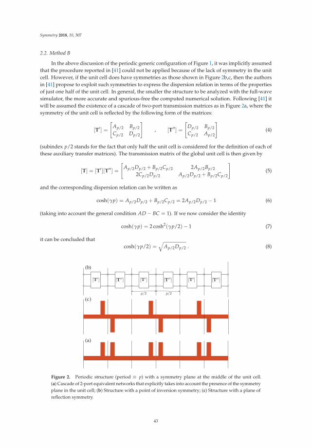
Symmetry 2018, 10, 307

2.2. Method B

In the above discussion of the periodic generic configuration of Figure 1, it was implicitly assumedthat the procedure reported in [41] could not be applied because of the lack of symmetry in the unitcell. However, if the unit cell does have symmetries as those shown in Figure 2b,c, then the authorsin [41] propose to exploit such symmetries to express the dispersion relation in terms of the propertiesof just one half of the unit cell. In general, the smaller the structure to be analyzed with the full-wavesimulator, the more accurate and spurious-free the computed numerical solution. Following [41] itwill be assumed the existence of a cascade of two-port transmission matrices as in Figure 2a, where thesymmetry of the unit cell is reflected by the following form of the matrices:

[T′] =[

Ap/2 Bp/2Cp/2 Dp/2

], [T′′] =

[Dp/2 Bp/2Cp/2 Ap/2

](4)

(subindex p/2 stands for the fact that only half the unit cell is considered for the definition of each ofthese auxiliary transfer matrices). The transmission matrix of the global unit cell is then given by

[T] = [T′][T′′] =[

Ap/2Dp/2 + Bp/2Cp/2 2Ap/2Bp/22Cp/2Dp/2 Ap/2Dp/2 + Bp/2Cp/2

](5)

and the corresponding dispersion relation can be written as

cosh(γp) = Ap/2Dp/2 + Bp/2Cp/2 = 2Ap/2Dp/2 − 1 (6)

(taking into account the general condition AD − BC = 1). If we now consider the identity

cosh(γp) = 2 cosh2(γp/2)− 1 (7)

it can be concluded thatcosh(γp/2) =

√Ap/2Dp/2 . (8)

(b)

(c)

(a)

Figure 2. Periodic structure (period ≡ p) with a symmetry plane at the middle of the unit cell.(a) Cascade of 2-port equivalent networks that explicitly takes into account the presence of the symmetryplane in the unit cell; (b) Structure with a point of inversion symmetry; (c) Structure with a plane ofreflection symmetry.

43

Symmetry 2018, 10, 307

This dispersion equation is exactly the same as the one given in ([41] Equation (6)) (note thatthe minimum period was denoted as 2p in [41] and p in this work). In principle we can compute theproduct Ap/2Dp/2 from the scattering parameters provided by the full-wave simulation of half theunit cell when considered isolated. However, if we proceed this way, all the higher-order interactionsbetween the two halves of the unit cell would be ignored. (The two-port transmission matrices [T′]and [T′′] should rather be considered again as “effective” transmission matrices, in the understandingthat the fundamental mode might not be the only one that contributes to the interaction between thetwo halves of the unit cell.)

Alternatively we could have proceeded in the manner reported in [41] by introducing a short/opencircuit in the structure in order to compute Ap/2Dp/2 in terms of the auxiliary impedances Zel and Zmag

defined in [41]. These are the input impedances of the one-port network obtained by substituting thesymmetry plane located at the center of the unit cell (see Figure 2) with a short circuit (Zel) or an opencircuit (Zmag). This procedure is found equivalent to starting with the whole unit cell and then applyingthe even/odd excitation technique [3,4]. As this method implies the setting of electric/magnetic wallsat the middle of the structure, both procedures are fully equivalent provided the actual existence ofa reflection symmetry plane in the structure that allows for the application of the even/odd excitationprocedure. As an example, this symmetry condition is satisfied for the geometry given in Figure 2cbut not for the one in Figure 2b. This equivalence, or lack of equivalence, could be irrelevant if itwere not for the fact that the presence of electric/magnetic walls in the full-wave simulation is whatactually ensures that the higher-order interaction between the two symmetric halves of the unit cell isappropriately taken into account. It is also apparent that the use of these magnetic/electric walls doesnot imply that the higher-order interaction between adjacent whole unit cells is taken into account,since only one unit cell is indeed analyzed with the full-wave simulator. Moreover, the placing ofa magnetic wall in the input port of the half unit cell imposed in [41] does not affect this discussion;actually this magnetic wall is not necessary when the input lumped port is taken at the middle of theunit cell [41] (this fact has repeatedly been checked by many numerical simulations carried out by theauthors of the present work). In brief, the technique reported in [41] can, in principle, be applied togeometries of the type shown in Figure 2b,c, but the application of that technique to the geometryin Figure 2b would only account for the electromagnetic interactions between the two halves of theunit cell as long as this interaction is carried out exclusively by the fundamental mode (in other words,the two stubs in each unit cell should be sufficiently far apart so as to ensure the absence of interactionsthrough high-order modes). It leads us to the somehow trivial finding that the higher-order interactionbetween adjacent cells can only be taken into account by simulating a cascade of multiple unit cells(as done in Method A) or, at most, by taking advantage of reflection symmetry planes (not inversionpoints, as it is the case shown in Figure 2b) to simulate half the cascade of unit cells terminated withelectric/magnetic walls. This result will be numerically studied and validated in next section.

A general conclusion drawn above was that only method A can properly account for high-orderinteractions between different unit cells, and thus method B should be restricted to those situationswhere this interaction can be neglected. However, a possible and convenient way to account forthe high-order interactions between adjacent cells, which takes advantage of the combination ofmethods A and B, is to apply method B to an extended cell of period P = 2p. In this case, the ABCDparameters in (8) would correspond just to the unit cell of period p, which because of the presence ofa reflection-symmetry wall in the middle of the extended cell (Ap = Dp) would lead to a dispersionequation completely equivalent to (3) if N had been set to 2 in method A. Certainly this combinedprocedure can be applied to cells of more extended periodicity with the purpose of accounting forinter-cell interactions with simulations that only involve half the number of cells.

Interestingly, the above discussion about symmetry in periodic structures turns out to be veryrelevant when dealing with the circuit modeling of structures with glide/twisted symmetry [44,45].This topic has recently surged due to some interesting application papers [46–49], where it isclearly shown that the behavior of periodic structures with glide symmetry is not equivalent

44

Symmetry 2018, 10, 307

to their counterpart without this feature, thus giving an apparent clue on the different roleplayed by the higher-order mode coupling when different types of symmetry are involved.Furthermore, this difference in coupling provided by the glide symmetry has been found to giveadvantageous features that can enhance the performance of many practical devices [46,48,49].According to our discussion above, the periodic structure with glide symmetry (whose unit cellincorporates a central inversion point) cannot rigorously be modeled by the analysis of just one of thetwo subcells of the unit cell (unlike periodic structures whose unit cell does have a reflection symmetryplane). Actually, the authors of [47] claim that their circuit model is valid provided that the upper andlower stubs in ([47], Figure 2c,d) do not overlap. Our premise here is that their proposed simplifiedcircuit modeling of the glide-symmetric structure is valid as long as the upper/lower position of thestubs is irrelevant; namely, when the higher-order coupling between the stubs is not very important.When both stubs overlap this possible difference in the higher-order coupling between upper/lowerposition is crucial, being less and less relevant as the distance between the stubs increases. In practice,as already reported in [50], there may be many practical situations where just the inclusion of the firsthigh-order mode suffices to obtain accurate results.

Also, the above discussion can be related to a very recent contribution in the circuit modelingof non-symmetrical reciprocal network [51]. Although that paper deals with non-periodic structures,its underlying rationale can easily be extended to the periodic case, in which the general conclusionsreached in [51] are found congruent with the discussions reported here.

3. Results

In this section the main issues discussed in previous sections will be numerically validated. First,the general advantage of using Method B will be pointed out when possible. Certainly MethodA will provide, in principle, more accurate results since it deals with a more realistic electromagneticscenario in which many of the couplings between different unit cells are taken into account. However,the unavoidable computational load implicit in the treatment of electrically large and complexstructures may lead to very long computational times and non-negligible levels of numerical noise.This last effect can become very relevant when dealing, for instance, with leaky-wave 1-D periodicconfigurations, where the eventual high radiation leakage in the structure can make the power in theoutput port several orders of magnitude smaller than in the input port. This numerical noise is alsovery relevant when computing the attenuation constant of below-cutoff and/or complex modes inclosed waveguiding system. A few selected examples will be discussed in the next subsections toclarify these points and provide some insights on the virtues and limitations of the proposed methods.

3.1. Periodic Printed Microstrip Lines

Our first case study in Figure 3 shows the comparison between the results of methods A and B fortwo printed microstrip lines periodically loaded with inductive/capacitive discontinuities. These lineswere previously studied in [38,52] and, in this example, HFSS commercial software [29] has been usedfor the required full-wave simulations. Both structures exhibit a band gap starting when its periodp equals half the line wavelength (λg/2) (as shown in [35,38]). Although not explicitly shown in thefigures, our results agree well with those reported in [38,52].

In Figure 3a the results for the dispersion diagram (both the phase, β, and the attenuation,α, constants) corresponding to method A have been computed using one cell (N = 1) and fivecells (N = 5). In this structure, the differences between the N = 1 and N = 5 cases are very small,clearly meaning that the inter-cell coupling is well accounted for by just the fundamental mode.The data corresponding to method B have been obtained by using the even-odd excitation procedureto study the unit cell (namely, just one of the two symmetric halves with electric/magnetic walls aresimulated). Certainly, the results using this procedure are found identical to the ones obtained by theprocedure proposed in ([41], Equation (12)) as well as to the “Method A N = 1” curve. The excellent

45

Symmetry 2018, 10, 307

agreement between the “Method B” curve and the results with N = 1 can be considered as a firstvalidation of the congruence of methods A and B in this circumstance.

6

7

8

9

10

11

12

13

14

0 0.2 0.4 0.6 0.8 1

Freq

(GH

z)

p/

p/

Method B Method A N=1 Method A N=5

wsp

xz

rw

(a)

10

12

14

16

18

20

22

24

26

0 0.2 0.4 0.6 0.8 1

Freq

(GH

z)

p/

p/

Method B Method A N=1 Method A N=3 Method A N=5

gp

xz

rw

(b)

Figure 3. Dispersion diagram of the periodic printed microstrip lines shown as insets. The substrateof the lines has thickness h and relative permittivity εr. (a) p = 5.6 mm, w = 0.6 mm, ws = 0.2 mm,εr = 10.2 and h = 0.635 mm; (b) p = 4 mm, w = 0.6 mm , g = 0.2 mm, εr = 10.2 and h = 0.767 mm.

In the structure analyzed in Figure 3b, previously studied in [52], the results provided by method Afor one, three, and five cells (denoted as N = 1, N = 3, and N = 5 respectively) are compared withthose obtained by method B, taking now an extended period of 2p (namely, the simulated subcellwith electric/magnetic walls has a length of p, and thus the obtained results are found to be identicalto the case “Method A N = 2”, although this fact is not explicitly shown in the figure since the twocorresponding curves would overlap). It is interesting to observe the appearance of slight discrepanciesbetween the results of method A when different number of cells are considered and, furthermore,that a clear convergence pattern is not observed in the analyzed frequency range. These facts are partlyattributable to the high values of the attenuation constant in the stopband (there appear values ofα/k0 > 1), which causes the results with a few cells to be affected by numerical noise due to the verylow level of power that reaches the output port (power along z is given by P(z) = P(0)e−2αz; that is,an attenuation of A(dB) = 8.69αz, which means A = 13.11N dB at 18 GHz, with N being the numberof cells in the structure). In this situation, the convenient convergence test to ensure the reliability ofthe results provided by method A cannot be carried out. Actually, although not explicitly shown inFigure 3b, the results with a higher number of cells are found to increasingly deteriorate.

46

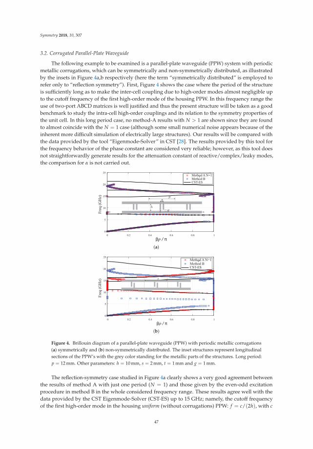
Symmetry 2018, 10, 307

3.2. Corrugated Parallel-Plate Waveguide

The following example to be examined is a parallel-plate waveguide (PPW) system with periodicmetallic corrugations, which can be symmetrically and non-symmetrically distributed, as illustratedby the insets in Figure 4a,b respectively (here the term “symmetrically distributed” is employed torefer only to “reflection symmetry”). First, Figure 4 shows the case where the period of the structureis sufficiently long as to make the inter-cell coupling due to high-order modes almost negligible upto the cutoff frequency of the first high-order mode of the housing PPW. In this frequency range theuse of two-port ABCD matrices is well justified and thus the present structure will be taken as a goodbenchmark to study the intra-cell high-order couplings and its relation to the symmetry properties ofthe unit cell. In this long period case, no method-A results with N > 1 are shown since they are foundto almost coincide with the N = 1 case (although some small numerical noise appears because of theinherent more difficult simulation of electrically large structures). Our results will be compared withthe data provided by the tool “Eigenmode-Solver” in CST [28]. The results provided by this tool forthe frequency behavior of the phase constant are considered very reliable; however, as this tool doesnot straightforwardly generate results for the attenuation constant of reactive/complex/leaky modes,the comparison for α is not carried out.

0

5

10

15

20

25

0 0.2 0.4 0.6 0.8 1

Freq

(GH

z)

p /

Method A N=1pMethod BCST-ES

(a)

0

5

10

15

20

25

0 0.2 0.4 0.6 0.8 1

Freq

(GH

z)

p /

Method A N=1pMethod BCST-ES

(b)

Figure 4. Brillouin diagram of a parallel-plate waveguide (PPW) with periodic metallic corrugations(a) symmetrically and (b) non-symmetrically distributed. The inset structures represent longitudinalsections of the PPW’s with the grey color standing for the metallic parts of the structures. Long period:p = 12 mm. Other parameters: h = 10 mm, s = 2 mm, t = 1 mm and g = 1 mm.

The reflection-symmetry case studied in Figure 4a clearly shows a very good agreement betweenthe results of method A with just one period (N = 1) and those given by the even-odd excitationprocedure in method B in the whole considered frequency range. These results agree well with thedata provided by the CST Eigenmode-Solver (CST-ES) up to 15 GHz; namely, the cutoff frequencyof the first high-order mode in the housing uniform (without corrugations) PPW: f = c/(2h), with c

47

Symmetry 2018, 10, 307

being the vacuum speed of light and h the height of the uniform PPW. As expected, discrepancies startto appear beyond this frequency, when the presence of this second propagative mode in the uniformsections of the PPW makes that the cascade of two-port ABCD matrices cannot properly accountfor the unavoidable multi-mode inter-cell coupling that will appear. It should be highlighted that,for frequencies where the regime is no longer monomode in the non-corrugated PPW, the cascadeof single two-port transfer matrices is not presumed to work satisfactorily because of the propagativemulti-mode nature of the guiding field rather than for possible neglected effects of high-order evanescentmodes. Thus, beyond this monomode band, neither method A nor method B are expected to provideaccurate results.

Let us now consider the inversion-symmetry structure shown in the inset of Figure 4b.The structure exhibits an inversion point at the center of the unit cell, circumstance that will haveinteresting consequences for a particular choice of the period, as it will be discussed later. The curvesin Figure 4b show again a good agreement within the monomode band between the results of method Aand those provided by the CST-ES. However, the data given by method B, which here completelyignores the inversion-symmetry nature of the unit cell, are in full disagreement with the above twoset of results. It clearly proves that method B, as expected, drastically fails when high-order couplingbetween the two subcells forming the inversion-symmetry unit cell is significant and not properlyincorporated to the model. This fact seems to be in contrast with the thesis apparently sustained in [41].Of course, the method would properly work if the subcells only interact through the fundamentalpropagating mode, as it would be the case for relatively large separation between the stubs. In thislatter case the structures with mirror symmetry and with inversion symmetry would have the sameresponse.

Next, the short-period case is studied in Figure 5, where it is again shown the cases correspondingto the presence or absence of a reflection symmetry plane at the middle of the unit cell. In both cases itis now included the data for “Method A N = 5” since high-order inter-cell coupling is expected whenthe pair of corrugations of each unit cell is electrically close to adjacent ones. Figure 5a shows thesymmetrically-distributed case and, again, a perfect agreement is found between “Method A N = 1” and“Method B”. These methods also show a good agreement with the “CST-ES” data in the first passbandup to 5 GHz where p/λ0 � 1/10. For higher frequencies, the inter-cell couplings cannot be wellaccounted for by the cascade of two-port ABCD matrices and, therefore, the methods are not expectedto give accurate quantitative results (although they still provide a good qualitative picture of the banddiagram of the structure). The data corresponding to “Method A N = 5” shows a significantly betteragreement with the “CST-ES” curve in the whole first passband, although important discrepanciesappear in the stopband due to the expected numerical noise caused by the strong attenuation inthis band. There is neither a good agreement in the second passband because of the multi-modenature of the band at higher frequencies. Due to the unreliability of these “Method A N = 5” dataoutside the first passband, they are not shown in the figure. Regarding the inversion-symmetrycase in Figure 5b, the first relevant feature is the complete lack of agreement between the results of“Method A N = 1” and “Method B” even at very low frequencies, which clearly highlights the needof appropriately considering the multi-mode interactions that appear here between the two halvesof the unit cell. Since the first passband in this case appears below 5 GHz, a very good agreement isnow found between the “Method A N = 1” and “CST-ES”. For higher frequencies there is not such agood quantitative agreement, although the qualitative behavior is approximately captured until theonset of the multi-mode propagation regime. In this inversion-symmetry case, the “Method A N = 5”curve does show a good quantitative agreement within the entire single-band regime, agreement thatextends up to the onset of the multi-mode regime. An interesting feature of this structure is thewidening of the second bandpass of negative-group velocity nature [53], which now extends from 8 to13 GHz approximately.

48

Symmetry 2018, 10, 307

0

5

10

15

20

0 0.2 0.4 0.6 0.8 1

Freq

(GH

z)

p /

Method A N=1Method A N=5Method BCST-ES

(a)

0

5

10

15

20

0 0.2 0.4 0.6 0.8 1

Freq

(GH

z)

p /

Method A N=1

Method BCST-ES

Method A N=5

(b)

Figure 5. Brillouin diagram of a parallel-plate waveguide with periodic metallic corrugations(a) symmetrically and (b) non-symmetrically distributed. Short period: p = 6 mm. Other parameters:h = 10 mm, s = 2 mm, t = 1 mm and g = 1 mm.

An interesting further step in the study of corrugated PPWs is the case presented in Figure 6,where the period of the structure is taken as twice the distance between the corrugations [47]. Actually,for the symmetrically-distributed corrugation case shown in Figure 6a, the true period of the structureis now p = s, although the dispersion relation will be plotted for an “extended” period p = 2s forthe sake of comparison with the inversion-symmetry case in Figure 6b [the true period of which isp = 2s]. The CST-EC curve in Figure 6a shows a first passband that now extends up to about 8 GHz;interestingly, the onset of the second bandstop in Figure 5a. Actually, it is found that the first stopbandin this structure disappears as the distance between corrugations approaches the true period of thestructure (p → s). In this figure it is also observed that the “Method A N = 2” gives sufficientlyaccurate quantitative results in this first passband but drastically fails for higher frequencies (in thesecalculations, a structure with two unit cells, p = 2s, has been taken). The curve corresponding to“Method A N = 10” only improves the agreement with CST-ES in the first passband but also fails forhigher frequencies (the data are not shown). In this case, the expected relevant inter-cell propagativeand evanescent high-order coupling would make it necessary either the use of a multi-port approach orthe solution of the corresponding non-linear eigenvalue problem to compute the complex propagationconstant of the structure. The case considered in Figure 6b is an example of a structure having glidesymmetry [46–49]. The curves of Figure 6b show, similarly to the previous inversion-symmetry unit-cellcases, a great disagreement between the results of Method A (N = 1) and Method B. Rather interestingis the comparison of the “Method A N = 5” and “CST-ES” curves. Now there appears a good agreementbetween both curves even for frequencies beyond 15 GHz. This good agreement outside the monobandregime is attributed to the fact that the first high-order mode of the housing PPW is not expectedto be highly excited in the glide-symmetric structure. The existence of electrically-close periodicinversion points in this structure would presumably reduce the excitation level of modes with an even

49

Symmetry 2018, 10, 307

profile along the vertical direction. Apart from this reasonable good agreement in the quantitativeresults shown by both curves, they show that the passband of this structure has grown considerably,now extending up to 13.8 GHz. This surprising fact, already reported in [46–49], is one of the mostrelevant features of glide-symmetric structures and is likely to find more and more applications in thefuture (a similar widening of a stopband can also be found in other type of glide-symmetric structures).

0

5

10

15

20

0 0.2 0.4 0.6 0.8 1

Freq

(GH

z)

p /


2

(a)

0

5

10

15

20

0 0.2 0.4 0.6 0.8 1

Freq

(GH

z)

p /


(b)

Figure 6. Brillouin diagram of a parallel-plate waveguide with periodic metallic corrugations(a) symmetrically [p = 2p = 4 mm] and (b) glide-symmetrically distributed [p = 4 mm].Other parameters: h = 10 mm, s = 2 mm, t = 1 mm and g = 1 mm.

4. Conclusions

In this work we have presented a thorough discussion on the pros and cons of computing thedispersion relation of 1-D periodic guiding/radiating structures by means of a combined methodthat makes use of full-wave simulations data obtained from commercial software tools along witha simplifying equivalent-network model. This method can take advantage of both the high flexibilityof simulators to deal with general structures and the further analytical treatment of the data providedby the employed simplified electromagnetic model of the problem as a cascade of two-port equivalentnetworks.

Some general conclusions that have been discussed in this work are summarized below:

• The most general and reliable method to compute the dispersion diagram of periodic structuresis the solution of Maxwell’s equations in the unit cell of the structure subject to periodicboundary conditions. The major disadvantage of this eigenvalue approach is that it involves thesearching for complex zeros, a task that is not easily systematized in the form of general-purposecomputer codes.

• The so-called Methods A and B in Section 2 are alternative combined approaches that avoid thesearching of complex zeros. If the unit cell of the periodic structure has a reflection-symmetry

50

Symmetry 2018, 10, 307

plane, then a further combination of these two methods is proposed as a very convenient andefficient tool.

• Due to the simplification implicit in the modeling of the periodic structure as a cascade of two-portequivalent networks, the possible excitation of high-order propagative modes in the uniformsections of the housing structure will restrict the application of this technique to the so-calledmonoband regime.

• The combined technique would need to deal with structures with many unit cells in order to takeinto account the possible inter-cell coupling due to high-order evanescent modes. When inter-cellcoupling due to either propagative or evanescent high-order modes can be neglected, this methodis always expected to work properly.

• In contrast with the above fact, some authors have claimed that the convenient treatment ofjust one unit cell would suffice if a proper even-odd periodic excitation technique is applied.In this work it is discussed that this methodology can be used reliably only when there isa reflection-symmetry plane in the unit cell or the interaction between the two halves of the unitcell is carried out by only the fundamental mode.

• Finally, it has also been discussed that glide-symmetric structures, whose interesting propertieshave recently been the object of intensive study, will require the modeling of the unitcell as a multi-port equivalent network or the solution of the corresponding rigorouseigenvalue problem.

Author Contributions: The contributions of all of the authors were the same. All of them have worked togetherto develop the present manuscript.

Funding: This research was funded by [the Spanish Ministerio de Ciencia, Innovación y Universidades withEuropean Union FEDER funds] grant number [TEC2017-84724-P].

Acknowledgments: The authors would like to express their gratitude to Alejandro Martínez-Ros for hiscontribution in the first steps of the present work.


Abbreviations

The following abbreviations are used in this manuscript:

CST Computer Simulation TechnologyFSS Frequency Selective Surface(s)HFSS High Frequency Structure SimulatorPPW Parallel Plate Waveguide

References

1. Montgomery, C.G.; Dicke, R.H.; Purcell, E.M. Principles of Microwave Circuits; MIT Radiation Laboratory Series;McGraw-Hill: New York, NY, USA, 1948; Volume 8.

2. Marcuvitz, N. Waveguide Handbook; MIT Radiation Laboratory Series; McGraw-Hill: New York, NY, USA,1951; Volume 10.

3. Collin, R. Field Theory of Guided Waves; McGraw Hill: New York, NY, USA, 1960.4. Pozar, D.M. Microwave Engineering, 3rd ed.; Wiley: Hoboken, NJ, USA, 2005.5. Cameron, R.J.; Kudsia, C.M.; Mansour, R.R. Microwave Filters for Communication Systems; Wiley: Hoboken, NJ,

USA, 2007.6. Eleftheriades, G.V.; Balmain, K.G. Negative-Refraction Metamaterials: Fundamental Properties and Applications;

Wiley: Hoboken, NJ, USA, 2005.7. Martín, F. Artificial Transmission Lines for RF and Microwave Applications; Wiley: Hoboken, NJ, USA, 2015.8. Jackson, D.R.; Oliner, A.A. Leaky-wave antennas. In Modern Antenna Handbook; John Wiley and Sons:

Hoboken, NJ, USA, 2007; Chapter 7, pp. 325–367.9. Munk, B. Frequency Selective Surfaces: Theory and Design; John Wiley and Sons: Hoboken, NJ, USA, 2000.10. Huang, J.; Encinar, J.A. Reflectarray antennas; Wiley, Inter Science: Hoboken, NJ, USA, 2007.

51

Symmetry 2018, 10, 307

11. Gagnon, N.; Petosa, A.; McNamara, D.A. Research and development on phase-shifting surfaces (PSSs).IEEE Antennas Propag. Mag. 2013, 55, 29–48. [CrossRef]

12. Martini, E.; Maci, S. Metasurface Transformation Theory. In Transformation Electromagnetics and Metamaterials;Springer: London, UK, 2014; pp. 83–116.

13. Kurokawa, K. An Introduction to the Theory of Microwave Circuits; Academic Press: San Francisco, CA,USA, 1969.

14. Varela, J.E.; Esteban, J. Characterization of waveguides with a combination of conductor and periodicboundary contours: Application to the analysis of bi-periodic structures. IEEE Trans. Microw. Theory Tech.2012, 60, 419–430. [CrossRef]

15. Rodríguez-Berral, R.; Mesa, F.; Medina, F. Analytical multimodal network approach for 2-D arrays of planarpatches/apertures embedded in a layered medium. IEEE Trans. Antennas Propag. 2015, 63, 1969–1984.[CrossRef]

16. Mesa, F.; Rodríguez-Berral, R.; Medina, F. Unlocking complexity with ECA. IEEE Microw. Mag. 2018, 19,44–65. [CrossRef]

17. Hong, J.S. Microstrip Filters for RF/Microwave Applications, 2nd ed.; Wiley: Hoboken, NJ, USA, 2011.18. Feng, X.; Ke, W. Guided-wave and leakage characteristics of substrate integrated waveguide. IEEE Trans.

Microw. Theory Tech. 2005, 33, 66–73. [CrossRef]19. Bozzi, M.; Pasian, M.; Perregrini, L.; Wu, K. On the losses in substrate integrated waveguides and cavities.

Int. J. Microw. Wirel. Technol. 2009, 1, 395–401. [CrossRef]20. Rubio, J.; Gómez-García, A.; Gómez-Alcalá, R.; Campos-Roca, Y.; Zapata, J. Overall formulation for multilayer

SIW circuits based on addition theorems and the generalized scattering matrix. IEEE Microw. Wirel.Compon. Lett. 2018, 28, 485–487. [CrossRef]

21. Collin, R.E.; Zucker, F.J.; (Eds) Antenna Theory; McGraw-Hill: New York, NY, USA, 1969.22. Peterson, A.F.; Ray, S.L.; Mittra, R. Computational Methods for Electromagnetics; IEEE Press: New York,

NY, USA, 1998.23. Dudley, D.G. Mathematical Foundations for Electromagnetic Theory; IEEE Press: New York, NY, USA, 1994.24. Felsen, L.B.; Marcuvitz, N. Radiation and Scattering of Waves; Prentice-Hall: Upper Saddle River, NJ, USA, 1973.25. Rodríguez-Berral, R.; Mesa, F.; Medina, F. Systematic and efficient root finder for computing the modal

spectrum of planar layered waveguides. Int. J. RF Microw. Comput. Eng. 2004, 14, 73–83. [CrossRef]26. Kowalczyk, P. Complex Root Finding Algorithm Based on Delaunay Triangulation. ACM Trans. Math. Softw.

2015, 41, 19. [CrossRef]27. Zouros, G.P. CCOMP: An efficient algorithm for complex roots computation of determinantal equations.

Comput. Phys. Commun. 2018, 222, 339–350. [CrossRef]28. CST Microwave Studio. 2017. Available online: https://www.cst.com/products/cstmws (accessed on

July 2018).29. ANSYS High Frequency Structure Simulator (HFSS). Available online: https://www.ansys.com/products/

electronics/ansys-hfss (accessed on July 2018).30. Sampath, M.K. On addressing the practical issues in the extraction of RLGC parameters for lossy

multiconductor transmission lines using S-parameter models. In Proceedings of the Electrical Performance ofElectronic Packaging (EPEP), San Jose, CA, USA, 27–29 October 2008; pp. 259–262.

31. Apaydin, N.; Zhang, L.; Sertel, K.; Volakis, J.L. Experimental validation of frozen modes guided on printedcoupled transmission lines. IEEE Trans. Microw. Theory Tech. 2012, 60, 1513–1519. [CrossRef]

32. Liu, Z.; Zhu, L.; Wu, Q.; Xiao, G. A short-open calibration (SOC) technique to calculate the propagationcharacteristics of substrate integrated waveguide. In Proceedings of the 2015 IEEE MTT-S InternationalMicrowave Workshop Series on Advanced Materials and Processes for RF and THz Applications, IEEE MTT-SIMWS-AMP, Suzhou, China, 1–3 July 2015.

33. Conciauro, G.; Guglielmi, M.; Sorrentino, R. Advanced Modal Analysis; Wiley: Hoboken, NJ, USA, 1999.34. Esteban, J.; Rebollar, J.M. Characterization of corrugated waveguides by modal analysis. IEEE Trans. Microw.

Theory Tech. 1991, 39, 937–943. [CrossRef]35. Baccarelli, P.; Di Nallo, C.; Paulotto, S.; Jackson, D.R. A full-wave numerical approach for modal analysis of

1D periodic microstrip structures. IEEE Trans. Microw. Theory Tech. 2006, 54, 1350–1362. [CrossRef]

52

Symmetry 2018, 10, 307

36. Paulotto, S.; Baccarelli, P.; Frezza, F.; Jackson, D.R. Full-Wave modal dispersion analysis and broadsideoptimization for a class of microstrip CRLH leaky-wave antennas. IEEE Trans. Microw. Theory Tech. 2008, 56,2826–2837. [CrossRef]

37. Mao, S.G.; Chen, M.Y. Propagation characteristics of finite-width conductor-backed coplanar waveguideswith periodic electromagnetic bandgap cells. IEEE Trans. Microw. Theory Tech. 2002, 50, 2624–2628.

38. Zhu, L. Guided-wave characteristics of periodic microstrip lines with inductive loading: Slow-wave andbandstop behaviors. Microw. Opt. Technol. Lett. 2004, 41, 77–79. [CrossRef]

39. Valerio, G.; Paulotto, S.; Baccarelli, P.; Burghignoli, P.; Galli, A. Accurate Bloch analysis of 1-D periodic linesthrough the simulation of truncated structures. IEEE Trans. Antennas Propag. 2011, 59, 2188–2195. [CrossRef]

40. Martínez-Ros, A.J.; Mesa, F. A study on the dispersion relation of periodic structures using commercialsimulators. In Proceedings of the 2017 Computing and Electromagnetics International Workshop (CEM),Barcelona, Spain, 21–24 June 2017; pp. 15–16.

41. Eberspacher, M.A.; Eibert, T.F. Dispersion analysis of complex periodic structures by full-wave solution ofeven-odd-mode excitation problems for single unit cells. IEEE Trans. Antennas Propag. 2013, 61, 6075–6083.[CrossRef]

42. Monni, S.; Gerini, G.; Neto, A.; Tijhuis, A.G. Multi-mode equivalent networks for the design and analysis offrequency selective surfaces. IEEE Trans. Antennas Propag. 2007, 55, 2824–2835. [CrossRef]

43. Kaipa, C.S.R.; Yakovlev, A.B.; Medina, F.; Mesa, F. Transmission through stacked 2-D periodic distributions ofsquare conducting patches. J. Appl. Phys. 2012, 112, 033101. [CrossRef]

44. Hessel, A.; Oliner, A.A.; Chen, M.; Li, R. Propagation in periodically loaded waveguides with highersymmetries. Proc. IEEE 1973, 61, 183–195. [CrossRef]

45. Amari, S.; Vahldieck, R.; Bornemann, J. Accurate analysis of periodic structures with an additional symmetryin the unit cell from classical matrix eigenvalues. IEEE Trans. Microw. Theory Tech. 1998, 46, 1513–1515.[CrossRef]

46. Quevedo-Teruel, O.; Ebrahimpouri, M.; Kehn, M.N.M. Ultra-wideband metasurface lenses based onoff-shifted opposite layers. IEEE Antennas Wirel. Propag. Lett. 2016, 15, 484–487. [CrossRef]

47. Valerio, G.; Sipus, Z.; Grbic, A.; Quevedo-Teruel, O. Accurate equivalent-circuit descriptions of thinglide-symmetric corrugated metasurfaces. IEEE Trans. Antennas Propag. 2017, 65, 2695–2700. [CrossRef]

48. Dahlberg, O.; Mitchell-Thomas, R.; Quevedo-Teruel, O. Reducing the dispersion of periodic structures withtwist and polar glide symmetries. Sci. Rep. 2017, 7, 10136. [CrossRef] [PubMed]

49. Ebrahimpouri, M.; Rajo-Iglesias, E.; Sipus, Z.; Quevedo-Teruel, O. Cost-Effective gap waveguide technologybased on glide-symmetric holey EBG structures. IEEE Trans. Microw. Theory Tech. 2018, 6, 927–934. [CrossRef]

50. Naqui, J.; Duran-Sindreu, M.; Fernandez-Prieto, A.; Mesa, F.; Medina, F.; Martin, F. Multimode propagationand complex waves in CSRR-based transmission-line metamaterials. IEEE Antennas Wirel. Propag. Lett. 2012,11, 1024–1027. [CrossRef]

51. Abdo-Sanchez, E.; Camacho-Peñalosa, C.; Martin-Guerrero, T.; Esteban, J. Equivalent circuits fornon-symmetric reciprocal two-ports based on eigen-state formulation. IEEE Trans. Microw. Theory Tech.2017, 65, 4812–4822. [CrossRef]

52. Rodriguez-Berral, R.; Mesa, F.; Baccarelli, P.; Burghignoli, P. Excitation of a periodic microstrip line byan aperiodic delta-gap source. IEEE Antennas Wirel. Propag. Lett. 2009, 8, 641–644. [CrossRef]

53. Hwang, R. Negative group velocity and anomalous transmission in a one-dimensionally periodic waveguide.IEEE Trans. Antennas Propag. 2006, 54, 755–760. [CrossRef]


53

symmetryS S

Article

On the Electric-Magnetic Duality Symmetry:Quantum Anomaly, Optical Helicity,and Particle Creation

Iván Agulló 1, Adrián del Río 2 and José Navarro-Salas 3,*

1 Department of Physics and Astronomy, Louisiana State University, Baton Rouge, LA 70803-4001, USA;[email protected]

2 Centro de Astrofísica e Gravitacâo—CENTRA, Departamento de Física, Instituto Superior Técnico—IST,Universidade de Lisboa, 1049 Lisboa, Portugal; [email protected]

3 Departamento de Física Teórica and IFIC, Centro Mixto Universidad de Valencia-CSIC, Facultad de Física,Universidad de Valencia, 46100 Burjassot, Valencia, Spain


Received: 14 November 2018; Accepted: 13 December 2018; Published: 17 December 2018

Abstract: It is well known that not every symmetry of a classical field theory is also a symmetryof its quantum version. When this occurs, we speak of quantum anomalies. The existence ofanomalies imply that some classical Noether charges are no longer conserved in the quantumtheory. In this paper, we discuss a new example for quantum electromagnetic fields propagatingin the presence of gravity. We argue that the symmetry under electric-magnetic duality rotationsof the source-free Maxwell action is anomalous in curved spacetimes. The classical Noether chargeassociated with these transformations accounts for the net circular polarization or the optical helicityof the electromagnetic field. Therefore, our results describe the way the spacetime curvature changesthe helicity of photons and opens the possibility of extracting information from strong gravitationalfields through the observation of the polarization of photons. We also argue that the physicalconsequences of this anomaly can be understood in terms of the asymmetric quantum creation ofphotons by the gravitational field.

Keywords: electric-magnetic duality symmetry; quantum anomalies; optical helicity; electromagneticpolarization; particle creation

1. Introduction

Symmetries are at the core of well-established physical theories, and they keep playing a centralrole in the mainstream of current research. Fundamental Lagrangians in physics are founded onsymmetry principles. Moreover, symmetries are linked, via Noether’s theorem, to conservations laws.Well-known examples are the energy and momentum conservation and its relation with the invarianceunder space–time translations, as well as the conservation of the net fermion number (the differencein the number of fermions and anti-fermions that is proportional to the net electric charge) in Dirac’srelativistic theory, which result from the global phase invariance of the action.

When the symmetries of free theories are also preserved by interactions, the conservation laws aremaintained, and they can be used to understand patterns in diverse physical phenomena. In quantumelectrodynamics, for instance, the phase invariance is preserved by the coupling of the Dirac and theelectromagnetic field, and this ensures the conservation of the net fermion number in all physicalprocesses [1]. Another illustrative example is the gravitationally induced creation of particles, eitherbosons or fermions, in an expanding homogenous universe [2–5]. This particle creation occurs inpairs, and the symmetry of the background under space-like translations ensures that, if one particle is


Symmetry 2018, 10, 763

created with wavenumber�k, its partner has wavenumber −�k. As a consequence, there is no creation ofnet momentum, as expected on symmetry grounds. In a similar way, phase invariance implies that thegravitational field cannot create a net fermion number in an expanding universe.

However, in special cases, the implications of classical symmetries do not extend to quantumtheory, and the classical charge conservation breaks down. This was first noticed by studying masslessfermions coupled to an electromagnetic field [6,7]. A massless fermion is called a (Weyl) left-handedfermion if it has helicity h = −1/2, and a right-handed fermion if h = +1/2 (A left-handed(right-handed) anti-fermion has helicity h = +1/2 (−1/2)). Recall that the equations of motionfor the two sectors decouple in the massless limit, and this allows one to write a theory for masslessfermions that involves only one of the two helicities, something that is not possible for non-zero mass.The action of this theory also enjoys phase invariance, so the number of left-handed and right-handedfermions is separately conserved. This is to say, in the classical theory, there are two independentNoether currents, jμ

L and jμR, associated with left- and right-handed massless fermions, respectively,that satisfy continuity equations ∂μ jμL = 0 and ∂μ jμR = 0. Rather than using jμL and jμR, it is morecommon to re-write these conservation laws in terms of the so-called vector and axial currents, definedby their sum and difference, respectively, jμ = jμR + jμL = ψγμψ and jμ5 = jμR − jμ

L = ψγμγ5ψ, where ψ

is the four-component Dirac spinor, that encapsulates both left- and right-handed (Weyl) fermions,and γμ, γ5 are the Dirac matrices.

What is the situation in quantum theory? It turns out that the conservation law for jμ holds alsoquantum mechanically, so the quantum number NR + NL (associated with the net fermion number,i.e., the electric charge) is preserved in any physical process. For instance, in the presence of atime-dependent electromagnetic background, charged fermions and antifermions are spontaneouslycreated (this is the electromagnetic analog of the gravitationally induced particle creation mentionedabove [8–10]), but in such a way that the total fermion number (or electric charge) does not change.This is because the number of created right- or left-handed antifermions equals the number of left- orright-handed fermions:

NR + NL = (#R1/2 − #R

−1/2) + (#L−1/2 − #L

1/2) = 0 . (1)

However, it turns out that the difference in the created number of right-handed and left-handedfermions is not identically zero. This means that it is possible to create a net amount of helicity:

NR − NL = (#R1/2 − #R

−1/2)− (#L−1/2 − #L

1/2) = [#1/2 − #−1/2] . (2)

The simplest scenario where this is possible is for a constant magnetic field, say, in the third spatialdirection �B = (0, 0, B), together with a pulse of electric field parallel to it, �E = (0, 0, E(t)). One canshow that, in this situation, the net creation of helicity per unit volume V is given by (see [1] for a proofinvolving an adiabatic electric pulse)

Δ(NR − NL)

V= − q2

2π2

∫ t2

t1

dt �E · �B , (3)

where q is the electric charge of the fermion, and the fermionic field is assumed to start in the vacuumstate at early times before the electric field is switched on. Hence, if the integral

∫ t2t1

dt �E · �B isdifferent from zero, particles with different helicities are created in different amounts. In contrast,NR + NL remains strictly constant. For an arbitrary electromagnetic background, the previous resultgeneralizes to

Δ(NR − NL) = − q2

2π2

∫ t2

t1

dt∫

d3x �E · �B . (4)

56

Symmetry 2018, 10, 763

The key point is that Equation (4) is equivalent to the quantum-mechanical symmetry breaking ofthe fermion chiral symmetry: ψ → ψ′ = e−iεγ5

ψ, as expressed in the anomalous non-conservation ofthe current [6,7].

∂μ〈jμ5 〉 = − q2h8π2 Fμν

∗Fμν (5)

where Fμν is the electromagnetic field strength, ∗Fμν ≡ 12 εμναβFαβ its dual, and the presence of h makes

manifest that this is a quantum effect. Equations (5) and (4) are connected by the standard relationbetween a current and the charge associated with it:

∫d3x〈j05〉 = h(NR − NL).

The discovery of the chiral anomaly of Equation (5) was not arrived at by computing thenumber of fermions created, but rather by directly computing the quantity ∂μ〈jμ

5 〉. In that calculation,the anomaly arises from the renormalization subtractions needed to calculate the expectation value〈jμ5 〉. The operator jμ

5 is non-linear (quadratic) in the fermion field, and in quantum field theoryexpectation values of non-linear operators are plagued with ultraviolet divergences. One mustuse renormalization techniques to extract the physical, finite result. A detailed study shows thatrenormalization methods that respect the gauge invariance of the electromagnetic background breakthe fermionic chiral symmetry of the classical theory. The fact that Expression (5) was able to accuratelyexplain the decay ratio of processes that could not be understood otherwise, like the decay of theneutral pion to two photons, was an important milestone in the quantum field theory and the studyof anomalies.

A similar anomaly appears when the electromagnetic background is replaced by a gravitationalfield [11]. In this case, renormalization methods that respect general covariance give rise to a violationof the classical conservation law ∇μ jμ

5 = 0, which becomes

∇μ〈jμ5 〉 = − h192π2 Rμναβ

∗Rμναβ (6)

where Rμναβ is the Riemann tensor and ∗Rμναβ its dual, and ∇μ is the covariant derivative.For gravitational fields for which a particle interpretation is available at early and late times, this chiralanomaly also manifests in the net helicity contained in the fermionic particles created duringthe evolution:

Δ(NR − NL) = − 1192π2

∫ t2

t1

∫Σ

d4x√−g Rμναβ

∗Rμναβ . (7)

Typical configurations where this integral is non-zero are the gravitational collapse of a neutronstar, or the merger of two compact objects as the ones recently observed by the LIGO-Virgocollaboration [12,13].

In contrast to the anomaly of Equation (5) induced by an electromagnetic background, the chiralanomaly induced by gravity affects every sort of massless spin-1/2 fields, either charged or neutral.This is a consequence of the universal character of gravity, encoded in the equivalence principle,that guarantees that, if Equation (6) is valid for a type of massless spin-1/2 field, it must also be validfor any other type.

There is no reason to believe, however, that these anomalies are specific to spin 1/2 fermions,and one could in principle expect that a similar effect will arise for other types of fields that classicallyadmit chiral-type symmetries. This is the case of photons. One then expects that photons propagatingin the presence of a gravitational field will not preserve their net helicity, or, in the language of particles,that the gravitational field will created photons with different helicities in unequal amounts, in the sameway it happens for fermions (one also expects a similar effect for gravitons). For photons, the analogof the classical chiral symmetry of fermions is given by electric-magnetic duality rotations [14]

�E′ = cos θ �E + sin θ �B�B′ = cos θ �B − sin θ �E . (8)

57

Symmetry 2018, 10, 763

As first proved in [15], these transformations leave the action of electrodynamics invariant ifsources (charges and currents) are not present, and the associated Noether charge is precisely thedifference between the intensity of the right- and left-handed circularly polarized electromagneticwaves, i.e., the net helicity. This symmetry is exact in the classical theory even in the presence ofan arbitrary gravitational background, as pointed out some years later in [16]. However, in exactanalogy with the fermionic case, quantum effects can break this symmetry of the action and inducean anomaly [17,18]. In the language of particles, this would imply that the difference in the numberof photons with helicities h = ±1, NR − NL, is not necessarily conserved in curved spacetimes.The analogy with the fermionic case also suggests that the current jμD associated with the symmetryunder duality rotations of the classical theory fails to be conserved quantum mechanically, with anon-conservation law of the type

∇μ〈jμD〉 = α hRμναβ

∗Rμναβ . (9)

where α is a numerical coefficient to be determined. In a recent work [18,19], we have proved thatthis is in fact the case, and obtained that α is different from zero and given by α = − 1

96π2 . In thispaper, we will provide a general overview of these results from a different perspective, and with moreemphasis on conceptual aspects.

2. Electric-Magnetic Duality Rotations and Self- and Anti Self-Dual Fields

To study electric-magnetic rotations of Equation (8), it is more convenient to change variables tothe self- and anti-self-dual components of the electromagnetic field, defined by �H± ≡ 1√

2(�E ± i �B),

since for them the transformation of Equation (8) takes a diagonal form:

�H′± = e∓ iθ �H± . (10)

A discrete duality transformation ��E = �B, ��B = −�E corresponds to θ = π/2. Then, the operatori� produces i � �H± = ± �H±. It is for this reason that �H+ and �H− are called the self- and anti-self-dualcomponents of the electromagnetic field, respectively.

There are other aspects that support the convenience of these variables. For instance, under aLorentz transformation, the components of �E and �B mix with each other. Indeed, under an infinitesimalLorentz transformation of rapidity�η , the electric and magnetic fields transform as �E′ = �E−�η ∧ �B,�B′ =�B +�η ∧ �E. (We recall that the rapidity �η completely characterizes a Lorentz boost: its modulus containsthe information of the Lorentz factor γ, via cosh |�η| = γ, and its direction indicates the direction of theboost). However, when �E and �B are combined into �H±, it is easy to see that the components of �H+ and�H− no longer mix:

�H′± = �H± ± i�η ∧ �H± . (11)

Note also that, under an ordinary infinitesimal (counterclockwise) rotation of angle α > 0 aroundthe direction of a unit vector �n, the complex vectors �H± transform as �H′± = �H± + α�n ∧ �H±. Hence,a boost corresponds to a rotation of an imaginary angle. These are the transformation rules associatedwith the two irreducible representations of the Lorentz group for fields of spin s = 1. In the standardterminology [20,21], they correspond to the (0, 1) representation for �H+, and the (1, 0) one for �H−.More generally, for any element of the restricted Lorentz group SO+(1, 3) (rotations + boots), the abovecomplex fields transform as

�H′± = e−i(α�n ±i�η)·�J �H± (12)

where �J are the infinitesimal generators of the group of rotations. The ± sign in the aboveequation distinguishes the two inequivalent (three-dimensional) representations of the Lorentz group.They are, however, equivalent under the subgroup of rotations. This makes transparent the fact thatelectrodynamics describes fields of spin s = 1, something that is more obscure when working with �Eand �B, the field strength Fμν, or even the vector potential Aμ.

58

Symmetry 2018, 10, 763

Another useful aspect of self- and anti-self-dual variables concerns the equations of motion.The source-free Maxwell equations

�∇ · �E = 0 , �∇ · �B = 0�∇× �E = −∂t �B , �∇× �B = ∂t �E (13)

when written in terms of �H±, take the form

�∇ · �H± = 0 , �∇× �H± = ±i ∂t �H± . (14)

Notice that, in contrast to �E and �B, the self- and anti-self-dual fields are not coupled by thedynamics. The general solution to these field equations is a linear combination of positive and negativefrequency plane waves

�H±(t,�x) =∫ d3k

(2π)3

[h±(�k) e−i(k t−�k·�x) + h∗∓(�k) ei(k t−�k·�x)

]ε±(�k) (15)

where k = |�k| and h±(�k) are complex numbers that quantify the wave amplitudes. The polarizationvectors are given by ε±(�k) = 1√

2(e1(�k)± i e2(�k)) where e1 and e2 are any two real, space-like unit

vectors transverse to k (we choose their orientation such that e1 × e2 = +k). Positive-frequency Fouriermodes h±(�k) e−i(k t−�k·�x) ε±(�k) describe waves with helicity h = 1 for self-dual fields, and with negativehelicity h = −1 for anti-self-dual fields. This is also in agreement with the general fact that a masslessfield associated with the Lorentz representation (0, j) describes particles with helicity +j, while a(j, 0)-field describes particles with helicity −j [20]. Compared with massless fermions, �H+ is theanalog of a right-handed Weyl spinor, which transforms under the (0, 1/2) Lorentz representation,and �H− is the analog of a left-handed Weyl spinor.

The constraints �∇ · �H± = 0 can be used to introduce the potentials �A±, as follows:

�H± = ± i �∇× �A±. (16)

Maxwell equations then reduce to first-order differential equations for the potentials:

± i �∇× �A± = − ∂t �A± + �∇A0± . (17)

Both sets of equations, for the fields of Equation (14) and for the potentials of Equation (17),can be written more compactly as follows (the equations for �H− and �A− are obtained by complexconjugation)

αabI ∂a HI

+ = 0 , αabI ∂a A+ b = 0 . (18)

The numerical constants αabI are three 4 × 4 matrices, for I = 1, 2, 3, and the bar over αab

I indicatescomplex conjugation. The components of these matrices in an inertial frame are

αab1 =

⎛⎜⎜⎜⎝0 −1 0 01 0 0 00 0 0 i0 0 −i 0

⎞⎟⎟⎟⎠ αab2 =

⎛⎜⎜⎜⎝0 0 −1 00 0 0 −i1 0 0 00 i 0 0

⎞⎟⎟⎟⎠ αab3 =

⎛⎜⎜⎜⎝0 0 0 −10 0 i 00 −i 0 01 0 0 0

.

⎞⎟⎟⎟⎠ (19)

It is trivial to check by direct substitution that Equation (18) is equivalent to Equations (14) and (17),respectively. These anti-symmetric matrices are Lorentz invariant symbols. They are self-dual (i � αab

I =

αabI ), and the conjugate matrices are anti-self-dual (i � αab

I = −αabI ).

The two sets of equations in Equation (18) were shown in [19] to contain the same information.One can thus formulate source-free Maxwell theory entirely in terms of complex potentials.

59

Symmetry 2018, 10, 763

3. Noether Symmetry and Conserved Charge

In this section, we show that electric-magnetic rotations of Equation (8) are a symmetry of theclassical theory, and obtain an expression for the associated conserved charge. This can be moreeasily done by working in Hamiltonian formalism. The phase space of electrodynamics is usuallyparametrized by the pair of fields (�A(�x),�E(�x)), with �B = �∇× �A. The Hamiltonian of the theory iseasily obtained by the Legendre transform from the Lagrangian, and it reads

H =12

∫d3x

[�E2 + (�∇× �A)2 − A0 (�∇ · �E)

]. (20)

In this expression, A0(�x) is regarded as a Lagrangian multiplier that enforces the Gauss law constraint�∇ · �E = 0. The phase space is equipped with a Poisson structure given by {Ai(�x), Ej(�x′)} = δ

ji δ(3)(�x −

�x′), which induces a natural symplectic product Ω[(�A1,�E1), (�A2,�E2)] = − 12

∫d3x

[�E1 · �A2 − �E2 · �A1

].

From the form of the electric-magnetic rotations of Equation (8), we see that the infinitesimaltransformation of the canonical variables reads

δ�A = �Z , δ�E = �∇× �A (21)

where �Z is defined by �E =: −�∇× �Z; therefore, it can be understood as an “electric potential” (notethat in the source-free theory �Z can be always defined, since �∇ · �E = 0).

Now, the generator of the transformation of Equation (21) can be determined by

QD = Ω[(�A,�E), (δ�A, δ�E)] = −12

∫d3x [�E · δ�A − �A · δ�E] =

12

∫d3x [�A · �B − �Z · �E] . (22)

QD is gauge invariant, and one can easily check that it generates the correct transformation bycomputing Poisson brackets

δ�B = {�B, QD} = {∇× �A, QD} = −�E

δ�E = {�E, QD} = �B . (23)

It is also straightforward to check that δH = {H, Q} = 0. Therefore, the canonical transformationgenerated by QD, i.e., the electric-magnetic duality transformation of Equation (21), is a symmetry ofthe source-free Maxwell theory, and QD is a constant of motion.

Taking into account the form of the generic solutions, Equation (15), to the field equations,the conserved charge reads

QD =∫ d3k

(2π)3 k

[|h+(�k)|2 − |h−(�k)|2

]. (24)

This expression makes it clear that QD is proportional to the difference in the intensity of the self-and anti-self-dual parts of field or, equivalently, the difference between the right and left circularlypolarized components. In the quantum theory, QD/h measures the difference in the number of photonswith helicities h = +1 and h = −1. For this reason, we recognize QD as the V-Stokes parameter thatdescribes the polarization state of the electromagnetic radiation.

Although we have restricted here to Minkowski spacetime, the argument generalizes to situationsin which a gravitational field is present [16]. A generally covariant proof in curved spacetimes in theLagrangian formalism is given in [19], where the associated Noether current was obtained:

jμD =12

[Aν

�Fμν − Zν Fμν]

. (25)

60

Symmetry 2018, 10, 763

4. Analogy with Dirac Fermions and the Quantum Anomaly

The goal of this section is to compute the vacuum expectation value of the current jμD associated

with the symmetry under electric-magnetic rotations, and to use the result to evaluate whether thesetransformations are also a symmetry of the quantum theory. A convenient strategy to achieve this is torealize that, in the absence of electric charges and currents, Maxwell’s theory can be formally written asa (bosonic) spin 1 version of the Dirac theory for a real spin 1/2 field. The convenience of writing thetheory in this form is that it allows one to take advantage of numerous and powerful tools developedto compute the chiral anomaly for fermions. Hence, we will start in Section 4.1 by summarizing thetheory of massless spin 1/2 fermions and the calculation of the fermionic chiral anomaly, and we willcome back to the electromagnetic case in Section 4.2.

4.1. Fermions in Curved Spacetime

To better motivate the analogy between electric-magnetic rotations and chiral rotations of fermions,it is convenient to write the Dirac field in terms of two Weyl spinors ψL and ψR as follows (see forinstance [1,22]):

ψ ≡(

ψLψR

), ψ ≡ ψ†β = (ψ†

L, ψ†R) (26)

where β is the matrix

β ≡(

0 II 0

). (27)

The spinor ψL transforms according to the (1/2, 0) representation of the Lorentz algebra, while thespinor ψR transforms with the (0, 1/2) representation. The Dirac equation

iγμ∂μψ = mψ (28)

takes the form

i

(0 σμ

σμ 0

)(ψLψR

)= m

(ψLψR

)(29)

where σμ = (I,�σ) and�σ are the Pauli matrices. Numerically β agrees with the Dirac matrix γ0, and itis for this reason that the two matrices are commonly identified (although they have a different indexstructure; see e.g., [22]). For massless fermions, the theory is invariant under the chiral transformationsψ → ψ′ = eiθγ5 ψ, with γ5 = i

4! εαβγδγαγβγγγδ

γ5 =

(−I 00 I

.

)(30)

Therefore,

ψ =

(ψLψR

)→ ψ′ = eiγ5θψ =

(e−iθψLeiθψR

.

)(31)

Noether’s theorem associates with this symmetry transformation the chiral current jμ5 = ψγμγ5ψ.

The spatial integral of its time-component is the charge

Q5 =∫

d3x(ψ†RψR − ψ†

LψL) , (32)

61

Symmetry 2018, 10, 763

and it is classically conserved.This charge counts the difference in the number of positive and negative helicity states, in close

analogy to the dual charge of Equation (24) for the electromagnetic case. As we mentioned in theintroduction, this quantity is a constant of motion in the quantum theory in Minkowski space, but thisis not necessarily true in the presence of a gravitational background, as we now explain in more detail.

In the presence of gravity, the Dirac equation for a massless spin 1/2 fields takes the form (see,for instance, [23])

iγμ(x)∇μψ(x) = 0 (33)

where γμ(x) = eμa (x)γa are the Dirac gamma matrices in curved space, eμ

a (x) is a Vierbein ororthonormal tetrad in terms of which the curved metric gμν is related to the Minkowski metricηab by gμν eμ

a eνb = ηab, while γa are the Minkowskian gamma matrices (that satisfy {γa, γb} = 2ηab).

∇μ is the covariant derivate acting on spin 1/2 fields:

∇μψ = (∂μ + iωμabΣab)ψ (34)

where Σab = − 18 [γ

a, γb] are the generators of the (1/2, 0)⊕(0, 1/2) representation of the Lorentz

group, and wμ is the standard spin connexion, defined in terms of the Vierbein and the Christoffel

symbols Γαμβ by (wμ)a

b = eaα∂μeα

b + eaαeβ

b Γαμβ.

The axial symmetry is maintained at the classical level, or in other words, the conservation law∇μ jμA = 0 holds for any solution of the equations of motion. Quantum mechanically, to check whetherthe symmetry is maintained one needs to evaluate the vacuum expectation value of the operator ∇μ jμ

A.The result, originally computed in [11], is given by

〈∇μ jμA〉 =2ih

(4π)2 tr[γ5E2(x)] (35)

where E2(x) is the second DeWitt coefficient (see the appendix for a sketch of the derivation, and [23]for a pedagogical calculation using different renormalization methods). In short, the DeWitt coefficientsare local functions constructed from curvature tensors that encode the information of the short distancebehavior (x′ → x) of the solution K(τ, x, x′) of a heat-type equation associated with the Dirac operatorD ≡ iγμ∇μ (for this reason, this function K is called the Heat-Kernel):

i∂τK(τ, x, x′) = D2K(τ, x, x′) . (36)

The asymptotic form of K(τ, x, x) as τ → 0 defines the En(x) coefficients by

K(τ, x, x) ∼ −i(4πτ)2

∞

∑n=0

(iτ)nEn(x) . (37)

E(x) are local quantities encoding analytical information of the Klein–Gordon operator D2 inEquation (36)

D2ψ = (gμν∇μ∇ν +Q(x))ψ = 0 (38)

and are determined by the geometry of the spacetime background. The result for the E2(x) is [23]

E2(x) =

[− 1

30�R +

172

R2 − 1180

RμνRμν +1

180RαβμνRαβμν

]I (39)

+112

WμνWμν +12Q2 − 1

6RQ+

16�Q

62

Symmetry 2018, 10, 763

where Wμν is defined by Wμνψ = [∇μ,∇ν]ψ, and

Q =14

R , Wμν = −iRμναβeαa eβ

b Σab. (40)

The non-trivial contribution to the axial anomaly comes entirely from the WμνWμν termand produces

〈∇μ jμA〉 =

2ih(4π)2 tr[γ5E2(x)] = − 2ih

(4π)21

12RμνabRμνcdtr[γ5ΣabΣcd]

=h

192π2 Rμνλσ�Rμνλσ . (41)

If, in addition to the gravitational background, the fermion field propagates also on anelectromagnetic background, there is another contribution to the anomaly (this one is proportionalto the square of the electric charge q of the fermion). The extra contributions to Wμν and Q areWμν = iqFμν and Q = 2qFμνΣμν, and the expression for 〈∇μ jμA〉 becomes

〈∇μ jμA〉 =

h192π2 Rμνλσ

�Rμνλσ − hq2

8π2 Fμν�Fμν . (42)

To finish this section, recall that there is another type of spin 1/2 fermions known as Majoranaspinors. They are the “real” versions of Dirac’s spinors. Mathematically, while for Dirac masslessfermions the two Weyl spinors ψL and ψR in Equation (26) are independent of each other, this isnot true for Majorana spinors, for which there is an extra condition ψR = iσ2ψ∗

L [1]. Furthermore,the Lagrangian density for Majorana spinors carries an additional normalization factor 1/2 comparedto Dirac’s Lagrangian. Since Majorana spinors do not carry an electric charge (q = 0), the presence ofan electromagnetic background does not induce any anomaly, and the coefficient in the gravitationalsector of the anomaly is half of the value obtained for a Dirac fermion.

4.2. Electrodynamics in Curved Spacetime

Consider Maxwell theory in the absence of electric charges and currents. This theory canbe described by a classical action that is formally analog to the action of a Majorana 4-spinor.Rather than proving from scratch that the familiar Maxwell action can be re-written in the formjust mentioned (see [19]), we will simply postulate the new action and show then that it reproducesthe correct equations of motion. Consider then the following action in terms of self-dual and antiself-dual variables:

S[A+, A−] = −14

∫d4x√−g Ψ iβμ∇μΨ (43)

where

Ψ =

⎛⎜⎜⎜⎝A+

H+

A−

H−

⎞⎟⎟⎟⎠ , Ψ = (A+, H+, A−, H−) , βμ = i

⎛⎜⎜⎜⎝0 0 0 αμ

0 0 −αμ 00 αμ 0 0

−αμ 0 0 0

.

⎞⎟⎟⎟⎠ (44)

Note that Ψ is formally analog to a Majorana 4-spinor rather than a Dirac one, since its lowertwo components are complex conjugate from the upper ones. Therefore, the action of Equation (43)is the analog of Majorana’s action. The independent variables in this action are the potentials Aμ

±,and the fields �H± are understood as shorthands for their expressions in terms of the potentials (seeSection 2). Note also that Equation (43) is a first-order action (i.e., first-order in time derivatives),

63

Symmetry 2018, 10, 763

while the standard Maxwell’s action is second order. ∇μ in Equation (43) is the covariant derivativeacting on the field Ψ, given by

∇μΨ = (∂μ + iωμab Mab)Ψ (45)

and Mab is

Mab =

⎛⎜⎜⎜⎝Σab 0 0 00 +Σab 0 00 0 Σab 00 0 0 −Σab

⎞⎟⎟⎟⎠ (46)

where Σσραβ = δ

ραδσ

β − δρβδσ

α is the generator of the (1/2, 1/2) representation of the Lorentz group, while+Σσρ

I J and −Σσρ

I J are the generators of the (0, 1)⊕ (0, 0) and (1, 0)⊕ (0, 0) representations, respectively.Using some algebraic properties of the matrices α (see [19] for more details), it is not difficult to

find that βμ satisfies the Clifford algebra

{βμ, βν} = 2gμνI . (47)

It can also be checked that ∇νβμ(x) = 0. These matrices can then be thought of as the spin 1counterpart of the Dirac γμ matrices. Furthermore, one can also introduce the “chiral” β5 matrix in asimilar way:

β5 ≡ i4!

εαβγδβαβββγβδ =

⎛⎜⎜⎜⎝−I 0 0 00 −I 0 00 0 I 00 0 0 I

,

⎞⎟⎟⎟⎠ (48)

satisfying properties analogous to the Dirac case:

{βμ, β5} = 0 , β25 = I . (49)

Further details and properties of these matrices can be studied in [19].Although the basic variables in the action are the potentials A±

μ , at the practical level one canwork by considering Ψ and Ψ as independent fields. Note that this is the same as one does whenworking with Majorana spinors. The equations of motion take the form

δSδΨ

= 0 −→ iβμ∇μΨ = 0 . (50)

They contain four equations, one for each of the four components of Ψ. The upper two are theequations α

μν

I ∇μ A+ν = 0 and α

μνI ∇μHI

+ = 0. The lower two are complex conjugated equations.Since these equations are precisely Maxwell’s equations written in self- and anti-self-dual variables,this proves that the action of Equation (43) describes the correct theory.

Now we study how the classical electric-magnetic symmetry and its related conservation lawarise in this formalism. By means of the chiral matrix β5, an electric-magnetic duality rotation can bewritten in the following form, manifestly analog to a chiral transformation for Dirac fields:

Ψ → eiθβ5 Ψ , Ψ → Ψeiθβ5 . (51)

Recalling the explicit form of β5 in Equation (48), one infers that the upper two components ofΨ, namely (A+, H+), encode the self-dual, or positive chirality sector of the theory, while the lowertwo components (A−, H−) describe the anti-self-dual or the negative chiral sector. The Lagrangian

64

Symmetry 2018, 10, 763

density in Equation (43) remains manifestly invariant under these rotations, and in the language of Ψthe Noether current reads

jμD =

14

Ψβμβ5Ψ . (52)

The corresponding Noether charge yields

QD =∫

ΣtdΣμ jμD =

14

∫Σt

dΣ3 Ψβ0β5Ψ (53)

where dΣ3 is the volume element of a space-like Cauchy hypersurface Σt. This formula for QD is in fullagreement to that calculated in previous sections (see Equation (22)), generalized to curved spacetimes.

The calculation of the vacuum expectation value 〈∇μ jμD〉 in the quantum theory follows exactlythe same steps shown above for fermions. Namely, 〈∇μ jμ

D〉 is given again [18,19] in terms of the secondDeWitt coefficient E2(x) by

〈∇μ jμD〉= − ih

32π2 tr[β5E2] , (54)

where E2(x) is now obtained from the heat kernel K associated with the Maxwell operator D = iβμ∇μ,rather than the Dirac operator iγμ∇μ. The DeWitt coefficient is still given by Equation (39), but nowEquation (40) needs to be replaced by

QΨ ≡ 12

β[α βμ] Wαμ Ψ (55)

andWαμΨ ≡ [∇α,∇μ]Ψ =

12

Rαμσρ MσρΨ . (56)

With this, Equation (54) becomes

〈∇μ jμD〉ren = − h96π2 Rαβμν

�Rαβμν . (57)

This result reveals that quantum fluctuations spoil the conservation of the axial current jμD andbreak the classical symmetry under electric-magnetic (or chiral) transformations, if the spacetimecurvature is such that the curvature invariant Rαβμν

�Rαβμν is different from zero.

5. Discussion

The result shown in Equation (57) implies that the classical Noether charge QD is not necessarilyconserved in the quantum theory, and its change between two instants t1 and t2 can be written as

Δ 〈QD〉 = − h96π2

∫ t2

t1

∫Σ

d4x√−g Rαβμν

�Rαβμν = − h6π2

∫ t2

t1

dt∫

Σd3x√−g EμνBμν (58)

where in the last equality we have written Rαβμν�Rαβμν in terms of the electric Eμν and magnetic Bμν

parts of the Weyl curvature tensor. Note the close analogy with the chiral spin 1/2 anomaly shownin Equation (4). This result implies that the polarization state of the quantum electromagnetic fieldcan change in time, even in the complete absence of electromagnetic sources, due to the influence ofgravitational dynamics and quantum electromagnetic effects (notice the presence of h). In this precisesense, one can think about the spacetime as an optically active medium.

Since Δ 〈QD〉 is proportional to h, one could expect the net effect of the anomaly to be small.However, recall that Δ 〈QD〉 = h(NR − NL). Thus, the net number NR − NL is only given by the(dimensionless) geometric integral on the RHS of Equation (58). A sufficiently strong gravitational

65

Symmetry 2018, 10, 763

background could lead to a significant effect. It is also important to remark that Expression (58)accounts for the net helicity created out of an initial vacuum state—we call this spontaneous creationof helicity. However, it is well-known in the study of particle creation by gravitational fields that thespontaneous creation effect for bosons always comes together with the stimulated counterpart, if theinitial state is not the vacuum but rather contains quanta on it (see [2,24,25]). The stimulated effectis enhanced by the number of initial quanta. For the same reason, the value of Δ 〈QD〉 is expectedto be enhanced if the initial state of radiation is not the vacuum but rather an excited state, as forinstance a coherent state which describes accurately the radiation emitted by, say, an astrophysicalobject. However, remember that the average number of photons in such a coherent state is macroscopic,so it can lead to detectable effects. Therefore, it is conceivable that the change in the polarization ofelectromagnetic radiation crossing a region of strong gravitational field, produced for instance by themerger of two compact objets, takes macroscopic values. The computation of the exact value of theRHS of Equation (58) in such a situation requires the use of numerical relativity techniques, and thiswill be the focus of a future project.

Finally, we want to mention that the experimental investigation of this anomaly could be relevantin other areas of physics, as in condensed matter physics [26], non-linear optics [27], or analoguegravity in general. For instance, metamaterials can be designed to manifest properties that aredifficult to find in nature [28]. In this case, the medium, and not a distribution of mass-energy,can originate effective geometries [27]. They thus may mimic a curved spacetime with optimalvalues of Equation (58) and could serve to test the photon right–left asymmetry originating from theelectric-magnetic quantum anomaly.

Author Contributions: The authors contributed equally in writing this article. All authors read and approved thefinal manuscript.

Funding: This research was funded with Grants. No. FIS2014-57387-C3-1-P, No. FIS2017-84440-C2-1-P, No.FIS2017-91161-EXP, No. SEV-2014-0398, and No. SEJI/2017/042 (Generalitat Valenciana), COST action CA15117(CANTATA), supported by COST (European Cooperation in Science and Technology), NSF CAREER Grant No.PHY-1552603, ERC Consolidator Grant No. MaGRaTh-646597.

Acknowledgments: We thank A. Ashtekar, P. Beltran, E. Bianchi, A. Ferreiro, S. Pla, and J. Pullin for useful discussions.


Appendix A. Some Details Regarding the Calculation of ∇μ jμA in Curved Spacetimes

In this appendix, we give a sketch of the derivation of Equation (35). The operator of interest,∇μ jμA, is quadratic in the fermion fields, and thus suffers from ultraviolet (UV) divergences. As aconsequence, its vacuum expectation value must incorporate renormalization counterterms in order tocancel out all of them and to provide a finite physically reasonable result:

〈∇μ jμA〉ren = 〈∇μ jμA〉 − 〈∇μ jμA〉Ad(4) . (A1)

Here, 〈∇μ jμA〉Ad(4) denotes the (DeWitt–Schwinger) asymptotic expansion up to the fourthadiabatic order [23]. Namely, the renormalization method works by expressing 〈∇μ jμA〉 in termsof the Feymann two-point function S(x, x′) = −i〈TΨ(x)Ψ(x′)〉 and then replacing S(x, x′) with[S(x, x′) − S(x, x′)Ad(4)], where S(x, x′)Ad(4) denotes the DeWitt-Schwinger subtractions up to thefourth adiabatic order, and finally taking the limit x → x′.

It is convenient to introduce an auxiliary parameter s > 0 in order to regularize spurious infrareddivergences in intermediate steps; s will be set to zero at the end of the calculation. This parameter isintroduced by replacing the wave equation DΨ = 0 by (D+s)Ψ = 0, where D ≡ iγμ∇μ. As a result,

∇μ jμA(x) = ∇μ [Ψ(x)γμγ5 Ψ(x)] = −i

[Ψ(x)

←D γ5 Ψ(x)− Ψ(x)γ5

→DΨ(x)

]= lim

s→0x→x′

−2i s Ψ(x)γ5Ψ(x′) = lims→0x→x′

−2i s Tr[γ5Ψ(x)Ψ(x′)] (A2)

66

Symmetry 2018, 10, 763

where we have used {γμ, γ5} = 0. Picking up an arbitrary vacuum state |0〉, we have

〈∇μ jμA〉 = lims→0x→x′

2 s Tr[γ5 S(x, x′, s)

], (A3)

and the renormalized expectation value is given by

〈∇μ jμA〉ren = lims→0x→x′

12

s Tr[γ5

(S(x, x′, s)− S(x, x′, s)Ad(4)

)]. (A4)

Here, S(x, x′, s) encodes the information of the vacuum state, and the role of S(x, x′, s)Ad(4) is toremove the ultra-violet divergences—which are the same regardless of the choice of vacuum. It is nowuseful to write S(x, x′, s)Ad(4) = [(Dx − s)G(x, x′, s)]Ad(4), since it is known that [23]

G(x, x′, s) ∼ hΔ1/2(x, x′)16π2

∞

∑k=0

Ek(x, x′)∫ ∞

0dτ e−i (τs2+ σ(x,x′)

2τ ) (iτ)(k−2) . (A5)

In this expression, σ(x, x′) represents half of the geodesic distance squared between x and x′,Δ1/2(x, x′) is the Van Vleck-Morette determinant, and Ek(x, x′) are the DeWitt coefficients introducedin the main text (Ek(x) ≡ limx′→x Ek(x, x′)).

We can safely take now the limit x = x′ in which the two points merge. Due to the symmetry ofthe classical theory, the bare contribution S(x, x′, s) in Equation (A4) vanishes for any choice of vacuumstate. As a result, 〈∇μ jμ

A〉ren arises entirely from the subtraction terms, S(x, x′, s)Ad(4). This means that〈∇μ jμA〉ren is independent of the choice of vacuum. On the other hand, it is not difficult to see that onlythe terms with k = 2 in Equation (A5) produce a non-vanishing result. Additionally, terms involvingderivatives of E2(x, x′) must be disregarded because they involve five derivatives of the metric andhence are of the fifth adiabatic order. With all these considerations, Expression (A4) leads then toFormula (35).

References

1. Peskin, M.E.; Schroeder, D.V. An Introduction to Quantum Field Theory; Addison-Wesley: Reading, MA,USA, 1995.

2. Parker, L. The Creation of Particles in an Expanding Universe. Ph.D. Thesis, Harvard University, Cambridge,MA, USA, 1966.

3. Parker, L. Particle creation in expanding universes. Phys. Rev. Lett. 1968, 21, 562. [CrossRef]4. Parker, L. Quantized fields and particle creation in expansing universes. I. Phys. Rev. 1969, 183, 1057–1068.

[CrossRef]5. Parker, L. Quantized fields and particle creation in expansing universes. II. Phys. Rev. D 1971, 3, 346–356.

[CrossRef]6. Adler, S.L. Axial vector vertex in spinor electrodynamics. Phys. Rev. 1969, 177, 2426. [CrossRef]7. Bell, J.S.; Jackiw, R. A PCAC puzzle: π0 → γγ in the σ model. Nuovo Cimento A 1969, 51, 47. [CrossRef]8. Schwinger, J. On gauge invariance and vacuum polarization. Phys. Rev. 1951, 82, 664. [CrossRef]9. Dunne, G. Heisenberg-Euler effective Lagrangians: Basis and extensions. In I. Kogan Memorial Volume,

From Fields to Strings: Circumnavigating Theoretical Physics; Shifman, M., Vainshtein, A., Wheater, J., Eds.;World Scientific: Singapore, 2007.

10. Ferreiro, A.; Navarro-Salas, J. Pair creation in electric fields, anomalies, and renormalization of the electriccurrent. Phys. Rev. D 2018, 97, 125012. [CrossRef]

11. Kimura, T. Divergence of axial-vector current in the gravitational field. Progress Theor. Phys. 1969, 42, 1191.[CrossRef]

12. Abbott, B.P.; Jawahar, S.; Lockerbie, N.A.; Tokmakov, K.V. (LIGO Scientific Collaboration and VirgoCollaboration). Observation of Gravitational Waves from a Binary Black Hole Merger. Phys. Rev. Lett.2016, 116, 061102. [CrossRef] [PubMed]

67

Symmetry 2018, 10, 763

13. Abbott, B.P.; Jawahar, S.; Lockerbie, N.A.; Tokmakov, K.V. (LIGO Scientific Collaboration and VirgoCollaboration). GW170817: Observation of Gravitational Waves from a Binary Neutron Star Inspiral.Phys. Rev. Lett. 2017, 119, 161101. [CrossRef] [PubMed]

14. Jackson, J.D. Classical Electrodynamics; Wiley: New York, NY, USA, 1998.15. Calkin, M.G. An invariance property of the free electromagnetic field. Am. J. Phys. 1965, 33, 958–960.

[CrossRef]16. Deser, S.; Teitelboim, C. Duality transformations of Abelian and non-Abelian gauge fields. Phys. Rev. 1976,

D13, 1592. [CrossRef]17. Agullo, I.; Del Rio, A.; Navarro-Salas, J. Gravity and handedness of photons. Int. J. Mod. Phys. D 2017,

26, 1742001. [CrossRef]18. Agullo, I.; Del Rio, A.; Navarro-Salas, J. Electromagnetic duality anomaly in curved spacetimes.

Phys. Rev. Lett. 2017, 118, 111301. [CrossRef] [PubMed]19. Agullo, I.; Del Rio, A.; Navarro-Salas, J. Classical and quantum aspects of electric-magnetic duality rotations

in curved spacetimes. Phys. Rev. D. 2018, 98, 125001. [CrossRef]20. Weinberg, S. The Quantum Theory of Fields; Cambridge University Press: Cambridge, UK, 1995; Volume 1.21. Alvarez-Gaume, L.; Vazquez-Mozo, M. An Invitation to Quantum Field Theory; Springer: Heidelberg,

Germany, 2012.22. Srednicki, M. Quantum Field Theory; Cambridge University Press: Cambridge, UK, 2007.23. Parker, L.; Toms, D. Quantum Field Theory in Curved Spacetime; Cambridge University Press: Cambridge,

UK, 2009.24. Agullo, I.; Parker, L. Non-gaussianities and the Stimulated creation of quanta in the inflationary universe.

Phys. Rev. D 2011, 83, 063526. [CrossRef]25. Agullo, I.; Parker, L. Stimulated creation of quanta during inflation and the observable universe.

Gen. Rel. Grav. 2011, 43, 2541–2545. [CrossRef]26. Gooth, J.; Niemann, A.C.; Meng, T.; Grushin, A.G.; Landsteiner, K.; Gotsmann, B.; Menges, F.; Schmidt, M.;

Shekhar, C.; Süß, V.; et al. Experimental signatures of the mixed axial-gravitational anomaly in the Weylsemimetal NbP. Nature 2017, 547, 324. [CrossRef] [PubMed]

27. Leonhardt, U.; Philbin, T.G. General relativity in electrical engineering. New J. Phys. 2006, 8, 247. [CrossRef]28. Pendry, J.B.; Schurig, D.; Smith, D.R. Controlling Electromagnetic Electromagnetic Fields. Science 2006, 312,

1780–1782. [CrossRef]


68

symmetryS S

Article

On the Evolutionary Form of the Constraintsin Electrodynamics

István Rácz 1,2

1 Faculty of Physics, University of Warsaw, Ludwika Pasteura 5, 02-093 Warsaw, Poland;[email protected] or [email protected]

2 Wigner RCP, H-1121 Budapest, Konkoly Thege Miklós út 29-33, Hungary

Received: 12 November 2018; Accepted: 18 December 2018; Published: 22 December 2018

Abstract: The constraint equations in Maxwell theory are investigated. In analogy with some recentresults on the constraints of general relativity, it is shown, regardless of the signature and dimensionof the ambient space, that the “divergence of a vector field”-type constraint can always be put intolinear first order hyperbolic form for which the global existence and uniqueness of solutions to aninitial-boundary value problem are guaranteed.

Keywords: Maxwell theory; constraint equations; evolutionary equations

1. Introduction

The Maxwell equations, as we have known them since the seminal addition of Ampere’s law byMaxwell in 1865, are [1]:

∇× H = J + ∂tD ∇× E + ∂tB = 0 (1)

∇ · D = q ∇ · B = 0 , (2)

where E and B are the macroscopic electric and magnetic field variables, which in a vacuum are relatedto D and H by the relations D = ε0 E and H = μ−1

0 B, where ε0 and μ0 are the dielectric constant andmagnetic permeability and where q and J stand for charge and current densities, respectively.

The top two equations in Equation (1) express that the time-dependent magnetic field inducesan electric field and also that the changing electric field induces a magnetic field even if there areno electric currents. Obviously, there have been plenty of brilliant theoretical, experimental andtechnological developments based on the use of these equations. Nevertheless, from time to time, somenew developments (for a recent examples, see, for instance, [2,3]) have stimulated reconsideration ofclaims that previously were treated as text-book material in Maxwell theory.

In this short note, the pair of simple constraint equations on the bottom line in Equation (2) arethe center of interest. These relations for the divergence of a vector field are customarily treatedas elliptic equations. The main purpose of this letter is to show that by choosing basic variables ina geometrically-preferred way, the constraints in Equation (2) can also be solved as evolutionaryequations. This also happens in the more complicated case of the constraints in general relativity [4].

Once the Maxwell Equations (1) and (2) are given, it is needless to explain in detail what is meantto be the ambient spacetime (tacitly, it is assumed to be the Minkowski spacetime) or the initial datasurface (usually chosen to be a “t = const” hypersurface in Minkowski spacetime). As seen below,the entire argument, outlined in more detail in the succeeding sections, is very simple. In addition,it applies with almost no cost to a generic ambient space (M, gab), with a generic three-dimensionalinitial data surface Σ. We shall treat the generic case, i.e., solve the “divergence of a vector fieldtype constraint”,

∇ · L = � , (in index notation) DiLi = � , (3)


Symmetry 2019, 11, 10

for a vector field L or (in index notation) Li with a generic source �, on a fixed, but otherwisearbitrary initial data surface, Σ. As an initial data surface can always be viewed as a time slicein an ambient spacetime, (M, gab), it is also straightforward to assign a Riemannian metric hij to Σ,the one induced by gab on Σ. In Equation (3) above, Di stands for the unique torsion-free covariantderivative operator that is compatible with metric hij.

Note that for the Maxwell system, given by Equations (1) and (2), the two divergences of a vectorfield constraint decouple, so it suffices to solve them independently. Note also that it is easy to see thatall the arguments presented in the succeeding subsections generalize to an arbitrary n ≥ 3 dimensionof Σ. Nevertheless, for the sake of simplicity, our consideration here will be restricted to the case ofthree-dimensional initial data surfaces.

Since the constraints are almost exclusively referred to as elliptic equations in text-books, one mayquestion the point of putting them into evolutionary form. We believe that the appearance of timeevolution in a Riemannian space could itself be of interest in its own right. Nevertheless, it isimportant to emphasize that there are valuable applications of the proposed new method. For instance,it may offer solutions to problems that are hard to solve properly in the standard elliptic approach.An immediate example of this sort arises in the initialization of the time evolution of point chargesgoverned by the coupled Maxwell–Lorentz equations. As pointed out recently in [2], unless suitableadditional conditions are applied in addition to the Maxwell constraints, the electromagnetic fielddevelops singularities along the light cones emanating from the original positions of the point charges.It is important to be mentioned here that analogous problems arise in the context of the initialization ofthe time evolution of binary black hole configurations. In both cases, singularities are involved, whichin the case of the Maxwell–Lorentz system are located at the point charges, whereas in the binaryblack hole case, at the spacetime singularities. The main task is to construct physically-adequate initialdata specifications such that they are regular everywhere apart from these singularities. In the caseof binary black hole configurations, this can be done by using the superposed Kerr–Schild metric,as an auxiliary ingredient in determining the freely-specifiable fields. Then, suitable “initial data”are chosen, in the distant radiation-dominated region, to the evolutionary form of the Hamiltonian andmomentum constraints of general relativity. The desired initial data are completed finally by solvingthe corresponding initial value problem [5]. A completely analogous procedure is proposed to be usedin initializing the time evolution of a pair of interacting point charges in Maxwell theory (a detailedoutline of this proposal is given in Section 4). In this case, the “superposed” Liénard–Wiechert vectorpotentials are used, as an auxiliary ingredient to prescribe the freely-specifiable fields. In addition,suitable initial data have to be chosen with respect to the evolutionary forms of the constraints (seeEquation (16) below) in a distant radiation-dominated region. The desired initial data can then becompleted by solving the evolutionary form of the constraints Equation (2) as an initial value problem.It is remarkable that while in the conventional elliptic approach, some assumptions (in most casestacit ones) are always used concerning the blow up rate (while approaching the singularities) of theconstrained fields, no such fictitious “inner boundary condition” is applied anywhere in the proposednew method. It is indeed the evolutionary form of constraints itself that tells the constrained variableshow they should evolve from their weak field values towards and up to the singularities.

An additional, and not the least important, potential advantage of the proposed new methodis that it offers an unprecedented flexibility in solving the constraint equations. This originatesfrom the fact that neither the choice of the underlying foliations of the three-dimensional initial datasurface Σ, nor the choice of the evolutionary flow have any limitations. This makes the proposedmethod applicable to a high variety of problems that might benefit from this new approach to solvingthe constraints.

Another advantage of this new approach to the constraints is that, regardless of the choice offoliation and flow, the geometrically-preferred set of variables constructed in carrying out the mainsteps of the procedure always satisfy a linear first order symmetric hyperbolic equation. Consideringthe robustness of the approach, it is remarkable that, starting with the “divergence of a vector field

70

Symmetry 2019, 11, 10

constraint”, the global existence of a unique smooth solution for the geometrically-preferred dependentvariables (under suitable regularity conditions on the coefficients and source terms) is guaranteed forthe linear first order symmetric hyperbolic equation (see, e.g., Subsection VIII.12.1 in [6]).

2. Preliminaries

The construction starts by choosing a three-dimensional initial data surface Σ with an inducedRiemannian metric hij and its associated torsion-free covariant derivative operator Di. Σ may beassumed to lie in an ambient space (M, gab) whose metric could have either a Lorentzian or Euclideansignature. More importantly, Σ will be assumed to be a topological product:

Σ ≈ R×S , (4)

where S could be of a two-surface with arbitrary topology. In the simplest practical case, however,S would have either a planar, cylindrical, toroidal, or spherical topology. In these cases, we mayassume that there exists a smooth real function ρ : Σ → R whose ρ = const level sets give the Sρ

leaves of the foliation and that its gradient ∂iρ does not vanish, apart from some isolated locationswhere the foliation may degenerate. (If, for instance, Σ has the topology R3, S3, S2 ×R, or S2 × S1 andit is foliated by topological two-spheres, then there exists one, two, or in the later two cases, no pointsof degeneracy at all. If point charges are involved, it may be preferable to place the associated physicalsingularities at the location of these degeneracies. Note also that we often write partial derivatives∂/∂xi in shorthand by ∂i.)

The above condition guarantees (as indicated in Figure 1) that locally, Σ is smoothly foliated by aone-parameter family of ρ = const level two-surfaces Sρ.

Σ

Sρ

Figure 1. The initial data surface Σ foliated by a one-parameter family of two-surfaces Sρ is indicated.

Given these leaves, the non-vanishing gradient ∂iρ can be normalized to a unit normal

ni = ∂iρ/√

hij(∂iρ)(∂jρ), using the Riemannian metric hij. Raising the index according to ni = hijnj

gives the unit vector field normal to Sρ. The operator γij formed from the combination of ni and ni

and the identity operator δij,

γij = δi

j − ninj (5)

projects fields on Σ to the tangent space of the Sρ leaves.We also apply flows interrelating the fields defined on the successive Sρ leaves. A vector field ρi

on Σ is called a flow if its integral curves intersect each of the leaves precisely once and it is normalizedsuch that ρi∂iρ = 1 holds everywhere on Σ. The contraction N = ρjnj of ρi with ni and its projectionNi = γi

j ρj of ρi to the leaves are referred to as the “lapse” and “shift” of the flow, and we have:

ρi = N ni + Ni . (6)

71

Symmetry 2019, 11, 10

The inner geometry of the Sρ leaves can be characterized by the metric:

γij = γ ki γ l

j hkl (7)

induced on the ρ = const level surfaces. It is also known that a unique torsion-free covariant derivativeoperator Di associated with the metric γij acts on fields intrinsic to the Sρ leaves, e.g., acting on thefield Nl = γp

l Np obtained by the projection of Np according to:

DiNj = γki γl

jDk[

γpl Np

]. (8)

It is straightforward to check that Di is indeed metric compatible in the sense that Dkγij vanishes.Note also that the exterior geometry of the Sρ leaves can be characterized by the extrinsic

curvature tensor Kij and the acceleration ˙ni of the unit normal, given by:

Kij =12

Lnγij and ˙ni = nl Dlni = −Di ln N , (9)

where Ln is the Lie derivative operator with respect to the vector field ni and N is the lapse of the flow.

3. The Evolutionary Form of the Constraints

This section is to put the divergence-type constraint Equation (3) into evolutionary form. This isachieved by applying a 2+ 1 decomposition where, as we see below, the main conclusion is completelyinsensitive to the choice of the foliation and of the flow.

Consider first an arbitrary co-vector field Li on Σ. By making use of the projector γ ij defined in

the previous section, we obtain:

Li = δ ji Lj = (γ j

i + njni) Lj = λ ni + Li , (10)

where the boldfaced variables λ and Li are fields intrinsic to the individual Sρ leaves of the foliationof Σ. They are defined via the contractions:

λ = nl Ll and Li = γ ji Lj . (11)

By applying an analogous decomposition of DiLj, we obtain:

DiLj = δ kiδ

ljDk

[δ p

l Lp]= (γ k

i + nkni)(γlj + nl nj)Dk

[(γ p

l + npnl) Lp]

, (12)

which, in terms of the induced metric Equation (7), the associated covariant derivative operator,the extrinsic curvature, and the acceleration Equation (9), can be written as:

DiLj =[

Diλ + ni Lnλ]nj + λ (Kij+ ni ˙nj) + DiLj − ninj ( ˙nlLl)

+{

ni LnLj − ni Ll Klj − nj Ll Kl

i}

. (13)

By contracting the last equation with the inverse hij = γ ij + ninj of the three-metric hij on Σ,we obtain:

Dl Ll = hijDiLj = (γ ij + ninj) DiLj = Lnλ + λ (Kll) + DlLl + ˙nlLl . (14)

By virtue of Equation (3) and in accord with the last equation, it is straightforward to see that thedivergence of a vector field constraint can be put into the form:

Lnλ + λ (Kll) + DlLl + ˙nlLl = � . (15)

72

Symmetry 2019, 11, 10

Now, by choosing arbitrary coordinates (x2, x3) on the ρ = const leaves and by Lie draggingthem along the chosen flow ρi, coordinates (ρ, x2, x3) adapted to both the foliation Sρ and the flowρi = (∂ρ)i can be introduced on Σ. In these coordinates, Equation (15) takes the strikingly simple formin terms of the lapse and shift of the flow,

∂ρλ − NK∂Kλ + λ N (KLL) + N

[DLLL + ˙nLLL] = � . (16)

Some remarks are now in order. First, Equation (16) is a scalar equation whereby it is naturalto view it as an equation for the scalar part λ = niLi of the vector field Li on Σ and to solve it for λ.All the coefficients and source terms in Equation (16) are determined explicitly by freely specifying thefields LL and �, whereas the metric hij and its decomposition in terms of the variables N, NI , γI J , is alsoknown throughout Σ. Thus, Equation (16) can be solved for λ. Note that Equation (16) is manifestlyindependent of the choice made for the foliation and flow and also that Equation (16) is always a linearhyperbolic equation for λ, with ρ “playing the role of time”.

4. A Simple Example

Though the results in the previous section are mathematically all robust, it would be pointless tohave the proposed evolutionary form of the constraints unless one could apply it in solving certainproblems of physical interest. In order to get some hints of how the proposed techniques work,this section is to give an outline of a construction that could be used to get meaningful initialization ofthe time evolution of a pair of moving point charges in Maxwell theory.

Recall first that accelerated charges are known to emit electromagnetic radiation. An interestingparticular case is when the radiation is emitted by a pair of point charges moving as dictatedby their mutual electromagnetic field. To start off, choose the t = 0 time slice in a backgroundMinkowski spacetime. This time slice itself is a three-dimensional Euclidean space R3 that can beendowed with the conventional Cartesian coordinates (x, y, z) as a three-parameter family of inertialobservers has already been chosen in the ambient Minkowski background. Assume that on thistime slice, the two point charges are located on the y = z = 0 line at x = ±a (with some a > 0),each moving with some initial speed. Choose then a one-parameter family of confocal rotationalsymmetric ellipsoids:

x = a · cosh ρ · cos χ

y = a · sinh ρ · sin χ · cos ϕ

z = a · sinh ρ · sin χ · sin ϕ .

(17)

It is straightforward to check that R3 gets to be foliated by the ρ = const level surfaces, which areconfocal rotational ellipsoids:

x2

a2 · cosh2ρ+

y2 + z2

a2 · sinh2ρ= 1 , (18)

with focal points f+ = (a, 0, 0) and f− = (−a, 0, 0). Note also that each member of the two-parameterfamily of curves determined by the relations χ = const, ϕ = const, with 0 < χ ≤ 2π, parameterizedby ρ (≥ 0), intersect ρ = const level surfaces precisely once. The introduced new coordinates (ρ, χ, ϕ)

cover the complement of the two focal points in R3. Choose this complement as our initial datasurface Σ. These coordinates, adopted with respect to the ρ : Σ → R foliation and to the flow vectorfield ρi on Σ, are such that ρi is parallel to the χ = const, ϕ = const coordinate lines and is normalizedsuch that ρi(∂iρ) = 1. The pertinent laps and shift, N and Ni, of this coordinate bases vector ρi = (∂ρ)i

can also be determined as described in Section 2.Following then a strategy analogous to the one applied in getting the binary black hole initial

data in general relativity [5], one may proceed as follows. By superposing the Liénard–Wiechert vectorpotentials relevant for the individual point charges, moving with certain initial speeds, determine first

73

Symmetry 2019, 11, 10

the corresponding auxiliary Faraday tensor (aux)Fab. Restrict it to the t = 0 initial data surface, andextract there the auxiliary electric (aux)E and magnetic (aux)B fields. These electric and magnetic partsof (aux)Fab are meant to be defined with respect to the aforementioned three-parameter family ofstatic observers (moving in the background Minkowski spacetime with four velocity ua = (∂t)a).Split these vector fields, as described at the beginning of Section 3, into scalar and two-dimensionalvector parts; we get (aux)Ei = (aux)ε ni +

(aux)E i and (aux)Bi = (aux)β ni +(aux)Bi, respectively.

The two-dimensional vector parts (aux)EA and (aux)BA, of the auxiliary electric (aux)E and magnetic(aux)B fields, are well-defined smooth fields on Σ. As they encode important information about themomentary kinematical content of the considered system, e.g., the initial speeds and locations of theinvolved point charges, the fields (aux)EA and (aux)BA are used as the freely-specified part of datathroughout Σ. Once this has been done, the radiation content of the initial data, for the physical E andB, in the far zone has to be introduced by choosing—based on measurements, expectations, and/orintuition—two smooth functions, (0)ε and (0)β, on a level surface ρ = ρ0 (for some sufficiently largereal value of ρ0) in Σ. These are the initial data with respect to the pertinent forms of Equation (16) thatcan be deduced—as described in Sections 2 and 3—from the constraints equations in Equation (2).

Remarkably, for arbitrarily small values of ε > 0, unique smooth solutions ε and β to the(decoupled) evolutionary form of the constraint equations exist in the region bounded by the ρ = ρ0

and ρ = ε level surfaces (one could integrate the equations also outwards, with respect to ρ = ρ0;nevertheless, if one is interested in the behavior of the initial data in the near zone region, then theaforementioned domain is the relevant one). The corresponding unique smooth solutions smoothlyextend onto Σ, even in the ε → 0 limit, in spite of the fact the solutions are known to blow up at thefocal points where the point charges are located initially. Using the unique smooth solution ε and β,corresponding to the choices made for the initial data (0)ε and (0)β at ρ = ρ0, the initialization of thephysical electric and magnetic fields is given as Ei = ε ni +

(aux)E i and Bi = β ni +(aux)Bi, respectively.

Note that they will differ from (aux)Ei and (aux)Bi as the initial data (0)ε and (0)β, for the pertinentforms of Equation (16), were chosen to differ from (aux)ε and (aux)β. More importantly, once theelectric and magnetic fields E and B are initialized in the way prescribed above, the conventional timeevolution equations of the coupled Maxwell–Lorentz system (including the two ones in Equation (1))relevant for the pair of interacting point charges should be solved (possible by numerical means).Notably, due to the above outlined initialization, the radiation that will emerge from the consecutiveaccelerating motion of the pair of point charges is guaranteed to be consistent with the radiationimposed, by specifying initial data (0)ε and (0)β, at the ρ = ρ0 level surface located in the far zone.

5. Final Remarks

By virtue of the main result of this note, the “divergence of a vector-type constraint” can alwaysbe solved as a linear first order hyperbolic equation for the scalar part of the vector variable underconsideration. As was emphasized in the Introduction, robust mathematical results guarantee theglobal existence of unique smooth solutions (under suitable regularity conditions on the coefficientsand source terms) to the linear first order symmetric hyperbolic equations of the form of Equation (16).

The real strength of the proposed method emanates from the freedom we have in choosing theapplied 1 + 2 decomposition. As we saw no matter how the foliation, determined by a smooth realfunction ρ : Σ → R, and the flow vector field ρi are chosen, the pertinent ρ coordinate will alwaysplay the role of time in the pertinent evolutionary form of the constraints. In order to provide someevidence concerning the capabilities and some of the prosperous features of the proposed method, thebasic steps of initializing the time evolution of a pair of interacting point charges were also outlined.This simple example should also provide a clear manifestation of the agreement, which always comesalong with the use of the proposed evolutionary form of the constraints in electrodynamics.

Funding: This project was supported by the POLONEZprogram of the National Science Centre of Poland, whichhas received funding from the European Union‘s Horizon 2020 research and the innovation program under theMarie Skłodowska-Curie Grant Agreement No. 665778.

74

Symmetry 2019, 11, 10

Acknowledgments: The author is deeply indebted to Jeff Winicour for his careful reading and for a number ofhelpful comments and suggestions.

Conflicts of Interest: The author declares no conflict of interest.

References

1. Jackson, J.D. Classical Electrodynamics, 3rd ed.; John Wiley & Sons, Inc.: Hoboken, NJ, USA, 1999.2. Deckert, D.-A.; Hartenstein, V. On the initial value formulation of classical electrodynamics. J. Phys. A

Math. Theor. 2016, 49, 445202. [CrossRef]3. Medina, R.; Stephany, J. Momentum exchange between an electromagnetic wave and a dispersive medium.

arXiv 2018, arXiv:1801.09323.4. Rácz, I. Constrains as evolutionary systems. Class. Quant. Grav. 2016, 33, 015014. [CrossRef]5. Rácz, I. A simple method of constructing binary black hole initial data. Astron. Rep. 2018, 62, 953–958.6. Choquet-Bruhat, Y. Introduction to General Relativity, Black Holes and Cosmology; Oxford University Press:

Oxford, UK, 2015.

c© 2018 by the author. Licensee MDPI, Basel, Switzerland. This article is an open accessarticle distributed under the terms and conditions of the Creative Commons Attribution(CC BY) license (http://creativecommons.org/licenses/by/4.0/).

75

symmetryS S

Article

Maxwell Electrodynamics in Terms ofPhysical Potentials

Parthasarathi Majumdar 1,* and Anarya Ray 2

1 Indian Association for the Cultivation of Science, Kolkata 700032, India2 Department of Physics, Presidency University, Kolkata 700032, India* Correspondence: [email protected]

Received: 11 June 2019; Accepted: 12 July 2019; Published: 14 July 2019

Abstract: A fully relativistically covariant and manifestly gauge-invariant formulation of classicalMaxwell electrodynamics is presented, purely in terms of gauge-invariant potentials without entailingany gauge fixing. We show that the inhomogeneous equations satisfied by the physical scalar andvector potentials (originally discovered by Maxwell) have the same symmetry as the isometry ofMinkowski spacetime, thereby reproducing Einstein’s incipient approach leading to his discovery ofspecial relativity as a spacetime symmetry. To arrive at this conclusion, we show how the Maxwellequations for the potentials follow from stationary electromagnetism by replacing the Laplacianoperator with the d’Alembertian operator, while making all variables dependent on space andtime. We also establish consistency of these equations by deriving them from the standard Maxwellequations for the field strengths, showing that there is a unique projection operator which projectsonto the physical potentials. Properties of the physical potentials are elaborated through their iterativeNöther coupling to a charged scalar field leading to the Abelian Higgs model, and through a sketch ofthe Aharonov–Bohm effect, where dependence of the Aharonov–Bohm phase on the physical vectorpotential is highlighted.

1. Introduction

The standard textbook formulation of Maxwell electrodynamics, in vacua with sources, entailslinear first order partial differential equations for electric and magnetic field strengths �E and �B.Conventionally, the equations for these field strengths are first cast in terms of the scalar andvector potentials, φ and �A. The resulting second order equations for the potentials are found tobe noninvertible because of the gauge ambiguity of the potentials—addition of gradients of arbitrary(gauge) functions to any solution generates an equivalence class of solutions for the potentials, relatedby local gauge transformations. All the gauge potentials in a gauge-equivalent class give the sameelectromagnetic field strengths. This gauge ambiguity has often led people to consider gauge potentialsas unphysical, in comparison to the ‘physical’ (gauge-invariant) field strengths. The standard procedurefor getting to the solutions is to ‘gauge fix’ the potentials, i.e., impose subsidiary conditions on themso that the ambiguity may be resolved. There is a nondenumerably infinite set of such subsidiary‘gauge conditions’, each one as ad hoc as the other, and none with any intrinsic physical relevance.This entire approach, tenuous as it is, avoids facing up to the central issue: Why are the equationsfor the potentials noninvertible in the first place? Is Nature so unkind as to provide us with uniquegauge-invariant equations for quantities which themselves are infinitely ambiguous? The answer is anemphatic No!

In his succinctly beautiful history of the Maxwell equations of electrodynamics, Nobel Laureatetheoretical physicist C. N. Yang [1] recalls how Faraday first identified the concept of the ‘electrotonicstate’ as the origin of the induced electromotive force, purely as a result of his extraordinaryexperimental research and physical intuition. The idea of the vector potential was introduced by


Symmetry 2019, 11, 915

Thomson (Lord Kelvin) in 1851, ostensibly as a solution of ∇ · �B = 0. Five years later, in a brilliantidentification of Thomson’s vector potential with Faraday’s electrotonic state, Maxwell wrote down,for the first time ever, the equation �E = − �A, which led him to his Law VI: The electromotive force onany element of a conductor is measured by the instantaneous rate of change of the electrotonic intensity on thatelement, whether in magnitude or direction. Yang further writes: “The identification of Faraday’s elusiveidea of the electrotonic state (or electrotonic intensity, or electrotonic function) with Thomson’s vectorpotential is, in my opinion, the first great conceptual breakthrough in Maxwell’s scientific research...”,also, “Indeed, the concept of the vector potential remained central in Maxwell’s thinking throughouthis life.”

From our standpoint, it is inconceivable that such an outstanding experimentalist as Faradaywould focus on a concept which we call the vector potential, if indeed it is ‘unphysical’, as oftenperceived nowadays among a certain group of physicists. Likewise, Maxwell’s preoccupation with thesame concept would have been a continuation of an illusory pursuit if the vector potential is indeedunphysical. Interestingly, Maxwell himself was apparently quite aware of the gauge ambiguity ofthe Maxwell equations for �E and �B as mentioned above, but according to Yang [1], on the issueof gauge-fixing Maxwell was silent: ‘He did not touch on that question, but left it completelyindeterminate.’ This is where we speculate on the reason: Maxwell was perhaps aware that hisequations themselves provided, in today’s parlance, a unique projection operator which projects ontothe physical part of the vector potential. Clearly, �E and �B depend solely on this physical part of thevector potential and are quite independent of the unphysical pure gauge part. The manner in which theprojection operator isolates the gauge-invariant physical part of the vector potential, can, of coursebe reproduced by a gauge choice as well—however, such a choice is by no means essential. Gaugechoices (or gauge-fixings) merely constrain the unphysical part of the gauge potential, leaving thegauge-invariant physical part quite untouched, as they must.

To reiterate, the reason that the equations for the potentials are noninvertible in the first placeis because their intrinsic analytic structure involves a projection operator which has a nontrivialkernel of unphysical ‘pure gauge’ vector fields! This simple observation renders any ‘gauge fixing’superfluous, since it is now obvious that the equations are to be interpreted in terms of projectedphysical, gauge-invariant potentials not belonging to the kernel of the projection operator, hence obeyingvery simple wave equations that are immediately uniquely invertible without the need for anyimposition of additional ‘gauge conditions’. We find it surprising that this simple fact has not beenclarified in any of the number of currently popular textbooks on classical electrodynamics. Froma physical standpoint, this approach, in contrast to the standard one based on the field strengths,immediately divulges the essence of electromagnetism as the theory of electromagnetic waves undervarious circumstances. All other field configurations (in vacuo) can be easily explained once thepropagation and generation of electromagnetic waves is understood in terms of the physical potentials.

There is another lacuna in extant textbook treatments of Maxwell electrodynamics—the absenceof a fully relativistically covariant formulation of the subject ab initio. Special relativity is intrinsicallyembedded in Maxwell electrodynamics with charge and current sources in empty space, as wasdiscovered by Einstein in 1905 [2]. If, as per standard practice, the fundamental equations are writtenin terms of the electric and magnetic fields, the relativistic invariance of these equations is far fromobvious. This emerges only after some effort is given to relate the electric and magnetic fields indifferent inertial reference frames connected by Lorentz boosts. In contrast, if the equations are cast interms of the physical electromagnetic scalar and vector potentials introduced by Maxwell, then thesepotentials and the equations they obey can be easily combined to yield a structure that is manifestlyinvariant under Lorentz boosts as well as spatial rotations, i.e., the full Lorentz transformations. Giventhat it is easier always to compute four, rather than six, field components for given source charge andcurrent densities, it stands to reason to begin any formulation of electrodynamics from the (physical)potentials, rather than the field strengths.

78

Symmetry 2019, 11, 915

Despite its antiquity, a formulation of classical electrodynamics that, from the outset, is fullyrelativistically covariant, is somehow not preferred in the very large number of excellent textbookscurrently popular, with perhaps the sole exception of [3]. Even so, the issue of the gauge ambiguity andthe full use of electromagnetic potentials rather than fields has not been dealt with adequately, evenin this classic textbook. Thus, while relativistically covariant Lienard–Wiechert potentials describingthe solution of Maxwell’s equations due to an arbitrarily moving relativistic point charge have beenobtained, the corresponding field strengths and the radiative energy–momentum tensor have not beengiven such a manifestly covariant treatment. The more widely used textbook [4] also fills this gap onlyin part. Since special relativity is so intrinsic to Maxwell vacuum electrodynamics with sources, it isonly befitting that the entire formalism exhibit this symmetry explicitly. The subtle interplay withgauge invariance is also a hallmark of this theory, which forms the basis of our current understandingof the fundamental interactions of physics.

We end this introduction with the disclaimer—this paper is exclusively on Maxwell electrodynamics.As such, it does not discuss theoretically interesting generalizations involving magnetic charges andlarge gauge transformations. Interesting as these ideas are, there is no observational evidence yet thatthey are applicable to the physical universe, so these ideas remain within the domain of speculation.Of course, the moment a magnetic monopole is observed as an asymptotic state, our paper stands to beimmediately falsified. This, however, is not a lacuna of the paper, rather it is its strength that it ‘sticks itsneck out’ so to speak, in contrast with the plethora of theoretical papers whose veracity or relevancevis-a-vis the physical universe remains forever in doubt. Regarding the generalization of electrodynamicswith both electric and magnetic charges, the construction of a local field theory is still not without issues.Whether this is a hint from Nature about the relevance of such ideas, still remains unclear. In our favor,the entire description being in terms of a single 4-vector potential has a virtue: The electric and magneticaspects are actually unified in this description. If magnetic monopoles were present, this unificationwould actually be absent, in favor of a duality symmetry—the electric–magnetic duality. It is not unlikelythat even though this duality symmetry is dear to some theoretical physicists, Nature does not make useof it, if the evidence so far is to be taken into account. In regard to large gauge transformations, recentwork on asymptotic symmetries of flat spacetime has led to interesting issues regarding electrodynamicgauge transformations, which may serve as research topics for the future.

This paper is structured as follows: In Section 2 we first exhibit gauge-invariant physical potentialsfor stationary electromagnetism (electrostatics and magnetostatics) and show how they satisfy identicalequations underlining their inherent unity. We then generalize this to full electrodynamics with aneat substitution, and show that the standard Maxwell equations for field strengths emerge from these.In the next section, we demonstrate the invariance of the Maxwell equations for the physical potentialsunder Lorentz transformations, characterized by a 4× 4 matrix Λ which includes both spatial rotationsand Lorentz boosts. We argue that this symmetry of Maxwell electrodynamics is also the isometry ofthe Minkowski metric of flat spacetime. Next, we complete the circle by showing how the equations forthe physical potentials can be derived covariantly from the covariant Maxwell equations for the fieldstrengths and exhibit the form of the projection operator, which enables this projection onto physicalpotentials. Then, in Section 4, we show how the physical potentials can be coupled gauge-invariantly tocharged scalar fields through the technique of iterative Nöther coupling, leading to the classical AbelianHiggs model. We also provide a sketch to show that the Aharonov–Bohm phase is a functional of thephysical potentials alone, completely independent of the unphysical pure gauge part. We conclude inSection 5.

79

Symmetry 2019, 11, 915

2. Gauge-Invariant Physical Potentials

2.1. Stationary Electromagnetism and Physical Potentials

Electrostatics is described by the equations

∇ · �E = ρ,

∇× �E = 0, (1)

where constants appropriate to choice of units have been set to unity. The solution of the secondline of Equation (1) is E = −∇φ, where φ is the scalar potential. φ is unique modulo an addedconstant.Substitution of this solution into the first line of Equation (1) results in the Poisson equationfor φ:

∇2φP = −ρ. (2)

Here, we have added a subscript P to φ to emphasize its physicality. Equation (2) has the(inhomogeneous) solution:

φP(�x) =∫

d3x′ ρ(�x′)|�x −�x′| . (3)

Likewise, stationary magnetism begins with the equation:

∇ · �B = 0,∇× �B = �j.

(4)

Apparently, the equations in (4) have nothing in common with their electrostatic counterpart (1),leading to the idea espoused in textbooks that electrostatics and magnetostatics are two separatedisciplines. We now show that this idea is not correct at all, once the equations are transcribed in termsof the physical scalar and vector potentials.

Solving the first of the Equation (4) in terms of the vector potential �A : �B = ∇× �A, and substitutingthat in the second line of (4) yields

∇(∇ · �A)−∇2 �A =�j . (5)

Now, Equation (5) cannot be solved uniquely for �A because of the gauge ambiguity—there is aninfinity of gauge-equivalent solutions for any �A that satisfies (5). Usually, the way out of this ambiguity,as mentioned in almost all textbooks, is gauge fixing—choose ∇ · �A to be any specific function f (�x),leading to the vectorial Poisson equation which can be solved immediately with suitable boundaryconditions, for every given source �j. The choice f (�x) = 0 is called the Coulomb gauge in sometextbooks. But this is not what we propose to do here!

Instead, consider the Fourier transform of (5):

−�k[�k · �A(�k)] + k2 �A(�k) = �j(�k) , (6)

where k2 = kaka , a = 1, 2, 3. Switching to component notation, Equation (6) can be rewritten as

k2 Pab Ab = jb, (7)

where the projection operator Pab is defined as

Pab ≡ δab − kakbk2 , Pab Pbc = Pac . (8)

80

Symmetry 2019, 11, 915

Clearly, in defining this projection operator, we have chosen k2 �= 0, i.e.,�k is a nonzero vector. We shallcomment on the zero vector situation below.

Define now the projected vector potential �AP through the equation

APa ≡ Pab Ab . (9)

This projected vector potential satisfies two very important properties: First of all, it isgauge-invariant and hence, physical! This follows from the fact that kaPab = 0 ∀ �k �= 0. Secondly,this last relation also implies that the projected vector potential satisfies

�k · �AP = 0 ⇒ ∇ · �AP = 0 (10)

automatically, without having to make any gauge choice! Note that this is not the so-called Coulomb gaugechoice. It is rather the consequence of defining the projected vector potential AP using the projectionoperator that occurs already in Maxwell’s equations for magnetostatics. No extraneous choice needs tobe made for this physical projection—it is a unique projection. In fact, it now becomes clear as to whyAmpere’s law, written out in terms of the full vector potential, is not invertible: This equation involvesthe projection operator Pab, projection operators are not invertible because they have a nontrivialkernel—here, it is the set of pure gauge configurations expressible as ∇a for arbitrary scalar functionsa. Once the projected vector potential AP is defined, it satisfies the vector Poisson equation

∇2 �AP = −�j, (11)

with the solution (in Fourier space)

�AP =�jk2 . (12)

In position space, this solution is

�AP(�x) =∫

d3x′�j(�x′)|�x −�x′| , (13)

which clearly shows that, unlike the magnetic field, the vector potential tracks the current producing it.There is an issue of a residual gauge invariance for k2 = 0 which has been excluded from our

earlier discussion. If k2 = 0, in position space, this would be taken to imply that the projected vector�AP has the residual ambiguity under the gauge transformation �AP → �AP +∇ω with ∇2ω = 0.However, from the uniqueness of solutions of Laplace equation, we know that choosing the boundarycondition ω = constant at spatial infinity implies that ω = consteverywhere, thereby precluding anysuch residual ambiguity for the physical �AP.

Summarizing stationary electromagnetism, we have, as the fundamental equations in terms ofthe physical potentials,

∇2φP = −ρ. (14)

∇2 �AP = −�j. (15)

∇ · �AP = 0 . (16)

The great mathematical unity between the physical electric potential and magnetic vectorpotentials, in terms of the equations they satisfy, need hardly be overemphasized. It is also perhaps themost succinct manner of presentation of stationary electromagnestism.

81

Symmetry 2019, 11, 915

2.2. Formulation of Full Electrodynamics in Terms of Physical Potentials

The passage from the stationary Equations (14)–(16) to the full time-dependent equations forthe physical potentials follows the exceedingly simple rule: Allow all functions of space to now befunctions of space and time, i.e., �x and t—and make the simple change ∇2 → �2 in Equations (14)and (15), where, �2 ≡ ∇2 − (∂2/∂t2) is the d’Alembertian operator, and we are using units such thatc = 1. Further, the divergence-free condition (16) is to be augmented by the ‘spacetime’ divergence-freecondition (∂φP/∂t) +∇ · �A = 0, leading to the Maxwell equations for the physical electromagneticscalar and vector potentials:

�2φP = −ρ,

�2 �AP = −�j,∂φP∂t

+ ∇.�AP = 0 , (17)

where all other constants are absorbed into redefinitions of ρ and�j.Equation (17) can be motivated physically ab initio from the most important characteristic of

electrodynamics, namely, that they must yield electromagnetic waves traveling through empty space.Indeed, the top two equations in (17) are nothing but inhomogeneous wave equations, recalling that thed’Alembertian is the wave operator. The last equation is a special characteristic property of the physicalpotentials φP , �AP, which is relevant to ensure that the electromagnetic waves in empty space havetransverse polarization. We think that electromagnetic waves constitute the most important physicalproperty of electrodynamics, and our formulation of Maxwell’s theory in terms of the potentials bringsout this characteristic immediately and without the need for extraneous manipulations. Thus, one canstart with the formulation in terms of Equation (17) by pointing out that they epitomize electromagneticwaves, and form the basis of what we see, of ourselves, of worlds outside ours and also in terms ofconstructing theories of fundamental interactions.

The standard Maxwell equations for the electric and magnetic field strengths, �E and �B, resultfrom (17) immediately upon using Maxwell’s definition of Faraday’s ‘electrotonic’ state, as defined inthe introduction: �E ≡ −∂�AP/∂t −∇φP and Thomson’s definition �B ≡ ∇× �AP. One obtains

∇ · �E = ρ,

∇ · �B = 0,

∇× �E = −∂�B∂t

,

∇× �B = �j +∂�E∂t

. (18)

3. Special Relativity as a Symmetry of Maxwell’s Equations

3.1. Manifest Lorentz Symmetry

Observe that these equations can be combined into the 4-vector potential AP with componentsAμ

P, μ = 0, 1, 2, 3, with A0P = −AP0 = φ, and Am

P = AP,m, m = 1, 2, 3, where �AP = {AmP |m = 1, 2, 3}.

Similarly, the charge and current densities can be combined into a current density 4-vector J withcomponents Jμ (μ = 0, 1, 2, 3) = ({ρ, ja}, a = 1, 2, 3).

Writing ∂μ ≡ ∂/∂xμ, Equation (17) can now be summarized as

�2 AμP = −Jμ,

∂μ AμP = 0 .

(19)

Raising and lowering of indices are effected by the Minkowski spacetime invariant metric tensorημν = ημν = diag(−1, 1, 1, 1).

82

Symmetry 2019, 11, 915

It is to be noted that Equations (17) and (19) are not gauge-fixed versions of equations for potentialscorresponding to standard Maxwell equations, even though they look enticingly similar. In otherwords, the second of the equations in (19) is not a gauge choice, but a compulsion from Nature. We shallmake this clear shortly. Thus, these equations are to be treated at the same physical footing as thestandard Maxwell equations for the field strengths, containing the same physical information as thelatter, without any ambiguity.

Observe now that the d’Alembertian operator �2 ≡ ημν∂μ∂ν is invariant under the transformation∂μ → ∂′μ = Λμ

ν∂ν, provided the transformation matrix Λ satisfies

ημν Λμρ Λν

σ = ηρσ . (20)

It follows that both lines of Equation (19) are invariant under these transformations, ifA′μ(x′) = Λμ

ν Aν(x) , J′μ(x′) = Λμν Jν(x) , and x′μ = Λμ

νxν, with the transformation matricesΛμ

ν satisfying (20). As is expected, the coordinate transformations leave invariant the squaredinvariant interval in Minkowski spacetime ds2 = ημν dxμ dxν. Thus, the transformations that leavethe equations of electrodynamics invariant are precisely the same transformations that constitutea symmetry of Minkowski spacetime. It is obvious that these are the full Lorentz transformations,including spatial rotations and Lorentz boosts, e.g., if Λ0

0 = 1 , Λ0m = 0, the remaining 3 × 3

submatrix constitutes the orthogonal transformation matrix corresponding to rotations in 3-space.Likewise, if Λ0

0 = γ = Λ11; Λ0

1 = −βγ = Λ10 etc., that constitutes a Lorentz boost in the +x1

direction. The Lorentz factor γ = (1 − β2)−1/2. Thus, all Lorentz boosts and spatial rotations are justchoices for the Λ matrix subject to the restriction (20).

The standard Lorentz-covariant equations of vacuum electrodynamics involving field strengthsare easily obtained from Equation (19) upon using the standard definition Fμν ≡ ∂μ APν − ∂ν APμ,

leading immediately to the transformation law under the Λ-transformations: F(Λ)μν = Λρ

μΛσν Fρσ,

and the equations

∂μFμν = −Jν,

∂μ(eμνρσ Fρσ) = 0 . (21)

We acknowledge the influence of the Feynman lectures on physics [5] in basing the formulationpresented above on the potentials rather than the fields. However, the delineation of the central role ofthe projection operator inherent in the Maxwell equations, for stationary electromagnetism above, as alsofor the full theory, to be given in the subsection to follow, is original to the best of our knowledge.

3.2. Closing the Circle: Physical Vector Potentials from the Standard Formulation

3.2.1. With Sources

We begin by defining the field strengths Fμν in terms of the standard gauge potential Aμ (i.e.,without the subscript ‘P‘): Fμν ≡ ∂μ Aν − ∂μ Aν. The second of the standard Maxwell equations (21)results immediately. The first of (21) is then either postulated on the basis of experiments, or derivedfrom the Maxwell action [3]. Be that as it may, one may substitute the above definition of the fieldstrengths Fμν in terms of the gauge potentials, yielding

∂μ∂μ Aν − ∂ν∂μ Aμ = −Jν, (22)

83

Symmetry 2019, 11, 915

which, under Fourier transformation (in four dimensions) with Fourier variable ki, i = 0, 1, 2, 3, leadsto the equation

−k2 Pνμ A(k)μ = Jν(k). (23)

Pνμ ≡ δν

μ +kνkμ

k2 , k2 ≡ kρkρ �= 0 . (24)

We first confine to the inhomogeneous Maxwell equation, and take up the homogeneous caselater. The projection operator Pν

μ above possesses the properties characteristic of projection operatorsin general.

Pμν Pν

ρ = Pμρ . (25)

Pμν kν f (k) = 0 ∀ f (k). (26)

where (26) characterizes the vectors in the kernel of the projection operator.The fact that the vacuum Maxwell equation with sources is expressed uniquely and naturally in

terms of a projection of the gauge potential, without having to make any choices, is of crucial importance,since the projection is clearly on the gauge-invariant physical subspace. This projected vector potential,defined as APμ ≡ Pν

μ Aν, has the following essential properties, which can be easily gleaned fromFourier space: (a) ∂μ Aμ

P = 0, i.e., it is spacetime transverse; (b) under gauge transformations Aμ →A(ω)

μ = Aμ + ∂μω, the projected (physical) vector potential A(ω)Pμ = APμ, i.e., it is gauge-invariant and

hence, physical! This implies that

Aμ = APμ + ∂μa, (27)

so that the entire burden of gauge transformations of Ai is carried by a(x) : Aμ → Aμ + ∂μω ⇒a(ω) = a + ω, which underlines the complete unphysicality of the pure gauge part (‘longitudinal’mode) a of A. It also follows trivially that Fμν(A) = Fμν(AP), which means that invariance undergauge transformations does not represent a physical symmetry, but merely a redundancy in the gaugepotential [6]. One also sees that Equation (19) results immediately from our consideration, so we havecome full circle. In fact, in Fourier space, we have an explicit solution for the physical potential APμ interms of the sources:

APμ(k) = − Jμ(k)k2 (28)

so that, given the form of the 4-vector source, the physical potential and field strengths are determinedin spacetime through appropriate inverse Fourier transforms.

In our proof of the gauge invariance of the projected 4-vector potential AP above, the special caseof gauge functions ω satisfying �2ω = 0 has been excluded. We notice that if such gauge functionsare retained, the projected 4-vector potential is seen have a residual gauge ambiguity involving thespacetime gradient of such gauge functions. This residual ambiguity arises even if we impose theLorentz–Landau gauge as in the standard textbooks. Note that this residual ambiguity may beeliminated, as in standard procedure, if we restrict our attention to electromagnetic field strengths thatdecay to vanishingly small values at infinity. This implies that the projected physical potential mustvanish at infinity as well, leaving the longitudinal mode a to turn into a constant at most at infinity.This implies that the only gauge transformations that are permitted at infinity and solve the waveequation, are constants, whose gradients vanish everywhere. Thus, just as with stationary magneticfields, the residual gauge ambiguity is no cause for concern.

84

Symmetry 2019, 11, 915

3.2.2. Without Sources

Consider now the homogeneous or null case, when Jμ = 0 in Equation (22). In this case, if k2 �= 0,the projected vector potential, which is proved to be physical and gauge-invariant above, must vanish,leaving only the unphysical pure gauge part which leads to vanishing field strengths. That solution isdevoid of any physical interest.

Thus, it is obvious that for nontrivial electromagnetic fields, k2 = 0, i.e., k is a null spacetimevector. In this case, it also follows from the Fourier transformed version of (22) that, for every nontrivialnull vector k, we must have

k · A = 0 ⇒ ∂μ Aμ = 0. (29)

Observe that this is not a choice, but simply follows from the standard Maxwell equations written outin terms of the vector potential.

We recall that 4-dimensional spacetime M(3, 1) can be represented at every point as the Cartesianproduct M(1, 1)×R2, where the first factor is two-dimensional Lorentzian spacetime, and the second isjust the Euclidean plane [7]. With this, we realize that there is another null vector n linearly independentof k, which, together with k, spans M(1, 1). One can always choose n such that n · k = −1 for oursignature of the Lorentzian metric.

Now, what is known about propagation of electromagnetic waves in vacuum [3,4] is that thesewaves are endowed with transverse spatial polarization, i.e., the electric field (and hence the 3-vectorpotential) must oscillate in a plane transverse to the spatial direction of propagation. This impliesthat, for freely propagating electromagnetic waves in vacua, the 4-vector potential cannot possiblyhave any component in the direction of propagation of light in spacetime, thereby precluding anycomponents tangent to M(1, 1). It can have only two spacelike physical components, both lying in theEuclidean plane R2. These physical requirements must be encoded in the projection operator for thesource-free case.

It follows that the physical vector potential, defined as

APμ ≡ Pμν Aν , Pμν ≡ ημν + kμnν + nνkμ , (30)

has the properties of being transverse to M(1, 1), having two components both of which are tangentialto the Euclidean plane, and is also gauge-invariant.

k · AP = 0 = n · AP . (31)

The latter property follows from the uniqueness of solutions of the two-dimensional Laplaceequation. Thus, the gauge-invariant, physical components of the 4-potential satisfying the homogeneouswave equation have their polarization vectors pointing in the two linearly-independent directions ofthe Euclidean plane R2. It follows that the projected physical 4-potential AP is spacelike in character.Thus, gauge-invariance is at the root of transverse polarization of electromagnetic waves in vacuum.

4. Applications of the Physical Potentials

4.1. Coupling to Charged Scalar Fields

The action for a self-interacting charged scalar field ψ is, in general, given by the action

S0[ψ] =∫

d4x[∂μψ(∂μψ)∗ − V(|ψ|)] . (32)

85

Symmetry 2019, 11, 915

Using the radial decomposition ψ = (1/√

2)ρ(x) exp iΘ(x), this action is rewritten as

S0[ρ, Θ] =∫

d4x[12

∂μρ∂μρ +12

ρ2∂μΘ∂μΘ − V(ρ)] . (33)

This action is clearly invariant under the global U(1) transformation ρ → ρ , Θ → Θ + ω, for aconstant real parameter ω. The conserved Nöther current corresponding to this global symmetry isgiven by Jμ = ρ2∂μΘ.

We now add the Maxwell action SMax[AP] = −(1/4)∫

d4xFμν(AP)Fμν(AP) to S0. The couplingof the charged scalar field to the physical potential is now affected through the interaction termS1 =

∫d4xJμ Aμ

P, leading to the full action S[ρ, Θ, AP] = S0 + SMax + S1. It is obvious that S is alsosymmetric under global U(1) transformation of the Θ field, with both ρ, AP remaining invariant.However, because of the additional interaction term S1, the conserved Nöther current correspondingto the global symmetry is now augmented to J′μ = ρ2(∂μΘ + APμ). Following the prescription of theiterative Nöther coupling [8], we now couple this augmented current to the physical potential AP,so as to obtain the full action

S′[ρ, Θ, AP] =∫

d4x[−14

FμνFμν +12

∂μρ∂μρ +12

ρ2(DμΘDμΘ)− V(ρ)] , (34)

where DμΘ ≡ ∂μΘ+ APμ. This action is clearly invariant under global U(1) symmetry transformations.Further iterations of the Nöther current interaction leads to no new terms in the action [8].

If this action is rewritten in terms of the full gauge potential Aμ ≡ AμP + ∂μa, with a(x) ≡∫

d4xG(x − x′)∂′μ Aμ(x′) , �2G(x − x′) = δ(4)(x − x′), and we introduce a new field χ ≡ Θ − a, thenDμΘ = ∂μ(χ + a) + (Aμ − ∂μa) = ∂μχ + Aμ ≡ Dμχ. Writing φ = (1/

√2)ρ exp iχ, we obtain the

net action

S′[φ, A] =∫

d4x[Dμφ(Dμφ)∗ − V(|φ|)− 14

Fμν(A)Fμν(A)], (35)

where Dμφ = ∂μφ + iAμφ. This action is clearly invariant under local U(1) gauge transformations:φ → φ exp iω(x) , Aμ → Aμ − ∂μω. Thus, the iterative Nöther coupling prescription leads uniquelyto the U(1) gauge-invariant action for the charged scalar field (35). The starting point is of course thephysical vector potential APμ. In terms of the fields ρ, χ, AP, and a, the local U(1) gauge transformationsdo not affect ρ, AP but only χ → χ + ω , a → a − ω. The minimal coupling prescription is not usedhere, but emerges from the prescription of iterative Nöther coupling.

4.2. Aharonov–Bohm Effect

The Aharonov–Bohm effect [9] is historically the first tested proposal to underline the physicalityof magnetic vector potential �AP. This effect is a quantum mechanical effect which shows that the wavefunction of an electron in a closed orbit in a classical vector potential (even if there is no magnetic fieldin the region) will pick up a geometric phase given by the anholonomy of the vector potential along theclosed curve. This phase is thus given by the expression Φ(�A) =

∫C�A · d�l, where C is a noncontractible

loop. Now, in our approach, the vector potential admits the decomposition �A = �AP + �AU , where�AU = ∇a(�x) with a(�x) ≡ ∫

d3x′∇′ · �A(x′)/|�x − �x′|. If the scalar a(�x) is single-valued everywhereon C, then it is obvious that Φ(�A) = Φ(�AP)! In other words, the physically measured geometricphase Φ(AP) is dependent only on the physical projection AP of the gauge potential, and is quiteindependent of the pure gauge part dependent on a(x).

5. Conclusions

We saw in the last section that physical effects stemming from nontrivial configuration spaces oftest charges, like the Aharonov–Bohm effect, actually reinforce our contention that the gauge-invariantprojection of the 4-vector potential plays the key role at the expense of the pure gauge piece. This

86

Symmetry 2019, 11, 915

approach completely demystifies the topic of gauge ambiguity, and champions special relativitythrough a totally Lorentz-covariant approach, free of gauge ambiguities.

Recently, it has been shown [8] that any non-Abelian gauge theory (with matter interactions)is classically equivalent to a set of Abelian gauge fields, whose self-interaction and interactionwith matter are generated by a process of iterative Nöther coupling, without invoking the minimalcoupling prescription. Since Abelian gauge fields are completely described by their physical projection,as elaborated in this paper, a mathematically simpler description of non-Abelian gauge fields, avoidingany Faddeev–Popov gauge fixing, can be envisaged using our results. A preliminary attempt in thisdirection has been made in [6]. We hope to report more complete results elsewhere.

A related issue is that our approach can avoid the conundrum discussed many years ago by Guptaand Bleuler [10], associated with canonical quantization of the free Maxwell field, when the gaugepotential is gauge fixed by means of a Lorentz-invariant gauge condition like the Lorenz–Landaugauge. Due to the indefinite spacetime metric, states in the Fock space of the theory are seen topossess negative norm. Gupta and Bleuler proposed that these unphysical Fock space states mustbe eliminated by subsidiary conditions imposed on the Fock space. In our approach, the projected4-potential is actually a spacelike 4-vector with vanishing projection along the two linearly independentnull directions of Minkowski 4-spacetime. The physical subspace of polarizations is R2, so problemsassociated with the indefinite metric of Minkowski spacetime ought not to be of consequence. Wehope to report on this in detail elsewhere.

We have also been recently informed that similar projection operators have been considered insome contemporary works on quantum field theory, e.g., [11–14]. Even earlier, it was apparently J. L.Synge who first proposed projection operators to project out the physical degrees of freedom [15] ofthe electromagnetic field interacting with test charges. However, the formulation given here is that ofthe authors of this paper. Earlier, it has also been extensively discussed in class lectures on Maxwellelectrodynamics given by one of us (PM) since 2005.

Author Contributions: The authors contribute equally to this paper.

Funding: This research received no external funding.

Acknowledgments: One of us (P.M.) would like to thank J. Navarro-Salas for his immense help in submitting thispaper to Symmetry and his subsequent advise regarding publication.


References

1. Yang, C.N. The conceptual origins of Maxwell’s equations and gauge theory. Phys. Today 2014, 67, 45.[CrossRef]

2. Einstein, A. Zur Elektrodynamik bewegter Körper. Ann. Phys. 1905, 17, 37; reprinted as On theElectrodynamics of Moving Bodies. In The Principle of Relativity; Dover: New York, NY, USA, 1952. [CrossRef]

3. Landau, L.D.; Lifschitz, E.M. Classical Theory of Fields; Pergamon Press: Oxford, UK, 1975.4. Jackson, J.D. Classical Electrodynamics; Wiley Eastern: Hoboken, NJ, USA, 1974.5. Feynman, R.P. The Feynman Lectures on Physics; Addison-Wesley Publishing Co.: Boston, MA, USA, 1963;

Volume 2.6. Bhattacharjee, S.; Majumdar, P. Gauge-free Coleman-Weinberg Potential. Eur. Phys. J. C 2013, 73, 2348;

e-Print arXiv:1302.7272.7. Synge, J.L. Model Universes with Spherical Symmetry. Ann. Mat. Pura Appl. 1974, 86, 239–255. [CrossRef]8. Basu, A.; Majumdar, P.; Mitra, I. Gauge-invariant Matter Field Actions from Iterative Nöther Coupling.

Phys. Rev. D 2018, 98, 105018; e-Print arXiv: 1711.05608.9. Aharonov, Y.; Bohm, D. Significance of Electromagnetic Potentials in the Quantum Theory. Phys. Rev. 1959,

115, 485. [CrossRef]10. Itzykson, C.; Zuber, J.B. Quantum Field Theory; McGraw-Hill Inc.: New York, NY, USA, 1980.11. Srednicki, M. Quantum Field Theory; Cambridge University Press: Cambridge, UK, 2007.

87

Symmetry 2019, 11, 915

12. Van Holten, J.W. Aspects of BRST quantization. In Topology and Geometry in Physics; Springer:Berlin/Heidelberg, Germany, 2005.

13. Bick, E.; Steffen, F.D. (Eds.) Springer Lecture Notes in Physics 659. Available online: https://www.springer.com/gp/book/9783540231257 (accessed on 10 June 2019).

14. Online Lecture Notes on Quantum Field Theory by David Tong. Available online: http://www.damtp.cam.ac.uk/user/tong/qft.html (accessed on 10 June 2019).

15. Synge, J.L. Point Particles and Energy Tensors in Special Relativity. Ann. Mat. Pura Appl. 1970, 84, 33–59.[CrossRef]


88

symmetryS S

Article

A Non-Local Action for Electrodynamics:Duality Symmetry and the Aharonov-BohmEffect, Revisited

Joan Bernabeu 1,2 and Jose Navarro-Salas 3,*

1 Physik Department, Ludwig-Maximilians-Universität München, Theresienstraße 37, D-80333 München,Germany; [email protected]

2 Physik Department, Technische Universität München, James Franck Straße 1, D-85748 Garching, Germany3 Departamento de Física Teórica and IFIC, Centro Mixto Universidad de Valencia-CSIC, Facultad de Física,

Universidad de Valencia, Valencia, 46100 Burjassot, Spain* Correspondence: [email protected]

Received: 5 September 2019; Accepted: 19 September 2019; Published: 21 September 2019

Abstract: A non-local action functional for electrodynamics depending on the electric and magneticfields, instead of potentials, has been proposed in the literature. In this work we elaborate andimprove this proposal. We also use this formalism to confront the electric-magnetic duality symmetryof the electromagnetic field and the Aharonov–Bohm effect, two subtle aspects of electrodynamicsthat we examine in a novel way. We show how the former can be derived from the simple harmonicoscillator character of vacuum electrodynamics, while also demonstrating how the magnetic versionof the latter naturally arises in an explicitly non-local manner.

Keywords: non-local action; electrodynamics; electromagnetic duality symmetry; Aharonov-Bohm effect

1. Introduction

Locality is a preferred virtue of fundamental field theories. Electrodynamics, the paradigm offield theory, and general relativity, the modern and finest description of gravity, are very importantexamples. Both theories are consistent with local causality and the conservation of energy andmomentum. Maxwell’s and Einstein’s equations are systems of partial differential equations for theirfundamental fields: the electromagnetic and metric tensors, respectively. The two sets of field equationscan also be derived from an action functional. The Hilbert-Einstein action itself is also local in themetric field. However, to derive the Maxwell equations from a local action one has to introduce theelectromagnetic potentials. To construct an action depending exclusively on gauge invariant quantitiesone must necessarily sacrifice locality. This issue is very rarely treated in the literature, despite of thefact that it is a question that may naturally arise in graduate courses on basic field theory and classicalelectrodynamics (see, for instance [1,2] and references therein). Within the context of constraineddynamical systems [3–5], a non-local action functional describing Maxwell theory, dependent on theelectric and magnetic fields, was sketched in Ref. [6]. In this paper we will focus on this proposal andrelated aspects of quantum mechanics and the theory of Noether’s symmetries.

As remarked above, electrodynamics is commonly formulated in terms of Hamilton’s variationalprinciple through the action functional S[Aμ] =

∫d4xLEM, where the Lagrangian density for the

electromagnetic field in the presence of an external current source Jμ ≡ (ρ, J), is given by [7,8]

LEM ≡ −14

FμνFμν − Aμ Jμ . (1)


Symmetry 2019, 11, 1191

The action is regarded as a functional of the 4-vector potential Aμ = (A0, A), where Fμν ≡∂μ Aν − ∂ν Aμ is the electromagnetic field tensor. Ei = −F0i and Bi = − 1

2 εijkFjk are the componentsof the electric and magnetic fields (E and B), respectively, and the metric η = diag(1,−1,−1,−1)was used to lower and raise indices in Jμ, Fμν, and ∂μ (e.g., Jμ = ημν Jν). [Throughout this work weuse Lorentz-Heaviside units and take c = 1. We also assume the Einstein summation convention forrepeated indices and ε123 = 1. Additionally, greek letter indices refer to time and Cartesian spacecoordinates whereas latin letter indices only refer to the latter. Furthermore, simultaneous spacetimepoints are labelled as x ≡ (t, x) and x′ ≡ (t, x′). Finally, it is assumed that all fields decay to 0at infinity.]

The inhomogeneous Maxwell equations

∇× B − ∂tE = J , (2)

∇ · E = ρ , (3)

are obtained by varying the action with respect to δAμ and imposing δS = 0. One gets immediately∂μ(∂μ Aν − ∂ν Aμ) = Jν, and rewriting the potential in terms of the electric and magnetic fields,Gauss’ law (3) and the Ampere-Maxwell equation (2) are readily obtained. The fact that (2) and (3)only hold on-shell (i.e., when the Euler-Lagrange equations for Aμ hold) contrasts with the off-shellnature of the homogeneous Maxwell equations

∇× E + ∂tB = 0 , (4)

∇ · B = 0 , (5)

which are trivially satisfied by the definition of Fμν in terms of the potentials, or equivalentlyE = −∇A0 − ∂

∂t A, B = ∇× A in vector notation. This distinction between two types of Maxwellequations can seem somewhat forced, as in essence it is only due to the choice of Aμ as the field of theaction functional. Nevertheless, it is the price to be paid to deal with a local action, i.e., one where LEM

depends on the value of Aμ(x) and finitely many derivatives at a single spacetime point x.An alternative local action functional is given by [2]

S[Aμ, Fμν] =∫

d4x[14

FμνFμν − 12

Fμν(∂μ Aν − ∂ν Aμ)− Aμ Jμ] . (6)

Fμν and Aμ are here considered to be completely independent dynamical variables. The equationof motion for Fμν is Fμν = ∂μ Aν − ∂ν Aμ, and plugging this into the action (6) one gets the standardaction S[Aμ] =

∫d4xLEM. This alternative first-order action (6) is very efficient to prove [2] that the

covariant Feynman rules for quantum electrodynamics obtained from the functional integral approachare indeed equivalent to the rules derived within the canonical formalism.

The use of potentials in (1) is also useful to study electrodynamics with matter sources.Recycling the field-matter interaction term −Aμ Jμ present in (1), inserting the charge distribution(the dot refers to a total time derivative)

ρ(x′) = eδ3(x(t)− x′) and J(x′) = ex(t)δ3(x(t)− x′), (7)

and adding a kinetic energy term, the standard Lagrangian that describes the motion of anon-relativistic particle of mass m and charge e within an external electromagnetic field,

Lp =12

mx2 + eA · x − eA0, (8)

90

Symmetry 2019, 11, 1191

is recovered. Despite the fact that the action Sp[x] =∫

dtLp is explicitly dependent on the potentials,the equations of motion, which in this case are just the Lorentz force

mx = e(E + x × B), (9)

can be expressed solely in terms of the electromagnetic field, similarly to the case of Equations (2)and (3) with respect to the action S. Consequently, in classical mechanics where δSp = 0 strictly definesthe dynamics of the particle, this formulation does not pose anything more than possibly an aestheticnuisance. However, in the context of quantum mechanics, where the contribution of trajectories withδSp �= 0 to the path integral is not negligible [9], this formulation does become an issue with theinterpretation of the Aharonov–Bohm (AB) effect [10–14] .

As mentioned above, the first aim of this paper is to study the non-local formulation suggested byJackiw [6]. It is of first-order in time derivatives, but spatially non-local. We will elaborate on thisproposal finding a slightly more simplified expression for the action functional than that originallyproposed [6] (see the comments after Equation (29)). This alternative non-local action turns out to bevery efficient to analyze the electric-magnetic duality symmetry of free electrodynamics, and, as abonus, to gain new insights on the AB effect.

2. The Free Non-Local (Duality Invariant) Action

A wide family of first-order Lagrangians in classical mechanics can be expressed as

L = ωij qi pj − H(q, p) , (10)

where the constants ωij are the components of the off-diagonal block term of the symplectic tensor

Ω =

(0 ω

−ω 0

)(11)

and H(q, p) is the system’s Hamiltonian [3,6]. As the notation hints, q = {qi} and p = {pi} are thesets of (phase space) variables. If ω has an inverse ω−1, then their brackets are simply {qi, pj} ≡ωij ({qi, qj} = {pi, pj} = 0), where ωij are the components of ω−1. The conventional choice forsimple Hamiltonian systems is ωij = δij, and hence q and p are canonically conjugate variables with{qi, pj} = δij. However, when ω is not invertible, one typically faces a constrained system, examplesof which we give below.

The Lagrangian (10) can be generalized to a Lagrangian density for the context of field theory.Besides summing over the discrete degrees of freedom in the non-Hamiltonian component of (10),one must also sum over (i.e., integrate) the continuous degrees of freedom. Thus, the Lagrangiandensity of the conjugate fields φ and π can be expressed in terms of the Hamiltonian density H(φ, π) as

L =∫

d3x′ωij(x, x′)∂tφi(x)π j(x′)−H(φ, π) (12)

with {φi(x), π j(x′)} ≡ ωij(x, x′), if ω is invertible. The most conventional choice for ω in field theory isωij(x, x′) = δijδ

3(x− x′), which leads to the local Lagrangian density L = ∂tφi(x)π j(x)−H(φ, π). For

H(φ, π) =12(π2 + (∇φ)2) +

12

m2φ2 (13)

we have the usual free scalar Klein-Gordon theory, with field equations ∂tφ = π and ∂tπ = (∇2 −m2)φ,which easily combine into the Klein-Gordon wave equation (∂2

t −∇2 + m2)φ = 0, consistent with{φi(x), π j(x′)} = δijδ3(x − x′).

91

Symmetry 2019, 11, 1191

A more involved example is given by taking ωij(x, x′) as the divergenceless or transversedelta function

ωij(x, x′) = δTij(x − x′) ≡ δijδ

3(x − x′) + ∂i∂j1

4π|x − x′| . (14)

It is convenient to briefly recall here that a generic vector field F always decomposes univocally [15]into a transverse vector FT, obeying ∇ · FT = 0, plus a longitudinal one FL, with ∇ × FL = 0.The transverse delta can then be used to project the transverse component,∫

d3x′δTij(x − x′)Fj(x′) = Fi

T(x) . (15)

Choosing the variables to be vector fields φ → E, π → A with a Hamiltonian density given by

H0(E, A) =12[(E2 + (∇× A)2] , (16)

then the (non-local) Lagrangian density reads

L0 =∫

d3x′δTij(x − x′)∂tEi(x)Aj(x′)−H0(E, A) . (17)

In contrast with the Klein-Gordon example, this Lagrangian density, due to the extra contribution tothe delta function, cannot be reduced to a local one in terms of the chosen fields E, A. Furthermore,Equation (17) is invariant under gauge transformations A′ = A +∇ξ. By taking variations andassuming the appropriate boundary conditions one obtains the field equations

Ei = −∫

d3x′δTij(x − x′)∂t Aj(x′) = −∂t Ai

T , (18)

[∇× (∇× A)]i =∫

d3x′δTij(x − x′)∂tEj(x′) = ∂tEi

T . (19)

However, after some manipulations one can transform the above equations into the following setof local field equations

∂tE = ∇× (∇× A) , ∇× E + ∂t(∇× A) = 0 , (20)

∇ · E = 0 . (21)

The source-free versions of (2)–(4) are recovered with the identification B = ∇× A. Equation (5)identically follows from the definition of the magnetic field in terms of A, hence completing the fullset of vacuum Maxwell equations. Note how the Gauss law constraint (21) was obtained withoutexplicitly introducing any Lagrange multiplier. Also note how the transverse delta can project AT,leading to the Lagrangian density

L0 = ∂tE · AT − 12

[E2 + (∇× AT)

2]

, (22)

where the longitudinal component of A has naturally decoupled from the theory. That this is thecase seems natural, as AL does not possess indispensable physical value due to the aforementionedgauge invariance. Please note that although (22) is apparently a local expression, there is a hiddennon-locality in the (constrained and gauge-independent) transverse vector potential. Solving now theconstraint (21) (i.e., taking E = ET) into (23) we finally get

L0 = ∂tET · AT − 12[E2

T + (∇× AT)2] . (23)

92

Symmetry 2019, 11, 1191

In this way we therefore recover the completely reduced form of the electromagnetic Lagrangiandensity. A bonus of the above discussion is that one can immediately work out the brackets ofthe theory: δT

ij(x − x′) can be inverted for transverse vector fields and hence the expected [16–18]

{EiT(x), Aj

T(x′)} = δTij(x − x′) is derived.

2.1. Non-Local Formulation for the Electromagnetic Field in Terms of E and B

Our last and most important example consists of defining the object ωij(x, x′) for the electric andmagnetic field themselves. The solution involves a derivative of the Green’s function for the Laplacianoperator � ≡ ∂i∂i, and it is given by

ωij(x, x′) = εijk∂k−1

4π|x − x′| . (24)

This expression can be regarded as the simplest way to enforce the appropriate physicaldimensions for ωij(x, x′)∂tEiBj and consistency with respect to electric-magnetic duality symmetry(see next subsection for more details). Together with the conventional electromagnetic Hamiltoniandensity we can construct, in the absence of sources, the action SNL,0[E, B] =

∫d4xLNL,0, a functional

exclusively dependent on the electromagnetic field, with a first-order Lagrangian density

LNL,0 =∫

d3x′ ωij(x, x′)∂tEi(x)Bj(x′)− 12(E2(x) + B2(x)) . (25)

It is quite remarkable that this action yields all of the four vacuum Maxwell equations. The integralterm in (25) introduces an explicit non-locality, as the fields at spatially separated points x = (t, x)

and x′ = (t, x′) "interact” with one another. This coupling is nonetheless weighed by ωij(x, x′),leading it to steadily decay as x and x′ become further apart. Taking variations of Ei and Bi,simultaneously exploiting the standard fall-off conditions of the fields at infinity, one can showthat the equations of motion are just the Hemholtz decomposition [15] of the free electromagnetic field,

Ei(x) = −∫

d3x′ωij(x, x′)∂tBj(x′) , (26)

Bi(x) =∫

d3x′ωij(x, x′)∂tEj(x′) . (27)

Applying a divergence and a curl on (26) and (27) immediately provides the vacuum versions ofEquations (2)–(5),

∇× E = −∂tB , ∇× B = ∂tE , (28)

∇ · E = 0 , ∇ · B = 0 . (29)

The non-local Lagrangian density LNL,0 is similar to the one given in Ref. [6], up to thecontributions of two Lagrange multipliers, which we find unnecessary in the absence of sources. As inthe previous case [(17) and (23)], the constraints (29) can be solved into the Lagrangian density (25).In this situation, where the fields are necessarily transverse, ω does possess an inverse, leading to theanticipated [17] brackets

{EiT(x), Bj

T(x′)} = −εijk∂kδ3(x − x′) . (30)

Note also how (17), and consequently (23), can also be recovered from (25) by introducing thevector potential A such that B = ∇× A.

2.2. Electric-Magnetic Duality Symmetry

The fact that (25) is formulated solely in terms of E and B means that it is manifestly dual, quite incontrast to the standard formulation (1). It is straightforward to prove that the discrete transformations

93

Symmetry 2019, 11, 1191

E → −B, B → E and their continuous generalization as electric-magnetic duality rotations [7] withparameter θ, (

E′

B′

)=

(cos θ sin θ

− sin θ cos θ

)(E

B

), (31)

leave the Maxwell equations invariant. It is, however, not such a simple task [19–22] to prove that (31)are a symmetry in the Noether sense, i.e., that their infinitesimal version

δE = θB, δB = −θE, (32)

leaves the Lagrangian L =∫

d3L invariant, up to a total time derivative and without making use ofthe field equations.

Employing the standard formulation (1), the transformations (32) clearly will not sufficeas Noether’s theorem requires the transformations of the dynamic fields, Aμ in this case.However, the problem is actually deeper. The introduction of the potentials implies thatEquations (4) and (5) hold, which for consistency would also require, through the use of (32),the equations ∇ × B − ∂tE = 0 and ∇ · E = 0. However, within the Lagrangian formalism it isforbidden to use the latter (on-shell) equations to prove that the duality rotations are a symmetry ofthe theory. Consequently, the transformation in (32) cannot be applied directly [20,21] on (1) withNoether’s Theorem. A way out of this tension is to project the original duality rotations on thetransverse fields (ET, AT) and consider the reduced Lagrangian (23) [20,21]. The new form of theduality symmetry is then non-local.

On the other hand, the application of Noether’s theorem with (25) is swift and even elegant.While the bracket has become more intricate in the transition from using A and E to B and E,the Hamiltonian density now has the well known form of the isotropic simple harmonic oscillator (SHO),

H(q, p) =12(q2 + p2) (normalized). (33)

The presence of the SHO in this context shouldn’t be too surprising, as it is a well-known fact thatvacuum electromagnetic field satisfies the wave equations ∂μ∂μE and ∂μ∂μB = 0, which are just thefield version of the SHO equations qi + k2qi = 0 and pi + k2 pi = 0. Thus, (25) can be viewed as a thefirst-order Lagrangian of a SHO with non-canonical, i.e., {qi, pj} �= δij, commutation relations. As withthe canonical, i.e., {qi, pj} = δij, SHO, this system is also invariant under phase space rotations(

q′i

p′i

)=

(cos θ sin θ

− sin θ cos θ

)(qi

pi

). (34)

However, while in the canonical case this symmetry implies conservation of energy, the non-trivialcase preserves a more general quantity, which using Noether’s theorem is straight-forwardly shownto be

Q =12

ωij(qiqj + pi pj). (35)

Of course, phase space rotations (34) are just electric-magnetic rotations (31) in the formalismof (25) and (30), where E and B are the (non-canonical) dynamic variables. Thus we can conclude thatin the context of the non-local formulation exposed here, electric-magnetic duality is analogous to thephase space rotation symmetry of the SHO, with the conserved quantity being

QD =12

∫∫d3xd3x′ωij(x, x′)

[Ei(x)Ej(x′) + Bi(x)Bj(x′)

]. (36)

94

Symmetry 2019, 11, 1191

Assuming now that the electric and magnetic fields are transverse, the vector potentials A(x) andZ(x) can be introduced such that E = −∇× Z and B = ∇× A. It is then easily proven that the abovenon-local quantity (36) becomes the local

QD =12

∫d3x[Z · (∇× Z) + A · (∇× A)] , (37)

equivalent to the conserved charge obtained by Calkin [19] and Deser-Teitelboim [20]. An extendeddiscussion in the quantum theory is given in [22–25].

We would like to remark that the conservation law ddt QD = 0 should be modified in the

presence of charged matter, since duality rotations are no longer symmetries of the theory. Note thatthis is somewhat similar to the chirality transformation of fermions [8]. Chirality rotations aresymmetries for massless fermions, implying that ∂μ jμ

5 = 0, where jμ5 ≡ ψγμγ5ψ, and the correspondingconservation of the chiral charge Q5 ≡ ∫ d3xj05. In presence of a mass term, d

dt Q5 = 0 would also bemodified accordingly.

3. The Non-Local Action with Matter

The non-local action presented in the previous section can be straightforwardly generalizedto accommodate for the presence of matter. This is a important issue since the interaction of theelectromagnetic field with matter has both fundamental and applied significance. This new actionfunctional SNL[E, B, λ] =

∫d4xLNL, essentially based on Ref. [6], has the electric and magnetic fields

as its dynamical fields as well as a Lagrange multiplier λ that imposes Gauss’ law (3) as a constraint,

LNL =∫

d3x′ ωij(x, x′)[∂tEi(x) + Ji(x)]Bj(x′)− 12(E2 + B2)− λ(∇ · E − ρ). (38)

In the above expression ωij(x, x′) is again given by (24). We note that a single Lagrange multiplierλ is introduced here, instead of the two employed in Ref. [6]. This Lagrangian provides all four ofMaxwell’s equations if there is electric charge conservation, i.e., ρ +∇ · J = 0, a prerequisite that isused in the standard formulation (1) as well to preserve gauge invariance. For instance, if the matterfield is given by a Dirac spinor ψ, with electric charge q and mass m, we should replace ρ = qψψ andJi = qψγiψ in (38). One can then complete the action by adding the standard local free action for theDirac field such that the Lagrangian of the complete theory reads

L = (iψγμ∂μψ − mψψ) +∫

d3x′ ωij(x, x′)[∂tEi(x) + qψγiψ(x)]Bj(x′)− 12(E2 + B2)− λ(∇ · E − qψψ). (39)

In addition to the constraint (3) enforced by λ, the equations of motion for the action (38) are

Ei = ∂iλ −∫

d3x′ωij(x, x′)∂tBj(x′) (40)

Bi =∫

d3x′ωij(x, x′)[∂tEj(x′) + J j(x′)] , (41)

which correspond to the Helmholtz decomposition of the electromagnetic field coupled to anexternal source. Gauss’ law for the magnetic field is recovered by taking the divergence of (41),while the time-dependent Maxwell Equations (2) and (4) are obtained by applying a curl on (41)and (40) respectively.

The standard formalism in terms of the potentials can also be recovered solving the non-timeevolving Equation (5). Applying the variable change B → A such that B = ∇× A along with therelabelling A0 ≡ −λ, it can be shown that (38) becomes

L = (∂tE + J) · AT − 12

[E2 + (∇× AT)

2]+ A0 (∇ · E − ρ) , (42)

95

Symmetry 2019, 11, 1191

which is of a similar form to (22). Hence, the introduction of the vector potential makes the non-localLagrangian density become the standard first-order Lagrangian density after removing the excesslongitudinal component of A. However, it is important to keep in mind that (38) and (42) are not fullyequivalent, as the equation ∇ · B = 0 holds as a proper Euler-Lagrange equation for (38), while it isassumed off-shell for (42).

Nevertheless, it is not difficult to see that (38) can be obtained by introducing the explicitexpression of AT into (42)

AiT(x) =

∫d3x′ωij(x, x′)Bj(x′) (43)

and assuming (5) holds. Therefore, even though the formalism in terms of (38) is not equivalent to theone of (1) or (42), in some instances it will be useful to obtain results for the non-local viewpoint bysimply substituting (43) wherever A appears in results derived from the local viewpoint, whichis equivalent to imposing the Coulomb gauge, i.e., ∇ · A = 0 or A = AT. This property canbe illustrated by considering the Lagrangian of the non-relativistic particle (8). Inserting (43) andrelabelling λ ≡ −A0, a new Lagrangian is obtained,

LNL,p[x] =12

mx2 + e∫

d3x′ωij(x, x′) xiBj(x′) + eλ(x). (44)

Alternatively, (44) could have been obtained by applying the same procedure that was used toobtain (8) on (38). While the Lagrangian LNL,p appears to be non-local with respect to the magneticfield, the equations of motion are expectedly the Lorentz force (9), which is local in both E and B.This is reassuring, as in a classical δS = 0 context no possibly non-local phenomenon is observed.

Things are not so simple however in a quantum context, a fact best depicted by considering themagnetic AB effect with Feynman’s path integral method. The details of the setup considered here toanalyse the AB effect are described in Figure 1. The action for this process is given by SNL,p =

∫dtLNL,p

with λ = 0, and it can thus be proven that the propagator for the electrons getting from the source tothe screen is

K(xf, tf; x1, t1) = exp[

ieh

∫above

dsi∫

d3x′ωij(s, x′)Bj(x′)] ∫

aboveD[x(t)] exp

[iS0

h

]

+ exp[

ieh

∫below

dsi∫

d3x′ωij(s, x′)Bj(x′)] ∫

belowD[x(t)] exp

[iS0

h

]. (45)

This result can be obtained using an analogous method to the one shown in Ref. [14]. The termS0 =

∫dt 1

2 mx2 is the free particle action while subscripts “above” and “below” in (45) are usedto distinguish paths that curl above the cylinder from those that curl below. As it is known fromthe standard analysis of the AB effect, all paths curling above have a common phase, while thosecurling below have another, a property that appears explicitly in (45). In contrast to the standardanalysis however, these phases are explicitly non-local with respect to the physically relevant quantity,the magnetic field B inside the cylinder, instead of being local in the vector potential A outside.Therefore, the non-locality suggested by the standard derivation of the magnetic AB effect appearsnaturally in the non-local prescription of electrodynamics described here. While the result (45) canbe derived by simply applying the Coulomb gauge on (8) [26], we stress how here it has really beenproven from a more fundamental action (38), and not from an arbitrary choice of gauge.

96

Symmetry 2019, 11, 1191

Figure 1. Experimental setup we will consider to analyse the magnetic AB effect. A source of electronsis located at the point x1, from which one is emitted at a time t1. Between the source and a screenon the other side of the setup there is a wall, containing two slits A and B, and a long impenetrablecylinder behind it. Inside the cylinder, oriented parallel to the z-axis, there is a magnetic field B = zB0,while outside B = 0. The electrons can trace two types of deterministic paths to reach the point xf onthe screen at a time tf, either above (e.g., γ1) or below (e.g., γ2) the cylinder.

The cylindrical symmetry of the setup ensures that an analytical value of the nonlocal interactionterm, equivalent to the transverse component AT of the vector potential (43), can be obtained,

∫d3x′ωij(x, x′)Bj(x′) =

[ΦB

2πρϕϕϕ

]i, (46)

where ρ2 = (x1)2 + (x2)2 is the distance squared with respect to the center of the cylinder and ϕϕϕ is theunit vector associated with the azimuthal angle. This result can be derived by evaluating the volumeintegral directly as we have done for completeness in the Appendix A, or treating AT as a shorthandfor the interaction term (left-hand-side (LHS) of (46)) and recycling the standard derivation [14].The relevant phase difference is thus the expected AB phase,

Δϕ =eh

[∫above

AT · ds −∫

belowAT · ds

]=

eΦB

h. (47)

where ΦB is the magnetic flux through the cylinder.

4. Conclusions

Non-locality is a reasonably objectionable feature, but we feel the fomulation of electrodynamicstreated here, elaborating and improving on a proposal sketched in [6], will at least be useful toshed some light on the subtle topic of action functionals independent of potentials. We have arguedhow non-locality seems to be unescapable in an electromagnetic field-dependent formalism due tothe non-trivial commutation relations {E, B}. It is nonetheless important to keep in mind that thefield-matter action (38) is not completely independent of potentials, as the Lagrange multiplier λ in (38)is actually just a relabelled (Coulomb gauge) scalar potential. However, it is consistent to assume λ = 0in the context of electric-magnetic duality or the magnetic AB effect, meaning they can be studiedwithout concern.

On one hand, the former can be seen as a manifestation of the phase-space rotation symmetry ofthe SHO. It is worth recalling how this symmetry was derived with an action where all the Maxwellequations hold solely on-shell, in contrast with past derivations, which assume some of them off-shell.On the other hand, an arguably plausible interpretation for the AB effect was deduced. In a classical

97

Symmetry 2019, 11, 1191

context, where δS = 0, the equations of motion (9) of (44) are local in both E and B despite thenon-locality of the action. Therefore the correspondence principle holds, i.e., when h → 0 theinteraction of the particle with the electromagnetic field is local. In a quantum context howevertrajectories with δS �= 0 are not negligible, hence the non-locality of the action can materialize (45) withthe AB effect. Through this scope, manifest non-locality is thus an exclusively quantum affair, and webelieve this is also one of the lessons of this note.

We would like to remark that we are not advocating to avoid the use of field potentials to analyzeelectrodynamics or its generalizations (nonabelian gauge theories). The purpose of this work is topoint out that it could be useful to reanalyze electrodynamics from a nonlocal perspective (using onlythe electric and magnetic fields). In so doing this we have filled a gap in the literature and obtain,as a bonus, new insights on two important topics in electrodynamics: i) the electromagnetic dualitysymmetry, and ii) the AB effect.

After finishing this work we became aware of the work [27], concerning a formulation ofelectrodynamics without a gauge-fixing procedure. We think that there is a close connection with ourwork that could merit to be further explored.

Author Contributions: The authors contributed equally in writing this article. All authors read and approved thefinal manuscript.

Funding: This research was funded with Grants. No. FIS2017-84440-C2-1-P, No. FIS2017-91161-EXP,No. SEV-2014-0398, and No. SEJI/2017/042 (Generalitat Valenciana).

Acknowledgments: J.N.-S. thanks I. Agullo and A. del Rio for useful discussions.


Appendix A. Interaction Term in the A.B. Effect

Preliminary considerations:

• The expression for the magnetic field is B(x) = zΘ(R2 − x2 − y2), where Θ is the Heaviside stepfunction and x = (x, y, z).

• The volume region is a cylinder C of radius R, with a length L1 and L2 over and under the xy planerespectively. Furthermore, it will be assumed that the cylinder is long i.e., L2

1, L22 � R2, x2 + y2.

Due to its equivalence with the nonlocal interaction term (LHS of (46)), we will use AT as ashorthand to refer to it. It can thus be proven that

AT(x) =B0

4πz ×

∫C

d3x′∇(

1|x − x′|

)=

B0

4πz ×

∫∂C

dS′ 1|x − x′| .

where a corollary of the Divergence theorem was used in the second equality.The surface of the cylinder is composed by a circular wall and the two lids on either end.

However, since the lids have a normal vector dS′ ∝ z and z × z = 0, their contributions to thetotal integral are 0. Consequently, the only relevant contribution to the integral comes from the circularwall, with a normal vector dS′ = ρρρ′Rdφ′dz′ where ρρρ′ = (cos φ′, sin φ′, 0):

=B0

4πz ×

∫ 2π

0Rdφ′ρρρ′

∫ L1

−L2

dz′(

z′2 + α(φ′))−1/2

(A1)

=B0

4πz ×

∫ 2π

0Rdφ′ρρρ′

[log(√

α(φ′) + L21 + L1

)+ log

(√α(φ′) + L2

2 + L2

)− log

(α(φ′)

)]

where α(φ′) = (x − R cos φ′)2 + (y − R sin φ′)2 was introduced for brevity. However, expressions of

98

Symmetry 2019, 11, 1191

the form log(√

α(φ′) + L2 + L)

can be disregarded by taking into account the firstpreliminary consideration,

∫ 2π

0dφ′ρρρ′ log

(√α(φ′) + L2 + L

)≈ log(2L)

∫ 2π

0dφ′ρρρ′ = 0.

Therefore the expression for AT is now a one-dimensional integral

AT(x) = −B0R4π

∫ 2π

0dφ′φφφ′ log

[(x − R cos φ′)2 + (y − R sin φ′)2

]. (A2)

where z × ρρρ′ = φφφ′, with φφφ

′= (− sin φ′, cos φ′, 0). Equation (A2) can be reinterpreted as a complex

integral, zA = AxT + iAy

T, over a circle of radius R on the complex plane

zA(x, y) = − B0

4π

∮γ

dz log |z − z0|2 (A3)

where z0 = x + iy and γ(s) = Reis. Ignoring for now the multiplicative constant −B0/4π, the integralcan be split into two, ∮

γdz log |z − z0|2 =

∮γ

dz log(z − z0) +∮

γdz log(z∗ − z∗0) (A4)

=∮

γdz log(z − z0) + R2

∮γ

dzlog(z − z∗0)

z2 (A5)

where the latter equality is due to the easily proven general property for circular contour integrals,∮γ dz f (z∗) = R2

∮γ dz f (z)/z2. The value of (A5) will depend on whether z0 is inside or outside

the disk delimited by γ on the complex plane C (see Figure A1). In terms of the original problem,this means that the expressions for AT inside and outside the solenoid will be different. In the lattercase, ρ2 ≡ x2 + y2 > R2, meaning that

zA(x, y) =B0πR2

2π

−y + ixx2 + y2 . (A6)

and

AT(x) =B0πR2

2π(x2 + y2)(−y, x, 0) =

B0πR2

2πρφφφ =

ΦB

2πρφφφ (A7)

where ΦB = B0πR2 and φφφ = (−y/ρ, x/ρ, 0). This is the expected result outside the cylinder. On theother hand, inside ρ2 ≡ x2 + y2 < R2. Evaluating (A5) in this situation gives

zA =B0

2(−y + ix) (A8)

so thatAT(x) =

B0

2(−y, x, 0) =

B0ρ

2φφφ. (A9)

This is the expected result for the transverse component of the vector potential in a finite volumeunder a constant magnetic field (in this case, a cylinder with B = B0z), where AT(x) = − 1

2 x × B.

99

Symmetry 2019, 11, 1191

Figure A1. Complex plane representation of z0 = x + iy outside and inside the cylinder.

References

1. DeWitt, B. Quantum theory without electromagnetic potentials. Phys. Rev. 1962, 125, 2189. [CrossRef]2. Coleman, S. Aspects of Symmetry; Cambridge University Press: Cambridge, UK, 1985.3. Faddeev, L.; Jackiw, R. Hamiltonian reduction of unconstrained and constrained systems. Phys. Rev. Lett.

1988, 60, 1692. [CrossRef] [PubMed]4. Henneaux, M.; Teitelboim, C. Quantization of Gauge Systems; Princeton University: Princeton, NJ, USA, 1992.5. Barbero, G.F.J.; Díaz, B.; Margalef-Bentabol, J.; Villaseñor, E.J.S. Dirac’s algorithm in the presence of

boundaries: A practical guide to a geometric approach. arXiv 2019, arXiv:1904.11790.6. Jackiw, R. Constrained quantization without tears. In Constraint Theory and Quantization Methods:

From Relativistic Particles to Field Theory and General Relativity; Colomo, F., Lusanna, L., Marmo, G., Eds.;World Scientific: River Edge, NJ, USA, 1994; p. 448, arXiv:hep-th/9306075.

7. Jackson, J.D. Classical Electrodynamics; Wiley: New York, NY, USA, 1998.8. Peskin, M.E.; Schroeder, D.V. An Introduction to Quantum Field Theory; Westview Press: Boulder, CO,

USA, 1995.9. Feynman, R.P.; Hibbs, A.R. Quantum Mechanics and Path Integrals; McGraw-Hill: New York, NY, USA, 1965.10. Aharonov, Y.; Bohm, D. Significance of electromagnetic potentials in the quantum theory. Phys. Rev.

1959, 115, 485. [CrossRef]11. Aharonov, Y.; Bohm, D. Further considerations on electromagnetic potentials in the quantum theory.

Phys. Rev. 1961, 123, 1511. [CrossRef]12. Feynman, R.P.; Leighton, R.B.; Sands, M. The Feynman Lectures on Physics Vol. 2: Mainly Electromagnetism and

Matter; Addison-Wesley: Boston, MA, USA, 1979.13. Peshkin, M.; Tonomura, A. The Aharonov-Bohm Effect; Springer: Berlin, Germany, 1989.14. Sakurai, J.J.; Napolitano, J. Modern Quantum Mechanics; Cambridge University Press: Cambridge, UK, 2017.15. Griffiths, D.J. Introduction to Electrodynamics; Prentice Hall: Upper Saddle River, NJ, USA, 1981.16. Bjorken, J.D.; Drell, S.D. Relativistic Quantum Fields; McGraw-Hill: New York, NY, USA, 1965.17. Vogel, W.; Welsch, D.G. Quantum Optics; John Wiley and Sons: Hoboken, NJ, USA, 2006.18. Weinberg, S. Lectures on Quantum Mechanics; Cambridge University Press: Cambridge, UK, 2015.19. Calkin, M.G. An invariance property of the free electromagnetic field. Am. J. Phys. 1965, 33, 958–960.

[CrossRef]20. Deser, S.; Teitelboim, C. Duality transformations of Abelian and non-Abelian gauge fields. Phys. Rev. D

1976, 13, 1592. [CrossRef]21. Deser, S. Off-shell electromagnetic duality invariance. J. Phys. A 1982, 15, 1053. [CrossRef]22. Agullo, I.; del Rio, A.; Navarro-Salas, J. Electromagnetic duality anomaly in curved spacetimes. Phys. Rev. Lett.

2017, 118, 111301. [CrossRef]23. Agullo, I.; del Rio, A.; Navarro-Salas, J. Gravity and handedness of photons. Int. J. Mod. Phys. D 2017,

26, 1742001. [CrossRef]

100

Symmetry 2019, 11, 1191

24. Agullo, I.; del Rio, A.; Navarro-Salas, J. Classical and quantum aspects of electric-magnetic duality rotationsin curved spacetimes. Phys. Rev. D 2018, 98, 125001. [CrossRef]

25. Agullo, I.; del Rio, A.; Navarro-Salas, J. On the Electric-Magnetic Duality Symmetry: Quantum Anomaly,Optical Helicity, and Particle Creation. Symmetry 2018, 10, 763. [CrossRef]

26. Stewart, A.M. Role of nonlocality of the vector potential in the Aharonov-Bohm effect. Can. J. Phys.2013, 91, 373. [CrossRef]

27. Majumdar, P.; Ray, A. Maxwell Electrodynamics in Terms of Physical Potentials. Symmetry 2019, 11, 915.[CrossRef]


101

symmetryS S

Article

Geometric Objects: A Quality Index toElectromagnetic Energy Transfer Performance inSustainable Smart Buildings

Juan C. Bravo and Manuel V. Castilla *

Higher Polytechnic School, University of Seville, Seville 41011, Spain; [email protected]* Correspondence: [email protected]; Tel.: +34-954-556-440

Received: 29 October 2018; Accepted: 28 November 2018; Published: 29 November 2018

Abstract: Sustainable smart buildings play an essential role in terms of more efficient energy.However, these buildings as electric loads are affected by an important distortion in the current andvoltage waveforms caused by the increasing proliferation of nonlinear electronic devices. Overall,buildings all around the world consume a significant amount of energy, which is about one-third ofthe total primary energy resources. Optimization of the power transfer process of such amount ofenergy is a crucial issue that needs specific tools to integrate energy-efficient behaviour throughoutthe grid. When nonlinear loads are present, new capable ways of thinking are needed to considerthe effects of harmonics and related power components. In this manner, technology innovations arenecessary to update the power factor concept to a generalized total or a true one, where differentpower components involved in it calculation, properly reflect each harmonic interaction. This workaddresses an innovative theory that applies the Poynting Vector philosophy via Geometric Algebrato the electromagnetic energy transfer process providing a physical foundation. In this framework,it is possible to analyse and detect the nature of disturbing loads in the exponential growth ofnew globalized buildings and architectures in our era. This new insight is based on the conceptof geometric objects with different dimension: vector, bivector, trivector, multivector. Within thispaper, these objects are correlated with the electromagnetic quantities responsible for the energy flowsupplied to the most common loads in sustainable smart buildings. Besides, it must be consideredthat these phenomena are characterized by a quality index multivector appropriate even for detectingharmonic sources. A numerical example is used to illustrate the clear capabilities of the suggestedindex when it applies to industrial loads for optimization of energy control systems and enhancecomfort management in smart sustainable buildings.

Keywords: smart building; harmonics; geometric algebra; Poynting Multivector

1. Introduction

1.1. Motivation

Nowadays, professional and academic experts have started to consider the term “SmartSustainable Cities” [1] so as to incorporate the different aspects of sustainability in the classical“smart cities” new concept. In fact, literature tends to consider a sustainable city as a whole placeof sustainable smart buildings that have a strong environmental focus with a balance within thebuildings and the city between infrastructures, information and communications technology (ICT),smart technologies, and urban metabolism, focusing mainly on consumption and energy saving [2].

Buildings all around the world consume a significant amount of energy, which is about one-thirdof the total primary energy resources [3]. For this reason, building energy efficiency has turned outto be a multi-faceted problem and the majority of harmonic problems affecting sustainable smart


Symmetry 2018, 10, 676

buildings are generated within new applications and grids of global architectures. This is due, in part,to a proliferation of non-linear loads connected to the networks of the building. These technologies asCCTV recognition systems, automatic smart air conditioning equipment, artificial intelligence (AI),the latest generation of computers, all types of smart detectors and warning systems, and other powerelectronic equipment are the main sources of such problems. The result of using such highly non-linearload is that the current waveform is distorted. Thus, causing an excessive harmonic of current andvoltage. Besides the proximity of many of this new smart building category (industrial and residentialsmart constructions) will contribute to the distortion of the electric power quality of the feeder, whichsupplies these constructions and new architectures. These harmonics can cause serious problemsin power systems, excessive heat of appliances and machines, aging of electronic component and adecreased capacity, failures of the safety devices and measures of protection, lower power factor andconsequently, a reducing power system efficiency due to increasing losses. All these effects are someof the main results of harmonics in power distribution systems. Note, that Harmonic distortion cancause significant costs in distribution networks. Harmonic cost consists of harmonic energy losses,premature aging and de-rating of electrical equipment. The difference between the known generationand the estimated consumption is considered as the energy loss.

Other causes of energy loss and, consequently, an increase in the cost of it, are due to the lackof control of energy efficiency in the thermal performance of buildings and energy balance. Most ofthe building heat losses occur through the building envelope. In recent years, an important numberof papers on quantification and optimization of energy efficiency in buildings has been publishedreferring to the standard for buildings. Many of these works have been developed in different areas ofapplication such energy losses in the building envelope as HVAC systems (heating, ventilation and airconditioning), windows, etc. All these works have in common the aim of making efficient buildingsfrom an energy point of view to be sustainable. Particularly, in [4], an original approach for the U-valueevaluation (analogies with coeval buildings, the calculation method, the in-situ measurements and thelaboratory tests) is taken. In [5], measures of energy efficiency and optimization in the building sectorare also evaluated.

In this article, it is proposed an energy quality multivector index (EQI) based on the GeneralizedPoynting Multivector (GPM) theory, that possesses clear advantages from the viewpoint of harmonicsources detection and minimization in sustainable smart buildings.

1.2. Literature Review

Valuable contributions in electromagnetic field applied to the electric power theory analysis undermulti-sinusoidal conditions have been appeared so far in the literature. Despite they have differentinterpretations, most of them share the common denominator of dealing with the suitability of thePoynting Vector to explain the electromagnetic energy flow in electric systems [6].

In sinusoidal systems, Complex Algebra provides an appropriate framework to analyse therelationship between the Complex Poynting Vector and the energy flow [7].

In one-ports under periodic multi-sinusoidal linear/non-linear operation this issue has still somefundamental unsolved aspects. Nevertheless, some progress has unquestionably been made fromnumerous valuable contributions in the literature [8–21], each one of them trying to clarify differentaspects of the problem by applying the classic Poynting vector (PV) concept. Among them [8,9,14,15]masterfully explain the power factor concept and the physical mechanism of energy propagation inelectric power systems; Ferrero et al. in [17] reconsiders the physical meaning assigned to the non-activecomponents of the Park instantaneous power; Balci et al. in [20] describes the transition between PVand instantaneous active and reactive powers; and Faria et al. in [11] computes the instantaneouspower directly from Maxwell’s equations together with the evaluation of the PV flux. On the otherhand, several applications are given by means of PV: Lundin et al. in [10] analyses synchronousgenerators using field simulations; De León et al. in [12] identifies terms in nonlinear-switched circuits;Cheng et al. in [13] calculates the reactive power of iced transmission line; Todeschini et al. in [16]

104

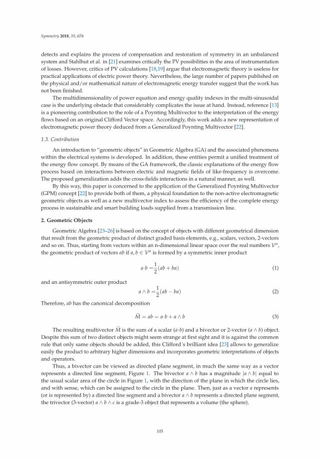
Symmetry 2018, 10, 676

detects and explains the process of compensation and restoration of symmetry in an unbalancedsystem and Stahlhut et al. in [21] examines critically the PV possibilities in the area of instrumentationof losses. However, critics of PV calculations [18,19] argue that electromagnetic theory is useless forpractical applications of electric power theory. Nevertheless, the large number of papers published onthe physical and/or mathematical nature of electromagnetic energy transfer suggest that the work hasnot been finished.

The multidimensionality of power equation and energy quality indexes in the multi-sinusoidalcase is the underlying obstacle that considerably complicates the issue at hand. Instead, reference [13]is a pioneering contribution to the role of a Poynting Multivector to the interpretation of the energyflows based on an original Clifford Vector space. Accordingly, this work adds a new representation ofelectromagnetic power theory deduced from a Generalized Poynting Multivector [22].

1.3. Contribution

An introduction to “geometric objects” in Geometric Algebra (GA) and the associated phenomenawithin the electrical systems is developed. In addition, these entities permit a unified treatment ofthe energy flow concept. By means of the GA framework, the classic explanations of the energy flowprocess based on interactions between electric and magnetic fields of like-frequency is overcome.The proposed generalization adds the cross-fields interactions in a natural manner, as well.

By this way, this paper is concerned to the application of the Generalized Poynting Multivector(GPM) concept [22] to provide both of them, a physical foundation to the non-active electromagneticgeometric objects as well as a new multivector index to assess the efficiency of the complete energyprocess in sustainable and smart building loads supplied from a transmission line.

2. Geometric Objects

Geometric Algebra [23–26] is based on the concept of objects with different geometrical dimensionthat result from the geometric product of distinct graded basis elements, e.g., scalars, vectors, 2-vectorsand so on. Thus, starting from vectors within an n-dimensional linear space over the real numbers Vn,the geometric product of vectors ab if a, b ∈ Vn is formed by a symmetric inner product

a·b =12(ab + ba) (1)

and an antisymmetric outer product

a ∧ b =12(ab − ba) (2)

Therefore, ab has the canonical decomposition

M = ab = a·b + a ∧ b (3)

The resulting multivector M is the sum of a scalar (a·b) and a bivector or 2-vector (a ∧ b) object.Despite this sum of two distinct objects might seem strange at first sight and it is against the commonrule that only same objects should be added, this Clifford´s brilliant idea [23] allows to generalizeeasily the product to arbitrary higher dimensions and incorporates geometric interpretations of objectsand operators.

Thus, a bivector can be viewed as directed plane segment, in much the same way as a vectorrepresents a directed line segment, Figure 1. The bivector a ∧ b has a magnitude |a ∧ b| equal tothe usual scalar area of the circle in Figure 1, with the direction of the plane in which the circle lies,and with sense, which can be assigned to the circle in the plane. Then, just as a vector a represents(or is represented by) a directed line segment and a bivector a ∧ b represents a directed plane segment,the trivector (3-vector) a ∧ b ∧ c is a grade-3 object that represents a volume (the sphere).

105

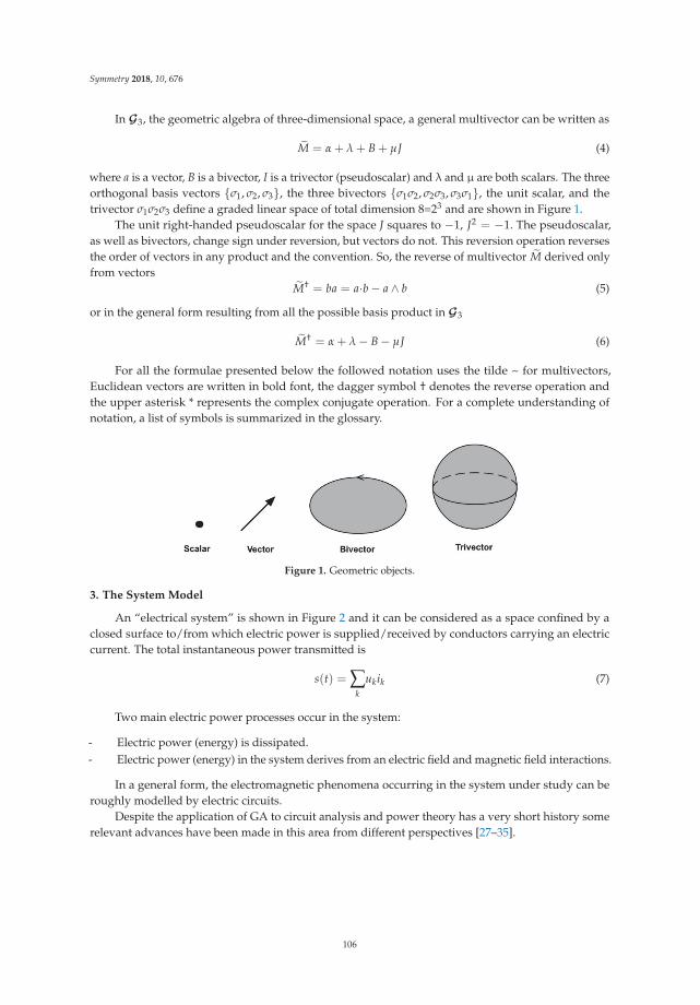
Symmetry 2018, 10, 676

In G3, the geometric algebra of three-dimensional space, a general multivector can be written as

M = α + λ + B + μJ (4)

where a is a vector, B is a bivector, I is a trivector (pseudoscalar) and λ and μ are both scalars. The threeorthogonal basis vectors {σ1, σ2, σ3}, the three bivectors {σ1σ2, σ2σ3, σ3σ1}, the unit scalar, and thetrivector σ1σ2σ3 define a graded linear space of total dimension 8=23 and are shown in Figure 1.

The unit right-handed pseudoscalar for the space J squares to −1, J2 = −1. The pseudoscalar,as well as bivectors, change sign under reversion, but vectors do not. This reversion operation reversesthe order of vectors in any product and the convention. So, the reverse of multivector M derived onlyfrom vectors

M† = ba = a·b − a ∧ b (5)

or in the general form resulting from all the possible basis product in G3

M† = α + λ − B − μJ (6)

For all the formulae presented below the followed notation uses the tilde ~ for multivectors,Euclidean vectors are written in bold font, the dagger symbol † denotes the reverse operation andthe upper asterisk * represents the complex conjugate operation. For a complete understanding ofnotation, a list of symbols is summarized in the glossary.

Figure 1. Geometric objects.

3. The System Model

An “electrical system” is shown in Figure 2 and it can be considered as a space confined by aclosed surface to/from which electric power is supplied/received by conductors carrying an electriccurrent. The total instantaneous power transmitted is

s(t) = ∑k

ukik (7)

Two main electric power processes occur in the system:

- Electric power (energy) is dissipated.- Electric power (energy) in the system derives from an electric field and magnetic field interactions.

In a general form, the electromagnetic phenomena occurring in the system under study can beroughly modelled by electric circuits.

Despite the application of GA to circuit analysis and power theory has a very short history somerelevant advances have been made in this area from different perspectives [27–35].

106

Symmetry 2018, 10, 676

Figure 2. Electrical system.

4. Generalized Poynting Multivector

In this work, space coordinates and time (frequency) coordinates have a differentiated treatment.Space domain remains represented by the classical Euclidean approach, the harmonic field in both,time and frequency domains, are characterized by complex geometric algebra, CGn. The completespace-time framework results in the hybrid CGt

n −R3 structure named Generalized Euclidean Space(CGn −R3 for space-frequency domain) [22].

In this CGn −R3 algebraic approach, the Generalized Poynting Multivector (GPM) is defined as

Π = ∑p,q

(Ep � H

∗q

)(8)

where Ep and Hq vectors are called ‘spatial geometric phasors’ of the electric and magnetic harmonicfields, H

∗q vector is the conjugate of the q-th harmonic spatial geometric phasor Hq and ‘�’ is the

generalized geometric product (GGP) [27].From this multivectorial field theory, the flux of the GPM quantity for a volume υ enclosed by a

surface ς, (GPM theorem), can be expanded into two terms.�ς

n·Π dς =�ς

∑p

n·Pp dς+�ς

∑p �=q

n·Dpq dς = S (9)

where n is the unitary vector orthogonal to the infinitesimal surface dς, P is the PoyntingMultivector (PM) and D is the Complementary Poynting Multivector (CPM) and S = U � I∗ isthe Power Multivector.

In Equation (10) are present three “electromagnetic geometric objects”: the complex vectors Ep

and Hq, the complex scalar

P = ∑p

Ep � H∗p (10)

and the complex bivector

D = ∑p<q

(Ep � H

∗q + Eq � H

∗p

)(11)

From CGn structure, Equation (10) explains the total power energy flow because contains thecomponent P related with the power contribution due to frequency-like products and the componentD associated to the mutual influence of the harmonic components of the fields. Observe that in classicalapproach this last term vanishes due to the orthogonality of harmonics basis. Nevertheless, a nullaverage value of power without any net energy transferred must be also considered to understand the

107

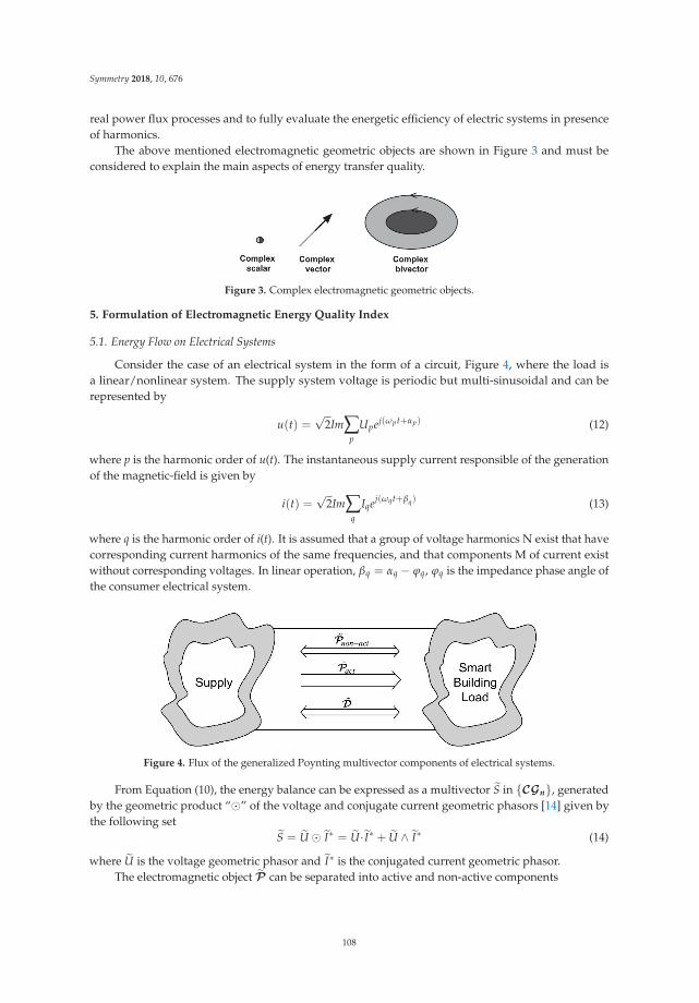
Symmetry 2018, 10, 676

real power flux processes and to fully evaluate the energetic efficiency of electric systems in presenceof harmonics.

The above mentioned electromagnetic geometric objects are shown in Figure 3 and must beconsidered to explain the main aspects of energy transfer quality.

Figure 3. Complex electromagnetic geometric objects.

5. Formulation of Electromagnetic Energy Quality Index

5.1. Energy Flow on Electrical Systems

Consider the case of an electrical system in the form of a circuit, Figure 4, where the load isa linear/nonlinear system. The supply system voltage is periodic but multi-sinusoidal and can berepresented by

u(t) =√

2Im∑p

Upej(ωpt+αp) (12)

where p is the harmonic order of u(t). The instantaneous supply current responsible of the generationof the magnetic-field is given by

i(t) =√

2Im∑q

Iqej(ωqt+βq) (13)

where q is the harmonic order of i(t). It is assumed that a group of voltage harmonics N exist that havecorresponding current harmonics of the same frequencies, and that components M of current existwithout corresponding voltages. In linear operation, βq = αq − ϕq, ϕq is the impedance phase angle ofthe consumer electrical system.

Figure 4. Flux of the generalized Poynting multivector components of electrical systems.

From Equation (10), the energy balance can be expressed as a multivector S in {CGn}, generatedby the geometric product “�” of the voltage and conjugate current geometric phasors [14] given bythe following set

S = U � I∗ = U· I∗ + U ∧ I∗ (14)

where U is the voltage geometric phasor and I∗ is the conjugated current geometric phasor.The electromagnetic object P can be separated into active and non-active components

108

Symmetry 2018, 10, 676

P = ∑p

Ppact+∑

p

Ppnon−act= Re

⎧⎨⎩∑p

Pp

⎫⎬⎭︸︷︷︸Pact

+ jIm

⎧⎨⎩∑p

Pp

⎫⎬⎭︸︷︷︸Pnon−act

(15)

where the set Pact transfers the harmonic active power and the set Pnon−act transport the scalarnon-active power (classical reactive power). The only component of P that transfer useful energy isPact, Figure 4.

Hence, by virtue of (10), it is obtains

�ς

∑p

→1 Z · Pp dς =

�ς

∑p

→1 Z · Ep � H

∗p dς =∑

P

Up Ipejφp σ0 (16)

The PM (P) is associated to the energy density at a point on the surface given in terms of theharmonic spatial geometric phasor of electric and magnetic fields at that point. Observe that the PMcoincides with the classic Complex Poynting Vector only in pure sinusoidal case.

The real part of P in (16), P = Re

{�ς

∑p

→1 Z · Pp dς

}, permits a direct interpretation in terms of

average energy flow, (i.e. active power P).

The imaginary part of P in (16), Q = Im

{�ς

∑p

→1 Z · Pp dς

}, is the scalar non-active power.

In general, it can be verified that PM P considers direction and sense, not only of active powercomponents Ppact

but also of scalar non-active components Ppnon−actThus, the possible reverse

sense of any harmonic Ppactis very important for a correct identification of harmonic source

locations and for determining the responsibility of the utility electrical system and the associatedload. Thus, if Ppact

≥ 0(Pp ≥ 0

)the energy flow is unidirectional toward the load. On the other way,

if Ppact≤ 0

(Pp ≤ 0

)the flow is generated in the nonlinearity of the load.

A more detailed develop of the CPM (D) is

D = ∑p<q

Ep � H∗q + Eq � H

∗p = ∑

p < qp, q ∈ N

Dpq + ∑p∈N,q∈M

Dpq

= Re

⎧⎪⎪⎪⎪⎪⎨⎪⎪⎪⎪⎪⎩∑

p < qp, q ∈ N


Dpq

⎫⎪⎪⎪⎪⎪⎬⎪⎪⎪⎪⎪⎭︸︷︷︸Dact

+ jIm

⎧⎪⎪⎪⎪⎪⎨⎪⎪⎪⎪⎪⎩∑

p < qp, q∈N


Dpq

⎫⎪⎪⎪⎪⎪⎬⎪⎪⎪⎪⎪⎭︸︷︷︸Dnon−act

(17)

Moreover, the flux of the Complementary Poynting Multivector is given by

�ς

∑p<q

→1 Z · Dpq dς = D (18)

where D can be associated to the polluting nature components, Dact and Dnon−act, that do not help intransferring useful energy and

D = ∑p < qlinear

{(

Up Iq ejϕq − Uq Ipejϕp)

ej(αp−αq))}

σpq + ∑p<q

non−linear

Up Iq ej(αp−βq)σpq (19)

109

Symmetry 2018, 10, 676

is the non-active power bivector called distortion power.Through (9), (16) and (18), it can be observed that the energy flow that it is originated from the

surface of the source in the electrical system equals the flow that enters in the load surface.

5.2. Electromagnetic Quality Index (EQI)

The aim of this paper is to propose a multivectorial index ξ, based on electromagnetic geometricobjects, capable to characterize the performance of the power transfer or the efficiency of thetransmission equipment in single-phase circuits with multi-harmonic signals. This figure of meritcan be an important piece of information for the interpretation of the electromagnetic energy flowin presence of disturbing loads. On the contrary, the classic THD index (Total Harmonic Distortion)for the measurement of the harmonic distortion level is not able to give any information about thedisturbance nature.

To this end, a new index that integrally reflects the nature of the different energy quality situationsis defined. This is expressed as

ξ =

�ς

→1 ZΠdς

Re

{�ς

∑p∈N

→1 Z · Pp dς

} = 1 + j

Im

{�ς

∑p∈N

→1 Z · Pp dς

}

Re

{�ς

∑p∈N

→1 Z · Pp dς

} +

�ς

∑p �=q

→1 Z · Dpq dς

Re

{�ς

∑p∈N

→1 Z · Pp dς

} (20)

or also,

ξ =

Re

{�ς

∑p=1

→1 Z · P1 dς

}+jIm

{�ς

∑p=1

→1 Z · P1 dς

}

Re

{�ς

∑p

→1 Z · Pp dς

} +

+

Re

{�ς

∑p �=1

→1 Z · Pp dς

}+jIm

{�ς

∑p �=1

→1 Z · Pp dς

}

Re

{�ς

∑p

→1 Z · Pp dς

} +

+

�ς

∑p �=q

→1 Z · Dpq dς

Re

{�ς

∑p

→1 Z · Pp dς

}

(21)

The power factor PF can be written as

PF =1∣∣∣∣∣∣ξ∣∣∣∣∣∣ =

∣∣∣∣∣∣∣∣∣∣Re

{�s

∑p

→1 Z · Pp ds

}∣∣∣∣∣∣∣∣∣∣∣∣∣∣∣∣∣∣�

s

→1 Z · Π ds

∣∣∣∣∣∣∣∣ (22)

It is noteworthy that the power factor is not an exhaustive index for energy quality. In fact,combining (20) and (22) the power factor could be brought to unity, but the electrical systems wouldstill operate in multi-sinusoidal mode.

Equations (21), (22) and (23) show that the index ξ contains terms that keep direction and sense,allowing harmonic source detection. This property is very important to achieve an appropriatedcompromise between the energy quality index and the power factor. Moreover, the dominantharmonic source should be based on an evaluation of non-active scalar and bivector electromagneticgeometric object components of the Generalized Poynting Multivector. This subject is discussed in thenext subsection.

110

Symmetry 2018, 10, 676

5.3. Illustrative Comparison between Different Non-Active Electromagnetic Geometric Objects

It is seen from (12) and (17) that U1 and I1 are the sinusoidal voltage and current geometric phasorand Up and Iq are the harmonic voltage and current geometric phasor when p �= 1, q �= 1 respectively.Obviously, the voltage geometric phasor U1 produces the sinusoidal electric field spatial geometricphasor E1 and the harmonic voltage Up generates the harmonic field Ep. Similarly the sinusoidalcurrent I1 geometric phasor produces the sinusoidal magnetic field spatial geometric phasor H1 andthe harmonic current Iq generates the harmonic field Hq. The interaction among these fields producesthe cited characteristic electromagnetic geometric objects Π, P and D. The objects P and D areseparated into an active and a non-active component as in Equations (15) and (17). In these equations,the different non-active scalar and bivector electromagnetic objects assume different expressionsdepending on the electrical system nature.

Starting from these considerations, a new philosophy is proposed for the detection of the dominantharmonic source that is based on the comparison of these non-active components to explain the powerquality concept. For more detail, the following situations are considered:

• Sinusoidal case: p = q = 1 ⇒ N = {1}

Πsin = P1 = Re{P1

}︸︷︷︸

P1act

+ j Im{P1

}︸︷︷︸P1non−act

(23)

and

ξsin = 1 + j

Im

{�ς

∑p∈1

→1 Z · P1 dς

}

Re

{�ς

∑p∈1

→1 Z · P1 dς

} (24)

In this case, the quantity Im{P1} = P1non−act can be considered as minimum reference value toimprove the energy quality, since it is the only non-active electromagnetic geometric object. It is thewell established fundamental reactive power (Q) that can be reduced to zero by shunts capacitors∣∣∣∣∣∣

∣∣∣∣∣∣Im⎧⎨⎩�

ς∑p∈1

→1 Z · P1 dς

⎫⎬⎭∣∣∣∣∣∣∣∣∣∣∣∣ = 0 (25)

and consequently, ∣∣∣∣∣∣ξsin∣∣∣∣∣∣ = 1 ⇒ PF1 = 1 (26)

where PF1 is the fundamental power factor, also known as the displacement power factor

PF1 = cos(ϕ1) (27)

The quantity Re{P1

}= P1act transfers the fundamental active power (useful energy) and is

associated to the instantaneous active power.

• Multi-sinusoidal linear case: p ∈ N, q ∈ N

111

Symmetry 2018, 10, 676

If the electrical system is linear, the current requested by the loads and voltage supplied by themains share the same harmonic order and the equation (8) yields the linear GPM Πlin

Πlin = ∑p=q

Pp + ∑p �=q

Dpq =

= ∑p=q

Ppact︸︷︷︸Pact

+ P1non−act + ∑p,q∈N>1

Ppnon−act︸︷︷︸jPnon−act

+ ∑p,q∈N

Dpq︸︷︷︸Dlin

(28)

The linear EQM is given by

ξlin = 1 + j

Im

{�ς

∑p∈N

→1 Z · Pp dς

}

Re

{�ς

∑p∈N

→1 Z · Pp dς

} +

�ς

∑p,q∈N

→1 Z · Dpq dς

Re

{�ς

∑p∈N

→1 Z · Pp dς

} (29)

The quantities Im

{�ς

∑p∈N

→1 Z · Pp dς

}and Im

{�ς

∑p,q∈N

→1 Z · Dpq dς

}in (29) should be minimized

by shunt capacitors or reduced to zero by shunt reactance one-ports. In these conditions

ξlin = 1 +

Re�ς

∑p,q∈N

→1 Z · Dpq dς

Re

{�ς

∑p∈N

→1 Z · Pp dς

} ⇒∣∣∣∣∣∣ξlin

∣∣∣∣∣∣ >1 ⇒ PF < 1 (30)

From (30), it results that for linear electrical systems under multi-sinusoidal conditions,the criterion

Im

⎧⎨⎩�ς

∑p∈N

→1 Z · Pp dς

⎫⎬⎭ = 0 (31)

Im

⎧⎨⎩�ς

∑p,q∈N

→1 Z · Dpq dς

⎫⎬⎭ = 0 (32)

does not represent the conditions of highest power factor.

• Multi-sinusoidal non-linear case: p ∈ N, q ∈ N ∪ M

In this case, the presence of the nonlinear loads causes some current components (q ∈ M) whichharmonic orders are not present in the voltage supplied to the electrical system. It is well known thatwhen a non-linear o time-varying electrical system is present, it injects disturbances even if the supplyvoltage is sinusoidal. In view of (8), the non-linear GPM can be written as follows,

Πnon−lin = ∑p=q

Pp + ∑p �=q

Dpq =

= ∑p=q

Ppact︸︷︷︸Pact

+ jP1non−act + ∑p,q∈N>1

Ppnon−act︸︷︷︸jPnon−act

+ ∑p,q∈N

Dpq︸︷︷︸Dlin

+ ∑p ∈ N,q ∈ M

Dpq

︸︷︷︸Dnon−lin

(33)

112

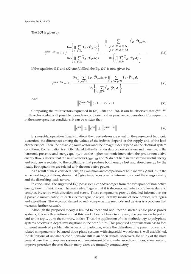
Symmetry 2018, 10, 676

The EQI is given by

ξnon−lin = 1 + j

Im

{�ς

∑p∈N

→1 Z · Pp dς

}

Re

{�ς

∑p∈N

→1 Z · Pp dς

} +

�ς

∑p ∈ N, q ∈ Np ∈ N, q ∈ M

→1 Z · Dpq dς

Re

{�ς

∑p∈N

→1 Z · Pp dς

} (34)

If the equalities (31) and (32) are fulfilled, the Eq. (34) is now given by,

ξnon−lin = 1 +

Re�ς

∑p,q∈N

→1 Z · Dpq dς +

�ς

∑p∈N,q∈M

→1 Z · Dpq dς

Re

{�ς

∑p∈N

→1 Z · Pp dς

} (35)

And ∣∣∣∣∣∣ξnon−lin∣∣∣∣∣∣ > 1 ⇒ PF < 1 (36)

Comparing the multivectors expressed in (26), (30) and (36), it can be observed that ξnon−lin

multivector contains all possible non-active components after passive compensation. Consequently,in the same operation conditions, it can be written that∣∣∣∣∣∣ξsin

∣∣∣∣∣∣ ≤ ∣∣∣∣∣∣ξlin∣∣∣∣∣∣ ≤ ∣∣∣∣∣∣ξnon−lin

∣∣∣∣∣∣ (37)

In sinusoidal operation (ideal situation), the three indexes are equal. In the presence of harmonicdistortion, the differences among the values of the indexes depend of the supply and of the loadcharacteristics. Then, the possible ξ multivectors and their magnitudes depend on the electrical systemconditions. Each situation is strictly related to the distortion state of power system and therefore, to theharmonic presence and energy quality, thus, the higher harmonic interaction, the greater non-activeenergy flow. Observe that the multivectors Pnon−act and D do not help in transferring useful energyand only are associated to the oscillations that produce both, energy lost and stored energy by theloads. Both quantities are related with the non-active power.

As a result of these considerations, an evaluation and comparison of both indexes, ξ and PF, in thesame working conditions, shows that ξ give two pieces of extra information about the energy qualityand the disturbing loads nature.

In conclusion, the suggested EQI possesses clear advantages from the viewpoint of non-activeenergy flow minimization. The main advantage is that it is decomposed into a complex-scalar andcomplex-bivectors with direction and sense. These components provide detailed information fora possible minimization of each electromagnetic object term by means of new devices, strategies,and algorithms. The accomplishment of such compensating methods and devices is a problem thatwarrants further research.

Although the proposed theory is limited to linear and non-linear distorted single-phase powersystems, it is worth mentioning that this work does not have in any way the pretension to put anend to the topic, quite the contrary, in fact. Thus, the application of this methodology to polyphasesystems deserves in-depth investigations in the near future. This proposed approximation has to facedifferent unsolved problematic aspects. In particular, while the definition of apparent power andrelated components in balanced three-phase systems with sinusoidal waveforms is well established,the definitions of unbalance conditions are still in an open debate. Moreover, the study of the mostgeneral case, the three-phase systems with non-sinusoidal and unbalanced conditions, even needs toimprove precedent theories that in many cases are mutually contradictory.

113

Symmetry 2018, 10, 676

It is remarkable that the structure of geometric algebra gives a new insight to phase domain andconstitutes a powerful tool for the treatment of periodic distorted signals. In this framework, powerdefinition deals with the key concept of geometric phasors, i.e. algebraic time-averaged quantitiesthat are far from being instantaneous ones. In this regard, depending on the considered application,this can be a major restriction. Thus, applications such as instantaneous active filters or fast responsecompensation devices, are out of the scope of this study, as well. For the same reason, electricsignals disturbed with non-stationary events such as transients, sag, swells, etc. are not considered inthis work.

6. Numerical Example

In order to validate the use and relevance of the Poynting Multivector suggested in this paper,sustainable and smart building loads supplied from a transmission line are analysed in the CGn −R3

framework. In a simplistic manner, the conductors are considered as rectangular and parallelsuperconductors meant to facilitate the propagation of energy from source to load, Figure 5. Units ofphysical quantities are the standard units of the MKSA system and thus are omitted.

Figure 5. Industrial system: Sustainable smart building.

Two parallel plane conductors in linear media are considered. Both conductors, of thickness λ andwidth γ, are separated by a dielectric material of thickness ρ. We suppose that γ � λ, ρ. By ignoringeddy currents, line impedance, fringing effects, three cases are analysed:

6.1. Linear Load Supplied by A Sinusoidal Voltage Source

Voltage and a hypothetic resulting current are respectively

u(t) =√

2(200 sin ω1t)

i(t) =√

2[10 sin(ω1t − 36.87◦)]

Then, from [13], the spatial geometric phasors of the electric E and magnetic H∗

fields can beexpressed as

E =1d

(200ej0σ1

)→1 X ; H

∗=

1h

(10ej36.87σ1

)→1 Y

114

Symmetry 2018, 10, 676

and the electromagnetic geometric objects and associated power are

�ς

∑p=1

→1 Z · P dς =

⎛⎝1600︸︷︷︸P1

+j1200︸︷︷︸Q1

⎞⎠σ0

�ς

∑p �=q

→1 Z · D dς = 0; D = 0

ξsin = 1 + j12001600

σ0 ⇒∣∣∣∣∣∣ξsin

∣∣∣∣∣∣ = 1.25 ; PF = 0.8

6.2. Linear Load Supplied by A Non-Sinusoidal Sinusoidal Voltage Source

Voltage and hypothetic resulting current are

u(t) =√

2(200 sin ω1t + 50 sin ω2t)

i(t) =√

2[10 sin(ω1t − 36.87◦) + 5 sin(ω2t + 53.13◦)]

and the spatial geometric phasors of the electric E and magnetic H∗

fields can be expressed as

E =1d

(200ej0σ1 + 50ej0σ2

)→1 X

H∗=

1h

(10ej36.87σ1 + 5e−j53.13σ2

)→1 Y

�ς

∑p

→1 Z · P dς =

⎛⎝1750︸︷︷︸P

+j1000︸︷︷︸Q

⎞⎠σ0

�ς

∑p �=q

→1 Z · D dς = D = [200 − j1100]︸︷︷︸

D12

σ12

ξnon−lin = 1 + j10001750

σ0 +[200 − j1100]σ12

1750σ0∣∣∣∣∣∣ξnon−lin∣∣∣∣∣∣ = 1.32

PF = 0.76

6.3. Non-Linear Load Supplied by A Non-Sinusoidal Sinusoidal Voltage Source

Voltage and hypothetic resulting current are

u(t) =√

2(200 sin ω1t + 50 sin ω2t)

i(t) =√

2[10 sin(ω1t − 36.87◦) + 5 sin(ω2t + 53.13◦) + 5 sin(ω3t + 45◦)]

and the spatial geometric phasors of the electric E and magnetic H∗

fields can be expressed as

E =1d

(200ej0σ1 + 50ej0σ2

)→1 X

E =1d

(200ej0σ1 + 50ej0σ2

)→1 X

115

Symmetry 2018, 10, 676

�ς

∑p

→1 Z · P dς = [(1600 + 1200) + j(150 − 200)]σ0 =

⎛⎝1750︸︷︷︸P

+j1000︸︷︷︸Q

⎞⎠σ0

�ς

∑p �=q

→1 Z · D dς = D = [200 − j1100]︸︷︷︸

D12

σ12 +[125

√2 − j125

√2]

︸︷︷︸D23

σ13 +[500

√2 − j500

√2]

︸︷︷︸D13

σ23

ξnon−lin = 1 + j10001750

σ0 +[200 − j1100]σ12 +

[125

√2 − j125

√2]σ13 +

[500

√2 − j500

√2]σ23

1750σ0∣∣∣∣∣∣ξnon−lin∣∣∣∣∣∣ = 1.44

PF = 0.69

As in (37), it should be noticed in this example that{∣∣∣∣∣∣ξsin∣∣∣∣∣∣ = 1.25

}<{∣∣∣∣∣∣ξlin

∣∣∣∣∣∣ = 1.32}<{∣∣∣∣∣∣ξnon−lin

∣∣∣∣∣∣ = 1.44}

Comparing the multivectors ξ of the above three cases, it can be observed that they contain allpossible non-active components. In this way, the possible reverse sense of any harmonic of active,reactive and distortion powers is very important for a correct identification of harmonic sourcelocations, and for determining the responsibility of the utility side (generator) and the consumer side(load) [20,21]. Thus, the suggested index ξ possesses clear advantages from the viewpoint of non-activepower flow minimization.

7. Conclusions

The analysis of sustainable smart buildings is key to new future buildings, new complexarchitectures, and its usefulness extends to smart cities. Analyses of quality of the construction typicallyfocus on applying methodologies that evaluate quality objectives at environmental, construction andbuilding levels. Research has shown that a multivector quality index can be useful for detection ofharmonic sources of new sustainable smart buildings.

Along this line this paper presents a reformulation of Poynting Vector in terms of the GeometricAlgebra framework when inefficiencies caused by harmonics are considered. In this environment,each geometric object represents a different kind of energy flux. Thus, the distinct and well-knownpower terms in electric power systems, i.e. Active, Reactive, Distortion and Apparent powers acquirea new interpretation and dimension by means of multivectors. This novel approach is applicableto smart architectural single-phase power systems with linear/non-linear loads under sinusoidal ornon-sinusoidal conditions. By this means, the behaviour of the energy flux is summarized by theproposed electromagnetic energy index EQI. In addition, the meaning of this original index is deeplyanalysed and discussed, concluding that its capability to deal with geometric properties, namelymagnitude, direction and sense, makes it perfectly appropriate for detection and minimization ofharmonic sources.

Furthermore, it is an excellent tool to interpret the cited power flow distribution. Thus, theintroduction of this figure of merit supposes not only a generalization of the traditional power factorin electric power networks but also the key to the electromagnetic energy transfer between mainsand loads. The global efficiency of a system is truth evaluated by this index because it includes allpossible interactions.

It is remarkable that traditional Poynting Vector is a particular case of the proposedgeneralized Poynting Multivector when no cross interactions are present between different harmonics.This correlation is now precisely understood as the outer product between geometric phasors ofdifferent energy levels. Thus, this fact is crucial for future research proposals on the design of passive

116

Symmetry 2018, 10, 676

and/or active architectures for selective compensation, optimization algorithms and measurementtechniques for harmonic pollution monitoring.

The electromagnetic nature of the power components could be the key that opens a broad rangeof new interesting research lines in electrical engineering and all energy efficiency related matters.

Author Contributions: All authors contributed equally to this work. All authors wrote, reviewed and commentedon the manuscript. All authors have read and approved the final manuscript.


Glossary of Symbols

R real numbersC complex vector spaceGn Geometric Algebra in n-dimensional real spaceCGn Complex Geometric AlgebraCGt

n −R3 time generalized geometric euclidean spaceCGn −R3 frequency generalized geometric euclidean space→1 X ,

→1 Y ,

→1 Z Euclidean canonical basis

σ1...k canonical basis of Gn

σp basis vector of Gn

σpσq = σpq basis bivectors of Gn

σ1σ2σ3 trivector or pseudoscalar of Gn

λ, μ scalars or 0-grade geometric objecta, b vectors or 1-grade geometric objectB bivector or 2-grade geometric objectJ pseudoscalar or n-grade geometric objectM generic multivectorΠ generalized Poynting multivector (GPM)P Poynting multivector (PM)D Complementary Poynting multivector (CPM)E electric field geometric phasorH magnetic field geometric phasor� generalized geometric product· inner product∧ outer productj imaginary unit∗ conjugated operation† reverse operation~ multivector characterizationUp p-th harmonic voltage rms valueIq q-th harmonic current rms valueP active power or real part of 0-grade power multivectorQ reactive power or imaginary part of 0-grade power multivectorD distortion power or 2-grade powerS power multivector∣∣∣∣∣∣S∣∣∣∣∣∣, S apparent power multivector

ωp p-th harmonic frequencyαp phase angle of p-th voltage geometric phasorβq phase angle of q-th current geometric phasorφq q-th impedance phase angleξ electromagnetic quality index multivector (EQI)PF power factor

117

Symmetry 2018, 10, 676

References

1. Ibrahim, M.; El-Zaart, A.; Adams, C. Smart Sustainable Cities roadmap: Readiness for transformationtowards urban sustainability. Sustain. Cities Soc. 2018, 37, 530–540. [CrossRef]

2. Höjer, M.; Wangel, J. Smart sustainable cities: Definition and challenges. In ICT Innovations for Sustainability;Hilty, L., Aebischer, B., Eds.; Springer: Cham, Switzerland, 2015; pp. 333–349.

3. Pervez, H.S.; Nursyarizal, B.M.N.; Perumal, N.; Irraivan, E.; Taib, I. A review on optimized control systemsfor building energy and comfort management of smart sustainable buildings. Renew. Sustain. Energy Rev.2014, 34, 409–429. [CrossRef]

4. Nardi, I.; Lucchi, E.; Rubeis, T.; Ambrosini, D. Quantification of heat energy losses through the buildingenvelope: A state-of-the-art analysis with critical and comprehensive review on infrared thermography.Build. Environ. 2018, 146, 190–205. [CrossRef]

5. Karmellos, M.; Kiprakis, A.; Mavrotas, G. A multi-objective approach for optimal prioritization of energyefficiency measures in buildings: Model, software and case studies. Appl. Energy. 2015, 139, 131–150.[CrossRef]

6. Poynting, J.H. On the transfer of energy in the electromagnetic field. Philos. Trans. R. Soc. 1884, 175, 343–361.[CrossRef]

7. Steinmetz, C.P. Theory and Calculation of Alternating Current Phenomena; McGraw Publishing Company:New York, NY, USA, 1900.

8. Emanuel, A.E. Powers in nonsinusoidal situations a review of definitions and physical meaning. IEEE Trans.Power Deliv. 1990, 5, 1377–1389. [CrossRef]

9. Emanuel, A.E. Poynting vector and the physical meaning of nonactive powers. IEEE Trans. Instrum. Meas.2005, 54, 1457–1462. [CrossRef]

10. Lundin, U.; Bolund, B.; Leijon, M. Poynting vector analysis of synchronous generators using field simulations.IEEE Trans. Magn. 2007, 43, 3601–3606. [CrossRef]

11. Faria, J.A.B. The role of Poynting’s vector in polyphase power calculations. Eur. Trans. Electr. Power 2009, 19,683–688. [CrossRef]

12. De León, F.; Cohen, J. AC power theory from Poynting Theorem: Accurate identification of instantaneouspower components in nonlinear-switched circuits. IEEE Trans. Power Deliv. 2010, 25, 2104–2112. [CrossRef]

13. Cheng, P.; Yang, F.; Luo, H.; Guo, H.; Ran, W.; Yang, Y.; Ullah, I. A method to calculate the reactive power oficed transmission line based on Poynting vector and FDFD. Int. J. Appl. Electromagn. Mech. 2016, 50, 417–433.[CrossRef]

14. Emanuel, A.E. About the Rejection of Poynting Vector in Power Systems Analysis. Electr. Power Qual. Util. J.2007, 13, 43–49.

15. Emanuel, A.E. Power Definitions and the Physical Mechanism of Power Flow; Wiley: Hoboken, NJ, USA, 2010.16. Todeschini, G.; Emanuel, A.E.; Ferrero, A.; Morando, A.P. A Poynting vector approach to the study of the

Steinmetz compensator. IEEE Trans. Power Deliv. 2007, 22, 1830–1833. [CrossRef]17. Ferrero, A.; Leva, S.; Morando, A.P. An approach to the non-active power concept in terms of the

poynting-park vector. Eur. Trans. Electr. Power 2001, 11, 291–299. [CrossRef]18. Czarnecki, L.S. Considerations on the Concept of Poynting Vector Contribution to Power Theory

Development. In Proceedings of the 6th International Workshop on Power Definitions and MeasurementsUnder Nonsinusoidal Conditions, Milano, Italy, 13–15 October 2003.

19. Czarnecki, L.S. Could Power Properties of Three-Phase Systems Be Described in Terms of the PoyntingVector? IEEE Trans. Power Deliv. 2006, 21, 339–344. [CrossRef]

20. Balci, M.; Hocaoglu, M.; Power, S.A. Transition from Poynting vector to instantaneous power. In Proceedingsof the 12th International Conference on Harmonics and Quality of Power, Cascais, Portugal, 1–5 October2006.

21. Stahlhut, J.W.; Browne, T.J.; Heydt, G.T. The Assessment of the Measurement of the Poynting Vector forPower System Instrumentation. In Proceedings of the 39th North American Power Symposium, Las Cruces,NM, USA, 30 September–2 October 2007; pp. 237–241.

22. Castilla, M.; Bravo, J.C.; Ordonez, M.; Montano, J.C. An approach to the multivectorial apparent power interms of a generalized poynting multivector. Prog. Electromagn. Res. B 2009, 15, 401–422. [CrossRef]

23. Clifford, W.K. Applications of Grassmann’s Extensive Algebra. Am. J. Math. 1878, 1, 350. [CrossRef]

118

Symmetry 2018, 10, 676

24. Hestenes, D. A unified language for mathematics and physics. their Appl. Math. Phys. 1986. [CrossRef]25. Chappell, J.M.; Drake, S.P.; Seidel, C.L.; Gunn, L.J.; Iqbal, A.; Allison, A.; Abbott, D. Geometric algebra for

electrical and electronic engineers. Proc. IEEE 2014. [CrossRef]26. Doran, C.; Lasenby, A. Geometric Algebra for Physicists; Cambridge University Press: Cambridge, UK, 2009.27. Castilla, M.; Bravo, J.C.; Ordóñez, M.; Montaño, J.C. Clifford theory: A geometrical interpretation of

multivectorial apparent power. IEEE Trans. Circuits Syst. I Regul. Pap. 2008, 55, 3358–3367. [CrossRef]28. Castilla, M.; Bravo, J.C.; Ordonez, M.; Montaño, J.C.; Lopez, A.; Borras, D.; Gutierrez, J. The geometric

algebra as a power theory analysis tool. In Proceedings of the 2008 International School on NonsinusoidalCurrents and Compensation, Lagow, Poland, 10–13 June 2008.

29. Castilla, M.; Bravo, J.C.; Ordóñez, M. Geometric algebra: A multivectorial proof of Tellegen’s theorem inmultiterminal networks. IET Circuits, Devices Syst. 2008, 2, 383–390. [CrossRef]

30. Bravo, J.C.; Castilla, M.V. Energy Conservation Law in Industrial Architecture: An Approach throughGeometric Algebra. Symmetry 2016, 8, 92. [CrossRef]

31. Castro-Núñez, M.; Londoño-Monsalve, D.; Castro-Puche, R.M. the conservative power quantity based onthe flow of energy. J. Eng. 2016, 2016, 269–276. [CrossRef]

32. Petroianu, A.I. A geometric algebra reformulation and interpretation of Steinmetz’s symbolic method andhis power expression in alternating current electrical circuits. Electr. Eng. 2015, 97, 175–180. [CrossRef]

33. Menti, A.; Zacharias, T.; Milias-Argitis, J. Geometric Algebra: A Powerful Tool for Representing PowerUnder Nonsinusoidal Conditions. IEEE Trans. Circuits Syst. I Regul. Pap. 2007, 54, 601–609. [CrossRef]

34. Castro-Nunez, M.; Castro-Puche, R. Advantages of Geometric Algebra Over Complex Numbers in theAnalysis of Networks With Nonsinusoidal Sources and Linear Loads. IEEE Trans. Circuits Syst. I Regul. Pap.2012, 59, 2056–2064. [CrossRef]

35. Herrera, R.S.S.; Salmeron, P.; Vazquez, J.R.R.; Litran, S.P.P.; Perez, A. Generalized instantaneous reactivepower theory in poly-phase power systems. In Proceedings of the 13th European Conference on PowerElectronics and Applications, Barcelona, Spain, 8–10 September 2009; pp. 1–10.


119

symmetryS S

Article

Denoising of Magnetocardiography Based onImproved Variational Mode Decomposition andInterval Thresholding Method

Yanping Liao, Congcong He * and Qiang Guo

Department of Information and Communication Engineering, Harbin Engineering University,Harbin 150001, China; [email protected] (Y.L.); [email protected] (Q.G.)* Correspondence: [email protected]; Tel.: +86-188-4510-3530

Received: 23 May 2018; Accepted: 5 July 2018; Published: 9 July 2018

Abstract: Recently, magnetocardiography (MCG) has attracted increasing attention as a non-invasiveand non-contact technique for detecting electrocardioelectric functions. However, the severebackground noise makes it difficult to extract information. Variational Mode Decomposition (VMD),which is an entirely non-recursive model, is used to decompose the non-stationary signal into theintrinsic mode functions (IMFs). Traditional VMD algorithms cannot control the bandwidth of eachIMF, whose quadratic penalty lacks adaptivity. As a result, baseline drift noise is still present ormedical information is lost. In this paper, to overcome the unadaptable quadratic penalty problem,an improved VMD model via correlation coefficient and new update formulas are proposed todecompose MCG signals. To improve the denoising precision, this algorithm is combined with theinterval threshold algorithm. First, the correlation coefficient is calculated, to determine quadraticpenalty, in order to extract the first IMF made up of baseline drift. Then, the new update formulasderived from the variance that describes the noise level are used, to perform decomposition on therest signal. Finally, the Interval thresholding algorithm is performed on each IMF. Theoretical analysisand experimental results show that this algorithm can effectively improve the output signal-to-noiseratio and has superior performance.

Keywords: magnetocardiography; quadratic penalty; variational mode decomposition; correlationcoefficient; interval thresholding method

1. Introduction

In recent years, the research on signal processing, modeling, imaging theory, and methodsrelated to bio-electromagnetism has become a hot topic. With the efforts of many experts andscholars, this field already has high-level research results. The magnetocardiography [1] signal playsan increasingly important role in heart disease diagnosis, which is detected with SuperconductingQuantum Interference Devices (SQUID) [2] and has considerable advantages over electrocardiography(ECG) [3]. As the detecting instrument of the magnetocardiography signal, the SQUID operates fromlow to high temperature, and changes the number of channels from the original single channel intomultiple channels. Magnetocardiography signals transmitted to the human chest surface are incrediblyhelpful toward both cardiac model reconstruction and clinical application [4,5]. The relationshipbetween heart function and heart disease is studied by researching the characteristics of magneticfield strength changes at different locations; this type of study can be called interdisciplinary basicresearch. Generally, such measurements are conducted in order to detect small magnetic field signalsin the presence of large background noise [6,7]. Removing background noise and recovering usefulsignals are chief objectives. For periodic signals, adequate suppression of uncorrelated noise may oftenbe achieved by the signal averaging method [8]. If the signal and noise have separate bandwidths,


Symmetry 2018, 10, 269

one can use conventional frequency domain filtering [9] techniques. Adaptive filtering techniques [10]measure the noise level of the measurement signal channels by measuring the noise channels. However,these simple preprocessing methods have limited effectiveness. The wavelet transform method [11]for signal denoising is based on the use of a set of predefined basis functions, in order to decomposethe measured signals and remove components corresponding to noise. The main disadvantage of thismethod is that the selection of wavelet basis seriously affects the denoising results. Empirical ModeDecomposition (EMD) [12,13] is one of the decomposition methods of signal denoising, and is widelyused to decompose a signal into different modes recursively. This method is, however, prone tomode mixing, and limited by sensitivity to noise and sampling [14]. The mode mixing is significantlyreduced by a modified noise-assisted data analysis method known as the Ensemble Empirical ModeDecomposition (EEMD) method [14,15]. The denoising principle of magnetocardiography (MCG)signals by EEMD based methods was reported in [16,17]. However, the decomposition results wereunsatisfactory because of the low signal-to-noise ratio. In addition, the decomposition results of EMDand EEMD heavily depend on the extremum seeking algorithm and the ending criterion. A lack ofmathematical approach and predefined filter boundaries reduce the accuracies of such detections [18].Lately, based on the definition of intrinsic mode functions (IMF), a new adaptive decomposition methodcalled Variational Mode Decomposition (VMD) [19] has been proposed. Supporting documents [20]proposed using the VMD method to denoise ECG signals. However, the research results showed thatthe decomposition results lack adaptability. The results of studies [21,22] showed that baseline driftnoise was not filtered out by the VMD method. In practice, it is not always possible to have the firstIMF to be a noise-only IMF.

In order to overcome the problems above, we propose an improved VMD method that determinesthe bandwidth of modes adaptively via the optimized quadratic penalty. The proposed correlationcoefficient, between the IMF obtained by VMD [19,23] and the baseline drift model, is calculatedrepeatedly until the criterion is satisfied and the baseline drift noise is extracted. The new IMFsare then obtained by using new proposed update formulas that can be deduced by the relationshipbetween the penalty factor and noise. The interval threshold method is used for the subsequentprocessing of each component, which removes noise components.

The rest of this paper is organized as follows: Section 2 introduces the data model required forthe VMD algorithm. In Section 3, a new VMD scheme based on the correlation coefficient and newupdated formulas is proposed. The application for denoising methods of MCG is shown in Section 4.Conclusions are given in Section 5.

2. Data Model

In the expression of the traditional EMD and EEMD methods, the IMF is defined as a functionwhere the difference between the number of zeros and poles does not exceed one [24]. In recent studies,the definition of the modality is changed to amplitude-modulated-frequency-modulated (AM-FM)signal, defined as follows:

uk(t) = Ak(t) cos(φk(t)) (1)

In the above equation, the phase φk(t) is a non-decreasing function, whose first derivative isφ′

k(t) > 0, where the envelope Ak(t) is non-negative; both the envelope Ak(t) and the instantaneousfrequency ωk(t) vary much slower than the phase φk(t) [25,26].

The Hilbert transform [27] is the convolution of a real function and the corresponding impulseresponse of h(t) = 1/πt in time domain. It is an all-pass filter, characterized by the transfer functionH(ω) = −jsgn(ω) = −jω/|ω| in frequency domain. The Hilbert transform of a purely real IMF uk(t)can be expressed as uk(t), and the complex-valued analytic signal is now defined as:

uk,A(t) = uk(t) + juk(t) = Ak(t)[cos(φ(t))− j sin(φ(t))]= Ak(t)e−jφ(t) (2)

122

Symmetry 2018, 10, 269

where φ(t) is the phase, while the amplitude is governed by the real envelope. The expressionAk(t). ω(t) = dφ(t)/dt is the instantaneous frequency. The amplitude Ak for kth IMF signal changesslowly enough.

Research has shown, on a sufficiently long interval, that the mode can be considered to be a purelyharmonic signal. In other words, the newer definition of signal components is slightly more restrictivethan the original one, and the VMD mode is the particular case of the EMD mode.

3. Proposed New VMD Scheme

VMD as a new decomposition method, is a process to solve variational problems based onclassic Wiener filtering and Hilbert transformation. We can use the VMD method to decompose amulti-component signal into several band-limited modes non-recursively, which are redefined as IMFs.However, the VMD algorithm cannot extract baseline drift noise when decomposing MCG signals.As such, a new VMD method framework is proposed in this paper.

3.1. Eliminate Baseline Drift Noise Using Proposed Formulas

To overcome the unadaptable quadratic penalty problem, we propose an improved VMD methodwith correlation coefficient and new update formulas. First, we need to extract the expected baselinedrift noise that will be included in the first mode. The steps are given as follows:

1. Compute the associated analytic signal of each mode uk by means of the Hilbert transform, that is:

uk,A(t) =(

δ(t) +j

πt

)∗ uk(t) (3)

2. Mix each mode with an exponential adjustment to the respective estimated center frequency inorder to shift the mode spectrum to “baseband”.

uk,A(t) =[(

δ(t) +j

πt

)∗ uk(t)

]e−jωkt (4)

where ωk is the center frequency of the kth IMF uk(t).3. Estimate the bandwidth through the squared L2-norm of the gradient. The expression of the

constrained variational problem is as follows:⎧⎪⎪⎨⎪⎪⎩min

{uk},{ωk}

{∑k‖∂t

[(δ(t) + j

πt

)∗ uk(t)

]e−jωkt‖2

2

}s.t.

K∑

k=1uk(t) = f (t)

(5)

where {uk} = {u1, . . . , uK} and {ωk} = {ω1, . . . , ωK} are shorthand notations for the set of allmodes and their center frequencies. In order to render the problem unconstrained, a quadraticpenalty term α and Lagrangian multiplier λ are brought in. The quadratic penalty can encouragereconstruction fidelity, typically in the presence of additive Gaussian noise. The Lagrangeequation can enforce constraints strictly. Therefore, we introduce the augmented Lagrangeequation L as follow [28]:

L({uk}, {ωk}, λ(t)) = αK∑

k=1‖∂t

[(δ(t) + j

πt

)∗ uk(t)

]e−jωkt‖2

2 + ‖ f (t)−K∑

k=1uk(t)‖2

2 + λ(t), f (t)−K∑

k=1uk(t) (6)

123

Symmetry 2018, 10, 269

Alternate direction method of multipliers (ADMM) is brought to solve the original minimizationproblem [29–31]. To update the mode uk, we can get the equivalent minimization problem asthe following:

un+1k = argmin

uk∈X

{α

K

∑k=1

∥∥∥∥∂t

[(δ(t) +

jπt

)∗ uk(t)

]e−jωkt‖2

2+

∥∥∥∥ f (t)−K

∑i=1

ui(t)− λ(t)2

‖22

}(7)

where n is the number of iterations. Now, making use of the Parseval/Plancherel Fourier isometryunder the L2 norm, this problem can be solved in spectral domain. Then, performing a change ofvariables ω ← ω− ωk in the first term, we can get the following expression:

un+1k = argmin

uk ,uk∈X

⎧⎨⎩α‖j(ω − ωk)[(1 + sgn(ω))uk(ω)]‖22 +

∥∥∥∥∥ f (ω)− ∑i

ui(ω) +λ(ω)

2

∥∥∥∥∥2

2

⎫⎬⎭ (8)

Exploiting the Hermitian symmetry of the real signals, we can write both terms as half-spaceintegrals, then making the negative frequencies of the first variation disappeared as follows:

un+1k (ω) =

f (ω)− ∑i<k un+1i (ω)− ∑i>k un

i (ω) +λn(ω)

2

1 + 2α(ω − ωn

k)2 (9)

This is clearly identified as Wiener filtering of the current residual, with signal prior 1/(ω − ωn

k)2;

the time domain mode is obtained as the real part of the inverse Fourier transform of this filteredanalytic signal. In order to obtain each component, the center frequency, corresponding to eachcomponent, needs to be solved. The center frequency appears in the bandwidth prior, but not in thereconstruction fidelity term. The relevant problem thus reads:

ωn+1k = argmin

ωk

{‖∂t

[(δ(t) +

jπt

)∗ uk(t)

]e−jωkt‖2

2

}(10)

As before, the optimization can be taken place in Fourier domain, and we end up optimizing:

ωn+1k =

∫ ∞0 ω|uk(ω)|2dω∫ ∞

0 |uk(ω)|2dω(11)

In general, the baseline drift frequency is lower than the low frequency component of the MCGsignal. The center frequency of the first IMF is approximately zero, and we need to reduce thebandwidth of the first IMF until the signal and baseline drift are separated. We need to know thatthe larger the penalty factor, the narrower the mode bandwidth. After completing the above iterativeprocess, we can get the final uk(ω) and ωk. In order to extract low-frequency baseline drift noise,we need to follow the above process to obtain the first IMF:

u1(t) = ejω1t(

12π

∫ ∞

−∞u1(ω)ejωtdω

)(12)

To understand the relationship between the first IMF and baseline drift noise, we propose thecorrelation coefficient to estimate the relationship. Assuming that the baseline drift noise model isu1

′ (t) and the correlation coefficient ρ′ are calculated by Equation (13):

ρ′ = ∑i (u1i′ − u1

′ )(u1i − u1)√∑i (u1i

′ − u1′ )2 ∑i(u1i − u1)

2(13)

124

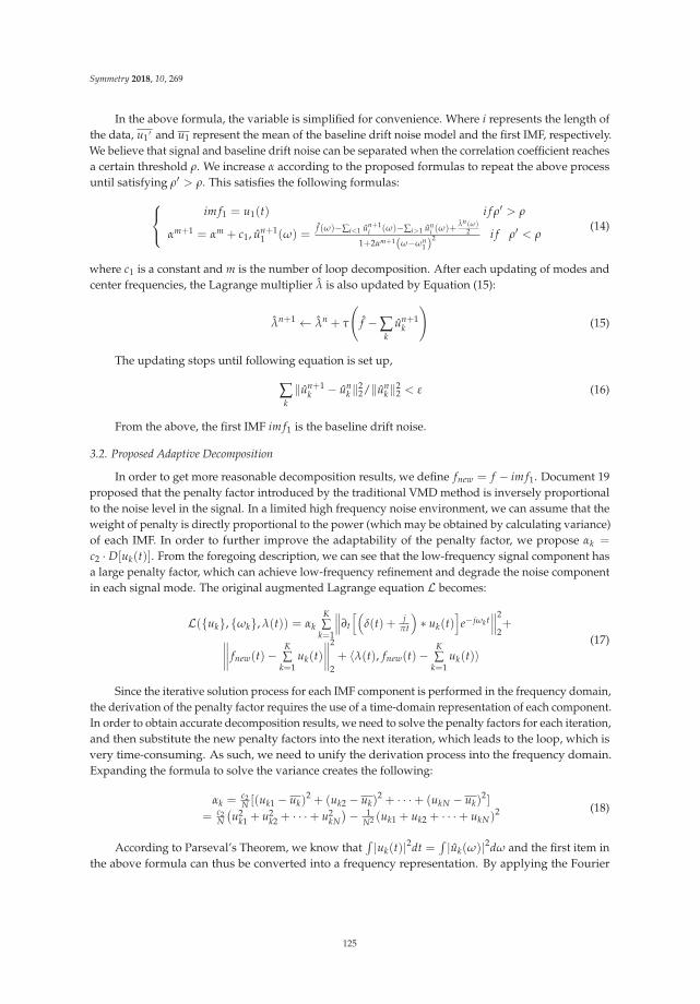
Symmetry 2018, 10, 269

In the above formula, the variable is simplified for convenience. Where i represents the length ofthe data, u1

′ and u1 represent the mean of the baseline drift noise model and the first IMF, respectively.We believe that signal and baseline drift noise can be separated when the correlation coefficient reachesa certain threshold ρ. We increase α according to the proposed formulas to repeat the above processuntil satisfying ρ′ > ρ. This satisfies the following formulas:⎧⎨⎩

im f1 = u1(t) i f ρ′ > ρ

αm+1 = αm + c1, un+11 (ω) =

f (ω)−∑i<1 un+1i (ω)−∑i>1 un

i (ω)+λn(ω)

2

1+2αm+1(ω−ωn1 )

2 i f ρ′ < ρ(14)

where c1 is a constant and m is the number of loop decomposition. After each updating of modes andcenter frequencies, the Lagrange multiplier λ is also updated by Equation (15):

λn+1 ← λn + τ

(f − ∑

kun+1

k

)(15)

The updating stops until following equation is set up,

∑k‖un+1

k − unk ‖2

2/‖unk ‖2

2 < ε (16)

From the above, the first IMF im f1 is the baseline drift noise.

3.2. Proposed Adaptive Decomposition

In order to get more reasonable decomposition results, we define fnew = f − im f1. Document 19proposed that the penalty factor introduced by the traditional VMD method is inversely proportionalto the noise level in the signal. In a limited high frequency noise environment, we can assume that theweight of penalty is directly proportional to the power (which may be obtained by calculating variance)of each IMF. In order to further improve the adaptability of the penalty factor, we propose αk =

c2 · D[uk(t)]. From the foregoing description, we can see that the low-frequency signal component hasa large penalty factor, which can achieve low-frequency refinement and degrade the noise componentin each signal mode. The original augmented Lagrange equation L becomes:

L({uk}, {ωk}, λ(t)) = αkK∑

k=1

∥∥∥∂t

[(δ(t) + j

πt

)∗ uk(t)

]e−jωkt

∥∥∥2

2+∥∥∥∥ fnew(t)−

K∑

k=1uk(t)

∥∥∥∥2

2+ 〈λ(t), fnew(t)−

K∑

k=1uk(t)〉

(17)

Since the iterative solution process for each IMF component is performed in the frequency domain,the derivation of the penalty factor requires the use of a time-domain representation of each component.In order to obtain accurate decomposition results, we need to solve the penalty factors for each iteration,and then substitute the new penalty factors into the next iteration, which leads to the loop, which isvery time-consuming. As such, we need to unify the derivation process into the frequency domain.Expanding the formula to solve the variance creates the following:

αk =c2N [(uk1 − uk)

2 + (uk2 − uk)2 + · · ·+ (ukN − uk)

2]

= c2N(u2

k1 + u2k2 + · · ·+ u2

kN)− 1

N2 (uk1 + uk2 + · · ·+ ukN)2 (18)

According to Parseval’s Theorem, we know that∫ |uk(t)|2dt =

∫ |uk(ω)|2dω and the first item inthe above formula can thus be converted into a frequency representation. By applying the Fourier

125

Symmetry 2018, 10, 269

transform of the second term to the above formula, we can get the frequency–domain description ofpenalty factor:

αk = c2N∫ ∞

0 |uk(ω)|2dω − 2πuk2(0)

2πN2 (19)

where c2 is a constant and N is the length of the data. Combine the penalty factor into the previousupdate formulas, we can get the new update formulas for uk(ω), ωk and αk:⎧⎪⎪⎪⎪⎪⎨⎪⎪⎪⎪⎪⎩

un+1k (ω) =

fnew(ω)−∑i<k un+1i (ω)−∑i>k un

i (ω)+λn(ω)

2

1+2αnk (ω−ωn

k )2

ωn+1k =

∫ ∞0 ω|uk(ω)|2dω∫ ∞

0 |uk(ω)|2dω

αn+1k = c2

N∫ ∞

0 |uk(ω)|2dω−2πuk2(0)

2πN2

(20)

The Lagrange multiplier update formula and iteration stop criterion remain unchanged.

3.3. Iterative Thresholding and Improved VMD Method

In this section, we obtain a new denoising process by combining the interval threshold and theimproved variational mode decomposition. In this paper, the hard and soft thresholding methods,with multiples of Donoho-Johnstone threshold known as universal threshold parameters, are proposed,in order to cut off each IMF after performing the improved VMD. The threshold parameters aredefined as:

Tk = Cmedian(|uk(t)− median(uk(t))|)

0.6745

√2 ln N (21)

where C is a constant and N is the length of the data. It is necessary to adopt a scale dependentthreshold for each IMF instead of an identical universal threshold for all IMFs. The values of thescaling factor C are the range [0.6, 1.2]. We use the interval thresholding (IT) method to alleviate thecatastrophic consequences caused by the direct application of thresholding. In this method, the firststep is to find the zero points of each IMF. The second step is to compare the threshold and theextremum between two zero crossing intervals; if the extremum exceeds the threshold, it will allow allof the samples within the interval to be retained. The interval thresholding can be represented as:

ck

(Zk

i

)=

⎧⎨⎩ ck

(Zk

i

),

∣∣∣ck

(rk

i

)∣∣∣ > Tk

0∣∣∣ck

(rk

i

)∣∣∣ ≤ Tk(22)

where i varies from 1 to Nk, Nk indicates the number of zero crossings of the kth IMF, ck

(rk

i

)indicates

the sample at the time instance rki between the two successive zero points at Zk

i and Zki+1, and ck

(Zk

i

)refers to the samples from the instant Zk

i to Zki+1 of the kth IMF.

Summarizing this denoising process as follows: First, the MCG signal with noise is decomposedinto corresponding IMFs by improved VMD. The first order IMF, including the baseline drift noise,is eliminated. Second, the interval thresholding is performed on the rest IMFs. Clearly, the higher theorder, the greater the frequency of the IMF. The detailed procedures are as follows:

1. Acquire the MCG signal with noise and initialize the number of modes k, the default of thepenalty factor α is 2000, the default of the bandwidth τ is 0.

2. Determine the value of penalty factor by performing the improved VMD method based on thecorrelation coefficient and obtain the first IMF.

3. Eliminate the first IMF that contains baseline drift noise. Decompose the rest signal with the finalupdate formulas and obtain several IMFs.

4. Perform the interval thresholding operation on the IMFs obtained from step 3.5. Add all the processed IMFs together and refactor the MCG signal.

126

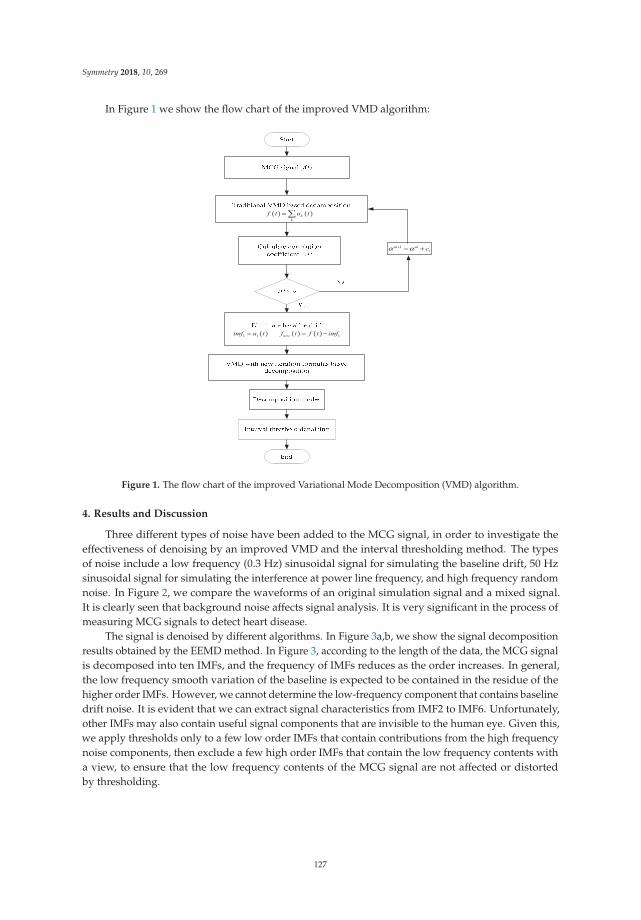
Symmetry 2018, 10, 269

In Figure 1 we show the flow chart of the improved VMD algorithm:

( ) ( )kk

f t u t=

m m cα α+ = +

( ) ( ) ( )newimf u t f t f t imf= = −

Figure 1. The flow chart of the improved Variational Mode Decomposition (VMD) algorithm.

4. Results and Discussion

Three different types of noise have been added to the MCG signal, in order to investigate theeffectiveness of denoising by an improved VMD and the interval thresholding method. The typesof noise include a low frequency (0.3 Hz) sinusoidal signal for simulating the baseline drift, 50 Hzsinusoidal signal for simulating the interference at power line frequency, and high frequency randomnoise. In Figure 2, we compare the waveforms of an original simulation signal and a mixed signal.It is clearly seen that background noise affects signal analysis. It is very significant in the process ofmeasuring MCG signals to detect heart disease.

The signal is denoised by different algorithms. In Figure 3a,b, we show the signal decompositionresults obtained by the EEMD method. In Figure 3, according to the length of the data, the MCG signalis decomposed into ten IMFs, and the frequency of IMFs reduces as the order increases. In general,the low frequency smooth variation of the baseline is expected to be contained in the residue of thehigher order IMFs. However, we cannot determine the low-frequency component that contains baselinedrift noise. It is evident that we can extract signal characteristics from IMF2 to IMF6. Unfortunately,other IMFs may also contain useful signal components that are invisible to the human eye. Given this,we apply thresholds only to a few low order IMFs that contain contributions from the high frequencynoise components, then exclude a few high order IMFs that contain the low frequency contents witha view, to ensure that the low frequency contents of the MCG signal are not affected or distortedby thresholding.

127

Symmetry 2018, 10, 269

(a) (b)

Figure 2. A comparison of the approximately pure magnetocardiography (MCG) signal with the noisysignal; waveform characteristics can be clearly seen in (a); (b) shows the signal waveform with threekinds of noise. The signal is drowned in the noise under high noise circumstances.

(a) (b)

Figure 3. The noisy signal and the intrinsic mode functions (IMFs) obtained by Ensemble EmpiricalMode Decompositioning (EEMD) are shown in (a,b).

In Figure 4, we compare the original signal with the reconstructed signals obtained from EEMDbased denoising methods using soft and hard thresholding. The results show that the hard thresholdprocessing can reconstruct the QRS peak waves, but there are obvious errors in the reconstruction ofother signal parts. The signal obtained by soft thresholding processing has errors compared with theoriginal signal, especially the QRS peaks. It is seen from Figure 4 that EEMD algorithm is difficultto distinguish noise components from signal components. And the number of low frequency IMFsis too many to result in waveform distortion after performing thresholding operation. It may alsobe noted that, hard-IT (hard thresholding subsequently interval thresholding) is adopted for EEMDbased denoising of the experimental data. At the same time, we can see that the signal waveform isnot smooth and slightly distorted.

Based on the bandwidth of the measurement signal and multiple tests, the number of modesdecomposed by VMD is assigned to 6. The original algorithm proposer studied some of theconvergence characteristics of the VMD algorithm and its sensitivity to the initial conditions, then gotrelatively suitable initialization parameters. The initial value of quadratic penalty α is assigned to2000, and the default of the bandwidth τ is 0. With this method, the MCG signal is divided intoseveral frequency bands centering on respective center frequency, which benefits subsequent operation.As shown in Figure 5a, the MCG signal is divided into six IMFs. The baseline drift noise is found

128

Symmetry 2018, 10, 269

in IMF1. In Figure 5b, we compare the original signal with the reconstructed signals obtained fromVMD methods with soft and hard thresholding. The results show that the baseline of the reconstructedsignal is not uniform with the original signal. To make matters worse, there is serious distortion inthe reconstructed signal from the soft thresholding processing. It is obvious that the algorithm cannoteffectively remove baseline drift noise. The decomposition process of the algorithm lacks of adaptability.Improper decomposition results can easily lead to waveform distortion after threshold processing.

To get a better result, we use the proposed method to decompose the signal. According to manyexperiments, we choose the parameter value with better effect as the next simulation initial values.The threshold value ρ of correlation coefficient is assigned as 0.95. The value of the scaling factorc1 is the range 1500 and 2000. The value of c2 can be set according to the detailed data features andis assigned as 3.5. As Figure 6 shown, the baseline noise is extracted. After removing the noise,the signal is divided into six modes adaptively. According to iterative formulas for multiple iterations,the penalty factors for six components are [1790, 987, 956, 218, 223, 208]. The decomposition results areshown in Figure 7a and the denoising results are shown in Figure 7b.

Figure 4. A comparison of the original signal (dotted line) with the reconstructed signals (solid line)obtained from EEMD based denoising methods with soft and hard thresholding. The panelabove is the result of hard thresholding processing and the following panel is the result of softthresholding processing.

129

Symmetry 2018, 10, 269

(a) (b)

Figure 5. The noisy signal and the IMFs obtained from VMD are shown in (a). A comparison ofthe original signal (dotted line) with the reconstructed signals (solid line) obtained from VMD baseddenoising methods with soft and hard thresholding is shown in (b). The panel above is the result ofhard thresholding processing and the following panel is the result of soft thresholding processing.

The range of the value of the penalty factors can support the adaptive decomposition result.From this result, it can be seen that the low-frequency IMF’s penalty factors are large, and the penaltyfactor increases approximately with the increasing of the center frequency, achieving the purpose ofthe meticulous decomposition of low-frequency signal component. In addition, we can obtain a set ofdifferent penalty factors by adjusting the size of c2 to adjust the decomposition result. By comparingthe reconstructed signal with the original signal, we can find that the fitting degree between thereconstructed signal and the original signal is good, and all three kinds of noise in the signal areeffectively removed. It may also be noted that, signal to noise ratio improvement is much better of thehard interval thresholding (IT) method compared to the soft interval thresholding.

In order to better compare the performance of the algorithms, we use the root-mean-square error(the square root of the mean of the sum of squared residuals, RMSE) to characterize the fitting degreeof the reconstructed signal and the original signal. In Figure 8, we compare the root-mean-squaredeviation (RMSE) of the three methods with the input signal-to-noise ratio (SNR). In the case of lowinput SNR, the RMSE of the improved VMD method is significantly less than the other two methods,and the method has better denoising performance even with the low input SNR.

Figure 6. The first IMF obtained from the improved VMD method (solid line) and baseline drift noise(dotted line). It is seen that the solid line and the dotted line basically coincide. This method caneffectively remove baseline drift noise.

130

Symmetry 2018, 10, 269

(a) (b)

Figure 7. (a) The noisy signal and the IMFs obtained from the improved VMD method; (b) Acomparison of the original signal (dotted line) with the reconstructed signals (solid line) obtainedfrom the improved VMD method with soft and hard thresholding for interval thresholding. The panelabove is the result of hard thresholding processing and the following panel is the result of softthresholding processing.

Figure 8. The root-mean-square deviation (RMSE) of the EEMD, the VMD, and the improved VMDmethods are revealed, for both soft and hard thresholding of interval thresholding. The improvedVMD method outperforms other methods.

In Figure 9, we compare the performance of the original VMD method, the improved VMDmethod, and the EEMD methods, using soft and hard thresholding in each case. For computing SNR,the logarithmic ratio of variance of a signal (from the beginning of P-wave to the end of T-wave for onecardiac cycle) to the variance of noise (from the end of T-wave to the beginning of P-wave, i.e., in theTP interval) has been taken. The reduction in the SNR for the soft thresholding method is due to thereduction of signal components of the lower frequency IMFs. Hereafter, hard-IT (hard thresholdingis subsequently applied to the interval thresholds) is appropriate for both EEMD and VMD baseddenoising of the experimental data. It is seen from Figure 9 that the improved VMD method is capableof achieving better SNR when compared with EEMD and VMD methods.

131

Symmetry 2018, 10, 269

From the above simulation results, we can see that the proposed algorithms have betterdenoising performance compared with EEMD and VMD methods. It should be noted, however,that the waveform is still distorted, even by the proposed method; this is a crucial detail inelectrocardiographic-like signals. One encouraging factor, is that results of medical research haveshown that the QRS spikes and S-T waves contain information on the main electrical functionparameters of the heart. The MCG signal is filtered by the algorithm proposed in this paper, in orderto obtain QRS spikes and S-T waves that approximate the original signal. Although there are slightdisturbances in the QRS spikes and S-T waves obtained by filtering, it does not affect the calculation ofheart related parameters! Measurements of magnetic field energy and current density remain accurate).In the case of the low input signal-to-noise ratio used in this paper, the SNR improvement of theproposed algorithm can be up to 20 dB. The algorithm filtering results can support feature extractionof MCG and detection of heart disease.

Figure 9. The variation of the output signal-to-noise ratio (SNR) by EEMD, VMD and the improvedVMD methods with soft and hard thresholds for interval thresholding. The improved VMD methodoutperforms other methods.

Despite these positive results, the MCG signals measured in a clinical non-magnetic shieldingenvironment would still contain a large amount of background noise, which would still cause thewaveform, denoised by the improved VMD method proposed in this paper, to produce severedistortion. In order to solve this problem, we need to study the spatial filtering technology in order tofurther denoise the MCG signal, in efforts to achieve the purpose of joint filtering in the time domain,frequency domain, and space domain.

5. Conclusions

The proposed method in this paper overcomes the unadaptable quadratic penalty problem ofVMD, which improves the availability and precision of denoising of the MCG signal. This methodadaptively adjusts the bandwidth of modes by repeatedly executing the VMD method with differentquadratic penalties. The low-frequency noise is eliminated, according to the correlation coefficientfor baseline drift noise, and the first mode. The new update formulas are used to decompose residualsignals adaptively. Then, threshold processing is performed on each IMF to eliminate other noise.The simulation experiments show the superiority of the improved VMD in denoising performanceof the MCG signal. The acceleration of the proposed method, and the suitable signal preprocessingmethods, should be considered in future research and applications.

132

Symmetry 2018, 10, 269

Author Contributions: Conceptualization, Y.L. and Q.G.; Methodology, C.H.; Software, C.H.; Validation, Y.L. andQ.G.; Writing—original draft, C.H.; Writing—review & editing, Y.L. and C.H.

Funding: This work is supported partially by the National Key Research and Development Program of China(2016YFC0101700), by National Natural Science Foundation of China 61301201 and 61371175, HeilongjiangPostdoctoral Research Foundation LBH-Q14039.

Acknowledgments: The authors are grateful to the anonymous referees for their valuable comments andsuggestions that improved this paper.

Conflicts of Interest: The authors declare no conflicts of interest.

References

1. Mäkijärvi, M.; Montonen, J.; Toivonen, L. Identification of patients with ventricular tachycardia aftermyocardial infarction by high-resolution magnetocardiography and electrocardiography. J. Electrocardiol.1993, 26, 117–124. [CrossRef]

2. Shanehsazzadeh, F.; Fardmanesh, M. Low Noise Active Shield for SQUID-Based MagnetocardiographySystems. IEEE Trans. Appl. Supercond. 2017, 99, 1–5. [CrossRef]

3. Farré, J.; Shenasa, M. Medical Education in Electrocardiography. J. Electrocardiol. 2017, 50, 400–401. [CrossRef][PubMed]

4. Fenici, R.; Brisinda, D. Magnetocardiography provides non-invasive three-dimensional electroanatomicalimaging of cardiac electrophysiology. Anatol. J. Cardiol. 2006, 22, 595. [CrossRef] [PubMed]

5. Ha, T.; Kim, K.; Lim, S. Three-Dimensional Reconstruction of a Cardiac Outline by Magnetocardiography.IEEE Trans. Biomed. Eng. 2015, 62, 60–69. [CrossRef] [PubMed]

6. Mariyappa, N.; Parasakthi, C.; Sengottuvel, S. Dipole location using SQUID based measurements:Application to magnetocardiography. Phys. C Supercond. 2012, 477, 15–19. [CrossRef]

7. Tiporlini, V.; Alameh, K. Optical Magnetometer Employing Adaptive Noise Cancellation for UnshieldedMagnetocardiography. Univ. J. Biomed. Eng. 2013, 1, 16–21. [CrossRef]

8. Kim, K.; Lee, Y.H.; Kwon, H. Averaging algorithm based on data statistics in magnetocardiography.Neurol. Clin. Neurophysiol. 2004, 2004, 42. [PubMed]

9. Dang-Ting, L.; Ye, T.; Yu-Feng, R.; Hong-Wei, Y.; Li-Hua, Z.; Qian-Sheng, Y.; Geng-Hua, C. A novel filterscheme of data processing for SQUID-based Magnetocardiogram. Chin. Phys. Lett. 2008, 25, 2714–2717.[CrossRef]

10. Tiporlini, V.; Nguyen, N.; Alameh, K. Adaptive noise canceller for magnetocardiography. InProceedings of the High Capacity Optical Networks and Enabling Technologies, Riyadh, Saudi Arabia,19–21 December 2011; pp. 359–363.

11. Dong, Y.; Shi, H.; Luo, J. Application of Wavelet Transform in MCG-signal Denoising. Mod. Appl. Sci. 2010, 4,20. [CrossRef]

12. Huang, N.E.; Shen, Z.; Long, S.R.; Wu, M.C.; Shih, H.H.; Zheng, Q.; Yen, N.C.; Tung, C.C.; Liu, H.H. Theempirical mode decomposition and the Hilbert spectrum for nonlinear and non-stationary time seriesanalysis. Proc. R. Soc. Lond. A 1998, 454, 903–995. [CrossRef]

13. Attoh-Okine, N.; Barner, K.; Bentil, D.; Zhang, R. Editorial: The empirical mode decomposition and thehilbert-huang transform. EURASIP J. Adv. Signal Process. 2008. [CrossRef]

14. Wu, Z.; Huang, N.E. Ensemble empirical mode decomposition method: A noise-assisted data analysismethod. Adv. Adapt. Data Anal. 2009, 1, 1–41. [CrossRef]

15. Tong, W.; Zhang, M.; Yu, Q. Comparing the applications of EMD and EEMD on time–frequency analysis ofseismic signal. J. Appl. Geoph. 2012, 83, 29–34.

16. Mariyappa, N.; Sengottuvel, S.; Parasakthi, C. Baseline drift removal and denoising of MCG data usingEEMD: Role of noise amplitude and the thresholding effect. Med. Eng. Phys. 2014, 36, 1266–1276. [CrossRef][PubMed]

17. Mariyappa, N.; Sengottuvel, S.; Patel, R. Denoising of multichannel MCG data by the combination of EEMDand ICA and its effect on the pseudo current density maps. Biomed. Signal Process. Control. 2015, 18, 204–213.[CrossRef]

18. Smruthy, A.; Suchetha, M. Real-Time Classification of Healthy and Apnea Subjects Using ECG Signals WithVariational Mode Decomposition. IEEE Sens. J. 2017, 17, 3092–3099. [CrossRef]

133

Symmetry 2018, 10, 269

19. Dragomiretskiy, K.; Zosso, D. Variational Mode Decomposition. IEEE Trans. Signal Process. 2014, 62, 531–544.[CrossRef]

20. Sun, Z.G.; Lei, Y.; Wang, J. An ECG signal analysis and prediction method combined with VMD and neuralnetwork. In Proceedings of the IEEE International Conference on Electronics Information and EmergencyCommunication, Macau, China, 21–23 July 2017; pp. 199–202.

21. Maji, U.; Pal, S. Empirical mode decomposition vs. variational mode decomposition on ECG signalprocessing: A comparative study. In Proceedings of the International Conference on Advances in Computing,Communications and Informatics, Jaipur, India, 21–24 September 2016; pp. 1129–1134.

22. Mert, A. ECG signal analysis based on variational mode decomposition and bandwidth property.In Proceedings of the IEEE Signal Processing and Communication Application Conference, Zonguldak,Turkey, 16–19 May 2016; pp. 1205–1208.

23. Viswanath, A.; Jose, K.J.; Krishnan, N. Spike Detection of Disturbed Power Signal Using VMD .Procedia Comput. Sci. 2015, 46, 1087–1094. [CrossRef]

24. Kopsinis, Y.; Mclaughlin, S. Development of EMD-Based Denoising Methods Inspired by WaveletThresholding. IEEE Trans. Signal Process. 2009, 57, 1351–1362. [CrossRef]

25. Daubechies, I.; Lu, J.; Wu, H.T. Synchrosqueezed wavelet transforms: An empirical mode decomposition-liketool. Appl. Comput. Harmonic Anal. 2011, 30, 243–261. [CrossRef]

26. Gilles, J. Empirical Wavelet Transform. IEEE Trans. Signal Process. 2013, 61, 3999–4010. [CrossRef]27. Unser, M.; Sage, D.; Van, D.V.D. Multiresolution monogenic signal analysis using the Riesz-Laplace wavelet

transform. IEEE Trans. Image Process. 2009, 18, 2402–2418. [CrossRef] [PubMed]28. Bertsekas, D.P. Multiplier methods: A survey. Automatica 1976, 12, 133–145. [CrossRef]29. Hestenes, M.R. Multiplier and gradient methods. J. Optim. Theory Appl. 1969, 4, 303–320. [CrossRef]30. Rockafellar, R.T. A dual approach to solving nonlinear programming problems by unconstrained

optimization. Math. Program. 1973, 5, 354–373. [CrossRef]31. Boley, D. Local Linear Convergence of the Alternating Direction Method of Multipliers on Quadratic or

Linear Programs. Siam J. Optim. 2013, 23, 2183–2207. [CrossRef]


134

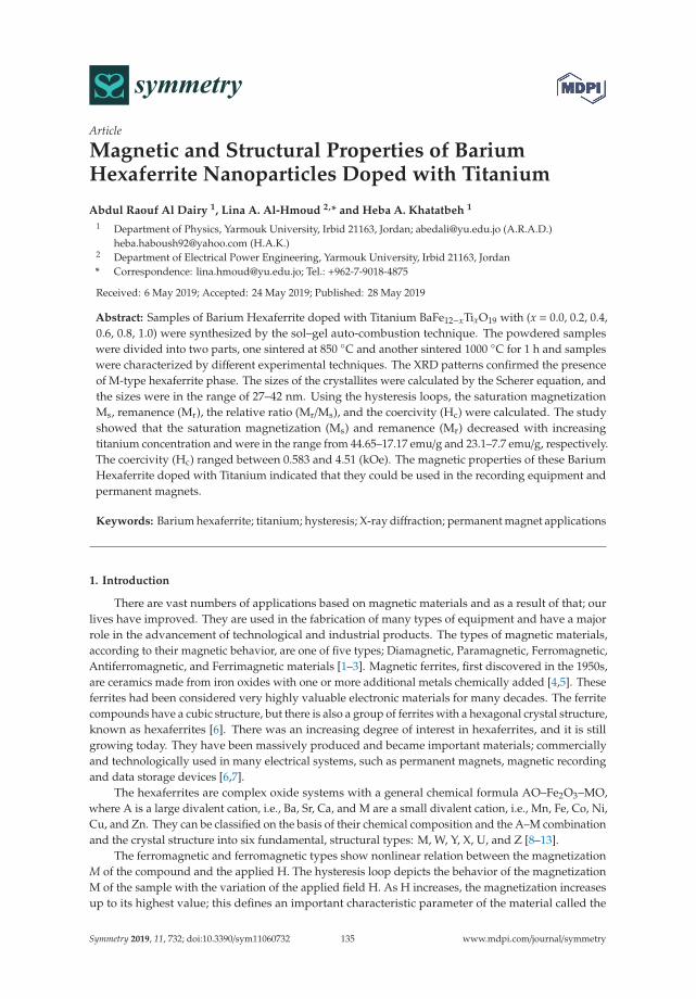
symmetryS S

Article

Magnetic and Structural Properties of BariumHexaferrite Nanoparticles Doped with Titanium

Abdul Raouf Al Dairy 1, Lina A. Al-Hmoud 2,* and Heba A. Khatatbeh 1

1 Department of Physics, Yarmouk University, Irbid 21163, Jordan; [email protected] (A.R.A.D.)[email protected] (H.A.K.)

2 Department of Electrical Power Engineering, Yarmouk University, Irbid 21163, Jordan* Correspondence: [email protected]; Tel.: +962-7-9018-4875

Received: 6 May 2019; Accepted: 24 May 2019; Published: 28 May 2019

Abstract: Samples of Barium Hexaferrite doped with Titanium BaFe12−xTixO19 with (x = 0.0, 0.2, 0.4,0.6, 0.8, 1.0) were synthesized by the sol–gel auto-combustion technique. The powdered sampleswere divided into two parts, one sintered at 850 ◦C and another sintered 1000 ◦C for 1 h and sampleswere characterized by different experimental techniques. The XRD patterns confirmed the presenceof M-type hexaferrite phase. The sizes of the crystallites were calculated by the Scherer equation, andthe sizes were in the range of 27–42 nm. Using the hysteresis loops, the saturation magnetizationMs, remanence (Mr), the relative ratio (Mr/Ms), and the coercivity (Hc) were calculated. The studyshowed that the saturation magnetization (Ms) and remanence (Mr) decreased with increasingtitanium concentration and were in the range from 44.65–17.17 emu/g and 23.1–7.7 emu/g, respectively.The coercivity (Hc) ranged between 0.583 and 4.51 (kOe). The magnetic properties of these BariumHexaferrite doped with Titanium indicated that they could be used in the recording equipment andpermanent magnets.

Keywords: Barium hexaferrite; titanium; hysteresis; X-ray diffraction; permanent magnet applications

1. Introduction

There are vast numbers of applications based on magnetic materials and as a result of that; ourlives have improved. They are used in the fabrication of many types of equipment and have a majorrole in the advancement of technological and industrial products. The types of magnetic materials,according to their magnetic behavior, are one of five types; Diamagnetic, Paramagnetic, Ferromagnetic,Antiferromagnetic, and Ferrimagnetic materials [1–3]. Magnetic ferrites, first discovered in the 1950s,are ceramics made from iron oxides with one or more additional metals chemically added [4,5]. Theseferrites had been considered very highly valuable electronic materials for many decades. The ferritecompounds have a cubic structure, but there is also a group of ferrites with a hexagonal crystal structure,known as hexaferrites [6]. There was an increasing degree of interest in hexaferrites, and it is stillgrowing today. They have been massively produced and became important materials; commerciallyand technologically used in many electrical systems, such as permanent magnets, magnetic recordingand data storage devices [6,7].

The hexaferrites are complex oxide systems with a general chemical formula AO–Fe2O3–MO,where A is a large divalent cation, i.e., Ba, Sr, Ca, and M are a small divalent cation, i.e., Mn, Fe, Co, Ni,Cu, and Zn. They can be classified on the basis of their chemical composition and the A–M combinationand the crystal structure into six fundamental, structural types: M, W, Y, X, U, and Z [8–13].

The ferromagnetic and ferromagnetic types show nonlinear relation between the magnetizationM of the compound and the applied H. The hysteresis loop depicts the behavior of the magnetizationM of the sample with the variation of the applied field H. As H increases, the magnetization increasesup to its highest value; this defines an important characteristic parameter of the material called the


Symmetry 2019, 11, 732

saturation magnetization Ms at high enough applied fields. The value of the field needed to reach thesaturation magnetization depends on the nature of the material, method of preparation, and otherintrinsic and extrinsic parameters. The magnetization retains a value even at zero applied fields calledthe remnant magnetization or the remanence Mr. This parameter has particular importance in the caseof permanent magnets production because it defines the magnetization of a magnet in the absenceof an applied external field. The size of the opposite field needed to reduce M to zero is called thecoercivity Hc. The value of the coercive field, the coercivity, defines the so-called magnetic hardness ofthe magnetic material [14].

Many research groups prepared these ferrites and investigated the effect of the dopants on themagnetic properties of such M-type magnetic hexaferrites [15–33]. The hexaferrites are of great interestfor applications in the microwave technology and others. S.V. Trukhanov et al. studied the effect ofgallium doping on the properties of barium hexaferrite, BaFe12-xGaxO19 (x ≤ 1.2), prepared by theceramic technology method [34,35]. They showed that the unit cell monotonically decreases withincreasing x and these Ga doped hexaferrites can effectively absorb high-frequency electromagneticradiation. The maximum of the real part of permeability depends on the level of substitution bytitanium cations and it is located in the region of 5–6 GHz. For gallium-substituted hexaferrites, thereal part of permittivity decreases more slowly at low frequencies and almost monotonically withconcentration. In last case, the real and imaginary parts of the permeability have a peak in the region of49–51 GHz, which is determined by the level of diamagnetic substitution. Researchers have prepared(BaFe11.9Al0.1O19)1−x(BaTiO3)x with x = 0. 0.25, 0.5, 0.75, and 1 bicomponent compounds using theceramic technique [36]. The researchers reported that these hexaferrites exhibited ferroelectricity at roomtemperature and the coercive field was lower due to the contribution of the microstructure-dependentshape anisotropy to the magnetic anisotropy energy and the behavior of these samples was discussedbased on the grain size, density, and porosity. The magnetic and dipole moments in BaFe12-xInxO19

hexaferrites were studied by S. V. Trukhanov group [37]. These indium doped samples were preparedby solid reaction method as published by coworkers of the same group before [38]. The samples werestudied by high resolution neutron powder diffraction and vibrating sample magnetometry in thetemperature range of 4–730 K. They showed that spontaneous polarization was established due to thedisplacement of Fe3+(In3+) cations and the appearance of nonzero electric dipole moment, which causesthe formation of the z-component of the spontaneous polarization. The crystal structure and magneticproperties of BaFe12-xMexO19 (Me = In3+ or Ga3+ and x = 0.1–1.2) solid solutions were studied usingthe time–of–flight neutron diffraction method [39]. The workers reported that the electric field–inducedpolarization was observed in these barium hexaferrite solid solutions at room temperature. Using theGorter’s model, the researchers found that the magnetic moments of iron ions were oriented alongthe hexagonal axis which is the easy axis of magnetization. The previously mentioned works of S.V.Trukhanov and co-workers proved that the magnetoelectric characteristics of M-type hexaferritesfabricated by a modified ceramic technique can be more advanced than those for the well-known roomtemperature BiFeO3 orthoferrite multiferroic.

The main goal of this project was to study the effect of Titanium substitution on the magnetic andstructural properties of the barium hexaferrites prepared according to the formula BaFe11.9TixO19 withx = 0.0, 0.2, 0.4, 0.6, 0.8, 1.0.

2. Experimental Techniques

A number of ferrite samples BaFe12-xTixO19 with (x = 0.0, 0.2, 0.4, 0.6, 0.8, 1.0) were prepared byusing the sol-gel auto combustion technique. The chemicals used for the preparation of the sampleswere Fe(NO3)3, Ba(NO3)2, and TiCl3 and were dissolved in 100 ml of de-ionized water. Citric acid wasadded to the solution, and the molar ratio for the metallic mixture to acid was kept at 3:1 [33]. Using ahot plate and continuous stirring, the solution was heated up to a temperature of 80 ◦C. A solution ofammonia was added to the mixture to reach a pH value of 8.0. The solution was then heated slowly to450 ◦C for several hours until a viscous brown gel mixture is formed. The gel was heated further to a

136

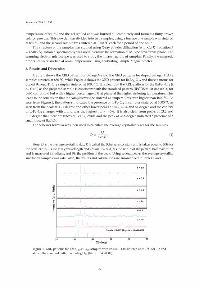
Symmetry 2019, 11, 732

temperature of 550 ◦C and the gel ignited and was burned out completely and formed a fluffy browncolored powder. This powder was divided into two samples, using a furnace one sample was sinteredat 850 ◦C and the second sample was sintered at 1000 ◦C each for a period of one hour.

The structure of the samples was studied using X-ray powder diffraction (with Cu-Kα radiation λ

= 1.5405 Å). Infrared spectroscopy was used to ensure the formation of M-type hexaferrite phase. Thescanning electron microscope was used to study the microstructure of samples. Finally, the magneticproperties were studied at room temperature using a Vibrating Sample Magnetometer.

3. Results and Discussion

Figure 1 shows the XRD pattern for BaFe12O19 and the XRD patterns for doped BaFe12-xTixO19

samples sintered at 850 ◦C, while Figure 2 shows the XRD pattern for BaFe12O19 and those patterns fordoped BaFe12-xTixO19 samples sintered at 1000 ◦C. It is clear that the XRD pattern for the BaFe12O19 (i.e., x = 0) as the prepared sample is consistent with the standard pattern (JPCDS #: 00-043-0002) forBaM compound but with a higher percentage of that phase at the higher sintering temperature. Thisleads to the conclusion that the samples must be sintered at temperatures even higher than 1000 ◦C. Asseen from Figure 2, the patterns indicated the presence of α-Fe2O3 in samples sintered at 1000 ◦C asseen from the peak at 33.1 degree and other lower peaks at 24.2, 49.4, and 54 degree and the contentof α-Fe2O3 changes with x and was the highest for x = 0.6. It is also clear from peaks at 53.2 and61.8 degree that there are traces of FeTiO3 oxide and the peak at 28.8 degree indicated a presence of asmall trace of BaTiO3.

The Scherrer formula was then used to calculate the average crystallite sizes for the samples:

D =kλβ cosθ

. (1)

Here, D is the average crystallite size, K is called the Scherrer's constant and is taken equal to 0.89 forthe hexaferrite, λis the x-ray wavelength and equals1.5405 Å, βis the width of the peak at half maximumand is measured in radians, and θis the position of the peak. Using several peaks, the average crystallitesize for all samples was calculated; the results and calculations are summarized in Tables 1 and 2.

Figure 1. XRD patterns for BaFe12-xTixO19 samples with (x = 0.0–1.0) sintered at 850 ◦C for 1 h andshown the standard pattern of BaFe12O19 (file no.: 043-0002).

137

Symmetry 2019, 11, 732

Figure 2. XRD patterns BaFe12-xTixO19 samples with (x = 0.0–1.0) sintered at 1000 ◦C for 1 h and shownthe standard XRD pattern of BaFe12O19 (file no.: 043-0002).

The average crystallite sizes were found to be in the range of (27–36) nm for samples sinteredat 850 ◦C, and the average crystallite sizes for samples sintered at 1000 ◦C were found to be in therange of (35–41.5) nm. This may lead us to conclude that Ti substitution improved the BaM phasecrystallinity especially at the sintering temperature of 1000 ◦C.

Table 1. The calculated average crystallite sizes for the system BaFe12-xTixO19 with (x = 0.0–1.0) sinteredat T = 850 ◦C.

Sample(2θ)-Position

(Degrees)Size(nm)

Average Size(nm)

BaFe12O19

(x = 0.0)

32.19 24.8

27.234.14 29.337.1 29.6

40.33 2755.1 25.3

BaFe11.8Ti0.2O19

(x = 0.2)

33.1 27.3

30.335.67 3349.51 25.454.1 35.3

BaFe11.6Ti0.4O19

(x = 0.4)

33.3 34.1

3435.8 35.9

49.65 33.354.26 32.7

BaFe11.4Ti0.6O19

(x = 0.6)

33.31 39

36.535.79 4149.69 34.654.24 31.5

BaFe11.2Ti0.8O19

(x= 0.8)

33.39 34.2

3435.86 35.949.7 33.354.3 32.7

BaFe11.0Ti1.0O19

(x = 1.0)

33.31 39

36.335.69 41.349.54 34.654.15 30.4

138

Symmetry 2019, 11, 732

Table 2. The calculated average crystallite sizes for the system BaFe12-xTixO19 with (x = 0.0–1.0) sinteredat T = 1000 ◦C.

Sample(2θ)-Position

(Degrees)Size(nm)

Average Size(nm)

BaFe12O19

(x = 0.0)

32.4 30.3

34.934.34 4140.55 36.455.31 31.7

BaFe11.8Ti0.2O19

(x = 0.2)

32.29 38.9

38.734.23 41.140.44 41.955.1 32.8

BaFe11.6Ti0.4O19

(x = 0.4)

32.26 43.1

41.534.22 45.740.42 46.555.19 30.6

BaFe11.4Ti0.6O19

(x = 0.6)

32.29 43

4134.27 45.740.48 39.954.23 35.3

BaFe11.2Ti0.8O19

(x = 0.8)

33.27 45.6

40.534.24 43.340.96 36.554.19 36.7

BaFe11.0Ti1.0O19

(x = 1.0)

33.23 43.1

3835.7 41.3

40.93 32.254.19 35.3

To prove the presence of M-type hexaferrite phase, Infra-Red (IR) analysis was used becausethe IR- spectra can point to its presence. The samples were mixed with 0.05% KBr in order to get anacceptable resolution of the compound bands. IR spectra of the as-prepared samples were obtainedwith a wave number varying between 300 cm−1 to 1000 cm−1 and the results are summarized inFigures 3 and 4 for the two sintering temperatures, respectively.

Figure 3. Infra-Red (IR) spectra of BaFe12-xTixO19 sintered at T = 850 ◦C.

139

Symmetry 2019, 11, 732

1000 900 800 700 600 500 400

x=1.0x=0.8x=0.6

x=0.4

x=0.2x=0.0

T=1000oC

tr

ansm

ittan

ce

wavenumber (cm-1)Figure 4. IR spectra of BaFe12-xTixO19 sintered at T = 1000 ◦C.

As seen from Figures 3 and 4, the IR spectra of the sintered samples have absorption bands atwave numbers in the range 430−590 cm−1, which are characteristic to the formation of ferrites. Thepeaks were clearer for those samples sintered at 1000 ◦C. The peak at about 430 cm−1 is due to bendingof the absorption bands of the metal-oxygen and that at about 590 cm−1 is due stretching of these bands.

Figure 5 shows an SEM image for one of the samples, namely BaFe12-xTixO19 (with x = 0.2),which was sintered at T = 1000 ◦C. It shows that grains are ultrafine and almost have homogeneousdistribution. The image also shows that the platelets have sizes in the range of 200 nm to 500 nm.

Figure 5. SEM image for BaFe12-xTixO19 (x = 0.2) sample sintered at T = 1000 ◦C.

140

Symmetry 2019, 11, 732

Based on X-ray results and IR data, we believe that samples are improved if heat-treated at1000 ◦C.

We studied only magnetic properties for samples sintered at 1000 ◦C. Magnetic measurementswere carried out at room temperature by a VSM with applied field between 0 and 10 kOe. The groupof hysteresis loops (HL) for all samples is shown in Figure 6. The loops do indicate that all the samplesare indeed hard magnetic materials. The values of remanence magnetization and coercive field for eachsample were read directly from graphs of loops. Since it is expected that samples have high magneticanisotropy, we used the law of approach to saturation (LAS) to calculate the saturation magnetization.This is simply found by plotting M versus 1/H2 for values taken from high field region and all samplesgave perfect straight linear graphs. The intercept of that line is equal to the saturation magnetization.

Figure 6. Hysteresis loops for the samples BaFe12-xTixO19 (x = 0.0 − 1.0) sintered at 1000 ◦C.

Table 3 shows summary of the calculated values for the saturation magnetization, the remanencemagnetization, the reduced magnetization, and the coercivity.

Table 3. The saturation magnetization, remanence magnetization, reduced remnant magnetization andcoercive field for the system BaFe12-xTixO19 (x = 0.0–1.0).

x Ms (emu/g) Mr (emu/g) Mrs (emu/g) Hc (kOe)

0.0 44.65 23.0606 0.5165 4.510.2 45.24 19.7474 0.4365 3.45570.4 44.83 19.5835 0.4368 1.65540.6 39.99 12.9342 0.3234 0.5830.8 20.39 9.5829 0.47 1.3851.0 17.17 7.7163 0.4494 1.11455

The saturation magnetization shows inverse relation titanium concentration. The partialsubstitution of Fe by titanium ions in these hexaferrites has affected the values of MS, which dependson the amount of Ti ions diffusing into the BaM crystal in which Ti+3 ions partially replace Fe+3.However, the higher the Ti concentration results in lower Ms because other phases are then formed aswas concluded from XRD data.

Hard ferrites typically have a high value of Mr, which is about 50% of the saturation magnetization(Ms), therefore the reduced remnant magnetization (Mrs = Mr/Ms) must be nearly 0.5, and this is

141

Symmetry 2019, 11, 732

true for samples consisting of single-domains and random orientations of grains [32]. Table 3 showsthat the values of Mrs are very close to 50%. The coercive field, Hc, for the samples varied with Ticoncentration and it ranged between 0.6 and 4.5 kOe as can be seen in Table 3. A plot of Ms and Hc

versus the concentration of titanium is shown in Figure 7.

Figure 7. Saturation magnetization and coercive field versus Ti concentration.

We calculated the average paramagnetic behavior for each sample by approximating the loop bya straight line as shown in Figure 8. Of course, this behavior is correct only for shallow applied fields,but we found that there is a general trend in these samples that can be depicted by the slopes of theselines. Slopes of these lines are listed in Table 4. The slopes are related to the magnetic susceptibilityand increased slowly by increasing the concentration up to x = 0.6 and then decreases to half its valueafter that.

Figure 8. The hysteresis loop for the system BaFe12-xTixO19 (x = 0.2) approximated by a straight line.

142

Symmetry 2019, 11, 732

Table 4. The slope and hysteresis losses (in W) for the system BaFe12-xTixO19 (x = 0.0–1.0).

Concentration (x) Slope Hysteresis Losses (W)

0.0 0.004908 518,5800.2 0.005326 402,7000.4 0.00571 212,1800.6 0.005252 71,9140.8 0.002623 84,9821.0 0.002229 58,080

We also calculated hysteresis losses for each sample and the calculated values are listed in Table 4.It is clear from the values of losses that Ti concentration could be a scaling factor for magnetic energystored when these materials are used in components of electromagnetic devices. This behavior isdisplaced in Figure 9. Losses are significant and almost linear for x < 0.6.

Figure 9. Hysteresis losses (in W) BaFe12-xTixO19 (x = 0.0–1.0) sintered at 1000 ◦C.

4. Conclusions

A group of BaFe12-xTixO19 samples with (x = 0.0–1.0) were prepared by sol-gel-auto combustionmethod and were sintered at 850 ◦C and 1000 ◦C for 1 h in air. The XRD data and IR data analysisconfirmed the presence of M type phase of the hexaferrite in these samples, and the higher sinteringtemperature showed an improvement of crystallinity. The average crystallite size for all samples wasin the range of 27–42 nm. We believe that these are suitable to obtain the reasonable signal to noiseratio when used in a high-density recording medium. The values of saturation magnetization (Ms) andretentivity (Mr) calculated values decreased with increasing the Ti concentration, and this may resultfrom particle size effects. The addition of titanium reduced the saturation magnetization from about 45emu/g down to 17.2 emu/g. The rest of the magnetic properties that include coercivity, remanencemagnetization, reduced remnant magnetization, and hysteresis losses suggest that these materialsare beneficial in the components of electromagnetic devices that are used in recording technologyand permanent magnets. We suggest that further work is needed to study the effect of sinteringtemperatures and very low controlled Ti concentrations. In addition, structural and magnetic studies attemperatures above and below room temperature using other techniques could be of great importance.

Author Contributions: Formal analysis, L.A.A.-H.; Methodology, H.A.K.; Supervision, A.R.A.D. All authorscontribute equally to this manuscript.

Funding: This research received no external funding.

143

Symmetry 2019, 11, 732

Acknowledgments: This research work was supported by the Deanship of Graduate Studies and Research,Yarmouk University, Irbid, Jordan; project 7/2017. We acknowledge the help of Prof. A. Hammoudeh in preparationof samples and IR data.


References

1. Gutfleisch, O.; Willard, M.A.; Bruck, E.; Chen, C.H.; Sankar, S.G.; Liu, J.P. Magnetic materials and devices forthe 21st century: Stronger, lighter, and more energy efficient. Adv. Mater. 2011, 23, 821–842. [CrossRef]

2. Cullity, B.D.; Graham, C.D. Introduction to Magnetic Materials; John Wiley & Sons: New York, NY, USA, 2011.3. Bini, R.A.; Marques, R.F.C.; Santos, F.J.; Chaker, J.A.; Jafelicci, M., Jr. Synthesis and functionalization of

magnetite nanoparticles with different amino-functional alkoxysilanes. J. Magn. Magn. Mater. 2012, 324,534–539. [CrossRef]

4. Cochardt, A. Recent ferrite magnet developments. J. Appl. Phys. 1966, 37, 1112–1115. [CrossRef]5. Sugimoto, M. The past, present, and future of ferrites. J. Am. Ceram. Soc. 1999, 82, 269–280. [CrossRef]6. Pullar, R.C. Hexagonal ferrites: A review of the synthesis, properties and applications of hexaferrite ceramics.

Prog. Mater. Sci. 2012, 57, 1191–1334. [CrossRef]7. Koutzarova, T.; Kolev, S.; Ghelev, C.; Grigorov, K.; Nedkov, I. Structural and magnetic properties and

preparation techniques of nanosized M-type hexaferrite powders. In Advances in Nanoscale Magnetism;Springer: Berlin, Germany, 2009; pp. 183–203.

8. Maswadeh, Y.; Mahmood, S.H.; Awadallah, A.; Aloqaily, A.N. Synthesis and structural characterizationof nonstoichiometric barium hexaferrite materials with Fe:Ba ratio of 11.5–16.16. In IOP Conference Series:Materials Science and Engineering; IOP Publishing Ltd.: Philadelphia, PA, USA, 2015.

9. Radwan, M.; Rashad, M.M.; Hessien, M.M. Synthesis and characterization of barium hexaferrite nanoparticles.J. Mater. Process. Technol. 2007, 181, 106–109. [CrossRef]

10. Martirosyan, K.S.; Galstyan, E.; Hossain, S.M.; Wang, Y.-J.; Litvinov, D. Barium hexaferrite nanoparticles:synthesis and magnetic properties. Mater. Sci. Eng. B 2011, 176, 8–13. [CrossRef]

11. Meng, Y.Y.; He, M.H.; Zeng, Q.; Jiao, D.L.; Shukla, S.; Ramanujan, R.V.; Liu, Z.W. Synthesis of barium ferriteultrafine powders by a sol–gel combustion method using glycine gels. J. Alloy. Compd. 2014, 583, 220–225.[CrossRef]

12. Kouril, K. Local structure of hexagonal ferrites studied by NMR. (2013). Available online: https://www.researchgate.net (accessed on 20 March 2019).

13. Wu, M. M-Type barium hexagonal ferrite films. In Advanced Magnetic MaterialsAdv; InTech Open: LondonUK, 2012.

14. Awadallah, A.M.; Sami, M. Effects of preparation conditions and metal ion substitutions for barium andiron on the properties of M-type barium hexaferrites. Ph.D. Research Proposal, The University of Jordan,Amman, Jordan, 2012. [CrossRef]

15. Zhang, H.; Zeng, D.; Liu, Z. The law of approach to saturation in ferromagnets originating from themagnetocrystalline anisotropy. J. Magn. Magn. Mater. 2010, 322, 2375–2380. [CrossRef]

16. Bsoul, I.; Mahmood, S.H. Magnetic and structural properties of BaFe12−xGaxO19 nanoparticles. J. Alloy.Compd. 2010, 489, 110–114. [CrossRef]

17. Awawdeh, M.; Bsoul, I.; Mahmood, S.H. Magnetic properties and Mössbauer spectroscopy on Ga, Al, and Crsubstituted hexaferrites. J. Alloy. Compd. 2014, 585, 465–473. [CrossRef]

18. Packiaraj, G.; Panchal, N.R.; Jotania, R.B. Structural and Dielectric studies of Cu substituted Barium hexaferriteprepared by Sol-gel auto combustion technique. Solid State Phenom. 2014, 209, 102–106. [CrossRef]

19. Mahmood, S.H.; Aloqaily, A.N.; Maswadeh, Y.; Awadallah, A.; Bsoul, I.; Juwhari, H. Structural and magneticproperties of Mo-Zn substituted (BaFe12-4xMoxZn3xO19) M-type hexaferrites. Mater. Sci. Res. India 2014, 11,9–20. [CrossRef]

20. Haneda, K.; Hiroshi, K. Intrinsic coercivity of substituted BaFe12O19. Japan. J. Appl. Phys. 1973, 12, 355.[CrossRef]

21. Dushaq, G.H.; Mahmood, S.H.; Bsoul, I.; Juwhari, H.K.; Lahlouh, B.; AlDamen, M.A. Effects of molybdenumconcentration and valence state on the structural and magnetic properties of BaFe11.6MoxZn0.4-xO19

hexaferrites. Acta Metall. Sin. (English Letters) 2013, 26, 509–516. [CrossRef]

144

Symmetry 2019, 11, 732

22. Ali, I.; Islam, M.U.; Awan, M.S.; Ahmad, M. Effects of Ga–Cr substitution on structural and magneticproperties of hexaferrite (BaFe12O19) synthesized by sol–gel auto-combustion route. J. Alloy. Compd. 2013,547, 118–125. [CrossRef]

23. Wang, S.; Ding, J.; Shi, Y.; Chen, Y.J. High coercivity in mechanically alloyed BaFe10Al2O19. J. Magn. Magn.Mater. 2000, 219, 206–212. [CrossRef]

24. Ali, I.; Islam, M.U.; Awan, M.S.; Ahmad, M.; Ashiq, M.N.; Naseem, S. Effect of Tb3+ substitution on thestructural and magnetic properties of M-type hexaferrites synthesized by sol–gel auto-combustion technique.J. Alloy. Compd. 2013, 550, 564–572. [CrossRef]

25. Sharma, R.; Bisen, D.P.; Shukla, U.; Sharma, B.G. X-ray diffraction: a powerful method of characterizingnanomaterials. Recent Res. Sci. Technol. 2012, 4, 77–79.

26. Uvarov, V.; Popov, I. Metrological characterization of X-ray diffraction methods at different acquisitiongeometries for determination of crystallite size in nano-scale materials. Mater. Charact. 2013, 85, 111–123.[CrossRef]

27. Stuart, B.H. Experimental methods. In Infrared Spectroscopy: Fundamentals And Applications; John Wiley &Sons, Ltd.: Hoboken, NJ, USA, 2005; pp. 15–44.

28. Coates, J. Interpretation of infrared spectra, a practical approach. In Encyclopedia of Analytical Chemistry; JohnWiley & Sons Ltd.: Chichester, UK, 2000; pp. 10815–10837.

29. Goldstein, J.; Yakowitz, H. Practical Scanning Electron Microscopy: Electron and Ion Microprobe Analysis; Springer:Boston, MA, USA, 1975.

30. Aravind, A. Synthesis and characterization of 3d-transition metals doped ZnO thin films and nanostructuresfor possible spintronic applications. Ph.D. Thesis, Cochin University of Science and Technology, Kerala,India, 2012.

31. Monshi, A.; Foroughi, M.R.; Monshi, M.R. Modified Scherrer equation to estimate more accuratelynano-crystallite size using XRD. World J. Nano Sci. Eng. 2012, 2, 154–160. [CrossRef]

32. Mahmood, S.H.; Dushaq, G.H.; Bsoul, I.; Awawdeh, M.A.; Juwhari, H.K.; Lahlouh, B.; AlDamen, M.A.Magnetic properties and hyperfine interactions in M-type BaFe12-2xMoxZnxO19 hexaferrites. J. Appl. Math.Phys. 2014, 2, 77–87. [CrossRef]

33. Li, Y.; Wang, Q.; Yang, H. Synthesis, characterization, and magnetic properties of nanocrystalline BaFe12O19

Ferrite. Curr. Appl. Phys. 2009, 9, 1375–1380. [CrossRef]34. Trukhanov, S.V.; Trukhanov, A.V.; Kostishyn, V.G.; Panina, L.V.; Trukhanov, A.V.; Turchenko, V.A.;

Tishkevich, D.I.; Trukhanova, E.L.; Yakovenko, O.S.; Matzui, L.Y.; et al. Effect of gallium doping onelectromagnetic properties of barium hexaferrite. J. Phys. Chem. Solid. 2017, 111, 142–152. [CrossRef]

35. Trukhanov, S.V.; Trukhanov, A.V.; Kostishyn, V.G.; Panina, L.V.; Trukhanov, An.V.; Turchenko, V.A.;Tishkevich, D.I.; Trukhanova, E.L.; Yakovenko, O.S.; Matzui, L.Yu. Investigation into the structural featuresand microwave absorption of doped barium hexaferrites. Dalton Trans. 2017, 46, 9010–9021. [CrossRef]

36. Trukhanov, S.V.; Trukhanov, A.V.; Salem, M.M.; Trukhanova, E.L.; Panina, L.V.; Kostishyn, V.G.; Darwish, M.A.;Trukhanov, A.V.; Zubar, T.I.; Tishkevich, D.I.; et al. Preparation and investigation of structure, magneticand dielectric properties of (BaFe11.9Al0.1O19)1-x-(BaTiO3)x bicomponent ceramics. Ceram. Int. 2018, 44,21295–21302. [CrossRef]

37. Trukhanov, S.V.; Trukhanov, A.V.; Turchenko, V.A.; Trukhanov, An.V.; Tishkevich, D.I.; Trukhanova, E.L.;Zubar, T.I.; Karpinsky, D.V.; Kostishyn, V.G.; Panina, L.V.; et al. Magnetic and dipole moments in indiumdoped barium hexaferrites. J. Magn. Magn. Mater. 2018, 457, 83–96. [CrossRef]

38. Trukhanov, S.V.; Trukhanov, A.V.; Turchenko, V.A.; Kostishyn, V.G.; Panina, L.V.; Kazakevich, I.S.;Balagurov, A.M. Structure and magnetic properties of BaFe11.9In0.1O19 hexaferrite in a wide temperaturerange. J. Alloy. Compd. 2016, 689, 383–393. [CrossRef]

39. Turchenko, V.A.; Trukhanov, S.V.; Balagurov, A.M.; Kostishyn, V.G.; Trukhanov, A.V.; Panina, L.V.;Trukhanova, E.L. Features of crystal structure and dual ferroic properties of BaFe12-xMexO19 (Me = In3+ andGa3+; x = 0.1–1.2). J. Magn. Magn. Mater. 2018, 464, 139–147. [CrossRef]


145

symmetryS S

Article

Design and Analysis of a Plate Type ElectrodynamicSuspension Structure for Ground HighSpeed Systems

Zhaoyu Guo 1, Danfeng Zhou 1,2, Qiang Chen 1, Peichang Yu 1 and Jie Li 1,*

1 Maglev Research Center, College of Intelligence Science and Technology, National University ofDefense Technology, Changsha 410073, China

2 State Key Laboratory of Functional Materials for Informatics, Shanghai Institute of Microsystem andInformation Technology, Chinese Academy of Sciences, Shanghai 200050, China


Received: 8 July 2019; Accepted: 29 August 2019; Published: 4 September 2019

Abstract: The research of ground high speed systems has been popular, especially after theannouncement of Hyperloop concept, and the analysis of the suspension structure is criticalfor the design of the system. This paper focuses on the design and analysis of a plate typeelectrodynamic suspension (EDS) structure for the ground high speed system. The working principleof proposed whole system with functions of levitation, guidance and propulsion is presented, and theresearched EDS structure is composed of permanent magnets (or superconducting magnets) andnon-ferromagnetic conductive plates. Levitation and guidance are achieved by forces generatedthrough the motion of the magnets along the plates. The plate type EDS structure is analyzed bythree-dimensional (3D) finite element method (FEM) in ANSYS Maxwell. Structure parameters thataffect the EDS performances are investigated, which include dimensions of magnets and plates,plate material, the relative position between magnets and plates, and arrangement of magnets.The properties of forces are discussed, especially for the levitation force, and the levitation workingpoint is decided based on the analysis. Levitation-drag ratio of the plate type structure is investigated,and it improves with the increasing of vehicle velocity. The analysis results indicate that the platetype EDS structure is feasible for applications in ground high speed systems. The following studywill focus on the dynamic research of the EDS system.

Keywords: magnetic levitation; electrodynamic structure; ground high speed system;finite element analysis

1. Introduction

Nowadays, the research of ground high speed systems including high speed train and superspeed test sled has been popular with the increasing demand for higher speed. For example, Elon Muskpresented the concept of Hyperloop in 2013 and the Evacuated Tube Transportation (ETT) has receivedmuch attention from research institutes and the transportation industry [1,2]. Compared with wheel-railstructure, contactless design is expected to be adopted in ground high speed systems to minimizefrictions, vibrations and noises during the operation. Magnetic levitation (maglev) is the most widelystudied contactless technology and the maglev train is a well-known application. The maglev trainhas a different working principle from conventional wheel-rail train driving forward by frictions,as it achieves levitation through interaction between the magnets aboard and the rails and producespropulsion force electromechanically without contact with the rails [3].

The Electrodynamic Suspension (EDS) repulsion system and the Electromagnetic Suspension(EMS) attraction systems are two main kinds of maglev systems [4]. The EDS system achieves levitation


Symmetry 2019, 11, 1117

by the electromagnetic repulsive force between the magnet and the non-ferromagnetic conductive rail.The relative motion of the magnet along the rail will induce eddy current in the ground conductor,and according to Lenz law, the magnetic field induced by the eddy current will oppose the magneticfield from the aboard magnet to generate repulsive force [5]. When the moving vehicle reaches acertain speed, the repulsive force increases enough to levitate the train. Thus, the EDS structure doesnot need active control and is an essential open-loop stable system [6]. Superconducting (SC) magnetand permanent magnet (PM) are two excitation sources applied in EDS system, and there are twokinds of EDS rails: continuous conductive plate and discrete metal coil. The Holloman High SpeedTest Track (after maglev update) is a typical continuous EDS structure with copper plates embedded inthe guideway, and the SC magnets aboard interact with the plates to provide levitation and guidanceforces through relative motion [7]. The sled is propelled by solid fuel rocket motors, and the testspeed reached 673 km/h in 2008. However, the rocket motor is expensive and cannot be reused,and it is hard to adjust the running speed during operation. The publications about Holloman HighSpeed Test Track are few and about the program update and some flight test results without criticalcharacteristics analysis mentioned. A representative of typical discrete EDS system is the SC maglevtrain of JR Company in Japan, which adopts figure-eight null flux coils to achieve a high levitation-dragratio [8]. The levitation coil and the propulsion coil are at the same side of the SC magnet, and theground transportation speed record of 603 km/h was made by the SC maglev train on the YamanashiLine in 2015. Unlike the EDS system, electromagnet is adopted in EMS structure to interact with theferromagnetic rail to generate attractive electromagnetic force. EMS is an open-loop unstable systemand active control of currents in the electromagnet is needed to achieve levitation at the expectedgap [9,10]. Now, the top operation speed of EMS train is 430 km/h from the TR train on Shanghaimaglev line [11].

EMS and EDS both have advantages in the application. Through active control of currents in theelectromagnet, accurate levitation gap could be realized in EMS system and the dynamic performanceduring operation is adjustable. However, the electromagnet is heavy and the ancillary equipment,such as power supply, signal detection, and control systems, make the whole structure complex.Additionally the operation of high speed will make the conduction of real-time control difficult.Another problem is the obvious eddy current in the steel rail at high speeds [12,13], which will reducethe levitation force and lead to increasing currents and heat in the electromagnet. Compared with EMS,EDS has been attracting more attention in the research of ground high speed systems. The design andanalysis of a Hyperloop structure including levitation and propulsion control system was conductedby Abdelrahman et al. [14], and null flux coil structure was adopted. An all-in-one system containingfunctions of levitation, propulsion and guidance was presented by Ji et al., and conductive plate EDSstructure was adopted in the design [15]. A high-temperature superconducting EDS system used inthe high speed maglev train was studied by Hao et al.; a mirror method was proposed for calculatingand the accuracy was verified by the FEM model [16].

This paper focuses on the design and analysis of a plate type EDS structure for ground highspeed systems. Since fluctuation of electrodynamic forces in coil type EDS structure is obvious dueto discrete arrangement of coils [17] and the manufacture of coils is relatively complex, conductiveplate rails are adopted to interact with aboard moving magnets to provide levitation and guidance.Meanwhile, magnetic fields from the other side of the magnets are used for propulsion, which couldsimplify the whole system. The EDS structure is analyzed by finite element method, and parameters ofmagnets and plates that affect the EDS performance are investigated. The forces properties at constantspeeds are analyzed and the analysis results have shown that the researched plate type EDS structureis promising for application in the ground high speed systems.

2. Proposed Ground High Speed System

The designed ground high speed structure is composed of two subsystems, levitation systemand propulsion system, as shown in Figure 1. Axis X is the lateral direction, axis Y is the vehicle

148

Symmetry 2019, 11, 1117

moving direction, and axis Z is the vertical direction where the vehicle is levitated. The vehicle bodyis mounted upon the propulsion stator and magnets are placed on both lateral sides of the vehicle.SC magnet and PM can be adopted as excitation source in the design, and PM is selected in thispaper. Non-ferromagnetic metal plates (copper plates or aluminum plates) are embedded in the lateralsymmetrical guideway beams, and the supporting structures including beams and buttress are madeof non-metallic material to avoid effect on propulsion and levitation. When the magnet aboard movesalong the rails, eddy current is induced in the plates and the interaction between the magnet and theeddy current will generate levitation, guidance and drag forces. The double plate (upper and lower)structure is adopted and the center-line of the magnets is lower than that of the double plates in axis Z.The overlap area between the magnet and the lower plate is larger than the one with the upper plate,and the resultant on the magnet in axis Z will be upward levitation force. The linear synchronousmotor contains the magnet mover and the long hollow stator coils. It can be seen that both sidesof magnets are used in the system to get high utilization of magnetic fields and simplify the wholestructure. Traveling wave magnetic fields are generated by flowing three-phase AC in the hollow statorcoils, and the magnetic fields interact with the magnet aboard to achieve electromagnetic thrust andsynchronous motion. The deceleration is conducted by reversing the direction of the stator currents toproduce braking forces, and the drag forces from metal plates could also make a part of contribution.

Figure 1. Proposed structure of ground high speed system.

3. Analysis of the Plate Type EDS Structure

The double plate structure could be divided to two single plates, and the magnetic forces actingon the magnet are the resultant of component forces from single plates. It is reasonable to analyzeproperties of the single plate structure for simplicity, and the side view of the single plate structure isshown in Figure 2.

xy

z

Figure 2. Single plate electrodynamic suspension (EDS) structure.

149

Symmetry 2019, 11, 1117

According to the Ampere circuital theorem, the relationship between the induced current densityJ and the magnetic flux density B in the plate can be described as:

∣∣∣∣∣∣∣∣∣∣

→i

→j

→k

∂∂x

∂∂y

∂∂z

Bx By Bz

∣∣∣∣∣∣∣∣∣∣= μ(Jx + Jy + Jz) (1)

Then: ⎧⎪⎪⎪⎪⎪⎨⎪⎪⎪⎪⎪⎩Jx = 1

μ (∂Bz∂y −

∂By∂z )

Jy = 1μ (∂Bx∂z − ∂Bz

∂x )

Jz =1μ (∂By∂x − ∂Bx

∂y )

(2)

Based on Lorentz law, the levitation, drag and guidance forces between the plate and themagnet are:

Fl =�

(JxBy − JyBx)dVFd =

�(JxBz − JzBx)dV

Fg =�

(JyBz − JzBy)dV(3)

where V is the integral domain in the plate and μ is the permeability of the plate. The magnetic field andforce equations are complex to solve, and approximations are usually involved in the derivation [18–20].The analytical approach has its limited applicability in the initial design of the plate type EDS structure,and finite element simulation (FEM) using ANSYS Maxwell is adopted to study the characteristics ofthe EDS magnetic forces. The parameters of proposed EDS structure for FEM simulation are listedin Table 1, which are adopted in the construction of a prototype platform for test. The mesh plot ofthe simulation model in ANSYS and the pole pith of the two magnets are shown in Figure 3, and thefollowing analysis is on the constant speed in axis Y without electrodynamic terms in axes X and Z.

Table 1. Parameters of the FEM model. PM: permanent magnet.

Variable Symbol Value Unit

Length of magnet (Y axis) lm 230 mmHeight of magnet (Z axis) Hm 200 mm

Thickness of magnet (X axis) Tm 20 mmPole pitch of magnets (Y axis) τ 270 mm

Remanence of PM Br 1.3 TCoercivity of PM Hc 940 kA/m

Relative permeability of PM μr 1.09Height of plate (Z axis) Hp 200 mm

Thickness of plate (X axis) Tp 8 mmGap between magnet and plate (X axis) G 10 mmHeight difference between mid-lines of

magnet and plate (Z axis) h 70 mm

τ

Figure 3. Mesh plot of the simulation model in ANSYS.

150

Symmetry 2019, 11, 1117

3.1. Levitation Working Point

The height difference h is an important parameter in the EDS structure, and it can be regarded asthe working point of levitation. The simulation is conducted at the speed of 10 m/s, and the results ofthree forces are shown in Figure 4. The guidance and the drag forces have the same trend. The valuesdecrease with the increasing of the height difference h, and this can be explained by the change ofoverlap area between the magnet and the plate in qualitative analysis. However, the levitation force isdifferent from the other two. At small values of h, the levitation force increases with the growing of theheight difference h. It reaches the top value at around 60 mm, and then stays relatively constant for arange of values. Then, with the further increase of h, the levitation force will decrease as the other twoforces. The trend of levitation force could also be explained qualitatively. When h = 0, the magnetand the plate are mid-lines coincided, the levitation force is 0 due to symmetry. With the increasing ofh, the symmetry is destroyed and the levitation force appears and increases. Then, with the furtherincreasing of h at a large value, the interaction between the magnet and the plate will be very weakand the forces will all be zero in the end.

Figure 4. EDS forces as a function of height difference h (speed 10 m/s).

The levitation-drag ratio is shown in Figure 5, and it grows with the increase of h. The heightdifference h is set to 70 mm (about 1/3 of magnet height 200 mm) to provide adequate levitation force,as listed in Table 1. However, the levitation force around the working point changes little, and thesystem could not provide sufficient levitation stiffness at current setting. Because the PM is unableto generate strong enough magnetic fields, the working point cannot be set in the domain with largeheight differences (such as around 110 mm in Figure 4). Thus, the height difference h can be set aroundpoint of 1/3 height of magnet to provide enough levitation force when PM is used, and the workingpoint can be moved to a larger h beyond 1/3 height of magnet to achieve stronger levitation stiffness ifSC magnet is adopted in the system.

151

Symmetry 2019, 11, 1117

Figure 5. Levitation-drag ratio as a function of height difference h at a speed of 10 m/s.

3.2. Guidance Stiffness

Guidance stiffness is an important performance index in the maglev system, which is related withlateral stability. The guidance stiffness of the system can be studied by changing the gap G between themagnet and the plate at speeds of 10 m/s and 100 m/s, respectively. The guidance force results areshown in Figure 6. The value of G is set to 10 mm in the system as shown in Table 1. When the gapfrom one side of the vehicle body moves to 8 mm, then the gap value on the other side will be 12 mm.The guidance force on the vehicle from both sides of plates will be ΔF = 683 N− 590 N = 93 N, andthe guidance stiffness 23 N/mm is calculated at the speed of 10 m/s. Similarly the guidance force andthe stiffness at the speed of 100 m/s are 249 N and 62 N/mm, respectively. The stiffness at low speeds isrelatively insufficient compared with that at a high speed, and guidance wheels could be designed inthe EDS structure.

Figure 6. Guidance force as a function of the gap between the magnet and the plate.

3.3. Effects of Speed

Since the EDS force is based on the relative motion between the magnet and the plate, it is essentialto research the effects of vehicle speed on magnetic forces. The forces in three axes at different velocitieswith the structure parameters in Table 1 are shown in Figure 7. The performances of copper andaluminum plates are compared in the simulation.

152

Symmetry 2019, 11, 1117

Figure 7. EDS forces as a function of magnet velocity.

The results show that the levitation force and the guidance force increase with magnet velocity atinitial low speeds; then, they will stay relatively constant when reaching high speeds. This is beneficialfor the super speed system that the system can be steadily levitated on the set height at speeds beyondthe critical point, and the constant guidance force will not heighten the demand on structural strengthof the vehicle body. The performance of drag force is different from the other two forces. It increasesat the initial low speeds and after reaching the peak value, the force decreases with the increasing ofmagnet speed. Thus, the ratio of the levitation force and the drag force becomes higher at relativehigh velocities, as shown in Figure 8, which is beneficial for application in the ground high speedsystem. Additionally, it can be seen that the EDS structure with copper plate could provide betterlevitation-drag ratio than aluminum plate.

Figure 8. Levitation drag ratio over magnet velocity.

Magnetic forces are generated by reactions between the magnets and the eddy currents in theplates. It is essential to study the eddy current property, and the eddy current distributions on the platesurface at different vehicle speeds are shown in Figure 9. To make the analysis easier to understand,only one permanent magnet is adopted here and the principles are same for NS poles arranged magnets.In the simulation models, the magnets move from right to left and the rainbow color presents themagnitude of induced eddy current densities. It can be seen that the maximum value of eddy currenton the plate becomes larger with the increasing of speed at first (for example from 2 m/s to 10 m/s)and then will stay almost constant at high speeds (for example at 70 m/s and 100 m/s). The simplifiedillustration of interaction between the magnet and the plate with single magnet in cross-section view isshown in Figure 10.

153

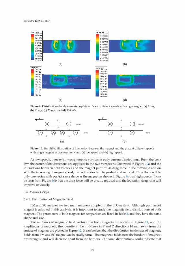
Symmetry 2019, 11, 1117

(a) (b)

(c) (d)

Figure 9. Distribution of eddy currents on plate surface at different speeds with single magnet, (a) 2 m/s,(b) 10 m/s, (c) 70 m/s, and (d) 100 m/s.

(a) (b)

Figure 10. Simplified illustration of interaction between the magnet and the plate at different speedswith single magnet in cross-section view: (a) low speed and (b) high speed.

At low speeds, there exist two symmetric vortices of eddy current distributions. From the Lenzlaw, the current flow directions are opposite in the two vortices as illustrated in Figure 10a and theinteractions between both vortices and the magnet perform as drag force in the moving direction.With the increasing of magnet speed, the back vortex will be pushed and reduced. Thus, there will beonly one vortex with perfect same shape as the magnet as shown in Figure 9c,d at high speeds. It canbe seen from Figure 10b that the drag force will be greatly reduced and the levitation-drag ratio willimprove obviously.

3.4. Magnet Design

3.4.1. Distribution of Magnetic Field

PM and SC magnet are two main magnets adopted in the EDS system. Although permanentmagnet is adopted in this analysis, it is important to study the magnetic field distributions of bothmagnets. The parameters of both magnets for comparison are listed in Table 2, and they have the sameshape and size.

The rainbows of magnetic field vector from both magnets are shown in Figure 11, and theamplitudes of magnetic flux density at the mid-lines in Y and Z directions 10 mm away from thesurface of magnets are plotted in Figure 12. It can be seen that the distribution tendencies of magneticfields from PM and SC magnet are basically same. The magnetic fields near the borders of magnetsare strongest and will decrease apart from the borders. The same distributions could indicate that

154

Symmetry 2019, 11, 1117

the analysis results of PM are also appropriate for SC magnet, and the difference is that the SC couldprovide much stronger magnetic fields through adjusting the flowing currents in the SC coils.

Table 2. Parameters of both magnets. SC: superconducting.

Variable Value Unit

Length 230 mmHeight 200 mm

Thickness 20 mmRemanence of PM 1.3 TCoercivity of PM 940 kA/m

Relative permeability of PM 1.09Current in SC magnet 18.8 kA

(a) (b)

Figure 11. Rainbows of magnetic field vector, (a) PM, (b) SC magnet.

(c) (d)

Figure 12. Distributions of magnetic flux density: (a) Y direction of PM, (b) Z direction of PM,(c) Y direction of SC magnet, and (d) Z direction of SC magnet.

155

Symmetry 2019, 11, 1117

3.4.2. Magnet Thickness

The height and the pole length of the permanent magnets are decided by the design of thepropulsion, which is not involved here. The magnet pole face is 23 cm × 20 cm, the remanence of theNdFeB magnet is 1.3 T and the coercivity is 940 kA/m. Magnetic flux densities of the center point onthe magnet surface are illustrated in Figure 13. As can be seen, although the magnetic flux densitystrengthens with increasing magnet thickness, the increment becomes gentle with the increasing of thethickness. Considering the manufacture and the magnet weight, it is not a good idea to get strongmagnetic field through increasing the magnet thickness and 20 mm is selected as listed in Table 1.

Figure 13. Magnetic flux density over magnet thickness.

3.4.3. Magnet Length

The effects of different magnet lengths on levitation force are researched. The pole length ofthe permanent magnets is 270 mm, which is decided from the propulsion calculation. The resultsare shown in Table 3, and the speed is 10 m/s. Although levitation force becomes larger with theincrease of magnet length, the increment is narrow when the magnet length approaches the pole length.Furthermore, the long and large permanent magnet is fragile and difficult to manufacture, thus a230 mm long magnet was selected in the design.

Table 3. Levitation forces with different magnet lengths.

Magnet Length (mm) Levitation Force (N)

190 230200 236210 240220 256230 268240 280250 288260 295270 297

3.4.4. Magnet Arrangement

Although the magnets are alternately arranged in magnetic N and S poles for propulsion in theproposed system as shown in Figure 3, it is still helpful to research the influence of magnet arrangementon magnetic forces, especially the levitation force. Three kinds of magnet arrangements are studied:single magnet, same pole arranged magnets (such as NN), and NS poles arranged magnets (shown inFigure 3); the results are shown in Figure 14. Double value of single magnet arrangement is includedto be as a reference.

156

Symmetry 2019, 11, 1117

Figure 14. Levitation forces with different magnet arrangements (NN and NS) over magnet velocity.

It can be seen that the levitation force value of NS arranged magnets is larger than the doublevalue of single magnet, and the value of NN arranged magnets is smaller than the double one. This canbe explained in qualitative analysis. For the NN arranged magnets, the change rate of magnetic fieldgenerated by the back N pole magnet in conductive plate is gentler than the one by the front magnet.According to Lenz law, the back magnet will generate weaker induced voltage and eddy current,which will make the levitation force of NN arranged magnets smaller than the double value of singlemagnet. However, the change rate of magnetic field generated by the back magnet in conductive plateis more dramatic than the one by the front magnet. Then, the back magnet will generate strongerinduced voltage and eddy current, which will make the levitation force of NS arranged magnets largerthan the double value of single magnet. The eddy current distributions of NN and NS arrangedmagnets at speeds of 10 m/s and 100 m/s are shown in Figure 15. It is obvious that the NS arrangedmagnets could induce stronger eddy currents than NN arranged magnets, which has verified theexplanation. From the above analysis, we can also get that there exist difference between the two forcesfrom the front and the back magnets, and this will be studied in the following.

(a) (b)

(c) (d)

Figure 15. Distribution of eddy currents on plate surface at different speeds with NN and NS arrangedmagnets: (a) NN magnets at 10 m/s, (b) NS magnets at 10 m/s, (c) NN magnets at 100 m/s, and (d) NSmagnets at 100 m/s.

157

Symmetry 2019, 11, 1117

3.5. Plate Design

3.5.1. Plate Materials

In the proposed EDS structure, the plate should be non-ferromagnetic conductive. Two commonmaterials copper and aluminum are separately studied, whose conductivities are 58 MS/m and 38 MS/m,respectively. The comparisons of forces and levitation-drag ratios are shown in Figures 7 and 8,respectively. The levitation force and the guidance force from the copper plate increase faster than thatfrom the aluminum plate at low speeds, but the difference becomes minor when the magnet speedis high and the forces tend to be the same. The drag force from the copper plate is larger than thealuminum one at the initial low speeds, and after the peak value it decreases faster than the aluminumone. Levitation-drag ratio is an important index, and from Figure 8, the EDS structure with copperplate could provide a higher levitation-drag ratio than aluminum plate.

3.5.2. Plate Height

Plate height is an important factor that will influence the interaction area between the magnet andthe plate. The simulation results of different plate heights with constant height difference h 70 mm atspeed of 10 m/s are shown in Figure 16. The forces in three directions including levitation drag andguidance grow with the increasing of plate height, and the guidance force increases fastest. Consideringhigh plate will bring large drag force and high construction cost, 200 mm (the same height with PM) isadopted in the system design.

Figure 16. Levitation force as a function of plate height.

3.5.3. Plate Thickness

Plate thickness is another important parameter to be designed in the plate type EDS structure.Because of the skin effect at high speeds, the analysis is selected at speed of 100 m/s. The three forcesand levitation-drag ratio are shown in Figure 17. It can be seen that the levitation and the guidanceforces become larger with the increasing of thickness at first and will stay constant, and the drag forcedecreases with the increasing of thickness and the change becomes mild at relatively large thickness.Thus, the levitation-drag ration improves with the increasing of plate thickness. Considering theconstruction cost, 8 mm is selected in the system design.

158

Symmetry 2019, 11, 1117

(a) (b)

Figure 17. Simulation results of different thicknesses of plate at speed of 100 m/s. (a) Levitation, drag,and guidance forces, (b) levitation drag ratio.

3.6. Distribution of Levitation Forces on NS Magnets

In the above analysis in Section 3.4.4, it is explained that there is difference between the levitationforces of the front magnet and the back magnet in the NS arranged magnets. This is important toresearch, since the uneven distribution of levitation forces will lead to imbalance of vehicle duringoperation. The comparison of levitation forces of the front and the back magnets at different speedsare shown in Figure 18. The levitation force from the back magnet increases faster than that from thefront magnet at the low speeds, and then it decreases slightly until the two forces are same value.The non-uniform distribution of levitation forces on NS magnets during the vehicle operation is obviouswhen the vehicle is at a low or middle speed, which indicates a higher standard for the vehicle design.

Figure 18. Simulation results of levitation forces of the front and the back magnets.

4. Conclusions

A plate type EDS structure proposed for ground high speed systems is analyzed in this paper.The ground high speed system is integrated with functions of levitation, propulsion and guidance,and the EDS structure is composed of non-ferromagnetic conductive plate and PM (or SC magnet).The designed plate type EDS structure is researched by FEM simulations, and characteristics of theEDS structure are analyzed based on the results.

• The levitation working point is better to be set around 1/3 height of PM to get enough levitationforce, and it can be moved to a larger h when SC magnet is applied in the design.

• The lateral stiffness at low speeds is relatively insufficient compared with that at high speeds,and guidance wheels can be adopted.

159

Symmetry 2019, 11, 1117

• The effects of different speeds on magnetic forces are studied and the levitation-drag ratio improveswith the increasing of magnets speed.

• PM and SC magnet have the same distribution of magnetic field, and the proper thicknessand length of magnet are set. NS arranged magnets show better performance than NNarranged magnets.

• Copper plate could provide larger levitation force and higher levitation-drag ratio than aluminumplate. Proper height and thickness of plate are decided based on the performance and theconstruction cost.

• The non-uniform distribution of levitation forces on NS magnets will disappear at high speeds.

The results show that the proposed EDS structure is a promising option for application in groundhigh speed systems. Future research will focus on the study of dynamics properties of the plate typeEDS structure, especially the under-damped characteristics of EDS structure during operation.

Author Contributions: Conceptualization, Z.G. and J.L.; methodology, D.Z.; software, Z.G.; formal analysis, Q.C.;investigation, P.Y.; writing—original draft preparation, Z.G.; writing—review and editing, D.Z.; supervision, J.L.;project administration, J.L.

Funding: This research was supported by the National Key R&D Program of China (No. 2016YFB1200601), and theOpening Foundation of the State Key Laboratory of Functional Materials for Informatics (No. SKL-2017-07).


References

1. Palacin, R. Hyperloop, the electrification of mobility, and the future of rail travel. IEEE Electr. Mag. 2016, 4,4–51. [CrossRef]

2. Hyperloop Alpha. Available online: http://www.spacex.com/hyperloopalpha (accessed on 12 August 2013).3. Lee, H.W.; Kim, K.C.; Lee, J. Review of maglev train technologies. IEEE Trans. Magn. 2006, 42, 1917–1925.

[CrossRef]4. Yan, L. Development and application of the maglev transportation system. IEEE Trans. Appl. Supercond.

2008, 18, 92–99. [CrossRef]5. Davey, K. Analysis of an electrodynamic Maglev system. IEEE Trans. Magn. 1999, 35, 4259–4267. [CrossRef]6. Long, Z.; He, G.; Xue, S. Study of EDS & EMS hybrid suspension system with permanent-magnet halbach array.

IEEE Trans. Magn. 2011, 47, 4717–4724. [CrossRef]7. Hsu, Y.H.; Langhom, A.; Ketchen, D.; Holland, L.; Minto, D.; Doll, D. Magnetic levitation upgrade to the

Holloman High Speed Test Track. IEEE Trans. Appl. Supercond. 2009, 19, 2074–2077. [CrossRef]8. Okubo, T.; Ueda, N.; Ohashi, S. Effective control method of the active damper system against the

multidirectional vibration in the superconducting magnetically levitated bogie. IEEE Trans. Appl. Supercond.2016, 26. [CrossRef]

9. Lee, C.Y.; Jo, J.M.; Han, Y.J. Design, fabrication, and operating test of the Prototype HTS electromagnet forEMS-based maglev. IEEE Trans. Appl. Supercond. 2012, 22. [CrossRef]

10. Xu, J.; Geng, Q.; Li, Y.; Li, J. Design, fabrication and test of an HTS magnetic suspension experimental system.IEEE Trans. Appl. Supercond. 2016, 26. [CrossRef]

11. Yan, L. Suggestion for selection of Maglev option for Beijing-Shanghai high-speed line. IEEE Trans. Appl.Supercond. 2004, 14, 936–939. [CrossRef]

12. Du, J.; Ohsaki, H. Numerical analysis of eddy current in the EMS-Maglev system. In Proceedings of the6th IEEE International Conference on Electrical Machines and Systems, 2003, ICEMS 2003, Beijing, China,9–11 November 2003; pp. 761–764.

13. Ding, J.; Yang, X.; Long, Z.; Dang, N. Three dimensional numerical analysis and optimization ofelectromagnetic suspension system for 200 km/h maglev train considering eddy current effect. IEEE Access.2018, 6, 1547–1555. [CrossRef]

14. Abdelrahman, A.S.; Sayeed, J.; Youssef, M.Z. Hyperloop transportation system: Analysis, design, control andimplementation. IEEE Trans. Ind. Electron. 2018, 65, 7427–7436. [CrossRef]

160

Symmetry 2019, 11, 1117

15. Ji, W.Y.; Jeong, G.; Park, C.B.; Jo, I.H.; Lee, H.W. A study of non-symmetric double-sided linear inductionmotor for Hyperloop all-in-one system (Propulsion, Levitation, and Guidance). IEEE Trans. Magn. 2018, 54.[CrossRef]

16. Hao, L.; Huang, Z.; Dong, F.; Qiu, D.; Shen, B.; Jin, Z. Study on electrodynamic suspension system withhigh-temperature superconducting magnets for a high-speed maglev train. IEEE Trans. Appl. Supercond.2019, 29, 1–5. [CrossRef]

17. Mulcahy, T.M.; He, J.; Rote, D.M.; Rossing, T.D. Forces on a magnet moving past figure-eight coils.IEEE Trans. Magn. 1993, 29, 2947–2949. [CrossRef]

18. Knowles, R. Dynamic circuit and Fourier series methods for moment calculation in electrodynamic repulsivemagnetic levitation system. IEEE Trans. Magn. 1982, 18, 953–960. [CrossRef]

19. Lee, J.; Bae, D.K.; Kang, H.; Ahn, M.C.; Lee, Y.; Ko, T.K. Analysis on ground conductor shape and size effectto levitation force in static type EDS simulator. IEEE Trans. Appl. Supercond. 2010, 20, 896–899. [CrossRef]

20. Ko, W.; Ham, C. A novel approach to analyze the transient dynamics of an electrodynamic suspensionmaglev. IEEE Trans. Magn. 2007, 43, 2603–2605. [CrossRef]


161

symmetryS S

Article

Optimal Structural Design of a Magnetic Circuit forVibration Harvesters Applicable in MEMS

Zoltán Szabó 1, Pavel Fiala 2,*, Jirí Zukal 3, Jamila Dedková 3 and Premysl Dohnal 3

1 CVVOZE Centre—Department of Theoretical and Experimental Electrical Engineering,Brno University of Technology, Technicka 12, 616 00 Brno, Czech Republic; [email protected]

2 SIX Centre—Department of Theoretical and Experimental Electrical Engineering,Brno University of Technology, Technicka 12, 616 00 Brno, Czech Republic

3 Department of Theoretical and Experimental Electrical Engineering, Brno University of Technology,Technicka 12, 616 00 Brno, Czech Republic; [email protected] (J.Z.); [email protected] (J.D.);[email protected] (P.D.)

* Correspondence: [email protected]; Tel.: +420-604-076-280

Received: 28 November 2019; Accepted: 22 December 2019; Published: 6 January 2020

Abstract: The paper discusses the results of research into a vibration-powered milli- or micro generator(MG). The generator harvests mechanical energy at an optimum level, utilizing the vibration of itsmechanical system. The central purpose of our report is to outline the parameters that are significantfor implementing the actual design to harvest the maximum (optimum) energy possible withinperiodic symmetrical systems, while respecting the typical behavior of the output voltage. Therelevant theoretical outcomes influence the measurability and evaluation of the physical quantitiesthat characterize the designed structures. The given parameters, which are currently defined inmillimeters, are also applicable within the micrometer range, or MEMS. The article compares some ofthe published microgenerator concepts and design versions by using effective power density, amongother parameters, and it also brings complementary comments on the applied harvesting techniques.The authors demonstrate minor variations in the magnetic rotationally symmetric circuit geometrythat affect the pattern of the device’s instantaneous output voltage; in this context, the suitability ofthe individual design approaches that are to be used with MEMS as a vibration harvesting system isanalyzed in terms of properties that are applicable in Industry 4.0.

Keywords: Harvesting; low-power applications; vibration; micro-generator; optimal solution;magnetic circuit; periodical structure; effective power density; symmetry

1. Introduction

In recent years, alternative sources of energy have become the main subject of numerous researchprojects [1–22], with the optimum energy conversion being one of the central points of focus. Such atransformation is often ensured through a vibration microgenerator [23–26]. Effective energy harvestersexploiting the mechanical vibrations and related non-stationary magnetic fields have already beeninvestigated and reported [2].

The comparative approach applied to harvesters for milli- or micro generators (MGs) withinstudy [18] allows for an effective evaluation of different conversion concepts, namely, interpretationsof Faraday’s law of induction. An optimal harvester design to yield the maximum power is obtainablevia minor structural modifications that may substantially change the resulting performance whilethe parameters (including the weight, volume, and vibrations) remain virtually identical to those ofstandard harvesters. Different papers, including [2], detail functional magnetic circuits for vibrationharvesters, where the model experiments and a comparison of various versions illustrate the effect ofmagnetic circuit modifications on the output voltage and power of a harvester. Advantageously, the


Symmetry 2020, 12, 110

devices can be grouped into periodic structures and also used in closed systems, such as automobiles,aircraft, and other units that are suitable for the inclusion of harvesters as additional and reliable energysources. The possibilities of residual energy harvesting are examined in article [3]; the discussioncomprises, among other aspects, specific harvester installation conditions, and requirements.

As regards the microgenerator design (Figure 1), Figure 2a introduces the most widely preferredprinciple (I, [2,3]); in the given context, it is necessary to respect the general conclusions of Faraday’slaw of induction as formulated in, for example, Equation (1) and Figure 2b below. Figure 2 showsmultiple processes and elements, including the magnetization of the permanent magnet M; magneticflux Φ; magnetic lines of force; oriented area S enclosed by the coil thread; electric coil; and, characterof the generator’s core motion with respect to the coil. The related Figure 2c then introduces a designversion that minimizes the impact of external electromagnetic fields (non-stationary) on the principalfunction of the generator.

(a)

(b)

Figure 1. The principal configuration of the core of the milli- or micro generator (MG): (a) a beamversion, principle I; (b) a beam version, principle II [2].

164

Symmetry 2020, 12, 110

(a)

(b)

(c)

Figure 2. The basic arrangement of the investigated rotationally symmetric geometry device exploitingFaraday´s induction law: (a) the classic solution; (b) the novel arrangement; and, (c) the option with aclosed magnetic circuit to minimize (optimize) the impact of external magnetic fields [2].

The generator was modeled to facilitate optimal design of the dimensions (minimum size andweight m) [2]. The vibrations measured with critical positioning of the device reached the maximum ofG = 0.2 g (g = 9.81 ms−2). In the discussed concept, the resonance might vary, according to the origin ofthe vibrations, from the tuned resonance frequency f r by up to tens of percent.

As regards the optimum design variant, the critical parameter consisted in the boundary sensitivityof the generator to the minimum vibration amplitude; the relevant value corresponded to 0.01 g–0.05 g.

165

Symmetry 2020, 12, 110

In the following portions of the presentation, the proposed structural problems and methods for theirsolution will be discussed.

Microgenerator systems and relevant manufacturing methods were discussed on a comprehensivebasis previously [2–5]; the structural details and consequences are indicated herein, as in Figures 2–4.

(a) (b)

Figure 3. The basic arrangement of the investigated device exploiting Faraday´s induction law: (a) theMG core; and (b) the magnetic flux density distribution along the z axis, line A-A.

(a) (b) (c) ( )

(e) (f) (g)

Figure 4. The electric voltage induction in the applied coil, (a–g), according to Faraday´s law ofinduction [2].

166

Symmetry 2020, 12, 110

2. Designing the MG

The microgenerator utilizes an external environment that is characterized by the occurrence ofmechanical vibrations, exploiting a suitable mechanical coupling to dampen these vibrations andgenerate an electric power Pout. The required output power Pout of the optimal design depends on thetype of the output load Z. The optimal arrangement of the MG is based on the concepts in Figure 1,Figure 2c, and Figure 3, with the magnetization orientation indicated. In terms of the mechanicalproperties, the device was discussed in dedicated papers and patents, such as [10,25]. Figure 4 presentsdetails of the transformation process and electricity generation; the actual engineering approachadopted in solving these procedures then embodies the necessary precondition for the subsequentidentification of the optimal design. The mathematical model outlined in [2] is, in a basic form,incorporated in the corresponding Formula (5), below.

Figure 3, as above, presents one of the progressive options available for seating the movingpart of the generator, a solution that eliminates the classic spring or girded beam (Figure 1). Thedesigned system (Figure 3), is tuned to the mechanical oscillation resonance frequency f res andit constitutes the basis of the optimal approach. Such an arrangement allows for us to reach themaximum possible harvest rate and transform the field into an electric voltage; Figure 4 shows thecorresponding preconditions.

3. Modeling the MG

To support our approaches, the paper includes fundamental parts of the relevant mathematicalmodel, which is defined, for example, within referenced publications [1–3]. In the given context, themodel can be formulated, as

∮

E(t) · d = −∫S

∂B(t)∂t

dS +

∮

(v(t) ×B(t)) · d (1)

where E(t) denotes the electric field intensity vector, B(t) is the magnetic flux density vector, v(t)represents the generator core position drift in time (the instantaneous velocity) vector, S stands forthe cross section of the area with magnetic flux Φ, and l denotes the curve along the boundary of theS. Figure 4 illustrates the change of the magnetic flux of the field (ti1, . . . , ti4) and also the resultinginduction of the voltage u. The behavior of the voltage u(t) can be evaluated by following the stepsthat are indicated in Figure 4; this behavior assumes the validity of Equation (1), magnetic flux Φconfiguration, and electric coil shape with an active surface Sc.

We need to know the values of energy and transformation rate to be able to evaluate the efficiencyof the proposed design (Figure 2c). The state equation can be defined with respect to the energyconservation law regarding the considered problem [1–3]. Subsequently, the kinetic and potentialenergies, Wk and Wp, respectively, which are related to the movement of the generator’s core, can bedefined as

Wk =12

m v2, Wp = m g z. (2)

where m is the mass of the MG system, v denotes the mean velocity, and g represents the gravityconstant.

The equation of state used by the authors of [1] and [2] captures the electromechanical coupling inthe device, being expressed as

m g z− ∫

∫VJ

(J×B)dV · nd − ∫VJc

12

J2

γ dV = 12 m(

d zdt

)2

η∫

VM

12 BMHMdV = 1

2 m(

d zdt

)2 (3)

167

Symmetry 2020, 12, 110

where dz/dt is the moving part drift in time, further measurable as the velocity v; η represents themagnetic field transformation efficiency; n denotes the normal vector; γ is the specific conductivity ofthe wire; is the length of the shift caused by the specific strength; B denotes the magnetic flux densityvector; J represents the current density vector; VJc stands for the coil wire volume; and, VJ is the volumeof the electrically conductive components. The MG system then also includes the braking forces

md2zdt2 + lc

dzdt

+ k z = Fz, (4)

where d2z/d t2 is the acceleration of the moving part, dz/d t denotes the velocity v of the moving parts,m represents the mass, k stands for the stiffness coefficient, lc is the damping coefficient, and Fz is theforces affecting the moving parts. The simplified model is described as

md2zdt2 + lc

dzdt

sign(dzdt

)dzdt

+ k z =(mm + mp

)g(t) −

∫VJ

((dzdt×Bbr

)×B)· n dV −

∫Jc

(in×B) · n d, (5)

where Bbr is the braking magnetic flux density, Jv denotes the current density of the electrically conductivecomponents, Jcirc represents the current density in the coil winding, and i stands for the instantaneousvalue of the current through the coil. The geometrical model that is applied in ANSYS (Version 12,ANSYS inc., Houston, USA) is presented in sources [23], ref. [2] as well as Figures 3a and 5a. Figure 6, asbelow, shows the typical analysis of the ANSYS numerical model. The novel (optimal) generator designwas tested on both a pneumatic and an electrodynamic shaker to verify the magnetic independence ofthe proposed solution. The magnetic circuit is designed such that its structure is enclosed within thebody of the generator, ensuring reduced sensitivity to the external magnetic field and its changes. Thisparameter is of interest for application in the periodic structure of the outlined design usable in MEMS.The assumptions embodied in the variant from Figure 2c were experimentally verified.

(a)

(b)

Figure 5. A geometrical model of the tested MG [2]: (a) the core of MG; and, (b) the functional samplesubjected to a shaker-based test of the double-action winding.

168

Symmetry 2020, 12, 110

(a)

(b)

(c)

Figure 6. A geometrical rotationally SYMMETRIC model of the MG0 based on principle II [2]: (a)the ANSYS geometrical model; (b) the core; and, (c) the optimal design, detailed distribution of themagnetic flux density module B [T].

4. Selecting the MG Core Design

Within the design of the generator, the ANSYS system [4] was used for the numerical analysisand to optimize the key parts. A mathematical model exploiting partial differential equations furtherdescribed the electromagnetic field distribution [1,2]. This model becomes evident from Formulas (3),(5); the non-linear equations, which define the behavior of the external electric circuit [1–3]; and, themechanical model of the main parts of the generator. There is mutual action between the mechanicaland the electromagnetic effects. The partial differential equations of a coupled electro-mechanicalcircuit [4,5] were used to build the physical model.

A simplified model was employed to design the generator components. The model utilizedlumped parameters, as shown in Figure 7, and it also assumed various versions of the magnetic fieldchanges described with respect to the phase perspective, as indicated in Figure 4a–g. The individualparts, comprising the permanent magnet, air gap, electrical winding, magnetic circuit, electric coil, oneturn of the winding, pole extension, beam, body, and core of the magnetic part of the generator, aredenoted by using the reference symbols in Figure 7a.

169

Symmetry 2020, 12, 110

(a) (b)

Figure 7. The MG core with a ferromagnetic circuit according to principle II [2]: (a) a structurallysimple variant, acceleration g within the interval of 0.01 g–0.3 g; (b) a scheme of the configuration.

A lumped parameters model can describe these components in order to perform quick assessmentof the properties of the proposed concept. The above structures are classifiable into two groups: Oneof these exploits the approach where a magnetic field moves with respect to a fixed coil, as shown inFigure 7b; the other then utilizes an electric coil moving with respect to a stationary magnetic fieldand fixed to the body of a generator. Regarding the above analysis, we also examine the conceptof a magnetic field moving with respect to an electric coil fixed to the body of a generator based onprinciple II (Figure 3a), in which the ferromagnetic circuit is fully closed and its components do notmove against each other.

The generator design versions were used to build a series of models in ANSYS and then employedto examine the vibration energy harvesting rate. As a result, we can demonstrate the distribution ofthe magnetic flux density module B and the magnetic field intensity module H in Figure 6c of thefunctional sample according to the configurations that are presented in Figure 6a,b.

5. Critical Parameters of the MG Design

The critical parameters are outlined in sources [1,2,26] and can be categorized into the followingareas:

• mechanical dynamics;• electromagnetic field; and,• electronic systems (power management blocks).

In terms of the mechanical dynamics, the optimal state depends on finding an interval of themechanical approach to a vibration system for the known resonant frequency f res. Regarding this task,an aspect of major importance consists in the nonlinear stiffness coefficient k in the entire generatorsystem (Figure 8). If the factor is adequately considered, then the device is capable of providing anoperational efficiency of approximately 90%; in such conditions, the MG will operate at its maximumefficiency with minimal vibrations. The nonlinearity of the stiffness coefficient k depends on the choiceof principal approach (Figure 1a,b and also Figures 6–8).

170

Symmetry 2020, 12, 110

Figure 8. The applied stiffness characteristics [2], coefficient k; the behavior is nonlinear in both of theMG magnetic circuit principles.

Such an approach to the mechanical configuration of the MG is suitable for multiple purposes inmicrotechnology, including the formation of fields of resonant MGs (Figures 9–12). Two approacheswere tested as regards the electromagnetic field: one utilizing air to substitute for the ferromagneticmaterial in the magnetic field (principle II, Figure 1b), and the other applying a ferromagnetic materialaccording to Figure 3a. Figure 9 demonstrates a solution to facilitate the further development of theprogressive concept (principle II) through changes of the dimensional parameters of the design, t1, t2,φD1 − φD3.

Figure 9. A component diagram of the MG0 design with the linearized coefficient of stiffness k (basedon principle II).

171

Symmetry 2020, 12, 110

(a) (b)

Figure 10. A component diagram of the MG0 design with the linearized coefficient of stiffness k (basedon principle II); (a) configuration A, and (b) its output voltage Uout.

(a) (b)

Figure 11. A component diagram of the MG0 design with the linearized coefficient of stiffness k (basedon principle II); (a) configuration B, and (b) its output voltage.

(a) (b)

Figure 12. A component diagram of the MG0 design with the linearized coefficient of stiffness k (basedon principle II); (a) configuration C, and (b) its output voltage.

Figures 10–12 demonstrate the difference in the shapes of the electric voltage induced in the coilof the generator at some characteristic settings of the design parameters t1, t2, φD1 − φD3.

172

Symmetry 2020, 12, 110

6. Microstructures

In order to apply the above-defined principles and conclusions, we have to consider the relevantfigures (MG principle II, Figures 1b, 3a and 9, Figures 10–12, where Sc is the effective area of the coil,Figure 2c; Sp denotes the area of the pole extension; t1 represents the thickness of the pole extension ofthe MG core; Nseg is the number of the electrical winding segments; Npol is the number of the poleextensions of the core and shell; and, f (dg/dt), g (dg/dt) denote the time variation of the gravitationalacceleration of the moving part of the microgenerator. The correct setting of the MG0 structure,Figures 9–11, can be verified through measuring or evaluating the behavior of the output voltage onthe terminals of the MG segment. The obtained instantaneous values of the patterns of the voltage u(t)are then applicable in expressing, via the indirect method and based on the above formula (5), theobserved physical quantities of the model.

As regards vibration energy harvesting within the microdimension, it is necessary to utilizein the MG fields the discussed principle II (Figure 7), together with certain variants of the relevantconfigurations of the magnetic circuit and winding (Figures 9–12). Thus, the preset requirements forthe generator sensitivity and effective use of the space will enable us to harvest a high amount ofresidual energy. Figure 13, below, illustrates an exemplary periodic MG structure. The actual design(Figures 10–12) or other parameters can be altered to ensure the desired shape of the output voltage(Figures 10b, 11b and 12b) and also the conversion effectivity rate in transforming the mechanicalvibrations to electrical energy.

Figure 13. A field of periodically configured MGs an exemplary structure.

The optimal design of a symmetrically structured sensitive vibration harvester (principle II,Figure 1b to operate in the resonant band can be applied in segmentation into microgeneratorstructures, as in Figure 13). Segmented microgenerators clustered as units (a MEMS harvester) can bearranged into fields. In this type of configuration, the designer has to consider the condition in whichthe length of the excitation vibration wave is

λv � L, L = N(ls + lh) (6)

where L denotes the length of a side of the periodic structure, ls represents the length of the MG element,and lh is the space between the elements of the periodically structured field of microgenerators. Duringthe propagation of vibrations, the structure behaves such that the electric voltage is almost in phase atthe output of the windings.

The actual engineering of the procedure to facilitate, especially in terms of the size, the transitionfrom a minigenerator to a microdevice (MEMS) is accompanied by not only technological questions andproblems, but also the fundamental requirement of respecting the principles that are characterized inthis paper. Generally, it is possible to suggest that the set of usable magnetic materials comprises itemssuch as nano Ni and convenient permalloys deposited via sputter coating or lamination. The weight of

173

Symmetry 2020, 12, 110

the flat structure, ms, then determines the achievable resonant frequency, harvesting efficiency, andadjustment of the harvester’s lower sensitivity limit. Importantly, each concrete application of theprinciple requires designing a suitable MEMS structure by using the above-shown models.

7. Comparing MG Concepts, Designs, and Structures

Current experiments with vibration microgenerators converting energy via magnetic induction(vibration/electric energy) employ various harvesting approaches (principle I, principle II) and magneticcircuit structures [2]; thus, the devices exhibit diverse output power and conversion efficiency rateswith respect to the given size and vibration frequency spectrum [12–22]. When engineering a periodicmicrostructure, a designer has to consider the degree of efficiency at which the transformed energy(mechanical vibrations) is to be harvested, and they then select the microstructure element accordingly,while utilizing available technologies. Several specific methods and the obtained results by differentresearch groups are compared below, Figures 14–18; in this context, the relevant concepts and structuresof vibration generator transformation elements applied internationally are also discussed in view ofthe samples MG I–MG IV presented herein (Figures 19–21).

(a) (b)

Figure 14. The silicon-based concepts developed by (a) Kulkarni et al. [11] and (b) Zhu et al. [13].

Figure 15. The vibration microgenerator designed by Beeby et al. [12].

Figure 16. The electromagnetic design by Wang et al. [15].

174

Symmetry 2020, 12, 110

Figure 17. The electromagnetic vibration energy harvester using cylindrical geometry, developed byYang et al. [16].

(a) (b)

Figure 18. The permanent magnet (a) having a spring in the cylindrical structure of the energyharvester [18], (b) tested sample designed by Lee et al. [17].

Figure 19. The basic symmetric magnetic circuit, structural design [2] according to Principles I and II,invariably with magnetic damping in the limit position of the rocking arm [3].

175

Symmetry 2020, 12, 110

(a) (b) (c)

Figure 20. The tested microgenerator [2] based on Principle I: (a) MG I—the dimensions of 90 × 40 ×30 mm, Uout max = 300 V; (b) MG II—the dimensions of 50 × 27 × 25 mm, Uout max = 20 V; and (c) theinstantaneous behavior of the output electrical voltage in MG I and MG II (the effect of the stiffnesscoefficient k—Figure 8).

(a) (b) (c)

Figure 21. The devices based on Principle II [2]: (a) MG III—the dimensions of 50× 25× 25 mm, Uout max

= 10 V; (b) MG IV—the dimesnions of 50 × 35 × 25 mm, Uout max = 20 V; and, (c) the instantaneousbehavior of the output electrical voltage in MG III and MG IV (the effect of the stiffness coefficientk—Figure 8).

The microgenerators that are characterized in Figures 14–18 correspond to the concepts and designversions of the vibration generator magnetic circuit and housing outlined by the authors of this paper.The solution from Figure 2a corresponds to the embodiments that are discussed within articles [14,15],comprising a clearly open magnetic circuit and an induction coil unfavorably positioned with respectto the movement of the permanent magnet. The concepts and tests that are presented in [11,13]relate to the configuration from Figure 2b, where the induction coil is positioned and oriented suchthat the harvester provides a higher efficiency; however, the magnetic circuit is not markedly closed.The technique adopted by Yang et al. [16] approaches the effective configuration from Figure 2c; theresearchers employed the non-linear, non-monotonous function of the stiffness coefficient k, namely,the function specified as the solution respecting Principle I, Figure 1a). By contrast, Beeby et al. [12]proposed an interpretation that, when compared to our investigation, resembles the system stiffnesscoefficient within Principle II–Figure 1b.

At the DTEEE FEEC, BUT, comparative tests were performed of a vibration generator (Figure 19)with magnetic damping [2] of the mobile arm’s movement; these testing cycles comprised designvariants MG I–MG II according to Principle I and also versions MG III–MG IV exploiting PrincipleII. The parameters obtained in selected generators are summarized in Table 1; a wider comparison isavailable in study [18] (as in table 4).

176

Symmetry 2020, 12, 110

Table 1. The parameters of selected vibration generators.

ReferencePermanentMagnet

Type

GeneratorBody

Size x, y,z [m]

ResonantFrequency

f r [Hz]

AmplitudeMech.Part A

[m]

OutputPower

Pout [W]

OutputVoltageUout [V]

LoadResistance

R [Ω]

AccelerationG, g = 9.81

[m/s]

EffectivePower

Density[W/m3]

Beebyet al. [12],

2007− 375 mm3 52 − 2 × 10−6 0.428

RMS 4000 0.06 g ≈6

Zhu et al.[13], 2010 FeNdB 2000 mm3 67.6–98 0.6 × 10−3 61.6–156.6

× 10−6 − − 0.06 g ≈30–80

Kulkarniet al. [11],

2008FeNdB 3375 mm3 60–9840 1.5 × 10−3 0.6 × 10−6 0.025 52,700 0.398–4 g ≈0.2

Wanget al. [15],

2007FeNdB 256 mm3 121.25 0.738 ×

10−3 - 0.06 - 1.5 g -

Lee et al.[17], 2012 FeNdB 1.4 × 10−4

m3 16 − 1.52 ×10−3 4.8 5460 0.2 g ≈10

Yanget al., [16],

2014.− 50,000

mm3 22–25 13.4 ×10−3 0.7–2.0 110 0.6 g ≈270

Elvinet al., [14],

2011− 15,000

mm3 112 − 4 × 10−6 0.007 986 - ≈0.26

MG I [2],2006 FeNdB 90, 40, 30

mm 20–3550 ×

10−6–400× 10−6

70 × 10−3 4–60 (300)p-p 7500 0.15–0.4 g ≈650

MG II [2],2006 FeNdB 50, 27, 25

mm 17–2550 ×

10−6–400× 10−6

19.5 ×10−3 6−15 5000 0.1–0.7 g ≈60

MG III FeNdB 50, 25, 25mm 21–31.5

50 ×10−6–400× 10-6

5.0 × 10−3 1.0–2.5 600 0.05–0.4 g ≈15

MG IV FeNdB 50, 35, 25mm 21–31.5

50 ×10−6–400× 10−6

8.0 × 10−3 1.0–2.5 1200 0.05–0.4 g ≈18

*Lith.battery

[19], 2018≈40 × 106

*supercap[20], 2010 ≈3–5

*fuel ≈4 × 109

*U235 ≈9 × 1016

If application in microelectronics and periodic systems is assumed, then the solution displayed inFigure 2c appears to be advantageous; however, at major vibrations, namely, ones between 0.3 g and1.0 g, it is beneficial to configure the magnetic circuit and coil as set out within Principle I, Figure 1a).Where the external vibrations drop below 0.3 g (0.01 g–0.2 g), Principle II, Figure 1b, has to be applied.A generator configuration design requires an analysis of the magnetic field expected for the activesection of the device and overall presetting of the maximum values of the specific magnetic flux densityB into the air gap that is to contain the generator winding, Figure 6; such an analysis and presettinghave to facilitate the maximum magnetic flux change in time and space, as formulated within Faraday’slaw of induction (1) and to enable geometrical configuration of the winding shown in Figure 4. Inthe given context, it is advantageous to employ the double action system to facilitate a magnetic fluxchange, as indicated in Figures 5a and 7.

Figure 20 presents the tested generators MG I–MG II that exploit Principle I and the energyharvesting efficiency rates yielded from Figure 2c, exhibiting various size versions together withdifferent parameters and measured patterns of the output electrical voltage Uout.

177

Symmetry 2020, 12, 110

Figure 21 presents the embodiments of MG III and MG IV respecting the magnetic circuitconfiguration according to Principle II and the energy harvesting effectivity scheme that characterizesthe variant from Figure 2c.

The last column of Table 1 comprises data that are related to effective power density [W/m3];this quantity enables us to express the effectivity of individual generator concepts and structures asregards harvesting quality. The last four lines indicate a comparable quantity for fossil and nuclearfuels, batteries, and supercaps.

For comparison purposes, Table 1 contains a quantity denoted as “effective power density“; inthis context, it would probably be interesting to also indicate the harvesting rate of the microgenerator,but such a task appears to be rather problematic. Although the efficiency of a resonant harvester canbe preset to a desired level, as demonstrated via Formulas (1)–(5), the associated model (5), and the testcycles visualized in Figures 19–21 the achievable efficiency rate markedly depends on the quality of themechanical coupling between the vibration source, the power management unit, and other relevantparameters; our tests yielded final rates between 50 and 95%. The problem was analyzed by differentauthors already previously [2–5,24].

8. Conclusions

The paper discussed the outcomes of a theoretical investigation into the design and principlesof mini/micro generators to facilitate mechanical vibration energy harvesting [2]. The main productof the continuous research consists in simulation-based determination of the optimum rotationallysymmetric geometry design versions and parameters of a relevant magnetic circuit.

The advantageous solutions and options are embodied in the generator design versions accordingto the proposed principles I and II, which ensure the necessary resistive loads and associatedimpedances. Exploiting the measured output voltages of the selected variants, the derived theoreticalmodels can evaluate the harvester quality and fabrication procedure. Using the hybrid measurementapproach combined with a numerical model, it is possible to classify other physical quantities of theelectromagnetic field inside the generator.

The harvesters fabricated according to principle II, utilized in the range of f r = 10–50 Hz (frequentin the automotive and aeronautics sectors), are integrable into miniaturized microgenerator structuresworking within the range of G = 0.05 g–0.08 g. This concept could advantageously employ in practicethe higher level of vibrations available compared to the design based on principle I [3]. The generatorsthat employ principle I operate at vibration levels higher than G ≥ 0.15 g. Generally, the windingconfiguration variants convenient for the frequency ranges of f v = 1–10 Hz, f v = 50–150 Hz aredemonstrated in Figure 2b,c.

We discussed selected samples of microgenerators to evaluate multiple quantities, includingthe effective power density (Table 1). This quantity is utilized as the parameter enabling us tochoose the source of energy applicable in the given task or unit and determine whether the actualselection of the correct approach is a parameter for facilitating effective designing of MEMS structures.The knowledge that was obtained through the experiments is beneficial for the use of autonomouselectro-mechanico-electronic systems in Industry 4.0 projects.

Author Contributions: P.F. contributed to the theoretical part, numerical model, and experiments; he also wrotethe paper. Z.S. conceived and designed the experiments; J.D. contributed to the optimization procedures; andP.D., J.Z. evaluated the experiments and graphics. All authors have read and agreed to the published version ofthe manuscript.

Acknowledgments: The research was financed by the National Sustainability Program under grant No. LO1401and supported within a grant of Czech Science Foundation (GA 17-00607S). For the actual analyses and experiments,the infrastructure of the SIX Center was used.

Conflicts of Interest: The authors declare no conflict of interest. The founding sponsors had no role in the designof the study; in the collection, analyses, or interpretation of data; in the writing of the manuscript, and in thedecision to publish the results.

178

Symmetry 2020, 12, 110

References

1. Stratton, J.A. Theory of Electromagnetic Field; Czech Version; SNTL: Praha, Czech Republic, 1961.2. Szabo, Z.; Fiala, P.; Dohnal, P. Magnetic circuit modifications in resonant vibration harvesters. Mech. Syst.

Signal Process. 2018, 99, 832–845. [CrossRef]3. Fiala, P. Vibration Generator Conception; Research Report in Czech; DTEEE, Brno University of Technology:

Brno, Czech Republic, 2003; p. 95.4. Jirku, T.; Fiala, P.; Kluge, M. Magnetic resonant harvesters and power management circuit for magnetic

resonant harvesters. Microsyst. Technol. 2010, 16, 677–690. [CrossRef]5. Fiala, P.; Jirku, T. Analysis and Design of a Minigenerator, Progress in Electromagnetics 2008. In Proceedings

of the PIERS 2014 in Guangzhou, Guangzhou, China, 25–28 August 2014; pp. 749–753.6. Madinei, H.; Khodaparast, H.H.; Adhikari, S.; Friswell, M. Design of MEMS piezoelectric harvesters with

electrostatically adjustable resonance frequency. Mech. Syst. Signal Process. 2016, 81, 360–374. [CrossRef]7. Scapolan, M.; Tehrani, M.G.; Bonisoli, E. Energy harvesting using parametric resonant system due to

time-varying damping. Mech. Syst. Signal Process. 2016, 79, 149–165. [CrossRef]8. Gatti, G.; Brennan, M.; Tehrani, M.; Thompson, D. Harvesting energy from the vibration of a passing train

using a single-degree-of-freedom oscillator. Mech. Syst. Signal Process. 2016, 66, 785–792. [CrossRef]9. Davino, D.; Krejcí, P.; Pimenov, A.; Rachinskii, D.; Visone, C. Analysis of an operator-differential model for

magnetostrictive energy harvesting. Commun. Nonlinear Sci. Numer. Simul. 2016, 39, 504–519. [CrossRef]10. Saravanan, S.; Dubey, R. Optical absorption enhancement in 40 nm ultrathin film silicon solar cells assisted

by photonic and plasmonic modes. Opt. Commun. 2016, 377, 65–69. [CrossRef]11. Kulkarni, S.; Koukharenko, E.; Torah, R.; Tudor, J.; Beeby, S.; O’Donnell, T.; Roy, S.; Beeby, S. Design,

fabrication and test of integrated micro-scale vibration-based electromagnetic generator. Sens. Actuators APhys. 2008, 145, 336–342. [CrossRef]

12. Beeby, S.P.; Torah, R.N.; Torah, M.J.; O’Donnell, T.; Saha, C.R.; Roy, S. A microelectromagnetic generator forvibration energy harvesting. J. Micromech. Microeng. 2007, 17, 1257–1265. [CrossRef]

13. Zhu, D.; Roberts, S.; Tudor, M.J.; Beeby, S.P. Design and experimental characterization of a tunablevibration-based electromagnetic micro-generator. Sens. Actuators A Phys. 2010, 158, 284–293. [CrossRef]

14. Elvin, N.G.; Elvin, A.A. An experimentally validated electromagnetic energy harvester. J. Sound Vib. 2011,330, 2314–2324. [CrossRef]

15. Wang, P.-H.; Dai, X.-H.; Fang, D.-M.; Zhao, X.-L. Design, fabrication and performance of a new vibration-basedelectromagnetic micro power generator. Microelectron. J. 2007, 38, 1175–1180. [CrossRef]

16. Yang, J.; Yu, Q.; Zhao, J.; Zhao, N.; Wen, Y.; Li, P.; Qiu, J. Design and optimization of a bi-axial vibration-drivenelectromagnetic generator. J. Appl. Phys. 2014, 116, 114506. [CrossRef]

17. Lee, B.-C.; Rahman, A.; Hyun, S.-H.; Chung, G.-S. Low frequency driven electromagnetic energy harvesterfor self-powered system. Smart Mater. Struct. 2012, 21, 125024. [CrossRef]

18. Siddique, A.R.M.; Mahmud, S.; Van Heyst, B. A comprehensive review on vibration based micro powergenerators using electromagnetic and piezoelectric transducer mechanisms. Energy Convers. Manag. 2015,106, 728–747. [CrossRef]

19. Quinn, J.B.; Waldmann, T.; Richter, K.; Kasper, M.; Wohlfahrt-Mehrens, M. Energy Density of CylindricalLi-Ion Cells: A Comparison of Commercial 18650 to the 21700 Cells. J. Electrochem. Soc. 2018, 165,A3284–A3291. [CrossRef]

20. Liu, C.; Yu, Z.; Neff, D.; Zhamu, A.; Jang, B.Z. Graphene-Based Supercapacitor with an Ultrahigh EnergyDensity. Nano Lett. 2010, 10, 4863–4868. [CrossRef] [PubMed]

21. Zhu, D.; Tudor, M.J.; Beeby, S.P. Strategies for increasing the operating frequency range of vibration energyharvesters. J. Meas. Sci. Technol. 2010, 21, 22001. [CrossRef]

22. El-Hami, M.; Glynne-Jones, P.; White, N.; Hill, M.; Beeby, S.; James, E.; Brown, A.; Ross, J. Design andfabrication of a new vibration-based electromechanical power generator. Sens. Actuators A Phys. 2001, 92,335–342. [CrossRef]

23. ANSYS Users Manual, (1991–2019). USA. Available online: www.ansys.com (accessed on 1 July 2018).24. Fiala, P.; Hadas, Z.; Singule, Z.; Ondrusek, C.; Szabo, Z. A Vibrational Generator for Electric Energy Producing,

(in CZ Vibracní Generator pro Výrobu Elektrické Energie). Patent No. 305591-CZ, 12 September 2006.

179

Symmetry 2020, 12, 110

25. Fiala, P. Fotovoltaický Element Zahrnující Rezonátor (A Photovoltaic Element with an Included Resonator).Patent No. 303866, 27 January 2011.

26. Fiala, P.; Szabo, Z.; Marcon, P.; Roubal, Z. Mini-and Microgenerators Applicable in the MEMS Technology,Smart Sensors, Actuators, and MEMS VIII. Proc. SPIE 2017, 10246, 1–8. [CrossRef]


180

MDPISt. Alban-Anlage 66

4052 BaselSwitzerland

Tel. +41 61 683 77 34Fax +41 61 302 89 18

www.mdpi.com

Symmetry Editorial OfficeE-mail: [email protected]

www.mdpi.com/journal/symmetry

MDPI St. Alban-Anlage 66 4052 Basel Switzerland

Tel: +41 61 683 77 34 Fax: +41 61 302 89 18

www.mdpi.com ISBN 978-3-03943-125-0

Symmetry in Electromagnetism - MDPI

Documents

Transcript of Symmetry in Electromagnetism - MDPI