arX

iv:1

308.

2221

v1 [

astr

o-ph

.CO

] 1

1 A

ug 2

013

Noether Gauge Symmetry Approach in Quintom Cosmology

Adnan Aslam1 Mubasher Jamil1 Davood Momeni 2

and

Ratbay Myrzakulov 2 Muneer Ahmad Rashid1 Muhammad Raza 3

Center for Advanced Mathematics and Physics (CAMP), National University of Sciences

and Technology (NUST), H-12, Islamabad, Pakistan

Eurasian International Center for Theoretical Physics, Eurasian National University,

Astana 010008, Kazakhstan

Department of Mathematics, COMSATS Institute of Information Technology (CIIT),

Sahiwal Campus, Pakistan

Received ; accepted

– 2 –

ABSTRACT

In literature usual point like symmetries of the Lagrangian have been intro-

duced to study the symmetries and the structure of the fields. This kind of

Noether symmetry is a subclass of a more general family of symmetries, called

Noether Gauge Symmetries (NGS). Motivated by this mathematical tool, in this

article, we discuss the generalized Noether symmetry of Quintom model of dark

energy, which is a two component fluid model of quintessence and phantom fields.

Our model is a generalization of the Noether symmetries of a single and multiple

components which have been investigated in detail before. We found the general

form of the quintom potential in which the whole dynamical system has a point

like symmetry. We investigated different possible solutions of the system for di-

verse family of gauge function. Specially, we discovered two family of potentials,

one corresponds to a free quintessence (phantom) and the second is in the form of

quadratic interaction between two components. These two families of potential

functions are proposed from the symmetry point of view, but in the quintom

models they are used as phenomenological models without clear mathematical

justification. From integrability point of view, we found two forms of the scale

factor: one is power law and second is de-Sitter. Some cosmological implications

of the solutions have been investigated.

Subject headings: Cosmology; Noether symmetries; Quintom fields; Dynamical

systems; Cosmography; Local stability

– 3 –

1. Introduction

Einstein gravity inspired from the equivalence principle, follows the Mach’s principle

as the matter creates the geometry or space time concept. There is no reasonable and clear

motive to believe that Einstein gravity must work beyond the solar system and compatiable

to describe the large scale structure of the whole universe, as well as the gravity in compact

objects and solar system. Just on an adhoc basis and by assuming that the equivalence

principle also works on large scale, the relativistic cosmology of Einstein gravity has

been constructed. Because gravity as a theory for gravitation treats like a gauge theory,

cosmology based on such a gauge theory of gravity is basically a highly non-linear system

of differential equations. It means even there is no uniqueness principle or theorem for the

solutions of the equations. This is a weak point or very bad freedom in the theory as a

mathematical point of view. Symmetry is a key point for non linear differential equations.

Modern approach is how to find the general point like symmetries of a given Lagrangian

(holonomic or non-holonomic). This appropriate powerful method to find and investigate

the solutions of linear (non linear) dynamical systems reduces the numbers of the unknown

functions by construction of invariants, the quantities which remain invariance under gauge

transformations. Cosmological models are dynamical systems with attractors and integrable

families. It means, if we start from an initial value of fields then the cosmological time

evolutionary scheme, in the infinite time domain, asymptotically tends to a state which is

free from the initial conditions. The generic behavior of this type also appears in the other

models of cosmology based on modifications of Einstein gravity.

Noether symmetry is a point like symmetry of Lagrangian and is defined on a tangent

space of the configuration coordinates and their adjoint momenta. Recently, it has been

applied widely in Cosmology from modified curvature gravities to Einstein-Cartan theories

(see (Capozziliello et al. 2012) for a brief review).

– 4 –

The motivation to apply Noether symmetry for cosmological models is that in scalar

fluid models of dark exotic fluid, quintessence, phantom or quintom, the potential function

is not a unique and known function of fields. In fact, to choose a suitable and physically

acceptable potential function, we have two major approaches: One is to select a potential

function by reconstruction of a special cosmological behavior following a well known

model like LCDM or phantom fluids. This is reconstruction method and can be used as

a useful tool for fixing the potential function. Second method is that we have used some

phenomenological facts invited from high energy physics. For example, Higgs bosonic

models have been used in inflationary scenarios and the potential function is in the form

that it has spontenaous symmetry breaking and also renormalizable in the quantum model.

Beyond these two major links to the potential function in scalar field models, the better

approach is to find the potential function by restriction of a general symmetry. Any

symmetry in a Lagrangian defines a conserved charge and from these conservation laws, we

can reduce the numbers of unknown functions, especially, we are able to find the explicit

forms of potential function which posses a definite symmetry. Noether symmetry or a more

generalized form of it, Noether gauge symmetry gives us such opportunity to reduce the

system to a first order system of partial differential equations (PDEs) for generators. The

solution of such first order PDEs give us the form of generators, conserved charges and

especially the form of the interaction potential function.

Back to the cosmology, we know that numerous astrophysical observations indicate

that the observable universe is undergoing accelerated expansin. This feature has not a

unique full consistent description as a theoretical or phenomenological model. Another

associated startling feature of this expansion is that the state parameter of dark energy

is dynamical which progressively evolves from sub-negative values to super-negative

values (i.e. cross of cosmological constant boundary w = −1), a phenomenon called

the Phantom Crossing. This phantom crossing has been reported in many scenarios of

– 5 –

cosmology based on the dark energy. Recently modified theories of gravity proposed

and one can find numerous theories of modified gravity in the literature, such as

f(R) (R is the Ricci scalar) (Nojiri et al. 2011; Nojiri et al. 2006), f(R,G) where G is

Gauss-Bonnet invariant , f(R, T ) gravity (T is the trace of energy-momentum tensor)

(Harko et al. 2011; Jamil et al. 2012b; Sharif et al. 2012), f(R,Lm) gravity where Lm is

the matter Lagrangian (Lobo et al. 2012; Harko et al. 2013) and other ones.

Numerous exact solutions of black holes, wormholes and cosmological models have

been found in these theories. Recently, the Noether symmetries of f(R) and f(τ) gravity

(where τ is the torsion of space) (Jamil et al. 2013a; Maluf 2013; Jamil et al. 2013b;

Jamil et al. 2012c; Jamil et al. 2012d; Jamil et al. 2012e; Sadjadi 2012; Darabi 2012)

have been investigated which help in restricting the astrophysically viable forms of these

functions (Jamil et al. 2011; Hussain et al. 2012; Jamil et al 2012f; Aslam et al. 2013;

Jamil et al. 2012a; Shamir et al. 2012). Speciefically, by adopting the Noether symmetry

approach, power-law forms (f(R) ∼ Rn and f(τ) ∼ τm, where m and n are finite

constants of order unity) appear (see references in (Jamil et al. 2011; Hussain et al. 2012;

Jamil et al 2012f; Aslam et al. 2013; Jamil et al. 2012a; Shamir et al. 2012)).

One of the these alternative models and the most simple ones is scalar field models, in

which we trust to the time evolution of the scalar field as a solver of the dark energy problem.

In the literature, it has been introduced the idea of Quintom, in agreement with the current

observations (Feng et al. 2005),(Elizalde et al. 2004). Later, their model was constrained

and fitted with the data of microwave background, supernova and galaxy clustering

(Xia et al. 2005; Li et al. 2006). The quintom idea was then extended in other gravitational

setups such as loop quantum cosmology, braneworlds, string theory and Gauss-Bonnet

gravity (Wei et al. 2007; Saridakis et al. 2008a; Saridakis 2008b; Sadeghi et al. 2008;

Zhang et al. 2010). Recently, wormhole solutions have been studied in Quintom scenario

– 6 –

(Kuhfittig et al. 2010). For a review on quintom dark energy model, see (Cai et al. 2010).

Quintom model has a generic unknown potential function of double fields which remains

as a phenomenological function and time evolution of the model is not able to give any

information on the form of it. In this paper, we calculate the Noether gauge symmetries

of the quintom Lagrangian in the physical background of Friedmann-Robertson-Walker

(FRW) space-time. We will propose two cases of potential with this kind of symmetry.

In this paper, our plan is as follows: In section-II, we write down the Lagrangian, the

idea of Noether gauge symmetries and the corresponding system of equations. In section-III,

we solve the system of differential equations under some assumptions and constraints on

the model parameters and calculate the Noether symmetries and the first integrals. We

discuss stability in section-IV. Finally we conclude in last section.

2. Model

We begin from the simple double field quintom action in four dimensions

(Elizalde et al. 2004),(Feng et al. 2005):

S =1

2

∫

d4x√−g

[

R + φ;µφ;µ − σ;µσ

;µ − 2V (φ, σ)]

. (1)

Here g denotes the determinant of the Riemannian metric, {φ, σ} are the pair of fields

and V (φ, σ) is potential function of fields which is an unknown function of the model. By

observational data the spatial curvature of the space is negligible. So we adopt the spatially

flat FRW metric as the following

gµν = diag(1,−a2(t)Σ3).

Here Σ3 is metric of three dimensional Euclidean space. We can rewrite the following field

equations

2a

a+ (

a

a)2 = −p, (2)

– 7 –

φ+ 3Hφ+dV

dφ= 0, (3)

σ + 3Hσ − dV

dσ= 0. (4)

Here the effective pressure and dark energy read

ρ =1

2φ2 − 1

2σ2 + V (φ, σ), (5)

p =1

2φ2 − 1

2σ2 − V (φ, σ). (6)

The point like Lagrangian of (1) is

L(a, a, φ, φ, σ, σ) = −3aa2 + a3(1

2φ2 − 1

2σ2 − V (φ, σ)). (7)

Lagrangian is holonomic and it posses time translation as trivial symmetry.

We define a vector field

X = T ∂

∂t+ α

∂

∂a+ β

∂

∂φ+ γ

∂

∂σ(8)

is a Noether gauge symmetry (NGS) of the Lagrangian, if

XL+ LDtT = DtG, (9)

where the coefficients T , α, β, γ and gauge function G (all functions of (a, φ, σ)) are

determined from the Noether symmetry conditions.

Symmetries of the Lagrangian (Noether symmetries), also called the symmetries

of the action integral, are very important as these give double reduction in the order

of the corresponding Euler-Lagrange equation and also provide conserved quantities

(Stephani 1989; Bluman 2010; Ibragimov 1999; Aslam et al. 2012).

Applying (7) in (9) we obtain the following system of the PDEs

Ta = 0, Tφ = 0, Tσ = 0,

– 8 –

βσ − γφ = 0,

6ασ − a2γa = 0,

−6αφ + a2βa = 0,

a3γt +Gσ = 0,

a3βt −Gφ = 0,

6aαt +Ga = 0,

α + 2aαa − aTt = 0,

3α + 2aβφ − aTt = 0,

3α+ 2aγσ − aTt = 0,

3a2V α + a3βVφ + a3γVσ + a3V Tt +Gt = 0. (10)

This is a linear system of partial differential equations. The interaction potential V (φ, σ)

will be determined by the above partial differential equations. This potential is in fact a

phenomenological form with parameters which can be adjusted using the data and in favor

of fitting to the astrophysical values. As we know the form of V (φ, σ) is just a typical

function and in a classical level it has any arbitrary form. Restriction of the form of V (φ, σ)

is one of the most important results of this paper. We will show how NGS helps us to fix

the form of V (φ, σ) without any reference to the phenomenological facts.

3. Solutions

Finding all solutions of (10) is a hard job. Although, we have constraints on the forms

of the functions but the number of functions and freedom to fix them is wide. In this

section, we will study some particular solutions of (10) in different cases. In each case, we

will find the corresponding generators and show the closed algebra of the generators.

– 9 –

Case 1: For the gauge function to be arbitrary constant, in which the (10) is integrable

for set of functions to give the following particular solutions

G = constant

V = V (φ, σ) = arbitrary

This case gives us no information about the generic form of interaction potential between

quintom components. Moreover, in this case explicitly, the generators can not be obtained

directly from (10). In this special case with a constant gauge, the only possible symmetry

X =∂

∂t. (11)

It defines the time translation symmetry corresponds to the conservation of first integral

(energy) of system. This case is the minimal symmetry of system and here we do not gain

much more information than before. This corresponds to the families of potential which

people put as adhoc phenomenological functions. Due to arbitrary of the gauge such models

are gauge invariant in the language of symmetry.

Case 2: As we can check easily, system given by (10) has another very important

solution for potential even when we set gauge as constant. The second non trivial family is

G = constant,

V = V (φ, σ) = F (1

2c1(σ

2 − φ2) + c2σ − c3φ).

The following form of interaction reported before as a viable model of acceleration expansion

in the frame of quintom models (Cai et al. 2010). It corresponds to two family of quadratic

potentials. In spite of the previous case, here the dynamical behavior of whole system is

determined by a closed set of equations of motion. The corresponding Noether symmetries

are

X1 =∂

∂t,

– 10 –

X2 = (c1σ + c2)∂

∂φ+ (c1φ+ c3)

∂

∂σ.

These symmetry generators form the simple commutative algebra

[X1,X2] = 0. (12)

This family has the crossing phantom line, stable attractors and also a gauge invariance

description. We will study it more later.

Case 3: With constant gauge there also exists another family, in which we treat one

scalar field to be free and another to move in a specific potential field. The family of

solutions here refers to a noninteractive quintom models, and also, the generic form of the

interaction as a single value function remains undetermined. Just to report the result we

write here

G = constant,

V = V (φ, σ) = F (φ).

One possibility is to take F (φ) ∼ φ2 and investigate the dynamical behavior of fields.

In this case, the corresponding Noether symmetries are

X1 =∂

∂t,

X2 =∂

∂σ,

that form the commutative algebra

[X1,X2] = 0. (13)

The case if on a free phantom, a constraint quintessence field is subjected to an unknown

potential function F (φ). Due to the free phantom σ it is not very interesting as a double

scalar field model.

– 11 –

Case 4: One special non-trivial gauge is that when we consider a time translational

(boost) symmetry through the gauge function. The simple linear time translation admits

the following form of gauge and a non trivial interaction function

G = c1t+ c2,

V = V (φ, σ) = −c1φ+ F (σ).

The first term in interaction potential acts as a linear term and has no non-trivial

contribution to the dynamical behavior of the system. Although it exerts a constant

force field but we can absorb it inside the fields equation by redefining the scalar field as

φ → φ+ c1t2/2. In this case, the Lagrangian becomes time dependent and the Hamiltonian

is not conserved. It implies a friction in the system due to the existence of a time

dependence Hamiltonian. Here the corresponding Noether symmetry is

X =∂

∂t+

1

a3∂

∂φ. (14)

Case 5: By a weak rotation scheme if we change t → φ, another non zero gauge has

been obtained as the following

G = c1φ+ c2,

V = V (φ, σ) = F (σ).

It defines a single mode dynamical quintom model and also, here we cannot fix the

interaction function. We have a gauge freedom and one possibility is to obtain it by taking

F (σ) ∼ σ2. The corresponding Noether symmetries are

X1 =∂

∂t,

X2 = (c1t

a3+ F (a))

∂

∂φ,

– 12 –

and the corresponding Lie algebra is

[X1,X2] = c11

a3∂

∂φ. (15)

This case is the σ → φ version of the case 4. By the same reason we are not interesting to

it.

Case 6: The case of constant gauge has the following possibility:

G = constant,

V = V (φ, σ) = constant.

It corresponds to two free scalar degrees and cannot explain the cosmological behavior of

the model in accelerated expansion era. We have the corresponding Noether symmetries:

X1 =∂

∂t,

X2 = σ∂

∂φ+ φ

∂

∂σ,

X3 =∂

∂σ,

X4 = F (a)∂

∂φ.

The closed complete commutative algebra corresponding to these Noether symmetries is

[X1,X2] = [X1,X3] = [X1,X4] = [X2,X4] = [X3,X4] = 0, (16)

[X2,X3] = − ∂

∂φ. (17)

4. Exact solutions

In a dynamical system, when the symmetries are fixed by a tool like NGS, which we

applied here, the next reasonable question is how to find the exact solutions for different

– 13 –

fields using the symmetry generators. Especially Noether symmetries are useful when we

can find the interaction potential functions of the system. If the generators form a complete

non commutative and fully associative algebra, it is possible to find exact solutions due to

the wide class of symmetries of the original Lagrangian. In our case, because the system

has six different families of symmetries, so we only examine two simple cases to find exact

solutions for scale factor and fields.

For this purpose, we find the invariants and scale parameter for the case (4) for

c1 = 0. As, there is only one Noether symmetry, so the corresponding conserved quantity

or invariant is

I = 3aa2 − 1

2a3φ2 +

1

2a3σ2 − a3F (σ) + φ. (18)

(19)

Now the field equations (2)-(4) for the Lagrangian (7) for the Case-4 are

3a2 + 3a2(

1

2φ2 − 1

2σ2 − F (σ)

)

+ 6aa = 0,

φ+ 3a

aφ = 0,

σ + 3a

aσ − dF (σ)

dσ= 0.

I is a conserved quantity, so it must be equal to some constant c say. Field equations (2)-(4)

must satisfy this constraint. We have the following solutions of the field equations (2)-(4),

for the constant c = 0

φ = c3

a = c2 exp(±√6

3t)

F = 2

σ = c1

– 14 –

and for the constant c 6= 0

φ = c2

a =1

2(6c)

1

3 t2

3

F = 0

σ =

∫

√

2a(c− 3aa2)

a2dt+ c1,

where c1, c2 and c3 are constants. The solutions, which we have found here, have interesting

cosmological implications. For example, the exponential scale factor denotes a de-Sitter

epoch and the power law family corresponds to a fluid with equation of state of stiff fluid

w = −2. In the later case, the explicit form of field σ reads as the following:

σ(t) = c1 +2√2

3log t. (20)

The corresponding Hubble parameter is:

H(t) =2

3t. (21)

The model mimics LCDM model.

5. Cosmography

The form of the quintom interaction given in Case2, is very interesting. In this section,

we want to find the full numerical time evolutionary scheme of the model, with this

potential. Before the full cosmography analysis based on different scenarios for evolution

of the universe in an accelerating universe has been investigated(Bamba et al. 2012).

Attractors and cosmological predictions have been investigated in details. As a very special

case, due to the specific form of the potential function which we obtained by NGS, we

will study cosmological predictions of our restricted model as a special two fluids scenario

– 15 –

for dark energy. So, in our case we have the explicit form of V (φ, σ), so the numerical

analysis is done more easily. In our case, specifically we want to know, how the scale factor,

quintessence and phantom fields evolve in time when we fix the form of the potential as

Case2, by symmetry. Further, as a cosmological result, we want to study the behaviors of

deceleration parameter and EoS parameter, given by weff =peffρeff

as a function of time. In

(12) we make choice F = X as an arbitrary function, also for numerical reasons we choose

c1 = 1, c2 = c3 =12, so that the potential becomes

V (σ, φ) =1

2(σ − φ)(σ + φ+ 1).

The system of equations of motion becomes

φ+ 3Hφ− 1

2(1 + φ) = 0, (22)

σ + 3Hσ − 1

2(1 + σ) = 0, (23)

2H + 3H2 +1

2(φ2 − σ2)− 1

2(σ − φ)(σ + φ+ 1) = 0, (24)

which can be integrated numerically for a set of functions[

H, φ, σ]

. We put the following

initial condition: t = 0, H(t) = H0, φ(0) = 1, φ(0) = 0.2, σ(0) = −0.2, σ(0) = −1.

Here we give the illustration of graphs:

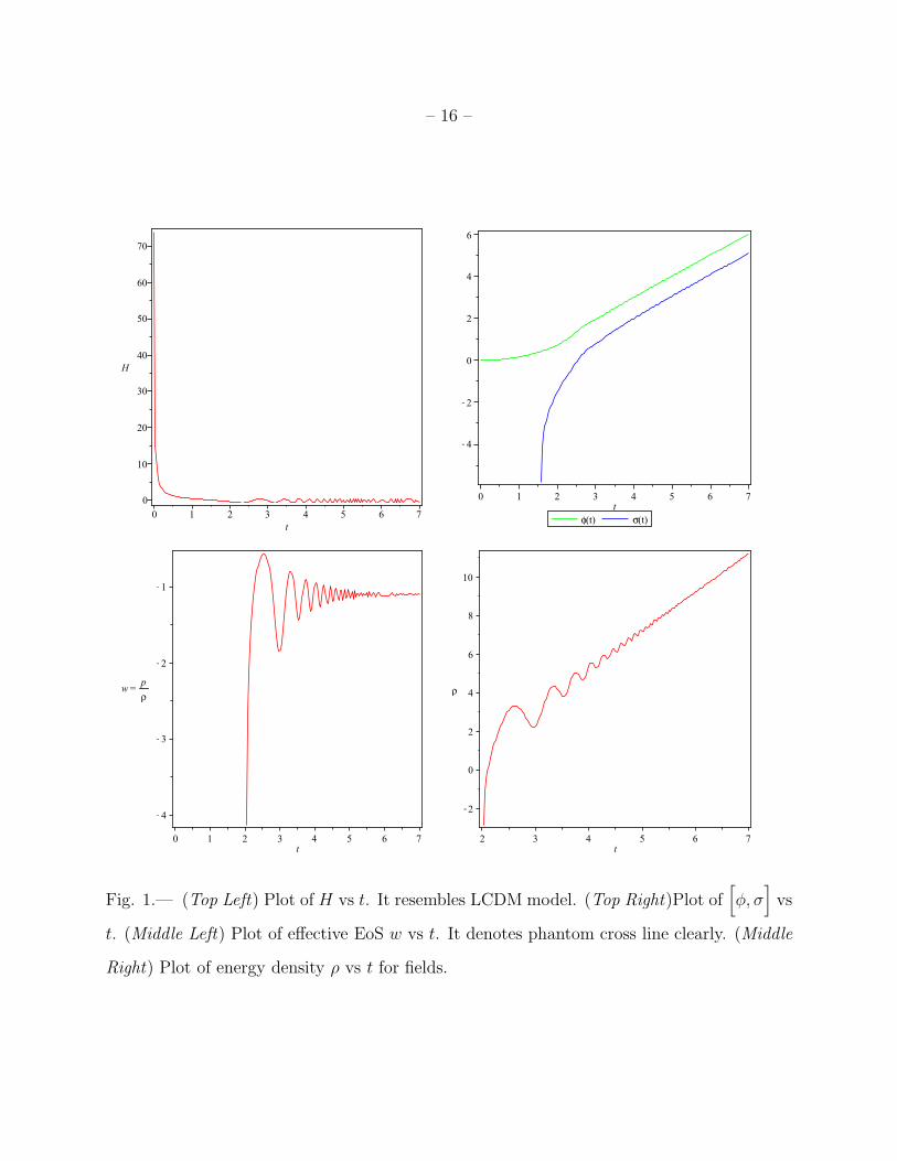
From Fig. 1, we deduce that the behavior of Hubble parameter closely mimics the

standard cold dark matter model with vacuum energy. The Hubble parameter has the

highest value in the early Universe while it suddenly decreases.

In Fig. 2, we plot φ and σ over cosmic time. Asymptotically their evolution becomes

the same, while for small values of time, φ approaches zero (initial state) while σ approaches

-5.

We plotted the equation of state parameter against cosmic time in Fig. 3. Now this w

parameter has contributions from the pressure and energy density of both quintessence and

– 16 –

Fig. 1.— (Top Left) Plot of H vs t. It resembles LCDM model. (Top Right)Plot of[

φ, σ]

vs

t. (Middle Left) Plot of effective EoS w vs t. It denotes phantom cross line clearly. (Middle

Right) Plot of energy density ρ vs t for fields.

– 17 –

phantom fields. For the suitable choice of parameters, it appears that w begins to evolve

from a highly negative value and gradually rising to positive values. During this stage, it

obviously crosses the w = −1 boundary. It turns out that w follows an oscillatory behavior

which gradually diminishes until t = 7. We remark that this value of time does not coincide

with the present time since the choice of parameters is kept arbitrary. It is noticeable that

w remains less than −1 at large time scales.

From Fig. 4, we observe that the total conserved energy density increases with time

globally. However locally, there are fluctuations in the energy density over time. It turns out

that energy density increases when the phantom scalar field dominates, while it decreases

when the quintessence field decays. For large cosmic time, the energy density is dominated

by the phantom energy. we also observe that the total energy density increases with time

globally. However locally, there are fluctuations in the energy density over time. It turns out

that energy density increases when the phantom scalar field dominates while it decreases

when the quintessence field decays. For large cosmic time, the energy density dominates.

6. Stability

In double fields model stability problem has been studied before (Ito et al. 2012). We

are interesting in studying the local stability of the system. Formally, we want to know that

the de-Sitter space is stable or not. We write the system of the dynamical equations in the

following autonomous system of equations:

x1 = −3Hx1 +1 + φ

2, (25)

x2 = −3Hx2 +1 + σ

2, (26)

σ = x1, (27)

– 18 –

φ = x2, (28)

H = −1

2

(

3H2 +1

2(x2

1 − x22)−

1

2(σ − φ)(σ + φ+ 1)

)

. (29)

Stationary (critical point) of the system is:

Xc = (x1 = 0, x2 = 0, φ = −1, σ = −1, H = 0).

The model with H = 0 is a sub case of de-Sitter so called as static model or Einstein

universe. We perturb the system around this critical point up to first order to find:

δχ− 1

2δχ = 0, χ = σ − φ, (30)

δH +1

4δχ = 0. (31)

General solution of the model is written as the following:

δχ = δχ0 sin(t/√2 + θ0), δH =

√2

4δχ0 cos(t/

√2 + θ0).

Oscillatory solutions indicate that the model is stable under small perturbation in first

order. So our quintom scenario predicts the stability scenario of de-Sitter case.

7. Conclusions

To explain the acceleration expansion era of the current universe quintom model

proposed as a double field model, contained of two fields, quintessence and phantom field.

The typical form of the potential function V (σ, φ) remains as a phenomenological unknown

function. In this article, we studied Noether gauge symmetry of quintom cosmology with

arbitrary potentials via Noether Gauge symmetry, as a generalization of the popular

Noether symmetry. Such an approach has been previously investigated in the quintom

cosmology for dynamical system analysis. We presented the Noether symmetry generators

for a typical interactive quintom model. In general, we obtained six families of quintom

– 19 –

models based on different generators. In case 1, we took the gauge field constant and

with the time translation symmetry. Family 2, corresponded to two families of quadratic

potentials where the dynamical behavior of whole system determined by a closed set of

equations of motion. In this family V (φ, σ) = F (12c1(σ

2 − φ2) + c2σ − c3φ). For this case,

we performed cosmography analysis in details. It is interesting to note that the behavior of

Hubble parameter closely mimics the standard cold dark matter model with vacuum energy.

Furthermore, the total energy density increases with time monotonically, globally. Also,

numerically, we deduced that EoS parameter w began to evolve from a highly negative

value and gradually rising to positive values. Also we showed that Einstein space is stable

as a special case. During this stage, it obviously crosses the w = −1 boundary. So, we

extend the cosmology of quintom models beyond the phenomenological potential functions

by a new approach of Noether Gauge Symmetry. Further, as we know the equivalent

presentation of quintom theory gives specific fluid with a pair of effective energy density

and pressure. Consequently, the exact solutions for the generators and the potential

function found, remain to be solutions for field equations in the other equivalent description

via fluids with effective quantities. In this new representation, conservation of energy in

terms of the Liouvile’s form isDρeffDt

= 0 where it is equivalent to the usual conservation

equation ˙ρeff + 3H(ρeff + peff) = 0. In this equivalent form, NGS of point like scalar field

Lagrangian now represent a kind of the symmetry in fluid description. Existence of a closed

algebra between the generators defines a sub class of Lie symmetries. This Lie symmetry

now transfers to the fluid’s equivalent description and so the corresponding Noether charges

(fluid’s invariants) remain conservative for effective fluid. So, the quintom model inspired

from the Noether gauge symmetry is able to give a set of reasonable predictions. Finally,

we mention here that this method may be applied to generalized quintom model introduced

in (Nojiri et al. 2005). In such generalized quintom models by using NGS, we will be able

to find explicitly the form of the potential function .

– 20 –

The work of M. Jamil is supported from the financial grant No. 20-2166/NRPU/RD/HEC/12-

5699 of the Higher Education Commission, Pakistan.

– 21 –

REFERENCES

Aslam, A., Jamil, M., Momeni, D., Myrzakulov, R.: Canadian J. Phys. 91, 93 (2013)

[arXiv:1212.6022]

Aslam, A., Qadir, A.: Journal of applied Mathematics, 532690, 14 (2012)

Bamba, K., Capozziello, S., Nojiri, S., Odintsov, S.D.: Astrophys.Space Sci. 342 (2012)

155-228 [arXiv:1205.3421]

Bluman, G. W., Cheviakov, A. F. Anco, S. C.: Applications of Symmetry Methods to

Partial Differential Equations, Springer Science, New York, 2010

Cai, Y. F., Saridakis, E. N.,Setare, M. R., Xia, J. Q.: Phys. Rept. 493, 1 (2010)

[arXiv:0909.2776 [hep-th]]

Capozziello, S., De Laurentis, M., Odintsov,S. D.: Eur. Phys. J. C 72, 2068 (2012)

[arXiv:1206.4842 [gr-qc]]

Darabi, F.: arXiv:1207.0212 [gr-qc] (2012)

Elizalde,E., Nojiri, S., Odintsov,S.D.: Phys. Rev. D 70 (2004) 043539 [hep-th/0405034]

Feng, B., Wang, X., Zhang, X.: Phys. Lett. B 607, 35 (2005)

Harko, T., Lobo, F. S.N., Nojiri, S., Odintsov, S. D.: Phys. Rev. D 84, 024020 (2011)

Harko, T., Lobo, F. S. N., Minazzoli, O.: Phys. Rev. D 87, 047501 (2013)

Hussain, I., Jamil, M., Mahomed, F. M.: Astrophys. Space Sci. 337, 373 (2012)

Ibragimov, N.H.: Elementary Lie Group Analysis and Ordinary Differential Equations,

John Wiely, 1999

Ito, Y., Nojiri, S., Odintsov, S. D. :arXiv:1111.5389

– 22 –

Jamil, M., Ali, S., Momeni, D., Myrzakulov, R.: Eur. Phys. J. C 72, 1998 (2012a)

Jamil, M., Mahomed, F. M., Momeni, D.: Phys. Lett. B 702, 315 (2011)

Jamil, M., Momeni, D., Myrzakulov, R.: Chin. Phys. Lett. 29, 109801 (2012b)

Jamil, M., Momeni, D., Myrzakulov, R.: Eur. Phys. J. C 73, 2267 (2013a)

Jamil, M., Momeni, D., Myrzakulov, R.: Gen. Relat. Grav. 45, 263 (2013b)

Jamil, M., Momeni, D., Myrzakulov, R., Rudra, P.: J. Phys. Soc. Jpn. 81, 114004(2012c)

Jamil, M., Momeni, D., Myrzakulov, R.: Eur. Phys. J. C 72, 2122 (2012d)

Jamil, M., Momeni, D., Myrzakulov, R.: Eur. Phys. J. C 72, 1959 (2012e)

Jamil, M., Momeni, D., Myrzakulov, R.: Eur. Phys. J. C 72,2137 (2012f)

Kuhfittig, P. K.F., Rahaman, F., Ghosh, A.: Int. J. Theor. Phys. 49, 1222 (2010)

Lazkoz, R., LeUZn, G., Quiros, I.: Phys. Lett. B 649, 103 (2007)

Li, H., Feng, B., Xia, J-Q., Zhang, X.: Phys. Rev. D 73, 103503 (2006)

Lobo, F. S. N., Harko, T.: arXiv:1211.0426 [gr-qc] (2012)

Maluf, J.W.: arXiv:1303.3897 [gr-qc] (2013)

Nojiri, S., Odintsov, S.D.: Gen. Rel. Grav. 38 (2006) 1285 [hep-th/0506212]

Nojiri, S., Odintsov, S.D.: eConf C 0602061 (2006) 06 [Int. J. Geom. Meth. Mod. Phys. 4

(2007) 115] [hep-th/0601213]

Nojiri, S., Odintsov, S.D.: Phys. Rept. 505, 59 (2011)

Sadeghi, J., Setare, M. R., Banijamali, A., Milani,F.: Phys. Lett. B 662, 92 (2008)

– 23 –

Sadjadi, H. M.: Phys. Lett. B 718, 270 (2012)

Saridakis, E.N.: JCAP 0804, 020 (2008a)

Saridakis, E.N.: Phys. Lett. B 661, 335 (2008b)

Shamir, M. F., Jhangeer, A., Bhatti, A. A.: Chin. Phys. Lett. 29, 080402(2012)

Sharif, M., Zubair, M.: JCAP 03, 028 (2012)

Stephani, H.: Differential Equations: Their Solutions Using Symmetry, Cambridge

University Press, New York, 1989

Wei, H., Zhang, S. N.: Phys. Rev. D 76, 063005 (2007)

Xia, J-Q., Feng, B., Zhang, X.: Mod. Phys. Lett. A 20, 2409(2005)

Zhang, J., Gui, Y-X.: Commun. Theor. Phys. 54, 380 (2010)

This manuscript was prepared with the AAS LATEX macros v5.2.