arX

iv:1

109.

4903

v1 [

hep-

th]

22

Sep

2011

Quantum string cosmology in the phase space

Ruben Cordero∗ and Erik Dıaz†

Departamento de Fısica, Escuela Superior de Fısica y Matematicas del IPN

Unidad Adolfo Lopez Mateos, Edificio 9, 07738, Mexico D.F., Mexico

Hugo Garcıa-Compean‡

Departamento de Fısica, Centro de Investigacion y de Estudios Avanzados del IPN

P.O. Box 14-740, 07000 Mexico D.F., Mexico

Francisco J. Turrubiates§

Departamento de Fısica, Escuela Superior de Fısica y Matematicas del IPN

Unidad Adolfo Lopez Mateos, Edificio 9, 07738, Mexico D.F., Mexico.

(Dated: September 23, 2011)

Abstract

Deformation quantization is applied to quantize gravitational systems coupled with matter.

This quantization procedure is performed explicitly for quantum cosmology of these systems in

a flat minisuper(phase)space. The procedure is employed in a quantum string minisuperspace

corresponding to an axion-dilaton system in an isotropic FRW Universe. The Wheeler-DeWitt-

Moyal equation is obtained and its corresponding Wigner function is given analytically in terms

of Meijer’s functions. Finally, this Wigner functions is used to extract physical information of the

system.

PACS numbers: 03.65.-w, 03.65.Ca, 11.10.Ef, 03.65.Sq

∗Electronic address: cordero@esfm.ipn.mx†Electronic address: erik˙harry@hotmail.com‡Electronic address: compean@fis.cinvestav.mx§Electronic address: fturrub@esfm.ipn.mx

1

I. INTRODUCTION

Our contribution to the VIII Mexican workshop on gravitation and mathematical-physics

2010 focused on explaining the implementation of the deformation quantization formalism

to a gravitational field coupled to matter. Also it was considered its application to diverse

cosmological models and the baby Universe system. The analysis included a minisuperspace

approach of the de Sitter model, the Kantowski-Sachs Universe (for the commutative and

non-commutative cases) and finally we discussed the case of string cosmology with a dilaton

exponential potential. The detailed construction is presented in [1] (and references therein)

and will not be repeated here. Instead we will apply the formalism to another case using the

minisuperspace approach of string cosmological models involving axion and dilaton fields in

a curved space. The issues we will discuss in section two involve mainly a brief review of

the Weyl-Wigner-Groenewold-Moyal (WWGM) formalism of deformation quantization [2]

in the context of quantum cosmological models. This is an integral functional formalism and

it is well defined in the case of the whole Wheeler’s superspace of 3-metrics in the ADM’s

description of gravity and matter.

The four dimensional low energy effective field theory action of string theory contains at

least three massless fields: the graviton, the axion and the dilaton [3]. Indirect evidences of

low energy string theory can appear in the physical consequences of the axion in a curved

spacetime [4]. In string theory the dilaton is quite relevant since it defines the string coupling

constant.

One of the most important models of string cosmology is the pre-big-bang scenario [5]. It

incorporates the target space string duality through the scale factor duality. This predicts a

decreasing curvature for negative values of the time coordinate. This curvature is the spec-

ular image of the so-called post-big-bang cosmology. The pre-big-bang cosmology scenario

is important as it is a modification produced by string theory which is (at least perturba-

tively) a consistent theory of quantum gravity. Thus it is expected to describe the correct

modification to standard general relativity at very early times. The prediction is that there

is not a standard big-bang singularity since it is smoothed by the scale factor duality coming

from target space duality. In the present paper we study precisely the quantum cosmological

model regarding the pre-big-bang scenario in the context of the quantization of the phase

space of the minisuperspace of these models. In particular we discuss the cosmological model

2

of a string theory in four dimensions with axion and dilaton fields in a curved space [6].

The rest of the paper is organized as follows. In section three, we apply the deformation

quantization formalism to string cosmology with axion and dilation in a curved minisuper-

space approach and we find the exact Wigner functional which is equivalent to the quantum

states of the Universe. In the last section, we give our final remarks.

II. DEFORMATION QUANTIZATION OF THE GRAVITATIONAL FIELD COU-

PLED TO MATTER

We start by giving a brief overview of the Hamiltonian formalism for the gravitational

field. In particular we consider the ADM decomposition of general relativity coupled to

matter (see for instance [7]). We take a globally hyperbolic spacetime modeled with a pseudo

Riemannian manifold (M, g) whereM = Σ×R and ds2 = gµνdxµdxν = −(N2−N iNi)(dt)

2+

2Nidxidt + hijdx

idxj , with signature (−,+,+,+). Here hij is the intrinsic metric on the

hypersurface Σ, N is the lapse function and N i is the shift vector. The superspace is defined

by Riem(Σ) = hij(x), Φ(x)|x ∈ Σ where Φ is the scalar field. Let Met(Σ) = hij(x)|x ∈ Σwhich is an infinite dimensional manifold. The moduli space of the theory is M = Riem(Σ)

Diff(Σ)

or for pure gravity M = Met(Σ)Diff(Σ)

where Diff(Σ) is the group of diffeomorphisms of Σ. The

corresponding phase space is given by Γ∗ ∼= T ∗Met(Σ) = (hij(x), πij(x)), where πij = ∂LEH

∂hij

and LEH is the Einstein-Hilbert Lagrangian. In the following we will deal with fields at the

moment t = 0 (on Σ) and we put hij(x, 0) ≡ hij(x) and πij(x, 0) ≡ πij(x).

The kind of systems considered here are invariant under diffeomorphisms thus their canon-

ical Hamiltonian is pure constraint. Therefore we only should worry to solve the constraints

of the theory. These are the momentum and the Hamiltonian constraint. This latter is

written as

H⊥(x) = 4ϑ2Gijklπijπkl −

√h

4ϑ2(3R − 2Λ

)+

1

2

√h

(π2

h+ hijΦ,iΦ,j + 2V (Φ)

)= 0, (1)

where ϑ2 = 4πGN , π = ∂LM

∂Φ, with LM stands for the matter Lagrangian, Λ is the cosmo-

logical constant, 3R(h) is the scalar curvature of Σ, Gijkl =12h−1/2

(hikhjl + hilhjk − hijhkl

),

,j denotes partial derivative with respect to xj and h is the determinant of hij . One of the

most important structures for quantization is the Poisson bracket between hij and πkl given

3

by

hij(x), πkl(y)PB =1

2(δki δ

lj + δkj δ

li)δ(x− y). (2)

The canonical quantization promotes the canonical variables to operators acting on some

Hilbert space (or Fock space). In the h-representation they look like: hij |hij,Φ〉 = hij |hij,Φ〉,πij|hij ,Φ〉 = −i~ δ

δhij(x)|hij,Φ〉, Φ|hij,Φ〉 = Φ(x)|hij ,Φ〉 and πΦ|hij ,Φ〉 = −i~ δ

δΦ(x)|hij,Φ〉.

These operators satisfy the commutation relations

[hij(x), πkl(y)] =

i~

2(δki δ

lj + δkj δ

li)δ(x− y), (3)

and similar expressions for the matter part. The Hamiltonian constraint at the quantum

level is given by H⊥|Ψ〉 = 0. In the h-representation we have the constraint given by

[− 4ϑ2Gijkl

δ2

δhijδhkl+

√h

4ϑ2

(− 3R(h) + 2Λ + 4κ2T 00

)]Ψ[hij ,Φ] = 0 , (4)

where 〈hij,Φ|Ψ〉 = Ψ[hij ,Φ] and T00 = − 1

2hδ2

δΦ2 +12hijΦ,iΦ,j + V (Φ). This equation is called

the Wheeler-DeWitt (WDW) equation for the wave function of the Universe Ψ[hij ,Φ].

The deformation quantization of gravity in ADM formalism and constrained systems has

been considered in [8]. In the rest of the paper we assume that the superspace has a flat

metric Gijkl to ensure the existence of the Fourier transform.

Let F [hij, πij; Φ, πΦ] be a functional on the phase space Γ∗ (Wheeler’s phase superspace)

and let F [µij , λij;µ, λ] be its Fourier transform

F [µij, λij;µ, λ] =

∫DπijDhijDπΦDΦexp

− i

∫dx

(µij(x)hij(x) + λij(x)π

ij(x)

+ µ(x)Φ(x) + λ(x)πΦ(x)

)F [hij, π

ij; Φ, πΦ], (5)

where Dhij =∏

x dhij(x), Dπij =∏

x dπij(x), DΦ =

∏x dΦ(x), DπΦ =

∏x dπΦ(x). By

analogy to the quantum mechanics case, we define the Weyl quantization map W as follows

F = W(F [hij , πij ; Φ, πΦ]) :=

∫D(λij

2π

)D(µij

2π

)D(

λ

2π

)D( µ

2π

)F [µij , λij ;µ, λ]U [µij , λij ;µ, λ], (6)

where

U [µij , λij ;µ, λ] := exp

i

∫dx

(µij(x)hij(x) + λij(x)π

ij(x) + µ(x)Φ(x) + λ(x)πΦ(x)

). (7)

Here hij , πij , Φ and πΦ are the field operators defined by: hij(x)|hij,Φ〉 = hij(x)|hij,Φ〉,

πij(x)|πij , πΦ〉 = πij(x)|πij , πΦ〉, Φ(x)|hij ,Φ〉 = Φ(x)|hij ,Φ〉, πΦ(x)|πij, πΦ〉 = πΦ(x)|πij , πΦ〉 .

4

The Campbell-Baker-Hausdorff formula, commutator algebra and the completeness relations

lead to an explicit form for the operator U to be

U [µij, λij;µ, λ] =

∫DhijDΦexp

i

∫dxµij(x)hij(x) + µ(x)Φ(x)

×∣∣∣∣hij −

~λij2,Φ− ~λ

2

⟩⟨hij +

~λij2,Φ +

~λ

2

∣∣∣∣. (8)

One immediately obtains the following structure

F =

∫D(πij

2π~

)DhijD

( πΦ2π~

)DΦF [hij, π

ij; Φ, πΦ]Ω[hij , πij; Φ, πΦ], (9)

where the operator Ω is the Stratonovich-Weyl quantizer and it is given by

Ω[hij , πij ; Φ, πΦ] =

∫D(~λij

2π

)DµijD

(~λ

2π

)Dµ

× exp

− i

∫dx

(µij(x)hij(x) + λij(x)π

ij(x) + µ(x)Φ(x) + λ(x)πΦ(x)

)U [µij , λij ;µ, λ]. (10)

This operator can be written in the following form (that can be very useful to invert the

mapping W)

Ω[hij , πij ; Φ, πΦ] =

∫Dξij

∫Dξ exp

− i

~

∫dxξij(x)π

ij(x) + ξ(x)πΦ(x)

×∣∣∣∣hij −

ξij2,Φ− ξ

2

⟩⟨hij +

ξij2,Φ+

ξ

2

∣∣∣∣. (11)

The space A of all functionals on the phase space Γ∗ i.e. A := F = F [hij , πij; Φ, πΦ],

forms with the usual product an associative and commutative algebra. This algebra can

be deformed into an associative and non-commutative algebra A⋆ with the ⋆−product. In

relation to the W map this ⋆ product is defined as: W−1(F · G) = F ⋆ G for any pair of

functionals F and G in A. Thus the ⋆ product is defined as

(F ⋆ G)[hij , πij; Φ, πΦ] := W−1(F G) = Tr

Ω[hij , π

ij; Φ, πΦ]F G

, (12)

or after some straightforward computations

(F ⋆ G

)[hij , π

ij; Φ, πΦ] = F [hij , πij; Φ, πΦ] exp

i~

2

↔PG[hij, π

ij ; Φ, πΦ], (13)

where↔P is the operator given by

↔P :=

∫dx

( ←δ

δhij(x)

→δ

δπij(x)−

←δ

δπij(x)

→δ

δhij(x)

)+

∫dx

( ←δ

δΦ(x)

→δ

δπΦ(x)−

←δ

δπΦ(x)

→δ

δΦ(x)

). (14)

5

Let ρ be the density operator of a quantum state. The functional ρW [hij , πij; Φ, πΦ] corre-

sponding to ρ reads

ρW [hij , πij; Φ, πΦ] = Tr

Ω[hij , π

ij; Φ, πΦ]ρ

:=

∫D(ξij2π~

)D(

ξ

2π~

)exp

− i

~

∫dx

(ξij(x)π

ij(x) + ξ(x)πΦ(x)

)

×⟨hij +

ξij2,Φ+

ξ

2

∣∣∣∣ρ∣∣∣∣hij −

ξij2,Φ− ξ

2

⟩. (15)

For a pure state of the system ρ = |Ψ〉〈Ψ| we have

ρW[hij , π

ij ; Φ, πΦ] =

∫D(

ξij2π~

)D(

ξ

2π~

)exp

− i

~

∫dx

(ξij(x)π

ij(x) + ξ(x)πΦ(x)

)

×Ψ∗[hij −

ξij2,Φ− ξ

2

]Ψ

[hij +

ξij2,Φ+

ξ

2

]. (16)

It is now possible to write the Hamiltonian constraint in terms of the ⋆−product and the

Wigner functional as

H⊥ ⋆ ρW[hij , π

ij; Φ, πΦ] = 0. (17)

This is the Moyal deformation of the Wheeler-DeWitt equation an we will just called it the

Wheeler-DeWitt-Moyal (WDWM) equation.

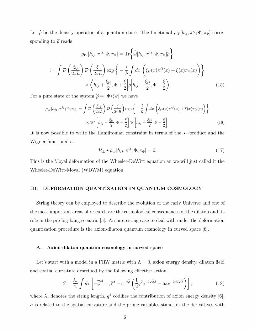
III. DEFORMATION QUANTIZATION IN QUANTUM COSMOLOGY

String theory can be employed to describe the evolution of the early Universe and one of

the most important areas of research are the cosmological consequences of the dilaton and its

role in the pre-big-bang scenario [5]. An interesting case to deal with under the deformation

quantization procedure is the axion-dilaton quantum cosmology in curved space [6].

A. Axion-dilaton quantum cosmology in curved space

Let’s start with a model in a FRW metric with Λ = 0, axion energy density, dilaton field

and spatial curvature described by the following effective action

S =λs2

∫dτ

[−φ′2

+ β ′2 − e−2φ

(1

2q2e−2

√3β − 6κe−2β/

√3

)], (18)

where λs denotes the string length, q2 codifies the contribution of axion energy density [6],

κ is related to the spatial curvature and the prime variables stand for the derivatives with

6

respect to the dilaton time [9].

Using now the variables φ = φ+√3β, y = φ

√3+β =

√3(φ− 2 ln a− ln

∫d3xλ3s

), we obtain

that

S =λs4

∫dτ[φ′2 − y′2 − q2e−2φ + 12κe−2y/

√3]. (19)

The corresponding WDW equation takes the following form

HΨ(y, φ) =1

λs

(~2∂2y − ~

2∂2φ +1

4λ2sq

2e−2φ − 3λ2sκe− 2√

3y

)Ψ(y, φ) = 0. (20)

The solutions of this equation are obtained by the method of separation of variables Ψ(y, φ) =

χα(y)ψα(φ). In this way we get for the χα(y) and ψα(φ) parts the following equations

~2∂2yχα(y) + (α2 − 3λ2sκe

−2y/√3)χα(y) = 0, (21)

~2∂2φψα(φ) +

(α2 − λ2sq

2

4e−2φ

)ψα(φ) = 0 (22)

where α is the separation constant.

We consider the case for κ > 0, for which the general solutions to both parts are given by

χα(y) = A1Ii√

3α~

(3λs√κe

− y√3/~) + A2Ki

√3α~

(3λs√κe

− y√3/~), (23)

ψα(φ) = B1Iiα~(λsqe

−φ/2~) +B2Kiα~(λsqe

−φ/2~). (24)

To avoid an infinite value of the wave function as y → −∞ and φ → −∞ we must choose

χα(y) ∼ Ki√

3α~

(3λs√κe

− y√3/~) and ψα(φ) ∼ Kiα

~(λsqe

−φ/2~), which corresponds to the pre-

big-bang regime for α2 < 3λ2sκe−2y/

√3 and where Kiν(x) denotes the MacDonald function

of imaginary order. Using the result given in [10] we normalize the χα(y) part of the wave

function in the following form

∫ ∞

−∞dyχ∗

α(y)χα′(y) = δ(α2 − α′2), (25)

and a similar expression can be found for the φ part.

In order to write the WDWM equation (17) it is very useful to employ the next relation

f(x, p) ⋆ g(x, p) = f

(x+

i~

2

→∂ p, p−

i~

2

→∂ x

)g(x, p), (26)

from which we obtain the following equation(−(Py −

i~

2

→∂ y

)2

+

(Pφ − i~

2

→∂ φ

)2

+1

4λ2sq

2e−2

(

φ+ i~2

→∂ Pφ

)

− 3λ2sκe− 2√

3

(

y+ i~2

→∂ Py

))ρ(y, Py, φ, Pφ) = 0.

(27)

7

02

46

y

-2-1

01

2

Py

-1.0

-0.5

0.0

0.5

1.0

Ρ

0 1 2 3 4 5 6 7-2

-1

0

1

2

y

Py

FIG. 1: The Wigner function and its density are plotted in the y variable (~ = 1, α = 1). The figure on

the left shows many oscillations due to the interference among wave functions of expanding and contracting

universes. The thick curve on the right figure corresponds to the classical trajectory which coincides with

the maximum of the Wigner function.

The last expression can be split into two equations corresponding to its real part

[−P 2

y +~2

4∂2y + P 2

φ − ~2

4∂2φ +

1

4λ2sq

2e−2φ cos(~∂Pφ

)− 3λ2

sκe− 2√

3ycos

(~√3∂Py

)]ρ(y, Py, φ, Pφ) = 0, (28)

and its imaginary part

[~(Py∂y)− ~(Pφ∂φ)−

1

4λ2sq

2e−2φ sin(~∂Pφ

)+ 3λ2

sκe− 2√

3ysin

(~√3∂Py

)]ρ(y, Py, φ, Pφ) = 0. (29)

We propose ρ(y, Py, φ, Pφ) = ρy(y, Py)ρφ(φ, Pφ), and taking into account that eia∂xf(x) =

f(x+ ia) then from the two previous equations we obtain the following results:

For the function ρy(y, Py)

[−P 2

y + µ2 +ν4

4P 2y

]ρy(y, Py) +

~

4Py

(ν2u(y)

i~Py− 2iu(y)√

3

)(ρy

(y, Py +

i~√3

)− ρy

(y, Py −

i~√3

))

−u2(y)

~

[1

Py +i~√3

(ρy

(y, Py +

2i~√3

)− ρy(y, Py)

)− 1

Py − i~√3

(ρy(y, Py)− ρy

(y, Py −

2i~√3

))]

+ν2u(y)

i~

[ρy(y, Py +

i~√3)

Py +i~√3

−ρy(y, Py − i~√

3)

Py − i~√3

]− u(y)

(ρy

(y, Py +

i~√3

)+ ρy

(y, Py −

i~√3

))= 0, (30)

8

0

2

4

6

Φ

-2-1

01

2

PΦ

-1.0

-0.5

0.0

0.5

1.0

Ρ

0 1 2 3 4 5 6 7-2

-1

0

1

2

Φ

PΦ

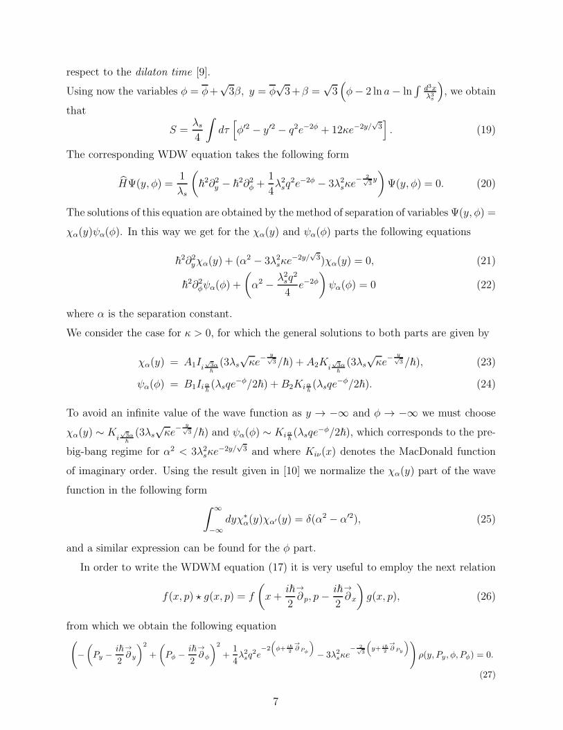
FIG. 2: The Wigner function and its density are plotted in the φ variable (~ = 1, α = 1). The figure on the

left shows oscillations of higher amplitude with respect to the y part. In the right figure the thick curve is

the classical trajectory and corresponds the maximum of the Wigner function (the φ < 0 region is classical

forbidden).

and for the function ρφ(φ, Pφ)[P 2φ − µ2 − ν4

4P 2φ

]ρφ(φ, Pφ)−

~

4Pφ

(ν2w(φ)

i~Pφ− 2iw(φ)

)(ρφ(φ, Pφ + i~)− ρφ(φ, Pφ − i~))

−w2(φ)

~

[1

Pφ + i~(ρφ(φ, Pφ + 2i~)− ρφ(φ, Pφ))−

1

Pφ − i~(ρφ(φ, Pφ)− ρφ(φ, Pφ − 2i~))

]

+ν2w(φ)

i~

[ρφ(φ, Pφ + i~)

Pφ + i~− ρφ(φ, Pφ − i~)

Pφ − i~

]+ w(φ)(ρφ(φ, Pφ + i~) + ρφ(φ, Pφ − i~)) = 0, (31)

where we have defined the functions u(y) = 3λ2sκe

− 2√3y

2and w(φ) = λ2

sq2e−2φ

8.

It is hard to solve the last two equations, so to obtain their solutions we will follow a different

approach and will use the integral representation for the Wigner function. We can found its

y part by computing

ρy(y, Py) =1

2π

∫ ∞

−∞ψ∗(y − ~q/2) exp(−iqPy)ψ(y + ~q/2)dq

=|A2|22π

∫ ∞

−∞K∗

i√

3α~

(3λs√κe

− (y−~q/2)√3 /~) exp(−iqPy)Ki

√3α~

(3λs√κe

− (y+~q/2)√3 /~)dq. (32)

Defining the variables ω = e~q/2√3 and z = a = 3λs

~

√κe−y/

√3, we get:

ρy(y, Py) =

√3|A2|2π~

∫ ∞

0

Ki√

3α~

(zω)ωσ− 12K

i√

3α~

(z/ω)dω, (33)

where σ = −12− 2

√3

~iPy and |A2|2 =

√3 sinh(π

√3α~

)

π2~2.

9

Using now the following result (see Sec. 19.6 formula (25) in [11] and the comment in

[12])

∫ ∞

0

dw(wz)1/2wσ−1Kµ(a/w)Kν(wz) = 2−σ−5/2aσG4004

(a2z2

16

∣∣∣∣µ− σ

2,−µ− σ

2,1

4+

ν

2,1

4− ν

2

), (34)

where G4004

(a2z2

16

∣∣∣∣µ−σ2, −µ−σ

2, 14+ ν

2, 14− ν

2

)is a special case of Meijer’s G function (see Sec.

5.3 in [13])

Gmnpq

z∣∣∣∣ai, i = 1, ..., p

bj , j = 1, ..., q

, (35)

we obtain the following expression

ρy(y, Py) =sinh(π

√3α~

)

4π3~2

ey√3

λs√κ

(3u(y)

2~2

)−√3

~iPy

×G4004

(9u2(y)

4~4

∣∣∣∣1

4+

i√3

~

(α2+ Py

),1

4+

i√3

~

(−α

2+ Py

),1

4+

i√3α

2~,1

4− i

√3α

2~

). (36)

Now, employing the Meijer’s function property

xσGmnpq

x∣∣∣∣ai, i = 1, ..., p

bj , j = 1, ..., q

= Gmn

pq

x∣∣∣∣ai + σ, i = 1, ..., p

bj + σ, j = 1, ..., q

, (37)

equation (36) can be written as

ρy(y, Py) =sinh(π

√3α~

)

4π3~2

ey√3

λs√κ

×G4004

(9u2(y)

4~4

∣∣∣∣1

4+

i√3

2~(α+ Py),

1

4+

i√3

2~(−α+ Py),

1

4+

i√3

2~(α− Py),

1

4+

i√3

2~(−α− Py)

). (38)

It is possible to verify that this Wigner function indeed satisfy equation (30).

Performing a similar procedure we can obtain the following Wigner function for the φ part

ρφ(φ, Pφ) =sinh(πα

~)

2π3~2

eφ

λsq

×G4004

(w2(φ)

4~4

∣∣∣∣1

4+

i

2~(α+ Pφ),

1

4+

i

2~(−α+ Pφ),

1

4+

i

2~(α− Pφ),

1

4+

i

2~(−α− Pφ)

), (39)

which fulfills Eqn. (31).

We can gain some physical insight if we plot the Wigner functions of the corresponding

y and dilaton parts for several values of α. For the y part and α = 1 Fig. 1 shows that the

classical trajectory is near the highest peaks of the Wigner function. For values of α smaller

than one there are less oscillations but the classical trajectory does not correspond to the

highest peaks, in fact, there is an ample region where the Wigner function is large. For

10

values of α bigger than one it can be observed an increment in the number of oscillations of

Wigner function and the peaks of the oscillations are far away from the classical trajectory

(these plots are not showed in the paper). We conclude that the quantum interference effects

are enhanced for larger values of α. A similar behavior is obtained for the dilaton part for

α, nevertheless from Fig. 2 its amplitude is larger. The parameter α can be interpreted as

the energy of the y and φ parts, the matter (dilaton axion part) has positive energy and any

fluctuation of it induces a variation of the energy in the gravitational part (the scale factor)

in order to vanish the total energy.

IV. FINAL REMARKS

In this paper we have presented the WWGM formalism for a gravitational field coupled

to matter in the flat superspace (and flat phase superspace) where the Stratonovich-Weyl

quantizer, the star product and the Wigner functional are obtained. These results can be

used in general situations but in a first approach we applied [1] the formalism to some in-

teresting minisuperspace models widely studied in the literature, in particular we studied

here the axion-dilaton quantum cosmology model with non-vanishing spatial curvature. We

found the corresponding WDWM equation and the equivalent differential-difference equa-

tion. These equations have an exact solution in terms of the Meijer’s functions. We have

seen that the parameter α has an interpretation of energy for the components y and φ. For

an arbitrary total constant energy any fluctuation in the energy of matter does induce a

corresponding fluctuation in the gravitational part in such a way that both are compen-

sated. Moreover, we found that for small values of α there are fewer oscillations in the

gravitational part of the Wigner function but the classical trajectory does not correspond to

the highest peaks. In the case of bigger values of α there is a clear increment in the number

of oscillations of Wigner function, being its peaks far away from the classical trajectory. We

observe also that the quantum interference effects for larger values of α are enhanced. The

same situation is regarded for the dilaton part but with larger amplitude oscillations. It

is worth to mention that the construction presented here can be employed to treat other

cosmological models.

11

Acknowledgments

The work of R. C., H. G.-C. and F. J. T. was partially supported by SNI-Mexico, CONA-

CyT research grants: J1-60621-I, 103478 and 128761. In addition R. C. and F. J. T. were

partially supported by COFAA-IPN and by SIP-IPN grants 20111070 and 20110968.

[1] R. Cordero, H. Garcıa-Compean and F. J. Turrubiates, Phys. Rev. D 83, 125030 (2011).

[2] C. K. Zachos, D. B. Fairlie and T. L. Curtright, Quantum Mechanics in phase space, World

Scientific, Singapore, 2005.

[3] J. Polchinski, String Theory, Vol. 1 & 2, Cambridge University Press, England, 1998.

[4] S. Das, P. Jain, J. P. Ralston and R. Saha, JCAP 0506, 002 (2005).

[5] M. Gasperini and G. Veneziano, Phys. Rept., 373, 1 (2003). [arXiv:hep-th/0207130].

[6] M. Dabrowski, Ann. Phys. 10, 195 (2001).

[7] D. L. Wiltshire, “An introduction to quantum cosmology,” [gr-qc/0101003].

[8] F. Antonsen, “Deformation quantisation of gravity,” [arXiv:gr-qc/9712012]; “Deformation

quantisation of constrained systems,” [arXiv:gr-qc/9710021].

[9] K. A. Meissner and G. Veneziano, Mod. Phys. Lett. A 6, 3397 (1991).

[10] R. Szmytkowski and S. Bielski, J. Math. Anal. Appl. 365, 195 (2010).

[11] A. Erdelyi et al., Tables of Integral Transform, Bateman Manuscript Project, McGarw-Hill,

New York, 1954.

[12] T. Curtright, D. Fairlie and C. Zachos, Phys. Rev. D 58, 025002 (1998).

[13] A. Erdelyi et al., Higher Transcendental Functions, Bateman Manuscript Project, McGraw-

Hill, New York, 1953.

12