String Algorithm on GPUPU

The project report is prepared for

Faculty of Engineering

Multimedia University

in partial fulfilment for

Bachelor of Engineering

FACULTY OF ENGINEERING

MULTIMEDIA UNIVERSITY

February 2013

STRING ALGORITHM ON GPGPU

by

ONG WEN MEI

1081104562

Session 2012/2013

ii

The copyright of this report belongs to the author under the terms of the Copyright

Act 1987 as qualified by Regulation 4(1) of the Multimedia University Intellectual

Property Regulations. Due acknowledgement shall always be made of the use of any

material contained in, or derived from, this report.

iii

Declaration

I hereby declare that this work has been done by myself and no portion of the work

contained in this report has been submitted in support of any application for any

other degree or qualification of this or any other university or institute of learning.

I also declare that pursuant to the provisions of the Copyright Act 1987, I have not

engaged in any unauthorised act of copying or reproducing or attempt to copy /

reproduce or cause to copy / reproduce or permit the copying / reproducing or the

sharing and / or downloading of any copyrighted material or an attempt to do so

whether by use of the University’s facilities or outside networks / facilities whether

in hard copy or soft copy format, of any material protected under the provisions of

sections 3 and 7 of the Act whether for payment or otherwise save as specifically

provided for therein. This shall include but not be limited to any lecture notes,

course packs, thesis, text books, exam questions, any works of authorship fixed in

any tangible medium of expression whether provided by the University or otherwise.

I hereby further declare that in the event of any infringement of the provisions of the

Act whether knowingly or unknowingly the University shall not be liable for the

same in any manner whatsoever and undertake to indemnify and keep indemnified

the University against all such claims and actions.

Signature : ________________________

Name : ONG WEN MEI

Student ID : 1081104562

Date : FEBRUARY 2013

iv

Dedication

This thesis is dedicated to

my beloved parents,

family

and friends.

v

Acknowledgements

I would like to express my gratitude towards various people whom during

this several months of my final year project, had provided me with great assistance.

Without their help and support, this project would not have been completed on time.

First and foremost, I would like to express my deepest appreciation to my

supervisor, Mr. Vishnu Monn Baskaran. He had given me a lot of constructive

remarks and professional insights which improved my work vastly in many ways. I

would also like to thank my project moderator, Dr. Ian Chai for his ideas and

opinions for me.

A special note of thanks goes to my mentors from MIMOS Berhad (Kuala

Lumpur division), Dr. Ettikan Kandasamy & Dr. Chong Poh Kit for their advice and

guidance throughout my project. They have taught me a lot of things in terms of

technical aspects, which helped me in many significant ways.

Lastly, I would like to thank the staff and students of Multimedia University,

Cyberjaya as well as other related people who have sacrificed their time in helping

and supporting me in any way during the completion of this project.

vi

Abstract

Since the last decade, the concept of general purpose computing on graphics

processors was introduced and has since garnered significant adaptation in the

engineering industry. The use of a Graphics Processing Unit (GPU) as a many-core

processing architecture for the purpose of general-purpose computation yields

performance improvement of several orders-of magnitude. One example in

leveraging a GPU for improved computational performance is the parallelization of

string searching algorithms.

The string search algorithm is often required to be performed on large datasets.

However, string algorithms are commonly optimised to be performed using a

Central Processing Unit (CPU) and risks high levels of computational bottlenecks.

As such, this dissertation first identifies these bottlenecks by analysing the design

and implementation of a serial Bloom Filter algorithm. Based on the analysed

results, a parallel Bloom Filter algorithm is proposed, which utilizes software

threads (i.e., OpenMP) on a multi-core processor for data parallelism. Experimental

results suggest that a multi-core driven (i.e., Using 8 logical processors) parallel

Bloom Filter algorithm exhibits performance speed up of up to 3.3x for a set of 10

million strings.

The design and implementation of the parallel Bloom Filter algorithm is then

extended into a GPU processor using the Compute Unified Device Architecture

(CUDA) parallel computing platform. The proposed parallel Bloom Filter algorithm

on CUDA segments the string list into blocks of words and threads in generating the

bit table, which is used during the string matching process. This method maximizes

the computational performance and sustains consistent string matching results.

Experimental results suggest that a GPU driven (i.e., Using 256 CUDA cores)

parallel Bloom Filter algorithm further extends the performance speed up to 5.5x for

a set of 10 million strings.

vii

In addition, this dissertation also analyses the searching drawback of a Bloom Filter

algorithm in locating matching string positions. As such, an alternative parallel

Quick Search string algorithm is designed, implemented and assessed in an effort to

address this drawback.

viii

Table of Contents

Declaration ............................................................................................................... iii

Dedication .................................................................................................................. iv

Acknowledgements .................................................................................................... v

Abstract ..................................................................................................................... vi

List of Figures .......................................................................................................... xii

List of Tables ............................................................................................................ xv

List of Mathematical Equations ............................................................................ xvi

List of Abbreviations ............................................................................................. xvii

List of Mathematical Symbols ............................................................................ xviii

CHAPTER 1: INTRODUCTION ........................................................................ 1

1.1 Preamble ....................................................................................................... 1

1.2 Current Trend ................................................................................................ 1

1.3 Problem Statement ........................................................................................ 2

1.4 Motivation and Proposed Solution ............................................................... 3

1.5 Objectives ..................................................................................................... 3

1.6 Report Structure ............................................................................................ 4

CHAPTER 2: LITERATURE REVIEW ............................................................ 5

2.1 Search Algorithm .......................................................................................... 5

2.2 Linear Sequential Search .............................................................................. 5

2.3 Binary Search ................................................................................................ 6

ix

2.4 Hash Tables ................................................................................................... 7

2.5 Bloom Filter .................................................................................................. 8

2.5.1 Algorithm Description ........................................................................... 8

2.5.2 False Positive Probability ...................................................................... 9

2.5.3 Advantages .......................................................................................... 11

2.6 Parallel Processing ...................................................................................... 12

2.7 OpenMP ...................................................................................................... 13

2.8 CUDA ......................................................................................................... 15

2.8.1 Architecture of a CUDA-capable GPU ............................................... 15

2.8.2 CUDA Programming Model ............................................................... 16

2.8.3 CUDA Memory Model ........................................................................ 18

2.8.4 CUDA Execution Model ..................................................................... 19

2.9 CUDA C ..................................................................................................... 21

2.9.1 Device Function ................................................................................... 22

2.9.2 Basic Device Memory Management ................................................... 22

2.9.3 Launching Parallel Kernels ................................................................. 23

2.9.4 Shared Memory ................................................................................... 24

2.9.5 Thread Synchronization ....................................................................... 24

2.10 Applications of CUDA ............................................................................... 24

2.10.1 Oil Resource Exploration .................................................................... 25

2.10.2 Design Industry ................................................................................... 25

2.10.3 Weather and Climate ........................................................................... 25

2.11 Existing CUDA String Algorithms ............................................................. 26

CHAPTER 3: PERFORMANCE DRAWBACK OF A SERIAL BLOOM

FILTER STRING SEARCH ALGORITHM ....................................................... 28

3.1 Introduction ................................................................................................. 28

3.2 Program Flow ............................................................................................. 28

3.2.1 Loading Input Files .............................................................................. 30

3.2.2 Data Pre-processing ............................................................................. 31

x

3.2.3 Class Objects ....................................................................................... 32

3.2.4 Filter Insertion ..................................................................................... 34

3.2.5 Filter Searching ................................................................................... 38

3.3 AP Hash Function ....................................................................................... 39

3.4 System Assessment ..................................................................................... 41

3.4.1 Assessment Environment .................................................................... 41

3.4.2 Performance Assessment ..................................................................... 41

CHAPTER 4: DATA PARALLELISATION OF A BLOOM FILTER

USING OPENMP .................................................................................................... 45

4.1 Program Design .......................................................................................... 45






CHAPTER 5: CUDA IMPLEMENTATION OF THE BLOOM FILTER

STRING SEARCH ALGORITHM ....................................................................... 53

5.1 Program Design .......................................................................................... 53

5.1.1 Offset Calculation ................................................................................ 55






CHAPTER 6: FURTHER DEDUCTIONS FROM PERFORMANCE

COMPARISON …………………………………………………………………..68

6.1 Performance Assessment for Parallel CPU and GPU Implementations ..... 68

6.2 System Assessment for the GPGPU Implementation on Different GPUs .. 71

xi



CHAPTER 7: QUICK SEARCH ALGORITHM FOR LOCATION

IDENTIFICATION ................................................................................................. 76

7.1 Algorithm Description ................................................................................ 76

7.1.1 Bad Character Rule .............................................................................. 77

7.2 Program Design .......................................................................................... 77

7.2.1 Serial Implementation ......................................................................... 78

7.2.2 OpenMP Implementation .................................................................... 80

7.2.3 CUDA Implementation ....................................................................... 81




CHAPTER 8: CONCLUSIONS AND FUTURE WORK ............................... 88

8.1 Summary of Work ...................................................................................... 88

8.2 Conclusions ................................................................................................. 88

8.3 Future Work ................................................................................................ 89

References ................................................................................................................ 90

xii

List of Figures

Figure 2.1: Linear Sequential Search for "Amy". ....................................................... 6

Figure 2.2: Binary Search for Eve. .............................................................................. 6

Figure 2.3: Using Hash Table to search for Dan's data. .............................................. 8

Figure 2.4: An empty Bloom Filter. .......................................................................... 10

Figure 2.5: The Bloom Filter after adding first element. .......................................... 11

Figure 2.6: The Bloom Filter after adding second element. ...................................... 11

Figure 2.7: False positive in Bloom filter. ................................................................. 11

Figure 2.8: Hyperthreading Block Diagram. ............................................................. 13

Figure 2.9: OpenMP execution models. .................................................................... 14

Figure 2.10: Architecture of a CUDA-capable GPU. ................................................ 16

Figure 2.11: Heterogeneous architecture. .................................................................. 16

Figure 2.12: CUDA compute grid, block and thread architecture............................. 17

Figure 2.13: Cuda device memory model. ................................................................ 18

Figure 2.14: Architecture of a Streaming Multiprocessor (SM). .............................. 20

Figure 2.15: Dual Warp Scheduler in a Streaming Multiprocessor. ......................... 20

Figure 3.1: Flowchart for the main program. ............................................................ 29

Figure 3.2: Pre-processing of input text file. ............................................................. 31

Figure 3.3: Flowchart for inserting one element. ...................................................... 36

Figure 3.4: Time taken for Filter Insertion implemented using serial programming.

................................................................................................................. 42

Figure 3.5: Time taken for Filter Search implemented using serial programming. .. 42

Figure 3.6: Total time taken for Bloom Filter algorithm (insert and search)

implemented using serial programming. ................................................. 43

Figure 4.1: Execution Model for OpenMP Insert (T represents number of parallel

threads). ................................................................................................... 47

Figure 4.2: Execution Model for OpenMP Search (T represents number of parallel

threads). ................................................................................................... 48

Figure 4.3: Time taken and performance gain for Filter Insertion when implemented

using serial programming and OpenMP. ................................................. 50

xiii

Figure 4.4: Time taken and performance gain for Filter Search when implemented

using serial programming and OpenMP. ................................................. 50

Figure 4.5: Total time taken and performance gain for Bloom Filter algorithm (insert

and search) when implemented using serial programming and OpenMP.

................................................................................................................. 51

Figure 5.1: Execution Model for insert() function (for one batch of data with batch

size of 50,000). ........................................................................................ 57

Figure 5.2: Execution Model for contain() function (for one batch of data with batch

size = 50,000). ......................................................................................... 61

Figure 5.3: Total time taken for Bloom Filter (insert and search) when implemented

on CUDA using different batch sizes (8 and 50,000). ............................ 64


using serial programming and CUDA. .................................................... 65


using serial programming and CUDA. .................................................... 65

Figure 5.6: Total time taken and performance gain for Bloom Filter (insert and

search) when implemented using serial programming and CUDA. ........ 66


using OpenMP and CUDA (Quadro4000). ............................................. 69


using OpenMP and CUDA (Quadro4000). ............................................. 69

Figure 6.3: Total time taken and performance gain for Bloom Filter (insert and

search) when implemented using OpenMP and CUDA (Quadro4000). . 70

Figure 6.4: Time taken and performance comparison for Filter Insert when executed

using GeForce 530 and Quadro4000. ...................................................... 72

Figure 6.5: Time taken and performance comparison for Filter Search when

executed using GeForce 530 and Quadro4000. ....................................... 73

Figure 6.6: Total execution time and performance gain when executing the Bloom

Filter algorithm (insert and search) on GeForce 530 and Quadro4000. .. 73

Figure 6.7 Part of the bit-table for 1000 strings. ....................................................... 74

Figure 7.1: Mismatch character is found in pattern. .................................................. 77

Figure 7.2: Mismatch character is absent in pattern. ................................................. 77

file:///C:/Users/WM/Desktop/finalised%20thesis.docx%23_Toc346941493


xiv

Figure 7.3: Quick Search Algorithm. ........................................................................ 78

Figure 7.4: OpenMP Execution Model for boyer_moore() function when 8 parallel

threads are launched. ............................................................................... 80

Figure 7.5: CUDA execution model for cuda_boyer_moore() function with 2000

queries. ..................................................................................................... 82

Figure 7.6: Time taken for Quick Search when the size of the input word list is fixed

at 110,000. ............................................................................................... 83

Figure 7.7: Performance ratio when the size of the input word list is fixed at

110,000. ................................................................................................... 84

Figure 7.8: Time taken for Quick Search when the size of the query list is fixed at

2000. ........................................................................................................ 85

Figure 7.9: Performance ratio when the size of the query list is fixed at 2000. ........ 86





xv

List of Tables

Table 3.1: CBloom_parameters Class Members. ...................................................... 32

Table 3.2: CBloom_parameters Class Functions. ..................................................... 32

Table 3.3: CSimple_bloom_filter Class Members. ................................................... 33

Table 3.4: CSimple_bloom_filter Class Functions. .................................................. 34

Table 3.5: CPU Specifications. ................................................................................. 41

Table 5.1: Variables which are transferred once throughout the entire program. ..... 53

Table 5.2: Values stored in each variable on the host memory. ................................ 54

Table 5.3: Device pointers for variables which are transferred in batches. .............. 54

Table 5.4: Device Properties. .................................................................................... 62

Table 6.1: Device Properties. .................................................................................... 71

xvi

List of Mathematical Equations

Probability of a bit not set to 1 by a certain hash function ………………………10

Probability of a bit not set to 1 by any of the hash functions ………………………10

Probability of a bit not set to 1 after inserting n elements ………………………10

Probability of a bit set to 1 after inserting n elements ………………………10

False positive probability ………………………………………………………10

The limit of fpp as m approaches 0 ……………………………………………....10

The limit of fpp as n approaches infinity …………………………………........10

The size of Bloom Filter ………………………………………………………32

Representation of symbols used in checking Bernstein’s Conditions ………43

Bernstein’s Conditions for first 2 string elements in the list ………………43

Bernstein’s Conditions for any 2 string elements ………………………………43

Bernstein’s Conditions for n string elements ………………………………43

Performance gain for OpenMP implementation of Bloom Filter ………………48

Performance gain for CUDA implementation of Bloom Filter ………………64

Index of result array ………………………………………………………………80

xvii

List of Abbreviations

1D 1-dimensional

2D 2-dimensional

3D 3-dimensional

ALU Arithmetic logic unit

AP Arash Partow

API Application programming interface

CPU Central processing unit

CUDA Compute Unified Device Architecture

DRAM Dynamic random-access memory

GDDR Graphics Double Data Rate

GUI Graphical user interface

GPGPU General-purpose computing on Graphics Processing Unit

GPU Graphics processing unit

IEEE Institute of Electrical and Electronics Engineering

LFSR Linear feedback shift register

NCAR National Center for Atmospheric Research

OpenGL Open Graphics Library

OpenMP Open Multiprocessing

PDC Parallel data cache

SM Streaming multiprocessor

SMT Simultaneous multithreading

SP Streaming processors

WRF Weather Research and Forecasting model

xviii

List of Mathematical Symbols

fpp false positive probability

k number of hash functions

m size of bit array

n number of elements

O(log n) logarithmic time complexity

O(n) linear time complexity

time taken for a Bloom Filter in serial implementation

time taken for a Bloom Filter in OpenMP implementation

time taken for a Bloom Filter in CUDA implementation

𝕚 set of words in the word list

𝕠 set of resultant hash operations

empty set

1

CHAPTER 1: INTRODUCTION

1.1 Preamble

General-purpose computing on a Graphics Processing Unit (GPGPU) is the

utilization of a Graphics Processing Unit (GPU) to handle computation in

applications which are traditionally performed by the Central Processing Unit

(CPU). It involves using a GPU along with a CPU with the aim of accelerating

general-purpose scientific and engineering applications. The multicore architecture

of a CPU encourages thread-level parallelism and data-level parallelism whereas a

GPU contains hundreds of smaller cores with high efficiency and are designed for

parallel performance. Hence, computation-intensive portions of the application

which can be done in parallel are handled by the GPU while the remaining serial

portion of the code by the CPU. This leads to applications which run considerably

faster.

This project focuses on using GPGPU to develop a string manipulating algorithm. It

is also compared with serial implementation as well as data-level parallel

implementation on a CPU to verify its advantage over a CPU-only implementation.

1.2 Current Trend

Computing technology began with a single core processor, where only one operation

could be performed at a time. Instruction pipelining was then introduced such that

the processor’s cycle time is reduced and throughput of instructions is increased [1].

Starting from 2005, CPU manufacturers have begun offering processors with more

than one core. In recent years, 3-, 4-, 6- and 8-core CPU have been developed.

Leading CPU manufacturers have also announced plans for CPUs with even more

cores. The most recent development is the introduction of a new coprocessor, Intel

2

Xeon Phi, which has 60 cores and can be programmed like the conventional x86

processor core [2]. Continuous development on increasing CPU cores has proven

that parallel computing is the current trend.

The first GPU served to support line drawing and area filling. Blitter, a type of

stream processor, accelerates the movement, manipulation and combination of

multiple arbitrary bitmaps [3]. The GPU was also equipped with a coprocessor

which has its own instruction set, hence allowing graphics operations to be invoked

without CPU intervention. In 1990s, GPU began supporting 2-dimensional (2D)

graphical user interface (GUI) acceleration. Various application programming

interfaces (APIs) were also created. By the mid-1990s, GPUs had begun supporting

3-dimensional (3D) graphics. NVIDIA became the first GPU company to produce a

chip which could be programmed for shading, allowing each pixel and each

geometric vertex to be processed by a program before being projected onto the

screen. Continuous development in early 2000s led to the ability of pixel and vertex

shaders to implement looping and lengthy floating point math [4]. The flexibility of

GPUs had become increasingly comparable to that of CPUs. In recent years, GPUs

have been equipped with generic stream processing units, allowing them to evolve

into more generalized computing devices. The GPGPU has since been applied in

applications which require high arithmetic throughput, and have shown better

performance than conventional CPU.

1.3 Problem Statement

In the case of string search, large datasets may be processed using computer clusters.

A computer cluster consists of several loosely connected computers which work

together. However, using computer clusters for processing large string datasets

proves to be costly. Hence, an alternative option is needed such that the processing

of large string datasets can be efficient yet cost effective.

3

The rise of GPU computing is a good solution as an alternative option. Due to the

high arithmetic throughput of GPUs, applications running on them will be less

computationally expensive aside from being more cost effective as compared to

traditional central processing technologies.

1.4 Motivation and Proposed Solution

This project is motivated by the need to increase the efficiency in processing large

datasets, specifically strings. In recent years, the computing industry has been

concentrating on parallel computing. With the introduction of NVIDIA’s Compute

Unified Device Architecture (CUDA) for GPUs in 2006, GPUs which excel at

computation are created [5]. A GPU offers high performance throughput with little

overhead between the threads. By performing uniform operations on independent

data, massive data parallelism in application can be achieved. This provides an

opportunity for data processing to be completed in less time. In addition, GPU

requires lower cost and consumes less power compared to computers having similar

performance. It is also available in almost every computer nowadays.

1.5 Objectives

a. Identify the computational bottleneck of a serial Bloom Filter

implementation

b. Design and develop Bloom Filter string search algorithm based on data

parallelism on a multicore processor architecture using Open

Multiprocessing (OpenMP)

c. Extend the data parallelism design of the Bloom Filter string search

algorithm to a many-core architecture using the CUDA parallel computing

platform

d. Identify the searching limitation of the Bloom Filter algorithm

e. Propose and implement a Quick Search algorithm based on data parallelism

both on a multicore and a many-core architecture

4

1.6 Report Structure

The report for this project consists of:

Chapter 2 presents background information on the different searching algorithms,

namely Linear Sequential Search, Binary Search and Hash Tables. The chosen

algorithm, Bloom Filter, is also discussed in this chapter. Background information

on OpenMP and CUDA are provided in this chapter as well.

In Chapter 3, the detailed design of the project for a serial CPU implementation of

the Bloom Filter algorithm is explained. The computational load of the algorithm is

identified.

Chapter 4 proposes a parallel CPU implementation of the algorithm based on the

serial version designed in Chapter 3. The difference in performance between the

serial CPU and parallel CPU implementations is discussed as well.

In Chapter 5, the combined CPU and GPU implementation is proposed to further

improve the time efficiency of the algorithm. Performance comparison is made

between the serial CPU version and the CUDA version.

Chapter 6 proposes the deduction obtained from comparing the OpenMP

implementation with the CUDA implementation. A performance analysis is also

made between CUDA implementation on different graphic cards.

Chapter 7 suggests another string algorithm, Quick Search algorithm, to address the

limitation of a Bloom Filter in location identification.

Lastly, Chapter 8 provides a summary of the project and concludes the thesis. A

recommendation section is included for future researches and designs.

5

CHAPTER 2: LITERATURE REVIEW

This chapter introduces several types of search algorithms. The description of the

chosen string search algorithm for this project is also included. Information

regarding OpenMP, CUDA, and CUDA C constitute parts of this chapter as well.

Applications of CUDA and existing CUDA string algorithms are given before this

chapter is concluded.

2.1 Search Algorithm

A search algorithm is used to find an element with specified properties among a

collection of elements. Computers systems usually store large amount of data from

which individual records are to be retrieved or located based on a certain search

criterion. It may also be used to solely check for the existence of the desired

element.

2.2 Linear Sequential Search

Linear search algorithm represents one of the earliest and rudimentary search

algorithms. In this algorithm, the search starts from the beginning and walks till the

end of the array, checking each element of the array for a match. If the match is

found, the search stops. Else, the search will continue until a match is found or until

the end of the array is reached [6]. Figure 2.1 illustrates this algorithm.

Apart from using arrays, this algorithm can be implemented using linked lists. The

“next” pointer will point to the next element in the list. The algorithm follows this

pointer until the query is found, or until a NULL pointer is found thus indicating that

the query is not in the list. The advantage of linked list over array is that the former

allows easy addition of entries and removal of existing entries.

6

This algorithm is useful when the datasets are limited in size as it is a

straightforward algorithm. It also proves to be useful when the data to be searched is

regularly changing. The weakness of this algorithm is that it consumes too much

time when the dataset increases in size. This is because it is an O(n) algorithm [7].

Figure 2.1: Linear Sequential Search for "Amy".

2.3 Binary Search

Searching a sorted dataset is a common task. When the data is already sorted,

utilizing the binary search algorithm would be a wise choice. To begin, the position

of the middle element is first calculated. A comparison is made between this element

and the query. If the query is found to be smaller in value, the search will be

continued on elements from the beginning until the middle. Else, the search will

proceed onto elements after the middle until the end. The time complexity for binary

search is O(log n) [8]. An example of binary search is given in Figure 2.2.

Figure 2.2: Binary Search for Eve.

7

In the case whereby the data is not sorted yet, a binary search tree would come in

handy. A binary search tree is either empty or a key that fulfils 2 conditions can be

found in each of its nodes [9]. The conditions are: the left child of a node contains a

key that is less than the key in its parents, while the right child of a node contains a

key that is more than the key in its parents. To search for an element in the binary

search tree, the data at the root node is first inspected if it matches the query. If it

doesn’t match, the branches of the tree will be searched recursively. If it is smaller,

then a recursive search is done on the left subtree. If it is greater, then the right

subtree is searched. If the tree is null, it indicates that the query isn’t found. If the

data is already sorted and if the characters are entered in order, then the binary tree

will become unbalanced and it degenerates into a linked list. This leads to the

algorithm being inefficient. To avoid this problem, an efficient algorithm is needed

to balance the binary search tree.

2.4 Hash Tables

A hash table is used to implement an associative array, a structure that maps keys to

values. A hash function is used to convert the keys into numbers that are small

enough to be practical for a table size [10]. To build a simple hash table, the key

(database) is sent to the hash function. The value returned from the hash function

then becomes the hash table index for storing the index of the key in the database.

To search for a query, the query is sent to the hash function to obtain the hash table

index. The element stored at that index will give the location of the key in the

database. The information required from the database entry can then be retrieved as

shown in Figure 2.3. A collision will occur when more than one key produce the

same index after the hash function is performed. Collisions can be resolved by

replacement, open addressing or chaining [11].

8

Figure 2.3: Using Hash Table to search for Dan's data.

Hash table proves to be a good choice when the keys are sparsely distributed. It is

also chosen when the primary concern is the speed of access to the data. However,

sufficient memory is needed to store the hash table. This will lead to limitations in

the datasets as a larger hash table will be needed to cater for a larger dataset.

2.5 Bloom Filter

Bloom Filter was introduced in 1970, by Burton Howard Bloom [12]. It is a

memory-efficient data structure which rapidly indicates whether an element is

present in a set. A false positive indicates that a given condition is present when it is

not while a false negative indicates an absence when it is actually present. In the

case of Bloom Filter, false positives are possible, but not false negatives. Addition of

elements to the set is possible, but not removal. Adding more elements to the set

increases the probability of false positives, if the filter size is fixed.

2.5.1 Algorithm Description

A Bloom Filter is implemented as an array of m bits, all set to 0 initially. k different

hash functions are defined; each will map or hash the set elements to one of the m

9

array positions [13]. The hash functions must give uniform random distributed

results, such that the array can be filled up uniformly and randomly [14].

Bloom Filter supports two basic operations, which are add and query. To add (or

i.e., insert) an element into the filter, the element is passed to each of the k hash

functions and k indices of the Bloom Filter array are generated. The corresponding

bits in the array are then set to 1. To check for the presence of an element in the set,

in other words query for it, the element is passed to each of the hash functions to get

indices of the array. If any of the bits at these array positions is found to be 0, then

the element is confirmed not in the set. If all of the bits at these positions are set to 1,

then either the element is indeed present in the set, or the bits have been set to 1 by

chance when other elements are inserted hence causing false positive [15].

It is impossible to remove of an element from the Bloom Filter [16]. This is because

if the corresponding bits of the element to be removed are reset to 0, there is no

guarantee that those bits do not carry information for other elements. If one of those

bits is reset, another element which happens to be encoded to the same bit will then

give a negative result when it is queried, hence the term false negative. Therefore,

the only way to remove the element from the Bloom Filter would be to reconstruct

the filter itself sans the unwanted element. By reconstructing the filter, false negative

will be eliminated.

2.5.2 False Positive Probability

As stated in Section 2.5, false positive occurs when a result indicates that a condition

has been fulfilled although in reality it has not. This subsection describes the

mathematical derivation of the false positive probability.

Assuming that the hash functions used are independent and uniformly distributed,

the array position will be selected with equal probability.

Let k represent the number of hash functions,

m represent the number of bits in the array,

10

n represent the number of inserted elements, and

fpp represent the probability of false positive.

The probability that a certain bit is set to 1 by one of the hash functions during

element insertion is

[12]

Probability of a bit not set to 1 by a certain hash function

(2-1)

Probability of a bit not set to 1 by any of the hash functions

(2-2)

Probability of a bit not set to 1 after inserting n elements

(2-3)

Probability of a bit set to 1 after inserting n elements

(2-4)

When a false positive occurs, all the corresponding bits are set to 1; the algorithm

erroneously claims that the element is in the set. The probability of all corresponding

bits of an element being set to 1 is given as [17]

[ (

)

]

(2-5)

Based on Equation 2.5,

when m decreases: (

)

(2-6)

when n increases:

(

)

(2-7)

Hence, it can be concluded that the probability of false positive increases when m

decreases or when n increases. When the size of a dataset is large, n will be a large

value. To minimize the false positive probability, m would need to be set to a large

value (i.e., using a large Bloom Filter). Trade-off between false positive probability

and memory space is thus required.

Figure 2.4 shows an empty Bloom Filter (all bits set to 0) with

Figure 2.4: An empty Bloom Filter.

11

3 hash functions are performed on an element ( )

The corresponding bits (bits 2, 10 and 11) in the Bloom Filter are set to 1 (coloured)

Figure 2.5: The Bloom Filter after adding first element.

The hash functions are performed on a second element.

The corresponding bits (bits 0, 7 and 10) are then set to 1.

One of the bit positions (bit 10) is coincidently the same as for the first element.

Figure 2.6: The Bloom Filter after adding second element.

Hash functions are performed on a query (neither same as first nor second element).

The bits at position 2, 7 and 11 are checked. Since the bits at these locations are set,

the filter will indicate that the query is present in the dataset. However, the query is

actually not part of the dataset as it differs from the first and second element. Hence,

false positive has occurred.

Figure 2.7: False positive in Bloom filter.

2.5.3 Advantages

The Bloom Filter algorithm shows a significant advantage in terms of space saving,

as compared to other algorithms involving arrays, linked lists, binary search trees or

hash tables. Most of these algorithms store the data items themselves, hence the

number of bits required may vary depending on the type of data stored. Additional

overhead for pointers is needed when linked list is used. Bloom Filter, on the other

hand, requires a fixed number of bits per element regardless of the size of the

elements. However, space saving comes at a price. The downside of Bloom Filter is

the existence of false positive probability and no removal of elements once they are

inserted. Despite so, these constraints are usually acceptable, making Bloom Filter a

preferred option when the dataset is large and space is an issue.

12

A unique property of Bloom Filter is that the time taken to add an element or to

check for the existence of an element in the set is a fixed constant, O(k) [18]. In

other words, it is regardless of the number of elements already inserted in the set.

The lookups in the Bloom Filter algorithm are independent of each other and thus

can be performed in parallel.

Bloom Filter also proves to come in handy when privacy of data is preferred. In a

social peer-to-peer network, Bloom Filter can be used for bandwidth efficient

communication of datasets. Network users are able to send sets of content while

having their privacy protected. The content may be the interests and/or taste of the

peer [19]. Bloom Filter protects the privacy of the data as it does not literally present

the content to the other peer. At the same time, the small filter size contributes to a

narrow bandwidth requirement.

2.6 Parallel Processing

Parallel processing, also known as parallel computing, involves executing a program

using more than one CPU or processor core. The computational speed of a program

will increase as more engines are running it. Higher throughput can then be

achieved. There are a few types of parallelism, namely bit-level parallelism,

instruction-level parallelism, data parallelism and task parallelism [20]. Bit-level

parallelism is achieved by increasing the processor word size. Instruction-level

parallelism allows a few operations in a computer program to be performed

simultaneously. Data parallelism can be achieved when each processor in a

multiprocessor system performs the same task on different sets of data. Task

parallelism, on the other hand, can be achieved when each processor executes

different processes on the same or different data.

13

Figure 2.8: Hyperthreading Block Diagram.

Hyper-threading, as illustrated in Figure 2.8, is Intel’s version of simultaneous

multithreading (SMT). For each physical processor core, 2 virtual cores are

addressed by the operating system [21]. The main execution resources are shared.

However, each virtual processor has its own complete set of Architecture State (AS).

The operating system will be under the impression of having 2 logical processors;

hence 2 threads or processes can be scheduled simultaneously.

2.7 OpenMP

OpenMP is an API that is designed to support multiprocessing programming (in

terms of multithreading). It allows creation and synchronization of threads as

designed in the program [22]. However, the thread is not seen in the code.

#pragma directives are needed to inform the compiler that a certain part of the

code can be parallelised. The way data can be accessed and modified may need to be

clarified in the code.

14

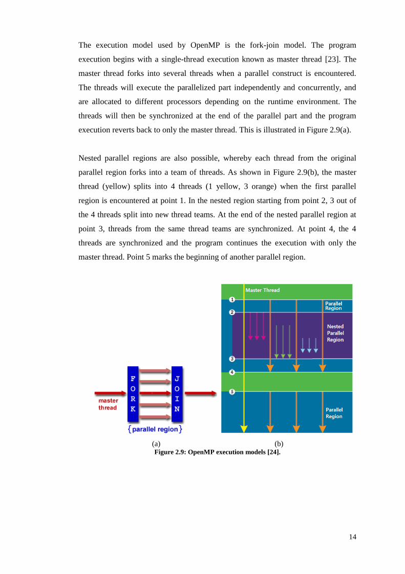
The execution model used by OpenMP is the fork-join model. The program

execution begins with a single-thread execution known as master thread [23]. The

master thread forks into several threads when a parallel construct is encountered.

The threads will execute the parallelized part independently and concurrently, and

are allocated to different processors depending on the runtime environment. The

threads will then be synchronized at the end of the parallel part and the program

execution reverts back to only the master thread. This is illustrated in Figure 2.9(a).

Nested parallel regions are also possible, whereby each thread from the original

parallel region forks into a team of threads. As shown in Figure 2.9(b), the master

thread (yellow) splits into 4 threads (1 yellow, 3 orange) when the first parallel

region is encountered at point 1. In the nested region starting from point 2, 3 out of

the 4 threads split into new thread teams. At the end of the nested parallel region at

point 3, threads from the same thread teams are synchronized. At point 4, the 4

threads are synchronized and the program continues the execution with only the

master thread. Point 5 marks the beginning of another parallel region.

(a) (b) Figure 2.9: OpenMP execution models [24].

15

2.8 CUDA

CUDA is a parallel programming paradigm that was released in November 2006 by

NVIDIA [25]. Apart from being used to develop software for graphics processing,

this architecture alleviates many of the limitations that previously prevented general-

purpose computation from being performed legitimately by the graphics processor.

2.8.1 Architecture of a CUDA-capable GPU

Previous generations of GPU partitioned computing resources into vertex and pixel

shaders, whereas the CUDA architecture included a unified shader pipeline. This

enables every arithmetic logic unit (ALU) on the chip to be marshalled by a program

intending to perform general-purpose computations [26]. The ALUs were also built

to comply with the Institute of Electrical and Electronics Engineers (IEEE)

requirements for single-precision floating-point arithmetic. The instruction set used

by the ALUs are those tailored for general computations instead of those specifically

for graphics. Apart from having arbitrary read and write access to memory, the

execution units on the GPU have access to shared memory, a software-managed

cache. The addition of these features allows the GPU to excel at general-purpose

computation apart from performing traditional graphical tasks.

Figure 2.10 shows the architecture of a CUDA-capable GPU. The GPU is organized

into an array of highly threaded streaming multiprocessors (SMs). 2 SMs form a

building block for the GPU in Figure 2.10. However, different generations of CUDA

GPUs may have different number of SMs in a building block. Each SM has a

number of streaming processors (SPs) that share control logic and instruction cache

[27]. The graphics double data rate (GDDR) DRAM, denoted as global memory in

Figure 2.10, are different compared to those in a CPU motherboard. For computing

applications, they function as very-high-bandwidth, off-chip memory, but with more

latency than the typical system memory. If the application is massively parallel, then

the higher bandwidth will make up for the longer latency.

16

Figure 2.10: Architecture of a CUDA-capable GPU [28].

2.8.2 CUDA Programming Model

Figure 2.11: Heterogeneous architecture [29].

The CPU, known as the host, executes functions (or serial code as shown in Figure

2.11). Parallel portion of the application is executed on the device (GPU) as kernel.

The kernel is executed as an array of threads, in parallel. The same code is executed

1 building block 1 SM 1 core

17

by all threads, but different paths may be taken. The threads can be identified by its

IDs, for the purpose of selecting input or output data, and to make control decisions

[4]. The threads are grouped into blocks, which in turn are grouped into a grid.

Hence, the kernel is executed as a grid of blocks of threads. The grid and each block

may be one-dimensional, two-dimensional or three-dimensional. The architecture is

illustrated in Figure 2.12.

Figure 2.12: CUDA compute grid, block and thread architecture.

Cooperation among threads within a block may be needed for memory accesses and

results sharing. Shared memory is accessible by all threads within the same block

only. This restriction to “within a block” permits scalability [28]. When the number

of threads is large, fast communication between the threads will not be feasible.

However, each block is executed independently and the blocks may be distributed

across an arbitrary number of SMs.

18

2.8.3 CUDA Memory Model

The host (CPU) and device (GPU) memories are separate entities. There is no

coherence between the host and device [30]. Hence, in order to execute a kernel on a

device, manual data synchronization is required. This is done by allocating memory

on the device and then transferring the relevant data from the host memory to the

allocated device memory. After device execution, the resultant data will need to be

transferred back from the device memory to the host memory.

Figure 2.13: Cuda device memory model [31].

As shown in Figure 2.13, the global memory is a memory that the host code can

transfer data to and from the device. This memory is relatively slow as it does not

provide caching. Constant memory and texture memory allow read-only access by

19

the device code. API functions help programmers to manage data in these memories.

Each thread has its own set of registers and local memory. Local variables of the

kernel functions are usually allocated in the local memory [32]. Shared memory is

shared among threads in the same block whereas global memory is shared by all the

blocks. Shared memory is fast compared to global memory. It is also known as

parallel data cache (PDC). All these memories (excluding constant memory) may be

read and written to by the kernel.

2.8.4 CUDA Execution Model

As mentioned in Section 2.8.2, the main (serial) program runs on the host (i.e., the

CPU) while certain code regions run on the device (i.e., the GPU). The execution

configuration is written as <<< blocksPerGrid, threadsPerBlock >>>.

The value of these two variables must be less than the allowed sizes depending on

the device specifications. The maximum number of blocks and threads that can

reside in a Streaming Multiprocessor depends on the compute capability of the

device.

Figure 2.14 shows the architecture of a Streaming Multiprocessor (SM) for a device

with CUDA compute and graphics architecture, code-named Fermi architecture.

There are a total of sixteen load/store (LD/ST) units, allowing source and destination

address to be calculated for sixteen threads per clock [33]. The four special function

units (SFU) are used to execute transcendental instructions such as sin, cosine,

reciprocal and square root. There are thirty-two cores in an SM, grouped into two

groups of sixteen cores each. Each core has its own floating point unit (FPU) and

arithmetic logic unit (ALU).

20

Figure 2.14: Architecture of a Streaming Multiprocessor (SM) [34].

Figure 2.15: Dual Warp Scheduler in a Streaming Multiprocessor [34].

21

After a block has been assigned to an SM, it will be further divided into 32-thread

units known as warps. All threads of a warp are scheduled together for execution.

Each SM has two warp schedulers, as illustrated in Figure 2.15. Two warps can be

issued and executed concurrently in an SM. The SM double-pumps each group of

sixteen cores to execute one instruction for each of the two warps. If there are eight

SMs in a device, a total of 256 threads will be executed in a clock.

When an instruction executed by the threads in a warp requires the result from a

previous long-latency operation, the warp will not be selected for execution [28].

Another resident warp which has its operands ready will then be selected for

execution. This mechanism is known as latency hiding. If there is more than one

warp ready for execution, a warp will be selected for execution based on the priority

mechanism. Warp scheduling hides the long waiting time of warp instructions by

executing instructions from other warps. As a result, the overall execution

throughput will not be slowed down due to long-latency operations.

As a conclusion for the execution model, each thread is executed by a core, each

block is executed on a multiprocessor and several concurrent blocks may reside on a

multiprocessor. Each kernel is executed on a device.

2.9 CUDA C

Prior to the introduction of CUDA C, Open Graphics Library (OpenGL) and

DirectX were the only means to interact with a GPU. Data had to be stored in

graphics textures and computations had to be written in shading languages which are

special graphics-only programming languages [4]. In 2007, NVIDIA added a

relatively small number of keywords into the industry-standard C for the sake of

harnessing some of the special features of the CUDA Architecture, and introduced a

compiler for this language, CUDA C. This has also made CUDA C the first

language specifically designed by a GPU company to facilitate general-purpose

computing on GPUs. A specialized hardware driver is also provided so that the

22

CUDA Architecture’s massive computational power may be exploited. With all

these improvements by NVIDIA, programmers no longer need to disguise their

computations as graphic problems, nor do they require knowledge of OpenGL and

DirectX.

2.9.1 Device Function

The number of blocks within a grid and number of threads per block must be

specified when calling the kernel function. A Kernel function has a return type

void. It also has a qualifier __global__ to indicate that the function is called

from the host code and it is to be executed on the device. The device functions are

handled by NVIDIA’s compiler where as the host functions are handled by the

standard host compiler [35]. The input arguments of the kernel function must point

to the device memory.

2.9.2 Basic Device Memory Management

a) To allocate the device global memory: cudaMalloc()

i. Call this function from the host (CPU) code to allocate a piece of

global memory (in GPU) for an object.

ii. The first function argument is the address of a pointer to the allocated

object.

iii. The second function argument is the size of the allocated object in

terms of bytes.

iv. Example:

float* dev_a;

cudaMalloc ( (void**) &dev_a, sizeof (int) );

b) To copy from the host (CPU) memory to the device (GPU) memory and vice

versa: cudaMemcpy()

i. The first function argument is the pointer to the destination.

23

ii. The second function argument is the pointer to the source.

iii. The third argument indicates the number of bytes to be copied.

iv. The fourth argument indicates the direction of transfer (host to host,

host to device, device to host, or device to device).

v. Example (host to device):

cudaMemcpy ( dev_a, &host_a, sizeof (int),

cudaMemcpyHostToDevice );

vi. Example (device to host):

cudaMemcpy (&host_a, dev_a, sizeof (int),

cudaMemcpyDeviceToHost);

c) To free the device memory: cudaFree()

i. Call this function from the host (CPU) code to free an object.

ii. The function argument is the pointer to the freed object.

iii. Example: cudaFree (dev_a);

2.9.3 Launching Parallel Kernels

a) Launching with parallel blocks

i. Example: kernel <<<N, 1>>> (dev_a, dev_b)

There will be N copies of the kernel() being launched.

blockIdx.x can be used to index the arrays whereby each

block handles different indices

b) Launching with parallel threads within a block

i. Example: kernel <<<1, N>>> (dev_a, dev_b)

There will be N copies of the kernel() launched.

threadIdx.x is used to index the arrays

24

c) Launching with parallel threads and blocks

i. Example: kernel <<< M, N>>> (dev_a, dev_b)

There will be M × N copies of kernel() launched.

The unique array index for each entry is given by:

Index=threadIdx.x + blockIdx.x*blockDim.x

BlockDim.x refers to the number of threads per block

2.9.4 Shared Memory

Parallel threads have a mechanism to communicate. Threads within a block share an

extremely fast, on-chip memory known as shared memory. Shared memory is

declared with the keyword __shared__. Data is shared among threads in a block.

It is not visible to threads in other blocks running in parallel.

2.9.5 Thread Synchronization

Parallel threads also have a mechanism for synchronization. Synchronization is

needed to prevent data hazards such as read-after-write hazard [36]. The function

used to synchronize thread is __syncthreads(). Threads in the block will wait

until all threads have hit the __syncthreads() instruction before proceeding

with the next instruction. An important point to note is that threads are only

synchronized within a block.

2.10 Applications of CUDA

Various industries and applications have enjoyed a great deal of success by building

applications in CUDA C. The improvement in performance is often of several

orders-of-magnitude. The following shows a few ways in which CUDA Architecture

and CUDA C have been put into successful use.

25

2.10.1 Oil Resource Exploration

The oil prices in the global market continue to rise steeply causing the urgent need

to find new sources of energy. However, the exploration and drilling of deep wells

are very costly. To minimize the risks of failure in drilling, 3D seismic imaging

technology is now being used for oil exploration [37]. Such technology allows for a

detailed look at potential drilling sites. However, terabytes of complex data are

involved when imaging complex geological areas. With the introduction of faster

and more accurate code by SeismicCity, the computational intensity of the

algorithms has increased by 10-fold. Such algorithms would then require large

number of CPUs setup, which is impractical. Running CUDA on NVIDIA Tesla

server system solves this problem. The massively parallel computing architecture

offers a significant performance increase over the CPU configuration.

2.10.2 Design Industry

Conventionally, physical cloth samples of the intended clothing line are needed for

prototyping and to gain support from potential investors [38]. This consumes a lot of

time as well as cost, causing wastage. OptiTex Ltd introduced 3-D technology which

modernizes this process by allowing designers to simulate the look and movement of

clothing designs on virtual models. By using a GPU for computation, the developers

managed to obtain a 10-fold performance increase in addition to removing

bottlenecks that occurred in the CPU environment. With the promising performance

by the GPU computing solution, production costs and design cycle time has been

greatly reduced.

2.10.3 Weather and Climate

The most widely used model for weather prediction is Weather Research and

Forecasting Model (WRF). Despite having large-scale parallelism in these weather

models, the increase in performance is due to the increase in processor speed instead

of from increased parallelism [39]. With the development of National Center for

26

Atmospheric Research’s (NCAR’s) climate and weather models from Terascale to

Petascale class applications, conventional computer clusters and addition of more

CPUs prove to be no longer effective for speed improvement. To improve overall

forecasting speed and accuracy of the models, the NCAR technical staffs have

collaborated with the researchers at University of Colorado and came up with

NVIDIA GPU Computing solutions. It is observed that there is a 10-fold

improvement in speed for Microphysics after porting to CUDA. The percentage of

Microphysics in the model source code is less than 1 per cent, but a 20 per cent

speed improvement for the overall model is observed when converted to CUDA.

2.11 Existing CUDA String Algorithms

The simplest algorithm for string search is Brute-Force algorithm. The algorithm

tries to match the pattern (query) to the text (input word list) by scanning the text

from left to right. In the sequential form, a single thread will conduct the search and

outputs to the console if a match is found. In the CUDA version, N threads can be

used to conduct for the same search [40]. The difference lays in that each of the N

parallel threads attempts to search for a match, in parallel. When the thread founds a

match, the data structure used to store the found indices will be updated. The

drawback of Brute Force algorithm is its incompetency in speed. Despite its

implementation in CUDA, the text will need to be scanned from beginning till the

end. Hence, this algorithm is more suitable when simplicity is of higher priority

compared to speed.

Another algorithm which has been implemented in CUDA is QuickSearch, a variant

of the popular Boyer-Moore Algorithm [41]. “Bad character shift” is precomputed

for the pattern (query) before searching is performed. The main disadvantage is the

space requirement. If the pattern and/or the text are long, more space will be needed.

A research paper by Raymond Tay [42] has explored the usage of GPUs to support

batch oriented workloads by implementing the Bloom Filter algorithm. A

27

performance gain was obtained when the Bloom Filter algorithm was implemented

using CUDA. Hence, Bloom Filter is chosen to be the implemented algorithm in this

project, with the aim of achieving similarly positive results when large datasets are

involved. Bloom Filter is also chosen as it requires a fixed number of bits per

element irrespective of the size of the elements. In other words, less space will be

required compared to the aforementioned algorithms when the input file is large. In

addition to that, the time taken for the algorithm to check for an element is

regardless of the number of elements in the set. The lookups are independent of each

other and thus can be parallelized, providing an opportunity for the algorithm to be

implemented using CUDA.

The following chapter thus investigates the performance limitation of a serial Bloom

Filter in justifying the need for a parallel design, both on CPU and GPU domains.

28

CHAPTER 3: PERFORMANCE

DRAWBACK OF A SERIAL BLOOM

FILTER STRING SEARCH

ALGORITHM

3.1 Introduction

The Bloom Filter algorithm is first implemented only on the CPU, using serial

programming. This marks the simplest way of programming. It serves as a

benchmark for performance comparison with parallel as well as GPGPU versions of

the program.

3.2 Program Flow

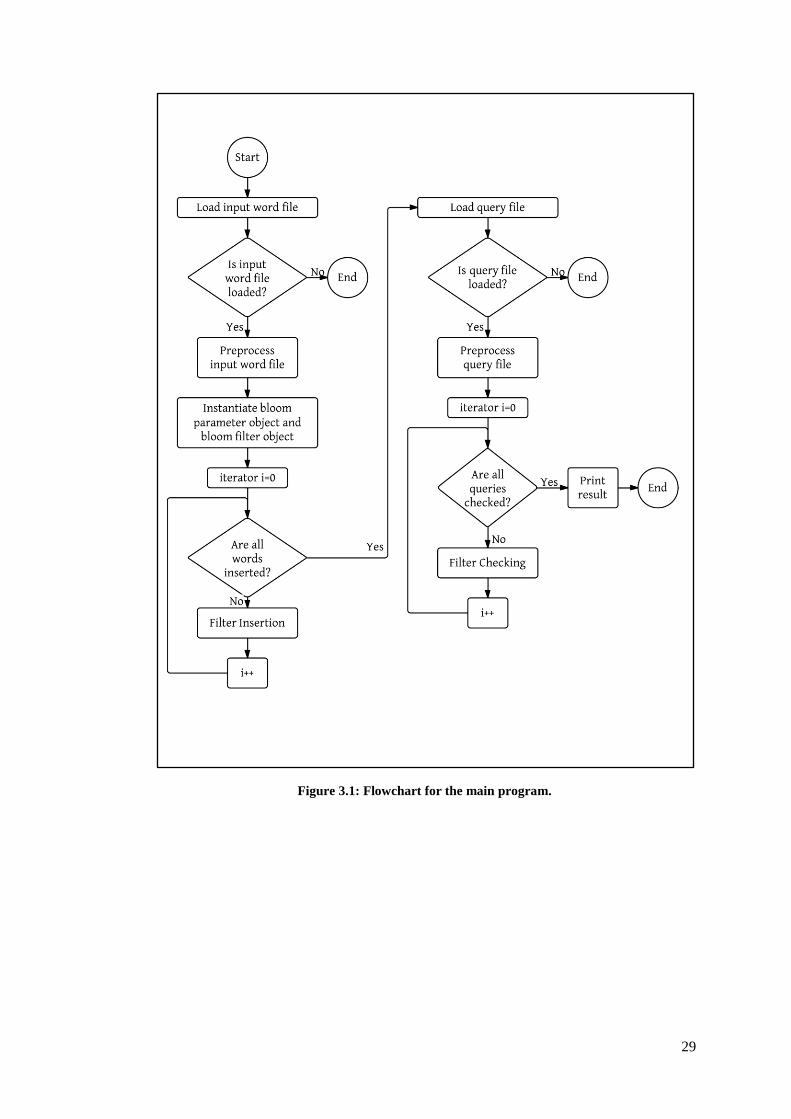
By referring to Figure 3.1, the program begins with the loading of input word file

into the CPU memory. If the word file is not found and it fails to be loaded, the

console will show failure in loading file and the program terminates. The word file

is then processed before the Bloom Filter is instantiated. The filter is inserted by

setting the bits based on the hash functions performed on the strings in the word file.

After all elements have been inserted, the input query file is loaded into the CPU

memory. Similar to the word file, failure in loading the file will result in program

termination. Processing of queries is required before the filter is checked for the

queries. If the query is in the word file, a message is printed on the console stating

its presence. After all queries have been searched and the results have been printed,

the program terminates.

29

Figure 3.1: Flowchart for the main program.

30

3.2.1 Loading Input Files

Program Listing 3.1 describes the file-loading function used in this project. A

character pointer-to-pointer for the word array and an integer pointer for the number

of words are passed from the main function into the file-loading function as shown

in Line 1. If the word file is successfully loaded, the integer pointer is updated based

on the number of strings in the file. This is portrayed in Line 19. The pointer-to-

pointer then points to an array of pointers. Each pointer points to a string in the word

file. This relates to Lines 27-31. The same algorithm is used to read both input word

file and query file.

Program Listing 3.1: Input file loading.

1 bool load_word_list(int argc, char* pArgv[], char**

&ppWord_list_ptr_array, int* pWordnum)

2 {

3 static const char wl_list[] = {"word-list-1k.txt"};

4 std::cout << "Loading list " << wl_list << ".....";

5

6 ifstream stream;

7 stream.open(wl_list, ios::in);

8 if (!stream)

9 {

10 std::cout << "Error: Failed to open file '" << wl_list

<< "'" << std::endl;

11 return false;

12 }

13

14 char temp[WORDLENGTH] = {'\0'};

15

16 while(!stream.eof())

17 {

18 stream.getline(temp,WORDLENGTH);

19 (*pWordnum)++;

20 }

21

22 ppWord_list_ptr_array = new char*[*pWordnum];

23

24 stream.clear();

25 stream.seekg(0);

26

27 for(int i=0; i<(*pWordnum); i++)

28 {

29 ppWord_list_ptr_array[i] = new char[WORDLENGTH];

30 stream.getline(ppWord_list_ptr_array[i],WORDLENGTH);

31 }

32

33 std::cout << " Complete." << std::endl;

34 return true;

35 }

31

3.2.2 Data Pre-processing

There are typically 3 operations involved in data pre-processing, namely preparing

and filling up index tables to indicate the starting position (offset from the beginning

of the contiguous space) and the size of each string, allocating contiguous space (on

host) for the input strings, and copying the strings into the allocated space. It can be

illustrated in Figure 3.2.

Figure 3.2: Pre-processing of input text file.

Data pre-processing is done for serial CPU programming as well, so that a fair

comparison can be made when parallel programming and GPGPU are implemented.

The performance comparison will be made solely based on the Bloom Filter

algorithm, excluding the time taken for pre-processing the data.

32

3.2.3 Class Objects

Two classes are introduced in the program, namely CBloom_parameters and

CSimple_bloom_filter. The members and functions of the

CBloom_parameters class are described in Table 3.1 and Table 3.2,

respectively.

Table 3.1: CBloom_parameters Class Members.

Class Member Significance

BP_fpp Indicates the false positive probability of an

element

BP_k Indicates the number of hash functions to be

performed

BP_n Indicates the number of elements in the filter

BP_random_seed A value used in generation of salt

BP_table_size Gives the size of the Bloom Filter

Table 3.2: CBloom_parameters Class Functions.

Function Name Function

BP_compute_parameters() Computes the size of the Bloom Filter

CBloom_parameters()

Class constructor which initializes the

number of elements, the number of hash

functions, fpp, value of random seed and

calls the class function

BP_compute_parameters()

The calculation of the size of Bloom Filter in the class function

BP_compute_parameters() in Table 3.2 is deduced from Equation 2.5 (which

shows the equation for fpp). The value of fpp is initially set at

. The size of the

Bloom Filter is hence calculated based on the following equation:

(3-1)

33

Table 3.3 describes the members of the CSimple_bloom_filter class.

Table 3.3: CSimple_bloom_filter Class Members.

Class Member Significance

BF_bit_table_ Bit-table array with each element storing

8 bits

BF_inserted_element_count_ Gives the total number of string elements

inserted into the Bloom Filter

BF_random_seed_ A random value used in generating salts

for hash functions

BF_raw_table_size_ Size of BF_bit_table_

BF_salt_count_ Gives the number of hash functions used

BF_table_size_ Gives the actual size of the Bloom Filter

(bit-table array size × 8 )

salt_

Each element of the array is used as an

initial hash value (before the hash

function is performed) such that the same

hash algorithm will produce different

results when performed on the same

string element

The class member BF_bit_table_ is set as a volatile variable such that the

compiler reads the bit-table from its storage location (in memory) each time it is

referenced in the program. If the volatile keyword is not used, the compiler

might generate the code that re-uses previously read value from the register. In the

case of serial programming, the possibility of cache miss is almost zero. However, in

a multi-threaded program with the compiler’s optimizer enabled, cache incoherency

will lead to inaccurate results. This is because each processor has its own cache

memory and change in one copy of the operand might not be visible to other copies.

Hence the bit-table array is set to volatile in the serial implementation as well for a

fair comparison.

34

The functions of the CSimple_bloom_filter class are described in Table 3.4.

Table 3.4: CSimple_bloom_filter Class Functions.

Function Name Function

~CSimple_bloom_filter() Class destructor

compute_indices() Computes the indices of the bit table

contains() Checks for the presence of a query

CSimple_bloom_filter()

Class constructor which initializes the number of

elements, the number of hash functions, the

value of random seed, an empty bit-table, the

size of the bit-table and calls the class function

generate_unique_salt()

effective_fpp() Calculates the effective fpp of the Bloom Filter

element_count() Indicates the total number of elements inserted

into the filter.

generate_unique_salt() Generates salts for the hash functions

hash_ap() Performs hash function on the element

insert() Inserts elements into the filter

size() Gives the size of the Bloom Filter

3.2.4 Filter Insertion

To insert an element (string) into the Bloom Filter, the element and its length are

passed into a class function called insert() as shown in Program Listing 3.2.

Program Listing 3.2: Serial filter insertion.

1 for (int i=0; i<g_Wordnumber; i++)

2 {

3

filter1.insert(&(g_pTotalwordarray[g_pAccumulative_Wordlengt

h[i]]), g_pWordlength[i]);

4 5 }

35

Figure 3.3 shows the algorithm for the insert() function. The iterator i is

incremented after a single hash function is performed and one of the bits in the

Bloom Filter is set to 1. After performing k number of hash functions and setting the

Bloom Filter k number of times, one string element (word) is considered inserted.

The hash algorithm will be described in detail in Section 3.3. The flow as portrayed

in the flowchart below is repeated for all elements.

Figure 3.3: Flowchart for inserting one element.

36

To insert an element (string) into the Bloom Filter refers to setting certain values of

the bit table to the value “1”. A bit_mask array of size 8 is used in the program.

Each element of the array consists of 8 bits. The reason for using a bit_mask

array is to eliminate collision when 2 elements contribute the same bit index.

Algorithm 1 shows the insertion for one element. Conversely, Program Listing 3.3

illustrates the code implementation.

Algorithm 3.1: Generate bit-table for one element

1 bit_index ← 0

2 bit ← 0

3 iterator i ← 0

4 While i <BF_salt_count_ do

5 perform hash function

6 bit_index = hash % BF_table_size_

7 bit = bit_index % 8

8 bit_table [bit_index/8] |= bit_mask[bit]

9 Increase the iterator

10 end

Program Listing 3.3: Filter insert function for one string element.

1 inline void insert(char* key_begin, int length)

2 {

3 unsigned int bit_index = 0;

4 unsigned int bit = 0;

5

6 for (unsigned int i = 0; i < BF_salt_count_; ++i)

7 {

8 compute_indices(hash_ap(key_begin,length,salt_[i]),

bit_index,bit);

9 BF_bit_table_[bit_index / bits_per_char] |=

bit_mask[bit];

10 }

11

12 ++BF_inserted_element_count_;

13 }

37

Example:

Originally, BF_bit_table_[20] stores 0x00

1. element “above” gives bit_index = 20, bit = 0;

Hence, BF_bit_table_[20] |= bit_mask[0]

0x00 |= 0x01

BF_bit_table_[20] now stores 0x01

2. element “beyond” gives bit_index = 20, bit = 5;

Hence, BF_bit_table_[20] |= bit_mask[5]

0x01 |= 0x20

BF_bit_table_[20] now stores 0x21

3.2.5 Filter Searching

To check for the existence of a query in the input word list, a similar process as filter

insertion is performed. The same bit_mask array is used as in the case of bit-table

generation. The query and its length are passed into a class function called

contain(). Algorithm 2 describes this function. The hash value and the table

index are calculated as shown in Lines 5 to 8. The bit at the calculated position is

checked for its Boolean value. If the bit_mask element is not retrievable, then the

query is confirmed to be non-existent in the word-list. The function returns a false

to the main program as shown in Line 10. If all hash functions have been performed

and all respective bit_mask elements have been retrieved, then either the query is

present in the word-list or a false positive has occurred. The function returns a true

to the main program. The entire process as described in Algorithm 2 is repeated for

n number of queries.

Algorithm 3.2: Checking bit-table for one element

1 bit_index ← 0

2 bit ← 0

3 iterator i ← 0

38

4 While i <BF_salt_count_ do

5 perform hash function

6 bit_index = hash % BF_table_size_

7 bit = bit_index % 8

8 bit_table [bit_index/8] & bit_mask[bit]

9 if bit_mask element is not retrieved

10 return false to main function


12 end

13 return true to main function

Examples:

BF_bit_table_[20]stores 0x21 after all elements of the word-list have been

inserted.

1. query “beyond” gives bit_index = 20, bit = 5;

Hence, BF_bit_table_[20] & bit_mask[5]

0x21 & 0x20

bit_mask[5] is retrieved, hence query is found.

2. query “tiger” gives bit_index = 20, bit = 7;

Hence, BF_bit_table_[20] & bit_mask[7]

0x21 & 0x80

bit_mask[7] is not retrieved, hence query is not found.

3.3 AP Hash Function

The chosen algorithm for the hash function is Arash Partow (AP) hash function. It is

a hybrid rotative and additive hash function algorithm that resembles a simple

Linear Feedback Shift Register (LFSR) [43]. When the feedback function of an

LFSR is chosen appropriately, the output sequence of bits will appear random.

39

Therefore, by using AP hash algorithm, the calculated hash values (and hence bit

table indices) will be random, collisions can be reduced. The hash algorithm is

described as below:

Algorithm 3.3: Computes the hash value for a string

1 loop ← 0

2 iterator ← first character of the string

3 hash ← one of the elements of salt array

4 While word_length >=8 do

5 m ← first 4 characters pointed by iterator

6 n ← next 4 characters pointed by iterator


8 ( ) * (

)+

9 (

10 Word_length is reduced by 8

11 end

12 p ← first 4 characters pointed by iterator


14 If (loop & 0x01):

15 ( ) * (

)+

16 Else

17 (



20 end

21 x ← first 2 characters pointed by iterator


23 If (loop & 0x01):

24 ( ) * (

)+

40

25 Else

26 (



29 end

30 If word_length=1:

31

32 Return hash

3.4 System Assessment

3.4.1 Assessment Environment

This project was implemented in the Microsoft Windows platform; the chosen

software for development was Microsoft Visual Studio 2010. The CPU

specifications are given as follows:

Table 3.5: CPU Specifications.

Processor Intel Core™ i7-2700K at 3.50GHz

Installed Memory (RAM) 8.00 GB

3.4.2 Performance Assessment

The results were collected for different dataset sizes, ranging from 1000 strings to

10,000,000 strings. The length of each string in the word-list and query-list is no

more than 20 characters. 500 hashes were performed on each string. The average

values (of the time taken) after five runs were used to plot the following graphs.

Figure 3.4 shows the time taken for inserting strings into the filter while Figure 3.5

shows the time taken to query for strings. The total time taken for the insertion and

querying is illustrated in Figure 3.6. Time taken to print the search results was not

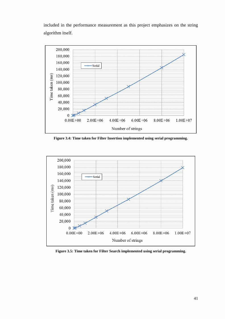
41

included in the performance measurement as this project emphasizes on the string

algorithm itself.

Figure 3.4: Time taken for Filter Insertion implemented using serial programming.

Figure 3.5: Time taken for Filter Search implemented using serial programming.

42

Figure 3.6: Total time taken for Bloom Filter algorithm (insert and search) implemented using

serial programming.

All three figures have shown a linear increase in the processing time for the Bloom

Filter algorithm when the data size was increased. As shown in Figure 3.4,

approximately 180 seconds were needed to insert 10,000,000 strings into the filter.

Similar amount of time was needed to search for 10,000,000 queries, as portrayed in

Figure 3.5. Hence, the total amount of time taken for the Bloom Filter algorithm for

a dataset size of 10,000,000 was approximately 360 seconds. Observation of the

CPU utilization displayed only

of the logical processors was used for executing the

program. This has shown that the CPU was underutilized despite having a hardware

that supports multicore and hyperthreading.

When the number of strings (n) increments by 1, the total number of hash functions

to be performed increases by a factor of k. The computational load in this algorithm

is hence identified as the hash functions performed on the strings. In order to reduce

the execution time of the algorithm, a more time-efficient programming paradigm is

needed.

43

The repetitive process of performing hash functions on different strings suggests that

parallelisation may be applied. Hence, Bernstein’s Conditions are examined to

ensure that the hashings of strings are independent of each other.

Suppose that 𝕚 represents a set of words in the word list,

𝕠 represents a set of resultant hash operations

Let 𝕚 where 𝕠 ; and

𝕚 where 𝕠 ; (3-2)

Since 𝕚 𝕠 , and

𝕚 𝕠 , and

𝕠 𝕠 , (3-3)

The insertion process for both 𝕚 and 𝕚 can be executed concurrently.

By deduction,

𝕚 𝕠 , and

𝕚 𝕠 , and

𝕠 𝕠 (3-4)

Hence,

𝕚 𝕠 𝕠 𝕠 , and

𝕚 𝕚 𝕚 𝕠 , and

𝕠 𝕠 𝕠 𝕠 (3-5)

From Eq. (3.2), Eq. (3.3), Eq. (3.4) and Eq. (3.5), since all three Bernstein’s

Conditions are satisfied, it is proven that the data has no dependency on each other.

Thus, is has been confirmed that the hashing algorithm for different strings can be

executed concurrently. The next chapter discusses the implementation of the Bloom

Filter algorithm using parallel programming by leveraging on the compute

capabilities of a multicore processor.

44

CHAPTER 4: DATA

PARALLELISATION OF A BLOOM

FILTER USING OPENMP

The previous chapter has proven that data parallelisation of the Bloom Filter

algorithm is in fact possible. Hence, this chapter describes the design and

development of a parallel Bloom Filter string search algorithm on a multicore

architecture.

4.1 Program Design

The program flow for the Bloom Filter algorithm implemented using OpenMP is

similar to the serial programming implementation. The only changes made are on

the Bloom Filter insertion and querying functions. Both functions involve

performing the same tasks on different sets of data, thus providing an opportunity

for data parallelism to be implemented.

Prior to implementing parallelisation in the program, the maximum number of

threads that can run at a time was obtained by calling the library function

omp_get_max_threads(). To set the number of parallel threads, the library

function omp_set_num_threads() was called.


The algorithm for insertion using OpenMP is similar to that of using serial

programming. Program Listing 4.1 illustrates the code implementation of

insertProcess(). This function receives a pointer pointing to the input string

45

array (*pTotalwordarray), a pointer pointing to the table storing length of each

input string (*pWordlength) and a pointer pointing to the table storing offsets of

each string (pAccumulative_Wordlength). Atomic operation is required

when updating the bit-table, as shown in Line 13 of Program Listing 4.1. This

allows protection against simultaneous writes on the same bit-table location by

different threads. Nested parallel region was not implemented as it introduces

additional overhead. Since there is enough parallelism in the main program flow, it

is more efficient to use all threads at this level rather than to create nested regions in

the insertProcess() function. Figure 4.1 depicts the execution model for

insertProcess()which relates to Program Listing 4.1.

Program Listing 4.1 OpenMP Filter Insert Function.

1 void insertProcess(int totalWords, char *pTotalwordarray,

int *pAccumulative_Wordlength, int *pWordlength)

2 {

3 int j = 0;

4 #pragma omp parallel for private(j)

5 for (int i=0; i<totalWords; i++)

6 {



9 for (j = 0; j < BF_salt_count_; ++j)

10 {

11 compute_indices(hash_ap(&(pTotalwordarray

[pAccumulative_Wordlength[i]]),

pWordlength[i],salt_[j]),bit_index,bit);

12 {

13 #pragma omp atomic

14 BF_bit_table_[bit_index/bits_per_char] |=

bit_mask[bit];

15 }

16 }

17 ++BF_inserted_element_count_;

18 }

19 }

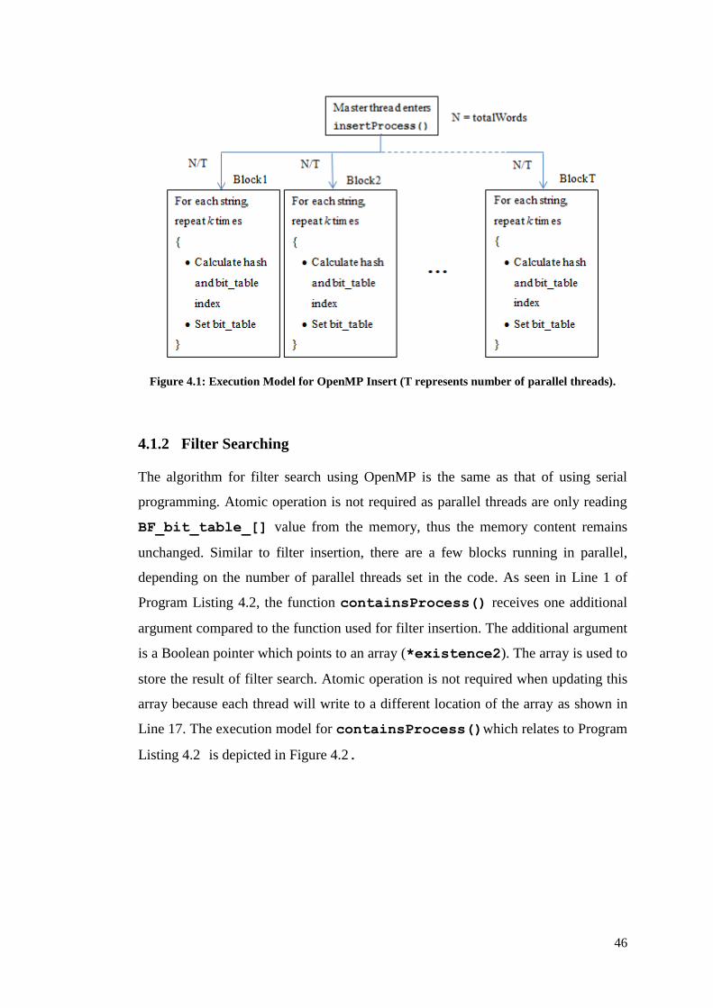
46

Figure 4.1: Execution Model for OpenMP Insert (T represents number of parallel threads).


The algorithm for filter search using OpenMP is the same as that of using serial

programming. Atomic operation is not required as parallel threads are only reading

BF_bit_table_[] value from the memory, thus the memory content remains

unchanged. Similar to filter insertion, there are a few blocks running in parallel,

depending on the number of parallel threads set in the code. As seen in Line 1 of

Program Listing 4.2, the function containsProcess() receives one additional

argument compared to the function used for filter insertion. The additional argument

is a Boolean pointer which points to an array (*existence2). The array is used to

store the result of filter search. Atomic operation is not required when updating this

array because each thread will write to a different location of the array as shown in

Line 17. The execution model for containsProcess()which relates to Program

Listing 4.2 is depicted in Figure 4.2.

47

Program Listing 4.2 OpenMP Filter Search Function.

Figure 4.2: Execution Model for OpenMP Search (T represents number of parallel threads).

1 void containsProcess(int totalQueries, char *pTotalqueryarray,

int *pAccumulative_Querylength, int *pQuerylength,

bool* existence2)

2 {

3 int j =0 ;

4

5 #pragma omp parallel for private(j)

6 for (int i=0; i<totalQueries; i++)

7 {



10

11 for (j = 0; j < BF_salt_count_; ++j)

12 {

13 compute_indices(hash_ap(&(pTotalqueryarray

[pAccumulative_Querylength[i]]),

pQuerylength[i],salt_[j]),bit_index,bit);

14

15 if ((BF_bit_table_[bit_index / bits_per_char] &

16 bit_mask[bit]) != bit_mask[bit])

17 existence2[i] = false;

18 }

19 }

20 }

48



A similar test setup and sample data set from Section 3.4.1 is adapted here. For the

OpenMP implementation, the function omp_get_max_threads() returned a

value of 8 when it was called. This is because there are 4 cores on the machine, and

each core allows hyperthreading. Hence, the number of parallel threads was set to 8

using the function omp_set_num_threads().


Prior to results collection, the bit-table and result array obtained from OpenMP and

serial implementations were compared. The comparison results confirmed that

identical bit-tables and result arrays were obtained.

The performance of the Bloom Filter algorithm executed using OpenMP was

measured against the same algorithm running in serial. The execution time was

recorded for filter insertion and querying only, excluding the time to print the bit-

table and the searching result to text files. The results for execution time were

plotted using the average value of five runs. The performance gain of the OpenMP

implementation over the serial implementation was also calculated and plotted in the

graphs.

Let represent the time taken for the Bloom Filter in a serial implementation

represent the time taken for the Bloom Filter in an OpenMP

implementation

The performance gain (or performance ratio or speedup factor) is calculated as:

(4-1)

49

Figure 4.3, Figure 4.4 and Figure 4.5 show the execution time and the performance

gains for the Bloom Filter algorithm when it is executed using serial programming

and OpenMP.

Figure 4.3: Time taken and performance gain for Filter Insertion when implemented using

serial programming and OpenMP.

Figure 4.4: Time taken and performance gain for Filter Search when implemented using serial

programming and OpenMP.

50

Figure 4.5: Total time taken and performance gain for Bloom Filter algorithm (insert and

search) when implemented using serial programming and OpenMP.

As observed from Figure 4.3, Figure 4.4 and Figure 4.5, the processing time for the

Bloom Filter was longer when serial programming was implemented as compared to

OpenMP. When the size of the dataset was set at 10,000,000, the time taken for the

serial filter insertion was approximately 180 seconds as compared to 60 seconds for

OpenMP; hence a speedup of 3.0x was achieved. For filter search, the serial

implementation took 180 seconds while the OpenMP implementation took

approximately 48 seconds. A speedup factor of 3.8x was exhibited in Figure 4.4 for

the dataset size of 10,000,000. Summation of the time taken for the filter insertion

and the filter search led to a total of 360 seconds for the serial implementation and

100 seconds for the OpenMP implementation. Hence, a speedup of 3.3x was

recorded for the dataset size of 10,000,000 strings. This can be observed in Figure

4.5. The reason for the performance gain in the OpenMP implementation over the

serial implementation is there were 8 threads working (processing the strings) in

parallel when the algorithm was implemented using OpenMP.

The performance gain of OpenMP over serial programming showed a steep increase

when the input data is small in size. Data sizes greater than 500,000 strings show an

almost constant speedup factor (approximately 2.9x for insertion, 3.7x for searching

and 3.3x for overall). A reasonable explanation for this is the processing speed of the

51

CPU has reached its saturation point. Further speedup could only be obtained if

more parallel threads were launched inline with the existence of more logical

processors.

Since there were 8 threads running in parallel, theoretically the speedup factor

should be 8.0x. However, the maximum speed up attained was less than 4.0x. A

reasonable explanation for this is the bit-table insertion was not fully parallelisable.

Atomic operation was introduced hence the insertion function degenerated into

serial programming when more than 1 thread attempted to access the same bit-table

element. Threading overhead also introduced delay to the algorithm.

Despite the inability to obtain the expected performance gain, the implementation of

OpenMP had been very encouraging. It has proven that the performance of the

Bloom Filter algorithm is better when it is implemented in a multicore architecture.

However, with the advent of the many core processing technology, the performance

of the parallel Bloom Filter algorithm can be further improved by leveraging on the

compute capabilities of this technology. As such, the following chapter explores the

design and implementation of a parallel Bloom Filter algorithm on a many core

architecture.

52

CHAPTER 5: CUDA

IMPLEMENTATION OF THE BLOOM

FILTER STRING SEARCH

ALGORITHM

As suggested in the previous chapter, the Bloom Filter algorithm is then

implemented on a GPU, which offers a massively parallel architecture. This chapter

describes the design and development of the Bloom Filter algorithm on the many-

core architecture.

5.1 Program Design

Threads in the GPU do not have direct access to the CPU memory. Hence, explicit

data transfer from the CPU memory to the GPU memory is required. A device

pointer is first allocated using cudaMalloc(). cudaMemcpy() is then used for

data transfer into the GPU global memory. Table 5.1 shows the data which are

transferred only once (from CPU to GPU) throughout the entire program.

Table 5.1: Variables which are transferred once throughout the entire program.

Variable on host (CPU) memory Pointer to device (GPU) memory

filter2.salt_ dev_pSalt_

filter2.BF_table_size_ dev_pTable_size

filter2.BF_bit_table_ dev_pBit_table

bit_mask dev_pBit_mask

The size of memory available on the GPU is limited as compared to the CPU; it is

approximately 25% that of the CPU memory. On Windows, the maximum allowable

53

run time for each kernel launch is five seconds. When the size of the data transferred

is large, the blocks of threads are queued for execution; leading to a long execution

time which might exceed the run time limit. As a result, data processing has to be

performed in batches. For each batch of data, the device pointers are reallocated and

the data are copied into the GPU global memory. The pointers are then freed after

the kernel has completed its tasks. The variables which are transferred in batches are

listed in Table 5.2 while Table 5.3 shows the associated device memory pointers.

Table 5.2: Values stored in each variable on the host memory.

Variable on host (CPU) memory Significance

g_pTotalwordarray[] 1-Dimensional (1D) character array

(input word)

g_pWordlength[] Length of each input word

g_pAccumulative_Wordlength[] Offset of each input word

g_offset Total number of characters of

previously processed strings

g_Remaining_words

Remaining number of strings when

the data size is not an exact

multiple of the batch size

g_pTotalqueryarray[] 1D character array (query)

g_pQuerylength[] Length of each query

g_pAccumulative_Querylength[] Offset of each query

g_Query_result[] Array for storing search result

Table 5.3(a): Device pointers for variables which are transferred in batches.

Variable on host (CPU) memory Pointer to device (GPU) memory

g_pTotalwordarray[] dev_pTotalwordarray

g_pWordlength[] dev_pWordlengthtable

g_pAccumulative_Wordlength[] dev_pOri_Accu_length

g_offset dev_pOffset

g_Remaining_words dev_pNum

g_pTotalqueryarray[] dev_pTotalqueryarray

54

Table 5.3(b): Device pointers for variables which are transferred in batches.

g_pQuerylength[] dev_pQuerylengthtable

g_pAccumulative_Querylength[] dev_pOri_Query_accu_leng

th

g_Query_result[] dev_pQuery_result

As aforementioned, the batch size of the data is limited due to the Windows

“watchdog” timer as well as the size of the GPU memory. Hence, for both filter

insertion and searching, the batch size is chosen as 50,000 strings. Smaller batch size

is feasible but not recommended. This is because additional constant overhead is

generated each time data transfer is invoked. Hence, fewer invocation of copy

operation is preferred. A performance comparison was made between the batch size

of 8 and 50,000. This will be explained in detail in Section 5.2.2.

5.1.1 Offset Calculation

Since batch processing is performed, the values stored in the respective offset tables

(for words and queries) will be invalid for the subsequent batches of data. A CUDA

kernel is launched in order to calculate the offset position of each string in each data

batch. Another piece of GPU memory is allocated and the pointer to this memory

(dev_pAccu_length for input word or dev_pQuery_accu_length for

query) is passed in as one of the kernel arguments. The actual offset of each string

(of the current batch) would then be: the value in the original offset table minus the

total length of previously processed strings.

To maximize the utilization of the CUDA cores, the number of threads per block is

set to the maximum allowable value (i.e., 1024 for Quadro 4000). The variable

BLOCK is a global constant, fixed at 50,000. The number of blocks for kernel

invocation is set to (BLOCK+1023)/1024 (for each data batch of 50,000 strings)

or (g_Remaining_words+1023)/1024 (for the remaining strings when the

total data size is not an exact multiple of 50,000) in order to prevent too few threads

from being launched whenever BLOCK or g_Remaining_words is not an exact

55

multiple of 1024. Program Listing 5.1 describes the kernel functions used for offset

calculations. offset1() (Line 8 to Line 14) is invoked to calculate for 50,000

strings while offset() (Line 1 to Line 6) is invoked to calculate for the remaining

strings when the total number of strings is not an exact multiple of 50,000. As can be

seen from the code, offset() receives one extra argument, dev_pNum,

compared to offset1(). This argument indicates the number of remaining

strings. The index of each thread is calculated in Line 3 (and Line 10). The condition

checking in Line 4 (and Line 11) is needed so that the calculations in Line 5 (and

Line 12) will not be performed when the thread index overshoots the end of the

array.

Program Listing 5.1 Kernel functions for offset calculations.


The kernel function to insert string elements into the Bloom Filter receives several

pointers to the device memory, which are dev_pTotalwordarray,

dev_pWordlengthtable, dev_pAccu_length, dev_pSalt_,

dev_pTable_size, dev_pBit_mask, and dev_pBit_table.

1 __global__ void offset (int* dev_pAccu_length,

int* dev_pOffset, int* dev_pNum,

int* dev_pOri_Accu_length)

2 {

3 int tid = threadIdx.x + blockIdx.x * blockDim.x;

4 if (tid < (*dev_pNum))

5 dev_pAccu_length[tid] = dev_pOri_Accu_length[tid] –

(*dev_pOffset);

6 }

7

8 __global__ void offset1 (int* dev_pAccu_length,

int* dev_pOffset, int* dev_pOri_Accu_length)

9 {

10 int tid = threadIdx.x + blockIdx.x * blockDim.x;

11 if (tid < BLOCK)

12 dev_pAccu_length[tid] = dev_pOri_Accu_length[tid] –

(*dev_pOffset);

13

14 }

56

As mentioned in Section 5.1.1, the value for BLOCK is 50,000, which is the chosen

batch size. K is also a global constant, with the value of 500. It is the number of hash

functions to be performed on each string. There will be BLOCK×K copies of the

insert() function being launched for each batch of data. As for the remaining

strings, g_Remaining_words×K copies of the aforementioned function are

launched.

Figure 5.1: Execution Model for insert() function (for one batch of data with batch size of

50,000).

Bloom Filter Bits Array

Queued blocks

SM 0

Queued blocks

SM 7

Queued blocks

SM 1

Block (0,0,0)

(String 0)

Block (1,0,0)

(String 1)

Block (2,0,0)

(String 2)

SM 0

Block (3,0,0)

(String 3)

Block (4,0,0)

(String 4)

Block (5,0,0)

(String 5)

SM 1

Block (21,0,0)

(String 21)

SM 7

Block (22,0,0)

(String 22)

Block (23,0,0)

(String 23)

…

Block (5,0,0)

Thread (0,0,0)

(Hash function

number 1)

Thread (1,0,0)

(Hash function

number 2)

Thread (2,0,0)

(Hash function

number 3) …

Thread (499,0,0)

(Hash function

number 500)

insert()

String 0 String 1 String 2 String 49999 …

Maximum 20 characters per string

57

Figure 5.1 illustrates the execution model for the insert() function for one batch

of strings. Conversely, Program Listing 5.2 illustrates the code implementation. If

the total number of strings is not an exact multiple of the batch size, the filter

insertion will be executed on the device using the similar model but with fewer

blocks. The number of threads per block remains the same (500).

As illustrated in Figure 5.1, after invoking the kernel, each block will process one

string. The string is copied from the GPU global memory into the shared memory to

allow faster memory access by each thread within the block. Hence, the ID of the

block is used to obtain the string (and its length) that it to be processed by the block.

This is shown in Lines 4 and 9 of Program Listing 5.2.

Figure 5.1 has also shown that each thread within a block will perform a different

hash function on the same string. Each thread will then set one of the elements in the

Bloom Filter bit-table (referred to as bit array in Figure 5.1) after calculating the

associated index. Therefore, the ID of the thread is used to obtain the associated salt

element which is used as the initial hash value, as shown in Line 15.

Similar to the OpenMP implementation of the Bloom Filter algorithm, atomic

operation has to be performed when setting the bit-table (as shown in Line 58). By

using atomic operation, race condition is avoided as the operation is performed

without interference from other threads.

Figure 5.1 has shown 3 resident blocks in each SM. There are also queued blocks for

each SM. The justification for this is provided in Section 5.2.2.

Program Listing 5.2(a) CUDA Insert Function.

1 __global__ void insert(char* pDev_totalwordarray,

int* pDev_wordlengthtable, int* pDev_accu_length, unsigned

int *pDev_salt_, unsigned long int *pDev_table_size,

unsigned int *pDev_bit_mask, unsigned int *pDev_bit_table)

2 {

3 __shared__ char* itr;

4 int remaining_length = pDev_wordlengthtable[blockIdx.x];

5

58

Program Listing 5.2(b) CUDA Insert Function.

6 if (threadIdx.x == 0)

7 {

8 itr = (char*)malloc(remaining_length*sizeof (char));

9 memcpy(itr,

(char*)pDev_totalwordarray+(pDev_accu_length[blockIdx.x]),

remaining_length * sizeof (char));

10 }

11

12 __syncthreads();

13 int position = 0;

14 unsigned int loop = 0;

15 unsigned int value = pDev_salt_[threadIdx.x];

16 while (remaining_length >= 8)

17 {

18 const unsigned int& i1 = *(reinterpret_cast

<const unsigned int*>(itr + position));

19 position += sizeof(unsigned int);

20 const unsigned int& i2 = *(reinterpret_cast



22 value ^= (value << 7) ^ i1 * (value >> 3) ^

(~((value << 11) + (i2 ^ (value >> 5))));

23 remaining_length -= 8;

24 }

25


27 {

28 const unsigned int& i = *(reinterpret_cast


29 if (loop & 0x01)

30 value ^= (value << 7) ^ i * (value >> 3);

31 else

32 value ^= (~((value << 11) + (i ^(value>> 5))));

33 ++loop;



36 }

37


39 {

40 const unsigned short& i = *(reinterpret_cast

<const unsigned short*>(itr + position));

41 if (loop & 0x01)

42 value ^= (value << 7) ^ i * (value >> 3);

43 else

44 value ^= (~((value << 11) + (i ^(value>> 5))));

45 ++loop;


47 position += sizeof(unsigned short);

48 }

49

50 if (remaining_length)

51 {

52 value += ((*(itr + position)) ^ (value * 0xA5A5A5A5))

+ loop;

53 }

59

Program Listing 5.2(c) CUDA Insert Function.


The kernel function to query the Bloom Filter for string elements receives several

pointers to the device memory, which are dev_pTotalqueryarray,

dev_pQuerylengthtable, dev_pQuery_accu_length, dev_pSalt_,

dev_pTable_size, dev_pBit_mask, dev_pBit_table, and

dev_pQuery_result.

As stated in Table 5.2 and Table 5.3, dev_pQuery_result points to the array

(in the GPU global memory) which stores the result of the contain() function.

Prior to invoking the kernel, the entire array is set to a Boolean value of true.

Figure 5.2 illustrates the execution model for this function for one batch of queries.

If the total number of queries is not an exact multiple of the batch size, the filter

searching will be executed using the similar model but with fewer blocks. The

number of threads per block remains the same (500).

Similar to the insert() function, each block performs searching for one query

and each thread within the block performs a hash function on the same query. Each

thread also computes the bit-table index and checks the bit-table. If any of the

threads within the block finds that the bit-table is not set, the result array at the index

position indicated by the block ID will be set to false. In example, by referring to

Figure 5.2, if Thread(2,0,0) of Block(5,0,0) detects that the bit-table is not set, then

dev_pQuery_result[5] will be set to false.

54

55 int bit_index = value % (*pDev_table_size);

56 int bit = bit_index % 0x08;

57

58 atomicOr ( &(pDev_bit_table[bit_index / bits_per_char]) ,

pDev_bit_mask[bit] );

59

60 if (threadIdx.x == 0)

61 free (itr);

62 }

60

Bloom Filter Bits Array

Queued blocks

SM 0

Queued blocks

SM 7

Queued blocks

SM 1

Query 0 Query 1 Query 2 Query 49999 …

Block (0,0,0)

(Query 0)

Block (1,0,0)

(Query 1)

Block (2,0,0)

(Query 2)

SM 0

Block (3,0,0)

(Query 3)

Block (4,0,0)

(Query 4)

Block (5,0,0)

(Query 5)

SM 1

Block (21,0,0)

(Query 21)

SM 7

Block (22,0,0)

(Query 22)

Block (23,0,0)

(Query 23)

…

Block (5,0,0)

Thread (0,0,0)

(Hash function

number 1)

Thread (1,0,0)

(Hash function

number 2)

Thread (2,0,0)

(Hash function

number 3) …

Thread (499,0,0)

(Hash function

number 500)

Query Result Array

0 … 5 49999 …

Figure 5.2: Execution Model for contain() function (for one batch of data with batch

size = 50,000).

contain()

Maximum 20 characters per Query

61

Atomic operation is not needed for this kernel function because only threads within

the same block will write to the same array location and the value written is the

same (which is false) regardless of which thread is writing to it. The results are

then copied from the GPU memory to the CPU memory after the kernel has finished

executing.



Prior to implementing this project using GPGPU, the environment for development

has to be set up. The CUDA toolkit was installed and the necessary settings were

chosen for the Microsoft Visual Studio project. The project was implemented as a

combination of code running on a CPU and on a GPU. The compute-intensive part

that can be parallelized was implemented on the GPU using CUDA C programming.

Table 5.4: Device Properties.

Device Model Quadro 4000

CUDA compute capability 2.0

Global memory size 2048 Mbytes

Number of multiprocessors (SM) 8

Number of CUDA Cores/SM 32

Number of threads/warp 32

GPU clock rate 0.95 GHz

Maximum number of threads per multiprocessor 1536

Maximum number of threads per block 1024

Maximum number of warps per multiprocessor 48

Maximum number of block per multiprocessor 8

62


By referring to the GPU device property in Table 5.4, the maximum number of

resident blocks per SM is 8 due to its compute capability. However, since each block

is launched with 500 threads, only 3 blocks can reside in an SM due to the

maximum limit of resident threads per SM (1536), hence the execution models are

as illustrated in Figure 5.1 and Figure 5.2. Since there are 8 SMs for this device, a

maximum of 24 blocks are being executed concurrently. The rest of the blocks will

be in queues. Threads in each block are grouped into warps of size 32. Hence, there

are 16 warps in a block, giving a total of 48 warps in an SM. The SM is thus

considered to have achieved maximum occupancy. The execution of a warp is

scheduled by the warp schedulers in the SM.

In order to verify that the algorithm was correctly ported over to the CUDA

architecture, a comparison was made between the bit-table and the result array

obtained from the CUDA implementation and those obtained from the serial

implementation. The comparison results confirmed that identical bit-tables and

result arrays were obtained.

To measure the performance of the algorithm in the different implementations, the

execution time was recorded for the filter insertion and searching only. The time

taken to print the bit-table and the searching results to text files was excluded. The

average values of five runs (for all dataset sizes) were used to plot the graphs in this

section.

As mentioned in Section 5.1, the performance of the Bloom Filter algorithm

implemented on CUDA was compared when the batch size was fixed at 8 and when

it was fixed at 50,000. Figure 5.3 shows the total time taken for the insertion and

searching of the Bloom Filter.

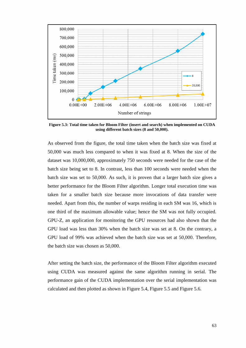
63

Figure 5.3: Total time taken for Bloom Filter (insert and search) when implemented on CUDA

using different batch sizes (8 and 50,000).

As observed from the figure, the total time taken when the batch size was fixed at

50,000 was much less compared to when it was fixed at 8. When the size of the

dataset was 10,000,000, approximately 750 seconds were needed for the case of the

batch size being set to 8. In contrast, less than 100 seconds were needed when the

batch size was set to 50,000. As such, it is proven that a larger batch size gives a

better performance for the Bloom Filter algorithm. Longer total execution time was

taken for a smaller batch size because more invocations of data transfer were

needed. Apart from this, the number of warps residing in each SM was 16, which is

one third of the maximum allowable value; hence the SM was not fully occupied.

GPU-Z, an application for monitoring the GPU resources had also shown that the

GPU load was less than 30% when the batch size was set at 8. On the contrary, a

GPU load of 99% was achieved when the batch size was set at 50,000. Therefore,

the batch size was chosen as 50,000.

After setting the batch size, the performance of the Bloom Filter algorithm executed

using CUDA was measured against the same algorithm running in serial. The

performance gain of the CUDA implementation over the serial implementation was

calculated and then plotted as shown in Figure 5.4, Figure 5.5 and Figure 5.6.

64

Let represent the time taken for the Bloom Filter in a CUDA implementation.

The performance gain (or performance ratio or speedup factor) is calculated as:

(5-1)


serial programming and CUDA.

Figure 5.5: Time taken and performance gain for Filter Search when implemented using serial

programming and CUDA.

65

Figure 5.6: Total time taken and performance gain for Bloom Filter (insert and search) when

implemented using serial programming and CUDA.

Figure 5.4, Figure 5.5 and Figure 5.6 show the execution time and the performance

gains for the Bloom Filter algorithm when it was executed using serial programming

and CUDA. As observed from the three figures, the processing time for the Bloom

filter was longer when serial programming was implemented as compared to the

CUDA implementation. Approximately 35 seconds were needed for inserting

10,000,000 strings into the CUDA filter whereas 180 seconds were needed by the

serial filter; hence a performance speedup of 5.5x was achieved. The filter search for

10,000,000 strings (queries) exhibited an almost similar amount of time and

speedup. As a result, a speedup factor of approximately 5.5x can be observed from

Figure 5.6 as well, whereby the serial filter took 360 seconds for the algorithm while

the CUDA filter took 69 seconds.

For a more in-depth assessment, it can be observed that the performance gain of

CUDA over serial programming showed a dramatic increase when the size of the

input data was small. By referring to Figure 5.6, CUDA implementation of the

algorithm took slightly less amount of execution time when there were 10,000

strings, contributing to a speedup factor of 1.2x. When the size of the dataset was

increased to 100,000, the speedup factor increased to approximately 2.6x. A speedup

factor of 4.4x was achieved when the dataset consisted of 500,000 strings. However,

66

the increase in performance gain slowed down upon reaching this data size. For data

size greater than 3,000,000 strings, the speedup factor increased at an even slower

rate. The speedup factor was approximately 5.2x for 3,000,000 strings and 5.5x for

10,000,000 strings. The declination of the increase rate of speedup factor could be

due to resource limitation (number of CUDA cores and SMs).

For the case of filter insertion, atomic instruction was involved when the bit-table

was updated by more than one thread. Each atomic write to the global memory

location was performed in a serial manner. This introduced delay as the program

could not be entirely parallelised when such condition occurs.

In the filter querying function, there is a conditional branch statement to check if the

bit-table element has been set. In the case whereby the threads within a warp

diverged due to the conditional statement, each branch path would be executed

serially by the warp. After all paths have been completed, the threads would

converge back to the same execution path. The divergence thus introduced delay

into the algorithm.

CUDA implementation of the algorithm has shown a positive performance speedup

whereby it reached approximately 5.5x. Despite having a maximum of 256 threads

executing in parallel in one clock, the performance speedup did not reach 256x. This

is because the time taken for copying the data from the CPU memory to the GPU

memory was included in the performance measurement. Although the algorithm has

already exploited the use of shared memory with the purpose of reducing the

computational time, the bit-table remained in the GPU global memory. This is

because updates to the bit-table must be visible to all threads. Consequently, the

performance of the algorithm was affected due to the low global memory

bandwidth. In spite of that, there has been an overall improvement for the CUDA

implementation of the algorithm compared to the serial CPU implementation.

67

CHAPTER 6: FURTHER DEDUCTIONS

FROM PERFORMANCE COMPARISON

In the previous chapters, serial implementation of the Bloom Filter algorithm has

served as the benchmark for comparison. This chapter investigates the performance

comparison between parallel programming on a CPU and on a GPU. An analysis

was also done to compare the performance of the algorithm when executed on

different GPUs.

6.1 Performance Assessment for Parallel CPU and GPU

Implementations

Theoretically, the GPU execution will consume less time compared to the parallel

CPU execution as a GPU has a massively parallel structure. The results collected

from this project support this theory. The size of the datasets ranges from 1,000

strings to 10,000,000 strings. The average values after five runs were used to plot

the graphs. The performance gain is calculated as the ratio of the time taken by the

CUDA implementation (using Quadro4000) to the time taken by the OpenMP

implementation (with 8 parallel threads).

Figure 6.1, Figure 6.2 and Figure 6.3 show the time taken for the filter insertion,

filter search and the total time (insert and search) for the algorithm, respectively.

68


OpenMP and CUDA (Quadro4000).

Figure 6.2: Time taken and performance gain for Filter Search when implemented using

OpenMP and CUDA (Quadro4000).

69

Figure 6.3: Total time taken and performance gain for Bloom Filter (insert and search) when

implemented using OpenMP and CUDA (Quadro4000).

A similar trend can be observed in all three figures. Figure 6.1 recorded a 1.8x

speedup for the filter insertion when the number of strings was 10,000,000, whereby

the OpenMP implementation took approximately 62 seconds while the CUDA

implementation took roughly 35 seconds. In Figure 6.2, a gain of 1.48x was

recorded when searching was performed for 10,000,000 strings. 48 seconds were

needed for OpenMP whereas 34 seconds were taken by CUDA. Therefore, the

speedup factor for the total time taken was recorded as approximately 1.65x, as

portrayed in Figure 6.3.

Figure 6.3 has also shown that the OpenMP and CUDA implementations took

approximately equal amount of time when the number of strings was 100,000 in

both input word list and query list. The speedup factor for the CUDA

implementation then increased from 1.3x (for 500,000 strings) to 1.5x (for 2,000,000

strings). This marks a substantial increase in the performance speedup when the data

size was smaller than 2,000,000. As the data size increased further, the performance

speedup increased in a slow but steady manner. At 10,000,000 strings, the

performance speedup reached approximately 1.65x. A possible explanation for this

decreasing speedup factor is the GPU resources have reached an almost saturated

70

point. In addition, more copy operations were invoked when the data size increases,

hence incurring more overheads since the data were processed in batches.

6.2 System Assessment for the GPGPU Implementation on

Different GPUs


Table 6.1: Device Properties.

Device Model GeForce 530 Quadro4000

CUDA compute capability 2.1 2.0

Global memory size 1024 MBytes 2048 Mbytes

Number of multiprocessors (SM) 2 8

Number of CUDA Cores/SM 48 32

GPU clock rate 1.40 GHz 0.95 GHz

Maximum number of threads per

multiprocessor 1536 1536

Maximum number of threads per block 1024 1024

Total number of registers available per block 32768 32768

Table 6.1 shows the comparison of specifications between the 2 GPUs used in the

performance assessment, namely GeForce 530 and Quadro4000. The compute

capabilities affect the throughput of the native arithmetic instructions. Compute

capability 2.1 generally allows more operations per clock cycle per multiprocessor.

However, there are more multiprocessors in Quadro4000, hence providing an

advantage over GeForce 530. The total number of CUDA cores in Quadro4000 is

also higher compared to GeForce 530, allowing more operations to be performed in

parallel. The GPU clock rate for Quadro4000 is less, thus the performance gain of

Quadro4000 over GeForce 530 is expected to be less obvious.

71


For the Quadro4000 performance assessment, the results were taken from Section

5.2.2. The Bloom Filter algorithm was executed on the GeForce 530 device and the

time taken for the algorithm was recorded. The algorithm was executed for five

times for each dataset size. The average values were then used to plot the graphs in

Figure 6.4, Figure 6.5 and Figure 6.6. The performance gain is calculated as the ratio

of the time taken when executed on a Quadro4000 device against the time taken

when executed on a GeForce 530 device.

Figure 6.4: Time taken and performance comparison for Filter Insert when executed using

GeForce 530 and Quadro4000.

72

Figure 6.5: Time taken and performance comparison for Filter Search when executed using

GeForce 530 and Quadro4000.

Figure 6.6: Total execution time and performance gain when executing the Bloom Filter

algorithm (insert and search) on GeForce 530 and Quadro4000.

Figures 6.4, 6.5 and 6.6 illustrate the results collected for different dataset sizes after

executing the same program on different GPUs. The collected results correspond to

the expectation of Quadro4000 providing a computational edge over GeForce 530.

The curvature for the performance gain in all three figures is similar. By referring to

73

Figure 6.4, a speedup of 1.9x was achieved for inserting 10,000,000 strings into the

filter, whereby GeForce 530 took 66 seconds while 35 seconds was recorded for

Quadro4000. To search the filter for 10,000,000 queries, 48 seconds were needed by

GeForce 530 while 34 seconds were needed by Quadro4000. This relates to a

speedup factor of 1.45x as shown in Figure 6.5.

Based on the total execution time (filter insertion and search) as shown in Figure

6.6, Quadro4000 has shown a performance gain of approximately 1.3x when the

dataset consist of about 10,000 strings. A gain of 1.65x was achieved when the size

of the dataset was increased to 100,000. Upon reaching the dataset size of 2,000,000

strings, the gain in performance reached its peak of slightly more than 1.7x. When

the number of strings was increased further, the performance gain suffered a

minimal decrease. For a dataset size of 10,000,000, GeForce 530 took

approximately 115 seconds while Quadro4000 took roughly 69 seconds, exhibiting a

performance gain of 1.7x. The decrease in the performance gain could be due to the

limitation of resources in both devices causing the processing of data blocks to be

queued. The higher clock rate of GeForce 530 could be accounted for this decrease

in performance gain.

The encouraging results from this project have proven that the implementation of the

Bloom filter algorithm using GPGPU is feasible. However, this algorithm does not

support locating the query in the input word-list. This is because hash algorithm has

been performed on the input strings. The location of each string in the word-list was

not stored and was irretrievable from the hash value.

Figure 6.7 shows part of the bit-table after 1000 strings were inserted into the Bloom

Filter. The entire bit-table is not shown for brevity purpose.

… 187 56 31 65 192 201 … Figure 6.7 Part of the bit-table for 1000 strings.

As seen in the figure, the resultants of the OR operation in the algorithm constitute

the elements of the bit-table array. As such, it is evident that no information

74

regarding the string location was inserted into the bit-table. Consequently, location

identification of the strings is impossible. Hence, another string searching algorithm

is investigated in the following chapter, with the aim of addressing this drawback.

75

CHAPTER 7: QUICK SEARCH

ALGORITHM FOR LOCATION

IDENTIFICATION

This chapter discusses the implementation of the Quick Search algorithm for

location identification. It attempts to address the limitation of Bloom Filter in

finding the position of query in input word-list.

7.1 Algorithm Description

The Quick Search algorithm is adapted from the Boyer-Moore algorithm, whereby it

utilizes only the bad-character shift table [44]. The query string is known as pattern.

The algorithm attempts to find the location of the pattern in the text (the input word

file). Pre-processing is done on the pattern, so that sections of the text can be

skipped when searching is performed. This results in lower constant factor compared

to other string search algorithms. A longer pattern length usually reduces the

searching time as longer sections of the text may be skipped.

The algorithm begins by aligning the first character of the pattern with the first

character of the text. A character-by-character comparison is made between the

pattern and the text, starting from the right-most character of the pattern. If a

mismatch is found, then the pattern is shifted right by a number of positions

depending on the bad character rule. If the beginning of the pattern is reached, it

indicates that the pattern has been found in the text. Searching of pattern (in text)

can be resumed by proceeding with a new alignment, and repeating the entire

process until the alignment has past the end of text.

76

7.1.1 Bad Character Rule

Figure 7.1: Mismatch character is found in pattern [45].

Figure 7.1 depicts that the mismatched character “B” in the text exist in earlier part

of the pattern. Hence, the pattern may be shifted to the right until both “B” in the

text and the pattern are aligned. Character comparisons will resume after the new

alignment is done. If the mismatch character does not exist in the pattern at all, the

entire pattern may be shifted forward. This is illustrated in the following figure.

Figure 7.2: Mismatch character is absent in pattern [45].

7.2 Program Design

As illustrated in Figure 7.3, the program begins with loading the input word file and

processing all the strings into a 1D character array (text). The query (pattern) file is

then loaded and flattened into a 1D character array as well. An integer array is

created to store the results of the Quick Search algorithm. Each element of the array

corresponds to the location for one pattern in the text. The Quick Search algorithm is

performed for all the patterns and the results are printed to a .txt file.

77

Figure 7.3: Quick Search Algorithm.

7.2.1 Serial Implementation

As suggested from the flowchart in Figure 7.3, the QuickSearch algorithm is

performed on one pattern at a time. Each time the function boyer_moore() is

called, one element in the result array is updated. The function boyer_moore()

receives 7 arguments from the main function. At line 15 of Program Listing 7.1, the

function badcharshift()is called. This function creates the bad-character-shift

array of size 255 by setting each element to the value of . The

ASCII value of each character in the pattern is used as an array index. Array element

at that index is then set to the value of displacement of the corresponding character

from the last character of the pattern. This is done at Lines 5-9 of Program Listing

7.1.

78

After the bad-character-shift table is built, the search for pattern location begins. The

pattern (referred as pat in the code) is compared with the text (referred as string

in the code). If the pattern and text do not match, the pattern is shifted by a number

of positions depending on the bad-character-shift table. Line 32 shows the shifting

step. If the pattern and text matches, the location of the pattern in the text is found

by comparing the offset in the text (ind) with the value stored in the offset table

(pointed by g_pAccumulative_Wordlength). This is portrayed in Line 25. If

a match is found, the element of the result array (pointed by g_location) is

updated with the location.

Program Listing 7.1 Generating bad-character-shift table and searching for query.

1 void badcharshift(char *pat, int patlen, int bc[])

2 {

3 int i;

4

5 for (i=0; i < ALPHABET_LEN; ++i)

6 bc[i] = patlen+1;

7

8 for (i=0; i < patlen; ++i)

9 bc[pat[i]] = patlen - i;

10 }

11

12 void boyer_moore (char *pat, int patlen, char *string,

int stringlen, int* g_pAccumulative_Wordlength,

int g_Wordnumber, int* g_location)

13 {

14 int bc[ALPHABET_LEN];

15 badcharshift(pat, patlen, bc);

16

17 int ind=0;

18

19 while (ind < (stringlen-patlen) )

20 {

21 if (memcmp (pat, string+ind, patlen) == 0)

22 {

23 for (int a=0; a<g_Wordnumber; a++)

24 {

25 if (g_pAccumulative_Wordlength[a]==ind)

26 {

27 (*g_location) = a+1;

28 a=g_Wordnumber;

29 }

30 }

31 }

32 ind += bc[string[ind+patlen]];

33 }

36 return;

37 }

79

7.2.2 OpenMP Implementation

The number of parallel threads has been set to 8 by calling the function

omp_set_num_threads(). Figure 7.4 illustrates the execution model for the

OpenMP implementation. Each thread will perform searching for one query and

then it will update the associated element of the result array. The design of the

program is similar to that of the serial implementation. The only difference is

#pragma directives are added in the main function, as shown in Line 1 and Line 3

of Program Listing 7.2. The search function remains the same as that of in the serial

implementation.

Program Listing 7.2 Calling boyer_moore() function in the main program.

1 #pragma omp parallel

2 {

3 #pragma omp for

4 for (int i=0; i<g_Querynumber; i++)

5 {

6 boyer_moore(g_ppQuery_list_ptr_array[i],

g_pQuerylength[i], g_pTotalwordarray,

g_Totalwordlength, g_pAccumulative_Wordlength,

g_Wordnumber, &(g_location[i]));

7 }

8 }

Block 0

Master thread

Performs

search

for N/8

Queries

Performs

search

for N/8

Queries

Performs

search

for N/8

Queries

Performs

search

for N/8

Queries

Block 1 Block 2 Block 7

…

N = Number of queries

N/8 N/8 N/8 N/8

Figure 7.4: OpenMP Execution Model for boyer_moore() function when 8 parallel threads

are launched.

80

7.2.3 CUDA Implementation

After loading and processing the input word file and the query file, the text and the

pattern must be copied from the CPU memory into the GPU memory. Due to the

limitations in the GPU resources and the maximum allowable kernel execution time,

only 2000 patterns can be passed into the kernel for processing in one invocation.

Hence, searches are performed in batches when the number of patterns exceeds

2000. The kernel function is invoked by calling

cuda_boyer_moore<<< BLOCK, THREAD >>>

(dev_pTotalWordArray, dev_pTotalWordLength,

dev_pTotalWordnum, dev_pAccumulative_Wordlength,

dev_pTotalQueryArray, dev_pQuerylength,

dev_pTotalQuerynum, dev_pAccumulative_Querylength,

dev_pResults);

The value for BLOCK is set at 63, while the value for THREAD is set at 32. Since

each SM can have a maximum of 8 resident blocks and there are 8 SMs in the

device used, it is speculated that all blocks will be residing in the SM at the same

time. There will be no queuing of blocks. The device pointers passed into the kernels

serve the same purposes as in the Bloom Filter algorithm.

Each thread in each block performs the complete Quick Search algorithm for one

pattern. The index of the result array is calculated as:

(7-1)

The associated element of the result array is then updated by each thread. This is

illustrated in Figure 7.5. The kernel function is identical to the boyer_moore()

function in serial and OpenMP implementations.

81

Query 0 Query 1 Query 2 Query 1999 …

Block (0,0,0)

(Queries 0-31)

SM 0

Block (2,0,0)

(Queries 64-95)

Block (3,0,0)

(Queries 96-127)

Block (7,0,0)

(Queries 224-255)

Block (1,0,0)

(Queries 32-63)

Block (4,0,0)

(Queries 128-159)

SM 1 SM 7

Block (5,0,0)

(Queries 160-191)

Block (6,0,0)

(Queries 192-223)

Block (8,0,0)

(Queries 256-287)

Block (10,0,0)

(Queries 320-351)

Block (11,0,0)

(Queries 352-383)

Block (15,0,0)

(Queries 480-511)

Block (9,0,0)

(Queries 288-319)

Block (12,0,0)

(Queries 384-415)

Block (13,0,0)

(Queries 416-447)

Block (14,0,0)

(Queries 448-479)

Block (56,0,0) (Queries 1792-1823)

Block (58,0,0) (Queries 1856-1887)

Block (59,0,0) (Queries 1888-1919)

Block (57,0,0) (Queries 1824-1855)

Block (60,0,0) (Queries 1920-1951)

Block (61,0,0) (Queries 1952-1983)

Block (62,0,0) (Queries 1984-1999)

…

cuda_boyer_moore()

Thread 0

Query 480 … Thread 1

Query 481

Thread 2

Query 482

Result 480 … Result 481 Result 482 Result 511

Thread 31

Query 511

… …

Figure 7.5: CUDA execution model for cuda_boyer_moore() function with 2000 queries.

82



The CPU specifications are as stated in Table 3.5 of Section 3.4.1. The OpenMP

implementation utilizes 8 threads for the parallelised region of the code.

Quadro4000 was used as the GPU device for the CUDA implementation.


For each dataset size, the Quick Search algorithm was executed 5 times on each

implementation (serial, OpenMP and CUDA). The average values were then used to

plot the graphs in this section. The performance gain for the OpenMP

implementation over the serial implementation is calculated as the ratio of the time

taken when implemented in a serial program against the time taken when

implemented in a data-parallelised CPU program. The ratio of the time taken in the

serial implementation over the time taken in the CUDA implementation gives the

performance gain for the CUDA implementation over the serial implementation.

Figure 7.6: Time taken for Quick Search when the size of the input word list is fixed at 110,000.

83

Figure 7.7: Performance ratio when the size of the input word list is fixed at 110,000.

Figure 7.6 depicts the total time taken for the Quick Search algorithm when the

input word list was fixed at 110,000 strings while the number of queries was varied

from 10,000 to 100,000. As observed from the figure, when the number of queries

was increased, the time taken for searching increased as well. The total time

recorded for searching 100,000 strings are 38 seconds, 8 seconds and 63 seconds for

the serial, OpenMP and CUDA implementations, respectively.

For the case of OpenMP implementation, the increase in the searching time was less

obvious compared to the serial and CUDA implementations. This is because the

increment in the data size was shared among 8 parallel threads. A peak gain of 5.8x

was recorded when the algorithm was performed for 50,000 queries. As shown in

Figure 7.7, the speedup factor for the OpenMP implementation was inconsistent.

The inconsistency in the CPU runtime may have contributed to the fluctuating

results.

As observed in Figure 7.6, the CUDA implementation of the Quick Search

algorithm took a much longer time compared to the serial version. This is portrayed

in Figure 7.7 as well, whereby the ratio of the CUDA implementation over the serial

84

implementation was less than 1 for all sizes of the query list. A performance ratio of

approximately 0.6x was recorded. A possible explanation is the approach taken in

the CUDA implementation was not fully optimized. The text (input word list) and

the queries were located in the global memory of the device; hence long latency was

generated when the character comparison was made between the queries and the

text. In addition, since the algorithm had to be performed in batches when the

number of queries exceeds 2000, more invocations of the copy operation were

performed. This led to more data transfer overheads, thus consuming more time.

The performance for each implementation of the Quick Search algorithm was also

recorded when the number of queries was fixed at 2,000 while the number of strings

in the word list was varied from 10,000 to 100,000. Figure 7.8 and Figure 7.9

illustrates the results obtained.

Figure 7.8: Time taken for Quick Search when the size of the query list is fixed at 2000.

85

Figure 7.9: Performance ratio when the size of the query list is fixed at 2000.

The higher number of strings in the word list implies a longer text length was

involved in the Quick Search algorithm. Hence, more time was needed for the

algorithm when the length of the text was longer. This corresponds to the results

shown in Figure 7.8, whereby the time taken for searching 2,000 queries in a

100,000 word list was 640 milliseconds for the serial implementation, 200

milliseconds for the OpenMP implementation and 900 milliseconds for the CUDA

implementation.

From Figure 7.9, it is observed that the performance gain for the OpenMP

implementation over the serial implementation showed a gradual increase (but with

minimal fluctuations) when the input word list was increased in size. The gain in

performance was less dramatic compared to the case when the size of the query list

was varied. This is because parallelisation was distributed based on the number of

queries. Hence, the increase in the computational load due to the word list size

would have less impact on the improvement ratio of the OpenMP implementation.

The CUDA implementation has again showed worse result when it was compared to

the serial implementation. As shown in Figure 7.9, there was a slight increase from

86

0.5x for 10,000 input strings to almost 0.7x for 40,000 input strings. However, the

performance ratio remained constant at 0.7x upon reaching 50,000 input strings. No

further performance improvement could be obtained. This could be due to the

storage of the text and the queries in the global memory of the device; thus inducing

delay when the data were fetched (for character comparisons) due to the narrow

memory bandwidth.

The Quick Search algorithm has managed to overcome the drawback of the Bloom

Filter algorithm in location identification. The OpenMP implementation of the

algorithm has shown the best performance among the three implementations

whereas the CUDA implementation obtained the worst performance. A hypothesis

deduced here is the usage of the global memory for storing the constantly-used data

will result in an inefficient algorithm due to the long memory access latency. An

attempt to imitate the CUDA implementation of the algorithm based on the abstract

submission by Raymond Tay was unsuccessful due to the lack of information given

in the paper. The current implementation adapted in this project does not show the

advantage of the CUDA implementation over the serial implementation. As such, a

different strategy in designing would be required for a performance improvement,

which is recommended as part of the future work.

87

CHAPTER 8: CONCLUSIONS AND

FUTURE WORK

8.1 Summary of Work

One of the objectives of the project is to identify the computational bottleneck of the

serial implementation of the Bloom filter. The repetitive hashing procedures has

been proven to be the main contributor of the hash computational load. Hence, data

parallelisation by using OpenMP has been implemented as part of this project. The

main objective of this project is to design and develop a string searching algorithm

using GPGPU. Implementation of Bloom Filter using CUDA has proved to be

feasible and has given positive results. The limitation of the Bloom Filter algorithm

has been identified as its inability to locate the position of the query in the input

word list. Quick Search algorithm was then investigated to overcome the drawback

of Bloom Filter.

8.2 Conclusions

The massively parallel computing architecture of a GPU provides an opportunity for

string searching algorithms to be implemented using CUDA. Thus, Bloom Filter has

been chosen to be implemented in this project. The research of this project also

includes designing and developing a parallel CPU implementation of the algorithm.

A performance speedup of 3.3x was attained for the dataset size of 10,000,000. The

performance of the Bloom Filter algorithm using the CUDA implementation was

also benchmarked. For 10,000,000 strings, a gain of 5.5x was obtained in the

performance of the algorithm. Hence, it can be concluded that utilising a GPU to

perform a computationally expensive algorithm improves the performance of the

program. However, the improvement in performance is affected by the architecture

88

and the compute capability of the GPU. The Bloom Filter algorithm offers space and

time efficiencies; however it is not suitable if location identification is needed.

Quick Search would be a more appropriate algorithm if space efficiency is not a

primary concern.

8.3 Future Work

The Bloom Filter algorithm implemented in this project has limited the number of

hash functions to a specific value. The amount of space required for storing the bit-

table and the false positive probability are calculated based on that value.

Optimization can be performed in order to obtain the optimal number of hash

functions such that the size of the bit-table can be reduced without increasing the

false positive probability.

Implementation of Quick Search algorithm using CUDA can be investigated further

by restructuring the algorithm when it is ported over to CUDA architecture.

Improvement in performance will be obtained if the algorithm is optimised for

processing on a GPGPU.

The algorithm developed in this project is implemented on a single card within a

single machine. Future work can be done to improve the performance by running the

algorithm using multiple cards within a single machine or across several machines

(i.e., GPU clusters).

89

References

[1] K. Murakami, N. Irie, M. Kuga, and S. Tomita, “SIMP (Single Instruction

Stream/Multiple Instruction Pipelining): A Novel High-speed Single-processor

Architecture,” in Proceedings of the 16th Annual International Symposium on

Computer Architecture 1989, pp. 78-83, Japan, May 1989.

[2] A. Heinecke, M. Klemm, and H. Bungartz, “From GPGPU to many-core: Nvidia

Fermi and Intel Many Integrated Core architecture,” Computing in Science

Engineering, vol. 14, no. 2, pp. 78-83, March 2012.

[3] D. Luebke, N. Govindaraju, M. Harris, J. Kruger, A. Lefohn, T. Purcell, and J. D.

Owens, “A Survey of General-Purpose Computation on Graphics Processing

Hardware,” Computer Graphics Forum, vol. 26, pp. 80-113, 2007.

[4] E. Kandrot and J. Sanders, “CUDA by Example,” Addison Wesley, 2000, pp. 5-10.

[5] J. Nickolls, I. Buck, M. Garland, and K. Skadron, “Scalable Parallel Programming

with CUDA,” ACM Magazine, vol. 6, no. 2, pp. 40-53, March 2008.

[6] P. S. Deshpande and O.G. Kakde, “C & Data Structure,” James Walsh, 2003, pp.

210-216.

[7] N. Dale, “C++ Plus Data Structures,” Ty Field, 2013, pp. 243-245.

[8] G. Pai, “Data Structures and Algorithms – Concepts, Techniques and Applications,”

McGraw-Hill Education, 2008, pp. 221.

[9] T. H. Cormen, C. E. Leiserson, R. L. Rivest, and C. Stein, “Introduction to

Algorithms,” McGraw-Hill Education, 2001, pp. 253-255.

[10] B. W. Kernighan and R. Pike, “The Practice of Programming,” Pearson Education,

1999, pp. 55.

[11] I. Chai and J. D. White, “Structuring Data and Building Algorithm,” McGraw-Hill

Education, 2009, pp. 190-215.

[12] Z. Chen, “A Multi-layer Bloom Filter for Duplicated URL Detection,” in the 3rd

International Conference on Advanced Computer Theory and Engineering

(ICACTE) 2010, pp. 586-591, China, August 2010.

[13] A. Natarajan, S. Subramanian, and K. Premalatha, “A Comparative Study of

Cuckoo Search and Bat Algorithm for Bloom Filter Optimisation in Spam

Filtering,” in International Journal of Bio-Inspired Computation, pp. 2-10, 2012.

[14] B. Chazelle, J. Kilian, R. Rubinfield, and A. Tal, “The Bloomier Filter: An Efficient

Data Structure for Static Support Lookup Tables,” in Proceedings of the Fifteenth

Annual ACM-SIAM Symposium on Discrete Algorithms, pp. 30-39, USA, January

2004.

[15] H. J. Chao, “Aggregated Bloom Filters for Intrusion Detection and Prevention

Hardware,” in the IEEE Global Telecommunications Conference 2007, pp. 342-400,

USA, November 2007.

[16] B. H. Bloom, “Space/time Trade-offs in Hash Coding with Allowable Errors,”

Communications of ACM, vol. 13, pp. 422-426, 1970.

90

[17] D. Eppstein and M.T. Goodrich, “Invertible Bloom Filters,” in the 10th International

Workshop on Algorithms and Data Structures, pp. 644-646, Halifax, Canada,

August 2007.

[18] J. Lin, “TMACS: Type-based Distributed Middleware for Mobile Ad-hoc

Networks,” ProQuest, 2009, pp. 35-36.

[19] A. Broder and M. Mitzenmacher, “Network Applications of Bloom Filters: A

Survey,” Internet Mathematics, pp. 636-646, 2002.

[20] D. Shikhare and P. R. Prakash, “Introduction to Parallel Processing,” Prentice-Hall,

2000, pp. 123-130.

[21] M. R. Bhujade, “Parallel Computing,” New Age International, 2004, pp. 240-242.

[22] Getting Started with OpenMP, Intel Software, http://software.intel.com/en-

us/articles/getting-started-with-openmp, Last visited: 28 December 2012.

[23] A. Marowka, “Analytic Comparison of Two Advanced C Language-based Parallel

Programming Models,” in Third International Symposium on Parallel and

Distributed Computing, pp. 410-456, Ireland, 2004.

[24] OpenMP, Lawrence Livermore National Laboratory,

https://computing.llnl.gov/tutorials/openMP/, Last visited: 10 January 2013.

[25] R. Farber, “CUDA Application Design and Development,” Elsevier, 2011, pp. 3-4.

[26] Z. Fan, W. Li, C. Tan, and D.C. Liu, “GPU Based Tissue Doppler Imaging,” in 5th

International Conference on Bioinformatics and Biomedical Engineering, pp. 1-4,

Chengdu, 2011.

[27] R. Salman, E. Test, R. Stack, V. Kecman, and Q. Li, “GPUSVM: A Comprehensive

CUDA Based Support Vector Machine Package,” Central European Journal Of

Computer Scienece, vol. 1, no. 4, pp. 387-405, December 2011.

[28] W. M. Hwu and D. B. Kirk, “Programming Massively Parallel Processors: A

Hands-on Approach,” Elsevier, 2010, pp. 30.

[29] S. Cook, “CUDA Programming: A Developer’s Guide to Parallel Computing with

GPUs,” Elsevier, 2011, pp. 15-24.

[30] Liang, T. Yeu, Y. W. Chang, and H. F. Li, “A CUDA Programming Toolkit on

Grids,” International Journal of Grid and Utility Computing, pp. 209-220, 2012.

[31] 3D Game Engine Programming - CUDA Memory Model,

http://3dgep.com/?p=2012, Last visited: 15 January 2013.

[32] Wang, Tao, L. Guo, G. Li, J. Li, R. Wang, M. Ren, and J. He, “Implementing the

Jacobi Algorithm for Solving Eigenvalues of Symmetric Matrices with CUDA,” in

the IEEE Seventh International Conference on Networking Architecture and

Storage, pp. 69-78, Xiamen, China, 2012.

[33] M. Bahi, “High Performance by Exploiting Information Locality through Reverse

Computing,” in 23rd

International Symposium on Computer Architecture and High

Performance Computing, pp. 102-114, Brazil, October 2011.

[34] NVIDIA’s Next Generation CUDA Compute Architecture, version 1.1, NVIDIA,

USA, pp. 8-9.

[35] R. Farber, “CUDA Application Design and Development,” Elsevier, 2011, pp. 58-

59.

http://software.intel.com/en-us/articles/getting-started-with-openmp

http://software.intel.com/en-us/articles/getting-started-with-openmp

https://computing.llnl.gov/tutorials/openMP/

http://3dgep.com/?p=2012

91

[36] NVIDIA CUDA C Programming Guide, version 4.2, NVIDIA, USA, 2012, pp. 89-

93.

[37] NVIDIA - Seismic City, http://www.nvidia.com/object/seismiccity.html, Last

visited: 25 December 2012.

[38] NVIDIA - Optitex, http://www.nvidia.com/object/optitex.html, Last visited: 26

December 2012.

[39] M. Vachharajani, “GPU Acceleration of Numerical Weather Prediction,” in 2008

IEEE International Symposium on Parallel and Distributed Processing, pp. 89-105,

Florida, USA, April 2008.

[40] G. Navarro, “A Guided Tour to Approximate String Matching,” ACM Computing

Surveys, vol. 33, pp. 31-53, 2001.

[41] H. Bluthgen, P. Osterloh, H. Blume, and T. Noll, “A Hardware Implementation for

Approximate Text Search in Multimedia Applications,” in Proceedings of IEEE

ICME, pp. 1425-1428, USA, 2000.

[42] R. Tay, “Demonstration of Exact String Matching Algorithms using CUDA,”

unpublished.

[43] General- Purpose Hash Function Algorithms,

http://www.partow.net/programming/hashfunctions/index.html, Last visited: 10

December 2012.

[44] G. A. Stephen, “String Searching Algorithms,” World Scientific, 2000, pp. 9-15.

[45] Y. Huang, “Supercomputing Research Advances,” Nova Science, 2008, pp. 60-72.

http://www.nvidia.com/object/seismiccity.html

http://www.nvidia.com/object/optitex.html

http://www.partow.net/programming/hashfunctions/index.html#VariousFormsOfHashing

String Algorithm on GPUPU

Documents

Transcript of String Algorithm on GPUPU