arX

iv:h

ep-t

h/03

0716

0v3

16

Dec

200

3 JHEP11(2003)065

Published by Institute of Physics Publishing for SISSA/ISAS

Received: July 28, 2003

Revised: October 10, 2003

Accepted: November 27, 2003

Saltatory de Sitter string vacua

Cristina Escoda, Marta Gomez-Reino and Fernando Quevedo

DAMTP, Centre for Mathematical Sciences, University of Cambridge

Cambridge CB3 0WA U.K.

E-mail: C.Escoda@damtp.cam.ac.uk, M.Gomez-Reino@damtp.cam.ac.uk,

f.quevedo@damtp.cam.ac.uk

Abstract: We extend a recent scenario of Kachru, Kallosh, Linde and Trivedi to fix the

string moduli fields by using a combination of fluxes and non-perturbative superpotentials,

leading to de Sitter vacua. In our scenario the non-perturbative superpotential is taken

to be either, the racetrack scenario or the N = 1∗ superpotential for an SU(N) theory,

originally computed by Dorey and recently rederived using the techniques of Dijkgraaf-Vafa.

The fact that this superpotential includes the full instanton contribution gives rise to the

existence of a large number of minima, increasing with N . In the absence of supersymmetry

breaking these correspond to supersymmetric anti de Sitter vacua. The introduction of

antibranes lifts the minima to a chain of (non-supersymmetric) de Sitter minima with

the value of the cosmological constant decreasing with increasing compactification scale.

Surprisingly a similar picture occurs for the simpler system of the racetrack scenario. The

relative semiclassical stability of these vacua is studied. Possible cosmological implications

of these potentials are also discussed.

Keywords: D-branes, Superstring Vacua.

c© SISSA/ISAS 2008 http://jhep.sissa.it/archive/papers/jhep112003065/jhep112003065.pdf

JHEP11(2003)065

Contents

1. Introduction 1

2. Fluxes and moduli fixing 3

3. The general scalar potential 6

3.1 The supersymmetric potential 6

3.2 Supersymmetry breaking 7

4. Superpotentials with two exponentials 7

4.1 The racetrack scenario 7

4.2 A finite instanton sum 8

5. N = 1∗ theory 9

5.1 Background 10

5.2 The scalar potential 11

5.2.1 Numerical analysis 12

5.2.2 Analytical considerations 14

5.3 Supersymmetry breaking 16

5.3.1 Analytical considerations 16

5.3.2 Numerical results 17

6. Stability of the vacua 19

6.1 Vacuum decay 21

6.2 Comparing tunneling probabilities 22

7. Discussion 24

8. Note added in revised version 26

1. Introduction

Supersymmetry breaking and moduli fixing have been the main obstacles for string theory

to make contact with low energy physics. These questions are also essential for the study

of any possible cosmological implications of the theory. Over the years there have been

several proposals to solve these problems. Supersymmetry breaking mechanisms include

the effect of non-perturbative field theoretical effects such as gaugino condensation and,

more recently, the explicit breaking due to the presence of antibranes or brane intersections

– 1 –

JHEP11(2003)065

in low scale string models. The remnant potential for the moduli fields in these cases is

such that the global minimum is either anti de Sitter space with a very large (negative)

vacuum energy or the potential is of the runaway type, towards infinite extra dimension

and/or zero string coupling. The problem is then not how to break supersymmetry but

actually what to do, after breaking it, with the remaining potential for the moduli.

Recently there has been interesting progress towards the solution of the continuum

vacuum degeneracy problem in string theory. The introduction of fluxes of RR or NS-NS

forms [1]–[5] has proven to be very efficient to fix many of the moduli fields, including the

dilaton. However in typical orientifold (or F -theory) compactifications, the overall Kahler

modulus cannot be fixed by this effect [2, 4].

An interesting proposal to also fix this modulus, due to Kachru, Kallosh, Linde and

Trivedi (KKLT) [6], combines the fluxes with non-perturbative superpotentials that have

been discussed in string theory in the past, consisting of a single exponential of the cor-

responding modulus. The modulus is then stabilised for a supersymmetric anti de Sitter

point. The further inclusion of anti D3 branes breaks supersymmetry explicitly and can lift

the minimum of the potential to a de Sitter minimum with varying value of the cosmological

constant, depending on the different parameters of the theory. Even though this is a very

simple set-up, involving much fine tuning and the simplest non-perturbative superpoten-

tial, it represents a concrete step forward towards fixing the moduli after supersymmetry

breaking, with a potentially realistic value of the vacuum energy.

In a different direction, progress has also been made in the understanding of non-

perturbative effects in supersymmetric field theories. In particular, several techniques have

been developed that allow the computation of the exact non-perturbative superpotentials.

In some simple cases they have been derived in closed form encoding the infinite sum of

exponentials of the inverse gauge coupling expected from the full instanton and fractional

instanton effects.

In this note, we slightly extend the KKLT proposal by considering more general non-

perturbative superpotentials than the single exponential considered in KKLT. In particular

we consider the non-perturbative superpotential for a supersymmetric theory for which the

exact superpotential has been computed explicitly, including the infinite instanton sum.

This is the so-called N = 1∗ theory [7, 8].

The structure of the potentials generated in this way is such that there are many

AdS supersymmetric minima in the absence of the antibranes and many de Sitter min-

ima in their presence, with intermediate configurations having both dS and AdS vacua,

all non-supersymmetric. The minima are such that the value of the vacuum energy de-

creases with increasing value of the compactification scale. This rich vacuum structure

may have interesting physical implications and can serve as a concrete nontrivial example

illustrating the possible ‘landscape’ of string theory [9]. It is also similar to the staircase

potentials proposed by Abbott [10] and to the models presented in [11, 12, 13] exhibit-

ing a dynamical relaxation of the cosmological constant. Furthermore, there is enough

freedom to fine tune one of the minima to have a cosmological constant as small as re-

quired. The presence of several de Sitter minima could also lead to interesting realisations

of inflation.

– 2 –

JHEP11(2003)065

We also consider simpler cases in which the superpotential is a finite sum of exponen-

tials as it appears in the much studied racetrack scenarios [14]. These are the simplest

extensions of the mechanism of KKLT and, in the cases that lead to several minima, they

serve as simple examples to study the transition between different vacua.

This article is organised as follows: After briefly reviewing the effect of fluxes to fix the

moduli in the next section, we start considering in section 3, the general scalar potential for

the Kahler modulus field for arbitrary superpotential. In section 4 we first consider the case

of superpotentials with two exponentials which can give rise to one or two different minima.

Section 5 discusses the potential for the N = 1∗ theory with its rich vacuum structure with

and without breaking supersymmetry. Section 6 is dedicated to the stability analysis of

the different minima. We recover in particular the results of KKLT about the life time of

the dS minimum with smallest positive value of the cosmological constant which is much

larger than the age of the universe but smaller than the Poincare recurrence time. We also

discuss the relative probability for tunneling between different minima.

2. Fluxes and moduli fixing

Type-IIB strings have RR and NS-NS antisymmetric 3-form field strengths, H3 and F3

respectively, that can have a (quantised) flux on 3-cycles of the compactification manifold.

1

4π2α′

∫

AF3 = M ,

1

4π2α′

∫

BH3 = −K , (2.1)

where K and M arbitrary integers and A and B different 3-cycles of the Calabi-Yau

manifold.

The inclusion of fluxes of RR and/or NS-NS forms in the compact space allows for the

existence of warped metrics that can be computed in regions close to a conifold singularity

of the Calabi-Yau manifold, with a warp factor that is exponentially suppressed, depending

on the fluxes, as:

a0 ∼ e−2πK/3gsM . (2.2)

Therefore fluxes can naturally generate a large hierarchy. Here gs is the string coupling

constant.

Fluxes have also proven very efficient for fixing many of the string moduli, including

the axion-dilaton field of type-IIB theory S = eφ + ia. A very general analysis of orientifold

models of type IIB, or its equivalent realisation in terms of F -theory, has been done by

Kachru and collaborators [4, 5]. In the F theory approach, the geometrical picture corre-

sponds to an elliptically fibered four-fold Calabi-Yau space Z with base space M and the

elliptic fiber corresponding to the axion-dilaton field S.

The consistency condition in terms of tadpole cancellation implies a relationship be-

tween the charges of D-branes, O-planes and fluxes that can be written as follows:

ND3 − ND3 + Nflux =χ(Z)

24, (2.3)

– 3 –

JHEP11(2003)065

where the left hand side counts the number of D3 branes and antibranes as well as the flux

contribution to the RR charge:

Nflux =1

2κ210T3

∫

MH3 ∧ F3 . (2.4)

The r.h.s. of (2.3) refers to the Euler number of the four-fold manifold Z or in terms of

orientifolds of type IIB, to the contribution of the D3-brane charge due to orientifold planes

and D7-branes. Here κ10 refers to the string scale in 10D and T3 to the tension of the D3

branes.

The fluxes generate a superpotential on the low-energy four-dimensional effective action

of the Gukov-Vafa-Witten form [3]:

W =

∫

MG3 ∧ Ω , (2.5)

where G3 = F3 − iSH3 with S the dilaton field and Ω is the unique (3, 0) form of the

corresponding Calabi-Yau space.

In the simplest models there will be one single Kahler structure modulus defining the

overall size of the Calabi-Yau space which we denote by T = r4 + ib where r is the scale

of the extra dimensions and b an axion field coming from the RR 4-form (T = iρ in the

conventions of [4, 6]). The relevance of this modulus is that it is the one that cannot be

fixed by the fluxes. Its Kahler potential is of the no-scale form, that is:

K = K(ϕi, ϕ∗i ) − 3 log (T + T ∗) , (2.6)

with K the Kahler potential for all the other fields ϕi except for T . This implies that the

supersymmetric scalar potential takes the form

VSUSY = eK(

KijDiWDjW)

, (2.7)

with Kij the inverse of the Kahler metric Kij = ∂i∂jK and DiW = ∂iW + W∂iK the

Kahler covariant derivative. The T dependence of the Kahler potential is such that the

contribution of T to the scalar potential cancels precisely the term −3eK |W |2 of the stan-

dard supergravity potential, this is the special property of no-scale models [15]. Since this

potential is positive definite, the minimum lies at zero, with all the fields except for T fixed

from the conditions DiW = 0. This minimum is supersymmetric if DT W = W = 0 and

not supersymmetric otherwise.

Since the superpotential does not depend on T , we can see in this way that the fluxes

can fix all moduli but T . In order to fix T KKLT procede as follows:

1. Choose a vacuum in which supersymmetry would be broken by the T field, such that

W = W0 6= 0.

2. Consider a non-perturbative superpotential generated by euclidean D3-brane or by

gaugino condensation due to a non-abelian sector of wrapped N D7-branes. For which

– 4 –

JHEP11(2003)065

the gauge coupling is 8π2

g2YM

= 2π r4

gs= 2π Re T . Which induces a superpotential of the

form Wnp = Be−2πT/N . Combining the two sources of superpotentials W0 + Wnp,

they find an effective scalar potential with a non-trivial minimum at finite T and

the standard runaway behaviour towards infinity, as usual. The non-trivial minimum

corresponds to negative cosmological constant giving rise to a supersymmetric AdS

vacuum.

3. In order to obtain de Sitter vacua, KKLT, consider the effect of including anti D3

branes, still satisfying the condition (2.3). This has the net effect of adding an extra

(non-supersymmetric) term to the scalar potential of the form:

V = VSUSY +D

(Re T )3(2.8)

with the constant D = 2a40T3/g

4s paramterizing the lack of supersymmetry of the

potential. Here a0 is the warp factor at the location of the anti D3 branes and T3 the

antibrane tension. The net effect of this is that for suitable values of D the original

AdS minimum gets lifted to a dS one with broken supersymmetry. See figure 1.

Here we will modify the KKLT

Figure 1: The scalar potential considered in [6] with

one single de Sitter minimum.

scenario in two ways. First, regard-

ing the original fluxes, we can con-

sider the supersymmetric configuration

where W0 = 0 with the form G3 be-

ing of the (2, 1) type. That is we

may include a non-vanishing W0 part

in the superpotential but it will not

be necessary. Second, regarding the

non-perturbative superpotential, we ex-

plore the simplest N = 1 supersym-

metric model for which the full non-

perturbative superpotential has been

computed, including the contribution

from all (infinite) instantons. This is

the so-called N = 1∗ model, constructed from mass deformation of N = 4 super Yang-

Mills.

Our first minor modification allows to start with an explicit supersymmetric model,

before considering the low-energy non-perturbative effects. This avoids the need to fine

tune the value of W0 in looking for non-trivial minima. Our second modification allows

exploring the possibility of an exact instanton calculation, instead of a single instanton

calculation as it is usually considered. We will see that this exact superpotential will have

a constant piece (similar to W0) and an infinite sum of exponential terms, allowing for a

very rich vacuum structure. For completeness, we also considered simpler superpotentials

including a sum of two exponentials as in the racetrack scenario.

– 5 –

JHEP11(2003)065

3. The general scalar potential

3.1 The supersymmetric potential

The standard N = 1 supergravity formula for the potential in Planck units reads

VSUSY = eK

∑

i,j

KijDiWDjW − 3|W |2

, (3.1)

where i, j runs over all moduli fields. As we already mentioned, Kij = ∂i∂jK where K

is the corresponding Kahler potential and DiW = ∂iW + (∂iK)W . In our case we are

working with a model having only one Kahler modulus, (that is, h1,1(M) = 1) as we will

be focusing on the T field. All other fields are assumed to have been fixed by the fluxes

just as in [6] so the superpotential W will depend on the superfield T .

Then our purpose is to study the scalar potential V (T ) which also depends on the

Kahler potential. We take the weak coupling result in 4-dimensional string models, namely

K = −3 log(T + T ∗) , (3.2)

and neglect possible perturbative and non-perturbative corrections. For simplicity of no-

tation we will write the field T in terms of its real and imaginary parts:

T ≡ X + iY . (3.3)

Using (3.1) and (3.2) the scalar potential turns out to be

VSUSY =1

8X3

1

3|2XW ′ − 3W |2 − 3|W |2

, (3.4)

where by ′ we understand derivatives with respect to the field T . To compute the super-

symmetric minima of the scalar potential we need to calculate the derivative of (3.4) that

is given by

V ′ =∂V

∂T=

(2XW ′′ − 2W ′)(2XW ′ − 3W )∗ − 2(W ′)∗(2XW ′ − 3W )

24X3, (3.5)

Notice then that there can be two types of extrema. The supersymmetric extrema

appear when

2XW ′ − 3W = 0 . (3.6)

In this case the value of the potential at the extremum is clearly negative definite leading

to an anti de Sitter vacuum. These extrema are minima provided that:

|XW ′′ − W ′| > |W ′| . (3.7)

The nonsupersymmetric extrema occur at

(XW ′′ − W ′) = (W ′)∗e2iγ , (3.8)

where γ = arg(2XW ′ − 3W ).

In all cases considered here, our analysis shows that the condition (3.8) is never fulfilled

at the minima. Then all minima are supersymmetric and lead to negative cosmological

constants.

– 6 –

JHEP11(2003)065

3.2 Supersymmetry breaking

Following the lines of [6], to uplift the anti de Sitter vacua to de Sitter vacua we will

introduce in our model a D3. This will break the supersymmetry of the system. The

introduction of the antibrane does not introduce extra translational moduli as its position

is fixed by the fluxes [16], so it just contributes to the energy density of the system. This

contribution is given by [16]

δV =D

X3, (3.9)

where the coefficient D is a function of the tension of the brane T3 and of the warp factor

a0 and has the form D = 2a40T3

g4s

, where gs denotes the string coupling. The coefficient

D depends on the fluxes through the dependence of the warp factor a0 on them and it is

therefore quantised, although the range of values of the fluxes can be such that for practical

purposes it may be considered as an almost continuum variation [6, 27].

If we add this supersymmetry breaking term to the scalar potential (3.4) we have now

that the expression for the scalar potential is given by

V = VSUSY + δV . (3.10)

The effect of the supersymmetry breaking term depends on the range of values of the

parameter D. If D is very small, the potential will not change substantially and the

minima remain anti de Sitter. For a critical value of D one of the minima will move up to

zero vacuum energy and then to de Sitter space. Continuing increasing D, more minima

become de Sitter until all of them are de Sitter. If D is larger than another critical value

the nonsupersymmetric term starts dominating the potential and starts eliminating the

different extrema to make the potential runaway with X. The range of values of D will

depend very much on the form of W and we will illustrate the behaviour in the examples

below.

4. Superpotentials with two exponentials

Our main interest in this paper is to consider non trivial superpotentials including all

instanton contributions in terms of an infinite sum of exponentials. For simplicity we

will first discuss the simpler case of superpotentials with just two exponentials. We then

consider the following superpotential

W = W0 + Ae−aT + B e−bT . (4.1)

4.1 The racetrack scenario

This superpotential has an interest by itself since it includes the standard racetrack scenario

(when W0 = 0), very much discussed in order to fix the dilaton field at weak coupling. The

origin of the so-called racetrack scenario is the condensation of gauginos of a product of

gauge groups. For an SU(N)×SU(M) group we would have a = 2π/N and b = 2π/M . For

large values of N and M , with M close to N the minimum is guaranteed to lie in the large

field region. A similar result will happen for the field T taken to be the gauge coupling at a

– 7 –

JHEP11(2003)065

12 14 16 18 20 22 24

0

20

40

60

80

100

00

Figure 2: Contour plot for a racetrack type

potential with several minima.

Figure 3: Graph of the scalar potential with

a = 0.1, A = 1, B = 5 ·104 and W0 = −10−3.

product gauge group coming from the D7 sector. Turning on W0 it is possible to find more

than one minimum that, following the KKLT method, would then lead to many (order 10)

de Sitter vacua depending on the values of the parameters W0, N,M,A,B. In figure 2 we

present a contour plot of the potential illustrating this behaviour with W0 ∼ −10−3 and

all other constants in the range 1, 10.

4.2 A finite instanton sum

The potential takes a manageable form if we assume b = 2a which allows more than one

minima and we will follow mostly for illustration purposes. In this case using (3.1), (3.2)

and (4.1) the scalar potential turns out to be

VSUSY =ae−4aX

6X2

[

6B e2aXW0 cos(2aY ) + 6B2 + 3A2 e2aX + 4aB2X +

+ aA2X e2aX + AeaX(3 e2aXW0 + B(9 + 4aX)) cos(aY )]

. (4.2)

Notice that this potential is periodic in Y with period 2π/a, and is also invariant under

the reflexion Y → −Y .

From (4.2) it is easy to see that if W0 is negative (W0 < 0) the minima of the potential

will be located at Y = Y (n) = πn/a, n = 0,±1,±2, . . . For each value of Y (n) we will find

a minimum at X = X(n). Since the potential (4.2) is periodic in Y with period 2π/a we

will just consider the cases n = 0 and n = 1, being the rest of the cases copies of these two.

We will denote these minima as (X(±), Y (±)), where + will denote the case n = 0 and −will denote the case n = 1. In figure 3 we show an explicit example of the potential (4.2).

At the minima of the potential we have that

∂XV |Y =Y (±)= 0 =⇒ W0 = −e−2aX(±)

3

(

±AeaX(±)(3 + 2aX(±)) + B(3 + 4aX(±))

)

.

(4.3)

– 8 –

JHEP11(2003)065

Using this we can get the values of the potential at the minima. Those values are given by

V(±)0 = − a2

6X(±)(±Ae−aX(±)

+ 2B e−2aX(±))2 . (4.4)

Note that from (4.3) we find that X(+) > X(−) and then from (4.4) V(+)0 > V

(−)0 . Also

note from (4.4) that we will always have two non-degenerate minima with null or negative

value of the potential, that is, we will have either Minkowski or AdS vacua.

On the other hand, if W0 is positive (W0 > 0), the points located at Y = Y (n) = πn/a,

n = 0,±1,±2, . . . are no longer minima, but maxima. In this case we find that the scalar

potential will have two degenerate minima in every 2π/a period of Y . Those minima fulfill

Y (1) + Y (2) = 2π/a and X(1) = X(2) (the reason for that is the invariance of (4.2) under

Y → −Y ). This means that we should need more exponential terms in (4.2) in order

to have at least two non-degenerate minima. Therefore we will concentrate in the case

W0 < 0, as is the simplest case of that type. The analysis of the case W0 > 0 is analogous

to the case considered in [6], where they analyse the case of a scalar potential with just

one minimum.

Now, we will study what is the effect of breaking supersymmetry in this model. The

introduction of the supersymmetry breaking term (3.9) acts in the following way: when

D/(X(±))3 ≪ V(±)0 the potential is almost not affected, and we still have two AdS minima.

If we increase the value of D such that D/(X(±))3 ∼ V(±)0 , the value of the scalar potential

at the minima increases with D, so the minima will eventually become positive (dS minima).

For larger values of D the minima become saddle points and then disappear.

Also notice that the supersymmetry breaking term (3.9) does not involve Y , therefore

the new potential will also be periodic in Y with the same period as before, and its minima

will also be located at Y = Y (n) = πn/a, n = 0,±1,±2, . . . Again, for each value of Y (n) we

will find a minimum in X but now at different values than in the supesymmetric case. We

will denote these values as X(n). For each of those values we will find again two different

values of the potential. It is interesting to note that the position of the minima in the non-

supersymmetric case (X = X(±), Y = Y (±)) does not vary significantly from the position

of the minima in the supersymmetric case (X = X(±), Y = Y (±)).

Therefore, for a given value of D such that D/(X(±))3 ∼ V(±)0 the non-susy scalar

potential will have two different minima that, depending on the value of the constants, can

be either positive or negative. If we want to describe the present stage of the acceleration

of the universe within this framework, we would like both minima to be dS minima, such

that V(+)0 > V

(−)0 ∼ 10−120 in Planck units. This can always be done in this model for

example by fine-tuning the value of D. In figure 4 we show an explicit example where the

two AdS minima that appear in the supersymmetric case shown in figure 3 become two dS

minima in the non-supersymmetric case.

5. N = 1∗ theory

In this section, we would like to study more general superpotentials were the full instanton

sum has been computed, being the simplest such case the N = 1∗ theory. The N = 1∗

– 9 –

JHEP11(2003)065

100 150 200 250 3000

1·10-13

2·10-13

3·10-13

4·10-13

5·10-13

101 102 103 104 1050

2·10-13

4·10-13

6·10-13

8·10-13

1·10-12

1.2·10-12

(a) Cross section of the scalar potential at Y =

0 and Y = π/a.

(b) Cross section of the scalar potential along

a line that joins the two minima.

Figure 4: Example of a configuration with a = 0.1, A = 1, B = 5 · 104, W0 = −10−3, and

D = 3.5 · 10−7. In this case we find a configuration with two de Sitter minima.

theory is mass deformed N = 4 super Yang-Mills in which the N = 1 chiral multiplets

inside the N = 4 Yang-Mills multiplet are given a mass. At the moment we do not

have a concrete example where this theory appears at low energies on the D7-branes. We

may think of ways that it could arise, for instance since the D-branes break one half of

the supersymmetries, they tend to have a N = 4 gauge theory inside. Having a model

that breaks supersymmetry to N = 1 outside the brane would naturally induce masses

to the chiral multiplets. However here we will take the N = 1∗ superpotential only as

an illustrative example of what we can expect from full instanton contributions to the

superpotential.

5.1 Background

Let us first review what the N = 1∗ theory is, starting from SU(N), N = 4 super Yang-

Mills. The SU(N), N = 4 super Yang-Mills theory can be written in terms of N = 1

superfields as a gauge theory with three massless chiral superfields Φi in the adjoint of

SU(N) with superpotential

W = ǫijk Tr Φi [Φj,Φk] . (5.1)

A deformation of this theory by adding mass terms to these superfields

∆W = mi Tr Φ2i , (5.2)

with all mi 6= 0 breaks supersymmetry to N = 1. This is the N = 1∗ theory. There are

further deformations of the original N = 4 theory that may be considered [18].

The classical vacua of this theory can be found by solving ∂WT /∂Φi = 0 for WT =

W + ∆W , which leads to

[Φi,Φj ] = ǫijkmkΦk (5.3)

and therefore the solutions correspond to N -dimensional representations of the SU(2) al-

gebra, giving rise to the different phases of the theory.

The massive (Higgs and confining) phases of this theory are well understood. They

are labelled by a triplet of integers (p, q, k) with pq = N and 0 < k < q. These phases

– 10 –

JHEP11(2003)065

interpolate from the full confining phase q = N to the full Higgs phase p = N . The

exact superpotential for N = 1∗ was derived by using instanton techniques for the theory

compactified on a circle. The compactification to three dimensions is a computational trick

and it turns out that the superpotential is independent of the compactification radius [7].

After integrating out the gauge fields, the superpotential depends only on the (complex)

gauge coupling τ and takes the form:1

Wp,q,k(τ) = E2(τ) − p

qE2

(

p

qτ +

k

q

)

. (5.4)

Here and later in this section by En we will denote the Eisenstein modular functions.

The modular properties of the superpotential show that under a SL(2, Z) transforma-

tion

τ → aτ + b

cτ + d(5.5)

the effective theory in a given phase is not invariant but it exchanges different phases by

changing the values of p, q, k. For instance τ → τ + 1 requires (p, q, k) → (p, q, k + p) and

τ → −1/τ implies (p, q, k) → (α, Nα , k′) with α = gcd(q, k) and k′ having a complicated

dependence on p, q, k with k′ = 0 if k = 0, indicating the exchange of Higgs and confining

phases under this transformation.

It is interesting to note that the validity of this exact non-perturbative result has

been checked using string theory techniques [8] and more recently from Dijkgraaf-Vafa

techniques [17, 18], making this expression very robust.

5.2 The scalar potential

Following [19] we will now promote the parameter τ to a full N = 1 superfield that we

identify with the modulus field2 T = −iτ . Then the superpotential (5.4) can be written in

terms of T as

Wp,q,k(T ) = E2(T ) − p

qE2

(

p

qT − i

k

q

)

, (5.6)

The superpotential Wp,q,k(T ) transforms as a modular form of weight 2 once the values

of p, q, k are transformed accordingly. As we already mentioned, the net effect of a SL(2, Z)

transformation is that it changes one massive phase to a different phase.

For concreteness we will concentrate in the confining phase p = 1, q = N , for which

it is enough to set k = 0, since k 6= 0 can be reached by a translation T → T − ik. In

1An overall factor of order m3 = N3

24m1m2m3 appears multiplying the superpotential, where mi are the

masses of the chiral superfields of the N = 4 theory. This will scale the scalar potential by a particular

scale, which we take as unity for simplicity, but need to keep it in mind when combining with the non-

supersymmetric case and to take care of actual number estimates regarding the value of the cosmological

constant. For consistency we have to take the scale set by the mi’s to be hierarchically smaller than the

string scale. It is not yet clear if these small mass parameters will be achieved in explicit models.2In reference [19] the corresponding field was the dilaton S rather than T then the difference between

the potential calculated there and the supersymmetric potential we consider here is only in the factor of 3

in the Kahler potential. The main difference appears when we consider the nonsupersymmetric case.

– 11 –

JHEP11(2003)065

this case the scalar potential will be given by (3.4) where now the superpotential and its

derivative take the form

W (T ) = E2(T ) − 1

NE2

(

T

N

)

, (5.7)

W ′(T ) =π

6

(E4(T ) − E2(T )2) − 1

N2

(

E4

(

T

N

)

− E2

(

T

N

)2)

. (5.8)

We will mostly work with the En(T ) expansions in terms of the variable q = e−2πT that

are given by

E2 = 1 − 24

∞∑

n=1

σ1(n)qn , E4 = 1 + 240

∞∑

n=1

σ3(n)qn , (5.9)

where σp(n) is the sum of the pth powers of all divisors of n. E4 is a modular form of

weight 4 so E4(1/T ) = T 4E4(T ), while E2 fails to be a modular form of weight two since

E2

(

1

T

)

= −T 2E2(T ) +6T

π. (5.10)

Since there is already a constant term in the expansion of the superpotential we will

perform most of our analysis considering W0 = 0 which means no supersymmetry breaking

by the fluxes themselves. Contrary to the case with one single exponential, we will find

many minima without needing to tune the value of W0 to obtain large compactification

volume naturally once we break supersymmetry. We will see later how W0 affects our

results.

5.2.1 Numerical analysis

In order to perform reliable computations with the Eisenstein series we use the ‘weak

coupling’ or large radius expansion of W (T ) in eq. (5.6) only when 2π X > N . For other

ranges we can use the property (5.10). For instance, for 1 < 2π X < N we can transform

the E2(T/N) term to obtain

W (T ) = E2(T ) +N

T 2E2

(

N

T

)

− 6

πT. (5.11)

Similarly, when 2π X < 13 we can trans-N 2 3 4

X 1.46 1.70 1.82

Vmin −1.73 · 10−2 −1.60 · 10−2 −1.32 · 10−2

Table 1: Minima of the scalar potential.

form both terms in W (T ) to obtain

W (T ) = − 1

T 2E2(T ) +

N

T 2E2

(

N

T

)

.

(5.12)

For N ≤ 4 we have that the minima appear when 2π X > N , so that one has to use

the expression (5.7) for the superpotential. One finds the supersymmetric minima are at

Y = N/2 and X (when N ≤ 4) at the values given in table 1.

For N ≥ 5 the flat direction at Y = N/2 turns into a saddle point and pairs of

supersymmetric minima Ti1, Ti2 on either side in the Y direction appear, such that Yi1 +

Yi2 = N and Xi1 = Xi2. Examples of these are given in table 2.

3We have to keep in mind that in these regimes there may be substantial corrections to the Kahler

potential which are not under control.

– 12 –

JHEP11(2003)065

N 5 6 7 8 9

X 1.48 1.65 1.77 1.85 1.88

Y 2.24 2.40 2.63 2.88 3.13

Vmin −1.35 · 10−2 −1.37 · 10−2 −1.27 · 10−2 −1.16 · 10−2 −1.07 · 10−2

Table 2: Minima of the scalar potential for several cases.

N = 30 N = 40 N = 50

X Y Vmin X Y Vmin X Y Vmin

1.20 6.44 −1.12 · 10−2 1.28 6.95 −5.72 · 10−3 1.10 7.52 −3.43 · 10−3

1.32 11.71 −1.34 · 10−2 1.44 8.73 −1.68 · 10−2 1.15 14.36 −8.58 · 10−3

1.57 8.40 −1.70 · 10−2 1.60 15.31 −1.54 · 10−2 1.36 8.92 −1.36 · 10−2

1.65 12.15 −1.16 · 10−2 1.76 11.32 −1.46 · 10−2 1.59 10.98 −1.70 · 10−2

2.08 5.69 −5.21 · 10−3 1.84 16.77 −1.06 · 10−2 1.76 18.97 −1.39 · 10−2

2.17 6.56 −4.19 · 10−3 1.82 14.24 −1.26 · 10−2

1.92 21.30 −9.10 · 10−3

2.24 7.32 −3.51 · 10−3

Table 3: Minima of the scalar potential for N = 30, 40, 50.

1 2 3 4 5

10

20

30

40

50

Figure 5: Graph for the scalar potential

with N = 100.

Figure 6: Contour graph for the scalar po-

tential with N = 100.

For N ≥ 10 we have that the minima begin to appear when 2π X < N , so that one has

to use the expression (5.11) for the superpotential to compute the scalar potential (3.4).

This needs to be done in order to have a convergent series expansion in (5.9). Using this

we find a lot of supersymmetric minima in the scalar potential, noting that the number of

minima increases with N . We list some of the results table 3.

Also we present in figure 5 a 3D plot of the potential for the case N = 100 illustrating

the rich structure of the potential with many supersymmetric AdS minima. In figure 6 we

present a contour plot showing the location of the minima and how the landscape changes

in field space.

– 13 –

JHEP11(2003)065

N Number of MinG MinX

Minima X Y Vmin X Y Vmin

10 2 1.28 3.59 −1.11 · 10−2 1.85 3.32 −1.01 · 10−2

20 3 1.76 7.84 −1.43 · 10−2 1.96 4.65 −6.92 · 10−3

30 5 1.57 8.40 −1.70 · 10−2 2.08 5.69 −5.21 · 10−3

40 6 1.44 8.73 −1.69 · 10−2 1.28 6.95 −5.73 · 10−3

50 7 1.59 10.98 −1.70 · 10−2 1.10 7.52 −3.46 · 10−3

60 10 1.45 10.78 −1.70 · 10−2 1.20 7.62 −1.62 · 10−3

70 10 1.53 12.62 −1.76 · 10−2 2.32 8.61 −2.67 · 10−3

80 10 1.62 14.45 −1.69 · 10−2 1.13 8.85 −1.07 · 10−3

90 10 1.49 13.75 −1.78 · 10−2 2.38 9.73 −2.16 · 10−3

100 10 1.55 15.28 −1.76 · 10−2 2.41 10.25 −1.97 · 10−3

200 15 1.52 20.98 −1.76 · 10−2 2.56 14.37 −1.06 · 10−3

300 19 1.60 26.00 −1.74 · 10−2 2.70 17.50 −7.26 · 10−4

400 20 1.49 29.59 −1.80 · 10−2 2.68 20.20 −5.53 · 10−4

500 25 1.47 32.20 −1.77 · 10−2 2.70 22.60 −4.46 · 10−4

600 25 1.50 36.31 −1.79 · 10−2 2.73 24.70 −3.74 · 10−4

700 27 1.47 37.80 −1.75 · 10−2 2.75 26.60 −3.22 · 10−4

800 31 1.62 45.70 −1.72 · 10−2 2.77 28.43 −2.83 · 10−4

900 34 1.56 46.10 −1.76 · 10−2 2.78 30.10 −2.52 · 10−4

1000 38 1.48 46.50 −1.72 · 10−2 2.78 31.80 −2.28 · 10−4

Table 4: Number of minima for different values of N in the supersymmetric case.

To illustrate the fact that we find an increasing number of minima when we increase N ,

and also other interesting facts, we present in table 4 some other results of the numerical

analysis. Note that by MinG in table 4 we denote the global minimum of the potential and

by MinX we denote the minimum with a largest (finite) value of X.

From the information shown in table 4 we may extract some general remarks regarding

the minima. First, the number of minima grows quite fast when N grows. Also the potential

at the minimum with larger value of X increases with N . Furthermore, even though we

do not have a general proof, for all the cases we have analysed, all the vacua of this theory

happen to be supersymmetric.

Finally, although it is not necessary in our case, following [6] we have studied the

effect of turning on W0. Notice that with W0 = 0 we have many minima but all of them

correspond to not too large values of the compactification scale X. We have found that

tuning W0 has the effect of allowing minima with very large values of X improving the

validity of the field theoretical analysis of the potential. Otherwise the general structure

of the potential remains the same.

5.2.2 Analytical considerations

The scalar potential (3.4) appears to be, in general terms, too complicated to do an analyt-

ical study of its minima for a superpotential such as the N = 1∗ one. In fact, introducing

the superpotential (5.11) into the condition (3.8) that is used to find the supersymmetric

minima we arrive to non linear equations that cannot be solved analytically.

– 14 –

JHEP11(2003)065

In any case, some interesting features appear when we study the behaviour of the

potential in the limit (2π X)N ≫ X2 +Y 2. In that limit the superpotential W can be well

approximated by the function

W ∼ 1 +N

T 2− 6

πT. (5.13)

This approximation is derived from (5.11) just by keeping the constant terms in the E2

expansions and neglecting the exponential terms.

Using the approximate superpotential in (5.13), we find that the condition for a super-

symmetric minimum, i.e., 2XW ′ − 3W = 0, reduces to a cubic equation in X which can

be solved analytically. This cubic equation is given by:

(

288

π+ 2Nπ

)

X − 168X2 + 24πX3 = 18N , (5.14)

with Y given in terms of X by the following relation:

Y =

√

N +X(3πX − 16)

π. (5.15)

The full form of the solutions for X and Y is not very enlightening, but they allow an

expansion in powers of 1/N that happens to be more useful.4

Xmin =9

π− 3240

π3

1

N+

5015520

π5

1

N2+ · · · (5.16)

Ymin =√

N

(

1 +99

2π2

1

N− 502281

8π4

1

N2+ · · ·

)

(5.17)

It is clear from these expressions that when N is large the solution for X will tend

asymptotically to 9/π, and Y will tend to√

N . It is also possible to compute the value of

the potential in this minimum (also as an expansion in power series of N) substituting the

approximate expression for the superpotential W given in (5.13) into (3.4). Its expansion

in powers of 1/N is given by

Vmin = −2π

27

1

N+

50

3π

1

N2+ · · · . (5.18)

In fact, this minimum is the minimum with the largest finite value of X. Also we have found

that for N ≥ 50 these results (5.14), (5.15) and (5.18) agree well with those obtained in

the numerical analysis (see table 4). This minimum is in fact the minimum that appears to

have the largest value of the potential for large values of N . This will play an important role

in the next section, where we explore the minima of the potential when the supersymmetry

is broken.

4The equation (5.14) has of course three solutions for X, but only one of the three solutions of the cubic

equation gives a positive Xmin in the range of validity of the approximation.

– 15 –

JHEP11(2003)065

5.3 Supersymmetry breaking

In this subsection we will study the changes produced in the structure of the vacua when

we introduce in the scalar potential the supersymmetry breaking term (3.9). We will see

that with the introduction of such a term it is possible to lift the vacua from anti de Sitter

vacua to de Sitter vacua, for some range of the parameter D.5

5.3.1 Analytical considerations

As in the previous case, the scalar potential (3.10) appears to be, in general terms, too

complicated to do an analytical description of its minima. In fact, introducing the super-

potential (5.11) into the scalar potential (3.10) and minimizing it to find the minima leads

to non linear equations that cannot be solved analytically.

In any case, similarly to the previous cases, some interesting features appear when

one studies the behaviour of the potential in the limit 2π X N ≫ (X)2 + (Y )2. As in

the previous case, in that limit the superpotential W can be well approximated by the

function (5.13).

Using the approximate superpotential in (5.13), we find that the condition for minimum

reduces to two polynomial equations in X , Y . Those equations cannot be solved in general

but for N large it is easy to find that Y is given in terms of X by the following relation:

Y =

√

5NπX + 6X2(πX − 7)

6(πX − 1). (5.19)

Using this relation (5.19), we find a complicated polynomial equation on just X. This

equation can be simplified for large N to a cubic polynomial on X2, and therefore can be

solved analytically. In fact, what we found is that only two of the solutions are positive

and then lead to two real positive solutions for X. Nevertheless just one of these two

solutions is a minimum, the other one corresponding to a saddle point. The solution

found is proportional to√

N , with the proportionality constant given in terms of the

supersymmetry breaking parameter D. That is, the solutions for the minimum are given

by Xmin = f(D)N1/2.

The exact form of the function f(D) is a complicated expression, but in any case it is

possible to extract some useful features from it. In fact, it is easy to see that f(D) is an

increasing function on D, until it reaches an upper bound DM . For values D > DM the

values of the function f(D) are no longer real, this meaning that the potential would have

no minima. Therefore, in the limit of validity of the analytical analysis, there is a bound

for the supersymmetry breaking parameter D if we want the potential to have minima.

This bound is given by

D <1

360(27 + 7

√21) ≡ DM . (5.20)

5Recall that the N = 1∗ superpotential has a mass scale m3. This was irrelevant for the discussion of

the supersymmetric case since it could be rescaled out of the potential, affecting only its absolute value at

the minima. We have to keep this in mind when considering the range of variation of the parameters W0

and D which will carry now an extra scale determined by m.

– 16 –

JHEP11(2003)065

Therefore, for values of the supersymmetry breaking parameter D larger than this bound

we will not find any minima of the scalar potential.

When the bound in D is saturated we find that

XMmin =

√

5

12(−4 +√

21)N1/2 , (5.21)

These values for X and D allow an expansion in powers of 1/N of the potential in the

minimum. We find that the value of the potential is positive and is given by

V Mmin = 0.0406

1

N3/2+ 0.0386

1

N2+ · · · (5.22)

Also from the form of f(D) it is clear that one can fine-tune the supersymmetry

breaking parameter D so that the value of the scalar potential in the minimum Xmin

approaches arbitrarily to zero. In fact one can compute the value of D such that Vmin = 0.

The full expression is not very useful, but it allows an expansion in power series in 1/N ,

which is given by

D0 =3

20− 9

20π

√

3

5N+

99

1600π2

1

N+ · · · , (5.23)

and also the values of Xmin and Ymin are

X0min =

√

5

12N +

17

8π− 99

64π2

√

3

5N+ · · · (5.24)

Y 0min =

√

5

4N − 1

8π√

3− 3463

192π2

√

1

5N+ · · · (5.25)

where the value of Y 0min is obtained from (5.19). Also remember that V 0

min = 0.

In fact, we have found that for N ≥ 50 these results agree well with those obtained in

the numerical analysis, as we will show in the following subsection.

5.3.2 Numerical results

In this subsection we present the results found in the numerical analysis of the scalar

potential in the non-supersymmetric case. We have computed numerically the minima of

the potential for D = D0 for several values of N , such as N = 50, N = 100, N = 500 and

N = 1000. The results obtained from the analysis are shown in table 5.

As a matter of comparison with the supersymmetric case, we show in figure 7 the

scalar potential for N = 100 with supersymmetry broken.

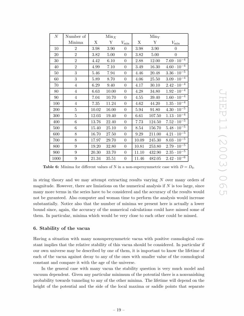
Finally we show in table 6 a similar information as the one shown in table 4 in the last

subsection, where we write the number of minima varying with N . In table 6 we denote

by MinX,Y the minima with largest value of X,Y . We can notice that the number of

minima still increases with N but slower than in the supersymmetric case. An argument

for this is that the non-supersymmetric term δV tends to smooth out the potential as it

moves the minima up, so some of the minima eventually disappear. Another implication of

this term is that the minima tend to have larger value of the compactification scale, large

enough to create a hierarchy as compared to the string scale, as desired phenomenologicaly.

– 17 –

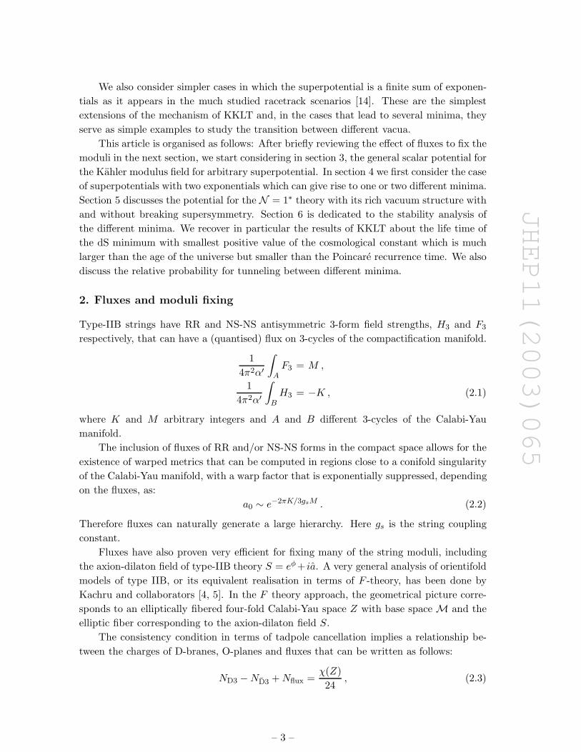
JHEP11(2003)065

N = 50 N = 100

X Y Vmin X Y Vmin

2.63 14.24 1.71 · 10−3 2.95 22.24 1.23 · 10−3

4.46 20.48 3.36 · 10−4 3.77 37.26 5.36 · 10−4

5.46 7.94 0 4.62 44.20 1.35 · 10−4

7.35 11.24 0

N = 500 N = 1000

X Y Vmin X Y Vmin

2.88 47.61 1.88 · 10−3 3.02 68.96 1.74 · 10−3

3.40 52.65 1.18 · 10−3 5.89 192.46 9.23 · 10−5

5.43 118.30 1.31 · 10−4 5.89 207.54 9.23 · 10−5

5.46 131.72 1.30 · 10−4 6.69 240.77 4.18 · 10−5

6.31 158.00 4.62 · 10−5 6.69 259.23 4.18 · 10−5

6.30 175.33 4.62 · 10−5 8.24 321.20 1.38 · 10−5

8.49 237.24 8.59 · 10−6 8.24 345.46 1.38 · 10−5

15.33 25.11 0 11.46 482.05 2.42 · 10−6

21.34 35.51 0

Table 5: Minima of the scalar potential for several non-supersymmetric cases.

Furthermore, unlike the supersymmetric case, the minima appear to be ordered in X, where

by ordered we mean that the value of the potential decreases as X increases. The one with

largest compactification scale has a smallest cosmological constant.

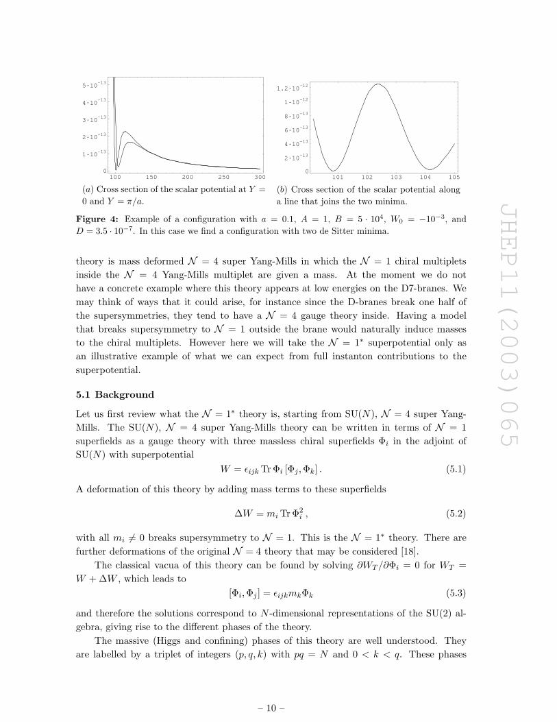
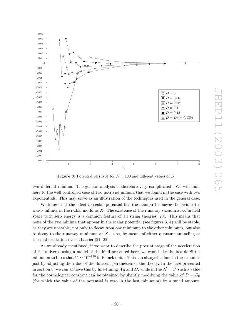
In figure 8 we illustrate the effect

Figure 7: Graph for the non-supersymmetric scalar

potential with N = 100.

of the non-supersymmetric term in the

potential. The value of the potential

at the minima is presented for several

values of the parameter D. For D = 0

we have the supersymmetric case with

more minima and not ordered, the in-

creasing of the parameter D will re-

duce the number of minima, increase

the value of the compactification scale

at the minima and order them from

larger to smaller values of the cosmo-

logical constant as the radius increases.

Turning on a nonvanishing value of

W0 tends to change some of these con-

clusions. The minimum with the largest

value of X can be lifted to positive vacuum energy while some of the other ones remain

anti de Sitter. Besides this, the number of minima stays of the same order.

We can see that, in general, increasing the value of N substantially increases the

number of vacua and the value of X at the minima. Notice that N can be quite large

– 18 –

JHEP11(2003)065

N Number of MinX MinY

Minima X Y Vmin X Y Vmin

10 2 3.98 3.90 0 3.98 3.90 0

20 2 3.82 5.00 0 3.82 5.00 0

30 2 4.42 6.10 0 2.88 12.00 7.69 · 10−4

40 2 4.99 7.10 0 3.49 16.30 4.60 · 10−4

50 3 5.46 7.94 0 4.46 20.48 3.36 · 10−5

60 3 5.89 8.70 0 4.06 25.50 3.09 · 10−4

70 4 6.29 9.40 0 4.17 30.10 2.42 · 10−4

80 4 6.63 10.00 0 4.28 34.80 1.92 · 10−4

90 4 7.04 10.70 0 4.55 39.40 1.60 · 10−4

100 4 7.35 11.24 0 4.62 44.20 1.35 · 10−4

200 5 10.02 16.00 0 5.94 91.80 4.30 · 10−5

300 5 12.03 19.40 0 6.61 107.50 1.13 · 10−4

400 6 13.76 22.40 0 7.73 124.50 7.52 · 10−5

500 6 15.40 25.10 0 8.54 156.70 5.48 · 10−5

600 8 16.70 27.50 0 9.29 211.00 4.21 · 10−5

700 8 17.97 29.70 0 10.09 245.30 8.03 · 10−5

800 9 19.20 32.80 0 10.81 253.80 2.79 · 10−5

900 9 20.30 33.70 0 11.10 432.90 2.35 · 10−5

1000 9 21.34 35.51 0 11.46 482.05 2.42 · 10−6

Table 6: Minima for different values of N in a non-supersymmetric case with D = D0.

in string theory and we may attempt extracting results varying N over many orders of

magnitude. However, there are limiations on the numerical analysis if N is too large, since

many more terms in the series have to be considered and the accuracy of the results would

not be guranteed. Also computer and woman time to perform the analysis would increase

substantially. Notice also that the number of minima we present here is actually a lower

bound since, again, the accuracy of the numerical calculations could have missed some of

them. In particular, minima which would be very close to each other could be missed.

6. Stability of the vacua

Having a situation with many nonsupersymmetric vacua with positive cosmological con-

stant implies that the relative stability of this vacua should be considered. In particular if

our own universe may be described by one of them, it is important to know the lifetime of

each of the vacua against decay to any of the ones with smaller value of the cosmological

constant and compare it with the age of the universe.

In the general case with many vacua the stability question is very much model and

vacuum dependent. Given any particular minimum of the potential there is a nonvanishing

probability towards tunneling to any of the other minima. The lifetime will depend on the

height of the potential and the side of the local maxima or saddle points that separate

– 19 –

JHEP11(2003)065

0.006

0.005

0.004

0.003

0.002

0.001

0

-0.001

-0.002

-0.003

-0.004

-0.005

-0.006

-0.007

-0.008

-0.009

-0.01

-0.011

-0.012

-0.013

-0.014

-0.015

-0.016

-0.017

-0.018

-0.019

-0.02

V

8 7 6 5 4 3 2 1

X

D = 0

D = 0.06

D = 0.08

D = 0.1

D = 0.12

D = D0(= 0.139)

Figure 8: Potential versus X for N = 100 and different values of D.

two different minima. The general analysis is therefore very complicated. We will limit

here to the well controlled case of two notrivial minima that we found in the case with two

exponentials. This may serve as an illustration of the techniques used in the general case.

We know that the effective scalar potential has the standard runaway behaviour to-

wards infinity in the radial modulus X. The existence of the runaway vacuum at ∞ in field

space with zero energy is a common feature of all string theories [20]. This means that

none of the two minima that appear in the scalar potential (see figures 3, 4) will be stable,

as they are unstable, not only to decay from one minimum to the other minimum, but also

to decay to the runaway minimum at X → ∞, by means of either quantum tunneling or

thermal excitation over a barrier [21, 22].

As we already mentioned, if we want to describe the present stage of the acceleration

of the universe using a model of the kind presented here, we would like the last de Sitter

minimum to be so that V ∼ 10−120 in Planck units. This can always be done in these models

just by adjusting the value of the different parameters of the theory. In the case presented

in section 3, we can achieve this by fine-tuning W0 and D, while in the N = 1∗ such a value

for the cosmological constant can be obtained by slightly modifying the value of D = D0

(for which the value of the potential is zero in the last minimum) by a small amount.

– 20 –

JHEP11(2003)065

Doing so one can always get the desired value for V in the last de Sitter minimum. We will

restrict here to the analysis of the case considered in section 3, so we will have two minima

with different values of the scalar potential V(+)0 , V

(−)0 such that V

(+)0 > V

(−)0 ∼ 10−120.

Therefore we will have a model with several decay possibilities. In fact from the minimum

at V(+)0 it is possible to decay either to the minimum at V

(−)0 or to the minimum at X → ∞,

while from the minimum at V(−)0 it is just possible to decay to the minimum at X → ∞.

We will also comment some features of the N = 1∗ case. In order to analyse this issue we

will review several features of tunneling theories taking into account gravitational effects,

following the original work of Coleman and De Luccia [21].

6.1 Vacuum decay

Let us consider a theory of a scalar field ϕ with a potential V (ϕ) which has two local

minima at ϕ1, ϕ2 with V (ϕ1) > V (ϕ2). Both of the minima are stable classically but the

vacuum state at ϕ = ϕ1 (that is, the false vacuum) is unstable against quantum tunneling

and will finally decay into the true vacuum state at ϕ = ϕ2, this vacuum decay proceeding

through the materialisation of a bubble of true vacuum within the false vacuum phase.

The tunneling action is given by

S(ϕ) =

∫

d4x√

g

(

−1

2R +

1

2(∂ϕ)2 + V (ϕ)

)

, (6.1)

with a tunneling probability between two vacua, per unit time and unit volume, given by

P (ϕ) ≈ e−B = e−S(ϕ)+S(ϕ1) . (6.2)

Here ϕ is a solution of the equations of motion, which is usually referred to as “the bounce”,

and S(ϕ1) is the euclidean action in the initial configuration ϕ = ϕ1. In the limit of small

energy density between the two vacua Coleman and De Luccia showed that the coefficient

B can be calculated in a closed form. Although in the general case it is usually very

difficult to find analytical solutions for the Coleman-De Luccia instantons and calculate

the probability of decay through quantum tunneling, the computation can be simplified

within the range of validity of the thin-wall approximation. This approximation is valid

when the thickness of the transition region between the true and the false vacuum is small

compared with the radius of the bubble. In Minkowski space, the condition Vmin ≪ Vmax

usually means that the thin-wall approximation is applicable, so the false vacuum state

will decay through the materialisation of a bubble of true vacuum within the false vacuum

phase, which is a quantum tunneling effect (by Vmax we denote the high of the de Sitter

maximum that separates two minima). That condition is usually fulfilled in the model

considered here, and we will explicitly check later that in those cases we are always within

the limits of the thin-wall approximation.

Now let us consider the case in which we have a vacuum with positive cosmological

constant (a dS vacuum) and a vacuum with null cosmological constant (a Minkowski vac-

uum).6 For those cases Coleman and De Luccia found that the decay will be produced

6This is always our case unless in the decay from V(+)0 to V

(−)0 , that are both de Sitter vacua. Never-

theless, as V(+)0 ≫ V

(−)0 ∼ 10−120, it is a good approximation to consider that the decay is also from dS to

Minkowski.

– 21 –

JHEP11(2003)065

through a nucleation of a bubble of radius7 ρ = 12S1

4ǫ+3S21, where ǫ denotes the energy density

difference between the two vacua ǫ = V (ϕ1) − V (ϕ2). As the final vacuum has null cos-

mological constant V (ϕ2) = 0, then ǫ = V (ϕ1). Also S1 denotes the tension of the bubble

wall, that is given by

S1 =

∫ ϕ2

ϕ1

dϕ√

2V (ϕ) , (6.3)

The coefficient B is then given by

B =24π/ǫ

(1 + 4ǫ/3S21 )2

. (6.4)

The thin-wall approximation is justified in this context if ρ and√

3/ǫ are large compared

with the range of variation of the scalar field ϕ, that is, ρ,√

3/ǫ ≫ ∆ϕ.

6.2 Comparing tunneling probabilities

In this subsection we will compute the probabilities of all possible tunneling trajectories

between the different vacua of the potential (3.10), (4.2). Nevertheless before doing so we

need to make a remark: In our case we have a potential that depends on two scalar fields.

When two or more fields are involved obtaining the bounce ϕ, and therefore computing

tunneling probabilities, becomes a much more difficult task (see for example [23]), except

in trivial cases.

An example of a trivial case is to consider the tunneling from any of the minima

to the runaway minimum at X → ∞. In those cases the lines Y = 0, π/a are always

minima of the potential in the Y direction, so we can consider a one-dimensional potential

V (±,∞) = V (X,Y = 0, π/a) and analyse the tunneling probability in the standard way (we

would obtain one-dimensional graphs like the ones shown in figure 4b). Also note that the

scalar field ϕ is defined in such a way that the kinetic term in the action (6.1) is canonical.

In our analysis, the complex scalar field T has a kinetic term that is given by the derivatives

of the Kahler potential (3.2), and is given by 34(X)2

(∂X∂X + ∂Y ∂Y ). If we consider that

Y is fixed then the kinetic term coming from the Kahler potential reads 34(∂ ln X)2, so the

canonical field would be of the form ϕ(±,∞) =√

32 ln X.

On the other hand, the case of computing the tunneling probability from the minimum

V(+)0 to the minimum V

(−)0 is more subtle, as we cannot trivially reduce it to the one-

dimensional case in the same way as the previous case. It is however possible to find

a lower bound for the tunneling probability by replacing the multi-field potential by a

suitably chosen single field potential, as any chosen trajectory will have larger tension (6.3)

than the minimum one. As we are interested in comparing probabilities such a bound

will be enough for us. Therefore we can consider that the line that joins the two minima

together is a good approximation for the bounce (as we already mentioned, this is an

upper bound for the tension, as the bounce is the one that minimises the action). Then

we can consider that Y = ∆Y (+,−)

∆X(+,−) X + b where by ∆X,Y (+,−) we denote the difference

in the value of X,Y between both minima, clearly ∆Y (+,−) = π/a, while the value of

7In units of MP = 1.

– 22 –

JHEP11(2003)065

∆X(+,−) cannot be written analytically. If we use this relation between the fields X and

Y we recover again the standard one-dimensional case where the canonical field will now

be ϕ(+,−) =√

32(1 + (∆Y (+,−)

∆X(+,−) )2) ln X.

In order for this model to be useful for explaining the actual acceleration stage of

the universe and also the smallness of the cosmological constant we should check that

the tunneling probability for the decay from V(+)0 to V

(−)0 is larger than the tunneling

probability for the decay from V(+)0 to the minimum at V = 0, and also that the minimum

at V(−)0 has a decay time larger than the life of the universe.

Let us begin by computing the decay probability from the minimum at V(+)0 to the

minimum at V = 0 and comparing it with the decay probability from the minimum at

V(+)0 to the minimum at V

(−)0 . For those cases we will have from (6.4) that the probability

will be given in both cases by

P ≈ exp

(

− 24π2/V(+)0

(1 + 4V(+)0 /3S2

1)2

)

, (6.5)

as V(+)0 ≫ V

(−)0 . Therefore it is clear that the decay with smaller tension S1 will be the

most probable. The tension of the bubble wall in both cases can be written as

S(+,∞)1 ∼

√

V(+,∞)1 ∆ϕ(+,∞) , S

(+,−)1 .

√

V(+,−)1 ∆ϕ(+,−) . (6.6)

where V(+,∞)1 , V

(+,−)1 denote the height of the maxima that separates any two minima

(see figure 4a and 4b). Also ∆ϕ(+,∞), ∆ϕ(+,−) denote the variation of the canonical field

in each case. As can be shown in figure 4 we have that 1 & ∆ϕ(+,∞) ≫ ∆ϕ(+,−) and

V(+,∞)1 & V

(+,−)1 , so then we will have in general terms that S

(+,∞)1 > S

(+,−)1 . Therefore

we find that in this case it is more probable to decay to the minimum V(−)0 ∼ 10−120 than

to the minimum V = 0 at X → ∞.

Now we must compute the probability of decay from the minimum at V(−)0 to the

minimum at V = 0. In this case the tension of the bubble wall can be written as

S(−,∞)1 ∼

√

V(−,∞)1 ∆ϕ(−,∞) , (6.7)

where V(−,∞)1 is the height of the maximum that separates the two minima. From the form

of the potential shown in figure 4a, we can assume that ∆ϕ ∼ O(1), so it is clear from (6.7)

that S21 ≫ V

(−)0 . Therefore for the decay probability one simply gets

P(−,∞) ≈ exp

(

− 24π2/V(−)0

(1 + 4V(−)0 /3S2

1 )2

)

∼ exp

(

−24π2

V(−)0

+64π2

S21

+ · · ·)

. (6.8)

For V(−)0 ∼ 10−120 this probability is extremely small, so therefore, this dS vacuum can be

considered stable in practical terms. Also note that the thin-wall approximation is always

true within this model as O(1) & ∆ϕ and ρ, (V(±)0 )−1/2 ≫ 1.

It is interesting to note that the analysis of the stability of the last minimum in the

N = 1∗ is very similar to this last case. The reason for that is the following: the analytical

discussion of the scalar potential in the non-supersymmetric case developed in section 4

– 23 –

JHEP11(2003)065

showed that apart from the minimum we also find a saddle point located in (for D = D0)

X0sp = 1.12

√N + 1.32 + 1.33

1√N

+ · · · (6.9)

Y 0sp = 1.44

√N + 0.37 − 1.36

1√N

+ · · · (6.10)

with a value of the potential given by

V 0sp = 0.11

1

N3/2− 0.46

1

N2+ 1.57

1

N5/2+ · · · (6.11)

This value of the potential it is small for large N , but is still big compared with 10−120

for reasonable values of N . As this point is a maximum in one direction but a minimum

in the other directions, we can perform an analysis of the stability of the vacua following

the lines of the two exponential case. As in this case we also find ∆ϕ ∼ O(1) and Vsp ≫V 0

min ∼ 10−120 we will arrive to the same conclusion as the one in (6.8).

In the N = 1∗ potentials, as in all the cases with many minima, a typical situation

may be that some of the minima would correspond to de Sitter space and others to anti de

Sitter. We may imagine living in the one corresponding to de Sitter space with the smallest

value of the cosmological constant and would wonder about its decay probability towards

a global minimum with negative cosmological constant. As discussed in [21], the decay to

a state of negative vacuum energy may or may not occurr and may lead to gravitational

collapse. This has been recently reanalysed in [24].

Finally we would like to mention that it is also necessary to check that the decay

times of the de Sitter vacua are also not too long. The fact that a de Sitter space has

finite entropy introduces a time scale that is the Poincare recurrence time tr [25]. This

quantity is given by tr ∼ eSdS , where SdS denotes the entropy of the de Sitter space. For dS

space the entropy has a simple sign-reversal relation with respect to the euclidean action

calculated for the false vacuum dS solution ϕ = ϕ0, which is given by −24π2/V0. Then

the recurrence time can be written as tr ∼ e24π2/V0 . An interesting property of this kind

of models is that the decay time of the de Sitter vacua never exceeds the recurrence time

of the de Sitter space tr. This was first noticed in [6] and can be easily checked from the

following expression

ln trln tdecay

= ln (1 + 4V(±)0 /3S2

1)2 > 0 =⇒ tr > tdecay . (6.12)

The problems related to the decay time tdecay exceeding the recurrence time tr will then

not appear in these models.

7. Discussion

We have presented examples of multiple de Sitter vacua in string theory. Even though

the examples we consider are still relatively simple, they illustrate what can be expected

from the general vacuum structure of string theory, i.e. a multitude of vacua with different

values of the cosmological constant.

– 24 –

JHEP11(2003)065

The parameters of the theory allow for one of the minima to have a cosmological

constant as small as we want. This requires fine tuning8 but it can be ameliorated given

the large number of minima, indicating an anthropic approach to the cosmological constant

problem, as advocated by different authors [10, 12]. The number of minima increases

with the rank of the gauge group N . Furthermore since there is an underlying SL(2, Z)

symmetry behind the N = 1∗ theory, we may expect that there could be further, possibly

infinite, minima if we explore other fundamental domains of this group. We have essentially

only explored N copies of the strips defined by −1/2 < Y < 1/2 for X outside the unit

circle in the upper half plane. For each of these strips, the modular group has an infinite

number of fundamental domains that could indicate a huge multiplication of the number

of minima, inequivalent from the ones we found since SL(2, Z) is not a symmetry of the

theory.9 However their study is beyond the limit of validity of our effective actions which

are trusted only for X greater than the string scale. Furthermore our potentials have

periodicity N in the Y direction. Any correction that would slightly break this periodicity

could give rise to an infinite number of minima.

The large number of vacua that can appear in these theories due to the nontrivial

superpotential complements the already rich structure of vacua due to the presence of the

fluxes [26]. The large number of 3-cycles in typical Calabi-Yau manifolds imply a large

amount of possibilities. Remember also that although the combination of the fluxes KM

is restricted by the tadpole cancellation condition, the ration K/M is a free (quantised)

parameter.10 This combination appears in the warp factor and allows the tuning of the

parameter D to get a small cosmological constant, defining the ‘discretuum’ of vacua as de-

scribed in [9, 12, 27]. All these effects were present in the single exponential case considered

in KKLT. The large number of vacua we found has to be multiplied by this degeneracy. Al-

though it may not be large enough degeneracy for a naturally small cosmological constant,

the greater the number of minima the more natural is to find a cosmological constant of

the right size.

The fact that our potentials depend nontrivially on at least two real fields X,Y makes

the discussion of the system more interesting than for single field potentials in several

ways. Since we may have many de Sitter minima, if we imagine the universe starting in

any of them, it would leave naturally to different periods of inflation, either from tunneling

between minima but also by naturally rolling after the tunnelings. There are so many

valleys and hills in the potential that it may not be impossible to find regions of slow roll

between different minima.

This combination of tunneling plus rolling has been considered in the past on different

models of inflation such as open inflation [29, 30]. A detailed study of the possibility for

8The fact that we do not need to have a nonvanishing superpotential from the fluxes (W0) indicates

we do not need to fine tune this quantity as in [6]. However we still need to fine tune the supersymmetry

breaking parameter D which even though is discrete it can be varied almost continuosly [6, 27].9Notice also that in computing the scalar potential we restricted ourselves to one single phase of the

N = 1∗ theory. In general we could consider any other values of p and q.10Notice that typical four-folds can have Euler number between 103 and 106 [28], allowing for many

different combinations of M and K to satisfy the tadpole condition.

– 25 –

JHEP11(2003)065

these potentials to give rise to realistic (eternal) inflation would be clearly of great interest.

For this we recall that the main obstacle to have successfull inflation from string theory is

precisely the lack of control of the moduli potentials. In particular the different proposals

of D-brane inflation [31] assume that there is an unknown stringy mechanism that fixes the

moduli and then, after that, D-brane inflation could occur. This is clearly a very strong

assumption and so far attempts of combining D-brane inflation with moduli fixing have

been running into problems.11 Therefore we may consider seriously the possibility that

actually the modulus T could be the inflaton field, and these potentials could give rise to

interesting combinations of inflationary processes. This is clearly a possible subject for

future investigation.

Another open question left unanswered here is the detailed analysis of the decays of

the different minima. This is complicated by the facts that we have two-field potentials

and that the fields do not have canonically normalised kinetic terms. Our discussion

was mostly carried for the simplest case of two exponentials with only two minima, but

clearly a complete analysis for the N = 1∗ and other more general potentials would be

needed.

Even though our models are relatively simple, they illustrate the potential richness of

the string landscape once the different ‘moduli’ fields acquire nontrivial potentials. We do

not pretend that the superpotentials discussed here, such as the one from the N = 1∗ the-

ory, would be particularly special over other more realistic realisations of non-perturbative

potentials. Actually, we regard it as an interesting tool which includes all the ingredi-

ents expected from non-perturbative physics, in particular the infinite instanton sum can

be under control thanks to the mathematical properties of modular forms. Other non-

perturbative superpotentials recently derived, including different deformations of N = 4

theory [18] would be interesting to study.

The mechanism of KKLT, although very interesting, takes the simplest class of models

in which only one modulus is left unfixed by the fluxes. In more realistic models we would

expect many moduli left unfixed by the fluxes and finding a many fields non-perturbative

potential for them would be an important challenge. We regard our study here as a

nontrivial, yet manageable, realisation of the multi-vacua scenario in string theory and

hope it may be of interest to explore further properties of the space of string vacua.

8. Note added in revised version

The analysis presented in this article was performed using a supersymmetry breaking term

induced in the potential due to the inclusion of an anti D3-brane in the configuration. Such

a term was taken to be given by δV = D/X3, with D a positive constant depending on the

fluxes turned on in the compactification. Nevertheless, when this work was already finished

it was pointed out in [32] that this induced term is not the one to be used if the anti D3 brane

is in the warped region, as it is. The correct term should be δV = D/X2 (with D also a

positive, flux-dependent, constant). This arises because the supersymmetry breaking term

11S. Kachru and J. Maldacena private communication [32].

– 26 –

JHEP11(2003)065

N = 50 N = 100 N = 100

X Y Vmin X Y Vmin X Y Vmin

1.70 10.98 1.28 · 10−3 1.09 45.37 3.79 · 10−2 1.94 18.12 0

1.97 18.96 4.72 · 10−4 1.49 13.20 9.10 · 10−3 2.06 27.47 7.14 · 10−4

2.15 14.25 0 1.66 15.28 2.13 · 10−3 2.35 22.29 6.26 · 10−4

2.65 21.30 9.33 · 10−4 1.80 38.15 2.91 · 10−3 2.55 29.86 1.02 · 10−3

1.80 38.15 2.91 · 10−3 2.70 36.87 1.09 · 10−3

1.82 41.84 9.05 · 10−4

N = 500

X Y Vmin X Y Vmin X Y Vmin

1.46 28.5 1.26 · 10−2 2.13 108.6 4.01 · 10−4 1.5 30.2 8.04 · 10−3

2.20 113.7 3.84 · 10−4 1.57 32.2 4.34 · 10−3 2.23 47.6 3.62 · 10−4

1.63 116.9 3.46 · 10−3 2.23 59.7 1.12 · 10−3 1.64 132.1 7.10 · 10−3

2.25 65.4 7.58 · 10−4 1.66 34.4 2.14 · 10−3 2.48 68.1 9.44 · 10−4

1.77 37.0 5.37 · 10−4 2.51 52.7 9.66 · 10−4 1.78 138.4 2.14 · 10−3

2.53 146.2 1.11 · 10−3 1.79 89.0 1.97 · 10−3 2.58 74.8 9.41 · 10−4

1.82 92.8 1.14 · 10−3 2.60 139.5 1.09 · 10−3 1.85 134.4 5.09 · 10−4

2.68 139.4 1.102 · 10−3 1.90 40.0 0 2.91 87.3 1.15 · 10−3

2.04 58.0 1.24 · 10−3 2.95 79.3 1.11 · 10−3 2.05 43.5 8.48 · 10−6

Table 7: Minima of the scalar potential for several non-supersymmetric cases.

coming from the inclusion of an anti D3-brane in the warped compactifications considered

here scales like e4A/X3, and in the highly warped regime e4A ∼ Xe−8πK/3gsM . This fact

does not change the main conclusions of the paper although it changes the numerical

analysis. We briefly summarize in this added note the changes produced in the numerical

analysis.

As it was found in the D/X3 case, with the introduction of the supersymmetry breaking

term D/X2 it is also possible to lift the vacua from anti de Sitter vacua to de Sitter vacua,

for some range of the parameter D. Again we found that the effect of the supersymmetry

breaking term depends on the range of values of the parameter D. If D is very small

(compared with the value of the potential in the supersymmetric case), the potential will

not change substantially and the minima remain anti de Sitter. For a critical value of D one

of the minima will move up to zero vacuum energy and then to de Sitter space. Continuing

increasing D, more minima become de Sitter until all of them are either de Sitter or

Minkowski. We will denote by D0 that precise value of the parameter D such that all the

values of the potential at the minima are positive or zero. If D > D0 the nonsupersymmetric

term starts dominating the potential and starts eliminating the different extrema to make

the potential runaway with X.

Actually, we have computed numerically the minima of the potential for D = D0 for

several values of N , such as N = 50, N = 100 and N = 500. The results obtained from the

analysis are shown in table 7, where in those cases D0 = 0.04836, 0.04958, and 0.04969 for

N = 50, 100, and 500 respectively.

– 27 –

JHEP11(2003)065

Also we show in figure 9 the scalar

Figure 9: Graph for the non-supersymmetric scalar

potential with N = 100.

potential for N = 100 when the super-

symmetry is broken. Note that com-

paring with figure 7 the main differ-

ences are that now the potential is less

smooth and therefore has more minima

(this can also be seen by comparing the

information shown in table 5 and ta-

ble 7).

In table 8 we show a similar in-

formation as the one shown in table 6,

where we write the number of minima

varying with N . In table 8 we denote by

MinX,Y the minima with largest value

of X,Y and by MinV =0 the minima

with vanishing value of the potential.

We can notice that the number of minima increases with N more or less in the same rate

than in the supersymmetric case and then faster than in the D/X3 case. The reason for

N Number MinX MinY MinV =0

Minima X Y Vmin X Y Vmin X Y

10 1 2.4 3.31 0 2.4 3.31 0 2.4 3.31

20 2 3.41 4.83 1.07 · 10−3 3.41 4.83 1.02 · 10−3 1.95 7.84

30 2 2.33 12.13 0 2.33 12.13 0 2.33 12.13

40 4 2.54 16.74 1.01 · 10−3 2.54 16.71 1.01 · 10−3 1.94 11.32

50 4 2.65 21.32 9.35 · 10−4 2.65 21.31 9.35 · 10−4 2.15 14.25

60 5 2.91 25.88 9.74 · 10−4 2.91 25.88 9.74 · 10−4 1.84 13.23

70 6 3.26 30.52 1.14 · 10−3 3.26 30.52 1.14 · 10−3 1.98 15.53

80 8 3.62 35.09 1.10 · 10−3 3.62 35.09 1.10 · 10−3 2.10 17.74

90 8 2.61 33.38 8.76 · 10−4 1.73 37.73 1.59 · 10−3 1.82 16.28

100 10 2.7 36.87 1.10 · 10−3 1.82 41.84 9.06 · 10−4 1.94 18.12

200 21 2.84 53.81 1.13 · 10−3 2.84 53.85 1.13 · 10−3 1.88 87.82

300 23 2.84 123.86 1.20 · 10−3 2.26 124.10 1.38 · 10−3 1.94 31.54

400 22 3.15 75.72 1.15 · 10−3 2.54 83.10 9.56 · 10−4 1.88 87.71

500 27 2.84 123.81 1.10 · 10−3 2.26 124.10 1.38 · 10−3 1.94 31.50

600 28 3.34 95.55 1.19 · 10−3 2.81 167.72 1.19 · 10−3 1.92 44.41

700 29 3.43 76.41 1.54 · 10−3 2.27 148.15 5.10 · 10−4 2.05 55.16

800 29 3.43 76.41 1.54 · 10−3 3.21 109.92 1.18 · 10−3 2.05 55.16

900 29 3.46 133.21 1.14 · 10−3 3.38 133.21 1.18 · 10−3 2.04 58.05

1000 32 3.15 120.73 1.19 · 10−3 3.07 129.22 1.19 · 10−3 2.02 60.59

Table 8: Minima for different values of N in a non-supersymmetric case with D = D0.

– 28 –

JHEP11(2003)065

0.04

0.03

0.02

0.01

0

-0.01

-0.02

V

43.83.63.43.232.82.62.42.221.81.61.41.21X

D = 0D = 0.015D = 0.03D = 0.04D = D0 = 0.049

Figure 10: Potential versus X for N = 100 and different values of D.

this is that the value of D for which all the anti de Sitter minima of the potential get lifted

is smaller than in the D/X3 case, and therefore in the present case the δV term smooths

less the potential.

Also, in figure 10 we illustrate the effect of the corrected non-supersymmetric term in

the potential. The value of the potential at the minima is presented for several values of the

parameter D. For D = 0 we have the supersymmetric case, the increasing of the parameter

D will reduce the number of minima and increase the value of the compactification scale

at the minima. Note that now the minima are not ordered for increasing X, and also that

the values of the compactification scale at the minima are, in general, smaller than in the

D/X3 case but still large enough so that our approximations remain valid.

Summarising: the difference with the 1/X3 potentials is that now there are more de

Sitter minima, they are no longer ordered with respect to the size of the extra dimension

and the value of the volume at the minima tends to be smaller than in the 1/X3 case, but

still large enough for the large radius approximation to be trustable.

Finally we would like to point out that the 1/X3 behaviour of the nonsupersymmetric

part of the potential presented in the main text is still relevant. This is due to the recent

proposal in [33] in which instead of introducing an anti D3 brane on the throat, a flux of

– 29 –

JHEP11(2003)065

magnetic fields on the D7 branes is considered. This adds an extra term in the potential

which happens to be proportional to 1/X3 if the D7 brane is not sitting on the throat

and to 1/X2 if the D7 brane is on the throat. In each case the rest of the analysis is as

presented in here and therefore both potentials are relevant depending on the location of

the D7 branes.

Acknowledgments

We would like to thank P. Berglund, J.J. Blanco-Pillado, M. Bucher, C. Burgess, L. Ibanez,

S. Kachru, A. Linde, R. Rabadan and A. Uranga for useful conversations. The work of

M.G.-R. is supported by Fundacion Ramon Areces. C.E. is funded by EPSRC and F.Q.

by PPARC.

References

[1] A. Strominger, Superstrings with torsion, Nucl. Phys. B 274 (1986) 253;

B. de Wit, D.J. Smit and N.D. Hari Dass, Residual supersymmetry of compactified D = 10

supergravity, Nucl. Phys. B 283 (1987) 165;

K. Becker and M. Becker, M-theory on eight-manifolds, Nucl. Phys. B 477 (1996) 155

[hep-th/9605053];

S. Sethi, C. Vafa and E. Witten, Constraints on low-dimensional string compactifications,

Nucl. Phys. B 480 (1996) 213 [hep-th/9606122];

T.R. Taylor and C. Vafa, RR flux on Calabi-Yau and partial supersymmetry breaking, Phys.

Lett. B 474 (2000) 130 [hep-th/9912152];

B.R. Greene, K. Schalm and G. Shiu, Warped compactifications in M and F theory, Nucl.

Phys. B 584 (2000) 480 [hep-th/0004103];

C.S. Chan, P.L. Paul and H. Verlinde, A note on warped string compactification, Nucl. Phys.

B 581 (2000) 156 [hep-th/0003236];

M. Grana and J. Polchinski, Supersymmetric three-form flux perturbations on AdS5, Phys.

Rev. D 63 (2001) 026001 [hep-th/0009211];

S.S. Gubser, Supersymmetry and F-theory realization of the deformed conifold with three-form

flux, hep-th/0010010;

A.R. Frey and J. Polchinski, N = 3 warped compactifications, Phys. Rev. D 65 (2002) 126009

[hep-th/0201029];

P.K. Tripathy and S.P. Trivedi, Compactification with flux on K3 and tori, J. High Energy

Phys. 03 (2003) 028 [hep-th/0301139];

S.P. de Alwis, On potentials from fluxes, hep-th/0307084.

[2] K. Dasgupta, G. Rajesh and S. Sethi, M-theory, orientifolds and G-flux, J. High Energy Phys.

08 (1999) 023 [hep-th/9908088].

[3] S. Gukov, C. Vafa and E. Witten, CFT’s from Calabi-Yau four-folds, Nucl. Phys. B 584

(2000) 69 [hep-th/9906070].

[4] S.B. Giddings, S. Kachru and J. Polchinski, Hierarchies from fluxes in string

compactifications, Phys. Rev. D 66 (2002) 106006 [hep-th/0105097].

[5] S. Kachru, M.B. Schulz and S. Trivedi, Moduli stabilization from fluxes in a simple IIB

orientifold, J. High Energy Phys. 10 (2003) 007 [hep-th/0201028].

– 30 –

JHEP11(2003)065

[6] S. Kachru, R. Kallosh, A. Linde and S.P. Trivedi, De Sitter vacua in string theory, Phys. Rev.

D 68 (2003) 046005 [hep-th/0301240].

[7] N. Dorey, An elliptic superpotential for softly broken N = 4 supersymmetric Yang-Mills theory,

J. High Energy Phys. 07 (1999) 021 [hep-th/9906011].

[8] J. Polchinski and M.J. Strassler, The string dual of a confining four-dimensional gauge theory,

hep-th/0003136.

[9] L. Susskind, The anthropic landscape of string theory, hep-th/0302219.

[10] L.F. Abbott, A mechanism for reducing the value of the cosmological constant, Phys. Lett. B

150 (1985) 427.

[11] J.D. Brown and C. Teitelboim, Neutralization of the cosmological constant by membrane

creation, Nucl. Phys. B 297 (1988) 787.

[12] R. Bousso and J. Polchinski, Quantization of four-form fluxes and dynamical neutralization

of the cosmological constant, J. High Energy Phys. 06 (2000) 006 [hep-th/0004134].

[13] J.L. Feng, J. March-Russell, S. Sethi and F. Wilczek, Saltatory relaxation of the cosmological

constant, Nucl. Phys. B 602 (2001) 307 [hep-th/0005276].

[14] N.V. Krasnikov, On supersymmetry breaking in superstring theories, Phys. Lett. B 193

(1987) 37.

[15] E. Cremmer, S. Ferrara, C. Kounnas and D.V. Nanopoulos, Naturally vanishing cosmological

constant in N = 1 supergravity, Phys. Lett. B 133 (1983) 61;

J.R. Ellis, A.B. Lahanas, D.V. Nanopoulos and K. Tamvakis, No-scale supersymmetric

standard model, Phys. Lett. B 134 (1984) 429.

[16] S. Kachru, J. Pearson and H. Verlinde, Brane/flux annihilation and the string dual of a

non-supersymmetric field theory, J. High Energy Phys. 06 (2002) 021 [hep-th/0112197].

[17] R. Dijkgraaf and C. Vafa, Matrix models, topological strings and supersymmetric gauge

theories, Nucl. Phys. B 644 (2002) 3 [hep-th/0206255]; On geometry and matrix models,

Nucl. Phys. B 644 (2002) 21 [hep-th/0207106]; A perturbative window into non-perturbative

physics, hep-th/0208048.

[18] N. Dorey, T.J. Hollowood, S. Prem Kumar and A. Sinkovics, Exact superpotentials from

matrix models, J. High Energy Phys. 11 (2002) 039 [hep-th/0209089]; Massive vacua of

N = 1∗ theory and s-duality from matrix models, J. High Energy Phys. 11 (2002) 040

[hep-th/0209099].

[19] A. Font, M. Klein and F. Quevedo, The dilaton potential from N = 1∗, Nucl. Phys. B 605

(2001) 319 [hep-th/0101186].

[20] M. Dine and N. Seiberg, Is the superstring weakly coupled?, Phys. Lett. B 162 (1985) 299.

[21] S.R. Coleman and F. De Luccia, Gravitational effects on and of vacuum decay, Phys. Rev. D

21 (1980) 3305.

[22] S.W. Hawking and I.G. Moss, Supercooled phase transitions in the very early universe, Phys.

Lett. B 110 (1982) 35.

[23] A. Kusenko, Improved action method for analyzing tunneling in quantum field theory, Phys.

Lett. B 358 (1995) 51 [hep-ph/9504418].

– 31 –

JHEP11(2003)065

[24] T. Banks, Heretics of the false vacuum: gravitational effects on and of vacuum decay, II,

hep-th/0211160.

[25] L. Dyson, J. Lindesay and L. Susskind, Is there really a de Sitter/CFT duality, J. High

Energy Phys. 08 (2002) 045 [hep-th/0202163];

L. Dyson, M. Kleban and L. Susskind, Disturbing implications of a cosmological constant, J.

High Energy Phys. 10 (2002) 011 [hep-th/0208013];

N. Goheer, M. Kleban and L. Susskind, The trouble with de Sitter space, J. High Energy Phys.

07 (2003) 056 [hep-th/0212209].

[26] S. Ashok and M.R. Douglas, Counting flux vacua, hep-th/0307049.

[27] A.R. Frey, M. Lippert and B. Williams, The fall of stringy de Sitter, Phys. Rev. D 68 (2003)

046008 [hep-th/0305018].

[28] P. Candelas, E. Perevalov and G. Rajesh, Toric geometry and enhanced gauge symmetry of

F-theory/heterotic vacua, Nucl. Phys. B 507 (1997) 445 [hep-th/9704097];

A. Klemm, B. Lian, S.S. Roan and S.T. Yau, Calabi-Yau fourfolds for M- and F-theory

compactifications, Nucl. Phys. B 518 (1998) 515 [hep-th/9701023].

[29] M. Bucher, A.S. Goldhaber and N. Turok, An open universe from inflation, Phys. Rev. D 52

(1995) 3314 [hep-ph/9411206].

[30] A. Liddle and D. Lyth, Cosmological inflation and large scale structure, Cambridge

University Press, Cambridge 2000.

[31] For a review with many references see F. Quevedo, Lectures on string/brane cosmology,

Class. and Quant. Grav. 19 (2002) 5721 [hep-th/0210292].

[32] S. Kachru, R. Kallosh, A. Linde, J. Maldacena, L. McAllister and S. P. Trivedi, Towards

inflation in string theory, JCAP 0310 (2003) 013 [hep-th/0308055].

[33] C.P. Burgess, R. Kallosh and F. Quevedo, De Sitter string vacua from supersymmetric

d-terms, J. High Energy Phys. 10 (2003) 056 [hep-th/0309187].

– 32 –