arX

iv:a

stro

-ph/

9606

137v

1 2

1 Ju

n 19

96

SUSX-TH-96-008

astro-ph/9606137

Correlations in Cosmic String Networks

Graham R. Vincent(a)∗

Mark Hindmarsh(a)†

Mairi Sakellariadou(b)‡

February 5, 2008

(a)School of Mathematical and Physical Sciences

University of Sussex

Brighton BN1 9QH

UK

(b)Departement de Physique Theorique

Universite de Geneve

Quai Ernest-Amsermet 24

CH-1211 Geneve 4

Switzerland

Abstract

We investigate scaling and correlations of the energy and momentum in an

evolving network of cosmic strings in Minkowski space. These quantities are of

great interest, as they must be understood before accurate predictions for the power

spectra of the perturbations in the matter and radiation in the early Universe can

be made. We argue that Minkowski space provides a reasonable approximation to

a Friedmann background for string dynamics and we use our results to construct a

simple model of the network, in which it is considered to consist of randomly placed

segments moving with random velocities. This model works well in accounting for

features of the two-time correlation functions, and even better for the power spectra.

∗E-mail: g.r.vincent@sussex.ac.uk†E-mail: m.b.hindmarsh@sussex.ac.uk‡E-mail: mairi@karystos.unige.ch

1

1 Introduction

Phase-ordering dynamics after a cosmological phase transition may explain the origin of

structure in our universe [1]. Our interest is in the role of one class of theories - cosmic

strings [2].

Recent attention has focused on cosmic strings formed during the breaking of the

grand unified symmetry, which naturally generates perturbations in the matter and ra-

diation fields of the right order for structure formation. However, to make diagnostic

predictions between cosmic strings, other defects and inflation-based theories we need

to use a detailed theory of the cosmological evolution of perturbations. There exists a

well-founded theory for the standard inflationary scenario of gaussian fluctuations in the

gravitational potential. In extending the theory to cover defect-based theories there are

three principal issues to be faced. Firstly, although the initial conditions are random,

they are not gaussian which makes averaging over the ensembles of defects a numerical

problem. Secondly, the creation of the defects must conserve energy-momentum: hence

there are compensating fluctuations in the fluid components on super-horizon scales.

Thirdly, in the subsequent evolution, the defect stress-energy Θµν must be included in

the Einstein equations. Defects form an unusual component of the total stress-energy,

in that the metric perturbations only affect the evolution of the defect network to sec-

ond order, so in the linear approximation we can evolve the network in the unperturbed

background metric. Its stress-energy then acts as a source term for the familiar set of

differential equations governing the evolution of the perturbations. As demonstrated by

Veeraraghavan and Stebbins [3], the solutions to the Einstein equations describing the

subsequent evolution of perturbation variables with a source term can be expressed as a

convolution of a suitable Green’s function (dependent on the usual cosmological param-

eters) with the source term integrated over time. For a set of perturbation variables ∆a

and a set of source terms Sb related to Θµν

∆a(k, η) =∫ η

ηi

dη′ Gab(η, η′)Sb(k, η′) (1)

where η and η′ are conformal times and k is the wavenumber of the mode. Calculating

the power in these variables will then involve integrating over the two-time correlator

〈|∆a(k, η)|2〉 =∫ η

ηi

dη′ dη′′ Gab(η, η′)Gac(η, η′′)〈Sb(k, η′)Sc(k, η′′)〉 (2)

When using the Veeraraghavan-Stebbins formalism, the Green’s functions can be calcu-

lated from standard cosmological perturbation theory: analytically in the simplest cases,

or numerically for a more realistic universe. However, in the absence of a workable ana-

2

lytic treatment of string evolution (although see [4] and [5]) we must rely for the moment

on a numerical study of the two-time correlators.

In a simplified model the Universe consists of two fluids: a pressureless CDM com-

ponent and a tightly-coupled baryon-photon fluid. In the convenient synchronous gauge,

the sources are Θ00 and ikjΘ0j (which we shall hereafter call U), when the equations

are rewritten using the energy-momentum pseudotensor introduced by Veeraraghavan

and Stebbins [3]. In the Newtonian gauge they are also the sources of curvature fluctu-

ations [6]. It is therefore the two-time correlation functions of these variables that we

study. Such a study is particularly timely in view of recent work on the power spectrum

of Cosmic Microwave Background around the degree scale from strings [7, 8] and from

global textures [9, 10]. As emphasised by Albrecht et al [11], the distinctive appearance

of “Doppler” peaks and troughs seen in inflationary calculations and texture models de-

pend sensitively on the temporal coherence of the sources. If one assumes little coherence

the peaks are washed out; on the other hand an assumption of total coherence preserves

them. Magueijo et al in [7] assumed that strings were effectively incoherent and obtained

a rather featureless CMB power spectrum at large multipole l. In [8] this assumption

was justified by a numerical study of the two-time energy-density correlator.

In contrast both Durrer et al [9] and Crittenden and Turok [10] assumed maximum

coherence for their texture models and found that the peaks were preserved, albeit in

positions typical of isocurvature models [6]. It is therefore clear that understanding

the temporal coherence of string sources is of great importance when calculating their

microwave background signals.

In this paper we present the results of some numerical “experiments” evolving strings

in Minkowski space. Using Minkowski space rather than a Friedmann model may seem

rather unrealistic. However, we expect a network of strings evolving in Minkowski space

to have all the essential features of one in a Friedmann background. A tangled initial

state consisting of a few probably “infinite” strings plus a scale free distribution of loops

straightens out under tension and continually self intersects resulting in the transfer

of energy into very small fast moving loops. The infinite string approaches “scaling” in

which it is characterised as a set of more or less Brownian random walks. The step length

of the walks and their average separation are both approximately equal to an overall

network scale ξ, which increases linearly with time (as naive dimensional analysis would

suggest). The length density of the infinite string decreases as ξ−2, again as dimensional

analysis suggests. In fact, ξ is conventionally defined so that the length density is precisely

1/ξ2 [12]. The effect of an expanding background is to damp coherent motions on super-

horizon scales. However the network scale is much less that the horizon size so one can

argue that the expansion does not significantly affect the network dynamics. The great

3

advantage of Minkowski space is that the network evolution is very easy to simulate

numerically: the code is generally many times shorter than an equivalent code for a

Friedmann background [13, 14], and makes fewer demands on both RAM and CPU time.

We are therefore able to get much better statistical significance from the data.

We present results from an extensive programme of numerical simulations for the two-

time correlators of Θ00 and U , and use a simple model to explain most of the features we

observe. It turns out that, to a good approximation, the network can be thought of as

consisting of randomly placed segments of string with random velocities. The segments

are of length ξ and number density ξ−3, thus reproducing the correct behaviour for the

length density.

In this model it is easy to show that the coherence time-scale in a Fourier mode of

wavenumber k is determined by the time segments take to travel a distance k−1. The

model in fact predicts that the correlations between the energy density at times η and

η′ decrease as exp(−16k2v2(η − η′)2), where v is the r.m.s string velocity. Hence we can

talk of a coherence time-scale ηc =√

3/vk, which is the time over which the correlation

function falls to e−1

2 of its equal time value. Given that we find v2 = 0.36, the model

predicts ηc ≃ 3/k. Our results actually indicate that at high k, ηc decreases faster than

k−1, but we have some evidence that this behaviour is a lattice artifact.

2 Flat Space Strings

We use a development of a code written by one of us some time ago [15, 16]. Initial string

realisations are generated using the Vachaspati-Vilenkin algorithm [17]. This mimics

the Kibble mechanism for the spontaneous breaking of a scalar U(1) symmetry with a

“Mexican hat” potential, as the Universe cools through a thermal phase transition.

This initial configuration is set up for evolution on a cubic lattice with fundamental

lattice side δ. We are free to alter the initial correlation length ξ0 in terms of δ and we

may add structure to the network by placing a percentage Pc of cusps randomly along

the string. Cusps are string links which are confined to one lattice site and which move

at the speed of light. Adding cusps avoids peculiarities arising from having long straight

segments of string in the initial conditions.

In Minkowski space the string equations of motion are

X′′ = X (3)

where ˙= ∂/∂η and ′ = ∂/∂σ; η is time and σ is a space-like parameter along the string.

If we regard Minkowski space as a Friedmann-Roberston-Walker Universe in the limit

4

that the expansion rate goes to zero, then η can be identified as FRW conformal time.

X = X(σ, η) is a position three-vector which satisfies

X′ · X = 0 (4)

X′2 + X2 = 1 (5)

This is a convenient set of constraints, as (5) ensures that the energy of a segment of

string is proportional to its length in σ.

We solve this using the Smith-Vilenkin algorithm [18] which is based on the exact

finite difference solution to (3),

X(σ, η + δ) = X(σ + δ, η) + X(σ − δ, η) −X(σ, η − δ) (6)

If the string points are initially defined on the sites of a cubic lattice (Nδ)3, then (6)

ensures that they remain on the lattice at time steps of δ. One can see from (6) that

stationary elementary segments have length (and hence energy) of 2δ and point in one

of six directions.

Because the string points lie on the sites of the lattice, identifying crossing events

is easy. When two strings cross, they intercommute with a probability which is set to

1. Loops with energy greater than or equal to a threshold value of Ec are allowed to

leave the network, while reconnections are forbidden for loops with energy equal to Ec.

Forbidding reconnections allows energy to leave the network fairly efficiently; otherwise

it takes much longer for the effect of the initial conditions to wear off. The natural and

usual value for Ec is the minimum segment length, 2δ. In fact, most of the energy in the

string network goes into the smallest possible loops. In some sense, the cusps model the

gravitational radiation of a realistic string network: They travel at the speed of light and

do not subsequently interact with the network.

Each realisation is evolved on a (64δ)3 or a (128δ)3 lattice with approximately 7500 or

60000 points describing the string network. For calculating quantities like power spectra

and two-time correlation functions we typically average over 50 realisations.

3 Results

The energy-momentum tensor for a cosmic string at a point x is

Θµν(x) =∫

dσ(XµXν − X ′µX ′ν)δ(3)(x −X(σ, η)) (7)

It is simple to calculate this on a cubic lattice for our string realisations, and use a Fast

Fourier Transform to get a Fourier mode representation. Here we want to measure the

5

0 10 20 30 40 50 600

2

4

6

8

10

12

14

16

η

ξ

Figure 1: The energy-density length scale ξ over time η for a 1283 lattice, averaged over

50 realisations

power spectra of Θ00(k) and U(k). These are calculated by averaging the amplitudes

over all Fourier modes with a wavenumber between k and k + 2π/δ.

Previous work [15, 16, 19] has tried to identify those features of the network that are

scaling, when a relevant length scale grows with the horizon. For example, we can define

the familiar energy density scale ξ by ξ2 = µ/ρinf where ρinf is the density of string with

energy greater than ξ. (This apparently circular definition works because we know the

initial step length ξ0 and to calculate ρinf we use ξ from the previous time step). Scaling

is reached when x = ∂ξ/∂η is constant. In the cases considered here x = 0.15 (Ec = 2δ)

and x = 0.12 (Ec = 4δ). The usual definition for scaling, that x = ξ/η is constant, can

not be used here as throughout our simulations ξ0 is too large to be ignored. For this

reason, we express all scaling functions in terms of ξ, rather than η. The behaviour of ξ

is shown in Figure 1.

The infinite string energy-momentum power spectra also exhibit scaling behaviour,

which we express in terms of the scaling functions P ρ and P U . We also consider the

equal time cross correlation function 〈U(k)Θ∗00(k)〉 which is a real function within the

ensemble errors.

〈|Θ00(k, η)|2〉 =V P ρ(kξ)

ξ(8)

〈U(k)Θ∗00(k)〉 =

V XρU(kξ)

ξ(9)

〈|U(k, η)|2〉 =V P U(kξ)

ξ(10)

6

k ξ

P ρ (k ξ )

0 5 10 15 20 25 300

0.2

0.4

0.6

0.8

1

1.2

1.4

1.6

1.8

Figure 2: Scaling function for the energy density as defined by equation (8) The solid

line is the measured scaling function with 1−σ error bars from ensemble averaging. The

dashed line is the fitted function equation (12). The dash-dot line is the predicted form

from our model, the last line in equation (24).

These scaling forms are fixed by the requirement that the density fluctuations obey the

scaling law∫ ξ−1

0d3k 〈|Θ00(k, η)|2〉 ∝ ξ−4 (11)

with a similar law for the other components of Θµν . We display our results for P ρ, XρU

and P U in Figures 2, 3 and 4 along with fits to the following forms

P ρ(z) =a

(1 − (bz) + (cz)n)1/n(12)

XρU(z) =d

(1 − (ez) + (fz)m)2/m(13)

P U(z) =g

(1 − (hz) + (jz)p)0.66/p(14)

which are motivated by a requirement of white noise at large scales due to uncorre-

lated initial conditions and good single parameter fits to P ρ ∼ (kξ)−0.98±0.06, P U ∼(kξ)−0.66±0.03 and XρU ∼ (kξ)−2.0±0.1 at small scales.

The errors indicate ensemble standard deviation. The other parameters are a = 1.18,

b = 0.25, c = 0.24, n = 6, d = 0.23, e = 0.3, f = 0.5, m = 3, g = 0.07, h = 0.15,

j = 0.18 and p = 1.59. We consistently get a peak for P ρ(z) and P U(z) at kξ ≃ 3 which

corresponds to a physical wavelength of about 2ξ. However, it is difficult to be certain

about the initial rise in the power spectrum because the error bars are large. In the

notation of Magueijo et al the peak corresponds to an xc = kη of approximately 20.

7

k ξ

X ρ U (k ξ )

0 5 10 15 20 25 30 35 40

0

0.05

0.1

0.15

0.2

0.25

0.3

Figure 3: Scaling fucnction for the equal time energy-momentum cross correlator as

defined by equation (9). The solid line is the measured scaling function with 1− σ error

bars from ensemble averaging. The dashed line is the fitted function equation (13). The

dash-dot line is the predicted form from our model, equation (36).

k ξ

P U (k ξ )

0 5 10 15 20 25 300

0.01

0.02

0.03

0.04

0.05

0.06

0.07

0.08

0.09

0.1

Figure 4: Scaling fucnction for the momentum density as defined by equation (10) The

solid line is the measured scaling function with 1−σ error bars from ensemble averaging.

The dashed line is the fitted function equation (14). The dash-dot line is the predicted

form from our model, the last line in equation (26).

8

As discussed above, the real importance of Θ00 and Θ0i in the context of perturbation

theory is how they are correlated over time. We performed k-space measurements of the

two-time correlation functions

Cρρ(k; η, η′) = V −1〈Θ00(k, η)Θ∗00(k, η′)〉 (15)

CρU(k; η, η′) = V −1〈U(k, η)Θ∗00(k, η′)〉 (16)

CUU(k; η, η′) = V −1〈U(k, η)U∗(k, η′)〉 (17)

During the scaling era they are well approximated by

Cρρ =1√ξξ′

√

P ρ(kξ)P ρ(kξ′)e− 1

2Υ2k2(1−(k∆))(η−η′)2 (18)

CρU =1√ξξ′

√

P ρ(kξ)P ρ(kξ′)e− 1

2Υ′2k2(η−η′)2(

α

k√

ξξ′− Υ′2k(η − η′)) (19)

CUU =1√ξξ′

√

P U(kξ)P U(kξ′)e− 1

2Υ′′2k2(η−η′)2(1 − Υ′′2k2(η − η′)2) (20)

where we have used the scaling forms of the power spectra and cross-correlator and

ξ = ξ(η), ξ′ = ξ(η′). The imaginary component of these correlators is consistent with

zero within the ensemble errors. The forms of these functions are motivated by a model

which we describe in the next section.

The values for Υ, Υ′ and Υ′′ are given in Table 1. ∆ is approximately 3δ. These

parameters were determined by minimisation of the χ-squared for each realisation. The

normal distribution of parameters obtained allows an estimate to be made of each pa-

rameter and its 1 − σ errors. We stress that we consider equations (18), (19) and (20)

to be an approximation, although a good one for |η − η′| ≤ 8k−1. For comparison, the

energy and momentum correlators fall to half their maximum value at |η − η′| ≃ 3k−1.

Outside the range given there are two effects present in the measured correlators which

invalidate the model. The first is small k-dependent oscillations about zero as predicted

by Turok [22]. The second is sharp peaks in the correlators at small scales which we take

to be an effect of defining strings on the lattice. Figures 5, 6 and 7 show the measured

Ec Υ α Υ′ Υ′′

2δ 0.21 ± 0.05 0.19 ± 0.05 0.42 ± 0.05 0.36 ± 0.07

4δ 0.18 ± 0.05 0.16 ± 0.05 0.42 ± 0.05 0.42 ± 0.06

Table 1: Fitted parameters for the models in equations (18), (19) and (20)

functions at a time η′ = 22δ (which is within the scaling era of our simulations).

9

η / δ

k δ

10

15

20

25

30

35

00.5

11.5

22.5

3

−2

0

2

4

6

x 104

Figure 5: Two-time correlation function 〈Θ00(k, η)Θ∗00(k, η′)〉 for η′ = 22δ

η / δ

k δ10

1520

2530

35

00.5

11.5

22.5

33.5

−2000

0

2000

4000

6000

8000

10000

Figure 6: Two-time correlation function 〈U(k, η)Θ∗00(k, η′)〉 for η′ = 22δ

η / δ

k δ10

1520

2530

35

0

0.5

1

1.5

2

2.5

3

−1000

0

1000

2000

3000

4000

Figure 7: Two-time correlation function 〈U(k, η)U∗(k, η′)〉 for η′ = 22δ

10

From the gaussian fall-off over time we see that for a given mode with wavenumber

k the network energy density decorrelates on a characteristic time scale which goes like

1/Υk√

(1 − (k∆)) and the momentum density varies as 1/Υ′′k for Ec = 2δ.

4 Theoretical Model

4.1 Power Spectra

We can use a very simple model to account for the forms given in (12) and (14), if not

the precise details. From (7) we get

Θµν(k) =∫

dσ (XµXν − X ′µX ′ν)eik·X(σ,η) (21)

At any given time the power spectrum is

〈|Θ00(k, η)|2〉 = 〈∫

dσ dσ′ eik·(X(σ,η)−X(σ′ ,η))〉 (22)

We then make some assumptions about the statistics of the network. Firstly, that for

each lag σ− = σ−σ′, the quantities Xi(σ)−Xi(σ′), Xi(σ) and X ′

i(σ) are gaussian random

variables with zero mean. Secondly, that the distribution of strings is isotropic. Then

〈|Θ00(k)|2〉 =∫

dσ dσ′ e− 1

6k2〈(X(σ)−X(σ′))2〉

(23)

=1

2

∫

dσ+ dσ− e− 1

6k2Γ(σ−)

where we have introduced the function Γ(σ − σ′) = 〈(X(σ) −X(σ′))2〉 and changed

variables to σ− = σ − σ′ and σ+ = σ + σ′. We will also use t2 = 〈X′2〉. The third

assumption is that the network is described by a collection of randomly placed string

segments of length ξ/t and total energy V ξ−2, where V is the volume of the simulation

box. Then Γ = t2ξ2(σ−/ξ)2 and L = 12

∫

dσ+ = V ξ−2. If we define z = σ−t/ξ then

〈|Θ00(k, η)|2〉 = L∫

dσ− e− 1

6k2t2ξ2(σ−/ξ)2

=Lξ

t

∫ 1

2

− 1

2

dz e− 1

6(kξ)2z2

(24)

=V

ξt

2√

6

kξerf(

kξ

2√

6)

Thus the scaling form of (8) emerges quite naturally. If we compare (24) with (8), we can

write the predicted form of the scaling function P ρ(kξ). The large and short wavelength

11

limits are

P ρ(kξ) =

(kξ)0 if kξ << 2√

6

(kξ)−1 if kξ >> 2√

6(25)

This function is plotted along with the measured and fitted model in Figure 2. It should

be noted that the normalisation is given by the model along with the measurement for t,

and not introduced by hand. This model does better at predicting the measured power

spectrum than a random walk model, in which the power on large scales goes like k−2.

Therefore, although each individual string is a random walk, they must be highly (anti)

correlated on large scales.

Similarly, the power spectrum for U becomes

〈|U(k)|2〉 = 〈∫

dσ dσ′ kikjXi(σ)Xj(σ′)eik·(X(σ,η)−X(σ′ ,η))〉

= L∫

dσ− (13V(σ−) − 1

9k2Π2(σ−))e− 1

6k2Γ(σ−) (26)

=2V

3ξt

∫ 1

2

0dz (V(z/t) − 1

3(kξ)2Π2(z/t)e− 1

6(kξ)2z2

where V and Π are the correlation functions

V(σ) = 〈X(σ) · X(0)〉 (27)

Π(σ) = 〈X(σ) · (X(σ) −X(0))〉 (28)

and V(σ−/ξ) and Π(σ−/ξ) are their scaling forms. We have measured these correlation

functions elsewhere [19], and we can use them to calculate the scaling function P U .

The result is plotted in Figure 4. Although for very large kξ this model predicts a

(kξ)−1 behaviour, within the k-range of our simulations the model agrees well with our

measurements giving a fit to (kξ)−0.66, although the normalisation is not so impressive

as for the energy-density.

4.2 Two-time correlation functions

In order to calculate the two-time correlation functions in this framework we need the

two-time correlation functions Γ(σ, σ′, η, η′), V(σ, σ′, η, η′) and Π(σ, σ′, η, η′). However,

we have not yet measured these quantities and instead resort to crude modelling. If we

consider small scales we may assume that each segment is moving at a velocity v2 = 〈X2〉in a random direction orthogonal to the orientation of the segment so that

Γ(σ−, η, η′) = t2σ2− + v2(η − η′)2 (29)

12

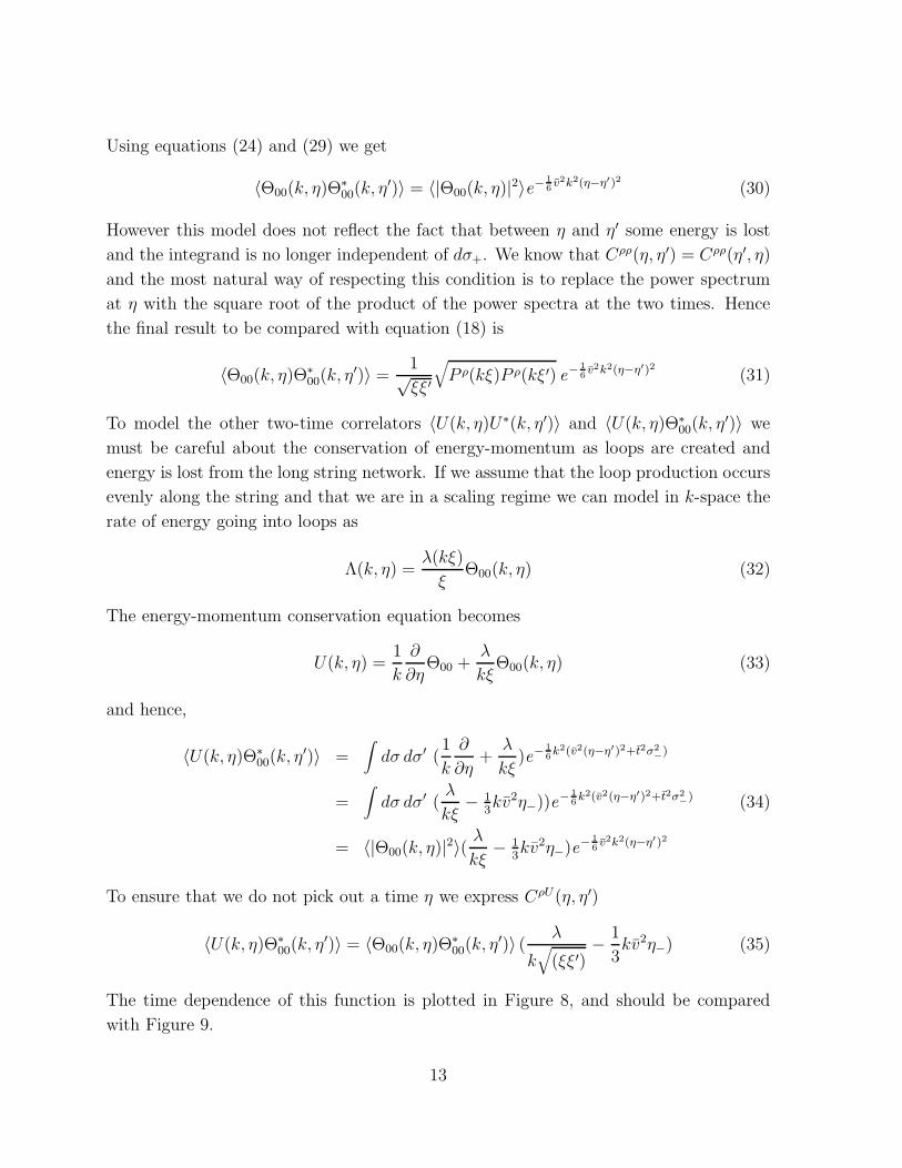
Using equations (24) and (29) we get

〈Θ00(k, η)Θ∗00(k, η′)〉 = 〈|Θ00(k, η)|2〉e− 1

6v2k2(η−η′)2 (30)

However this model does not reflect the fact that between η and η′ some energy is lost

and the integrand is no longer independent of dσ+. We know that Cρρ(η, η′) = Cρρ(η′, η)

and the most natural way of respecting this condition is to replace the power spectrum

at η with the square root of the product of the power spectra at the two times. Hence

the final result to be compared with equation (18) is

〈Θ00(k, η)Θ∗00(k, η′)〉 =

1√ξξ′

√

P ρ(kξ)P ρ(kξ′) e− 1

6v2k2(η−η′)2 (31)

To model the other two-time correlators 〈U(k, η)U∗(k, η′)〉 and 〈U(k, η)Θ∗00(k, η′)〉 we

must be careful about the conservation of energy-momentum as loops are created and

energy is lost from the long string network. If we assume that the loop production occurs

evenly along the string and that we are in a scaling regime we can model in k-space the

rate of energy going into loops as

Λ(k, η) =λ(kξ)

ξΘ00(k, η) (32)

The energy-momentum conservation equation becomes

U(k, η) =1

k

∂

∂ηΘ00 +

λ

kξΘ00(k, η) (33)

and hence,

〈U(k, η)Θ∗00(k, η′)〉 =

∫

dσ dσ′ (1

k

∂

∂η+

λ

kξ)e− 1

6k2(v2(η−η′)2+t2σ2

−)

=∫

dσ dσ′ (λ

kξ− 1

3kv2η−))e− 1

6k2(v2(η−η′)2+t2σ2

−) (34)

= 〈|Θ00(k, η)|2〉( λ

kξ− 1

3kv2η−)e− 1

6v2k2(η−η′)2

To ensure that we do not pick out a time η we express CρU(η, η′)

〈U(k, η)Θ∗00(k, η′)〉 = 〈Θ00(k, η)Θ∗

00(k, η′)〉 (λ

k√

(ξξ′)− 1

3kv2η−) (35)

The time dependence of this function is plotted in Figure 8, and should be compared

with Figure 9.

13

k δ

η / δ 1015

2025

30

0

1

2

3

−0.2

0

0.2

Figure 8: Model of time dependence of 〈U(k, η)Θ∗00(k, η′)〉

k δ

η / δ 1015

2025

30

0

1

2

3

−0.2

0

0.2

Figure 9: Measured time dependence of 〈U(k, η)Θ∗00(k, η′)〉

14

These plots assume a value of λ measured from the simulations. We find it to be

roughly constant at large kξ at λ ≃ 0.32 (±0.03). Including loop production shifts where

the cross-correlator goes to zero from η = η′ to λ − 13k2v2η−

√

(ξξ′)) = 0. The effect

of energy loss through loop production on the momentum of the long string may also

account for the form of the equal time cross-correlator. If we take η = η′ in equation

(35), which in terms of this model gives the correlation between the long string energy

and the reaction momentum from loop production, we get

XρU(kξ) =λ

kξP ρ(kξ) (36)

This neatly explains the (kξ)−2 dependence in equation (13), although the measured

normalisation is only 60% of that given by the independently measured λ and equation

(36). One reason for this discrepancy may be that our model assumes loop production

occurs evenly along the string at a constant rate, whereas we observe loop production

in more discrete bursts. The prediction from equation (36) is plotted in Figure 3, along

with the measured scaling function.

We find that the effect of the loop production term is insignificant for 〈U(k, η)U∗(k, η′)〉and we will drop it in the following expression:

〈U(k, η)U∗(k, η′)〉 =1

k2

∫

dσ dσ′ ∂

∂η

∂

∂η′e− 1

6k2(v2(η−η′)2+t2σ2

−)

(37)

= 〈|Θ00(k, η)|2〉 v2

3(1 − v2

3k2(η − η′)2)e− 1

6v2k2(η−η′)2

Again to ensure CUU(η, η′) = CUU(η′, η), we use the product of the square root of the

power spectra, so that

〈U(k, η)U∗(k, η′)〉 =1√ξξ′

√

P ρ(kξ)P ρ(kξ′)v2

3(1 − v2

3k2(η − η′)2)e− 1

6v2k2(η−η′)2 (38)

Equation (38) incorrectly predicts U to have the same kξ dependence in its power spec-

trum as the energy, with a relative normalisation given by v2/3. We expect a proper

treatment in terms of the two-time on-string correlators for Π, V and Γ to remedy this

problem. The time dependence of this function is plotted in Figure 10. As one can verify

by comparison with Figure 11, the simplest of assumptions has provided a reasonable

approximation to the measured time dependence.

In this section we have motivated the forms in equations (18), (19) and (20). From

the model, and using the measurements t2 = 0.637 ± 0.010 and v2 = 0.363 ± 0.010,

we can make predictions for the coherence parameters Υ, Υ′ and Υ′′, and the relative

15

k δ

η / δ

1015

2025

3035

0

1

2

3

−0.2

0

0.2

0.4

0.6

0.8

Figure 10: Model of time dependence of 〈U(k, η)U∗(k, η′)〉

k δ

η / δ

1015

2025

3035

0

1

2

3

−0.2

0

0.2

0.4

0.6

0.8

Figure 11: Measured time dependence of 〈U(k, η)U∗(k, η′)〉

16

quantity model measured

Υ 0.35 ± 0.02 0.21 ± 0.05

Υ′ 0.35 ± 0.02 0.42 ± 0.05

Υ′′ 0.35 ± 0.02 0.36 ± 0.07

R 0.35 ± 0.02 0.38 ± 0.1

Table 2: Parameters for the forms given in equations (18), (19) and (20) as predicted by

our model and measured from the simulations. Note a complication in comparing the

values of Υ, due to a lattice effect in equation (18) as discussed in the text.

normalisation R = 〈Θ00(k, η)Θ∗00(k, η′)〉/〈U(k, η)U∗(k, η′)〉. The measured values are for

Ec = 2δ. The comparison for Υ is complicated by an apparent lattice effect accounted for

in equation (18) by the length scale ∆. We assume that as ∆ goes to zero and the form in

equation (18) approaches that in equation (31), allowing a comparison to be made. Not

surprisingly, the model is not wholly satisfactory. We know that the momentum density

does not have the same (kξ) dependence as the energy density, which is predicted by (38).

Also from (18) we see that the strings decorrelate on a time scale ∼ 1/k√

(1 − (k∆)) and

not k−1. One might think that both features are understandable as it is well known that

strings move faster on smaller scales. This gives faster decorrelation and greater power

in the momentum density on small scales than the simple model would suggest. Having

said this, we note that the scale ∆ introduced in equation (18) is close to the lattice

scale and is fairly constant throughout the simulation. Consequently, the departure from

a k−1 coherence time may be due to the fact that the strings are defined at all times

on the lattice. It is puzzling that this effect does not show up in the other correlators.

Furthermore, the model does not account for the oscillations about zero in the two-time

correlators. The oscillations are present in all three two-time correlators, but are most

obvious in Figures 9 and 11. As Turok has recently pointed out [22], such oscillations

should appear in the Fourier transforms of two-time spatial correlators because of a

causality constraint which sets the correlator to zero for causally disconnected points.

5 Conclusions

We have demonstrated the scaling properties of the power spectra and cross correlator

of two important energy-momentum quantities, the density Θ00 and the velocity U , and

given the large k behaviour. We have also studied the two-time correlators and measured

the time coherence in the network.

17

We find that the energy and the momentum power spectra are peaked at around

kξ ≃ 3, where ξ ≃ 0.15η, thereafter decaying as (kξ)−1 and (kξ)−0.66 respectively over

the range of our simulations. The cross-correlator decays as (kξ)−2 and is peaked at

kξ ≃ 2.

For a mode of spatial frequency k, the two-time correlation functions of Θ00 and U

display correlations over time scales of ηc ≃ 4.7k−1 and ηc ≃ 2.4k−1 respectively. The

time scale η2c is the variance in the Gaussian fall-off as a function of the time difference

(see equations (18) and (20)). We have presented simple models to explain the qualitative

results, predicting the power spectra and cross correlator including normalisations, to a

reasonable accuracy, and accounted for the features of the two-time correlation functions.

The model describes the string network as a set of randomly placed segments of

length ξ/t, where t = (1 − v2)1

2 , with random velocities. We assume that relevant

quantities such as velocities and extensions between points with a given separation in σ

are gaussian random variables. We can then reduce ensemble averaging to the study of

two-point correlations along the string, which we must model or measure.

From the model we can show that the characteristic coherence time scale for a mode

of spatial frequency k is ηc ≃ 3/k. Our simulations give a similar result, although at very

small scales ηc decrease faster than k−1. This we believe to be a lattice effect.

There are potential pitfalls in taking the Minkowski space string network as a source

for the fluid perturbation variables in a Friedmann model. For example, the energy

conservation equation is modified to

Θ00 +a

a(Θ00 + Θ) − kU = −Λ (39)

where a(η) is the scale factor and Θ = Θii the trace of the spatial components of Θµν .

Since Θ is unconstrained by any conservation equation, its fluctuations could drive a

fluctuating component in Θ00 whose time scale would go like a/a [23]. However, we find

that 〈|Θ|2〉 << 〈|Θ00|2〉 and believe the introduction of the a/a term to be a small effect.

If we take the simulations at face value, the implications for the appearance of the

Doppler peaks are not entirely clear cut. The coherence time is smaller than, but of

the same order of magnitude as, the period of acoustic oscillations in the photon baryon

fluid at decoupling, which is roughly 11/k [24]. This is in turn smaller than the time

at which the power in the energy and velocity sources peak, approximately 20/k. The

computations of Magueijo et al [8] of the Microwave Background angular power spectrum

for various source models suggest small or absent secondary peaks. However, our string

correlation functions can be used as realistic sources to settle the issue.

18

Acknowledgements

We wish to thank Andy Albrecht, Nuno Antunes, Pedro Ferreira, Paul Saffin and Albert

Stebbins for useful discussions.

GRV and MBH are supported by PPARC, by studentship number 94313367, Ad-

vanced Fellowship number B/93/AF/1642 and grant number GR/K55967. MS is sup-

ported by the Tomalla Foundation. Partial support is also obtained from the European

Commission under the Human Capital and Mobility programme, contract no. CHRX-

CT94-0423.

References

[1] A. Vilenkin and E.P.S. Shellard, Cosmic Strings and other Topological Defects (Cam-

bridge University Press, Cambridge, 1994)

[2] M. Hindmarsh and T. Kibble Rep. Prog. Phys 58 477 (1994)

[3] S. Veeraraghavan and A. Stebbins Ap. J. 365, 37 (1990)

[4] D. Austin, E. J. Copeland and T. W. B. Kibble Phys. Rev. D48, 5594 (1993)

[5] M. Hindmarsh SUSX-TH-96-005 hep-th/9605332 (unpublished)

[6] W. Hu, D. N. Spergel and M. White astro-ph 9605193

[7] J. Magueijo, A. Albrecht, D. Coulson and P. Ferreira Phys. Rev. Lett. 76 2617 (1996)

[8] J. Magueijo, A. Albrecht, D. Coulson and P. Ferreira MRAO-1917

astro-ph/9605047

[9] R. Durrer, A. Gangui and M. Sakellariadou Phys. Rev. Lett. 76 579 (1996)

[10] R. G. Crittenden and N. Turok Phys. Rev. Lett. 75, 2642 (1995)

[11] A. Albrecht, D. Coulson, P. Ferreira and J. Magueijo Phys. Rev. Lett. 76 1413 (1996)

[12] E. J. Copeland, T. W. B. Kibble and D. Austin Phys. Rev. D45 (1992)

[13] A. Albrecht and N. Turok Phys. Rev. D40, 973 (1989)

[14] D. P. Bennett, in “Formation and Evolution of Cosmic Strings”, eds. G. Gibbons,

S. Hawking and T. Vachaspati, (Cambridge University Press, Cambridge. 1990); F.

R. Bouchet ibid.; E. P. S. Shellard and B. Allen ibid.;

19

[15] M. Sakellariadou and A. Vilenkin Phys. Rev. D37, 885 (1988)

[16] M. Sakellariadou and A. Vilenkin Phys. Rev. D42, 349 (1990)

[17] T. Vachaspati and A. Vilenkin Phys. Rev. D30, 2036 (1984)

[18] A.G. Smith and A. Vilenkin Phys. Rev. D36, 990 (1987)

[19] M. Hindmarsh, M.Sakellariadou and G. Vincent (in preparation)

[20] M. Hindmarsh Ap. J. 431, 534 (1994)

[21] M. Hindmarsh Nucl. Phys. B (Proc. Suppl.) 43, 50 (1995)

[22] N. Turok astro-ph/9604172 (1996)

[23] A. Stebbins, private communication (1996)

[24] P. J. E. Peebles The Large Scale Structure of the Universe (Princeton University

Press, Princeton, 1980)

20