Twistor Approach to String Compactifications

HAL Id: tel-00682454https://tel.archives-ouvertes.fr/tel-00682454

Submitted on 26 Mar 2012

HAL is a multi-disciplinary open accessarchive for the deposit and dissemination of sci-entific research documents, whether they are pub-lished or not. The documents may come fromteaching and research institutions in France orabroad, or from public or private research centers.

L’archive ouverte pluridisciplinaire HAL, estdestinée au dépôt et à la diffusion de documentsscientifiques de niveau recherche, publiés ou non,émanant des établissements d’enseignement et derecherche français ou étrangers, des laboratoirespublics ou privés.

Twistor Approach to String CompactificationsSergey Alexandrov

To cite this version:Sergey Alexandrov. Twistor Approach to String Compactifications. High Energy Physics - Theory[hep-th]. Université montpellier II, 2012. tel-00682454

https://tel.archives-ouvertes.fr/tel-00682454

https://hal.archives-ouvertes.fr

Laboratoire Charles Coulomb

UNIVERSITE MONTPELLIER II

These d’habilitation

L’Approche Twistorielle aux

Compactifications de la Theorie des Cordes

Sergey Alexandrov

Soutenue le 5 mars 2012 devant le jury compose de :

M. De WIT Bernard, rapporteur,M. MINASIAN Ruben, rapporteur,M. NEVEU Andre, president du jury,M. PIOLINE Boris,M. ROCHE Philippe,M. ZAREMBO Konstantin, rapporteur.

Resume

Un des aspects fascinants de la theorie des cordes, c’est qu’elle vit dans l’espace-temps dedix dimensions. Mais cela implique que, pour la relier a des observations phenomenologiques,elle devrait etre compactifiees a quatre dimensions. Un cas particulierement riche, maistoujours faisable correspond a la compactification sur une variete de Calabi-Yau qui donnea basse energie une theorie effective avec la supersymetrie N = 2. L’action de cette theorieest completement determinee par la metrique sur son espace des modules qui comporte deuxcomposantes correspondant aux multiplets vectoriels et hypermultiplets. La premiere estclassiquement exacte et bien comprise, alors que la derniere recoit des corrections quantiqueset est connue de porter une geometrie compliquees quaternion-Kahlerrienne.

Dans cette these, nous presentons nos resultats sur la description complete non-perturbativede l’espace des modules des hypermultiplets. Nous montrons comment toutes les correctionsquantiques, qui comprennent des contributions perturbatives d’une boucle ainsi que cellesnon-perturbatives venant des D-branes et NS5-branes, sont incorporees dans le cadre del’approche twisteurielle. Ce cadre, que nous elaborons ici en detail, fournit une descrip-tion mathematique puissante des varietes hyperkahleriennes et quaternion-Kahleriennes etil est indispensable pour la formulation de la geometrie non-perturbative de l’espace desmodules des hypermultiplets. Nous presentons egalement de nouveaux resultats sur la du-alite-S, symetrie miroir quantique, les connexions a des modeles integrables et aux cordestopologiques.

Abstract

One of the fascinating aspects of string theory is that it lives in spacetime of ten di-mensions. But this implies that, to relate it to phenomenological observations, it should becompactified down to four dimensions. A particularly rich, but still tractable case corre-sponds to compactification on a Calabi-Yau manifold which gives at low energies an effectivetheory with N = 2 supersymmetry. The action of this theory is completely determined bythe metric on its moduli space which has two components corresponding to vector and hy-permultiplets. The first is classically exact and well understood, whereas the latter receivesquantum corrections and is known to carry a complicated quaternion-Kahler geometry.

In this thesis we present our results on obtaining the complete non-perturbative descrip-tion of the hypermultiplet moduli space. We show how all quantum corrections, whichinclude perturbative one-loop contributions as well as non-perturbative ones due to D-braneand NS5-brane instantons, are incorporated in the framework of the twistor approach. Thisframework, which we elaborate here in detail, provides a powerful mathematical descriptionof hyperkahler and quaternion-Kahler manifolds and is indispensable for formulating thenon-perturbative geometry of the hypermultiplet moduli space. We also present new insightson S-duality, quantum mirror symmetry, connections to integrable models and topologicalstrings.

Remerciements

C’est un grand plaisir a remercier tous mes collaborateurs qui ont partage avec moi durant

ces dernieres annees leur connaissance profonde et idees passionnantes. Ma grande recon-

naissance va a Jan Manschot, Daniel Persson, Philippe Roche, Frank Saueressig, Stefan Van-

doren, et surtout a Boris Pioline dont l’energie illimitee et devouement a la physique etaient

indispensables pour beacoup de developpements presentes ici. Je voudrais egalement re-

mercier Vladimir Fateev, Nikolay Gromov, Vladimir Kazakov, Ivan Kostov, Andrew Neitzke,

Vasily Pestun, Sylvain Ribault, Pedro Vieira et Konstantin Zarembo pour de nombreuses

discussions importantes.

Contents

Introduction 1

I Moduli spaces in gauge and string theories 51 Calabi-Yau compactifications of string theory . . . . . . . . . . . . . . . . . 5

1.1 Calabi-Yau manifolds and their moduli spaces . . . . . . . . . . . . . 51.2 Type II supergravities in 10 and 4 dimensions: field content . . . . . 81.3 Low energy effective action . . . . . . . . . . . . . . . . . . . . . . . . 11

2 Hypermultiplet moduli space . . . . . . . . . . . . . . . . . . . . . . . . . . . 142.1 Symmetries and dualities . . . . . . . . . . . . . . . . . . . . . . . . . 142.2 Tree level metric and c-map . . . . . . . . . . . . . . . . . . . . . . . 162.3 Quantum corrections . . . . . . . . . . . . . . . . . . . . . . . . . . . 172.4 Where we are . . . . . . . . . . . . . . . . . . . . . . . . . . . . . . . 18

3 Compactified gauge theory . . . . . . . . . . . . . . . . . . . . . . . . . . . . 21

II Twistor approach to quaternionic geometries 231 HK spaces . . . . . . . . . . . . . . . . . . . . . . . . . . . . . . . . . . . . . 23

1.1 Twistorial construction . . . . . . . . . . . . . . . . . . . . . . . . . . 231.2 Holomorphic Darboux coordinates and transition functions . . . . . . 241.3 O(2) HK manifolds and their deformations . . . . . . . . . . . . . . . 261.4 Branch cuts and open contours . . . . . . . . . . . . . . . . . . . . . 28

2 QK spaces . . . . . . . . . . . . . . . . . . . . . . . . . . . . . . . . . . . . . 302.1 HKC construction and twistor space . . . . . . . . . . . . . . . . . . 302.2 Transition functions . . . . . . . . . . . . . . . . . . . . . . . . . . . 322.3 The metric . . . . . . . . . . . . . . . . . . . . . . . . . . . . . . . . 332.4 Toric QK geometries, deformations and isometries . . . . . . . . . . . 342.5 QK/HK correspondence . . . . . . . . . . . . . . . . . . . . . . . . . 34

IIITree level and perturbative corrections 371 Tree level moduli space in the twistor description . . . . . . . . . . . . . . . 372 Perturbative moduli space . . . . . . . . . . . . . . . . . . . . . . . . . . . . 40

2.1 One-loop correction in the twistor space . . . . . . . . . . . . . . . . 402.2 Moduli space metric . . . . . . . . . . . . . . . . . . . . . . . . . . . 40

IV D-brane instantons 421 D-instanton corrected twistor space . . . . . . . . . . . . . . . . . . . . . . . 42

1.1 BPS rays and transition functions in the one-instanton approximation 42

iv

CONTENTS

1.2 All orders construction . . . . . . . . . . . . . . . . . . . . . . . . . . 461.3 Darboux coordinates and contact potential . . . . . . . . . . . . . . . 471.4 Symplectic invariance . . . . . . . . . . . . . . . . . . . . . . . . . . . 48

2 Gauge theories and wall-crossing . . . . . . . . . . . . . . . . . . . . . . . . . 492.1 BPS instantons . . . . . . . . . . . . . . . . . . . . . . . . . . . . . . 492.2 Wall-crossing . . . . . . . . . . . . . . . . . . . . . . . . . . . . . . . 50

3 Integrability . . . . . . . . . . . . . . . . . . . . . . . . . . . . . . . . . . . . 523.1 Relation to TBA . . . . . . . . . . . . . . . . . . . . . . . . . . . . . 523.2 Potentials, free energy and Yang–Yang functional . . . . . . . . . . . 523.3 S-matrix . . . . . . . . . . . . . . . . . . . . . . . . . . . . . . . . . . 543.4 Y-system and unusual features of TBA . . . . . . . . . . . . . . . . . 56

V Quantum mirror symmetry and S-duality 571 Type IIB formulation . . . . . . . . . . . . . . . . . . . . . . . . . . . . . . . 57

1.1 D-branes and charge quantization . . . . . . . . . . . . . . . . . . . . 581.2 S-duality and mirror symmetry . . . . . . . . . . . . . . . . . . . . . 591.3 Monodromy invariance and spectral flow symmetry . . . . . . . . . . 61

2 S-duality in twistor space . . . . . . . . . . . . . . . . . . . . . . . . . . . . . 632.1 Classical S-duality . . . . . . . . . . . . . . . . . . . . . . . . . . . . 632.2 Inclusion of instantons: general construction . . . . . . . . . . . . . . 642.3 D(-1)-D1-instantons . . . . . . . . . . . . . . . . . . . . . . . . . . . 682.4 D3-instantons . . . . . . . . . . . . . . . . . . . . . . . . . . . . . . . 69

3 Non-perturbative mirror map . . . . . . . . . . . . . . . . . . . . . . . . . . 72

VI NS5-brane instantons 741 Topological issues . . . . . . . . . . . . . . . . . . . . . . . . . . . . . . . . . 752 Fivebrane corrections to the contact structure . . . . . . . . . . . . . . . . . 77

2.1 S-duality on the job . . . . . . . . . . . . . . . . . . . . . . . . . . . . 772.2 Consistency checks . . . . . . . . . . . . . . . . . . . . . . . . . . . . 78

3 Fivebrane partition function and topological strings . . . . . . . . . . . . . . 803.1 Relation to the topological string amplitude . . . . . . . . . . . . . . 803.2 Fivebrane partition function from twistor space . . . . . . . . . . . . 81

VIIExample: universal hypermultiplet 831 Four-dimensional QK spaces . . . . . . . . . . . . . . . . . . . . . . . . . . . 83

1.1 Przanowski description . . . . . . . . . . . . . . . . . . . . . . . . . . 831.2 QK spaces with isometries . . . . . . . . . . . . . . . . . . . . . . . . 841.3 Relation to the twistor description . . . . . . . . . . . . . . . . . . . 85

2 Geometry of the universal hypermultiplet . . . . . . . . . . . . . . . . . . . . 872.1 Perturbative universal hypermultiplet . . . . . . . . . . . . . . . . . . 872.2 Instanton corrections as perturbations . . . . . . . . . . . . . . . . . 88

Conclusions 91

References 94

v

Introduction

String theory is the most promising candidate for the theory of quantum gravity. AtPlanck scale it provides a consistent and unified description of all interactions. However, toconnect this high energy description to the low energy world accessible to current observa-tions and to make falsifiable predictions is an extremely difficult problem. One of the maincomplications is that the theory is formulated initially in ten-dimensional spacetime andshould be compactified down to four dimensions. The resulting theory, of course, cruciallydepends on the internal manifold one compactifies on. On one hand, this opens plenty ofpossibilities and makes string theory very rich. On the other hand, this raises the questionof how to choose the right compactification.

Furthermore, even if we could answer this question, one would still have to find the cor-responding effective theory in four dimensions. Although in the classical regime it can beobtained by the simple Kaluza-Klein reduction, generically, even its low energy approxima-tion is affected by quantum corrections. In string theory they can be of two types: eitherweighted by the parameter α′ controlling string tension and counting loops on the stringworld sheet, or dependent on the string coupling constant gs counting string loops in thetarget space. Moreover, besides the usual loop corrections, the low energy effective actionreceives non-perturbative contributions. They represent the most non-trivial part of theproblem. In particular, this is due to the absence of a string instanton calculus which wouldallow their microscopic calculation, as can be done, for example, in gauge theories.

As a result, our ability to find the effective theory strongly depends on how complicatedthe compactification manifold is chosen to be. For instance, it can be very helpful if the cho-sen compactification is known to lead to effective theories satisfying some generic restrictions,such as being invariant under various symmetries or dualities. One of the very importantcharacteristics of this sort is the amount of supersymmetry preserved after compactifica-tion. The more one has supersymmetry, the more constraints the low energy effective actionshould satisfy.

In this thesis we will concentrate on the case with N = 2 supersymmetry. This is asomewhat compromised situation between the very rigid and much more simple case ofN = 4 supersymmetry, on one hand, and the phenomenologically relevant, but extremelycomplicated case with N = 1 supersymmetry or without it at all, on the other hand. Thus,what we are going to consider is already sufficiently rich to contain a lot of interesting andquite non-trivial physics, but at the same time it is still amenable to a deep analyticalanalysis.

Besides, our consideration will be restricted to string theories of type II. As is well known,in this case in order that the compactified theory has N = 2 supersymmetry, the compact-ification manifold should be Calabi-Yau. Then in the low energy limit one finds N = 2supergravity coupled with a set of matter fields. One of the consequences of N = 2 supersym-

1

Introduction

metry is that the low energy effective action is completely determined by the metric on themoduli space parametrized by four-dimensional scalar fields. Furthermore, the moduli spaceis always factorized to two disconnected components corresponding to the moduli spaces ofvector and hypermultiplets. Whereas the first one is classically exact and well understood,the metric on the hypermultiplet moduli space MHM receives various quantum correctionsand at the full non-perturbative level remains still unknown. To find its non-perturbative de-scription, and thus the complete low energy effective action for compactification on arbitraryCalabi-Yau, is our primary goal.

It is useful to know that there is a simplified version of this problem. It appears uponconsideration of a supersymmetric N = 2 four-dimensional gauge theory compactified ona circle. The effective theory in three dimensions is also determined by the metric on itsmoduli space Mgt

3d corrected by non-perturbative contributions. As we will see below, thehypermultiplet moduli space and the one appearing in this gauge theory context are closelyrelated to each other and in some sense the former can be reduced to the latter in a certainapproximation.

Let us briefly compare the two moduli spaces between each other. First of all, both ofthem are quaternionic manifolds. More precisely, due to constraints of N = 2 supersym-metry, MHM is quaternion-Kahler (QK) and Mgt

3d is hyperkahler (HK). We will describein detail these types of geometries in the second chapter. Here we note that, before eventrying to find the non-perturbative geometry of the moduli spaces, one has to address apure mathematical problem of how to parametrize such quaternionic manifolds. It is almosthopeless to find the complete metric, and the non-perturbative description is feasible onlyif all information about the metric can be encoded in a certain potential function. Due tothis reason, we first develop the so called twistor approach to the description of quaternionicspaces which solves this parametrization problem. It allows to encode all geometric informa-tion on a quaternionic manifold in a set of holomorphic functions, thereby revealing the wellknown connection between N = 2 supersymmetry and holomorphicity. We postpone thediscussion of the twistor approach till chapter II. At this point we would like just to mentionthat it encodes the HK geometry into a complex symplectic structure, whereas in the case ofQK geometry it gives rise to a complex contact structure on its twistor space. Although thelatter is just an odd-dimensional analogue of the former, the difference between them turnsout to be substantial. As a result, QK spaces appear to be more complicated than HK onesand one may think that the level of this complication is precisely what differs gravity fromgauge theories.

A more concrete understanding of this idea comes when one looks at the non-perturbativecorrections to the classical metrics onMgt

3d andMHM. All these corrections are of instantonictype originating either from BPS particles winding around the compactification circle on thegauge theory side, or from Euclidean D-branes and NS5-branes wrapping non-trivial cycles ofthe Calabi-Yau on the string theory side. In a certain sense the effects of D-branes on MHM

can be identified with the effects of the BPS particles on Mgt3d. Later we will see how this

identification can be made precise. In particular, the D-instanton corrected contact structureon the twistor space of MHM is reduced to the symplectic structure on Mgt

3d. However, thisdoes not work anymore upon inclusion of NS5-branes. There is no a gauge theory analoguefor the instantons coming from these branes and they represent a pure stringy effect. It isresponsible for why the string theory story is so different and so complicated compared tothe gauge theory one.

2

Introduction

Although the final goal, namely, to find a complete non-perturbative description of thehypermultiplet moduli space MHM, has not been achieved yet, a great progress has beendone in this direction. This review aims to present these achievements.

• We start with a general overview of Calabi-Yau compactifications of Type II stringtheories. We discuss generic restrictions on their moduli spaces, which symmetries theyshould realize and describe the hypermultiplet moduli space at the classical level. Then wepresent the current status of the problem and compare it with the gauge theory case.

• In the second chapter we develop an important mathematical machinery which isnecessary to efficiently describe HK and QK geometries. It is based on the so called twistorspaces associated with the initial quaternionic manifolds. It is this twistor description thatwas at origin of the progress presented in the following chapters.

• In the third chapter we show how the classical moduli space can be reformulated usingthis twistor approach. Afterwards we include a one-loop correction into this description,which is supposed to exhaust all perturbative corrections to the moduli space. In this waywe explicitly evaluate the full perturbative metric.

• In the next chapter we turn to the non-perturbative effects where we restrict ourselvesto the instanton corrections due to D-instantons. We show how they are nicely incorporatedat the level of the twistor space and discuss the relation of this construction to its gaugetheory cousin and the so called wall-crossing phenomenon. Then in the same chapter wereveal an intimate relation to integrability via Thermodynamic Bethe Ansatz (TBA).

• Whereas the construction of the forth chapter was suited for type IIA string theory, inthe fifth chapter we turn to the type IIB formulation. In particular, we discuss how mirrorsymmetry and S-duality are realized on MHM and on its twistor space and obtain instantoncorrections to the quantum mirror map.

• The sixth chapter is devoted to the last missing part of the full non-perturbative pictureof the hypermultiplet moduli space — the effects of NS5-branes. We discuss their partitionfunction, how they affect the topology of the moduli space and derive the correspondinginstanton corrections in the one-instanton approximation by applying S-duality to the knownD-instantons. Finally, we uncover an intriguing relation of the NS5-brane corrections totopological strings and their wave functions.

• Finally, in the last chapter we exemplify some of the previous results on the simplestcase of the four-dimensional hypermultiplet moduli space, which is known by the name ofuniversal hypermultiplet. In this case QK spaces allow a detailed description in terms ofsolutions of a certain non-linear differential equation. We establish precise relations be-tween different approaches to encode the QK geometry and obtain some implications for theinstanton corrections.

As can be seen from this overview, most of the results presented here are derived andformulated using the twistor approach, what explains also the title of the thesis. However, itprovides only a mathematical framework. Without explicit microscopic calculations, the onlyadditional physical input which one has at our disposal is a set of symmetries respected bythe moduli space metric. A remarkable fact is that these symmetries turn out to be sufficient,at least in principle, to determine the complete non-perturbative geometry of MHM or, moreprecisely, to parametrize it in terms of a set of topological characteristics of Calabi-Yausuch as Gromov-Witten and Donaldson-Thomas invariants, which are supposed to be ourinput data. Our results show that the idea to use the symmetries of string theory can berealized by combining it with the twistor approach and using the fact that any isometry

3

Introduction

on a QK space is lifted to a holomorphic action on its twistor space. This provides a verystrong constraint which fixes both the metric and the symmetry transformations which allget quantum corrections. In particular, as mentioned above, this strategy allows to find theaction of mirror symmetry at the non-perturbative level.

It is worth also to emphasize that the non-perturbative description of MHM and Mgt3d

shows various connections to integrable structures. Combining these observations with thefact that such complicated system seems to admit an exact description hints towards inte-grability of gauge and string theories with N = 2 supersymmetry. Although this is alreadya well established situation in the context of N = 4 SYM and AdS/CFT [1], here we havea chance to get it with two times less supersymmetries. While there have been alreadyobserved many intriguing connections of N = 2 theories to the integrable world [2, 3, 4, 5],their complete understanding is still lacking. We hope that this work may shed some lighton this fascinating subject.

4

Chapter I

Moduli spaces in gauge and stringtheories

1 Calabi-Yau compactifications of string theory

As is well known, all five consistent superstring theories are formulated in ten dimensions.Therefore, to connect any of them to the four-dimensional world, one should compactify iton a six-dimensional compact manifold. Then at low energies in four dimensions one findsan effective field theory which is typically given by supergravity coupled to various matterfields. In particular, if one restricts to the lowest order in the string tension α′, all fieldscome from the massless string sector and there are no terms in the effective action with morethan two derivatives. However, the precise form of the effective action depends, of course,on the internal compact manifold chosen for compactification, background fluxes, etc.

Here we are interested in type II superstring theories and in their compactifications whichhave N = 2 supersymmetry in the low energy limit. The presence of 8 unbroken superchargesimposes certain restrictions on the internal space which are equivalent to the condition thatit is a Calabi-Yau manifold. In this section we describe the general structure of the effectivetheory appearing in Calabi-Yau compactifications with particular emphasis on its modulispace which completely determines the low energy action. However, first we need to reviewsome basic facts about Calabi-Yau geometry.

1.1 Calabi-Yau manifolds and their moduli spaces

A Calabi-Yau manifold Y can be defined as a compact complex manifold with a Ricci-flatKahler metric. It can be shown to have holonomy group contained in SU(n), where n isits complex dimension, and vanishing first Chern class c1(Y). Here we are interested in thecase n = 3. It has also been proven that given a Kahler manifold with vanishing first Chernclass, in the given Kahler class, there is a unique metric which is Richi-flat and thus definesa Calabi-Yau manifold.

These properties fix some of the topological characteristics of Calabi-Yau spaces. Forexample, the Hodge diamond which provides the dimensions of the Dolbeault cohomology

5

Chapter I: Moduli spaces in gauge and string theories

groups Hp,q(Y) takes the following form

10 0

0 h1,1 01 h2,1 h2,1 1

0 h1,1 00 0

1

(I.1)

It implies several immediate consequences:

• Since the Hodge numbers give also dimensions of the homology groups, one observesthat H1(Y) and H5(Y) are trivial so that any Calabi-Yau does not have non-trivialone- and five-dimensional cycles.

• The Euler characteristic can be easily calculated and is given by

χY =∑p,q

(−1)p+qhp,q(Y) = 2(h1,1(Y)− h2,1(Y)

). (I.2)

• The fact h3,0(Y) = 1 ensures the existence and uniqueness up to a holomorphic factorof nowhere vanishing holomorphic (3,0)-form, commonly denoted by Ω.

It is clear that Ω uniquely determines the complex structure of Y. On the other hand,the information about the Kahler structure is contained in the Kahler (1,1)-form J . Sincethese two structures uniquely determine the Calabi-Yau metric, they parametrize the modulispace of Calabi-Yau manifolds. Thus, the moduli space factorizes into the space of complexstructure deformations given locally by H2,1(Y,C) and the space of Kahler class deformationscoinciding with H1,1(Y,R). In fact, from the string theory point of view it is natural toconsider a complexification of the Kahler deformations as well because the metric alwaysappears together with the antisymmetric B-field from the NS-NS sector which naturallycombines with the Kahler form as B + iJ . Denoting the resulting moduli spaces of complexstructure and complexified Kahler deformations by KC(Y) and KK(Y), the moduli spacewhich should be analyzed is given by

MY = KC(Y)×KK(Y). (I.3)

Both factors in (I.3) come with a natural metric which makes them special Kahler man-ifolds. Such a manifold of complex dimension n has a metric defined by a Kahler potential

gab = ∂a∂bK(z, z), (I.4)

which is completely determined by a holomorphic, homogeneous of degree 2 function F (X)of n + 1 variables XΛ, Λ = 0, 1, . . . , n. This function is called prepotential and it defines theKahler potential as follows

K = − log[2 Im

(XΛFΛ(X)

)], (I.5)

6

§1 Calabi-Yau compactifications of string theory

where we denoted FΛ = ∂XΛF, FΛΣ = ∂XΛ∂XΣF , etc. The coordinates za, a = 1, . . . , n,parametrizing the special Kahler manifold are related to the homogeneous coordinates XΛ

as za = Xa/X0.The holomorphic (3,0)-form Ω and the complexified Kahler (1,1)-form provide natural

candidates for the metric, the above defined coordinates and the prepotential. We describenow these two cases separately, which gives us also an opportunity to introduce a few usefulformulae.

Complex structure moduli

The holomorphic (3,0)-form Ω gives rise to the following Kahler potential on KC(Y) writtenas

K = − log i

∫

Y

Ω ∧ Ω. (I.6)

To introduce the corresponding holomorphic coordinates on KC(Y), it is convenient to con-sider the full de Rham cohomology group

H3 = H3,0 ⊕H2,1 ⊕H1,2 ⊕H0,3 (I.7)

and its dual H3(Y). It is always possible to choose a basis of the latter group given by three-cycles AΛ and BΛ such that the only non-vanishing intersection numbers are AΛ#BΣ = δΛ

Σ.They can be thought as A and B-cycles, correspondingly. Given such a basis, we define

XΛ =

∫

AΛ

Ω, FΛ =

∫

BΛ

Ω. (I.8)

Of course, these 2(h2,1 +1) coordinates are not all independent since the deformations of thecomplex structure span only a h2,1-dimensional space. As a result, one can always tune thebasis of cycles such that all FΛ are functions of XΛ. Moreover, the Riemann bilinear identity

∫

Y

χ ∧ ψ =∑

Λ

(∫

AΛ

χ

∫

BΛ

ψ −∫

BΛ

χ

∫

AΛ

ψ

)(I.9)

for closed 3-forms χ and ψ, applied to χ = Ω, ψ = ∂ΛΩ, ensures that FΛ are derivativesof a homogeneous function which can be obtained as F = 1

2XΛFΛ. This function defines

the prepotential on the space of complex structure moduli. Then the Kahler potential (I.6)coincides with the one following from (I.5).

Kahler moduli

In this case one should consider instead the even cohomology group

Heven = H0 ⊕H2 ⊕H4 ⊕H6. (I.10)

Let us choose a basis in this space parametrized by ωI = (1, ωi) and ωI = (ωY, ωi) where ωY

is the volume form such that

ωi ∧ ωj = δji ωY, ωi ∧ ωj = κijkω

k, (I.11)

7


and the indices run over I = (0, i) = 0, 1, . . . , h1,1(Y).1 The second equality in (I.11) definestriple intersection numbers of the Calabi-Yau. Choosing the dual basis γi of 2-cycles and abasis γi of 4-cycles, they can also be given as κijk =

∫Y

ωi ∧ ωj ∧ ωk = 〈γi, γj, γk〉. Then the

natural metric on KK(Y) is defined by

gi =1

4V∫

Y

ωi ∧ ?ωj = ∂i∂ (− log 8V) , (I.12)

where

V =1

6

∫

Y

J ∧ J ∧ J (I.13)

is the volume of the Calabi-Yau.The holomorphic coordinates on KK(Y) arise as

vi ≡ bi + iti =

∫

γi

(B + iJ). (I.14)

Defining the homogenous coordinates via XI = (1, vi), the prepotential on the Kahler modulispace can be written in terms of the intersection numbers

F (X) = −1

6

κijkXiXjXk

X0. (I.15)

Then (I.5) indeed leads to the Kahler potential from (I.12). As we will see, the cubic prepo-tential (I.15) is only an approximation, valid in the limit of large volume, of the prepotentialwhich appears in string compactifications.

1.2 Type II supergravities in 10 and 4 dimensions: field content

To obtain the low energy effective description of compactified type II string theories, it isconvenient to start from the corresponding supergravity theories in 10 dimensions. Thereare two versions of ten-dimensional supergravity corresponding to the two versions of typeII superstring — type IIA and type IIB. The bosonic sector of both of them consists fromNS-NS fields and R-R fields. The former feature the ten-dimensional metric, a two-form B2

and the dilaton φ,2 whereas the latter comprise p-form potentials Ap with p = 1, 3 in typeIIA and p = 0, 2, 4 in type IIB with additional self-duality constraint on the field strengthof A4

F5 = ?F5. (I.16)

To compactify these theories on a Calabi-Yau Y, one should expand the ten-dimensionalfields in the basis of harmonic forms on Y. For even p-forms, such a basis was alreadyintroduced below (I.10). For odd p, one should consider only 3-forms since H1(Y) andH5(Y) are trivial. We label the basis 3-forms as αΛ and βΛ, which are chosen to be dualto the B and A-cycles, correspondingly. In the following we will be interested only in thebosonic sector since the fermionic contributions can be restored, at least in principle, by usingsupersymmetry. Below we summarize the result of its effective four-dimensional description.

1From now on, the indices Λ,Σ (resp. a, b) always run from 0 (resp. 1) till h2,1(Y), whereas I, J (resp.i, j) go till h1,1(Y).

2In this section all ten-dimensional fields will be labeled by hat and p-forms will carry the low index p.

8


Type IIA

The bosonic sector of type IIA supergravity in ten dimensions is described by the followingaction [6]

SIIA =1

2

∫ [e−2φ

(R ? 1 + 4dφ ∧ ?dφ− 1

2H3 ∧ ?H3

)

−(F2 ∧ ?F2 + F4 ∧ ?F4

)− B2 ∧ dA3 ∧ dA3

],

(I.17)

where the field strengths for the RR gauge potentials and the antisymmetric B-field aredefined as

H3 = dB2, F2 = dA1, F4 = dA3 − A1 ∧ H3 (I.18)

Upon compactification all fields are decomposed as shown in the third line of Table I.1. Inparticular, the metric gives rise to the complex scalars za and the real scalars ti because, as weknow from the previous subsection, its deformations, comprising deformations of the complexstructure and of the Kahler class, are in one-to-one correspondence with the harmonic (2,1)and (1,1)-forms, respectively.

Type IIA NS-NS R-R

10d gXY B2 φ A1 A3

4d gµν ti za B2 + biωi φ A01 A3 + Ai

1 ∧ ωi + ζΛαΛ + ζΛβΛ

4d dual gµν ti zalσ bi φ A0

1

lconst Ai

1 ζΛ ζΛ

Table I.1: Field content of 10d type IIA supergravity and its Calabi-Yau compactification.The last line shows the field content after dualization of p-forms in four dimensions. Thegreen, blue and red colors indicate fields from the gravitational, vector and hypermultiplets,respectively.

All four-dimensional fields organize in N = 2 supermultiplets:

gravitational multiplet (gµν , A01)

tensor multiplet (B2, φ, ζ0, ζ0)

h2,1 hypermultiplets (za, ζa, ζa)h1,1 vector multiplets (Ai

1, vi ≡ bi + iti)

This list however does not include the 3-form A3. The reason is that such a field carries nodegrees of freedom since in four dimensions it can be dualized to a constant. In the followingwe will put it to zero, although in [7] it has been shown that it can play an importantrole inducing a gauge charge for the NS-axion σ. The latter scalar in turn appears afterdualization of the 2-form B2. As a result of this dualization, the tensor multiplet convertsinto an additional hypermultiplet and the resulting field content is shown in the last line ofTable I.1 where different colors distinguish different types of N = 2 multiplets.

Note that the hypermultiplet dual to the tensor multiplet is always present in spectrum,independently on the Hodge numbers of the Calabi-Yau. Due to this reason it is calleduniversal hypermultiplet. When h2,1 vanishes it exhausts all hypermultiplets and the problemof its effective description represents the simplest case of the problem considered in this work.

9


Type IIB

Now we turn to the type IIB supergravity. The bosonic part of its action reads [6]

SIIB =1

2

∫ [e−2φ

(R ? 1 + 4dφ ∧ ?dφ− 1

2H3 ∧ ?H3

)

−(F1 ∧ ?F1 + F3 ∧ ?F3 +

1

2F5 ∧ ?F5

)− A4 ∧ dH3 ∧ dA2

],

(I.19)

where

H3 = dB2, F1 = dA0, F3 = dA2−A0∧H3, F5 = dA4− 1

2A2∧H3+

1

2B2∧dA2, (I.20)

and the equations of motion following from the action (I.19) should be supplemented by theself-duality condition (I.16).3 As in the type IIA case, we present the result of the expansionof ten-dimensional fields in Table I.2.

Type IIB NS-NS R-R

10d gXY B2 φ A0 A2 A4

4d gµν ti za B2 + biωi φ c0 A2 + ciωi Di2ωi + Diω

i + AΛ1 αΛ + A1,ΛβΛ

4d dual gµν ti zalψ bi φ c0

lc0 ci

lci A0

1 Aa1

Table I.2: Field content of 10d type IIB supergravity and its Calabi-Yau compactification.The last line shows the field content after dualization of 2-forms in four dimensions. Thegreen, blue and red colors indicate fields from the gravitational, vector and hypermultiplets,respectively.

A new feature here is that the self-duality condition implies that the scalars Di and thevectors A1,Λ are dual to the 2-forms Di

2 and to the vectors AΛ1 , respectively. Therefore, they

are redundant fields and do not contribute to the spectrum. The remaining fields againcombine in N = 2 supermultiplets as follows:

gravitational multiplet (gµν , A01)

double-tensor multiplet (B2, A2, φ, c0)h1,1 tensor multiplets (ti, bi, ci, Di

2)h2,1 vector multiplets (Aa

1, za)

Finally, all 2-forms can be dualized into scalars. This maps the double-tensor and h1,1 tensormultiplets into h1.1 + 1 hypermultiplets. The resulting spectrum is shown in the last line ofTable I.2.

From this analysis one concludes that in four dimensions in both cases one obtains N = 2supergravity given by the gravitational multiplet coupled to two types of matter multiplets:vector multiplets (VM), whose bosonic sector contains a gauge field and a complex scalar,and hypermultiplets (HM) each having 4 real scalars. The number of the multiplets isdetermined by the Hodge numbers according to the following table:

3It is possible also to write a covariant action which incorporates the self-duality condition [8, 9].

10


type IIA type IIB

hypermultiplet h2,1 + 1 h1,1 + 1vector multiplets h1,1 h2,1

This result is in perfect agreement with the statement of mirror symmetry that typeIIA string theory compactified on a Calabi-Yau manifold Y should be equivalent to typeIIB string theory compactified on a mirror Calabi-Yau Y. The mirror manifold has swapedHodge numbers with respect to the original Calabi-Yau

h2,1(Y) = h1,1(Y), h1,1(Y) = h2,1(Y), (I.21)

which agrees with the spectrum presented above.

1.3 Low energy effective action

The action of N = 2 supergravity coupled to nV vector multiplets and nH hypermultiplets tothe large extent is fixed by supersymmetry. At the two-derivative level, corresponding to thelow energy approximation of string theory, the vector and hypermultiplets stay decoupledfrom each other and interact only via gravitational interaction. Thus, in the Einstein framethe bosonic part of the action splits into three terms

Seff =1

2

∫R ? 1 + SVM + SHM. (I.22)

The effective action for the vector multiplets is known to have the following general form[10, 11]4

SVM =

∫ [−1

2ImNIJF I ∧ ?FJ +

1

2ReNIJF I ∧ FJ +Ki(v, v)dvi ∧ ?dv

], (I.23)

where the field strength of the graviphoton F0 is combined with other gauge fields and NIJ

is a complex matrix dependent on the scalars vi and their complex conjugates. Moreover,the couplings NIJ and Ki are not arbitrary, but restricted further by N = 2 supersymmetry.In particular, Ki must be the metric on a special Kahler manifold parametrized by vi. Inother words, it is determined by a prepotential F , a homogeneous holomorphic function,according to (I.5). Furthermore, the gauge couplings NIJ are also determined by the sameprepotential [10]

NIJ(v, v) = FIJ − i[N · v]I [N · v]J

vKNKLvL, (I.24)

where we introduced NIJ = −2 Im FIJ and used vI = (1, vi). Note that ImNIJ is negativedefinite so that the kinetic term in (I.23) is well defined.

As to the hypermultiplet effective action, it is given by a non-linear σ-model

SHM =

∫d4x gαβ(q)∂µqα∂µq

β, (I.25)

4We use here the notations for indices appropriate for the type IIA case.

11


where qα, α = 1, . . . , 4nH , denotes the collection of all scalar fields from the hypermultipletsector. As in the case of vector multiplets, the target space metric gαβ(q) is not arbitrary.The N = 2 supersymmetry requires that it defines a quaternion-Kahler (QK) manifold [12].We will study this type of geometry in detail in chapter II.

Thus, one concludes that the low energy effective action of Calabi-Yau compactificationsof type II superstring theory is completely determined by the metric on the moduli space,which is parametrized by the scalars of vector and hypermultiplets. At the two derivativelevel, the complete moduli space is factorized

M4d = MVM ×MHM, (I.26)

where the first factor is required to be special Kahler, whereas the second factor must bequaternion-Kahler.

The holomorphic prepotential F describing MVM is tree level exact, i.e. it does notreceive any gs-corrections, and can be explicitly computed. In particular, in type IIB theory,where the vector multiplet moduli space coincides with the space of complex structure defor-mation of Calabi-Yau, MVM = KC , the prepotential is also free of α′-corrections. Therefore,in this case the effective action obtained for the vector multiplets by the usual Kaluza-Kleinreduction is exact. As a result, the prepotential turns out to be the same as the one definedvia (I.8) by the holomorphic 3-form Ω.

On the other hand, in type IIA theory where MVM appears as the space of complexifiedKahler class deformations, MVM = KK , the natural prepotential (I.15) gives only the largevolume approximation of the complete geometry of the moduli space. The correct prepo-tential can be derived using mirror symmetry which requires in particular that the modulispaces of type IIA and type IIB theories compactified on mirror Calabi-Yaus coincide. Dueto the factorization (I.26), this implies that

MA/BVM (Y) = MB/A

VM (Y), MA/BHM (Y) = MB/A

HM (Y). (I.27)

As a result, one can find the prepotential in type IIA from the known exact prepotential inthe type IIB formulation. The result is given by the following expression [13, 14]

F (X) = −κijkX iXjXk

6X0+

1

2AIJXIXJ+χY

ζ(3)(X0)2

2(2πi)3− (X0)2

(2πi)3

∑

kiγi∈H+2 (Y)

n(0)ki

Li3

(e2πikiX

i/X0)

.

(I.28)It consists of four contributions. The first term is the cubic prepotential (I.15) which ap-peared in the analysis of Kahler deformations of Calabi-Yau. The second quadratic term isdetermined by a real symmetric matrix AIJ and is usually omitted since it does not affectthe Kahler potential. However, as we will see in section V.1, it turns out to be crucial fornon-perturbative mirror symmetry. Therefore, we include it from the very beginning. Theremaining two terms represent α′-corrections and thus they are stringy effects which cannotbe obtained by the Kaluza-Klein reduction. In particular, the third term is the only pertur-bative α′-correction, determined by the Euler characteristic of the Calabi-Yau, whereas thelast term gives a contribution of worldsheet instantons, which are exponentially suppressedin α′. In this term the sum goes over effective divisors belonging to the second homologygroup, the trilogarithm Li3(x) =

∑∞n=1 xn/n3 encodes multi-covering effects, and n

(0)ka

are the

12


genus zero Gopakumar-Vafa invariants. It is useful to note that viewing ζ(3) as Li3(1), one

can include the one-loop correction into the sum by defining n(0)0 = −χY/2.

Anyway, one concludes that the holomorphic prepotential is generically known, beingdetermined in terms of some topological invariants of the Calabi-Yau threefold, and thereforethe vector multiplet sector is completely under control.

On the other hand, the situation in the hypermultiplet sector is much more complicated.The difficulty is twofold. First, MHM is a quaternion-Kahler manifold. This is a morecomplicated type of geometry than special Kahler. The main problem with QK manifoldsis how to parametrize their metrics. In the special Kahler case this is done through theholomorphic prepotential, but in the QK case there is no single function playing the role ofsuch prepotential. We will show below that this problem is solved by using a certain twistorspace construction which provides us with a set of holomorphic functions generalizing theprepotential of the special Kahler geometry.

The second difficulty is that, contrary to MVM, gαβ(q) receives all possible gs-corrections,both perturbative and non-perturbative [15]. The later are especially complicated sincethe rules of the string instanton calculus are not established so that the straightforwardmicroscopic calculation cannot be performed. As a result, we need to use other methods tofind these corrections such as various symmetries and dualities existing in string theory.

As a result, the exact non-perturbative metric on the hypermultiplet moduli space, andtherefore the low energy effective action, remains so far unknown. This metric will be thecentral object of our interest and our main purpose will be to describe the progress whichhas been achieved in the description of the non-perturbative geometry of MHM.

13


2 Hypermultiplet moduli space

2.1 Symmetries and dualities

Before we give explicit expressions for the classical metric on the hypermultiplet moduli spaceand its quantum corrections, it is important to understand the general symmetry propertiesof MHM. In the absence of explicit microscopic calculations, these symmetries are actuallythe only tool to access the quantum corrected metric. To help the reader, we summarizein Table I.3 the field content of the hypermultiplet moduli spaces in type IIA and type IIBtheories.

NS-NS R-R

complex structure/Kahlerdeformations of Y

dilaton NS-axionperiods of p-formgauge potentials

Type IIA za φ σ ζΛ ζΛ

Type IIB vi ≡ bi + iti φ ψ c0 ci ci c0

Table I.3: Coordinates on MHM and their physical origin.

• Symplectic invariance

In the type IIA formulation the four-dimensional fields are defined with respect to abasis of 3-cycles, (AΛ,BΛ). However, there is no canonical choice for such a basis. Onecan apply to it a symplectic transformation O ∈ Sp(2h2,1 + 2,Z)

O :

(AΛ

BΛ

)7→

(a bc d

)(AΛ

BΛ

), (I.29)

where a,b, c and d are integer valued (h2,1 + 1)× (h2,1 + 1) matrices obeying

aTc− cTa = bTd− dTb = 0,

aTd− cTb = 1,(I.30)

and the new basis will still satisfy all required properties. Such transformation of thebasis of 3-cycles induces a symplectic transformation of the four-dimensional fields.In particular (ζΛ, ζΛ) form a symplectic vector, φ and σ are invariant, whereas thetransformation of za is induced by the symplectic transformation of the vector (XΛ, FΛ)built from the homogeneous coordinates and the prepotential. Since physics shouldnot depend on the choice of the basis, the compactified theory, and the metric on MHM

in particular, should be invariant under this symplectic symmetry.

• SL(2,Z) duality

On the other hand, the type IIB string theory is known to be invariant under S-duality[16], which is in fact generalized to SL(2,R) symmetry of the supergravity action(I.19) [17, 18]. After compactification on a Calabi-Yau, this ten-dimensional symmetry

14

§2 Hypermultiplet moduli space

descends to a symmetry of the four-dimensional effective theory. Whereas in the largevolume, small string coupling limit one still has the continuous SL(2,R) symmetrygroup, one expects that it becomes broken to SL(2,Z) by α′ and gs corrections. Thissymmetry plays an extremely important role in our approach. However, we postponethe discussion of its action on the physical fields till chapter V because understandingthe correct transformation laws requires a thorough analysis of various subtle issues.

• Heisenberg symmetry

Since the scalars in the last two columns of Table I.3 appear as periods or duals ofvarious gauge fields, the moduli space should inherit a remnant of the gauge symmetriesof the original ten-dimensional theory. As a result, MHM turns out to be invariantunder the so called Peccei-Quinn symmetries which act as certain shifts of the RR-fields and the NS-axion [19]. Their action is most easily described in the type IIAformulation where they form the Heisenberg algebra:

TH,κ :(ζΛ, ζΛ, σ

) 7→ (ζΛ + ηΛ, ζΛ + ηΛ, σ + 2κ− ηΛζΛ + ηΛζΛ

), (I.31)

so thatTH2,κ2TH1,κ1 = TH1+H2,κ1+κ2+ 1

2〈H1,H2〉, (I.32)

where H = (ηΛ, ηΛ) and we introduced a symplectic invariant scalar product

〈H,H ′〉 = ηΛη′Λ − η′ΛηΛ. (I.33)

At the perturbative level, the parameters (ηΛ, ηΛ, κ) can take any real value. However,as we will discuss below, instanton corrections break these symmetries to a discretesubgroup with (ηΛ, ηΛ) ∈ H3(Y,Z), κ ∈ Z.

• Monodromy invariance

There is another Peccei-Quinn symmetry which is not contained in the Heisenberggroup (I.31). Its origin is clear in the type IIB formulation where MHM includes thefields bi originating from the 2-form B2 and therefore inheriting the corresponding gaugesymmetry. As usual, the symmetry acts by shifting these fields, but also affecting someother fields. However, in contrast to the Heisenberg transformations, it is a continuoussymmetry only in the large volume limit, or the large complex structure limit in typeIIA. Upon including any quantum or α′ corrections, it is broken to a discrete subgroupand it is interpreted as monodromy invariance around the large volume point in KK .The latter is in fact a particular subset of symplectic transformations. Nevertheless, itis worth to consider it on its own because on the type IIB side the general symplecticinvariance is not explicit. We will return to this symmetry when we consider the typeIIB formulation in more detail in chapter V.

• Mirror symmetry

Finally, as we already know, mirror symmetry identifies the moduli space in type IIA(type IIB) theory with the moduli space in type IIB (resp. type IIA) compactifiedon the mirror Calabi-Yau (I.27). This implies that, upon correct identification of thecoordinates, the metrics on the moduli space in the two formulations must be identical.

15


As a result, all symmetries which have been observed in one formulation, should alsobe present in the other one. However, being rewritten in the new coordinates, theymay become hidden and are not easy to deal with. Thus, each symmetry is naturallyassociated with one of the two formulations. For example, the type IIA formulationis adapted to symplectic invariance, whereas the type IIB formulation is suited forSL(2,Z) duality. On the other hand, mirror symmetry allows to pass from one toanother.

2.2 Tree level metric and c-map

From Table I.3 it follows that MHM always contains fields parameterizing either KC or KK

depending on whether we are considering type IIA or type IIB formulation, respectively.Therefore, one can expect that the metric on MHM restricted to these subspaces coincideswith the corresponding special Kahler metric determined by a holomorphic prepotential. Infact, it turns out that at the string tree level the full metric on MHM is determined by theprepotential governing the vector multiplets. Such a map from a special Kahler metric to aquaternion-Kahler metric is known as c-map.

The existence of the c-map is not accidental but has a concrete physical explanation.It relies on compactification to three dimensions and the use of T-duality. Namely, let usconsider a compactification of type IIA and type IIB theories on the same Calabi-Yau timesa circle S1. The T-duality along the circle relates the two theories so that

IIA/(Y× S1

R

) ' IIB/(Y× S1

1/R

). (I.34)

On the other hand, their low energy descriptions can be obtained by compactifying thefour-dimensional effective theories from the previous section on the circle S1. Upon suchcompactification, each gauge field gives rise to two massless scalars in three dimensions:one comes from the component of the four-dimensional gauge field along the circle andthe second appears by dualizing the remaining three-dimensional vector field. As a result,all vector multiplets in four dimensions descend to hypermultiplets in three dimensions.Moreover, one additional hypermultiplet arises from the metric. The corresponding part ofthe effective action is given by a non-linear σ-model with a quaternion-Kahler target space.Thus, in both type IIA and type IIB cases, the full moduli space in three dimensions is givenby a product of two QK manifolds

M3d = QC(Y)×QK(Y) (I.35)

which are extensions of the complex structure and complexified Kahler moduli spaces ofthe Calabi-Yau, respectively. One of the factors in (I.35) corresponds to the HM modulispace MHM of the four-dimensional theory and the other one comes from the vector andgravitational multiplets in the way just described. The T-duality (I.34) simply exchangesthe two factors.

This shows that MHM in type IIA (resp. type IIB) theory can be obtained by compact-ifying the vector multiplet sector in type IIB (resp. type IIA) compactified on the sameCalabi-Yau. At the classical level one ignores the instanton contributions related to windingmodes along the compactification circle (see below section 3) and the simple Kaluza-Klein

reduction is sufficient to get the metric on MA/BHM from the metric on MB/A

VM . This explainswhy both of them are described by the same holomorphic prepotential.

16


To present the result of this c-map procedure, we restrict ourselves to the type IIAformulation. To get the corresponding result in type IIB theory, it is enough to apply mirrorsymmetry. However, we will not touch this second formulation till chapter V. In the typeIIA case, in the coordinates given in Table I.3, the metric reads as follows [11, 20]

ds2Mtree

HM=

1

r2dr2 − 1

2r( ImN )ΛΣ

(dζΛ −NΛΛ′dζΛ′

) (dζΣ − NΣΣ′dζΣ′

)

+1

16r2

(dσ + ζΛdζΛ − ζΛdζΛ

)2

+ 4Kabdzadzb,(I.36)

where we introduced a convenient notation for the dilaton r ≡ eφ ∼ 1/g2(4), which encodes

also the effective string coupling in four dimensions.

2.3 Quantum corrections

String theory produces two types of corrections to the results obtained by the Kaluza-Klein compactification: α′ and gs-corrections which may be both perturbative and non-perturbative. α′-corrections appear together with the volume of the Calabi-Yau and there-fore they affect only the sector comprising the moduli ti. This is the reason why in thevector multiplet sector only the holomorphic prepotential of type IIA formulation gets thesecorrections. Due to the c-map, in the hypermultiplet sector the situation in reversed: themoduli space metric is α′-exact in type IIA and receives corrections in type IIB. Due tomirror symmetry, both cases are described by the same metric determined completely bythe prepotential and given in (I.36).

However, this metric is valid only at tree level of string perturbation theory and furtheraffected by gs-corrections. The string coupling arises from the dilaton. It is always a partof the hypermultiplet sector and this is why MHM gets gs-corrections whereas MVM is treelevel exact. Let us make an account of these corrections and their general properties:

• Perturbative corrections

Perturbative gs-corrections come from string loop diagrams. It is clear that they shouldrepresent an expansion in powers of the dilaton, which is the counting parameter of thestring loop expansion. Besides, they should preserve the continuous Heisenberg sym-metry (I.31) and be consistent with the known results from string loop computations[21, 22].

• Non-perturbative corrections

Non-perturbative corrections are always associated with instanton effects. In our caseall relevant instantons have a geometric interpretation and can be viewed as Euclideanbranes wrapping non-trivial cycles of Calabi-Yau so that they appear as point-likeobjects from the four-dimensional point of view. In string theory there are two typesof branes which give such contributions:

– D-brane instantons

First, these are Dp-branes of string theory with p even in type IIA and p odd intype IIB. They have p + 1 dimensional world-volumes and therefore are expectedto wrap the cycles of the corresponding dimension. But since any Calabi-Yau

17


does not have non-trivial 1- and 5-dimensional cycles, on the type IIA side onlyD2-branes wrapping non-trivial 3-dimensional cycles of Y can give non-vanishingcontributions to the hypermultiplet metric. Such D2-branes are labeled by acharge vector γ = (pΛ, qΛ) indicating the cycle wrapped by the brane, qΛAΛ +pΛBΛ. Due to this, the branes with vanishing pΛ wrap only A-cycles and can becalled A-D2-branes. It is known that mirror symmetry maps them to D(-1) andD1-branes on the type IIB side. Similarly, B-D2-branes having non-vanishing pΛ

are mapped to D3 and D5 branes.

On general ground it is known that the D-instanton corrections have the followingform [15]

δds2|D2 ∼ e−2π|Zγ |/gs−2πi(qΛζΛ−pΛζΛ), (I.37)

where (z0 ≡ 1)Zγ(z) = qΛzΛ − pΛFΛ(z) (I.38)

is the central charge function determined by the charge vector. This function givesthe “strength” of the instanton, whereas the imaginary terms are the so calledaxionic couplings which show that the RR-fields are similar to the theta-angle inQCD. In particular, these couplings are responsible for breaking the continuousHeisenberg symmetry (I.31) to a discrete subgroup, except the last isometry alongσ. A similar picture arises on the type IIB side where the role of the θ-angles isplayed by the RR-fields c0, ci, ci and c0 and the charge vector γ should be replacedby a charge characterizing a D5-D3-D1-D(-1) bound state.

– NS5-brane instantons

The second type of branes is provided by the so called NS5-branes, magnetic dualto fundamental strings, which have 6-dimensional world-volume and therefore canwrap the whole Calabi-Yau. Again it is known on general ground that NS5-branecontributions behave as [15]

δds2|NS5 ∼ e−2π|k|V/g2s−iπkσ, (I.39)

where V is the Calabi-Yau volume. Thus, they are exponentially suppressedcomparing to D-instantons and characterized by a coupling to the NS-axion σ.This last fact leads to breaking the last remaining continuous symmetry fromthe Heisenberg group generated by κ-shifts in (I.31). As a result, the full non-perturbative HM moduli space does not have any continuous isometries, but onlya set of discrete ones which have been presented in section 2.1.

2.4 Where we are

Until a few years ago, the tree level metric (I.36) and the general properties of quantumcorrections reviewed above exhausted all our knowledge about the HM moduli space. Butlast years marked a remarkable progress in this direction. It was initiated by the work[23], further elaborated in [24], where the c-map was formulated in terms of a projectivesuperspace [25, 26, 27]. This description of QK geometry allows to encode its metric ina holomorphic function, projective superspace Lagrangian, and is closely related to thetwistor space approach which we develop below. But it works only in the case when the QK

18


Hypermultiplet sector MHM Vector multiplet sector MVM

IIA / Y IIB / Y IIA / Y IIB / Y

α′ −¾mirror

¾c-mapα′, 1`

6SL(2,Z)

1`, A-D2 α′, D(-1), D1

6e/m duality

1`, A-D2, B-D2 α′, D(-1), D1, D3, D5

6SL(2,Z)

α′, D(-1), D1, D3, D5, NS51`, D2, NS5

¾mirror

-mirror

¾mirror

Fig. I.1: Prospective duality chain for determining the quantum corrected low energyeffective action of type II strings compactified on a generic Calabi-Yau Y and its mirrorpartner Y [30].

space has a sufficient number of commuting isometries and therefore has a restricted area ofapplicability. Nevertheless, this established a framework for studying quantum correctionsand the first new result obtained in this way was the 1-loop contribution to the superspaceLagrangian [28]. Then the one-loop corrected metric has been explicitly calculated in [A2]performing a superconformal quotient [29]. Moreover, it is believed now that this is theonly perturbative correction and all higher loop contributions can be removed by a fieldredefinition.

Furthermore, there is a procedure, suggested in [30] and shown in Fig. I.1, which allows,at least in principle, to restore all missing non-perturbative contributions by using SL(2,Z)-duality, symplectic invariance and mirror symmetry. In this duality chain, one can starteven from the vector multiplet moduli space which in the type IIB formulation does notreceive any corrections. As we already mentioned several times, the α′-corrected metric onMVM on the type IIA side can be obtained via mirror symmetry. Through the c-map itgives rise to the tree level HM metric in type IIB, which should be amended by the one-loop correction discussed just above. This correction together with α′-contributions breakthe SL(2,R) invariance of the classical metric. Enforcing its discrete version, SL(2,Z),one obtains contributions due to D1-D(-1)-instantons which are mirror symmetric to A-D2-instantons on the type IIA side. All D2-brane contributions can be restored by symplectictransformations and are mapped by repeated action of mirror symmetry to D3- and D5-brane instantons on the type IIB side. Another application of S-duality then gives rise toNS5-brane and D5–NS5 bound state instantons. Finally, applying mirror symmetry one lasttime produces the NS5-brane corrections in the type IIA formulation.

19


Where are we now on this route to the full non-perturbative description of the HM modulispace? As described below, now we have control over all D-instanton corrections in the typeIIA formulation. Moreover, on the type IIB side we have a complete description of D(-1)-D1-instantons and D3-D5 and NS5-brane contributions in the one-instanton approximation.Although these results have been obtained by following the path presented in Fig. I.15, wewill not repeat it in detail. Instead, in chapter IV we will jump immediately to the descriptionof D2-instantons on the type IIA side and present the final construction. Before that howeverwe will have to develop necessary mathematical tools (chapter II) and to reformulate theperturbative metric using this new framework (chapter III).

5The first step up towards non-perturbative contributions has been done in [31], mirror symmetry has beenapplied in [30], then all D-brane instantons have been included in [A5, A6], and one-instanton contributionsdue to NS5-branes have been found in [A11].

20

§3 Compactified gauge theory

3 Compactified gauge theory

Let us recall that T-duality in three dimensions (I.34) relates type IIA and type IIB theories,compactified on the same Calabi-Yau and on circles of opposite radii, exchanging the modulispaces coming from HM and VM sectors of the four-dimensional effective theory. Since thisduality is expected to hold at the non-perturbative level, the HM moduli space we consideredin the previous section can be realized also via circle compactifications of the vector multipletsector

MB/AHM (Y) = MB/A

HM (Y× S11/R) 'MA/B

VM (Y× S1R). (I.40)

The quantum corrections to MHM are then mapped to the loop corrections from the Kaluza-Klein states and to the non-perturbative corrections due to four-dimensional BPS black holeswith NUT charge k whose world-line winds around the compactification circle.

Although this reinterpretation does not help in finding the non-perturbative descriptionof MHM, it provides a simplified version of our story which can be obtained in the limitwhere gravity is decoupled and one remains with a N = 2 supersymmetric gauge theory.In four dimensions, in the low energy limit such a theory is described by a set of vectormultiplets which comprise U(1) gauge fields and complex scalars. Here we are concentratedon the Coulomb branch of the moduli space where the scalars acquire vacuum expectationvalues zI and the initial (non-abelian) gauge group is broken to U(1)r with r being the rankof the gauge group and giving the number of the vector multiplets.

The complex scalars span a moduli space Mgt4d which carries a special Kahler metric of

rigid type determining the low energy action. Such metric, as in the usual special Kahlercase, is defined by a holomorphic prepotential. But instead of (I.5), its Kahler potential isgiven by

K = −2 Im(zIFI(z)

). (I.41)

Then the bosonic part of the effective action reads as [32]

S4d =1

4π

∫ [− Im FIJ

(dzI ∧ ?dzJ + F I ∧ ?FJ

)+ Re FIJ F I ∧ FJ

]. (I.42)

Thus, as in the case of vector multiplets in N = 2 supergravity, the low energy theory iscompletely determined by the prepotential, which in this case is provided by the Seiberg-Witten solution [33].

However, we are interested really in a compactification of such theory on a circle ofradius R [34]. Upon compactification, the vector multiplets give rise to the same number ofhypermultiplets and the low energy effective action is given by a non-linear σ-model witha hyperkahler target space Mgt

3d, which is another type of quaternionic geometries to bedescribed in the next chapter. This is a gauge theory analogue of the statement about theHM moduli space in string theory.

The space Mgt3d is parameterized by complex scalars zI and by Wilson lines of the gauge

potential around the circle, which have “electric” ζI and “magnetic” components ζI and areall periodic. The perturbative metric on Mgt

3d follows from the simple 3d truncation of the4d vector multiplet Lagrangian (I.42) and thus is completely defined by the holomorphicprepotential F (z). This construction is known as rigid c-map [11]. However, this metricgets instanton contributions from the massive spectrum due to BPS particles going aroundthe compactification circle. For large compactification radius R these contributions are

21


exponentially suppressed since for a particle of charge γ = (qI , pI) they are weighted by

e−2πR|Zγ | where Zγ is the same central charge function as in (I.38) giving the mass of theBPS particle.

These instanton corrections look exactly the same as D-instanton corrections to MHM.Therefore, one may expect that the D-instanton corrected HM moduli space appearing inCalabi-Yau compactifications of type II string theory and the exact moduli space of a 4dN = 2 gauge theory compactified on a circle have similar descriptions. We will see belowthat these expectations turn out to be correct and indeed, without NS5-brane instantons,the constructions of MHM and Mgt

3d in the framework of the twistor approach look almostidentical. The NS5-brane corrections however are a distinguishing feature of string theory,which does not have an analogue in supersymmetric gauge theories. In a sense their presencemarks the difference between QK and HK spaces and why the former are more complicatedthan the latter.

22

Chapter II

Twistor approach to quaternionicgeometries

In the previous chapter we encountered two types of quaternionic geometries: hyperkahlerand quaternion-Kahler spaces. The former are relevant for supersymmetric gauge theoriesand the latter appear in Calabi-Yau compactifications of type II string theory. The typicalproblem which one needs to solve in this context is to find a quantum corrected metric onthe quaternionic space in question. On the other hand, it is hopeless to try to find quantumcorrections in a gauge or string theory directly to the components of the metric. Therefore,we need to understand how such spaces can be conveniently parametrized and in the best caseto find an analogue of the holomorphic prepotential of the special Kahler geometry, whichwould incorporate quantum corrections in an easy way. This problem has been addressed in[A3, A4] and here we present the resulting construction.

1 HK spaces

1.1 Twistorial construction

A hyperkahler manifold K of dimension 4n is defined as a Riemannian manifold whoseholonomy group is contained in Sp(n). K is a particular case of Kahler manifold and moreoverit is Ricci-flat. In fact, K admits a two-parameter family of integrable complex structureswith respect to which the metric is Kahler

J(t, t) =1− tt

1 + ttJ3 +

t + t

1 + ttJ2 + i

t− t

1 + ttJ1, t ∈ C ∪∞ = CP 1, (II.1)

where J i, i = 1, 2, 3, are three distinct complex structures which satisfy the algebra ofquaternions

J i J j = εijkJk − δij (II.2)

and thus define the quaternionic structure of the HK manifold. If ωi are Kahler forms for thecomplex structures J i and ω± = −1

2(ω1 ∓ iω2), the Kahler form for the complex structure

(II.1) can be written as

ω(t, t) =1

1 + tt

((1− tt)ω3 − 2itω+ + 2itω−

). (II.3)

23

Chapter II: Twistor approach to quaternionic geometries

It is natural to consider the direct product ZK = K × CP 1 where the second factor isassociated to the sphere of complex structures. It is known as the twistor space of K. It isa Kahler manifold with the Kahler form (II.3) degenerate along the CP 1 direction dt andwith the complex structure given by J(t, t) on the base K and by the standard CP 1 complexstructure on the fiber.

It turns out that this twistor space carries two additional structures which allow to encodethe geometry of K in a very convenient way. The first is given by a holomorphic 2-form Ωwhich defines a holomorphic symplectic structure on each fiber of the holomorphic bundleπ : ZK → CP 1. At finite t it can be expressed through ωi as follows

Ω(t) = ω+ − itω3 + t2ω−. (II.4)

Since ω+ is holomorphic in the complex structure J3, the first two coefficients of the expansionof Ω around t = 0 allow to read off both, the holomorphic coordinates and the Kahler (1,1)-form. Together they are sufficient to reproduce the metric on K.

The second additional structure provides a real structure on ZK. It is defined as acombined action of the complex conjugation and the antipodal map on CP 1, τ [t] = −1/t,and it must be compatible with all other structures of the twistor space. In particular, itshould preserve the holomorphic 2-form Ω up to a t-dependent holomorphic factor. It is easyto see that the expression (II.4) satisfies this requirement.

Taken altogether, the holomorphic symplectic structure on the fibers and the real struc-ture turn out to be sufficient to ensure that ZK is the twistor space of a hyperkahler mani-fold. Thus, the problem of parametrization of HK manifolds can be reformulated as a similarproblem for their twistor spaces where it reduces to a characterization of consistent pairs ofsymplectic and real structures [26].

1.2 Holomorphic Darboux coordinates and transition functions

Let us first concentrate on the holomorphic symplectic structure represented by the holomor-phic 2-form Ω. More precisely, Ω appears to be a section of the O(2)-twisted holomorphicvector bundle Λ2T ∗

F (2) where TF = Ker(dπ) is the tangent bundle along the fibers of π. Atrivial extension of the Darboux theorem ensures that locally it is always possible to chooseholomorphic coordinates νI

[i], µ[i]I plus the coordinate on the fiber t where this section is given

byΩ[i] = dνI

[i] ∧ dµ[i]I , (II.5)

with I = 0, 1, . . . , n − 1 and 4n = dimR K. It is important however that this can be doneonly locally, which is indicated by the index [i] enumerating different open patches Ui where(II.5) is valid. Extending (II.5) out of the patch, the coordinates will eventually developa singularity and thus cannot be globally defined. Therefore, in general, one has to coverthe twistor space by such patches and in each patch to choose the appropriate Darbouxcoordinates.

To ensure consistency with the real structure on ZK, it will be convenient to appropriatelyadapt the covering. To this end, we assume that the antipodal map preserves the coveringand the image of Ui is another patch Uı. Then the compatibility of the symplectic and realstructures can be formulated as the following reality constraint

τ(Ω[i]) = Ω[ı] (II.6)

24

§1 HK spaces

so that the Darboux coordinates may be chosen to satisfy similar relations, all with signplus, under the combined action of the complex conjugation and the antipodal map.

Of course, on the overlap of two patches Ui ∩ Uj the two coordinate systems should berelated by a transformation, which is not however arbitrary but preserves the holomorphic2-form up to a t-dependent factor

Ω[i] = f 2ij Ω[j] mod dt. (II.7)

Here fij are transition functions of the O(1) bundle on CP 1 which are described in detail in[A3]. In particular, they satisfy

fijfjk = fik, fii = 1, τ(f 2ij) = f 2

ı , (II.8)

and the transition function between the two poles of CP 1 explicitly reads as f0∞ = t. Theirappearance in (II.7) is related to the fact that Ω is an O(2)-twisted section.

The condition (II.7) implies that the local Darboux coordinates are related by (O(2)-twisted) symplectic transformations. Such transformations are generated by holomorphicfunctions on ZK, which we call transition functions. To write them explicitly, it is convenientto change variables and to work with ηI

[i] ≡ (it)−1f 20iν

I[i] instead of νI

[i], where the index 0 refers

to some fixed patch U0 which we choose to be the one around the north pole t = 0. Thisallows to avoid the factor fij in the most equations. Then, taking transition functions to befunctions of the initial “position” and the final “momentum” coordinates, H [ij](η[i], µ

[j], t),the gluing conditions look as follows

ηI[j] = ηI

[i] − ∂µ

[j]I

H [ij], µ[j]I = µ

[i]I + ∂ηI

[i]H [ij]. (II.9)

It should be clear that the transition functions are not completely arbitrary, but mustsatisfy various compatibility conditions. Their exact form can be found in [A3], whereashere we just briefly mention what they require:

• H [ji] must be a generating function of the inverse of the symplectomorphism generatedby H [ij], which implies they are related by a Legendre transform;

• symplectomorphisms between different couples of patches should compose properly sothat on the overlap of three patches Ui∩Uj ∩Uk, the transformation generated by H [ij]

must be the same as a composition of the transformations generated by H [ik] and H [kj];

• to be consistent with the reality conditions on Darboux coordinates in all patches, thetransition functions must satisfy

τ (H [ij]) = H [ı]. (II.10)

Besides, it is important to remember that the Darboux coordinates, and hence the transitionfunctions, are not uniquely defined. In each patch Ui, it is still possible to perform a localsymplectomorphism generated by a regular holomorphic function G[i](η[i], µ

[i], t). Such agauge transformation will affect all transition functions related to this patch by a regularcontribution.

The transition functions are the main object of our interest because it is these functionsthat play the role of the prepotentials we were looking for. In particular, they will be used to

25


encode quantum corrections to the moduli space metrics. These transition functions containall geometric information about the initial HK and its twistor spaces. In other words, if onegives a covering of the twistor space and the associated system of transition functions, thenit is possible (at least in principle) to extract the metric from this information.

To achieve this goal, the first step is to find the Darboux coordinates as functions of thefiber coordinate t and coordinates qα on the base. Such solutions, called twistor lines, canbe found from the gluing conditions (II.9). Then substituting them into (II.5) for Ω[0] andexpanding in t, the constraints of HK geometry ensure that the expansion takes the form(II.4). From the first two coefficients one extracts the complex structure and the Kahlerform so that the metric can be easily found.

Of course, the most difficult problem on this way is to solve the gluing conditions. Theirdiscrete form is not very convenient for this purpose. Instead they can be rewritten in anintegral form [A6]

ηI[i](t, q

α) = xI + t−1uI − tuI − 1

2

∑j

∮

Cj

dt′

2πit′t′ + t

t′ − t∂

µ[j]I

H [ij](t′),

µ[i]I (t, qα) = %I +

1

2

∑j

∮

Cj

dt′

2πit′t′ + t

t′ − t∂ηI

[i]H [ij](t′),

(II.11)

where t ∈ Ui, which is the projection of Uj on CP 1, Cj is a contour surrounding Uj in thecounterclockwise direction, whereas complex uI and real xI , %I are free parameters playingthe role of coordinates on the base HK manifold K. The sum in (II.11) goes over all patchesincluding those which do not intersect with Ui. In that case the transition functions aredefined by the cocycle condition and by analytic continuation.

In terms of solutions of these equations, it is possible to give an explicit formula forthe Kahler potential in the complex structure J3, which can be expressed as an integral oftransition functions [35, A6]

KK =1

4π

∑j

∮

Cj

dt

t

[H [ij] − ηI

[i]∂ηI[i]H [ij] +

(t−1uI − tuI

)∂ηI

[i]H [ij]

]. (II.12)

In this complex structure the holomorphic coordinates on K are given by the coefficients ofthe leading terms in the small t expansion of ηI

[0] and µ[0]I and therefore coincide with

uI and wI ≡ i

2µ

[0]Λ |t=0 =

i

2%I +

1

8π

∑j

∮

Cj

dt

t∂ηI

[i]H [0j]. (II.13)

1.3 O(2) HK manifolds and their deformations

The construction presented above becomes particularly simple and explicit in the case ofO(2) HK manifolds where it coincides with the projective superspace approach. In this casethe twistor space ZK is supposed to have n global O(2) sections which may be identified withthe Darboux coordinates νI . The fact that they are globally well defined implies that thecorresponding sections ηI are the same in all patches. This is possible only if the transitionfunctions H [ij] do not depend on the conjugate coordinates µ

[j]I what ensures that the HK

26

§1 HK spaces

space has n commuting isometries. Taking into account this independence in (II.11), oneimmediately finds that1

ηI(t, qα) = xI + t−1uI − tuI . (II.14)

At the same time, the r.h.s. of the equation determining µ[i]I becomes independent of them

and thus represents an explicit formula for these coordinates, and not an equation to besolved.

The independence of the transition functions on a half of coordinates simplifies manyequations. For example, the consistency conditions spelled above eq. (II.10) and the gaugetransformations generated by regular functions G[i] are written as

H [ji] = −H [ij], H [ik] + H [kj] = H [ij], H [ij] 7→ H [ij] + G[i] −G[j]. (II.15)

Besides, the formula for the Kahler potential (II.12) can be interpreted as a Legendre trans-form of the following Lagrangian [25, 26]

L(uI , uI , xI) =1

4π

∑j

∮

Cj

dt

tH [0j](ηI , t) (II.16)

with respect to the coordinates xI

KK(u, u, w, w) = 〈L(uI , uI , xI)− xI(wI + wI)〉xI . (II.17)

This formula clearly shows that the Kahler potential and the metric do not depend on thecoordinates i%I = wI − wI so that ∂%I

provide the set of commuting Killing vectors on K.Assume now that our transition functions can be represented as

H [ij](η[i], µ[j], t) = H [ij]

(0) (η[i], t) + H [ij](1) (η[i], µ

[j], t), (II.18)

where H [ij](1) is considered as a perturbation around H [ij]

(0) . Then one can try to find the metricon K by a perturbative expansion in powers of H [ij]

(1) . The equations (II.11) determiningthe holomorphic Darboux coordinates are particularly suited for such perturbative analysis.Indeed, as was noted above, in the leading approximation the coordinates ηI

[i] are globally well

defined and given in (II.14), whereas µ[i]I are obtained by integrating ∂ηIH [ij]

(0) (η, t). Then atthe nth order of perturbative expansion, one first finds ηI

[i] by evaluating H [ij](1) on the Darboux

coordinates found at the previous step and gets µ[i]I afterwards by substituting ηI

[i] at nth

order and µ[j]I at (n− 1)th order in the r.h.s. of (II.11).

The linear approximation has been considered in detail in [A3]. In particular, it hasbeen shown that the Kahler potential is given by the same Legendre transform as in (II.17)where the Lagrangian is defined by the full perturbed transition functions. As a result, itbecomes %I-dependent and there are no isometries anymore. The linear deformation of theKahler potential is provided by the Penrose transform of the perturbing transition functionsevaluated on the unperturbed Darboux coordinates

K(1)(u, u, w, w) =1

4π

∑j

∮

Cj

dt

tH [0j]

(1) (η, µ[j], t). (II.19)

1In [A3] also the case of n O(2k) global sections has been described in this formalism. The correspondingtransition functions are again µI -independent and the expansion of the Darboux coordinates ηI comprisethen 2k + 1 terms generalizing (II.14). However, for k > 1 the integral representation (II.11) is not theconvenient starting point and should be appropriately modified. Here we restrict to the case k = 1 due toits relevance for the physical applications.

27


ζ+ ζ −ζ+ ζ −

0

1/0

1

2 3

4

Fig. II.1: Logarithmic branch cuts and integration contours. The solid black line representsthe branch cut of µ[0](t), and the semi-dotted red lines are the branch cuts of H [0+]. On theleft, the dotted line is an initial contour used to derive the integral representation (II.11). Onthe right, the dotted line is the final figure-eight contour along which one integrates log η.The part of the contour between points 2 and 4 lies on a different Riemann sheet of thelogarithm.

1.4 Branch cuts and open contours

So far we implicitly assumed that the singularities, developed by the Darboux coordinatesand canceled by transition functions going from one patch to another, are of the pole type.The presence of branch cuts introduces additional complications. If a branch cut does notbelong to one patch, but goes through several patches, in the formulas like (II.11) onecannot use the usual contours Ci because they are not closed anymore being split by the cut.Fortunately, in [A3] it has been shown that the mutual compatibility of transition functionsensures that one can always reconnect the contours in such a way they the standard integralformulas as (II.11) are still valid. The new feature which arises here is that the transitionfunctions having branch cuts may be integrated along more complicated contours than justthe ones surrounding the patches. What is important however is that these contours appearto be always closed.

A typical example is provided by the figure-eight contour encircling two logarithmicsingularities. It appears, for example, in the situation when there are two transition functionshaving a similar logarithmic term

H [0±] = ±c log η, (II.20)

where U± are the patches surrounding the roots t = ζ± of η(t) = 0. In this case a combinationof two (non-closed) contours C+ and C− can be reconnected to the figure-eight contour asshown on Fig. II.1.

A very important remark is that the transition functions with branch cuts allow aneffective description in terms of open contours. Namely, it is clear that the contribution ofan integral of a singular transition function around its branch cut, up to possible residues atthe end points, can be equally obtained by integrating its discontinuity along the cut. Thesame is true for the figure-eight contours with the difference that the integral goes now alonga contour joining two branch singularities and representing a cut of a Darboux coordinate.(In the above example, this is the line joining ζ±. Note that the cuts of Darboux coordinatesand transition functions do not necessarily coincide.) Therefore, instead of working withsingular transition functions and the corresponding complicated contours, one can describetheir effect on Darboux coordinates by their discontinuities associated to open contours.

28

§1 HK spaces

Geometrically this result is obtained by shrinking the patches surrounding the branchpoints (U± in the above example) along a line, say `, joining them. This allows to extend theDarboux coordinates from the bounding patches till `, whereas the shrunken patches reducejust to small discs around the end points of ` and may be even completely removed if the endpoints do not produce any residue contributions. However, the analytical continuations fromthe left and right of ` do not match, but differ by the discontinuity of the initial singulartransition function across the branch cut (more precisely, its appropriate derivative). Thesame effect is ensured by adding to the integral representation (II.11) a line integral along `of the above discontinuity.

Thus, instead of assigning a set of open patches and transition functions, a HK manifoldcan be characterized by providing a set of (closed or open) contours on CP 1 and a set ofassociated holomorphic functions H [ij]. We will see that most of the instanton correctionsto the gauge and string moduli spaces are introduced precisely in this way being associatedwith open contours.

29


2 QK spaces

2.1 HKC construction and twistor space

Now we pass to the more complicated case of QK spaces appearing in supergravity [36]. AQK manifoldQ is a 4n-dimensional Riemannian manifold whose holonomy group is containedin Sp(n) × SU(2). Similarly to HK spaces, it carries a quaternionic structure representedby a triple of almost complex structures J i satisfying the algebra (II.2). These J i give rise

to the quaternionic two-forms ~ωQ(X, Y ) = gQ( ~JX, Y ), which are covariantly closed withrespect to the SU(2) part ~p of the Levi-Civita connection and proportional to the curvatureof ~p,

d~ωQ + ~p× ~ωQ = 0, d~p +1

2~p× ~p =

ν

2~ωQ, (II.21)

where the proportionality coefficient is related to the Ricci scalar curvature as R = 4n(n+2)ν.In the limit of vanishing ν the quaternion-Kahler geometry becomes hyperkahler. We aremainly interested in the case of negative curvature.

A more complicated nature of the QK geometry compared to the HK one can be seenfrom the fact that the former is not even Kahler (so that the name is somewhat misleading).As a result, we do not have at our disposal such quantities like Kahler potential which canbe used to derive the metric in a simple way. Fortunately, to each QK manifold one canassociate in a canonical way a HK space KQ with some additional properties. It is calledhyperkahler cone (HKC) or Swann bundle [37] and appears as a C2/Z2 bundle over Q. Inthe physical parlance, when the HKC space is realized as the target space of an N = 2supersymmetric σ-model [29], the additional properties or, more precisely, restrictions canbe interpreted as conditions of superconformal symmetry. This implies that there is a scalingsymmetry and an SU(2) symmetry coming from the RR-sector of the σ-model. This givesprecisely 4 degrees of freedom to be factored out to go from the HKC space down to the QKbase.

Not only this construction allows to work with an easier type of geometry, but theadditional symmetries make it even more special. In particular, they lead to the existenceof the so called hyperkahler potential χ such that the metric on KQ, in real coordinates,satisfies

gMN = DM∂Nχ. (II.22)

In any complex structure χ reduces to a Kahler potential. Thus, this is a very convenientquantity to work with, encoding the geometry of the Swann bundle.

However, this construction does not solve yet the problem of parametrization of QKmanifolds. Nevertheless, it suggests a natural strategy: since the parametrization problemof HK spaces is solved by considering their twistor spaces, one should start from such twistorspace and impose the conditions ensuring that this is the twistor space of a hyperkahler cone.After factoring out the auxiliary degrees of freedom, this procedure leads to the twistor spaceZQ of the initial QK manifold, which in fact appears as an intermediate step in the Swannconstruction. Namely, it is a CP 1 bundle over Q, whereas KQ is a C× bundle over ZQ. Thus,one has the following chain of bundles

ZKQ → KQ → ZQ → Q, (II.23)

where at each step the real dimension is decreased by 2.

30

§2 QK spaces

It turns out that in terms of transition functions on ZKQ , the condition that KQ is a HKCrequires that these functions do not depend explicitly on t and are (quasi-)homogeneous2

of first degree in ηI [A4]. One can then impose these conditions in the formulas of theprevious section and extract the corresponding equations describing the initial QK manifold.In particular, due to the homogeneity condition, ηI appear now as projective coordinates.Singling out one of them, say ηα, one ends up with an odd number of inhomogeneous onesgiven by (I = (Λ, α), Λ = 0, . . . , n− 1)

ξΛ =ηΛ

ηα, ξΛ = µΛ, α = µα. (II.24)

These are holomorphic coordinates on the twistor space ZQ. In particular, since none ofthem coincides with the coordinate on the CP 1 fiber, this demonstrates that, in contrast tothe twistor space of a HK manifold, ZQ is a non-trivial bundle with fibers which are notholomorphic.

The most important for us is what is happening with the symplectic structure representedby a set of holomorphic 2-forms Ω[i]. It turns out that it descends to a holomorphic contactstructure on ZQ. The latter is provided by a set of holomorphic one-forms X [i], defined upto rescaling by a nowhere vanishing holomorphic smooth function, such that X [i] ∧ (dX [i])n

is the non-vanishing holomorphic top form. To obtain X [i] from Ω[i], it is sufficient to writethe holomorphic 2-form as a differential of the Liouville form

Ω[i] = dΘ[i], Θ[i] = νI[i]dµ

[i]I , (II.25)

and divide the latter by να[i],

X [i] = (να[i])

−1Θ[i] = dα[i] + ξΛ[i]dξ

[i]Λ . (II.26)

This shows that ξΛ[i], ξ

[i]Λ and α[i] are local Darboux coordinates for the contact one-form X [i],

which can be thought as an odd-dimensional counterpart of the symplectic structure.The existence of the holomorphic contact structure is the characteristic feature of the

twistor space of a QK manifold [36, 38]. Moreover, it is known to be proportional to a certaincanonical (1,0)-form Dt defined by the SU(2) connection ~p

X [i] =4

iteΦ[i]

Dt, Dt = dt + p+ − itp3 + t2p−, (II.27)

where t again denotes the coordinate on the CP 1 fiber of the twistor space. The proportion-ality coefficient is given in terms of a function Φ[i] ≡ Φ[i](qα, t), holomorphic in t, which werefer as “contact potential”. Note that in general it is defined only locally what is reflectedby the patch index. Nevertheless, this is a very important quantity for several reasons. Firstof all, its real part provides the Kahler potential on the twistor space ZQ

K[i]ZQ = log

1 + tt

|t| + Re Φ[i]. (II.28)

2Here “quasi” refers to the possibility of a mild modification of the homogeneity condition due to logarith-mic terms in the transition functions of the kind considered in section 1.4. The modification is characterizedby a set of constant parameters called “anomalous dimensions”. Although they affect some of the followingequations, in this subsection we assume that they all vanish (see [A4] for complete results). However, weintroduce them back in (II.35) because they are responsible for physically important effects.

31


Secondly, it gives rise to a certain function on the QK base manifold

φ ≡ Re[Φ[+](t = 0)

], (II.29)

where [+] denotes the patch around t = 0. This new function turns out to be closely relatedto the hyperkahler potential on the HKC

χ =eφ

4r[, (II.30)

where r[ is a certain function invariant under the SU(2) isometric action on KQ, with weightone under dilations (see [A4] for more details). Thus, φ is a natural potential to be associatedwith a QK space. Moreover, in physical applications it can be identified with the dilatonfield and acquires nice transformation properties under action of symmetries.

Finally, note that the contact one-form and the Darboux coordinates are subject to thereality conditions written as

τ(X [i]) = X [ı]. (II.31)

2.2 Transition functions

As in the HK case, the geometry of the twistor space is encoded in the gluing conditionsbetween different coordinate systems given by (ξΛ

[i], ξ[i]Λ , α[i]), which provide the canonical

representation of the contact one-form (II.26). However, now the gluing conditions become abit more complicated since they describe local contact transformations. Such transformationsare generated by holomorphic functions of ξΛ

[i] in one patch and ξ[j]Λ , α[j] in another patch,

which we denote by the same symbol H [ij] as in the previous section. Similarly to (II.7), thecontact one-form is rescaled by a holomorphic factor

X [i] = f 2ij X [j], (II.32)

but this factor turns out to be completely determined by the transition functions

f 2ij = 1− ∂α[j]H [ij]. (II.33)

The gluing conditions for the Darboux coordinates read as [A6]

ξΛ[j] = ξΛ

[i] − ∂ξ[j]Λ

H [ij] + ξΛ[j] ∂α[j]H [ij],

ξ[j]Λ = ξ

[i]Λ + ∂ξΛ

[i]H [ij],

α[j] = α[i] + H [ij] − ξΛ[i]∂ξΛ

[i]H [ij],

(II.34)

and can be rewritten in the following integral form

ξΛ[i](t, q

α) = AΛ + t−1Y Λ − tY Λ − 1

2

∑j

∮

Cj

dt′

2πit′t′ + t

t′ − t

(∂

ξ[j]Λ

H [ij] + ξΛ[j] ∂α[j]H [ij]

),

ξ[i]Λ (t, qα) = BΛ +

1

2

∑j

∮

Cj

dt′

2πit′t′ + t

t′ − t∂ξΛ

[i]H [ij] − 2icΛ log t, (II.35)

α[i](t, qα) = Bα +1

2

∑j

∮

Cj

dt′

2πit′t′ + t

t′ − t

(H [ij] − ξΛ

[i]∂ξΛ[i]H [ij]

)− 2i

(cα log t + cΛ

(Y Λt−1 + Y Λt

)).

32

§2 QK spaces

Here complex Y Λ and real AΛ, BΛ, Bα parametrize the space of solutions of the gluing con-ditions and can be chosen as coordinates on Q. However, they contain 4n + 1 variables, onemore than is needed for a 4n-dimensional QK manifold. One auxiliary coordinate can beabsorbed by a phase rotation of the CP 1 coordinate t, which allows to choose, for example,Y 0 to be real. On the other hand, cΛ and cα are just numerical parameters. They providethe so called “anomalous dimensions” mentioned in footnote 2. They arise due to the possi-bility to have transition functions on the HKC KQ which are not simply homogeneous, butquasi-homogeneous and characterize this “anomalous” behavior.

As is the case for the Kahler potential of HK spaces, there is an integral representationof the contact potential introduced above in terms of solutions of the equations (II.35). It isgiven by the following formula

Φ[i](t, qα) = φ− 1

2

∑j

∮

Cj

dt′

2πit′t′ + t

t′ − tlog

(1− ∂α[j]H [ij]

(1) (t′)), (II.36)

where the t-independent part reads as

eφ =1

16π

∑j

∮

Cj

dt

t

(t−1Y Λ − tY Λ

)∂ξΛ

[i]H [ij] +

cΛ

2AΛ +

cα

2. (II.37)

Finally, note that the conclusions of section 1.4 are equally applied to the given case andin all above equations some of the contours may be taken to be open. This is a sign of thepresence of branch cuts and there is always a possibility to reformulate such a constructionin terms of the usual open patches and closed contours only. But the latter is usually muchmore involved than the one in terms of open contours.

2.3 The metric

As in the previous section, the first and the most complicated step on the way to the metricis to solve the gluing conditions (II.35) and to find the holomorphic Darboux coordinates asfunctions of coordinates on Q and the CP 1 coordinate t. Once this step is completed, theprocedure to extract the metric is straightforward, although more involved than in the HKcase. It involves the following steps [A4, A5]:

1. compute the components of the SU(2) connection from (II.26), (II.27), (II.36) and(II.37);

2. compute the triplet of quaternionic 2-forms ~ωQ using the second equation in (II.21);

3. expand the holomorphic one-forms dξΛ, dξΛ and dα around t = 0 and project themalong the baseQ, producing local one-forms on Q of Dolbeault type (1, 0), which allowsto get the almost complex structure J3;

4. obtain the metric via g = ω3Q · J3.

We refer to [A5] for further details where all elements of the construction are expressed interms of first few coefficients of the expansion of Darboux coordinates around t = 0.

33


2.4 Toric QK geometries, deformations and isometries

There exists a QK analogue of O(2) HK spaces where the integral equations (II.35) provideexplicit expressions for the Darboux coordinates and we do not have any equations to solveanymore. This is the case where the transition functions are independent of ξ

[j]Λ and α[j],

which describes QK manifolds with n + 1 commuting isometries. We will call them toricgeometries. The corresponding Killing vectors are given by ∂BΛ

and ∂Bα and their momentmaps provide global sections on the twistor space which coincide with the unit function anda half of Darboux coordinates

ξΛ = t−1Y Λ + AΛ − tY Λ. (II.38)

The HKC of a toric manifold is an O(2) HK space whose Kahler potential appears as aLegendre transform (II.17). Thus, the toric manifolds are those QK spaces which can bedescribed using the projective superspace approach and this fact has been extensively usedin the study of quantum corrections to the HM moduli space in [23, 28, 31].

Generic QK spaces can be viewed as perturbations around the toric case if the transitionfunctions can be represented as in (II.18). Again, the integral equations (II.35) can be usedto provide a perturbative solution expanded in powers of H [ij]

(1) . The linear approximationwas studied in detail in [A4].

A generic perturbation breaks all continuous isometries of Q. However, if an isometryhas survived, it is known that it can be lifted to a holomorphic isometry of the twistorspace ZQ. Moreover, even if a continuous symmetry is broken by perturbations to a discretesubgroup, the remaining discrete isometry should still be realizable on ZQ holomorphically.This property was instrumental in our study of string moduli spaces because a combinationof discrete symmetries with holomorphicity turns out to be sufficiently powerful to generateall quantum corrections to the classical metric.

Besides the toric geometries, there is another special case which is worth to considerin detail. Let us assume that Q has one continuous isometry. One can always choose theDarboux coordinates such that the corresponding holomorphic Killing vector on ZQ is ∂α[i] .As a result, our transition functions are independent on the coordinates α[j] which leads tocrucial simplifications. First of all, in this case the functions fij (II.33) become trivial sothat the contact one-form becomes globally defined. Besides, the contact potential (II.36) isalso real, globally defined and independent on t, Φ[i] = φ(qα). But more importantly is thatsuch Q can be identified locally with a HK space of the same dimension. This identificationwas called QK/HK correspondence [A12] and plays an important role for moduli spaces intheories with N = 2 supersymmetry.

2.5 QK/HK correspondence

The QK/HK correspondence is a one-to-one map between a QK space with a quaternionicisometry and a HK space of the same dimension also having an isometry and equipped witha hyperholomorphic line bundle L [A12] (see also [39]). This map can be constructed quiteexplicitly if one proceeds as follows

K(4n+4)Q

Q(4n) K(4n)

(II.39)

34

§2 QK spaces

It means that, first, one associates a HKC KQ to the initial QK manifold. In particular, theisometry on Q gives rise to a tri-holomorphic isometry on KQ. Then at the second step thisisometry can be used to perform a hyperkahler quotient which produces a HK space of thesame dimension as the initial QK space.

Following this procedure, it is possible to give explicit formulae for the dual HK metricand the hyperholomorphic connection of L . Let the initial QK metric and the SU(2)connection are represented as

ds2Q = β (dθ + Θ)2 + ds2

Q/∂θ, p3 = −1

ρ(dθ + Θ) + Θ′ (II.40)

where ∂θ generates the isometry, Θ is a connection one-form, β is a function on Q invariantunder ∂θ, and we chose a SU(2) frame such that the QK moment map ~µQ for ∂θ is alignedalong the third axis and described by a function ρ. Then the dual metric is found to be[A12]

ds2K =

dρ2

ρ− 2ρ ds2

Q/∂θ+ 4ρ |p+|2 + (γ + ρ) (dθ′ + Θ′)2

, (II.41)

where we traded β for a new function γ defined by

β =γ + ρ

2ρ2γ. (II.42)

As is clear from (II.41), the dual metric possesses an isometry generated by ∂θ′ . It is alsopossible to show that the curvature of the connection

λL = γ (dθ′ + Θ′) + Θ (II.43)

is a (1,1)-form in all complex structures and thus defines a hyperholomorphic line bundle.It is very important to consider the HK space together with this line bundle, because thereare many QK spaces which are mapped to the same HK manifold and which differ only bythe form of the hyperholomorphic connection λL .

In fact, the QK/HK correspondence becomes particularly simple in our twistor approach.Indeed, as indicated in the previous subsection, one can always adjust Darboux coordinatessuch that the transition functions are α-independent, which implies that the coordinate θshould be identified with Bα. Then the gluing conditions (II.34) for ξΛ and ξΛ reduce to theusual symplectomorphisms identical to (II.9) so that the equations determining the twistorlines in HK and QK cases become equivalent. From this fact one immediately concludesthat, to describe the dual spaces, Q and K, in the twistor approach, it is sufficient to takethe same covering of their twistor spaces and the same transition functions

H[ij]K (η, µ, t) = H

[ij]Q (η, µ), (II.44)

which implies also a simple relation between the Darboux coordinates

ηΛ(t) = ξΛ(e−iθ′t), µΛ(t) = ξΛ(e−iθ′t) (II.45)

provided we identifyuΛ = Y Λeiθ′ , xΛ = AΛ, %Λ = BΛ. (II.46)

35


The relation (II.44) shows that the image of the duality map (II.39) consists of those HKspaces whose transition functions can be taken independent on the CP 1 coordinate t. Thisindependence is the origin of the isometry along θ′.

This construction leaves aside so far the remaining Darboux coordinate α. It is preciselythis holomorphic coordinate that is responsible for the existence of the hyperholomorphicline bundle L on K. It defines a holomorphic section on ZK and appears as a potential forthe connection λL

KL = Im α, λL =1

2i(∂ − ∂)KL . (II.47)

It is interesting that the contact potential eφ (II.37) of the QK geometry also plays animportant role: it is proportional to the moment map ρ (see (II.40)) [A4] and relates theKahler potentials for the HK metric and the hyperholomorphic curvature

4eφ = KK + KL . (II.48)

The above formulae have been written ignoring the possibility to have non-vanishinganomalous dimensions which appear explicitly in (II.35). However, it is easy to incorporatethem and one finds that their variation induces just a coordinate transformation on the dualHK manifold [A12], whereas both, the metric and the hyperholomorphic curvature, stayinvariant. Thus, it seems that the QK/HK correspondence erases any information aboutthem. But this is not the case as the anomalous dimensions affect the hyperholomorphicconnection λL changing it by an exact term. This is a manifestation of the fact, the QK/HKcorrespondence produces λL in a fixed Kahler gauge. This is clear from (II.43) as Kahlertransformations involving dθ′ change the function γ and, as a consequence, the QK metric(II.40).

Why is this pure mathematical duality relevant for us? The point is that the QK/HKcorrespondence relates the local and rigid c-map metrics based on the same prepotentialF . Besides, the same relation continues to hold upon inclusion of the one-loop correctionon the QK side: as we will see in section III.2, in the twistor description it appears as anon-vanishing anomalous dimension cα and hence does not affect the dual HK metric. Thus,the QK/HK correspondence provides a nice connection between perturbative metrics on theHM moduli space MHM of compactified Type II string theory and the moduli space Mgt

3d ofcircle compactification of a N = 2 gauge theory, considered in section I.3.3 It shows that,although the HM moduli space is quaternion-Kahler, it can be viewed as coming from amore simple hyperkahler space.

Moreover, as was discussed in section I.2.3, all D-instanton corrections to the metric onMHM preserve the isometry along the NS-axion. Therefore, in the approximation wherethe instanton corrections from NS5-branes are ignored, MHM is still subject to the QK/HKcorrespondence. A remarkable fact is that the image of this map is again given by Mgt

3d, nowcorrected by BPS instantons, so that the latter can be identified with the D-instantons instring theory. This provides an explanation why their twistor constructions, which we aregoing to present in chapter IV, look very similar. At the same time, we see that the inclusionof NS5-brane contributions destroys the correspondence and makes the moduli space MHM

truly quaternion-Kahler.

3It should be noted however that the holomorphic prepotentials relevant for gauge and string theories areof different types. In particular, the image of the local c-map metric under the QK/HK correspondence is aHK metric of Lorentzian signature, whereas the metric on Mgt

3d should be positive definite.

36

Chapter III

Tree level and perturbativecorrections

1 Tree level moduli space in the twistor description

The tree level metric on the HM moduli space is obtained by the c-map procedure as de-scribed in section I.2.2 and is given explicitly in (I.36). It possesses several continuous isome-tries which, in particular, include the Heisenberg symmetry transformations (I.31) shiftingthe RR-fields and the NS-axion. This implies that at tree level MHM is a toric QK manifold.Its twistor description has been proposed in [A4] heavily relying on the results of [23, 24]which used the projective superspace formalism. The latter essentially coincides with ourtwistor description of HK spaces which are constrained to be hyperkahler cones with n + 1commuting isometries. Here we present only the final construction.

As we learnt in the previous chapter, to define a QK manifold, it is sufficient to provideits covering and the associated set of transition functions. In practice, we will always worklocally in the moduli space. As a result, we should care only about the covering of the CP 1

fiber and the Darboux coordinates develop singularities only in t.

Taking this comment into account, we consider the Riemann sphere and introduce acovering by three patches, U+,U− and U0: the first patch surrounds the north pole (t = 0),the second is around the south pole (t = ∞), and the third one covers the region around theequator of the sphere, as is shown on Fig. III.1. It is clear that in this case there are onlytwo independent transition functions defined on the intersection of U0 with U±. It turns outthat this construction produces the HM moduli space provided these functions are chosenas follows

H [+0] = F (ξ), H [−0] = F (ξ). (III.1)

Since we are describing a toric QK manifold, the transition functions depend only on theDarboux coordinates ξΛ. For these coordinates we do not have to specify the patch becausethey are globally defined as in (II.38). The full set of Darboux coordinates can be easily

37

Chapter III: Tree level and perturbative corrections

Fig. III.1: Covering of CP 1 by three patches and the associated transition functions.

found using (II.35) and in the patch U0 they are given by [24]

ξΛ[0] = ζΛ +

τ2

2

(t−1zΛ − t zΛ

),

ξ[0]Λ = ζΛ +

τ2

2

(t−1FΛ(z)− t FΛ(z)

),

α[0] = σ +τ2

2

(t−1W (z)− t W (z)

),

(III.2)

whereW (z) ≡ FΛ(z)ζΛ − zΛζΛ (III.3)

and used the following redefinition of coordinates

AΛ = ζΛ, BΛ = ζΛ − ζΣ Re FΛΣ(z), Bα = −1

2

(σ + ζΛBΛ

), Y Λ =

τ2

2zΛ. (III.4)

The new coordinates1 ζΛ, ζΛ, σ, za turn out to coincide with the physical fields of the com-pactified string theory in the type IIA formulation. Comparing with Table I.3, one observesthat we are missing the dilaton φ. It can be obtained from the additional coordinate τ2,which is in fact identified with the ten-dimensional string coupling. More precisely, the dila-ton appears as the contact potential, which does not depend on the CP 1 coordinate due tothe isometries and therefore can be considered as a coordinate on the moduli space. Using(II.37), one finds

eΦ = eφ =τ 22

16K(z, z). (III.5)

The last thing which we need to explain regarding (III.2) is α[i]. This is a shifted versionof α[i] defined as

α[i] = −2α[i] − ξΛ[i]ξ

[i]Λ . (III.6)

It is more convenient because α[0] is explicitly invariant under symplectic transformations(I.29). At the same time, (ξΛ

[0], ξ[0]Λ ) form a symplectic vector. This property ensures the

1Note that z0 ≡ 1 and therefore Y 0 = τ2/2 is real in agreement with the comment below (II.35).

38

§1 Tree level moduli space in the twistor description

symplectic invariance of the whole construction. Besides, it demonstrates the distinguishedrole of the patch U0. In other patches the Darboux coordinates can be obtained by usingthe gluing conditions (II.34) with the transition functions (III.1). In U± the poles at t = 0and t = ∞, respectively, are canceled, but the explicit symplectic invariance is broken.

From this twistor construction and the generic behavior of the instanton correctionsdescribed in section I.2.3, one can already learn a few lessons on how these correctionsshould be incorporated. Comparing the dependence of the Darboux coordinates (III.2)on the RR-fields and the NS-axion with the leading form of the D-brane and NS5-braneinstantons, (I.37) and (I.39), one finds that the transition functions encoding them shouldscale, respectively, as

Hγ ∼ e−2πi(qΛξΛ−pΛξΛ), Hk ∼ e−πikαhk(ξ, ξ). (III.7)

Thus, the Darboux coordinates ξΛ, ξΛ and α can be viewed as a twistor space lift of ζΛ, ζΛ

and σ. This also implies that if one introduces only D2-instantons associated with A-cycles,i.e. one puts pΛ = 0, then the Darboux coordinates ξΛ remain unmodified and given by thetree level result (III.2).

Following the procedure outlined in section II.2.3, one can derive the metric on the QKmanifold defined by the above covering and transition functions. Being expressed in termsof the type IIA physical fields, the metric coincides with the well known result for the treelevel metric on the HM moduli space (I.36), which confirms the validity of our construction.Note that the transition functions (III.1) are completely defined in terms of the holomorphicprepotential. This is essentially the content of the c-map. Thus, in our formalism it gets asimple and nice realization by means of the identification (III.1).

39

Chapter III: Tree level and perturbative corrections

2 Perturbative moduli space

2.1 One-loop correction in the twistor space

A way to incorporate the one-loop gs-correction has been suggested in [28]. The proposal hasbeen formulated in the projective superspace framework based on symmetry considerationsand on the previous results of [21, 40, 22, 41]. Namely, it was found that the one-loopcorrection gives rise to an additional term in the Lagrangian (II.16) of the following form

L1-loop =c

πi

∫

C8

dt

tηα log ηα, (III.8)

where C8 is the figure-eight contour encircling the two zeros of ηα(t) and c is a deformationparameter which encodes the one-loop correction. This parameter was found in [28] bymatching the microscopic string calculations of [21, 22] and is completely determined by theEuler characteristic of the Calabi-Yau,

c = − χY

192π. (III.9)

The deformation term (III.8) precisely corresponds to the situation described in sectionII.1.4 and is generated by a quasi-homogeneous transition function ηα log ηα. As we know,such contributions do not descend to non-trivial transition functions on the twistor space ofthe initial QK manifold, but instead they give rise to non-vanishing anomalous dimensions.Indeed, as was shown in [A4], to obtain the one-loop corrected HM moduli space, it issufficient to supplement the transition functions (III.1) by one non-vanishing anomalousdimension

cα = −2c =χY

96π, cΛ = 0. (III.10)

This simple modification incorporates all perturbative effects because, as was argued in[28, A4], the moduli space metric does not get higher loop corrections.

This correction affects the last Darboux coordinate in (III.2) and the contact potential.From (II.35) and (II.37), one finds

α[0] = σ +τ2

2

(t−1W (z)− t W (z)

)+

iχY

24πlog t, eφ =

τ 22

16K(z, z) +

χY

192π. (III.11)

Thus, the only effect of the one-loop correction is the introduction of logarithmic singularitiesat the north and south poles of CP 1 and a shift of the dilaton by a constant term. Of course,its effect on the metric is much more significant. It will be the subject of the next subsection.

2.2 Moduli space metric

First, the one-loop corrected metric has been found in [28], however, in a somewhat inexplicitform. A much more simple and explicit expression has been obtained in [A2] by performingthe standard superconformal quotient [29] of the HKC defined by the tree level Lagrangianand its correction (III.8). Later the same result has been reproduced from the twistor

40

§2 Perturbative moduli space

formulation of the previous subsection [A4]. As a result, the one-loop corrected metric wasfound to be

ds2Mpert

HM=

r + 2c

r2(r + c)dr2 − 1

2r( ImN )ΛΣ

(dζΛ −NΛΛ′dζΛ′

)(dζΣ − NΣΣ′dζΣ′

)

+2c

r2K

∣∣∣zΛdζΛ − FΛdζΛ∣∣∣2

+r + c

16r2(r + 2c)Dσ2 +

4(r + c)

rKabdzadzb,

(III.12)

where Dσ is the one-form

Dσ = dσ + ζΛdζΛ − ζΛdζΛ + 8cAK (III.13)

corrected at one-loop by the Kahler connection

AK =i

2(Kadza −Kadza) . (III.14)

Thus, we observe that the effect of the one-loop correction, described by the numericalcoefficient c (III.9), is to modify the dilaton-dependent coefficients of various terms and toadd an additional term to the connection (III.13). The latter describes the circle bundle ofthe NS-axion over the torus of the RR-fields. This bundle and the one-loop correction to itscurvature will play an important role in the study of NS5-brane contributions in chapter VI.

More importantly, the one-loop correction introduces a curvature singularity at r = −2cfor c < 0. One expects that it should be resolved by instanton corrections. Such a resolutioncan only happen once all corrections, including those which come from NS5-branes, are takeninto account at all orders. Since this goal has not been achieved yet, this resolution problemremains open. The apparent singularities at r = 0 and r = −c can be shown to be ofcoordinate nature [A7].

41

Chapter IV

D-brane instantons

1 D-instanton corrected twistor space

The metric (III.12) presented in the previous chapter provides the complete perturbativedescription of the HM moduli space. The next step is to include non-perturbative corrections.As we saw in section I.2.3, they come either from D-branes wrapping non-trivial cycles orNS5-branes. In this chapter we will concentrate on the former type of corrections andpostpone the latter till chapter VI. This implies that we are working in the region of themoduli space where the string coupling determined by the dilaton is small and thereforethe NS5-brane corrections are exponentially suppressed comparing to the D-instanton ones.Besides, we restrict ourselves to the type IIA formulation so that our results should explicitlyrespect symplectic invariance. The mirror type IIB formulation will be considered in the nextchapter.

Thus, here our aim is to present the construction of the HM moduli space in the type IIAformulation which includes contributions from D-brane instantons. We do not go throughits derivation, which followed the chain of dualities shown in Fig. I.1, but give just thefinal picture [A5, A6]. However, for reader’s convenience, we approach it in several steps.First, we explain how one can incorporate contributions coming from D-branes wrapping oneparticular cycle of the Calabi-Yau. Then we superpose contributions from different cyclesobtaining a description valid in the one-instanton approximation. And finally we explain hownon-linear effects can be taken into account, which produces the final construction encodingall D-instanton corrections.

1.1 BPS rays and transition functions in the one-instanton ap-proximation

Let us start by picking up a non-contractible cycle on the Calabi-Yau which can give riseto non-trivial instanton corrections to the HM metric. Since we are working in the typeIIA formulation, D-instantons arise only from D2-branes and thus one should consider athree-dimensional cycle. More precisely, this should be a special Lagrangian submanifold ina homology class qΛγΛ − pΛγΛ ∈ H3(Y,Z) [42]. The vector γ = (pΛ, qΛ) can be seen as thecharge associated to the brane, with −γ being the charge of the anti-brane. Our first goalis to show how one can generate non-perturbative contributions to the HM metric comingfrom these particular BPS objects.

42

§1 D-instanton corrected twistor space

The construction we are going to present crucially relies on the twistor methods devel-oped in chapter II and can be viewed as an enrichment of the twistor space describing theperturbative HM moduli space from the previous chapter. Thus, what we need is to pro-vide a refinement of the covering, used in that description and shown in Fig. III.1, and togive transition functions associated with the new patches. Once this task is completed, theD-instanton corrected metric can be found following the recipe of section II.2.3.

To describe the new covering, let us recall that every charge vector gives rise to thecentral charge function Zγ(z) (I.38). For fixed complex structure moduli za, the phase ofthis function can be used to define the so called “BPS ray” `γ. This is a line on CP 1 goingbetween the north and south poles along the direction determined by arg Zγ(z):

`γ = t : Zγ(z)/t ∈ iR−. (IV.1)

It is clear that the “BPS ray” associated with the anti-brane of the opposite charge −γ is itsantipodal image. Together they form a circle which splits the patch U0 into two patches. Itturns out that the D-instanton contributions related to D2-branes of charge ±γ are generatedby introducing discontinuities of the Darboux coordinates across the circle. This implies thatthere should be a non-trivial transition function which can be shown to be defined in termsof the dilogarithm function Li2(x) =

∑∞n=1 xn/n2. Across the BPS ray `γ it is given by [A5]

Hγ(ξ, ξ) =Ω(γ)

(2π)2Li2

(σD(γ)e−2πiΞγ

), (IV.2)

where Ξγ = qΛξΛ − pΛξΛ, whereas Ω(γ) and σD(γ) are numerical factors to be discussedbelow. Across the opposite ray `−γ the transition function is given by a similar expressionwhere the sign in the exponent and in the argument of σD is flipped, which is nothing elsebut H−γ provided Ω(γ) do not depend on the sign of the charge, Ω(γ) = Ω(−γ).

Few comments about the transition functions (IV.2) are in order:

• The function (IV.2) is consistent with the expected scaling (III.7), whereas the sum inthe dilogarithm encodes multi-covering effects.

• The direction of the BPS ray `γ is chosen such that the function Hγ evaluated on thetree level Darboux coordinates (III.2) is exponentially decreasing as t → 0 or ∞ along`γ. It is clear that this property continues to hold for all contours which lie in thehalf-plane centered at `γ.

• The coefficients Ω(γ) in (IV.2) are some numbers which carry a topological informa-tion about the Calabi-Yau manifold. For pΛ = 0 they coincide with the genus zeroGopakumar-Vafa invariants determining the instanton part of the holomorphic prepo-tential (I.28) in the mirror formulation,

Ω(0, qΛ) = n(0)qa

for qa 6= 0, Ω(0, (0, q0)) = χY. (IV.3)

For generic charge they are expected to be integer and were related to the generalizedDonaldson–Thomas invariants introduced in [43] and satisfying the so called KS wall-crossing formula which will be explained in section 2.2.

43

Chapter IV: D-brane instantons

Fig. IV.1: Two coverings of CP 1. The left picture shows a regular covering by open patcheswhich generates the HM twistor space affected by one D-instanton. The covering on the rightis obtained in the limit where the strips U± go to zero width along the BPS rays `±γ, whilemaintaining a non-zero size at the north and south pole.

• The other numerical factor σD(γ) in (IV.2) is a “quadratic refinement of the intersectionform” on the charge lattice Γ. It is defined as a homomorphism σ : Γ → U(1), i.e. aphase assignment such that

σD(γ + γ′) = (−1)〈γ,γ′〉 σD(γ) σD(γ′), (IV.4)

where we used the symplectic scalar product defined in (I.33). The general solution of(IV.4) can be parametrized as [44]

σD(γ) = E

(−1

2qΛpΛ + qΛθΛ

D − pΛφD,Λ

)≡ σΘD

(γ), (IV.5)

where Θ = (θΛ, φΛ) are the so called characteristics and we introduced a very conve-nient notation E(z) = exp [2πiz]. In the case when the characteristics are half-integer,the quadratic refinement becomes just a sign factor. Although it seems to be harmless,its presence is important for consistency with wall-crossing [45] and affects the globalstructure of the moduli space [A10, A11].

• In (IV.2) we did not specify the patch indices of the Darboux coordinates enteringthe arguments of Hγ. This is because this form of the transition function is validstrictly speaking only in the one-instanton approximation. In this approximation it issufficient to use for ξΛ, ξΛ their perturbative expressions in the patch U0 (III.2). At thefull non-linear level one should evaluate ξΛ on the left of the BPS ray and ξΛ on theright, which would naively spoil the symplectic invariance of the construction. For themoment we ignore this complication and will address it below in section 1.2.

• The presented construction of the instanton corrected HM moduli space is an exampleof the description based on the use of open contours. We discussed such possibility in

44


Fig. IV.2: “Octopus-like” and “melon-like” coverings of CP 1 and the associated transitionfunctions.

section II.1.4. Here the open contours are given by the BPS rays `γ and, as expected,introduce branch cuts in the Darboux coordinates. This fact leads to the necessity tomodify also the transition functions between U0 and the patches U± around the polesbecause the tree level transition functions (III.1) are not sufficient to remove the cuts.This goal can be achieved by considering

H [+0] = F (ξ[+]) + Gγ, H [−0] = F (ξ[−])− Gγ, (IV.6)

where the instanton part is described by the function

Gγ(Ξγ) =iΩ(γ)

4π3

∫ −i∞

0

Ξ dΞ

Ξ2γ − Ξ2

Li2(σD(γ)e−2πi Ξ

). (IV.7)

It has two branch cuts from t = 0 and t = ∞ to the two roots of Ξγ(t) = 0. Thediscontinuity along these cuts is precisely given by Hγ which allows to get regularcoordinates in U±.

• Moreover, the transition functions (IV.6) can be used to provide a description of thesame moduli space which uses only open patches and closed contours. For this pur-pose, one extends the patches U± down to the equator with a non-vanishing mutualintersection as shown in Fig. IV.1. This gives a completely regular description of thetwistor space where the functions (IV.6) and the anomalous dimension (III.10) are theonly input data. The previous picture with the BPS rays arises upon shrinking U±along `±γ while retaining a finite size around the north and south pole [A6].

To include D-branes wrapping other cycles, one should repeat the above procedure asso-ciating with each charge a new BPS ray and introducing across it a discontinuity describedby the transition function given by the same formula (IV.2). As a result, one obtains the“melon-like” picture (Fig. IV.2) where the covering consists of sectors of CP 1 divided bythe contours `γ and the usual patches U±.

45


Similarly one can generalize the formulation based on open patches. This leads to thepicture shown on the left of Fig. IV.2 which resembles two octopuses with touching fingers.The corresponding transition functions are given by (IV.6) with the functions Gγ summedover different charges.

Although it is straightforward to evaluate the Darboux coordinates in the one-instantonapproximation [A5], we refrain from giving them explicitly. Instead, in section 1.3 we pro-vide the full result which includes all D-instanton corrections to all orders in the instantonexpansion. From this result the one-instanton approximation will trivially follow.

1.2 All orders construction

Let us go beyond the one-instanton approximation which was used so far. It turns out thatfor this purpose one should just adjust the transition functions (IV.2) in the way that ensuresthe symplectic invariance and consistency with wall-crossing.

Let us order all charges γ ∈ Γ (including those for anti-branes) according to decreasing ofthe phase of the central charge function and enumerate them by the index a. Furthermore,the sector bounded by `γa−1 and `γa on Fig. IV.2 will be denoted by Ua and we define

Ξ[ab]γc≡ qc,ΛξΛ

[a] − pΛc ξ

[b]Λ , Ξγa ≡ Ξ[aa]

γa. (IV.8)

Then the above two requirements uniquely fix the gluing conditions for the Darboux coor-dinates ξΛ

[a], ξ[a]Λ across the BPS rays which must be given by

ξΛ[a+1] = ξΛ

[a] −Ω(γa)

2πipΛ

a log(1− σD(γa)e

−2πiΞγa),

ξ[a+1]Λ = ξ

[a]Λ − Ω(γa)

2πiqa,Λ log

(1− σD(γa)e

−2πiΞγa).

(IV.9)

It is easy to check that these transformations are symplectomorphisms in the (ξ, ξ)-subspaceand therefore there should be a Hamiltonian function generating them. This function wouldcoincide with (IV.2) if not the fact, mentioned on page 44, that its arguments should belongto different patches. The correct transition function can nevertheless be found [A6], althoughit is given only implicitly by

H [a a+1](ξ[a], ξ[a+1]) = Hγa −

1

2qa,ΛpΛ

a (H ′γa

)2, (IV.10)

where Hγ(Ξγ) is defined in (IV.2) and Ξγa should be understood as a function of Ξ[a a+1]γa (and

thus as a function of the arguments of H [a a+1]) defined through the transcendental equation

Ξ[a a+1]γa

= Ξγa − qa,ΛpΛa H ′

γa(Ξγa). (IV.11)

This complicated definition is designed to ensure that

∂ξΛ[a]

H [a a+1] = qa,ΛH ′γa

, ∂ξ[a+1]Λ

H [a a+1] = −pΛa H ′

γa(IV.12)

and thus the gluing conditions (IV.9) are indeed satisfied.Similarly, the transition functions to the poles (IV.6) acquire non-linear terms. Their

exact expressions can be found in [A6] and are quite involved. However, the instanton termsin H [±0] do not affect the evaluation of the metric and are needed only for consistency of theconstruction. Altogether the above data completely define the HM moduli space in the typeIIA formulation with inclusion of all D-brane instantons.

46


1.3 Darboux coordinates and contact potential

Although the transition functions uniquely define the twistor space and the underlyingquaternionic manifold, to actually compute the metric one needs to solve the integral equa-tions (II.35) for the twistor lines. In our case, they can be shown to reduce to the followingsystem [45, A6]

Ξγ(t) = Θγ +τ2

2

(t−1Zγ − tZγ

)

+1

8π2

∑

γ′Ω(γ′) 〈γ, γ′〉

∫

`γ′

dt′

t′t + t′

t− t′log

(1− σD(γ′)e−2πiΞγ′ (t

′))

,(IV.13)

whereΘγ ≡ qΛζΛ − pΛζΛ. (IV.14)

These equations encode all non-trivialities of the problem. Once the functions Ξγ(t) areknown, the Darboux coordinates can be easily given in terms of the integral which appearsalso on the r.h.s. of (IV.13)

Jγ(t) =

∫

`γ

dt′

t′t + t′

t− t′log

(1− σD(γ)e−2πiΞγ (t′)

). (IV.15)

Indeed, one finds the following result [A6]

ξΛ[a] = ζΛ +

τ2

2

(t−1zΛ − t zΛ

)+

1

8π2

∑

b

Ω(γb)pΛb Jγb

(t),

ξ[a]Λ = ζΛ +

τ2

2

(t−1FΛ − t FΛ

)+

1

8π2

∑

b

Ω(γb)qb,ΛJγb(t), (IV.16)

α[a] = σ +τ2

2

(t−1W − tW)

+iχX

24πlog t +

i

8π3

∑

b

Ω(γb)

∫

`γb

dt′

t′t + t′

t− t′Lγb

(t′),

where t ∈ Ua,

W = W − 1

8π2

∑

b

Ω(γb) ZγbJγb

(0), (IV.17)

and in the last Darboux coordinate we used

Lγ(t) = L(σD(γ)e−2πiΞγ (t)

)− 1

2log σD(γ) log

(σD(γ)e−2πiΞγ (t)

), (IV.18)

L(z) = Li2(z) +1

2log z log(1− z). (IV.19)

The latter function is known as the Rogers dilogarithm. To complete the set of geometricdata, we also give a formula for the contact potential, which can still be identified with thedilaton. Computing (II.37) in our situation gives the following result [A6]

eφ =τ 22

16K(z, z) +

χX

192π

− iτ2

64π2

∑a

Ω(γa)

∫

`γa

dt

t

(t−1Zγa − tZγa

)log

(1− σD(γa)e

−2πiΞγa (t)).

(IV.20)

47


In the limit of small string coupling, the equations (IV.13) are well suited for perturbativetreatment. Regarding the last term as a perturbation, one can easily generate an instantonexpansion which is equivalent to the expansion in powers of Ω(γ). In particular, to get theone-instanton approximation, one should take

Ξγ(t) = Θγ +τ2

2

(t−1Zγ − tZγ

)(IV.21)

and substitute it into (IV.15) and subsequent formulae. It is interesting to note that if onerestricts the attention to a sector in the charge lattice where all charges satisfy the followingcondition

〈γa, γb〉 = 0, (IV.22)

the last term in (IV.13) vanishes and the linear instanton approximation becomes exact. Aparticular set of such “mutually local states” is given, for example, by D2-branes wrappingonly A-cycles which all have pΛ = 0.

1.4 Symplectic invariance

Although the Darboux coordinates (IV.16) and the contact potential (IV.20) perfectly re-spect the symplectic symmetry, one can wonder why this is not the case for the transitionfunctions (IV.10) and whether one can find a more invariant formulation? It is clear that theanswer to the first question is hidden in the asymmetry in the arguments of H [a a+1]: theybelong to different patches and therefore do not form a symplectic vector. Precisely this factis also the reason for the presence of the non-symplectic invariant quadratic term in (IV.10).

Therefore, if the second question has an affirmative answer, it should be possible to writethe transition functions generating gluing conditions across BPS rays as functions of Darbouxcoordinates in one patch. However, not every function of such form can be considered as agenerating function of symplectomorphisms in the (ξ, ξ)-subspace. It is easy to check that afunction H [ij](ξ[i], ξ

[i]) generates a symplectomorphism if it satisfies the following condition

∂ξΛ[i]H [ij] d

(∂

ξ[i]Λ

H [ij])

= ∂ξ[i]Λ

H [ij] d(∂ξΛ

[i]H [ij]

). (IV.23)

In other words, this property ensures that the transformation

ξΛ[j] = ξΛ

[i] − ∂ξ[i]Λ

H [ij], ξ[j]Λ = ξ

[i]Λ + ∂ξΛ

[i]H [ij] (IV.24)

preserves the symplectic form dξΛ ∧ dξΛ. Moreover, it can easily be lifted to a contacttransformation provided the Darboux coordinate α transforms as

α[j] = α[i] − 2H [ij] + ξΛ[i]∂ξΛ

[i]H [ij] + ξ

[i]Λ ∂

ξ[i]Λ

H [ij]. (IV.25)

Remarkably, the condition (IV.23) is identically satisfied if the function H [ij] dependson its arguments only through their linear combination. This is precisely our case wherethe linear combination is given by Ξγ! Thus, it is legal to take H [a a+1] = Hγa and oneeasily verifies that the transformations generated by (IV.24) coincide with the ones given in(IV.9), whereas (IV.25) explicitly shows how the dilogarithm function of (IV.2) turns intothe Rogers dilogarithm appearing in (IV.16).

48

§2 Gauge theories and wall-crossing

2 Gauge theories and wall-crossing

2.1 BPS instantons

As was discussed in section I.3, N = 2 supersymmetric gauge theories compactified ona circle give rise to moduli spaces carrying a hyperkahler geometry. At the perturbativelevel the metric on such moduli space is obtained via rigid c-map and is determined bythe holomorphic prepotential of the four-dimensional theory. But there are also instantoncontributions which come from the massive BPS states of the spectrum and look similar tothe D-instanton corrections in superstring theory considered above.

The complete non-perturbative description of these BPS instanton contributions hasbeen developed in [45]. It is based on the twistor space approach presented in section II.1and the resulting picture is essentially identical to the description of D-instantons from theprevious section. Namely, with each BPS state one associates a BPS ray whose positionis defined by the phase of the central charge and the Darboux coordinates on the oppositesides of the ray are related by the symplectomorphism (IV.9). In particular, the Darbouxcoordinates are given by solution of the same system of non-linear integral equations (IV.13).A mathematical explanation of this similarity is provided by the QK/HK correspondencepresented in section II.2.5 and can be traced back to the presence of continuous isometrieson the two sides of the duality. In our case they originate from R-symmetry and due toignorance of NS5-brane instantons, respectively.

Although the description of [45] is sufficient to get the metric on the moduli space, inthe following we will need an explicit formula for the Kahler potential. It was derived in[A9] from the general formula (II.12) specified for our covering and transition functions. Thefinal result reads as follows

KMgt3d

=R2

8K(z, z) +

1

4NIJ

(ζIζJ +

1

64π4

∑

a,b

Ω(γa)Ω(γb)pIap

Jb

∫

`γa

Dat

∫

`γb

Dbt′)

− 1

16π3

∑a

Ω(γa)

∫

`γa

dt

t

[Li2

(σ(γa)e

−2πiΞγa)− 2πiζI

(qa,I − pJ

a Re FIJ

)log

(1− σ(γa)e

−2πiΞγa)]

+i

128π4

∑

a 6=b

Ω(γa)Ω(γb) 〈γa, γb〉∫

`γa

Dat

∫

`γb

Dbt′ t + t′

t− t′, (IV.26)

where we abbreviated

Dat =dt

tlog

(1− σ(γa)e

−2πiΞγa (t)). (IV.27)

Here the Kahler potential is written in terms of the real coordinates on the moduli space.To be applied for the computation of the metric, it should be reexpressed as a function ofthe holomorphic coordinates (II.13) which in our case can be taken as

zI and wI ≡ ζI − FIJζJ − 1

8π2

∑a

Ω(γa)(qa,I − FIJ(z)pJ

a

) ∫

`γa

Dat. (IV.28)

Note that the quantity (IV.26) is not explicitly symplectic invariant. Instead, KMgt3d

can be

shown to transform by a Kahler transformation [A9] so that it is perfectly consistent withthe symplectic symmetry.

49


2.2 Wall-crossing

So far we were working over a fixed point in the moduli space. Let us assume now that weare slowly changing the moduli zI . As a result, one changes also the phases of the centralcharges Zγ(z) and, consequently, the position of BPS rays. It is natural to expect that atsome point two BPS rays may align and then exchange their order. On the other hand,it is easy to see that the symplectomorphisms across the BPS rays are not commutativeprovided they correspond to non-mutually local charges, 〈γ, γ′〉 6= 0. Thus, two differentorders of BPS rays lead to two different solutions for Darboux coordinates and, therefore, totwo different metrics. But how is this possible given the fact that the metric on our modulispace must be continuous?

To achieve the continuity of the metric, one should take into account the wall-crossingphenomenon and, in fact, the behavior we have just observed is its nice geometric mani-festation. Indeed, it has been known for long time [46, 47, 48] that in both gauge theoriesand supergravity there are certain walls of codimension 1 in the moduli space, called lines ofmarginal stability, where the spectrum of single-particle BPS states discontinuously jumps.This means that, crossing the wall, some BPS states either decay or on the contrary recom-bine to form a bound state. For example, it is known that the distance between two centersin a two-centered black hole solution is given by [48]

r12 =1

2

〈γ1, γ2〉 |Zγ1 + Zγ2|Im

(Zγ1Zγ2

) . (IV.29)

Due to the presence of the denominator, the hypersurface in the moduli space where thetwo central charges, Zγ1 and Zγ2 , align splits the moduli space into two parts. In one partr12 is positive and in the second it is negative. But a negative distance is meaningless whichindicates that in this region of the moduli space the two-centered solution is unstable anddecays.

This example illustrates the general fact that the lines of marginal stability appear wherethe phases of two or more central charge functions coincide. This is precisely the conditionfor the alignment of BPS rays in our twistor construction! Thus, already at this point wesee that the two phenomena are related two each other.

Furthermore, the information about the single-particle spectrum is contained in the BPSindices Ω(γ), which appear explicitly in our transition functions (IV.2). The wall-crossingimplies that, besides the charge, they carry also a piecewise-constant dependence on themoduli zI and jump across the lines of marginal stability. Thus, there are two origins ofdiscontinuity in our story: the jump of Ω(γ) and the reordering of BPS rays. This gives achance that they can cancel each other and the resulting metric would be continuous. Aswas shown in [45], this is indeed the case.

In fact, this result is a direct consequence of a formula suggested by Kontsevich andSoibelman [43] which determines Ω(γ) on one side of the wall if they are known on theopposite side. Let us introduce operators

Uγ = exp

( ∞∑n=1

enγ

n2

)(IV.30)

constructed from the generators of the Lie algebra of infinitesimal symplectomorphisms of

50

§2 Gauge theories and wall-crossing

the complex torus which satisfy

[eγ, eγ′ ] = (−1)〈γ,γ′〉〈γ, γ′〉 eγ+γ′ . (IV.31)

Then given two charges, γ1 and γ2, whose central charges align, the KS formula states thatthe product of symplectomorphisms U

Ω(γ;z)γ , ordered according to decreasing of the phase of

Zγ(z), stays the same on the two sides of the wall, i.e.

x∏γ=nγ1+mγ2

m>0,n>0

UΩ−(γ)γ =

y∏γ=nγ1+mγ2

m>0,n>0

UΩ+(γ)γ . (IV.32)

Identifying eγ = σD(γ)e−2πiΞγ , one recognizes in the operator UΩ(γ;z)γ the exponentiated tran-

sition function (IV.2), whereas its adjoint action on eγ′ reproduces the symplectomorphisms(IV.9). Given these identifications, the KS formula is nothing else but the statement that thewall-crossing does not change the symplectic structure of the twistor space. As a result, thetwo effects mentioned above compensate each other and the resulting metric on the modulispace is continuous.

Although originally this interpretation of the KS wall-crossing formula has been developedin the context of gauge theories and symplectic geometry, it can also be lifted to contactgeometry associated with quaternion-Kahler spaces [A12]. To this end, it is enough to showthat the transformations of the Darboux coordinate α induced by Uγ satisfy a propertysimilar to (IV.32). These transformations can be read off from (IV.16) or (IV.25) andare given by the Rogers dilogarithm. Then the corresponding wall-crossing formula becomesequivalent to one of the dilogarithm identities and one concludes that our twistor constructionconsistently implements the wall-crossing in the context of superstring theory.

51


3 Integrability

3.1 Relation to TBA

It turns out that the instanton corrected moduli spaces described above, in both cases ofgauge and string theory, are intimately related to an integrable structure. This relationis based on the observation of [45] that the equations (IV.13), which encode geometricinformation about the twistor space and its base manifold, turn out to coincide with theequations of Thermodynamic Bethe Ansatz, very well known in the theory of two-dimensionalintegrable models [49]. To establish this relation, for each BPS particle of type a one defines

• rapidity parameter θ as t = ieiψa+θ where ψa = arg Zγa ,

• spectral density εa(θ) = 2πi(Ξγa(ie

iψa+θ)−Θγa

),

• mass βma = 2πτ2|Zγa| with β being the inverse temperature,

• chemical potential βµa = −2πiΘγa + log(−σ(γa)),

• kernel

φab(θ) = − i

2〈γa, γb〉 eθ + ei(ψb−ψa)

eθ − ei(ψb−ψa), (IV.33)

and denotes na = Ω(γa). Then all BPS rays are mapped to the real axis and the integralequations (IV.13) take the following form

maβ cosh θ = εa(θ) +1

2π

∑

b

nb

∫ ∞

−∞dθ′ φab(θ − θ′) log

(1 + eβµb−εb(θ

′))

. (IV.34)

These equations are identical to the standard TBA equations except for the factors na whichcan be interpreted as weights of particles of type a.

Although this is a curious observation, one can ask whether this is just a coincidence or areflection of some deep relation between the non-perturbative moduli spaces and integrability.In the following subsections we will give two observations which put the observed relationon a firmer ground and thus support the second option [A9].

3.2 Potentials, free energy and Yang–Yang functional

First of all, if the above observation is more than a coincidence then it should be possible torelate not only equations but also some physically or mathematically interesting quantities.Let us consider first the case of gauge theories. In this case the moduli space is HK andthe most natural quantity to consider is the Kahler potential. Its full non-perturbativeexpression was given in (IV.26). In [A9] it was found that if one extracts its symplecticinvariant, instanton part, it turns out to coincide with an important quantity in the theoryof TBA which is known as Yang–Yang functional. This is a functional which generates theaction principle for the TBA equations following from it by varying with respect to the

52

§3 Integrability

spectral densities. It can be conveniently written as [50]

W [ϕ, ρ] =1

8π2

∑

a,b

∫dθ

∫dθ′ φab(θ − θ′)ρa(θ)ρb(θ

′)

+1

2π

∑a

∫dθ

[ρa(θ)ϕa(θ)− na Li2

(eλa(θ)−ϕa(θ)

)].

(IV.35)

Here ϕa(θ) is the interacting part of the spectral density and λa(θ) encodes its free parttogether with the chemical potential

ϕa(θ) = εa(θ)−maβ cosh θ, λa(θ) = β(µa −ma cosh θ)− πi. (IV.36)

Varying (IV.35) with respect to ϕa and ρa and using (IV.36), one indeed gets the TBAequations (IV.34). The critical value of the Yang–Yang functional is then given by

Wcr = − 1

8π2

∑

a,b

nanb

∫dθ

∫dθ′ φab(θ − θ′) log

(1− eλa(θ)−ϕa(θ)

)log

(1− eλb(θ

′)−ϕb(θ′))

− 1

2π

∑a

na

∫dθ Li2

(eλa(θ)−ϕa(θ)

). (IV.37)

Comparison of this expression with the exact Kahler potential (IV.26) of the gauge theorymoduli space reveals that it reproduces two instanton symplectic invariant terms of thelatter. Thus, one has the following relation

KMgt3d

=R2

8K(z, z)− 1

4N IJ(wI − wI)(wJ − wJ)

+1

64π4

∑

a,b

Ω(γa)Ω(γb)Qab

∫

`γa

Dat

∫

`γb

Dbt′ +

1

8π2Wcr,

(IV.38)

where N IJ is the inverse of NIJ = −2 Im FIJ , Qab is constructed in terms of charges as

Qab =1

4NIJpI

apJb + N IJ

(qa,I − pK

a Re FIK

) (qb,J − pL

b Re FJL

), (IV.39)

and we rewrote several contributions in terms of the holomorphic coordinates wI defined in(IV.28).

Let us now turn to string theory. In this case the moduli space is QK and does not havea Kahler potential or any other function which gives the metric in an easy way. The most“close” quantity of that kind is provided by the contact potential φ. We already saw thatit plays an important role being, for example, associated with the four-dimensional stringcoupling. Besides, it is also closely related to the hyperkahler potential on the correspondingHKC (see (II.30)). Due to these reasons, it is natural to expect that it will play also acertain role in the correspondence with integrable systems. And this indeed turns out to bethe case: it is trivial to see that the instanton part of the contact potential (IV.20) coincideswith the free energy of the integrable system given by

F(β) =β

2π

∑a

ma

∫ ∞

−∞dθ cosh θ log

(1 + eβµa−εa(θ)

), (IV.40)

53


so that one has the following relation

eφ =τ 22

16K(z, z) +

χX

192π− 1

32π2F(β). (IV.41)

Thus, in both cases we have a relation between fundamental quantities characterizing thegeometry and physics of the model. Moreover, given the form of (IV.38) and (IV.41) and thefact that the free energy is usually considered as one of the most important quantities in thecontext of TBA, the string theory relation looks somewhat simpler and more fundamentalthan the gauge theory one. This indicates that may be the full string theory result will stillbe consistent with integrability.

3.3 S-matrix

The second observation concerns the integrability of the S-matrix corresponding to the TBA(IV.34). In integrable two-dimensional models the S-matrix is factorizable and is completelydetermined by its two-particle sector. The two-particle S-matrix in turn can be obtainedfrom the kernel of the integral TBA equation because φab(θ) is known to be given by itslogarithmic derivative: φab(θ) = −i∂ log Sab

∂θ. Integrating (IV.33), one finds the following

result

Sab(θ) ∼[sinh

(1

2(θ + i(ψa − ψb))

)]〈γa,γb〉. (IV.42)

As was noticed in [45], this S-matrix is non-unitary. However, it is not necessarily a problemsince integrability does not require unitarity. On the other hand, it imposes on the S-matrixa set of severe conditions. This is their complete list:

• Lorentz invariance — It implies that the S-matrix should depend only on the rapiditydifference of two particles θ = θa − θb.

• Zamolodchikov algebra — It means that the particle creation operators must satisfyΦa(θ)Φb(θ

′) = Sab(θ − θ′)Φb(θ′)Φa(θ). Applying this identity twice, one gets the fol-

lowing restriction on the S-matrix

Sab(θ)Sba(−θ) = 1. (IV.43)

• Crossing symmetry — It relates the scattering in the s- and t-channels and requiresthat

Sba(πi− θ) = Sab(θ), (IV.44)

where a denotes the antiparticle of a particle of type a.

• Yang-Baxter equation — It means that the order in which the particles are scatteredshould not matter and can be depicted as follows

54

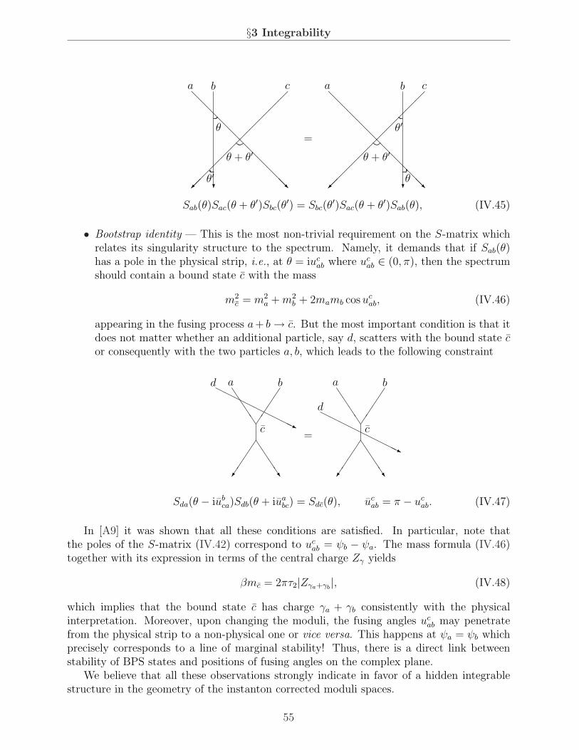
§3 Integrability

@@

@@

@@

@@

@@@R

@@

@@

@@

@@

@@@R

¡¡

¡¡

¡¡

¡¡

¡¡¡ª

¡¡

¡¡

¡¡

¡¡

¡¡¡ª? ?

a ab bc c

θ θ′

θ′ θ

θ + θ′ θ + θ′=

Sab(θ)Sac(θ + θ′)Sbc(θ′) = Sbc(θ

′)Sac(θ + θ′)Sab(θ), (IV.45)

• Bootstrap identity — This is the most non-trivial requirement on the S-matrix whichrelates its singularity structure to the spectrum. Namely, it demands that if Sab(θ)has a pole in the physical strip, i.e., at θ = iuc

ab where ucab ∈ (0, π), then the spectrum

should contain a bound state c with the mass

m2c = m2

a + m2b + 2mamb cos uc

ab, (IV.46)

appearing in the fusing process a+ b → c. But the most important condition is that itdoes not matter whether an additional particle, say d, scatters with the bound state cor consequently with the two particles a, b, which leads to the following constraint

JJ

JJ

JJ

JJ

JJ

JJ

JJ

JJ

À

À

HHHHHHHHHjHHHHHHHHHj

a ad

d

bb

c c=

Sda(θ − iubca)Sdb(θ + iua

bc) = Sdc(θ), ucab = π − uc

ab. (IV.47)

In [A9] it was shown that all these conditions are satisfied. In particular, note thatthe poles of the S-matrix (IV.42) correspond to uc

ab = ψb − ψa. The mass formula (IV.46)together with its expression in terms of the central charge Zγ yields

βmc = 2πτ2|Zγa+γb|, (IV.48)

which implies that the bound state c has charge γa + γb consistently with the physicalinterpretation. Moreover, upon changing the moduli, the fusing angles uc

ab may penetratefrom the physical strip to a non-physical one or vice versa. This happens at ψa = ψb whichprecisely corresponds to a line of marginal stability! Thus, there is a direct link betweenstability of BPS states and positions of fusing angles on the complex plane.

We believe that all these observations strongly indicate in favor of a hidden integrablestructure in the geometry of the instanton corrected moduli spaces.

55


3.4 Y-system and unusual features of TBA

TBA equations are integral equations on spectral densities. Quite often it is useful to rewritethem in the form of finite-difference equations which are known as Y-system (see [51] for areview). For this purpose one introduces the Y-functions

Ya(θ) = −eβµa−εa(θ) (IV.49)

and, using ψa = ψa+π and Θa = −Θa, one easily verifies that our TBA leads to the followingrelations [A9]

Ya

(θ +

πi

2

)Ya

(θ − πi

2

)=

∏

a<b<a

[1− Yb

(θ + i

(π2

+ ψa − ψb

))]nγb〈γa,γb〉

. (IV.50)

This is the Y-system for the case at hand. For a general configuration of charges it isextremely complicated and possesses a few unusual features:

• First, on the l.h.s. of (IV.50) one multiplies functions associated with a particle andits antiparticle, whereas usually one has only one function.

• Second, on the r.h.s. the Y-functions are all evaluated at different points, whereasusually their arguments do not contain any shifts. Moreover, usually the fusing anglesand the only shifts appearing in functional relations are rational multiples of π. Herethey are completely arbitrary and vary continuously with the moduli zI .

• Third, usually the power of each factor in the product on the r.h.s is related to theincidence matrix of a graph which structure is severely constrained by the periodicityof the Y-system. This incidence matrix is equivalently described by the matrix Nab =∫ +∞−∞ φab(θ)dθ. In our case it is just not defined because the kernel is not integrable.

In fact, these features can be traced back to the following properties of the original TBA:

• The spectral densities and Y-functions satisfy somewhat unusual reality conditions

εa(θ) = εa(−θ), Ya(θ) = Ya(−θ). (IV.51)

As a result, there is no parity symmetry and the Y-functions are not necessarily realon the real axis of the spectral parameter.

• The kernel φab(θ) (IV.33) is not decaying at infinity.

• The system is supplied by arbitrary imaginary chemical potentials µa.

Altogether, these features make our TBA much more complicated than one usually encoun-ters in two-dimensional integrable models. In particular, the techniques developed to extractthe free energy and Y-functions in the high-temperature limit, which corresponds either toa small compactification radius in gauge theory or to the strong coupling limit in string the-ory, become inapplicable. To generalize these techniques to the present context representsan interesting mathematical problem.

56

Chapter V

Quantum mirror symmetry andS-duality

1 Type IIB formulation

So far we considered the HM moduli space in type IIA string theory. Let us now turn to thetype IIB formulation compactified on the mirror CY Y. Although these two formulationsshould be equivalent according to mirror symmetry, it is of great importance to have bothof them at our disposal. There are many issues which are difficult to deal with in oneframework, but which become easy in another. Besides, the properties of their D-branes andtheir explicit symmetries are also quite different. In particular, type IIB theory provides uswith the powerful S-duality, which was indispensable in getting many of the results presentedin this review. Finally, at the full quantum level, mirror symmetry itself is so far only aconjecture and needs to be proven.

Let us therefore, before going into details, summarize the main differences between thetwo mirror formulations. The first difference is the physical nature of coordinates on themoduli space. From Table I.3 one observes that in type IIB the complex structure moduliza are replaced by the complexified Kahler moduli va (I.14)1, whereas the periods of theRR 3-form potential are replaced by periods of even-dimensional RR forms (the preciserelation between the periods and the fields c0, ca, ca, c0 will be given in (V.16)). Note thatit is convenient to combine one of these potentials, τ1 ≡ c0, with the ten-dimensional stringcoupling τ2 ≡ 1/gs into the ten-dimensional axio-dilaton field τ = τ1 + iτ2.

The second difference is the symmetry which characterizes each particular formulation.Whereas type IIA theory is explicitly invariant under symplectic transformations, the char-acteristic feature of type IIB is the presence of SL(2,Z) duality. In particular, the physicalfields should form a representation of this duality group. Therefore, if mirror symmetryholds at quantum level, our constructions done in the type IIA framework must have ahidden SL(2,Z) symmetry which should become explicit after passing to the type IIB for-mulation.

Finally, recall that D-branes in type IIB have even-dimensional world-volumes and there-fore they give rise to instanton effects by wrapping even-dimensional cycles of Calabi-Yau.

1We use the indices a, b to label coordinates on KK because we work on the mirror Calabi-Yau Y forwhich h1,1(Y) = h2,1(Y). Thus, this is not in contradiction with our conventions spelled in footnote 1.

57

Chapter V: Quantum mirror symmetry and S-duality

Thus, there is a series of instanton contributions to the moduli space metric coming fromD(-1), D1, D3 and D5-branes as well as from the NS5-brane pertaining to both formula-tions. Although all D-instanton corrections should follow by mirror symmetry from theconstruction of the previous chapter, to write them explicitly in the type IIB framework isan extremely difficult problem. The main obstacle is that it requires the knowledge of themirror map at the non-perturbative level. As we will show, this problem has been solvedonly partially. But before entering this subject, we need to understand better some of thetype IIB features mentioned above.

1.1 D-branes and charge quantization

The first problem we are going to discuss is how to characterize D-brane instantons on thetype IIB side. It turns out that the picture where some n-dimensional objects wrap n-dimensional non-trivial cycles and are classified by integers enumerating these cycles is toonaive. The correct mathematical description associates BPS D-instantons to elements inthe derived category of coherent sheaves D(Y) [52, 53]. In particular, for non-vanishing D5-brane charge p0, a D5-D3-D1-D(-1)-instanton configuration can be represented as a coherentsheaf E on Y, of rank rk(E) = p0. The charge vector classifying such configurations is givenby the expansion of the so called generalized Mukai vector in the basis of even-dimensionalcohomology [54]

γ′ ≡ ch(E)

√Td(Y) = p0 + paωa − q′aω

a + q′0ωY, (V.1)

where ch(E) and Td(Y) are the Chern character of E and Todd class of T Y. This leads tothe following expressions for the charges

pa =

∫

γa

c1(E) , q′a = −(∫

γa

ch2(E) +p0

24c2,a

),

q′0 =

∫

Y

(ch3(E) +

1

24c1(E) c2(Y)

),

(V.2)

which explicitly shows that the charges q′Λ are not integer. This becomes problematic re-garding applications to mirror symmetry. Indeed, the charges in the type IIA formulationare classified by H3(X,Z) and hence integer. Thus, there seems to be a clash between thetwo charge lattices and one needs to understand how they are related to each other.

This problem has been solved in [A11]. The idea is to compare the central charge asso-ciated to a D-instanton and given in type IIB by

Zγ′ =

∫

Y

e−vaωaγ′, (V.3)

with the central charge (I.38) known from type IIA theory where the prepotential should berestricted to its large volume limit

F cl(X) = −κabcXaXbXc

6X0+

1

2AΛΣXΛXΣ. (V.4)

We emphasize that it is important to keep the quadratic term despite it does not affectthe Kahler potential on KK . Then, upon identification of the moduli za = va, the two

58

§1 Type IIB formulation

expressions coincide provided

q′Λ = qΛ − AΛΣpΣ. (V.5)

Thus, this is the matrix AΛΣ that makes possible the conversion of rational charges intointeger ones. However, this conversion works only if the matrix satisfies a set of conditions.Their full list reads as follows [A11]:

i) A00 ∈ Z,

ii) A0a ∈ c2,a

24+ Z,

iii) Aabpb − 1

2κabcp

bpc ∈ Z for ∀pa ∈ Z,

iv)1

6κabcp

apbpc +1

12c2,ap

a ∈ Z for ∀pa ∈ Z.

(V.6)

Although the last two conditions look completely non-trivial, remarkably they are indeedfulfilled in few examples where AΛΣ has actually been computed. For example, on the quinticCalabi-Yau one has

κ111 = 5, A11 = −11

2, c2,1 = 50 (V.7)

and it is amusing to check that (V.6) does hold. In general, these conditions can be consideredas a consequence of mirror symmetry. They ensure that the charge vector γ = (pΛ, qΛ) isvalued in Heven(X ,Z) and can be meaningfully identified with the homology class of a specialLagrangian submanifold on the mirror type IIA side. In contrast, the primed charges (V.2)belong to a shifted lattice

q′a ∈ Z−p0

24c2,a − 1

2κabcp

bpc, q′0 ∈ Z−1

24pac2,a. (V.8)

1.2 S-duality and mirror symmetry

We had to start with the subtle issue of quantization of D-brane charges, even before consid-ering the type IIB formulation at the perturbative level, because it turns out that the shiftby the matrix AΛΣ (V.5) revealed above has important implications on the mirror map andS-duality transformations.

To see how this comes about, let us first establish how mirror symmetry relates theperiods of RR potentials on type IIA and type IIB sides. All these periods appear linearlyin the imaginary part of the D-instanton action whose real part is determined by the centralcharge. Thus, it is natural to find the relation by equating D-instanton actions in type IIAand in type IIB theories. In the former case the action is given in (I.37) and in the lattercase it is known to be [55, 42]

SD-IIB = 2πg−1s |Zγ′|+ 2πi

∫

Y

γ′ ∧ Aevene−B2 . (V.9)

Decomposing the RR potential Aeven as

Aevene−B2 = ζ0 − ζaωa − ζ ′aω

a − ζ ′0ωY (V.10)

59


and using the identification (V.5) between the charges, one finds the same axionic couplingsas in (I.37) provided the primed periods are shifted in a way similar to the charges

ζ ′Λ = ζΛ − AΛΣζΛ. (V.11)

This result indicates that all symplectic vectors experience such a shift under mirrorsymmetry. This shift corresponds to a symplectic transformation whose meaning is to removethe quadratic term from the prepotential (I.28) (or (V.4))

F ′(X) = F (X)− 1

2AΛΣXΛXΣ. (V.12)

Thus, in terms of primed variables, in the small coupling, large volume limit the metric onthe HM moduli space is obtained from (I.36) by plugging in the cubic prepotential (I.15).

However, this is not yet what we want. We need a formulation which is explicitly SL(2,R)invariant. It can be achieved by a further change of variables which provides the classicalmirror map [56]

za = ba + ita, ζ0 = τ1, ζa = −(ca − τ1ba),

ζ ′a = ca +1

2κabc bb(cc − τ1b

c), ζ ′0 = c0 − 1

6κabc babb(cc − τ1b

c),

σ = −2(ψ +1

2τ1c0) + ca(c

a − τ1ba)− 1

6κabc bacb(cc − τ1b

c).

(V.13)

The advantage of the variables appearing on the r.h.s. of (V.13) is that they are adapted tothe action of SL(2,R) symmetry. Under a transformation

g =

(a bc d

)(V.14)

with ad− bc = 1, they transform as

τ 7→ aτ + b

cτ + d, ta 7→ ta|cτ + d|, ca 7→ ca − c2,aε(g),

(ca

ba

)7→

(a bc d

)(ca

ba

),

(c0

ψ

)7→

(d −c−b a

) (c0

ψ

).

(V.15)

It is straightforward to verify that the classical HM metric obtained by the change of variables(V.13) is indeed invariant under the action (V.15).

Some comments are in order:

• The continuous SL(2,R) symmetry holds only classically. Already α′-corrections to theholomorphic prepotential given by the last two terms in (I.28) break it. However, thediscrete subgroup SL(2,Z) can be restored by including D(-1) and D1-instanton cor-rections [31] and the full non-perturbative metric on MHM is also expected to preservethis symmetry.

• Combining the classical mirror map (V.13) with the expansion (V.10), one finds thefollowing definitions of the RR scalars in terms of period integrals [7, A5]

c0 = A0, ca =

∫

γa

A2, ca = −∫

γa

(A4 − 1

2B2 ∧ A2),

c0 = −∫

Y

(A6 − B2 ∧ A4 +1

3B2 ∧ B2 ∧ A2).

(V.16)

60

§1 Type IIB formulation

However, these expressions are meaningful only at the classical level. In general, wedefine the type IIB physical fields as those which transform under SL(2,Z) accordingto the law (V.15). Of course, this makes possible that the mirror map (V.13) receivesquantum corrections and one of our aims is to show how they can be obtained.

• The S-duality transformation (V.15) differs from the standard one [40, 56] by thepresence of a constant shift in the transformation law of the D3-axion ca. The shiftis taken to be proportional to the multiplier system ε(g) of the Dedekind eta functionη(τ) which is a fractional number defined, up to the addition of integers, by the ratio

η

(aτ + b

cτ + d

)/η(τ) = e2πiε(g)(cτ + d)1/2. (V.17)

The necessity to introduce this shift can be understood from two reasons which areboth related to the effects induced by the matrix AΛΣ [A11]. First, S-duality andthe Heisenberg symmetry (I.31) are not completely uncorrelated. The transformation

generated by gb =(

1 b0 1

)should actually be the same as the Heisenberg shift with

parameter η0 = b. But without transforming ca, the mismatch (V.11) between primed(used in S-duality) and unprimed (used in Heisenberg symmetry) variables makes thesetwo transformations different. Although this coincidence might seem to be not crucial,the second issue shows that it is really needed. The problem is that, in the absenceof the shift of ca, the axionic couplings coming with D-instanton contributions are notinvariant under the same transformation gb due to the fractional nature of the primedcharges q′Λ. If this was the case, this would spoil the SL(2,Z) symmetry. Fortunately,the correction of the S-duality transformation of ca cures both these problems.

1.3 Monodromy invariance and spectral flow symmetry

There is another important symmetry which must be taken into account in the non-perturbativeanalysis of the HM moduli space. This is monodromy invariance originating from the pos-sibility to go around singularities in the moduli space of complexified Kahler deformationsKK(Y). Since the metric on MHM must be regular, such monodromies should leave it invari-ant. Here we are particularly interested in the monodromy around the large volume pointwhich is induced by a large gauge transformation of the B-field acting as

ba 7→ ba + εa , εa ∈ Z. (V.18)

Moreover, due to the presence of the B-field in the definition of the RR scalars (V.10), themonodromy is accompanied by the symplectic rotation

ζa 7→ ζa + εaζ0, ζ ′a 7→ ζ ′a − κabcζbεc − 1

2κabcε

bεcζ0,

ζ ′0 7→ ζ ′0 − ζ ′aεa +

1

2κabcζ

aεbεc +1

6κabcε

aεbεcζ0.(V.19)

Note that being rewritten in terms of the unprimed RR-fields, i.e. composed with thesymplectic transformation (V.11), the symplectic matrix becomes integer valued. Indeed, an

61


easy calculation yields [A11]

(ζΛ

ζΛ

)7→ ρ(M) ·

(ζΛ

ζΛ

), ρ(M) =

1 0 0 0εa δa

b 0 0

−La(ε) −κabcεc δa

b 0L0(ε) Lb(ε) + 2Abcε

c −εb 1

, (V.20)

where we introduced two functions

L0(εa) =

1

6κabcε

aεbεc +1

12c2,a εa, La(ε

a) =1

2κabcε

bεc − Aabεb. (V.21)

Due to the conditions (V.6), both these functions are integer valued for εa ∈ Z which ensuresour statement.

A nice fact is that the D-instanton action (V.9) stays invariant under the above mon-odromy transformation if it is supplemented by a similar transformation of charges

γ 7→ γ[ε] = ρ(M) · γ. (V.22)

Since the symplectic matrix is integer valued, the transformation preserves the charge latticeand is therefore admissible. In the following we call it spectral flow.

Due to the invariance of the D-instanton action, the combined action of the monodromyand the spectral flow preserves also the BPS indices Ω(γ; v), where we indicated explicitlytheir piecewise constant dependence on the Kahler moduli. This dependence is importantsince the spectral flow alone in general does not leave the indices invariant [57]: the trans-formation can change the position of walls of marginal stability and a given point in themoduli space may turn out to fall in a different chamber.

Given this “spectral flow symmetry”, it is convenient also to introduce combinations ofcharges which are invariant under the spectral flow. Such combinations are easily computedand are given by [A11, A13]

p0 6= 0 : qa = q′a +1

2κabc

pbpc

p0, q0 = q′0 +

paq′ap0

+1

3κabc

papbpc

(p0)2,

p0 = 0

pa 6= 0: q0 = q′0 −

1

2κabq′aq

′b,

(V.23)

where we distinguished two cases and introduced the matrix κab ≡ κabcpc together with its

inverse κab. If not the dependence on the moduli, one could say that the BPS indices arefunctions of these charges only. Finally, it is important to note that for p0 = 0 the invariantcharge is bounded from above,

q0 ≤ qmax0 =

1

24

(κabcp

apbpc + c2,apa). (V.24)

62

§2 S-duality in twistor space

2 S-duality in twistor space

The characteristic feature of the type IIB formulation is the S-duality symmetry. In our termsit is generated by the transformation (V.15) of the type IIB physical fields parametrizing theHM moduli space. However, as we saw in the previous chapters, quantum corrections to theHM metric are naturally formulated at the twistor space level. Therefore, it is natural toask how S-duality acts on the twistor space and which constraints it imposes on the twistorconstruction. In this section we answer these questions and moreover provide a reformulationof the D-instanton corrected twistor space of chapter IV which explicitly respects S-duality.

2.1 Classical S-duality

We start from the classical twistor space which is described by the Darboux coordinates(III.2) with the classical prepotential (V.4). As usual, it is convenient to define the primedvariables

ξ′Λ = ξΛ − AΛΣξΛ, α′ = α− 1

2AΛΣξΛξΣ. (V.25)

In the patch U0 they are given by the same expressions but with ζΛ replaced by ζ ′Λ and with

the prepotential given by F ′cl = −16

κabcXaXbXc

X0 .As was mentioned in section II.2.4, all isometries of a QK manifold can be lifted to a

holomorphic action on its twistor space. In particular, this implies that S-duality, representedin the classical approximation by the SL(2,R) symmetry group, should have a holomorphicrepresentation on the Darboux coordinates ξΛ, ξΛ and α. This indeed turns out to be thecase provided the fiber coordinate t transforms as

t 7→ 1 + tc,d− t

tc,d− − t

= − tc,d+ − t

1 + tc,d+ t

, (V.26)

where tc,d± denote the two roots of cξ0(t) + d = 0

tc,d± =

cτ1 + d∓ |cτ + d|cτ2

, tc,d+ tc,d

− = −1. (V.27)

Then the transformations (V.15), the mirror map (V.13) and the explicit expressions for theDarboux coordinates in the classical limit in terms of the type IIA fields lead to the followingnon-linear holomorphic action in the patch U0 [A5]

ξ0 7→ aξ0 + b

cξ0 + d, ξa 7→ ξa

cξ0 + d, ξ′a 7→ ξ′a +

c

2(cξ0 + d)κabcξ

bξc − c2,aε(g),

(ξ′0α′

)7→

(d −c−b a

)(ξ′0α′

)+

1

6κabcξ

aξbξc

(c2/(cξ0 + d)

−[c2(aξ0 + b) + 2c]/(cξ0 + d)2

).

(V.28)

Moreover, one finds that

eφ 7→ eφ

|cτ + d| , KZ 7→ KZ − log(|cξ0 + d|), X [i] 7→ X [i]

cξ0 + d(V.29)

so that the Kahler potential varies by a Kahler transformation and the complex contactstructure stays invariant. This ensures that S-duality is indeed a symmetry of the classicaltwistor space.

63


2.2 Inclusion of instantons: general construction

The action of S-duality in the classical approximation (V.28) has been obtained using ex-plicit expressions for the Darboux coordinates. The only non-trivial step was to find thecorrect transformation of the fiber coordinate (V.26). However, once we include instantoncorrections, we do not have such expressions at our disposal anymore. Instead, the Darbouxcoordinates are determined by complicated integral equations and in the best case can beexpressed through integrals of type (IV.15). Therefore, the first natural step would be tounderstand how such integrals, or more generally the integrals of type

∑j

∮

Cj

dt′

t′t′ + t

t′ − tH(ξ, ξ), (V.30)

transform under S-duality.To discuss this issue, we restrict ourselves to the instanton corrections with the vanishing

five-brane charge p0 = 0. As is clear from (IV.16), this ensures that the Darboux coordinateξ0 remains uncorrected and is given globally by the same classical expression (III.2). Thisimplies in turn that the transformation of t should also be unchanged and one can use theformula (V.26).

But now we arrive at a problem: the measure and the kernel in the integral (V.30)transform in a complicated way which does not allow for a simple geometric interpretation.Fortunately, this problem can be cured by a modification of the integration kernel whichamounts just to a coordinate redefinition on the moduli space [A14]. Let us define

K(t, t′) =1

2

(t′ + t

t′ − t+

1/t′ − t′

1/t′ + t′

)=

(1 + tt′)(t′ − t)(1/t′ + t′)

. (V.31)

Then it is easy to check that K(t, t′) dt′t′ is invariant under S-duality!2 Since K(t, t′) differs

from the original kernel by a t-independent term, this additional contribution can be ab-sorbed into a redefinition of the constant terms in the t-expansion of Darboux coordinates.Thus, to write them in terms of the new kernel, it is sufficient to redefine ζΛ, ζΛ and σ. Afterthis redefinition, we are ready to give our main result.

2To understand the origin of the new kernel, it might be helpful to change the fiber coordinate to [A13]

z =t + it− i

.

In its terms one has

t = −i1 + z

1− z, ξ0 = τ1 + iτ2

1/z + z

1/z − z.

The new coordinate has the advantage of having a simpler transformation under S-duality

z 7→ cτ + d

|cτ + d| z.

Moreover, it provides a very simple representation for the new kernel

K(t, t′)dt′

t′=

12

z′ + z

z′ − z

dz′

z′,

which makes its invariance transparent.

64


The following theorem not only shows how S-duality is realized to all orders in theinstanton expansion in the absence of five-brane instantons, but also gives conditions on thetransition functions ensuring the SL(2,Z) symmetry.3

Theorem [A14]: Let the twistor space Z is defined by the covering

Z = U0 ∪ U+ ∪ U− ∪(∪′m,nUm,n

), (V.32)

where the patches U± cover the north and south poles of CP 1, Um,n are mapped to each otherunder the antipodal map and SL(2,Z)-transformations

τ [Um,n] = Uτ(m),τ(n), (V.33)

Um,n 7→ Um′,n′ ,

(m′

n′

)=

(a cb d

) (m

n

), (V.34)

and U0 covers the rest. The associated transition functions are taken to be

H [+0] = F cl(ξΛ[+]), H [−0] = F cl(ξΛ

[−]), H [(m,n)0] = Gm,n(ξΛ[m,n], ξ

[0]a ), (V.35)

where the holomorphic functions Gm,n are required to transform under SL(2,Z) as

Gm,n 7→ Gm′,n′

cξ0 + d− c

2

κabc∂ξ[0]a

Gm′,n′∂ξ[0]b

Gm′,n′

(cξ0 + d)2

(ξc[m′,n′] −

2

3∂

ξ[0]c

Gm′,n′

)+ reg. (V.36)

where +reg. denotes equality up to terms regular in the patch Um′,n′.Then the following statements hold:

1. The Darboux coordinates in the patch U0, as functions of the fiber coordinate t, aregiven by the following expressions:

ξ0 = ζ0 +τ2

2

(t−1 − t

),

ξa[0] = ζa

cl + t−1Y a − tY a +∑m,n

′∮

Cm,n

dt′

2πit′K(t, t′)∂

ξ[0]a

Gm,n,

ξ[0]Λ = ζcl

Λ + t−1F clΛ (Y )− tF cl

Λ (Y )−∑m,n

′∮

Cm,n

dt′

2πit′K(t, t′)∂ξΛ

[m,n]Gm,n, (V.37)

α[0] = −1

2(σ + ζΛζΛ)cl − (

t−1 + t) (

t−1F cl(Y ) + tF cl(Y ))− ζΛ

cl

(t−1F cl

Λ (Y )− tF clΛ (Y )

)

−∑m,n

′∮

Cm,n

dt′

2πit′

[K(t, t′)

(1− ξΛ

[m,n](t′)∂ξΛ

[m,n]

)Gm,n

+(tt′)−1F cl

a (Y ) + tt′F cla (Y )

1/t′ + t′∂

ξ[0]a

Gm,n

],

where Cm,n are contours on CP 1 surrounding Um,n in the counter-clockwise directionand τ2, ζ

0, ζacl, ζ

clΛ , σcl, Y a are some coordinates on the QK base.

3To avoid cluttering of notations, we omit primes on the RR fields, Darboux coordinates and holomorphicprepotential. Thus we ignore the effects due to the matrix AΛΣ. But they can be easily restored byperforming the corresponding symplectic transformation. The primes on sums over m,n will denote thatthe value m = n = 0 is omitted.

65


2. Provided these coordinates are identified with the following combinations of the physicaltype IIB fields

ζ0 = τ1, ζacl = −(ca − τ1b

a),

ζcla = ca +

1

2κabc bb(cc − τ1b

c), ζcl0 = c0 − 1

6κabc babb(cc − τ1b

c),

σcl = −2(ψ +1

2τ1c0) + ca(c

a − τ1ba)− 1

6κabc bacb(cc − τ1b

c) +τ 22

3κabcb

abbbc,

Y 0 =τ2

2, Y a =

τ2

2(ba + ita) +

∑m,n

′∮

Cm,n

dt

2πit2

∂ξ[0]a

Gm,n

(1/t + t)2 ,

(V.38)

the Darboux coordinates (V.37) transform under SL(2,Z) transformations (V.15) and(V.26) according to the classical laws (V.28).

3. The same transformation rules hold also in the patches Um,n, with the understandingthat the Darboux coordinates appearing on the r.h.s. are those attached to the patchUm′,n′, e.g. ξa

[m,n] 7→ ξa[m′,n′]/(cξ

0 + d).

4. The contact potential is given by

eΦ =2

3τ2

κabc Im Y a Im Y b Im Y c (V.39)

− 1

16π

∑m,n

′∮

Cm,n

dt

t

[(t−1Y Λ − tY Λ

)∂ξΛ

[m,n]Gm,n +

(t−1F cl

a (Y )− tF cla (Y )

)∂

ξ[0]a

Gm,n

]

and transforms under SL(2,Z) as in (V.29)

As a result, the quaternion-Kahler manifold associated to the above twistorial data carriesan isometric action of SL(2,Z).

Some comments are in order:

• The patches Um,n,U± are not necessarily all different. Typically, Um,n are associatedto zeros of mξ0 + n denoted above by tm,n

± . Then one might have Ukm,kn = Um,n fork ∈ N and U± coinciding with U0,n for n > 0 and n < 0, respectively. If this is thecase, the functions Gm,n should be defined for m,n coprime only.

• Another possibility is to include open contours similar to the BPS rays appearing inthe type IIA description. In fact, all previous statements hold for an arbitrary set ofcontours Cm,n mapped unto each other by SL(2,Z). For example, Cm,n can be an opencontour from tm,n

+ to tm,n− . In this case however the structure of patches might be more

complicated. The only requirement on the covering is that it is invariant under theantipodal map and SL(2,Z) transformations so that a patch Ui is mapped to somepatch Uic,d

. The Darboux coordinates in each patch are given by the formulas (V.37)and transform under S-duality by (V.28) where the coordinates on the r.h.s. are fromthe patch Uic,d

.

• If the transition function Gm,n is associated with such an open contour, the regularterms in its SL(2,Z) transformation are not allowed anymore. In other words, thetransformation (V.36) should be exact, because in this case the transition functionalready represents a discontinuity through a logarithmic branch cut.

66


• If not the quadratic and cubic terms in Gm,n, the transformation law (V.36) wouldsimply mean that the transition functions are similar to modular functions of weight(−1, 0). More precisely, such a modular function would arise as a formal sum of Gm,n

over all patches. However, the non-linear terms spoil the simple modular transforma-tion. They appear due to the fact that the arguments of transition functions are takenin different patches and are completely similar to the quadratic terms in (IV.10). But,in contrast to the situation in type IIA theory, it is not known whether there is asimplified description which allows to get rid of them.

• Note that the coordinate change (V.38) is almost identical to the classical mirror map(V.13). There are only two differences. First, Y a (usually related to za) acquires anadditional instanton contribution. Second, the coordinate σcl differs from σ in (V.13)by the presence of the last term. Although it is a classical contribution, it was absorbedinto σcl to simplify the expression for α in terms of Y a.

• This theorem assumes that the functions Gm,n are independent on ξ0 and α, whichis equivalent to the ignorance of five-brane instanton corrections. At the moment, itis known how to generalize the above results to include such dependence only in theone-instanton approximation [A14]. As one could suspect, in this approximation theS-duality invariance is again ensured by the requirement that the transition functionstransform with the modular weight (−1, 0), i.e. their transformation should be givenby the first term in (V.36).

• Finally, note that all anomalous dimensions are taken to vanish. On the other hand,on the type IIA side the anomalous dimension cα is non-zero and encodes the one-loopgs-correction to the HM metric (see section III.2.1). This implies that in the type IIBtwistor space the one-loop correction appears from a completely different origin.

These results provide a general framework for the twistorial construction of the HMmoduli space in the type IIB formulation. All D(-1), D1 and D3-instanton corrections shouldfit the conditions of the above theorem. In particular, the transition functions generatingthese corrections should transform according to (V.36). But this theorem does not answerto the main question: what are these transition functions? The theorem does not specifythem, but only imposes conditions on their transformation properties. On the other hand, ifmirror symmetry does hold at quantum level, the resulting moduli space should agree withthe one constructed in the type IIA formulation. Thus, there should exist a resummationprocedure which, starting from the description of chapter IV, allows to find the transitionfunctions relevant in type IIB theory and they should automatically satisfy the required S-duality constraint (V.36). This might be considered as a very non-trivial test of consistencyof the type IIA construction. Below we report on the results in this direction.

This reasoning does not apply to D5-brane instantons. They are not invariant underS-duality and therefore should be treated separately. In fact, S-duality mixes them withNS5-branes. This fact will be used in chapter VI to generate the latter corrections and thusto get an access to the complete non-perturbative description of MHM.

67


2.3 D(-1)-D1-instantons

Let us first consider D(-1)-D1-instanton corrections, i.e. those which have vanishing magneticcharge pΛ. In this case one has great simplifications. First of all, as indicated in sectionIV.1.3, in the sector with vanishing pΛ the linear instanton approximation for Darbouxcoordinates becomes exact so that they are not given by complicated integral equations,but known explicitly. Moreover, since the transition functions should be ξΛ-independent,all non-linear terms in the transformation law for Gm,n (V.36) vanish and the transitionfunctions in the type IIB formulation are expected to originate from a simple modular form.

How the type IIB description of this sector, fitting the theorem of the previous subsection,arises from the type IIA construction of D-instantons has been shown in [A7].4 The idea isthat one should perform a Poisson resummation of the Darboux coordinates with respectto D-brane charge q0. Then the couple of integers (m,n) from the theorem originates asfollows: n appears in the process of Poisson resummation as the integer conjugate to q0 andm comes from the expansion of the dilogarithm in the type IIA transition functions, i.e. itcounts multi-covering effects.

The resulting twistor space can be described by the covering (V.32) where Um,n surroundtm,n+ (see Fig. V.1) and by the transition functions (V.35) with

GD1m,n(ξ) = − i

(2π)3

∑

qaγa∈H+2 (Y)∪0

n(0)qa

e−2πimqaξa

m2(mξ0 + n), m 6= 0,

GD10,n(ξ) = − i(ξ0)2

(2π)3

∑

qaγa∈H+2 (Y)∪0

n(0)qa

e2πinqaξa/ξ0

n3.

(V.40)

It is easy to check that they do satisfy the transformation property

Gm,n 7→ Gm′,n′

cξ0 + d+ reg. (V.41)

and the possibility to drop the regular terms is important. Note also that∑

n>0 GD10,n pro-

vides the sum of the one-loop and worldsheet instanton α′-corrections to the prepotential(I.28). Since U0,n = U+, they are combined with its classical piece given by H [+0] to the fullholomorphic prepotential.

Although this twistor space looks completely different from the one we started with onthe type IIA side, it turns out that they are related by a certain gauge transformation.This means that in different patches one should perform certain contact transformationsgenerated by regular functions. However, these generating functions can have singularitiesoutside their patch of definition. As a result, the transformed Darboux coordinates mayhave different singularities than the initial ones and the covering should be adapted to thenew analytic structure as well. In this way a careful analysis allows to relate the melon-liketype IIA picture to the type IIB formulation given here.

4In fact, D(-1) and D1-instanton contributions have been obtained before the invention of the type IIAconstruction based on the BPS rays and played an important role on the way to it [31]. However, thesecontributions were found only in the form of corrections to the hyperkahler potential (II.30) on the associatedHKC. Neither the complete twistor formulation, nor its relation to the type IIA twistor space were known.

68


Fig. V.1: The covering and transition functions incorporating D(-1)-D1-instantons.

Finally, note that the formula (V.39) for the contact potential can be easily evaluatedand gives the following result

eφ =τ 22

2V(ta) +

√τ2

8(2π)3

∑

qaγa∈H+2 (Y)∪0

n(0)qa

∑m,n

′ τ3/22

|mτ + n|3 (1 + 2π|mτ + n|qata) e−Sm,n,qa , (V.42)

which was first obtained in [31] by starting from the one-loop expression and by enforcingthe SL(2,Z) symmetry. Here

Sm,n,qa = 2πqa|mτ + n| ta − 2πiqa(mca + nba) (V.43)

is the classical action of a D1-D(-1)-instanton or, more precisely, an Euclidean (m, n)-stringwrapped around the effective curve qaγ

a.

2.4 D3-instantons

This sector is already not so well understood and at the moment only some preliminaryresults are accessible in the linear instanton approximation. To present these results, werestrict ourselves to the sector with fixed D3-brane charge pa because it should be preservedby S-duality. Besides, we replace the integer-valued BPS indices Ω(γ; v) by rational invariantsconstructed as

Ω(γ; v) =∑

d|γ

1

d2Ω(γ/d; v). (V.44)

They encode multi-covering effects and allow to replace the dilogarithm in the transitionfunctions (IV.2) by simple exponential. Thus, our starting point is

Hγ =Ω(γ; v)

(2π)2σD(γ)E

(paξ′a − q′aξ

a − q′0ξ0)

, (V.45)

with the charge vector restricted to γ = (0, pa, qa, q0).

69


Fig. V.2: The set of open contours and transition functions incorporating D3-instantons.

The advantage of the rational invariants is the possibility to use a combination of thespectral flow symmetry (V.22) and modular invariance. In our approximation one can neglectthe dependence of Ω(γ; v) on the Kahler moduli and then their invariance with respect tothe spectral flow symmetry allows to write that

Ω(0, pa, q′a, q′0) ≡ Ωpa,µa(q0), (V.46)

where q0 is the invariant charge (V.23) and µa is the residue class of q′aγa modulo the

sublattice Λ = γaκabεb, εaγa ∈ H4(Y,Z). These quantities can be used to construct the

following function

hpa,µa(τ) =∑

q0≤qmax0

Ωpa,µa(q0)E(−q0τ) , (V.47)

which is known to be a vector-valued modular form of weight (− b22− 1, 0) with multiplier

system given by E(c2,apaε(g)) [58, 59, 57] where ε(g) is the same multiplier system of the

Dedekind eta function which appears in (V.15). The crucial property of the function hpa,µa(τ)is that it is completely determined by its polar part consisting of the terms in the sum whichare singular in the limit τ2 →∞. As a result, all Ωpa,µa(q0) for negative q0 can be expressedin terms of just a finite number of rational BPS indices given by Ωpa,µa(q0) for 0 ≤ q0 ≤ qmax

0 .We refer to [60, 59] for the explicit expression.

After using this result for the rational invariants, one can show that the resummationover (negative) q0 leads to the following ansatz for the transition functions [A13]

GD3m,n,pa,qa

=1

2π2(mξ0 + n)E

(−1

2Aabp

apb

) ∑

0≤q0≤qmax0

Ωpa,µa(q0) (−1)q′apa

(V.48)

×E

(pagm,n[ξ′a]−

(q0 +

1

2κabq′aq

′b

)gm,n[ξ0]− q′agm,n[ξa]

)R−1− b2

2

(2πiq0

m(mξ0 + n)

),

where

Rw(x) = 1− 1

Γ(1− w)

∫ ∞

x

e−zz−wdz (V.49)

70


and gm,n is the SL(2,Z) group element (V.14) with c = m, d = n acting on the Darbouxcoordinates by the transformation law (V.28). Up to the last factor, which was studied indetail in [59], it is immediate to see that under S-duality these functions do transform asrequired by the theorem of section 2.2, i.e. according to (V.41) and without the necessityto drop any regular contributions. Thus, one gets the first sign that the D3-instanton sectoradmits a consistent implementation of S-duality.

Moreover, note that the functions (V.48) have essential singularities at t = tm,n± . This

indicates that they should be associated with contours Cm,n,pa,qa joining these two points onCP 1 (see Fig. V.2). As a result, the complete set of contours is given by an infinite numberof copies of the melon-like picture, which we had in type IIA, rotated into each other bySL(2,Z) transformations so that it is consistent with the action of S-duality. However, thedetails of this construction, as well as its extension to all orders in the instanton expansionremain still unclear.

71


3 Non-perturbative mirror map

Once we understand how S-duality is realized at the level of the twistor space, we can addressanother important issue: the non-perturbative mirror map. The problem is that, to applymirror symmetry, one needs a relation between the type IIA and type IIB physical fields,which maps the hypermultiplet metrics in the two mirror formulations into each other. In theclassical approximation such relation is furnished by the classical mirror map (V.13). Butit is expected to receive all possible quantum corrections, both in α′ and gs. The relationincluding these corrections will be called non-perturbative mirror map and can be viewed asa realization of quantum mirror symmetry.

In general, to find quantum corrections to the mirror map is an extremely complicatedproblem because the only condition which fixes the mirror map is that after its applicationthe metric must be invariant under the action of SL(2,Z) (V.15). However, this conditionbecomes more explicit once we lift it to the twistor space because here SL(2,Z) should actnot only isometrically, but also holomorphically. As a result, this condition gives rise to aself-determining system where the consistency between mirror symmetry and S-duality isenough to find both of them. The consistency condition can be formulated as the followingequation

Ξ (m[g · qIIB], g · t) = g · Ξ, (V.50)

where Ξ denotes all Darboux coordinates, qIIB are the type IIB physical fields, g· is the actionof an SL(2,Z) transformation and m is the non-perturbative mirror map. This conditionmeans that the SL(2,Z) action on Darboux coordinates can be evaluated in two ways. Thefirst one, which is shown on the l.h.s., uses the explicit expression of the Darboux coordinatesfollowing from our twistor construction in the type IIA formulation. Of course, it gives themas functions of the type IIA fields. Therefore, to evaluate the action of g, one needs touse the (to be found) mirror map which expresses them in terms of the type IIB fieldswhose transformations are known by definition. The second way, shown on the r.h.s., is aholomorphic action of SL(2,Z) directly on the Darboux coordinates. In the classical limitit is given by (V.28) and in principle one could expect that it gets modified by quantumcorrections. However, all our results indicate that it actually stays the same at the fullnon-perturbative level [A7]. Thus, the equality (V.50) of the two SL(2,Z) actions providesa very non-trivial condition on the mirror map m.

In fact, the theorem from section 2.2 essentially gives a solution to the equation (V.50).Indeed, the relations (V.38) substituted into the Darboux coordinates (V.37) show how thelatter depend on the type IIB fields so that S-duality is correctly realized. In particular,they ensure the holomorphic transformations (V.28). Thus, the only thing which remains tobe found is a relation between ζa

cl, ζclΛ , σcl, Y a and the type IIA fields. This relation in turn

follows from the change of the kernel as described on page 64. For example, restricting tothe D1-D(-1)-instanton sector and in the presence of all α′-corrections, one finds [A14]

ζacl = ζa, Y a =

τ2

2za,

ζclΛ = ζ ′Λ −

1

2

∑

γ=(0,qΛ)

∫

`γ

dt

2πit

1/t− t

1/t + t∂ξΛHγ, (V.51)

σcl = σ − τ 22

3(zΛ + zΛ)(F ′

Λ + F ′Λ) +

∑

γ=(0,qΛ)

∫

`γ

dt

2πit

1/t− t

1/t + t

(1− (

ξΛ − 12ζΛ

)∂ξΛ

)Hγ.

72

§3 Non-perturbative mirror map

Resumming over q0, one can express the same relation in terms of the transition functionsof the type IIB formulation (V.40). The instanton terms will be given by contour integralswith the contours surrounding the points tm,n

+ . Such integrals can be easily evaluated andtherefore in this case it is possible to write the mirror map in a very explicit form. We referto [A7] for the explicit expressions.

This result completely solves the problem of quantum mirror symmetry in the approx-imation where five-brane and D3-instantons are neglected. The latter corrections are stilldescribed by the theorem, so the relations (V.38) solve the most difficult part of the problem.However, it still remains to relate ζa

cl, ζclΛ , σcl to the type IIA axionic fields. This should be

done by a resummation of the Darboux coordinates which should bring them from (IV.16)to the type IIB form (V.37). Unfortunately, as was mentioned in section 2.4, this has notbeen done yet in a satisfactory way.

For five-branes the situation is even more complicated because the corresponding correc-tions are expected to affect even the SL(2,Z) transformation of the fiber coordinate t (V.26).Moreover, S-duality requires to include into consideration NS5-brane instantons, which re-main unknown on the type IIA side. Thus, even before addressing the issue of quantummirror symmetry in the presence of five-branes, we need to understand how to generate theNS5-brane instanton contributions. This will be the subject of the next chapter.

73

Chapter VI

NS5-brane instantons

The instanton corrections coming from NS5-branes are the last missing piece of the con-struction of the complete non-perturbative geometry of the hypermultiplet moduli space (atleast in type IIA picture). In this chapter we present a progress in understanding the gen-eral structure of these contributions and an attempt to incorporate them into the twistordescription of MHM.

There are several reasons why the NS5-brane contributions are difficult to find. Let uspoint out some of them:

• First of all, the NS5-brane is a complicated dynamical object whose dynamics is not wellunderstood. In particular, its world-volume theory, especially in the case of multiplefivebranes, is not known to the full extent.

• In the type IIA formulation, it is expected that the world-volume theory involves a self-dual 3-form flux H which is an electric source for the RR 3-form potential A3 [61, 62].The self-duality constraint implies that fluxes on three-cycles γ, γ′, corresponding toD2-NS5 bound states, cannot be measured (nor defined) simultaneously if the inter-section product 〈γ, γ′〉 is non-vanishing. A mathematical consequence of this fact isthat the NS5-brane partition function cannot be a simple function, but only a sectionof a certain bundle.

• Another complication is that, upon inclusion of NS5-brane contributions, all continuousisometries of the moduli space MHM become broken. In particular, this implies thatone does not have the QK/HK correspondence at our disposal anymore and one hasto apply the full machinery of the contact geometry.

• Finally, since the NS5-instantons introduce dependence on the NS-axion σ, it becomesnow important to take into account the full Heisenberg symmetry group (I.31), includ-ing its non-commutative nature. Due to this, one can expect the same complications aspassing from a classical theory to its quantum version where the role of the quantizationparameter is played by the NS5-brane charge.

Besides these issues, there are many other subtleties all of which require a special care.In particular, there is a subtle interplay between the description of instanton contributionsand the topology of the moduli space. Therefore, before attacking the problem of NS5-braneinstantons, we analyze the topological structure of MHM and its implications.

74

§1 Topological issues

1 Topological issues

The global structure of MHM can be specified by providing a group of discrete identificationsof the coordinates parametrizing the moduli space which act isometrically on it. Besidessymplectic invariance and S-duality, one has two additional discrete symmetries provided byHeisenberg and monodromy transformations (see section I.2.1). What we need is to betterunderstand their action and what it implies for NS5-brane contributions.

Let us concentrate for simplicity on the type IIA formulation. In type IIB the pictureis completely similar and can be obtained using mirror symmetry. At fixed, vanishinglysmall string coupling gs and ignoring the NS-axion (i.e., modding out by translations alongσ, which are symmetries of the perturbative theory), the “reduced” HM moduli space isknown to be topologically the so called intermediate Jacobian Jc(Y). This is a torus bundleover the complex structure moduli space KC(Y) with fiber T ≡ H3(Y,R)/H3(Y,Z), whichparametrizes the space of harmonic RR three-form fields C over Y modulo large gaugetransformations [63]. This is precisely the topology consistent with the structure of D-instanton corrections (I.37) where the axionic couplings arise as periods of C over the cyclewrapped by the brane.

The next step is to include in this picture the NS-axion σ. It parametrizes a certaincircle bundle CNS5 over Jc(Y) and our primary goal is to understand the topology of thisbundle. This can be done on the basis of two observations. First, let us consider the generalstructure of NS5-brane corrections to the metric shown in (I.39). We can also write them inthe following form

δds2|NS5 ∼ e−4πkeφ−iπkσ Z(k)NS5(N , ζΛ, ζΛ) (VI.1)

where the tensorial nature of the metric was ignored. The second factor can be interpretedas a partition function of k NS5-branes. An important observation is that consistency of theinstanton correction (VI.1) requires that eiπkσ and Z(k)

NS5 are valued in the same circle bundle.Although it could seem to be a rather trivial statement, in fact, it leads to certain

restrictions on both the partition function and symmetry transformations of the NS-axion.For example, let us consider the restriction of the circle bundle CNS5 to the torus T . It isknown [64] that the bundle where the fivebrane partition function Z(k)

NS5 lives has a restrictionsuch that its first Chern class coincides with the Kahler class of T

c1(CNS5)|T = ωT ≡ dζΛ ∧ dζΛ. (VI.2)

This means that the partition function should transform non-trivially under the large gaugetransformations of the RR-fields. The precise transformation, and correspondingly the fi-bration of CNS5 over the torus T , is specified by a choice of quadratic refinement σNS5(γ),which satisfies the same defining relation (IV.4) as the one for D-instantons and can equallybe expressed in terms of characteristics Θ = (θΛ, φΛ) as in (IV.5). Although it is temptingto identify the characteristics Θ and ΘD for two types of instantons, we refrain from doingso as a priori there is no reason for them to coincide. Then the partition function satisfiesthe following twisted periodicity condition

Z(k)NS5(N , C + H) = (σΘ(H))k E

(k

2(ηΛζΛ − ηΛζΛ)

)Z(k)

NS5(N , C), (VI.3)

where we abbreviated C = (ζΛ, ζΛ) and H = (ηΛ.ηΛ) ∈ H3(Y,Z).

75

Chapter VI: NS5-brane instantons

Now we return to the instanton correction (VI.1). Since it must be invariant under thelarge gauge transformations, the condition (VI.3) immediately gives the shift of the NS-axion which must accompany the transformation of the RR-fields. As a result, we have thefollowing symmetry generators

T ′H,κ :

(ζΛ, ζΛ, σ

) 7→ (ζΛ + ηΛ, ζΛ + ηΛ, σ + 2κ− ηΛζΛ + ηΛζΛ + 2c(H)

), (VI.4)

where (H, κ) ∈ H3(Y,Z)× Z and

c(H) = −1

2ηΛηΛ + ηΛθΛ − ηΛφΛ mod 1, (VI.5)

so that σΘ(H) = (−1)2c(H). One observes that the generators T ′H,κ are almost identical to

the generators of the Heisenberg algebra (I.31). The precise relation is given by T ′H,κ =

TH,κ+c(H). Thus, our topological considerations have revealed an extra shift to be added tothe naive Heisenberg transformations [A10]. This extra shift is important for consistency ofthe group action and effectively abelianizes the non-commutative Heisenberg algebra whenone considers it on functions of the form Fk(ζ, ζ, σ) = eiπkσFk(ζ, ζ).

So far we discussed how CNS5 fibers over the torus of the RR-fields, which is encodedin the action of the Heisenberg symmetry (VI.4). It remains to understand the fibration ofCNS5 over the complex structure moduli space KC(Y), which is tied with the monodromytransformations. To this aim, we use our second observation that the perturbative metric(III.12) suggests that the connection defining CNS5 is determined by the one-form Dσ (III.13)whose curvature is given by

d

(Dσ

2

)= ωT +

χY

24ωSK, (VI.6)

where ωT and ωSK = − 12π

dAK are the Kahler forms on T and KC(Y), and the coefficient 1/2takes into account that σ has periodicity 2. The first term is in nice agreement with (VI.2).On the other hand, the second term in (VI.6), originating from the one-loop correction tothe HM metric, has support on KC(Y) and implies that the NS-axion picks up anomalousvariations under monodromies. Indeed, it is easy to check that the following transformation

C 7→ ρ(M) · C, σ 7→ σ +χY

24πIm fM + 2κ(M), (VI.7)

where M is a monodromy in KC(Y), fM is a local holomorphic function determined by therescaling Ω 7→ efM Ω of the holomorphic 3-form around the monodromy and κ(M) is anundetermined constant defined modulo 1, is a symmetry of the metric (III.12). It is veryimportant to keep the constant contribution given by the last term since without it one easilyends up with an inconsistency: a trivial rescaling Ω 7→ e2πiΩ would lead to identificationsσ ∼ σ + χY/12 in conflict with the periodicity modulo 2 of σ. Thus, consistency requiresthe introduction of a unitary character of the monodromy group, e2πiκ(M) [A10, A11]. Thenthe instanton correction (VI.1) implies that the fivebrane partition function should undergoa similar anomalous transformation. As we will see in section 3, this may have furtherimplications for topological string amplitudes. Unfortunately, the explicit form of the unitarycharacter remains unknown so far.

76

§2 Fivebrane corrections to the contact structure

2 Fivebrane corrections to the contact structure

2.1 S-duality on the job

As follows from the duality chain presented in Fig. I.1, the most direct way to get NS5-branecorrections to the HM moduli space metric is to use the SL(2,Z) symmetry of the type IIBformulation. It exchanges D5 and NS5-branes and therefore allows to get the latter contribu-tions once we know the former. However, what we know exactly is not D5-brane corrections,but D2-instantons in type IIA. D5-instantons follow by applying the mirror map, but as wediscussed in the previous chapter, the mirror map is not known at the full non-perturbativelevel. Without its non-perturbative completion, we can get only a quasiclassical or one-instanton approximation to D5 and consequently to NS5-brane corrections. Nevertheless,already such a result would represent a substantial progress. Here we are going to presentthe corrections to the contact structure which result from such analysis and which have beenfound in [A11].

We proceed as follows: start from the known expression for D2-instanton contributionswith charge vector γ = (p0 6= 0, pa, qa, q0) neglecting all multi-instantons, apply the classicalmirror map (V.13) which maps D2-branes to D5-D3-D1-D(-1) bound states, and sum overall images under SL(2,Z). The transformation matrix is chosen to be

g =

(a b

−k/p0 p/p0

)∈ SL(2,Z), (VI.8)

where one takes (c, d) = (−k/p0, p/p0) to run over coprime integers and the integers (a, b),ambiguous up to the addition of (k/p0,−p/p0), are chosen such that ap + bk = p0. Then p0

is identified as gcd(p, k), whereas k will be interpreted as NS5-brane charge.

One can perform this procedure directly at the level of the twistor space. This ensuresthat, even working in the quasiclassical approximation, one satisfies all constraints of QKgeometry. In this approach an instanton correction is encoded in two pieces of data: a contouron CP 1 and a holomorphic function on the twistor space which describes the transitionfunction associated with the contour. For D-instantons these data are given by the BPSrays `γ (IV.1) and the functions Hγ (IV.2). It will however be useful to pass to the rationalBPS invariants Ω(γ) (V.44), as has been done for D3-instantons. Thus, our starting pointis provided by

Hγ =Ω(γ)

(2π)2σD(γ)E

(pΛξ′Λ − q′ΛξΛ

), (VI.9)

where we passed also to the primed charges and Darboux coordinates, (V.5) and (V.25).After this change, no mirror map is already required, since the primed variables are thosewhich properly represent the action of SL(2,Z) (V.28). As a result, the new data which aresupposed to introduce NS5-brane corrections are given by

Hk,p,γ = g ·Hγ, `k,p,γ = g · `γ, (VI.10)

where γ = (pa, qa, q0) denotes the remaining D3-D1-D(-1)-charges and the hatted charges qΛ

denote the combinations (V.23) invariant under the spectral flow.

77


Using the S-duality action (V.28), one easily finds [A11]

Hk,p,γ = −Ω(γ)

(2π)2

k

p0

(ξ0 − n0

)σD(γ)E

(kSα +

p0 (kqa(ξa − na) + p0q0)

k2(ξ0 − n0)+ a

p0q′0k

− c2,apaε(g)

),

(VI.11)where

Sα = α + nΛξΛ + F cl(ξ − n)− 1

2AΛΣnΛnΣ, (VI.12)

and we denoted n0 = p/k, na = pa/k, valued in Z/k. The factor (p − kξ0)/p0 has beenintroduced to ensure that the functions (VI.11) satisfy the transformation law (V.41) withGm,n ∼ H−mp0,np0,γ (without regular contributions). As a result, they satisfy the extension ofthe theorem of section 2.2, mentioned on page 67, which allows the dependence of transitionfunctions on ξ0 and α.

On the other hand, the transformation (V.26), which is still valid in our approximation,can be used to find the contour `k,p,γ. It is easily seen to be a half-circle stretching between

the two zeros of ξ0−n0, which are nothing else but the points t−k,p± . As a result, one obtains

exactly the same picture as one had for D3-instantons in Fig. V.2. This shows that in typeIIB fivebrane instantons are nicely combined with D3-instantons.

2.2 Consistency checks

Altogether Hk,p,γ and `k,p,γ provide the data which are expected to encode the fivebranecorrections to the contact structure of the type IIB HM moduli space in the one-instantonapproximation. However, before we can actually claim that the deformation they inducecorrectly introduces fivebrane instanton corrections, they should pass several consistencychecks. Here we present two very non-trivial tests which allow to consider them as a seriouscandidate for the right description of fivebrane contributions.

Heisenberg and monodromy transformations

Besides S-duality, MHM should carry an isometric action of the Heisenberg symmetry andmonodromy invariance. In section 1 we found how these symmetries should be realized atthe non-perturbative level: they are given by (VI.4) and (VI.7), respectively. As usual, theycan be lifted to a holomorphic action on the twistor space and should preserve the contactstructure. In our terms this implies that the transition functions and the associated contoursare mapped to each other, i.e. the image of Hk,p,γ should be Hk,p′,γ′ for a suitably chosenmap (p, γ) 7→ (p′, γ′), with the contours `k,p,γ following the same pattern.

In [A11] it was shown that our twistorial data, Hk,p,γ and `k,p,γ, do satisfy this conditionup to some phase factors. More precisely, one has

T ′H,κ ·Hk,p,γ = ν(η)Hk,p−kη0,γ[−kηa/p0], Mεa ·Hk,p,γ[pε/p0] = ν ′(ε)Hk,p,γ[−pε/p0], (VI.13)

where γ[ε] denotes the image of the charge vector γ under the spectral flow (V.22) withparameter εa, and ν(η), ν ′(ε) are the constant phase factors which can be found in [A11]. Thecancelation of all dependence on the Darboux coordinates in the symmetry transformations(VI.13) is very promising, but the presence of the phases indicates some tension betweenS-duality, Heisenberg and monodromy invariance and suggests that it may be necessary to

78

§2 Fivebrane corrections to the contact structure

relax some of our assumptions about the way these symmetries are realized. In particular,it is possible that S-duality is realized only as a finite index subgroup of the full SL(2,Z).In the absence of a satisfactory resolution of this problem, we simply ignore the anomalousphase factors and proceed further. Moreover, it turns out that for k = 1 the phase ν(η) canbe canceled by a suitable choice of characteristics

θΛD = 0, φ0 = A00/2, φa − φD

a = Aaa. (VI.14)

We will use this choice in the next section and the results obtained there seem to confirm itscorrectness. Unfortunately, no choice was found which would lead to cancelations in othercases.

Fivebrane instanton action

The second consistency check is to show that the corrections to the metric generated bythe transition functions (VI.11) indeed have the form of the NS5-brane contributions (I.39).In other words, we need to compute the instanton action corresponding to (VI.11). Thesimplest way to do this is to evaluate the Penrose transform of Hk,p,γ

∫

`k,p,γ

dt

tHk,p,γ(ξ(t), ξ(t), α(t)). (VI.15)

This is a typical integral which describes instanton corrections to various quantities. Whilethe precise form of the integration kernel can be different and vary from one quantity toanother, it does not affect the leading saddle point approximation we are interested in.

Substituting the tree level expressions for the Darboux coordinates (III.4), it is straight-forward to find the saddle point and to evaluate the resulting instanton action Sk,p.γ. Theexpression is a bit cumbersome and we refer to [A11] for its explicit form. As a cross-checkone can verify that the same expression is obtained by applying the classical mirror map andS-duality to the classical D-instanton action (I.37)

Sk,p.γ = g · Sγ, Sγ = 2πτ2|Zγ|+ 2πi(qΛζΛ − pΛζΛ). (VI.16)

The fivebrane action crucially simplifies in the small string coupling limit τ2 → ∞. In thisapproximation one finds

Sk,p.γ ≈ πk(4 eφ− i(nΛ− ζΛ)NΛΣ(nΣ− ζΣ)

)+iπk

(σ + (ζΛ − 2nΛ)ζΛ

)− 2πimΛzΛ, (VI.17)

where we used the following notations

n0 =p

k, na =

pa

k, ma =

p0

kqa, m0 =

ap0

kq′0 − c2,ap

aε(g). (VI.18)

It is clear that the NS5-brane action (I.39) is a part of our result. Moreover, the firstterm matches precisely the instanton action obtained in [65], based on a classical analysisof instanton solutions in N = 2 supergravity, while the other terms restore the appropriateaxionic couplings. Thus, the transition functions (VI.11) are in perfect agreement with thesupergravity description of NS5-branes.

79


3 Fivebrane partition function and topological strings

3.1 Relation to the topological string amplitude

During long time it was suspected that the NS5-brane partition function Z(k)NS5 is closely

related to the topological string partition function Ztop [66, 67]. There are several reasons toexpect such a relation. In particular, for k = 1 they are both governed by Donaldson-Thomasinvariants and, in addition, they both behave as wave functions. For topological strings thisis a well known fact coming from the holomorphic anomaly equations satisfied by Ztop andthe possibility to define it for different polarizations of the symplectic space H3(Y,R) [68].For NS5-branes this is a consequence of the Heisenberg algebra or, equivalently, the twistedperiodicity condition (VI.3). Indeed, the most general function satisfying this condition canbe written as a non-Gaussian theta series

Z(k)Θ,µ(N , ζΛ, ζΛ) =

∑

n∈Γm+µ+θ

Ψk,µR

(ζΛ − nΛ

)E

(k(ζΛ − φΛ)nΛ +

k

2(θΛφΛ − ζΛζΛ)

), (VI.19)

where Ψk,µR (ζΛ) is a kernel of the theta series which also depends on the complex structure

moduli and the string coupling. One observes that the unknown kernel depends only on ahalf of the variables parametrizing the torus T . In the given case, these are ζΛ. On theother hand, one can give a similar representation where the kernel depends instead on ζΛ

and is related to the original one by a Fourier transform. This indicates that Ψk,µR (ζ) should

be viewed as a wave function in the ζ-representation. Moreover, it should transform in themetaplectic representation under changes of symplectic basis similarly to the topologicalwave function in the real polarization. Due to this, it is tempting to suggest that these twoobjects should be somehow identified.

It turns out that the results presented in the previous section allow to put these ideason a firm ground. To this aim, let us consider a formal sum of the holomorphic functions(VI.11) for k = 1 over the integer charges p, pa and qΛ:

H(1)NS5(ξ, ξ, α) =

∑p,pa,qΛ

H1,p,γ(ξ, ξ, α). (VI.20)

This sum is formal because each term is attached to a different contour on CP 1. Never-theless, it can be meaningfully inserted into general formulas for Darboux coordinates andthe contact potential, provided the sum is performed after integration along CP 1. From themathematical point of view, it just defines a section of H1(ZMpert

HM,O(2)).

As we know from the previous section, for k = 1 there exists a choice of characteristics(VI.15) such that the section H

(1)NS5 is invariant under the Heisenberg symmetry. As a result,

it can be recast into the form very similar to the non-Gaussian theta series (VI.19)

H(1)NS5(ξ, ξ, α) =

1

4π2

∑

nΛ

H(1)NS5

(ξΛ − nΛ

)E

(α + nΛ(ξΛ − φΛ)

). (VI.21)

A remarkable fact is that the function H(1)NS5 appearing in this representation turns to be

proportional to the wave function of the topological A-model on Y in the real polarization,which should be analytically continued to complex values of its argument [A11],

H(1)NS5(ξ

Λ) ∼ ΨtopR (ξΛ). (VI.22)

80

§3 Fivebrane partition function and topological strings

The proportionality factor can be expressed in terms of Mac-Mahon function and dependsonly on ξ0.

The relation (VI.22) provides a direct link between the NS5-brane instantons in type IIBstring theory on a Calabi-Yau Y and A-model topological strings on the same Calabi-Yau.By mirror symmetry, one expects that NS5-brane instantons in type IIA on Y should berelated to the topological B-model on Y. On the other hand, despite the relation (VI.22) is

very concrete, the unclear status of the sum over charges in the definition of H(1)NS5 raises some

questions about its physical interpretation which certainly require a deeper understandingof the physics behind it.

3.2 Fivebrane partition function from twistor space

Due to the complicated nature of NS5-branes, to define their partition function is a verynon-trivial problem. One of the standard approaches to this problem is a holomorphicfactorization [69, 44]. It does allow to find a partition function which has the form of thetheta series (VI.19) and reproduces the classical fivebrane instanton action (VI.17). However,the validity of this approach is very restricted. First of all, it ignores all non-linear effects onthe fivebrane worldvolume so that it gives only a Gaussian approximation of the full partitionfunction. Then, in type IIA, it takes into account only the degrees of freedom of the self-dual3-form flux H, whereas we expect also a non-trivial dependence on the complex structuremoduli and the string coupling. And finally, it involves some further simplifying assumptionswhich do not seem to hold in general [A11]. Thus, while the holomorphic factorization likelycaptures the right topological properties of the fivebrane partition function, it is not able toproduce the complete result.

On the other hand, our twistor approach suggests a natural candidate for the full partitionfunction: it can be defined by summing the Penrose transform (VI.15) over charges

Z(k,µ)NS5 =

∑

p,pa,qa,q0

∫

`k,p,γ

dt

tHk,p,γ(ξ(t), ξ(t), α(t)), (VI.23)

where the vector µa is the residue class defined below (V.46). Note that this definitionabsorbs the dependence on the NS-axion so that it actually coincides with the r.h.s. of(VI.1). In [A11] the sum over electric charges has been performed explicitly. Besides, thesaddle point evaluation of the Penrose transform in section 2.2 has been generalized toinclude the normalization factor which should correspond to the one-loop determinant. Asa result, for k = 1 in the small coupling limit, this prefactor was found to be

F ∼ (zΛ Im FΛΣzΣ

)−1t−2+

χY24

s ef1(z), (VI.24)

wherets = 4 eKτ−1

2 (ζΛ − nΛ) ImNΛΣzΣ (VI.25)

is the saddle point and f1(z) is the holomorphic part of the one-loop vacuum amplitude ofthe topological B-model. The appearance of f1(z) further strengthens the connection withtopological strings. Moreover, it is consistent with the monodromy transformations of theNS-axion (VI.7). Indeed, denoting by L the line bundle over KC(Y) in which the holomor-

phic three-form Ω is valued, ef1(z) is a section of L1−χY24

+b34 which does not have a canonical

81


definition unless χY is divisible by 24. Due to this, one expects that its monodromy trans-formation also contains a unitary character κ(M) which appears in (VI.7) and the condition

that the total partition function Z(k)NS5 is well defined requires that the two characters are the

same.Finally, we show how the fivebrane partition function (VI.23) can be encoded in a certain

state in the Hilbert space H of square-integrable functions on H3(Y,R). To this aim, letus consider a specific state |ΨΓm,k,µ〉 ∈ H, which has the following simple representation interms of its wave function ΨΓm,k,µ

R (ζΛ) in the real polarization

ΨΓm,k,µR (ζΛ) =

∑n∈Γm+µ

δ(ζΛ − nΛ

)e2πik φΛnΛ

. (VI.26)

Besides, we introduce two sets of operators, TΛ and TΛ, acting on H. Their action on anarbitrary wave function in the real polarization reads

TΛ ·ΨR(ζΛ) = 2πkζΛΨR(ζΛ), TΛ ·ΨR(ζΛ) = −i∂ζΛΨR(ζ

Λ), (VI.27)

so that they satisfy the Heisenberg algebra

[TΛ, TΣ] = 2πikδΛΣ. (VI.28)

with the NS5-brane charge playing the role of the Planck constant. Then the fivebranepartition function (VI.23) appears as the Penrose transform of a matrix element

Z(k,µ)NS5 =

∫dt

te2πikα 〈ΨΓm,k,µ| ei(ξΛTΛ−ξΛTΛ)|H(k,µ)

NS5 〉, (VI.29)

where |H(k,µ)NS5 〉 is the state whose wave-function in the real polarization is given by an exten-

sion of H(1)NS5 from (VI.21) to arbitrary NS5-brane charge k and residue class µa. This is the

state we were looking for. As we know from (VI.22), it essentially coincides with the stateassociated to the topological string wave function.

82

Chapter VII

Example: universal hypermultiplet

Until now we considered the HM moduli space which is obtained by compactifying type IIstring theory on arbitrary Calabi-Yau. While our results uniquely determine the quantumcorrected metric on MHM, it is difficult to give its explicit form beyond the perturbativeapproximation. However, there exists a special case where such an explicit representation ispossible. This is the case of type IIA string theory compactified on a rigid Calabi-Yau, whichhas vanishing Hodge number h2,1 and therefore does not have complex structure moduli. Inthis case the effective theory contains only one hypermultiplet, which is known by the nameuniversal hypermultiplet (UHM) and was briefly mentioned on page 9. Since nH = 1, the HMmoduli space is four-dimensional which is the simplest possible case of a quaternion-Kahlermanifold. This is the reason why the UHM was extensively studied in the literature, seefor instance [70, 71, 72, 73, 22, 41, 74], and in fact the first insights to many of the resultsreported here have been obtained from these studies.

In this chapter we are going to specialize our general results to the particular case ofthe UHM. Moreover, we use the fact that four-dimensional QK manifolds can be describedin terms of solutions of just one non-linear differential equation. We establish a connectionbetween this description and our twistor approach, which allows to immediately translatethe results for the quantum corrections to the contact structure on the twistor space to thecorresponding corrections to the metric.

1 Four-dimensional QK spaces

1.1 Przanowski description

A four-dimensional QK manifold is an Einstein space with a non-vanishing cosmologicalconstant and a self-dual Weyl curvature. In the case of positive cosmological constant thereare actually only two possibilities: the four-sphere S4 and the complex projective planeCP 2. However, we are interested in the case of negative scalar curvature which is muchmore non-trivial and allows for continuous deformations.

It is worth to mention that the limit of zero curvature corresponds to four-dimensionalHK manifolds. The metric on such manifolds, which are thus Ricci-flat and self-dual, is wellknown to be encoded in solutions of the so called heavenly equations [75]. It is less knownthat a similar result holds also for a non-vanishing cosmological constant. It was shown byPrzanowski [76] that locally it is always possible to find complex coordinates zα such that

83

Chapter VII: Example: universal hypermultiplet

the metric takes the form

ds2Q = − 6

Λ

(hαβ dzα dzβ + 2eh |dz2|2

)≡ 2gαβ dzα dzβ, (VII.1)

where hα = ∂h/∂zα, etc. It is completely determined in terms of a single real functionh(zα, zα) and the constraints of quaternionic geometry require that the function must satisfythe following non-linear partial differential equation

Prz(h) ≡ h11h22 − h12h12 + (2h11 − h1h1) eh = 0. (VII.2)

To show that the metric (VII.1) is indeed quaternion-Kahler, it is sufficient to verify theconditions (II.21), where in four dimensions the coefficient ν is related to the cosmologicalconstant as ν = Λ/3. They are satisfied provided the SU(2)-connection and the quaternionictwo-forms are expressed in terms of h as follows [77, A8]

p+ = eh/2dz2, p3 =i

2(∂ − ∂)h, p− = (p+)∗,

ω+Q =

6

Λeh/2h1 dz1 ∧ dz2, ω3

Q = 2i gαβ dzα ∧ dzβ, ω−Q = (ω+Q)∗.

(VII.3)

It is important to emphasize that solutions of the Przanowski equation (VII.2) are notin a one-to-one correspondence with the self-dual Einstein metrics. In general, there areinfinitely many ways of expressing a given metric in the form (VII.1). One can distinguishbetween two types of ambiguities. The first comes from the following holomorphic change ofcoordinates

z1 → z′1 = f(z1, z2), z2 → z′2 = g(z2),

h(z1, z2) → h′(z1, z2) = h(f(z1, z2), g(z2)

)− log∣∣g2(z

2)∣∣2 (VII.4)

which, supplemented by the above change of the Przanowski function, provides a symmetryof the metric [78]. The second ambiguity roots in the choice of complex structure definedby the coordinates zα. A QK space has infinitely many local integrable complex structuresand any of them can be used to achieve the Przanowski ansatz (VII.1). In general, differentcomplex structures lead to different solutions of the Przanowski equation which are related toeach other through a non-holomorphic change of variables. As we will see, this phenomenonhas a natural interpretation in the framework of the twistor approach.

1.2 QK spaces with isometries

If a four-dimensional QK manifold has an isometry, there exists even a simpler description.It is provided by the Tod ansatz [79] which can be written in local coordinates (ρ, z, z, ψ) inthe form

ds2M = − 3

Λ

[P

ρ2

(dρ2 + 4eT dzdz

)+

1

Pρ2(dθ + Θ)2

], (VII.5)

where the isometry acts as a shift in the coordinate θ. Here, T is a function of (ρ, z, z),P ≡ 1− 1

2ρ∂ρT , and Θ is a one-form such that

dΘ = i(∂zPdz − ∂zPdz) ∧ dρ− 2i ∂ρ(P eT )dz ∧ dz. (VII.6)

84

§1 Four-dimensional QK spaces

The Einstein self-duality condition of the metric imposes on the function T the three-dimensional continuous Toda equation

∂z∂zT + ∂2ρ eT = 0, (VII.7)

which also plays the role of the integrability condition for (VII.6).This description can be related to the more general one due to Przanowski if one chooses

the coordinates zα such that the Killing vector ∂θ acts by shifting the imaginary part of z1.Then the condition that this action is isometric is equivalent to h1 = h1 and the relationbetween h, z1, z2 and T, ρ, z is given by the Lie-Backlund transformation [80, 81]

z = z2, ρ = 1/(2h1), T = h + 2 log ρ. (VII.8)

Similarly, in the case of two commuting isometries, there is an ansatz due to Calderbankand Pedersen [82] which encodes the metric in terms of solutions of the Laplace equationon the hyperbolic plane. We refer to [A8] for the relation of this ansatz to the Toda andPrzanowski equations.

1.3 Relation to the twistor description

The above results provide an explicit parametrization of the four-dimensional QK metricsin terms of solutions of differential equations. However, this leaves us with the problem ofsolving these non-linear equations and an additional problem that different solutions can infact describe the same manifold. This should be contrasted with the twistor approach whereany consistent set of holomorphic transition functions defines a quaternionic manifold, butto get the metric, in general, requires solving some (integral) equations.

A relation between these two descriptions has been established in [A8]. It comes fromthe observation that the metric on Q can be expressed through the Kahler potential and thecontact one-form on its twistor space [29]

ds2Q ≡

12

Λ

(ds2

ZQ − e−2KZQ |X |2) , (VII.9)

where the r.h.s. should be restricted to any real-codimension 2 (local) complex submanifoldC transverse to the contact distribution, i.e. such that X|C 6= 0. This form of the metricessentially coincides with the Przanowski ansatz (VII.1) and allows to identify the Przanowskifunction with the restriction of the Kahler potential on ZQ to the submanifold C up to aKahler transformation

h = −2KC + FC + FC. (VII.10)

Moreover, one can show that a set of constraints to be satisfied by the Kahler potential,which include in particular the Monge-Ampere equation representing the Kahler-Einsteinproperty of the metric on ZQ, reduces to the single Przanowski equation (VII.2).

This derivation also demonstrates that choosing different complex submanifolds, onegenerates different solutions of the Przanowski equation. A particular choice of C specifiesa local integrable complex structure on Q. As a result, this choice appears to be the originof the non-holomorphic ambiguity in the Przanowski description mentioned in the end ofsection 1.1. In practice, the complex submanifold C can be specified by the vanishing of some

85


holomorphic function C(ξ, ξ, α) = 0 on ZQ. Then it is enough to solve this condition withrespect to one of the holomorphic coordinates and substitute the solution into the Kahlerpotential.

A particular convenient choice of the complex submanifold is provided by C = 1/ξ becausethis is the only choice which can be equivalently described as a hypersurface of constantfiber coordinate t, namely t = 0. In this case, one can explicitly identify the Przanowskicoordinates zα and function h with coefficients of the Darboux coordinates (II.35) in thesmall t-expansion. More precisely, one has [A8]

z1 =i

2α

[+]0 + cα log Y − c0A, z2 =

i

2ξ

[+]0 + c0 log Y,

h = −2φ + 2 logY

2.

(VII.11)

Conversely, some of the first coefficients and the constant part of the contact potential canbe expressed through the Przanowski function

Y =eh/2

|h1| , ξ[+]0 = Y φ

[+]1 +

h2

h1

, φ[+]0 = − log(2h1). (VII.12)

In the presence of an isometry these relations can be further simplified. For example, thecontact potential becomes globally defined and t-independent so that Φ[i] = φ and one candrop the first term in the expression for ξ

[+]0 . Using (VII.8), one also finds an explicit relation

between the twistor data and the Toda potential

ρ = eφ, T = 2 log(Y/2). (VII.13)

In particular, the radial coordinate is identified with the contact potential and therefore inthe context of string theory coincides with the four-dimensional string coupling.

86

§2 Geometry of the universal hypermultiplet

2 Geometry of the universal hypermultiplet

2.1 Perturbative universal hypermultiplet

The perturbative metric on the moduli space of the universal hypermultiplet can be obtainedfrom the one-loop metric (III.12) where there are no complex structure moduli za and thereis only one pair of the RR fields ζ, ζ. In addition, since a degree 2 homogeneous functionof one argument is necessarily quadratic, the holomorphic prepotential must be of the formF = τ

2X2. The complex parameter τ is the modulus of the intermediate Jacobian Jc(Y)

defined in section VI.1. Although it does affect the global structure of the moduli space,locally it can be absorbed into a redefinition of the RR scalars. For simplicity, we restrictit to be τ = −i/2 so that K = N = 1 and N = −i/2. As a result, the perturbative metrictakes the form [22, 41]

ds2UHM =

r + 2c

r2(r + c)dr2 +

r + 2c

r2

∣∣∣∣dζ +i

2dζ

∣∣∣∣2

+r + c

16r2(r + 2c)

(dσ + ζdζ − ζdζ

)2

. (VII.14)

It is easy to recognize that the metric (VII.14) falls in the Tod ansatz (VII.5) where oneshould take [74]

T = log(ρ + c), (VII.15)

identify the coordinates as

ρ = r, z = −1

4(ζ − 2iζ), θ = −1

8σ, (VII.16)

and put Λ = −3/2. It is trivial to check that (VII.15) indeed satisfies the Toda equation(VII.7) being its one of the most trivial solutions. The one-loop deformation appears as asimple shift of the radial coordinate, which is a symmetry of the Toda equation.

Similarly, one can put the metric into the Przanowski form provided one takes [A1]

z1 = −(r + c log(r + c)− 1

8ζ2

)− i4(σ + ζζ), z2 = −1

4(ζ − 2iζ),

h = − logr2

r + c.

(VII.17)

These equations perfectly agree with the identifications (VII.11) where the Darboux coor-dinates are taken from chapter III with τ2 excluded in favor of the contact potential r = eφ

(III.11). Thus, the Darboux coordinates we are working with, in the patch U0, are given by

ξ[0] = ζ + 2√

r + c(t−1 − t

),

ξ[0] = ζ − i√

r + c(t−1 + t

),

α[0] = σ − i√

r + c(t−1(ζ − 2iζ) + t(ζ + 2iζ)

)− 8ic log t.

(VII.18)

To check that the function h (VII.17) does solve the Przanowski equation (VII.2), one shouldexpress r as a function of zα. In presence of the one-loop correction this can be done onlyimplicitly, which is however sufficient to compute the derivatives of h and to verify theequation.

87


Finally, we mention that there is a surprising duality between the one-loop correctedUHM described here and the c = 1 non-critical string theory compactified on the self-dualradius [A15] (for a review of c = 1 strings, see [83, 84]). Both systems are represented bythe same solution of the Toda equation and the twistor description of the UHM turns out tobe equivalent to the Lax formulation of the integrable structure of the c = 1 string theory.

2.2 Instanton corrections as perturbations

To write the instanton corrected UHM metric, one should find a solution of the Przanowskiequation (VII.2) which would incorporate these contributions. Of course, it is almost im-possible task given the complicated nature of this equation. If one ignores the NS5-braneinstantons, so that the isometry along the NS-axion remains preserved, it is possible to usethe Toda description of section 1.2. However, it does not much simplify the problem as theequation to be solved is still a non-linear equation in partial derivatives.

Nevertheless, both these equations become very powerful once one is interested only inlinear deformations of the one-loop corrected metric (VII.14). This restriction is equivalentto the one-instanton approximation which was discussed repeatedly in the previous chapters.In this approximation, one can expand the “master” equation, (VII.2) or (VII.7), around asolution representing the perturbative metric. As a result, one obtains a linear differentialequation which is much easier to solve. Of course, not all solutions of these linearizedequations are physically relevant and some conditions which select the admissible solutionsshould be imposed.

This procedure has been carried out in [74] for the Toda equation and in [A1] for thePrzanowski equation. The following three types of solutions have been found:

δh(2)p,q =

C

re−2πi(qζ−pζ)K0

(4π

√(r + c)(4q2 + p2)

), (VII.19)

δh(2′)p,k,± =

C

r

(√1 + ζ2

16(r+c)− ζ

4√

r+c

)16πck

√16(r + c) + ζ2

e±2πi(pζ−k(σ+ζζ))e−π(p−kζ)√

16(r+c)+ζ2,(VII.20)

δh(5)k,± =

C

re±πikσ eπk(4r−( 1

4ζ2+ζ2))

(r + c)4cπk

∫ ∞

1

e−8πk(r+c)t dt

t1+8πck, (VII.21)

where the charges are restricted to satisfy p > 0, kζ < 0 for the second solution and k > 0for the last one. These solutions are not unique. In particular, any function obtained byapplying a Heisenberg transformation to (VII.19)-(VII.21) or a linear combination thereof isalso a solution of the Przanowski equation linearized around (VII.17).

Furthermore, the first solution has a transparent physical meaning: this is just an in-stanton correction due to a D2-brane with charge (p, q). Its leading large r asymptotics,corresponding to the small gs limit, perfectly agrees with (I.37), whereas the Bessel functionprovides all subleading contributions. Similarly, comparing the third solution with (I.39),one recognizes an NS5-brane instanton. Applying the Heisenberg shift of ζ and integratingover the shift parameter, one can obtain another solution which differs only by the exponen-tial factor. Its leading asymptotics reads e±πik(σ+ζζ)−πk(4r+ 1

2ζ2) and reproduces the NS5-brane

action (VI.17) from the previous chapter. The possibility to represent NS5-brane instantonsin different forms can be considered as a realization of the wave function property discussedin section VI.3.1.

88

§2 Geometry of the universal hypermultiplet

Finally, the second solution does not have an obvious interpretation. Its axionic couplingsindicate that it should represent a bound state of NS5 and D2-branes, but the real part of theinstanton action has a somewhat unusual form. Although there is a BPS solution in classicalsupergravity which reproduces such instanton action [85], the microscopic interpretation of(VII.20) remains unclear.

More generally, it turns out that the linearized Przanowski equation around a solution hcan be written in the following form [A8]

dPrzh (δh) = eh |h1|4[− 3

2Λ∆ + 1

]δh

|h1|2 = 0. (VII.22)

In the case with an isometry when h1 = h1, the second order differential operator ∆ coin-cides with the Laplace-Beltrami operator defined by the metric (VII.1) one expands around.Otherwise, ∆ is given by its generalization involving a certain connection term, which un-fortunately has not been understood from a geometric point of view. In any case, the de-formations of h appear as eigenmodes of this operator. The specific eigenvalue 2Λ/3 = R/6corresponds to a conformally coupled massless scalar field. In this case, the eigenmodes ofthe Laplace-Beltrami operator are known to be generated by Penrose-type contour integrals[24]. This establishes a link with our twistor approach. Indeed, using identifications (VII.11),it was shown in [A8] that if the transition functions can be represented as in (II.18) whereH [ij]

(1) is treated as a perturbation, the corresponding variation of the Przanowski function isgiven by

δh = −h1

∑j

∮

Cj

dt

2πitH [ij]

(1) . (VII.23)

Moreover, for the UHM metric (VII.14) one can explicitly verify that (VII.23) satisfies thelinearized equation (VII.22) for any set of holomorphic functions and associated closed con-tours. One may also consider open contours provided one makes sure that all boundarycontributions coming from the integration by parts and the action of the Laplace operatoron the limits of integration cancel each other. This turns out to be the case when the endpoints of the contour lie on any complex submanifold of the twistor space.

The simple formula (VII.23) allows to translate our results on deformations of the con-tact structure on the twistor space induced by instanton corrections directly to the variationof the metric, without necessity to solve any equations. It is sufficient to take the transi-tion functions associated with a given type of instantons, evaluate them on the Darbouxcoordinates (VII.18) and integrate along the corresponding contour. Substituting the resultinto (VII.1) then produces an instanton corrected metric on the UHM moduli space in theone-instanton approximation. Note that all open contours appeared so far do satisfy thecondition that their ends belong to a complex submanifold: for the contours `γ associatedto D2-branes the submanifold is defined by 1/ξ = 0 and for the contours relevant for D3 andfivebranes in type IIB these are mξ + n = 0.

In this way, in particular, one can reproduce the solutions of the linearized Przanowskiequation given above. For example, the simple exponential function H(1) ∼ e−2πi(qξ−pξ), whichis a single term from the dilogarithm sum (IV.2), reproduces δh

(2)p,q. On the other hand, to

get δh(5)k,±, one should take

H(1) ∼ (ξ ± 2iξ)8πck e±πikα−πk( 14ξ2+ξ2), (VII.24)

89


and choose a contour C connecting t = ∞ (t = 0) to the point t± corresponding to thecomplex submanifold ξ ± 2iξ = 0, namely

t± = −[

4√

r + c

±ζ + 2iζ

]±1

. (VII.25)

Although such holomorphic functions did not appear in our studies of fivebrane correctionsbased on S-duality, it is tempting to suggest that they may be relevant for the type IIAdescription of NS5-brane instantons. These functions correspond to the so called symmetricgauge where none of the Heisenberg shifts (I.31), except the shift of the NS-axion, is anexplicit symmetry. Therefore, the complete answer should involve a double sum over bothshifts of ξ and ξ generalizing the theta function representation (VI.21) [86]. Although itis possible to relate it to the usual ξ and ξ-representations, the symmetric gauge is plau-sible due to the simplicity of the transition function (VII.24). Moreover, it appears to besymplectic invariant since the quadratic term in the exponent is nothing else but the Hessepotential evaluated on the symplectic vector (ξ, ξ). This fact also opens a possibility for ageneralization of (VII.24) to higher dimensions. However, this part of the full picture hasnot been understood yet and our story about the twistor approach to the non-perturbativeHM moduli space stops here.

90

Conclusions

In this review we summarized a progress in understanding quantum corrections to thehypermultiplet moduli space. Just five years ago only the tree level metric and some frag-mentary facts about its quantum corrections were known, whereas now we are already veryclose to the complete non-perturbative picture! We have shown how such a coherent picturearises step by step: starting from the one-loop correction to the tree level metric, incorpo-rating D-instantons, and finishing with NS5-brane contributions, all included consistentlywith the constraints of quaternion-Kahler geometry.

To achieve these results, it was crucial to apply the twistor approach to quaternionicgeometries, which has been developed precisely for this purpose. It originated as a general-ization of the projective superconformal approach, which marked many important findingsin theories with N = 2 supersymmetry, but is restricted to quaternionic spaces with suffi-cient number of commuting isometries. In contrast, the twistor approach does not have anyrestrictions and in its framework many non-trivial physical effects obtain a simple and nicegeometric description.

On the way, we have also gained new insights into the action of S-duality, realization ofquantum mirror symmetry, and connection to integrable models. The last point is especiallyencouraging since it gives a hope that the whole problem possesses a hidden integrablestructure. Its discovery would certainly have a great impact on the subject and could providenew hints to the fundamental structure of string theory.

Furthermore, the study of NS5-brane corrections revealed their close connection to topo-logical strings. Although such a connection was suspected to exist already long ago, we wereable to give it a precise form. However, its implications have not been investigated yet andare still to be understood.

Of course, there still remains a lot of work to be done before the main problem addressedhere can be claimed to be completely solved. Moreover, in the course of achieving this goal,one opens new research directions which raise new issues and new questions. Therefore, wewould like to finish this review with a list of problems which, from our viewpoint, are eithervery interesting or indispensable for further progress:

• The most urgent problem is to extend the results reported here on instanton correctionsdue to D3, D5 and NS5-branes to the multi-instanton level. Such extension shouldalso provide the complete non-perturbative mirror map and make a conclusion aboutthe fate of S-duality: Is it realized as the full SL(2,Z) group or only as some of itssubgroups?

• In chapter VI we found instanton corrections due to NS5-branes in the linear approx-imation. The resulting picture is adapted to the type IIB formulation as it explicitly

91

Conclusions

respects S-duality. On the other hand, very often the results, which exist in the twomirror formulations, appear in type IIA in a simpler form than in type IIB, as is thecase, for example, for D-instantons. Therefore, it is natural to ask how the NS5-branecontributions look like in the type IIA picture? Note that this formulation is expectedto be explicitly invariant under symplectic transformations, but it is not clear how toreconcile this requirement with the theta function representation (VI.19), which is aconsequence of the Heisenberg symmetry. Some hints to a possible resolution of thispuzzle can be found in the study of instanton corrections to the universal hypermulti-plet presented in the last chapter.

• An important problem is to show that the full non-perturbative moduli space metric isfree of any singularities. In particular, this implies that the instanton corrections mustresolve the one-loop singularity at r = −2c. This requirement gives a very non-trivialconsistency check on our construction.

At present, it is not clear how such a resolution can be demonstrated. Probably, itshould involve some resummation of the sum over charges and taking into accountmulti-instanton contributions. This in turn raises the problem that, in contrast to thegauge theory case, the BPS indices Ω(γ) in string theory are exponentially growingand therefore the sum over charges is divergent. In [87] it was argued that this sumcan be considered as an asymptotic series and be resumed using a generalized Boreltechnique. As a result, the ambiguity of the asymptotic series turns out to be of theorder of NS5-brane instantons so that the latter are expected to convert this seriesinto a convergent one. To show that this is indeed the case is another important openproblem.

• A series of questions arises from the observed relation of D-instanton corrections tointegrable models described by Thermodynamic Bethe Ansatz. First of all, it wouldbe interesting to understand what is the precise integrable structure behind this TBAand what is its physical interpretation from the string point of view. In particular,how to extract the two dimensions, where the integrable model is supposed to live, instring theory?

It should be noted that for N = 2 supersymmetric gauge theories there is a specialchamber in the moduli space where the spectrum takes a particularly simple form[88]. In this canonical chamber the BPS states can be associated with the nodes ofa Dynkin diagram and the scalar product between their charges are provided by thecorresponding Cartan matrix. The phases of the central charges turn out to be orderedalso in a special way and, as a result, the TBA equations for the metric on the instantoncorrected moduli space can be mapped to the Y-system of the standard ADE integrablemodels [5]. Whether similar results hold in the string theory context remains unclear.

• A very interesting question is whether the integrability of D-instantons is extended toinclude NS5-brane contributions? An affirmative answer to this question could haveimportant implications. Whereas the relation between D-instantons and integrabilityis fascinating, in a sense, it is not completely unexpected. As we know, in this approxi-mation the HM moduli space is dual by the QK/HK correspondence to a HK manifoldand a relation between the hyperkahler geometry and integrability has been observed

92

Conclusions

long ago [2]. On the other hand, we are not aware of any examples where the formercan be replaced by the contact geometry. Thus, the HM moduli space corrected byNS5-brane instantons has a chance to provide the first example of such type.

Moreover, in the presence of NS5-branes, the Heisenberg symmetry becomes isomorphicto the quantum torus algebra, where the fivebrane charge plays the role of the quantumdeformation parameter. Therefore, it is natural to suspect that the inclusion of NS5-branes corresponds to some quantum deformation of a classical integrable system. Inparticular, a natural hypothesis is that the D-instanton transition functions on thetype IIA side get modified to be given by the quantum dilogarithm. However, muchmore work is required to establish whether this is indeed the case.

• A closely related question is whether the refined BPS invariants, which appear naturallyin N = 2 gauge theories in presence of line defects [89] and are subject to the motivicwall-crossing formula [43, 90], play some role also in our story? S-duality used to getfivebrane contributions seems to imply that the usual Donaldson-Thomas invariantsare enough to describe all instanton corrections. However, if the above idea about thequantum dilogarithm is not completely false, the refined invariants do have a chanceto appear.

• Finally, one may expect that the results presented in this review will have some im-portant implications for other domains of string theory which include, in particular,topological strings and the physics of BPS black holes. Hopefully, at least some ofthese results can also be extended to vacua with N = 1 supersymmetry and be usefulfor phenomenological model building.

93

References

[A1] S. Alexandrov, F. Saueressig, and S. Vandoren, “Membrane and fivebrane instantonsfrom quaternionic geometry,” JHEP 09 (2006) 040, hep-th/0606259.

[A2] S. Alexandrov, “Quantum covariant c-map,” JHEP 05 (2007) 094, hep-th/0702203.

[A3] S. Alexandrov, B. Pioline, F. Saueressig, and S. Vandoren, “Linear perturbations ofHyperkahler metrics,” Lett. Math. Phys. 87 (2009) 225–265, 0806.4620.

[A4] S. Alexandrov, B. Pioline, F. Saueressig, and S. Vandoren, “Linear perturbations ofquaternionic metrics,” Commun. Math. Phys. 296 (2010) 353–403, 0810.1675.

[A5] S. Alexandrov, B. Pioline, F. Saueressig, and S. Vandoren, “D-instantons andtwistors,” JHEP 03 (2009) 044, 0812.4219.

[A6] S. Alexandrov, “D-instantons and twistors: some exact results,” J. Phys. A42 (2009)335402, 0902.2761.

[A7] S. Alexandrov and F. Saueressig, “Quantum mirror symmetry and twistors,” JHEP09 (2009) 108, 0906.3743.

[A8] S. Alexandrov, B. Pioline, and S. Vandoren, “Self-dual Einstein Spaces, HeavenlyMetrics and Twistors,” J.Math.Phys. 51 (2010) 073510, 0912.3406.

[A9] S. Alexandrov and P. Roche, “TBA for non-perturbative moduli spaces,” JHEP1006 (2010) 066, 1003.3964.

[A10] S. Alexandrov, D. Persson, and B. Pioline, “On the topology of the hypermultipletmoduli space in type II/CY string vacua,” Phys.Rev. D83 (2011) 026001, 1009.3026.

[A11] S. Alexandrov, D. Persson, and B. Pioline, “Fivebrane instantons, topological wavefunctions and hypermultiplet moduli spaces,” JHEP 1103 (2011) 111, 1010.5792.

[A12] S. Alexandrov, D. Persson, and B. Pioline, “Wall-crossing, Rogers dilogarithm, andthe QK/HK correspondence,” 1110.0466.

[A13] S. Alexandrov, J. Manschot, and B. Pioline, “S-duality and D3-instantons.” Inprogress.

[A14] S. Alexandrov, “S-duality in twistor space.” In progress.

[A15] S. Alexandrov and P. Roche, “c-map as c = 1 string.” In progress.

94

REFERENCES

[1] N. Beisert et al., “Review of AdS/CFT Integrability: An Overview,” 1012.3982.

[2] R. Donagi and E. Witten, “Supersymmetric Yang-Mills Theory And IntegrableSystems,” Nucl. Phys. B460 (1996) 299–334, hep-th/9510101.

[3] L. F. Alday, D. Gaiotto, and Y. Tachikawa, “Liouville Correlation Functions fromFour-dimensional Gauge Theories,” Lett. Math. Phys. 91 (2010) 167–197, 0906.3219.

[4] N. A. Nekrasov and S. L. Shatashvili, “Quantum integrability and supersymmetricvacua,” Prog. Theor. Phys. Suppl. 177 (2009) 105–119, 0901.4748.

[5] S. Cecotti, A. Neitzke, and C. Vafa, “R-Twisting and 4d/2d Correspondences,”1006.3435.

[6] J. Polchinski, “String theory. Vol. 2: Superstring theory and beyond,”. Cambridge,UK: Univ. Pr. (1998) 531 p.

[7] J. Louis and A. Micu, “Type II theories compactified on Calabi-Yau threefolds in thepresence of background fluxes,” Nucl. Phys. B635 (2002) 395–431, hep-th/0202168.

[8] G. Dall’Agata, K. Lechner, and D. P. Sorokin, “Covariant actions for the bosonicsector of D = 10 IIB supergravity,” Class. Quant. Grav. 14 (1997) L195–L198,hep-th/9707044.

[9] G. Dall’Agata, K. Lechner, and M. Tonin, “D = 10, N = IIB supergravity:Lorentz-invariant actions and duality,” JHEP 07 (1998) 017, hep-th/9806140.

[10] B. de Wit and A. Van Proeyen, “Potentials and Symmetries of General Gauged N=2Supergravity: Yang-Mills Models,” Nucl. Phys. B245 (1984) 89.

[11] S. Cecotti, S. Ferrara, and L. Girardello, “Geometry of type II superstrings and themoduli of superconformal field theories,” Int. J. Mod. Phys. A4 (1989) 2475.

[12] J. Bagger and E. Witten, “Matter couplings in N = 2 supergravity,” Nucl. Phys.B222 (1983) 1.

[13] P. Candelas, X. C. de la Ossa, P. S. Green, and L. Parkes, “A pair of Calabi-Yaumanifolds as an exactly soluble superconformal theory,” Nucl. Phys. B359 (1991)21–74.

[14] S. Hosono, A. Klemm, S. Theisen, and S.-T. Yau, “Mirror symmetry, mirror map andapplications to Calabi-Yau hypersurfaces,” Commun. Math. Phys. 167 (1995)301–350, hep-th/9308122.

[15] K. Becker, M. Becker, and A. Strominger, “Five-branes, membranes andnonperturbative string theory,” Nucl. Phys. B456 (1995) 130–152, hep-th/9507158.

[16] C. M. Hull and P. K. Townsend, “Unity of superstring dualities,” Nucl. Phys. B438(1995) 109–137, hep-th/9410167.

95

REFERENCES

[17] N. Berkovits and W. Siegel, “Superspace effective actions for 4D compactifications ofheterotic and Type II superstrings,” Nucl. Phys. B462 (1996) 213–248,hep-th/9510106.

[18] N. Berkovits, “Conformal compensators and manifest type IIB S-duality,” Phys. Lett.B423 (1998) 265–273, hep-th/9801009.

[19] B. de Wit, F. Vanderseypen, and A. Van Proeyen, “Symmetry structure of specialgeometries,” Nucl. Phys. B400 (1993) 463–524, hep-th/9210068.

[20] S. Ferrara and S. Sabharwal, “Quaternionic manifolds for type II superstring vacuaof Calabi-Yau spaces,” Nucl. Phys. B332 (1990) 317.

[21] I. Antoniadis, S. Ferrara, R. Minasian, and K. S. Narain, “R4 couplings in M- andtype II theories on Calabi-Yau spaces,” Nucl. Phys. B507 (1997) 571–588,hep-th/9707013.

[22] I. Antoniadis, R. Minasian, S. Theisen, and P. Vanhove, “String loop corrections tothe universal hypermultiplet,” Class. Quant. Grav. 20 (2003) 5079–5102,hep-th/0307268.

[23] M. Rocek, C. Vafa, and S. Vandoren, “Hypermultiplets and topological strings,”JHEP 02 (2006) 062, hep-th/0512206.

[24] A. Neitzke, B. Pioline, and S. Vandoren, “Twistors and Black Holes,” JHEP 04(2007) 038, hep-th/0701214.

[25] A. Karlhede, U. Lindstrom, and M. Rocek, “Selfinteracting tensor multiplets inN = 2 superspace,” Phys. Lett. B147 (1984) 297.

[26] N. J. Hitchin, A. Karlhede, U. Lindstrom, and M. Rocek, “Hyperkahler metrics andsupersymmetry,” Commun. Math. Phys. 108 (1987) 535.

[27] U. Lindstrom and M. Rocek, “New hyperkahler metrics and new supermultiplets,”Commun. Math. Phys. 115 (1988) 21.

[28] D. Robles-Llana, F. Saueressig, and S. Vandoren, “String loop correctedhypermultiplet moduli spaces,” JHEP 03 (2006) 081, hep-th/0602164.

[29] B. de Wit, M. Rocek, and S. Vandoren, “Hypermultiplets, hyperkahler cones andquaternion-Kahler geometry,” JHEP 02 (2001) 039, hep-th/0101161.

[30] D. Robles-Llana, F. Saueressig, U. Theis, and S. Vandoren, “Membrane instantonsfrom mirror symmetry,” Commun.Num.Theor.Phys. 1 (2007) 681, 0707.0838.

[31] D. Robles-Llana, M. Rocek, F. Saueressig, U. Theis, and S. Vandoren,“Nonperturbative corrections to 4D string theory effective actions from SL(2,Z)duality and supersymmetry,” Phys. Rev. Lett. 98 (2007) 211602, hep-th/0612027.

[32] N. Seiberg, “Supersymmetry and Nonperturbative beta Functions,” Phys. Lett.B206 (1988) 75.

96

REFERENCES

[33] N. Seiberg and E. Witten, “Monopole Condensation, And Confinement In N=2Supersymmetric Yang-Mills Theory,” Nucl. Phys. B426 (1994) 19–52,hep-th/9407087.

[34] N. Seiberg and E. Witten, “Gauge dynamics and compactification to threedimensions,” hep-th/9607163.

[35] U. Lindstrom and M. Rocek, “Properties of hyperkahler manifolds and their twistorspaces,” Commun.Math.Phys. 293 (2010) 257–278, 0807.1366.

[36] S. M. Salamon, “Quaternionic Kahler manifolds,” Invent. Math. 67 (1982), no. 1,143–171.

[37] A. Swann, “Hyper-Kahler and quaternionic Kahler geometry,” Math. Ann. 289(1991), no. 3, 421–450.

[38] C. LeBrun, “Fano manifolds, contact structures, and quaternionic geometry,”Internat. J. Math. 6 (1995), no. 3, 419–437, dg-ga/9409001.

[39] A. Haydys, “Hyper-Kahler and quaternionic Kahler manifolds with S1-symmetries,”J. Geom. Phys. 58 (2008), no. 3, 293–306.

[40] H. Gunther, C. Herrmann, and J. Louis, “Quantum corrections in the hypermultipletmoduli space,” Fortsch. Phys. 48 (2000) 119–123, hep-th/9901137.

[41] L. Anguelova, M. Rocek, and S. Vandoren, “Quantum corrections to the universalhypermultiplet and superspace,” Phys. Rev. D70 (2004) 066001, hep-th/0402132.

[42] P. S. Aspinwall, “D-branes on Calabi-Yau manifolds,” hep-th/0403166.

[43] M. Kontsevich and Y. Soibelman, “Stability structures, motivic Donaldson-Thomasinvariants and cluster transformations,” 0811.2435.

[44] D. Belov and G. W. Moore, “Holographic action for the self-dual field,”hep-th/0605038.

[45] D. Gaiotto, G. W. Moore, and A. Neitzke, “Four-dimensional wall-crossing viathree-dimensional field theory,” Commun.Math.Phys. 299 (2010) 163–224,0807.4723.

[46] P. C. Argyres, A. E. Faraggi, and A. D. Shapere, “Curves of marginal stability in N= 2 super-QCD,” hep-th/9505190.

[47] F. Ferrari and A. Bilal, “The Strong-Coupling Spectrum of the Seiberg-WittenTheory,” Nucl. Phys. B469 (1996) 387–402, hep-th/9602082.

[48] F. Denef, “Supergravity flows and D-brane stability,” JHEP 0008 (2000) 050,hep-th/0005049.

[49] A. B. Zamolodchikov, “Thermodynamic Bethe Ansatz in Relativistic Models. ScalingThree State Potts and Lee-Yang Models,” Nucl. Phys. B342 (1990) 695–720.

97

REFERENCES

[50] N. A. Nekrasov and S. L. Shatashvili, “Quantization of Integrable Systems and FourDimensional Gauge Theories,” 0908.4052.

[51] A. Kuniba, T. Nakanishi, and J. Suzuki, “T-systems and Y-systems in integrablesystems,” J. Phys. A44 (2011) 103001, 1010.1344.

[52] M. Kontsevich, “Homological algebra of mirror symmetry,” in Proceedings of theInternational Congress of Mathematicians, Vol. 1, 2 (Zurich, 1994), pp. 120–139.Birkhauser, Basel, 1995. alg-geom/9411018.

[53] M. R. Douglas, “D-branes, categories and N = 1 supersymmetry,” J. Math. Phys. 42(2001) 2818–2843, hep-th/0011017.

[54] R. Minasian and G. W. Moore, “K-theory and Ramond-Ramond charge,” JHEP 11(1997) 002, hep-th/9710230.

[55] M. Marino, R. Minasian, G. W. Moore, and A. Strominger, “Nonlinear instantonsfrom supersymmetric p-branes,” JHEP 01 (2000) 005, hep-th/9911206.

[56] R. Bohm, H. Gunther, C. Herrmann, and J. Louis, “Compactification of type IIBstring theory on Calabi-Yau threefolds,” Nucl. Phys. B569 (2000) 229–246,hep-th/9908007.

[57] J. Manschot, “Stability and duality in N=2 supergravity,” Commun.Math.Phys. 299(2010) 651–676, 0906.1767.

[58] J. de Boer, M. C. N. Cheng, R. Dijkgraaf, J. Manschot, and E. Verlinde, “A fareytail for attractor black holes,” JHEP 11 (2006) 024, hep-th/0608059.

[59] J. Manschot and G. W. Moore, “A Modern Fareytail,” Commun. Num. Theor. Phys.4 (2010) 103–159, 0712.0573.

[60] R. Dijkgraaf, J. M. Maldacena, G. W. Moore, and E. P. Verlinde, “A black holeFarey tail,” hep-th/0005003.

[61] J. Callan, Curtis G., J. A. Harvey, and A. Strominger, “Worldbrane actions for stringsolitons,” Nucl. Phys. B367 (1991) 60–82.

[62] I. A. Bandos, A. Nurmagambetov, and D. P. Sorokin, “The type IIA NS5-brane,”Nucl. Phys. B586 (2000) 315–330, hep-th/0003169.

[63] D. R. Morrison, “Mirror symmetry and the type II string,” Nucl. Phys. Proc. Suppl.46 (1996) 146–155, hep-th/9512016.

[64] E. Witten, “Five-brane effective action in M-theory,” J. Geom. Phys. 22 (1997)103–133, hep-th/9610234.

[65] M. de Vroome and S. Vandoren, “Supergravity description of spacetime instantons,”Class. Quant. Grav. 24 (2007) 509–534, hep-th/0607055.

[66] R. Dijkgraaf, E. P. Verlinde, and M. Vonk, “On the partition sum of the NSfive-brane,” hep-th/0205281.

98

REFERENCES

[67] N. Nekrasov, H. Ooguri, and C. Vafa, “S duality and topological strings,” JHEP0410 (2004) 009, hep-th/0403167.

[68] E. Witten, “Quantum background independence in string theory,” hep-th/9306122.

[69] E. Witten, “Five-brane effective action in M-theory,” J. Geom. Phys. 22 (1997)103–133, hep-th/9610234.

[70] A. Strominger, “Loop corrections to the universal hypermultiplet,” Phys. Lett. B421(1998) 139–148, hep-th/9706195.

[71] K. Becker and M. Becker, “Instanton action for type II hypermultiplets,” Nucl. Phys.B551 (1999) 102–116, hep-th/9901126.

[72] M. Gutperle and M. Spalinski, “Supergravity instantons and the universalhypermultiplet,” JHEP 06 (2000) 037, hep-th/0005068.

[73] S. V. Ketov, “Summing up D-instantons in N = 2 supergravity,” Nucl. Phys. B649(2003) 365–388, hep-th/0209003.

[74] M. Davidse, F. Saueressig, U. Theis, and S. Vandoren, “Membrane instantons and deSitter vacua,” JHEP 09 (2005) 065, hep-th/0506097.

[75] J. F. Plebanski, “Some solutions of complex Einstein equations,” J. Math. Phys. 16(1975) 2395–2402.

[76] M. Przanowski, “Locally Hermite Einstein, selfdual gravitational instantons,” ActaPhys. Polon. B14 (1983) 625–627.

[77] H. Looyestijn and S. Vandoren, “On NS5-brane instantons and volume stabilization,”JHEP 0804 (2008) 024, 0801.3949.

[78] M. Przanowski, “The Group theoretical analysis of gravitational instantonequations,” J. Math. Phys. 31 (1990) 300–307.

[79] K. P. Tod, “The SU(∞)-Toda field equation and special four-dimensional metrics,”in Geometry and physics (Aarhus, 1995), vol. 184 of Lecture Notes in Pure and Appl.Math., pp. 307–312. Dekker, New York, 1997.

[80] M. Przanowski, “Killing vector fields in selfdual, Euclidean Einstein spaces withLambda not equal 0,” J. Math. Phys. 32 (1991) 1004–1010.

[81] P. Tod, “A note on Riemannian anti-self-dual Einstein metrics with symmetry,”hep-th/0609071.

[82] D. M. J. Calderbank and H. Pedersen, “Selfdual Einstein metrics with torussymmetry,” J. Differential Geom. 60 (2002), no. 3, 485–521.

[83] I. R. Klebanov, “String theory in two-dimensions,” hep-th/9108019.

[84] S. Alexandrov, “Matrix quantum mechanics and two-dimensional string theory innon-trivial backgrounds,” hep-th/0311273.

99

REFERENCES

[85] M. Davidse, M. de Vroome, U. Theis, and S. Vandoren, “Instanton solutions for theuniversal hypermultiplet,” Fortsch. Phys. 52 (2004) 696–701, hep-th/0309220.

[86] L. Bao, A. Kleinschmidt, B. E. W. Nilsson, D. Persson, and B. Pioline, “InstantonCorrections to the Universal Hypermultiplet and Automorphic Forms on SU(2,1),”Commun. Num. Theor. Phys. 4 (2010) 187–266, 0909.4299.

[87] B. Pioline and S. Vandoren, “Large D-instanton effects in string theory,” JHEP 07(2009) 008, 0904.2303.

[88] A. D. Shapere and C. Vafa, “BPS structure of Argyres-Douglas superconformaltheories,” hep-th/9910182.

[89] D. Gaiotto, G. W. Moore, and A. Neitzke, “Framed BPS States,” 1006.0146.

[90] T. Dimofte and S. Gukov, “Refined, Motivic, and Quantum,” Lett. Math. Phys. 91(2010) 1, 0904.1420.

100

Twistor Approach to String Compactifications

Documents

Transcript of Twistor Approach to String Compactifications