arX

iv:1

407.

4699

v2 [

hep-

th]

20 J

ul 2

014

Background Independent String Field Theory

Itzhak Bars and Dmitry Rychkov

Department of Physics and Astronomy,

University of Southern California, Los Angeles, CA 90089-0484, USA

Abstract

We develop a new background independent Moyal star formalism in bosonic open string field

theory, rendering it into a more transparent and computationally more efficient theory. The new

star product is formulated in a half-phase-space, and because phase space is independent of any

background fields that the string propagates in, the interactions expressed with the new star

product are background independent. The interaction written in this basis has a large amount of

symmetry, including a supersymmetry OSp(d|2) that acts on matter and ghost degrees of freedom,

and simplifies computations. The BRST operator that defines the quadratic kinetic term of string

field theory may be regarded as the solution of the equation of motion A ⋆ A = 0 of a purely

cubic background independent string field theory. We find an infinite number of non-perturbative

solutions to this equation, and are able to associate them to the BRST operator of conformal field

theories on the worldsheet. Thus, the background emerges from a spontaneous-type breaking of

a purely cubic highly symmetric theory. The form of the BRST field breaks the symmetry in a

tractable way such that the symmetry continues to be useful in practical perturbative computations

as an expansion around some background. The new Moyal basis is called the σ-basis, where σ is

the worldsheet parameter of an open string. A vital part of the new star product is a natural

and crucially needed mid-point regulator in this continuous basis, so that all computations are

finite. The regulator is removed after renormalization and then the theory is finite only in the

critical dimension. Boundary conditions for D-branes at the endpoints of the string are naturally

introduced and made part of the theory as simple rules in algebraic computations. The formalism

is tested by computing some perturbative quantities and finding agreement with previous methods.

We are now prepared for new non-perturbative computations. A byproduct of our approach is an

astonishing suggestion of the formalism: the roots of ordinary quantum mechanics may originate

in the rules of non-commutative interactions in string theory.

Keywords: String field theory, Moyal star product, BRST charge, non-perturbative string theory.

1

Contents

I. Introduction 4

II. What is the Moyal ⋆ product in MSFT? 8

A. The new ⋆ product 10

III. Moyal ⋆ in QM as inspiration for string joining 13

A. String Joining iQM versus QM 17

IV. Regulator 24

A. Regulated delta functions 25

B. Midpoint not treated separately 28

V. Representations of CFT operators in MSFT 30

A. Map from CFT to MSFT and operator products 31

B. Ghosts 33

C. Stress tensor, BRST current and BRST operator 36

1. Regulated QM operators 37

2. iQM Representation of Regulated QM Operators 39

D. The MSFT action 42

E. Siegel gauge 46

F. OSp(d|2) Supersymmetry Acting on Matter and Ghosts 50

G. Effective non-Perturbative Purely Cubic Quantum Action 52

VI. Illustrations with Flat Space CFT 55

A. Oscillators in σ-space and Perturbative Vacuum 55

B. The Monoid in the σ-basis 59

VII. Outlook 62

Acknowledgments 65

VIII. Appendix 65

A. Old Discrete Basis Versus New σ-Basis 65

B. The BRST Gauge Transformations for an Invariant Action 71

2

References 73

3

I. INTRODUCTION

In this paper we develop string field theory (SFT) that is independent of backgrounds.

The progress is due to a new new background independent star product to describe string-

string interactions. This ⋆ product improves the mathematical structure and the computa-

tional framework of open string field theory (SFT) [1] under general conditions, including

curved spacetimes or more general string backgrounds consistent with conformal symmetry

on the worldsheet.

The basic approach in the current paper is similar to the Moyal star formulation of string

field theory (MSFT) previously constructed in flat space-time [2]-[5]. However, now we

develop the Moyal star product ⋆ in a new basis which is independent of any string back-

grounds; this is the σ-basis for the open string degrees of freedom XM (σ) as parametrized

by the worldsheet parameter σ, with 0 ≤ σ ≤ π, at a fixed value of τ . In this approach,

rather than expressing the string field as a functional ψ (X) of the full string coordinate

XM (σ) , the string field is taken to be a functional A (x+, p−) of half of the phase space of

the string, where xM+ (σ) is the symmetric part of XM (σ) under reflections relative to the

midpoint, xM+ (σ) = 12

(

XM (σ) +XM (π − σ))

, while p−M (σ) = 12(PM (σ)− PM (π − σ)) is

the antisymmetric part of the momentum density PM = ∂Sstring/(

∂τXM)

, where the string

action Sstring corresponds to a conformal field theory (CFT) with any set of background

fields consistent with the conformal symmetry of the worldsheet. Note that p− (σ) is the

canonical conjugate to x− (σ) and commutes with x+ (σ) in the first quantization of the

string. Thus the field A (x+, p−) is related to the field ψ (X) = ψ (x+, x−) by a Fourier

transform from x− to p−. String joining in position space ψ (X (σ)) is represented by the

new Moyal product in the basis A (x+ (σ) , p− (σ)). This ⋆ product is expressed in the half

phase space without any reference to the details of the CFT, thus being independent of any

backgrounds.

A second new feature is that, the BRST operator Q for any conformal field theory is now

represented as an anticommutator in MSFT, QA (x, p) = {Q (x, p) , A (x, p)}⋆ , purely in

terms of only the new star product ⋆, involving the string field A (x, p) with another special

string field Q (x, p) that represents the operation of Q on A. We give an explicit expression

for the string field Q (x, p) for any corresponding conformal field theory (CFT). This field

4

Q (x, p) satisfies (not as an operator Q2 = 0, but as a string field)

Q (x, p) ⋆ Q (x, p) = 0. (1.1)

In this formulation of string field theory, computations can be carried out purely algebraically

by starting from the MSFT action, without ever referring to conformal field theory, thus

avoiding the complexities of conformal maps which is the difficult part of computations in

other approaches to string field theory [1][8].

A third new feature is the introduction of D-brane boundary conditions at the end points

of the string in the SFT context. In our formalism part of the information about D-branes

can be introduced in a natural way through simple alterations in the algebraic computational

procedure as we will indicate.

A major simplification in structural clarity and computational technique in MSFT is ob-

tained in the current paper. The new formulation is not only more transparent but it also

displays larger symmetries that mix the matter and the ghost degrees of freedom, such as

the supersymmetry OSp(d|2) . The quadratic A⋆A, cubic A⋆A⋆A, or any higher products of

the string field all have the higher symmetry of the star product for any CFT. However, the

BRST operator is less symmetric due to the structure of ghosts versus matter. For this rea-

son, the quadratic kinetic term of string field theory breaks the higher symmetry of the cubic

interactions. Nevertheless, in the Siegel gauge, in the case of flat d = 26 background, there

is an accidental OSp(26|2) supersymmetry which greatly simplifies computations involving

ghosts.

Moreover, it is possible to rearrange the effective quantum SFT action (where A includes

all ghost numbers) into a purely cubic term Seff = 13g2

0

∫ (

A ⋆ A ⋆ A)

, with A = (g0A+Q),

and Q ⋆ Q = 0 as in (1.1). This form of the effective action displays the full symmetry, and

is background independent thanks to the background independence of the new star product.

Then the emergent quadratic term,∫

(A ⋆ Q ⋆ A) in the expansion in powers of g0, is viewed

as coming from a spontaneous-type breaking that rearranges the purely cubic theory A3

into a perturbative expansion around a background-dependent perturbative vacuum defined

by the string field Q (x, p). The purely cubic form of the action is the best way to see the

background independence of MSFT which is possible because of the background independent

new ⋆ product.

Although the motivation for developing the new formalism is to deal with the issues of

5

strings in curved spaces (in particular cosmological backgrounds) and generalizations such

as supersymmetry (which we are working on), it should not escape the reader that the

formalism sheds new light and develops new tools of computation that apply also in the flat

perturbative theory. Indeed, the new Moyal product in the σ-basis, if taken with only trivial

flat-space string background, reproduces more efficiently the same computational results as

the Moyal ⋆ product in previous bases [2],[9], or the original star product that relies on the

CFT formalism on the worldsheet [1].

MSFT is already known to successfully describe string theory in flat space-time by using

the previous Moyal ⋆ product [2]. For example, it yielded the 4-tachyon perturbative off-

shell string scattering amplitudes (beyond the on-shell Veneziano model) in copious detail

not available before the computation in [5]. Furthermore, MSFT led to the development

of analytic techniques [3][4][5] for computing the nonperturbative vacuum of SFT [4]. Al-

though the non-perturbative program remained incomplete at that time, we will indicate

how similar analytic methods will work much better with the new Moyal star product. In

both perturbative and non-perturbative cases analytic results in string theory that were not

obtained before with other approaches were presented, thus demonstrating the usefulness of

MSFT as a tool that produces new analytic results in string theory. In this paper the good

features of MSFT that led to successes are preserved while MSFT is generalized in several

directions thanks to the simplifications introduced by the σ-basis for the star product and

the BRST operator. The rest of this paper is organized as follows.

• In section (II) we explain the new Moyal product that represents string joining or

splitting. This is an improvement over the old discrete Moyal star product [2]. The

new product operates on string fields A (x, p) which are labeled by half of the phase

space of the string(

xM (σ) , pM (σ))

which is denoted in low case letters (x, p) , in

contrast to the full phase space(

XM (σ) , PM (σ))

which is denoted in capital letters

(X,P ) .

• In section (III) we discuss the similarities and differences of the Moyal product [10]

in ordinary quantum mechanics (QM) versus the Moyal product in string field theory

which represents string joining. Although (x (σ) , p (σ)) is part of the phase space

that consists of only commuting operators in QM, this same half phase space becomes

non-commutative under the Moyal star ⋆ product that represents string joining. The

6

non-commutativity which is due to string interactions induces a QM-like system which

we call induced quantum mechanics (iQM). Based on the similarities between QM and

iQM Moyal products, we identify an algebraic system in the half phase space (x, p)

whose properties are just like quantum mechanics. The rules of iQM become the

guiding principle for the rest of the paper for constructing the interacting string field

theory as well as for performing practical computations.

• In section (IV) we discuss the regularization that is essential to resolve midpoint

singularities in explicit computations in string field theory. We give the regulated and

final version of the background independent star product, and provide an example of

how the regulated ⋆ product is used for computations. The regulator is removed after

renormalization of the cubic coupling constant g0 as shown in [5]. In this section we

also indicate how D-branes with non-trivial boundary conditions at the ends of the

string are introduced and made part of the new formalism. In Appendix-A it is shown

that if the background CFT is the flat background then the Moyal star product in

the new σ-basis can be explicitly related to the old discrete Moyal basis [2] in which

computations of interacting strings were performed in the past [3][4][5], thus showing

that the new star product reproduces all of the previously successful computations.

• In section (V) we show how the elementary quantum operators of the first quantized

string, including the full phase space for matter and b, c ghosts,(

XM (σ) , PM (σ))

,

are represented in terms of only the new string-joining Moyal product in terms of the

half phase space(

xM (σ) , pM (σ))

of the iQM. Using these representation rules we

map the quantum operators O(

XM (σ) , PM (σ))

, associated with any conformal field

theory (CFT) on the worldsheet, to the iQM space string field O(

xM (σ) , pM (σ))

. In

particular we construct the stress tensor T , BRST current JB and BRST operator Q

as string fields in the half phase space, T (x, p) , JB (x, p) , Q (x, p) , acting on general

string fields A (x, p) only with the new Moyal star product within iQM. Then we

construct the action for MSFT in this iQM formalism. The proof that the new MSFT

action has a BRST gauge symmetry is given in Appendix-B.

• In section (VG) we discuss the quantum effective action for string field theory and show

that it can be brought to a highly symmetric purely cubic form. The equation of motion

of the purely cubic SFT is A (x, p)⋆A (x, p) = 0. The BRST field Q (x, p) in Eq.(1.1) is

7

clearly a solution, Asol (x, p) = Q (x, p), and since with our methods we can construct a

Q (x, p) for all CFTs on the worldsheet, we clearly have an inifite number of solutions.

Then, including fluctuations, the general field is A (x, p) = Q (x, p) + g0A (x, p) . This

allows us to regard the perturbative setup of string field theory in powers of g0 as

the analog of a spontaneously broken version of a highly symmetric cubic theory.

The last paragraphs in this section show how we can easily construct a large class of

non-perturbative solutions in string field by using our methods.

• In section (VI) we give an explicit expression for the perturbative vacuum in this

formalism and outline how to perform perturbative computations. We give the result

of a perturbative computation for the off-shell 3-tachyon amplitude for the case of

the CFT with a flat background. This is a test that our new methods reproduce

previously computed non-trivial quantities. As already mentioned, the discussion in

Appendix-A guarantees that for the CFT with a flat background there will always

be agreement between computations performed with the new Moyal star product and

the corresponding computations, such as amplitudes [5], performed in terms of the

discrete Moyal product.

• Finally in section (VII) we give an outline of where we are heading with non-

perturbative computations and physical applications of this formalism.

II. WHAT IS THE MOYAL ⋆ PRODUCT IN MSFT?

The well known Moyal product [10] is a non-commutative associative product between

any two classical functions of phase space, A1 (x, p) ⋆ A2 (x, p) = A12 (x, p) , that yields a

new function in phase space. The property of this product is that it reproduces one to one

all products of corresponding quantum operators A1(x, p)A2(x, p) = A12(x, p) in standard

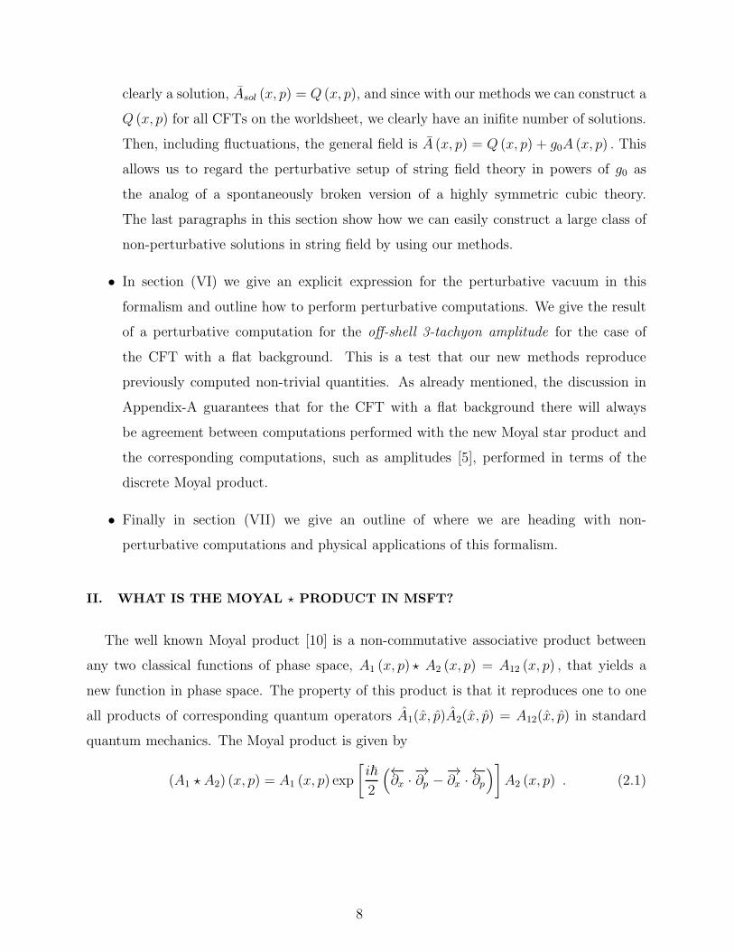
quantum mechanics. The Moyal product is given by

(A1 ⋆ A2) (x, p) = A1 (x, p) exp

[

i~

2

(←−∂x ·−→∂p −

−→∂x ·←−∂p

)

]

A2 (x, p) . (2.1)

8

where the left/right arrows mean differentiation of the function on the left/right sides. For

practical computations it is also convenient to write it in the forms

(A1 ⋆ A2) (x, p) = A1

((

x′ +i~

2

−→∂

∂p

)

,

(

p′ − i~

2

−→∂

∂x

))

A2 (x, p) , (2.2)

= A1 (x′, p′)A2

((

x− i~

2

←−∂

∂p′

)

,

(

p+i~

2

←−∂

∂x′

))

, (2.3)

where (x′, p′) is set to (x, p) after differentiation. All results of quantum mechanics in the

standard operator Hamiltonian formalism can be replicated in the Moyal formalism. For

example, the basic phase space variables satisfy, x ⋆ p = xp + i~2and p ⋆ x = xp − i~

2, while

their star commutator is

[xµ, pν ]⋆ = xµ ⋆ pν − pν ⋆ xµ = i~δµν , (2.4)

which is the expected result for the basic canonical quantization rules of the operators

[x, p] = i~ in the Hamiltonian formalism.

In the form of Eq.(2.5) the Moyal product is valid for fermions provided the orders of

fermionic xM , pM or fermionic A1, A2 are respected. To include both bosons and fermions(

xM , pM)

we denote M = (µ,m) where µ labels bosons and m labels fermions; we also

permit functions of phase space A (x, p) that could be either bosonic or fermionic. We will

define (−1)M or (−1)A where the exponent M or A means the grade, M,A = 0 for bosons

and M,A = 1 for fermions. Thus (−1)M or A = (−1)0 = 1 for bosons, and (−1)M or A

= (−1)1 = −1 for fermions. Changing the order of factors would cost an extra minus sign

when they are both fermions, such as−→∂ pM

←−∂ xM =

←−∂ xM

−→∂ pM (−1)MN . Then, the Moyal

product that works for both bosons and fermions is

(A1 ⋆ A2) (x, p) = A1 (x, p) exp

[

i~

2

(−→∂ pM

←−∂ xM − ←−∂ pM

−→∂ xM

)

]

A2 (x, p) . (2.5)

where the order of the derivatives and their order relative to A1, A2 need to be respected.

This gives the commutation rules (2.4) for boson as above, and also gives the anticommu-

tation rule for fermions

{xm, pn}⋆ = xm ⋆ pn + pn ⋆ xm = i~δmn , (2.6)

where we watch the orders when taking derivatives as follows,

A←−∂ xN = (−1)AN ∂xNA, or xM

←−∂ xN = (−1)MN ∂xNxM = (−1)M δMN . (2.7)

9

Then the general star commutator for any M = (µ,m) gives

[xM , pN}⋆ = i~δMN , (2.8)

for both bosons and fermions, where the symbol [·, ·}⋆ means either commutator or anti-

commutator as needed. The expressions in (2.2,2.3) could be used also for both bosons and

fermions.

We emphasize that the usual anticommutation rules for fermions, with both xm and pm

Hermitian must contain ~ rather than i~ on the right hand side of Eq.(2.6). In this paper,

for notational uniformity of the Moyal product for both bosons and fermions, we wish to

use i~, so this implies that in this paper xm for fermions is defined to be antihermitian while

pm is Hermitian.

A. The new ⋆ product

In the Moyal formulation of SFT (MSFT), string joining, not ordinary quantum mechan-

ics, is also represented by a stringy Moyal ⋆ product as discovered in [2]. In this paper we

suggest a new formulation of MSFT with the following new version of the ⋆ in the σ-basis

⋆ = exp

[

i

4

∫ π

0

dσ sign(π

2− σ

)(−→∂ pM (σ)

←−∂ xM (σ,ε) −

←−∂ pM (σ)

−→∂ xM (σ,ε)

)

]

. (2.9)

One of the most important properties of this expression is that it is independent of any

background conformal field theory (CFT) that describes the free string. The reason for

background independence independence is the fact that it is defined in phase space. The no-

tion of phase space is quite independent of any Lagrangian formalism on the worldsheet that

describes the free string propagating in some background fields. Although the Lagrangian

provides a background dependent relation between velocities and momenta through the stan-

dard definition PM = ∂S/(

∂τXM)

, the properties of phase space(

XM , PM

)

are completely

independent of the Lagrangian. Note in particular the natural upper and lower indices: no

background metric is involved in lowering the index of PM . This is the key to background

independence. Since it will require quite a few details to explain how this ⋆ product is de-

rived, we highlight here the crucial conceptual features of this formalism to focus the reader

on aspects that are important for SFT.

1. The ⋆ in (2.9) contains the small parameter ε in the x (σ, ε) which is a regulator to

separate the midpoint clearly in the process of string joining. As explained later, a

10

regulator is crucially needed to resolve ambiguities and related associativity anomalies

that were identified in the past [3][7]. This avoids the danger of formal manipulations

that could lead to wrong computations, thus making the new MSFT a finite theory in

which every step of a computation is well defined.

2. We define the basis on which the derivatives ∂p(σ), ∂x(σ,ε) in the star product act. The

string field A (x (σ, ε) , p (σ)) is a functional of half of the phase space of the string as

follows. This half-phase-space (x (σ, ε) , p (σ)) is the regulated σ-basis which is closely

related to the position basis ψ (X (σ, ε)) by a Fourier transform. The regulated string

position X (σ, ε) , which contains a small parameter ε, is related to the unregulated

one X (σ) by a simple redefinition of the choice of independent position degrees of

freedom to be used to label the string field ψ (X (σ, ε)) . The relation is X (σ, ε) =

exp(

−ε√

−∂2σ)

X (σ) as will be explained below in some detail. The unregulated

momentum P (σ) is the canonical conjugate to the unregulated X (σ). The position

and momentum degrees of freedom are split into the symmetric/antisymmetric parts

relative to the midpoint at σ = π/2

x± (σ, ε) =1

2(X (σ, ε)±X (π − σ, ε)) , (2.10)

p± (σ) =1

2(P (σ)± P (π − σ)) . (2.11)

For simplicity of notation in most of the paper we will omit the ± on x+ and p− (but

keep the ± for p+ and x−), thus we will use interchangeably the following notation

x+ (σ, ε) ≡ x (σ, ε) and p− (σ) ≡ p (σ) . (2.12)

Thus, the position space string field ψ (X (σ, ε)) is a functional of the symmet-

ric and antisymmetric parts of the string position ψ (X) = ψ (x+, x−) . The field

A (x+ (σ, ε) , p− (σ)) is a half-fourier transform of the field ψ (X) = ψ (x+, x−) in the

antisymmetric variable only

ψ (x+, x−)Fourier→x−→p−

A (x+, p−) (2.13)

Hence the antisymmetric p− (σ) = −p− (π − σ) is the canonical conjugate to the an-

tisymmetric part of the string x− (σ, ε) in usual first quantization if the regulator ε is

ignored. Similarly, the even label x+ (σ, ε) = x+ (π − σ, ε) is the symmetric part of the

11

position, and it includes a regulated midpoint x (ε) = X (π/2, ε) = x+ (π/2, ε). Due to

the symmetry/antisymmetry properties, it is evident that x+ (σ, ε) , p− (σ) are compat-

ible observables: namely, their operator counterparts x+ (σ, ε) , p− (σ) commute with

each other in the first quantization of the string, that is, although[

X (σ, ε) , P (σ′)]

6= 0

does not vanish at σ = σ′, the commutator [x+ (σ, ε) , p− (σ′)] = 0 does vanish for all

values of σ, σ′. Hence as eigenvalues of commuting operators, (x+ (σ, ε) , p− (σ)) is a

set of complete labels for the string field A (x+ (σ, ε) , p− (σ)) which is nothing but the

wavefunction in first quantization taken in an appropriate basis A (x+ (σ, ε) , p− (σ)) =

〈x+ (σ, ε) , p− (σ) |A〉.

3. The dot products that appear in the ⋆, such as←−∂ x(σ,ε) ·

−→∂ p(σ), mean

−→∂ p(σ) ·

←−∂ x(σ,ε) =

−→∂

∂pM (σ)

←−∂

∂xM (σ, ε), (2.14)

where the sum overM = (µ,m) includes matter and ghosts (xµ, xm) , where the ghosts

xm with m = c, b account for the fermionic ghost degrees of freedom b±± (σ, τ) and

c± (σ, τ) as given explicitly in Eq.(5.7). This ⋆ product applies to both bosons (label

µ) and fermions (label m). Changing the order of factors would cost a minus sign in

the fermion-like ghost directions M = m as explained after Eq.(2.4).

4. Because no metric appears in the contraction of covariant and contravariant indices of

canonical variables, the dot product in Eq.(2.14) is background independent for any

set of background fields in a conformal field theory that describes the string action

and the BRST operator.

5. The matter and ghosts in each supervector xM , pM in Eq.(2.4) can be rotated into

each other under OSp(d|2) supertransformations, xM → xN (S−1)MN and pM → S N

M pN

where S ∈OSp(d|2) mixes matter and ghost degrees of freedom. The new star product

in Eq.(2.9), and therefore the string interaction terms in the new MSFT are evidently

symmetric under this OSp(d|2). Although this symmetry is broken by the BRST

operator, keeping track of this symmetry greatly simplifies computations.

6. The sum over the degrees of freedom in the integral in (2.9), i4

∫ π

0dσ sign

(

π2− σ

)

(· · · ) ,may be rewritten as a half-range integral i

2

∫ π/2

0dσ (· · · ) after taking into account the

antisymmetric properties of (· · · ) . This shows clearly that only half of the string phase

12

space degrees of freedom are relevant in our formulation. We prefer the version with

the full range integral because the sign(

π2− σ

)

factor will clarify several interesting

features.

7. The antisymmetry of the integrand (· · · ) in (2.9) shows that the midpoint x (ε) =

x (π/2, ε) has no contribution to the non-trivial properties of the ⋆ since, at the mid-

point, the quantity (· · · ) vanishes due to the antisymmetry of ∂/∂p− (σ) , namely

∂/∂p− (π/2) = 0. Accordingly, the ⋆ product (2.9) is local at the midpoint since

∂/∂x (ε) does not occur in it. That is, in the product A1 ⋆ A2 = A12 the three fields

A1, A2, A12 are all functions of the same midpoint x (ε) , showing that the joining of

strings is implemented locally at the same midpoints of the first, second and final

strings. This desired property of string joining is automatically implemented in our

formalism using, xM+ (σ, ε) for all σ, without the need of a special treatment of the

midpoint. This is a very important key feature that greatly simplified our formalism.

In the next section we will first review some of the properties of the standard Moyal

product in quantum mechanics for a self sufficient presentation, and then indicate how to

deduce from those properties that string joining is also conveniently expressed as the ⋆

product given above.

III. MOYAL ⋆ IN QM AS INSPIRATION FOR STRING JOINING

It is useful to recall the essential ingredients of how the Moyal product works in quantum

mechanics (QM) because these same mathematical ingredients are behind the Moyal star

product that describes string joining or splitting in the context of SFT [1] as discovered in

[2]. We will use the same method as [2] again in this paper to construct the new ⋆ product in

the σ-basis and show that in this formalism MSFT may be viewed as a quantum mechanics

type system which we call henceforth induced quantum mechanics (iQM) to distinguish it

from ordinary QM.

In QM each quantum operator A(x, p) has a matrix representation in position space,

〈xL|A|xR〉 = ψ (xL, xR) , where xL, xR are eigenvalues of the position operator x. All prop-

erties of the product of two operators A12 = A1A2 is captured by the matrix product,

〈xL|A12|xR〉 = 〈xL|A1A2|xR〉 =∫

dz〈xL|A1|z〉〈z|A2|xR〉, which we may write in terms of the

13

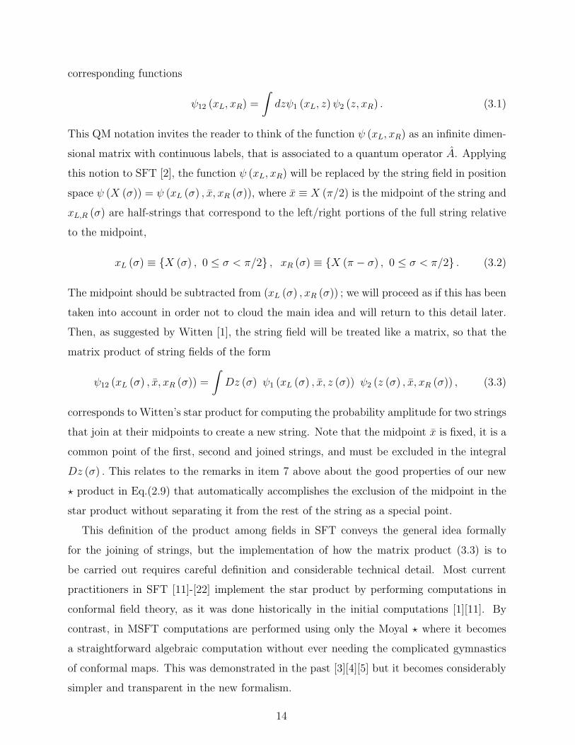
corresponding functions

ψ12 (xL, xR) =

∫

dzψ1 (xL, z)ψ2 (z, xR) . (3.1)

This QM notation invites the reader to think of the function ψ (xL, xR) as an infinite dimen-

sional matrix with continuous labels, that is associated to a quantum operator A. Applying

this notion to SFT [2], the function ψ (xL, xR) will be replaced by the string field in position

space ψ (X (σ)) = ψ (xL (σ) , x, xR (σ)), where x ≡ X (π/2) is the midpoint of the string and

xL,R (σ) are half-strings that correspond to the left/right portions of the full string relative

to the midpoint,

xL (σ) ≡ {X (σ) , 0 ≤ σ < π/2} , xR (σ) ≡ {X (π − σ) , 0 ≤ σ < π/2} . (3.2)

The midpoint should be subtracted from (xL (σ) , xR (σ)) ; we will proceed as if this has been

taken into account in order not to cloud the main idea and will return to this detail later.

Then, as suggested by Witten [1], the string field will be treated like a matrix, so that the

matrix product of string fields of the form

ψ12 (xL (σ) , x, xR (σ)) =

∫

Dz (σ) ψ1 (xL (σ) , x, z (σ)) ψ2 (z (σ) , x, xR (σ)) , (3.3)

corresponds to Witten’s star product for computing the probability amplitude for two strings

that join at their midpoints to create a new string. Note that the midpoint x is fixed, it is a

common point of the first, second and joined strings, and must be excluded in the integral

Dz (σ) . This relates to the remarks in item 7 above about the good properties of our new

⋆ product in Eq.(2.9) that automatically accomplishes the exclusion of the midpoint in the

star product without separating it from the rest of the string as a special point.

This definition of the product among fields in SFT conveys the general idea formally

for the joining of strings, but the implementation of how the matrix product (3.3) is to

be carried out requires careful definition and considerable technical detail. Most current

practitioners in SFT [11]-[22] implement the star product by performing computations in

conformal field theory, as it was done historically in the initial computations [1][11]. By

contrast, in MSFT computations are performed using only the Moyal ⋆ where it becomes

a straightforward algebraic computation without ever needing the complicated gymnastics

of conformal maps. This was demonstrated in the past [3][4][5] but it becomes considerably

simpler and transparent in the new formalism.

14

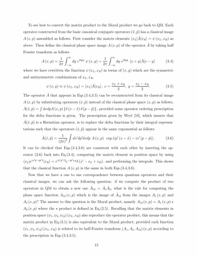
To see how to convert the matrix product to the Moyal product we go back to QM. Each

operator constructed from the basic canonical conjugate operators (x, p) has a classical image

A (x, p) assembled as follows. First consider the matrix elements 〈xL|A|xR〉 = ψ (xL, xR) as

above. Then define the classical phase space image A (x, p) of the operator A by taking half

Fourier transform as follows

A (x, p) =1

2π

∫ ∞

−∞dy e2ipy ψ (x, y) =

1

2π

∫ ∞

−∞dy e2ipy 〈x+ y|A|x− y〉 (3.4)

where we have rewritten the function ψ (xL, xR) in terms of (x, y) which are the symmetric

and antisymmetric combinations of xL, xR,

ψ (x, y) ≡ ψ (xL, xR) = 〈xL|A|xR〉, x =xL + xR

2, y =

xL − xR2

. (3.5)

The operator A that appears in Eqs.(3.4,3.5) can be reconstructed from its classical image

A (x, p) by substituting operators (x, p) instead of the classical phase space (x, p) as follows,

A(x, p) =∫

dxdpA (x, p) {δ (x− x) δ (p− p)} , provided some operator ordering prescription

for the delta functions is given. The prescription given by Weyl [10], which insures that

A(x, p) is a Hermitian operator, is to replace the delta functions by their integral represen-

tations such that the operators (x, p) appear in the same exponential as follows

A(x, p) =1

(2π)2

∫

dx′dp′dxdp A (x, p) exp (ip′ (x− x)− ix′ (p− p)) . (3.6)

It can be checked that Eqs.(3.4,3.6) are consistent with each other by inserting the op-

erator (3.6) back into Eq.(3.4), computing the matrix element in position space by using

〈xL|eix′p−ip′x|xR〉 = eix′p′/2e−ip′xRδ (x′ − xL + xR) , and performing the integrals. This shows

that the classical function A (x, p) is the same in both Eqs.(3.4,3.6).

Now that we have a one to one correspondence between quantum operators and their

classical images, we can ask the following question: if we compute the product of two

operators in QM to obtain a new one A12 = A1A2, what is the rule for computing the

phase space function A12 (x, p) which is the image of A12 from the images A1 (x, p) and

A2 (x, p)? The answer to this question is the Moyal product, namely A12 (x, p) = A1 (x, p) ⋆

A2 (x, p) where the ⋆ product is defined in Eq.(2.5). Recalling that the matrix elements in

position space (ψ1, ψ2, ψ12) (xL, xR) also reproduce the operator product, this means that the

matrix product in Eq.(3.1) is also equivalent to the Moyal product, provided each function

(ψ1, ψ2, ψ12) (xL, xR) is related to its half-Fourier transform (A1, A2, A12) (x, p) according to

the prescription in Eqs.(3.4,3.5).

15

Coming back to SFT, the content of the previous paragraph was the basic inspiration in

[2] that led to the rewriting of the matrix-like product in Eq.(3.3) as a Moyal product. In

[2] this was done for the modes of the string in a flat target spacetime. Using Eq.(2.9) we

now do it in the σ-basis which can be used in the presence of any set of background fields

in a conformal field theory that describes a string. So, imitating Eq.(2.5) we are led to its

stringy analog in (2.9) in order to reproduce the matrix product in string joining

A12 (x+ (σ, ε) , p− (σ)) = A1 (x+ (σ, ε) , p− (σ)) ⋆ A2 (x+ (σ, ε) , p− (σ)) , (3.7)

where we replace the pointlike (x, p) in Eq.(2.5) by the stringlike (x+ (σ, ε) , p− (σ)) , includ-

ing the regulator ε. For now ignore the complication of the midpoint in Eq.(3.3) which is

what the ε is for; we will explain this below. The basis (x+ (σ, ε) , p− (σ)) emerges from

taking into account the map between ψ and A in Eq.(3.4,3.5). In this map we must take

x+ (σ, ε) = 12(xL (σ, ε) + xR (σ, ε)) , while p− (σ) should be the Fourier transform parameter

for x− (σ, ε) = 12(xL (σ, ε)− xR (σ, ε)). This means x+ (σ, ε) is the symmetric part of the

string X (σ, ε), while p− (σ) is the antisymmetric part of the momentum P (σ) . So, in terms

of the full string degrees of freedom (X (σ, ε) , P (σ)) the relevant symmetric/antisymmetric

parts are given precisely by Eqs.(2.10-2.12). This explains the logic why, except for some

midpoint details, string joining is represented by the Moyal star product. We will discuss

the details of the midpoint, but for now note that x+ (σ, ε) includes the midpoint but the

string joining Moyal star excludes it as outlined in item (7) in section (IIA). So no special

treatment of the midpoint is needed.

It is important to emphasize that the new formalism applies now to string theory for any

set of conformally consistent background fields contained in the worldsheet CFT. This is

because the ⋆ product is expressed in terms of the phase space degrees of freedom which is a

notation that is independent of the geometrical details of the background fields. The infor-

mation about the background geometry is buried in the canonical formalism that includes

the relation between the velocity and momentum as well as in the stress tensor or BRST

operator of the CFT. But none of this geometrical information enters in the star product

(2.9). Hence the star product for string joining defined in this way provides a background

independent method of expressing string-string interactions via the joining of strings.

16

A. String Joining iQM versus QM

Although the setup presented above for the Moyal ⋆ in MSFT resembles quantum me-

chanics (QM), the stringy ⋆ in Eq.(2.9) does not arise because of the first quantization of

the string as was the case of the particle in Eq.(2.5). Instead, the star product (2.9) is

designed to formulate string joining or splitting. The resemblance to QM is intriguing and

it even invites the thought that string joining could be considered as an origin for QM as

we comment at the end of this section.

Below we will use the induced quantum mechanics (iQM) basis (x+ (σ, ε) , p− (σ)) to con-

struct a representation of the first quantized QM operators of the string(

X (σ, ε) , P (σ))

.

That is, QM will be built from iQM. This representation will clarify the relation and the dif-

ference between QM and iQM while also show how to represent all string theory operators,

such as the stress tensor, BRST current JB (σ) and the BRST operator, in the iQM basis

(x+ (σ, ε) , p− (σ)) for any conformal field theory on the worldsheet (CFT) that describes the

string moving in a conformally consistent set of background fields.

Starting from the definitions of x±, p± in Eq.(2.10), we write the full string first quantized

QM operators X (σ, ε) , P (σ) in terms of the antisymmetric and symmetric parts

XM (σ, ε) = xM+ (σ, ε) + xM− (σ, ε) , PM (σ) = p+M (σ) + p−M (σ) , (3.8)

The regulator ε will be carefully discussed in section IV but it is not needed to explain the

concepts in this section. Although we will carry on the regulator ε for consistency with

the rest of the paper, the reader would probably understand this section more easily by

first setting ε = 0 everywhere, and then reviewing it again by recalling the definition of

the regulated position operator, XM (σ, ε) = exp(−ε√

−∂2σ)XM (σ) , and that M = (µ,m)

denotes µ for spacetime and m for ghosts.

The QM rules for the first quantization of the string are (anticommutator for the ghosts)

[XM (σ, ε) , PN (σ′)} = [e−ε|∂σ |XM (σ) , PN (σ′)} = iδMN δε (σ, σ′) , (3.9)

where |∂σ| ≡√

−∂2σ and

δε (σ, σ′) ≡ e−ε|∂σ |δ (σ, σ′) (3.10)

is a regulated delta function defined below. Here PM (σ) is defined for any conformal field

theory, with arbitrary string background fields, in the canonical way, from the string La-

grangian, PM (σ) = ∂Lstring/∂(∂τXM (σ)). Note that, for any set of background fields in

17

the CFT Lstring, the position XM (σ) is a contravariant vector while the momentum PM (σ)

is a covariant vector, so that the commutation rules (3.9), with δMN δε (σ, σ′) on the right

hand side, are background independent. Furthermore, the δ (σ, σ′) is a Dirac delta function

which must be consistent with Neumann or Dirichlet boundary conditions at the end points

σ = 0, π and σ′ = 0, π (D-branes). There are two types: δnnε (σ, σ′) for Neumann-Neumann,

and δddε (σ, σ′) for Dirichlet-Dirichlet, as given in Eqs.(4.2-4.5). Mostly we simply write

δε (σ, σ′) and use the appropriate version when necessary. When it becomes important to

keep track of boundary condition properties in different directions M, more carefully we

will write δMN δεM (σ, σ′) , where δεM (σ, σ′) stands for δnnε (σ, σ′) or δddε (σ, σ′) . There will be

more refinements introduced for the δ (σ, σ′)’s, including “even” δ+ (σ, σ′), “odd” δ− (σ, σ′) ,

and “midpoint” δ (σ, σ′) versions, that include also a regulator ε, as will be shown explicitly

below. Thus, D-branes enter our formalism in this way through the details of these delta

functions that are sensitive to the boundary conditions applied to the ends of the string.

From (3.9) the QM rules for the operators x±, p± are derived. First note that the even

degrees of freedom commute with the odd ones

[x± (σ, ε) , p∓ (σ′)] = 0, (3.11)

while the non-trivial QM rules are

[x± (σ, ε) , p± (σ′)] =1

4

[

e−ε|∂σ |(

X (σ)± X (π − σ))

,(

P (σ′)± P (π − σ′))]

(3.12)

=i

2e−ε|∂σ | (δ (σ, σ′)± δ (π − σ, σ′)) ≡ i

2δ±ε (σ, σ′) . (3.13)

The last equation defines the even and odd regulated delta functions δ±ε (σ, σ′) that will

appear again later. Their explicit formulas are given in Eqs.(4.6-4.9) and their properties

are illustrated for a small ε in Figs.(1,2).

The eigenvalues of the operator XM (σ, ε) form a complete set of labels for the wavefunc-

tion (string field) in position space ψ (X (σ, ε)) ≡ ψ (x+ (σ, ε) , x− (σ, ε)) . This labelling

is equivalent to the position space labelling without a regulator, namely Ψ (X (σ)) =

ψ (X (σ, ε)) , but as independent labels we prefer to use the eigenvalues of the regulated

X (σ, ε) which amounts to a reshuffling of the eigenvalues of the unregulated X (σ) . Either

way, the unregulated operator P (σ) is represented in position space by the unregulated

derivative P (σ)→ −i∂/∂X (σ) . However, since we insist on the regulated labeling we must

18

use the chain rule to compute it on ψ (X (σ, ε)) , that is

iPM (σ)ψ (X (·, ε)) = ∂ψ (X (·, ε))∂XM (σ)

=

∫

dσ′∂ψ (X (·, ε))∂XN (σ′, ε)

∂XN (σ′, ε)

∂XM (σ)

=

∫

dσ′∂ψ (X (·, ε))∂XM (σ′, ε)

e−ε|∂σ′ |δ (σ, σ′)

= e−ε|∂σ |∂ψ (X (·, ε))∂XM (σ, ε)

. (3.14)

Here we have used the definition of X (σ′, ε), and the natural differential rule for the unreg-

ulated symbols ∂X (σ′) /∂X (σ) = δ (σ, σ′) , to obtain the following rules of computation.

regulated delta: ∂X(σ′,ε)∂X(σ)

= e−ε|∂σ |δ (σ, σ′) ≡ δε (σ, σ′) ,

unregulated delta: ∂X(σ′,ε)∂X(σ,ε)

= δ (σ, σ′) ,

regulated delta: e−ε|∂σ | ∂X(σ′,ε)∂X(σ,ε)

= e−ε|∂σ|δ (σ, σ′) ≡ δε (σ, σ′) ,

(3.15)

The last one, which is the only rule needed to represent the momentum according to

Eq.(3.14), always yields well defined regulated results. So, when ψ is just X (σ′, ε) , we

get P (σ)ψ = −ie−ε|∂σ | ∂X(σ′,ε)∂X(σ,ε)

= −iδε (σ, σ′) , which is consistent with the commutation

rules (3.9). Rewriting this in terms of the symmetric/antisymmetric labels we get the rep-

resentation for p±

ip±M (σ)ψ (x+ (·, ε) , x− (·, ε)) = 1

2e−ε|∂σ |

(

∂ψ (x+, x−)

∂x± (σ, ε)

)

(3.16)

and the rules for computation are

∂x± (σ′, ε)

∂x± (σ, ε)= (δ (σ, σ′)± δ (π − σ, σ′)) ≡ δ± (σ, σ′) , unregulated delta, (3.17)

so that when ψ is just x± (σ′, ε) , we get p± (σ)ψ = − i2e−ε|∂σ | ∂x±(σ′,ε)

∂x±(σ,ε)= −iδ±ε (σ, σ′) , a

regulated delta, which is consistent with the commutation rules (3.12).

In summary, in position space we have the following representation of the full string QM

operators

XM (σ, ε)ψ (x+, x−) =(

xM+ (σ, ε) + xM− (σ, ε))

ψ (x+, x−) (3.18)

PM (σ)ψ (x+, x−) = −i

2e−ε|∂σ |

(

∂ψ (x+, x−)

∂xM+ (σ, ε)+∂ψ (x+, x−)

∂xM− (σ, ε)

)

, (3.19)

and to compute we use the differentiation rules in Eq.(3.17).

We now turn to the string field in the mixed phase space basis A (x+, p−) , which is the

Fourier transform of ψ (x+, x−) in the (−) variable as in Eq.(2.13). The path-integral Fourier

19

transform of ψ(

xM+ (·, ε) , xM− (·, ε))

is precisely A (x (·, ε) , p (·))

A (x (·, ε) , p (·)) =∫

(Dx− (·, ε)) exp[

−i∫ π

0

dσ xM− (σ, ε) pM (σ)

]

ψ (x+ (·, ε) , x− (·, ε))(3.20)

In the Fourier exponent we divided by a factor of 2 as compared to Eq.(3.4) to take into

account the double counting due to the antisymmetry of x− (σ, ε) · p (σ) when reflected from

π/2. In the basis A (x+, p−) the operators x+ (σ, ε) , p− (σ) are diagonal, while the operators

p+, x− act like derivatives. Either by taking Fourier transform of Eqs.(3.18,3.19) or directly

from the commutation rules (3.12) we derive the representations of all operators x±, p± on

this basis

x+ (σ, ε)A (x+, p−) = x+ (σ, ε)A (x+, p−) , p− (σ)A (x+, p−) = e−ε|∂σ|p− (σ)A (x+, p−)

(3.21)

xM− (σ, ε)A (x+, p−) =i

2

∂A (x+, p−)

∂p−M (σ), p+M (σ)A (x+, p−) = −

i

2e−ε|∂σ |∂A (x+, p−)

∂xM+ (σ, ε). (3.22)

Then the full string QM operators have the following representation

XM (σ, ε)A (x+, p−) =

(

xM+ (σ, ε) +i

2

∂

∂p−M (σ)

)

A (x+, p−) , (3.23)

PM (σ)ψ (x+, x−) = e−ε|∂σ|(

p−M (σ)− i

2

∂

∂xM+ (σ, ε)

)

A (x+, p−) . (3.24)

From Eq.(3.9) to Eq.(3.24) we described the QM of the string in any background CFT

and how to represent its basic quantum operators X, P on the field A (x+, p−). This is

sufficient to obtain the representation of any other observable in this CFT, such as the

BRST operator, in the MSFT formalism. We will do this later, but first we relate this

differential operator representation to something more elegant in the language of the Moyal

⋆ product.

Now we turn to the induced QM (iQM) generated by the Moyal ⋆ for string joining for

any CFT. We will show that QM is represented in terms of iQM. First observe that using

the ⋆ in Eq.(2.9), and the differentiation rules (3.17), we get a non-trivial ⋆ commutator

20

between x+ (σ, ε) and p− (σ)

[xM+ (σ1, ε) , p−N (σ2)}⋆= xM+ (σ1, ε) ⋆ p−N (σ2)− (−1)MN p−N (σ2) ⋆ x

M+ (σ1, ε)

= iδMN sign(π

2− σ1

)

δ− (σ1, σ2) = iδMN δ+ (σ1, σ2) sign(π

2− σ2

)

≡ iδMN δ+− (σ1, σ2) . (3.25)

This is the induced QM. It has nothing to do with ordinary quantum mechanics since

under QM the operators xM+ (σ1, ε) , p−N (σ2) commute with each other as seen in Eq.(3.11),

whereas their eigenvalues do not commute under the string-joining iQM of Eq.(3.25).

The Dirac δ+− (σ1, σ2) function, that combines the sign function with the unregulated

delta functions δ± of Eq.(3.13), satisfies the appropriate (nn) or (dd) boundary conditions

consistent with the properties of xM+ (σ1, ε) , p−N (σ2). Furthermore, relative to the midpoint

δ+− (σ1, σ2) is symmetric in σ1 → (π − σ1) and antisymmetric in σ2 → (π − σ2) . The equiv-alence of the two forms of δ+− (σ1, σ2) given above is verified by using the properties of the

unregulated delta functions as follows

δ+− (σ1, σ2) = sign(π

2− σ1

)

δ− (σ1, σ2) (3.26)

= sign(π

2− σ1

)

(δ (σ1, σ2)− δ (σ1, π − σ2))

= sign(π

2− σ2

)

δ (σ1, σ2)− sign(π

2− (π − σ2)

)

δ (σ1, π − σ2)

= sign(π

2− σ2

)

δ (σ1, σ2)− sign(

−(π

2− σ2

))

δ (σ1, π − σ2)

= (δ (σ1, σ2) + δ (σ1, π − σ2)) sign(π

2− σ2

)

= δ+ (σ1, σ2) sign(π

2− σ2

)

. (3.27)

Thus, δ+− (σ1, σ2) is a distribution that has the following important properties under re-

flections from the midpoint: it is even under σ1 → (π − σ1) and odd under σ2 → (π − σ2)and vanishes at both σ1 = π/2 and σ2 = π/2. These properties can be verified from the

two equivalent forms of δ+− (σ1, σ2) given above, or by integrating with smooth functions,

or by expanding in modes. This means in Eq.(3.25) that the midpoint xM (ε) = xM+ (π/2, ε)

star-commutes with p−N (σ2) including σ2 = π/2, so the midpoint does not participate in

the joining operation of strings - this is one of the desired properties of the ⋆ product as

emphasized in point 7 in section (IIA). This vital property is encoded in the ⋆ product in

Eq.(2.9) as well as the δ+− (σ1, σ2) that appears in the iQM.

21

Central features of the iQM follows from the following left and right products of the field

with the classical half phase space x+ (σ, ε) , p− (σ)

xM+ (σ, ε) ⋆ A (x+, p−) =

(

xM+ (σ, ε) +i

2sign

(π

2− σ

)

∂p−M (σ)

)

A (x+, p−) (3.28)

A (x+, p−) ⋆ xM+ (σ, ε) = A (x+, p−)

(

xM+ (σ, ε)− i

2

←−∂ p−M (σ)sign

(π

2− σ

)

)

(3.29)

p−M (σ) ⋆ A (x+, p−) =

(

p−M (σ)− i

2sign

(π

2− σ

)

∂xM+ (σ,ε)

)

A (x+, p−) (3.30)

A (x+, p−) ⋆ p−M (σ) = A (x+, p−)

(

p−M (σ) +i

2

←−∂ xM

+(σ,ε)sign

(π

2− σ

)

)

(3.31)

By comparing these results to Eqs.(3.23,3.24) we see that the full string QM operators

XM (σ, ε) , PM (σ) can be represented in terms of the string joining star product in the half

phase space as follows

XM (σ, ε)A (x+, p−) =

θ(

π2− σ

)

xM+ (σ, ε) ⋆ A (x+, p−)

+θ(

σ − π2

)

A (x+, p−) ⋆ xM+ (σ, ε) (−1)MA

, (3.32)

PM (σ)A (x+, p−) = e−ε|∂σ |

θ(

π2− σ

)

p−M (σ) ⋆ A (x+, p−)

+θ(

σ − π2

)

A (x+, p−) ⋆ p−M (σ) (−1)MA

, (3.33)

where the sign factor (−1)MA accounts for boson/fermion properties of the field A and the

operator labeled by M. Described in words, the structures (3.32,3.33) show that depending

on whether σ is less or more than π/2 the action of the full string quantum operators

XM (σ, ε) , PM (σ) on the field is reproduced by the left or right Moyal ⋆ product with

the half phase space. In more detail, one can check that the star product reproduces the

non-derivative as well the derivative terms in Eqs.(3.23,3.24) for all 0 ≤ σ ≤ π, including

σ = π/2, since

1 = θ(π

2− σ

)

+ θ(

σ − π

2

)

, (3.34)

1 = sign(π

2− σ

)(

θ(π

2− σ

)

− θ(

σ − π

2

))

. (3.35)

It is clear that this works correctly as long as σ 6= π/2. In order to also work correctly at

σ = π/2 we must define carefully what values the symbols sign(

π2− σ

)

, θ(

π2− σ

)

, θ(

σ − π2

)

take at σ = π/2. Thus, in our definition, the distribution sign(

π2− σ

)

does not vanish at

σ = π/2, but rather its value at π/2 is ±1 depending on the approach to the midpoint

from below or above as σ → π/2 ∓ 0. Similarly, in our definitions, the functions θ(

π2− σ

)

22

or θ(

σ − π2

)

do not take the value 1/2 at σ = π/2, but rather they are equal to 1 or 0

depending on the approach to the midpoint from below or above as σ → π/2 ∓ 0. Then,

sign(

π2− σ

)

= θ(

π2− σ

)

− θ(

σ − π2

)

, takes the values ±1 as usual, except that this does

not vanish at π/2 due to the careful definition. Hence Eq.(3.35) is satisfied for all 0 ≤ σ ≤ π,

including σ = π/2.

One can now check that all the rules of quantum mechanics from Eq.(3.9) to Eq.(3.24)

are correctly reproduced by the iQM representation of the operators (3.32,3.33), including

at the midpoint σ = π/2. From now on we do not need anymore the ± labels on the x+, p−

and we can write the representation of the quantum operators more simply as

XM (σ, ε)A (x, p) =

xM (σ, ε) ⋆ A (x, p) , if 0 ≤ σ ≤ π/2

A (x, p) ⋆ xM (σ, ε) (−1)MA , if π/2 ≤ σ ≤ π, (3.36)

PM (σ)A (x, p) =

(

e−ε|∂σ |pM (σ))

⋆ A (x, p) , if 0 ≤ σ ≤ π/2

A (x, p) ⋆(

e−ε|∂σ |pM (σ))

(−1)MA , if π/2 ≤ σ ≤ π. (3.37)

We also do not need to watch too carefully the midpoint x (ε) in most cases since we have

seen that x (ε) acts trivially (like a number, or an eigenvalue) under the ⋆ in iQM. If need

be, at σ = π/2 we can use Eqs.(3.32,3.33) or equivalently Eqs.(3.23,3.24) if more care is

warranted in some computations.

Indeed, note that the ⋆ in iQM in Eq.(3.33) does produce correctly a derivative contri-

bution of the momentum operator PM (σ) at the midpoint with a regulator PM (π/2) →(−i/2) e−ε|∂π/2| (∂/∂x (π/2, ε)) , as it should be, according to QM in Eq.(3.24). This is a bit

subtle and requires more explanation. Having pointed out earlier that the derivatives in the

star product do not act on the midpoint when considering string joining, one may wonder

how the midpoint derivative in Eq.(3.24) is reproduced from the star product representation

in Eq.(3.33). This subtle point is explained as follows. Consider evaluating the star products

in (3.33) by using (3.30,3.31) and concentrate on the derivative piece which takes the form

− i

4e−ε|∂σ |

[

(

θ(π

2− σ

)

− θ(

σ − π

2

))

∫ π

0

dσ′δ− (σ, σ′) sign(π

2− σ′

) ∂A

∂x+ (σ′, ε)

]

, (3.38)

where the delta function arises from ∂p− (σ) /∂p− (σ′) = δ− (σ, σ′) . Naively this expression

appears to vanish at σ = π/2 since δ− (σ, σ′) vanishes at the midpoint, and hence no midpoint

contribution; but more care is needed. The distribution in the integrand has the following

property according to Eqs.(3.26-3.27), δ− (σ, σ′)sign(

π2− σ′) =sign

(

π2− σ

)

δ+ (σ, σ′) . Both

23

of these forms vanish at the midpoint as argued in (3.26-3.27). However, using the second

form, the sign function sign(

π2− σ

)

can be pulled out of the dσ′ integral, and after combining

it with the theta function factor in (3.38) it gives an overall factor of 1 according to Eq.(3.35),

including at the midpoint (we emphasize the careful definition of the sign function). In the

remaining dσ′ integrand δ+ (σ, σ′) by itself does not vanish at the midpoint, and Eq.(3.38)

yields the following result (recall that δ+ (σ, σ′) has two peaks in the range [0, π])

− i

4e−ε|∂σ|

[∫ π

0

dσ′δ+ (σ, σ′)∂A

∂x+ (σ′, ε)

]

= − i2e−ε|∂σ | ∂A

∂x+ (σ, ε). (3.39)

This is consistent with the expected result in Eq.(3.24) which includes the midpoint

derivative. The subtle property here is that the distribution sign(

π2− σ

)

δ+ (σ, σ′) =

δ− (σ, σ′)sign(

π2− σ′) has no support at the midpoint, but δ+ (σ, σ′) by itself does. The

theta function factor was crucial to remove the sign factor sign(

π2− σ

)

and lead the non-

trivial midpoint contribution. This exercise makes it evident that there are circumstances

in some computations where midpoint derivatives can arise from the new star product, and

this is indeed desirable, although straightforward generic string joining A ⋆ B is not one of

those circumstances.

IV. REGULATOR

Consider the fundamental canonical QM operators in string theory(

XM (σ) , PM (σ))

at

fixed τ for any CFT on the worldsheet. A basic tool of computation in CFT is the operator

product expansion which is a form of regularization that controls operator products at

the same point on the worldsheet. A moment of reflection would indicate that the same

regularization effect is captured by our proposed choice of independent degrees of freedom(

XM (σ, ε) , PM (σ))

where XM (σ, ε) = e−ε|∂σ |X (σ) is regulated while PM (σ) is not. This

is because |∂σ| ≡√

−∂2σ plays the role of an approximate time translation operator on the

worldsheet for a short amount of time even when there are background fields present in

the CFT. Thus applying a Euclidean time translation in the form e−ε|∂σ|X (σ) displaces the

worldsheet point from (σ, τ = 0) to (σ, τ = −iε) . Equivalently a point on the unit circle in

the complex z plane (z ≡ e±iσ) moves to the inside of the unit circle when the Euclidean

time translator e−ε|∂σ | acts on it, namely e−ε|∂σ |z = e−ε|∂σ |e±iσ = e−ε±iσ = z, with |z| < 1. In

this computation we used the fact that e±iσ (and similarly e±inσ) are degenerate eigenstates

24

of the operator |∂σ| , that is

|∂σ| e±inσ =√

−∂2σe±inσ = |n| e±inσ. (4.1)

Hence changing X (σ) to XM (σ, ε) amounts precisely to what is done in operator products

when two points are slightly displaced relative to each other, one on the unit circle and the

other inside the unit circle. By defining the theory including the regulator ε as proposed,

we can control all the relevant operator products in CFT at all intermediate stages of CFT

computations. Carrying this ε over to MSFT as we have done in the previous sections

insures that all MSFT computations will be finite at all intermediate stages. Only at the

end of MSFT computations we will set ε = 0 after a renormalization of the cubic coupling

constant.

A. Regulated delta functions

To perform computations in MSFT we must use the differentiation rules, such as

e−ε|∂σ2 | (∂X (σ1, ε) /∂X (σ2, ε)) etc., that emerged in section (IIIA) to represent the basic

quantum operators X (σ, ε) , P (σ) . The result of such derivatives involves various types of

delta functions, with or without regularization, that are also sensitive to D-brane boundary

conditions. In later computations there will be circumstances in which we must multiply

such delta functions with each other. Products of unregulated delta functions are not well

defined. However, in our case the parameter ε provides just the required regularization to

render such products well defined. Since the regularized deltas will be used for computation,

we provide the needed details for them below.

The basic case from which all others follow is the delta function that appears in the

QM commutation rules in Eq.(3.9)[

XM (σ1, ε) , PN (σ2)]

= iδMN δMε (σ1, σ2) , where the M

on δMε (σ1, σ2) is a reminder that in the direction M the operators satisfy either Neumann-

Neumann (nn) or Dirichlet-Dirichlet (dd) boundary conditions. Accordingly δMε (σ1, σ2) will

be either δnnε (σ1, σ2) or δddε (σ1, σ2) .

Thus for (nn) we have the following unique expression, δnnε (σ1, σ2) = e−ε|∂σ1 | δnn (σ1, σ2) ,that is a periodic Dirac delta function δnn (σ1, σ2) (when ε = 0) which also satisfies the

boundary conditions - its derivatives vanish at the string ends for either σ1 = 0, π or σ2 =

0, π. The regulated version is computed easily since cosnσ1 is an eigenstate of |∂σ1| , namely

25

|∂σ1| cosnσ1 =

√

−∂2σ1cos nσ1 = |n| cosnσ1. Hence the regulated δnnε (σ1, σ2) is

δnnε (σ1, σ2) =1

π+

2

π

∑

n≥1

e−εn cosnσ1 cosnσ2. (4.2)

By writing the cosines in terms of exponentials the series turns into a convergent geometric

series for any positive ε, so that it can be summed up and written in the following exact

form, and then approximated for small ε

δnnε (σ1, σ2) =1

2π

(

sinh ε2cosh ε

2

sinh2 ε2+ sin2 σ1−σ2

2

+sinh ε

2cosh ε

2

sinh2 ε2+ sin2 σ1+σ2

2

)

≃ ε/π

ε2 + 4 sin2 σ1−σ2

2

+ε/π

ε2 + 4 sin2 σ1+σ2

2

(4.3)

≃ δ

(

2 sinσ1 − σ2

2

)

+ δ

(

2 sin

(

σ1 + σ22

))

Recall that only the range 0 ≤ σ1, σ2 ≤ π matters. The first term has a peak at σ1 = σ2

when σ1, σ2 are both in the range [0, π] , while the second term has no peak in this range

unless σ1, σ2 are both at the end points 0 or π. For example if σ2 = 0 (or π) both terms have

peaks at σ1 = 0 (or π), but as seen with a nonzero ε, only half of the area under each curve

falls within the range [0, π] , so the effect is that the end points are included with the same

strength as any interior point. This is what should be expected with Neumann-Neumann

boundary conditions.

Similarly, for Dirichlet-Dirichlet boundary conditions δddε (σ1, σ2) appears in the commu-

tation rules. Due to the D-brane boundaries it must vanish at both string ends σ1 = 0, π

and σ2 = 0, π. Then it is uniquely given by

δddε (σ1, σ2) ≡2

π

∞∑

n=1

e−εn sinnσ1 sinnσ2. (4.4)

Summing up the geometric series we obtain the exact form for any ε and approximate forms

for small ε

δddε (σ1, σ2) =1

2π

(

sinh ε2cosh ε

2

sinh2 ε2+ sin2 σ1−σ2

2

− sinh ε2cosh ε

2

sinh2 ε2+ sin2 σ1+σ2

2

)

≃ ε/π

ε2 + 4 sin2 σ1−σ2

2

− ε/π

ε2 + 4 sin2 σ1+σ2

2

(4.5)

≃ δ

(

2 sinσ1 − σ2

2

)

− δ(

2 sin

(

σ1 + σ22

))

26

The first term has a peak at σ1 = σ2 while the second one has no peak in the range

0 ≤ σ1, σ2 ≤ π unless σ1, σ2 are both at the end points, but at either end point the peaks

of the two terms cancel each other. So there is no support at the end points. This is what

should be expected with Dirichlet-Dirichlet boundary conditions.

Now we can compute the other delta functions, δ±ε (σ1, σ2) = δε (σ1, σ2)± δε (σ1, π − σ2) ,either (nn) or (dd) , that emerge in taking derivatives with respect to xM+ (σ, ε) or pM (σ) .

These are given by

δ+nnε (σ1, σ2) =

2

π+

4

π

∑

e≥2

e−εe cos eσ1 cos eσ2, e = 2, 4, 6, · · · (4.6)

δ−nnε (σ1, σ2) =

4

π

∑

o≥1

e−εo cos oσ1 cos oσ2, o = 1, 3, 5, · · · (4.7)

where (e, o) are (even,odd) positive integers. Similarly, for (dd) boundary conditions we

have

δ+ddε (σ1, σ2) =

4

π

∑

o≥1

e−εo sin oσ1 sin oσ2, o = 1, 3, 5, · · · (4.8)

δ−ddε (σ1, σ2) =

4

π

∑

e≥2

e−εe sin eσ1 sin eσ2, e = 2, 4, 6, · · · (4.9)

The infinite sums can again be performed exactly. The result is obtained by applying the

instruction δ±Mε (σ1, σ2) = δMε (σ1, σ2) ± δMε (σ1, π − σ2) to the expressions in Eqs.(4.3,4.3)

for M = (nn) or (dd). Their fully summed exact expressions for any ε are

δ+nnε (σ1, σ2) =

2 (sinh 2ε) (cosh 2ε− cos 2σ1 cos 2σ2)

π (cosh 2ε− cos 2 (σ1 − σ2)) (cosh 2ε− cos 2 (σ1 + σ2))(4.10)

δ−nnε (σ1, σ2) =

8 (sinh ε) (cosσ1) (cosσ2)(

1 + cosh2 ε− cos2 σ1 − cos2 σ2)

π (cosh 2ε− cos 2 (σ1 − σ2)) (cosh 2ε− cos 2 (σ1 + σ2))(4.11)

δ+ddε (σ1, σ2) =

8 (sinh ε) (sin σ1) (sin σ2)(

cos2 σ1 + cos2 σ2 + sinh2 ε)

π (cosh 2ε− cos 2 (σ1 − σ2)) (cosh 2ε− cos 2 (σ1 + σ2))(4.12)

δ−ddε (σ1, σ2) =

2 (sinh 2ε) (sin 2σ1) (sin 2σ2)

π (cosh 2ε− cos 2 (σ1 − σ2)) (cosh 2ε− cos 2 (σ1 + σ2))(4.13)

From this we see that δ±Mε (σ1, σ2) have two peaks in the range 0 ≤ σ1, σ2 ≤ π, one at σ1 = σ2

and the other at σ1 = π − σ2. For small ε, the (nn) , (dd) distributions are almost the same

for most of the range, but they differ close to the end points as seen by comparing the plots

in Figs.(1,2), namely δ±ddε (σ1, σ2) vanishes at the end points. In the case of δ+M

ε (σ1, σ2)

27

both peaks are positive, but in the case of δ−Mε (σ1, σ2) the second peak is negative; so when

the peaks are at the midpoint σ1 = π/2 = σ2, the peaks in δ+Mε (σ1, σ2) add, while the

peaks in δ−Mε (σ1, σ2) cancel each other. Finally, when the peaks are all the way at the end

points, δ±nnε (σ1, σ2) have support with half of the area under each peak at each end point,

but δ±ddε (σ1, σ2) vanishes at each end point. These properties are illustrated in Figs.(1,2)

for a finite but small value of ε. As ε approaches zero the peaks become very tall and very

narrow while the plots for (nn) and (dd) appear to converge to each other and become the

same. But they are actually different from each other exactly at the end points even when

ε = 0.

∆Ε-nnHΣ, Σ '=

∆Ε+nn HΣ, Σ '=

Plot forΕ = 1 �10 andΣ ' = 1 �10

0.2 0.4 0.6 0.8 1.0Σ�Π

-3

-2

-1

1

2

3

∆Ε±nnHΣ,Σ'<

Fig.(1) - Plot of δ±nnε (σ, σ′) for ε = 1/10 and σ′ = 1/10

∆Ε-ddHΣ, Σ '=

∆Ε+dd HΣ, Σ '=

Plot forΕ = 1 �10 andΣ ' = 1 �10

0.2 0.4 0.6 0.8 1.0Σ�Π

-3

-2

-1

1

2

3

∆Ε±ddHΣ,Σ'<

Fig.(2) - Plot of δ±ddε (σ, σ′) for ε = 1/10 and σ′ = 1/10

B. Midpoint not treated separately

We have seen that the new ⋆ product (2.9) does not treat the midpoint in a special way,

nevertheless is able to subtly exclude the midpoint from the star product in the process of

28

string joining. This desirable outcome seems natural but it took a lot of effort to reach this

stage: after going through many several alternative formalisms in which the midpoint was

explicitly separated as suggested in the discussion after Eq.(3.3), we eventually discovered

that there is a better way of choosing the independent variables to label the string field, as

presented above, and then the midpoint need not be treated separately from the rest.

To clarify this point let us show how one could setup a formalism in which the midpoint

is treated differently from the rest. The regulated delta functions are very useful to provide

the following well defined separation

x+ (σ, ε) = x (σ, ε) +δε (σ, π/2)

δε (0)x (ε) ; δε (0) ≡ δε (π/2, π/2) ≃

1

πε(4.14)

where the midpoint is x (ε) = x (π/2, ε) . The x (σ, ε) which vanishes at the midpoint,

x (π/2, ε) = 0, is the rest of the symmetric x+ (σ, ε) . Then treating x (σ, ε) , x (ε) as in-

dependent variables, and using the chain rule, we construct the derivative representation of

the canonical variable P+ (σ) in Eq.(3.16)

P+ (σ)→ −i2

(

e−ε|∂σ | ∂

∂x+ (σ, ε)

)

=−i2

(

e−ε|∂σ | ∂

∂x (σ, ε)

)

− iδε (σ, π/2)δε (0)

∂

∂x (ε). (4.15)

Then the differentiation rules become more complicated, such as

e−ε|∂σ |∂x (σ′, ε)

∂x (σ, ε)= δ+ε (σ, σ′)− 2

δε (σ, π/2) δε (σ′, π/2)

δε (0), (4.16)

which is consistent with vanishing at either σ = π/2 or σ′ = π/2.

Continuing in this way the star product is constructed just like Eq.(2.9) but with

∂/∂x (σ, ε) appearing instead of ∂/∂x (σ, ε) , so that it conforms to the separation of the

midpoint implied by string joining in Eq.(3.3). Indeed, such a star product is guaranteed

not to touch the midpoint. This is because x (ε) is independent of x (σ, ε) and therefore

∂x (ε) /∂x (σ, ε) = 0 insures that the midpoint is unaffected by the ⋆.

This reformulation can certainly be carried on, as we did for quite a while during our

investigation, and wasted quite a bit of time and effort. The formalism became messy, cum-

bersome and obscure on some issues. However, we finally noticed that the star product (2.9)

does the same job for string joining whether written in terms of ∂/∂x (σ, ε) or ∂/∂x (σ, ε) .

This is because, as seen from (4.15), the difference in the star product (i.e. constructed with

∂/∂x (σ, ε) as compared to ∂/∂x (σ, ε)) comes from the second term on the right hand side

in the following equation

∂

∂x (σ, ε)· ∂

∂p (σ)=

∂

∂x (σ, ε)· ∂

∂p (σ)+ 2

δ (σ, π/2)

δε (0)

∂

∂x (ε)· ∂

∂p (σ)(4.17)

29

where the nonregulated delta appears in the numerator of the second term on the right

hand side because e−ε|∂σ | has been removed from (4.15). However the extra piece drops

out under the integral∫

dσ in the star product, δ (σ, π/2) (∂/∂p (σ)) → 0, since formally

∂/∂p (π/2) = 0. This shows that the string-joining ⋆ in (2.9) could avoid the midpoint

even though ∂/∂x (σ, ε) in Eq.(4.17) appears to include it. We are careful to say that this

argument is formal because there are delicate circumstances in which there is a midpoint

contribution from the star product as noted in Eqs.(3.38-3.39). However, this is a desirable

behavior of the star product in such circumstances, hence we concluded that there is no

need to separate the midpoint from the rest of x (σ, ε) . The ⋆ formalism in terms of the full

x (σ, ε) greatly simplifies and becomes much easier for computations while providing new

insights as will be seen in what follows.

V. REPRESENTATIONS OF CFT OPERATORS IN MSFT

A key ingredient in the construction of SFT is the BRST operator QB that appears in

the quadratic kinetic term. Constructing the representation of the BRST operator in the

convenient space (x (σ, ε) , p (σ)) is the remaining task to construct the MSFT action.

The BRST operator QB can be associated to any exact conformal field theory (CFT) with

any set of background fields that satisfy the exact CFT conditions. To proceed with our

formulation we first define the basic (unregulated) canonical conjugates XM (σ),PM (σ) both

for the string and ghost degrees of freedom from the Lagrangian for the CFT. Recall that

XM has contravariant indices and PM (σ, τ) = ∂SCFT /∂(

∂τXM (σ, τ)

)

has covariant indices;

there is no metric involved in lowering the index for PM , it has a contravariant M index for

any set of background fields in the CFT. Next consider for this CFT the corresponding stress

tensor T±± (σ) , BRST current J±B (σ) and BRST operator QB , and if desired any vertex

operator, but written in terms of these canonical operators. Furthermore, perform normal

ordering and insert the regulator ε so that T±± (σ, ε) , J±B (σ, ε) , QB (ε) are well defined as

quantum operators. In particular, insure that(

QB (ε))2

= 0 as an operator in CFT when

ε → 0. As outlined in the previous section, the regulator ε is basically equivalent to the

regulator implied in operator products in a CFT; with our prescription, the regulator is

built in so one can proceed to computations algebraically, using only the properties of the

operators, without any further reference to the CFT. We will illustrate this with an example

30

below.

A. Map from CFT to MSFT and operator products

Once the steps above are performed for the CFT by using standard CFT methods, the

next step is to compute the representation of these operators, in particular QB (ε) , on the

string field in our basis A(

xM (·, ε) , pM (·))

. With our setup this step is straightforward

because all we need to do is replace every operator XM (σ) , PM (σ) that appears in the

CFT operators by their representations given in Eqs.(3.23,3.24) as differential operators.

But an equivalent and a much more elegant representation is the corresponding Moyal ⋆

representation in Eqs.(3.36,3.37). Hence a CFT operator of the form O(

XM (σ) , PM (σ))

,

where O is some function of the canonical variables, will act on the string field A as follows

O(

X (σ, ε) , P (σ))

A (x, p) =

O⋆

(

x (σ, ε) , e−ε|∂σ |p (σ))

⋆ A for 0 ≤ σ ≤ π2,

A ⋆ O⋆

(

x (σ, ε) , e−ε|∂σ |p (σ))

(−1)|A||O| for π2≤ σ ≤ π.

(5.1)

Here (−1)|A||O| is the sign for bose/fermi generalization. The function

O⋆

(

x (σ, ε) , e−ε|∂σ |p (σ))

is star multiplied on the left or right of A depending on the

value of the local worldsheet parameter σ. The functional form of O⋆

(

x, e−ε|∂σ |p)

is identical

to the functional form of O(

X, P)

. Within the function O⋆

(

x, e−ε|∂σ |p)

there are star

products among the factors of x (σ, ε) or e−ε|∂σ |p (σ) which must appear in the same

order as the original quantum ordered CFT operators in O(

X, P)

. This representation

is possible because the Moyal ⋆ product is an associative product just like products of

quantum operators are also associative. This map from CFT operators O(

X, P)

to their

MSFT representations O⋆

(

x, e−ε|∂σ|p)

follows directly from the map between QM to iQM

and vice-versa.

If all the star products within O⋆

(

x, e−ε|∂σ |p)

are evaluated, it reduces to a classical

function of x (σ, ε) , e−ε|∂σ |p (σ) . The classical O(

x, e−ε|∂σ |p)

obtained in this way is a field

just like A (x, p). Hence the representation of the CFT operator O reduces to the Moyal ⋆

product between two fields as follows

O(

X (σ, ε) , P (σ))

A (x, p) =

O(

x, e−ε|∂σ |p)

⋆ A (x, p) for 0 ≤ σ ≤ π2,

A (x, p) ⋆ O(

x, e−ε|∂σ |p)

(−1)|A||O| for π2≤ σ ≤ π,

(5.2)

31

where the functional form of O (x, p) is closely related to O⋆

(

x, e−ε|∂σ |p)

as just described,

while O⋆

(

x, e−ε|∂σ |p)

has an identical form to the CFT operator O(

X, P)

. This transparent

relationship between any CFT operator and its representation in MSFT is not only elegant,

but is also useful for practical computations in string field theory in both flat and curved

spaces. The reason is that now the mathematics is algebraically the same as usual quantum

mechanics and we can use all we know in QM both mathematically and intuitively to perform

computations in MSFT.

For clarity we provide an example of the correspondence between CFT operators and

their representation as functions with star products. Consider the normal ordered T01 com-

ponent of the matter energy-momentum tensor for the string in flat space T01

(

X, P)

=

14

(

: πP (σ) ∂σX (σ, ε) :)

, where in addition to normal ordering we also introduced the reg-

ulator ε. First define the normal ordering and then apply this operator on a state in Moyal

space in the case σ ≤ π/2

T01

(

X (σ, ε) , P (σ))

A (x, p)

=π

4

(

: P (σ) ∂σXε (σ, ε) :)

A (x, p) =π

4

(

P (σ) ∂σXε (σ, ε)−∆′ (ε))

A (x, p)

=π

4

(

e−ε|∂σ |p (σ) ⋆ ∂σx (σ, ε)−∆′ (ε))

⋆ A (x, p) (5.3)

=π

4

(

: e−ε|∂σ |p (σ) ⋆ ∂σx (σ, ε) :)

⋆ A (x, p)

= T ⋆01

(

x, e−ε|∂σ|p)

⋆ A (x, p)

where we denoted the normal ordering constant, ∆′ (ε) = limσ′→σ ∂σ′〈P (σ) X (σ′, ε)〉, whichis zero in this flat spacetime example. The ⋆ product within the operator T ⋆

01

(

x, e−ε|∂σ |p)

=

π4: e−ε|∂σ|p (σ) ⋆ ∂σx (σ, ε) : can be evaluated to finally construct the corresponding classical

field T01 (x, p), although this step may not be convenient to perform in some cases. For

example for QB it is more transparent and easier to perform computations with Q⋆B than

with the corresponding classical function QB.

It is worth to note that the procedure in Eq. (5.1) depends only on the canonical structure,

therefore the expressions are valid for any general CFT, including any set of background

fields.

The transparent relationship of the present MSFT formalism to conformal field theory

is now apparent. For example, operator products in MSFT are computed with the same

procedure in CFT by simply replacing products of first quantized operators in CFT by their

32

star product counterparts in MSFT applied on A (x, p), such as

O1(

X (σ1, ε) , P (σ1))

O2(

X (σ2, ε) , P (σ2))

A (x, p)

= O1⋆

(

x (σ1, ε) , e−ε|∂σ1 |p (σ1)

)

⋆ O2⋆

(

x (σ2, ε) , e−ε|∂σ2 |p (σ2)

)

⋆ A (x, p) , (5.4)

where we assumed both σ1 and σ2 are smaller than π/2. If one of them is larger than π/2 it

would appear on the right side of A. The QM to iQM map we have constructed above shows

that computations of operator products in CFT, OiOj = cijkOk, would be reproduced one

to one in MSFT by using the Moyal ⋆ star product and yield the same operator product

coefficients cijk in

Oi⋆ ⋆ O

j⋆ = cijkOk

⋆ . (5.5)

Hence we can take over all such results that are already computed in CFT and directly use

them in MSFT without any further effort.

In particular, consider the stress tensor T±± (σ) for any CFT. The CFT operator products

T±± (σ1) T±± (σ2) are directly reproduced one to one by using the star products in MSFT

T ⋆±±

(

x (σ1, ε) , e−ε|∂σ1 |p (σ1)

)

⋆ T ⋆±±

(

x (σ2, ε) , e−ε|∂σ2|p (σ2)

)

when σ1, σ2 are both on either

side of the midpoint, and including the midpoint.

B. Ghosts

Up to now we have treated the ghosts in a unified notation as the fermionic part of

the OSp(d|2) vectors. In this section we are going to give the explicit connection to the

B±± (σ, τ) , C± (σ, τ) ghosts of conformal field theory. As usual we use capital letters B,C

to denote the CFT quantities and reserve low case letters b, c for MSFT labels. Since we

have the same set of ghosts for any set of conformal background fields in the matter sector

of any CFT, we can consider the ghost space as being always in a flat background. Recall

the mode expansion

B±± (σ, τ) =

∞∑

n=−∞bne

−in(τ±σ), C± (σ, τ) =

∞∑

n=−∞cne

−in(τ±σ). (5.6)

Let B±± (σ) , C± (σ) denote the full string first quantized operators at τ = 0. Hence

B±± (σ) = B (±σ) and C± (σ) = C (±σ) , so we have just two operators B (σ) , C (σ) that

are each other’s canonical conjugates according to the first quantization of the string. Af-

ter expanding e∓inσ = cosnσ ∓ i sinnσ, we define position-momentum operators Xb,c (σ),

33

Pb,c (σ) as the parts of B, C associated with the cosine or sine series as follows

B (±σ) =(

−iXb (σ)± π∂σPc (σ))

, C (±σ) =(

πPb (σ)∓ i |∂σ|−2 ∂σXc (σ)

)

. (5.7)

The Xc,b (σ) , Pc,b (σ) are cosine series, just like the matter sector (Xµ (σ) , Pµ (σ)) when the

latter are in flat space,

Xb,c (σ) = Xb,c0 +

√2∑

n≥1

Xb,cn cosnσ, πPb,c (σ) = P(b,c)0 +

√2∑

n≥1

P(b,c)n cos nσ, (5.8)

but the combinations that appear in B (σ) , C (σ), namely |∂σ|−2 ∂σXc (σ) or π∂σPc (σ) , are

sine series since |∂σ|k ∂σ cosnσ = −nk+1 sinnσ for any k. The correspondence for the modes

is (recall Xb,c are antihermitian while Pb,c are hermitian as explained following Eq.(2.8) )

Xb0 = ib0, X

bn≥1 =

i√2

(

bn + b−n

)

, Xcn≥1 = −

n√2(cn − c−n) , (5.9)

Pb0 = c0, Pb,n≥1 =1√2(cn + c−n) , Pc,n≥1 =

i√2n

(

bn − b−n

)

, (5.10)

and their inverse is

b0 = −iXb0, bn≥1 =

i√2

(

−Xbn≥1 − nPc,n≥1

)

, b(−n≤1) =i√2

(

−Xbn≥1 + nPc,n≥1

)

, (5.11)

c0 = Pb0, cn≥1 =1√2

(

−1

nXc

n≥1 + Pb,n≥1

)

, c(−n≤1) =1√2

(

1

nXc

n≥1 + Pb,n≥1

)

. (5.12)

The remaining zero modes (Xc0, P0c) drop out in these expressions for B (σ) , C (σ) because

|∂σ|k ∂σ applied on a constant is zero. So both (Xc0, P0c) may be taken as zero or they may

be treated as additional non-vanishing zero modes in intermediate stages of the formalism.

In any case they drop out in the relevant structures of the MSFT dynamics.

We now introduce the regulated operators for ghosts, Xc,b (σ, ε) , Pc,b (σ) , namely

Xc,b (σ, ε) ≡ e−ε|∂σ |Xc,b (σ) , while Pc,b (σ) remain unregulated, in parallel to the matter

sector. Since the Xc,b (σ, ε) , Pc,b (σ) satisfy (nn) boundary conditions, their QM anticom-

mutation rules are (m = c, b)

{

Xm (σ, ε) , Pm′ (σ′)}

= iδmm′ δnnε (σ, σ′) . (5.13)

Note that i appears on the right hand side of Eq.(5.13) in accord with the comments fol-

lowing Eq.(2.8). The corresponding anticommutation rules for the modes X(b,c)n , P(b,c)n are

consistent with the anticommutation rules for the ghost operators B (σ) , C (σ) or the ghost

modes{

b±n, c∓n′

}

= δnn′.

34

Just like the matter sector, the ghosts Xm (σ, ε) , Pm (σ) are split into their even and odd

parts xm± (σ, ε) , p±m (σ) as in Eqs.(2.10,2.11) and then treated in a unified way with the

bosons as part of the OSp(d|2) supervectors as we did in all previous sections. Then the

string field is labeled as A(

xM+ (σ, ε) , p−M (σ))

including the eigenvalues of the simultaneous

ghost observables(

xb+, p−b, xc+, p−c

)

. Next we compute the representation of the full ghost

operators on the string field which may be labeled by the eigenvalues as A(

xb,c+ , p−b,c

)

or equivalently as A (b, c) where (b, c) refer to Eqs.(5.18-5.20) below. This corresponds to

specializing Eqs.(3.23,3.24), Eqs.(3.32,3.33) and Eqs.(3.36,3.37) to the caseM = m = (b, c) .

From these it is useful to extract the ⋆ representation of the regulated full string ghost

operators

B (±σ, ε) =(

−ie−ε|∂σ|Xb (σ, ε)± π∂σPc (σ))

, (5.14)

C (±σ, ε) =(

πPb (σ)∓ ie−ε|∂σ | |∂σ|−2 ∂σXc (σ, ε)

)

, (5.15)

as follows

B (+σ, ε)A (b, c) =

b (σ, ε) ⋆ A (b, c) , if 0 ≤ σ ≤ π/2

A (b, c) ⋆ b (σ, ε) (−1)A , if π/2 ≤ σ ≤ π, (5.16)

and

C (+σ, ε)A (b, c) =

c (σ, ε) ⋆ A (b, c) , if 0 ≤ σ ≤ π/2

A (b, c) ⋆ c (σ, ε) (−1)A , if π/2 ≤ σ ≤ π. (5.17)

The low case b (σ, ε) , c (σ, ε) correspond to the following combinations of(

xb,c+ , p−b,c

)

b (σ, ε) = e−ε|∂σ |(

−ixb+ (σ, ε) + π∂σp−c (σ))

,

c (σ, ε) = e−ε|∂σ|(

πp−b (σ)− i |∂σ|−2 ∂σxc+ (σ, ε)

)

.(5.18)

When written in terms of the modes, this gives the regulated b (σ, ε) , c (σ, ε) in terms of the

unregulated odd/even modes of the ghosts in Eq.(5.6)

b (σ, ε) = b0 +∑

o≥1

(be + b−e) e−2εe cos eσ − i

∑

e≥2

(bo − b−o) e−εo sin oσ, (5.19)

c (σ, ε) =∑

e≥2

(co + c−o) e−εo cos oσ − i

∑

o≥1

(ce − c−e) e−2εe sin eσ, (5.20)

where e = 2, 4, 6, · · · are positive even integers and o = 1, 3, 5, · · · are positive odd integers.

Clearly (b (σ, ε) , c (σ, ε)) is only half of the ghost phase space in (5.6). Note that c (σ, ε) has

35

no zero mode as mentioned after Eq.(5.10). Furthermore, b is even while c is odd under

reflections from the midpoint

b (σ, ε) = b (π − σ, ε) , c (σ, ε) = −c (π − σ, ε) . (5.21)

The (b (σ, ε) , c (σ, ε)) given above are constructed from the eigenvalues of the ghost operators,

bn and cn, in such combinations that clearly anticommute with each other under the standard

QM rules. By contrast, under the string-joining ⋆ product in (2.9) (b (σ, ε) , c (σ, ε)) do not

commute with each other in the induced iQM. Using Eq.(3.25), and (5.18), we compute that

they satisfy the following iQM anticommutation rule

{b (σ1, ε) , c (σ2, ε)}⋆ = 2πe−ε|∂σ1 |e−ε|∂σ2 |δnn+dd (σ1, σ2) , (5.22)

where

δnn+dd (σ1, σ2) =1

2

(

δ+nn (σ1, σ2) sign(π

2− σ2

)

+ sign(π

2− σ1

)

δ−dd (σ1, σ2))

. (5.23)

where δ+nn (σ1, σ2) , δ−dd (σ1, σ2) are given in (4.6-4.9) and figures Fig. 1,2. The sign

functions that appear in δnn+dd (σ1, σ2) are essential. This expression obeys similar relations

to Eqs.(3.26-3.27). From the midpoint properties of δ, namely δ (π/2, σ2) = 0 = δ (σ1, π/2) ,

we see that the midpoint ghost degrees of freedom act trivially under the string joining ⋆

product, just as desired.

In practical computations sometimes it is useful to use the star product directly in terms

of b, c as in Eq.(5.22) or sometimes revert back to xb,c+ , p−b,c through Eq.(5.18) and write

everything in terms of xM (σ, ε) , pM (σ) to take advantage of the OSp(d|2) symmetry of the

⋆ product. The (b, c) basis is useful for constructing the representation of the BRST operator

as in the next section.

C. Stress tensor, BRST current and BRST operator

In this section we discuss the BRST charge and the associated building blocks, stress

tensor and BRST current, in the MSFT formalism. The plan is to first define the regulated

first quantized operators in QM and then construct their iQM representations in terms of

only the string-joining Moyal star product

36

1. Regulated QM operators

The BRST operator in QM is defined as an integral over the left and right moving BRST

currents for the full string [27]

QB (ε) =1

π

∫ π

0

JB (σ, ε) dσ, with JB (σ, ε) ≡ 1

2

(

JB+ (σ, ε) + JB

− (σ, ε))

, (5.24)

where we also introduce the regulator ε as shown below. In the QM operator formalism the

regulated and normal ordered current is defined as

JB± (σ, ε) =:

2C (±σ, ε)(

Tm±± (σ, ε) + 1

2T gh±± (σ, ε)

)

+ aC (±σ, ε)+3

2(−i∂±σ) (−i∂±σ + 1) C (±σ, ε)

:, a = −1 (5.25)

When ε → 0 this agrees with standard definitions, e.g. see [27], [28]. The total derivative

term in the second line drops out in the computation of the integral BRST operator, but

is needed to insure that JB± is a conformal tensor. The constant coefficient a arises from

normal ordering, and is fixed to a = −1 by requiring the BRST operator to satisfy Q2B = 0.

To provide an example of the consistent regularization, we take the case of the flat space

CFT with trivial background fields, where the regularized operator for the matter energy-

momentum tensor Tm±± (σ, ε) takes the form

Tm±± (σ, ε) =:

1

4

[

πP µ (σ)± e−ε|∂σ|∂σXµ (σ, ε)

]2

: (5.26)

with the regulator ε included. There is also an identical form for the regulated ghost stress

tensor, which is the same for all CFTs, as given below in Eq.(5.33). In these expressions we

could have written e−ε|∂σ |X (σ, ε) = X (σ, 2ε), but we should keep it as given in (5.26) because

we are committed to the notation that the independent degrees of freedom are designated as

X (σ, ε) . The reader familiar with string theory can verify that the expressions above revert

to the familiar unregulated expressions in the ε→ 0 limit [27].

Next we introduce the regulated ghost stress tensor T gh±± (σ, ε) in terms of the regulated

C (±σ, ε) , B (±σ, ε) operators of Eq.(5.14), and compute it as follows

T gh±± =: i

(

∂±σC (±σ, ε) B (±σ, ε) + 1

2C (±σ, ε) ∂±σB (±σ, ε)

)

: (5.27)

=:i

2

(

∂±σC (±σ, ε) B (±σ, ε) + ∂±σ

(

C (±σ, ε) B (±σ, ε)))

:

=i

2:

e−ε|∂σ |Xc (σ, ε)

∓πi∂σPb (σ)

e−ε|∂σ|Xb (σ, ε)

±iπ∂σPc (σ)

: −12i∂±σJ

gh± (σ, ε) . (5.28)

37

where, Jgh± (σ, ε) = C (±σ, ε) B (±σ, ε) , is the ghost number current density1. T gh

±± (σ, ε)

can be written in a more appealing Sp(2)-invariant form by raising and lowering indices

in the ghost sector, Pm = −iǫmm′

Pm′ etc. (namely P b = −iPc and P c = iPb), using the

antisymmetric Sp(2) metric ηmm′ ≡ iǫmm′ , which satisfies

(

−iǫmm′)

(iǫm′n) = δmn : ǫbc = −ǫcb = −ǫbc = ǫcb = 1. (5.32)

Then we can write the manifestly Sp(2) invariant expression for T gh±±

T gh±± =

1

4(iǫmm′) :

π∂σPm (σ)

∓e−ε|∂σ |Xm (σ, ε)

π∂σPm′

(σ)

∓e−ε|∂σ |Xm′

(σ, ε)

: −12i∂±σJ

gh± , (5.33)

It is now interesting to note the similarities and differences between the ghost stress tensor

and the matter stress tensor in flat space given in Eq.(5.26). Setting aside the extra total

derivative term 12∂±σJ

gh± , the structure of T gh

±± is similar to Tmatter±± in flat space except for the

following differences: the metric in flat space is the Minkowski metric ηµν whereas the metric

in ghost space is the Sp(2) metric ηmn = iǫmn; furthermore the ∂σ derivative structure is

different; however had the derivative structure been the same as the bosonic sector then there

would have been an OSp(d|2) symmetry in the kinetic energy operator (see however section

(VF) below for an improved supersymmetric basis). Consider the zeroth Virasoro operator

L0 = 1π

∫ π

0dσ∑

±

(

Tmatter±± + T gh

±±

)

which is the kinetic energy operator in the Siegel gauge

as seen below. Doing integration by parts in the σ integral, and recalling |∂σ| =√

−∂2σ,then L0 for the flat CFT case takes the form

L(flat)0 =

1

π

∫ π

0

dσ :

12ηµν

(

π2P µP ν + Xµ |∂σ|2 Xν)

+12iǫmn

(

π2Pm |∂σ|2 P n + XmXn)

:, (5.34)

1 The regulated ghost number operator is (after dropping total derivatives in the integrations below)

Ngh =1

2π

∫ π

0

dσ∑

±

: C (±σ, ε) B (±σ, ε) :

=1

π

∫ π

0

dσ :(

ie−ε|∂σ |Xb (σ, ε) πPb (σ)− ie−ε|∂σ |Xc (σ, ε) πPc (σ))

: (5.29)

= g0 + i(

Xb0P0b − Xc

0P0c + · · ·)

(5.30)

= g0 − xb0

∂

∂xb0

+ xc0

∂

∂xc0

+ · · · , (5.31)

where g0 is a charge associated with the string state. For the string field A that appears in the action we

have g0 = 2. See also below.

38

This shows more clearly how the OSp(d|2) symmetry of the star product in the cubic term

of the action is broken in the quadratic term down to OSp(d)×Sp(2).For the example of flat CFT the regulated BRST current takes the form

J(flat)B (σ, ε) =:

πPb

[(

π2P µPµ + X ′µX ′µ

)

+(

iπ2P ′bP

′c + iXcXb

)

+ 1]

+iπ∂−1σ Xc

[

X ′µPµ + P ′cX

c + P ′bX

b]

+ ∂σ (...)

:, (5.35)

where all XM should be replaced by their regulated form e−ε|∂σ |XM (σ, ε) while all PM

remain unregulated PM (σ) . The BRST operator is the integral of this current, Q(flat)B =

∫ σ

0dσJ

(flat)B (σ, ε) . As is well known, the vanishing Q2

B = 0 requires d = 26.

2. iQM Representation of Regulated QM Operators

Having defined the regulated version of the first quantized operators, next we write the

iQM representations of all these QM operators when they act on the string field A (x, p) by

following the prescription given in the previous section in Eq.(5.1). In particular, we are

interested in all values of σ below or above the midpoint. Hence, for the BRST current we

have (with step functions as in Eqs.(3.32,3.33))

JB (σ, ε)A (x, p) =

θ(

π2− σ

)

j⋆ (σ, ε) ⋆ A (x, p)

+θ(

σ − π2

)

A (x, p) ⋆ j⋆ (σ, ε) (−1)A

(5.36)

The iQM image of the BRST current j±⋆ (σ, ε) is expressed in terms of the half phase space

in both the matter and ghost sectors. In the previous sections these were lumped together

as supervectors xM (σ, ε) , pM (σ) where the xb,c (σ, ε) and pb,c (σ) components referred to the

ghosts. As explained in the next section, a combination of xb,c, pb,c is written in terms of

b (σ, ε) , c (σ, ε) that form the half phase space more directly related to the operators B, C as

given in Eqs.(5.16,5.17) which are the equivalent of Eq.(3.32,3.33) in just the ghost sector.

It is suggestive to write the Moyal basis expression for J±⋆ (σ, ε) in terms of b (σ, ε) , c (σ, ε)

rather than xb,c (σ, ε) and pb,c (σ) as follows so that the iQM parallel to the operator QM

version in (5.25) is evident

j⋆ (σ, ε) =∑

±:

2c (±σ, ε)(

Tm±±⋆ (σ, ε) +

12T gh±±⋆ (σ, ε)

)

+ ac (±σ, ε)+3

2(−i∂±σ) ((−i∂±σ) + 1) c (±σ, ε)

: . (5.37)

39

Taking the integral of both sides of Eq.(5.36), we obtain the representation of the QM BRST

charge in the MSFT formalism

QBA (x, p) =

(

1

2π

∫ π/2

0

dσj⋆ (σ, ε)

)

⋆ A (x, p) + (−1)AA (x, p) ⋆

(

1

2π

∫ π

π/2

dσj⋆ (σ, ε)

)

= Q (x, p) ⋆ A (x, p)− (−1)AA (x, p) ⋆ Q (x, p) . (5.38)

The relative minus sign in the second term on the second line arises because j⋆ (σ, ε) is

antisymmetric relative to the midpoint j⋆ (π − σ, ε) = −j⋆ (σ, ε) , leading to

Q (x, p) ≡ 1

2π

∫ π/2

0

dσj⋆ (σ, ε) = −1

2π

∫ π

π/2

dσj⋆ (σ, ε) =1

2π

∫ π

0

dσsign(π

2− σ

)

j⋆ (σ, ε) .

(5.39)

Hence, the representation of the QM BRST operator reduces to the super-commutator (5.38)

in iQM in the MSFT formalism. It must be emphasized that the integral that defines the

string field Q (x, p) in Eq.(5.39) is over the half string. For the CFT with flat background

Q (x, p) is given by (normal ordering is implied, and ′ means ∂σ)

Q (x, p) =1

2π

∫ π/2

0

dσ

πpb(

π2pµpµ + x′µx′µ + iπ2p′bp′c + ixcxb

)

+i∂−1σ xc

(

πpµx′µ + πp′cx

c + πp′bxb)

(5.40)

where all xM (pM) are symmetric (antisymmetric) under reflections from the midpoint and

appear everywhere in Q (x, p) in the regulated forms

xM → e−ε|∂σ |xM+ (σ, ε) , pM → e−ε|∂σ |p−M (σ) . (5.41)

For the general CFT the matter part in (5.40) is modified as follows, while the ghost

sector in (5.40) is common to all CFTs so it remains unchanged. We begin with the matter

stress tensor Tmatter (σ, ε) for the desired CFT written in terms of phase space (Xµ, Pµ) by

using the standard canonical procedure (replacing all velocities by momenta). Recall that

in the general CFT all positions are defined with an upper index Xµ while the lower index

in Pµ naturally follows from the CFT action SCFT (X, ∂X) by using the standard canonical

procedure Pµ = ∂SCFT /∂ (∂τXµ). All operators

(

Xµ, Pµ

)

in Tmatter (σ, ε) are quantum

ordered to insure Tmatter is normal ordered and has the correct quantum properties as the

generator of conformal transformations on the worldsheet. After this step the operators(

Xµ, Pµ

)

are replaced by half of the phase space (xµ, pµ) in the regulated form shown in

40

(5.41), in the same order as the operators but with star products ⋆ inserted in between

non-commuting factors. Then this Tmatter (σ, ε) is inserted in the BRST operator to obtain

the BRST field Q (x, p) that modifies (5.40) to a general CFT.

As explained just before Eq.(5.2) by evaluating all the star products within Q (x, p) it

can be expressed as a classical function Q (x, p) which is a string field just like A (x, p) .

For example, for the flat CFT, evaluating all the star products in (5.37) is equivalent to

forgetting all the ⋆’s and replacing the constant a by a shifted value that depends on the

regulator ε.

In the operator formalism the normal ordered BRST charge in any CFT is quantum

ordered to be nilpotent

Q2B = 0. (5.42)

For the flat CFT background this condition is satisfied at the critical dimension d = 26 and

intercept a = −1. In the MSFT approach the nilpotency property for any CFT has the

following interesting consequence by using the associativity property of the ⋆

0 = Q2BA = QB

(

Q ⋆ A− (−1)AA ⋆ Q)

= Q ⋆(

Q ⋆ A− (−1)AA ⋆ Q)

− (−1)A+1(

Q ⋆ A− (−1)AA ⋆ Q)

⋆ Q

= (Q ⋆ Q) ⋆ A− A ⋆ (Q ⋆ Q)

= [(Q ⋆ Q) , A]⋆ (5.43)

Since this commutator must vanish for any A, we conclude that the star product of the fields

Q⋆Q must be a constant, and possibly zero. To figure out what the constant is we need to

compute the following star-anticommutator

Q ⋆ Q =1

2{Q,Q}⋆ =

1

4π

∫ π/2

0

dσ1

∫ π/2

0

dσ2 {j⋆ (σ1, ε) , j⋆ (σ2, ε)}⋆ . (5.44)

This anticommutator naively would be zero for two fermions; however the star product turns

them essentially into non-anticommuting operators in iQM such that the anticommutator

has support only in sharply local regions where σ1 approaches σ2. Given the map we have

established between iQM and QM, the exact parallel of this iQM computation can be done in

the operator QM version in any CFT. Therefore, we can simply take over the known universal

results for the local operator products{

JB (σ1, ε) , JB (σ2, ε)}

for the BRST current in any

CFT [e.g. [28] Eq.(4.3.10)], restrict σ1, σ2 to only the left (or right) half of the string, and

41

integrate σ1, σ2 in the range for half of the string [0, π/2]. The same local computation was

used to prove Q2B = 0 but in that case the range of the integrals is [0, π] . The result of the

half-string integrals is the same as the full string integrals because the support comes only

from sharply local regions, in our case within the region 0 ≤ σ1, σ2 ≤ π/2. The non-trivial

anticommutator has three terms [28]: Q2B =

∫ ∫∑2

i=0 αi (σ1) δ(i) (σ1, σ2) , where δ

(i) are the

zeroth, first and second derivatives of the delta function i = 0, 1, 2. The integrals vanish

for i = 1, 2, while the coefficient α0 is proportional to (c− 26)(

C∂2σC)

so it vanishes for

any critical CFT c = 26. Therefore the field Q (x, p) is actually nilpotent provided the

corresponding CFT satisfies the criticality conditions, namely the same conditions for which

Q2B = 0. Hence, for the flat CFT

Q (x, p) ⋆ Q (x, p) = 0, iff c = 26, and a = 1, (5.45)

where c is the central charge of the CFT and a is the “intercept”. For the general CFT,

provided the background fields have the correct properties at the quantum level for the

theory to be a CFT, namely Q2B = 0 for the operator, then the corresponding Q (x, p)

constructed with the prescription above will also satisfy Q (x, p) ⋆ Q (x, p) = 0 under the

string-joining Moyal ⋆ product.

We have established that the BRST QM operator QB is represented in iQM as a super-

inner product with the nilpotent field Q (x, p) as given in Eq.(5.39).

D. The MSFT action

To construct the action for MSFT we need three ingredients: the star product, the BRST

operator, and a rule for integration that has the property∫

QBA = 0. We already have the

first two, now we define the rule for integration which is equivalent to a supertrace or a super-

integral over all the phase space degrees of freedom in the induced quantum mechanics

Str (A) ≡∫

(

DxM+ (·, ε))

(Dp−M (·)) A (x, p) . (5.46)

This super-integral in phase space is indeed a supertrace of an operator A in iQM, as is well

known in the Moyal product literature. So using the notions of supertrace and its cyclic

properties, we immediately know that the supertrace of a supercommutator is always zero,

42

hence the desired property∫

QBA = 0 is satisfied∫

QBA = Str ([Q,A}⋆) = 0. (5.47)

To see this result directly as the property of the phase space integral, we compute∫

QBA

by using the iQM representation (5.38) of the BRST operator in terms of the field Q (x, p)

as follows∫

QBA =

∫

(DxDp)(

Q (x, p) ⋆ A (x, p)− (−1)AA (x, p) ⋆ Q (x, p))

. (5.48)

Under the integral the ⋆ can be removed when there are only two fields because each non-

trivial piece of the Moyal ⋆ (2.9) can be rewritten as a total derivative and would lead to

vanishing terms at the boundaries of phase space where A (x, p) is assumed to vanish. The

remaining ordinary product between the two classical string fields(

QA− (−1)AAQ)

is

trivially zero since the second term cancels the first term after interchanging the orders of A

and Q. Hence, once again we have proven∫

QBA = 0, so we have chosen a good integration

rule.

Now we can convert the cubic action for open string field theory proposed by Witten [1]

S (Ψ) = −Str(

1

2Ψ ⋆

(

QBΨ)

+g03Ψ ⋆Ψ ⋆Ψ

)

(5.49)

to our new MSFT formalism by the rules developed in the previous sections for representing

QM operators. In particular, for a fermionic A (x, p) (i.e. (−1)A = −1) recall that the BRSToperator QB is represented in iQM with an anticommutator involving the field Q (x, p)

QBA = {Q,A}⋆ = Q ⋆ A + A ⋆ Q. (5.50)

The fermionic field Q (x, p) is the specific string field given in Eq.(5.39) for any CFT (or

Eq.(5.40) for the flat CFT).

We digress temporarily to discuss ghost numbers of string fields before we construct the

action. The ghost number operator Ngh has the following representation when applied on

any string field A (x, p)

NghA =1

2

∫ π

0

dσ

2πg + xc (σ) ∂

∂xc(σ)+ pb (σ)

∂∂pb(σ)

−xb (σ) ∂∂xb(σ)

− pc (σ) ∂∂pc(σ)

A (5.51)

=

gA + xce∂

∂xce+ pob

∂∂pob

−xb0 ∂∂xb

0

− xbe ∂∂xb

e− poc ∂

∂poc

A, (5.52)

43

where we used xb0 = ib0 and there is an implied summation over the even and odd integer

modes, e = 2, 4, 6, · · · and o = 1, 3, 5, · · · . The operator gA = gAA gives an eigenvalue gA

that corresponds to a ghost charge gA assigned to the field A. The eigenvalue gA may differ

for various fields A (x, p). The star products of any A with the field Q, namely the Q ⋆ A

or A ⋆Q that appear in (5.50), must have the total Ngh increased by +1 relative to A since

the operator QB has ghost number +1, namely[

Ngh, QB

]

= +QB. This implies that, for the

special field Q (x, p)

NghQ (x, p) = (+1)Q (x, p) . (5.53)

Taking into account the explicit form of Q (x, p) in (5.39,5.40) and the action of the deriva-

tives in (5.51) on this Q, we conclude that the eigenvalue of g that appears in (5.51) when

applied on Q is zero gQ = 0.

We now consider the kinetic term of the Witten action (5.49) transcribed to our basis

Skin (A) = −Str(

1

2A ⋆

(

QBA)

)

= −Str(

1

2A ⋆ {Q,A}⋆

)

= −Str (A ⋆ Q ⋆ A) . (5.54)

In the last line we used the cyclic property of the Str to simplify the kinetic term to its

final form. In Eq.(5.54) the ⋆ product is our regulated Moyal ⋆ product of Eq.(2.9) which

has zero ghost number, and the supertrace is the phase space integral over half of the

full string’s classical phase space as in Eq.(5.46), which includes the ghost zero mode xb0

or equivalently the ghost midpoint xb ≡ xb (π/2) mode. This integration rule2 has ghost

number +1 (because of the∫

dxb0 or∫

dxb), therefore the integrand, or the argument of

2 The Str or integration rule∫

contains an equal number of non-zero b, c ghost modes(

xbe, x

ce, pob, poc

)

,

where e = 2, 4, 6, · · · labels even modes and o = 1, 3, 5, · · · labels odd modes, while both A and∫

depend

on only one ghost zero mode xb0. The other ghost zero mode, c0, is not in the half phase space: it acts on

A (x, p) as a derivative c0A (x, p) = i∂b0A (x, p). Since b, c have opposite ghost numbers, the ghost numbers

of the non-zero modes cancel out in the integration rule, leaving unbalanced only the zero mode dxb0. Hence

the total integration rule has ghost number +1, which is opposite to that of xb0, since Grassman integration

is defined as being equivalent to the derivative,∫

dxb0 × xb

0 = ∂xb

0

xb0 = 1. Another approach for the same

result is to consider the measure of integration in the σ basis. which contains at each σ 6= π/2 the ghost

pairs Dxb+ (σ)Dp−b (σ) and similarly Dxc

+ (σ)Dp−c (σ) . At each σ 6= π/2 the measure of integration has

ghost number 0 because x, p have opposite ghost numbers. However at σ = π/2, there is an additional

unpaired Dxb+ (π/2) with ghost number +1 (opposite to ghost number of xb). This is because all momenta

pb,c (σ) vanish at σ = π/2 while xc+ (π/2) is not integrated as an additional independent mode since xc (σ)

has no zero mode as explained after Eq.(5.10). Thus the unpaired midpoint mode xb ≡ xb+ (π/2) causes

the integration rule∫

dxb or the Str to have ghost number +1.

44

the Str, namely (A ⋆ Q ⋆ A) , must have ghost number −1. Accordingly, taking into account

(5.53), the total ghost number of the field A in Eq.(5.54) must be −1. Then, for the field A

that appears in the action we must have total ghost numbers assigned as follows

NghA (x, p) = −A (x, p) , Ngh (Q (x, p) ⋆ A (x, p)) = 0. (5.55)

This implies that in Eq.(5.51) a nontrivial gA = gAA, is included in the total ghost number

NghA = (−1)A. We will see that the perturbative vacuum, including zero modes of the

ghosts, will require gA = 2 for A (x, p) .

Next we turn to the cubic interaction term. Given NghA = −A and NghStr= (+1)Str, a

straightforward term of the form Str(A ⋆ A ⋆ A) is inconsistent with total zero ghost number

for the action. Hence there has to be some midpoint insertions to achieve the correct zero

total ghost number. There is a unique answer that gives the final form of the total action

as follows

S (A) = −Str(

A ⋆ Q ⋆ A +g03A ⋆ ∂bA ⋆ ∂bA

)

. (5.56)

where we have defined the midpoint ghost derivative

∂bA ≡ ∂xbA =∂A

∂xb (π/2), (5.57)

which is discussed further below. The equation of motion that follows from this action is

{Q,A}⋆ + g0 {∂bA, ∂bA}⋆ = 0. (5.58)

The action (5.56) is invariant under the BRST gauge transformation given by

δΛA = [Q,Λ]⋆ + g0 {∂bA, ∂bΛ}⋆ , (5.59)

where Λ is an arbitrary bosonic string field with ghost number −2. Then every term in this

equation has total ghost number −1. The proof of this gauge symmetry, δΛS = 0, is given

in Appendix-B.

We elaborate now on the properties of the midpoint ghost derivative ∂bA. Midpoint

degrees of freedom are insensitive to our star product as explained earlier and in Appendix-A.

The required midpoint insertions in our formalism, denoted by ∂bA, amounts to a derivative

with respect to the midpoint ghost coordinate xb (π/2) . This could also be written as a

star-anticommutator with the field pb (σ) at the midpoint

∂bA ≡∂A (x, p)

∂xb (π/2)= −i

{

pb

(π

2

)

, A (x, p)}

⋆. (5.60)

45

Then the field ∂bA has ghost number zero and our interaction term in (5.56), A⋆ ∂bA⋆ ∂bA,

has the desired ghost number −1. More generally, after doing the integral over the midpoint

xb we obtain, with any three distinct fields,

∫

dxb (A1 ⋆ ∂bA2 ⋆ ∂bA3) =

∫ ′∂bA1 ⋆ ∂bA2 ⋆ ∂bA3, (5.61)

where∫ ′

implies integration over the remaining modes (excluding the midpoint xb ≡xb (π/2)). Hence, under the integral

∫

dxb in (5.56) there is a symmetry in moving the

derivative ∂b from one field to another (noting ∂2b= 0), so our interaction term in the ac-

tion (5.56) is symmetric under the cyclic interchange of the fields. Hence in (5.56) there is

no need for parentheses that prescribe the order of operations of the star products and/or

derivatives ∂b.

It must be noted that, if the field is expressed in terms of independent ghost modes

that distinguish the midpoint (see section (VIIIA)),(

xb, xb,ce , p(b,c)o)

, where xb = xb (π/2) =

x0 +√2∑

e coseπ2xe is the midpoint, then the midpoint derivative ∂b is equivalent to a

derivative with respect to the single midpoint mode xb

∂bA =∂A(

xb,c (σ) , pb,c (σ) , · · ·)

∂xb (π/2)= ∂xbA

(

xb, xb,ce , p(b,c)o, · · ·)

. (5.62)

We can use any of the expressions in (5.62) for computing ∂bA depending on the basis which

is used in specific computations, i.e. the new continuous σ basis whose ⋆ product does not

distinguish the midpoint, or the old discrete mode basis whose ⋆ product did distinguish the

midpoint (see section (VIIIA) for more details).

E. Siegel gauge

The general field in MSFT A(

xM , pM)

may be written more explicitly in terms of the

ghosts in the b, c combinations given in (5.18) as A (xµ, pµ, b, c) . We recall that in this basis

c (σ, ε) has no zero mode while b (σ, ε) has a zero mode b0 = 1π

∫ π

0dσb (σ, ε) = −ixb0 (see

Eq.(5.9)). The field may be expanded in powers of xb0, and since this is a fermion, the

general expansion has only two terms

A = xb0A(0) + A(−1) (5.63)

where A(0) or A(−1) do not contain xb0, and the labels (i) mean ghost number i = 0,−1.

46

Now we choose the Siegel gauge which satisfies xb0As = 0, where the subscript

s indicates the Siegel gauge. The zero mode ghost operator xb0 is given by xb0 =(

i2π

∫ π

0dσ(

B (σ, ε) + B (−σ, ε)))

. From the iQM representation of the QM operator B

given in Eq.(5.16), we note that the operator x0 is diagonal on A (x, p), so that xb0As =

xb0As =(

0A(0)s + xb0A

(−1)s

)

= 0, where we have used(

xb0)2

= 0. Hence, in this gauge we must

have A(−1)s = 0, or

As = xb0A(0)s , (5.64)

with the understanding that the zero-ghost-number field A(0)s is independent of xb0. In the

further deliberations it is sometimes convenient to consider the midpoint coordinate xb

instead of the zeroth mode xb0 because the star product of the midpoint xb with any string

field is trivial as discussed earlier and in Appendix-A. That is, taking into account xb0 =

xb +∑

ewexbe, with we ≡ −

√2 (−1)e/2 as in (8.10), any field of the form (5.63) can be

rewritten as:

A = xb0A(0) + A(−1) = xbA(0) + A(−1), with A(−1) =

∑

e

wexbeA

(0) + A(−1), (5.65)

where neither A(0) nor A(−1) contain the zero mode xb0 or the midpoint mode xb. Hence in

the Siegel gauge

As = xb0A(0)s = xbA(0)

s + A(−1)s , with A(−1)

s ≡ wexbeA

(0)s . (5.66)

We now see that the midpoint ghost derivative is ∂bAs = A(0)s , and insert it where it occurs

in the action (5.56) and the equation of motion (5.58) in the Siegel gauge

∂bAs ⋆ ∂bAs = A(0)s ⋆ A(0)

s . (5.67)

To complete the Siegel gauge we also need to identify the dependence of the field Q (x, p)

on the zero ghost mode xb0. Recall that for the QM operator QBA it is well known that the

xb0 dependence is isolated as follows [29]

QBA =(

L0 − 1)

∂xb0A + Q1A + xb0Q2A, (5.68)

where the operators(

Q1, Q2

)

, with ghost numbers (1, 2) respectively, do not depend on

xb0. Taking into account that we have, pb (σ) ⋆ A =(

pb (σ) +i2∂xb(σ)

)

A when σ ≤ π/2, and

47

A ⋆ pb (σ) = A(

pb (σ)− i2

←−∂ xb(σ)

)

when σ ≥ π/2, we deduce that for the field Q (x, p) we

have the parallel property

QBA = {Q,A}⋆ =({

L0, ∂xb0A}

⋆− ∂xb

0A)

+ {Q1, A}⋆ + xb0 [Q2, A]⋆ , (5.69)

where L0 (x, p) , Q1 (x, p) , Q2 (x, p) are fields given below (of the corresponding ghost num-

bers) that do not contain any dependence on xb0, and applied on A with anticommutators

or commutators in the iQM as determined by their ghost numbers.

Now we examine {Q,As} in the Siegel gauge As = xb0A(0)s , and after taking into account

(

xb0)2

= 0, we find

{Q,As} =({

L0, A(0)s

}

⋆− A(0)

s

)

− xb0[

Q1, A(0)s

]

⋆, (5.70)

where the last term is a star-commutator since Q1 is fermionic while A(0)s is bosonic.

Using the results in Eqs.(5.66-5.70) we now evaluate the action (5.56) in the Siegel gauge

by using the rules of Grassmann integration,∫

dxb0xb0 = 1 and

∫

dxb0 = 0, we obtain

Ss = −Str′(

A(0)s ⋆

(

L0 −1

2

)

⋆ A(0)s +

g03A(0)

s ⋆ A(0)s ⋆ A(0)

s

)

, (5.71)

where Str′ no longer contains the integration over ghost zero mode xb0. Similarly we evaluate

the equation of motion (5.58) in the Siegel gauge by identifying the coefficients for the zeroth

power and the first power of xb0

{

L0, A(0)s

}

⋆−A(0)

s + g0A(0)s ⋆ A(0)

s = 0,[

Q1, A(0)s

]

⋆= 0. (5.72)

Note that the last equation is a constraint that supplements the equation of motion that

follows from the gauge fixed action (5.71). The constraint amounts to applying all the

remaining Virasoro constraints on the Siegel gauge field A(0)s .

To complete this section we give the explicit form of the fields L0 (x, p) and Q1 (x, p) that

correspond to the iQM representation of corresponding QM operators L0 and Q1. The string

field Q1 (x, p) is the field Q (x, p) after dropping all the effects of the zero ghost mode xb0.

The string field L0 (x, p) is obtained from Eqs.(5.36-5.39) and is given by

L0 (x, p) =1

π

∫ π/2

0

dσ∑

±

(

Tm⋆± + T gh

⋆±

)

(

xM+ , p−M

)

, (5.73)

where the integral is over half the string, and matter Tm± is for any CFT. To be fully explicit,

we give the example of the flat CFT in d = 26, for which the expressions for Tm⋆±, T

gh⋆± are

48

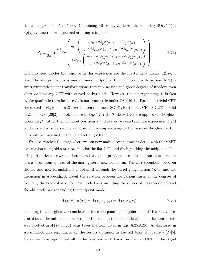
similar as given in (5.26,5.33). Combining all terms, L0 takes the following SO(25, 1)×Sp(2) symmetric form (normal ordering is implied)

L0 =1

2π

∫ π/2

0

dσ

ηµν

π2e−ε|∂σ |pµ (σ) ⋆ e−ε|∂σ |pν (σ)

+e−ε|∂σ |∂σxµ (σ, ε) ⋆ e−ε|∂σ |∂σx

ν (σ, ε)

+iεmn

π2e−ε|∂σ |∂σpm (σ) ⋆ e−ε|∂σ |∂σpn (σ)

+e−ε|∂σ |xm (σ, ε) ⋆ e−ε|∂σ |xn (σ, ε)

. (5.74)

The only zero modes that survive in this expression are the matter zero modes (xµ0 , p0µ) .

Since the star product is symmetric under OSp(d|2) , the cubic term in the action (5.71) is

supersymmetric under transformations that mix matter and ghost degrees of freedom even

when we have any CFT with curved backgrounds. However, the supersymmetry is broken

by the quadratic term because L0 is not symmetric under OSp(26|2) : For a non-trivial CFT

the curved background in L0 breaks even the linear SO(d) ; for the flat CFT SO(26) is valid

in L0 but OSp(26|2) is broken since in Eq.(5.74) the ∂σ derivatives are applied on the ghost

momenta pm rather than on ghost positions xm. However, we can bring the expression (5.74)

to the expected supersymmetric form with a simple change of the basis in the ghost sector.

This will be discussed in the next section (VF).

We have reached the stage where we can now make direct contact in detail with the MSFT

formulation using old star ⋆ product for the flat CFT and distinguishing the midpoint. This

is important because we can then claim that all the previous successful computations are now

also a direct consequence of the more general new formalism. The correspondence between

the old and new formulations is obtained through the Siegel gauge action (5.71) and the

discussion in Appendix-A about the relation between the various bases of the degrees of

freedom, the new σ-basis, the new mode basis including the center of mass mode x0, and

the old mode basis including the midpoint mode,

A (x (σ) , p (σ)) = A (x0, xe, po) = A (x, xe, po) , (5.75)

assuming that the ghost zero mode xb0 or the corresponding midpoint mode xb is already inte-

grated out. The only remaining zero mode is the matter zero mode xµ0 . Then the appropriate

star product in A (x0, xe, po) basis takes the form given in Eqs.(8.25,8.26). As discussed in

Appendix-A this reproduces all the results obtained in the old basis A (x, xe, po) [2]-[5].

Hence we have reproduced all of the previous work based on the flat CFT in the Siegel

49

gauge. We are now prepared to tackle non-perturbative computations with a more efficient

tool.

F. OSp(d|2) Supersymmetry Acting on Matter and Ghosts

In the discussion above we noted that the star product has an OSp(d|2) matter-ghost

supersymmetry for any CFT, but the stress tensors for matter versus ghosts as well as the

ghost structure of the BRST operator break this supersymmetry. So, the kinetic term of the

SFT action (5.56) breaks the supersymmetry while the interactions are supersymmetric.

Consequently, in Feynman-like diagram computations in the Siegel gauge, in the flat

CFT case, the breaking of OSp(d|2) is in the propagator and not in the interactions. Since

the breaking of the supersymmetry amounts to moving the ∂σ derivative from the ghost

Pm to the ghost Xm in the expression for L0 in (5.34) or L0 in (5.74), we can construct a

simple algorithm to simplify all computations as if there is OSp(d|2) symmetry in the full

theory, and then modify the final computation with a simple rule that takes into account

this breaking of the symmetry in propagators. This algorithm was noted and used efficiently

in past computations in MSFT [3][4][5] and will be illustrated below with an example.

However, we discovered that there is a better approach: it is possible to rewrite the

theory in a slightly modified basis of the ghost degrees of freedom such as to display fully

the OSp(d|2) symmetry in the Siegel gauge (but not in the general gauge) including in

the kinetic term or the propagators. We may then use supersymmetric propagators in all

computations in the Siegel gauge. The final results in computations, such as amplitudes,

are the same as before [3][4][5].

To show how this works we need to review the ghost sector and show that there is a more

general way to extract the ghost phase space operators(

Xm, Pm

)

from the ghost(

B, C)

operators. Namely, instead of Eq.(5.7), we can introduce a more general formula which

includes a parameter α as follows

B (±σ) =(

−iXb (σ)± π |∂σ|α−1 ∂σPc (σ))

,

C (±σ) =(

πPb (σ)∓ i |∂σ|−α−1 ∂σXc (σ)

)

.(5.76)

Taking α = 1 reproduces (5.7). Results of any computations should be independent of α

since this is only a rewriting of the same(

B, C)

operators. Indeed we have checked that

50

physical quantities, such as amplitudes, are independent of α. So we may explore if the

parameter α leads to some interesting consequences resulting from this rearrangement of

the degrees of freedom. The answer is yes: as it will be pointed out below, choosing α = −1rather than α = 1, will be useful to display a supersymmetry between matter and ghost

degrees of freedom in the Siegel gauge.

For the more general definition (5.76), the modes in Eqs.(5.9,5.10) generalize to the

following form including the parameter α

Xb0 = ib0, X

bn≥1 =

i√2

(

bn + b−n

)

, Xcn≥1 = −

nα

√2(cn − c−n) , (5.77)

Pb0 = c0, Pb,n≥1 =1√2(cn + c−n) , Pc,n≥1 =

i√2nα

(

bn − b−n

)

, (5.78)

and similarly for the inverse relations

b0 = −iXb0, bn≥1 =

i√2

(

−Xbn≥1 − nαPc,n≥1

)

, b(−n≤1) =i√2

(

−Xbn≥1 + nαPc,n≥1

)

, (5.79)

c0 = Pb0, cn≥1 =1√2

(

−n−αXcn≥1 + Pb,n≥1

)

, c(−n≤1) =1√2

(

n−αXcn≥1 + Pb,n≥1

)

. (5.80)

Then, the regulated expression in (5.14) are generalized as

B (±σ, ε) =(

−ie−ε|∂σ |Xb (σ, ε)± π |∂σ|α−1 ∂σPc (σ))

, (5.81)

C (±σ, ε) =(

πPb (σ)∓ ie−ε|∂σ | |∂σ|−α−1 ∂σXc (σ, ε)

)

, (5.82)

The ghost stress tensor Eq.(5.33) is also generalized to include the effects of α

T gh±± =

1

4(iǫmm′) :

π |∂σ|α−1

2 ∂σPm (σ)

∓e−ε|∂σ | |∂σ|1−α2 Xm (σ, ε)

π |∂σ|α−1

2 ∂σPm′

(σ)

∓e−ε|∂σ | |∂σ|1−α2 Xm′

(σ, ε)

: −12i∂±σJ

gh±

(5.83)

while the zero mode Virasoro operator in (5.34) generalizes to the following form

L0 =1

π

∫ π

0

dσ

12ηµν

(

π2P µP ν + Xµ |∂σ|2 Xν)

+12iǫmn

(

π2Pm |∂σ|1+α P n + Xm |∂σ|1−α Xn)

. (5.84)

Now it is evident that for α = −1 (as opposed to α = 1 in (5.34)) this expression has

the same form for both the matter and ghost parts. In fact, for α = −1 this displays an

OSp(d|2) supersymmetry between matter and ghost degrees of freedom in the operator L0

that determines the kinetic term in the Siegel gauge. Recall that the interaction terms are

51

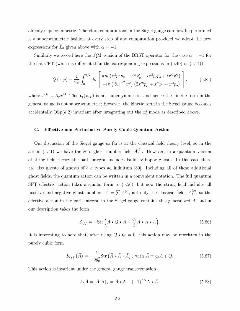
already supersymmetric. Therefore computations in the Siegel gauge can now be performed

is a supersymmetric fashion at every step of any computation provided we adopt the new

expressions for L0 given above with α = −1.Similarly we record here the iQM version of the BRST operator for the case α = −1 for

the flat CFT (which is different than the corresponding expressions in (5.40) or (5.74))

Q (x, p) =1

2π

∫ π/2

0

dσ

πpb(

π2pµpµ + x′µx′µ + iπ2pcpb + ix′bx′c)

−iπ(

|∂σ|−2 x′c) (

2x′µpµ + x′cpc + x′bpb)

. (5.85)

where x′M ≡ ∂σxM . This Q(x, p) is not supersymmetric, and hence the kinetic term in the

general gauge is not supersymmetric; However, the kinetic term in the Siegel gauge becomes

accidentally OSp(d|2) invariant after integrating out the xb0 mode as described above.

G. Effective non-Perturbative Purely Cubic Quantum Action

Our discussion of the Siegel gauge so far is at the classical field theory level, so in the

action (5.71) we have the zero ghost number field A(0)s . However, in a quantum version

of string field theory the path integral includes Faddeev-Popov ghosts. In this case there

are also ghosts of ghosts of b, c types ad infinitum [30]. Including all of these additional

ghost fields, the quantum action can be written in a convenient notation. The full quantum

SFT effective action takes a similar form to (5.56), but now the string field includes all

positive and negative ghost numbers, A =∑

A(i), not only the classical fields A(0)s , so the

effective action in the path integral in the Siegel gauge contains this generalized A, and in

our description takes the form

Seff = −Str(

A ⋆ Q ⋆ A+g03A ⋆ A ⋆ A

)

. (5.86)

It is interesting to note that, after using Q ⋆ Q = 0, this action may be rewritten in the

purely cubic form

Seff

(

A)

= − 1

3g20Str(

A ⋆ A ⋆ A)

, with A ≡ g0A+Q. (5.87)

This action is invariant under the general gauge transformation

δΛA = [A,Λ}⋆ = A ⋆ Λ− (−1)AΛ Λ ⋆ A. (5.88)

52

where Λ includes all ghost numbers, just like A does. From this we see that (5.86) is also

invariant by substituting A in terms of A as in (5.87).

The purely cubic version has been noted before by many authors [31] as a formal property

of SFT for the open string. But in many treatments various anomalies, including associa-

tivity anomalies [3][7], emerged that could not be satisfactorily resolved, so as to cast doubt

on the utility of this observation. Indeed not having a satisfactory resolution of anomalies

leads to wrong conclusions [3]. In our formalism we have introduced a reliable regulator ε

as part of the definition of the new MSFT. With this regulator there are no anomalies and

this allows us to use the purely cubic form of the action reliably.

Thus we will take the fundamental non-perturbative form of regulated MSFT to be of the

purely cubic form (5.87), including our reliable regulator ε discussed throughout this paper.

This form of the action has some remarkable properties as follows

• The ⋆ is background independent, it does not depend on any specific CFT, it is defined

only by an abstract phase space. Similarly, the field A (x, p) is independent of any CFT.

• This action has a huge amount of symmetry because all supercanonical transformations

of (x, p) leave the Moyal product invariant. The action is invariant when the field A

transforms under a similarity transformation in the iQM as follows

A→ A′ = U ⋆ A ⋆ U−1, where U =(

eε(x,p))

⋆with any ε (x, p) , (5.89)

where ε (x, p) is regarded as a generator of supercanonical transformations on matter

and ghosts in the iQM.

• A subset of supercanonical transformations is a finite global subset of super rotations

OSp(d|2) that act linearly on the supervectors(

xM , pM)

, namely xM → (Sx)M and

pM → (S−1p)M , with S ∈ OSp(d|2) (more accurately OSp((d− 1, 1) |2)). These

supertransformations mix the matter and ghost degrees of freedom. The Moyal ⋆ in

(2.9) and the phase space integration measure (5.46) are manifestly invariant under this

OSp(d|2). Hence when A (x, p) is transformed as A (x, p) → A (Sx, S−1p) the action

is invariant. When the action is rewritten in terms of Q and A as in Eq.(5.86), the

matter-ghost symmetry is spontaneously broken (i.e. hidden); it is still manifest in the

cubic term but broken in the quadratic term because Q is not manifestly symmetric.

53

Keeping track of the broken symmetry is easy and it turns out to be valuable because

this simplifies computations (see below).

• Rewriting the purely cubic theory back into the form in Eq.(5.86) is analogous to

spontaneous breakdown. It is a rearrangement of the non-perturbative theory into a

perturbative expansion around a classical solution of the non-perturbative equation of

motion

A (x, p) ⋆ A (x, p) = 0. (5.90)

The BRST field Q (x, p) associated to any CFT, as given in Eqs.(5.39) is an exact

solution of this equation Asol (x, p) = Q (x, p). Our approach for the construction of

Q (x, p) for any CFT given in the previous section provides an infinite number of solu-

tions to Eq.(5.90), namely one for each exact conformal CFT. The perturbative expan-

sion of the field in power of g0 around this solution is A (x, p) = Q (x, p) + g0A (x, p) .

Inserting this in the non-perturbative action (5.87) produces the perturbative setup

in Eq.(5.86) or Eq.(5.56).

• Although the non-perturbative theory is background independent, the perturbative

expansion A (x, p) = Q (x, p) + g0A (x, p) is obviously dependent on the background

field Q (x, p) that defines the CFT associated to the choice of the solution Q (x, p) . All

CFTs correspond to solutions of the non-perturbative equation. But it is not clear if

all solutions of (5.90) are CFTs.

• Using the observation in the previous paragraph we can now obtain a large class of

non-perturbative solutions to the standard string field theory equation of motion QA+

g0A⋆A = 0, namely, since this equation may be written as (Q1 (x, p) + g0A (x, p))2 = 0

where Q1 (x, p) is associated with some CFT1, we can give a solution for A in the form

g0A (x, p) = Q2 (x, p)−Q1 (x, p) (5.91)

where Q2 (x, p) is another CFT2 that is constructed from the same degrees of freedom

(x, p) . In principle there are an infinite number of solutions. In practice, going over

pairs of exactly conformal CFTs that we know how to handle (such as those similar to

[23]-[26]), Eq.(5.91) provides a non-perturbative explicit solution to string field theory.

54

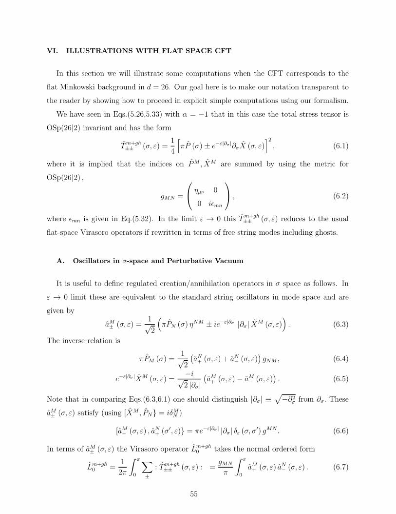
VI. ILLUSTRATIONS WITH FLAT SPACE CFT

In this section we will illustrate some computations when the CFT corresponds to the

flat Minkowski background in d = 26. Our goal here is to make our notation transparent to

the reader by showing how to proceed in explicit simple computations using our formalism.

We have seen in Eqs.(5.26,5.33) with α = −1 that in this case the total stress tensor is

OSp(26|2) invariant and has the form

Tm+gh±± (σ, ε) =

1

4

[

πP (σ)± e−ε|∂σ |∂σX (σ, ε)]2

, (6.1)

where it is implied that the indices on PM , XM are summed by using the metric for

OSp(26|2) ,

gMN =

ηµν 0

0 iǫmn

, (6.2)

where ǫmn is given in Eq.(5.32). In the limit ε → 0 this Tm+gh±± (σ, ε) reduces to the usual

flat-space Virasoro operators if rewritten in terms of free string modes including ghosts.

A. Oscillators in σ-space and Perturbative Vacuum

It is useful to define regulated creation/annihilation operators in σ space as follows. In

ε → 0 limit these are equivalent to the standard string oscillators in mode space and are

given by

aM± (σ, ε) =1√2

(

πPN (σ) ηNM ± ie−ε|∂σ | |∂σ| XM (σ, ε))

. (6.3)

The inverse relation is

πPM (σ) =1√2

(

aN+ (σ, ε) + aN− (σ, ε))

gNM , (6.4)

e−ε|∂σ |XM (σ, ε) =−i√2 |∂σ|

(

aM+ (σ, ε)− aM− (σ, ε))

. (6.5)

Note that in comparing Eqs.(6.3,6.1) one should distinguish |∂σ| ≡√

−∂2σ from ∂σ. These

aM± (σ, ε) satisfy (using [XM , PN} = iδMN )

[aM− (σ, ε) , aN+ (σ′, ε)} = πe−ε|∂σ | |∂σ| δε (σ, σ′) gMN . (6.6)

In terms of aM± (σ, ε) the Virasoro operator Lm+gh0 takes the normal ordered form

Lm+gh0 =

1

2π

∫ π

0

∑

±: Tm+gh

±± (σ, ε) : =gMN

π

∫ π

0

aM+ (σ, ε) aN− (σ, ε) . (6.7)

55

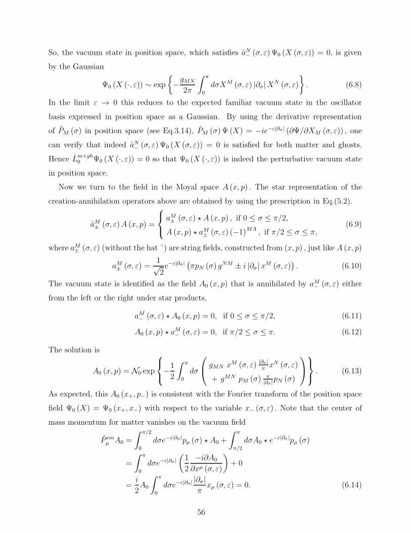
So, the vacuum state in position space, which satisfies aN− (σ, ε)Ψ0 (X (σ, ε)) = 0, is given

by the Gaussian

Ψ0 (X (·, ε)) ∼ exp

{

−gMN

2π

∫ π

0

dσXM (σ, ε) |∂σ|XN (σ, ε)

}

. (6.8)

In the limit ε → 0 this reduces to the expected familiar vacuum state in the oscillator

basis expressed in position space as a Gaussian. By using the derivative representation

of PM (σ) in position space (see Eq.3.14), PM (σ) Ψ (X) = −ie−ε|∂σ | (∂Ψ/∂XM (σ, ε)) , one

can verify that indeed aN− (σ, ε) Ψ0 (X (σ, ε)) = 0 is satisfied for both matter and ghosts.

Hence Lm+gh0 Ψ0 (X (·, ε)) = 0 so that Ψ0 (X (·, ε)) is indeed the perturbative vacuum state

in position space.

Now we turn to the field in the Moyal space A (x, p) . The star representation of the

creation-annihilation operators above are obtained by using the prescription in Eq.(5.2).

aM± (σ, ε)A (x, p) =

aM± (σ, ε) ⋆ A (x, p) , if 0 ≤ σ ≤ π/2,

A (x, p) ⋆ aM± (σ, ε) (−1)MA , if π/2 ≤ σ ≤ π,(6.9)

where aM± (σ, ε) (without the hat ˆ) are string fields, constructed from (x, p) , just like A (x, p)

aM± (σ, ε) =1√2e−ε|∂σ | (πpN (σ) gNM ± i |∂σ| xM (σ, ε)

)

. (6.10)

The vacuum state is identified as the field A0 (x, p) that is annihilated by aM− (σ, ε) either

from the left or the right under star products,

aM− (σ, ε) ⋆ A0 (x, p) = 0, if 0 ≤ σ ≤ π/2, (6.11)

A0 (x, p) ⋆ aM− (σ, ε) = 0, if π/2 ≤ σ ≤ π. (6.12)

The solution is

A0 (x, p) = N0 exp

−12

∫ π

0

dσ

gMN xM (σ, ε) |∂σ |πxN (σ, ε)

+ gMN pM (σ) π|∂σ |pN (σ)

. (6.13)

As expected, this A0 (x+, p−) is consistent with the Fourier transform of the position space

field Ψ0 (X) = Ψ0 (x+, x−) with respect to the variable x− (σ, ε) . Note that the center of

mass momentum for matter vanishes on the vacuum field

P cmµ A0 =

∫ π/2

0

dσe−ε|∂σ |pµ (σ) ⋆ A0 +

∫ π

π/2

dσA0 ⋆ e−ε|∂σ |pµ (σ)

=

∫ π

0

dσe−ε|∂σ|(

1

2

−i∂A0

∂xµ (σ, ε)

)

+ 0

=i

2A0

∫ π

0

dσe−ε|∂σ| |∂σ|πxµ (σ, ε) = 0. (6.14)

56

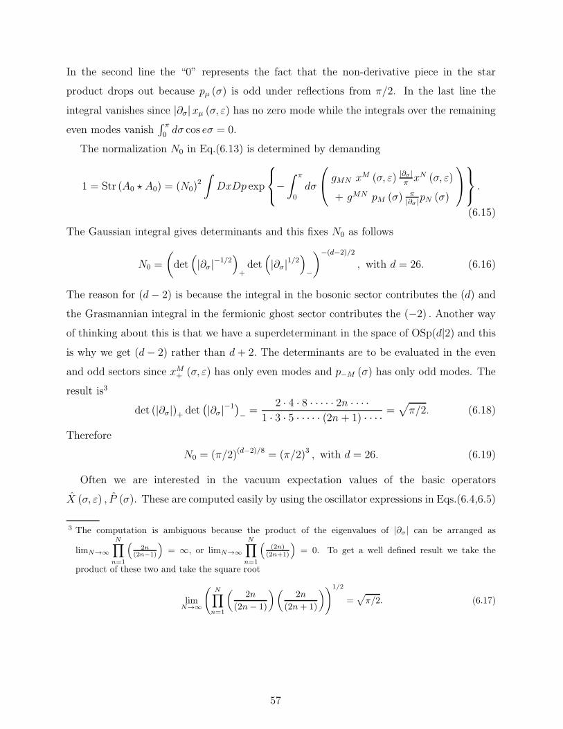
In the second line the “0” represents the fact that the non-derivative piece in the star

product drops out because pµ (σ) is odd under reflections from π/2. In the last line the

integral vanishes since |∂σ|xµ (σ, ε) has no zero mode while the integrals over the remaining

even modes vanish∫ π

0dσ cos eσ = 0.

The normalization N0 in Eq.(6.13) is determined by demanding

1 = Str (A0 ⋆ A0) = (N0)2

∫

DxDp exp

−∫ π

0

dσ

gMN xM (σ, ε) |∂σ |πxN (σ, ε)

+ gMN pM (σ) π|∂σ |pN (σ)

.

(6.15)

The Gaussian integral gives determinants and this fixes N0 as follows

N0 =

(

det(

|∂σ|−1/2)

+det(

|∂σ|1/2)

−

)−(d−2)/2

, with d = 26. (6.16)

The reason for (d− 2) is because the integral in the bosonic sector contributes the (d) and

the Grasmannian integral in the fermionic ghost sector contributes the (−2) . Another wayof thinking about this is that we have a superdeterminant in the space of OSp(d|2) and this

is why we get (d− 2) rather than d + 2. The determinants are to be evaluated in the even

and odd sectors since xM+ (σ, ε) has only even modes and p−M (σ) has only odd modes. The

result is3

det (|∂σ|)+ det(

|∂σ|−1)

− =2 · 4 · 8 · · · · · 2n · · · ·

1 · 3 · 5 · · · · · (2n + 1) · · · · =√

π/2. (6.18)

Therefore

N0 = (π/2)(d−2)/8 = (π/2)3 , with d = 26. (6.19)

Often we are interested in the vacuum expectation values of the basic operators

X (σ, ε) , P (σ). These are computed easily by using the oscillator expressions in Eqs.(6.4,6.5)

3 The computation is ambiguous because the product of the eigenvalues of |∂σ| can be arranged as

limN→∞

N∏

n=1

(

2n(2n−1)

)

= ∞, or limN→∞

N∏

n=1

(

(2n)(2n+1)

)

= 0. To get a well defined result we take the

product of these two and take the square root

limN→∞

(

N∏

n=1

(

2n

(2n− 1)

)(

2n

(2n+ 1)

)

)1/2

=√

π/2. (6.17)

57

and the properties of the vacuum state. For example, for 0 < σ1, σ2 < π/2,

〈e−ε|∂σ1|XM (σ1, ε) e−ε|∂σ2|XN (σ2, ε)〉

= − −i√2 |∂σ1

|−i√2 |∂σ2

|Str(

A0 ⋆(

aM− (σ1, ε) aN+ (σ2, ε)A0

))

Str (A0 ⋆ A0)

=π

2e−ε|∂σ1 |e−ε|∂σ2 | |∂σ2

|−1 δ (σ1, σ2) gMN (6.20)

and similarly for vacuum expectation values that involve PM (σ) we find

〈e−ε|∂σ1|XM (σ1, ε) PN (σ2)〉 = iπ

2e−ε|∂σ1 |e−ε|∂σ2 |δ (σ1, σ2) δMN (6.21)

〈PM (σ1) PN (σ2)〉 =π

2e−ε|∂σ1|e−ε|∂σ2|δ (σ1, σ2) gMN (6.22)

Using these expressions we can use Wick’s theorem (or equivalently operator products) to

rewrite products of operators X ’s or P ’s in terms of normal ordered products. The exact

parallel steps is available in the Moyal formulation, but these products occur as star products

either on the left side or the right side of the field A (x, p) , for example if both σ1, σ2 are

less than π/2

O (σ1) O (σ2)A (x, p) = O⋆ (σ1) ⋆ O⋆ (σ2) ⋆ A (x, p) . (6.23)

Wick’s theorem or operator products computed in familiar operator language have the exact

parallel in the Moyal formalism and therefore the c-number coefficients are identical in either

formalism, as in Eq.(5.5). Therefore we can borrow well known results for quantum operator

products in the CFT and use them directly for the star products of the corresponding fields

in the induced iQM.

The expression for the matter vacuum (6.13) includes the ghost contribution

Aghost0 (x, p) = Ngh

0 exp

{

−i∫ π

0

dσ

(

xb (σ, ε)|∂σ|πxc (σ, ε) + pc (σ)

π

|∂σ|pb (σ)

)}

. (6.24)

which we discuss a bit more to emphasize that this is the ghost SL (2,R) vacuum. It is

known that there are two ghost vacuum states A0± that by definition satisfy the following

relations:

b0A0+ = A0−, c0A0− = A0+, (6.25)

while

b0A0− = c0A0+ = 0. (6.26)

58

Their ghost numbers should differ by one:

Ngh (A0+) = Ngh (A0−) + 1, (6.27)

and their star product satisfies (recall Str has ghost number 1):

Str (A0+ ⋆ A0−) = Str(

A0+ ⋆(

b0A0+

))

= Str (A0− ⋆ (c0A0−)) = 1, (6.28)

Str (A0+ ⋆ A0+) = Str (A0− ⋆ A0−) = 0. (6.29)

Therefore, we can conclude that the ghost number of A0− is −1, while Ngh (A0+) = 0. The

SL (2,R) vacuum state has the ghost number 0, therefore it can be considered as the vacuum

state A0+.

Hence, the ghost vacua are the following

A0+ (x, p) = Ngh0 exp

{

−i∫ π

0

dσ

(

xb (σ, ε)|∂σ|πxc (σ, ε) + pc (σ)

π

|∂σ|pb (σ)

)}

, (6.30)

A0− (x, p) = −iNgh0 xb0 exp

{

−i∫ π

0

dσ

(

xb (σ, ε)|∂σ|πxc (σ, ε) + pc (σ)

π

|∂σ|pb (σ)

)}

. (6.31)

This works correctly with the normalization conditions above (recall Str includes the Grass-

mannian integral∫

dxb0). In the Siegel gauge (5.64) we had, As = xb0A(0)s , with A

(0)s not

containing the ghost zero mode xb0. Hence A(0)s ∼ Agh

0+ matches all the properties as the

SL(2, R) invariant vacuum.

B. The Monoid in the σ-basis

A very useful tool for computations in MSFT is the monoid algebra developed in [3][4].

This arises as follows. We have seen above that the perturbative vacuum state A0 is the

Gaussian string field (6.13). Excited perturbative string states are represented by the same

Gaussian field multiplied by polynomials of (x, p). The polynomials in perturbative states

can be generated by taking derivatives with respect to the shift λx or λp of a shifted gaussian

A ∼ exp (−xx− pp+ λxx+ λpp) , and then setting the λ′s to zero. On the other hand, at

least some non-perturbative states are also shifted gaussian-like states, but with a different

quadratic and linear exponent than the one for the perturbative states. This suggests that

fields of the shifted-gaussian form are very common in explicit computations. It was found in

[3][4] that they have nice mathematical properties that are directly useful in the computation

of amplitudes, including the Veneziano amplitude [5].

59

The set of shifted gaussians of interest are of the form

AN ,M,λ = N e−ξiMijξj−ξiλi . (6.32)

where the ξi stand for (x, p) and the symbols Mij , λi are parameters, while N is a normal-

ization. They close under the Moyal star product as follows

AN1,M1,λ1⋆ AN2,M2,λ2

= AN12,M12,λ12, (6.33)

The ξi are a set of non-commutative (super)variables (matter and ghost phase spaces) which

satisfy

[ξi, ξj}⋆ = sij , (6.34)

with sij a constant matrix which is antisymmetric when both i and j are bosonic and

is symmetric when both i and j are fermionic. The (N12,M12, λ12) are computed from

(N1,M1, λ1) and (N2,M2, λ2) as follows. Given the data for (N1,M1, λ1) and (N2,M2, λ2)

we first define the matrices m

m1 =M1s, m2 =M2s, m12 =M12s; (6.35)

then the result for m12, λ12,N12 takes the form [2][3][4]

m12 = (m1 +m2m1) (1 +m2m1)−1 + (m2 −m1m2) (1 +m1m2)

−1 , (6.36)

λ12 = (1−m1) (1 +m2m1)−1 λ2 + (1 +m2) (1 +m1m2)

−1 λ1 (6.37)

N12 =N1N2

sdet (1 +m2m1)1/2e

1

4((λ1+λ2)(M1+M2)−1(λ1+λ2)−λ12(M12)

−1λ12). (6.38)

The reader may consult [2][3][4] for detailed properties of this monoid algebra and how it is

used for both perturbative and non-perturbative computations in string field theory. In our

formulation here this algebra is consistent with the OSp(d|2) supersymmetry, and therefore

we use supertrace and superdeterminants instead of the trace and determinant in [2][3][4].

The results in (6.36-6.38) were computed for the Moyal star product in a discrete mode

space, but the same formal result applies also with our new Moyal star product in σ-space.

In the present case the non-commutative variables are labelled by i which is a combination

of discrete (M) and continuous (σ) labels. The shifted gaussian in our new formalism is

AN ,M,λ ≡ N exp

(

−(∫ π

0

∫ π

0

dσdσ′ξi (σ)Mij (σ, σ′) ξj (σ′)

)

−∫ π

0

dσξi (σ) λi (σ)

)

(6.39)

60

where ξi (σ) =(

xM (σ) , pM (σ))

are the string half-phase degrees of freedom, Mij (σ, σ′) is

a complex square matrix and λi (σ) is a complex column matrix. Under the Moyal star

product they form a closed algebra called a monoid (which is almost a group, except for the

inverse condition). Taking into account the star commutation rules in (3.25) we identify the

matrix sij with the new type of labels as follows

sij =

i=

xM (σ)

pM (σ)

j= xN (σ′) , pN (σ′)

0 i1−NδMN δ+− (σ, σ′)

(−i)1−N ′

δ NM δ−+ (σ, σ′) 0

(6.40)

where δ+− (σ, σ′) is given in Eqs.(3.26-3.27), while δ−+ (σ, σ′) is the transpose of the “matrix”

δ+− and then re-labelled by replacing σ ↔ σ′. The parameters Mij and λi of the shifted

gaussian take the form

Mij =

i=

xM (σ)

pM (σ)

j= xN (σ′) , pN (σ′)

aMN (σ, σ′) b NM (σ, σ′)

bMN (σ, σ′) dMN (σ, σ′)

, λi =

λxM (σ)

λpM (σ)

(6.41)

where the diagonal entries ofM are (super)symmetric matrices while the off diagonal entries

are related by a (super) transposition

bMN (σ, σ′) = (−1)MN b NM (σ′, σ) . (6.42)

The matrix m =Ms becomes

mji =Miks

kj =

b NM (σ, σ′) sign (π/2− σ′) aMN (σ, σ′) sign (π/2− σ′) (−1)N

dMN (σ, σ′) sign (π/2− σ′) bMN (σ, σ′) sign (π/2− σ′) (−1)N

(6.43)

Then they are combined according to the rules (6.36-6.38) to obtain the result for the monoid

algebra.

As an example, for perturbative computations, the matrix Mij (σ, σ′) is fairly simple. It

follows from the vacuum state given in (6.13)

Mpertij =

gMN|∂σ |πδ+ε (σ, σ′) 0

0 gMN π|∂σ |δ

−ε (σ, σ′)

(6.44)

In general the regulated delta function in (6.44) satisfies D-brane boundary conditions as

discussed in section (IVA). The regulator ε insures that all computations are well defined.

61

The regulator is removed after renormalization of the cubic coupling constant g0 as shown in

[5]. For example, for the D25 brane we would use in (6.44) the δ±nnε (σ, σ′) in all directionsM.

But if more complicated D-brane boundary conditions are desired, then in the corresponding

directions M we would use the δ±nnε or δ±dd

ε given in section (IVA). In this way, by making

only minimal changes through the regulated delta functions, non-trivial D-brane boundary

conditions are implemented easily in our new MSFT formalism.

If theM in (6.44) is used in monoid computations directly in the form shown in (6.44) with

δnn, then this approach reproduces all the results of the computations obtained previously

in [2][3][4][5], including the off-shell 4-tachyon (Veneziano) scattering amplitude.

VII. OUTLOOK

The central structure in this paper is the new Moyal ⋆ product in the σ-basis in Eq.(2.9)

that implements the interactions of strings. The string fields A (x, p) that are multiplied

with this product are labeled by half of the phase space of the string(

xM+ (σ) , p−M (σ))

as

opposed to the full phase space(

XM (σ) , PM (σ))

. The label M = (µ, b, c) includes both

the spacetime “matter µ” and the (b, c) ghosts in an OSp(d|2) covariant notation. The star

product ⋆, which is independent of the details of any conformal field theory on the worldsheet

(CFT), is background independent and is invariant under this supersymmetry for all CFTs.

The symmetric xM+ (σ) = 12

(

XM (σ) +XM (π − σ))

and the antisymmetric p−M (σ) =

12(PM (σ)− PM (π − σ)) commute with each other in the quantum mechanics (QM) of the

first quantized string, and therefore they are simultaneous observables in QM. The eigen-

values (x+, p−) of these simultaneous observables provide a complete set of labels for the

first quantized string states 〈xM+ (σ) , p−M (σ) |. The string field A (x, p) corresponds to the

probability amplitude of a general string state |A〉 that has the given phase space configu-

ration A (x, p) = 〈xM+ (σ) , p−M (σ) |A〉. Hence the Moyal product in Eq.(2.9) which creates

a non-commutativity in the space of eigenvalues(

xM+ (σ) , p−M (σ))

has nothing to do with

the Moyal product in QM despite the close mathematical similarities. However this close

similarity is interpreted in this paper as an induced quantum mechanics (iQM) that governs

the fundamental string interactions.

To be able to compute reliably in string field theory we need a regulator to obtain unam-

biguous results. The essential role of the regulator is to tame some singularities associated

62

with the midpoint of the string at π/2. In this paper the regulator is the dimensionless small

parameter ε. We regulated at first the QM quantum operators of the first quantized string

by defining X (σ, ε) , while no regularization is needed for the operator PM (σ) , as discussed

in section (IV). Consequently, the eigenvalues of the half phase space are also regularized,

so that the string field is regularized with the ε through its labels A(

xM+ (σ, ε) , p−M (σ))

.

On this regularized basis we showed how to represent all QM operators that belong to any

CFT, by their string-field-counterparts in the induced iQM. This representation involves

only star products of the string fields. In particular some crucial operators that are needed

to construct string field theory, i.e. the stress tensor T±±, the BRST current jB and the

BRST operator, for any CFT are constructed as regularized string fields that operate in the

induced iQM. Using them we constructed the regularized action for the new Moyal string

field theory (MSFT).

An important aspect of the new formulation is that the regularized midpoint of the string

xM+ (π/2, ε) is not isolated from the rest of the string degrees of freedom in its treatment under

the ⋆ product. Nevertheless the new product has the magical property that the midpoint

xM+ (π/2, ε) acts trivially as a complex number (no derivatives induced on the field) when

it is star-multiplied with any string field xM+ (π/2, ε) ⋆ A (x, p) = A (x, p) ⋆ xM+ (π/2, ε) =

xM+ (π/2, ε)A (x, p) . Remarkably, this important property of the midpoint in string joining

is automatically implemented by the new Moyal ⋆.

We constructed an infinite number of solutions to the non-perturbative equation of motion

A ⋆ A = 0 of the purely cubic theory, in the form Asol (x, p) = Q (x, p) , where the BRST

field Q (x, p) is derived with our methods from any CFT on the worldsheet. We turned this

observation into a method for finding an infinite number of non-perturbative solutions to

the string field equation, QA + g0A ⋆ A = 0, in the form, g0A = Q2 − Q1, where Qi (x, p)

correspond to the BRST fields (as obtained with our methods) of a pair of conformal field

theories CFTi.

We have shown that all successful computations previously accomplished in MSFT using

the old regularized Moyal star product (which was tied to the flat CFT in d = 26, and treated

the midpoint as special), are also reproduced by the new formalism when the same flat CFT

is used. However the advantage of the new approach is that it also applies to any curved

CFT and can easily include the effects of D-brane boundary conditions. The applications of

the new features will be explored in future work in several directions as follows.

63

It would be a very interesting exercise to apply our formalism to some simple cases of

exact CFTs. Sometime ago some of the earliest examples of exact conformal field theories

that describe strings in curved spaces with one time coordinate were suggested [23] and

studied at the classical and first quantized levels [24]-[26]. The BRST operator Q (x, p)

associated with such models is constructed in terms of a current algebra (or Kac-Moody

algebra) basis which replaces the half phase space (x (σ) , p (σ)). Using the properties of the

current algebra should be an important tool to compute in these special curved spaces using

our MSFT approach.

We are eager to aim our new MSFT approach to investigate the physical circumstances

in which string theory should play its most important physical role. Noting that string field

theory (SFT) is a complete approach that incorporates generally both the curved background

and the interactions in the non-perturbative description of the theory, it is very important to

pursue the SFT avenue despite the fact that computations may be difficult. The areas that

we think are important to investigate with our MSFT formalism includes very early cosmol-

ogy in the vicinity of cosmological singularities as well as black hole or black D-brane type

singularities. In particular, there has been some new developments in identifying uniquely

cosmological backgrounds that are geodesically complete across cosmological singularities

[32] to which we plan to apply our formalism.

An understanding of the very early cosmology of the universe through string theory has

been tradionally a hope that it would eventually yield an explanation of why we live in

four dimensions and provide the ingredients of the Standard Model of particle physics, such

as the number of generations and their symmetry structures. It is believed that string

physics is unavoidable in the deeply small and highly curved quantum mechanical regions

of space-time. In this paper we have developed sharper tools to address such issues in

the context of the new MSFT, including string-string interactions both perturbatively and

non-perturbatively, and hope to make further progress in the pursuit of these goals.

We wish to conclude with a speculation on the origin of quantum mechanics. A by-

product of our approach is an astonishing suggestion of the formalism: the roots of ordinary

quantum mechanics may originate from the non-commutative interactions in string theory.

Indeed, the string joining Moyal star induces non-commutativity between otherwise commu-

tative string degrees of freedom (x+ (σ, ε) , p− (σ)). We draw again the attention of the reader

to the remarkable property that even though the operators (x+ (σ, ε) , p− (σ)) commute in

64

QM, their eigenvalues (x+ (σ, ε) , p− (σ)) do not commute with each other under the induced

iQM as seen in Eq.(3.25). This non-commutativity under the string-joining star product is

what led to the representation of the QM operators in the basis of iQM as in Eqs.(3.36,3.37)

in the language of only the string joining star product. The reader is invited to read sec-

tion (IIIA) in reverse by starting from Eqs.(3.36,3.37) and interpreting its contents as the

emergence of QM from iQM rather than the other way around. Then it seems astonishing

that the half-phase-space (x+ (σ, ε) , p− (σ)) in iQM under the string joining ⋆ generates the

conventional QM commutation rules for the full phase space operators(

X (σ, ε) , P (σ))

.

Assuming that string theory is right that it underlies all physics, it is then very tempting to

speculate that the source of QM rules in all physics may simply be the rules of interactions

in string theory as seen explicitly in our paper. This could be the long sought explanation

of where QM comes from. This exciting point is very important in its own right, and it will

be pursued further.

Acknowledgments

This research was partially supported by the U.S. Department of Energy. IB thanks

CERN for hospitality while part of this research was performed.

VIII. APPENDIX

A. Old Discrete Basis Versus New σ-Basis

In this section we are going to show that the new σ-basis formalism that does not distin-

guish the midpoint is equivalent to the old discrete basis that distinguished the midpoint.

The old formalism was developed in [2][3][4][5]. By not distinguishing the midpoint we have

a cleaner and more efficient approach in practical computations.

The unregulated position and momentum degrees of freedom x+ (σ) and p− (σ) in the new

σ basis can be written in terms of modes with even and odd cosine expansions respectively,

x+ (σ) = x0 +√2∑

e

xe cos eσ; p− (σ) =

√2

π

∑

o

po cos oσ, (8.1)

where e = 2, 4, 6, · · · and o = 1, 3, 5, · · · . Their Moyal ⋆ commutator, using the new ⋆

65

product (2.9), is the delta-function that has two forms (3.25)

[x+ (σ) , p− (σ′)]⋆new = iδ+nn (σ, σ′) ε (π/2− σ′) = iε (π/2− σ) δ−nn (σ, σ′) . (8.2)

Using the mode expansion for these delta functions we can compare the two results(

2

π+

4

π

∑

e

cos eσ cos eσ′

)

ε (π/2− σ′) = ε (π/2− σ) 4π

∑

o

cos oσ cos oσ′. (8.3)

It can be verified that this is an identity [3]. The commutator contains two terms, one with

and one without the zero mode:

[x+ (σ) , p− (σ′)]⋆new =

√2

π

∑

o

[x0, po]⋆new cos oσ′ +2

π

∑

e,o

[xe, po]⋆new cos eσ cos oσ′, (8.4)

By comparing the Fourier modes to the answer (8.2) we extract the mode commutators

and find that they are expressed in terms of the matrix elements of the special matrix T

introduced in [2]

[x0, po]⋆new = 2iT0o, [xe, po]⋆new = 2iTeo, (8.5)

where

Teo =4

π

∫ π/2

0

dσ cos eσ cos oσ =4

π

o (−1)(e−o−1)/2

e2 − o2 , (8.6)

T0o =2√2

π

∫ π/2

0

dσ cos oσ =2√2

πosin

oπ

2=

2√2

π

(−1)(o−1)/2

o. (8.7)

A useful identity is [3] (a sum over e is implied)

cos oσ = ε(π

2− σ

)(

cos eσ − cos eπ

2

)

Teo. (8.8)

These star commutators for the modes (8.5-8.7) that were obtained with the new Moyal

product (2.9) in the σ basis are identical to those given by the old Moyal product in the

discrete basis for the flat CFT case, once we write po = peTeo where pe is introduced [2] as a

convenient change of basis (it does not mean the even momentum modes in p+ (σ)). Hence

the old and new Moyal products are equivalent for the flat CFT. But the new σ basis ⋆

product (2.9) is more powerful since it is valid for all CFTs due to the fact that the phase

space notation in the σ basis is independent of the background fields.

There is one more subtle point in this equivalence which is related to the midpoint. In

the old approach the midpoint,

x ≡ x (π/2) = x0 +√2∑

e≥2

xe coseπ

2, (8.9)

66

was distinguished as an independent mode (instead of x0) and did not appear in the old star

product which was expressed only in terms of xe, pe (where pe is related to po = peTeo). Then

the midpoint x had a trivial star product (i.e. it acted on fields with the ordinary product

for complex numbers) and in particular commuted with the momentum modes under the

string joining ⋆. We want to verify that the new ⋆ product also has the same properties for

the midpoint even though the new ⋆ (2.9) does not distinguish the midpoint. It is useful

to note the following notation for we, vo and the relations among these symbols and the

midpoint

x0 = x+ wexe, with we = −√2 cos

eπ

2= −√2 (−1)e/2 , (8.10)

vo ≡ T0o = weTeo, (8.11)

where a summation over e is implied. The last equation follows from integrating both sides

of (8.8). Note that vo or equivalently T0o is really related to the midpoint at π/2 since

[x, po]⋆new = [(x0 − wexe) , po]⋆ = 2i (T0o − weTeo) = 0. (8.12)

This verifies the last crucial point in the equivalence of the old and new star products: even

though the midpoint x was not distinguished in the new star product, x behaves as if it is

insensitive to the derivatives implicit in the new Moyal product and therefore it acts just

like a complex number under the new ⋆, which is the same as under the old ⋆.

It is also instructive to verify the equivalence in reverse. That is, suppose we are given

the commutators (8.5-8.7) and (8.12) under the old product ⋆old with the same result, and

let us derive the local commutators in the continuous σ-basis (8.2) by using only the old star

product. By writing out x+ (σ) , p− (σ′) in terms of modes (8.1) and using (8.5-8.7) with ⋆old

we get the same form as (8.4)

[x+ (σ) , p− (σ′)]⋆old = 2i

√2

π

∑

o

T0o cos oσ′ + 2i

2

π

∑

e,o

Teo cos eσ cos oσ′. (8.13)

Now insert the results (8.6-8.8) for T0o, Teo given in the old literature [2] and compute the

67

right hand side of this equation. We find

=

2i√2π

∑

o

(

2√2

π

∫ π/2

0dσ1 cos oσ1

)

cos oσ′

+2i 2π

∑

e,o

(

4π

∫ π/2

0dσ1 cos eσ1 cos oσ1

)

cos eσ cos oσ′

= i2

π

∫ π/2

0

dσ1δ− (σ1, σ

′) + i

∫ π/2

0

dσ1

(

δ+ (σ1, σ)−2

π

)

δ− (σ1, σ′)

= iδ+nn (σ, σ′) ε (π/2− σ′) . (8.14)

Therefore, the old product ⋆old reproduces the new product ⋆new in the σ basis.

Hence the same string field can be rewritten in the different bases

A (x+ (σ) , p− (σ)) = A (x0, xe, po) = A (x0, xe, po)|x0=x+wexe= A (x, xe, po) . (8.15)

and the joining of strings can be expressed equivalently in either the old or the new star

products if the CFT is flat. To show some subtleties of how this works, we begin with the

relation between the old and new bases. The old star product is (using (2.2) with fixed x)

A1 (x, xe, po) ⋆old A2 (x, xe, po) = A1 (x, (x′e + iTeo∂po) , (p

′o − iTeo∂xe)) ⋆ A2 (x, xe, po) (8.16)

where in the last formula we used Eq.(2.2). Rewrite this in terms of the new basis

A1,2 (x0, xe, po) making explicit that x0 is a function of x and xe when the old star product

is used:

A1 (x, xe, po) ⋆old A2 (x, xe, po) (8.17)

= A1 (x0 (x, xe) , xe, po) ⋆old A2 (x0 (x, xe) , xe, po) (8.18)

= A1 ((x′ + we (x

′e + iTeo∂po)) , (x

′e + iTeo∂po) , (p

′o − iTeo∂xe)) A2 (x0 (x, xe) , xe, po) (8.19)

= A1

((

x′0 +i

2∂p

)

, (x′e + iTeo∂po) , (p′o − iTeo (∂xe + we∂x0

))

)

A2 (x0, xe, po) . (8.20)

= A1 (x0, xe, po) ⋆new A2 (x0, xe, po) (8.21)

where the last step is proven below. The following manipulations are used in obtaining

(8.20) from the previous line: for the first factor,(

x′0 +i2∂p)

, note

x′ + we (x′e + iTeo∂po) = x′0 + iweTeo∂po = x′0 + iT0o∂po = x′0 +

i2∂p,

with ∂p ≡ 2T0o∂po = 2vo∂po =1π

∫ π

0dσε

(

π2− σ

)

∂p−(σ),(8.22)

and for the last factor note,

(p′o − iTeo∂xe)A2 (x0 (x, xe) , xe, po) =

(

p′o − iTeo(

∂x0

∂xe∂x0

+ ∂xe

))

A2, (8.23)

68

where the ∂x0term in (8.23) takes care of applying the derivative Teo∂xe on the xe in x0 (x, xe)

by using the chain rule, with

∂x0

∂xe= we, and ∂x0

=1

2

∫ π

0

dσ∂x+(σ), (8.24)

while the last ∂xe in (8.23) is applied to xe which is not inside x0 (x, xe) in A2. In this way

we have established in general the equivalence of the old and new star products (8.17) and

(8.21). Any computation can be performed by switching between the old/new versions of

the star as long as sufficient care is used as demonstrated above.

On the way to prove the equivalence of (8.20) and the new ⋆ product in the σ-basis via

(8.21), we first note that the expression in (8.20) is reproduced from (8.21) by defining a

new star product in the (x0, xe, po) mode basis that includes the center of mass mode x0

that is explicitly shown as follows

⋆new = (⋆xe,po) exp

(

i

2

(←−∂ xM

0

−→∂ pM −

←−∂ pM

−→∂ xM

0

)

)

, (8.25)

where ∂pM = 2vo∂pMois defined as in (8.22), and (⋆xe,po) is the non-zero mode contribution

given by

(⋆xe,po) = exp(

iTeo

(←−∂ xM

e

−→∂ pMo

−←−∂ pMo

−→∂ xM

e

))

. (8.26)

In particular, as applications of this mode-version of the new star, note that for products

with the center of mass mode, xµ0 or xb0, we get

xM0 ⋆new A (x0, xe, po) =

(

xM0 +i

2∂pM

)

A (x0, xe, po) , (8.27)

however, for products with the midpoint we get (as in (8.12))

xM ⋆new A (x0, xe, po) = xMA (x0, xe, po) , (8.28)

where there are no derivatives on the right hand side, showing again that the midpoint x is

insensitive to the derivatives in the new star product, and acts just like a complex number.

Finally, to prove the equality between the star products in the new σ-basis and the new

mode basis (8.25) we use the mode expansions of the position and momentum (8.1) and

69

compute the mode expansion of their derivatives by using the chain rule as follows:

x+ (σ) = x0 +√2∑

e xe cos eσ,

∂x+(σ) =2π

(

∂x0+√2∑

e cos eσ ∂xe

)

∂x+(σ)x+ (σ′) = δ+nn (σ, σ′) ,

(8.29)

p− (σ) =√2π

∑

o po cos oσ,

∂p−(σ) = 2√2∑

o cos oσ ∂po ,

∂p−(σ)p− (σ′) = δ−nn (σ, σ′) .

(8.30)

The first term (and similarly the second term) in the exponential of the new star product

in (2.9) can be evaluated in terms of modes

i4

∫ π

0dσ−→∂ p−(σ) ·

←−∂ x(σ)ε

(

π2− σ

)

= i4

∫ π

0dσε

(

π2− σ

)

(

2√2∑

o cos oσ−→∂ po

)

·(

2π

(←−∂ x0

+√2∑

e cos eσ←−∂ xe

))

=(

i42π2√2∫ π

0dσε (π/2− σ) cos oσ

)−→∂ po ·

←−∂ x0

+ ”−→∂ po

←−∂ xe”

=(

i42π2√22∫ π/2

0dσ cos oσ

)−→∂ po ·

←−∂ x0

+ ”−→∂ po

←−∂ xe”

= iT0o−→∂ po ·

←−∂ x0

+ iTeo−→∂ po ·

←−∂ xe.

(8.31)

where we used ”−→∂ po

←−∂ xe” as a short notation to include the integrals that are not shown

explicitly to save space. Putting together all the terms in the exponential of (2.9), leads

exactly to Eq. (8.25), thus proving that the ⋆ in the continuous σ-basis (2.9) and the ⋆ in

the discreet basis (8.25) that includes the center of mass mode are identical.

Therefore, we have proven (noting the relation (8.15) between A and A) that

A1 (x, xe, po) ⋆old A2 (x, xe, po) ,

= A1 (x0, xe, po) ⋆new A2 (x0, xe, po) , (8.32)

= A1 (x+ (σ) , p− (σ)) ⋆new A2 (x+ (σ) , p− (σ)) .

In the ⋆newthe center of mass mode x0 is active in the string joining as an independent degree

of freedom; this is in contrast to ⋆old where the midpoint x is passive as an independent degree

of freedom. We have shown that ⋆old and ⋆new are completely equivalent, but they must be

used consistently in their own basis. As we saw above in Eq.(8.20), ∂xe does not mean the

same thing in the various bases because partial derivatives imply that some variables are

fixed while evaluating derivatives, but the quantities held fixed are different in the various

bases: x fixed in the old basis, while x0 fixed in the new basis. Hence one must be careful in

70

such computations. Clearly, as long as we stick consistently to only one basis, or be careful

in the translation as in the steps in Eqs.(8.17-8.21), there will be no errors.

The advantage of the new star is that there is a lot of simplification in the σ formalism

because the midpoint does not need to be distinguished. Furthermore, the σ basis is clearly

background independent and applies to all CFT backgrounds that may be used in the

constructions of the BRST field Q (x, p) . Moreover, quantum operators products that are

well known in the QM of any CFT apply directly also in the parallel induced iQM of the

MSFT formalism, thus rendering the computations in the new MSFT much easier.

B. The BRST Gauge Transformations for an Invariant Action

The MSFT action (5.56) has the following form when the midpoint integration is made

explicit

S = −Str′∫

dxb(

A ⋆ Q ⋆ A+g03A ⋆ ∂xbA ⋆ ∂xbA

)

= −Str′(

∂xb (A ⋆ Q ⋆ A) +g03∂xbA ⋆ ∂xbA ⋆ ∂xbA

)

, (8.33)

Str′ is the remainder of the phase space integration that does not include the midpoint ghost

modes. The gauge transformation that leaves this action invariant is the following

δΛA = [Q,Λ]⋆ + g0{∂xbA, ∂xbΛ}⋆ . (8.34)

Analyzing the ghost numbers in Eq. (8.34) we conclude that the gauge parameter Λ is

bosonic with ghost number −2.Let us check the invariance under the transformation (8.34).

δΛS = −Str′∂xb

(δΛA ⋆ Q ⋆ A+ A ⋆ Q ⋆ δΛA)

+g0δΛA ⋆ (∂xbA)2⋆

(8.35)

= −Str′∂xb

(Q ⋆ Λ− Λ ⋆ Q+ g0 {∂xbA, ∂xbΛ}⋆) ⋆ Q ⋆ A

+A ⋆ Q ⋆ (Q ⋆ Λ− Λ ⋆ Q + g0 {∂xbA, ∂xbΛ}⋆)

+g0 (Q ⋆ Λ− Λ ⋆ Q + g0 {∂xbA, ∂xbΛ}⋆) ⋆ (∂xbA)2⋆

(8.36)

Next we use the cyclic property of the supertrace, and the star nilpotency of the BRST field

71

Q ⋆ Q = 0, to cancel kinetic terms and reorganize the interaction terms

δΛS = Str′

∂xb

(Q ⋆ Λ ⋆ Q ⋆ A−Q ⋆ Λ ⋆ Q ⋆ A)

+ (−Λ ⋆ Q2⋆ ⋆ A+ A ⋆ Q2

⋆ ⋆ Λ)

+g0∂xb

Q ⋆

−∂xb (A ⋆ ∂xbA ⋆ Λ)

+∂xb (A ⋆ ∂xbΛ ⋆ A)

+∂xb (Λ ⋆ ∂xbA ⋆ A)

(8.37)

The first term vanishes explicitly while the second term takes the form

δΛS = g0Str′ [∂xbQ ⋆ ∂xb (Λ ⋆ ∂xbA ⋆ A + A ⋆ ∂xbΛ ⋆ A−A ⋆ ∂xbA ⋆ Λ)] . (8.38)

In the next step we expand the string field A and the gauge parameter Λ in the powers of xb:

A = xbA(0) + A(−1), Λ = xbΛ(−1) + Λ(−2). (8.39)

The BRST charge contributes

∂xbQ ≡ Q++ =

∫ π/2

0

dσp−b (σ) ⋆ xc+ (σ) . (8.40)

where Q++ has ghost number +2. Therefore, δΛS can be reorganized into the form

δΛS = g0Str′ {Q++Ψ} ,

with

Ψ =[

Λ(−2),(

A(0))2]

⋆+{

A(−1),{

Λ(−1), A(0)}}

⋆. (8.41)

We dropped the star product in Str′ (Q++ ⋆Ψ) because it is allowed under the supertrace.

Next we examine this Str′. Making the Grassmann integrals explicit as being equivalent to

derivatives, we can write

Str′ (Q++Ψ) =

= Tr

{

∏

σ′

[

∂∂p−b(σ′)

∂∂xb

+(σ′)

∂∂p−c(σ′)

∂∂xc

+(σ′)

(

∫ π/2

0dσp−b (σ)x

c+ (σ)

)

Ψ(

p−b, xc+, p−c, x

b+

)

]

}

∼ Tr

(

∫ π/2

0dσ[

∂∂p−c(σ)

∂∂xb

+(σ)

Ψ(

p−b, xc+, p−c, x

b+

)

]

p−b=xc+,=p−c,=xb

+=0

)

where Tr is the remaining bosonic integrals. Now, substituting Ψ from (8.41) the two

derivatives in the last line produce several (anti)commutators. To see this we write out the

bose/fermi components of A and Λ

A = xbA(0) + A(−1), Λ = xbΛ(−1) + Λ(−2). (8.42)

72

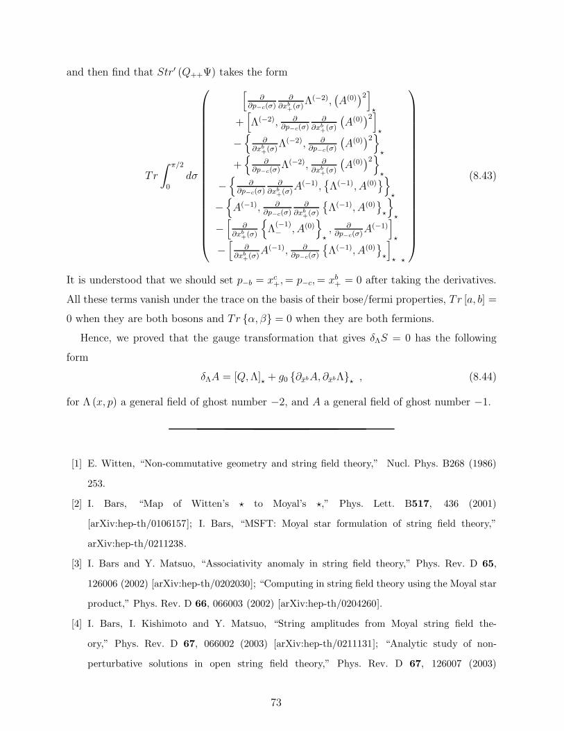
and then find that Str′ (Q++Ψ) takes the form

Tr

∫ π/2

0

dσ

[

∂∂p−c(σ)

∂∂xb

+(σ)

Λ(−2),(

A(0))2]

⋆

+[

Λ(−2), ∂∂p−c(σ)

∂∂xb

+(σ)

(

A(0))2]

⋆

−{

∂∂xb

+(σ)

Λ(−2), ∂∂p−c(σ)

(

A(0))2}

⋆

+{

∂∂p−c(σ)

Λ(−2), ∂∂xb

+(σ)

(

A(0))2}

⋆

−{

∂∂p−c(σ)

∂∂xb

+(σ)A(−1),

{

Λ(−1), A(0)}

}

⋆

−{

A(−1), ∂∂p−c(σ)

∂∂xb

+(σ)

{

Λ(−1), A(0)}

⋆

}

⋆

−[

∂∂xb

+(σ)

{

Λ(−1)− , A(0)

}

⋆, ∂∂p−c(σ)

A(−1)]

⋆

−[

∂∂xb

+(σ)A(−1), ∂

∂p−c(σ)

{

Λ(−1), A(0)}

⋆

]

⋆ ⋆

(8.43)

It is understood that we should set p−b = xc+,= p−c,= xb+ = 0 after taking the derivatives.

All these terms vanish under the trace on the basis of their bose/fermi properties, Tr [a, b] =

0 when they are both bosons and Tr {α, β} = 0 when they are both fermions.

Hence, we proved that the gauge transformation that gives δΛS = 0 has the following

form

δΛA = [Q,Λ]⋆ + g0 {∂xbA, ∂xbΛ}⋆ , (8.44)

for Λ (x, p) a general field of ghost number −2, and A a general field of ghost number −1.

[1] E. Witten, “Non-commutative geometry and string field theory,” Nucl. Phys. B268 (1986)

253.

[2] I. Bars, “Map of Witten’s ⋆ to Moyal’s ⋆,” Phys. Lett. B517, 436 (2001)

[arXiv:hep-th/0106157]; I. Bars, “MSFT: Moyal star formulation of string field theory,”

arXiv:hep-th/0211238.

[3] I. Bars and Y. Matsuo, “Associativity anomaly in string field theory,” Phys. Rev. D 65,

126006 (2002) [arXiv:hep-th/0202030]; “Computing in string field theory using the Moyal star

product,” Phys. Rev. D 66, 066003 (2002) [arXiv:hep-th/0204260].

[4] I. Bars, I. Kishimoto and Y. Matsuo, “String amplitudes from Moyal string field the-

ory,” Phys. Rev. D 67, 066002 (2003) [arXiv:hep-th/0211131]; “Analytic study of non-

perturbative solutions in open string field theory,” Phys. Rev. D 67, 126007 (2003)

73

[arXiv:hep-th/0302151]; “Fermionic ghosts in Moyal string field theory,” JHEP 0307, 027

(2003) [arXiv:hep-th/0304005].

[5] I. Bars and I. Y. Park, “Improved off-shell scattering amplitudes in string field theory and

new computational methods”, Phys. Rev. D69 (2004) 086007 [hep-th/0311264].

[6] I. Bars, “MSFT: Moyal star formulation of string field theory,” in Proc. 3rd International

Sakharov Conference on Physics, hep-th/0211238.

[7] T. G. Erler, “A fresh look at midpoint singularities in the algebra of string fields”, JHEP

2005, 042 (2005) [arXiv:hep-th/0304044.1].

[8] D. J. Gross and A. Jevicki, “Operator formulation of interacting string field theory,” Nucl.

Phys. B 287, 225 (1987).

[9] M. R. Douglas, H. Liu, G. Moore and B. Zwiebach, “Open string product as a continu-

ous Moyal product”, JHEP 04 (2002) 022 [hep-th/0202087]; D. M. Belov “Representation

of the small conformal algebra in kappa-basis”, arXiv:hep-th/0210199; D. M. Belov and C.

Lovelace, “Star products made easy”, Phys.Rev. D 68, 066003 (2003) [arXiv:hep-th/0304158];

D. M. Belov and Konechny, “On spectral density of Neumann matrices”, Phys.Lett. B 558,

111 (2003) [arXiv:hep-th/0210169]; “On continuous Moyal product structure in string field

theory”, hep-th/0207174; E. Fuchs, M. Kroyter and A. Marcus, “Virasoro operators in the

continuous basis of string field theory”, JHEP 11 (2202) 046 [arXiv:hep-th/0210155]; “Con-

tinuous half-string representation of string field theory”, arXiv:hep-th/0307148.

[10] H. Weyl, “Quantenmechanik und Gruppentheorie,” Zeitschrift fur Physik 46 (1927) 1.

H. J. Gronewold, “On the principles of elementary quantum mechanics”. Physica 12 (1946)

4054.

J. E. Moyal, “Quantum mechanics as a statistical theory,” Mathematical Proceedings of the

Cambridge Philosophical Society, 45 (1949) 99.

T. L. Curtright and C. K. Zachos, “Quantum mechanics in phase space,” Asia Pacific Physics

Newsletter 1 (2012) 37 [arXiv:1104.5269].

[11] S. Giddings, “The Veneziano amplitude from interacting string field theory,” Nucl. Phys.

B278 (1986) 242.

[12] L. Rastelli, A. Sen, and B. Zwiebach, “Vacuum string field theory,” hep-th/0106010.

[13] I.Ya. Aref’eva, D.M. Belov, A.A. Giryavets, A.S. Koshelev, P.B. Medvedev, “Non-

commutative field theories and (super)string field theories,” Part. fields Proc. XI Jorge Andre

74

Swieca Summer Sch. Sao Paulo, Brazil,January 14-27, 2001, 160 (2001) [ hep-th/0111208]; I.

Arefeva, R. Gorbachev, P. Medvedev, and D. Rychkov, “Three lectures on (super)string field

theories,” Proceedings of 3rd Summer School “Modern Math. Phys.”, Zlatibor, Serbia and

Montenegro, August (2004), pp. 205–233.

[14] I. Ellwood, J. Shelton, and W. Taylor, “Tadpoles and closed string backgrounds in open string

field theory,” JHEP 07 (2003) 059 [hep-th/0304259v2].

[15] L. Bonora, C. Maccaferri, D. Mamone and M. Salizzoni, “Topics in string field theory,”

arXiv:hep-th/0304270.

[16] M. Schnabl, “Analytic solution for tachyon condensation in open string field theory,”

Adv.Theor.Math.Phys. 10 (2006) 433 [hep-th/0511286].

[17] Y. Okawa, L. Rastelli, B. Zwiebach, “Analytic Solutions for Tachyon Condensation with

General Projectors,” hep-th/0611110.

[18] E. Fuchs and M. Kroyter, “On the validity of the solution of string field theory,” JHEP 0605

(2006) 006 [hep-th/0603195].

[19] W. Taylor and B. Zwiebach, “D-Branes, Tachyons, and String Field Theory,”

hep-th/0311017v3.

[20] Y. Okawa, “Real analytic solutions for marginal deformations in open superstring field theory,”

JHEP 0709 (2007) 082 [arXiv:0704.3612].

[21] T. Erler, M. Schnabl, “A simple analytic solution for tachyon condensation,” JHEP 0910

(2009) 066 [arXiv:0906.0979].

[22] M. Schnabl, “Algebraic solutions in Open String Field Theory - A Lightning Review,” Acta

Polytechnica 50, no. 3 (2010) 102 [arXiv:1004.4858].

[23] I. Bars and D. Nemeschansky, “String Propagation in Backgrounds With Curved Space-time,”

Nucl.Phys. B348 (1991) 89;

E. Witten, “On string theory and black holes,” Phys. Rev. D 44, 314 (1991);

I. Bars, “Curved space-time strings and black holes,” in Proceedings, Sakharov

memorial lectures in physics, vol. 1, pp 473-482, or KEK scanned document

(http://ccdb5fs.kek.jp/cgi-bin/img index?9109148);

“Superstrings on curved spacetimes,” in Erice Theor. Phys. 224 (1992)

[arXiv:hep-th/9210079v2]; “Curved spacetime geometry for strings and affice current algebra,”

in Perspectives in Mathematical Physics, Penner, R. (ed.) et al., 51 [arXiv:hep-th/9309042];

75

I. Bars and K. Sfetsos, “A Superstring Theory in Four Curved Space-Time Dimensions,” Phys.

Lett. B 277, 269 (1992) [arXiv:hep-th/9111040];

C. Nappi and E. Witten, “A WZW model based on a non-semi-simple group,” Phys. Rev.

Lett. 71, 3751 (1993) [arXiv:hep-th/9310112].

[24] I. Bars and K. Sfetsos, “Generalized Duality and Singular Strings in Higher Dimensions,”

Mod. Phys. Lett. A 7, 1091 (1992) [arXiv:hep-th/9110054v2]; “Global Analysis of New

Gravitational Singularities in String and Particle Theories,” Phys. Rev. D 46 (1992) 4495

[arXiv:hep-th/9205037]; “Conformally Exact Metric and Dilaton in String Theory on Curved

Spacetime,” Phys. Rev. D 46, 4510 (1992) [arXiv:hep-th/9206006]; “Exact Effective Ac-

tion and Spacetime Geometry in Gauged WZW Models,” Phys. Rev. D 48, 844 (1993)

[arXiv:hep-th/9301047v3]; “SL(2,R)xSU(2)/R2 string model in curved spacetime and exact

conformal results,” Phys. Lett. B 301 (1993) 183 [arXiv:hep-th/9208001];

I. Bars and J. Schulze, “Folded Strings Falling into a Black Hole,” Phys. Rev. D 51, 1854

(1995) [arXiv:hep-th/9405156v3];

I. Bars, “Classical Solutions of a 2D string in any curved spacetime,” in Journee Cosmologique

0399 (1994) [arXiv:hep-th/9411217].

[25] A. Tseytlin and K. Sfetsos, Nucl.Phys. B415 (1994) 116; Phys. Rev. D49 (1994) 2933; Nucl.

Phys. B427 (1994) 245.

[26] I. Bars, “Ghost-Free Spectrum of a Quantum String in SL(2,R) Curved Spacetime,” Phys.

Rev. D 53, 3308 (1996) [arXiv:hep-th/9503205v2];

J. M. Maldacena and H. Ooguri, “Strings in AdS 3 and the SL(2,R) WZW Model. Part 1:

The Spectrum,” J.Math. Phys. 42, 2929 (2001) [arXiv:hep-th/0001053v3]; “Strings in AdS 3

and the SL(2,R) WZW Model. Part 2: Euclidean Black Hole,” J.Math.Phys. 42, 2961 (2001)

[arXiv:hep-th/0005183]; “Strings in AdS 3 and the SL(2,R) WZW Model. Part 3: Correlation

Functions,” Phys. Rev. D 65 106006 (2002) [arXiv:hep-th/0111180v2];

I. Bars, C. Deliduman and D. Minic, “String Theory on AdS(3) Revisited,”

arXiv:hep-th/9907087v2.

[27] M. Green, J. Schwarz and E. Witten, Superstring Theory, Vol. 1, Cambridge Univ. Press,

1987.

[28] J. Polchinski, String Theory, Vol. 1, Cambridge Univ. Press, 1998.

[29] W. Siegel, ”Covariantly second quantized string II,” Phys. Lett. 151B (1985) 391; ibid. ”In-

76

troduction to string field theory”, Adv. Ser. Math. Phys. 8. Reprinted as hep-th/0107094

[30] C. Thorn, “String field theory,” Phys. Reports, 175 (1989) 1.

[31] G. Horowitz, J. Lykken, R. Rhom and A. Strominger, “Purely cubic action for string field

theory,” Phys. Rev. Lett. 57 (1986) 283.

[32] I. Bars, P. Steinhardt and N.Turok, “Dynamical string tension in string theory with spacetime

Weyl invariance,” arXiv:1407.0992, to appear in Fortschr. Phys. (2014).

77