arX

iv:h

ep-t

h/04

0619

5v2

15

Nov

200

4

Preprint typeset in JHEP style - PAPER VERSION hep-th/0406195

KIAS-P04025

Tachyonic Inflation in a Warped String Background

Joris Raeymaekers

School of Physics, Korea Institute for Advanced Study, 207-43,

Cheongnyangni 2-Dong, Dongdaemun-Gu, Seoul 130-722, Korea

E-mail: joris@kias.re.kr

Abstract: We analyze observational constraints on the parameter space of tachyonic

inflation with a Gaussian potential and discuss some predictions of this scenario. As

was shown by Kofman and Linde, it is extremely problematic to achieve the required

range of parameters in conventional string compactifications. We investigate if the

situation can be improved in more general compactifications with a warped metric and

a varying dilaton. The simplest examples are the warped throat geometries that arise in

the vicinity of of a large number of space-filling D-branes. We find that the parameter

range for inflation can be accommodated in the background of D6-branes wrapping a

three-cycle in type IIA. We comment on the requirements that have to be met in order

to realize this scenario in an explicit string compactification.

Contents

1. Introduction 2

2. Overview of tachyonic inflation 3

3. Tachyonic inflation with a Gaussian potential: constraints and pre-

dictions 6

4. Problems for tachyonic inflation in unwarped compactifications 9

5. The role of warping 10

6. Warped backgrounds from space-filling D-branes 11

7. Improved inflation in the background of D6-branes 12

8. Discussion 14

– 1 –

1. Introduction

Inflation [1, 2] is an attractive idea that explains the homogeneity and isotropy of the

universe as well as the observed spectrum of density perturbations. Observations of the

cosmic microwave background [3,4] increasingly constrain the class of viable models of

inflation. Constructing such models in string theory is therefore an important challenge.

See [5] for a review of string-inspired inflation models.

In string theory, the open string tachyon is a natural candidate to play the role

of the inflaton. The tachyonic instability is related to the presence of an unstable

D-brane in the theory. Brane decay as a time-dependent process was first considered

by Sen [6] and and the possibilities for driving cosmological inflation were explored

by many authors [7–11]. An important objection to the tachyonic inflation scenario

was made by Kofman and Linde [12]. They showed that it is extremely difficult to

accommodate realistic inflation in conventional string compactifications. The problem

is, roughly speaking, that there is no natural small parameter to suppress the energy

scale of inflation; hence inflation occurs at Planck energies and the density perturbations

produced during the inflationary stage are much too large.

In this note, we will explore whether more general string backgrounds can be found

where an additional small parameter is present and where the problems for tachyonic

inflation can be overcome. A natural generalization which can be realized in string

theory is that of a warped compactification, where the 4-dimensional metric contains an

overall factor that can vary of the compactified space. Since the parameters governing

the tachyonic action depend also on the dilaton, we achieve more freedom by allowing

it to vary over the compact manifold as well. This is a natural generalization of the

definition of warping as a varying dilaton contributes to the warp factor in the Einstein

frame.

We consider the simplest examples of warped backgrounds, which can be obtained

by wrapping a large number of space-filling D-branes on a cycle of the compact manifold.

The backreaction then produces a ‘throat region’ with significant warping and varying

dilaton. We find that the parameter range for inflation can be accommodated in the

background of D6-branes wrapping a three-cycle in type IIA. What makes inflation

possible in this background is the property that the string coupling decreases faster

than the (string frame) warp factor as we approach the branes. In order to trust the

supergravity approximation far enough into the warped region, the number of D6-

branes has to be large: at least of order 106 if we want to achieve slow-roll and of order

1013 if we insist on a realistic perturbation spectrum. This poses the problem of finding

a way to cancel the RR tadpoles without interfering with inflation. We speculate on

how this might be achieved, leaving a more detailed investigation for the future.

– 2 –

This paper is organized as follows. Section 2 gives an overview of slow-roll and den-

sity perturbations in tachyonic inflation. Section 3 analyzes the parameter constraints

and predictions of tachyonic inflation with a Gaussian potential. In section 4 we review

the objections raised by Kofman and Linde, and in section 5 we derive a condition

for improving the situation in a warped background. In section 6 we consider warped

brane backgrounds and find that inflation can be improved in the D6-brane background

which we analyze in more detail in section 7. In section 8 we discuss requirements that

have to be met in order to realize the scenario in an explicit string compactification.

2. Overview of tachyonic inflation

In this section we will briefly review the properties of tachyonic inflation. Our discussion

will closely follow [10]. The premise is that the effective dynamics of the universe during

the inflationary stage is described by 3+1 dimensional gravity coupled to a scalar field

T with an action of the Born-Infeld type:

S =

∫

d4x√−g

(

Mpl2

2R − AV (T )

√

1 + B∂µT∂µT

)

. (2.1)

Here, V (T ) is a positive definite potential with a maximum at T = 0 and normalized

to V (0) = 1; A and B represent positive constants. As we will see later, if the model

arises from a string compactification in the presence of an unstable D-brane, A and B

turn out to depend on the string length and, importantly, on the dilaton and the warp

factor.

A homogeneous tachyon field T (t) acts as a perfect fluid source for gravity with

energy density and pressure given by:

ρ =AV (T )

√

1 − BT 2(2.2)

p = −AV (T )√

1 − BT 2 (2.3)

The dynamics follows from the equation of motion for the tachyon and the Friedmann

equation:

T

1 − BT 2+ 3HT +

V ′

BV= 0 (2.4)

H2 =1

3Mpl2

AV (T )√

1 − BT 2(2.5)

– 3 –

where H is the Hubble parameter. Accelerated expansion occurs when ρ + 3p < 0 or,

equivalently,

T 2 <2

3B. (2.6)

Inflation will persist for many e-folds if the scalar field rolls sufficiently slowly, i.e. if

the friction term in (2.4) dominates over the acceleration term:

T < 3HT . (2.7)

During slow-roll inflation, the equations of motion can be approximated by

3HT +V ′

BV= 0 (2.8)

H2 =1

3Mpl2 AV. (2.9)

The replacement of the second-order system (2.4, 2.5) by the first-order equations (2.8,

2.9) is justified as the solution of the latter acts as an attractor [10]. We define slow-roll

parameters ǫ1, ǫ2 by

ǫ1 =3B

2T 2 (2.10)

ǫ2 = 2T

HT(2.11)

so that the conditions for slow-roll inflation (2.6, 2.7) become ǫ1 ≪ 1, |ǫ2| ≪ 1. Inflation

ends when ǫ1 = 1. Using the slow-roll equations of motion, we can rewrite these

conditions as requirements on the flatness of the potential V (T ):

ǫ1 ≃ Mpl2

2AB

V ′2

V 3≪ 1 (2.12)

ǫ2 ≃ Mpl2

AB

(

−2V ′′

V 2+ 3

V ′2

V 3

)

≪ 1. (2.13)

The dependence of the slow-roll parameters on A, B can also be understood by making

a field redefinition to a canonically normalized field. For inflation near the top of

the potential (which is the case we will study), the canonically normalized field is

T =√

ABV T ≈√

ABT . Hence the slow-roll parameters, which each contain two

derivatives of V with respect to T , are proportional to (AB)−1. The fact that the

constants A, B, and hence the dilaton and the warp factor, enter in the slow-roll

parameters will be essential for our construction of a string background in which ǫ1, ǫ2

are naturally small.

– 4 –

The number of e-folds between the tachyon value T and the end of inflation Te is

given by

N(T ) ≃ AB

Mpl2

∫ T

Te

V 2

V ′dT

Various observables related to scalar and gravitational fluctuations were computed

in [10]. To first order in the slow-roll parameters, the scalar and gravitational power

spectra are given by

PR(k) =H2

8π2Mpl2ǫ1

(2.14)

Pg(k) =2H2

π2Mpl2 (2.15)

where the right hand side is to be evaluated at aH = k. To leading order, the tensor-

scalar ratio r, the scalar spectral index n and the tensor spectral index nT are given

by:

r ≡ Pg

PR

= 16ǫ1 (2.16)

n − 1 ≡ d lnPR(k)

d ln k= −2ǫ1 − ǫ2 (2.17)

nT ≡ d lnPg(k)

d ln k− 2ǫ1. (2.18)

The running of the spectral indices is, to leading order,

dn

d ln k= −2ǫ1ǫ2 − ǫ2ǫ3 (2.19)

dnT

d ln k= −2ǫ1ǫ2 (2.20)

where

ǫ2ǫ3 =Mpl

4

(AB)2

(

2V ′′′V ′

V 4− 10

V ′′V ′2

V 5+ 9

V ′4

V 6

)

.

These relations are identical to the ones for a canonical scalar where the standard

slow- roll parameters ǫ, η (see e.g. [3] for a definition) are related to ours by ǫ =

ǫ1, η = 2ǫ1 − 12ǫ2. The difference between the tachyon and a canonical scalar shows

up at the next order in the slow-roll parameters [10]. Consistency relations between

the observables reduce the number of independent ones to 4, which can be taken to

be (PR, n, r, dn/d lnk). For a given potential V (T ), the observational limits on two

observables can be used to constrain A and B, giving two predictions for the other

observables.

– 5 –

3. Tachyonic inflation with a Gaussian potential: constraints

and predictions

In this section we will analyze the restrictions imposed on tachyonic inflation with a

Gaussian potential from the requirements of slow-roll inflation and agreement with

observations of the cosmic microwave background anisotropy. We perform an analysis

to first order in the slow-roll parameters following the standard procedure [13].

An unstable space-filling D-brane in superstring theory is described by an action

of the form (2.1), where we take the potential to be Gaussian:

V (T ) = e−T 2

.

This potential has been argued [14] to give a good description for small T and we will

assume that it is sufficiently accurate throughout the whole inflationary stage. Inflation

starts when the brane decays and the tachyon rolls down from the top of the potential.

This is a model of eternal inflation [15] because of quantum fluctuations occasionally

returning the field to the top of the potential.

We will now discuss the constraints on the parameters A, B from observations as

well as some predictions of the model. Because of the property V ′′ < V ′2/V , the

last 60 or so ‘observable’ e-folds can occur either at negative curvature V ′′ < 0 or at

small positive curvature 0 < V ′′ < V ′2/V . We will call these ‘region I’ and ‘region II’

respectively1. The slow-roll parameters are

ǫ1 ≃ 2Mpl2

ABT 2eT 2

ǫ2 ≃ 4Mpl2

AB(1 + T 2)eT 2

ǫ2ǫ3 ≃ 16Mpl4

(AB)2T 2(2 + T 2)e2T 2

. (3.1)

Hence inflation occurs if T is sufficiently small and

AB

4Mpl2 ≫ 1. (3.2)

The end of inflation is determined by

T 2e eT 2

e ≃ AB

2Mpl2 (3.3)

1These regimes correspond to models of ‘class A’ and ‘class B’ respectively in the classification

of [3].

– 6 –

and the number of e-folds until the end of inflation is

N(T ) ≃ AB

4Mpl2

(

E1(T2) − E1(T

2e )

)

(3.4)

where E1 is the exponential integral E1(x) =∫

∞

xdu e−u

u.

To compare with observations, we have to evaluate the observables at the time

when cosmological scales cross the horizon. In the numerical estimates below, we will

take this to be the value T∗ for which N∗ ≃ 60, even though the latter value depends on

the details of reheating, which are uncertain for this model (see section 8). The value

of T∗ determines whether observable inflation occurs in region I (T∗ < 1) or region II

(T∗ > 1).

We now discuss the predictions of the model in more detail. We use the obser-

vational limits on n and PR from [3] to constrain A and B and treat the values of

r, dn/d lnk as predictions of the model. Concretely, we proceed as follows: for a given

value of n we use the relations (3.3, 3.4) to solve for the corresponding values of T∗

and AB/Mpl2. We can then determine r, dn/d lnk from (2.16, 2.19, 3.1) and obtain A

through the relation (2.14) and the observational constraint on PR, leading to

A

Mpl4 ≃ 24π2 ǫ1∗

V∗

× 0.71 × 2.95 × 10−9.

One distinctive feature of the model is that the spectral index n is not a monotonic

function of T∗ but reaches a maximum at nmax ≃ 0.9704 for T∗ ≃ 1.06 (see figure

1(a)). As we vary N∗ between 40 and 100, the value of nmax varies between 0.956 ≤nmax ≤ 0.982 (see figure 1(b)). Current observations [3] are consistent with n in the

(a) (b)0.5 1 1.5 2 2.5

0.965

0.966

0.967

0.968

0.969

0.97

0.971

40 50 60 70 80 90 100

0.96

0.965

0.97

0.975

0.98

Figure 1: (a) n in function of T∗ for N∗ = 60. (b) nmax as a function of N∗.

range 0.94 ≤ n ≤ 1 so the model predicts a value in the lower part of this range with

– 7 –

a minimum deviation from the scale invariant value n = 1. This feature is a likely

candidate for future observational falsification.

In region I, the allowed range of n corresponds to the following values for r:

0.0086 ≤ r ≤ 0.079

Although these values lie within the current observational bound r ≤ 0.16 for this type

of model [3], they may be large enough to come within range of future experiments.

Figure 2(a) shows r as a function of n for various values of N∗. Linked to this relatively

(a) (b)0.950.955 0.960.9650.970.9750

0.02

0.04

0.06

0.08

0.1

0.12

0.950.9550.960.9650.970.975-0.0007

-0.0006

-0.0005

-0.0004

-0.0003

-0.0002

Figure 2: (a) r versus n and (b) dn/d ln k versus n for N∗ = 50 (dashed line), N∗ = 60 (solid

line) and N∗ = 70 (dot-dashed line).

sizeable fraction of gravitational waves is the prediction of a relatively high inflationary

energy scale ρ1/4:

9.8 × 1015Gev ≤ ρ1/4 ≤ 1.7 × 1016GeV.

Hence inflation occurs quite close to the susy GUT scale in this model.

The running of the spectral index is very small and negative:

−1.9 × 10−4 ≥ dn/d lnk ≥ −4.9 × 10−4

which is well within the allowed range −0.02 ≤ dn/d ln k ≤ 0.004 [3]. Figure 2(b) shows

dn/d ln k as a function of n for various values of N∗.

The combination AB/Mpl2 ranges over

70.4 ≤ AB/Mpl2 ≤ 1102

and A/Mpl4 varies between

2.7 × 10−10 ≤ A ≤ 6.7 × 10−9.

– 8 –

(a) (b)0.95 0.955 0.96 0.965 0.97 0.975

200

400

600

800

1000

1200

1400

0.950.9550.960.9650.970.975

2·10-9

4·10-9

6·10-9

8·10-9

1·10-8

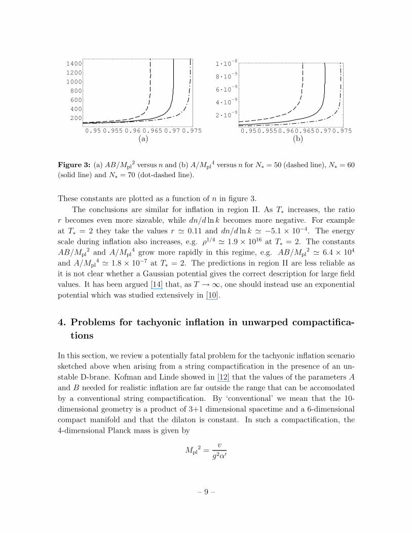
Figure 3: (a) AB/Mpl2 versus n and (b) A/Mpl

4 versus n for N∗ = 50 (dashed line), N∗ = 60

(solid line) and N∗ = 70 (dot-dashed line).

These constants are plotted as a function of n in figure 3.

The conclusions are similar for inflation in region II. As T∗ increases, the ratio

r becomes even more sizeable, while dn/d ln k becomes more negative. For example

at T∗ = 2 they take the values r ≃ 0.11 and dn/d ln k ≃ −5.1 × 10−4. The energy

scale during inflation also increases, e.g. ρ1/4 ≃ 1.9 × 1016 at T∗ = 2. The constants

AB/Mpl2 and A/Mpl

4 grow more rapidly in this regime, e.g. AB/Mpl2 ≃ 6.4 × 104

and A/Mpl4 ≃ 1.8 × 10−7 at T∗ = 2. The predictions in region II are less reliable as

it is not clear whether a Gaussian potential gives the correct description for large field

values. It has been argued [14] that, as T → ∞, one should instead use an exponential

potential which was studied extensively in [10].

4. Problems for tachyonic inflation in unwarped compactifica-

tions

In this section, we review a potentially fatal problem for the tachyonic inflation scenario

sketched above when arising from a string compactification in the presence of an un-

stable D-brane. Kofman and Linde showed in [12] that the values of the parameters A

and B needed for realistic inflation are far outside the range that can be accomodated

by a conventional string compactification. By ‘conventional’ we mean that the 10-

dimensional geometry is a product of 3+1 dimensional spacetime and a 6-dimensional

compact manifold and that the dilaton is constant. In such a compactification, the

4-dimensional Planck mass is given by

Mpl2 =

v

g2α′

– 9 –

where

v =2V6

(2π)7α′3(4.1)

with g the closed string coupling and V6 the volume of the compactification manifold.

In order for the effective action (2.1) to be applicable, the α′ and string loop corrections

should be small which requires g < 1 and v > 1.

For simplicity, let’s consider the case of a space-filling non-BPS D3-brane in type

IIA (the conclusions are unchanged if one takes a higher dimensional brane wrapping

some of the internal directions). The parameters A and B are then given by

A =

√2

(2π)3gα′2(4.2)

B = 8 ln 2α′ (4.3)

The condition (3.2) for slow-roll becomes

g/v ≫ (2π)3

2√

2 ln 2≃ 127. (4.4)

So in order to get many e-folds of inflation we need either a large string coupling or

small compactification volume.

The situation gets much worse if, in addition, we require the density fluctuations

to fall within observational constraints. For example, we saw in the previous section

that, for inflation in region I, the parameter A satisfies

A/Mpl4 < 6.7 × 10−9.

Combining this with (4.4) implies that v has to be extremely small:

v ≪ 5.7 × 10−13.

The same order of magnitude was found in [12] from constraints on gravitational wave

production. For such tiny values of the compactified volume, α′ corrections almost

certainly render the action (2.1) unreliable.

5. The role of warping

The discussion of the previous section assumed a conventional compactification in which

the 10-dimensional geometry is a product of 3+1-dimensional spacetime and a compact

6-dimensional manifold. However, string theory allows more general, warped compact-

ifications [16, 17] where the 10-dimensional string frame metric is of the form

ds2 = e2C(y)gµν(x)dxµdxν + gmn(y)dymdyn. (5.1)

– 10 –

The warp factor e2C can become very small in a certain region while its average is

of order 1 [17]. Processes taking place in the warped region are redshifted leading to

a hierarchy of energy scales. It is natural to ask whether one can find warped com-

pactifications where the slow-roll parameters are similarly suppressed and the problems

sketched in the previous sections can be overcome. A crucial extra ingredient is that

we shall also allow the dilaton to vary over the compact manifold:

φ = φ0 + φ(y). (5.2)

The 4-dimensional Planck mass in such a compactification is

Mpl2 =

v

g2α′

where g = eφ0 and the ‘warped volume’ v now depends on the warp factor and the

dilaton:

v =2

(2π)7α′3

∫

d6y√

g6e−2φ+2C .

We will consider compactifications where the average value of e−2φ+2C is of order 1 so

for our purposes there is no difference between v and v defined in (4.1). Embedding

a non-BPS D3-brane in this background2 leads to an effective action of the form (2.1)

with the expressions (4.2,4.3) for A and B now replaced by

A =

√2e4C−φ

(2π)3gα′2(5.3)

B = 8 ln 2α′e−2C . (5.4)

while the condition (4.4) for slow-roll inflation gets replaced by

ge2C−φ

v≫ 127. (5.5)

Hence we see that slow-roll can be facilitated in backgrounds where locally

e2C−φ ≫ 1. (5.6)

6. Warped backgrounds from space-filling D-branes

Simple examples of warped backgrounds are the ones obtained by wrapping a large

number of space-filling D-branes on a cycle of the compact manifold. The backreaction

2for the type IIB case one should use a D3 − D3 pair, which is also described by an action of the

form (2.1) but with a complex scalar T .

– 11 –

then produces a ‘throat region’ with significant warping and varying dilaton. Let

us consider a large number N of Dp-branes (3 ≤ p ≤ 6) wrapping a p − 3 cycle.

Such backgrounds are a generalization of the p = 3 brane case considered by Verlinde

in [18]. The explicit supergravity solution can easily be written down for a toroidal

compactification; the modifications for the more general case are unimportant for our

purposes. Using coordinates (xµ, ya, yi), µ = 0, . . . , 3, a = 1, . . . , p−3, i = p−2, . . . , 9−p, the string frame geometry in the vicinity of the branes can be approximated by

ds2 = H−1/2p (ηµνdxµdxν + dyadya) + H1/2

p dyidyi (6.1)

e2φ = g2H3−p

2p (6.2)

with

Hp =(rp

r

)7−p

(6.3)

(rp)7−p = 25−pπ

5−p

2 Γ

(

7 − p

2

)

gN(α′)7−p

2 (6.4)

and we have defined a radial coordinate r2 = yiyi. We have also assumed that r/rp ≪ 1.

For large r, the geometry is modified and glues smoothly into a compact manifold. The

α′ corrections to the supergravity approximation (6.2) are unimportant provided that

gN ≫ 1 and, for p > 3, [19]rp

r≪ (gN)

4(p−3)(7−p) (6.5)

where, on the right hand side, we have neglected a numerical factor greater than one.

String loop corrections can be safely ignored in the region of interest (rp/r ≫ 1). For

the moment we shall assume that the number of branes N can be made arbitrarily

large and come back to the restrictions from RR tadpole cancellation in the discussion

in section 8.

These geometries are of the warped type (5.1, 5.2) with

e2C−φ =(rp

r

)

(7−p)(p−5)4

.

Since rp/r ≫ 1 we see that the condition (5.6) for improving slow-roll inflation can be

met only for p = 6 while for the other values of p the warping makes matters worse!

7. Improved inflation in the background of D6-branes

Hence we shall work from now on with the D6-brane background in type IIA with a

non-BPS D3-brane embedded in the throat region. The parameters A and B in Planck

– 12 –

units are then

A/Mpl4 =

√2

(2π)3

g3

v2

(rp

r

)−1/4

(7.1)

BMpl2 = 8 ln 2

v

g2

(rp

r

)1/2

. (7.2)

Eliminating rp/r we find a relation between v and g:

v ≃ 0.056

(

A

Mpl4

)−2/3

(BMpl2)−1/3g4/3. (7.3)

Using this relation we can explore which

0 0.2 0.4 0.6 0.8 10

5

10

15

20

Figure 4: v versus g for inflation with, from

top to bottom, n = 0.94, n = 0.95, n =

0.96, n = 0.97 (region I) and n = 0.97 (re-

gion II).

values of v and g can give rise to realistic in-

flation by plugging in the appropriate values

for A and B from the analysis in section 3.

From figure 4 we see that it is now possi-

ble to accommodate realistic inflation with

v > 1 and g < 1, the situation becoming

better for inflation in region I for smaller

values of n. For example, for n = 0.97 in

region I, we need g > 0.34 in order to have

v > 1, while for n = 0.94 we only need

g > 0.10. The situation becomes worse for

inflation in region II where, for example for

n = 0.97, one needs g > 1 to obtain v > 1.

We can also estimate the the number of D6-branes required in order in order to

be able trust the supergravity approximation (6.2) in the region of significant warping.

This number turns out to be quite large. The condition (6.5) gives the minimal number

of D6-branes Nmin as

Nmin =1

g

(rp

r

)3/4

.

Let us first look at the number of branes required to meet the slow-roll condition (5.5),

which can be written asg4/3

v≫ 127

N1/3min

.

Hence we need the number of branes to be at least of order 106 or so to accommodate

slow-roll in the g < 1, v > 1 region. Requiring that, in addition, the perturbation

spectrum falls within observational constraints further increases Nmin. Using (7.1, 7.2)

– 13 –

we can express Nmin in terms of A and B:

Nmin ≃ 5.88AB2.

Using the values of A, B appropriate for inflation in region I, one finds that one needs

Nmin to be at least of order 1014.

8. Discussion

We saw in section 3 that a tachyonic scalar with a Gaussian potential can provide a

viable inflationary scenario within current observational bounds. The main predictions

are an upper limit on the scalar spectral index n ≤ 0.98 and a sizeable production

of gravitational waves with the scale of inflation close to the susy GUT scale. We

proposed a mechanism to attain the required parameter range in string theory by

embedding the unstable brane in the throat geometry produced by a large number of

D6-branes wrapping a three-cycle in the compact manifold. We shall now comment on

some of the hurdles that need to be overcome in order to realize this idea in a concrete

string compactification.

First of all, our setup requires a compactification that includes a sufficient number

of D6-branes. Since the D6-branes carry RR charge, consistency requires that the RR

tadpoles be cancelled by introducing objects with negative RR charge. In a supersym-

metric Minkowski space compactification, this requires introducing a sufficient number

of orientifold O6-planes [20]. Although it is not unthinkable that there exist orien-

tifold compactifications with of the order 106 D6-branes required for getting e-folds3,

it is doubtful whether the number of branes can be as high as the order 1014 needed

for obtaining realistic density perturbations. Another way of cancelling the tadpoles

is by introducing anti-D6 branes. In a Minkowski space compactification this breaks

supersymmetry and jeopardizes the long-term stability of the compactification due to

the attractive forces between branes and anti-branes; the question is then whether it

is possible to find a setup that is sufficiently stable to allow the inflationary phase

to take place. Yet another possibility would be to start with a compactification to

4-dimensional anti-de Sitter space before introducing supersymmetry-breaking effects

such as the unstable D3-brane. In anti-de Sitter compactifications it is possible to can-

cel the RR tadpoles of an arbitrary number of D6-branes with anti-branes in a stable

manner without breaking supersymmetry4. Explicit examples were constructed in [22].

3For example, in the case of F-theory compactifications, examples are known which allow up to

order 104 D3-branes [21].4We would like to thank Frederik Denef for pointing this out to us.

– 14 –

Adding the unstable brane (and possibly other supersymmetry breaking effects to raise

the value of the cosmological constant) to such a background may yield a configura-

tion that is sufficiently stable to support inflation. We leave these issues for further

investigation.

We also want to stress that, in the present work, we have implicitly assumed that

it is possible to stabilize the scalar moduli of the compactification. Much progress

has been made recently in constructing flux compactifications in type IIB/F-theory

with all moduli stabilized [23, 24], and the interplay between moduli stabilization and

various inflationary scenarios has been addressed [25]. In our case, it is of particular

importance to stabilize those moduli that are sourced by the tachyon, such as the

volume modulus of the compactified manifold, in order for inflation to work. The issue

of moduli stabilization is also important for obtaining a sensible late-time cosmology,

as the value of the potential for the moduli contributes to the cosmological constant.

In the light of this comment one might wonder whether tachyonic inflation could

also be realized in other corners of the string theory moduli space, where the problem

of moduli stabilization is under better control. In the present example, the condition

(5.5) for improving slow-roll was met because, in the D6-brane background, the string

coupling eφ decreases faster than the the warp factor e2C when we approach the branes.

Alternatively, one might look for more complicated warped backgrounds which have,

for example, a region where e2C is of order one while eφ becomes very small.

Finally, a realistic inflation model has to incorporate a mechanism for reheating

the universe by converting the energy contained in the inflaton field into radiation. The

proposal of [11], in which unstable branes decay into stable D-branes containing the

standard model, is likely to be amenable to the present context.

Acknowledgments

It is a pleasure to thank Frederik Denef, Sandip Trivedi, Sudhakar Panda and K.P.

Yogendran for discussions and useful correspondence.

References

[1] A. D. Linde, “Particle Physics And Inflationary Cosmology,” Harwood, Chur,

Switzerland (1990).

[2] A. R. Liddle and D. H. Lyth, “Cosmological Inflation And Large-Scale Structure,”

Cambridge University Press, Cambridge, England (2000).

– 15 –

[3] H. V. Peiris et al., “First year Wilkinson Microwave Anisotropy Probe (WMAP)

observations: Implications for inflation,” Astrophys. J. Suppl. 148, 213 (2003)

[arXiv:astro-ph/0302225].

[4] C. L. Bennett et al., “First Year Wilkinson Microwave Anisotropy Probe (WMAP)

Observations: Preliminary Maps and Basic Results,” Astrophys. J. Suppl. 148, 1

(2003) [arXiv:astro-ph/0302207].

[5] F. Quevedo, “Lectures on string / brane cosmology,” Class. Quant. Grav. 19, 5721

(2002) [arXiv:hep-th/0210292].

[6] A. Sen, “Rolling tachyon,” JHEP 0204, 048 (2002) [arXiv:hep-th/0203211];

A. Sen, “Tachyon matter,” JHEP 0207, 065 (2002) [arXiv:hep-th/0203265];

A. Sen, “Field theory of tachyon matter,” Mod. Phys. Lett. A 17, 1797 (2002)

[arXiv:hep-th/0204143];

A. Sen, “Time and tachyon,” Int. J. Mod. Phys. A 18, 4869 (2003)

[arXiv:hep-th/0209122].

[7] G. W. Gibbons, “Cosmological evolution of the rolling tachyon,” Phys. Lett. B 537, 1

(2002) [arXiv:hep-th/0204008].

[8] M. Fairbairn and M. H. G. Tytgat, “Inflation from a tachyon fluid?,” Phys. Lett. B

546, 1 (2002) [arXiv:hep-th/0204070].

[9] S. Mukohyama, Phys. Rev. D 66, 024009 (2002) [arXiv:hep-th/0204084]; A. Feinstein,

Phys. Rev. D 66, 063511 (2002) [arXiv:hep-th/0204140]; T. Padmanabhan, Phys. Rev.

D 66, 021301 (2002) [arXiv:hep-th/0204150]; A. V. Frolov, L. Kofman and

A. A. Starobinsky, Phys. Lett. B 545, 8 (2002) [arXiv:hep-th/0204187]; D. Choudhury,

D. Ghoshal, D. P. Jatkar and S. Panda, Phys. Lett. B 544, 231 (2002)

[arXiv:hep-th/0204204]; M. Sami, Mod. Phys. Lett. A 18, 691 (2003)

[arXiv:hep-th/0205146]; M. Sami, P. Chingangbam and T. Qureshi, Phys. Rev. D 66,

043530 (2002) [arXiv:hep-th/0205179]; J. c. Hwang and H. Noh, Phys. Rev. D 66,

084009 (2002) [arXiv:hep-th/0206100]; Y. S. Piao, R. G. Cai, X. m. Zhang and

Y. Z. Zhang, Phys. Rev. D 66, 121301 (2002) [arXiv:hep-ph/0207143]; X. z. Li,

D. j. Liu and J. g. Hao, arXiv:hep-th/0207146; B. Wang, E. Abdalla and R. K. Su,

Mod. Phys. Lett. A 18, 31 (2003) [arXiv:hep-th/0208023]; M. C. Bento, O. Bertolami

and A. A. Sen, Phys. Rev. D 67, 063511 (2003) [arXiv:hep-th/0208124]; C. j. Kim,

H. B. Kim and Y. b. Kim, Phys. Lett. B 552, 111 (2003) [arXiv:hep-th/0210101];

Y. S. Piao, Q. G. Huang, X. m. Zhang and Y. Z. Zhang, Phys. Lett. B 570, 1 (2003)

[arXiv:hep-ph/0212219]; X. z. Li and X. h. Zhai, Phys. Rev. D 67, 067501 (2003)

[arXiv:hep-ph/0301063]; G. W. Gibbons, Class. Quant. Grav. 20, S321 (2003)

[arXiv:hep-th/0301117]; Z. K. Guo, Y. S. Piao, R. G. Cai and Y. Z. Zhang, Phys. Rev.

– 16 –

D 68, 043508 (2003) [arXiv:hep-ph/0304236]; M. Majumdar and A. C. Davis, Phys.

Rev. D 69, 103504 (2004) [arXiv:hep-th/0304226]; D. Choudhury, D. Ghoshal,

D. P. Jatkar and S. Panda, JCAP 0307, 009 (2003) [arXiv:hep-th/0305104]; Y. S. Piao

and Y. Z. Zhang, arXiv:hep-th/0307074; L. R. W. Abramo and F. Finelli, Phys. Lett.

B 575, 165 (2003) [arXiv:astro-ph/0307208]; M. C. Bento, N. M. C. Santos and

A. A. Sen, arXiv:astro-ph/0307292; V. Gorini, A. Y. Kamenshchik, U. Moschella and

V. Pasquier, arXiv:hep-th/0311111; B. C. Paul and M. Sami, arXiv:hep-th/0312081;

A. Sen, arXiv:hep-th/0312153; J. M. Aguirregabiria and R. Lazkoz, Mod. Phys. Lett. A

19, 927 (2004) [arXiv:gr-qc/0402060]; J. M. Aguirregabiria and R. Lazkoz, Phys. Rev.

D 69, 123502 (2004) [arXiv:hep-th/0402190]; G. Calcagni, Phys. Rev. D 69, 103508

(2004) [arXiv:hep-ph/0402126]; C. Kim, H. B. Kim, Y. Kim, O. K. Kwon and

C. O. Lee, arXiv:hep-th/0404242; E. Papantonopoulos and I. Pappa, Mod. Phys. Lett.

A 15, 2145 (2000) [arXiv:hep-th/0001183]; E. Papantonopoulos and I. Pappa, Phys.

Rev. D 63, 103506 (2001) [arXiv:hep-th/0010014].

[10] A. Steer and F. Vernizzi, “Tachyon inflation: Tests and comparison with single scalar

field inflation,” arXiv:hep-th/0310139.

[11] J. M. Cline, H. Firouzjahi and P. Martineau, “Reheating from tachyon condensation,”

JHEP 0211, 041 (2002) [arXiv:hep-th/0207156];

N. Barnaby and J. M. Cline, “Creating the universe from brane-antibrane

annihilation,” arXiv:hep-th/0403223.

[12] L. Kofman and A. Linde, “Problems with tachyon inflation,” JHEP 0207, 004 (2002)

[arXiv:hep-th/0205121].

[13] D. H. Lyth and A. Riotto, “Particle physics models of inflation and the cosmological

density perturbation,” Phys. Rept. 314, 1 (1999) [arXiv:hep-ph/9807278].

[14] A. Sen, “Supersymmetric world-volume action for non-BPS D-branes,” JHEP 9910,

008 (1999) [arXiv:hep-th/9909062];

M. R. Garousi, “Tachyon couplings on non-BPS D-branes and Dirac-Born-Infeld

action,” Nucl. Phys. B 584, 284 (2000) [arXiv:hep-th/0003122];

E. A. Bergshoeff, M. de Roo, T. C. de Wit, E. Eyras and S. Panda, “T-duality and

actions for non-BPS D-branes,” JHEP 0005, 009 (2000) [arXiv:hep-th/0003221];

N. D. Lambert and I. Sachs, “Tachyon dynamics and the effective action

approximation,” Phys. Rev. D 67, 026005 (2003) [arXiv:hep-th/0208217];

M. R. Garousi, “On-shell S-matrix and tachyonic effective actions,” Nucl. Phys. B 647,

117 (2002) [arXiv:hep-th/0209068];

D. Kutasov and V. Niarchos, “Tachyon effective actions in open string theory,” Nucl.

Phys. B 666, 56 (2003) [arXiv:hep-th/0304045];

– 17 –

M. R. Garousi, “Slowly varying tachyon and tachyon potential,” JHEP 0305, 058

(2003) [arXiv:hep-th/0304145].

[15] A. Vilenkin, “The Birth Of Inflationary Universes,” Phys. Rev. D 27, 2848 (1983);

A. D. Linde, “Eternal Chaotic Inflation,” Mod. Phys. Lett. A 1, 81 (1986).

[16] C. S. Chan, P. L. Paul and H. Verlinde, “A note on warped string compactification,”

Nucl. Phys. B 581, 156 (2000) [arXiv:hep-th/0003236];

I. R. Klebanov and M. J. Strassler, “Supergravity and a confining gauge theory:

Duality cascades and chiSB-resolution of naked singularities,” JHEP 0008, 052 (2000)

[arXiv:hep-th/0007191];

S. Kachru, “Lectures on warped compactifications and stringy brane constructions,”

arXiv:hep-th/0009247;

S. B. Giddings, S. Kachru and J. Polchinski, “Hierarchies from fluxes in string

compactifications,” Phys. Rev. D 66, 106006 (2002) [arXiv:hep-th/0105097].

[17] B. R. Greene, K. Schalm and G. Shiu, “Warped compactifications in M and F theory,”

Nucl. Phys. B 584, 480 (2000) [arXiv:hep-th/0004103].

[18] H. Verlinde, “Holography and compactification,” Nucl. Phys. B 580, 264 (2000)

[arXiv:hep-th/9906182].

[19] N. Itzhaki, J. M. Maldacena, J. Sonnenschein and S. Yankielowicz, “Supergravity and

the large N limit of theories with sixteen supercharges,” Phys. Rev. D 58, 046004

(1998) [arXiv:hep-th/9802042].

[20] E. G. Gimon and J. Polchinski, “Consistency Conditions for Orientifolds and

D-Manifolds,” Phys. Rev. D 54, 1667 (1996) [arXiv:hep-th/9601038].

[21] A. Klemm, B. Lian, S. S. Roan and S. T. Yau, “Calabi-Yau fourfolds for M- and

F-theory compactifications,” Nucl. Phys. B 518, 515 (1998) [arXiv:hep-th/9701023].

[22] B. S. Acharya, F. Denef, C. Hofman and N. Lambert, “Freund-Rubin revisited,”

arXiv:hep-th/0308046.

[23] S. Kachru, R. Kallosh, A. Linde and S. P. Trivedi, “De Sitter vacua in string theory,”

Phys. Rev. D 68, 046005 (2003) [arXiv:hep-th/0301240].

[24] F. Denef, M. R. Douglas and B. Florea, “Building a better racetrack,” JHEP 0406,

034 (2004) [arXiv:hep-th/0404257].

[25] S. Kachru, R. Kallosh, A. Linde, J. Maldacena, L. McAllister and S. P. Trivedi,

“Towards inflation in string theory,” JCAP 0310, 013 (2003) [arXiv:hep-th/0308055];

– 18 –

M. R. Garousi, M. Sami and S. Tsujikawa, “Inflation and dark energy arising from

rolling massive scalar field on the D-brane,” arXiv:hep-th/0402075;

H. Firouzjahi and S. H. H. Tye, “Closer towards inflation in string theory,” Phys. Lett.

B 584, 147 (2004) [arXiv:hep-th/0312020].

C. P. Burgess, J. M. Cline, H. Stoica and F. Quevedo, “Inflation in realistic D-brane

models,” arXiv:hep-th/0403119;

O. DeWolfe, S. Kachru and H. Verlinde, “The giant inflaton,” JHEP 0405, 017 (2004)

[arXiv:hep-th/0403123];

N. Iizuka and S. P. Trivedi, “An inflationary model in string theory,”

arXiv:hep-th/0403203;

A. Buchel and A. Ghodsi, “Braneworld inflation,” arXiv:hep-th/0404151;

K. Dasgupta, J. P. Hsu, R. Kallosh, A. Linde and M. Zagermann, “D3/D7 brane

inflation and semilocal strings,” arXiv:hep-th/0405247;

– 19 –