arX

iv:0

901.

0609

v1 [

hep-

ph]

6 J

an 2

009

ANL-HEP-PR-08-80EFI-08-31

FERMILAB-PUB-08-562-T

Gauge-Higgs Unification, Neutrino Masses and

Dark Matter in Warped Extra Dimensions

Marcela Carenaa,b, Anibal D. Medina d

Nausheen R. Shah b and Carlos E.M. Wagner b,c,e

Theoretical Phys. Dept., Fermi National Laboratory, Batavia, IL 60510, USA a

Department of Physics, Enrico Fermi Institute b

and Kavli Institute for Cosmological Physics c,

University of Chicago, 5640 S. Ellis Ave., Chicago, IL 60637, USA

Department of Physics, UC Davis, One Shields Ave, Davis, CA 95616 d

HEP Division, Argonne National Laboratory, 9700 Cass Ave., Argonne, IL 60439, USA e

January 6, 2009

Abstract

Gauge Higgs Unification in Warped Extra Dimensions provides an attractive solution to thehierarchy problem. The extension of the Standard Model gauge symmetry to SO(5) × U(1)Xallows the incorporation of the custodial symmetry SU(2)R plus a Higgs boson doublet withthe right quantum numbers under the gauge group. In the minimal model, the Higgs massis in the range 110–150 GeV, while a light Kaluza Klein (KK) excitation of the top quarkappears in the spectrum, providing agreement with precision electroweak measurements and apossible test of the model at a high luminosity LHC. The extension of the model to the leptonsector has several interesting features. We discuss the conditions necessary to obtain realisticcharged lepton and neutrino masses. After the addition of an exchange symmetry in the bulk,we show that the odd neutrino KK modes provide a realistic dark matter candidate, with amass of the order of 1 TeV, which will be probed by direct dark matter detection experimentsin the near future.

1

1 Introduction

Warped Extra Dimensions present an elegant solution to the hierarchy problem, where all funda-mental parameters are of the order of the Planck scale. The weak scale–Planck scale hierarchy isobtained by an exponential warp factor, which is naturally small provided the Higgs field is local-ized towards the so-called infrared brane [1]. If all Standard Model (SM) fields propagate in thebulk, the theory leads to the presence of Kaluza Klein (KK) modes which tend to be localizedtowards the IR brane and therefore couple sizably to the Higgs. This in turn leads to large mixingbetween the heavy SM particles and their KK modes, leading to modifications of the electroweakparameters and therefore to strong constraints from electroweak precision measurements [2]–[7].These constraints may be weakened by the introduction of brane kinetic terms [8]–[11] or custodialsymmetries [12], [13], which allow the presence of KK modes with masses of the order of a few TeV.

One of the attractive features of these models is the natural explanation of the hierarchy offermion masses by the localization of the fermion fields in the bulk [16]–[18]. The chiral propertiesof the fermions are obtained by imposing an orbifold symmetry and demanding that the fields areodd or even under such a symmetry. Fermion fields that are even under the orbifold symmetryat the infrared and ultraviolet branes present zero modes, which are chiral and therefore may beidentified with the SM fermion fields. The localization of the zero modes is governed by the bulkmass parameter ck, with k the curvature of the extra dimension and c, a number of order one. Whilethe zero modes of chiral fields with c > 1/2 couple weakly to the Higgs and are therefore light, theheavy SM fields are associated with bulk mass parameters c ≤ 1/2. Due to the exponential behaviorof the zero mode wave functions, large hierarchies between the fermion masses are generated bysmall variations of the corresponding c-parameters.

Gauge Higgs Unification models identify the Higgs field with the five dimensional component ofthe gauge fields [19]. An extended gauge symmetry is necessary for the successful implementation ofthis mechanism. In particular, models based on the gauge group SO(5)×U(1)X include the custodialand weak gauge symmetry via SO(5) ⊃ SO(4) ≡ SU(2)L × SU(2)R [20],[21] [22]. Moreover,provided the SO(5) symmetry is broken to a subgroup of SO(4) by boundary conditions at bothbranes, the fifth dimensional components of SO(5)/SO(4) have the proper quantum numbers to beidentified with the Higgs field, which is exponentially localized towards the IR brane.

Since the Higgs originates from gauge fields, its tree level potential vanishes. In a previouswork [25], we computed the one-loop effective potential and demonstrated that electroweak sym-metry breaking, with the proper generation of third generation quark and gauge boson masses maybe obtained for the same values of the bulk mass parameters that lead to agreement with precisionelectroweak data at the one-loop level. Moreover, we showed that the Higgs mass is in the range110–150 GeV and that a light KK mode of the top quark, T ′, appears in the spectrum, with a masssmall enough so that the KK gluon may decay into it. The presence of this light KK mode has astrong impact on the phenomenology of the model [26]. For instance, searches for the KK gluonby its decay into top-quarks [27],[28], [29] is rendered difficult due to the presence of the additionaldominant decay mode into KK top-quarks and the broadness of the KK gluon. On the contrary, theconstructive interference between the QCD and KK gluon induced pair production of the top-quarkKK mode allows to search for a T ′ for values of the masses much larger than those at reach in the

2

case of just the QCD production cross section.In this article, we will analyze the addition of the lepton sector in the gauge Higgs unification

scenario. To add leptons, we will proceed in a similar way as for the quark sector. The left-handedleptons will be added in a fundamental representation of SO(5), with QX = 0, while the right-handed neutrino and charged lepton fields will be added in a fundamental representation and a 10

of SO(5) also with charge QX = 0, respectively.Due to the gauge origin of the Higgs field, a possible local infrared brane operator (LH) LH/M ,

which could lead to large values of the neutrino Majorana masses, should come from the fifthdimensional component of the covariant derivative of the lepton fields and therefore can only nat-urally arise from the integration of the right-handed neutrinos, with a local IR Majorana mass.Indeed, since the fields associated with the right-handed neutrino zero modes are singlets under theconserved gauge groups on both the infrared and ultraviolet branes, one can always add Majoranamasses for these fields on the infrared and ultraviolet branes. We will therefore consider these massesand implement a See-Saw mechanism for the generation of the light neutrino masses [31],[32]. Wewill show how to incorporate these masses within the context of these models, obtain the modifiedprofile functions and define the conditions to derive a realistic spectrum.

Furthermore, the introduction of an exchange symmetry [43], which is preserved in the bulk,yields a natural dark matter candidate in the spectrum, that may be identified with the odd KKmodes of the right-handed neutrino. This exchange symmetry requires the identification of thebulk mass parameter of the dark matter candidate with the one of the right-handed neutrinos,establishing a connection between neutrino masses and the relic dark matter density. We will showthat, if the odd fermions are assumed to be Dirac particles, the predicted relic density is the correctone for Dirac fermion masses of the order of 1 TeV. In the Majorana case, somewhat smaller massesare allowed, and the results depend on the relative values of the ultraviolet and infrared Majoranamasses. We will show that in both the Dirac and Majorana cases, direct detection experiments willefficiently probe the existence of the proposed dark matter candidates.

The article is organized as follow: In section 2 we discuss the properties of leptons in scenariosof Gauge Higgs Unification. In section 3 we discuss the generation of charged lepton and neutrinomasses. In section 4 we analyze the possibility of incorporating dark matter via an exchange bulksymmetry, analyzing the couplings and the annihilation diagrams, as well as the direct detection ofthese dark matter candidates. We reserve section 5 for our conclusions. Some technical details aregiven in the Appendix.

2 Leptons in Gauge Higgs Unification Scenarios

The goal of the current work is to add the lepton sector into the minimal Gauge Higgs Unificationmodel described above, including right handed neutrinos, with brane Majorana masses. We willproceed in a similar way as in the quark case [25], and discuss the general question of charged leptonand neutrino mass generation.

Similar to the quark sector, we let the SM SU(2)L lepton doublet containing the left-handedcharged leptons and neutrinos, lL and νL, arise from a 50 of SO(5) × U(1)X , where the subscript

3

refers to the U(1)X charge. The right handed neutrino, NR will be included as the singlet componentin a fundamental representation of SO(5), while the right-handed charged lepton, lR, is placed in a100 of SO(5) analogously to the dR. One may also include brane mass terms connecting differentmultiplet components, as well as new brane Majorana masses for the right handed neutrino NR:

(

MUV δ(y) −MIRδ(y − L))

NRNR. (1)

The right handed neutrino, NR, in principle could be identified with the singlet right-handedcomponent in the same multiplet as the left-handed leptons. However, in order to naturally suppresslepton flavor violation effects and maintain agreement with precision electroweak measurements,the left-handed leptons should be localized towards the UV brane [14],[15]. The zero modes of thecorresponding right-handed multiplet will therefore be localized towards the IR brane. This impliesthat even with a natural scale for the brane masses O(MP l), the exponential suppression of the wavefunction at the UV brane would lead to a effective Majorana mass for NR which is much smallerthan the Planck scale. This, in turn, after the implementation of the See-Saw mechanism, leadsto too large values for the observed neutrino masses. Therefore, as we will discuss below, it willprove to be necessary to have the left-handed leptons in a different multiplet as the right-handedneutrinos.

If NR belongs to the same multiplet as the left-handed leptons:

ξi1L ∼ Li

1L =

(

χei

1L(−,+)1 lni

L (+,+)0

χni

1L(−,+)0 lei

L (+,+)−1

)

⊕ N iL(−,−)0 , (2)

ξi2R ∼

T i1R =

ψ′iR(−,+)1

N ′iR(−,+)0

E ′iR(−,+)−1

⊕ T i2R =

ψ′′iR (−,+)1

N ′′iR (−,+)0

EiR(+,+)−1

⊕ Li2R =

(

χei

2R(−,+)1 l′′ni

R (−,+)0

χni

2R(−,+)0 l′′ei

R (−,+)−1

)

,

Alternatively, the right-handed neutrino can be incorporated in a different multiplet from theleft-handed lepton one. The two multiplet assignments are as follows:

ξi1L ∼ Li

1L =

(

χei

1L(−,+)1 lni

L (+,+)0

χni

1L(−,+)0 lei

L (+,+)−1

)

⊕ N ′iL(−,+)0 ,

ξi2R ∼ Li

2R =

(

χei

2R(−,+)1 l′ni

R (−,+)0

χni

2R(−,+)0 l′ei

R (−,+)−1

)

⊕ N iR(+,+)0 ,

(3)

ξi3R ∼

T i1R =

ψ′iR(−,+)1

N ′iR(−,+)0

E ′iR(−,+)−1

⊕ T i2R =

ψ′′iR (−,+)1

N ′′iR (−,+)0

EiR(+,+)−1

⊕ Li3R =

(

χei

3R(−,+)1 l′′ni

R (−,+)0

χni

3R(−,+)0 l′′ei

R (−,+)−1

)

,

4

where we show the decomposition under SU(2)L×SU(2)R, and explicitly write the U(1)EM charges.The Lis are bidoublets of SU(2)L × SU(2)R, with SU(2)L acting vertically and SU(2)R actinghorizontally. The T i

1’s and T i2’s transform as (3, 1) and (1, 3) under SU(2)L ×SU(2)R, respectively,

while N i and N ′i are SU(2)L × SU(2)R singlets. The superscripts, i = 1, 2, 3, label the threegenerations.

We also show the parities on the indicated 4D chirality, where − and + stands for odd and evenparity conditions and the first and second entries in the bracket correspond to the parities in the UVand IR branes respectively. Let us stress that while odd parity is equivalent to a Dirichlet boundarycondition, the even parity is a linear combination of Neumann and Dirichlet boundary conditions,that is determined via the fermion bulk equations of motion as discussed below. The boundaryconditions for the opposite chirality fermion multiplet can be read off the ones above by a flip inboth chirality and boundary condition, for example (−,+)L → (+,−)R. In the absence of mixingamong multiplets satisfying different boundary conditions, the SM fermions arise as the zero-modesof the fields obeying (+,+) boundary conditions. The remaining boundary conditions are chosenso that SU(2)L × SU(2)R is preserved on the IR brane and so that mass mixing terms, necessaryto obtain the SM fermion masses after EW symmetry breaking, can be written on the IR brane.Consistency of the above parity assignments with the original orbifold Z2 symmetry at the IR branewas discussed in Appendix B of Ref. [25]. The three families will behave similarly, and therefore, wewill drop the family indices and concentrate only on one lepton family. Large mixing angles in thelepton sector can be naturally obtained while suppressing lepton flavor changing neutral currentsif the left-handed leptons have similar bulk mass parameters, ci1 [36],[37], and in the following wewill assume them to be equal. We will return to this issue in section 3.3. The zero modes of theleptons are too light and too weakly coupled to the Higgs boson to affect the Higgs potential in anysignificant way. The lepton KK modes may be coupled more strongly to the Higgs, but their gaugeinvariant mass is much larger than the Higgs induced one and therefore they tend to contributeonly weakly to both the Higgs potential and to precision electroweak observables.

One can add localized brane mass terms to the Lagrangian in both the one and the two multipletcases:

L1 = −2δ(x5 − L)[

L1LML2L2R + h.c.

]

−[

MIRδ(x5 − L) −MUV δ(x5)]

NRNR ; (4)

L2 = −2δ(x5 − L)[

N ′LML1

NR + L1LML2L3R + h.c.

]

−[

MIRδ(x5 − L) −MUV δ(x5)]

NRNR .(5)

With the introduction of the brane mixing terms, the different multiplets are now related viathe equations of motion. The fermions, like the gauge bosons, can be expanded in their KK basis:

ψL(x, x5) =∑

n

fL,n(x5, h)ψL,n(x), ψR(x, x5) =∑

n

fR,n(x5, h)ψR,n(x). (6)

Solving the equations of motion in the presence of h becomes complicated, as the different modesare mixed. However, 5D gauge symmetry relates these solutions to solutions with h = 0 [23], withΩ(x5, h), the gauge transformations that removes the vev of h:

Ω(x5, h) = exp

[

−iChhT4

∫ x5

0

dy a−2(y)

]

. (7)

5

The form of the bulk profile functions at h = 0 is given in Appendix A.The boundary masses lead to a redefinition of the effective boundary conditions for the fermion

fields at the branes. Let’s first analyze the case of a Dirac boundary mass term on the infrared brane,ML, involving fields from different multiplets Ψi

LΨjR, i, j = 1, 2, 3 for the different multiplets. Quite

generally, we shall call the profile of the left-handed field and the right-handed field participating inthe mass term gL and hR, respectively. The right handed component, Ψi

R with profile function gR

and the left-handed component ΨjL with profile function hL have Dirichlet boundary conditions on

the brane, and therefore gR(L) = hL(L) = 0. The equations of motion of the fields are affected bythe localized masses, which induce a discontinuity on the odd-parity profile functions at the infraredbrane. Indeed, keeping only the relevant terms, the integration of the equation of motion leads to

∫ L+ǫ

L−ǫ

(∂5gR)dx5 =

∫ L+ǫ

L−ǫ

2MLhR δ(x5 − L)dx5. (8)

Therefore, we obtain:limǫ→0

gR(L− ǫ) = −MLhR(L), (9)

and, similarly for the hL

limǫ→0

hL(L− ǫ) = ML2gL(L). (10)

Eq. (9) and (10) can now be reinterpreted as the new boundary conditions for the profiles at theIR brane.

Analogously, one can analyze the effect of the Majorana boundary mass, Mi, where i = IR orUV . Let’s take the specific case of the field NR, with a profile function hR. Its chiral partner willhave a profile function hL having an odd parity profile on both branes. The equation of motionin the presence of both the Majorana masses and the Dirac mass term ML1

leads to the followingrelationship

∫ y+ǫ

y−ǫ

(∂5hL)dx5 =

∫ y+ǫ

y−ǫ

[

(±2MihR − hL)δ(x5 − y) − 2ML1gLδ(x5 − L)

]

dx5. (11)

where the minus and plus signs are associated with the boundary conditions at y = L, and y =0, respectively. The odd parity at the branes then implies a Dirichlet boundary condition forthe function hL, which as before will present a discontinuity at the brane. For the IR boundaryconditions we obtain:

limǫ→0

hL(L− ǫ) = MIRhR(L) +ML1gL(L). (12)

For the UV boundary condition, instead:

limǫ→0

hL(0 + ǫ) = MUV hR(0). (13)

Eq. (12-13) can now be reinterpreted as the new boundary condition for the profiles at the branes.The generalization of these expressions to the general case is straightforward.

6

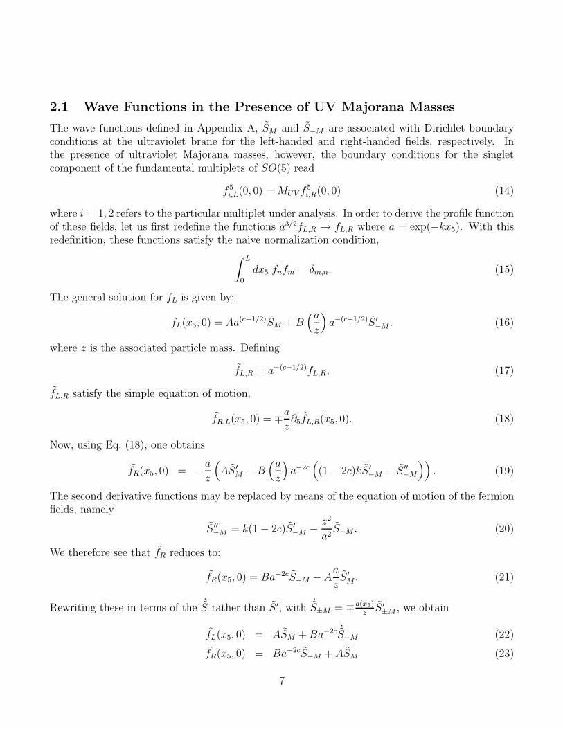
2.1 Wave Functions in the Presence of UV Majorana Masses

The wave functions defined in Appendix A, SM and S−M are associated with Dirichlet boundaryconditions at the ultraviolet brane for the left-handed and right-handed fields, respectively. Inthe presence of ultraviolet Majorana masses, however, the boundary conditions for the singletcomponent of the fundamental multiplets of SO(5) read

f 5i,L(0, 0) = MUV f

5i,R(0, 0) (14)

where i = 1, 2 refers to the particular multiplet under analysis. In order to derive the profile functionof these fields, let us first redefine the functions a3/2fL,R → fL,R where a = exp(−kx5). With thisredefinition, these functions satisfy the naive normalization condition,

∫ L

0

dx5 fnfm = δm,n. (15)

The general solution for fL is given by:

fL(x5, 0) = Aa(c−1/2)SM +B(a

z

)

a−(c+1/2)S ′−M . (16)

where z is the associated particle mass. Defining

fL,R = a−(c−1/2)fL,R, (17)

fL,R satisfy the simple equation of motion,

fR,L(x5, 0) = ∓az∂5fL,R(x5, 0). (18)

Now, using Eq. (18), one obtains

fR(x5, 0) = −az

(

AS ′M − B

(a

z

)

a−2c(

(1 − 2c)kS ′−M − S ′′

−M

))

. (19)

The second derivative functions may be replaced by means of the equation of motion of the fermionfields, namely

S ′′−M = k(1 − 2c)S ′

−M − z2

a2S−M . (20)

We therefore see that fR reduces to:

fR(x5, 0) = Ba−2cS−M −Aa

zS ′

M . (21)

Rewriting these in terms of the ˙S rather than S ′, with ˙S±M = ∓a(x5)zS ′±M , we obtain

fL(x5, 0) = ASM +Ba−2c ˙S−M (22)

fR(x5, 0) = Ba−2cS−M + A ˙SM (23)

7

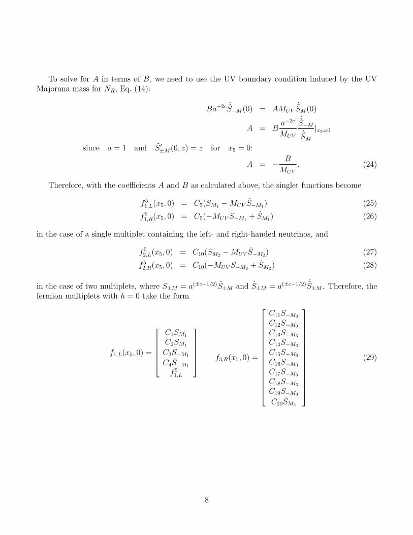
To solve for A in terms of B, we need to use the UV boundary condition induced by the UVMajorana mass for NR, Eq. (14):

Ba−2c ˙S−M(0) = AMUV˙SM(0)

A = Ba−2c

MUV

˙S−M

˙SM

|x5=0

since a = 1 and S ′±M(0, z) = z for x5 = 0:

A = − B

MUV. (24)

Therefore, with the coefficients A and B as calculated above, the singlet functions become

f 51,L(x5, 0) = C5(SM1

−MUV S−M1) (25)

f 51,R(x5, 0) = C5(−MUV S−M1

+ SM1) (26)

in the case of a single multiplet containing the left- and right-handed neutrinos, and

f 52,L(x5, 0) = C10(SM2

−MUV S−M2) (27)

f 52,R(x5, 0) = C10(−MUV S−M2

+ SM2) (28)

in the case of two multiplets, where S±M = a(±c−1/2)S±M and S±M = a(±c−1/2) ˙S±M . Therefore, thefermion multiplets with h = 0 take the form

f1,L(x5, 0) =

C1SM1

C2SM1

C3S−M1

C4S−M1

f 51,L

f3,R(x5, 0) =

C11S−M3

C12S−M3

C13S−M3

C14S−M3

C15S−M3

C16S−M3

C17S−M3

C18S−M3

C19S−M3

C20SM3

(29)

8

in the case of a single multiplet containing the left-handed and right-handed neutrinos, and

f1,L(x5, 0) =

C1SM1

C2SM1

C3S−M1

C4S−M1

C5SM1

f2,L(x5, 0) =

C6S−M2

C7S−M2

C8S−M2

C9S−M2

f 52,L

f3,R(x5, 0) =

C11S−M3

C12S−M3

C13S−M3

C14S−M3

C15S−M3

C16S−M3

C17S−M3

C18S−M3

C19S−M3

C20SM3

(30)

in the two multiplet case, where the Ci are normalization constants.

3 Lepton Spectrum

Applying the boundary conditions at x5 = L, taking into account the mass mixing terms fromEqs. (4) and (5) and using the procedure defined in Eqs. (9)–(12), we derive the conditions on thelepton wave functions f(L, h) in the presence of the Higgs field. In the case of only one multipletcontaining both the left-handed and right-handed neutrinos one gets the following conditions at theIR brane:

f 1,...,41,R +ML2

f 1,...,43,R = 0 f 5

1,L −MIRf51,R = 0

f 1,...,43,L −ML2

f 1,...,41,L = 0 f 5,...,10

3,L = 0

(31)

In the two multiplets, instead, one obtains:

f 1,...,41,R +ML2

f 1,...,43,R = 0 f 5

1,R +ML1f 5

2,R = 0 f 1,...,42,L = 0

f 1,...,43,L −ML2

f 1,...,41,L = 0 f 5

2,L −ML1f 5

1,L −MIRf52,R = 0 f 5,...,10

3,L = 0

(32)

where the superscripts denote the vector components.This defines a system of linear equations for the normalization constants Ci. Asking that the

determinant of the functional coefficients of this system vanishes in order to get a non-trivial solu-

9

tion [24], one obtains the following relations:

˙S5−M3

= 0 (33)

M2L2SM1

S−M3+ ˙SM1

˙S−M3= 0 (34)

2SM3

[

M2L2S−M3

˙S−M1+ S−M1

˙S−M3

]

−M2L2

˙S−M1sin[

λhfh

]2

= 0 (35)

2[

−M4L2SM1

S2−M3

[

˙S−M1(SM1

− e2c1kLMUV˙S−M1

) +MIR(1 − SM1S−M1

+ e2c1kLMUV S−M1

˙S−M1)]

−M2L2S−M3

[

2S2M1S−M1

− SM1

[

1 +MIRS−M1

˙SM1− e2c1kLMUV S−M1

(2MIRS−M1− ˙S−M1

)]

−MIR˙S2M1

˙S−M1− e2c1kLMUV (MIRS−M1

+ ˙SM1

˙S2−M1

)]

˙S−M3

−S−M1

[

˙SM1(SM1

−MIR˙SM1

) + e2c1kLMUV (1 − SM1S−M1

+MIRS−M1

˙SM1)]

˙S2−M3

]

+(M2L2MIRS−M3

+ ˙S−M3)[

M2L2S−M3

[

SM1+ e2c1kLMUV

˙S−M1(SM1

S−M1− ˙SM1

˙S−M1)]

+[

e2c1kLMUV S−M1+ ˙SM1

(SM1S−M1

− ˙SM1

˙S−M1)]

˙S−M3

]

sin[

λhfh

]2

= 0 (36)

in the case of a singlet neutrino multiplet, and

˙S3−M2

= 0 (37)

˙S5−M3

= 0 (38)

[

M2L2SM1

S−M3+ ˙SM1

˙S−M3

]2

= 0 (39)

2SM3

[

M2L2S−M3

˙S−M1+ S−M1

˙S−M3

]

−M2L2

˙S−M1sin[

λhfh

]2

= 0 (40)

10

2[

M2L2S−M3

[

(1 − SM1S−M1

)(SM2− e2c2kLMUV

˙S−M2) ˙S−M2

+MIR(1 − SM1S−M1

)

(1 − SM2S−M2

+ e2c2kLMUV S−M2

˙S−M2) +M2

L1SM1

˙S−M1(1 − SM2

S−M2+ e2c2kLMUV S−M2

˙S−M2)]

S−M1

[

M2L1SM1

(1 − SM2S−M2

+ e2c2kLMUV S−M2

˙S−M2) − ˙SM1

[

˙S−M2(SM2

− e2c2kLMUV˙S−M2

)

+MIR(1 − SM2S−M2

+ e2c2kLMUV S−M2

˙S−M2)]]

˙S−M3

]

+[

M2L2S−M3

[

−2M2L1SM1

˙S−M1− SM2

˙S−M2+ e2c2kLMUV

˙S2−M2

+MIR(−3 + 2SM1S−M1

+ SM2S−M2

− e2c2kLMUV S−M2

˙S−M2)]

+[

2MIRS−M1

˙SM1−M2

L1(1 + 2SM1

S−M1− SM2

S−M2+ e2c2kLMUV S−M2

˙S−M2)]

˙S−M3

]

sin[

λhfh

]2

+[

M2L2MIRS−M3

+M2L1

˙S−M3

]

sin[

λhfh

]4

= 0 (41)

in the case of two multiplets. In the above, for simplicity, we did not write the dependence on Land z and furthermore, we have used the Crowian:

− ˙SM(x5, z)˙S−M (x5, z) + SM(x5, z)S−M(x5, z) = 1 . (42)

The roots of the above equations define the values of z corresponding to the masses of the leptonzero modes and KK modes in the presence of the Higgs fields.

3.1 Charged Lepton Masses

Since the charged lepton masses are given by the mixing of the first and third multiplet via ML2,

the expression determining its mass is formally the same for the case in which the right-handedneutrino is in the same multiplet as the left-handed one as for the two neutrino multiplet case(Eqs. (35) and (40)). Additionally, since the lepton masses are much smaller then k, one can use anexpansion of SM for small values of z/k. As we shall show, the approximate functions we derive inthis way agree very well with the full numerical investigation we carried out. We shall concentrateon values of c1 >

∼ 0.5, which are preferred to cancel flavor violation effects in a natural way andprovide agreement with precision electroweak data [15],[36].

At small values of z compared to k, one can express the function SM in the form [24]:

SM ≈ z

∫ x5

0

a−1(y)e−2Mydy + O(z3) . (43)

Using this in Eq. (35), we can solve for the mass:

(

z

k

)

=ML2

e(1

2+c3)kL sin[λh

fh]√

2 (12− c1)(c

23 − 1

4)

√

[

(12− c3)(e

2(c1−1

2)kL − 1) −M2

L2(c1 − 1

2)(e2(c3−

1

2)k − 1)

]

(e2(1

2+c3)kL − 1)

. (44)

11

If c1 > 0.5 and −0.5 < c3 < c1, this reduces to:

(

z

k

)

= ML2e(

1

2−c1)kL sin

[

λh

fh

]

√

2 (c1 −1

2)(c3 +

1

2) (45)

For c1 > 0.5 and c3 > c1, instead,

(

z

k

)

= e(1

2−c3)kL sin

[

λh

fh

]

√

2 (c23 −1

4) (46)

Finally, for the case c1 > 0.5 and c3 < −0.5:

(

z

k

)

= ML2e(1+c3−c1)kL sin

[

λh

fh

]

√

2 (1

2− c1)(c3 +

1

2) (47)

where we have assumed that ML26= 0. We note that in the above, the lepton masses depend at

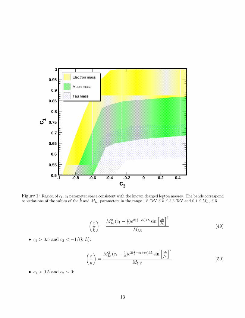
most linearly on ML2. As shown in Fig. 1, the above relations are verified by our numerical results.

Realistic lepton masses may be obtained for e.g. for c1 ≃ 0.6 and c3 ≃ −0.55, −0.65 and −0.8 for thecase of the tau, muon and electron, respectively. If a common value of c1 for the three generationsis demanded, as explained above, and for values of ML2

of order one, as chosen in Fig. 1, the valueof c1 is restricted to be in the range 0.5 <

∼ c1 <∼ 0.75. Larger values of c1 become incompatible with

the heavier charged lepton masses.

3.2 Neutrino Masses

The Neutrino masses are analyzed in a similar manner. First we look at the case in which theleft-handed and right-handed neutrinos belong to the same muliplet case. For c1 > 0.5,

(

z

k

)

=(c1 − 1

2)e2(

1

2−c1)kL sin[λh

fh]2

MIR(48)

From Eq. (48) we see that values of c1 ∼ 1 would be necessary in order to get the correct valuesfor the neutrino masses. However, values of c1 ≃ 1 are strongly constrained in order to reproducethe proper charged lepton masses. Indeed, as we emphasized at the end of last section, the propervalues of τ and µ masses may not be obtained for c1 ∼ 1. Therefore, we conclude that if all c1’sare about the same, as preferred to obtain large flavor mixing naturally without inducing largelepton flavor changing effects [36], two multiplets are required in order to obtain the correct leptonspectrum.

In the two multiplet case, the dependence of the neutrino masses on the mixing with the thirdmultiplet through ML2

is always exponentially suppressed. Therefore, we shall set ML2= 0 in the

following approximate expressions. The approximate mass expressions, for

• c1 > 0.5 and c2 > 1/(k L):

12

3c-1 -0.8 -0.6 -0.4 -0.2 0 0.2 0.4

1c

0.5

0.55

0.6

0.65

0.7

0.75

0.8

0.85

0.9

0.95

1

Electron mass

Muon mass

Tau mass

Figure 1: Region of c1, c3 parameter space consistent with the known charged lepton masses. The bands correspondto variations of the values of the k and ML2

parameters in the range 1.5 TeV <∼ k <

∼ 5.5 TeV and 0.1 <∼ ML2

<∼ 5.

(

z

k

)

=M2

L1(c1 − 1

2)e2(

1

2−c1)kL sin

[

λhfh

]2

MIR

(49)

• c1 > 0.5 and c2 < −1/(k L):

(

z

k

)

=M2

L1(c1 − 1

2)e2(

1

2−c1+c2)kL sin

[

λhfh

]2

MUV

(50)

• c1 > 0.5 and c2 ∼ 0:

13

(

z

k

)

=M2

L1(c1 − 1

2)e2(

1

2−c1)kL sin

[

λhfh

]2

MUV +MIR(51)

where in Eq. (51) we have assumed MUV 6= −MIR.In the linear regime, (λh/fh)

2 ≪ 1, these neutrino masses become proportional to the squareof the Higgs vev, and show the characteristic See-Saw behavior governed by the brane Majoranamasses. From the above expressions we see that it will only be possible to generate the correct orderof the neutrino masses when c2 >

∼ −0.4. Moreover, for c2 & 0, the values of c1 are such that thecorrect heavy lepton masses cannot be generated. These conclusions are verified in our numericalwork. We present the relevant parameter space in the c1 − c2 plane leading to the correct orderof the neutrino masses in Fig. 2. The width of the bands for the different masses corresponds tovarying k and the different brane masses in the range indicated in Fig. 2. As indicated by the aboveexpressions, we were not able to numerically find any solutions for c2 < −0.5. Finally, althoughpositive values of c2 are not represented in Fig. 2, the neutrino masses become independent of c2for c2 > 0, and therefore the values of c1 are the same as for c2 = 0.

3.3 Flavor Problem

In the above, we have not discussed the problem of flavor. It is well known that, if the effectiveYukawa couplings have an anarchic structure, large flavor violating effects are induced, which mayonly be suppressed by pushing the KK masses to values above 10 TeV, excluding any possiblephenomenology of warped extra dimensional models at the LHC, as well as any possible darkmatter candidate coming from the KK modes (see, for example Ref. [33] as well as Ref. [34] for analternative approach to this question). The problem stems in part from the fact that the Yukawacouplings and the bulk mass parameters are not diagonalized in the same basis, and thereforethe quark mass eigenstates have flavor violating couplings with the gluon KK modes. A possiblesolution to this problem is to demand an alignment between the bulk mass parameters and theYukawa couplings, as has been proposed in Ref. [35]. Flavor violation in the lepton sector can alsobe suppressed by a similar alignment [36],[37]. This is equivalent to demanding that the bulk massparameters obey the following relationships:

c3 = I + a3k2Y †

l Yl

c2 = I + a2k2Y †

ν Yν

c1 = I + alk2YlY

†l + aνk

2YνY†ν ; (52)

where Yl and Yν are the effective charged lepton and neutrino Yukawa couplings and al, aν , a2

and a3 are numerical constants and the ci are now matrices where the off-diagonal terms mix thedifferent generations.

The Gauge-Higgs unification structure introduced above demands a redefinition of the aboveequations, since no explicit Yukawa coupling has been written. As can be seen from Eqs. (45)–(47),

14

2c-0.4 -0.3 -0.2 -0.1 -0

1c

0.55

0.6

0.65

0.7

0.75

0.8

0.85

0.9

0.95

1

Neutrino Masses

0.007 eV

0.05 eV

0.1 eV

Figure 2: Region of c1, c2 parameter space consistent with the neutrino masses of interest: c1 > 0.5 and −0.5 <

c2 < 0. The bands correspond to variations of the values of the parameters k, ML1and MUV,IR in the range

1.5 TeV <∼ k <

∼ 5 TeV, 0.1 <∼ ML1

<∼ 1.5 and 0.5 <

∼ MIR,UV<∼ 2.5.

and Eqs. (49)–(51), the role of the Yukawa coupling is now being played by the boundary massesML1

and ML2. Hence, the above equations must be rewritten as

c3 = I + a32M†L2ML2

c2 = I + a21M†L1ML1

c1 = I + a12ML2M †

L2+ a11ML1

M †L1

; (53)

If a12 ≫ a11, the charged lepton masses would be diagonalized in the same basis as the bulkmass parameters, inducing minimal flavor violation in the lepton sector. In this case, all flavorviolation will be associated with the charged currents, leading to values of the lepton flavor violationprocesses consistent with experiment for KK masses as low as a few TeV. As emphasized above, largemixing angles may naturally arise within this framework, if all left-handed zero modes localizationparameters take equal values, namely when a12 ≃ a11 ≃ 0 [36].

15

The results of Refs. [36],[37] show that it is possible to impose a flavor symmetry in this classof models such that no large flavor violation occurs. In this work, we will assume that this, ora similar [38],[39],[40] flavor protection exists, and will postpone a more detailed analysis of thisquestion for future work.

4 Dark Matter

Dark Matter in warped extra dimensions was first introduced in Ref. [41] within a frameworkwhich solves the proton stability problem in unification scenarios. The introduction of a KK parityin warped extra dimensions, leading to a stable dark matter candidate, was further proposed inRef. [42]. In this work, we shall proceed in a different way: Following Ref. [43], we shall introducean additional exchange Z2 symmetry under which all the lepton multiplets introduced so far wouldbe even. One can then define extra fermion multiplets, that will be chosen as the “odd” partnersof the lepton multiplets. If this symmetry is preserved, the lightest odd particle (LOP) will bestable, and therefore can be considered as a possible dark matter candidate. In the framework ofRef. [43] the equality of the even and odd mass parameters was enforced by giving the originalfermions, whose even and odd combinations form the even and odd fields, different charges underan extended U(1)X1

× U(1)X2gauge symmetry. Since in our case the leptons are neutral under

U(1)X this property does not hold. Additionally, contrary to Ref. [43], we shall assume that thequark and gauge boson multiplets do not have odd partners.

Even though, the structure of our model does not require the equality of the bulk masses for theodd and even fields, for simplicity, we shall assume that the bulk mass parameters are identified witheach other and are controlled by the requirement of obtaining the correct small neutrino masses viathe see-saw mechanism. Our assumption is equivalent to requiring that there are no off-diagonalbulk mass parameters mixing the original fields for which the Z2 exchange symmetry holds.

In order to explore this possibility, we shall identify the multiplet containing the dark mattercandidate with the odd partners of the second lepton multiplet containing the right-handed neutri-nos. As has been shown in the previous section, this demands values of c2 <

∼ 0, and therefore weshall require the bulk mass parameter of the dark matter candidate to be in this range.

The exchange symmetry, introduced in Ref. [43] allows arbitrary boundary masses between evenfields, necessary for obtaining the proper lepton masses, as well as between the odd fields. Boundarymasses mixing odd and even fields are, instead, forbidden by this symmetry. On the other hand,the boundary conditions for the even and odd fields are independent of each other. Therefore, themain link between even and odd fields is through the identification of the bulk mass parameters.For simplicity, we shall choose the boundary conditions of the odd partners of the chiral first andthird lepton multiplets, containing the left-handed and right-handed charged leptons, to be thesame as the one of the even biodoublet components, (- +) and (+ -), respectively. For values of thebulk masses c1 > 0.5 and c3 < −0.5, these fields will be relatively heavy, with masses about a fewtimes k, and decoupled from the Higgs.

For the second multiplet, the odd fields, denoted by ξo will have the same boundary conditionsas ξ2 for the even bidoublets. However, since the fifth component does not contain a zero mode,

16

it must have different boundary conditions on the IR and UV branes. That leaves us with twooptions for the left handed component of this field: (+,−) or (−,+). The goal here is to considerthe possibility of a neutral odd lepton, mainly singlet under the SU(2)L × SU(2)R symmetry, as adark matter candidate. The singlet and the doublet states mix via their interactions with the Higgsfield, which will act as a small perturbation to their masses. In order to make the coupling to theHiggs effective and to split the doublet and singlet masses, we shall choose the singlet right-handedfield to have the same boundary conditions on the IR brane as the bidoublet left-handed field forat least one of the three odd partners of the second multiplets. Therefore, the boundary conditionsfor the odd multiplet containing the LOP are chosen to be:

ξoR ∼ Lo

R =

(

CoR(−,+)1 n′o

R(−,+)0

noR(−,+)0 C ′o

R(−,+)−1

)

⊕ NoR(+,−)0 , (54)

Regarding the other two generations of odd partners of the second multiplets, for simplicity, wewill choose their singlet states to have the opposite boundary conditions from the one presented inEq. (54). This would force their masses to be heavy for c2 ≤ 0, ensuring that the multiplet withthe boundary conditions given by Eq. (54), ξo, would generate the LOP. In addition, small Diracboundary masses may be included, which would allow a small mixing between the odd multipletsinducing decays of the heavier generation odd states to the LOP, through the weak gauge bosonsand the Higgs boson. Even in the case of a very small mixing, due to the large mass differences,the lifetime of these heavy odd partners would naturally be very short, and therefore these heavierodd multiplets would not contribute to the LOP relic density in any relevant way.

Finally, in order to estimate the dark matter density, we shall restrict ourselves to the first levelof odd KK modes, since they give the dominant contribution to the annihilation cross section. Thisis due not only to their relatively small masses with respect to the heavier modes in the tower, butalso due to their larger couplings to the LOP. We have checked that the inclusion of the secondKK level leads to a very small modification of the annihilation cross section and therefore of thefreeze-out temperature and the predicted relic density. Let us finally comment that in the regionconsistent with the proper dark matter density, the mixing between the singlet and doublet particlesis small and these particles lead to only a small contribution to the Higgs effective potential andthe precision electroweak observables.

Similar to the standard model fields discussed in the previous section, the boundary conditions,Eq. (54), lead to a set of equations which determine the masses of our odd multiplet fermions. Forthe KK modes that couple to the Higgs boson, in the case of vanishing Majorana masses for theodd fields, we find the following condition

sin

[

λh

fh

]2

+ ˙SM2

˙S−M2= 0. (55)

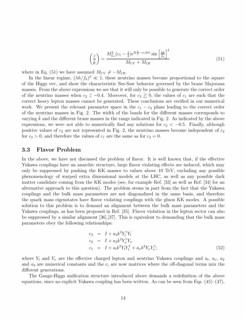
The solutions for the LOP are plotted in Fig. 3. The behavior of the LOP mass may beunderstood from the h = 0 limit. In this limit, the singlet and doublet states don’t mix and thesinglet becomes the lightest odd particle for c2 < 0, while the doublet becomes the LOP for c2 > 0.At c2 = 0 and h = 0, the singlet and doublet masses are degenerate. When h 6= 0 the singlet and

17

2c-0.6 -0.4 -0.2 0 0.2 0.4 0.6

(T

eV)

1m

0

1

2

3

4

5

6

Doublet LOP Singlet LOP

Figure 3: The Dirac mass of the LOP, m1 as a function of c2, the localization parameter for the odd fermions forthree values of k = 1.5, 2.2 and 3.8 TeV.

doublet states mix and their masses are split by the Higgs v.e.v. Only the lightest state mass isplotted in Fig. 3. In the presence of the Higgs, at c2 = 0, the LOP is an equal admixture of thesinglet and doublet state. As we move away from c2 = 0, the roots of the determinant will startsplitting into two clearly spaced masses. For c2 < 0, the lighter mass is mostly a singlet state andthe heavier one is mostly a doublet state. Since these are Dirac particles, the positive and negativeroots of the determinant are equal.

4.1 Odd Majorana Masses

In the above, we have not considered the impact of Majorana mass terms that could in principle bewritten for this multiplet, both on the IR and the UV branes, as was done for the even neutrinos,and would modify the couplings to the Higgs boson. Including the Majorana masses for the oddmultiplet, the equation determining the odd lepton masses is given by

˙S−M2

(

˙SM2−MIRo

SM2− e2c2kLMUVo

(

S−M2−MIRo

˙S−M2

))

+ sin[

λhfh

]2

= 0

(56)

The effect of introducing the Majorana mass terms can be seen in the different negative and

18

2c-0.6 -0.4 -0.2 0 0.2 0.4 0.6

(T

eV)

1m

0

1

2

3

4

5

6

=0.5UV

Doublet LOP, M

=0UV

Doublet LOP, M

=0.5IR

=0.5, MUV

Singlet LOP, M

=1IR

=0.5, MUV

Singlet LOP, M

=0UV

Singlet LOP, M

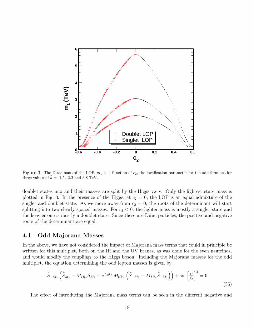
Figure 4: The Majorana mass of the LOP, m1 as a function of c2, the localization parameter for the odd fermions,with different values of MUV marked, and for three values of k = 1.5, 2.2 and 3.8 TeV (corresponding to the threeconvergent purple circle lines from bottom to top for c2 > 0), and two different values of MIRo

= 1 and 0.5 for eachk and MUVo

(from top to bottom for c2 < 0).

positive masses as one moves away from MUVo,MIRo

= 0. Due to the different behavior of the

functions S and ˙S, by inspection, we can see that the positive and negative roots of Eq. (56) will nolonger be equal. The two Dirac states have been split into four Majorana states. These states canstill be recognized as two mostly singlet and two mostly doublet states by comparing their massesto the charged states. In the following, we will sometimes refer to these states as singlet or doublet,where it should be understood that these are not really the original states, but those mixed by theHiggs. Without the mixing, the coupling between the singlet-singlet and the doublet-doublet statesand the Higgs would vanish. Therefore, we expect the singlet-singlet coupling to be suppressedcompared with the coupling of the mostly singlet state to the mostly doublet states. Additionally,looking at Fig. 4 we see that as expected, the Majorana masses don’t effect the mass of the LOPwhen the LOP is mainly a doublet state (purple circles for c2 > 0), as the convergence of thedifferent curves corresponding to the different values of MIRo

and MUVoclearly show.

The behavior of the LOP mass as well as its coupling to the Higgs may be studied by looking

19

at the roots of Eq. (56). Using the small z expansion for SM , we obtain

z ∼ 2 k

(

1

2+ c2

) MIRoMUVo

− e2c2kL cos[

λhfh

]2

e2c2kLMIRo+ 4

( 1

2+c2)

( 1

2−c2)

MUVo

, (57)

which is valid for the case in which at least one of the Majorana masses is non-vanishing and c2 < 0,in which the singlet becomes the LOP. This clearly shows that when only one of the Majoranamasses is non-zero, we get a See-Saw effect governing the LOP mass. This behavior is confirmed inour numerical analysis plotted in Fig. 4.

Observe that if only the ultraviolet mass is non-vanishing, the mass of the LOP (which is mainlya left-handed singlet) is exponentially suppressed, unless c2 ≃ 0. Indeed, in the limit of vanishinginfrared Majorana masses, Eq. (57) reduces to

z ∼ −k(

1

2− c2

) e2c2kL cos[

λhfh

]2

2MUVo

. (58)

As can be seen from Eq. (58), the higher operator coupling of the LOP to the Higgs is also suppressedfor c2 < 0. We will show that the annihilation cross section for a mainly singlet state is sufficientlyenhanced only when the s-channel Higgs diagram becomes sizable and therefore, unless c2 ≃ 0, theDark Matter density becomes very large compared to the experimentally observed value.

As both MIRoand MUVo

are turned on, we see an abrupt change in the behavior of the massspectrum for c2 < 0, which becomes independent of the exact value of MUVo

and only depends onk and MIRo

,

z ∼ k MIRo

2

(

1

2− c2

)

. (59)

The LOP mass in this case is of the order of k, and does not show an explicit dependence on theHiggs vaccum expectation value. Indeed, as can be seen from Eq. (57), the effective coupling to theHiggs for c2 < 0 is exponentially suppressed. Therefore, as happens in the case of vanishing MIRo

,a good dark matter candidate may only be obtained for values of c2 & 0.

When c2 ∼ 0, the mass can be approximated by:

z ∼ kMIRo

MUVo− e2c2kL cos

[

λhfh

]2

e2c2kLMIRo+ 4MUVo

(60)

We see that for MIRo, MUVo

∼ O(1), for values of h in the linear regime and very small values ofc2, we can get a cancelation resulting in very small LOP masses. This behavior is clearly portrayedin Fig. 4.

Finally, let us analyze the case MIRo6= 0 and MUVo

= 0. As MIRois turned on, it strongly

modifies the spectrum with respect to the Dirac case for negative values of c2. In this case, the

20

LOP becomes mostly a right-handed singlet and its mass is given by

z ∼ −k (1 + 2c2)cos[

λhfh

]2

MIRo

. (61)

As seen in Eq. (61), the LOP mass in this case is, again, of the order of the weak scale but with anexplicit Higgs v.e.v. dependence induced by a higher order operator coupling with a characteristicscale of the order of the KK masses. Therefore the coupling of the LOP to the Higgs becomessizable for KK masses of the order of the TeV scale, allowing for the possibility of a dark mattercandidate for c2 < 0.

In the following section, we shall perform a more precise quantitative analysis of the masses andcouplings associated with the annihilation cross section of the singlet state for both the Majoranaand Dirac cases.

4.2 Couplings of the Odd Leptons

4.2.1 Higgs Couplings

To calculate the couplings of the Majorana and Dirac states with the Higgs, the profile functionof the odd leptons which couple to the Higgs bosons need to be computed. The mass eigenstateprofile functions are given in terms of combinations of the profile functions without the Higgs. Inthe particular case of the neutral odd leptons these are admixtures of the neutral states belongingto the bidoublet and the singlet state, with normalization coefficients C2, C3 and C5.

The boundary conditions determine the coefficients C3 and C5 as functions of C2. The fermionprofile functions in the presence of the Higgs are given by:

f 2L(h) =

1

2e

1

2(1−2c2)kx

(

e2c2kx ˙S−M2

(

C2

(

1 + cos

[

λh

fh

])

− C3

(

1 − cos

[

λh

fh

]))

−√

2(SM2− e2c2kxMUVo

˙S−M2) C5 sin

[

λh

fh

])

(62)

f 3L(h) =

1

2e

1

2(1−2c2)kx

(

e2c2kx ˙S−M2

(

C3

(

1 + cos

[

λh

fh

])

− C2

(

1 − cos

[

λh

fh

]))

−√

2(SM2− e2c2kxMUVo

˙S−M2) C5 sin

[

λh

fh

])

(63)

f 5L(h) =

1

2e

1

2(1−2c2)kx

(

2(SM2− e2c2kxMUVo

˙S−M2) C5 cos

[

λh

fh

]

+√

2e2c2kx ˙S−M2(C2 + C3) sin

[

λh

fh

])

(64)

21

(TeV)1m0 1 2 3 4 5 6

Hig

gs

Co

up

ling

s

0

0.5

1

1.5

2

2.5

1,1Dλ

2,2Dλ

1,2Dλ

2,1Dλ

Figure 5: Higgs couplings to the Dirac particles for three values of k ∼ 1.5, 2.2 and 3.8 TeV corresponding tom1 ∼ 2, 3 and 6 TeV for c2 = 0 from left to right, as a function of the singlet LOP mass m1.

f 2R(h) =

1

2e

1

2(1−2c2)kx

(

e2c2kxS−M2

(

C2

(

1 + cos

[

λh

fh

])

− C3

(

1 − cos

[

λh

fh

]))

+√

2(e2c2kxMUVoS−M2

− ˙SM2) C5 sin

[

λh

fh

])

(65)

f 3R(h) =

1

2e

1

2(1−2c2)kx

(

e2c2kxS−M2

(

C3

(

1 + cos

[

λh

fh

])

− C2

(

1 − cos

[

λh

fh

]))

+√

2(e2c2kxMUVoS−M2

− ˙SM2) C5 sin

[

λh

fh

])

(66)

f 5R(h) =

1

2e

1

2(1−2c2)kx

(

2( ˙SM2− e2c2kxMUVo

S−M2) C5 cos

[

λh

fh

]

+√

2e2c2kxS−M2(C2 + C3) sin

[

λh

fh

])

(67)

where the functions S and ˙S are functions of x5 and the masses z of the odd fermions.For the doublet and singlet states mixed by the Higgs, a non-trivial solution may be only obtained

22

(TeV)1m0 0.5 1 1.5 2 2.5 3 3.5 4 4.5 5

Hig

gs

cou

plin

gs

0

0.2

0.4

0.6

0.8

1

1.2

1.4

1.6

= 0.5IR

= 0, MUV M

1,1Mλ

1,2Mλ

1,3Mλ

1,4Mλ

Figure 6: Higgs couplings to the Majorana particles for three values of k ∼ 1.5, 2.2 and 3.8 TeV corresponding tom1 ∼ 1.7, 2.5 and 4.7 TeV for c2 = 0, from left to right, as a function of the singlet LOP mass m1.

if the following relations are fulfilled.

C3 = C2 (68)

C5 = C2

√2e2c2kL ˙S−M2

cot[

λhfh

]

L

SM2− e2c2kLMUVo

˙S−M2

; . (69)

For the neutral leptons which decouple from the Higgs, instead, the following relations are fulfilled:

C3 = −C2 (70)

C5 = 0 (71)

This implies that only the symmetric combination of neutral bidoublet states with coefficientsgiven by Eq. (68) and (69), couple to the Higgs. Moreover, the normalization coefficient C2 may be

23

2c-0.5 -0.4 -0.3 -0.2 -0.1 0 0.1

Hig

gs

cou

plin

gs

0

0.5

1

1.5

2

= 0.5IR

= 0.5, MUV M

1,1Mλ

1,2Mλ

1,3Mλ

1,4Mλ

Figure 7: Higgs couplings to the Majorana particles for three values of k ∼ 1.5, 2.2 and 3.8 TeV as a function ofc2, when the singlet is the LOP. The smaller values of k correspond to the smaller couplings (the lower curve).

computed by demanding well normalized functions, namely,

C2 =

(

∫ L

0

∑

i=2,3,5 (|f iL|2 + |f i

R|2)|C2|2

dx

)−1/2

. (72)

The above definition is appropriate in the Majorana case, in which the left-handed components ofthe fermions acquire contributions from both the original left-handed and the (charge conjugate)right-handed modes, Eqs. (62)–(67). In the Dirac case, the left-handed and right-handed functionsacquire equal normalizations and therefore the proper factor C2 is equal to the one computed abovedivided by

√2. In the following, we will keep the above definition of C2 for both the Majorana and

Dirac cases and take care of the proper√

2 factors explicitly.To calculate the couplings, we also need the Higgs profile and normalization:

fh = Che2kx (73)

Ch =g5

√

∫ L

0a(x)−2dx

(74)

24

Defining Ξ(mi, mj):

Ξ(mi, mj) = −e−kx

2ChC

∗2 (mi)C2(mj)fh

[

f 5∗R (mi)

[

f 2L(mj) + f 3

L(mj)]

−[

f 2∗R (mi) + f 3∗

R (mi)]

f 5L(mj)

]

(75)the left-right couplings of the Higgs with the different states, Ψi

LHΨj, in the Majorana and Diraccases can be written as:

λMi,j =

∫ L

0

(Ξ(mi, mj) + Ξ∗(mj , mi)) dx (76)

λDi,j = 2

∫ L

0

Ξ(mi, mj) dx (77)

the factor of 2 in the Dirac coupling is due to the definition of the C2 factor discussed above.Observe that, while in the Majorana case λM

ij = λM ∗ji , there is no such relation in the Dirac case.

The different couplings are plotted in Figs. 5 – 7. For the Dirac case and c2 <∼ 0, represented in

Fig. 5, small values of the masses are obtained for smaller values of c2. The left-right couplings ofthe singlet and doublet states, λD

1,2 acquire large values for negative values of c2. This stems fromthe fact that for this case, the left-handed singlet component is localized towards the IR brane.As c2 goes to 0, the localization effects become less pronounced and this coupling starts gettingsuppressed. The λD

i,i couplings have the opposite behavior to the cross couplings. For c2 negative,the mass difference between the singlet and the doublet state is large, while their mixing is small.Since the self-couplings of the mass eigenstates are induced by the product of the singlet and doubletcomponents of these states, they become very suppressed. However, as c2 goes to zero, the masseigenvalues become symmetric and antisymmetric combinations of the singlet and doublet states,and the self couplings of the mass eigenstates become large, while the cross couplings tend to zero.

In the Majorana case with MUVo= 0, although the quantitative values are not the same, the

λM1,1 and λM

1,4 couplings behave similarly to the λD1,1 couplings, since m1 and m4 are the two mostly

singlet states, which are split due to the non-zero MIRo. When both the Majorana masses are non-

zero, we see an abrupt change in the behavior of the couplings. As mentioned before, for c2 < 0 theself-coupling of the lightest state is exponentially suppressed. This behavior is clearly demonstratedin the Higgs dependent part of the approximation for the LOP given in Eq. (57). The couplings ofthe LOP to the mostly doublet states, however, continue to be large.

4.2.2 Couplings to the Z and W± Bosons

The Z couplings to the lepton sector are defined in a similar manner to the couplings with thequark sector [25],[26]. However, in the lepton case QX = 0 and the neutral states that couple tothe Higgs have C3 = C2, implying that f 2

L,R(h) = f 3L,R(h). Therefore, the Z, and all its KK modes,

as well as the neutral components of the SU(2)R gauge bosons don’t have any couplings with anytwo of these states. However, the orthogonal neutral state in the bidoublet, which does not coupleto the Higgs has C3 = −C2 and C5 = 0. Hence, an off-diagonal coupling exists between this mode,the neutral states that couple to the Higgs and the Z.

25

(TeV)1m0 1 2 3 4 5 6

L

,R±WD g

0

0.05

0.1

0.15

0.2

0.25

L±W

D g

R±W

D g

Figure 8: W± couplings to the Dirac particles for c2 < 0 and three values of k ∼ 1.5, 2.2 and 3.8 TeV, which, forc2 = 0, correspond approximately to m1 ∼ 2, 3 and 5.6 TeV, from left to right as a function of the singlet LOPmass. Larger values of m1 are associated with larger values of c2.

The W± couple the charged fermions with the neutral components. In component form, thecoupling is between f 1,4

L,R(h) and f 2,3,5L,R (h). The profile functions and their normalization coefficients

for the neutral components were given in Eqs. (67) – (68). The charged fermions and the neutralcomponent of the bidoublet which don’t couple to the Higgs state are both governed by the samefive dimensional wave-function, namely:

f iL = Cie

1

2(1+2c2)kx ˙S−M2

(78)

f iR = Cie

1

2(1+2c2)kxS−M2

(79)

These fermion masses are given by the roots of ˜S−M2and since the Majorana masses don’t influence

them, they are always Dirac states. Further, it can be shown trivially that the W− coupling to theLOP and the positive charged state is equal to the coupling of the LOP to W+ and the negativecharged states. In the annihilation cross-section, we will only be interested in the couplings betweenthe two charged fermions and the LOP. We will denote these couplings by gWL,R

. The expressionfor these couplings is given in Appendix B. Similarly, for the Z we will only be interested in the

26

(TeV)1m0 0.5 1 1.5 2 2.5 3 3.5 4 4.5 5

L

,R±WM g

0

0.05

0.1

0.15

0.2 = 0.5

IR = 0, MUVM

L±W

M g

R±W

M g

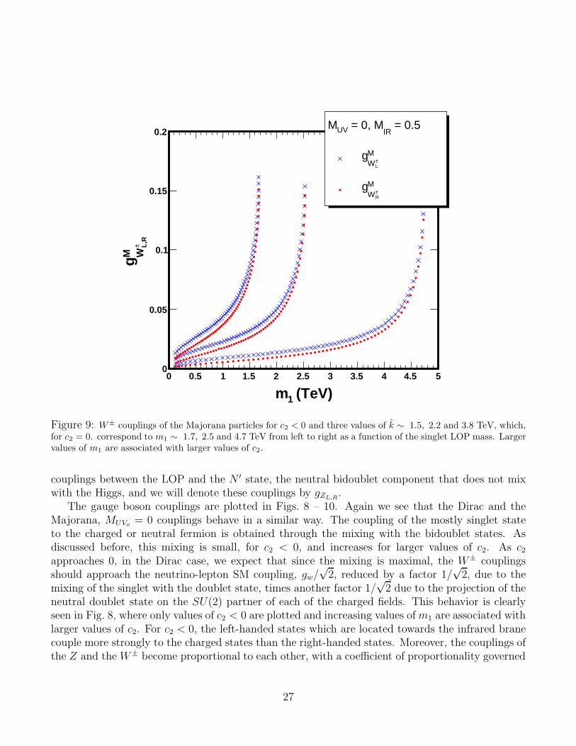
Figure 9: W± couplings of the Majorana particles for c2 < 0 and three values of k ∼ 1.5, 2.2 and 3.8 TeV, which,for c2 = 0. correspond to m1 ∼ 1.7, 2.5 and 4.7 TeV from left to right as a function of the singlet LOP mass. Largervalues of m1 are associated with larger values of c2.

couplings between the LOP and the N ′ state, the neutral bidoublet component that does not mixwith the Higgs, and we will denote these couplings by gZL,R

.The gauge boson couplings are plotted in Figs. 8 – 10. Again we see that the Dirac and the

Majorana, MUVo= 0 couplings behave in a similar way. The coupling of the mostly singlet state

to the charged or neutral fermion is obtained through the mixing with the bidoublet states. Asdiscussed before, this mixing is small, for c2 < 0, and increases for larger values of c2. As c2approaches 0, in the Dirac case, we expect that since the mixing is maximal, the W± couplingsshould approach the neutrino-lepton SM coupling, gw/

√2, reduced by a factor 1/

√2, due to the

mixing of the singlet with the doublet state, times another factor 1/√

2 due to the projection of theneutral doublet state on the SU(2) partner of each of the charged fields. This behavior is clearlyseen in Fig. 8, where only values of c2 < 0 are plotted and increasing values ofm1 are associated withlarger values of c2. For c2 < 0, the left-handed states which are located towards the infrared branecouple more strongly to the charged states than the right-handed states. Moreover, the couplings ofthe Z and the W± become proportional to each other, with a coefficient of proportionality governed

27

2c-0.5 -0.4 -0.3 -0.2 -0.1 0 0.1

L

,R±WM g

0

0.05

0.1

0.15

0.2

= 0.5IR

= 0.5, MUVM

L±W

M g

R±W

M g

Figure 10: W± couplings to the Majorana particles for three values of k ∼ 1.5, 2.2 and 3.8 TeV as a function ofc2 for the singlet LOP. The smaller values of k correspond to the smaller couplings (the lower curve).

by cos θW , namely

gZL,R=

gWL,R

cos θW

(80)

The additional factor of√

2 that appears between SM couplings of neutrinos to the Z and W , isnot present in this case.

In the case of zero ultraviolet Majorana mass but non-vanishing MIRo, depicted in Fig. 9,

the behavior is similar to the Dirac case but the couplings are reduced due to the larger singletcomponents of the Majorana particles. Also, there is a sizable reduction of the left-handed couplingsdue to the larger right-handed component of the Majorana state. Observe that as MUVo

is turnedon, for c2 < 0, the couplings to the gauge bosons become independent of c2.

Finally, as c2 becomes positive, the couplings increase, due to the larger bidoublet componentof the LOP.

28

)1

t (p )2

(pt

)1

(k1 N )2

(k1N

H

Figure 11: Feynman Diagram for the process N1 + N1 → t + t

4.3 Annihilation Cross Section

We will denote the neutral states mixed by the Higgs by Ni, where i = 1, 2, or i = 1, 2, 3, 4 forthe two Dirac or four Majorana states respectively, where i labels the states in increasing order oftheir absolute masses. C± will denote the charged fermions and, as said before, N ′ will denote thebidoublet neutral fermion which does not couple to the Higgs. The N1 is the LOP, our dark mattercandidate.

Ignoring co-annihilation effects, we consider the following five dominant processes for N1N1

annihilation: N1 + N1 → t t, H H, Z Z and W+ W− (observe that due to the cancelation of theZ coupling to the states that couple to the Higgs, the Z H annihilation channel is suppressed).The Feynman diagrams contributing to each of these processes are shown in Figs. 11 – 14. Thevirtual Ni exchanges in these diagrams should be understood to be summed over i, where i as notedabove runs over the appropriate index depending on whether we are considering the Dirac or theMajorana case. The v in the following formulae is the relative velocity between the initial particlesin the center of mass frame. λHtt, λHZZ , λHWW and λH are the couplings of the Higgs to the top,the W± and Z bosons, and itself, which were discussed in Refs. [25] and [26].

4.3.1 N1 + N1 → t+ t

Due to the cancelation of the coupling of N1 to the Z, the annihilation into fermion pairs proceedsvia an s-channel Higgs interchange, and is therefore proportional to the corresponding fermion mass.Therefore, only the top contributes in a relevant way. The Dirac and Majorana cross-sections aregiven by the same formula, but the Higgs coupling should be understood to be the one appropriatefor each case. Assuming m1 > mt, we obtain:

< σv >tt=λ2

1,1λ2Httv

2

8πm21

(

1 − m2t

m21

)3/2(

1 − m2H

4m21

)−2

(81)

29

)1

H (p )2

H (p

)1

H (p )2

H (p

)1

(k1 N )2

(k1N

)1

(k1 N )2

(k1

N

i N

H

i N

)1

H (p )2

H (p

)2

(k1N)1

(k1 N

Figure 12: Feynman Diagrams contributing to the process N1 + N1 → H + H

4.3.2 N1 + N1 → H +H

The annihilation into Higgs pairs proceeds via an s-channel Higgs interchange diagram, which issubdominant, and the t-channel interchange of the neutral odd fermions. The result, in the limitmH ≪ m1, m2, is given by:

< σv >DHH=

v2

8π2

[

λD 21,1

16m21

λ2H

m21

−∑

i

λD1,1

4m21

λH

mi

(

(

λD 21,i + λD 2

i,1

) m1

mi

(

1 +m2

1

3m2i

)

+ 2λD1,iλ

Di,1

(

1 +m2

1

m2i

))

+∑

i,j

1

mimj

(

1 +m1

mi

)−2(

1 +m1

mj

)−2(

2λD1,jλ

Dj,1

(

1 +m2

1

m2j

)(

2λD1,iλ

Di,1

(

1 +m2

1

m2i

)

+(

λD 21,i + λD 2

i,1

) m1

mi

(

1 +m1

3m2i

))

+(

λD 21,j + λD 2

j,1

) m1

mj

(

(

λD 21,i + λD 2

i,1

) m1

mi

(

1 +m1

3m2i

(

1 +m2

i

m2j

)

+m4

1

m2im

2j

)

+ 2λD1,iλ

Di,1

(

1 +m2

1

m2i

)(

1 +m2

1

3m2j

))]

(82)

where we have taken the couplings to be real. The sum runs over the two Dirac states labeled bytheir masses, m1 and m2. In the case of real couplings, the Majorana cross-section can be simply

30

seen from the above with the replacement λMi,j = 1/2(λD

i,j + λDj,i), and the indices now run over the

four Majorana states:

< σv >MHH=

v2

2π2

[

λM 21,1

64m21

λ2H

m21

−∑

i

λM1,1λ

M 21,i

8m21

λH

mi

((

1 +m2

1

m2i

)

+m1

mi

(

1 +m2

1

3m2i

))

+∑

i,j

λM 21,j λM 2

1,i

mimj

(

1 +m1

mi

)−2(

1 +m1

mj

)−2((

1 +m2

1

m2j

)((

1 +m2

1

m2i

)

+m1

mi

(

1 +m2

1

3m2i

))

+m1

mj

(

m1

mi

(

1 +m1

3m2i

(

1 +m2

i

m2j

)

+m4

1

m2im

2j

)

+

(

1 +m2

1

m2i

)(

1 +m2

1

3m2j

))]

(83)

4.3.3 N1 + N1 → W+W−, Z + Z

The annihilation into the W± and Z gauge bosons also proceeds via the s-channel interchange ofa Higgs, plus the t-channel interchange of the charged fermion C± and the neutral fermion N ′,respectively. In the formula below, the label G corresponds to either the W± or Z gauge bosons,and α = 1 for the W+W− cross-section and α = 1/2 for the ZZ case. The diagrams contributing tothe process in the Dirac case are given in Fig. 13. For the Majorana case, two additional diagramscontribute, and are given in Fig. 14. Using the properties of the Majorana couplings, one candemonstrate that these new diagrams are equal to the ones associated to the cross diagrams inthe amplitudes for the annihilation into the W± (due to the interchange of the fermion of oppositecharge) and Z gauge bosons. Therefore, the cross-section is given by the same formula for both theDirac and Majorana cases, but with appropriate couplings, and a factor β = 2 for the Majoranacase, and β = 1 for the Dirac case. Although in the numerical analysis the full annihilation crosssection was used, for simplicity, we will only quote the cross-section for the longitudinal modes, in

31

)1

(p+Z, W )2

(p-Z, W

)1

(p+Z, W )2

(p-Z, W

)1

(k1 N )2

(k1N

)1

(k1 N

-

N’, C

+ N’, C

)1

(p+Z, W )2

(p-Z, W

)2

(k1N)1

(k1 N

H

)2

(k1N

Figure 13: Feynman Diagrams contributing to the process N1 + N1 → W+W−, Z + Z. The intermediate state iseither the charged fermion C± for the W± case, or the orthogonal bidoublet, N ′ for the Z.

the limit mW , mZ < mH << m1:

< σv >GG = α

1

4πm2G

m41

m4f

(

g2GL

− g2GR

)2

(

1 +m2

1

m2f

)−2

+m2

1v2

πm4G

[

λ21,1

16

λ2HGG

m21

− β λ1,1

λHGG

mf

(

1 +m2

1

m2f

)−2(

gGLgGR

(

1 +m2

1

3m2f

)

−(

g2GL

+ g2GR

) m1

3mf

(

1 +m2

1

m2f

))

+ β2 2

3

m21

m2f

(

1 +m2

1

m2f

)−4

6g2GLg2

GR

(

1 +m2

1

m2f

+5m4

1

3m4f

+1

3

m61

m6f

)

− m1

mf

(

1 +m2

1

m2f

)2

×(

4gGLgGR

(

g2GL

+ g2GR

)

−(

g4GL

+ g4GR

) m1

mf

))]]

(84)

These cross-sections are plotted in Figs. 15–17. For negative c2 (smaller values ofm1), we observean interesting correlation between the annihilation cross sections into W±, Z and Higgs pairs. Wesee a dominance of the longitudinal modes for this range of values of c2 and the magnitudes ofthe W±, Z Z and H H cross-sections obey the 2 : 1 : 1 behavior expected due to the Goldstoneequivalence theorem. For larger values of c2, the bidoublet component of the LOP increases andthe transverse components of the gauge bosons are no longer subdominant in their contribution to

32

)2

(p-

Z, W )1

(p+Z, W

)1

(k1 N )2

(k1N

-N’, C + N’, C

)2

(p-

Z, W )1

(p+Z, W

)2

(k1N)1

(k1 N

Figure 14: Additional Feynman Diagrams contributing to the process N1 + N1 → W+W−, Z +Z for the Majoranacase. The intermediate state is either the charged fermion C± for the W± case, or the orthogonal bidoublet, N ′ forthe Z.

the annihilation cross section.Our extensive numerical and analytic study showed that for negative c2, the major contributions

to theW± and Z Z cross-sections are due to the s-channel Higgs exchange. In theH H cross-section,this is matched by the contribution from the virtual exchange of the Ni in the t-channel. Therefore,as emphasized before, for c2 < 0, a sizable annihilation cross section may only be obtained whenthe Higgs coupling to the LOP becomes of order one.

4.4 Dark Matter Density

We shall follow the standard formalism for the calculation of the thermal dark matter density [44], [45].In calculating the annihilation cross-sections, we used the non-relativistic approximation for the ini-tial particles. The cross-section used in calculating the dark matter density is the sum of all thedifferent contributions in the previous sections and will be denoted by < σv >T , and xF = m/TF

as usual. The relative velocity is related to the freeze-out temperature:

< v2 >rel =6

xF, (85)

xF = log

(

c (c + 2)

√

90π

xF g∗g0

2π3m1MP l < σv >T

)

. (86)

The non-relativistic expansion of the thermal annihilation cross section may be expressed as

< σv >T = σ0 + σ1 < v2 >≃ σ0 + 6 σ1/xF . (87)

The dark matter density is then given by

ΩDM =γs0xF

ρcMP l(σ0 + 3σ1/xF )

√

45

πg∗ , (88)

33

(TeV)1m0 1 2 3 4 5 6

(p

b)

D σ

0

0.2

0.4

0.6

0.8

1

1.2

1.4

1.6

DWWσ DZZσ DHHσ Dttσ

Figure 15: The cross-section contributions to the annihilation of the Dirac LOP for (from top to bottom) k = 1.5,2.2 and 3.8 TeV.

where c = 1/2, MP l = 1.2×1019 GeV, g∗ = 112, s0 = 2889.2/cm3, ρc = 5.3×10−6GeV/cm3, g0 = 2is the degrees of freedom of our dark matter candidate and γ = 2 or 1 to account for the antiparticlesfor the Dirac and Majorana case respectively. We take g0 = 2 in the Dirac case since we computethe density of the particle and antiparticle separately. The factor γ = 2 in the relic density thenaccounts for the duplication of the density from both the N1 particle and the antiparticle in thiscase.

To check the veracity of our calculations, we extensively studied the limit of the Majorana casereducing to the Dirac case asMIRo

andMUVogo to 0. As the Majorana masses go to 0, the two singlet

masses start getting degenerate in mass, and the N1 N1 and the N2 N2 cross-sections become equal.To properly analyze this limit, then, we must take co-annihilation between the lightest Majoranasates into account [45]. One can check that the coupling of the Higgs to each of the degenerateLOP Majorana states, HNiNi, becomes equal to the one of the Higgs to the LOP in the Dirac case.Moreover, the cross coupling of the Higgs, HN1N2, vanishes identically in the limit of vanishingMajorana masses. Further simple relations exist between the Higgs couplings to fermions in theMajorana and Dirac cases. One can check that due to these relations the annihilation cross sectioninto Higgs states in the Majorana case NiNi → H H become the same as the N1N1 → H H crosssection in the Dirac case. The same happens in the case of annihilation into fermions.

In the case of gauge bosons the situation is more complicated. As noted in calculating the

34

(TeV)1m0 0.5 1 1.5 2 2.5 3 3.5 4 4.5 5

(p

b)

M σ

0

0.5

1

1.5

2 = 0.5IR

= 0, MUV M

MWWσ

MZZσ

MHHσ

Mttσ

Figure 16: The cross-section contributions to the annihilation of the Majorana LOP with MIRo= 0.5 and MUVo

=0, for (from top to bottom) k = 1.5, 2.2 and 3.8 TeV.

couplings, the gauge boson couplings in the Majorana case are reduced by a factor 1/√

2. Thisimplies that for the W± and Z Z, the interference between the t and s-channel diagrams is reducedby 1/2 and the t-channel diagrams by 1/4 compared to the Dirac cross-section case. These factorsare exactly compensated for by the extra diagrams that contribute in the Majorana case (Fig. 14),and therefore one obtains that the equality of annihilation cross sections defined above for the Higgsfinal states extends to all final states. We also verified that the N1 N2 annihilation cross-section isexactly 0 in this limit. Including co-annihilation between the two Majorana states [45], the effectivedegrees of freedom are then 4, and the effective cross-section is 1

2σD, where σD is the annihilation

cross section between N1 and its antiparticle in the Dirac case. Therefore, in this limit the darkmatter density due to the Dirac and Majorana cases in the limit MUVo,IRo

→ 0 is exactly the same,as expected.

We plotted the values of c2 and m1 leading to the correct dark matter density in both the Diracand the Majorana cases in Fig. 18. We restricted the values of k >

∼ 1.2 TeV, for which the SM Higgscouplings are close to their SM values. This provides a lower bound on the LOP mass and on thevalue of c2. The bands in this figure represent the relic density uncertainty. We see that in theDirac case, we can only obtain the correct dark matter density for values of 2 TeV >

∼ m1>∼ 1 TeV

and c2 >∼ −0.4, consistent with the exchange symmetry. The value of k is correlated with the value

of m1, and is constrained to be in the range 2 TeV >∼ k >

∼ 1.2 TeV for the above range of masses.

35

c-0.15 -0.1 -0.05 0 0.05 0.1 0.15

(p

b)

M σ

0

0.5

1

1.5

2

2.5

= 0.5IR

= 0.5, MUV M

MWW

σ

MZZ

σ

MHH

σ

Mttσ

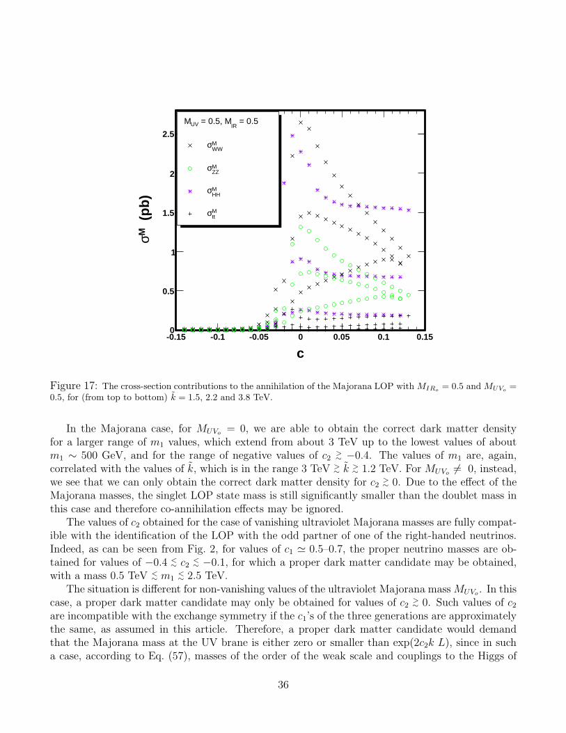
Figure 17: The cross-section contributions to the annihilation of the Majorana LOP with MIRo= 0.5 and MUVo

=0.5, for (from top to bottom) k = 1.5, 2.2 and 3.8 TeV.

In the Majorana case, for MUVo= 0, we are able to obtain the correct dark matter density

for a larger range of m1 values, which extend from about 3 TeV up to the lowest values of aboutm1 ∼ 500 GeV, and for the range of negative values of c2 >

∼ −0.4. The values of m1 are, again,correlated with the values of k, which is in the range 3 TeV >

∼ k >∼ 1.2 TeV. For MUVo

6= 0, instead,we see that we can only obtain the correct dark matter density for c2 >

∼ 0. Due to the effect of theMajorana masses, the singlet LOP state mass is still significantly smaller than the doublet mass inthis case and therefore co-annihilation effects may be ignored.

The values of c2 obtained for the case of vanishing ultraviolet Majorana masses are fully compat-ible with the identification of the LOP with the odd partner of one of the right-handed neutrinos.Indeed, as can be seen from Fig. 2, for values of c1 ≃ 0.5–0.7, the proper neutrino masses are ob-tained for values of −0.4 <

∼ c2 <∼ −0.1, for which a proper dark matter candidate may be obtained,

with a mass 0.5 TeV <∼ m1

<∼ 2.5 TeV.

The situation is different for non-vanishing values of the ultraviolet Majorana mass MUVo. In this

case, a proper dark matter candidate may only be obtained for values of c2 >∼ 0. Such values of c2

are incompatible with the exchange symmetry if the c1’s of the three generations are approximatelythe same, as assumed in this article. Therefore, a proper dark matter candidate would demandthat the Majorana mass at the UV brane is either zero or smaller than exp(2c2k L), since in sucha case, according to Eq. (57), masses of the order of the weak scale and couplings to the Higgs of

36

2c-0.4 -0.3 -0.2 -0.1 0 0.1 0.2

(T

eV)

1m

0.5

1

1.5

2

2.5

3

3.5 Dirac Case = 0

UV = 0.5, MIR M

= 0UV

= 1, MIR M

= 0.5UV

= 0.5, MIR M

Figure 18: Parametric plot of m1, the mass of the LOP, versus c2, the localization parameter of the odd fermions,when ΩDM ∼ 0.23 ± 0.1. The two lines for each value of the Majorana masses are associated with the upper andlower bound on ΩDM .

order one would be obtained.Observe that the difficulty in obtaining a proper dark matter candidate for MUVo

6= 0 stems fromthe fact that we have assumed equal bulk mass parameters for the fermions interchanged by theZ2 exchanged symmetry introduced in Refs. [43]. Although this is an attractive possibility, since itallows a connection between the dark matter properties and the neutrino masses, this does not needto be the case. Values of c2 >

∼ 0 would be allowed in the more general case, or for a more generaldiscrete symmetry. Alternatively, if the value of c1 of the left-handed leptons was allowed to bedifferent for the three generations, values of c2 >

∼ 0 would be consistent with values of c1 compatiblewith the relatively small electron mass.

4.5 Direct Dark Matter Detection through Higgs Exchange

The annihilation cross section for the odd neutrinos becomes of the proper size for sizable values ofthe coupling of the odd neutrino to the Higgs boson, λ11 ≃ 0.3 – 0.7, with larger couplings associatedwith larger LOP masses. Such large couplings induce a relatively large scattering cross section of

37

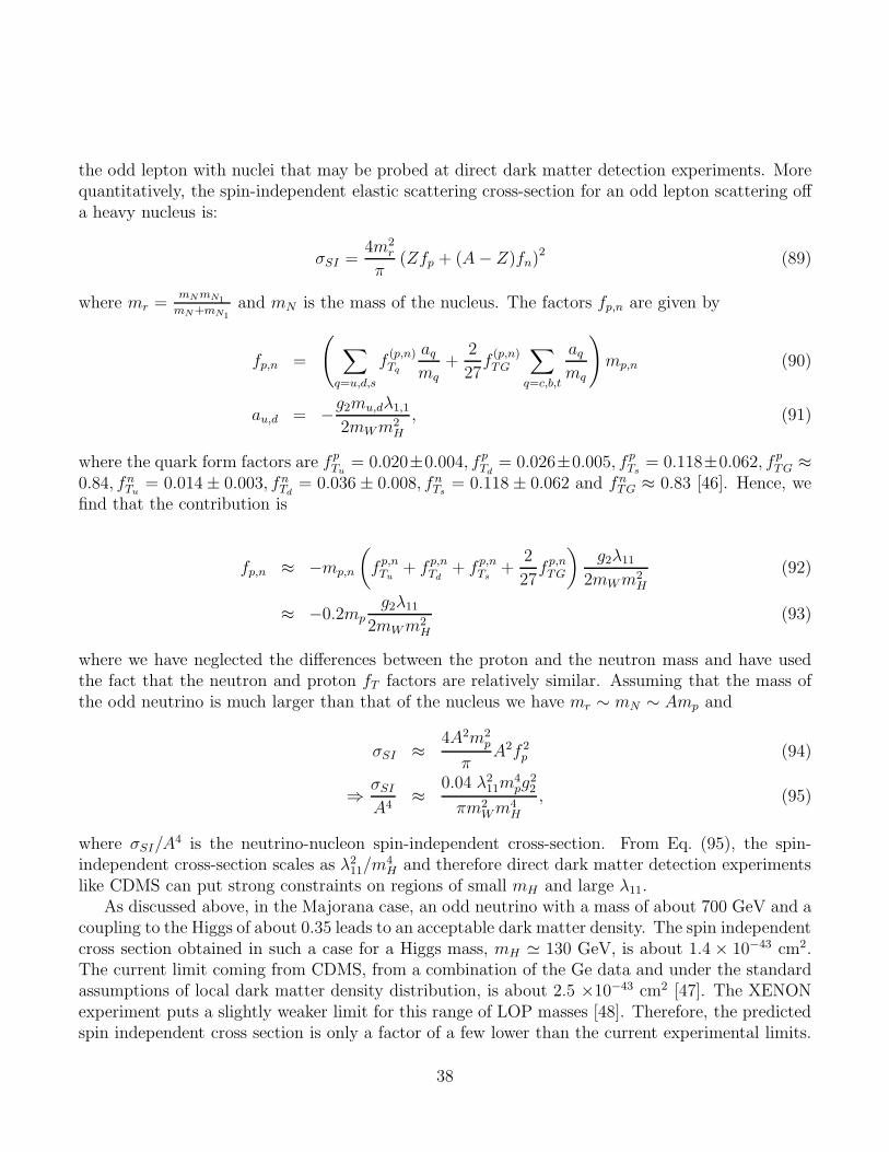
the odd lepton with nuclei that may be probed at direct dark matter detection experiments. Morequantitatively, the spin-independent elastic scattering cross-section for an odd lepton scattering offa heavy nucleus is:

σSI =4m2

r

π(Zfp + (A− Z)fn)2 (89)

where mr =mN mN1

mN+mN1

and mN is the mass of the nucleus. The factors fp,n are given by

fp,n =

(

∑

q=u,d,s

f(p,n)Tq

aq

mq

+2

27f

(p,n)TG

∑

q=c,b,t

aq

mq

)

mp,n (90)

au,d = −g2mu,dλ1,1

2mWm2H

, (91)

where the quark form factors are f pTu

= 0.020±0.004, f pTd

= 0.026±0.005, f pTs

= 0.118±0.062, f pTG ≈

0.84, fnTu

= 0.014 ± 0.003, fnTd

= 0.036 ± 0.008, fnTs

= 0.118 ± 0.062 and fnTG ≈ 0.83 [46]. Hence, we

find that the contribution is

fp,n ≈ −mp,n

(

f p,nTu

+ f p,nTd

+ f p,nTs

+2

27f p,n

TG

)

g2λ11

2mWm2H

(92)

≈ −0.2mpg2λ11

2mWm2H

(93)

where we have neglected the differences between the proton and the neutron mass and have usedthe fact that the neutron and proton fT factors are relatively similar. Assuming that the mass ofthe odd neutrino is much larger than that of the nucleus we have mr ∼ mN ∼ Amp and

σSI ≈4A2m2

p

πA2f 2

p (94)

⇒ σSI

A4≈

0.04 λ211m

4pg

22

πm2Wm

4H

, (95)

where σSI/A4 is the neutrino-nucleon spin-independent cross-section. From Eq. (95), the spin-

independent cross-section scales as λ211/m

4H and therefore direct dark matter detection experiments

like CDMS can put strong constraints on regions of small mH and large λ11.As discussed above, in the Majorana case, an odd neutrino with a mass of about 700 GeV and a

coupling to the Higgs of about 0.35 leads to an acceptable dark matter density. The spin independentcross section obtained in such a case for a Higgs mass, mH ≃ 130 GeV, is about 1.4 × 10−43 cm2.The current limit coming from CDMS, from a combination of the Ge data and under the standardassumptions of local dark matter density distribution, is about 2.5 ×10−43 cm2 [47]. The XENONexperiment puts a slightly weaker limit for this range of LOP masses [48]. Therefore, the predictedspin independent cross section is only a factor of a few lower than the current experimental limits.

38

For larger masses, of about 1 TeV, the Higgs couplings grows to about 0.38 and the predicted crosssection is therefore about 1.65 × 10−43 cm2, while the CDMS bound is about two times larger. Inthe Dirac case, the couplings are about fifty percent larger than in the Majorana case and thereforethe predicted cross section for a mass m1 ≃ 1 TeV is slightly above the CDMS reported bound. Onewould be able to conclude that the Dirac case for mH

<∼ 130 GeV is therefore disfavored. There are,

however, uncertainties of order of a few associated with the local dark matter density distributionand the nuclear form factors which should be taken into account before ruling out a specific model.It is expected that both the XENON and CDMS experiments will further improve their sensitivityby about an order of magnitude by the end of 2009 [49], [50]. Therefore, even considering possibleuncertainties associated with the local density and the nuclear form factors, the minimal modeldiscussed in this article should be probed by these experiments in the near future.

Let us comment that the mass of the N1 particle may be in the appropriate range to providean explanation of the anomalous excess in electrons and positrons observed by the Pamela [51]and ATIC [52] experiments. However, since in these model these particles decay mostly into Higgsand gauge bosons, if these particles are distributed throughout the halo of the galaxy, an excess ofpositrons of the size observed by these experiments will need a large boost factor enhancement andwould probably lead to an unobserved excess of antiprotons [53],[54].

5 Conclusions

In this article, we have considered the question of incorporating the charged and neutral leptonsin a Gauge-Higgs Unification scenario based on the gauge group SO(5) × U(1)X in warped extradimensions. These models are attractive since the SO(4) ≡ SU(2)L × SU(2)R subgroup of SO(5)incorporates in a natural way the weak gauge group as well as an appropriate custodial symmetrygroup in order to suppress large contributions to the precision electroweak observables. Moreover,the fifth dimensional components of SO(5)/SO(4) gauge bosons have the right quantum numbersto play the role of the Higgs doublet responsible for the breakdown of the electroweak symmetry.

We have shown that, similar to the quark sector, the leptons can be incorporated by includingthe left-handed zero modes in a fundamental representation of SO(5) and the right-handed chargedleptons in a 10 of SO(5). The model includes right-handed neutrinos which are singlets under theSO(4)×U(1)X group and can therefore acquire localized Majorana masses on the IR and UV branes.The simple inclusion of the right-handed neutrinos in the same multiplet as the charged leptons,fails to produce the correct lepton masses. The correct charged lepton and neutrino masses maybe obtained from a three multiplet structure similar to the quark case. The bulk mass parametersc1, c2 and c3 of the left-handed leptons, right-handed neutrinos and right-handed charged leptons,respectively acquire values c1 ≃ 0.5 – 0.7, −0.4 <

∼ c2 <∼ −0.1 and −0.9 < c3 < −0.5, where larger

negative values of c3 correspond to the first generation leptons.We have further investigated the possibility of incorporating a dark-matter candidate by in-

cluding an exchange symmetry, under which all SM leptons multiplets are even, and which ensuresthe stability of the lightest odd lepton partner. We therefore analyzed the possibility of associat-ing the dark matter with the lightest neutral components of the odd leptons, transforming in the

39

fundamental representation of SO(5). We have shown that these neutral components have inter-esting properties. The neutral leptons that couple to the Higgs do not have self couplings to theZ-boson. However, these neutral states couple to the orthogonal combination of neutral states inthe bidoublet and to the Z, as well as to the charged leptons and the W -gauge boson.

We computed the couplings of the neutral odd leptons to the gauge bosons and the Higgs ina functional way and computed the dominant contributions to the annihilation cross section intoHiggs, neutral and charged gauge bosons and fermions (top-quark) final states. We considered thecases in which the Majorana masses for the neutral leptons vanish in both branes (Dirac case) aswell as the case in which at least one of them is non-vanishing. By doing that, we have shown thatin the Dirac case, a proper dark matter candidate may be obtained for masses of about 1 TeV to2 TeV and localization parameter −0.4 <

∼ c2 <∼ −0.1 in agreement with the exchange symmetry.

If only the Majorana mass in the infrared brane is non-vanishing, one obtains lower values of therequired odd-lepton masses, which may be of about 500 GeV to 2.5 TeV, and a range for thelocalization parameter −0.4 <

∼ c2 <∼ −0.1. Finally, in the case that the Ultraviolet Majorana mass

is different from zero, the self-couplings of the LOP with the Higgs is exponentially suppressed forc2 < 0 and becomes non-vanishing only for c2 ≃ 0, for which a proper dark matter may be obtainedwith a mass similar to the one obtained when only MIR is different from zero. This last possibilityis incompatible with the exchange symmetry and the proper neutrino masses if a common valuesof c1 is assumed for the three families.

The collider signatures of these models have been previously discussed in the literature. Theodd leptons introduced in this article will be hard to detect at collider experiments, since the massesof the charged and neutral non-LOP odd leptons are above a few TeV, and they have relativelyweak interactions. In all cases, a proper dark matter candidate is obtained for values of the self-coupling of N1 to the Higgs of about 0.3 – 0.7, with larger Higgs couplings corresponding to largerLOP masses, for which the cross section of the dark matter with nuclei becomes sizable. We havecomputed the dark matter cross section with nuclei and have shown that these models will beprobed by the CDMS and XENON direct dark matter detection experiments in the near future.

Acknowledgments

We would like to thank Shri Gopalakrishna, Howard Haber, Eduardo Ponton, Jose Santiago andTim Tait for useful discussions and comments. Work at ANL is supported in part by the US DOE,Div. of HEP, Contract DE-AC02-06CH11357. Fermilab is operated by Fermi Research Alliance,LLC under Contract No. DE-AC02-07CH11359 with the United States Department of Energy. Wewould like to thank the Aspen Center for Physics and the KITPC, China, where part of this workhas been done.

40

APPENDIX

A Profile Functions at h = 0.

In the h = 0 gauge, we redefine ψ = a2(x5)ψ and we write our vector-fermionic fields in terms ofchiral fields. We can KK decompose the fermionic chiral components as,

ψL,R =∞∑

n=0

ψnL,R(xµ)fL,R,n(x5) (A.1)

where f is normalized by:∫ L

0

dx5a−1(x5)fnfm = δm,n. (A.2)

Therefore the profile function for the zero mode fermion corresponds to a−1/2(x5)f0.From the 5D action, concentrating on the free fermionic fields, we can derive the following first

order coupled equations of motion for fL,R,n,

(∂5 +M)fR,n = (z/a(x5))fL,n; (∂5 −M)fL,n = −(z/a(x5))fR,n (A.3)

We see from Eq. (A.3) that we can redefine fR,L,n = e−Mx5 fR,L,n and relate the opposite chiralcomponent of the same vector-like field by fR,n = (−a(x5)/z)∂5fL,n. For the left handed field havingDirichlet boundary conditions on the UV brane, we can derive a second order equation for the chiralcomponent fL,n:

[

∂25 +

(

a′

a+ 2M

)

∂5 +z2

a2

]

fL,n = 0 (A.4)

the solution of which we shall call SM(x5, z), with boundary conditions SM(0, z) = 0, S ′M(0, z) = z.

Similarly, if the right-handed field fulfills Dirichlet boundary conditions on the UV-brane, wecan redefine fR,L,n = eMx5 fR,L,n and then relate the opposite chirality via fL,n = (a(x5)/z)∂5fR,n.We can further write the equation of motion for fR,n:

[

∂25 +

(

a′

a− 2M

)

∂5 +z2

a2

]

fR,n = 0. (A.5)

We shall correspondingly denote the solution to this equation with S−M(x5, z), fulfilling the bound-ary conditions S−M(0, z) = 0, S ′

−M(0, z) = z.The solution to Eq. (A.4) is given by [3]:

SM(x5, z) =πz

2ka−c− 1

2 (x5)

[

J 1

2+c

(z

k

)

Y 1

2+c

(

z

ka(x5)

)

− Y 1

2+c

(z

k

)

J 1

2+c

(

z

ka(x5)

)]

. (A.6)

The solution for Eq. (A.5), S−M , is given by Eq. (A.6) with the replacement c→ −c.

41

B Coupling of the charged gauge bosons

Following the notation of Ref. [26], the W± boson profile functions are given by:

f 1G(h) = S(x5)

(

cos

[

λh

fh

]

CG1

+1√2

sin

[

λh

fh

]

CG1R

)

− 1√2C(x5) sin

[

λh

fh

]

CG1L

(B.1)

f 1L

G (h) =1

2

(

S(x5)

((

cos

[

λh

fh

]

− 1

)

CG1R

+√

2 sin

[

λh

fh

]

CG1

)

+ C(x5)

(

1 + cos

[

λh

fh

])

CG1L

)

(B.2)

f 1R

G (h) =1

2

(

S(x5)

((

cos

[

λh

fh

]

+ 1

)

CG1R

−√

2 sin

[

λh

fh

]

CG1

)

+ C(x5)

(

1 − cos

[

λh

fh

])

CG1L

)

(B.3)

The normalization coefficients CG1,1R

, in terms of CG1L

are given by:

CG1

= CG1L

−4 cos[

λhfh

]

LC(L)′S(L)′ + Chhe

2kL sin[

λhfh

]

L(C(L)′S(L) + C(L)S(L)′)

√2S(L)′

(

Chhe2kL cos[

λhfh

]

LS(L) + 2 sin

[

λhfh

]

LS(L)′

) (B.4)

CG1R

= −CG1L

C(L)′

S(L)′(B.5)

The five dimensional weak coupling is defined as g5w = gw

√L. In terms of these, the Dirac

couplings for W+ and Z, (denoted by G), are given by:

gDG1L,R2L,R

= −g5w

∫ L

0

(

~f+,0′

1L,R.(

f 1G(h)T 1 + f 1L

G (h)T 1L + f 1R

G (h)T 1R)

. ~f 02L,R

)

dx5

= −g5w

∫ L

0

(

f 1∗L,R(h)

(

f 5L,R(h)f 1

G(h) + f 2L,R(h)f 1L

G (h) − f 3L,R(h)f 1R

G (h)))

dx5

(B.6)

Again, due to our choice of normalization for the coefficient C2, the factor√

2, coming from thedefinition of the W± fields, is not present in this expression. The Majorana couplings are given interms of the Dirac couplings,

gM =1√2gD, (B.7)

with gD given in Eq. (B.6).

42

References

[1] L. Randall and R. Sundrum, Phys. Rev. Lett. 83, 3370 (1999) [arXiv:hep-ph/9905221].

[2] H. Davoudiasl, J. L. Hewett and T. G. Rizzo, Phys. Lett. B 473, 43 (2000)[arXiv:hep-ph/9911262].

[3] A. Pomarol, Phys. Lett. B 486, 153 (2000) [arXiv:hep-ph/9911294].

[4] S. Chang, J. Hisano, H. Nakano, N. Okada and M. Yamaguchi, Phys. Rev. D 62, 084025 (2000)[arXiv:hep-ph/9912498].

[5] T. Gherghetta and A. Pomarol, Nucl. Phys. B 586, 141 (2000) [arXiv:hep-ph/0003129];

[6] C. Csaki, J. Erlich and J. Terning, Phys. Rev. D 66, 064021 (2002) [arXiv:hep-ph/0203034].

[7] J. L. Hewett, F. J. Petriello and T. G. Rizzo, JHEP 0209, 030 (2002) [arXiv:hep-ph/0203091].

[8] H. Davoudiasl, J. L. Hewett and T. G. Rizzo, Phys. Rev. D 68, 045002 (2003)[arXiv:hep-ph/0212279].

[9] M. S. Carena, E. Ponton, T. M. P. Tait and C. E. M. Wagner, Phys. Rev. D 67, 096006 (2003)[arXiv:hep-ph/0212307].

[10] M. S. Carena, A. Delgado, E. Ponton, T. M. P. Tait and C. E. M. Wagner, Phys. Rev. D 68,035010 (2003) [arXiv:hep-ph/0305188].

[11] M. S. Carena, A. Delgado, E. Ponton, T. M. P. Tait and C. E. M. Wagner, Phys. Rev. D 71,015010 (2005) [arXiv:hep-ph/0410344].

[12] K. Agashe, A. Delgado, M. J. May and R. Sundrum, JHEP 0308, 050 (2003)[arXiv:hep-ph/0308036].

[13] K. Agashe, R. Contino, L. Da Rold and A. Pomarol, Phys. Lett. B 641, 62 (2006)[arXiv:hep-ph/0605341].

[14] M. Carena, E. Ponton, J. Santiago and C. E. M. Wagner, Nucl. Phys. B 759, 202 (2006)[arXiv:hep-ph/0607106].

[15] M. S. Carena, E. Ponton, J. Santiago and C. E. M. Wagner, Phys. Rev. D 76, 035006 (2007)[arXiv:hep-ph/0701055].

[16] N. Arkani-Hamed and M. Schmaltz, Phys. Rev. D 61, 033005 (2000) [arXiv:hep-ph/9903417].

[17] Y. Grossman and M. Neubert, Phys. Lett. B 474, 361 (2000) [arXiv:hep-ph/9912408].

[18] S. J. Huber and Q. Shafi, Phys. Lett. B 498, 256 (2001) [arXiv:hep-ph/0010195].

43

[19] N. S. Manton, Nucl. Phys. B 158, 141 (1979); Y. Hosotani, Phys. Lett. B 126, 309(1983); H. Hatanaka, T. Inami and C. S. Lim, Mod. Phys. Lett. A 13, 2601 (1998)[arXiv:hep-th/9805067]; I. Antoniadis, K. Benakli and M. Quiros, New J. Phys. 3, 20(2001) [arXiv:hep-th/0108005]; M. Kubo, C. S. Lim and H. Yamashita, Mod. Phys. Lett.A 17, 2249 (2002) [arXiv:hep-ph/0111327]; C. Csaki, C. Grojean and H. Murayama, Phys.Rev. D 67, 085012 (2003) [arXiv:hep-ph/0210133]; N. Haba, M. Harada, Y. Hosotaniand Y. Kawamura, Nucl. Phys. B 657, 169 (2003) [Erratum-ibid. B 669, 381 (2003)][arXiv:hep-ph/0212035]; C. A. Scrucca, M. Serone and L. Silvestrini, Nucl. Phys. B 669, 128(2003) [arXiv:hep-ph/0304220]; G. Burdman and Y. Nomura, Nucl. Phys. B 656, 3 (2003)[arXiv:hep-ph/0210257].

[20] R. Contino, Y. Nomura and A. Pomarol, Nucl. Phys. B 671, 148 (2003)[arXiv:hep-ph/0306259].

[21] K. Agashe and R. Contino, Nucl. Phys. B 742, 59 (2006) [arXiv:hep-ph/0510164].

[22] R. Contino, L. Da Rold and A. Pomarol, Phys. Rev. D 75, 055014 (2007)[arXiv:hep-ph/0612048].

[23] Y. Hosotani and M. Mabe, Phys. Lett. B 615, 257 (2005) [arXiv:hep-ph/0503020].

[24] A. Falkowski, Phys. Rev. D 75, 025017 (2007) [arXiv:hep-ph/0610336].

[25] A. D. Medina, N. R. Shah and C. E. M. Wagner, Phys. Rev. D 76, 095010 (2007)[arXiv:0706.1281 [hep-ph]].

[26] M. Carena, A. D. Medina, B. Panes, N. R. Shah and C. E. M. Wagner, Phys. Rev. D 77,076003 (2008) [arXiv:0712.0095 [hep-ph]].

[27] K. Agashe, A. Belyaev, T. Krupovnickas, G. Perez and J. Virzi, arXiv:hep-ph/0612015.

[28] B. Lillie, L. Randall and L. T. Wang, arXiv:hep-ph/0701166.

[29] B. Lillie, J. Shu and T. M. P. Tait, arXiv:0706.3960 [hep-ph].

[30] K. Agashe, G. Perez and A. Soni, Phys. Rev. D 75, 015002 (2007) [arXiv:hep-ph/0606293].

[31] S. J. Huber and Q. Shafi, Phys. Lett. B 544, 295 (2002) [arXiv:hep-ph/0205327].

[32] S. J. Huber and Q. Shafi, Phys. Lett. B 583, 293 (2004) [arXiv:hep-ph/0309252].

[33] C. Csaki, A. Falkowski and A. Weiler, JHEP 0809, 008 (2008) [arXiv:0804.1954 [hep-ph]].

[34] S. Casagrande, F. Goertz, U. Haisch, M. Neubert and T. Pfoh, JHEP 0810, 094 (2008)[arXiv:0807.4937 [hep-ph]].

[35] A. L. Fitzpatrick, L. Randall and G. Perez, Phys. Rev. Lett. 100, 171604 (2008).

44

[36] G. Perez and L. Randall, arXiv:0805.4652 [hep-ph].

[37] M. C. Chen and H. B. Yu, arXiv:0804.2503 [hep-ph].

[38] C. Csaki, C. Delaunay, C. Grojean and Y. Grossman, JHEP 0810, 055 (2008) [arXiv:0806.0356[hep-ph]].

[39] C. Csaki, A. Falkowski and A. Weiler, arXiv:0806.3757 [hep-ph].

[40] J. Santiago, JHEP 0812, 046 (2008) [arXiv:0806.1230 [hep-ph]].

[41] K. Agashe and G. Servant, Phys. Rev. Lett. 93, 231805 (2004) [arXiv:hep-ph/0403143].

[42] K. Agashe, A. Falkowski, I. Low and G. Servant, JHEP 0804, 027 (2008) [arXiv:0712.2455[hep-ph]].

[43] G. Panico, E. Ponton, J. Santiago and M. Serone, Phys. Rev. D 77, 115012 (2008)[arXiv:0801.1645 [hep-ph]].

[44] E. W. Kolb and M. S. Turner, Front. Phys. 69, 1 (1990).

[45] K. Griest and D. Seckel, Phys. Rev. D 43, 3191 (1991).

[46] G. B. Gelmini, P. Gondolo and E. Roulet, Nucl. Phys. B 351, 623 (1991).

M. Srednicki and R. Watkins, Phys. Lett. B 225, 140 (1989).

M. Drees and M. Nojiri, Phys. Rev. D 48, 3483 (1993) [arXiv:hep-ph/9307208].

J. R. Ellis, A. Ferstl and K. A. Olive, Phys. Lett. B 481, 304 (2000) [arXiv:hep-ph/0001005].

[47] Z. Ahmed et al. [CDMS Collaboration], arXiv:0802.3530 [astro-ph].

[48] J. Angle et al. [XENON Collaboration], Phys. Rev. Lett. 100, 021303 (2008) [arXiv:0706.0039[astro-ph]].

[49] http://xenon.astro.columbia.edu/presentations/Aprile IDM08.pdf

[50] T. Bruch [CDMS Collaboration], AIP Conf. Proc. 957, 193 (2007).

[51] O. Adriani et al., arXiv:0810.4995 [astro-ph].

[52] J. Chang et al., Nature 456, 362 (2008).

[53] See, for example, M. Cirelli, M. Kadastik, M. Raidal and A. Strumia, arXiv:0809.2409 [hep-ph].

[54] J. Hall and D. Hooper, arXiv:0811.3362 [astro-ph].

45