ANL-HEP-PR-07-34EFI-07-15

Gauge-Higgs Unification and Radiative Electroweak

Symmetry Breaking in Warped Extra Dimensions

Anibal D. Medina a,d, Nausheen R. Shah b,d

and Carlos E.M. Wagner b,c,d

Department of Astronomy and Astrophysics a, Enrico Fermi Institute b

and Kavli Institute for Cosmological Physics c,

University of Chicago, 5640 S. Ellis Ave., Chicago, IL 60637, USA

HEP Division, Argonne National Laboratory, 9700 Cass Ave., Argonne, IL 60439, USA d

February 5, 2008

Abstract

We compute the Coleman Weinberg effective potential for the Higgs field in RS Gauge-Higgs unification scenarios based on a bulk SO(5)× U(1)X gauge symmetry, with gauge andfermion fields propagating in the bulk and a custodial symmetry protecting the generationof large corrections to the T parameter and the coupling of the Z to the bottom quark. Wedemonstrate that electroweak symmetry breaking may be realized, with proper generation ofthe top and bottom quark masses for the same region of bulk mass parameters that lead togood agreement with precision electroweak data in the presence of a light Higgs. We computethe Higgs mass and demonstrate that for the range of parameters for which the Higgs bosonhas Standard Model-like properties, the Higgs mass is naturally in a range that varies betweenvalues close to the LEP experimental limit and about 160 GeV. This mass range may beprobed at the Tevatron and at the LHC. We analyze the KK spectrum and briefly discuss thephenomenology of the light resonances arising in our model.

arX

iv:0

706.

1281

v2 [

hep-

ph]

11

Sep

2007

1 Introduction

High energy physics experiments in recent years have confirmed the predictions of the StandardModel (SM), a renormalizable, chiral gauge theory based on the group SU(3)c × SU(2)L × U(1)Y .In particular, the low energy dynamics of fermions and gauge bosons of the theory have beentested with great accuracy. The origin of masses of these fundamental particles, however, remainsa mystery. In the SM, masses arise through the vacuum expectation value (vev) of a scalar fielddoublet, which spontaneously breaks the electroweak (EW) symmetry SU(2)L×U(1)Y → U(1)EM .A physical, neutral scalar field, the so called Higgs field, appears in the spectrum. Information onthe mass of this scalar particle may be obtained through the quantum corrections that it inducesto the masses and couplings of the EW gauge bosons. Consistency of the SM predictions withexperimental observations is improved for small values of the Higgs mass, mH , close to the currentexperimental bound, mH ≥ 114.4 GeV [1].

There are several aspects of the mechanism of the origin of mass that demand explanation. Onone hand, the scale of the spontaneous symmetry breaking is governed by the size of the scalarmass parameter appearing in the Higgs field effective potential, and is much smaller than thePlanck scale, the only known mass scale in nature, besides the dynamical generated QCD scaleΛQCD. Moreover, this scale is associated with a negative value of the squared Higgs mass. Thereis, however, no dynamical explanation for the origin of the Higgs effective potential, or for theassociated breakdown of the EW symmetry. Finally, the hierarchy of the fermion masses of thedifferent generations remains unexplained.

Warped extra dimensions provide a theoretically attractive framework for the solution of thehierarchy problem of the SM. For one extra spatial dimension as in RS1 [2], the curvature k inthe extra dimension induces a warp factor on the four dimensional metric, which depends on theposition in the extra dimension. The coordinate point, x5 = 0, is associated with a trivial scalefactor, leading to natural scales of the order of the Planck scale. The other boundary in thecompact dimension, x5 = L, is associated with natural scales that are smaller by an exponentialfactor exp(−kL). For natural values of k of the order of the Planck scale and values of kL ' 30, aHiggs field, located at x5 = L will naturally acquire a vev of the order of the weak scale. Neitherthe origin of the breakdown of the EW symmetry, nor the hierarchy of fermion masses, however,are explained by these considerations.

The propagation of fermions and gauge fields in the extra dimension enables a possible ex-planation for the fermion mass hierarchy. Indeed, chirality of the fermion zero modes is ensuredby imposing an orbifold symmetry S1/Z2. Even fields under this orbifold symmetry acquire zeromodes whose masses arise from the vev of the Higgs field. For fermion fields, the equations of mo-tion demand that fields of opposite chirality to those having zero modes are odd under the orbifoldsymmetry and therefore have no zero modes. Finally, localization in the fifth dimension is controlledby a mass parameter c. The variation of c by factors of order one induces exponential variationsin the overlap of the fermion wave functions with the Higgs field wave function and therefore onthe induced masses for the fermions [3],[4]. Third generation left handed chiral quark fields whichcouple strongly to the Higgs are associated with a mass parameter c < 1/2, and therefore theirzero-modes are localized towards the so-called infra-red (IR) brane at x5 = L. On the contrary,

1

first and second generation left handed chiral fermions have mass parameters c > 1/2 and the zeromodes are localized towards the so-called ultraviolet (UV) brane at x5 = 0.

Gauge-Higgs unification models [5] provide a solution to the last mysterious aspect of the SM,while leading to a dynamical origin for the Higgs field effective potential. The gauge symmetry ofthe SM is extended in the bulk and broken at the boundaries. The Higgs is associated with thefifth component of gauge fields in the direction of the broken gauge symmetry. The gauge bosonsassociated with the broken symmetry are odd under the orbifold symmetry and the fifth componentis guaranteed to be even, leading to the presence of massless scalar fields in the theory, with nopotential at tree-level. The Coleman-Weinberg Higgs potential is then determined by quantumcorrections. For certain values of the fermion mass parameters, this effective potential leads tothe Higgs field acquiring a non-zero vev and to the proper generation of gauge boson and fermionmasses.

Warped extra dimensions have a rich spectrum of four dimensional Kaluza-Klein (KK) excita-tions. In particular, after EW symmetry breaking, the KK modes of the weak gauge fields mixwith the would-be zero modes, inducing important modifications to the masses and couplings ofgauge fields at tree-level. Such large modifications would render the theory inconsistent for valuesof the gauge field’s masses at the reach of the LHC [6]. Recently, it was realized that these largecorrections may be prevented by extending the weak gauge symmetry in the bulk of the extradimension to incorporate the custodial symmetry: SU(2)L × SU(2)R [7]. Moreover, a left-rightparity symmetry, PLR is necessary to prevent large corrections to the bottom-quark couplings [8].A gauge extension of the EW sector of the model to SO(5)×U(1)X provides a framework in whichgauge-Higgs unification and custodial symmetry are possible. The Higgs potential is fully calculableat one-loop level and a prediction for the Higgs boson mass may be obtained.

Consistency of the theory at the quantum level, however, demands that the possible largecorrections to precision electroweak parameters induced by the fermions of the theory be computed.It was recently shown that complete consistency may be obtained for certain values of the massparameters associated with the fermions of the third generation [9, 10], provided the Higgs remainslight, as is expected in Gauge-Higgs unification models.

In this work, we compute the dynamically generated Higgs potential in models similar to theones previously analyzed in Refs. [9, 10, 11]. The Higgs potential is calculated by means of a gener-alization of the framework discussed in Ref. [12] and the specifics of our model are complementaryto the one discussed in Ref. [11]. We find that a consistent breakdown of the EW symmetry, with adynamical generation of masses of the gauge bosons and the third generation quarks may only beobtained for certain values of the fermion mass bulk parameters. Interestingly enough, these massparameters are the same as those demanded by consistency with experimental observations at thequantum level [13]. Moreover, the Higgs boson is predicted to be light, with mass mH in the rangeto be probed by the Tevatron and the LHC in the near future.

This article is organized as follows. In section 2 we describe our 5-dimensional (5D) model andderive the gauge boson spectral functions. Furthermore, we analyze the W gauge boson form factorat low energy, defining its coupling to the Higgs field. In section 3 we derive the fermion spectralfunctions, necessary to compute the loop-induced Higgs effective potential and the fermion massspectrum. We also compute the top quark form factor at low energy and the associated Yukawa

2

coupling. Section 4 deals with the explicit computation of the effective potential. In section 5 wepresent the numerical analysis of the effective potential for the Higgs and the KK spectrum of thetheory. We reserve section 6 for our conclusions.

2 5-Dimensional Model and Gauge Fields

We are interested in a 5D gauge theory with gauge group SO(5)×U(1)X . The geometry of our space-time will be that of RS1 [2], with an orbifolded extra spatial dimension in the interval x5 ∈ [0, L].The metric for such a geometry is given by

ds2 = a2(x5)ηµνdxµdxν − dx2

5 . (1)

where a(x5) = e−kx5 . The space spanning the fifth dimension corresponds to a slice of AdS5, withbranes attached at the two boundary points: x5 = 0 (UV brane) and x5 = L (IR brane).

We place our gauge fields, AM = AαMTα and BM , in the bulk, where Tα are the hermitian

generators of the fundamental representation of SO(5) and generically Tr[Tα.Tβ] = C(5)δα,β. Theexplicit form of the generators [14] are given in Appendix A.

Our fermions ψ also live in the bulk, and they transform under a representation tα of SO(5).However, for the moment, we concentrate only on the gauge content of our model. The phenomeno-logically required fermionic content will be discussed in detail in Section 3.

The 5D action is

S5D =

∫d4x

∫ L

0

dx5√g

(− 1

4g25

TrFMNFMN − 1

4g2X

GMNGMN + ψ(iΓNDN −M)ψ

), (2)

where DN = ∂N − iAαN tα − iBN and g5 and gX are the 5D dimensionful gauge couplings.The choice C(5) = 1 is a convenient choice, since it allows us to identify the eigenvalues of our

generators as the weak isospin, with the four dimensional coupling given by g2 = g25/L. Any other

choice for C(5) may be absorbed into a redefinition of the gauge fields or the gauge coupling leavingthe physics unchanged.

To construct a realistic 4D low energy theory, we will break the 5D SO(5) × U(1)X gaugesymmetry down to the subgroup SO(4)×U(1)Y = SU(2)L×SU(2)R×U(1)Y on the IR brane andto SU(2)L × U(1)Y on the UV brane, where Y/2 = T 3R + QX is the hypercharge and QX is theU(1)X associated charge which is accommodated to obtain the correct hypercharge. We divide thegenerators of SO(5) as follows: the generators of SU(2)L,R are denoted by T aL,R and taL,R , whilethe generators from the coset SO(5)/SO(4) are denoted by T a and ta.

In order to obtain the correct hypercharge and therefore the right Weinberg angle θW , we needto rotate the fields A3R

M ∈ SU(2)R and BM ∈ U(1)X [15],(A′3RM

AYM

)=

(cφ −sφsφ cφ

).

(A3RM

BM

)(3)

cφ ≡g5√

g25 + g2

X

, sφ ≡gX√g25 + g2

X

. (4)

3

where we will enforce AYµ to have even parity, corresponding to the hypercharge gauge boson in the4D low energy limit. From now on we will drop the prime on A′3R , and it will be understood thataR refers to 1R, 2R and ′3R.

To implement the breaking of SO(5) on the two branes as stated above, we impose the followingboundary conditions on the gauge fields:

∂5AaL,Yµ = AaR,a

µ = AaL,Y5 = 0 , x5 = 0 (5)

∂5AaL,aR,Yµ = Aaµ = AaL,aR,Y

5 = 0 , x5 = L . (6)

These boundary conditions lead to 4D scalars ha originating from Aa5. At tree level, the ha’shave a flat potential and therefore may be thought of as a dual description of Goldstone bosonsarising after spontaneous breaking of the global symmetry in 4D. Furthermore, AaL

µ and AYµ alsohave zero modes which will become massive as soon as the ha’s develop a vev, leading ultimatelyto electroweak symmetry breaking.

Part of our work consists of obtaining the mass spectrum of the theory in the presence of the vevof ha. The Higgs forms a bidoublet under SO(4), whose doublet component under SU(2)L is given

by H ∝ (h1 + ih2, h4 − ih3)t, with charge 0 under the U(1)X . The SO(4) symmetry in principleimplies that we can choose any one of the components to be the only non-zero one acquiring a vev.However, we want the scalar Higgs to be a neutral particle, therefore, we choose < h4 >= h.

We KK-expand the fields [12],

Aaµ(x, x5) =∑n

fan(x5, h)Aµ,n(x) Aa5(x, x5) =∑n

∂5fan(x5, h)

mn(h)hn(x)

Aaµ(x, x5) =∑n

f an(x5, h)Aµ,n(x) Aa5(x, x5) =Ch

a2(x5)ha(x) +

∑n

∂5fan(x5, h)

mn(h)hn(x) (7)

where we have put the explicit dependence on x5 for the scalars ha(x). The normalization constant

is chosen so that the scalars are canonically normalized, Ch = g5(∫ L

0a−2)−1/2. We wish to solve for

the KK profiles fn(x5, h) so that the 5D action may be rewritten in terms of a tower of 4D fieldsAn(x) whose kinetic and mass terms, after proper diagonalization, take the form:

S5D =

∫d4x

1

2(∂µh

a)2 +∑n

(−1

4[∂µAν,n − ∂νAµ,n]2 +

1

2m2n(h)A2

µ,n

)+ . . .

(8)

This is done by solving the equations of motion in the presence of the scalar vev, and satisfying theboundary conditions implied by Eqs. (5) and (6).

It turns out that solving the equations of motion in the presence of h is complicated, as thesemix the Neumann and Dirichlet modes. However, 5D gauge symmetry relates these solutions tosolutions with h = 0 [16]. To that end, focusing on the gauge fields, we perform the following gaugetransformation on them

fα(x5, h)Tα = Ω−1(x5, h)fα(x5, 0)TαΩ(x5, h), (9)

4

where Ω(x5, h) is the gauge transformations that removes the vev of h:

Ω(x5, h) = exp

[−iChhT 4

∫ x5

0

dy a−2(y)

]. (10)

In the h = 0 gauge, the gauge KK profiles satisfy the following equation of motion:(∂2

5 + 2a′

a∂5 +

m2n

a2

)fαn (x5, 0) = 0 (11)

which is the same for both Dirichlet and Neumann modes. We call the independent solutionsC(x5,mn) and S(x5,mn), which satisfy the following initial conditions: C(0, z) = 1, C ′(0, z) = 0,S(0, z) = 0 and S ′(0, z) = z. The explicit form of these solutions are given by [17]:

C(x5, z) =πz

2ka−1(x5)

[Y0

(zk

)J1

(z

ka(x5)

)− J0

(zk

)Y1

(z

ka(x5)

)](12)

S(x5, z) =πz

2ka−1(x5)

[J1

(zk

)Y1

(z

ka(x5)

)− Y1

(zk

)J1

(z

ka(x5)

)](13)

Note from Eq. (10) that for x5 = 0, fαn (x5, 0) = fαn (x5, h). This implies that the gauge KKprofiles satisfying the UV boundary conditions given in Eq. (5), can be directly written in terms ofthe basis functions defined above as

faLn (x5, 0) = Cn,aL

C(x5,mn), f an(x5, 0) = Cn,aS(x5,mn)

fYn (x5, 0) = Cn,YC(x5,mn), faRn (x5, 0) = Cn,aR

S(x5,mn)(14)

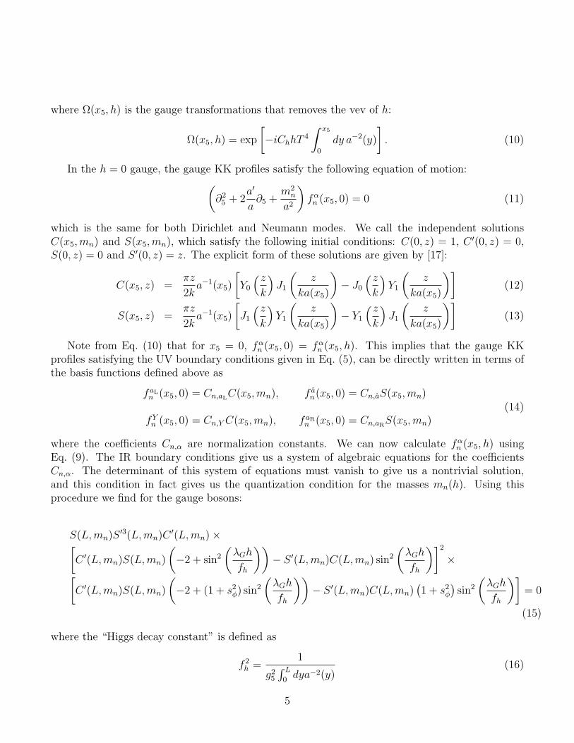
where the coefficients Cn,α are normalization constants. We can now calculate fαn (x5, h) usingEq. (9). The IR boundary conditions give us a system of algebraic equations for the coefficientsCn,α. The determinant of this system of equations must vanish to give us a nontrivial solution,and this condition in fact gives us the quantization condition for the masses mn(h). Using thisprocedure we find for the gauge bosons:

S(L,mn)S ′3(L,mn)C ′(L,mn)×[C ′(L,mn)S(L,mn)

(−2 + sin2

(λGh

fh

))− S ′(L,mn)C(L,mn) sin2

(λGh

fh

)]2

×[C ′(L,mn)S(L,mn)

(−2 + (1 + s2

φ) sin2

(λGh

fh

))− S ′(L,mn)C(L,mn)

(1 + s2

φ

)sin2

(λGh

fh

)]= 0

(15)

where the “Higgs decay constant” is defined as

f 2h =

1

g25

∫ L0dya−2(y)

(16)

5

and λ2G = 1/2. Furthermore, using the Wronskian relation

S ′(x5, z)C(x5, z)− C ′(x5, z)S(x5, z) = z a−2(x5) (17)

we can rewrite the quantization condition in a more convenient form:

S(L,mn)S ′3(L,mn)C ′(L,mn)[2a2

LC′(L,mn)S(L,mn) +mn sin2

(λGhfh

)]2×[

2a2LC′(L,mn)S(L,mn) + (1 + s2

φ)mn sin2(λGhfh

)]= 0

(18)

Therefore the KK mass spectrum for the W and Z bosons, with the correct Weinberg anglegiven by s2

φ ' tan2 θW ' (0.23/0.77) ' 0.2987, is given by the zeroes of the following equations:

1 + FW,Z(m2n) sin2

(λGh

fh

)= 0 , FW (z2) =

z

2a2LC′(L, z)S(L, z)

FZ(z2) =(1 + s2

φ)z

2a2LC′(L, z)S(L, z)

. (19)

We will identify the first zero of these equations with the masses of W and Z, respectively, andwe shall denote the masses of the first excited states as mW 1 and mZ1 , associated with the secondzeroes of both equations.

We can gain some physical insight if we look at Eq. (18) in the limit h = 0. In that case, thisequation reduces to,

S4(L,mn)S ′3(L,mn)C ′4(L,mn) = 0 (20)

We can identify the zeroes coming from C ′4(L,mn) = 0 with the KK mass spectrum of the 4 gaugebosons belonging to SU(2)L×U(1)Y which are even on both the UV and the IR branes. In the sameway, we identify the zeroes of S ′3(L,mn) = 0 with the KK spectrum of the 3 SU(2)R gauge bosonswhich are odd on the UV brane and even in the IR brane. S4(L,mn) = 0 is identified with the KKspectrum of the 4 SO(5)/SO(4) gauge bosons which are odd on both the UV and IR branes. Thusin Eq. (18) we associate the photon KK spectrum with the zeroes of C ′(L,mn) = 0.

2.1 Gauge Boson Form Factors at Low Energy

At small momenta, below the scale k ≡ k exp(−kL), the form factor for the W gauge bosons canbe approximated by

FW (−p2) ≈ g2f 2h

2p2; g =

g5√L. (21)

From the last equation, we can find an analytic expression for the W-mass:

m2W ≈

g2f 2h

2sin2

(λGh

fh

)+O(m4

W/k2). (22)

6

From this expression we can calculate the Higgs-W-W coupling, λHWW , at linear order, by simplytaking the derivative of m2

W with respect to the vev of h:

λHWW =∂m2

W

∂h= g2λGfh sin

(λGh

fh

)cos

(λGh

fh

)= gmw cos

(λGh

fh

)→ gmw (23)

where we used λG = 1/√

2 and in the last step note that in the limit λGh/fh 1 we recover theSM Higgs-W-W coupling. We will discuss the physical implications of the above limiting case insection 5.

3 Fermionic KK profiles

The SM fermions are embedded in full representations of the bulk gauge group. The presence ofthe SU(2)R subgroup of the full bulk gauge symmetry ensures the custodial protection of the Tparameter [7]. In order to have a custodial protection of the ZbLbL coupling, the choice T 3

R(bL) =T 3L(bL) has to be enforced [8]. An economical choice is to let the SM SU(2)L top-bottom doublet

arise from a 52/3 of SO(5) × U(1)X , where the subscript refers to the U(1)X charge. As discussedin [9], putting the SM SU(2)L singlet top in the same SO(5) multiplet as the doublet, withoutfurther mixing, is disfavored since for the correct value of the top quark mass this leads to a largenegative contribution to the T parameter at one loop. Hence we let the right-handed top quark arisefrom a second 52/3 of SO(5)×U(1)X . The right handed bottom can come from a 102/3 that allowsus to write the bottom Yukawa coupling. For simplicity, and because it allows the generation of theCKM mixing matrix, we make the same choice for the first two quark generations. We thereforeintroduce in the quark sector three SO(5) multiplets per generation as follows:

ξi1L ∼ Qi1L =

(χui

1L(−,+)5/3 quiL (+,+)2/3

χdi1L(−,+)2/3 qdi

L (+,+)−1/3

)⊕ u′iL(−,+)2/3 ,

ξi2R ∼ Qi2R =

(χui

2R(−,+)5/3 q′uiR (−,+)2/3

χdi2R(−,+)2/3 q′di

R (−,+)−1/3

)⊕ uiR(+,+)2/3 ,

(24)

ξi3R ∼

T i1R =

ψ′iR(−,+)5/3

U ′iR(−,+)2/3

D′iR(−,+)−1/3

⊕ T i2R =

ψ′′iR (−,+)5/3

U ′′iR (−,+)2/3

DiR(+,+)−1/3

⊕Qi3R =

(χui

3R(−,+)5/3 q′′uiR (−,+)2/3

χdi3R(−,+)2/3 q′′di

R (−,+)−1/3

),

where we show the decomposition under SU(2)L×SU(2)R, and explicitly write the U(1)EM charges.The Qis are bidoublets of SU(2)L × SU(2)R, with SU(2)L acting vertically and SU(2)R actinghorizontally. The T i1’s and T i2’s transform as (3,1) and (1,3) under SU(2)L×SU(2)R, respectively,while ui and u′i are SU(2)L × SU(2)R singlets. The superscripts, i = 1, 2, 3, label the threegenerations.

7

We also show the parities on the indicated 4D chirality, where − and + stands for odd andeven parity conditions and the first and second entries in the bracket correspond to the parities inthe UV and IR branes respectively. Let us stress that while odd parity is equivalent to a Dirichletboundary condition, the even parity is a linear combination of Neumann and Dirichlet boundaryconditions, that is determined via the fermion bulk equations of motion as discussed below.

The boundary conditions for the opposite chirality fermion multiplet can be read off the onesabove by a flip in both chirality and boundary condition, (−,+)L → (+,−)R for example. Inthe absence of mixing among multiplets satisfying different boundary conditions, the SM fermionsarise as the zero-modes of the fields obeying (+,+) boundary conditions. The remaining boundaryconditions are chosen so that SU(2)L × SU(2)R is preserved on the IR brane and so that massmixing terms, necessary to obtain the SM fermion masses after EW symmetry breaking, can bewritten on the IR brane. Consistency of the above parity assignments with the original orbifold Z2

symmetry at the IR brane will be discussed in Appendix B.As remarked above, the zero-mode fermions can acquire EW symmetry breaking masses through

mixing effects. The most general SU(2)L × SU(2)R × U(1)X invariant mass Lagrangian at the IRbrane – compatible with the boundary conditions – is, in the quark sector,

Lm = 2δ(x5 − L)[u′LMB1uR + Q1LMB2Q3R + Q1LMB3Q2R + h.c.

], (25)

where MB1 , MB2 and MB3 are dimensionless 3×3 matrices, and matrix notation is employed. In Ap-pendix B we will show how these mass terms may be generated from an SO(5) invariant Lagrangianusing the spurion formalism. To prevent negative corrections to the T parameter [18], [9, 10], wewill take MB3 to be the null matrix. In Appendix C however we briefly discuss the modifications ofthe effective Higgs potential induced by a non-zero value of MB3 . Moreover since the Higgs effectivepotential is most sensitive to the third generation, we will concentrate on this one, discarding familyindices.

With the introduction of these brane mixing terms, the different multiplets are now related viathe equations of motion. In the case of a mass term involving Ψ1

LΨ2R, with the fields having profile

functions gL and hR, the odd parity profile gR on the IR brane is related to hR:∫ L+ε

L−ε(∂5gR)dx5 =

∫ L+ε

L−ε(2MhR − gR)δ(x5 − L)dx5. (26)

The odd parity we demand at the IR brane implies a Dirichlet boundary condition for the functiongR. Therefore, we can rewrite:

limε→0

gR(L− ε) = −MhR(L), (27)

and, similarly:limε→0

hL(L− ε) = MgL(L). (28)

Eq. (27) and (28) can now be reinterpreted as the new boundary conditions for the profiles at theIR brane.

The fermions, like the gauge bosons, can be expanded in their KK basis:

ψL(x, x5) =∑n

fL,n(x5, h)ψL,n(x), ψR(x, x5) =∑n

fR,n(x5, h)ψR,n(x). (29)

8

In the h = 0 gauge, we redefine ψ = a2(x5)ψ and we write our vector-fermionic fields in terms ofchiral fields. We can KK decompose the fermionic chiral components as,

ψL,R =∞∑n=0

ψnL,R(xµ)fL,R,n(x5) (30)

where f is normalized by: ∫ L

0

dx5a−1(x5)fnfm = δm,n. (31)

Therefore the profile function for the zero mode fermion corresponds to a−1/2(x5)f0.From the 5D action, Eq. (2), concentrating on the free fermionic fields, we can derive the

following first order coupled equations of motion for fL,R,n,

(∂5 +M)fR,n = (z/a(x5))fL,n; (∂5 −M)fL,n = −(z/a(x5))fR,n (32)

We see from Eq. (32) that we can redefine fR,L,n = e−Mx5 fR,L,n and relate the opposite chiralcomponent of the same vector-like field by fR,n = (−a(x5)/z)∂5fL,n. For the left handed field havingDirichlet boundary conditions on the UV brane, we can derive a second order equation for the chiralcomponent fL,n: [

∂25 +

(a′

a+ 2M

)∂5 +

z2

a2

]fL,n = 0 (33)

the solution of which we shall call SM(x5, z), with boundary conditions SM(0, z) = 0, S ′±M(0, z) = z.

Similarly, we can redefine fR,L,n = eMx5 fR,L,n and then relate the opposite chirality via fL,n =(a(x5)/z)∂5fR,n. If the right-handed field fulfills Dirichlet boundary conditions on the UV-brane,we can write the equation of motion for fR,n:[

∂25 +

(a′

a− 2M

)∂5 +

z2

a2

]fR,n = 0. (34)

We shall correspondingly denote the solution to this equation with S−M(x5, z), fulfilling the bound-ary conditions S−M(0, z) = 0, S ′−M(0, z) = z.

As emphasized before, the solutions of the opposite chirality, are related to these solutions via the

the first order equations of motion, Eqs. (32), which we rewrite as ˙S±M(x5, z) = ∓(a(x5)/z)∂5S±M(x5, z).Here M = −ck, and the ± is chosen depending on whether we want an odd (-) boundary conditionon the UV brane for the left-handed or right-handed fermionic field. The solution to Eq. (33) isgiven by [17]:

SM(x5, z) =πz

2ka−c−

12 (x5)

[J 1

2+c

(zk

)Y 1

2+c

(z

ka(x5)

)− Y 1

2+c

(zk

)J 1

2+c

(z

ka(x5)

)]. (35)

The solution for Eq. (34) is given by Eq. (35), with the replacement c→ −c.

9

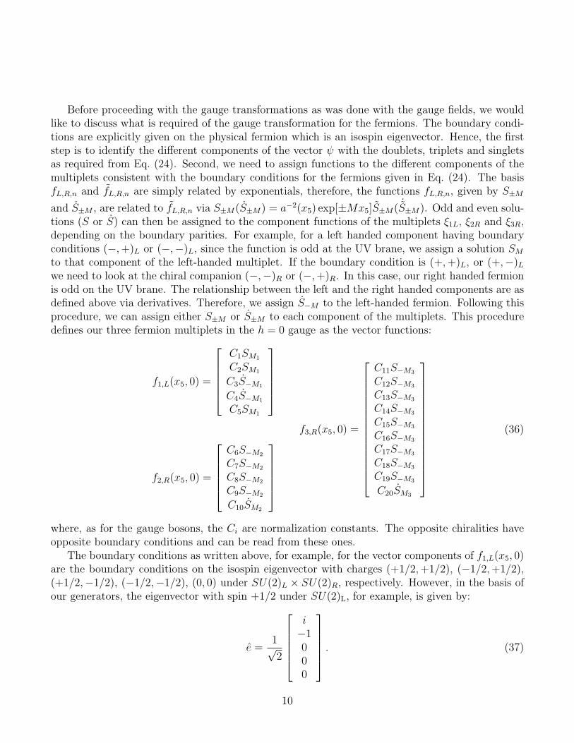
Before proceeding with the gauge transformations as was done with the gauge fields, we wouldlike to discuss what is required of the gauge transformation for the fermions. The boundary condi-tions are explicitly given on the physical fermion which is an isospin eigenvector. Hence, the firststep is to identify the different components of the vector ψ with the doublets, triplets and singletsas required from Eq. (24). Second, we need to assign functions to the different components of themultiplets consistent with the boundary conditions for the fermions given in Eq. (24). The basisfL,R,n and fL,R,n are simply related by exponentials, therefore, the functions fL,R,n, given by S±M

and S±M , are related to fL,R,n via S±M(S±M) = a−2(x5) exp[±Mx5]S±M( ˙S±M). Odd and even solu-tions (S or S) can then be assigned to the component functions of the multiplets ξ1L, ξ2R and ξ3R,depending on the boundary parities. For example, for a left handed component having boundaryconditions (−,+)L or (−,−)L, since the function is odd at the UV brane, we assign a solution SMto that component of the left-handed multiplet. If the boundary condition is (+,+)L, or (+,−)Lwe need to look at the chiral companion (−,−)R or (−,+)R. In this case, our right handed fermionis odd on the UV brane. The relationship between the left and the right handed components are asdefined above via derivatives. Therefore, we assign S−M to the left-handed fermion. Following thisprocedure, we can assign either S±M or S±M to each component of the multiplets. This proceduredefines our three fermion multiplets in the h = 0 gauge as the vector functions:

f1,L(x5, 0) =

C1SM1

C2SM1

C3S−M1

C4S−M1

C5SM1

f2,R(x5, 0) =

C6S−M2

C7S−M2

C8S−M2

C9S−M2

C10SM2

f3,R(x5, 0) =

C11S−M3

C12S−M3

C13S−M3

C14S−M3

C15S−M3

C16S−M3

C17S−M3

C18S−M3

C19S−M3

C20SM3

(36)

where, as for the gauge bosons, the Ci are normalization constants. The opposite chiralities haveopposite boundary conditions and can be read from these ones.

The boundary conditions as written above, for example, for the vector components of f1,L(x5, 0)are the boundary conditions on the isospin eigenvector with charges (+1/2,+1/2), (−1/2,+1/2),(+1/2,−1/2), (−1/2,−1/2), (0, 0) under SU(2)L × SU(2)R, respectively. However, in the basis ofour generators, the eigenvector with spin +1/2 under SU(2)L, for example, is given by:

e =1√2

i−1000

. (37)

10

To simplify matters, so that the boundary conditions can be taken to be on the eigenvector:

e =

10000

(38)

the transformation Ω needs to be in the basis consistent with Eq. (38), or we can also think aboutthis as changing the fermion vector functions given in Eq. (36) to the basis of our generators. Thismeans that we have to first understand how the eigenvectors of T 3R,L decompose in the canonicalbasis for both the 52/3 and the 102/3.

For the 52/3 fermions, the basis transformation for ξ1L, ξ2R is given by

A = 1√2

−i −1 0 0 00 0 −i 1 00 0 i 1 0−i 1 0 0 0

0 0 0 0√

2

(39)

For 102/3, the transformation matrix for ξ3R is given by

B = 1√2

i 1 0 0 0 0 0 0 0 00 0 −i 1 0 0 0 0 0 00 0 −i −1 0 0 0 0 0 0−i 1 0 0 0 0 0 0 0 00 0 0 0 −1 i 0 0 0 0

0 0 0 0 0 0√

2 0 0 00 0 0 0 1 i 0 0 0 00 0 0 0 0 0 0 −1 i 0

0 0 0 0 0 0 0 0 0√

20 0 0 0 0 0 0 1 i 0

(40)

Therefore, once the UV boundary conditions define the vectors as in Eq. (36), we change basesto be able to implement the gauge transformation and then transform back so that the IR boundaryconditions can be imposed. Using the transformations defined in Eq. (39) and (40), we can writethe final fermion vector functions in the presence of the vev of h as:

f1,L(x5, h) = AΩA−1f1,L(x5, 0) (41)

f2,R(x5, h) = AΩA−1f2,R(x5, 0) (42)

f3,R(x5, h) = BΩB−1f3,R(x5, 0) (43)

Applying the boundary conditions at x5 = L, taking into account the mass mixing terms from

11

Eq. (25) and using the procedure defined in Eqs. (27) and (28), we derive the conditions on f(L, h):

f 1,...,41,R +MB2f

1,...,43,R = 0 f 5

1,R +MB1f52,R = 0 f 1,...,4

2,L = 0

f 1,...,43,L −MB2f

1,...,41,L = 0 f 5

2,L −MB1f51,L = 0 f 5,...,10

3,L = 0

(44)

where the superscripts denote the vector components.Asking that the determinant of this system of equations vanishes so that we get a non-trivial

solution, we notice that all dependence on the prefactors a−3/2(x5) exp[±Mx5] relating S±M , S±M

and S±M ,˙S±M drops out, and thus we conclude that one of the following equations should vanish:

S′3−M2

= 0 (45)

S ′5−M3= 0 (46)[

M2B2SM1S−M3 −

a2L

z2S ′M1

S ′−M3

]2= 0 (47)

2SM3

[M2

B2S−M3S

′−M1

+ S−M1S′−M3

]−M2

B2S ′−M1

sin2(λF hfh

)= 0 (48)

2[M2

B1SM1

(−1 + SM2S−M2

)(M2

B2S−M3S

′−M1

+ S−M1S′−M3

)+

SM2S′−M2

(M2

B2

(−1 + SM1S−M1

)S−M3 −

a2L

z2S−M1S

′M1S ′−M3

)]+[

M2B2SM2S−M3S

′−M2

+M2B1

(2M2

B2SM1S−M3S

′−M1

+ S ′−M3+ 2SM1S−M1S

′−M3−

SM2S−M2S′−M3

)]sin2

(λF hfh

)−M2

B1S ′−M3

sin4(λF hfh

)= 0 (49)

where for simplicity we did not write the dependence on L and z and furthermore, we have usedthe Crowian:

− ˙SM(x5, z)˙S−M(x5, z) + SM(x5, z)S−M(x5, z) = 1 . (50)

In the following, and for simplicity, we shall omit the tildes and refer to the solutions S±M by S±M .The same value λF = 1/

√2 is found in the fermionic case, so from now on λ = λG = λF . The

solutions to Eqs. (45), (46) and (47) can be interpreted as the KK spectrum of exotic fermions.We shall name these states E3, E2 and E1, respectively. Eq. (48) is the KK mass spectrum for thebottom quark and Eq. (49) gives the KK spectrum for the top quark.

We can rewrite Eqs. (48) and (49) in the same form as the gauge bosons:

1 + Fb(m2n) sin2

(λh

fh

)= 0 , (51)

1 + Ft1(m2n) sin2

(λh

fh

)+ Ft2(m

2n) sin4

(λh

fh

)= 0 (52)

12

where

Fb(z2) = −

M2B2S ′−M1

2SM3(M2B2S−M3S

′−M1

+ S−M1S′−M3

)(53)

Ft1(z2) =

F1(z2)

Fd(z2)(54)

Ft2(z2) =

F2(z2)

Fd(z2), (55)

F1(z2) = M2

B2SM2S−M3S

′−M2

+M2B1

[2M2

B2SM1S−M3S

′−M1

+

S ′−M3+ 2SM1S−M1S

′−M3− SM2S−M2S

′−M3

](56)

F2(z2) = −M2

B1S ′−M3

(57)

Fd(z2) = 2

[M2

B1SM1 (−1 + SM2S−M2)

(M2

B2S−M3S

′−M1

+ S−M1S′−M3

)+

SM2S′−M2

(M2

B2(−1 + SM1S−M1)S−M3 −

a2L

z2S−M1S

′M1S ′−M3

)](58)

Equations (19), (51) and (52) are the starting point for computing the one-loop effective potentialfor the scalars ha.

It is physically very illuminating to interpret the origin of the fermionic resonances if we con-template the fermionic determinant in the case h = 0:

SM3 = 0 SM2S′M1

+M2B1SM1S

′M2

= 0

S′5−M3

= 0 (M2B2S−M3S

′−M1

+ S−M1S′−M3

)2 = 0

S′4−M2

= 0 (M2B2SM1S−M3 −

a2L

z2S ′M1

S ′−M3)2 = 0

(59)

We recall that the way we defined the initial fermionic functions (S±M) was via the boundarycondition on the UV brane and the chirality. However, since we are in the h = 0 gauge, we can usethe boundary conditions on the IR brane to further give us the final equations the functions haveto satisfy:

(−,−)L ⇒ SM(L) = 0, (−,−)R ⇒ S−M(L) = 0(−,+)L → SM → (+,−)R ⇒ S ′M(L) = 0, (−,+)R → S−M → (+,−)L ⇒ S ′−M(L) = 0

(60)

We can now interpret Eq. (59) in a simple way: the first equation in the first line provides themass spectrum for the singlet right handed bottom. This with the first equation in the second lineprovide the mass spectrum of the triplet components T1R, T2R of ξ3R. The second equation in thefirst line may be identified with the mass spectrum of the singlet tR and its modification from themixing mass term with u′L. It can be shown from this equation that the light top resonances willbe mostly the KK modes of the right handed top. From the first equation in the third line we

13

get the mass spectrum for Q2R. Additionally we can also see here the mixing of the bidoublets Q1

and Q3. The second equation in the second line is related to the mass spectrum for the (tL, bL)t

doublet and its mixing with (q′′u3L, q′′d3L)t. The second equation in the third line may be identified as

the spectrum of a new fermionic state coming from the doublet-doublet mixing between (χu1L, χd1L)t

and (χu2L, χd2L)t.

3.1 Top Mass and Yukawa Coupling at Low Energy

At small momenta, the solution to Eq. (35) takes the form:

SM ≈ z

∫ x5

0

a−1(x5)e−2Mydy +O(z3) . (61)

Replacing this in Eq. (49), keeping only quadratic terms in z and for simplicity neglecting the smallMB2 effects, we find that the top quark spectral equation reduces to:

A

(z

k

)2

+M2B1

[1 +B

(z

k

)2]

sin2

(λh

fh

)−M2

B1sin4

(λh

fh

)= 0, (62)

where A and B are coefficients given by:

A = −(1

2+ c1) +M2

B1(1

2+ c2)

2(14− c21)(1

2+ c2)

; B =(1

4− c22)− 1

2(1

4− c21)

2(14− c21)(1

4− c22)

. (63)

Solving Eq. (62) for z2, we find that the top mass takes the form

(mt

k

)2

≈ −M2

B1sin2

(λhfh

)cos2

(λhfh

)A+M2

B1B sin2

(λhfh

) +O(m3t/k

3), (64)

which can also be written as(mt

k

)2

≈2M2

B1sin2

(λhfh

)cos2

(λhfh

)(1

4− c21)(1

4− c22)

(12− c2)(1

2+ c1) +M2

B1

[(1

4− c22) cos2

(λhfh

)+ 1

2(1

4− c21) sin2

(λhfh

)] . (65)

This expression is similar to the one obtained in a related model in Ref. [11]. From this expressionwe can calculate the Yukawa coupling of the top, Yt, at linear order, by simply taking the derivativeof mt with respect to h:

Yt =√

2∂mt

∂h' mtg

mW

√2

cos(

2λhfh

)cos(λhfh

) , (66)

where we note that in the limit λh/fh 1, we recover the SM top Yukawa coupling.

14

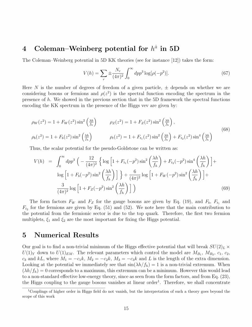
4 Coleman–Weinberg potential for ha in 5D

The Coleman–Weinberg potential in 5D KK theories (see for instance [12]) takes the form:

V (h) =∑r

± Nr

(4π)2

∫ ∞0

dpp3 log[ρ(−p2)]. (67)

Here N is the number of degrees of freedom of a given particle, ± depends on whether we areconsidering bosons or fermions and ρ(z2) is the spectral function encoding the spectrum in thepresence of h. We showed in the previous section that in the 5D framework the spectral functionsencoding the KK spectrum in the presence of the Higgs vev are given by:

ρW (z2) = 1 + FW (z2) sin2(λhfh

)ρZ(z2) = 1 + FZ(z2) sin2

(λhfh

),

ρb(z2) = 1 + Fb(z

2) sin2(λhfh

)ρt(z

2) = 1 + Ft1(z2) sin2

(λhfh

)+ Ft2(z

2) sin4(λhfh

) (68)

Thus, the scalar potential for the pseudo-Goldstone can be written as:

V (h) =

∫ ∞0

dpp3(− 12

(4π)2

log[1 + Ft1(−p2) sin2

(λh

fh

)+ Ft2(−p2) sin4

(λh

fh

)]+

log[1 + Fb(−p2) sin2

(λh

fh

)] +

6

(4π)2log[1 + FW (−p2) sin2

(λh

fh

)]+

3

(4π)2log[1 + FZ(−p2) sin2

(λh

fh

)] )(69)

The form factors FW and FZ for the gauge bosons are given by Eq. (19), and Fb, Ft1 andFt2 for the fermions are given by Eq. (51) and (52). We note here that the main contribution tothe potential from the fermionic sector is due to the top quark. Therefore, the first two fermionmultiplets, ξ1 and ξ2 are the most important for fixing the Higgs potential.

5 Numerical Results

Our goal is to find a non-trivial minimum of the Higgs effective potential that will break SU(2)L×U(1)Y down to U(1)EM . The relevant parameters which control the model are MB1 , MB2 , c1, c2,c3 and kL, where M1 = −c1k, M2 = −c2k, M3 = −c3k and L is the length of the extra dimension.Looking at the potential we immediately see that sin(λh/fh) = 1 is a non-trivial extremum. When(λh/fh) = 0 corresponds to a maximum, this extremum can be a minimum. However this would leadto a non-standard effective low-energy theory, since as seen from the form factors, and from Eq. (23),the Higgs coupling to the gauge bosons vanishes at linear order1. Therefore, we shall concentrate

1Couplings of higher order in Higgs field do not vanish, but the interpretation of such a theory goes beyond thescope of this work

15

Figure 1: Higgs Mass vs top mass in GeV. Blue (dark gray) crosses represent the linear regime, green (light gray)x’s the non-linear regime and black dots where a minimum for the effective potential exists.

only in the regions of parameter space such that 0 < sin(λh/fh) < 1 with 0 < λh/fh < π/2. Afterobtaining a non-trivial minimum, we calculate k by finding the first zero of Eq. (19) and settingthis mass equal to the W mass [19]. This is the mass that the W zero-mode gets from interactingwith the Higgs vev. Since the relationship between the Z and the W form factors remains the sameas in the SM, we also recover a consistent mass for the Z boson.

Having obtained k, we calculate the top-quark mass, given by the first zero of Eq. (52), anddemand that its value is in the phenomenological range mtop ∈ [140, 170] GeV. We take such a widerange since we consider the result of our calculation to be associated with the running top-quarkmass evaluated at a scale of the order of the weak scale. Due to the strong gauge coupling, therunning top-quark mass varies rapidly between values of mtop ∼ 140 GeV, for a scale of the orderof a few TeV, to values of mtop ∼ 165 GeV, for a scale of order of the top quark pole mass Mt.Furthermore, we also calculate the bottom quark mass, given by the first zero of Eq. (51), anddemand it to be in the phenomenological range mbottom ∈ [2, 4] GeV. The Higgs mass is given by

16

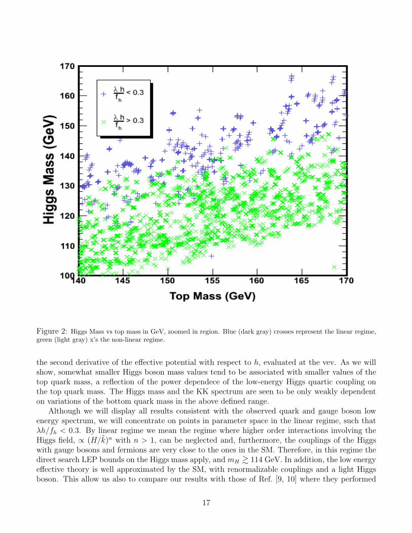
Figure 2: Higgs Mass vs top mass in GeV, zoomed in region. Blue (dark gray) crosses represent the linear regime,green (light gray) x’s the non-linear regime.

the second derivative of the effective potential with respect to h, evaluated at the vev. As we willshow, somewhat smaller Higgs boson mass values tend to be associated with smaller values of thetop quark mass, a reflection of the power dependece of the low-energy Higgs quartic coupling onthe top quark mass. The Higgs mass and the KK spectrum are seen to be only weakly dependenton variations of the bottom quark mass in the above defined range.

Although we will display all results consistent with the observed quark and gauge boson lowenergy spectrum, we will concentrate on points in parameter space in the linear regime, such thatλh/fh < 0.3. By linear regime we mean the regime where higher order interactions involving theHiggs field, ∝ (H/k)n with n > 1, can be neglected and, furthermore, the couplings of the Higgswith gauge bosons and fermions are very close to the ones in the SM. Therefore, in this regime thedirect search LEP bounds on the Higgs mass apply, and mH & 114 GeV. In addition, the low energyeffective theory is well approximated by the SM, with renormalizable couplings and a light Higgsboson. This allow us also to compare our results with those of Ref. [9, 10] where they performed

17

Figure 3: Higgs Mass (GeV) vs k (TeV). Blue (dark gray) crosses represent the linear regime, green (light gray)x’s the non-linear regime and black dots where a minimum for the effective potential exists.

calculations in the linear regime as defined above.We can interpret k as the associated mass scale of our theory and of the order of the natural

UV cut off of the low-energy, SM-like effective theory. The scale k is inversely proportional toλh/fh and therefore as we move away from the linear regime, we are pushing the UV cut-off lowerand additionally causing the linear couplings of the Higgs to become smaller. Therefore, the theorybecomes increasingly non-renormalizable, which leads to the need of taking into account higher orderKK-states (beyond zero-modes) in the calculation of low-energy processes, thus making connectionwith SM predictions harder. When k < 2.5 TeV, KK bosonic and fermionic resonances of exoticand SM fields have a chance to be detected in the next generation colliders such as the LHC; hence,we will be specifically interested in those regions.

We performed two major numerical parameter scans. In the first one we scanned the parameterspace for values ci ∈ [−1, 1] with i = 1, 2, 3 and MB1 ,MB2 ∈ [0, 5]. We used kL = 30 in our numerical

18

Figure 4: Minimum vs MB1 . Blue (dark gray) crosses represent the linear regime, green (light gray) x’s thenon-linear regime. The sparse region for higher values of MB1 is due to a coarser grid scanned in that region.

calculations for the masses since the results are invariant under variations of kL ∈ [30, 34] 2. Thefirst scan was done with a coarse grid and before we discuss details of our numerical results, wewould like to point out that the effective potential is a completely well behaved function of allthe parameters, therefore, we expect that the gaps in our scanned space are smoothly filled. Wefound that even though for some value of the other parameters, non-trivial minima existed fornearly all the regions of ci and MBi, we only found phenomenologically consistent gauge bosons,top and bottom quark masses in the following regions of parameter space: 0 ≤ |c1| ≤ 0.3, 0.35 ≤|c2| ≤ 0.45, 0.55 ≤ |c3| ≤ 0.6, 1 . MB1 and MB2 < MB1 . Though the results show a skewsymmetry between positive and negative values, we decided to concentrate on negative values of c2and c3, since interestingly enough, this is the region which is consistent with electroweak precisionmeasurements [9]. Furthermore, positive values of c1 lead to a smaller overlap of the left-handed top

2k, obtained from demanding a W-mass in accordance with experiments, adjusts itself so that k remains approx-imately constant

19

Figure 5: Minimum vs k (TeV). Blue (dark gray) crosses represent the linear regime, green (light gray) x’s thenon-linear regime

and bottom zero modes with physics at the IR brane, leading to a stronger suppression of potentiallydangerous flavor changing operators [20]. Therefore, it is in this region where we performed a morethorough scan taking smaller steps for the ci.

In Figure 1 we notice a clear relationship between the Higgs and the top-quark masses, whereon the plot we have included the bigger coarse scan of parameter space. Focusing on the interestingphenomenological region, we see in Figure 2 that in the linear regime we get Higgs masses thattend to be above 115 GeV, which is above the experimental bound from LEP, and below 160 GeV.Furthermore, there is a somewhat weak dependence of the Higgs mass values on the precise valueof the running top quark mass. Higgs mass values closer to the current experimental bound areobtained for the smallest values of the top quark mass in the phenomenologically allowed range. InFigure 3, we manifestly see that in the linear regime we may obtain masses for the Higgs which arecompatible with 1.5 TeV . k . 2.5 TeV.

Figure 4 provides us with information about the 5D parameter MB1 which as increased moves

20

Figure 6: c1 vs c2. Blue (dark gray) crosses represent the linear regime, green (light gray) x’s the non-linear regimeand black dots where a minimum for the effective potential exists.

the minimum to higher values of λh/fh, getting into the non-linear regime. We conclude that toremain in the linear regime, we cannot have an arbitrarily high MB1 boundary mass parameter.

The behavior fh ∝ 1/k is seen in Figure 5 where, moreover, we notice that for the linear regime,values of k & 1.5 TeV are obtained. This low value of k will lead to interesting phenomenology forthe decays of light KK-fermions and KK-bosons.

In Figure 6 we see that a selected region of the plane c1 − c2 is suitable for minimizing theeffective potential with the experimentally observed W , Z, top and bottom masses, and that thelinear regime basically applies through out this region. As emphasized before, c1 & 0 and c2 . −0.4are the ones preferred by consistency with electroweak precision measurements [9]. In Figure 7we noticed that the same phenomenologically accepted region for c2 in the c2 − c3 plane with−0.6 ≤ c3 ≤ −0.55 is chosen and it is also homogenously covered in the linear regime.

Figures 8 and 9 are very interesting for collider phenomenology and therefore deserve specialattention. Even though we haven’t included the plot, we calculated the mass of the W first excited

21

Figure 7: c2 vs. c3. Blue (dark gray) crosses represent the linear regime, green (light gray) x’s the non-linearregime and black dots where a minimum for the effective potential exists.

KK state numerically and verified the relation mW1 ≈ 2.5 k. If the masses of these fermionsare below the black line denoting mW 1/2, the decay of W1 and Z1 to pairs of these fermions iskinematically available. Note here however, that for c1 > 0, mE1

1is always greater than mW 1/2.

Moreover, these exotic fermions are unstable. The decay products of T1 are analyzed in Ref. [10].The first top KK excited state, will mainly decay to Zt, Ht, Wb. The charged 5/3 fermions of E1

1

will necessarily decay to Wt from charge conservation, leading to interesting phenomenology [21]. Inaddition, the lightest KK quark state T 1, the top quark (via its right- and left-handed couplings) andthe bottom quark (via its left-handed coupling) will be included in the KK gluon decay products.This is a distinctive feature of this model when compared with the predominant decay into right-handed top quarks in the models considered in Refs. [22],[23].

22

Figure 8: mW 1 vs mTop1,2,3 in TeV. Also marked is mW 1/2 showing that only the first excited top mode can decayinto gauge bosons. Blue (dark gray) crosses represent the linear regime with c1 > 0, gray (light gray) crosses thelinear regime with c1 < 0, red x’s (dark gray) the non-linear regime with c1 > 0, green x’s (light gray) the non-linearwith c1 < 0.

6 Conclusions

In this article, we computed the one-loop Coleman Weinberg potential for the Higgs field in a specificmodel of Gauge-Higgs unification in warped extra dimensions. We chose the specific group SO(5)×U(1)X , which allows the introduction of custodial symmetries protecting the precision electroweakobservables as well as a Higgs field with the proper quantum numbers under the electroweak gaugegroups. As a first step, we computed the spectral functions of the fermions and gauge bosons of thetheory when the Higgs field acquires a vev. These are then used to calculate the effective potentialfor the Higgs. We demand non-trivial minima that lead to the proper values of the gauge bosonand fermion masses in the low energy theory. This requirement leads to a selection of a restrictedregion of parameters. Interestingly enough, the selected regions of parameters coincide with the ones

23

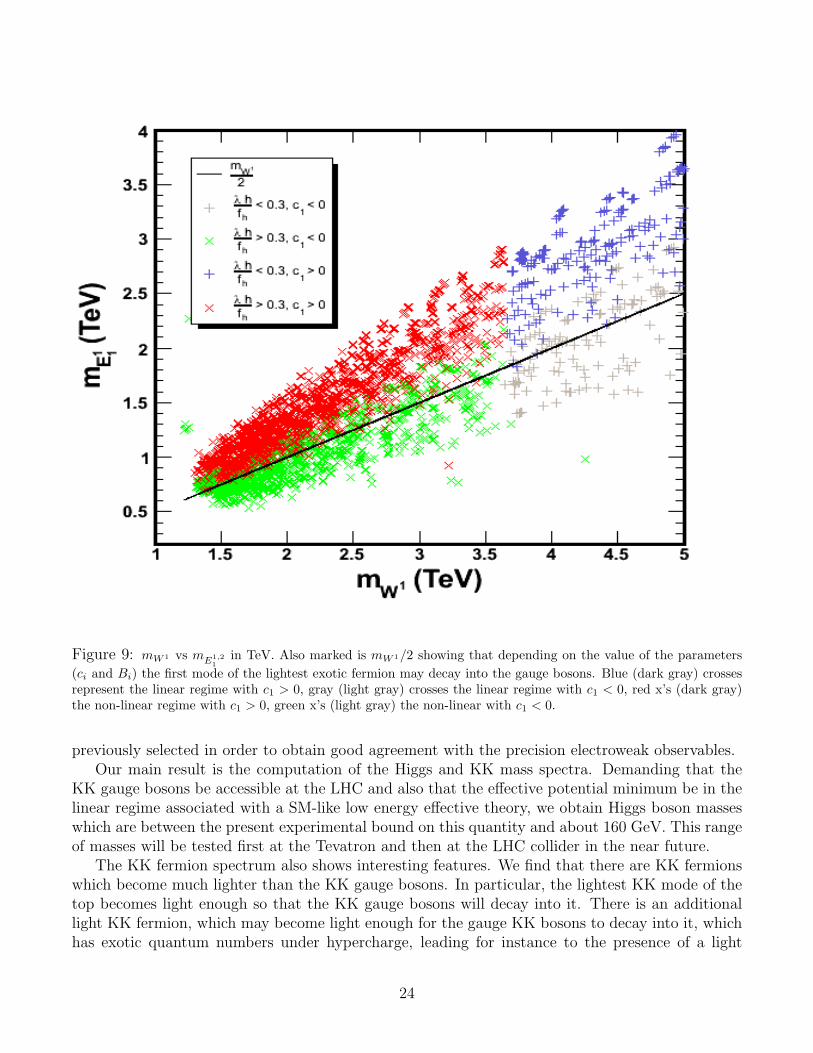
Figure 9: mW 1 vs mE1,21

in TeV. Also marked is mW 1/2 showing that depending on the value of the parameters(ci and Bi) the first mode of the lightest exotic fermion may decay into the gauge bosons. Blue (dark gray) crossesrepresent the linear regime with c1 > 0, gray (light gray) crosses the linear regime with c1 < 0, red x’s (dark gray)the non-linear regime with c1 > 0, green x’s (light gray) the non-linear with c1 < 0.

previously selected in order to obtain good agreement with the precision electroweak observables.Our main result is the computation of the Higgs and KK mass spectra. Demanding that the

KK gauge bosons be accessible at the LHC and also that the effective potential minimum be in thelinear regime associated with a SM-like low energy effective theory, we obtain Higgs boson masseswhich are between the present experimental bound on this quantity and about 160 GeV. This rangeof masses will be tested first at the Tevatron and then at the LHC collider in the near future.

The KK fermion spectrum also shows interesting features. We find that there are KK fermionswhich become much lighter than the KK gauge bosons. In particular, the lightest KK mode of thetop becomes light enough so that the KK gauge bosons will decay into it. There is an additionallight KK fermion, which may become light enough for the gauge KK bosons to decay into it, whichhas exotic quantum numbers under hypercharge, leading for instance to the presence of a light

24

fermion with charge 5/3e with interesting phenomenological properties.

Acknowledgements

We would like to thank Debajyoti Choudhury, Ben Lillie, Arjun Menon, Jing Shu, Tim Tait and par-ticularly Marcela Carena, Eduardo Ponton and Jose Santiago for useful discussions and comments.Work at ANL is supported in part by the US DOE, Div. of HEP, Contract DE-AC02-06CH11357.This work was also supported in part by the U.S. Department of Energy through Grant No. DE-FG02-90ER40560.

25

APPENDIX

A SO(5) Generators

The generators of the fundamental representation of SO(5), with Tr[Tα.Tβ] = C(5)δαβ, are givenby:

TaL,R

i,j = −i√C(5)

2

[1

2εabc(δbi δ

cj − δbjδci )± (δai δ

4j − δaj δ4

i )

],

T ai,j = −i√C(5)

2(δai δ

5j − δaj δ5

i ), (A.1)

where T a (a = 1, 2, 3, 4) and T aL,R (aL,R = 1, 2, 3) are the generators of SO(5)/SO(4) and SO(4)respectively.

B Fermion Parity Assignments and Brane Masses

Since the Higgs has positive parity, in order to preserve the Z2 orbifold symmetry, we need to ensurethat the product of the parities of the fermions coupled via the Higgs is always positive. The Higgsprofile is doubly exponentially suppressed on the UV brane, therefore, we will restrict ourselves todiscussion of parities on the IR brane.

Concentrating on the parities of the first two multiplets given in Eq. (24), we notice that theproduct of the fermion parities coupled by the Higgs is not positive. One way to fix this would beto switch the parities for the SO(4) singlet components:

[+,−] ⇔ [+,+]. (B.1)

Due to the introduction of the brane mass terms as in Eq. (25), and looking at Eq. (44) we notethat the switch in parity is exactly equivalent to taking M2

B1→ 1/M2

B1. Thus the physical results

presented in this work are invariant under the switch of parity with just the above mentioned changein MB1 .

Another way to understand the realization of the Z2 symmetry is via the spurion formalism. Weintroduce a spurion field transforming in the fundamental representation of SO(5), and acquiring avery large vev in the SO(4) singlet direction, breaking the SO(5) gauge symmetry to SO(4) on theIR brane. We also introduce local fermionic degrees of freedom on the brane and write large localmass terms involving the spurion, between these degrees of freedom and the ones propagating inthe bulk. The fermion parities are chosen to be those preserving Z2. By using a procedure similarto the one outlined in Eqs. (26), (27) and (28), we can now change the bulk fermion IR boundaryconditions while preserving Z2 to give the model we are considering in this work. This mechanismwould allow us to change the IR boundary conditions not just of the SO(4) singlet fields in the 5’s,but also of the bidoublets in the 5’s or in the 10. For the case of the SO(4) singlet fields in the 5’s,

26

we need to add SO(5) singlet fermions on the IR brane, that couple to the 5’s via the spurion field.For the case of the bidoublets in the 10 or in the 5’s, we need to add local 5’s and singlet fermionson the IR brane, and couple them appropriately to the bulk 10 or 5’s via gauge invariant massesor couplings to the spurion field (SO(5) singlet fields are necessary to remove unwanted degreesof freedom). In this way, one could start with the opposite IR parities for the three bidoublets tothe ones given in Eq. (24), thus preserving the Z2 symmetry, and reach the choice of bulk fermionboundary conditions used in this work.

The same spurion mechanism can be used to write the brane mass terms in Eq. (25) in anSO(5) invariant way. A spurion field which is a 5 under SO(5), can be used to write the bidoublet-bidoublet mixing brane mass term, MB2 , between the 5 and the 10 multiplets. The spurion fieldis coupled to these two via a Yukawa type interaction which can be adjusted to give MB2 ∼ O(1).This field can be the same as the one that is used to change the parities of the fermions as describedin the last paragraph. The same procedure, but now using a 15 ≡ 14⊕ 1 of SO(5) can be used togenerate the mass mixing terms between the singlets, MB1 . The 15 required can be thought of asarising from a tensor product of the 5 spurion field: 5⊗ 5 ≡ 10⊕14⊕1. Note that this mechanismwill not generate a localized bare mass for the Higgs due to gauge invariance.

C Flip Parities for Q2R and the Introduction of MB3

We also studied the effects of flipping the parities of Q2R as was done in the context of Ref. [10].In this case, the parity assignments for the rest of our fermionic content remains the same exceptfor Q2R which now takes the form,

Q2R =

(χui

2R(+,−)5/3 q′uiR (+,−)2/3

χdi2R(+,−)2/3 q′di

R (+,−)−1/3

). (C.1)

If we keep the same boundary mass terms as in Eq. (25) and calculate the fermionic spectralfunctions we obtain,

S4M2

= 0 (C.2)

S ′5−M3= 0 (C.3)[

M2B2SM1S−M3 + ˙SM1

˙S−M3

]2= 0 (C.4)

2SM3

[M2

B2S−M3

˙S−M1 + S−M1

˙S−M3

]−M2

B2

˙S−M1 sin2(λF hfh

)= 0 (C.5)

2[M2

B2S−M3

(−SM2 + SM1SM2S−M1 +M2

B1SM1

˙SM2

˙S−M1

)+

S−M1

(SM2

˙SM1 +M2B1SM1

˙SM2

)˙S−M3

]+(M2

B2SM2S−M3 −M2

B1

˙SM2

˙S−M3

)sin2

(λF hfh

)= 0 (C.6)

From these expressions we expect that the only non-trivial EW breaking vacua will be generatedwhen λFh/fh = π/2 which, as discussed in section 5, leads to a theory which is highly non-renormalizable. We performed limited numerical analysis which confirmed this expectation.

27

For completeness and as a reference for future work we write the expression for the determinantin the case of a non-zero mass mixing boundary term MB3 as in Eq. (25). For simplicity, we turnoff the singlet mass mixing MB1 . Keeping parities as in our original model, we derive the followingfermionic spectral functions,

˙S5−M3

= 0 (C.7)[M2

B2SM1S−M3

˙S−M2 +M2B3SM1S−M2

˙S−M3 + ˙SM1

˙S−M2

˙S−M3

]= 0 (C.8)

2SM3

[M2

B2S−M3

˙S−M1

˙S−M2 +M2B3S−M2

˙S−M1

˙S−M3 + S−M1

˙S−M2

˙S−M3

]−M2

B2

˙S−M1

˙S−M2 sin2(λF hfh

)= 0 (C.9)

2SM2

[M4

B2SM1S

2−M3

˙SM1

˙S−M1

˙S2−M2

+M2B2S−M3

˙S−M2

(2M2

B3SM1S−M2

˙SM1

˙S−M1+(−1 + 2SM1S−M1

)˙SM1

˙S−M2

)˙S−M3+(

M4B3SM1S

2−M2

˙SM1

˙S−M1 +M2B3

(−1 + 2SM1S−M1

)S−M2

˙SM1

˙S−M2 + S−M1

˙S2M1

˙S2−M2

)˙S2−M3

]+(M4

B2SM1SM2S

2−M3

˙S2−M2

+M2B2S−M3

˙S−M2

(SM2

˙SM1

˙S−M2

−2M2B3SM1

(SM2(−2 + SM1S−M1)S−M2 −

˙S−M1

˙SM1

˙SM2

˙S−M2

))˙S−M3

+M2B3

(M2

B3SM1S−M2

(2− 2SM1S−M1 + SM2S−M2

)+ ˙SM1

˙S−M2

(−2SM2S−M2

˙SM1

˙S−M1+

SM1S−M1

˙SM2

˙S−M2 + ˙SM1

˙SM2

˙S−M1

˙S−M2

))˙S2−M3

)sin2

(λF hfh

)−M2

B3

˙S−M3(M2B2SM1S−M3

˙S−M2 + (M2B3SM1S−M2 + ˙SM1

˙S−M2)˙S−M3) sin4

(λF hfh

)= 0 (C.10)

Due to the term proportional to sin4 (λFh/fh), we expect to have EWSB in this case, withnon-trivial minima that for some region of parameter space could lie in the linear regime as in themodel studied in this work.

References

[1] R. Barate et al. [LEP Working Group for Higgs boson searches], Phys. Lett. B 565, 61 (2003)[arXiv:hep-ex/0306033].

[2] L. Randall and R. Sundrum, Phys. Rev. Lett. 83, 3370 (1999) [arXiv:hep-ph/9905221].

[3] Y. Grossman and M. Neubert, Phys. Lett. B 474, 361 (2000) [arXiv:hep-ph/9912408].

[4] S. J. Huber and Q. Shafi, Phys. Lett. B 498, 256 (2001) [arXiv:hep-ph/0010195].

28

[5] N. S. Manton, Nucl. Phys. B 158, 141 (1979); Y. Hosotani, Phys. Lett. B 126, 309 (1983);H. Hatanaka, T. Inami and C. S. Lim, Mod. Phys. Lett. A 13, 2601 (1998) [arXiv:hep-th/9805067]; I. Antoniadis, K. Benakli and M. Quiros, New J. Phys. 3, 20 (2001) [arXiv:hep-th/0108005]; M. Kubo, C. S. Lim and H. Yamashita, Mod. Phys. Lett. A 17, 2249 (2002)[arXiv:hep-ph/0111327]; G. von Gersdorff, N. Irges and M. Quiros, Nucl. Phys. B 635, 127(2002) [arXiv:hep-th/0204223]; C. Csaki, C. Grojean and H. Murayama, Phys. Rev. D 67,085012 (2003) [arXiv:hep-ph/0210133]; N. Haba, M. Harada, Y. Hosotani and Y. Kawamura,Nucl. Phys. B 657, 169 (2003) [Erratum-ibid. B 669, 381 (2003)] [arXiv:hep-ph/0212035];C. A. Scrucca, M. Serone and L. Silvestrini, Nucl. Phys. B 669, 128 (2003) [arXiv:hep-ph/0304220]; C. A. Scrucca, M. Serone, L. Silvestrini and A. Wulzer, JHEP 0402, 049(2004) [arXiv:hep-th/0312267]; N. Haba, Y. Hosotani, Y. Kawamura and T. Yamashita, Phys.Rev. D 70, 015010 (2004) [arXiv:hep-ph/0401183]; C. Biggio and M. Quiros, Nucl. Phys.B 703, 199 (2004) [arXiv:hep-ph/0407348]; Y. Hosotani, S. Noda and K. Takenaga, Phys.Lett. B 607, 276 (2005) [arXiv:hep-ph/0410193]; G. Cacciapaglia, C. Csaki and S. C. Park,JHEP 0603, 099 (2006) [arXiv:hep-ph/0510366]; G. Panico, M. Serone and A. Wulzer, Nucl.Phys. B 739, 186 (2006) [arXiv:hep-ph/0510373]; G. Panico, M. Serone and A. Wulzer,arXiv:hep-ph/0605292; R. Contino, Y. Nomura and A. Pomarol, Nucl. Phys. B 671, 148 (2003)[arXiv:hep-ph/0306259].

[6] H. Davoudiasl, J. L. Hewett and T. G. Rizzo, Phys. Lett. B 473, 43 (2000) [arXiv:hep-ph/9911262].

[7] K. Agashe, A. Delgado, M. J. May and R. Sundrum, JHEP 0308, 050 (2003) [arXiv:hep-ph/0308036].

[8] K. Agashe, R. Contino, L. Da Rold and A. Pomarol, Phys. Lett. B 641, 62 (2006) [arXiv:hep-ph/0605341].

[9] M. Carena, E. Ponton, J. Santiago and C. E. M. Wagner, Nucl. Phys. B 759, 202 (2006)[arXiv:hep-ph/0607106].

[10] M. Carena, E. Ponton, J. Santiago and C. E. M. Wagner, arXiv:hep-ph/0701055.

[11] R. Contino, L. Da Rold and A. Pomarol, Phys. Rev. D 75, 055014 (2007) [arXiv:hep-ph/0612048].

[12] A. Falkowski, Phys. Rev. D 75, 025017 (2007) [arXiv:hep-ph/0610336].

[13] K. Agashe and R. Contino, Nucl. Phys. B 742, 59 (2006) [arXiv:hep-ph/0510164].

[14] K. Agashe, R. Contino and A. Pomarol, Nucl. Phys. B 719, 165 (2005) [arXiv:hep-ph/0412089].

[15] Y. Sakamura and Y. Hosotani, Phys. Lett. B 645, 442 (2007) [arXiv:hep-ph/0607236].

[16] Y. Hosotani and M. Mabe, Phys. Lett. B 615, 257 (2005) [arXiv:hep-ph/0503020].

29

[17] A. Pomarol, Phys. Lett. B 486, 153 (2000) [arXiv:hep-ph/9911294].

[18] M. E. Peskin and T. Takeuchi, Phys. Rev. D 46, 381 (1992).

[19] W. M. Yao et al. [Particle Data Group], J. Phys. G 33, 1 (2006).

[20] T. Gherghetta and A. Pomarol, Nucl. Phys. B 586, 141 (2000) [arXiv:hep-ph/0003129];

[21] C. Dennis, M. Karagoz Unel, G. Servant and J. Tseng, arXiv:hep-ph/0701158.

[22] B. Lillie, L. Randall and L. T. Wang, arXiv:hep-ph/0701166.

[23] K. Agashe, A. Belyaev, T. Krupovnickas, G. Perez and J. Virzi, arXiv:hep-ph/0612015.

30