Uni�cation Factoring for E�cient Execution of Logic Programs�S. Dawson C.R. Ramakrishnan I.V. Ramakrishnan K. SagonasS. Skiena T. Swift D.S. WarrenDepartment of Computer ScienceSUNY at Stony BrookStony Brook, NY 11794-4400AbstractThe e�ciency of resolution-based logic programming languages, such as Prolog, dependscritically on selecting and executing sets of applicable clause heads to resolve against subgoals.Traditional approaches to this problem have focused on using indexing to determine the smallestpossible applicable set. Despite their usefulness, these approaches ignore the non-determinisminherent in many programming languages to the extent that they do not attempt to optimizeexecution after the applicable set has been determined.Uni�cation factoring seeks to rectify this omission by regarding the indexing and uni�cationphases of clause resolution as a single process. This paper formalizes that process through theconstruction of factoring automata. A polynomial-time algorithm is given for constructing opti-mal factoring automata which preserve the clause selection strategy of Prolog. More generally,when the clause selection strategy is not �xed, constructing an optimal automaton is shown tobe NP-complete, solving an open trie minimization problem.Uni�cation factoring is implemented through a source code transformation that preserves thefull semantics of Prolog. This transformation is speci�ed in the paper, and using it, several well-known programs show performance improvements of up to 100% across three di�erent systems.A prototype of uni�cation factoring is available through anonymous ftp.Contact author: Steven DawsonE-mail: sdawson@cs.sunysb.eduTel.: (516) 632-8470Fax: (516) 632-8334�The main text of this extended abstract consists of approximately 13 pages. The appendix contains only supple-mentary reference material and is not part of this abstract.

1 IntroductionIn logic programming languages, such as Prolog, a predicate is de�ned by a sequence of Hornclauses. When resolving a goal, a clause becomes applicable if its head uni�es with the goal, andeach applicable clause is invoked in textual order. Uni�cation of a clause head with a goal involvestwo basic operations: elementary match operations and computing substitutions for variables inthe two terms. When there are common parts among the clause heads, it should be possible toshare the basic operations corresponding to these common parts and do them without redundancy.Developing such techniques is a problem of considerable importance for e�cient evaluation of logicprograms.Traditionally this optimization is viewed as a two-phase process. The �rst phase, known as the in-dexing phase, examines non-variable parts of the goal and clause heads to compute amatch set whichis a superset of all uni�able clauses. While indexing essentially does match operations, the substi-tutions are computed in the second, or uni�cation, phase when the goal is uni�ed with the clausesin the match set. For example, indexing yields the three clauses fp(a; b; c); p(a; b; d); p(a; c; c)g forthe call p(a;X; Y ) on the predicate in Figure 1a. In the uni�cation phase each of the three clausesis uni�ed in textual order. In this phase six substitutions are computed { three for each of the twovariables. In addition three match operations are performed requiring rescanning of terms alreadyseen during indexing. But observe that it su�ces to compute only two substitutions for X andthree for Y . Furthermore repeating the match operation is unnecessary. Thus the e�ciency ofuni�cation of clause heads with the goal can be considerably enhanced by sharing the uni�cationoperations not only in the indexing but also in the uni�cation phase.Although techniques for sharing tests needed for computing match sets have been extensivelyresearched (such as indexing techniques for logic programming, e.g., see [8, 1, 7, 4, 5, 13]; patternmatching for functional and term rewriting systems e.g., see [10]; and decision trees for concurrentlogic languages e.g., [6, 11]), optimizing the sharing of uni�cation operations has not been explored.Extant indexing techniques in logic programming, on completing indexing, unify each clause headin the match set separately with the goal. That is, execution after indexing is not optimized. Evenrescanning parts already seen during indexing is seldom avoided (see [1, 4]) since in general thisrequires either large indexing structures (e.g., the switching tree of [5]) or elaborate information tobe maintained and manipulated at run time. In any case since each clause head is uni�ed separatelywith the goal, the other problem of sharing substitutions still remains.Rather than viewing head uni�cation as two separate and independent stages we regard it asa single process in which both the indexing and uni�cation phases are blended. We present atechnique, called uni�cation factoring , to unify clause heads e�ciently with any arbitrary goal.In contrast to matching trees (e.g., [5, 13]), the technique presented here does not rely on modeinformation. Uni�cation factoring transforms the source program into another in which the basicuni�cation operations common to clause heads and the goal are factored out ; i.e., they can all beshared. For instance, the program in Figure 1a can be transformed into the program in Figure 1bby uni�cation factoring. Now the call p(a;X; Y ) on this transformed predicate will result in onlyone match operation and compute two substitutions for X ; the three substitutions computed for Yremain unchanged. Observe that in the transformed program, the match operation is shared andonly the needed substitutions are computed for X .Uni�cation factoring is a uniform technique that can enhance the overall e�ciency of unifyingclause heads with a goal by optimizing not just the matching operations (as is done by indexingtechniques) but also other operations (such as computing substitutions). In other words, it canhandle non-deterministic execution more e�ciently. Moreover, since there is no division into two1

p(a,b,c).p(a,b,d).p(a,c,c).p(b,a,c). p(a,X,Y) :- p1(X,Y).p(b,a,c).p1(b,X) :- p2(X).p1(c,X) :- p3(X).p2(c).p2(d).p3(c).(a) (b)Figure 1: Original predicate (a) and transformed version (b)separate phases, the di�cult interface problem of eliminating rescans of terms no longer exists. Ingeneral there are several di�erent ways to factor out uni�cation operations in a program, yieldingtransformed programs with di�ering performance. The interesting problem then is the design ofoptimal uni�cation factoring, i.e., one that results in a program that has the best performance.We propose a solution to this problem. In contrast to existing indexing techniques, which requirecompiler and/or engine modi�cations, uni�cation factoring is implemented as a source-to-sourcetransformation needing no engine changes. We develop the technique of uni�cation factoring intwo parts. In the �rst part we construct a factoring automaton that models the process of unifyinga goal with a set of clause heads as is done in the WAM (see Section 2). Common uni�cationoperations are factored out by this automaton. The second part constitutes the algorithm fortransforming this automaton into Prolog code (see Section 4).Summary of Results1. We describe an algorithm for constructing (at compile time) an optimal factoring automatonthat faithfully models Prolog's textual order-preserving clause selection strategy. We ex-ploit this strategy for constructing an optimal automaton in polynomial time using dynamicprogramming (see Section 3).2. We show that on relaxing the order-preserving strategy, construction of an optimal automatonbecomes NP-complete (see Section 3). Our hardness result solves a trie minimization problemleft open by Comer and Sethi [3].3. We provide experimental evidence that our transformation can consistently improve speeds ofProlog programs by factors up to 2 to 3 on widely available Prolog systems, namely, Quintus,SICStus, and XSB (see Section 5). Our results also indicate that, although the transformationcan in principle increase code size by at most a constant factor, in practice this increase isnever more than 10%, and in fact, code space decreases in some cases.2 Uni�cation FactoringThe factoring automaton decomposes the uni�cation process into a sequence of elementary uni�-cation operations that model instructions in the WAM. It is structured as a tree, with the root asthe start state, and the edges, denoting transitions, representing elementary uni�cation operations.Each transition is associated with the cost of performing the corresponding operation. Every leafstate represents a clause, and the transitions on the path from the root to a leaf represent the setof elementary operations needed to unify the head of that clause with a goal. The total cost of allthese transitions is the cost of this uni�cation. Common edges in the root-to-leaf paths of two leavesrepresent common operations that are needed to unify the goal with those two clauses. Sharing2

the operations associated with common edges thus amounts to factoring the process of unifyingthe goal with the clause heads. Note that, since the transitions represent uni�cation operations,all possible transitions out of a state are attempted; i.e., the automaton is non-deterministic. Inthe following, we formalize the notion of factoring automaton. Our formalization is inspired bywork on pattern matching and term rewriting (see, e.g., [10]). In the next section we describe theconstruction of optimal automata.The Factoring AutomatonWe assume the standard de�nitions of term, and the notions of substitution and subsumption ofterms. A position in a term is either the empty string � that reaches the root of the term, or �:i,where � is a position and i is an integer, that reaches the ith child of the term reached by �. Bytj� we denote the symbol at position � in t. For example, p(a; f(X))j2:1 = X . We denote the setof all positions by �. Terms are built from a �nite set of function symbols F and a countable setof variables V [ V̂, where V̂ is a set of position variables. The variables in the set V̂ are of theform X�, where � is a position, and are used simply as a notational convenience to mark certainpositions of interest in a term. The symbol t (possibly subscripted) denotes terms; �; �0; . . . denoteelements of the set F [V ; ; 0; . . . denote elements of the set F [V [�; and f; g; h denote functionsymbols. The arity of a symbol � is denoted by arity(�); note that the arity of variable symbolsis 0. Simultaneous substitution of a term t0 at a set of positions P in term t is denoted t[P t0].For example, p(X1; f(X2:1); X3)[f2:1; 3g b] = p(X1; f(b); b).A factoring automaton performs uni�cation as a series of elementary uni�cation operations. Ateach stage in the computation we need to capture the operations that have been performed, as wellas those that remain to be done. We use the notion of skeleton, which is a term over F [ V [ V̂ todenote this partial computation. Elements of F [ V in a skeleton represent uni�cation operationsthat have been performed. Position variables denote portions of the goal where the remainingoperations will be performed. Given a skeleton its fringe de�nes the positions to be explored foruni�cation to progress. Formally,De�nition 2.1 (Skeleton and Fringe) A skeleton is a term over F [ V [ V̂. The fringe of askeleton S, denoted fringe(S), is the set of all positions � such that Sj� = X� and X� 2 V̂ .For example, for the goal q(f(U);W )) the skeleton q(X1; g(X2:1; X2:3; X2:3)) captures the fact thatthe substitution for W has been partially computed (to be g(X2:1; X2:3; X2:3)), and that the �rstargument of the goal has not yet been explored. The fringe of this skeleton is f1; 2:1; 2:3g.Each state in the automaton represents an intermediate stage in the uni�cation process. Witheach state is associated a skeleton and a subset of clauses, called the compatible set of the state.The clause heads in the compatible set share each uni�cation operation done on the path from theroot to that state. Hence, each clause head in the compatible set is subsumed by the skeleton ofthat state. Recall that the fringe of a skeleton represents the positions in the partially uni�ed goalthat remain to be explored. A state then speci�es one such position, and each outgoing transitionrepresents a uni�cation operation involving that position. We label the transition unify(�; ), where is either a function symbol or variable in the clause head, or another position in the (partiallyuni�ed) goal. (Positions in the label are pre�xed with \$" to avoid confusion with integers.)For example, in Figure 2a the label on the transition from s1 to s2 speci�es unifying position 1 ofthe goal with a. The compatible set for state s2 is fp(a; b; c); p(a; b; d); p(a; c; c)g and clause headsin that set share the operation unify($1; a). In Figure 4b (p. 9) the label on the transition from s1to s2 speci�es unifying positions 1 and 2 in the goal, while the label on the transition from s2 tos5 speci�es unifying position 2 in the goal with the variable X (in the head of clause 1).3

A transition from a state indicates progress in the uni�cation process. For a transition labeledunify(�; ), the skeleton of the destination state is obtained by extending the skeleton S of the cur-rent state using the operation extend(S; �; ) de�ned below. Intuitively, S is extended by replacingall occurrences of X� in S by the term corresponding to . If is a function symbol, this term has as root and position variables representing new fringe positions as its children. If is a position,this term is the position variable X . Otherwise, this term is the variable itself.De�nition 2.2 (Skeleton extension) The extension of a skeleton S at fringe position � by ,denoted extend(S; �; ), is the skeleton S 0 such thatS0 = S[P t] where P = f�0 j Sj�0 = X�gand t = 8><>: (X�:1; . . . ; X�:k) ( 2 F and k = arity( )) ( 2 V)X ( 2 �)For example, in the skeleton q(X1; g(X2:1; X2:3; X2:3)), the operation unify($1; f=1) results in ex-tending the skeleton to q(f(X1:1); g(X2:1; X2:3; X2:3)). The operation unify($1:1; $2:1) further ex-tends the skeleton to q(f(X2:1); g(X2:1; X2:3; X2:3)).c1p(a,b,c) c2p(a,b,d) c3p(a,c,c) c4p(b,a,c)

s1 :p(X ,X ,X )2 31

s2 :2

s3 :

s4 : s5 : s6 :

p(a,X ,X )2 3 p(b,X ,X )32

p(a,b,X )3 p(a,c,X )3 p(b,a,X )3

unify($3,c)

unify($1,b)

unify($2,b)

unify($1,a)

unify($2,c) unify($2,a)

unify($3,c) unify($3,d) unify($3,c)

1

2

3 3 3

c1p(a,b,c) c2p(a,b,d) c3p(a,c,c) c4p(b,a,c)

p(a,b,X )3 p(b,a,X )3

s1 :p(X ,X ,X )2 31

s2 : s3 : s4 :

s5 : s6 : s7:

p(X ,b,X )31 p(X ,c,X )1 3 p(X ,a,X )1 3

p(X ,c,c)1

unify($3,c) unify($3,d) unify($3,c)

3 3

2

unify($1,a)

unify($2,c)unify($2,b) unify($2,a)

1 1

1

3

unify($3,c) unify($1,b)

unify($1,a)(a) (b)Figure 2: Factoring automata for program in Figure 1aWe now formally de�ne the factoring automaton as follows:De�nition 2.3 (Factoring Automaton) A factoring automaton for a set of clauses C and askeleton S is an ordered tree whose edges are labeled with unify(�; ), and with each node s (astate) is associated a skeleton Ss, a position �s 2 fringe(Ss) (if s is not a leaf), and a non-emptycompatible set Cs � C of clause heads such that:1. Every clause head in Cs is subsumed by Ss,2. the root state has S as the skeleton and C as the compatible set,3. for each edge (s; d) with label unify(�s; ), Sd = extend(Ss; �s; ), and4. the collection of sets fCd j (s; d) is an edgeg is a partition of Cs.The partitioning of the compatible set Cs at a fringe position �s in the above de�nition ensuresthat transitions specify uni�cation operations involving �s in the goal, and either: 1) a functionsymbol or variable appearing at �s in at least one of the clause heads in Cs; or 2) another (fringe)position in the goal. Each set in the partition is a compatible set of one of the next states of Ss, andall the clause heads in it share the uni�cation operation speci�ed by the corresponding transition.4

Construction Using the programs in Figures 1a (p. 2) and 4a (p. 9) and the correspondingautomata in Figures 2a (p. 4) and 4b for illustration, we informally describe the construction of afactoring automaton. For a predicate p=n an automaton is built incrementally starting with theskeleton p(X1; . . . ; Xn) for the root state s1 and the set of clauses de�ning p=n as its compatibleset. From a given state s we \expand" the automaton as follows. We �rst choose a position �s fromthe fringe of its skeleton Ss. We then partition the compatible set Cs into sets Cd1 ; . . . ; Cdk suchthat in each Cdi , all clause heads specify the same uni�cation operation, unify(�s; i), at �s. Forexample, at state s2 in Figure 2a, the compatible set fp(a; b; c); p(a; b; d); p(a; c; c)g is partitionedinto fp(a; b; c); p(a; b; d)g, which share the uni�cation operation unify($2; b), and fp(a; c; c)g, whichhas operation unify($2; c). We create new states d1; . . . ; dk such that for each state di, Cdi is itscompatible set, Sdi = extend(Ss; �s; i) is its skeleton, and the edge (s; di) is the transition into di,labeled with unify(�s; i). The process of expanding the automaton is repeated on all states thathave non-empty fringes.To partition the clauses, we identify the set of possible uni�cation operations for each clausehead at a given fringe position �. For a linear clause head t, the only possible uni�cation operationinvolves the symbol at position � in the clause head, i.e., unify(�; tj�). For a non-linear clausehead, there is an additional possible operation for each fringe position in the head having a termidentical to that at position �. That is, for each fringe position �0 6= �, such that the subtermsrooted at � and �0 are identical, unify(�; �0) is also a possible operation. Two clause heads maythen be included in the same partition i� their respective sets of possible uni�cation operationscontain an identical1 operation.Operation Uni�cation of a goal with the clause heads begins at the root of the automaton. Fromeach state, a transition is made to the next state by performing the speci�ed uni�cation operationon the partially uni�ed goal. If more than one transition is possible, the �rst such transition ismade, and the remaining transitions are marked as pending. When a leaf is reached, the body ofthe corresponding clause is invoked. Whenever failure occurs, either within the automaton (due tofailure of a uni�cation operation), or during execution of a clause body, the automaton backtracksto the nearest state with pending transitions. The process then continues with the next pendingtransition. The automaton fails on backtracking when there are no states with pending transitions.For example, in Figure 2a for the goal p(a; b;X), only the transition labeled unify($1; a) is possiblefrom state s1. Similarly, from state s2 only the transition labeled unify($2; b) is possible. At states4, since both outgoing transitions from this state are possible, the transition labeled unify($3; d)is marked as pending, and the transition labeled unify($3; c) is made, thus unifying X with c andinvoking the body of clause 1. Upon backtracking (to state s4), the transition labeled unify($3; d)is taken, unifying X with d and invoking the body of clause 2. Observe that uni�cations of thegoal with the heads of clauses 1 and 2 share the operations of unifying argument 1 with a andargument 2 with b. The above informal description of the automaton's operation can be formalizedand its soundness and completeness can be readily established; these are routine and omitted.Note that a factoring automaton as de�ned above does not adhere to the order-preserving clauseselection strategy of Prolog. For example, on query p(X; Y ) the answers computed by the programin Figure 3a appear in the order hp(a; b); p(b; c); p(a; d)i, while the factoring automaton in Figure 3bfor the same program computes the answers in the order hp(a; b); p(a; d); p(b; c)i. To preserve clauseorder, each state in the automaton must consider its compatible clauses as a sequence and partitionthis sequence into a collection of subsequences. For this we introduce the following concept ofsequential factoring automaton (SFA).1Variable symbols in distinct clauses are assumed to be distinct.5

De�nition 2.4 (Sequential Factoring Automaton) A sequential factoring automaton for a se-quence hc1; c2; . . . ; cni of clauses is a factoring automaton A such that, in a left-to-right preordertraversal of A, leaf i is visited before leaf i+ 1, for 1 � i < n.Figure 3c shows an SFA for the program in Figure 3a. We refer to factoring automata that are notsequential as non-sequential factoring automata (NSFA).p(a,b).p(b,c).p(a,d). p(X , X )1 2

1 :s

c1

p(b, X )2

s3 :

c2c3p(a, d)

p(a, X )2

s2 :

1

p(a, b)

2

p(b, c)

unify($1,b)

2

unify($1,a)

unify($2,d) unify($2,c)unify($2,b)

p(X , X )1 2

1 :s

p(b, X )2 p(a, X )2p(a, X )2

s2 : s3 : s :4

c2c1 c3

1

2 2 2

unify($1,a) unify($1,b) unify($1,a)

p(b, c) p(a, d)p(a, b)

unify($2,d)unify($2,c)unify($2,b)(a) (b) (c)Figure 3: Predicate (a) and non-sequential (b) and sequential (c) automata3 Optimal AutomataThe cost of unifying a goal with the clause heads depends on both the goal and the automaton withwhich the uni�cations are performed. For instance, for the goal p(a;X; c), the automaton given inFigure 2a (p. 4) performs three matches and two bindings, whereas the automaton in Figure 2bperforms �ve matches and three bindings. The uni�cation of the goal p(X; b; c), on the other hand,requires three matches and two bindings in the automaton of Figure 2a, whereas the automaton inFigure 2b performs only two matches and one binding. Thus, the relative costs of automata varywith the goal. We assume no knowledge of the goal at compile time, and hence, we choose theworst case performance of an automaton as the measure of its cost. An optimal automaton, hence,is one with the lowest worst-case cost2. We exploit the order-preserving clause selection strategy ofSFAs for constructing an optimal SFA in polynomial time. On the other hand, when clause orderis not preserved, as in an NSFA, we show that constructing an optimal automaton is NP-complete.Optimal SFAThe following three readily established properties of an optimal SFA are used in its construction.Property 1 Each sub-automaton is optimal for the clauses in the compatible set and skeletonassociated with the root of the sub-automaton.Property 2 Any uni�cation that can be shared will be shared. That is, in an optimal SFA, notwo adjacent transitions from any given state have the same label.Property 3 Transitions from a state partition its compatible set of clauses into subsequences.To construct an optimal automaton for a sequence of clauses C and initial skeleton S, we consider,for each position in the fringe of S, the least cost automaton that can be constructed by �rst2Whereas an optimal factoring automaton minimizes the total number of uni�cation operations over all clauseheads, an optimal decision tree minimizes the number of tests needed to identify any one clause.6

inspecting that position. From Properties 2 and 3 it follows that the transitions out of a stateand their order are uniquely determined by the position chosen. Since these transitions representthe partition of the compatible set of clauses, to construct an optimal automaton for a given startposition, we �rst compute this partition. We then construct optimal automata for each sequence ofclauses in the partition, and the corresponding extended skeletons. From Property 1 it follows thatthese optimal sub-automata can be combined to produce an optimal automaton for the selectedstart position. The lowest cost automata among the automata constructed for each position isan optimal SFA for C and S. The recursive construction sketched above lends itself to a dynamicprogramming solution. Below we formalize the construction by �rst considering linear clause heads.Construction in the presence of non-linear clause heads is discussed later.Linear clause heads We use a function part to partition the clause sequence C into the minimumnumber of subsequences that share uni�cation operations at this position.De�nition 3.1 (Partition) Given a sequence ht1; . . . ; tni of clause heads corresponding to thesequence of clauses C, a pair of integers (i; i0), 1 � i � i0 � n, and a position �, the partition of Cby �, denoted part(i; i0; �), is the set of triples (�; j; j 0), i � j � j 0 � i0, such that j and j 0 are theend points of a maximal subsequence of clause heads in hti; . . . ; ti0i having symbol � at position �.That is, (�; j; j 0) 2 part(i; i0; �) i�1. for all j � k � j 0, tk j� = �,2. either j = i or tj�1j� 6= �, and3. either j 0 = i0 or tj0 j� 6= �.Each triple (�; j; j 0) computed by part represents a transition associated with the uni�cation opera-tion involving � and �. For example, the partition of sequence hp(a; b); p(b; c); p(a; d)i at position 1is fhp(a; b)i; hp(b; c)i; hp(a; d)ig. The skeleton of the next state resulting from the transition isextend(S; �; �). The compatible clauses of this state form the subsequence hCj; . . . ; Cj0i.For each subsequence in a partition there are one or more fringe positions in the skeleton witha symbol common to all clause heads in the subsequence. From Property 2 it follows that theuni�cation operations at these positions will be shared by all clause heads in the subsequence. Weuse the function common to identify such operations and extend the skeleton to record their e�ect:De�nition 3.2 (Common) Given a skeleton S, a sequence ht1; . . . ; tni of clause heads, and apair of integers (i; i0), 1 � i � i0 � n, common(S; i; i0) is a pair (E; S 0), where E represents the setof uni�cation operations common to fti; . . . ; ti0g, and S 0 is the extended skeleton:common(S; i; i0) = 8><>: (E [ f(�; �)g; S0), if 9� 2 fringe(S) such that tj j� = �, i � j � i0,where (E; S 0) = common(extend(S; �; �); i; i0)(f g; S), otherwiseFor example, given skeleton S = p(X1; X2; X3) and the sequence hp(a; b; c); p(a; b; d); p(a; b; e)i,common(S; 1; 3) = (f(1; a); (2; b)g; p(a; b;X3)).The worst case cost of an SFA is when all transitions are taken. Assuming that all elementaryuni�cation operations have unit cost, the cost of an optimal SFA for clause sequence hCi; . . . ; Ci0iand skeleton S is expressed by the following recurrence:cost(i; i0; S) = min�2fringe(S)( X(�;j;j0)2part(i;i0;�)(cost(j; j 0; S 0) + jEj; where (E; S 0) = common(S; j; j 0))) (1)7

Note that jEj is the number of common uni�cation operations for a subsequence in a partition. Alsonote that the recurrence assumes that subsequence hti; . . . ; ti0i has no common part with respectto skeleton S. Thus, the cost of an optimal automaton for a predicate p=m consisting of n clausesis given by jEj+ cost(1; n; S), where (E; S) = common(p(X1; . . . ; Xm); 1; n).Using the above recurrence, it is straightforward to construct an optimal SFA based on dynamicprogramming, where an optimal automaton for each subsequence of clauses is recorded in a table.A complete example of this construction is given in the appendix. Note that, since hti; . . . ; ti0i hasno common part with respect to the skeleton, a skeleton S is uniquely determined, given i and i0.Hence, the cost recurrence has only two independent parameters, i and i0, and the table used inthe dynamic programming algorithm will be indexed by i and i0.Given n clauses with at mostm symbols in each clause head, the number of possible subsequencesis O(n2), and hence, the number of table entries is O(n2). The number of partitioning positionsconsidered for each entry is O(m). For each position, part requires O(n) time. Identi�cation ofcommon operations for all subsequences in a partition can be accomplished in O(m) time via aprecomputed matrix (that requires O(mn) time and space). Thus, the time required to compute oneentry in the table is O(m(n+m)), and the overall time needed to compute an optimal automatonis O(n2m(n+m)). Therefore,Theorem 3.3 An optimal SFA can be constructed in polynomial time.In the recurrence for the cost of an optimal SFA, it is assumed that all uni�cation operationshave unit cost, and that recording pending transitions has zero cost. The recurrence can be easilymodi�ed to accommodate these costs (see appendix for details).Non-linearity By suitably modifying part and common, Equation 1 above can be used evenin the presence of nonlinear clause heads. Consider the program in Figure 4a. The dynamicprogramming algorithm for linear clause heads yields the automaton in Figure 4b. Observe that thisautomaton does not share the operation that uni�es arguments 1 and 2 that is common to clauses 1and 2. These operations can be shared by considering relationships among di�erent positions withina clause head. For this we view each clause head as a set of equations. For example, the threeclause heads in Figure 4a correspond to the sets of equations fX1 = X;X2 = X;X3 = a;X1 = X2g,fX1 = Y;X2 = Y;X3 = b;X1 = X2g, and fX1 = U;X2 = V;X3 = Wg respectively. The uni�cationoperations involving position 1 are X1 = X and X1 = X2 for clause 1, X1 = Y and X1 = X2for clause 2, and X1 = U for clause 3. Thus, the minimum partition based on position 1 splitsthe clauses into two sets: the �rst consisting of clauses 1 and 2, with the corresponding uni�cationoperation X1 = X2; and the second consisting of clause 3, with the operation X1 = U . Usingpart and common functions that partition and identify common operations based on equation setsyields the optimal automaton in Figure 4c. Note that the size of the equation set corresponding toeach clause head is quadratic in the number of symbols in the head. Thus, part , common , and thedynamic programming algorithm still remain polynomial in the worst case.For nonlinear heads we need to estimate the cost of unifying two positions in the goal. In generalthis cost is unbounded, since the cost of unifying two positions in a term depends on the sizes of thesubterms. Hence, there is no suitable measure for estimating the worst-case cost of an automaton.Nevertheless, if the size of terms is bounded (as in Datalog programs), Theorem 3.3 still holds.8

p(X,X,a).p(Y,Y,b).p(U,V,W). s1 :p(X ,X ,X )2 31

s2 : s3 : s4 :

s5 : s6 : s7:

c1 c2 c3

p(X ,X ,X )2 2 3p(X ,X ,X )2 2 3 p(U,X ,X )2 3

p(X,X,X )3 p(Y,Y,X )3 p(U,V,X )33 3 3

1

2 2 2

unify($1,$2)unify($1,$2) unify($1,U)

unify($2,X) unify($2,Y)

unify($3,a) unify($3,b) unify($3,W)

p(X,X,a) p(Y,Y,b) p(U,V,W)

unify($2,V)

s1 :p(X ,X ,X )2 31

c1 c2 c3

p(U,X ,X )2 3

p(X,X,X )3 p(Y,Y,X )3

s6 :s5 :s4 :

s3:s2 :

p(X ,X ,X )2 2 3

p(U,X ,W)23 3

1

unify($3,a) unify($3,b)

p(X,X,a) p(Y,Y,b) p(U,V,W)

unify($1,$2) unify($1,U)

unify($2,X) unify($2,Y)

2 3

2

unify($3,W)

unify($2,V)

p(X,X,Y) :-p1(X,Y).p(U,V,W).p1(X,a).p1(X,b).(a) (b) (c) (d)Figure 4: Non-linear predicate (a), automata (b) and (c), and transformation (d)Optimal NSFAAlthough Properties 1 and 2 hold in an optimal NSFA, Property 3 does not. In particular, thetransitions from a state can partition its compatible clauses into subsets . Constructing an optimalNSFA may require enumerating optimal automata for a large number of subsets of clauses for eachposition associated with a state. In fact, we show:Theorem 3.4 The problem of constructing an optimal NSFA is NP-complete.The hardness of �nding an optimal factoring automaton is demonstrated by viewing the automa-ton as an order-containing full trie (in the terminology of Comer and Sethi [3]), and showing thatthe corresponding trie minimization problem is NP-complete. Although in [3] the hardness of con-structing minimal full tries and minimal order-containing pruned tries were shown, the hardness of�nding a minimal order-containing full trie was left open (the proof appears in the appendix). Notethat �nding an optimal decision tree [9] corresponds to order-containing pruned trie minimization.4 Transformation AlgorithmThe algorithm used to translate a factoring automaton into Prolog code is described using theprograms in Figure 1 (p. 2) and the automaton in Figure 2a (p. 4) as an example. In an automaton,each state with multiple outgoing transitions, called a branch point , is associated with a newpredicate. When a state is reached, the computation that remains to be done is performed by theassociated predicate. The fringe variables of the state are passed as arguments to the predicate, sincethese represent the positions where remaining computations are to be performed. Furthermore, anyhead variables in the skeleton are also passed as arguments, since they may be referenced in theclause body. For example, in Figure 2a state s1 is associated with predicate p with argumentsX1; X2 and X3, and state s2 is associated with predicate p1 with arguments X2 and X3.Note that the transitions from a branch point represent alternative uni�cations to be performed.Hence, the associated predicate is de�ned by a set of clauses, one for each outgoing transition.Each clause performs the sequence of uni�cations associated with the transitions leading to thenext branch point or leaf. In the automaton in Figure 2a the �rst clause of p needs to perform theuni�cation X1 = a, and thus the head of the clause is p(a;X2; X3). If the sequence of transitionsends in a branch point, the body of the clause is a call to the predicate associated with that branchpoint; otherwise, it is the body of the clause associated with the leaf. In the above example, thebody of the �rst clause of p is p1(X2; X3). 9

An algorithm to translate any factoring automaton into Prolog code is given in Figure 5. Thealgorithm is invoked with the start state and the name of the predicate as arguments. The clausesof the translated program are added to the set P (initially empty). The complete translation of theautomaton in Figure 2a appears in Figure 1b (p. 2). Similarly, the translation of the automaton inFigure 4c (p. 9) appears in Figure 4d.algorithm translate(state; pname)let f�1; . . . ; �mg be fringe(Sstate)let fY1; . . .Ykg be the set of head variables (i.e., 2 V) in skeleton Sstateforeach edge (state ; dest)let state 0 be the �rst branch point or leaf on the path from state through desthead pname(Y1; . . . ; Yk; t1; . . . ; tm), where ti is the subterm of skeleton Sstate0 rooted at �iif state 0 is a branch pointlet pname 0 be a new predicate namebody pname 0(Y1; . . . ; Yk; X�01 ; . . . ; X�0l ), where �01; . . . ; �0l are the fringe positions of Sstate0translate(state 0; pname 0)else =� state 0 is a leaf �=body body of clause Cstate0add (head :� body) to P Figure 5: Translation AlgorithmObserve that choosing the appropriate transition in the automaton corresponds to an indexingoperation in the resulting program. If more than one transition is possible at any state, a choicepoint will be placed during execution of the transformed program. Thus, the operations of recordingpending transitions and backtracking through them in the automaton correspond to placing andbacktracking through choice points in the execution of the resulting Prolog program.Transformation in the presence of cutsIn general, uni�cation factoring at the source-level does not preserve the semantics of predicatescontaining cuts. For example, on query p(X; Y ) the program in Figure 6a computes hp(a; b)i, whilethe optimal transformed program in Figure 6b returns hp(a; b); p(b; d)i. This problem arises duep(a,b) :- !.p(a,c).p(b,d). p(a, X) :- p1(X).p(b, d).p1(b) :- !.p1(c).(a) (b)Figure 6: Unsound transformation of a program with a cut.to implicit scoping of cuts in Prolog. Speci�cally, a cut removes the choice point placed when thecurrent predicate was called, as well as all subsequent choice points. We say that a cut cuts to themost recent choice point of the current predicate. If this choice point can be explicitly speci�ed,then the transformation still preserves the program's semantics. In the XSB compiler, for instance,uni�cation factoring is performed after a transformation that makes the scope of cuts explicit3.3See appendix for an example that illustrates cut transformation.10

5 Implementation and PerformanceA direct execution of the transformed program can introduce unnecessary ine�ciences mainly dueto increased data movement and procedure calls on newly introduced predicates.Data movement In the WAM, the arguments of a predicate are stored in WAM registers, wherethe ith argument is kept in register i. If the ith argument of one predicate is used as the jth argumentin a call to another, that argument must be moved from register i to register j. Consider the twoclauses in Figure 7a and the result of the transformation (�g. 7b). Each call to p2=2 in the bodyp(a,b,c).p(a,c,d). p(a,X,Y) :- p2(X,Y).p2(b,c).p2(c,d). p(a,X,Y) :- p2( ,X,Y).p2( ,b,c).p2( ,c,d).(a) (b) (c)Figure 7: Original (a) and transformed predicate before (b) and after (c) data movement reductionof p=3 requires movement of two arguments. Such movement can be reduced in a number of ways,including the use of place-holding arguments (see Figure 7c). However, the potential for reducingdata movement is limited by a system's indexing facilities. To index calls in Figure 7c, for example,would require a system, such as XSB, that is able to index on an argument other than the �rst.Inlining By inlining the new predicates, calls to them are avoided, reducing execution time.Secondly, since these predicates are not user callable, symbol table size is reduced. Thirdly, sincethese predicates have only one call site, inlining does not create multiple copies, reducing code space.Finally, inlining restores the call structure of the original program, making the transformationtransparent to program tracing.Performance Table 1 shows the e�ect of performing uni�cation factoring as a source transfor-mation (that includes data movement optimization) in three di�erent Prolog systems4. In thattable, the columns labeled `Speedup' list the ratio of the CPU time taken by each query on thetransformed program to that on the original program. The increase in the sizes of object �les dueto the program transformation are listed under the heading `Object size increase'. All �gures wereobtained using standard WAM indexing (�rst argument, principal functor). The columns labeled`Inline' illustrate the bene�ts of inlining, as implemented in the XSB compiler.Programs dnf (Dutch national ag), border (from CHAT-80 [12]), LL(k) (a parser), and replace(an expression translator) and the corresponding queries were taken from [1]. The programs map(a map coloring program), mergesort, and mutest (a theorem prover) are benchmarks from theAndorra system. The Synchem benchmarks are queries on a 5,000-fact chemical database. Theisotrees program illustrates the e�ect of sharing non-linear uni�cations5.Based on the performance we �rst summarize the strengths of uni�cation factoring. Factoringof match operations in structures results in improved indexing and hence in performance, e.g.,dnf, LL(2), LL(3), and map. Similarly factoring on shared arguments as in border improves4The systems used were Quintus Prolog Release 3.0, SICStus Prolog 2.1 #9, and XSB version 1.4.0. All benchmarkswere run on a SparcStation 2 running SunOS 4.1.1. Benchmark programs can be obtained by anonymous ftp fromcs.sunysb.edu in the directory /pub/XSB/benchmarks.5The isotrees program and a small sample of the Synchem database, both original and transformed, and queriesappear in the appendix. 11

Program [Query] Speedup Object size increaseSource Inline Source InlineQuintus SICStus XSB XSB Quintus SICStus XSB XSBdnf [s1] 2.12 1.32 1.99 2.48 1.07 1.03 1.06 1.01dnf [s2] 2.05 1.33 1.89 2.39dnf [s3] 1.83 1.40 1.68 2.03LL(1) [p] 0.83 0.59 1.10 1.16 1.13 1.17 1.13 1.01LL(2) [q] 1.18 1.16 1.32 1.40 1.12 1.14 1.08 1.02LL(3) [r] 1.22 1.21 1.54 1.63 1.17 1.14 1.08 1.00border [medit.] 2.00 1.29 2.11 2.38 1.05 1.04 0.99 0.93border [hungary] 1.58 1.14 1.64 1.84border [albania] 1.08 1.00 1.03 1.16replace.sw [neg] 0.82 0.86 0.97 0.97 1.00 1.05 0.98 0.96replace.sw [<] 0.77 0.82 0.91 0.93replace.sw [mul] 0.96 0.96 0.98 1.00Synchem [alcohol] 2.16 1.96 1.99 2.27 1.62 1.47 1.37 1.04Synchem [ether] 2.65 2.33 2.93 3.55Synchem [cc dbl] 2.71 2.53 2.67 2.97map 1.51 1.50 1.17 1.36 1.18 1.19 1.25 1.09mergesort 0.99 0.97 1.32 1.41 1.10 1.07 1.05 1.00mutest 0.96 0.93 0.99 1.00 1.07 1.05 1.10 1.01isotrees (linear) 0.83 0.83 1.11 1.18 1.09 1.04 1.09 0.98isotrees (non-linear) 0.99 0.93 1.14 1.23 1.05 1.03 1.00 0.92Table 1: Speedups and object size increases for uni�cation factoringperformance. Speedups in mergesort and isotrees are due essentially to sharing of computedsubstitutions. The isotrees example also illustrates the bene�ts of factoring non-linear uni�cation.In programs such as Synchem, where both match operations and computed substitutions are shared,the performance gains are much more signi�cant. Finally, uni�cation factoring does not degradeperformance in the absence of sharable operations, as in the mutest example.The XSB speedups are generally larger than those for Quintus and SICStus, even when inliningis not performed. XSB's engine, which supports restricted SLG resolution, requires more expensivetrailing, and untrailing than the WAM. The number of these operations is reduced by uni�cationfactoring. Parallel Prologs such as Andorra have similar expenses so that uni�cation factoring canbe expected to provide similar speedups for such systems.The transformation increases the size of the object �les only by small amounts. The largestincrease is for the Synchem database, and is mainly the result of the increase in symbol table sizedue to the new predicates introduced by the transformation. But notice that by inlining even thishas been substantially reduced.Programs LL(1) and replace.sw show a slowdown mainly due to factoring uni�cations on anoutput argument, resulting in loss of indexing. Recall that an optimal factoring automaton isfound assuming no knowledge of the goal. When modes are known, we could �rst build a completeswitching tree for all the input-moded arguments (as in [5]), and then attach optimal SFAs forthe unmoded arguments at the leaves of the switching tree. Note, however, that the space of aswitching tree can be exponential in the worst case. Hence we use the following simple technique ofbuilding SFAs in the presence of modes. We divide the fringe positions into input-moded positionsand unmoded positions, and all input-moded positions are inspected before any unmoded positionis inspected. The e�ectiveness of this technique is indicated in Table 2.12

Program [Query] SpeedupSource InlineQuintus SICStus XSB XSBBefore After Before After Before After Before AfterLL(1) [p] 0.86 1.30 0.61 1.11 1.09 1.49 1.16 1.57replace.sw [neg] 0.82 3.60 0.86 3.22 0.97 4.27 0.97 4.35replace.sw [<] 0.77 2.65 0.82 2.10 0.91 2.58 0.93 2.65replace.sw [mul] 0.96 1.20 0.96 1.21 0.98 1.09 1.00 1.13Table 2: Speedups before and after mode optimization6 DiscussionE�cient handling of non-determinism, traditionally ignored by indexing methods, is one of thekey strengths of uni�cation factoring. To re ect non-determinism, a factoring automaton makesall possible transitions at each state. In contrast, pattern matching tries and decision trees makeat most one transition from any state. Thus, the optimality criteria for factoring automata di�ersubstantially from those of the other two structures, necessitating the new techniques developed inthis paper for constructing optimal automata.Our experimental results show that uni�cation factoring is a practical technique that can achievesubstantial speedups for logic programs, while requiring no changes in the WAM and resulting invirtually no increase in code size. Furthermore, the speedups obtained by the source-to-sourcetransformation on all three Prolog systems are comparable to those obtained by the indexingtechnique of [1] that involved extensive compiler and WAM modi�cations.The speedups observed may be even more substantial when uni�cation factoring is applied toprograms which are themselves produced by transformations. For instance, the HiLog transfor-mation [2] increases the declarativeness of programs by allowing uni�cation on predicate symbols(among other extensions from Prolog). If implemented naively, however, HiLog can cause a de-crease in e�ciency for clause access. Experiments have shown that uni�cation factoring can leadto speedups of 3 to 4 on HiLog code. Given the demonstrable performance of uni�cation factoringand its simplicity to implement, it is reasonable to expect that uni�cation factoring may become afundamental tool for logic program compilation.Uni�cation factoring has been incorporated in the XSB system, which is available by anonymousftp from cs.sunysb.edu in directory /pub/XSB.References[1] T. Chen, I. V. Ramakrishnan, and R. Ramesh. Multistage indexing algorithms for speedingProlog execution. In Joint International Conference/Symposium on Logic Programming, pages639{653, 1992.[2] W. Chen, M. Kifer, and D. S. Warren. HiLog: A foundation for higher-order logic program-ming. Journal of Logic Programming, 15(3):187{230, 1993.[3] D. Comer and R. Sethi. The complexity of trie index construction. Journal of the ACM,24(3):428{440, July 1977. 13

[4] W. Hans. A complete indexing scheme for WAM-based abstract machines. In InternationalSymposium on Programming Language Implementation and Logic Programming, pages 232{244, 1992.[5] T. Hickey and S. Mudambi. Global compilation of Prolog. Journal of Logic Programming,7:193{230, 1989.[6] S. Kliger and E. Shapiro. From decision trees to decision graphs. In North American Conferenceon Logic Programming, pages 97{116, 1991.[7] D. Palmer and L. Naish. NUA-Prolog: An extension to the WAM for parallel Andorra. InInternational Conference on Logic Programming, pages 429{442, 1991.[8] R. Ramesh, I. V. Ramakrishnan, and D. S. Warren. Automata-driven indexing of Prologclauses. In ACM Symposium on Priciples of Programming Languages, pages 281{290. ACMPress, 1990.[9] R. L. Rivest and L. Hya�l. Constructing optimal binary decision trees is NP-complete. Infor-mation Processing Letters, 5(1):15{17, May 1976.[10] R. C. Sekar, I. V. Ramakrishnan, and R. Ramesh. Adaptive pattern matching. In InternationalConference on Automata, Languages, and Programming, number 623 in LNCS, pages 247{260.Springer Verlag, 1992. To appear in SIAM J. Comp.[11] E. Tick and M. Korsloot. Determinacy testing for nondeterminate logic programming lan-guages. ACM Transactions on Programming Languages and Systems, 16(1):3{34, January1994.[12] D. H. D. Warren and F. C. N. Pereira. An e�cient easily adaptable system for interpretingnatural language queries. American Journal of Computational Linguistics, 8(3-4):110{122,1982.[13] N. Zhou, T. Takagi, and K. Ushijima. A matching tree oriented abstract machine for Prolog.In International Conference on Logic Programming, pages 159{173. MIT Press, 1990.14

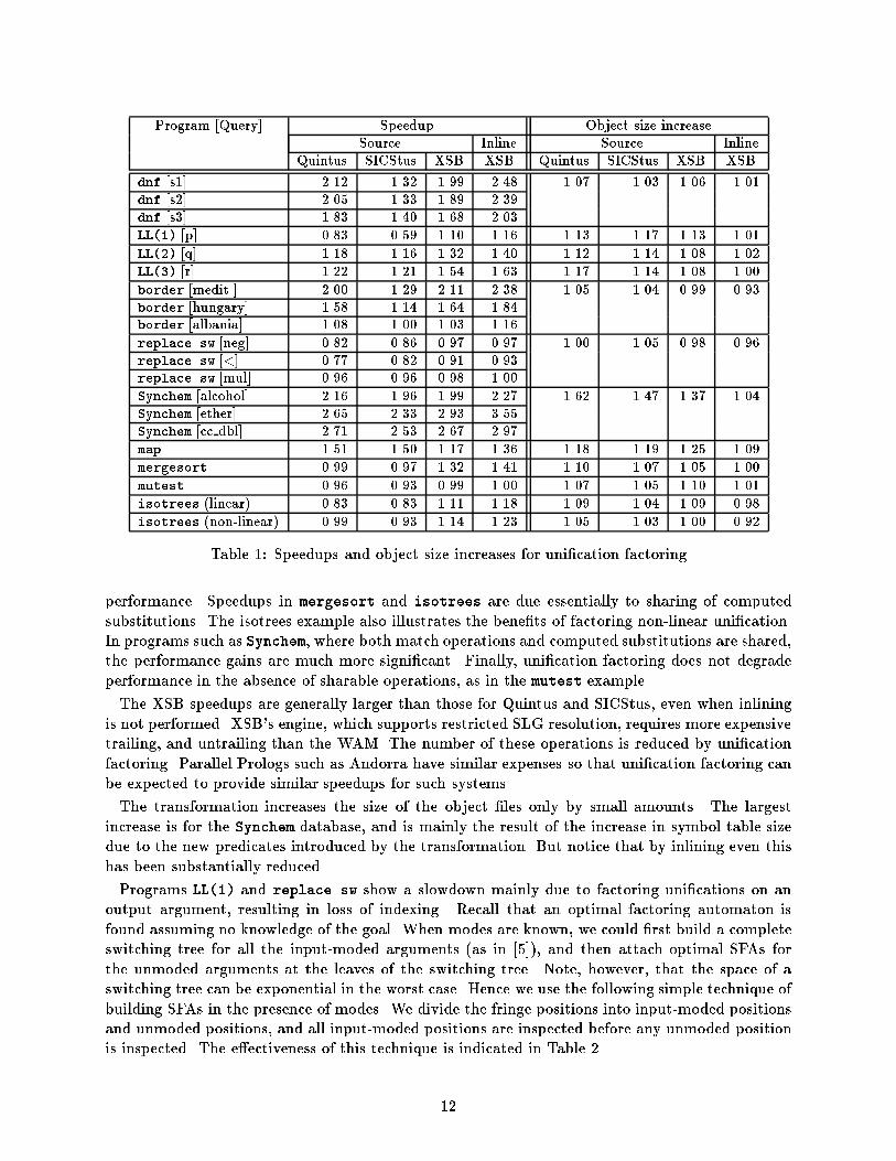
A AppendixThis appendix contains supplementary reference material. The extended abstract is self-containedand does not rely on this material.A.1 Optimal SFA constructionConstruction of an optimal SFA for the sequence of clauses hp(a; b; c); p(a; b; d); p(a; c; c); p(b; a; c)ide�ning the predicate in Figure 8a begins with the computation of its cost, using Equation 1 (p. 7).The cost and root position of the lowest cost automaton computed for a subsequence with endpoints (i; i0) at any point in the computation is stored in a table at entry (i; i0), where i is the rowand i0 the column (see Figure 9).We begin by �nding positions having symbols common to all four clauses:common(p(X1; X2; X3); 1; 4) = (f g; p(X1; X2; X3)):There are no common positions, so any of positions $1, $2, and $3 might be used for the root state.We �rst try position 1, and compute the partition:part(1; 4; $1) = f(a; 1; 3); (b; 4; 4)g:We now need to compute optimal sub-automata for subsequences hp(a; b; c); p(a; b; d); p(a; c; c)i andhp(b; a; c)iRepeating the above process for subsequence (1; 3),common(p(X1; X2; X3); 1; 3) = (f($1; a)g; p(a;X2; X3))shows that subsequence (1; 3) has one common position ($1) leaving positions $2 and $3 as possibleroot positions for the sub-automaton. We �rst choose position $2:part(1; 3; $2) = f(b; 1; 2); (c; 3; 3)gContinuing similarly for subsequence (1; 2) givescommon(p(a;X2; X3); 1; 2) = (f($2; b)g; p(a; b;X3))part(1; 2; $3) = f(c; 1; 1); (d; 2; 2)gcommon(p(a; b;X3); 1; 1) = (f($3; c)g; p(a; b; c))common(p(a; b;X3); 2; 2) = (f($3; d)g; p(a; b; d))Now, each subsequence is a single clause. Since all positions in a single clause are common positions,no positions for further partitioning are available, and the cost for each single clause is 0. Thus,the cost of the sub-automaton for subsequence (1; 2) rooted at $3 is 2 (one each for transitionsunify($3; c) and unify($3; d)). Cost 2 and position 3 are then stored in entry (1; 2) of the table.Returning to compute the cost for subsequence (3; 3),common(p(a;X2; X3); 3; 3) = (f($2; c); ($3; c)g; p(a; c; c))gives the cost of the sub-automaton for subsequence (1; 3) with root position $2 as 1 + 2 + 2 = 5(one for transition unify($2; b); one each for transitions unify($2; c) and unify($3; c); and two ascomputed for subsequence (1; 2). Thus, cost 5 and position 2 are stored in entry (1; 3) of the table.15

Completing the computation for sequence (1; 4) at position $1 yields additional costs of one(for transition unify($1; a)) and three (transitions unify($1; b), unify($2; a), and unify($3; c) forsubsequence (4; 4)), giving a total cost of 9. Thus, cost 9 and position 1 are stored in entry (1; 4)of the table (highlighted). The automaton corresponding to this cost and position is shown inFigure 8b. Verifying that no other choice of position yields a better automaton is left to theinterested reader. Note that the shaded entries in the table are not used in computing the cost ofan optimal automaton.p(a,b,c).p(a,b,d).p(a,c,c).p(b,a,c).c1p(a,b,c) c2p(a,b,d) c3p(a,c,c) c4p(b,a,c)

s1 :p(X ,X ,X )2 31

s2 :2

s3 :

s4 : s5 : s6 :

p(a,X ,X )2 3 p(b,X ,X )32

p(a,b,X )3 p(a,c,X )3 p(b,a,X )3

unify($3,c)

unify($1,b)

unify($2,b)

unify($1,a)

unify($2,c) unify($2,a)

unify($3,c) unify($3,d) unify($3,c)

1

2

3 3 3(a) (b)Figure 8: Predicate and optimal SFA constructed by dynamic programming2 3 41

Pos:

Cost: 0

- Pos:

Cost: 2

3 Pos:

Cost: 5

2

Pos:

Cost: 2

1

1

2

3

4

Pos:

Cost: 0

-

Pos:

Cost: 0

-

Pos:

Cost: 0

-

i

i

Pos:

Cost:

1

9

’

Figure 9: Table of costs and positions for sample SFA constructionA.2 Cost functionRecall that Equation 1 for the cost of an optimal SFA, assumed that all uni�cation operations haveunit cost, and that recording pending transitions has zero cost. The recurrence can be modi�edas follows to account for these costs. Let costunify(�; �) be the cost of the uni�cation operationinvolving position � and � and costchoice (�) represent the cost of choosing a transition when multipletransitions are possible at position �. Note that the cost of recording pending transitions can bemodeled using costchoice (�). Accounting for these costs, an optimal SFA can be computed using16

the following recurrence:cost(i; i0; S) = min�2fringe(S)(costchoice (�) + X(�;j;j0)2part(i;i0;�)(cost(j; j 0; S0) + X(�0;�0)2E costunify(�0; �0)))where (E; S 0) = common(S; j; j 0)Clearly, theorem 3.3 still holds; i.e., an optimal automata under the modi�ed cost criterion can beconstructed in polynomial time.A.3 NP-completeness of optimal NSFA constructionA non-sequential factoring automaton can be viewed abstractly as a trie, in which the clause headsof a predicate are viewed as strings of symbols. Optimization of an NSFA (when elementaryuni�cation operations are assumed to have unit cost) thus corresponds to trie minimization. Inthe terminology of Comer and Sethi [3], an NSFA corresponds to a full order-containing trie (fullO-trie), where \full" refers to the fact any root-to-leaf path in the trie examines an entire string,and \order-containing" means that di�erent paths may examine characters (positions) in di�erentorders.Theorem A.1 The minimization problem for full O-tries (FOT) is NP-complete.Proof: We show that the trie minimization problem is NP-hard by reduction from the minimumset cover problem (SC). The minimum set cover problem can be stated as follows: Given a �niteset U = fu1; . . . ; ung, a collection C = fC1; . . . ; Cmg of subsets of U , and a positive integer k � m,do there exist k or fewer subsets in C whose union is S?Let ISC be an instance of SC. We construct an instance IFOT of FOT with 2n strings, each oflength 2(n +m)2 + m, as follows. Each string consists of three �elds: a \Test" �eld, consistingof m characters; a \Blue" �eld, consisting of (n+m)2 characters; and a \Red" �eld, consisting of(n+m)2 characters: T1T2 � � �Tm| {z }Test B1B2 � � �B(n+m)2| {z }Blue R1R2 � � �R(n+m)2| {z }RedFor each element ui 2 U two strings are constructed: a Red string and a Blue string. In the Redstring, Tj = 0, for 1 � j � m; Bl = i and Rl = 0, for 1 � l � (n +m)2. The ith Red string thushas the form 0 � � �0| {z }Test i � � � i| {z }Blue 0 � � �0| {z }RedIn the Blue string, Tj = 1 if ui 2 Cj, otherwise 0, for 1 � j � m; Bl = i and Rl = 0, for1 � l � (n+m)2. The ith Blue string thus has the formT1T2 � � �Tm| {z }Test 0 � � �0| {z }Blue i � � � i| {z }RedChecking a character in the Test �eld of a Blue string can be thought of testing for membership ofan element of U in a subset.Observe that the Red and Test �elds in every Red string are identical, and that each Blue �eldis distinct. For a set consisting entirely of Red strings, a minimal trie must test all characters inthe Red and Test �elds before testing any character in the Blue �eld, since the �rst test in the17

Blue �eld e�ectively partitions the set into individual strings (see Figure 10a). The order of testingwithin the Red and Test �elds is unimportant, as is the order of testing within the Blue �eld.Also observe that the Blue �eld in every Blue string is identical, and that each Red �eld is distinct.A minimal trie for a set of Blue strings must test all characters in the Blue �eld before testing anycharacter in the Red �eld. In general, testing characters in the Test �eld will incrementally partitionthe set. Thus, a minimal trie for Blue strings will typically have the form shown in Figure 10b.1R

0 ...

...

Tm

0

(n+m) 2

(n+m) 2

1T

...

...

(n+m) 2

(n+m) 2 (n+m) 2

nR

i1 nRi

i1 nRi

m

0

0

. . .

1B

. . .

B B

R

(n+m) 2

B1

...

(n+m) 2

(n+m) 2

...

...

(n+m) 2 (n+m) 2

nB

1R 1R

i1 nBi

i1 nBi

Testm

0

0

B

. . .

. . . RR(a) (b)Figure 10: Minimal tries for sets of Red (a) and Blue (b) stringsThe above observations lead to the following bounds on the sizes of minimal tries for monochro-matic sets of strings.Lemma A.1.1 Given a set S consisting entirely of Red strings, such that jSj = nR, the numberof edges in a minimal full O-trie for S is exactly (nR + 1)(n+m)2 +m.Lemma A.1.2 Given a set S consisting entirely of Blue strings, such that jSj = nB, the numberof edges in a minimal full O-trie for S is no more than (nB + 1)(n+m)2 +mnB.The main idea in constructing a minimal full trie is to order the tests such that less partitioningoccurs near the root and more occurs toward the leaves. Therefore, to build a minimal trie forthe 2n Blue and Red strings constructed from ISC , testing in the Test �eld should precede testingin the Blue and Red �elds. Observe that testing a character in the Test �eld partitions a setcontaining both Blue and Red strings into one set containing only Blue strings (on a branchlabeled \1") and another containing Red and perhaps some Blue strings (on a branch labeled \0"{see Figure 11a). Testing a character in the Red (Blue) �eld, on the other hand, partitions the set18

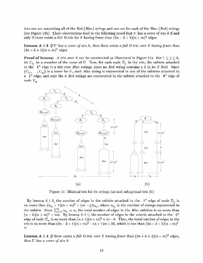
into one set containing all of the Red (Blue) strings and one set for each of the Blue (Red) strings(see Figure 11b). These observations lead to the following proof that U has a cover of size k if andonly if there exists a full O-trie for S having fewer than (2n+ k + 2)(n+m)2 edges.Lemma A.1.3 If U has a cover of size k, then there exists a full O-trie over S having fewer than(2n+ k + 2)(n+m)2 edges.Proof of lemma: A trie over S can be constructed as illustrated in Figure 11a. For 1 � j � k,let Cij be a member of the cover of U . Now, for each node Tij in the trie, the subtrie attachedto the \1" edge is a trie over Blue strings, since no Red string contains a 1 in its T �eld. SincefCi1 ; . . . ; Cikg is a cover for U , each Blue string is represented in one of the subtries attached toa \1" edge, and only the n Red strings are represented in the subtrie attached to the \0" edge ofnode Tik .Ti1

Ti2

..

.

B1

B1

(n+m) 2B

(n+m) 2B

...

...

R 1B1

(n+m) 2B (n+m) 2R

0

...

...

Tik1 0

. . .

Test

Red

Test

Blue

. . .

(n+m) 2

(n+m) 2

0

01

1

. . .

. . .

Test

Red

Test

Red

k

2n

i1

(n+m) 2

(n+m) 2

nB

nBnR

0 . . .

Red

Test

Blue

m

. . .. . .

iR

(a) (b)Figure 11: Minimal trie for 2n strings (a) and suboptimal trie (b)By lemma A.1.2, the number of edges in the subtrie attached to the \1" edge of node Tij isno more than (nsj + 1)(n +m)2 + (m � j)nsj , where nsj is the number of strings represented inthe subtrie. Since Pkj=1 nsj = n, the total number of edges in the Blue subtries is no more than(n + k)(n +m)2 +mn. By lemma A.1.1, the number of edges in the subtrie attached to the \0"edge of node Tik is no more than (n+ 1)(n+m)2+m� k. Thus, the total number of edges in thetrie is no more than (2n+ k+1)(n+m)2+ (n+1)m+2k, which is less than (2n+ k+2)(n+m)2.2Lemma A.1.4 If there exists a full O-trie over S having fewer than (2n+ k + 2)(n+m)2 edges,then U has a cover of size k. 19

Proof of lemma: It su�ces to show that any trie over S having fewer than (2n+ k+ 2)(n+m)2edges must be of the form shown in Figure 11a. Given a set S 0 of strings containing nR Red stringsand nB Blue strings, the root of a minimal trie over S 0 must be a T node. If, instead, the root werea R node, the trie would have at least (2nB + nR + 1)(n+m)2 edges (see Figure 11b). Similarly,a trie with a B root node would have at least (2nR + nB + 1)(n+m)2 edges. Replacement of anyof the k T nodes in the trie in Figure 11a by a R or B node would therefore result in at least(n � k)(n + m)2 additional edges. Thus, any trie having fewer than (2n + k + 2)(n +m)2 edgesmust be of the form shown in Figure 11a, which can exist only if U has a cover of size k. 2Lemmas A.1.3 and A.1.4 together establish the transformation from ISC to IFOT . The remainingdetails showing that the transformation is polynomial in the size of ISC and that FOT 2 NP arestandard, and are omitted.A.4 Cut transformationFigure 12b shows the e�ect of applying the cut transformation used in XSB to the predicate inFigure 12a. Uni�cation factoring is then applied to the cut transformed program, yielding thepredicate in Figure 12c. The semantics of the original predicate is preserved.p(a,b) :- !.p(a,c).p(b,d). p(X,Y) :- $savecp(Z), $p(X,Y,Z).$p(a,b,X) :- $cutto(X).$p(a,c, ).$p(b,d, ). p(X,Y) :- $savecp(Z), $p(X,Y,Z).$p(a,X,Y) :- $p1(X,Y).$p(b,d, ).$p1(b,X) :- $cutto(X).$p1(c, ).(a) (b) (c)Figure 12: Predicate (a), cut transformed (b), and factored (c)A.5 Benchmark programsIsotreesThe isotrees predicate in Figure 13a illustrates uni�cation factoring in the presence of non-linearity.Observe that, in the second and third clauses, the function symbol tree=2 is common (in position 1as well as position 2), and there is a common non-linearity between positions 1:1 and 2:1. Linearfactoring (sharing only common function symbols) yields the program in Figure 13b, while non-linear factoring yields the program in Figure 13c. The benchmark query appears in Figure 13d.SynchemA small sample of the Synchem database appears in Figure 14a. The sample presented containspartial information about the structure of three di�erent molecules, and is intended only for illus-tration. The transformation of this sample via optimal SFA construction is given in Figure 14b,and the queries used for benchmarks appear in Figure 14c.20

isotrees(void,void).isotrees(tree(X,L1,R1),tree(X,L2,R2)) :-isotrees(L1,L2),isotrees(R1,R2).isotrees(tree(X,L1,R1),tree(X,L2,R2)) :-isotrees(L1,R2),isotrees(R1,L2).(a)isotrees(void,void).isotrees(tree(X1,X2,X3),tree(X4,X5,X6)) :-isotrees2(X1,X2,X3,X4,X5,X6).isotrees2(X,L1,R1,X,L2,R2) :-isotrees(L1,L2),isotrees(R1,R2).isotrees2(X,L1,R1,X,L2,R2) :-isotrees(L1,R2),isotrees(R1,L2).(b)isotrees(void,void).isotrees(tree(X1,X2,X3),tree(X1,X4,X5)) :-isotrees2(X1,X2,X3,X4,X5).isotrees2(X,L1,R1,L2,R2) :-isotrees(L1,L2),isotrees(R1,R2).isotrees2(X,L1,R1,L2,R2) :-isotrees(L1,R2),isotrees(R1,L2).(c)test :-X = tree(1, tree(2, tree(4, tree(8, void, void), tree(9, void, void)),tree(5, tree(10, void, void), tree(11, void, void))),tree(3, tree(6, tree(12, void, void), tree(13, void, void)),tree(7, tree(14, void, void), tree(15, void, void)))),isotrees(X,_). (d)Figure 13: Isotrees: original (a), linear (b), non-linear (c), query (d)21

chem('Phthalic acid, monomethyl ester',c(0),o(1),2).chem('Phthalic acid, monomethyl ester',c(0),h(14),2).chem('Phthalic acid, monomethyl ester',o(1),c(0),2).chem('Phthalic acid, monomethyl ester',o(1),c(2),2).chem('Methyl p_hydroxybenzoate',c(0),o(1),2).chem('Methyl p_hydroxybenzoate',c(4),c(5),3).chem('Methyl p_hydroxybenzoate',c(4),c(11),3).chem('Methyl p_hydroxybenzoate',c(4),h(15),3).chem('2_Methyl_2_nitropropane',n(1),o(2),4).chem('2_Methyl_2_nitropropane',n(1),o(3),4).chem('2_Methyl_2_nitropropane',c(4),c(0),2).chem('2_Methyl_2_nitropropane',c(4),h(8),2).(a)chem('Phthalic acid, monomethyl ester', _303, _304, 2) :-'chem_#309'(_303, _304).chem('Methyl p_hydroxybenzoate', c(_310), _311, _312) :-'chem_#317'(_310, _311, _312).chem('2_Methyl_2_nitropropane', _318, _319, _320) :-'chem_#325'(_318, _319, _320).'chem_#309'(c(0), _305) :-'chem_#306'(_305).'chem_#309'(o(1), c(_307)) :-'chem_#308'(_307).'chem_#306'(o(1)).'chem_#306'(h(14)).'chem_#308'(0).'chem_#308'(2).'chem_#317'(0, o(1), 2).'chem_#317'(4, _313, 3) :-'chem_#316'(_313).'chem_#316'(c(_314)) :-'chem_#315'(_314).'chem_#316'(h(15)). 'chem_#315'(5).'chem_#315'(11).'chem_#325'(n(1), o(_321), 4) :-'chem_#322'(_321).'chem_#325'(c(4), _323, 2) :-'chem_#324'(_323).'chem_#322'(2).'chem_#322'(3).'chem_#324'(c(0)).'chem_#324'(h(8)).(b)alcohol(M) :-chem(M,c(I1),o(I2),2),chem(M,o(I2),h(_),2),chem(M,c(I1),X,N1), X \== o(I2),chem(M,c(I1),Y,N2), Y \== o(I2), Y \== X,( chem(M,c(I1),Z,N3), Z \== o(I2), Z \== X, Z \== Y ; N3 = 0 ),N1 + N2 + N3 =:= 6.ether(M) :- chem(M,c(I1),o(O),2), chem(M,c(I2),o(O),2), I1 =\= I2.cc_double(M) :-chem(M,c(I1),c(I2),4),chem(M,c(I1),X,N1), X \== c(I2),( N1 =:= 4 ; N1 =:= 2, chem(M,c(I1),Y,2), Y \== c(I2), Y \== X ),chem(M,c(I2),Z,N3), Z \== c(I1),( N3 =:= 4 ; N3 =:= 2, chem(M,c(I2),W,2), W \== c(I1), W \== Z ).(c)Figure 14: Original (a) and transformed (b) Synchem sample, and queries (c)22