arX

iv:0

911.

3793

v2 [

hep-

th]

1 D

ec 2

009

Gravity-Yang-Mills-Higgs unification

by enlarging the gauge group

Alexander Torres-Gomez and Kirill Krasnov

School of Mathematical Sciences

University of Nottingham

November 2009

Abstract

We revisit an old idea that gravity can be unified with Yang-Mills theory by enlarging

the gauge group of gravity formulated as gauge theory. Our starting point is an action that

describes a generally covariant gauge theory for a group G. The Minkowski background

breaks the gauge group by selecting in it a preferred gravitational SU(2) subgroup. We

expand the action around this background and find the spectrum of linearized theory to

consist of the usual gravitons plus Yang-Mills fields charged under the centralizer of the

SU(2) in G. In addition, there is a set of Higgs fields that are charged both under the

gravitational and Yang-Mills subgroups. These fields are generically massive and interact

with both gravity and Yang-Mills sector in the standard way. The arising interaction of

the Yang-Mills sector with gravity is also standard. Parameters such as the Yang-Mills

coupling constant and Higgs mass arise from the potential function defining the theory.

Both are realistic in the sense explained in the paper.

1 Introduction

There have been numerous attempts to unify Einstein’s theory of gravity with gauge fields

describing other interactions. One such unification proposal is that of Kaluza-Klein, where the

metric and gauge fields arise from a higher-dimensional metric tensor upon compactification

of extra dimensions. This scenario has become an indispensable part of string theory, which

also provides another unifying perspective by viewing gravity and Yang-Mills as excitations of

closed and open strings respectively. For more details on string-inspired unification schemes

see a recent exposition [1].

1

There have also been attempts to unify gravity with gauge theory without introducing extra

dimensions. There is, however, a very strong no-go theorem [2] that shows that at least one type

of such unification is impossible. The theorem states that the symmetry group of the S-matrix

of a consistent quantum field theory (in Minkowski spacetime) is the product of Poincare and

internal gauge group. In other words, the spacetime and internal symmetries do not mix. The

only way to go around this statement is via supersymmetric extensions of Poincare group [3].

Now, since gravity can be (at least loosely) viewed as a gauge theory for the diffeomor-

phism group, and the later contains Poincare group as that of rigid global transformations, the

Coleman-Mandula theorem [2] is sometimes interpreted as saying that no unification of gravity

and gauge theory that puts together diffeomorphisms and gauge transformations is possible. In

this discussion, however, one must be careful to distinguish between local gauge invariances of

a theory and global symmetries whose presence or absence depends on a particular state one

works with, see [4] that emphasizes this point.

While it may be difficult or impossible to “unify” diffeomorphisms and gauge transforma-

tions into a single gauge group, this is not the only possible way to approach the unification

problem. To understand how a different type of unification might be possible, let us recall that

in the so-called first-order formalism gravity becomes a theory of metrics as well as Lorentz

group spin connections. The “internal” Lorentz group acts by rotating the frame and has no

effect on the metric. Thus, the physical dynamical variable is still the metric, one simply added

some gauge variables and enlarged the gauge group, which in this formulation is a (semi-) direct

product of the diffeomorphism group and SO(1, 3). Further, in the Hamiltonian formulation

this theory can be easily cast into one on the Yang-Mills phase space. This is done by adding

to the action a term that vanishes on-shell [5]. The phase space is then that of pairs SU(2)

connection plus the canonically conjugate “electric” field. Thus, after the trick of adding an on-

shell unimportant term, gravity becomes a generally covariant theory of an SU(2) connection.

The spacetime metric (tetrad) is still a dynamical variable but in this formulation it receives

the interpretation of the momentum canonically conjugate to the connection.

Yang-Mills theory, on the other hand, after it is written for a general spacetime metric, also

becomes a generally covariant theory of a connection and spacetime metric. One could then

attempt to put the two generally covariant gauge theories together in some way that combines

the “internal” gauge groups, while leaving the total gauge group to be a (semi-) direct product

of diffeomorphisms and “internal” symmetries. This would not be in any conflict with the no-go

theorem [2] for what is unified is not the Poincare and internal symmetry groups. This might

not be what can be legitimately called a unification, for the end gauge group is not simple, but

this idea does lead to some interesting “unified” theories, as we hope to be able to demonstrate

in this paper.

As far as we are aware, the first proposal of this type was put forward in [6, 7], with the idea

being precisely to extend the gauge group of gravity formulated in tetrad first-order formalism

2

as a theory of the Lorentz connection. This proposal was later pushed forward in [8, 9], see

also [10] for the most recent development. The key point of this proposal is that it is a non-

degenerate metric that breaks the gauge symmetry of the unified theory down to a smaller

group consisting of SO(1, 3) for gravity and some ”internal” group for Yang-Mills fields.

A similar in spirit, but very different in the realization idea was proposed in [11], and further

developed in [12, 13, 14]. This approach stems from the fact that Einstein’s general relativity

(GR) can be reformulated as a theory on the Yang-Mills phase space. At the time of writing

[11] it was achieved in Ashtekar’s Hamiltonian formulation of GR [15] that interprets gravity as

a special generally covariant (complexified) SU(2) gauge theory. The fact that gravity in this

formulation becomes a theory of connection suggests that a gauge group larger than SU(2) can

be considered. This is what was attempted in [11, 12, 13, 14], with the main result of [14] being

that Yang-Mills theory arises in an expansion of the theory around the de Sitter background.

The idea to put together the “internal” gauge groups of gravity and gauge theory is an

interesting one. However, its particular realizations available in the literature are not without

problems. Thus, the approach reviewed and further developed in [10] does a very good job in

describing the fermionic content of the theory. Bosons, on the other hand, are described less

convincingly in that many new propagating degrees of freedom (DOF) are introduced. The

other approach [14] is also not very convincing since it works at the phase space level, and it is

generally very difficult to approach a theory if no action principle is prescribed. Another aspect

of the particular realization given in [14] is that it naturally describes a complexified GR put

together with complexified Yang-Mills. No natural reality conditions that would convert this

into a physical theory were given.

The unification by enlarging the internal gauge group proposal was recently revisited in

[16], where the new action principle [17] for a class of modified gravity theories [18], extended

to a larger gauge group was used. This work also avoided the reality conditions problem by

extending the gauge group of an explicitly real formulation of gravity that works with the

Lorentz, not with the complexified rotation group. Specifically, it was suggested in [16] that

the action of the type proposed in [17] considered for a general Lie group G describes gravity in

its SO(4) part plus Yang-Mills fields in the remaining quotient G/SO(4). As in [14], the Yang-

Mills coupling constant is related in [16] to the cosmological constant. As in the approach [6, 7],

in [16] it is a non-degenerate metric that breaks the symmetry down to a smaller gauge group.

The approach of [16] is also similar to that of [6, 7] in that many new bosonic degrees of freedom

are introduced. Thus, it was shown in [19] that the BF-type action of [17] for G = SO(4) does

not anymore describe pure gravity theory in that it describes six new DOF.

In this paper we take the described unification idea one step further. Our approach is

similar in spirit to [16] in that we start from an action principle of the type first proposed in

[17]. However, unlike in [16], we interpret only a (complexified) SU(2) subgroup of the gauge

group G as that corresponding to gravity. The part of the gauge group that commutes with

3

this gravitational SU(2) is then seen to describe Yang-Mills fields, and the part that does not

commute with SU(2) describes charged scalar, i.e. Higgs, fields. We note that the suggestion

that in unifications of this type the ”off-diagonal” part of the Lie algebra corresponds to Higgs

fields is contained already in [16].

Our approach is also similar to the original proposal [14] that enlarged the SU(2) gravi-

tational gauge group. However, in contrast to [14] that worked at the phase space level our

starting point is an action principle that makes a much more systematic analysis possible. Also

the details of our proposal differ significantly from that of [14] in that a semi-realistic (more

on this below) unification is achieved without the need for a cosmological constant. Thus, the

Yang-Mills coupling constant in our scheme is related not to the cosmological constant, which

we set to zero, but to a certain other parameter of the theory. This features of our proposal

also makes it different from that of [16].

More specifically, we start from a generally covariant gauge theory for a (complex) semi-

simple Lie group G, with certain reality conditions later imposed to select real physical con-

figurations. A particularly simple solution of the theory describes Minkowski spacetime. This

solution breaks G down to a (complexified) SU(2) times the centralizer of SU(2) in G. The

spectrum of linearized theory around the Minkowski background is then shown to consist of the

usual gravitons with their two propagating DOF, gauge bosons charged under the centralizer

of SU(2) in G, and a set of scalar Higgs fields. The Higgs fields are in general massive, with the

mass being related to a certain parameter of the potential defining the theory. After the reality

conditions are imposed all sectors of the theory have a positive-definite Hamiltonian. We also

work out interactions to cubic order and show that all interactions are precisely as expected.

That is, all non-gravitational fields interact with gravity via their stress-energy tensor, and the

interactions in the non-gravitational sector are also standard and are as expected for Higgs

fields. Thus, our unification scheme passes the zeroth order test of being not in any obvious

contradiction with observations. However, to obtain a truly realistic unification model many

problems have to be solved. In particular, fermionic DOF are not considered in this paper

at all. Thus, our results provide only one of the first steps along this potentially interesting

research direction. We return to open questions of our approach in the discussion section.

In this paper we have illustrated the general G case by considering the simplest non-trivial

example of G = SU(3). This example is rather generic, and the same technology that we

develop for G = SU(3) can be used for any Lie group. We could have presented a general

semi-simple case treatment phrased in terms of the root basis in the Lie algebra. However, at

this stage of the development of the theory it is not clear if there is any added value in doing

things in full generality. We thus decided to keep our discussion as simple as possible and treat

one example that, if necessary, is easily extendible to the general situation.

Another general remark on this paper is as follows. As the reader will undoubtedly notice,

a sizable part of our paper is occupied by the Hamiltonian analysis of various sectors, or of

4

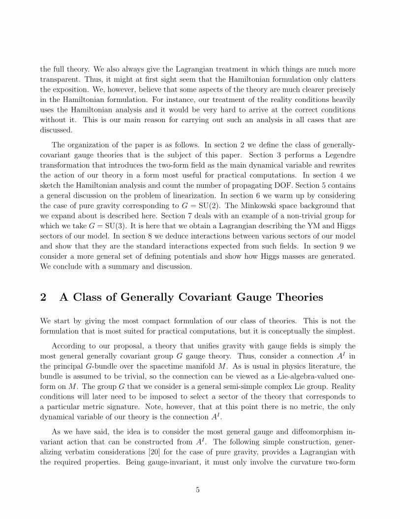
the full theory. We also always give the Lagrangian treatment in which things are much more

transparent. Thus, it might at first sight seem that the Hamiltonian formulation only clatters

the exposition. We, however, believe that some aspects of the theory are much clearer precisely

in the Hamiltonian formulation. For instance, our treatment of the reality conditions heavily

uses the Hamiltonian analysis and it would be very hard to arrive at the correct conditions

without it. This is our main reason for carrying out such an analysis in all cases that are

discussed.

The organization of the paper is as follows. In section 2 we define the class of generally-

covariant gauge theories that is the subject of this paper. Section 3 performs a Legendre

transformation that introduces the two-form field as the main dynamical variable and rewrites

the action of our theory in a form most useful for practical computations. In section 4 we

sketch the Hamiltonian analysis and count the number of propagating DOF. Section 5 contains

a general discussion on the problem of linearization. In section 6 we warm up by considering

the case of pure gravity corresponding to G = SU(2). The Minkowski space background that

we expand about is described here. Section 7 deals with an example of a non-trivial group for

which we take G = SU(3). It is here that we obtain a Lagrangian describing the YM and Higgs

sectors of our model. In section 8 we deduce interactions between various sectors of our model

and show that they are the standard interactions expected from such fields. In section 9 we

consider a more general set of defining potentials and show how Higgs masses are generated.

We conclude with a summary and discussion.

2 A Class of Generally Covariant Gauge Theories

We start by giving the most compact formulation of our class of theories. This is not the

formulation that is most suited for practical computations, but it is conceptually the simplest.

According to our proposal, a theory that unifies gravity with gauge fields is simply the

most general generally covariant group G gauge theory. Thus, consider a connection AI in

the principal G-bundle over the spacetime manifold M . As is usual in physics literature, the

bundle is assumed to be trivial, so the connection can be viewed as a Lie-algebra-valued one-

form on M . The group G that we consider is a general semi-simple complex Lie group. Reality

conditions will later need to be imposed to select a sector of the theory that corresponds to

a particular metric signature. Note, however, that at this point there is no metric, the only

dynamical variable of our theory is the connection AI .

As we have said, the idea is to consider the most general gauge and diffeomorphism in-

variant action that can be constructed from AI . The following simple construction, gener-

alizing verbatim considerations [20] for the case of pure gravity, provides a Lagrangian with

the required properties. Being gauge-invariant, it must only involve the curvature two-form

5

F I = dAI + (1/2)[A, A]I , where [·, ·]I is the Lie-bracket and the wedge product of forms is

assumed. Consider the 4-form F I ∧ F J . This is a 4-form valued in the space of symmetric

bilinear forms in g, the Lie-algebra of G. Choosing an arbitrary volume 4-form (vol) we can

write F I∧F J = (vol)ΩIJ , where now ΩIJ is a symmetric n×n matrix, where n = dim(g). Since

(vol) is defined only modulo rescalings (vol) → α(vol), so is the matrix ΩIJ that under such

rescalings transforms as ΩIJ → (1/α)ΩIJ . Let us now introduce a function f(X) of symmetric

n×n matrices XIJ with the following properties. First, the function has to be gauge-invariant:

f(adgX) = f(X), where adg is the adjoint action of the gauge group on the space of symmetric

bilinear forms on the Lie algebra. Second, the function must be holomorphic (we work with

complex-valued quantities). Third, and most important, the function must be homogeneous of

degree one f(αX) = αf(X). This property allows it to be applied to the 4-form F I ∧F J , with

the result being again a 4-form. Indeed, we have f(F I ∧F J) = (vol)f(ΩIJ), and it is easy to see

that due to the homogeneity of f(·), the resulting 4-form does not depend on which particular

volume form (vol) is chosen. Thus, the quantity f(F I ∧ F J) is an invariantly-defined 4-form,

and it can be integrated over the spacetime manifold to produce an action:

S[A] =

∫

M

f(F I ∧ F J). (1)

As we have already said, the action is complex, so later certain reality conditions will be

imposed.

The presented formulation (1) is conceptually nice, but it is very difficult to deal with in

practice. One of the main reasons for this is that there is no natural background around which

the theory can be expanded to produce a physically meaningful perturbation theory. This can

be seen as follows. The first variation of the action (1) is given by:

δS =

∫∂f

∂F I∧ DAδAI , (2)

where the derivative of f(·) with respect to F I can be shown to make sense and is a certain

g-valued 2-form. The second variation is given by:

δ2S =

∫1

2

∂f

∂F I∧ [δA, δA]I +

∂2f

∂F I∂F JDAδAI ∧ DAδAJ , (3)

where the second derivative of f(·) is a zero-form. Now, the most natural ”vacuum” of the

theory seems to be

F I = 0,∂f

∂F I= 0,

∂2f

∂F I∂F J6= 0. (4)

Indeed, this would indeed be a ”vacuum” of the theory in the sense that the first derivative

of the ”potential” function vanishes, which then automatically satisfies the field equations

DA(∂f/∂F I) = 0, and only the second derivative is non-trivial. From (3) we see that in this

6

case the first ”mass” term is absent, and there is only the ”kinetic” term for the connection.

Thus, it seems like the perfect vacuum to expand about. However, an immediate problem with

this vacuum is that in the absence of any background structure the second derivative in (4) can

only be proportional to the Killing form gIJ , which then gives a degenerate kinetic term. So,

there does not seem to be any way to build a meaningful perturbation theory around (4).

As an aside remark we mention that the fact that the “kinetic” form in (3) is necessarily

degenerate is very important for the possibility to describe gravity as a gauge theory. Indeed,

as work [21] showed, general relativity can be put in the form (1) for G = SU(2) and a very

special choice of the function f(·). At the same time, it is known to be impossible to describe

gravity that is mediated by a spin two particle in terms of a gauge field that corresponds

to a spin one particle. The resulution of this seeming paradox lies in the fact that the pure

connection formulation (1) of gravity does not allow for a well defined perturbation theory

around Minkowski background, and so the particles that it describs are not spin one as would

be the case in any other gauge theory. Below we shall see how the usual spin two graviton

arises via certain “duality” trick.

A conventional perturbative treatment for theory (1) is possible, but requires a rather

strange, at least from the pure connection point of view, choice of vacuum. Thus, as we shall

see in details in the following sections, the usual perturbative expansion around a flat metric

corresponds in the pure connection language to an expansion around the following point:

F I = 0,∂f

∂F I6= 0. (5)

This is a very strange point to expand the theory about, for one seems to be sitting at a point

that is not a minimum of the ”potential”. However, the non-zero right-hand-side of the first

derivative of the potential receives the interpretation of essentially the Minkowski metric, and

a usual expansion then results. It might seem that this choice introduces a ”mass” term for

the connection, but this is not so. In fact, the second ”kinetic” term is still a total derivative

and plays no role, and there is only the ”mass” term. However, as we shall see, the connection

is no longer a natural variable in this case, and one works with a certain new two-form field BI

via which the connection is expressed as AI ∼ ∂BI , so what appears as a mass term is in fact

the usual kinetic one but for the two-form field.

This discussion motivates introduction of a new set of dynamical fields. These are originally

introduced via the standard ”Legendre transform” trick so that integrating them out one gets

an original action (1). However, one can then also integrate out the original connection field

and obtain a theory for the new fields only. This point of view turns out to be very profitable,

and we develop it in the next section.

7

3 Two-form field formulation

There are at least two different ways to arrive at the new formulation. One of them is via a

Legendre transform from (1), the other one by thinking about generalizations of BF theory.

3.1 Legendre transform

As we have already explained, we introduce a new set of fields, given by a g-valued two-form

BI . The action that we would like to consider is then of BF-type and is given by:

S[A, B] =

∫

M

gIJBI ∧ F J − 1

2V (BI ∧ BJ). (6)

Here V (·) is again a G-invariant, holomorphic and homogeneous order one function of symmetric

n×n matrices, and as such it can be applied to the 4-form BI ∧BJ , with the result being again

a 4-form. The quantity gIJ is the Killing-Cartan form on g.

Integrating out BI by solving its field equation:

F I =1

2

∂V

∂BI, (7)

which is algebraic in BI , we get back the formulation (1) with f(·) being an appropriate

Legendre transform of V (·). However, the formulation (6) is much more powerful in that we

can now choose a constant BI background and obtain a well-defined perturbation theory. We

will later see how both gravity and Yang-Mills theory appear in such a perturbative expansion.

An alternative viewpoint on the ”Legendre transform” described is as follows. As we shall see

below, the new two-form field that we have introduced is essentially the momentum canonically

conjugate to the connection AI . Thus, a meaningful analogy for the relation between (1) and

(6) is the relation between Lagrangian and Hamiltonian formulation of mechanics. The former

one uses only position variables as dynamical variables, but leads to second-derivative equations

of motion. The later contains an independent variable - momentum, and leads to first order

equations of motion. Thus, loosely speaking, the action (6) can be referred to as (1) written in

the ”Hamiltonian form” in which the momentum variable becomes an independent dynamical

field.

Before we proceed with an analysis of properties of the theory (6), we would like to present

an alternative derivation of this action.

3.2 Generalization of BF theory

An alternative way to arrive at (6) is to consider possible ways to generalize the topological BF

theory. For the case of G = SU(2) this was done in [22], and here we generalize this analysis

8

to a semi-simple Lie group. Following this reference we begin with the action

S[A, B] =

∫gIJ BI ∧ F J − 1

2ΦIJ BI ∧ BJ , (8)

where BI is a two-form valued in g, F I is the curvature F I = dAI + 12f I

JKAJ ∧ AK of AI , f IJK

are the structure constants, and ΦIJ is a function (zero-form) valued in the symmetric product

of two copies of g. At this stage this quantity is undetermined. But we should say already

now that it is not to be thought of as an independent field to be varied with respect to, for it

will later be fixed by Bianchi identities. Note that only the symmetric part of ΦIJ enters the

action, this is why it is assumed symmetric from the beginning. Our conventions are that we

raise and lower indices with the Killing-Cartan metric gIJ and its inverse gIJ . We also note

that for a semi-simple Lie algebra we can always find a basis in which the metric is diagonal,

i.e. gIJ = δIJ , where δIJ is the Kronecker delta.

Varying this action with respect to the connection AL and the field BL we get, respectively,

DABI ≡ dBI + f IJK AJ ∧ BK = 0 , (9)

F I = ΦIJ BJ . (10)

We see that the idea of the above action ansatz is to generalize BF theory in such a way that

the equation (9) relating B and A is unchanged, while we now allow for a non-zero curvature.

As we have already said, we do not consider a variation with respect to ΦIJ because we will

later show that the Bianchi identities fix this quantity in terms of certain components of the

two-form field BI .

Let us now take the covariant exterior derivative of (10) and use (9) together with the

Bianchi identity DAF I = 0. We obtain

DAΦIJ ∧ BJ = 0 . (11)

Now, the covariant exterior derivative of DABI is

DA(DABI) = f IJKdAJ ∧ BK + f I

JKfKLM AJ ∧ AL ∧ BM . (12)

Using the Jacobi identity fNIJfL

NK + fNJKfL

NI + fNKIf

LNJ = 0, the equation above can be rewritten

as

DA(DABI) = f IJL F J ∧ BL , (13)

and using equation (9) and equation (10) we get

f IJL ΦJ

K BK ∧ BL = 0 . (14)

Let us now compute the wedge product between (11) and the one-form ιξBI , which has

components (ιξBI)µ = ξαBI

αµ, where ξ is an arbitrary vector field. We get:

DΦIJ ∧ ιξB(I ∧ BJ) = 0 . (15)

9

But using ιξB(I ∧ BJ) = 1

2ιξ(B

I ∧ BJ), we can rewrite this as:

DΦIJ ∧ ιξ(BI ∧ BJ) = 0 . (16)

Let us now define the ”internal” metric hIJ by means of the following relation

BI ∧ BJ = hIJ (vol), (17)

where (vol) is an arbitrary volume 4-form. We can then rewrite (16) as:

hIJ DΦIJ ∧ ιξ(vol) = 0 . (18)

Using the definition of hIJ , we can also rewrite (14) as

f IJK ΦJ

L hLK = 0 . (19)

Now, computing hIJ DΦIJ

hIL DΦIL = hIL (dΦIL + 2 f IJK AJ ΦKL) , (20)

we can see that the second term in the right hand side vanishes because of (19) and the condition

that the Lie algebra is semi-simple. The later is used because for a semi-simple Lie algebra it

is possible to define a Killing-Cartan metric, in our case δIJ , with respect to which the object

fIJK = δIL fLJK is completely anti-symmetric. Our final result is:

hIJ ∂µΦIJ ξµ = 0 , (21)

which implies

hIJ ∂µΦIJ = 0 , (22)

since ξ is an arbitrary vector.

The above equation implies that the quantities hIJ and ΦIJ are not independent. Let us

define the “potential function” V := hIJ ΦIJ . Then,

dV = ΦIJ dhIJ + hIJ dΦIJ = ΦIJ dhIJ , (23)

where we have used (22). This means that: a) the potential V is only a function of hIJ , i.e.,

V = V (hIJ) and; b) the quantities ΦIJ are given

ΦIJ =∂V

∂hIJ(24)

and; c) the potential V is a homogeneous function of order one in hIJ since

V = hIJ ∂V

∂hIJ. (25)

Thus, using the above definition of hIJ , and the fact that V (·) is homogeneous, we can rewrite

the action (8) as

S =

∫gIJ BI ∧ F J − 1

2V (BI ∧ BJ) , (26)

which is exactly the action (6) we have obtained in the previous subsection.

10

3.3 Parameterizations of the potential

As defined so far, the theory is specified by the potential function V (·). In the action (6) it is

applied to a 4-form, which makes things rather inconvenient in practice, since we do not have

much experience with functions of forms. Thus, it is desirable to rewrite it as a usual function of

a matrix. We have already discussed how to do it by introducing an auxiliary volume form, but

it would be nice if we could avoid any arbitrariness such as that of rescalings of (vol). A possible

way to do this is as follows. With our choice of conventions dxµ ∧ dxν ∧ dxρ ∧ dxσ = −ǫµνρσd4x

and we have:

BI ∧ BJ =1

4BI

µνBJρσdxµ ∧ dxν ∧ dxρ ∧ dxσ = −1

4ǫµνρσBI

µνBJρσd4x, (27)

where ǫµνρσ is a density weight one object that does not require a metric for its definition.

Thus, if we now define a densitized ”internal metric”

hIJ =1

4BI

µνBJρσ ǫµνρσ , (28)

we can write the action as

S[B, A] =

∫gIJ BI ∧ F J +

1

2V (h) d4x . (29)

Thus, the potential function is now applied to an n× n matrix (densitized), and its derivatives

can be computed via the usual partial differentiation. For example, the first variation of this

action can be seen to be given by

δS =

∫δBI ∧

(gIJF J − ∂V (h)

∂hIJBJ

)− gIJDABI ∧ δAJ . (30)

Indeed, the variation of the last, potential term is given by:

1

2

∫∂V (h)

∂hIJ

1

2δBI

µνBJρσ ǫµνρσd4x = −

∫∂V (h)

∂hIJδBI ∧ BJ , (31)

where the matrix of first derivatives (∂V (h)/∂hIJ ) is an object of density weight zero. Then,

the field equations of our theory can be written as:

FI =∂V (h)

∂hIJBJ (32)

DBI ≡ dBI + f IJK AJ ∧ BK = 0 . (33)

In the literature on this class of theories a different parameterization of the potential is

sometimes used, see e.g. the original paper [17], and also the unification paper [16]. Thus, to

11

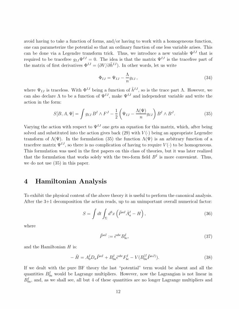
avoid having to take a function of forms, and/or having to work with a homogeneous function,

one can parameterize the potential so that an ordinary function of one less variable arises. This

can be done via a Legendre transform trick. Thus, we introduce a new variable ΨIJ that is

required to be tracefree gIJΨIJ = 0. The idea is that the matrix ΨIJ is the tracefree part of

the matrix of first derivatives ΦIJ = (∂V/∂hIJ ). In other words, let us write

ΦIJ = ΨIJ − Λ

ngIJ , (34)

where ΨIJ is traceless. With ΦIJ being a function of hIJ , so is the trace part Λ. However, we

can also declare Λ to be a function of ΨIJ , make ΨIJ and independent variable and write the

action in the form:

S[B, A, Ψ] =

∫gIJ BI ∧ F J − 1

2

(ΨIJ − Λ(Ψ)

ngIJ

)BI ∧ BJ . (35)

Varying the action with respect to ΨIJ one gets an equation for this matrix, which, after being

solved and substituted into the action gives back (29) with V (·) being an appropriate Legendre

transform of Λ(Ψ). In the formulation (35) the function Λ(Ψ) is an arbitrary function of a

tracefree matrix ΨIJ , so there is no complication of having to require V (·) to be homogeneous.

This formulation was used in the first papers on this class of theories, but it was later realized

that the formulation that works solely with the two-form field BI is more convenient. Thus,

we do not use (35) in this paper.

4 Hamiltonian Analysis

To exhibit the physical content of the above theory it is useful to perform the canonical analysis.

After the 3+1 decomposition the action reads, up to an unimportant overall numerical factor:

S =

∫dt

∫

Σ

d3x(P aIAI

a − H)

, (36)

where

P aI := ǫabcBIbc, (37)

and the Hamiltonian H is:

− H = AI0DaP

aI + BI0aǫ

abcF Ibc − V (B

(I0aP

aJ)). (38)

If we dealt with the pure BF theory the last “potential” term would be absent and all the

quantities BI0a would be Lagrange multipliers. However, now the Lagrangian is not linear in

BI0a, and, as we shall see, all but 4 of these quantities are no longer Lagrange multipliers and

12

should be solved for. The equations one obtains by varying the Lagrangian with respect to BI0a

are:

ǫabcF Ibc = V IJ

(1) PaJ , (39)

where V IJ(1) denotes the matrix of first partial derivatives of the function V (·) with respect to

its arguments:

V IJ(1) :=

∂V (h)

∂hIJ. (40)

The equations (39) can be solved in quite a generality by finding a convenient basis in the Lie

algebra. Thus, consider the momenta P aI . There are at least n−3 vectors N Iα, α = 1, . . . , n−3

that are orthogonal to the momenta:

P aIN Iα = 0, ∀a, α. (41)

These vectors can be chosen (uniquely up to SO(n − 3) rotations) by requiring:

N IαN I

β = δαβ . (42)

We can then use the qauntities P aI , a = 1, 2, 3, N Iα, α = 1, . . . , n−3 as a basis in the Lie algebra.

We can now decompose the quantity BI0a as:

BI0a = P bIB

˜ ab + N IαBα

a , (43)

where B˜ ab, B

αa are components of BI

0a in this basis. There are in total 3n components of BI0a and

they are represented here as 9 quantities B˜ ab as well as 3(n − 3) quantities Bα

a . The argument

of the function V (·) is now given by:

B(I0aP

aJ) = P b(IP aJ)B˜ ab + N (I

α Bαa P aJ). (44)

It is clear that this depends only on the symmetric part B˜ ab of the components B

˜ ab. Thus, the

anti-symmetric part of this 3 × 3 matrix cannot be determined from the equations (39) and

thus Na in B˜ [ab] := (1/2)ǫabcN

c remain Lagrange multipliers. It is also clear that due to the

homogeneity of V (·) one more component of BI0a cannot be solved for. This can be chosen for

example to be the trace part BI0aP

aI , which will then play the role of the lapse function. All

other 6+3(n−3)−1 components of BI0a can be solved for for a generic function V (·), i.e. under

the condition that the matrix of second derivatives of V (·) is non-degenerate. We are not going

to demonstrate this in full generality, but will verify it in the linearized theory below.

After the quantities BI0a are solved for we substitute them into (38) and obtain the following

Hamiltonian:

− H = AI0DaP

aI + NaP bIF Iab + NΛ(F, P ), (45)

13

where N is the lapse function and Λ(F, P ) is an approprite Legendre transform of V (·) that

now becomes a function of the curvature F Iab and momentum P aI . Thus, there are n Gauss as

well as 4 diffeomorphism constraints in the theory. It should be possible to check by an explicit

computation that they are first class, as was done, for example for the case of G = SU(2) in

[23], but we shall not attempt this here, postponing such an analysis till the linearized case

considerations. The above arguments allow a simple count of the degrees of freedom described

by the theory: we have 3n configurational degrees of freedom minus n Gauss constraints minus

4 diffeomoprhisms, thus leading to 2n−4 DOF. Thus, when G = K×SU(2) the above count of

DOF gives the right number for a gravity plus K Yang-Mills theory. For a general G one might

suspect that the centralizer of the gravitational SU(2) describes Yang-Mills, while other part

of the Lie algebra corresponds to some new kind of fields. Below we will unravel their nature

by considering the linearized theory. We also note that the above count of degrees of freedom

agrees with the one presented in [19] for the case G = SO(4). Thus, it was seen there that the

theory describes in total 2 · 6 − 4 = 8 DOF, which were interpreted as those corresponding to

2 graviton polarizations plus six new DOF.

5 The Linearized Theory: General considerations

As we have seen in the previous section, the mechanism that selects the gravitational SU(2) in

G is that the momentum variable P aI provides a map from the (co-) tangent space to the spatial

slice into g. This selects a 3-dimensional subspace in g that plays the role of the gravitational

gauge group. Below we are going to see this mechanism at play at the level of the Lagrangian

formulation, by studying the linearization of the action (6). In this section it will be convenient

to introduce a certain numerical prefactor in front of this action so that the normalization of

the graviton kinetic term in the case of gravity will come out right. Thus, we shall from now

on consider the following action

S[A, B] = 4i

∫

M

gIJBI ∧ F J − 1

2V (BI ∧ BJ), (46)

where i =√−1.

5.1 Kinetic term

In this section we present some general considerations that apply to any background. We

specialize to the Minkowski spacetime background in the next section. Let us call the first term

in (46) SBF and the second “potential” term SBB . Then, the second variation of SBF is given

by:

δ2SBF = 4i

∫2δBI ∧ DAδAI + BI ∧ [δA, δA]I , (47)

14

and the action linearized around B0, A0 is obtained by evaluating this on B0, A0.

As we have already mentioned, we are to view our theory as that of the two-form field BI ,

with the connection AI to be eliminated (whenever possible, see below) by solving its field

equations. Thus, let us assume that we are given a background two-form BI0 . The linearized

connection is then to be determined from the linearized equation (9) that reads:

D0δBI + [δA, B0]

I = 0, (48)

where D0 is the covariant derivative with respect to the background connection AI0. Now the

background two-form BI0 is a map from the six-dimensional space of bivectors to g, and thus

selects in g at most a 6-dimensional preferred subspace. Let us denote this subspace by k. This

subspace may or may not be closed under Lie brackets, but for simplicity, in this paper we shall

assume that our background BI0 is such that k is a Lie subalgebra (below we shall make an even

stronger assumption about k). It is then clear that the part of δAI that lies in the centralizer

of k in g drops from the equation (48) and cannot be solved for. As we shall later see, this will

be the part of the group that is to describe Yang-Mills fields. The other part of δAI can in

general be found. For this part of the connection both terms in (47) are of the same form due

to (48), and the linearized action can be written compactly as:

δ2SBF = 4i

∫δBI ∧ D0δA

I , (49)

where δAI has to be solved for from (48). On the other hand, for the subgroup of g that

centralizes k the last term in (47) is absent and we have:

δ2SBF = 8i

∫δBI ∧ D0δA

I . (50)

Thus, our analysis of the ”kinetic” term is going to be different for different parts of the Lie

algebra.

5.2 Potential term

In this subsection we compute the second variation of the potential term SBB and discuss how

it can be evaluated on a given background. We have:

δ2SBB = 4i

∫2

∂2V (h)

∂hKL∂hIJ(B0δB)IJ(B0δB)KL +

∂V (h)

∂hIJ(δBδB)IJ , (51)

where the integration measure d4x is implied, and we have introduced notations

(B0δB)IJ =1

4ǫµνρσB

(I0 µνδB

J)ρσ, (δBδB)IJ =

1

4ǫµνρσδBI

µνδBJρσ, (52)

15

and where the matrix of second derivatives is of density weight minus one.

Let us now discuss how the derivatives of the potential can be computed. In general, with

the potential function V (h) being homogeneous order one function of an n×n matrix, it can be

reduced to a function of ratios of its invariants. A subset of invariants is obtained by considering

traces of powers of hIJ . However, in general these are not all invariants, and other invariants

will be introduced and discussed below in section 9. But for now, to simplify the discussion,

let us consider a special class of potentials that only depend on the invariants obtained as the

traces of powers of hIJ . Many aspects of our theory can be seen already for this special choice.

Thus, consider the potential of the form:

V =Tr h

nf

(Tr h2

(Tr h)2, . . . ,

T r hn

(Tr h)n

). (53)

where f is now an arbitrary function of its n − 1 arguments, Tr h = gIJ hIJ and

Tr hp = hM1

M2hM2

M3· · · · · · hMp

M1, (54)

for p ≥ 2. In fact, in view of the fact that the rank of hIJ is at most six, not all the invariants

are independent, so we could consider only 5 first arguments of f(·). Note that f(·) here is

distinct from the function used in the action (1) in the pure connection formulation of our

theory: it is now an arbitrary function of its arguments, while this symbol in (1) stands for a

homogeneous order one function.

The parameterization given allows derivatives to be computed. Thus, the first derivative of

the potential function with respect to hIJ is

∂V (h)

∂hIJ=

gIJ

nf +

Tr h

n

∂f

∂hIJ, (55)

with (∂f/∂hIJ ) given by

∂f

∂hIJ=

n∑

p=2

f ′p

∂

∂hIJ

(Tr hp

(Tr h)p

)

=n∑

p=2

pf ′p

(hp−1

IJ

(Tr h)p− Tr hp

(Tr h)p+1gIJ

)(56)

where f ′p is the derivative of f with respect to its argument (Tr hp/(Tr h)p) and hp

IJ is

hpIJ = hIM1

hM1

M2· · · · · · hMp−1

J . (57)

The second derivative of V (h) is given by:

∂2V (h)

∂hKL∂hIJ=

gIJ

n

∂f

∂hKL+

gKL

n

∂f

∂hIJ+

Tr h

n

∂2f

∂hKL∂hIJ, (58)

16

with (∂2f/∂hKL∂hIJ ) given by

∂2f

∂hKL∂hIJ=

n∑

p=2

n∑

q=2

f ′′pq

∂

∂hIJ

(Tr hp

(Tr h)p

)∂

∂hKL

(Tr hq

(Tr h)q

)

+

n∑

p=2

f ′p

∂2

∂hKL∂hIJ

(Tr hp

(Tr h)p

), (59)

where f ′′pq stands for the derivative of f ′

p with respect to its q argument and

∂2

∂hKL∂hIJ

(Tr hp

(Tr h)p

)=

p

(Tr h)p

∂hp−1IJ

∂hKL− p2 hp−1

IJ

(Tr h)p+1gKL − p2 hp−1

KL

(Tr h)p+1gIJ

+p(p + 1) Tr hp

(Tr h)p+2gIJgKL , (60)

with

∂hp−1IJ

∂hKL= gI(K hL)M1

· · · · · · hMp−3

J+hI(K hL)M1·· · · hMp−4

J +· · · · · ·+hIM1· · · · · · hMp−3

(K gL)J . (61)

With the above formulas for the fist and second derivative of the potential it is relatively easy

to find the linearized action for any semi-simple Lie group.

6 The G = SU(2) Case: Gravity

As we have already mentioned, the case G = SU(2) describes (complexified) gravity theory. A

particular choice of the potential function, see below, gives general relativity, while a general

potential corresponds to a family of deformations of GR. In this section, as a warm-up to the

general G case, we shall study the corresponding linearized theory. Such an analysis has already

appeared in [24]. However, our method and goals here differ significantly from that reference.

6.1 The metric

To understand how G = SU(2) case can describe gravity we need to see how the spacetime

metric described by the theory is encoded. The answer to this is very simple: there is a unique

(conformal) metric that makes the triple Bi, where i is the su(2) index, into a set of self-dual

two-forms. This is the so-called Urbantke metric [25]

√−ggµν ∼ ǫijkBi

µαBjνβBk

ρσ ǫαβρσ (62)

17

that is defined modulo an overall factor. We remind the reader that at this stage all our fields

are complex, and later reality conditions will be imposed to select physical real Lorentzian

signature metrics.

Alternatively, given a metric gµν one can easily construct a “canonical” triple of self-dual

two-forms that encode all information about gµν . This proceeds via introducing tetrad one-

forms θI , with I = 0, 1, 2, 3 here. One then constructs the two-forms ΣIJ := θI ∧ θJ and

takes the self-dual part of ΣIJ with respect to IJ . The resulting two-forms are automatically

self-dual. They can be explicitly constructed by decomposing I = (0, a) and then writing:

Σa = iθ0 ∧ θa − 1

2ǫabcθb ∧ θc. (63)

Here i =√−1 is the imaginary unit. Its presence in this formula has to do with the fact

that self-dual quantities in a spacetime of Lorentzian signature are necessarily complex. Thus,

even though at this stage there is no well defined signature (all quantities are complex), it is

convenient to introduce i here so that later appropriate reality conditions are easily imposed.

We note that “internal” Lorentz rotations of the tetrad θI at the level of Σa boil down to

(complexified) SU(2) rotations of Σa.

A general su(2)-valued two-form field Bi carries more information than just that about a

metric. Indeed, one needs 3 × 6 numbers to specify it, while only 10 are necessary to specify

a metric. A very convenient description of the other components is obtained by introducing a

metric defined by Bi via (62) and then using the “metric” self-dual two-forms (63) as a basis

and decomposing:

Bi = biaΣ

a. (64)

The quantities bia give 9 components, the metric gives 10, and the choice of “internal” frame

for Σa adds 3 more components. There is also a freedom of rescalings bia → Ω−2bi

a, Σa → Ω2Σa,

as well as freedom of SO(3) rotations acting simultaneously on Σa and bia, overall producing 18

independent components of Bi.

When one substitutes the parameterization (64) into the action (6) one finds that the fields bia

are non-propagating and should be integrated out. Once this is done one obtains an “effective”

Lagrangian for the metric described by Σa. Below we shall see how this works in the linearized

theory. However, we first need to choose a background.

6.2 Minkowski background

The Minkowski background is described in our framework by a collection of metric two-forms

(63) constructed from the Minkowski metric. Thus, we choose an arbitrary time plus space

18

split and write:

Σa0 = idt ∧ dxa − 1

2ǫabcdxb ∧ dxc, (65)

where dt, dxa, a = 1, 2, 3 form a tetrad for the Minkowski metric ds2 = −dt2 +∑

a(dxa)2. Our

two-form field background is then chosen to be

Bi0 = δi

aΣa0, (66)

where δia is an arbitrary SO(3) matrix that for simplicity can be chosen to be the identity

matrix.

In what follows we will also need a triple of anti-self dual metric forms that, together with

(63) form a basis in the space of two-forms. A convenient choice is given by:

Σa0 = idt ∧ dxa +

1

2ǫabcdxb ∧ dxc. (67)

The following formulas, which can be shown to follow directly from definitions (65) and

(67), are going to be very useful

Σa0 µσΣbσ

0 ν = −δab ηµν + ǫabc Σc0 µν , (68)

Σaµν0 Σb

0 µν = 4 δab , (69)

ǫabc Σa0 µσΣbσ

0 λΣc0 λµ = −4! , (70)

ǫabc Σa0 µνΣ

b0 ρσΣdνσ

0 = −2δcd ηµρ , (71)

Σa0 µνΣ

a0 ρσ = ηµρηνσ − ηµσηνρ − iǫµνρσ , (72)

where ηµν is the Minkowski metric. We are going to refer to them as the algebra of Σ’s.

The first of the relations above, namely (68), is central, for all others (apart from (72)) can be

derived from it. It is useful to develop some basis-independent understanding of this relation.

We are working with the Lie algebra su(2) and are considering a basis Xa in it in which

the structure constants read [Xa, Xb] = ǫabcXc. This is the basis given by Xa = −(i/2)σa,

where σa are Pauli matrices. The metric gab = δab on the Lie algebra can be obtained as

gab = −2Tr(XaXb). Then (68) can be understood as follows: the product of two Σ’s is given

by minus the metric plus the structure constants times Σ. We will see that in this form the

relations (68) persist to any basis in su(2).

6.3 Linearized action

We are now going to linearize the G = SU(2) theory around the background (66). Thus, we

take:

Bi = Bi0 + bi . (73)

19

As we have already discussed, to linearize the kinetic BF term of the action we need to solve

for the linearized connection if we can. This is certainly possible for the case at hand, as we

shall now see.

If we denote the linearized connection by ai we have to solve the following system of equa-

tions

dbi + ǫijk aj ∧ Bk

0 = 0 , (74)

where we have used the fact that the background connection is zero. It is convenient at this

stage to replace all i-indices by a-ones, which we can do using the background object δia that

provides such an identification. We can now use the self-duality ǫµνρσΣa0 µν = 2iΣa µν

0 of the

background to rewrite this equation as

1

2iǫµνρσ∂νb

aρσ + ǫabcab

νΣc µν0 = 0. (75)

We now multiply this equation by Σa αβ0 Σd

0 αµ, and use the identity (71) to get:

aaβ =

1

2Σb α

0 β Σa0 αµ

1

2iǫµνρσ∂νb

bρσ, or aa

β =1

4iΣb α

0 β Σa0 αµ(∂bb)µ, (76)

where we have introduced a compact notation:

(∂bb)µ := ǫµνρσ∂νbbρσ (77)

for a multiple of the Hodge dual of the exterior derivative of the perturbation two-form.

The BF part of the linearized action was obtained in (49). We need to divide the second

variation given in this formula by 2 to get the correct action quadratic in the perturbation.

Thus, we have:

S(2)BF = 2i

∫ba ∧ daa = −i

∫aa

µ(∂ba)µ, (78)

where we have written everything in index notations and integrated by parts to put the deriva-

tive on baµν , and used the definition (77). Now substituting (76) we get:

S(2)BF =

1

4

∫ηαβΣa

0 αµ(∂bb)µΣb0 βν(∂ba)ν . (79)

Let us now linearize the potential term. For this we need to know the background hij as well

as the matrices of first and second derivatives for the background. Using (65) is easy to see that

hij0 = 2iδij. Since the background volume form is just the identity we can now safely remove

the density weight symbol from the matrix hij0 . Also, as before, let us replace all i-indices by

a-indices using δia. Using (55) and the fact that the first derivatives (∂f/∂hab) vanish on this

background we immediately get:∂V

∂hab

∣∣∣∣h0

=δab

3f0, (80)

20

where f0 is the background value of the function f in the parameterization (53). It is not

hard to see that this value plays the role of the cosmological constant of the theory, so in our

Minkowski background it is necessarily zero by the background field equations. The matrix of

second derivatives of the potential is easily evaluated using (58) and we find:

∂2V

∂hcd∂hab

∣∣∣∣h0

=g

2i

(δa(cδd)b −

1

3δabδcd

), (81)

where we have introduced:

g :=∑

p=2,3

(f ′p)0 p(p − 1)

3p. (82)

This is a constant of dimensions of the cosmological constant 1/L2. It is going to play a role of

a parameter determining the strength of gravity modifications.

We can now write the linearized potential term (51). We must divide it by two to get the

correct action for the perturbation. This gives:

S(2)BB = −g

2

∫ (δa(cδd)b −

1

3δabδcd

) (Σa µν

0 bbµν

) (Σc ρσ

0 bdρσ

). (83)

Note that the tensor in brackets here is just the projector on the tracefree part. This fact will

be important in our Hamiltonian analysis below. Our total linearized action is thus (79) plus

(83).

6.4 Symmetries

The quadratic form obtained above is degenerate, and its degenerate directions correspond

to the symmetries of the theory. These are not hard to write down. An obvious symmetry

is that under (complexified) SO(3) rotations of the fields. Considering an infinitesimal gauge

transformation of the background Σa0 µν we find that the action must be invariant under the

following set of transformations:

δωbaµν = ǫabcωbΣc

0 µν , (84)

where ωa are infinitesimal generators of the transformation. It is clear that (83) is invariant

since it involves only the ab-symmetric part of (Σa µν0 bb

µν), and the transformation (84) affects

the anti-symmetric part. Let us check the invariance of the kinetic term (79). We have the

following expression for the variation:

1

2

∫ηαβΣa

0 αµ(∂δωbb)µΣb0 βν(∂ba)ν . (85)

21

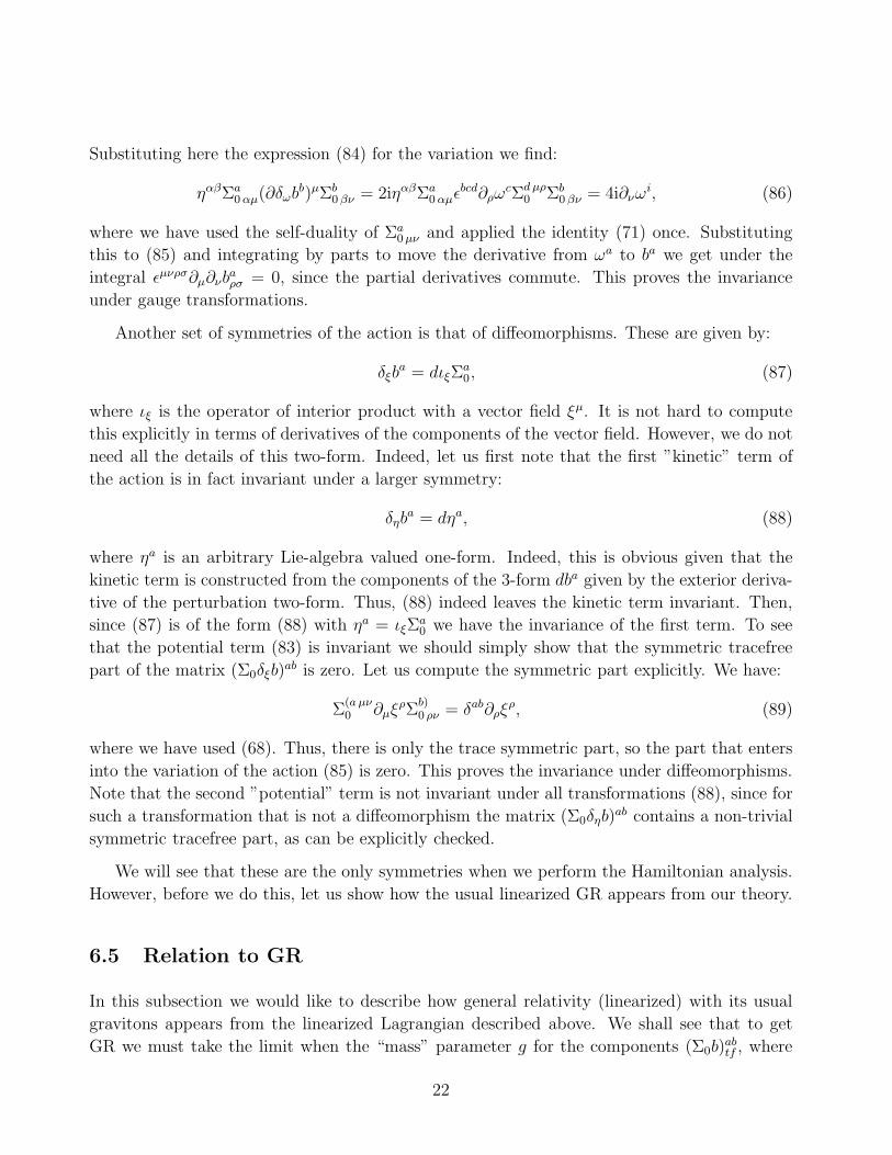
Substituting here the expression (84) for the variation we find:

ηαβΣa0 αµ(∂δωbb)µΣb

0 βν = 2iηαβΣa0 αµǫbcd∂ρω

cΣd µρ0 Σb

0 βν = 4i∂νωi, (86)

where we have used the self-duality of Σa0 µν and applied the identity (71) once. Substituting

this to (85) and integrating by parts to move the derivative from ωa to ba we get under the

integral ǫµνρσ∂µ∂νbaρσ = 0, since the partial derivatives commute. This proves the invariance

under gauge transformations.

Another set of symmetries of the action is that of diffeomorphisms. These are given by:

δξba = dιξΣ

a0, (87)

where ιξ is the operator of interior product with a vector field ξµ. It is not hard to compute

this explicitly in terms of derivatives of the components of the vector field. However, we do not

need all the details of this two-form. Indeed, let us first note that the first ”kinetic” term of

the action is in fact invariant under a larger symmetry:

δηba = dηa, (88)

where ηa is an arbitrary Lie-algebra valued one-form. Indeed, this is obvious given that the

kinetic term is constructed from the components of the 3-form dba given by the exterior deriva-

tive of the perturbation two-form. Thus, (88) indeed leaves the kinetic term invariant. Then,

since (87) is of the form (88) with ηa = ιξΣa0 we have the invariance of the first term. To see

that the potential term (83) is invariant we should simply show that the symmetric tracefree

part of the matrix (Σ0δξb)ab is zero. Let us compute the symmetric part explicitly. We have:

Σ(a µν0 ∂µξ

ρΣb)0 ρν = δab∂ρξ

ρ, (89)

where we have used (68). Thus, there is only the trace symmetric part, so the part that enters

into the variation of the action (85) is zero. This proves the invariance under diffeomorphisms.

Note that the second ”potential” term is not invariant under all transformations (88), since for

such a transformation that is not a diffeomorphism the matrix (Σ0δηb)ab contains a non-trivial

symmetric tracefree part, as can be explicitly checked.

We will see that these are the only symmetries when we perform the Hamiltonian analysis.

However, before we do this, let us show how the usual linearized GR appears from our theory.

6.5 Relation to GR

In this subsection we would like to describe how general relativity (linearized) with its usual

gravitons appears from the linearized Lagrangian described above. We shall see that to get

GR we must take the limit when the “mass” parameter g for the components (Σ0b)abtf , where

22

tf stands for the tracefree part, is sent to infinity. Indeed, the potential part (83) depends

precisely on these components, and when the parameter g is sent to infinity these components

are effectively set to zero. We shall now see that this gives GR.

It is not hard to show that in general the tracefree part htfµν := hµν − (1/4)ηµνh

ρρ of the

metric perturbation hµν defined via gµν = ηµν + hµν corresponds in our language of two forms

to the anti-self-dual part of the two-form perturbation:

(baµν)asd = Σa ρ

0 [µ htf

ν]ρ. (90)

The fact that this two-form is anti-self-dual can be easily checked by contracting it with Σb µν0

and using the algebra (68). The result is zero, as appropriate for an anti-self-dual tow-form.

In addition to (90) there is in general also the self-dual part of the two-form perturbation.

However, in the limit g → ∞ all but the trace part of this gets set to zero by the potential

term. The trace part, on the other hand, is proportional to the trace part ηµνhµν of the metric

perturbation. To simplify the analysis it is convenient to set this to zero ηµνhµν = 0. This is

allowed since in pure gravity the trace of the perturbation does not propagate. Then (90) is

the complete two-form perturbation, and we can drop the tf symbol.

To simplify the analysis further, instead of deriving the full linearized action for the metric

perturbation hµν , let us work in the gauge where the perturbation is transverse ∂µhµν = 0. Let

us then compute the quantity (∂ba)µ in this gauge. Using anti-self-duality of baµν given by (90)

we have:

ǫµνρσ∂νbaρσ = −2i∂νb

a µν . (91)

Substituting here the explicit expression (90) and using the transverse gauge condition we get:

(∂ba)µ = iΣa νρ0 ∂νh

µρ . (92)

We can now substitute this into the action (79) to get:

S(2) = − 1

4

∫ηαβΣa

0 αµΣb ρσ0 ∂ρh

µσΣb

0 βνΣa γδ0 ∂γh

νδ (93)

= − 1

4

∫ηαβ(δγ

αδδµ − δδ

αδγµ − iǫ γδ

αµ )(δρβδ

σν − δσ

βδρν − iǫ ρσ

βν )∂ρhµσ∂γh

νδ ,

where we have used (72) to get the second line. We can now contract the indices and take into

account the tracefree as well as the transverse condition on hµν . We get the following simple

action as the result:

S(2) = −1

2

∫∂µhρσ∂µhρσ, (94)

which is the correctly normalized transverse traceless graviton action. Note that in the passage

to GR we have secretly assumed that hµν in (90) is a real metric perturbation. Below we will

see how to impose the reality conditions on our theory that this comes out. Also note that the

sign in front of (94) is correct for our choice of the signature being (−, +, +, +).

23

6.6 Hamiltonian analysis of the linearized theory

For a finite g our theory describes a deformation of GR. Since not all components of the two-

form perturbation baµν are dynamical, the nature of this deformation is most clearly seen in the

Hamiltonian framework. This is what this subsection is about.

We note that the outcome of this rather technical subsection is that at ”low” energies

E2 ≪ g the modification can be ignored and one can safely work with the usual linearized GR.

Thus, it may be advisable to skip this subsection on the first reading. Let us start by analyzing

the kinetic BF-part.

Kinetic term. Expanding the product of two Σ-matrices in (79) using (68) we can write the

linearized Lagrangian density for the BF-part as

LBF =1

4(∂ba)µ(∂bb)ν

(ǫabc Σc

0 µν + δab ηµν

). (95)

Let us now perform the space plus time decomposition. Thus, we split the spacetime index as

µ = (0, a), where a = 1, 2, 3. Note that we have denoted the spatial index by the same lower

case Latin letter from the beginning of the alphabet that we are already using to denote the

internal su(2) index. This is allowed since we can use spatial projection of the Σa0 µν two-form

to provide such an identification. Thus, from (63) we have:

Σa0 bc = −ǫa

bc , (96)

and

Σa0 0b = iδa

b . (97)

Let us now use these simple relations to obtain the space plus time decomposition of the

Lagrangian. First, we need to know components of the (∂ba)µ vector. The time component is

given by:

(∂ba)0 = ǫ0bcd∂bbacd = −∂bt

ab, (98)

where our conventions are ǫ0abc = −ǫabc and we have introduced:

tab := ǫbcdbacd. (99)

The spatial component of (∂ba)µ is given by:

(∂ba)b = ǫb0cd∂0bacd + 2ǫbc0d∂cb

a0d = ∂0t

ab − 2ǫbcd∂cba0d. (100)

Now, the Lagrangian (95) is given by:

LBF = −1

4(∂ba)0(∂ba)0 +

1

2(∂ba)0(∂bb)dǫabcΣc

0d +1

4(∂ba)e(∂bb)f(ǫabcΣc

ef + δabδef). (101)

24

Substituting the above expressions we get:

LBF = − 1

4∂bt

ab∂ctac − i

2∂dt

ad(∂0tbc − 2ǫcef∂eb

b0f )ǫ

abc (102)

−1

4(∂0t

ae − 2ǫemn∂mba0n)(∂0t

bf − 2ǫfpq∂pbb0q)(ǫ

abcǫcef − δabδef).

Our fields are now therefore ba0b and tab. There will also be another, potential part to

this Lagrangian, but it does not contain time derivatives, so the conjugate momenta can be

determined already at this stage. Thus, it is clear that the field ba0b is non-dynamical since the

Lagrangian does not depend on its time derivatives. The momentum conjugate to tab, on the

other hand, is given by:

πab :=∂LBF

∂(∂0tab)= − i

2ǫabc∂dt

cd − 1

2(∂0t

ef − 2ǫfpq∂pbe0q)(ǫ

aecǫcbf − δaeδbf ). (103)

It is not hard to check that the momentum variable is simply related to the spatial projection

of the connection (76) as:

πab = −2iaa

b . (104)

To rewrite the Lagrangian in the Hamiltonian form one must solve for the velocities ∂0tab

in terms of the momenta πab. However, it is clear that not all the velocities can be solved for

- there are constraints. A subset of these constraints is given by the µ = 0 component of the

(75) equation that, when written in terms of πab, becomes:

Ga := ǫabcπbc + i∂btab = 0. (105)

These are primary constraints that must be added to the Hamiltonian with Lagrange multipli-

ers.

Thus, the expression for velocities in terms of momenta will contain undetermined functions.

These functions are simply the aa0 components of the connection, as well as (at this stage

undetermined) ba0b components of the two-form field. The expression for velocities is given by

the spatial components of equation (75). After some algebra it gives:

∂0tab = 2ǫbef∂eb

a0f − 2ǫabcac

0 − ǫaedǫdbfπef . (106)

Let us now obtain a slightly more convenient expression for the Lagrangian. Indeed, recall

that using the compatibility equation between the connection and the two-form perturbation,

we could have chosen to write our linearized action (78) as

S(2)BF = −2i

∫ǫabcΣa

0 ∧ ab ∧ ac = −2

∫Σa µνǫabcab

µacν . (107)

25

Introducing the time plus space split and writing the result in terms of the momentum variable

(104) we get the following Lagrangian:

LBF = −2ǫabcπabac0 −

1

2ǫaef ǫabcπbeπcf . (108)

We can now easily find the BF-part of the Hamiltonian:

HBF = πab∂0tab − LBF = 2πabǫbef∂eb

a0f − 1

2ǫaef ǫabcπbeπcf . (109)

We need to add to this the primary constraints (105) with Lagrange multipliers. Thus, the

total Hamiltonian coming from the BF part of the action is

HtotalBF = 2πabǫbef∂eb

a0f − 1

2ǫaef ǫabcπbeπcf + ωaGa. (110)

This is, of course, the standard result for the linearized BF Hamiltonian. If not for the potential

term, the Hamiltonian would be a sum of terms generating the topological constraint ∂[bπac] = 0

and the Gauss constraint (105). Let us now consider the other BB part of the Lagrangian.

Potential part. We can rewrite the linearized Lagrangian density for the BB part (83) as

LBB = −g

2

(b(aµνΣ

b)µν0

)tf

(b(aρσΣ

b)ρσ0

)tf

, (111)

where tf stands for the tracefree parts of the matrices. Splitting the space and time indices

gives:(b(aµνΣ

b)µν0

)

tf= −

(2ib

(ab)0 + t(ab)

)

tf, (112)

and so

LBB = −g

2

(2ib

(ab)0 + t(ab)

)

tf

(2ib

(ab)0 + t(ab)

)

tf. (113)

Analysis of the constraints. Thus, the total linearized Hamiltonian density H = HtotalBF −LBB

is given by

H = 2πabǫbef∂ebaf0 − 1

2ǫaef ǫabcπbeπcf + ωaGa +

g

2

(2ib

(ab)0 + t(ab)

)

tf

(2ib

(ab)0 + t(ab)

)

tf.

It is now clear that only the anti-symmetric part and trace parts of bab0 remain Lagrange

multipliers in the full theory. These are the generators of the diffeomorphisms. The other part

of bab0 , namely the symmetric traceless is clearly non-dynamical and should be solved for from

its field equations. Varying the Hamiltonian with respect to this symmetric tracefree part we

get

(2ib

(ab)0 + t(ab)

)

tf=

i

g

(ǫef(a∂eπ

b)f

)

tf. (114)

26

Now writing:

bab0 = iNδab +

1

2ǫabcN c + (b

(ab)0 )tf (115)

and substituting the symmetric tracefree part from (114) we get the following Hamiltonian

H = −2N iǫabc∂aπbc − 2∂[aπab]N

b + ωaGa (116)

− 1

2ǫaef ǫabcπbeπcf + i

(ǫef(a∂eπ

b)f

)

tf(t(ab))tf +

1

2g

(ǫef(a∂eπ

b)f

)

tf

(ǫpq(a∂pπ

b)q

)tf

.

The reason why we introduced a factor of i in front of the lapse function will become clear

below. One can recognize in the first line the usual Hamiltonian, diffeomorphism and Gauss

linearized constraints of Ashtekar’s Hamiltonian formulation of general relativity [15]. The first

two terms in the second line comprise the Hamiltonian. Finally, the last term is due to the

modification and goes away in the limit g → ∞.

It is not hard to show that the reduced phase space for the above system is obtained by

considering πab, tab that are symmetric, traceless and transverse ∂aπab = 0, ∂at

ab = 0. On such

configurations the matrix ǫefa∂eπfb is automatically symmetric traceless and transverse. The

reduced phase space Hamiltonian density is then given by:

Hphys =1

2(πab)2 + iǫefa∂etfbπab +

1

2g(∂aπbc)2, (117)

where we have integrated by parts and put the derivative on tab in the second term. This

Hamiltonian is complex, so we need to discuss the reality conditions.

Reality conditions. So far our discussion was in terms of complex-valued fields. Thus, the

reduced phase space obtained above after imposing the constraints and quotienting by their

action was complex dimension 2 + 2. Reality conditions need to be imposed to select the

physical phase space corresponding to Lorentzian signature gravity.

In the case of GR that corresponds to g → ∞ the reality condition could be guessed from

the form of the Hamiltonian (117). Indeed, we can write it as:

HphysGR =

1

2

(πab + iǫefa∂etfb

)2+

1

2(∂atbc)2. (118)

Thus, it is clear that we just need to require tab and πab + iǫefa∂etfb to be real. This procedure,

however, does not work for the full Hamiltonian because of the last term in (117).

Let us now note that the last term in (117), when written in momentum space behaves as

E2/M2, where E is the energy and M2 = g is the modification parameter. Thus, for energies

E ≪ M the modification term is much smaller than the term π2 and can be dropped. It is

natural to expect that gravity is only modified close to the Planck scale, so it is natural to

27

expect M2 ≈ M2p , where Mp is the Planck mass. With this assumption the last term in (117) is

unimportant for ”ordinary” energies and can be dropped. Thus, if we are to work at energies

much smaller than the Planck scales ones then we do not need to go beyond GR described by

the first two terms in (117).

The above discussion shows that a discussion of the reality conditions for the full Hamil-

tonian (117), even though possible and necessary if one is interested in the behavior of the

theory close to the Planck scale, is not needed if one only wants to work for with much smaller

energies. For this reason, and in order not to distract the reader from the main line of the

argument, a somewhat technical reality conditions discussion for the full theory is placed in the

Appendix.

Now that we understood how the simplest case G = SU(2) gives rise to gravity we can apply

the same procedure to more interesting cases of a larger gauge group. We consider the example

of SU(3) that well illustrates the general pattern.

7 The G = SU(3) Case: Gravity-Maxwell system

In this section we perform an analysis analogous to that in the previous section but taking a

larger gauge group. As before, we first consider the complex theory, and only at the end impose

the reality conditions. Let us start by reviewing some basic facts about the su(3) Lie algebra.

7.1 Lie algebra of SU(3)

The standard matrix representation of the Lie algebra of SU(3) consist of all traceless anti-

hermitian 3 x 3 complex matrices. The standard basis for su(3) space is given by the imaginary

unit times a generalization of Pauli matrices, known as Gell-Mann matrices. These hermitian

matrices are given by:

λ1 =

0 1 0

1 0 0

0 0 0

, λ2 =

0 −i 0

i 0 0

0 0 0

, λ3 =

1 0 0

0 −1 0

0 0 0

,

λ4 =

0 0 1

0 0 0

1 0 0

, λ5 =

0 0 −i

0 0 0

i 0 0

, λ6 =

0 0 0

0 0 1

0 1 0

,

λ7 =

0 0 0

0 0 −i

0 i 0

, λ8 =

1√3

1 0 0

0 1 0

0 0 −2

. (119)

28

[↓,→] T+ T− Tz V+ V− W+ W− Y

T+ 0 Tz −T+ 0 − 1√

2W−

1√

2V+ 0 0

T− −Tz 0 T−

1√

2W+ 0 0 − 1

√

2V− 0

Tz T+ −T− 0 1

2V+ − 1

2V− − 1

2W+

1

2W− 0

V+ 0 − 1√

2W+ − 1

2V+ 0 1

2(√

3Y + Tz) 0 1√

2T+ −

√

3

2V+

V−

1√

2W− 0 1

2V− − 1

2(√

3Y + Tz) 0 − 1√

2T− 0

√

3

2V−

W+ − 1√

2V+ 0 1

2W+ 0 1

√

2T− 0 1

2(√

3Y − Tz)−√

3

2W+

W− 0 1√

2V− − 1

2W− − 1

√

2T+ 0 − 1

2(√

3Y − Tz) 0√

3

2W−

Y 0 0 0√

3

2V+ −

√

3

2V−

√

3

2W+ −

√

3

2W− 0

Table 1: Commutators between T+, T−, Tz, V+, V−, W+, W−, Y .

However, in our computations the Cartan-Weyl basis is going to be more convenient. Let

us recall that in the Cartan-Weyl formalism one starts with the maximally commuting Cartan

subalgebra, which in our case is spanned by two elements λ3, λ8. One then selects basis vectors

that are eigenstates of the elements of Cartan under the adjoint action. This leads to the

following basis, see [26],[27]

T± =1√2(Tx ± i Ty) V± =

1√2(Vx ± iVy) W± =

1√2(Wx ± i Wy)

Tz =1

2λ3 Y =

1

2λ8 , (120)

where Tx = 12λ1, Ty = 1

2λ2, Vx = 1

2λ4, Vy = 1

2λ5, Wx = 1

2λ6 and Wy = 1

2λ7. Then the Cartan

subalgebra is Hi = Span(Tz, Y ), and the commutator between any of the Hi’s and the rest

of the elements of the basis Eα, Eα = T+, T−, Tz, V+, V−, W+, W−, is a multiple of Eα, i.e.

[Hi, Eα] = αi Eα. One considers the αi’s, for i = 1, 2, as the components of a vector, called

a root of the system. In this case we have six roots, i.e. 1, 0, −1, 0, 12,√

32, −1

2,−

√3

2,

−12,√

32, 1

2,−

√3

2. The Lie brackets between elements of this basis are given in Table 1. We

also need to know the metric gIJ = −2Tr(TITJ) in this basis. It is given in Table 2.

7.2 Background

Let us now discuss how a background to expand around can be chosen. A background two-

form field BI0 is a map from the space of bivectors, which is 6-dimensional, to the Lie algebra in

question. Thus, its image is at most 6-dimensional subspace in su(3). There are many different

subspaces one can consider. In this paper we study the simplest possibility. Thus, we choose

29

〈↓ | →〉 T+ T− Tz V+ V− W+ W− Y

T+ 0 −1 0 0 0 0 0 0

T− −1 0 0 0 0 0 0 0

Tz 0 0 −1 0 0 0 0 0

V+ 0 0 0 0 −1 0 0 0

V− 0 0 0 −1 0 0 0 0

W+ 0 0 0 0 0 0 −1 0

W− 0 0 0 0 0 −1 0 0

Y 0 0 0 0 0 0 0 −1

Table 2: Components for the internal metric in the base T+, T−, Tz, V+, V−, W+, W−, Y .

BI0 such that the image of the space of 2-forms that it produces in su(3) is 3-dimensional.

Moreover, we choose this image to be an su(2) Lie sub-algebra. Even further, we choose this

sub-algebra to be that spanned by T+, T−, Tz. Clearly, this is not the only su(2) sub-algebra

in su(3). Other possibilities include V+, V−, 12

(√3Y + Tz

) and W+, W−, 1

2

(√3Y − Tz

). In

this paper we do not study these different possibilities, leaving a more thorough investigation

to further research. We believe that the example we choose to study is sufficiently illustrating.

Thus, our background is essentially the same as the one we considered in the previous

section. This is motivated by our desire to have the usual gravity theory arising as the part

of the larger theory we are now considering. Since in the general Lie algebra context it is

convenient to work with the Cartan-Weyl basis, we need to change the basis of basic two-forms

(65) as well. This can be worked out as follows. In the previous section we were using a

basis in the Lie algebra in which the structure constants were given by ǫabc. If we denote the

corresponding generators by Xa then [Xa, Xb] = ǫabcXc. On the other hand, for generators Ta

used in (120) we have [Ta, Tb] = iǫabcTc. The relation between these two bases is Xa = −iTa.

We can then define a new set of self-dual two-forms Σ±, Σz via:

Σ ≡∑

a=1,2,3

ΣaXa = Σ+T+ + Σ−T− + ΣzTz. (121)

This gives

Σ+ =−i√

2

(Σ1 − i Σ2

)Σ− =

−i√2

(Σ1 + iΣ2

)Σz = −i Σ3 . (122)

The su(3)-valued two-form Σ is our background to expand about.

30

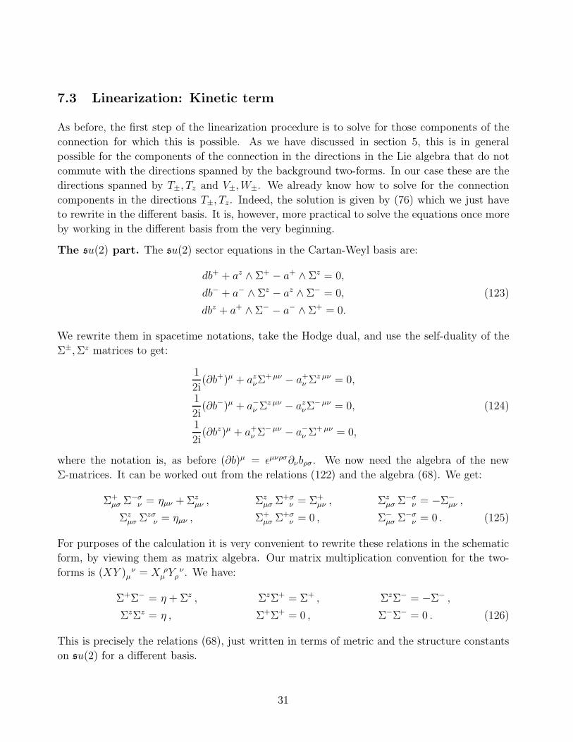
7.3 Linearization: Kinetic term

As before, the first step of the linearization procedure is to solve for those components of the

connection for which this is possible. As we have discussed in section 5, this is in general

possible for the components of the connection in the directions in the Lie algebra that do not

commute with the directions spanned by the background two-forms. In our case these are the

directions spanned by T±, Tz and V±, W±. We already know how to solve for the connection

components in the directions T±, Tz. Indeed, the solution is given by (76) which we just have

to rewrite in the different basis. It is, however, more practical to solve the equations once more

by working in the different basis from the very beginning.

The su(2) part. The su(2) sector equations in the Cartan-Weyl basis are:

db+ + az ∧ Σ+ − a+ ∧ Σz = 0,

db− + a− ∧ Σz − az ∧ Σ− = 0, (123)

dbz + a+ ∧ Σ− − a− ∧ Σ+ = 0.

We rewrite them in spacetime notations, take the Hodge dual, and use the self-duality of the

Σ±, Σz matrices to get:

1

2i(∂b+)µ + az

νΣ+ µν − a+

ν Σz µν = 0,

1

2i(∂b−)µ + a−

ν Σz µν − azνΣ

−µν = 0, (124)

1

2i(∂bz)µ + a+

ν Σ−µν − a−ν Σ+ µν = 0,

where the notation is, as before (∂b)µ = ǫµνρσ∂νbρσ. We now need the algebra of the new

Σ-matrices. It can be worked out from the relations (122) and the algebra (68). We get:

Σ+µσ Σ−σ

ν = ηµν + Σzµν , Σz

µσ Σ+σν = Σ+

µν , Σzµσ Σ−σ

ν = −Σ−µν ,

Σzµσ Σzσ

ν = ηµν , Σ+µσ Σ+σ

ν = 0 , Σ−µσ Σ−σ

ν = 0 . (125)

For purposes of the calculation it is very convenient to rewrite these relations in the schematic

form, by viewing them as matrix algebra. Our matrix multiplication convention for the two-

forms is (XY ) νµ = X ρ

µ Y νρ . We have:

Σ+Σ− = η + Σz , ΣzΣ+ = Σ+ , ΣzΣ− = −Σ− ,

ΣzΣz = η , Σ+Σ+ = 0 , Σ−Σ− = 0 . (126)

This is precisely the relations (68), just written in terms of metric and the structure constants

on su(2) for a different basis.

31

In matrix product conventions, the equations (124) take the following transparent form:

1

2i(∂b+) + Σ+az − Σza+ = 0,

1

2i(∂b−) + Σza− − Σ−az = 0, (127)

1

2i(∂bz) + Σ−a+ − Σ+a− = 0,

where the convention is that the second spacetime index of Σ is contracted with the spacetime

index of a.

We can now solve (127) by using the algebra (126). To this end we multiply the first

equation by Σ+ and the second one by Σ−. This leads to two equations involving only a± but

not az. We can obtain another two equations of the same sort by multiplying the last equation

in (124) by Σ±. Then adding-subtracting the resulting equations we get:

a+ = − 1

4i

(Σ−Σ+(∂b+) + Σ+(∂bz)

), a− = − 1

4i

(Σ+Σ−(∂b−) − Σ−(∂bz)

). (128)

To obtain the last component of the connection we multiply the first equation in (127) by

Σ− and second by Σ+, and then subtract the resulting equations. We find Σ−a+ − Σ+a− =

−(1/2i)(∂bz) using (128). We get:

az = − 1

4i

((∂bz) + Σ−(∂b+) − Σ+(∂b−)

). (129)

It is now easy to write the su(2) part of the linearized BF part of the action. Using the

metric components given in Table 2, from (78) we have:

Ssu(2)BF = −1

4

∫(∂b+)

(Σ+Σ−(∂b−) − Σ−(∂bz)

)+ (∂b−)

(Σ−Σ+(∂b+) + Σ+(∂bz)

)(130)

+(∂bz)((∂bz) + Σ−(∂b+) − Σ+(∂b−)

),

where again our convenient schematic form of the notation is used. This is simplified to give:

Ssu(2)BF = −1

2

∫(∂b+)(η + Σz)(∂b−) + (∂b−)Σ+(∂bz) − (∂b+)Σ−(∂bz) +

1

2(∂bz)(∂bz). (131)

We could now use this as the starting point of the Hamiltonian analysis similar to the one in

the previous section. However, it is clear that its results are basis-independent, so we do not

need to repeat it. Still, the above considerations are quite useful as a warm-up for the more

involved analysis that now follows.

The part that does not commute with su(2). Let us denote the four directions V±, W±collectively by index α = 4, 5, 6, 7. We have to solve the following system of equations:

dbα + fαβa aβ ∧ Σa = 0 , (132)

32

where the terms fαab aa ∧ Σb are absent since the corresponding structure constants are zero.

Explicitly, using table 1 we have:

db4 − 1√2

a6 ∧ Σ+ − 1

2a4 ∧ Σz = 0 , (133)

db5 +1√2

a7 ∧ Σ− +1

2a5 ∧ Σz = 0 , (134)

db6 − 1√2

a4 ∧ Σ− +1

2a6 ∧ Σz = 0 , (135)

db7 +1√2

a5 ∧ Σ+ − 1

2a7 ∧ Σz = 0 . (136)

We can solve this system using the same technology that we used above for the su(2) sector.

Thus, we take the Hodge dual of the above equations, use the self-duality of the Σ’s, and rewrite

everything in the schematic matrix form. We get:

1

2i(∂b4) − 1√

2Σ+a6 − 1

2Σza4 = 0 ,

1

2i(∂b5) +

1√2

Σ−a7 +1

2Σza5 = 0 ,

1

2i(∂b6) − 1√

2Σ−a4 +

1

2Σza6 = 0 , (137)

1

2i(∂b7) +

1√2

Σ+a5 − 1

2Σza7 = 0 .

We can now manipulate these equations using the algebra (126). Thus, let us multiply the

third equation by√

2Σ+ and subtract the result from the first equation. This gives:

1

2i(∂b4) −

√2

2iΣ+(∂b6) + (η +

1

2Σz)a4 = 0. (138)

It is now easy to find a4 by noting that (η + (1/2)Σz)−1 = (4/3)(η − (1/2)Σz). Thus, we have:

a4 =1

3i

(√2Σ+(∂b6) − (2η − Σz)(∂b4)

). (139)

Similarly, we multiply the last equation by√

2Σ− and add it to the second equation. Mul-

tiplying then by the inverse of (η − (1/2)Σz) we get:

a5 = − 1

3i

(√2Σ−(∂b7) + (2η + Σz)(∂b5)

). (140)

To find a6 we multiply the first equation by√

2Σ− and subtract the result from the third

equation. We then multiply the result by the inverse of (η − (1/2)Σz). We get:

a6 =1

3i

(√2Σ−(∂b4) − (2η + Σz)(∂b6)

). (141)

33

Finally, to find a7 we multiply the second equation by√

2Σ+ and add the result to the last

equation. Multiplying the result by the inverse of (η + (1/2)Σz) we get:

a7 = − 1

3i

(√2Σ+(∂b5) + (2η − Σz)(∂b7)

). (142)

We should now substitute the above results into the relevant part of the action. This is

again obtained from (78) by taking into account the expression for the metric. We shall refer

to this part of the action as ”Higgs” in view of its interpretation to be developed later. We

have:

SHiggsBF = i

∫a4(∂b5) + a5(∂b4) + a6(∂b7) + a7(∂b6), (143)

where we took into account and extra minus sign that comes from the metric. Substituting

here the above connections, we get, after some simple algebra:

SHiggsBF =

2

3

∫ √2(∂b5)Σ+(∂b6) −

√2(∂b4)Σ−(∂b7) (144)

−(∂b4)(2η + Σz)(∂b5) − (∂b6)(2η − Σz)(∂b7).

A more illuminating way to write this action is by introducing two two-component fields:

(b4

b6

) (b5

b7

). (145)

It is not hard to see that this split of the ”Higgs” sector part of the Lie algebra is just the split

into two irreducible representation spaces with respect to the action of the gravitational SU(2).

In terms of these columns the above action takes the following form:

SHiggsBF =

2

3

∫ ((∂b5) (∂b7)

)( −2η + Σz√

2Σ+√

2Σ− −2η − Σz

)((∂b4)

(∂b6)

). (146)

Below we will use this action as the starting point for an analysis that will eventually exhibit

the physical DOF propagating in this sector.

Centralizer U(1) part. We cannot solve for the components of the connection in the part

that commutes with su(2). In our case this is the direction Y of the Lie algebra. We shall refer

to this part of the action as ”YM”. Thus, the action remains of BF type:

SY MBF = −4i

∫b8 ∧ da8, (147)

where the extra minus sign is the one in the metric.

34

7.4 Linearization: Potential term

As in the SU(2) case our background internal metric hIJ0 is just 2igab in the su(2) directions

and zero in all other directions. Since the background metric is flat we shall drop the tilde from

hIJ in this section. We compute the matrix of first derivatives of the potential using (55). We

get:

∂V

∂hab

∣∣∣∣0

=f0

8gab, (148)

∂V

∂haα

∣∣∣∣0

=0 , (149)

∂V

∂hαβ

∣∣∣∣0

=

(f0

8− 1

8

6∑

p=2

(f ′p)0

p

3p−1

)gαβ . (150)

Here f0, (f′p)0 are the value of the function and its derivatives at the background, and index

α stands for all directions in the Lie algebra that are not in su(2). The quantity f0 can be

identified with a multiple of the cosmological constant. More specifically:

Λ = −3f0

8. (151)

Let us also define another constant of dimensions 1/L2:

κ ≡ 1

8

6∑

p=2

(f ′p)0

p

3p−1. (152)

Then we have:

∂V

∂hαβ

∣∣∣∣0

= −(Λ/3 + κ)gαβ . (153)

The sum here and in the previous formula is taken over p = 2, . . . , 6, because the function f can

at most depend on 5 ratios of 6 invariants of the matrix hIJ . It has at most only 6 independent

invariants since it is constructed from the map BIµν that has the rank at most six. Since we

want to work with the Minkowski spacetime background we should set Λ = 0, which we do in

what follows.

We now need to compute the matrix of second derivatives. Let us first obtain its su(2) part.

Using (58) we get:

∂2V

∂hcd∂hab=

g

2i

(ga(cgd)b −

1

3gabgcd

), (154)

where we have defined:

g =1

8

6∑

p=2

(f ′p)0

p(p − 1)

3p−1. (155)

35

As in the SU(2) case this constant is going to measure strength of gravity modifications. Both

κ and g constants have dimensions of 1/L2 and are, in general, independent parameters of our

linearized theory, related to first derivatives (f ′p)0 of the function f of the ratios.

Let us now compute the matrix of second derivatives in its part not in su(2). We only need

its mixed components aα and bβ. The computation is easy and using (58) we get:

∂2V

∂haα∂hbβ

∣∣∣∣0

=κ

4igabgαβ. (156)

We note that in this computation only one of the terms in (61) survives, and this is the reason

why it is the constant κ that appears in this formula.

We can now compute all the potential parts. We use (51) which we have to divide by two

to get the correct quadratic action. For the su(2) gravitational part the result is unchanged

from that in the previous section and we have:

SgravBB = −g

2

∫ (ga(cgd)b −

1

3gabgcd

) (Σa µν

0 bbµν

) (Σc ρσ

0 bdρσ

). (157)

The ”Higgs” and ”YM” parts of the potential term are both given by:

SHiggs−Y MBB = −κ

4

∫gabgαβ(Σa µνbα

µν)(Σb ρσbβ

ρσ) + 2igαβǫµνρσbαµνb

βρσ, (158)

so the indices α, β here take values 4, 5, 6, 7, 8. We can further simplify this using (72). We get:

SHiggs−Y MBB = −κ

∫gαβbα µνbβ ρσP−

µνρσ. (159)

where

P− =1

2

(ηµ[ρησ]ν +

i

2ǫµνρσ

)(160)

is the anti-self-dual projector.

7.5 Symmetries

We have seen that the su(2) sector of the theory is completely unchanged from what we have

obtained in the G = SU(2) case. One can moreover see that diffeomorphisms still act only

within this sector. Indeed, the action of a diffeomorphism in the direction of a vector field

ξµ is still given by (87) and only changes the su(2) part of the two-form field. Similarly, the

SU(2) gauge transformations act only on the su(2) sector. Thus, the gravity story that we have

considered in the previous section is unchanged.

36

Let us now consider what happens in directions not in su(2). Let us first consider the ”Higgs”

sector spanned by V±, W±. A gauge transformation with the gauge parameter ω valued in this

sector acts as δωb = [ω, Σ]. In components this reads:

δωb4 = − 1√2

ω6Σ+ − 1

2ω4Σz ,

δωb5 =1√2

ω7Σ− +1

2ω5Σz ,

δωb6 = − 1√2

ω4Σ− +1

2ω6Σz , (161)

δωb7 =1√2

ω5Σ+ − 1

2ω7Σz .

The remaining part of the Lie algebra is that spanned by Y . The corresponding gauge

transformation has no effect on the two-form field b8 (nor on bα, α = 4, 5, 6, 7) since it commutes

with the background. However this gauge transformation does act on the connection a8 by the

usual U(1) gauge transformation a8 → a8+dω8. The kinetic part (147) clearly remains invariant,

and the potential part is invariant since it only depends on b8 that does not transform.

7.6 Low energy limit of the ”Higgs” sector

Our analysis of the ”YM” sector presented below will show that the parameter κ that appeared

in the ”Higgs-YM” part of the potential (158) must be taken to be of the order M2p , where Mp

is the Planck mass. This will be follow from the fact that the YM coupling constant should

be of order unity in a realistic unification scheme, which then immediately implies κ ∼ M2p .

Another way to reach the same conclusion is to note that Mp is the only scale in our problem,

so all dimensionful quantities must be of the Planck size, see more on this in the last discussion

section. If this is the case then the role of the potential term (158) for the ”Higgs” sector

is to make the anti-self-dual components of the two-forms bαµν ”infinitely massive” and thus

effectively set them to zero. This is quite similar to what happened in the gravitational sector

in the limit g → ∞ with the babtf components. Thus, we see that in the low energy limit E2 ≪ κ

the two-forms bαµν can be effectively assumed to be self-dual. As such they can be expanded in

the background self-dual two-forms Σa0 µν . After such an ansatz is substituted into the action

(146) the result simplifies considerably. However, in order to exhibit the physical modes we

need to introduce some convenient gauge-fixing. Inspecting (161) we see that it is possible to

set to zero the following components of the bαa:

b4+ = 0, b5

− = 0, b6− = 0, b7

− = 0. (162)

37

This gauge turns out to be very convenient. We now write the gauge-fixed two-forms bαµν as

follows:

b4µν =

1

2

(1√2b4−Σ−

µν +

√3

2b4zΣ

zµν

),

b5µν =

1

2

(1√2b5+Σ+

µν +

√3

2b5zΣ

zµν

),

b6µν =

1

2

(1√2b6+Σ+

µν +

√3

2b6zΣ

zµν

), (163)

b7µν =

1

2

(1√2b7−Σ−

µν +

√3

2b7zΣ

zµν

),

where the independent fields are now b4−, b5

+, b6+, b7

− and bαz and the ”strange” normalization

coefficients are chosen in order for the Lagrangian to be obtained to have the canonical form.

Substituting (163) into (146) and using the algebra of Σ-matrices we get the following simple

effective low-energy action:

SHiggseff = −

∫∂µb5

+∂µb4− + ∂µb7

−∂µb6+ + ∂µb5

z∂µb4z + ∂µb7

z∂µb6z. (164)

This form of the Lagrangian makes the reality conditions necessary to get a real theory

obvious. Indeed, it is clear that the reality conditions are:

(b5+)∗ = b4

−, (b7−)∗ = b6

+, (b5z)

∗ = b4z , (b7

z)∗ = b6

z . (165)

These conditions can be compactly stated by introducing the following su(2)⊗g valued object:

b :=(b4−T+ + b4

zTz

)⊗ V+ +

(b5+T− + b5

zTz

)⊗ V− (166)

+(b6+T− + b6

zTz

)⊗ W+ +

(b7−T+ + b7

zTz

)⊗ W−

and requiring it to be hermitian:

b† = b. (167)

The action can also be written quite compactly in terms of b. Indeed, using the pairing given

by the 〈·, ·〉 metric in the Lie algebra we get:

LHiggseff = −〈∂µb†, ∂µb〉 (168)

for the low-energy E2 ≪ κ effective ”Higgs” sector Lagrangian. It is thus clear that, at least

in the low energy regime, the ”Higgs” sector of our theory consists just of 4 complex massless

scalar fields with the usual Lagrangian. It is not hard to show that in the finite κ limit the

content of this sector does not change, and is still given by massless fields.

38

7.7 Hamiltonian formulation for the Higgs sector

In this subsection we obtain the Hamiltonian formulation of the sector spanned by V±, W±.

After the analysis performed in the previous subsection such an analysis is not really necessary

as we know what the propagating DOF described by this sector are like, and we even know the

correct reality conditions. However, we decided to perform such an analysis for completeness,

and also to confirm the reality conditions found from the Hamiltonian perspective. One finds

the Hamiltonian analysis to be exactly parallel to that in the gravitational case, with even the

final expression for the Hamiltonian being analogous. This subsection is quite technical and the

reader is advised to skip it on the first reading. As in the case of gravity, we start by performing

the space plus time split of the kinetic BF part.

BF-Part. From (144) our Lagrangian density is:

LHiggsBF =

2√

2

3

((∂b5)µ(∂b6)ν Σ+

µν − (∂b4)µ(∂b7)νΣ−µν

)

−2

3

((∂b4)µ(∂b5)ν(2ηµν + Σz

µν) + (∂b6)µ(∂b7)ν(2ηµν − Σzµν))

. (169)

Now, denoting the indices 4, 5, 6, 7 collectively by α, we have:

(∂bα)0 = −∂btαb, (∂bα)a = ∂0t

αa − 2ǫabc∂bbα0c, (170)

where we have introduced the configurational variables

tαa := ǫabcbαbc. (171)

We do not need an expression for the expanded Lagrangian (169) because a more compact

expression in terms of the conjugate momenta will be obtained below. For now let us compute

the momenta conjugate to the configurational variables tαa. It is sufficient to compute just one

of the momenta to see the pattern. We have:

π4a :=∂LHiggs

BF

∂∂0t4a= − 2

√2

3

(Σ−

ab(∂0t7b − 2ǫbef∂eb

70f ) + Σ−

0a∂bt7b)

(172)

−4

3(∂0t

5a − 2ǫ ef

a ∂eb50f ) −

2

3

(Σz

ab(∂0t5b − 2ǫbef∂eb

50f ) + Σz

0a∂bt5b).

Comparing it to (140) we see that π4a = 2ia5a. This is precisely analogous to the relation (104)

we had in the case of gravity. Indeed, the above relation can be rewritten as π4a = −2ig4αaαa ,

which generalizes (104). The other momenta are obtained as follows:

παa = −2igαβaβa . (173)

39

We now need to solve for the velocities in terms of the momenta and substitute the result

into the Lagrangian. Similarly to the case of gravity the velocities can be obtained by taking

the spatial component of the equations (137). We get:

∂0t4a − 2ǫ bc

a ∂bb40c = i

√2Σ+

0aa60 +

1√2

Σ+ ba π7b + i Σz

0aa40 +

1

2Σz b

a π5b ,

∂0t5a − 2ǫ bc

a ∂bb50c = −i

√2Σ−

0aa70 −

1√2

Σ− ba π6b − i Σz

0aa50 −

1

2Σz b

a π4b ,

∂0t6a − 2ǫ bc

a ∂bb60c = i

√2 Σ−

0aa40 +

1√2

Σ− ba π5b − i Σz

0aa60 −

1

2Σz b

a π7b , (174)

∂0t7a − 2ǫ bc

a ∂bb70c = −i

√2Σ+

0aa50 −

1√2

Σ+ ba π4b + i Σz

0aa70 +

1

2Σz b

a π6b .

The time projections of the equations (137) are then the Gauss constraints.

For the last step we start from a convenient expression for the Lagrangian. This is given by

an analog of (107), which reads:

LHiggsBF = − 2gabΣ

a µνf bαβaα

µaβν (175)

= − 2√

2Σ+ µνa5µa

6ν + 2

√2Σ−µνa4

µa7ν + 2Σz µνa4

µa5ν − 2Σz µνa6

µa7ν ,

where faαβ are the structure constants. Expanding it, and converting the spatial components of

the connection into momenta we get:

LHiggsBF =

1√2Σ+ abπ4aπ7b −

1√2Σ− abπ5aπ6b −

1

2Σz abπ5aπ4b +

1

2Σz abπ7aπ6b

−i√

2Σ+ a0 (a5

0π7a − π4aa60) + i

√2Σ− a

0 (a40π6a − π5aa

70)

+iΣz a0 (a4

0π4a − π5aa50) − iΣz a

0 (a60π6a − π7aa

70) .

We can now compute the Hamiltonian:

HHiggsBF = παa∂0t

αa − LHiggsBF = 2παaǫ

abc∂bbα0c +

1

2gabg

αγgβδfaαβΣb efπγeπδf , (176)

The obtained expression is not the full Hamiltonian. To obtain the later we need to add 4

Gauss constraints that are obtained as the time components of the compatibility equations

(137). We will not need an explicit form of the Gauss constraints since we already know from

(161) what is generated by them.

The BB-Part. Let us now consider the potential part (159). The corresponding Lagrangian

density reads:

LHiggsBB = −κP−

µνρσgαβbα µνbβ ρσ. (177)

40

Expanding the spacetime index we get:

LHiggsBB = κgαβ(bα a

0 bβ0a −

1

4tαatβa) + iκgαβbα

0atβa. (178)

Total Hamiltonian. We now form the total Hamiltonian HHiggs = HHiggsBF − LHiggs

BB and

integrate out the non-dynamical fields bα0a. We get the following expressions for these fields by

solving their field equations:

bα0a =

1

κgαβǫabc∂

bπcβ − i

2tαa . (179)

This should be compared with (114) that we have in the gravitational sector. We now substitute

this back to get the Hamiltonian with second-class constraints solved for:

HHiggs =1

2gabg

αγgβδfaαβΣb efπγeπδf − i(ǫabc∂bπαc)t

αa +

1

κgαβ(ǫabc∂bπαc)(ǫ

aef∂eπβf) , (180)

plus Gauss constraints with their corresponding Lagrange multipliers. Note also that the Hamil-

tonian we have obtained is analogous to the one in the case of gravity (116). Indeed, there is

similarly the π2 term and a (ǫ∂π)t term with an imaginary unit in front. There is also a ∂2π2

term with a parameter of dimensions 1/M2 as a coefficient. Note that for any value of the

parameter κ this Hamiltonian describes modes that are massless. To rewrite this Hamiltonian

in terms of physical propagating modes we need to understand the gauge-fixing.

Gauge-fixing. To choose a convenient gauge-fixing that eliminates the gauge transformation

freedom, let us discuss what the two-forms Σ±, Σz become after they get projected onto the

spatial hypersurface. Thus, let us find analogs of relations (97), (96). Let us introduce the

following 3 spatial vectors:

Σ+0a := ma, Σ−

0a := ma, Σz0a := na. (181)

Then, taking various projections of (126), it is easy to check that the following relations hold:

mama = mama = 0, mana = mana = 0, (182)

mama = 1, nana = 1.

Taking different projections of (126) one finds the spatial pull-backs of the two-forms in terms

of the vectors introduced:

Σ+ab = namb − manb = −iǫabcm

c, Σ−ab = manb − namb = −iǫabcm

c, (183)

Σzab = mamb − mamb = −iǫabcn

c.

We now use (161) to fix the gauge as in (162). In terms of the configurational variables tαa

the gauge conditions read:

t4− = 0, t5+ = 0, t6+ = 0, t7− = 0, (184)

41

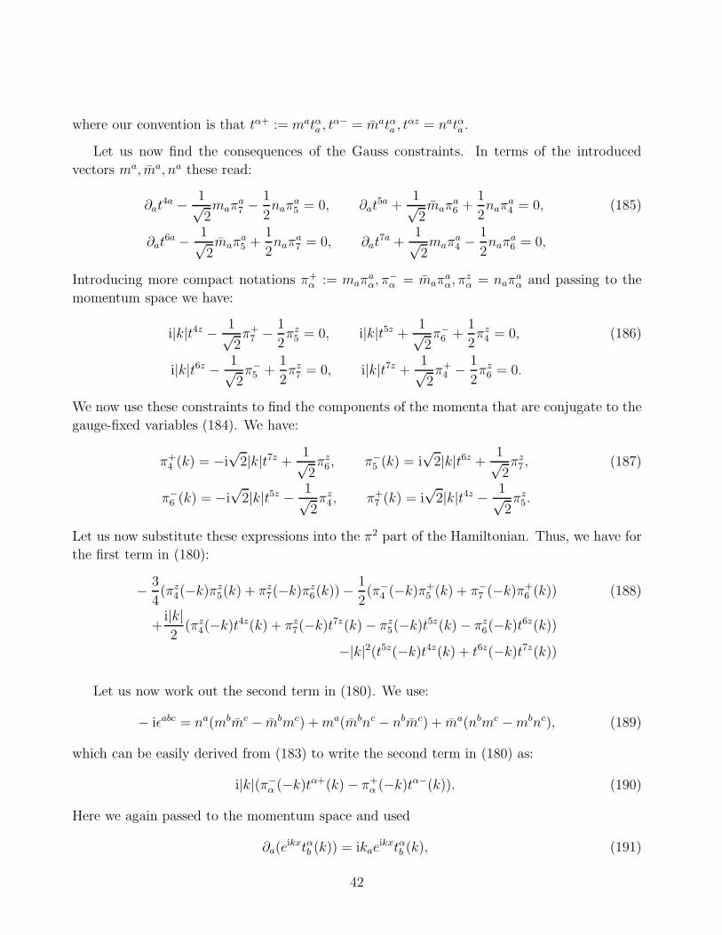
where our convention is that tα+ := matαa , tα− = matαa , tαz = natαa .

Let us now find the consequences of the Gauss constraints. In terms of the introduced

vectors ma, ma, na these read:

∂at4a − 1√

2maπ

a7 −

1

2naπ

a5 = 0, ∂at

5a +1√2maπ

a6 +

1

2naπ

a4 = 0, (185)

∂at6a − 1√

2maπ

a5 +

1

2naπ

a7 = 0, ∂at

7a +1√2maπ

a4 −

1

2naπ

a6 = 0,

Introducing more compact notations π+α := maπ

aα, π−

α = maπaα, πz

α = naπaα and passing to the

momentum space we have:

i|k|t4z − 1√2π+

7 − 1

2πz

5 = 0, i|k|t5z +1√2π−

6 +1

2πz

4 = 0, (186)

i|k|t6z − 1√2π−

5 +1

2πz

7 = 0, i|k|t7z +1√2π+

4 − 1

2πz

6 = 0.

We now use these constraints to find the components of the momenta that are conjugate to the

gauge-fixed variables (184). We have:

π+4 (k) = −i

√2|k|t7z +

1√2πz

6 , π−5 (k) = i

√2|k|t6z +

1√2πz

7 , (187)

π−6 (k) = −i

√2|k|t5z − 1√

2πz

4 , π+7 (k) = i

√2|k|t4z − 1√

2πz

5.

Let us now substitute these expressions into the π2 part of the Hamiltonian. Thus, we have for

the first term in (180):

− 3

4(πz

4(−k)πz5(k) + πz

7(−k)πz6(k)) − 1

2(π−

4 (−k)π+5 (k) + π−

7 (−k)π+6 (k)) (188)

+i|k|2

(πz4(−k)t4z(k) + πz

7(−k)t7z(k) − πz5(−k)t5z(k) − πz

6(−k)t6z(k))

−|k|2(t5z(−k)t4z(k) + t6z(−k)t7z(k))

Let us now work out the second term in (180). We use:

− iǫabc = na(mbmc − mbmc) + ma(mbnc − nbmc) + ma(nbmc − mbnc), (189)

which can be easily derived from (183) to write the second term in (180) as:

i|k|(π−α (−k)tα+(k) − π+

α (−k)tα−(k)). (190)

Here we again passed to the momentum space and used

∂a(eikxtαb (k)) = ikae

ikxtαb (k), (191)

42

where ka = |k|na is a vector in the direction of na. This makes only two of the terms from

(189) survive. Expanding and using the gauge-fixing conditions (184) we get for this term:

i|k|(π−4 (−k)t4+(k) + π−

7 (−k)t7+(k) − π+5 (−k)t5−(k) − π+

6 (−k)t6−(k)). (192)

The total Hamiltonian in the E2 ≪ κ low energy limit is given by the sum of two terms, i.e.,

(188) and (192).

Reality conditions. Let us now discuss the reality conditions that are appropriate in the

E2 ≪ κ low energy limit. It is clear that they can be determined by ”completing the square”,

similar to what we have seen in the Hamiltonian formulation of the gravitational sector (in the

low energy limit). Thus, let us write the total Hamiltonian as:

HHiggs = −3

4

(πz

4(−k) − 2i|k|3

t5z(−k)

)(πz

5(k) − 2i|k|3

t4z(k)

)− 4

3|k|2t5z(−k)t4z(k) (193)

−3

4

(πz

7(−k) − 2i|k|3

t6z(−k)

)(πz

6(k) − 2i|k|3

t7z(k)

)− 4

3|k|2t6z(−k)t7z(k)

−1

2

(π−

4 (−k) − 2i|k|t5−(−k)) (

π+5 (k) − 2i|k|t4+(k)

)− 2|k|2t5−(−k)t4+(k)

−1

2

(π−

7 (−k) − 2i|k|t6−(−k)) (

π+6 (k) − 2i|k|t7+(k)

)− 2|k|2t6−(−k)t7+(k) .

The form of the reality conditions is now obvious. Indeed, we introduce new momenta

variables:

πz4(k) = πz

4(k) +2i|k|

3t5z(k), πz

5(k) = πz5(k) − 2i|k|

3t4z(k), (194)

πz6(k) = πz

6(k) − 2i|k|3

t7z(k), πz7(k) = πz

7(k) +2i|k|

3t6z(k),

π−4 (k) = π−

4 (k) + 2i|k|t5−(k), π+5 (k) = π+

5 (k) − 2i|k|t4+(k),

π+6 (k) = π+

6 (k) − 2i|k|t7+(k), π−7 (k) = π−

7 (k) + 2i|k|t6−(k),

and then require the following reality conditions:

πz4(−k) = −(πz

5(k))∗, πz7(−k) = −(πz

6(k))∗, (195)

π−4 (−k) = −(π+

5 (k))∗, π−7 (−k) = −(π+

6 (k))∗

t5z(−k) = −(t4z(k))∗, t6z(−k) = −(t7z(k))∗,

t5−(−k) = −(t4+(k))∗, t6−(−k) = −(t7+(k))∗.

It is not hard to see that these conditions are the same as we have derived earlier in the

Lagrangian framework, see (165). Indeed, the extra minus present in (195) is due to the

following transformation properties of the basic two-forms:

(Σ+ab)

∗ = −Σ−ab, (Σz

ab)∗ = −Σz

ab (196)

43

that directly follow from (183). The obtained real positive definite Hamiltonian is that of 4

complex massless scalar fields, so we have full agreement with our Lagrangian analysis above.

Reality conditions and the Hamiltonian for the full finite κ theory can be obtained via precisely

the same method as in the gravitational sector case treated in the Appendix. We refrain from

giving such an analysis in this work, as it becomes even more technical.

7.8 YM sector

In this subsection we work out the Lagrangian for the remaining part of the theory, which lives

in the part of the gauge group that commutes with the background su(2). The total Lagrangian

we start with is a sum of kinetic term (147) and the potential term (159), with an extra sign

in the potential term coming from the metric component g88 = −1. This gives:

LY M = 2iǫµνρσb8µν∂ρa

8σ + κP−µνρσb8

µνb8ρσ. (197)

The further analysis is greatly simplified by making use of the reality condition for the b8µν

two-form from the outset. Thus, as we will also confirm by the Hamiltonian analysis in the

next subsection, the two-form b8µν needs to be purely imaginary:

b8µν := −ib8

µν , (b8µν)

∗ = b8µν . (198)

This immediately leads to simplifications as the real part of the Lagrangian (197) is then given

simply by:

LY Mreal = 2ǫµνρσ b8

µν∂ρa8σ − κ

2b8 µν b8

µν . (199)

Taking a variation with respect to b8µν we learn that:

b8µν =

1

κǫµνρσF ρσ, (200)

where Fµν = ∂µa8ν − ∂νa

8µ is the curvature of our U(1) gauge field, which is therefore, for real

κ, real. Substituting the result back into the Lagrangian we get:

LY M = −2

κ(Fµν)

2. (201)

This is the standard YM Lagrangian with the coupling constant:

g2Y M =

κ

8. (202)

To convert this into a physical coupling constant we recall that we need to multiply the La-

grangian by 32πG, as this is exactly the prefactor that converts the canonically-normalized

44

graviton Lagrangian (94) into the Einstein-Hilbert one. Thus, the physical coupling constant

in our arising YM theory is given by:

g2Y M = 4πGκ. (203)

Realistic particle physics coupling constants are of the order of unity (and smaller), so we learn

that the parameter κ must be of the order M2p , which is what we have been using in the previous

subsections.

7.9 Reality conditions for the YM sector

In this subsection we perform the Hamiltoanian analysis of the YM sector with the main aim

being to obtain the reality conditions used above. As in all other cases considered, the reality

conditions become obvious once the Hamiltonian is written down.

We start from the Lagrangian (197). Expanding

ǫµνρσb8µν∂ρa

8σ = −2ǫabcb8

0a∂ba8c − t8a(∂0a

8a − ∂aa

80), (204)

where t8a := ǫabcb8bc, we see that the momentum conjugate to the connection a8

a is

π8a :=∂LY M

∂∂0a8a

= −2it8a. (205)

The Hamiltonian is then:

HY M = 4iǫabcb80a∂ba

8c − a8

0∂aπ8a + κ(b8 a

0 b80a +

1

16π8aπ8

a) −κ

2b80aπ

8a. (206)

We find the non-dynamical fields b80a via their field equations and get:

b80a = −2i

κǫabc∂

ba8c +1

4π8

a. (207)

Substituting this back into (206) we get the ”physical” Hamiltonian

HY Mphys =

4

κ

(ǫabc∂ba

8c +

iκ

8π8a

)2

+κ

16π8aπ8

a. (208)

It is now clear that the ”correct” reality conditions that give rise to a real positive definite

Hamiltonian is:

Im(ǫabc∂ba8c) +

κ

8Re(π8a) = 0, Im(π8a) = 0. (209)

From (207) and (205) it is easy to see that these reality conditions are equivalent to the condition

that b8µν two-form is purely imaginary, which is what we have used in the previous subsection.

45

Passing to the real phase space and imposing the Gauss constraint ∂aπ8a = 0 as well as

the transverse gauge condition ∂aa8a = 0 we get the following simple expression for the real

Hamiltonian:

HY Mreal =

4

κ(∂aa

8 realb )2 +

κ

16(π8a)2, (210)

which again confirms that the parameter κ/8 plays the role of g2Y M .

8 Interactions

In this section we work out (some of the) cubic order interactions for our theory. Our main goal

is to verify that the YM and Higgs sectors interacts with the gravitational field in the usual

way, and that the YM-Higgs interaction is also standard. We start with general considerations

on the cubic order expansion of our theory.

8.1 General considerations

The third variation of the BF-term is

δ3SBF = 4i

∫3 δBI ∧ [δA, δA]I , (211)

and the third variation of the BB-term is

δ3SBB = 4i

∫d4x

(4

∂3V (h)

∂hMN∂hKL∂hIJ(B0δB)IJ(B0δB)KL(B0δB)MN (212)

+ 6∂2V (h)

∂hKL∂hIJ(B0δB)IJ(δBδB)KL

). (213)

As in the case of the quadratic order expansion, it is most laborious to compute the deriva-

tives of the potential. We have already computed the second derivative above. The third

derivative of V (h) is given by:

∂3V (h)

∂hMN∂hKL∂hIJ=

gIJ

n

∂2f

∂hMN∂hKL+

gKL

n

∂2f

∂hMN∂hIJ+

gMN

n

∂2f

∂hKL∂hIJ(214)

+Tr h

n

∂3f

∂hKL∂hKL∂hIJ,

46

where the third derivative of the function of the ratios is given by

∂3f

∂hMN∂hKL∂hIJ=

n∑

p=2

n∑

q=2

n∑

p=2

f ′′′pqr

∂

∂hIJ

(Tr hp

(Tr h)p

)∂

∂hKL

(Tr hq

(Tr h)q

)∂

∂hMN

(Tr hr

(Tr h)r

)

+

n∑

p=2

n∑

q=2

f ′′pq

∂

∂hIJ

(Tr hp

(Tr h)p

)∂2

∂hMN∂hKL

(Tr hq

(Tr h)q

)

+

n∑

p=2

n∑

q=2

f ′′pq

∂

∂hKL

(Tr hp

(Tr h)p

)∂2

∂hMN∂hIJ

(Tr hq

(Tr h)q

)

+

n∑

p=2

n∑

q=2

f ′′pq

∂

∂hMN

(Tr hp

(Tr h)p

)∂2

∂hKL∂hIJ

(Tr hq

(Tr h)q

)

+

n∑

p=2

f ′p

∂3

∂hMN∂hKL∂hIJ

(Tr hp

(Tr h)p

), (215)

where f ′′′pqr stands for the derivative of f ′′

pq with respect to its r argument and

∂3

∂hKL∂hKL∂hIJ

(Tr hp

(Tr h)p

)=

p

(Tr h)p

∂2hp−1IJ

∂hMN∂hKL

− p2

(Tr h)p+1

(gIJ

∂hp−1KL

∂hMN+ gKL

∂hp−1IJ

∂hMN+ gMN

∂hp−1IJ

∂hKL

)

+p2(p + 1)

(Tr h)p+2

(gIJ gKL hp−1

MN + gIJ gMN hp−1KL + gKL gMN hp−1

IJ

)

− p(p + 1)(p + 2) Tr hp

(Tr h)p+3gIJ gKL gMN . (216)

The first derivative of a power of hIJ is given by (61). We have not found a sufficiently simple

general expression for the second derivative of hp−1IJ with respect to hMN hKL, but the expression

(61) can be easily differentiated for any given p. The above expressions can be used to obtain

the third derivatives of the potential for our background. The results are given in the next

subsection.

8.2 Interactions with gravity

In this paper we shall not consider gravitational sector self-interactions. They are easily com-

putable, but since the main emphasis of this work is on unification, it is of much more interest

to compute the interactions of other fields with gravity and their self-interactions. In this

subsection we consider the coupling of non-gravitational fields to gravity.

47

Thus, at least one of the perturbation fields δBI is to be taken to lie in the gravitational

sector. It is then easy to see that this is the only interaction in the cubic order. Indeed,

where two of the three perturbation fields lie in the gravitational sector and there is only one

non-gravitational perturbation, there is no interaction coming from the potential part since

∂2V (h)

∂haα∂hbc

∣∣∣∣∣0

= 0,∂3V (h)

∂heα∂hcd∂hab

∣∣∣∣∣0

= 0, (217)

where α stands for the non-gravitational part of the Lie algebra. There is also no interaction

coming from the kinetic part of the action for the structure constant f IJK is zero when two of

the indices are in the su(2) part and only one index is in the non-gravitational part. Thus we

only need to consider the interaction that is linear in the graviton perturbation. It is natural

to expect that this coupling is that to the stress-energy tensor of our non-gravitational fields,

and this will be confirmed below.

The interaction coming from the kinetic term is only non-trivial for the Higgs sector fields

(since the structure constant with two of its indices in the ”YM” part of the Lie algebra and

one in su(2) is zero since the YM and the gravitational parts commute). This interaction is of

the schematic type h(∂b)2, which is as expected for scalar fields coupled to gravity. We are not

going to work out this term, even though it is not hard to do it using the explicit formulas for

the connections worked out above.

Let us concentrate on the interactions coming from the potential part of the action, as being

the most interesting one. The relevant derivatives of the potential are as follows:

∂2V (h)

∂hαβ∂hab

∣∣∣∣∣0

=0, (218)

∂2V (h)

∂hbβ∂haα

∣∣∣∣∣0

=κ

4igαβgab,

∂3V (h)

∂hdβ∂hcα∂hab

∣∣∣∣∣0

=gαβ

2(2i)2

((κ − g)

(ga(cgd)b −

1

3gabgcd

)− κ

3gabgcd

).

Note that the fact that the first quantity is zero is not completely trivial, at it involves a precise

cancellation of two otherwise non-zero terms.

We can now compute the relevant interaction terms using (212). We need to divide this

expression by 3! to remove the extra multiplicity introduced by taking the third variation of

the action. An additional simplification comes from the fact that in the first term in the third

derivative in (218) we have a matrix projecting onto the tracefree part of the gravitational

two-form perturbation matrix Σa µν0 bb

µν . This part is zero when the parameter g → ∞, which is

the limit of the usual GR that we are considering. Thus, this part drops out and we have for

48

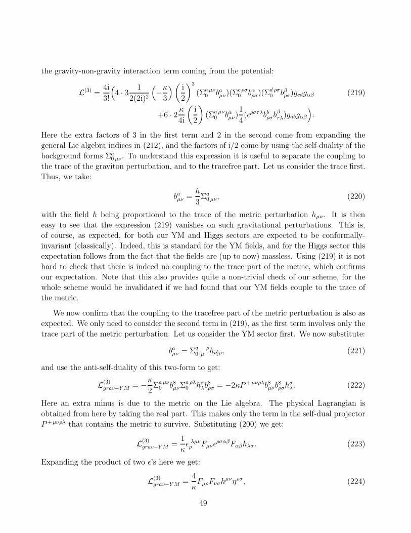
the gravity-non-gravity interaction term coming from the potential:

L(3) =4i

3!

(4 · 3 1

2(2i)2

(−κ

3

)( i

2

)3

(Σa µν0 ba

µν)(Σc ρσ0 bα

ρσ)(Σd ρσ0 bβ

ρσ)gcdgαβ (219)

+6 · 2 κ

4i

(i

2

)(Σa µν

0 bαµν)

1

4(ǫρστλbb

ρσbβτλ)gabgαβ

).

Here the extra factors of 3 in the first term and 2 in the second come from expanding the

general Lie algebra indices in (212), and the factors of i/2 come by using the self-duality of the

background forms Σa0 µν . To understand this expression it is useful to separate the coupling to

the trace of the graviton perturbation, and to the tracefree part. Let us consider the trace first.

Thus, we take:

baµν =

h

3Σa

0 µν , (220)

with the field h being proportional to the trace of the metric perturbation hµν . It is then

easy to see that the expression (219) vanishes on such gravitational perturbations. This is,

of course, as expected, for both our YM and Higgs sectors are expected to be conformally-

invariant (classically). Indeed, this is standard for the YM fields, and for the Higgs sector this

expectation follows from the fact that the fields are (up to now) massless. Using (219) it is not

hard to check that there is indeed no coupling to the trace part of the metric, which confirms

our expectation. Note that this also provides quite a non-trivial check of our scheme, for the

whole scheme would be invalidated if we had found that our YM fields couple to the trace of

the metric.

We now confirm that the coupling to the tracefree part of the metric perturbation is also as

expected. We only need to consider the second term in (219), as the first term involves only the

trace part of the metric perturbation. Let us consider the YM sector first. We now substitute:

baµν = Σa ρ

0 [µ hν]ρ, (221)

and use the anti-self-duality of this two-form to get:

L(3)grav−Y M = −κ

2Σa µν

0 b8µνΣ

a ρλ0 hσ

λb8ρσ = −2κP+ µνρλb8

µνb8ρσhσ

λ. (222)

Here an extra minus is due to the metric on the Lie algebra. The physical Lagrangian is

obtained from here by taking the real part. This makes only the term in the self-dual projector

P+µνρλ that contains the metric to survive. Substituting (200) we get:

L(3)grav−Y M =

1

κǫ λµνρ Fµνǫ

ρσαβFαβhλσ. (223)

Expanding the product of two ǫ’s here we get:

L(3)grav−Y M =

4

κFµρFνσhµνηρσ, (224)

49

in which expression we recognize precisely the coupling to the stress-energy tensor that arises

from the YM Lagrangian (201). The sign in front is different from that in (201) because the

variation of the metric with two upper indices is given by minus hµν . Thus, the arising coupling

of our YM fields to the gravitational sector is correct.

Let us now discuss the coupling of the Higgs sector to gravity. It is easy to see that in

the low-energy approximation in which E2 ≪ κ and the two-forms bαµν are self-dual there is no

coupling coming from the potential term. Indeed, we have already discussed that there is no

coupling to the trace part of the metric perturbation. Thus, there is only the second term in

(219) that can contribute. However, it contains a factor of (ǫρστλbbρσbβ

τλ) which is contraction of

a self-dual Higgs two-form and an anti-self-dual gravitational one. So, it is zero and the only

interaction term in the Higgs sector comes from the kinetic term of the action. As we have

already discussed, it is of the h(∂b)2 form, which is just the coupling of the metric perturbation

to the stress-energy tensor of our set of massless fields. We are not going to work out the details

as they are slightly messy, but we hope that the discussion given is sufficient to show that the

interaction is as expected.

8.3 Interactions in the non-gravitational sector

Let us now concentrate on the interactions in the non-gravitational sector, most interestingly

those between the YM and Higgs sectors.

First, we note that there are no cubic interactions in the non-gravitational sector that come

from the potential term. Indeed, such an interaction term involves three perturbation two-forms

bαµν with the Lie algebra index outside of su(2). It is not hard to see that the corresponding

derivatives of the potential vanish:

∂2V (h)

∂hβγ∂haα

∣∣∣∣∣0

= 0,∂3V (h)

∂hcγ∂hbβ∂haα

∣∣∣∣∣0

= 0. (225)

Thus, at cubic order we only need to consider the interactions coming from the kinetic

term. It is not hard to see that there are no self-interactions in the Higgs or YM sectors, but

there are two possible types of interaction between these sectors. One of them comes from the

term gαβbαfβγ8a

γa8, the other comes from b8f 8αβaαaβ , where α now stands for the Higgs sector

index. The second of this is an interaction of the type (1/κ)F (∂b)2, and is thus suppressed at

low energies by E2/κ. However, the first interaction is non-trivial and important even at low

energies. In fact, it is not hard to show that this is the standard interaction of the gauge field

a8 with the conserved U(1) current of the Higgs sector that is charged under the YM subgroup.

We are not going to spell out the details that are again slightly messy, but the important point

is that the YM-Higgs sectors interaction is also as expected for a set of scalar fields charged

under the YM gauge group (Higgs fields).

50

9 More general potentials: Mass generation

Up to now we have for simplicity considered a very special class of potentials that depend only

on the invariants constructed from the ”internal” metric hIJ using the Killing-Cartan metric

gIJ . It is not hard to show that due to the fact that the rank of hIJ is at most six, there is at

most six such independent invariants, and thus only at most five ratios to be considered as the

arguments of the function f(·) in (53). However, it is clear that these are not the only possible

invariants. Indeed, the most general gauge-invariant function of hIJ can also involve invariants

constructed using the structure constants f IJK . For instance, let us consider

ffhhh := fPQRfSTU hPShQT hRU , (226)

where the indices on the structure constants are raised using the metric on the group. More

generally, one can construct a matrix:

(ffhh)IJ := f IQRfJTU hQT hRU (227)

and build more complicated invariants from traces of powers of hIJ and (ffhh)IJ . This leads to

a much more general set of gauge-invariant functions. In this section we shall study implications

of such more general potentials. Our main point in this section is that these more general

potential functions lead naturally to Higgs fields becoming massive. This is very important

for phenomenology, for massless Higgs fields interacting with the ”visible” YM sector in the

standard way is obviously inconsistent with observations.

9.1 Potential with an extra invariant

For simplicity, in this paper we shall consider only one additional invariant given by (226). We

shall see that such a potential is sufficient to generate masses for the Higgs sector particles.

It is not hard to consider even more general potentials, but we refrain from doing it in this

already lengthy paper.

Thus, let us consider the potential depending on one more invariant

V (h) =Tr h

nF

(Tr h2

(Tr h)2, . . . ,

T r hn

(Tr h)n,ff hhh

(Tr h)3

), (228)

where we have divided (226) by (Tr h)3 to make the potential homogeneous degree one. Then,

the first derivative with respect to h is

∂V (h)

∂hIJ=

gIJ

nF +

Tr h

n

∂F

∂hIJ, (229)

51

with (∂F/∂hIJ ) given by

∂F

∂hIJ=

n∑

p=2

F ′p

∂

∂hIJ

(Tr hp

(Tr h)p

)+ F ′

n+1

∂

∂hIJ

(ffhhh

(Tr h)3

)(230)

where F ′p is the derivative of F with respect to its argument (Tr hp/(Tr h)p), F ′

n+1 is the

derivative of F with respect to its last argument and

∂

∂hIJ

(ffhhh

(Tr h)3

)=

3 fPQ

(IfRS

J) hPRhQS

(Tr h)3− 3 ffhhh

(Tr h)4gIJ . (231)

Now, let us compute the second derivative of V with respect to h. We get

∂2V (h)

∂hKL∂hIJ=

gIJ

n

∂F

∂hKL+

gKL

n

∂F

∂hIJ+

Tr h

n

∂2F

∂hKL∂hIJ, (232)

with (∂2F/∂hKL∂hIJ ) given by

∂2F

∂hKL∂hIJ=

n∑

p=2

F ′p

∂2

∂hKL∂hIJ

(Tr hp

(Tr h)p

)+ F ′

n+1

∂2

∂hKL∂hIJ

(ffhhh

(Tr h)3

)(233)

+

n∑

p=2

n∑

q=2

(F ′′

pq

∂

∂hKL

(Tr hq

(Tr h)q

)+ F ′′

p(n+1)

∂

∂hKL

(ffhhh

(Tr h)3

))∂

∂hIJ

(Tr hp

(Tr h)p

)

+

n∑

p=2

(F ′′

(n+1)p

∂

∂hKL

(Tr hp

(Tr h)p

)+ F ′′

(n+1)(n+1)

∂

∂hKL

(ffhhh

(Tr h)3

))∂

∂hIJ

(ffhhh

(Tr h)3

),

where F ′′pq stands for the derivative of F ′

p with respect to its q argument and similar for F ′′p(n+1)

and F ′′(n+1)(n+1). It is easy to show that

∂2 (ffhhh)

∂hIJ∂hKL= −6 fP

K)(IfQ

J)(L hPQ . (234)

Using the equations above, we obtain the following expressions

∂V

∂hab

∣∣∣∣0

=0 , (235)

∂V

∂hαβ

∣∣∣∣0

= −(

κ +2λ

3

)gαβ , (236)

∂2V

∂hbβ∂haα

∣∣∣∣0

=κ

4igab gαβ +

λ

6igcdf

cabf

dαβ , (237)

where we have set (F )0 = 0 and defined

λ =(F ′

n+1)0

8. (238)

The parameter κ is as before, see (152), with the function F (·) of one more invariant in place

of f(·).

52

9.2 Higgs sector masses

In this subsection we show that the new parameter λ introduced above receives the interpreta-

tion of mass squared of the Higgs sector scalar fields. To this end, let us work out the quadratic

part of the action that comes from the potential, concentrating only on the λ-dependent part.

The κ-dependent part was already taken care of by setting the Higgs sector perturbation two-

forms bαµν to be self-dual, and this is unchanged for our more general potential. Dividing (51)

by two, using the self-duality of bαµν in the second term and simplifying we get:

S(2)λ = −2λ

3

∫1

4gcdf

cabf

dαβ(Σa µν

0 bαµν)(Σ

b µν0 bβ

µν) − gαβbα µνbβµν . (239)

We now substitute in this expression the expansions (163) for our two-forms (in a specific

gauge). It is not hard to see that only the term f zabf

zαβ contributes and we get:

S(2)λ = λ

∫b4−b5+ + b6+b7− + b4zb5z + b6zb7z = −m2

Higgs〈b†,b〉, (240)

where

m2Higgs = −λ. (241)

Thus, as all other physical parameters arising in our theory, the mass of the Higgs sector

particles also comes from the defining potential.

10 Discussion

In view of the length of this paper it is probably appropriate to recap our logic and emphasize

the main results that we have obtained. Thus, we have started with a generally-covariant

gauge theory for a group G, with the action given by (1). At this stage all fields are complex

and reality conditions are later imposed to select the physical, real sector of the theory. We

then perform the Legendre transform and pass to the two-form field formulation (6). Our phase

space analysis in section 4 is only needed to get a better idea of what should be expected for the

number of propagating DOF of the theory. It does not form an essential part of our argument.

The main analysis starts in section 6 where we analyze the simplest case G = SU(2) and show

how it describes the usual gravity in the limit when a certain parameter of the potential is

taken to be large, or, alternatively, for low energies. For a finite value of the parameter (or for

Planckian energies) one gets a modified gravity theory with two propagating DOF. However,

as the low-energy limit of our theory is still given by GR, we do not need to understand the

nature of this modification for purposes of this paper.

We start with the analysis of the pure gravity case by describing how the Minkowski space-

time looks like in the language of two-forms, see (65). The action is then expanded to quadratic

53

order, and the field equations for the connection field are solved for, with the solution given by

(76). After the solution is substituted into the action one gets the linearized kinetic term (79)

as a functional of only the two-form perturbation. This is supplemented with the potential

term part (83). After the parameter g is taken to infinity one gets GR written in terms of

two-forms, with a very compact linearized action (79). This action is considerably simpler than

the one in terms of the metric perturbation, and the relation between the two arises via (90).

We also perform the Hamiltonian analysis of the linearized theory, to show how the usual two

polarizations of the graviton arise in this language. In the g → ∞ limit this analysis reproduces

Ashtekar’s Hamiltonian formulation of GR, in its linearized version. The main purpose of this

analysis is to select the reality conditions for the gravitational sector. These are particularly

clear in the Hamiltonian formulation, and later in the paper the same strategy of deducing the

reality conditions from the form of the Hamiltonian is used for other fields. In this section we

only discuss the rather simple reality conditions appropriate in the GR limit g → ∞. The finite

g case reality conditions are deduced in the Appendix, for completeness.

Once the SU(2) case is understood we enlarge the gauge group to G = SU(3). We take the

same set of two-forms (65) for the background, which thus selects in the su(3) Lie algebra a

preferred gravitational su(2) subalgebra. The analysis of the gravitational part is unchanged,

but we have carried it out once more using a different basis in the Lie algebra (root basis),

in preparation for the analysis of the non-gravitational sectors. These split into a part that

commutes with su(2) and that will later be identified with the YM sector, and the part that

does not commute with su(2) and becomes the Higgs sector.

Let us start with the Higgs sector. As in the case of gravity, we first solve the equations for

the connections aαµ in terms of the perturbation two-forms bα

µν and then substitute the result

back into the action. The resulting kinetic part of the action as a functional of the two-forms bαµν

is given by (146). There is also the part (159) coming from the potential. Similarly to the case

of gravity, the role of the potential part, in the low-energy limit, is to set certain components

of the two-form field bαµν to zero. After this is done, the perturbation two-forms bα

µν becomes

self-dual and can be expanded in the basis of self-dual two-forms (65). The coefficients in this

expansion become our Higgs fields. They can be seen to be charged under the gravitational

SU(2) subgroup, comprising two irreducible representations of spin 1/2 of SU(2). They also

transform non-trivially under the part of the gauge group that does not commute with SU(2),

and so they are not all physical. A convenient gauge is given by (163). Finally, our Higgs

fields are charged under the part of the gauge group that commutes with SU(2), i.e. under

the YM subgroup, which in the case of G = SU(3) is U(1). After a gauge is fixed, one

obtains a Lagrangian for the physical fields, and this is found to be just the usual one for

a set of 8 massless fields. We then determined the reality conditions needed to make it into

a real Lagrangian with positive definite Hamiltonian. These can be read off from either the

Lagrangian we have obtained, or from the Hamiltonian formulation that is also developed. The

end result is a set of 4 complex (and at this stage massless) scalar fields with the usual real

54

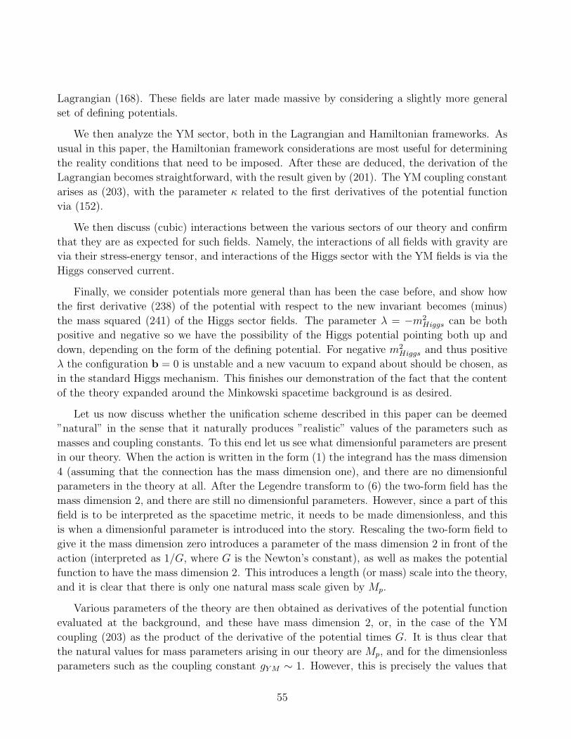
Lagrangian (168). These fields are later made massive by considering a slightly more general

set of defining potentials.

We then analyze the YM sector, both in the Lagrangian and Hamiltonian frameworks. As

usual in this paper, the Hamiltonian framework considerations are most useful for determining

the reality conditions that need to be imposed. After these are deduced, the derivation of the

Lagrangian becomes straightforward, with the result given by (201). The YM coupling constant

arises as (203), with the parameter κ related to the first derivatives of the potential function

via (152).

We then discuss (cubic) interactions between the various sectors of our theory and confirm

that they are as expected for such fields. Namely, the interactions of all fields with gravity are

via their stress-energy tensor, and interactions of the Higgs sector with the YM fields is via the

Higgs conserved current.

Finally, we consider potentials more general than has been the case before, and show how

the first derivative (238) of the potential with respect to the new invariant becomes (minus)

the mass squared (241) of the Higgs sector fields. The parameter λ = −m2Higgs can be both

positive and negative so we have the possibility of the Higgs potential pointing both up and

down, depending on the form of the defining potential. For negative m2Higgs and thus positive

λ the configuration b = 0 is unstable and a new vacuum to expand about should be chosen, as

in the standard Higgs mechanism. This finishes our demonstration of the fact that the content

of the theory expanded around the Minkowski spacetime background is as desired.

Let us now discuss whether the unification scheme described in this paper can be deemed

”natural” in the sense that it naturally produces ”realistic” values of the parameters such as

masses and coupling constants. To this end let us see what dimensionful parameters are present

in our theory. When the action is written in the form (1) the integrand has the mass dimension

4 (assuming that the connection has the mass dimension one), and there are no dimensionful

parameters in the theory at all. After the Legendre transform to (6) the two-form field has the

mass dimension 2, and there are still no dimensionful parameters. However, since a part of this

field is to be interpreted as the spacetime metric, it needs to be made dimensionless, and this

is when a dimensionful parameter is introduced into the story. Rescaling the two-form field to

give it the mass dimension zero introduces a parameter of the mass dimension 2 in front of the

action (interpreted as 1/G, where G is the Newton’s constant), as well as makes the potential

function to have the mass dimension 2. This introduces a length (or mass) scale into the theory,

and it is clear that there is only one natural mass scale given by Mp.

Various parameters of the theory are then obtained as derivatives of the potential function

evaluated at the background, and these have mass dimension 2, or, in the case of the YM

coupling (203) as the product of the derivative of the potential times G. It is thus clear that

the natural values for mass parameters arising in our theory are Mp, and for the dimensionless

parameters such as the coupling constant gY M ∼ 1. However, this is precisely the values that

55

are ”realistic”. Indeed, as our Higgs fields interact with the ”visible” YM sector, we need to

explain why they are not observed. This is explained by their very high mass that makes

them essentially irrelevant for the low energy physics. Second, the realistic values of the YM

coupling constants of particle physics are order one, and precisely such values are natural in our

unification scheme. Overall, our unification model is ”realistic” in the sense that it reproduces

everything that could be desired from such a simple setup.

An important ingredient that is missing from our simple-minded model is that of the usual

symmetry breaking mechanism of particle physics. Such a breaking, if present, would introduce

additional mass scales into the theory and make it much richer. The model considered in this

paper in which the bakground only broke the G symmetry down to the gravitational and YM

ones did not break the YM gauge group. However, it is clear that our model naturally allows

for such further breaking of symmetry. Indeed, we could take the background to be more non-

trivial and give to some of our Higgs fields a non-trivial vacuum expectation value. Since our

Higgs fields interact with the YM sector in the standard way, the effect of such a non-trivial

VEV is also going to be standard - the YM symmetry is going to be broken, with some of the

gauge fields becoming massive. It is then very interesting that in our scheme this standard

particle physics symmetry breaking mechanism receives a new interpretation. Indeed, a non-

trivial VEV for the Higgs is now on the same footing as a non-zero value for the metric. In

other words, in our unification scenario the Higgs fields and the metric are just different parts

of a single two-form field multiplet BIµν . Details of, for example, Hamiltonian analysis of the

gravitational and Higgs sectors also confirm a very close analogy between the two. Thus, in

a sense, it is the Higgs fields and the metric that become truly unified in our scenario. It is

of considerable interest to study such more involved symmetry breaking scenarios. The goal

would be to see if a truly realistic unification that puts together some GUT gauge group, a set

of Higgs fields required to break it to the gauge group of the standard model as well as gravity

is possible. This question is, however, beyond the scope of this paper.

Yet another very important ingredient that is missing from our scenario is fermions. These

are usually unproblematic for any scenario that operates in Minkowski spacetime. However,

we start with a generally covariant theory with no metric in it, so it is not at all clear how and

if fermions can be added. At the moment, this is probably the most serious objection against

our scenario, but we remain hopeful that fermions can be described in our framework. The

only possibility for this seems to be to further enlarge the connection field in (1) and make it

”fermionic”. This might also require a ”generalized” connection that is no longer a one-form,

as fermions that we would like to obtain are not forms. We leave investigation of all these

difficult but very interesting questions to further research.

Finally, let us briefly touch on the question of quantization. The theory we have considered

was classical, but, of course, it has to be quantized. It is then clear that our action (1) is non-

renormalizable in the usual sense of the word. Indeed, expanding the theory around Minkowski

spacetime we have obtained a Lagrangian consisting of some renormalizable pieces – in the Higgs

56

and YM sectors – as well as gravity with its non-renormalizable interactions. However, there

are also higher order interactions that are non-renormalizable, and the full action is given by

an expansion containing an infinite number of non-renormalizable terms. Thus, the full theory

is non-renormalizable. This is, of course, as expected, for we cannot hope to bring together a

non-renormalizable theory (gravity) with renormalizable other interactions in a renormalizable

unified theory. At best, we can hope for a non-renormalizable unified theory, and this is what

is happening in our scenario.

At the same time, what our starting action (1) describes is just the most general generally-

covariant gauge theory. For this reason it can be expected that the class of theories (1) obtained

by considering all possible potentials f(·) is closed under renormalization. Indeed, all terms that

could arise as counterterms are already included into (1) and so the only effect of renormalization

should be in the renormalizing the defining function f(·). This expectation is consistent with

the outcome of our analysis. Indeed, we have seen that, for instance, the YM theory gauge

coupling is just a certain parameter of the potential defining the theory. This parameter is

known to flow with energy, and from the perspective of our scheme this corresponds to a

flow in the potential function. If the sole effect of renormalization is a flow in the space of

potentials, the non-renormalizability of our theory ceases to be much of a problem. Indeed,

it is then possible to hope for a non-problematic UV fixed point corresponding to some very

special potential that would thus provide a UV completion of our theory. In this context it is

interesting to remark that, since the gauge coupling is known to flow to zero value in the UV

(asymptotic freedom), and such coupling in our scheme is on the same footing with e.g. the

parameter g describing the strength of gravity modifications, it is natural to expect that g flows

to zero in the UV as well. However, it is not hard to see that this corresponds to the defining

potential V (·) flowing towards the one of the topological BF theory. Thus, at least prior to any

concrete analysis, it seems that the sought UV completion may be given by the topological BF

theory, something that in the past has been suggested in the literature in other contexts. All

in all, the absence of the usual ”finite number of counterterms” renormalizability of our theory

may not be a problem as the theory may possibly be renormalizable in the sense of Weinberg

[28] as containing all possible counterterms, see also [29] for a more modern exposition of the

notion of ”effective renormalizability”.

To summarize, there are many open problems of our scenario, notably questions of whether a

realistic grand unification is possible, whether fermions can be described in the same framework,

and whether the expectation of effective renormalizability is realized. However, it appears to

us that in spite of all the open problems the scenario described already suggests some very

interesting new interpretations and and is thus worthy of further exploration.

Acknowledgements. ATG was supported by a Mathematical Sciences Research Scholarship

and KK by an EPSRC Advanced Fellowship.

57

Appendix: Reality conditions for modified gravity

The ”correct” reality conditions for the full modified gravity theory can be worked out from

the condition Bi ∧ (Bj)∗ = 0. In linearized theory this becomes:

Σa ∧ (bb)∗ = Σb ∧ ba, or Σa µν(bbµν)

∗ + Σb µνbaµν = 0, (242)

where (ba)∗ is the complex conjugate two-form perturbation and Σ is given by (67). We now

rewrite this reality condition using the space plus time split. We get:

i(tab − (tba)∗) + 2(bab0 + (bba

0 )∗) = 0. (243)

To get this condition we have used Σabc = ǫa

bc, Σa0b = iδa

b and recalled the definition (99) of

the configurational variable. We should now analyze this condition together with the already

known solution (115), (114) for the components bab0 .

Let us first consider the trace and anti-symmetric parts of (243). Then in the tracefree

symmetric gauge for tab these conditions simply state that the lapse and shift functions N, Na

are real. This explains why the factor of i was introduced in (115) in front of the lapse.

Consider now the symmetric tracefree part of (243). The corresponding components of bab0

are known from (114) and we arrive at the following condition on the phase space variables:

1

2gRe(ǫef(a∂eπ

b)f

)tf

= Im(tab)tf . (244)

In the case g → ∞ that corresponds to GR this implies that (tab)tf is real, but in the modified

case the situation is more interesting.

In addition to (244) there is another condition that is obtained by requiring that (244) is

preserved under the evolution. Thus, we need to compute the Poisson bracket of (244) with the

Hamiltonian and impose the resulting condition as well. The computation is a bit technical,

but at this phase space level there is no way to avoid it. Indeed, even in the case of GR it is

clear from the form of the Hamiltonian (116) that the relevant condition cannot be that the

momentum is real, for the Hamiltonian would be complex due to the presence of the second

term in the second line. The computation of the Poisson bracket can be done as follows. First,

we introduce the real and imaginary parts of the phase space variables:

tab = tab1 + itab

2 , πab = πab1 + iπab

2 . (245)

Second, we substitute this decomposition into the action written in the Hamiltonian form. The

resulting action has real and imaginary parts. It is not hard to convince oneself that any one

of these two parts can be used as an action for the system, the resulting equations are the

same due to Riemann-Cauchy equations that follow from the fact that the original action was

58

holomorphic. We choose to work with the real part of the action. The relevant Poisson brackets

are easily seen to be

πab1 (x), t1 cd(y) = δ(a

c δb)d δ3(x − y), πab

2 , (x)t2 cd(y) = −δ(ac δ

b)d δ3(x − y), (246)

with all the other ones being zero. The real part of the Hamiltonian (with the constraint part

already imposed and dropped) reads:

Hreal =1

2(πab

1 )2 − 1

2(πab

2 )2 − ǫefa∂eπbf1 tab

2 − ǫefa∂eπbf2 tab

1 +1

2g(∂aπbc

1 )2 − 1

2g(∂aπbc

2 )2.

We can now compute the Poisson bracket with the reality condition (244) that becomes:

1

2gǫefa∂eπ

fb1 = tab

2 . (247)

The Poisson bracket with the left-hand-side is:

Hreal,1

2gǫefa∂eπbf

1 = − 1

2g∆πab

2 . (248)

The Poisson bracket with the right-hand-side is:

Hreal, tab2 = πab

2 + ǫefa∂etbf1 − 1

g∆πab

2 . (249)

Thus, the sought conditions that guarantees the consistency of (247) is:

πab2 + ǫefa∂etbf1 − 1

2g∆πab

2 = 0. (250)

We now need to solve this for πab2 , which gives:

πab2 = − ǫefa∂etbf1

1 − ∆/2g, (251)

where the denominator should be understood as a formal power series in powers of ∆/g. When

g → ∞ we reproduce the GR result reviewed in the beginning of this subsection.

We now have to substitute this, as well as the expression (247) for tab2 into the action. This

is a simple exercise with the result being:

Sreal =

∫dt d3x

(πab

GR∂0tabGR − 1

2

((πab

GR)2 + (∂atbcGR)2))

, (252)

where we have defined:

πabGR = πab

1 , tabGR =

tab1

1 − ∆/2g. (253)

These are the phase space variables in terms of which the Hamiltonian takes the standard GR

form. This shows how an explicitly real formulation with a positive definite Hamiltonian can

be obtained. We also see that for any finite value of g the graviton is unmodified.

59

References

[1] C. Vafa, “Geometry of Grand Unification,” arXiv:0911.3008 [math-ph].

[2] S. R. Coleman and J. Mandula, “All Possible Symmetries of the S Matrix,” Phys. Rev.

159, 1251 (1967).

[3] R. Haag, J. T. Lopuszanski and M. Sohnius, “All Possible Generators Of Supersymmetries

Of The S Matrix,” Nucl. Phys. B 88, 257 (1975).

[4] R. Percacci, “Mixing internal and spacetime transformations: some examples and coun-

terexamples,” J. Phys. A 41, 335403 (2008) [arXiv:0803.0303 [hep-th]].

[5] S. Holst, “Barbero’s Hamiltonian derived from a generalized Hilbert-Palatini action,” Phys.

Rev. D 53, 5966 (1996) [arXiv:gr-qc/9511026].

[6] R. Percacci, “Spontaneous Soldering,” Phys. Lett. B 144, 37 (1984).

[7] R. Percacci, “The Higgs Phenomenon in Quantum Gravity,” Nucl. Phys. B 353, 271 (1991)

[arXiv:0712.3545 [hep-th]].

[8] F. Nesti, “Standard Model and Gravity from Spinors,” Eur. Phys. J. C 59, 723 (2009)

[arXiv:0706.3304 [hep-th]].

[9] F. Nesti and R. Percacci, “Graviweak Unification,” J. Phys. A 41, 075405 (2008)

[arXiv:0706.3307 [hep-th]].

[10] F. Nesti and R. Percacci, “Chirality in unified theories of gravity,” arXiv:0909.4537 [hep-

th].

[11] P. Peldan, “Ashtekar’s variables for arbitrary gauge group,” Phys. Rev. D 46, 2279 (1992)

[arXiv:hep-th/9204069].

[12] P. Peldan, “Unification of gravity and Yang-Mills theory in (2+1)-dimensions,” Nucl. Phys.

B 395, 239 (1993) [arXiv:gr-qc/9211014].

[13] S. Chakraborty and P. Peldan, “Towards a unification of gravity and Yang-Mills theory,”

Phys. Rev. Lett. 73, 1195 (1994) [arXiv:gr-qc/9401028].

[14] S. Chakraborty and P. Peldan, “Gravity and Yang-Mills theory: Two faces of the same

theory?,” Int. J. Mod. Phys. D 3, 695 (1994) [arXiv:gr-qc/9403002].

[15] A. Ashtekar, “New Hamiltonian Formulation of General Relativity,” Phys. Rev. D 36,

1587 (1987).

60

[16] L. Smolin, “The Plebanski action extended to a unification of gravity and Yang-Mills

theory,” arXiv:0712.0977 [hep-th].

[17] K. Krasnov, “Renormalizable Non-Metric Quantum Gravity?,” arXiv:hep-th/0611182.

[18] I. Bengtsson, “The Cosmological constants,” Phys. Lett. B 254, 55 (1991).

[19] S. Alexandrov and K. Krasnov, “Hamiltonian Analysis of non-chiral Plebanski Theory and

its Generalizations,” Class. Quant. Grav. 26, 055005 (2009) [arXiv:0809.4763 [gr-qc]].

[20] K. Krasnov, “Metric Lagrangians with two propagating degrees of freedom,”

arXiv:0910.4028 [gr-qc].

[21] R. Capovilla, T. Jacobson and J. Dell, “General Relativity Without the Metric,” Phys.

Rev. Lett. 63, 2325 (1989).

[22] K. Krasnov, “Plebanski gravity without the simplicity constraints,” Class. Quant. Grav.

26, 055002 (2009) [arXiv:0811.3147 [gr-qc]].

[23] K. Krasnov, “On deformations of Ashtekar’s constraint algebra,” Phys. Rev. Lett. 100,

081102 (2008) [arXiv:0711.0090 [gr-qc]].

[24] L. Freidel, “Modified gravity without new degrees of freedom,” arXiv:0812.3200 [gr-qc].

[25] H. Urbantke, “On Integrability Properties Of SU(2) Yang-Mills Fields. I. Infinitesimal

Part,” J. Math. Phys. 25, 2321 (1984).

[26] H. Georgi, ”Lie Algebras in Particle Physics”, 2nd Edition Westview Press, U.S., 1991.

[27] R. Cahn, ”Semi-Simple Lie Algebras and Their Representation”, The Benjamin/ Cum-

mings Publishing Company, U.S., 1984.

[28] S. Weinberg, “Phenomenological Lagrangians,” Physica A 96, 327 (1979).

[29] S. Weinberg, “Effective Field Theory, Past and Future,” arXiv:0908.1964 [hep-th].

61