arX

iv:h

ep-t

h/03

0305

3v1

6 M

ar 2

003

LYCEN 2002-54UFES-DF-OP2003/1December 16, 2013

Observables

in

Topological Yang-Mills Theories

Jose Luis Boldo∗,1, Clisthenis P. Constantinidis∗,∗∗,1,2,

Francois Gieres∗∗∗, Matthieu Lefrancois∗∗∗ and Olivier Piguet∗,1

∗ Universidade Federal do Espırito Santo (UFES), CCE, Departamento de Fısica,Campus Universitario de Goiabeiras, BR-29060-900 - Vitoria - ES (Brasil)

∗∗ The Abdus Salam ICTP, Strada Costiera 11, I - 34014 - Trieste (Italy)

∗∗∗ Institut de Physique Nucleaire, Universite Claude Bernard (Lyon 1),43, boulevard du 11 novembre 1918, F - 69622 - Villeurbanne (France)

E-mails: jboldo@cce.ufes.br, clisthen@cce.ufes.br,

gieres@ipnl.in2p3.fr, lefrancois@ipnl.in2p3.fr, piguet@cce.ufes.br

Abstract: Using topological Yang-Mills theory as example, we discuss the definition

and determination of observables in topological field theories (of Witten-type) within the

superspace formulation proposed by Horne. This approach to the equivariant cohomology

leads to a set of bi-descent equations involving the BRST and supersymmetry operators

as well as the exterior derivative. This allows us to determine superspace expressions for

all observables, and thereby to recover the Donaldson-Witten polynomials when choosing

a Wess-Zumino-type gauge.

1Supported in part by the Conselho Nacional de Desenvolvimento Cientıfico e Tecnologico(CNPq – Brazil).

2Supported in part by the Coordenacao de Aperfeicoamento de Pessoal de Nıvel Superior(CAPES – Brazil).

1

Contents

1 Introduction 3

2 Symmetries 4

2.1 Superspace . . . . . . . . . . . . . . . . . . . . . . . . . . . . . . . . . 4

2.2 BRST-formalism . . . . . . . . . . . . . . . . . . . . . . . . . . . . . 6

2.3 Topological Yang-Mills theory in superspace . . . . . . . . . . . . . . 7

2.4 Topological Yang-Mills in the Wess-Zumino gauge . . . . . . . . . . . 9

2.4.1 Symmetry transformations in the WZ-gauge . . . . . . . . . . 9

2.4.2 Witten’s observables and descent equations . . . . . . . . . . . 10

2.4.3 Combining all symmetries . . . . . . . . . . . . . . . . . . . . 11

3 Observables in the superspace formalism 12

3.1 Equivariant cohomology and Witten’s observables . . . . . . . . . . . 12

3.2 The bi-descent equations . . . . . . . . . . . . . . . . . . . . . . . . . 15

3.3 Superform solutions of the bi-descent equations . . . . . . . . . . . . 18

3.4 General solution of the bi-descent equations for the pair (d,D) . . . . 22

4 Explicit expressions 23

4.1 An example of bi-descent and superdescentequations . . . . . . . . . 23

4.2 Some examples of observables . . . . . . . . . . . . . . . . . . . . . . 24

4.2.1 Solution corresponding to the Casimir of U(1) . . . . . . . . . 25

4.2.2 Solution corresponding to the Casimir of SU(2) . . . . . . . . 26

4.2.3 An example of “composite observables” . . . . . . . . . . . . . 27

5 Concluding remarks 27

A Proofs of some propositions and lemmas 28

2

A.1 Proof of Proposition 3.1 . . . . . . . . . . . . . . . . . . . . . . . . . 28

A.2 Proof of Lemma 1 . . . . . . . . . . . . . . . . . . . . . . . . . . . . . 29

A.3 Proof of Proposition 3.3 . . . . . . . . . . . . . . . . . . . . . . . . . 29

A.4 Proof of Proposition 3.4 . . . . . . . . . . . . . . . . . . . . . . . . . 30

1 Introduction

Topological field theories have been introduced some fifteen years ago [1, 2] andcontinue to represent a field of active interest, e.g. see ref. [3, 4, 5]. The purpose ofthe present work is to come back to the issue of determining all of the observablesfor these theories (for some general reviews, see ref. [6]). These observables areof a global nature, e.g. knot invariants in Chern-Simons theory [2] or Donaldsoninvariants in topological Yang-Mills (YM) theory [1] as well as the counterparts ofthe latter in topological gravity [7]. For topological YM and gravity theories, theseobservables belong to the so-called equivariant cohomology as originally shown byWitten in his pioneering work on 4d topological YM theory [1] and further elucidatedin the sequel from the mathematical point of view [8]. Equivariant cohomologyamounts to computing the cohomology of a supersymmetry-like operator Q (whichis the BRST operator associated to the local shift symmetry of gauge fields) in thespace of gauge invariant local functionals of the fields. A crucial point is that thecohomology of Q, although empty in the space of the unrestricted local functionals,becomes nonempty if gauge invariance is imposed on these functionals [8, 9].

As pointed out by Horne [10], the supersymmetry operator may be representedas the derivative with respect to a Grassmann-odd parameter θ within a superfieldformalism in which gauge invariance is implemented as supergauge invariance fol-lowing the introduction of a superconnection. Although superfield formulations ofthis type have been found to be quite useful for the discussion of the dynamics andsymmetries of topological models of Witten-type (also termed cohomological fieldtheories) [10, 8, 11], they have not been considered so far for the determinationof observables. The present paper fills this gap and shows that one can directlyapply the powerful methods and results of the BRST cohomology associated to (su-per)gauge invariance [12]. This provides a complete basis of observables and – asexpected – it allows us to recover Witten’s results which have been tackled usingother approaches in the past [13, 9, 14, 15].

We shall be fairly explicit in our presentation since the present work will serve as abasis for the systematic study [16, 17] of more complex models involving equivariantcohomology like topological gravity in various dimensions [7] and YM theories withmore than one supersymmetry generator [18, 5]. We note that the techniques that

3

we develop for the treatment of bi-descent equations should also be useful in othercontexts where equations of this type appear, e.g. see [4].

Our paper is organized as follows. In section 2, we present the general frameworkand, in particular, the BRST formalism for topological YM theories in the super-space associated with the shift supersymmetry. If the supergauge invariance is fixedby a Wess-Zumino type condition, we recover the field content and transformationlaws that have been considered in the original literature [1, 8, 13]. In section 3, wedetermine the cohomology of the BRST operator in the functional space constrainedby the requirements of supersymmetry invariance and zero ghost-number. We shallsee that it corresponds to a certain subset of the cohomology H(S|d) of the BRSToperator S modulo the exterior derivative d in the space of differential forms whosecoefficients are superfields. Some explicit examples are presented in section 4. Anappendix gathers the proofs of several lemmas and propositions presented in themain body of the text.

Although the formalism is motivated by 4-dimensional topological YM theories,the value of the spacetime dimension will not be specified. In fact, we shall notconsider the dynamics nor address the problem of gauge-fixing (requiring the intro-duction of antighosts and Lagrange multiplier fields) and thereby our results havea purely algebraic character. In particular, they are completely independent of thespacetime dimension.

2 Symmetries

Topological field theories of Witten-type can be obtained from extended supersym-metric gauge theories by performing an appropriate twist. The invariance underextended supersymmetry transformations then gives rise to a shift symmetry in thetopological model. Thus, the latter invariance is often referred to as supersymmetrytransformation and it can be conveniently described in a superspace [10, 8]. Thesuperspace formulation that we shall use is the one of Horne [10], though the latterauthor did not elaborate on supergauge transformations whose inclusion is essentialfor the discussion of observables. Let us first introduce superspace and the geometricobjects that it supports.

2.1 Superspace

We extend the n-dimensional spacetime manifold by a single Grassmannian variableθ so as to obtain a superspace parametrized by local coordinates (x, θ). We assigna “supersymmetry-number” (SUSY-number or SUSY-charge for short) to all fields

4

and variables3: for the variable θ, this number is −1 and, quite generally, an upperor lower θ-index on a field corresponds to a SUSY-number −1 or +1, respectively.

A superfield is a function on superspace,

F (x, θ) = f(x) + θf ′

θ(x) , (2.1)

where f(x) has the same Grassmann parity as F (x, θ) while its superpartner f ′θ(x)

has the opposite parity. To be more precise, the superfield (and thereby its compo-nents) is also supposed to transform in a specific way under supersymmetry trans-formations, see eqs.(2.5) below.

A p-superform admits the expansion

Ωp(x, θ) =p

∑

k=0

Ωp−k(x, θ) (dθ)k , (2.2)

where Ωp−k has k lower θ-indices that we did not spell out. The components Ωq(x, θ)of the p-superform (2.2) are q-forms whose coefficients are superfields:

Ωq(x, θ) =1

q!Ωµ1···µq

(x, θ) dxµ1 · · · dxµq = ωq(x) + θω′

qθ(x) . (2.3)

Superspace expressions of the form (2.3) will be referred to as superfield forms inthe sequel. In the expansion (2.3) and in the following, the wedge product symbolis always omitted. Moreover, we shall adhere to the notational conventions used inthe previous expressions: functions or forms on ordinary spacetime are denoted bysmall case letters (e.g. f, f ′

θ, ωq, ω′qθ, . . .), superfields or superfield forms by upper

case letters (e.g. F,Ωq, . . .) and p-superforms with p ≥ 1 (e.g. Ωp) by upper caseletters with a “hat”.

The exterior derivative in superspace is defined by

d = d+ dθ∂θ with d = dxµ∂µ . (2.4)

We have 0 = d 2 = d 2 = (dθ∂θ)2 = [d, dθ∂θ] where the bracket [·, ·] denotes the

graded commutator.

A global, infinitesimal supersymmetry transformation is given by a translationof the θ-variable, i.e. θ → θ + εθ. Thus, it is a supercoordinate transformationgenerated by the vector field εθ∂θ ≡ εθQ whereQ = ∂θ represents the supersymmetrygenerator. The latter operator is nilpotent (i.e. Q2 = 0) and it raises the SUSY-number by one unit. The supersymmetry transformations of the superfield (2.1) andof its component fields read as

QF = ∂θF

Qf = f ′θ , Qf ′

θ = 0 .(2.5)

3Originally this number was referred to as “ghost-number” U [1].

5

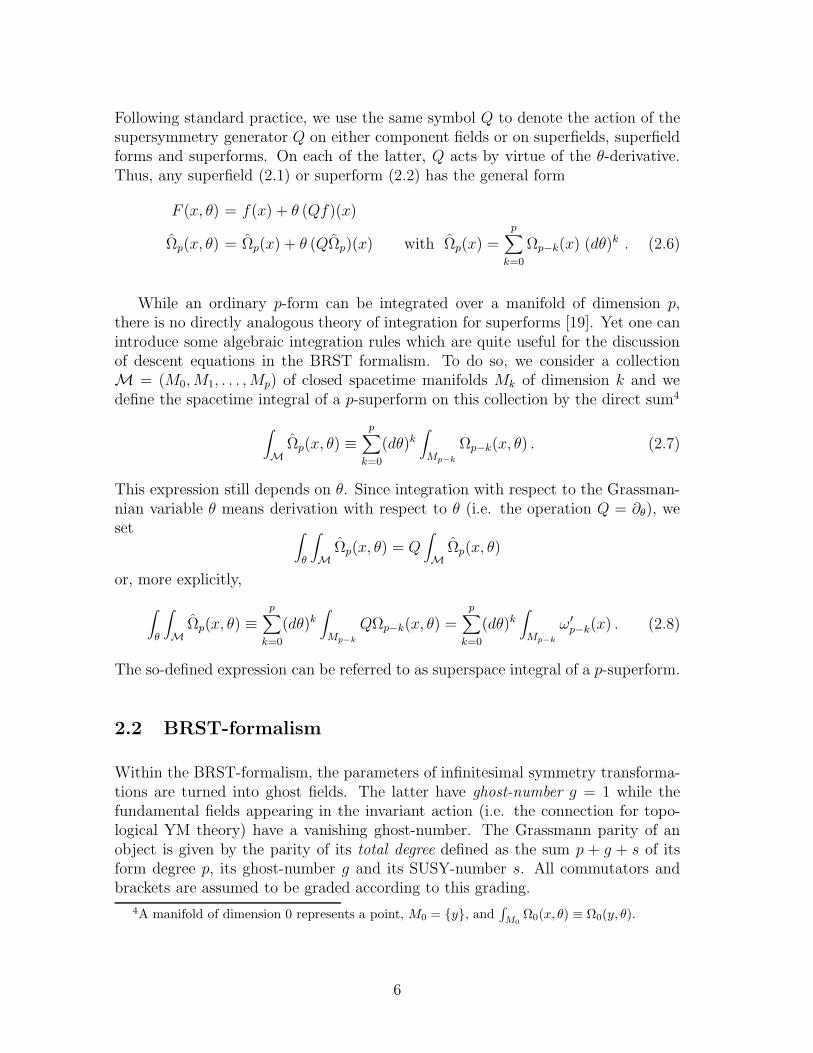
Following standard practice, we use the same symbol Q to denote the action of thesupersymmetry generator Q on either component fields or on superfields, superfieldforms and superforms. On each of the latter, Q acts by virtue of the θ-derivative.Thus, any superfield (2.1) or superform (2.2) has the general form

F (x, θ) = f(x) + θ (Qf)(x)

Ωp(x, θ) = Ωp(x) + θ (QΩp)(x) with Ωp(x) =p

∑

k=0

Ωp−k(x) (dθ)k . (2.6)

While an ordinary p-form can be integrated over a manifold of dimension p,there is no directly analogous theory of integration for superforms [19]. Yet one canintroduce some algebraic integration rules which are quite useful for the discussionof descent equations in the BRST formalism. To do so, we consider a collectionM = (M0,M1, . . . ,Mp) of closed spacetime manifolds Mk of dimension k and wedefine the spacetime integral of a p-superform on this collection by the direct sum4

∫

M

Ωp(x, θ) ≡p

∑

k=0

(dθ)k∫

Mp−k

Ωp−k(x, θ) . (2.7)

This expression still depends on θ. Since integration with respect to the Grassman-nian variable θ means derivation with respect to θ (i.e. the operation Q = ∂θ), weset ∫

θ

∫

M

Ωp(x, θ) = Q∫

M

Ωp(x, θ)

or, more explicitly,

∫

θ

∫

M

Ωp(x, θ) ≡p

∑

k=0

(dθ)k∫

Mp−k

QΩp−k(x, θ) =p

∑

k=0

(dθ)k∫

Mp−k

ω′

p−k(x) . (2.8)

The so-defined expression can be referred to as superspace integral of a p-superform.

2.2 BRST-formalism

Within the BRST-formalism, the parameters of infinitesimal symmetry transforma-tions are turned into ghost fields. The latter have ghost-number g = 1 while thefundamental fields appearing in the invariant action (i.e. the connection for topo-logical YM theory) have a vanishing ghost-number. The Grassmann parity of anobject is given by the parity of its total degree defined as the sum p + g + s of itsform degree p, its ghost-number g and its SUSY-number s. All commutators andbrackets are assumed to be graded according to this grading.

4A manifold of dimension 0 represents a point, M0 = y, and∫

M0

Ω0(x, θ) ≡ Ω0(y, θ).

6

2.3 Topological Yang-Mills theory in superspace

The basic variables are the connection 1-superform A(x, θ) and the ghost super-field C(x, θ) which corresponds to infinitesimal supergauge transformations. Thesevariables are Lie algebra valued, i.e.

A = AaTa , C = CaTa , [Ta, Tb] = fabcTc ,

where the matrices Ta represent the generators of the Lie group that is chosen asstructure group of the theory.

The BRST transformations of A and C describing the supergauge invariance ofthe theory read as

SA = −(dC + [A, C]) , SC = −C2 . (2.9)

The so-defined BRST operator S is nilpotent, i.e. S2 = 0.

Let us now introduce the components of the 1-superform A,

A = A(x, θ) + dθ Aθ(x, θ) , (2.10)

as well as the spacetime components of all superfield forms:

A(x, θ) = a(x) + θ ψθ(x) , C(x, θ) = c(x) + θ c′θ(x)

Aθ(x, θ) = χθ(x) + θ φθθ(x) . (2.11)

Here, a denotes the connection 1-form associated to ordinary gauge transformationsand c the corresponding ghost. In the sequel, the covariant derivative with respectto a will be denoted by Dac = dc+ [a, c] and the θ-indices labeling spacetime fieldswill be omitted in order to simplify the notation.

Substitution of (2.10) into (2.9) yields the BRST transformations of A and Aθ,

SA = −(dC + [A,C]) ≡ −DAC , SAθ = −(∂θC + [Aθ, C]) (2.12)

and the expansions (2.11) provide the BRST transformations of the spacetime fields:

Sa = −Dac , Sc = −c2

Sψ = −[c, ψ] −Dac′ , Sc′ = −[c, c′]

Sφ = −[c, φ] − [χ, c′] , Sχ = −[c, χ] − c′ .

(2.13)

The supersymmetry transformations of all component fields appearing in (2.11) fol-low from (2.5):

Qa = ψ , Qχ = φ , Qc = c′

Qψ = 0 , Qφ = 0 , Qc′ = 0 .(2.14)

7

We have the graded commutation relations

[S, Q] = [S, d] = [d,Q] = 0 .

It is quite useful to consider the following redefinitions of superfields:

Ψ ≡ ∂θA +DAAθ = ψ +DAAθ

Φ ≡ ∂θAθ + A2θ = φ+ A2

θ

K ≡ −(∂θC + [Aθ, C]) = −c′ − [Aθ, C] .

(2.15)

In fact, in terms of these expressions, the dθ-expansion of the supercurvature formF = dA+ A2 reads as

F = FA + Ψ dθ + Φ (dθ)2 , with FA = dA+ A2 , (2.16)

while the BRST transformations read as

SA = −DAC , SC = −C2

SΨ = −[C,Ψ] , SΦ = −[C,Φ]

SAθ = K , SK = 0 ,

(2.17)

and the supersymmetry transformations are given by

QA = Ψ −DAAθ , QΨ = −DAΦ − [Aθ,Ψ]

QFA = −DAΨ − [Aθ, FA] , QΦ = −[Aθ,Φ] .(2.18)

We note that Q acts on A,Ψ,Φ and the curvature FA according to

Q = Q0 + S|C=Aθ,

with

Q0A = Ψ , Q0Ψ = −DAΦ , Q0Φ = 0 (2.19)

(Q0)2 = infinitesimal supergauge transformation with parameter Φ .

Thus, the operatorQ0 is nilpotent when acting on an invariant polynomial dependingon the variables FA,Ψ,Φ, DAΨ, DAΦ.

In this paper, all space-time forms will be taken as polynomials of the basicforms a, ψ, χ, φ, c, c′ and their d-derivatives. Superfield forms and superforms willbe taken as polynomials of the basic superfield forms A, Aθ, C and their ∂θ- andd-derivatives. Since we only discuss the kinematics, we do not fix a priori the space-time dimension. The respective functional spaces will be denoted by

E : space-time forms , ES : superfield forms , ES : superforms . (2.20)

We conclude this section with two results which will be important for our inves-tigations:

8

Proposition 2.1 The cohomology H(Q) of the supersymmetry operator Q inthe space E , ES or ES is trivial, i.e.

If Qϕ = 0 , then ϕ = Qϕ′ ,

with both ϕ and ϕ′ belonging to either E , ES or ES .(2.21)

Proof: For the functional space E ,the proof follows from the fact that all fieldsrepresent Q-doublets f, f ′ with Qf = f ′ and Qf ′ = 0, and from a well-knownresult according to which such doublets do not contribute to the cohomology (e.g.see proposition 5.8. of reference [21]). The extension of this result to the spaces ES

and ES is straightforward, the action of the operator Q being given on these spacesby the derivative ∂θ. q.e.d.

Proposition 2.2 (“Algebraic Poincare Lemma”). The cohomology H(d) ofthe exterior derivative d in the space E , ES or ES is trivial.

Proof: The result for the space E is well known [12] within the present contextwhere the space-time dimension is not fixed a priori. The extension to the spacesES or ES follows by considering an expansion in θ or in θ and dθ, respectively, andby using the linearity of d. q.e.d.

2.4 Topological Yang-Mills in the Wess-Zumino gauge

2.4.1 Symmetry transformations in the WZ-gauge

The supergauge freedom can be reduced to the ordinary gauge freedom by imposingthe Wess-Zumino (WZ) supergauge condition

χ = 0 . (2.22)

By virtue of eqs.(2.13), the S-invariance of this condition requires c′ = 0. The S-variations (2.13) then reduce to the BRST transformations in the WZ-gauge whichdescribe ordinary gauge transformations:

Sa = −Dac , Sψ = −[c, ψ] , Sφ = −[c, φ] , Sc = −c2 . (2.23)

Condition (2.22) is not invariant under the SUSY generator Q, i.e. under the vari-ations (2.14). A modified SUSY operator Q which leaves this condition stable isobtained by combining Q with a compensating BRST transformation (2.13) accord-ing to

Q = Q+ S|χ=c=0, c′=φ on a, ψ, φ . (2.24)

9

Thus, we get the supersymmetry transformations in the WZ-gauge,

Qa = ψ , Qψ = −Daφ , Qφ = 0 , (2.25)

which satisfy

Q2 = infinitesimal gauge transformation with parameter φ . (2.26)

A crucial point of the theory is the fact that the operator Q is nilpotent whenacting on invariant polynomials, very much like the operator Q0 defined in (2.19).We also note that the algebra generated by the forms a, ψ and φ and their exteriorderivatives, together with the action of the operators S and Q given by (2.23) and(2.25) is isomorphic to the algebra generated by the superfield forms A, Ψ and Φ(defined in eq.(2.15)) and their exterior derivatives, together with the action of theoperators S and Q0 given by (2.17) and (2.19).

The supersymmetry-BRST formalism defined by eqs.(2.25) and (2.23) is the oneused by Witten in his pioneering work on four-dimensional topological YM theory [1].We emphasize that the only ghost field in this approach is c (as well as c′ in a generalsupergauge). This fact is in contrast to some other approaches where ψ and φ haveghost-numbers 1 and 2, respectively (e.g. see [8, 13])5.

For later reference, we display the θ-expansion of the superconnection A and ofthe associated curvature F = dA + A2 in the WZ-gauge (cf. (2.16)):

A = a + θ ψ + θdθ φ

F = Fa + ψ dθ + φ (dθ)2 − θ Daψ − θdθ Daφ . (2.27)

2.4.2 Witten’s observables and descent equations

The expression (2.27) of F has the form

F = F + θ QF with F ≡ Fa + ψ dθ + φ (dθ)2 , (2.28)

i.e. it is of the same form as a generic superform in a general gauge, cf. eq.(2.6).More specifically, one can check that we have

QF = −(DaF) (dθ)−1 , (2.29)

where the notation (dθ)−1 is symbolic, though it can be further justified.

The quantity F represents the curvature of the universal bundle considered byBaulieu and Singer [13] in their derivation of Witten’s observables. (Actually, these

5In fact, in these approaches our ghost- and SUSY-numbers are added together so as to yield asingle BRST ghost-number.

10

authors did not introduce the monomials dθ, rather they associated ghost-numbers1 and 2 to ψ and φ, respectively.) For the derivation of observables, we can argueas follows. For m = 1, 2, . . ., we have

Tr Fm = TrFm + θ QTrFm ,

where the first term yields the Donaldson-Witten polynomials,

TrFm = TrFam + Tr (mFa

m−1ψ)dθ + · · ·+ Tr (mψφm−1)(dθ)2m−1 + Trφm(dθ)2m

≡2m∑

p=0

ωp (dθ)2m−p (2.30)

and where the second term represents a total derivative by virtue of eq.(2.29):

QTrFm = −dTrFm (dθ)−1 .

By substituting the expansion (2.30) into the last relation, we obtain Witten’s de-scent equations for the polynomials ωp:

Qωp + dωp−1 = 0 ( p = 0, 1, . . . , 2m ) . (2.31)

Here and in the following, the forms of negative form degree are assumed to vanishby convention.

2.4.3 Combining all symmetries

It is possible to incorporate the transformations (2.25) into the BRST algebra byintroducing a constant commuting ghost ε: the BRST operator then acts on a, ψ, φaccording to

Stot = S + εQ (2.32)

and on c, ε according to

Stotc = −c2 + ε2φ , Stotε = 0 , (2.33)

which ensures the nilpotency of the operator Stot. More explicitly, we have theexpansion [9]

Stot = S0 + εS1 + ε2S2 , (2.34)

withS0a = −Dac , S1a = ψ , S2a = 0

S0ψ = −[c, ψ] , S1ψ = −Daφ , S2ψ = 0

S0φ = −[c, φ] , S1φ = 0 , S2φ = 0

S0c = −c2 , S1c = 0 , S2c = φ .

(2.35)

11

where(S0)

2 = 0 , [S0, S1] = 0 , (S1)2 + [S0, S2] = 0 . (2.36)

In terms of the notation introduced above, we have S0 = S and S1 = Q on a, ψ, φ.If we only consider functionals ∆ depending on a, ψ, φ and not on c (i.e. functionalsof zero ghost-number), then the last relation of (2.36) is nothing but (2.26). If thesefunctionals are, in addition, gauge invariant, then the operator S1 is nilpotent:

S0∆ = 0 = S2∆ =⇒ (S1)2∆ = 0 . (2.37)

Its cohomology is referred to as equivariant cohomology and will be further discussedin the next section. (Thus, equivariant cohomology is the cohomology of the operatorS1 in the space of local functionals of a, ψ, φ and c restricted by S2 - and S0 -invariance.)

To conclude, we note that the algebra (2.32)(2.33) can also be obtained alonga slightly different, though equivalent line of reasoning. In fact, we could includethe supersymmetry variations generated by εQ right away into the BRST trans-formations (2.13): the stability of the WZ-condition (2.22) then restricts the ghostfield c′ to be equal to εφ and readily yields the results (2.32)(2.33). The decou-pling (2.23)(2.25) is realized [9] by considering the filtration N = ε ∂/∂ε and theexpansion (2.34).

3 Observables in the superspace formalism

In the following, the expression sϕgp denotes a p-form ϕ of ghost-number g and

SUSY-number s.

3.1 Equivariant cohomology and Witten’s observables

Let us first consider the WZ-gauge setting described in the preceding section since thelatter has been chosen in all former discussions of observables. The representation(2.34)-(2.36) of the complete set of symmetry transformations is quite useful forspecifying the cohomological characterization of observables. As is well known, thecohomology of the operator Stot is empty [8]. Not so the equivariant cohomologywhich can be described in several different ways [1, 8]. As mentioned in the lastsection, it can be characterized as the cohomology of the operator Q (defined by(2.25)) in the space of the gauge invariant local functionals of a, ψ, φ [1]. Thus, atform degree zero, one looks for a local functional s∆(0) =

∫

M0

sω00(x) which solves

the Q-cocycle condition, i.e.Q s∆(0) = 0 , (3.1)

12

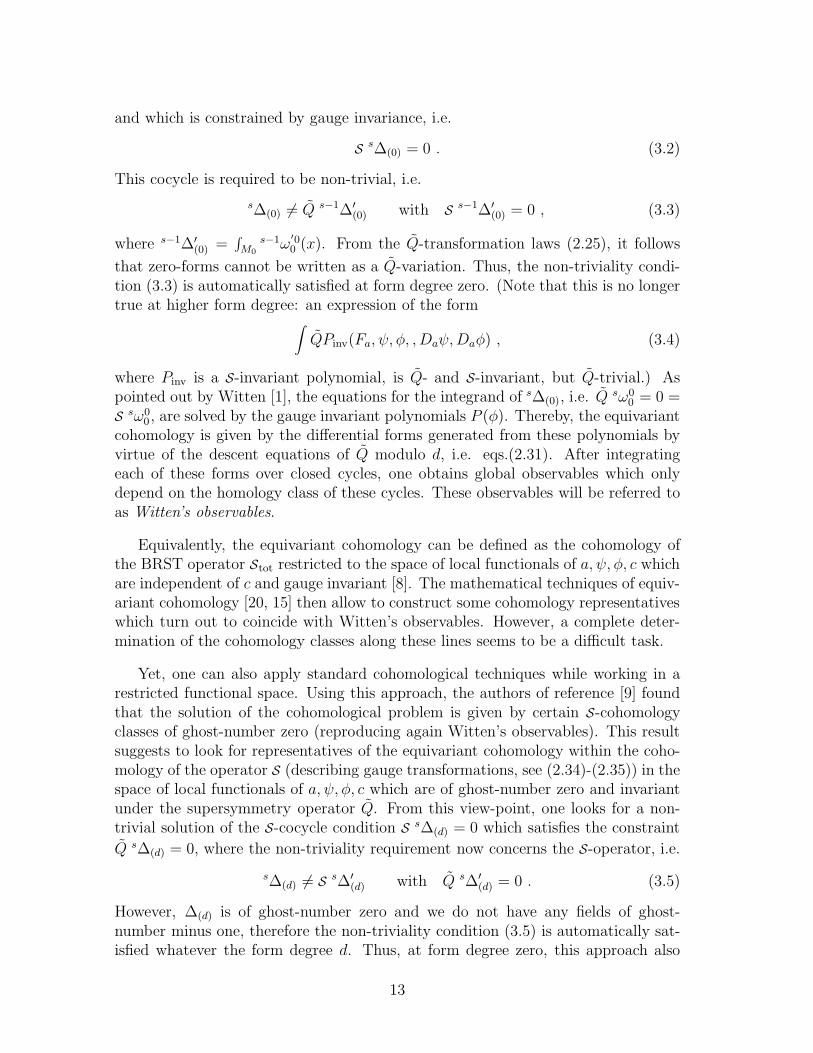
and which is constrained by gauge invariance, i.e.

Ss∆(0) = 0 . (3.2)

This cocycle is required to be non-trivial, i.e.

s∆(0) 6= Q s−1∆′

(0) with S s−1∆′

(0) = 0 , (3.3)

where s−1∆′

(0) =∫

M0

s−1ω′00 (x). From the Q-transformation laws (2.25), it follows

that zero-forms cannot be written as a Q-variation. Thus, the non-triviality condi-tion (3.3) is automatically satisfied at form degree zero. (Note that this is no longertrue at higher form degree: an expression of the form

∫

QPinv(Fa, ψ, φ, ,Daψ,Daφ) , (3.4)

where Pinv is a S-invariant polynomial, is Q- and S-invariant, but Q-trivial.) Aspointed out by Witten [1], the equations for the integrand of s∆(0), i.e. Q sω0

0 = 0 =S sω0

0, are solved by the gauge invariant polynomials P (φ). Thereby, the equivariantcohomology is given by the differential forms generated from these polynomials byvirtue of the descent equations of Q modulo d, i.e. eqs.(2.31). After integratingeach of these forms over closed cycles, one obtains global observables which onlydepend on the homology class of these cycles. These observables will be referred toas Witten’s observables.

Equivalently, the equivariant cohomology can be defined as the cohomology ofthe BRST operator Stot restricted to the space of local functionals of a, ψ, φ, c whichare independent of c and gauge invariant [8]. The mathematical techniques of equiv-ariant cohomology [20, 15] then allow to construct some cohomology representativeswhich turn out to coincide with Witten’s observables. However, a complete deter-mination of the cohomology classes along these lines seems to be a difficult task.

Yet, one can also apply standard cohomological techniques while working in arestricted functional space. Using this approach, the authors of reference [9] foundthat the solution of the cohomological problem is given by certain S-cohomologyclasses of ghost-number zero (reproducing again Witten’s observables). This resultsuggests to look for representatives of the equivariant cohomology within the coho-mology of the operator S (describing gauge transformations, see (2.34)-(2.35)) in thespace of local functionals of a, ψ, φ, c which are of ghost-number zero and invariantunder the supersymmetry operator Q. From this view-point, one looks for a non-trivial solution of the S-cocycle condition S s∆(d) = 0 which satisfies the constraint

Q s∆(d) = 0, where the non-triviality requirement now concerns the S-operator, i.e.

s∆(d) 6= S s∆′

(d) with Q s∆′

(d) = 0 . (3.5)

However, ∆(d) is of ghost-number zero and we do not have any fields of ghost-number minus one, therefore the non-triviality condition (3.5) is automatically sat-isfied whatever the form degree d. Thus, at form degree zero, this approach also

13

reduces to the cohomology problem (3.1)(3.2) without any further requirements. Athigher form degree, it regards as non-trivial the solutions of the form (3.4) whichare trivial representatives of equivariant cohomology.

The latter approach can easily be extended beyond the WZ-gauge: in a generalsupergauge, the equivariant cohomology can be determined by looking for the ghost-number zero cohomology classes of the BRST operator (2.9) or (2.13) in the spaceof the supersymmetric local functionals (the supersymmetry transformations beingdefined by means of the operator Q according to (2.14)). In the following, weshall completely determine this cohomology while working within the superspaceformalism, only specifying to the WZ-gauge (χ = 0) towards the end.

Thus, let us consider a fixed SUSY-number s ≥ 0 and a fixed degree d ≥ 0. Thetask is to find a solution of the cocycle condition

Ss∆(d) = 0 , (3.6)

satisfying the SUSY constraint

Q s∆(d) = 0 . (3.7)

Here,s∆(d) =

∫

Md

sω0d(x) (3.8)

denotes a local functional of SUSY-number s which depends on the components ofthe superfield forms A,Aθ, C and their exterior derivatives. Since the solution of theproblem (3.6)(3.7) proceeds in several steps, we shall present a summary of resultsat the end of each of the following sections.

Our discussion will be purely algebraic and does not assume a specification of thespacetime dimension n. If the latter is specified, all forms of degree greater than nvanish identically. Those of degree d smaller than n can be integrated over orientedsubmanifolds Md. The latter manifolds are assumed to be closed which implies theabsence of boundary terms upon integration over Md. Thus, we exclude from ourdiscussion the “trivial” solution of (3.6)(3.7) which exists for d = 2m,

0∆(2m) =∫

M2m

0ω02m ≡

∫

M2m

TrFam (m = 1, 2, . . . ) , (3.9)

since the Pontrjagin density TrFam is locally given by the exterior derivative of the

Chern-Simons form of degree 2m− 1.

Before tackling the cohomological problem in full generality, we already note thatthe determination of observables that we presented for the WZ-gauge in subsection2.4.2 can be generalized to a general supergauge as follows.

According to equation (2.6), the curvature 2-superform has the general form

F (x, θ) = F (x) + θ (QF )(x) ,

14

where the first term of this expansion can also be written as F∣

∣

∣

θ=0≡ F |. (In the

WZ-gauge, the latter expression reduces to the form F introduced in eq.(2.28).) Form = 1, 2, . . ., the 2m-superform Tr Fm(x, θ) admits an analogous expression:

Tr Fm = Tr F |m + θ QTr Fm

with Tr F |m =2m∑

p=0

2m−pw0p (dθ)2m−p . (3.10)

Since Tr Fm is a closed superform,

0 = dTr Fm = (dθ∂θ + d) Tr Fm = (QTr Fm) dθ + dTr Fm ,

it follows by projection onto the θ = 0 component that

QTr F |m = −(dTr F |m) (dθ)−1 .

By substituting the expansion (3.10) into this relation, we get Witten’s descentequations in a general supergauge:

Q 2m−pw0p + d 2m−p+1w0

p−1 = 0 ( p = 0, 1, . . . , 2m ) . (3.11)

Explicit expressions for the polynomials wp for m = 1 and m = 2 will be given insection 4 below and here we only note that 0w0

2m = TrFam whatever the value of m.

The task of the next subsections is to determine if other solutions can be obtainedby virtue of a systematic study in superspace.

3.2 The bi-descent equations

In this section, we shall show that the cohomological problem (3.6)(3.7) leads to aset of bi-descent equations involving superfield forms. Let us first solve the SUSYconstraint (3.7) for s∆(d) given by (3.8). For the integrand sω0

d(x), it implies

Q sω0d + d s+1ω0

d−1 = 0 . (3.12)

In view of this relation, we shall prove the following proposition:

Proposition 3.1 Let p and s be non-negative integers. (Here, we do not referto the ghost-number which only represents a passive label in this proposition.)

(i) The cocycle condition

Q sωp + d s+1ωp−1 = 0 (3.13)

implies the Q modulo d triviality of the space-time form sωp and the d moduloQ triviality of the space-time form s+1ωp−1:

sωp = Q s−1ϕp + d sϕp−1 (3.14)

s+1ωp−1 = Q sϕp−1 + d s+1ϕp−2 , (3.15)

15

with the same space-time form sϕp−1 appearing in both equations.

(ii) The same result holds for superfield forms, i.e.

Q sΩp + d s+1Ωp−1 = 0 (3.16)

implies

sΩp = Q s−1Φp + d sΦp−1 (3.17)

s+1Ωp−1 = Q sΦp−1 + d s+1Φp−2 . (3.18)

Proof: See appendix A.1.

With the help of this proposition, we deduce from (3.12) that

sω0d = Q s−1ω0

d . (3.19)

Here and in the following, the total derivative term is suppressed without loss ofgenerality, since it does not contribute to the integrated cocycle s∆(d). Furthermore,without loss of generality, we can assume s−1ω0

d to be a superfield form

s−1Ω0d = s−1ω0

d + θ Q s−1ω0d , (3.20)

so that (3.19) reads assω0

d = Q s−1Ω0d .

Since the operator Q acts on superfield forms by the θ-derivative, this shows thats∆(d) is the superspace integral of s−1Ω0

d:

Q s∆(d) = 0 =⇒ s∆(d) =∫

Md

Q s−1Ω0d . (3.21)

Next, we turn to the cocycle condition (3.6). Since the cohomology of d in thespace of local field polynomials is trivial [12], this condition implies the descentequations6

S sωd−pp + d sωd−p+1

p−1 = 0 ( p = 0, . . . , d ) . (3.22)

Lemma 1 The SUSY constraint implies that every form in (3.22) (and not justthe one of highest form degree, i.e. sω0

d) can be written as a SUSY variation,

sωd−pp = Q s−1Ωd−p

p ( p = 0, . . . , d ) , (3.23)

where s−1Ωd−pp is a superfield form.

6Every form of negative form degree, ghost-number or SUSY-number is assumed to vanish byconvention.

16

The proof of this statement proceeds by induction, see appendix A.2.

We note that in eqs.(3.22) and thus in (3.23) and in the equations to follow,the array of descent equations may terminate at some positive form degree that wedenote by p > 0. (A simple illustration of such a “termination of descent” withinabelian gauge theory (with field strength F = da) is given by the cocycles ω0

3 = aFand ω1

2 = cF , which satisfy Sω03 + dω1

2 = 0 and Sω12 = 0, so that p = 2 in this case.)

In such a case, we use the convention that every form of form degree less than p isvanishing.

We are now going to prove:

Proposition 3.3 For given values of s and d, the descent equations (3.22)together with the SUSY constraint (3.23) imply a set of descent equationsinvolving superfield forms and all of the three indices:

S s−r−1Ωd−p+rp + d s−r−1Ωd−p+r+1

p−1 +Q s−r−2Ωd−p+r+1p = 0

( r = 0, . . . , s− 1 ; p = 0, . . . , d ) .(3.24)

We shall call this set of equations the bi-descent equations for the pair (d, s).

Proof: In order to derive this result, we first rewrite (3.22), using the result (3.23),as

Q(

S s−1Ωd−pp + d s−1Ωd−p+1

p−1

)

= 0 .

The triviality of the Q-cohomology then implies

S s−1Ωd−pp + d s−1Ωd−p+1

p−1 +Q s−2Ωd−p+1p = 0 ( p = 0, . . . , d ) , (3.25)

where s−2Ωd−p+1p is again taken to be a superfield form. The latter equation is

nothing but (3.24) with r = 0. The validity of the bi-descent equations for all valuesof r is shown by induction, see appendix A.3. q.e.d.

The bi-descent equations for the pair (d, s) as given by eqs.(3.24) involve theforms s−r−1Ωd−p+r

p which all have the same total degree

D = d+ s− 1 . (3.26)

In the following, we shall consider this number to be fixed to some arbitrary valueD ≥ 0. For given values of D, d and s related by (3.26), the bi-descent equationsfor the pair (d, s) then become the bi-descent equations for the pair (d,D), i.e. thesame set of equations with a different labeling of ghost- and SUSY-indices:

S D−p−gΩgp + d D−p−gΩg+1

p−1 +Q D−p−g−1Ωg+1p = 0

( p = 0, . . . , d ; g = d− p, . . . , D − p ) .(3.27)

17

We note that the domain of variation of the indices p and g in this set of equations is aparallelogram Par(d,D) in the (p, g) plane which is bounded by the straight lines p =0, p = d, p+g = d and p+g = D. More precisely, each point of Par(d,D) representsexactly one of the bi-descent equations (3.27), these equations being parametrized bythe form degree and ghost-number of the S-term. The example D = 3 is presentedin detail in section 4.

Summary: By definition, the observables of the theory are the integrated localfunctionals s∆(d) of the form (3.8) satisfying the cocycle condition (3.6) and thesupersymmetry constraint (3.7). For a fixed maximal degree D ≡ d + s − 1 ≥ 0,they are given by superspace integrals of superfield d-forms of ghost-number 0, i.e.

D−d+1∆(d) =∫

Md

Q D−dΩ0d ( d = 0, . . . , D ) , (3.28)

where D−dΩ0d is a non-trivial solution of the bi-descent equations for the pair (d,D),

i.e. eqs.(3.27).

3.3 Superform solutions of the bi-descent equations

When varying d from 0 to its maximum valueD, the parallelograms Par(d,D) fill upthe triangle Tri(D) of vertices (0, 0), (D, 0) and (0, D). The points of this triangledescribe in a one-to-one fashion the bi-descent equations for the forms of total degreeD, i.e. the bi-descent equations for the pairs (d,D) with d = 0, . . . , D:

S D−p−gΩgp + d D−p−gΩg+1

p−1 +Q D−p−g−1Ωg+1p = 0

( p ≥ 0 , g ≥ 0 , p+ g ≤ D ) .(3.29)

The bi-descent equations (3.27) represent subsets of the latter equations which areclosed in the sense that each equation of (3.29) corresponding to a point (p, g) ∈Par(d,D) only involves forms corresponding to points of Par(d,D), i.e. it rep-resents an equation of the set (3.27). Hence a non-trivial solution of (3.29) alsorepresents a solution of (3.27). However, the converse is not necessarily true. In-deed, two forms D−p−gΩg

p and D−p−g(Ω′)gp belonging to the intersection of two

parallelograms Par(d,D) and Par(d′, D) might represent different solutions of thetwo corresponding sets of bi-descent equations.

In this subsection, we shall look for solutions of the system of equations (3.29),thereby providing a special set of solutions of the bi-descent equations (3.27). Thesearch of the general solution of eqs.(3.27) is postponed to section 3.4.

We first introduce the set of q-superforms (cf. eq.(2.2))

ΩD−qq =

q∑

p=0

q−pΩD−qp (dθ)q−p ( q = 0, . . . , D ) , (3.30)

18

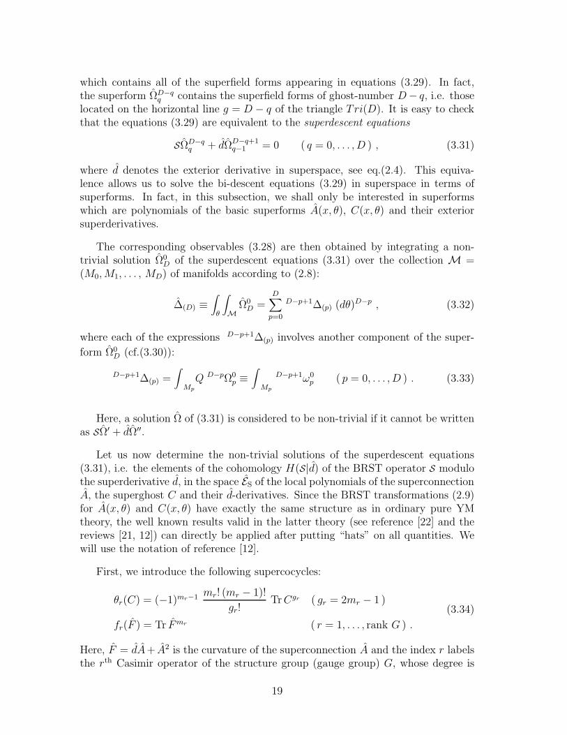
which contains all of the superfield forms appearing in equations (3.29). In fact,the superform ΩD−q

q contains the superfield forms of ghost-number D− q, i.e. thoselocated on the horizontal line g = D − q of the triangle Tri(D). It is easy to checkthat the equations (3.29) are equivalent to the superdescent equations

SΩD−qq + dΩD−q+1

q−1 = 0 ( q = 0, . . . , D ) , (3.31)

where d denotes the exterior derivative in superspace, see eq.(2.4). This equiva-lence allows us to solve the bi-descent equations (3.29) in superspace in terms ofsuperforms. In fact, in this subsection, we shall only be interested in superformswhich are polynomials of the basic superforms A(x, θ), C(x, θ) and their exteriorsuperderivatives.

The corresponding observables (3.28) are then obtained by integrating a non-trivial solution Ω0

D of the superdescent equations (3.31) over the collection M =(M0,M1, . . . , MD) of manifolds according to (2.8):

∆(D) ≡∫

θ

∫

M

Ω0D =

D∑

p=0

D−p+1∆(p) (dθ)D−p , (3.32)

where each of the expressions D−p+1∆(p) involves another component of the super-

form Ω0D (cf.(3.30)):

D−p+1∆(p) =∫

Mp

Q D−pΩ0p ≡

∫

Mp

D−p+1ω0p ( p = 0, . . . , D ) . (3.33)

Here, a solution Ω of (3.31) is considered to be non-trivial if it cannot be writtenas SΩ′ + dΩ′′.

Let us now determine the non-trivial solutions of the superdescent equations(3.31), i.e. the elements of the cohomology H(S|d) of the BRST operator S modulothe superderivative d, in the space ES of the local polynomials of the superconnectionA, the superghost C and their d-derivatives. Since the BRST transformations (2.9)for A(x, θ) and C(x, θ) have exactly the same structure as in ordinary pure YMtheory, the well known results valid in the latter theory (see reference [22] and thereviews [21, 12]) can directly be applied after putting “hats” on all quantities. Wewill use the notation of reference [12].

First, we introduce the following supercocycles:

θr(C) = (−1)mr−1 mr! (mr − 1)!

gr!TrCgr ( gr = 2mr − 1 )

fr(F ) = Tr Fmr ( r = 1, . . . , rank G ) .

(3.34)

Here, F = dA+ A2 is the curvature of the superconnection A and the index r labelsthe rth Casimir operator of the structure group (gauge group) G, whose degree is

19

denoted by mr. The cocycles (3.34) are related by superdescent equations involving

superforms[

θr

]gr−p

pof form degree p ≥ 0 and ghost-number gr − p:

S[

θr

]gr−p

p+ d

[

θr

]gr−p+1

p−1= 0 ( p = 0, . . . , gr ) ,

with[

θr

]gr

0= θr(C) and d

[

θr

]0

gr

= fr(F ) .(3.35)

According to the last equation, the “top” superform[

θr

]0

gr

is the Chern-Simons

superform of degree gr associated to the rth Casimir operator.

Obviously, (3.35) corresponds to the superdescent equations (3.31) and thusyields a solution of the latter equations. More general solutions are found by mul-tiplying the cocycle θr(C) by a certain number of factors fs(F ) since the latter areboth S- and d-invariant. Thus, we introduce the following supercocycle (belongingto the S-cohomology in the space ES):

HR ≡ θr1(C)fr2

(F ) · · · frL(F ) ,

with L ≥ 1 , ri ≤ ri+1 .(3.36)

This cocycle is of ghost-number gr1and superform degree DR =

L∑

i=2

2mri(cf.(3.34)).

By virtue of equations (3.35), the superforms

Ωgr1

−p

DR+p =[

θr1

]gr1−p

pfr2

(F ) · · ·frL(F ) ( p = 0, . . . , gr1

; L ≥ 1 ) (3.37)

obey the superdescent equations

SΩgr1

−p

DR+p + dΩgr1

−p+1DR+p−1 = 0 ( p = 0, . . . , gr1

) . (3.38)

The most general solution of the superdescent equations (3.31) in the space ES isobtained by considering a supercocycle of the form (3.36) which is non-linear inthe monomials θr(C). However, in view of the construction of observables (whichhave zero ghost-number by definition), we are only interested in the most generalsolution containing superforms of ghost-number 0 and the latter are given by (3.37)according to the results of section 10.7 of reference [12], adapted to the presentsuperspace formalism.

The corresponding observables are now constructed according to (3.32)(3.33), byusing (3.37) for p = gr1

, i.e.

Ω0D =

[

θr1

]0

gr1

fr2(F ) · · ·frL

(F ) ≡D

∑

p=0

D−pΩ0p (dθ)D−p ,

with D = DR + gr1= 2

L∑

i=1

mri− 1 , L ≥ 1 .

(3.39)

20

Note that D is necessarily odd.

There is an alternative way of writing the observables which amounts to a sim-pler manner of extracting the polynomials D−p+1ω0

p(x) from the superform Ω0D. This

procedure is suggested by the fact that the exterior derivative d = dθ ∂θ + d differsfrom the superspace SUSY operator ∂θ by a factor dθ and the addition of a space-time derivative. Indeed, let us consider the exterior derivative of Ω0

D and write itsexpansion with respect to dθ (see (2.16)(2.30)):

dΩ0D = fr1

(F ) · · ·frL(F ) = fr1

(FA) · · ·frL(FA) +

D∑

p=0

D+1−pW 0p (dθ)D+1−p ,

(3.40)with

D−p+1W 0p = Q D−pΩ0

p + d D−p+1Ω0p−1

= D−p+1ω0p(x) + d D−p+1Ω0

p−1(x, θ) .

Henceforth, in the integral (3.33) which yields the observables, we can substitutethe form D−p+1ωp by the value of D−p+1Wp at θ = 0:

D−p+1∆(p) =∫

Mp

D−p+1w0p ( p = 0, . . . , D ) ,

with D−p+1w0p = D−p+1W 0

p

∣

∣

∣

θ=0.

(3.41)

Before concluding, we note that application of the superderivative d to (3.40)and use of its nilpotency, leads to

Q D−p+1W 0p + d D−p+2W 0

p−1 = 0 ( p = 0, . . . , D ) ,

which, taken at θ = 0, yields

Q D−p+1w0p + d D−p+2w0

p−1 = 0 ( p = 0, . . . , D ) . (3.42)

These relations for the integrands D+1−pw0p of the observables (3.41) are nothing but

Witten’s descent equations in a general supergauge (generalizing eqs.(2.31) whichhold in the WZ-gauge and involve Q rather than Q). In the WZ-gauge, the poly-nomials D+1−pw0

p reduce - by construction - to the Donaldson-Witten polynomialsdiscussed in subsection 2.4.2. In particular, in the WZ-gauge, we obtain

D+1ω00 = fr1

(φ) · · ·frL(φ) with L ≥ 1, ri ≤ ri+1 , (3.43)

i.e. Witten’s well-known result [1] that the algebra of observables is generated, atform degree zero, by the invariant monomials fs(φ). The examples D = 1 and D = 3will be presented in more detail in section 4.

21

Anticipating the discussion of the next subsection, which shows that there areno other non-trivial observables, we can summarize our results as follows.

Summary: Apart from the ‘trivial’ observables (3.9), there exist further ones. Allof these observables, as defined by the conditions (3.6) and (3.7), are given byeqs.(3.41). In the latter expressions, the superfield forms D−p+1W 0

p are the coef-

ficients appearing in the expansion (3.40), the superform Ω0D being the non-trivial

solution (3.39) of the superdescent equations (3.31) in the space ES of polynomials inthe basic superforms A, C and their exterior superderivatives. The forms D−p+1w0

p

satisfy the generalization of Witten’s descent equations to a general supergauge, i.e.eqs.(3.42).

3.4 General solution of the bi-descent equations for the pair

(d,D)

As noted at the beginning of the last section, the solutions of the superdescentequations (3.31) in the space ES (which is generated by the superforms A, C andthe operators S, d) represent a priori only a special set of solutions of the bi-descentequations for the pair (d,D), i.e. eqs.(3.27). Henceforth, we have to determine thegeneral non-trivial solution of the latter equations in order to obtain the general setof observables. At this point, we only state and comment on the main result, leavingthe proof for appendix A.4.

Proposition 3.4 The general solution of the bi-descent equations (3.27) forthe pair (d,D) is generated, at ghost-number zero, by two classes of solutions.The first one is given by the superfield forms

D−dΩ0d (dθ)D−d =

[

[

θr1

]0

gr1

fr2(F ) · · · frL

(F )]

s=D−d, p=d

with D = 2L

∑

i=1

mri− 1 , L ≥ 1 ,

(3.44)

where the Chern-Simons superform[

θr

]0

gr

and supercurvature invariant fr(F )

are defined by (3.35)(3.34).

The second class of solutions depends on the superfield forms FA,Ψ and Φdefined in eqs.(2.16)(2.15) and it is given by

D−dΩ0d = D−dZ0

d (FA,Ψ,Φ, DAΨ, DAΦ) . (3.45)

Here, D−dZ0d is an arbitrary invariant polynomial of its arguments, which has

a form degree d and SUSY-number D−d and which is non-trivial in the sensethat D−dZ0

d 6= d D−dΦ0d−1 +Q D−d−1Φ0

d.

22

Proof: See appendix A.4.

Concerning the invariant forms (3.45), we note that they represent the generalcohomology classes of the BRST operator S in the space ES by virtue of a mereadaptation of the results of section 8 of reference [12].

According to (3.33), the observables are obtained as integrals of the Q-variationof the solutions (3.44)(3.45) over a d-dimensional manifold. The ones correspond-ing to (3.44) coincide with the corresponding expressions calculated in section 3.3(i.e. (3.41) with p = d) since the corresponding integrands only differ by a totalderivative. In fact, for d = 0, 1, . . . , D, the superfield forms D−dΩ0

d given in (3.44)are nothing but those introduced in (3.39). Hence, the solutions (3.44) provide thesame observables as the superform solutions (3.39).

On the other hand, for the solutions (3.45), one gets the integrals

D−d+1∆(d) =∫

Md

Q D−dZ0d (FA,Ψ,Φ, DAΨ, DAΦ) . (3.46)

As pointed out after equation (2.18), the operator Q simply reduces to Q0 whenacting on an invariant polynomial D−dZ0

d . Yet, as noted after equation (2.26), theaction of Q0 is isomorphic to the one of the operator Q describing supersymmetrytransformations in the WZ-gauge. This means that the solution (3.46), if written outin the WZ-gauge, is simply the Q-variation of a gauge invariant polynomial. Thus, itis trivial in the sense of equivariant cohomology , see eqs.(3.1)-(3.3). This explicitlyshows that the cohomology defined by equations (3.6)-(3.7) is not equivalent to theequivariant cohomology: the difference is precisely given by the expressions of theform (3.46), which are manifestly Q-trivial.

We conclude that, apart from the solutions (3.45) which are “equivariantly” triv-ial, the general solution of the bi-descent equations that we described in this sectiondoes not yield any more solutions than those obtained in terms of superforms insection 3.3. In other words, the solution constructed by using superforms representsthe most general, equivariantly non-trivial expression for the observables.

4 Explicit expressions

4.1 An example of bi-descent and superdescent

equations

There is a graphical way of representing the sets of bi-descent equations which allowsus to exhibit explicitly the combinatorics leading to the superdescent equations(3.31).

23

By way of illustration, let us consider the case of total degree D = 3. We have10 superfield forms 3−p−gΩg

p in the bi-descent equations for total degree D = 3, i.e.eqs.(3.29), which can be represented in the (p, g) diagram:

g ↑

3 •2 • •1 • • •0 • • • •

0 1 2 3p→

E.g. the point on the outer right represents the form 0Ω03. The forms listed in

the previous diagram appear in different sets of bi-descent equations (3.27): ford = 0, 1, 2, 3 and D = 3, the latter bi-descent equations correspond to the followingsub-diagrams of the previous diagram:

d = 0 : d = 1 : d = 2 : d = 3 :

•• • •

•• •• • •

•• • • • •

• • • •

Thus, one clearly sees how the parallelograms representing equations (3.27) overlapfor the various values of d (and a fixed valueD) finally covering the full triangle in the(p, g) plane which represents the bi-descent equations (3.29). Obviously, this trianglealso represents the superdescent equations (3.31). The latter equations presentlytake the same form as the descent equations in 3-dimensional Chern-Simons fieldtheory for which the solution is well known, e.g. see reference [21]. Thus, for D = 3,the non-trivial solution of the superdescent equations (3.31) is given by

Ω03 = Tr (AdA+

2

3A3) , Ω1

2 = Tr (AdC) , Ω21 = Tr (CdC) , Ω3

0 = −13

TrC3 .

(4.1)

4.2 Some examples of observables

In this section, we consider the structure group U(1) × SU(2) to illustrate theconclusions of section 3. For this group, there are two Casimir operators: the U(1)generator itself (the charge) and the quadratic Casimir of SU(2). Their degrees arerespectively m1 = 1 and m2 = 2.

In the sequel, we shall use an index ‘(a)’ for ‘abelian’. The ghosts, connections

24

and curvatures are, respectively, given by the following superfields and -forms:

U(1) : C(a) , A(a) , F(a) = dA(a)

SU(2) : C , A , F = dA+ A2 .

The “canonical” basis (3.34) of the cohomology H(S) reads as

θ1 = θ1(C) = C(a) , f1 = f1(F(a)) = F(a)

θ2 = θ2(C) = −13TrC3 , f2 = f2(F ) = Tr F 2

(4.2)

and the canonical descent equations (3.35) involve the forms

U(1) : [θ1]10 = θ1 , [θ1]

01 = A(a)

SU(2) : [θ2]30 = θ2 , [θ2]

21 = Tr (CdC)

[θ2]12 = Tr (AdC) , [θ2]

03 = Tr (AdA+ 2

3A3) .

(4.3)

Let us now look for the observables that can be deduced from the cohomology of S

modulo d, i.e. from the non-trivial solutions of the superdescent equations (3.31).We shall consider three cases, namely the two sets of basic observables correspondingto the two Casimir operators, and one set of “composite” observables.

An example of a solution of the superdescent equations which does not yieldobservables is obtained from the bottom superform Ω4

0 = θ1θ2: this provides asimple illustration of the general formalism where the climbing stops at the formdegree equal to the ghost-number of θ1, namely degree 1.

4.2.1 Solution corresponding to the Casimir of U(1)

The superdescent equations for total degree D = 1,

SΩ10 = 0 , SΩ0

1 + dΩ10 = 0 ,

are solved by the superforms

Ω10 = 0Ω1

0 = θ1 = C(a)

Ω01 = 0Ω0

1 + 1Ω00 dθ = A(a) .

The latter coincide with the “canonical” superforms (4.3) for U(1).

According to the results of section 3.3 (see eqs.(3.40)(3.41)), the observables areobtained from the superspace exterior derivative of the top superform Ω0

1 (which hasghost-number zero) and given by the expansion at θ = 0:

dΩ01

∣

∣

∣

θ=0= F(a)

∣

∣

∣

θ=0= F(a) + 1w0

1 dθ + 2w00 (dθ)2 ,

with F(a) = da(a) ,1w0

1 = ψ(a) + dχ(a) ,2w0

0 = φ(a).(4.4)

25

Apart from the ‘trivial’ observable∫

M2F(a), the observables are the integrals of the

forms 1w01,

2w00 on closed submanifolds M1 and M0, respectively. The polynomials

wp satisfy Witten’s descent equations in a general supergauge, i.e. eqs.(3.42).

Equivalently – cf.(3.32)-(3.33) – the superspace integral of the superform Ω01 over

a collection M = (M0,M1) of closed submanifolds is a direct sum of two integrals,

∆(1) ≡∫

θ

∫

M

Ω01 =

∫

M

∂θΩ01 =

1∑

p=0

(dθ)1−p∫

Mp

2−pω0p , (4.5)

where the p-forms 2−pω0p are the coefficients of the expansion of ∂θΩ

01. Each integral

in (4.5) defines an expression belonging to the SUSY-constrained cohomology of S.These integrals coincide with those of the forms wp defined in (4.4).

In the WZ-gauge χ = 0, the expressions (4.4) reduce to the Donaldson-Wittenpolynomials generated from the invariant φ(a) using the supersymmetry operator Q,see eqs.(2.30) with m = 1. In our approach, these polynomials have been generatedforD = 1 from the bottom superform Ω1

0 = C(a) which solves superdescent equations.

4.2.2 Solution corresponding to the Casimir of SU(2)

The bottom form Ω30 = θ2 has total degree D = 3 and the solution of the superde-

scent equations is given by the superforms (4.1). These expressions coincide withthe canonical superforms (4.3) for SU(2). Applying again proposition 4, we obtainthe observables from the expansion

dΩ03

∣

∣

∣

θ=0= Tr F 2

∣

∣

∣

θ=0= TrFa

2 +3

∑

p=0

4−pw0p (dθ)4−p , (4.6)

the last term being an exterior derivative. By substituting the component fieldexpansions (2.10)(2.11) of A into Ω0

3, we obtain the following explicit expressions forthe spacetime forms:

4w00 = Tr (φ2 + 2φχ2)

3w01 = Tr 2(ψφ+ ψχ2 + φDaχ) + dTr (2

3χ3)

2w02 = Tr (ψ2 + 2φFa + 2ψDaχ) + dTr (χDaχ)

1w03 = Tr (2ψFa) + dTr (2χFa)) .

(4.7)

The observables are the integrals of these forms (and of TrFa2) on closed submani-

folds of appropriate dimension.

In the WZ-gauge χ = 0, the expressions for the observables again reduce toWitten’s result (generated from the quadratic invariant Trφ2), i.e. eqs.(2.30) withm = 2.

26

4.2.3 An example of “composite observables”

As stated at the end of section 3.3, all other observables are integrals whose inte-grands are polynomials of the forms wp that we constructed in the last two subsec-tions (i.e. of the forms associated to the Casimir operators). Let us illustrate thiswith the simplest example, generated by the bottom form Ω1

2 = θ1f1 which is oftotal degree 3. The corresponding top superform is given by Ω0

3 = A(a)F(a) and the

expansion of its superderivative dΩ03 = (F(a))

2 yields the following integrands for theobservables:

4w00 = (2w0

0)2 = φ2

(a)

3w01 = 2 (1w0

1) (2w00)

2w02 = 2 2w0

0 F(a) + (1w01)

2

1w03 = 2 1w0

1 F(a)

0w04 = F 2

(a) .

(4.8)

Obviously, these forms are polynomials in the basic forms given in eqs.(4.4) and inthe abelian curvature invariant f1 = F(a).

5 Concluding remarks

We have shown that the problem of determining the equivariant cohomology oftopological Yang-Mills theories can be reduced to that of computing the Yang-Mills BRST cohomology (modulo d) in the space of polynomials depending on thecomponents of the Yang-Mills superconnection A, its superghost C and their exteriorderivatives – all these components being superfields. The determination of thiscohomology relies on different extensions of well-known techniques [12], on one handto superspace, and on the other hand to the case where one has two BRST-likeoperators, namely S and Q. This leads to the consideration of “bi-descent equations”generalizing the usual descent equations.

Our main result is the following one. Apart from solutions of the bi-descentequations that are trivial in the sense of equivariant cohomology (i.e. the trivialobservables determined by (3.45)), the general non-trivial solution (3.44) of theseequations (describing an observable s∆(d) of dimension d and SUSY-number s) isgiven as the superspace integral

∫

Mddθ s−1Ω0

d, where s−1Ω0d is a coefficient of some

superform which has total degree D = d+s−1, this superform being a solution of aset of “super-descent equations”. In other words, the observables are determined bythe cohomology of the BRST operator (modulo the exterior superderivative d) in thespace of superforms which are polynomials in the superconnection A, the Faddeev-Popov ghost-superfield C and their exterior superderivatives. When specialized

27

to the Wess-Zumino gauge, our result reproduces Witten’s observables [1]. Thegeneralization of our approach to more complex models is currently under studyand will be reported upon elsewhere [16, 17].

Acknowledgments: O.P. thanks the Institut de Physique Nucleaire of the Uni-versite Claude Bernard, Lyon, and all its staff for its very kind hospitality duringa stay which has been at the origin of this work. F.G. acknowledges discussionswith Francois Delduc. C.P.C thanks LPTHE (Universite Paris 6) and the AbdusSalam Institute – ICTP (Trieste) for hospitality and as well ICTP for an AssociateFellowship.

A Proofs of some propositions and lemmas

A.1 Proof of Proposition 3.1

The proof of the results (3.14)(3.15) and (3.17)(3.18) is based on the triviality ofthe cohomologies H(Q) and H(d) for the functional spaces E and ES, respectively,see propositions 2.1 and 2.2. Here, we outline the proof of (3.14)(3.15), the one of(3.17)(3.18) being analogous.

Equation (3.14) follows from the cocycle condition (3.13) by virtue of a corollaryof theorem 9.2 of ref. [12]. In the present context, this corollary states that, if thecohomologies H(Q) and H(d) are both trivial, and if a form sωp is Q-invariantmodulo d (i.e. condition (3.13) holds), then sωp is Q-exact modulo d, i.e. (3.14)holds. The same corollary, with the roles of Q and d interchanged, implies thats+1ωp−1 is d-exact modulo Q, i.e.

s+1ωp−1 = d s+1χp−2 +Q sχp−1 . (A.1)

By substituting the expressions (3.14) and (A.1) into (3.13), we obtain the equation

dQ ( sχp−1 −sϕp−1) = 0 ,

which, due to the triviality of the cohomology H(d), implies

Q ( sχp−1 −sϕp−1) + d s+1χp−2 = 0 .

This Q modulo d invariance condition is solved by

sχp−1 = sϕp−1 +Q s−1ξp−1 + d sξp−2 .

Introducing this result into eq.(A.1) and defining

s+1ϕp−2 = s+1χp−2 −Q sξp−2

finally yields the result (3.15).

28

A.2 Proof of Lemma 1

The proof proceeds by induction. Equation (3.23) already holds at form degree d.Let us assume relation (3.23) to be true at form degree p + 1 and show its validityat degree p. By applying Q to the descent equation (3.22) at degree p+1 and usingthe induction hypothesis, we find

dQ sωd−pp = 0 .

Due to the triviality of the d-cohomology, this equation implies the Q modulo dcocycle condition

Q sωd−pp + d s+1ωd−p

p−1 = 0 .

According to Proposition 3.1, the general solution of the latter is

sωd−pp = Q s−1ωd−p

p + d sωd−pp−1 .

Discarding the derivative term since it does not contribute to the descent equation(3.22) at degree p+1, we thus obtain the result (3.23) after replacing the spacetimeform s−1ωd−p

p by a superfield form s−1Ωd−pp thanks to the argument leading from

(3.19) to (3.20).

A.3 Proof of Proposition 3.3

The first part of the proof was already presented after Proposition 3.3.

In order to prove the validity of the bi-descent equations (3.24) for all values ofr by induction, it is convenient to use the formalism of “extended forms” [23]. Thelatter involve superfield forms of the same total degree, but of different form degreesand ghost-numbers. In general, an extended form Ωd+r is supposed to be of the formΩd+r = Ω0

d+r +Ω1d+r−1 + · · ·+Ωd+r

0 , but, for the present application, we truncate theexpansion so as to have d as highest form degree, i.e. we consider

s−1−rΩd+r =d

∑

p=0

s−1−rΩd−p+rp ( r = 0, . . . , s− 1 ) . (A.2)

The “extended differential” acting on these extended forms is defined by

d = S + d (A.3)

and it is nilpotent (d 2 = 0).

The set of bi-descent equations (3.24) may then be rewritten in terms of extendedforms as

d s−r−1Ωd+r +Q s−r−2Ωd+r+1 = d s−r−1Ωrd ( r = 0, . . . , s− 1 ) , (A.4)

29

where the (d+1)-form on the right-hand side cancels the spurious (d+1)-form whichis present on the left-hand side.

Knowing that (A.4) is true for r = 0 (i.e. eq.(3.25)) and assuming that it holdsfor r, let us prove it for r+1. Application of the nilpotent operator d to (A.4) yields

Q d s−r−2Ωd+r+1 = d S s−r−1Ωrd .

We now use the d-form component of equation (A.4), which is nothing but thebi-descent equation (3.24) for p = d and a fixed index r, to get

Q d s−r−2Ωd+r+1 = −dQ s−r−2Ωr+1d = Qd s−r−2Ωr+1

d .

Due to the triviality of the Q-cohomology, this relation implies the existence of anextended form s−r−3Ωd+r+2 and thus leads to equation (A.4) with r + 1.

A.4 Proof of Proposition 3.4

Since we are specifically interested in solving, for some fixed values of d and D, thebi-descent equations (3.27) which correspond to the parallelogram Par(d,D) definedthereafter, we have to restrict the functional space to that of superfield forms havingSUSY-number s and form degree p constrained by

s ≤ D − d , p ≤ d . (A.5)

Thus, we introduce truncated q-superforms (more simply referred to as truncatedforms in the following) of ghost-number g:

Ωgq =

[

Ωgq

]tr≡

d∑

p=q−D+d

q−pΩgp (dθ)q−p . (A.6)

Here, the coefficients q−pΩgp are superfield forms. In the special case where q+g = D,

the truncated form (A.6) contains superfield forms of ghost-number g belonging tothe parallelogram Par(d,D). Depending on the relative values of g, D and d,the expansion (A.6) may involve terms of negative SUSY-number or negative formdegree, but all of these terms vanish by virtue of our conventions.

Moreover, we define the (nilpotent) truncated differential d which has the prop-erty of mapping truncated forms to truncated forms:

d Ω =[

dΩ]tr

, (A.7)

We note that the arguments in brackets in the definitions (A.6)(A.7) are superforms.Truncation simply means cutting down all of their components which do not satisfythe condition (A.5).

30

The space of truncated forms for the fixed pair (d,D) will be denoted by E(d,D).It is generated by the basic superfield forms A, Aθ, C and the action of the operatorsS, d and Q, the latter operator giving rise to the expressions

QA = ψ, QAθ = φ, QC = c′ .

The obvious relations

[

ΩΦ]tr

=[

ΩΦ]tr

d[

ΩΦ]tr

=[

(d Ω)Φ ± Ωd Φ]tr

,(A.8)

which hold for arbitrary truncated superforms Ω and Φ, show that the projectionfrom the algebra of superforms to the algebra of truncated superforms represents anhomomorphism.

In terms of truncated superforms, the bi-descent equations for the pair (d,D),i.e. eqs.(3.27), read as

SΩgD−g + d Ωg+1

D−g−1 = 0 ( g = 0, . . . , D ) . (A.9)

These truncated superdescent equations define the cohomology H(S|d ) of S modulod in the functional space E(d,D). This cohomological problem can be solved usingthe algebraic techniques of reference [12].

Thus, as before, we do not fix the form degree and we assume that the forms ofnegative form degree, ghost-number or SUSY-number vanish. The first step consistsof determining the cohomology H(S) in the functional space ES of superfield formsintroduced in (2.20) (and subsequently in the functional space E(d,D)). In this respect,it is convenient to consider the superfield variables A, Aθ, C, Ψ, Φ, K where Ψ,Φ and K have been defined in eqs.(2.15). By virtue of the BRST transformations(2.17), the fields Aθ and K form a BRST doublet and therefore they are absent fromthe cohomology [21, 12]. The remaining fields consist of the gauge superfield form Aand its ghost C, as well as the two “matter superfields” Ψ and Φ. From this fact, weconclude [12] that the cohomology H(S) is algebraically generated by the invariantpolynomials depending on C, the supercurvature FA and the matter superfieldsΨ,Φ – all of which fields transform covariantly – as well as their covariant exteriorderivatives. More precisely, the cohomology H(S) in the space ES is generated bythe cocycles

θr(C) ( r = 1, . . . , rank G ) and P inv(FA, Ψ, Φ, DAΨ, DAΦ) , (A.10)

where θr is the cocycle (3.34) associated to the rth Casimir operator of the struc-ture group G and where P inv(· · ·) is any invariant polynomial of its arguments.A straightforward generalization of this result from superfield forms to truncatedsuperforms yields the following lemma.

31

Lemma A.1 The cohomology H(S) in the functional space E(d,D) is given bythe truncated forms whose non-vanishing coefficients are polynomials in thesuperfield forms given in (A.10).

Let us now determine the cohomologyH(S|d ) in the space E(d,D) by starting fromthe bottom equation of (A.9), i.e. the equation for g = D: SΩD

0 = 0. Accordingto lemma A.1, the general non-trivial solution of the latter equation is given by atruncated superform ΩD

0 = 0ΩD0 which is a polynomial in the θr’s. However, just

as in the case of complete superform solutions discussed in section 3.3, only a linearterm in θr(C) allows us to work our way up to ghost-number zero, i.e. to constructobservables. Therefore, we assume that ΩD

0 = θr(C) for some value of r. The totaldegree D will then be odd and given by

D = gr = 2mr − 1 , (A.11)

where mr is the degree of the rth Casimir operator.

The form ΩD0 = θr(C) generates a special solution of the truncated superdescent

equations (A.9), namely the truncation to the parallelogram Par(d,D) of the su-

performs[

θr

]g

D−g( g = 0, . . . , D ) obeying the superdescent equations (3.35). For

the top form, this yields

Ω0D = D−dΩ0

d (dθ)D−d =[

[

θr

]0

D

]tr

.

The general solution corresponding to the same bottom form ΩD0 is obtained by

adding to it the general solution of the truncated superdescent equations beginningwith ΩD

0 = 0. Since we are only interested in cohomology classes, we shall considerthe slightly more general, though equivalent form

ΩD0 = SΦD−1

0 , (A.12)

where ΦgD−1−g is a truncated (D− 1− g)-superform of ghost-number g. Solving this

problem for a value of D which is not necessarily equal to gr as in (A.11) will give usthe general solution of (A.9) corresponding to a bottom form ΩD

0 which is vanishingor trivial in the sense of eq.(A.12).

The procedure is iterative. Let us assume that we have arrived, at the stage ofghost-number g + 1, to the trivial solution

Ωg+1D−g−1 = SΦg

D−g−1 + d Φg+1D−g−2

for some truncated superforms ΦgD−g−1 and Φg+1

D−g−2. By inserting this expression

into the descent equation (A.9) for ghost-number g and using the nilpotency of d ,we obtain

S(

ΩgD−g − d Φg

D−g−1

)

= 0 .

32

From lemma A.1, it follows that the solution of this relation is given by

ΩgD−g = SΦg−1

D−g + d ΦgD−g−1 + Zg

D−g , (A.13)

where the truncated superform ZgD−g belongs to the cohomology H(S) as given by

lemma A.1, if there exists a representative of the latter with the right ghost-numberand form degree. The supercocycle Zg

D−g has to satisfy a consistency condition en-suring that the next descent equation in (A.9) is integrable. Indeed, let us substitute(A.13) into the descent equation for ghost-number g − 1, thus obtaining

S(

Ωg−1D−g+1 − d Φg−1

D−g

)

+ d ZgD−g = 0 . (A.14)

In order for this equation to admit a solution Ωg−1D−g+1, there must exist a truncated

superform Hg−1D−g+1 such that

SHg−1D−g+1 + d Zg

D−g = 0 . (A.15)

Then, the solution of (A.14) is given by

Ωg−1D−g+1 = SΦg−2

D−g+1 + d Φg−1D−g + Hg−1

D−g+1 + Zg−1D−g+1 , (A.16)

where Zg−1D−g+1 is again an element of H(S) which, in turn, has to obey a consistency

condition like (A.15).

Discarding for the moment all of the supercocycles Z which have appeared ormay still appear during this process, we finally arrive, at ghost-number zero, to thetrivial solution

Ω0D = d Φ0

D−1 ,

which, according to definition (A.6), reads explicitly as

D−dΩ0d = d D−dΦ0

d−1 +Q D−d−1Φ0d . (A.17)

By virtue of equation (3.28), this solution corresponds to a vanishing observable:D−d+1∆(d) ≡

∫

MdQ D−dΩ0

d = 0.

Let us now go back to one of the steps where a cohomological term Z appears.Since this term belongs to the cohomology H(S), it is a polynomial in the cocycles(A.10) – again to be taken as (at most) linear in the θr(C). Thus, we considera generic term of one of the two following forms, which generalizes the superformexpression (3.36):

Z0D = P 0

D(FA, Ψ, Φ, DAΨ, DAΦ) (A.18)

orZ

gr1

D−gr1= θr1

(C) P 0D−gr1

(FA, Ψ, Φ, DAΨ, DAΦ) . (A.19)

Here, θr1(C) denotes the cocycle (3.34) of ghost-number gr1

, while the truncatedsuperforms P 0

D and P 0D−gr1

are invariant polynomials of their arguments.

33

Let us begin with the solution (A.18) which may be encountered in the laststep of the process described above, namely at ghost-number zero. In this case, thecoefficient D−dZ0

d of the truncated form Z0D = D−dZ0

d (dθ)D−d is a BRST invariantpolynomial in the superfield forms FA, Ψ, Φ and their covariant derivatives as inequation (A.10). By virtue of (A.13) with g = 0, the expression Ω0

D = Z0D solves the

truncated superdescent equations (A.9). This solution is cohomologically non-trivialif

D−dZ0d 6= d D−dΦ0

d−1 +Q D−d−1Φ0d . (A.20)

This result yields the second class of solutions announced in proposition 3.4, i.e. theone given in equation (3.45).

Next, we turn to the case given by the solution (A.19), which case may be encoun-tered at a ghost-number gr1

> 0. We now have to solve the consistency condition(A.15). We recall that the cocycle θr1

generates a set of (complete) superforms[

θr1

]gr1−p

p( p = 0, . . . , gr1

) obeying the superdescent equations (3.35). Substituting

the expression (A.19) into (A.15) and using the superdescent equation (3.35) for

the ghost cocycle[

θr1

]gr1−1

1, we obtain the following relation with the help of the

properties (A.8):

SHgr1

−1D−gr1

+1 −[(

S[

θr1

]gr1−1

1

)

P 0D−gr1

]tr

+ (−1)gr1 θr1(C) d P 0

D−gr1= 0 . (A.21)

Here, the exponent ‘tr’ of the second term means truncation according to the defi-nition (A.6). The last term in (A.21) is a non-trivial S-cohomology class, whereasthe first two terms are S-exact. Therefore, both expressions must vanish separately.This implies the following consistency condition for P :

d P 0D−gr1

= 0 . (A.22)

Assuming this relation to hold, condition (A.21) can now be solved by

Hgr1

−1D−gr1

+1 =[

[

θr1

]gr1−1

1P 0

D−gr1

]tr

, (A.23)

where we discarded possible S-exact terms as well as terms belonging to H(S) which,for their part, would generate further solutions. As a matter of fact, the solution(A.23) is the first of a chain of truncated supercocycles

HgD−g ≡

[

[

θr1

]g

gr1−gP 0

D−gr1

]tr

( g = 0, . . . , gr1− 1 ) , (A.24)

which obey the following truncated superdescent equations by virtue of eqs.(3.35)and (A.22):

SHgD−g + d Hg+1

D−g−1 = 0 ( g = 0, . . . , gr1− 1 ) . (A.25)

We still have to solve condition (A.22). This requires the determination of thecohomology H(d ) in the space E(d,D), the result being expressed by the followinglemma:

34

Lemma A.2 The cohomology H(d ) in the space E(d,D) is given by the trun-cated superforms of ghost-number 0 and total degree D:

Ω0D = D−dΩ0

d (dθ)D−d . (A.26)

Here, D−dΩ0d is a BRST invariant polynomial in the superfield forms FA, Ψ, Φ

and their covariant derivatives as in eq.(A.10), of degree d and ghost-number0, but subject to the non-triviality condition

D−dΩ0d 6= d D−dΦ0

d−1 +Q D−d−1Φ0d ,

where the superfield forms D−dΦ0d−1 and D−d−1Φ0

d are the components of a

truncated superform belonging to E(d,D). In particular, the cohomology H(d )is trivial for truncated superforms of degree strictly smaller than D.

Proof: In this proof, we do not specify the ghost-number which is irrelevant for thepresent discussion. We have to solve the equation d Ωq = 0 for the truncated form(A.6). Let us begin with the generic case, i.e. q < D. The condition d Ωq = 0 canthen be written as a set of equations, one for each form degree:

Q q−p−1Ωp+1 + d q−pΩp = 0 ( p = q −D + d, . . . , d− 1 ) . (A.27)

The first of these equations, namely the one for p = q − D + d, may be solved byusing proposition 3.1 (see (3.13)-(3.18)), which yields

D−dΩq−D+d = Q D−d−1Φq−D+d + d D−dΦq−D+d−1

D−d−1Ωq−D+d+1 = Q D−d−2Φq−D+d+1 + d D−d−1Φq−D+d .(A.28)

Substituting this result into the second equation of the set (A.27), we get

Q(

D−d−2Ωq−D+d+2 − d D−d−2Φq−D+d+1

)

= 0 ,

whose solution, due to the triviality of H(Q), is given by

D−d−2Ωq−D+d+2 = Q D−d−3Φq−D+d+2 + d D−d−2Φq−D+d+1 . (A.29)

The procedure continues along these line until the solution of the last equation ofthe set (A.27):

q−dΩd = Q q−d−1Φd + d q−dΦd−1 . (A.30)

By combining these results, we conclude that, for q < D, we have

Ωq = d Φq−1 , with Φq−1 =d

∑

p=q−D+d−1

q−1−pΦp (dθ)q−1−p , (A.31)

i.e. the general solution is trivial. Thus, we are left with the case q = D, i.e. thecocycle condition d ΩD = 0, which is identically satisfied, whence the result (A.26).q.e.d.

35

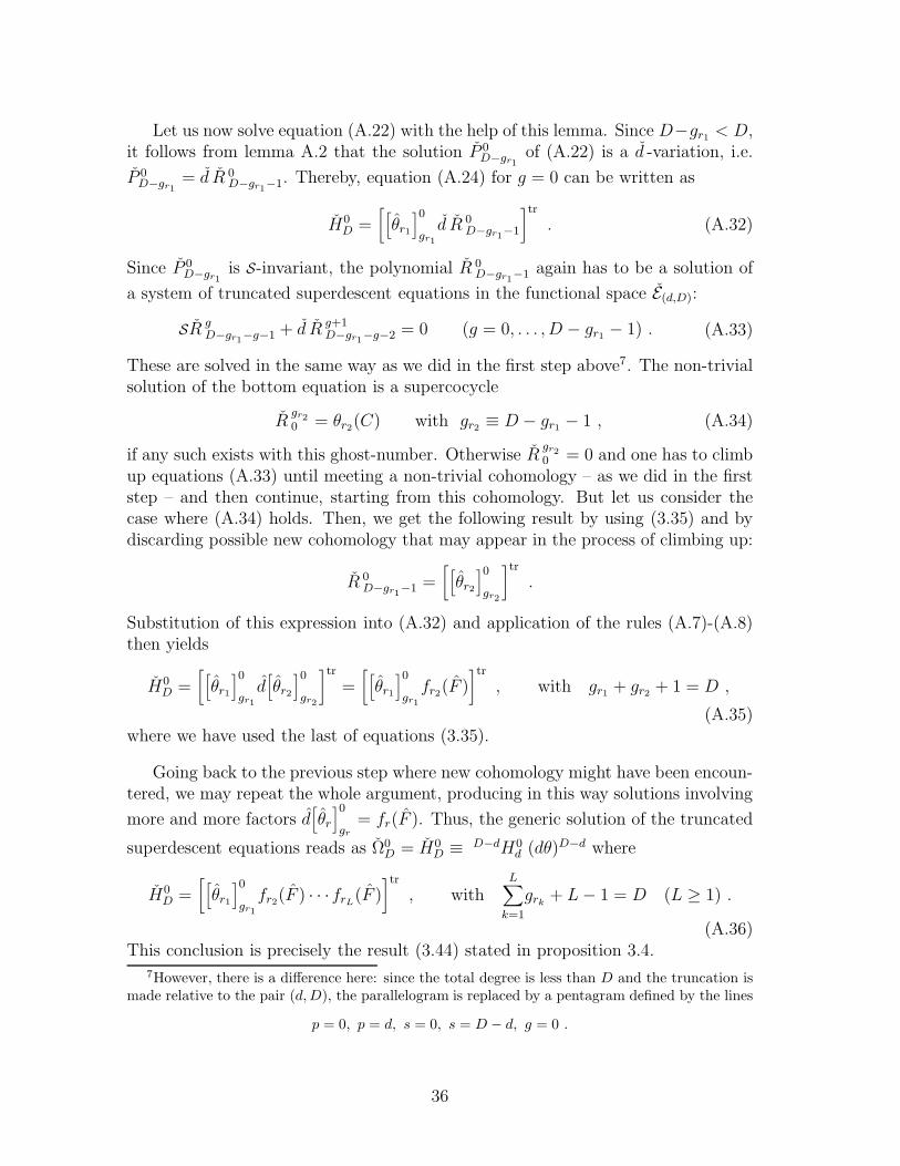
Let us now solve equation (A.22) with the help of this lemma. Since D−gr1< D,

it follows from lemma A.2 that the solution P 0D−gr1

of (A.22) is a d -variation, i.e.

P 0D−gr1

= d R 0D−gr1

−1. Thereby, equation (A.24) for g = 0 can be written as

H0D =

[

[

θr1

]0

gr1

d R 0D−gr1

−1

]tr

. (A.32)

Since P 0D−gr1

is S-invariant, the polynomial R 0D−gr1

−1 again has to be a solution of

a system of truncated superdescent equations in the functional space E(d,D):

SR gD−gr1

−g−1 + d R g+1D−gr1

−g−2 = 0 (g = 0, . . . , D − gr1− 1) . (A.33)

These are solved in the same way as we did in the first step above7. The non-trivialsolution of the bottom equation is a supercocycle

Rgr2

0 = θr2(C) with gr2

≡ D − gr1− 1 , (A.34)

if any such exists with this ghost-number. Otherwise Rgr2

0 = 0 and one has to climbup equations (A.33) until meeting a non-trivial cohomology – as we did in the firststep – and then continue, starting from this cohomology. But let us consider thecase where (A.34) holds. Then, we get the following result by using (3.35) and bydiscarding possible new cohomology that may appear in the process of climbing up:

R 0D−gr1

−1 =[

[

θr2

]0

gr2

]tr

.

Substitution of this expression into (A.32) and application of the rules (A.7)-(A.8)then yields

H0D =

[

[

θr1

]0

gr1

d[

θr2

]0

gr2

]tr

=[

[

θr1

]0

gr1

fr2(F )

]tr

, with gr1+ gr2

+ 1 = D ,

(A.35)where we have used the last of equations (3.35).

Going back to the previous step where new cohomology might have been encoun-tered, we may repeat the whole argument, producing in this way solutions involving

more and more factors d[

θr

]0

gr

= fr(F ). Thus, the generic solution of the truncated

superdescent equations reads as Ω0D = H0

D ≡ D−dH0d (dθ)D−d where

H0D =

[

[

θr1

]0

gr1

fr2(F ) · · ·frL

(F )]tr

, withL

∑

k=1

grk+ L− 1 = D (L ≥ 1) .

(A.36)This conclusion is precisely the result (3.44) stated in proposition 3.4.

7However, there is a difference here: since the total degree is less than D and the truncation ismade relative to the pair (d, D), the parallelogram is replaced by a pentagram defined by the lines

p = 0, p = d, s = 0, s = D − d, g = 0 .

36

References

[1] E. Witten, “Introduction to cohomological theories”, Int.J.Mod.Phys. A6 (1991)2775.E. Witten, “Topological quantum field theory”, Commun.Math.Phys. 117

(1988) 353.

[2] E. Witten, “Quantum field theory and the Jones polynomials”, Commun.Math.Phys. 121 (1989) 351.

[3] D. Bellisai, F. Fucito, A. Tanzini and G. Travaglini, “Multi-instantons, su-persymmetry and topological field theories”, Phys.Lett. B480 (2000) 365,[hep-th/0002110].P. de Medeiros, C. M. Hull, B. Spence and J. M. Figueroa-O’Farrill, “Confor-mal topological Yang-Mills theory and de Sitter holography”, JHEP 0208 (2002)055, [hep-th/0111190].A.S. Cattaneo, J. Frohlich and B. Pedrini “Topological field theory interpreta-tion of string topology”, [math.GT/0202176].C. Hofman and J. S. Park, “Topological open membranes”, [hep-th/0209148].

[4] L. Baulieu, P.A. Grassi and D. Zwanziger, “Gauge and topological symme-tries in the bulk quantization of gauge theories”, Nucl.Phys. B597 (2001) 583[hep-th/0006036].

[5] B. Geyer and D. Mulsch, “NT = 4 equivariant extension of the 3D topologicalmodel of Blau and Thompson”, Nucl.Phys. B616 (2001) 476,[hep-th/0108042].B. Geyer and D. Mulsch, “Higher dimensional analogue of the Blau-Thompsonmodel and NT = 8, d = 2 Hodge-type cohomological gauge theories”,[hep-th/0211061].

[6] D. Birmingham, M. Blau, M. Rakowski and G. Thompson, “Topological fieldtheory”, Phys.Rep. 209 (1991) 129.P. van Baal, “An introduction to topological Yang-Mills theory”,Acta Phys.Polon. B21 (1990) 73.

[7] R. Myers and V. Periwal, “Topological gravity and moduli space”, Nucl.Phys.B333 (1990) 536.R. Myers, “New observables for topological gravity”, Nucl.Phys. B343 (1990)705.R. Myers and V. Periwal, “Invariants of smooth 4-manifolds from topologicalgravity”, Nucl.Phys. B361 (1991) 290.L. Baulieu and I.M. Singer, “Conformally invariant gauge fixed actions for 2-dtopological gravity”, Commun.Math.Phys. 135 (1991) 253.C. M. Becchi, R. Collina and C. Imbimbo, “A functional and Lagrangian for-mulation of two dimensional topological gravity”, in “Symmetry and Simplicity

37

in Physics: A Symposium on the Occasion of Sergio Fubini’s 65th Birthday,Torino, Italy, 24-26 February, 1994”, W.M. Alberico and S. Sciuto, eds. (WorldScientific, 1994), [hep-th/9406096].F. Thuillier, “Some remarks on topological 4d-gravity”, J.Geom.Phys. 27 (1998)221, [hep-th/9707084].

[8] P. van Baal, S. Ouvry and R. Stora, “On the algebraic characterization ofWitten’s topological Yang-Mills theory”, Phys.Lett. B220 (1989) 159.

[9] F. Delduc, N. Maggiore, O. Piguet and S. Wolf, “Note on constrained cohomol-ogy”, Phys.Lett. B385 (1996) 132, [hep-th/9605158].

[10] J.H. Horne, “Superspace version of topological theories, Nucl.Phys. B318 (1989)22.

[11] C. Aragao de Carvalho and L. Baulieu, “Local BRST symmetry and superfieldformulation of the Donaldson-Witten theory”, Phys.Lett. B275 (1992) 323.

[12] G. Barnich, F. Brandt and M. Henneaux, “Local BRST cohomology in gaugetheories”, Phys.Rep. 338 (2000) 439.

[13] L. Baulieu and I.M. Singer,“Topological Yang-Mills symmetry”, Nucl.Phys.(Proc.Suppl.) B5 (1988) 12.

[14] A. Blasi and R. Collina, “Basic cohomology of topological quantum field theo-ries”, Phys.Lett. B222 (1989) 419.

[15] R. Stora, F. Thuillier and J. C. Wallet, “Algebraic structure of cohomologicalfield theory models and equivariant cohomology”, Lectures at the CaribbeanSpring School of Mathematics and Theoretical Physics, St. Francois, Guade-loupe, May 30 - June 13, 1993, preprint ENSLAPP-A-481-94,

[16] C.P. Constantinidis, F. Gieres, M. Lefrancois and O. Piguet, in preparation.

[17] J.L. Boldo, C.P. Constantinidis, J.A. Nogueira, and O. Piguet, in preparation.

[18] M. Blau and G. Thompson, “N = 2 topological gauge theory, the Euler charac-teristic of moduli spaces, and the Casson invariant”, Commun.Math.Phys. 152

(1993) 41, [hep-th/9112012].M. Blau and G. Thompson, “Aspects of NT ≥ 2 topological gauge theories andD-branes”, Nucl.Phys. B492 (1997) 545, [hep-th/9612143].

[19] F.A. Berezin, “Introduction to Superanalysis”, (Reidel Publ. Co., Dordrecht1987).R.F. Picken and K. Sundermeyer, “Integration on supermanifolds and a gener-alized Cartan calculus”, Commun.Math.Phys. 102 (1986) 585-604.P. Deligne et al. (eds.), “Quantum Fields and Strings: A Course for Mathe-maticians, Vol. 1”, (American Mathematical Society, 1999).

38

[20] V.W. Guillemin and S. Sternberg, “Supersymmetry and Equivariant de RhamTheory”, (Springer-Verlag, Berlin 1999).N. Berline, E. Getzler and M. Vergne, “Heat Kernels and Dirac Operators”,(Springer-Verlag, Berlin 1992).

[21] O. Piguet and S.P. Sorella, “Algebraic Renormalization”, Lecture Notes inPhysics m28, (Springer-Verlag, Berlin 1995).

[22] M. Dubois-Violette, M. Talon and C.M. Viallet, “New results on BRS coho-mology in gauge theory”, Phys.Lett. B158 (1985) 231.M. Dubois-Violette, M. Talon and C.M. Viallet, “BRS algebras: analysis of theconsistency equations in gauge theory”, Commun.Math.Phys. 102 (1985) 105.M. Dubois-Violette, M. Talon and C.M. Viallet, “Anomalous terms in gaugetheory: relevance of the structure group”, Ann.Inst.Henri Poincare 44 (1986)103.

[23] J. Thierry-Mieg, “Geometrical reinterpretation of Faddeev-Popov ghost parti-cles and BRS transformations”, J.Math.Phys. 21 (1980) 2834.L. Bonora and M. Tonin, “Superfield formulation of extended BRS symmetry”,Phys.Lett. 98B (1981) 48.R. Stora, in “New Developments in Quantum Field Theory and Statistical Me-chanics”, Cargese 1976, M. Levy and P. Mitter, eds., NATO ASI Ser. B, Vol.26 (Plenum Press, 1977).R. Stora, in “Progress in Gauge Field Theory”, Cargese 1983, G. ’t Hooft et al.eds., NATO ASI Ser. B, Vol. 115 (Plenum Press, 1984).L. Baulieu and J. Thierry-Mieg, “The principle of BRS symmetry: An alterna-tive approach to Yang-Mills theories”, Nucl.Phys. B197 (1982) 477.

39