arX

iv:h

ep-t

h/94

0411

5v1

19

Apr

199

4

US-FT-8/93

hep-th/9404115

March, 1994

TOPOLOGICAL MATTER IN FOUR DIMENSIONS

M. Alvarez and J.M.F. Labastida⋆

Departamento de Fısica de Partıculas

Universidade de Santiago

E-15706 Santiago de Compostela, Spain

ABSTRACT

Topological models involving matter couplings to Donaldson-Witten theory

are presented. The construction is carried using both, the topological algebra and

its central extension, which arise from the twisting of N = 2 supersymmetry in

four dimensions. The framework in which the construction is based is constituted

by the superspace associated to these algebras. The models show new features

of topological quantum field theories which could provide either a mechanism for

topological symmetry breaking, or the analog of two-dimensional mirror symmetry

in four dimensions.

⋆ E-mail: LABASTIDA@GAES.USC.ES

1. Introduction

Topological matter in two dimensions [1,2,3,4] have shown to be a very interest-

ing framework to formulate [5,6] some problems related to mirror manifolds [7-13].

Some geometrical questions which are difficult to answer for a given Calabi-Yau

manifold can be stated as simpler geometrical questions in terms of the correspond-

ing mirror manifold(s). Furthermore, when an N = 2 Landau-Ginzburg model is

known for the mirror manifold(s), those questions can be stated in terms of proper-

ties of the corresponding deformed chiral ring whose structure is fixed by the form

of the Landau-Ginzburg potential. Topological matter models have the property

that out of the complicated structure of N = 2 superconformal theories they ex-

tract the information regarding the geometrical questions which arise in terms of

mirror pairs. It turns out that, after twisting N = 2 supersymmetry [14,2], there

are two types of topological matter models [5,4]. These two types are described by

two different forms of topological sigma models, which are called A and B models.

Given a mirror pair M and M′, the vacuum expectation values (vev) of observ-

ables of the A topological sigma model whose target manifold is M are related

to the ones of the B model whose target manifold is M′ [5]. These vev are much

harder to compute for A models than for B models. Thus the simpler computations

which can be done for B models translate as answers to difficult geometrical ques-

tions stated in terms of computations of vev in the A model. Furthermore, when

the Landau-Ginzburg potential associated to the Calabi-Yau manifold is known,

the vev for B models can be stated in terms of much simpler computations in the

corresponding topological Landau-Ginzburg model [3].

Vafa has recently raised the question [6] of whether or not there exist some

kind of mirror phenomena in four dimensions. For example, it would be very

interesting if difficult problems as the computation of Donaldson invariants [14]

could be stated in much simpler terms, as it happens in two dimensions when a

Landau-Ginzburg description is available. The motivation of the work presented

in this paper is to study this question from the point of view of twisting N = 2

1

supersymmetry. A brief account of part of the results presented here have been

reported in [15].

There are two equivalent approaches to understand the existence of two types

of topological models in two dimensions. One approach consists of performing two

different twists of N = 2 supersymmetry since in two dimensions it is possible to

twist using any of the two U(1) chiral currents [5]. The second approach is the

result of performing one of the twists to each of the two N = 2 supersymmetry

matter multiplets in two dimensions [4]. These multiplets are defined from chiral

and twisted chiral superfields [16]. Of course, the second type of twist, when

applied to these multiplets, does not lead to new theories.

In this paper we show that in four dimensions only one type of twist is pos-

sible. This suggest that one should study the second approach in order to obtain

topological models, namely, one should study the twisting of different N = 2 mul-

tiplets which describe the same on-shell physics before the twisting. Topological

Yang-Mills in four dimensions can be thought as the result of twisting an N = 2

supersymmetric vector multiplet [14]. Only one representation of this vector mul-

tiplet is known and therefore it seems that in this way no new topological model

could be obtained. In this paper we report the results of an exhaustive analysis

of other possible formulations of the vector multiplet from a superspace point of

view. No new topological model with fields of spin no higher than two has been

found.

The situation is rather different when one considers N = 2 supersymmetric

matter fields. For example, several representations are known for the N = 2

hypermultiplet [17,18,19]. This clearly opens a line of investigation. However, this

line deviates somehow from the original motivation of the present work, namely, the

construction of a theory related to topological Yang-Mills theory which could allow

a simpler way to compute Donaldson invariants. In order to keep ourselves within

our original goal, we consider in this work topological matter coupled to topological

Yang-Mills. This will lead to a generalization of Donaldson invariants which might

2

well be the ones that could possess features similar to mirror symmetry.

As reported in [15], topological matter coupled to topological Yang-Mills seems

to possess unexpected properties. It turns out that some of the resulting models

loose some of their topological features. This is an indication that the mirror-like

hypothesis in four dimensions, if valid, is more complicated than in two dimensions.

In fact, one of the generalizations of Donaldson invariants seems to lead to non-

topological quantities. Although it shares many of the properties of Donaldson

invariants, it might have a weak dependence on the metric of the four dimensional

manifold. This fact connects with one of the most important physical problems

in topological quantum field theory, namely, the problem of finding mechanisms

to break their topological symmetry. To study a possible mechanism leading to

symmetry breaking it seems natural to study couplings of topological Yang-Mills

theory to matter multiplets. It is in this context where, indeed, a breaking of

the topological symmetry could appear. The matter models presented in this

work are topological models. However, when the coupling of these models to

topological Yang-Mills is carried out such a property is lost. It turns out that

the observables, although share many of the properties as the ones in topological

quantum field theories, acquire a dependence on the metric of the four dimensional

manifold. These results were briefly reported in [15]. In this work we present a

full account of the results reported in [15] in what regards the structure of one

particular representation of the N = 2 hypermultiplet [17,18], and we present the

study of another representation.

The second representation of N = 2 supersymmetric matter treated in this

paper is based on the relaxed hypermultiplet [19]. Only a truncated version of the

theory resulting after the twisting is presented. The model is coupled to topological

Yang-Mills and the theory constructed in this way turns out to be a topological

quantum field theory. The observables are the same one as the ones in topological

Yang-Mills but in this case the observables acquire corrections due to the presence

of matter fields. The relation between the two forms of topological matter in four

dimensions is discussed in sect. 8.

3

Let us make a brief summary of how the paper is organized. In sect. 2,

the twisting of N = 2 supersymmetry in four dimensions is performed obtaining

the resulting four dimensional topological algebra. It is shown that the twist is

unique up to reversal of orientation. The corresponding topological superspace is

constructed. In sect. 3, topological Yang-Mills is constructed in the framework

of topological superspace and its uniqueness is discussed. In sect. 4, a central

extension of the topological algebra is presented, which is needed since one of

the representations of the hypermultiplet chosen in this work possesses a non-

vanishing central charge. The rest of the section deals with the construction of the

topological matter multiplet associated to the twisted form of the representation

of the N = 2 hypermultiplet built in [17,18]. In sect. 5, the coupling of the

resulting topological matter to topological Yang-Mills is carried out. Section 6

presents a truncated version of the model presented in sect. 5. In sect. 7 the

energy-momentum tensors of the models considered in the previous sections are

constructed and analyzed. Section 8 presents a topological matter model related

to a twisted version of the relaxed hypermultiplet. Finally, in sect. 9 we state our

final comments and remarks. An appendix describes the conventions used in this

paper.

4

2. Topological Algebra in 4D

In this section we will analyze the possible twistings of N = 2 supersymmetry

in four dimensions. Our conclusion is that the twisting procedure is unique (up to

orientation reversal).

We will construct the 4D topological algebra by twisting the algebra of N = 2

supersymmetry. This is the four-dimensional analogue of the construction pre-

sented in [4]. As we will argue the twisting procedure is essentially unique. Our

starting point is the algebra of N = 2 supersymmetry. We will denote the Poincare

generators by Pαβ , Jαβ, Jαβ. For a summary of the index-convention used in this

paper see the appendix. Supersymmetry generators are denoted by Qaα, Qa

α while

internal SU(2) generators by T ba . The N = 2 supersymmetry algebra takes the

form [20]:

{Qaα, Qb

β } = δ ba Pαβ,

{Qaα, Qbβ} = 0,

[Qaα, Pββ] = [Jαβ , Qcγ ] = 0,

[Jαβ , Qcγ ] =i

2Cγ(αQcβ),

[Jαβ, Qc

γ ] =i

2Cγ(αQ

cβ),

[Jαβ, Pγγ ] =i

2Cγ(αPβ)γ ,

[Jαβ, Pγγ ] =i

2Cγ(αPγβ).

[Jαβ, Jγδ] = − i

2δ

(γ(αJ

δ)β),

[Jαβ, Jγδ] = − i

2δ

(γ(α J

δ)

β),

[Jαβ, Jγδ] = [Pαα, Pββ] = 0,

[T ba , Qcγ ] = −1

2(δ b

c Qaγ − 1

2δ ba Qcγ),

[T ba , Q

cγ ] =

1

2(δ c

a Qb

γ − 1

2δ ba Q

cγ ),

[T ba , T

dc ] =

1

2(δ d

a Tb

c − δ bc T

da ),

(2.1)

All other (anti)commutators vanish or are found by hermitian conjugation. Notice

that we do not consider central charges. The Lorentz generator is symmetric in its

two indices. The SU(2) generators T ba satisfy T a

a = 0, being only three of them

independent. To carry out the twisting procedure it is convenient to introduce a

matrix Cab and its inverse Cab to raise and lower isospin indices. These matrices

are antisymmetric and satisfy,

CabCcd = δ c

a δd

b − δ da δ

cb . (2.2)

5

It allows to redefine the SU(2) generators T ba in the more convenient form,

Tab = T ca Ccb, (2.3)

which turn out to be symmetric due to the condition T aa = 0. In terms of the

new SU(2) generators the entries of the algebra (2.1) which are modified by this

redefinition become

[Tab, Qcγ ] = −1

4Cc(bQa)γ ,

[Tab, Qc

γ ] =1

4δ c(a|Qb)γ ,

[Tab, Tcd] = −1

4C(c|(bTa)|d).

(2.4)

The N = 2 supersymmetry algebra (2.1) possesses an additional U(1) symmetry.

This symmetry, whose generator will be denoted by U , is such that,

[U,Qaα] = Qaα, [U,Qaα] = −Qa

α, (2.5)

while it acts trivially on the rest on the generators. This symmetry will turn out

to be the ghost number symmetry of the twisted theory.

The twisting procedure consists of a redefinition of the Lorentz generators and

an identification of the isospin indices as right-handed spin indices relative to the

new Lorentz generator:

JAB = JAB − 2iTAB, (2.6)

where capital letters will denote for the moment new spin indices. The coefficient

in (2.6) is uniquely determined by the requirement that Jαβ possess a commutator

with itself as the one of a Lorentz generator. The choice JAB → Jαβ is, however,

a matter of convention. The opposite choice (i.e., JAB → Jαβ) would lead to a

mirror image algebra (left-handed ↔ right-handed) of the one we are about to

construct. If we denote the SU(2) group associated to the generator Jαβ (Jαβ) as

SU(2)L (SU(2)R), and the internal SU(2) group as SU(2)I, what we are doing in

6

(2.6) is to replace SU(2)L × SU(2)R by SU(2)L × SU(2)′R, where SU(2)′R is the

diagonal sum of SU(2)R and SU(2)I. The choice opposite to the one taken in

(2.6) would have led to SU(2)′L ×SU(2)R. Using (2.6) one finds that the following

combination of components of the supersymmetry generator transforms as a scalar

under JAB:

[JAB, Q+− −Q−+] = 0, (2.7)

which leads to the definition of the “scalar” under the new Lorentz transformations:

Q = −i(Q+− −Q−+) = CABQAB. (2.8)

Furthermore, one finds that

{Q,Q} = 0, (2.9)

which gives a first indication of the topological structure of the resulting algebra.

The choice (2.8) is unique up to a constant, i.e., (2.8) is the unique linear com-

bination of components of Qaα (up to a global factor) such that it behaves as a

scalar under the new Lorentz generators (2.6) and satisfies Q2 = 0. The rest of the

components of Qaα build a symmetric generator,

HAB = Q(AB). (2.10)

Finally, it is straightforward to show that the rest of the SUSY generators, Qa

α ,

build a generator,

GAA = CBAQB

A , (2.11)

which transforms as a vector under the new Lorentz generator (2.6):

[JAB, GCC ] =i

2CC(AGB)C . (2.12)

It is now simple to work out the full form of the topological algebra in terms of

its defining generators Q,Hαβ, Gαα, Jαβ , Jαβ, Pαβ where we have dropped the tilde

7

from JAB and renamed the spin indices with capital letters by the standard Greek

notation. We underline commuting vector indices:

{Q,Q} = 0,

{Q,Hαβ} = 0,

{Hαβ, Hγδ} = 0,

{Q,Gαβ} = Pαβ ,

{Hαβ , Gγδ} = C(α|γ|Pβ)δ,

{Gαβ , Gγδ} = 0,

[Q,Pαβ] = [Hγδ, Pαβ] = 0,

[Pαβ , Pγδ] = [Gγδ, Pαβ ] = 0,

[Q, Jαβ ] = [Q, Jαβ] = 0.

[Jαβ , Hγδ] =i

2C(γ|(αHβ)|δ),

[Jαβ, Gγδ] =i

2Cγ(αGβ)δ,

[Jαβ, Jγδ] = − i

2C(α|(γ Jδ)|β),

[Hγδ, Jαβ] = 0,

[Jαβ, Gγδ] =i

2Cδ(αGγβ),

[Jαβ, Jγδ] = 0,

[Jαβ, Jγδ] =i

2C(γ|(βJα)|δ),

(2.13)

The essential feature of this algebra, which encodes its topological character,

is contained in the anticommutator between Q and Gαβ . This anticommutator ex-

presses that the translation generator Pαβ is Q-exact. This is a necessary condition

for a theory to have an energy-momentum tensor which is Q-exact and therefore

topological. Note that a nilpotent self-dual operator Hαβ is present in this algebra.

The mirror image algebra, which would have resulted from the choice JAB → Jαβ

in (2.6) would have contained an anti-self-dual operator Hαβ .

From (2.5), (2.8), (2.10) and (2.11), it turns out that the U(1) charges of the

new generators are,

[U,Q] = Q, [U,Hαβ] = Hαβ , [U,Gαβ] = −Gαβ , (2.14)

while it is zero for the rest of the generators. In the twisted algebra the charges in

(2.14) are called ghost numbers.

Our next task is to construct the superspace corresponding to the topological

algebra (2.13). Besides the space-time coordinates xαβ we introduce anticommut-

ing coordinates θ, θαβ and θαβ , associated to the odd generators Q, Hαβ and Gαβ ,

8

respectively. A point in superspace is therefore labeled by 4+8 quantities xαβ , θ,

θαβ and θαβ . The representation of the operators entering (2.13) in terms of these

coordinates is the following:

Pαβ = i∂

∂xαβ,

Q =∂

∂θ+i

2θαβ ∂

∂xαβ,

Hαβ =∂

∂θαβ+i

2C(α|γθ

γβ ∂

∂xβ)β,

Gαβ =∂

∂θαβ+i

2θ

∂

∂xαβ− i

2Cαδθ

γδ ∂

∂xγβ.

(2.15)

Superspace covariant derivatives D, Dαβ and Dαβ are introduced as operators

which (anti)commute with Pαβ , Q, Hαβ and Gαβ. Their representation in terms

of the superspace coordinates is,

D = i( ∂∂θ

− i

2θαβ ∂

∂xαβ

),

Dαβ = i( ∂

∂θαβ− i

2C(α|γθ

γβ ∂

∂xβ)β

),

Dαβ = i( ∂

∂θαβ− i

2θ

∂

∂xαβ+i

2Cαδθ

γδ ∂

∂xγβ

).

(2.16)

The prefactors are chosen for later convenience. It is simple to verify that, indeed,

{D,Q} = {D,Hαβ} = {D,Gαβ} = 0,

{Dαβ, Q} = {Dαβ , Hγδ} = {Dαβ , Gγδ} = 0,

{Dαβ, Q} = {Dαβ , Hγδ} = {Dαβ , Gγδ} = 0.

(2.17)

The algebra of the superspace covariant derivatives turns out to be the following,

{D,D} = {Dαβ, Dγδ} = {D,Dαβ} = {Dαβ, Dγδ} = 0,

{D, ∂αβ} = {Dαβ, ∂γδ} = {Dαβ, ∂γδ} = 0,

{D,Dαβ} = i∂αβ ,

{Dαβ, Dγδ} = iC(α|γ∂β)δ.

(2.18)

9

The superspace formulation allows to construct theories which contain all the

symmetries present in the topological algebra (2.13). The procedure is first to

introduce multiplets and then suitable actions which fix their kinematics and in-

teractions. Matter multiplets are usually constructed by imposing superspace co-

variant constraints on tensor superfields. These constraints involve the superspace

covariant derivatives (2.16), and therefore due to the relations (2.17) their covari-

ance under the topological algebra is guaranteed. Other multiplets as, for exam-

ple, vector multiplets, are introduced by constructing gauge superspace covariant

derivatives and then imposing gauge covariant constraints on their algebra. In the

next section we will present in this framework a theory for the vector multiplet

which is equivalent to topological Yang-Mills theory as formulated in [14], and we

will study other possible sets of constraints which might lead to other models.

10

3. Topological vector multiplet

Let us consider a gauge group G and connections A, Aαβ , Aαβ and Aαβ which

allow to define gauge superspace covariant derivatives:

∇ = D − iA,

∇αβ = Dαβ − iAαβ ,

∇αβ = Dαβ − iAαβ ,

∇αβ = Dαβ − iAαβ .

(3.1)

Notice that A, Aαβ and Aαβ are anticommuting superfields. Often we will use a

condensed notation for superspace indices. We will denote by I the set of indices

−, αβ, αβ, αβ, by J the set −, γδ, γδ, γδ, etc. Notice that refers to no index, i.e.,

∇ ≡ ∇− or A ≡ A−. Using this notation (3.1) takes the condensed form,

∇I = DI − iAI . (3.2)

These gauge superspace covariant derivatives possess the following superspace al-

gebra,

[∇I ,∇J} = TIJK∇K − iFIJ , (3.3)

where TIJK is the superspace torsion in (2.18),

T−,αβγδ = iδ γ

α δδ

β,

Tαβ,γδρσ = iC(α|γδ

ρβ) δ

σδ,

(3.4)

while all other components are zero. In (3.3), FIJ are superfield strengths. Con-

straints on the form of these superfield strengths define the vector multiplet. The

11

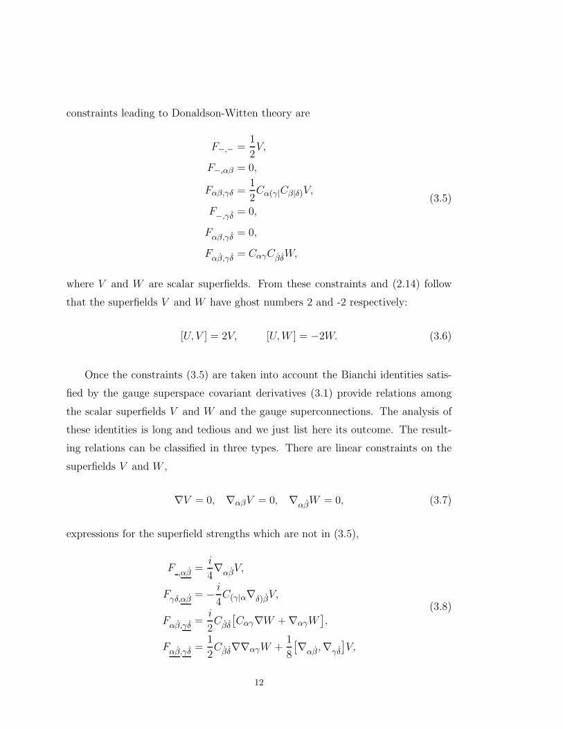
constraints leading to Donaldson-Witten theory are

F−,− =1

2V,

F−,αβ = 0,

Fαβ,γδ =1

2Cα(γ|Cβ|δ)V,

F−,γδ = 0,

Fαβ,γδ = 0,

Fαβ,γδ = CαγCβδW,

(3.5)

where V and W are scalar superfields. From these constraints and (2.14) follow

that the superfields V and W have ghost numbers 2 and -2 respectively:

[U, V ] = 2V, [U,W ] = −2W. (3.6)

Once the constraints (3.5) are taken into account the Bianchi identities satis-

fied by the gauge superspace covariant derivatives (3.1) provide relations among

the scalar superfields V and W and the gauge superconnections. The analysis of

these identities is long and tedious and we just list here its outcome. The result-

ing relations can be classified in three types. There are linear constraints on the

superfields V and W ,

∇V = 0, ∇αβV = 0, ∇αβW = 0, (3.7)

expressions for the superfield strengths which are not in (3.5),

F ,αβ =i

4∇αβV,

Fγδ,αβ = − i

4C(γ|α∇δ)βV,

Fαβ,γδ =i

2Cβδ

[Cαγ∇W + ∇αγW

],

Fαβ,γδ =1

2Cβδ∇∇αγW +

1

8

[∇αβ ,∇γδ

]V,

(3.8)

12

and, finally, second order constraints among the fields V and W ,

∇γδ∇σαW =1

2C(γ|(σC

βτFα)β,|δ)τ − 1

8C(γ|(α∇ β

σ) ∇|δ)βV. (3.9)

The relations (3.7), (3.8) and (3.9), are very important in the analysis of the

independent component fields of the theory. They represent the consequences of

the relations (3.5) which define the vector-like topological multiplet.

The theory under construction possesses the full symmetry generated by the

topological algebra (2.13). Of particular importance are the odd symmetries gen-

erated by Q, Hαβ and Gαβ. Let Φ be a generic superfield. The transformations

corresponding to these symmetries take the form,

δΦ = iǫQΦ,

δ′Φ = iǫαβHαβΦ,

δ′′Φ = iǫαβGαβΦ,

(3.10)

where ǫ, ǫαβ and ǫαβ are scalar, self-dual and vector constant anticommuting pa-

rameters. The theory is also invariant under gauge transformations. These take

the form,

δKAI = DIK, (3.11)

where AI is any of the connections in (3.1) and K an arbitrary scalar superfield.

Superspace actions are defined as integrations over superspace. The full su-

perspace measure has the 8 anticommuting coordinates θ, θαβ and θαβ plus the

ordinary 4 space-time commuting coordinates. The dimension of this measure is

therefore 0 if one associate the standard value 1/2 to the dimensions of θ, θαβ and

θαβ . This implies that it is not possible to write a suitable action unless one takes

only part of the superspace measure [20]. In the untwisted analysis this would

correspond to the choice of a chiral measure. In virtue of constraints (3.7) there

13

exist an essentially unique suitable action with zero ghost number which involves

the fields V and W and is Q-exact. This action is:

S0 =

∫d4xd4θTr(W 2), (3.12)

where d4θ denotes the measure built from θ and θαβ : dθdθ11dθ12dθ22. The pres-

ence of dθ in the measure assures that the action is Q-exact. Another suitable

superspace action of zero ghost number can be built making use of the part of the

full superspace measure not present in (3.12): d4θ: dθ11dθ12dθ21dθ22. Taking into

account (3.7) the only non-trivial choice is:

S1 =

∫d4xd4θTr(V 2). (3.13)

Both, S0 and S1, are invariant under the symmetries generated by the generators

(2.13), and turn out to be equivalent. Their Lagrangians differ by a total derivative

which is proportional to the integrand of the second Chern class.

Our next task is to formulate the theory in terms of component fields. We will

do this projection in a covariant approach taking a Wess-Zumino gauge [20]. The

form of the supergauge transformation (3.11) indicates that the odd connections,

say Aαβ, transform as,

δKAαβ =∂

∂θαβK + ... (3.14)

and therefore the lowest component of the superfield Aαβ can be gauged away

algebraicaly using one of the higher components of K. The Wess-Zumino gauge

consists of making a gauge choice while projecting into component fields of the type

that we have just described for all the components of the odd connections and the

higher components of the even connection Aαβ . Some of these components are

expressed via (3.5) and (3.8) in terms of the components of the fields V and W .

One is left with only the lowest component of the even connection Aαβ , the gauge

invariance corresponding to the lowest component of K, and the components of

14

the fields V and W which are independent after taking into account the constraints

(3.7), (3.8) and (3.9). We define these independent components as,

W | = 21/2λ,

∇W | = 25/4η,

∇αβW | = 25/4χαβ ,

V | = 23/2φ,

∇αβV | = −i23/4ψαβ ,

∇(ασ∇ σβ)V | = 8Gαβ,

(3.15)

The numerical factors introduced in (3.15) are such that the final form of the

theory coincides with the one in [14]. In (3.15) | means theta-independent part.

Notice that our projection procedure is covariant. All component fields appearing

in (3.15) transform in the adjoint representation under gauge transformations with

parameter κ = K|. On the other hand, the only component of the connections left,

Aαβ |, which will be denoted simply as Aαβ transforms in the standard way under

gauge transformations,

δκAαβ = ∇αβκ. (3.16)

Our next task is to compute the symmetry transformations of the component

fields generated by Q, Hαβ and Gαβ. To carry this out one must project the

transformations (3.10) taking into account that the Wess-Zumino gauge has been

chosen. Let us compute as an example of the procedure the transformation of the

field η in (3.15) under the symmetry generated by Q. One finds,

δη = iǫQ∇W | = ǫ∇∇W |, (3.17)

where in the last step the fact that we work in a Wess-Zumino gauge has been

15

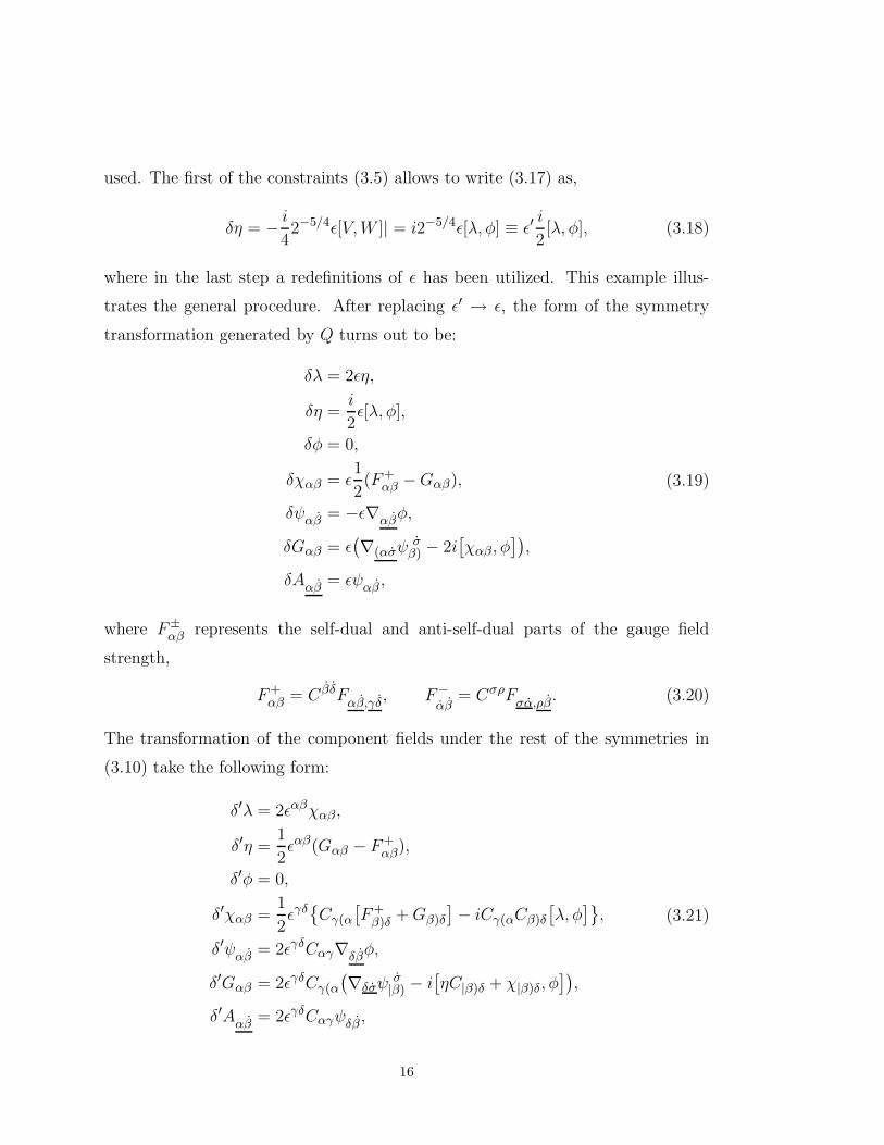
used. The first of the constraints (3.5) allows to write (3.17) as,

δη = − i

42−5/4ǫ[V,W ]| = i2−5/4ǫ[λ, φ] ≡ ǫ′

i

2[λ, φ], (3.18)

where in the last step a redefinitions of ǫ has been utilized. This example illus-

trates the general procedure. After replacing ǫ′ → ǫ, the form of the symmetry

transformation generated by Q turns out to be:

δλ = 2ǫη,

δη =i

2ǫ[λ, φ],

δφ = 0,

δχαβ = ǫ1

2(F+

αβ −Gαβ),

δψαβ = −ǫ∇αβφ,

δGαβ = ǫ(∇(ασψ

σβ) − 2i

[χαβ, φ

]),

δAαβ = ǫψαβ ,

(3.19)

where F±αβ represents the self-dual and anti-self-dual parts of the gauge field

strength,

F+αβ = C βδFαβ,γδ, F−

αβ= CσρFσα,ρβ. (3.20)

The transformation of the component fields under the rest of the symmetries in

(3.10) take the following form:

δ′λ = 2ǫαβχαβ,

δ′η =1

2ǫαβ(Gαβ − F+

αβ),

δ′φ = 0,

δ′χαβ =1

2ǫγδ{Cγ(α

[F+

β)δ +Gβ)δ

]− iCγ(αCβ)δ

[λ, φ

]},

δ′ψαβ = 2ǫγδCαγ∇δβφ,

δ′Gαβ = 2ǫγδCγ(α

(∇δσψ

σ|β) − i

[ηC|β)δ + χ|β)δ, φ

]),

δ′Aαβ = 2ǫγδCαγψδβ ,

(3.21)

16

δ′′λ = 0,

δ′′η =i

2ǫαβ∇αβλ,

δ′′χαβ =i

2ǫγδC(α|γ ,∇β)δλ

δ′′φ = −iǫαβψαβ ,

δ′′ψαβ =i

2ǫγδ{CγαF

−βδ

+ Cβδ

(iCγα

[φ, λ

]+Gαγ

)},

δ′′Gαβ = ǫστ{iC(β|σ∇α)τη + C(α|σ

[ψβ)τ , λ

]+ i∇(ατχβ)σ − 2i∇στχαβ

},

δ′′Aαβ = iǫγδCδβ

(Cγαη + χαγ

).

(3.22)

These symmetries close among themselves as dictated by (2.13) up to gauge trans-

formations. Finally, the U transformations of the component fields, or ghost num-

bers, can be computed easily from (2.14), (3.6) and (3.15). They are,

[U, λ] = − 2λ,

[U, η] = − η,

[U, χαβ] = − χαβ ,

[U, φ] =2φ,

[U, ψαβ ] =ψαβ ,

[U,Gαβ] =0.(3.23)

Of course, the gauge field Aαβ has zero ghost number.

The action S0 in (3.12) can be easily written in terms of component fields after

taking into account that,

S0 =1

e2

∫d4xd4θTr(W 2) =

1

6e2

∫d4xDDα

βDβγDγ

αTr(W 2)|

=1

6e2

∫d4xDTr∇α

β∇βγ∇γ

α(W 2)|,(3.24)

where again use has been made of the fact that a Wess-Zumino gauge has been

chosen. In (3.24) e is a dimensionless gauge coupling constant. Using the con-

straints of the theory and the definitions (3.15) one finds, up to irrelevant global

17

factors

S0 =1

e2

∫d4xTr

{Q,

1

2

(F+

αγ +Gαγ

)χαγ + 2λ∇ατψ

ατ + 2iλ[η, φ]}

=1

e2

∫d4xTr

{1

8

(F 2

+ −G2)− χαγ∇αβψ

βγ − i

2φ{χαγ , χ

αγ}

+ 2η∇ατψατ

− iλ{ψατ , ψ

ατ}− λ∇ατ∇ατφ+ 2iφ

{η, η}

+[λ, φ

]2}.

(3.25)

This action is invariant under all the symmetry transformations of the theory

(3.20), (3.21) and (3.22), as well as under gauge transformations. If one generalizes

this action to an arbitrary curved four dimensional manifold by introducing a

metric tensor it turns out that it is again invariant under all symmetries provided

the parameters of the first three are covariantly constant:

Dαβǫ = 0, Dαβǫγσ = 0, Dαβǫγσ = 0, (3.26)

where Dαβ is a covariant derivative which contains gauge and Christoffel connec-

tions. Certainly, it is not guaranteed in general that a covariantly constant vector

and a self-dual tensor exist for an arbitrary four-manifold. Thus, in general the

Hαβ and Gαβ symmetries do not exist. On the other hand, if one insists in having

these symmetries one is led to topological gravity. Namely, if these covariantly con-

stant vector and self-dual tensor do not exist let us gauge these global symmetries

so that the parameters become arbitrary. This is the form advocated in [4] to build

couplings to topological gravity in two dimensions. A similar construction should

be carried out in four dimensions. It would be interesting if this approach to four

dimensional topological gravity [21-24] leads to a theory of the type recently built

in [25].

Let us recall here the form of the observables in Donaldson-Witten theory.

These are built out of the following basic ones [14]. Let γ be a homology cycle on

18

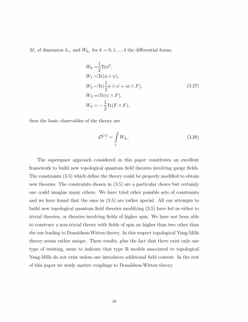
M , of dimension kγ , and Wkγfor k = 0, 1, ..., 4 the differential forms,

W0 =1

2Trφ2,

W1 =Tr(φ ∧ ψ),

W2 =Tr(1

2ψ ∧ ψ + iφ ∧ F ),

W3 =iTr(ψ ∧ F ),

W4 = − 1

2Tr(F ∧ F ),

(3.27)

then the basic observables of the theory are

O(γ) =

∫

γ

Wkγ. (3.28)

The superspace approach considered in this paper constitutes an excellent

framework to build new topological quantum field theories involving gauge fields.

The constraints (3.5) which define the theory could be properly modified to obtain

new theories. The constraints chosen in (3.5) are a particular choice but certainly

one could imagine many others. We have tried other possible sets of constraints

and we have found that the ones in (3.5) are rather special. All our attempts to

build new topological quantum field theories modifying (3.5) have led us either to

trivial theories, or theories involving fields of higher spin. We have not been able

to construct a non-trivial theory with fields of spin no higher than two other than

the one leading to Donaldson-Witten theory. In this respect topological Yang-Mills

theory seems rather unique. These results, plus the fact that there exist only one

type of twisting, seem to indicate that type B models associated to topological

Yang-Mills do not exist unless one introduces additional field content. In the rest

of this paper we study matter couplings to Donaldson-Witten theory.

19

4. Topological matter multiplets

Our starting point will be the representation of the N = 2 hypermultiplet

formulated in [17,18]. This multiplet has a non-vanishing central charge and there-

fore, an extension of the topological algebra (2.13) is required. The final form of

the extended algebra is obvious from the form of the twisting. The only relations

in (2.13) which change are,

{Q,Q} = Z,

{Hαβ, Hγδ} = Cα(γ|Cβ|δ)Z,

{Gαβ, Gγδ} = CαγCβδZ,

[Z, anything} = 0,(4.1)

where Z is the central charge generator. Notice that one could still have general-

ized the extended topological algebra introducing a dimensionless constant in the

anticommutator {Hαβ, Hγδ}. We have analyzed this possibility and it seems im-

possible to construct invariant actions unless such a dimensionless constant is one.

As we will describe below, the presence of central charges makes the construction

of invariant actions very restrictive. Notice also that the relations (4.1) break the

U(1) symmetry. Taking into account (2.14), the best we can do is to maintain a

Z4 ghost number symmetry assigning U -charge 2 to the central charge generator

Z. Indeed, with this assignment, the U(1) symmetry is preserved by the relations

(4.1) modulo 4.

Let us introduce the extended superspace corresponding to (4.1). Let z be a

new real commuting coordinate corresponding to the central charge generator Z.

We define:

Z = i∂

∂z,

Q = Q(0) +i

2θ∂

∂z,

Hαβ = H(0)αβ +

i

2θαβ

∂

∂z,

Gαβ = G(0)

αβ+i

2θαβ

∂

∂z,

(4.2)

where the superscript (0) refers to the operators without central charge. Superspace

covariant derivatives are introduced as operators which (anti)commute with Pαβ ,

20

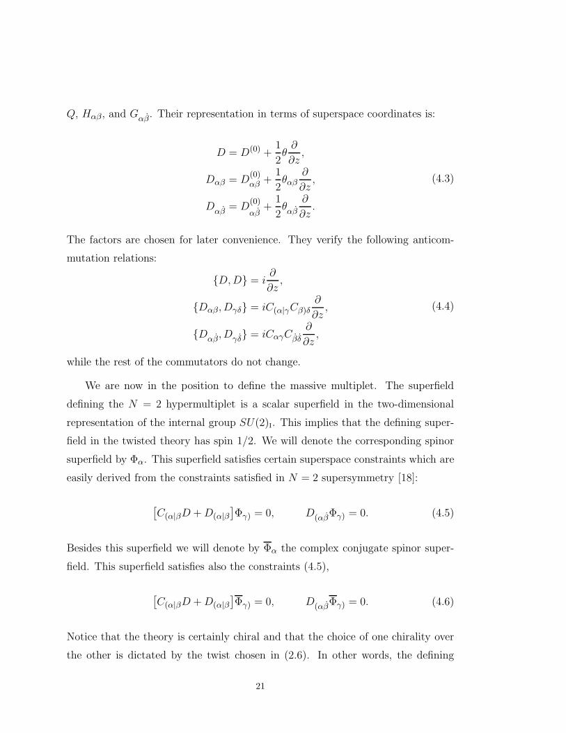
Q, Hαβ, and Gαβ. Their representation in terms of superspace coordinates is:

D = D(0) +1

2θ∂

∂z,

Dαβ = D(0)αβ +

1

2θαβ

∂

∂z,

Dαβ = D(0)

αβ+

1

2θαβ

∂

∂z.

(4.3)

The factors are chosen for later convenience. They verify the following anticom-

mutation relations:

{D,D} = i∂

∂z,

{Dαβ, Dγδ} = iC(α|γCβ)δ∂

∂z,

{Dαβ, Dγδ} = iCαγCβδ

∂

∂z,

(4.4)

while the rest of the commutators do not change.

We are now in the position to define the massive multiplet. The superfield

defining the N = 2 hypermultiplet is a scalar superfield in the two-dimensional

representation of the internal group SU(2)I. This implies that the defining super-

field in the twisted theory has spin 1/2. We will denote the corresponding spinor

superfield by Φα. This superfield satisfies certain superspace constraints which are

easily derived from the constraints satisfied in N = 2 supersymmetry [18]:

[C(α|βD +D(α|β

]Φγ) = 0, D(αβΦγ) = 0. (4.5)

Besides this superfield we will denote by Φα the complex conjugate spinor super-

field. This superfield satisfies also the constraints (4.5),

[C(α|βD +D(α|β

]Φγ) = 0, D(αβΦγ) = 0. (4.6)

Notice that the theory is certainly chiral and that the choice of one chirality over

the other is dictated by the twist chosen in (2.6). In other words, the defining

21

superfields (which before the twisting transformed as the (0,0,1/2) representation of

SU(2)L×SU(2)R×SU(2)I) transform under the (0,1/2) representation of SU(2)L×SU(2)′R. The superfields Φα and Φα have ghost number 0.

The constraints (4.5) imply that there are not component fields with spin higher

than 1/2. This fact can be easily demonstrated after working out the following

useful identities which are a consequence of the constraints (4.5) and the algebra

(4.4):(CαβD +Dαβ

)Φγ = 2CαγDΦβ ,

(CαβD +Dαβ

)DΦγ = −iCβγ∂Φα,

DαβΦγ =1

2CαγDτ βΦτ ,

DαγDβγΦδ = −2iCβδ∂Φα,

DD τη Φη = 2i∂ τ

η Φη,

DαγDτ

η Φη = −2i∂τ

(αΦγ),

∂DΦα = −1

2∂ατD

τη Φη,

∂Dτ βΦτ = 4∂τ βDΦτ ,

∂2Φγ = ∂αβ∂αβΦγ .

(4.7)

One observes that all the possible higher spin components can be expressed in

terms of lower ones. Furthermore, the last equation, which can be rewritten as

the condition P 2 +Z2 = 0, truncates the infinite expansion of the superfield Φα in

powers of z, remaining a finite number of component fields. Of course, a similar

set of relations as the ones in (4.7) holds for Φα.

Component fields are defined introducing adequate superspace derivatives.

From (4.7) follows that the only independent component fields are:

Φα

∣∣ = Hα,

DΦα

∣∣ = 2−1/4uα,

DραΦρ∣∣ = 25/4vα,

∂Φα

∣∣ = i21/2Kα,

Φα

∣∣ = Hα,

DΦα

∣∣ = 2−1/4uα,

DραΦρ∣∣ = 25/4vα,

∂Φα

∣∣ = i21/2Kα.

(4.8)

22

Again, the numerical factors in these definitions are chosen for later convenience.

The Q-transformations of the component fields are easily obtained using (4.2),

(4.4) and (4.7). They turn out to be:

δHα = ǫuα,

δuα = −ǫKα,

δvα = iǫ∂ραHρ,

δKα = iǫ∂ατvτ .

(4.9)

In a similar way the Hαβ and Gαβ transformations are worked out:

δ′Hα = 2ǫβγCβαuγ ,

δ′uα = 2ǫβγCβαKγ ,

δ′vα = −2iǫβγ∂βαHγ ,

δ′Kα = 2iǫβγCβα∂γβvβ,

δ′′Hα = ǫβγCβαvγ ,

δ′′uα = iǫβγ∂αγHβ,

δ′′vα = ǫβγCγαKβ,

δ′′Kα = −iǫβγCβα∂δγuδ.

(4.10)

Finally the z-transformations become,

δzHα = −zKα,

δzuα = −iz∂ααvα,

δzvα = iz∂ααuα,

δzKα = z Hα.

(4.11)

In this equation z is a parameter and should not be confused with the coordi-

nate z introduced in the extended superspace as in (4.2). In these last sets of

transformations the underlines of vector indices in partial derivatives have been

removed since after the projection there are not anticommuting vector indices. Of

course, a similar set of transformations holds for the overlined fields. The ghost

numbers of the component matter fields can be obtained easily from (4.8) and the

fact that the superfield Φα has ghost number 0. It turns out that the set of matter

fields (Hα, uα, vα, Kα) and (Hα, uα, vα, Kα) have both ghost numbers (0, 1,−1, 2).

These ghost numbers are the charges of the Z4 symmetry of the extended topolog-

ical algebra.

23

Since central charges are present in the theory there is not a natural measure

to construct invariant actions. Certainly, one must require Z-invariance and this

is not guaranteed by measures as the ones taken in (3.12) and (3.13). Actually, it

is rather hard to find Z-invariant actions. Guided by the formulation of N = 2

supersymmetry in [18] there are at least two quantities invariant under all the

symmetries of the extended topological algebra (4.2). These lead to the following

terms entering the action for the topological hypermultiplet,

Lf0 =

∫d4x[D2C β

α −DσβDσα +DασDβσ](

Φα ↔∂ Φβ

)|,

Lfm =

∫d4x[D2C β

α −DσβDσα +DασDβσ](

ΦαΦβ

)|,

(4.12)

where the superscript “f” stands for free. The first quantity contains the kinetic

part while the second correspond to a mass term. The action Lf0 has ghost number

0 and thus models based on this action possess a Z4 symmetry. However, the

action Lfm has ghost number 2. This implies that in models where m 6= 0 the ghost

number symmetry is broken to Z2.

The most general form of the full action is, after writing (4.12) in terms of the

component fields (4.8),

Lf =Lf0 +mLf

m

=

∫d4x[H

αHα + iuα∂ααv

α − ivα∂ααuα +K

αKα

+m(K

αHα −H

αKα

)+m

(uαuα + vαvα

)],

(4.13)

where m is an arbitrary mass parameter.

The following redefinition of the auxiliary fields K and K isolates a mass term

for H and H :

Kα

= K ′α +mHα,

Kα = K ′α −mHα.

(4.14)

24

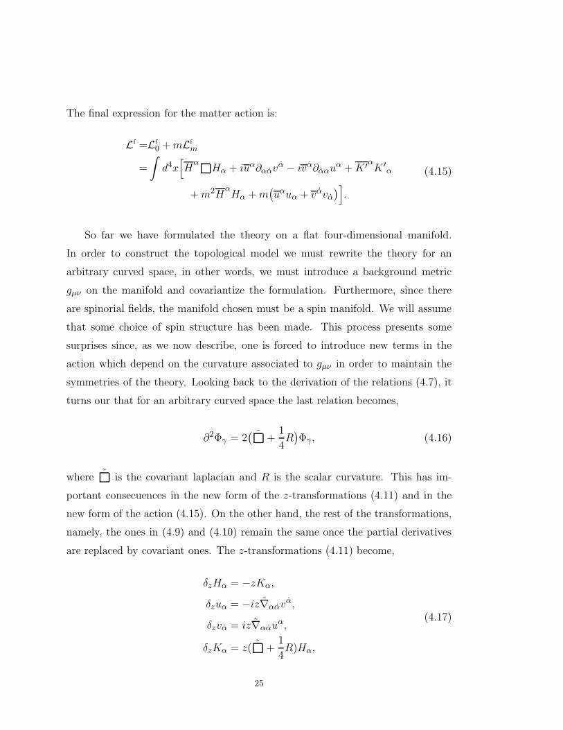
The final expression for the matter action is:

Lf =Lf0 +mLf

m

=

∫d4x[H

αHα + iuα∂ααv

α − ivα∂ααuα +K ′αK ′

α

+m2HαHα +m

(uαuα + vαvα

)].

(4.15)

So far we have formulated the theory on a flat four-dimensional manifold.

In order to construct the topological model we must rewrite the theory for an

arbitrary curved space, in other words, we must introduce a background metric

gµν on the manifold and covariantize the formulation. Furthermore, since there

are spinorial fields, the manifold chosen must be a spin manifold. We will assume

that some choice of spin structure has been made. This process presents some

surprises since, as we now describe, one is forced to introduce new terms in the

action which depend on the curvature associated to gµν in order to maintain the

symmetries of the theory. Looking back to the derivation of the relations (4.7), it

turns our that for an arbitrary curved space the last relation becomes,

∂2Φγ = 2( ˜ +

1

4R)Φγ , (4.16)

where ˜ is the covariant laplacian and R is the scalar curvature. This has im-

portant consecuences in the new form of the z-transformations (4.11) and in the

new form of the action (4.15). On the other hand, the rest of the transformations,

namely, the ones in (4.9) and (4.10) remain the same once the partial derivatives

are replaced by covariant ones. The z-transformations (4.11) become,

δzHα = −zKα,

δzuα = −iz∇ααvα,

δzvα = iz∇ααuα,

δzKα = z( ˜ +1

4R)Hα,

(4.17)

25

where ∇αα denotes the covariant derivative. The final form of the action is,

Lg =Lg

0 +mLgm

=

∫

M

d4x√g[H

α( ˜ +

1

4R)Hα + iuα∇ααv

α − ivα∇ααuα +K ′αK ′

α

+m2HαHα +m(uαuα + vαvα)

].

(4.18)

The superscript g in (4.18) indicates that a choice of metric and spin structure

has been made. This action is invariant under Q and z transformations. However,

it is not invariant under Hαβ and Gαβ transformations unless their corresponding

parameters satisfy,

∇αβǫγσ = 0, ∇αβǫγσ = 0. (4.19)

Certainly, not all spin manifolds admit covariantly constant vectors or self-dual

tensors. Therefore, those symmetries do not exist in general. However, as discussed

before, these symmetries might be useful to construct the coupling to topological

gravity.

Using the covariantized version of (4.9) it is simple to verify that for m = 0 the

action (4.18) is Q-exact. Notice that contrary to the case of topological Yang-Mills,

this is not obvious from the form of the superspace action (4.12). In fact, it turns

out that,

Lg

0 ={Q, Λg

}, (4.20)

where,

Λg =1

2

∫

M

d4x√g[iH

α∇ααvα + ivα∇ααH

α −Kαuα − uαKα

]. (4.21)

The invariance under Q and Z of Lg

0 can be regarded simply as a consequence of

(4.20) and the relations:

[Q,Z] = 0, [Z, Λg] = 0. (4.22)

Equation (4.20) does not ensure that the model we have built is topological,

26

since from the Q-exactness of the whole action it does not follow that the energy-

momentum tensor is also Q-exact. This would be so if the Q-transformations would

not contain covariant derivatives, which is not our case. Nevertheless we show

below that the non-Q-exact part of the energy-momentum tensor vanishes on-shell.

On the other hand, the Q-exactness of the action makes the theory exact in the

small coupling limit. These two facts suffice to render the theory topological. This

implies [14] that the vacuum expectation values of operators which are invariant

under Q-transformations lead to topological invariant quantities. A description

of the observables of this theory was presented in [15]. These turn out to be

a very restrictive set because of the strong conditions imposed by z-invariance.

As we will observe in the discussion concerning the coupling of these models to

topological Yang-Mills in the next section, the z-symmetry is so restrictive that

the only observables are the ones of the form (3.28).

27

5. Matter coupling to Donaldson-Witten theory

We will construct the coupling of the topological hypermultiplet of the previous

section to Donaldson-Witten theory covariantizing the algebra of the extended

superspace derivatives, imposing the gauge constraints (3.5), and covariantizing

the defining constraints on the matter superfields. Let us therefore pick a gauge

group G and introduce gauge connections as in (3.1). The form of the constraints

(3.5) now becomes:

{∇,∇} = i(∂ − 1

2V),

{∇αβ ,∇γδ} = iC(α|γCβ)δ

(∂ − 1

2V),

{∇αβ ,∇γδ} = iCαγCβδ

(∂ −W

),

(5.1)

where the scalar superfields V and W are the same as in (3.5). The remaining

fundamental (anti)commutation relations do not change. As the central charge

commutes with everything, the gauge sector of the theory is as before (the Bianchi

identities remain unchanged). On the other hand, the matter sector has to be

reconsidered.

Let us consider a commuting spinor superfield Φα which transforms under a

representation of the gauge group G, and another spinor superfield Φα

which trans-

form under the conjugate representation. The covariant form of the constraints

(4.5), which are the defining equations of the hypermultiplet, now read,

[C(α|β∇ + ∇(α|β

]Φγ) = 0, ∇(αβΦγ) = 0. (5.2)

The equivalent of the identities (4.7), which determine the set of independent

28

component fields, consist of the set of equations:(Cαβ∇ + ∇αβ

)Φγ =2Cαγ∇Φβ,

∇αβΦγ =1

2Cαγ∇τ βΦτ ,

∇αγ∇ γδ Φδ =4i

(W − ∂

)Φα,

∇∇ τη Φη =2i∇ τ

η Φη,

∇αγ∇τηΦη = − 2i∇ τ

(αΦγ),

∂∇Φα = − 1

2∇ατ∇ τ

η Φη +W∇Φα +1

2∇WΦα +

1

2∇ατWΦτ ,

∂∇τ βΦτ =4∇τ β∇Φτ +1

2V∇τ βΦτ + ∇τ βV Φτ ,

∂2Φα =2 Φα +i

4∇αβV∇

βτ Φτ − i∇W∇Φα,

+ i∇ατW∇Φτ +W∂Φα +1

2V ∂Φα

+ iGατΦτ − 1

4

{V,W

}Φα.

(5.3)

We will carry out a covariant projection into component fields. This means that

component fields must be defined as in (4.8) replacing ordinary superspace deriva-

tives by covariant ones:

Φα

∣∣ = Hα,

∇Φα

∣∣ = 2−1/4uα,

∇ραΦρ∣∣ = 25/4vα,

∂Φα

∣∣ = i21/2Kα,

Φα

∣∣ = Hα,

∇Φα

∣∣ = 2−1/4uα,

∇ραΦρ∣∣ = 25/4vα,

∂Φα

∣∣ = i21/2Kα.

(5.4)

The transformation laws of these component fields are derived making use of (3.10)

and the relations (5.3). For Q-transformations these are:

δHα =ǫuα,

δuα = − ǫ(Kα + iφHα

),

δvα =iǫ∇ααHα,

δKα =iǫ(∇ααv

α − λuα,

− ηHα − χαβHβ),

δHα =ǫuα,

δuα = − ǫ(Kα − iφHα

),

δvα =iǫ∇ααHα,

δKα =iǫ(∇ααv

α + λuα,

+ ηHα + χαβHβ),

(5.5)

29

while for Hαβ-transformations,

δ′Hα = 2ǫγδCγαuδ,

δ′uα = 2ǫγδCγα

(Kδ + iφHδ

),

δ′vα = −2iǫγδ∇γαHδ,

δ′Kα = 2iǫγδCγα

(∇δβv

β − λuδ

− ηHδ − χδβHβ),

δ′Hα = 2ǫγδCγαuδ,

δ′uα = 2ǫγδCγα

(Kδ − iφHδ

),

δ′vα = −2iǫγδ∇γαHδ,

δ′Kα = 2iǫγδCγα

(∇δβv

β + λuδ

+ ηHδ + χδβHβ),

(5.6)

and, finally, for Gαβ transformations,

δ′′Hα = ǫγδCγαvδ,

δ′′uα = iǫγδ∇αδHγ ,

δ′′vα = ǫγδCδα

(Kγ + iλHγ

),

δ′′Kα = −iǫγδCγα

(∇ρδu

ρ

− iψρδHρ + φvδ

),

δ′′Hα = ǫγδCγαvδ,

δ′′uα = iǫγδ∇αδHγ ,

δ′′vα = ǫγδCδα

(Kγ − iλHγ

),

δ′′Kα = −iǫγδCγα

(∇ρδu

ρ

+ iψρδHρ − φvδ

).

(5.7)

On the other hand, it is also important to work out the form of the z-

transformations, these become:

δzHα = − zKα,

δzuα = − iz(∇ααv

α − λuα − ηHα − χαβHβ),

δzvα =iz(∇ααu

α + φvα − iψααHα),

δzKα =z(

Hα + ψααvα − 1

2

{λ, φ

}− iηuα + iχαβH

β

+i

2GαβH

β + iλKα + iφKα

),

(5.8)

δzHα = − zKα,

δzuα = − iz(∇ααv

α + λuα + ηHα + χαβHβ),

δzvα =iz(∇ααu

α − φvα + iψααHα),

δzKα =z(

Hα − ψααvα − 1

2

{λ, φ

}+ iηuα − iχαβH

β

− i

2GαβH

β − iλKα − iφKα

).

(5.9)

30

In the transformations (5.5), (5.6), (5.7), (5.8) and (5.9) commuting vector indices

have not been underlined since at the component level there is not risk to be

mistaken.

The coupled matter action turns out to be made out of the covariantization of

the terms in (4.12):

LtYM0 =

∫d4x[∇2C β

α −∇σβ∇σα + ∇ασ∇βσ](

Φα ↔∂ Φβ

)|,

LtYMm =

∫d4x[∇2C β

α −∇σβ∇σα + ∇ασ∇βσ](

ΦαΦβ

)|,

(5.10)

where the superscript tYM indicates that the fields of topological Yang-Mills have

been considered in the action (5.10) as background fields. Before writing the action

in components let us analyze the form of the symmetry transformations when the

theory is placed on an arbitrary spin manifold endowed with a metric gµν . All

transformations in (5.5), (5.6) and (5.7) remain the same after the replacement

of the Yang-Mills covariant derivative ∇αβ by the full covariant derivative Dαβ

introduced in (3.26). On the other hand, since the last equation of (5.3) gets a

term involving the scalar curvature,

∂2Φα =2(

+1

4R)Φα +

i

4DαβVD β

τ Φτ − i∇W∇Φα,

+ iDατW∇Φτ +W∂Φα +1

2V ∂Φα

+ iGατΦτ − 1

4

{V,W

}Φα,

(5.11)

the z-transformation of Kα and K ′α become modified in the following form:

δzKα =z[(

+1

4R)Hα + ψααv

α − 1

2

{λ, φ

}− iηuα + iχαβH

β

+i

2GαβH

β + iλKα + iφKα

],

δzKα =z[(

+1

4R)Hα − ψααv

α − 1

2

{λ, φ

}+ iηuα − iχαβH

β

− i

2GαβH

β − iλKα − iφKα

].

(5.12)

In (5.11) and (5.12) represents the full covariant laplacian. The rest of the

31

z-transformations in (5.8) and (5.9) have the same form once the replacement

∇αβ → Dαβ is performed.

From these terms the full action is defined as in (4.13). Writing it in terms of

the component fields and redefining the auxiliary fields K and K as in (4.14) one

finds,

Lg,tYM =Lg,tYM

0 +mLg,tYMm

=

∫

M

d4x√g[K ′αK ′

α +Hα(

+1

4R)Hα +

i

2H

αF+

αβHβ + iuαDααv

α

− ivαDααuα +H

αψααv

α − vαψααHα − iH

αηuα − iuαηHα + iH

αχαβu

β

− iuαχαβHβ − iuαλuα − ivαφvα +

i

2H

αGαβH

β − 1

2H

α{φ, λ

}Hα

+m2HαHα +m

(uαuα + vαvα

)− imH

α(φ+ λ

)Hα

],

(5.13)

where M denotes the four-dimensional spin manifold where the theory is defined.

This action is invariant under the full extended topological algebra provided the

parameters satisfy the relations (3.26). Certainly, in general, only the Q-symmetry

will hold. At this moment one should ask if the action Lg,tYM

0 in (5.13) is Q-

exact as was the case for the action with no coupling to topological Yang-Mills.

Contrary to the action (4.13), Lg,tYM

0 is not Q-exact. In addition it turns out that

the energy-momentum tensor is not Q-exact and therefore it is not clear if the

theory is topological. Examples of topological theories whose action is not Q-exact

but its energy momentum is are known [3,4]. However, this is not the case here.

Certainly, the mass terms of mLg,tYMm in (5.13) break the topological symmetry.

What is in some sense unexpected is that the action Lg,tYM

0 also might lead to a

breaking of the topological symmetry. The analysis of this phenomena is carried

out in the sect. 7. To finish this section let us finally write the full action Sg of

the topological model under consideration. This action is,

Sg = Lg

YM + Lg,tYM

0 , (5.14)

where Lg,tYM

0 is the action given in (5.13) and LgYM is the covariantized form of the

32

action (3.25):

Lg

YM =1

e2

∫

M

d4x√gTr{1

8

(F 2

+ −G2)− χαγDαβψ

βγ − 2λ φ+ 2ηDατψ

ατ

− iλ{ψατ , ψ

ατ}− i

2φ{χαγ , χ

αγ}

+ 2iφ{η, η}

+[λ, φ

]2}.

(5.15)

In this action the gauge field can be taken in any representation of the gauge group,

for example, one could think just in the representation chosen for the matter fields

in (5.13). The difference between choosing one representation or another is just a

global factor which can be reabsorbed in the coupling constant e. Because of the

Q-exactness of (5.15) (see (3.25)) the observables of the theory are independent of

e.

To show that the action Lg,tYM

0 in (5.13) is not Q-exact one just has to write

all possible terms quadratic in matter fields with ghost number -1. It turns out

that no combination of those terms leads to Lg,tYM

0 . The z-symmetry present in

Lg,tYM

0 is very restrictive. If Lg,tYM

0 were Q of some quantity, presumably such a

quantity should be invariant under z-transformations. However, it does not exist

a z-invariant of ghost number -1 and quadratic in the matter fields. On the other

hand, it is clear from the form of the action for the free case in (4.20) that part of

the Lg,tYM

0 is Q exact. Indeed, one finds that

Lg,tYM

0 = {Q,Λg} + Lg,tYM

0 , (5.16)

where,

Λg =1

2

∫

M

d4x√g[iH

αDααvα + ivαDααH

α −Kαuα − uαKα

], (5.17)

33

and,

Lg,tYM

0 =1

2

∫

M

d4x√g[H

αψααv

α − vαψααHα − iH

αηuα − iuαηHα

+ iHαχαβu

β − iuαχαβHβ − 2ivαφvα −H

α{φ, λ

}Hα

+ iHαGαβH

β − iK ′αφHα + iHαφK ′

α

].

(5.18)

This part of the action seems as complicated as the original action (5.13). Notice,

however, that in (5.18) there are only interaction vertices. The form of the energy-

momentum tensor of this theory will be studied in sect. 7.

34

6. The truncated theory

So far, the models we have presented possess all the symmetries of the topolog-

ical algebra, provided that (3.26) holds. It turns out that the resulting theory can

be truncated making it simpler. This truncation consist of disregarding the fields

λ, η and χ, and the auxiliary field G in both the coupling of matter to Donaldson-

Witten theory and the matter fields transformation laws. In other words, matter

is coupled to a minimal set of gauge fields, Aµ, its Q-partner ψµ and the field φ.

We give now the truncated δ and δ′′ transformations for this minimal set of fields:

δAαα = ǫψαα,

δψαβ = −ǫDαβφ,

δφ = 0,

δ′′Aαα = 0,

δ′′ψαα =i

2ǫγδCγαF

−αδ,

δ′′φ = −iǫβγψβγ .

(6.1)

It is simple to verify that the Q-transformations close up to gauge transforma-

tions generated by φ:[δ2, δ1

]Aαα = −2iǫ1ǫ2Dααφ

[δ2, δ1

]ψαα = 2iǫ1ǫ2

[ψαα, φ

].

(6.2)

As for the G-transformations, one would expect that the commutator of two of

them would give a gauge transformation generated by λ. This is indeed what

happens, although in the truncated case this is zero since λ has been set to zero,

[δ′′2, δ

′′1

]Aαα =

[δ′′2, δ

′′1

]ψαα = 0. (6.3)

Now we should calculate the commutator of a Q and a G-transformation to make

sure of having a topological algebra. It should give a derivative of the field on

which the transformations act. This comes out to be true.

[δ, δ′′

]Aαα = − i

2ǫǫγδCγαF

−αδ,

[δ, δ′′

]ψαα = − i

2ǫǫγδCγαDρ(αψ

ρ

δ),

[δ, δ′′

]φ = −iǫǫγδDγδφ.

(6.4)

We now give the action of the truncated Q and G-transformations on matter fields

35

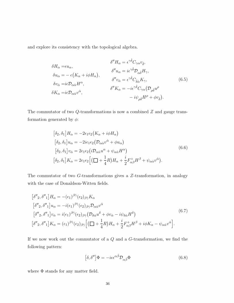
and explore its consistency with the topological algebra.

δHα =ǫuα,

δuα = − ǫ(Kα + iφHα

),

δvα =iǫDααHα,

δKα =iǫDααvα,

δ′′Hα = ǫγδCγαvδ,

δ′′uα = iǫγδDαδHγ ,

δ′′vα = ǫγδCδαKγ ,

δ′′Kα = −iǫγδCγα

(Dρδu

ρ

− iψρδHρ + φvδ

).

(6.5)

The commutator of two Q-transformations is now a combined Z and gauge trans-

formation generated by φ:

[δ2, δ1

]Hα = −2ǫ1ǫ2

(Kα + iφHα

)

[δ2, δ1

]uα = −2iǫ1ǫ2

(Dααv

α + φuα

)

[δ2, δ1

]vα = 2ǫ1ǫ2

(iDααu

α + ψααHα)

[δ2, δ1

]Kα = 2ǫ1ǫ2

[(+

1

4R)Hα +

i

2F+

αβHβ + ψααv

α).

(6.6)

The commutator of two G-transformations gives a Z-transformation, in analogy

with the case of Donaldson-Witten fields.

[δ′′2, δ

′′1

]Hα = −(ǫ1)

βγ(ǫ2)βγKα

[δ′′2, δ

′′1

]uα = −i(ǫ1)βγ(ǫ2)βγDααv

α

[δ′′2, δ

′′1

]vα = i(ǫ1)

βγ(ǫ2)βγ

(Dδαu

δ + φvα − iψδαHδ)

[δ′′2, δ

′′1

]Kα = (ǫ1)

βγ(ǫ2)βγ

[(+

1

4R)Hα +

i

2F+

αβHβ + iφKα − ψααv

α].

(6.7)

If we now work out the commutator of a Q and a G-transformation, we find the

following pattern:

[δ, δ′′

]Φ = −iǫǫαβDαβΦ (6.8)

where Φ stands for any matter field.

36

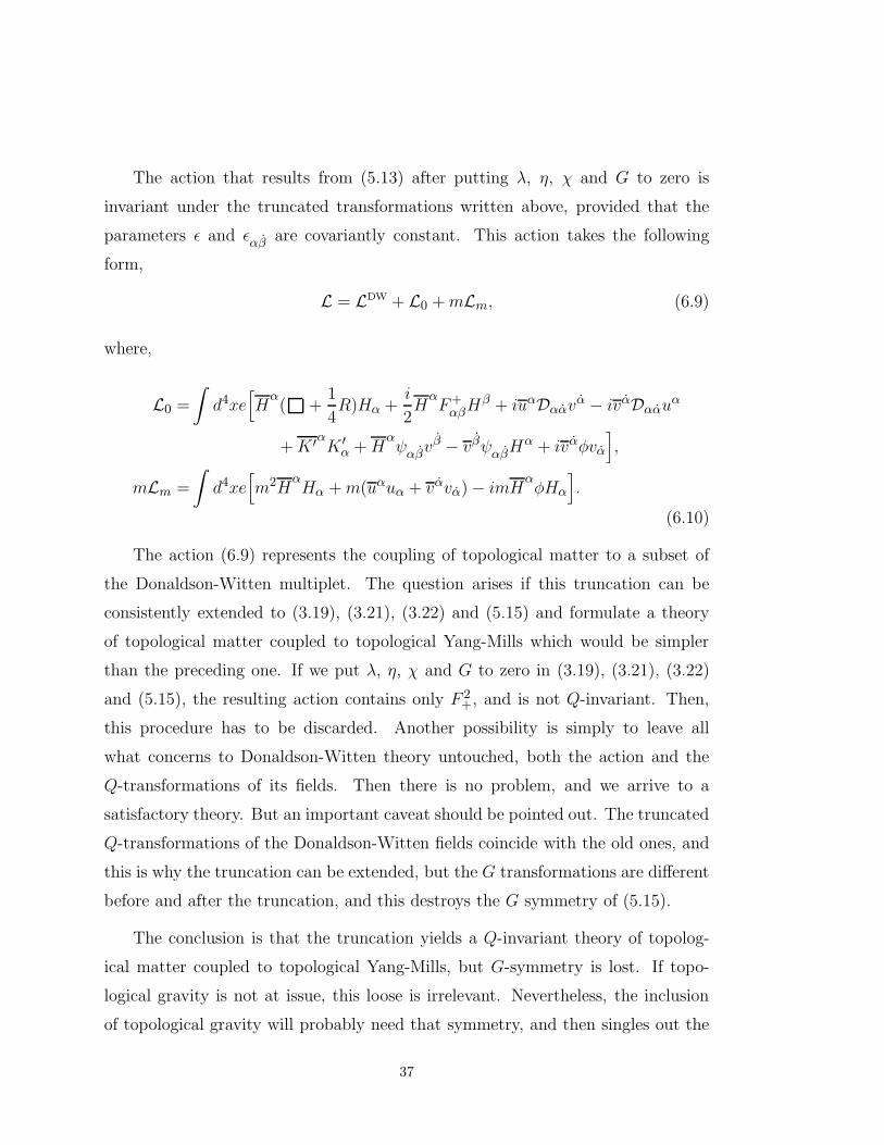
The action that results from (5.13) after putting λ, η, χ and G to zero is

invariant under the truncated transformations written above, provided that the

parameters ǫ and ǫαβ are covariantly constant. This action takes the following

form,

L = LDW + L0 +mLm, (6.9)

where,

L0 =

∫d4xe

[H

α( +

1

4R)Hα +

i

2H

αF+

αβHβ + iuαDααv

α − ivαDααuα

+K ′αK ′α +H

αψαβv

β − vβψαβHα + ivαφvα

],

mLm =

∫d4xe

[m2H

αHα +m(uαuα + vαvα) − imH

αφHα

].

(6.10)

The action (6.9) represents the coupling of topological matter to a subset of

the Donaldson-Witten multiplet. The question arises if this truncation can be

consistently extended to (3.19), (3.21), (3.22) and (5.15) and formulate a theory

of topological matter coupled to topological Yang-Mills which would be simpler

than the preceding one. If we put λ, η, χ and G to zero in (3.19), (3.21), (3.22)

and (5.15), the resulting action contains only F 2+, and is not Q-invariant. Then,

this procedure has to be discarded. Another possibility is simply to leave all

what concerns to Donaldson-Witten theory untouched, both the action and the

Q-transformations of its fields. Then there is no problem, and we arrive to a

satisfactory theory. But an important caveat should be pointed out. The truncated

Q-transformations of the Donaldson-Witten fields coincide with the old ones, and

this is why the truncation can be extended, but the G transformations are different

before and after the truncation, and this destroys the G symmetry of (5.15).

The conclusion is that the truncation yields a Q-invariant theory of topolog-

ical matter coupled to topological Yang-Mills, but G-symmetry is lost. If topo-

logical gravity is not at issue, this loose is irrelevant. Nevertheless, the inclusion

of topological gravity will probably need that symmetry, and then singles out the

37

whole theory as the only one to which it can be consistently coupled. As for the

topological character of the theory, this feature depends on the Q-exactness of its

energy-momentum tensor. It should be fully Q-exact off-shell because the action

is not exact and therefore no equations of motion can be used. These aspects of

the theory are discussed in the next section.

38

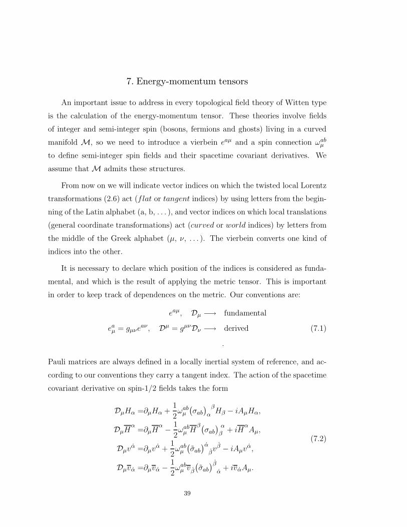
7. Energy-momentum tensors

An important issue to address in every topological field theory of Witten type

is the calculation of the energy-momentum tensor. These theories involve fields

of integer and semi-integer spin (bosons, fermions and ghosts) living in a curved

manifold M, so we need to introduce a vierbein eaµ and a spin connection ωabµ

to define semi-integer spin fields and their spacetime covariant derivatives. We

assume that M admits these structures.

From now on we will indicate vector indices on which the twisted local Lorentz

transformations (2.6) act (flat or tangent indices) by using letters from the begin-

ning of the Latin alphabet (a, b, . . . ), and vector indices on which local translations

(general coordinate transformations) act (curved or world indices) by letters from

the middle of the Greek alphabet (µ, ν, . . . ). The vierbein converts one kind of

indices into the other.

It is necessary to declare which position of the indices is considered as funda-

mental, and which is the result of applying the metric tensor. This is important

in order to keep track of dependences on the metric. Our conventions are:

eaµ, Dµ −→ fundamental

eaµ = gµνeaν , Dµ = gµνDν −→ derived

.

(7.1)

Pauli matrices are always defined in a locally inertial system of reference, and ac-

cording to our conventions they carry a tangent index. The action of the spacetime

covariant derivative on spin-1/2 fields takes the form

DµHα =∂µHα +1

2ωab

µ

(σab

) β

αHβ − iAµHα,

DµHα

=∂µHα − 1

2ωab

µ Hβ(σab

) α

β+ iH

αAµ,

Dµvα =∂µv

α +1

2ωab

µ

(σab

)αβvβ − iAµv

α,

Dµvα =∂µvα − 1

2ωab

µ vβ

(σab

)βα

+ ivαAµ.

(7.2)

39

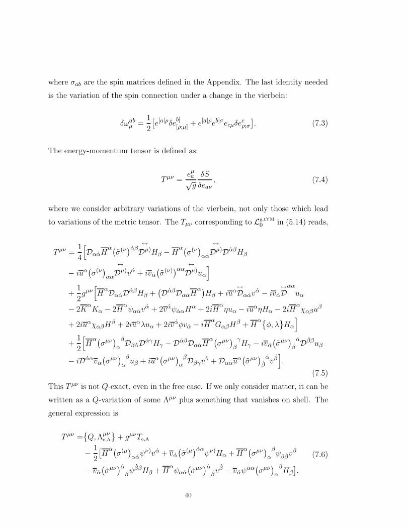
where σab are the spin matrices defined in the Appendix. The last identity needed

is the variation of the spin connection under a change in the vierbein:

δωabµ =

1

2

[e[a|ρδe

b][ρ;µ]

+ e[a|ρeb]σecµδecρ;σ

]. (7.3)

The energy-momentum tensor is defined as:

Tµν =eµa√g

δS

δeaν, (7.4)

where we consider arbitrary variations of the vierbein, not only those which lead

to variations of the metric tensor. The Tµν corresponding to Lg,tYM

0 in (5.14) reads,

Tµν =1

4

[DααH

α(σ(ν)αβ

↔

Dµ)Hβ −Hα(σ(ν)αα

↔

Dµ)DαβHβ

− iuα(σ(ν)αα

↔

Dµ)vα + ivα

(σ(ν)

)αα↔

Dµ)uα

]

+1

2gµν[H

αDααDαβHβ +(DαβDααH

α)Hβ + iuα

↔Dααv

α − ivα

↔D

αα

uα

− 2KαKα − 2H

αψααv

α + 2vαψααHα + 2iH

αηuα − iuαηHα − 2iH

αχαβu

β

+ 2iuαχαβHβ + 2iuαλuα + 2ivαφvα − iH

αGαβH

β +Hα{φ, λ

}Hα

]

+1

2

[H

α(σµν) β

αDβαDαγHγ −DαβDααH

α(σµν) γ

βHγ − ivα

(σµν) α

βDββuβ

− iDααvα

(σµν) β

αuβ + iuα

(σµν) β

αDβγv

γ + Dααuα(σµν) α

βvβ].

(7.5)

This Tµν is not Q-exact, even in the free case. If we only consider matter, it can be

written as a Q-variation of some Λµν plus something that vanishes on shell. The

general expression is

Tµν ={Q,Λµν

e,A

}+ gµνTe,A

− 1

2

[H

α(σ(µ)ααψν)vα + vα

(σ(µ)αα

ψν)Hα +Hα(σµν) β

αψββv

β

− vα

(σµν)α

βψββHβ +H

αψαα

(σµν)α

βvβ − vαψ

αα(σµν) β

αHβ

].

(7.6)

40

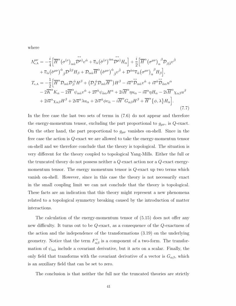
where

Λµνe,A = − i

4

[H

α(σ(ν)αα

↔

Dµ)vα + vα

(σ(ν)αα

↔

Dµ)Hα

]+i

2

[H

α(σµν) β

αDββv

β

+ vα

(σµν)α

βDββHβ + DααH

α(σµν)α

βvβ + Dααvα

(σµν) β

αHβ

],

Te,A = −1

2

[H

αDααD αβ H

β +(D α

β DααHα)Hβ − iuα

↔Dααv

α + ivα↔Dααu

α

− 2KαKα − 2H

αψααv

α + 2vαψααHα + 2iH

αηuα − iuαηHα − 2iH

αχαβu

β

+ 2iuαχαβHβ + 2iuαλuα + 2ivαφvα − iH

αGαβH

β +Hα{φ, λ

}Hα

].

(7.7)

In the free case the last two sets of terms in (7.6) do not appear and therefore

the energy-momentum tensor, excluding the part proportional to gµν , is Q-exact.

On the other hand, the part proportional to gµν vanishes on-shell. Since in the

free case the action is Q-exact we are allowed to take the energy-momentun tensor

on-shell and we therefore conclude that the theory is topological. The situation is

very different for the theory coupled to topological Yang-Mills. Either the full or

the truncated theory do not possess neither a Q-exact action nor a Q-exact energy-

momentum tensor. The energy momentum tensor is Q-exact up two terms which

vanish on-shell. However, since in this case the theory is not necessarily exact

in the small coupling limit we can not conclude that the theory is topological.

These facts are an indication that this theory might represent a new phenomena

related to a topological symmetry breaking caused by the introduction of matter

interactions.

The calculation of the energy-momentum tensor of (5.15) does not offer any

new difficulty. It turns out to be Q-exact, as a consequence of the Q-exactness of

the action and the independence of the transformations (3.19) on the underlying

geometry. Notice that the term F+αβ is a component of a two-form. The transfor-

mation of ψαα include a covariant derivative, but it acts on a scalar. Finally, the

only field that transforms with the covariant derivative of a vector is Gαβ , which

is an auxiliary field that can be set to zero.

The conclusion is that neither the full nor the truncated theories are strictly

41

topological, since the action is Q-invariant, but not Q-exact, and the energy-

momentum tensor is Q-exact only on-shell. As the theory does not coincide with

its classical limit, the non Q-exact terms in Tµν cannot be discarded.

42

8. Another type of topological matter in 4D

So far all our models have been built starting from an N = 2 theory and per-

forming a twist. One can also think of starting directly from a set of fields which

satisfy some δ-transformation properties, and try to write an action invariant un-

der that transformations. The only drawback of this approach is the difficulty to

implement other symmetries (as δ′ or δ′′). We present now an example of this

procedure, which turns out to be a truncated twisted version of the relaxed hyper-

multiplet [19]. The analysis to build this model from the relaxed hypermultiplet

will not be presented here. It goes along the same lines as the ones which led to

the matter models in the previous sections. We present only the truncated model

and therefore all symmetries but the one corresponding to Q have been lost. A

coupling of this model to topological gravity would need the full theory. Its form

will presented elsewhere.

The basic set of fields of the model has the same spin content as in the previous

model. We will denote these fields by Hα, uα, vα, and Lα. The reasons to make

some of the choices done for the previous model will become clear below. The

symmetry transformations turn out to be:

δHα = uα,

δuα = 0,

δvα = Lα −∇ αα Hα,

δLα = ∇ αα uα,

δHα = uα,

δuα = 0,

δvα = Lα −∇ α

α Hα,

δLα

= ∇ αα uα.

(8.1)

Note that this δ is nilpotent, which considerably simplifies the issue of writing in-

variant actions; it suffices to look for δ-exact functionals of the fields with the right

dimension and ghost number. The field Lα has the right dimension to be an auxil-

iary field, and it can be thought as the field needed to render the δ-transformation

nilpotent. The next task is to find out the action which is annihilated by this

transformation. The choice which leads to a δ-exact action with kinetic terms and

43

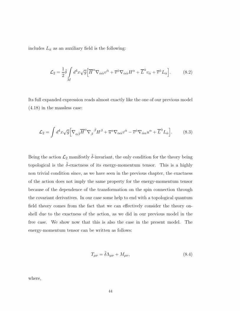
includes Lα as an auxiliary field is the following:

L2 =1

2δ

∫

M

d4x√g[H

α∇ααvα + vα∇ααH

α + Lαvα + vαLα

]. (8.2)

Its full expanded expression reads almost exactly like the one of our previous model

(4.18) in the massless case:

L2 =

∫d4x

√g[∇αβH

α∇ ββ Hβ + uα∇ααv

α − vα∇ααuα + L

αLα

]. (8.3)

Being the action L2 manifestly δ-invariant, the only condition for the theory being

topological is the δ-exactness of its energy-momentum tensor. This is a highly

non trivial condition since, as we have seen in the previous chapter, the exactness

of the action does not imply the same property for the energy-momentum tensor

because of the dependence of the transformation on the spin connection through

the covariant derivatives. In our case some help to end with a topological quantum

field theory comes from the fact that we can effectively consider the theory on-

shell due to the exactness of the action, as we did in our previous model in the

free case. We show now that this is also the case in the present model. The

energy-momentum tensor can be written as follows:

Tµν = δΛµν +Mµν , (8.4)

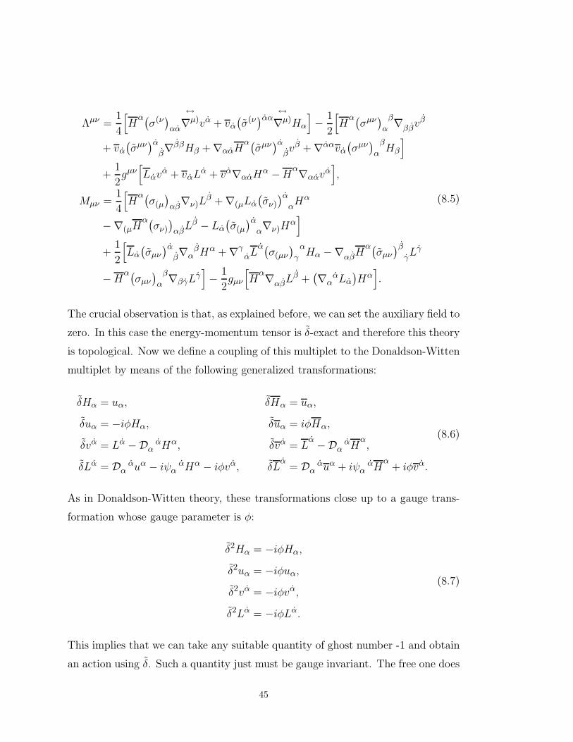
where,

44

Λµν =1

4

[H

α(σ(ν)αα

↔

∇µ)vα + vα

(σ(ν)αα

↔

∇µ)Hα

]− 1

2

[H

α(σµν) β

α∇ββv

β

+ vα

(σµν)α

β∇ββHβ + ∇ααH

α(σµν)α

βvβ + ∇ααvα

(σµν) β

αHβ

]

+1

2gµν[Lαv

α + vαLα + vα∇ααH

α −Hα∇ααv

α],

Mµν =1

4

[H

α(σ(µ

)αβ

∇ν)Lβ + ∇(µLα

(σν)

)ααHα

−∇(µHα(σν)

)αβLβ − Lα

(σ(µ

)αα∇ν)H

α]

+1

2

[Lα

(σµν

)αβ∇ β

α Hα + ∇γαL

α(σ(µν

) α

γHα −∇αβH

α(σµν

)βγLγ

−Hα(σµν

) β

α∇βγL

γ]− 1

2gµν

[H

α∇αβLβ +

(∇ α

α Lα

)Hα].

(8.5)

The crucial observation is that, as explained before, we can set the auxiliary field to

zero. In this case the energy-momentum tensor is δ-exact and therefore this theory

is topological. Now we define a coupling of this multiplet to the Donaldson-Witten

multiplet by means of the following generalized transformations:

δHα = uα,

δuα = −iφHα,

δvα = Lα −D αα Hα,

δLα = D αα uα − iψ α

α Hα − iφvα,

δHα = uα,

δuα = iφHα,

δvα = Lα −D α

α Hα,

δLα

= D αα uα + iψ α

α Hα

+ iφvα.

(8.6)

As in Donaldson-Witten theory, these transformations close up to a gauge trans-

formation whose gauge parameter is φ:

δ2Hα = −iφHα,

δ2uα = −iφuα,

δ2vα = −iφvα,

δ2Lα = −iφLα.

(8.7)

This implies that we can take any suitable quantity of ghost number -1 and obtain

an action using δ. Such a quantity just must be gauge invariant. The free one does

45

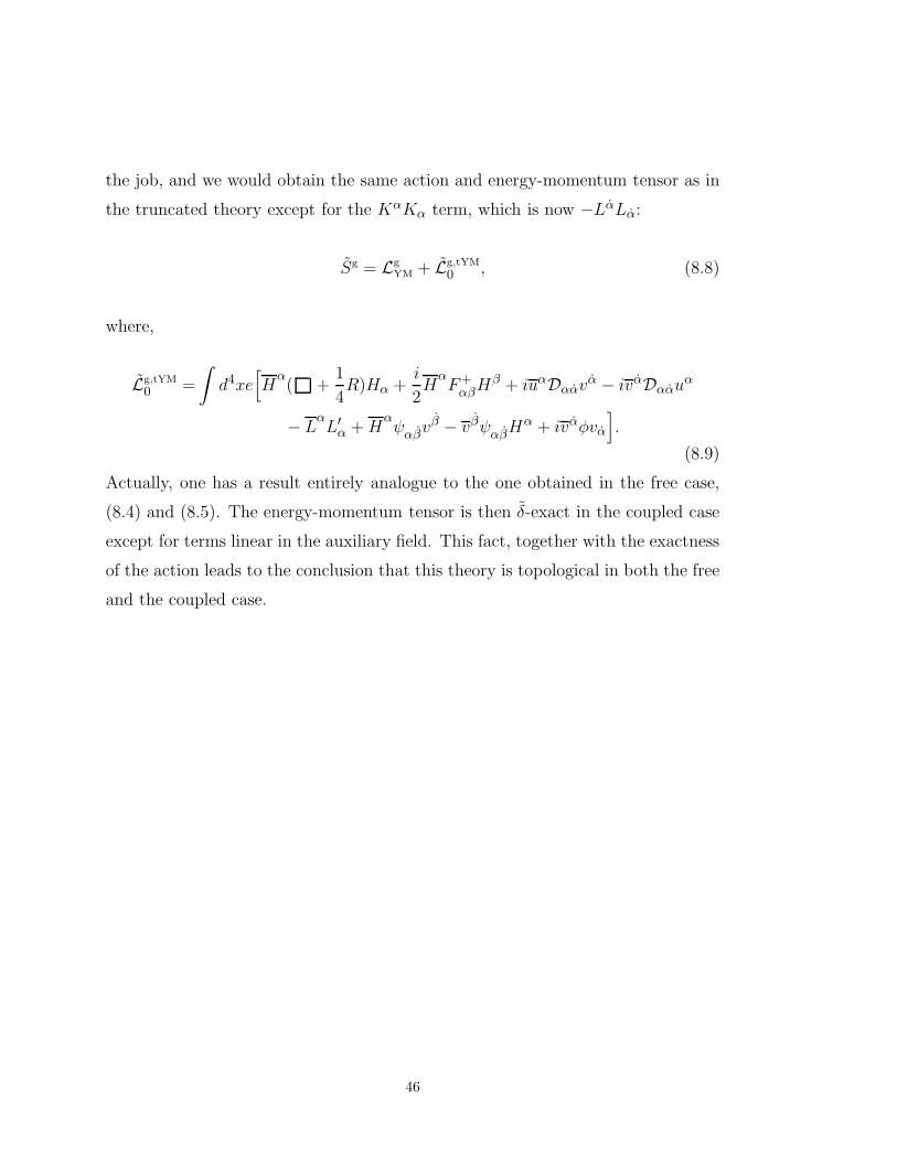
the job, and we would obtain the same action and energy-momentum tensor as in

the truncated theory except for the KαKα term, which is now −LαLα:

Sg = Lg

YM + Lg,tYM

0 , (8.8)

where,

Lg,tYM

0 =

∫d4xe

[H

α( +

1

4R)Hα +

i

2H

αF+

αβHβ + iuαDααv

α − ivαDααuα

− LαL′

α +Hαψαβv

β − vβψαβHα + ivαφvα

].

(8.9)

Actually, one has a result entirely analogue to the one obtained in the free case,

(8.4) and (8.5). The energy-momentum tensor is then δ-exact in the coupled case

except for terms linear in the auxiliary field. This fact, together with the exactness

of the action leads to the conclusion that this theory is topological in both the free

and the coupled case.

46

9. Final comments and remarks

Let us first analyze the features of the possible observables of the models pre-

sented in the previous sections. Observables are Q-invariant quanties constructed

out of the fields of the theory. Certainly, the observables (3.28) of topological

Yang-Mills theory are Q-invariant quantities since all the fields entering in them

possess the same Q-transformations before and after the coupling to matter fields.

One would like to have another set of observables involving matter fields. We have

done a thorough analysis to find observables which involve matter fields and we

have not found any. This analysis goes in two steps. First, one writes all possi-

ble gauge invariant operators quadratic in matter fields of a given ghost number.

Then one checks if it is possible to obtain a linear combination of them which is

Q-invariant and it is not Q-exact. Our analysis shows that there are no operators

a that type. Considering powers of these operators one is led the same conclusion.

One is therefore left to the study of the observables (3.28) in the presence of mat-

ter. Of course, the resulting vev of the operators (3.28) are rather different than

in the theory with no matter. There are relevant contributions from the matter

fields in their functional integration. These contributions are very important. In-

deed, for the models of sect. 6 and 7 it is not guaranteed that these observables

lead to topological quantitites. This follows from the fact that both, the action

and energy-momentum tensor of the theory, are not Q-exact. For the topological

matter model of sect. 8, however, since the action is Q-exact, the small coupling

limit is exact and the observables do indeed lead to topological quantities.

The computation of these observables using the action (5.14) leads to quantities

which are labeled, besides the usual homology cycles, by the matter representation

chosen in the action (5.14). These quantities have properties very similar to Don-

aldson invariants. Let us denote by H∗(M) the homology groups of the spin mani-

fold M . These observables are also polynomials on H∗(M)×H∗(M)× . . .×H∗(M)

as Donaldson invariants are. This property is based only on the fact that the exte-

rior differential of any of the operators (3.27) is Q-exact. There is no need to have

47

a Q-exact energy-momentum tensor for this to hold, just a Q-invariant action as it

is the case. On the other hand, these observables, as in Donaldson-Witten theory,

can be computed in the limit e→ 0. The reason for this is that all the dependence

on the coupling constant e in (5.14) and (8.8) is contained in a part of the action

which is Q-exact. Again, there is no need of a Q-exact energy-momentum tensor

for this to hold. This implies in particular that the vev of the observables are

independent of e. Thus, the quantities associated to the vev of arbitrary products

of the operators (3.28) constitute a generalization of Donaldson invariants which,

however, it is not guaranteed that in general are topological invariants. The break-

ing of the invariance comes from the fact for an arbitrary product of operators

(3.28),

2√g

δ

δgµν〈∏

O(γ)〉 = 〈∏

O(γ)τµν〉, (9.1)

where τµν is the part of the energy-momentum tensor which is not Q-exact. For

models based on the action (5.14) one does not possess an argument ensuring that

(9.1) vanishes. For models based on the action (8.8), however, one can argue that

the right hand side of (9.1) vanishes using the Q-exactness of the action.

It is also important to remark that the actions (5.14) and (8.8) of the models

under considerations have a very similar structure. Their difference is very subtle

since it resides in the form of the auxiliary fields. One would have to study in detail

the role played by the auxiliary fields. Two possibilities could occur. If their role

is trivial, the model based on the action (5.14) would be equivalent to the model

based on the action (8.8) and therefore one could conclude that the model based

on (5.14) is topological. If the role played by the auxiliary fields is non-trivial the

model based on the action (5.14) could very well represent a situation in which

the topological symmetry is broken. In either case that model is interesting and

deserves further investigations.

Let us consider finally the question of the mirror-like behavior in four dimen-

sions. The two models which have been constructed do not seem to lead to this

48

kind of phenomena. Their difference resides on the auxiliary fields and these pos-

sess rather simple couplings. It is likely that one has to study the coupling of

the two types of matter to topological gravity to observe some kind of mirror-like

phenomena. Certainly, the structure of the couplings of the auxiliary fields of the

matter multiplets will be much more complicated. This study, however, requires

to build the full theory resulting from the twisting of the relaxed hypermultiplet,

and not the truncated one presented in sect. 8. An additional set of auxiliary

fields appear in that situation which announces that the analysis of the models are

rather different. Matter couplings to topological gravity will be studied in future

works.

Acknowledgements: We would like to thank A. V. Ramallo for very helpful discus-

sions. This work was supported in part by DGICYT under grant PB90-0772 and

by CICYT under grants AEN93-0729 and AEN94-0928.

49

APPENDIX

In this work we use spinor notation for all Lorentz representations, denoting

spinor indices by Greek letters, dotted for (0, 12), and undotted for (1

2 , 0). An

arbitrary irreducible representation (L,R) is labeled with 2L totally symmetrized

undotted indices, and 2R totally symmetrized dotted indices. The symmetrization

symbol of N indices means the sum over all their permutations without 1/N !, and

similarly for antisymmetrization. For instance:

X(αβ) =Xαβ +Xβα,

X[αβ] =Xαβ −Xβα,(A.1)

and similarly for dotted indices. Spinor indices are raised and lowered by the

second-rank antisymmetric symbol Cαβ:

ψα = ψβCβα, ψα = Cαβψβ . (A.2)

The same convention holds for dotted indices. The Cαβ symbol is defined as follows:

Cαβ =

(0 −ii 0

)= Cαβ , Cαβ =

(0 i

−i 0

)= Cαβ . (A.3)

Vectors belong to the (12 ,

12) representation, and are labeled with one undotted

and one dotted index. We have to distinguish two kinds of vectors: commuting

and anticommuting. We underline the composite index in the case of commuting

vectors. Examples of these two types of vectors are Aαβ and ψαβ . Tangent vector

indices are denoted with lower-case roman letters, and are related to the αβ basis

by some Clebsch-Gordan coefficients, the Pauli matrices,

Xαβ = σ αβa Xa Xa =

1

2σ a

αβXαβ. (A.4)

Pauli matrices with world vector indices are defined by means of the vierbein:

(σµ

)αα

= eaµ(σa

)αα,

(σµ

)αα= eaµ

(σa

)αα. (A.5)

50

The vierbein satisfies the usual relations

eµaeaν = gµν , eµaebµ = ηab, (A.6)

where ηab is the flat minkowskian metric tensor. The vierbein is required to be

covariantly constant:

∇µeaν = 0. (A.7)

This last identity relates the vierbein to the spin connection:

ωabµ =

1

2

[e[a|ρe

b][ρ;µ] + e[a|ρeb]σecµe

cρ;σ

]. (A.8)

Although the spin connection does not transform as a tensor, its variation does.

This property permits to calculate δωabµ simply going to a locally inertial system

of reference and covariantizing the result. Its variation is given in (7.4).

Pauli matrices satisfy the following identities

(σµσν

)αβ

=gµνδ αβ

+ 2(σµν)α

β,

(σµσν

) β

α=gµνδ β

α + 2(σµν) β

α.

(A.9)

which also serve to define the spin matrices σµν and σµν . These matrices are

antisymmetric in their vector indices and symmetric in their spin indices. Some

useful identities needed in the calculation of the energy-momentum tensor are:

(σµν) β

α

(σλ)ββ

= − 1

2gλ[µ

(σν])αβ

+i

2ǫµνλκ

(σκ

)αβ,

(σµν)α

β

(σλ)ββ

= − 1

2gλ[µ

(σν])αβ − i

2ǫµνλκ

(σκ

)αβ,

(σλ)αα

(σµν)α

β=

1

2gλ[µ

(σν])αβ

+i

2ǫµνλκ

(σκ

)αβ,

(σλ)αα(

σµν) β

α=

1

2gλ[µ

(σν])αβ − i

2ǫµνλκ

(σκ

)αβ.

(A.10)

Self-dual tensors in four dimensions have two symmetric undotted indices. The

self-dual part of an antisymmetric second-order tensor can be extracted using the

51

spin matrices, σab:

X+αβ = 2Xab

(σab

)αβ, X−

αβ= 2Xab

(σab

)αβ. (A.11)

52

REFERENCES

1. E. Witten, Comm. Math. Phys. 118(1988), 411

2. T. Eguchi and S.K. Yang, Mod. Phys. Lett. A5(1990), 1693

3. C. Vafa, Mod. Phys. Lett. A6(1991), 337

4. J.M.F. Labastida and P.M. Llatas, Nucl. Phys. B379(1992), 220

5. E. Witten, “Mirror Manifolds and Topological Field Theory”, in Essays on

Mirror Manifolds, ed. S.-T.Yau (International Press, 1992)

6. C. Vafa, “Topological Mirrors and Quantum Rings”, in Essays on Mirror

Manifolds, ed. S.-T.Yau (International Press, 1992)

7. L.J. Dixon, in Superstrings, Unified Theories and Cosmology 1987, (G.

Furlan et al., eds.) World Scientific, 1988, pag. 67

8. W. Lerche, C. Vafa and N.P. Warner, Nucl. Phys. B324(1989), 427

9. B.R. Greene and M.R. Plesser, Nucl. Phys. B338(1990), 15

10. P. Candelas, M. Lynker and R. Schmmrigk, Nucl. Phys. B341(1990), 383

11. P.S. Aspinwall, C.A. Lutken and G.G. Ross, Phys. Lett. B241(1990), 373

12. P. Candelas, X.C. de la Ossa, P.S. Green and L. Parkes, Nucl.

Phys. B359(1991), 21, Phys. Lett. B258(1991), 118

13. S. Ferrara, M. Bodner and A.C. Cadavid, Phys. Lett. B247(1990), 25

14. E. Witten, Comm. Math. Phys. 117(1988), 353

15. M. Alvarez and J.M.F. Labastida, Phys. Lett. B315(1993), 251

16. S.J. Gates, C. Hull and M. Rocek, Nucl. Phys. B248(1984), 157

17. P. Fayet, Nucl. Phys. B113(1976), 135

18. M.F. Sohnius, Nucl. Phys. B138(1978), 109

19. P.S. Howe, K.S. Stelle and P.K. Townsend, Nucl. Phys. B214(1983), 519

53

20. J. Gates, M. Grisaru, M. Rocek and W. Siegel, “Superspace” (Benjamin,

1984)

21. E. Witten, Phys. Lett. B206(1988), 601

22. J.M.F. Labastida and M. Pernici, Phys. Lett. B213(1988), 319

23. R.C. Myers and V. Periwal, Nucl. Phys. B333(1990), 536

24. R.C. Myers, Phys. Lett. B252(1990), 365

25. D. Anselmi and P. Fre, Nucl. Phys. 392(1993), 401, Nucl. Phys. 404(1993),

288

54