Topological discretization of bosonic strings

Gustavo Arciniega,1, a) Francisco Nettel,1, a) Leonardo Patino,1, a) and Hernando

Quevedo2, b)

1)Departamento de Fısica, Facultad de Ciencias, Universidad Nacional Autonoma

de Mexico,

A.P. 50-542, Mexico D.F. 04510, Mexico

2)Instituto de Ciencias Nucleares, Universidad Nacional Autonoma de Mexico,

A.P. 70-543, Mexico D.F. 04510, Mexico

(Dated: 3 December 2013)

We apply the method of topological quantization to obtain the bosonic string topo-

logical spectrum propagating on a flat background. We define the classical config-

uration of the system, and construct the corresponding principal fiber bundle (pfb)

that uniquely represents it. The topological spectrum is defined through the char-

acteristic class of the pfb. We find explicit expressions for the topological spectrum

for particular configurations of the bosonic strings on a Minkowski background and

show that they lead to a discretization of the total energy of the system.

PACS numbers: 02.40.-k, 11.25.-w

a)Electronic mail: gustavo.arciniega, fnettel, leopj@ciencias.unam.mxb)Electronic mail: quevedo@nucleares.unam.mx

1

arX

iv:1

111.

2355

v1 [

mat

h-ph

] 9

Nov

201

1

I. INTRODUCTION

The main motivation to develop the method of topological quantization is to find an

alternative to the ideas that prevail about the quantization of the gravitational fields. Nev-

ertheless, as the method evolved we found ourselves exploring other classical theories with

well established quantum counterparts, such as nonrelativistic quantum mechanics (finite

number of degrees of freedom) and the bosonic string theory. So far, the canonical quantiza-

tion, the most successful method to describe the discrete features of nature, still has to work

out some answers for the theory of General Relativity. There are some unsolved challenges

in the quantization of gravity, among them we find the problem of time, the lack of under-

stanting of the ultimate meaning of the quantization of spacetime, the causality issues due

to a fluctuant metric, the reconstruction problem and the appearance of nonrenormalizable

divergences3,9. At the present time, the main candidates for a quantum theory of gravity,

i.e., string theory and loop quantum gravity, both use canonical quantization as it stands.

We propose, with the method of topological quantization, to extract the discrete nature of

physical systems without making assumptions or putting by hand any rule external to the

geometric/topological structure that we use to represent the system under study.

Dirac’s idea7 about the discretization of the relation between the charge of a magnetic

monopole and a moving electron in the field generated by the former was the starting point

to propose topological quantization as an alternative way of understanding the discrete

nature of physical systems. In particular, the method was utilized to analyze the case

of gravitational fields19,20 and developed further for mechanical systems16–18. The concept

of topological quantization and the fundamental idea beneath these calculations has been

broadly used in different contexts related to charge quantization in Yang-Mills theories6,

instantons and monopoles configurations23,24, topological models of electromagnetism22, cur-

rent quantization of nanostructures2 and in the theory of superconductors4,11. Its relation

to the cohomology theory has been also analyzed1. Examples of topological quantization

can also be found in text books where its geometric formulation is applied to physical sys-

tems described by a hermitian line bundle8. We will generalize this approach to include the

case of an arbitrary physical system in the sense that we will provide a strict mathematical

definition of classical configurations. Furthermore, the complete picture of topological quan-

tization should also include the definition of states and its dynamical evolution in terms of

2

geometric/topological structures, which, currently, is under research. In the beginning of

this program we already established the geometric representation of the physical systems

and from it we defined the topological spectrum.

In the next section we briefly review some general aspects of the bosonic string theory.

In section III we give some elements of topological quantization and state the existence and

unicity of the principal fiber bundle (pfb) that represents the physical system, followed by

the general definition of topological spectrum. Section IV addresses the construction of the

particular pfb and the definition of the topological spectrum for a bosonic string in a general

background spacetime. In section V, we turn our attention to the case of the bosonic string

on a Minkowski background and its pfb. The analysis of the topological spectrum for some

particular configurations is carried out. Finally, in section VI we discuss our results and

consider their implications over the embedding energy of the string.

II. GENERAL ASPECTS OF THE BOSONIC STRING

The action integral for the free bosonic string moving in a general spacetime is given by

the Nambu-Goto (N-G) action10,21, which is proportional to the area of the worldsheet that

describes the propagation of the string over a fixed background. To review this, consider a

two-dimensional manifold M parametrized by xa, a = 1, 2, and a D-dimensional manifold

N with coordinates Xµ, µ = 0, . . . , D − 1 and a metric tensor G. Let X : M → N be

a smooth map from M, the worldsheet, to the spacetime N . The induced metric on the

embedded worldsheet is given by the pullback of G through the X mapping, g = X∗G,

whose components are,

gab =∂Xµ

∂xa∂Xν

∂xbGµν . (1)

Then, the N-G action is written out in terms of the induced metric as,

SNG = −T∫d2x√|g|, (2)

where T is the tension of the string and g ≡ det(gab). The N-G action has two symmetries,

the invariance under diffeomorphism on the worldsheet x′a = x′a(x) and the invariance under

diffeomorphisms on the spacetime X ′µ = X ′µ(X).

It is usual to start from an action, classically equivalent to (2), in which an auxiliary

3

metric field γ is introduced on the worldsheet,

SP = − 1

4πα′

∫d2x√|γ| γabgab, (3)

where α′ is related to the string tension by T = 12πα′

. This is known as the Polyakov

action10,21 and from a mathematical point of view is a harmonic map (or nonlinear sigma

model)12. If we vary the Polyakov action with respect to the field γ we obtain the two-

dimensional energy-momentum tensor Tab = 4π√γδSP

δγabfor the worldsheet,

Tab = gab −1

2γcdgcdγab = 0, (4)

which can be understood as a set of constraints that, among other things, suffice to prove

the equivalence of (2) and (3).

Varying with respect to Xµ the equations of motion that determine the dynamics of the

string propagating in the spacetime follow,

1√|γ|∂a

(√|γ| γab∂bXµ

)+ Γµαβ γ

ab∂aXα∂bX

β = 0, (5)

with ∂a ≡ ∂∂xa

. When the background metric is Gµν = ηµν the equations become,

∂a(√−γ γab∂bXµ

)= 0. (6)

We are interested in exact solutions to (6) as they will be necessary to find the induced

metric which has a fundamental role in the explicit calculation of the topological spectrum.

The Polyakov action possesses, besides the two symmetries of the N-G action, a third

invariance under the Weyl transformation, a local rescaling of the metric tensor γ ′ = eω(x)γ.

In section V we will analyze the general solution of (6) in order to find the topological

spectrum for some configurations.

III. FUNDAMENTALS OF TOPOLOGICAL QUANTIZATION

A complete description of a physical system must include observables, states and its

dynamical evolution. We further know that sometimes the observables have a discrete

behavior. It is the aim of topological quantization to provide these three elements for any

physical system from a geometric/topological outset and to find out if there is a discrete

pattern in such description. Nowadays, we have established the first part of the method,

4

which refers to the definition of the topological spectrum for some observables, meanwhile

the definition of states and their dynamics remains as work in progress.

We present here some basic elements for the definition of the topological spectrum. We

define the classical configuration as a unique pair (M, ω) composed by a Riemannian man-

ifold M and a connection ω that represents the physical system. Uniqueness, in this case,

means that two isomorphic manifolds with the same connection are identical classical con-

figurations. As an example consider a gauge theory over a Minkowski spacetime Mη; this

Riemannian manifold together with the connection one-form A, which takes values in the

Lie algebra of a gauge group G, form the classical configuration.

Furthermore, with the classical configuration we can build the pfb P , using the Rieman-

nian manifoldM as the base space and the symmetry group of the theory G as the structure

group identical to the standard fiber.

Given a local section si which bears a local trivialization (Ui, φi) where Ui ⊂ M and

φi : Ui×G→ π−1(Ui)14, it is possible to introduce a connection ω on P through the pullback

s∗i ω = ωi where ωi is the connection ω on the open set Ui in the base space M. It can be

shown that using these elements and the reconstruction theorem13,14 a unique principal fiber

bundle exists which represents the physical system for the considered classical configuration.

This has been done in the context of gravitational fields20 and for mechanical systems18. We

shall show a similar result for the case in turn.

Once we have constructed the principal fiber bundle P from the classical configuration

(M, ω) the topological invariant properties of P can be used to characterize the physical

system. This can be done employing the characteristic class of the pfb C(P), that integrated

over a cycle ofM constitutes also an invariant of the bundle. The characteristic class C(P),

properly normalized leads to, ∫C(P) = n, (7)

where n is an integer called the characteristic number5. For the cases we analyze, the

symmetry group of the theory may be reduced to an orthogonal group SO(k) by introducing

an orthonormal frame on the base manifold. Then, the characteristic class for such bundles

is the Pontrjagin class p(P), or the Euler class e(P) in case of k being an even integer.

These characteristic classes can be spelled out in terms of the curvature two-form R of the

base space by means of the polynomials invariant under the action of the structure group

5

SO(k)15,

det

(It− R

2π

)=

k∑j=0

pk−j(R)tj. (8)

The Euler class e(P), only defined for even k, is expressed in terms of the curvature

two-form R of a (pseudo-)Riemannian connection on the base space as5,15,

e(P) =(−1)m

22mπmm!εi1i2···i2mR

i1i2∧Ri3

i4∧ · · · ∧Ri2m−1

i2m, (9)

where 2m = k. It is clear that being in terms of the curvature form, the characteristic classes

depend on some parameters λi, i = 1, . . . , s which bear physical information of the system;

thus, once we integrate the characteristic class, we end up with a discrete relation for λi,∫C(P) = f(λ1, . . . , λs) = n, (10)

where n ∈ Z. This relationship is what we define as the topological spectrum and constitutes

a discretization for some of the parameters determining the properties of the physical system

of interest. In the next section we will explore in detail these definitions and the existence

and uniqueness of the pfb for the bosonic string system.

IV. BOSONIC STRING ON A GENERAL BACKGROUND

In this section we construct explicitly the principal fiber bundle for the bosonic string on

a general background. It is natural in this case to consider the worldsheet M embedded in

the spacetime N as the base space provided with the induced metric g = X∗G. Hence, the

classical configuration is (Mg, ω), where ω is the Levi-Civita connection on M compatible

with g. We take the invariance under diffeomorphisms on the worldsheet as the structure

group (isomorphic to the standard fiber), since this is the fundamental symmetry of the two

dimensional action integral.

The group of diffeomorphisms onM can be reduced to the orthogonal group by introduc-

ing a semiorthonormal frame. Indeed, given {ei} with i = 1, 2, an orientable orthonormal

frame onM such that g(ei, ej) = ηij, two distinct bases are related by an orthogonal trans-

formation, e′i = ej(Λ−1)j i, where Λ ∈ SO(1, 1). There is a one-form basis {θi} dual to

the orthonormal frame from which it is possible to express the induced metric tensor as

g = ηij θi⊗ θj; thus, the reduction of the symmetry group to SO(1, 1) is accomplished.

6

Therefore, the principal fiber bundle P can be constructed from the classical configuration

(Mg, ω′), with ω′ the spin connection taking values in the Lie algebra so(1, 1), and SO(1, 1)

as the structure group. This is summarized in the following result:

Theorem: A bosonic string propagating in a general background (N ,G) described by

the Nambu-Goto action can be represented by a unique principal fiber bundle P , with

the semi-Riemannian manifold (M, g) as the base space, SO(1, 1) as the structure group

(identical to the standard fiber) and with a g−compatible connection ω which takes values

in the Lie algebra so(1, 1).

The proof of this theorem is completely analogous to the one that appears in previous

works18,20 and we refer the reader to them for the details. It should be sufficient to mention

that it rests on the reconstruction theorem for fiber bundles13.

The Euler characteristic class for the principal fiber bundle P with a two-dimensional

base space and SO(1, 1) as the structure group reduces from (9) to

e(P) = − 1

2πR1

2. (11)

In the conformal gauge, using coordinates {τ, σ} in Eq.(1), the worldsheet metric turns out

to be conformal to the two-dimensional Minkowski metric, g = gσση.

In this gauge the Euler characteristic class takes the following explicit form,

e(P) = − 1

4π

[∂τ

(1

gσσ∂τgσσ

)− ∂σ

(1

gσσ∂σgσσ

)]dτ ∧ dσ. (12)

Consequently, the determination of the topological spectrum reduces to the computation

of the conformal factor gσσ and the integral∫C(P) = n ∈ Z, regardless of the background

metric. This shows for this particular case that the formalism of topological quantization is

background independent. We will use this property in the following sections to determine

specific topological spectra on diverse backgrounds.

V. BOSONIC STRING ON A MINKOWSKI BACKGROUND

The worldsheet that minimizes the action of a bosonic string propagating in a flat back-

ground, Gµν = ηµν is described by the set of embedding functions {Xµ} satisfying the

equations of motion (−∂2τ + ∂2σ

)Xµ(τ, σ) = 0, (13)

7

with general solution

Xµ(τ, σ) = F µ(τ + σ) +Gµ(τ − σ). (14)

We have chosen the conformal gauge to write these and the forthcoming expressions. The

set (4) of constraint equations takes the form

(∂τXµ∂τX

ν + ∂σXµ∂σX

ν) ηµν = 0,

∂τXµ∂σX

νηµν = 0, (15)

from which the conformal factor of the induced metric can be computed. Let us see how in

the case of a Minkowski background choosing the light cone gauge leaves no residual gauge

freedom. Consider a whole class of gauges given by25,

n ·X(τ, σ) = βα′(n · p)τ,

(n · p)σ =2π

β

∫ σ

0

dσ n ·P τ (τ, σ), (16)

where n is a unitary vector which fixes the relation between the parameters of the worldsheet

with the spacetime coordinates, and n ·X = nµXνηµν . The constant β determines whether

we are dealing with an open (β = 2) or closed (β = 1) string; P τ is the momentum density

along the string, and p the four momentum. Using light cone coordinates for the background

space,

X+ =X0 +X1

√2

,

X− =X0 −X1

√2

,

XI = XI , con I = 2, . . . , D − 1, (17)

the line element for the Minkowski spacetime takes the following form

ds2G = −2dX+dX− + dXIdXJδIJ . (18)

The light cone gauge is fixed choosing the unitary vector n as,

nµ =

(− 1√

2,

1√2, 0, . . . , 0

). (19)

Then, the equations (16) that determine this specific gauge read,

X+(τ, σ) = βα′p+τ,

p+σ =2π

β

∫ σ

0

dσP τ+(τ, σ), (20)

8

where n · P τ is constant along the string and consequently p+ too, and we notice that the

gauge is completely fixed.

From this we also see that the parameter σ takes values in the interval [0, 2π] for a closed

string (periodic boundary conditions). From the constraints equations (15) in this gauge,

∂τX− =

1

2α′p+(∂τX

I∂τXJ + ∂σX

I∂σXJ)δIJ ,

∂σX− =

1

α′p+∂τX

I∂σXJδIJ , (21)

we observe that the component X− can be found once the transverse sector XI(τ, σ), I =

2, . . . , D − 1, is solved; therefore, it does not represent a dynamical degree of freedom.

To obtain the topological spectrum integrating the Euler form (12), we must first find

the conformal factor of the induced metric gσσ, which in view of the constraints (21) reduces

to

gσσ = ∂σXI∂σX

JδIJ . (22)

It is clear now that the conformal factor only depends on the dynamics of the string, that

is, the transverse sector XI for the solution to the equations of motion.

A. Topological spectrum for the closed bosonic string

In this section we will obtain the topological spectrum for some particular configurations

(solutions) of the closed bosonic string. In this case periodic boundary conditions must be

imposed10,

Xµ(τ, σ1) = Xµ(τ, σ2) (23)

∂σXµ(τ, σ1) = ∂σX

µ(τ, σ2) (24)

γab(τ, σ1) = γab(τ, σ2), (25)

where σ1 = 0 and σ2 = 2π. The solutions are described through two sets of oscillation

modes, which are usually interpreted as left moving {αµk} and right moving {αµk} waves

along the string21. In the conformal gauge the solutions may be expressed as,

Xµ(τ, σ) = xµ0 +√

2α′αµ0τ +

√α′

2

∞∑k=1

1√ωk

(αµke

−iωk(τ−σ)

+αµk∗eiωk(τ−σ) + αµke

−iωk(τ+σ) + αµk∗eiωk(τ+σ)

), (26)

9

where, here and throughtout this section, µ = 0, . . . , D − 1 and ωk = k. The periodicity in

σ has been considered, leading to the condition that the zero modes are equal, αµ0 = αµ0 .

The constraints can also be expressed as two independent sets of equations in terms of the

modes of oscillation

Lk =1

2

∑p∈Z

αµp−kανpηµν = 0 Lk =

1

2

∑p∈Z

αµp−kανpηµν = 0. (27)

In the light cone gauge the dynamical fields XI(τ, σ) take the same form as above (26),

just considering the transverse index I instead of the spatiotemporal µ. Only these transverse

fields enter in the expression for the conformal factor gσσ. We introduce the polar notation

for the modes coefficients, αIk = rIke−iγIk and αIk = rIke

−iγIk , such that the solutions for the

transverse fields are written as

XI(τ, σ) = xI0 +√

2α′αI0τ

+√

2α′∞∑k=1

1√ωk

[rIk cosωk(τ − σ + γIk) + rIk cosωk(τ + σ + γIk)

]. (28)

Then, the metric function gσσ which determines the Euler characteristic class (12) in this

gauge is given in general by a infinite sum of oscillation modes,

gσσ(τ, σ) = 2α′∞∑

k,l=1

√ωkωl

[rIk sinωk(τ − σ + γIk)− rIk sinωk(τ + σ + γIk)

]×[rJl sinωl(τ − σ + γJl )− rJl sinωl(τ + σ + γJl )

]δIJ . (29)

It then follows that the integration of the corresponding topological invariant involves

the manipulation of infinite series with the consequent technical difficulties. Hence, we take

into account particular configurations with only a few nonvanishing modes of oscillation that

allow us to reach concrete expressions for their spectra.

B. Topological spectrum of particular configurations

To investigate how the interaction of different modes of oscillation affects the geometric

properties of the underlying pfb, let us consider the case of a right mode αJ1k 6= 0 in the

direction J1, and a left mode in a different direction J2, αJ2l 6= 0. The transverse fields that

10

involve these modes of oscillation are

XJ1 = xJ10 +√

2α′αJ10 τ +√

2α′rJ1k√ωk

cos ωk(τ − σ + γJ1k ),

XJ2 = xJ20 +√

2α′αJ20 τ +√

2α′rJ2l√ωl

cos ωl(τ + σ + γJ2l ), (30)

where we have expressed the coefficients in the polar notation. In all the other transverse

directions J 6= J1, J2, the fields describe only the motion of the center of mass, XJ(τ, σ) =

xJ0 +√

2α′αJ0 τ . The conformal factor for the induced metric is,

gσσ = 2α′[ωk(r

J1k )2 sin2 ωk(τ − σ + γJ1k ) + ωl(r

J2l )2 sin2 ωl(τ + σ + γJ2l )

], (31)

and the Euler characteristic class,

e(P) =ω2kω

2l (r

J1k r

J2l )2 sin 2ωk(τ − σ + γJ1k ) sin 2ωl(τ + σ + γJ2l )

π[(rJ1k )2 sin2 ωk(τ − σ + γJ1k ) + (rJ22 )2 sin2 ωl(τ + σ + γJ2l )

]2dτ ∧ dσ. (32)

In order to integrate the Euler form (32) we must specify the limits in the domain of

integration. For the parameter σ the interval is [0, 2π] and is fixed, while for τ we notice

that the above expression is periodic in this parameter and we may choose a complete

cycle. To perform the integral it is convenient to use null-like coordinates patches that cover

the entire domain of integration, for the details of the calculation we refer the reader to the

appendix A. In this case, it turns out that the integral of the Euler class vanishes identically,

meaning that no discrete relation between the parameters rJ1k and rJ2l is established. This is

so due to the lack of interaction between the modes as they point in perpendicular directions

of the background spacetime.

Next we calculate the topological spectrum for the string with two nonvanishing modes

of oscillation in the same transverse direction, that is, a right k-mode αJk and a left l-mode

αJl . The transverse field in the relevant direction I = J is

XJ(τ, σ) = xJ0 +√

2α′αJ0 τ

+√

2α′[rk√ωk

cosωk(τ − σ + γk) +rl√ωl

cosωl(τ + σ + γl)

], (33)

where we have used again the polar notation, αJk = rke−iγk y αJl = rle

−iγl . In all the

remaining directions, I 6= J , the solutions describe the motion of the center of mass and

only depend on τ .

11

The conformal factor is given by

gσσ(τ, σ) = 2α [√ωk rk sinωk(τ − σ + γr)−

√ωl rl sinωl(τ + σ + γl)]

2, (34)

and the Euler form as

e(τ, σ) = − 2(ωkωl)32 rkrl cosωk(τ − σ + γk) cosωl(τ + σ + γl)

π[√ωk rk sinωk(τ − σ + γk)−

√ωl rl sinωl(τ + σ + γl)

]2 dτ ∧ dσ. (35)

To obtain the topological spectrum we must integrate this expression for σ ∈ [0, 2π] and

a period in τ .

We use the coordinate transformation (A1) and cover the region of integration as ex-

plained in Appendix A. For the regions I and IV the Euler characteristic class takes the

following form

e(x, y) = − 1

π

rkrl√ωkωl(√

ωk rkx−√ωl rly

)2 dx ∧ dy, (36)

and for the type II and III we have

e(x, y) = − 1

π

rkrl√ωkωl(√

ωk rkx+√ωl rly

)2 dx ∧ dy. (37)

The outcome of the integration yields a discrete relation between the amplitudes of the

oscillation modes rk and rl,

4

πωkωl ln

[(√ωl rl +

√ωk rk

)2(√ωl rl −

√ωk rk

)2]

= n, (38)

where n is an integer. This is the topological spectrum for the case of two nonvanishing

modes of oscillation (right and left) in the same direction of the flat background space. We

show in figure 1 the allowed values for rk and rl according to the relation (38).

Now we can add another nonvanishing mode of oscillation to the ones we had in the

previous case. Then, there are two modes in the direction I = J1, αJ1k , αJ1l right and left

respectively, and a third right k-mode in a independent direction I = J2, αJ2k (the case of

including a left mode instead can be treated in a similar fashion). The relevant transverse

fields are,

XJ1(τ, σ) = xJ10 +√

2α′αJ10

+√

2α′[rJ1k√ωk

cosωk(τ − σ + γJ1k ) +rJ1l√ωl

cosωl(τ + σ + γJ1l )

], (39)

12

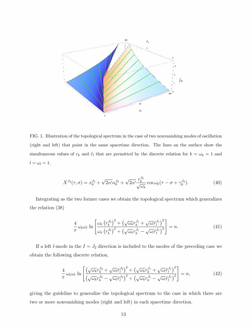
FIG. 1. Illustration of the topological spectrum in the case of two nonvanishing modes of oscillation

(right and left) that point in the same spacetime direction. The lines on the surface show the

simultaneous values of rk and rl that are permitted by the discrete relation for k = ωk = 1 and

l = ωl = 1.

XJ2(τ, σ) = xJ20 +√

2α′αJ20 +√

2α′rJ2k√ωk

cosωk(τ − σ + γJ2k ). (40)

Integrating as the two former cases we obtain the topological spectrum which generalizes

the relation (38)

4

πωkωl ln

[ωk(rJ2k)2

+(√

ωkrJ1k +

√ωlr

J1l

)2ωk(rJ2k)2

+(√

ωkrJ1k −

√ωlr

J1l

)2]

= n. (41)

If a left l-mode in the I = J2 direction is included to the modes of the preceding case we

obtain the following discrete relation,

4

πωkωl ln

[(√ωkr

J2k +

√ωlr

J2l

)2+(√

ωkrJ1k +

√ωlr

J1l

)2(√ωkr

J2k −

√ωlr

J2l

)2+(√

ωkrJ1k −

√ωlr

J1l

)2]

= n, (42)

giving the guideline to generalize the topological spectrum to the case in which there are

two or more nonvanishing modes (right and left) in each spacetime direction.

13

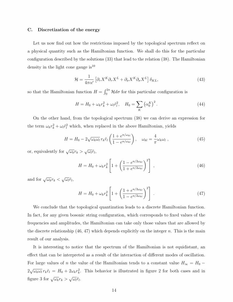
C. Discretization of the energy

Let us now find out how the restrictions imposed by the topological spectrum reflect on

a physical quantity such as the Hamiltonian function. We shall do this for the particular

configuration described by the solutions (33) that lead to the relation (38). The Hamiltonian

density in the light cone gauge is10

H =1

4πα′[∂τX

K∂τXL + ∂σX

K∂σXL]δKL, (43)

so that the Hamiltonian function H =∫ 2π

0Hdσ for this particular configuration is

H = H0 + ωkr2k + ωlr

2l , H0 =

∑K

(αK0)2. (44)

On the other hand, from the topological spectrum (38) we can derive an expression for

the term ωkr2k + ωlr

2l which, when replaced in the above Hamiltonian, yields

H = H0 − 2√ωkωl rkrl

(1 + en/ωkl

1− en/ωkl

), ωkl =

4

πωkωl , (45)

or, equivalently for√ωkrk >

√ωlrl,

H = H0 + ωkr2k

[1 +

(1− en/2ωkl

1 + en/2ωkl

)2], (46)

and for√ωkrk <

√ωlrl,

H = H0 + ωkr2k

[1 +

(1 + en/2ωkl

1− en/2ωkl

)2]. (47)

We conclude that the topological quantization leads to a discrete Hamiltonian function.

In fact, for any given bosonic string configuration, which corresponds to fixed values of the

frequencies and amplitudes, the Hamiltonian can take only those values that are allowed by

the discrete relationship (46, 47) which depends explicitly on the integer n. This is the main

result of our analysis.

It is interesting to notice that the spectrum of the Hamiltonian is not equidistant, an

effect that can be interpreted as a result of the interaction of different modes of oscillation.

For large values of n the value of the Hamiltonian tends to a constant value H∞ = H0 −

2√ωkωl rkrl = H0 + 2ωkr

2k. This behavior is illustrated in figure 2 for both cases and in

figure 3 for√ωkrk >

√ωlrl.

14

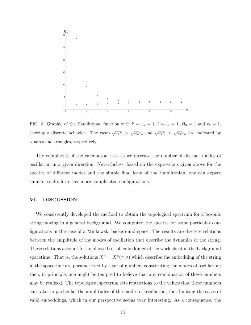
FIG. 2. Graphic of the Hamiltonian function with k = ωk = 1, l = ωl = 1, H0 = 1 and rk = 1,

showing a discrete behavior. The cases√ωlrl >

√ωkrk and

√ωlrl <

√ωkrk are indicated by

squares and triangles, respectively.

The complexity of the calculation rises as we increase the number of distinct modes of

oscillation in a given direction. Nevertheless, based on the expressions given above for the

spectra of different modes and the simple final form of the Hamiltonian, one can expect

similar results for other more complicated configurations.

VI. DISCUSSION

We consistently developed the method to obtain the topological spectrum for a bosonic

string moving in a general background. We computed the spectra for some particular con-

figurations in the case of a Minkowski background space. The results are discrete relations

between the amplitude of the modes of oscillation that describe the dynamics of the string.

These relations account for an allowed set of embeddings of the worldsheet in the background

spacetime. That is, the solutions Xµ = Xµ(τ, σ) which describe the embedding of the string

in the spacetime are parametrized by a set of numbers constituting the modes of oscillation;

then, in principle, one might be tempted to believe that any combination of these numbers

may be realized. The topological spectrum sets restrictions to the values that these numbers

can take, in particular the amplitudes of the modes of oscillation, thus limiting the cases of

valid embeddings, which in our perspective seems very interesting. As a consequence, the

15

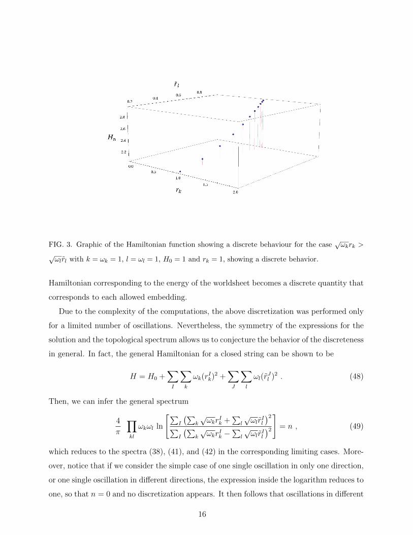
FIG. 3. Graphic of the Hamiltonian function showing a discrete behaviour for the case√ωkrk >

√ωlrl with k = ωk = 1, l = ωl = 1, H0 = 1 and rk = 1, showing a discrete behavior.

Hamiltonian corresponding to the energy of the worldsheet becomes a discrete quantity that

corresponds to each allowed embedding.

Due to the complexity of the computations, the above discretization was performed only

for a limited number of oscillations. Nevertheless, the symmetry of the expressions for the

solution and the topological spectrum allows us to conjecture the behavior of the discreteness

in general. In fact, the general Hamiltonian for a closed string can be shown to be

H = H0 +∑I

∑k

ωk(rIk)

2 +∑J

∑l

ωl(rJl )2 . (48)

Then, we can infer the general spectrum

4

π

∏kl

ωkωl ln

[∑I

(∑k

√ωkr

Ik +

∑l

√ωlr

Il

)2∑I

(∑k

√ωkrIk −

∑l

√ωlrIl

)2]

= n , (49)

which reduces to the spectra (38), (41), and (42) in the corresponding limiting cases. More-

over, notice that if we consider the simple case of one single oscillation in only one direction,

or one single oscillation in different directions, the expression inside the logarithm reduces to

one, so that n = 0 and no discretization appears. It then follows that oscillations in different

16

transverse directions do not interact with each other. As soon as we consider a configura-

tion with at least two different modes of oscillation in the same direction, the topological

spectrum becomes nontrivial, leading to discrete relationships between different modes.

The general spectrum (49) could be used to rewrite the general Hamiltonian (48) in such

a way that the discreteness of the energy becomes plausible, as in the particular Hamiltonian

(45). The final expression of the Hamiltonian, however, will depend on the relation between

different modes of oscillation as, for example, given in Eq.(46).

One important result of the investigation of the topological spectrum of bosonic strings

is that it does not depend on the background spacetime, in the sense that the expression for

the spectrum depends only on the conformal factor of the induced metric which, in turn,

can easily be derived, independently of the specific form of the background metric. This

opens the possibility of investigating discretization conditions for bosonic strings moving on

curved backgrounds in the same manner as described in the present work. This issue is

currently under investigation.

It would be interesting to compare the discretization conditions which follow from topolog-

ical quantization with those that appear in the context of canonical quantization. However,

this comparison is not yet possible. In fact, as mentioned before, two important elements

of the quantization procedure are still lacking in the approach presented here, namely, the

concepts of quantum states and quantum evolution.

ACKNOWLEDGMENTS

This work was partially support by DGAPA-UNAM No. IN106110 and No. IN108309.

F. N. acknowledges support from DGAPA-UNAM (postdoctoral fellowship).

Appendix A: Details on the integration of the Euler form

In order to integrate the Euler form (32) we must specify the limits in the domain of

integration. For the parameter σ the interval is [0, 2π] and is fixed, while for τ we notice

that the expression for the Euler form is periodic in this parameter and we may choose a

complete cycle. To perform the integral it is convenient to use null-like coordinates patches

17

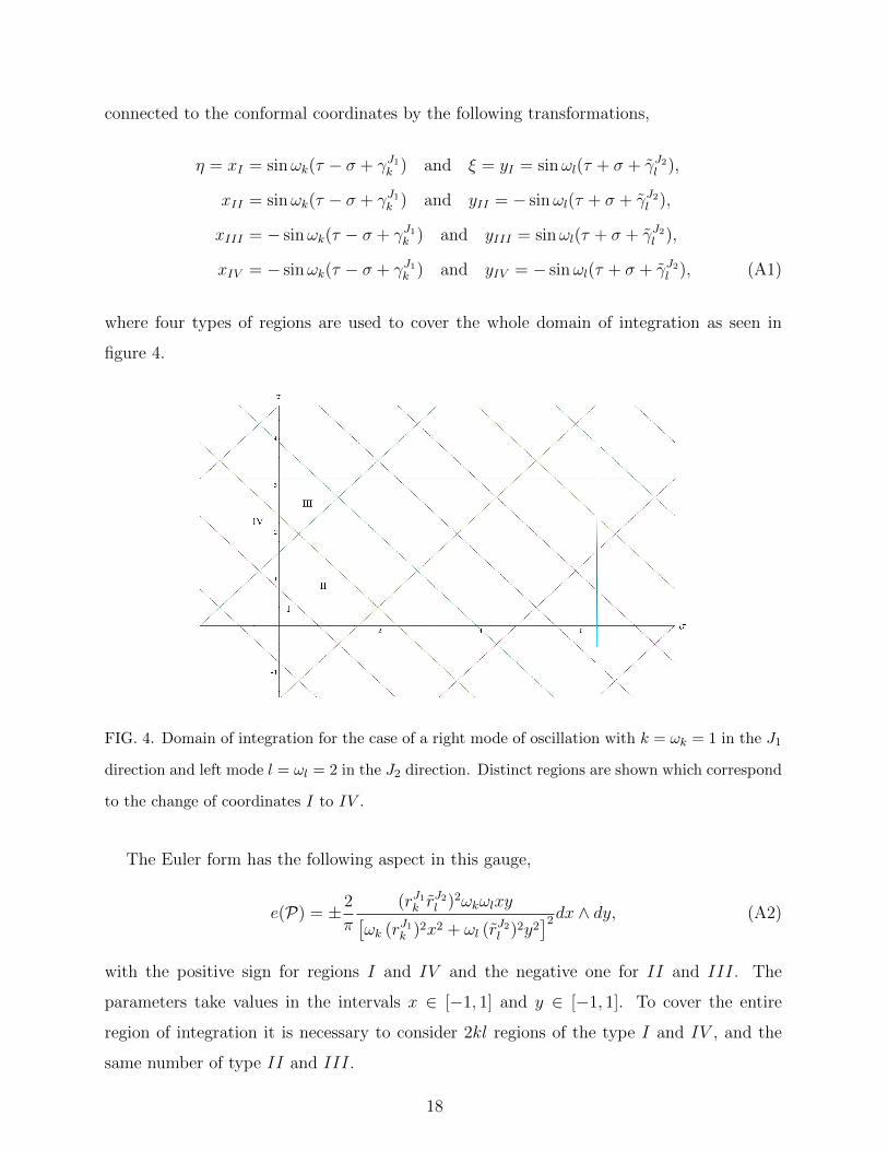
connected to the conformal coordinates by the following transformations,

η = xI = sinωk(τ − σ + γJ1k ) and ξ = yI = sinωl(τ + σ + γJ2l ),

xII = sinωk(τ − σ + γJ1k ) and yII = − sinωl(τ + σ + γJ2l ),

xIII = − sinωk(τ − σ + γJ1k ) and yIII = sinωl(τ + σ + γJ2l ),

xIV = − sinωk(τ − σ + γJ1k ) and yIV = − sinωl(τ + σ + γJ2l ), (A1)

where four types of regions are used to cover the whole domain of integration as seen in

figure 4.

FIG. 4. Domain of integration for the case of a right mode of oscillation with k = ωk = 1 in the J1

direction and left mode l = ωl = 2 in the J2 direction. Distinct regions are shown which correspond

to the change of coordinates I to IV .

The Euler form has the following aspect in this gauge,

e(P) = ± 2

π

(rJ1k rJ2l )2ωkωlxy[

ωk (rJ1k )2x2 + ωl (rJ2l )2y2

]2dx ∧ dy, (A2)

with the positive sign for regions I and IV and the negative one for II and III. The

parameters take values in the intervals x ∈ [−1, 1] and y ∈ [−1, 1]. To cover the entire

region of integration it is necessary to consider 2kl regions of the type I and IV , and the

same number of type II and III.

18

In this case, for any type of region the integral of the Euler class vanishes,∫ 1

−1

∫ 1

−1dxdy e(x, y) = 0. (A3)

This procedure to perform the integration is employed for the other particular configu-

rations considered.

REFERENCES

1Alvarez, O., “Topological quantization and cohomology,” Comm. Math. Phys. 100, 279–

309 (1985).

2Bulgadaev, S. A., “Topological quantization of current in quantum tunnel contacts,”

Pis’ma v Zh. Eksper. Teoret. Fiz. 83, 659–663 (2006).

3Carlip, S., “Quantum gravity: a progress report,” Rep. Prog. Phys. 64, 885–942 (2001).

4Choi, M. Y., “Bloch oscillation and topological quantization,” Phys. Rev. B 50, 13875–

13878 (1994).

5Choquet-Bruhat, Y., DeWitt-Morette, C., and Dillard-Bleick, M., Analysis, Manifolds and

Physics (Elsevier Science Publishers, 1982).

6Deguchi, S., “Atiyah-Singer index theorem in an so(3) Yang-Mills-Higgs system and deriva-

tion of a charge quantization condition,” Prog. Theor. Phys. 118, 769–784 (2007).

7Dirac, P. A. M., “Quantised singularities in the electromagnetic field,” Proc. Roy. Soc. A

133, 60–72 (1931).

8Frankel, T., The Geometry of Physics, 2nd ed. (Cambridge University Press, 2004).

9Isham, C. J., “Structural issues in quantum gravity,” Gen. Rel. Grav. GR14, 167–209

(1997).

10Johnson, C. V., D-Branes (Cambridge University Press, 2003).

11Leone, R. and Levy, L., “Topological quantization by controlled paths: Application to

Cooper pairs pumps,” Phys. Rev. B 77, 064524–064539 (2008).

12Misner, C. W., “Harmonic maps as models for physical theories,” Phys. Rev. D 18, 4510–

4524 (1978).

13Naber, G. L., Topology, Geometry and Gauge Fields (Springer Verlag, New York, 1997).

14Nakahara, M., Geometry, Topology and Physics, 2nd ed. (Taylor & Francis, 2003).

15Nash, C. and Sen, S., Topology and Geometry for Physicists (Academic Press, 1983).

19

16Nettel, F. and Quevedo, H., “Topological spectrum of classical configurations,” AIP Conf.

Proc. 956, 9–14 (2007).

17Nettel, F. and Quevedo, H., “Topological quantization of the harmonic oscillator,” Int. J.

of Pure and Appl. Math. 70, 117–123 (2011).

18Nettel, F., Quevedo, H., and Rodrıguez, M., “Topological spectrum of mechanical sys-

tems,” Rep. Math. Phys. 64, 355–365 (2009).

19Patino, L. and Quevedo, H., “Bosonic and fermionic behavior in gravitational configura-

tions,” Mod. Phys. Lett. A 18, 1331–1342 (2003).

20Patino, L. and Quevedo, H., “Topological quantization of gravitational fields,” J. Math.

Phys. 46, 22502–22513 (2005).

21Polchinski, J., String Theory Vols. 1 and 2 (Cambridge University Press, 1998).

22Ranada, A. F. and Trueba, J. L., “Topological quantization of the magnetic flux,” Found.

Phys. 36, 427–436 (2006).

23Schwarz, A. S., “On regular solutions of Euclidean Yang-Mills equations,” Phys. Lett. B

67, 172–174 (1977).

24Zhong, W. J. and Duan, Y. S., “Topological quantization of instantons in SU(2) Yang-Mills

theory,” Chin. Phys. Lett. 25, 1534–1537 (2008).

25Zwiebach, B., A First Course in String Theory (Cambridge University Press, 2004).

20