PHYSICAL REVIEW B 89, 205315 (2014)

Partially split Hall bar: Tunneling in the bosonic integer quantum Hall effect

Michael Mulligan1 and Matthew P. A. Fisher2

1Microsoft Research, Station Q, Elings Hall, University of California, Santa Barbara, California 93106-6105, USA2Department of Physics, University of California, Santa Barbara, California 93106, USA

(Received 20 February 2014; published 23 May 2014)

We study point-contact tunneling in the integer quantum Hall state of bosons. This symmetry-protectedtopological state has electrical Hall conductivity equal to 2e2/h and vanishing thermal Hall conductivity. Incontrast to the integer quantum Hall state of fermions, a point contact can have a dramatic effect on thelow-energy physics. In the absence of disorder, a point contact generically leads to a partially split Hall bargeometry. We describe the resulting intermediate fixed point via the two-terminal electrical (Hall) conductance ofthe edge modes. Disorder along the edge, however, both restores the universality of the two-terminal conductanceand helps preserve the integrity of the Hall bar within the relevant parameter regime.

DOI: 10.1103/PhysRevB.89.205315 PACS number(s): 73.43.Jn, 03.65.Vf, 11.25.Hf

I. INTRODUCTION

The low-energy excitations of a quantum Hall droplet livealong the edges of the sample. When two opposing edgesof the same droplet are well separated, the bulk mobilitygap prevents tunneling interactions between these low-energyexcitations. However, if a constriction is introduced such thatthe two opposing sides meet near a point, the amplitude forinteredge tunneling can be appreciable. At finite temperature,the resulting quasiparticle tunneling degrades the Hall currentas it allows backscattering between opposing edges at the pointcontact.

As an example, consider the Laughlin states at filling frac-tion ν = 1/m. These states have (fractionally) quantized Hallconductance G0(T ) = νe2/h in the absence of a constriction.Tunneling at any such constriction is generically dominatedby the transfer of (fractionally) charged νe quasiparticles andleads to the reduction of the Hall current by the amount,Ga(T ) − νe2/h = −aT 2ν−2 for some positive constant a [1].While this perturbative result is necessarily only valid fortemperatures, T 2−2ν � ah

νe2 , it shows the marked differencebetween the integral and fractional quantum Hall regimeswhen extrapolated to zero temperature. For the integral case,the conductance is merely reduced by a finite, constant valuethat is independent of temperature. In the fractional case,2 − 2ν > 0, so the perturbative calculation indicates that theeffect of backscattering at the point contact on the Hallconductance is to reduce its value as the temperature islowered, eventually leading to a vanishing Hall conductance.This means that the Hall droplet has effectively split intotwo pieces. The perturbative picture is supported by an exactsolution at certain filling fractions: the theoretical model thatdescribes the edge mode conductance is integrable at ν = 1/3and at other Laughlin states after fine tuning to a single relevantinteraction [2,3].

The above results can be understood purely from theperspective of the low-energy edge modes. Consider thesituation where the Hall fluid is put on the infinite strip. Forthe ν = 1/m Laughlin states, the counter-propagating edgemodes living on each side of the strip together form a nonchiralLuttinger liquid. The point contact provides a perturbationat a single spatial point that scatters a left moving modeinto a right moving mode and vice versa. The (boundary)

scaling dimension of this tunneling operator � = ν and isrelevant, in the renormalization group (RG) sense, if ν < 1. Ifrelevant, the perturbation drives the theory to a new infrared(IR) fixed point which, in the Laughlin case, corresponds toa fully disconnected geometry where the Hall bar has splitin two. When ν = 1, the perturbation is exactly marginal anddescribes a line of fixed points parameterized by the coefficientof this perturbing operator. In Figs. 1(a) and 1(c), we drawthe geometries corresponding to the fully connected and fullydisconnected fixed points present in point-contact perturbedHall states. The analysis of the Laughlin states immediatelygeneralizes to other Abelian fractions with the basic conclusionbeing that an Abelian fluid perturbed by a point contact willgenerically flow to a new IR fixed point if the Abelian statehas quasiparticles with fractional braid statistics.

From the edge point of view, the point contact is animpurity that leads at low energies to a change in the boundaryconditions for the edge modes at the location of the impurity, ifthe tunneling operator is relevant [2,4]. In the simplest of cases,an example of which is provided by the state considered inthis paper, the boundary conditions describe how left movingedge modes a reflected into right moving edge modes andvice versa. Thus a boundary RG flow is initiated by thepresence of the point contact. (A boundary RG flow is onewhere the edge mode dispersion remains gapless along the RGtrajectory, while there is a change in the conformally invariantboundary conditions between the ultraviolet (UV) and IR fixedpoints [5].) This flow is characterized by the change in theAffleck-Ludwig boundary entropy [6]; the boundary entropy isa scalar quantity that functions much like the central charge [7]in 1 + 1d conformal field theory (CFT) as it monotonicallydecreases along boundary RG trajectories [8].

Using the celebrated bulk-boundary correspondence ofChern-Simons theory, Fendley, Fisher, and Nayak made abeautiful observation relating the behavior of the edge and bulktheories upon perturbation of a Hall state by a point contact [9].They identified the change in the boundary entropy with thechange in the bulk thermodynamic entropy of the Hall state.The change in the latter quantity is negative because a splittingof the Hall bar implies a decrease in the amount of uncertaintyregarding the state of the fluid. The change in both quantitiesis equal to − ln(D), where the total quantum dimension of

1098-0121/2014/89(20)/205315(11) 205315-1 ©2014 American Physical Society

MICHAEL MULLIGAN AND MATTHEW P. A. FISHER PHYSICAL REVIEW B 89, 205315 (2014)

(a) Vacuum

Vacuum

Hall Fluid Hall Fluid

Vacuum

Vacuum

Hall Fluid Hall Fluid

Vacuum

Vacuum

Hall FluidHall Fluid

(b)

(c)

FIG. 1. (Color online) Qualitative geometries of the Hall bar atthe various fixed points. The fully connected geometry in (a) describesa single-component Hall bar. The partially split geometry in (b)represents the intermediate fixed point present in certain parameterregimes in the bosonic IQH state, spin Hall insulator, and thebosonic E8 state. The fully disconnected geometry in (c) describesa Hall bar consisting of two disconnected components coupled via apoint-contact interaction.

a topological state, D =√∑

i d2i = 1/S00 � 1, where di are

the quantum dimensions of the individual quasiparticles of atopological state and S00 is the 00-th entry of the modularS- matrix. This identification unites the bulk and boundaryviewpoints on the behavior of the Hall fluid upon perturbationby a point contact.

In this paper, a long-range entangled (topological) state ofmatter is defined to be a gapped state with nonzero topologicalentanglement entropy [10–12], − ln(D), and so D > 1; ashort-range entangled (topological) state is then a gappedstate with vanishing topological entanglement entropy, D = 1.Thus, in the absence of symmetry considerations, a pointcontact has a very different effect on Hall states that arelong-range entangled versus those that are only short-rangeentangled: long-range entangled states generally split in twounder RG flow while short-range entangled states do not.An RG trajectory between the fully connected and fullydisconnected limits is only possible when D > 1. Otherwise,there must either be a fixed line connecting the fully connectedand fully disconnected fixed points or there must be anintermediate fixed point that prevents a direct flow betweenthese two limits. To emphasize this point, we sketch in Fig. 2the qualitative RG flows for a few illustrative quantum Hallliquids.

In 2 + 1d, short-range entangled states of fermions are builtfrom layers of ν = 1 Laughlin states which are characterizedby their thermal Hall conductance [13] (in the absence of anysymmetry), a quantity that measures the chiral central chargeof the state. For an Abelian state, the chiral central charge issimply the difference in the number of left and right movingedge modes. As we have reviewed, a point contact in thissystem is merely an exactly marginal perturbation and does

Generic Long-Range Entangled RG Flow

(i)

Generic Short-Range Entangled RG Flows

(ii)

(iii)

(iv)

FIG. 2. (Color online) Qualitative boundary renormalizationgroup flow diagrams of point-contact perturbed Hall fluids. The (blue)left-most dot represents the fixed point describing a fully connectedHall bar geometry while the right-most (red) dot represents the fixedpoint that describes a Hall bar geometry that has fully split intotwo pieces. A (green) dot in between represents an intermediate fixedpoint. A fixed point is IR stable with respect to a particular (irrelevant)operator if the arrow on the line connected to it is directed towardsthe representative dot, while a line with no arrow indicates a fixedline. Fractional quantum Hall states realize (i). Integer quantum Hallstates of fermions realize the fixed line drawn in (ii). The bosonicinteger quantum Hall state—the state that is the subject of thispaper—realizes (ii) and (iii) in the dirty and clean limits, respectively.The bosonic E8 state realizes (iv). The spin Hall insulator realizes(ii)–(iv) in various edge interaction parameter regimes.

not lead to a splitting of the Hall droplet as the temperatureis lowered. In the absence of symmetry, short-range entangledstates of bosons are built from layers of the E8 state, which havea minimum of eight chiral edge modes [14–17]. In contrast tothe ν = 1 Laughlin state, the lowest dimension point-contacttunneling operator for the E8 state has (boundary) scalingdimension � = 2 and is strictly irrelevant. Again, the statedoes not split in two as the temperature is lowered.

Symmetry-protected topological states are short-rangeentangled states that are stabilized by a particular globalsymmetry [18–21]. If the symmetry is broken, the state isadiabatically connected to the trivial vacuum state withouta closing of the bulk gap. It is interesting to ask whethersymmetry-protected states can display novel behavior that isnot shared by short-range entangled or long-range entangledstates obeying no symmetry requirements.

This question has been studied in the context of the time-reversal invariant spin Hall insulator [22,23]. These authorsmapped the Lagrangian describing the edge modes of the spinHall insulator to the Lagrangian of two decoupled Luttingerliquids of spin and charge bosons. The Luttinger parameters, gc

and gs , cannot take arbitrary values; rather, they are constrainedto lie upon the line gc × gs = 1. As we would expect, thereis no RG flow between the fully connected and disconnectedfixed points. Away from the marginal point in parameter spaceat gc = gs = 1, there is always an intermediate fixed pointthat is IR stable or unstable, depending upon where on theline, gc × gs = 1, the electron-electron interactions lie.

In this paper, we study the simplest bosonic symmetry-protected topological state that respects a U(1) charge-conservation symmetry [24,25]. The electrical Hall conductiv-ity of this bosonic state takes the minimum value σxy = 2e2/h

consistent with the fact that it is short-range entangled andcan border the trivial vacuum. Within this note, we refer tothis state as the bosonic integer quantum Hall (IQH) state. (Asecond candidate for this name is the previously mentioned E8

205315-2

PARTIALLY SPLIT HALL BAR: TUNNELING IN THE . . . PHYSICAL REVIEW B 89, 205315 (2014)

bosonic state that has eight chiral edge modes.) Interestinglyand in contrast to the spin Hall insulator, we find that thepoint contact (almost) always generates an RG trajectory to anew fixed point that describes a Hall droplet that has partiallysplit in two. The RG diagram for this flow is shown in Fig. 2,case (iii). Here, we are assuming that the edge is clean andthat we are working away from the single point in parameterspace where the point-contact perturbation is marginal. Wecharacterize the resulting IR stable fixed point in terms ofobservable current-current correlation functions. Surprisingly,we also find that the flow to this fixed point is integrable inthe same sense that the RG flow of the point-contact perturbedfractional quantum Hall state is integrable.

Disorder along the edge modifies this picture [26,27]. Inthe domain of attraction of the strong disorder fixed point, theleading point-contact tunneling term turns out to be marginal.And so the point-contact perturbed Hall bar is described by thefixed line drawn in Fig. 2, case (ii). Disorder has the benefitof restoring the universality of the two-terminal electrical Hallconductance of the edge modes to its value inferred from thebulk topological order of the state.

The remainder of this note is organized as follows. In Sec. II,we introduce and define the bosonic IQH state. In Sec. III, wedescribe how edge equilibration drives the system towards astrong-disorder fixed point where the two-terminal electricalHall conductance equals 2e2/h. In Sec. IV, we add the pointcontact and describe the resulting fixed point for a clean edge.In Sec. V, we calculate various current-current correlationfunctions in order to characterize the different fixed points. InSec. VI, we summarize and conclude.

II. THE BOSONIC IQHE

In the present section, we define the bulk and boundaryactions that describe the bosonic IQH state in order to setthe stage for the description of edge equilibration and point-contact tunneling in the following sections.

A. Bulk action

By the bosonic IQH state, we mean the symmetry-protected topological state of bosons stabilized by U(1) charge-conservation symmetry [24,25]. This state has vanishingthermal Hall conductivity, an electrical Hall conductivityσxy = 2e2/h, and the ability to border the topologically trivialvacuum. This latter constraint means that the state can existpurely as a 2 + 1d topological phase and need not live on theboundary of a 3 + 1d space-time.

The bosonic IQH state can be described using AbelianChern-Simons theory and the so-called K-matrix formal-ism [28]. The bulk action is

Sbulk =∫

d2xdt

(εμνρ

4πKIJ a

μ

I ∂νaρ

J − εμνρ

2πtIA

μ∂νaρ

I

), (1)

where the K matrix, KIJ = (σx)IJ = (0 11 0), and the charge-

vector tI = (1,1). Here, we are assuming the state is formedfrom bosonic constituents of charge e that we set to unityunless otherwise specified. The gauge fields a

μ

I describe thenumber currents of the bosons on each “layer” indexed byI = 1,2 and Aμ is a background electromagnetic field. The

spacetime index μ = 0,1,2 = t,x,y. Our convention for thetotally anti-symmetric tensor εμνρ is to choose ε012 = 1.

The thermal Hall conductivity is equal to the signature ofKIJ in units of π2k2

BT /3h. In units of e2/h, the electricalHall conductivity σxy = tI (K−1)IJ tJ = 2. Quasiparticle exci-tations are labeled by an integer vector nI = (n1,n2); theircharge is given by tI (K−1)IJ nJ = n1 + n2 and their mu-tual statistics by exp(2πin′

I (K−1)IJ nJ ) = exp(2πi(n′1n2 +

n′2n1)) = 1. The self-statistics of a quasiparticle nI is obtained

by halving the expression for the mutual statistical angle andreplacing n′

I = nI , thereby giving unity for any exchange.Thus all quasiparticles are bosonic and have integral charge.

B. Edge action

The bulk Chern-Simons theory requires the presence ofgapless edge modes living along the boundary of any spaceupon which the theory is defined [29,30]. We consider thebosonic IQH state to live on a strip of width W in the y

direction and length 2L → ∞ in the x direction. Thus thereare two disconnected edges that we refer to as the top andbottom of the Hall bar located at, say, y = W and y = 0,respectively. For every bulk gauge field a

μ

I and for eachboundary component, we introduce the bosonic edge modes φI

and φI . Our convention is to take the φI fields to live on the topof the Hall bar and the φI fields to live along the bottom of thebar. The two sets of edge modes φI and φJ are used to describethe local tunneling physics, but not the global dynamics of theentire Hall droplet.

The action for these edge modes is

Sedge = 1

4π

∫dtdx[KIJ ∂tφI ∂xφJ − VIJ ∂xφI ∂xφJ

+ KIJ ∂t φI ∂xφJ − VIJ ∂xφI ∂xφJ

+ 2εμν(tIAμ(W )∂νφI + tIAμ(0)∂νφI )], (2)

where KIJ = −KIJ = (0 11 0), tI = tI = (1 1), and VIJ ,VIJ

are symmetric, positive-definite matrices that parametrizethe density-density and current-current or forward scatteringinteractions along a given edge. Clearly, the kinetic structure(and, therefore, the operator algebra) of the theory defined bythe KIJ ,KIJ matrices is inherited from the bulk topologicalorder, while the VIJ ,VIJ interactions are nonuniversal fromthe perspective of the bulk physics as they depend upon edgeproperties. The edge modes are periodically identified,

φI ∼ φI + 2πaI , φI ∼ φI + 2πbI , aI ,bI ∈ Z. (3)

The background electromagnetic gauge field Aμ propagatesthroughout the bulk and we denote its restriction to a givenedge by Aμ(y) for y = 0,W , while suppressing its t and x

coordinates. Aμ couples to the edge current densities, jμ

I =εμν

2π∂νφI and j

μ

I = εμν

2π∂νφI .

Because the signature of KIJ vanishes, the general expec-tation is that a symmetry is required to stabilize the modes ona given edge from the generation of a mass gap. While thereare exceptions to this rule [31–34], the edge of the bosonicIQH state is not one of them. Charge conservation protectsthe edge modes from the possible generation of a gap viabackscattering. Indeed, a general backscattering operator onthe top edge has the form cos(n1φ1 + n2φ2). This operator

205315-3

MICHAEL MULLIGAN AND MATTHEW P. A. FISHER PHYSICAL REVIEW B 89, 205315 (2014)

carries total charge tI (K−1)IJ nJ = n1 + n2 and so we requiren1 = −n2 for neutrality. However, a mass-generating termmust have equal left �L and right �R scaling dimensions, thatis, such a term must have vanishing spin. The field redefinitionsin Eq. (4) and the action (5) show that cos[n(φ1 − φ2)] has spinequal to �R − �L = −n2. So we conclude that the edge of thebosonic IQH state is stable as long as charge conservation ismaintained. Phrased in terms of the null vector criterion [31],the edge is stable because there does not exist a nontrivialneutral null vector for the bosonic IQH state.

In the remainder of the paper, we make the simplifyingassumption that VIJ = VIJ . In general, there is no relationbetween VIJ and VIJ when the two edges are disconnected.However, this assumption is reasonable in an actual samplethat has one connected boundary. As will be shown in the nextsection, this assumption with VIJ = δIJ is an RG attractorin the presence of relevant disorder scatterers. Later on, wecomment upon the fate of our proposed phase diagram whenVIJ = VIJ . However, we leave to future work the thoroughinvestigation of the dynamics of the point-contact tunnelingwhen the simplification VIJ = VIJ is relaxed.

To study the effects of the density-density and current-current interactions parameterized by VIJ on the physics of apoint contact, it is convenient to perform a field redefinitionand rewrite Sedge in terms of left and right moving chiral fields.We assume V11 and V22 are positive. We then define

φ1 = 1√2g

(XR + XL), φ2 =√

g√2

(XR − XL),

(4)

φ1 = 1√2g

(XR + XL), φ2 =√

g√2

(−XR + XL),

where g = √V11/V22 and XR,XR (XL,XL) are functions of

x − t (x + t). In terms of the left and right moving fields, Sedge

becomes

Sedge = 1

4π

∫dtdx{∂xXR(∂t − vR∂x)XR

+ ∂xXL(−∂t − vL∂x)XL + ∂xXR(∂t − vR∂x)XR

+ ∂xXL(−∂t − vL∂x)XL + εμνAμ∂ν[g+(XR

+XL) + g−(XL + XR)]}, (5)

where vR/L = √V11V22 ± V12 and g± = √

2( 1√g

± √g). Re-

call that the tilded and untilded fields are spatially separatedand refer to edge modes on the bottom and top of the Hall bar,respectively. The gauge field Aμ that multiplies these fields isunderstood to be evaluated at the location of the edge modethat it multiplies.

It is convenient to set all velocities vR = vL = 1. Thissimplification does not affect the phase diagram of thepoint-contact perturbed Hall bar as the velocities of the edgemodes do not affect tunneling exponents; nor does this affectthe two-terminal conductances calculated in later sectionssince the action in Eq. (5) is diagonal. (If Eq. (5) happenednot to be diagonal, a conductance would, in general, dependupon the velocities [26].) Setting the velocities to all be equalwill help simplify the formulas presented later. We will allowarbitrary g± consistent with the assumption that all chiral edgemodes move with the same velocity.

III. EDGE EQUILIBRATION

The Kubo formula can be used to express the two-terminalelectrical Hall conductance G for the edge modes on thetop and bottom of a Hall bar in terms of a current-currentcorrelation function:

G = e2

��

∫ �

0dx ′ lim

ω→0

∫ ∞

−∞dτeiωτ 〈J (x,τ )J (x ′,0)〉

ω, (6)

where we have analytically continued to imaginary time,t → iτ . The conductance in Eq. (6) relates the current J (x,τ )through the point x ∈ [0,�] found in linear response to aconstant electric field applied to a length � section within awire of infinite extent.

Notice that we take the ω → 0 limit before performing theintegral over x ′ [35]. In the dc ω → 0 limit, the right-hand sideof Eq. (6) does not depend upon where in [0,�] the particular x

is chosen. In Sec. V, we will evaluate two other conductancesby varying the choice of current-current correlation functionconsidered. Note that the conductance above is denoted inSec. V by Gx,x.

The total current running through the point x along the topand bottom of the Hall bar,

J (x,τ ) = − i

2π∂τ (φ1(x,τ ) + φ2(x,τ ) + φ1(x,τ ) + φ2(x,τ ))

= g+2π

(∂zXL(z) − ∂zXR(z))

+ g−2π

(∂zXL(z) − ∂zXR(z)), (7)

where z = x + iτ,z = x − iτ,∂z = 12 (∂x − i∂τ ), and ∂z =

12 (∂x + i∂τ ).

We distinguish the two-terminal Hall conductance G fromthe electrical Hall conductivity previously denoted by σxy . G

generally differs from σxy in that it depends upon properties ofand conditions at the edge while σxy , as defined previously, isan (intensive) property of the bulk state. Indeed, because thebosonic IQH state is nonchiral, the value of the conductanceG depends upon the VIJ interactions [26,27]. Using theaction (5), we find that Eq. (6) evaluates to G = ( 1

g+ g) e2

h.

Details of the calculation that leads to this conclusion can befound in Sec. V.

The interaction-dependent value for the two-terminal Hallconductance is meaningful since an actual experimentalistmeasuring the Hall conductance runs a current along the bar,measures the voltage difference between the top and bottomof the Hall bar, and then takes the ratio of the current tovoltage drop in order to abstract the Hall conductance. Thisshould be contrasted with the conductance of interacting 1Dquantum channels for which it is necessary to attach leads tothe sample which, if Fermi liquidlike, return a conductanceof e2/h per channel [35,36]. The use of the Kubo formulain Eq. (6) generalizes [26,27] to the interacting case theLandauer-Buttiker formalism for the study of the conductanceof noninteracting electrons [37,38].

Only at g = 1 do we obtain the equality G = σxy = 2e2/h.The key physical reason for the difference between G andσxy when g = 1 is due to the lack of equilibration betweenmodes on a given edge. We have seen how charge conservationand translation invariance prevent mass-generating couplings

205315-4

PARTIALLY SPLIT HALL BAR: TUNNELING IN THE . . . PHYSICAL REVIEW B 89, 205315 (2014)

between φ1 with φ2. However, these symmetries also pre-vent edge equilibration. We generally expect any physicallyrealized edge to have some amount of disorder that breakstranslation invariance. Such disorder allows the transfer ofcharge between the two modes with the impurities absorbingthe excess momenta. In other words, impurities allow φ1 andφ2 to equilibrate.

Thus we are lead to consider charge and momentumexchange via an impurity. It is sufficient to consider a singleedge for this analysis and so we concentrate on the top edge; anidentical conclusion is drawn for the bottom edge. The lowestdimension tunneling term between φ1 and φ2 that preservescharge conservation has the form,

Sdisorder =∫

dtdx[ξ (x)eiφ1−iφ2 + H.c.], (8)

where ξ (x) is a complex Gaussian random variable satisfying,〈〈ξ ∗(x)ξ (x ′)〉〉 = Dδ(x − x ′). The double bracket denotes adisorder average. The above term tunnels a φ1 mode into a φ2

mode and vice versa. Any momentum mismatch is absorbedby the field ξ .

D functions as a coupling constant for this interactionbetween φ1 and φ2. The leading RG equation for D takesthe form [39],

∂D

∂�= [3 − 2�R(g)]D, (9)

where �R(g) = 12 (g + 1

g) equals the scaling dimension of the

operator, exp(iφ1 − iφ2). Thus disorder is relevant if 12 (3 −√

5) < g < 12 (3 + √

5).Let us suppose that we are in a region of parameter space

where disorder is relevant. For general g within this regime,perturbation theory is certainly not reliable. To access thestrong coupling fixed point, we switch to the charged φρ andneutral φσ fields:

φρ = 1

2√

2(g+XR + g−XL),

(10)

φσ = 1

2√

2(g−XR + g+XL).

The motivation for this redefinition is that it is φρ that entersinto the definition of the charge current in Eq. (5) whileonly the neutral field φσ is involved in the disorder-mediatedinteraction, Eq. (8).

Let us write the action in terms of these fields and showthat at the strong-disorder fixed point, the charge and neutralsectors decouple. Setting the background gauge field to zero,the action for the edge modes on the top edge in Eq. (5) maybe rewritten as

S = 1

4π

∫dtdx

[∂xφρ

(∂t − v

2∂x

)φρ

+ ∂xφσ

(−∂t − v

2∂x

)φσ − vρσ ∂xφρ∂xφσ

+ (ξ (x)ei√

2φσ + H.c.)

], (11)

where

v = g + 1

g, vρσ = g − 1

g. (12)

Notice the appearance of an emergent SU(2) global symmetrygenerated by the currents cos(

√2φσ ), sin(

√2φσ ), and ∂tφσ

when vρσ = 0. This occurs when g = 1. The emergent SU(2)symmetry allows an exact solution for the neutral sector of themodel. (The charged sector is already described by a free-fieldtheory at this decoupled point.) Considering small deviationsaway from the decoupled fixed point, the exact solution showsthat the decoupled fixed point action, Eq. (11) at vρσ = 0,describing the charged and neutral modes is attractive [26].

In summary, disorder, if relevant, drives the system towardsthe g = 1 point, where the two-terminal Hall conductancetakes its universal value (from the bulk perspective), G =σxy = 2e2/h. Interestingly, the point-contact perturbation ismarginal at this fixed point as we will see shortly.

IV. POINT-CONTACT TUNNELING FIXED POINTS

A. Point-contact perturbations

For well separated boundaries, terms that couple the twosets of edge modes together are absent due to locality. The ma-trix element defining the possible interaction is exponentiallysmall as long as the bulk gap is nonzero. Indeed, a tunnelingoperator of lowest dimension tunnels a single boson from oneedge to the other and, in general, has amplitude proportionalto exp(−bMW ) where M is the bulk gap, W is the distancebetween the top and bottom edges, and b is a positive constant.

However, a point-contact constriction allows nonzero tun-neling between the top and bottom edge modes at a singlespatial location. See Fig. 1 for the relevant geometrical picturesillustrating the possible tunneling. About the fully connectedgeometry displayed in Fig. 1(a), the lowest dimension tunnel-ing operators take the form,

OI,J (x) = cos(φI − φJ )δ(x), (13)

where we have chosen coordinates so that the single tunnelingevent occurs at the origin. The operator OI,J tunnels a unitcharge boson from mode φI into mode φJ at x = 0. From theaction Eq. (5), we determine the (boundary) scaling dimen-sions �I,J of the four lowest dimension tunneling terms to be

�I,J = 12 (g2I−3 + g2J−3), (14)

for I,J = 1,2. (Note that depending upon the values of g,some subset of the four operators could have higher harmonicsthat tunnel multiple bosons at a time which are more relevantthan some of the other listed fields; when listing the fouroperators above, we are implicitly considering their higherharmonics as well and so we will not mention them explicitlyfurther.) The resulting RG equations for each boundaryoperator with coupling cI,J is then

1

cI,J

∂cI,J

∂�= 1 − �I,J . (15)

At g = 1, all four operators are marginal, while for g = 1,there is a single relevant operator. For a particular choice of g,the relevant operator OI,J can be determined from the valuesof I,J = 1,2 satisfying g3−2I > 1 and g3−2J > 1. We see that

205315-5

MICHAEL MULLIGAN AND MATTHEW P. A. FISHER PHYSICAL REVIEW B 89, 205315 (2014)

for g = 1 both O1,2 and O2,1 are irrelevant; for g > 1, O1,1 isrelevant, while for g < 1, O2,2 is relevant.

In the previous section, we observed that edge equilibrationis relevant when 1

2 (3 − √5) < g < 1

2 (3 + √5), and the system

is driven towards a strong-disorder fixed point where g = 1and all four tunneling terms are marginal. The point-contactanalysis in the remainder of this section assumes either g isoutside the attractive regime of this strong-disorder fixed point,or that the edge is sufficiently clean and studied at high enoughtemperatures so that disorder has not had “time” to renormalizethe system to the g = 1 point.

We emphasize that for g = 1, either O1,1 or O2,2 is relevantat weak coupling, but not both. It is this fact that resultsin an easily tractable IR attractive fixed point describinga partially split Hall droplet. The single relevant operatordrives a (boundary) RG trajectory where the Hall bar partiallypinches off; however, it does not split into two disconnectedliquids. We schematically illustrate the partially split geometrycorresponding to this fixed point in Fig. 1(b).

In the next two sections, we describe the boundary fixedpoint that results from perturbation by O1,1 (O2,2) for g > 1(g < 1) and demonstrate its stability. (In fact, these two fixedpoints can be mapped into one another by a simple changeof variables.) To this end, consider the fully disconnectedgeometry drawn in Fig. 1(c) where there are two disconnectedHall bars coupled together at a single point contact. As wewill describe, from precisely the same analysis as above, thereexists a single relevant (boundary) tunneling term that drivesan RG trajectory towards a partially split geometry. We willprovide evidence that this IR fixed point is the same as the oneobtained by starting from the fully connected Hall droplet ofFig. 1(a), thus implying a single, isolated IR stable fixed pointseparating the fixed points describing the fully connected andfully disconnected geometries.

We caution that our analysis is valid at weak initial tunnelingcoupling. Our results assume that the single relevant tunnelingterm dominates the IR physics. This assumption is certainlyreasonable given our setup and we confirm its consistencyin our analysis below. However, we point out that whenVIJ = VIJ , there exist parameter regimes where two relevanttunneling terms compete (there is always at least one relevantoperator). We leave the interesting question of the precise char-acterization of the resulting IR fixed point(s) to future work.

B. Repulsive g > 1 interactions

1. The approach from the fully connected fixed point

When g > 1, O1,1 = cos(φ1 − φ1)δ(x) is the most relevanttunneling operator. It has (boundary) scaling dimension �1,1 =1g

. Tunneling of the φ2 boson into the φ2 boson by the operatorO2,2 is strictly irrelevant.

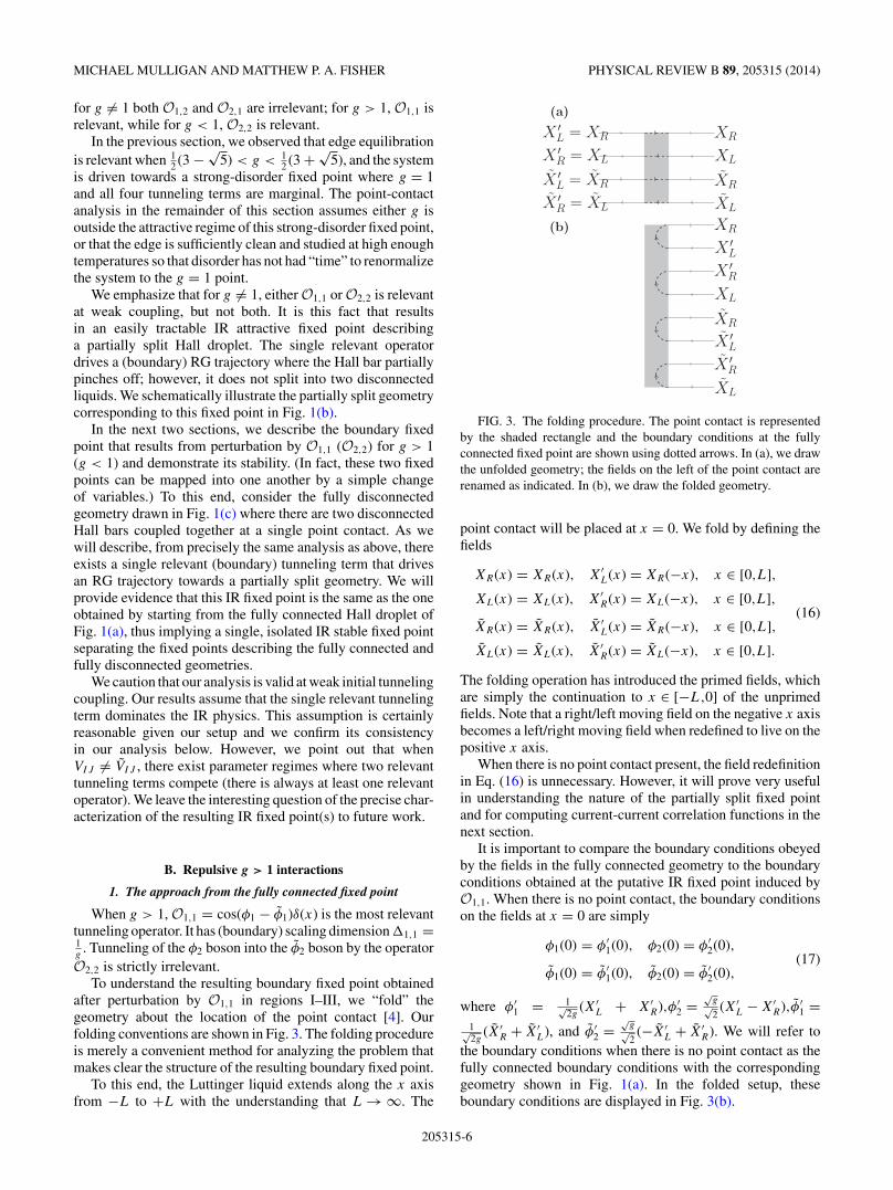
To understand the resulting boundary fixed point obtainedafter perturbation by O1,1 in regions I–III, we “fold” thegeometry about the location of the point contact [4]. Ourfolding conventions are shown in Fig. 3. The folding procedureis merely a convenient method for analyzing the problem thatmakes clear the structure of the resulting boundary fixed point.

To this end, the Luttinger liquid extends along the x axisfrom −L to +L with the understanding that L → ∞. The

(a)

X ′L = XR XR

X ′R = XL XL

X ′L = XR XR

X ′R = XL XL

(b) XR

X ′L

X ′R

XL

XR

X ′L

X ′R

XL

FIG. 3. The folding procedure. The point contact is representedby the shaded rectangle and the boundary conditions at the fullyconnected fixed point are shown using dotted arrows. In (a), we drawthe unfolded geometry; the fields on the left of the point contact arerenamed as indicated. In (b), we draw the folded geometry.

point contact will be placed at x = 0. We fold by defining thefields

XR(x) = XR(x), X′L(x) = XR(−x), x ∈ [0,L],

XL(x) = XL(x), X′R(x) = XL(−x), x ∈ [0,L],

(16)XR(x) = XR(x), X′

L(x) = XR(−x), x ∈ [0,L],

XL(x) = XL(x), X′R(x) = XL(−x), x ∈ [0,L].

The folding operation has introduced the primed fields, whichare simply the continuation to x ∈ [−L,0] of the unprimedfields. Note that a right/left moving field on the negative x axisbecomes a left/right moving field when redefined to live on thepositive x axis.

When there is no point contact present, the field redefinitionin Eq. (16) is unnecessary. However, it will prove very usefulin understanding the nature of the partially split fixed pointand for computing current-current correlation functions in thenext section.

It is important to compare the boundary conditions obeyedby the fields in the fully connected geometry to the boundaryconditions obtained at the putative IR fixed point induced byO1,1. When there is no point contact, the boundary conditionson the fields at x = 0 are simply

φ1(0) = φ′1(0), φ2(0) = φ′

2(0),(17)

φ1(0) = φ′1(0), φ2(0) = φ′

2(0),

where φ′1 = 1√

2g(X′

L + X′R),φ′

2 =√

g√2(X′

L − X′R),φ′

1 =1√2g

(X′R + X′

L), and φ′2 =

√g√2(−X′

L + X′R). We will refer to

the boundary conditions when there is no point contact as thefully connected boundary conditions with the correspondinggeometry shown in Fig. 1(a). In the folded setup, theseboundary conditions are displayed in Fig. 3(b).

205315-6

PARTIALLY SPLIT HALL BAR: TUNNELING IN THE . . . PHYSICAL REVIEW B 89, 205315 (2014)

In order to study the nontrivial boundary fixed point inducedby the perturbation O1,1, it is convenient to first make thefollowing field redefinitions by introducing the right and leftmoving fields Ri and Lj for i,j = 1, . . . ,4:

XR = 12 (R1 + R2 + R3 + R4),

X′R = 1

2 (−R1 − R2 + R3 + R4),

XR = 12 (R1 − R2 + R3 − R4),

X′R = 1

2 (−R1 + R2 + R3 − R4), (18)

XL = 12 (−L1 − L2 + L3 + L4),

X′L = 1

2 (L1 + L2 + L3 + L4),

XL = 12 (−L1 + L2 + L3 − L4),

X′L = 1

2 (L1 − L2 + L3 − L4).

All fields are understood to live on the half-line, x ∈ [0,L].For convenience, we provide the inverse of the transformationin Eq. (18):

R1 = 12 (XR − X′

R + XR − X′R),

R2 = 12 (XR − X′

R − XR + X′R),

R3 = 12 (XR + X′

R + XR + X′R),

R4 = 12 (XR + X′

R − XR − X′R),

(19)L1 = 1

2 (−XL + X′L − XL + X′

L),

L2 = 12 (−XL + X′

L + XL − X′L),

L3 = 12 (XL + X′

L + XL + X′L),

L4 = 12 (XL + X′

L − XL − X′L).

The action remains diagonal after the field redefinitions inEq. (18), however, the coupling to the gauge field is changed. Interms of these fields, the fully connected boundary conditionsin Eq. (17) become

Ri(0) = Li(0), (20)

for all i.We are now ready to study the effects of the point contact.

An important point is that because we have (redundantly)doubled the number of fields in folding the geometry, a pointcontact now corresponds to two boundary perturbations. In thefolded geometry, the operator O1,1 becomes

O1,1 → cos(φ1 − φ1)δ(x) + cos(φ′1 − φ′

1)δ(x). (21)

Hopefully without leading to any confusion, we will continueto refer to this operator in the folded geometry as O1,1.

The benefit of the field redefinitions in Eq. (18) is that theboundary conditions induced by the operator O1,1 are easy toanalyze. The effect of the point-contact perturbation, O1,1, isto freeze:

φ1(0) = φ1(0), φ′1(0) = φ′

1(0). (22)

These two conditions take a simple form when written in termsof the Ri,Lj fields: R2(0) = L2(0) and R4(0) = −L4(0). Thusthe point contact only changes the boundary condition relatingR4 to L4. The boundary conditions on the other pair of fields,

Ri,Lj for i,j = 1,3, are unaffected by the point contact and,therefore, remain the same as in the fully connected case,Eq. (20).

Summarizing, we find that the point-contact perturbationdrives a boundary RG flow to the fixed point characterized bythe boundary conditions,

Ri(0) = Li(0), i = 1,2,3, R4(0) = −L4(0). (23)

If we form the nonchiral bosons χi = Ri + Li , then the effectof the point contact is to drive the (integrable) boundary flowfrom the Neumann to the Dirichlet boundary condition for χ4

with the other three fields maintaining their initial Neumannconditions at the point contact. The boundary conditions inEq. (23) define the partially split fixed point and, for brevity,we shall refer to these boundary conditions as the partiallysplit boundary conditions.

2. The approach from the fully disconnected fixed point

We now wish to give evidence for the stability or attrac-tiveness of the partially split fixed point. As we have seen,starting from the fully connected fixed point, perturbationby the relevant operator O1,1 drives the system towards thepartially split fixed point.

Consider instead the approach to the partially split fixedpoint from the fully disconnected geometry where there aretwo bosonic IQH droplets interacting via a single point contactdrawn schematically in Fig. 1(c). In terms of the folded fieldsof Fig. 3(a), the fully disconnected geometry is defined by thefollowing boundary conditions:

φ1(0) = φ1(0), φ2(0) = φ2(0),(24)

φ′1(0) = φ′

1(0), φ′2(0) = φ′

2(0).

To facilitate comparison with the fully connected boundaryconditions in Fig. 3, the fully disconnected boundary condi-tions are drawn in Fig. 4. Rewritten in terms of the Ri,Lj

fields, these conditions become

R1(0) = −L1(0), R2(0) = L2(0),(25)

R3(0) = L3(0), R4(0) = −L4(0).

Thus, if the partially split fixed point is an attractor, the effectof the point contact at the fully disconnected fixed point mustbe to change the boundary condition relating R1 and L1 inorder to match Eq. (23).

To verify that this does indeed occur, we shall unfold thegeometry beginning at the disconnected fixed point boundaryconditions, Eq. (24), and show that the leading point-contactperturbation drives the theory to the partially split fixed point.[The following unfolding and refolding is not necessary forthis analysis. Instead, we may arrive at the same conclusion byanalyzing the effects of the leading point-contact perturbationat the fixed point defined in Eq. (24).] Using Eq. (24) andFig. 4, we define the fields

ϕ1 = 1√2g

(XR + XL), ϕ2 =√

g√2

(XR − XL),

(26)

ϕ1 = 1√2g

(X′R + X′

L), ϕ2 =√

g√2

(−X′R + X′

L).

205315-7

MICHAEL MULLIGAN AND MATTHEW P. A. FISHER PHYSICAL REVIEW B 89, 205315 (2014)

(a)

X ′L XR

X ′R XL

X ′L XR

X ′R XL

(b) XR

X ′L

X ′R

XL

XR

X ′L

X ′R

XL

FIG. 4. The boundary conditions at the fully disconnected fixedpoint. The point contact is represented by the shaded rectangle andthe boundary conditions at the fully disconnected fixed point areshown using dotted arrows. (a) and (b) Respective unfolded and foldedgeometries. (Compared to Fig. 3, we have smeared out the pointcontact even further in order to avoid line crossings in the figure.)

In making these definitions, we have identified XL(x) =XR(−x) and similarly for the other tilded fields shown inFig. 4. The action for the fully disconnected geometry takesexactly the same form, Eq. (2), as the action for the fullyconnected geometry with the replacements φI ↔ ϕI , φI ↔ ϕI

(along with the understanding that we are now describing edgemodes belonging to disconnected Hall samples).

The leading point-contact perturbation in the unfolded vari-ables takes the form: O′

1,1 = cos(ϕ1 − ϕ1)δ(x). To analyze theeffects of this operator, we fold the geometry as shown in Fig. 4.(In contrast to how we folded when starting at the fully con-nected fixed point, we now introduce tilded left and right mov-ing fields instead of primed left and right moving fields.) As wepreviously noted, folding splits the point-contact perturbationinto two boundary operators and imposes the constraints:

XR + XL = X′R + X′

L, XR + XL = X′R + X′

L. (27)

By taking linear combinations of these two equations andusing Eq. (19), we see that in terms of the Ri and Lj variables,these boundary conditions become: R1 = L1 and R2 = L2.O′

1,1 does not affect the boundary conditions of R3,4 andL3,4 given in Eq. (25). We recognize the resulting boundaryconditions as describing the partially split fixed point. Thusthe leading point-contact perturbation drives an RG trajectoryfrom either the fully connected or fully disconnected fixedpoints to the partially split fixed point in the IR, therebyimplying the existence of a single, isolated fixed point inbetween these two limits.

3. Stability of the partially split fixed point

Having demonstrated the symmetry between the twoapproaches to the partially split fixed point, we now askwhether there exist additional instabilities at this IR fixed

point. In other words, are there potential runaway “directions”in coupling constant space?

To determine the stability of the partially split fixedpoint, we need only enumerate all boundary perturbationsat the partially split fixed point and compute their scalingdimensions. In the unfolded language, an arbitrary tunnelingperturbation takes the form

Oai ,bj= cos(a1φ1 + a2φ2 + b1φ1 + b2φ2)δ(x), (28)

for ai,bj ∈ Z. In this notation, the four operators con-sidered previously are written as O1,1 = O(1,0),(1,0),O1,2 =O(1,0),(0,1),O2,1 = O(0,1),(1,0), and O2,2 = O(0,1),(0,1). We mustcompute the dimensions of these operators at the partially splitfixed point. The IR scaling dimensions will generally differfrom the values taken at the UV fixed point.

To begin, we need to constrain the form of the operatorso that it conserves U (1) charge. Neutrality requires: a1 +a2 + b1 + b2 = 0. To compute the scaling dimension, we firstexpress Oai ,bj

in terms of the Ri,Lj fields. We then imposethe partially split boundary conditions in Eq. (23) to write theLj fields in terms of the Ri . The scaling dimensions are thenread off from the temporal decay at x = 0 of the two-pointcorrelation function of Oai ,bj

(t) finding,

�ai,bj(g) = 1

4

[(a1 + b1)2

g+ g

(3a2

2 + 3b22 + 2a2b2

)], (29)

subject to the neutrality constraint.No operator Oai ,bj

is relevant at the partially splitfixed point. Consider the following low-dimensional exam-ples. O1,2 = cos(φ1 − φ2)δ(x) and O2,1 = cos(φ1 − φ2)δ(x)are both of scaling dimension, �1,2 = �2,1 = 1

4 (3g + 1/g).O2,2 = cos(φ2 − φ2)δ(x) has scaling dimension, �2,2 = g.Both sets of operators, along with all other operators givenin Eq. (28), are irrelevant when g > 1. (The operator O1,1

becomes the identity operator at the partially split fixed pointas its constraint is satisfied on all states.)

C. Attractive g < 1 interactions

It is straightforward to apply the method outlined in theprevious section to the case when g < 1. Therefore we canmore or less state the following results instead of providing afull derivation as in the previous section.

When g < 1, the most relevant operators at the fullyconnected and fully disconnected fixed point are O2,2 andO′

2,2, respectively (using notation introduced previously). Justas the boundary conditions induced by O1,1 only involved R2,4

and L2,4, the conditions imposed byO2,2 only involve R1,3 andL1,3. Around the fully connected fixed point, the conditions,φ2 = φ2 and φ′2 = φ′2 imposed by the leading point-contactperturbation when g < 1 results in a fixed point characterizedby the boundary conditions:

R1(0) = −L1(0), R2(0) = L2(0),(30)

R3(0) = L3(0), R4(0) = L4(0).

(About the fully disconnected fixed point, O′2,2 drives the

system to the same IR stable partially split fixed point, butinstead involves the fields R3,4 and L3,4.) The RG diagramfor this flow takes the form shown in Fig. 1, case (iii). Thestability of the fixed point, Eq. (30), is also immediate since

205315-8

PARTIALLY SPLIT HALL BAR: TUNNELING IN THE . . . PHYSICAL REVIEW B 89, 205315 (2014)

the lowest dimension tunneling operator is O1,1, which hasboundary scaling dimension equal to 1/g > 1 for g < 1. Thusthe transformation g ↔ 1/g and R1,L1 ↔ R4,L4 takes usbetween the fixed point induced byO1,1 (O′

1,1) andO2,2 (O′2,2).

V. TWO-TERMINAL CONDUCTANCES

We now describe how the boundary conditions charac-terizing the various fixed points studied in the previoussection are reflected in the current-current correlation functionsthat determine two-terminal electrical conductances at zerotemperature. The leading finite temperature corrections tothe zero temperature conductances calculated here scale as−aT 2�−2, where � is the smallest scaling dimension ofa tunneling operator at a given fixed point and a is somenon-negative constant.

The conductances that we are interested in relate the currentthrough the point x ∈ [0,�] about the dashed lines shown inFig. 5 obtained in response to a constant electric field appliedto a section of wire of length �. The currents are

Jx(x,τ ) = 1√22π

[(1√g

+ √g

)(∂zXL(z) − ∂zXR(z))

+(

1√g

− √g

)(∂zXL(z) − ∂zXR(z))

],

Jy(x,τ ) = 1√22π

[(1√g

+ √g

)(∂zX

′L(z) − ∂zXR(z))

+(

1√g

− √g

)(∂zXL(z) − ∂zX

′R(z))

],

(a) X′L

X′R

XR XL

X′R

X′L XL XR

(b) X′L

X′R

XR XL

X′R

X′L XL XR

(c) X′L

X′R

XR XL

X′R

X′L XL XR

FIG. 5. (Color online) The dashed lines in the above three figuresdenote the line through which the three currents in Eq. (31) flow; theconductances in Eq. (32) measure the flow of charge through thisline. As a point of reference, (a) measures the conductance along theHall bar for the current Jx, (b) measures the conductance across theHall bar for the current Jy, and (c) measures a skew conductance withrespect to the fully connected fixed point of Fig. 1(a) for the currentJs. The green square represents a possible (boundary) interactioninduced by a point contact and the modes are labeled according tothe conventions of Fig. 3.

Js(x,τ ) = 1√22π

[(1√g

+ √g

)(∂zXL(z) + ∂zX

′L(z))

−(

1√g

− √g

)(∂zXR(z) + ∂zX

′R(z))

], (31)

where z = x + iτ . Using the Kubo formula, we shall calculatethe following three conductances at the fixed points previouslydescribed for g > 1:

G(A)a,a = e2

��

∫ �

0dx ′ lim

ω→0

∫ ∞

−∞dτeiωτ 〈Ja(x,τ )Ja(x ′,0)〉A

ω,

(32)

where A = FC,PS, or FD denote the fully connected, partiallysplit, and fully disconnected fixed points and a = x,y, or s.

The first two conductances of Eq. (31) are sufficient todistinguish the fixed points and make particularly clear thesymmetry present at the partially split fixed point. From theperspective of a fully connected geometry shown in Fig. 1(a),G

(FC)x,x measures the conductance along the bar, while G

(FC)y,y

measures the conductance across the Hall bar. G(FC)s,s is a

type of skew conductance where the potential on leads ondiametrically opposite sides of the point contact are raisedrelative to the other two. Its value, however, is independent ofthe particular fixed point considered and we shall not considerit further.

The central results of this section are the following two-terminal electrical conductances:

G(FC)x,x = G

(FD)y,y =

(1

g+ g

)e2

h,

G(FD)x,x = G

(FC)y,y = 0, (33)

G(PS)x,x = G

(PS)y,y = 1

g

e2

h.

We note the equality of the conductances along and acrossthe Hall bar at the partially split fixed point. Using eitherthe mapping described in the previous section or an explicitcalculation, the conductances for g < 1 are obtained bysubstituting g ↔ 1/g in Eq. (33). Interestingly, setting e2/h =1, the conductance at the partially split fixed point is equal tothe boundary scaling dimension of the operatorO1,1 (O′

1,1) thatdrives the system towards the intermediate fixed point fromeither the fully connected or fully disconnected fixed points.

In order to calculate G(A)x,x , for instance, we need the

following correlation functions. Note that only a subset of thenonzero correlation functions are listed with the additionalcorrelators obtained by methods exactly similar to thosethat we state below. Correlation functions containing purely(anti-)holomorphic fields are not generally affected by theboundary conditions at the point contact:

〈∂zXR(z)∂z′XR(z′)〉A = 1

(z − z′)2,

(34)

〈∂zXL(z)∂z′XL(z′)〉A = 1

(z − z′)2,

and similarly for other two-point correlators of pairs of purely(anti-)holomorphic fields. Correlation functions between two

205315-9

MICHAEL MULLIGAN AND MATTHEW P. A. FISHER PHYSICAL REVIEW B 89, 205315 (2014)

different (anti-)holomorphic fields vanish. However, correla-tors between a holomorphic field and an anti-holomorphic fielddo depend upon the specific boundary conditions at the pointcontact:

〈∂zXR(z)∂z′X′L(z′)〉A = 1

(z′ + z)2

(δA,FC + 1

2δA,PS

),

〈∂zXR(z)∂z′XL(z′)〉A = − 1

2(z′ + z)2δA,PS,

(35)

〈∂zXR(z)∂z′XL(z′)〉A = 1

(z′ + z)2

(δA,FD + 1

2δA,PS

),

〈∂zXR(z)∂z′X′L(z′)〉A = 1

2(z′ + z)2δA,PS.

In deriving Eq. (35), we used the field redefinition in Eq. (18)and the fact that

〈∂zRi(z)∂z′Lj (z′)〉A = ±δij

1

(z′ + z)2, (36)

if Ri(0,τ ) = ±Lj (0,τ ) at the point contact.We are now ready to verify the conductances quoted in

Eq. (33). The calculations of G(A)x,x and G

(A)y,y are related by

the replacements, XR,L ↔ X′R,L and δA,FD ↔ δA,FC. (The

calculation of G(A)s,s proceeds analogously.) Therefore we only

show the calculation of G(A)x,x below.

The correlation function in the top line of Eq. (32) factorsinto twelve nonzero terms:

〈Jx(x,τ )Jx(x ′,0)〉A = 1

8π2

[(1√g

+ √g

)2

(〈∂zXR(z)∂z′XR(z′)〉A − 〈∂zXR(z)∂z′XL(z′)〉A − 〈∂zXL(z)∂z′XR(z′)〉A

+〈∂zXL(z)∂z′XL(z′)〉A) +(

1√g

− √g

)2

(〈∂zXR(z)∂z′XR(z′)〉A − 〈∂zXR(z)∂z′XL(z′)〉A

−〈∂zXL(z)∂z′XR(z′)〉A + 〈∂zXL(z)∂z′XL(z′)〉A) −(

1

g− g

)(〈∂zXR(z)∂z′XL(z′)〉A

+〈∂zXL(z)∂z′XR(z′)〉A + 〈∂zXR(z)∂z′XL(z′)〉A + 〈∂zXL(z)∂z′XR(z′)〉A], (37)

where z = x + iτ and z′ = x ′. Making use of Eqs. (34)and (35) in the above equation and substituting into the Kuboformula, Eq. (32), we encounter integrals of the form:

∫ ∞

−∞dτ

eiωτ

[±iτ + (x − x ′)]2= 2πωe−|x−x ′ |ω�(±(x − x ′)),

(38)

where �(x) = 1 for x > 0 and �(x) = 0 for x < 0 is theHeaviside step function. (The nonzero difference |x − x ′|functions as an UV regulator of the τ integral.) Taking thedc ω → 0 limit and integrating over x ′, we find

G(A)x,x = e2

h

[(1

g+ g

)−

(1

g+ g

)δA,FD − gδA,PS

]. (39)

Thus we have checked the value of G(A)x,x quoted in Eq. (33).

The calculation of G(A)y,y proceeds in precisely the same way

with the substitution XR,L ↔ X′L,R in Eq. (37).

VI. SUMMARY

In this note, we have studied how the bosonic integerquantum Hall state responds to two distinct perturbations:disorder and point-contact tunneling. The bosonic IQH state isstable as long as charge conservation is maintained, however,the two-terminal electrical Hall conductance inferred from theconductance of its edge modes leads to a value that dependscontinuously on a particular edge-mode interaction parameterthat we denoted by g. When intermode equilibration occursvia impurities, the interaction parameterized by g renormalizestowards the value g = 1 at which the two-terminal electrical

conductance G takes the universal value of 2e2/h and theleading point-contact tunneling perturbation is marginal.

Equilibration via interactions induced by impurities alongthe edge is only a relevant perturbation when g is within acertain range of values. Outside of the domain of attractionof the strong-disorder fixed point, these impurity-mediatedinteractions are irrelevant and so equilibration does not occur.The two-terminal electrical conductance then depends uponthe edge interaction parameter g.

When the impurity-mediated interactions are irrelevant orwhen the temperature cuts off the RG flow towards the strong-disorder fixed point, we may consider how a point contactaffects the bosonic IQH state. Away from the g = 1 point,a point contact drives a boundary RG trajectory to a single,isolated IR stable fixed point where the Hall bar partially splitsinto two pieces. The partially split fixed point is characterizedby equal two-terminal electrical conductances both along andacross the Hall bar.

This point-contact induced partial splitting should becontrasted with other short-range entangled states whose RGtrajectories are drawn in Fig. 2. Fermionic IQH states donot split under renormalization group flow as a result ofperturbation by a point contact—this perturbation is exactlymarginal—and instead are described by a line of fixed points.All point contact perturbations of the E8 state of bosons arestrictly irrelevant and do not affect the low-energy physics atweak coupling [14–17].

The time-reversal invariant spin Hall insulator showsbehavior similar to its bosonic counterpart studied in thispaper. In contrast to the spin Hall insulator, the bosonicIQH state generically admits a relevant point contactperturbation.

205315-10

PARTIALLY SPLIT HALL BAR: TUNNELING IN THE . . . PHYSICAL REVIEW B 89, 205315 (2014)

Long-range entangled states generally do split as a result ofa relevant point-contact perturbation. Thus, the bosonic integerquantum Hall state in the clean limit and the spin Hall insulatorfit somewhere in between fermionic IQH states and long-rangeentangled states in terms of their response to a point contact.

This behavior is in keeping with the general interpretationof point-contact induced RG flows as dynamical loss ofentropy [9]. Because “there is no entropy to lose,” short-rangeentangled states cannot RG flow between fully connected andfully disconnected fixed points; there must either be no flow,or a flow to or from an intermediate fixed point where the Hallbar has partially split. The RG diagrams in Fig. 2, cases (ii)and (iii), of the bosonic integer quantum Hall effect reflect thisbehavior.

Boundary conformal fixed points have a beautiful descrip-tion in terms of boundary states [5]. Indeed, the Affleck-Ludwig boundary entropy [6] characterizing the boundaryrenormalization group flow naturally emerges within thisformalism. It is an interesting open question to consider howthe boundary state formalism could shed light on the propertiesof the IR unstable boundary fixed point obtained from thepoint-contact perturbed E8 state.

In the clean limit, the edge interaction parameter g wastaken to be constant and equal on both edges, which interactedvia the point contact. It might be interesting to consider amore general, but related, setup described by a junction of

four quantum wires each with an independent interactionparameters gi . (See Ref. [[40]] for the cases of two- andthree-wire junctions.)

The one-to-many nature of the association between the bulktopological order of an Abelian Hall state and its edge modeshas been emphasized recently [17,41]: the same bulk state canadmit more than one distinct edge phase. Ignoring symmetry,the spin-Hall insulator admits an edge transition to a phase inwhich the low-energy edge excitations are identical to those ofthe bosonic integer quantum Hall state. While this transitionnecessarily breaks time reversal, it is entirely possible for it tobe the most relevant instability of the spin-Hall edge modes(when time-reversal is allowed to be broken) by fine-tuningedge interaction parameters (the analog of what we calledVIJ ). It would be interesting to consider in further work therelation between these two edge phases.

ACKNOWLEDGMENTS

We are grateful to Jennifer Cano, Chetan Nayak, andEugeniu Plamadeala for helpful discussions. This researchwas supported in part by the National Science Foundationunder Grant DMR-1101912 (M.P.A.F.) and by the CaltechInstitute of Quantum Information and Matter, an NSF PhysicsFrontiers Center with support of the Gordon and Betty MooreFoundation (M.P.A.F.).

[1] C. L. Kane and M. P. A. Fisher, Phys. Rev. B 46, 15233 (1992).[2] P. Fendley, A. W. W. Ludwig, and H. Saleur, Phys. Rev. Lett.

74, 3005 (1995).[3] P. Fendley, A. W. W. Ludwig, and H. Saleur, Phys. Rev. B 52,

8934 (1995).[4] E. Wong and I. Affleck, Nucl. Phys. B 417, 403 (1994).[5] J. L. Cardy, Nucl. Phys. B 324, 581 (1989).[6] I. Affleck and A. W. W. Ludwig, Phys. Rev. Lett. 67, 161 (1991).[7] A. Zamolodchikov, JETP Lett. 43, 730 (1986).[8] D. Friedan and A. Konechny, Phys. Rev. Lett. 93, 030402 (2004).[9] P. Fendley, M. P. Fisher, and C. Nayak, J. Statist. Phys. 126,

1111 (2007).[10] A. Hamma, R. Ionicioiu, and P. Zanardi, Phys. Lett. A 337, 22

(2005).[11] A. Kitaev and J. Preskill, Phys. Rev. Lett. 96, 110404

(2006).[12] M. Levin and X.-G. Wen, Phys. Rev. Lett. 96, 110405 (2006).[13] C. L. Kane and M. P. A. Fisher, Phys. Rev. B 55, 15832 (1997).[14] A. Kitaev, Annals Phys. 321, 2 (2006).[15] A. Kitaev, http://online.kitp.ucsb.edu/online/topomat11/kitaev.[16] Y.-M. Lu and A. Vishwanath, Phys. Rev. B 86, 125119 (2012).[17] E. Plamadeala, M. Mulligan, and C. Nayak, Phys. Rev. B 88,

045131 (2013).[18] L. Fu and C. L. Kane, Phys. Rev. B 76, 045302 (2007).[19] X.-L. Qi, T. L. Hughes, and S.-C. Zhang, Phys. Rev. B 78,

195424 (2008).[20] X. Chen, Z.-X. Liu, and X.-G. Wen, Phys. Rev. B 84, 235141

(2011).

[21] X. Chen, Z.-C. Gu, Z.-X. Liu, and X.-G. Wen, Phys. Rev. B 87,155114 (2013).

[22] C.-Y. Hou, E.-A. Kim, and C. Chamon, Phys. Rev. Lett. 102,076602 (2009).

[23] J. C. Y. Teo and C. L. Kane, Phys. Rev. B 79, 235321 (2009).[24] T. Senthil and M. Levin, Phys. Rev. Lett. 110, 046801 (2013).[25] P. Ye and X.-G. Wen, Phys. Rev. B 87, 195128 (2013).[26] C. L. Kane, M. P. A. Fisher, and J. Polchinski, Phys. Rev. Lett.

72, 4129 (1994).[27] C. L. Kane and M. P. A. Fisher, Phys. Rev. B 51, 13449 (1995).[28] X. G. Wen, Adv. Phys. 44, 405 (1995).[29] S. Elitzur, G. W. Moore, A. Schwimmer, and N. Seiberg, Nucl.

Phys. B 326, 108 (1989).[30] X.-G. Wen, Int. J. Mod. Phys. B 06, 1711 (1992).[31] F. D. M. Haldane, Phys. Rev. Lett. 74, 2090 (1995).[32] M. Levin, Phys. Rev. X 3, 021009 (2013).[33] Juven Wang and Xiao-Gang Wen, arXiv:1212.4863.[34] M. Barkeshli, C.-M. Jian, and X.-L. Qi, Phys. Rev. B 88, 235103

(2013).[35] D. L. Maslov and M. Stone, Phys. Rev. B 52, R5539 (1995).[36] I. Safi and H. J. Schulz, Phys. Rev. B 52, R17040 (1995).[37] R. Landauer, Phil. Mag. 21, 863 (1970).[38] M. Buttiker, Phys. Rev. Lett. 57, 1761 (1986).[39] T. Giamarchi and H. J. Schulz, Phys. Rev. B 37, 325 (1988).[40] C.-Y. Hou, A. Rahmani, A. E. Feiguin, and C. Chamon, Phys.

Rev. B 86, 075451 (2012).[41] J. Cano, M. Cheng, M. Mulligan, C. Nayak, E. Plamadeala, and

J. Yard, Phys. Rev. B 89, 115116 (2014).

205315-11