Modeling the Regular Constraint with IntegerProgramming

Marie-Claude Cote1,3, Bernard Gendron2,3, and Louis-Martin Rousseau1,3

1 Departement de mathematiques appliquees et genie industriel, Ecole Polytechniquede Montreal, Montreal, Canada

2 Departement d’informatique et de recherche operationnelle, Universite de Montreal,Montreal, Canada

3 Interuniversity Research Center on Enterprise Networks, Logistics andTransportation, Montreal, Canada

{macote,bernard,louism}@crt.umontreal.ca

Abstract. Many optimisation problems contain substructures involvingconstraints on sequences of decision variables. Such constraints can bevery complex to express with mixed integer programming (MIP), whilein constraint programming (CP), the global constraint regular easilyrepresents this kind of substructure with deterministic finite automata(DFA). In this paper, we use DFAs and the associated layered graphstructure built for the regular constraint consistency algorithm to de-velop a MIP version of the constraint. We present computational resultson an employee timetabling problem, showing that this new modelingapproach can significantly decrease computational times in comparisonwith a classical MIP formulation.

1 Introduction

Many optimisation problems contain substructures involving constraints onsequences of decision variables. Such substructures are often present, for ex-ample, in rostering and car sequencing problems. This paper uses constraintprogramming (CP) global constraint regular [1] and integrates it to mixed inte-ger programming (MIP) models to express constraints over sequences of decisionvariables. Specifically, we use the layered graph built by the regular constraintconsistency algorithm to formulate a network flow problem that represents fea-sible sequences of values. This modeling approach allows MIP formulations touse the expressiveness of deterministic finite automata (DFA), in a way similarto the regular constraint. We present an application of this approach with anemployee timetabling problem.

The paper is organized as follows. Section 2 presents a review of the literatureon modeling constrained sequences of variables with MIP and CP and providesbackground material about the CP regular constraint and network flow theory.Section 3 gives details about the MIP version of the regular constraint. Finally,Section 4 describes an employee timetabling problem and compares computa-tional results obtained with a classical MIP model of the problem and with thealternative formulation using the MIP regular constraint.

P. Van Hentenryck and L. Wolsey (Eds.): CPAIOR 2007, LNCS 4510, pp. 29–43, 2007.c© Springer-Verlag Berlin Heidelberg 2007

30 M.-C. Cote, B. Gendron, and L.-M. Rousseau

2 Literature Review

2.1 MIP Formulations

The literature on staff scheduling and rostering problems offers many differentapproaches to model constrained sequences of decision variables (see [2,3] forrecent surveys on staff scheduling and rostering).

Mathematical programming approaches to model sequences of variables canbe divided in three categories: set covering with explicit formulations (Dantzig[4], Segal [5]), set covering with implicit formulations (Moondra [6], Bechtoldsand Jacobs [7,8], Thompson [9], Aykin [10], Brusco and Jacobs [11]) and compactformulations (Laporte et al. [12], Balakrishnan and Wong [13], Isken [14]).

Cezik et al. [15] propose a MIP formulation for the Weekly Tour Schedul-ing Problem. It handles the weekly horizon by combining seven daily shift-timetabling models in a network flow framework, which handles the weeklyrequirements. The network flow framework is similar to the structure wepropose here. Millar et Kiragu [16] and Ernst et al. [17] use a layered networkto represent allowed transitions between shift patterns to develop rosters. Theshift patterns are fixed a priori. Sodhi [18] combines weekly patterns to create anentire cyclic roster by forming a directed graph with nodes representing allowedweekly patterns and arcs representing allowed week-to-week transitions betweenthese patterns. A MIP model is then used to find an optimal cyclic path to coverall the weeks of the roster. None of these works suggest a way to generate theshift patterns automatically. We present a way to implicitly express a large setof rules and represent all possible patterns for a given planning horizon.

2.2 CP Formulations

CP global constraints allow to formulate some rules over sequences of decisionvariables in an expressive way. In particular, the pattern constraint and thestretch constraint are well adapted to these types of problems. The regularconstraint, introduced in [1], can express several existing global constraints. Thisconstraint enables to formulate constrained sequences of variables effectively withCP. Before we define the regular constraint, we briefly introduce importantdefinitions related to automata theory and regular languages (for more detailson the subject, see [19]).

A deterministic finite automaton (DFA) is described by a 5-tuple Π =(Q, Σ, δ, q0, F ) where:

– Q is a finite set of states;– Σ is an alphabet;– δ : Q × Σ → Q is a transition function;– q0 ∈ Q is the initial state;– F ⊆ Q is a set of final states.

Modeling the Regular Constraint with Integer Programming 31

An alphabet is a finite set of symbols. A language is a set of words, formedby symbols over a given alphabet. Regular languages are languages recognizedby a DFA.

The regular constraint is defined as follows:

Definition 1. (Regular language membership constraint).Let Π = (Q, Σ, δ, q0, F ) denote a DFA, let L(Π) be the associated regular lan-guage and let X = x1, x2, . . . , xn be a finite sequence of variables with respectivefinite domains D1, D2, . . . , Dn ⊆ Σ. Then

regular(X, Π) = {(d1, . . . , dn)|di ∈ Di, d1d2 . . . dn ∈ L(Π)}

Note, that other variants of the regular constraint have been studied, in par-ticular, a soft-regular constraint for over constrained problems [20] and acost-regular approach [21].

For the rest of this work, we are interested in the layered graph representa-tion of the regular constraint used for the consistency algorithm. Let X be asequence of variables constrained by a regular constraint, n be the sequencelength and k be the number of states in the DFA Π of the constraint. Let Gbe the associated layered graph. G has n + 1 layers (N1, N2, . . . , Nn+1). Eachlayer counts at most k nodes, associated with the DFA states. We note qi

k thenode representing state k of Π in layer i of G. The initialize() procedure in[1] builds G. At the end of the procedure, every arc out of a layer i of G repre-sents a consistent value for domain Di and each path from initial state q0 to afinal state qn+1

f , f ∈ F represents an admissible instantiation for the variables X .

Example 1. Let Σ = {a, b, c} be an alphabet and Π be a DFA, representedin Figure 1, recognizing a regular language over this alphabet. The constraintregular(X, Π), where X = x1, x2, . . . , x5 and D1 = D2 = . . . = D5 = {a, b, c},would give the layered graph in Figure 2 after the initialize() procedure [1].

The layered graph suggested in [1] is not the only encoding available for theregular constraint. Notably, Quimper and Walsh [22] proposed to encode itusing a simple sequence of ternary constraints. They use the sequence of decisionvariables X and introduce the sequence of variables Q0 to Qn to represent the

1 2 3 4

5

a b a

aba

cc

Fig. 1. DFA Π with each state shown as a circle, each final state as double circle, andeach transition as an arc

32 M.-C. Cote, B. Gendron, and L.-M. Rousseau

1 1 1 1 1 1

2 2 2 2 2 2

3 3 3 3 3 3

4 4 4 4 4 4

5 5 5 5 5 5

a

ca

b b b

a

b b

a a a

a a

c c c c

X1 X2 X3 X4 X5

Fig. 2. Layered graph builded by the initialize() procedure for regular(x1, x2, . . . , x5, Π)

states of the DFA. Then, transition constraints C(xi+1, Qi, Qi+1) are posted for0 ≤ i < n, which hold iff Qi+1 = δ(xi+1, Qi), where δ is the transition function.To complete the encoding, unary constraints Q0 = q0 and Qn ∈ F are alsoposted. Basically, after a filtering of the domains on such an encoding, eachconsistent triplet (xi+1, Qi, Qi+1) is equivalent to an arc in the layered graphdescribed above and each triplet are linked together by the the state variables(Q0 to Qn).

2.3 Network Flow Theory

Let G = (V, A) be a directed graph with V , the vertex set, A, the arc set, andnonnegative capacities μij associated with each arc (i, j) ∈ A. We distinguishtwo special nodes in G: the source node s and the sink node t. A flow from sto t in G is defined by the flow variables fij on each arc (i, j) that representthe amount of flow on this arc. The flow is subject to the following constraints,where w is the value of the flow from s to t:

∑

{j:(i,j)∈A}fij −

∑

{j:(j,i)∈A}fji =

⎧⎨

⎩

w, for i = s,0, for all i ∈ V − {s, t},−w, for i = t,

(1)

0 ≤ fij ≤ μij , ∀(i, j) ∈ A. (2)

Equations (1) ensure that for any node q �= s, t, the amount of flow entering q isequal to the amount of flow leaving q. They are called flow conservation equa-tions. Constraints (2) ensure that the amount of flow on an arc is nonnegativeand does not exceed its capacity.

For more information on network flow theory, we refer to [23].

Modeling the Regular Constraint with Integer Programming 33

3 MIP Regular Constraint

The use of DFAs to express constraints on values taken by sequences of variablesis very useful in CP. Equivalent constraints can be very complex to formulate ina MIP 0-1 compact model. The aim of our work is precisely to propose a way toformulate MIP 0-1 compact models by using DFAs. Our approach is based onthe CP regular constraint. Before presenting the MIP regular constraint, werecall a well-known correspondence between CP and MIP 0-1 variables.

Let Xi be a CP variable in a sequence of n variables with domain Di, i =1, 2, . . . , n. We define a corresponding set of MIP 0-1 variables as follows. Forall i, for all j ∈ Di, we associate a 0-1 variable xij . We also need the followingconstraints:

∑j∈Di

xij = 1 for all i. These constraints ensure that only one valueis assigned to a position of the sequence. A solution with xij = 1 means “positioni of the sequence is assigned to value j”.

The idea behind the MIP regular constraint is to use the layered graph builtand filtered by the initialize() procedure for the consistency algorithm of theCP regular constraint [1]. We create a similar graph, but, instead of having,between each layer of the graph, arcs related to values of a domain, we havea MIP 0-1 variable for each arc of the graph. With little adjustment of thisstructure, we can approach the problem as a network flow problem. With oneunit of flow entering and leaving the graph and capacities equal to one on eacharc, each “position” is assigned to exactly one value. This property captures the∑

j∈Dixij = 1, ∀i constraints.

To complete the transformation, we have to define a source node and a sinknode in this graph. The source node is simply the node related to the initial stateof the associated DFA on the first layer. We introduce a sink node t connectedto each node representing a final state of the DFA on the last layer. A feasibleflow in this graph represents an instantiation in the CP version.

To write the flow conservation equations correctly, we must consider that, inthe CP layered graph, multiple arcs representing the same value may be relatedto the same variable. For instance, in the graph of Figure 2, x3b would correspondto the arc from node 2 of layer 3 to node 3 of layer 4, and, to the arc from node3 of layer 3 to node 3 of layer 4.

To distinguish the arcs we introduce the sijqk∈ {0, 1} flow variables, where

sijqkis the amount of flow on the arc leaving node representing state qk of

layer i with value j. These variables are unique due to the determinism of theautomaton. We also introduce the variables sfqk

∈ {0, 1} to represent the arcsleaving the final states of the last layer. The variable w ∈ {0, 1} is the amountof flow entering and leaving the graph.

An arc from a to c with label b is defined as a triplet (a, b, c). We noteinArcs[i][k] and outArcs[i][k] the sets of arcs entering and leaving the nodeqk of layer i. The MIP formulation of the regular constraint is then written asfollows:

34 M.-C. Cote, B. Gendron, and L.-M. Rousseau

∑

j∈Ω10

s1jq0 = w, (3)

∑

(j,q′k)∈Δik

s(i−1)jq′k

=∑

j∈Ωik

sijqk, ∀i ∈ {2, . . . , n} , qk ∈ N i, (4)

∑

(j,q′k)∈Δ(n+1)k

snjq′k

= sfqk, ∀qk ∈ Nn+1, (5)

∑

qk∈Nn+1

sfqk= w, (6)

xij =∑

qk∈Σij

sijqk, ∀i ∈ {1, . . . , n} , j ∈ Di, (7)

sijqk∈ {0, 1} i ∈ {1, . . . , n} , qk ∈ N i, j ∈ Ωik, (8)

sfqk∈ {0, 1} qk ∈ Nn+1, (9)

where Δik ={(j, q′k)|(q′k, j, qk) ∈ inArcs[i][k]}, Ωik={j|(qk, j, ) ∈ outArcs[i][k]},Σij = {qk|(qk, j, ) ∈ outArcs[i][k]}.

Constraints (7) link the decision variables x with the flow variables. Note thatin a case where the MIP regular constraint is the only constraint in the MIPModel, the decision variables and constraints (7) are not needed in the model.Without them, the resulting model is a network flow formulation that can besolved by a specialized algorithm [23].

Thus, introducing a MIP regular constraint to a MIP model induces the addi-tion of a set of flow conservation linear constraints (3)-(6) and linking constraints(7) to the model. We use a procedure with the following signature:

AddMIPRegular(Π(Q,Σ,δ,q0, F ), n, x, w, M),

to add the linear constraints associated with a MIP regular constraint to amodel M , given a DFA Π , the decision variables x subject to the constraint,the length of the sequence n formed by these variables and the amount of floww entering the graph.

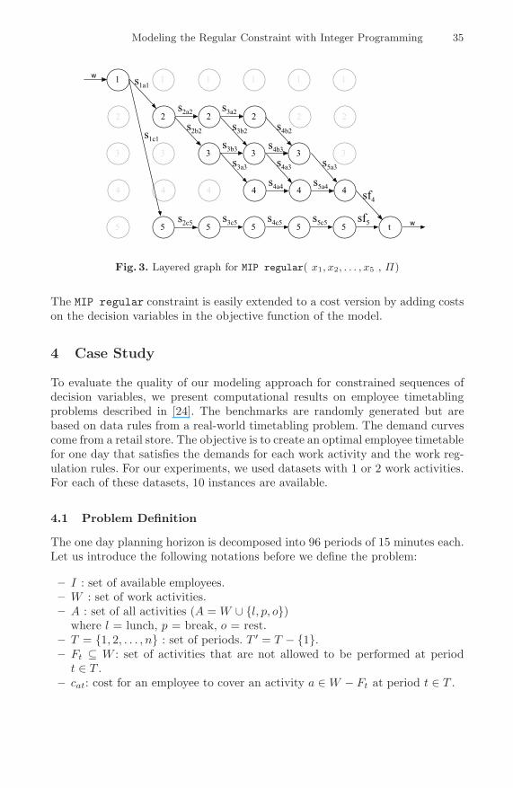
Example 2. Figure 3 is the graph for MIP regular(x1, x2, . . . , x5, Π), where Π isthe DFA presented in Figure 1. With the domains of Example 1, the constraintwould add all the flow conservation constraints related to this graph and thefollowing “linking” constraints to the MIP model:

x1a = s1a1 x2a = s2a2 x3a = s3a2 + s3a3 x4a = s4a3 + s4a4 x5a =s5a3 + s5a4x1b = 0 x2b = s2b2 x3b = s3b2 + s3b3 x4b = s4b2 + s4b3 x5b = 0x1c = s1c1 x2c = s2c5 x3c = s3c5 x4c = s4c5 x5c = s5c5

Modeling the Regular Constraint with Integer Programming 35

1 1 1 1 1 1

2 2 2 2 2 2

3 3 3 3 3 3

4 4 4 4 4 4

5 5 5 5 5 5

s1a1

w

t

s1c1

s2a2

s2b2

s3a2

s2c5

s3c5

s4c5

s5c5

sf5

sf4

w

s3b2

s4b2

s3b3

s4b3

s3a3

s4a3

s5a3

s4a4

s5a4

Fig. 3. Layered graph for MIP regular( x1, x2, . . . , x5 , Π)

The MIP regular constraint is easily extended to a cost version by adding costson the decision variables in the objective function of the model.

4 Case Study

To evaluate the quality of our modeling approach for constrained sequences ofdecision variables, we present computational results on employee timetablingproblems described in [24]. The benchmarks are randomly generated but arebased on data rules from a real-world timetabling problem. The demand curvescome from a retail store. The objective is to create an optimal employee timetablefor one day that satisfies the demands for each work activity and the work reg-ulation rules. For our experiments, we used datasets with 1 or 2 work activities.For each of these datasets, 10 instances are available.

4.1 Problem Definition

The one day planning horizon is decomposed into 96 periods of 15 minutes each.Let us introduce the following notations before we define the problem:

– I : set of available employees.– W : set of work activities.– A : set of all activities (A = W ∪ {l, p, o})

where l = lunch, p = break, o = rest.– T = {1, 2, . . . , n} : set of periods. T ′ = T − {1}.– Ft ⊆ W : set of activities that are not allowed to be performed at period

t ∈ T .– cat: cost for an employee to cover an activity a ∈ W − Ft at period t ∈ T .

36 M.-C. Cote, B. Gendron, and L.-M. Rousseau

Work Regulation Rules

1. Activities a ∈ Ft are not allowed to be performed at period t ∈ T .2. If an employee is working, he must cover between 3 hours and 8 hours of

work activities.3. If a working employee covers at least 6 hours of work activities, he must have

two 15 minute-breaks and a lunch break of 1 hour.4. If a working employee covers less than 6 hours of work activities, he must

have a 15 minute break, but no lunch.5. If performed, the duration of any activity a ∈ W is at least 1 hour (4

consecutive periods).6. A break (or lunch) is necessary between two different work activities.7. Work activities must be inserted between breaks, lunch and rest stretches.8. Rest shifts have to be assigned at the beginning and at the end of the day.

Demand Covering

1. The required number of employees for activity a ∈ W −Ft at period t ∈ T isdat. Undercovering and overcovering are allowed. The cost of undercoveringactivity a ∈ W − Ft at period t ∈ T is c−at and the cost of overcoveringactivity a ∈ W − Ft at period t ∈ T is c+

at.

The following sections present two ways of modeling this problem. The firstmodel is a classical MIP formulation that does not exploit the MIP regularconstraint. The second model uses the MIP regular constraint.

4.2 A Classical MIP Model

Decision Variables

xiat ={

1, if employee i ∈ I covers activity a ∈ A at period t ∈ T ,0, otherwise.

Work Regulation Rules

Rule 1:

xiat = 0, i ∈ I, t ∈ T, a ∈ Ft. (10)

Rule 2:

wi ={

1, if employee i ∈ I is working,0, otherwise.

∑

a∈A

xiat = wi, i ∈ I, t ∈ T, (11)

12wi ≤∑

t∈T

∑

a∈W−Ft

xiat ≤ 32wi, i ∈ I. (12)

Modeling the Regular Constraint with Integer Programming 37

Rules 3 and 4:

ui ={

1, if employee i covers at least 6 hours of work activities,0, otherwise.

∑

t∈T

∑

a∈W−Ft

xiat − 8ui ≤ 24, i ∈ I, (13)

∑

t∈T

∑

a∈W−Ft

xiat ≥ 23ui, i ∈ I, (14)

∑

t∈T

xipt = ui + wi, i ∈ I, (15)

∑

t∈T

xilt = 4ui, i ∈ I. (16)

Rule 5:

viat ={

1, if employee i ∈ I starts activity a ∈ A at period t ∈ T ,0, otherwise.

viat ≥ xiat − xia(t−1), i ∈ I, t ∈ T, a ∈ W − Ft ∪ {o} , (17)viat ≤ xiat, i ∈ I, t ∈ T, a ∈ W − Ft ∪ {o} , (18)

viat ≤ 1 − xia(t−1), i ∈ I, t ∈ T, a ∈ W − Ft ∪ {o} , (19)xilt′ ≥ vilt, i ∈ I, t ∈ T, t′ = t, t + 1, t + 2, t + 3, (20)

xiat′ ≥ viat, i ∈ I, t ∈ T, t′ = t, t + 1, t + 2, t + 3, a ∈ W − Ft. (21)

Rule 6:

viat ≤ 1 −∑

a′∈W−Ft−1

xia′(t−1), i ∈ I, t ∈ T ′, a ∈ W − Ft. (22)

Rule 7:

xipt ≤ 1 − xil(t−1), i ∈ I, t ∈ T ′, (23)

xipt ≤∑

a∈W−Ft−1

xia(t−1), i ∈ I, t ∈ T ′, (24)

xipt ≤∑

a∈W−Ft+1

xia(t+1), i ∈ I, t ∈ T ′, (25)

vilt ≤ 1 − xip(t−1) , i ∈ I, t ∈ T ′, (26)

vilt ≤∑

a∈W−Ft−1

xia(t−1), i ∈ I, t ∈ T ′, (27)

vilt ≤∑

a∈W−Ft+1

xia(t+1), i ∈ I, t ∈ T ′. (28)

38 M.-C. Cote, B. Gendron, and L.-M. Rousseau

Rule 8:

v−it =

⎧⎨

⎩

1, if employee i ∈ I covers at least one working activitybeginning before period t ∈ T ;

0, otherwise.

v+it =

⎧⎨

⎩

1, if employee i ∈ I covers at least one working activitybeginning after period t ∈ T ;

0, otherwise.

v−it ≤∑

t−<t

∑

a∈W−Ft−

viat− , i ∈ I, t ∈ T ′, (29)

v−it ≥∑

a∈W−Ft−

viat− , i ∈ I, t ∈ T, t− < t, (30)

v+it ≤

∑

t+>t

∑

a∈W−Ft+

viat+ , i ∈ I, t ∈ T ′, (31)

v+it ≥

∑

a∈W−Ft+

viat+ , i ∈ I, t ∈ T, t+ > t, (32)

xiot ≤ (1 − v−it ) + (1 − v+it ), i ∈ I, t ∈ T. (33)

Demand Covering

∑

i∈I

xiat − s+at + s−at = dat, t ∈ T, a ∈ W − Ft. (34)

Objective Function

min∑

t∈T

∑

a∈W−Ft

(∑

i∈I

catxiat + c+ats

+at + c−ats

−at). (35)

4.3 A MIP Regular Model

To observe the impact of modeling with the MIP regular constraint, we includeseveral rules of the problem in a DFA and we formulate the other rules and theobjective function as stated in the previous section. Work regulation rules 1 to4 and demand covering constraints are formulated as in the classical model, andwork regulation rules 5 to 8 are included in the DFA. We use the DFA suggestedin [21] for the same problem. The DFA presented in Figure 4 is for the problemwith two work activities (a and b on the Figure). It is easily generalized for anynumber of work activities. Let us denote Πn the DFA for the problem with nwork activities.

We insert a MIP regular constraint for each employee i ∈ I to the model.This constraint ensures that the covering of the activities a ∈ A for each t ∈ Tfor any employee i is a word recognized by the DFA Π|W |.

AddMIPRegular(Π|W |, |T |, xi, wi, M), ∀i ∈ I. (36)

Modeling the Regular Constraint with Integer Programming 39

a a a

a

b b b

l l l

p

l

a

l

b

a

b

a

b o

o

oo

bp

Fig. 4. DFA Π2 for 2 activities

where M is the model presented in the previous section without work regulationconstraints 5 to 8. Specifically, the output of the procedure gives the model Mwith the following variables and constraints:

sitaqk

= amount of flow on the arc leaving the node qk ∈ N t of layer t ∈ Twith activity value a ∈ A for employee i ∈ I.

sf iqk

= amount of flow leaving the node qk ∈ Nn+1 for employee i ∈ I.

∑

a∈Ω10

si1jq0

= wi, ∀i ∈ I, (37)

∑

(a,q′k)∈Δtk

si(t−1)aq′

k=

∑

a∈Ωtk

sitaqk

, ∀i ∈ I, t ∈ T ′, qk ∈ N t, (38)

∑

(a,q′k)∈Δ(n+1)k

sinaq′

k= sf i

qk, ∀i ∈ I, qk ∈ Nn+1, (39)

∑

qk∈Nn+1

sf iqk

= wi, i ∈ I, (40)

xiat =∑

qk∈Σta

sitaqk

, ∀i ∈ I, t ∈ T, a ∈ A, (41)

sitaqk

∈ {0, 1} i ∈ I, t ∈ T, qk ∈ N t, a ∈ Ωtk, (42)

sf iqk

∈ {0, 1} i ∈ I, qk ∈ Nn+1, (43)

where Δtk={(a, q′k)|(q′k, a, qk) ∈ inArcs[t][k]}, Ωtk={a|(qk, a, ) ∈ outArcs[t][k]},Σta = {qk|(qk, a, ) ∈ outArcs[t][k]}.

40 M.-C. Cote, B. Gendron, and L.-M. Rousseau

4.4 Computational Results

Experiments were run on a 3.20 GHz Pentium 4 using the MIP solver CPLEX10.0. All results obtained within the 3600 seconds elapsed time limit are within1% of optimality. Table 1 presents the results for the problem described beforewith one work activity. For the two work-activity problems, we only show resultsfor the MIP regular model in Table 2 as experiments on the classical model didnot give any integer results within the time limit. In the tables, |C| and |V | arethe number of constraints and the number of variables after CPLEX presolvealgorithm, Time is the elapsed execution time in seconds, Cost is the solutioncost and Gap is the gap between the initial LP lower bound, ZLP , and the valueof the best known solution to the MIP model, ZMIP :

Gap =(

ZMIP −ZLP

ZLP

)× 100

The symbol “>” in the Time column means that no integer solution was foundwithin the time limit.

Table 1. Results for the classical MIP model and the MIP regular model for 1 workactivity

Classical MIP model MIP regular modelId |C| |V | Time Cost Gap |C| |V | Time Cost Gap

1 29871 4040 1706,36 172,67 24,31 1491 1856 1,50 172,67 24,312 56743 5104 > 2719 3976 1029,01 164,58 1,013 56743 5104 > 2719 3976 393,96 169,44 0,364 45983 4704 3603,98 149,42 13,49 2183 3144 39,89 133,45 1,365 40447 4360 3603,99 152,47 6,07 1915 2728 10,41 145,67 0,876 40447 4360 3603,70 135,92 5,28 1915 2728 20,36 135,06 1,497 45551 4608 > 2183 3144 6,25 150,36 0,738 56743 5104 > 2719 3976 274,92 148,05 0,589 36175 4156 3603,84 182,54 28,11 1759 2416 15,47 182,54 28,1110 45983 4704 3603,91 153,38 5,09 2183 3144 5,50 147,63 0,95

The experiments on the one work-activity instances show that the MIPregular modeling approach significantly decreases computational time in com-parison with the classical MIP formulation for the given employee timetablingproblem. It is also interesting to observe that the use of the MIP regular con-straint reduces the model size.

With our approach, within the one hour time limit, we solved all the instancesto optimality for the one work-activity problems with an average execution timeof 180 seconds. For the two work-activity problems, six instances were solved tooptimality within one hour with an average execution time of 550 seconds. Theseresults are competitive with those of the branch-and-price approach described in[21]. Indeed, as reported in [21], for the one work-activity problems, 8 instancesare solved to optimality by the branch-and-price with an average of 144 seconds

Modeling the Regular Constraint with Integer Programming 41

Table 2. Results for the MIP regular model for 2 work activities

Id |C| |V | Time Cost Gap

1 3111 5084 623 201,78 0,002 3779 6192 3600,64 214,42 1,373 3991 6412 748,94 260,8 1,004 4475 7512 1128,73 245,87 1,005 3559 5668 3600,53 412,31 10,776 3879 6116 107,75 288,88 0,917 3199 4972 45,44 232,14 12,298 5799 9740 643,73 536,83 0,599 4583 7680 3600,61 309,69 3,9210 4667 7584 3600,55 265,67 2,12

of computation time, while for the two work-activity problems, 8 instances aresolved to optimality by the same approach with an average execution time of394 seconds.

An asset of our method over the approach suggested in [21] is the very littledevelopment time needed. Once the model using MIP regular is automaticallytranslated into a MIP model, any existing MIP solver can be used to solve it.

5 Conclusion

We presented a new MIP modeling approach for sequences of decision vari-ables inspired by the CP regular constraint. As for the CP constraint, the MIPregular constraint uses a DFA to express rules over constrained sequences ofvariables. It then gives a flow formulation of the layered graph built for theconsistency algorithm of the regular constraint. We compared our modelingapproach to a classical MIP formulation on an employee timetabling problem.Computational results on instances of this problem showed that the use of theMIP regular constraint to model the subset of constraints on sequences of vari-ables, significantly improves solution times.

The idea of using global constraints in MIP has been considered before. Inparticular, Achterberg [25] present a programming system (SCIP) to integrateCP and MIP based on a branch-and-cut-and-price framework that features globalconstraints (see also the references therein for other similar contributions). TheMIP regular constraint formulation is a new contribution in this direction toallow MIP to benefit from CP. A natural next step in this trend would be toformulate a MIP version of the grammar constraints introduced in [26] and [22].

Acknowledgments. We thank Marc Brisson for his help with the implemen-tation and experiments.

42 M.-C. Cote, B. Gendron, and L.-M. Rousseau

References

1. Pesant, G.: A regular membership constraint for finite sequences of variables. Proc.of CP’04, Springer-Verlag LNCS 3258 (2004) 482–495

2. Ernst, A., Jiang, H., Krishnamoorthy, M., Sier, D.: Staff scheduling and rostering:A review of applications, methods and models. European Journal of OperationalResearch 153 (2004) 3–27

3. Ernst, A., Jiang, H., Krishnamoorthy, M., Owens, B., Sier, D.: An annotatedbibliography of personnel scheduling and rostering. Annals of Operations Research127 (2004) 21–144

4. Dantzig, G.: A comment on Edie’s traffic delay at toll booths. Operations Research2 (1954) 339–341

5. Segal, M.: The operator-scheduling problem: A network-flow approach. OperationsResearch 22 (1974) 808–823

6. Moondra, B.: An LP model for work force scheduling for banks. Journal of BankResearch 7 (1976) 299–301

7. Bechtolds, S., Jacobs, L.: Implicit optimal modeling of flexible break assigments.Management Science 36 (1990) 1339–1351

8. Bechtolds, S., Jacobs, L.: The equivalence of general set-covering and implicitinteger programming formulations for shift scheduling. Naval Research Logistics43 (1996) 223–249

9. Thompson, G.: Improved implicit modeling of the labor shift scheduling problem.Management Science 41 (1995) 595–607

10. Aykin, T.: Optimal shift scheduling with multiple break windows. ManagementScience 42 (1996) 591–602

11. Brusco, M., Jacobs, L.: Personnel tour scheduling when starting-time restrictionsare present. Management Science 44 (1998) 534–547

12. Laporte, G., Nobert, Y., Biron, J.: Rotating schedules. European Journal ofOperational Research 4(1) (1980) 24–30

13. Balakrishan, A., Wong, R.: Model for the rotating workforce scheduling problem.Networks 20 (1990) 25–42

14. Isken, M.: An implicit tour scheduling model with applications in healthcare.Annals of Operations Research, Special Issue on Staff Scheduling and Rostering128 (2004) 91–109

15. Cezik, T., Gunluk, O., Luss., H.: An integer programming model for the weeklytour scheduling problem. Naval Research Logistic 48(7) (1999)

16. Millar, H., Kiragu, M.: Cyclic and non-cyclic scheduling of 12 h shift nurses bynetwork programming. European Journal of Operational Research 104(3) (1998)582–592

17. Ernst, A., Hourigan, P., Krishnamoorthy, M., Mills, G., Nott, h., Sier, D.: Rosteringambulance officers. Proceedings of the 15th National Conference of the AustralianSociety for Operations Research, Gold Coast (1999) 470–481

18. Sodhi, M.: A flexible, fast, and optimal modeling approach applied to crew rosteringat London Underground. Annals of Operations Research 127 (2003) 259–281

19. Hopcroft, J.E., Ullman, J.D.: Introduction to automata theory, languages andcomputation. Addison Wesley (1979)

20. van Hoeve, W.J., Pesant, G., Rousseau, L.M.: On global warming: Flow-based softglobal constraints. Journal of Heuristics 12(4-5) (2006) 347–373

21. Demassey, S., Pesant, G., Rousseau, L.M.: A cost-regular based hybrid columngeneration approach. Constraints 11(4) (2006) 315–333

Modeling the Regular Constraint with Integer Programming 43

22. Quimper, C.G., Walsh, T.: Global grammar constraints. Proc. of CP’06, Springer-Verlag LNCS 4204 (2006) 751–755

23. Ahuja, R., Magnanti, T., Orlin, J.: Network Flows. Prentice Hall (1993)24. Demassey, S., Pesant, G., Rousseau, L.M.: Constraint programming based column

generation for employee timetabling. Proc. 2th Int. Conf. on Intergretion of AIand OR techniques in Constraint Programming for Combinatorial OptimizationProblems - CPAIOR’05, Springer-Verlag LNCS 3524 (2005) 140–154

25. Achterberg, T.: SCIP - a framework to integrate constraint and mixed in-teger programming. Technical Report 04-19, Zuse Institute Berlin (2004)http://www.zib.de/Publications/abstracts/ZR-04-19/.

26. Sellmann, M.: The theory of grammar constraints. Proc. of CP’06, Springer-VerlagLNCS 4204 (2006) 530–544