Regular polygon detection

Nick Barnes1, Gareth Loy2, David Shaw1 and Antonio Robles-Kelly1

1. National ICT Australia, Locked Bag 8001, Canberra, ACT, 2601, Australia,1. Dept. Information Engineering, The Australian National University.

2. Computer Vision & Active Perception Laboratory, Royal Institute of Technology (KTH), Stockholm

Abstract

This paper describes a new robust regular polygon de-tector. The regular polygon transform is posed as a mix-ture of regular polygons in a five dimensional space. Giventhe edge structure of an image, we derive the a posterioriprobability for a mixture of regular polygons, and thus theprobability density function for the appearance of a mix-ture of regular polygons. Likely regular polygons can beisolated quickly by discretising and collapsing the searchspace into three dimensions. The remaining dimensionsmay be efficiently recovered subsequently using maximumlikelihood at the locations of the most likely polygons in thesubspace. This leads to an efficient algorithm. Also the aposteriori formulation facilitates inclusion of additional apriori information leading to real-time application to roadsign detection. The use of gradient information also reducesnoise compared to existing approaches such as the gener-alised Hough transform. Results are presented for imageswith noise to show stability. The detector is also applied totwo separate applications: real-time road sign detection foron-line driver assistance; and feature detection, recoveringstable features in rectilinear environments.

1 Introduction

In scenes containing manufactured artefacts, features of-ten appear as regular polygons. In road scenes, triangular,rectangular and octagonal signs display critical information.Polygonal shapes appear frequently in the structure of of-fice environments. Corners are common partial polygons,but over a large range of scales regular polygons representmuch more indoor structure. In outdoor scenes, brickwork,office buildings, windows, etc., all exhibit features that canbe recognised repeatably by regular polygon detection.

The literature related to this topic is vast, covering lineand analytical shape estimation and perceptual grouping,as well as road sign detection. There are two alternativeschools of approach: model-driven approaches; and per-ceptual grouping approaches that are frequently data driven.The model-driven approaches typically employ retinotropic

mappings, whereby local features are detected purely lo-cally, and pixel information is incorporated directly intofeature detection. Grouping approaches take low-level fea-tures, such as edges (but also alternatively raw edge pixels)and apply matching and clustering based methods.

In perceptual grouping, image elements are grouped ac-cording to some perceptual criteria. Several authors haveinvestigated iterative relaxation style operators for group-ing edgels. This began with Shashua and Ullman [19],which required many iterations, and was refined by Guy andMedioni [6] among others so as to be O(k2) where k is thenumber of edgels. At a high level this can be composedas recovering a graph of relational arrangement. A com-mon approach is spectral graph theory [15, 18]. Probabilis-tic approaches in this area include Bayes nets [4] and com-bining evidence from raw edge attributes [2]. More recentapproaches have used EM [17, 3]. One of the basic algo-rithmic approaches here is examining pairwise relations. Ifthe elements being examined are edge pixels then the com-plexity is at least O(N2), where N is the image size.

Alternatively, we may fit functions to the image data.The Hough transform [7] and circular Hough transform [14]vote to an in-place representation of the shape to be de-tected. The circular Hough detects circle centres, and theHough transform detects the closest line point to the origin(this mapping is in the same space in the log-Hough trans-form [22] in log-polar images). Each pixel ‘votes’ for eachfeature that it could possibly be a part of. This approachis inherently robust, as gaps, noise, and partial occlusionare ignored, but appear as a decreased strength of the fea-ture. Such algorithms are local in their computation witheach point only being registered for shapes that it can bepart of. These methods have been generalised [1] to detectarbitrary shapes. The original Hough transform has a rel-atively simple mapping for each pixel, however, the gener-alisations vote into higher dimensions, and quickly becomecomputationally intensive on serial architectures. Further,parallelisation is non-trivial due to the high dimensionality.

The Hough transform can be formulated as maximumlikelihood estimation [21]. Kiryati and Bruckstein [9] for-mulated robust maximum likelihood line finding on a grid,assuming independent noise between points. Geyer et al.

1

[5], applied a sampled likelihood function approach to esti-mation of the essential matrix. Makadia and Daniilidis [13]formulated a Hough-like algorithm in motion space for esti-mating robot position using a Radon transform formulationwith a distance-based soft characteristic function.

Variants of shape detector have also included edge orien-tation information. The radial symmetry detector [12] im-proves on the circular Hough giving O(Nl) performance,where l is the range of radii of the shapes being examined.A similar approach can be applied to regular polygons [11].However, only one regular polygon type could be detectedat a time and the angle vote applied to the whole image toresolve orientation was computationally expensive.

Road sign recognition research has been around sincethe mid 1980’s. Good results may be achieved with a clas-sification approaches such as normalised cross correlation[16]. However, this is computationally intensive per pixel.A standard approach is to first apply a low computationalcost detection stage reducing classification to a fraction ofthe image stream. Typically this is through assumptionsabout scene structure, colour, or a combination of both (e.g.,[16, 8]). Although these assumptions are sound for manyroad scenarios, the breakdown of a driver assistance sys-tem on hills and corners is not acceptable. Colour methodsalso break down under the enormous variation in lightingchrominance in outdoor situations, and segmenting out selfsimilar regions is not robust in scenes with dense overheadbranches that shadow the road. Instead, we propose a illu-mination invariant shape detection approach to find likelycandidates, to be followed by recognition.

We propose a computationally efficient algorithm to re-cover regular polygons using an a posteriori probability ap-proach taking advantage of locality and gradient informa-tion. Rather than summing support, we recover the likeli-hood of the probability density function for all regular poly-gons in an image. The algorithm breaks the task into twostages: 1) resolving likely regular polygons in a lower di-mensional space; 2) taking the most likely regular polygonsand resolving their final parameters in higher dimensionalspace. This allows us to recover all regular polygons inone computationally efficient algorithm. The algorithm isO(Nlrw), where N is the size of the image, l is the max-imum radius length, r is the number of radii being consid-ered, and w is the width of the operation of the distancefunction. w is close to one pixel for most implementations,and r and l tend to be small numbers leading to a more ef-ficient algorithm. We demonstrate that in constrained casesthis can lead to real-time implementations.

2 Regular polygons

Archimedes gave a scientific method for calculating πto arbitrary precision. The sum of the lengths of a regularpolygon of n sides inscribed on a circle is smaller than thecircumference, and the sum of the lengths of the sides cir-cumscribed around a circle is greater than the perimeter of

Figure 1. Left, a sample five sided (n = 5)polygon. Right, the line over which the centremay be for a given oriented edge pixel, asdescribed in Equation 10.

the circle. We take our regular polygon definition that cir-cumscribed around a circle. For an n sided regular polygon,divide the circle into a set of n, n

2π angle isosceles triangles,where the centre point of the baseline falls on the circle.Lengths of the individual sides is l(n, r) = 2r tan π

n .We may define a regular polygon as having a centroid

in Euclidean 2-space (cx, cy), the radius r of the circle itis circumscribed about, an orientation γ, and a number ofsides n. Thus we may define a regular polygon transformas a function frp that maps the space of all possible reg-ular polygons (regular polygon space) to 3D space. Reg-ular polygon space is five dimensional, and the transformforms a mapping: frp : R4,Z → R3, where the integer di-mension is the number of sides (three or greater for closedpolygons) and the space mapped to is image position plusorientation of edges. Specifically, we label regular polygonspace: Φ = (cx, cy, r, γ, n). An example shape explainingthe parameters is shown in Figure 1.

The mapping of all regular polygons into the image from5D regular polygon space is the integral across the space:

frp =∫

Φ

frp(φ)dφ. (1)

The typical discrete image is a sampling over a regularCartesian grid. The gradient of the image is a set of gradientpixels x = (xj , j = 1, ...s) ∈ I corresponding to all theedge pixels of the regular polygons, plus any noise.

3 Likelihood formulation

A gradient image with a set of points x may be regardedas the result of the transform from regular polygon space ofsome set of polygons φm ∈ Φ, where m = 1 . . .M . In or-der to recover φm from the xj , we may estimate the proba-bility density function over regular polygon space given xj ,considering the image as the result of a mixture of regularpolygons, each of which is a Gaussian. That is:

f =M∑

m=1

αmp(φm|x), (2)

where αm is a mixing parameter. If we assume a uniform

mixture, then αm is constant for allm. We may apply BayesLaw:

M∑m=1

p(φm|x) =M∑

m=1

p(x|φm)p(φm)p(x)

(3)

Note that there is a distinction between a regular polygonin the scene and what appears in an image. An accidentalview where several straight lines at different scene depthsalign to form a polygon is not a world structure, but is apolygon in the image. We may say that any apparent reg-ular polygon is a regular polygon in the image. Further,with incomplete data, any edge pixel may be regarded aspart a regular polygon. Thus, the edge image can be seenas being made up of regular polygons with noise. The re-sult of this noise has two effects: edge displacement andgradient error. Due to standard image noise, or an imper-fect scene edge (e.g., a faded road sign), the gradient edgein the image may be displaced slightly. There is also someresidual uncertainty of position due to image sampling. Allof these effects on the gradient edge may be reasonably ap-proximated by a Gaussian in 3D over the parameters. Thegradient error results from the effect of intensity noise inthe image, and relation between orientation and intensityvalues is a sinusoid. For small angles the error in orienta-tion will be linear and therefore may also be approximatedby a Gaussian. Note that some authors choose to take gradi-ent magnitude as a measure of edge certainty, however, it isalso highly correlated with the intensity contrast of the un-derlying image. Thus, we threshold the gradient magnitudeto basic noise, and set the remaining xj to unit magnitude.If required, the magnitude can also be included as a contin-uous measure of gradient certainty in this formulation.

We may take it that the xj are the result of a set of poly-gons with missing data. Also, that the noise in the appear-ance of the edge pixels in their position and estimated orien-tation is additive and independent between the points. Thenwe may take the probability of the Gaussian mixture of reg-ular polygons in the image for the full set of points to be:

M∑m=1

p(φm|x) =M∑

m=1

∏j

p(xj |φm)p(φm)p(xj)

(4)

Then, following Kiryati and Bruckstein [9], the proba-bility density for an individual polygon φm and edge pointxj can be modelled as a Gaussian in 3D xj = (xj , yj , θj)with zero mean and a point-specific covariance matrix:

p(xj |φm) =exp

(−g(xj , frp(Φ))Σ−1

j g(xj , frp(Φ))

2π|Σj |12

,

(5)where g(xj , frp(Φ)) is a function giving the distance fromthe edge pixel to the closest point on the image projectionof the the regular polygon, Σj is the covariance matrix:

Σj =

σ2xj

σxyj σxθj

σxyjσ2

yjσyθj

σxθjσyθj

σ2θj

(6)

and |Σj | is the determinant of the covariance matrix. Bythe independence of noise between points, we may take theproduct over all edge points:

p(x|φm) =∏j

exp(−g(xj , frp(Φ))Σ−1

j g(xj , frp(Φ))

2π|Σj |12

,

(7)Substituting back into Equation 3:

M∑m=1

p(φm|x) = (8)

m∑m=1

∏j

exp(−g(xj ,frp(Φ))Σ−1j g(xj ,frp(Φ))p(φm)

2π|Σj |12 p(xj)

Taking log-likelihoods and collecting constants:

M∑m=1

log(L(φm|x) = (9)

m∑m=1

∑j

−g(xj , frp(Φ))Σ−1j g(xj , frp(Φ)) + const

3.1 Matching to the regular polygon function

Two major issues are posed by the formulation of Equa-tion 10. The term g(xj , frp(Φ)) is the distance from xj tothe nearest point on the regular polygon, i.e., this requiresfinding the nearest point. Also, Φ is a 5D space, and so opti-mising may be computationally expensive, while we wouldlike to have a real time implementation.

As regular polygon space is high dimensional, the imageis low dimensional, and edge points are sparse in general,we may pose the problem as a mapping from image edgepixels to possible regular polygons. We wish to form theinverse mapping f−1

rp from xj to regular polygons that itmay be a part of, i.e., Φ. f−1

rp will allow us to create afunction g(xj ,Φ) that gives a distance metric from the pointxj to the regular polygon defined by Φ.

Consider f−1rp for a given xj , for unknown r and γ. If we

do not consider the edge gradient at xj , a regular polygon ofany number of sides may have a centre anywhere, the sub-space of Φ that xj may be an element of is large, and thefunction f−1

rp is intractable. However, we may recover ori-entation using a standard image processing operator (e.g.,Sobel) giving xj = (xj , yj , θj), where θj is the direction ofthe maximum intensity gradient. In this case the orientationof the regular polygon is constrained. Indeed, regardlessof n, (cx, cy) is constrained to be on a line, orthogonal to

the gradient, at a distance r from (xj , yj). This relationis as shown in Figure 1. We maintain the standard of rep-resenting this in polar coordinates, but follow Weiman inrepresenting a straight-line segment in the complex plane[23]. Consider that z1 is a complex number, with argumentθj − π

2 , and modulus 1, we have:

h(xj) =∫ t= l

2r

t=− l2r

xj + r(z1t+ iz1)dt, (10)

where xj is the (xj , yj) component of the point representedin the complex plane, and l is the side length given n and r.

Using Equation 10, we may define a new regular polygondetection sub-space that is ambiguous in γ and n, but henceonly 3D, and computationally simple. To form the detectionsubspace, we need only form the likelihood density functionof Equation 10 over (cx, cy, r). Let this new subspace beΨ = (cx, cy, r), and the function from this space to theimage be frps (s for subspace).

In order to collapse the dimension of number of sides,we may assume the longest possible side length, that of atriangle. In the case of other shapes with shorter sides, thiswill lead to some edge pixels being considered that are notactually part of the true regular polygon. However, theseambiguities may be resolved subsequently. Thus, for anyparticular ψ ∈ Ψ, we may define g as the minimum distancefrom Ψ to the line defined in Equation 10.

Regular polygon detection: Using Equation 10 to findlikelihood density across a Ψ, we may take the peaks of thedistribution as the set of n regular polygons that are mostlikely in this subspace, by the assumption of zero mean, ifwe assume that the actual regular polygons are spatially sep-arate. We will deal with the difficulties that arise from thisassumption subsequently. Rather than recover the variancedirectly, we resolve the remaining dimensions in a secondstage. This separation is computationally motivated. Byfinding most likely polygons in a reduced space, we mayfocus computation on the most likely polygons, and ignoreparts of Ψ1 that are not likely to have any regular polygonspresent. This will be sufficient to recover all polygons tosome required likelihood, if we investigate regular polygonsin the reduced space down to the required likelihood as thelikelihood in Φ is an overestimate of that in Ψ.

In practice the variance constitutes: remaining dimen-sions of n and γ; and, regular polygons (or partially visi-ble regular polygons) that are overlayed. This may resultin a figure that has a number edges of different length, forwhich likelihood is overestimated. For example, consideran octagon, where all sides are the length of sides for thecorresponding triangle, although this is a correct octagon,its likelihood may be overestimated in Φ.

Resolving orientation and shape: Now we have re-solved the mean for ψh = (cxh, cyh, rh) ∈ Ψ for the setof regular polygons that are most likely in Ψ. We may con-

1and of the image if we truncate our distance function.

struct a likelihood function given this information to resolvethe remaining dimensions, that is:

log(L(o, n|x, cx, cy, r)) = (11)∑j

−g(xj , frp(Φ))Σ−1j g(xj , frp(Φ)) + const

With a truncated distance function, for each point in de-tection subspace we may consider only the local xj , thismay be assembled by maintaining a list of the parametersfor the xj that contributed to that point. This includes itsbasic parameters, plus its distance as defined by g in the 3Dsubspace, let this be dj . We may iterate over n, and inte-grate over γ and compute the log-likelihood of the prob-ability density function over the remaining parameters us-ing Equation 11. This is now a reduced dimensional spacesearch, however an efficient approximation to this algorithmis discussed in the implementation.

4 Implementation

Computation of the complete regular polygon likelihooddistribution is intractable. Instead we discretely sample thedistribution in a manner that is appropriate for the applica-tion. Note that a coarse-to-fine strategy may be employed orfound peaks may be better located by subsequent EM. Thelikelihood distribution can subsampled by a simple scan linealgorithm through xj . If one considers the distance functionto be the soft characteristic function of [13], then the log-likelihood estimation may be considered as a Hough-likealgorithm for estimation of regular polygon parameters.

Using g2, the likelihood contribution of a regular poly-gon of xj rapidly becomes small as distance increases.Thus, if L(xj |Ψ) < ε, we set it to zero. Given this formula-tion, the algorithm can operate by, for each edge pixel, stepalong the line of h for the width implied by ε, and adjustthe log likelihood of each sample point of the distributionaccording to L(xj |Ψ). Alternatively, we may approximateby adjusting only the closest pixels to the line, and convolv-ing the likelihood with a Gaussian. Thus for each xj , weupdate log-likelihoods for rlw points in Ψ, where w is thewidth implied by ε. In practice, small w is sufficient, for afast implementation this may be one to two pixels. Also, formost specific applications, r may be over a small range.

The second stage of the algorithm can also be imple-mented more computationally efficiently. In practice, oneis typically seeking either the set of k regular polygons withthe maximum likelihood, or all regular polygons with a like-lihood greater than a threshold. Let us assume initially thatthe xj in the list are all actually part of the polygon. In thiscase, γ will be a mixture of Gaussians corresponding to theorientations of each of the component edges. We may definethe log-likelihood of the probability of a regular polygon asthe sum over the edges, splitting Equation 11 over edges,and replacing frp(Φ) with each of the edges from Equation

Given edge elements xj of an image, detect regular poly-gons with n ∈ N sides. For each polygon radius r:

1. Estimate likelihood image:

(a) For each xj : Compute all triangle locations pk

that could generate xj , accumulate locations ina vote image, and record information: pk, ∠xj

and distance mk along line h.

(b) Convolve vote image with Gaussian to generatediscrete approximation of likelihood image.

2. Evaluate each maxima qi for each n ∈ N :

(a) Build a weighted angular histogram of allrecorded ∠xj values with mk < l(n,r)

2,

weighted by a Gaussian of ‖pk − qi‖2.

(b) Convolve histogram with string of impulsefunctions δ(γ − 2π

n), the γ that maximises this

convolution is the most likely orientation of ann sided polygon, and the values at γ± 2π

nu, u ∈

Z indicate the support for each side.

(c) Total support is determined as a function of thesupport for each side of the shape.

Figure 2. Summary of the algorithm.

10. In order for an xj to be an element of any particularedge, θj must fall within the expected variance of the meanfor the orientation of the edge.

As edge length may be less with known n, an edge-baseddistance function (with orientation) is more constrainedthan g(xj , frps(Ψ)) adjusted to include orientation. Thus,if we approximate the distance function, by its distance dj ,multiplied by a distance function over θj , this is an upperbound on the actual edge distance function. If we take theweighted xj over θ and convolve it with a Gaussian cor-responding to our expected variance in θ, then this formsan approximate upper bound on the log-likelihood of theprobability density function of individual edge orientations.We may use this to hypothesis test for γ and n, by takingeach hypothesis in turn and summing over edges in the up-per bound density function by direct look up at the expectedangles, to form the upper bound density function across ourremaining parameters. Rather than for all γ we may takethe top p peaks as this corresponds to upper bounds likeli-hoods of the most likely edges. For each of these we mayform the complete likelihood function of Equation 11. Asthe mean of the maximum likelihood orientation may notcorrespond to the mean orientation of the most likely edge.If required an EM search may be performed over orientationin the neighbourhood of these peaks.

For real applications, the number of radii being exploredis not large, and the sampling can be coarse. Further if it isacceptable to overstate the likelihood, and precise positionis not required, the algorithm may cease without removingedge pixels. Implementation is summarised in Figure 2.

With no a priori scene information, we may assume that

the xj appear with an isotropic distribution, except for reg-ular polygons. However, in a road scene, for example, theedges of the road and dividing lines often result in longpiecewise straight edges. In this case, the probability ofmultiple edge points appearing together, with the same gra-dient, that are not part of something we wish to consider asa regular polygon, is greater than the probability of pixelsappearing together randomly in the image.

In such a case, we may determine a priori distributionsfrom a set of images that is representative of the incomingimages. From this we may adjust the likelihoods to reflectthe number of supporting edges from the support for eachof the edges. In such long clear line scenarios, we found itwas effective to incorporate negative probability weightingat the ends of the line of influence of the xj . This preventedover emphasis of strongly contrasting long lines.

Finally, where other information is known a priori wemay incorporate this information into our function, and sim-plify computation. This will be explained in more detail inthe context of road sign detection in the following section.

5 Experimental results

We evaluate performance in the presence of noise in ar-tificial images, as well as on real images. By incorporatingprior knowledge about the appearance of the road scene, wewere able to adapt the algorithm to run at 20Hz for 320×240images in which it was able to reliably detect a road sign in atest sequence taken from the vehicle in Figure 5(a). Finally,we demonstrate the application of a constrained version asa feature detector for wide-baseline matching for robot cor-ridor navigation on the robot shown in Figure 5(b).

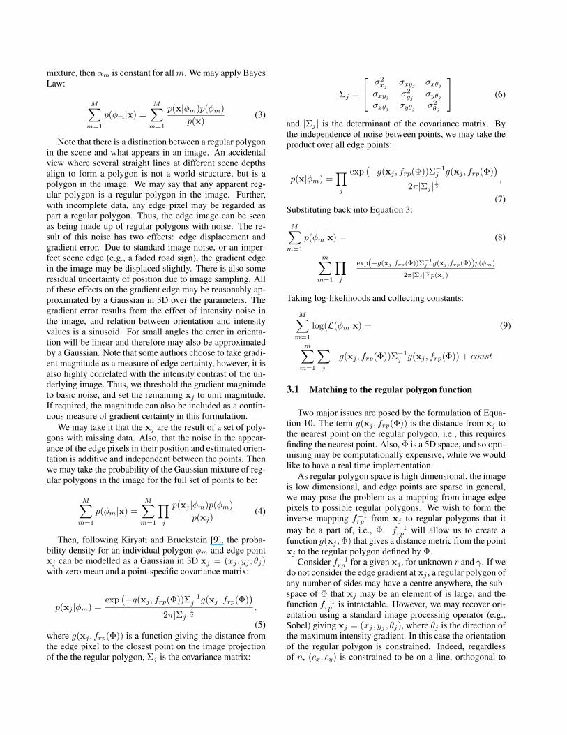
On still images: The detector was evaluated on a rangeof images containing regular polygons. Figures 3 and 4show detection results for searching for 3 to 8 sided reg-ular polygons over radii r ∈ {8, 11, 14, 17}. Note that thisnon-continuous range of radii is adequate to detect shapesat neighbouring radii. Figure 3(b) shows the approximationof the likelihood image generated by the algorithm; note thepeaks at the centres of the shapes detected in (c). The finaloutput (d) illustrates both the impressive detection perfor-mance, and illustrates some of the artefacts of the method.Owing to the Gaussian modelling of edge and centroid loca-tions the shapes detected do not always exactly overlay theedge locations of the original shapes. Also, polygons maybe found with alignment of partial edges, and are awardedlow (but not zero) strength accordingly.

The majority of incorrect hypotheses correspond to poly-gons of a small number of sides. There are two reasons forthis: firstly, (for n ≤ 8) as n increases it becomes less likelythat n edges will be ‘accidentally’ aligned by noise; sec-ondly the prevalence of right angles in built environmentsgives a strong prior for finding squares.

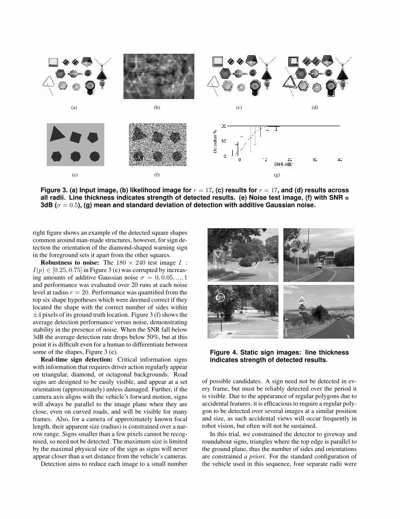
Figure 4 shows the detector operating on outdoor im-ages, here the near-perfect regular polygon nature of theroad signs ensure that they are strongly detected. The top

(a) (b) (c) (d)

(e) (f) (g)

Figure 3. (a) Input image, (b) likelihood image for r = 17, (c) results for r = 17, and (d) results acrossall radii. Line thickness indicates strength of detected results. (e) Noise test image, (f) with SNR =3dB (σ = 0.5), (g) mean and standard deviation of detection with additive Gaussian noise.

right figure shows an example of the detected square shapescommon around man-made structures, however, for sign de-tection the orientation of the diamond-shaped warning signin the foreground sets it apart from the other squares.

Robustness to noise: The 180 × 240 test image I :I(p) ∈ [0.25, 0.75] in Figure 3 (e) was corrupted by increas-ing amounts of additive Gaussian noise σ = 0, 0.05, ..., 1and performance was evaluated over 20 runs at each noiselevel at radius r = 20. Performance was quantified from thetop six shape hypotheses which were deemed correct if theylocated the shape with the correct number of sides within±4 pixels of its ground truth location. Figure 3 (f) shows theaverage detection performance versus noise, demonstratingstability in the presence of noise. When the SNR fall below3dB the average detection rate drops below 50%, but at thispoint it is difficult even for a human to differentiate betweensome of the shapes, Figure 3 (e).

Real-time sign detection: Critical information signswith information that requires driver action regularly appearon triangular, diamond, or octagonal backgrounds. Roadsigns are designed to be easily visible, and appear at a setorientation (approximately) unless damaged. Further, if thecamera axis aligns with the vehicle’s forward motion, signswill always be parallel to the image plane when they areclose, even on curved roads, and will be visible for manyframes. Also, for a camera of approximately known focallength, their apparent size (radius) is constrained over a nar-row range. Signs smaller than a few pixels cannot be recog-nised, so need not be detected. The maximum size is limitedby the maximal physical size of the sign as signs will neverappear closer than a set distance from the vehicle’s cameras.

Detection aims to reduce each image to a small number

Figure 4. Static sign images: line thicknessindicates strength of detected results.

of possible candidates. A sign need not be detected in ev-ery frame, but must be reliably detected over the period itis visible. Due to the appearance of regular polygons due toaccidental features, it is efficacious to require a regular poly-gon to be detected over several images at a similar positionand size, as such accidental views will occur frequently inrobot vision, but often will not be sustained.

In this trial, we constrained the detector to giveway androundabout signs, triangles where the top edge is parallel tothe ground plane, thus the number of sides and orientationsare constrained a priori. For the standard configuration ofthe vehicle used in this sequence, four separate radii were

(a) (b)

Figure 5. (a) Inside the intelligent vehicle,cameras monitoring the road scene appearin place of the rear-vision mirror. (b) NOMADrobot equip with camera pair.

sufficient of 6, 8, 10, and 12 pixels. The a priori constraintover number of sides and radii meant that gradient orienta-tions outside the constraints could not be part of these ori-ented polygons, so could be disregarded a priori. Theseorientations were 0◦, 120◦ and 240◦ each±12◦. Thus, onlythe first stage of the algorithm was required to recover allambiguity. The constrained algorithm was able to run inless than 50ms per frame (320 × 240 image), based on animplementation in C++ on a standard PC, equivalent to thatmounted in the vehicle. This is quite adequate for a sign tobe visible for many frames in any reasonable situation for aroad vehicle, and hence is real-time.

The road trial is on a sequence, see Figure 6, and thesign is of a detectable size for 48 frames. A sample detec-tion image is shown in Figure 6. For detection, we requiredthe sign to be one of the two most likely triangles for anyradius for an initial image, and then one of the top 10 forthe next k images. False positive and false negative curvesare shown in Figure 7. Although the sign was not detectedas one of the top two candidates in every image, it was re-liably detected many times over the image sequence. Theprocessing of recognition using normalised cross correla-tion for each candidate is less than 1ms in our system, sothe number of false positives was well within computation

Figure 6. Most likely triangles backprojectedonto an image midway through the sequence,and likelihood function for radius 8.

Figure 7. Average and standard deviation ofnumber of false positives (top) and false neg-atives (bottom), given number of frames k thatthe sign is required to be present.

limits for real time processing.Indoor scenes: In a project to develop vision-based

robotic mapping, we applied the regular polygon detectorto detect square-like features. Here n is set, but γ must beresolved, i.e., 1D ambiguity after initial detection. The de-tector was run at three different radii, and found all squaresabove a low likelihood. It detects stable edges that are thebasis of squares, but is tolerant to incomplete edges andsome affine distortion. Figure 8 shows a sample image. Thedetector was applied to pairs of images taken from the robotas it was navigating in an indoor office environment, mov-ing at approximately 0.3 ms−1. With images three secondsapart the baseline was wide, approximately one metre. Oncorners the robot turned mostly in place, leading to shifts ofmore than half the image of features, see Figure 9. Featureswere matched according to size and orientation, the localgreyscale environment and position, and used to calculatethe fundamental matrix to recover motion. Results showeda high percentage of the found points matched (around 70%typically) correctly over frames moving down the corridor,but reduced over rotation as expected. Figure 9 shows atypical images taken from the sequence of 69 images as itturns around a corner. The matches show promising initialresults. Figure 9 (c) shows the matches obtained by SIFT[10], using the reference implementation with its packagedparameters.2 Note that the detector will be most effectivein this type of rectilinear environment, however, it is highlysuitable to be part of a battery of detectors for matching. Itsspeed of operation makes it plausible for robotic mappingapplications. See [20] for complete implementation details.

6 Conclusions

Regular polygon detection is an important problem withmultiple applications in robotics and computer vision. Us-ing an a posteriori probability approach, we presented a new

2http://www.cs.ubc.ca/ lowe/keypoints/

algorithm for detecting regular polygons. We defined thecontinuous log-likelihood of the probability density func-tion of regular polygons. In order to make the algorithmcomputationally efficient we find initial likely regular poly-gons in a lower dimensional space, and then resolve the re-maining parameters for likely regular polygons. We pre-sented an efficient algorithm based on this, and adaptationsof this algorithm that can run at 20Hz detecting signs in anintelligent vehicle application. Experimental results showthe efficacy and robustness of the algorithm, and its ap-plication to driver assistance, and as a feature detector formatching, applied to a robot sequence for mapping.

Acknowledgements

National ICT Australia is funded by the Australian Gov-ernment’s Backing Australia’s Ability initiative, in partthrough the Australian Research Council. The supportof the STINT foundation through the KTH-ANU grantIG2001-2011-03 is gratefully acknowledged.

References

[1] D. H. Ballard. Generalizing the hough transform to detectarbitrary shapes. Pattern Recognition, 13(2):111–122, 1981.

[2] I. J. Cox, J. M. Rehg, and S. L. Hingorani. A bayesian mul-tiple hypothesis approach to contour segmentation. Interna-tional Journal of Computer Vision, 11:5–24, 1993.

[3] D. Crevier. A probabilistic method for extracting chains ofcollinear segments. Image and Vision Computing, 76(1):36–53, 1999.

[4] W. Dickson. Feature grouping in a hierarchical probabisticnetwork. Image and Vision Computing, 9(1):51–57, 1991.

[5] C. Geyer, S. Sastry, and R. Bajcsy. Euclid meets fourier: Ap-plying harmonic analysis to essential matrix estimation in om-nidirectional cameras. OMNIVIS04, 2004.

[6] G. Guy and G. Medioni. Inferring global perceptual contoursfrom local features. International Journal of Computer Vi-sion, 20(1-2):113–33, Oct. 1996.

[7] P. V. C. Hough. Method and means for recognizing complexpatterns. Dec. 1962. U.S. Patent, 3,069,654.

[8] S.-H. Hsu and C.-L. Huang. Road sign detection and recogni-tion using matching pursuit method. Image and Vision Com-puting, 19:119–129, 2001.

Figure 8. Square features: colour representslikelihood decreasing from black to light grey.

(a) (b) (c)

Figure 9. Matches for turning a corner. Theblack lines represent correct matches, whilethe light ones represent erroneous matches.(c) Matches found using SIFT, only one found.

[9] N. Kiryati and A. M. Bruckstein. Heteroscedastic houghtransform (htht): An efficient method for robust line fittingin the ‘errors in the variables’ problem. Computer Vision andImage Understanding, 78(1):69–83, Apr. 2000.

[10] D. G. Lowe. Distinctive image features from scale-invariant keypoints. International Journal of Computer Vi-sion, 60(2):91–110, 2004.

[11] G. Loy and N. Barnes. Fast shape-based road sign detectionfor a driver assistance system. In Proc. IROS2004, 2004.

[12] G. Loy and A. Zelinsky. Fast radial symmetry for detectingpoints of interest. IEEE Trans Pattern Analysis and MachineIntelligence, 25(8):959–973, Aug. 2003.

[13] A. Makadia and K. Daniilidis. Correspondenceless ego-motion estimation using an imu. In Proc. ICRA’05,Barcelona, Spain, April 2005.

[14] L. G. Minor and J. Sklansky. Detection and segmentation ofblobs in ifrared images. IEEE Trans. on Systems, Man, andCybernetics, 11(3):194–201, 1981.

[15] P. Perona and W. T. Freeman. Factorization approach togrouping. In ECCV’98, pages 655–70, 1998.

[16] G. Piccioli, E. D. Micheli, P. Parodi, and M. Campani. Ro-bust method for road sign detection and recognition. Imageand Vision Computing, 14(3):209–223, 1996.

[17] A. Robles-Kelly and E. R. Hancock. A probabilistic spectralframework for grouping and segmentation. Pattern Recogni-tion, 37(7):1387–1405, 2004.

[18] S. Sarkar and K. L. Boyer. Quantitative measures of changebased on feature organisation: Eigenvalues and eigenvectors.Computer Vision and Image Understanding, 71(1):110–136,1998.

[19] A. Sha’asua and S. Ullman. Structural saliency: The detec-tion of globally salient structures using a locally connectednetwork. In Proc. ICCV’98, pages 321–327, 1988.

[20] D. Shaw and N. Barnes. Regular polygon detection as aninterest point operator for slam. In Proc. ACRA’04, 2004.www.araa.asn.au/acra/acra2004.

[21] R. S. Stephens. Probabilistic approach to the hough trans-form. Image and Vision Computing, 9(1):66–71, 1991.

[22] C. F. R. Weiman. Polar exponential sensor arraysunify iconic and hough space representation. In Pro-ceedings SPIE:Intelligent Robots and Computer VisionVIII:Algorithms and Techniques, pages 832–842, 1989.

[23] C. F. R. Weiman and G. Chaikin. Logarithmic spiral gridsfor image processing and display. Computer Graphics andImage Processing, 11:197–226, 1979.