Curvature-Constrained Shortest Paths in a Convex Polygon(Extended Abstract)

Pankaj K. Agarwal� Therese Biedly Sylvain LazardzSteve Robbinsx Subhash Suri{ Sue Whitesidesk

Abstract

Let B be a point robot moving in the plane, whose path is con-strained to have curvature at most1, and letP be a convex polygonwith n vertices. We study the collision-free, optimal path-planningproblem forB moving between twoconfigurationsinsideP (a con-figuration specifies both a location and a direction of travel). Wepresent anO(n2 log n) time algorithm for determining whether acollision-free path exists forB between two given configurations. Ifsuch a path exists, the algorithm returns a shortest one. We providea detailed classification of curvature-constrained shortest paths in-side a convex polygon and prove several properties of them, whichare interesting in their own right. Some of the properties are quitegeneral and shed some light on curvature-constrained shortest pathsamid obstacles.�Center for Geometric Computing, Computer Science Depart-ment, Duke University, Box 90129, Durham, NC 27708–0129, USA;pankaj@cs.duke.edu; http://www.cs.duke.edu/˜pankaj/.Supported in partby National Science Foundation research grant CCR–93–01259, by ArmyResearch Office MURI grant DAAH04–96–1–0013, by a Sloan fellowship,by a National Science Foundation NYI award and matching funds from Xe-rox Corporation, and by a grant from the U.S.-Israeli Binational ScienceFoundation.ySchool of Computer Science, McGill University, 3480 UniversityStreet, Montreal, Qc, H3A 2A7, Canada; therese@cgm.cs.mcgill.ca.zSchool of Computer Science, McGill University;lazard@cgm.cs.mcgill.ca. Supported in part by an INRIA postdoctoralaward.xSchool of Computer Science, McGill University; stever@cs.mcgill.ca.Supported by an FCAR scholarship.{Department of Computer Science, Washington University CampusBox 1045, One Brookings Drive, St. Louis, MO 63130-4899, USA;suri@cs.wustl.edu;http://www.cs.wustl.edu/˜suri/. Research partially sup-ported by NSF Grant CCR-9501494.kSchool of Computer Science, McGill University; sue@cs.mcgill.ca.Supported by NSERC and FCAR research grants.

1 Introduction

The path-planningproblem, a central problem in robotics,involves planning a collision-free path for a robot movingamid obstacles, and has been widely studied (see, e.g., thebook by Latombe [17] and the survey papers by Schwartzand Sharir [25] and Halperin, Kavraki and Latombe [12]).In the simplest form, given a moving point robotB, a setof obstacles, and a pair of configurationsI andF specify-ing locations forB, we wish to find a continuous, collision-free path forB from I to F . This formulation, however,does not take into account the dynamic constraints (for in-stance, bounds on velocity, acceleration or curvature), theso-callednonholonomic constraints, imposed on a robot byits physical limitations (see [17] for a more detailed discus-sion). Although there has been considerable recent workin the robotics literature on nonholonomic motion-planningproblems (see [3, 4, 14, 16, 18, 20, 26, 31, 32] and referencestherein), relatively little theoretical work has been done inthis important area.

In this paper, we study the path-planning problem for apoint robot whose configurations are specified by giving botha location and a direction of travel. This means that any so-lution to the path-planning problem for given initial and finalconfigurationsI andF must respect the directions of travelspecified byI andF as well as the locations they specify.Furthermore, we require the path of the robot to have cur-vature at most1. This curvature constraint arises naturallywhen the point robot models a real-world robot with a mini-mum turning radius; see for example [17]. Recently Reif andWang [24] confirmed that the problem of deciding whetherthere exists a collision-free curvature-constrained path forBbetween two given configurations amid obstacles is NP-hard.This motivates interest in studying various special cases. Inthis paper we propose an efficient algorithm for computing acurvature-constrained shortest path inside a convex polygon.

We establish several new properties of shortest paths in-side a convex polygon and use these properties to charac-terize shortest paths. Using these properties of shortest pathsand some results in computational geometry [2, 8], we presentan efficient algorithm that, given initial and desired final con-

figurationsI andF in the polygon, determines whether acurvature-constrained path fromI to F exists, and if so,computes a shortest one.

1.1 Previous results

Dubins [10] was perhaps the first to study curvature con-strained shortest paths. He proved that, in the absence of ob-stacles, a curvature-constrained shortest path from any startconfiguration to any final configuration consists of at mostthree segments, each of which is either a straight line or anarc of a circle of unit radius, assuming that the curvature ofthe path is upper bounded by1. Reeds and Shepp [23] ex-tended this obstacle-free characterization to robots that areallowed to make reversals, that is, to back up. Using ideasfrom control theory, Boissonnat, Cerezo and Leblond [4]gave an alternative proof for both cases, and recently Suss-mann [29] was able to extend the characterization to the3-dimensional case. In the presence of obstacles, Fortune andWilfong [11] gave a2poly(n;m) time algorithm, wheren isthe total number of vertices in the polygons defining the ob-stacles andm is the number of bits of precision with whichall points are specified; their algorithm only decides whethera path exists, without necessarily finding one. Jacobs andCanny [13], Wang and Agarwal [30], and Sellen [27, 28]gave approximation algorithms for computing an"-robustpath. (Informally, a path is"-robust if"-perturbations of cer-tain points along the path do not violate the feasibility ofthe path.) For the restricted case of pairwise disjointmoder-ate obstacles, i.e., convex obstacles whose boundaries havecurvature bounded by1, Agarwal, Raghavan and Tamaki [1]gave efficient approximation algorithms. Boissonnat andLazard [5] gave anO(n2 logn) time algorithm for comput-ing an exact shortest path for the case when the edges ofthe pairwise disjoint moderate obstacles are circular arcs ofunit radius or line segments. Their algorithm can be usedto compute an optimal curvature constrained path inside aconvex polygon in timeO(n7). Wilfong [31] studied a re-stricted problem in which the robot must stay on one ofmline segments (thought of as “lanes”), except to turn betweenlanes. For a scene withn obstacle vertices, his algorithmpreprocesses the scene in timeO(m2(n2 + logm)), follow-ing which queries are answered in timeO(m2). There hasalso been work on computing curvature-constrained pathswhenB is allowed to make reversals [3, 19, 21]. Other,more general, dynamic constraints have been considered in[6, 7, 9, 22].

1.2 Our model and results

LetB be a point robot andP a closed convex polygon withnvertices. For simplicity we assume that the edges ofP are ingeneral position: no two edges are parallel and no unit-radiuscircle is tangent to three edges ofP . A configurationX forB is a pair(LOC(X); (X)), whereLOC(X) is a point in theplane representing the location of the robot and (X) is anangle between0 and2� representing its orientation. When

the meaning is clear, we often writeX instead ofLOC(X).The image of a differentiable function� : [0; l] ! R2

is called apath. We denote both the function and the pathit defines by�. We regard a path� as oriented from�(0)to �(l). We assume a path� is parameterized by its arclength, and we letk�k denote its length. We say that� isa path from a configurationX to another configurationY if�(0) = LOC(X), �(l) = LOC(Y ), and the oriented angles(with respect to the positivex-axis) of�0(0) and�0(l) are (X) and (Y ), respectively. A path is calledmoderateifits average curvature is at most1 in every positive-length in-terval.1 This implies that the curvature is at most1 wheneverit is defined.

Any curve that lies entirely within the closed polygonPis calledfree. A path isfeasibleif it is moderate and free. Afeasible path� from a configurationX to another configura-tion Y is optimalif its length is minimum among all feasiblepaths fromX to Y (it can be shown that whenever a feasi-ble path fromX to Y exists, then an optimal such path alsoexists [13]).

Main Results. Let P be ann-vertex convex polygon in theplane, and letI andF be two configurations insideP .

(i) We prove that an optimal path fromI toF consists of atmost eight maximal segments, each of which is either aline segment or a circular arc of unit radius.

(ii) We give anO(n2 logn) time algorithm to determinewhether a feasible path fromI to F exists. If such apath exists, then the algorithm returns an optimal pathfrom I to F . If there are onlyk edges ofP within dis-tance6 from bothI andF , then the running time of ouralgorithm can be improved toO((n+ k2) logn),

Our algorithm is significantly faster than the algorithmimplicit in the work of Boissonnat and Lazard [5], whoserunning time would beO(n7). Our paper is organized asfollows. In Section 2, we present basic definitions, notation,and useful known results. In Section 3, we give a classifica-tion of the optimal path. In Sections 4 and 5, we describe ouralgorithms. Section 6 concludes.

2 Geometric Preliminaries

Given a configurationX , the oriented line passing throughLOC(X) with orientation (X) is denotedLX . A configura-tionX belongsto an oriented path (or curve)� if LOC(X) 2� andLX is the oriented tangent line to� at LOC(X). Notethat a configurationX belongs to two oriented unit-radiuscircles. We will useC+X (resp.C�X ) to denote the two circlesof unit radius, oriented counterclockwise (resp. clockwise)to which the configurationX belongs.

If X andY are two points on a simple closed curve ,then +[X;Y ] (resp. �[X;Y ]) denotes the portion of

1Theaverage curvatureof a path� in the interval[s1; s2] is defined byk�0(s1)� �0(s2)k=js1 � s2j.

from X to Y in the counterclockwise (resp. clockwise) di-rection, includingX andY ; we will use +(X;Y ); �(X;Y )to denote portions excludingX;Y . Similarly, for a path�and two configurationsX;Y 2 �, we will use�[X;Y ] todenote the portion of� fromX to Y .

Segments and Dubins paths. Let � be a feasible path. Wecall a nonempty subpath of� aC-segment(resp.S-segment)if it is a circular arc of unit radius (resp. line segment) andmaximal. Asegmentis either aC-segment or anS-segment.When referring to aC-segment on a path�, we will callit a C+-segment (resp.C�-segment) if� induces a coun-terclockwise (resp. clockwise) orientation on it. Suppose�consists of aC-segment, anS-segment, and aC-segment;then we will say that� is of typeCSC, orC1SC2 if we wantto distinguish between the twoC-segments; superscripts+and�will be used to specify the orientations ofC-segmentsof �. Abusing the notation slightly, we will also useC1; C2to denote theC-segments andS to denote theS-segment of�. The above notation can be generalized to an arbitrarilylong sequence. Dubins [10] proved the following result.

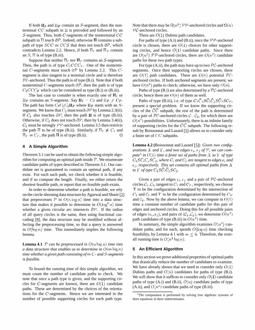
Lemma 2.1 (Dubins [10]) In an obstacle-free environment,an optimal path between any two configurations is of typeCCC or CSC, or a substring thereof.

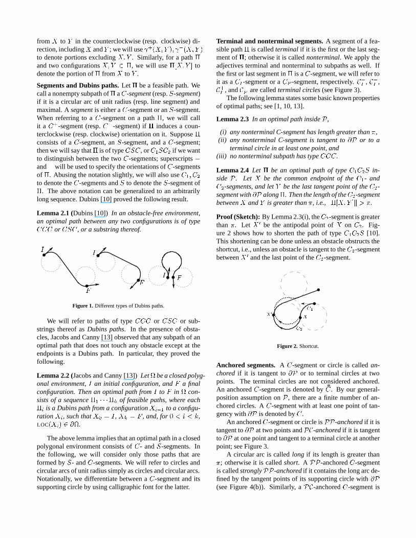
IFI FIFFigure 1. Different types of Dubins paths.

We will refer to paths of typeCCC or CSC or sub-strings thereof asDubins paths. In the presence of obsta-cles, Jacobs and Canny [13] observed that any subpath of anoptimal path that does not touch any obstacle except at theendpoints is a Dubins path. In particular, they proved thefollowing.

Lemma 2.2 (Jacobs and Canny [13])Let be a closed polyg-onal environment,I an initial configuration, andF a finalconfiguration. Then an optimal path fromI to F in con-sists of a sequence�1 � � ��k of feasible paths, where each�i is a Dubins path from a configurationXi�1 to a configu-rationXi, such thatX0 = I , Xk = F , and, for0 < i < k,LOC(Xi) 2 @.

The above lemma implies that an optimal path in a closedpolygonal environment consists ofC- andS-segments. Inthe following, we will consider only those paths that areformed byS- andC-segments. We will refer to circles andcircular arcs of unit radius simply as circles and circular arcs.Notationally, we differentiate between aC-segment and itssupporting circle by using calligraphic font for the latter.

Terminal and nonterminal segments. A segment of a fea-sible path� is calledterminal if it is the first or the last seg-ment of�; otherwise it is callednonterminal. We apply theadjectives terminal and nonterminal to subpaths as well. Ifthe first or last segment in� is aC-segment, we will refer toit as aCI -segment or aCF -segment, respectively.C+I , C�I ,C+F , andC�F are calledterminal circles(see Figure 3).

The following lemma states some basic known propertiesof optimal paths; see [1, 10, 13].

Lemma 2.3 In an optimal path insideP,

(i) any nonterminal C-segment has length greater than�,(ii) any nonterminal C-segment is tangent to@P or to a

terminal circle in at least one point, and(iii) no nonterminal subpath has typeCCC.

Lemma 2.4 Let � be an optimal path of typeC1C2S in-sideP . Let X be the common endpoint of theC1- andC2-segments, and letY be the last tangent point of theC2-segment with@P along�. Then the length of theC2-segmentbetweenX andY is greater than�, i.e.,k�[X;Y ]k > �.

Proof (Sketch): By Lemma 2.3(i), theC2-segment is greaterthan�. Let X 0 be the antipodal point ofX on C2. Fig-ure 2 shows how to shorten the path of typeC1C2S [10].This shortening can be done unless an obstacle obstructs theshortcut, i.e., unless an obstacle is tangent to theC2-segmentbetweenX 0 and the last point of theC2-segment. 2

C1C2XX0Figure 2. Shortcut.

Anchored segments. A C-segment or circle is calledan-chored if it is tangent to@P or to terminal circles at twopoints. The terminal circles are not considered anchored.An anchoredC-segment is denoted by��C. By our general-position assumption onP , there are a finite number of an-chored circles. AC-segment with at least one point of tan-gency with@P is denoted by�C.

An anchoredC-segment or circle isPP-anchoredif it istangent to@P at two points andPC-anchoredif it is tangentto @P at one point and tangent to a terminal circle at anotherpoint; see Figure 3.

A circular arc is calledlong if its length is greater than�; otherwise it is calledshort. A PP-anchoredC-segmentis calledstronglyPP-anchoredif it contains the long arc de-fined by the tangent points of its supporting circle with@P(see Figure 4(b)). Similarly, aPC-anchoredC-segment is

calledstronglyPC-anchoredif it contains the long arc be-tween a tangency point of its supporting circleC with @Pand a tangency point ofC with a terminal circle (see Fig-ure 5(a)).

C1C2 P IFC�IC+IC+FC�F

Figure 3. PC-anchored (C1) andPP-anchored (C2) circles.

Pockets. Let C be a circle intersecting@P at two or morepoints, and letX;Y be two consecutive intersection pointsof @P with C so that the short arc ofC joining X andYlies insideP . If C+[X;Y ] is the short arc and the turningangle2 of @P+(X;Y ) is less than�, then the closed regionbounded by@P+[X;Y ] andC+[X;Y ] is called apocket(seeFigure 4) and is denoted by�C[X;Y ]. Similarly we define apocket�C[X;Y ] whenC�[X;Y ] is the shorter arc. We willmostly be interested in pockets for whichC is tangent to@PatX .

CP X Y�C [X;Y ]F

I IF PY XC �C [X;Y ](a) (b)

Figure 4. Pockets.

It can be verified that the condition on the turning angleimplies that a pocket does not have enough room to contain aunit circle. Using this simple observation, we can prove thefollowing lemma, which will be crucial for characterizing theoptimal paths containing a strongly anchoredC-segment. Inparticular, the lemma implies that if a feasible path entersthe interior of a pocket, then it cannot escape the pocket (seeFigure 4).

Lemma 2.5 LetC be a circle tangent to@P atX that definesa pocket�C [X;Y ]. If a feasible path� from I to F enters(resp. escapes)�C [X;Y ] at X , then either� contains thesmall arc ofC joining X andY , or �[X;F ] � �C [X;Y ](resp.�[I;X ] � �C [X;Y ]).

2The turning angleof a convex polygonal chain isPi(� � �i), where�i is the interior angle at vertexi.

3 Classification of Optimal Paths

The goal of this section is to prove the first of our main re-sults, namely a detailed characterization of optimal paths inconvex polygons. We show that any optimal path is of typeCICSCCSCCF or a subsequence of this form. However,not every subsequence of the above sequence can form anoptimal path. The following theorem gives a more refineddescription of optimal path types. Recall that a segment hasnon-zero length by definition. In the following, we use� todenote a subpath of zero length.

Theorem 3.1 An optimal path� insideP either is a Dubinspath or has one of the types listed below. Except in case (B.i),all theC-segments labeled��C are strongly anchored.

(A) If � has no nonterminalCC subpath, then� has oneof the following types:

(A.i) �IS ��CS�F where�I 2 fCI ; �gand�F 2 fCF ; �g (see Figure 4(b))

(A.ii) �IS�F where�I 2 fCI ��C;CI ; �gand�F 2 f ��CCF ; CF ; �g (see Figure 5(a))

(B) If � has a nonterminalCC subpath, then� has one ofthe following types:

(B.i) CIC ��CCF or CI ��CCCF(B.ii) �IS ��CCCF or CIC ��CS�F where�I 2 fCI ; �g

and�F 2 fCF ; �g(B.iii) �I �C �C�F where�I 2 fCI ��CS;CIS;CI ; Sg and�F 2 fS ��CCF ; SCF ; CF ; Sg (see Figures 5(b), (c))

Proposition 3.2 The typeCICS �C �CSCCF , having eight seg-ments, does occur as an optimal path type.

Proof (Sketch): Figure 5(c) shows an instance ofP and ini-tial and final configurations in which a feasible path has eightsegments. We can argue that no paths of the other types de-scribed in Theorem 3.1 are feasible, which implies that theoptimal path is of the given type. 2

The proof of Theorem 3.1 is based on the following lem-mas.

Lemma 3.3 (Agarwal, Raghavan and Tamaki [1])An optimalpath has at most one nonterminalCC subpath. Moreover,any nonterminal C-segment that precedes (resp. follows) aC1C2 subpath is oriented the same way asC1 (resp.C2).

Next, we state a lemma, which can be proved using geo-metric perturbations similar to the ones used in [1, 5].

Lemma 3.4 (i) If an optimal path has a subpath of typeSCS, then theC-segment in that subpath is stronglyPP-anchored.(ii) If an optimal path has a subpath of typeC1C2C3S (orSC3C2C1) so that theC-segmentC2 does not touch@P ,thenC3 is stronglyPP-anchored.

I FP P IF

(b)CIS �C �CSCF(a)CI ��CS ��CCFIFC+FC+I

C�IC�F�C3

��C1�C2 ��C4(c)CI ��C1S �C2 �C3S ��C4CF

Figure 5. Examples of shortest paths.

We next characterize the optimal paths that contain astronglyPP-anchoredC-segment.

Lemma 3.5 If an optimal path� contains a stronglyPP-anchoredC-segment��C , then� is of typeCIS ��CSCF ,CIC ��CSCF , CIS ��CCCF , or a substring thereof (containing��C).

Proof (Sketch): By assumption,� = �I ��C�F . ��C is stronglyPP-anchored; hence its supporting circle,��C, has two or moreintersections with@P. LetX denote the first tangent pointof ��C with @P along�. LetY be the first point fromX on ��C— moving in the opposite sense of��C ’s orientation — whichintersects@P (see Figure 6). It is easy to prove that such aY exists, and that� ��C[X;Y ] defines a pocket. Lemma 2.5implies that the path up toX , i.e.�I and perhaps part of��C,is contained in the pocket. We can also prove that�I con-sists of at most two segments, so�I is eitherCIC, CIS, ora substring thereof. Likewise,�F is CCF , SCF , or a sub-string thereof. The result follows by noting that paths of typeCIC ��CCCF are ruled out by Lemma 2.3(iii). 2

We state now another lemma which will be useful for thealgorithm. The proof is similar to that of Lemma 3.5.

I XYF ��C PFigure 6. For the proof of Lemma 3.5. An optimal path containing astronglyPP-anchoredC-segment must start and end in a pocket.

Lemma 3.6 If an optimal path� contains a stronglyPC-anchoredC-segment��C whose supporting circle is not free,then� is of typeCI ��CSCF ,CI ��CCCF ,CIS ��CCF ,CIC ��CCF ,or a substring thereof (containing��C).

We now prove Theorem 3.1.

Proof of Theorem 3.1: The proof proceeds by consideringhow a nonterminalC-segment may appear in�. If there isno nonterminalC-segment in�, then� is of typeCISCFor a substring thereof, i.e.,� is a Dubins path.

Assume now that there is a nonterminalC-segment in�.Then such a segment belongs to a subpath of� of type eitherSCS or CC. Suppose� contains a subpath of typeSCS.By Lemma 3.4, theC-segment inSCS must be stronglyPP-anchored. Thus, by Lemma 3.5,� is of typeCIS ��CSCF ,or substrings (containingS ��CS) thereof. In other words,� isof type (A.i).

If � contains a nonterminalC-segment but not a subpathof type SCS, we know it must contain a subpath of typeCC. There are two cases to consider, depending on whethertheCC subpath is terminal.

Case 1:� does not contain any nonterminal subpath oftype CC. Thus, one of theC-segments in anyCC sub-path must be a terminal segment. Either� is of typeCICF ,CICCF (i.e., a Dubins path), or any nonterminalC-segmentis also adjacent to anS-segment.� must then be of typeCICSCCF , or any substring thereof containingS and a ter-minalCC. By Lemma 2.4, the nonterminalC-segments arestrongly anchored. All these types of paths are covered bytype (A.ii).

Case 2:� contains a nonterminal subpath of typeCC.By Lemma 3.3, it is theonly nonterminalCC subpath in�.Thus� has the form�ICC�F . A nonterminalC-segmentin �I must be followed by anS-segment, otherwise therewill be a nonterminalCCC subpath in� (Lemma 2.3(iii)).Furthermore, since we have noSCS subpath in�, a nonter-minalC segment must be preceded by a terminalC-segment.This means�I = CICS or a subsequence of it. The subse-quence cannot not be empty, for otherwise the middleCCsubpath would be terminal; nor can it be simplyCC, asnoted above. Thus,�I 2 fCICS;CIS;CI ; Sg. Similarly,�F 2 fSCCF ; SCF ; CF ; Sg.

If �I = CICS or �F = SCCF , then the nonterminalC-segment in�I or�F is strongly anchored by Lemma 2.4.

If both �I and�F contain anS-segment, then the non-terminalCC subpath in� is preceded and followed by anS-segment. Thus, bothC-segments of the nonterminalCCsubpath in� touch@P . Indeed, otherwise� contains a sub-path of typeSCC or CCS that does not touch@P , whichcontradicts Lemma 2.2. Hence, if both�I and�F containanS, � is of type (B.iii).

Suppose that neither�I nor�F contains anS-segment.Then, the path is of typeCICCCF . One of the nontermi-nal C-segments must touch@P by Lemma 2.2. ThisC-segment is also tangent to a terminal circle and is thereforePC-anchored. Thus the path is of type (B.i). Note that if bothnonterminalC-segments touch@P , then the path is of typeCI ��C ��CCF which can be considered as type (B.i) or (B.iii).

The last case to consider is when exactly one of�I or�F contains anS-segment. Say�I = CI and�F 6= CF .The path has formCIC1C2�F where�F starts with anS-segment. We know thatC2 must touch@P by Lemma 2.3(ii).If C1 also touches@P, then the path� is of type (B.iii).Otherwise, ifC1 does not touch@P, then by Lemma 3.4(ii),C2 must be stronglyPP-anchored. Lemma 3.5 then restrictsthe path� to be of type (B.ii). Similarly, if�I 6= CI and�F = CF , the path� is of type (B.ii). 24 A Simple Algorithm

Theorem 3.1 can be used to obtain the following simple algo-rithm for computing an optimal path insideP. We enumeratecandidate paths of types described in Theorem 3.1. Our can-didate set is guaranteed to contain an optimal path, if anyexist. For each such path, we check whether it is feasible,and if so compute the length. Finally, we either return theshortest feasible path, or report that no feasible path exists.

In order to determine whether a path is feasible, we relyon the circle-shooting data structure by Agarwal and Sharir [2]that preprocessesP in O(n logn) time into a data struc-ture that makes it possible to determine inO(log2 n) timewhether a given circular arc intersects@P. If the radiusof all query circles is the same, then using fractional cas-cading [8], the data structure may be modified without af-fecting the preprocessing time, so that a query is answeredin O(logn) time. This immediately implies the followinglemma.

Lemma 4.1 P can be preprocessed inO(n logn) time intoa data structure that enables us to determine inO(m logn)time whether a given path consisting ofmC- andS-segmentsis feasible.

To bound the running time of this simple algorithm, wemust count the number of candidate paths to check. Wenote that once a path type is given, and the supporting cir-cles forC-segments are known, there areO(1) candidatepaths. These are determined by the choices of the orienta-tions for theC-segments. Hence we are interested in thenumber of possible supporting circles for each path type.

Note that there may be(n2)PP-anchored circles and(n)PC-anchored circles.There areO(1) Dubins path candidates.For paths of type (A.i) and (B.ii), once thePP-anchored

circle is chosen, there areO(1) choices for other support-ing circles, and henceO(1) candidate paths. Since thereareO(n2) PP-anchored circles, there areO(n2) candidatepaths for these two path types.

For type (A.ii), the path may have up to twoPC-anchoredsegments. Once their supporting circles are chosen, thereareO(1) path candidates. There areO(n) potentialPC-anchored circles. If both anchored segments are present, wehaveO(n2) paths to check; otherwise, we have onlyO(n).

Paths of type (B.i) are also determined by aPC-anchoredcircle; hence there areO(n) of them as well.

Paths of type (B.iii), i.e. of typeCI ��C1S �Ci �CjS ��C2SCF ,present a special problem. If we know the supporting cir-cles of the �C �C subpath, the rest of the path is determinedby a pair ofPC-anchored circlesC1; C2, for which there areO(n2) possibilities. Unfortunately, there is an infinite familyof supporting circles for the�C �C subpath. The following re-sult by Boissonnat and Lazard [5] allows us to consider onlya finite set of�C �C subpaths.

Lemma 4.2 (Boissonnat and Lazard [5])Given two config-urationsX andY , and two edgesei, ej of P , we can com-pute3 in O(1) time a finite set of paths fromX to Y of typeC1S �Ci �CjSC2, where�Ci and �Cj are tangent to edgesei andej , respectively. This set contains all optimal paths fromXto Y of typeC1S �Ci �CjSC2.

Given a pair of edgesei; ej and a pair ofPC-anchoredcirclesC1; C2, tangent toCI andCF , respectively, we chooseX to be the configuration determined by the intersection ofCI andC1 andY to be the configuration determined byCFandC2. Now by the above lemma, we can compute inO(1)time a constant number of candidate paths for this pair ofedges and anchored circles. Doing this for all possible pairsof edges(ei; ej), and pairs of(C1; C2), we determineO(n4)path candidates of type (B.iii) inO(n4) time.

In summary, the simple algorithm examinesO(n4) can-didate paths, and for each, spendsO(logn) time checkingfeasibility, by Lemma 4.1 withm � 8. Therefore, the over-all running time isO(n4 logn).5 An Efficient Algorithm

In this section we prove additional properties of optimal pathsthat drastically reduce the number of candidates to examine.We have already shown that we need to consider onlyO(1)Dubins paths andO(n) candidates for paths of type (B.i).We will show that it suffices to consider onlyO(1) candidatepaths of type (A.i) and (B.ii),O(n) candidate paths of type(A.ii), andO(n2) candidate paths of type (B.iii).

3The computation is performed by solving four algebraic systems ofthree equations in three indeterminates.

Computing paths of type (A.i) and (B.ii). The paths oftypes (A.i) and (B.ii) contain a stronglyPP-anchoredC-segment��C . The circle ��C supporting��C defines one or twopockets that contain a point of tangency of��C with @P (seeFigures 4(b) and 6). By Lemma 2.5, we know thatI andFmust belong to these pockets. The following lemma statesthat there exists at most one circle with these properties.

Lemma 5.1 For a fixed pair of configurationsI; F , thereexists at most onePP-anchored circle��C so that the long arcdefined by the tangent points of��C with @P is free and so thatI andF belong to the pocket(s) defined by��C and its tangentpoints with@P. This circle can be computed inO(n) time.

By the lemma, we can compute, inO(n) time, a set ofO(1) candidate paths of types (A.i) and (B.ii). The candi-date paths may be checked for feasibility inO(logn) time.Therefore, an optimal path of type (A.i) or (B.ii) can be com-puted inO(n) time.

A monotonicity property of CCSC paths. Subpaths oftypeCCSC occur in both (A.ii) and (B.iii) path types. Inthis subsection, we ignore the polygonP , and study pathsfrom X to Y of typeC1C2SC3, with specified orientationson theC-segments. Then the circlesC1 andC3 supportingC1 andC3, respectively, are fixed. CircleC2 is determinedbyM , its tangent point withC1. For eachM 2 C1, there isat most one path�(M) of typeC1C2SC3 with the specifiedorientations onC-segments. For certain positions ofM , oneof the segments may vanish. These positions ofM are calledsingular points. The following lemma is proved by calculus.

Lemma 5.2 AsM moves along the oriented circleC1,k�(M)k increases monotonically, except at singular points.

At singular points where aC-segment vanishes, the pathlength changes by�2�. TheS-segment vanishes whenC2and C3 have opposite orientation and are tangent.4 Thus,there may be two singular points where theS-segment van-ishes. If there are two, they split the circleC1 into two arcs.Along one of the arcs, circlesC2 andC3 properly intersect,and so�(M) is not defined there. Thus, the singular pointscorresponding to a vanishingS-segment are the endpoints ofthe arc ofC1 on which the path is defined. There may beup to six singular points. See Figure 7 for an illustration ofsix singular points in a path of typeC+C�SC+. All thesingular points can be computed inO(1) time.

Computing type (A.ii) paths. As mentioned in Section 4,we can compute inO(n logn) time the feasible candidatesof type (A.ii) paths with at most onePC-anchored segment.If the path is of typeCI ��CS ��CCF , a simple analysis givesO(n2) candidates to check; we now use Lemma 5.2 to reducethe number of candidates and to compute them inO(n logn)time.

4TheS-segment may vanish even ifC2 andC3 have the same orientationandC2 = C3, but in this caseC2-segment also vanishes.

X YM1M2M3M4M5 C+YC+XFigure 7. Paths of typeC+C�SC+ from X to Y and the six singularpointsX,M1,M2, M3,M4 andM5 onC+X .

Fix the orientations of the terminalC-segments, and letCI andCF denote the circles supportingCI andCF , respec-tively. LetKI be the sequence ofPC-anchored circles thattouchCI and that are free, sorted by their tangent points withCI . The setKF is defined analogously, forPC-anchored cir-cles tangent toCF . Note thatKI andKF can be computed inO(n logn) time, and they haveO(n) elements.

By Lemma 3.6, circles supporting the��C-segments in anoptimal path� of typeCI ��C1S ��C2CF are free. Therefore, the��C2-segment of� lies on a circle ofKF . SupposeC2 2 KFsupports the��C2-segment of�. This fixes the terminal con-figuration of the subpathCI ��C1S ��C2. The above subsectionon monotonicity implies we have up to up to six singularpoints onCI .

Let � � CI be an arc joining two singular points andlet KI(�) � KI be the subsequence of circles that touchCI at a point in�. By Lemma 5.2, only the first circle ofKI(�) is a candidate forC1. Hence, at most six circles inKIare candidates forC1, and they can be computed inO(logn)time by performing a binary search. By examining eachC2 2KF in turn, we computeO(n) candidate paths inO(n logn)time. We can therefore conclude that an optimal path of type(A.ii) can be computed inO(n logn) time.

Computing type (B.iii) paths. Let � be an optimal path ofthe form�I �Ci �Cj�F , i.e. of type (B.iii). Suppose we knowthe edgesei; ej that are tangent to�Ci and �Cj , respectively.

If � does not contain any��C-segment in�I or �F , thenwe can compute� in O(logn) time using Lemmas 4.2 and4.1.

Consider now the case in which�I and�F each con-tains a ��C-segment, i.e.� is of typeCI ��CS �Ci �CjS ��CCF . Weshow that, givenei and ej , we can compute, inO(logn)time, a set ofO(1) candidate circles that contains the��C-segments of�. Given this set, we can compute the shortestfeasible path of the above type inO(logn) time, by Lem-mas 4.1 and 4.2. Thus, by considering allO(n2) pairs ofedges ofP , we can compute inO(n2 logn) time a set ofO(n2) candidate paths for this case. However, we will see

later that in some cases we need not consider allO(n2) pairsof edges ofP .

We first establish some simple properties of an optimalpath� of typeCI ��C1S �Ci �CjS ��C2CF . Assume without lossof generality that�Ci; �Cj are oriented clockwise and coun-terclockwise, respectively. By Lemma 3.3, the��C1-segmentis oriented clockwise, and the��C2-segment is oriented coun-terclockwise, i.e.,� is of typeC+I ��C�1 S �C�i �C+j S ��C+2 C�F . Let��C1, �Ci, �Cj , and��C2 denote the circles supporting theC-segments��C1, �Ci, �Cj , and ��C2, respectively.

Lemma 5.3 If an optimal path is of typeCI ��C1S �Ci �CjS ��C2CF ,then the circles��C1, �Ci, �Cj , and ��C2 are free.

Proof: Lemma 3.6 directly yields that��C1 and ��C2 are free.Suppose now for a contradiction that�Cj is not free. Asbefore, we assume that the orientations are such that� =C+I ��C�1 S �C�i �C+j S ��C+2 C�F . Let T be the tangent point be-tween �Ci and �Cj . Moving along �C+j , letX be the last tan-gent point between�Cj and@P . Starting atX and movingalong �C+j , letY be the first proper intersection point between�Cj and@P (see Figure 8).

By Lemma 2.4, the length of�Cj betweenT andX isgreater than�, i.e. k �C+j [T;X ]k > �. It follows that �Cj ,X and Y define a pocket� �Cj [X;Y ] (see Figure 8). ByLemma 2.5, this pocket contains�[X;F ] and therefore con-tains ��C2. We know the free circle��C2 cannot be entirely in-side a pocket. The path�CjS ��C2 enters the pocket atX , andsince��C2 is free, it is possible to escape the pocket by extend-ing segment��C2. This contradicts Lemma 2.5, establishingthat �Cj is free. A symmetric argument shows that circle�Ci isfree. 2

IF XTY

�C�i �C+j>�� �Cj [X;Y ]Figure 8. For the proof of Lemma 5.3.

We now introduce the following simple definition. Givena circleC and a pointX 2 C, a pointM 2 C is called thefirstfree point afterX alongC+ if and only if the circle tangentto C atM is free and for anyM 0 2 C+[X;M), the circletangent toC atM 0 is not free (in Figure 9,M� is the firstfree point afterML alongC+I ). Note thatM could beX .The circle tangent toC at the first free point afterX is calledthefirst free circle afterX alongC+.

We show that, givenI , F , ei andej , we can computein O(logn) time a set ofO(1) candidate circles that con-tain the ��C-segments of any optimal path fromI toF of type

C+I ��C�1 S �C�i �C+j S ��C+2 C�F . We show how to compute can-

didate circles for��C1; computing candidate circles for��C2 issimilar.

We identify two circlesC0 andC00 that are the candidatecircles for��C1. See Figure 9. LetC0 be the first free circle afterI alongC+I . If there is no free circle afterI alongC+I , thenC0 andC00 are not defined. Assume, after a possible rotation,that the lineL throughei is horizontal andP is aboveL. Ifthe distance betweenL and the center ofC+I is greater than2, thenC00 is not defined. Otherwise, there exist two circlesthat are aboveL and tangent to bothC+I andL. LetCL be theleftmost of these two circles, and letML be its tangent pointwith C+I . Let C00 be the first free circle afterML alongC+I .Note thatC0 andC00 only depend onI , C+I , and on the lineLthroughei.

IC0C00 = C1MLM1CL TM��C�i �C+j

eiej

LFC+I

Figure 9. For the proof of Lemma 5.4.

Lemma 5.4 Let� be an optimal path of typeC+I ��C�1 S �C�i �C+jS ��C+2 C�F , and letL be the line through the edge tangent to�Ci. Then ��C1 is supported byC0 or C00.Proof (Sketch): We prove the lemma only in the case whereC+I andCi properly intersect. LetT 2 � be the configurationat the tangent point between�Ci and �Cj . See Figure 9.

The circleC1 supporting the��C1-segment is tangent toC+I . As before, any choice of a pointM 2 C+I defines atmost one path�(M) of the formC+I C�1 SC�i , which beginsat I and ends atT , and whereC+I andC�1 are tangent atM .Let M� be the intersection point of theC+I - and ��C�1 seg-ments of the optimal path�. Then�(M�) is a subpath of� and so it is an optimal path fromI to T . By the mono-tonicity property (Lemma 5.2), and sinceC1 andCi are free(Lemma 5.3),M� must be the first free point alongC+I aftera singular point of�(M). SinceC+I andCi properly inter-sect, there are only two singular pointsI andM1 of �(M),whereM1 corresponds to the vanishing of��Ci.

If M� is the first free point afterI alongC+I , then ��C1 issupported byC0, the first free circle afterI . If M� is the firstfree point afterM1, then we show that��C1 is supported byC00, the first free circle afterML.

By Lemma 2.4, the arc length of�Ci from its tangent pointwith L to T must be at least�. In other words,T must be

in the right half of �Ci (asL is horizontal andP is aboveL). Therefore by definition ofML, the arc length ofCi in�(ML) is less than�.It follows that for any pointM 2 C+I [M1;ML], the arc

length ofCi in�(M) is less than�, so by Lemma 2.3,�(M)cannot be part of the optimal path. Thus,M� does not belongto C+I [M1;ML]. So if M� is the first free point afterM1,then it is the first free point afterML. In other words,��C1 issupported byC00. 2Lemma 5.5 C0 andC00 can be computed inO(logn) time.

Proof: Let � be the circle of radius2 concentric withC+I .Let I� (resp.M�) be the intersection point between� andthe ray emanating from the center ofC+I and going throughI(resp.ML) (see Figure 10). LetR be theretracted polygonof P with respect to a unit circle, i.e.,R is the set of pointsp such that the unit circle centered atp lies insideP; R isa convex polygonal region with at mostn edges, and it canbe computed in linear time. LetO0 be the first intersectionpoint between� andR starting atI� and moving along�+.The center ofC0 isO0. Indeed, by definition ofR, the circlecentered atO0 is free, and any circle (of unit radius) centeredat a point on�+[I�; O0) is not free. Similarly, the center ofC00 is the first intersection point between� andR starting atM� and moving along�+. Using the circle-shooting datastructure by Agarwal and Sharir [2],R can be preprocessedin O(n logn) time, so thatC0 andC00 can be computed inO(logn) time. 2�+

C+I II� MLM� R PO0C0 C00Figure 10. For the proof of Lemma 5.5.

By Lemmas 5.4 and 5.5, we can compute, inO(logn)time, two candidates for the circle supporting segment��C1.We can similarly compute two candidates for the circle sup-porting segment��C2. By Lemma 4.2, this gives usO(1)candidate paths, for which we may check the feasibility inO(logn) time. Hence, given two edgesei and ej of P,we can compute inO(logn) time, an optimal path of typeCI ��CS �Ci �CjS ��CCF , where �Ci and �Cj are tangent toei andej , respectively.

In the cases where the optimal path is of type (B.iii) withonly one ��C-segment in�I or �F , we get similar results.

For example, if an optimal path is of typeCI ��C1S �Ci �CjSCF ,then ��C1 and �Ci are free, and��C1 is supported by theC0 or C00defined above. Thus we obtain the following lemma.

Lemma 5.6 Let ei; ej be edges ofP . In O(logn) time, wecan compute an optimal path of type�I �Ci �Cj�F where�I 2fCI ��CS;CIS;CI ; Sg,�F 2 fS ��CCF ; SCF ; CF ; Sg and where�Ci and �Cj are tangent toei andej , respectively.

Now we describe how to find a suitable set of pairs ofedgesE such that if an optimal path fromI toF is of type (B.iii)(i.e.,�I �Ci �Cj�F ), then the pair of edges(ei; ej) tangent to�Ci and �Cj is in the setE .

From [1], we know that if an optimal path fromI toF isof type�I �C+i �C�j �F such that�Ci and �Cj are nonterminal,thenC+I intersects�Cj (the circle supporting�Cj), andC�F in-tersects�Ci (the circle supporting�Ci). Thus, the center of�Cj ,which is at most distance 1 from the boundary of the poly-gon, is at most distance 3 fromI . Since centers of�Ci and �Cjare distance 2 apart, they are each distance less than 5 fromI . Thus, edgesei andej are distance less than 6 fromI . Bysymmetry, they are also distance less than 6 fromF . There-fore, we can considerE to be the set of pairs of edges ofPthat are distance less than 6 from bothI andF . Letk denotethe number of edges ofP distance less than 6 from bothIandF . ThenjEj = k2, andE can be computed inO(k2)time. Lemma 5.6 then gives:

Lemma 5.7 An optimal path of type (B.iii) can be computedin O(k2 logn) time.

Putting everything together, we obtain the following.

Theorem 5.8 Given a convex polygonP , an initial configu-ration I , and a final configurationF , an optimal path fromI to F insideP can be computed in timeO((n+ k2) logn),wherek is the number of edges ofP at distance less than 6from bothI andF .

Proof: We have shown in the previous subsections that theDubins paths and the optimal paths of type (A.i), (A.ii), (B.i),and (B.ii) can be computed inO(n logn) time, while pathsof type (B.iii) can be computed inO(k2 logn) time. Choos-ing the shortest among all those paths yields an optimal path.26 Conclusion

Our classification of path types in a convex polygon yieldsa fast algorithm for computing an optimal path. An inter-esting question is whether the running time can be improvedto O(n logn) by proving additional properties of paths oftype (B.iii). Our results show that even for a convex poly-gon, optimal paths between two configurations can be rathercomplex. Such complex paths may be difficult to track bya mobile robot. Furthermore, they may arise as artifacts of

a tightly constricted environment. A direction for future re-search is to seek a realistic notion of feasibility that rejectshard-to-follow paths, while admitting fast computation ofoptimal paths.

Acknowledgments

This paper arose from research begun at the InternationalWorkshop on Bounded Radius of Curvature, organized byS. Whitesides and held at the Bellairs Research Institute ofMcGill University, March 9-16, 1997. We would like tothank Hazel Everett, Micha Godau, and Steve Wismath formany useful discussions.

References

[1] P. K. Agarwal, P. Raghavan, and H. Tamaki. Motion planningfor a steering-constrained robot through moderate obstacles.In Proc. 27th Annu. ACM Sympos. Theory Comput., pages343–352, 1995.

[2] P. K. Agarwal and M. Sharir. Circle shooting in a simple poly-gon. J. Algorithms, 14:69–87, 1993.

[3] J. Barraquand and J.-C. Latombe. Nonholonomic multi-bodymobile robots: Controllability and motion planning in thepresence of obstacles.Algorithmica, 10:121–155, 1993.

[4] J.-D. Boissonnat, A. Cerezo, and J. Leblond. Shortestpathsof bounded curvature in the plane.Internat. J. Intell. Syst.,10:1–16, 1994.

[5] J.-D. Boissonnat and S. Lazard. A polynomial-time algorithmfor computing a shortest path of bounded curvature amidstmoderate obstacles. InProc. 12th Annu. ACM Sympos. Com-put. Geom., pages 242–251, 1996.

[6] J. Canny, B. R. Donald, J. Reif, and P. Xavier. On the com-plexity of kinodynamic planning. InProc. 29th Annu. IEEESympos. Found. Comput. Sci., pages 306–316, 1988.

[7] J. Canny, A. Rege, and J. Reif. An exact algorithm for kin-odynamic planning in the plane.Discrete Comput. Geom.,6:461–484, 1991.

[8] B. Chazelle and L. J. Guibas. Fractional cascading: I. A datastructuring technique.Algorithmica, 1:133–162, 1986.

[9] B. R. Donald and P. Xavier. A provably good approximationalgorithm for optimal-time trajectory planning. InProc. IEEEInternat. Conf. Robot. Autom., pages 958–963, 1989.

[10] L. E. Dubins. On curves of minimal length with a constrainton average curvature and with prescribed initial and terminalpositions and tangents.Amer. J. Math., 79:497–516, 1957.

[11] S. Fortune and G. Wilfong. Planning constrained motion.Ann. Math. Artif. Intell., 3:21–82, 1991.

[12] D. Halperin, L. Kavraki, and J.-C. Latombe. Robotics. InCRC Handbook of Computational Geometry(J. Goodmandand J. O’Rourke, eds.), pages 755–778. CRC Press, Boca Ra-ton, NY, 1997.

[13] P. Jacobs and J. Canny. Planning smooth paths for mobilerobots. In Nonholonomic Motion Planning(Z. Li and J.Canny, eds.), pages 271–342. Kluwer Academic Publishers,Norwell, MA, 1992.

[14] P. Jacobs, J.-P. Laumond, and M. Taix. Efficient motionplanners for nonholonomic mobile robots.In Proc. of theIEEE/RSJ Internat. Workshop on Intell. Robots and Systems,pages 1229–1235, 1991.

[15] K. Kedem, R. Livne, J. Pach, and M. Sharir. On the union ofJordan regions and collision-free translational motion amidstpolygonal obstacles.Discrete Comput. Geom., 1:59–71, 1986.

[16] J.-C. Latombe. A fast path-planner for a car-like indoor mo-bile robot. In Proc. of the 9th National Conf. on Artif. Intell.,pages 659–665, 1991.

[17] J.-C. Latombe.Robot Motion Planning. Kluwer AcademicPublishers, Norwell, MA, 1991.

[18] J.-P. Laumond. Finding collision-free smooth trajectories fora non-holonomic mobile robot.In Proc. of the Internat. JointConf. on Artif. Intell., pages 1120–1123, 1987.

[19] J.-P. Laumond, P. Jacobs, M. Taix, and R. Murray. A mo-tion planner for nonholonomic mobile robots.IEEE Trans. onRobot. and Autom., 10:577–593, 1994.

[20] J.-P. Laumond, M. Taix, and P. Jacobs. A motion planner forcar-like robots based on global/local approach.In Proc. of theIEEE/RSJ Internat. Workshop on Intell. Robots and Systems,pages 765–773, 1990.

[21] B. Mirtich and J. Canny. Using skeletons for nonholonomicpath planning among obstacles. InProc. 9th IEEE Internat.Conf. Robot. Autom., pages 2533–2540, 1992.

[22] C. O’Dunlaing. Motion-planning with inertial constraints.Al-gorithmica, 2:431–475, 1987.

[23] J. A. Reeds and L. A. Shepp. Optimal paths for a car that goesboth forwards and backwards.Pacific J. Math., 145(2), 1990.

[24] J. Reif and H. Wang. The complexity of the two dimen-sional curvature-constrained shortest-path problem. InProc.3rd Workshop on the Algo. Found. of Robotics(P. K. Agarwal,L. E. Kavraki, and M. Mason, eds.). A. K. Peters, Wellesley,MA, 1998.

[25] J. T. Schwartz and M. Sharir. Algorithmic motion planning inrobotics. InAlgorithms and Complexity, volume A ofHand-book of Theoretical Computer Science(J. van Leeuwen, ed.),pages 391–430. Elsevier, Amsterdam, 1990.

[26] S. Sekhavat, P.Svestka, J.-P. Laumond, and M. Overmars.Multi-level path planning for non-holonomic robots usingsemi-holonomic subsystems. InWorkshop on the Algo.Found. of Robotics(J.-P. Laumond and M. Overmars, eds.),pages 79–96. A. K. Peters, Wellesley, MA, 1996.

[27] J. Sellen. Planning paths of minimal curvature,In Proc. of theIEEE Internat. Conf. Robot. and Autom., 1995.

[28] J. Sellen. Approximation and decision algorithms for cur-vature constrained path planning: A state-space approach.In Proc. 3rd Workshop on the Algorithmic Foundations ofRobotics(P. K. Agarwal, L. E. Kavraki, and M. Mason, eds.).A. K. Peters, Wellesley, MA, 1998.

[29] H. J. Sussmann. Shortest3-dimentional paths with a pre-scribed curvature bound. InConf. on Decision& Control,pages 3306–3311, 1995.

[30] H. Wang and P. K. Agarwal. Approximation algorithms forcurvature constrained shortest paths. InProc. 7th ACM-SIAMSympos. Discrete Algorithms, pages 409–418, 1996.

[31] G. Wilfong. Motion planning for an autonomous vehicle.InProc. IEEE Internat. Conf. Robot. Autom., pages 529–533,1988.

[32] G. Wilfong. Shortest paths for autonomous vehicles.In Proc.of the IEEE Internat. Conf. Robot. and Autom., pages 15–20,1989.