Combining Speed-up Techniques for Shortest-Path

Computations

Martin Holzer∗ Frank Schulz∗ Dorothea Wagner∗ Thomas Willhalm∗

March 9, 2006

Abstract

Computing a shortest path from one node to another in a directed graph is a verycommon task in practice. This problem is classically solved by Dijkstra’s algorithm.Many techniques are known to speed up this algorithm heuristically, while optimalityof the solution can still be guaranteed. In most studies, such techniques are consideredindividually. The focus of our work is combination of speed-up techniques for Dijkstra’salgorithm. We consider all possible combinations of four known techniques, namely goal-directed search, bidirectional search, multi-level approach, and shortest-path containers,and show how these can be implemented. In an extensive experimental study we comparethe performance of the various combinations and analyze how the techniques harmonizewhen applied jointly. Several real-world graphs from road maps and public transport andthree types of generated random graphs are taken into account.

1 Introduction

We consider the problem of (repeatedly) finding single-source single-target shortest pathsin large, sparse graphs. Typical applications of this problem include route planning sys-tems for cars, bikes, and hikers [Zhan and Noon, 2000, Barrett et al., 2002] or scheduledvehicles like trains and buses [Nachtigall, 1995, Preuss and Syrbe, 1997], spatial databases[Shekhar et al., 1997], and web searching [Barrett et al., 2000]. Usually, the problem is solvedby Dijkstra’s algorithm [Dijkstra, 1959], which is a label-setting single-source algorithm andas such can be terminated once the target is reached. Besides Dijkstra’s algorithm, with aworst-case running time of O(m+n log n) using Fibonacci heaps [Fredman and Tarjan, 1987],there are many recent algorithms that solve variants and special cases of the shortest-pathproblem with better running time (worst-case or average-case; see [Cherkassky et al., 1996] foran experimental comparison, [Zwick, 2001] for a survey, and [Goldberg, 2001b, Meyer, 2001,Pettie et al., 2002] for some more recent work).

The focus of this paper are variants of Dijkstra’s algorithm—also denoted as speed-uptechniques in the following—that further exploit the fact that a target is given. Typically,such improvements of Dijkstra’s algorithm cannot be proven to be asymptotically faster thanthe original algorithm, and are heuristics in this sense. However, it can be empirically shownthat they indeed improve the running time drastically for many realistic data sets. During

∗Address: Universitat Karlsruhe (TH), Fakultat fur Informatik, Postfach 6980, 76128 Karlsruhe, Germany.Email: {mholzer,fschulz,dwagner,willhalm}@ira.uka.de.

1

the last few years, several new techniques of that kind have been developed. In the scenariodescribed above, it is affordable, and applied by most of these new techniques, to precomputeand store additional information on shortest paths, which is used in the on-line phase to reducethe running time for solving a shortest-path query. In [Willhalm and Wagner, 2006], a surveyon such speed-up techniques for Dijkstra’s algorithm is provided (see also [Willhalm, 2005]).For our study, we exemplarily consider the following four speed-up techniques:

Goal-Directed Search. The given edge weights are modified to favor edges leading towardsthe target node [Hart et al., 1968, Shekhar et al., 1993]. With graphs from timetableinformation, a speed-up in running time of a factor of roughly 1.5 is reported in[Schulz et al., 2000].

Bidirectional Search. Start a second search backwards, from the target to the source (see[Ahuja et al., 1993], Section 4.5). Both searches stop when their search horizons meet.Experiments in [Pohl, 1969] showed that search space can be reduced by a factor of2, and in [Kaindl and Kainz, 1997] it was shown that combinations with goal-directedsearch can be beneficial.

Multi-Level Approach. This approach takes advantage of hierarchical coarsenings of thegiven graph, where additional edges have to be computed. These can be regarded asdistributed to multiple levels. Depending on the given query, only a small fractionof these edges have to be considered to find a shortest path. Using this technique,speed-up factors of more than 3.5 were observed for road map and public-transportgraphs [Holzer, 2003]. Timetable information queries could be improved by a factor of11 (see [Schulz et al., 2002]), and also in [Jung and Pramanik, 2002] good improvementfor road maps is reported.

Shortest-Path Containers. These containers provide a necessary condition for each edge,whether or not it has to be respected during the search. More precisely, the boundingbox of all nodes that can be reached on a shortest path using this edge is stored. Speed-up factors in the range between 10 and 20 can be achieved [Wagner and Willhalm, 2003].

Our main focus is combination of these speed-up techniques. We selected only four tech-niques in order to provide a detailed analysis of all possible combinations (the complexity ofthe analysis grows exponentially with the number of techniques under investigation). How-ever, we believe that hereby we cover the characteristics of most of the existing approaches:Goal-directed search and shortest-path containers, as several other approaches, too, are onlyapplicable if a layout of the graph is provided, and multi-level approach and shortest-pathcontainers both require a preprocessing, calculating additional edges and containers, respec-tively.

The combination of the four techniques is very natural, since all of the techniques modifythe search space of Dijkstra’s algorithm independently of each other: Goal-directed searchdirects the search space towards the target of the search by modifying the edge lengths;bidirectional search maintains two search spaces; the multi-level graph approach runs commonDijkstra’s algorithm on a subgraph of the augmented input graph; and with shortest-pathcontainers, search space can be pruned by ignoring such edges that for sure do not contributeto a shortest path.

The main question is whether the search space of a combination is better (i.e., smaller)than the one of a single speed-up technique. Another point concerns the additional effort

2

needed to reduce the search space. For example, with goal-directed search, edge weights haveto be calculated during the search. This additional effort usually increases the running timeper visited edge by a small constant factor. Considering a combination of techniques, theconstant factor per edge is higher than with a single technique, so there is a trade-off betweenreduction of search space and the additional running time per edge in the search space.

The single techniques are, as mentioned above, heuristics in the sense that the reductionof the search space cannot be proven in general. Hence, the same holds in particular fora combination of such techniques, and the method of choice to answer the questions posedabove is an extensive experimental study of the combinations. Since even the single speed-uptechniques do not work equally well on all kinds of graphs, we consider several types of bothreal-world and randomly generated graphs.

The next section contains, after some definitions, a description of the speed-up techniquesand shows in more detail how to combine them. Section 3 presents the experimental setupand data sets for the statistics, and the belonging results are given in Section 4. Section 5,finally, gives some conclusions.

2 Definitions and Problem Description

2.1 Definitions

A directed simple graph G is a pair (V,E), where V is the set of nodes and E ⊆ V × V theset of edges in G. Throughout this paper, the number of nodes, |V |, is denoted by n and thenumber of edges, |E|, by m.

A path in G is a sequence of nodes u1, . . . , uk such that (ui, ui+1) ∈ E for all 1 ≤ i < k.Given non-negative edge lengths l : E → R

+

0, the length of a path u1, . . . , uk is the sum of

weights of its edges,∑k−1

i=1l(ui, ui+1). The (single-source single-target) shortest-path problem

consists of finding a path of minimum length from a given source s ∈ V to a target t ∈ V .A graph layout is a mapping L : V → R

2 of the graph’s nodes to the Euclidean plane.For ease of notation, we will identify a node v ∈ V with its location L(v) in the plane. TheEuclidean distance between two nodes u, v ∈ V is then denoted by d(u, v).

2.2 Speed-up Techniques

Our base algorithm is Dijkstra’s algorithm using binary heaps as priority queue. In thissection, we provide a short description of the four speed-up techniques, whose combinationsare discussed in the next section. For a synopsis of the main features, cf. Table 1.

2.2.1 Goal-Directed Search (go)

This technique uses a potential function on the node set. The edge lengths are modified inorder to direct the graph search towards the target. Let λ be such a potential function. Thenew length of an edge (v,w) is defined to be l(v,w) := l(v,w) − λ(v) + λ(w). The potentialmust fulfill the condition that for each edge e, its new edge length l(e) is non-negative, inorder to guarantee optimal solutions.

In case edge lengths are Euclidean distances, the Euclidean distance d(u, t) of a node u tothe target t is a valid potential, due to the triangle inequality. Otherwise, a potential function

3

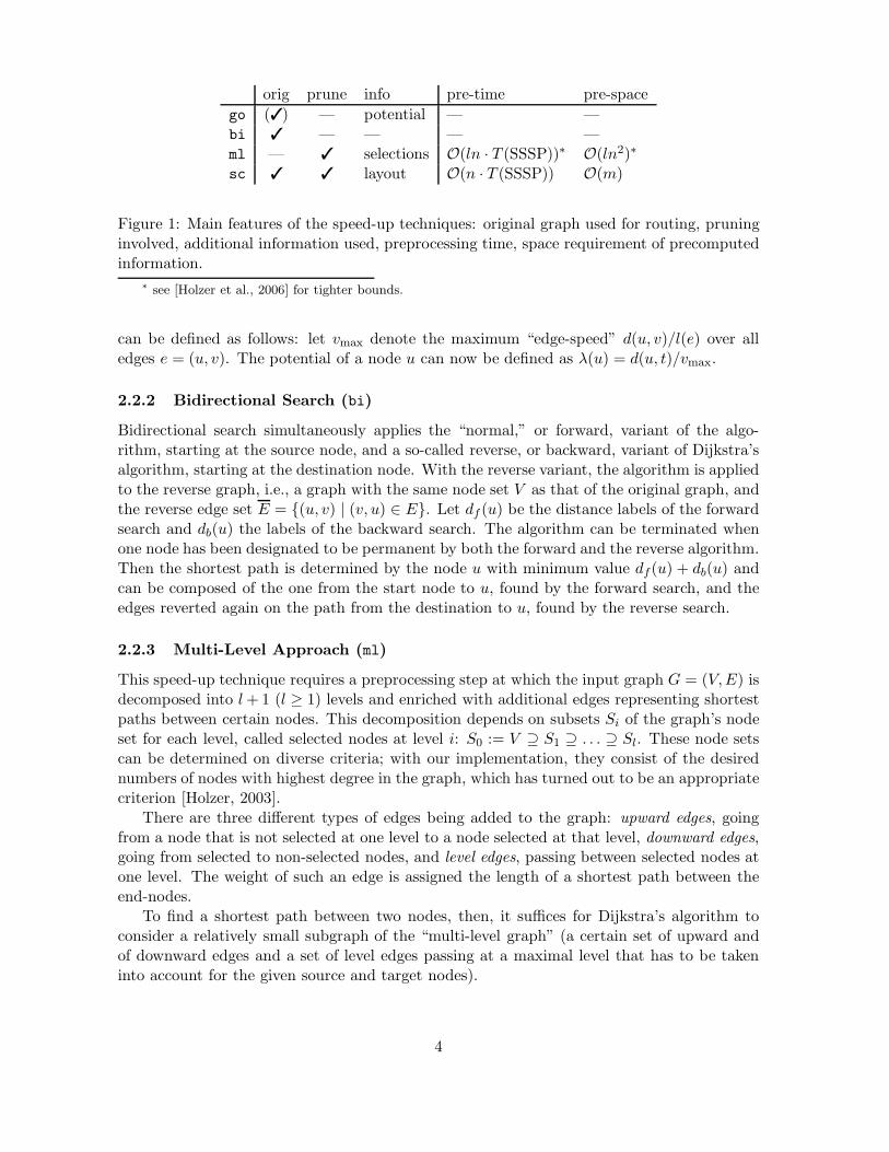
orig prune info pre-time pre-space

go (✓) — potential — —bi ✓ — — — —ml — ✓ selections O(ln · T (SSSP))∗ O(ln2)∗

sc ✓ ✓ layout O(n · T (SSSP)) O(m)

Figure 1: Main features of the speed-up techniques: original graph used for routing, pruninginvolved, additional information used, preprocessing time, space requirement of precomputedinformation.

∗ see [Holzer et al., 2006] for tighter bounds.

can be defined as follows: let vmax denote the maximum “edge-speed” d(u, v)/l(e) over alledges e = (u, v). The potential of a node u can now be defined as λ(u) = d(u, t)/vmax.

2.2.2 Bidirectional Search (bi)

Bidirectional search simultaneously applies the “normal,” or forward, variant of the algo-rithm, starting at the source node, and a so-called reverse, or backward, variant of Dijkstra’salgorithm, starting at the destination node. With the reverse variant, the algorithm is appliedto the reverse graph, i.e., a graph with the same node set V as that of the original graph, andthe reverse edge set E = {(u, v) | (v, u) ∈ E}. Let df (u) be the distance labels of the forwardsearch and db(u) the labels of the backward search. The algorithm can be terminated whenone node has been designated to be permanent by both the forward and the reverse algorithm.Then the shortest path is determined by the node u with minimum value df (u) + db(u) andcan be composed of the one from the start node to u, found by the forward search, and theedges reverted again on the path from the destination to u, found by the reverse search.

2.2.3 Multi-Level Approach (ml)

This speed-up technique requires a preprocessing step at which the input graph G = (V,E) isdecomposed into l + 1 (l ≥ 1) levels and enriched with additional edges representing shortestpaths between certain nodes. This decomposition depends on subsets Si of the graph’s nodeset for each level, called selected nodes at level i: S0 := V ⊇ S1 ⊇ . . . ⊇ Sl. These node setscan be determined on diverse criteria; with our implementation, they consist of the desirednumbers of nodes with highest degree in the graph, which has turned out to be an appropriatecriterion [Holzer, 2003].

There are three different types of edges being added to the graph: upward edges, goingfrom a node that is not selected at one level to a node selected at that level, downward edges,going from selected to non-selected nodes, and level edges, passing between selected nodes atone level. The weight of such an edge is assigned the length of a shortest path between theend-nodes.

To find a shortest path between two nodes, then, it suffices for Dijkstra’s algorithm toconsider a relatively small subgraph of the “multi-level graph” (a certain set of upward andof downward edges and a set of level edges passing at a maximal level that has to be takeninto account for the given source and target nodes).

4

2.2.4 Shortest-Path Containers (sc)

This speed-up technique requires a preprocessing computing all shortest- path trees. For eachedge e ∈ E, we compute the set S(e) of those nodes to which a shortest path starts with edgee. Using a given layout, we then store for each edge e ∈ E the bounding box of S(e) in anassociative array C with index set E.

It is then sufficient to perform Dijkstra’s algorithm on the subgraph induced by the edgese ∈ E with the target node included in C[e]. This subgraph can be determined on the fly, byexcluding all other edges in the search. (One can think of shortest-path containers as trafficsigns which characterize the region that they lead to.)

A variation of this technique is introduced in [Schulz et al., 2000], where as geometricobjects angular sectors instead of bounding boxes were used, for application to a timetableinformation system. An extensive study in [Wagner and Willhalm, 2003] showed that bound-ing boxes are the best geometric objects in terms of running time and competitive with muchmore complex geometric objects in terms of visited nodes.

2.3 Combining the Speed-up Techniques

In this section, we first outline the key notion of combining each pair of techniques and mo-tivate afterwards that extending these to combinations including three or all four techniquesis not difficult.

2.3.1 Goal-Directed Search and Bidirectional Search

Combining goal-directed and bidirectional search is not as obvious as it may seem at firstglance. [Pohl, 1969] provides a counter-example for the fact that simple application of agoal-directed search forward and backward yields a wrong termination condition. However,the alternative condition proposed there is shown in [Kaindl and Kainz, 1997] to be quiteinefficient, as the search in each direction almost reaches the source of the other direction.This often results in a slower algorithm.

To overcome these deficiencies, we simply use the very same edge weights l(v,w) :=l(v,w)− λ(v) + λ(w) for both the forward and the backward search. With these weights, theforward search is directed to the target t and the backward search has no preferred direction,but favors edges that are directed towards t. This proceeding always computes shortest paths,as an s-t-path is shortest independent of whether l or l is used for the edge weights.

2.3.2 Goal-Directed Search and Multi-Level Approach

As described in Section 2.2.3, the multi-level approach basically determines for each query asubgraph of the multi-level graph on which Dijkstra’s algorithm is finally run. The computa-tion of this subgraph does not affect edge lengths and thus goal-directed search can be simplyperformed on it.

2.3.3 Goal-Directed Search and Shortest-Path Containers

Similar to the multi-level approach, the shortest-path containers approach determines fora given query a subgraph of the original graph. Again, edge lengths are irrelevant for thecomputation of the subgraph and goal-directed search can be applied offhand.

5

gobi ml sc

Figure 2: Interdependencies of the speed-up techniques regarding preprocessing.

2.3.4 Bidirectional Search and Multi-Level Approach

Basically, bidirectional search can be applied to the subgraph defined by the multi-level ap-proach. In our implementation, that subgraph is computed on the fly during Dijkstra’salgorithm: for each node considered, the set of necessary outgoing edges is determined. Toperform a bidirectional search on the multi-level subgraph, a symmetric, backward version ofthe subgraph computation has to be implemented: for each node considered in the backwardsearch, the incoming edges that are part of the subgraph have to be determined. Shortestpaths are guaranteed since bidirectional search is run on a subgraph that preserves optimalityand, by the additional edges, only contains supplementary information consistent with theoriginal graph.

2.3.5 Bidirectional Search and Shortest-Path Containers

In order to take advantage of shortest-path containers in both directions of a bidirectionalsearch, a second set of containers is needed. For each edge e ∈ E, we compute the set Sb(e)of those nodes from which a shortest path ending with e exists. We store for each edge e ∈ Ethe bounding box of Sb(e) in an associative array Cb with index set E. The forward searchchecks whether the target is contained in C(e), the backward search, whether the source is inCb(e). It is easy to verify that by construction only such edges are pruned that do not formpart of any partial shortest path and thus of any shortest s-t-path.

2.3.6 Multi-Level Approach and Shortest-Path Containers

The multi-level approach enriches a given graph with additional edges. Each new edge (u1, uk)represents a shortest path (u1, u2, . . . , uk) in G. We annotate such a new edge (u1, uk) withC(u1, u2), the associated bounding box of the first edge on this path. This consistent labelingof new edges, which represent shortcuts in the original graph, ensures still shortest paths.

2.3.7 Extension to Arbitrary Combinations

Extracting the essence from the above discussion, we now motivate that assembling anycombination of our speed-up techniques can be done in a straight-forward manner. To thisend, we order the techniques in such a way that it reflects their interdependencies when itcomes to preprocessing (cf. Figure 2); the actual steps to be taken for a specific combinationcan then be seen from that ordering.

Bidirectional search requires supplementary information to be precomputed with boththe multi-level approach and shortest-path containers, while the multi-level technique entailsadditional work for shortest-path container preprocessing. Including goal-directed search doesnot affect preprocessing.

For justification of straight-forwardness of a new search algorithm, it suffices to verifythat each technique kicks in at a different spot and thus they do not impede one another:

6

street

n 1444 3045 16471 20466 25982 38823 45852 45073 51510 79456m 3060 7310 34530 42288 57620 79988 98098 91314 110676 172374

public transport

n 409 705 1660 2279 2399 4598 6884 10815 12070 14335m 1215 1681 4327 6015 8008 14937 18601 29351 33728 39887

planar

n 1000 2000 3000 4000 5000 6000 7000 8000 9000 10000m 5000 10000 15000 20000 25000 30000 35000 40000 45000 50000

waxman

n 938 1974 2951 3938 4949 5946 6943 7917 8882 9906m 4070 9504 14506 19658 24474 29648 34764 39138 44208 48730

hierarchical

n 1021 2017 3014 4010 5007 6002 7025 8021 9016 10012m 5814 10942 16138 21048 26064 31030 36124 41146 46246 51130

Table 1: Number of nodes and edges for all test graphs.

If including bidirectional search, we have to keep track of two search horizons and combinepartial shortest paths properly; with the multi-level approach, the search is performed ona subgraph of the enriched graph instead of the original graph; under use of shortest-pathcontainers, some edges may (additionally) be pruned; and performing goal-directed search,the lengths of the edges scanned are modified.

3 Experimental Setup

In this section, we provide details on the input data used, consisting of real-world and ran-domly generated graphs, and on the execution of the experiments.

3.1 Data

3.1.1 Real-World Graphs

In our experiments we included two sets of graphs that stem from real applications. As inother experimental work, it turned out that using realistic data is quite important, as theperformance of the algorithms strongly depends on the characteristics of the data. Note thatall our graphs are embedded either by geographic information or by construction.

Street Graphs. Our street graphs are networks of U.S. cities and their surroundings. Thesegraphs are bidirected, and edge lengths are Euclidean distances. The graphs are fairlylarge and very sparse because bends are represented by polygonal lines. (With such arepresentation of a street network, it is possible to efficiently find the nearest point in astreet by a point-to-point search.)

Public-Transport Graphs. A public-transport graph represents a network of trains, buses,and other scheduled vehicles. The nodes of such a graph correspond to stations or stops,

7

and there exists an edge between two nodes if there is a non-stop connection betweenthe respective stations. The weight of an edge is the average travel time of all vehiclesthat contribute to this edge. In particular, the edge lengths are not Euclidean distancesin this set of graphs.

3.1.2 Random Graphs

We generated three sets of random graphs: planar, Waxman, and some kind of hierarchicalgraphs. Each set consists of ten connected, bidirected graphs with (approximately) n = 1000·inodes (i = 1, . . . , 10) and an average out-degree of 2.5 (i.e., the graphs have approximately5n edges).

Random Planar Graphs. For construction of random planar graphs, we used a genera-tor provided by LEDA [Naher and Mehlhorn, 1999]. A given number, n, of nodes areuniformly distributed in a square with a lateral length of 1, and a triangulation of thenodes is computed. This yields a complete undirected planar graph. Finally, edges aredeleted at random until the graph contains 2.5 · n edges, and each of these is replacedby two directed edges, one in either direction.

Random Waxman Graphs. Construction of these graphs is based on a random graphmodel introduced by Waxman [Waxman, 1988]. We use this model in an attempt toemulate one aspect of our public-transport graphs, the existance of long-distance edges,i.e., edges linking rather far-apart nodes. As previous experiments showed, copyingnode degrees from public-transport graphs does not suffice to obtain random graphswith similar properties.

Input parameters to this model are the number of nodes n and two positive rationalnumbers α and β. The nodes are again distributed uniformly in a square of a laterallength of 1, and the probability that an edge (u, v) exists is β · exp(−d(u, v)/(

√2α)).

Higher β values increase the edge density, while smaller α values increase the densityof short edges in relation to long edges. To ensure connectedness and bidirectednessof the graphs, all nodes that do not belong to the largest connected component aredeleted (thus, slightly less than n nodes remain) and the graph is bidirected by insertionof missing reverse edges. We set α = 0.01 and empirically determined that settingβ = 2.5 · 1620/n yields the wanted number of edges.

Hierarchical Graphs. Our motivation for including such a type of graph in our experimentswas that several real-world graph classes exhibit some kind of hierarchical structure; e.g.,public-transport graphs as described above typically consist of few stations having greatnode degrees, forming a coarse overall network or backbone, as will be referred to in thefollowing, while the rest of the nodes are more locally connected and have considerablysmaller degrees.

Our generated hierarchical graphs can be regarded as 5×5 grids, constructed roughly asfollows: Pick n/14 nodes for the backbone, distribute the remaining nodes uniformly tothe 25 grid cells, and associate each backbone node with one cell. Construct a Delaunay-triangulation-based planar graph with an edge factor of 2.5 on the nodes of each celland the backbone nodes. For each cell, three nodes associated with it are linked tonodes from that cell such that all degrees of backbone nodes exceed the greatest degree

8

of all other nodes. Again, for each edge the respective back edge is inserted, and thelargest connected component of the entire graph thus obtained is finally returned.

3.2 Experiments

We implemented all combinations of speed-up techniques as described in Sections 2.2 and 2.3in C++, using the graph and priority queue data structures of the LEDA library (version 4.4;cf. [Naher and Mehlhorn, 1999]). The code was compiled with the GNU compiler (version3.3), and the experiments were carried out on an Intel Xeon machine with 2.6 GHz and 2 GBof memory, running Linux (kernel version 2.4).

For each graph and combination, we computed for a set of queries shortest paths, measur-ing two types of performance: the mean values of the running times (CPU time in seconds)and the number of nodes inserted in the priority queue (also called visited nodes in the fol-lowing). The queries were chosen at random and the amount of them was determined suchthat statistical relevance can be guaranteed (see also [Wagner and Willhalm, 2003]).

4 Experimental Results

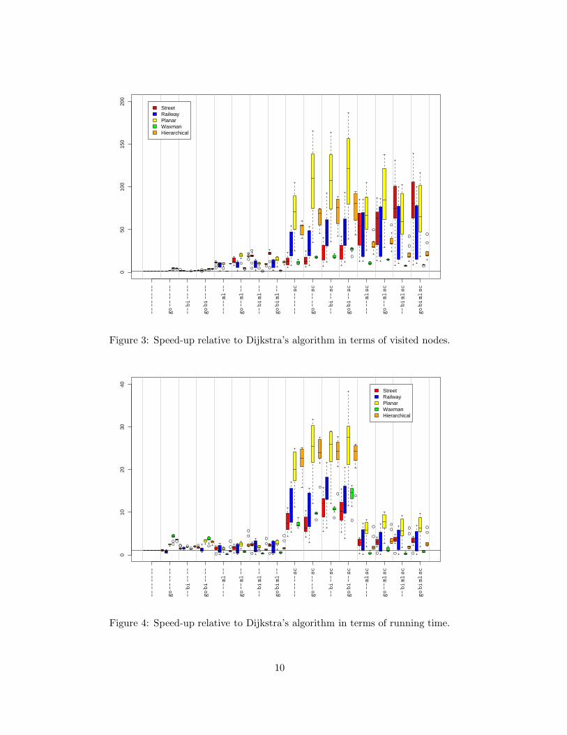
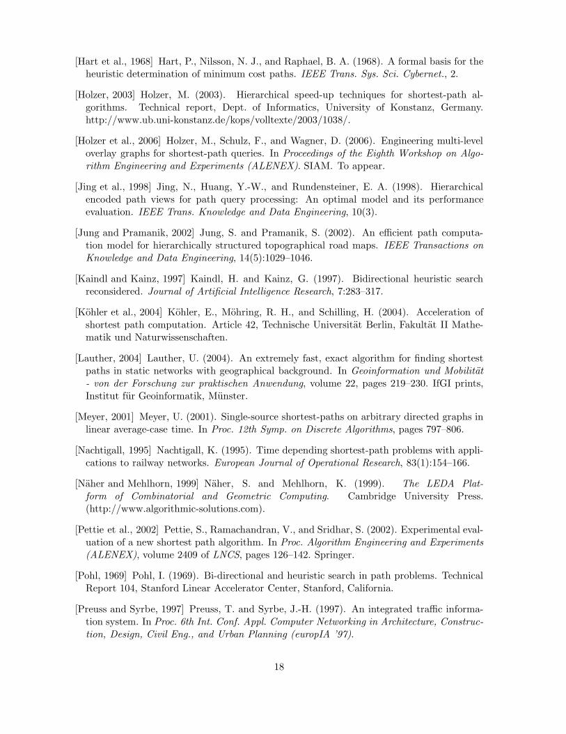
The main outcome of our experimental study is shown in Figures 3 and 4. Further diagramsthat we used for our analysis are depicted in Figures 5–9. Each combination is referred to bya 4-tuple of tokens: go (goal-directed), bi (bidirectional), ml (multi-level), sc (shortest-pathcontainer), and -- if the respective technique is not used (e.g., go -- ml sc). In all figures, thegraphs are ordered as listed in Table 1.

The outcomes referring to one graph class with one combination of techniques are summa-rized in the form of boxplots: the box represents the middle 50 percent of the respective values(with the median marked as a small horizontal line), the whiskers, i.e., the upper and lowerbounds of the dashed lines, are the extremal outcomes within a range 1.5 times the heightof the box above and below the border of the box, respectively, and outliers, i.e., outcomeslying beyond the whiskers, are drawn as circles.

We calculated two different values denoting relative speed-up: on the one hand, Figures 3–4 show the speed-up that we achieved compared to plain Dijkstra, i.e., for each combination oftechniques the ratio of the performance of plain Dijkstra and the performance of Dijkstra withthe specific combination of techniques applied. There are separate figures for the number ofnodes and running time. The horizontal line in each of these as well as the remaining diagramsmarks the border between gain and loss in efficiency relative to plain Dijkstra.

On the other hand, for each of the Figures 5–8, we focus on one technique T and show foreach combination containing T the speed-up (with respect to the number of visited nodes)that can be achieved compared to the combination without T . For example, when focusingon bidirectional search and considering the combination go bi -- sc, say, we investigate bywhich factor the performance gets better when the combination go bi -- bb is used instead ofgo -- -- sc only.

In the following, we discuss, for each technique separately, how combinations with thattechnique behave, and then turn to the relation of the two performance parameters measured,the number of visited nodes and running time: We define the overhead of a combination tobe the ratio of running time and the number of visited nodes. In other words, the overheadreflects the time spent per node.

9

050

100

150

200

StreetRailwayPlanarWaxmanHierarchical

--------

go------

--bi----

gobi----

----ml--

go--ml--

--biml--

gobiml--

------sc

go----sc

--bi--sc

gobi--sc

----mlsc

go--mlsc

--bimlsc

gobimlsc

Figure 3: Speed-up relative to Dijkstra’s algorithm in terms of visited nodes.

010

2030

40

StreetRailwayPlanarWaxmanHierarchical

--------

go------

--bi----

gobi----

----ml--

go--ml--

--biml--

gobiml--

------sc

go----sc

--bi--sc

gobi--sc

----mlsc

go--mlsc

--bimlsc

gobimlsc

Figure 4: Speed-up relative to Dijkstra’s algorithm in terms of running time.

10

4.1 Speed-up of the Combinations

4.1.1 Goal-Directed Search

Comparing the number of nodes visited with pure goal-directed search to that with plainDijkstra, speed-up varies a lot between the different types of graphs (cf. Figures 3 and 5): Weget a speed-up of about 2 for the planar graphs, and of 4 to 5 for the hierarchical and Waxmangraphs, which is surprisingly good compared to speed-up values of less than 2 observed withthe real-world graphs.

Adding goal-directed search to the multi-level approach performs a little worse than addingit to plain Dijkstra and with bidirectional search, we get another slight deterioration. Addingit to shortest-path containers is hardly beneficial (see also Figure 5).

Figure 4 reveals that, for real-world graphs, adding goal-directed search to any combina-tion does not improve the running time. For generated graphs, however, for most combinationsrunning time decreases when goal-directed search is applied additionally. In particular, it isadvantageous to add it to a combination containing the multi-level approach. To conclude,our experiments indicate that combining goal-directed search with the multi-level approachis generally a good idea.

4.1.2 Bidirectional Search

Pure bidirectional search yields a speed-up of between 1.5 and 2 for the number of visitednodes (cf. Figure 3) and for the running time (cf. Figure 4), for all types of graphs (for thehierarchical graphs, the speed-up, of a factor of more than 2, is even better).

For combinations of bidirectional search with other speed-up techniques, the situation isdifferent and depends heavily on the type of graph, as Figure 6 shows: For street graphs,bidirectional search almost always gives an actual speed-up compared to any combination oftechniques without bidirectional search. For Waxman and hierarchical graphs, almost noneof the combinations can be improved by additional application of bidirectional search. Onlyshortest-path containers and the combination of shortest-path containers with goal-directedsearch can always be improved through bidirectional search.

4.1.3 Multi-Level Approach

The multi-level approach crucially depends on the decomposition of the given graph, i.e., thebalancedness of the resulting multi-level graph. The Waxman graphs could not be decomposedproperly and therefore all combinations containing the multi-level approach yield speed-upfactors of less than 1 for the Waxman graphs, which means a slowing down (cf. Figure 4).

Thus, we consider only the remaining graph classes: with these graphs, pure multi-levelapproach reduces the number of visited nodes to a similar extent, the median values of theobserved speed-up factors (cf. Figure 7) ranging between 9 and 12 for all graph classes,which implies good decomposability, as required for the approach. Note that large ranges ofspeed-up factors inside one graph class can be observed (consider, e.g., the public-transportgraphs in Figure 7). Reasons for this behavior are on the one hand the fact that the achieveddecompositions are not always of similar quality within one graph class (e.g., the Frenchrailway network, with Paris as its center, is very different from the German railway network,which is more evenly spread); on the other hand, the speed-up achieved with the multi-levelapproach also depends on the size of the graph.

11

spee

d−up

01

23

45

6

StreetRailwayPlanarWaxmanHierarchical

go------

gobi----

go--ml--

gobiml--

go----sc

gobi--sc

go--mlsc

gobimlsc

Figure 5: Speed-up relative to the respective combination without goal-directed search interms of visited nodes.

spee

d−up

0.0

0.5

1.0

1.5

2.0

2.5

3.0

StreetRailwayPlanarWaxmanHierarchical

--bi----

gobi----

--biml--

gobiml--

--bi--sc

gobi--sc

--bimlsc

gobimlsc

Figure 6: Speed-up relative to the respective combination without bidirectional search interms of visited nodes.

12

spee

d−up

02

46

810

12

StreetRailwayPlanarWaxmanHierarchical

----ml--

go--ml--

--biml--

gobiml--

go

----mlsc

go--mlsc

--bimlsc

gobimlsc

Figure 7: Speed-up relative to the respective combination without multi-level approach interms of visited nodes.

spee

d−up

020

4060

8010

012

0

StreetRailwayPlanarWaxmanHierarchical

------sc

go----sc

--bi--sc

gobi--sc

----mlsc

go--mlsc

--bimlsc

gobimlsc

Figure 8: Speed-up relative to the respective combination without shortest-path containersin terms of visited nodes.

13

Adding the multi-level approach to goal-directed and bidirectional search and their com-bination also results in good improvement for the number of nodes (cf. Figure 7). In com-bination with shortest-path containers, the multi-level approach is beneficial only in the caseof street graphs.

Caused by the big overhead of the multi-level approach (cf. Figure 9), however, runningtime cannot be improved in the same order of magnitude as the number of nodes (cf. Figure 4).Also, the multi-level approach allows tuning of several parameters, such as the number oflevels and the choice of the selected nodes. This tuning crucially depends on the inputgraph [Holzer, 2003, Holzer et al., 2006]. Hence, we believe that considerable improvement ofthe presented results is possible if specific parameters are chosen for every single graph.

4.1.4 Shortest-Path Containers

Shortest-path containers work especially well when applied to planar graphs (see Figure 8);actually, speed-up even increases with the size of the graph (which again yields large ranges ofspeed-up factors within one graph class, as similarly observed with the multi-level approach).For Waxman graphs, the situation is completely different: with graph size, speed-up getssmaller (not shown in the diagrams). This can be explained by the fact that large Waxmangraphs have, due to construction, more long-distance edges than small ones. Because of this,shortest paths become more tortuous and the bounding boxes contain more “wrong” nodes.

Figures 3, 4, and 8 show that throughout the different types of graphs, shortest-path con-tainers individually as well as in combination with goal-directed and bidirectional search yieldexceptionally high speed-ups. Only the combinations that include the multi-level approachcannot be improved that much.

4.2 Overhead

For goal-directed and bidirectional search, the overhead (time per visited node) is quite small,while for shortest-path containers it is of a factor of about 2 compared to plain Dijkstra (cf.Figure 9). The overhead caused by the multi-level approach is generally high and variesquite a lot depending on the type of graph. As Waxman graphs do not decompose well, theoverhead for the multi-level approach is large and becomes even larger when the size of thegraph increases. For very large street graphs, the multi-level approach overhead increasesdramatically. We assume that it would be necessary to add another level for graphs of thissize.

It is also interesting to note that the relative overhead of the combination go bi ml -- issmaller than that of pure multi-level—especially for the generated graphs.

5 Conclusion and Outlook

To summarize, we conclude that there are speed-up techniques that combine well and otherswhere speed-up does not scale. Our main result is that goal-directed search and multi-level approach is a good combination and bidirectional search and shortest-path containerscomplement each other.

For real-world graphs, the combination -- bi ml sc is the best choice as to the number ofvisited nodes. In terms of running time, the winner is -- bi -- sc. For generated graphs, thebest combination is go bi -- sc for both the number of nodes and running time.

14

time

050

100

150

200

StreetRailwayPlanarWaxmanHierarchical

--------

go------

--bi----

gobi----

----ml--

go--ml--

--biml--

gobiml--

------sc

go----sc

--bi--sc

gobi--sc

----mlsc

go--mlsc

--bimlsc

gobimlsc

Figure 9: Average running time per visited node in µs.

15

When waiving an expensive preprocessing, the combination go bi -- -- is generally thefastest heuristic with smallest search space—except for Waxman graphs, for which pure goal-directed search is better. Actually, goal-directed search is the only speed-up technique thatworks comparatively well for Waxman graphs. Because of this specific behavior, we concludethat the planar and hierarchical graphs are a better approximation of the real-world graphsthan the Waxman graphs, which is also confirmed by the fact that with the multi-levelapproach, all graphs except the Waxman graphs exhibit similar behavior.

It would be interesting to further investigate combinations with improved variants of theapproaches considered in this paper (e.g., in [Holzer et al., 2006] speed-up factors of up to 50have been observed with road graphs in the multi-level approach) and other, very recentlydeveloped speed-up techniques relying on preprocessed information (which have already beenmentioned briefly in the introduction). The relation of the four techniques under investigationin this work to those other approaches is as follows:

(i) The ALT algorithm proposed in [Goldberg and Harrelson, 2005] improves goal-directedsearch by precomputed shortest-path information from and to so-called “landmark nodes”.The combination of this algorithm with bidirectional search was investigated in the samework.

(ii) Approaches relying on hierarchical decomposition of the underlying graph by meansof edge-separators [Jung and Pramanik, 2002, Flinsenberg, 2004] are often applied to roadnetworks, where the edge separators are usually determined by topographical information.Another approach relying on graph decompositions are the so-called hierarchically encodedpath views [Jing et al., 1998]. These techniques are very similar to the multi-level approach.

(iii) Techniques to divide a graph into regions and to store those very regions reachablevia an edge in bit-vectors attached to that edge [Kohler et al., 2004, Lauther, 2004] are closelyrelated to the shortest-path containers.

(iv) In the reach-based routing scheme [Gutman, 2004], for each vertex a “reach value”(which intuitively reflects the lengths of shortest paths on which it lies) is computed be-forehand and used during the online phase to speed up the shortest-path search. Thecombination of reach-based routing with goal-directed search has been shown to be fruit-ful [Goldberg et al., 2006]. In the latter work, also several improvements of the reach-basedrouting are presented.

(v) Finally, we would like to mention a speed-up technique that precomputes highwayhierarchies [Sanders and Schultes, 2005]. In the online phase, depending on the distancefrom the source and to the target, edges in lower levels of the hierarchy can be ignored. Thistechnique relies on a bidirectional variant of Dijkstra’s algorithm and is related to a variantof reach-based routing that uses reach values for edges (cf. [Goldberg et al., 2006]).

Another starting point for future work is given by the observation that, except for bidi-rectional search, the speed-up techniques under investigation in this work can be regardedas a standard run of Dijkstra’s algorithm on a modified graph. From a shortest path in themodified graph one can easily determine a shortest path in the original graph. It is an inter-esting question whether the techniques can be applied directly, or in a modified fashion, toimprove also the running time of other shortest-path algorithms.

Furthermore, specialized priority queues used in Dijkstra’s algorithm have been shownto be fast in practice [Dial, 1969, Goldberg, 2001a]. Using such queues would provide thesame results for the number of visited nodes. Running times, however, would be different andtherefore interesting to evaluate.

16

References

[Ahuja et al., 1993] Ahuja, R., Magnanti, T., and Orlin, J. (1993). Network Flows. Prentice–Hall.

[Barrett et al., 2002] Barrett, C., Bisset, K., Jacob, R., Konjevod, G., and Marathe, M.(2002). Classical and contemporary shortest path problems in road networks: Implemen-tation and experimental analysis of the TRANSIMS router. In Proc. 10th European Sym-posium on Algorithms (ESA), volume 2461 of LNCS, pages 126–138. Springer.

[Barrett et al., 2000] Barrett, C., Jacob, R., and Marathe, M. (2000). Formal-language-constrained path problems. SIAM Journal on Computing, 30(3):809–837.

[Cherkassky et al., 1996] Cherkassky, B. V., Goldberg, A. V., and Radzik, T. (1996). Short-est paths algorithms: Theory and experimental evaluation. Mathematical Programming,73:129–174.

[Dial, 1969] Dial, R. (1969). Algorithm 360: Shortest path forest with topological ordering.Communications of ACM, 12:632–633.

[Dijkstra, 1959] Dijkstra, E. W. (1959). A note on two problems in connexion with graphs.Numerische Mathematik, 1:269–271.

[Flinsenberg, 2004] Flinsenberg, I. C. (2004). Route Planning Algorithms for Car Navigation.PhD thesis, Technische Universiteit Eindhoven.

[Fredman and Tarjan, 1987] Fredman, M. L. and Tarjan, R. E. (1987). Fibonacci heaps andtheir uses in improved network optimization algorithms. Journal of the ACM, 34(3):596–615.

[Goldberg and Harrelson, 2005] Goldberg, A. and Harrelson, C. (2005). Computing the short-est path: A* search meets graph theory. In Proceedings of the 16th Annual ACM-SIAMSymposium on Discrete Algorithms (SODA 2005). SIAM.

[Goldberg et al., 2006] Goldberg, A., Kaplan, H., and Werneck, R. (2006). Reach for A*:Efficient point-to-point shortest path algorithms. In Proceedings of the Eighth Workshopon Algorithm Engineering and Experiments (ALENEX06). SIAM. To appear in the samevolume.

[Goldberg, 2001a] Goldberg, A. V. (2001a). Shortest path algorithms: Engineering aspects.In Proc. International Symposium on Algorithms and Computation (ISAAC), volume 2223of LNCS, pages 502–513. Springer.

[Goldberg, 2001b] Goldberg, A. V. (2001b). A simple shortest path algorithm with linearaverage time. In Proc. 9th European Symposium on Algorithms (ESA), volume 2161 ofLNCS, pages 230–241. Springer.

[Gutman, 2004] Gutman, R. J. (2004). Reach-based routing: A new approach to shortest pathalgorithms optimized for road networks. In Proc. 6th Workshop on Algorithm Engineeringand Experiments (ALENEX), pages 100–111. SIAM.

17

[Hart et al., 1968] Hart, P., Nilsson, N. J., and Raphael, B. A. (1968). A formal basis for theheuristic determination of minimum cost paths. IEEE Trans. Sys. Sci. Cybernet., 2.

[Holzer, 2003] Holzer, M. (2003). Hierarchical speed-up techniques for shortest-path al-gorithms. Technical report, Dept. of Informatics, University of Konstanz, Germany.http://www.ub.uni-konstanz.de/kops/volltexte/2003/1038/.

[Holzer et al., 2006] Holzer, M., Schulz, F., and Wagner, D. (2006). Engineering multi-leveloverlay graphs for shortest-path queries. In Proceedings of the Eighth Workshop on Algo-rithm Engineering and Experiments (ALENEX). SIAM. To appear.

[Jing et al., 1998] Jing, N., Huang, Y.-W., and Rundensteiner, E. A. (1998). Hierarchicalencoded path views for path query processing: An optimal model and its performanceevaluation. IEEE Trans. Knowledge and Data Engineering, 10(3).

[Jung and Pramanik, 2002] Jung, S. and Pramanik, S. (2002). An efficient path computa-tion model for hierarchically structured topographical road maps. IEEE Transactions onKnowledge and Data Engineering, 14(5):1029–1046.

[Kaindl and Kainz, 1997] Kaindl, H. and Kainz, G. (1997). Bidirectional heuristic searchreconsidered. Journal of Artificial Intelligence Research, 7:283–317.

[Kohler et al., 2004] Kohler, E., Mohring, R. H., and Schilling, H. (2004). Acceleration ofshortest path computation. Article 42, Technische Universitat Berlin, Fakultat II Mathe-matik und Naturwissenschaften.

[Lauther, 2004] Lauther, U. (2004). An extremely fast, exact algorithm for finding shortestpaths in static networks with geographical background. In Geoinformation und Mobilitat- von der Forschung zur praktischen Anwendung, volume 22, pages 219–230. IfGI prints,Institut fur Geoinformatik, Munster.

[Meyer, 2001] Meyer, U. (2001). Single-source shortest-paths on arbitrary directed graphs inlinear average-case time. In Proc. 12th Symp. on Discrete Algorithms, pages 797–806.

[Nachtigall, 1995] Nachtigall, K. (1995). Time depending shortest-path problems with appli-cations to railway networks. European Journal of Operational Research, 83(1):154–166.

[Naher and Mehlhorn, 1999] Naher, S. and Mehlhorn, K. (1999). The LEDA Plat-form of Combinatorial and Geometric Computing. Cambridge University Press.(http://www.algorithmic-solutions.com).

[Pettie et al., 2002] Pettie, S., Ramachandran, V., and Sridhar, S. (2002). Experimental eval-uation of a new shortest path algorithm. In Proc. Algorithm Engineering and Experiments(ALENEX), volume 2409 of LNCS, pages 126–142. Springer.

[Pohl, 1969] Pohl, I. (1969). Bi-directional and heuristic search in path problems. TechnicalReport 104, Stanford Linear Accelerator Center, Stanford, California.

[Preuss and Syrbe, 1997] Preuss, T. and Syrbe, J.-H. (1997). An integrated traffic informa-tion system. In Proc. 6th Int. Conf. Appl. Computer Networking in Architecture, Construc-tion, Design, Civil Eng., and Urban Planning (europIA ’97).

18

[Sanders and Schultes, 2005] Sanders, P. and Schultes, D. (2005). Highway hierarchies has-ten exact shortest path queries. In Proceedings 17th European Symposium on Algorithms(ESA).

[Schulz et al., 2000] Schulz, F., Wagner, D., and Weihe, K. (2000). Dijkstra’s algorithmon-line: An empirical case study from public railroad transport. ACM Journal of Exp.Algorithmics, 5(12).

[Schulz et al., 2002] Schulz, F., Wagner, D., and Zaroliagis, C. (2002). Using multi-levelgraphs for timetable information in railway systems. In Proc. 4th Workshop on AlgorithmEngineering and Experiments (ALENEX), volume 2409 of LNCS, pages 43–59. Springer.

[Shekhar et al., 1997] Shekhar, S., Fetterer, A., and Goyal, B. (1997). Materialization trade-offs in hierarchical shortest path algorithms. In Proc. Symp. on Large Spatial Databases,pages 94–111.

[Shekhar et al., 1993] Shekhar, S., Kohli, A., and Coyle, M. (1993). Path computation al-gorithms for advanced traveler information system (ATIS). In Proc. 9th IEEE Int. Conf.Data Eng., pages 31–39.

[Wagner and Willhalm, 2003] Wagner, D. and Willhalm, T. (2003). Geometric speed-up tech-niques for finding shortest paths in large sparse graphs. In Proc. 11th European Symposiumon Algorithms (ESA), volume 2832 of LNCS, pages 776–787. Springer.

[Waxman, 1988] Waxman, B. M. (1988). Routing of multipoint connections. IEEE Journalon Selected Areas in Communications, 6(9).

[Willhalm, 2005] Willhalm, T. (2005). Engineering Shortest Paths and Layout Algorithms forLarge Graphs. PhD thesis, Universitat Karlsruhe (TH), Fakultat Informatik.

[Willhalm and Wagner, 2006] Willhalm, T. and Wagner, D. (2006). Shortest path speeduptechniques. In Algorithmic Methods for Railway Optimization, LNCS. Springer. To appear.

[Zhan and Noon, 2000] Zhan, F. B. and Noon, C. E. (2000). A comparison between label-setting and label-correcting algorithms for computing one-to-one shortest paths. Journalof Geographic Information and Decision Analysis, 4(2).

[Zwick, 2001] Zwick, U. (2001). Exact and approximate distances in graphs - a survey. InProc. 9th European Symposium on Algorithms (ESA), LNCS, pages 33–48. Springer.

19