molecules

Review

Spin Hamiltonians in Magnets: Theories and Computations

Xueyang Li 1,2,† , Hongyu Yu 1,2,†, Feng Lou 1,2, Junsheng Feng 1,3, Myung-Hwan Whangbo 4 andHongjun Xiang 1,2,*

�����������������

Citation: Li, X.; Yu, H.; Lou, F.; Feng,

J.; Whangbo, M.-H.; Xiang, H. Spin

Hamiltonians in Magnets: Theories

and Computations. Molecules 2021, 26,

803. https://doi.org/10.3390/

molecules26040803

Academic Editor: Takashiro Akitsu

Received: 24 December 2020

Accepted: 2 February 2021

Published: 4 February 2021

Publisher’s Note: MDPI stays neutral

with regard to jurisdictional claims in

published maps and institutional affil-

iations.

Copyright: © 2021 by the authors.

Licensee MDPI, Basel, Switzerland.

This article is an open access article

distributed under the terms and

conditions of the Creative Commons

Attribution (CC BY) license (https://

creativecommons.org/licenses/by/

4.0/).

1 Key Laboratory of Computational Physical Sciences (Ministry of Education), State Key Laboratory ofSurface Physics, Department of Physics, Fudan University, Shanghai 200433, China;16110190006@fudan.edu.cn (X.L.); 20110190060@fudan.edu.cn (H.Y.); flou16@fudan.edu.cn (F.L.);fjs@hfnu.edu.cn (J.F.)

2 Shanghai Qi Zhi Institute, Shanghai 200232, China3 School of Physics and Materials Engineering, Hefei Normal University, Hefei 230601, China4 Department of Chemistry, North Carolina State University, Raleigh, NC 27695-8204, USA;

whangbo@ncsu.edu* Correspondence: hxiang@fudan.edu.cn† These authors contributed equally to this work.

Abstract: The effective spin Hamiltonian method has drawn considerable attention for its power toexplain and predict magnetic properties in various intriguing materials. In this review, we summarizedifferent types of interactions between spins (hereafter, spin interactions, for short) that may be usedin effective spin Hamiltonians as well as the various methods of computing the interaction parameters.A detailed discussion about the merits and possible pitfalls of each technique of computing interactionparameters is provided.

Keywords: spin Hamiltonian; magnetism; energy-mapping analysis; four-state method; Green’sfunction method

1. Introduction

The utilization of magnetism can date back to ancient China when the compass wasinvented to guide directions. Since the relationship between magnetism and electricity wasrevealed by Oersted, Lorentz, Ampere, Faraday, Maxwell, and others, more applicationsof magnetism have been invented, which include dynamos (electric generators), electricmotors, cyclotrons, mass spectrometers, voltage transformers, electromagnetic relays, pic-ture tubes, and sensing elements. During the information revolution, magnetic materialswere extensively employed for information storage. The storage density, efficiency, andstability were substantially improved by the discovery and applications of the giant magne-toresistance effect [1,2], tunnel magnetoresistance [3–9], spin-transfer torques [10–13], etc.Recently, more and more novel magnetic states such as spin glasses [14,15], spin ice [16,17],spin liquid [18–22], and skyrmions [23–28] were found, revealing both theoretical andpractical significance. For example, hedgehogs and anti-hedgehogs can be seen as thesources (monopoles) and the sinks (antimonopoles) of the emergent magnetic fields oftopological spin textures [29], while magnetic skyrmions have shown promise as ultradenseinformation carriers and logic devices [24].

To explain or predict the properties of magnetic materials, many models and methodshave been invented. In this review, we will mainly focus on the effective spin Hamiltonianmethod based on first-principles calculations, and its applications in solid-state systems. InSection 2, we will introduce the effective spin Hamiltonian method. Firstly, in Section 2.1,the origin and the computing methods of the atomic magnetic moments are presented.Then, from Sections 2.2–2.6, different types of spin interactions that may be included in thespin Hamiltonians are discussed. Section 3 will discuss and compare various methods ofcomputing the interaction parameters used in the effective spin Hamiltonians. In Section 4,we will give a brief conclusion of this review.

Molecules 2021, 26, 803. https://doi.org/10.3390/molecules26040803 https://www.mdpi.com/journal/molecules

Molecules 2021, 26, 803 2 of 26

2. Effective Spin Hamiltonian Models

Though accurate, first-principles calculations are somewhat like black boxes (thatis to say, they provide the final total results, such as magnetic moments and the totalenergy, but do not give a clear understanding of the physical results without furtheranalysis), and have difficulties in dealing with large-scale systems or finite temperatureproperties. In order to provide an explicit explanation for some physical properties andimprove the efficiency of thermodynamic and kinetic simulations, the effective Hamiltonianmethod is often adopted. In the context of magnetic materials where only the spin degreeof freedom is considered, it can also be called the effective spin Hamiltonian method.Typically, the effective spin Hamiltonian models need to be carefully constructed andinclude all the possibly important terms; then the parameters of the models need to becalculated based on either first-principles calculations (see Section 3) or experimental data(see Section 3.3). Given the effective spin Hamiltonian and the spin configurations, thetotal energy of a magnetic system can be easily computed. Therefore, it is often adoptedin Monte Carlo simulations [30] (or quantum Monte Carlo simulations) for assessing thetotal energy of many different configurations so that the finite temperature properties ofmagnetic materials can be studied. If the effects of atom displacements are taken intoaccount, the effective Hamiltonians can also be applied to the spin molecular dynamicssimulations [31–33], which is beyond the scope of this review.

In this review, we mainly focus on the classical effective spin Hamiltonian methodwhere atomic magnetic moments (or spin vectors) are treated as classical vectors. In manycases, these classical vectors are assumed to be rigid so that their magnitudes keep constantduring rotations. This treatment significantly simplifies the effective Hamiltonian models,and it is usually a good approximation, especially when atomic magnetic moments arelarge enough.

In this part, we shall first introduce the origin of the atomic magnetic moments aswell as the methods of computing atomic magnetic moments. Then different types of spininteractions will be discussed.

2.1. Atomic Magnetic Moments

The origin of atomic magnetic moments is explained by quantum mechanics. Supposethe quantized direction is the z-axis, an electron with quantum numbers (n, l , ml , ms) leadsto an orbital magnetic moment µl = −µBl and a spin magnetic moment µs = −geµBs,with their z components µlz = −mlµB and µsz = −gemsµB, where µB = |e|}

2m is the Bohrmagneton and ge ≈ 2 is the g-factor for a free electron. The energy of a magnetic moment µin a magnetic field B (magnetic induction) along z-direction is −µ · B = −µzB.

Considering the Russell-Saunders coupling (also referred to as L-S coupling), whichapplies to most multi-electronic atoms, the total orbital magnetic moment and the total spinmagnetic moment are µL = −µBL and µS = −geµBS, respectively, where L = ∑

ili and

S = ∑i

si are the summation over electrons. The quantum numbers of each electron can

usually be predicted by Hund’s rules. Owing to the spin–orbit interaction, L and S bothprecess around the constant vector J = L + S. The time-averaged effective total magneticmoment is µ = −gJµBJ, where

gJ = 1 +J(J + 1) + S(S + 1)− L(L + 1)

2J(J + 1)(1)

The atomic magnetic moments discussed above are based on the assumption that theatoms are isolated. Taking the influence of other atoms and external fields into account,the orbital interaction theory, the crystal field theory [34], or the ligand field theory [35,36]may be a better choice for theoretically predicting atomic magnetic moments. Notice thathalf-filled shells lead to a total L = 0, and that in solids and molecules, orbital moments ofelectrons are usually quenched, resulting in an effective L = 0 [37] (counterexamples maybe found for 4f elements or for 3d7 configurations as in Co(II)). Therefore typically µ = µS,

Molecules 2021, 26, 803 3 of 26

with its z component µz = −geSzµB (Sz is restricted to discrete values: S, S− 1, . . . ,−S).Usually, a nonzero µS results from singly filled (localized) d or f orbitals, while s and porbitals are typically either doubly filled or vacant so that they have no direct contributionto the atomic magnetic moments. Therefore, when referring to atomic magnetic moments,usually only the atoms in the d- and f -transition series need to be considered.

The atomic magnetic moments can also be predicted numerically employing first-principles calculations. Nevertheless, we should notice that traditional Kohn–Sham densityfunctional theory (DFT) calculations [38,39] (based on single-electron approximation) arenot reliable for predicting atomic magnetic moments, and hence require the considera-tion of strong correlation effect among electrons, especially when dealing with localizedd or f orbitals. Based on the Hubbard model [40], such problem can often be remediedby introducing an intra-atomic interaction with effective on-site Coulomb and exchangeparameters, U and J [41] (or only one parameter Ueff = U − J in Dudarev’s approach [42]).This approach is the DFT+U method [41–44], including LDA+U (LDA: Local densityapproximation), LSDA+U (LSDA: Local spin density approximation), GGA+U (GGA: Gen-eralized gradient approximation), and so forth, where “+U” indicates the Hubbard “+U”correction. The parameters U and J can be estimated according to experience or semi-empirically by seeking agreement with experimental results of some specific properties,which is convenient but not very reliable. Considering how the values of the parameters Uand J affect the prediction of atomic magnetic moments and other physical properties, wemay need to compute these parameters more rigorously. A typical approach is constrainedDFT calculations [43,45–47], where the local d or f charges are constrained to differentvalues in several calculations, so that the parameters U and J can be obtained. Anotherapproach based on constrained random-phase approximation (cRPA) [48–50] allows forconsidering the frequency (or energy) dependence of the parameters. More methods ofcomputing U and J are summarized in Ref. [43]. There are more accurate approachesfor dealing with strong correlated systems like DFT + Dynamical Mean Field Theory(DFT+DMFT) [51–55] and Reduced Density Matrix Functional Theory (RDMFT) [56,57],but they are much more sophisticated and computationally demanding so that they maybe impractical for large-scale calculations. Wave function (WF) methods, such as CompleteActive Space Self-Consistent Field (CASSCF) [58–61], Complete Active Space second-orderPerturbation Theory (CASPT2) [62–64], Complete Active Space third-order PerturbationTheory (CASPT3) [65], and Difference Dedicated Configuration Interaction (DDCI) [66–68],are also widely adopted by theoretical chemists for studying magnetic properties of materi-als (especially molecules), including atomic magnetic moments and magnetic interactions.These WF methods are also more accurate but more computationally demanding than theDFT+U method, more detailed discussions of which can be found in Ref. [69].

2.2. Heisenberg Model

The simplest effective spin Hamiltonian model is the classical Heisenberg model,which can be reduced to Ising model or XY model. The classical Heisenberg model can bewritten as

Hspin = ∑i,j>i

JijSi · Sj, (2)

where Si and Sj indicate the total spin vectors on atoms i and j, and the summation is overall relevant pairs (ij). Its form was suggested by Heisenberg, Dirac, and Van Vleck. Such aninteraction comes from the energy splitting between quantized parallel (ferromagnetic, FM;triplet state) and antiparallel (antiferromagnetic, AFM; singlet state) spin configurations.Jij > 0 and Jij < 0 prefer AFM and FM configurations, respectively. There may be adifference in the factor such as −1 and 1

2 between different definitions of Hspin, which isalso the case in other models as will be discussed.

Molecules 2021, 26, 803 4 of 26

The spatial wave function of two electrons should possess the form ofψ± = 1√

2[ψa(r1)ψb(r2)± ψb(r1)ψa(r2)], where ψa and ψb are any single-electron spa-

tial wave functions. A parallel triplet spin state and an antiparallel singlet spin state shouldcorrespond to an antisymmetric (ψ−) and a symmetric (ψ+) spatial wave function, respec-tively. For given ψa and ψb, the expectation value for the total energy of ψ− can be differentfrom that of ψ+, which gives a preference to the AFM or FM spin configuration. Whetherthe AFM or FM spin configuration is preferred depends on the circumstances, and theirenergy difference can be described as a Heisenberg term J12S1 · S2.

In the simple case of an H2 molecule, an AFM singlet spin state is preferred, whosesymmetric spatial wave function ψ+ corresponds to a bonding state [70,71]. However, thisleads to the total magnetic moment of zero because the two antiparallel electrons sharethe same spatial state. In another simple case, where ψa and ψb stands for two degenerateand orthogonal orbitals of the same atom, an FM triplet spin state is preferred, which isin agreement with Hund’s rules. Consider a set of orthogonal Wannier functions withφnλ(r − rα) resembling the nth atomic orbital with spin λ centered at the αth lattice site,and suppose there are Nh electrons each localized on one of the N lattice sites, each ionpossessing h unpaired electrons. If these h electrons have the same exchange integrals withall the other electrons, the interaction resulting from the antisymmetrization of the wavefunctions can be expressed as

Hex = ∑αα′

nn′

Jnn′(rα, rα′)

[14+ S(rα) · S(rα′)

](3)

which is called the Heisenberg exchange interaction [72]. After removing the constantterms, we can see such an interaction has the form of Hspin = ∑

i,j>iJijSi · Sj.

Based on molecular orbital analysis using φa and φb to denote the singly filled dorbitals of the two spin- 1

2 magnetic ions (i.e., d9 ions), Hay et al. [73] showed that theexchange interaction between the two ions can be approximately expressed as

J = −2Kab +∆2

Ueff = JF + JAF (4)

where

Kab ∝⟨

φa(1)φb(2)∣∣∣∣ 1r12

∣∣∣∣φb(1)φa(2)⟩

=∫

φ∗a (r1)φ∗b (r2)

1r12

φb(r1)φa(r2) > 0 (5)

Ueff = Jaa − Jab ∝⟨

φa(1)φa(2)∣∣∣∣ 1r12

∣∣∣∣φa(1)φa(2)⟩−⟨

φa(1)φb(2)∣∣∣∣ 1r12

∣∣∣∣φa(1)φb(2)⟩

> 0 (6)

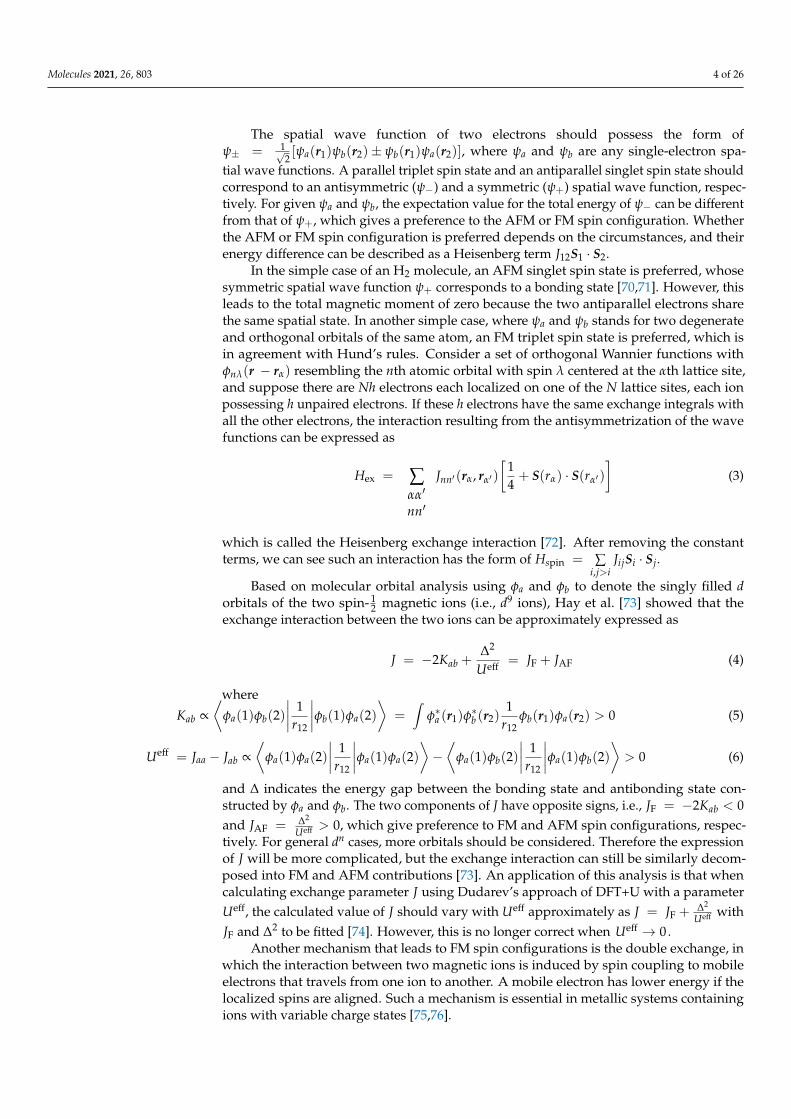
and ∆ indicates the energy gap between the bonding state and antibonding state con-structed by φa and φb. The two components of J have opposite signs, i.e., JF = −2Kab < 0and JAF = ∆2

Ueff > 0, which give preference to FM and AFM spin configurations, respec-tively. For general dn cases, more orbitals should be considered. Therefore the expressionof J will be more complicated, but the exchange interaction can still be similarly decom-posed into FM and AFM contributions [73]. An application of this analysis is that whencalculating exchange parameter J using Dudarev’s approach of DFT+U with a parameterUeff, the calculated value of J should vary with Ueff approximately as J = JF +

∆2

Ueff withJF and ∆2 to be fitted [74]. However, this is no longer correct when Ueff → 0 .

Another mechanism that leads to FM spin configurations is the double exchange, inwhich the interaction between two magnetic ions is induced by spin coupling to mobileelectrons that travels from one ion to another. A mobile electron has lower energy if thelocalized spins are aligned. Such a mechanism is essential in metallic systems containingions with variable charge states [75,76].

Molecules 2021, 26, 803 5 of 26

The superexchange is another important indirect exchange mechanism, where theinteraction between two transition-metal (TM) ions is induced by spin coupling to twoelectrons on a non-magnetic ligand (L) ion that connects them, forming an exchange pathof TM-L-TM type. Different mechanisms were proposed to explain the superexchangeinteraction. In Anderson’s mechanism [77,78], the superexchange results from virtualprocesses in which an electron is transferred from the ligand to one of the neighboringmagnetic ions, and then another electron on the ligand couples with the spin of the othermagnetic ion through exchange interaction. In Goodenough’s mechanism [79,80], theconcept of semicovalent bonds was invented, where only one electron given by the ligandpredominates in a semicovalent bond. Because of the exchange forces between the electronson the magnetic ion and the electron given by the ligand, the ligand electron with its spinparallel to the net spin of the magnetic ion will spend more time on the magnetic ionthan that with an antiparallel spin if the d orbital of the magnetic ion is less than half-filled, and vice versa. The magnetic atom and the ligand are supposed to be connectedby a semicovalent bond or a covalent bond when they are near, or by an ionic bond (orpossibly a metallic-like bond) otherwise. The superexchange interaction with semicovalentbonds existing is also called semicovalent exchange interaction. Kanamori summarizedthe dependence of the sign of the superexchange parameter (whether FM or AFM) onbond angle, bond type and number of d electrons (in different mechanisms), which is oftenreferred as Goodenough–Kanamori (GK) rules [80–82]. For the 180◦ (bond angle) case,generally, AFM interaction is expected between cations of the same kind (counterexamplesmay exist for d4 cases such as Mn3+-Mn3+, where the sign depends on the direction of theline of superexchange), and FM interaction is expected between two cations with more-than-half-filled and less-than-half-filled d-shells, respectively [81]. For the 90◦ case, theresults are usually the opposite [81]. A schematic diagram of superexchange interactions(between cations both with more-than-half-filled d-shell) is given in Figure 1. More detailsof the discussions can be found in Ref. [81] and Ref. [82].

Molecules 2021, 26, x FOR PEER REVIEW 5 of 26

localized spins are aligned. Such a mechanism is essential in metallic systems containing ions with variable charge states. [75,76]

The superexchange is another important indirect exchange mechanism, where the interaction between two transition-metal (TM) ions is induced by spin coupling to two electrons on a non-magnetic ligand (L) ion that connects them, forming an exchange path of TM-L-TM type. Different mechanisms were proposed to explain the superexchange in-teraction. In Anderson’s mechanism [77,78], the superexchange results from virtual pro-cesses in which an electron is transferred from the ligand to one of the neighboring mag-netic ions, and then another electron on the ligand couples with the spin of the other mag-netic ion through exchange interaction. In Goodenough’s mechanism [79,80], the concept of semicovalent bonds was invented, where only one electron given by the ligand pre-dominates in a semicovalent bond. Because of the exchange forces between the electrons on the magnetic ion and the electron given by the ligand, the ligand electron with its spin parallel to the net spin of the magnetic ion will spend more time on the magnetic ion than that with an antiparallel spin if the d orbital of the magnetic ion is less than half-filled, and vice versa. The magnetic atom and the ligand are supposed to be connected by a semico-valent bond or a covalent bond when they are near, or by an ionic bond (or possibly a metallic-like bond) otherwise. The superexchange interaction with semicovalent bonds existing is also called semicovalent exchange interaction. Kanamori summarized the de-pendence of the sign of the superexchange parameter (whether FM or AFM) on bond an-gle, bond type and number of d electrons (in different mechanisms), which is often re-ferred as Goodenough–Kanamori (GK) rules [80–82]. For the 180° (bond angle) case, gen-erally, AFM interaction is expected between cations of the same kind (counterexamples may exist for d4 cases such as Mn3+-Mn3+, where the sign depends on the direction of the line of superexchange), and FM interaction is expected between two cations with more-than-half-filled and less-than-half-filled d-shells, respectively [81]. For the 90° case, the results are usually the opposite [81]. A schematic diagram of superexchange interactions (between cations both with more-than-half-filled d-shell) is given in Figure 1. More details of the discussions can be found in Ref. [81] and Ref. [82].

Figure 1. A schematic diagram of superexchange interactions between transition-metal (TM) ions both with more-than-half-filled d-shell. According to Goodenough–Kanamori (GK) rules, the 180° and the 90° cases favor antiferromagnetic (AFM) and ferromagnetic (FM) arrangements of TM ions, respectively. The main difference is whether the two electrons of L occupy the same p orbital, leading to different tendencies for the alignments of the two electrons of L that interact with two TM ions.

Figure 1. A schematic diagram of superexchange interactions between transition-metal (TM) ionsboth with more-than-half-filled d-shell. According to Goodenough–Kanamori (GK) rules, the 180◦

and the 90◦ cases favor antiferromagnetic (AFM) and ferromagnetic (FM) arrangements of TM ions,respectively. The main difference is whether the two electrons of L occupy the same p orbital, leadingto different tendencies for the alignments of the two electrons of L that interact with two TM ions.

Molecules 2021, 26, 803 6 of 26

A counterexample of the GK rules can be found in the layered magnetic topologicalinsulator MnBi2Te4, which possesses intrinsic ferromagnetism [83]. In contrast, the pre-diction of the GK rules leads to a weak AFM exchange interaction between Mn ions. InRef. [84], the presence of Bi3+ was found to be essential for explaining this anomaly: d5

ions in TM-L-TM spin-exchange paths would prefer FM coupling if the empty p orbitalsof a nonmagnetic cation M (which is Bi3+ ion in the case of MnBi2Te4) hybridize stronglywith those of the ligand L (but AFM coupling otherwise). Oles et al. [85] pointed out thatthe GK rules may not be obeyed in transition metal compounds with orbital degrees offreedom (e.g., d1 and d2 electronic configurations) due to spin-orbital entanglement.

Exchange interactions between two TM ions also take place through the exchangepaths of TM-L . . . L-TM type [86], referred to as super-superexchanges, where TM ionsdo not share a common ligand. Each TM ion of a solid forms a TMLn polyhedron (typi-cally, n = 3–6) with the surrounding ligands L, and the unpaired spins of the TM ion areaccommodated in the singly filled d-states of TMLn. Since each d-state has a d-orbital ofTM combined out-of-phase with the p-orbitals of L, the unpaired spin of TM does notreside solely on the d-orbital of TM, as assumed by Goodenough and Kanamori, but isdelocalized into the p-orbitals of the surrounding ligands L. Thus, TM-L . . . L-TM typeexchanges occur and can be strongly AFM when their L . . . L contact distances are in thevicinity of the van der Waals distance so that the ligand p-orbitals overlap well across the L. . . L contact.

Another mechanism is the indirect coupling of magnetic moments by conductionelectrons, referred to as Ruderman–Kittel–Kasuya–Yosida (RKKY) interaction [87–90]. Thiskind of interaction between two spins S1 and S2 is also proportional to S1 · S2 with anexpression

HRKKY ∝ ∑q

χ(q)eiq·r21 S1 · S2. (7)

The magnetic dipole–dipole interaction (between magnetic moments µ1 and µ2 locatedat different atoms) with energy

V =1

R3

[µ1 · µ2 − 3

(R · µ1

)(R · µ2

)](8)

also has contributions to the bilinear term, but it is typically much weaker than the ex-change interactions in most solid-state materials such as iron and cobalt. The characteristictemperature of dipole–dipole interaction (or termed as “dipolar interaction”) in magneticmaterials is typically of the order of 1 K, above which no long-range order can be stabilizedby such an interaction [37]. However, in some cases, such as in several single-moleculemagnets (SMMs), the exchange interactions can be so weak that they are comparable to orweaker than dipolar interactions, thus the dipolar interactions must not be neglected [91].

For most magnetic materials, the Heisenberg interaction is the most predominantspin interaction. As a result, the simple classical Heisenberg model is able to explain themagnetic properties such as the ground states of spin configurations (FM or AFM) and thetransition temperatures (Curie temperature for FM states or Néel temperature for AFMstates) for many magnetic materials.

If some pairs of spins favor FM spin configurations while other pairs favor AFMconfigurations, frustration may occur, leading to more complicated and more interestingnoncollinear spin configurations. For example, the FM effects of double exchange resultingfrom mobile electrons in some antiferromagnetic lattices give rise to a distortion of theground-state spin arrangement and lead to a canted spin configuration [92]. A magneticsolid with moderate spin frustration lowers its energy by adopting a noncollinear su-perstructure (e.g., a cycloid or a helix) in which the moments of the ions are identical inmagnitude but differ in orientation or a collinear magnetic superstructure (e.g., a spindensity wave, SDW) in which the moments of the ions differ in magnitude but identical inorientation [93,94]. For a cycloid formed in a chain of magnetic ions, each successive spinrotates in one direction by a certain angle, so there are two opposite ways of rotating the

Molecules 2021, 26, 803 7 of 26

successive spins hence producing two cycloids opposite in chirality but identical in energy.When these two cycloids occur with equal probability below a certain temperature, theirsuperposition leads to a SDW [93,94]. On lowering the temperature further, the electronicstructure of the spin-lattice relaxes to energetically favor one of the two chiral cycloids sothat one can observe a cycloid state. The latter, being chiral, has no inversion symmetryand gives rise to ferroelectricity [95]. The spin frustration is also a potential driving forcefor topological states like skyrmions and hedgehogs [29].

2.3. The J Matrices and Single-Ion Anisotropy

The classical Heisenberg model can be generalized to a matrix form to include all thepossible second-order interactions between two spins (or one spin itself):

Hspin = ∑i,j>i

STi JijSj + ∑

iST

i AiSi (9)

where Jij and Ai are 3 × 3 matrices called the J matrix and single-ion anisotropy (SIA) ma-trix. The Jij matrix can be decomposed into three parts: The isotropic Heisenberg exchangeparameter Jij =

(Jij,xx + Jij,yy + Jij,zz

)/3 as in the classical Heisenberg model, the antisym-

metric Dzyaloshinskii–Moriya interaction (DMI) matrix Dij =(Jij − JT

ij

)/2 [96–98], and

the symmetric (anisotropic) Kitaev-type exchange coupling matrix Kij =(Jij + JT

ij

)/2−

JijI (where I denotes a 3 × 3 identity matrix). Thus Jij = JijI+Dij +Kij [99,100].Now we analyze the possible origin of these terms by means of symmetry analysis.

When considering interaction potential between (or among) spins, we should notice thatthe total interaction energy should be invariant under time inversion ({Sk} → {−Sk} ).Therefore, any odd order term in the spin Hamiltonian should be zero unless an externalmagnetic field is present when a term −∑

iµi · B = ∑

igeµBB · Si should be added to the

effective spin Hamiltonian. Ignoring the external magnetic field, the spin Hamiltonianshould only contain even order terms, with the lowest order of significance being thesecond-order (the zeroth-order term is a constant and therefore not necessary). If thespin-orbit coupling (SOC) is negligible, the total effective spin Hamiltonian Hspin shouldbe invariant under any global spin rotations, therefore Hspin should be expressed by onlyinner product terms of spins like terms proportional to Si · Sj,

(Si · Sj

)(Sk · Sl) and so on.

That is to say, when SOC is negligible, the second-order terms in the Hspin should onlyinclude the classical Heisenberg term ∑

i,j>iJijSi · Sj, which implies that those interactions

described by Ai, Dij, and Kij matrices all originate from SOC (HSO = λS · L). What is more,if the spatial inversion symmetry is satisfied by the lattice, Jij should be equal to JT

ij so thatthere will be no DMI (Dij = 0). That is to say, the DMI can only exist where the spatialinversion symmetry is broken.

The SIA matrix Ai has only six independent components and is usually assumed to besymmetric. If we suppose the magnitude of the classical spin vector Si to be independentof its direction, the isotropic part 1

3(Ai,xx +Ai,yy +Ai,zz

)I would be of no significance, and

therefore Ai would have only five independent components after subtracting the isotropicpart from itself. It is evident that the ST

i AiSi prefers the direction of Si along the eigenvectorof Ai with the lowest eigenvalue. If this lowest eigenvalue is two-fold degenerate, thedirections of Si favored by SIA will be those belonging to the plane spanned by the twoeigenvectors that share the lowest eigenvalue, in which case we say the ion i has easy-plane anisotropy. On the contrary, if the lowest eigenvalue is not degenerate while thehigher eigenvalue is two-fold degenerate, we say the ion i has easy-axis anisotropy. Inthese two cases (easy-plane or easy-axis anisotropy), by defining the direction of z-axisparallel to the nondegenerate eigenvector, the ST

i AiSi part would be simplified to Ai,zz(Sz

i)2

with only one independent component. The easy-axis anisotropy has been found to behelpful in stabilizing the long-range magnetic order and enhancing the Curie temperature

Molecules 2021, 26, 803 8 of 26

in two-dimensional or quasi-two-dimensional systems [101]. The easy-plane anisotropy inthree-dimensional ferromagnets can lead to the effect called “quantum spin reduction”,where the mean spin at zero temperature has a value lower than the maximal one due tothe quantum fluctuations [101,102]. Recently, several materials with unusually large easy-plane or easy-axis anisotropy were found [103–105], which, as single-ion magnets (SIMs),are promising for applications such as high-density information storage, spintronics, andquantum computing.

The DMI matrix Dij is antisymmetric and therefore has only three independent com-ponents, which can be expressed by a vector Dij with Dij,x = Dij,yz, Dij,y = Dij,zx, andDij,z = Dij,xy. Thus, the DMI can be expressed by cross product: ST

i DijSj = Dij ·(Si × Sj

).

Such an interaction prefers the vectors Si and Sj to be orthogonal to each other, with arotation (of Sj relative to Si) around the direction of −Dij. Together with Heisenberg termJijSi · Sj, the preferred rotation angle between Si and Sj relative to the collinear state pre-

ferred by the Heisenberg term would be arctan |Dij||Jij| . In Ref. [106], the DMI is shown to

determine the chirality of the magnetic ground state of Cr trimers on Au(111). The DMIis also important in explaining the skyrmion states in many materials such as MnSi andFeGe [24,26,27,29,107–110]. Materials with skyrmion states induced by DMI usually havea large ratio of |D1|

|J1|(typically 0.1~0.2) where the subscript “1” means nearest pairs [24,100].

In Ref. [100], strong enough DMI for the existence of helical cycloid phases and skyrmionicstates are predicted in Cr(I,X)3 (X = Br or Cl) Janus monolayers (e.g., for Cr(I,Br)3, sup-posing |Si| = 3

2 for any i, the corresponding interaction parameters are computed as

J1 = −1.800 meV and |D1| = 0.270 meV, thus |D1||J1|

= 0.150), though monolayers such asCrI3 only exhibit an FM state for lack of DMI. In Ref. [110], the nonreciprocal magnon spec-trum (and the associated spectral weights) of MnSi, as well as its evolution as a functionof magnetic field, is explained by a model including symmetric exchange, DMI, dipolarinteractions, and Zeeman energy (related to the magnetic field).

The Kitaev matrix Kij has five independent components as a symmetric matrix withzero trace. For the specific cases when Si and Sj are parallel to each other (pointing in thesame direction), ST

i KijSj would perform like STi AiSi and show preference to the direction

with the lowest eigenvalue of Kij; while when Si and Sj are antiparallel to each other,ST

i KijSj would prefer the direction with the highest eigenvalue of Kij. The differencebetween the highest and lowest eigenvalue of Kij can be defined as Kij (a scalar), whichcharacterizes the anisotropic contribution of Kij. Generally, the favorite direction of thespins is decided by both SIA and Kitaev interactions. The long-range ferromagnetic order inmonolayer CrI3 was explained by the anisotropic superexchange interaction since the Cr-I-Cr bond angle is close to 90◦ [111]. In Ref. [112], the interplay between the prominent Kitaevinteraction and SIA was studied to explain the different magnetic behaviors of CrI3 andCrGeTe3 naturally. For CrI3, supposing |Si| = 3

2 for any i, the Jij and Kij parameters betweennearest pairs are computed as−2.44 and 0.85 meV, respectively; while the only independentcomponent Ai,zz of Ai is −0.26 meV. For CrGeTe3, these three parameters are calculatedto be −6.64, 0.36, and 0.25 meV, respectively. These two kinds of interactions are inducedby SOC of the heavy ligands (I or Te) in these two materials (rather than the commonlybelieved Cr ions). Among different types of quantum spin liquids (QSLs), the exactlysolvable Kitaev model with a ground state being QSL (with Majorana excitations) [113]has attracted much attention. Materials that achieve the realization of such Kitaev QSLsas α-RuCl3 [114–116] and (Na1-xLix)2IrO3 [117,118] (with an effective S = 1/2 spin value)with honeycomb lattices are discovered. A possible Kitaev QSL state is also predicted inepitaxially strained Cr-based monolayers with S = 3/2, e.g., CrSiTe3 and CrGeTe3 [119].

2.4. Fourth-Order Interactions without SOC

Sometimes, higher-order interactions are also crucial for explaining the magneticproperties of some materials, especially if the magnetic atoms have large magnetic momentsor if the system is itinerant. As mentioned in Section 2.3, when SOC can be ignored, the

Molecules 2021, 26, 803 9 of 26

effective spin Hamiltonian should only include inner product terms of spins. Besidessecond-order Heisenberg terms like JijSi · Sj, the terms with the next lowest order (which is

fourth-order) are biquadratic (exchange) terms like Kij(Si · Sj

)2, three-body fourth-orderterms like Kijk

(Si · Sj

)(Si · Sk), and four-spin ring coupling terms like Kijkl

(Si · Sj

)(Sk · Sl).

That is to say, when SOC and external magnetic field are ignored, keeping the terms withorders no higher than fourth, the effective spin Hamiltonian can be expressed as

Hspin = ∑i,j>i

JijSi · Sj + ∑i,j>i

Kij(Si · Sj

)2+ ∑

i, j,k > j

Kijk(Si · Sj

)(Si · Sk) + ∑

i, j > i,k > i,l > k

Kijkl(Si · Sj

)(Sk · Sl) (10)

The biquadratic terms have been found to be important in many systems, such asMnO [120,121], YMnO3 [74], TbMnO3 [122], iron-based superconductor KFe1.5Se2 [123],and 2D magnets [124]. In the case of TbMnO3, besides the biquadratic terms, the four-spincouplings are also found to be important in explaining the non-Heisenberg behaviors [122];the three-body fourth-order terms are also found to be important in simulating the totalenergies of different spin configurations [125] (a list of the fitted values of each importantinteraction parameter in TbMnO3 is provided in the supplementary material of Ref. [125]).According to Ref. [126], in a Heisenberg chain system constructed from alternating S > 1

2and S = 1

2 site spins, the additional isotropic three-body fourth-order terms are foundto stabilize a variety of partially polarized states and two specific non-magnetic statesincluding a critical spin-liquid phase and a critical nematic-like phase. In Ref. [127], thefour-spin couplings were found to have a large effect on the energy barrier preventingskyrmions (or antiskyrmions) collapse into the ferromagnetic state in several transition-metal interfaces.

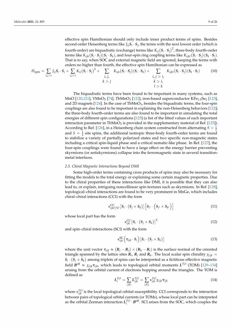
2.5. Chiral Magnetic Interactions Beyond DMI

Some high-order terms containing cross products of spins may also be necessary forfitting the models to the total energy or explaining some certain magnetic properties. Dueto the chiral properties of these interactions like DMI, it is possible that they can alsolead to, or explain, intriguing noncollinear spin textures such as skyrmions. In Ref. [128],topological–chiral interactions are found to be very prominent in MnGe, which includeschiral–chiral interactions (CCI) with the form

κCCijki′ j′k′

[Si ·(Sj × Sk

)][Si′ ·

(Sj′ × Sk′

)](11)

whose local part has the formκCC

ijk[Si ·(Sj × Sk

)]2 (12)

and spin–chiral interactions (SCI) with the form

κSCijk

(τijk · Si

)[Si ·(Sj × Sk

)](13)

where the unit vector τijk ∝(Rj −Ri

)× (Rk −Ri) is the surface normal of the oriented

triangle spanned by the lattice sites Ri, Rj and Rk. The local scalar spin chirality χijk =

Si ·(Sj × Sk

)among triplets of spins can be interpreted as a fictitious effective magnetic

field Beff ∝ χijkτijk, which leads to topological orbital moments LTO (TOM) [129–134]arising from the orbital current of electrons hopping around the triangles. The TOM isdefined as

LTOi = ∑

(jk)LTO

ijk = ∑(jk)

κTOijk χijkτijk (14)

where κTOijk is the local topological orbital susceptibility. CCI corresponds to the interaction

between pairs of topological orbital currents (or TOMs), whose local part can be interpretedas the orbital Zeeman interaction LTO

i · Beff. SCI arises from the SOC, which couples the

Molecules 2021, 26, 803 10 of 26

TOM to single spin magnetic moments. An illustration of CCI and SCI is provided inFigure 2. Considerations of CCI and SCI improved the fitting of the total energy in MnGe(see details in Ref. [128]). Moreover, the authors showed the possibility that the CCI maylead to three-dimensional topological spin states and therefore may be vital in decidingthe ground state of the spin configurations of MnGe, which was found to be a three-dimensional topological lattice (possibly built up with hedgehogs and anti-hedgehogs)experimentally [135].

Molecules 2021, 26, x FOR PEER REVIEW 10 of 26

𝑳 = 𝑳( ) = 𝜅 𝜒 𝝉( ) (14)

where 𝜅 is the local topological orbital susceptibility. CCI corresponds to the interac-tion between pairs of topological orbital currents (or TOMs), whose local part can be in-terpreted as the orbital Zeeman interaction 𝑳 ⋅ 𝑩 . SCI arises from the SOC, which cou-ples the TOM to single spin magnetic moments. An illustration of CCI and SCI is provided in Figure 2. Considerations of CCI and SCI improved the fitting of the total energy in MnGe (see details in Ref. [128]). Moreover, the authors showed the possibility that the CCI may lead to three-dimensional topological spin states and therefore may be vital in decid-ing the ground state of the spin configurations of MnGe, which was found to be a three-dimensional topological lattice (possibly built up with hedgehogs and anti-hedgehogs) experimentally [135].

Figure 2. Schematic diagrams of chiral–chiral interactions (CCI) and spin–chiral interactions (SCI), as provided by S. Grytsiuk et al. in Ref. [128]. Spins and topological orbital moments (TOMs) are denoted as black arrows and blue arrows, respectively. CCI can be regarded as interactions between TOMs, while SCI can be interpreted as interactions between TOM and local spins.

A new type of chiral pair interaction 𝑪 ⋅ (𝑺 × 𝑺 ) (𝑺 ⋅ 𝑺 ), named as chiral biquad-ratic interaction (CBI), which is the biquadratic equivalent of the DMI, was derived from a microscopic model and demonstrated to be comparable in magnitude to the DMI in magnetic dimers made of 3d elements on Pt(111), Pt(001), Ir(111) and Re(0001) surface with strong SOC [136]. Similar but generalized chiral interactions such as 𝑫 ⋅ (𝑺 ×𝑺 ) (𝑺 ⋅ 𝑺 ) and 𝑫 ⋅ (𝑺 × 𝑺 ) (𝑺 ⋅ 𝑺 ), named four-spin chiral interactions, were dis-cussed in Ref. [137], and they are found to be important in predicting a correct chirality for a spin spiral state of Fe chains deposited on the Re(0001) surface.

When there is a magnetic field, for a nonbipartite lattice, the magnetic field can cou-ple with the spin and produce a new term of the form 𝐽 𝑺 ⋅ 𝑺 × 𝑺 = 𝐽 𝜒 [138,139], which can be termed the three-spin chiral interaction (TCI) [140]. Such a chiral term can induce a gapless line in frustrated spin-gapped phases, and a critical chiral strength can change the ground state from spiral to Néel quasi-long-range-order phase [138]. This chiral term is also found to produce a chiral spin liquid state [141], where the time-reversal symmetry is broken spontaneously by the emergence of long-range order of scalar chirality [142].

Figure 2. Schematic diagrams of chiral–chiral interactions (CCI) and spin–chiral interactions (SCI), as provided by S.Grytsiuk et al. in Ref. [128]. Spins and topological orbital moments (TOMs) are denoted as black arrows and blue arrows,respectively. CCI can be regarded as interactions between TOMs, while SCI can be interpreted as interactions between TOMand local spins.

A new type of chiral pair interaction Cij ·(Si × Sj

) (Si · Sj

), named as chiral biquadratic

interaction (CBI), which is the biquadratic equivalent of the DMI, was derived from a mi-croscopic model and demonstrated to be comparable in magnitude to the DMI in magneticdimers made of 3d elements on Pt(111), Pt(001), Ir(111) and Re(0001) surface with strongSOC [136]. Similar but generalized chiral interactions such as Dijjk ·

(Sj × Sk

) (Si · Sj

)and

Dijkl · (Sk × Sl)(Si · Sj

), named four-spin chiral interactions, were discussed in Ref. [137],

and they are found to be important in predicting a correct chirality for a spin spiral state ofFe chains deposited on the Re(0001) surface.

When there is a magnetic field, for a nonbipartite lattice, the magnetic field can couplewith the spin and produce a new term of the form JijkSi ·

(Sj × Sk

)= Jijkχijk [138,139],

which can be termed the three-spin chiral interaction (TCI) [140]. Such a chiral term caninduce a gapless line in frustrated spin-gapped phases, and a critical chiral strength canchange the ground state from spiral to Néel quasi-long-range-order phase [138]. Thischiral term is also found to produce a chiral spin liquid state [141], where the time-reversalsymmetry is broken spontaneously by the emergence of long-range order of scalar chiral-ity [142].

2.6. Expansions of Magnetic Interactions

In general, a complete basis can be used to expand the spin interactions. One exampleis the spin-cluster expansion (SCE) [143–145], where unit vectors denoting the directionsof spins are used as independent variables and spherical harmonic functions are used inthe expressions of the basis functions. When SOC and the external magnetic field are not

Molecules 2021, 26, 803 11 of 26

important, as mentioned in Section 2.3, only inner products of spins need to be considered.Consequently, the expansion can be

Hspin = E0 +∞

∑n=1

Jn

∑nth nearest pairs 〈k,l〉

ek · el

+∞

∑n′=1

J′n′ ∑n′th type

(ek · el)(em · en) + · · · (15)

as used in Ref. [125]. When using expansions of spin vectors (or directions of the spins),suitable truncations on interaction distances and interaction orders are needed. Otherwise,the number of terms would be infinite, and as a result, the problem would be unsolvable.

3. Methods of Computing the Parameters of Effective Spin Hamiltonian Models

In this part, we mainly discuss the methods of computing the spin interaction parame-ters based on first-principles calculations of crystals, where periodic boundary conditionsare tacitly supposed. These methods include different kinds of energy-mapping analysis(see Section 3.1) and Green’s function method based on magnetic-force linear responsetheory (see Section 3.2). Discussions on the rigid spin rotation approximation and otherassumptions are provided in Section 3.3. The cases of clusters, where periodic boundaryconditions do not exist, will be briefly discussed in Section 3.3. Methods of obtaining spininteraction parameters from experiments will also be briefly mentioned in Section 3.3.

3.1. Energy-Mapping Analysis

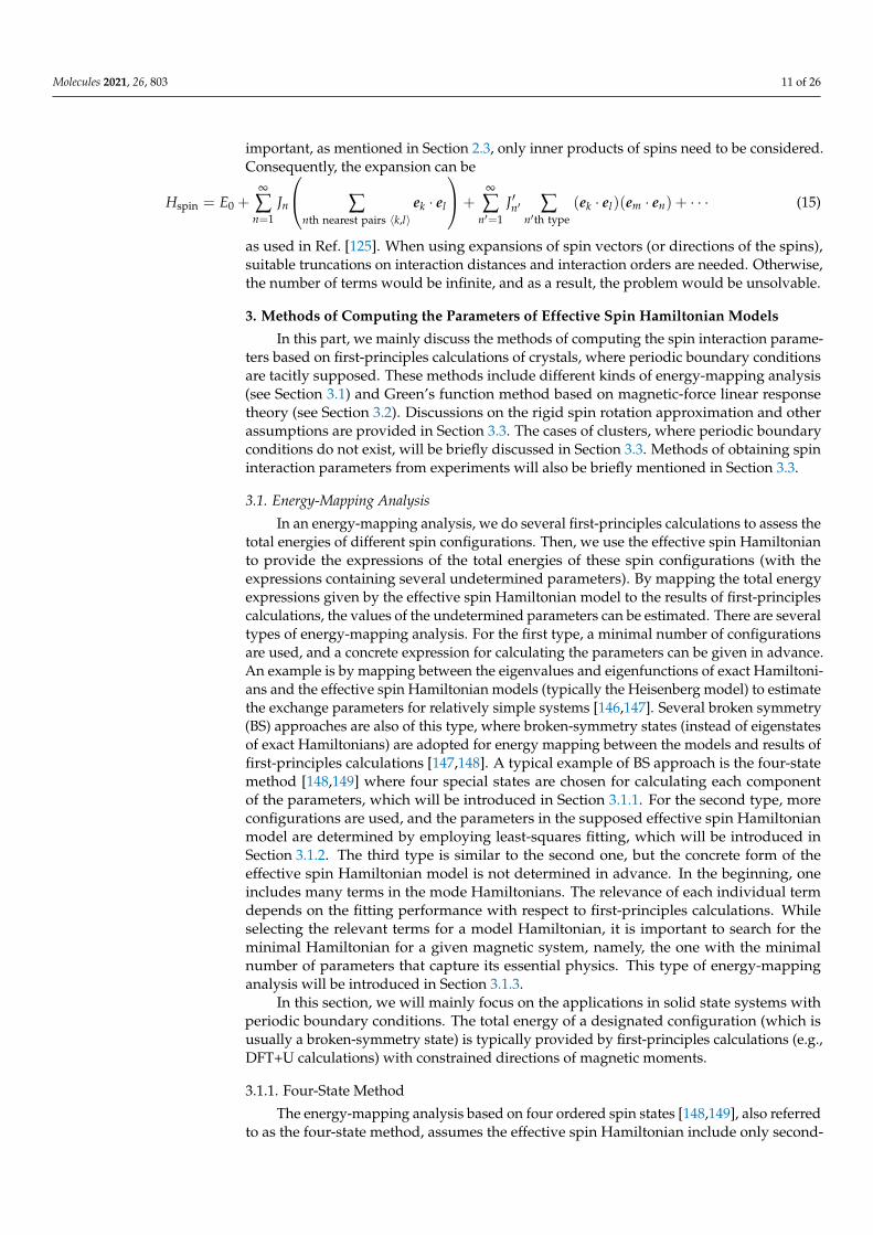
In an energy-mapping analysis, we do several first-principles calculations to assess thetotal energies of different spin configurations. Then, we use the effective spin Hamiltonianto provide the expressions of the total energies of these spin configurations (with theexpressions containing several undetermined parameters). By mapping the total energyexpressions given by the effective spin Hamiltonian model to the results of first-principlescalculations, the values of the undetermined parameters can be estimated. There are severaltypes of energy-mapping analysis. For the first type, a minimal number of configurationsare used, and a concrete expression for calculating the parameters can be given in advance.An example is by mapping between the eigenvalues and eigenfunctions of exact Hamiltoni-ans and the effective spin Hamiltonian models (typically the Heisenberg model) to estimatethe exchange parameters for relatively simple systems [146,147]. Several broken symmetry(BS) approaches are also of this type, where broken-symmetry states (instead of eigenstatesof exact Hamiltonians) are adopted for energy mapping between the models and results offirst-principles calculations [147,148]. A typical example of BS approach is the four-statemethod [148,149] where four special states are chosen for calculating each componentof the parameters, which will be introduced in Section 3.1.1. For the second type, moreconfigurations are used, and the parameters in the supposed effective spin Hamiltonianmodel are determined by employing least-squares fitting, which will be introduced inSection 3.1.2. The third type is similar to the second one, but the concrete form of theeffective spin Hamiltonian model is not determined in advance. In the beginning, oneincludes many terms in the mode Hamiltonians. The relevance of each individual termdepends on the fitting performance with respect to first-principles calculations. Whileselecting the relevant terms for a model Hamiltonian, it is important to search for theminimal Hamiltonian for a given magnetic system, namely, the one with the minimalnumber of parameters that capture its essential physics. This type of energy-mappinganalysis will be introduced in Section 3.1.3.

In this section, we will mainly focus on the applications in solid state systems withperiodic boundary conditions. The total energy of a designated configuration (which isusually a broken-symmetry state) is typically provided by first-principles calculations (e.g.,DFT+U calculations) with constrained directions of magnetic moments.

3.1.1. Four-State Method

The energy-mapping analysis based on four ordered spin states [148,149], also referredto as the four-state method, assumes the effective spin Hamiltonian include only second-

Molecules 2021, 26, 803 12 of 26

order terms (i.e., isotropic Heisenberg terms, DMI terms, Kitaev terms, and SIA terms).Each component of the parameters like Jij, Dij,x, Ai,xy, (Ai,yy − Ai,xx) and (Ai,zz − Ai,xx)can be obtained by first-principles calculations for four specified spin states [148]. Takingthe isotropic Heisenberg parameter Jij for example, with the spin-orbit coupling (SOC)switched off during the first-principles calculations, we use Eij,αβ ( α, β =↑, ↓ ) to denotethe energy of the configuration where spin i is parallel or antiparallel to the z direction (ifα =↑ or ↓ , respectively), spin j is parallel or antiparallel to the z direction (if β = ↑ or ↓ ,respectively), and all the spins except i and j are kept unchanged in the four states (whichwill be referred to as the “reference configuration”, usually chosen to be a low-energycollinear state). Then Jij can be expressed as

Jij =Eij,↑↑ + Eij,↓↓ − Eij,↑↓ − Eij,↓↑

4S2 (16)

The schematic diagrams of these four states are shown in Figure 3.

Molecules 2021, 26, x FOR PEER REVIEW 12 of 26

In this section, we will mainly focus on the applications in solid state systems with periodic boundary conditions. The total energy of a designated configuration (which is usually a broken-symmetry state) is typically provided by first-principles calculations (e.g., DFT+U calculations) with constrained directions of magnetic moments.

3.1.1. Four-State Method The energy-mapping analysis based on four ordered spin states [148,149], also re-

ferred to as the four-state method, assumes the effective spin Hamiltonian include only second-order terms (i.e., isotropic Heisenberg terms, DMI terms, Kitaev terms, and SIA terms). Each component of the parameters like 𝐽 , 𝑫 , , 𝔸 , , (𝔸 , − 𝔸 , ) and (𝔸 , −𝔸 , ) can be obtained by first-principles calculations for four specified spin states [148]. Taking the isotropic Heisenberg parameter 𝐽 for example, with the spin-orbit coupling (SOC) switched off during the first-principles calculations, we use 𝐸 , (𝛼, 𝛽 =↑, ↓) to denote the energy of the configuration where spin i is parallel or antiparallel to the z di-rection (if 𝛼 =↑ or ↓, respectively), spin j is parallel or antiparallel to the z direction (if 𝛽 = ↑ or ↓, respectively), and all the spins except i and j are kept unchanged in the four states (which will be referred to as the “reference configuration”, usually chosen to be a low-energy collinear state). Then 𝐽 can be expressed as 𝐽 = 𝐸 ,↑↑ + 𝐸 ,↓↓ − 𝐸 ,↑↓ − 𝐸 ,↓↑4𝑆 (16)

The schematic diagrams of these four states are shown in Figure 3.

Figure 3. Schematic diagrams of the four states adopted in the four-state method for computing 𝐽 . Except atoms i and j, all the other atoms are omitted in this diagram (which are kept the same in the four states). Spins pointing up and down are indicated with orange and blue balls, respec-tively. The total energies given by first-principles calculations corresponding to these four states are denoted as (a) 𝐸 ,↑↑, (b) 𝐸 ,↑↓, (c) 𝐸 ,↓↑, and (d) 𝐸 ,↓↓, respectively.

In general, the second-order effective spin Hamiltonian takes the form of 𝐻 = 𝑺 𝕁 𝑺, + 𝑺 𝔸 𝑺 (17)

and each component of the matrix 𝕁 and 𝔸 can also be obtained by first-principles cal-culations for four specified spin states. To compute 𝕁 , (𝑎, 𝑏 = 𝑥, 𝑦, 𝑧), we use 𝐸 , ,

Figure 3. Schematic diagrams of the four states adopted in the four-state method for computing Jij.Except atoms i and j, all the other atoms are omitted in this diagram (which are kept the same in thefour states). Spins pointing up and down are indicated with orange and blue balls, respectively. Thetotal energies given by first-principles calculations corresponding to these four states are denoted as(a) Eij,↑↑, (b) Eij,↑↓, (c) Eij,↓↑, and (d) Eij,↓↓, respectively.

In general, the second-order effective spin Hamiltonian takes the form of

Hspin = ∑i,j>i

STi JijSj + ∑

iST

i AiSi (17)

and each component of the matrix Jij and Ai can also be obtained by first-principlescalculations for four specified spin states. To compute Jij,ab (a, b = x, y, z), we use Eij,ab,αβ

( α, β = ↑, ↓ ) to denote the energy of the configuration where spin i is parallel or antiparallelto the a direction (if α = ↑ or ↓ , respectively), spin j is parallel or antiparallel to the bdirection (if β = ↑ or ↓ , respectively), and all the spins except for i and j are kept unchangedand parallel to the c-axis (c = x, y or z, c 6= a, c 6= b) with an appropriate referenceconfiguration and kept unchanged. Then, Jij,ab can be expressed as

Jij,ab =Eij,ab,↑↑ + Eij,ab,↓↓ − Eij,ab,↑↓ − Eij,ab,↓↑

4S2 (18)

Molecules 2021, 26, 803 13 of 26

To compute Ai,ab (a, b = x, y, z with a 6= b), we use Ei,ab,αβ ( α, β = ↑, ↓ ) to denote theenergy of the configuration where spin i is parallel to the direction whose a componentis ±

√2

2 (for α = ↑ or ↓ , respectively), b component is ±√

22 (for β = ↑ or ↓ , respectively),

and the other component is 0. Here all the spins except for i and j are parallel to the c-axis(c = x, y or z, c 6= a, c 6= b) with an appropriate reference configuration. Then, Ai,ab can beexpressed as

Ai,ab =Ei,ab,↑↑ + Ei,ab,↓↓ − Ei,ab,↑↓ − Ei,ab,↓↑

4S2 (19)

To compute (Ai,aa −Ai,bb) (a, b = x, y, z with a 6= b), we use Ei,ab,αβ ( α, β = ↑, ↓ or 0) todenote the energy of the configuration where spin i is parallel to the direction whose a com-ponent is ±1 or 0 (if α = ↑, ↓ or 0 , respectively), b component is ±1 or 0 (if β = ↑, ↓ or 0 ,respectively) and the other component is 0, while all the spins except i are parallel to thec-axis (c = x, y or z, c 6= a, c 6= b) with an appropriate reference configuration. Then(Ai,aa −Ai,bb) can be expressed as

Ai,aa −Ai,bb =Ei,ab,↑0 + Ei,ab,↓0 − Ei,ab,0↑ − Ei,ab,0↓

4S2 (20)

It is easy to verify that, by employing this four-state method, each component of theJij and Ai can be obtained with the effects of other second-order terms entirely cancelled.Now we take the effects of fourth-order terms (without SOC) into account and check ifthe algorithms for computing Jij and Ai are still rigorous. For Ai, we can find out thatthe effects of all these terms are correctly cancelled. For Jij, the effects of biquadraticterms, three-body fourth-order terms, and most of the four-spin ring coupling terms areperfectly cancelled, while only the terms like

(Si · Sj

)(Sk · Sl) (k, l 6= i, j) will interfere with

the calculation of Jij because (Sk · Sl) is constant during the calculation and therefore mixedwith the contribution of Jij

(Si · Sj

). The error of the calculated Jij originated from four-spin

ring coupling terms∑

i, j > i,k > i,l > k

Kijkl(Si · Sj

)(Sk · Sl) (21)

is given by∑

k 6= i or jl 6= i or j(l > k)

Kijkl(Sk · Sl) (22)

while there is no easy way to get rid of this problem perfectly. Other parts of the Jij(including Dij and Kij) are not affected by these fourth-order terms (without SOC), but byother types of fourth-order terms (like four-spin chiral interactions) if SOC is taken intoaccount (because of the similar reason).

In Ref. [122], the four-spin ring coupling interaction is found to be important inTbMnO3, and therefore leads to instability in calculating the Heisenberg parameters usingthe four-state method when changing the reference configurations. This problem is reme-died by calculating the Heisenberg parameter Jij twice with the four-state method usingthe FM and A-type AFM (A-AFM, see Figure 4c) as the reference configurations, and usetheir average value as the final estimation of Jij. The parameter of the vital ring couplinginteraction is obtained by calculating the difference between the two calculated Jij values(with FM and A-AFM reference configurations, respectively). This effective remedy isbased on the assumption that only one kind of ring coupling interaction is essential. How-ever, if there are more kinds of significant ring coupling or if we do not know which ringcoupling is essential in advance, such a method of calculating Jij is still not very trustworthy.Nevertheless, it is found that by taking the average of the calculated Jij with four-state

Molecules 2021, 26, 803 14 of 26

method with FM and G-type AFM (G-AFM, see Figure 4a) reference configurations, theinfluences of Kijkl

(Si · Sj

)(Sk · Sl) with k and l being nearest pairs are eliminated. The terms

Kijkl(Si · Sj

)(Sk · Sl) with non-nearest pairs of k and l still interfere with the calculation

of Jij, but they are generally very weak. Therefore, such a remedy to calculate Jij usingthe four-state method should work well in most cases. In cases when a G-AFM state (inwhich all the nearest pairs of spins are antiparallelly aligned) cannot be defined (e.g., atriangular or a Kagomé lattice), there may be more than two reference configurations touse in the four-state method so as to eliminate the effects of Kijkl

(Si · Sj

)(Sk · Sl) terms with

non-nearest pairs of k and l. These reference configurations need to be designed carefullyaccording to the specific circumstances to get rid of the effects of Kijkl

(Si · Sj

)(Sk · Sl) terms

as much as possible.

Molecules 2021, 26, x FOR PEER REVIEW 14 of 26

the FM and A-type AFM (A-AFM, see Figure 4c) as the reference configurations, and use their average value as the final estimation of 𝐽 . The parameter of the vital ring coupling interaction is obtained by calculating the difference between the two calculated 𝐽 values (with FM and A-AFM reference configurations, respectively). This effective remedy is based on the assumption that only one kind of ring coupling interaction is essential. How-ever, if there are more kinds of significant ring coupling or if we do not know which ring coupling is essential in advance, such a method of calculating 𝐽 is still not very trust-worthy. Nevertheless, it is found that by taking the average of the calculated 𝐽 with four-state method with FM and G-type AFM (G-AFM, see Figure 4a) reference configurations, the influences of 𝐾 (𝑺 ⋅ 𝑺 )(𝑺 ⋅ 𝑺 ) with k and l being nearest pairs are eliminated. The terms 𝐾 (𝑺 ⋅ 𝑺 )(𝑺 ⋅ 𝑺 ) with non-nearest pairs of k and l still interfere with the calcu-lation of 𝐽 , but they are generally very weak. Therefore, such a remedy to calculate 𝐽 using the four-state method should work well in most cases. In cases when a G-AFM state (in which all the nearest pairs of spins are antiparallelly aligned) cannot be defined (e.g., a triangular or a Kagomé lattice), there may be more than two reference configurations to use in the four-state method so as to eliminate the effects of 𝐾 (𝑺 ⋅ 𝑺 )(𝑺 ⋅ 𝑺 ) terms with non-nearest pairs of k and l. These reference configurations need to be designed care-fully according to the specific circumstances to get rid of the effects of 𝐾 (𝑺 ⋅ 𝑺 )(𝑺 ⋅𝑺 ) terms as much as possible.

Figure 4. Schematic diagrams of (a) G-type AFM, (b) C-type AFM, and (c) C-type AFM states. Spins pointing to two opposite directions (e.g., up and down) are indicated with orange and blue balls, respectively.

The main advantages of the four-state method are its relatively small amount of first-principles calculations and its relatively good cancellations of other relevant terms. A weakness is that it cannot analyze the uncertainties of the parameters, so that we do not know how precise those estimated values are. Another weakness, which is also shared with other energy-mapping analysis methods, is that the computed 𝕁 between 𝑺 and 𝑺 is actually the sum over 𝕁 with any lattice vector 𝑹 = 𝒓 − 𝒓 . Therefore, to get rid of the effects of other spin pairs, a relatively large supercell is needed.

The four-state method can also be generalized to compute biquadratic parameters, where the SOC needs to be switched off during the first-principles calculations. For calcu-lating 𝐾 in the term 𝐾 (𝑺 ⋅ 𝑺 ) , we can let 𝑺 pointing to the (1,0,0) direction, 𝑺 pointing to the (1,0,0), (−1,0,0), √ , √ , 0 and − √ , − √ , 0 directions, with other spins parallel to the z-axis. The corresponding total energies are denoted as 𝐸 , 𝐸 , 𝐸 , and 𝐸 , respectively. Then the 𝐾 can be expressed as 𝐾 = 𝐸 + 𝐸 − 𝐸 − 𝐸 (23)

It can be easily checked that the effects of other terms not higher than fourth order are totally eliminated. Therefore, this approach of calculating 𝐾 should be relatively rig-orous theoretically.

Figure 4. Schematic diagrams of (a) G-type AFM, (b) C-type AFM, and (c) C-type AFM states. Spins pointing to twoopposite directions (e.g., up and down) are indicated with orange and blue balls, respectively.

The main advantages of the four-state method are its relatively small amount offirst-principles calculations and its relatively good cancellations of other relevant terms. Aweakness is that it cannot analyze the uncertainties of the parameters, so that we do notknow how precise those estimated values are. Another weakness, which is also sharedwith other energy-mapping analysis methods, is that the computed Jij between Si and Sj isactually the sum over Jij′ with any lattice vector R = rj′ − rj. Therefore, to get rid of theeffects of other spin pairs, a relatively large supercell is needed.

The four-state method can also be generalized to compute biquadratic parameters,where the SOC needs to be switched off during the first-principles calculations. Forcalculating Kij in the term Kij

(Si · Sj

)2, we can let Si pointing to the (1, 0, 0) direction, Sj

pointing to the (1, 0, 0), (−1, 0, 0),(

1√2, 1√

2, 0)

and(− 1√

2,− 1√

2, 0)

directions, with otherspins parallel to the z-axis. The corresponding total energies are denoted as E1, E2, E3, andE4, respectively. Then the Kij can be expressed as

Kij = E1 + E2 − E3 − E4 (23)

It can be easily checked that the effects of other terms not higher than fourth order aretotally eliminated. Therefore, this approach of calculating Kij should be relatively rigoroustheoretically.

Note that the four-state methods [148,149] could also give the derivatives of ex-change interactions with respect to the atomic displacements without doing additionalfirst-principles calculations due to the Hellmann-Feynman theorem. These derivatives areuseful for the study of spin-lattice coupling related phenomena.

3.1.2. Direct Least Squares Fitting

Another type of energy-mapping analysis, instead of the four-state method, usesmore first-principles calculations with different spin configurations and fits the results

Molecules 2021, 26, 803 15 of 26

to the effective spin Hamiltonian using the least-squares method to estimate the parame-ters [74,122–124]. Ways of choosing spin configurations can depend on which parametersto estimate.

In Ref. [74], for the four Mn sites in a unit cell of YMnO3, the polar and azimuthalangles (θ,ϕ) of their spins are given by (0, 0), (0, 0),

(θ, 3π

2), and

(θ, π

2), respectively. By

changing the θ from 0◦ to 180◦, different configurations are produced. If the effective spinHamiltonian only contains Heisenberg terms, there will be a systematic deviation betweenthe predicted value given by the effective Hamiltonian and the calculated value given byfirst-principles calculations. Such a deviation is well remedied by adding biquadratic ex-change interactions into the effective Hamiltonian model. Thus, the biquadratic parameterscan be fitted. Similar approaches were adopted by others to calculate and show the impor-tance of biquadratic parameters and topological chiral–chiral contributions [122–124,128].Apart from using an angular variable for generating spin configurations, using two or morevariables is also practicable, or randomly chosen directions [106] can also be considered.Thus, more diverse configurations will be produced. The least-squares fitting will alsowork, but whether a systematic deviation exists will not be as apparent as the case whenonly one angular variable is used for generating configurations, and the fitting task may bemore laborious.

The main virtues of this method are that the reliability of the model can be checkedby the fitting performance and that the uncertainties of the parameters can be estimatedif needed. This method is especially suitable for calculations of biquadratic parametersand topological CCI. However, when talking about calculations of Heisenberg parameters,this method needs more first-principles calculations and is thus less efficient. Furthermore,the fitted result of the Heisenberg parameter Jij is vulnerable to the effects of other fourth-order interactions such as terms as

(Si · Sj

)(Si · Sk) and

(Si · Sj

)(Sk · Sl). Therefore, the

estimations of the Heisenberg parameters may not be very reliable if any of such fourth-order interactions are essential. This problem can be remedied by adding the related termsinto the effective Hamiltonian model, while it is not easy to decide which terms to includein the model beforehand.

A possible way to get rid of the effects of other high-order terms is to perform artificialcalculations where most of the magnetic ions are replaced by similar but nonmagnetic ions(e.g., substituting Fe3+ ions with nonmagnetic Al3+ ions) except for one or more ions to bestudied [150]. For example, when calculating SIA, only one magnetic ion is not substituted,and by rotating this magnetic ion and calculating the total energy, the SIA can be studied.When studying two-body interactions between Si and Sj, only two magnetic ions (at sitei and j) are not substituted, and by rotating the spins (or magnetic moments) of thesetwo magnetic ions, the interactions between them can be studied. Such a technique ofsubstituting atoms can be applied to energy mapping analysis based on either the four-statemethod or least-squares fitting. In this way, effects from interactions involving other sitesare effectively avoided. Nevertheless, this substitution method can make the chemicalenvironments of the remaining magnetic ions different from those in the system with nosubstitution. This may make the calculations of the interaction parameters untrustworthy.

3.1.3. Methods Based on Expansions and Selecting Important Terms

The traditional energy-mapping analysis needs to construct an effective spin Hamil-tonian first and then fit the undetermined parameters. However, it is not easy to give aperfect guess, especially when high-order interactions are essential. Such problems can besolved by considering almost all the possible terms utilizing some particular expansionwith appropriate truncations. Usually, there are too many possible terms to be considered,so a direct fitting is impracticable; it requires at least as many first-principles calculationsas the number of terms to determine, but leads to over-fitting problems due to too manyparameters to determine. So, it is necessary to decide whether or not to include eachterm into the effective spin Hamiltonian on the basis of their contributions to the fittingperformance.

Molecules 2021, 26, 803 16 of 26

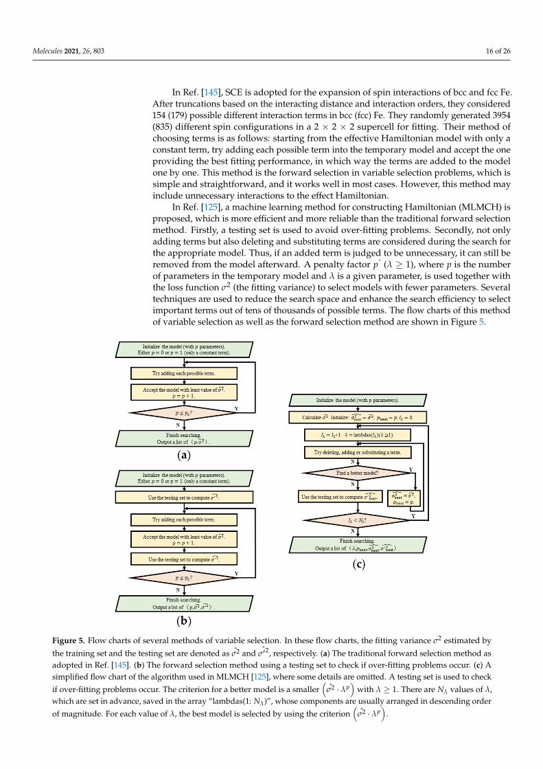
In Ref. [145], SCE is adopted for the expansion of spin interactions of bcc and fcc Fe.After truncations based on the interacting distance and interaction orders, they considered154 (179) possible different interaction terms in bcc (fcc) Fe. They randomly generated 3954(835) different spin configurations in a 2 × 2 × 2 supercell for fitting. Their method ofchoosing terms is as follows: starting from the effective Hamiltonian model with only aconstant term, try adding each possible term into the temporary model and accept the oneproviding the best fitting performance, in which way the terms are added to the modelone by one. This method is the forward selection in variable selection problems, which issimple and straightforward, and it works well in most cases. However, this method mayinclude unnecessary interactions to the effect Hamiltonian.

In Ref. [125], a machine learning method for constructing Hamiltonian (MLMCH) isproposed, which is more efficient and more reliable than the traditional forward selectionmethod. Firstly, a testing set is used to avoid over-fitting problems. Secondly, not onlyadding terms but also deleting and substituting terms are considered during the search forthe appropriate model. Thus, if an added term is judged to be unnecessary, it can still beremoved from the model afterward. A penalty factor p˘ (λ ≥ 1), where p is the numberof parameters in the temporary model and λ is a given parameter, is used together withthe loss function σ2 (the fitting variance) to select models with fewer parameters. Severaltechniques are used to reduce the search space and enhance the search efficiency to selectimportant terms out of tens of thousands of possible terms. The flow charts of this methodof variable selection as well as the forward selection method are shown in Figure 5.

Molecules 2021, 26, x FOR PEER REVIEW 17 of 26

Figure 5. Flow charts of several methods of variable selection. In these flow charts, the fitting variance 𝜎 estimated by the training set and the testing set are denoted as 𝜎 and 𝜎 , respectively. (a) The traditional forward selection method as adopted in Ref. [145]. (b) The forward selection method using a testing set to check if over-fitting problems occur. (c) A simplified flow chart of the algorithm used in MLMCH [125], where some details are omitted. A testing set is used to check if over-fitting problems occur. The criterion for a better model is a smaller 𝜎 ⋅ 𝜆 with 𝜆 ≥ 1. There are 𝑁 val-ues of 𝜆, which are set in advance, saved in the array “lambdas(1: 𝑁 )”, whose components are usually arranged in de-scending order of magnitude. For each value of 𝜆, the best model is selected by using the criterion 𝜎 ⋅ 𝜆 .

This method is advantageous in two ways: (a) Constructing the effective spin Ham-iltonians is carried out comprehensively, which makes it less likely to miss some critical interaction terms; (b) this method is general, so it can be applied to most magnetic mate-rials. The least-squares fitting needed in this approach can also provide the estimations for the uncertainties of the parameters. The flaw is that it needs lots of (typically hundreds of) first-principles calculations, which could be impracticable when a very large supercell is needed (especially when the material is metallic so that long-range interactions are es-sential). The way to generate spin configurations (typically randomly distributed among all possible directions, sometimes deviating only moderately from the ground state) may have some room for improvement.

3.2. Green’s Function Method Based on Magnetic-Force Linear Response Theory In Green’s function method based on magnetic-force linear response theory [151–

159], we need localized basis functions 𝜓 (𝒓) (𝑖, 𝑚, 𝜎 indicating the site, orbital, and spin indices, respectively) based on the tight-binding model. The localized basis functions can be provided by DFT codes together with Wannier90 [160,161] or codes based on lo-calized orbitals. By defining

Figure 5. Flow charts of several methods of variable selection. In these flow charts, the fitting variance σ2 estimated by

the training set and the testing set are denoted as σ2 and ˆσ′2, respectively. (a) The traditional forward selection method asadopted in Ref. [145]. (b) The forward selection method using a testing set to check if over-fitting problems occur. (c) Asimplified flow chart of the algorithm used in MLMCH [125], where some details are omitted. A testing set is used to check

if over-fitting problems occur. The criterion for a better model is a smaller(

σ2 · λp)

with λ ≥ 1. There are Nλ values of λ,which are set in advance, saved in the array “lambdas(1: Nλ)”, whose components are usually arranged in descending order

of magnitude. For each value of λ, the best model is selected by using the criterion(

σ2 · λp)

.

Molecules 2021, 26, 803 17 of 26

This method is advantageous in two ways: (a) Constructing the effective spin Hamil-tonians is carried out comprehensively, which makes it less likely to miss some criticalinteraction terms; (b) this method is general, so it can be applied to most magnetic materials.The least-squares fitting needed in this approach can also provide the estimations for theuncertainties of the parameters. The flaw is that it needs lots of (typically hundreds of)first-principles calculations, which could be impracticable when a very large supercellis needed (especially when the material is metallic so that long-range interactions areessential). The way to generate spin configurations (typically randomly distributed amongall possible directions, sometimes deviating only moderately from the ground state) mayhave some room for improvement.

3.2. Green’s Function Method Based on Magnetic-Force Linear Response Theory

In Green’s function method based on magnetic-force linear response theory [151–159],we need localized basis functions ψimσ(r) (i, m, σ indicating the site, orbital, and spinindices, respectively) based on the tight-binding model. The localized basis functions canbe provided by DFT codes together with Wannier90 [160,161] or codes based on localizedorbitals. By defining

Himjm′σσ′(R) = 〈ψimσ(r)|H|ψimσ(r + R)〉 (24)

Simjm′σσ′(R) = 〈ψimσ(r)|ψimσ(r + R) (25)

H(k) = ∑RH(R)eik·R (26)

S(k) = ∑RS(R)eik·R (27)

the Green’s function in reciprocal space and real space are defined as

G(k, ε) = (εS(k)−H(k))−1 (28)

andG(R, ε) =

∫BZ

G(k, ε)e−ik·Rdk (29)

Based on the magnetic force theorem [162], the total energy variation due to a pertur-bation (which is the rotation of spins in this case) from the ground state equals the changeof single-particle energies at the fixed ground-state potential:

δE =∫ EF

−∞εδn(ε)dε = −

∫ EF

−∞δN(ε)dε (30)

wheren(ε) = − 1

πImTr(G(ε)) (31)

andN(ε) = − 1

πImTr(ε−H) (32)

where traces are taken over orbitals. By defining

Pi = Hii(R = 0) = p0i l+→p i ·→σ (33)

with its componentPimm′ = p0

imm′l+ pimm′→e imm′ ·

→σ (34)

where→σ is the vector composed of Pauli matrices. By defining

Gim,jm′ = G0im,jm′l+

→Gim,jm′ ·

→σ (35)

Molecules 2021, 26, 803 18 of 26

the energy variation due to the two-spin interaction between sites i and j is

δEij = −2π

∫ EF

∞ImTr

(δHiGδHjG

)dε (36)

with δHi = δφi × pi. After mathematical simplification, the expression of δEij can bemapped to that given by the effective Hamiltonian model

Hspin = ∑i

STi AiSi + ∑

i,j>i

[JijSi · Sj + Dij ·

(Si × Sj

)+ ST

i KijSj

]+ ∑

i,j>iKij(Si · Sj

)2 (37)

(including all the second-order terms and a biquadratic term) to obtain the expressions ofthe parameters:

Jij = Im(

A00ij − Axx

ij − Ayyij − Azz

ij − 2Azzij Sref

i · Srefj

)(38)

Kuvij = Im

(Auv

ij + Avuij

)(39)

Duij = Re

(A0u

ij − Au0ij

)(40)

Bij = Im(

Azzij

)(41)

where

Auvij =

1π

∫ EF

−∞Tr{pzi G

uijp

zjG

vji

}dε (42)

with u, v ∈ {0, x, y, z} (the trace is also taken over orbitals), and Srefi indicates the un-

perturbed vector Si. An xyz average strategy can be adopted so that some componentsinaccessible from one first-principles calculation can be obtained [157].

The main advantages of this method are that it only requires one or three DFT calcula-tions to obtain all the parameters of second-order terms and biquadratic terms betweendifferent atoms, using only a small supercell (with a dense enough k-point sampling) to ob-tain interaction parameters between spins far away from each other. Therefore, it saves thecomputational cost compared to the energy-mapping analysis, especially when long-rangeinteractions are essential. It also avoids the difficulties of reaching self-consistent-fieldconvergence in DFT calculations for high-energy configurations, which may occur in theenergy-mapping analysis. This method is good at describing states near the ground statebut may not be so good at describing high-energy states. A limitation is that this methodcannot obtain SIA parameters, and its calculations for biquadratic parameters are not verytrustworthy [157]. The calculated Heisenberg parameter Jij is mixed with the contributionsof other fourth-order interactions such as terms like

(Si · Sj

)(Si · Sk) and

(Si · Sj

)(Sk · Sl).

Therefore, the results may be unreliable if any of such fourth-order interactions are essential.Another little flaw is the noise of a typical order of magnitude of a few µeV introduced bythe process of obtaining the Wannier orbitals [157]. In addition, the uncertainties of theparameters cannot be obtained by this method.

A recent study [140] considered the rotations of more than two spins as the pertur-bation and mapped the δE to the corresponding quantity given by an effective Hamil-tonian with more types of interactions, including terms proportional to Si ·

(Sj × Sk

),(

Si · Sj)(Sk · Sl) and

(Si × Sj

)(Sk · Sl). This enables one to obtain the expressions needed

for calculating the associated parameters. The derivations and forms of the expressionsare much more complicated compared with those from the second-order interactions dis-cussed above. This generalization of the traditional approach for calculating second-orderinteraction parameters remedied the problem of ignoring the effects of other high-orderinteractions to some extent. However, it is still a challenging task to get rid of the effects ofhigh-order interactions on calculating the Heisenberg parameters (and other second-orderparameters). The noise introduced by Wannier orbitals, the inability to determine SIA and

Molecules 2021, 26, 803 19 of 26

the uncertainties of the resulting parameters are still the drawbacks of this approach. Inaddition, this method cannot give the derivatives of exchange interactions with respect tothe atomic displacements, in contrast to the four-state method discussed above.

3.3. More Discussions on Calculating Spin Interaction Parameters

We should notice that, for all the methods discussed above, a rigid spin rotationapproximation is used. The latter is equivalent to the supposition that the magnitudesof the spins should be constant in different configurations. However, this is not alwaystrue. For example, the magnitudes of the spins may be a little different in FM and AFMstates. In Ref. [128], the energy-mapping analysis based on direct least-squares fitting (withconfigurations generated with different θ values) is adopted to study the spin interactionsof MnGe and FeGe, to find that the agreement between the calculations and the model isenhanced by allowing the magnitudes of the spins to depend on the parameter θ (whichdecides the configurations) instead of using the fixed magnitudes (see SupplementaryMaterials of Ref. [128]). It is possible to obtain the relationship between the magnitudesof the spins and the parameter θ with an appropriate fitting or interpolation so that fora configuration with a new value of θ, the magnitudes of spins and the total energy canbe predicted. Nevertheless, for a general spin configuration that cannot be described by asingle θ, the prediction for the magnitudes of the spins can be very difficult. This is whyone commonly employs the effective spin Hamiltonian by assuming that the magnitudesof the spins are constant.

Another perspective for the rigid spin rotation approximation, as implied in Ref. [143],is that even if the magnitudes of the spins are highly relevant to the configurations, thetotal energy can be fitted by using the directions of spins, instead of the spin vectorsthemselves, as the independent variables (which is mathematically equivalent to supposingthe magnitudes of the spins to be constant) and considering an appropriate expansion ofthese variables (spin directions). For example, supposing SOC can be ignored (supposingSOC is switched off during first-principles calculations), the Heisenberg term JijSi · Sj canbe expressed as JijSi · Sj = JijSiei · Sjej; the magnitudes of the spins Si and Sj depend onthe angles between these two spins or neighboring spin directions (e.g., ek). Therefore,

JijSi · Sj = J0, ijei · ej + C1(ei · ej

)2+ C2(ei · ek)

(ei · ej

)+ C3

(ej · ek′

)(ei · ej

)+ · · · . (43)

That is to say, the relevance of the magnitudes of spins to the configurations can betransferred to higher-order interactions when supposing the magnitudes of spins to beconstant. These “artificial” higher-order terms, only emerging for compensating for suchconfiguration dependency, are not very physical but can somewhat improve the fittingperformances (when such dependency is prominent).

All the methods discussed above assumes, besides the rigid spin rotation approxima-tion, that magnetic moments are localized on the atoms. In addition, we note that the DFTcalculation results depend on the chosen exchange-correlation functional and the value ofDFT+U parameters [157].

In the above discussions, we have supposed the periodic boundary conditions, forwe mainly focus on the studies of crystals. When dealing with clusters (e.g., single-molecule magnets), we can still arrange a cluster in a crystal (using periodic boundaryconditions) [159] with enough vacuum space to prevent the interactions between twoclusters belonging to different periodic cells. If no periodic boundary conditions exist,the energy-mapping analysis can still work, while Green’s function method based onmagnetic-force linear response theory will fail because the reciprocal space is not defined.For the cases without periodic boundary conditions, theoretical chemists have developedseveral other approaches (such as wave-function based quantum chemical approaches)for studying magnetic interactions [69,146,147,163–165], detailed discussions of which arebeyond the scope of this review.

The spin interaction parameters can also be obtained from comparing the experimentalresults of observable quantities such as transition temperatures, magnetization [166], spe-

Molecules 2021, 26, 803 20 of 26

cific heat [166], magnetic susceptibility [166,167], and magnon spectrum (given by inelasticneutron scattering measurements) [110,124,168–171] with the corresponding predictionsgiven by the effective Hamiltonian model, which is similar to the idea of energy-mappinganalysis based on least squares fitting. While the transition temperatures can only beused to roughly estimate the major interaction (typically the Heisenberg interaction be-tween nearest pairs), the magnon spectrum can provide more detailed information andthus widely adopted for obtaining interaction parameters. These experimental resultscan also be used for checking the reliability of effective spin Hamiltonian models and thecorresponding parameters obtained from first-principles calculations [172].

4. Conclusions

In this review, we summarized different types of spin interactions that an effectivespin Hamiltonian may include. Recent studies have shown the importance of severalkinds of high-order terms in some magnetic systems, especially biquadratic terms, four-spin ring interactions, topological chiral interactions, and chiral biquadratic interactions.In addition, we discussed in some detail the advantages and disadvantages of variousmethods of computing interaction parameters of the effective spin Hamiltonians. Theenergy-mapping analysis is easier to use, and it is less vulnerable to the effects of higher-order interactions (if carefully treated). Compared with the energy-mapping analysis,Green’s function method requires less first-principle calculations and a relatively smallsupercell. The energy-mapping analysis usually gives a relatively good description ofmany kinds of states with diverse energies, while Green’s function method provides amore accurate description of states close to the ground state (or the reference state). Bothmethods usually provide similar results and are both widely adopted in the studies ofmagnetic materials. We expect that first-principles based effective spin Hamiltonian willcontinue to play a key role in the investigation of novel magnetic states (e.g., quantum spinliquid and magnetic skyrmions).

Author Contributions: X.L. and H.Y. contributed equally to this work. Topic selection, X.L., F.L.,J.F., and H.X.; literature search, X.L., H.Y., J.F., F.L., and H.X.; analysis and discussions, X.L., H.Y.,J.F., H.X., and M.-H.W.; graphs, X.L., H.Y., and F.L.; writing-original draft preparation, X.L.; writing-review and editing, H.Y., F.L., H.X., M.-H.W., and J.F.; supervision, H.X. The manuscript was writtenthrough contributions of all authors. All authors have read and agreed to the published version ofthe manuscript.

Funding: This work is supported by NSFC (11825403, 11991061), the Program for Professor of SpecialAppointment (Eastern Scholar), the Qing Nian Ba Jian Program. J. S. Feng acknowledges the supportfrom Anhui Provincial Natural Science Foundation (1908085MA10) and the Opening Foundation ofState Key Laboratory of Surface Physics Fudan University (KF2019_07).

Conflicts of Interest: The authors declare no conflict of interest.

References1. Baibich, M.N.; Broto, J.M.; Fert, A.; Vandau, F.N.; Petroff, F.; Eitenne, P.; Creuzet, G.; Friederich, A.; Chazelas, J. Giant magnetore-

sistance of (001)Fe/(001) Cr agnetic superlattices. Phys. Rev. Lett. 1988, 61, 2472–2475. [CrossRef] [PubMed]2. Binasch, G.; Grunberg, P.; Saurenbach, F.; Zinn, W. Enhanced magnetoresistance in layered magnetic-structures with antiferro-

magnetic interlayer exchange. Phys. Rev. B 1989, 39, 4828–4830. [CrossRef] [PubMed]3. Julliere, M. Tunneling between ferromagnetic-films. Phys. Lett. A 1975, 54, 225–226. [CrossRef]4. Butler, W.H.; Zhang, X.G.; Schulthess, T.C.; MacLaren, J.M. Spin-dependent tunneling conductance of Fe vertical bar MgO vertical

bar Fe sandwiches. Phys. Rev. B 2001, 63, 054416. [CrossRef]5. Mathon, J.; Umerski, A. Theory of tunneling magnetoresistance of an epitaxial Fe/MgO/Fe(001) junction. Phys. Rev. B 2001, 63,

220403. [CrossRef]6. Bowen, M.; Cros, V.; Petroff, F.; Fert, A.; Boubeta, C.M.; Costa-Kramer, J.L.; Anguita, J.V.; Cebollada, A.; Briones, F.; de Teresa,

J.M.; et al. Large magnetoresistance in Fe/MgO/FeCo(001) epitaxial tunnel junctions on GaAs(001). Appl. Phys. Lett. 2001, 79,1655–1657. [CrossRef]

7. Yuasa, S.; Nagahama, T.; Fukushima, A.; Suzuki, Y.; Ando, K. Giant room-temperature magnetoresistance in single-crystalFe/MgO/Fe magnetic tunnel junctions. Nat. Mater. 2004, 3, 868–871. [CrossRef]

Molecules 2021, 26, 803 21 of 26

8. Parkin, S.S.P.; Kaiser, C.; Panchula, A.; Rice, P.M.; Hughes, B.; Samant, M.; Yang, S.H. Giant tunnelling magnetoresistance at roomtemperature with MgO (100) tunnel barriers. Nat. Mater. 2004, 3, 862–867. [CrossRef]

9. Ikeda, S.; Hayakawa, J.; Ashizawa, Y.; Lee, Y.M.; Miura, K.; Hasegawa, H.; Tsunoda, M.; Matsukura, F.; Ohno, H. Tunnelmagnetoresistance of 604% at 300 K by suppression of Ta diffusion in CoFeB/MgO/CoFeB pseudo-spin-valves annealed at hightemperature. Appl. Phys. Lett. 2008, 93, 082508. [CrossRef]

10. Ralph, D.C.; Stiles, M.D. Spin transfer torques. J. Magn. Magn. Mater. 2008, 320, 1190–1216. [CrossRef]11. Jonietz, F.; Muehlbauer, S.; Pfleiderer, C.; Neubauer, A.; Muenzer, W.; Bauer, A.; Adams, T.; Georgii, R.; Boeni, P.; Duine, R.A.; et al.

Spin Transfer Torques in MnSi at Ultralow Current Densities. Science 2010, 330, 1648–1651. [CrossRef]12. Pai, C.-F.; Liu, L.; Li, Y.; Tseng, H.W.; Ralph, D.C.; Buhrman, R.A. Spin transfer torque devices utilizing the giant spin Hall effect

of tungsten. Appl. Phys. Lett. 2012, 101, 122404. [CrossRef]13. Mellnik, A.R.; Lee, J.S.; Richardella, A.; Grab, J.L.; Mintun, P.J.; Fischer, M.H.; Vaezi, A.; Manchon, A.; Kim, E.A.; Samarth, N.;

et al. Spin-transfer torque generated by a topological insulator. Nature 2014, 511, 449–451. [CrossRef] [PubMed]14. Edwards, S.F.; Anderson, P.W. Theory of Spin Glasses. J. Phys. F-Met. Phys. 1975, 5, 965–974. [CrossRef]15. Binder, K.; Young, A.P. Spin-glasses-experimental facts, theoretical concepts, and open questions. Rev. Mod. Phys. 1986, 58,

801–976. [CrossRef]16. Bramwell, S.T.; Gingras, M.J.P. Spin ice state in frustrated magnetic pyrochlore materials. Science 2001, 294, 1495–1501. [CrossRef]17. Castelnovo, C.; Moessner, R.; Sondhi, S.L. Magnetic monopoles in spin ice. Nature 2008, 451, 42–45. [CrossRef] [PubMed]18. Anderson, P.W. Resonating valence bonds: A new kind of insulator? Mater. Res. Bull. 1973, 8, 153–160. [CrossRef]19. Shimizu, Y.; Miyagawa, K.; Kanoda, K.; Maesato, M.; Saito, G. Spin liquid state in an organic Mott insulator with a triangular

lattice. Phys. Rev. Lett. 2003, 91, 107001. [CrossRef]20. Balents, L. Spin liquids in frustrated magnets. Nature 2010, 464, 199–208. [CrossRef]21. Yan, S.; Huse, D.A.; White, S.R. Spin-Liquid Ground State of the S = 1/2 Kagome Heisenberg Antiferromagnet. Science 2011, 332,

1173–1176. [CrossRef]22. Han, T.-H.; Helton, J.S.; Chu, S.; Nocera, D.G.; Rodriguez-Rivera, J.A.; Broholm, C.; Lee, Y.S. Fractionalized excitations in the

spin-liquid state of a kagome-lattice antiferromagnet. Nature 2012, 492, 406–410. [CrossRef] [PubMed]23. Skyrme, T.H.R. A unifield field theory of mesons and baryons. Nucl. Phys. 1962, 31, 556–569. [CrossRef]24. Fert, A.; Cros, V.; Sampaio, J. Skyrmions on the track. Nat. Nanotechnol. 2013, 8, 152–156. [CrossRef]25. Muehlbauer, S.; Binz, B.; Jonietz, F.; Pfleiderer, C.; Rosch, A.; Neubauer, A.; Georgii, R.; Boeni, P. Skyrmion Lattice in a Chiral

Magnet. Science 2009, 323, 915–919. [CrossRef]26. Neubauer, A.; Pfleiderer, C.; Binz, B.; Rosch, A.; Ritz, R.; Niklowitz, P.G.; Boeni, P. Topological Hall Effect in the A Phase of MnSi.

Phys. Rev. Lett. 2009, 102, 186602. [CrossRef]27. Pappas, C.; Lelievre-Berna, E.; Falus, P.; Bentley, P.M.; Moskvin, E.; Grigoriev, S.; Fouquet, P.; Farago, B. Chiral Paramagnetic

Skyrmion-like Phase in MnSi. Phys. Rev. Lett. 2009, 102, 197202. [CrossRef]28. Roessler, U.K.; Bogdanov, A.N.; Pfleiderer, C. Spontaneous skyrmion ground states in magnetic metals. Nature 2006, 442, 797–801.

[CrossRef]29. Fujishiro, Y.; Kanazawa, N.; Tokura, Y. Engineering skyrmions and emergent monopoles in topological spin crystals. Appl. Phys.

Lett. 2020, 116, 090501. [CrossRef]30. Hastings, W.K. Monte-carlo sampling methods using markov chains and their applications. Biometrika 1970, 57, 97–109. [CrossRef]31. Ma, P.-W.; Woo, C.H.; Dudarev, S.L. Large-scale simulation of the spin-lattice dynamics in ferromagnetic iron. Phys. Rev. B 2008,

78, 024434. [CrossRef]32. Ma, P.-W.; Dudarev, S.L.; Woo, C.H. Spin-lattice-electron dynamics simulations of magnetic materials. Phys. Rev. B 2012, 85,

184301. [CrossRef]33. Omelyan, I.P.; Mryglod, I.M.; Folk, R. Algorithm for molecular dynamics simulations of spin liquids. Phys. Rev. Lett. 2001, 86,

898–901. [CrossRef] [PubMed]34. Van Vleck, J.H. Theory of the variations in paramagnetic anisotropy among different salts of the iron group. Phys. Rev. 1932, 41,

208–215. [CrossRef]35. Ballhausen, C.J. Introduction to Ligand Field Theory; McGraw-Hill: New York, NY, USA, 1962.36. Griffith, J.S. The Theory of Transition-Metal Ions; Cambridge University Press: Cambridge, UK, 1964.37. Mattis, D.C. The Theory of Magnetism Made Simple: An. Introduction to Physical Concepts and to Some Useful Mathematical Methods;

World Scientific Publishing Company: Singapore, 2006.38. Hohenberg, P.; Kohn, W. Inhomogeneous electron gas. Phys. Rev. B 1964, 136, B864. [CrossRef]39. Kohn, W.; Sham, L.J. Self-consistent equations including exchange and correlation effects. Phys. Rev. 1965, 140, A1133. [CrossRef]40. Hubbard, J. Electron correlations in narrow energy bands. Proc. R. Soc. Lond. Ser. A-Math. Phys. Sci. 1963, 276, 238–257.41. Liechtenstein, A.I.; Anisimov, V.I.; Zaanen, J. Density-functional theory and strong-interactions-orbital ordering in mott-hubbard

insulators. Phys. Rev. B 1995, 52, R5467–R5470. [CrossRef]42. Dudarev, S.L.; Botton, G.A.; Savrasov, S.Y.; Humphreys, C.J.; Sutton, A.P. Electron-energy-loss spectra and the structural stability

of nickel oxide: An LSDA+U study. Phys. Rev. B 1998, 57, 1505–1509. [CrossRef]43. Himmetoglu, B.; Floris, A.; de Gironcoli, S.; Cococcioni, M. Hubbard-Corrected DFT Energy Functionals: The LDA + U Description

of Correlated Systems. Int. J. Quantum Chem. 2014, 114, 14–49. [CrossRef]

Molecules 2021, 26, 803 22 of 26

44. The VASP Manual—Vaspwiki. Available online: https://www.vasp.at/wiki/index.php/The_VASP_Manual (accessed on 3February 2021).

45. Dederichs, P.H.; Blugel, S.; Zeller, R.; Akai, H. Ground-states of constrained systems-application to cerium impurities. Phys. Rev.Lett. 1984, 53, 2512–2515. [CrossRef]

46. Hybertsen, M.S.; Schluter, M.; Christensen, N.E. Calculation of coulomb-interaction parameters for la2cuo4 using a constrained-density-functional approach. Phys. Rev. B 1989, 39, 9028–9041. [CrossRef]

47. Gunnarsson, O.; Andersen, O.K.; Jepsen, O.; Zaanen, J. Density-functional calculation of the parameters in the andersonmodel-application to Mn in CdTe. Phys. Rev. B 1989, 39, 1708–1722. [CrossRef]

48. Springer, M.; Aryasetiawan, F. Frequency-dependent screened interaction in Ni within the random-phase approximation. Phys.Rev. B 1998, 57, 4364–4368. [CrossRef]

49. Kotani, T. Ab initio random-phase-approximation calculation of the frequency-dependent effective interaction between 3delectrons: Ni, Fe, and MnO. J. Phys. Condens. Matter 2000, 12, 2413–2422. [CrossRef]

50. Aryasetiawan, F.; Imada, M.; Georges, A.; Kotliar, G.; Biermann, S.; Lichtenstein, A.I. Frequency-dependent local interactions andlow-energy effective models from electronic structure calculations. Phys. Rev. B 2004, 70, 195104. [CrossRef]

51. Metzner, W.; Vollhardt, D. Correlated lattice fermions in dinfinity dimensions. Phys. Rev. Lett. 1989, 62, 324–327. [CrossRef][PubMed]

52. Georges, A.; Kotliar, G. Hubbard-model in infinite dimensions. Phys. Rev. B 1992, 45, 6479–6483. [CrossRef] [PubMed]53. Georges, A.; Kotliar, G.; Krauth, W.; Rozenberg, M.J. Dynamical mean-field theory of strongly correlated fermion systems and the

limit of infinite dimensions. Rev. Mod. Phys. 1996, 68, 13–125. [CrossRef]54. Pavarini, E.; Koch, E.; Vollhardt, D.; Lichtenstein, A. The LDA+ DMFT approach to strongly correlated materials. Reihe Modeling

Simul. 2011, 1, 2–13.55. Embedded DMFT Functional Tutorials. Available online: http://hauleweb.rutgers.edu/tutorials/ (accessed on 3 February 2021).56. Yang, W.T.; Zhang, Y.K.; Ayers, P.W. Degenerate ground states and a fractional number of electrons in density and reduced

density matrix functional theory. Phys. Rev. Lett. 2000, 84, 5172–5175. [CrossRef] [PubMed]57. Sharma, S.; Dewhurst, J.K.; Lathiotakis, N.N.; Gross, E.K.U. Reduced density matrix functional for many-electron systems. Phys.

Rev. B 2008, 78, 201103. [CrossRef]58. Roos, B.O.; Taylor, P.R.; Siegbahn, P.E.M. A complete active space scf method (casscf) using a density-matrix formulated super-ci

approach. Chem. Phys. 1980, 48, 157–173. [CrossRef]59. Siegbahn, P.E.M.; Almlof, J.; Heiberg, A.; Roos, B.O. The complete active space scf (casscf) method in a newton-raphson

formulation with application to the HNO molecule. J. Chem. Phys. 1981, 74, 2384–2396. [CrossRef]60. Knowles, P.J.; Sexton, G.J.; Handy, N.C. Studies using the casscf wavefunction. Chem. Phys. 1982, 72, 337–347. [CrossRef]61. Snyder, J.W., Jr.; Parrish, R.M.; Martinez, T.J. alpha-CASSCF: An Efficient, Empirical Correction for SA-CASSCF To Closely

Approximate MS-CASPT2 Potential Energy Surfaces. J. Phys. Chem. Lett. 2017, 8, 2432–2437. [CrossRef] [PubMed]62. Roos, B.O.; Linse, P.; Siegbahn, P.E.M.; Blomberg, M.R.A. A simple method for the evaluation of the 2nd-order perturbation

energy from external double-excitations with a casscf reference wavefunction. Chem. Phys. 1982, 66, 1–2, 197–207. [CrossRef]63. Andersson, K.; Malmqvist, P.A.; Roos, B.O.; Sadlej, A.J.; Wolinski, K. Second-order perturbation theory with a CASSCF reference

function. J. Phys. Chem. 1990, 94, 5483–5488. [CrossRef]64. Andersson, K.; Malmqvist, P.A.; Roos, B.O. 2nd-order perturbation-theory with a complete active space self-consistent field

reference function. J. Chem. Phys. 1992, 96, 1218–1226. [CrossRef]65. Werner, H.J. Third-order multireference perturbation theory—The CASPT3 method. Mol. Phys. 1996, 89, 645–661. [CrossRef]66. Miralles, J.; Daudey, J.P.; Caballol, R. Variational calculation of small energy differences—The singlet-triplet gap in Cu2Cl6 2.

Chem. Phys. Lett. 1992, 198, 555–562. [CrossRef]67. Miralles, J.; Castell, O.; Caballol, R.; Malrieu, J.P. Specific ci calculation of energy differences—transition energies and bond-

energies. Chem. Phys. 1993, 172, 33–43. [CrossRef]68. Malrieu, J.P.; Daudey, J.P.; Caballol, R. Multireference self-consistent size-consistent singles and doubles configuration-interaction

for ground and excited-states. J. Chem. Phys. 1994, 101, 8908–8921. [CrossRef]69. Malrieu, J.P.; Caballol, R.; Calzado, C.J.; de Graaf, C.; Guihery, N. Magnetic Interactions in Molecules and Highly Correlated

Materials: Physical Content, Analytical Derivation, and Rigorous Extraction of Magnetic Hamiltonians. Chem. Rev. 2014, 114,429–492. [CrossRef] [PubMed]

70. Heitler, W.; London, F. Wechselwirkung neutraler Atome und homöopolare Bindung nach der Quantenmechanik. Z. Für Phys.1927, 44, 6–7, 455–472. [CrossRef]

71. Levine, D.S.; Head-Gordon, M. Clarifying the quantum mechanical origin of the covalent chemical bond. Nat. Commun. 2020, 11,4893. [CrossRef]

72. White, R.M.; White, R.M.; Bayne, B. Quantum Theory of Magnetism; Springer: Berlin/Heidelberg, Germany, 1983.73. Hay, P.J.; Thibeault, J.C.; Hoffmann, R. Orbital interactions in metal dimer complexes. J. Am. Chem. Soc. 1975, 97, 4884–4899.

[CrossRef]74. Novak, P.; Chaplygin, I.; Seifert, G.; Gemming, S.; Laskowski, R. Ab-initio calculation of exchange interactions in YMnO(3).

Comput. Mater. Sci. 2008, 44, 79–81. [CrossRef]

Molecules 2021, 26, 803 23 of 26

75. Zener, C. Interaction between the d-shells in the transition metals. 2. ferromagnetic compounds of manganese with perovskitestructure. Phys. Rev. 1951, 82, 403–405. [CrossRef]

76. Anderson, P.W.; Hasegawa, H. Considerations on double exchange. Phys. Rev. 1955, 100, 675–681. [CrossRef]77. Anderson, P.W. Antiferromagnetism—Theory of superexchange interaction. Phys. Rev. 1950, 79, 350–356. [CrossRef]78. Kramers, H. L’interaction entre les atomes magnétogènes dans un cristal paramagnétique. Physica 1934, 1, 182–192. [CrossRef]79. Goodenough, J.B.; Loeb, A.L. Theory of ionic ordering, crystal distortion, and magnetic exchange due to covalent forces in spinels.

Phys. Rev. 1955, 98, 391–408. [CrossRef]80. Goodenough, J.B. Theory of the role of covalence in the perovskite-type manganites la,m(ii) mno3. Phys. Rev. 1955, 100, 564–573.

[CrossRef]81. Kanamori, J. Superexchange interaction and symmetry properties of electron orbitals. J. Phys. Chem. Solids 1959, 10, 87–98.

[CrossRef]82. Goodenough, J.B. Magnetism and the Chemical Bond; Interscience Publishers: New York, NY, USA, 1963; Volume 1.83. Gong, C.; Li, L.; Li, Z.; Ji, H.; Stern, A.; Xia, Y.; Cao, T.; Bao, W.; Wang, C.; Wang, Y.; et al. Discovery of intrinsic ferromagnetism in

two-dimensional van der Waals crystals. Nature 2017, 546, 265–269. [CrossRef] [PubMed]84. Li, J.; Ni, J.Y.; Li, X.Y.; Koo, H.J.; Whangbo, M.H.; Feng, J.S.; Xiang, H.J. Intralayer ferromagnetism between S = 5/2 ions in

MnBi2Te4: Role of empty Bi p states. Phys. Rev. B 2020, 101, 201408. [CrossRef]85. Oles, A.M.; Horsch, P.; Feiner, L.F.; Khaliullin, G. Spin-orbital entanglement and violation of the Goodenough-Kanamori rules.

Phys. Rev. Lett. 2006, 96, 147205. [CrossRef] [PubMed]86. Whangbo, M.H.; Koo, H.J.; Dai, D. Spin exchange interactions and magnetic structures of extended magnetic solids with localized

spins: Theoretical descriptions on formal, quantitative and qualitative levels. J. Solid State Chem. 2003, 176, 417–481. [CrossRef]87. Ruderman, M.A.; Kittel, C. Indirect exchange coupling of nuclear magnetic moments by conduction electrons. Phys. Rev. 1954, 96,

99–102. [CrossRef]88. Zener, C. Interaction between the d-shells in the transition metals. Phys. Rev. 1951, 81, 440–444. [CrossRef]89. Kasuya, T. A Theory of metallic ferromagnetism and antiferromagnetism on zeners model. Prog. Theor. Phys. 1956, 16, 45–57.

[CrossRef]90. Yosida, K. Magnetic properties of cu-mn alloys. Phys. Rev. 1957, 106, 893–898. [CrossRef]91. Zhang, L.; Zhang, Y.-Q.; Zhang, P.; Zhao, L.; Guo, M.; Tang, J. Single-Molecule Magnet Behavior Enhanced by Synergic Effect of

Single-Ion Anisotropy and Magnetic Interactions. Inorg. Chem. 2017, 56, 7882–7889. [CrossRef]92. Degennes, P.G. Effects of double exchange in magnetic crystals. Phys. Rev. 1960, 118, 141–154. [CrossRef]93. Gordon, E.E.; Derakhshan, S.; Thompson, C.M.; Whangho, M.-H. Spin-Density Wave as a Superposition of Two Magnetic States

of Opposite Chirality and Its Implications. Inorg. Chem. 2018, 57, 9782–9785. [CrossRef] [PubMed]94. Koo, H.-J.; PN, R.S.; Orlandi, F.; Sundaresan, A.; Whangbo, M.-H. On Ferro- and Antiferro-Spin-Density Waves Describing the

Incommensurate Magnetic Structure of NaYNiWO6. Inorg. Chem. 2020, 59, 17856–17859. [CrossRef]95. Xiang, H.J.; Whangbo, M.H. Density-functional characterization of the multiferroicity in spin spiral chain cuprates. Phys. Rev.

Lett. 2007, 99, 257203. [CrossRef] [PubMed]96. Dzyaloshinsky, I. A thermodynamic theory of “weak” ferromagnetism of antiferromagnetics. J. Phys. Chem. Solids 1958, 4,

241–255. [CrossRef]97. Moriya, T. Anisotropic superexchange interaction and weak ferromagnetism. Phys. Rev. 1960, 120, 91–98. [CrossRef]98. Moriya, T. New mechanism of anisotropic superexchange interaction. Phys. Rev. Lett. 1960, 4, 228–230. [CrossRef]99. Xu, C.; Xu, B.; Dupe, B.; Bellaiche, L. Magnetic interactions in BiFeO3: A first-principles study. Phys. Rev. B 2019, 99, 104420.

[CrossRef]100. Xu, C.; Feng, J.; Prokhorenko, S.; Nahas, Y.; Xiang, H.; Bellaiche, L. Topological spin texture in Janus monolayers of the chromium

trihalides Cr(I, X)(3). Phys. Rev. B 2020, 101, 060404. [CrossRef]101. Spirin, D.V. Magnetization of two-layer ferromagnets with easy-plane and/or easy-axis single-site anisotropy. J. Magn. Magn.

Mater. 2003, 264, 121–129. [CrossRef]102. Onufrieva, F.P. Magnetic property anomalies of ferromagnets with mono-ionic anisotropy. Fiz. Tverd. Tela 1984, 26, 3435–3437.103. Zadrozny, J.M.; Xiao, D.J.; Atanasov, M.; Long, G.J.; Grandjean, F.; Neese, F.; Long, J.R. Magnetic blocking in a linear iron(I)

complex. Nat. Chem. 2013, 5, 577–581. [CrossRef] [PubMed]104. Liu, J.; Chen, Y.-C.; Liu, J.-L.; Vieru, V.; Ungur, L.; Jia, J.-H.; Chibotaru, L.F.; Lan, Y.; Wernsdorfer, W.; Gao, S.; et al. A Stable

Pentagonal Bipyramidal Dy(III) Single-Ion Magnet with a Record Magnetization Reversal Barrier over 1000 K. J. Am. Chem. Soc.2016, 138, 5441–5450. [CrossRef] [PubMed]

105. Deng, Y.-F.; Wang, Z.; Ouyang, Z.-W.; Yin, B.; Zheng, Z.; Zheng, Y.-Z. Large Easy-Plane Magnetic Anisotropy in a Three-CoordinateCobalt(II) Complex Li(THF)(4) Co(NPh2)(3). Chem. A Eur. J. 2016, 22, 14821–14825. [CrossRef]

106. Antal, A.; Lazarovits, B.; Udvardi, L.; Szunyogh, L.; Ujfalussy, B.; Weinberger, P. First-principles calculations of spin interactionsand the magnetic ground states of Cr trimers on Au(111). Phys. Rev. B 2008, 77, 174429. [CrossRef]

107. Bak, P.; Jensen, M.H. Theory of helical magnetic-structures and phase-transitions in mnsi and fege. J. Phys. C Solid State Phys.1980, 13, L881–L885. [CrossRef]

108. Yu, X.Z.; Kanazawa, N.; Onose, Y.; Kimoto, K.; Zhang, W.Z.; Ishiwata, S.; Matsui, Y.; Tokura, Y. Near room-temperature formationof a skyrmion crystal in thin-films of the helimagnet FeGe. Nat. Mater. 2011, 10, 106–109. [CrossRef]

Molecules 2021, 26, 803 24 of 26

109. Huang, S.X.; Chien, C.L. Extended Skyrmion Phase in Epitaxial FeGe(111) Thin Films. Phys. Rev. Lett. 2012, 108, 267201.[CrossRef]

110. Weber, T.; Waizner, J.; Tucker, G.S.; Georgii, R.; Kugler, M.; Bauer, A.; Pfleiderer, C.; Garst, M.; Boeni, P. Field dependence ofnonreciprocal magnons in chiral MnSi. Phys. Rev. B 2018, 97, 224403. [CrossRef]

111. Lado, J.L.; Fernandez-Rossier, J. On the origin of magnetic anisotropy in two dimensional CrI3. 2d Materials 2017, 4, 035002.[CrossRef]

112. Xu, C.; Feng, J.; Xiang, H.; Bellaiche, L. Interplay between Kitaev interaction and single ion anisotropy in ferromagnetic CrI3 andCrGeTe3 monolayers. Npj Comput. Mater. 2018, 4, 57. [CrossRef]

113. Kitaev, A. Anyons in an exactly solved model and beyond. Ann. Phys. 2006, 321, 2–111. [CrossRef]114. Banerjee, A.; Bridges, C.A.; Yan, J.Q.; Aczel, A.A.; Li, L.; Stone, M.B.; Granroth, G.E.; Lumsden, M.D.; Yiu, Y.; Knolle, J.; et al.

Proximate Kitaev quantum spin liquid behaviour in a honeycomb magnet. Nat. Mater. 2016, 15, 733–740. [CrossRef] [PubMed]115. Baek, S.H.; Do, S.H.; Choi, K.Y.; Kwon, Y.S.; Wolter, A.U.B.; Nishimoto, S.; van den Brink, J.; Buechner, B. Evidence for a

Field-Induced Quantum Spin Liquid in alpha-RuCl3. Phys. Rev. Lett. 2017, 119, 037201. [CrossRef]116. Zheng, J.; Ran, K.; Li, T.; Wang, J.; Wang, P.; Liu, B.; Liu, Z.-X.; Normand, B.; Wen, J.; Yu, W. Gapless Spin Excitations in the

Field-Induced Quantum Spin Liquid Phase of alpha-RuCl3. Phys. Rev. Lett. 2017, 119, 227208. [CrossRef] [PubMed]117. Cao, G.; Qi, T.F.; Li, L.; Terzic, J.; Cao, V.S.; Yuan, S.J.; Tovar, M.; Murthy, G.; Kaul, R.K. Evolution of magnetism in the single-crystal

honeycomb iridates (Na1-xLix)(2)IrO3. Phys. Rev. B 2013, 88, 220414. [CrossRef]118. Manni, S.; Choi, S.; Mazin, I.I.; Coldea, R.; Altmeyer, M.; Jeschke, H.O.; Valenti, R.; Gegenwart, P. Effect of isoelectronic doping on

the honeycomb-lattice iridate A(2)IrO(3). Phys. Rev. B 2014, 89, 245113. [CrossRef]119. Xu, C.; Feng, J.; Kawamura, M.; Yamaji, Y.; Nahas, Y.; Prokhorenko, S.; Qi, Y.; Xiang, H.; Bellaiche, L. Possible Kitaev Quantum

Spin Liquid State in 2D Materials with S = 3/2. Phys. Rev. Lett. 2020, 124, 087205. [CrossRef]120. Harris, E.A.; Owen, J. Biquadratic exchange between Mn2+ ions in MgO. Phys. Rev. Lett. 1963, 11, 9. [CrossRef]121. Rodbell, D.S.; Harris, E.A.; Owen, J.; Jacobs, I.S. Biquadratic exchange and behavior of some antiferromagnetic substances. Phys.

Rev. Lett. 1963, 11, 10. [CrossRef]122. Fedorova, N.S.; Ederer, C.; Spaldin, N.A.; Scaramucci, A. Biquadratic and ring exchange interactions in orthorhombic perovskite

manganites. Phys. Rev. B 2015, 91, 165122. [CrossRef]123. Zhu, H.-F.; Cao, H.-Y.; Xie, Y.; Hou, Y.-S.; Chen, S.; Xiang, H.; Gong, X.-G. Giant biquadratic interaction-induced magnetic

anisotropy in the iron-based superconductor A(x)Fe(2-y)Se(2). Phys. Rev. B 2016, 93, 024511. [CrossRef]124. Kartsev, A.; Augustin, M.; Evans, R.F.L.; Novoselov, K.S.; Santos, E.J.G. Biquadratic exchange interactions in two-dimensional

magnets. Npj Comput. Mater. 2020, 6, 150. [CrossRef]125. Li, X.-Y.; Lou, F.; Gong, X.-G.; Xiang, H. Constructing realistic effective spin Hamiltonians with machine learning approaches.

New J. Phys. 2020, 22, 053036. [CrossRef]126. Ivanov, N.B.; Ummethum, J.; Schnack, J. Phase diagram of the alternating-spin Heisenberg chain with extra isotropic three-body

exchange interactions. Eur. Phys. J. B 2014, 87, 226. [CrossRef]127. Paul, S.; Haldar, S.; von Malottki, S.; Heinze, S. Role of higher-order exchange interactions for skyrmion stability. Nat. Commun.

2020, 11, 4756. [CrossRef]128. Grytsiuk, S.; Hanke, J.P.; Hoffmann, M.; Bouaziz, J.; Gomonay, O.; Bihlmayer, G.; Lounis, S.; Mokrousov, Y.; Bluegel, S. Topological-

chiral magnetic interactions driven by emergent orbital magnetism. Nat. Commun. 2020, 11, 511. [CrossRef] [PubMed]129. Hoffmann, M.; Weischenberg, J.; Dupe, B.; Freimuth, F.; Ferriani, P.; Mokrousov, Y.; Heinze, S. Topological orbital magnetization

and emergent Hall effect of an atomic-scale spin lattice at a surface. Phys. Rev. B 2015, 92, 020401. [CrossRef]130. Hanke, J.P.; Freimuth, F.; Nandy, A.K.; Zhang, H.; Bluegel, S.; Mokrousov, Y. Role of Berry phase theory for describing orbital

magnetism: From magnetic heterostructures to topological orbital ferromagnets. Phys. Rev. B 2016, 94, 121114. [CrossRef]131. Dias, M.D.S.; Bouaziz, J.; Bouhassoune, M.; Bluegel, S.; Lounis, S. Chirality-driven orbital magnetic moments as a new probe for

topological magnetic structures. Nat. Commun. 2016, 7, 13613. [CrossRef] [PubMed]132. Hanke, J.-P.; Freimuth, F.; Bluegel, S.; Mokrousov, Y. Prototypical topological orbital ferromagnet gamma-FeMn. Sci. Rep. 2017, 7,

41078. [CrossRef] [PubMed]133. Dias, M.D.S.; Lounis, S. Insights into the orbital magnetism of noncollinear magnetic systems. Proc. SPIE 2017, 10357, 103572A.134. Lux, F.R.; Freimuth, F.; Bluegel, S.; Mokrousov, Y. Engineering chiral and topological orbital magnetism of domain walls and

skyrmions. Commun. Phys. 2018, 1, 60. [CrossRef]135. Tanigaki, T.; Shibata, K.; Kanazawa, N.; Yu, X.; Onose, Y.; Park, H.S.; Shindo, D.; Tokura, Y. Real-Space Observation of Short-Period

Cubic Lattice of Skyrmions in MnGe. Nano Lett. 2015, 15, 5438–5442. [CrossRef]136. Brinker, S.; Dias, M.D.S.; Lounis, S. The chiral biquadratic pair interaction. New J. Phys. 2019, 21, 083015. [CrossRef]137. Laszloffy, A.; Rozsa, L.; Palotas, K.; Udvardi, L.; Szunyogh, L. Magnetic structure of monatomic Fe chains on Re(0001): Emergence

of chiral multispin interactions. Phys. Rev. B 2019, 99, 184430. [CrossRef]138. Parihari, D.; Pati, S.K. Effect of chiral interactions in frustrated magnetic chains. Phys. Rev. B 2004, 70, 180403. [CrossRef]139. Kostyrko, T.; Bulka, B.R. Canonical perturbation theory for inhomogeneous systems of interacting fermions. Phys. Rev. B 2011, 84,

035123. [CrossRef]140. Mankovsky, S.; Polesya, S.; Ebert, H. Extension of the standard Heisenberg Hamiltonian to multispin exchange interactions. Phys.

Rev. B 2020, 101, 174401. [CrossRef]

Molecules 2021, 26, 803 25 of 26

141. Wen, X.G.; Wilczek, F.; Zee, A. Chiral spin states and superconductivity. Phys. Rev. B 1989, 39, 11413–11423. [CrossRef]142. Bauer, B.; Cincio, L.; Keller, B.P.; Dolfi, M.; Vidal, G.; Trebst, S.; Ludwig, A.W.W. Chiral spin liquid and emergent anyons in a

Kagome lattice Mott insulator. Nat. Commun. 2014, 5, 5137. [CrossRef]143. Drautz, R.; Fahnle, M. Spin-cluster expansion: Parametrization of the general adiabatic magnetic energy surface with ab initio

accuracy. Phys. Rev. B 2004, 69, 104404. [CrossRef]144. Singer, R.; Faehnle, M. Construction of basis functions for the spin-cluster expansion of the magnetic energy on the atomic scale

in rotationally invariant systems. J. Math. Phys. 2006, 47, 113503. [CrossRef]145. Singer, R.; Dietermann, F.; Faehnle, M. Spin Interactions in bcc and fcc Fe beyond the Heisenberg Model. Phys. Rev. Lett. 2011,

107, 017204. [CrossRef] [PubMed]146. Reinhardt, P.; Habas, M.P.; Dovesi, R.; Moreira, I.D.; Illas, F. Magnetic coupling in the weak ferromagnet CuF2. Phys. Rev. B 1999,

59, 1016–1023. [CrossRef]147. Illas, F.; Moreira, I.D.R.; de Graaf, C.; Barone, V. Magnetic coupling in biradicals, binuclear complexes and wide-gap insulators: A

survey of ab initio wave function and density functional theory approaches. Theor. Chem. Acc. 2000, 104, 265–272. [CrossRef]148. Xiang, H.; Lee, C.; Koo, H.-J.; Gong, X.; Whangbo, M.-H. Magnetic properties and energy-mapping analysis. Dalton Trans. 2013,

42, 823–853. [CrossRef] [PubMed]149. Xiang, H.J.; Kan, E.J.; Wei, S.-H.; Whangbo, M.H.; Gong, X.G. Predicting the spin-lattice order of frustrated systems from first

principles. Phys. Rev. B 2011, 84, 224429. [CrossRef]150. Weingart, C.; Spaldin, N.; Bousquet, E. Noncollinear magnetism and single-ion anisotropy in multiferroic perovskites. Phys. Rev.

B 2012, 86, 094413. [CrossRef]151. Liechtenstein, A.I.; Katsnelson, M.I.; Antropov, V.P.; Gubanov, V.A. Local spin-density functional-approach to the theory of

exchange interactions in ferromagnetic metals and alloys. J. Magn. Magn. Mater. 1987, 67, 65–74. [CrossRef]152. Katsnelson, M.I.; Lichtenstein, A.I. First-principles calculations of magnetic interactions in correlated systems. Phys. Rev. B 2000,

61, 8906–8912. [CrossRef]153. Katsnelson, M.I.; Kvashnin, Y.O.; Mazurenko, V.V.; Lichtenstein, A.I. Correlated band theory of spin and orbital contributions to

Dzyaloshinskii-Moriya interactions. Phys. Rev. B 2010, 82, 100403. [CrossRef]154. Lounis, S.; Dederichs, P.H. Mapping the magnetic exchange interactions from first principles: Anisotropy anomaly and application

to Fe, Ni, and Co. Phys. Rev. B 2010, 82, 180404. [CrossRef]155. Szilva, A.; Costa, M.; Bergman, A.; Szunyogh, L.; Nordstrom, L.; Eriksson, O. Interatomic Exchange Interactions for Finite-

Temperature Magnetism and Nonequilibrium Spin Dynamics. Phys. Rev. Lett. 2013, 111, 127204. [CrossRef] [PubMed]156. Korotin, D.M.; Mazurenko, V.V.; Anisimov, V.I.; Streltsov, S.V. Calculation of exchange constants of the Heisenberg model in

plane-wave-based methods using the Green’s function approach. Phys. Rev. B 2015, 91, 224405. [CrossRef]157. He, X.; Helbig, N.; Verstraete, M.J.; Bousquet, E. TB2J: A Python Package for Computing Magnetic Interaction Parameters.

Available online: https://arxiv.org/abs/2009.01910 (accessed on 3 February 2021).158. Wan, X.; Yin, Q.; Savrasov, S.Y. Calculation of magnetic exchange interactions in Mott-Hubbard systems. Phys. Rev. Lett. 2006, 97,

266403. [CrossRef]159. Boukhvalov, D.W.; Dobrovitski, V.V.; Katsnelson, M.I.; Lichtenstein, A.I.; Harmon, B.N.; Kogerler, P. Electronic structure and

exchange interactions in V-15 magnetic molecules: LDA+U results. Phys. Rev. B 2004, 70, 054417. [CrossRef]160. Mostofi, A.A.; Yates, J.R.; Lee, Y.-S.; Souza, I.; Vanderbilt, D.; Marzari, N. wannier90: A tool for obtaining maximally-localised

Wannier functions. Comput. Phys. Commun. 2008, 178, 685–699. [CrossRef]161. Pizzi, G.; Vitale, V.; Arita, R.; Bluegel, S.; Freimuth, F.; Geranton, G.; Gibertini, M.; Gresch, D.; Johnson, C.; Koretsune, T.; et al.

Wannier90 as a community code: New features and applications. J. Phys. Condens. Matter 2020, 32, 165902. [CrossRef]162. Wang, X.D.; Wang, D.S.; Wu, R.Q.; Freeman, A.J. Validity of the force theorem for magnetocrystalline anisotropy. J. Magn. Magn.

Mater. 1996, 159, 337–341. [CrossRef]163. Flygare, W.H. Magnetic-interactions in molecules and an analysis of molecular electronic charge distribution from magnetic

parameters. Chem. Rev. 1974, 74, 653–687. [CrossRef]164. Brown, J.M.; Sears, T.J. Reduced form of the spin-rotation hamiltonian for asymmetric-top molecules, with applications to ho2

and nh2. J. Mol. Spectrosc. 1979, 75, 111–133. [CrossRef]165. Lahti, P.M.; Ichimura, A.S. Semiempirical study of electron exchange interaction in organic high-spin pi-systems—classifying

structural effects in organic magnetic molecules. J. Org. Chem. 1991, 56, 3030–3042. [CrossRef]166. Chattopadhyay, S.; Lenz, B.; Kanungo, S.; Panda, S.K.; Biermann, S.; Schnelle, W.; Manna, K.; Kataria, R.; Uhlarz, M.; Skourski, Y.;

et al. Pronounced 2/3 magnetization plateau in a frustrated S = 1 isolated spin-triangle compound: Interplay between Heisenbergand biquadratic exchange interactions. Phys. Rev. B 2019, 100, 094427. [CrossRef]

167. Takano, K.; Sano, K. Determination of exchange parameters from magnetic susceptibility. J. Phys. Soc. Jpn. 1997, 66, 1846–1847.[CrossRef]

168. Turek, I.; Kudrnovsky, J.; Drchal, V.; Bruno, P. Exchange interactions, spin waves, and transition temperatures in itinerant magnets.Philos. Mag. 2006, 86, 1713–1752. [CrossRef]

169. Lancon, D.; Ewings, R.A.; Guidi, T.; Formisano, F.; Wildes, A.R. Magnetic exchange parameters and anisotropy of the quasi-two-dimensional antiferromagnet NiPS3. Phys. Rev. B 2018, 98, 134414. [CrossRef]

Molecules 2021, 26, 803 26 of 26

170. Chen, L.; Chung, J.-H.; Gao, B.; Chen, T.; Stone, M.B.; Kolesnikov, A.I.; Huang, Q.; Dai, P. Topological Spin Excitations inHoneycomb Ferromagnet CrI3. Phys. Rev. X 2018, 8, 041028. [CrossRef]

171. Oba, M.; Nakamura, K.; Akiyama, T.; Ito, T.; Weinert, M.; Freeman, A.J. Electric-Field-Induced Modification of the Magnon Energy,Exchange Interaction, and Curie Temperature of Transition-Metal Thin Films. Phys. Rev. Lett. 2015, 114, 107202. [CrossRef][PubMed]

172. Nishino, M.; Yoshioka, Y.; Yamaguchi, K. Effective exchange interactions and magnetic phase transition temperatures in Prussianblue analogs: A study by density functional theory. Chem. Phys. Lett. 1998, 297, 51–59. [CrossRef]