Graphs, Streaming and Relational Computations over ...

Go with the Flow: Graphs, Streaming and Relational Computations overDistributed Dataflow

by

Reynold Shi Xin

A dissertation submitted in partial satisfactionof the requirements for the degree of

Doctor of Philosophy

in

Computer Science

in the

GRADUATE DIVISION

of the

UNIVERSITY OF CALIFORNIA, BERKELEY

Committee in charge:

Professor Michael Franklin, Co-chairProfessor Ion Stoica, Co-chair

Professor Joseph GonzalezProfessor Joshua Bloom

Spring 2018


Copyright c© 2018

by

Reynold Shi Xin

Abstract


by

Reynold Shi Xin

Doctor of Philosophy in Computer Science

University of California, Berkeley

Professor Michael Franklin, Co-chairProfessor Ion Stoica, Co-chair

Modern data analysis is undergoing a “Big Data” transformation: organizationsare generating and gathering more data than ever before, in a variety of formatscovering both structured and unstructured data, and employing increasingly so-phisticated techniques such as machine learning and graph computation beyond thetraditional roll-up and drill-down capabilities provided by SQL. To cope with thebig data challenges, we believe that data processing systems will need to providefine-grained fault recovery across a larger cluster of machines, support both SQLand complex analytics efficiently, and enable real-time computation.

This dissertation builds on Apache Spark, a distributed dataflow engine, andcreates three related systems: Spark SQL, Structured Streaming, and GraphX. SparkSQL combines relational and procedural processing through a new API calledDataFrame. It also includes an extensible query optimizer to support a wide varietyof data sources and analytic workloads. Structured Streaming extends Spark SQL’sDataFrame API and query optimizer to automatically incrementalize queries, sousers can reason about real-time stream data as batch datasets, and have the sameapplication operate over both stream data and batch data. GraphX recasts graphspecific system optimizations as dataflow optimizations, and provides an efficientframework for graph computation on top of Spark.

The three systems have enjoyed wide adoption in industry and academia, andtogether they laid the foundation for Spark’s 2.0 release. They demonstrate thefeasibility and advantages of unifying disparate, specialized data systems on top ofdistributed dataflow systems.

1

To my family

i

Contents

Contents ii

List of Figures vi

List of Tables ix

Acknowledgements x

1 Introduction 11.1 Challenges of Big Data . . . . . . . . . . . . . . . . . . . . . . . . . . . 1

1.2 Distributed Dataflow Frameworks . . . . . . . . . . . . . . . . . . . . 2

1.3 Apache Spark . . . . . . . . . . . . . . . . . . . . . . . . . . . . . . . . 3

1.3.1 Resilient Distributed Datasets (RDDs) . . . . . . . . . . . . . . 4

1.3.2 Fault Tolerance Guarantees . . . . . . . . . . . . . . . . . . . . 6

1.4 Expanding Use Cases . . . . . . . . . . . . . . . . . . . . . . . . . . . . 6

1.5 Summary and Contributions . . . . . . . . . . . . . . . . . . . . . . . 8

2 Spark SQL: SQL and DataFrames 92.1 Introduction . . . . . . . . . . . . . . . . . . . . . . . . . . . . . . . . . 9

2.2 Shark: The Initial SQL Implementation . . . . . . . . . . . . . . . . . . 11

2.2.1 System Overview . . . . . . . . . . . . . . . . . . . . . . . . . . 11

2.2.2 Executing SQL over Spark . . . . . . . . . . . . . . . . . . . . . 12

2.2.3 Engine Extensions . . . . . . . . . . . . . . . . . . . . . . . . . 12

2.2.4 Complex Analytics Support . . . . . . . . . . . . . . . . . . . . 13

2.2.5 Beyond Shark . . . . . . . . . . . . . . . . . . . . . . . . . . . . 14

2.3 Programming Interface . . . . . . . . . . . . . . . . . . . . . . . . . . . 15

2.3.1 DataFrame API . . . . . . . . . . . . . . . . . . . . . . . . . . . 15

2.3.2 Data Model . . . . . . . . . . . . . . . . . . . . . . . . . . . . . 16

ii

2.3.3 DataFrame Operations . . . . . . . . . . . . . . . . . . . . . . . 17

2.3.4 DataFrames versus Relational Query Languages . . . . . . . . 17

2.3.5 Querying Native Datasets . . . . . . . . . . . . . . . . . . . . . 18

2.3.6 In-Memory Caching . . . . . . . . . . . . . . . . . . . . . . . . 19

2.3.7 User-Defined Functions . . . . . . . . . . . . . . . . . . . . . . 19

2.4 Catalyst Optimizer . . . . . . . . . . . . . . . . . . . . . . . . . . . . . 20

2.4.1 Trees . . . . . . . . . . . . . . . . . . . . . . . . . . . . . . . . . 20

2.4.2 Rules . . . . . . . . . . . . . . . . . . . . . . . . . . . . . . . . . 21

2.4.3 Using Catalyst in Spark SQL . . . . . . . . . . . . . . . . . . . 22

2.4.4 Extension Points . . . . . . . . . . . . . . . . . . . . . . . . . . 26

2.5 Advanced Analytics Features . . . . . . . . . . . . . . . . . . . . . . . 28

2.5.1 Schema Inference for Semistructured Data . . . . . . . . . . . 28

2.5.2 Integration with Spark’s Machine Learning Library . . . . . . 30

2.5.3 Query Federation to External Databases . . . . . . . . . . . . . 32

2.6 Performance Evaluation . . . . . . . . . . . . . . . . . . . . . . . . . . 32

2.6.1 SQL Performance . . . . . . . . . . . . . . . . . . . . . . . . . . 33

2.6.2 DataFrames vs. Native Spark Code . . . . . . . . . . . . . . . . 34

2.6.3 Pipeline Performance . . . . . . . . . . . . . . . . . . . . . . . 35

2.7 Research Applications . . . . . . . . . . . . . . . . . . . . . . . . . . . 36

2.7.1 Generalized Online Aggregation . . . . . . . . . . . . . . . . . 36

2.7.2 Computational Genomics . . . . . . . . . . . . . . . . . . . . . 36

2.8 Discussion . . . . . . . . . . . . . . . . . . . . . . . . . . . . . . . . . . 37

2.8.1 Why are Previous MapReduce-Based Systems Slow? . . . . . 37

2.8.2 Other Benefits of the Fine-Grained Task Model . . . . . . . . . 40

2.9 Related Work . . . . . . . . . . . . . . . . . . . . . . . . . . . . . . . . 41

2.10 Conclusion . . . . . . . . . . . . . . . . . . . . . . . . . . . . . . . . . . 42

3 Structured Streaming: Declarative Real-Time Applications 433.1 Introduction . . . . . . . . . . . . . . . . . . . . . . . . . . . . . . . . . 43

3.2 Stream Processing Challenges . . . . . . . . . . . . . . . . . . . . . . . 45

3.2.1 Low-Level APIs . . . . . . . . . . . . . . . . . . . . . . . . . . . 46

3.2.2 Integration in End-to-End Applications . . . . . . . . . . . . . 46

3.2.3 Operational Challenges . . . . . . . . . . . . . . . . . . . . . . 47

3.2.4 Cost and Performance . . . . . . . . . . . . . . . . . . . . . . . 48

3.3 Structured Streaming Overview . . . . . . . . . . . . . . . . . . . . . . 48

iii

3.4 Programming Model . . . . . . . . . . . . . . . . . . . . . . . . . . . . 51

3.4.1 A Short Example . . . . . . . . . . . . . . . . . . . . . . . . . . 51

3.4.2 Model Semantics . . . . . . . . . . . . . . . . . . . . . . . . . . 52

3.4.3 Streaming Specific Operators . . . . . . . . . . . . . . . . . . . 54

3.5 Query Planning . . . . . . . . . . . . . . . . . . . . . . . . . . . . . . . 57

3.5.1 Analysis . . . . . . . . . . . . . . . . . . . . . . . . . . . . . . . 57

3.5.2 Incrementalization . . . . . . . . . . . . . . . . . . . . . . . . . 58

3.5.3 Optimization . . . . . . . . . . . . . . . . . . . . . . . . . . . . 58

3.6 Application Execution . . . . . . . . . . . . . . . . . . . . . . . . . . . 59

3.6.1 State Management and Recovery . . . . . . . . . . . . . . . . . 59

3.6.2 Microbatch Execution Mode . . . . . . . . . . . . . . . . . . . . 60

3.6.3 Continuous Processing Mode . . . . . . . . . . . . . . . . . . . 61

3.6.4 Operational Features . . . . . . . . . . . . . . . . . . . . . . . . 63

3.7 Use Cases . . . . . . . . . . . . . . . . . . . . . . . . . . . . . . . . . . 65

3.7.1 Information Security Platform . . . . . . . . . . . . . . . . . . 65

3.7.2 Live Video Stream Monitoring . . . . . . . . . . . . . . . . . . 67

3.7.3 Online Game Performance Analysis . . . . . . . . . . . . . . . 67

3.7.4 Databricks Internal Data Pipelines . . . . . . . . . . . . . . . . 67


3.8.1 Performance vs. Other Streaming Systems . . . . . . . . . . . 68

3.8.2 Scalability . . . . . . . . . . . . . . . . . . . . . . . . . . . . . . 70

3.8.3 Continuous Processing . . . . . . . . . . . . . . . . . . . . . . . 70

3.9 Related Work . . . . . . . . . . . . . . . . . . . . . . . . . . . . . . . . 71

3.10 Conclusion . . . . . . . . . . . . . . . . . . . . . . . . . . . . . . . . . . 72

4 GraphX: Graph Computation on Spark 734.1 Introduction . . . . . . . . . . . . . . . . . . . . . . . . . . . . . . . . . 73

4.2 Background . . . . . . . . . . . . . . . . . . . . . . . . . . . . . . . . . 76

4.2.1 The Property Graph Data Model . . . . . . . . . . . . . . . . . 76

4.2.2 The Graph-Parallel Abstraction . . . . . . . . . . . . . . . . . . 76

4.2.3 Graph System Optimizations . . . . . . . . . . . . . . . . . . . 78

4.3 The GraphX Programming Abstraction . . . . . . . . . . . . . . . . . 79

4.3.1 Property Graphs as Collections . . . . . . . . . . . . . . . . . . 79

4.3.2 Graph Computation as Dataflow Ops. . . . . . . . . . . . . . . 80

4.3.3 GraphX Operators . . . . . . . . . . . . . . . . . . . . . . . . . 81

iv

4.4 The GraphX System . . . . . . . . . . . . . . . . . . . . . . . . . . . . . 85

4.4.1 Distributed Graph Representation . . . . . . . . . . . . . . . . 85

4.4.2 Implementing the Triplets View . . . . . . . . . . . . . . . . . 87

4.4.3 Optimizations to mrTriplets . . . . . . . . . . . . . . . . . . . . 88

4.4.4 Additional Optimizations . . . . . . . . . . . . . . . . . . . . . 90


4.5.1 System Comparison . . . . . . . . . . . . . . . . . . . . . . . . 92

4.5.2 GraphX Performance . . . . . . . . . . . . . . . . . . . . . . . . 94

4.6 Related Work . . . . . . . . . . . . . . . . . . . . . . . . . . . . . . . . 95

4.7 Discussion . . . . . . . . . . . . . . . . . . . . . . . . . . . . . . . . . . 97

4.8 Conclusion . . . . . . . . . . . . . . . . . . . . . . . . . . . . . . . . . . 98

5 Conclusion 995.1 Innovation Highlights and Broader Impact . . . . . . . . . . . . . . . 99

5.1.1 Spark SQL . . . . . . . . . . . . . . . . . . . . . . . . . . . . . . 99

5.1.2 Structured Streaming . . . . . . . . . . . . . . . . . . . . . . . . 100

5.1.3 GraphX . . . . . . . . . . . . . . . . . . . . . . . . . . . . . . . 100

5.2 Future Work . . . . . . . . . . . . . . . . . . . . . . . . . . . . . . . . . 101

Bibliography 103

v

List of Figures

1.1 Lineage graph for the RDDs in our Spark example. Oblongs representRDDs, while circles show partitions within a dataset. Lineage istracked at the granularity of partitions. . . . . . . . . . . . . . . . . . . 5

2.1 Shark Architecture . . . . . . . . . . . . . . . . . . . . . . . . . . . . . 12

2.2 Interfaces to Spark SQL, and interaction with Spark. . . . . . . . . . . 15

2.3 Catalyst tree for the expression .9513.6x+(1+2). . . . . . . . . . . . . . . . . . 21

2.4 Phases of query planning in Spark SQL. Rounded rectangles repre-sent Catalyst trees. . . . . . . . . . . . . . . . . . . . . . . . . . . . . . 22

2.5 A comparision of the performance evaluating the expresion .9513.6x+x+x,where .9513.6x is an integer, 1 billion times. . . . . . . . . . . . . . . . . 25

2.6 A sample set of JSON records, representing tweets. . . . . . . . . . . 29

2.7 Schema inferred for the tweets in Figure 2.6. . . . . . . . . . . . . . . 29

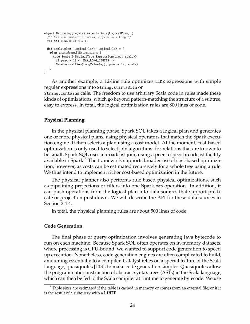
2.8 A short MLlib pipeline and the Python code to run it. We start with aDataFrame of (text, label) records, tokenize the text into words, run aterm frequency featurizer (.9513.6HashingTF) to get a feature vector, then trainlogistic regression. . . . . . . . . . . . . . . . . . . . . . . . . . . . . . 31

2.9 Performance of Shark, Impala and Spark SQL on the big data bench-mark queries [104]. . . . . . . . . . . . . . . . . . . . . . . . . . . . . . 33

2.10 Performance of an aggregation written using the native Spark Pythonand Scala APIs versus the DataFrame API. . . . . . . . . . . . . . . . 35

2.11 Performance of a two-stage pipeline written as a separate Spark SQLquery and Spark job (above) and an integrated DataFrame job (below). 35

2.12 Task launching overhead . . . . . . . . . . . . . . . . . . . . . . . . . . 40

3.1 The components of Structured Streaming. . . . . . . . . . . . . . . . . 49

vi

3.2 Structured Streaming’s semantics for two output modes. Logically,all input data received up to a point in processing time is viewedas a large input table, and the user provides a query that defines aresult table based on this input. Physically, Structured Streamingcomputes changes to the result table incrementally (without having tostore all input data) and outputs results based on its output mode.For complete mode, it outputs the whole result table (left), while forappend mode, it only outputs newly added records (right). . . . . . 54

3.3 Using .9513.6mapGroupsWithState to track the number of events per session, timing outsessions after 30 minutes. . . . . . . . . . . . . . . . . . . . . . . . . . 56

3.4 State management during the execution of Structured Streaming. In-put operators are responsible for defining epochs in each input sourceand saving information about them (e.g., offsets) reliably in the write-ahead log. Stateful operators also checkpoint state asynchronously,marking it with its epoch, but this does not need to happen on everyepoch. Finally, output operators log which epochs’ outputs havebeen reliably committed to the idempotent output sink; the very lastepoch may be rewritten on failure. . . . . . . . . . . . . . . . . . . . . 59

3.5 Information security platform use case. . . . . . . . . . . . . . . . . . 65

3.6 vs. Other Systems . . . . . . . . . . . . . . . . . . . . . . . . . . . . . . 69

3.7 System Scaling . . . . . . . . . . . . . . . . . . . . . . . . . . . . . . . . 69

3.8 Throughput results on the Yahoo! benchmark. . . . . . . . . . . . . . 69

3.9 Latency of continuous processing vs. input rate. Dashed line showsmax throughput in microbatch mode. . . . . . . . . . . . . . . . . . . 70

4.1 GraphX is a thin layer on top of the Spark general-purpose dataflowframework (lines of code). . . . . . . . . . . . . . . . . . . . . . . . . . 74

4.2 Example use of mrTriplets: Compute the number of older followersof each vertex. . . . . . . . . . . . . . . . . . . . . . . . . . . . . . . . 82

4.3 Distributed Graph Representation: The graph (left) is representedas a vertex and an edge collection (right). The edges are divided intothree edge partitions by applying a partition function (e.g., 2D Par-titioning). The vertices are partitioned by vertex id. Co-partitionedwith the vertices, GraphX maintains a routing table encoding theedge partitions for each vertex. If vertex 6 and adjacent edges (shownwith dotted lines) are restricted from the graph (e.g., by subgraph),they are removed from the corresponding collection by updating thebitmasks thereby enabling index reuse. . . . . . . . . . . . . . . . . . 86

vii

4.4 Impact of incrementally maintaining the triplets view: For bothPageRank and connected components, as vertices converge, commu-nication decreases due to incremental view maintenance. The initialrise in communication is due to message compression (Section 4.4.4);many PageRank values are initially the same. . . . . . . . . . . . . . 89

4.5 Sequential scan vs index scan: Connected components on the Twit-ter graph benefits greatly from switching to index scan after the 4thiteration, while PageRank benefits only slightly because the set ofactive vertices is large even at the 15th iteration. . . . . . . . . . . . . 90

4.6 Impact of automatic join elimination on communication and run-time: We ran PageRank for 20 iterations on the Twitter dataset withand without join elimination and found that join elimination reducesthe amount of communication by almost half and substantially de-creases the total execution time. . . . . . . . . . . . . . . . . . . . . . . 91

4.7 System Performance Comparison. (c) Spark did not finish within8000 seconds, Giraph and Spark + Part. ran out of memory. . . . . . 93

4.8 Strong scaling for PageRank on Twitter (10 Iterations) . . . . . . . . 93

4.9 Effect of partitioning on communication . . . . . . . . . . . . . . . . 93

4.10 Fault tolerance for PageRank on uk-2007-05 . . . . . . . . . . . . . . 93

4.11 Graph Analytics Pipeline: requires multiple collection and graphviews of the same data. . . . . . . . . . . . . . . . . . . . . . . . . . . 97

viii

List of Tables

4.1 Graph Datasets. Both graphs have highly skewed power-law degreedistributions. . . . . . . . . . . . . . . . . . . . . . . . . . . . . . . . . . 94

ix

Acknowledgements

I would like to express my sincerest gratitude to my advisor, Michael Franklin,for his guidance and support during my PhD studies. He gave me enough freedomto pursue my own ideas, yet pushed gently enough to make sure I was focused andstayed on track. It is from the discussions with him that I learned what it meant tobe a researcher: identifying problems, coming up with hypotheses, verifying them,disseminating knowledges, and making the world a better place.

The work in this dissertation started in a meeting I had with Ion Stoica and MateiZaharia on porting Hive to run over Spark in 2011. These two amazing researchershave been my de facto co-advisors. Ion taught me to be relentless and think big,and this thesis would not be without Matei’s initial work on Spark. Their emphasison attacking real-world, practical problems and pursuit for simplicity have forevershaped my view towards not only research but also engineering.

Michael Armbrust has been my closest collaborator in the last four years. Al-though I can’t think of another person with whom I have had more disagreementswith over Scala (and SBT), these conflicting views have sparkled many of the ideaspresented in this dissertation.

Through my work in Spark, I have been incredibly lucky to be able to work witha brilliant group of researchers and engineers. Together with Patrick Wendell, AliGhodsi, Xiangrui Meng, Tathagata Das, Josh Rosen, Davies Liu, Srinath Shankar,Shivaram Venkataraman, Kay Ousterhout, Joseph Gonzalez, Ankur Dave, andcountless others, our work also drove Spark to what it is today.

I am also grateful for the collaborators and graduate students that helped shapenot only my research but my whole graduate experience. An incomplete list of theseamazing colleagues include: Alan Fekete, Alon Halevy, Donald Kossmann, TimKraska, Sam Madden, Scott Shenker, Sameer Agarwal, Sara Alspaugh, Peter Bailis,Neil Conway, Dan Crankshaw, Cliff Engle, Daniel Haas, Shaddi Hasan, TimothyHunter, Haoyuan Li, David Moore, Aurojit Panda, Gene Pang, Evan Sparks, LiwenSun, Beth Trushkowsky, Andrew Wang, Jiannan Wang, Eugene Wu, David Zhu. Iwould also like to thank Sam Lightstone and Renee Miller for bringing me into thedatabase field in my undergraduate years.

Finally, it is not possible for me to adequately express how much credit myfamily deserve. They have been behind me and given me their unconditionalsupport, even if that meant to sacrifice the time we spent together. I am foreverindebted to their endless love, companionship, patience.

x

Chapter 1

Introduction

For the past few decades, data warehouses have been the primary data reposito-ries for analytics. Different teams within an organization get together to define adata model based on their business requirements. Achieving consensus on the datamodel often requires months, if not years, of discussions. Once such model is cre-ated, live transactional data, presented in tabular forms, are extracted, transformed,and loaded (ETL) into data warehouses at regular intervals. Business analystscreate reports and perform ad-hoc queries using SQL against the data warehouses.From a software architecture perspective, such data warehouses typically employthe Massively Parallel Processing (MPP) architecture, scaling often to only a fewhigh-end physical machines.

1.1 Challenges of Big Data

With the rise of the Internet, e-commerce, and connected devices, modern dataanalysis is undergoing a “Big Data” transformation. Unlike what’s described above,big data is defined by the following four key properties. The first three properties,volume, velocity, and variety, have been famously identified by Gartner as the “3Vsof Big Data” [5].

1. Volume: Data volumes are expanding drastically, creating the need to scale outboth data storage and processing across clusters of hundreds, if not thousands,of commodity machines. Most MPP databases employ a coarse-grained re-covery model, in which an entire query has to be resubmitted if a machinefails in the middle of a query. This approach works well for short querieswhen a retry is inexpensive, but faces significant challenges for long queriesas clusters scale up [9].

2. Velocity: The velocity of data arriving is also increasing. Often without humanin the loop, data can be generated and arrive at the speed of light. This opensup the opportunity for organizations to deploy systems that process data in

1

real-time. Nightly batch systems are no longer sufficient. In addition to thereal-time nature of data, business requirements also change at a faster pace,making it difficult to create a commonly agreed upon data model.

3. Variety: Semi-structured and unstructured data, such as images, text, andvoice, are becoming more common, while traditional data systems were builtto handle primarily structured, tabular data.

4. Complexity: The complexity of analysis has also grown. Modern data analysisoften employs sophisticated statistical methods, such as machine learningalgorithms, that go well beyond the roll-up and drill-down capabilities oftraditional database systems. While it may be possible to implement some ofthese functionalities using user-defined functions (UDFs) in MPP databases,these algorithms are often difficult to express and debug using UDFs. Theyare also computationally more expensive, exacerbating the need for systemsto recover gracefully from machine failures or mitigate slowdowns that arecommon in large clusters.

To tackle the big data problem, the industry has created a new class of systemsbased on a distributed dataflow architecture. At the time this thesis first started,MapReduce [48] and Dryad [69] were the most prominent examples of such systems.They employ a fine-grained fault tolerance model suitable for large clusters, wheretasks on failed or slow nodes can deterministically be re-executed on other nodes.These systems are also fairly general: [41] shows that these systems can expressmany statistical and machine learning algorithms, support unstructured data, and“schema-on-read” for greater flexibility.

However, dataflow engines lack many of the features that make MPP databasesefficient, and thus exhibit high latencies of tens of seconds to hours, even on simpleSQL queries. They are also designed primarily for batch analytics, and thus areunsuitable for real-time data processing. As such, most organizations tend to usethese systems alongside MPP databases to perform complex analytics.

To provide an effective environment for big data analysis, processing systemswill need to provide fine-grained fault recovery across a larger cluster of machines,support both SQL and complex analytics efficiently, and enable real-time compu-tation. This dissertation develops three related systems: Spark SQL, StructuredStreaming, and GraphX, that explore building effective systems for big data on topof a distributed dataflow engine.

1.2 Distributed Dataflow Frameworks

We use the term distributed dataflow framework to refer to cluster computeframeworks like MapReduce and its various generalizations. Although details varyfrom one framework to another, they typically satisfy the following properties:

2

1. a data model consisting of typed collections (i.e., a generalization of tables tounstructured data).

2. a coarse-grained data-parallel programming model composed of deterministicoperators which transform collections (e.g., map, group-by, and join).

3. a scheduler that breaks each job into a directed acyclic graph (DAG) of tasks,where each task runs on a (horizontal) partition of data, and the edges in thegraph indicate the input/output dependencies.

4. a runtime that can tolerate stragglers and partial cluster failures withoutrestarting.

MapReduce is a special distributed dataflow framework. Its programmingmodel exposes only two operators: map and reduce (a.k.a., group-by), and conse-quently each MapReduce job can contain at most two layers in its DAG of tasks.More modern frameworks such as DryadLINQ [129] and Spark [131] expose addi-tional dataflow operators such as fold and join, and can execute tasks with multiplelayers of dependencies. More generally, many shared-nothing parallel databasesalso satisfy the description of distributed dataflow frameworks when user-definedfunctions are employed, although databases typically have weaker fault-toleranceguarantees.

Distributed dataflow frameworks have enjoyed broad adoption for a widevariety of data processing tasks, including iterative machine learning. They havealso been shown to scale to thousands of nodes operating on petabytes of data.

1.3 Apache Spark

In order to understand the projects and ideas in this thesis, it is importantinitially to examine the background of Apache Spark.

Spark is a distributed dataflow framework with APIs in Scala, Java andPython [20]. Spark was initially released in 2010 by the UC Berkeley AMPLab,and the project was donated to the Apache Software Foundation in 2013 (and thus“Apache Spark”). It has since become the most active open source project for bigdata processing, with over 1200 people [4] having contributed code to the project.

Spark has several features that are particularly relevant to the work in thisdissertation:

1. Spark’s storage abstraction called Resilient Distributed Datasets (RDDs) [131]enables applications to keep data in memory, which is essential for complexanalytics such as machine learning algorithms and graph algorithms.

2. RDDs permit user-defined data partitioning, and the execution engine can ex-ploit this to co-partition RDDs and co-schedule tasks to avoid data movement.

3

This primitive is essential for performance optimizations for both relationalquery processing and advanced analytics.

3. Spark logs the lineage of operations used to build an RDD, enabling automaticreconstruction of lost partitions upon failures. Since the lineage graph isrelatively small even for long-running applications, this approach incursnegligible runtime overhead, unlike checkpointing, and can be left on withoutconcern for performance. Furthermore, Spark supports optional in-memorydistributed replication to reduce the amount of recomputation on failure.

4. Spark provides high-level programming APIs in Scala, Java, and Python thatcan be easily extended.

Next, we explain Resilient Distributed Datasets, the primary programmingabstraction of Spark.

1.3.1 Resilient Distributed Datasets (RDDs)

Spark’s main abstraction is resilient distributed datasets (RDDs), which are im-mutable, partitioned collections that can be created through various data-paralleloperators (e.g., map, group-by, hash-join). Each RDD is either a collection of data storedin an external storage system, such as a file in HDFS [2], or a derived dataset createdby applying operators to other RDDs. For example, given an RDD of (visitID, URL)pairs for visits to a website, we might compute an RDD of (URL, count) pairs byapplying a map operator to turn each event into an (URL, 1) pair, and then a reduceto add the counts by URL.

In Spark’s native API, RDD operations are invoked through a functional interfacesimilar to DryadLINQ [129] in Scala, Java or Python. For example, the Scala codefor the query above is:

val visits: RDD[String] = spark.hadoopFile("hdfs://...")

val counts: RDD[(String, Int)] = visits.map(v => (v.url, 1))

.reduceByKey((a, b) => a + b)

RDDs can contain arbitrary data types as elements (since Spark runs on theJVM, these elements are Java objects), and are automatically partitioned acrossthe cluster, but they are immutable once created, and they can only be createdthrough Spark’s deterministic parallel operators. These two restrictions, however,enable highly efficient fault recovery. In particular, instead of replicating each RDDacross nodes for fault-tolerance, Spark remembers the lineage of the RDD (the graphof operators used to build it), and recovers lost partitions by recomputing themfrom base data [131].1 For example, Figure 1.1 shows the lineage graph for theRDDs computed above. If Spark loses one of the partitions in the (URL, 1) RDD,

1 We assume that external files for RDDs representing data do not change, or that we can take asnapshot of a file when we create an RDD from it.

4

visits (HDFS file)

(URL, 1) pairs counts

map reduceByKey

Figure 1.1: Lineage graph for the RDDs in our Spark example. Oblongs representRDDs, while circles show partitions within a dataset. Lineage is tracked at thegranularity of partitions.

for example, it can recompute it by rerunning the map on just the correspondingpartition of the input file.

The RDD model offers several key benefits in our large-scale in-memory com-puting setting. First, RDDs can be written at the speed of DRAM instead of thespeed of the network, because there is no need to replicate each byte written toanother machine for fault-tolerance. DRAM in a modern server is over 10× fasterthan even a 10-Gigabit network. Second, Spark can keep just one copy of each RDDpartition in memory, saving precious memory compared with a replicated system,since it can always recover lost data using lineage. Third, when a node fails, itslost RDD partitions can be rebuilt in parallel across the other nodes, allowing faultrecovery.2 Fourth, even if a node is just slow (a “straggler”), we can recomputenecessary partitions on other nodes because RDDs are immutable so there are noconsistency concerns with having two copies of a partition.

One final note about the API is that RDDs are evaluated lazily. Each RDDrepresents a “plan” to compute a dataset, but Spark waits until the execution ofcertain output operations, such as count, to launch a computation. This allows theengine to do some simple query optimization, such as pipelining operations. Forinstance, in the example above, Spark will pipeline reading lines from the HDFSfile with the map operation, so that it never needs to materialize the intermediateresults. While such optimization is extremely useful, it is also limited because theengine does not understand the structure of the data in RDDs (which is arbitraryJava/Python objects) or the semantics of user functions (which contain arbitrarycode).

2 To provide fault tolerance across “shuffle” operations like a parallel reduce, the executionengine also saves the “map” side of the shuffle in memory on the source nodes, spilling to disk ifnecessary.

5

1.3.2 Fault Tolerance Guarantees

As data volume and analysis complexity increase, the runtime of data intensiveprograms also increases. As a result, it is more likely for stragglers or faults to occurin the course of a job. Spark provides the following fault tolerance properties:

1. Spark can tolerate the loss of any set of worker nodes. The execution enginewill re-execute any lost tasks and recompute any lost RDD partitions usinglineage.3 This is true even within a query: Spark will rerun any failed tasks,or lost dependencies of new tasks, without aborting the query.

2. Recovery is parallelized across the cluster. If a failed node contained 100RDD partitions, these can be rebuilt in parallel on 100 different nodes, quicklyrecovering the lost data.

3. The deterministic nature of RDDs also enables straggler mitigation: if a taskis slow, the system can launch a speculative “backup copy” of it on anothernode, as in MapReduce [48].

The RDD model is expressive, fault-tolerant, and well-suited for distributedcomputation. In the next section, we discuss why the RDD model alone is notsufficient to capture the common analytic workloads.

1.4 Expanding Use Cases

As demonstrated in previous sections, Spark’s RDD model was well suitedfor distributed computation. Immediately after Spark was open sourced, we saworganizations in the real world migrating their existing big data applications overfrom earlier generation systems such as Apache Hive [121]. As Spark’s adoptiongrew, we started to see new applications that were previously less common. Thissection documents the challenges early users encountered and how we addressthem in this thesis.

We see primarily four classes of big data use cases among Spark users [44]:

Interactive Analysis: A common use case is to query data interactively. In thiscontext, SQL is the standard language used by virtually all software tools andusers. The lack of SQL support in Spark was a huge inhibitor, because only themost sophisticated users would be able to perform interactive analysis using Spark.Chapter 2 introduces Spark SQL and discusses executing SQL queries efficientlyover Spark.

Extract, transform, load (ETL): One of the earliest and most popular use cases forSpark was to extract data from different data sources, join them, transform them,

3 Support for master recovery could also be added by reliably logging the RDD lineage graphand the submitted jobs, because this state is small, but we have not implemented this yet.

6

and then load them into other data sources. This is also sometimes referred to asa data pipeline. These ETL jobs are typically developed and maintained by dataengineers and employ custom code. Although they can sometimes be expressedin the form of SQL queries with user-defined functions, most ETL applicationdevelopers apply modern software engineering techniques that make SQL as aprogramming language a poor fit due to the lack of proper IDEs, continuousintegration and deployment tooling support.

While the RDD model provides a programmatic interface in Scala, the RDDabstraction does not differentiate the logical plan and the physical plan, makingit difficult for Spark to optimize user programs. As a result, users often need tohand tune their applications for better performance. In addition to executing SQLqueries, Chapter 2 shows how Spark SQL’s query optimizer and execution enginecan be extended to support a declarative, programmatic API called DataFrame thatis more suitable for building data pipelines.

Streaming Processing: Many large-scale data sources operate in real time, includ-ing sensors, logs from mobile applications, and the Internet of Things. The RDDmodel was designed to capture static, batch computation. Spark Streaming [133]was the first attempt at extending the RDD model to support stream processing.Spark Streaming worked by chunking a stream of data into infinite sets of smallbatch datasets, and required users to implement their batch jobs and streaming jobstwice, using completely different APIs. This approach led to diverging semanticsof users’ batch and stream pipelines over time. Chapter 3 develops StructuredStreaming, an extension to Spark SQL that automatically incrementalizes queryplans, and thus enabling users to write their data pipelines once but operate onboth batch and stream data.

Machine Learning and Graph Computation: As advanced analytics such as ma-chine learning and graph computation become increasingly common, many spe-cialized systems have been designed and implemented to support these workloads.These workloads, however, are only part of the larger analytic pipelines that oftenrequire distributed dataflow systems. Naively implementing these workloads onSpark leads to suboptimal performance that can be orders-of-magnitude slowerthan specialized systems. Chapter 4 presents GraphX, an efficient implementationof graph processing on top of Spark. Note that several systems to support machinelearning on Spark have been developed, but are beyond the scope of this thesis.Interested readers are referred to [115] for details.

To summarize, this thesis explores designs that expand Spark to cover theaforementioned use cases efficiently and effectively. In order to accomplish that, anew relational engine is created to support both SQL and the DataFrame program-ming model. The same engine is extended to support incremental computationand stream processing. Last but not least, the end of the thesis develops graphcomputation on top of dataflow engine.

7

1.5 Summary and Contributions

This dissertation is organized as follows.

Chapter 2 develops Spark SQL, a novel approach to combine relational queryprocessing with complex analytics. It unifies SQL with the DataFrame programmingmodel popularized by R and Python, enabling its users to more effectively deal withbig data applications that require a mix of processing techniques. It includes anextensible query optimizer called Catalyst to support a wide range of data sourcesand algorithms in big data. Spark SQL was initially open sourced and included inSpark in 2014, and has since become the most widely used component in Spark.

Chapter 3 develops Structured Streaming, an extension to Spark SQL that sup-ports real-time and streaming applications. Specifically, Structured Streaming canautomatically incrementalize queries against static, batch datasets to process stream-ing data. Structured Streaming is also designed to support end-to-end applicationsthat combine streaming, batch, and ad-hoc analytics, and to make them “correct bydefault”, with prefix consistency and exactly-once processing. Structured Stream-ing was open sourced in 2016, as part of Spark 2.0. We have observed multiplelarge-scale production use cases, the largest of which processes over 1PB of dataper month.

Chapter 4 presents GraphX on Spark, a system created by this dissertation tosupport graph processing. Historically, graph processing systems evolved sepa-rately from distributed dataflow frameworks for better performance. GraphX isan example of unifying graph processing with distributed dataflow systems. Byidentifying the essential dataflow patterns in graph computation and recastingoptimizations in graph processing systems as dataflow optimizations, GraphX canrecover the performance of specialized graph processing systems within a general-purpose distributed dataflow framework. GraphX was merged into Spark in its1.2 release. In Spark 2.0, it became the main graph processing system, in lieu of anolder system called Bagel.

Each of the aforementioned sections also covers the related works.

Finally, Chapter 5 concludes and discusses possible areas for future work.

8

Chapter 2

Spark SQL: SQL and DataFrames

As discussed in the previous chapter, modern data analysis is undergoing a “BigData” transformation, requiring data processing systems to support more than justSQL. This chapter develops Spark SQL, a new relational query processing systemthat combines SQL and the DataFrame programming API for complex analytics.We first describe Shark, our initial attempt at implementing SQL on top of Spark.We then describe Spark SQL’s user-facing API and the core internals to supportthat API, followed by performance evaluation on the system. Finally, we discussresearch applications and related work.

2.1 Introduction

Big data applications require a mix of processing techniques, data sources andstorage formats. The earliest systems designed for these workloads, such as Map-Reduce, gave users a powerful, but low-level, procedural programming interface.Programming such systems was onerous and required manual optimization by theuser to achieve high performance. As a result, multiple new systems sought toprovide a more productive user experience by offering relational interfaces to bigdata. Systems like Pig, Hive, Dremel [98, 121, 88] and Shark (Section 2.2) all takeadvantage of declarative queries to provide automatic optimizations.

While the popularity of relational systems shows that users often prefer writ-ing declarative queries, the relational approach is insufficient for many big dataapplications. First, users want to perform ETL to and from various data sourcesthat might be semi- or unstructured, requiring custom code. Second, users wantto perform advanced analytics, such as machine learning and graph processing,that are challenging to express in relational systems. In practice, we have observedthat most data pipelines would ideally be expressed with a combination of bothrelational queries and complex procedural algorithms. Unfortunately, these twoclasses of systems—relational and procedural—have until now remained largelydisjoint, forcing users to choose one paradigm or the other.

9

This chapter describes our effort to combine both models in Spark SQL, a majorextension in Apache Spark [131]. Rather than forcing users to pick between arelational or a procedural API, however, Spark SQL lets users seamlessly intermixthe two.

Spark SQL bridges the gap between the two models through two contributions.First, Spark SQL provides a DataFrame API that can perform relational operationson both external data sources and Spark’s built-in distributed collections. This APIis similar to the widely used data frame concept in R [108], but evaluates operationslazily so that it can perform relational optimizations. Second, to support the widerange of data sources and algorithms in big data, Spark SQL introduces a novelextensible optimizer called Catalyst. Catalyst makes it easy to add data sources,optimization rules, and data types for domains such as machine learning.

The DataFrame API offers rich relational/procedural integration within Sparkprograms. DataFrames are collections of structured records that can be manipulatedusing Spark’s procedural API, or using new relational APIs that allow richer opti-mizations. They can be created directly from Spark’s built-in distributed collectionsof Java/Python objects, enabling relational processing in existing Spark programs.Other Spark components, such as the machine learning library, take and produceDataFrames as well. DataFrames are more convenient and more efficient thanSpark’s procedural API in many common situations. For example, they make it easyto compute multiple aggregates in one pass using a SQL statement, something thatis difficult to express in traditional functional APIs. They also automatically storedata in a columnar format that is significantly more compact than Java/Pythonobjects. Finally, unlike existing data frame APIs in R and Python, DataFrameoperations in Spark SQL go through a relational optimizer, Catalyst.

To support a wide variety of data sources and analytics workloads in Spark SQL,we designed an extensible query optimizer called Catalyst. Catalyst uses features ofthe Scala programming language, such as pattern-matching, to express composablerules in a Turing-complete language. It offers a general framework for transformingtrees, which we use to perform analysis, planning, and runtime code generation.Through this framework, Catalyst can also be extended with new data sources,including semi-structured data such as JSON and “smart” data stores to which onecan push filters (e.g., HBase); with user-defined functions; and with user-definedtypes for domains such as machine learning. Functional languages are known to bewell-suited for building compilers [123], so it is perhaps no surprise that they madeit easy to build an extensible optimizer. We indeed have found Catalyst effective inenabling us to quickly add capabilities to Spark SQL, and since its release we haveseen external contributors easily add them as well.

Spark SQL was released in May 2014, and is now the most actively developedcomponent [4] in Apache Spark. Spark SQL has already been deployed in verylarge scale environments. For example, a large Internet company [67] uses SparkSQL to build data pipelines and run queries on an 8000-node cluster with over100 PB of data. Each individual query regularly operates on tens of terabytes. In

10

addition, many users adopt Spark SQL not just for SQL queries, but in programsthat combine it with procedural processing. For example, 2/3 of customers ofDatabricks Cloud, a hosted service running Spark, use Spark SQL within otherprogramming languages. Performance-wise, we find that Spark SQL is competitivewith SQL-only systems on Hadoop for relational queries. It is also up to 100× fasterand more memory-efficient than naive Spark code in computations expressible inSQL.

More generally, Spark SQL is an important evolution of the core Spark API.While Spark’s original functional programming API was quite general, it offeredonly limited opportunities for automatic optimization. Spark SQL simultaneouslymakes Spark accessible to more users and improves optimizations for existing ones.Within Spark, the community is now incorporating Spark SQL into more APIs:DataFrames are the standard data representation in a new “ML pipeline” API formachine learning, and we hope to expand this to other components, such as GraphXand streaming.

More fundamentally, our work shows that MapReduce-like execution modelscan be applied effectively to SQL, and offers a promising way to combine relationaland complex analytics.

2.2 Shark: The Initial SQL Implementation

In this section, we give an overview of Shark, the first implementation of SQLover Spark that attempted to combine relational query processing with complexanalytics. Many of the ideas in Shark have been reimplemented and inspired majorfeatures in Spark SQL. Refer to [127] for more details on Shark.

2.2.1 System Overview

Shark is compatible with Apache Hive, enabling users to run Hive queriesmuch faster without any changes to either the queries or the data. Thanks to itsHive compatibility, Shark can query data in any system that supports the Hadoopstorage API, including HDFS and Amazon S3. It also supports a wide range ofdata formats such as text, binary sequence files, JSON, and XML. It inherits Hive’sschema-on-read capability and nested data types [121].

Figure 2.1 shows the architecture of a Shark cluster, consisting of a single masternode and a number of worker nodes, with the warehouse metadata stored in anexternal transactional database. When a query is submitted to the master, Sharkcompiles the query into operator tree represented as RDDs, as we shall discuss inthe next subsection. These RDDs are then translated by Spark into a graph of tasksto execute on the worker nodes.

Cluster resources can optionally be allocated by a resource manager (e.g.,Hadoop YARN [2] or Apache Mesos [65]) that provides resource sharing and

11

!!Master!Node

!!Worker!Node

HDFS!DataNode

Resource!Manager!Daemon

!Spark!Runtime

Execution!Engine

Memstore

!!Worker!Node

HDFS!DataNode

Resource!Manager!Daemon

!Spark!Runtime

Execution!Engine

Memstore

Resource!Manager!SchedulerMetastore(System!Catalog)

Master!Process

HDFS!NameNode

Figure 2.1: Shark Architecture

isolation between different computing frameworks, allowing Shark to coexist withengines like Hadoop.

2.2.2 Executing SQL over Spark

Shark runs SQL queries over Spark using a three-step process similar to tradi-tional RDBMSs: query parsing, logical plan generation, and physical plan genera-tion.

Given a query, Shark uses the Hive query compiler to parse the query andgenerate an abstract syntax tree. The tree is then turned into a logical plan and basiclogical optimization, such as predicate pushdown, is applied. Up to this point, Sharkand Hive share an identical approach. Hive would then convert the operator intoa physical plan consisting of multiple MapReduce stages. In the case of Shark, itsoptimizer applies additional rule-based optimizations, such as pushing LIMIT downto individual partitions, and creates a physical plan consisting of transformations onRDDs rather than MapReduce jobs. We use a variety of operators already present inSpark, such as map and reduce, as well as new operators we implemented for Shark,such as broadcast joins. Spark’s master then executes this graph using standardMapReduce scheduling techniques, such as placing tasks close to their input data,rerunning lost tasks, and performing straggler mitigation [131].

2.2.3 Engine Extensions

While the basic approach outlined in the previous section makes it possible torun SQL over Spark, doing it efficiently is challenging. The prevalence of UDFs andcomplex analytic functions in Shark’s workload makes it difficult to determine anoptimal query plan at compile time, especially for new data that has not undergone

12

ETL. In addition, even with such a plan, naıvely executing it over Spark (or otherMapReduce runtimes) can be inefficient. In this, we outline several extensions wemade to Spark to efficiently store relational data and run SQL.

Partial DAG Execution (PDE): Systems like Shark and Hive are frequently usedto query fresh data that has not undergone a data loading process. This precludesthe use of static query optimization techniques that rely on accurate a priori datastatistics. To support dynamic query optimization in a distributed setting, weextended Spark to support partial DAG execution (PDE), a technique that allowsdynamic alteration of query plans based on data statistics collected at run-time. Thedynamic optimization is used to choose physical join execution strategies (broadcastjoin vs shuffle join) and to mitigate stragglers.

Columnar Memory Store: Shark implements a columnar memory store that en-codes data in a compressed form using JVM primitive arrays. Compared withSpark’s built-in cache, this store significantly reduces the space footprint overheadof JVM objects as well as speeding up garbage collection.

Data Co-partitioning: In some warehouse workloads, two fact tables are frequentlyjoined together. For example, the TPC-H benchmark frequently joins the lineitemand order tables. A technique commonly used by MPP databases is to co-partitionthe two tables based on their join key in the data loading process. In distributedfile systems like HDFS, the storage system is schema-agnostic, which preventsdata co-partitioning. Shark allows co-partitioning two tables on a common key forfaster joins in subsequent queries. When joining two co-partitioned tables, Shark’soptimizer constructs a DAG that avoids the expensive shuffle and instead uses maptasks to perform the join.

Partition Statistics and Map Pruning: Shark implements a form of data skippingcalled Map Pruning. The columnar memory store automatically tracks statistics(min value and max value) for each column for each partition. When a query isissued, the query optimizer uses this information to prune partitions that definitelydo not have matches. It has been shown in [127] that this technique reduces the sizeof data scanned for queries by a factor of 30 in real workloads.

2.2.4 Complex Analytics Support

A key design goal of Shark is to provide a single system capable of efficient SQLquery processing and complex analytics such as machine learning. Shark offers anAPI in Scala that can be called in Spark programs to extract Shark data as an RDD.Users can then write arbitrary Spark computations on the RDD, where they getautomatically pipelined with the SQL ones.

As an example of Scala integration, Listing 2.1 illustrates a data analysis pipelinethat performs logistic regression [63] over a user database using a combination ofSQL and Scala.

13

def logRegress(points: RDD[Point]): Vector {

var w = Vector(D, _ => 2 * rand.nextDouble - 1)

for (i <- 1 to ITERATIONS) {

val gradient = points.map { p =>

val denom = 1 + exp(-p.y * (w dot p.x))

(1 / denom - 1) * p.y * p.x

}.reduce(_ + _)

w -= gradient

}

w

}

val users = sql2rdd("SELECT * FROM user u JOIN comment c ON c.uid=u.uid")

val features = users.mapRows { row =>

new Vector(extractFeature1(row.getInt("age")),

extractFeature2(row.getStr("country")),

...)}

val trainedVector = logRegress(features.cache())

Listing 2.1: Logistic Regression Example

The map, mapRows, and reduce functions are automatically parallelized by Sharkto execute across a cluster, and the master program simply collects the output ofthe reduce function to update w. They are also pipelined with the reduce step ofthe join operation in SQL, passing column-oriented data from SQL to Scala codethrough an iterator interface.

The DataFrame API in Spark SQL was in part inspired by this functionality inShark.

2.2.5 Beyond Shark

While Shark showed good performance and good opportunities for integrationwith Spark programs, it had three important challenges. First, Shark could only beused to query external data stored in the Hive catalog, and was thus not useful forrelational queries on data inside a Spark program (e.g., on the errors RDD createdmanually above). Second, the only way to call Shark from Spark programs wasto put together a SQL string, which is inconvenient and error-prone to work within a modular program. Finally, the Hive optimizer was tailored for MapReduceand difficult to extend, making it hard to build new features such as data types formachine learning or support for new data sources.

With the experience from Shark, we wanted to extend relational processing tocover native RDDs in Spark and a much wider range of data sources. We set thefollowing goals for Spark SQL:

14

Spark SQL

Resilient Distributed Datasets

Spark

JDBC Console User Programs (Java, Scala, Python)

Catalyst Optimizer

DataFrame API

Figure 2.2: Interfaces to Spark SQL, and interaction with Spark.

1. Support relational processing both within Spark programs (on native RDDs)and on external data sources using a programmer-friendly API.

2. Provide high performance using established DBMS techniques.

3. Easily support new data sources, including semi-structured data and externaldatabases amenable to query federation.

4. Enable extension with advanced analytics algorithms such as graph processingand machine learning.

The rest of this chapter describes the core components and innovations in SparkSQL that address these goals.

2.3 Programming Interface

Spark SQL runs as a library on top of Spark, as shown in Figure 2.2. It exposesSQL interfaces, which can be accessed through JDBC/ODBC or through a command-line console, as well as the DataFrame API integrated into Spark’s supportedprogramming languages. We start by covering the DataFrame API, which lets usersintermix procedural and relational code. However, advanced functions can alsobe exposed in SQL through UDFs, allowing them to be invoked, for example, bybusiness intelligence tools. We discuss UDFs in Section 2.3.7.

2.3.1 DataFrame API

The main abstraction in Spark SQL’s API is a DataFrame, a distributed collectionof rows with the same schema. A DataFrame is equivalent to a table in a relationaldatabase, and can also be manipulated in similar ways to the “native” distributedcollections in Spark (RDDs).1 Unlike RDDs, DataFrames keep track of their schemaand support various relational operations that lead to more optimized execution.

1 We chose the name DataFrame because it is similar to structured data libraries in R and Python,and designed our API to resemble those.

15

DataFrames can be constructed from tables in a system catalog (based on externaldata sources) or from existing RDDs of native Java/Python objects (Section 2.3.5).Once constructed, they can be manipulated with various relational operators, suchas where and groupBy, which take expressions in a domain-specific language (DSL)similar to data frames in R and Python [108, 101]. Each DataFrame can also beviewed as an RDD of Row objects, allowing users to call procedural Spark APIssuch as map.2

Finally, unlike traditional data frame APIs, Spark DataFrames are lazy, in thateach DataFrame object represents a logical plan to compute a dataset, but no execu-tion occurs until the user calls a special “output operation” such as save. This en-ables rich optimization across all operations that were used to build the DataFrame.

To illustrate, the Scala code below defines a DataFrame from a table in Hive,derives another based on it, and prints a result:

users = spark.table("users")

young = users.where(users("age") < 21)

println(young.count())

In this code, users and young are DataFrames. The snippet users("age") < 21 isan expression in the data frame DSL, which is captured as an abstract syntax treerather than representing a Scala function as in the traditional Spark API. Finally,each DataFrame simply represents a logical plan (i.e., read the users table and filterfor age ¡ 21). When the user calls count, which is an output operation, Spark SQLbuilds a physical plan to compute the final result. This might include optimizationssuch as only scanning the “age” column of the data if its storage format is columnar,or even using an index in the data source to count the matching rows.

We next cover the details of the DataFrame API.

2.3.2 Data Model

Spark SQL uses a nested data model based on Hive [66] for tables andDataFrames. It supports all major SQL data types, including boolean, integer,double, decimal, string, date, and timestamp, as well as complex (i.e., non-atomic)data types: structs, arrays, maps and unions. Complex data types can also be nestedtogether to create more powerful types. Unlike many traditional DBMSes, SparkSQL provides first-class support for complex data types in the query language andthe API. In addition, Spark SQL also supports user-defined types, as described inSection 2.4.4.

Using this type system, we have been able to accurately model data from avariety of sources and formats, including Hive, relational databases, JSON, andnative objects in Java/Scala/Python.

2These Row objects are constructed on the fly and do not necessarily represent the internal storageformat of the data, which is typically columnar.

16

2.3.3 DataFrame Operations

Users can perform relational operations on DataFrames using a domain-specificlanguage (DSL) similar to R data frames [108] and Python Pandas [101]. DataFramessupport all common relational operators, including projection (select), filter (where),join, and aggregations (groupBy). These operators all take expression objects in alimited DSL that lets Spark capture the structure of the expression. For example,the following code computes the number of female employees in each department.

employees

.join(dept, employees("deptId") === dept("id"))

.where(employees("gender") === "female")

.groupBy(dept("id"), dept("name"))

.agg(count("name"))

Here, employees is a DataFrame, and employees("deptId") is an expression rep-resenting the deptId column. Expression objects have many operators that returnnew expressions, including the usual comparison operators (e.g.,=== for equalitytest, > for greater than) and arithmetic ones (+, -, etc). They also support aggregates,such as count("name"). All of these operators build up an abstract syntax tree (AST)of the expression, which is then passed to Catalyst for optimization. This is unlikethe native Spark API that takes functions containing arbitrary Scala/Java/Pythoncode, which are then opaque to the runtime engine. For a detailed listing of the API,we refer readers to Spark’s official documentation [20].

Apart from the relational DSL, DataFrames can be registered as temporary tablesin the system catalog and queried using SQL. The code below shows an example:

users.where(users("age") < 21).registerTempTable("young")

ctx.sql("SELECT count(*), avg(age) FROM young")

SQL is sometimes convenient for computing multiple aggregates concisely, andalso allows programs to expose datasets through JDBC/ODBC. The DataFramesregistered in the catalog are still unmaterialized views, so that optimizations canhappen across SQL and the original DataFrame expressions. However, DataFramescan also be materialized, as we discuss in Section 2.3.6.

2.3.4 DataFrames versus Relational Query Languages

While on the surface, DataFrames provide the same operations as relationalquery languages like SQL and Pig [98], we found that they can be significantly easierfor users to work with thanks to their integration in a full programming language.For example, users can break up their code into Scala, Java or Python functions thatpass DataFrames between them to build a logical plan, and will still benefit fromoptimizations across the whole plan when they run an output operation. Likewise,developers can use control structures like if statements and loops to structure theirwork.

17

To simplify programming in DataFrames, we also made Spark SQL analyzelogical plans eagerly (i.e., to identify whether the column names used in expressionsexist in the underlying tables, and whether their data types are appropriate), eventhough query results are computed lazily. Thus, Spark SQL reports an error as soonas user types an invalid line of code instead of waiting until execution. This is againeasier to work with than a large SQL statement.

2.3.5 Querying Native Datasets

Real-world pipelines often extract data from heterogeneous sources and run awide variety of algorithms from different programming libraries. To interoperatewith procedural Spark code, Spark SQL allows users to construct DataFramesdirectly against RDDs of objects native to the programming language. Spark SQLcan automatically infer the schema of these objects using reflection. In Scala andJava, the type information is extracted from the language’s type system (fromJavaBeans and Scala case classes). In Python, Spark SQL samples the dataset toperform schema inference due to the dynamic type system.

For example, the Scala code below defines a DataFrame from an RDD of Userobjects. Spark SQL automatically detects the names (“name” and “age”) and datatypes (string and int) of the columns.

case class User(name: String, age: Int)

// Create an RDD of User objects

usersRDD = spark.parallelize(

List(User("Alice", 22), User("Bob", 19)))

// View the RDD as a DataFrame

usersDF = usersRDD.toDF

Internally, Spark SQL creates a logical data scan operator that points to the RDD.This is compiled into a physical operator that accesses fields of the native objects.It is important to note that this is very different from traditional object-relationalmapping (ORM). ORMs often incur expensive conversions that translate an entireobject into a different format. In contrast, Spark SQL accesses the native objectsin-place, extracting only the fields used in each query.

The ability to query native datasets lets users run optimized relational operationswithin existing Spark programs. In addition, it makes it simple to combine RDDswith external structured data. For example, we could join the users RDD with atable in Hive:views = ctx.table("pageviews")

usersDF.join(views, usersDF("name") === views("user"))

18

2.3.6 In-Memory Caching

Like Shark before it, Spark SQL can materialize (often referred to as “cache”)hot data in memory using columnar storage. Compared with Spark’s native cache,which simply stores data as JVM objects, the columnar cache can reduce mem-ory footprint by an order of magnitude because it applies columnar compressionschemes such as dictionary encoding and run-length encoding. Caching is partic-ularly useful for interactive queries and for the iterative algorithms common inmachine learning. It can be invoked by calling cache() on a DataFrame.

2.3.7 User-Defined Functions

User-defined functions (UDFs) have been an important extension point fordatabase systems. For example, MySQL relies on UDFs to provide basic supportfor JSON data. A more advanced example is MADLib’s use of UDFs to imple-ment machine learning algorithms for Postgres and other database systems [42].However, database systems often require UDFs to be defined in a separate pro-gramming environment that is different from the primary query interfaces. SparkSQL’s DataFrame API supports inline definition of UDFs, without the complicatedpackaging and registration process found in other database systems. This featurehas proven crucial for the adoption of the API.

In Spark SQL, UDFs can be registered inline by passing Scala, Java or Pythonfunctions, which may use the full Spark API internally. For example, given a modelobject for a machine learning model, we could register its prediction function as aUDF:val model: LogisticRegressionModel = ...

ctx.udf.register("predict",

(x: Float, y: Float) => model.predict(Vector(x, y)))

ctx.sql("SELECT predict(age, weight) FROM users")

Once registered, the UDF can also be used via the JDBC/ODBC interface bybusiness intelligence tools. In addition to UDFs that operate on scalar values likethe one here, one can define UDFs that operate on an entire table by taking its name,as in MADLib [42], and use the distributed Spark API within them, thus exposingadvanced analytics functions to SQL users. Finally, because UDF definitions andquery execution are expressed using the same general-purpose language (e.g., Scalaor Python), users can debug or profile the entire program using standard tools.

The example above demonstrates a common use case in many pipelines, i.e., onethat employs both relational operators and advanced analytics methods that arecumbersome to express in SQL. The DataFrame API lets developers seamlessly mixthese methods.

19

2.4 Catalyst Optimizer

To implement Spark SQL, we designed a new extensible optimizer, Catalyst,based on functional programming constructs in Scala. Catalyst’s extensible designhad two purposes. First, we wanted to make it easy to add new optimization tech-niques and features to Spark SQL, especially to tackle various problems we wereseeing specifically with “big data” (e.g., semistructured data and advanced analyt-ics). Second, we wanted to enable external developers to extend the optimizer—forexample, by adding data source specific rules that can push filtering or aggregationinto external storage systems, or support for new data types. Catalyst supportsboth rule-based and cost-based optimization.

While extensible optimizers have been proposed in the past, they have typicallyrequired a complex domain specific language to specify rules, and an “optimizercompiler” to translate the rules into executable code [59, 60]. This leads to a signifi-cant learning curve and maintenance burden. In contrast, Catalyst uses standardfeatures of the Scala programming language, such as pattern-matching [49], to letdevelopers use the full programming language while still making rules easy tospecify. Functional languages were designed in part to build compilers, so we foundScala well-suited to this task. Nonetheless, Catalyst is, to our knowledge, the firstproduction-quality query optimizer built on such a language.

At its core, Catalyst contains a general library for representing trees and applyingrules to manipulate them.3 On top of this framework, we have built libraries specificto relational query processing (e.g., expressions, logical query plans), and severalsets of rules that handle different phases of query execution: analysis, logicaloptimization, physical planning, and code generation to compile parts of queries toJava bytecode. For the latter, we use another Scala feature, quasiquotes [113], thatmakes it easy to generate code at runtime from composable expressions. Finally,Catalyst offers several public extension points, including external data sources anduser-defined types.

2.4.1 Trees

The main data type in Catalyst is a tree composed of node objects. Each node hasa node type and zero or more children. New node types are defined in Scala as sub-classes of the TreeNode class. These objects are immutable and can be manipulatedusing functional transformations, as discussed in the next subsection.

As a simple example, suppose we have the following three node classes for avery simple expression language:4

3Cost-based optimization is performed by generating multiple plans using rules, and thencomputing their costs.

4 We use Scala syntax for classes here, where each class’s fields are defined in parentheses, withtheir types given using a colon.

20

Add

Attribute(x) Add

Literal(1) Literal(2)

Figure 2.3: Catalyst tree for the expression x+(1+2).

• Literal(value: Int): a constant value

• Attribute(name: String): an attribute from an input row, e.g., “x”

• Add(left: TreeNode, right: TreeNode): sum of two expressions.

These classes can be used to build up trees; for example, the tree for the expres-sion x+(1+2), shown in Figure 2.3, would be represented in Scala code as follows:

Add(Attribute(x), Add(Literal(1), Literal(2)))

2.4.2 Rules

Trees can be manipulated using rules, which are functions from a tree to anothertree. While a rule can run arbitrary code on its input tree (given that this tree isjust a Scala object), the most common approach is to use a set of pattern matchingfunctions that find and replace subtrees with a specific structure.

Pattern matching is a feature of many functional languages that allows extractingvalues from potentially nested structures of algebraic data types. In Catalyst, treesoffer a transformmethod that applies a pattern matching function recursively onall nodes of the tree, transforming the ones that match each pattern to a result. Forexample, we could implement a rule that folds Add operations between constantsas follows:tree.transform {

case Add(Literal(c1), Literal(c2)) => Literal(c1+c2)

}

Applying this to the tree for x+(1+2), in Figure 2.3, would yield the new tree x+3.The case keyword here is Scala’s standard pattern matching syntax [49], and can beused to match on the type of an object as well as give names to extracted values (c1and c2 here).

The pattern matching expression that is passed to transform is a partial function,meaning that it only needs to match to a subset of all possible input trees. Catalystwill tests which parts of a tree a given rule applies to, automatically skipping overand descending into subtrees that do not match. This ability means that rules onlyneed to reason about the trees where a given optimization applies and not those

21

SQL Query

DataFrame

Unresolved Logical Plan Logical Plan Optimized

Logical Plan Physical

Plans Physical

Plans RDDs Selected Physical

Plan

Analysis Logical Optimization

Physical Planning

Cos

t Mod

el

Physical Plans

Code Generation

Catalog

Figure 2.4: Phases of query planning in Spark SQL. Rounded rectangles representCatalyst trees.

that do not match. Thus, rules do not need to be modified as new types of operatorsare added to the system.

Rules (and Scala pattern matching in general) can match multiple patterns in thesame transform call, making it very concise to implement multiple transformationsat once:tree.transform {

case Add(Literal(c1), Literal(c2)) => Literal(c1+c2)

case Add(left, Literal(0)) => left

case Add(Literal(0), right) => right

}

In practice, rules may need to execute multiple times to fully transform a tree.Catalyst groups rules into batches, and executes each batch until it reaches a fixedpoint, that is, until the tree stops changing after applying its rules. Running rulesto fixed point means that each rule can be simple and self-contained, and yet stilleventually have larger global effects on a tree. In the example above, repeatedapplication would constant-fold larger trees, such as (x+0)+(3+3). As anotherexample, a first batch might analyze an expression to assign types to all of theattributes, while a second batch might use these types to do constant folding. Aftereach batch, developers can also run sanity checks on the new tree (e.g., to see thatall attributes were assigned types), often also written via recursive matching.

Finally, rule conditions and their bodies can contain arbitrary Scala code. Thisgives Catalyst more power than domain specific languages for optimizers, whilekeeping it concise for simple rules.

In our experience, functional transformations on immutable trees make thewhole optimizer very easy to reason about and debug. They also enable paralleliza-tion in the optimizer, although we do not yet exploit this.

2.4.3 Using Catalyst in Spark SQL

We use Catalyst’s general tree transformation framework in four phases, shownin Figure 2.4: (1) analyzing a logical plan to resolve references, (2) logical planoptimization, (3) physical planning, and (4) code generation to compile parts ofthe query to Java bytecode. In the physical planning phase, Catalyst may generate

22

multiple plans and compare them based on cost. All other phases are purely rule-based. Each phase uses different types of tree nodes; Catalyst includes librariesof nodes for expressions, data types, and logical and physical operators. We nowdescribe each of these phases.

Analysis

Spark SQL begins with a relation to be computed, either from an abstract syntaxtree (AST) returned by a SQL parser, or from a DataFrame object constructed usingthe API. In both cases, the relation may contain unresolved attribute references orrelations: for example, in the SQL query SELECT col FROM sales, the type of col, oreven whether it is a valid column name, is not known until we look up the tablesales. An attribute is called unresolved if we do not know its type or have notmatched it to an input table (or an alias). Spark SQL uses Catalyst rules and aCatalog object that tracks the tables in all data sources to resolve these attributes. Itstarts by building an “unresolved logical plan” tree with unbound attributes anddata types, then applies rules that do the following:

• Looking up relations by name from the catalog.

• Mapping named attributes, such as col, to the input provided given operator’schildren.

• Determining which attributes refer to the same value to give them a uniqueID (which later allows optimization of expressions such as col = col).

• Propagating and coercing types through expressions: for example, we cannotknow the type of 1 + col until we have resolved col and possibly cast itssubexpressions to compatible types.

In total, the rules for the analyzer are about 1000 lines of code.

Logical Optimization

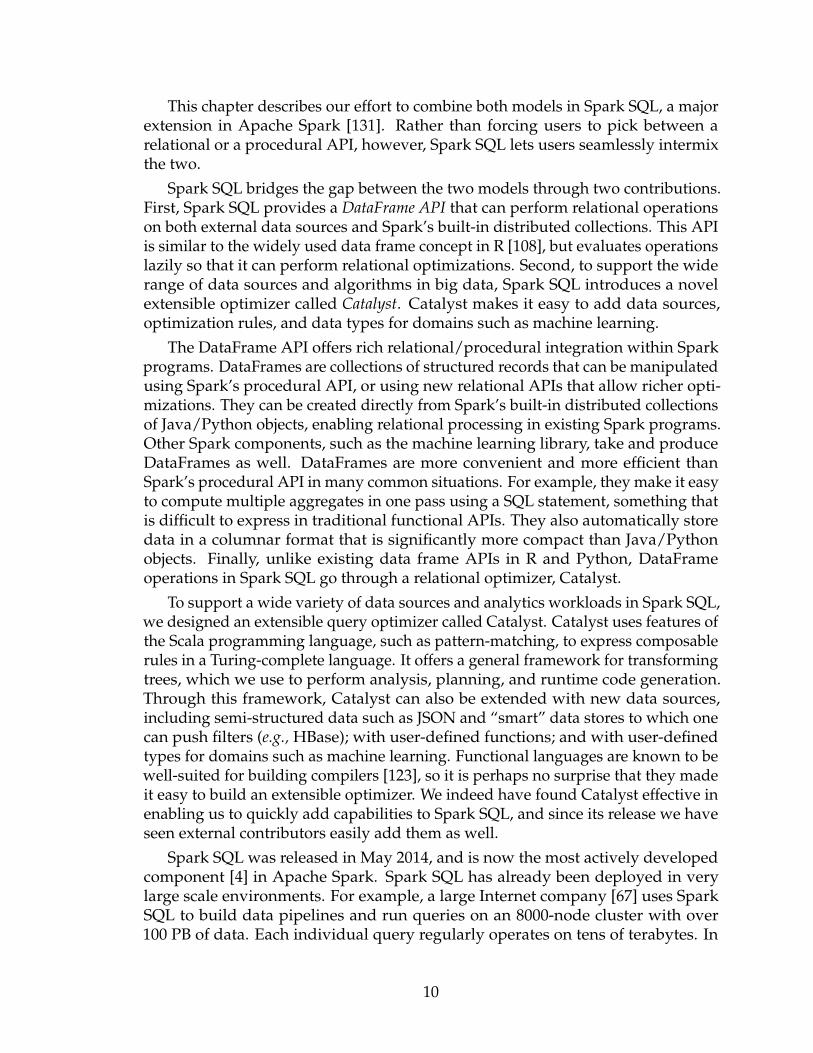
The logical optimization phase applies standard rule-based optimizations to thelogical plan. These include constant folding, predicate pushdown, projection prun-ing, null propagation, Boolean expression simplification, and other rules. In general,we have found it extremely simple to add rules for a wide variety of situations.For example, when we added the fixed-precision DECIMAL type to Spark SQL, wewanted to optimize aggregations such as sums and averages on DECIMALs with smallprecisions; it took 12 lines of code to write a rule that finds such decimals in SUMand AVG expressions, and casts them to unscaled 64-bit LONGs, does the aggregationon that, then converts the result back. A simplified version of this rule that onlyoptimizes SUM expressions is reproduced below:

23

object DecimalAggregates extends Rule[LogicalPlan] {

/** Maximum number of decimal digits in a Long */

val MAX_LONG_DIGITS = 18

def apply(plan: LogicalPlan): LogicalPlan = {

plan transformAllExpressions {

case Sum(e @ DecimalType.Expression(prec, scale))

if prec + 10 <= MAX_LONG_DIGITS =>

MakeDecimal(Sum(LongValue(e)), prec + 10, scale)

}

}

As another example, a 12-line rule optimizes LIKE expressions with simpleregular expressions into String.startsWith orString.contains calls. The freedom to use arbitrary Scala code in rules made thesekinds of optimizations, which go beyond pattern-matching the structure of a subtree,easy to express. In total, the logical optimization rules are 800 lines of code.

Physical Planning

In the physical planning phase, Spark SQL takes a logical plan and generatesone or more physical plans, using physical operators that match the Spark execu-tion engine. It then selects a plan using a cost model. At the moment, cost-basedoptimization is only used to select join algorithms: for relations that are known tobe small, Spark SQL uses a broadcast join, using a peer-to-peer broadcast facilityavailable in Spark.5 The framework supports broader use of cost-based optimiza-tion, however, as costs can be estimated recursively for a whole tree using a rule.We thus intend to implement richer cost-based optimization in the future.

The physical planner also performs rule-based physical optimizations, suchas pipelining projections or filters into one Spark map operation. In addition, itcan push operations from the logical plan into data sources that support predi-cate or projection pushdown. We will describe the API for these data sources inSection 2.4.4.

In total, the physical planning rules are about 500 lines of code.

Code Generation

The final phase of query optimization involves generating Java bytecode torun on each machine. Because Spark SQL often operates on in-memory datasets,where processing is CPU-bound, we wanted to support code generation to speedup execution. Nonetheless, code generation engines are often complicated to build,amounting essentially to a compiler. Catalyst relies on a special feature of the Scalalanguage, quasiquotes [113], to make code generation simpler. Quasiquotes allowthe programmatic construction of abstract syntax trees (ASTs) in the Scala language,which can then be fed to the Scala compiler at runtime to generate bytecode. We use

5 Table sizes are estimated if the table is cached in memory or comes from an external file, or if itis the result of a subquery with a LIMIT.

24

0 10 20 30 40

Generated

Hand-written

Intepreted

Runtime (seconds)

Figure 2.5: A comparision of the performance evaluating the expresion x+x+x, wherex is an integer, 1 billion times.

Catalyst to transform a tree representing an expression in SQL to an AST for Scalacode to evaluate that expression, and then compile and run the generated code.

As a simple example, consider the Add, Attribute and Literal tree nodes in-troduced in Section 2.4.2, which allowed us to write expressions such as (x+y)+1.Without code generation, such expressions would have to be interpreted for eachrow of data, by walking down a tree of Add, Attribute and Literal nodes. Thisintroduces large amounts of branches and virtual function calls that slow downexecution. With code generation, we can write a function to translate a specificexpression tree to a Scala AST as follows:def compile(node: Node): AST = node match {

case Literal(value) => q"$value"

case Attribute(name) => q"row.get($name)"

case Add(left, right) =>

q"${compile(left)} + ${compile(right)}"

}

The strings beginning with q are quasiquotes, meaning that although they looklike strings, they are parsed by the Scala compiler at compile time and representASTs for the code within. Quasiquotes can have variables or other ASTs splicedinto them, indicated using $ notation. For example, Literal(1)would become theScala AST for 1, while Attribute("x") becomes row.get("x"). In the end, a treelike Add(Literal(1), Attribute("x")) becomes an AST for a Scala expression like1+row.get("x").

Quasiquotes are type-checked at compile time to ensure that only appropriateASTs or literals are substituted in, making them significantly more useable thanstring concatenation, and they result directly in a Scala AST instead of runningthe Scala parser at runtime. Moreover, they are highly composable, as the codegeneration rule for each node does not need to know how the trees returned byits children were built. Finally, the resulting code is further optimized by theScala compiler in case there are expression-level optimizations that Catalyst missed.Figure 2.5 shows that quasiquotes let us generate code with performance similar tohand-tuned programs.

We have found quasiquotes very straightforward to use for code generation, andwe observed that even new contributors to Spark SQL could quickly add rules fornew types of expressions. Quasiquotes also work well with our goal of running on

25

native Java objects: when accessing fields from these objects, we can code-generatea direct access to the required field, instead of having to copy the object into a SparkSQL Row and use the Row’s accessor methods. Finally, it was straightforward tocombine code-generated evaluation with interpreted evaluation for expressions wedo not yet generate code for, since the Scala code we compile can directly call intoour expression interpreter.

In total, Catalyst’s code generator is about 700 lines of code.

2.4.4 Extension Points

Catalyst’s design around composable rules makes it easy for users and third-party libraries to extend. Developers can add batches of rules to each phase of queryoptimization at runtime, as long as they adhere to the contract of each phase (e.g.,ensuring that analysis resolves all attributes). However, to make it even simpler toadd some types of extensions without understanding Catalyst rules, we have alsodefined two narrower public extension points: data sources and user-defined types.These still rely on facilities in the core engine to interact with the rest of the rest ofthe optimizer.

Data Sources

Developers can define a new data source for Spark SQL using several APIs,which expose varying degrees of possible optimization. All data sources mustimplement a createRelation function that takes a set of key-value parameters andreturns a BaseRelation object for that relation, if one can be successfully loaded.Each BaseRelation contains a schema and an optional estimated size in bytes.6 Forinstance, a data source representing MySQL may take a table name as a parameter,and ask MySQL for an estimate of the table size.

To let Spark SQL read the data, a BaseRelation can implement one of severalinterfaces that let them expose varying degrees of sophistication. The simplest,TableScan, requires the relation to return an RDD of Row objects for all of the datain the table. A more advanced PrunedScan takes an array of column names toread, and should return Rows containing only those columns. A third interface,PrunedFilteredScan, takes both desired column names and an array of Filter objects,which are a subset of Catalyst’s expression syntax, allowing predicate pushdown.7

The filters are advisory, i.e., the data source should attempt to return only rowspassing each filter, but it is allowed to return false positives in the case of filters thatit cannot evaluate. Finally, a CatalystScan interface is given a complete sequence

6 Unstructured data sources can also take a desired schema as a parameter; for example, there isa CSV file data source that lets users specify column names and types.

7At the moment, Filters include equality, comparisons against a constant, and IN clauses, each onone attribute.

26

of Catalyst expression trees to use in predicate pushdown, though they are againadvisory.

These interfaces allow data sources to implement various degrees of optimiza-tion, while still making it easy for developers to add simple data sources of virtuallyany type. We and others have used the interface to implement the following datasources:

• CSV files, which simply scan the whole file, but allow users to specify aschema.

• Avro [18], a self-describing binary format for nested data.

• Parquet [19], a columnar file format for which we support column pruning aswell as filters.

• A JDBC data source that scans ranges of a table from an RDBMS in paralleland pushes filters into the RDBMS to minimize communication.

To use these data sources, programmers specify their package names in SQLstatements, passing key-value pairs for configuration options. For example, theAvro data source takes a path to the file:

CREATE TEMPORARY TABLE messages

USING com.databricks.spark.avro

OPTIONS (path "messages.avro")

All data sources can also expose network locality information, i.e., which ma-chines each partition of the data is most efficient to read from. This is exposedthrough the RDD objects they return, as RDDs have a built-in API for data local-ity [131].

Finally, similar interfaces exist for writing data to an existing or new table. Theseare simpler because Spark SQL just provides an RDD of Row objects to be written.

User-Defined Types (UDTs)

One feature we wanted to allow advanced analytics in Spark SQL was user-defined types. For example, machine learning applications may need a vector type,and graph algorithms may need types for representing a graph, which is possibleover relational tables [126]. Adding new types can be challenging, however, asdata types pervade all aspects of the execution engine. For example, in Spark SQL,the built-in data types are stored in a columnar, compressed format for in-memorycaching (Section 2.3.6), and in the data source API from the previous section, weneed to expose all possible data types to data source authors.

In Catalyst, we solve this issue by mapping user-defined types to structurescomposed of Catalyst’s built-in types, described in Section 2.3.2. To register a Scala

27

type as a UDT, users provide a mapping from an object of their class to a CatalystRow of built-in types, and an inverse mapping back. In user code, they can now usethe Scala type in objects that they query with Spark SQL, and it will be converted tobuilt-in types under the hood. Likewise, they can register UDFs (see Section 2.3.7)that operate directly on their type.

As a short example, suppose we want to register two-dimensional points (x, y)as a UDT. We can represent such vectors as two DOUBLE values. To register the UDT,we write the following:class PointUDT extends UserDefinedType[Point] {

def dataType = StructType(Seq( // Our native structure

StructField("x", DoubleType),

StructField("y", DoubleType)

))

def serialize(p: Point) = Row(p.x, p.y)

def deserialize(r: Row) =

Point(r.getDouble(0), r.getDouble(1))

}

After registering this type, Points will be recognized within native objects thatSpark SQL is asked to convert to DataFrames, and will be passed to UDFs definedon Points. In addition, Spark SQL will store Points in a columnar format whencaching data (compressing x and y as separate columns), and Points will be writableto all of Spark SQL’s data sources, which will see them as pairs of DOUBLEs. We usethis capability in Spark’s machine learning library, as we describe in Section 2.5.2.

2.5 Advanced Analytics Features

In this section, we describe three features we added to Spark SQL specificallyto handle challenges in “big data” environments. First, in these environments,data is often unstructured or semistructured. While parsing such data procedu-rally is possible, it leads to lengthy boilerplate code. To let users query the dataright away, Spark SQL includes a schema inference algorithm for JSON and othersemistructured data. Second, large-scale processing often goes beyond aggregationand joins to machine learning on the data. We describe how Spark SQL is beingincorporated into a new high-level API for Spark’s machine learning library [89].Last, data pipelines often combine data from disparate storage systems. Buildingon the data sources API in Section 2.4.4, Spark SQL supports query federation,allowing a single program to efficiently query disparate sources. These features allbuild on the Catalyst framework.

2.5.1 Schema Inference for Semistructured Data

Semistructured data is common in large-scale environments because it is easyto produce and to add fields to over time. Among Spark users, we have seen veryhigh usage of JSON for input data. Unfortunately, JSON is cumbersome to work

28

{

"text": "This is a tweet about #Spark",

"tags": ["#Spark"],

"loc": {"lat": 45.1, "long": 90}

}

{

"text": "This is another tweet",

"tags": [],

"loc": {"lat": 39, "long": 88.5}

}

{

"text": "A #tweet without #location",

"tags": ["#tweet", "#location"]

}

Figure 2.6: A sample set of JSON records, representing tweets.

text STRING NOT NULL,

tags ARRAY<STRING NOT NULL> NOT NULL,

loc STRUCT<lat FLOAT NOT NULL, long FLOAT NOT NULL>

Figure 2.7: Schema inferred for the tweets in Figure 2.6.

with in a procedural environment like Spark or MapReduce: most users resortedto ORM-like libraries (e.g., Jackson [71]) to map JSON structures to Java objects, orsome tried parsing each input record directly with lower-level libraries.

In Spark SQL, we added a JSON data source that automatically infers a schemafrom a set of records. For example, given the JSON objects in Figure 2.6, the libraryinfers the schema shown in Figure 2.7. Users can simply register a JSON file as atable and query it with syntax that accesses fields by their path, such as:

SELECT loc.lat, loc.long FROM tweets

WHERE text LIKE ’%Spark%’ AND tags IS NOT NULL

Our schema inference algorithm works in one pass over the data, and can also berun on a sample of the data if desired. It is related to prior work on schema inferencefor XML and object databases [27, 64, 95], but simpler because it only infers a statictree structure, without allowing recursive nesting of elements at arbitrary depths.

Specifically, the algorithm attempts to infer a tree of STRUCT types, each of whichmay contain atoms, arrays, or other STRUCTs. For each field defined by a distinctpath from the root JSON object (e.g.,tweet.loc.latitude), the algorithm finds themost specific Spark SQL data type that matches observed instances of the field.For example, if all occurrences of that field are integers that fit into 32 bits, it willinfer INT; if they are larger, it will use LONG (64-bit) or DECIMAL (arbitrary precision);if there are also fractional values, it will use FLOAT. For fields that display multipletypes, Spark SQL uses STRING as the most generic type, preserving the original JSONrepresentation. And for fields that contain arrays, it uses the same “most specific

29

supertype” logic to determine an element type from all the observed elements. Weimplement this algorithm using a single reduce operation over the data, which startswith schemata (i.e., trees of types) from each individual record and merges themusing an associative “most specific supertype” function that generalizes the types ofeach field. This makes the algorithm both single-pass and communication-efficient,as a high degree of reduction happens locally on each node.

As a short example, note how in Figures 2.6 and 2.7, the algorithm generalizedthe types of loc.lat and loc.long. Each field appears as an integer in one recordand a floating-point number in another, so the algorithm returns FLOAT. Note alsohow for the tags field, the algorithm inferred an array of strings that cannot be null.

In practice, we have found this algorithm to work well with real-world JSONdatasets. For example, it correctly identifies a usable schema for JSON tweets fromTwitter’s firehose, which contain around 100 distinct fields and a high degree ofnesting. Multiple Databricks customers have also successfully applied it to theirinternal JSON formats.

In Spark SQL, we also use the same algorithm for inferring schemas of RDDsof Python objects (see Section 2.3), as Python is not statically typed so an RDD cancontain multiple object types. In the future, we plan to add similar inference for CSVfiles and XML. Developers have found the ability to view these types of datasets astables and immediately query them or join them with other data extremely valuablefor their productivity.

2.5.2 Integration with Spark’s Machine Learning Library

As an example of Spark SQL’s utility in other Spark modules, MLlib, Spark’s ma-chine learning library, introduced a new high-level API that uses DataFrames [89].This new API is based on the concept of machine learning pipelines, an abstractionin other high-level ML libraries like SciKit-Learn [112]. A pipeline is a graph oftransformations on data, such as feature extraction, normalization, dimensionalityreduction, and model training, each of which exchange datasets. Pipelines are auseful abstraction because ML workflows have many steps; representing these stepsas composable elements makes it easy to change parts of the pipeline or to searchfor tuning parameters at the level of the whole workflow.

To exchange data between pipeline stages, MLlib’s developers needed a formatthat was compact (as datasets can be large) yet flexible, allowing multiple typesof fields to be stored for each record. For example, a user may start with recordsthat contain text fields as well as numeric ones, then run a featurization algorithmsuch as TF-IDF on the text to turn it into a vector, normalize one of the other fields,perform dimensionality reduction on the whole set of features, etc. To representdatasets, the new API uses DataFrames, where each column represents a feature ofthe data. All algorithms that can be called in pipelines take a name for the inputcolumn(s) and output column(s), and can thus be called on any subset of the fieldsand produce new ones. This makes it easy for developers to build complex pipelines

30

tokenizer tf lr

(text, label) (text, label, words)

(text, label, words, features)

model

data = <DataFrame of (text, label) records>

tokenizer = Tokenizer()

.setInputCol("text").setOutputCol("words")

tf = HashingTF()

.setInputCol("words").setOutputCol("features")

lr = LogisticRegression()

.setInputCol("features")

pipeline = Pipeline().setStages([tokenizer, tf, lr])

model = pipeline.fit(data)

Figure 2.8: A short MLlib pipeline and the Python code to run it. We start with aDataFrame of (text, label) records, tokenize the text into words, run a term frequencyfeaturizer (HashingTF) to get a feature vector, then train logistic regression.

while retaining the original data for each record. To illustrate the API, Figure 2.8shows a short pipeline and the schemas of DataFrames created.

The main piece of work MLlib had to do to use Spark SQL was to create a user-defined type for vectors. This vector UDT can store both sparse and dense vectors,and represents them as four primitive fields: a boolean for the type (dense or sparse),a size for the vector, an array of indices (for sparse coordinates), and an array ofdouble values (either the non-zero coordinates for sparse vectors or all coordinatesotherwise). Apart from DataFrames’ utility for tracking and manipulating columns,we also found them useful for another reason: they made it much easier to exposeMLlib’s new API in all of Spark’s supported programming languages. Previously,each algorithm in MLlib took objects for domain-specific concepts (e.g., a labeledpoint for classification, or a (user, product) rating for recommendation), and eachof these classes had to be implemented in the various languages (e.g., copied fromScala to Python). Using DataFrames everywhere made it much simpler to exposeall algorithms in all languages, as we only need data conversions in Spark SQL,where they already exist. This is especially important as Spark adds bindings fornew programming languages.

Finally, using DataFrames for storage in MLlib also makes it very easy to exposeall its algorithms in SQL. We can simply define a MADlib-style UDF, as describedin Section 2.3.7, which will internally call the algorithm on a table. We are alsoexploring APIs to expose pipeline construction in SQL.

31

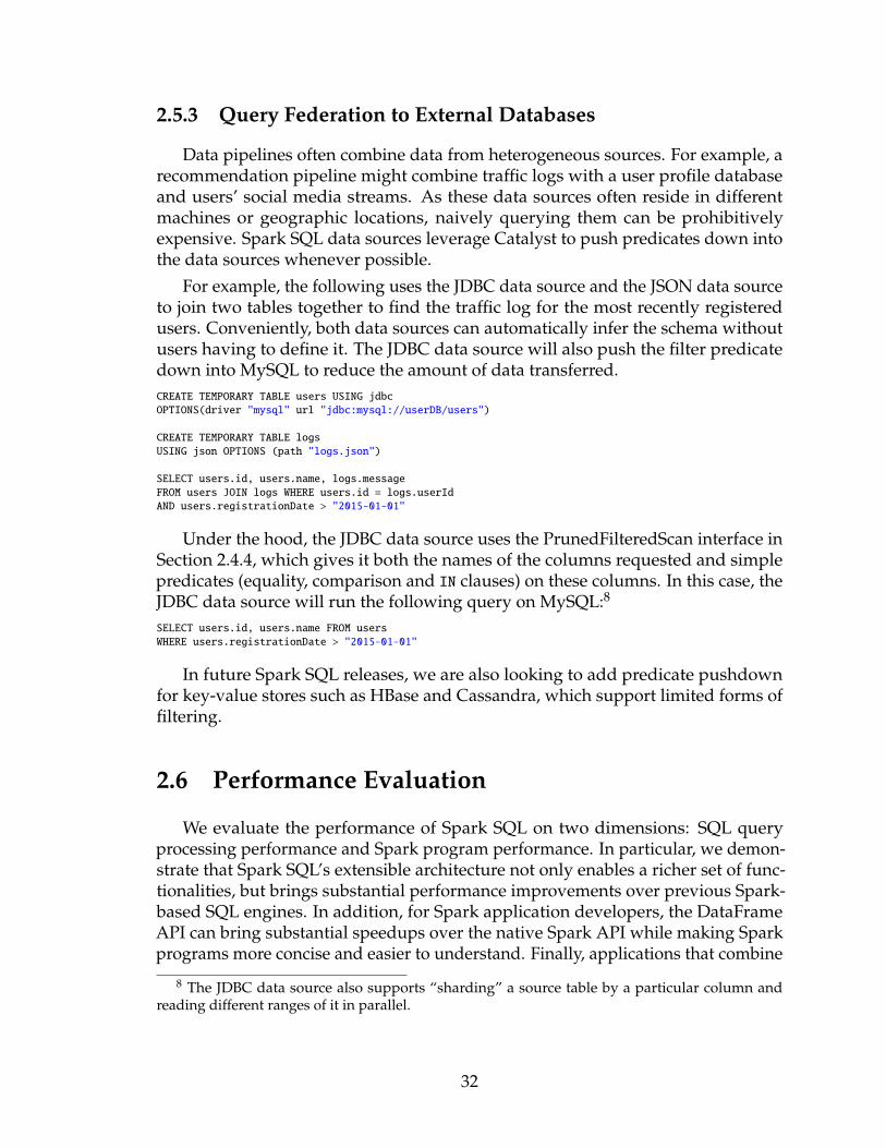
2.5.3 Query Federation to External Databases

Data pipelines often combine data from heterogeneous sources. For example, arecommendation pipeline might combine traffic logs with a user profile databaseand users’ social media streams. As these data sources often reside in differentmachines or geographic locations, naively querying them can be prohibitivelyexpensive. Spark SQL data sources leverage Catalyst to push predicates down intothe data sources whenever possible.

For example, the following uses the JDBC data source and the JSON data sourceto join two tables together to find the traffic log for the most recently registeredusers. Conveniently, both data sources can automatically infer the schema withoutusers having to define it. The JDBC data source will also push the filter predicatedown into MySQL to reduce the amount of data transferred.CREATE TEMPORARY TABLE users USING jdbc

OPTIONS(driver "mysql" url "jdbc:mysql://userDB/users")

CREATE TEMPORARY TABLE logs

USING json OPTIONS (path "logs.json")

SELECT users.id, users.name, logs.message

FROM users JOIN logs WHERE users.id = logs.userId

AND users.registrationDate > "2015-01-01"

Under the hood, the JDBC data source uses the PrunedFilteredScan interface inSection 2.4.4, which gives it both the names of the columns requested and simplepredicates (equality, comparison and IN clauses) on these columns. In this case, theJDBC data source will run the following query on MySQL:8

SELECT users.id, users.name FROM users

WHERE users.registrationDate > "2015-01-01"

In future Spark SQL releases, we are also looking to add predicate pushdownfor key-value stores such as HBase and Cassandra, which support limited forms offiltering.

2.6 Performance Evaluation

We evaluate the performance of Spark SQL on two dimensions: SQL queryprocessing performance and Spark program performance. In particular, we demon-strate that Spark SQL’s extensible architecture not only enables a richer set of func-tionalities, but brings substantial performance improvements over previous Spark-based SQL engines. In addition, for Spark application developers, the DataFrameAPI can bring substantial speedups over the native Spark API while making Sparkprograms more concise and easier to understand. Finally, applications that combine

8 The JDBC data source also supports “sharding” a source table by a particular column andreading different ranges of it in parallel.

32

0 5

10 15 20 25 30 35 40

1a 1b 1c

Run

time

(s)

Query 1 (Scan) Shark Impala Spark SQL

0 50

100 150 200 250 300 350 400 450

2a 2b 2c

Run

time

(s)

Query 2 (Aggregation) Shark Impala Spark SQL

0 100 200 300 400 500 600 700

3a 3b 3c

Run

time

(s)

Query 3 (Join) Shark Impala Spark SQL

0

200

400

600

800

Run

time

(s)

Query 4 (UDF) Shark Spark SQL

Figure 2.9: Performance of Shark, Impala and Spark SQL on the big data benchmarkqueries [104].

relational and procedural queries run faster on the integrated Spark SQL enginethan by running SQL and procedural code as separate parallel jobs.

2.6.1 SQL Performance

We compared the performance of Spark SQL against Shark and Impala [3]using the AMPLab big data benchmark [124], which uses a web analytics workloaddeveloped by Pavlo et al. [104]. The benchmark contains four types of querieswith different parameters performing scans, aggregation, joins and a UDF-basedMapReduce job. We used a cluster of six EC2 i2.xlargemachines (one master, fiveworkers) each with 4 cores, 30 GB memory and an 800 GB SSD, running HDFS2.4, Spark 1.3, Shark 0.9.1 and Impala 2.1.1. The dataset was 110 GB of data aftercompression using the columnar Parquet format [19].

Figure 2.9 shows the results for each query, grouping by the query type. Queries1–3 have different parameters varying their selectivity, with 1a, 2a, etc being themost selective and 1c, 2c, etc being the least selective and processing more data.Query 4 uses a Python-based Hive UDF that was not directly supported in Impala,but was largely bound by the CPU cost of the UDF.

33

We see that in all queries, Spark SQL is substantially faster than Shark andgenerally competitive with Impala. The main reason for the difference with Sharkis code generation in Catalyst (Section 2.4.3), which reduces CPU overhead. Thisfeature makes Spark SQL competitive with the C++ and LLVM based Impala enginein many of these queries. The largest gap from Impala is in query 3a where Impalachooses a better join plan because the selectivity of the queries makes one of thetables very small.

2.6.2 DataFrames vs. Native Spark Code

In addition to running SQL queries, Spark SQL can also help non-SQL devel-opers write simpler and more efficient Spark code through the DataFrame API.Catalyst can perform optimizations on DataFrame operations that are hard to dowith hand written code, such as predicate pushdown, pipelining, and automaticjoin selection. Even without these optimizations, the DataFrame API can result inmore efficient execution due to code generation. This is especially true for Pythonapplications, as Python is typically slower than the JVM.

For this evaluation, we compared two implementations of a Spark program thatdoes a distributed aggregation. The dataset consists of 1 billion integer pairs, (a,b) with 100,000 distinct values of a, on the same five-worker i2.xlarge cluster as inthe previous section. We measure the time taken to compute the average of b foreach value of a. First, we look at a version that computes the average using the mapand reduce functions in the Python API for Spark:sum_and_count = \

data.map(lambda x: (x.a, (x.b, 1))) \

.reduceByKey(lambda x, y: (x[0]+y[0], x[1]+y[1])) \

.collect()

[(x[0], x[1][0] / x[1][1]) for x in sum_and_count]

In contrast, the same program can written as a simple manipulation using theDataFrame API:df.groupBy("a").avg("b")

Figure 2.10, shows that the DataFrame version of the code outperforms thehand written Python version by 12×, in addition to being much more concise. Thisis because in the DataFrame API, only the logical plan is constructed in Python,and all physical execution is compiled down into native Spark code as JVM byte-code, resulting in more efficient execution. In fact, the DataFrame version alsooutperforms a Scala version of the Spark code above by 2×. This is mainly due tocode generation: the code in the DataFrame version avoids expensive allocation ofkey-value pairs that occurs in hand-written Scala code.

34

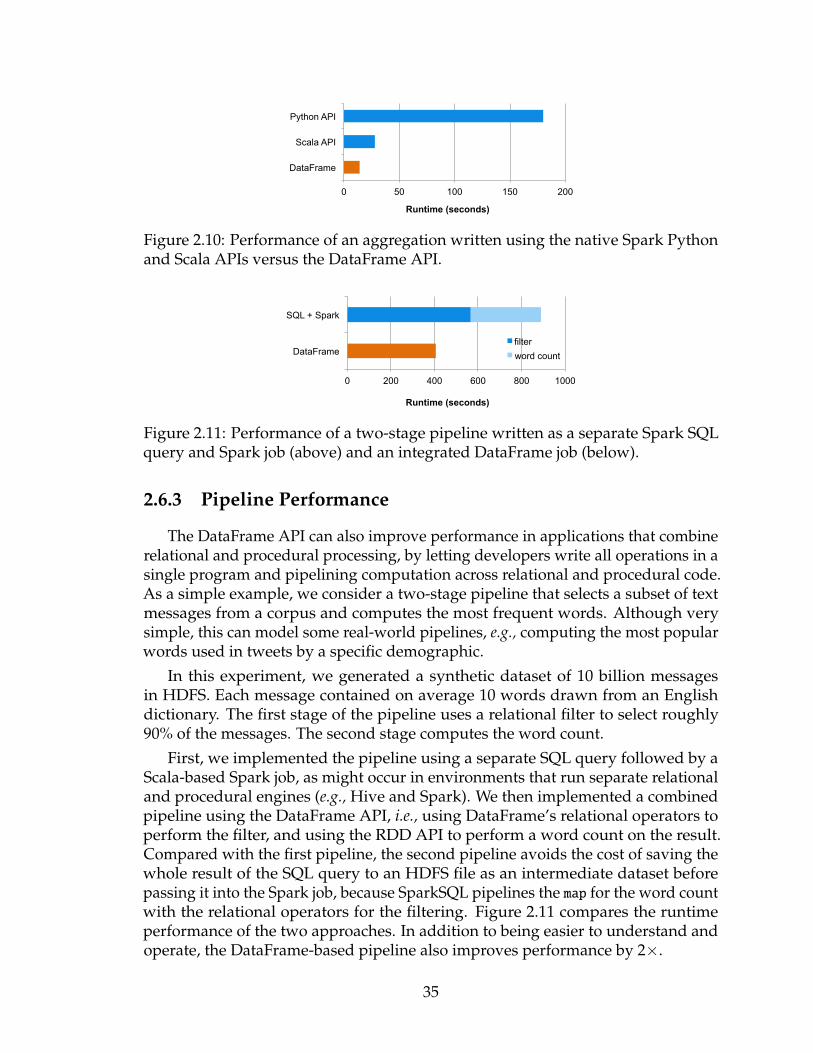
0 50 100 150 200

DataFrame

Scala API

Python API

Runtime (seconds)

Figure 2.10: Performance of an aggregation written using the native Spark Pythonand Scala APIs versus the DataFrame API.

0 200 400 600 800 1000

DataFrame

SQL + Spark

Runtime (seconds)

filter word count

Figure 2.11: Performance of a two-stage pipeline written as a separate Spark SQLquery and Spark job (above) and an integrated DataFrame job (below).

2.6.3 Pipeline Performance

The DataFrame API can also improve performance in applications that combinerelational and procedural processing, by letting developers write all operations in asingle program and pipelining computation across relational and procedural code.As a simple example, we consider a two-stage pipeline that selects a subset of textmessages from a corpus and computes the most frequent words. Although verysimple, this can model some real-world pipelines, e.g., computing the most popularwords used in tweets by a specific demographic.

In this experiment, we generated a synthetic dataset of 10 billion messagesin HDFS. Each message contained on average 10 words drawn from an Englishdictionary. The first stage of the pipeline uses a relational filter to select roughly90% of the messages. The second stage computes the word count.

First, we implemented the pipeline using a separate SQL query followed by aScala-based Spark job, as might occur in environments that run separate relationaland procedural engines (e.g., Hive and Spark). We then implemented a combinedpipeline using the DataFrame API, i.e., using DataFrame’s relational operators toperform the filter, and using the RDD API to perform a word count on the result.Compared with the first pipeline, the second pipeline avoids the cost of saving thewhole result of the SQL query to an HDFS file as an intermediate dataset beforepassing it into the Spark job, because SparkSQL pipelines the map for the word countwith the relational operators for the filtering. Figure 2.11 compares the runtimeperformance of the two approaches. In addition to being easier to understand andoperate, the DataFrame-based pipeline also improves performance by 2×.

35

2.7 Research Applications

In addition to the immediately practical production use cases of Spark SQL, wehave also seen significant interest from researchers working on more experimentalprojects. We outline two research projects that leverage the extensibility of Catalyst:one in approximate query processing and one in genomics.

2.7.1 Generalized Online Aggregation

Zeng et al. have used Catalyst in their work on improving the generality ofonline aggregation [134]. This work generalizes the execution of online aggregationto support arbitrarily nested aggregate queries. It allows users to view the progressof executing queries by seeing results computed over a fraction of the total data.These partial results also include accuracy measures, letting the user stop the querywhen sufficient accuracy has been reached.

In order to implement this system inside of Spark SQL, the authors add a newoperator to represent a relation that has been broken up into sampled batches.During query planning a call to transform is used to replace the original full querywith several queries, each of which operates on a successive sample of the data.

However, simply replacing the full dataset with samples is not sufficient tocompute the correct answer in an online fashion. Operations such as standardaggregation must be replaced with stateful counterparts that take into account boththe current sample and the results of previous batches. Furthermore, operationsthat might filter out tuples based on approximate answers must be replaced withversions that can take into account the current estimated errors.

Each of these transformations can be expressed as Catalyst rules that modifythe operator tree until it produces correct online answers. Tree fragments thatare not based on sampled data are ignored by these rules and can execute usingthe standard code path. By using Spark SQL as a basis, the authors were able toimplement a fairly complete prototype in approximately 2000 lines of code.

2.7.2 Computational Genomics

A common operation in computational genomics involves inspecting overlap-ping regions based on a numerical offsets. This problem can be represented as a joinwith inequality predicates. Consider two datasets, a and b, with a schema of (startLONG, end LONG). The range join operation can be expressed in SQL as follows:

SELECT * FROM a JOIN b

WHERE a.start < a.end

AND b.start < b.end

AND a.start < b.start

AND b.start < a.end

36

Without special optimization, the preceding query would be executed by manysystems using an inefficient algorithm such as a nested loop join. In contrast, aspecialized system could compute the answer to this join using an interval tree.Researchers in the ADAM project [97] were able to build a special planning rule intoa version of Spark SQL to perform such computations efficiently, allowing them toleverage the standard data manipulation abilities alongside specialized processingcode. The changes required were approximately 100 lines of code.

2.8 Discussion

Spark SQL, and its earlier predecessor, Shark, shows that it is possible to run fastrelational queries in a fault-tolerant manner using the fine-grained deterministictask model introduced by MapReduce. This design offers an effective way to scalequery processing to ever-larger workloads, and to combine it with rich analytics. Inthis section, we consider two questions: first, why were previous MapReduce-basedsystems, such as Hive, slow, and what gave Spark SQL its advantages? Second, arethere other benefits to the fine-grained task model? We argue that fine-grained tasksalso help with multitenancy and elasticity, as has been demonstrated in MapReducesystems.

2.8.1 Why are Previous MapReduce-Based Systems Slow?

Conventional wisdom is that MapReduce is slower than MPP databases forseveral reasons: expensive data materialization for fault tolerance, inferior datalayout (e.g., lack of indices), and costlier execution strategies [103, 118]. Our ex-ploration of Hive confirms these reasons, but also shows that a combination ofconceptually simple “engineering” changes to the engine (e.g., in-memory storage)and more involved architectural changes (e.g., partial DAG execution) can alleviatethem. We also find that a somewhat surprising variable not considered in detailin MapReduce systems, the task scheduling overhead, actually has a dramaticeffect on performance, and greatly improves load balancing if minimized. There isno fundamental reason why this overhead needs to be large, and Spark makes itseveral orders of magnitude lower than Hadoop.

Intermediate Outputs: MapReduce-based query engines, such as Hive, materializeintermediate data to disk in two situations. First, within a MapReduce job, the maptasks save their output in case a reduce task fails [48]. Second, many queries needto be compiled into multiple MapReduce steps, and engines rely on replicated filesystems, such as HDFS, to store the output of each step.

For the first case, we note that map outputs were stored on disk primarily asa convenience to ensure there is sufficient space to hold them in large batch jobs.Map outputs are not replicated across nodes, so they will still be lost if the mappernode fails [48]. Thus, if the outputs fit in memory, it makes sense to store them in

37

memory initially, and only spill them to disk if they are large. Spark SQL’s shuffleimplementation does this by default, and sees far faster shuffle performance (andno seeks) when the outputs fit in RAM. This is often the case in aggregations andfiltering queries that return a much smaller output than their input.9 Anotherhardware trend that may improve performance, even for large shuffles, is SSDs,which would allow fast random access to a larger space than memory.

For the second case, engines that extend the MapReduce execution model togeneral task DAGs can run multi-stage jobs without materializing any outputs toHDFS. Many such engines have been proposed, including Dryad, Tenzing andSpark [69, 38, 131].

Data Format and Layout: While the naıve pure schema-on-read approach to Map-Reduce incurs considerable processing costs, many systems use more efficientstorage formats within the MapReduce model to speed up queries. Hive itselfsupports “table partitions” (a basic index-like system where it knows that certainkey ranges are contained in certain files, so it can avoid scanning a whole table),as well as column-oriented representation of on-disk data [121]. We go further inSpark SQL by using fast in-memory columnar representations within Spark. SparkSQL does this without modifying the Spark runtime by simply representing a blockof tuples as a single Spark record (one Java object from Spark’s perspective), andchoosing its own representation for the tuples within this object.

Another feature of Spark that helps Spark SQL, but was not present in previousMapReduce runtimes, is control over the data partitioning across nodes. This letsus co-partition tables.

Finally, one capability of RDDs that we do not yet exploit is random reads. WhileRDDs only support coarse-grained operations for their writes, read operations onthem can be fine-grained, accessing just one record [131]. This would allow RDDsto be used as indices. Tenzing can use such remote-lookup reads for joins [38].

Execution Strategies: Hive spends considerable time on sorting the data beforeeach shuffle and writing the outputs of each MapReduce stage to HDFS, bothlimitations of the rigid, one-pass MapReduce model in Hadoop. More generalruntime engines, such as Spark, alleviate some of these problems. For instance,Spark supports hash-based distributed aggregation and general task DAGs.

To truly optimize the execution of relational queries, however, we found itnecessary to select execution plans based on data statistics. This becomes difficultin the presence of UDFs and complex analytics functions, which we seek to supportas first-class citizens in Spark SQL. To address this problem, we proposed partialDAG execution (PDE), which allows our modified version of Spark to change thedownstream portion of an execution graph once each stage completes based ondata statistics. PDE goes beyond the runtime graph rewriting features in previous

9 Systems like Hadoop also benefit from the OS buffer cache in serving map outputs, but wefound that the extra system calls and file system journaling from writing map outputs to files stilladds overhead (Section ??).

38

systems, such as DryadLINQ [129], by collecting fine-grained statistics about rangesof keys and by allowing switches to a completely different join strategy, such asbroadcast join, instead of just selecting the number of reduce tasks.

Task Scheduling Cost: Perhaps the most surprising engine property that affectedSpark SQL, however, was a purely “engineering” concern: the overhead of launch-ing tasks. Traditional MapReduce systems, such as Hadoop, were designed formulti-hour batch jobs consisting of tasks that were several minutes long. Theylaunched each task in a separate OS process, and in some cases had a high latencyto even submit a task. For instance, Hadoop uses periodic “heartbeats” from eachworker every 3 seconds to assign tasks, and sees overall task startup delays of 5–10seconds. This was sufficient for batch workloads, but clearly falls short for ad-hocqueries.

Spark avoids this problem by using a fast event-driven RPC library to launchtasks and by reusing its worker processes. It can launch thousands of tasks persecond with only about 5 ms of overhead per task, making task lengths of 50–100ms and MapReduce jobs of 500 ms viable. What surprised us is how much thisaffected query performance, even in large (multi-minute) queries.

Sub-second tasks allow the engine to balance work across nodes extremely well,even when some nodes incur unpredictable delays (e.g., network delays or JVMgarbage collection). They also help dramatically with skew. Consider, for example,a system that needs to run a hash aggregation on 100 cores. If the system launches100 reduce tasks, the key range for each task needs to be carefully chosen, as anyimbalance will slow down the entire job. If it could split the work among 1000tasks, then the slowest task can be as much as 10× slower than the average withnegligible on the job response time! After implementing skew-aware partitionselection in PDE, we were somewhat disappointed that it did not help comparedto just having a higher number of reduce tasks in most workloads, because Sparkcould comfortably support thousands of such tasks. However, this property makesthe engine highly robust to unexpected skew.

In this way, Spark stands in contrast to Hadoop/Hive, where using the wrongnumber of tasks was sometimes 10× slower than an optimal plan, and there hasbeen considerable work to automatically choose the number of reduce tasks [77, 62].Figure 2.12 shows how job execution times vary as the number of reduce taskslaunched by Hadoop and Spark in a simple aggregation query on a 100-node cluster.Since a Spark job can launch thousands of reduce tasks without incurring muchoverhead, partition data skew can be mitigated by always launching many tasks.

More fundamentally, there are few reasons why sub-second tasks should notbe feasible even at higher scales than we have explored, such as tens of thousandsof nodes. Systems like Dremel [88] routinely run sub-second, multi-thousand-node jobs. Indeed, even if a single master cannot keep up with the schedulingdecisions, the scheduling could be delegated across “lieutenant” masters for subsetsof the cluster. Fine-grained tasks also offer many advantages over coarser-grainedexecution graphs beyond load balancing, such as faster recovery (by spreading out

39

0 1000 2000 3000 4000 5000

02000

4000

6000

Number of Hadoop Tasks

Tim

e (

seconds)

0 1000 2000 3000 4000 5000

50

100

150

200

Number of Spark Tasks

Tim

e (

seconds)

Figure 2.12: Task launching overhead

lost tasks across more nodes) and query elasticity [99]; we discuss some of thesenext.

2.8.2 Other Benefits of the Fine-Grained Task Model

The fine-grained task model also provides other attractive properties. We wishto point out two benefits that have been explored in MapReduce-based systems.

Elasticity: In traditional MPP databases, a distributed query plan is selected once,and the system needs to run at that level of parallelism for the whole duration of thequery. In a fine-grained task system, however, nodes can appear or go away duringa query, and pending work will automatically be spread onto them. This enablesthe database engine to naturally be elastic. If an administrator wishes to removenodes from the engine (e.g., in a virtualized corporate data center), the engine cansimply treat those as failed, or (better yet) proactively replicate their data to othernodes if given a few minutes’ warning. Similarly, a database engine running ona cloud could scale up by requesting new VMs if a query is expensive. Amazon’sElastic MapReduce [1] already supports resizing clusters at runtime.

Multitenancy: The same elasticity, mentioned above, enables dynamic resourcesharing between users. In some traditional MPP databases, if an important queryarrives while another large query is using most of the cluster, there are few optionsbeyond canceling the earlier query. In systems based on fine-grained tasks, onecan simply wait a few seconds for the current tasks from the first query to finish,and start giving the nodes tasks from the second query. For instance, Facebookand Microsoft have developed fair schedulers for Hadoop and Dryad that allowlarge historical queries, compute-intensive machine learning jobs, and short ad-hocqueries to safely coexist [130, 70].

40

2.9 Related Work

Programming Model Several systems have sought to combine relational process-ing with the procedural processing engines initially used for large clusters. Asdiscussed earlier, Shark is the predecessor to Spark SQL, running on the same en-gine and offering the same combination of relational queries and advanced analytics.Spark SQL improves on Shark through a richer and more programmer-friendly API,DataFrames, where queries can be combined in a modular way using constructs inthe host programming language (see Section 2.3). It also allows running relationalqueries directly on native RDDs, and supports a wide range of data sources beyondHive.

One system that inspired Spark SQL’s design was DryadLINQ [129], whichcompiles language-integrated queries in C# to a distributed DAG execution engine.LINQ queries are also relational but can operate directly on C# objects. SparkSQL goes beyond DryadLINQ by also providing a DataFrame interface similar tocommon data science libraries [108, 101], an API for data sources and types, andsupport for iterative algorithms through execution on Spark.

Other systems use only a relational data model internally and relegate proce-dural code to UDFs. For example, Hive and Pig [121, 98] offer relational query lan-guages but have widely used UDF interfaces. ASTERIX [26] has a semi-structureddata model internally. Stratosphere [13] also has a semi-structured model, but offersAPIs in Scala and Java that let users easily call UDFs. PIQL [23] likewise providesa Scala DSL. Compared to these systems, Spark SQL integrates more closely withnative Spark applications by being able to directly query data in user-defined classes(native Java/Python objects), and lets developers mix procedural and relationalAPIs in the same language. In addition, through the Catalyst optimizer, Spark SQLimplements both optimizations (e.g., code generation) and other functionality (e.g.,schema inference for JSON and machine learning data types) that are not present inmost large-scale computing frameworks. We believe that these features are essentialto offering an integrated, easy-to-use environment for big data.

Finally, data frame APIs have been built both for single machines [108, 101]and clusters [46, 28]. Unlike previous APIs, Spark SQL optimizes DataFramecomputations with a relational optimizer.

Extensible Optimizers The Catalyst optimizer shares similar goals with extensi-ble optimizer frameworks such as EXODUS [59] and Cascades [60]. Traditionally,however, optimizer frameworks have required a domain-specific language to writerules in, as well as an “optimizer compiler” to translate them to runnable code.Our major improvement here is to build our optimizer using standard features of afunctional programming language, which provide the same (and often greater) ex-pressivity while decreasing the maintenance burden and learning curve. Advancedlanguage features helped with many areas of Catalyst—for example, our approachto code generation using quasiquotes (Section 2.4.3) is one of the simplest and most

41

composable approaches to this task that we know. While extensibility is hard tomeasure quantitatively, one promising indication is that Spark SQL had over 50external contributors in the first 8 months after its release.

For code generation, LegoBase [75] recently proposed an approach using gener-ative programming in Scala, which would be possible to use instead of quasiquotesin Catalyst.

Advanced Analytics Spark SQL builds on recent work to run advanced analyticsalgorithms on large clusters, including platforms for iterative algorithms [131] andgraph analytics [126, 82]. The desire to expose analytics functions is also sharedwith MADlib [42], though the approach there is different, as MADlib had to usethe limited interface of Postgres UDFs, while Spark SQL’s UDFs can be full-fledgedSpark programs. Finally, techniques including Sinew and Invisible Loading [120, 10]have sought to provide and optimize queries over semi-structured data such asJSON. We hope to apply some of these techniques in our JSON data source.

2.10 Conclusion

We have developed Spark SQL, a new module in Apache Spark providing richintegration with relational processing. Spark SQL builds on the lessons learnedfrom its predecessor, Shark, the initial SQL implementation on Spark that is heavilytied to Hive internals. Spark SQL extends Spark with a declarative DataFrame APIto allow relational processing, offering benefits such as automatic optimization, andletting users write complex pipelines that mix relational and complex analytics. Itsupports a wide range of features tailored to large-scale data analysis, includingsemi-structured data, query federation, and data types for machine learning. Toenable these features, Spark SQL is based on an extensible optimizer called Cata-lyst that makes it easy to add optimization rules, data sources and data types byembedding into the Scala programming language. User feedback and benchmarksshow that Spark SQL makes it significantly simpler and more efficient to write datapipelines that mix relational and procedural processing, while offering substantialspeedups over previous SQL-on-Spark engines.

42

Chapter 3

Structured Streaming: DeclarativeReal-Time Applications

This chapter develops Structured Streaming, an extension to Spark SQL to sup-port stream processing. We first describe the technical and operational challengesfrom stream processing, and present how Structured Streaming’s ability to incre-mentalize query plans addresses those challenges. We also present use cases wehave seen in production and conduct performance evaluation on the system. Weend the chapter by surveying related work.

3.1 Introduction

Many large-scale data sources operate in real time, including sensors, logs frommobile applications, and the Internet of Things. As organizations have gotten betterat capturing this data, they also want to process it in real time, whether to givehuman analysts the freshest possible data or drive automated decisions. Enablingbroad access to streaming computation requires systems that are scalable, easy touse and easy to integrate into business applications.

While there has been tremendous progress in distributed stream processingsystems in the past few years [17, 52, 12, 93, 43], these systems still remain fairlychallenging to use in practice. In this chapter, we begin by describing these chal-lenges, based on our experience with Spark Streaming [133], one of the earlieststream processing systems to provide a relatively high-level, functional API. Wefind that two challenges frequently came up with users. First, streaming systemsoften asked users to think in terms of low-level, physical execution concepts, suchas at-least-once delivery, state storage and triggering modes, that are unique tostreaming. Second, many systems focused only on streaming computation, butin real use cases, streaming was a part of a larger business application that alsoincludes batch processing, joins with static data, and interactive queries. Integrating

43

streaming systems with these other systems (e.g., maintaining transactionality)requires significant engineering.

Motivated by these challenges, we describe Structured Streaming, a new high-level API for stream processing that was added to Apache Spark in summer2016. Structured Streaming builds on many ideas in recent stream processingsystems, such as separating processing time from event time and triggers in GoogleDataflow [12], using a relational execution engine for performance [36], and offeringa language-integrated API [52, 133], but aims to make them simpler to use andintegrated with the rest of Apache Spark. Specifically, Structured Streaming differsfrom other widely used open source streaming APIs in two ways:

• Incremental query model: Structured Streaming automatically incremental-izes queries on static datasets expressed through Spark’s SQL and DataFrameAPIs, meaning that users often only need to understand Spark’s batch APIs towrite a streaming query, similar to [56]. Event time concepts are especially easyto express in this model, making them easier to understand. Although incre-mental query execution and view maintenance are well studied [29, 107, 135],we believe Structured Streaming is the first effort to adopt them in a widelyused open source system.

• Support for end-to-end applications: Structured Streaming’s API and built-in connectors aim to make it easy to write code that is “correct by default”when interacting with external systems and their code can be integrated intolarger applications using Spark and other systems. Data sources and sinksfollow a simple transactional model that enables “exactly-once” computationby default. The incrementalization based API also allows users to run astreaming query as a batch job or develop hybrid applications that join streamswith static data computed through Spark’s batch APIs. In addition, userscan manage multiple streaming queries dynamically and run interactivequeries on consistent snapshots of stream output, making it possible to writeapplications that go beyond computing a fixed result to let users refine anddrill into streaming data.

Beyond these benefits, we have made several design choices in StructuredStreaming that simplify operation and increase performance. First, StructuredStreaming reuses the Spark SQL execution engine, including its optimizer andruntime code generator. This leads to high throughput compared to other stream-ing systems (e.g., 4× the throughput of Apache Flink in the Yahoo! StreamingBenchmark [40]), as in Trill [36], and also lets Structured Streaming automaticallyleverage new SQL functions added to Spark. The engine runs in a microbatchexecution mode by default [133] but we are also extending it to support low-latencycontinuous operators for some queries because the API is agnostic to executionstrategy [21].

Second, we found that operating a streaming application can be challenging,and designed the engine to support failures, code updates and recomputation of

44

already outputted data. For example, one common issue is that new data in a streamcauses an application to crash, or worse, to output an incorrect result that users donot notice until much later (e.g., due to mis-parsing an input field). In StructuredStreaming, each application maintains a write-ahead event log in human-readableJSON format that operators can use to restart the application from an arbitrarypoint. If the application crashes due to an error in a user-defined function, operatorscan update the UDF and restart from where it left off, which happens automaticallywhen the restarted application reads the log. If it was outputting incorrect datainstead, operators can restart from a point before the bad data started arrivingand recompute results from there; this works provided old enough checkpointinformation was kept.

Since Structured Streaming became part of open source Spark in 2016, wehave observed a number of use cases, through the open source mailing lists aswell as production use cases on Databricks’ cloud service. We end the chapterwith some example use cases. Production applications range from interactivenetwork security analysis and automated alerts to incremental Extract, Transformand Load (ETL). Users often leverage the design of the engine in interesting ways,e.g., running a streaming query “discontinuously” as a series of single-microbatchjobs to leverage Structured Streaming’s transactioal input and output withouthaving to pay for cloud servers running 24/7. The largest production applicationswe discuss process over 1 PB of data per month on hundreds of machines. We alsoshow that Structured Streaming outperforms Apache Flink and Kafka Streams by4× and 90× respectively in the widely used Yahoo! Streaming Benchmark [40].

The rest of this chapter is organized as follows. We start by discussing streamprocessing challenges based on our experience with Spark Streaming in Section 3.2.Next, we give an overview of Structured Streaming (Section 3.3), then describeits API (Section 3.4), query planning (Section 3.5) and execution and operation(Section 3.6). In Section 3.7, we describe several large use cases. We then measurethe system’s performance in Section 3.8, discuss related work in Section 3.9 andconclude in Section 4.8.

3.2 Stream Processing Challenges

Despite extensive progress in the past few years, distributed streaming appli-cations are still still generally considered hard to develop and operate. Beforedesigning Structured Streaming, we spent time discussing the challenges in thisdomain with users and designers of other streaming systems, including SparkStreaming, Truviso, Storm, Flink, Dataflow and others. This section discusses themain challenges we saw.

45

3.2.1 Low-Level APIs

Streaming systems were invariably considered more difficult to use than batchones due to complex API semantics. Some complexity is to be expected due to newconcerns that arise only in streaming: for example, the user needs to think aboutwhat type of intermediate results the system should output before it has receivedall the data relevant to a particular entity, e.g., to a customer’s browsing session ona website. However, other complexity arises due to the low-level nature of manystreaming APIs: these APIs often ask users to specify applications at the level ofphysical operators with complex semantics instead of a more declarative level.

As a concrete example, the Google Dataflow model [12] has a powerful APIwith a rich set of options for handling event time aggregation, windowing andout-of-order data. However, in this model, users need to specify a windowing mode,triggering mode and trigger refinement mode (essentially, whether the operatoroutputs deltas or accumulated results) for each aggregation operator. Adding anoperator that expects deltas after an aggregation that outputs accumulated resultswill lead to unexpected results. In essence, the raw API [25] asks the user to write aphysical operator graph, not a logical query, so every user of the system needs tounderstand the intricacies of incremental processing.

Other APIs, such as Spark Streaming [133] and Flink’s DataStream API [53], arealso based on writing DAGs of physical operators and offer a complex array ofoptions for managing state [55]. In addition, reasoning about applications becomeseven more complex in systems that relax exactly-once semantics [17], effectivelyrequiring the user to design and implement a consistency model.

To address this issue, we designed Structured Streaming to make simple appli-cations simple to express using its incremental query model. In addition, we foundthat adding customizable stateful processing operators to this model still enabledadvanced users to build their own processing logic, such as custom session-basedwindows, while staying within the incremental model (e.g., these same opera-tors also work in batch jobs). Other open source systems have also recently beenadding incremental SQL queries [54, 43], and of course such queries have long beenstudied [29, 107, 135].

3.2.2 Integration in End-to-End Applications

The second challenge we found was that nearly every streaming workloadmust run in the context of a larger application, and this integration often requiredsignificant engineering effort. Many streaming APIs focus primarily on readingstreaming input from a source and writing streaming output to a sink, but end-to-end business applications need to perform other tasks. Examples include:

• The business purpose of the application may be to enable interactive querieson fresh data. In this case, streaming is used to compute and update summary

46

tables in a structured storage system such as a SQL database or ApacheHive [121]. It is important that when the streaming job updates its result, itdoes so atomically, so queries do not see partially written results. This can bechallenging with file-based big data systems like Apache Hive, where multiplefiles need to “appear” in parallel, or even with parallel load commands in adata warehouse.

• An Extract, Transform and Load (ETL) job might need to join a stream withstatic data loaded from another storage system or transformed using otherSpark code. In this case, it is important to be able to reason about consistencyacross the two systems (what happens when the static data is updated?), andit is helpful to write transformations on both datasets in the same API.

• A team may occasionally need to run its streaming business logic in a batchapplication, e.g., to backfill a result on old data or test alternate versions ofthe code. Rewriting the code in a separate system would be time-consumingand error-prone.

We address this challenge by integrating Structured Streaming closely withSpark’s batch and interactive APIs.

3.2.3 Operational Challenges

One of the largest challenges to deploying streaming applications in practice ismanagement and operation. Some key issues include:

• Failures: This is the most heavily studied issue in the research literature.In addition to single node failures, systems also need to support gracefulshutdown and restart of the whole application, e.g., to let operators migrate itto a new cluster.

• Code Updates: Applications are rarely perfect, so developers may need toupdate their code. After an update, they may want the application to restartwhere it left off, or possibly to recompute past results that were erroneous dueto a bug. Both cases need to be supported in the streaming system’s statemanagement and fault recovery mechanisms. In addition, updates to thestreaming system itself (e.g., a patch to Spark) should be supported as much aspossible.

• Rescaling: Applications see varying load over time, and generally increasingload in the long term, so operators may want to scale them up and downdynamically, especially in the cloud. Systems based on a static communicationtopology, while conceptually simple, are difficult to scale dynamically.

• Stragglers: Instead of outright failing, nodes in the streaming system can slowdown due to hardware or software issues and degrade the throughput of thewhole application. Systems should automatically handle this situation.

47

• Monitoring: Streaming systems need to give operators clear visibility intoper-node load, backlogs, state size, etc. to let them make good operationaldecisions.

3.2.4 Cost and Performance

Beyond operational and engineering issues, the cost-performance of streamingapplications can be an obstacle because these applications run 24/7. For example,without dynamic rescaling, an application will always consume its peak resources,and even with rescaling, it may be more expensive to update a result continuouslythan to run a periodic batch job. We thus designed Structured Streaming to leverageall the execution optimizations in Spark SQL.

So far, we chose to optimize throughput as our main performance metric becausewe found that it was often the most important metric in large-scale streamingapplications. Applications that require a distributed streaming system usually workwith large data volumes coming from external sources (e.g., mobile devices, sensorsor IoT), where data may already incur a delay just getting to the system. This is onereason why event time processing is an important feature in these systems [12]. Incontrast, latency-sensitive applications such as high-frequency trading or physicalsystem control loops often run on a single scale-up processor, or even customhardware like ASICs and FPGAs [14]. However, we also designed StructuredStreaming to support executing over latency-optimized engines, and are building acontinuous processing mode for this task [21], which we describe in Section 3.6.3.This is a change over Spark Streaming, where microbatching was “baked into” theAPI.

3.3 Structured Streaming Overview

Structured Streaming aims to tackle the stream processing challenges we identi-fied through a combination of API design and execution engine design, includingfeatures to simplify operation. In this section, we give a brief overview of the enginebefore diving into each of these topics in the following sections. Figure 3.1 showsan overview of the Structured Streaming system.

Input and Output. Structured Streaming connects to a variety of input sourcesand output sinks for I/O. To provide “exactly-once” output and fault tolerance, itplaces two restrictions on sources and sinks, which are similar to other exactly-oncesystems [133, 52]:

1. Input sources must be replayable, allowing the system to re-read recent inputdata if a node crashes. In practice, organizations use a reliable message bussuch as Amazon Kinesis or Apache Kafka [16, 73] for this purpose, or simplya durable file system.

48

Structured Streaming

Input Streams

Spark Tables

Output Sink

Log State StoreO

ptim

izer

Incr

emen

taliz

er MicrobatchExecution

ContiuousProcessing

data.where($“state” === “CA”)

.groupBy(window($“time”, “30s”))

.avg(“latency”)

DataFrame or SQL Query

Figure 3.1: The components of Structured Streaming.

2. Output sinks must support idempotent writes, to ensure reliable recovery if anode fails while writing. Structured Streaming can also provide atomic outputfor some sinks that support it, where any update to the job’s output appearsat once even if it was written by multiple nodes working in parallel.

In addition to external systems, Structured Streaming also supports input andoutput from tables in Spark SQL. For example, users can compute a static tablefrom any of Spark’s batch input sources and join it with a stream, or ask StructuredStreaming to output to an in-memory Spark table that users can query interactively.

API. Users program Structured Streaming by writing a query against one or morestreams and tables using Spark SQL’s batch APIs—SQL and DataFrames. Thisquery defines an output table that the user wants to compute, assuming that eachinput stream is replaced by a table holding all the data received from that stream sofar. The engine then determines how to compute and materialize this output table ina sink incrementally, using similar techniques to incremental view maintenance [29,107]. Different sinks also support different output modes, which determine how thesystem may update their results—for example, some sinks are by nature append-only, while others allow updating records in place by key.

To support streaming specifically, Structured Streaming also adds several APIfeatures that fit in the existing Spark SQL API:

• Triggers control how often the engine will attempt to compute a new resultand update the output sink, as in Dataflow [12].

49

• Users can mark a column as denoting event time (a timestamp set at the datasource), and set a watermark policy to determine when enough data has beenreceived to output a result for a specific event time, as in [12].

• Stateful operators allow users to track and update mutable state by key in orderto implement complex processing, such as custom session-based windows.These are similar to Spark Streaming’s updateStateByKey API [133].

Note that windowing, another key feature for streaming, is done using SparkSQL’s existing aggregation operators. In addition, all the new APIs in StructuredStreaming also work in batch jobs.

Execution. Once it has received a query, Structured Streaming optimizes it, incre-mentalizes it, and begins executing it. The system uses a microbatch model similarto Discretized Streams in Spark Streaming by default, which supports dynamicload balancing, rescaling, fault recovery and straggler mitigation by dividing workinto small tasks [133]. In addition, a new continuous processing mode uses moretraditional long-running operators [57] to provide lower latency at the cost of morestatic scheduling (Section 3.6.3).

In both cases, Structured Streaming uses two forms of durable storage to achievefault tolerance. First, a write-ahead log keeps track of which data has been processedand reliably written to the output sink from each input source. For some outputsinks, this log can be integrated with the sink to make updates to the sink atomic.Second, the system uses a larger-scale state store to hold snapshots of operator statesfor long-running aggregation operators. These are written asynchronously, and maybe “behind” the latest data written to the output sink; the system will automaticallytrack which state it has last updated in its log, and recompute state starting fromthat point in the data on failure. Both the log and state store can run over pluggablestorage systems (e.g., HDFS or S3).

Operational Features. Using the durability of the write-ahead log and state store,users can achieve several forms of rollback and recovery. An entire StructuredStreaming application can be shut down and restarted on new hardware. Runningapplications also tolerate node crashes, additions and stragglers automatically, bysending tasks to new nodes. For code updates to UDFs, it is sufficient to stop andrestart the application, and it will begin using the new code. In addition, users canmanually roll back the application to a previous point in the log and redo the part ofthe computation starting then, beginning from an older snapshot of the state store.

In addition, Structured Streaming’s ability to execute with microbatches letsit “adaptively batch” data so that it can quickly catch up with input data if theload spikes or if a job is rolled back, then return to low latency later. This makesoperation significantly simpler (e.g., operators can safely update code more often).

The next sections go into detail about Structured Streaming’s API (§3.4), queryplanning (§3.5) and job execution and operation (§3.6).

50

3.4 Programming Model

Structured Streaming combines elements of Google Dataflow [12], incrementalqueries [29, 107, 135] and Spark Streaming [133] to enable stream processing beneaththe Spark SQL API. In this section, we start by showing a short example, thendescribe the semantics of the model and the streaming-specific operators we addedin Spark SQL to support streaming use cases (e.g., stateful operators).

3.4.1 A Short Example

Structured Streaming operates within Spark’s structured data APIs—SQL,DataFrames and Datasets. The main abstraction users work with is tables (calledDataFrames or Datasets in the language APIs), which each represent a view to becomputed from input sources to the system.1 When users create a table/DataFramefrom a streaming input source, and attempt to compute it, Spark will automaticallylaunch a streaming computation.

As a simple example, let us start with a batch job that counts clicks by countryof origin for a web application. Suppose that the input data is JSON files and theoutput should be Parquet. This job can be written with Spark DataFrames in Scalaas follows:

// Define a DataFrame to read from static data

data = spark.read.format("json").load("/in")

// Transform it to compute a result

counts = data.groupBy($"country").count()

// Write to a static data sink

counts.write.format("parquet").save("/counts")

Changing this job to use Structured Streaming only requires modifying the inputand output sources, not the transformation in the middle. For example, if newJSON files are going to continually be uploaded to the /in directory, we can modifyour job to continually update /counts by changing only the first and last lines:

// Define a DataFrame to read streaming data

data = spark.readStream.format("json").load("/in")

// Transform it to compute a result

counts = data.groupBy($"country").count()

// Write to a streaming data sink

counts.writeStream.format("parquet")

1 Spark SQL offers several slightly different APIs that map to the same underlying query engine.The DataFrame API, modeled after data frames in R and Pandas [108, 101], offers a simple interfaceto build relational queries programmatically that is familiar to many users. The Dataset API addsstatic typing over DataFrames, similar to RDDs [131]. Alternatively, users can write SQL. All APIsproduce a relational query plan.

51

.outputMode("complete").start("/counts")

The output mode parameter on the sink here specifies how Structured Streamingshould update the sink. In this case, the complete mode means to write a completeresult file for each update, because the file output sink chosen does not supportfine-grained updates. However, other sinks, such as key-value stores, support moresophisticated output modes (e.g., updating just changed keys).

Under the hood, Structured Streaming will automatically incrementalize thequery specified by the transformation(s) from input sources to data sinks, andexecute it in a streaming fashion. The engine will also automatically maintain stateand checkpoint it to external storage as needed—in this case, for example, we havea running count aggregation since the start of the stream, so the engine will keeptrack of the running counts for each country.

Finally, the API also naturally supports windowing and event time throughSpark SQL’s existing support aggregation operators. For example, instead of count-ing data by country, we could count it in 1-hour sliding windows advancing every5 minutes by changing just the middle line of the computation as follows:

// Count events by windows on the "time" field

data.groupBy(window($"time","1h","5min")).count()

The time field here (event time) is just a field in the data, similar to countryearlier. Users can also set a watermark on this field to let the system forget state forold windows after a timeout (§3.4.3).

3.4.2 Model Semantics

Formally, we define the semantics of Structured Streaming’s execution model asfollows:

1. Each input source provides a partially ordered set of records over time. Weassume partial orders here because some message bus systems are paralleland do not define a total order across records—for example, Kafka dividesstreams into “partitions” that are each ordered.

2. The user provides a query to execute across the input data that can output aresult table at any given point in processing time. Structured Streaming willalways produce results consistent with running this query on a prefix of thedata in all input sources. That is, it will never show results that incorporate oneinput record but do not incorporate its ancestors in the partial order. Moreover,these prefixes will be increasing over time.

3. Triggers tell the system when to run a new incremental computation and updatethe result table. For example, in microbatch mode, the user may wish to triggeran incremental update every minute (in processing time).

52

4. The sink’s output mode specifies how the result table is written to the outputsystem. The engine supports three distinct modes:

• Complete: The engine writes the whole result table at once, e.g., replacinga whole file in HDFS with a new version. This is of course inefficientwhen the result is large.

• Append: The engine can only add records to the sink. For example, amap-only job on a set of input files results in monotonically increasingoutput.

• Update: The engine updates the sink in place based on a key for eachrecord, updating only keys whose values changed.

Figure 3.2 illustrates the model visually. One attractive property of the model isthat the contents of the result table (which is logically just a view that need never bematerialized) are defined independently of the output mode (whether we outputthe whole table on every trigger, or only deltas). In contrast, APIs such as Dataflowrequire the equivalent of an output mode on every operator, so users must planthe whole operator DAG keeping in mind whether each operator is outputtingcomplete results or positive or negative deltas, effectively incrementalizing thequery by hand.

A second attractive property is that the model has strong consistency semantics,which we call prefix consistency. First, it guarantees that when input records arerelatively ordered within a source (e.g., log records from the same device), thesystem will only produce results that incorporate them in the same records (e.g.,never skipping a record). In addition, because the result table is defined based on alldata in the input prefix at once, we know that all rows in the result table reflect eachinput records. For example, in some systems based on message-passing betweennodes, the node that receives a record might send an update to two downstreamnodes, but there is no guarantee that the outputs from these are synchronized.

In summary, with the Structured Streaming models, as long as users understanda regular Spark or DataFrame query, they can understand the content of the resulttable for their job and the values that will be written to the sink. Users need notworry about consistency, failures or incorrect processing orders.

Finally, the reader might notice that some of the output modes we defined areincompatible with certain types of query. For example, suppose we are aggregatingcounts by country, as in our code example in the previous section, and we want touse the append output mode. There is no way for the system to guarantee it hasstopped receiving records for a given country, so this combination of query andoutput mode will not be allowed by the system. We describe which combinationsare allowed in Section 3.5.1.

53

t=1

InputTable

ProcessingTime

ResultTable

OutputWritten

t=2 t=3

Que

ry

t=1

Trigger: every 1 sec

t=2 t=3

Que

ry

Complete Output Mode Append Output Mode

Trigger: every 1 sec

Figure 3.2: Structured Streaming’s semantics for two output modes. Logically, allinput data received up to a point in processing time is viewed as a large inputtable, and the user provides a query that defines a result table based on this input.Physically, Structured Streaming computes changes to the result table incrementally(without having to store all input data) and outputs results based on its outputmode. For complete mode, it outputs the whole result table (left), while for appendmode, it only outputs newly added records (right).

3.4.3 Streaming Specific Operators

Many Structured Streaming queries can be written using just the standardoperators built intp Spark SQL, such as selection, joins and aggregation. However,to support some new requirements unique to streaming, we added two new typesof operators to Spark SQL: watermarking operators tell the system when to “close”an event time window and output results or forget state, and stateful operators letusers write custom logic to implement custom complex processing. Crucially, bothof these new operators still fit within Structured Streaming’s incremental semantics(§3.4.2), and both can also be used in batch applications.

Event Time Watermarks

From a logical point of view, the key idea in event time is to treat application-specified timestamps as an arbitrary field in the data, allowing records to arrive out-of-order [76, 12]. We can then use standard operators and incremental processingto update results grouped by event time. In practice, however, it is useful for the

54

processing system to have some loose bounds on how late data can arrive, for tworeasons:

1. Allowing arbitrarily late data might require storing arbitrarily large state. Forexample, if we count data by 1-minute event time window, the system needsto remember a count for every 1-minute window since the application began,because a late record might still arrive for any particular minute. This canquickly lead to large amounts of state, especially if combined with anothergrouping key (e.g., group by minute and city).

2. Some sinks do not support data retraction, making it useful to be able towrite the results for a given event time after a timeout. For example, manydownstream applications want to start working with a “final” result fromstreaming analytics eventually, and might not be able to handle retractions.Append-mode sinks also do not support retractions.

Structured Streaming lets developers set a watermark [12] for event timecolumns using the withWatermark operator. This operator gives the system a delaythreshold tC for a given timestamp column C. At any point in time, the watermarkfor C is max(C)− tC, that is, tC seconds before the maximum event time seen so farin C. Note that this choice of watermark is naturally robust to backlogged data: ifthe system cannot keep up with the input rate for a period of time, the watermarkwill not move forward arbitrarily during that time, and all events that arrivedwithin at most T seconds of being produced will still be processed.

When present, watermarks affect when stateful operators can forget old state(e.g., if grouping by a window derived from a watermarked column), and whenStructured Streaming will output data with an event time key to append-modesinks. Different input streams can have different watermarks.

Stateful Operators

For developers who want to write custom stream processing logic, StructuredStreaming’s stateful operators are “UDFs with state” that give users control overthe computation while fitting into Structured Streaming’s semantics and faulttolerance mechanisms. There are two stateful operators, mapGroupsWithState andflatMapGroupsWithState. Both operators act on data that has been assigned a keyusing groupByKey, and let the developers track and update a state for each key usingcustom logic, as well as output records for each key. They are closely based onSpark Streaming’s updateStateByKey operator [133].

The mapGroupsWithState operator, on a grouped dataset with keys of type K andvalues of type V, takes as argument an update function with the following arguments:

• key of type K

• newValues of type Iterator[V]

55

// Define an update function that simply tracks the

// number of events for each key as its state, returns

// that as its result, and times out keys after 30 min.

def updateFunc(key: UserId, newValues: Iterator[Event],

state: GroupState[Int]): Int = {

val totalEvents = state.get() + newValues.size()

state.update(totalEvents)

state.setTimeoutDuration("30 min")

return totalEvents

}

// Use this update function on a stream, returning a

// new table lens that contains the session lengths.

lens = events.groupByKey(event => event.userId)

.mapGroupsWithState(updateFunc)

Figure 3.3: Using mapGroupsWithState to track the number of events per session,timing out sessions after 30 minutes.

• state of type GroupState[S], where S is a user-specified class.

The operator will invoke this function whenever one or more new values arereceived for a key. On each call, the function receives all of the values that werereceived for that key since the last call (multiple values may be batched for effi-ciency). It also receives a state object that wraps around a user-defined data typeS, and allows the user to update the state, drop this key from state tracking, orset a timeout for this specific key (either in event time or processing time). Thisallows the user to store arbitrary data for the key, as well as implement custom logicfor dropping state (e.g., custom exit conditions when implementing session-basedwindows).

Finally, the update function returns a user-specified return type R for its key. Thereturn value of mapGroupsWithState is a new table with the final R record outputtedfor each group in the data (when the group is closed or times out). For example, thedeveloper may wish to track user sessions on a website using mapGroupsWithState,and output the total number of pages clicked for each session.

To illustrate, Figure 3.3 shows how to use mapGroupsWithState to track usersessions, where a session is defined as a series of events with the same userId andgaps less than 30 minutes between them. We output the final number of events ineach session as our return value R. A job could then compute metrics such as theaverage number of events per session by aggregating the result table lens.

The second stateful operator, flatMapGroupsWithState, is very similar tomapGroupsWithState, except that the update function can return zero or more val-ues of type R per update instead of one. For example, this operator could be usedto manually implement a stream-to-table join. The return values can either bereturned all at once, when the group is closed, or incrementally across calls to the

56

update function. Both operators also work in batch mode, in which case the updatefunction will only be called once.

3.5 Query Planning

We implemented Structured Streaming’s query planning using the Catalystextensible optimizer in Spark SQL, which allows writing composable rules usingpattern matching in Scala, as described in Section [? ]. Query planning proceeds inthree stages: analysis to determine whether the query is valid, incrementalizationand optimization.

3.5.1 Analysis

The first stage of query planning is analysis, where the engine validates theuser’s query and resolves the attributes and data types referred to in the query.Structured Streaming uses Spark SQL’s existing analysis passes to resolve attributesand types, but adds new rules to check that the query can be executed incrementallyby the engine. It also checks that the user’s chosen output mode is valid for thisspecific query.

The rules for when each output mode is allowed are as follows:

• Complete mode: Only aggregation queries are allowed, where the amountof state that needs to be tracked is proportional to the number of keys in theresult as opposed to the total number of input records. Queries that only doselection operations, for example, are not allowed because they would requirestoring all the input data.2

• Append mode: In this mode, the engine must be able to guarantee that anoutput record will not be updated once it writes it. (More formally, querieshere should be monotonic [15].) Only selections, joins with static tables, andaggregations over event time on streams with watermarks are allowed. Foraggregations over event time, Structured Streaming only outputs a key whenthe watermark has moved past its event time.

• Update mode: All queries support this mode, which allows updating pastrecords based on a key.

These rules aim to establish two main goals: (1) that Structured Streaming neednot remember an indefinitely large amount of input, which would be virtually guar-anteed to be a bug in the user’s application, and (2) that it respects the limitationsof the output sink (e.g., append only). A full description of the supported modes isavailable in the Spark documentation [114].

2 Although input sources in Structured Streaming should support replaying recent data on failure,most will only retain data for a limited time (e.g., Kafka and Kinesis).

57

3.5.2 Incrementalization

As of Spark 2.2.0, Structured Streaming can incrementalize a restricted set ofqueries, which can contain:

• Any number of selections, projections and SELECT DISTINCTs.

• Any number of inner or right outer joins between a stream and a static table.

• Stateful operators like mapGroupsWithState (§3.4.3).

• Up to one aggregation (possibly on compound keys).

• Sorting after an aggregation, only in complete output mode.

Work is also under way to support other types of queries, such as stream-to-stream joins on event time windows.

These supported queries are mapped, using transformation rules, to physicaloperators that perform both computation and state management. For example, anaggregation in the user query might be mapped to a StatefulAggregate operator thattracks open groups inside Structured Streaming’s state store (§3.6.1) and outputsthe desired result. Internally, Structured Streaming also tracks an output mode foreach physical operator in the DAG produced during incrementalization, similarto the refinement mode for aggregation operators in Dataflow [12]. For example,some operators may update emitted records (equivalent to update mode), whileothers may only emit new records (append mode). Crucially, however, users do nothave to specify these intra-DAG modes manually.

Incrementalization is an active area of work in Structured Streaming, but wehave found that even the fairly simple set of queries supported today is broadlyapplicable in many use cases (§3.7). We expect to add more advanced incremental-ization techniques later.

3.5.3 Optimization

The final stage of planning is optimization. Structured Streaming applies mostof the optimization rules in Spark SQL, such as predicate pushdown, projectionpushdown, expression simplification and others. In addition, it uses Spark SQL’sTungsten binary format for data in memory (avoiding the overhead of Java objects),and its runtime code generator to compile chains of operators to Java bytecodethat runs over this format. This design means that most of the work in logical andexecution optimization for analytical workloads in Spark SQL automatically appliesto streaming.

58

Operator DAGInput Streams Output Sink

Log State Store

Rea

d In

put

Sele

ct

Stat

eful

Aggr

egat

e

Writ

e O

utpu

t

EpochOffsets

Async StateCheckpoints

Figure 3.4: State management during the execution of Structured Streaming. Inputoperators are responsible for defining epochs in each input source and savinginformation about them (e.g., offsets) reliably in the write-ahead log. Statefuloperators also checkpoint state asynchronously, marking it with its epoch, butthis does not need to happen on every epoch. Finally, output operators log whichepochs’ outputs have been reliably committed to the idempotent output sink; thevery last epoch may be rewritten on failure.

3.6 Application Execution

The final component of Structured Streaming is its execution strategy. In thissection, we describe how the engine tracks state, and then the two execution modes:microbatching via fine-grained tasks and the in-development continuous processingmode. We then discuss operational features to simplify management.

3.6.1 State Management and Recovery

At a high level, Structured Streaming tracks state in a manner similar to SparkStreaming [133], in both its microbatch and continuous modes. The state of anapplication is tracked using two external storage systems: a write-ahead log thatsupports durable, atomic writes at low latency, and a state store that can store largeramounts of data durably and allows parallel access (e.g., S3 or HDFS). StructuredStreaming uses these systems together to recover on failure.

The engine places two requirements on input sources and output sinks to pro-vide fault tolerance. First, input sources should be replayable, i.e., allow re-readingrecent data using some form of identifier, such as a stream offset. Durable messagebus systems like Kafka and Kinesis meet this need. Second, output sinks should beidempotent, allowing Structured Streaming to rewrite some already written data onfailure. Sinks can implement this in different ways.

59

Given these properties, Structured Streaming performs state tracking using thefollowing mechanism, as shown in Figure 3.4:

1. As input operators read data, the master node of the Spark application definesepochs based on offsets in each input source. For example, Kafka and Kinesispresent topics as a series of partitions, each of which are byte streams, andallow reading data using offsets in these partitions. The master writes thestart and end offsets of each epoch durably to the log.

2. Any operators requiring state checkpoint their state periodically and asyn-chronosuly to the state store, using incremental checkpoints when possible.They store the epoch ID along with each checkpoint written. These check-points do not need to happen on every epoch or to block processing.3

3. Output operators write the epochs they committed to the log. The masterwaits for all nodes running an operator to report a commit for a given epochbefore allowing commits for the next epoch. Depending on the sink, themaster can also run an operation to finalize the writes from multiple nodes ifthe sink supports this. This means that if the streaming application fails, onlyone epoch may be partially written.4

4. Upon recovery, the new instance of the application starts by reading the log tofind the last epoch that has not been committed to the sink, including its startand end offsets. It then uses the offsets of earlier epochs to reconstruct theapplication’s in-memory state from the last epoch written to the state store.This just requires loading the old state and running those epochs with thesame offsets while disabling output. Finally, the system reruns the last epochand relies on the sink’s idempotence to write its results, then starts definingnew epochs.

Finally, all of the state management in this design is transparent to user code.Both the aggregation operators and custom stateful processing operators (e.g.,mapGroupsWithState) automatically checkpoint state to the state store, without re-quiring custom code to do it. The user’s data types only need to be serializable.

3.6.2 Microbatch Execution Mode

Structured Streaming jobs can execute in two modes: microbatching or continu-ous operators. The microbatch mode uses the discretized streams execution model

3 In Spark 2.2.0, we actually make one checkpoint per epoch, but we plan to make them lessfrequent in a future release, as is already done in Spark Streaming.

4 Some sinks, such as Amazon S3, provide no way to atomically commit multiple writes fromdifferent writer nodes. In such cases, we have also created data sources for Spark that check both thestorage system and the streaming application’s log to read only complete epochs. This lets otherSpark applications still see a correct view [22].

60

from Spark Streaming [133], and inherits its benefits, such as dynamic load bal-ancing, rescaling, straggler mitigation and fault recovery without whole-systemrollback.

In this mode, epochs are typically set to be a few hundred milliseconds to a fewseconds, and each epoch executes as a traditional Spark job composed of a DAG ofindependent tasks [131]. For example, a query doing selection followed by statefulaggregation might execute as a set of “map” tasks for the selection and “reduce”tasks for the aggregation, where the reduce tasks track state in memory on workernodes and periodically checkpoint it to the state store. As in Spark Streaming, thismode provides the following benefits:

• Dynamic load balancing: Each operator’s work is divided into small, in-dependent tasks that can be scheduled on any node, so the system can au-tomatically balance these across nodes if some are executing slower thanothers.

• Fine-grained fault recovery: If a node fails, only its tasks need to be rerun,instead of having to roll back the whole cluster to a checkpoint as in mostsystems based on topologies of long-lived operators. Moreover, the lost taskscan be rerun in parallel, further reducing recovery time [133].

• Straggler mitigation: Spark will launch backup copies of slow tasks as itdoes in batch jobs, and downstream tasks will simply use the output fromwhichever copy finishes first.

• Rescaling: Adding or removing a node is simple as tasks will automaticallybe scheduled on all the available nodes.

• Scale and throughput: Because this mode reuses Spark’s batch execution en-gine, it inherits all the optimizations in this engine, such as a high-performanceshuffle implementation [125] and the ability to run on thousands of nodes.

The main disadvantage of this mode is a higher minimum latency, as there isoverhead to launching a DAG of tasks in Spark. In practice, however, latencies ofa few seconds are achievable even on large clusters and are acceptable for manyapplications where data takes a similar amount of time to even be uploaded to thesystem (e.g., those collecting data from mobile devices).

3.6.3 Continuous Processing Mode

A new continuous processing mode under active development for Spark 2.3 [21]enables execution Structured Streaming jobs using long-lived operators as in atraditional streaming systems such as TelegraphCQ and Borealis [37, 6]. This modeenables lower latency at a cost of less operational flexibility (e.g., limited supportfor rescaling the job at runtime).

61

The key enabler for this execution mode was choosing a declarative API forStructured Streaming that is not tied to the execution strategy. For example, theoriginal Spark Streaming API had some operators based on processing time thatleaked the concept of microbatches into the programming model, making it hard tomove programs to another type of engine. In contrast, Structured Streaming’s APIand semantics are independent of the execution engine: continuous execution issimilar to having a much larger number of triggers. Note that unlike systems basedpurely on unsynchronized message passing, such as Storm [17], we do retain theconcept of triggers and epochs in this mode so the output from multiple nodes canbe coordinated and committed together to the sink.

Because the API supports fine-grained execution, Structured Streaming jobscould theoretically run on any existing distributed streaming engine design [52, 6,37]. In continuous processing, we sought to implement a simple continuous opera-tor engine that lives inside Spark and can reuse Spark’s scheduling infrastructureand per-node operators (e.g., code-generated operators). The first version, currentlyunder development, only support “map” jobs (i.e., no shuffle operations), whichwere one of the most common scenarios where users wanted lower latency. Thedesign can also be extended to support shuffles, however. Compared to microbatchexecution, there are two differences when using continuous processing:

• The master launches long-running tasks on each partition using Spark’s sched-uler that each read one partition of the input source (e.g., Kinesis stream) butexecute multiple epochs. If one of these tasks fails, e.g., due to a node crash,Spark will automatically relaunch it on another node, which will start process-ing that same partition.

• Epochs are coordinated differently. The master periodically tells nodes to starta new epoch, and receives a start offset for the epoch on each input partition,which it inserts into the write-ahead log. When it asks them to start the nextepoch, it also receives end offsets for the previous one, writes these to the log,and tells nodes to commit the epoch when it has written all the end offsets.Thus, the master is not on the critical path for inspecting all the input sourcesand defining start/end offsets.

In practice, we found that the main use case where organizations wanted lowlatency and the scale of a distributed processing engine was “stream to stream”map operations to transform data before it is used in other streaming applications.For example, an organization might upload events to Kafka, run some simple ETLtransformations as a streaming map job, and write the transformed to Kafka againfor consumption by multiple downstream applications. In this type of architecture,every streaming transformation job will add latency to all downstream applications,so organizations wish to minimize this latency. For this reason, we have chosen toonly focus on map jobs in the first version of continuous processing, but in generalit is possible to use a full distributed streaming design.

62

3.6.4 Operational Features

We used several properties of our execution strategy and API to design a numberof operational features in Structured Streaming that tackle common problems indeployments.

Code Updates

Developers can update User-Defined Functions (UDFs) in their program andsimply restart the application to use the new version of the code. For example, ifa UDF is crashing on a particular input record, that epoch of processing will fail,so the developer can update the code and restart the application again to continueprocessing. This also applies to stateful operator UDFs, which can be updatedas long as they retain the same schema for their state objects. We also designedSpark’s log and state store formats to be binary compatible across Spark frameworkupdates.

Manual Rollback

Sometimes, an application outputs wrong results for some time before a usernotices: for example, a field that fails to parse might simply be reported as NULL.Therefore, rollbacks are a fact of life for many operators. In Structured Streaming,it is easy to determine which records went into each epoch from the write-aheadlog and roll back the application to the epoch where a problem started occurring.We chose to store the write-ahead log as JSON to let administrators perform theseoperations manually.5 As long as the input sources and state store still have datafrom the failed epoch, the job can start again from a previous point. Message buseslike Kafka are typically configured for several weeks of retention so rollbacks areoften possible. Moreover, Structured Streaming’s support for running the samecode as a batch job and for rescaling means that administrators can run the recoveryon a temporarily larger cluster to catch up quickly.

Hybrid Batch and Streaming Execution

The most obvious benefit of Structured Streaming’s unified API is that users canshare code between batch and streaming applications, or run the same program as abatch job for testing. However, we have also found this useful in purely streamingapplications, in two scenarios:

• “Run-once” triggers for cost savings: Many Spark users wanted the transaction-ality and state management properties of a streaming engine without running

5 One additional step they may have to do is remove faulty data from the output sink, dependingon the sink chosen. For the file sink, for example, it’s straightforward to find which files were writtenin a particular epoch and remove those.

63

servers 24/7. Virtually all ETL workloads require tracking how far in theinput one has gotten and which results have been saved reliably, which can bedifficult to implement by hand. These functions are exactly what StructuredStreaming’s state management provides. Thus, several organizations imple-mented ETL jobs by running a single epoch of a Structured Streaming job everyfew hours as a batch computation, using the provided “run once” trigger thatwas originally designed for testing. This leads to significant cost savings (inone case, up to 10× [128]) for lower-volume applications. With all the majorcloud providers now supporting per-second or per-minute billing [24], webelieve this type of “discontinuous processing” will become more common.

• Adaptive batching: Even streaming applications occasionally experience largebacklogs. For example, a link between two datacenters might go down,temporarily delaying data transfer, or there might simply be a spike in useractivity. In these cases, Structured Streaming will automatically execute longerepochs in order to catch up with the input streams, often achieving similarthroughput to Spark’s batch jobs. This will not greatly increase latency, giventhat data is already backlogged, but will let the system catch up faster. In cloudenvironments, operators can also add extra nodes to the cluster temporarily.

Monitoring

Structured Streaming uses Spark’s existing metrics API and structured event logto report information such as number of records processed, bytes shuffled acrossthe network, etc. These interfaces are familiar to operators and easy to connect to avariety of monitoring tools using existing connectors.

Fault and Straggler Recovery

As discussed in §3.6.2, Structured Streaming’s microbatch mode can recoverfrom node failures, stragglers and load imbalances using Spark’s fine-grained taskexecution model. The continuous processing mode recovers from node failuresby launching the failed partition on a new node, but does not yet protect againststragglers or load imbalance.

Perhaps most importantly for operators, we aimed to make both StructuredStreaming’s semantics and its fault tolerance model easy to understand. With asimple design, operators can form an accurate model of how a system runs andwhat various actions will do without having know all its internal details.

64

IDS

IDS

IDS…

alertsStreaming ETL

S3 S3

S3

raw logslogs

(parquet format)

structured data(e.g., dataframes)

security analyst

installqueries as alerts

notificationsStreaming

ETL

Streaming alerts

Interactiveanalytics

Figure 3.5: Information security platform use case.

3.7 Use Cases

First released in 2016, Structured Streaming has been part of Apache Spark andare supported by various cloud vendors. Databricks started supporting StructuredStreaming on its managed cloud service [45] since 2016, and today, the cloud serviceis running hundreds of production streaming applications at a given time (i.e.,applications running 24/7). The largest of these applications ingest over 1 PB ofdata per month and run on hundreds of servers. Structured Streaming is also usedinternally by Databricks to monitor services, including the execution of StructuredStreaming itself. In this section, we describe three production workloads thatleverage various aspects of Structured Streaming, as well as the Databricks internaluse case.

3.7.1 Information Security Platform

A large organization has used Structured Streaming to develop a large-scalesecurity platform to enable over 100 analysts to scour through network traffic logs toquickly identify and respond to security incidents, as well as to generate automatedalerts. This platform combines streaming with batch and interactive queries and isthus a great example of the system’s support for end-to-end applications.

Figure 3.5 shows the architecture of the platform. Intrusion Detection Systems(IDSes) monitor all the network traffic in the organization, and output logs to S3.From here, a Structured Streaming jobs ETLs these logs into the Parquet columnarformat to reduce the size and improve query speed. Other Structured Streaming jobsprocess the Parquet logs into additional structured tables (e.g., by joining with otherdata). Analysts query these tables interactively, either using SQL or Dataframes,to detect and diagnose new attack patterns. If they identify a compromise, they

65

also look back through historical data to trace previous actions from that attacker.Finally, in parallel, the Parquet logs are processed by another Structured Streamingcluster that generates alerts based on pre-written rules.

The key challenges in realizing this platform are (1) building a robust andscalable streaming pipeline, while (2) providing the analysts with an effective envi-ronment to query both fresh and historical data. Using standard tools and servicesavailable on AWS, a team of 20 people took over six months to build and deploy aprevious version of this platform in production. This previous version had severallimitations, including only being able to store a small amount of data for histori-cal queries due to using a traditional data warehouse for the interactive queries.In contrast, a team of five engineers was able to reimplement the platform usingStructured Streaming in two weeks. The new platform was simultaneously morescalable and able to support more complex analysis using Spark’s ML APIs. Next,we provide a few examples to illustrate the advantages of Structured Streamingthat made this possible.

First, Structured Streaming’s ability to adaptively vary the batch size enabledthe developers to build a streaming pipeline that deals not only with spikes in theworkload, but also with failures and code upgrades. Consider a streaming job thatgoes offline either due to failure or upgrades. When the cluster is brought backonline, it will start automatically to process the data all the way back from themoment it went offline. Initially, the cluster will use large batches to maximize thethroughput. Once it catches up, the cluster switches to small batches for low latency.This allows operators to regularly upgrade clusters without the fear of excessivedowntime.

Second, the ability to join a stream with other streams, as well as with histor-ical tables, has considerably simplified the analysis. Consider the simple task offiguring out which device a TCP connection originates at. It turns out that thistask is challenging in the presence of mobile devices, as these devices are givendynamic IP addresses every time they join the network. Hence, from TCP logsalone, is not possible to track down the end-points of a connection. With StructuredStreaming, an analyst can easily solve this problem. She can simply join the TCPlogs with DHCP logs to map the IP address to the MAC address, and then use theorganization’s internal database of network devices to map the MAC address to aparticular machine and user. In addition, users were able to do this join in real timeusing stateful operators as both the TCP and DHCP logs were being streamed in.

Finally, using the same system for streaming, interactive queries and ETL hasprovided developers with the ability to quickly iterate and deploy new alerts. Inparticular, it enables analysts to build and test queries for detecting new attacks onoffline data, and then deploy these queries directly on the alerting cluster. In oneexample, an analyst developed a query to identify exfiltration attacks via DNS. Inthis attack, malware leaks confidential information from the compromised host bypiggybacking this information into DNS requests sent to an external DNS serverowned by the attacker. One simplified query to detect such an attack essentially

66

computes the aggregate size of the DNS requests sent by every host over a timeinterval. If the aggregate is greater than a given threshold, the query flags thecorresponding host as potentially being compromised. The analyst used historicaldata to set this threshold, so as to achieve the desired balance between false positiveand false negative rates. Once satisfied with the result, the analyst simply pushedthe query to the alerting cluster. The ability to use the same system and the sameAPI for data analysis and for implementing the alerts led not only to significantengineering cost savings, but also to better security, as it is significantly easier todeploy new rules.

3.7.2 Live Video Stream Monitoring

A large media company is using Structured Streaming to compute qualitymetrics for their live video traffic and interactively identify delivery problems. Livevideo delivery is especially challenging because network problems can severelydisrupt utility. For pre-recorded video, clients can use large buffers to mask issues,and a degradation at most results in extra buffering time; but for live video, aproblem may mean missing a critical moment in a sports match or similar event.This organization collects video quality metrics from clients in real time, performsETL operations and aggregation using Structured Streaming, then stores the resultsin a data warehouse. This allows operations engineers to interactively query freshdata to detect and diagnose quality issues (e.g., determine whether an issue is tiedto a specific ISP, video server or other cause).

3.7.3 Online Game Performance Analysis

A large gaming company uses Structured Streaming to monitor the latencyexperienced by players in a popular online game with tens of millions of monthlyactive users. As in the video use case, high network performance is essential for theuser experience when gaming, and repeated problems can quickly lead to playerchurn. This organization collects latency logs from its game clients to cloud storageand then performs a variety of streaming analyses. For example, one job joinsthe measurements with a table of Internet Autonomous Systems (ASes) and thenaggregates the performance by AS over time to identify poorly performing ASes.When such an AS is identified, the streaming job triggers an alert, and operatorscan contact the AS in question to remediate the issue.

3.7.4 Databricks Internal Data Pipelines

Databricks has been using Spark since the start of the company to monitor itscloud service, understand the workload, trigger alerts and let engineers interactivelydebug issues. The monitoring pipeline produces dozens of interactive dashboardsas well as structured Parquet tables for ad-hoc queries. These dashboards also play

67

a key role for business users to understand which customers have increasing or de-creasing usage, prioritize feature development, and proactively identify customersexperiencing problems.

Databricks built at least three versions of a monitoring pipeline using a combi-nation of batch and streaming APIs starting three years ago, and in all the cases,the major challenges were operational. Despite substantial engineering investment,pipelines could be brittle, experiencing frequent failures when aspects of inputdata changed (e.g., new schemas or reading from more locations than before), andupgrading them was a daunting exercise. Worse yet, failures and upgrades of-ten resulted in missing data, so manual re-run of jobs to reconstruct the missingdata was frequent. Testing pipelines was also challenging due to their relianceon multiple distinct Spark jobs and storage systems. Databricks’ experience withStructured Streaming shows that it successfully addresses many of these challenges.Not only were they able to reimplement their pipelines in weeks, but the manage-ment overhead decreased drastically. Restartability coupled with adaptive batching,transactional sources/sinks and well-defined consistency semantics have enabledsimpler fault recovery, upgrades, and rollbacks to repair old results. Moreover, wecan test the same code in batch mode on data samples or use many of the samefunctions in interactive queries.

Databricks’ pipelines with Structured Streaming also combine its batch andstreaming capabilities. For example, the pipeline to monitor streaming jobs startswith an ETL job that reads JSON events from Kafka and writes them to a columnarParquet table in S3. Dozens of other batch and streaming jobs then query thistable to produce dashboards and other reports. Because Parquet is a compact andcolumn-oriented format, this architecture consumes drastically fewer resources thanhaving every job read directly from Kafka, and simultaneously places less load onthe Kafka brokers. Overall, streaming jobs’ latencies range from seconds to minutes,and users can also query the Parquet table interactively in seconds.


In this section, we measure the performance of Structured Streaming using con-trolled benchmarks. We study performance vs. other systems on the Yahoo! Stream-ing Benchmark [40], scalability, and the throughput-latency tradeoff with continu-ous processing.

3.8.1 Performance vs. Other Streaming Systems

To evaluate performance compared to other streaming engines, we used theYahoo! Streaming Benchmark [40], a widely used workload that has also beenevaluated in other open source systems. This benchmark requires systems to read

68

0.7

16

65

0

20

40

60

80

Milli

ons

of re

cord

s/s

Apac

he F

link

Kafk

a St

ream

s

Stru

ctur

edSt

ream

ing

Figure 3.6: vs. Other Systems

0

50

100

150

200

250

0 10 20

Milli

ons

of re

cord

s/s

Number of Nodes

Figure 3.7: System Scaling

Figure 3.8: Throughput results on the Yahoo! benchmark.

ad click events, join them against a static table of ad campaigns by campaign ID,and output counts by campaign on 10-second event-time windows.

We compared Kafka Streams 0.10.2, Apache 1.2.1 and Spark 2.2.0 on a clusterwith ten r3.xlarge Amazon EC2 workers (each with 4 virtual cores and 30 GBRAM) and one master. For Flink, we used the optimized version of the benchmarkpublished by dataArtisans for a similar cluster [61]. Like in that benchmark, thesystems read data from a Kafka cluster running on the workers with 40 partitions(one per core), and write results to Kafka. The original Yahoo! benchmark usedRedis to hold the static table for joining ad campaigns, but we found that Rediscould be a bottleneck, so we replaced it with a table in each system (a KTable inKafka, a DataFrame in Spark, and an in-memory hash map in Flink).

Figure 3.6 shows each system’s maximum stable throughput, i.e., the throughputit can process before a backlog begins to form. We see that streaming system perfor-mance can vary significantly. Kafka Streams implements a simple message-passingmodel through the Kafka message bus, but only attains 700,000 records/second onour 40-core cluster. Apache Flink reaches 16 million records/s, which is similar tothe 15 million reported by dataArtisans on a similar cluster [61], though we wereonly able to achieve this number when we changed the input data to have just onead per campaign (the default of 10 ads per campaign resulted in lower through-put). Finally, Structured Streaming reaches 65 million records/s, more than 4× thethroughput of Flink. This particular Structured Streaming query is implementedusing just DataFrame operations with no UDF code. The performance thus comes

69

1

10

100

1000

0 200000 400000 600000 800000 1000000

Late

ncy

(ms)

Input Rate (records/s)

Figure 3.9: Latency of continuous processing vs. input rate. Dashed line shows maxthroughput in microbatch mode.

solely from Spark SQL’s built in execution optimizations, including storing datain a compact binary format and runtime code generation. As pointed out by theauthors of Trill [36] and others, execution optimizations can make a large differencein streaming workloads, and many systems based on per-record operations do notmaximize performance.

3.8.2 Scalability

Figure 3.7 shows how Structured Streaming’s performance scales for the Ya-hoo! benchmark as we vary the size of our cluster. We used 1, 5, 10 and 20 c4.2xlargeAmazon EC2 workers (with 8 virtual cores and 15 GB RAM each) and the sameexperimental setup as in §3.8.1, including one Kafka partition per core. We see thatthroughput scales close to linearly, from 11.5 million records/s on 1 node to 225million records/s on 20 nodes (i.e., 160 cores).

3.8.3 Continuous Processing

We benchmarked Spark’s in-development continuous processing mode on a 4-core server to show the latency-throughput tradeoffs it can achieve. (Since partitionsrun independently in this mode, we expect the latency to stay the same as morenodes are added.) Figure 3.9 shows the results for a map operation reading fromKafka, with the dashed line showing the maximum throughput achievable bymicrobatch mode. We see that continuous mode is able to achieve much lowerlatency without a large drop in throughput (e.g., less than 10 ms latency at half themaximum throughput of microbatching). Its maximum stable throughput is alsoslightly higher because microbatch mode incurs latency due to task scheduling.

70

3.9 Related Work

Structured Streaming builds on many existing systems for stream processing andbig data analytics, including Spark SQL’s DataFrame API, Spark Streaming [133],Dataflow [12], incremental query systems [29, 107, 135] and distributed streamprocessing [57]. At a high level, the main contributions of this work are:

• An account of real-world user challenges with streaming systems, includingoperational challenges that are not always discussed in research (§3.2).

• A simple, declarative programming model that incrementalizes a widelyused batch API (Spark DataFrames/SQL) to provide similar capabilities toDataflow [12] and other streaming systems, and experience with this modelin real-world applications.

• An execution engine providing high throughput, fault tolerance, and uniqueoperational features such as rollback and hybrid batch and streaming exe-cution (§3.6.4). With the rest of Spark, this lets users easily build end-to-endbusiness applications.

From an API standpoint, the closest work is incremental query systems [29, 107,135], including recent distributed systems such as Stateful Bulk Processing [80] andNaiad [87]. Structured Streaming’s API is an extension of Spark SQL, includingits declarative DataFrame interface for programmatic construction of relationalqueries. Apache Flink also recently added a table API (currently in beta) for definingrelational queries that can map to either streaming or batch execution [54], but thisAPI lacks some of the features of Structured Streaming, such as custom statefuloperators (§3.4.3).

Other recent streaming systems have language-integrated APIs that operateat a lower, more “imperative” level. In particular, Spark Streaming [133], GoogleDataflow [12] and Flink’s DataStream API [53] provide various functional operatorsbut require users to choose the right DAG of operators to implement a particularincrementalization strategy (e.g., when to pass on deltas versus complete results);essentially, these are equivalent to writing a physical execution plan. StructuredStreaming’s API is simpler for users who are not experts on incrementalization.Structured Streaming adopts the definitions of event time, processing time, wa-termarks and triggers from Dataflow but incorporates them in an incrementalmodel.

For execution, Structured Streaming uses concepts similar to discretized streamsfor microbatch mode [133] and traditional streaming engines for continuous pro-cessing mode [57, 37, 6]. It also builds on an analytical engine for performancelike Trill [36]. The most unique contribution here is the integration of batch andstreaming queries to enable sophisticated end-to-end applications. As described in§3.7, Structured Streaming users can easily write applications that combine batch,interactive and stream processing using the same code (e.g., security log analysis).

71

In addition, they leverage powerful operational features such as run-once triggers(running a streaming application “discontinuously” as batch jobs to retain its trans-actional features but lower costs), code updates, and batch processing to handlebacklogs or code rollbacks (§3.6.4).

3.10 Conclusion

Stream processing is a powerful tool, but streaming systems are still difficultto use, operate and integrate into larger applications. We designed StructuredStreaming to simplify all three of these tasks while integrating with the rest ofApache Spark. Structured Streaming provides a simple declarative API that justincrementalizes a Spark SQL computation, and a fast execution engine built onSpark SQL that outperforms other open source systems. Experience across hun-dreds of production use cases shows that users can leverage the system to buildsophisticated business applications that combine batch, streaming and interactivequeries in complex ways.

72

Chapter 4

GraphX: Graph Computation onSpark

The previous two chapters develop relational query processing in a new context,with programming APIs beyond SQL and continuous execution modes against bothbatch and streaming data. This chapter develops GraphX and explores the designspace in building a graph computation framework on top of a distributed dataflowframework. We first provide background in the property graph data model and thegraph-parallel abstraction. We then recast graph-parallel operations as dataflowoperations to enable graph processing on top of Spark. We conduct experiments todemonstrate that GraphX matches the performance of specialized graph processingsystems, while enabling a wider range of computation.

4.1 Introduction

The growing scale and importance of graph data has driven the developmentof numerous specialized graph processing systems including Pregel [85], Power-Graph [58], and many others [34, 39, 119]. By exposing specialized abstractionsbacked by graph-specific optimizations, these systems can naturally express and ef-ficiently execute iterative graph algorithms like PageRank [100] and community de-tection [79] on graphs with billions of vertices and edges. As a consequence, graphprocessing systems typically outperform general-purpose distributed dataflowframeworks like Hadoop MapReduce by orders of magnitude [58, 83].

While the restricted focus of these systems enables a wide range of system opti-mizations, it also comes at a cost. Graphs are only part of the larger analytics processwhich often combines graphs with unstructured and tabular data. Consequently,analytics pipelines (e.g., Figure 4.11) are forced to compose multiple systems whichincreases complexity and leads to unnecessary data movement and duplication.Furthermore, in pursuit of performance, graph processing systems often abandonfault tolerance in favor of snapshot recovery. Finally, as specialized systems, graph

73

GraphX (2,500)!

Spark (30,000) !

GAS Pregel API (34)!

PageRank (20)!

Connected Comp. (20)!

K-core!(60)! Triangle!

Count!(50)!

LDA!(220)!

SVD++!(110)!

Figure 4.1: GraphX is a thin layer on top of the Spark general-purpose dataflowframework (lines of code).

processing frameworks do not generally enjoy the broad support of distributeddataflow frameworks.

In contrast, general-purpose distributed dataflow frameworks (e.g., Map-Reduce [47], Spark [132], Dryad [68]) expose rich dataflow operators (e.g., map,reduce, group-by, join), are well suited for analyzing unstructured and tabular data,and are widely adopted. However, directly implementing iterative graph algorithmsusing dataflow operators can be challenging, often requiring multiple stages ofcomplex joins. Furthermore, the general-purpose join and aggregation strategies de-fined in distributed dataflow frameworks do not leverage the common patterns andstructure in iterative graph algorithms and therefore miss important optimizationopportunities.

Historically, graph processing systems evolved separately from distributeddataflow frameworks for several reasons. First, the early emphasis on single stagecomputation and on-disk processing in distributed dataflow frameworks (e.g., Map-Reduce) limited their applicability to iterative graph algorithms which repeatedlyand randomly access subsets of the graph. Second, early distributed dataflow frame-works did not expose fine-grained control over the data partitioning, hindering theapplication of graph partitioning techniques. However, new in-memory distributeddataflow frameworks (e.g., Spark and Naiad) expose control over data partitioningand in-memory representation, addressing some of these limitations.

Given these developments, we believe there is an opportunity to unify advancesin graph processing systems with advances in dataflow systems enabling a singlesystem to address the entire analytics pipeline. In this chapter we explore the designof graph processing systems on top of general purpose distributed dataflow systems.We argue that by identifying the essential dataflow patterns in graph computationand recasting optimizations in graph processing systems as dataflow optimizationswe can recover the advantages of specialized graph processing systems within ageneral-purpose distributed dataflow framework. To support this argument we

74

introduce GraphX, an efficient graph processing framework embedded within theSpark [132] distributed dataflow system.

GraphX presents a familiar, expressive graph API (Section 4.3). Using theGraphX API we implement a variant of the popular Pregel abstraction as well as arange of common graph operations. Unlike existing graph processing systems, theGraphX API enables the composition of graphs with unstructured and tabular dataand permits the same physical data to be viewed both as a graph and as collectionswithout data movement or duplication. For example, using GraphX it is easy to joina social graph with user comments, apply graph algorithms, and expose the resultsas either collections or graphs to other procedures (e.g., visualization or rollup).Consequently, GraphX enables users to adopt the computational pattern (graph orcollection) that is best suited for the current task without sacrificing performance orflexibility.

We built GraphX as a library on top of Spark (Figure 4.1) by encoding graphsas collections and then expressing the GraphX API on top of standard dataflowoperators. GraphX requires no modifications to Spark, revealing a general methodto embed graph computation within distributed dataflow frameworks and distillgraph computation to a specific join–map–group-by dataflow pattern. By reducinggraph computation to a specific pattern we identify the critical path for systemoptimization.

However, naively encoding graphs as collections and executing iterative graphcomputation using general-purpose dataflow operators can be slow and inefficient.To achieve performance parity with specialized graph processing systems, GraphXintroduces a range of optimizations (Section 4.4) both in how graphs are encodedas collections as well as the execution of the common dataflow operators. Flexiblevertex-cut partitioning is used to encode graphs as horizontally partitioned col-lections and match the state of the art in distributed graph partitioning. GraphXrecasts system optimizations developed in the context of graph processing systemsas join optimizations (e.g., CSR indexing, join elimination, and join-site specification)and materialized view maintenance (e.g., vertex mirroring and delta updates) andapplies these techniques to the Spark dataflow operators. By leveraging logicalpartitioning and lineage, GraphX achieves low-cost fault tolerance. Finally, byexploiting immutability GraphX reuses indices across graph and collection viewsand over multiple iterations, reducing memory overhead and improving systemperformance.

We evaluate GraphX on real-world graphs and compare against direct imple-mentations of graph algorithms using the Spark dataflow operators as well asimplementations using specialized graph processing systems. We demonstrate thatGraphX can achieve performance parity with specialized graph processing systemswhile preserving the advantages of a general-purpose dataflow framework. Insummary, the contributions of this chapter are:

1. an integrated graph and collections API which is sufficient to express existinggraph abstractions and enable a much wider range of computation.

75

2. an embedding of vertex-cut partitioned graphs in horizontally partitionedcollections and the GraphX API in a small set of general-purpose dataflowoperators.

3. distributed join and materialized view optimizations that enable general-purpose distributed dataflow frameworks to execute graph computation atperformance parity with specialized graph systems.

4. a large-scale evaluation on real graphs and common benchmarking algorithmscomparing GraphX against widely used graph processing systems.

4.2 Background

In this section we review the design trade-offs and limitations of graph process-ing systems and distributed dataflow frameworks. At a high level, graph processingsystems define computation at the granularity of vertices and their neighborhoodsand exploit the sparse dependency structure pre-defined by the graph. In contrast,general-purpose distributed dataflow frameworks define computation as dataflowoperators at either the granularity of individual items (e.g., filter, map) or acrossentire collections (i.e., operations like non-broadcast join that require a shuffle).

4.2.1 The Property Graph Data Model

Graph processing systems represent graph structured data as a propertygraph [109], which associates user-defined properties with each vertex and edge.The properties can include meta-data (e.g., user profiles and time stamps) andprogram state (e.g., the PageRank of vertices or inferred affinities). Property graphsderived from natural phenomena such as social networks and web graphs oftenhave highly skewed, power-law degree distributions and orders of magnitude moreedges than vertices [79].

In contrast to dataflow systems whose operators (e.g., join) can span multiple col-lections, operations in graph processing systems (e.g., vertex programs) are typicallydefined with respect to a single property graph with a pre-declared, sparse structure.While this restricted focus facilitates a range of optimizations (Section 4.2.3), it alsocomplicates the expression of analytics tasks that may span multiple graphs andsub-graphs.

4.2.2 The Graph-Parallel Abstraction

Algorithms ranging from PageRank to latent factor analysis iteratively transformvertex properties based on the properties of adjacent vertices and edges. Thiscommon pattern of iterative local transformations forms the basis of the graph-parallelabstraction. In the graph-parallel abstraction [58], a user-defined vertex program

76

Listing 4.1: PageRank in Pregel: computes the sum of the inbound messages,updates the PageRank value for the vertex, and then sends the new weightedPageRank value to neighboring vertices. Finally, if the PageRank did not changethe vertex program votes to halt.def PageRank(v: Id, msgs: List[Double]) {

// Compute the message sum

var msgSum = 0

for (m <- msgs) { msgSum += m }

// Update the PageRank

PR(v) = 0.15 + 0.85 * msgSum

// Broadcast messages with new PR

for (j <- OutNbrs(v)) {

msg = PR(v) / NumLinks(v)

send_msg(to=j, msg)

}

// Check for termination

if (converged(PR(v))) voteToHalt(v)

}

is instantiated concurrently for each vertex and interacts with adjacent vertexprograms through messages (e.g., Pregel [85]) or shared state (e.g., PowerGraph [58]).Each vertex program can read and modify its vertex property and in some cases [58,83] adjacent vertex properties. When all vertex programs vote to halt the programterminates.

As a concrete example, in Listing 4.1 we express the PageRank algorithm asa Pregel vertex program. The vertex program for the vertex v begins by sum-ming the messages encoding the weighted PageRank of neighboring vertices. ThePageRank is updated using the resulting sum and is then broadcast to its neighbors(weighted by the number of links). Finally, the vertex program assesses whether ithas converged (locally) and votes to halt.

The extent to which vertex programs run concurrently differs across systems.Most systems (e.g., [34, 58, 85, 110]) adopt the bulk synchronous execution model,in which all vertex programs run concurrently in a sequence of super-steps. Somesystems (e.g., [58, 83, 119]) also support an asynchronous execution model thatmitigates the effect of stragglers by running vertex programs as resources becomeavailable. However, the gains due to an asynchronous programming model areoften offset by the additional complexity and so we focus on the bulk-synchronousmodel and rely on system level techniques (e.g., pipelining and speculation) toaddress stragglers.

While the graph-parallel abstraction is well suited for iterative graph algorithmsthat respect the static neighborhood structure of the graph (e.g., PageRank), it isnot well suited to express computation where disconnected vertices interact orwhere computation changes the graph structure. For example, tasks such as graphconstruction from raw text or unstructured data, graph coarsening, and analysis

77

Listing 4.2: Gather-Apply-Scatter (GAS) PageRank: The gather phase combinesinbound messages. The apply phase consumes the final message sum and updatesthe vertex property. The scatter phase defines the message computation for eachedge.def Gather(a: Double, b: Double) = a + b

def Apply(v, msgSum) {

PR(v) = 0.15 + 0.85 * msgSum

if (converged(PR(v))) voteToHalt(v)

}

def Scatter(v, j) = PR(v) / NumLinks(v)

that spans multiple graphs are difficult to express in the vertex centric programmingmodel.

4.2.3 Graph System Optimizations

The restrictions imposed by the graph-parallel abstraction along with the sparsegraph structure enable a range of important system optimizations.

The GAS Decomposition: Gonzalez et al. [58] observed that most vertex pro-grams interact with neighboring vertices by collecting messages in the form of ageneralized commutative associative sum and then broadcasting new messages inan inherently parallel loop. They proposed the GAS decomposition which splitsvertex programs into three data-parallel stages: Gather, Apply, and Scatter. In List-ing 4.2 we decompose the PageRank vertex program into the Gather, Apply, andScatter stages.

The GAS decomposition leads to a pull-based model of message computation: thesystem asks the vertex program for value of the message between adjacent verticesrather than the user sending messages directly from the vertex program. As aconsequence, the GAS decomposition enables vertex-cut partitioning, improvedwork balance, serial edge-iteration [110], and reduced data movement. However,the GAS decomposition also prohibits direct communication between vertices thatare not adjacent in the graph and therefore hinders the expression of more generalcommunication patterns.

Graph Partitioning: Graph processing systems apply a range of graph-partitioning algorithms [74] to minimize communication and balance computation.Gonzalez et al. [58] demonstrated that vertex-cut [51] partitioning performs wellon many large natural graphs. Vertex-cut partitioning evenly assigns edges tomachines in a way that minimizes the number of times each vertex is cut.

Mirror Vertices: Often high-degree vertices will have multiple neighbors on thesame remote machine. Rather than sending multiple, typically identical, messagesacross the network, graph processing systems [58, 83, 90, 106] adopt mirroringtechniques in which a single message is sent to the mirror and then forwarded to

78

all the neighbors. Graph processing systems exploit the static graph structure toreuse the mirror data structures.

Active Vertices: As graph algorithms proceed, vertex programs within a graphconverge at different rates, leading to rapidly shrinking working sets (the collectionof active vertex programs). Recent systems [50, 58, 83, 85] track active verticesand eliminate data movement and unnecessary computation for vertices that haveconverged. In addition, these systems typically maintain efficient densely packeddata-structures (e.g., compressed sparse row (CSR)) that enable constant-time accessto the local edges adjacent to active vertices.

4.3 The GraphX Programming Abstraction

We now revisit graph computation from the perspective of a general-purposedataflow framework. We recast the property graph data model as collections andthe graph-parallel abstraction as a specific pattern of dataflow operators. In theprocess we reveal the essential structure of graph-parallel computation and identifythe key operators required to execute graph algorithms efficiently.

4.3.1 Property Graphs as Collections

The property graph, described in Section 4.2.1, can be logically represented as apair of vertex and edge property collections. The vertex collection contains the vertexproperties uniquely keyed by the vertex identifier. In the GraphX system, vertexidentifiers are 64-bit integers which may be derived externally (e.g., user ids) or byapplying a hash function to the vertex property (e.g., page URL). The edge collectioncontains the edge properties keyed by the source and destination vertex identifiers.

By reducing the property graph to a pair of collections we make it possibleto compose graphs with other collections in a distributed dataflow framework.Operations like adding additional vertex properties are naturally expressed as joinsagainst the vertex property collection. The process of analyzing the results of graphcomputation (i.e., the final vertex and edge properties) and comparing propertiesacross graphs becomes as simple as analyzing and joining the corresponding collec-tions. Both of these tasks are routine in the broader scope of graph analytics but arenot well served by the graph parallel abstraction.

New property graphs can be constructed by composing different vertex andedge property collections. For example, we can construct logically distinct graphswith separate vertex properties (e.g., one storing PageRanks and another storingconnected component membership) while sharing the same edge collection. Thismay appear to be a small accomplishment, but the tight integration of vertices andedges in specialized graph processing systems often hinders even this basic formof reuse. In addition, graph-specific index data structures can be shared across

79

CREATE VIEW triplets AS

SELECT s.Id, d.Id, s.P, e.P, d.P

FROM edges AS e

JOIN vertices AS s JOIN vertices AS d

ON e.srcId = s.Id AND e.dstId = d.Id

Listing 4.3: Constructing Triplets in SQL: The column P represents the propertiesin the vertex and edge property collections.

graphs with common vertex and edge collections, reducing storage overhead andimproving performance.

4.3.2 Graph Computation as Dataflow Ops.

The normalized representation of a property graph as a pair of vertex and edgeproperty collections allows us to embed graphs in a distributed dataflow framework.In this section we describe how dataflow operators can be composed to expressgraph computation.

Graph-parallel computation, introduced in Section 4.2.2, is the process of com-puting aggregate properties of the neighborhood of each vertex (e.g., the sum of thePageRanks of neighboring vertices weighted by the edge values). We can expressgraph-parallel computation in a distributed dataflow framework as a sequence ofjoin stages and group-by stages punctuated by map operations.

In the join stage, vertex and edge properties are joined to form the triplets view1

consisting of each edge and its corresponding source and destination vertex proper-ties. The triplets view is best illustrated by the SQL statement in Listing 4.3, whichconstructs the triplets view as a three way join keyed by the source and destinationvertex ids.

In the group-by stage, the triplets are grouped by source or destination vertex toconstruct the neighborhood of each vertex and compute aggregates. For example, tocompute the PageRank of a vertex we would execute:

SELECT t.dstId, 0.15+0.85*sum(t.srcP*t.eP)

FROM triplets AS t GROUP BY t.dstId

By iteratively applying the above query to update the vertex properties until theyconverge, we can calculate the PageRank of each vertex.

These two stages capture the GAS decomposition described in Section 4.2.3. Thegroup-by stage gathers messages destined to the same vertex, an intervening mapoperation applies the message sum to update the vertex property, and the join stagescatters the new vertex property to all adjacent vertices.

Similarly, we can implement the GAS decomposition of the Pregel abstraction by

1 The triplet terminology derives from the classic Resource Description Framework (RDF), dis-cussed in Section 4.6.

80

Listing 4.4: Graph Operators: transform vertex and edge collections.class Graph[V, E] {

// Constructor

def Graph(v: Collection[(Id, V)],

e: Collection[(Id, Id, E)])

// Collection views

def vertices: Collection[(Id, V)]

def edges: Collection[(Id, Id, E)]

def triplets: Collection[Triplet]

// Graph-parallel computation

def mrTriplets(f: (Triplet) => M,

sum: (M, M) => M): Collection[(Id, M)]

// Convenience functions

def mapV(f: (Id, V) => V): Graph[V, E]

def mapE(f: (Id, Id, E) => E): Graph[V, E]

def leftJoinV(v: Collection[(Id, V)],

f: (Id, V, V) => V): Graph[V, E]

def leftJoinE(e: Collection[(Id, Id, E)],

f: (Id, Id, E, E) => E): Graph[V, E]

def subgraph(vPred: (Id, V) => Boolean,

ePred: (Triplet) => Boolean)

: Graph[V, E]

def reverse: Graph[V, E]

}

iteratively composing the join and group-by stages with data-parallel map stages.Each iteration begins by executing the join stage to bind active vertices with theiroutbound edges. Using the triplets view, messages are computed along each tripletin a map stage and then aggregated at their destination vertex in a group-by stage.Finally, the messages are received by the vertex programs in a map stage over thevertices.

The dataflow embedding of the Pregel abstraction demonstrates that graph-parallel computation can be expressed in terms of a simple sequence of join andgroup-by dataflow operators. Additionally, it stresses the need to efficiently main-tain the triplets view in the join stage and compute the neighborhood aggregatesin the group-by stage. Consequently, these stages are the focus of performanceoptimization in graph processing systems. We describe how to implement themefficiently in Section 4.4.

4.3.3 GraphX Operators

The GraphX programming abstraction extends the Spark dataflow operators byintroducing a small set of specialized graph operators, summarized in Listing 4.4.

81

F

E D

A

C

B 42 23

30

19 75

16

mapF( ) = 1 A B

42 23

Vertex Id Property A 0 B 2 C 1 D 1 E 0 F 3

Source Property

Target Property

Resulting Vertices

Message to vertex B

val graph: Graph[User, Double]

def mapUDF(t: Triplet[User, Double]) =

if (t.src.age > t.dst.age) 1 else 0

def reduceUDF(a: Int, b: Int): Int = a + b

val seniors: Collection[(Id, Int)] =

graph.mrTriplets(mapUDF, reduceUDF)

Figure 4.2: Example use of mrTriplets: Compute the number of older followers ofeach vertex.

The Graph constructor logically binds together a pair of vertex and edge propertycollections into a property graph. It also verifies the integrity constraints: that everyvertex occurs only once and that edges do not link missing vertices. Conversely,the vertices and edges operators expose the graph’s vertex and edge propertycollections. The triplets operator returns the triplets view (Listing 4.3) of thegraph as described in Section 4.3.2. If a triplets view already exists, the previoustriplets are incrementally maintained to avoid a full join (see Section 4.4.2).

The mrTriplets (Map Reduce Triplets) operator encodes the essential two-stage process of graph-parallel computation defined in Section 4.3.2. Logically,the mrTriplets operator is the composition of the map and group-by dataflowoperators on the triplets view. The user-defined map function is applied to eachtriplet, yielding a value (i.e., a message of type M) which is then aggregated at thedestination vertex using the user-defined binary aggregation function as illustratedin the following:

SELECT t.dstId, reduceF(mapF(t)) AS msgSum

FROM triplets AS t GROUP BY t.dstId

The mrTriplets operator produces a collection containing the sum of the inboundmessages keyed by the destination vertex identifier. For example, in Figure 4.2we use the mrTriplets operator to compute a collection containing the number of

82

Listing 4.5: GraphX Enhanced Pregel: An implementation of the Pregel abstractionusing the GraphX API.def Pregel(g: Graph[V, E],

vprog: (Id, V, M) => V,

sendMsg: (Triplet) => M,

gather: (M, M) => M): Collection[V] = {

// Set all vertices as active

g = g.mapV((id, v) => (v, halt=false))

// Loop until convergence

while (g.vertices.exists(v => !v.halt)) {

// Compute the messages

val msgs: Collection[(Id, M)] =

// Restrict to edges with active source

g.subgraph(ePred=(s,d,sP,eP,dP)=>!sP.halt)

// Compute messages

.mrTriplets(sendMsg, gather)

// Receive messages and run vertex program

g = g.leftJoinV(msgs).mapV(vprog)

}

return g.vertices

}

older followers for each user in a social network. Because the resulting collectioncontains a subset of the vertices in the graph it can reuse the same indices as theoriginal vertex collection.

Finally, Listing 4.4 contains several functions that simply perform a dataflowoperation on the vertex or edge collections. We define these functions only for callerconvenience; they are not essential to the abstraction and can easily be definedusing standard dataflow operators. For example, mapV is defined as follows:

g.mapV(f) ≡ Graph(g.vertices.map(f), g.edges)

In Listing 4.5 we use the GraphX API to implement a GAS decomposition of thePregel abstraction. We begin by initializing the vertex properties with an additionalfield to track active vertices (those that have not voted to halt). Then, while thereare active vertices, messages are computed using the mrTriplets operator and thevertex program is applied to the resulting message sums.

By expressing message computation as an edge-parallel map operation followedby a commutative associative aggregation, we leverage the GAS decompositionto mitigate the cost of high-degree vertices. Furthermore, by exposing the entiretriplet to the message computation we can simplify algorithms like connectedcomponents. However, in cases where the entire triplet is not needed (e.g., PageRankwhich requires only the source property) we rely on UDF bytecode inspection (seeSection 4.4.3) to automatically drop unused fields from join.

83

Listing 4.6: Connected Components: For each vertex we compute the lowest reach-able vertex id using Pregel.def ConnectedComp(g: Graph[V, E]) = {

g = g.mapV(v => v.id) // Initialize vertices

def vProg(v: Id, m: Id): Id = {

if (v == m) voteToHalt(v)

return min(v, m)

}

def sendMsg(t: Triplet): Id =

if (t.src.cc < t.dst.cc) t.src.cc

else None // No message required

def gatherMsg(a: Id, b: Id): Id = min(a, b)

return Pregel(g, vProg, sendMsg, gatherMsg)

}

In Listing 4.6 we use the GraphX variant of Pregel to implement the connectedcomponents algorithm. The connected components algorithm computes the lowestreachable vertex id for each vertex. We initialize the vertex property of each vertexto equal its id using mapV and then define the three functions required to use theGraphX Pregel API. The sendMsg function leverages the triplet view of the edgeto only send a message to neighboring vertices when their component id shouldchange. The gatherMsg function computes the minimum of the inbound messagevalues and the vertex program (vProg) determines the new component id.

Combining Graph and Collection Operators: Often groups of connected ver-tices are better modeled as a single vertex. In these cases, it can be helpful coarsenthe graph by aggregating connected vertices that share a common characteristic(e.g., web domain) to derive a new graph (e.g., the domain graph). We use theGraphX abstraction to implement graph coarsening in Listing 4.7.

The coarsening operation takes an edge predicate and a vertex aggregationfunction and collapses all edges that satisfy the predicate, merging their respectivevertices. The edge predicate is used to first construct the subgraph of edges that areto be collapsed (i.e., modifying the graph structure). Then the graph-parallel con-nected components algorithm is run on the subgraph. Each connected componentcorresponds to a super-vertex in the new coarsened graph with the component idbeing the lowest vertex id in the component. The super-vertices are constructedby aggregating all the vertices with the same component id using a data-parallelaggregation operator. Finally, we update the edges to link together super-verticesand generate the new graph for subsequent graph-parallel computation.

The coarsen operator demonstrates the power of a unified abstraction by com-bining both data-parallel and graph-parallel operators in a single graph-analyticstask.

84

Listing 4.7: Coarsen: The coarsening operator merges vertices connected by edgesthat satisfy the edge predicate.def coarsen(g: Graph[V, E],

pred: (Id,Id,V,E,V) => Boolean,

reduce: (V,V) => V) = {

// Restrict graph to contractable edges

val subG = g.subgraph(v => True, pred)

// Compute connected component id for all V

val cc: Collection[(Id,ccId)] =

ConnectedComp(subG).vertices

// Merge all vertices in same component

val superV: Collection[(ccId,V)] =

g.vertices.leftJoin(cc)

.groupBy(CC_ID, reduce)

// Link remaining edges between components

val invG = g.subgraph(ePred = t => !pred(t))

val remainingE: Collection[(ccId,ccId,E)] =

invG.leftJoin(cc).triplets.map {

e => (e.src.cc, e.dst.cc, e.attr)

}

// Return the final graph

Graph(superV, remainingE)

}

4.4 The GraphX System

GraphX achieves performance parity with specialized graph processing systemsby recasting the graph-specific optimizations of Section 4.2.3 as optimizations on topof a small set of standard dataflow operators in Spark. In this section we describethese optimizations in the context of classic techniques in traditional databasesystems including indexing, incremental view maintenance, and join optimizations.Along the way, we quantify the effectiveness of each optimization; readers arereferred to Section 4.5 for details on datasets and experimental setup.

4.4.1 Distributed Graph Representation

GraphX represents graphs internally as a pair of vertex and edge collectionsbuilt on the Spark RDD abstraction. These collections introduce indexing andgraph-specific partitioning as a layer on top of RDDs. Figure 4.3 illustrates thephysical representation of the horizontally partitioned vertex and edge collectionsand their indices.

The vertex collection is hash-partitioned by the vertex ids. To support frequentjoins across vertex collections, vertices are stored in a local hash index within each

85

Edges

1 2

1 3

edge partition A

1 4

5 4

edge partition B

1 5edge partition C

1 6

6 5

clustered indices on source vertex

2

3

4

edgepartition A

edgepartition B

6

edgepartition C 1

5

Graph

Vertices

vertex partition A

1

2

3

1

1

1

bitmask

vertex partition B

4

5

6

1

1

0

bitmask

hash indices on vertex id

Routing Table

partition A

1CB 1A 1,2,3

partition B

A4,55,6C

B

Figure 4.3: Distributed Graph Representation: The graph (left) is represented asa vertex and an edge collection (right). The edges are divided into three edgepartitions by applying a partition function (e.g., 2D Partitioning). The vertices arepartitioned by vertex id. Co-partitioned with the vertices, GraphX maintains arouting table encoding the edge partitions for each vertex. If vertex 6 and adjacentedges (shown with dotted lines) are restricted from the graph (e.g., by subgraph),they are removed from the corresponding collection by updating the bitmasksthereby enabling index reuse.

partition (Section 4.4.2). Additionally, a bitmask stores the visibility of each vertex,enabling soft deletions to promote index reuse (Section 4.4.3).

The edge collection is horizontally partitioned by a user-defined partition func-tion. GraphX enables vertex-cut partitioning, which minimizes communication innatural graphs such as social networks and web graphs [58]. By default edges areassigned to partitions based on the partitioning of the input collection (e.g., theoriginal placement on HDFS). However, GraphX provides a range of built-in parti-tioning functions, including a 2D hash partitioner with strong upper bounds [35]on the communication complexity of operators like mrTriplets. This flexibilityin edge placement is enabled by the routing table, described in Section 4.4.2. Forefficient lookup of edges by their source and target vertices, the edges within apartition are clustered by source vertex id using a compressed sparse row (CSR) [111]

86

representation and hash-indexed by their target id. Section 4.4.3 discusses howthese indices accelerate iterative computation.

Index Reuse: GraphX inherits the immutability of Spark and therefore all graphoperators logically create new collections rather than destructively modifying exist-ing ones. As a result, derived vertex and edge collections can often share indices toreduce memory overhead and accelerate local graph operations. For example, thehash index on vertices enables fast aggregations, and the resulting aggregates sharethe index with the original vertices.

In addition to reducing memory overhead, shared indices enable faster joins.Vertex collections sharing the same index (e.g., the vertices and the messages frommrTriplets) can be joined by a coordinated scan, similar to a merge join, withoutrequiring any index lookups. In our benchmarks, index reuse reduces the per-iteration runtime of PageRank on the Twitter graph by 59%.

The GraphX operators try to maximize index reuse. Operators that do notmodify the graph structure (e.g., mapV) automatically preserve indices. To reuseindices for operations that restrict the graph structure (e.g., subgraph), GraphX relieson bitmasks to construct restricted views. In cases where index reuse could lead todecreased efficiency (e.g., when a graph is highly filtered), GraphX uses the reindexoperator to build new indices.

4.4.2 Implementing the Triplets View

As described in Section 4.3.2, a key stage in graph computation is constructingand maintaining the triplets view, which consists of a three-way join between thesource and destination vertex properties and the edge properties.

Vertex Mirroring: Because the vertex and edge property collections are par-titioned independently, the join requires data movement. GraphX performs thethree-way join by shipping the vertex properties across the network to the edges,thus setting the edge partitions as the join sites [84]. This approach substantiallyreduces communication for two reasons. First, real-world graphs commonly haveorders of magnitude more edges than vertices. Second, a single vertex may havemany edges in the same partition, enabling substantial reuse of the vertex property.

Multicast Join: While broadcast join in which all vertices are sent to each edgepartition would ensure joins occur on edge partitions, it could still be inefficientsince most partitions require only a small subset of the vertices to complete the join.Therefore, GraphX introduces a multicast join in which each vertex property is sentonly to the edge partitions that contain adjacent edges. For each vertex GraphXmaintains the set of edge partitions with adjacent edges. This join site information isstored in a routing table which is co-partitioned with the vertex collection (Figure 4.3).The routing table is associated with the edge collection and constructed lazily uponfirst instantiation of the triplets view.

The flexibility in partitioning afforded by the multicast join strategy enables

87

more sophisticated application-specific graph partitioning techniques. For example,by adopting a per-city partitioning scheme on the Facebook social network graphUgander et al. [122] showed a 50.5% reduction in query time. In Section 4.5.1 weexploit the optimized partitioning of our sample datasets to achieve up to 56%reduction in runtime and 5.8× reduction in communication compared to a 2D hashpartitioning.

Partial Materialization: Vertex replication is performed eagerly when vertexproperties change, but the local joins at the edge partitions are left unmaterializedto avoid duplication. Instead, mirrored vertex properties are stored in hash mapson each edge partition and referenced when constructing triplets.

Incremental View Maintenance: Iterative graph algorithms often modify onlya subset of the vertex properties in each iteration. We therefore apply incrementalview maintenance to the triplets view to avoid unnecessary movement of unchangeddata. After each graph operation, we track which vertex properties have changedsince the triplets view was last constructed. When the triplets view is next accessed,only the changed vertices are re-routed to their edge-partition join sites and thelocal mirrored values of the unchanged vertices are reused. This functionality ismanaged automatically by the graph operators.

Figure 4.4 illustrates the impact of incremental view maintenance for bothPageRank and connected components on the Twitter graph. In the case of PageRank,where the number of active vertices decreases slowly because the convergencethreshold was set to 0, we see only moderate gains. In contrast, for connectedcomponents most vertices are within a short distance of each other and convergequickly, leading to a substantial reduction in communication from incremental viewmaintenance. Without incremental view maintenance, the triplets view would needto be reconstructed from scratch every iteration, and communication would remainat its peak throughout the computation.

4.4.3 Optimizations to mrTriplets

GraphX incorporates two additional query optimizations for the mrTripletsoperator: filtered index scanning and automatic join elimination.

Filtered Index Scanning

The first stage of the mrTriplets operator logically involves a scan of the tripletsview to apply the user-defined map function to each triplet. However, as iterativegraph algorithms converge, their working sets tend to shrink, and the map functionskips all but a few triplets. In particular, the map function only needs to operateon triplets containing vertices in the active set, which is defined by an application-specific predicate. Directly scanning all triplets becomes increasingly wasteful asthe active set shrinks. For example, in the last iteration of connected componentson the Twitter graph, only a few of the vertices are still active. However, to execute

88

0 5 10 15 20Iteration

0

1000

2000

3000

4000

5000

6000

7000

8000

Com

munic

ati

on (

MB

)

PageRank

Connected Components

Figure 4.4: Impact of incrementally maintaining the triplets view: For bothPageRank and connected components, as vertices converge, communication de-creases due to incremental view maintenance. The initial rise in communication isdue to message compression (Section 4.4.4); many PageRank values are initially thesame.

mrTriplets we still must sequentially scan 1.5 billion edges and check whethertheir vertices are in the active set.

To address this problem, we introduced an indexed scan for the triplets view.The application expresses the current active set by restricting the graph using thesubgraph operator. The vertex predicate is pushed to the edge partitions, whereit can be used to filter the triplets using the CSR index on the source vertex id(Section 4.4.1). We measure the selectivity of the vertex predicate and switch fromsequential scan to clustered index scan when the selectivity is less than 0.8.

Figure 4.5 illustrates the benefit of index scans in PageRank and connectedcomponents. As with incremental view maintenance, index scans lead to a smallerimprovement in runtime for PageRank and a substantial improvement in runtimefor connected components. Interestingly, in the initial iterations of connectedcomponents, when the majority of the vertices are active, a sequential scan isslightly faster as it does not require the additional index lookup. It is for this reasonthat we dynamically switch between full and indexed scans based on the fractionof active vertices.

Automatic Join Elimination

In some cases, operations on the triplets view may access only one of the vertexproperties or none at all. For example, when mrTriplets is used to count the degreeof each vertex, the map UDF does not access any vertex properties. Similarly, whencomputing messages in PageRank only the source vertex properties are used.

89

0 2 4 6 8 10 12 14 16Iteration

0

5

10

15

20

25

30

Runti

me (

s)

Seq. scan: PageRank

Index scan: PageRank

Seq. scan: Conn. Comp.

Index scan: Conn. Comp.

Figure 4.5: Sequential scan vs index scan: Connected components on the Twittergraph benefits greatly from switching to index scan after the 4th iteration, whilePageRank benefits only slightly because the set of active vertices is large even at the15th iteration.

GraphX uses a JVM bytecode analyzer to inspect user-defined functions atruntime and determine whether the source or target vertex properties are referenced.If only one property is referenced, and if the triplets view has not already beenmaterialized, GraphX automatically rewrites the query plan for generating thetriplets view from a three-way join to a two-way join. If none of the vertex propertiesare referenced, GraphX eliminates the join entirely. This modification is possiblebecause the triplets view follows the lazy semantics of RDDs in Spark. If the usernever accesses the triplets view, it is never materialized. A call to mrTriplets istherefore able to rewrite the join needed to generate the relevant part of the tripletsview.

Figure 4.6 demonstrates the impact of this physical execution plan rewrite oncommunication and runtime for PageRank on the Twitter follower graph. Wesee that join elimination cuts the amount of data transferred in half, leading toa significant reduction in overall runtime. Note that on the first iteration thereis no reduction in communication. This is due to compression algorithms thattake advantage of all messages having exactly the same initial value. However,compression and decompression still consume CPU time so we still observe nearlya factor of two reduction in overall runtime.

4.4.4 Additional Optimizations

While implementing GraphX, we discovered that a number of low level en-gineering details had significant performance impact. We sketch some of themhere.

Memory-based Shuffle: Spark’s default shuffle implementation materializes the

90


0

5

10

15

20

25

Runti

me (

s)

Three Way Join

Two Way Join via Join Elimination


0

2000

4000

6000

8000

10000

12000

14000

Com

munic

ati

on (

MB

)

Three Way Join

Two Way Join via Join Elimination

Figure 4.6: Impact of automatic join elimination on communication and runtime:We ran PageRank for 20 iterations on the Twitter dataset with and without joinelimination and found that join elimination reduces the amount of communicationby almost half and substantially decreases the total execution time.

temporary data to disk. We modified the shuffle phase to materialize map outputsin memory and remove this temporary data using a timeout.

Batching and Columnar Structure: In our join code path, rather than shuffling thevertices one by one, we batch a block of vertices routed to the same target join siteand convert the block from row-oriented format to column-oriented format. Wethen apply the LZF compression algorithm on these blocks to send them. Batchinghas a negligible impact on CPU time while improving the compression ratio of LZFby 10–40% in our benchmarks.

Variable Integer Encoding: While GraphX uses 64-bit vertex ids, in most cases theids are much smaller than 264. To exploit this fact, during shuffling, we encodeintegers using a variable-encoding scheme where for each byte, we use only the first7 bits to encode the value, and use the highest order bit to indicate whether we needanother byte to encode the value. In this case, smaller integers are encoded withfewer bytes. In the worst case, integers greater than 256 require 5 bytes to encode.This technique reduces communication in PageRank by 20%.


In this section we demonstrate that, for iterative graph algorithms, GraphX isover an order of magnitude faster than directly using the general-purpose dataflow

91

operators described in Section 4.3.2 and is comparable to or faster than specializedgraph processing systems.

We evaluate the performance of GraphX on several graph-analytics tasks, com-paring it with the following:

1. Apache Spark 0.9.1: the base distributed dataflow system for GraphX. Wecompare against Spark to demonstrate the performance gains relative to thebaseline distributed dataflow framework.

2. Apache Giraph 1.1: an open source graph computation system based on thePregel abstraction.

3. GraphLab 2.2 (PowerGraph): the open-source graph computation systembased on the GAS decomposition of vertex programs. Because GraphLab isimplemented in C++ and all other systems run on the JVM, given identicaloptimizations, we would expect GraphLab to have a slight performanceadvantage.

We also compare against GraphLab without shared-memory parallelism (de-noted GraphLab NoSHM). GraphLab communicates between workers on the samemachine using shared data structures. In contrast, Giraph, Spark, and GraphX adopta shared-nothing worker model incurring extra serialization overhead betweenworkers. To isolate this overhead, we disabled shared-memory by forcing GraphLabworkers to run in separate processes.

It is worth noting that the shared data structures in GraphLab increase thecomplexity of the system. Indeed, we encountered and fixed a critical bug inone of the GraphLab shared data structures. The resulting patch introduced anadditional lock which led to a small increase in thread contention. As a consequence,in some cases (e.g., Figure 4.7c) disabling shared memory contributed to a smallimprovement in performance.

All experiments were conducted on Amazon EC2 using 16 m2.4xlarge workernodes. Each node has 8 virtual cores, 68 GB of memory, and two hard disks. Thecluster was running 64-bit Linux 3.2.28. We plot the mean and standard deviationfor multiple trials of each experiment.

4.5.1 System Comparison

Cross-system benchmarks are often unfair due to the difficulty in tuning eachsystem equitably. We have endeavored to minimize this effect by working closelywith experts in each of the systems to achieve optimal configurations. We emphasizethat we are not claiming GraphX is fundamentally faster than GraphLab or Giraph;these systems could in theory implement the same optimizations as GraphX. Instead,we aim to show that it is possible to achieve comparable performance to specializedgraph processing systems using a general dataflow engine while gaining commondataflow features such as fault tolerance.

92

Graph

Lab

Graph

Lab

NoSHM

Graph

X

Graph

X rand

Giraph

Optim

ized

Spar

k

Naive

Spa

rk0

500

1000

1500

2000

2500

Runti

me (

s)

244 301 251315

200

1784

2128

(a) Conn. Comp. Twitter

Graph

Lab

Graph

Lab

NoSHM

Graph

X

Graph

X rand

Giraph

Optim

ized

Spar

k

Naive

Spa

rk0

500

1000

1500

2000

2500

3000

3500

Runti

me (

s) f

or

20 Ite

rati

ons

249442 419

532596

857

3098

(b) PageRank Twitter

Graph

Lab

Graph

Lab

NoSHM

Graph

X

Graph

X rand

Giraph

Optim

ized

Spar

k

Naive

Spa

rk0

1000

2000

3000

4000

5000

6000

7000

8000

Runti

me (

s)

714 647 800

1460

0 0

(c) Conn. Comp. uk-2007-05∗

Graph

Lab

Graph

Lab

NoSHM

Graph

X

Graph

X rand

Giraph

Optim

ized

Spar

k

Naive

Spa

rk0

1000

2000

3000

4000

5000

6000

7000

8000

9000

Runti

me (

s) f

or

20 Ite

rati

ons

833 885462

10451235

1759

8299

(d) PageRank uk-2007-05

Figure 4.7: System Performance Comparison. (c) Spark did not finish within 8000seconds, Giraph and Spark + Part. ran out of memory.

0 10 20 30 40 50 60 70Nodes

0

100

200

300

400

500

Runti

me (

s) f

or

10

Ite

rati

ons

Figure 4.8: Strong scalingfor PageRank on Twitter(10 Iterations)

1 2 3 4 5 6 7 8Iteration

0

1000

2000

3000

4000

5000

6000

7000

8000

Com

munic

ati

on (

MB

)

128 partitions

16 partitions

Figure 4.9: Effect of par-titioning on communica-tion

No failure Failure &2x repli-cation

Failure &recompu-

tation

Failure &restart

0

200

400

600

800

1000

Runti

me (

s)

557

631

760

948

Figure 4.10: Fault toler-ance for PageRank on uk-2007-05

While we have implemented a wide range of graph algorithms on top of GraphX,we restrict our performance evaluation to PageRank and connected components.These two representative graph algorithms are implemented in most graph process-ing systems, have well-understood behavior, and are simple enough to serve as aneffective measure of the system’s performance. To ensure a fair comparison, ourPageRank implementation is based on Listing 4.1; it does not exploit delta messagesand therefore benefits less from indexed scans and incremental view maintenance.Conversely, the connected components implementation only sends messages whena vertex must change component membership and therefore does benefit fromincremental view maintenance.

For each system, we ran both algorithms on the twitter-2010 and uk-2007-05graphs (Table 4.1). For Giraph and GraphLab we used the included implementa-tions of these algorithms. For Spark we implemented the algorithms both usingidiomatic dataflow operators (Naive Spark, as described in Section 4.3.2) and us-ing an optimized implementation (Optimized Spark) that eliminates movement

93

Dataset Edges Verticestwitter-2010 [32, 31] 1,468,365,182 41,652,230uk-2007-05 [32, 31] 3,738,733,648 105,896,555

Table 4.1: Graph Datasets. Both graphs have highly skewed power-law degreedistributions.

of edge data by pre-partitioning the edges to match the partitioning adopted byGraphX.

Both GraphLab and Giraph partition the graph according to specialized parti-tioning algorithms. While GraphX supports arbitrary user defined graph partition-ers including those used by GraphLab and Giraph, the default partitioning strategyis to construct a vertex-cut that matches the input edge data layout thereby mini-mizing edge data movement when constructing the graph. However, as point ofcomparison we also tested GraphX using a randomized vertex-cut (GraphX Rand).We found (see Figure 4.7) that for the specific datasets used in our experimentsthe input partitioning, which was determined by a specialized graph compres-sion format [31], actually resulted in a more communication-efficient vertex-cutpartitioning.

Figures 4.7a and 4.7c show the total runtimes for connected components algo-rithm. We have excluded Giraph and Optimized Spark from Figure 4.7c becausethey were unable to scale to the larger web-graph in the allotted memory of thecluster. While the basic Spark implementation did not crash, it was forced to re-compute blocks from disk and exceeded 8000 seconds per iteration. We attributethe increased memory overhead to the use of edge-cut partitioning and the need tostore bi-directed edges and messages for the connected components algorithm.

Figures 4.7b and 4.7d show the total runtimes for PageRank for 20 iterations oneach system. In Figure 4.7b, GraphLab outperforms GraphX largely due to shared-memory parallelism; GraphLab without shared memory parallelism is much closerin performance to GraphX. In 4.7d, GraphX outperforms GraphLab because theinput partitioning of uk-2007-05 is highly efficient, resulting in a 5.8x reduction incommunication per iteration.

4.5.2 GraphX Performance

Scaling: In Figure 4.8 we evaluate the strong scaling performance of GraphXrunning PageRank on the Twitter follower graph. As we move from 8 to 32 machines(a factor of 4) we see a 3x speedup. However as we move to 64 machines (afactor of 8) we only see a 3.5x speedup. While this is hardly linear scaling, it isactually slightly better than the 3.2x speedup reported by GraphLab [58]. The poorscaling performance of PageRank has been attributed by [58] to high communicationoverhead relative to computation for the PageRank algorithm.

It may seem surprising that GraphX scales slightly better than GraphLab giventhat Spark does not exploit shared memory parallelism and therefore forces the

94

graph to be partitioned across processors rather than machines. However, Figure 4.9shows the communication of GraphX as a function of the number of partitions.Going from 16 to 128 partitions (a factor of 8) yields only an approximately 2-foldincrease in communication. Returning to the analysis of vertex-cut partitioningconducted by [58], we find that the vertex-cut partitioning adopted by GraphXmitigates the 8-fold increase in communication.

Fault tolerance: Existing graph systems only support checkpoint-based fault tol-erance, which most users leave disabled due to the performance overhead. GraphXis built on Spark, which provides lineage-based fault tolerance with negligibleoverhead as well as optional dataset replication. We benchmarked these fault toler-ance options for PageRank on uk-2007-05 by killing a worker in iteration 11 of 20,allowing Spark to recover by using the remaining copies of the lost partitions orrecomputing them, and measuring how long the job took in total. For comparison,we also measured the end-to-end time for running until failure and then restartingfrom scratch on the remaining nodes using a driver script, as would be necessary inexisting graph systems. Figure 10 shows that in case of failure, both replication andrecomputation are faster than restarting the job from scratch, and moreover theyare performed transparently by the dataflow engine.

4.6 Related Work

In Section 4.2 we described the general characteristics shared across many of theearlier graph processing systems. However, there are some exceptions to many ofthese characteristics that are worth noting.

While most of the work on large-scale distributed graph processing has focusedon static graphs, several systems have focused on various forms of stream process-ing. One of the earlier examples is Kineograph [39], a distributed graph processingsystem that constructs incremental snapshots of the graph for offline static graphanalysis. In the multicore setting, GraphChi [78] and later X-Stream [110] intro-duced support for the addition of edges between existing vertices and betweencomputation stages. Although conceptually GraphX could support the incrementalintroduction of edges (and potentially vertices), the existing data-structures wouldrequire additional optimization. Instead, GraphX focuses on efficiently support-ing the removal of edges and vertices: essential functionality for offline sub-graphanalysis.

Most of the optimizations and programming models of earlier graph processingsystems focus on a single graph setting. While some of these systems [81, 58, 110]are capable of operating on multiple graphs independently, they do not expose an APIor present optimizations for operations spanning graphs (or tables). One notableexception is CombBLAS [34] which treats graphs (and data more generally) asmatrices and supports generalized binary algebraic operators. In contrast GraphX

95

preserves the native semantics of graphs and tables and provides a simple API tocombine data across these representations.

The triplets view in GraphX is related to the classic Resource Description Frame-work [86] (RDF) data model which encodes graph structured data as subject-predicate-object triplets (e.g., NYC-isA-city). Numerous systems [7, 33, 96] have been proposedfor storing and executing SPARQL [105] subgraph queries against RDF triplets. LikeGraphX, these systems rely heavily on indexing and clustering for performance.Unlike GraphX, these systems are not distributed or do not address iterative graphalgorithms. Nonetheless, we believe that the optimizations techniques developedfor GraphX may benefit the design of distributed graph query processing.

There have been several recent efforts at exploring graph algorithms withindataflow systems. Najork et al. [94], compares implementations of a range of graphalgorithms on the DryadLINQ [68] and SQL Server dataflow systems. However, theresulting implementations are fairly complex and specialized, and little is discussedabout graph-specific optimizations. Both Ewen et al. [50] and Murray et al. [92]proposed dataflow systems geared towards incremental iterative computationand demonstrated performance gains for specialized implementations of graphalgorithms. While this work highlights the importance of incremental updates ingraph computation, neither proposed a general method to express graph algorithmsor graph specific optimizations beyond incremental dataflows. Nonetheless, webelieve that the GraphX system could be ported to run on-top of these dataflowframeworks and would potentially benefit from advances like timely dataflows [92].

At the time of publication, the Microsoft Naiad team had announced initialwork on a system called GraphLINQ [91], a graph processing framework on-top ofNaiad which shares many similarities to GraphX. Like GraphX, GraphLINQ aims toprovides rich graph functionality within a general-purpose dataflow framework. Inparticular GraphLINQ presents a GraphReduce operator that is semantically similarto the mrTriplets operator in GraphX except that it operates on streams of verticesand edges. The emphasis on stream processing exposes opportunities for classicoptimizations in the stream processing literature as well as recent developments likethe Naiad timely dataflows [92]. We believe this further supports the advantagesof embedding graph processing within more general-purpose data processingsystems.

Others have explored join optimizations in distributed dataflow frameworks.Blanas et al. [30] show that broadcast joins and semi-joins compare favorably withthe standard MapReduce style shuffle joins when joining a large table (e.g., edges)with a smaller table (e.g., vertices). Closely related is the work by Afrati et al. [11]which explores optimizations for multi-way joins in a MapReduce framework.They consider joining a large relation with multiple smaller relations and provide apartitioning and replication strategy similar to classic 2D partitioning [35]. However,in contrast to our work, they do not construct a routing table forcing the systemto broadcast the smaller relations (e.g., the vertices) to all partitions of the largerrelation (e.g., the edges) that could have matching tuples. Furthermore, they force a

96

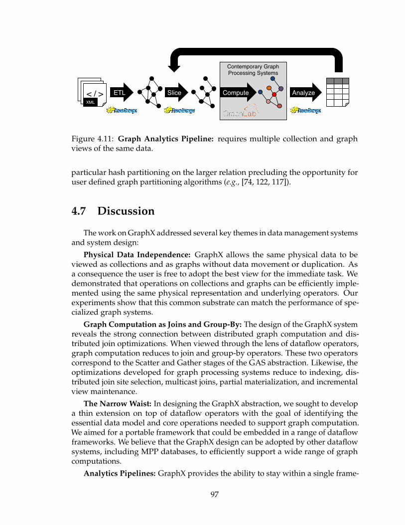
Contemporary Graph Processing Systems!

< / >!< / >!< / >!XML!

ETL! Slice! Compute! Analyze!

Figure 4.11: Graph Analytics Pipeline: requires multiple collection and graphviews of the same data.

particular hash partitioning on the larger relation precluding the opportunity foruser defined graph partitioning algorithms (e.g., [74, 122, 117]).

4.7 Discussion

The work on GraphX addressed several key themes in data management systemsand system design:

Physical Data Independence: GraphX allows the same physical data to beviewed as collections and as graphs without data movement or duplication. Asa consequence the user is free to adopt the best view for the immediate task. Wedemonstrated that operations on collections and graphs can be efficiently imple-mented using the same physical representation and underlying operators. Ourexperiments show that this common substrate can match the performance of spe-cialized graph systems.

Graph Computation as Joins and Group-By: The design of the GraphX systemreveals the strong connection between distributed graph computation and dis-tributed join optimizations. When viewed through the lens of dataflow operators,graph computation reduces to join and group-by operators. These two operatorscorrespond to the Scatter and Gather stages of the GAS abstraction. Likewise, theoptimizations developed for graph processing systems reduce to indexing, dis-tributed join site selection, multicast joins, partial materialization, and incrementalview maintenance.

The Narrow Waist: In designing the GraphX abstraction, we sought to developa thin extension on top of dataflow operators with the goal of identifying theessential data model and core operations needed to support graph computation.We aimed for a portable framework that could be embedded in a range of dataflowframeworks. We believe that the GraphX design can be adopted by other dataflowsystems, including MPP databases, to efficiently support a wide range of graphcomputations.

Analytics Pipelines: GraphX provides the ability to stay within a single frame-

97

work throughout the analytics process, eliminating the need to learn and supportmultiple systems (e.g., Figure 4.11) or write data interchange formats and plumbingto move between systems. As a consequence, it is substantially easier to iterativelyslice, transform, and compute on large graphs as well as to share data-structuresacross stages of the pipeline. The gains in performance and scalability for graphcomputation translate to a tighter analytics feedback loop and therefore a moreefficient work flow.

Adoption: GraphX was publicly released as part of the 0.9.0 release of theApache Spark open-source project. It has since generated substantial interest inthe community and has been used in production at various places [67]. Despite itsnascent state, there has been considerable open-source contribution to GraphX withcontributors providing some of the core graph functionality. We attribute this to itswide applicability and the simple abstraction built on top of an existing, populardataflow framework.

4.8 Conclusion

In this work we introduced GraphX, an efficient graph processing system thatenables distributed dataflow frameworks such as Spark to naturally express andefficiently execute iterative graph algorithms. We identified a simple pattern of join–map–group-by dataflow operators that forms the basis of graph-parallel computation.Inspired by this observation, we proposed the GraphX abstraction, which representsgraphs as horizontally-partitioned collections and graph computation as dataflowoperators on those collections. Not only does GraphX support existing graph-parallel abstractions and a wide range of iterative graph algorithms, it enables thecomposition of graphs and collections, freeing the user to adopt the most naturalview without concern for data movement or duplication.

Guided by the connection between graph computation and dataflow opera-tors, we recast recent advances in graph processing systems as range of classicoptimizations in database systems. We recast vertex-cut graph partitioning ashorizontally-partitioned vertex and edge collections, active vertex tracking as in-cremental view maintenance, and vertex mirroring as multicast joins with routingtables. As a result, for graph algorithms, GraphX is over an order of magnitudefaster than the base dataflow system and is comparable to or faster than specializedgraph processing systems. In addition, GraphX benefits from features provided byrecent dataflow systems such as low-cost fault tolerance and transparent recovery.

98

Chapter 5

Conclusion

This chapter concludes the dissertation. We summarize the contributions andbroader industry impact from each of the three systems. Finally, we discuss futurework.

5.1 Innovation Highlights and Broader Impact

All three systems, Spark SQL, Structured Streaming, and GraphX, developedin this dissertation, share a common theme: modern analytics are becoming morediverse. The types of analytics are becoming more diverse: complex analytics suchas machine learning and graph processing are becoming increasingly common inaddition to relational query processing. The programming languages are becomingmore diverse: data engineers use Scala and Java, data scientists use Python andR, while business analysts still predominantly use SQL. Finally, the frequency ofanalytics are becoming more diverse as well: many organizations that started withbatch analytics that happen once a day are now employing real-time streaming datapipelines to increase the velocity of data-driven decisions.

These three systems have been widely adopted in industry. Combined together,the three systems laid the foundation for Spark 2.0.

5.1.1 Spark SQL

Spark SQL integrates relational processing with Spark’s functional programmingAPI for complex analytics. Built on our experience with Shark, Spark SQL lets Sparkprogrammers leverage the benefits of relational processing (e.g., declarative queriesand optimized storage), and lets SQL users call complex analytics libraries in Spark(e.g., machine learning). Compared to previous systems, Spark SQL makes two mainadditions. First, it offers much tighter integration between relational and proceduralprocessing, through a declarative DataFrame API that integrates with proceduralSpark code. Second, it includes a highly extensible optimizer, Catalyst, built using

99

features of the Scala programming language, that makes it easy to add composablerules, control code generation, and define extension points. Using Catalyst, wehave built a variety of features (e.g., schema inference for JSON, machine learningdata types, and query federation to external databases) tailored for the complexneeds of modern data analysis. We see Spark SQL as an evolution of both SQL-on-Spark and of Spark itself, offering richer APIs and optimizations while keeping thebenefits of the Spark programming model. More fundamentally, Spark SQL and itspredecessor Shark show that dataflow execution models can be applied effectivelyto SQL, and offer a promising way to combine relational and complex analytics.

Since its initial experimental open source release in 2014, Spark SQL has becomethe most widely used and developed module in Spark. The DataFrame API becamethe de facto programming API in Spark’s 2.0 release. While the initial RDD APIremains as an important lower level API, most user applications have migratedover from the RDD API to the DataFrame API. Given that Spark is one of the mostpopular open source projects in Big Data, it is very likely that the DataFrame API isthe most widely used API in big data.

5.1.2 Structured Streaming

With the ubiquity of streaming data, organizations need stream processing sys-tems that are scalable, easy to use, and easy to integrate into business applications.Structured Streaming builds on Spark SQL, and exposes a high-level, declarativestreaming API. Structured Streaming differs from other recent streaming APIs, suchas Google Dataflow, in two main ways. First, it is a purely declarative API basedon automatically incrementalizing a static relational query (expressed using SQLor DataFrames), as opposed to APIs that ask the user to design a DAG of physicaloperators. This makes it accessible to non-experts. Second, Structured Streamingis designed to support end-to-end real-time applications that combine streamingwith batch and interactive analysis. We found that many real-world applicationsrequired this type of integration, and this integration was often the most challeng-ing part of building them. Structured Streaming achieves high performance usingSpark SQL’s code generation engine and outperforms Apache Flink by up to 4×and Kafka Streams by 90×. It also offers powerful operational features such asrollbacks, code updates, and mixed streaming/batch execution.

Structured Streaming was initially released in 2016. We have observed severalhundred large-scale production use cases, the largest of which processes over 1 PBof data per month.

5.1.3 GraphX

GraphX is an embedded graph processing system built on top of Apache Spark.GraphX presents a familiar composable graph abstraction that is sufficient to express

100

existing graph APIs, yet can be implemented using only a few basic dataflowoperators (e.g., join, map, group-by).

In pursuit of graph processing performance, the systems community has largelyabandoned general-purpose distributed dataflow frameworks in favor of special-ized graph processing systems that provide tailored programming abstractions andaccelerate the execution of iterative graph algorithms. In this paper we argue thatmany of the advantages of specialized graph processing systems can be recoveredin a modern general-purpose distributed dataflow system.

To demonstrate this, we implemented GraphX on top of Spark, a dataflowframework. To achieve performance parity with specialized graph systems, GraphXrecasts graph-specific optimizations as distributed join optimizations and materi-alized view maintenance. By leveraging advances in distributed dataflow frame-works, GraphX brings low-cost fault tolerance to graph processing. We evaluateGraphX on real workloads and demonstrate that GraphX achieves an order ofmagnitude performance gain over the base dataflow framework and matches theperformance of specialized graph processing systems while enabling a wider rangeof computation.

GraphX was merged into Spark in version 1.2. In Spark 2.0, it became the maingraph processing library, in lieu of Bagel.

5.2 Future Work

Our work on these systems points to a larger research agenda in the unificationof specialized data processing systems. Recent advances in specialized systemsfor topic modeling, graph processing, stream processing, and deep learning haverevealed a range of new system optimizations and design trade-offs. However, thefull potential of these systems is often realized in their integration (e.g., applyingdeep learning to text and images in a social network). By casting these systemswithin a common paradigm we may reveal common patterns and enable newanalytic capabilities. In this context, the main areas of future work are:

AI, Deep Learning, and Machine Learning on Dataflows: One cannot avoid draw-ing attention to AI, deep learning, and machine learning when discussing dataanalytics in 2018. Many systems, both hardware [72] and software [8, 102], havebeen built specifically for developing and executing deep learning and machinelearning algorithms. These systems achieve high performance for numeric compu-tation through highly optimized kernels that employ data-parallel CPU and GPUinstructions.

There are two general approaches in using dataflow systems for machine learn-ing. The first approach uses the dataflow systems across the entire pipeline, fromdata loading, to feature engineering, to training. In this approach, the trainingalgorithm is implemented entirely in these dataflow systems, using dataflow orrelational operators. The second approach is to “integrate”. In this approach, users

101

leverage dataflow systems for data loading, feature engineering, and parallelization,but run the specialized software (e.g., PyTorch) for training. Compared with thefirst approach, the second approach typically achieves higher performance for thetraining part, at the cost of increased operational complexity and lower performancein data exchange.

One fruitful area of research is to explore whether a single dataflow system canefficiently and effectively support machine learning pipelines end-to-end, from dataloading, to feature engineering, to training. This will require the development ofnew code generation engines that can combine relational processing with highlyefficient numeric computations. KeystoneML [116] is an early attempt at this.

GraphFrames: The graph abstraction in GraphX is analogous to the RDD abstrac-tion for distributed collection of data. It is a lower level, expressive API, but lacksoptimization opportunities due to the extensive use of user-defined functions aswell as coupling of physical plans and logical plans. A possible extension is tocombine the ideas in Spark SQL and GraphX to create GraphFrames, a DataFrame-based approach for programming graph applications. This new approach canenable graph specific optimizations by extending the Catalyst query optimizer.

Streaming, Incremental Graph Computation: Similar to streaming data that areconstantly changing, real-life graph structures are rarely static. Members on socialnetworks make new connections all the time, while an interest graph would beupdated each time a user ”likes” an item. All operations in GraphX are batch-oriented, and any update on a graph would require recomputing the entire datapipeline.

Incremental graph computation will be a fruitful research area, by minimizingthe computation cost of small graph updates. This will require both API changes torestrict operations to be algebraic, as well as system changes that can automaticallyincrementalize graph computation plans.

Unifying multi-core with distributed dataflows: In the course of this dissertation,the increase of CPU clock speed has largely plateaued. Instead, CPUs are increasingin core-count. It is not uncommon to see machines with 128 cores. With such highcore counts, future multi-core systems resemble distributed systems more than theydo traditional single-node systems. We believe there is a tremendous opportunity todesign simple software architectures, based on dataflows, that can scale well fromsingle-node multi-core systems, for small to medium amounts of data, to clusters ofthousands of machines, for large amounts of data.

We hope the lessons learned in this dissertation can help facilitate further re-search in the above areas, and create innovative solutions that shape new systemdirections.

102

Bibliography

[1] http://aws.amazon.com/elasticmapreduce/.

[2] Apache Hadoop project. http://hadoop.apache.org/.

[3] Apache Impala project. https://github.com/cloudera/impala.

[4] Apache Spark project contributor graph.https://github.com/apache/spark/graphs/contributors.

[5] Deja VVVu: Others Claiming Gartners Construct for Big Data. Gartner BlogNetwork, 2012.

[6] Daniel J. Abadi, Yanif Ahmad, Magdalena Balazinska, Mitch Cherniack, Jeonghyon Hwang, Wolfgang Lindner, Anurag S. Maskey, Er Rasin, Esther Ryvkina,Nesime Tatbul, Ying Xing, and Stan Zdonik. The design of the borealis streamprocessing engine. In In CIDR, pages 277–289, 2005.

[7] Daniel J. Abadi, Adam Marcus, Samuel R. Madden, and Kate Hollenbach.SW-Store: A vertically partitioned DBMS for semantic web data management.PVLDB, 18(2):385–406, 2009.

[8] Martin Abadi, Paul Barham, et al. Tensorflow: A system for large-scalemachine learning. In 12th USENIX Symposium on Operating Systems Designand Implementation (OSDI 16), pages 265–283, 2016.

[9] Azza Abouzeid et al. Hadoopdb: an architectural hybrid of mapreduce anddbms technologies for analytical workloads. VLDB, 2009.

[10] Azza Abouzied, Daniel J. Abadi, and Avi Silberschatz. Invisible loading:Access-driven data transfer from raw files into database systems. In EDBT,2013.

[11] Foto N. Afrati and Jeffrey D. Ullman. Optimizing joins in a map-reduceenvironment. In EDBT, pages 99–110, 2010.

[12] Tyler Akidau, Robert Bradshaw, Craig Chambers, Slava Chernyak, Rafael J.Fernandez-Moctezuma, Reuven Lax, Sam McVeety, Daniel Mills, FrancesPerry, Eric Schmidt, and Sam Whittle. The dataflow model: A practical

103

approach to balancing correctness, latency, and cost in massive-scale, un-bounded, out-of-order data processing. Proc. VLDB Endow., 8(12):1792–1803,August 2015.

[13] Alexander Alexandrov et al. The Stratosphere platform for big data analytics.The VLDB Journal, 23(6):939–964, December 2014.

[14] Intel Altera. Financial/hpc – financial offload. https://www.altera.com/solutions/industry/computer-and-storage/applications/computer/

financial-offload.html, 2017.

[15] Peter Alvaro, Neil Conway, Joseph M. Hellerstein, and William R. Marczak.Consistency analysis in bloom: A calm and collected approach. In In Proceed-ings 5th Biennial Conference on Innovative Data Systems Research, pages 249–260,2011.

[16] Amazon. Amazon Kinesis. https://aws.amazon.com/kinesis/, 2017.

[17] Apache Storm. http://storm-project.net.

[18] Apache Avro project. http://avro.apache.org.

[19] Apache Parquet project. http://parquet.incubator.apache.org.

[20] Apache Spark project. http://spark.apache.org.

[21] Michael Armbrust. SPARK-20928: Continuous processing mode for struc-tured streaming. https://issues.apache.org/jira/browse/SPARK-20928, 2017.

[22] Michael Armbrust, Bill Chambers, and Matei Zaharia.Databricks delta: A unified data management system for real-time big data. https://databricks.com/blog/2017/10/25/

databricks-delta-a-unified-management-system.html, 2017.

[23] Michael Armbrust, Nick Lanham, Stephen Tu, Armando Fox, Michael JFranklin, and David A Patterson. The case for PIQL: a performance insightfulquery language. In SOCC, 2010.

[24] Jeff Barr. New – per-second billing for EC2 instancesand EBS volumes. https://aws.amazon.com/blogs/aws/

new-per-second-billing-for-ec2-instances-and-ebs-volumes/, 2017.

[25] Apache Beam. Apache Beam programming guide. https://beam.apache.org/documentation/programming-guide/, 2017.

[26] Alexander Behm et al. Asterix: towards a scalable, semistructured data plat-form for evolving-world models. Distributed and Parallel Databases, 29(3):185–216, 2011.

104

https://www.altera.com/solutions/industry/computer-and-storage/applications/computer/financial-offload.html



https://aws.amazon.com/kinesis/

http://storm-project.net

https://databricks.com/blog/2017/10/25/databricks-delta-a-unified-management-system.html

https://databricks.com/blog/2017/10/25/databricks-delta-a-unified-management-system.html

https://aws.amazon.com/blogs/aws/new-per-second-billing-for-ec2-instances-and-ebs-volumes/

https://aws.amazon.com/blogs/aws/new-per-second-billing-for-ec2-instances-and-ebs-volumes/

https://beam.apache.org/documentation/programming-guide/

https://beam.apache.org/documentation/programming-guide/

[27] Greet Jan Bex, Frank Neven, and Stijn Vansummeren. Inferring XML schemadefinitions from XML data. In VLDB, 2007.

[28] BigDF project. https://github.com/AyasdiOpenSource/bigdf.

[29] Jose A. Blakeley, Per-Ake Larson, and Frank Wm Tompa. Efficiently updatingmaterialized views. SIGMOD Rec., 15(2):61–71, June 1986.

[30] Spyros Blanas, Jignesh M. Patel, Vuk Ercegovac, Jun Rao, Eugene J. Shekita,and Yuanyuan Tian. A comparison of join algorithms for log processing inMapReduce. In Proceedings of the 2010 ACM SIGMOD International Conferenceon Management of Data, SIGMOD ’10, pages 975–986, New York, NY, USA,2010. ACM.

[31] Paolo Boldi, Marco Rosa, Massimo Santini, and Sebastiano Vigna. Layered la-bel propagation: A multiresolution coordinate-free ordering for compressingsocial networks. In WWW, pages 587–596, 2011.

[32] Paolo Boldi and Sebastiano Vigna. The WebGraph framework I: Compressiontechniques. In WWW’04.

[33] Jeen Broekstra, Arjohn Kampman, and Frank van Harmelen. Sesame: Ageneric architecture for storing and querying rdf and rdf schema. In Pro-ceedings of the First International Semantic Web Conference on The Semantic Web,ISWC ’02, pages 54–68, 2002.

[34] Aydin Buluc and John R. Gilbert. The combinatorial BLAS: design, imple-mentation, and applications. IJHPCA, 25(4):496–509, 2011.

[35] Umit V. Catalyurek, Cevdet Aykanat, and Bora Ucar. On two-dimensionalsparse matrix partitioning: Models, methods, and a recipe. SIAM J. Sci.Comput., 32(2):656–683, 2010.

[36] Badrish Chandramouli, Jonathan Goldstein, Mike Barnett, Robert DeLine,Danyel Fisher, John C. Platt, James F. Terwilliger, and John Wernsing. Trill:A high-performance incremental query processor for diverse analytics. Proc.VLDB Endow., 8(4):401–412, December 2014.

[37] Sirish Chandrasekaran, Owen Cooper, Amol Deshpande, Michael J. Franklin,Joseph M. Hellerstein, Wei Hong, Sailesh Krishnamurthy, Samuel R. Mad-den, Fred Reiss, and Mehul A. Shah. Telegraphcq: Continuous dataflowprocessing. In Proceedings of the 2003 ACM SIGMOD International Conferenceon Management of Data, SIGMOD ’03, pages 668–668, New York, NY, USA,2003. ACM.

[38] B. Chattopadhyay, , et al. Tenzing a sql implementation on the mapreduceframework. PVLDB, 4(12):1318–1327, 2011.

105

[39] Raymond Cheng, Ji Hong, Aapo Kyrola, Youshan Miao, Xuetian Weng, MingWu, Fan Yang, Lidong Zhou, Feng Zhao, and Enhong Chen. Kineograph:taking the pulse of a fast-changing and connected world. In EuroSys, pages85–98, 2012.

[40] Sanket Chintapalli, Derek Dagit, Bobby Evans, Reza Farivar, Tom Graves,Mark Holderbaugh, Zhuo Liu, Kyle Nusbaum, Kishorkumar Patil, BoyangPeng, and Paul Poulosky. Benchmarking streaming computation en-gines at Yahoo! https://yahooeng.tumblr.com/post/135321837876/

benchmarking-streaming-computation-engines-at, 2015.

[41] C. Chu et al. Map-reduce for machine learning on multicore. Advances inneural information processing systems, 19:281, 2007.

[42] J. Cohen, B. Dolan, M. Dunlap, J.M. Hellerstein, and C. Welton. Mad skills:new analysis practices for big data. VLDB, 2009.

[43] Confluent. Ksql: Streaming sql for kafka. https://www.confluent.io/product/ksql/, 2017.

[44] Databricks. Apache Spark Survey 2016 Results Now Available. https://databricks.com/blog/2016/09/27/spark-survey-2016-released.html,2016.

[45] Databricks. Databricks unified analytics platform. https://databricks.com/product/unified-analytics-platform, 2017.

[46] DDF project. http://ddf.io.

[47] J. Dean and S. Ghemawat. Mapreduce: simplified data processing on largeclusters. In OSDI, 2004.

[48] Jeffrey Dean and Sanjay Ghemawat. MapReduce: Simplified data processingon large clusters. In OSDI, 2004.

[49] Burak Emir, Martin Odersky, and John Williams. Matching objects withpatterns. In ECOOP 2007 – Object-Oriented Programming, volume 4609 of LNCS,pages 273–298. Springer, 2007.

[50] Stephan Ewen, Kostas Tzoumas, Moritz Kaufmann, and Volker Markl. Spin-ning fast iterative data flows. Proc. VLDB, 5(11):1268–1279, July 2012.

[51] Uriel Feige, MohammadTaghi Hajiaghayi, and James R. Lee. Improved ap-proximation algorithms for minimum-weight vertex separators. In Proceedingsof the Thirty-seventh Annual ACM Symposium on Theory of Computing, STOC’05, pages 563–572, New York, NY, USA, 2005. ACM.

[52] Apache Flink. Apache flink. http://flink.apache.org, 2017.

106

https://yahooeng.tumblr.com/post/135321837876/benchmarking-streaming-computation-engines-at

https://yahooeng.tumblr.com/post/135321837876/benchmarking-streaming-computation-engines-at

https://www.confluent.io/product/ksql/

https://www.confluent.io/product/ksql/

https://databricks.com/blog/2016/09/27/spark-survey-2016-released.html

https://databricks.com/blog/2016/09/27/spark-survey-2016-released.html

https://databricks.com/product/unified-analytics-platform

https://databricks.com/product/unified-analytics-platform

http://flink.apache.org

[53] Apache Flink. Flink datastream api programming guide. https:

//ci.apache.org/projects/flink/flink-docs-release-1.3/dev/

datastream_api.html, 2017.

[54] Apache Flink. Flink table & sql api beta. https://ci.apache.org/projects/flink/flink-docs-release-1.3/dev/table/index.html, 2017.

[55] Apache Flink. Working with state. https://ci.apache.org/projects/flink/flink-docs-release-1.3/dev/stream/state.html, 2017.

[56] M.J. Franklin, S. Krishnamurthy, N. Conway, A. Li, A. Russakovsky, andN. Thombre. Continuous analytics: Rethinking query processing in a network-effect world. CIDR, 2009.

[57] Lukasz Golab and M. Tamer Ozsu. Issues in data stream management. SIG-MOD Rec., 32(2):5–14, June 2003.

[58] Joseph E. Gonzalez, Yucheng Low, Haijie Gu, Danny Bickson, and CarlosGuestrin. Powergraph: Distributed graph-parallel computation on naturalgraphs. OSDI’12, pages 17–30, Berkeley, CA, USA, 2012. USENIX Association.

[59] G. Graefe and D.J. DeWitt. The EXODUS optimizer generator. In SIGMOD,1987.

[60] Goetz Graefe. The Cascades framework for query optimization. IEEE DataEngineering Bulletin, 18(3), 1995.

[61] Jamie Grier. Extending the Yahoo! streaming benchmark. https://

data-artisans.com/blog/extending-the-yahoo-streaming-benchmark,2016.

[62] B. Guffler et al. Handling data skew in mapreduce. In CLOSER’11.

[63] Trevor Hastie, Robert Tibshirani, and Jerome Friedman. The Elements ofStatistical Learning: Data Mining, Inference, and Prediction. Springer PublishingCompany, New York, NY, 2009.

[64] Jan Hegewald, Felix Naumann, and Melanie Weis. XStruct: efficient schemaextraction from multiple and large XML documents. In ICDE Workshops, 2006.

[65] Benjamin Hindman, Andrew Konwinski, Matei Zaharia, Ali Ghodsi, An-thony D. Joseph, Randy H. Katz, Scott Shenker, and Ion Stoica. Mesos: Aplatform for fine-grained resource sharing in the data center. In NSDI, 2011.

[66] Hive data definition language. https://cwiki.apache.org/confluence/display/Hive/LanguageManual+DDL.

[67] Andy Huang and Wei Wu. Mining ecommerce graph data with spark atalibaba taobao. http://databricks.com/blog/2014/08/14/mining-graph-data-with-spark-at-alibaba-taobao.html, 2014.

107

https://ci.apache.org/projects/flink/flink-docs-release-1.3/dev/datastream_api.html



https://ci.apache.org/projects/flink/flink-docs-release-1.3/dev/table/index.html

https://ci.apache.org/projects/flink/flink-docs-release-1.3/dev/table/index.html

https://ci.apache.org/projects/flink/flink-docs-release-1.3/dev/stream/state.html

https://ci.apache.org/projects/flink/flink-docs-release-1.3/dev/stream/state.html

https://data-artisans.com/blog/extending-the-yahoo-streaming-benchmark

https://data-artisans.com/blog/extending-the-yahoo-streaming-benchmark

https://cwiki.apache.org/confluence/display/Hive/LanguageManual+DDL

https://cwiki.apache.org/confluence/display/Hive/LanguageManual+DDL

[68] M. Isard, M. Budiu, Y. Yu, A. Birrell, and D. Fetterly. Dryad: distributeddata-parallel programs from sequential building blocks. In EuroSys, pages59–72, 2007.

[69] Michael Isard, Mihai Budiu, Yuan Yu, Andrew Birrell, and Dennis Fetterly.Dryad: distributed data-parallel programs from sequential building blocks.In EuroSys, 2007.

[70] Michael Isard, Vijayan Prabhakaran, Jon Currey, Udi Wieder, Kunal Talwar,and Andrew Goldberg. Quincy: Fair scheduling for distributed computingclusters. In SOSP, November 2009.

[71] Jackson JSON processor. http://jackson.codehaus.org.

[72] Norman P. Jouppi, Cliff Young, et al. In-datacenter performance analysis of atensor processing unit. CoRR, abs/1704.04760, 2017.

[73] Apache Kafka. Kafka. http://kafka.apache.org, 2017.

[74] G. Karypis and V. Kumar. Multilevel k-way partitioning scheme for irregulargraphs. J. Parallel Distrib. Comput., 48(1):96–129, 1998.

[75] Yannis Klonatos, Christoph Koch, Tiark Rompf, and Hassan Chafi. Buildingefficient query engines in a high-level language. PVLDB, 7(10):853–864, 2014.

[76] S. Krishnamurthy, M.J. Franklin, J. Davis, D. Farina, P. Golovko, A. Li, andN. Thombre. Continuous analytics over discontinuous streams. In SIGMOD,2010.

[77] YongChul Kwon et al. Skewtune: mitigating skew in mapreduce applications.In SIGMOD ’12, 2012.

[78] A. Kyrola, G. Blelloch, and C. Guestrin. GraphChi: Large-scale graph compu-tation on just a PC. In OSDI, 2012.

[79] J. Leskovec, K. J. Lang, A. Dasgupta, , and M. W. Mahoney. Communitystructure in large networks: Natural cluster sizes and the absence of largewell-defined clusters. Internet Mathematics, 6(1):29–123, 2008.

[80] Dionysios Logothetis, Christopher Olston, Benjamin Reed, Kevin C. Webb,and Ken Yocum. Stateful bulk processing for incremental analytics. InProceedings of the 1st ACM Symposium on Cloud Computing, SoCC ’10, pages51–62, New York, NY, USA, 2010. ACM.

[81] Y. Low et al. GraphLab: A new parallel framework for machine learning. InUAI, pages 340–349, 2010.

[82] Yucheng Low, Danny Bickson, Joseph Gonzalez, Carlos Guestrin, Aapo Ky-rola, and Joseph M. Hellerstein. Distributed GraphLab: A framework formachine learning and data mining in the cloud, April 2012.

108

http://kafka.apache.org

[83] Yucheng Low, Joseph Gonzalez, Aapo Kyrola, Danny Bickson, CarlosGuestrin, and J. M. Hellerstein. Distributed GraphLab: A Framework forMachine Learning and Data Mining in the Cloud. PVLDB, 2012.

[84] Lothar F. Mackert and Guy M. Lohman. R* optimizer validation and per-formance evaluation for distributed queries. In VLDB’86, pages 149–159,1986.

[85] G. Malewicz, M. H. Austern, A. J.C Bik, J.C. Dehnert, I. Horn, N. Leiser, andG. Czajkowski. Pregel: a system for large-scale graph processing. In SIGMOD,pages 135–146, 2010.

[86] Frank Manola and Eric Miller. RDF primer. W3C Recommendation, 10:1–107,2004.

[87] Frank McSherry, Derek Murray, Rebecca Isaacs, and Michael Isard. Differen-tial dataflow. In Proceedings of CIDR 2013, January 2013.

[88] Sergey Melnik, Andrey Gubarev, Jing Jing Long, Geoffrey Romer, ShivaShivakumar, Matt Tolton, and Theo Vassilakis. Dremel: interactive analysisof web-scale datasets. Proc. VLDB Endow., 3:330–339, Sept 2010.

[89] Xiangrui Meng, Joseph Bradley, Evan Sparks, and ShivaramVenkataraman. ML pipelines: a new high-level API for MLlib.https://databricks.com/blog/2015/01/07/ml-pipelines-a-new-high-level-api-for-mllib.html.

[90] Jayanta Mondal and Amol Deshpande. Managing large dynamic graphsefficiently. In Proceedings of the 2012 ACM SIGMOD International Conference onManagement of Data, SIGMOD ’12, pages 145–156, New York, NY, USA, 2012.ACM.

[91] Derek Murray. Building new frameworks on Naiad, April 2014.

[92] Derek G. Murray, Frank McSherry, Rebecca Isaacs, Michael Isard, PaulBarham, and Martın Abadi. Naiad: A timely dataflow system. In SOSP’13.

[93] Derek G. Murray, Frank McSherry, Rebecca Isaacs, Michael Isard, PaulBarham, and Martın Abadi. Naiad: A timely dataflow system. pages 439–455,2013.

[94] Marc Najork, Dennis Fetterly, Alan Halverson, Krishnaram Kenthapadi, andSreenivas Gollapudi. Of hammers and nails: An empirical comparison ofthree paradigms for processing large graphs. In Proceedings of the Fifth ACMInternational Conference on Web Search and Data Mining, WSDM ’12, pages103–112. ACM, 2012.

109

[95] S. Nestorov, S. Abiteboul, and R. Motwani. Extracting schema from semistruc-tured data. In ICDM, 1998.

[96] Thomas Neumann and Gerhard Weikum. RDF-3X: A RISC-style engine forRDF. VLDB’08.

[97] Frank Austin Nothaft, Matt Massie, Timothy Danford, Zhao Zhang, UriLaserson, Carl Yeksigian, Jey Kottalam, Arun Ahuja, Jeff Hammerbacher,Michael Linderman, Michael J. Franklin, Anthony D. Joseph, and David A.Patterson. Rethinking data-intensive science using scalable analytics systems.In SIGMOD, 2015.

[98] Christopher Olston, Benjamin Reed, Utkarsh Srivastava, Ravi Kumar, andAndrew Tomkins. Pig latin: a not-so-foreign language for data processing. InSIGMOD ’08, pages 1099–1110.

[99] Kay Ousterhout et al. The case for tiny tasks in compute clusters. In HotOS’13.

[100] L. Page, S. Brin, R. Motwani, and T. Winograd. The pagerank citation ranking:Bringing order to the web. Technical Report 1999-66, Stanford InfoLab, 1999.

[101] pandas Python data analysis library. http://pandas.pydata.org.

[102] Adam Paszke, Sam Gross, Soumith Chintala, Gregory Chanan, Edward Yang,Zachary DeVito, Zeming Lin, Alban Desmaison, Luca Antiga, and AdamLerer. Automatic differentiation in pytorch. 2017.

[103] A. Pavlo et al. A comparison of approaches to large-scale data analysis. InSIGMOD, 2009.

[104] Andrew Pavlo, Erik Paulson, Alexander Rasin, Daniel J. Abadi, David J. De-Witt, Samuel Madden, and Michael Stonebraker. A comparison of approachesto large-scale data analysis. In SIGMOD ’09, 2009.

[105] Eric Prud’hommeaux and Andy Seaborne. SPARQL query language for RDF.Latest version available as http://www.w3.org/TR/rdf-sparql-query/, Jan-uary 2008.

[106] Josep M. Pujol, Vijay Erramilli, Georgos Siganos, Xiaoyuan Yang, NikosLaoutaris, Parminder Chhabra, and Pablo Rodriguez. The little engine(s) thatcould: scaling online social networks. In SIGCOMM, pages 375–386, 2010.

[107] X. Qian and Gio Wiederhold. Incremental recomputation of active relationalexpressions. IEEE Trans. on Knowl. and Data Eng., 3(3):337–341, September1991.

[108] R project for statistical computing. http://www.r-project.org.

[109] I. Robinson, J. Webber, and E. Eifrem. Graph Databases. O’Reilly Media,Incorporated, 2013.

110

http://www.w3.org/TR/rdf-sparql-query/

[110] Amitabha Roy, Ivo Mihailovic, and Willy Zwaenepoel. X-stream: Edge-centricgraph processing using streaming partitions. SOSP ’13, pages 472–488. ACM,2013.

[111] Y. Saad. Iterative Methods for Sparse Linear Systems. Society for Industrial andApplied Mathematics, Philadelphia, PA, USA, 2nd edition, 2003.

[112] scikit-learn: machine learning in Python. http://scikit-learn.org.

[113] Denys Shabalin, Eugene Burmako, and Martin Odersky. Quasiquotes forScala, a technical report. Technical Report 185242, Ecole PolytechniqueFederale de Lausanne, 2013.

[114] Apache Spark. Spark documentation. http://spark.apache.org/docs/latest, 2017.

[115] Spark machine learning library (MLlib). http://spark.incubator.apache.org/docs/latest/mllib-guide.html.

[116] Evan R. Sparks, Shivaram Venkataraman, Tomer Kaftan, Michael J. Franklin,and Benjamin Recht. Keystoneml: Optimizing pipelines for large-scale ad-vanced analytics. In IEEE ICDE 2017, pages 535–546, 2017.

[117] Isabelle Stanton and Gabriel Kliot. Streaming graph partitioning for largedistributed graphs. Technical Report MSR-TR-2011-121, Microsoft Research,November 2011.

[118] Michael Stonebraker et al. Mapreduce and parallel dbmss: friends or foes?Commun. ACM.

[119] Philip Stutz, Abraham Bernstein, and William Cohen. Signal/collect: graphalgorithms for the (semantic) web. In ISWC, 2010.

[120] Daniel Tahara, Thaddeus Diamond, and Daniel J. Abadi. Sinew: A SQLsystem for multi-structured data. In SIGMOD, 2014.

[121] Ashish Thusoo, Joydeep Sen Sarma, Namit Jain, Zheng Shao, Prasad Chakka,Ning Zhang, Suresh Antony, Hao Liu, and Raghotham Murthy. Hive-apetabyte scale data warehouse using Hadoop. In ICDE, 2010.

[122] Johan Ugander and Lars Backstrom. Balanced label propagation for partition-ing massive graphs. In Proceedings of the Sixth ACM International Conference onWeb Search and Data Mining, WSDM ’13, pages 507–516, New York, NY, USA,2013. ACM.

[123] Philip Wadler. Monads for functional programming. In Advanced FunctionalProgramming, pages 24–52. Springer, 1995.

[124] Patrick Wendell. Comparing large scale query engines. https://amplab.cs.berkeley.edu/2013/06/04/comparing-large-scale-query-engines/.

111

http://spark.apache.org/docs/latest

http://spark.apache.org/docs/latest

http://spark.incubator.apache.org/docs/latest/mllib-guide.html

http://spark.incubator.apache.org/docs/latest/mllib-guide.html

https://amplab.cs.berkeley.edu/2013/06/04/comparing-large-scale-query-engines/

https://amplab.cs.berkeley.edu/2013/06/04/comparing-large-scale-query-engines/

[125] Reynold Xin et al. GraySort on Apache Spark by Databricks. http:

//sortbenchmark.org/ApacheSpark2014.pdf.

[126] Reynold S. Xin, Joseph E. Gonzalez, Michael J. Franklin, and Ion Stoica.Graphx: A resilient distributed graph system on spark. In First InternationalWorkshop on Graph Data Management Experiences and Systems, GRADES ’13,2013.

[127] Reynold S. Xin, Josh Rosen, Matei Zaharia, Michael J. Franklin, Scott Shenker,and Ion Stoica. Shark: Sql and rich analytics at scale. In Proceedings of the 2013ACM SIGMOD International Conference on Management of Data, SIGMOD ’13,2013.

[128] Burak Yavuz and Tyson Condie. Running streaming jobs once aday for 10x cost savings. https://databricks.com/blog/2017/05/22/

running-streaming-jobs-day-10x-cost-savings.html, 2017.

[129] Yuan Yu, Michael Isard, Dennis Fetterly, Mihai Budiu, Ulfar Erlingsson,Pradeep Kumar Gunda, and Jon Currey. DryadLINQ: A system for general-purpose distributed data-parallel computing using a high-level language. InOSDI ’08, 2008.

[130] Matei Zaharia, Dhruba Borthakur, Joydeep Sen Sarma, Khaled Elmeleegy,Scott Shenker, and Ion Stoica. Delay scheduling: A simple technique forachieving locality and fairness in cluster scheduling. In EuroSys 10, 2010.

[131] Matei Zaharia, Mosharaf Chowdhury, Tathagata Das, Ankur Dave, JustinMa, Murphy McCauley, Michael Franklin, Scott Shenker, and Ion Stoica.Resilient distributed datasets: A fault-tolerant abstraction for in-memorycluster computing. In NSDI, 2012.

[132] Matei Zaharia, Mosharaf Chowdhury, Tathagata Das, Ankur Dave, JustinMa, Murphy McCauley, Michael J. Franklin, Scott Shenker, and Ion Stoica.Resilient distributed datasets: A fault-tolerant abstraction for in-memorycluster computing. NSDI’12, 2012.

[133] Matei Zaharia, Tathagata Das, Haoyuan Li, Timothy Hunter, Scott Shenker,and Ion Stoica. Discretized streams: Fault-tolerant streaming computation atscale. In SOSP, 2013.

[134] Kai Zeng et al. G-OLA: Generalized online aggregation for interactive analysison big data. In SIGMOD, 2015.

[135] Yue Zhuge, Hector Garcıa-Molina, Joachim Hammer, and Jennifer Widom.View maintenance in a warehousing environment. In Proceedings of the 1995ACM SIGMOD International Conference on Management of Data, SIGMOD ’95,pages 316–327, New York, NY, USA, 1995. ACM.

112

http://sortbenchmark.org/ApacheSpark2014.pdf

http://sortbenchmark.org/ApacheSpark2014.pdf

https://databricks.com/blog/2017/05/22/running-streaming-jobs-day-10x-cost-savings.html

https://databricks.com/blog/2017/05/22/running-streaming-jobs-day-10x-cost-savings.html

Graphs, Streaming and Relational Computations over ...

Documents

Transcript of Graphs, Streaming and Relational Computations over ...