Shortest Path Optimization of theCyberKnife treatment in Radiotherapy

Kortste-pad optimalisatie van de CyberKnife-behandeling bijradiotherapie

by

Joris Mühlsteff

in partial fulfillment of the requirements for the degree of

Bachelor of Sciencein Applied Mathematics

at the Delft University of Technology,to be defended publicly on Thursday July 6, 2017 at 11:00 PM.

SupervisorDrs. ir. M. Keijzer, TU Delft

Commitee membersDr.ir. S. Breedveld, Erasmus MC RotterdamDr. D.C. Gijswijt, TU DelftDr. J.G. Spandaw, TU Delft

Preface

This bachelor thesis was written as part of the curriculum for students of the bachelor AppliedMathematics at the TU Delft. For my Bachelorproject, I did an internship at the ErasmusMedical Center Rotterdam. The project itself took place at the Daniel den Hoed location, whichspecializes in oncology.

I would like to thank the following people: Marleen Keijzer, my supervisor from the TU Delftfor bringing me in contact with the Erasmus Medical Center and for advice on the project andthe thesis. Sebastiaan Breedveld, my supervisor at the Erasmus Medical Center, for guiding methrough most of the project, doing plan quality calculations and for overall support during theinternship. And lastly, I would like to thank my fellow research colleagues at the faculty, formaking my internship at the Erasmus Medical Center a true fun experience for me to remember.

This internship was a great opportunity for me to apply knowledge of mathematics to solve realworld problems.

iii

iv

Summary

The main goal of this report is to improve the traveltime of the CyberKnife treatment, used forradiotherapy, without loss of plan quality. This is done by using optimization techniques, suchas Dijkstra’s Algorithm, as well as incorporating Hamiltonian paths and the Traveling SalesmanProblem. All calculations are done using Matlab, a numerical computing software.

With the above mentioned techniques, we created OPA, an Optimal Path Algorithm, that isbased on finding Hamiltonian paths, combined with the iterated process of interchanging nodeswith adjacent ones. With OPA, the traveltimes for 31 patients have been brought down by 35.9%on average, without any significant loss of plan quality.

v

vi

Contents

1 Introduction 1

1.1 Radiotherapy . . . . . . . . . . . . . . . . . . . . . . . . . . . . . . . . . . . . . . 1

1.2 The CyberKnife . . . . . . . . . . . . . . . . . . . . . . . . . . . . . . . . . . . . . 1

2 Problem description 5

2.1 Research goals . . . . . . . . . . . . . . . . . . . . . . . . . . . . . . . . . . . . . 5

2.2 Overview . . . . . . . . . . . . . . . . . . . . . . . . . . . . . . . . . . . . . . . . 6

2.3 Study Design . . . . . . . . . . . . . . . . . . . . . . . . . . . . . . . . . . . . . . 6

3 Shortest Path Optimization 9

3.1 Asymmetrical Dijkstra Algorithm (ADA) . . . . . . . . . . . . . . . . . . . . . . 9

3.1.1 Methods . . . . . . . . . . . . . . . . . . . . . . . . . . . . . . . . . . . . . 10

3.1.2 Results . . . . . . . . . . . . . . . . . . . . . . . . . . . . . . . . . . . . . 11

3.2 Symmetrical Dijkstra Algorithm (SDA) . . . . . . . . . . . . . . . . . . . . . . . 12

3.2.1 Methods . . . . . . . . . . . . . . . . . . . . . . . . . . . . . . . . . . . . . 12

3.2.2 Results . . . . . . . . . . . . . . . . . . . . . . . . . . . . . . . . . . . . . 14

3.3 Hamiltonian Path Algorithm (HPA) . . . . . . . . . . . . . . . . . . . . . . . . . 15

3.3.1 Methods . . . . . . . . . . . . . . . . . . . . . . . . . . . . . . . . . . . . . 15

3.3.2 Results . . . . . . . . . . . . . . . . . . . . . . . . . . . . . . . . . . . . . 18

3.4 Comparison of methods . . . . . . . . . . . . . . . . . . . . . . . . . . . . . . . . 19

4 Neighbour Path Algorithm (NPA) 21

4.1 Computing Neighbour Paths . . . . . . . . . . . . . . . . . . . . . . . . . . . . . . 21

4.1.1 Methods . . . . . . . . . . . . . . . . . . . . . . . . . . . . . . . . . . . . . 21

vii

viii CONTENTS

4.1.2 Results . . . . . . . . . . . . . . . . . . . . . . . . . . . . . . . . . . . . . 23

4.2 Analysis of Convergence . . . . . . . . . . . . . . . . . . . . . . . . . . . . . . . . 24

4.3 Plan Quality . . . . . . . . . . . . . . . . . . . . . . . . . . . . . . . . . . . . . . 26

5 Additional restrictions 27

5.1 Starting Nodes . . . . . . . . . . . . . . . . . . . . . . . . . . . . . . . . . . . . . 27

5.1.1 Methods . . . . . . . . . . . . . . . . . . . . . . . . . . . . . . . . . . . . . 27

5.2 Dummy Nodes . . . . . . . . . . . . . . . . . . . . . . . . . . . . . . . . . . . . . 28

5.2.1 Methods . . . . . . . . . . . . . . . . . . . . . . . . . . . . . . . . . . . . . 28

5.3 Concluding Results . . . . . . . . . . . . . . . . . . . . . . . . . . . . . . . . . . . 28

6 Conclusions 31

7 Recommendations 33

Bibliography 35

Appendices 37

A Matlab codes . . . . . . . . . . . . . . . . . . . . . . . . . . . . . . . . . . . . . . 39

B Traveltimes of all algorithms . . . . . . . . . . . . . . . . . . . . . . . . . . . . . . 49

C New paths . . . . . . . . . . . . . . . . . . . . . . . . . . . . . . . . . . . . . . . . 51

Chapter 1

Introduction

1.1 Radiotherapy

In the history of medicine, different treatments for cancer have been developed, such as radio-therapy, surgery and chemotherapy. However, nowadays more than 50% of the people diagnosedwith cancer, undergo a radiotherapy treatment [1]. During a radiotherapy treatment, the tumoris treated locally witch ionizing radiation, which destroys the malignant cells, while sparingthe surrounding healthy tissue as much as possible [2]. Some other forms of radiotherapy in-clude stereotactic radiosurgery (focusing high-power energy on a small area of the body) andbrachytherapy (placing a radiation source inside the tumor).

Whenever a patient has to undergo radiotherapy, a computed tomography scan (CT-scan) hasto be made of the patient, on which a treatment plan is designed. This plan tells which partsshould be irradiated and with what level [3]. After this, the treatment is delivered by a treatmentdevice, which will be further outlined in the next section.

1.2 The CyberKnife

The CyberKnife is a robotic radiosurgery system that was invented by Dr. John R. Adler, a Stan-ford University professor and Peter and Russell Schonberg of Schonberg Research Corporation.It is used for treating a variety of tumors, such as lung, prostate, and head-and-neck tumors.For this project, we will focus on prostate cancer patients only. Since 2004, the Radiotherapydepartment of the Erasmus Medical Center Rotterdam started using the CyberKnife, as seen inFigure 1.1, for precise radiations.

1

2 CHAPTER 1. INTRODUCTION

Figure 1.1: CyberKnife used at the Erasmus Medical Center Rotterdam

The treatment plan for a patient contains a selection of around 25 out of 110 nodes which isfound to be best fitting for the treatment of that patient. The nodes mentioned in the treatmentplan are the nodes from which radiation is delivered.

For the actual treatment of the patient, a virtual grid is placed around the patient. Since thenodes emanated from treatment plans made for prostate cancer patients, the grid is shaped likea semisphere, containing 110 candidate nodes, as seen in Figure 1.2.

Figure 1.2: Breedveld, S. (2013). CyberKnife search space. Towards automated treatment plan-ning in radiotherapy. The blue rectangle represents the operating table.

1.2. THE CYBERKNIFE 3

If for example a head-and-neck tumor had to be treated, the shape of the grid would resemblesomething close to three-quarter of a sphere, since traveling underneath the head is also possiblewith the CyberKnife.

The approximately 25 nodes used to radiate the patient are the so called mustpass nodes, whilethe remaining ∼85 nodes can be used as traveling nodes for the CyberKnife to move from onenode to the other, the so called inbetween nodes. There are also 8 dummy nodes, which are usedfor the sole purpose of serving as inbetween nodes. Radiation from these nodes is not possible.Note that the inbetween nodes change for every patient, as each patient has a different set ofmustpass nodes.

Movement of the CyberKnife is restricted to grid lines between the nodes. This has to do withsafety reasons. The three-dimensional grid is placed around the patient so that the CyberKnifemoves safely alongside the patient without touching him or her. If the machine were not to movearound the grid lines, but simply around the fastest route from one node to another, which wouldbe a straight line in Euclidean space, the machine could injure the patient. Therefore it travelsaround the patient by the pre-programmed lines. If the CyberKnife has to travel from node A toadjacent node B, it could do so directly by a straight line. However, if there is not a direct pathfrom node A to B, the CyberKnife may first need to move to an adjacent node C. This processis repeated until the node B can be directly reached.

4 CHAPTER 1. INTRODUCTION

Chapter 2

Problem description

2.1 Research goals

Now that we have a decent understanding of the working of the CyberKnife, we can formulateour general research question:

“How can we optimize the traveltime of the CyberKnife?"

Before we start thinking of any strategies to answer this question, there are still some importantrestrictions of the CyberKnife which we will need to take into consideration:

• The CyberKnife can only travel from nodes to higher-numbered nodes. This means thatif the CyberKnife for example has to travel from node 1 to 4, it could do so by going from1 to 3 to 4, but not by going from 1 to 5 to 4. This is because of mechanical limitations,such as cables of the robotic arm getting tied up.

• The order in which the mustpass nodes are visited cannot be altered. The CyberKnifecurrently visits the mustpass nodes in ascending order.

• It is also determined in the treatment plan which mustpass nodes need to be visited.Deviating from these nodes may result in loss of plan quality.

Based on these restrictions, we can split up our research question into three sub-questions:

1. How can we travel as fast as possible from node A to node B?

2. Does changing the order of the mustpass nodes benefit the traveltime?

3. Does replacing mustpass nodes with adjacent nodes benefit the traveltime, without loss ofplan quality?

Now we can start outlaying our steps to answer these questions.

5

6 CHAPTER 2. PROBLEM DESCRIPTION

2.2 Overview

In Chapter 3 we will take a look at the first two sub-questions. We will discuss three relatedmethods for finding shortest paths through the mustpass nodes, and compare results. In Chapter4, we will continue with the last sub-question: finding adjacent solutions without degrading theplan quality. We will first develop a method for finding adjacent solutions, after which we cancheck whether the plan quality is still acceptable. In Chapter 5 we will look at two additionalrestrictions that came along the research. Lastly, we will discuss our results in Chapter 6 andgive further recommendations in Chapter 7.

Since this project is done almost entirely in Matlab, there will be pseudocode provided for allthe Matlab programs. The actual Matlab code is added in Appendix A.

2.3 Study Design

The Erasmus Medical Center Rotterdam provided a dataset containing a cell with mustpassnodes of plans for the patients, as well as a traversal matrix: a matrix of traveltimes betweenthe nodes. The cell contains nodes of 30 patients, from which 20 patients have 30 mustpassnodes, and 10 patients have 32 mustpass nodes. Besides the nodes for the 30 patients, they alsoprovided 25 nodes for a class solution [4]. This is a path that is acceptable for all patients. Sinceit contains less nodes than the paths for the patients, it does not result in a optimal treatmentplan, but saves more time on the other hand. We will include this path as our ‘patient 0’.

The traversal matrix is a 110 × 110 matrix, mustpass nodes and inbetween nodes mixed, sobecause of its size, it is not possible to fully display the matrix, so a small section of it isdisplayed in Table 2.1. Note that the matrix is the same for all patients, as these times concernthe traveltimes of the nodes in the grid, which is stored information.

1 2 3 4 5 6 7 81 0 8.5 x x x x x 10.82 x 0 3.7 8 5.3 7 10.2 5.73 x x 0 7.7 x 9.5 12.7 74 x x x 0 4.3 x 13.7 x5 x x x x 0 8 11.5 10.26 x x x x x 0 4.7 9.27 x x x x x x 0 11.78 x x x x x x x 0

Table 2.1: Section of the asymmetrical traversal matrix. Traveltimes denoted in seconds.

The time it takes the CyberKnife to travel from node A to node B, with A < B, can be foundin matrix element (A,B). Note that if A > B, we always find x as a result, because travelingto a lower-numbered node is not possible with this implementation. This is coherent with therestrictions mentioned in section 2.1.There are also some x’s above the diagonal. This implies that there is not a direct path betweenthose nodes. For example, if the algorithm has to travel from node 1 to node 5, it first checksall the directly reachable nodes from node 1. From those nodes, it checks if node 5 now can be

2.3. STUDY DESIGN 7

directly reached. It keeps doing so until node 5 can be directly reached, or until a shorter pathwith more nodes is found. For example if 1 → 2 → 4 → 5 would be faster than 1 → 3 → 5,because traveling from node 3 to 5 is apparently very inefficient. Lastly, traveling to a node itselfhas no traveltime, and therefore the diagonal entries are all 0.

8 CHAPTER 2. PROBLEM DESCRIPTION

Chapter 3

Shortest Path Optimization

This chapter contains three related algorithms for finding shortest paths through the mustpassnodes. For each algorithm, an explanation of its functioning will be provided, both in words,pseudocode and visual. The chapter will be concluded with a comparison of the three algorithms.

3.1 Asymmetrical Dijkstra Algorithm (ADA)

In this section, we will give a description of the current programming of the CyberKnife. Thismethod utilizes the Asymmetrical Dijkstra Algorithm (ADA). For the construction of the algo-rithm, an implementation of Dijkstra from Mathworks [5] was used. A pseudocode descriptionof Dijkstra’s algorithm [6] is shown in Algorithm 1.

Input Graph G = (V,E) with traveltimes on edges; starting node s; finish node f ;Ouput Shortest distance from s to f ;

W = set of all unvisited nodes;for all vertices v in G do

d(s, v) =∞;d(s, s) = 0;add v to W ;

endwhile W 6= ∅ do

u = vertex with minimal d(s, u);W = W\{u};for each neighbour v ∈W of u do

d(s, v) = min{d(s, v), d(s, u) + d(u, v)};end

end

Algorithm 1: Pseudocode description of Dijkstra’s algorithm.

9

10 CHAPTER 3. SHORTEST PATH OPTIMIZATION

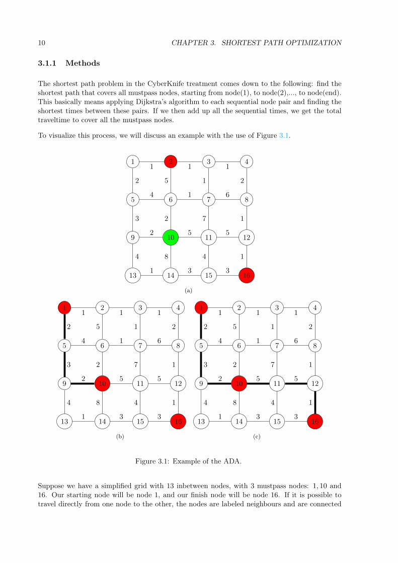
3.1.1 Methods

The shortest path problem in the CyberKnife treatment comes down to the following: find theshortest path that covers all mustpass nodes, starting from node(1), to node(2),..., to node(end).This basically means applying Dijkstra’s algorithm to each sequential node pair and finding theshortest times between these pairs. If we then add up all the sequential times, we get the totaltraveltime to cover all the mustpass nodes.

To visualize this process, we will discuss an example with the use of Figure 3.1.

1 2 3 4

5 6 7 8

9 10 11 12

13 14 15 16

1 1 1

4 1 6

2 5 5

1 3 3

2

3

4

5

2

8

1

7

4

2

1

1

(a)

1 2 3 4

5 6 7 8

9 10 11 12

13 14 15 16

1 1 1

4 1 6

2 5 5

1 3 3

2

3

4

5

2

8

1

7

4

2

1

1

(b)

1 2 3 4

5 6 7 8

9 10 11 12

13 14 15 16

1 1 1

4 1 6

2 5 5

1 3 3

2

3

4

5

2

8

1

7

4

2

1

1

(c)

Figure 3.1: Example of the ADA.

Suppose we have a simplified grid with 13 inbetween nodes, with 3 mustpass nodes: 1, 10 and16. Our starting node will be node 1, and our finish node will be node 16. If it is possible totravel directly from one node to the other, the nodes are labeled neighbours and are connected

3.1. ASYMMETRICAL DIJKSTRA ALGORITHM (ADA) 11

with an edge with the traveltime between those node on it, as displayed in Figure 3.1(a). TheADA will now apply Dijkstra’s algorithm with starting node 1 and finish node 10. It finds theshortest path as displayed in Figure 3.1(b). Note that 1 → 2 → 3 → 7 → 6 → 10 is actuallya shorter path, but since that contains a traversal to a lower-numbered node, it is not possible.The ADA then applies Dijkstra’s algorithm with starting node 10 and and finish node 16 andfinds the shortest path as displayed in Figure 3.1(c). After having computed all the sequentialshortest paths, the ADA then adds up all the sequential traveltimes which results in the finaltraveltime. In our example, this results in a path length of 18.

A pseudocode description of the ADA is displayed in Algorithm 2. The full Matlab code is addedin Appendix A.1.

Input Mustpass odes for all patients; Traversal matrix;Output Shortest paths and traveltimes for all patients;

for all patients doSort all nodes in ascending order;

endInitialize table with results ;for all patients do

Initialize table with nodes times between sequential mustpass node pairs;for nodes per patient do

Compute traveltimes between sequential mustpass node pairs with Dijkstraimplementation;

endSum all sequential node times;Return traveltime

endAlgorithm 2: Pseudocode for the Asymmetrical Dijkstra algorithm

3.1.2 Results

Using the data from the Erasmus Medical Center Rotterdam, the ADA results in the traveltimesdenoted in Figure 3.2. These are the current traveltimes of the CyberKnife for the 30 patients.The full table with results is added in Appendix B.

12 CHAPTER 3. SHORTEST PATH OPTIMIZATION

Figure 3.2: Traveltimes of 31 patients, computed with the ADA.

3.2 Symmetrical Dijkstra Algorithm (SDA)

We will now take our first step in improving the current programming of the CyberKnife, byremoving the first restriction in Section 2.1, which states that the CyberKnife can only travelto lower-numbered inbetween nodes. The algorithm presented in this section uses the sameimplementation of Dijkstra’s algorithm, but with a minor modification in the input, which willbe explained in the next section.

3.2.1 Methods

We do now allow traveling to lower-numbered inbetween nodes, so we need to know the traveltimefrom node A to node B, where A > B. The most staightforward choice would be the sametraveltime from node B to node A. This means we have to modify the matrix from Section 3.1.1,by mirroring it over its diagonal, which will result in a symmetrical matrix with zeros on thediagonal. A section of the now symmetrical traversal matrix is denoted in Table 3.1.

3.2. SYMMETRICAL DIJKSTRA ALGORITHM (SDA) 13

1 2 3 4 5 6 7 81 0 8.5 x x x x x 10.82 8.5 0 3.7 8 5.3 7 10.2 5.73 x 3.7 0 7.7 x 9.5 12.7 74 x 8 7.7 0 4.3 x 13.7 x5 x 5.3 x 4.3 0 8 11.5 10.26 x 7 9.5 x 8 0 4.7 9.27 x 10.2 12.7 13.7 11.5 4.7 0 11.78 10.8 5.7 7 x 10.2 9.2 11.7 0

Table 3.1: Small part of the symmetrical node traversal matrix. Traveltimes denoted in seconds.

The x’s in the matrix are the same ones as in the matrix in Figure 2.1, meaning that there is not adirect path between the nodes. If the algorithm now has to find the shortest path from mustpassnode A to mustpass node B, it can now also pick inbetween nodes with a lower numbering thanA.

To visualize this process, we return to our example from Section 3.1.1.

1 2 3 4

5 6 7 8

9 10 11 12

13 14 15 16

1 1 1

4 1 6

2 5 5

1 3 3

2

3

4

5

2

8

1

7

4

2

1

1

(a)

1 2 3 4

5 6 7 8

9 10 11 12

13 14 15 16

1 1 1

4 1 6

2 5 5

1 3 3

2

3

4

5

2

8

1

7

4

2

1

1

(b)

Figure 3.3: Example of the SDA.

This time, we allow traveling to lower-numbered nodes, so the SDA can pick the path that wealready mentioned in 3.1.1, 1→ 2→ 3→ 7→ 6→ 10, as our shortest path from node 1 to node10, as displayed in Figure 3.3(a). The SDA then does the same for start node 10 and finish node10, which results in the shortest path 10→ 9→ 13→ 14→ 15→ 16, as shown in Figure 3.3(b).The total path length is now 16, which is an improvement over the ADA.

So our Symmetrical Dijkstra Algorithm (SDA) basically operates the same as the ADA, with theonly difference being that we feed the algorithm the symmetrical matrix instead of the asym-metrical matrix. Therefore the pseudocode description of the SDA is the same as in Algorithm2. The full Matlab code is added in Appendix A.2.

14 CHAPTER 3. SHORTEST PATH OPTIMIZATION

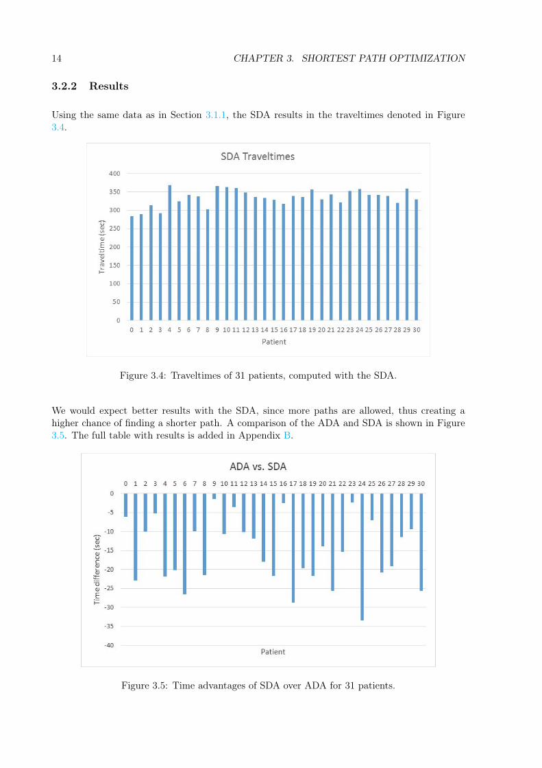
3.2.2 Results

Using the same data as in Section 3.1.1, the SDA results in the traveltimes denoted in Figure3.4.

Figure 3.4: Traveltimes of 31 patients, computed with the SDA.

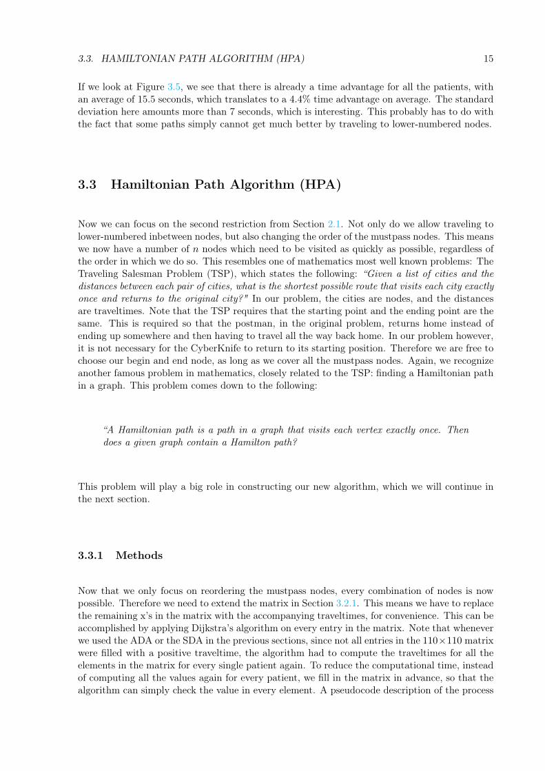
We would expect better results with the SDA, since more paths are allowed, thus creating ahigher chance of finding a shorter path. A comparison of the ADA and SDA is shown in Figure3.5. The full table with results is added in Appendix B.

Figure 3.5: Time advantages of SDA over ADA for 31 patients.

3.3. HAMILTONIAN PATH ALGORITHM (HPA) 15

If we look at Figure 3.5, we see that there is already a time advantage for all the patients, withan average of 15.5 seconds, which translates to a 4.4% time advantage on average. The standarddeviation here amounts more than 7 seconds, which is interesting. This probably has to do withthe fact that some paths simply cannot get much better by traveling to lower-numbered nodes.

3.3 Hamiltonian Path Algorithm (HPA)

Now we can focus on the second restriction from Section 2.1. Not only do we allow traveling tolower-numbered inbetween nodes, but also changing the order of the mustpass nodes. This meanswe now have a number of n nodes which need to be visited as quickly as possible, regardless ofthe order in which we do so. This resembles one of mathematics most well known problems: TheTraveling Salesman Problem (TSP), which states the following: “Given a list of cities and thedistances between each pair of cities, what is the shortest possible route that visits each city exactlyonce and returns to the original city?" In our problem, the cities are nodes, and the distancesare traveltimes. Note that the TSP requires that the starting point and the ending point are thesame. This is required so that the postman, in the original problem, returns home instead ofending up somewhere and then having to travel all the way back home. In our problem however,it is not necessary for the CyberKnife to return to its starting position. Therefore we are free tochoose our begin and end node, as long as we cover all the mustpass nodes. Again, we recognizeanother famous problem in mathematics, closely related to the TSP: finding a Hamiltonian pathin a graph. This problem comes down to the following:

“A Hamiltonian path is a path in a graph that visits each vertex exactly once. Thendoes a given graph contain a Hamilton path?

This problem will play a big role in constructing our new algorithm, which we will continue inthe next section.

3.3.1 Methods

Now that we only focus on reordering the mustpass nodes, every combination of nodes is nowpossible. Therefore we need to extend the matrix in Section 3.2.1. This means we have to replacethe remaining x’s in the matrix with the accompanying traveltimes, for convenience. This can beaccomplished by applying Dijkstra’s algorithm on every entry in the matrix. Note that wheneverwe used the ADA or the SDA in the previous sections, since not all entries in the 110×110 matrixwere filled with a positive traveltime, the algorithm had to compute the traveltimes for all theelements in the matrix for every single patient again. To reduce the computational time, insteadof computing all the values again for every patient, we fill in the matrix in advance, so that thealgorithm can simply check the value in every element. A pseudocode description of the process

16 CHAPTER 3. SHORTEST PATH OPTIMIZATION

is displayed in Algorithm 3. The full Matlab code is added in Appendix A.3.

Input Matrix used in the SDA;Output Symmetrical matrix with traveltimes for all node pairs and matrix with paths betweenall node pairs;

Initialize empty matrix for traveltimes ;Initialize empty matrix for paths ;

for all rows dofor all columns do

Compute the traveltimes and paths between every node pair with Dijkstra’s algorithm ;end

endAlgorithm 3: Pseudocode for computing the traveltimes and paths between every node pair

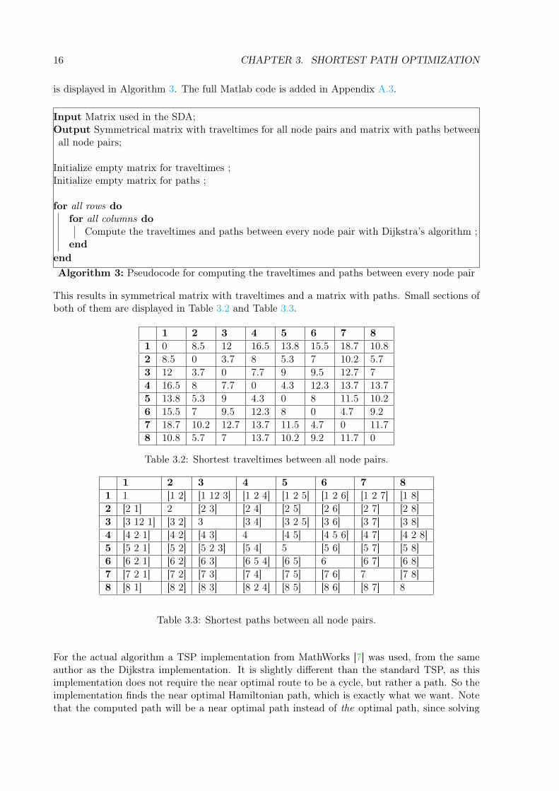
This results in symmetrical matrix with traveltimes and a matrix with paths. Small sections ofboth of them are displayed in Table 3.2 and Table 3.3.

1 2 3 4 5 6 7 81 0 8.5 12 16.5 13.8 15.5 18.7 10.82 8.5 0 3.7 8 5.3 7 10.2 5.73 12 3.7 0 7.7 9 9.5 12.7 74 16.5 8 7.7 0 4.3 12.3 13.7 13.75 13.8 5.3 9 4.3 0 8 11.5 10.26 15.5 7 9.5 12.3 8 0 4.7 9.27 18.7 10.2 12.7 13.7 11.5 4.7 0 11.78 10.8 5.7 7 13.7 10.2 9.2 11.7 0

Table 3.2: Shortest traveltimes between all node pairs.

1 2 3 4 5 6 7 81 1 [1 2] [1 12 3] [1 2 4] [1 2 5] [1 2 6] [1 2 7] [1 8]2 [2 1] 2 [2 3] [2 4] [2 5] [2 6] [2 7] [2 8]3 [3 12 1] [3 2] 3 [3 4] [3 2 5] [3 6] [3 7] [3 8]4 [4 2 1] [4 2] [4 3] 4 [4 5] [4 5 6] [4 7] [4 2 8]5 [5 2 1] [5 2] [5 2 3] [5 4] 5 [5 6] [5 7] [5 8]6 [6 2 1] [6 2] [6 3] [6 5 4] [6 5] 6 [6 7] [6 8]7 [7 2 1] [7 2] [7 3] [7 4] [7 5] [7 6] 7 [7 8]8 [8 1] [8 2] [8 3] [8 2 4] [8 5] [8 6] [8 7] 8

Table 3.3: Shortest paths between all node pairs.

For the actual algorithm a TSP implementation from MathWorks [7] was used, from the sameauthor as the Dijkstra implementation. It is slightly different than the standard TSP, as thisimplementation does not require the near optimal route to be a cycle, but rather a path. So theimplementation finds the near optimal Hamiltonian path, which is exactly what we want. Notethat the computed path will be a near optimal path instead of the optimal path, since solving

3.3. HAMILTONIAN PATH ALGORITHM (HPA) 17

the TSP is an NP-complete problem. This means we can find different solutions that approachthe optimal solution each time we run the program, because there is a random factor in theimplementation. More about this is examined in Chapter 7.

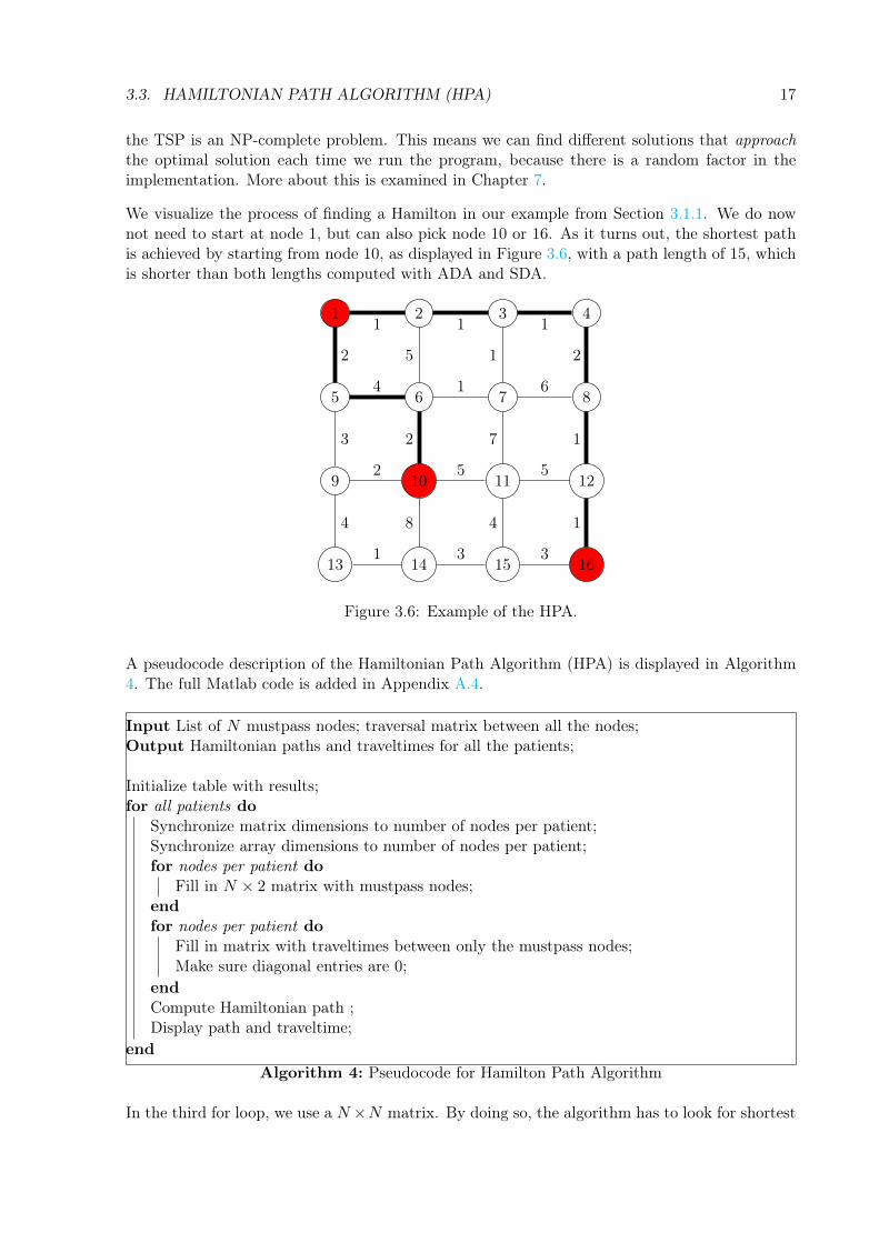
We visualize the process of finding a Hamilton in our example from Section 3.1.1. We do nownot need to start at node 1, but can also pick node 10 or 16. As it turns out, the shortest pathis achieved by starting from node 10, as displayed in Figure 3.6, with a path length of 15, whichis shorter than both lengths computed with ADA and SDA.

1 2 3 4

5 6 7 8

9 10 11 12

13 14 15 16

1 1 1

4 1 6

2 5 5

1 3 3

2

3

4

5

2

8

1

7

4

2

1

1

Figure 3.6: Example of the HPA.

A pseudocode description of the Hamiltonian Path Algorithm (HPA) is displayed in Algorithm4. The full Matlab code is added in Appendix A.4.

Input List of N mustpass nodes; traversal matrix between all the nodes;Output Hamiltonian paths and traveltimes for all the patients;

Initialize table with results;for all patients do

Synchronize matrix dimensions to number of nodes per patient;Synchronize array dimensions to number of nodes per patient;for nodes per patient do

Fill in N × 2 matrix with mustpass nodes;endfor nodes per patient do

Fill in matrix with traveltimes between only the mustpass nodes;Make sure diagonal entries are 0;

endCompute Hamiltonian path ;Display path and traveltime;

endAlgorithm 4: Pseudocode for Hamilton Path Algorithm

In the third for loop, we use a N ×N matrix. By doing so, the algorithm has to look for shortest

18 CHAPTER 3. SHORTEST PATH OPTIMIZATION

paths in a N × N matrix, where N ≤ 32, instead of the 110 × 110 matrix that both the SDAand ADA use. This is done to reduce the computational time of the HPA.

3.3.2 Results

Using the same data from Section 3.1.1, the HPA results in the traveltimes denoted in Figure3.7. The full table with traveltimes is added in Appendix B.

Figure 3.7: Traveltimes of 31 patients, computed with the HPA.

To compare results, a comparison of the HPA and ADA traveltimes is shown in Figure 3.8.

Figure 3.8: Time advantages of HPA over SDA for 31 patients.

3.4. COMPARISON OF METHODS 19

We see more equal time advantages for all patients, with an average of 53.0 seconds , whichtranslates to a 15.1% time advantage. This is already significantly better than the 4.4% of theSDA.

3.4 Comparison of methods

We have now discussed our methods for finding shortest paths. Out of all 3 of them, the HPAis clearly the best method. As seen in Figure 3.9, the method has a significant time advantagefor every patient, with an average of 68.3 seconds, which translates to a 19.4% time advantageon average.

Figure 3.9: Time advantages of HPA over ADA for 31 patients.

For as far as computational time, the ADA takes less than one second per patient to computethe shortest path and traveltime, while the HPA takes around 20 seconds per patient to do so.So the HPA runs quite slower compared to the ADA, but this is no surprise, since Hamilton isa more powerful algorithm than Dijkstra. Since 20 seconds is still a very reasonable time for aprogram to run, we still favor the HPA over the ADA and the SDA. The full table with shorterpaths is added in Appendix B.

20 CHAPTER 3. SHORTEST PATH OPTIMIZATION

Chapter 4

Neighbour Path Algorithm (NPA)

Now that we have answered the first two of our sub-questions, we can continue with the thirdsub-question: can we find shorter paths if we replace mustpass nodes with adjacent nodes thatresult in a better traveltime? We will answer this question in the section 4.1. Then, in Section4.2 we will do a convergence analysis of our method. Lastly, in Section 4.3 we will talk aboutthe plan quality of our newly found paths.

4.1 Computing Neighbour Paths

4.1.1 Methods

Our Neighbour Path Algorithm (NPA) takes the path computed with the HPA per patient asits standard path. It works in 2 basic steps:

1. Per node, find its neighbour nodes

2. Per node, replace the node with its neighbours, and check per neighbour if this results ina shorter path. If it does, replace the node with its neighbour.

To find neighbour nodes, we look at nodes that fall in a certain interval of degrees from theoriginal node. We chose an interval of 15◦, as we do not find any neighbours within 10◦, andany number above 15 results in too many neighbours, which would take too much computationaltime. Choosing 15◦ usually leads to around 7 neighbours. The full Matlab code on choosingthese neighbours is added in Appendix A.5.

Note that the NPA operates in a Greedy way. It only checks for a local minimum per node, andthen moves on to the next node. More about this is examined in Chapter 7.

For computation of the shortest path after replacing a node with a neighbour node, we useDijkstra, since the order of the mustpass nodes is fixed. This comes down to using the SDA. Apseudocode description is displayed in Algorithm 5. The full allgorithm is added in AppendixA.6.

21

22 CHAPTER 4. NEIGHBOUR PATH ALGORITHM (NPA)

Input A list of N mustpass nodes; traversal between all nodes;Output Neighbour paths for all patients; traveltimes for all patients; potential timeadvantages;

Initialize empty tables for results;for all patients do

Compute the Hamiltonian path;Copy nodes of Hamiltonian path into new vector;Set initial shortest traveltime equal to HPA traveltime;for all N nodes in the Hamiltonian path do

Find all neighbour nodes;Remember current node that is being replaced;for all neighbour nodes do

if neighbour node is not already in Hamiltonian path thenReplace current node with neighbour node;Compute traveltime of new path with Dijkstra;if Traveltime new path < initial traveltime then

Set new initial shortest traveltime equal to computed traveltime;Set new initial shortest path equal to computed path;Update current shortest path by replacing current node with neighbour node

endend

endIf neighbour node does not result in a better path, set replaced node back to previouslybest neighbour node;

endEnter results in tables;

endAlgorithm 5: Pseudocode for Neighbour Path Algorithm

4.1. COMPUTING NEIGHBOUR PATHS 23

4.1.2 Results

Using the same data from Section 3.1.1, the NPA results in the traveltimes denoted in Figure4.1. The full table with results is added in Appendix B.

Figure 4.1: Traveltimes computed with NPA for 31 patients.

Again, we see some improvement in the traveltimes compared to those of the HPA. This is furtherillustrated in Figure 4.2

Figure 4.2: Time advantages of NPA over HPA for 31 patients.

24 CHAPTER 4. NEIGHBOUR PATH ALGORITHM (NPA)

For 13 out of 30 patients, the NPA results in an average time advantage of 48.0 seconds over theHPA, which translates to about 17.6%. On top of the 19.4% improvement the HPA made overthe ADA, this means that the traveltimes for all 31 patients have been brought down already by25.6% from the ADA already.

4.2 Analysis of Convergence

As noted before, there is a random factor in the HPA. This causes the computed path to differ afew seconds each time the program is run. This raises a question: do these traveltimes eventuallydo converge to an optimal traveltime?

To check this hypothesis, we created the Iterated Neighbour Path Algorithm (INPA). It computesa shortest path with the NPA, takes the computed path as input and iterates the algorithm 10times. This way, the path gets slightly altered after each iteration. The iterations resulted inthree different pictures:

(a) Improvement until a few iterations. (b) No improvement.

(c) Improvement at first, then alternating between times.

Figure 4.3: 10 Iterations for different patients.

4.2. ANALYSIS OF CONVERGENCE 25

While the the traveltimes in 4.3(a) and 4.3(b) seem to converge, the traveltimes in 4.3(c) showsome more interesting behaviour. After two succesfull iterations, the traveltimes then start toalternate between 208 and 210 seconds. Unfortunately we do not have an explanation for this,but we can conclude that even though the traveltime does not always converge, it does not getany worse after a few iterations. It is fair to conclude that it is worth iterating the path foundwith the NPA at least 3-5 times. We should mention that there was a single case in whichthe traveltime got worse after one iteration and then alternated between two traveltimes. Thisspecific result is displayed in Figure 4.4.

Figure 4.4: Case where the traveltime gets worse.

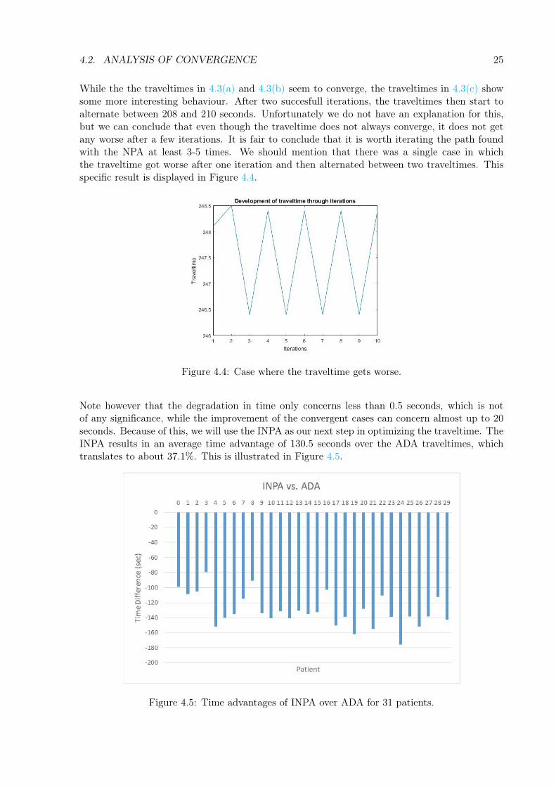
Note however that the degradation in time only concerns less than 0.5 seconds, which is notof any significance, while the improvement of the convergent cases can concern almost up to 20seconds. Because of this, we will use the INPA as our next step in optimizing the traveltime. TheINPA results in an average time advantage of 130.5 seconds over the ADA traveltimes, whichtranslates to about 37.1%. This is illustrated in Figure 4.5.

Figure 4.5: Time advantages of INPA over ADA for 31 patients.

26 CHAPTER 4. NEIGHBOUR PATH ALGORITHM (NPA)

The pseudocode for the INPA is similar to that of Algorithm 5, so it will not be included here.The full Matlab code is added in Appendix A.7.

4.3 Plan Quality

While a large section of this report is dedicated to shortest path optimization, it is also veryimportant that these newly found paths do not degrade too much in plan quality, or else theywill be useless. To verify this, Sebastiaan Breedveld did calculations on the plan quality eachtime after we found shorter paths. These calculations resulted in a Dosis-Volume-Histogram(DHV-Figure) for each patient. An example of a DHV-Figure is shown in Figure 4.6

Figure 4.6: DHV-Figure for a patient.

The continuous lines represent the results with the original paths, while the dotted line representsthe results with the convergent path found after 10 iterations. To not degrade in plan quality,it is important that the dotted lines stay as close as possible tot he continuous lines. As seenin Figure 4.6, most results remain the same, only the lower dose in the bladder degrades somein quality, while the high dose in the bladder improves slightly. The plan quality calculationsshowed that this result is quite usual for all of the patients. In fact, for some patients, the planquality remained almost identical. This means that our optimized paths are appropriate to use,since the plan quality does not degrade significantly.

Chapter 5

Additional restrictions

With the INPA, we have removed all the restrictions from Section 2.1. However, as the projectwas progressing, two new restrictions came by: starting nodes and dummy nodes. We will discussthe nature of these restrictions and how we fixed them. We will combine these restrictions intoone algorithm that will compute the final traveltimes for the patients.

5.1 Starting Nodes

There is a set of 45 nodes from which the CyberKnife can start its treatment. The traveltimewould benefit if the first node of the path is starting node. Otherwise the CyberKnife would firsthave to travel to the first node of the path, which might be on the other side of the grid. Thiswould harm the traveltime and be a waste of all time used to the compute the shortest path.

5.1.1 Methods

We took the result from the INPA, and added a starting node to the path. To incorporate thesestarting nodes in the paths, we had to distinguish three different cases of where the startingnodes can already be in the path:

1. There are no starting nodes in the path yet. The SNA then computes the traveltimes forall 45 starting nodes added to the path and picks the fastest. The path length increaseswith one.

2. There are starting nodes in the path, but not yet at the beginning of the path. The SNAputs all starting nodes in the path at the beginning, checks the travelime and picks thefastest. The path length does not change.

3. There are starting nodes in the path and one of them is already in the beginning. TheSNA does not need to do anything.

27

28 CHAPTER 5. ADDITIONAL RESTRICTIONS

5.2 Dummy Nodes

The last restriction that came along concerns dummy nodes. We briefly mentioned them inSection 1.2, but now we will fully incorporate them into the algorithm.

5.2.1 Methods

A brief recap, the dummy nodes are 8 nodes which are used for the sole purpose of serving asinbetween nodes. Radiation from these nodes is not possible. In the treatment plan, these nodeswill never be candidate mustpass nodes. So it is only during the INPA, that we need to modifythe algorithm, since they could be picked as neighbour nodes. Therefore we can use the INPAagain, with the addition of one line of code that checks if the algorithm does not pick a dummynode as its neighbour for replacement. This is done in the same style as line 48 in Appendix A.7.

With the addition of a starting node and the removal of dummy nodes, we have now completedour final algorithm, the Optimal Path Algorithm (OPA). A pseudocode description of the OPAis presented in Figure 6. The full Matlab code is added in Appendix A.8.

5.3 Concluding Results

We can now compute the final traveltimes for all patients with the OPA. Using the same datafrom Section 3.1.1, the OPA results in the traveltimes denoted in Figure 5.1. The full table withresults is added in Appendix B.

Figure 5.1: Traveltimes of 31 patients, computed with the OPA.

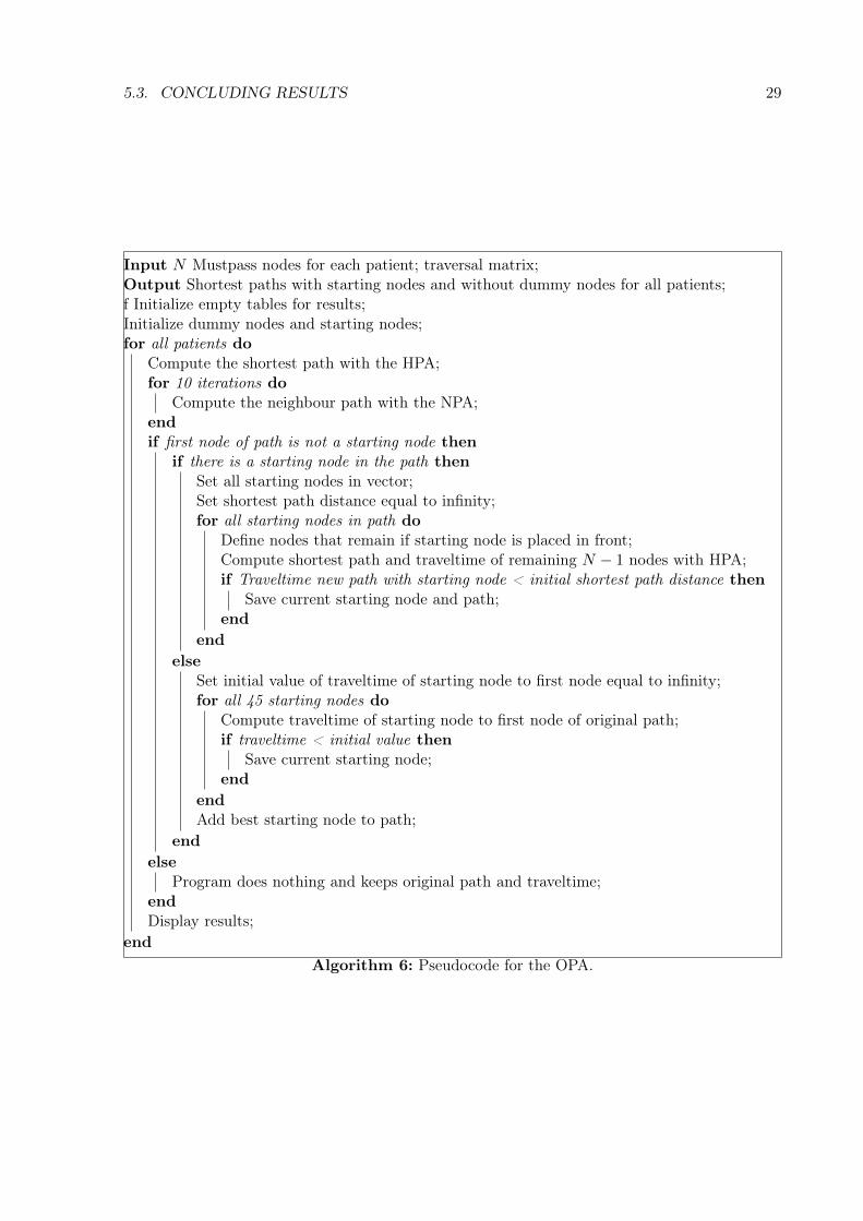
5.3. CONCLUDING RESULTS 29

Input N Mustpass nodes for each patient; traversal matrix;Output Shortest paths with starting nodes and without dummy nodes for all patients;f Initialize empty tables for results;Initialize dummy nodes and starting nodes;for all patients do

Compute the shortest path with the HPA;for 10 iterations do

Compute the neighbour path with the NPA;endif first node of path is not a starting node then

if there is a starting node in the path thenSet all starting nodes in vector;Set shortest path distance equal to infinity;for all starting nodes in path do

Define nodes that remain if starting node is placed in front;Compute shortest path and traveltime of remaining N − 1 nodes with HPA;if Traveltime new path with starting node < initial shortest path distance then

Save current starting node and path;end

endelse

Set initial value of traveltime of starting node to first node equal to infinity;for all 45 starting nodes do

Compute traveltime of starting node to first node of original path;if traveltime < initial value then

Save current starting node;end

endAdd best starting node to path;

endelse

Program does nothing and keeps original path and traveltime;endDisplay results;

endAlgorithm 6: Pseudocode for the OPA.

30 CHAPTER 5. ADDITIONAL RESTRICTIONS

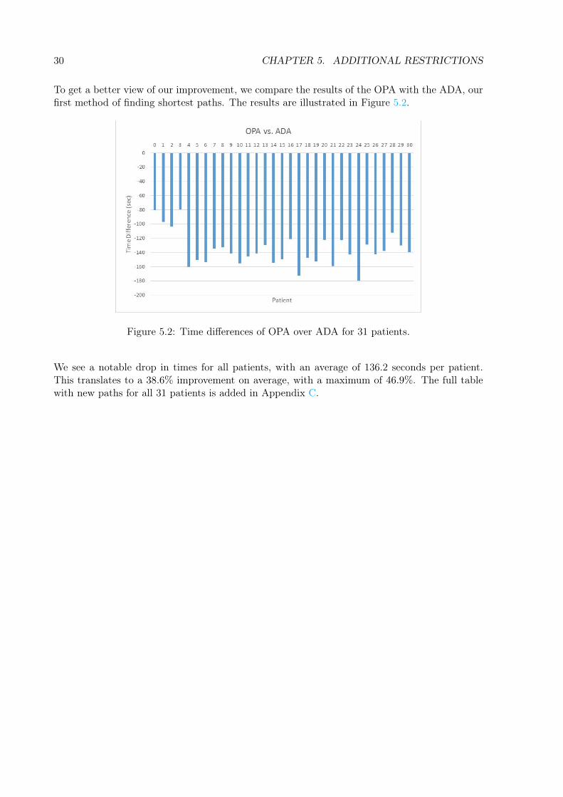
To get a better view of our improvement, we compare the results of the OPA with the ADA, ourfirst method of finding shortest paths. The results are illustrated in Figure 5.2.

Figure 5.2: Time differences of OPA over ADA for 31 patients.

We see a notable drop in times for all patients, with an average of 136.2 seconds per patient.This translates to a 38.6% improvement on average, with a maximum of 46.9%. The full tablewith new paths for all 31 patients is added in Appendix C.

Chapter 6

Conclusions

The main goal of this project was to optimize the traveltime of the CyberKnife. We split up thisgoal into three sub-goals, as formulated in Section 2.1. After 2 months of research, we achievedthe following results:

• With the SDA, the CyberKnife travels as fast as possible from node A to node B. Weexpanded this method with the HPA, which uses Hamiltonian paths. This changes theorder of the mustpass nodes, which on average dropped the initial traveltimes by almost20%. These results answered the first two of our research questions.

• Next up, we used the NPA to replace nodes in the path with adjacent nodes. This resultedin better paths for almost half of the patients, while the other half did not get worse.This result got sharpened when we noticed that iterating a new path into the NPA atleast once did improve the traveltime. After a few iterations, all the paths were eitherconverging, constant, or alternating between two better paths. So with the use of theINPA, our traveltimes had dropped 37.1% already. After these changes in the mustpassnodes, the plan quality did not lose a significant amount of quality. With these results, thelast sub-question was answered as well.

• Lastly, we modified the INPA slightly, because of the addition of starting nodes and theremoval of dummy nodes. This had to be done in order for the traveltime not to sufferunder certain restrictions of the CyberKnife. There was an extra restriction concerningimage blocking nodes, but we were not able to incorporate that restriction due to timelimitations. More about this is explained in Chapter 7.

All of the previously mentioned algorithms resulted in the OPA, our final algorithm which opti-mized original the traveltimes with 38.6% on average, without any significant loss of plan quality.

31

32 CHAPTER 6. CONCLUSIONS

Chapter 7

Recommendations

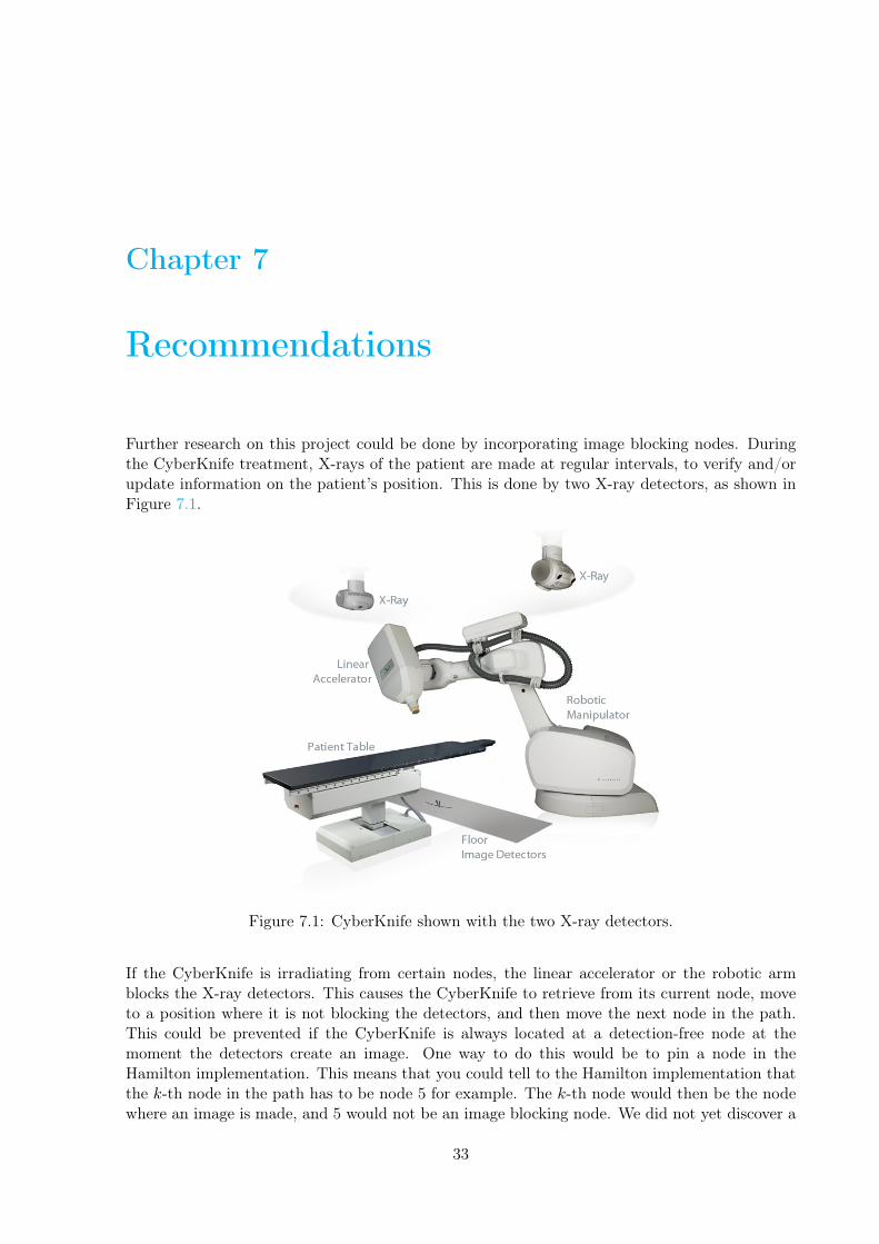
Further research on this project could be done by incorporating image blocking nodes. Duringthe CyberKnife treatment, X-rays of the patient are made at regular intervals, to verify and/orupdate information on the patient’s position. This is done by two X-ray detectors, as shown inFigure 7.1.

Figure 7.1: CyberKnife shown with the two X-ray detectors.

If the CyberKnife is irradiating from certain nodes, the linear accelerator or the robotic armblocks the X-ray detectors. This causes the CyberKnife to retrieve from its current node, moveto a position where it is not blocking the detectors, and then move the next node in the path.This could be prevented if the CyberKnife is always located at a detection-free node at themoment the detectors create an image. One way to do this would be to pin a node in theHamilton implementation. This means that you could tell to the Hamilton implementation thatthe k-th node in the path has to be node 5 for example. The k-th node would then be the nodewhere an image is made, and 5 would not be an image blocking node. We did not yet discover a

33

34 CHAPTER 7. RECOMMENDATIONS

way to achieve this with the current implementation, but perhaps there are other more suitableimplementations for this purpose.

The idea of pinning a node could also be of benefit in adding starting nodes. With the currentversion of the OPA, the algorithm has to identify the starting nodes, put them at the beginningand compute the traveltimes with HPA. It could save quite some for loops and thus computationaltime if this could be done by entering a few commands in the Hamilton implementation.

The NPA could also be more optimized. As mentioned in Section 4.1.1, the NPA operates in aGreedy way. It could for example be possible that replacing the first node with a sup-optimalneighbour results in a better overall path than replacing the first node with the optimal neighbour.Therefore the NPA is probably not the optimal method of computing neighbour solutions, butwe could not come up with any better solutions. Also computational times started to rise quicklyfrom that point, so heavier algorithms would have probably not fit in the time schedule.

One subject that was overlooked a bit is the ’random-factor’ in the Hamilton implementation.We did not do any research into why Hamilton implementation result in different traveltimeseach time. There also seems to be a little flaw in the OPA, as the path lengths of 4 patientswere changed from 30 to 32. After we ran the OPA again for the 4 patients separately, the pathlength changed back to their original lengths. However, since we concluded that the plan qualitydid not suffer significantly under these changes, we kept the changed path lengths in AppendixC.

Lastly, the OPA takes about 40 minutes to compute traveltimes and paths for all 30 patients.With all the above mentioned improvements, it should be possible to reduce the 40 minutescomputational time.

Bibliography

[1] American Cancer Society. Radiation therapy basics. https://www.cancer.org/treatment/treatments-and-side-effects/treatment-types/radiation/basics.html, 2017.

[2] Sebastiaan Breedveld. Towards automated treatment planning in radiotherapy. ErasmusMC, 2013.

[3] Radiological Society of North America. Linac (linear accelerator). https://www.radiologyinfo.org/en/info.cfm?pg=linac, 2017.

[4] L. Rossi, S. Breedveld, S. Aluwini, and B.J.M Heijmen. On the beam direction search spacein computerized non-coplanar beam angle optimization for imrt - prostate sbrt. ErasmusMC, 2012.

[5] Joseph Kirk. Dijkstra’s minimum cost path algorithm. https://nl.mathworks.com/matlabcentral/fileexchange/20025-dijkstra-s-minimum-cost-path-algorithm, 2015.

[6] Christos H.Papadimitriou and Kenneth Steiglitz. Combinatorial Optimization. Dover Publi-cations, Mineola, New York, 1998.

[7] Joseph Kirk. Fixed endpoints open traveling salesman problem - ge-netic algorithm. https://nl.mathworks.com/matlabcentral/fileexchange/21197-fixed-endpoints-open-traveling-salesman-problem-genetic-algorithm,2014.

35

36 BIBLIOGRAPHY

Appendices

37

Appendix A

Matlab codes

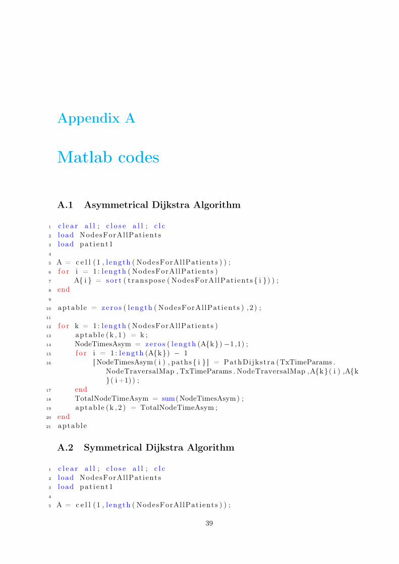
A.1 Asymmetrical Dijkstra Algorithm

1 c l e a r a l l ; c l o s e a l l ; c l c2 load NodesForAl lPat ients3 load pat i en t14

5 A = c e l l (1 , l ength ( NodesForAl lPat ients ) ) ;6 f o r i = 1 : l ength ( NodesForAl lPat ients )7 A{ i } = so r t ( t ranspose ( NodesForAl lPat ients { i }) ) ;8 end9

10 aptab le = ze ro s ( l ength ( NodesForAl lPat ients ) , 2 ) ;11

12 f o r k = 1 : l ength ( NodesForAl lPat ients )13 aptab le (k , 1 ) = k ;14 NodeTimesAsym = ze ro s ( l ength (A{k}) −1 ,1) ;15 f o r i = 1 : l ength (A{k}) − 116 [ NodeTimesAsym( i ) , paths { i } ] = PathDi jkstra (TxTimeParams .

NodeTraversalMap , TxTimeParams . NodeTraversalMap ,A{k}( i ) ,A{k}( i +1) ) ;

17 end18 TotalNodeTimeAsym = sum(NodeTimesAsym) ;19 aptab le (k , 2 ) = TotalNodeTimeAsym ;20 end21 aptab le

A.2 Symmetrical Dijkstra Algorithm

1 c l e a r a l l ; c l o s e a l l ; c l c2 load NodesForAl lPat ients3 load pat i en t14

5 A = c e l l (1 , l ength ( NodesForAl lPat ients ) ) ;

39

40 APPENDIX A. MATLAB CODES

6 f o r i = 1 : l ength ( NodesForAl lPat ients )7 A{ i } = so r t ( t ranspose ( NodesForAl lPat ients { i }) ) ;8 end9

10 SymMat = TxTimeParams . NodeTraversalMap + transpose (TxTimeParams .NodeTraversalMap ) ;

11 SymMat( end , end ) = 0 ;12

13 sp tab l e = ze ro s ( l ength ( NodesForAl lPat ients ) , 2 ) ;14

15 f o r k = 1 : l ength ( NodesForAl lPat ients )16 sp tab l e (k , 1 ) = k ;17 NodeTimesSym = ze ro s ( l ength (A{k}) −1 ,1) ;18 f o r i = 1 : l ength (A{k}) − 119 [ NodeTimesSym( i ) , paths { i } ] = PathDi jkstra (SymMat , SymMat ,A{k}(

i ) ,A{k}( i +1) ) ;20 end21 TotalNodeTimeSym = sum(NodeTimesSym) ;22 sp tab l e (k , 2 ) = TotalNodeTimeSym ;23 end24 sp tab l e

A.3 Total Matrices

1 TotalCosts = ze ro s (110 ,110) ;2 TotalPaths = c e l l (110 ,110) ;3

4 [ co s t s , paths ] = PathDi jkstra (SymMat , SymMat) ;5

6 f o r i = 1:1107 f o r j = 1:1108 TotalCosts ( i , j ) = co s t s ( i , j ) ;9 TotalPaths ( i , j ) = paths ( i , j ) ;

10 end11 end

A.4 Hamiltonian Path Algorithm

1 c l e a r a l l ; c l o s e a l l ; c l c2 load NodesForAl lPat ients3 load pat i en t14 load SymMat5 run Tota leMatr i ces6

7 hptable = ze ro s ( l ength ( NodesForAl lPat ients ) , 2 ) ;8

9 f o r k = 1 : l ength ( NodesForAl lPat ients )10 hptable (k , 1 ) = k ;

A.5. FINDING NEIGHOURS 41

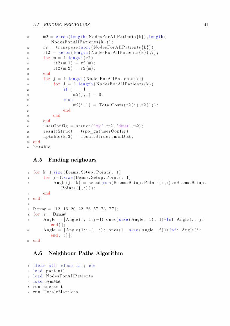
11 m2 = ze ro s ( l ength ( NodesForAl lPat ients {k}) , l ength (NodesForAl lPat ients {k}) ) ;

12 r2 = transpose ( s o r t ( NodesForAl lPat ients {k}) ) ;13 r t2 = ze ro s ( l ength ( NodesForAl lPat ients {k}) ,2 ) ;14 f o r m = 1 : l ength ( r2 )15 r t2 (m, 1 ) = r2 (m) ;16 r t2 (m, 2 ) = r2 (m) ;17 end18 f o r j = 1 : l ength ( NodesForAl lPat ients {k})19 f o r l = 1 : l ength ( NodesForAl lPat ients {k})20 i f j == l21 m2( j , l ) = 0 ;22 e l s e23 m2( j , l ) = TotalCosts ( r2 ( j ) , r2 ( l ) ) ;24 end25 end26 end27 userConf ig = s t r u c t ( ’ xy ’ , rt2 , ’ dmat ’ ,m2) ;28 r e s u l t S t r u c t = tspo_ga ( userConf ig )29 hptable (k , 2 ) = r e s u l t S t r u c t . minDist ;30 end31 hptable

A.5 Finding neighours

1 f o r k=1: s i z e (Beams . Setup . Points , 1)2 f o r j =1: s i z e (Beams . Setup . Points , 1)3 Angle ( j , k ) = acosd (sum(Beams . Setup . Points (k , : ) .∗Beams . Setup .

Points ( j , : ) ) ) ;4 end5 end6

7 Dummy = [12 16 20 22 26 57 73 7 7 ] ;8 f o r j = Dummy9 Angle = [ Angle ( : , 1 : j−1) ones ( s i z e ( Angle , 1) , 1) ∗ I n f Angle ( : , j :

end ) ] ;10 Angle = [ Angle ( 1 : j −1, : ) ; ones (1 , s i z e ( Angle , 2) ) ∗ I n f ; Angle ( j :

end , : ) ] ;11 end

A.6 Neighbour Paths Algorithm

1 c l e a r a l l ; c l o s e a l l ; c l c2 load pat i en t13 load NodesForAl lPat ients4 load SymMat5 run hoekte s t6 run Tota leMatr i ces

42 APPENDIX A. MATLAB CODES

7

8 C = c e l l ( l ength ( NodesForAl lPat ients ) , 1 ) ; %c e l l with the neighbourpaths

9 nt = ze ro s ( l ength ( NodesForAl lPat ients ) , 2 ) ; %tab l e with t r av e l t ime s10 ta = ze ro s ( l ength ( NodesForAl lPat ients ) , 2 ) ; %tab l e with the time

advantages11

12 f o r k = 1 : l ength ( NodesForAl lPat ients )13 nt (k , 1 ) = k ;14 ta (k , 1 ) = k ;15 %Compute the s ho r t e s t path f o r a l l p a t i en t s with Hamilton16 m2 = ze ro s ( l ength ( NodesForAl lPat ients {k}) , l ength (

NodesForAl lPat ients {k}) ) ;17 r2 = transpose ( s o r t ( NodesForAl lPat ients {k}) ) ;18 r t2 = ze ro s ( l ength ( NodesForAl lPat ients {k}) ,2 ) ;19 f o r m = 1 : l ength ( r2 )20 r t2 (m, 1 ) = r2 (m) ;21 r t2 (m, 2 ) = r2 (m) ;22 end23

24 f o r j = 1 : l ength ( NodesForAl lPat ients {k})25 f o r l = 1 : l ength ( NodesForAl lPat ients {k})26 i f j == l27 m2( j , l ) = 0 ;28 e l s e29 m2( j , l ) = TotalCosts ( r2 ( j ) , r2 ( l ) ) ;30 end31 end32 end33 userConf ig = s t r u c t ( ’ xy ’ , rt2 , ’ dmat ’ ,m2) ;34 r e s u l t S t r u c t = tspo_ga ( userConf ig ) ;35

36 %Compute the neighbour paths37 inp = rt2 ( r e s u l t S t r u c t . optRoute , 2) ; %copy the nodes o f the

Hamiltonpath in to a new vec to r inp38 ka = r e s u l t S t r u c t . minDist ; %s e t the i n i t i a l s h o r t e s t t r ave l t ime39

40 f o r b = 1 : l ength ( inp ) %check a l l the nodes in the Hamiltonpath41 f = f i nd ( Angle ( : , inp (b) ) <15) ; %f i nd the ne ighbours o f a

s p e c i f i e d node42 bestNode = inp (b) ; %remember the node that i s be ing rep laced43 f o r j = 1 : l ength ( f ) %check a l l the ne ighbours o f a node44 i f ~ismember ( f ( j ) , inp ) %make sure the new neighbour node

i s not a l r eady in the path45 inp (b) = f ( j ) ; %r ep l a c e the s p e c i f i e d node with the

neighours , and c a l c u l a t e the new path length46 f o r i = 1 : l ength ( inp ) − 147 [ NodeTimesSym( i ) , paths { i } ] = PathDi jkstra (SymMat

, SymMat , inp ( i ) , inp ( i +1) ) ; %c a l c u l a t e s h o r t e s t

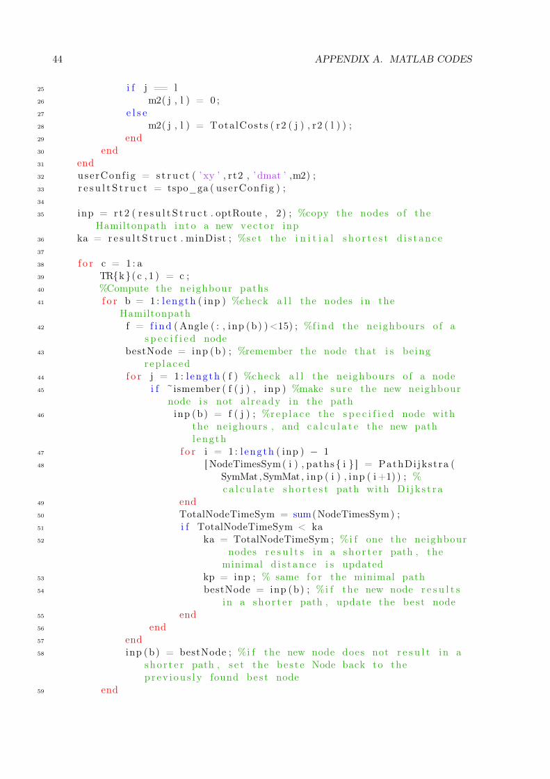
A.7. ITERATED NEIGHBOUR PATH ALGORITHM 43

path with D i j k s t r a48 end49 TotalNodeTimeSym = sum(NodeTimesSym) ;50 i f TotalNodeTimeSym < ka51 ka = TotalNodeTimeSym ; %i f one the neighbour

nodes r e s u l t s in a sho r t e r path , the minimald i s t anc e i s updated

52 kp = inp ; % same f o r the minimal path53 bestNode = inp (b) ; %i f the new node r e s u l t s in a

sho r t e r path , update the best node54 end55 end56 end57 inp (b) = bestNode ; %i f the new node does not r e s u l t in a

sho r t e r path , s e t the bes t e Node back to the p r ev i ou s l yfound best node

58 end59 C{k} = kp ;60 nt (k , 2 ) = ka ;61 ta (k , 2 ) = r e s u l t S t r u c t . minDist − ka ;62 end

A.7 Iterated Neighbour Path Algorithm

1 c l e a r a l l ; c l o s e a l l ; c l c2 load pat i en t13 load NodesForAl lPat ients4 load SymMat5 run Tota leMatr i ces6 run hoekte s t7

8 a = 10 ;9

10 TR = c e l l ( l ength ( NodesForAl lPat ients ) , 1 ) ;11 PR = c e l l ( l ength ( NodesForAl lPat ients ) , 1 ) ;12

13 f o r k = 1 :114 %Compute the s ho r t e s t path f o r a l l p a t i e n t s with Hamilton15 m2 = ze ro s ( l ength ( NodesForAl lPat ients {k}) , l ength (

NodesForAl lPat ients {k}) ) ;16 r2 = transpose ( s o r t ( NodesForAl lPat ients {k}) ) ;17 r t2 = ze ro s ( l ength ( NodesForAl lPat ients {k}) ,2 ) ;18 f o r m = 1 : l ength ( r2 )19 r t2 (m, 1 ) = r2 (m) ;20 r t2 (m, 2 ) = r2 (m) ;21 end22

23 f o r j = 1 : l ength ( NodesForAl lPat ients {k})24 f o r l = 1 : l ength ( NodesForAl lPat ients {k})

44 APPENDIX A. MATLAB CODES

25 i f j == l26 m2( j , l ) = 0 ;27 e l s e28 m2( j , l ) = TotalCosts ( r2 ( j ) , r2 ( l ) ) ;29 end30 end31 end32 userConf ig = s t r u c t ( ’ xy ’ , rt2 , ’ dmat ’ ,m2) ;33 r e s u l t S t r u c t = tspo_ga ( userConf ig ) ;34

35 inp = rt2 ( r e s u l t S t r u c t . optRoute , 2) ; %copy the nodes o f theHamiltonpath in to a new vec to r inp

36 ka = r e s u l t S t r u c t . minDist ; %s e t the i n i t i a l s h o r t e s t d i s t anc e37

38 f o r c = 1 : a39 TR{k}( c , 1 ) = c ;40 %Compute the neighbour paths41 f o r b = 1 : l ength ( inp ) %check a l l the nodes in the

Hamiltonpath42 f = f i nd ( Angle ( : , inp (b) ) <15) ; %f i nd the ne ighbours o f a

s p e c i f i e d node43 bestNode = inp (b) ; %remember the node that i s be ing

rep laced44 f o r j = 1 : l ength ( f ) %check a l l the ne ighbours o f a node45 i f ~ismember ( f ( j ) , inp ) %make sure the new neighbour

node i s not a l r eady in the path46 inp (b) = f ( j ) ; %r ep l a c e the s p e c i f i e d node with

the neighours , and c a l c u l a t e the new pathlength

47 f o r i = 1 : l ength ( inp ) − 148 [ NodeTimesSym( i ) , paths { i } ] = PathDi jkstra (

SymMat , SymMat , inp ( i ) , inp ( i +1) ) ; %c a l c u l a t e s h o r t e s t path with D i j k s t r a

49 end50 TotalNodeTimeSym = sum(NodeTimesSym) ;51 i f TotalNodeTimeSym < ka52 ka = TotalNodeTimeSym ; %i f one the neighbour

nodes r e s u l t s in a sho r t e r path , theminimal d i s t anc e i s updated

53 kp = inp ; % same f o r the minimal path54 bestNode = inp (b) ; %i f the new node r e s u l t s

in a sho r t e r path , update the best node55 end56 end57 end58 inp (b) = bestNode ; %i f the new node does not r e s u l t in a

sho r t e r path , s e t the bes t e Node back to thep r ev i ou s l y found best node

59 end

A.8. OPTIMAL PATH ALGORITHM 45

60 TR{c }( c , 2 ) = ka ;61 PR{k} = kp ;62 inp = kp ; %update input with the output o f the prev ious path63 end64 end

A.8 Optimal Path Algorithm

1 c l e a r a l l ; c l o s e a l l ; c l c2 load pat i en t13 load NodesForAl lPat ients4 load SymMat5 run Tota leMatr i ces6 run hoekte s t7

8 a = 10 ;9 f t = ze ro s ( l ength ( NodesForAl lPat ients ) , 1 ) ; %c r ea t e t ab l e f o r f i n a l

t r av e l t ime s f o r a l l the pa t i en t s10 snp = c e l l ( l ength ( NodesForAl lPat ients ) , 1 ) ; %c e l l with the s t a r t i n g

node paths11 s t a r tnode s = [1 26 28 29 30 36 :51 60 76 78 79 :83 85 :93 96 :100 102

1 1 0 ] ;12 dummy = [12 16 20 22 26 57 73 7 7 ] ; %these nodes cannot be in the path13

14 f o r k = 1 : l ength ( NodesForAl lPat ients )15 m2 = ze ro s ( l ength ( NodesForAl lPat ients {k}) , l ength (

NodesForAl lPat ients {k}) ) ;16 r2 = transpose ( s o r t ( NodesForAl lPat ients {k}) ) ;17 r t2 = ze ro s ( l ength ( NodesForAl lPat ients {k}) ,2 ) ;18 f o r m = 1 : l ength ( r2 )19 r t2 (m, 1 ) = r2 (m) ;20 r t2 (m, 2 ) = r2 (m) ;21 end22

23 f o r j = 1 : l ength ( NodesForAl lPat ients {k})24 f o r l = 1 : l ength ( NodesForAl lPat ients {k})25 i f j == l26 m2( j , l ) = 0 ;27 e l s e28 m2( j , l ) = TotalCosts ( r2 ( j ) , r2 ( l ) ) ;29 end30 end31 end32 userConf ig = s t r u c t ( ’ xy ’ , rt2 , ’ dmat ’ ,m2) ;33 r e s u l t S t r u c t = tspo_ga ( userConf ig ) ;34

35 inp = rt2 ( r e s u l t S t r u c t . optRoute , 2) ; %copy the nodes o f theHamiltonpath in to a new vecto r inp

36 ka = r e s u l t S t r u c t . minDist ; %s e t the i n i t i a l s h o r t e s t d i s t anc e

46 APPENDIX A. MATLAB CODES

37

38 f o r c = 1 : a39 %Compute the neighbour paths40 f o r b = 1 : l ength ( inp ) %check a l l the nodes in the

Hamiltonpath41 f = f i nd ( Angle ( : , inp (b) ) <15) ; %f i nd the ne ighbours o f a

s p e c i f i e d node42 bestNode = inp (b) ; %remember the node that i s be ing

rep laced43 f o r j = 1 : l ength ( f ) %check a l l the ne ighbours o f a node44 i f ~ismember ( f ( j ) , inp ) %make sure the new neighbour

node i s not a l r eady in the path45 i f ~ismember ( f ( j ) ,dummy) %make sure the new

neighbour node i s not a dummy node46 inp (b) = f ( j ) ; %r ep l a c e the s p e c i f i e d node

with the neighours , and c a l c u l a t e the newpath length

47 f o r i = 1 : l ength ( inp ) − 148 [ NodeTimesSym( i ) , paths { i } ] =

PathDi jkstra (SymMat , SymMat , inp ( i ) , inp( i +1) ) ; %c a l c u l a t e s h o r t e s t path withD i j k s t r a

49 end50 TotalNodeTimeSym = sum(NodeTimesSym) ;51 i f TotalNodeTimeSym < ka52 ka = TotalNodeTimeSym ; %i f one the

neighbour nodes r e s u l t s in a sho r t e rpath , the minimal d i s t anc e i s updated

53 kp = inp ; % same f o r the minimal path54 bestNode = inp (b) ; %i f the new node

r e s u l t s in a sho r t e r path , update thebest node

55 end56 end57 end58 end59 inp (b) = bestNode ; %i f the new node does not r e s u l t in a

sho r t e r path , s e t the bes t e Node back to thep r ev i ou s l y found best node

60 end61 inp = kp ; %update input with the output o f the prev ious path62 end63

64 %%%%%%%%%%%%%%%%%Add a s t a r t i n g node%%%%%%%%%%%%%%%%%%%%%%%%%%%%%%%%%%%

65 i f isempty ( i n t e r s e c t ( kp (1 ) , s t a r tnode s ) ) == 1 %checks i f the f i r s tnode o f the computed path i s not a s t a r t node

66 i f ~isempty ( i n t e r s e c t ( s tar tnodes , kp ) ) %s c ena r i o #1: the re i sa s t a r t i n g node in the computed sho r t e s t path

A.8. OPTIMAL PATH ALGORITHM 47

67 i s = i n t e r s e c t ( s tar tnodes , kp ) ; %de f i n e l ength o fi n t e r s e c t i o n o f s t a r tnode s and the computed sho r t e s tpath

68 spd = i n f ; %s e t the s ho r t e s t path d i s t anc e equal toi n f i n i t y

69 f o r i = 1 : l ength ( i s )70 newnodes = s e t d i f f ( kp , i s ( i ) ) ; %de f i n e the s e t o f

nodes without the s t a r t i n g node71 m2 = ze ro s ( l ength ( newnodes ) , l ength ( newnodes ) ) ;72 r2 = transpose ( s o r t ( newnodes ) ) ;73 r t2 = ze ro s ( l ength ( newnodes ) ,2 ) ;74 f o r m = 1 : l ength ( r2 )75 r t2 (m, 1 ) = r2 (m) ;76 r t2 (m, 2 ) = r2 (m) ;77 end78 f o r j = 1 : l ength ( newnodes )79 f o r l = 1 : l ength ( newnodes )80 i f j == l81 m2( j , l ) = 0 ;82 e l s e83 m2( j , l ) = TotalCosts ( r2 ( j ) , r2 ( l ) ) ;84 end85 end86 end87 userConf ig = s t r u c t ( ’ xy ’ , rt2 , ’ dmat ’ ,m2) ;88 r e s u l t S t r u c t = tspo_ga ( userConf ig ) ;89 i f c o s t s ( i s ( i ) , r t 2 ( r e s u l t S t r u c t . optRoute (1 ) ) ) +

r e s u l t S t r u c t . minDist < spd %f i nd the best o f a l ls t a r t i n g nodes

90 spd = co s t s ( i s ( i ) , r t 2 ( r e s u l t S t r u c t . optRoute (1 ) ) )+ r e s u l t S t r u c t . minDist ;

91 be s tS ta r t = i s ( i ) ;92 bestRoute = rt2 ( r e s u l t S t r u c t . optRoute ) ;93 end94 end95 newRoute = [ be s tS ta r t bestRoute ] ;96 f t ( k ) = spd97 snp{k} = newRoute ;98 newRoute99 e l s e %s c ena r i o #2: the re are no s t a r t i n g nodes in the

computed sho r t e s t path100 s f c = i n f ; %s e t the Shor t e s t Connection to the F i r s t node

equal to i n f i n i t y101 f o r n = 1 : l ength ( s ta r tnode s )102 ck = co s t s ( s t a r tnode s (n) , kp (1 ) ) ; %compute the c o s t s

o f the k−th s t a r t i n g node to the f i r s t node o f kp103 i f ck < s f c104 s f c = ck ;105 be s tS ta r t = s ta r tnode s (n) ;

48 APPENDIX A. MATLAB CODES

106 end107 end108 kp = [ be s tS ta r t kp ’ ] ;109 f t ( k ) = ka + s f c110 snp{k} = kp ;111 kp112 end113 e l s e %i f the f i r s t node o f the o r i g i n a l path i s a l r eady a

s t a r t i n g node , the program does not need to do anything , andr e tu rn s the o r i g i n a l path

114 f t ( k ) = ka115 snp{k} = kp ;116 kp117 end118 c l o s e a l l ;119 end

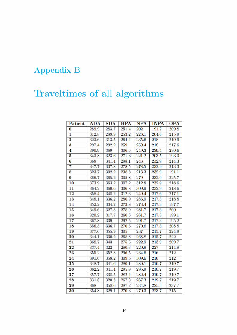
Appendix B

Traveltimes of all algorithms

49

50 APPENDIX B. TRAVELTIMES OF ALL ALGORITHMS

Appendix C

New paths

51

52 APPENDIX C. NEW PATHS