Estimating Maximum Concentrations for Open Path Monitoring Along a Fixed Beam Path
Upload
independentCategory
view
1download
0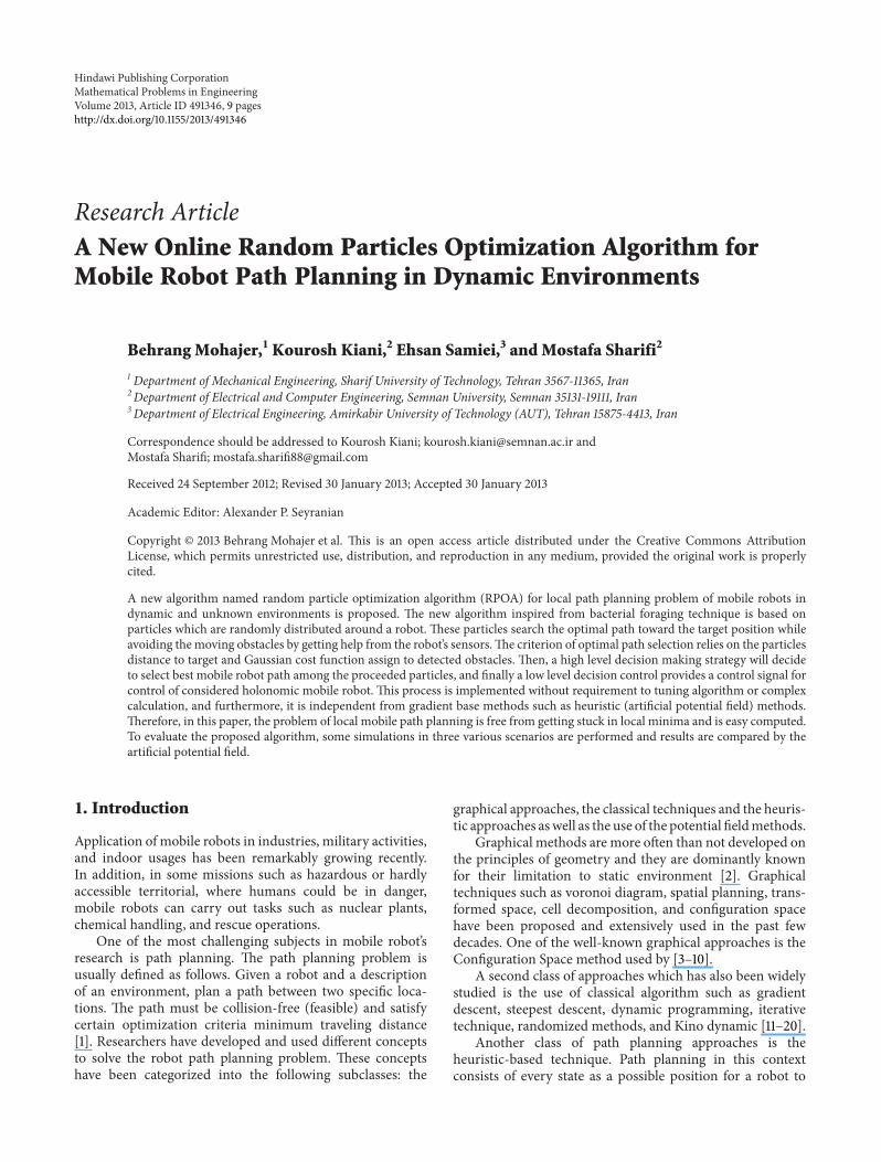
Hindawi Publishing CorporationMathematical Problems in EngineeringVolume 2013 Article ID 491346 9 pageshttpdxdoiorg1011552013491346
Research ArticleA New Online Random Particles Optimization Algorithm forMobile Robot Path Planning in Dynamic Environments
Behrang Mohajer1 Kourosh Kiani2 Ehsan Samiei3 and Mostafa Sharifi2
1 Department of Mechanical Engineering Sharif University of Technology Tehran 3567-11365 Iran2Department of Electrical and Computer Engineering Semnan University Semnan 35131-19111 Iran3Department of Electrical Engineering Amirkabir University of Technology (AUT) Tehran 15875-4413 Iran
Correspondence should be addressed to Kourosh Kiani kouroshkianisemnanacir andMostafa Sharifi mostafasharifi88gmailcom
Received 24 September 2012 Revised 30 January 2013 Accepted 30 January 2013
Academic Editor Alexander P Seyranian
Copyright copy 2013 Behrang Mohajer et al This is an open access article distributed under the Creative Commons AttributionLicense which permits unrestricted use distribution and reproduction in any medium provided the original work is properlycited
A new algorithm named random particle optimization algorithm (RPOA) for local path planning problem of mobile robots indynamic and unknown environments is proposed The new algorithm inspired from bacterial foraging technique is based onparticles which are randomly distributed around a robot These particles search the optimal path toward the target position whileavoiding themoving obstacles by getting help from the robotrsquos sensorsThe criterion of optimal path selection relies on the particlesdistance to target and Gaussian cost function assign to detected obstacles Then a high level decision making strategy will decideto select best mobile robot path among the proceeded particles and finally a low level decision control provides a control signal forcontrol of considered holonomic mobile robot This process is implemented without requirement to tuning algorithm or complexcalculation and furthermore it is independent from gradient base methods such as heuristic (artificial potential field) methodsTherefore in this paper the problem of local mobile path planning is free from getting stuck in local minima and is easy computedTo evaluate the proposed algorithm some simulations in three various scenarios are performed and results are compared by theartificial potential field
1 Introduction
Application of mobile robots in industries military activitiesand indoor usages has been remarkably growing recentlyIn addition in some missions such as hazardous or hardlyaccessible territorial where humans could be in dangermobile robots can carry out tasks such as nuclear plantschemical handling and rescue operations
One of the most challenging subjects in mobile robotrsquosresearch is path planning The path planning problem isusually defined as follows Given a robot and a descriptionof an environment plan a path between two specific loca-tions The path must be collision-free (feasible) and satisfycertain optimization criteria minimum traveling distance[1] Researchers have developed and used different conceptsto solve the robot path planning problem These conceptshave been categorized into the following subclasses the
graphical approaches the classical techniques and the heuris-tic approaches aswell as the use of the potential fieldmethods
Graphical methods are more often than not developed onthe principles of geometry and they are dominantly knownfor their limitation to static environment [2] Graphicaltechniques such as voronoi diagram spatial planning trans-formed space cell decomposition and configuration spacehave been proposed and extensively used in the past fewdecades One of the well-known graphical approaches is theConfiguration Space method used by [3ndash10]
A second class of approaches which has also been widelystudied is the use of classical algorithm such as gradientdescent steepest descent dynamic programming iterativetechnique randomized methods and Kino dynamic [11ndash20]
Another class of path planning approaches is theheuristic-based technique Path planning in this contextconsists of every state as a possible position for a robot to
2 Mathematical Problems in Engineering
move to and the transitions between these states are theactions the robot takes from the known information of thesurrounding environmentThe information that is valued themost by the algorithm is the cost of transitions from thecurrent state to the goal state The path taken is optimal ifthe sum of transition costs which are labeled global costsalso known as edge costs is a global minimal Global costsconsist of all known paths for the robot at a specific timeThealgorithm also has to be complete This technique is basedon inferential and evolutionary computationThere has beenseveral heuristic techniques in literatures such as potentialfield virtual force 119860
lowast algorithm 119864lowast algorithm genetic
algorithm memetic algorithm and simulated annealingArtificial potential fields (APFs) for collision avoidance
have attracted many researchers in the field of robotics Theidea of virtual forces acting on a robot has been proposedby Andrews and Hogan [21] and Khatib [22] This method isbased on the construction of a potential function around theobstacles deriving repulsive forces to the robot to avoid themon the contrary an attractive potential function was definedwith its center at the end position In these approaches thetarget applies an attractive force to the robot while obstaclesexert repulsive forces on the robotThe resultant force (sumofall forces) determines the direction and speed of movementA generalized potential field method that combines globaland local path planning has been introduced by Krogh andThorpe [23]
Path planning on other hand can be divided into twogroups according to the assumptions about the informationavailable for planning In path planning with completeinformation perfect knowledge about the robot and the envi-ronment are considered shapes of obstacles are computedalgebraically and path planning is implemented offline Inpath planning with incomplete information or sensor-basedplanning the obstacles can be of arbitrary shape and theinput information is in general local information from arange detector or a vision sensor [24] Path planning couldbe either local or global Local path planning means thatpath planning is done while the robot is moving in otherwords the algorithm is capable of producing a new path inresponse to environmental changes [25] On the other globalpath planning requires that environment to be completelyknown and all the features present within the terrain remainstatic and the algorithm generates a complete path from thestart point to the destination point before the robot starts itsmotion
In this paper a local path planning problem in anunknown environment for a holonomic mobile robot inthe presence of mobile obstacles is addressed In order toface this problem several approaches have been proposed inliteratures One of themost general techniques is based on theutilization of artificial potential fields (APFs) As mentionedabove this concept was introduced by Khatib [22] as a real-time obstacle avoidance methodThe major drawback of thisapproach is that the robot may get stuck in local minimaTo cope with this problem Vadakkepat et al introduceda new technique named evolutionary artificial potentialfield (EAPF) to address the path planning scenario withmobile obstacles Genetic algorithm was employed to derive
optimal potential field functions In addition an escape-forcealgorithm was performed to avoid being trapped in the localminima [26] Ge and Cui [27] proposed a new potential fieldmethod for motion planning of a mobile robot in a dynamicenvironment The new potential functions take into accountnot only the relative positions of the robot with respect tothe target and obstacles but also the relative velocities of therobot with respect to the target and obstaclesThen Poty et al[28] merged the approach proposed in [27] and the fractionalpotential for dynamic motion planning of mobile robotThe fractional potential was utilized to characterize dangerzone and risk coefficient of each obstacle Computer sim-ulations demonstrated that mobile robot avoided obstaclesand reached the target successfully Recently Munasinghe etal [29] proposed the velocity dipole field and its integrationwith the conventional potential field to form a new real-time obstacle avoidance algorithm Unlike the radial fieldlines of conventional potential field the velocity dipole fieldhas elliptical field lines that navigate a robot more skillfullyIt is useful to skillfully guide the robot around obstaclesquite similar to the way humans avoid moving obstaclesConn and Kam in [30] proposed a method where the mobileobstacles can be considered as stationary in the extendedworld by assuming time as one of the dimensions Howeverthis method required the mobile obstacle trajectory to beknown which is not applicable in real world
The organization of this paper is as follows In Section 2properties and assumptions of path planning in this proposalare described Section 3 introduces the proposed RPO algo-rithm for local path planning of mobile robots Simulationand numerical results are provided in Section 4 Finally inSection 5 we draw some conclusions and discuss about theproposed path planning method
2 System Modeling and Problem Formulation
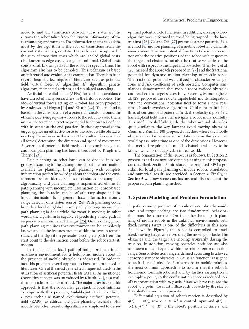
In path planning problem of mobile robots obstacle avoid-ance and target seeking are two fundamental behaviorsthat must be controlled On the other hand path plan-ning of mobile robots in the unknown environments withfixedmoving target is one of the difficulties in this areaAs shown in Figure 1 the robot is controlled to trackfixedmoving target while avoiding the moving obstacle Theobstacles and the target are moving arbitrarily during themission In addition moving obstacles positions are alsounknown unless they are within the robotrsquos sensor detectionrange Sensor detection range is defined according to allowedsensory distance to obstacles AGaussian function is assignedto each detected obstacle Furthermore in mobile roboticsthe most common approach is to assume that the robot isholonomic (omnidirectional) and by further assumption itis simply a point so the configuration space is reduced to a2D representation with 119909 119910 axis Since we have reduced therobot to a point we must inflate each obstacle by the size ofthe robotrsquos radius to compensate
Differential equation of robotrsquos motion is described by(119905) = 119906(119905) where 119906 isin 119877
2 is control input and 119902(119905) =
[119909(119905) 119910(119905)]119879
isin 1198772 is the robotrsquos position at time 119905 and
Mathematical Problems in Engineering 3
minus2 0 2 4 6 8 10 12minus2
0
2
4
6
8
10
12
119909
119910
Figure 1 The proposed RPO algorithm in fixed obstacle and target
assumed to be known all along the mission and 1199020(1199050) =
[1199090(119905) 1199100(119905)]119879
isin 1198772 is the robotrsquos initial position The target
position is also defined by 119901119866(119905) = [119909
119866(119905) 119910119866(119905)]119879
isin 1198772
3 Robot Path Planning inDynamic Environments
In this section an algorithm inspired from bacterial foragingmechanism is designed for local path planning of a mobilerobot in dynamic environment First we briefly review abacterial foraging technique and then the random particlealgorithm is proposed
31 Bacterial Foraging Optimization Algorithm Bacterial for-aging theory is based on the assumption that animals searchfor and obtain nutrients in a way that maximizes their energyintake 119864 per unit time 119879 spent foraging [31] Hence theyattempt to maximize their long-term average rate of energyintake
The main target in this algorithm for each bacterium isto find the minimum 119869(120579) 120579 isin 119877
119901 without considering thegradient nabla119869(120579) where 120579 is the position of a bacterium and119869(120579) is an attractant-repellent profile from the environment119869(120579) lt 0 119869(120579) = 0 and 119869(120579) gt 0 represent that the bac-terium at location 120579 is in nutrient rich neutral and noxiousenvironments respectively In fact in this algorithm we dealwith a nongradient optimization algorithm Chemotaxis isa foraging behavior that implements a type of optimizationwhere bacteria try to climbup the nutrient concentration (ielower and lower values of 119869(120579)) and avoids being at positions120579 where 119869(120579) ge 0 [1]
According to this algorithm 119894th bacterium at the position120579 takes a chemotaxis step 119895 with the step size 119888(119894) in therandom direction and calculate the cost function 119869(120579) at eachstep If the cost function of the new position 120579(119894 119895 + 1) thatis 119869(120579(119894 119895 + 1)) is smaller than the 119869(120579(119894 119895)) then anotherstep size 119888(119894) in the same previous direction will be takenThis process in the direction of lower cost function will
be continued until the maximum number of steps (119873119904) is
reachedThen after each119873119888chemotaxis step the least healthy
bacteria as stated by the cost function 119869(120579(119894 119895)) are replacedby the copies of healthy ones This procedure is calledreproduction step and it is followed by the eliminationndashdispersal (119873ed) event For each elimination-dispersal eventeach bacterium in the population is subjected to elimination-dispersal with probability 119875ed
32 The Random Particle Path Optimization Algorithm(RPOA) The proposed random particle optimization (RPO)algorithm is based on particles randomly distributed arounda robot In initial position of mobile robot (119902
0(1199050)) (119904 =
1 2 119899) virtual particles are generated and distributedrandomly on a circle with radius of 119862(119905) around the robotposition Each particle position (119904) in time 119905 could be definedas (120579119904(119905) isin 119877
2
) and the next position is calculated as
120579119904(119905 + 119889119905) = 120579
119904(119905) + 119862 (119905)
Δ (119905)
Δ (119905) (1)
where Δ(119905) isin 1198772 is a unit length random vector which is used
to define the direction particle in each timeThese particles intime 119905 +119889119905 search the optimal path toward the target positionwhile avoiding the moving obstacles by helping the robotrsquossensors Then the best particle which has found the mostoptimal path among other ones is chosen and the mobilerobot goes to the position of selected particle and it willcontinue again and again until the target is reached by theMR For choosing the best particle two different strategies arecombinedDistance norm to target position and cost function119869(120579119904(119905)) 120579 isin 119877
2 which is an attractant-repellent profile fromthe environment and according to section two is defined asGaussian function
321 DecisionMaking Strategy of Finding theOptimal ParticleWhen the mobile robot arrives at the moving obstacles itssensors detect obstaclesThen the algorithm virtually assignsa repellent Gaussian cost function to the obstacle by thefollowing formula
119869obstc
= 120572obstc exp (minus120583
obstc1003817100381710038171003817120579119894 (119905) minus 119875119874(119905)
1003817100381710038171003817
2
) (2)
where 120572obstc 120583obstc are constant values defining the height
and the width of the repellent respectively 119875119874
isin 1198772 denotes
the obstacle position detected by the robotrsquos sensor Notethat during the algorithm whenever an obstacle is withinthe robotrsquos sensor range 119869obstc has a value unless otherwiseits value is zero In other words repellent cost function allthrough the mission is defined as
119869obstc
=
120572obstc exp (minus120583
obstc1003817100381710038171003817120579119894 (119905) minus 119875119874(119905)
1003817100381710038171003817
2
)
1003817100381710038171003817119875119874 (119905) minus 119902 (119905)1003817100381710038171003817
2
le 120573
01003817100381710038171003817119875119874 (119905) minus 119902 (119905)
1003817100381710038171003817
2
gt 120573
(3)
In which 120573 is a robotrsquos sensor range Since the target posi-tion is always known we also assign an attractant Gaussian
4 Mathematical Problems in Engineering
Table 1 Fixed algorithm parameter
Number of bacteria 119904 = 100
Sensor detection range 119889sensor
= 12mAdaptive parameter
Step size length which isconsidered fixed all through the mission 119862(119905) = (112)119889
sensor
Table 2 Cost function parameter
Height of repellent 120572obstc
= 1
Width of repellent 120583obstc
= 4
Depth of attractant 120572goal
= 1
Width of attractant 120583goal
= 4
Table 3 Obstacle target and initial positions
First obstacle position [119909 119910]119879
= [3 2]119879
Second obstacle position [119909 119910]119879
= [9 8]119879
Third obstacle position [119909 119910]119879
= [72 7]119879
Forth obstacle position [119909 119910]119879
= [4 41]119879
Target position [119909 119910]119879
= [10 10]119879
Initial position [119909 119910]119879
= [0 0]119879
cost function to fixedmoving target position throughout themission the same as what we did for the obstacles
119869goal
= minus120572goal exp (minus120583
goal1003817100381710038171003817120579119894 (119905) minus 119875119866
1003817100381710038171003817
2
) (4)
where 120572goal 120583goal are constant values defining the height and
the width of the attractant respectively Total cost function isdefined as sum of repellent and attractant cost functions as
119869 = 119869obstc
+ 119869goal
(5)
The objectives of path planning are to simultaneously(1) move the robot on the path that under the minimumtime and cost arrive to the target while seeking it and (2)
avoid robot to collide with unknown obstacles moving inthe environment These objectives have to be achieved in anunknown environment with online computation In otherwords this paper presents an online algorithm for pathplanning mobile robots in unknown environments withouthaving prior information of obstacles and domain
322 High Level Decision Control High level decision con-trol designed for path planning mobile robot is based onartificial random particles in which at time 119905 ge 0 artificialparticles are placed at the position of robot and at time 119905+119889119905 ge
0 where 119889119905 is a small time they are randomly located overthe circle with radius 119862(119905) around the mobile robot In thisone-step-ahead algorithm the particle which could find thebest path at time 119905 + 119889119905 (whereas our objectives mentioned inSection 32 are satisfied) is selected as a best particle and robotwith a low level decision control signal (it will be discussed atSection 323) will put on the point found by the best particleand again from the new mobile position a group of artificial
0 2 4 6 8 10 12
05
1015minus1
minus05
0
05
1
15
119909 (m)119910 (m)
Hei
ght (
m)
Figure 2 Gaussian cost function used by the algorithm for obstaclesand target in RPO
02
46
810 0 2 4 6 8 10
0
10
20
30
40
119910 (m)
119909 (m)
Hei
ght (
m)
Figure 3 Cost function used by the algorithm for obstacles andtarget in APF
particles are distributed and the process goes on again andagainHence artificial particles generated in themainCPUofmobile robot alongwith the information given from the robotsensors could search mobile surroundings and determine therobotrsquos optimal path for one step ahead
A decision making strategy designed for finding the bestparticle among the others is based on both distance errorto target (119890119889
119904(119905 + 119889119905)) and cost function error 119890
119869
119904(119905) If 119889
119904(119905)
119889119904(119905 + 119889119905) represent the distance from particle 119904 to the target
at time 119905 and 119905 + 119889119905 and is defined as 119889119904(119905) = 120579
119904(119905) minus 119875
119866(119905)2
119889119904(119905 + 119889119905) = 120579
119904(119905 + 119889119905) minus 119875
119866(119905)2 respectively each particle
distance error and cost function error will be described as
119890119889
119904(119905 + 119889119905) = 119889
119904(119905 + 119889119905) minus 119889
119904(119905) 119904 = 1 2 119899
119890119869
119904(119905) = 119869 (120579
119904(119905 + 119889119905)) minus 119869 (120579
119904(119905)) 119904 = 1 2 119899
(6)
In time 119905+119889119905 all the 119890119889119904(119905) for 119904 = 1 2 119899 are computed
and then particles are sorted in order of ascending error 119890119889119904(119905)
in a vector 119878sort such that the particle with the lowest distanceerror is at top The first priority in this technique is to glidethe robot to the target Hence particles are considered as fitones that put on the higher part of vector 119878sort Furthermore
Mathematical Problems in Engineering 5
minus2 0 2 4 6 8 10 12minus2
0
2
4
6
8
10
12
119909 (m)
119910 (m
)
Figure 4 Fixed obstacle and goal position (red)The proposed RPOalgorithm (110321s) (blue) APF algorithm (112337 s)
0 1 2 3 4 5 6 7 8 9 100
05
1
15
2
25
3
Time (s)
Virt
ual f
orce
(N)
Figure 5 Exerted virtual force to the robot in APF method
among these fit particles one is chosen that has negative errorcost function 119890
119869
119904(119905) with priority to the lowest distance error
because they must be kept away from obstacles and having119890119869
119904(119905) gt 0 according to (3) represents that particles are in the
region of obstacles In fact in this decision making strategyfor finding the best particle a search on distance error 119890
119889
119904(119905)
from top to bottom is performed and the first particle with119890119869
119904(119905) lt 0 is selected as the best particle By using these two
techniques together objectives are also satisfiedNote that according to (3)ndash(5) when an obstacle is not in
the robotrsquos sensor range 119869obstc is zero and as a result minus2120572goallt
119890119869
119904(119905) lt 0 In this situation robot freely moves toward target
by choosing the first element of vector 119878sort since all of themhave 119890
119869
119904(119905) lt 0 But when robotrsquos sensor detect an obstacle
119869obstc gets a value and consequently minus2120572goal
lt 119890119869
119904(119905) lt 2120572
obstcIn this case the first particle in the ascended ordered of 119890119889
119904(119905)
which has the negative error 119890119869119904(119905) is selected as the best one
A modification could be performed on this strategy Inthe above strategy we have omitted particles with 119890
119869
119904(119905) gt 0
minus2 0 2 4 6 8 10 12minus2
0
2
4
6
8
10
12
119909 (m)
119910 (m
)
Figure 6 Fixed obstacle and goal position (red)The proposed RPOalgorithm (blue) APF algorithm got stuck in local minimum
because they are in the region of detected obstacle But to findthe optimal path we could let particles to somewhat approachto the obstacle in order to find that optimal path Actuallyif a particle fall into the region of a detected obstacle it willnot be omited but we allow that particle to approach nearbythe obstacle to find the new optimal path For this aim weintroduce a new parameter 120578which is a coefficient of 120572obstc indecision equation 119890
119869
119904(119905) lt 120578 and let the particle located in the
obstaclersquos region not to be omitted
323 Low Level Decision Control Low level decision controlof mobile robot is based on each time step Control law ischosen as follows
119906 (119905) = 119862 (119905)
(120579119904best
(119905 + 119889119905) minus 119902first
)
10038171003817100381710038171003817(120579119904best
(119905 + 119889119905) minus 119902first)10038171003817100381710038171003817
(7)
where 119902first
(119905) is the mobile robot position at time 119905 and120579119904best
(119905 + 119889119905) is a certain particle position at time 119905 + 119889119905 whichhas the optimal position and is supposed to be selected bythe algorithm and the robot will go through this particleposition To explicit this control law and to compare withclassical control law such as PI or PD it seems it operates asa P controller
4 Simulation Results
In this section we apply the proposed RPO algorithm ona mobile robot to find an optimal path for the robot toreach its target in the presence of obstacles This is an onlinealgorithm In fact we did not need any information andprior computation from the environment in which the robotperforms its taskThe only parameters that are obtained fromthe environment are the target position robot position anddata from obstacle detection sensors which practically canbe obtained from the sensors installed on the robot All ofthe other parameters are selected by the operator Then the
6 Mathematical Problems in Engineering
minus2 0 2 4 6 8 10 12minus2
0
2
4
6
8
10
12
(a)
minus2 0 2 4 6 8 10 12minus2
0
2
4
6
8
10
12
(b)
minus2 0 2 4 6 8 10 12minus2
0
2
4
6
8
10
12
(c)
minus2 0 2 4 6 8 10 12minus2
0
2
4
6
8
10
12
119909 (m)
119910 (m
)
(d)
Figure 7 Moving obstacle and fixed goal position
proposed algorithm is computed in the main CPU of themobile robot and it helps the robot to find optimal pathThenumber of obstacles and particles can effect on the real-timeperformances but with high speed CPUs there is no problemin real-time performance
To evaluate our results in this section three differentscenarios have been set up In the first scenario obstaclesand target are assumed to be fixed In the second one thealgorithm has been run on a dynamic environment with fixedtarget and unknown moving obstacles and in the third onebothmoving target and obstacles are evaluated Furthermoreto assess the performance of the algorithm a comparison toartificial potential field (APF) method is presented in bothscenarios
The algorithm parameters in simulation are set as shownin Table 1
As mentioned in Section 322 an attractant artificialGaussian function was donated to the target all through themission On the other hand when an obstacle is detected bymobile robot sensors a repellent artificial Gaussian function
is assigned to the obstacle Then the total cost function iscomputed as a sum of attractant and repellents Gaussianfunctions The parameters selected for the Gaussian costfunctions are as in Table 2 The parameters for simulationare defined arbitrarily but in real situation the dimension ofobstacles can be estimated by some sophisticated devices likeradars and so forth
41 Fixed Obstacles and Target In the first scenario all theobstacles and the target are assumed to be fixed by theposition given in Table 3 Note that obstacles positions areunknown and are detected by the robotrsquos sensors
The result has been shown in Figure 1 The red circlesaround the mobile robot show the robot sensor rangeWhenever an obstacle is detected by robotrsquos sensor thealgorithm dedicates a Gaussian function to it and makes therobot change its path to avoid it while it remains on its optimalpath Figure 2 shows these Gaussian functions used by thealgorithms To compare the proposed RPO algorithm by theconventional artificial potential field technique a simulation
Mathematical Problems in Engineering 7
minus5 0 5 10minus2
0
2
4
6
8
10
Robot path by APF
119909 (m)
119910 (m
)
minus2
0
2
4
6
8
10
119910 (m
)
minus5 0 5 10
Robot path by RPO
119909 (m)
(a)
0 50 100 150 200 250 300 350 4000
1
2
3
4
5
6
7
8
9
10
Time (s)
Virt
ual f
orce
(N)
(b)
Figure 8 (a) Spanned paths by the robot with two algorithms (b)Exerted virtual force to the robot in APF method
has been performed on the same condition Equations (8)and (9) are the most used potential field formula In the AFPmethod we suppose that all of the obstacles are unknownuntil they are within the robotrsquos sensor range and targetpositions are known and attractive potential function isdefined as
119880att (119902) =1
2120577 (
10038171003817100381710038171003817119902 (119905) minus 119875goal (119905)
10038171003817100381710038171003817
2
) (8)
where 120577 = 02 is some positive constant scaling factor from[22] and the repulsive potential function is defined as
119880rep (119902) =
1
2120578(
1
1205880(119902)
minus1
1205880
)
2
if 120588119900(119902) le 120588
0
0 if 120588119900(119902) gt 120588
0
(9)
where 120588119900is a positive constant and it represents allowance
distance to obstacle In this simulation 120588119900is selected same as
minus2 0 2 4 6 8 10 12minus2
0
2
4
6
8
10
12
119909 (m)
119910 (m
)
(a)
minus5 0 5 10minus2
0
2
4
6
8
10
Robot path by APF
119909 (m)
119910 (m
)
minus2
0
2
4
6
8
10
119910 (m
)
minus5 0 5 10
Robot path by RPO
119909 (m)
(b)
Figure 9 (a) Moving obstacle and fixed goal position (b) Spannedpaths by the robot with two algorithms
119889sensor to make both algorithms the same 120578 = 10 is a positive
scaling factor 120588119900(119902) is defined as 120588
119900(119902) = (119902(119905) minus 119875obstc(119905))
Figure 3 shows potential filed considered for this simulationFigure 4 shows paths ran by the both algorithm to reach tothe targetThe red line shows the path that robot has followeddue to the presented algorithm and the blue one refers to thepath generated by using the artificial potential field (APF)method Total virtual force exerted to the robot is also shownin Figure 5 As we expected in AFP target total force is zero
An important drawback ofAPFmethod is getting stuck inlocal minima In some certain conditions the potential fieldmethod results in minima other than the target in the planewhich absorb the robot so the robot may get stuck in theseminima and could not reach the target Producing attractingpoints other than the targets is an inherent drawback ofpotential field basedmethods In this simulation if we changeforth obstacle position to [119909 119910]
119879
= [4 4]119879 in AFP algorithm
8 Mathematical Problems in Engineering
minus2 0 2 4 6 8 10 12minus2
0
2
4
6
8
10
12
119909 (m)
119910 (m
)
Figure 10 Moving obstacle and target
mobile robot will stuck in local minimum as shown inFigure 6 whilemobile robot can find its optimal path to targetby the RPO algorithm
42 RandomMovingObstacle and FixedTarget In the secondscenario the robot should reach to a fixed target on a dynamicenvironment with unknown moving obstacles There aresix unknown obstacles in the environment which moverandomly The red circles around the mobile robot show therobot sensor range Since in this case we deal with movingobstacles we increase sensor detection range to 119889
sensor=
2 times 12m so that the collision avoidance of mobile robot withmoving obstacles is guaranteed 120588
119900is selected same as 119889sensor
to make both algorithms the same and other parameters arethe same as the previous one Figure 7 shows the obtainedresults Although the proposed algorithm is online and onestep ahead but it generates a near optimal path while theAPF generated path is much longer Generated paths by bothalgorithms as well as virtual force exerted on robots by theAFP are also shown in Figure 8
In this section if one of the obstacles positions rotatesaround the goal in AFP algorithm mobile robot will stuck inlocal minimum and with the constant rate rotate around thetarget and never gets it while the proposed RPO algorithmcan find its optimal path to target by the RPO algorithmThese results are shown in Figure 9
43 Random Moving Obstacle and Target In the third sce-nario the robot should reach to a moving target on a dynamicenvironment with unknown moving obstacles and a movingtarget There are six unknown obstacles in the environmentwhich move randomly Sensor detection range is 119889
sensor=
2m and 120588119900is selected same as 119889
sensor to make both algo-rithms the same Other parameters are the same as previoussimulations Figure 10 shows the obtained results The redcircles around the mobile robot at the target show the robotsensor range The green and violet circles represent paths ranby moving target and obstacles respectively Exerted virtual
minus5 0 5 10minus2
0
2
4
6
8
10
Robot path by APF
119909 (m)minus5 0 5 10
119909 (m)
119910 (m
)
minus2
0
2
4
6
8
10
119910 (m
)
Robot path by RPO
(a)
0 5 10 150
5
10
15
20
25
30
35
40
45
50
Time (s)
Virt
ual f
orce
(N)
(b)
Figure 11 (a) Spanned paths by the robot with two algorithms (b)Exerted virtual force to the robot in APF method
force by the APF and spanned paths by both algorithms areshown in Figure 11
5 Conclusion
Local path planning of mobile robots was addressed in thispaper In comparison to artificial potential field methodthe RPO gives much optimal solution in shorter timeFurthermore it is free from some drawbacks such as trappedstates or gradient of potential functions which could provideimpulsive force to the robot
References
[1] K Sugihara and J Smith ldquoGenetic algorithms for adaptivemotion planning of an autonomous mobile robotrdquo in Proceed-ings of the IEEE International Symposium on Computational
Mathematical Problems in Engineering 9
Intelligence in Robotics and Automation (CIRA rsquo97) pp 138ndash143Monterey Calif USA July 1997
[2] T Lozano-Perez ldquoA simple motion planning algorithm forgeneral robot manipulatorsrdquo IEEE Journal of Robotics andAutomation vol 3 no 3 pp 224ndash238 1987
[3] J Laumond ldquoFeasible trajectories for mobile robots withkinematic and environment constraintsrdquo in Proceedings of theInternational Conference on Intelligent Autonomous Systems(IAS rsquo86) pp 346ndash354 Amsterdam The Netherlands 1986
[4] E Palma-Villalon and P Dauchez ldquoWorld representation andpath planning for a mobile robotrdquo Robotica vol 6 no 1 pp 35ndash40 1988
[5] C S Tseng C Crane and J Duffy ldquoGenerating collision-free paths for robot manipulatorsrdquo Computers in MechanicalEngineering vol 7 no 2 pp 58ndash64 1988
[6] O Takahashi and R J Schilling ldquoMotion planning in a planeusing generalized Voronoi diagramsrdquo IEEE Transactions onRobotics and Automation vol 5 no 2 pp 143ndash150 1989
[7] G Song S Miller and N M Amato ldquoCustomizing PRMroadmaps at query timerdquo in Proceedings of the IEEE Interna-tional Conference on Robotics and Automation (ICRA rsquo01) pp1500ndash1505 Seoul Republic of Korea May 2001
[8] F Lingelbach ldquoPath planning using probabilistic cell decompo-sitionrdquo in Proceedings of the IEEE International Conference onRobotics and Automation pp 467ndash472 New Orleans La USA2004
[9] F Lingelbach ldquoPath planning for mobile manipulation usingprobabilistic cell decompositionrdquo in Proceedings of the IEEERSJInternational Conference on Intelligent Robots and Systems(IROS rsquo04) pp 2807ndash2812 Sendai Japan October 2004
[10] R Gayle A Sud M C Lin and D Manocha ldquoReactivedeformation roadmaps motion planning of multiple robots indynamic environmentsrdquo in Proceedings of the IEEERSJ Interna-tional Conference on Intelligent Robots and Systems (IROS rsquo07)pp 3777ndash3783 San Diego Calif USA November 2007
[11] O S Asaolu An intelligent path planner for autonomous mobilerobots [PhD thesis] Department of Systems EngineeringUniversity of Lagos Lagos Nigeria 2001
[12] O Ibidapo-Obe and O S Asaolu ldquoOptimization problems inapplied sciences from classical through stochastic to intelligentmetaheuristic approachesrdquo in Handbook of Industrial and Sys-tems Engineering A B Badiru Ed chapter 22 pp 1ndash18 CRCPress Taylor and Francis Group New York NY USA 2006
[13] O Ibidapo-Obe O S Asaolu and A B Badiru ldquoGeneral-ized solutions of the pursuit problem in three-dimensionalEuclidean spacerdquo Applied Mathematics and Computation vol119 no 1 pp 35ndash45 2001
[14] O Ibidapo-Obe O S Asaolu and A B Badiru ldquoA newmethod for the numerical solution of simultaneous nonlinearequationsrdquo Applied Mathematics and Computation vol 125 no1 pp 133ndash140 2002
[15] K Heero J Willemson A Aabloo and M Kruusmaa ldquoRobotsfind a better way a learningmethod formobile robot navigationin partially unknown environmentsrdquo in Proceedings of the 8thConference on Intelligent Autonomous Systems (IAS rsquo04) pp559ndash566 Amsterdam The Netherlands 2004
[16] J Fasola P E Rybski and M M Veloso ldquoFast goal navigationwith obstacle avoidance using a dynamic local visual modelrdquoin Proceedings of the 7th Brazilian Symposium on ArtificialIntelligence pp 1ndash6 Sao Luıs Brazil September 2005
[17] M Bikdash S Karagol and M Charifa ldquoMesh analysis withapplications in reduced-order modeling and collision avoid-ancerdquo in Proceedings of the COMSOL Users Conference pp 1ndash7Boston Mass USA 2006
[18] M Becker C M Dantas and W P Macedo ldquoObstacle avoid-ance procedure for mobile robotsrdquo in ABCM Symposium Seriesin Mechatronics vol 2 pp 250ndash257 ABCM 2006
[19] R Philippsen B Jensen and R Siegwart ldquoTowards real-timesensor-based path planning in highly dynamic environmentsrdquoSpringer Tracts in Advanced Robotics vol 35 pp 135ndash148 2007
[20] Y P Li T Zielinska M H Ang Jr and W Lin ldquoVehicledynamics of redundant mobile robots with powered casterwheelsrdquo in Proceedings of the 16th CISM-IFToMM SymposiumRomansy 16 Robot Design Dynamics and Control pp 221ndash228Warsaw Poland 2006
[21] J R Andrews and N Hogan ldquoImpedance control as a frame-work for implementing obstacle avoidance in a manipulatorrdquoin Control of Manufacturing Processes and Robotic Systems DE Hardt and W Book Eds pp 243ndash251 ASME Boston MassUSA 1983
[22] O Khatib ldquoReal-time obstacle avoidance for manipulatorsand mobile robotsrdquo in Proceedings of the IEEE InternationalConference on Robotics and Automation pp 500ndash505 St LouisMo USA March 1990
[23] B H Krogh and C E Thorpe ldquoIntegrated path planningand dynamic steering control for autonomous vehiclesrdquo inProceedings of the IEEE International Conference onRobotics andAutomation pp 1664ndash1669 San Francisco Calif USA April1986
[24] J Nygards P Skoglar J Karlholm R Bjorstrom andM UlvkloldquoTowards concurrent sensor and path planningrdquo Tech RepFOI 2005
[25] V O S Olunloyo and M K O Ayomoh ldquoAutonomous mobilerobot navigation using hybrid virtual force field conceptrdquoEuropean Journal of Scientific Research vol 31 no 2 pp 204ndash228 2009
[26] P Vadakkepat K C Tan and M L Wang ldquoEvolutionaryartificial potential fields and their application in real time robotpath planningrdquo in Proceedings of the Congress on EvolutionaryComputation (CEC rsquo00) pp 256ndash263 July 2000
[27] S S Ge and Y J Cui ldquoDynamic motion planning for mobilerobots using potential field methodrdquo Autonomous Robots vol13 no 3 pp 207ndash222 2002
[28] A Poty PMelchior andAOustaloup ldquoDynamic path planningformobile robots using fractional potential fieldrdquo in Proceedingsof the 1st International Symposium on Control Communicationsand Signal Processing (ISCCSP rsquo04) pp 557ndash561 March 2004
[29] S R Munasinghe C Oh J J Lee and O Khatib ldquoObstacleavoidance using velocity dipole field methodrdquo in Proceedingsof the International Conference on Control Automation andSystems (ICCAS rsquo05) Goyang Republic of Korea 2005
[30] R A Conn and M Kam ldquoRobot motion planning on N-dimensional star worlds among moving obstaclesrdquo IEEE Trans-actions on Robotics and Automation vol 14 no 2 pp 320ndash3251998
[31] KM Passino ldquoBiomimicry of bacterial foraging for distributedoptimization and controlrdquo IEEE Control Systems vol 22 no 3pp 52ndash67 2002
Submit your manuscripts athttpwwwhindawicom
Hindawi Publishing Corporationhttpwwwhindawicom Volume 2013
Game Theory
Journal ofApplied Mathematics
Hindawi Publishing Corporationhttpwwwhindawicom Volume 2013
Hindawi Publishing Corporationhttpwwwhindawicom Volume 2013
Complex Systems
Journal of
ISRN Operations Research
Hindawi Publishing Corporationhttpwwwhindawicom Volume 2013
Hindawi Publishing Corporationhttpwwwhindawicom Volume 2013
Abstract and Applied Analysis
Hindawi Publishing Corporationhttpwwwhindawicom Volume 2013
Industrial MathematicsJournal of
Hindawi Publishing Corporationhttpwwwhindawicom Volume 2013
OptimizationJournal of
ISRN Computational Mathematics
Hindawi Publishing Corporationhttpwwwhindawicom Volume 2013
Hindawi Publishing Corporationhttpwwwhindawicom Volume 2013
Mathematical Problems in Engineering
Hindawi Publishing Corporationhttpwwwhindawicom Volume 2013
Complex AnalysisJournal of
ISRN Combinatorics
Hindawi Publishing Corporationhttpwwwhindawicom Volume 2013
Hindawi Publishing Corporationhttpwwwhindawicom Volume 2013
Geometry
ISRN Applied Mathematics
Hindawi Publishing Corporationhttpwwwhindawicom Volume 2013
International Journal of Mathematics and Mathematical Sciences
Hindawi Publishing Corporationhttpwwwhindawicom Volume 2013
thinspAdvancesthinspin
DecisionSciences
HindawithinspPublishingthinspCorporationhttpwwwhindawicom Volumethinsp2013
Hindawi Publishing Corporationhttpwwwhindawicom Volume 2013
MathematicsJournal of
Hindawi Publishing Corporationhttpwwwhindawicom Volume 2013
Algebra
ISRN Mathematical Physics
Hindawi Publishing Corporationhttpwwwhindawicom Volume 2013
Discrete MathematicsJournal of
Hindawi Publishing Corporationhttpwwwhindawicom
Volume 2013
2 Mathematical Problems in Engineering
move to and the transitions between these states are theactions the robot takes from the known information of thesurrounding environmentThe information that is valued themost by the algorithm is the cost of transitions from thecurrent state to the goal state The path taken is optimal ifthe sum of transition costs which are labeled global costsalso known as edge costs is a global minimal Global costsconsist of all known paths for the robot at a specific timeThealgorithm also has to be complete This technique is basedon inferential and evolutionary computationThere has beenseveral heuristic techniques in literatures such as potentialfield virtual force 119860
lowast algorithm 119864lowast algorithm genetic
algorithm memetic algorithm and simulated annealingArtificial potential fields (APFs) for collision avoidance
have attracted many researchers in the field of robotics Theidea of virtual forces acting on a robot has been proposedby Andrews and Hogan [21] and Khatib [22] This method isbased on the construction of a potential function around theobstacles deriving repulsive forces to the robot to avoid themon the contrary an attractive potential function was definedwith its center at the end position In these approaches thetarget applies an attractive force to the robot while obstaclesexert repulsive forces on the robotThe resultant force (sumofall forces) determines the direction and speed of movementA generalized potential field method that combines globaland local path planning has been introduced by Krogh andThorpe [23]
Path planning on other hand can be divided into twogroups according to the assumptions about the informationavailable for planning In path planning with completeinformation perfect knowledge about the robot and the envi-ronment are considered shapes of obstacles are computedalgebraically and path planning is implemented offline Inpath planning with incomplete information or sensor-basedplanning the obstacles can be of arbitrary shape and theinput information is in general local information from arange detector or a vision sensor [24] Path planning couldbe either local or global Local path planning means thatpath planning is done while the robot is moving in otherwords the algorithm is capable of producing a new path inresponse to environmental changes [25] On the other globalpath planning requires that environment to be completelyknown and all the features present within the terrain remainstatic and the algorithm generates a complete path from thestart point to the destination point before the robot starts itsmotion
In this paper a local path planning problem in anunknown environment for a holonomic mobile robot inthe presence of mobile obstacles is addressed In order toface this problem several approaches have been proposed inliteratures One of themost general techniques is based on theutilization of artificial potential fields (APFs) As mentionedabove this concept was introduced by Khatib [22] as a real-time obstacle avoidance methodThe major drawback of thisapproach is that the robot may get stuck in local minimaTo cope with this problem Vadakkepat et al introduceda new technique named evolutionary artificial potentialfield (EAPF) to address the path planning scenario withmobile obstacles Genetic algorithm was employed to derive
optimal potential field functions In addition an escape-forcealgorithm was performed to avoid being trapped in the localminima [26] Ge and Cui [27] proposed a new potential fieldmethod for motion planning of a mobile robot in a dynamicenvironment The new potential functions take into accountnot only the relative positions of the robot with respect tothe target and obstacles but also the relative velocities of therobot with respect to the target and obstaclesThen Poty et al[28] merged the approach proposed in [27] and the fractionalpotential for dynamic motion planning of mobile robotThe fractional potential was utilized to characterize dangerzone and risk coefficient of each obstacle Computer sim-ulations demonstrated that mobile robot avoided obstaclesand reached the target successfully Recently Munasinghe etal [29] proposed the velocity dipole field and its integrationwith the conventional potential field to form a new real-time obstacle avoidance algorithm Unlike the radial fieldlines of conventional potential field the velocity dipole fieldhas elliptical field lines that navigate a robot more skillfullyIt is useful to skillfully guide the robot around obstaclesquite similar to the way humans avoid moving obstaclesConn and Kam in [30] proposed a method where the mobileobstacles can be considered as stationary in the extendedworld by assuming time as one of the dimensions Howeverthis method required the mobile obstacle trajectory to beknown which is not applicable in real world
The organization of this paper is as follows In Section 2properties and assumptions of path planning in this proposalare described Section 3 introduces the proposed RPO algo-rithm for local path planning of mobile robots Simulationand numerical results are provided in Section 4 Finally inSection 5 we draw some conclusions and discuss about theproposed path planning method
2 System Modeling and Problem Formulation
In path planning problem of mobile robots obstacle avoid-ance and target seeking are two fundamental behaviorsthat must be controlled On the other hand path plan-ning of mobile robots in the unknown environments withfixedmoving target is one of the difficulties in this areaAs shown in Figure 1 the robot is controlled to trackfixedmoving target while avoiding the moving obstacle Theobstacles and the target are moving arbitrarily during themission In addition moving obstacles positions are alsounknown unless they are within the robotrsquos sensor detectionrange Sensor detection range is defined according to allowedsensory distance to obstacles AGaussian function is assignedto each detected obstacle Furthermore in mobile roboticsthe most common approach is to assume that the robot isholonomic (omnidirectional) and by further assumption itis simply a point so the configuration space is reduced to a2D representation with 119909 119910 axis Since we have reduced therobot to a point we must inflate each obstacle by the size ofthe robotrsquos radius to compensate
Differential equation of robotrsquos motion is described by(119905) = 119906(119905) where 119906 isin 119877
2 is control input and 119902(119905) =
[119909(119905) 119910(119905)]119879
isin 1198772 is the robotrsquos position at time 119905 and
Mathematical Problems in Engineering 3
minus2 0 2 4 6 8 10 12minus2
0
2
4
6
8
10
12
119909
119910
Figure 1 The proposed RPO algorithm in fixed obstacle and target
assumed to be known all along the mission and 1199020(1199050) =
[1199090(119905) 1199100(119905)]119879
isin 1198772 is the robotrsquos initial position The target
position is also defined by 119901119866(119905) = [119909
119866(119905) 119910119866(119905)]119879
isin 1198772
3 Robot Path Planning inDynamic Environments
In this section an algorithm inspired from bacterial foragingmechanism is designed for local path planning of a mobilerobot in dynamic environment First we briefly review abacterial foraging technique and then the random particlealgorithm is proposed
31 Bacterial Foraging Optimization Algorithm Bacterial for-aging theory is based on the assumption that animals searchfor and obtain nutrients in a way that maximizes their energyintake 119864 per unit time 119879 spent foraging [31] Hence theyattempt to maximize their long-term average rate of energyintake
The main target in this algorithm for each bacterium isto find the minimum 119869(120579) 120579 isin 119877
119901 without considering thegradient nabla119869(120579) where 120579 is the position of a bacterium and119869(120579) is an attractant-repellent profile from the environment119869(120579) lt 0 119869(120579) = 0 and 119869(120579) gt 0 represent that the bac-terium at location 120579 is in nutrient rich neutral and noxiousenvironments respectively In fact in this algorithm we dealwith a nongradient optimization algorithm Chemotaxis isa foraging behavior that implements a type of optimizationwhere bacteria try to climbup the nutrient concentration (ielower and lower values of 119869(120579)) and avoids being at positions120579 where 119869(120579) ge 0 [1]
According to this algorithm 119894th bacterium at the position120579 takes a chemotaxis step 119895 with the step size 119888(119894) in therandom direction and calculate the cost function 119869(120579) at eachstep If the cost function of the new position 120579(119894 119895 + 1) thatis 119869(120579(119894 119895 + 1)) is smaller than the 119869(120579(119894 119895)) then anotherstep size 119888(119894) in the same previous direction will be takenThis process in the direction of lower cost function will
be continued until the maximum number of steps (119873119904) is
reachedThen after each119873119888chemotaxis step the least healthy
bacteria as stated by the cost function 119869(120579(119894 119895)) are replacedby the copies of healthy ones This procedure is calledreproduction step and it is followed by the eliminationndashdispersal (119873ed) event For each elimination-dispersal eventeach bacterium in the population is subjected to elimination-dispersal with probability 119875ed
32 The Random Particle Path Optimization Algorithm(RPOA) The proposed random particle optimization (RPO)algorithm is based on particles randomly distributed arounda robot In initial position of mobile robot (119902
0(1199050)) (119904 =
1 2 119899) virtual particles are generated and distributedrandomly on a circle with radius of 119862(119905) around the robotposition Each particle position (119904) in time 119905 could be definedas (120579119904(119905) isin 119877
2
) and the next position is calculated as
120579119904(119905 + 119889119905) = 120579
119904(119905) + 119862 (119905)
Δ (119905)
Δ (119905) (1)
where Δ(119905) isin 1198772 is a unit length random vector which is used
to define the direction particle in each timeThese particles intime 119905 +119889119905 search the optimal path toward the target positionwhile avoiding the moving obstacles by helping the robotrsquossensors Then the best particle which has found the mostoptimal path among other ones is chosen and the mobilerobot goes to the position of selected particle and it willcontinue again and again until the target is reached by theMR For choosing the best particle two different strategies arecombinedDistance norm to target position and cost function119869(120579119904(119905)) 120579 isin 119877
2 which is an attractant-repellent profile fromthe environment and according to section two is defined asGaussian function
321 DecisionMaking Strategy of Finding theOptimal ParticleWhen the mobile robot arrives at the moving obstacles itssensors detect obstaclesThen the algorithm virtually assignsa repellent Gaussian cost function to the obstacle by thefollowing formula
119869obstc
= 120572obstc exp (minus120583
obstc1003817100381710038171003817120579119894 (119905) minus 119875119874(119905)
1003817100381710038171003817
2
) (2)
where 120572obstc 120583obstc are constant values defining the height
and the width of the repellent respectively 119875119874
isin 1198772 denotes
the obstacle position detected by the robotrsquos sensor Notethat during the algorithm whenever an obstacle is withinthe robotrsquos sensor range 119869obstc has a value unless otherwiseits value is zero In other words repellent cost function allthrough the mission is defined as
119869obstc
=
120572obstc exp (minus120583
obstc1003817100381710038171003817120579119894 (119905) minus 119875119874(119905)
1003817100381710038171003817
2
)
1003817100381710038171003817119875119874 (119905) minus 119902 (119905)1003817100381710038171003817
2
le 120573
01003817100381710038171003817119875119874 (119905) minus 119902 (119905)
1003817100381710038171003817
2
gt 120573
(3)
In which 120573 is a robotrsquos sensor range Since the target posi-tion is always known we also assign an attractant Gaussian
4 Mathematical Problems in Engineering
Table 1 Fixed algorithm parameter
Number of bacteria 119904 = 100
Sensor detection range 119889sensor
= 12mAdaptive parameter
Step size length which isconsidered fixed all through the mission 119862(119905) = (112)119889
sensor
Table 2 Cost function parameter
Height of repellent 120572obstc
= 1
Width of repellent 120583obstc
= 4
Depth of attractant 120572goal
= 1
Width of attractant 120583goal
= 4
Table 3 Obstacle target and initial positions
First obstacle position [119909 119910]119879
= [3 2]119879
Second obstacle position [119909 119910]119879
= [9 8]119879
Third obstacle position [119909 119910]119879
= [72 7]119879
Forth obstacle position [119909 119910]119879
= [4 41]119879
Target position [119909 119910]119879
= [10 10]119879
Initial position [119909 119910]119879
= [0 0]119879
cost function to fixedmoving target position throughout themission the same as what we did for the obstacles
119869goal
= minus120572goal exp (minus120583
goal1003817100381710038171003817120579119894 (119905) minus 119875119866
1003817100381710038171003817
2
) (4)
where 120572goal 120583goal are constant values defining the height and
the width of the attractant respectively Total cost function isdefined as sum of repellent and attractant cost functions as
119869 = 119869obstc
+ 119869goal
(5)
The objectives of path planning are to simultaneously(1) move the robot on the path that under the minimumtime and cost arrive to the target while seeking it and (2)
avoid robot to collide with unknown obstacles moving inthe environment These objectives have to be achieved in anunknown environment with online computation In otherwords this paper presents an online algorithm for pathplanning mobile robots in unknown environments withouthaving prior information of obstacles and domain
322 High Level Decision Control High level decision con-trol designed for path planning mobile robot is based onartificial random particles in which at time 119905 ge 0 artificialparticles are placed at the position of robot and at time 119905+119889119905 ge
0 where 119889119905 is a small time they are randomly located overthe circle with radius 119862(119905) around the mobile robot In thisone-step-ahead algorithm the particle which could find thebest path at time 119905 + 119889119905 (whereas our objectives mentioned inSection 32 are satisfied) is selected as a best particle and robotwith a low level decision control signal (it will be discussed atSection 323) will put on the point found by the best particleand again from the new mobile position a group of artificial
0 2 4 6 8 10 12
05
1015minus1
minus05
0
05
1
15
119909 (m)119910 (m)
Hei
ght (
m)
Figure 2 Gaussian cost function used by the algorithm for obstaclesand target in RPO
02
46
810 0 2 4 6 8 10
0
10
20
30
40
119910 (m)
119909 (m)
Hei
ght (
m)
Figure 3 Cost function used by the algorithm for obstacles andtarget in APF
particles are distributed and the process goes on again andagainHence artificial particles generated in themainCPUofmobile robot alongwith the information given from the robotsensors could search mobile surroundings and determine therobotrsquos optimal path for one step ahead
A decision making strategy designed for finding the bestparticle among the others is based on both distance errorto target (119890119889
119904(119905 + 119889119905)) and cost function error 119890
119869
119904(119905) If 119889
119904(119905)
119889119904(119905 + 119889119905) represent the distance from particle 119904 to the target
at time 119905 and 119905 + 119889119905 and is defined as 119889119904(119905) = 120579
119904(119905) minus 119875
119866(119905)2
119889119904(119905 + 119889119905) = 120579
119904(119905 + 119889119905) minus 119875
119866(119905)2 respectively each particle
distance error and cost function error will be described as
119890119889
119904(119905 + 119889119905) = 119889
119904(119905 + 119889119905) minus 119889
119904(119905) 119904 = 1 2 119899
119890119869
119904(119905) = 119869 (120579
119904(119905 + 119889119905)) minus 119869 (120579
119904(119905)) 119904 = 1 2 119899
(6)
In time 119905+119889119905 all the 119890119889119904(119905) for 119904 = 1 2 119899 are computed
and then particles are sorted in order of ascending error 119890119889119904(119905)
in a vector 119878sort such that the particle with the lowest distanceerror is at top The first priority in this technique is to glidethe robot to the target Hence particles are considered as fitones that put on the higher part of vector 119878sort Furthermore
Mathematical Problems in Engineering 5
minus2 0 2 4 6 8 10 12minus2
0
2
4
6
8
10
12
119909 (m)
119910 (m
)
Figure 4 Fixed obstacle and goal position (red)The proposed RPOalgorithm (110321s) (blue) APF algorithm (112337 s)
0 1 2 3 4 5 6 7 8 9 100
05
1
15
2
25
3
Time (s)
Virt
ual f
orce
(N)
Figure 5 Exerted virtual force to the robot in APF method
among these fit particles one is chosen that has negative errorcost function 119890
119869
119904(119905) with priority to the lowest distance error
because they must be kept away from obstacles and having119890119869
119904(119905) gt 0 according to (3) represents that particles are in the
region of obstacles In fact in this decision making strategyfor finding the best particle a search on distance error 119890
119889
119904(119905)
from top to bottom is performed and the first particle with119890119869
119904(119905) lt 0 is selected as the best particle By using these two
techniques together objectives are also satisfiedNote that according to (3)ndash(5) when an obstacle is not in
the robotrsquos sensor range 119869obstc is zero and as a result minus2120572goallt
119890119869
119904(119905) lt 0 In this situation robot freely moves toward target
by choosing the first element of vector 119878sort since all of themhave 119890
119869
119904(119905) lt 0 But when robotrsquos sensor detect an obstacle
119869obstc gets a value and consequently minus2120572goal
lt 119890119869
119904(119905) lt 2120572
obstcIn this case the first particle in the ascended ordered of 119890119889
119904(119905)
which has the negative error 119890119869119904(119905) is selected as the best one
A modification could be performed on this strategy Inthe above strategy we have omitted particles with 119890
119869
119904(119905) gt 0
minus2 0 2 4 6 8 10 12minus2
0
2
4
6
8
10
12
119909 (m)
119910 (m
)
Figure 6 Fixed obstacle and goal position (red)The proposed RPOalgorithm (blue) APF algorithm got stuck in local minimum
because they are in the region of detected obstacle But to findthe optimal path we could let particles to somewhat approachto the obstacle in order to find that optimal path Actuallyif a particle fall into the region of a detected obstacle it willnot be omited but we allow that particle to approach nearbythe obstacle to find the new optimal path For this aim weintroduce a new parameter 120578which is a coefficient of 120572obstc indecision equation 119890
119869
119904(119905) lt 120578 and let the particle located in the
obstaclersquos region not to be omitted
323 Low Level Decision Control Low level decision controlof mobile robot is based on each time step Control law ischosen as follows
119906 (119905) = 119862 (119905)
(120579119904best
(119905 + 119889119905) minus 119902first
)
10038171003817100381710038171003817(120579119904best
(119905 + 119889119905) minus 119902first)10038171003817100381710038171003817
(7)
where 119902first
(119905) is the mobile robot position at time 119905 and120579119904best
(119905 + 119889119905) is a certain particle position at time 119905 + 119889119905 whichhas the optimal position and is supposed to be selected bythe algorithm and the robot will go through this particleposition To explicit this control law and to compare withclassical control law such as PI or PD it seems it operates asa P controller
4 Simulation Results
In this section we apply the proposed RPO algorithm ona mobile robot to find an optimal path for the robot toreach its target in the presence of obstacles This is an onlinealgorithm In fact we did not need any information andprior computation from the environment in which the robotperforms its taskThe only parameters that are obtained fromthe environment are the target position robot position anddata from obstacle detection sensors which practically canbe obtained from the sensors installed on the robot All ofthe other parameters are selected by the operator Then the
6 Mathematical Problems in Engineering
minus2 0 2 4 6 8 10 12minus2
0
2
4
6
8
10
12
(a)
minus2 0 2 4 6 8 10 12minus2
0
2
4
6
8
10
12
(b)
minus2 0 2 4 6 8 10 12minus2
0
2
4
6
8
10
12
(c)
minus2 0 2 4 6 8 10 12minus2
0
2
4
6
8
10
12
119909 (m)
119910 (m
)
(d)
Figure 7 Moving obstacle and fixed goal position
proposed algorithm is computed in the main CPU of themobile robot and it helps the robot to find optimal pathThenumber of obstacles and particles can effect on the real-timeperformances but with high speed CPUs there is no problemin real-time performance
To evaluate our results in this section three differentscenarios have been set up In the first scenario obstaclesand target are assumed to be fixed In the second one thealgorithm has been run on a dynamic environment with fixedtarget and unknown moving obstacles and in the third onebothmoving target and obstacles are evaluated Furthermoreto assess the performance of the algorithm a comparison toartificial potential field (APF) method is presented in bothscenarios
The algorithm parameters in simulation are set as shownin Table 1
As mentioned in Section 322 an attractant artificialGaussian function was donated to the target all through themission On the other hand when an obstacle is detected bymobile robot sensors a repellent artificial Gaussian function
is assigned to the obstacle Then the total cost function iscomputed as a sum of attractant and repellents Gaussianfunctions The parameters selected for the Gaussian costfunctions are as in Table 2 The parameters for simulationare defined arbitrarily but in real situation the dimension ofobstacles can be estimated by some sophisticated devices likeradars and so forth
41 Fixed Obstacles and Target In the first scenario all theobstacles and the target are assumed to be fixed by theposition given in Table 3 Note that obstacles positions areunknown and are detected by the robotrsquos sensors
The result has been shown in Figure 1 The red circlesaround the mobile robot show the robot sensor rangeWhenever an obstacle is detected by robotrsquos sensor thealgorithm dedicates a Gaussian function to it and makes therobot change its path to avoid it while it remains on its optimalpath Figure 2 shows these Gaussian functions used by thealgorithms To compare the proposed RPO algorithm by theconventional artificial potential field technique a simulation
Mathematical Problems in Engineering 7
minus5 0 5 10minus2
0
2
4
6
8
10
Robot path by APF
119909 (m)
119910 (m
)
minus2
0
2
4
6
8
10
119910 (m
)
minus5 0 5 10
Robot path by RPO
119909 (m)
(a)
0 50 100 150 200 250 300 350 4000
1
2
3
4
5
6
7
8
9
10
Time (s)
Virt
ual f
orce
(N)
(b)
Figure 8 (a) Spanned paths by the robot with two algorithms (b)Exerted virtual force to the robot in APF method
has been performed on the same condition Equations (8)and (9) are the most used potential field formula In the AFPmethod we suppose that all of the obstacles are unknownuntil they are within the robotrsquos sensor range and targetpositions are known and attractive potential function isdefined as
119880att (119902) =1
2120577 (
10038171003817100381710038171003817119902 (119905) minus 119875goal (119905)
10038171003817100381710038171003817
2
) (8)
where 120577 = 02 is some positive constant scaling factor from[22] and the repulsive potential function is defined as
119880rep (119902) =
1
2120578(
1
1205880(119902)
minus1
1205880
)
2
if 120588119900(119902) le 120588
0
0 if 120588119900(119902) gt 120588
0
(9)
where 120588119900is a positive constant and it represents allowance
distance to obstacle In this simulation 120588119900is selected same as
minus2 0 2 4 6 8 10 12minus2
0
2
4
6
8
10
12
119909 (m)
119910 (m
)
(a)
minus5 0 5 10minus2
0
2
4
6
8
10
Robot path by APF
119909 (m)
119910 (m
)
minus2
0
2
4
6
8
10
119910 (m
)
minus5 0 5 10
Robot path by RPO
119909 (m)
(b)
Figure 9 (a) Moving obstacle and fixed goal position (b) Spannedpaths by the robot with two algorithms
119889sensor to make both algorithms the same 120578 = 10 is a positive
scaling factor 120588119900(119902) is defined as 120588
119900(119902) = (119902(119905) minus 119875obstc(119905))
Figure 3 shows potential filed considered for this simulationFigure 4 shows paths ran by the both algorithm to reach tothe targetThe red line shows the path that robot has followeddue to the presented algorithm and the blue one refers to thepath generated by using the artificial potential field (APF)method Total virtual force exerted to the robot is also shownin Figure 5 As we expected in AFP target total force is zero
An important drawback ofAPFmethod is getting stuck inlocal minima In some certain conditions the potential fieldmethod results in minima other than the target in the planewhich absorb the robot so the robot may get stuck in theseminima and could not reach the target Producing attractingpoints other than the targets is an inherent drawback ofpotential field basedmethods In this simulation if we changeforth obstacle position to [119909 119910]
119879
= [4 4]119879 in AFP algorithm
8 Mathematical Problems in Engineering
minus2 0 2 4 6 8 10 12minus2
0
2
4
6
8
10
12
119909 (m)
119910 (m
)
Figure 10 Moving obstacle and target
mobile robot will stuck in local minimum as shown inFigure 6 whilemobile robot can find its optimal path to targetby the RPO algorithm
42 RandomMovingObstacle and FixedTarget In the secondscenario the robot should reach to a fixed target on a dynamicenvironment with unknown moving obstacles There aresix unknown obstacles in the environment which moverandomly The red circles around the mobile robot show therobot sensor range Since in this case we deal with movingobstacles we increase sensor detection range to 119889
sensor=
2 times 12m so that the collision avoidance of mobile robot withmoving obstacles is guaranteed 120588
119900is selected same as 119889sensor
to make both algorithms the same and other parameters arethe same as the previous one Figure 7 shows the obtainedresults Although the proposed algorithm is online and onestep ahead but it generates a near optimal path while theAPF generated path is much longer Generated paths by bothalgorithms as well as virtual force exerted on robots by theAFP are also shown in Figure 8
In this section if one of the obstacles positions rotatesaround the goal in AFP algorithm mobile robot will stuck inlocal minimum and with the constant rate rotate around thetarget and never gets it while the proposed RPO algorithmcan find its optimal path to target by the RPO algorithmThese results are shown in Figure 9
43 Random Moving Obstacle and Target In the third sce-nario the robot should reach to a moving target on a dynamicenvironment with unknown moving obstacles and a movingtarget There are six unknown obstacles in the environmentwhich move randomly Sensor detection range is 119889
sensor=
2m and 120588119900is selected same as 119889
sensor to make both algo-rithms the same Other parameters are the same as previoussimulations Figure 10 shows the obtained results The redcircles around the mobile robot at the target show the robotsensor range The green and violet circles represent paths ranby moving target and obstacles respectively Exerted virtual
minus5 0 5 10minus2
0
2
4
6
8
10
Robot path by APF
119909 (m)minus5 0 5 10
119909 (m)
119910 (m
)
minus2
0
2
4
6
8
10
119910 (m
)
Robot path by RPO
(a)
0 5 10 150
5
10
15
20
25
30
35
40
45
50
Time (s)
Virt
ual f
orce
(N)
(b)
Figure 11 (a) Spanned paths by the robot with two algorithms (b)Exerted virtual force to the robot in APF method
force by the APF and spanned paths by both algorithms areshown in Figure 11
5 Conclusion
Local path planning of mobile robots was addressed in thispaper In comparison to artificial potential field methodthe RPO gives much optimal solution in shorter timeFurthermore it is free from some drawbacks such as trappedstates or gradient of potential functions which could provideimpulsive force to the robot
References
[1] K Sugihara and J Smith ldquoGenetic algorithms for adaptivemotion planning of an autonomous mobile robotrdquo in Proceed-ings of the IEEE International Symposium on Computational
Mathematical Problems in Engineering 9
Intelligence in Robotics and Automation (CIRA rsquo97) pp 138ndash143Monterey Calif USA July 1997
[2] T Lozano-Perez ldquoA simple motion planning algorithm forgeneral robot manipulatorsrdquo IEEE Journal of Robotics andAutomation vol 3 no 3 pp 224ndash238 1987
[3] J Laumond ldquoFeasible trajectories for mobile robots withkinematic and environment constraintsrdquo in Proceedings of theInternational Conference on Intelligent Autonomous Systems(IAS rsquo86) pp 346ndash354 Amsterdam The Netherlands 1986
[4] E Palma-Villalon and P Dauchez ldquoWorld representation andpath planning for a mobile robotrdquo Robotica vol 6 no 1 pp 35ndash40 1988
[5] C S Tseng C Crane and J Duffy ldquoGenerating collision-free paths for robot manipulatorsrdquo Computers in MechanicalEngineering vol 7 no 2 pp 58ndash64 1988
[6] O Takahashi and R J Schilling ldquoMotion planning in a planeusing generalized Voronoi diagramsrdquo IEEE Transactions onRobotics and Automation vol 5 no 2 pp 143ndash150 1989
[7] G Song S Miller and N M Amato ldquoCustomizing PRMroadmaps at query timerdquo in Proceedings of the IEEE Interna-tional Conference on Robotics and Automation (ICRA rsquo01) pp1500ndash1505 Seoul Republic of Korea May 2001
[8] F Lingelbach ldquoPath planning using probabilistic cell decompo-sitionrdquo in Proceedings of the IEEE International Conference onRobotics and Automation pp 467ndash472 New Orleans La USA2004
[9] F Lingelbach ldquoPath planning for mobile manipulation usingprobabilistic cell decompositionrdquo in Proceedings of the IEEERSJInternational Conference on Intelligent Robots and Systems(IROS rsquo04) pp 2807ndash2812 Sendai Japan October 2004
[10] R Gayle A Sud M C Lin and D Manocha ldquoReactivedeformation roadmaps motion planning of multiple robots indynamic environmentsrdquo in Proceedings of the IEEERSJ Interna-tional Conference on Intelligent Robots and Systems (IROS rsquo07)pp 3777ndash3783 San Diego Calif USA November 2007
[11] O S Asaolu An intelligent path planner for autonomous mobilerobots [PhD thesis] Department of Systems EngineeringUniversity of Lagos Lagos Nigeria 2001
[12] O Ibidapo-Obe and O S Asaolu ldquoOptimization problems inapplied sciences from classical through stochastic to intelligentmetaheuristic approachesrdquo in Handbook of Industrial and Sys-tems Engineering A B Badiru Ed chapter 22 pp 1ndash18 CRCPress Taylor and Francis Group New York NY USA 2006
[13] O Ibidapo-Obe O S Asaolu and A B Badiru ldquoGeneral-ized solutions of the pursuit problem in three-dimensionalEuclidean spacerdquo Applied Mathematics and Computation vol119 no 1 pp 35ndash45 2001
[14] O Ibidapo-Obe O S Asaolu and A B Badiru ldquoA newmethod for the numerical solution of simultaneous nonlinearequationsrdquo Applied Mathematics and Computation vol 125 no1 pp 133ndash140 2002
[15] K Heero J Willemson A Aabloo and M Kruusmaa ldquoRobotsfind a better way a learningmethod formobile robot navigationin partially unknown environmentsrdquo in Proceedings of the 8thConference on Intelligent Autonomous Systems (IAS rsquo04) pp559ndash566 Amsterdam The Netherlands 2004
[16] J Fasola P E Rybski and M M Veloso ldquoFast goal navigationwith obstacle avoidance using a dynamic local visual modelrdquoin Proceedings of the 7th Brazilian Symposium on ArtificialIntelligence pp 1ndash6 Sao Luıs Brazil September 2005
[17] M Bikdash S Karagol and M Charifa ldquoMesh analysis withapplications in reduced-order modeling and collision avoid-ancerdquo in Proceedings of the COMSOL Users Conference pp 1ndash7Boston Mass USA 2006
[18] M Becker C M Dantas and W P Macedo ldquoObstacle avoid-ance procedure for mobile robotsrdquo in ABCM Symposium Seriesin Mechatronics vol 2 pp 250ndash257 ABCM 2006
[19] R Philippsen B Jensen and R Siegwart ldquoTowards real-timesensor-based path planning in highly dynamic environmentsrdquoSpringer Tracts in Advanced Robotics vol 35 pp 135ndash148 2007
[20] Y P Li T Zielinska M H Ang Jr and W Lin ldquoVehicledynamics of redundant mobile robots with powered casterwheelsrdquo in Proceedings of the 16th CISM-IFToMM SymposiumRomansy 16 Robot Design Dynamics and Control pp 221ndash228Warsaw Poland 2006
[21] J R Andrews and N Hogan ldquoImpedance control as a frame-work for implementing obstacle avoidance in a manipulatorrdquoin Control of Manufacturing Processes and Robotic Systems DE Hardt and W Book Eds pp 243ndash251 ASME Boston MassUSA 1983
[22] O Khatib ldquoReal-time obstacle avoidance for manipulatorsand mobile robotsrdquo in Proceedings of the IEEE InternationalConference on Robotics and Automation pp 500ndash505 St LouisMo USA March 1990
[23] B H Krogh and C E Thorpe ldquoIntegrated path planningand dynamic steering control for autonomous vehiclesrdquo inProceedings of the IEEE International Conference onRobotics andAutomation pp 1664ndash1669 San Francisco Calif USA April1986
[24] J Nygards P Skoglar J Karlholm R Bjorstrom andM UlvkloldquoTowards concurrent sensor and path planningrdquo Tech RepFOI 2005
[25] V O S Olunloyo and M K O Ayomoh ldquoAutonomous mobilerobot navigation using hybrid virtual force field conceptrdquoEuropean Journal of Scientific Research vol 31 no 2 pp 204ndash228 2009
[26] P Vadakkepat K C Tan and M L Wang ldquoEvolutionaryartificial potential fields and their application in real time robotpath planningrdquo in Proceedings of the Congress on EvolutionaryComputation (CEC rsquo00) pp 256ndash263 July 2000
[27] S S Ge and Y J Cui ldquoDynamic motion planning for mobilerobots using potential field methodrdquo Autonomous Robots vol13 no 3 pp 207ndash222 2002
[28] A Poty PMelchior andAOustaloup ldquoDynamic path planningformobile robots using fractional potential fieldrdquo in Proceedingsof the 1st International Symposium on Control Communicationsand Signal Processing (ISCCSP rsquo04) pp 557ndash561 March 2004
[29] S R Munasinghe C Oh J J Lee and O Khatib ldquoObstacleavoidance using velocity dipole field methodrdquo in Proceedingsof the International Conference on Control Automation andSystems (ICCAS rsquo05) Goyang Republic of Korea 2005
[30] R A Conn and M Kam ldquoRobot motion planning on N-dimensional star worlds among moving obstaclesrdquo IEEE Trans-actions on Robotics and Automation vol 14 no 2 pp 320ndash3251998
[31] KM Passino ldquoBiomimicry of bacterial foraging for distributedoptimization and controlrdquo IEEE Control Systems vol 22 no 3pp 52ndash67 2002
Submit your manuscripts athttpwwwhindawicom
Hindawi Publishing Corporationhttpwwwhindawicom Volume 2013
Game Theory
Journal ofApplied Mathematics
Hindawi Publishing Corporationhttpwwwhindawicom Volume 2013
Hindawi Publishing Corporationhttpwwwhindawicom Volume 2013
Complex Systems
Journal of
ISRN Operations Research
Hindawi Publishing Corporationhttpwwwhindawicom Volume 2013
Hindawi Publishing Corporationhttpwwwhindawicom Volume 2013
Abstract and Applied Analysis
Hindawi Publishing Corporationhttpwwwhindawicom Volume 2013
Industrial MathematicsJournal of
Hindawi Publishing Corporationhttpwwwhindawicom Volume 2013
OptimizationJournal of
ISRN Computational Mathematics
Hindawi Publishing Corporationhttpwwwhindawicom Volume 2013
Hindawi Publishing Corporationhttpwwwhindawicom Volume 2013
Mathematical Problems in Engineering
Hindawi Publishing Corporationhttpwwwhindawicom Volume 2013
Complex AnalysisJournal of
ISRN Combinatorics
Hindawi Publishing Corporationhttpwwwhindawicom Volume 2013
Hindawi Publishing Corporationhttpwwwhindawicom Volume 2013
Geometry
ISRN Applied Mathematics
Hindawi Publishing Corporationhttpwwwhindawicom Volume 2013
International Journal of Mathematics and Mathematical Sciences
Hindawi Publishing Corporationhttpwwwhindawicom Volume 2013
thinspAdvancesthinspin
DecisionSciences
HindawithinspPublishingthinspCorporationhttpwwwhindawicom Volumethinsp2013
Hindawi Publishing Corporationhttpwwwhindawicom Volume 2013
MathematicsJournal of
Hindawi Publishing Corporationhttpwwwhindawicom Volume 2013
Algebra
ISRN Mathematical Physics
Hindawi Publishing Corporationhttpwwwhindawicom Volume 2013
Discrete MathematicsJournal of
Hindawi Publishing Corporationhttpwwwhindawicom
Volume 2013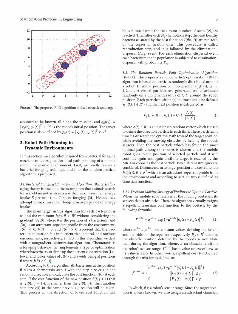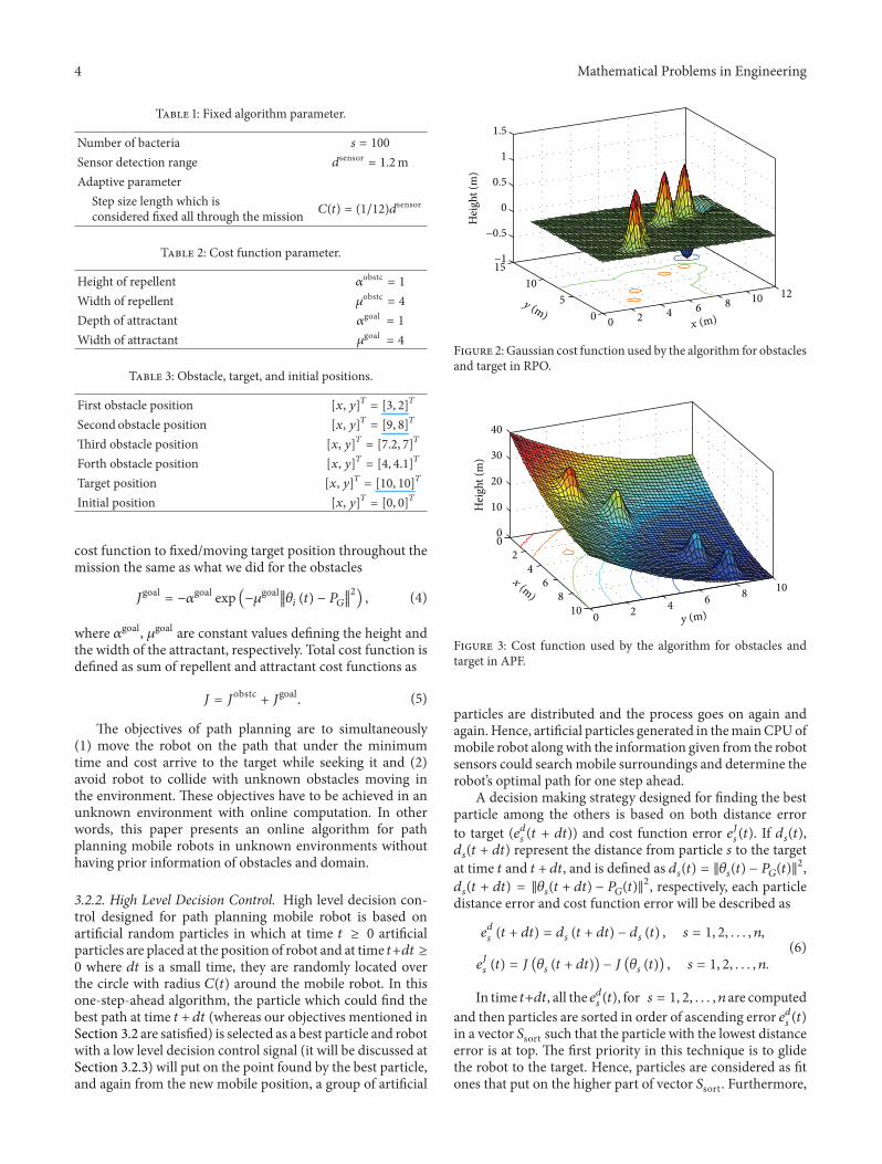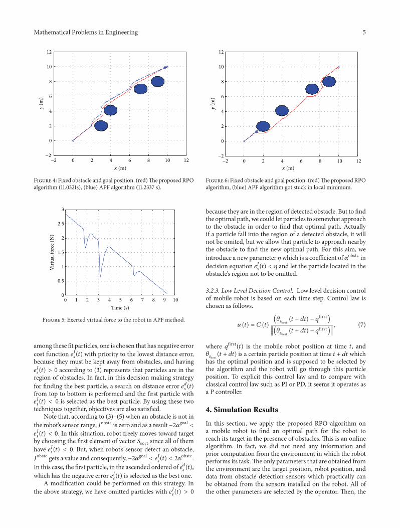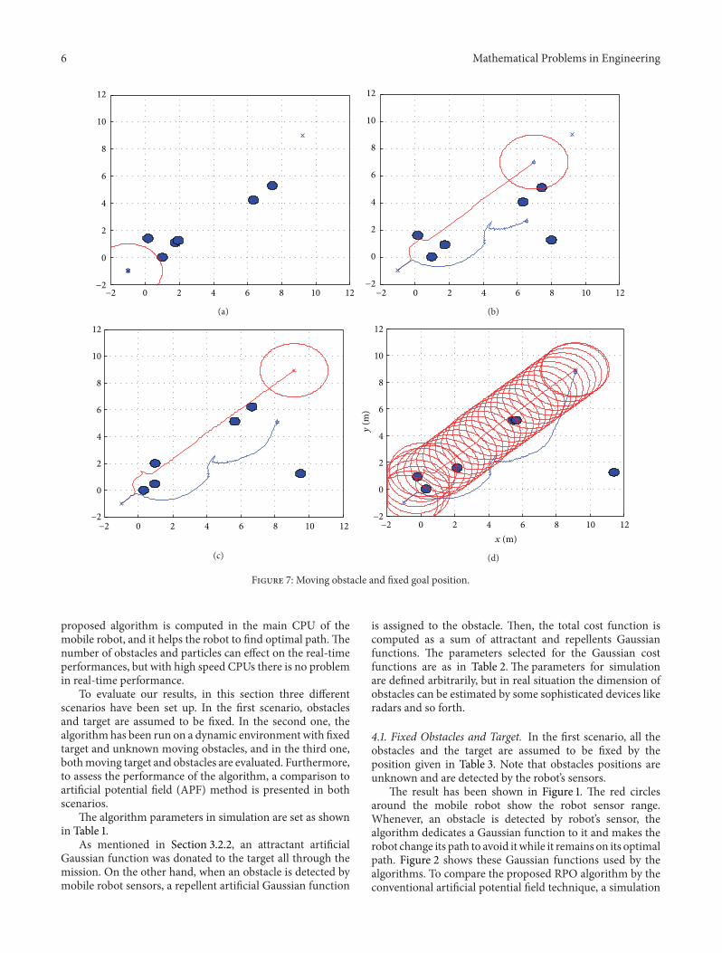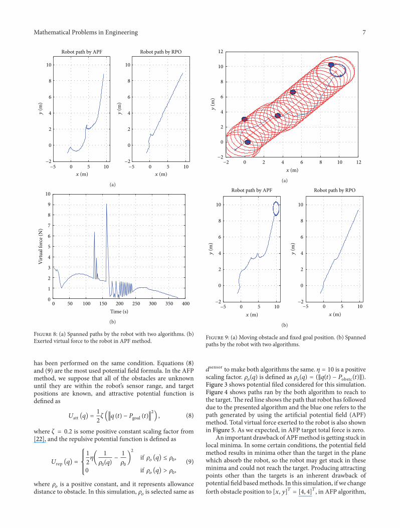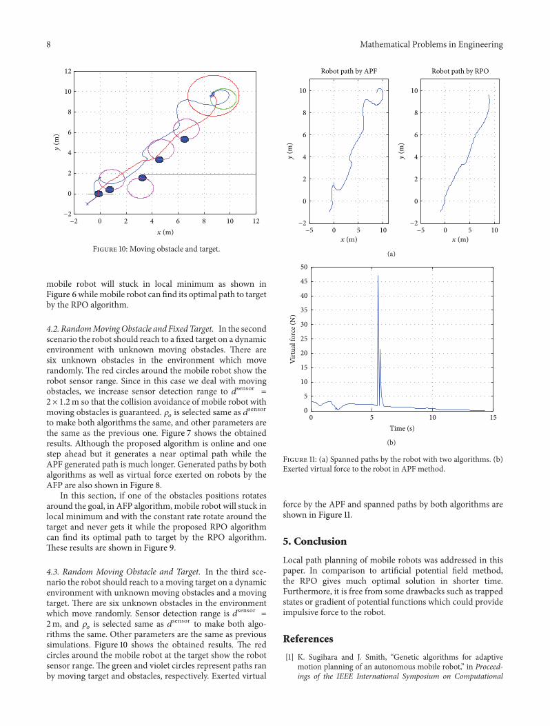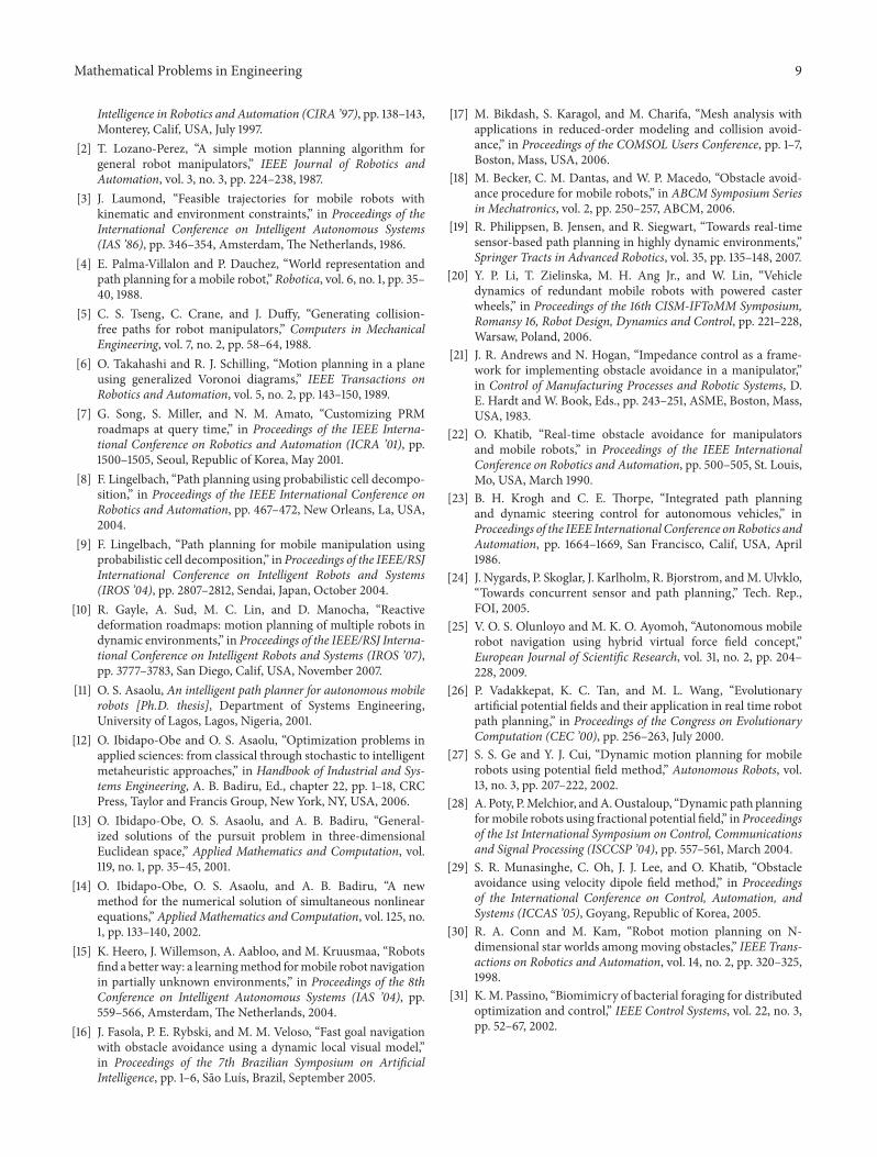
Copyright © 2022 FDOKUMEN