Quantile Regression Under Random CensoringBo Honor�ePrinceton UniversityShakeeb Khan�University of RochesterJames L. PowellUniversity of California at BerkeleyFirst Version: October 1993This Version: August 1999AbstractCensored regression models have received a great deal of attention in both the theoretical andapplied econometric literature. Most of the existing estimation procedures for either cross sec-tional or panel data models are designed only for models with �xed censoring. In this paper, anew procedure for adapting these estimators designed for �xed censoring to models with randomcensorship is proposed. This procedure is then applied to the CLAD and quantile estimators ofPowell(1984,1986a) to obtain an estimator of the regression coe�cients under a mild conditionalquantile restriction on the error term that is applicable to samples exhibiting �xed or randomcensoring. The resulting estimator is shown to have desirable asymptotic properties, and performswell in a small scale simulation study.

JEL Classi�cation: C24, C14, C13.Key Words: censored quantile regression, random censoring, Kaplan-Meier product limitestimator, accelerated failure time model.�Corresponding author. Dept. Economics, University of Rochester, Rochester, NY 14627; e-mail:skhan@troi.cc.rochester.edu. We are grateful to Jambe and Rodchenko for helpful comments on an ear-lier draft.

1 IntroductionOver the past decade, the censored regression model, known to economists as the Tobitmodel (after Tobin 1958), has been the object of much attention in the econometric lit-erature on semiparametric estimation. Relaxing the traditional parametric restrictions onthe form of the distribution of the underlying error terms, a number of consistent esti-mators have been proposed which require only weak conditions on these distributions, in-cluding: constant conditional quantiles (Powell(1984,1986a); Nawata (1990); Newey andPowell(1990), conditional symmetry (Powell(1986b), Lee(1993a,b), Newey(1991)), and inde-pendence of the errors and regressors (Duncan(1986); Fernandez(1986); Honor�e and Pow-ell(1993); Horowitz(1986, 1988); and Moon(1989)). These proposed estimators all exploitan assumption that the censoring values for the dependent variable are known for all obser-vations, even those that are not censored; while the typical estimator is constructed underthe presumption that the dependent variable is censored to the left at zero, it is generallystraightforward to modify it for either right or left censored data (or both) with variablecensoring values. Hereafter, in a loose analogy to panel data modelling, we refer to suchmodels as �xed censoring models, since the censoring values, though possibly variable, maynot be distributed independently from the regressors.A parallel literature in the statistics and biometrics literature has been concerned withestimation of the parameters of a related model, the regression model with random censoring.In this model the dependent variable typically represents the logarithm of a survival time(in which case the regression model corresponds to an accelerated failure time durationmodel), which is right-censored at varying censoring points which are observed only whenthe observation is censored. In addition, the censoring times are generally (but not always)assumed to be independently distributed of the regressors and error terms. Studies whichpropose semiparametric methods under random (right) censorship include Miller (1976),Prentice (1978), Buckley and James (1979), Koul, Suslara, and Van Ryzin (1981), Leurgans(1987), and Ritov (1990), among others. These estimation methods typically impose anassumption of independence of the error terms and covariates; those that do not imposeindependence instead require strong conditions on the censoring distribution which generallyrule out censoring at a constant value, as is typical in econometrics.In this paper we describe a method for adapting estimators proposed for �xed censoringto sampling with random right censorship. We apply this method to the censored least abso-lute deviations and quantile estimators of Powell (1984; 1986a) to obtain an estimator of the1

regression coe�cients which will be consistent under a relatively-weak quantile restrictionon the error terms, and which is equally applicable to samples with constant or randomcensoring. The following section describes this estimation approach, and compares the mod-i�ed form of the censored regression quantile estimator to other quantile-based estimatorsfor random censoring that have appeared in the statistics literature. Section 3 gives su�-cient conditions to ensure the root n-consistency and asymptotic normality of the proposedestimator, and section 4 analyzes its performance using a simulation study and an empiricalexample. The �nal section discusses application of the general estimation method to othercensored regression estimators in the econometric literature, and considers whether the as-sumption of independence of the censoring times and covariates could be relaxed. Proofs ofthe large-sample results of section 3 are available in a mathematical appendix.2 The Model and Estimation MethodThe object of estimation is the p-dimensional vector of regression coe�cients �0 in a linearlatent variable modely�i = x0i�0 + "i; i = 1; : : : ; n; (2.1)where y�i is the (uncensored and scalar) dependent variable of interest, xi is an observablep-vector of covariates, and "i is an unobserved error term. With right censorship, the latentvariable y�i is observed only when it is less than some scalar censoring variable ci; that is,the observed dependent variable yi isyi = minfy�i ; cig = minfx0i�0 + "i; cig: (2.2)In a random sample with �xed censoring, n independently-distributed observations on thetriple (yi; ci; xi) are assumed to be available; with random censoring, the observations are ofthe form (yi; di; xi), where di is a binary variable indicating whether the dependent variableis uncensored:di = 1fy�i < cig = 1fx0i�0 + "i < cig; (2.3)for \1fAg" the indicator function for the set A.2

For samples with �xed censoring, the estimators of �0 cited in the preceding section oftenare de�ned as solutions to minimization problems and/or estimating equations constructedusing sample averages of functions of the observable data and unknown parameters, i.e.,� = argmin� 1n nXi=1 �(yi; ci; xi; �) (2.4)or 0 �= 1n nXi=1 (yi; ci; xi; �) (2.5)for certain functions �(�) or (�). Of course, some estimators involve more complicated min-imands / estimating equations, de�ned using higher-order U -statistics or involving prelimi-nary (nonparametric) estimators of unknown functions, but the analysis of their large samplebehavior, though more di�cult, follows the same lines as in this simple case. Consistency of� is demonstrated after imposing appropriate conditions on the error terms, covariates, andcensoring values; one important step in the proof is to show that the true parameter value�0 is a unique solution to the population versions of the minimization problem or estimatingequations,�0 = argmin�E[�(yi; ci; xi; �)] (2.6)or 0 = E[ (yi; ci; xi; �)] i� � = �0: (2.7)Given such an identi�cation condition, application of a uniform law of large numbers to thesample average de�ning � ensures its consistency.Under random censorship, it is no longer possible to de�ne an estimator of �0 in thesame fashion as above, since the censoring variables fcig are not known for all i. However, ifthe censoring variables fcig are assumed to be independent of f(yi; xi)g, and if the marginalc.d.f. G(t) � Prfci � tg of the censoring values were known, a simple modi�cation of theestimation approach above would replace the functions �(yi; xi; ci; �) or (yi; xi; ci; �) by theirconditional expectations given the observable variables (yi; di; xi). That is, an M -estimatorof �0 corresponding to the foregoing minimization problem would be3

� = argmin� 1n nXi=1 E[�(yi; ci; xi; �) j (yi; di; xi)] (2.8)= argmin� 1n nXi=1 �(1� di) � �(yi; yi; xi; �) + di � [S(yi)]�1 � Z 1(yi < c)�(yi; c; xi; �)dG(c)� ;where S(t) � 1�G(c) is the survivor function for the censoring value ci. Similarly, � mightbe de�ned as solutions to estimating equations of the form0 �= 1n nXi=1 �(1� di) � (yi; yi; xi; �) + di � [S(yi)]�1 � Z 1(yi < c) (yi; c; xi; �)dG(c)� :(2.9)By iterated expectations, the population analogues to the sample averages de�ning � willbe the same moment functions, E[�(yi; ci; xi; �)] or E[ (yi; ci; xi; �)], as appear in the �xedcensorship case, so the same identi�cation conditions imposed for �xed censoring will applyunder random censoring.Unfortunately, when the censoring values fcig have a non-degenerate distribution it isunlikely that the censoring distribution function G(t) will be known a priori. Nevertheless,because of the assumed independence of the censoring value ci and the latent variable y�i ,this distribution function G(t) can be consistently estimated using the Kaplan-Meier productlimit estimator (Kaplan and Meier, 1958); this estimator G(t) uses only the pairs f(yi; di)gof dependent and indicator variables, and does not involve the covariates fxig or param-eter vector �. By substitution of the Kaplan-Meier estimator G(t) and survivor functionS(t) = 1 � G(t) into the previous minimization problem or estimating equations, feasibleestimators of �0 can be constructed, and consistency will follow from a demonstration ofuniform convergence of these sample moment functions to their limiting values.The estimation approach here is similar in spirit to that adopted by Buckley and James(1979), which adapted the \EM algorithm" (Dempster, Laird, and Rubin 1977) for max-imization of a parametric censored-data likelihood to the semiparametric setting with un-known error distribution. However, the Buckley-James estimator treats the latent dependentvariable y�i as \missing data" when the observed dependent variable is uncensored (using theKaplan-Meier estimator for the error distribution, applied to residuals b" � y� x0� and theircensoring points u � x0�, to estimate the conditional distribution of y�i given di = 0); incontrast, the present approach views the censoring value ci as \missing" when the latentdependent variable is uncensored. While the Buckley-James estimator does not require that4

the censoring values be independent of the regressors, it does impose that requirement forthe error distribution; in contrast, the present approach assumes independence of the cen-soring points and regressors, but may permit dependence of, say, the scale of the errors onthe covariates.To apply this general approach to a speci�c estimation problem, we consider the re-striction of a constant conditional �'th quantile on the distribution of the errors. That is,maintaining the assumption of independence of fcig and f("i; xi)g, we impose the additionalrestriction that the conditional distribution of the error terms "i given the covariates xisatis�esPrf"i � 0 j xig = � (2.10)for some known value of � in the interior of the unit interval. Under this condition, theconditional �'th quantile of the dependent variable yi given xi and ci is equal to minfx0�0; cig,as noted by Powell (1984, 1986a) and Newey and Powell (1990); that is,Prfyi � minfx0i�0; cig j xig � � and Prfyi � minfx0i�0; cig j xig � 1� �:(2.11)Under �xed censorship, a quantile estimator of �0 under this restriction was de�ned byNewey and Powell (1990) as� = argmin� 1n nXi=1 ��(yi �minfx0i�; cig); (2.12)where��(u) � [� � 1fu < 0g] � u; (2.13)this estimator is the censored-data analogue to the regression quantile estimator proposedby Koenker and Bassett (1978) for the linear model. Under regularity conditions, it wasshown that the estimator � solves a set of estimating equations obtained as approximate�rst-order conditions from this minimization problem:op(n�1=2) = 1n nXi=1 [� � 1fyi � x0i�g] � 1fx0i� < cig � xi: (2.14)5

For the special case � = 1=2; corresponding to a linear model for the conditional median ofy�i given xi, an equivalent representation would replace \��" with an absolute value functionin the minimization problem, and \[��1fyi � x0i�g]" with \signfyi�x0i�g" in the estimatingequations.To adapt the quantile estimator for �xed censoring to a sample subject to random cen-sorship, then, we de�ne the estimator as� = argmin� 1n nXi=1 E[��(yi �minfx0i�; cig) j (yi; di; xi)] (2.15)= argmin� 1n nXi=1 f(1� di) � ��(yi �minfx0i�; yig)+di � [S(yi)]�1 � Z 1(yi < c)��(yi �minfx0i�; cg)dG(c)� ;where \E[�]" denotes an expectation calculated using the product-limit estimator of G(t).For this minimization problem, the estimating equations obtained from the approximate�rst-order condition take a particularly simple form:op(n�1=2) = 1n nXi=1 �� � 1fyi > x0i�g � (1� �) � 1fyi � x0i�g � di � S(x0i�)=S(yi)��xi:(2.16)To verify that the limiting form of these estimating equations (replacing the sample averageand estimated survivor functions with their population analogues) has a solution at the truevalue �0, note that1fyi > x0i�0g � 1f"i > 0g � 1fci > x0i�0gso thatE[1fyi > x0i�0g j xi] = Prf"i > 0 j xig � S(x0i�0) = (1� �) � S(x0i�0);also, 1fyi � x0i�0g � di � S(x0i�0)=S(yi) � 1f"i � 0g � 1fy�i < cig � S(x0i�0)=S(y�i );implyingE [1fyi � x0i�0g � di � S(x0i�0)=S(yi) j xi; "i] = 1f"i � 0g � S(y�i ) � S(x0i�0)=S(y�i )6

and thusE [1fyi � x0i�0g � di � S(x0i�0)=S(yi) j xi] = Prf"i � 0 j xig � S(x0i�0) = � � S(x0i�0):Therefore, the limiting estimating equations hold when evaluated at the true value �0 :E h�� � 1fyi > x0i�g � (1� �) � 1fyi � x0i�g � di � S(x0i�)=S(yi)� � xii (2.17)= E[(� � (1� �) � S(x0i�0)� (1� �) � � � S(x0i�0)) � xi] = 0:Nevertheless, as noted by Powell (1984, 1986a), it is important that the estimator bede�ned as the minimizer of the quantile objective function rather than the solution to theseestimating equations, since multiple inconsistent roots to these equations may exist.Two other estimators under random censorship which exploit only a quantile restrictionhave previously been proposed; these approaches require stronger restrictions on the supportof the censoring distribution G(t) than are needed for the present estimator. For example,an extension of the approach of Koul, Suslara, and Van Ryzin (1981) to quantile regressionwas proposed by ????, which de�ned the estimator of the regression coe�cients as� = argmin� 1n nXi=1 di � [S(yi)]�1 � ��(yi � x0i�); (2.18)which can equivalently be written as the solution to the estimating equationsop(n�1=2) = 1n nXi=1 di � [S(yi)]�1 � [� � 1fyi � x0i�g] � xi; (2.19)this estimator exploits the fact thatE �di � [S(yi)]�1�[� � 1fyi � x0i�0g] � xi� (2.20)= E �1fy�i < ci) � [S(y�i )]�1 � [� � 1f"i � 0g] � xi�= E [[� � 1f"i � 0g] � xi]= 0provided S(y�i ) > 0 with probability one. Since S(t) = S(t) = 1ft < c0g when the censoringpoints ci = c0 with probability one, this estimation approach is not applicable for �xed7

(and constant) censoring except in the special cases Prfyi � c�g � 1 (i.e., no censoredobservations). Also, as noted by Halpern and Miller (1982), this estimator may be sensitiveto the particular realizations of the dependent variable yi(and corresponding regressors xi)which are large and uncensored, since the estimated survivor function for such observationswill be close to zero and imprecisely measured; however, this robustness problem may bemore pronounced for the original estimator proposed by Koul, et al., which is based uponsquared error loss, than for its quantile variant.More recently, Ying, Jung, and Wei (1991) proposed a quantile estimator for �0 underthe restriction Prf� � 0 j xg � � 2 (0; 1) using the implied relationPr fyi > x0i�0 j xig = Pr fx0i�0 < ci and "i > 0jxig (2.21)= Pr fx0i�0 < cij xig � Pr f"i > 0jxig= S (x0�0) � (1� �); (2.22)which yields an estimator � as a solution to estimating equations of the form0 �= 1N NXi=1 h[S(x0i�)]�1 � 1fyi > x0i�g � (1� �)i � xi: (2.23)Like the ????? estimator, this estimator will be well-de�ned and consistent only when S(x0i�)and S(x0i�0) are strictly positive with probability one, which would require Prfx0�0 � c0g � 1when the censoring values have a degenerate distribution. In contrast, the present approachis equally amenable to constant or random censoring; indeed, if the censoring points aredegenerate, so that S(t) = 1ft < c0g, then this estimator will be identical to the censoredquantile estimator proposed by Powell (1986a) for samples consisting of at least one censoredobservation, since S(t) = S(t) in this case.3 Large Sample Behavior of the Quantile EstimatorIn order to demonstrate the (root�n) consistency and asymptotic normality of the randomly-censored quantile regression estimator proposed above, it will be necessary to augment theregularity conditions imposed for its �xed-censoring counterpart to ensure, for example,that the Kaplan-Meier estimator of the censoring survivor function is su�ciently precise.Rather than searching for the most general conditions on the errors, covariates, and censoringtimes, we will impose stronger conditions (like compact support of the regressors) which will8

be straightforward to verify and simplify the derivations of the asymptotic theory for theestimator.We rewrite the estimator de�ned in (2.15) here as� � argmin�2BRn(�; S); (3.1)whereRn(�; S) � 1n nXi=1 f(1� di) � ��(yi �minfx0i�; yig) (3.2)+di � [S(yi)]�1 � Z 1(yi < c)��(yi �minfx0i�; cg)dG(c)�and B is the space of possible values of the parameter vector �0. In Newey and Powell(1990), a number of regularity conditions were imposed for the analysis of the estimatorwith �xed censoring, de�ned in (2.12) above. The following assumptions are a superset ofthe conditions imposed in that paper to ensure root�n consistency and asymptotic normalityin that case.Assumption P: The true parameter vector �0 is an interior point of the parameter spaceB, which is compact.Assumption M: The observations f(yi; di; xi); i = 1; : : : ; ng are a random sample forwhich yi and di are generated according to (2.2) and (2.3), for some random variables "i; xi,and ci satisfying the remaining conditions below.Assumption E: The error terms f"ig are absolutely continuously distributed with con-ditional density function f(� j x) given the regressors xi = x which has �'th quantile equalto zero, is bounded above, Lipschitz continuous in �, and is bounded away from zero in aneighborhood of zero, uniformly in xi. That is,Z 1f� � 0g � f(� j x)d� = �;and for some positive constants �0;�0, and �0,f(� j x) � �0; jf(�1 j x)� f(�2 j x)j � �0� j �1 � �2 j; andf(� j x) � �0 if j � j� �0: 9

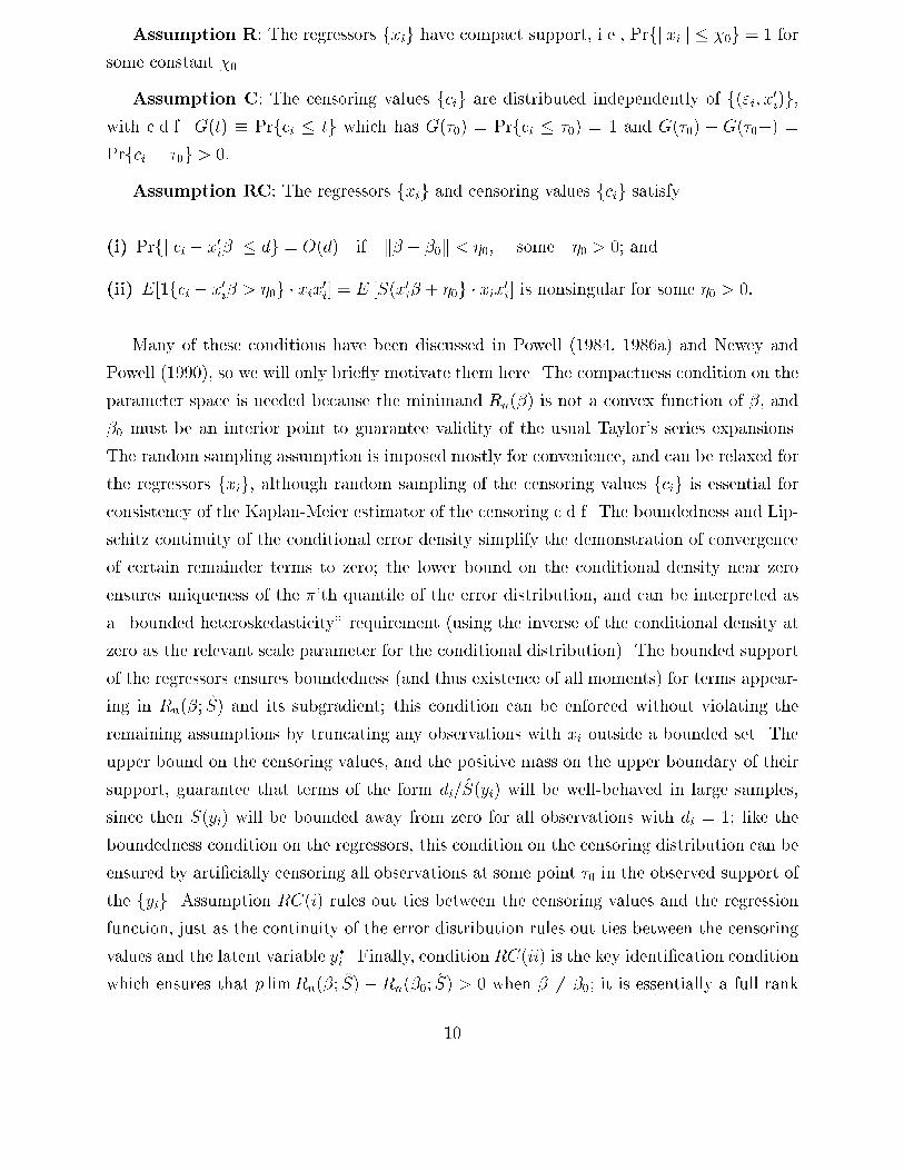
Assumption R: The regressors fxig have compact support, i.e., Prfkxik � �0g = 1 forsome constant �0.Assumption C: The censoring values fcig are distributed independently of f("i; x0i)g,with c.d.f. G(t) � Prfci � tg which has G(�0) = Prfci � �0) = 1 and G(�0) � G(�0�) =Prfci = �0g > 0:Assumption RC: The regressors fxig and censoring values fcig satisfy(i) Prfj ci � x0i� j� dg = O(d) if k� � �0k < �0; some �0 > 0; and(ii) E[1fci � x0i� > �0g � xix0i] = E [S(x0i� + �0g � xix0i] is nonsingular for some �0 > 0:Many of these conditions have been discussed in Powell (1984, 1986a) and Newey andPowell (1990), so we will only brie y motivate them here. The compactness condition on theparameter space is needed because the minimand Rn(�) is not a convex function of �, and�0 must be an interior point to guarantee validity of the usual Taylor's series expansions.The random sampling assumption is imposed mostly for convenience, and can be relaxed forthe regressors fxig, although random sampling of the censoring values fcig is essential forconsistency of the Kaplan-Meier estimator of the censoring c.d.f. The boundedness and Lip-schitz continuity of the conditional error density simplify the demonstration of convergenceof certain remainder terms to zero; the lower bound on the conditional density near zeroensures uniqueness of the �'th quantile of the error distribution, and can be interpreted asa \bounded heteroskedasticity" requirement (using the inverse of the conditional density atzero as the relevant scale parameter for the conditional distribution). The bounded supportof the regressors ensures boundedness (and thus existence of all moments) for terms appear-ing in Rn(�; S) and its subgradient; this condition can be enforced without violating theremaining assumptions by truncating any observations with xi outside a bounded set. Theupper bound on the censoring values, and the positive mass on the upper boundary of theirsupport, guarantee that terms of the form di=S(yi) will be well-behaved in large samples,since then S(yi) will be bounded away from zero for all observations with di = 1; like theboundedness condition on the regressors, this condition on the censoring distribution can beensured by arti�cially censoring all observations at some point �0 in the observed support ofthe fyig. Assumption RC(i) rules out ties between the censoring values and the regressionfunction, just as the continuity of the error distribution rules out ties between the censoringvalues and the latent variable y�i . Finally, condition RC(ii) is the key identi�cation conditionwhich ensures that p limRn(�; S) � Rn(�0; S) > 0 when � 6= �0; it is essentially a full rank10

condition for the cross product of the regressors corresponding to observations in which theconditional median of the latent variable y�i is uncensored, i.e., x0i�0 < ci.Under these conditions, it is straightforward to establish the strong consistency of theestimator � for ��, using a direct modi�cation of the arguments in Powell (1984; 1986a):Theorem 3.1 Under conditions P;M;E;R; C, and RC, the estimator � de�ned in (3.1) isstrongly consistent, i.e., � ! �0 with probability one.Demonstration of the root�n consistency and asymptotic normality of � is more delicate,since it involves the asymptotic distribution associated with the empirical process S(t), theKaplan-Meier estimator of the censoring survivor function. If S(t) were known, so that anestimator of �0 could be de�ned as~� � argmin�2B Rn(�;S); (3.3)it would be relatively simple to derive the asymptotically-normal distribution of ~�. Let i(�; S) � �� � 1fyi > x0i�g � (1� �) � 1fyi � x0i�g � di � S(x0i�)=S(yi)� � xi (3.4)and M0 � M(�0; S) � E[f(0 j xi) � S(x0i�0) � xix0i] = E[f(0 j x0i) � 1fx0i�0 < cig � xix0i]; (3.5)then the same arguments used in Powell (1984) could be used to show that, under theconditions imposed above, the estimator ~� would solve the estimating equationsop(n�1=2) = 1n nXi=1 i( ~�; S); (3.6)and would have asymptotic distribution given bypn(� � �0) d�! N (0;M�10 V0M�10 ); (3.7)whereV0 � E[ i(�0; S) � i(�0�; S)0]: (3.8)11

However, the feasible estimator � solves the estimating equationsop(n�1=2) = 1n nXi=1 i(�; S); (3.9)and since pn(S(t)�S(t)) = Op(1), a \correction term" for the preliminary estimation of thecensoring survivor function S(t) is needed for the asymptotic distribution of �. To obtainthe form of this correction term, we �rst de�ne the following term:Xn(t) � 1pn nXi=1[H (yi)]�1 �1fyi < tg � (1� i)� Z t�1[H (s)]�1 � 1fyi � sg ��(s);for H(t) � Prfyi > tg, the survivor function for yi, and�(t) � Z t�1[S(s)]�1dG(s);the cumulative hazard function for ci. The correction term for the estimation of the survivorfunction S(t) in the construction of � involves the integral of X(t), with respect to themeasureq(s) � limQn(s) a.s.; (3.10)whereQn(t) � 1n nXi=1 (1fyi � minft; x0i�0gg+ 1fmaxfyi; tg < x0i�g � S(x0i�)=S(yi))�di�xi:(3.11)De�ning�i � �i(�0; S;H;�; �) (3.12)� (1� �) � Z 1�1�[H(yi)]�1 � 1fyi < tg � (1� di)� Z t�1[H(s)]�1 � 1fyi � sg � d�(s)� dq(s)the asymptotic distribution of � depends on �i, as follows:Theorem 3.2 Under Assumptions P;M;E;R; C;RC, the estimator � satis�es the asymp-totic linearity conditionpn(� � �0) =M�10 1pn nXi=1 [ i(�0; S) + �i(�0; S;H;�; �)] + op(1)12

and is asymptotically normal,pn(� � �0) d�! N (0;M�10 V1M�10 );for V1 � E[( i + �i) � ( i + �i)0]:In order to use the asymptotic normality result of Theorem 4.2 to form asymptotic con�denceregions and hypothesis tests, a consistent estimator of the asymptotic covariance matrix of� is needed. Estimation of each of the matrices M0 and V1 poses technical problems, theformer because of its dependence on the error density (and thus requiring nonparametricestimation techniques), and the latter due to the complicated form of the correction term forpreliminary estimation of the survivor function S(t). For estimation of the Hessian matrixM0, the method proposed by Powell (1984), which replaces the unknown density with a(uniform) kernel term in a sample analogue to the de�nition of M0 in (3.5), can be easilyadapted to the present case. Another means to consistently estimate M0 was proposed byPakes and Pollard (1989), who suggested that the Hessian be estimated from a numericalderivative of the function appearing in the estimating equations,n(�) � 1n nXi=1 i(�; S); (3.13)about the point � = �; they note that this estimator will be consistent if the perturbationsused to construct the numerical derivative are of larger order thanpn, the rate of convergenceof �. Consistent estimation of an asymptotic covariance matrix analoguous to V1(but witha di�erent de�nition of (�) and Qn(�)) was considered by Ying, Jung, and Wei (1991), whoproposed an estimator of the formV � 1n nXi=1 ( i + �i) � ( i + �i)0; (3.14)where, in this setting, i and �i would be sample analogues of i and �i. That is, i � �� � 1fyi > x0i�g � (1� �) � 1fyi � x0i�g � di � S(x0i�)=S(yi)� � xi (3.15)13

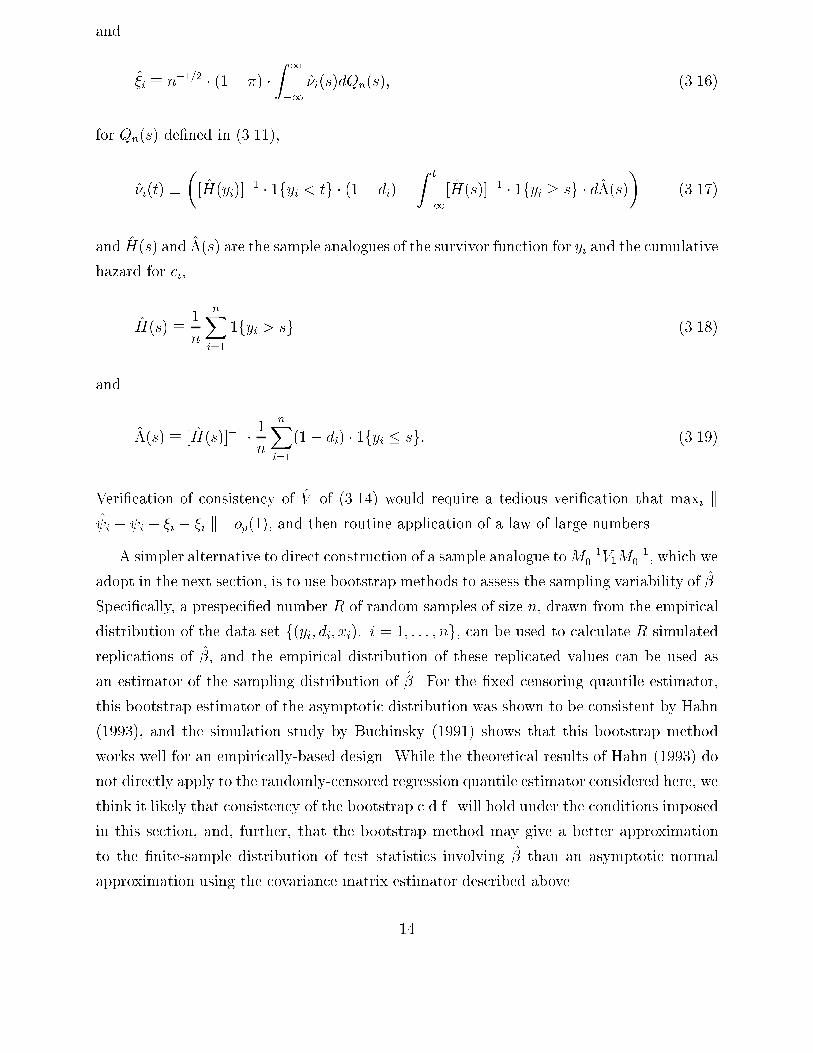
and �i � n�1=2 � (1� �) � Z 1�1 �i(s)dQn(s); (3.16)for Qn(s) de�ned in (3.11),�i(t) � �[H(yi)]�1 � 1fyi < tg � (1� di)� Z t�1[H(s)]�1 � 1fyi � sg � d�(s)� (3.17)and H(s) and �(s) are the sample analogues of the survivor function for yi and the cumulativehazard for ci,H(s) � 1n nXi=1 1fyi > sg (3.18)and �(s) � [H(s)]�1 � 1n nXi=1 (1� di) � 1fyi � sg: (3.19)Veri�cation of consistency of V of (3.14) would require a tedious veri�cation that maxi k i � i + �i � �i k= op(1), and then routine application of a law of large numbers.A simpler alternative to direct construction of a sample analogue toM�10 V1M�10 , which weadopt in the next section, is to use bootstrap methods to assess the sampling variability of �.Speci�cally, a prespeci�ed number R of random samples of size n, drawn from the empiricaldistribution of the data set f(yi; di; xi): i = 1; : : : ; ng, can be used to calculate R simulatedreplications of �, and the empirical distribution of these replicated values can be used asan estimator of the sampling distribution of �. For the �xed censoring quantile estimator,this bootstrap estimator of the asymptotic distribution was shown to be consistent by Hahn(1993), and the simulation study by Buchinsky (1991) shows that this bootstrap methodworks well for an empirically-based design. While the theoretical results of Hahn (1993) donot directly apply to the randomly-censored regression quantile estimator considered here, wethink it likely that consistency of the bootstrap c.d.f. will hold under the conditions imposedin this section, and, further, that the bootstrap method may give a better approximationto the �nite-sample distribution of test statistics involving � than an asymptotic normalapproximation using the covariance matrix estimator described above.14

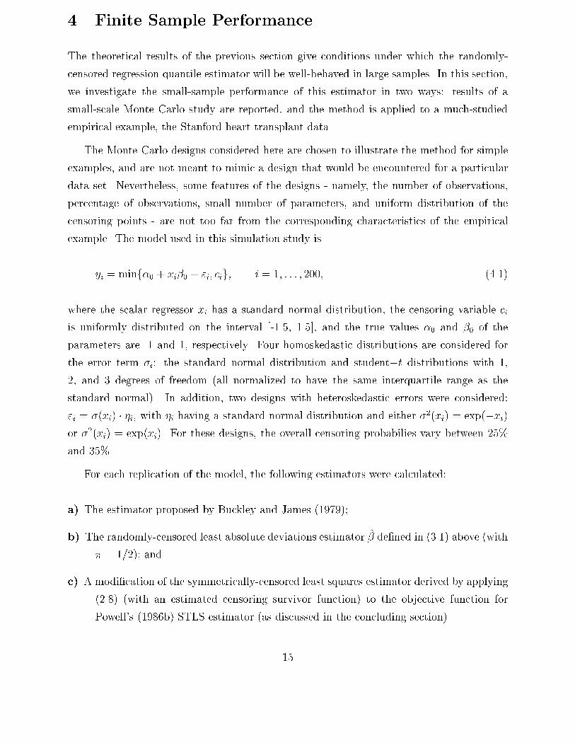
4 Finite Sample PerformanceThe theoretical results of the previous section give conditions under which the randomly-censored regression quantile estimator will be well-behaved in large samples. In this section,we investigate the small-sample performance of this estimator in two ways: results of asmall-scale Monte Carlo study are reported, and the method is applied to a much-studiedempirical example, the Stanford heart transplant data.The Monte Carlo designs considered here are chosen to illustrate the method for simpleexamples, and are not meant to mimic a design that would be encountered for a particulardata set. Nevertheless, some features of the designs - namely, the number of observations,percentage of observations, small number of parameters, and uniform distribution of thecensoring points - are not too far from the corresponding characteristics of the empiricalexample. The model used in this simulation study isyi = minf�0 + xi�0 + "i; cig; i = 1; : : : ; 200; (4.1)where the scalar regressor xi has a standard normal distribution, the censoring variable ciis uniformly distributed on the interval [-1.5, 1.5], and the true values �0 and �0 of theparameters are -1 and 1, respectively. Four homoskedastic distributions are considered forthe error term �i: the standard normal distribution and student�t distributions with 1,2, and 3 degrees of freedom (all normalized to have the same interquartile range as thestandard normal). In addition, two designs with heteroskedastic errors were considered:"i = �(xi) � �i, with �i having a standard normal distribution and either �2(xi) = exp(�xi)or �2(xi) = exp(xi). For these designs, the overall censoring probabilies vary between 25%and 35%.For each replication of the model, the following estimators were calculated:a) The estimator proposed by Buckley and James (1979);b) The randomly-censored least absolute deviations estimator � de�ned in (3.1) above (with� = 1=2); andc) A modi�cation of the symmetrically-censored least squares estimator derived by applying(2.8) (with an estimated censoring survivor function) to the objective function forPowell's (1986b) STLS estimator (as discussed in the concluding section).15

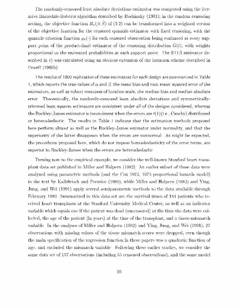
The randomly-censored least absolute deviations estimator was computed using the iter-ative Barrodale-Roberts algorithm described by Buchinsky (1991); in the random censoringsetting, the objective function Rn(�; S) of (3.2) can be transformed into a weighted versionof the objective function for the censored quantile estimator with �xed censoring, with thequantile criterion function ��(�) for each censored observation being evaluated at every sup-port point of the product-limit estimator of the censoring distribution G(t), with weightsproportional to the estimated probabilities at each support point. The STLS estimator de-scribed in c) was calculated using an obvious extension of the iteration scheme described inPowell (1986b).The results of 1000 replication of these estimators for each design are summarized in Table1, which reports the true values of � and �, the mean bias and root-mean-squared error of theestimators, as well as robust measures of location scale, the median bias and median absoluteerror. Theoretically, the randomly-censored least absolute deviations and symmetrically-trimmed least squares estimators are consistent under all of the designs considered, whereasthe Buckley-James estimator is inconsistent when the errors are t(1)(i.e., Cauchy) distributedor heteroskedastic. The results in Table 1 indicate that the estimation methods proposedhere perform almost as well as the Buckley-James estimator under normality, and that thesuperiority of the latter disappears when the errors are nonnormal. As might be expected,the procedures proposed here, which do not impose homoskedasticity of the error terms, aresuperior to Buckley-James when the errors are heteroskedastic.Turning now to the empirical example, we consider the well-known Stanford heart trans-plant data set published in Miller and Halpern (1982). An earlier subset of these data wereanalyzed using parametric methods (and the Cox 1972, 1975 proportional hazards model)in the text by Kalb eisch and Prentice (1980), while Miller and Halpern (1982) and Ying,Jung, and Wei (1991) apply several semiparametric methods to the data available throughFebruary 1980. Summarized in this data set are the survival times of 184 patients who re-ceived heart transplants at the Stanford University Medical Center, as well as an indicatorvariable which equals one if the patient was dead (uncensored) at the time the data were col-lected, the age of the patient (in years) at the time of the transplant, and a tissue-mismatchvariable. In the analyses of Miller and Halpern (1982) and Ying, Jung, and Wei (1991), 27observations with missing values of the tissue mismatch scores were dropped, even thoughthe main speci�cation of the regression function in these papers was a quadratic function ofage, and excluded the mismatch variable. Following these earlier studies, we consider thesame data set of 157 observations (including 55 censored observations), and the same model16

of the survival times,yi = minf�0 + �0xi + 0(xi)2 + "i; cig; (4.2)where the dependent variable yi is the logarithm (base 10) of the observed survival time (indays), and xi is the age of patient i. (For one observation, the survival time was listed aszero days; this was recoded to one for the statistical analysis here.)Table 2 reports the randomly-censored regression quantile coe�cient estimates at thethree quartiles | � = 0:25; 0:50; and 0.75 | along with the Buckley-James estimator andthe Ying-Jung-Wei coe�cient estimator given in the aforementioned study. The standarderrors for Buckley-James and the three quartile estimators were calculated as the medianabsolute deviation of the bootstrap c.d.f. (based upon R = 250 replications) divided by 0.67,which would (approximately) equal one for a standard normal distribution. Our results forBuckley-James di�er from those reported by Miller and Halpern (1982), which deleted 5observations from the sample with survival times less than 10 days.Looking across the various coe�cient estimates, the results appear fairly similar for allmethods, except that the slope coe�cients for the Ying, Jung, and Wei (1991) estimator areof smaller magnitude than those for the other procedures. Also, for the quartile estimatorsthere appears to be a \ attening" of the inverted-U shape of the regression function estimatesas � moves from 0.25 to 0.75. This attening, if statistically signi�cant, would indicateheteroskedasticity of the error distribution (or, admittedly, some other misspeci�cation ofthe model), with the conditional distributions for younger and older patients being moredispersed and skewed downward. To test for signi�cance of the di�erence between theestimated upper and lower quartile regression lines, a chi-squared statistic was constructedusing a quadratic form in these di�erences about the inverse of a bootstrap estimator of thecovariance matrix of the estimator, but the resulting test statistic was insigni�cant at allconventional levels of signi�cance, so the hypothesis of independence of the error terms andregressors would not be rejected using this test.5 Concluding RemarksAlthough the analysis of the preceding sections has concentrated on the properties of quantileestimators of the slope coe�cients, other estimation methods developed for �xed censoringare easily adapted to the present setting. For example, under the assumption of conditional17

symmetry of the error terms "i around zero given xi, Powell (1986b) proposed an estimatorwhich can be written as a minimizer of the form (2.4) above, with �rst-order condition ofthe form (2.5) having (yi; ci; xi; �) � [maxfyi; 2x0i� � cig � x0i�] � xi; (5.1)which has expectation zero when evaluated at the true value �0 under conditional symmetry.Modi�cation of this estimator, developed for �xed censoring, to random right censorship isimmediate using (2.8) and the Kaplan-Meier estimator, as described in section 2. The MonteCarlo results of section 4 suggests this estimator may have similar behavior to the randomly-censored quantile estimator with � = 1=2; at least for symmetric error distributions like theones considered there. While conditional symmetry may not be an attractive assumption foran accelerated failure time model (ruling out, for example, a Weibull model for durations),it may be more reasonable for other randomly-censored regression models.Another �xed-censoring estimation method which is easily adapted to random censoringis the method proposed by Honor�e (1992) for estimation of panel data models with censoring.For the special case of T = 2 time periods, the model Honor�e (1992) considers isyit = minfx0it�0 + �i + "it; citg; i = 1; : : : ; n; t = 1; 2; (5.2)where the term �i is an unobservable \�xed e�ect" which need not be independent of thecovariate vector xit. Under the assumption that "i2� "i1 is symmetrically distributed aboutzero given the regressors, Honor�e proposed an estimator which solves a �rst-order conditionof the form,op(n�1=2) = 1n nXi=1 �(ei;12(�)� ei;21(�)) � (xi2 � xi1); (5.3)where �(�) is a nondecreasing and odd function of its argument andei;12(�) � minfyi1 � x0i1�; ci1 � x0i2�g; (5.4)with an analogous de�nition of ei;21(�). With an appropriate rede�nition of the variables,these estimating equations are obviously of the form (2.5), so the transformation (2.9) yieldsestimating equations for random censoring when the censoring distribution G(t) is replacedby its Kaplan-Meier estimator. When �(�) = sign(�), this estimator is similar in structure to18

the randomly-censored regression quantile estimator studied above, and a simple extensionof the assumptions imposed in section 3 will su�ce to demonstrate the root�n consistencyand asymptotic normality of this estimator and others based upon di�erent choices of �(�).Under the assumption of independence of the error terms and regressors, Honor�e andPowell (1993) propose an estimator of �0 for model (2.3) which uses the same strategyas Honor�e's censored panel data estimator, but is based upon pairwise di�erences acrossindividuals rather than across time periods for each individual. That is, the estimator �solves estimating equations de�ned in terms of a second-order U-statistic,op(n�1=2) = n2 !�1Xi<j �(eij(�)� eji(�)) � (xi � xj); (5.5)with eij(�) � minfyi � x0i�; ci � x0j�g: (5.6)The approach described in section 2 will also work here, but may be computationally di�cult;since calculation of the empirical expectations over the unobserved values of ci using theKaplan-Meier c.d.f. estimator involves O(n) calculation, computing a random censoringversion of the estimating equations (5.5) will involve O(n4) summations, which may takesome time if n is large. It may be possible to reduce the number of calculations needed,at some cost of statistical precision, by replacing the calculation of an expectation overthe censoring value by a single draw from its estimated conditional distribution given theobserved data. Whether such an approach would yield a root�n consistent estimator is aninteresting question for additional research.Of the regularity conditions imposed in section 3 above, some may be relaxed without af-fecting the consistency or asymptotic normality of the estimator (for example, the assumptionof randomly-sampled regressors may be relaxed to permit deterministic regressors). How-ever, the assumption of independence of the censoring values fcig and the regressors fxigis crucial to the analysis above, and this assumption may be suspect in some settings. Forexample, in the Stanford heart transplant data set, larger censoring times correspond toearlier transplants; if transplants for younger or older patients were not typically performedin the earlier years, this would induce a dependence between censorship and the covariate,age. In general, if the regressors fxig have �nite support, then it should be possible to obtainconsistent estimators of the conditional censoring distribution G(t j x) � Prfci � t j xi = xg19

at each possible value of xi, which could then be substituted into the expectations in (2.8)and (2.9). If some components of the regressors are continuously distributed, it should bepossible to nonparametrically estimate the conditional censoring distribution by groupingobservations with adjacent values of xi; whether substitution of a conditional version of theproduct-limit estimator into (2.8) will yield a root�n consistent estimator is an interestingopen question for additional study.6 ReferencesAmemiya, T. (1985), Advanced Econometrics. Cambridge, Mass, Harvard University Press.Buchinsky, M. (1991), \A Monte Carlo Study of the Asymptotic Covariance Estimators forQuantile Regression Coe�cients," manuscript, Harvard University, January.Buckley, J. and I. James (1979), \Linear Regression with Censored Data," Biometrika, 66,429-436.Cox D.R. (1972), \Regression Models and Life Tables," Journal of the Royal StatisticalSociety Series B, 34,187-220.Cox D.R. (1975), \Partial Likelihood" Biometrika, 62, 269-276Cs�org�o, S. and L. Horvath (1983), \The Rate of Strong Uniform Consistency for the ProductLimit Estimator," Z. Wahrsch. verw. Gebiete, 62, 411-426.Duncan, G.M. (1986), \A Semiparametric Censored Regression Estimator," Journal ofEconometrics, 32, 5-34.Fernandez, L. (1986), \Nonparametric Maximum Likelihood Estimation of Censored Re-gression Models," Journal of Econometrics, 32, 35-57.Gill, R. D. (1980), \Censoring and Stochastic Integrals", Mathematical Centre Tracts, 124,Mathematisch Centrum, Amsterdam.Hahn, J. (1993), \Bootstrapping Quantile Regression Estimators," manuscript, Departmentof Economics, Harvard University.Honor�e, B.E. (1992), \Trimmed LAD and Least Squares Estimation of Truncated andCensored Regression Models with Fixed E�ects," Econometrica, 60, 533-565.20

Honor�e, B.E. and J.L. Powell (1993), \Pairwise Di�erence Estimators of Linear, Censored,and Truncated Regression Models," Journal of Econometrics, forthcoming.Horowitz, J.L. (1986), \A Distribution-Free Least Squares Estimator for Censored LinearRegression Models," Journal of Econometrics, 32, 59-84.Horowitz, J.L. (1988a), \Semiparametric M -Estimation of Censored Linear RegressionModels," Advances in Econometrics, 7, 45-83.Huber, P.J. (1967), \The Behavior of Maximum Likelihood Estimates Under NonstandardConditions," Proceedings of the Fifth Berkeley Symposium on Mathematical Statisticsand Probability, Berkeley, University of California Press, 4, 221-233.Huber, P.J. (1981), Robust Statistics. New York: Wiley.Kalb eisch, J.D. and R.L. Prentice (1980), The Statistical Analysis of Failure Time Data.New York: Wiley.Kaplan, E.L. and P. Meier (1958), \Nonparametric Estimation from Incomplete Data,"Journal of the American Statistical Association, 53, 457-481.Koenker, R. and G.S. Bassett (1978), \Regression Quantiles," Econometrica, 46, 33-50.Koul, H., V. Suslara, and J. Van Ryzin (1981), \Regression Analysis with Randomly RightCensored Data," Annals of Statistics, 9, 1276-1288.Lai, T.L. and Z. Ying (1991), \Rank Regression Methods for Left Truncated and RightCensored Data," Annals of Statistics, 19, 531-554.Lee, M.J. (1993a), \Windsorized Mean Estimator for Censored Regression Model," Econo-metric Theory, forthcoming.Lee, M.J. (1993b), \Quadratic Mode Regression," Journal of Econometrics, forthcoming.Leurgans, S. (1987), \Linear Models, Random Censoring, and Synthetic Data," Biometrika,74, 301-309.Lin, D.Y. and C.J. Geyer (1992), \Computational Methods for Semiparametric LinearRegression with Censored Data," Journal of Computational and Graphical Statistics,forthcoming. 21

Lin, J.S. and L.J. Wei (1992), \Linear Regression Analysis for Multivariate Failure TimeObservations," Journal of the American Statistical Association, forthcoming.Meier, P. (1975), \Estimation of Distribution Functions From Incomplete Data," in J. Gani,ed., Perspectives in Probability and Statistics. London: Academic Press.Miller, R. (1976), \Least Squares Regression with Censored Data," Biometrika, 63, 449-464.Miller, R. and J. Halpern (1982), \Regression with Censored Data," Biometrika, 69, 521-531.Moon, C-G. (1989), \A Monte Carlo Comparison of Semiparametric Tobit Estimators,"Journal of Applied Econometrics, 4, 361-382.Nawata, K. (1990), \Robust Estimation Based on Grouped-Adjusted Data in CensoredRegression Models," Journal of Econometrics, 43, 337-362.Newey, W.K. (1985), \Semiparametric Estimation of Limited Dependent Variable Modelswith Endogenous Explanatory Variables," Annales de l'Insee, 59/60, 219-236.Newey, W.K. (1989a), \E�cient Estimation of Tobit Models Under Symmetry," in Barnett,W.A., J.L. Powell, and G. Tauchen, eds., Nonparametric and Semiparametric Methodsin Econometrics and Statistics. Cambridge: Cambridge University Press.Newey, W.K. and J.L. Powell (1990), \E�cient Estimation of Linear and Type I CensoredRegression Models Under Conditional Quantile Restrictions," Econometric Theory, 6:295-317.Nolan, D. and D. Pollard (1987), \U -Processes: Rates of Convergence", Annals of Statistics,15, 780-799Pakes, A. and D. Pollard (1989), \Simulation and the Asymptotics of Optimization Esti-mators," Econometrica, 57, 1027-1058.Pollard, D. (1985), \New Ways to Prove Central Limit Theorems," Econometric Theory,1, 295-314.Powell, J.L. (1984), \Least Absolute Deviations Estimation for the Censored RegressionModel," Journal of Econometrics, 25, 303-325.Powell, J.L. (1986a), \Censored Regression Quantiles," Journal of Econometrics, 32, 143-155. 22

Powell, J.L. (1986b), \Symmetrically Trimmed Least Squares Estimation of Tobit Models,"Econometrica, 54, 1435-1460.Powell, J.L. (1991), \Estimation of Monotonic Regression Models Under Quantile Restric-tions," in W.A. Barnett, J.L. Powell, and G. Tauchen, eds., Nonparametric and Semi-parametric Methods in Econometrics and Statistics, Cambridge: Cambridge UniversityPress.Prentice, R.L. (1978), \Linear Rank Tests with Right Censored Data," Biometrika, 65,167-179.Ritov, Y. (1990), \Estimation in a Linear Regression Model with Censored Data," Annalsof Statistics, 18, 303-328.Robins, J.M. and A.A. Tsiatis (1992), \Semiparametric Estimation of an Accelerated Fail-ure Time Model with Time-Dependent Covariates," Biometrika, forthcoming.Ser ing, R.J. (1980), Approximations of Mathematical Statistics, Wiley, New York.Sherman, R.P. (1994), \Maximal Inequalities for Degenerate U -Processes with Applicationsto Optimization Estimators", Annals of Statistics, 22, 439-459Shorak, G. and J. Wellner (1986), Empirical Processes With Applications to Statistics. NewYork: Wiley.Tobin, J. (1958), \Estimation of Relationships for Limited Dependent Variables," Econo-metrica, 26, 24-36.Tsiatis, A.A. (1992), \Estimating Regression Parameters Using Linear Rank Tests for Cen-sored Data," Annals of Statistics, 18, 354-372.Wei, L.J., Z. Ying, and D.Y. Lin (1990), \Linear Regression Analysis of Censored SurvivalData Based on Rank Tests." Biometrika, 19, 417-442.Wang, J.-G. (1987), \A Note on the Uniform Consistency of the Kaplan-Meier Estimator"Annals of Statistics, 15, 1313-1316Ying, Z., S.H. Jung, and L.J. Wei (1991), \Survival Analysis with Median RegressionModels," manuscript, Department of Statistics, University of Illinois.23

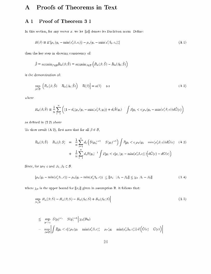
A Proofs of Theorems in TextA.1 Proof of Theorem 3.1In this section, for any vector x, we let kxk denote its Euclidean norm. De�ne:R(�) � E [��(yi �min(x0i�; ci))� ��(yi �min(x0i�0; ci))] (A.1)then the key step in showing consistency of:� � argmin�2BRn(�; S) � argmin�2B �Rn(�; S)�Rn(�0; S)�is the demonstration of:sup�2B ����Rn(�; S)�Rn(�0; S)��R(�)��� = o(1) a.s. (A.2)where Rn(�; S) � 1n nXi=1 �(1� di)��(yi �min(x0i�; yi)) + diS(yi)�1 Z I [yi < c]��(yi �min(x0i�; c))dG(c)�as de�ned in (3.2) above.To show result (A.2), �rst note that for all � 2 B,Rn(�; S)�Rn(�;S) = 1n nXi=1 di �S(yi)�1 � S(yi)�1�Z I [yi < c]��(yi �min(x0i�; c))dG(c) (A.3)+ 1n nXi=1 diS(yi)�1 Z I [yi < c]��(yi �min(x0i�; c))�dG(c)� dG(c)�Since, for any c and �1; �2 2 B,j��(yi �min(x0i�1; c))� ��(yi �min(x0i�2; c))j � kxikk�1 � �2k � �0k�1 � �2k (A.4)where �0 is the upper bound for kxik given in assumption R, it follows that:sup�2B ���Rn(�; S)�Rn(�;S)�Rn(�0; S) +Rn(�0;S)��� (A.5)� supy<�0 ���S(y)�1 � S(y)�1����0(2b0)+ sup�2B ����Z I [yi < c] (��(yi �min(x0i�; c))� ��(yi �min(x0i�0; c))) d�G(c)�G(c)�����24

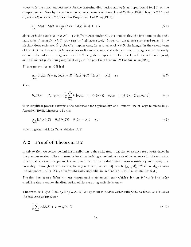
where �0 is the upper support point for the censoring distribution and b0 is an upper bound for k�k on thecompact set B. Now by the uniform convergence results of Shorack and Wellner(1986, Theorem 7.3.1 andequation (3) of section 7.3) (see also Proposition 1 of Wang(1987)),supy ���S(y)� S(y)��� = supy ���G(y)�G(y)��� = o(1) a.s. (A.6)along with the condition that S(�0�) > 0 (from Assumption C), this implies that the �rst term on the righthand side of inequality (A.5) converges to 0 alomost surely. Moreover, the almost sure consistency of theKaplan-Meier estimator G(y) for G(y) implies that, for each value of � 2 B, the integral in the second termof the right hand side of (A.5) converges to 0 almost surely, and this pointwise convergence can be easilyextended to uniform convergence over � 2 B using the compactness of B, the Lipschitz condition in (A.4),and a standard partitioning argument (e.g., in the proof of Theorem 4.2.1 of Amemiya(1985)).This argument has establishedsup�2B ���Rn(�; S)�Rn(�;S)�Rn(�0; S) +Rn(�0;S)��� = o(1) a.s. (A.7)Also, Rn(�;S)�Rn(�0;S) = 1n nXi=1 E ���(yi �min(x0i�; c))� ��(yi �min(x0i�0; c))��yi; di; xi� (A.8)is an empirical process satisfying the conditions for applicability of a uniform law of large numbers (e.g.,Amemiya(1985), Theorem 4.2.1), sosup�2B j(Rn(�;S)�Rn(�0;S))�R(�)j = o(1) a.s. (A.9)which together with (A.7), establishes (A.2).A.2 Proof of Theorem 3.2In this section, we derive the limiting distribution of the estimator, using the consistency result established inthe previous section. The argument is based on deriving a preliminary rate of convergence for the estimatorwhich is slower than the parametric rate, and then in turn establishing root-n consistency and asymptoticnormality. Throughout this section, for any matrix A, we let kAk denote (Pi;j A2ij)1=2 where Aij denotesthe components of A. Also, all asymptotically negligible remainder terms will be denoted by Rn(�).The �rst lemma establishes a linear representation for an estimator which solves an infeasible �rst ordercondition that assumes the distribution of the censoring variable is known:Theorem A.1 If � p! �0, �i � �(yi; xi; di) is any mean 0 random vector with �nite variance, and � solvesthe following relationship:1n nXi=1 i(�; S) + �i = op(n��) (A.10)25

where 0 < � � 1=2, then:� � �0 =M�10 1n nXi=1( i + �i) + op(n��) (A.11)Proof: Noting that E[ i(�; S)jxi] = S(x0i�)(� � F�jX(x0i(� � �0)) we �rst evaluate the expansion ofE[ i(�; S)] for � in a neighborhood of �0:Lemma A.1 as k� � �0k ! 0,E[S(x0i�)(� � F�jX(x0i(� � �0)))xi] = E[S(x0i�0)f�jX(0)xix0i](� � �0) + o(k� � �0k) (A.12)Proof: We add and substract E[S(x0i�0)(��F�jX(x0i(���0)))xi] from the left hand side of (A.12). We �rstshow that:E[(S(x0i�)� S(x0i�0))(� � F�jX(x0i(� � �0)))xi] = o(k� � �0k) (A.13)Note that a mean value expansion of F�jX(x0i(� � �0)) around 0 implies by the bound on the conditionaldensity of �i in a neighborhood of 0 of Assumption E, the bound on kxik in Assumption R, and the CauchySchwartz inequality that the left hand side of (A.13) is bounded above by:CE[jS(x0i�)� S(x0i�0)j]k� � �0k (A.14)where C is a constant re ecting the bounds in Assumptions E and R. By the dominated convergence theorem,E[jS(x0i�) � S(x0i�0)j] is o(1) as � ! �0 since S(x0i�0) is discontinuous on a set of probability zero byAssumption RC. This establishes (A.13). We next show thatE[S(x0i�0)(� � F�jX(x0i(� � �0)))xi] = E[S(x0i�0)f�jX(0)xix0i](� � �0) +O(k� � �0k2) (A.15)A mean value expansion of the left hand side of (A.15) yields:E[S(x0i�0)f�jX(0)xix0i](� � �0) +Rn (A.16)where kRnk is bounded above by:E[jf�jX(0)� f�jX(x0i( ~� � �0))jkxik2]k� � �0kwith ~� denoting the intermediate value in the mean value expansion. By the Lipschitz assumption on theconditional density of �i in a neighborhood of 0 (Assumption E), and the bound on kxik (Assumption R),the above term is is O(k� � �0k2), establishing (A.15). This shows (A.12). �26

Turning attention to the proof of the theorem, we let E[ i(�; S)] denote E[ i(�; S)]����=�.Express 1nPni=1 i(�; S) as1n nXi=1 i(�0; S) + 1n nXi=1 E[ i(�; S)] + 1n nXi=1 i(�; S)� i(�0; S)�E[ i(�; S)] (A.17)Turning attention to the second term in (A.17), we note that it immediately follows by Lemma A.1 and theconsistency of � that1n nXi=1 E[ i(�; S)] =M0 + op(1)We next show that the third term in (A.17) is op(n�1=2). By the consistency of �, it will su�ce to showthat for a sequence of numbers �n converging to 0 slowly enough, we have:supk���0k��n 1n nXi=1 i(�; S)� i(�0; S)�E[ i(�; S)] = op(n�1=2) (A.18)To show (A.18), by applying Lemma 2.17 in Pakes and Pollard(1989), it will su�ce to show the followingtwo results:I The class of functions ( i(�; S) : � 2 B) is Euclidean with respect to the envelope F , where E[F 2] <1.II lim�!�0 E[( i(�; S)� i(�0; S)2] = 0.To show I, we note by Lemmas 2.14(i) and 2.14(ii) of Pakes and Pollard(1989), it will su�ce to show theEuclidean property for the three classes a)(I [yi > x0i�] : � 2 B), b) (I [yi � x0i�] : � 2 B) c) (S(x0i�) : � 2 B).The Euclidean property for all three classes for the envelope F � 1 follows directly from Lemma 22(ii) inNolan and Pollard(1987) since the functions I [�] and S(�) are of bounded variation. This establishes I.To establish II, we note that it will su�ce to show that both E[jI [yi > x0i�] � I [yi > x0i�0]j] and E[(I [�i �x0i(� � �0)]S(x0i�) � I [�i � 0]S(x0i�0))2] converge to 0 as k� � �0k ! 0. To show the former, we note thatjI [yi > x0i�]� I [yi > x0i�0]j is bounded above by I [jyi � x0i�0j � kxikk� � �0k], and that:P (jyi � x0i�0j � kxikk� � �0k) � P (j�ij � kxikk� � �0k) + P (jci � x0i�0j � kxikk� � �0k)By Assumption E, the �rst term on the right hand side of the above expression converges to 0 as � ! �0 sincekxik is bounded by Assumption R. By Assumption RC, the second term converges to 0 as � ! �0, againusing the assumption that kxik is bounded. To show that E[(I [�i � x0i(� � �0)]S(x0i�)� I [�i � 0]S(x0i�0))2]converges to 0, it will su�ce to show that both E[jI [�i � x0i(� � �0)]� I [�i � 0]j] and E[(S(x0i�)�S(x0i�0)2]converge to 0 as � ! �0. The �rst term is bounded above by E[I [j�ij � kxikk�� �0k]] which converges to 0by assumption E, and the second term converges to 0 by the dominated convergence theorem, as S(x0i�0) isdiscontinuous on a set of probability 0 by Assumption RC. This establishes II and hence (A.18). Thus wehave shown that:1n nXi=1 i(�; S) = 1n nXi=1 i(�0; S) + (M0 + op(1))(� � �0) + op(n�1=2) (A.19)27

Combining this with (A.10), we have:1n nXi=1 i(�0; S) + �i + (M0 + op(1))(� � �0) = op(n��) (A.20)which by applying the Lindeberg-Levy central limit theorem and Slutsky's theorem, can be rearranged toyield the conclusion of the theorem. �Our next step is to establish a uniform linear representation for the Kaplan-Meier product limit estimatorused in the �rst stage.Lemma A.2 Let H(x) denote P (yi � x) and let �(�) denote the cumulative hazard function of ci. Letting��(x) denote �(x)� �(x�) we have the following linear representation for the product limit estimator:S(t)� S(t) = S(t) 1n nXi=1 H(yi)�1(1���(yi))�1I [yi � t](1� di) (A.21)� Z t0 H(s)�1(1���(s))�1I [yi � s]d�(s) +Rn(t)where sup0�t<1 jRn(t)j = op(n�1=2) (A.22)Proof: Note by the assumption that �0, the upper support point of ci, is mass point, we have S(t) � 0 = S(t)for all t > �0. It will thus su�ce to show that the linear representation holds uniformly over the interval[0; �0]. We �rst de�ne the following processes:N(t) = nXi=1 I [yi � t; di = 0]Y (t) = nXi=1 I [yi � t]M(t) = N(t)� Z t0 Y (s)d�(s)From the proof of Theorem 4.2.2. in Gill(1980), we haveS(t)� S(t) = S(t) 1n Z t0 (1���(s))�1 S(s�)S(s�) nI [Y (s) > 0]Y (s) dM(s) (A.23)for all t 2 [0; �0]. We thus have:S(t)� S(t) = S(t) 1n Z t0 (1���(s))�1H(s)�1dM(s) +Rn(t) (A.24)28

where n1=2Rn(t) = S(t) Z t0 (1���(s))�1 n�1=2H(s)�1 � S(s�)S(s�) n1=2I [Y (s) > 0]Y (s) ! dM(s) (A.25)so note it will su�ce to show that:sup0�s��0 n1=2jRn(s)j = op(1) (A.26)Let H(s) = (1���(s))�1 n�1=2H(s)�1 � S(s�)S(s�) n1=2I [Y (s) > 0]Y (s) !The process (1���(s))�1 S(s�)S(s�) n1=2I[Y (s)>0]Y (s) is bounded and predictable by the arguments used in the proofof Theorem 4.2.2 in Gill(1980). It immediately follows that the process H(s) is bounded and predictable,and note that H2(s)Y (s) is(1���(s))�2n�1H(s)�2Y (s)+ (A.27)(1���(s))�2 S2(s�)S2(s�) nI [Y (s) > 0]Y (s) � (A.28)2(1���(s))�2H(s)�1 S(s�)S(s�) (A.29)By Theorem 3.1, we have:sup0�s��0 jS(s)� S(s)j = op(1) (A.30)and note that Y (s)=n converges in probability to H(s), uniformly in [0; �0]. Since H(s) is bounded awayfrom 0 on [0; �0], this implies that terms in (A.27)-(A.29) converge uniformly on [0; �0] to(1���(s))�2H(s)�1(1���(s))�2H(s)�1and 2(1���(s))�2H(s)�1respectively. It thus follows thatsup0�s��0H2(s)Y (s) p! 0 (A.31)29

So by Theorem 4.2.1 of Gill(1980)n1=2Rn(�)) Z0 in D[0; �0] (A.32)where D[0; �0] is the space of right continuous functions with left hand limits, and Z0 is a process degenerateat 0. It immediately follows by Theorem 2.4.3 in Gill(1980) thatsup0�s��0 n1=2jRn(s)j = op(1) (A.33)This establishes (A.21). �Implicit in the result of the uniform linear representation is a rate of uniform convergence of the Kaplan-Meier estimator. To formally establish the uniform rate, we �rst show the Euclidean property of the classof functions in the summation of the linear representation:Lemma A.3 The class of functions(H(yi)�1(1���(yi))�1I [yi � t](1� di) � Z t0 H(s)�1(1���(s))�1I [yi � s]d�(s) (A.34): t 2 [0; �0])is Euclidean for a constant envelope.Proof: Note that the class H(yi)�1(1 � ��(yi))�1(1 � di) is trivially Euclidean for a constant envelope,and the class I [yi � t] is Euclidean for the envelope F � 1 by Example 2.11 in Pakes and Pollard(1989). Itfollows by Lemma 2.14(ii) of Pakes and Pollard(1989) that the class:(H(yi)�1(1���(yi))�1I [yi � t](1� di)is Euclidean for a constant envelope. Next we show the Euclidean property for the class of functions of yiand s, indexed by t:H(s)�1(1���(s))�1I [yi � s]I [yi � t] (A.35)The class of functions H(s)�1(1���(s))�1I [yi � s] is trivially Euclidean for a constant envelope, and theclass I [yi � t] is Euclidean for the envelope F � 1 by Example 2.11 in Pakes and Pollard(1989). It followsthat the class in (A.35) is Euclidean for a constant envelope by Lemma 2.14(ii) of Pakes and Pollard(1989).Therefore, by Lemma 5 in Sherman(1994), the class of functions of yi, indexed by t:Z t0 H(s)�1(1���(s))�1I [yi � s]d�(s) : t 2 [0; �0]is Euclidean for a constant envelope. It follows by Lemma 2.14(i) in Pakes and Pollard(1989) that the classin (A.34) is Euclidean for a constant envelope. �We now have the following result: 30

Lemma A.4 For any � < 1=2:supt2R+ jS(t)� S(t)j = op(n��) (A.36)Proof: Note that for any t � �0, we have S(t) � 0 = S(t), so it su�ces to show that:supt2[0;�0) jS(t)� S(t)j = op(n��)Working with the linear representation in (A.21), by the fact that the remainder term is op(n�1=2) uniformlyover [0; �0], it remains to show that:supt2[0;�0) ��� 1n nXi=1(H(yi)�1(1���(yi))�1I [yi � t](1� di) (A.37)� Z t0 H(s)�1(1���(s))�1I [yi � s]d�(s)��� = op(n��)By the Euclidean property of the class in (A.34) this follows directly by Corollary 9 in Sherman(1994). �The uniform rate of convergence will su�ce to establish a preliminary rate of convergence for the estimator�.Lemma A.5 For any � 2 (0; 1=2),� � �0 = op(n��) (A.38)Proof: We rewrite the �rst order condition as:1n nXi=1 i(�; S) + 1n nXi=1 i(�; S)� i(�; S) = op(n�1=2) (A.39)By linearizing the ratio S(x0i�)S(yi) around S(x0i�)S(yi) and the assumptions that di=S(yi) and kxik are bounded,Lemma A.4 implies that: 1n nXi=1 i(�; S)� i(�; S) = op(n��) (A.40)for any � 2 (0; 1=2). Thus we have:1n nXi=1 i(�; S) = op(n��) (A.41)to which we can apply Theorem A.1 with �i � 0 to conclude that ���0 = op(n��) +Op(n�1=2) = op(n��).�We next show the following result: 31

Lemma A.6 Let �i be de�ned as in equation (3.12). Then(1� �) 1n nXi=1 I [yi � x0i�0]di S(x0i�0)S(yi) � S(x0i�0)S(yi) !xi (A.42)has the representation:1n nXi=1 �i + op(n�1=2) (A.43)Proof: The proof is facilitated by decomposing �i as the sum of two components, which we denote by �1i; �2i,and are de�ned as :�1i = �(1� �) ZX I [x0i�0 � �0]�H(yi)�1I [yi � x0i�0](1� di) (A.44)� Z x0i�00 H(s)�1(1���(s))�1I [yi � s]d�(s)�xdFX (x)�2i = �(1� �) Z I [� � 0]I [x0�0 + � < c] S(x0�0)S(x0�0 + �) (A.45)� H(yi)I [yi � x0�0 + �](1� di)� Z x0�0+�0 H(s)�1(1���(s))�1I [yi � s]d�(s)!� xdFX;�(x; �)dFC(c)Linearizing the ratio S(x0i�)S(yi) around S(x0i�)S(yi) , we have by Lemma A.4 and the assumptions that kxik anddi=S(yi) are bounded that (A.42) can be written as:1n nXi=1(1� �)I [yi � x0i�0]diS(yi)�1(S(x0i�0)� S(x0i�0))xi+ (A.46)1n nXi=1(1� �)I [yi � x0i�0]diS(x0i�0)S(yi)�2(S(yi)� S(yi))xi + op(n�1=2) (A.47)We �rst establish a representation for (A.46). Here, we \plug in" the linear representation for S(�) � S(�)established in Lemma A.2. Noting that the \own observation" terms are asymptotically negligible, thisyields a U-statistic plus and asymptotically negligible term:1n(n� 1)Xi6=j (1� �)I [yi � x0i�0]diS(x0i�0)S(yi)�1� (A.48)�H(yj)�1(1���(yj))�1I [yj � x0i�0](1� dj)� Z x0i�00 H(s)�1(1���(s))�1I [yj � s]d�(s)�xi + op(n�1=2)32

The left hand side of the above expression is a second order U-statistic, and we denote its kernel functionby F(�i; �j) where �i = (yi; x0i; di)0. It is straightforward to show that E[kF(�i; �j)k2] < 1 by the assump-tions that di=S(yi); H(�)�1 and kxik are bounded. We note that E[F(�i; �j)] = E[F(�i; �j)j�i] = 0 and1nPnj=1 E[F(�i; �j)j�j ] can be written as 1nPni=1 �1i. Thus by a standard projection theorem for U-statistics(see for example Ser ing(1980)), (A.46) can be expressed as:1n nXi=1 �1i + op(n�1=2) (A.49)The same arguments can be used to represent (A.47) as:1n nXi=1 �2i + op(n�1=2) (A.50)This establishes the conclusion of the lemma. �We next establish the following lemma:Lemma A.71n nXi=1(1� �)di(I [yi � x0i�]� I [yi � x0i�0])di S(x0i�)S(yi) � S(x0i�)S(yi) !xi = op(n�1=2) (A.51)Proof: Fix � 2 (1=4; 1=2). By linearizing the ratio S(x0i�)S(yi) around S(x0i�)S(yi) , we have by Lemma A.4, and theassumption that kxik and di=S(yi) are bounded, that it su�ces to show:1n nXi=1 jI [yi � x0i�]� I [yi � x0i�0]jdi = op(n�1=2+�) (A.52)We note that the left hand side of the above expression is bounded above by:1n nXi=1 I [j�ij � kxikk� � �0k] (A.53)we can multiply this expression by I [k� � �0k � n�� ] and the resulting remainder term is op(n�1=2) byLemma A.5. Note that for any �, by Assumption E we have E[I [j�ij � kxikk���0k]] is O(k���0k). It willthus su�ce to show that:supk���0k�n�� ����� 1n nXi=1 I [j�ij � kxikk� � �0k]�E[I [j�ij � kxikk� � �0k]����� = op(n�1=2) (A.54)This follows by Lemma 2.17 in Pakes and Pollard(1989), since the class of functions indexed by � at hand isEuclidean for the envelope F � 1 by example 2.11 in Pakes and Pollard(1989), and P (j�ij � kxikk� � �0k)!0 as � ! �0 by Assumption E. �33

The �nal result which needs to be established before proving the main theorem is an equicontinuity conditionfor the Kaplan-Meier estimator:Lemma A.81n nXi=1 I [yi � x0i�]di S(x0i�)S(yi) � S(x0i�0)S(yi) � S(x0i�0)S(yi) + S(x0i�0)S(yi) !xi = op(n�1=2) (A.55)Proof: Again, we linearize the ratios S(x0i�)S(yi) , and S(x0i�0)S(yi) , which by Lemma A.4, and the bounds onkxik; di=S(yi) makes it su�ce to show that:1n nXi=1 I [yi � x0i�]diS(yi)�1 �S(x0i�)� S(x0i�)� S(x0i�0) + S(x0i�0)�xi = op(n�1=2) (A.56)and 1n nXi=1 I [yi � x0i�]diS(yi)�2 �S(x0i�)� S(x0i�0)��S(yi)� S(yi)�xi = op(n�1=2) (A.57)We �rst show (A.57). We note by Lemma A.4 and the bound on I [yi � x0i�]diS(yi)�2xi that it will su�ceto show:1n nXi=1 jS(x0i�)� S(x0i�0)j = op(n��) (A.58)for � 2 (1=4; 1=2). Assumption RC(i) implies that E[jS(x0i�)�S(x0i�0)j] = Op(k���0k), so by the consistencyof �, it will su�ce to show that for a sequence of numbers �n converging to 0 slowly enough that:supk���0k��n 1n nXi=1 jS(x0i�)� S(x0i�0)j �E [jS(x0i�)� S(x0i�0)j] = op(n�1=2) (A.59)Note that the class of functions (S(x0i�) : � 2 B) is Euclidean for the envelope F � 1 by Lemma 22(ii) inNolan and Pollard(1987). It immediately follows that the class (jS(x0i�)� S(x0i�0)j : � 2 B) is Euclidean fora constant envelope. Also, by Assumption RC(i) it follows that E �(S(x0i�)� S(x0i�0))2� ! 0 as � ! �0.(A.59) follows from Lemma 2.17 in Pakes and Pollard(1989), showing (A.57)We next show (A.56). Note that it can be shown as before that:1n nXi=1 di(I [yi � x0i�]� I [yi � x0i�0]) = Op(k� � �0k)so I [yi � x0i�] can be replaced with I [yi � x0i�0] in (A.56) and the resulting remainder term is op(n�1=2).By Lemma A.4 and the fact that S(t)� S(t) = 0 for t > �0, it will su�ce to show:supk���0k�n�� 1n nXi=1 I [yi � x0i�]diS(yi)�1I [x0i� � �0](S(x0i�)� S(x0i�)) (A.60)� I [x0i� � �0](S(x0i�0)� S(x0i�0))xi = op(n�1=2)34

We next plug in the linear representation of Lemma A.2. Again, by noting that the own observation termsare asymptotically negligible, the summation of the left hand side in (A.60) can be written as a U-statistic:1n(n� 1)Xi6=j I [yi � x0i�]diS(yi)�1(Qj(x0i�)�Qj(x0i�0))xi (A.61)where here we let Qi(t) denote the mean 0 process:S(t)(H(yi)�1(1���(yi))�1I [yi � t](1� di)� Z t0 H(s)�1(1���(s))�1I [yi � s]d�(s))Again, we let �i � (yi; xi; di), and let F(�i; �j ; �) denote the kernel of the U-process. Note to show (A.60),it will su�ce to show that:supk���0k�n�� 1n(n� 1)Xi6=j F(�i; �j ; �)�E[F(�i; �j ; �)j�j ] = op(n�1=2) (A.62)supk���0k�n�� 1n nXj=1E[F(�i; �j ; �)j�j ] = op(n�1=2) (A.63)We �rst show (A.63). Note that 1nPnj=1 E[F(�i; �j ; �)j�j ] can be written as:1n nXi=1 � ZX (Qi(x0�) �Qi(x0�0))xdFX (x)To which we can apply Lemma 2.17 in Pakes and Pollard(1989). We �rst show the class of functions of yi; di,indexed by � :�ZX Qi(x0�)xdFX (x) : � 2 B� (A.64)is Euclidean for a constant envelope. To do so, we �rst note the Euclidean property (for a constant envelope)of the class of functions of yi; di; xi, indexed by �,(Qi(x0i�)xi : � 2 B)follows from the same arguments used in showing the Euclidean property for the class in (A.34). Thus theclass in (A.64) is Euclidean for a constant envelope by Lemma 5 in Sherman(1994). We next show that:E � ZX (Qi(x0�)�Qi(x0�0))2xdFX (x) �! 0 (A.65)as � ! �0. For this it will su�ce to show that as � ! �0:E[jI [x0i� � �0]� I [x0i�0 � �0]j] ! 0 (A.66)E[jI [ci � x0i�]� I [ci � x0i�0]j] ! 0 (A.67)E 24 Z x0i�0x0i� H(s)�1(1���(s))�1I [yi � s]d�(s)!235 ! 0 (A.68)35

All three of these conditions follow from Assumption RC. This shows (A.64) and hence (A.63). To show(A.62) we note the U-process with kernel F(�i; �j ; �)�E[F(�i; �j ; �)j�j ] is degenerate. Similar arguments asabove can be used to establish the Euclidean property of this class of functions indexed by � 2 B, as wellas an analogous L2-continuity condition. Thus (A.63) follows directly from Corollary 8 in Sherman(1994).This shows (A.55). �We can now proceed to the main theorem:Theorem A.2 (Theorem 3.2 in text) The estimator � has the following asymptotic linear representation:� � �0 = 1n nXi=1M�10 ( i(�0; S) + �i) + op(n�1=2) (A.69)Proof: Write i(�; S) as 1i(�)� 2i(�) 3i(�; S)where 1i(�) = �I [yi > x0i�]xi (A.70) 2i(�) = (1� �)I [yi � x0i�]dixi (A.71) 3i(�; S) = S(x0i�)=S(yi) (A.72)Rearrange the �rst order condition:1n nXi=1 i(�; S) = op(n�1=2) (A.73)as: 1n nXi=1 i(�; S) +1n nXi=1 2i(�0)( 3i(�0; S)� 3i(�0; S) +1n nXi=1( 2i(�)� 2i(�0))( 3i(�0; S)� 3i(�0; S)) +1n nXi=1 2i(�)( 3i(�; S)� 3i(�; S)� 3i(�0; S) + 3i(�0; S)) = op(n�1=2)which by Lemmas 2-7 yields:1n nXi=1 i(�; S) + �i = op(n�1=2) (A.74)so the desired result follows from Theorem A.1 with � = 1=2 and �i = �i. �The limiting distribution in Theorem 3.2 follows by applying the Lindeberg-Levy central limit theorem tothe linear representation in Theorem A.2. 36

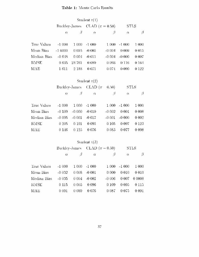
Table 1: Monte Carlo ResultsStudent t(1)Buckley-James CLAD (� = 0:50) STLS� � � � � �True Values -1.000 1.000 -1.000 1.000 -1.000 1.000Mean Bias -1.6000 0.695 -0.005 -0.004 0.009 0.015Median Bias -0.648 0.004 -0.011 -0.004 -0.000 0.007RMSE 9.635 23.761 0.089 0.093 0.116 0.164MAE 1.611 2.188 0.071 0.074 0.090 0.122Student t(2)Buckley-James CLAD (� � 0:50) STLS� � � � � �True Values -1.000 1.000 -1.000 1.000 -1.000 1.000Mean Bias -0.109 -0.000 -0.010 -0.002 0.001 0.008Median Bias -0.095 -0.001 -0.017 -0.001 -0.000 0.002RMSE 0.205 0.191 0.095 0.105 0.097 0.123MAE 0.146 0.125 0.076 0.083 0.077 0.098Student t(3)Buckley-James CLAD (� � 0:50) STLS� � � � � �True Values -1.000 1.000 -1.000 1.000 -1.000 1.000Mean Bias -0.032 0.008 -0.001 0.000 0.010 0.010Median Bias -0.035 0.004 -0.002 -0.006 0.007 0.0008RMSE 0.115 0.005 0.096 0.109 0.095 0.115MAE 0.091 0.089 0.076 0.087 0.075 0.09137

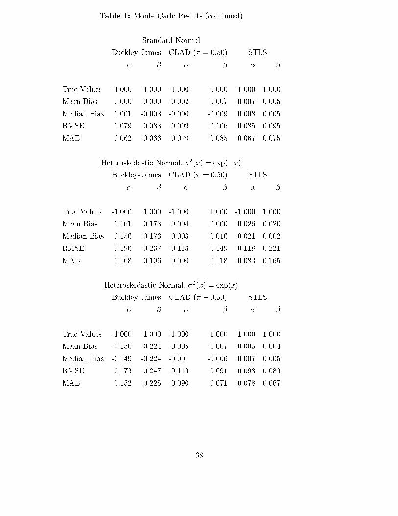
Table 1: Monte Carlo Results (continued)Standard NormalBuckley-James CLAD (� = 0:50) STLS� � � � � �True Values -1.000 1.000 -1.000 0.000 -1.000 1.000Mean Bias 0.000 0.000 -0.002 -0.007 0.007 0.005Median Bias 0.001 -0.003 -0.000 -0.009 0.008 0.005RMSE 0.079 0.083 0.099 0.106 0.085 0.095MAE 0.062 0.066 0.079 0.085 0.067 0.075Heteroskedastic Normal, �2(x) = exp(�x)Buckley-James CLAD (� = 0:50) STLS� � � � � �True Values -1.000 1.000 -1.000 1.000 -1.000 1.000Mean Bias 0.161 0.178 0.004 0.000 0.026 0.020Median Bias 0.156 0.173 0.003 -0.016 0.021 0.002RMSE 0.196 0.237 0.113 0.149 0.118 0.221MAE 0.168 0.196 0.090 0.118 0.083 0.165Heteroskedastic Normal, �2(x) = exp(x)Buckley-James CLAD (� � 0:50) STLS� � � � � �True Values -1.000 1.000 -1.000 1.000 -1.000 1.000Mean Bias -0.150 -0.224 -0.005 -0.007 0.005 0.004Median Bias -0.149 -0.224 -0.001 -0.006 0.007 0.005RMSE 0.173 0.247 0.113 0.091 0.098 0.083MAE 0.152 0.225 0.090 0.071 0.078 0.06738

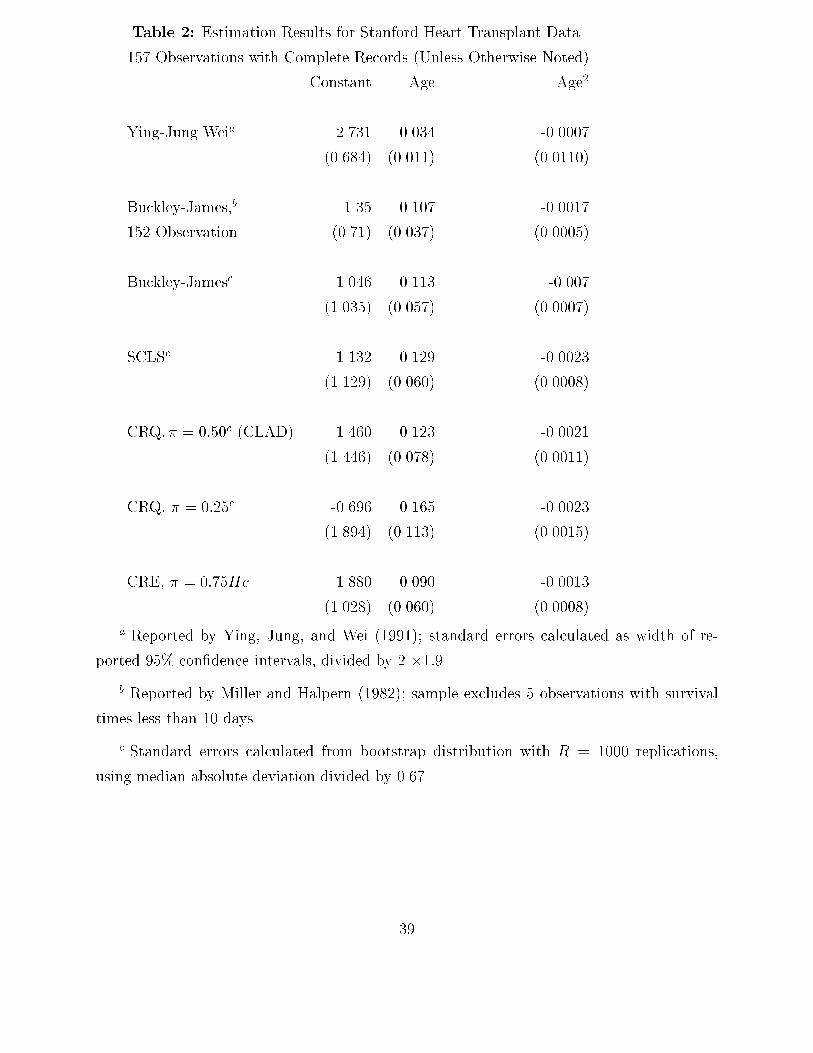
Table 2: Estimation Results for Stanford Heart Transplant Data.157 Observations with Complete Records (Unless Otherwise Noted)Constant Age Age2Ying-Jung Weia 2.731 0.034 -0.0007(0.684) (0.011) (0.0110)Buckley-James,b 1.35 0.107 -0.0017152 Observation (0.71) (0.037) (0.0005)Buckley-Jamesc 1.046 0.113 -0.007(1.035) (0.057) (0.0007)SCLSc 1.132 0.129 -0.0023(1.129) (0.060) (0.0008)CRQ, � = 0:50c (CLAD) 1.460 0.123 -0.0021(1.446) (0.078) (0.0011)CRQ, � = 0:25c -0.696 0.165 -0.0023(1.894) (0.113) (0.0015)CRE, � = 0:75Hc 1.880 0.090 -0.0013(1.028) (0.060) (0.0008)a Reported by Ying, Jung, and Wei (1991); standard errors calculated as width of re-ported 95% con�dence intervals, divided by 2 �1:9b Reported by Miller and Halpern (1982); sample excludes 5 observations with survivaltimes less than 10 days.c Standard errors calculated from bootstrap distribution with R = 1000 replications,using median absolute deviation divided by 0.67.39